Oasys GSAHelp Guide

8 Fitzroy StreetLondonW1T 4BJTelephone: +44 (0) 20 7755 4515

Central SquareForth StreetNewcastle Upon TyneNE1 3PLTelephone: +44 (0) 191 238 7559

e-mail: oasys@arup.comWebsite: http://www.oasys-software.com/

Copyright © O as ys 1985–2021

All rights reserved. No parts of this work may be reproduced in any form or by any means - graphic, electronic, ormechanical, including photocopying, recording, taping, or information storage and retrieval systems - without thewritten permission of the publisher.

Products that are referred to in this document may be either trademarks and/or registered trademarks of therespective owners. The publisher and the author make no claim to these trademarks.

While every precaution has been taken in the preparation of this document, the publisher and the author assume noresponsibility for errors or omissions, or for damages resulting from the use of information contained in thisdocument or from the use of programs and source code that may accompany it. In no event shall the publisher andthe author be liable for any loss of profit or any other commercial damage caused or alleged to have been causeddirectly or indirectly by this document.

Printed: December 2021

Oasys GSA

Copyright © Oasys 1985–2021

Oasys GSA

4 Copyright © O as ys 1985–2021

Table of Contents

Part I About GSA 15

................................................................................................................................... 151 Overview

................................................................................................................................... 152 What's new

................................................................................................................................... 163 GSA Analysis Features

................................................................................................................................... 174 GSA Design Features

................................................................................................................................... 185 GSA Program Features

................................................................................................................................... 196 Documentation

................................................................................................................................... 197 Design Codes

......................................................................................................................................................... 19Steel

......................................................................................................................................................... 21Concrete

................................................................................................................................... 238 Validation

................................................................................................................................... 239 Acknowledgements

Part II Getting Started 27

Part III Working with GSA 30

................................................................................................................................... 311 Dockable Panes

......................................................................................................................................................... 32Explorer Pane

......................................................................................................................................................... 34Output Pane

......................................................................................................................................................... 35Graphics Palette

......................................................................................................................................................... 37Property Pane

................................................................................................................................... 442 Table Views

......................................................................................................................................................... 44Single and Multi-page Tables

......................................................................................................................................................... 44Field Types

......................................................................................................................................................... 45Cell Operators

......................................................................................................................................................... 45Basic Operations in Tables

......................................................................................................................................................... 46Cutting, Copying and Pasting in tables

......................................................................................................................................................... 47Delete and Blank Records in Tables

......................................................................................................................................................... 47Find, Replace, Go To and Modify in Tables

......................................................................................................................................................... 48Copying To and From Spreadsheets

......................................................................................................................................................... 49Adjusting Data Display

......................................................................................................................................................... 49Colour In Tables

................................................................................................................................... 493 Output Views

......................................................................................................................................................... 50Output Settings

......................................................................................................................................................... 51Output View Table Format

......................................................................................................................................................... 51Selecting Data to Output

......................................................................................................................................................... 52Case and Entity Lists

......................................................................................................................................................... 52Outputting for a Selection Set of Entities

......................................................................................................................................................... 52Enveloping

......................................................................................................................................................... 52Data Extents

......................................................................................................................................................... 53Output Summary

......................................................................................................................................................... 53Output By Case, By Property, By Group

......................................................................................................................................................... 53Printing from Output View s

......................................................................................................................................................... 53Interacting w ith Spreadsheets

5Copyright © O as ys 1985–2021

Oasys GSA

................................................................................................................................... 544 Graphic Views

......................................................................................................................................................... 54Changing the Content of a Graphics View

......................................................................................................................................................... 55Basic Orientation of the Image

......................................................................................................................................................... 56Scaling the Image and Zooming

......................................................................................................................................................... 58Advanced orientation of the image

......................................................................................................................................................... 59Identifying What Is To Be Draw n

......................................................................................................................................................... 60Graphical Representation of Entities

......................................................................................................................................................... 62Current Grid

......................................................................................................................................................... 63Selection Sets

......................................................................................................................................................... 65Polylines in Graphic View s

......................................................................................................................................................... 67Adornments

......................................................................................................................................................... 72Shrinking Elements

......................................................................................................................................................... 72Colour In Graphic View s

......................................................................................................................................................... 73Shading Surfaces

......................................................................................................................................................... 73Unw rap Graphics

......................................................................................................................................................... 74Highlighting Element Edges

......................................................................................................................................................... 74Highlight Coincident Nodes

......................................................................................................................................................... 75Highlight Coincident Elements

......................................................................................................................................................... 75Resetting the Display

......................................................................................................................................................... 75Analysis and Design Layers

......................................................................................................................................................... 75Right-click Menus

......................................................................................................................................................... 76Graphic Fonts and Styles

......................................................................................................................................................... 76Animation

......................................................................................................................................................... 77Printing from Graphic View s

......................................................................................................................................................... 77Cursor Modes in Graphic View s

......................................................................................................................................................... 79Copying the Graphic Image to the Clipboard

................................................................................................................................... 795 Chart Views

......................................................................................................................................................... 79Chart Menus

......................................................................................................................................................... 80Chart Styles

................................................................................................................................... 826 Analysis

......................................................................................................................................................... 83Elements

......................................................................................................................................................... 87Analysis Types

......................................................................................................................................................... 89Running Analyses

......................................................................................................................................................... 90Summary

................................................................................................................................... 907 Sets and Lists

......................................................................................................................................................... 91Lists and Embedded Lists

................................................................................................................................... 948 Axes, Grids and Grid Planes

......................................................................................................................................................... 94Axis Sets

......................................................................................................................................................... 96Use of Axis Sets

......................................................................................................................................................... 96Projected Axes

......................................................................................................................................................... 97Grid Axes and the Current Grid

......................................................................................................................................................... 97Constraint Axes

......................................................................................................................................................... 98Element and Member Axes

......................................................................................................................................................... 98Grid Lines, Planes and Surfaces

................................................................................................................................... 999 Saved Views and Preferred Views

......................................................................................................................................................... 99Default View Settings

......................................................................................................................................................... 100Preferred View s

......................................................................................................................................................... 101Saved View s

......................................................................................................................................................... 101Auto View s

......................................................................................................................................................... 102Units and Numeric Format

......................................................................................................................................................... 102View Lists

......................................................................................................................................................... 102Batch Printing and Saving of View s

................................................................................................................................... 10310 Analysis Tasks and Cases

Oasys GSA

6 Copyright © O as ys 1985–2021

......................................................................................................................................................... 103Task View

......................................................................................................................................................... 103Task View Right-click Menu

......................................................................................................................................................... 105Tasks, Cases and the Analysis Wizard

......................................................................................................................................................... 105Copy and Paste Tasks and Cases

......................................................................................................................................................... 106Cases and Tasks

................................................................................................................................... 11311 Grid Planes and Grid Loading

......................................................................................................................................................... 113Specifying Grid Planes

......................................................................................................................................................... 113Specifying Grid Loading

......................................................................................................................................................... 114Displaying Grid Planes and Grid Loading

................................................................................................................................... 11412 Sections

......................................................................................................................................................... 115Section Profile

......................................................................................................................................................... 116Design Parameters

................................................................................................................................... 11613 Constraints

......................................................................................................................................................... 117Element Offsets

......................................................................................................................................................... 117Link Elements and Rigid Constraints

......................................................................................................................................................... 118Conflicting Constraints

......................................................................................................................................................... 118Automatic Constraints

................................................................................................................................... 11914 Miscellaneous

......................................................................................................................................................... 119Unlock File

......................................................................................................................................................... 119File Backups

......................................................................................................................................................... 119Delete Results from Files

......................................................................................................................................................... 119User Modules

......................................................................................................................................................... 120View List

......................................................................................................................................................... 121Evaluating Expressions

......................................................................................................................................................... 123Touch Gestures

................................................................................................................................... 12315 Toolbars and Keyboard Accelerators (shortcuts)

......................................................................................................................................................... 123Toolbars

......................................................................................................................................................... 130Keyboard Accelerators (shortcuts)

......................................................................................................................................................... 133Mouse accelerators (shortcuts)

................................................................................................................................... 13416 Patterned Load

................................................................................................................................... 13517 Mass and Weight

................................................................................................................................... 13618 String IDs

................................................................................................................................... 13619 Members and Element Meshes

Part IV GSA Data 139

................................................................................................................................... 1391 Titles

................................................................................................................................... 1392 Specification

......................................................................................................................................................... 139Units Specif ication

......................................................................................................................................................... 142General Specif ication

......................................................................................................................................................... 143Tolerances

......................................................................................................................................................... 144Design Specif ication

......................................................................................................................................................... 144Member Internal Restraint Specif ication

......................................................................................................................................................... 144Raft Analysis Specif ication

......................................................................................................................................................... 145Bridge Loading Analysis Specif ication

......................................................................................................................................................... 146Environmental Impact Specif ication

................................................................................................................................... 1463 Geometry

......................................................................................................................................................... 146Axes

......................................................................................................................................................... 149Grid Lines

......................................................................................................................................................... 150Grid Planes

......................................................................................................................................................... 150Grid Surfaces

......................................................................................................................................................... 151Polylines

7Copyright © O as ys 1985–2021

Oasys GSA

................................................................................................................................... 1524 Materials

......................................................................................................................................................... 152Material Grades

......................................................................................................................................................... 162Material Curves

................................................................................................................................... 1635 Properties : Section

......................................................................................................................................................... 165Section Profile

......................................................................................................................................................... 176Geometric Section Properties

......................................................................................................................................................... 178Reference Point

......................................................................................................................................................... 178Point Voids

......................................................................................................................................................... 178Steel Design

......................................................................................................................................................... 178Section Modif iers

......................................................................................................................................................... 179Section Design Pools

................................................................................................................................... 1806 Properties : General

......................................................................................................................................................... 180Spring Matrices

......................................................................................................................................................... 180Spring Properties

......................................................................................................................................................... 183Mass Properties

......................................................................................................................................................... 1832D Element Properties

......................................................................................................................................................... 1883D Element Properties

......................................................................................................................................................... 188Link Properties

......................................................................................................................................................... 189Cable Properties

......................................................................................................................................................... 190Damper Properties

......................................................................................................................................................... 191Spacer Properties

......................................................................................................................................................... 192External Matrix

......................................................................................................................................................... 192Environmental Impact Wizard

................................................................................................................................... 1927 Properties : Form-finding

......................................................................................................................................................... 193Force Density 1D

......................................................................................................................................................... 193Soap Film 1D

......................................................................................................................................................... 193Force Density 2D

......................................................................................................................................................... 194Soap Film 2D

................................................................................................................................... 1948 Properties : Concrete Slab

......................................................................................................................................................... 194Reinforcement

......................................................................................................................................................... 194Calculation

......................................................................................................................................................... 196Strength Reduction Factors

................................................................................................................................... 1969 Nodes

................................................................................................................................... 19710 Members

......................................................................................................................................................... 198Definition

......................................................................................................................................................... 199Design Properties

......................................................................................................................................................... 202Miscellaneous

......................................................................................................................................................... 2031D Member Axes

................................................................................................................................... 20411 Blocks

................................................................................................................................... 20512 Elements

......................................................................................................................................................... 208Element Types

......................................................................................................................................................... 215Element Axes

................................................................................................................................... 21813 Assemblies

................................................................................................................................... 21914 Constraints

......................................................................................................................................................... 219Generalised Restraints

......................................................................................................................................................... 220Rigid Constraints

......................................................................................................................................................... 222Joints

......................................................................................................................................................... 223Constraint Equations

......................................................................................................................................................... 224Tied Interfaces

................................................................................................................................... 22515 Loading

......................................................................................................................................................... 226Load Case Specif ication

Oasys GSA

8 Copyright © O as ys 1985–2021

......................................................................................................................................................... 227Nodal Loading

......................................................................................................................................................... 229Beam Loading

......................................................................................................................................................... 2362D Element Loading

......................................................................................................................................................... 2443D Element Loading

......................................................................................................................................................... 246Grid Loading

......................................................................................................................................................... 250Gravity

................................................................................................................................... 25116 Dynamic Response

......................................................................................................................................................... 251Response Spectra

......................................................................................................................................................... 261Frequency Damping

......................................................................................................................................................... 262Mode Damping

......................................................................................................................................................... 262Load Curve

......................................................................................................................................................... 263Dynamic Load Factor

......................................................................................................................................................... 263Frequency Weighting Curve

................................................................................................................................... 26317 Raft

......................................................................................................................................................... 263Soil

......................................................................................................................................................... 267Raft Interaction

......................................................................................................................................................... 268Pile Interaction

................................................................................................................................... 26818 Bridge

......................................................................................................................................................... 268Alignments

......................................................................................................................................................... 269Paths

......................................................................................................................................................... 271Vehicles

......................................................................................................................................................... 271Bridge Variable Load

......................................................................................................................................................... 273Influence Effects

......................................................................................................................................................... 275Path Loading

......................................................................................................................................................... 276Bridge Loading

................................................................................................................................... 28319 Analysis Stages

......................................................................................................................................................... 283Stage Definition

......................................................................................................................................................... 283Stage Properties

......................................................................................................................................................... 284Stage Materials

................................................................................................................................... 28420 Tasks and Cases

......................................................................................................................................................... 284Analysis Case Definition

......................................................................................................................................................... 285Analysis Wizard

......................................................................................................................................................... 302Advanced Solver Settings

......................................................................................................................................................... 309Soil-Structure Analysis Progress

......................................................................................................................................................... 309Combination Cases

......................................................................................................................................................... 310Design Wizard

................................................................................................................................... 31121 General Data

......................................................................................................................................................... 311Lists

......................................................................................................................................................... 312Case Descriptions

Part V Analysis in GSA 314

................................................................................................................................... 3141 Linear Static Analysis

......................................................................................................................................................... 314P-delta Analysis

......................................................................................................................................................... 315Linear 2D Element Analysis

................................................................................................................................... 3172 Nonlinear Static Analysis

......................................................................................................................................................... 317Modelling Implications

......................................................................................................................................................... 318Ties and Struts

......................................................................................................................................................... 318Dynamic Relaxation

......................................................................................................................................................... 320Explicit Nonlinear Static Analysis

......................................................................................................................................................... 320Analysis of Fabric Structures

......................................................................................................................................................... 320Form-Finding Analysis

................................................................................................................................... 3223 Dynamic Analysis

9Copyright © O as ys 1985–2021

Oasys GSA

......................................................................................................................................................... 322Modal Dynamic Analysis

......................................................................................................................................................... 324Ritz Dynamic Analysis

......................................................................................................................................................... 325Explicit Dynamic Analysis

......................................................................................................................................................... 325Dynamic Response Analysis

................................................................................................................................... 3294 Buckling Analysis

......................................................................................................................................................... 329Eigenvalue Buckling Analysis

......................................................................................................................................................... 330Nonlinear Buckling Analysis

................................................................................................................................... 3315 Dynamic Relaxation Analysis

......................................................................................................................................................... 332Nonlinear Analysis Options

......................................................................................................................................................... 336Dynamic Relaxation Convergence & Damping

................................................................................................................................... 3396 Model Stabil i ty Analysis

................................................................................................................................... 3407 Seismic Analysis

......................................................................................................................................................... 341Equivalent Static Procedures

......................................................................................................................................................... 341Response Spectrum Analysis

................................................................................................................................... 3468 Bridge Analysis

......................................................................................................................................................... 348Modelling Implications

......................................................................................................................................................... 349Delete Grid Loading Tool

......................................................................................................................................................... 349Automatic Path Generation

......................................................................................................................................................... 349Analysis

................................................................................................................................... 3519 Raft & Piled-raft Analysis

......................................................................................................................................................... 351Data Requirements

......................................................................................................................................................... 352Solution Method

......................................................................................................................................................... 353Raft Analysis Steps

......................................................................................................................................................... 354Piled-raft Analysis Steps

......................................................................................................................................................... 355Results

......................................................................................................................................................... 355Notes

................................................................................................................................... 35610 Analysis Stages

......................................................................................................................................................... 356Modelling Implications

......................................................................................................................................................... 357Analysis of Stages

......................................................................................................................................................... 358Results

......................................................................................................................................................... 358Stages and Graphic View s

................................................................................................................................... 35911 Analysis Envelopes

................................................................................................................................... 35912 Environmental Impact

................................................................................................................................... 36013 Wave loading

................................................................................................................................... 36314 LS-DYNA Analysis

................................................................................................................................... 36315 Results

......................................................................................................................................................... 363Static Analysis Results

......................................................................................................................................................... 363Modal Analysis Results

......................................................................................................................................................... 364Displacements

......................................................................................................................................................... 365Reactions

......................................................................................................................................................... 365Soil Contact Bearing Pressure

......................................................................................................................................................... 365Beam Element Results

......................................................................................................................................................... 3732D Element Results

......................................................................................................................................................... 3773D Element Results

......................................................................................................................................................... 378Assembly Results

................................................................................................................................... 37916 Displaying Data and Results

......................................................................................................................................................... 379Model Data Display Options

......................................................................................................................................................... 382Load Data Display Options

......................................................................................................................................................... 383Results Display Options

......................................................................................................................................................... 387Bridge Data Display Options

......................................................................................................................................................... 388Bridge Results Display Options

Oasys GSA

10 Copyright © O as ys 1985–2021

......................................................................................................................................................... 389Analysis Stage Data Display Options

......................................................................................................................................................... 389User Modules Display Options

......................................................................................................................................................... 389Analysis Diagnostics: Error norm

......................................................................................................................................................... 390Numeric formats

Part VI Design in GSA 392

................................................................................................................................... 3921 Concrete Design

......................................................................................................................................................... 392RC Slab Reinforcement Design

................................................................................................................................... 3932 Steel Design

......................................................................................................................................................... 394Generating Steel Member Restraints

......................................................................................................................................................... 394Member Results

......................................................................................................................................................... 396Steel Checks to AISC LRFD

......................................................................................................................................................... 396Steel Checks to AISC 360

......................................................................................................................................................... 397Steel Checks to AS 4100

......................................................................................................................................................... 398Steel Checks to BS 5950-1

......................................................................................................................................................... 401Steel checks to CSA S16

......................................................................................................................................................... 401Steel Checks to EN 1993

......................................................................................................................................................... 407Steel Checks to HKSUOS

......................................................................................................................................................... 408Steel Checks to IS 800

......................................................................................................................................................... 409Steel Checks to SANS 10162-1

......................................................................................................................................................... 411Results

......................................................................................................................................................... 412Tools

................................................................................................................................... 4123 Member Results

Part VII GSA Tools 414

................................................................................................................................... 4141 Welcome to GSA dialog

................................................................................................................................... 4142 Undo and Redo

................................................................................................................................... 4163 New Model Wizard

......................................................................................................................................................... 416Titles

......................................................................................................................................................... 416Structure

......................................................................................................................................................... 416Properties

................................................................................................................................... 4174 Data Generation Wizard

......................................................................................................................................................... 417Structure Types

......................................................................................................................................................... 417Portal Frame

......................................................................................................................................................... 418Grid

......................................................................................................................................................... 419Orthogonal Frame

......................................................................................................................................................... 420Truss

......................................................................................................................................................... 420Vierendeel

......................................................................................................................................................... 421Pratt Truss

......................................................................................................................................................... 422Pitched Portal

......................................................................................................................................................... 422Roof Truss

......................................................................................................................................................... 4232D Element Orthogonal Mesh

......................................................................................................................................................... 4232D Element Skew Mesh

......................................................................................................................................................... 4242D Element Elliptical Mesh

......................................................................................................................................................... 4253D Element Orthogonal Mesh

......................................................................................................................................................... 425Generate

................................................................................................................................... 4255 Preferences & Settings

......................................................................................................................................................... 425Preferences

......................................................................................................................................................... 430Miscellaneous Preferences

................................................................................................................................... 4326 Sculpting

......................................................................................................................................................... 433Sculpt Dialogs

11Copyright © O as ys 1985–2021

Oasys GSA

......................................................................................................................................................... 442Sculpt Geometry Cursor Modes

......................................................................................................................................................... 443Creating User Axes Graphically

......................................................................................................................................................... 444Creating Grid Planes Graphically

......................................................................................................................................................... 444Adding Nodes Graphically

......................................................................................................................................................... 444Modifying Nodes Graphically

......................................................................................................................................................... 445Collapsing Coincident Nodes

......................................................................................................................................................... 445Rounding Nodal Coordinates Graphically

......................................................................................................................................................... 445Adding Elements Graphically

......................................................................................................................................................... 446Connecting 1D Elements Graphically

......................................................................................................................................................... 447Splitting Elements Graphically

......................................................................................................................................................... 450Joining 1D Elements Graphically

......................................................................................................................................................... 451Convert Orientation Node to Angle

......................................................................................................................................................... 451Modifying 2D Elements From Linear To Quadratic

......................................................................................................................................................... 451Modifying 2D Elements from Quadratic to Linear

......................................................................................................................................................... 452Moving and Copying Entities Graphically

......................................................................................................................................................... 452Extruding Nodes and Elements Graphically

......................................................................................................................................................... 453Transforming Nodes Graphically

......................................................................................................................................................... 453Flexing Lines of Nodes Graphically

......................................................................................................................................................... 455Straightening Lines of Nodes Graphically

......................................................................................................................................................... 455Flipping Elements Graphically

......................................................................................................................................................... 455Spinning 2D Elements Graphically

......................................................................................................................................................... 455Modifying Elements Graphically

......................................................................................................................................................... 456Disconnecting Elements Graphically

......................................................................................................................................................... 456Deleting Nodes and Elements Graphically

......................................................................................................................................................... 457Create Wall/Core Assembly

......................................................................................................................................................... 457Creating Rigid Constraints Graphically

......................................................................................................................................................... 457Creating Joints Graphically

......................................................................................................................................................... 457Creating Nodal Loading Graphically

......................................................................................................................................................... 458Creating Element Loading Graphically

......................................................................................................................................................... 459Creating Grid Loading Graphically

......................................................................................................................................................... 460Deleting Loading Graphically

................................................................................................................................... 4607 File Tools

......................................................................................................................................................... 460Import GWA Data

......................................................................................................................................................... 460Footfall Response Data

................................................................................................................................... 4618 Output View Dialogs

......................................................................................................................................................... 461Wizard: Output Settings

......................................................................................................................................................... 463Output Wizard: Further Options

................................................................................................................................... 4649 Graphic View Dialogs

......................................................................................................................................................... 464Wizard: Graphic Settings

......................................................................................................................................................... 467Labels and Display Methods

......................................................................................................................................................... 475Deformation Settings

......................................................................................................................................................... 476Contour Settings

......................................................................................................................................................... 478Diagram Settings

......................................................................................................................................................... 480Bridge Options

......................................................................................................................................................... 481Further Options

......................................................................................................................................................... 482Animation Settings

......................................................................................................................................................... 483Orientation Settings

......................................................................................................................................................... 484Graphic Fonts and Styles

................................................................................................................................... 48510 Chart View Dialogs

......................................................................................................................................................... 485Non-linear Analysis

......................................................................................................................................................... 485Modal Analysis Details

......................................................................................................................................................... 486Harmonic Analysis

......................................................................................................................................................... 486Periodic Load Analysis

......................................................................................................................................................... 486Linear Time-history Analysis

Oasys GSA

12 Copyright © O as ys 1985–2021

......................................................................................................................................................... 487Footfall Analysis

......................................................................................................................................................... 488Storey Displacements and Forces

......................................................................................................................................................... 488Forces on 2D Element Cut

................................................................................................................................... 48911 Model Tools

......................................................................................................................................................... 491Manage Data

......................................................................................................................................................... 492Current Grid Definition

......................................................................................................................................................... 493Grid Layout Definition

......................................................................................................................................................... 493History

......................................................................................................................................................... 494Coordination

......................................................................................................................................................... 498Section Tools

......................................................................................................................................................... 500Checking Tools

......................................................................................................................................................... 502Model Tools

......................................................................................................................................................... 505Contact Constraints

......................................................................................................................................................... 507Create Grid Lines

......................................................................................................................................................... 507Building Modelling

......................................................................................................................................................... 510Bridge Modelling

......................................................................................................................................................... 514Dynamics

......................................................................................................................................................... 515Seismic

......................................................................................................................................................... 518Offshore

......................................................................................................................................................... 522Manage User Modules

......................................................................................................................................................... 523Result Map

......................................................................................................................................................... 523Miscellaneous Tools

................................................................................................................................... 52412 Miscellaneous Dialogs

......................................................................................................................................................... 524Find

......................................................................................................................................................... 525Replace

......................................................................................................................................................... 525Modify

......................................................................................................................................................... 526Go To

......................................................................................................................................................... 526Modify Curve

......................................................................................................................................................... 526Curve Data Selection

......................................................................................................................................................... 526GWA Import Options

......................................................................................................................................................... 527CAD Export Options

......................................................................................................................................................... 528CAD Import Options

......................................................................................................................................................... 530Nastran Export Options

......................................................................................................................................................... 530OpenSees Export Options

......................................................................................................................................................... 531ADC AdBeam Export

......................................................................................................................................................... 531AdSec Export

......................................................................................................................................................... 532Export Member Input Data to CSV

......................................................................................................................................................... 5321D Element Results

......................................................................................................................................................... 533Numeric Format

......................................................................................................................................................... 533Axes

Part VIII GSA Text Files 535

................................................................................................................................... 5351 Text Data File Format

................................................................................................................................... 5362 Reinforcement Template File

................................................................................................................................... 5403 Curve File

................................................................................................................................... 5414 Tab and Comma Separated Files

Part IX API and Command Line Interface 544

................................................................................................................................... 5441 GSA API

................................................................................................................................... 5442 Command File

Part X Interaction with Other Software 549

13Copyright © O as ys 1985–2021

Oasys GSA

................................................................................................................................... 5491 Analysis in LS-DYNA

................................................................................................................................... 5512 Text output

................................................................................................................................... 5513 Export options

......................................................................................................................................................... 551Input data

......................................................................................................................................................... 552ADC

......................................................................................................................................................... 552AdSec

......................................................................................................................................................... 552PDisp

......................................................................................................................................................... 552Steel Member(s)

......................................................................................................................................................... 553Footfall Response

......................................................................................................................................................... 553AutoCAD

......................................................................................................................................................... 553SAP2000

......................................................................................................................................................... 554Nastran

......................................................................................................................................................... 555OpenSees

................................................................................................................................... 5554 Import options

......................................................................................................................................................... 555Text f iles

......................................................................................................................................................... 556AutoCAD

......................................................................................................................................................... 556PDisp

................................................................................................................................... 5575 Links With 3D Modell ing Packages

......................................................................................................................................................... 557Revit

......................................................................................................................................................... 569IFC

Part XI Bibliography 573

Part XII Glossary 576

Part I

Oasys GSA

Copyright © O as ys 1985–2021 15

1 About GSA

1.1 Overview

Oasys GSA has developed from a program for the static analysis of three-dimensional structures

composed of skeletal elements, to become a complete analysis package with connection to spreadsheet,

CAD and design programs. GSA has been designed from the outset to be easy for the occasional user, yet

powerful enough to cope with large, complex models. It incorporates options for graphical and tabular

input of data and presentation of results. These allow input data to be entered and edited conveniently and

accurately, errors in the data to be diagnosed, validity of the analysis to be established and performance of

the structure to be assessed.

1.2 What's new

GSA 10.1 has a number of new features and changes. These include:

Ground spring, ground damper, and mass elements

Ground springs, ground dampers, and masses are no longer separate 0-dimensional elements but are

now applied directly onto the nodes as properties.

Things to note

When opening previous files, if the spring, damper or mass property axis is the same as nodal axis,

then the property will be assigned to the node and the 0D spring/damper/mass elements will be

removed.

If the property axis is different to the nodal axis then the stiffness, damping coefficients, or mass/inertia

attributes will be copied to a new property, transformed to the nodal axis direction, and assigned to the

nodes. In this situation compression and tension-only ground springs will become linear springs.

This works for the majority of old files, but in the following cases the results in 10.1 may differ from

previous versions. Warnings will be given if:

ground springs are tension or compression only and axis transformation is needed

ground springs use nonlinear spring curves and the property axis and nodal axis are not orthogonal

each other

the damper property axis and nodal axis are not orthogonal each other

there are analysis stages and spring, damper, or mass elements that are not in all of the analysis

stages.

Note that for model with analysis stages, the “Stage Properties” setting can be used to remove the nodal

stiffness/damping/mass from required stages.

In these situations we recommend that you adjust the model in the old version prior to opening. For

example, in these situations ensure that the nodal and property axes are the same and the properties are

updated as necessary:

If ground springs are tension or compression-only

When nonlinear spring curves are used by the spring property and the spring and nodal axes are not

orthogonal

Be especially careful where the node has constraints upon it, such as restraints, rigid constraints, joints,

or constraint equations, or if there are settlement loads on the affected nodes.

Oasys GSA

Copyright © O as ys 1985–202116

Design

The German steel national annex (DIN EN 1993-1-1:2005) has been added to Eurocode EC3.

Concrete design can now be performed on 2D members using a design task

Modelling

Meshing by Lines, Areas, and Regions has been replaced by 2D Members

3D members have been added, allowing the meshing of 3D elements. Wedge 6, Pyramid 5, and Tetra 4

element types have been added

Seismic analysis

The following response spectrum has been added:

Canadian NBCC (2015)

Australian AS 1170.4 (2007)

BIM

Links to Revit 2020

1.3 GSA Analysis Features

GSA 10 offers a wide range of structural analysis features

Static and dynamic* analysis

Linear and non-linear* analysis

Static analysis of vehicle loads*

P-delta analysis*

Eigenvalue (non-linear buckling) analysis*

Form-finding and lightweight structure analysis*

2D skeletal frame and grid analysis

3D skeletal frame and shell structural analysis

Seismic response analysis*

Harmonic analysis*

Linear time history analysis*

Explicit time history analysis*

Footfall induced vibration analysis*

Periodic load analysis*

Raft analysis and piled-raft analysis*

Non-linear (tie and strut) elements

Analysis in construction stages

Oasys GSA

Copyright © O as ys 1985–2021 17

Two dimensional and axisymmetric analysis

Large capacity

Efficient and stable solution algorithms

Analysis of applied load, applied displacements and settlements

Wizards to guide users in setting up data and analyses

Export and import of data to and from other analysis programs

(Prog ram fea tu res m ark ed * a re op tiona l and m ay no t b e ava ilab le on a ll insta lla tions.)

Additional features include

Sets of nodes may be constrained to act either identically in specified directions, or to act as a rigid body

in specified planes.

Loads may be applied on nodes, on elements or on surfaces representing floor or walls etc. In addition

to forces and moment applied to the structure, load types include gravity, prestress, thermal and

distortion loads.

Restraints and constraints can apply to non-global and user defined axis directions as well to global

axis directions

Displacements and forces are calculated at automatically determined intermediate points along 1D

elements.

Beam sections may be selected from a steel section database, which includes British, European, US

and Australian sections. Other options are to specify the dimensions of a general section (rectangular,

circular, I-section, etc.) or to specify the properties required for analysis explicitly.

1.4 GSA Design Features

GSA 10 offers a range of design features

Design of steel members with I, H, CHS, RHS and EA sections. Tees and Channel sections are

supported from GSA 8.6 onwards.

Design of concrete slabs and walls

Steel member design features include

Results are available in various forms, including numeric utilization ratios and calculations as rich text.

The different forms of result available mean that the user can avoid information overload, but can still

audit the calculations at a very basic level when appropriate.

Utilization ratios can be plotted (contoured) on the model just like any other numeric result, so enabling

rapid understanding of which parts of a structure are overstressed or are overdesigned.

Calculation results are marked up in colour to draw attention to problems and important results within

the calculations. They are available in both brief and verbose formats.

Restraints can be specified in detail so that the program can evaluate the effective buckling lengths of

complex multi-span beams. Alternatively, the user can specify the effective lengths (as is common in

other steelwork design packages). Assistance is available to set up restraints, which are necessarily

more complex than restraints used in analysis models.

Concrete slab and wall design features include

Output of reinforcement areas

Oasys GSA

Copyright © O as ys 1985–202118

All forces and moments are considered in calculating reinforcement areas, i.e. in-plane forces in both

directions, in-plane shear force, out-of-plane bending moments in both direction and twisting moment.

No limit for the shape of the slabs and walls, i.e. not limited the slabs/walls to be rectangle, they can be

any shapes, e.g. triangle and polygon etc.

The reinforcements in the two directions are allowed to be in any angle, i.e. not limited to be right angle

1.5 GSA Program Features

Units

GSA allows the user to work in any units. Several standard sets of units are provided to cover most

situations; these may be customised if required. Different units can be used in different views on the data

and output is annotated accordingly.

Data Input

For regular structures a Data Generation wizard will allow the user to specify the structure in terms of few

key parameters and automatically generate the model data. For more complex structures structural

geometry and loading data may be input through either the graphical data generator (“Sculpt”) or a more

traditional spreadsheet format.

Sculpt enables all structural geometry to be rapidly generated and edited on the screen using a cursor

controlled by a mouse. Dynamic viewing makes it possible to adjust the model as required. When the

structure is complete, all loading may be similarly generated and displayed diagrammatically. Structures

of complexity varying from simple to large skeletal frame models can be generated and complex 2D

element meshes can be generated using the automatic mesh generation facilities.

The alternative spreadsheet method incorporates many useful features for the generation and copying of

numerical data. Text input is normally specified by selection from a list of available items rather than by

entering numeric codes.

The two data generation methods are linked so that they can be used side by side.

Analysis

When an analysis is requested the data are checked for inter-module consistency. If errors are detected, a

report is prepared and the program returns to the data editing options; if not, the program proceeds with

the analysis with progress being reported to the screen throughout.

Design

Steel Design results are not stored. Instead, they are calculated as required to produce the diagrams,

contours or text output requested by the user, using the input data and analysis results to perform the

calculations.

Concrete Design is handled in two ways in. For beam design the user can export a model to AdBeam for

design. For slab design the required areas of steel are calculated and displayed as graphical or text output

as requested by the user, based on the analysis results.

All types of Design results are only available if the corresponding analysis results are available.

Output

Output can be in the form of tables showing the numerical results, graphics showing diagrams or

contours and charts showing plots of one variable against another for some analysis results

The units used for output may be specified interactively as standard or non-standard and default to those

used for input.

Oasys GSA

Copyright © O as ys 1985–2021 19

The axes directions in which results are given may be global, local (nodal or element) or user-defined.

User-defined axes may be Cartesian or cylindrical.

The format of numeric output may be specified in terms of either significant figures or decimal places.

Graphics

The graphics facility in GSA is designed to feel spontaneous in response to the commands of the user.

Various single key commands have the effect of producing standard views, adjusting the orientation, scale

and content of the drawn structure, windowing, zooming, labelling and annotating the display. Dynamic

viewing and animation of results provide powerful tools to aid the engineer in understanding the behaviour

of the structure.

The resulting graphics may be exported to an image file or sent direct to a printer.

Tabular Output

A wide choice of results may be displayed on the screen or printed.

Output results available include displacements, forces, beam stresses, reactions, and analysis details.

Tabular output can contain summaries of maximum and minimum values present in the selected output.

Links to Spreadsheets

Data from tables can be transferred to and from spreadsheets using the standard cut and paste facilities.

The GWA file (ASCII data file) is written as a tab-separated file to facilitate input into spreadsheet

programs.

1.6 Documentation

In addition to the help file there is further documentation on the use of GSA.

Getting Started

Theory

Slab Design

Concrete Code Reference

COM API Reference

IFC Reference

GWA Text File Format

GSA makes use of third party software. Details can be found here.

1.7 Design Codes

1.7.1 Steel

The table below shows the current or most recent steel design codes that are available in GSA.

Code Title Cou

ntry

Da

te

Other

versio

ns

Notes

AISC LRFD American Institute of USA D esign check s o f I , H , R H S, Tee , C hanne l

Oasys GSA

Copyright © O as ys 1985–202120

Steel Construction and C H S includ ing loca l capacity and

m em b er b uck ling check s (non -sway fram e

on ly).

ANSI/

AISC360

Specification for

Structural Steel

Buildings,American

Institute of Steel

Construction

USA 201

0

2005 D esign check s o f I , H , R H S, C H S, Tee ,

C hanne l and Ang le sections (stru t and tie

action on ly fo r ang les) includ ing loca l

capacity and m em b er b uck ling check s.

AS4100 Standards Australia Austra

lia

199

8

D esign check s o f I , H , R H S, C H S, Tee ,

C hanne l and Ang le sections includ ing loca l

capacity and m em b er b uck ling check s.

CSA S16 Design of steel

structures, CSA

Cana

da

201

4

2009

BS5950-1 Structural use of

steelwork in building.

Code of practice for

design - Rolled and

welded sections,

British Standards

Institution

UK 200

0

D esign check s o f I , H , R H S, C H S, Tee ,

C hanne l and Ang le sections (stru t and tie

action on ly fo r ang les) includ ing loca l

capacity and m em b er b uck ling check s.

EN 1993-1-

1

Eurocode3

Eurocode 3: Design of

steel structures,

European Committee

for Standardisation

Europ

e

200

5

D esign check s o f I , H , R H S, C H S, Tee ,

C hanne l and Ang le sections (stru t and tie

action on ly fo r ang les) includ ing loca l

capacity and m em b er b uck ling check s.

N a tiona l Annex included fo r GB, D E, IE , N L ,

FR , and SG

EN 1993-1-

2 Eurocode

3

Eurocode 3: Design of

steel structures - Fire,

European Committee

for Standardisation

Europ

e

200

5

N ationa l Annex fo r U K

HKSUOS Code of Practice for

the Structural Use of

Steel, Building

Authority Hong Kong

Hong

Kong

201

1

2005 D esign check s o f I , H , R H S, C H S, Tee ,

C hanne l and Ang le sections includ ing loca l

capacity and m em b er b uck ling check s.

IS800 General Construction

in Steel – Code of

Practice, Bureau of

Indian Standards

India 200

7

1984 D esign check s o f I , H , R H S, C H S, Tee ,

C hanne l and Ang le sections (stru t and tie

action on ly fo r ang les) includ ing loca l

capacity and m em b er b uck ling check s

SANS

10162-1

The structural use of

steel. Part 1: Limit-

states design of hot-

rolled steelwork, South

African Bureau of

Standards

South

Africa

201

1

D esign check s o f I , H , R H S, C H S, Tee ,

C hanne l and Ang le sections includ ing loca l

capacity and m em b er b uck ling check s.

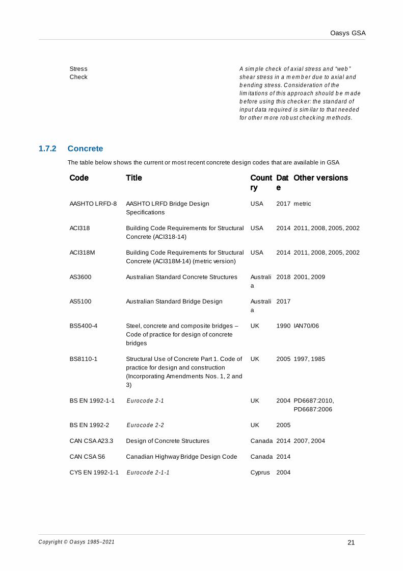
Oasys GSA

Copyright © O as ys 1985–2021 21

Stress

Check

A sim p le check o f axia l stress and “web ”

shear stress in a m em b er due to axia l and

b end ing stress. C onside ra tion o f the

lim ita tions o f th is app roach shou ld b e m ade

b e fo re using th is check e r: the standard o f

inpu t da ta requ ired is sim ila r to tha t needed

fo r o the r m ore rob ust check ing m e thods.

1.7.2 Concrete

The table below shows the current or most recent concrete design codes that are available in GSA

Code Title Count

ry

Dat

e

Other versions

AASHTO LRFD-8 AASHTO LRFD Bridge Design

Specifications

USA 2017 metric

ACI318 Building Code Requirements for Structural

Concrete (ACI318-14)

USA 2014 2011, 2008, 2005, 2002

ACI318M Building Code Requirements for Structural

Concrete (ACI318M-14) (metric version)

USA 2014 2011, 2008, 2005, 2002

AS3600 Australian Standard Concrete Structures Australi

a

2018 2001, 2009

AS5100 Australian Standard Bridge Design Australi

a

2017

BS5400-4 Steel, concrete and composite bridges –

Code of practice for design of concrete

bridges

UK 1990 IAN70/06

BS8110-1 Structural Use of Concrete Part 1. Code of

practice for design and construction

(Incorporating Amendments Nos. 1, 2 and

3)

UK 2005 1997, 1985

BS EN 1992-1-1 Eurocode 2 -1 UK 2004 PD6687:2010,

PD6687:2006

BS EN 1992-2 Eurocode 2 -2 UK 2005

CAN CSA A23.3 Design of Concrete Structures Canada 2014 2007, 2004

CAN CSA S6 Canadian Highway Bridge Design Code Canada 2014

CYS EN 1992-1-1 Eurocode 2 -1 -1 Cyprus 2004

Oasys GSA

Copyright © O as ys 1985–202122

DIN EN 1992-1-1 Eurocode 2 -1 -1 German

y

2004

DIN EN 1992-2 Eurocode 2 -2 German

y

2010

DS/EN 1992-1-1 Eurocode 2 -1 -1 Denmar

k

2004

DS/EN 1992-2 Eurocode 2 -2 Denmar

k

2005

EN1992-1-1 Eurocode 2: Design of concrete structures

– Part 1-1: General rules and rules for

buildings

2004

EN 1992-2 Eurocode 2: Design of concrete structures.

Concrete bridges - Design and detailing

rules

2005

Hong Kong Code

of Practice

Code of Practice for the Structural Use of

Concrete

Hong

Kong

2013 2004 (AMD 2007),

2004, 1987

Hong Kong

Structures Design

Manual

Structures Design Manual for Highways

and Railways

Hong

Kong

2013 2002

IRC:112 Code of Practice for Concrete Road Bridges India 2011

IRS Concrete

Bridge Code

Code of Practice for Plain, Reinforced &

Prestressed Concrete for General Bridge

Construction

India 1997

I.S. EN 1992-1-1 Eurocode 2 -1 -1 Ireland 2004

I.S. EN 1992-2 Eurocode 2 -2 Ireland 2005

IS 456 Plain and reinforced concrete – Code of

Practice

India 2000

NEN EN 1992-1-1 Eurocode 2 -1 -1 Netherl

ands

2004

NEN EN 1992-2 Eurocode 2 -2 Netherl

ands

2011

NF EN 1992-1-1 Eurocode 2 -1 -1 France 2005

NF EN 1992-2 Eurocode 2 -2 France 2006

NS-EN 1992-1-1 Eurocode 2 -1 -1 Norway 2004

PN-EN 1992-1-1 Eurocode 2 -1 -1 Poland 2008

Oasys GSA

Copyright © O as ys 1985–2021 23

SFS-EN1992-1-1 Eurocode 2 -1 -1 Finland

SS EN 1992-1-1 Eurocode 2 -1 -1 Singap

ore

2008

SS EN 1992-1-2 Eurocode 2 -2 Singap

ore

2012

UNE-EN 1992-1-1 Eurocode 2 -1 -1 Spain 2010

UNE-EN 1992-2 Eurocode 2 -2 Spain 2010

UNI EN 1992-1-1 Eurocode 2 -1 -1 Italy 2004

UNI EN 1992-2 Eurocode 2-2 Italy 2006

1.8 Validation

Before embarking on any analysis, the user should be aware of its limitations. The user should check the

validity of the results. Computer models should be as straightforward as possible to minimise the risk of

error, and designed to model the effects required by the user, e.g. a model to assess the stiffness of a

structure would not necessarily be the same as one to check the strength. It is often good practice to start

with a simple model and increase the complexity if the need arises.

Oasys Ltd implements a Quality Management System (QMS) that is certified to ISO 9001.  The certificate of

approval for the Oasys QMS is published on the Oasys web site. Oasys products are designed, developed

and tested in accordance with the procedures set out in this QMS.  A certificate is produced to confirm all

testing has been completed in accordance with the QMS, and this can be provided on request.

1.9 Acknowledgements

Arup

Many engineers have contributed to the development of GSA. In particular the dynamic relaxation solver is

based on the work of Alistair Day, the P-∆ and modal buckling options in GSA were developed in

conjunction with Pat Dallard, the RC Slab options have been developed by Ian Feltham, the footfall

analysis options by Peter Young and Mike Willford and the pattern loading by Don Ho.

Third Party Components

Oasys programs make use of the following third party components

Resizeable dialogs

Delaunay triangulation

CM2 MeshTools

LAPACK

See below for copyright and licensing details.

Oasys GSA

Copyright © O as ys 1985–202124

Resizeable dialogs

Copyright, and License:

Resizeable dialogs, Copyright (c) 2000-2001 by Paolo Messina. All Rights Reserved.

Delaunay triangulation

Copyright, and License:

Copyright (c) 2015 Simon Zeni (simonzeni@gmail.com)

Permission is hereby granted, free of charge, to any person obtaining a copy of this software and

associated documentation files (the "Software"), to deal in the Software without restriction, including

without limitation the rights to use, copy, modify, merge, publish, distribute, sublicense, and/or sell copies

of the Software, and to permit persons to whom the Software is furnished to do so, subject to the following

conditions:

The above copyright notice and this permission notice shall be included in all copies or substantial

portions of the Software.

THE SOFTWARE IS PROVIDED "AS IS", WITHOUT WARRANTY OF ANY KIND, EXPRESS OR IMPLIED,

INCLUDING BUT NOT LIMITED TO THE WARRANTIES OF MERCHANTABILITY, FITNESS FOR A

PARTICULAR PURPOSE AND NONINFRINGEMENT. IN NO EVENT SHALL THE AUTHORS OR

COPYRIGHT HOLDERS BE LIABLE FOR ANY CLAIM, DAMAGES OR OTHER LIABILITY, WHETHER IN AN

ACTION OF CONTRACT, TORT OR OTHERWISE, ARISING FROM, OUT OF OR IN CONNECTION WITH

THE SOFTWARE OR THE USE OR OTHER DEALINGS IN THE SOFTWARE.

https://github.com/Bl4ckb0ne/delaunay-triangulation

CM2 MeshTools

Copyright, and License:

CM2 MeshTools by Computing Objects. All Rights Reserved.

http://www.computing-objects.com/content/view/4/14/lang,en/

LAPACK

Copyright, and License:

Copyright (c) 1992-2011 The University of Tennessee and The University of Tennessee Research

Foundation. All rights reserved.

Copyright (c) 2000-2011 The University of California Berkeley. All rights reserved.

Copyright (c) 2006-2011 The University of Colorado Denver. All rights reserved.

COPYRIGHT

Additional copyrights may follow

HEADER

Redistribution and use in source and binary forms, with or without modification, are permitted provided that

the following conditions are met:

Oasys GSA

Copyright © O as ys 1985–2021 25

- Redistributions of source code must retain the above copyright notice, this list of conditions and the

following disclaimer.

- Redistributions in binary form must reproduce the above copyright notice, this list of conditions and the

following disclaimer listed in this license in the documentation and/or other materials provided with the

distribution.

- Neither the name of the copyright holders nor the names of its contributors may be used to endorse or

promote products derived from this software without specific prior written permission.

The copyright holders provide no reassurances that the source code provided does not infringe any patent,

copyright, or any other intellectual property rights of third parties. The copyright holders disclaim any liability

to any recipient for claims brought against recipient by any third party for infringement of that parties

intellectual property rights.

THIS SOFTWARE IS PROVIDED BY THE COPYRIGHT HOLDERS AND CONTRIBUTORS "AS IS" AND ANY

EXPRESS OR IMPLIED WARRANTIES, INCLUDING, BUT NOT LIMITED TO, THE IMPLIED WARRANTIES

OF MERCHANTABILITY AND FITNESS FOR A PARTICULAR PURPOSE ARE DISCLAIMED. IN NO EVENT

SHALL THE COPYRIGHT OWNER OR CONTRIBUTORS BE LIABLE FOR ANY DIRECT, INDIRECT,

INCIDENTAL, SPECIAL, EXEMPLARY, OR CONSEQUENTIAL DAMAGES (INCLUDING, BUT NOT LIMITED

TO, PROCUREMENT OF SUBSTITUTE GOODS OR SERVICES; LOSS OF USE, DATA, OR PROFITS; OR

BUSINESS INTERRUPTION) HOWEVER CAUSED AND ON ANY THEORY OF LIABILITY, WHETHER IN

CONTRACT, STRICT LIABILITY, OR TORT (INCLUDING NEGLIGENCE OR OTHERWISE) ARISING IN ANY

WAY OUT OF THE USE OF THIS SOFTWARE, EVEN IF ADVISED OF THE POSSIBILITY OF SUCH

DAMAGE.

http://www.netlib.org/lapack/

For further details of third party libraries see https://arup-group.github.io/oasys-combined/general/

Oasys_ThirdParty.pdf

Part II

Oasys GSA

Copyright © O as ys 1985–2021 27

2 Getting Started

GSA is a program for structural analysis, and it is assumed the user has a knowledge of structural

engineering concepts. The GSA help is aimed at explaining the features and use of the program but not

the structural concepts expressed in the program. A new user to GSA should refer to the Getting Started

manual which gives a worked example on the use of GSA.

Design & Analysis Layers

An engineer normally thinks of a structure in terms or beams and columns, and slabs and walls. These

are represented in GSA as members which form the structu ra l m ode l and live in the design laye r. These

are a convenient way to describe the basic structure. The members may or may not be connected, so

normally there will be a discrete connection between beams and columns, but there may be an implied

connection where a secondary connects to a primary beam part-way along its length. In order to analyse

the model the 1D members need to be properly connected and 2D members need to be meshed with

finite elements. GSA provides a tool to handle this mapping and create the ana lysis m ode l on the ana lysis

laye r.

It is encouraged to use the design layer to define the structure as this makes it easier to adjust the

analysis model, but there is nothing that prevents the engineer from building the model directly in the

analysis layer.

Data Modules

Data in GSA is held in modules that can (in most cases) be thought of as tables. So, for example, a simple

model may have a nodes module, an elements module, a beam sections module and some load

modules. The data for these tables can be entered directly via Table Views. However it is usually better to

use some more convenient (and less error prone) method of entering the data.

This section is concerned with the construction of the geometrical model (nodes, elements and

properties) and does not consider the loading.

There is no one correct way of building a model. The most appropriate method will depend on the shape

and complexity of the model. Familiarity with other programs, such as spreadsheets and CAD packages

will affect the approach, as will the availability of the geometric data in other formats.

Data Generation

The simplest way of constructing a model is to use the 'Data Generation' wizard. Templates are offered for

typical structural forms. The structure is specified by selecting a template and defining a few key

parameters.

Since this method is so quick and easy it is sometimes useful to generate from a template even if it is

known that the resulting geometry will have to be edited to arrive at the desired geometry.

Sculpting Models

Sculpting is the term used for graphical editing of the model via a Graphic View. The clear visual feedback

makes this method popular for all shapes, sizes and complexities of structure.

The mesh generation option in GSA makes sculpting a powerful tool for the meshing of irregular areas

with 2D elements.

Sculpting is covered in more detail in the “Working with the Program” section under “Working with Graphic

Views”.

Spreadsheets & CAD

For some structures there is a regularity which lends itself to definition of the structure in a spreadsheet. In

other cases the structure can be defined in terms of a number of parameters that are subject to change,

so spreadsheets give the flexibility to quickly generate variations on complex models. Data that is

Oasys GSA

Copyright © O as ys 1985–202128

generated in a spreadsheet can either be read as a text file, or included directly in tables using cut and

paste.

Structural models that exist in CAD packages may be transferred to GSA via the DXF and DWG file formats

(provided the information can be saved as a DXF file in the CAD package). This is useful both when the

geometric form has been defined by others and supplied in a CAD format and when it is felt that CAD is

the most appropriate tool for defining the geometry.

BIM

Models assembled in BIM packages can be imported into GSA either via an Industry Foundation Classes

(IFC) file or from the GSA/Revit link.

Part III

Oasys GSA

Copyright © O as ys 1985–202130

3 Working with GSA

This chapter describes how to use the GSA interface

Wizards

The New Model Wizard and Data Generation Wizard provide a quick way of generating simple structural

forms.

The New Model Wizard runs when you start a new document set up preliminary details about the structure

such as job details, structure type and units. The user may finish at this stage with an empty model or

proceed via “Generate data for the selected structure type” to select a structural form and then generate a

model based on a set of parameters defining this structure. At the end of this process a complete model is

generated ready for loading to be applied.

These wizards are covered in more detail in the GSA Tools section.

Cases

Loading and results are grouped into cases. Loads are grouped into load cases, primary results (those

calculated directly) are grouped into analysis case and secondary results (combinations of primary

results) are grouped into combination cases. For design there are design cases which associate a set of

results with a design code.

Cases are covered in more detail in the Analysis Tasks and Cases section.

Preferences

Preferences are set in the Preferences Dialog available from the “Tools | Preferences” (Ctrl+F7) menu

command.

Toolbar and dockable pane selection and positioning and window sizes are set each time the program is

closed.

Default settings for new Graphic Views and Output Views are saved as preferences. Several preferred

Graphic and Output Views may also be saved as preferences. Details are given in the Working with Saved

Views and Preferred Views

The preferences may be reset to their default “factory” setting by using the “Tools | Reset Preferences”

menu command. The option is given to reset all view settings. Specific view settings may be reset from

the Explorer Pane.

Toolbars and dockable panes

Toolbars and dockable panes can be controlled from the “View | Toolbars and Dockable Panes” menu

command or the GSA toolbar. Toolbars can be customised using the dropdown arrow at the end of the

bar. With the exception of the Lists toolbar all toolbars can be either docked (attached to the main frame) or

floating. Toolbars are covered in detail in the Toolbars and Keyboard Accelerators section. documentation.

File formats

The default file type for GSA is a GWB file. There is also an editable text file available (GWA) which can be

used when taking data to an earlier version of GSA . The text file format is given in GSA Text (ASCII) Data

File Format

There are also options to interact with other software through Import and Export functions. These are

described in detail in the Interaction with other software section.

Views

Explorer Panes– access to Table Views, Output Views, Saved Views and Preferred Views.

Oasys GSA

Copyright © O as ys 1985–2021 31

Output Panes– display properties; display results for individual nodes, elements and members; display

reports of the analysis process

Table Views – allow tables of input data to be edited.

Graphic Views – display a graphic image of the model offering graphical editing and graphical

representation of input data and results.

Output Views – display input data and results in tabular format.

Particular operations warrant their own sections:

Sculpting – graphical editing of data.

Undoing Edits – the Undo and Redo commands.

Saved Views and Preferred Views – saving Graphic View and Output View settings for re-use either with

the particular model or as preferences.

3.1 Dockable Panes

GSA uses dockable panes to control the model. These fall into four categories:

Explorer Pane offer tree controls that give access to input data modules (typically Table Views) , Output

Views and Saved Views.

Output Panes display text messages, results and task reports.

Graphics Palettes give direct control of Graphic Views.

Property Pane provide tools for editing entities.

Their default positions are shown below.

Dockable panes can be moved, floated and closed. When floating they are displayed on top of any other

view and they can be dragged outside the GSA window. They can be docked along any edge of the GSA

window, with any other dockable panes. When docked the part of the screen that is available for other

views excludes that occupied by the dockable panes. The default position can be recalled using the 'View |

Reset Toolbars and Dockable Panes' menu command. All dockable panes can all be toggled on and off

using the 'View | Show or Hide Dockable Panes' menu command (or button on the GSA toolbar), and

individual dockable panes can be opened and closed from the commands in the 'View | Toolbars and

Dockable Panes' sub-menu.

Oasys GSA

Copyright © O as ys 1985–202132

3.1.1 Explorer Pane

The Explorer Panes are a collection of Dockable Panes:

Data Explorer pane – gives access to all input data modules

Output Explorer pane – gives access to all Output Views that are available for the model.

View Explorer pane – gives access to all Saved Graphic Views and Saved Output Views.

Double clicking on an item will open the appropriate view.

The Explorer panes are dockable panes. The content of the Explorer panes always relates to the current

model.

Data Explorer pane

The Data Explorer pane organises the data into several categories.

Against each item is reported the number of records currently specified for the data module.

The right-click menu includes the following options:

Delete – delete the contents of the selected module or a branch of modules. (Only enabled when the

clicked item is editable.)

Copy – copy the contents of the selected module to the clipboard in GWA format.

Copy All – copy the whole model to the clipboard in GWA format.

Paste – paste the GWA formatted clipboard contents, overwriting the current data.

Paste Special – specify, via the GWA Import Options dialog box, how to paste the GWA formatted

clipboard data, including the option to overwrite or append and the option to select the modules that are

to be pasted.

Oasys GSA

Copyright © O as ys 1985–2021 33

Output Explorer pane

The Output Explorer pane organises the output data and results into several categories. Not all of these

categories may be visible as the list is updated dynamically; an item is offered only if there are data or

results to display and a category is only visible if there are items offered within that category.

Some results are available in more than one Output View, for example displacements are available under

“Nodal Results” as displacement at nodes or under “Beam and Spring Element Results” and “2D Element

Results” as displacements at positions on elements. Results that apply to the model as a whole are

reported as “Global Results”.

The right-click menu includes options to “Specify Output” and to “Open Summary”. “Specify Output”

displays the Output Settings dialog with the clicked item selected, giving the opportunity to further specify

the Output View settings before opening the view. “Open Summary” opens an Output View of just the

summary (Maxima and Minima) of the clicked item. In the “User Modules” branch the right-click menu also

gives access to the user module management dialogs.

View Explorer pane

The View Explorer pane gives access to:

New Graphic Views

Preferred Graphic Views

Saved Graphic Views

New Output Views

Preferred Output Views

Saved Output Views

View Lists

The right-click menus also offer commands for the management of these.

Opening a New Graphic View or New Output View simply opens a Graphic View or Output View with the

default settings. (These have the same affect as giving the “View | New Graphic View” or “View | New

Output View” menu commands, or the equivalent toolbar commands.)

Preferred views and saved views are offered only if these have previously been saved. An asterisk, “*”, is

appended to “Views” on the tab label when some saved Graphic Views or Output Views are present in the

current model.

Different right-click menus are displayed depending on whether the clicked item is a new view, preferred

view, saved view or view list.

The right-click menu for new views includes the option to reset the settings to GSA default. Note that the

“Tools | Reset Preferences” menu command also gives the option to reset the default Graphic View and

Output View settings.

The right-click menu for preferred views includes options to rename and delete the preferred view and to

“Delete All Preferred Graphic Views” or “Delete All Preferred Output Views”, respectively. Deleting all

preferred views does not reset the default view settings.

The right-click menu for saved views includes options to edit, copy, rename and delete the saved view and

to “Delete All Saved Graphic Views” or “Delete All Saved Output Views”, respectively.

Options to create new view lists, to edit, copy and otherwise manage existing view lists are available in the

Oasys GSA

Copyright © O as ys 1985–202134

right-click menu for view lists.

Preferred views, saved views and view lists can be printed directly from the right-click menu. Refer to Batch

Printing of Views for details.

Details of how to produce preferred and saved views and view lists are given in the Working with Saved

Views and Preferred Views documentation.

3.1.2 Output Pane

The output panes are a collection of Dockable Panes

Message Pane – displays properties for a selected item.

Result Pane – displays results for a selected item.

Report Pane – displays task logs (i.e. a history of Report View logs).

Right-click menu

Clicking the right mouse button when the cursor is over the Object Viewer displays a floating menu offering

the following commands:

Close Object Viewer

Copy

Select All

Print

Message Pane

The Message Pane displays properties for a selected item or a set of selected items. It is also where

messages from various operations are displayed.

In Graphic Views:

clicking on a node, element or member causes the properties for that item to be displayed in the

Message Pane, regardless of the current cursor mode.

selecting items and then using the “Graphics | Selection Properties” command displays properties

relating to the current selection.

For Beam, Bar, Tie and Strut elements, selection properties include:

total length,

total mass and

total surface area.

For 2D elements, selection properties include:

total area,

total element mass and

total additional mass.

For nodes, if two or three nodes are selected, selection properties include:

Oasys GSA

Copyright © O as ys 1985–2021 35

distance between nodes,

and, if three nodes are selected:

angle at nodes.

In Table Views:

In some Table Views properties for the current record can be displayed by giving the “View | Properties”

menu command. The Properties command is also accessible from the Table View right-click menu.

Result Pane

The Result Pane displays results for a selected item. This is done as follows:

1. Open the Result Pane by selecting 'View | Toolbars and Dockable Panes | Result Pane' command (or

clicking the Result Pane button toolbar button if available).

2. Select the required output option from the drop-down list at the top of the Result Pane. Only those

options currently available for the model are displayed.

3. Select the required case or cases in the Cases list at the top of a Graphic View.

4. In the Graphic View, click on a node, element or member to display their results.

The default output option is '<displayed result>'. In this setting clicking on a node, element or member in

the Graphic View causes the currently displayed result in that Graphic View to be reported in the Result

Pane. The currently displayed result in the Graphic View is determined by the following precedence:

1. The contoured data, if contouring is displayed.

2. The last specified diagram, if any diagrams are displayed.

3. Node or element displacements (depending on whether a node or element is clicked), if the deformed

image is displayed.

Report Pane

The Report Pane displays a history of all logs generated by GSA tasks, such as analysis and design. For

example, during an analysis the Report View displays the analysis log as it happens; upon completion the

report log stored with the model and displayed in the Report Pane.

The contents of the Report Pane can be deleted by using the Delete Report Logs button on the Report

Pane toolbar.

3.1.3 Graphics Palette

The Graphics Palettes are a collection of Dockable Panes that define what is displayed in the Graphics

view.

Graphics Display Palette – provides quick access to frequently used Graphic View settings.

Entity Display Palette – provides a convenient way of specifying the entities that are to be displayed.

Label Palette – provides a convenient way of setting labels.

Contour Palette – provides a convenient way of setting contours.

Diagram Palette – provides a convenient way of setting diagrams.

Each Graphics Palette includes a toolbar offering options that relate to the palette. All Graphics Palette

Oasys GSA

Copyright © O as ys 1985–202136

toolbars offer the Lock Image Update command. When Lock Image Update is set no updating of the

image in the current Graphic View occurs; unsetting Lock Image Update causes the image to be

regenerated picking up all the changes to the graphic settings that have been applied. Rotating, zooming

or panning the view unsets Lock Image Update. This feature is useful for large models which take a

significant time to update the view.

Graphics Display Palette

The Graphics Display Palette provides quick access to a frequently used subset of Graphic View settings.

The Graphics Display Palette toolbar offers:

Lock image update – (see above)

Wizard – opens the Graphics Settings dialog.

Reset display adornments – resets the Graphics Settings to the current defaults.

Right-clicking on a field displays a context menu offering the settings dialog for that field, where

appropriate.

Entity Display Palette

The Entity Display Palette provides a convenient way of specifying the entities that are to be displayed in

the current Graphic View in terms of saved lists, grid surfaces, properties, etc. The categories are offered

as branches on a tree control. The selected item is applied to the Display List for the current Graphic View.

The Entity Display Palette toolbar offers:

Lock image update – (see above)

Highlight mode – when set the entities selected in the tree control are highlighted in the Graphic View.

Check boxes – when set the tree control is displayed with check boxes against each item to allow

multiple selection.

Reset to all entities – resets the Display List to to 'all' and clears all Volumes.

Right-clicking on an item displays a context menu offering options to open the definition dialog, to select all

entities with that item set, and to display the properties for the item in the Message Pane, where

appropriate.

Label Palette

The Label Palette provides a convenient way of switching label options on and off in the current Graphic

View.

The Label Palette toolbar offers:

Lock image update – (see above)

Hide Labels – when set all labels are removed from the display in the current Graphic View, without

adjusting the labelling settings. Unsetting 'Hide Labels' re-displays the labels.

Reset labels – resets all labelling settings to default.

Labels and Display Methods – opens the Labels and Display Methods dialog.

Apply Adornments to Selection – when set labels are applied to the current selection only.

Oasys GSA

Copyright © O as ys 1985–2021 37

Contour Palette

The Contour Palette provides a convenient way of setting contours in the current Graphic View.

The Contour Palette toolbar offers:

Lock image update – (see above)

Hide Contours – when set contours are removed from the display in the current Graphic View, without

adjusting the contouring settings. Unsetting 'Hide Contours' re-displays the contours.

Reset contours – resets contour settings.

Layer combo – sets the output layer for 2D element stress contours.

Contour settings – opens the Contour Settings dialog.

Apply Adornments to Selection – when set contours are applied to the current selection only.

Diagram Palette

The Diagram Palette provides a convenient way of setting diagrams in the current Graphic View.

The Diagram Palette toolbar offers:

Lock image update – (see above)

Hide Diagrams – when set diagrams are removed from the display in the current Graphic View, without

adjusting the diagram settings. Unsetting 'Hide Diagrams' re-displays the diagrams.

Reset diagrams – resets diagram settings.

Layer combo – sets the output layer for 2D element stress diagrams.

Diagram settings – opens the Diagram Settings dialog.

Apply Adornments to Selection – when set diagrams are applied to the current selection only.

3.1.4 Property Pane

The Property pane is Dockable Pane that allows you to view and modify the default and current settings of

entities, such as nodes, elements, and members. It will show the defaults for any new entity if nothing is

currently selected, or it will show the current properties of any entity that is selected. If you select multiple

entities then it will show the properties that are common between them, and show "<varies>" for those that

differ.

Node properties

Oasys GSA

Copyright © O as ys 1985–202138

Node defaults

The Node Properties pane allows you to set the defaults or edit the properties of selected nodes. See

Nodes for more information.

Name text used for easy identification

Colour select from list

Position coordinates; existing nodes only

Axis select from list of Axis Sets to set the node's Constraint Axes

Restraint directions

Spring property gives the node a spring restraint. Select from the list generated from the Spring

Properties table

Mass property gives the node an additional mass. Select from the list generated from the Mass

Oasys GSA

Copyright © O as ys 1985–2021 39

Properties table

Damper property gives the node a damping value. Select from the list generated from the Damper

Properties table.

Local element size adjusts the local mesh density of a connected member. Note that it only affects 1D

members if the member element size is other than "none"

Element properties

Oasys GSA

Copyright © O as ys 1985–202140

Elem ent defaults

The Element Properties pane allows you to set the defaults or edit the properties of selected elements.

See Elements for more information.

Name text used for easy identification

Colour select from list

Oasys GSA

Copyright © O as ys 1985–2021 41

Element Type select from list; see Element Types for more details

Property select from list defined in Properties : Section, Spring Properties, 2D Element Properties, 3D

Element Properties, Link Properties, Cable Properties, Damper Properties, or Spacer Properties tables,

dependant on the Element Types chosen above

Group a user-defined number to aid loading and output; see Output By Case, By Property, By Group,

Colour In Graphic Views for more details

Orientation node input node number; see Element Axes for more details

Orientation angle input rotation angle in degrees; see Element Axes for more details

Releases partially disconnect elements from others; 1D elements only; see Elements for more details

Release stiffness partially disconnect elements from others; 1D elements only; see Elements for more

details

Offsets distance elements from others; see Elements for more details

Dummy elements that are ignored during analysis but can help with area loads; see Elements, 2D

Loads on Load Panels, and Modelling Implications for more details

Member properties

Oasys GSA

Copyright © O as ys 1985–202142

Mem ber defaults

Oasys GSA

Copyright © O as ys 1985–2021 43

The Member Properties pane allows you to set the defaults or edit the properties of selected members.

See Members for more information.

Name text used for easy identification

Colour select from list

Member type set the member to be 1D, 2D, or 3D

Axis select from list of Axis Sets

Property select from list defined in Properties : Section, Spring Properties, 2D Element Properties, 3D

Element Properties, Link Properties, Cable Properties, Damper Properties, or Spacer Properties tables,

dependant on the member type chosen above

Group a user-defined number to aid loading and output; see Output By Case, By Property, By Group,

Colour In Graphic Views for more details

Orientation node input node number; see Element Axes for more details

Orientation angle input rotation angle in degrees; see Element Axes for more details

Releases partially disconnect resulting end elements from others; 1D members only; see Elements for

more details

Release stiffness partially disconnect resulting end elements from others; 1D members only; see

Elements for more details

Offsets distance elements from others; see Elements for more details

Dummy elements that are ignored during analysis but ; see Elements, 2D Loads on Load Panels, and

Modelling Implications for more details

Automatic offsets

o End 1, End 2 offset 1D member and resulting 1D elements from connected 1D elements

o Internal offset 2D member resulting elements to face of 1D column and connect with a rigid

constraint

1D element type that will be created when the 1D member is meshed, select from list; see Element

Types for more details

2D analysis type that will be created when the 2D member is meshed, select from list, see Element

Types and Rigid Constraints for more details

Element size (m) sets the size of the resulting elements when the member is meshed, see Members

and Element Meshes for more details; if set to none and 1D then there will be no additional meshing

other than that derived from the connecting members; if set to none and 2D or 3D then the default

element size will be 1m. If the 2D member element size is negative then the mesh will consist only of

triangular elements.

Intersect with others the member will mesh with other members that overlap with it; eg untick for

crossed Tie bracing or Load Panels to prevent unwanted subdivision of resulting elements

End restraints sets 1D Member End Conditions for design calculations

Effective length sets 1D member effective lengths for design calculations; see Generating Steel

Member restraint for more details

Oasys GSA

Copyright © O as ys 1985–202144

3.2 Table Views

Most input data required by GSA can be entered in tables. Tables in GSA are similar to spreadsheets, but

there are a number of significant differences. These are highlighted in the sections below.

The shaded cells across the top of a table contain default values, which can be changed by the user.

These are placed in the current cell when the cell contents are entered as blank.

Note that some Cell operators operate with default values.

For many of the tables there is the option of defining the data in a Wizard. The wizard is available from the

Wizard button in the Data Options toolbar, or from the table context menu or with the shortcut Ctrl+W. The

use of wizards is necessary for some of the modules where it is not otherwise possible to select or set up

the required data.

Changes made in a table are immediately reflected in other tables, Output Views and Graphic Views, and

vice versa.

Note that in general, data cannot be entered or edited if results exist that would be invalidated by the

changes.

The details of the data entered in each table are covered in the Data in GSA section.

3.2.1 Single and Multi-page Tables

The simplest type of table in GSA contains data on a single page, which scrolls horizontally as required to

give a view on the complete module.

In other cases the data to be displayed is more complex or several data modules are related so it is

convenient to display the data on more than one page of a table. This leads to the following options:

For more complex data it is useful to be able to have more than one view on the data in the table, with

different pages providing a view on a different subset of the data. An example of this type of table is the

N odes table – here it is convenient to separate the node Coordinates, Constraints and Supports on to

separate pages. These pages give a view of different parts of the same node record. The complete record

can be viewed by selecting the All page. In tables like this there is an “All” page to provide a view of all the

data.

Another situation where multiple pages are convenient is where each record is in itself a table. In these

situations each record forms a page. In these tables the user can right click on the tab to insert or delete

pages or change the name of that page. An example of this type of table is the “Alignments” table, where

each alignment is defined by a table of curvature as a function of chainage.

Sometimes it is convenient to be able to group related modules into a single table. An example of this is

the N oda l Load ing table. Here the N ode Loads, A pp lied D is p lac em en ts and Se t t lem en ts are grouped

together on a single table: each page of the table relates to a different module.

For the multi-page tables the pages are changed by clicking on the appropriate tab.

3.2.2 Field Types

All the fields in GSA belong to one of the six following types:

Text – for names and labels.

Numeric – for item numbers and numeric values (e.g. topology item or node coordinate).

Numeric/Percentage – for entering values such as locations that can be entered as an actual value or

as a percentage (e.g. position of load on a beam).

Oasys GSA

Copyright © O as ys 1985–2021 45

Selection fields – for selecting from a list of items (e.g. element type). Depending on the “Show drop-

down list in selection fields” preference setting the required item may either be selected from a drop-

down list or typed in directly. In the latter case the program auto-completes with the first option that

matches what has been typed.

Selection/Numeric fields – for selecting from standard items or entering a value for a user defined

property (e.g. an axis Local or Global form list or 1, 2, etc for user defined).

List – for entry of lists (e.g. nodes, elements, etc).

Button – for access to wizards.

3.2.3 Cell Operators

The following operators may be entered in cells instead of typing in values.

Copy operators

= to copy the value from the same cell in the preceding

record.

=n to copy the value from the same cell in record n.

== to copy the values from the same cell and all

following cells in the preceding record.

==n to copy the values from the same cell and all

following cells in record n.

Increment operators

The increment operators copy the value from the same cell in the preceding record and perform an

operation on that. They apply to numeric fields only.

+=f to add f to the copied value.

to subtract f from the copied value.

*=f to multiply the copied value by f.

/=f to divide the copied value by f.

If the increment, f, is omitted then the default value is used as the increment.

3.2.4 Basic Operations in Tables

The current cell in the table is indicated by depression of the grey cells at the top and left of the table. When

navigating around the table the current cell is also indicated by a bold border around the cell. When editing

a cell the cursor flashes at the current position in the cell and the cell is said to be in edit mode. Basic

navigation and entry of data in tables is as follows.

Navigation

Moving around the table is done by using the arrow keys, Tab, Return, mouse clicks or the “Edit | Go

To” (Ctrl+G) menu command.

Ctrl+Home and Ctrl+End move the current cell to the first and last cell in the table, respectively.

Page Up and Page Down move the current cell a window-full of records up and down, respectively.

Oasys GSA

Copyright © O as ys 1985–202146

Simply navigating to a cell does not put the cell into edit mode.

Editing

The following actions change a cell to edit mode:

Typing in the cell, to cause the existing data to be replaced by what is typed.

Press F2, to highlight the existing data. Subsequent typing will replace any highlighted data.

Press Home or End, to place the cursor at the beginning or end of the existing data, respectively.

Clicking in the current cell, to place the cursor at the clicked position.

Having edited the contents of a cell the contents of the cell must be registered by doing one of the

following:

Press Return or Tab, moves to the next cell.

Press the up or down, moves row.

Press the left or r ight when the cursor is at the left-most or right-most positions, moves to the adjacent

cell.

Click on another cell.

In all cases the contents of the cell are validated and if invalid input is detected it must be corrected before

moving.

The Esc key can be used to undo an edit.

Selection

To select all the cells containing data, use the “Edit | Select All” (Ctrl+A) menu command or click on the

grey box at the very top left of the table. The selection is highlighted in inverted colours (as with any block

selection)

Select records or fields (rows or columns) of cells by clicking on their headers in the grey area.

To select any particular set of cells there are three options:

Use the “Edit | Select” menu command, which displays a dialogue box where a set of cells can be

defined in terms of records and fields.

Drag a box around them using the mouse.

Click on the start cell of the proposed block, then click on the final cell while holding down shift.

To cancel a selection, use “Edit | Select None” menu command or click anywhere in the table.

3.2.5 Cutting, Copying and Pasting in tables

Any selection of table data can be cut or copied to the clipboard, and the contents of the clipboard can be

pasted into a selected location in a table. The clipboard can be used to transfer data between table views,

graphic views, spreadsheets and other packages.

Cut

Cut records from the document and put them on the clipboard. Complete records must be selected before

cutting data. Cutting data to the clipboard replaces the contents previously stored there.

Many data records (e.g. loads) are deleted from the Table View after cutting the data. This avoids empty

records and causes subsequent records to be renumbered.

Oasys GSA

Copyright © O as ys 1985–2021 47

Records that are not renumbered are those whose record numbers are cross-referenced to other data,

and alteration would affect that other data. For example Node record numbers are not renumbered as they

are used to define element topology.

Copy

Copy blocks of selected data to the clipboard as tab delimited text. Copying data to the clipboard replaces

the contents previously stored there. Use the Export command to save selected data as tab delimited text.

Paste

Use the Paste command to insert a copy of the clipboard contents at the currently selected location. Blocks

of data (held in the clipboard in tab delimited format) are inserted if acceptable, see below.

If you highlight a destination block to paste data to, everything in the destination block will be overwritten on

pasting. The size and form of the destination block must be the same as that for data being pasted from.

Pasting a block of data when no cells are selected results in the block being pasted starting at the current

cell. In this case:

If pasting a block to an existing record, GSA gives the option to overwrite the existing data or to insert the

new data. If insert is chosen, data is inserted before the record containing the current cell.

If pasting a block to a cell beyond the existing data, it is pasted appended.

Note that for any of the paste operations, if partial record data is pasted resulting in blank cells, the blank

cells will be set to default values.

Other methods

Note that Cell operators may also be used to copy values from existing cells.

3.2.6 Delete and Blank Records in Tables

Complete records can be inserted, deleted (with renumbering of subsequent records) or blanked (without

renumbering).

To delete a selected record(s), use “Edit | Delete” (Del) menu command or the Delete key. The action of

the delete key will depend on the type of table. In tables in which no blank records are permitted, deleted

records are removed and the table is closed up. In tables in which blank records are permitted, delete will

clear or blank the selected records leaving subsequent records unchanged. If all the selected records are

already blank, the records are deleted to result in subsequent records being renumbered.

To insert a blank record(s) above the currently selected cell or record, use the “Edit | Insert” (Ins) menu

command. This inserts a record at a time and causes subsequent records to be renumbered.

3.2.7 Find, Replace, Go To and Modify in Tables

Find

Use the “Edit | Find” (Ctrl+F) menu command or the “Find” button on the Data Options toolbar to find

specified text or numbers in a Table. The Find Dialog Box appears:

Specify the exact entry you wish to find. This can be made case sensitive by checking the “Match case”

box.

Choose to search the “whole” table or a just a “selection”. Note – if a selection is required, it must be

highlighted before choosing the find command.

Choose to search “up” or “down” from the current cell. Once the end of the table is reached, the search

Oasys GSA

Copyright © O as ys 1985–202148

reverts back to the beginning of the table.

Click the “Find Next” button to find the first matching entry, and again for each subsequent matching

entry. GSA displays a warning message if the specified text is not found.

Go to

To find a specific record or page, use the “Edit | Go To” (Ctrl+G) menu command or the “Go To” button on

the Data Options toolbar. The record/page can be specified in several ways:

n go to record/page n

+n go forward by n records

-n go back by n records

+ go to next non-blank record

- go to previous non-blank record

* go to highest non-blank record/page

Replace

Use the “Edit | Replace” (Ctrl+H) menu command or the “Go To” button on the Data Options toolbar to

perform a search, as for Find, and also replace the specified text or numbers. The Replace Dialog Box

appears. This operates as for Find dialog with additions:

Specify the new entry you wish to replace the existing entry.

Upon finding a matching entry, click the “replace” button, or you can choose to “replace all” matching

entries.

Modify

Use the “Edit | Modify” (Ctrl+M) menu command or the Modify button on the Data Options toolbar to modify

numerical cell entries. Cells containing text remain unmodified. The Table View Modify dialog box appears.

The modifications specified here are applied to every cell value in the “selection” or the “whole” table view.

Specify the “modify by” value to be used in one of the following ways:

Add – add the value in the Modify By box.

Factor – factor by the value in the box.

Power – raise to the power of the value in the box.

Absolute – modify the selection to the absolute value (the modify by is ignored in this case).

3.2.8 Copying To and From Spreadsheets

For many purposes the preparation of some part of the model or loading, or post-processing of results will

require the use of spreadsheets.

To save data for use in spreadsheets, use the Export command.

Information can be cut/copied from tables in GSA and pasted into spreadsheets and vice versa. Also

results can be copied from Output Views and pasted into spreadsheets. Data copied from GSA or

spreadsheets is held as Tab delimited text.

If the user intends to create data in a spreadsheet, it is recommended that a dummy record be created in

GSA and copied to form a “template” in the spreadsheet.

Oasys GSA

Copyright © O as ys 1985–2021 49

3.2.9 Adjusting Data Display

There are a number of options for adjusting the display of data in tables. These are available from the

W indow | Se t t ings menu and from the Data Options toolbar.

Font

The font that is used in the table can be selected. This gives a standard Font selection dialog.

Units

This is available in tables in which units are used. Some of the data may be entered in one unit, the units

changed and subsequent data entered in a different set of units. All data in GSA is stored in SI units and

converted to the requested units upon display.

Axes

This option is only available for the nodes table and allows the coordinates to be entered or viewed in a

different sets of coordinates. This allows, for example, some of the nodes can be defined in a Cartesian

coordinate system and other in a cylindrical system.

Size Columns to Fit, Size Rows to Fit

The widths or heights of table columns and rows on the screen can be reduced to fit the displayed text.

3.2.10 Colour In Tables

The default colours in which entities are displayed in Graphic Views can be overridden by explicitly defined

colour. Explicit colour can be assigned to nodes,elements, members, materials, properties, and analysis

stages.

In tables, the rows for objects that have explicit colour definition are highlighted with a colour-wash

representation of the assigned colour.

Assignment of explicit colours in tables is by use of the Ed it | M od ify C o lou r menu command, having first

selected the records that are to be modified. M od ify C o lou r is also available on the right-click menu. This

opens the Select Colour dialog. The selected colour is indicated by a colour swatch, and the derived

colour-wash, by the partially hidden colour swatch. Setting the colour to unde fined unsets the explicit

colour assignment.

Note that explicit colour assignment can also by applied via Graphic Views.

In the element and member tables there is an option to check for and highlight incomplete elements.

These are entities that refer to non-existent nodes or properties, or where topology items are repeated.

Non-existent items are highlighted in red and repeated items are highlighted in blue.

3.3 Output Views

Output Views may be used to view input data and results in tabular format. Several Output Views may be

open at a time.

A new Output View may be opened using the V iew | N ew Ou tpu t V iew menu command.

The N ew Ou tpu t V iew command first displays the Output Settings dialog box. OK opens an Output View

containing the selected output; C ance l exits the dialog box without opening an Output View.

You can also open Output Views via the Output explorer. This opens the selected Output View with the

default output specification. Note that the default output specification is “All” cases and the first 25 nodes,

elements or members, so opening an Output View via the Output explorer for a large model can cause

Oasys GSA

Copyright © O as ys 1985–202150

huge quantities of output to be generated. When working with large models it is recommended that Output

Views be opened using the “New Output View” command and that the output specification be carefully

specified before requesting the output to be generated.

Default view settings, preferred views and saved views are available for Output Views. Refer to Working

with Saved Views and Preferred Views for details and to Working with the View Explorer pane for

accessing these.

3.3.1 Output Settings

All of the settings that specify the content of an Output View can be set either in the Output Settings dialog

box or in dialog boxes accessible from this. The Output Settings dialog box can be accessed by giving the

“Output | Output Settings” (Ctrl+W) menu command or the “Wizard” command on the Data Options toolbar.

When a new Output View is opened the default view settings are adopted.

Changes to view settings may be undone and redone using the V iew | U ndo V iew (Ctrl+Alt+Z) and V iew |

R edo V iew (Ctrl+Alt+Y) menu commands. These commands are also available on the Standard toolbar.

View settings for the current view may be applied to another Output View by clicking the V iew s e t t ings

pa in te r on the Standard toolbar to grab the current settings and then clicking in the other Output View. Click

the “View settings painter” again or press <Esc> to switch off the option without applying grabbed settings.

View settings may be copied to the clipboard from within the Output Settings dialog box. View settings on

the clipboard may be pasted into the view (i.e. applied to the view) either using Ed it | Pas te (Ctrl+V) or from

within the Output Settings dialog box. Note that Ed it | C opy copies the actual content of the view (see

Interacting with spreadsheets), not the view settings.

There are often other ways of editing the settings, as described below.

Units

By default the units in which data is output are the model units. These may be adjusted for individual

Output Views from the Output Settings dialog box or by using the W indow | Se t t ings | U n its menu

command. U n its is also available on the Data Options toolbar.

Numeric Output

By default the numeric format in which data is output is as set in the user preferences. This may be

adjusted for individual Output Views from the Output Settings dialog box or by using the W indow | Se t t ings

| N um er ic Fo r m at menu command. The precision of output can be adjusted using the W indow | Se t t ings |

Inc r eas e Pr ec is ion and W indow | Se t t ings | D ec r eas e Pr ec is ion menu commands; these increase or

decrease the number of significant figures or decimal places, depending on the current N um er ic Fo r m at

setting. N um er ic Fo r m at, Inc r eas e Pr ec is ion and D ec r eas e Pr ec is ion are also available on the Data

Options toolbar.

Output Axes

By default the axes in which data is output are the default for the data being output. Typically these are

global axes though certain data, like 1D element forces and stresses, is in local axes. The output of most

data can be transformed to specified axes for individual Output Views from the Output Settings dialog box

or by using the W indow | Se t t ings | A xes menu command. A xes is also available on the Data Options

toolbar.

Refer to the Output Options for details of default axes and of which data can be transformed.

Oasys GSA

Copyright © O as ys 1985–2021 51

3.3.2 Output View Table Format

Tables of output may be formatted by displaying the output in a standard Output View or a Grid Output

View. Output that is for inspection, presentation or printing is best formatted with a standard Output View,

while the Grid Output View is offered to facilitate the copying of output to spreadsheets.

New Output Views are opened in the standard Output View format. The default Output View table format is

saved with the default view settings.

A Grid Output View can be opened by giving the ‘Output | Grid Window’ when a standard Output View is

open. The Grid Output View is opened with the same output as is shown in the ‘parent’ standard Output

View and continues to be updated to reflect the ‘parent’ output while the parent view remains open.

There are advantages and disadvantages with each Output View table format. These are summarised as

follows.

Standard Output Views

Generally standard Output Views are best for the presentation or printing of output.

Advantages:

Table header of the "active" table remains at the top of the window

Output options may be specified directly.

Output format is optimised for printing / saving as PDF

Table formatting preserved well to spreadsheets if entire rows are selected and copied into a

spreadsheet

Disadvantages:

Individual columns may not be selected and copied to a spreadsheet

Grid Output View

Generally Grid Output Views are best for copying tables into spreadsheets.

Advantages:

Data is copied to the clipboard in tab separated format. This results in data being pasted in cells

correctly when pasting to spreadsheet.

Data may be selected by blocks, columns or rows of cells.

Tables may be displayed in a grid. (‘Window | Settings | Grid’)

Disadvantages:

Output format is optimised for regular tables of output but is not well suited to notes and other non-

tabular output.

Output options may not be specified directly (though the view does reflect the settings of the parent

standard Output View).

Note that the Output View table format is independent of, and should not be confused with the spreadsheet

format option.

3.3.3 Selecting Data to Output

Several tables can be displayed in a single Output View. Do this by using the Ctrl or Shift key to form

multiple selections of data tables in the Output Settings dialog box. Note that multiple selections may not

be formed on the Output explorer.

Oasys GSA

Copyright © O as ys 1985–202152

Refer to the Output Settings dialog box documentation for more details.

3.3.4 Case and Entity Lists

Where relevant, tables are output for those items identified in the case, node, element and member lists.

Changing a list from the default to a specific selection refines the content of the table.

These lists can be specified both in the Output Settings dialog box and via the Lists toolbar by first setting

the Display Option to the required entity type. The list of entities is then specified in the Display List. The

full GSA list syntax is available when specifying the list.

See Outputting for a selection set of entities for an automated way of updating entity lists by selecting items

in a Graphic View.

Note that R es e t to A ll En t it ies (or a ll in the “Lists” toolbar) resets entities lists to result in the whole model

being included thereby disabling any <cu rren t se lection> settings.

3.3.5 Outputting for a Selection Set of Entities

Sometimes the most convenient method of identifying the entities for which output is required is by

selecting the entities in a Graphic View. One way of transporting the current selection set to the entity list for

an Output View is to copy the selection in the Graphic View and then paste this into the entity list for the

Output View.

An automated way of achieving this is, on the Lists toolbar for the Output View, to set the Display Option to

the required entity and then setting the Display List to <cu rren t se lection>. When an entity list is set to

<curren t se lection> that entity list is set to the current selection set for that entity type and is updated as the

current selection is modified. If the current selection is empty then a ll is assumed. Unlike in Graphic

Views, the <cu rren t se lection> setting remains set and the list continues to be updated with the current

selection until the <cu rren t se lection> setting is switched off.

3.3.6 Enveloping

Where a case to be output is an enveloping case and the data can be enveloped the output produced

consists of the maximum value and minimum value and a reference to an envelope permutation number

that produced the maximum or minimum value. Note the reference to envelopes in the Output summary

section.

By default the envelope is produced for all components. It is possible to specify that the envelope be of a

particular sub ject com ponen t in which case other components are output as the coexistent values for the

permutation that produced the maximum or minimum value for the subject component.

Refer to the Output Settings: Further Options documentation for details on how to specify this.

The scope and limitations of envelopes are described in Enveloping in GSA.

3.3.7 Data Extents

Where only a particular range of values of a component are of interest, data extents can be specified.

These can be expressed in terms of minimum and/or maximum values, signed or as a magnitude, as an

inclusive or exclusive range. When data extents have been activated only records for which the value of the

sub ject com ponen t lies within the range are output.

Refer to the Output Settings: Further Options documentation for details on how to specify this.

Oasys GSA

Copyright © O as ys 1985–2021 53

3.3.8 Output Summary

Most tables can be summarised in terms of the maximum and minimum values encountered in the table

for each component. The maximum and minimum values are displayed in bold; the coexistent

components reported in the summary are the same as the coexistent values reported in the table, even

when the case being reported is an enveloping case.

For some data components (e.g. element length and element strain energy) a total for that component in

the specified table is included in the summary.

Whether or not the table and summary are output can be set in the Output Settings dialog box.

By default the summary includes only the single worst values. It is possible to set the number of worst

values in the Output Settings: Further Options. This results in several worst values being output in

descending sequence. Note that setting the number of worst values to a large number will result in an

output table of values in descending sequence, as opposed to node or element number sequence.

3.3.9 Output By Case, By Property, By Group

The default sequence of lines in a table of output that includes an entity number and a case number per

line is that the entities are output in ascending order and the cases are output in ascending order for each

entity. This sequence may be altered by selecting By C ase, By Property or By Group in the Output Settings

dialog box.

Selecting By C ase causes the table to be split into separate tables per case.

By Property – causes the table to be split into separate tables per element or member property. The

element type is considered when separating the tables so, for example, if there are beam elements with

property one and spring elements with property one these will appear in separate tables. However, Beams

and Bars of property one will appear in the same table since they share the same property.

By Group – causes the table to be split into separate tables per element or member group.

By Property and By Group do not affect tables of nodal data.

3.3.10 Printing from Output Views

The output may be printed by giving the File | Pr in t menu command. The printed image may be previewed

by giving the File | Pr in t Pr ev iew menu command. Pr in t and Pr in t Pr ev iew are also available on the

Standard toolbar.

The Page Se tup command on the Miscellaneous tab of the Preferences may be used to specify the format

of the border on the printed page.

The Pr in t command prints the output in the same font as is used on the screen.

The output may be printed condensed (i.e. in a small font). Typically the smallest font that is legible on

printed output is smaller than that on the screen. Specify the condensed print setting using the W indow |

Se t t ings | Fon t command. Fon t is also available on the Data Options toolbar. The print condensed setting

is stored as a preference.

3.3.11 Interacting with Spreadsheets

The spreadsheet format option is offered to assist in the interaction between Output Views and

spreadsheets. Spreadsheet format is selected in the Output Wizard: Further Options.

Spreadsheet format arranges tables such that all output for a given entity is output on one line,

concatenating what would otherwise be several lines. Note that when copying data in order to paste it into

Oasys GSA

Copyright © O as ys 1985–202154

a spreadsheet it is advisable either to copy from a Grid Output View if you want to target specific columns.

Otherwise, copying from a Standard Output View would work as well. See Output View table format for

details.

The export option in the Output Settings dialog box writes the output as currently specified (but not

necessarily currently displayed) to file in either tab or comma delimited text format. Note that it is possible

to use this option without displaying the output in an Output View. Do this by giving the “New Output View”

command, then, in the Output Settings dialog box, selecting the required output, exporting, and then

cancelling from the dialog box.

The “Output | Export Output” menu command writes the output as currently displayed to file in either tab or

comma delimited text format.

Copying a selection from the Output View, using “Edit | Copy” (Ctrl+C), copies the selected data onto the

clipboard in a format that is acceptable by most spreadsheet programs.

3.4 Graphic Views

Graphic Views may be used to view a graphical representation of the structure. Labels may be applied to

identify the entities that make up the model. Diagrams and contouring may be applied to gain an

understanding of the model and its behaviour.

A number of sculpt tools are provided to enable the model to be edited graphically. Sculpting is

documented in a separate section.

Several Graphic Views of a model may be open at a time.

A new Graphic View may be opened using the V iew | N ew Gr aph ic V iew (Alt+1) menu command.

Any of the enabled graphics toolbar buttons may be used to open a Graphic View when one is not already

open. When at least one Graphic View is already open, giving these commands causes the most recently

accessed Graphic View to be made the current view.

By default the rendering of the graphics for a Graphic View is carried out in a separate thread, to provide

better performance and to enable the rendering of the graphics to be interrupted. It is also possible to

open a Graphic View for which the rendering is processed in the same thread as the main GSA

application, by using the V iew | M is c e llaneous V iew Op t ions | N ew Gr aph ic V iew (main thread)

command.

Default view settings, preferred views and saved views are available for Graphic Views. Refer to Working

with Saved Views and Preferred Views for details and to Working with the View Explorer pane for

accessing these.

3.4.1 Changing the Content of a Graphics View

The content of a Graphic View can be set either in:

The Graphics Palettes. Refer to the Dockable Panes section for details on accessing these.

the Graphic Settings dialog box or in dialog boxes accessible from this. The Graphic Settings dialog box

can be accessed by:

o giving the “Graphics | Graphic Settings” (Ctrl+W) menu command.

o using the “Wizard” command on the Graphics Display Palette or Data Options toolbar.

o Double-clicking on the background of a Graphic View.

New Graphic Views use the default view settings unless there is a Saved Graphic View named

“startup” (case insensitive) in which case these settings are used.

Oasys GSA

Copyright © O as ys 1985–2021 55

Changes to view settings may be undone and redone using the “View | Undo View” (Ctrl+Alt+Z) and “View |

Redo View” (Ctrl+Alt+Y) menu commands. These commands are also available on the Standard toolbar.

View settings for the current view may be applied to another Graphic View by clicking the “View settings

painter” on the Standard toolbar to grab the current settings and then clicking in the other Graphic View.

Click the “View settings painter” again or press <Esc> to switch off the option without applying grabbed

settings.

View settings may be copied to the clipboard from within the Graphic Settings dialog box. View settings on

the clipboard may be pasted into the view (i.e. applied to the view) either using “Edit | Paste” (Ctrl+V) or

from within the Graphic Settings dialog box. Note that “Edit | Copy” copies either the actual content of the

view (see Copying the graphic image to the clipboard) or the current selection (see Copying sets to the

clipboard), not the view settings.

There are often other ways of editing the settings, as described below.

3.4.2 Basic Orientation of the Image

3.4.2.1 Standard Views

The initial view of the model depends on the dimensions of the model. Typically, vertically planar models

are displayed in elevation and other models are displayed in plan.

The following commands (and their associated accelerator keys) are available from the Gr aph ic s |

Or ien ta t ion | S tandar d V iew s menu to provide standard views of the image. The commands are also

available from the Or ien ta t ion toolbar.

Plan (P).

X Elevation (X).

Y Elevation (Y).

Isometric (I).

Skew View (K). This is a perspective projection.

Ground View (G). This is a perspective projection.

Reverse Plan (Alt+P).

Reverse X Elevation (Alt+X).

Reverse Y Elevation (Alt+Y).

In all cases a scale to fit is also carried out.

3.4.2.2 Changing the Orientation of the Image

The following methods may be used to rotate the image.

Dragging – Set the cursor mode to Rotate and drag the mouse. The sensitivity of the mouse movement

may be adjusted in the Graphics Preferences.

Shft+Drag with the mouse wheel (or middle button) held down (in any cursor mode) operates as

dragging in the Rotate cursor mode.

Arrow Keys – Each keystroke rotates the image about the object point by the amount currently set in the

Graphics Preferences. These commands may also be found in the “Graphics | Orientation | Rotate” menu,

for the sake of completeness.

Explicitly – The orientation may be specified in terms of longitude and latitude in the Orientation Settings

Oasys GSA

Copyright © O as ys 1985–202156

dialog box.

In all cases the rotations occur about the object point.

3.4.2.3 Regenerating the Image

The Gr aph ic s | Or ien ta t ion | R egener a te (F5) menu command (also on the Orientation toolbar)

regenerates and redraws the image without changing any parameters that specify the image.

Any operation that causes information to be added or removed from the image will also cause the image

to be regenerated. The image is always regenerated prior to printing.

Impact of zooming on symbols, diagrams and contours

Many of the operations dealing with the orientation, scaling and projection of the image do so without

regenerating the display. This makes the display of the image much quicker and enables these

operations to happen “live” on the full image. A consequence of this is that if, say, dots are drawn at nodes

when the image is zoomed the dots are zoomed by the same amount as the structure. The same occurs

to diagrams and contours, invalidating reported data scales. In this circumstance a message is reported

in the legend to indicate that data scales are unreliable.

Regenerating causes the image to be re-established from the data and view settings to result in all items

being drawn at the intended scale.

3.4.3 Scaling the Image and Zooming

3.4.3.1 Scaling to Fit

The image of the model is drawn in a Graphic View in a specified orientation, at a specified scale, centred

at a specified position. This section deals with scaling and positioning of the image, including zooming

and panning.

Note that many operations that change the structure scale reproduce the display without regenerating the

image. This can invalidate the reported scale for diagrams and contours. See Regenerating the image for

more details.

A scale to fit involves an automatic adjustment of the scale, object point, mid-point and eye distance to

result in the image fitting in the current view.

Scaling to fit occurs when any standard view is selected, when the Gr aph ic s | Or ien ta t ion | Sc a le to f it

(Ctrl+Home) menu command is given and when D o s c a le to f it is selected in the Graphic Settings dialog

box. Sc a le to f it is also available on the Orientation toolbar.

First the extents of the image are determined. These are based on the undeformed state of the part of the

model currently being drawn.

The object point is set to the centre of the extents.

The mid-point is set to 0,0,0 to result in the object point being drawn at the centre of the view.

A scale is calculated that will result in the extents, in their current orientation, fitting within the Auto-scale

margin as set in the Graphics Preferences. The image is regenerated if the R egener a te g r aph ic s on

s tandar d v iew preference is set in the Graphics Preferences.

Scaling may be set to be to an engineering scale by toggling the Gr aph ic s | Or ien ta t ion | Eng inee r ing

Sc a le menu command and in the Graphic Settings dialog box. When set, the calculated scale is rounded

up to the next engineering scale. If the view is an isometric view then it is the isometric scale that is set at

an engineering scale.

An eye distance is arbitrarily set. This is five times a dimension of the image, where the dimension is the

Oasys GSA

Copyright © O as ys 1985–2021 57

near extent to the far extent or, if that is zero, the left to right or the top to bottom.

The scale may be explicitly defined in the Graphic Settings dialog box. Note that when “Lock scale” is

checked in this dialog box the specified scale is preserved when the window is resized and when the

image is printed.

3.4.3.2 Zooming and Panning

In terms of the parameters that define a view, zooming and panning affect the structure scale and the mid-

point. These parameters may be adjusted explicitly via the Orientation Settings dialog box. More

commonly, though, higher level operations may be used to zoom or pan.

Zoom Cursor Mode – When in the Zoom cursor mode:

Dragging a rectangle in the window causes the image to be zoomed and panned to result in that

rectangle filling the Window. Only when the aspect ratios of the rectangle and window are identical will

this be exact; otherwise the scale is such that a t least all of the rectangle remains visible.

Click pans and zooms in. The image is panned to result in the point clicked on being at the mid-point of

the view. The structure scale is multiplied by (zoom factor) where the zoom factor is a Graphics

Preferences.

Ctrl+Click pans and zooms out. The image is panned to result in the point clicked on being at the mid-

point of the view. The structure scale is multiplied by (1 / zoom factor) where the zoom factor is a

Graphics Preferences.

Shft+Click pans. The image is panned to result in the point clicked on being at the mid-point of the view.

Dragging – When in the Rotate cursor mode:

Ctrl+Drag up and down zooms in and out respectively. The sensitivity is governed by the zoom

increment mouse sensitivity Graphics Preferences.

Shft+Drag pans the image. The sensitivity is governed by the pan increment mouse sensitivity Graphics

Preferences.

Intellimouse wheel – In any cursor mode:

Rolling the mouse wheel forwards and backwards zooms in and out respectively. Each notch on the

mouse wheel is equivalent to one Zoom In or Zoom Out command. If when rolling the mouse wheel the

cursor is over the Graphic View then the zoom occurs pinned at the cursor position.

Drag with the mouse wheel (or middle button) held down pans the image. The sensitivity is as for Shft

+Drag, under Dragging above.

Ctrl+Drag with the mouse wheel (or middle button) held down operates as Ctrl+Drag in the Rotate

cursor mode.

Menu commands – The following commands (and their associated accelerator keys) are available from

the “Graphics | Orientation” menu to allow zooming and panning.

Zoom In (Ctrl+Up). Multiplies the structure scale by (zoom factor) where the zoom factor is a Graphics

Preferences.

Zoom Out (Ctrl+Dn). Multiplies the structure scale by (1 / zoom factor).

Reset Pan (Shft+Home). Sets the mid-point to (0, 0, 0).

Pan Right (Shft+Rt). Adjusts the mid-point to result in the picture shifting left by 1/16

of the picture width.

Pan Left (Shft+Lft). Adjusts the mid-point to result in the picture shifting right by 1/16

of the picture width.

Oasys GSA

Copyright © O as ys 1985–202158

Pan Up (Shft+Up). Adjusts the mid-point to result in the picture shifting down by 1/16

of the picture height.

Pan Down (Shft+Down). Adjusts the mid-point to result in the picture shifting up by 1/16

of the picture

height.

Note that scaling to fit effectively resets any zooming and panning.

Note also that these operations do not affect the object point so, for example, rotations that occur after a

zoom or pan may not have the desired affect unless the object point is adjusted.

3.4.3.3 Scaling for Printed Output (and Changed Window Sizes)

There are various ways of specifying the structure scale, as discussed above. Broadly these fall into three

categories, namely by scaling to fit, by zooming and by specifying the scale explicitly. What happens to the

scale when producing printed graphical output or whenever the picture size changes depends on how the

current scale was specified, as follows.

Was scaled to fit – The image is scaled to fit the new picture size.

Was by zoom (or the model was rotated since a scale to fit) – The image is scaled to result in at least

the extents previously shown being visible in the new picture. More will be visible in one direction if the

aspect ratio of the new and old picture sizes are not the same.

Was explicitly defined and locked – The scale is not changed.

This default behaviour may be over-ridden by specifying the structure scale for the printed image in the

Graphic Settings dialog box.

3.4.4 Advanced orientation of the image

3.4.4.1 Adjusting the Object Point

The object point may be adjusted as follows.

Clicking – Set the cursor mode to Rotate and Ctrl+Click on the node or grid point at which you want the

object point to be set.

Explicitly – Specify the coordinates of the object point in the Orientation Settings dialog box.

Note that scaling to fit resets the object point to the centre of the cuboid surrounding the extents of the

currently drawn part of the model.

3.4.4.2 Orthographic and Perspective Projections

The view may be toggled between orthographic and perspective projections using the Gr aph ic s |

Or ien ta t ion | Pe r s pec t iv e Pr o j. (Ctrl+Alt+P) command.

If the eye distance has not been set when a perspective projection is requested then a default eye distance

is calculated as when the image is scaled to fit.

Note that some standard views are in perspective projection.

3.4.4.3 Adjusting the Eye Distance

The eye distance may be adjusted as follows.

Dragging – In the Rotate cursor mode Ctrl+Drag+Lft and +Rt to move the eye distance out and in

respectively. The sensitivity is governed by the eye distance increment mouse sensitivity Graphics

Oasys GSA

Copyright © O as ys 1985–2021 59

Preferences.

Ctrl+Drag with the mouse wheel (or middle button) held down (in any cursor mode) operates as Ctrl+Drag

in the Rotate cursor mode.

Menu commands – The following commands (and their associated accelerator keys) are available from

the Gr aph ic s | Or ien ta t ion menu to adjust the eye distance.

Eye Distance In (Ctrl+Rt). Multiplies the eye distance by (eye distance increment) where the eye distance

increment is a Graphics Preferences.

Eye Distance Out (Ctrl+Lft). Multiplies the eye distance by (1 / eye distance increment).

Explicitly – Specify the eye distance in the Orientation Settings dialog box.

The program imposes a minimum eye distance of 1mm.

Note that scaling to fit resets the eye distance.

3.4.5 Identifying What Is To Be Drawn

The part of the model that is drawn in a Graphic View may be specified in two ways: by volumes and by

lists. Both of these methods are extremely powerful ways of breaking down a large model into more

manageable or more presentable chunks. The volume method is better for situations where the part or

parts of the model that are to be included or excluded can conveniently be identified graphically; the list

method makes use of the list syntax to identify the drawn part of the model.

The two methods may be used independently or in combination.

Note that the scale to fit operation sets the extents of the drawn image on the basis of the current volumes

and lists. However, simply specifying a volume or list does not cause the extents or, indeed, object point to

be adjusted.

Note that R es e t to A ll En t it ies (or a ll in the Lists toolbar) resets both the volumes and entities lists to

result in the whole model being drawn.

The Gr aph ic s | D is p lay | H ide | H ide E lem en ts command temporarily switches the display of elements off.

Elements may then be un-hidden by giving the H ide E lem en ts command again. “Hide Elements” is also

available on the right-click menu. “Hide” commands are also available for members.

M o re:

Volume clipping

Entity lists

3.4.5.1 Volume Clipping

To identify the entities included in a volume,

Set the cursor mode to “Volume” .

Drag the mouse to specify a rectangle (elements within the volume are included; when Ctrl-dragging the

mouse, elements within the volume are excluded.).

Use Ctrl+mouse wheel to specify the near and far extents of the volume. Ctrl+rotate moves the near

plane of the volume; Shft-rotate moves the far plane of the volume; holding the mouse wheel down

while rotating refines the increment of movement.

The view may be in any orientation at the time the volume is specified since part of the definition of the

volume is an axis set which is constructed internally, based on the orientation at the time of forming the

Oasys GSA

Copyright © O as ys 1985–202160

volume. Whether an element is within a volume or not is determined by the current R e fe rence po in t o f

se lection item s setting in the Sculpting Preferences.

Several volumes may be defined at once at different orientations, some inclusive, some exclusive. The

included entities are the sub-set of entities included in all the volumes.

A volume is undone by clicking in the Graphic View when the cursor mode is set to Volume. Each click

removes the most recently specified volume. Shft+Click removes all specified volumes for the current

Graphic View.

3.4.5.2 Entity Lists

When identifying the drawn entities by the list method a list of entities is specified to identify the part of the

model that is to be included. The list is specified on the Lists toolbar for the view by first setting the Display

Option to the required entity type, whether Nodes, Elements or Members. The list of entities is then

specified in the Display List. The full GSA list syntax is available when specifying the list.

When the list is a list of elements and the Analysis Layer is being displayed or when the list is a list of

members and the Design Layer is being displayed, the list simply identifies the elements, or members,

that are to be included.

When the list is a list of elements and the Design Layer is being displayed, those members that are made

up of an element in the list are included.

When the list is a list of members and the Analysis Layer is being displayed, those elements that are part

of a member in the list are included.

When the list is a list of nodes then those elements or members attached to nodes in the list are included.

When an entity list is set to “<current selection>” that entity list is set to the current selection set for that

entity type. If the current selection is empty then “All” is assumed. (Unlike in Output Views, once acted upon

the “<current selection>” setting is forgotten about and the list is set to the contents of the model set.)

Another way of specifying the list of entities to be drawn is by using the “Edit | Draw Selection” menu

command. “Draw Selection” is also available on the right-click menu that is displayed when the cursor

mode is set to Select Nodes or Select Elements. The procedure is as follows.

1. Set the cursor mode to Select Nodes or Select Elements.

2. Select the nodes or elements to be drawn.

3. Give the “Draw Selection” command.

The entity type and list are then set according to the current selection.

3.4.6 Graphical Representation of Entities

3.4.6.1 Default Representation of Entities

There are various ways in which nodes, elements, members and geometric entities are represented in

Graphic Views.

Note that all surface colours are affected by the current shading settings, and all colours and symbol sizes

are affected by the current Graphic Fonts and Styles settings.

Note that the colours of entities stated below can be overridden by specifying the colour of entities explicitly.

Nodes

Nodes that are attached to elements or members are drawn only if the ‘dots at nodes’ label option is

switched on; unattached nodes are drawn only if the respective ‘draw unattached nodes’ display method is

Oasys GSA

Copyright © O as ys 1985–2021 61

switched on.

Standard nodes are drawn as circles.

Attached nodes are drawn black

Unattached nodes are drawn red

Nodes to be created where Members cross are drawn in yellow

Nodes in constraints are drawn in blue

Elements and Members

The colour of elements and members depends on the co lou r e lem en ts’ display method setting:

By type – each element type is assigned a distinct colour. When 2D elements are displayed ‘filled’ and

‘solid’ the top (+ve z) surface is drawn light grey and the bottom surface is drawn dark grey.

By property – each element property is assigned a unique colour. Elements are coloured according to

their property.

By material – each material is assigned a unique colour. Elements are coloured according to their

material.

By initial stage – each analysis stage is assigned a unique colour. Elements are coloured according to

their initial analysis stage.

3.4.6.2 Specifying Colour of entities

The colour of entities displayed in Graphic Views can be defined explicitly, as follows:

Colours can be assigned to the following object types:

Nodes

Elements and Members

Materials

Properties

Polylines

Analysis Stages

Displaying colours

When the view is set to colour elements b y p roperty, or b y m a te ria l or b y in itia l stage, elements (or

members) are displayed in the colour of the property, material or stage, respectively.

Otherwise entities are displayed in the colour of the entity.

If the colour is set to ‘undefined’ (the default) default colours are assumed.

Setting colours

The colours of objects are assigned using the M od ify C o lou r o f Se lec t ion command.

If the view is set to colour elements ‘by property’, or ‘by material’ or ‘by initial stage’ the colours of the

properties, materials or stages of the selected elements (or members), respectively, are modified.

Otherwise the colours of the selected entities are modified.

Choosing colours

Oasys GSA

Copyright © O as ys 1985–202162

Colours are chosen in the Select Colour dialog; either by selecting from a list of preset colours or by

picking in a Colour dialog.

The colour may be set to ‘undefined’.

The Select Colour dialog remembers the ‘last selected colour’.

The ‘last selected colour’ can be set by picking the currently assigned colour of an object, by using the

right-click ‘Pick Colour of This’ command.

The colour of all objects in the model can be reset to ‘undefined’ by using the ‘Clear Colour Modifications’

command.

3.4.7 Current Grid

The current grid is a plane of grid points or grid lines that may be displayed in a Graphic View; it does not

form part of the model but it may be used in conjunction with various sculpt commands to edit the model.

Coordinates are reported with respect to current grid axes.

The current grid is defined by reference to a grid plane, a grid layout and a set of grid lines.

When displayed in a Graphic View the current grid is represented as grid points or grid lines on the current

grid plane. Grid points are displayed on the current grid plane at the spacing specified by the current grid

layout. Grid lines, which, by definition, are in the global XY plane, are displayed projected onto the current

grid plane, but not at all if the current grid plane is vertical.

3.4.7.1 Defining and Adjusting the Current Grid

The current grid is a reference to a grid plane. The current grid plane may can be set on the Lists toolbar

for the view by first setting the Display Option to C urren t Grid. The current grid is then displayed in the

Display List and the available grid planes are offered in the drop-down list.

A quick way of switching the current grid to one at the elevation of a particular node is to right-click on the

node and give the “Set Current Grid to This” command on the right-click menu. The current grid is set to a

grid on which the node lies, first looking for one parallel to the existing current grid, then for any. If none

exists then the program offers to create one parallel to the existing current grid.

The grid can be switched on and off by:

the Sc u lp t | D r aw Gr id (Ctrl+Alt+G) command (also available on the Sculpt toolbar)

the D r aw Gr id option in the Graphics Display Palette

The D raw Grid command toggles between displaying grid lines, grid points and no grid, but grid lines are

only included in the toggle if grid lines have been specified and grid points are not included if the current

grid layout has been disabled in the Current Grid Definition dialog box.

Various sculpt operations make use of the grid.

3.4.7.2 Grid Coordinates and Snapping to Grid Points

The coordinates reported in the status bar are the coordinates of the cursor position on the current grid.

These are referred to as the grid coordinates. The grid coordinates are reported in the current grid axes

(and global axes, if these differ).

Snap to grid may be set by giving the Sc u lp t | Snap to Gr id Po in ts (Ctrl+Alt+S) menu command (also

available on the Sculpt toolbar). When this is set on, the grid coordinates are the coordinates of the

Oasys GSA

Copyright © O as ys 1985–2021 63

nearest grid point or intersection of grid lines on the current grid. Otherwise, the accuracy of the grid

coordinates is based on the screen resolution and the structure scale.

Note that when the construction grid is normal to the picture plane then no coordinates are reported in the

status bar.

3.4.8 Selection Sets

3.4.8.1 The Model Sets

A set is a collection of nodes, elements, members or grid points. Sets are only displayed graphically and

may only be specified graphically. There is no facility to save sets. However there are facilities to translate

between sets and lists. Many sculpt operations operate on sets. Sets may also be used to identify the part

of the model that is to be adorned with labels and diagrams etc.

There are four selection sets established for a model at the time a model is opened in GSA, referred to as

the model sets. These are sets of nodes, elements, members and grid points. The model sets are initially

empty.

The contents of the model sets may be edited from any Graphic View when the related selection cursor

mode is current. The selected items in a model set are highlighted on the image; when not in the

respective selection cursor mode the highlighting is greyed to indicate that the selection is disabled.

Reverting to that selection mode enables the selection.

Since the model sets are owned by the model and not the particular Graphic View and since the cursor

mode is set for all Graphic Views and not just the current one, the highlighting of the model sets occurs on

all open Graphic Views simultaneously.

3.4.8.2 Use of Selection Sets

Many sculpt commands operate on model sets.

It is possible to adorn just items in a model set with labels, diagrams and contouring.

Annotation of diagrams and contouring can be applied to a set. In this case it is not a model set that is

used but a set associated with the particular diagram or contour display. The set is automatically

configured to be of the type (node or element etc.) appropriate for the data being annotated.

3.4.8.3 Forming Selection Sets

Sets are formed using the mouse in an appropriate Graphic View cursor mode.

The functionality of the mouse is as follows.

Clicking or dragging empties the set, unless the Append to selection when click is unmodified

preference is set (in which case the previous selection is not emptied). Items identified by the click or

drag are selected.

Ctrl+Clicking or Ctrl+Dragging deselects the identified items; otherwise the previous selection is not

emptied.

Shft+Clicking or Shft+Dragging selects the identified items; the previous selection is not emptied.

Right-clicking on an entity displays a right-click menu that includes the option to select that entity. The

previous selection is replaced unless the Append to selection when click is unmodified preference is set.

The following menu commands are also available.

Ed it | Se lect A ll (Ctrl+A)

Oasys GSA

Copyright © O as ys 1985–202164

Ed it | Se lect N one (Esc) – This clears the selection for the current selection mode, but if there are no

items selected for the current selection mode then it clears all other selections.

Ed it | Inve rt Se lection

Ed it | Se lect S tring – When in the Select Elements cursor mode this selects a string of elements

attached to and aligned with any currently selected elements. When in the Select Nodes cursor mode

nodes along the string of elements are selected. The straightness tolerance preference is used to

determine whether an element is aligned, allowing this command to be used to select curved strings of

elements and nodes.

Ed it | Se lect H ighest C o inciden t – When in the Select Nodes or Select Elements cursor modes this

deselects all but the highest numbered coincident items in the current selection. E.g. If nodes 1 to 30

are selected and nodes 1 and 11 are coincident and nodes 2, 12 and 22 are coincident then giving this

command will result in only nodes 11 and 22 being selected. This command is useful for deleting

coincident nodes and elements (though note that nodes may not be deleted graphically when they are

referred to by elements).

Ed it | Se lect C lose To Vertica l 1D E lem en ts – When in the Select Elements cursor mode this selects all

1D elements that are within 1º of vertical but are not sufficiently close to vertical to be deemed vertical for

the local element axes definition.

Ed it | Se lect Ou t-Of-R ange – Enabled only when contours are displayed, this command selects all

entities for which the contoured data is out of the range of the current contour settings. E.g. If nodal Uz

0mm then “Select Out-Of-Range” will select all nodes for which the Uz displacement is less than

Entity selection can be by selection within a polyline. The procedure is as follows:

In the Polyline cursor mode, form a Polyline.

Switch to the required selection cursor mode (‘Select Nodes’ or ‘Select Elements’, etc.) cursor mode. All

entities within the polyline (as viewed) are appended to the current selection set for that entity type.

When the reference point of selection items is set to Drag to right – all; drag to left – any part, a polyline

specified in the clockwise direction (as viewed) selects all entities wholly within the polyline; whereas an

anti-clockwise polyline selects entities within or partly within the polyline.

Note also the scope for interaction with lists and the clipboard.

3.4.8.4 Interaction of Sets With Lists

When in a selection mode the Ed it | Sav e Se lec t ion A s L is t menu command saves the current selection

set to the Lists module as a list of the appropriate type. The list formed is a simple list made up of item

numbers and ranges of numbers; no attempt is made to recognise, for example, patterns in the element

properties or groups of selected elements.

Also, when in a selection mode the Ed it | Se lect L ist menu command allows a list to be appended to the

current selection set. The list can be a saved list, referred to by name, or explicitly defined. This latter option

is a useful method for showing the location of particular items.

Both Sav e Se lec t ion A s L is t and Se lec t L is t are also available on the Graphic View right-click menu when

in a selection mode.

Oasys GSA

Copyright © O as ys 1985–2021 65

3.4.8.5 Finding Entities

The interaction of sets with lists offers a method for finding entities that are described in list syntax to result

in those entities being selected in the Graphic View. The Ed it | Find menu command combines the various

steps into one. Find is also available on the Data Options toolbar.

3.4.8.6 Copying Sets to the Clipboard

When the current cursor mode is a selection mode the Ed it | C opy (Ctrl+C) menu command copies the

current selection set to the clipboard in GSA list format. This list may be pasted anywhere where a GSA list

is expected. The list formed is a simple list made up of item numbers and ranges of numbers; no attempt

is made to recognise, for example, patterns in the element properties or groups of selected elements.

Also, when in a selection mode the Ed it | Pas te (Ctrl+V) menu command pastes the list on the clipboard to

the view by appending the items to the current selection set. In this circumstance items in the list may be

separated by either spaces, tabs or may be on separate lines. An error message is given if the content of

the clipboard is not a valid list.

Both C opy and Pas te are also available on the Graphic View right-click menu when in a selection mode.

Nothing in a list held on the clipboard identifies the type of list so, for example, it is possible to copy a set of

nodes and paste the resulting list to somewhere where an element list is expected. This is unlikely to be

useful.

3.4.9 Polylines in Graphic Views

In GSA a polyline is a sequence of points in 3D space, which may optionally be specified in 2D, and which

may optionally be related to a grid plane. There is a Polylines module in which polylines can be saved.

There is also a current polyline which is displayed in Graphic Views when in the Polyline cursor mode.

The current polyline is drawn with respect to its grid plane axes or, if the grid plane is undefined, the

current grid axes. Polylines are represented in Graphic Views by lines connecting the points and a feint

line closing the polyline. Whether a polyline is considered as closed depends on the context in which it is

used. For example, a polyline used in the definition of a grid area load is assumed to be closed whereas

one used for a grid line load is not.

The current polyline may be edited from any Graphic View when in the Polyline cursor mode. The current

polyline is displayed on the image when in the Polyline cursor mode and greyed when the cursor mode is

changed.

Since the current polyline is “owned” by the model and not the particular Graphic View and since the cursor

mode is set for all Graphic Views and not just the current one, the display of the current polyline occurs on

all open Graphic Views simultaneously.

3.4.9.1 Use of Polylines

Polylines may be used for:

Creating an area for grid loading

Specifying a selection set

Selection sets may be formed by selecting entities within the current polyline.

Several sculpt commands require a polyline as input, including Create Grid Loading.

Polylines can include voids. The void is defined by having an anticlockwise set of points around the outer

Oasys GSA

Copyright © O as ys 1985–202166

perimeter which connect to a clockwise set of point to define a void before connecting back to the outer

perimeter.

When in the Polyline cursor mode the properties of the polyline can be obtained using the Gr aph ic s |

Se lec t ion Pr oper t ies command. Se lec t ion Pr oper t ies is also available on the Graphic View right-click

menu when in the Polyline mode. The properties include the length, perimeter, area, and accumulated

length.

3.4.9.2 Forming Polylines

Polylines are formed using the mouse in the Polyline cursor mode .

In the Polyline cursor mode the functionality of the mouse is as follows.

Clicking when the grid is drawn adds a point to the polyline at that position on the grid.

Clicking when the grid is not drawn adds a point to the polyline at that position on the picture plane; i.e.

on the plane normal to the line of sight through the object point.

Clicking on a node adds a point to the polyline at the position of the node. If the node is not in the plane

of the current grid the option is given to change the current grid to one at the elevation of the node. If the

current grid is changed then the polyline is displayed in the new current grid plane; otherwise the new

point is positioned at the projected position of the node on the current grid plane.

Dragging an existing point changes the position of that point to the grid position dragged to.

The following commands are also available on the right-click menu when in the Polyline cursor mode.

D e le te A ll Po lyline (Esc)

D e le te Po lyline Po in t (Del)

Se lect Po lyline

And on the main menu:

Ed it | Se lec t S t r ing – This extends the polyline forward from the last polyline segment, adding vertices at

the positions of closest aligned displayed nodes or grid points. The straightness tolerance preference

is used to determine whether a node or grid point is aligned, allowing this command to be used to

select curved polylines.

3.4.9.3 Interaction of Graphic Polylines with 2D Polylines module

When in the Polyline cursor mode the Ed it | Sav e Se lec t ion A s Po ly line command saves the currently

displayed polyline to the Polylines module, giving the option to overwrite an existing polyline or create a

new one.

Also, when in the Polyline cursor mode the Ed it | Se lec t Po ly line menu command allows an existing

polyline to be displayed as the current polyline.

On giving the Sav e Se lec t ion A s Po ly line or Se lec t Po ly line command an association is formed between

the current polyline and the saved polyline. This saved polyline is then offered as the default when calling

these commands. The association is cleared when the current polyline is deleted.

Both Sav e Se lec t ion A s Po ly line and Se lec t Po ly line are also available on the Graphic View right-click

menu when in the Polyline cursor mode.

Oasys GSA

Copyright © O as ys 1985–2021 67

3.4.10 Adornments

3.4.10.1 Labels

Nodes and elements can have labels applied to them. Generally the node and element labels identify

attributes of these such as node numbers, restraint conditions, element numbers, element axes etc.

Axes can also be labelled. An axis set is labelled by displaying the axis triad correctly positioned and

orientated on the image.

Labels are set using the Gr aph ic s | D is p lay | Labe ls and D is p lay M e thods menu command. Labe ls and

D is p lay M e thods is also available on the Graphic Display toolbar. Giving this command opens the Labels

and Display Methods dialog box.

Labels can be applied just to a selection of nodes or elements. If this is required then the items should be

selected prior to giving the Labe ls and D is p lay M e thods command. Refer to the Applying adornments to a

selection section for details.

Some of the more frequently used labelling options are accessible directly from the Labels toolbar.

Note that resetting the display reverts to the labels set in the default view settings.

Refer to the Displaying Data and Results section for a full list of available options.

The Gr aph ic s | D is p lay | H ide | H ide Labe ls command temporarily switches the labels off. Labels may

then be un-hidden by giving the H ide Labe ls command again. Adjusting any label settings while the labels

are hidden automatically un-hides the labels. “Hide Labels” is also available on the right-click menu.

3.4.10.2 Display Methods

Display methods are the methods by which the various element types are displayed. For example, beam

elements can be drawn as lines or solid sections, spring elements can be lines or coils, 2D elements can

be outlines, filled, with or without thickness.

The display methods include various options that affect the colour in which elements are displayed. The

colour may be according to the element type, element property, element group, element material, or by the

initial analysis stage in which the element is represented. Colouring by type helps distinguish between,

say, beam and bar elements. When colouring by property each property number used by the model is

automatically assigned a unique colour and the elements are coloured on that basis. Note that in models

referring to a large number of properties the colours of closely numbered properties become less distinct.

Colouring by element group or material is handled similarly.

The display methods also offer the option to set whether the various type of unattached nodes are drawn.

Display methods are set using the Gr aph ic s | D is p lay | Labe ls and D is p lay M e thods menu command.

Labe ls and D is p lay M e thods is also available on the Graphic Display toolbar. Giving this command

opens the Labels and Display Methods dialog box.

A common use of display methods is to display elements as solid entities. Switching on the Section

Display button on the Graphic Display toolbar has the effect of setting the display method for beams and

bars to Ou t lined & Filled and the display method for 2D elements to Filled & Th ic k nes s. Switching this off

reverts to L ine and Out line, respectively.

Note that resetting the display resets all display methods to the default view settings.

Refer to the Labels and Display Methods dialog box documentation for a full list of available options.

Oasys GSA

Copyright © O as ys 1985–202168

3.4.10.3 Diagrams

Diagrams can be drawn on the image to represent various input data and results. Typically diagrams are

associated with nodes or elements; for example, reactions or bending moments. These diagrams are

displayed only if the related node or element is drawn.

Some diagrams are not associated with nodes or elements; for example, grid point loads. These

diagrams are displayed if their position lies within the extents of the currently drawn structure.

Diagrams are specified using the Gr aph ic s | D is p lay | Se t t ings | D iag r am Se t t ings command. D iag r am

Set t ings is also available on the Graphic Display toolbar. Giving this command opens the Diagram

Settings dialog box.

Diagrams can be applied just to a selection of nodes or elements. If this is required then the items should

be selected prior to giving the D iag r am Se t t ings command. Refer to the Applying adornments to a

selection section for details.

Ranges of interest, units, numeric format, axes and scaling can be specified. Refer to the Diagram

Settings dialog box documentation for a full list of available options.

Some of the more frequently used diagram options are accessible directly from the Diagrams toolbar.

Selecting diagrams from the toolbar has the same affect as specifying the data type in the Diagram

Settings dialog box and leaving all other settings as default.

Refer to the Displaying Data and Results section for a full list of available diagrams.

Diagrams of several data types can be displayed together in a Graphic View. This can be done either from

the Diagram Settings dialog box, by using the New Diagram tab when a diagram is already being

displayed, or by using the Display Favourites toolbar commands.

Where the diagram is of data that is stored by case, the case displayed is as specified in the Cases field

in the Lists toolbar. Diagrams are drawn for each case referred to in the field; diagrams for each case are

superimposed. Diagram envelopes are displayed for enveloping cases.

Note that resetting the display switches off all diagrams.

The Gr aph ic s | D is p lay | H ide | H ide D iag r am s command temporarily switches any diagrams off.

Diagrams may then be un-hidden by giving the H ide D iag r am s command again. Adjusting any diagram

settings or rescaling the data while the diagrams are hidden automatically un-hides the diagrams. “Hide

Diagrams” is also available on the right-click menu.

See also :

Scaling of Diagrams, Contours and Deformations

Annotating diagrams and contours

3.4.10.4 Contours

Algorithms exist in GSA to enable any scalar value to be contoured for 1D and 2D elements and nodes.

Contours on nodes are displayed as balloons of varying diameters and colours. Contours on 1D elements

are displayed as barrels of varying diameters and colours.

Contours are displayed only if the related node or element is drawn.

Contours are specified using the Gr aph ic s | D is p lay | Se t t ings | C on tou r Se t t ings command. C on tou r

Se t t ings is also available on the Graphic Display toolbar. Giving this command opens the Contour

Settings dialog box.

Contours can be applied just to a selection of nodes or elements. If this is required then the items should

be selected prior to giving the C on tou r Se t t ings command. Refer to the Applying adornments to a

selection section for details.

Oasys GSA

Copyright © O as ys 1985–2021 69

By default the number of contours displayed is eight; the lowest and highest contour values are set at the

minimum and maximum values of data being contoured and the intervening contours are equally

dispersed.

The values and colours of contours or a constant contour interval can be specified.

The number of contours can be specified. No limit is imposed on the number that may be requested; the

more contours drawn, the less the distinction between colours of adjacent contours (though the colours

may be adjusted manually).

Contours may be drawn as lines or filled.

Contouring on elements and members when ‘section display’ is switched on displays the contouring on

the surface of the section for beams and on the top and bottom surfaces of 2D elements. Note that in this

mode it is not the surface values that are being contoured; the same values are being contoured as in

other contour representations but displayed on the surface of the elements.

Units, numeric format, axes and scaling can be specified. Refer to the Contour Settings dialog box

documentation for a full list of available options.

Refer to the Displaying Data and Results section for a full list of data available for contouring.

Where the contouring is of data that is stored by case, the case displayed is as specified in the Cases field

in the Lists toolbar. Contours are drawn for only the first case referred to in the field. Either the maximum or

minimum value is contoured for enveloping cases, as specified in the Contour Settings dialog box.

Note that resetting the display switches off all contours.

The Gr aph ic s | D is p lay | H ide | H ide C on tou r s command temporarily switches any contours off. Contours

may then be shown by giving the H ide C on tou r s command again. Adjusting any contour settings or

rescaling the data while the contours are hidden automatically un-hides the contours. “Hide Contours” is

also available on the right-click menu.

See also :

Scaling of Diagrams, Contours and Deformations

Annotating diagrams and contours

3.4.10.5 Deformed Image

Translational and rotational displacements can be represented as both diagrams and contours. A further

option is to display the image in its deformed state. In the deformed image the model is deformed at

nodes and along elements by the translational displacement, magnified by a factor to result in a visible

deformation.

The deformed image can be switched on using the Gr aph ic s | D is p lay | D e fo r m ed Im age menu

command. D e fo r m ed Im age is also available on the Graphic Display toolbar.

When the deformed image is displayed the undeformed or initial state image can be superimposed as a

series of dashed lines. The initial state image is displayed with the deformed image when the In itia l sta te

option is checked in the Deformation Settings dialog box.

The deformation settings can be specified using the Gr aph ic s | D is p lay | Se t t ings | D e fo r m a t ion Se t t ings

menu command. Giving this command opens the Deformation Settings dialog box.

When the deformed image is switched on animating the image results in the deformation being animated.

Note that resetting the display switches off the deformed image.

See also :

Oasys GSA

Copyright © O as ys 1985–202170

Scaling of diagrams, contours and deformations

3.4.10.6 Case List

The case list for a Graphic View can be specified both in the Graphic Settings dialog box and via the Lists

toolbar. The full GSA list syntax is available when specifying the list.

Diagrams and deformed images are drawn for each case specified in the case list. Contouring is

displayed for only the first case in the case list, referred to as the con tou ring case in the legend.

When Condense Cases is checked, the case list pull-down on the Lists toolbar is automatically trimmed to

offer only those cases in which current diagram and contouring data exists for the currently displayed

entities.

3.4.10.7 Scaling of Diagrams, Contours and Deformations

The scales at which diagrams, contour balloons and contour barrels are drawn and the magnification

factor applied to displacements to arrive at a deformed image may be referred to as data scales.

Data scales can be explicitly specified in the Further Options dialog box, which is accessed via the

respective se ttings dialog boxes. If they have not been specified or if the D o au to -s c a le option has been

checked then the scale is automatically calculated to result in a maximum size of diagram etc. of 15mm. If

“Lock scale” is checked the scale for that diagram or contour is not affected by any automatic rescaling.

Scaling may be set to be to an engineering scale by checking A u to -s c a le to eng inee r ing s c a le in the

Further Options dialog box. When set, the calculated scale is rounded up to the next engineering scale.

The auto-scaling process includes a calculation of the extents of the data being displayed. The data

extents are used when calculating contour values and when interpreting extents of interest in diagrams

when expressed in terms of percentages.

Whether data scales or data extents are recalculated when the case is changed depends on the

R ec a lc u la te d is p lay ed da ta s c a les on c hange o f c as e and R ec a lc u la te exten ts o f d is p lay ed da ta on

c hange o f c as e settings in the Graphics Preferences.

Giving the Gr aph ic s | D is p lay | R es c a le D a ta (Alt+Home) recalculates the scales for all current diagrams,

contours and the deformed image. R es c a le D a ta is also available on the Graphic Display toolbar.

A scale factor is applied to the calculated or specified data scale to result in a scale used for the display.

The scale factor is provided to offer a convenient way of increasing or decreasing the displayed scale of

diagrams, contours and deformed image. While the scale factors may be specified via the respective

se ttings dialog box usually they are adjusted via the D oub le siz e o f d iag ram s and H a lve siz e o f d iag ram s

commands on the Graphic Display toolbar. R es c a le da ta resets the scale factor to unity.

3.4.10.8 Applying Adornments to a Selection

Labels, diagrams and contours may be applied to all currently displayed entities (i.e. nodes or elements)

or they may be applied to a selection set. Once applied to a set that set is preserved with the adornment.

Changing the selection set has no effect on the entities to which currently displayed adornments are

applied. This allows, for example, bending moment diagrams to be displayed on one set of elements and

shear force diagrams to be displayed on a different set.

The easy way of applying labels, diagrams or contours to a selection set is by using the Gr aph ic s |

D is p lay | A pp ly A dor nm en ts to Se lec t ion command. A pp ly A dor nm en ts to Se lec t ion is also available on

the Contours and Diagrams toolbars. While the A pp ly A dor nm en ts to Se lec t ion command is set, any

labels, diagrams or contours are applied to the current selection set. If there is no selection of the relevant

type (e.g. no elements selected when bending moment diagrams are requested) then the diagrams are

applied to all entities.

Oasys GSA

Copyright © O as ys 1985–2021 71

The A pp ly A dor nm en ts to Se lec t ion command is a quick way of specifying what can otherwise be set in

the Labels and Display Methods dialog box or Diagram Settings | Further Options dialog box or Contour

Settings | Further Options dialog box, respectively.

3.4.10.9 Annotating Diagrams and Contours

Diagrams and contours can be annotated with the values represented by the diagram or contour. The

units and numeric format of the annotation is as specified via the Diagram Settings or Contour Settings

dialog box, respectively.

The annotation of 1D element diagrams can either be at diagram peaks or at all points along the element.

Diagram peaks are at element ends and where the diagram gradient changes sign or, when the diagram

is constant along the element, just at the element centre. Annotation is at all points when Fu ll anno ta tion is

checked in the Further Options dialog box which is accessed via the Diagram Settings dialog box.

In the case of contouring, the annotation replaces the contouring; the annotation is displayed in the colour

associated with the interval in which the value being annotated falls. Only the centre value is annotated for

2D elements unless there is found to be space to annotate at each nodal position.

Annotation may by applied to all entities, to a selection of entities or to none. This annotation setting is set

in the Further Options dialog box, which is accessible from both the Diagram Settings and Contour

Settings dialog boxes. Annotation By Se lection is used in conjunction with the Select for Annotation cursor

mode as follows.

1. Specify the diagrams and / or contours. Set the annotation to “By Selection” (the default).

2. Set the cursor mode to Select for Annotation.

3. Select the nodes or elements to be annotated.

4. Note that the Ed it | Se lec t A ll (Ctrl+A), Ed it | Se lec t N one and Ed it | Inv e r t Se lec t ion commands are

available in this cursor mode.

5. Only diagrams and contours set at the time of selecting the nodes or elements are annotated.

Another way of annotating a selection of entities is by using the Ed it | A nno ta te Se lec t ion menu

command. A nno ta te Se lec t ion is also available on the right-click menu that is displayed when the cursor

mode is set to Select Nodes or Select Elements. The procedure is as follows.

1. Set the cursor mode to Select Nodes or Select Elements.

2. Select the nodes or elements to be annotated.

3. Give the A nno ta te Se lec t ion command.

The Se lect fo r Anno ta tion cursor mode and the Anno ta te Se lection command have no effect on diagrams

and contours that have the annotation setting set to a ll or none.

3.4.10.10 Units, Numeric Format and Axes

The units, numeric format and axes may each be set for individual diagrams and contours via the Diagram

Settings or Contour Settings dialog box, respectively.

Some axes options are disabled for particular data options. Refer to the Displaying Data and Results

section for details.

The W indow | Se t t ings | U n its, W indow | Se t t ings | N um er ic Fo r m at, W indow | Se t t ings | Inc r eas e

Pr ec is ion, W indow | Se t t ings | D ec r eas e Pr ec is ion and W indow | Se t t ings | A xes menu commands

apply the settings to all existing diagrams and contours in the current Graphic View and also set defaults

for new diagrams and contours in the current Graphic View. The Increase Precision and D ecrease

Precision commands increase or decrease the number of significant figures or decimal places,

Oasys GSA

Copyright © O as ys 1985–202172

depending on the current N um eric Fo rm at setting. All these commands are also available on the Data

Options toolbar.

3.4.11 Shrinking Elements

Elements may be drawn shrunk by using the Gr aph ic s | D is p lay | Sh r ink menu command. Shr ink is also

available on the Graphic Display toolbar.

Shrinking the elements has the effect of pulling the nodal positions of elements towards the element

centre by the current Shrink factor. The Shrink factor is a Graphics Preferences.

3.4.12 Colour In Graphic Views

The overall colour of Graphic Views, such as whether colour or monochrome, or whether light or dark

background, can be adjusted via the Graphic Fonts and Styles settings.

The colour in which elements and members are displayed may be by element type, element property,

element group, element material, or by the initial analysis stage in which the element is represented. This

can be adjusted via the Display methods co lou r e lem en ts setting.

The default colours assigned elements and members can be overridden by explicitly defined colour.

Explicit colour can be assigned to elements, members, materials, properties, and analysis stages.

Depending on the display methods co lou r e lem en ts setting:

when colours are b y type then the colour assigned to the entity is used.

when colours are b y p roperty then the colour assigned to the respective property is used.

when colours are b y g roup explicit colours are ignored.

when colours are b y poo l explicit colours are ignored.

when colours are b y ana lysis m a te ria l then the colour assigned to the analysis material is used.

when colours are b y m a te ria l type explicit colours are ignored.

when colours are b y m a te ria l g rade then the colour assigned to the material grade is used.

when colours are b y in itia l stage then the colour assigned to the analysis stage is used.

Assignment of explicit colours is either by use of the Gr aph ic s | M od ify C o lou r o f Se lec t ion command,

having first selected the entities that are to be modified, or by right-clicking on an entity and giving the

M od ify C o lou r o f Th is command.

These commands open the Select Colour dialog.

The selected colour is indicated by a colour swatch, and the derived colour-wash, by the partially hidden

colour swatch.

Whether it is the explicit colour of the entity, or property, or material, or analysis stage that is modified is

determined by the current display methods ‘colour elements’ setting. E.g. if the ‘colour elements’ setting

is ‘by property’ then it is the colour of the property that is modified.

Setting the colour to ‘undefined’ unsets the explicit colour assignment.

The last colour assigned is stick y, in as much as that the Select Colour dialog remembers the last colour

specified. The right-click P ic k C o lou r o f Th is command sets that remembered colour to the colour of the

entity that was right-clicked on, as displayed; e.g. that would be the colour of the property if the co lou r

e lem en ts setting is b y p roperty.

All explicit colour assignment can be removed by using the Gr aph ic s | C lea r C o lou r M od if ic a t ions menu

Oasys GSA

Copyright © O as ys 1985–2021 73

command.

Note that explicit colour assignment can also by applied via Table Views.

3.4.13 Shading Surfaces

The Shade Sur fac es command adjusts the shade of colour filled surfaces according to the current lighting

settings. The incidence of the light on the surface, the brightness and the level of ambient light all effect the

shading.

The Shade Surfaces option may be set via the Display toolbar. The Shade Surfaces option is also

available in the Graphic Settings dialog box.

Lighting Settings

The lighting settings are made up of:

The position of a point light source, in global axes.

The colour of a point light source.

The colour of ambient light.

The specular exponent, a measure of the shininess of the surface. (Higher values = more shiny)

Adjusting Lighting Settings

The Gr aph ic s | Or ien ta t ion | Sh ine L igh t Fr om H er e (Ctrl+Alt+H) command sets the position of the point

light source to the current eye point, considering both the current direction of view and the distance of the

eye point from the object point, transformed into global directions.

All lighting settings can be edited in the Lighting Settings dialog box. Open the Lighting Settings dialog box

either by giving the Gr aph ic s | Or ien ta t ion | L igh t ing Se t t ings menu command or from the Graphic

Settings dialog box.

3.4.14 Unwrap Graphics

The Unwrap option in Graphic Views projects the displayed structure onto the surface of a cylinder or cone

and then unwraps the surface to produce a planar representation of the structure. The unwrapped image

can be adorned with labels, diagrams, contours, annotation, and can be generally manipulated in the

same way as the normal (wrapped) image.

How the structure is unwrapped is determined by the unwrap settings.

Unwrap Settings

There are four unwrap modes:

Don’t unwrap – unwrap mode is switched off.

Unwrap auto – unwrap onto a cylindrical surface. The cylinder is centred on the unwrap axes z and the

radius of the cylinder is the automatically assessed max. ‘unwrap axes’ r of the displayed nodes,

factored by the unwrap radius factor.

Unwrap explicit cylinder – unwrap onto a cylindrical surface. The cylinder is centred on the unwrap

axes z and the radius of the cylinder is specified by the unwrap radius.

Unwrap explicit cone – unwrap onto a conical surface. The cone is centred on the unwrap axes z and

the surface of the cone is defined by two cone surface points.

The surface is unwrapped onto the global ZX plane. The cylindrical unwrap modes unwrap splitting at

Oasys GSA

Copyright © O as ys 1985–202174

‘unwrap axes’ θ = 0. The conical unwrap mode unwraps splitting at ‘unwrap axes’ θ = 180 to result in the

apex of the cone at 0,0,0 and ‘unwrap axes’ θ = 0 being aligned with global Z.

The Grab Coor. option may be used in the ‘unwrap explicit cylinder’ and ‘unwrap explicit cone’ options to

populate the unwrap radius or cone surface points, respectively, with data derived from the currently

selected nodes. The coordinates of the selected nodes are transformed into ‘unwrap axes’, as specified at

the time the ‘Grab Coor.’ command is given.

Accessing the Unwrap Settings

Unwrap settings can be edited in the Unwrap Settings dialog box. Open the Unwrap Settings dialog box

either by giving the “Graphics | Orientation | Unwrap Settings” menu command or from the Graphic

Settings dialog box.

N .b . The U nwrap op tion is in tended as a too l fo r cla rifying the d isp lay o f da ta on a structu re . The p rocess o f

unwrapp ing con to rts 3D g lob a l space so som e g raph ica l ope ra tions tha t re ly on 3D space b e ing 3D m ay

b ehave unexpected ly; scu lp ting on an unwrapped im age m ay have b iz a rre consequences.

3.4.15 Highlighting Element Edges

Element edges can be highlighted using the Gr aph ic s | D is p lay | H igh ligh t Edges menu command. The

H igh ligh t Edges option is also available in the Graphic Settings dialog box.

The H igh ligh t Edges command has the following effect.

For 1D elements:

Ends of 1D elements that are attached to nodes that have just that element connecting into it are

highlighted.

For 2D elements:

Bad connectivity: Brown lines are drawn along each edge of 2D elements that:

is not connected to any other 2D element, or

is badly connected to any other 2D element (i.e. linear v. quadratic or different mid-side nodes), or

is upside-down with respect to other attached 2D elements in the same plane, or

is attached to only one other element and is upside-down with respect to that.

A proper connection is where two elements are connected the same way up all along their edges.

Mesh discontinuity: Yellow lines are drawn along the edge of a 2D element where no other 2D element

attached to that edge:

has the same property reference, or

lies in the same plane. The Facet angle Results Preference is used as the tolerance in determining

whether two elements lie within the same plane.

3.4.16 Highlight Coincident Nodes

The H igh ligh t C o inc iden t N odes command highlights all nodes found to be within the coincidence

tolerance of another. The coincidence tolerance is defined in the Sculpt Preferences.

Coincident nodes can be highlighted using the Gr aph ic s | D is p lay | H igh ligh t C o inc iden t N odes menu

command. The Highlight Coincident Nodes option is also available in the Graphic Settings dialog box.

Oasys GSA

Copyright © O as ys 1985–2021 75

3.4.17 Highlight Coincident Elements

The H igh ligh t C o inc iden t E lem en ts command highlights all elements found to have the same topologies

as another, regardless of topology sequence.

Coincident elements can be highlighted using the Gr aph ic s | D is p lay | H igh ligh t C o inc iden t E lem en ts

menu command. The Highlight Coincident Elements option is also available in the Graphic Settings

dialog box.

3.4.18 Resetting the Display

Resetting the display reverts all display options to their default settings.

The display can be reset using the Gr aph ic s | D is p lay | R es e t D is p lay A dor nm en ts menu command.

R es e t D is p lay A dor nm en ts is also available on the Graphic Display toolbar.

R ese t D isp lay Adornm en ts resets the settings to the default view settings. Specifically, R ese t D isp lay

Adornm en ts has the following effect.

All labels and display methods are set to the default view settings.

All diagrams and contours are switched off.

The image is drawn in its undeformed state.

The entity list is set to all elements and all nodes.

Volume clipping is switched off.

The entity lists, volumes, orientation, scaling, mid-point and object point are not affected by resetting the

display adornments. The Reset to All Entities menu command may be used to reset to the whole model

being drawn.

3.4.19 Analysis and Design Layers

You can look at two versions of a model: an analysis layer viewing elements and a design layer viewing

members.

The display can be switched between the layers using the Gr aph ic s | Sw itc h Lay e r (Ctrl+Alt+D) menu

command. The layer may also be set by, on the Lists toolbar for the view, setting the Display Option to

Layer and selecting the required layer in the Display List.

3.4.20 Right-click Menus

Clicking the right mouse button when the cursor is in a Graphic View displays a floating menu. The

commands offered in the floating menu depend on the current cursor mode and what the cursor was

pointing at when the button was clicked. Some commands are always offered regardless of context other

than it is a Graphic View that is current.

Most of the commands offered in the right-click menu are also available from the standard pull-down

menus. However the position dependent commands are only available on the right-click menus.

Cursor mode dependent commands

These commands relate to the current cursor mode. For example, Se lec t By L is t is offered when the

cursor mode is a se lection m ode and Po ly line Leng th is offered when the cursor mode is po lyline.

Position dependent commands

Oasys GSA

Copyright © O as ys 1985–202176

When the cursor is pointing at a node, element or member the right-click menu offers commands that

relate to the item pointed at. For example, N ode Pr oper t ies displays the attributes of the node pointed at,

Ed it Pr oper ty opens the property wizard for the element or member pointed at and Go to M a te r ia l D a ta

opens the Materials Table View at the record relating to the element or member pointed at.

Commands always offered

Certain commands always appear on the right-click menu, such as V iew Legend, which displays the

legend information in a message box.

3.4.21 Graphic Fonts and Styles

The fonts and styles of graphic entities can be adjusted from default in the following ways.

The colours of in-fill, lines, text, symbols and background can be set to monochrome.

All colours can be set negative on the screen, to result in a black background.

Factors can be applied to the size of text and symbols.

Separate settings apply to output to screen and output to printer.

The fonts and styles can be adjusted in the Graphic Fonts and Styles dialog box.

3.4.22 Animation

The image can be animated to produce an apparently continuous motion of the image in the Graphic View.

The animation can be by bouncing the image between its deflected and undeflected positions or by

stepping through a list of cases. The image can also be automatically rotated about the vertical (global Z)

axis through the object point.

When the case list for the Graphic View is a list of several load cases or several result cases (i.e. analysis

cases or combination cases) then the animation is by stepping through the list of cases. Note that a case

list comprising a mix of load cases and result cases does not satisfy this rule. Thus a case list “1 to 5”,

which, in the typical situation, is equivalent to “L1 to L5 A1 to A5” would not produce animation by stepping

through cases whereas “A1 to A5 C1 to C5” would.

When not animating cases and the deformed shape is switched on animation is of the deformation. When

the deformed image is of a mode shape the animation bounces between full positive and full negative

deflection.

Animation is activated by giving the Gr aph ic s | D is p lay | A n im a te command. A n im a te is also available on

the Graphic Display toolbar. Before animation commences there is often a pause while the program

assembles the images that make up the animation sequence.

While the image is animating the image can be rotated, zoomed and panned and the perspective view eye

distance can be adjusted. All of these operations can be carried out using the mouse when the Rotate

cursor mode is current.

The legend is not displayed during animation.

Animation can be cancelled by giving either the A n im a te command or the Stop command on the GSA

toolbar. Giving any command that cannot be acted on during the animation will also cause the animation

to stop.

Various animation settings can be specified using the Gr aph ic s | D is p lay | Se t t ings | A n im a t ion Se t t ings

menu command. Giving this command opens the Animation Settings dialog box.

Oasys GSA

Copyright © O as ys 1985–2021 77

3.4.23 Printing from Graphic Views

The graphic image may be printed by giving the File | Pr in t (Ctrl+P) menu command. The printed image

may be previewed by giving the File | Pr in t Pr ev iew menu command. Pr in t and Pr in t Pr ev iew are also

available on the Standard toolbar.

The Page Se tup command on the Miscellaneous tab of the Preferences may be used to specify the format

of the border on the printed page.

The scale at which the image is printed generally depends on how the displayed scale was achieved.

Refer to Scaling for printed output (and changed window sizes) for details.

When Pr in t by c as e in the Graphic Settings dialog box is checked each case is printed separately.

The underlying graphics code used for printing and print previewing is different to that used for display to

the screen. This may occasionally cause subtle differences between the screen image and the printed

image.

When printing to a monochrome device, lines, text and symbols are automatically output in black and in-fill

is converted to a shade of grey by the program. (The various printers and printer drivers interpret colours

differently, sometimes even to the extent of ignoring some colours.)

3.4.24 Cursor Modes in Graphic Views

There are various modes of operation of the cursor in Graphic Views. The following summarises the

scope of these cursor modes.

Rotate cursor mode

In general, left mouse button behaviour replicates right mouse button behaviour. Additional features

include:

Set centre of rotation

o Ctrl + left click

Reset centre of rotation

o Shift + left click

Zoom cursor mode

Incremental zoom

o Left click (zoom in)

o Ctrl + left click (zoom out)

Zoom to selection

o Left button drag

Volume cursor mode

New volume

o Left button drag (inclusive volume)

Oasys GSA

Copyright © O as ys 1985–202178

o Ctrl + left button drag (exclusive volume)

Adjust last volume depth

o Ctrl + wheel rotate (adjust near plane)

o Ctrl + Shift wheel rotate (adjust far plane)

Delete last volume

o Left click

Delete all volumes

o Ctrl + left click

Select cursor modes

New entity selection

o Left click

o Left button drag

Add to existing selection

o Shift + left click

o Shift + left button drag

Deselect entities

o Ctrl + left click

o Ctrl + left button drag

Polyline cursor mode

Add vertex

o Left click

Drag vertex

o Left button drag

Sculpt geometry cursor modes

Add node/point on new entity

o Left button click

Drag node on current grid plane

o Left button drag

Oasys GSA

Copyright © O as ys 1985–2021 79

3.4.25 Copying the Graphic Image to the Clipboard

When the current cursor mode is other than a selection mode the Ed it | C opy (Ctrl+C) menu command

copies the current image to the clipboard in both bitmap and Windows Meta-File format. The application to

which the image is pasted will automatically select its preferred format.

The image copied to the clipboard is as currently displayed, including orientation, scaling and

adornments.

Note that the WMF image includes the whole of the currently drawn structure, regardless of the current

zoom setting. If only part of the structure is required in the WMF image this should be specified either by

volume clipping or by entity list rather than by zooming.

When copying an image for pasting into the Titles view it is advisable to adjust the Graphic View window

size and aspect ratio to approximately the same as the Bitmap window in the Titles view.

Note that when the cursor mode is a selection mode the C opy command behaves differently. Refer to

Copying sets to the clipboard for details.

3.5 Chart Views

There are some results in GSA which are presented as charts, where results are plotted against another

parameter, for example, nodal displacements against time from time history analysis. Depending on the

chart option selected, there may be a large number of curves drawn on a single chart. Within the chart view

there are many options to help organize and display individual curves.

Many of the options for controlling chart view are available on the right-click (context menu) in the chart

view, for example, copying curve data on the chart view from right click menu.

3.5.1 Chart Menus

The right-click (context) menu in chart views is tailored to the data being presented. Certain functionality

will always be present, but other items will be present where appropriate.

Copy and Copy Points

There are two copy options. C opy copies the chart as a graphic which can then be pasted into other

documents. C opy Po in ts copies the points in a text format which can be conveniently pasted into

spreadsheets such as Excel. This is useful where further calculations based on the GSA results are

required.

Cursor Tooltip

By default no tooltip is displayed, but there are options to display a tooltip within the graph area. The

options are

Coordinates at Cursor – the tooltip displays the abscissa and ordinate values for the current cursor

position

Curve Values at Abscissa – the tooltip displays the values of all curves for the current abscissa

position. This may not be useful where there are a large number of curves on the chart.

Coordinates of Nearest Point – the tooltip displays the coordinate of the nearest point on any of the

displayed curves.

Chart Style

The C har t S ty le option opens the chart style wizard giving extensive control over the chart.

Oasys GSA

Copyright © O as ys 1985–202180

Show Symbols

This allows symbols for the nearest curve to be switched on/off.

Hide Curves

Where there are multiple curves it is useful to be able to switch individual curves on and off. When there

are multiple curves the individual curves can be toggled between hide/show. The “Hide” option opens a

dialog listing all the curves. A multiple selection allows a quick switching on or off of a block of curves. Hide

all and show all act as the names suggest.

Rescale & Zoom

Curves can be rescaled to fit and zoomed in or out from the menu, although zooming is more easily

controlled by the mouse wheel.

Line Weight

The allows the lines weight to be increased or decreased. This can be useful to help see the individual

curves more easily.

Curve Style

When near to a curve there is an option to edit the style of that curve. This allows the colour, line style and

weight, symbols etc. to be modified for that curve.

Save Image

There are a number of options for saving the charts in a graphical form. Select the appropriate file type

from png and jpeg.

Export

The export option allows either individual or all curves to be exported. These can be exported as csv curves

for import to spreadsheets, cur files for import to Oasys T/HIS and crv files.

Open in Sigraph

The chart presents a set of results and while the style of the chart and curves can be changed, no post-

processing of this data is permitted. When further processing of a curve or curves is required the data can

be exported to Oasys Sigraph which is designed for manipulation of chart data such as summing,

differentiating, fitting curves, etc.

3.5.2 Chart Styles

3.5.2.1 View Style

This page gives access to the overall style of the view

Show

Allows the user to switch on or off the following:

Legend - the legend displayed on the right of the chart

Border - the border around the graph area

Grid lines - the grid lines in the graph area

Axes - the axes on the abscissa and ordinate

Symbols - the symbols on the individual curves

Oasys GSA

Copyright © O as ys 1985–2021 81

Height and Width

This controls the height allowed for the header (at the top of the view) and the width of the legend (on the

right). The chart area can be selected to exclude the width of the legend panel (default) so that the legend

is not obscure by the curves.

Title, Sub-title and Note

These are title and sub-title displayed in the header of the chart and the note is displayed at the foot of the

legend.

Bar width

For a bar graph this defines the width of the individual bars

Cursor tooltip

By default no tooltip is display, but there are options to display a tooltip within the graph area. The options

are

Coordinates at Cursor - the tooltip display the abscissa and ordinate values for the current cursor

position

Curve Values at Abscissa - the tooltip displays the values of all curves for the current abscissa position.

This may not be useful where there are a large number of curves on the chart.

Coordinate of nearest point - the tooltip display the coordinate of the nearest point on any of the

displayed curves.

3.5.2.2 Axis Styles

This allows the display of the axes to be adjusted. Similar option exist for both abscissa and ordinate.

Label: the text that is displayed on the axis; this can be displayed in bold or italic. The label can include the

tag <UNIT>. In this case the tag will be replaced by the unit associated with this axis, for example if the axis

is time and the current units are seconds, <UNIT> will be replaced by [s]. Where the units are not as clearly

defined by the curve data a unit string can by forced by including the unit type explicitly in the tag, for

example <FORCE>.

Annotation: check to include the values on the axis.

Major tick marks/Minor tick marks: check to include on the axis.

Autoscale: scale chart to fit the data (default). When Autoscale is selected there is an option to include the

zero value in the autoscale calculation.

User defined: specify explicit scale.

Axis Type: display as Linear or Logarithmic axes (depending on the data in the curves).

Axis Position: position either on the zero line or at either extremity of the axis.

3.5.2.3 Curve Styles

This allows control of the individual curves in the chart. Selecting a curve in the list copies the details to the

bottom of the page where they can be modified. Right-clicking in the list allows the individual curve to be

switched on or off (hide) and symbols to be switched on or off.

Colour

Select a colour for the curve.

Oasys GSA

Copyright © O as ys 1985–202182

Component

Depending on the type of data different options are possible. For a scalar only value and modulus are

option, but for vector and tensor curves other components can be selected.

Line Style and Weight

Normally curves are drawn with solid lines but different line styles with dots and dashed are available.

The weight of the line can be adjust,for example for emphasis.

Symbol Style, Size and Frequency

When the chart is not a bar chart the user can select symbols to identify the actual data points. The size

can be varied from off, to any size from small, medium and large. The symbol frequency determines how

often these symbols are drawn. When a suitable symbol size has be selected for one curve this can the be

applied to all with Set all symbols to this size.

Hide

The hide check box allows individual curves to be switched on or off, The Hide all and Show all extend this

functionality to all curves.

3.5.2.4 Point Style

In some charts it is possible and useful to identify particular points. The can be either reference points to

particular data point, which may or may not lie on particular curves.

Label

This is a label to identify a particular point on the chart.

Colour, Symbol and Weight

This identifies the colour, the symbol and the weight to associate with a particular point. The options for

these are the same as for the curves.

Hide and Show

Individual points can be switched on or off and also the label associated with the point. Shortcuts allow for

all to be switched on or off.

3.6 Analysis

Different element types and analysis types are available in GSA. The types of analysis may be limited or

modified by the elements selected.

Analysis Task

Analysis in GSA is organised in tasks. So a linear static analysis or a modal dynamic analysis would each

be a single task.

Analysis Case

Each analysis task consists of one or more analysis cases. For static analysis the analysis cases are

closely associated with load cases, while for a modal dynamic analysis the analysis cases are associated

with modes and frequencies.

Oasys GSA

Copyright © O as ys 1985–2021 83

3.6.1 Elements

Element Types

The table below may aid decisions on which kinds of elements should be used in a model.

Element Type No of Nodes Description Limita

tions

See

also

1D Element Types

Bar 2 Models a bar or beam with axial, stiffness only – no

bending stiffness.

Relea

ses

are

not

releva

nt

Strut

eleme

nt, Tie

eleme

nt

Beam 2 Models a beam with axial, bending, shear and

torsional stiffness: Releases allow the ends of

beam elements to be pinned in any of the local

three rotation axes.

Warpi

ng

degre

es of

freedo

m are

not

consid

ered,

so

lateral

torsio

nal

buckli

ng

mode

s

cannot

be

consid

ered

in the

way

that

Euler

strut

buckli

ng

mode

s are.

Bar

eleme

nt,

Strut

eleme

nt, Tie

eleme

nt

Strut 2 Compression-only element. Stiffness depends on

section area, Young’s modulus and length.

No

mome

nt

stiffne

ss.

Analys

is

cases

Bar

eleme

nt,

Beam

eleme

nt

Oasys GSA

Copyright © O as ys 1985–202184

involvi

ng

model

s

contai

ning

these

eleme

nts

cannot

be

combi

ned,

becau

se

they

are

non-

linear.

Treate

d as

bar

eleme

nt for

modal

analys

is

Tie 2 Tension-only element. Stiffness depends on

section area, Young’s modulus and length.

No

mome

nt

stiffne

ss.

Analys

is

cases

involvi

ng

model

s

contai

ning

these

eleme

nts

cannot

be

combi

ned,

becau

se

they

are

non-

linear.

Bar

eleme

nt,

Beam

eleme

nt

Oasys GSA

Copyright © O as ys 1985–2021 85

Treate

d as

bar

eleme

nt for

modal

analys

is

Spring 2 A spring can have stiffness in one, or three

directions specified by one, two or three stiffness

parameters depending on the type selected: for

example: only one parameter is relevant for an axial

spring, whereas three stiffness parameters are

required for a general spring. Springs may be

translational or rotational.

Relea

ses

not

allowe

d.

Nodal

stiffne

ss

Damper 2 Damping elements work as dashpots. These are

only considered in explicit time-history analysis.

Relea

ses

not

allowe

d.

Nodal

dampi

ng

Link 2 Use links instead of very stiff elements. They

simulate elements with infinite stiffness without

causing numerical solver problems. Various types

are possible, that are stiff/free in different axes and

directions of movement.

Every

link

has a

constr

ained

node

Rigid

constr

aint

Cable 2 Tension only elements. Connect individual cable

elements together into a cable by giving them the

same property number.

Tie

eleme

nt,

Space

r

eleme

nt

Spacer 2 Spacers don’t affect the stiffness of a model: they

only control where the nodes end up on the form-

found surface. Connect individual spacer elements

together into a cable by giving them the same

property number.

Only

for

use

with

Soap-

film

form-

finding

with

GsRel

ax

solver.

Cable

eleme

nt

2D Element Types

Quad4 4 Linear shape functions. 2-D

eleme

nt

proper

ty

Oasys GSA

Copyright © O as ys 1985–202186

types

Quad8 8 Quadratic shape functions 2-D

eleme

nt

proper

ty

types

Tri3 3 Linear shape functions Canno

t

calcul

ate

shear

strain

s

accura

tely

due to

insuffi

cient

degre

es of

freedo

m.

2-D

eleme

nt

proper

ty

types

Tri6 6 Quadratic shape functions 2-D

eleme

nt

proper

ty

types

3D Element Types

Brick8 8 Linear shape functions, two types of Brick8

elements available, one is with finite size and one

is for modelling infinite boundary

Wedge6 6 Linear shape functions

Pyramid5 5 Linear shape functions

Tetra4 4 Linear shape functions

2D Element Property Types

This table shows the available material models for 2-D elements.

Type Stiff degrees of freedom

per node

Limitations Comments

Plane stress 2: In-plane translation

only. (x,y)

Assumes zero stress

normal to element

Plane Strain 2: In-plane translation

only. (x,y)

Only allowed in Plane

strain structures.

Assumes zero strain

normal to element

Axisymmetric 2: In-plane translation Only allowed in Strain normal to elements

Oasys GSA

Copyright © O as ys 1985–2021 87

only. (x,y) Axisymmetric structures. is “hoop” strain

(proportional to radial

movement and distance

from centre)

Fabric 2: In-plane translation

only. (x,y)

Disregards all moments

and out of plane forces.

Warp and weft stiffness as

well as in-plane

Poisson’s ratio can be

specified. Normally

tension only (non-linear).

A non-linear solver (such

as GsRelax) is needed to

get “out of plane” stiffness

effects due to fabric

displacement.

Flat plate 3: Out-of-plane translation

and rotations only. (z,xx,yy)

Similar to a shell element

but excluding in-plane

effects

Flat shell 5: All except rotation about

local z axis. (x,y,z,xx,yy)

6: All (x,y,z,xx,yy,zz) for

Allman-Cook forumation

Most commonly used 2D

element for modelling

slabs and walls.

Curved shell 6: All (x,y,z,xx,yy,zz) Not currently supported by

GSA, but available for

export.

Element can be curved out

of plane.

Load panel none Linear elements only For application of load to

adjacent beam elements

3.6.2 Analysis Types

The most common analysis in GSA is a linear static analysis. If a model is set up and loading defined a

linear static analysis can be initiated using the 'analyse' (sigma) button.

Other analysis types need to be set up using the analysis wizard to specify the particular parameters to

control that analysis.

Analysis Options

The main analysis options in GSA are:

Static analysis – linear static, static P-delta or nonlinear static

Dynamic analysis – modal dynamic, Ritz analysis, explicit time-history analysis and response analysis.

Both modal and Ritz option can be linear or can include P-delta effects (modal P-delta and Ritz P-delta).

The response analyses require a modal or Ritz analysis on which to base the response analysis which

can be response spectrum analysis, linear time history analysis, harmonic analysis, footfall induced

vibration analysis or periodic excitation analysis.

Buckling analysis – modal buckling and component buckling.

Raft analysis – soil-structure interaction (using PDisp)

Bridge analysis

Envelope analysis – a method of calculating results for combination cases with many permutations,

Oasys GSA

Copyright © O as ys 1985–202188

Envelope analysis records the permutation number for the maximum and minimum requested values

rather than relying on the result calculation each time they are requested.

Mass analysis – to determines the mass of the structure and the breakdown of mass.

Form finding analysis – for use with fabric and cable element models to determine the structural form.

Analogous to hanging chain model.

Model stability analysis – an analysis of the stiffness matrix to identify potential ill-conditioning problems.

Features & Limitations

Static – A direct solution of the linear analysis problem (except where non-linear elements such as tie,

strut, cable and some spring elements are used). Result cases can be combined post-analysis. Ignores

non-linear effects except for strut and ties.

Modal dynamic – Calculates the dynamic characteristics of the structure (natural frequencies and mode

shapes) using eigenanalysis, based on required number of eigenpairs. This is an iterative solution

considering linear behaviour only – struts, ties and cables are modelled as bars.

Ritz – Calculates approximate natural frequencies and mode shapes using force-dependent Ritz vectors.

This considers only linear behaviour – struts, ties and cables are treated as bars.

Buckling – Calculates the buckling characteristics (load factors and mode shapes) using eigenanalysis.

This is an iterative solution considering only linear behaviour – struts, ties and cable are treated as bars.

Does not consider buckling modes involving warping.

Static P-delta – similar to static analysis but the stiffness matrix is modified using geometric stiffness

(from the same or another analysis case).

Modal dynamic P-delta – similar to modal dynamic but stiffness is modified using geometric stiffness

(from a defined load case).

Ritz P-delta – similar to Ritz, but stiffness is modified using geometric stiffness (from a defined load case).

Explicit time history – a non-linear time history analysis using explicit time integration.

Nonlinear static – applies load and uses dynamic relaxation to iterates until nodal forces are in an

equilibrium state. It won’t find all possible results (e.g. snap through buckling may lead to more than one

valid solution). Generally this will be slower than a direct solution and may not always converge. Currently

does not handle brick elements.

Component buckling – allows determination of the effective length of a component (/member), taking into

consideration the restraint afforded by the rest of the structure.

Response spectrum – earthquake response based on statistical characterisation of seismic event.

Based on modal dynamic or Ritz analysis results.

Harmonic – response to a steady state sinusoidal excitation. Based on modal dynamic or Ritz analysis

results.

Linear time history – responses of structures subjected to dynamic loads or base acceleration. Linear

response only, i.e. large deformation and material plasticity are ignored. Based on modal dynamic or Ritz

analysis results.

Footfall – dynamic response analysis of structures subjected to the actions of human footfall. Based on

modal dynamic or Ritz analysis results.

Periodic excitation – similar to footfall but requires the user to define the periodic excitation functions.

Raft – soil-structure analysis of raft and piled-raft analysis. Superseded by modelling using brick

elements.

Bridge – bridge load optimisation with automatic path generation and influence analysis. Lane by lane,

Oasys GSA

Copyright © O as ys 1985–2021 89

and carriageway optimisation. As the number of analysis cases in the bridge analysis task depends on

the bridge specification and influence effects etc. all bridge analysis related data are locked once there is a

bridge analysis task.

Envelope – batch envelope generation and storage of envelope results. An alternative to the traditional 'on-

the-fly' envelopes.

3.6.3 Running Analyses

Analysis – simple static

The quickest way to run analyses is to use 'Analyse All' on the menu or the GSA toolbar. This runs a simple

static analysis or the analysis tasks that have been set up in the Analysis Wizard, You can also use the

“Analysis | Analyse All” menu command.

Individual analysis cases can be run via the Analysis Tasks window in the Data Explorer or the Analysis

task manager (available from the "Analysis | Manage tasks" menu command).

Giving the “Analyse All” command in this way automatically sets up analysis cases for each load case. (A

discussion on this subject is given in Working with the Program – Cases and Tasks.) A Report View is

opened for reporting progress during the analysis. A check is done on the data and then, provided that

there are no errors a GSS static analysis is performed.

Termination

The analysis may be aborted at any stage during the analysis by using the 'Stop' button on the status bar

or by closing the Report View.

Post analysis

After a successful analysis the 'Analyse All' command will be disabled and results will be available for

viewing in Graphic Views and Output Views. The input data is locked against editing, since any editing of

data upon which results depend would invalidate the results.

After a simple static analysis the results for load case 1 are stored in analysis case 1 etc. Since there is

this unambiguous, one to one relationship between load and analysis cases in this circumstance GSA

does not insist on specific reference to load cases or analysis cases. E.g. '1' may be used to refer to 'L1'

and 'A1'.

Deleting results

The results may be deleted using 'Analysis | Erase All Results' on the menu or the GSA toolbar. When the

analysis cases have been set up automatically, as described in 'Simple static analysis' above, the

analysis cases are deleted with the results.

Other analysis types & analysis wizard

Analysis cases will be set up automatically only for simple static analysis. If it is required to analyse

compound load cases or analyse using a different method or solver it is necessary to set up analysis

cases to describe the required analysis. This is done in the Analysis Wizard which may be opened using

'Analysis | New Analysis Task' on the menu or the Data Options toolbar.

Oasys GSA

Copyright © O as ys 1985–202190

When analysis cases have been set up (in the Wizard) but not analysed yet, the 'Analyse' command is

enabled and will analyse all analysis cases currently at “pre-analysis” status.

Using the “Delete All Results” command when analysis cases exist that have been set up via the Analysis

Wizard does not automatically delete the analysis cases with the results; however the option is given to

delete the analysis cases.

3.6.4 Summary

Analyse

The default analysis option in GSA is a linear static analysis. When this option is selected a linear static

analysis task is created and an analysis case is created corresponding to each load case defined in the

model. The results of the analysis are stored in analysis cases. For a linear static analysis these will be

global results, displacements, forces and moments, etc. corresponding to the applied loads. Modal

analysis also produces displacements, etc. but in this case these are natural frequencies (or load factors)

and mode shapes.

Analysis cases are set up automatically for a simple static analysis and but may also be set up via the

Analysis Wizard. The more advanced analysis options are always defined in the analysis wizard.

The “Analyse All” and “Delete All Results” commands behave as follows:

Analyse All

If no results exist, no analysis cases exist and some loads exist the “Analyse All” command sets up

analysis cases for and invokes a simple static analysis.

If some analysis cases exist that are at pre-analysis status the “Analyse All” command invokes the

analysis of these analysis case.

Otherwise the “Analyse” command is disabled.

Delete All Results

The 'Delete All Results' command deletes all results.

If the only analysis cases that exist were automatically created by a simple static analysis the “Delete

All Results” command will delete all the analysis cases.

If any analysis cases exist that were not automatically created then the “Delete All Results” command

prompts whether analysis cases are to be deleted.

There is always an opportunity to cancel the operation before any deleting is actually done.

The “Delete All Results” command is enabled whenever analysis cases exist.

It is evident that the “Analyse” and “Delete All Results” commands may both be enabled in some

circumstances.

The Analysis Wizard offers facilities for management of analysis cases.

The “Stop” command or closing the Report View aborts an analysis.

3.7 Sets and Lists

There are many instances in GSA where there is a need to work with collections of nodes, elements,

cases, etc. Depending on the context these can be either Se lec t ion Se ts or L is ts.

Lists are used where the user is required to specify a collection of entities. A list is expressed as a string

Oasys GSA

Copyright © O as ys 1985–2021 91

of text in a specific syntax.

Sets are only specified and displayed in Graphic Views though they can be translated into lists and used

elsewhere in the program. Forming and working with selection sets is described in detail in Working with

Graphic Views.

Lists can either be explicit or embedded.

3.7.1 Lists and Embedded Lists

Lists can be defined directly in the List table and then referred to in other tables where a list is required. In

the List table the user must define the list type and give the list a name. The name can then be used to

identify the list.

Embedded lists are lists included as part of another data record (e.g. the constraint and load records). In

this case the type of list can be inferred from the context and the name of the list is not required, so only the

list definition is required.

A list can be defined for the following entities:

Node

Element

Member

Case

Polyline

undefined

List Definition

The definition of a list uses a set of rules so that a list can be defined in a clear and unambiguous manner.

The vocabulary used is case insensitive and consists of:

n – item number by default node/element/member/case depending on the list type

to – to specify a range

not – to specify exclusions

step – to specify the granularity of a range

all – to specify all

none – to specify none

and – to specify items that match both of two conditions

or – to specify items that match one of two conditions (implied if omitted)

(…) – to clarify the order in which expressions are evaluated

#n – to include list number “n” in a list

Alternatively a list can refer to another list by name. In this case the list name is enclosed in quotes:

"name" – to include the list named “name” in a list

An element list can refer to a grid surface by name (enclosed by quotes). This specifies all elements

included in the grid surface.

Oasys GSA

Copyright © O as ys 1985–202192

The following letters are used as prefixes in:

Node lists

N – node (optional)

PS – spring property

PM – mass property

PD – damper property

Element lists

E – element (optional)

P – property

- identifies elements that reference the specified property, ignoring stage properties (typical)

PB – beam property

PS – spring property

PA – 2D property (area)

PV – 3D property (volume)

PL – link property

PR – rigid property

PG – spacer property (geodesic)

PC – cable property (chain)

PD – damper property

DCS – RC slab design property

G – group

M – analysis material

MS – steel grade

MC – concrete grade

MP – FRP grade

DMR – reinforcement grade

Member lists

E – member (optional)

P – property

PB – beam property

G – group

M – analysis material

MS – steel grade

MC – concrete grade

MP – FRP grade

Oasys GSA

Copyright © O as ys 1985–2021 93

DMR – reinforcement grade

L – member pool

Case lists

L – load case

M – mode

A – analysis case

C – combination case

Cnpp – permutation p of combination case n

- ranges of permutations can be specified, such as C4p1 to p5 or C4p1 to p* to specify all

permutations in a combination.

T – analysis task

n (with no prefix) is only valid when there is an unambiguous relationship between load or mode case

and analysis case.

Geometry based lists

X – nodes, elements or members on global X line passing through the node following

Y – ditto for Y

Z – ditto for Z

XY – nodes, elements or members on global XY plane passing through the node following

YZ – ditto for YZ

ZX – ditto for ZX

Notes: The items in a list should be separated by one or more space characters, except where there is a

parenthesis to separate items. Lists should not be self-referential. Self reference either directly or indirectly

would result in an error in interpreting the list. A set or list that is undefined or of the wrong type is

interpreted as an empty set of list.

Examples

Examples of lists are:

1 to 100 not (51 to 54) PB1 PA5

or

E1 to E100 not (51 to 54) or PB1 or PA5

A list of nodes on the XY plane passing through node 50 but excluding 43 to 49 would be

XY50 not (43 to 49)

The following associations apply:

a and b

not a

a or b

Notes

a and or b – not valid

not not a – valid (but not particularly useful)

Oasys GSA

Copyright © O as ys 1985–202194

not a and not b – equivalent to (not a) and (not b )

not (a or b) – equivalent to not a and not b

a b – equivalent to “a or b ”

The expression “a and b or c or not d” is evaluated as follows:

(a and b) or c or not d

((a and b) or c) or not d

((a and b) or c) or (not d)

(((a and b) or c) or (not d))

3.8 Axes, Grids and Grid Planes

3.8.1 Axis Sets

Axes

In order to make the most of GSA it is important to understand the axis systems available in GSA and how

they are used. The term axis is used to refer to axis sets or coordinate systems. The axis sets can be

either Cartesian (x, y, z), cylindrical (r, θ, z), or spherical (r, θ, φ). Spherical axis follow the physics (ISO)

convention: radial distance r, polar angle θ (theta), and azimuthal angle φ (phi).

The basic axis system is the Global Cartesian axis system, normally referred to as the Global axis system.

All other axis systems are located relative to the Global axis system. Global axis directions are generally

denoted X, Y and Z to distinguish from other, more general axis directions which use x, y and z.

Note that for cylindrical axes, if the radius (r) is zero then the theta angle (θ) is arbitrary and treated as zero.

Similarly for spherical axes, if the radius (r) is zero then the theta (θ) and phi (φ) angles are treated as zero,

and if the theta angle (θ) is zero then the phi angle (φ) is treated as zero.

All the axes systems in GSA are right handed axes systems.

Oasys GSA

Copyright © O as ys 1985–2021 95

Rotations about the axes follow the right hand screw rule

Predefined Axes

There are a number of predefined axes systems:

X elevation – to give an xy plane for the X elevation (origin at global origin, x in -Y, y in Z and z in -X).

Y elevation – to give an xy plane for the Y elevation (origin at global origin, x in X, y in Z and z in -Y)

Vertical – to give a vertically aligned axis set (origin at global origin, x in Z, y in X and z in Y)

Global cylindrical – origin at global origin, z in Z and θ = 0 in X

User Defined Axes

In addition to these are user defined axes. User defined axes can be either Cartesian, cylindrical or

spherical and are located in space by an origin. The x axis is defined by a vector direction in the x axis (xa)

direction and the xy plane (yp) of the axis is defined by any vector lying in the xy plane. The axis set is then

constructed from these vectors.

Oasys GSA

Copyright © O as ys 1985–202196

3.8.2 Use of Axis Sets

Axis sets are used widely in GSA. Some of the uses are

locating construction grids in space

node definition

applying constraint to nodes

orientation of spring, mass and 2D elements

orientation of loads

orientation of assemblies

examination of results

Note that cylindrical and spherical user defined axes cannot be used in some situations. The following

table summarises the use of cylindrical and spherical axes in GSA.

Feature Cylindrical & Spherical Axes Available

Constraint Axes: yes

Restraints yes

Joints (in GSS) yes

Joints (in GsRelax) no

Rigid Constraints no

Constraint Equations no

Link Elements no

Settlements yes

Grid Planes no

2D Element Properties yes

Node Loads yes

Applied Displacements yes

Beam Loads no

2D Element Loads no

Current Grid Axes yes

Output Axes yes (but data dependent)

3.8.3 Projected Axes

When working with 2D elements it is often desirable to inspect results transformed into user defined

directions in the plane of the element. Standard or user defined axis sets may be specified as output axes

for this purpose.

So as to arrive at an axis set that lies in the plane of the element, GSA ‘projects’ the xy plane of the

specified axis set on to the element. The method applied for projecting the axes is the same as for

calculating ‘2D element axes defined by axis set’, as described in the 2D element axes section.

Oasys GSA

Copyright © O as ys 1985–2021 97

3.8.4 Grid Axes and the Current Grid

The coordinates of all nodes are stored in global axes, however they are displayed and edited in the axes

of the current grid.

The current grid is a reference to a grid plane and the axes of the current grid are the axes referred to by

that grid plane elevated to the grid elevation defined for that grid plane. The default current grid is the global

grid plane (which refers to global axes and has the elevation set to zero).

The current grid is defined using the M ode l | D e f ine C ur r en t Gr id command or the A xes command on the

Data Options toolbar when the Nodes table is the current view.

The coordinates displayed in the status bar for a Graphic View are displayed in the axes of the current grid

(and also in global axes where these differ). Details of the use of the current grid in Graphic Views is given

in the Working with Graphic Views, Current Grid documentation.

The current grid axes can be Cartesian, cylindrical or spherical.

The term grid axes is sometimes used to refer to the xy axes of the grid plane. Since the grid plane is

planar there is no z component, though the z direction may be taken as being orthogonal to the x and y.

The term grid coo rd ina tes refers to the 2D (x and y) coordinates in a grid plane.

3.8.5 Constraint Axes

The constraint axis of a node (also referred to as the local axis of a node) is the axes that determines the

directions of constraints (such as restraints, joints, rigid constraints, constraint equations) or local axis

loads. Spring, mass and damper properties on a node also act in the constraint axis of the node.

The nodal constraint axes default to the Global axis, but you can set them to another axis set, whether

Cartesian, cylindrical, or spherical. If the nodal axis is Cartesian then the local x, y, and z will match the

constraint axis directions, but for cylindrical and spherical constraint axes the local nodal axis directions

depend on where the node is located in relation to the constrain axis origin.

If the nodal constraint axis is cylindrical, a local Cartesian axis is calculated at the location of each node,

with x in the radial (r) direction, y in the hoop (θ) direction and z unchanged. If the node is at the axis origin

or on the axis z axis (radius is zero) then the theta angle (θ) is assumed to be zero, meaning that nodal

constrained x, y, z directions are the same as the cylindrical axis definition.

If the nodal constraint axis is spherical, a local Cartesian axis is calculated at the location of each node

with x in the radial direction, y in the polar direction (θ) and z in the azimuthal direction (φ). If the node is at

the axis origin (radius is zero) then the θ and φ angles are assumed to be zero and the nodal constrained

x, y, z directions are the same as the spherical axis definition. If the node is on the polar axis (r is non-zero,

θ = zero) then the nodal constrained y direction is set to be the same as the x direction of the spherical axis

definition.

Oasys GSA

Copyright © O as ys 1985–202198

Local axes of nodes w ith a spher ical cons traint axis

If the node is positioned at any of these special cylindrical or spherical locations then it may be better to

use a Cartesian constraint axis for those nodes to avoid unexpected results.

See Axis Sets for more information.

3.8.6 Element and Member Axes

Each element has its own unique element axes based on the orientation information. The particular

definition of the element axes depends on the element type. Element axes are also referred to as the local

axes of an element.

3.8.7 Grid Lines, Planes and Surfaces

There are three grid related modules:

Grid lines - defining a grid of lines (typically in the global xy plane).

Grid planes - defining flat planes (typically in the global xy plane).

Grid surfaces - defining how grid loading should be related to grid planes.

Grid Lines

Grid lines are used to set out the basic geometry of typical building structures. The grid lines are typically

aligned with global x and y axes, but can be in a user defined axis to model skewed structures. Where a

circular geometry is required the grid lines can be defined as circular arcs.

Grid Planes

Oasys GSA

Copyright © O as ys 1985–2021 99

A grid plane is a planar surface, defined as being parallel to the xy plane of a specified axis set. (See Grid

axes and the current grid above.) The orientation of the plane is determined by the axis - typically global,

giving a horizontal plane; but vertical grid planes can be defined by selecting a different axis system. The

location of the grid plane is then fixed by the elevation of the grid plane which defined the z coordinate of

the grid plane axis at which the plane is located.

Horizontal grid planes can be identified as storeys for storey related calculations. A storey tolerance is

used to define what distance above and below the plane are considered to be associated with the plane.

Grid Surfaces

Grid surfaces are used to define how grid loading will be interpreted. A grid surface is located on a grid

plane and defines which elements are considered for grid loading and if these should be 1D or 2D

elements. The set may be further refined by use of the element list. Only elements that both lie within the

grid surface tolerance of the grid surface and are in the element list are included. The other parameters

define how the load should be distributed from the grid location to the analytic elements.

Grid loading is applied to a grid surface associated with a grid planes, positioned in grid plane

coordinates.

Bridge alignments are defined with respect to grid planes.

3.9 Saved Views and Preferred Views

Specifying the settings for Graphic Views and Output Views can be laborious. To remove the need to

repeatedly specify these, GSA offers the option to save these views as:

default view settings (saved as preference data),

preferred views (saved as preference data) and as

saved views (that are saved with the model).

View lists are sequenced collections of preferred views and saved views. These may be used to print

particular views in a particular order.

Options to rename and delete views and to reset default settings to GSA default are available on right-click

menus for the View Explorer pane.

3.9.1 Default View Settings

Opening a new Graphic View or Output View opens the view with the default view settings. The default view

settings are saved as preference data and may be adjusted to suit personal preferences.

This is done by, first, displaying a Graphic View or Output View with the required settings and then using

the V iew | Sav e D e fau lt V iew Se t t ings menu command (also on the right-click menus for the views).

Thereafter, whether in the current GSA session or subsequent sessions, new views will adopt the

adjusted default settings.

Stored Data

Since the default view settings are applied to all new Graphic and Output Views, no references to specific

data or results modules are stored.

In the case of Graphic Views this means that no diagrams or contours are stored with the settings.

Furthermore, the orientation of the structure is not stored, leaving the Graphic View to default to an

orientation that is appropriate for the structure.

Oasys GSA

Copyright © O as ys 1985–2021100

While the default Graphic View settings exclude any diagrams or contours, they do include diagram /

contour settings, i.e. the settings specified in the Diagram Settings dialog and the Contour Settings dialog

other than the reference to the module that is the subject of the diagram or contour. Such settings may be

saved as default by displaying a Graphic View that includes one diagram or contour with the desired

settings and saving the default settings for that view; – the diagram or contour will be ignored but the

related settings will be saved with the default settings.

The Output View table format, whether space separated tables or tab separated tables, is included with

the default Output View settings.

Using Default View Settings

Default view settings are applied whenever a New Graphic View or New Output View is opened. These

may be opened from the V iew menu, GSA toolbar and from the View Explorer pane.

3.9.2 Preferred Views

A displayed Graphic View or Output View can be saved as a preferred view. This may be done using the

V iew | Sav e A s Pr e fe r r ed V iew menu command (also on the right-click menus for the views). The

preferred view is then given a name and is saved with the preferences. Preferred views may be applied to

any model.

For example, a preferred Graphic View might be saved that has node do ts labels, e lem en t x labels and

element sh rink switched on. This might then be used for the sculpting of skeletal models.

Up to five preferred Graphic Views and five preferred Output Views may be saved.

Stored Data

Since preferred views can be applied to any model, only those settings that are model independent are

stored. So, for example, a preferred Graphic View includes the state of the legend and the diagram

annotation method but excludes the entity lists and scales.

Preferred Graphic Views exclude:

Structure scaling

Case list

Entities lists

Node and element sets to which diagrams and contours are applied

Node and element sets to which annotation is applied

Diagram / contour scaling

and include:

Structure orientation

Labels (but only those applied to All of the model)

Display methods

One diagram or contour (taking the earliest specified for the view)

Diagram / contour settings (but only up to 10 specified contour values)

Preferred Output Views exclude:

Case list

Entities lists

Oasys GSA

Copyright © O as ys 1985–2021 101

and include:

Data options, including multiple selection of modules

The option to save the window size and position is given at the time of saving the preferred view.

Using Preferred Views

Preferred views may be opened from the View Explorer pane. Preferred view settings may also be applied

to an existing view by, on the Lists toolbar for the view, setting the Display Option to V iew s and selecting

the required preferred view in the Display List. The V iew s Display Option is not offered when no preferred

views or saved views are present in the model.

3.9.3 Saved Views

A displayed Graphic View or Output View can be saved as a saved view. This may be done using the V iew

| Sav e Gr aph ic V iew and V iew | Sav e Ou tpu t V iew menu commands, respectively (also on the right-click

menus for the views).

There is no limit to the number of views that may be saved.

Stored Data

Saved views are stored with the model and all settings are stored, including the current print size and

orientation as specified in the Print Setup dialog and, optionally, the window size and position. Note the

special treatment of units and numeric format, below.

If, when a saved view is displayed, the saved window position is found to be outside the extents of the GSA

window then the saved window position is ignored.

Using Saved Views

Saved views may be opened from the View Explorer pane. Saved view settings may also be applied to an

existing view by, on the Lists toolbar for the view, setting the Display Option to V iew s and selecting the

required saved view in the Display List. The V iew s Display Option is not offered when no preferred views

or saved views or auto views are present in the model.

3.9.4 Auto Views

Auto views are views automatically generated on-the-fly, based on data that exists in the model.

Using Auto Views

Auto view settings may be applied to an existing view by, on the Lists toolbar for the view, setting the

Display Option to V iew s and selecting the required auto view in the Display List. The “Views” Display

Option is not offered when no preferred views or saved views or auto views are present in the model.

Auto View Options

The following auto views are available.

Storey Views – Storey views are offered when storey grid planes are present in the model. A storey view is

a plan view of the elements in the storey grid plane, the vertical elements attached beneath the storey grid

plane, with section shape labels and shrink on.

Oasys GSA

Copyright © O as ys 1985–2021102

3.9.5 Units and Numeric Format

Units and the numeric format are not saved with default preferred views and are only saved with named

preferred views and saved views if they have been explicitly specified for the view being saved.

When a Graphic View or Output View is opened, if the units are not specified the model units are

assumed. If the numeric format is not specified the numeric format specified in the Preferences Dialog is

assumed.

3.9.6 View Lists

A view list is a sequenced collection of preferred views and saved views. The main purpose of view lists is

to enable a list of views to be printed or saved to file in sequence and for that list to be preserved to allow

the same list of views to be printed or saved to file again later.

There is no limit to the number of view lists that may be saved.

Stored Data

A view list is stored as a list of view names coupled with view type, whether saved or preferred Graphic

View or Output View.

Using View Lists

Options to edit, print, save to file, rename and delete view lists are accessible from the View Explorer pane.

To create a new view list right click V iew L is ts in the View Explorer pane. or right-click on an item in the

View Lists branch and select N ew V iew L is t. Existing view lists may be edited by right-clicking on the view

list and selecting Ed it “ <v iew lis t nam e>” . Both of these open the View Lists dialog.

See also Batch Printing and Saving of Views.

3.9.7 Batch Printing and Saving of Views

Saved and preferred Graphic Views and Output Views can be printed and saved to file without opening the

view in GSA.

When saving to file the format of the saved file is determined by the respective ‘batch output file format’

setting in the Miscellaneous Preferences dialog.

The options are to print or save to file:

a selected view,

all views of a type (e.g. all saved Graphic Views),

all marked views of a type (e.g. all tagged Graphic Views),

a selected view list

all view lists and

all marked view lists.

The commands to invoke these options may be given either:

from the right-click menu for the View Explorer pane.

from the V iew | Ba tc h V iew Op t ions menu or

remotely (i.e. without running GSA interactively) by COM Automation or by Command File.

Oasys GSA

Copyright © O as ys 1985–2021 103

Marking Views for Printing and Saving to File

Saved and preferred Graphic Views and Output Views and view lists can be marked for printing or saving

to file by right-clicking on the view in the View Explorer pane and giving the “Mark <view name>” command.

Views can be unmarked by the same process. Marks on saved views are saved with the model. Marks on

preferred views are saved with the preferred view settings.

3.10 Analysis Tasks and Cases

3.10.1 Task View

Once a model has been created GSA is then used to analyse the model. Analysis tasks and analysis

cases are used to define the analysis.

The basic analysis unit in GSA is the analysis task. This gives the solver information about the analysis

that is to be carried out such as whether static or modal analysis is requested. Associated with each

analysis task is one or more analysis cases. Each analysis case holds details that are particular to the

case such as the case description. An analysis case may also be thought of as a container for a set of

results.

For example, a static analysis of a dead load case, a live load case and a wind load case would form a

single analysis task consisting of three analysis cases. Multiple analysis tasks can be set up, so, for

example, task 1 may be a static analysis, task 2 a static P-delta analysis and task 3 a modal dynamic

analysis. The Task View gives a way of inspecting and working with these tasks.

An analysis task can have one of the following states:

pre-analysis – the task is set up but has not yet been analysed

post-analysis – the task has been analysed and the model contains results

Each task can also be enabled or disabled.

When a static analysis of each load case is requested by simply giving the A na ly s is | A na ly s e Enab led

Tas k s command (or A na ly s e Enab led on the GSA toolbar) a static analysis task and analysis cases for

each load case are set up automatically. For every other type of analysis it is necessary to define the

analysis task and cases explicitly using the options described in this section.

Only pre-analysis tasks can be edited. It is useful to edit a task when, say, a solution has not converged

and some minor adjustment is required in the task details.

With the exception of the “Delete all results” command, all deleting of analysis tasks and cases should be

carried out from the Task View.

By using the Enab led option several tasks may be identified as being ready for analysis. This allows for a

key subset of tasks to be run.

See also the Getting Started section on Running Analyses.

3.10.2 Task View Right-click Menu

Clicking the right mouse button when the cursor is pointing at an item in the Task View displays a floating

menu that relates to that item.

This menu allows new tasks to be created, tasks to be edited, results deleted and analyses selected and

run. So for example a modal analysis task can be edited so that the maximum number of iterations can be

increased if convergence has not been achieved.

Oasys GSA

Copyright © O as ys 1985–2021104

The context sensitive menu splits the options into three main categories:

general options – this allows new tasks to be created, all results to be deleted and analyses to be

started.

task specific options – these allow tasks to be edited, renamed, deleted, selected for analysis or their

properties inspected.

case specific options – these allow cases to be renamed, their results to be deleted or their properties

inspected.

General Options

In the context sensitive menu the general options and paste are always present (although some options

may be disabled):

New Analysis Task – opens the Analysis Wizard to allow definition of a new analysis task.

Paste as New Task – pasting a new task (or tasks), appending to the existing tasks (see Copy and

Paste Tasks and Cases)

Enabled – toggle the enabled status of tasks

Enable All – re-enable all tasks

Analyse Enabled Tasks – starts the analysis of all marked tasks

Erase Results for Enabled Tasks

Delete All Tasks

Manage Tasks – opens a dialog which allows tasks to be quickly marked for analysis and for deletion of

the task/task results.

Terminate Analysis

Batch Analysis – this allows the solver to run without asking for any user intervention. If the Sav e f ile

a f te r ba tc h ana ly s is setting in the Miscellaneous Preferences is set then the data file is automatically

saved to disk upon successful completion of the analysis.

Show Description – this displays the case description rather than the case name in the Task View.

Task Specific Options

When a task is selected the context sensitive menu is expanded to include:

Open – opens the Analysis Wizard to allow the task to be modified. This can be used to completely

redefine the task, but it is more often used to modify parameters or add new analysis cases. If the task

is post-analysis the task cannot be edited but there is and option on the last page of the wizard to delete

results for specific cases.

Copy – copy the selected task (see Copy and Paste Tasks and Cases)

Analyse

Erase results – erases the results from the selected task and any associated tasks.

Delete – deletes the selected task and any associated tasks.

Rename – equivalent to in-place editing of the task name.

Properties – to display a summary of this task in the Message Pane.

Check Data for Task

Case Specific Options

Oasys GSA

Copyright © O as ys 1985–2021 105

When a case is selected the context sensitive menu is expanded to include:

Edit case – opens the Case Definition dialog to allow the case to be modified. This can be only be used

for static analysis options when no results are present.

Delete case / Delete case results – depending on the status of this case one or other option will be

offered. It is not possible to delete results when other results are dependent on these (e.g. results

referred to by an analysed analysis envelope cannot be deleted).

Rename case – equivalent to in-place editing of the case name.

Properties for case

3.10.3 Tasks, Cases and the Analysis Wizard

With the exception of simple linear static analysis, the Analysis Wizard is used to set up the data required

for an analysis – both the task and case information. The wizard hides the complexity of the inter-

relationship between these from the user.

The starting point is to select the type of analysis required, then depending on the analysis type a different

path is followed through the wizard, setting up the task and a case parameters.

Setting up static cases

The most common analysis in GSA is a static analysis and this can be the most tedious analysis to set

up. This is particularly so when there are many analysis cases or other issues such as stages or load

combinations that have to be considered. Consequently, for a static analysis (either linear, P-delta or full

non-linear) the Static Analysis Cases page is probably the most significant page in the Wizard.

When a simple analysis of all the load cases is required the “Create default cases” option gives an easy

way to set up the analysis cases. Likewise the copy cases from task option allows the loading conditions

from an existing task to be copied directly to the current task.

The Add and Edit buttons allow quick assembly of new or editing of existing analysis cases. These buttons

bring up a separate dialog that displays all the load cases that exist along with the load case titles (if they

exist). Double-clicking in this list append the load case to the load description. This makes it

straightforward to define loading such as 1.4 × "dead" + 1.6 × "imposed".

In addition to these there is a set of buttons that allow case names and descriptions to be copied to and

pasted from the clipboard. This means that a set of analysis cases can be set up externally, for example in

a spreadsheet:

and then copied and pasted directly into the wizard.

The up/down arrows give a convenient way to reorder the analysis cases in the task.

3.10.4 Copy and Paste Tasks and Cases

Data explorer

Data can be copied and pasted from the Data Explorer pane, including the task and case information. The

information is copied to the clipboard or pasted from the clipboard in GWA format. When copying an

analysis task several GWA records are copied: the analysis task and the analysis case associated with

the task. When pasting into the Data explorer the task information overwrites the task information that may

Oasys GSA

Copyright © O as ys 1985–2021106

exist in the model. The “Paste Special” option allows the data to be appended to or to overwrite the existing

task data.

Task View

The Task View also allows copy and paste operations for task and case data. As with the Data explorer the

information is copied to the clipboard or pasted from the clipboard in GWA format. The copy option in this

case is for the currently selected task. The paste option in this case can paste more than one task at a

time but pasted tasks and cases will always be appended and are subject to renumbering.

GWA records

At its simplest a task is defined by a task record (TASK keyword) and a set of analysis case records (ANAL

keyword). So a simple static analysis might look like:

For the case of simple static or modal analysis the TASK record can be omitted and a default GSS static

analysis task is assumed. The stage number (if required) is then appended to the record.

So a static analysis might be:

… or a modal analysis:

In the situation of a paste that appends the data, GSA will reorder the tasks and cases to avoid conflict with

existing tasks and cases. For multiple tasks this can mean reordering within the set of the cases being

pasted.

3.10.5 Cases and Tasks

Once a model is set up the user then wants to analyse the model. Before analysing the user should have

a clear idea of the differences between load cases, analysis cases and combination cases. For anything

other than simple linear static analysis it is also useful to have some idea of the relationship between

analysis cases and analysis tasks.

3.10.5.1 Load Cases

Loading is applied in load cases, so load cases are a convenient way of grouping together a collection of

loads that are to be considered together. Thus a load case may be set up to contain all the loads

associated with dead loads, another to contain all the loads associated with live loads etc.

In GSA the load cases are only used to group loading and are not used directly for analysis. The case type

Oasys GSA

Copyright © O as ys 1985–2021 107

information is used when exporting concrete design data in establishing which analysis cases may be

relevant.

3.10.5.2 Analysis Cases

Analysis cases are one of the basic concepts that needs to be understood for anything other than a linear

static analysis. It is important to understand the difference between a load case and analysis case. This is

best achieved by using an example.

Consider setting up a model with two load cases, one for dead load and one for live load. It can be useful

to keep these in separate load cases so let us assume the dead load is load case 1 and the live load is

load case 2. If we want to look at the deflections and forces from both of these loads, there are two

approaches: either carry out an analysis with the load in load case 1 and an analysis with the loads in load

case 2 and then combine the results post-analysis, or carry out an analysis with the loads in both load

cases 1 and 2. Provided the analysis is linear these will give the same results but for a non-linear analysis

they will be different. Using the prefix L for load case and A for analysis case we can summarise the

different approaches. In the first case we construct two analysis cases one corresponding to each load

case:

analysis case load case

A1 L1

A2 L2

and in the second, one analysis case corresponding to the combined loading in cases 1 and 2

analysis case load cases

A1 L1 + L2

The description of the analysis case for static loading has the general form

a1L

1 + a

2L

2 + …

The concept of analysis cases becomes more useful when applied to modal dynamic analysis where the

results relate to mode shapes of the structure and not to loading. Thus for a modal analysis we may have

ten analysis cases corresponding to modes 1 to 10 and these have nothing to do with loading.

Analysis cases cannot exist in isolation but are defined with respect to analysis tasks.

The types of analysis case are:

load – cases that relate to static loading e.g. 1.4L1 + 1.2L2

mode – modal results from dynamic or buckling analysis e.g. M1

response – response spectrum results e.g. R1

envelope – e.g. C1 or C2

See also Analysis tasks.

3.10.5.3 Analysis Tasks

An analysis task is a package of work for the solver. Thus we can have a static analysis task, a modal

analysis task, etc. Each analysis task has one or more analysis case(s). The distinction is that the cases

corresponds to result sets and define items such as loading (in the static case) while the task describes

what the solver has to do. So for example the task will determine which solver has to be used, what

solution option in that solver is required and other control parameters such as the number of iterations,

Oasys GSA

Copyright © O as ys 1985–2021108

convergence tolerances etc.

With the exception of a simple linear static analysis the analysis task is set up in the Analysis Wizard. Once

set up these analysis tasks can be managed in the Task View, where the analysis tasks and associated

analysis cases are displayed in a tree form.

3.10.5.4 Combination Cases

Combination cases are similar to analysis cases but differ in two respects:

Results for combination cases are inferred from analysis case results and not calculated explicitly.

Combination cases can be enveloping cases, as described in Enveloping in GSA.

The syntax of combination cases is similar to that of analysis cases, except that they are based on

analysis cases rather that load cases, thus

a1A

1 + a

2A

2 + …

However, the syntax of combination case descriptions is extended to allow specification of enveloping

cases.

As combination cases are linear combinations of analysis cases the results of a combination are only

valid if all the analysis cases are linear. This means that combination cases should not, in general, be

used with P-delta, non-linear analysis cases or when tie or strut elements are present in the model; in this

circumstance the desired effect can be achieved by specifying a combination of load cases in an analysis

case. In addition modal results represent mode shapes rather than a specific solution so combinations of

modal results are unlikely to be helpful.

3.10.5.5 Enveloping in GSA

Most results produced by GSA can be enveloped. A result envelope is the worst (maximum and minimum)

results encountered in a series of analysis or combination cases. Result envelopes are produced for

enveloping combination cases.

Envelopes may be specified in the Combination Cases table. The syntax of the combination case

description allows the use of various keywords for describing enveloping combination cases. Typically an

enveloping case will include the keyword “or”, though other syntax is available that is interpreted as such.

An enveloping case represents a number of permutations of simple cases; during the enveloping process

GSA compares the results for each of these simple cases to arrive at an envelope.

Envelopes described in the Combination Cases table are extracted from the permutations that the case

describes at the time of requesting output. This can be a time consuming operation especially when the

enveloping combination case identifies large numbers of permutations. (See below.) Alternatively Analysis

Envelopes may be calculated as a batch operation to store the envelope results for subsequent,

immediate display.

In Output Views the output for an enveloping case reports the maximum and minimum values, each

coupled with the permutation number of the permutation that produced that value. The permutation

numbers are listed against the interpreted simple cases in the Combination Case and Envelope Details

output. Output of envelopes may be either for all components listed or for a defined “subject component”

reported alongside coexistent values for other components.

Output of a particular permutation of an enveloping case may be requested.

Note: Where different components being enveloped in a table are related (and a component has a

direction as well as magnitude which can vary between cases – e.g. resolved forces and displacements,

Oasys GSA

Copyright © O as ys 1985–2021 109

2D element derived stresses) the relationship between the components will not be satisfied where the

values come from different permutations.

In Graphic Views enveloping is offered as follows.

The maximum and minimum deformed shape is drawn.

The maximum and minimum diagram is drawn and there is an option to annotate just the maximum or

minimum or both.

Either the maximum, minimum, absolute or signed absolute value is contoured.

Note: If a diagram of 2D element derived stresses is requested, what will be plotted is the most positive

Max and Min stresses at the most positive Angle, and the most negative Max and Min stresses at the most

negative Angle. If the Angle is from a different permutation to the Max and Min stresses this is not an

accurate representation of the state of stress.

An enveloping case yields maximum and minimum values, as discussed above. The syntax of the

combination case description also allows operators to be applied to enveloping cases to yield just the

maximum, just the minimum, the absolute or the signed absolute values. These operators are useful for

both specifying the required output and minimising the processing involved in calculating large enveloping

cases. Examples of their use are given in the Syntax of combination case descriptions section.

3.10.5.6 Syntax of Combination Case Descriptions

Combination cases may be used to combine the factored results of a number of analysis and combination

cases. They may also be used to identify a number of permutations of factored cases for the enveloping of

results. The former are referred to as “simple” combination cases and the latter as “enveloping”

combination cases.

Simple combination cases

The description of a simple combination case is made up of factored analysis and combination cases,

Rules:

‘0’ (zero) represents a data value of 0.0. I.e. 0.0 × (any case).

A missing factor implies a factor of 1.0.

A case factored by 0.0 is set to ‘0’ (zero) on validation.

A factor outside parentheses implies that the case references within the parentheses each have that

factor applied.

Case names within double quotes may be used instead of case reference numbers.

Recursion is not permitted. I.e. if combination A refers to combination B then combination B cannot refer

to combination A.

A simple combination case identifies a single permutation of factored analysis cases.

Enveloping combination cases

Keywords ‘or’, ‘to’, ‘#n’ and ‘"name"’ are available for describing enveloping combination cases.

Rules:

‘A1 or A2 or C3’ causes A1, A2 and C3 to be enveloped.

‘(1.4 or 1.0) A1’ causes 1.4A1 and 1.0A1 to be enveloped.

Oasys GSA

Copyright © O as ys 1985–2021110

‘A1 to A5’ is shorthand for ‘A1 or A2 or A3 or A4 or A5”. ‘C2 to C5” is valid but ‘A1 to C5’ is not valid.

References to Case Lists can also be used as shorthand for enveloping; each case in the list is

enveloped. For example, if List 3 is named “complex” and is a case list and has the description ‘C3 A1

to A9 step 2 not A5’ then entering ‘#3’ or ‘"complex"’ in the combination description is shorthand for ‘C3

or A1 or A3 or A7 or A9’.

Where the same name is associated with both a List and a Case the List takes precedence. For

example, if “complex” is the name of both a case list and a combination case then a reference to

‘"complex"’ is a reference to the case list.

as ‘or’.

You can also envelope all of the analysis cases in a task by the task number, for instance ‘T2’ will

envelope all of the cases in task 2.

An enveloping combination case evaluates a number of permutations of factored analysis cases. The

permutations derived from an enveloping combination case are listed in the Combination Case and

Envelope Details output. The output from an enveloping combination case typically reports the

maximum and minimum values occurring in these permutations, and identifies which permutation

produced this value. The user can choose to maximise/minimise a single “subject component” only; the

remaining values in the output will then be the coexistent values (e.g. maximum My y

with coexistent Fx,

Fz etc.).

Operators on enveloping combination cases

In the case where C1 and C2 are both enveloping combinations with 4 permutations then C1 + C2

produces 16 permutations; i.e. C1,P1 + C2,P1; C1,P1 + C2,P2; … C1,P4 + C2,P4. The amount of

processing involved in calculating the envelope of C1 and C2 can be reduced by enveloping just the

maximum and minimum values of C1 with the same of C2. This can be achieved by applying the following

operators to enveloping combinations so as to extract a single value from the envelope, as if the case

were a simple combination case.

Rules:

‘C3max’ yields just the maximum value from envelope C3.

‘C3min’ yields just the minimum value from envelope C3.

‘C3abs’ yields the greater of the absolute maximum and the absolute minimum value of envelope C3.

‘C3signabs’ is the same as “C3abs” except that the original sign is retained.

‘C3p2’ yields permutation 2 from envelope C3.

For example:

Case Value

A1 1

A2

A3

C3 = A1 to A3

C3max 1

C3min

C3abs 2

Oasys GSA

Copyright © O as ys 1985–2021 111

C3signabs

C3p2

Note the following limitations when results are produced for a case that includes an enveloping operator,

directly or indirectly:

The permutation references identifying the permutations that cause the results are not output.

“Envelope subject component only” (i.e. envelope of one component reported with coexistent values) is

not available.

Resolved values (e.g. |U|) are not output.

The deformed shape is not available.

Angles for 2D element principal stresses, forces and moments are not output. Principal diagrams are

not available. The values given for derived stresses, forces and moments are the numerical sum not the

vectorial sum (which is conservative).

Optimising envelopes

The enveloping operators may be used to minimise the processing involved in generating results for a

complex envelope which could otherwise require the calculation of thousands of permutations, slowing

down diagram and output view production dramatically.

For example:

Case Description Permutations

Calculated

Case Type

C1 A1 to A4 4 Envelope

C2 A5 to A10 6 Envelope

C3 C1 + C2 24 Envelope

C4 (C1max or C1min) +

(C2max or C2min)

10 Envelope

C5 C1max + C2max 10 Simple

C6 C1min + C2min 10 Simple

C7 C5 or C6 20 Envelope

C8 C1abs + C2abs 10 Simple

Note that:

The “Permutations Calculated” are the total number of permutations for which derived results have to be

calculated and compared to arrive at a value.

C3, C4 and C7 give the same results but C4 will produce them quickest.

The “Envelope” case type yields both maximum and minimum values.

The “Simple” case type yields a single value, even though several permutations may have been

calculated and compared to arrive at that value.

Combination examples

Examples of valid combination case descriptions:

Oasys GSA

Copyright © O as ys 1985–2021112

Case Description Permutations

C1 (Not an envelope)

C2 1.4A1 or 1.6A2 or A3 1.4A1

1.6A2

1.0A3

C3 1.0A1

C4 (Same as C3)

C5 C2 + (A4 or A5) 1.4A1 + 1.0A4

1.4A1 + 1.0A5

1.6A2 + 1.0A4

1.6A2 + 1.0A5

1.0A3 + 1.0A4

1.0A3 + 1.0A5

C6 A1 to A4 1.0A1

1.0A2

1.0A3

1.0A4

C7 A5 to A10 1.0A5

…

1.0A10

C8 (C6max or C6min) + (C7max or C7min) 1.0C6max +

1.0C7max

1.0C6max +

1.0C7min

1.0C6min +

1.0C7max

1.0C6min +

1.0C7min

C9 C6abs + C7abs (Not an envelope)

The following image shows a Graphic View bending moment diagram envelope.

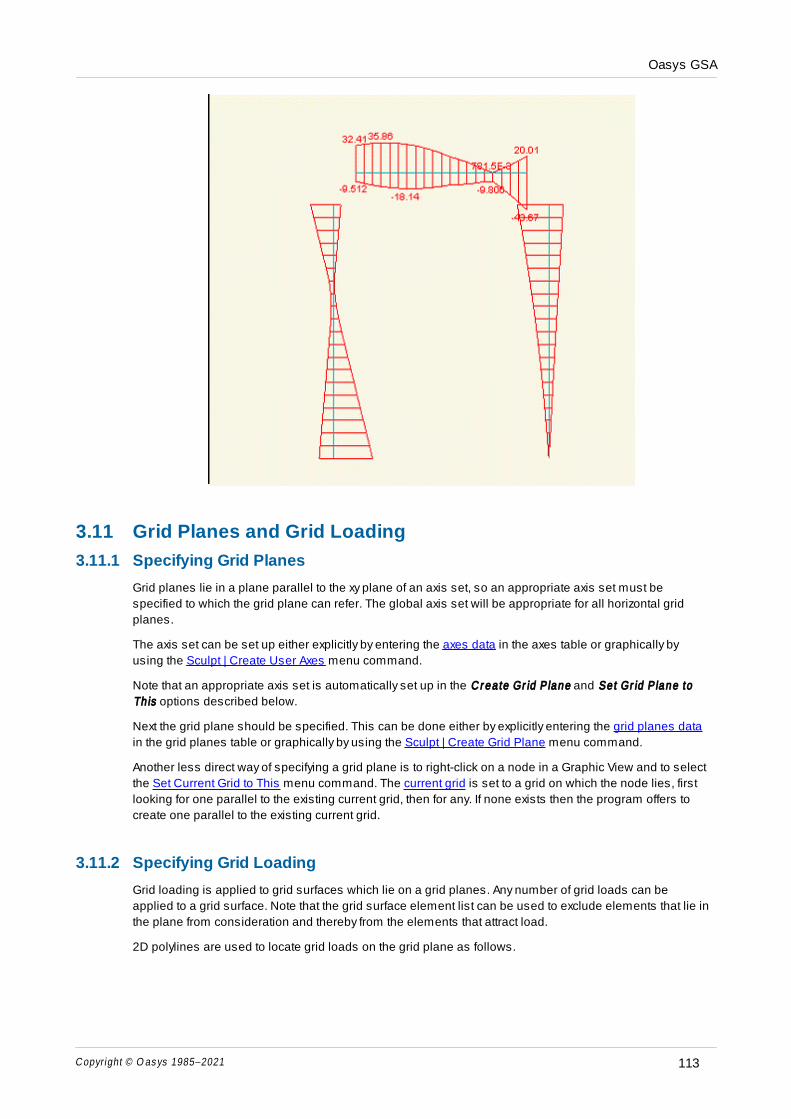
Oasys GSA

Copyright © O as ys 1985–2021 113

3.11 Grid Planes and Grid Loading

3.11.1 Specifying Grid Planes

Grid planes lie in a plane parallel to the xy plane of an axis set, so an appropriate axis set must be

specified to which the grid plane can refer. The global axis set will be appropriate for all horizontal grid

planes.

The axis set can be set up either explicitly by entering the axes data in the axes table or graphically by

using the Sculpt | Create User Axes menu command.

Note that an appropriate axis set is automatically set up in the C r ea te Gr id P lane and Se t Gr id P lane to

Th is options described below.

Next the grid plane should be specified. This can be done either by explicitly entering the grid planes data

in the grid planes table or graphically by using the Sculpt | Create Grid Plane menu command.

Another less direct way of specifying a grid plane is to right-click on a node in a Graphic View and to select

the Set Current Grid to This menu command. The current grid is set to a grid on which the node lies, first

looking for one parallel to the existing current grid, then for any. If none exists then the program offers to

create one parallel to the existing current grid.

3.11.2 Specifying Grid Loading

Grid loading is applied to grid surfaces which lie on a grid planes. Any number of grid loads can be

applied to a grid surface. Note that the grid surface element list can be used to exclude elements that lie in

the plane from consideration and thereby from the elements that attract load.

2D polylines are used to locate grid loads on the grid plane as follows.

Oasys GSA

Copyright © O as ys 1985–2021114

Grid point loads – When using the Sc u lp t | C r ea te Gr id Load ing | C r ea te Gr id Po in t Loads command a

load is applied at each point on the current polyline.

Grid line loads – The load line is defined by a reference to a 2D polyline. When using the Sc u lp t | C r ea te

Gr id Load ing | C r ea te Gr id L ine Load command a polyline is created from the current polyline (if an

identical one does not already exist) and this 2D polyline is referred to.

Grid area loads – The area is either defined as being the whole plane or as being bounded by a 2D

polyline. When using the Sc u lp t | C r ea te Gr id Load ing | C r ea te Gr id A r ea Load command a polyline is

created from the current polyline (if an identical one does not already exist) and this 2D polyline is

referred to.

2D polylines can be set up either explicitly by entering the 2D polylines data in the 2D polylines table or

graphically in the Polyline cursor mode. 2D polylines used for grid loading can be generally located. They

do not need to align with elements. They can be wholly within panels or spanning several panels.

Having set up an appropriate 2D polyline the grid loading can be set up either explicitly by entering the grid

point loads data, the grid line loads data or the grid area loads data in the grid loading table or graphically

using the sculpt options for creating grid loading graphically.

3.11.3 Displaying Grid Planes and Grid Loading

Grid planes

The following options are available for displaying grid planes in Graphic Views.

The grid is displayed on the current grid plane.

The Labels and Display Methods | Display Methods dialog ‘Draw current grid panels’ option displays

panels on the current grid plane.

Grid loading

Grid loading may be displayed as diagrams. Grid Area Loads may also be contoured.

If the current grid plane is not ‘Global’ then only loads that are applied to the current grid plane are

displayed.

Loads are not displayed on invalid panels. Use the Draw current grid panels option to verify that panels are

valid for the grid plane to which the loads are applied.

3.12 Sections

The properties of a beam (or related) element are determined by the section shape and material. These

are defined through a section definition and separate material definitions. In the most general case a

section can be comprise of several component parts and may vary in along the length of the element. The

variation along the length can be either a variation of the section dimensions, or in the case of a concrete

section a variation in the reinforcement.

At present GSA does not support multiple components but does allow for varying section dimensions

along the length of the section.

The material associated with a section component is defined in two parts: a material type and a material

grade, with an optional analysis material. Choosing a material type give the options of selecting a suitable

material grade. So for a steel material type the steel grades are offered, and for a concrete material type

the grades appropriate to the current design code are offered. For other material type various grade are

also offered but mainly as a means of initialising an analysis material.

If a material type and grade are chosen the relevant properties are copied into the GSA data structure. A

Oasys GSA

Copyright © O as ys 1985–2021 115

subsequent change to the design code will not update or delete these definitions. If updated properties

are required a new grade should be chosen after changing the design code.

In the case where a material type and material grade have been selected the material properties for

analysis can be inferred from the grade, so the analysis material can be set to 'from Grade' to use grade

derived values. The properties picked up from the grade are:

E – elastic modulus

ν – Poisson's ratio

G – shear modulus

ρ – density

α – thermal expansivity

For many analyses these properties are sufficient, but if the analysis properties need to be modified, for

example an elasto-plastic material, a separate analysis material can be defined.

The shape and dimensions of a section are defined with a section profile. For steel sections additional

design parameters can be specified.

Sections can have associated environmental parameters, such as embodied energy and CO2. These can

either be read from the environmental database or alternatively entered directly for the section. If no values

are defined for the section the material values are used.

3.12.1 Section Profile

The profile defines the shape of the section.

Profile

There are three basic ways of defining this:

Catalogue – this gives the option to choose a section from the different categories in various section

tables. This is intended for steel sections. For a catalogue section the profile description will always start

CAT.

Standard shapes – for most concrete sections a standard section will be used. The required shape is

chosen and the defining dimensions given to construct the section profile. For a standard shape the profile

description will always start STD followed by a characters denoting the section shape, e.g. R for

rectangular or CHS for a circular hollow section.

Geometric definition – for a section that cannot be selected from a catalogue or described by a standard

shape there is an option to define the geometry more directly, either as a perimeter or as a series of line

segments. The most commonly used of these is the perimeter option where the profile is defined by a

series of (y,z) points. This option also allows standard bridge beams to be imported stored as perimeter

sections. For a geometric section the profile will always start GEO.

Once the basic section is defined there are options to manipulate the basic definition by rotating, reflecting

and translating the profile.

Reference point

By default the reference point is taken as the geometric centroid of the section. In some cases it is

convenient to work with a different reference point. There are two options for modifying the reference point.

The first uses the extremes of the section: top/bottom and left/right. If further adjustment s required an

additional (y,z) offset can be specified directly

Tendon positions

Oasys GSA

Copyright © O as ys 1985–2021116

Tendon positions are holes in the section are distinct from voids. A rectangular hollow section would be a

section with a void. A tendon position hole is treated as a point area, so is only suitable for small or zero

area holes (positions) such tendon positions in bridge beams.

Bridge beams

GSA has a database of precast concrete bridge beams. These are considered as a special case of

perimeter sections. Rather than defining the perimeter directly the section is read from the database. In

addition to the perimeter, the database holds the positions for tendons. These are also imported as point

voids (holes with zero area). The user can then place tendons at the required positions in the section,

based on the point voids.

3.12.2 Design Parameters

The available design parameters depend on the material type.

Steel

Parameters used in the steel design such as section net:gross area ratio, and maximum plastic:elastic

ratio are defined here.

Concrete

A full description of the section requires details of the reinforcement. For a column the main reinforcement

is assumes to be the same along the length of the column, so only one definition of the reinforcement is

required. For a beam the reinforcement is assumed to be different at the ends from the middle, so three

reinforcement sets are required. The simplest way to define reinforcement is to use the reinforcement

templates. These provide a straightforward way to define the reinforcement for most commonly used

arrangements. In situations where this does not provide sufficient flexibility the general option can be used

which allow individual bars, or various type of lines of bars to be defined, and includes the option for pre-

stressed bars.

When the template option is used the cover, links (stirrups) and aggregate are required to determine the

position of the bars. All bars, and positioning checks are based on the currently selected design code.

For situations where bars are spread across a large section, requiring a large number of bars to be

positioned, there is an option for 'smeared' reinforcement. This assumes the reinforcement is spread

evenly across the section.

3.13 Constraints

In the most general sense constraints are where the user is putting some restriction on the free

displacement of the structure. Some constraint is required on all structures to prevent pure rigid body

motions. Thus in general the minimum number of constraints on a 3D structure is six, three suppressing

the translational rigid body modes and three suppressing the rotational rigid body modes.

In most cases there will be considerably more constraints than the minimum to suppress rigid body

motion. The general case of a constraint can be described by a constraint equation of the form

The types of constraints consist in GSA are:

Restraints and generalised restraints

Oasys GSA

Copyright © O as ys 1985–2021 117

Settlements

Element offsets

Link elements and rigid constraints

Joints

Constraint equations

Tied interfaces

These are discussed in more detail below.

It is important to avoid conflicting constraints. This is where there is more than a single constraint on a

particular degree of freedom. For example one degree of freedom on a node participating in both a joint

and a rigid constraint. Note that the constraints act on degrees of freedom so a node with a joint

constraining the z direction and a rigid constraint constraining the x, y and zz degrees of freedom, does not

cause any conflict.

There are two situations where GSA temporarily adds constraints to the model during an analysis. With 2D

elements automatic constraints can be added to account for the non-stiff degrees of freedom. The other is

when the user chooses additional restraint in a modal dynamic analysis.

3.13.1 Element Offsets

Another type of constraint that can be applied is in the form of element offsets. These are used where the

ends of the element are effectively rigid and it is required to offset the flexible part of the element. The

actual element can then be thought of as shorter than the node to node length of the element with the gaps

filled in with “rigid links”. Element offsets are most useful where the span of a beam is less that the

column to column centre-line distance or where the effect of eccentricity on the element is important.

Longitudinal offsets can be applied to 1D elements that refer to section properties (beam, bar, rod, strut

and tie). A positive offset is taken as the 'inwards' direction at both ends of the element, shortening the

flexible part of the element.

Transverse offsets can be applied to 1D beam elements (local y and z axis offsets) and 2D elements

(local z offset)

Taper offsets are used for 1D tapered elements to indicate which portion of the section taper applies to

that element

3.13.2 Link Elements and Rigid Constraints

At times there are very stiff sections in a model and generally it is not good to model these simply by

creating very stiff elements as this can lead to ill-conditioning problems. It is better to replace the elements

in these regions with link elements or rigid constraints. The action of link elements and rigid constraints is

substantially the same, the main difference being that a rigid constraint can include many nodes while a

link element can only include two nodes, but has some additional linkage options.

The basic idea behind link elements and rigid constraints is that one node is selected as the primary

node, and the others are the constrained nodes. Using the geometrical relationship between the

constrained and primary nodes it is possible to define the displacements and rotations at the constrained

node(s) in terms of the displacement and rotation of the primary. Likewise the forces and moments at the

constrained nodes can be transferred to equivalent forces and moments at the primary. Thus it is possible

to remove the constrained nodes from the solution and avoid the potential ill-conditioning problems.

The link element can also act as tension link, maintaining the geometrical relation ship while the element

is in tension; a compression link, maintaining the geometrical relation ship while the element is in

Oasys GSA

Copyright © O as ys 1985–2021118

compression or a bar maintaining the fixed length of the link but not applying any constraint on the rotation

of the link. These link types can only be used in the static nonlinear solver.

A custom link works in the same way as a joint by simply coupling degrees of freedom at the constrained

node to the same degree of freedom at the primary. As this does not take account of the geometry of the

element it is possible to create a custom link which does not enforce equilibrium.

The primary node of a link element is taken as the first node in the topology list for the element. The

primary node of a rigid constraint must be specified.

The constraint axes of nodes in a link element or rigid constraint must be the same and may only be

Cartesian; not cylindrical or spherical.

3.13.3 Conflicting Constraints

There are various rules that must be followed when specifying constraints. Failure to abide by these rules

results in constraints that are in conflict. Such conflicts are reported by the pre-analysis data checking.

The rules are as follows:

a constrained degree of freedom may be constrained to only one primary node.

a degree of freedom may not be constrained by more than one rigid constraint, link element, joint or

constraint equation.

a restraint applied at a constrained node may not conflict with the restraint conditions at its primary.

in a linear analysis a primary degree of freedom may not be a constrained degree of freedom to another

constraint. (Does not apply to nonlinear analysis.)

In addition:

the constrained nodes of Joints can be the primary nodes of Links and Rigid Constraints

the constrained nodes of Links can be the primary nodes of Rigid Constraints

Other arrangements of constrained and primary nodes can cause unbalanced nodal forces as well as

total loads and reactions.

3.13.4 Automatic Constraints

One further constraint that users should be aware of is the Automatic Constraint. These are constraints set

up by the Gss solver to enable the solution of shell models where the elements do not have stiffness in all

directions. Shell elements do not have a local zz degree of freedom. Thus when the elements are

transformed into a non-global plane they appear to have stiffness is all directions but one of the principal

stiffnesses at the nodes is zero. To avoid problems of zero stiffness at the solution stage these degrees of

freedom have to be removed from the solution. The method of doing this is termed applying Automatic

Constraints.

There are a number of ways to apply Automatic Constraints but the default method is to look at how flat the

surface is at a node. If all the elements at a node seem to be co-planar then the number of degrees of

freedom at that node are reduced to five rather than the normal six. Gss builds a list of automatic

constraints, which can then be examined by the user after the analysis stage.

Oasys GSA

Copyright © O as ys 1985–2021 119

3.14 Miscellaneous

3.14.1 Unlock File

It is possible for files to be left in a locked state if GSA terminated in an abnormal manner. In such a

situation the file can be unlocked prior to use with the Too ls | U n loc k File menu command. This option is

only available when there is no GSA model open.

3.14.2 File Backups

There are two file backup systems that are in operation while a model is open in GSA: the manual backup

and the timed backup. Both systems result in a temporary copy of the model (input data and results) being

preserved in the Oasys temporary folder in GWB file format.

When a model is opened, names for the two backup files are assigned. These are the filename with “_M”

or “_T” appended, for the manual backup and timed backup respectively, followed by a number to uniquely

associate the backup name with the GSA session. For example, a timed backup file might be called

MyFile_T9.gwb.

A manual backup is made immediately on opening a model. This may be overwritten by the “File | Manual

Backup” menu command.

A timed backup is automatically made periodically. The timed backup interval may be adjusted on the

Miscellaneous tab of the Preferences. Note that setting the interval to zero results in no timed backups

being made; this may be desirable when working with large models that take a long time to save. A timed

backup is only made if there has been a change to the data since the last timed backup. The timer is reset

when the model is saved or ‘saved as’ a GWB file.

The “File | Restore Manual Backup” command may be used to reset the model in your current GSA

session to the state as when the manual backup was taken. The backup data is applied to all views

currently open without changing the view settings. For example a Graphic View will continue to display the

image as currently orientated with the current adornments set but with the backed-up data applied. The

“File | Restore Timed Backup” commands operates similarly when a timed backup exists for the model.

The two backup files are automatically deleted when the model is properly closed. However, if the program

shuts down prematurely (as a result of program malfunction or power failure, etc.) then the backup files

remain on disk. In this circumstance, the next time GSA is run the Welcome dialog invites you to open a

backup file. Note the “Delete all backup files” button on this dialog box that is provided to encourage you to

tidy up your Oasys temporary folder.

3.14.3 Delete Results from Files

It is sometimes convenient to reduce the size of files by deleting results. It is tedious to have to do this

manually so the Too ls | D e le te R es u lts Fr om Files menu command is provided to do this. This allows the

user to select a set of files from which the results are to be deleted. This option is only available when

there is no GSA model open.

3.14.4 User Modules

User modules are the means by which users can feed their own data into a model for display by GSA

either as contours in a Graphic View or tables in an Output View. Nodal, element and member user

modules are available.

A nodal user module consists of one value per node in the model.

An element user module consists of values per position on the element. For 1D elements positions are

Oasys GSA

Copyright © O as ys 1985–2021120

expressed in terms of millionths of the way along the element. So for example position 0 is at end 1 of the

element, position 1000000 is at end 2, and position 333333 is a third of the way along the element. Values

must be specified at both ends of 1D elements (i.e. positions 0 and 1000000). For 2D elements a value is

expected at each topology position plus a centre value, though if the ‘centre only 2D’ flag is set only the

centre value is expected . User modules also have a name, a dimension (i.e. whether length, moment, etc.

or dimensionless) and a flag for discrete or continuous contours. A discrete contour is one that represents

the value that exists for that position and does not vary continuously along the element.

A member user module is similar to an element user module except that all members are 1D.

User modules may be supplied to GSA in text file (GWA) format. Refer to the Text File Format document for

a definition of the format. Data should be supplied in SI units. User modules can be appended to a GSA

model that has been saved in text file format and then opened or they can be imported into an existing

model using the File | Im por t | Text (GW A f ile ) menu command.

Once a user module has been fed into a model it remains part of the model, being saved in and read from

the GWB file. The user module management dialogs allow user modules to be deleted and renamed.

When user modules are present in a model they are offered as contour and diagram options for Graphic

Views and output options for Output Views. User module data are converted to the current units for display.

Note that contouring of element and member user module data requires values to have been specified at

all nodes on the element.

As well as outputting nodal user module data per node this data can be contoured on elements and can

be output per topology item per element.

Reading user modules from GWA files

When a user module is read from GWA file if the user module ID is specified as zero then the user module

is appended to the current user modules: the new user module is created by the user module title record

and the following user module records (with ID=0) supply values to the new user module.

If the specified imported user module ID references an existing user module and the imported user

module title data are compatible with the existing user module then imported user module values are

written into the existing user module, preserving the existing values except where overwritten by imported

values. However if the title data are incompatible then the existing values are nulled. Title data are

compatible if the ‘dimension’ and ‘is_centre’ fields are the same.

Generating user modules

User modules can be generated from contoured data in a Graphic View, using the Gr aph ic s | Gener a te

U s er M odu le command, and from displayed data in an Output View, using the Ou tpu t | Gener a te U s er

M odu les command. An option to generate user modules is also offered in the Output Settings dialog box.

(Hint: It is possible to generate user modules without first displaying the output by giving the New Output

View command to open the Output Settings dialog directly.) When generating from an Output View

separate user modules are generated for each component and for each case currently displayed.

3.14.5 View List

The View List dialog is used for creating a new view list and for editing an existing view list. It is displayed

by selecting “Edit “<view list name>” ” or “New View List” on the right-click menu having right-clicked on a

view list on the View Explorer pane.

View list name

The name by which the view list is referred. Giving the same name as another view list will result in that

view list being overwritten by this. It is preferable to give a name that is distinct from any saved or preferred

views since in some circumstances action is taken on the first view or view list with a given name.

Oasys GSA

Copyright © O as ys 1985–2021 121

Available Views

This tree control displays the names of all saved and preferred Graphic Views and Output Views. Views

that are already represented in the view list are marked with a tick. Double clicking on a view that is not

already in the view list will add the view to the bottom of the list. Double clicking on a view that is in the view

list removes all occurrences of that view from the list.

View List (in print order)

The view list.

Add

The selected view in the Available Views tree control is added to the bottom of the View List

Remove

The selected view in the View List is removed from the view list.

Move Up

The selected view in the View List is moved up one position.

Move Down

The selected view in the View List is moved down one position.

Print

The views in the View List are printed in the order in which they appear in the list.

Save to file

The views in the View List are saved to file in the order in which they appear in the list. The format of the

saved file is determined by the respective ‘batch output file format’ setting in the Miscellaneous

Preferences dialog.

3.14.6 Evaluating Expressions

GSA allows geometry and loading to be modified or defined using mathematical expressions. These are

mathematical expressions which can define a variation as a function of position (x,y,x)

Normal mathematical notation is used in expressions:

e.g. 1000*sin(x) + y 2

Arithmetic operations

The arithmetic operators are

+ addition

- subtraction

* multiplication

/ division

^ raise to power of

Normal operator precedence is followed. The constants pi (3.14...) and g (9.81...) are defined. Parenthesis

can be used to clarify the order of operations.

Oasys GSA

Copyright © O as ys 1985–2021122

Mathematical functions

The following functions can be used:

sqrt(x) square root

abs(x) absolute value

exp(x) e raised to power of

ln(x) natural logarithm

log(x) base 10 logarithm

sin(x) sine (in radians)

cos(x) cosine (in radians)

tan(x) tangent (in radians)

asin(x) inverse sine (in radians)

acos(x) inverse cosine (in radians)

atan(x) inverse tangent (in radians)

atan(y,x) inverse tangent of (y/x) (in radians)

sinh(x) hyperbolic sine

cosh(x) hyperbolic cosine

tanh(x) hyperbolic tangent

asinh(x) inverse hyperbolic sine

acosh(x) inverse hyperbolic cosine

atanh(x) inverse hyperbolic tangent

radians(x) conversion of degrees to radians

degrees(x) conversion of radians to degrees

floor(x) round a number down to integer value

ceil(x) round a number up to integer value

sign(x) return sign of number

max(x,y) maximum of two numbers

min(x,y) minimum of two numbers

Conditional expressions

Conditional expressions can be specified in the form:

if( condition, true_expression, false_expression )

The conditional operators are >,<,!=(or <>),>=,<=,==(or=) and the logical operators are && (and) and || (or).

Conditional expressions can be nested.

Oasys GSA

Copyright © O as ys 1985–2021 123

3.14.7 Touch Gestures

When operating GSA using gestures on a touch sensitive screen the following gestures are recognised.

tap - click

drag - drag

pinch - zoom

double finger drag - pan (in Graphic Views)

press and tap - right-click; press on target and click using a second finger (in Graphic Views)

3.15 Toolbars and Keyboard Accelerators (shortcuts)

Toolbars provide a short cut to the more commonly used commands. The List and Layer toolbars are

attached to the views to which they relate. All other toolbars can be docked (attached to the application

frame) or floating (free to be positioned by the user). The toolbars can be switched on and off as required

from the “View | Toolbars and Dockable Panes” menu command. Toolbars can be customised by clicking

the dropdown at the right or lower end of the toolbar and selecting "Add and Remove buttons" followed by

the toolbar name.

Standard

GSA

Data Options

Sculpt

Command

Labels

Diagrams

Contours

Orientation

Cursor Mode

Graphic Display

Lists

Keyboard Accelerators (keyboard shortcuts) give a quick route to a selection of commands. They cannot be

customised.

3.15.1 Toolbars

Toolbars provide a short cut to the more commonly used commands. The List and Layer toolbars are

attached to the views to which they relate. All other toolbars can be docked (attached to the application

frame) or floating (free to be positioned by the user). The toolbars can be switched on and off as required

from the “View | Toolbars and Dockable Panes” menu command. Toolbars can be customised by clicking

the dropdown at the right or lower end of the toolbar and selecting "Add and Remove buttons" followed by

the toolbar name.

Standard

GSA

Oasys GSA

Copyright © O as ys 1985–2021124

Data Options

Sculpt

Command

Labels

Diagrams

Contours

Orientation

Cursor Mode

Graphic Display

Lists

3.15.1.1 Standard

The standard toolbar handles the common Windows options:

New – create a new model

Open – open an existing file

Close – close the current model

Save – save the model to file

Cut – cut the data and place on clipboard

Copy – copy the data and place on the clipboard

Paste – paste the data from the clipboard into the model

Print – print the current view

Print Preview – preview the current view

Undo – undo the last edit

Redo – redo a previously undone edit

Undo view – undo the last change to the view settings

Redo view – redo a previously undone change to view settings

View settings painter – click once to grab the current view settings then click in a view of the same type to

apply the grabbed settings, or click again to switch off

Oasys GSA

Copyright © O as ys 1985–2021 125

3.15.1.2 GSA

The GSA toolbar provides access to some of the main GSA options:

Message Pane – show or hide the Message Pane

Property Pane – show or hide the Property Pane

Show or Hide Dockable Panes – Toggle on and off all dockable panes

Analyse – analyse the model

New Analysis Task – Set up a new analysis task using the wizard

Erase Results – delete all the results and optionally the analysis cases

New Design Task – Set up a new design task using the wizard

Toolbar Options – Use the dropdown arrow at the end of the bar to add or remove buttons for additional

commands

3.15.1.3 Data Options

The Data Options toolbar gives access to various methods for modify the way data can be viewed or edited

in Table Views, Graphic Views and Output Views:

Wizard – access the data wizard

Find – search data for particular value

Replace – search and replace values

Modify – modify the values in tables

Go To – go to particular record in table

Fonts and Styles – change the font

Units – change the current units

Numeric Format – change the current numeric format

Increase Precision – increase the number of significant figures or decimal places

Decrease Precision – decrease the number of significant figures or decimal places

Axes – change the current axes

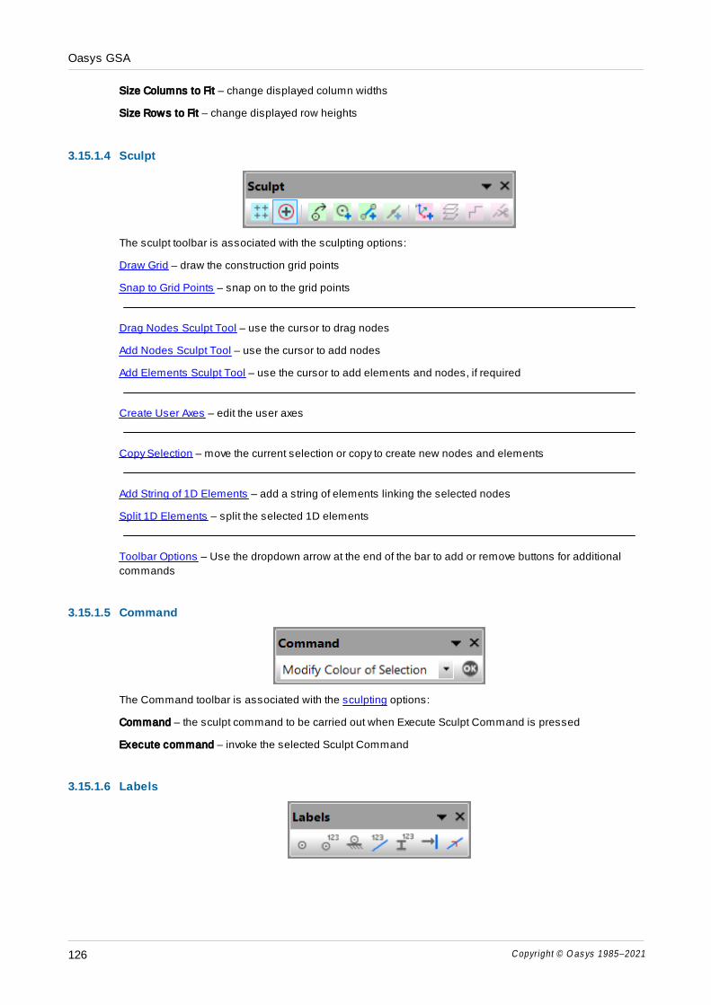
Oasys GSA

Copyright © O as ys 1985–2021126

Size Columns to Fit – change displayed column widths

Size Rows to Fit – change displayed row heights

3.15.1.4 Sculpt

The sculpt toolbar is associated with the sculpting options:

Draw Grid – draw the construction grid points

Snap to Grid Points – snap on to the grid points

Drag Nodes Sculpt Tool – use the cursor to drag nodes

Add Nodes Sculpt Tool – use the cursor to add nodes

Add Elements Sculpt Tool – use the cursor to add elements and nodes, if required

Create User Axes – edit the user axes

Copy Selection – move the current selection or copy to create new nodes and elements

Add String of 1D Elements – add a string of elements linking the selected nodes

Split 1D Elements – split the selected 1D elements

Toolbar Options – Use the dropdown arrow at the end of the bar to add or remove buttons for additional

commands

3.15.1.5 Command

The Command toolbar is associated with the sculpting options:

Command – the sculpt command to be carried out when Execute Sculpt Command is pressed

Execute command – invoke the selected Sculpt Command

3.15.1.6 Labels

Oasys GSA

Copyright © O as ys 1985–2021 127

The Labels toolbar gives quick access to a number of commonly used label options:

Label node dots – display dots at the nodes

Label node IDs – display the node numbers

Label restraints – label the restraints at nodes

Label element IDs – display the element numbers

Label section shapes – display the element section shapes

Label element releases – display the element releases

Label element x axis – display the element x axes

Toolbar Options – Use the dropdown arrow at the end of the bar to add or remove buttons for additional

label options

3.15.1.7 Diagrams

The Diagrams toolbar gives quick access to a number of commonly used diagram options:

All Load diagrams – display diagram of “All Loads”

|U| displacement diagrams – display diagram of “Displacements”

Fx, Fy and Fz reaction diagrams – display diagram of “Reaction Forces”

Fx axial force diagrams – display diagram of “Axial Force” (Fx)

Fz shear force diagrams – display diagram of “Shear Force” (Fz)

Myy bending moments diagrams – display diagram of “Bending Moment” (My y

)

2D principal stress diagrams – display diagram of principal 2D element stress

Apply Adornments to Selection – when set, apply labels, diagrams and contours to the current selection

set

Toolbar Options – Use the dropdown arrow at the end of the bar to add or remove buttons for additional

diagram options

3.15.1.8 Contours

The Contours toolbar gives quick access to a number of commonly used contour options:

|U| displacement contours – element displacements

Oasys GSA

Copyright © O as ys 1985–2021128

|F| reaction contours – nodal reaction forces”

Fx axial force contours – beam, bar and rod axial force (Fx)

Fz shear force contours – beam, bar and rod shear Force (Fz)

Myy bending moment contours – beam, bar and rod bending moment (My y

)

2D Wood-Armer moment, Mx + sgn(Mx)|Mxy| contours – 2D Wood-Armer moment (M*x = M

x + sgn(M

x)|

Mx y

|)

2D Wood-Armer moment, My + sgn(My)|Myx| contours – 2D Wood-Armer moment (M*y = M

y + sgn(M

y)|

My x

|)

Toolbar Options – Use the dropdown arrow at the end of the bar to add or remove buttons for additional

contour options

3.15.1.9 Orientation

The orientation toolbar is associated with the aspects of a Graphic View related to orientation and scaling:

Graphic View Regenerate – regenerate and redraw the view without changing the scale, orientation,

adornments or any other view settings

Plan – draw a plan view

X elevation – draw an x elevation

Y elevation – draw a y elevation

Isometric – draw an isometric (orthographic) view

Skew View – draw a skew (perspective) view

Ground View – draw a ground (perspective) view

Scale to Fit – scale the model to fit the view

Toolbar Options – Use the dropdown arrow at the end of the bar to add or remove buttons for additional

commands

3.15.1.10 Cursor Mode

Oasys GSA

Copyright © O as ys 1985–2021 129

The cursor mode toolbar is used to identify what the cursor should do in Graphic Views:

Rotate – dynamic viewing – rotation, zoom, pan, etc

Zoom – zoom in or out

Volume – select a volume – entities outside the volume are ignored

Omit from Display – select elements that are to be omitted from display – the display list is modified to

exclude the selected elements

Select Grid Points – select grid points

Select Nodes – select nodes

Select Elements – select elements

Polyline – create a polyline

Select For Annotation – select entities for annotation

3.15.1.11 Graphic Display

The graphic display toolbar governs the appearance of the graphical display:

Shrink – the elements are displayed sh runk from the nodes

Section Display – displays solid beam sections and solid 2D elements

Labels and Display Methods – accesses the Labe ls and D is p lay M e thods dialog

Deformed Image – draw the deformed image

Animate – animates the model

Shade Surfaces – shade surfaces according to current lighting conditions

Contour Settings – accesses the C on tou r Se t t ings dialog

Diagram Settings – accesses the D iag r am Se t t ings dialog

Reset Display – resets the display, only scale and orientation are retained

Rescale Data – rescales the data for the current diagram

Double Size of Diagram – increases the size of the diagrams

Halve Size of Diagram – reduces the size of the diagrams

Toolbar Options – Use the dropdown arrow at the end of the bar to add or remove buttons for additional

commands

Oasys GSA

Copyright © O as ys 1985–2021130

3.15.1.12 Lists

The Lists toolbar allows the user to select which cases are to be reported and how the content of the

display is to be adjusted in a Graphic View or Output View. The width of the toolbar automatically adjusts

with the width of the window thereby maximising the size of the Case List and Display List.

Case List – the list of cases that are currently selected.

Next Case – select the next item in the case list pull-down.

Previous Case – select the previous item in the case list pull-down.

Condense Cases – trim down the cases in the drop list to those where there is data

Broadcast case list – Set this case list in all Graphic Views and Output Views

Display Option – the method by which the display content is to be adjusted. This can be by adjusting the

list of entities, whether nodes, elements or members, or by selecting a saved view, in which case the

settings of the saved view are applied to the current view. In Graphic Views the current grid, layer and stage

can also be adjusted.

Display List – the entity list, saved view, layer or stage, depending on the Display Option setting.

Next Display – select the next item in the current display list pull-down.

Previous Display – select the previous item in the current display list pull-down.

Reset To All Entities – the lists are reset to “all” entities. In Graphic Views any specified volumes are also

cleared.

Pin Display – When pinned selecting a grid surface of elements also sets that as the current grid plane,

and vice versa

3.15.2 Keyboard Accelerators (shortcuts)

Key Action

Alt+0 Data Explorer pane

Alt+1 New Graphic View

Alt+2 New Output View

Alt+3 Message Pane

Alt+4 Property Pane

A Select for annotation

Ctrl+A Select All

Ctrl+Alt+A Reset to All Entities

B G Colour by group

B L Colour by pool

B M Colour by material

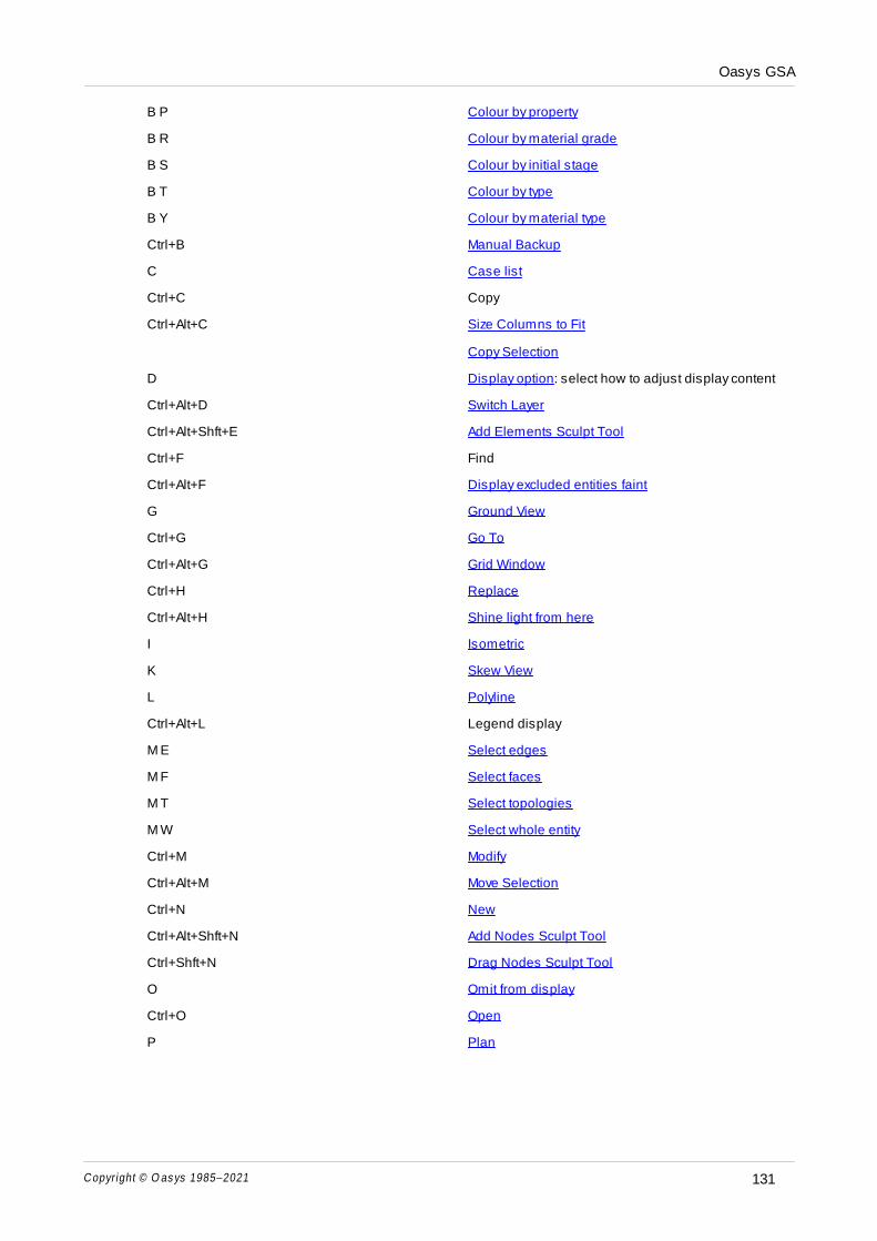
Oasys GSA

Copyright © O as ys 1985–2021 131

B P Colour by property

B R Colour by material grade

B S Colour by initial stage

B T Colour by type

B Y Colour by material type

Ctrl+B Manual Backup

C Case list

Ctrl+C Copy

Ctrl+Alt+C Size Columns to Fit

Copy Selection

D Display option: select how to adjust display content

Ctrl+Alt+D Switch Layer

Ctrl+Alt+Shft+E Add Elements Sculpt Tool

Ctrl+F Find

Ctrl+Alt+F Display excluded entities faint

G Ground View

Ctrl+G Go To

Ctrl+Alt+G Grid Window

Ctrl+H Replace

Ctrl+Alt+H Shine light from here

I Isometric

K Skew View

L Polyline

Ctrl+Alt+L Legend display

M E Select edges

M F Select faces

M T Select topologies

M W Select whole entity

Ctrl+M Modify

Ctrl+Alt+M Move Selection

Ctrl+N New

Ctrl+Alt+Shft+N Add Nodes Sculpt Tool

Ctrl+Shft+N Drag Nodes Sculpt Tool

O Omit from display

Ctrl+O Open

P Plan

Oasys GSA

Copyright © O as ys 1985–2021132

Alt+P Reverse Plan

Ctrl+P Print

Ctrl+Alt+P Perspective

R Rotate

Ctrl+Alt+R Size Rows to Fit

S E Select elements/members

S G Select grid points

S N Select nodes

Ctrl+S Save

Ctrl+Shft+S Save As

Ctrl+Alt+S Snap to Grid Points

V Volume

Ctrl+V Paste

Ctrl+W Wizard

Ctrl+Alt+W Define current grid

X X elevation

Ctrl+X Cut

Y Y elevation

Ctrl+Y Redo

Ctrl+Alt+Y Redo View

Z Zoom

Ctrl+Z Undo

Ctrl+Alt+Z Undo View

F1 Help

Shift+F1 Context help

F2 Highlight; Rename task/case

F4 Execute sculpt command

F5 Regenerate Graphic View

Ctrl+F7 Preferences

F11 Full screen

Esc Quit

Tab Next Cell

Return Next Cell

Insert Insert

Delete Delete

Ctrl+Delete Quick delete

Oasys GSA

Copyright © O as ys 1985–2021 133

Home Beginning of Table

Shft+Home Reset Pan

Ctrl+Home Move cell to Beginning; Scale to fit

Alt+Home Rescale data

End End of Table

Ctrl+End Move cell to End

Page Up Scroll up; Previous case

Ctrl+Page Up Previous display

Page Down Scroll down; Next case

Ctrl+Page Down Next display

Row Up; Up 7.5°

Pan Up

Zoom In

Fast rotate up

Column Left; Left 7.5°

Pan Left

Eye Distance Out

Fast rotate left

Column Right; Right 7.5°

Pan Right

Eye Distance In

Fast rotate right

Row Down; Down 7.5°

Pan Down

Zoom Out

Fast rotate down

3.15.3 Mouse accelerators (shortcuts)

The following mouse functions apply to all cursor modes. Functionality for specific cursor modes is

summarised in the cursor modes article.

Rotate

Right button drag

Zoom

Wheel rotate

Ctrl + right button drag up/down

Ctrl + mouse wheel drag up/down

Oasys GSA

Copyright © O as ys 1985–2021134

Zoom extents

Ctrl + Shift + left click

Pan

Mouse wheel drag

Shift + right button drag

Adjust lens length (perspective views only)

Ctrl + right button drag left/right

Ctrl + mouse wheel drag left/right

3.16 Patterned Load

Several tools are available to assist in defining patterned floor loading. These tools are focused on the

method described in the technical note An Efficient Alternative Approach for Patterned Load Analyses of

Arbitrary Multiple-ways Spanning Floor Systems. There are three tools, grouped under the M ode l | Bu ild ing

M ode lling menu item.

Create Load Panels on Storeys – examines the storey grid planes and creates load panel elements

Create Patterned Loads – allows specification of adverse and beneficial load factors and creates

elements loads for ‘mean’ and ‘difference’ loads.

Create Patterned Load Combinations – allows analysis cases to be selected and sets up the

combinations of ‘mean’ and ‘difference’ analysis cases to give maximum and minimum envelope cases.

Pattered load - typical workflow

Build a GSA modal as normal. In order to simplify the loading use storey grid planes to define the floor

levels. The ‘Create Load Panels on Storeys’ tool can then be used to create load panel elements where

the floor loading is to be applied.

Define the dead and imposed loads as normal, then use the ‘Create Patterned Loads’ tool to create a new

set of loads on the model. At this stage adverse/beneficial factors can be specified for the loads and there

is the option to include any of beam loads, face loads and gravity loads. These are then used to create a

mean load case and a set of difference load cases.

QiQQ

GiGG

i

QQQ

GGG

mean

fff

fff

22

22

,infsup,,infsup,

,infsup,,infsup,

Where subscripts G and Q relate to permanent (dead) load and variable (imposed) load respectively, and

sup and inf relate to unfavourable (adverse) and favourable (beneficial) effects respectively.

These are then used in a linear static analysis as normal.

The final stage is to use the ‘Create Patterned Load Combinations’ tool which then uses the mean load

case and difference load cases to set up combination cases that will give an envelope of the results for the

patterned loading.

Oasys GSA

Copyright © O as ys 1985–2021 135

3.17 Mass and Weight

Mass in the structure is represented by the mass of the structural elements and mass properties applied

to nodes. Weight is the effect of gravity on this mass. Mass is the key aspect for dynamic analysis while

weight is key for static loads.

Mass modification

There is scope to modify the basic mass of the elements, which can have an effect on both static and

dynamic analysis.

For a beam, bar, tie or strut elements the mass is the area × length × density. There is an option in the

section properties to modify the effective area of the section and this modification can either be applies or

ignored in the mass (and weight) calculations.

For a 2D element the mass is the area × ( thickness × density + additional mass). There is an option to

modify the effective thickness for mass and weight calculations

For mass properties on nodes the mass is specified directly. There is also an option to modify the mass

in different directions. This is only available for dynamic analysis and is primarily intended for fluid

structure interaction calculations.

Additional mass in dynamic analysis

When building a model it is convenient to ignore non-structural parts of a building and represent these as

loads: usually beam loads and 2D face/edge loads. If these are ignored in a dynamic analysis the

response will be incorrect. The ‘additional mass’ option for dynamic is intended to allow for these to be

properly included. In general these loads represent the effect of gravity of the non-structural aspects of the

building, so to convert these to mass the load vector is assembled and the mass is calculated (assuming

z is vertical) from

g

wm

fw z

Any ‘gravity’ loads are ignored in the additional mass calculation as the mass of these loads is defined

explicitly.

Weight from mass in static analysis

In a static analysis the weight of the structural elements is accounted for by gravity loading. The general

case is

mg

a

a

a

f

f

f

z

y

x

z

y

x

but the weight calculation corresponds to the factor being 0 for x and y and -1 for z so

fz mg

This is always based on a scalar mass so the mass modifiers applied to a mass properties are excluded.

The weight calculated from the mass is likely to be an underestimate as the mass of connections,

stiffening plates, etc. is ignored. This can be adjusted for by modifying the gravity factor, so for a 10%

Oasys GSA

Copyright © O as ys 1985–2021136

3.18 String IDs

Most GSA objects can have an associated string ID (sID). Typically these are used to associate GSA

objects with other objects, whether GSA or third party.

An example of the use of sIDs in GSA is when importing a Revit model - the Revit object id is assigned to

the corresponding member's sID.

GSA objects that cannot have sIDs assigned are:

Specification modules

Result modules

Loosely speaking, a string ID is a string and it is up to the author, or authoring application, to devise a

syntax for the string that makes sense to the author. However, there will be a rapid decline to mayhem if

some rules in the use of sIDs are not adhered to.

Rules in the use of String IDs

The typical format of a sID is a ‘tag, value’ pair, enclosed by curly braces. e.g. "{tag:value}"

An object may have several ‘tag, value’ pairs, possibly written by different authoring applications. e.g.

"{tag1:value1}{tag2:value2}{...}"

‘tag, value’ pairs may be nested. e.g. "{tag1:value1}{tag2:value2}{tag3:{sub-tag1:sub-value1}{sub-

tag2:sub-value2}...}"

An authoring application will devise a sID tag that will stand a good chance of being unique. e.g. "MyApp"

Nested ‘sub-tag, sub-value’ pairs are owned by the authoring application of the enclosing tag.

It is the duty of the authoring application not to destroy or corrupt any sID ‘tag | value’ pairs not written by

itself.

3.19 Members and Element Meshes

2D and 3D meshes are generated from 2D and 3D members

Adding members interactively

To add a member in the graphical view

1. Ensure that

a. The Grid Layout is set to the desired spacing

b. The correct Grid Plane is set

c. The grid display is on (Draw Grid or Ctrl+Alt+G)

d. The graphical display is set to the Design Layer

2. Use the Add Entities sculpt tool (Ctrl+Shift+Alt+E)

a. Set the member type in the Properties pane

b. Click on the graphical view to place the member nodes

i. for 1D Members, hold down the Ctrl key to add a chain of members. Release Ctrl before defining

the last node

Oasys GSA

Copyright © O as ys 1985–2021 137

ii. for 2D Members, finish by either clicking back on the first node or press Return

Nodes and lines can be added interactively to existing 2D members:

1. Select the member in the graphical view

2. Click the Add Entities sculpt tool

a. Ensure that the member type in the Properties pane matches the 2D member

b. To add a void: hold down the Shift keys while adding the corner points. Click back onto the first

node to close the void definition.

c. To add a line: hold down the Ctrl key while adding the lines. Press Esc to exit.

d. To add nodes: hold the Ctrl + Shift keys while adding the nodes. Press Esc to exit.

Meshing tips

Here are some tips on modelling for mesh generation:

Model the member to achieve the desired mesh; this is not necessarily exactly the same as a physical

representation.

Try to avoid placing internal nodes or the ends of internal elements close to member boundaries as this

will produce very small elements. Nodes on the member boundary are OK.

The number of elements generated along an edge will increase automatically as necessary to achieve

a feasible mesh and to reduce large discrepancies in the mesh.

Part IV

Oasys GSA

Copyright © O as ys 1985–2021 139

4 GSA Data

This chapter describes the different types of data that can be used to describe the model. The data is

organised in modules and displayed for input and editing in a number of dialogs and tables. It is also

possible to input and edit the data graphically (see 'Sculpting' in the 'Working with the Program' section).

All dialogs and tables can be accessed from the 'Model | Data Modules' pull down menu, or from the Data

explorer. Most tables have wizards which can be accessed from the 'Wizard' button on the 'Data Options'

toolbar, the 'Wizard' option on the table context menu or Ctrl+W.

4.1 Titles

The titles dialog can be accessed from the Data explorer and from the “Model | Data Modules | Titles”

menu command.

This sets the title information for the model.

The title entries are printed at the top of each page of output. For a new file, certain entries default to those

in the last file that was saved, but can be changed here.

Definition

Job Number, Initials

The job number, and initials are alphanumeric strings used to identify the job and the creator of the model.

This is not used in the analysis.

Job Title, Subtitle & Calculation Heading

The title and subtitle of the job and a description specific to this particular model.

Notes

Notes on the model can be stored here. This is a text field that can be appended to as required.

Location information

The location information if used to set some country and site specific information. For most GSA model

this can be ignored. The angle to north is used in some tools to identify the different faces of a building in

terms of north, south, east and west. The currency used the standard ISO 4217 three-letter currency

abbreviations.

4.2 Specification

4.2.1 Units Specification

GSA stores all data in SI unit, but allows the user to specify the units in which his model is defined. These

become the base units for working, however these can be changed at any time.

When creating a new model the user’s preferred units are used. These may be changed in the units

specification at any time. The units chosen here will be the default units used in GSA, however, local

changes of units can be made in individual views.

This can be accessed from the Data explorer, from the 'Model | Data Modules | Specification | Units

Specification' menu command, from the General Specification or from the Structure type page of the New

Model Wizard. The units specification sets the default units for the model.

Oasys GSA

Copyright © O as ys 1985–2021140

In addition the Units dialog is accessible from the Diagram Settings, Contour Settings and Output Settings

dialog boxes, and the units button on the Data Options toolbar where there is scope to modify units locally.

In this case units which are not relevant are disabled.

Units

Force

Used for force and force derived units such as moment, etc., but not for stress.

Length – large, small and section

Large length units are used for length and length derived units such as area. Sm a ll length units are used

for data that are typically small such as displacements and cross-sectional dimensions. Section length

units are typically used for cross-sectional properties.

Large length units are also used in units derived from length, such as moment.

Mass

Used for mass and mass derived units such as inertia, etc.

Time

Used for time and time derived units, such as frequency, etc.

Temperature

Used for temperature and temperature derived units such as coefficients of expansion.

Stress

Like displacements, stresses are one of the main results produced by a structural analysis package, so

they are assigned their own units distinct from force and length. These units are also used for stress

related quantities like the elastic modulus.

Strain

Strain is dimensionless however it is convenient to be able to work with strain units such as µ ε.

Velocity

Used for velocity and velocity derived units.

Acceleration

Sets the acceleration units to be used. Acceleration units are considered as distinct from length and time

units. It is common for accelerations to be specified in g so accelerations are given a separate unit.

Energy

Sets the energy units to be used. Energy units are considered as distinct from force and length units.

Angle

It is convenient to be able to choose between degrees and radians for angle measures.

Reset units

This allow the user to reset the units to

Preferred – those selected in the Preferred Units accessible from the Miscellaneous Preferences.

SI – standard SI units.

kN-m – a more useful set of units for structural analysis based on the SI system of units.

Oasys GSA

Copyright © O as ys 1985–2021 141

kip-ft – a set of units based on those commonly used in the USA.

kip-in – an alternative set of units based on those commonly used in the USA.

Notes

Other units are derived from these units, so for instance moments are derived from the force and length

units giving in the SI units set N m.

Note that data considered to be in units of ‘pressure’ (e.g. Grid Area Load values) are reported in units of

Force/Length², not Stress.

4.2.1.1 Preferred Units

In many cases there is a set of units which users will want to use for most of their work. In GSA these are

termed preferred units. These can be edited and set from the Input page in the Preferences. This brings

up a dialog box to allow individual units to be selected.

A selection of units for each of force, length, etc are offered. For these units the conversion factor are

known. If the required units are not in the list, the user can enter the name and must then set the

conversion factor. The pre-programmed units are:

Force – N, kN, MN, lbf, kip, tf

Length - large – m, cm, mm, ft, in

Length - small (displacement) – m, cm, mm, ft, in

Length - sections – m, cm, mm, ft, in

Mass – kg, t, kt, g, lb, Ton, slug, kip.s²/in, kip.s²/ft, lbf.s²/in, lbf.s²/ft, kip

Time – s, ms, min, h, d

Temperature – °C, K, °F

Stress – Pa, kPa, MPa, GPa, N/m², N/mm², kip/in², psi, psf, ksi

Strain – ε, %ε, mε, µ ε

Velocity – m/s, cm/s, mm/s, ft/s, in/s, km/h, mph

Acceleration – m/s², cm/s², mm/s², ft/s², in/s², g, %g, milli-g, Gal

Energy – J, KJ, MJ, GJ, kWh, in.lbf, ft.lbf, cal, Btu

Also set is the value for gravity, which is fixed at 9.80665m/s².

Along with the units that can be set here the user can also set the preferred currency units. No conversion

takes place between different currencies!

The preferred units are stored in the registry against the current user so that the next time GSA is used the

same units are offered as the preferred units.

4.2.1.2 Units in the model

Each GSA model has a set of units associated with it. These units are saved along with the data in the

GSA file. So when an existing model is opened the default model units will be those saved with the model.

When a new model is created the units used for that model are determined by looking at the users

preferred units. The base units for a model are changed in the Units Specification. This is accessed either

from the Units Specification. This gives the Units dialog, which allows the user to change the units

individually or for “standard” unit sets to be selected. The standard unit sets are summarised in the table

below:

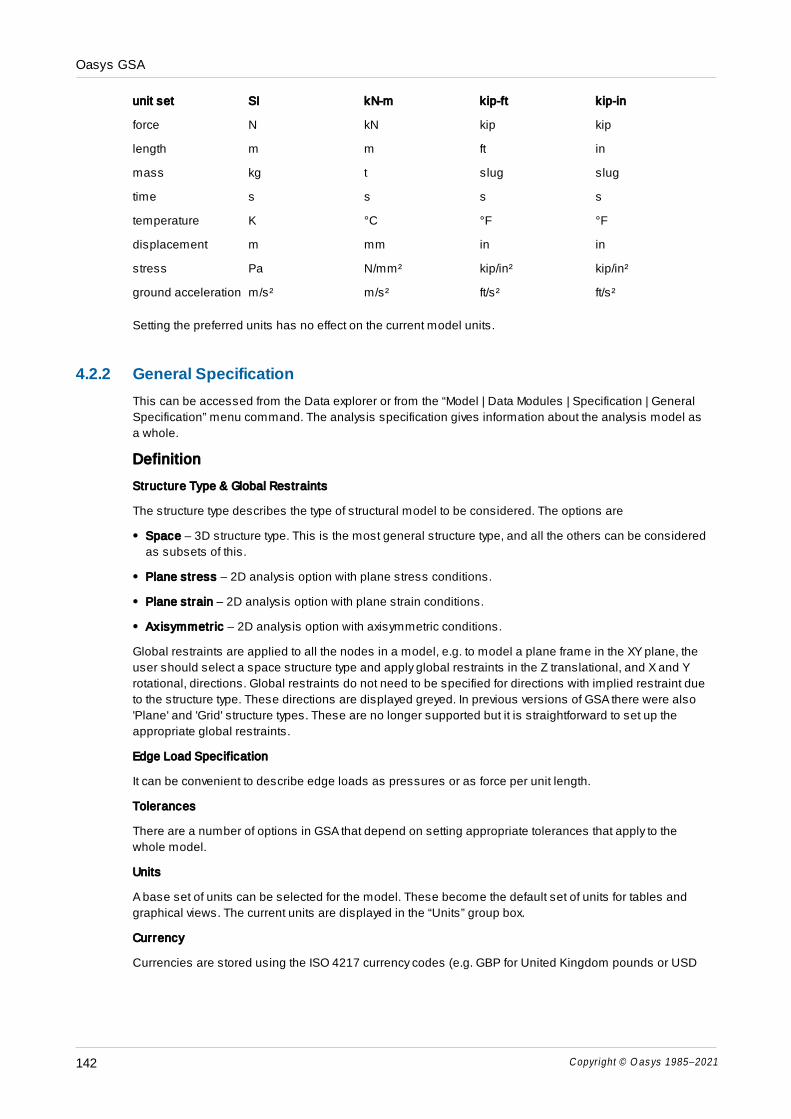
Oasys GSA

Copyright © O as ys 1985–2021142

unit set SI kN-m kip-ft kip-in

force N kN kip kip

length m m ft in

mass kg t slug slug

time s s s s

temperature K °C °F °F

displacement m mm in in

stress Pa N/mm² kip/in² kip/in²

ground acceleration m/s² m/s² ft/s² ft/s²

Setting the preferred units has no effect on the current model units.

4.2.2 General Specification

This can be accessed from the Data explorer or from the “Model | Data Modules | Specification | General

Specification” menu command. The analysis specification gives information about the analysis model as

a whole.

Definition

Structure Type & Global Restraints

The structure type describes the type of structural model to be considered. The options are

Space – 3D structure type. This is the most general structure type, and all the others can be considered

as subsets of this.

Plane stress – 2D analysis option with plane stress conditions.

Plane strain – 2D analysis option with plane strain conditions.

Axisymmetric – 2D analysis option with axisymmetric conditions.

Global restraints are applied to all the nodes in a model, e.g. to model a plane frame in the XY plane, the

user should select a space structure type and apply global restraints in the Z translational, and X and Y

rotational, directions. Global restraints do not need to be specified for directions with implied restraint due

to the structure type. These directions are displayed greyed. In previous versions of GSA there were also

'Plane' and 'Grid' structure types. These are no longer supported but it is straightforward to set up the

appropriate global restraints.

Edge Load Specification

It can be convenient to describe edge loads as pressures or as force per unit length.

Tolerances

There are a number of options in GSA that depend on setting appropriate tolerances that apply to the

whole model.

Units

A base set of units can be selected for the model. These become the default set of units for tables and

graphical views. The current units are displayed in the “Units” group box.

Currency

Currencies are stored using the ISO 4217 currency codes (e.g. GBP for United Kingdom pounds or USD

Oasys GSA

Copyright © O as ys 1985–2021 143

for United States Dollars). The currency can be changed to any of those supported by GSA or none.

4.2.3 Tolerances

Definition

General

The node co incidence is the tolerance within which nodes are assumed to be coincident. The g rid p lane is

the tolerance with which entities are considered to belong to a grid plane. Elements are considered to be

ve rtica l if the element x axis is within the angle from the global z axis. This affects the interpretation of the

element orientation information. E lem en t p lane is the angle within which elements are considered planar

Grid Loading Tolerances

The g rid edge stra igh tness is used when identifying panels on a grid surface (sets of elements that

enclose a region) the elements will be considered to form a single edge if the change in alignment is less

than this tolerance.

The g rid load ing edge to le rance is used if a beam or bar element is found inside the radius defined by the

edge tolerance, all of the load is assumed to apply directly to that element at the closest point.

The g rid p lane to le rance is used to determine if entities are on a grid plane if they are within this distance

of the grid plane.

(This option is only available when this dialog box is opened from the Preferences dialog box.)

The g rid load ing re finem en t to le rance is used where a grid surface is multi-way spanning in the algorithm

used to distribute the load uses a number integration scheme. The grid loading refinement tolerance

determines the density of the points used in the integration. Low tolerances will be adequate where a load

is spread over a large number of panels and it is the behaviour of the structure is of interest. Where a

single panel or a small number of panels are loaded and local effects are of interest a higher tolerance

may be preferred.

A high loading refinement tolerance may cause analyses to slow significantly.

Notes: The algorithm used is based on equilibrium considerations and not on satisfying the flexibility

conditions, so higher tolerance levels do not necessarily give better results. A high tolerance may slow the

expansion of the grid loading during the analysis.

Member Straightness Tolerance

The m axim um d iffe rence o f e lem en t o rien ta tion angle is the acceptable difference of the orientation

angles of all the elements constitute a member. The m axim um d istance from the cen tre line is the

allowable distance of deviation of the intermediate nodes of a member from the centre line. The o ffse t

d istance from cu rved m em b er controls the difference between the arc and the chord for curved members.

Form-finding

The b ar space r leg leng th is the acceptable deviation from the specified spacer leg length in form-finding

analysis.

Preferred

Update the tolerances with the tolerance preferences.

(This option is not available when this dialog box is opened from the Preferences dialog box.)

Oasys GSA

Copyright © O as ys 1985–2021144

4.2.4 Design Specification

The design codes for both steel and concrete design, and for loading.

Definition

Steel Design

This is the code that will be used for steel member utilisation checks and design. Internal restraint rules

can be established for the automatic generation of member restraints. A default steel grade can also be

selected.

Concrete Design

The code that will be used for concrete slab design. Superseded codes can be included and default

concrete and rebar models selected for the chosen design code.

The codes displayed are all the concrete design codes that GSA has available.

Load Design

Specified the design code used when generating load combinations.

4.2.5 Member Internal Restraint Specification

These are the default settings for steel member restraints, and are used if the member restraints are set

to "Auto". It works by checking member connections and adding design restraints where appropriate.

Definition

Axial buckling

Specifies that the secondary member can provide restraint against major and/or minor axes buckling of

the primary. An angle tolerance provide a limit on deciding which secondary members can provide

restraint.

Lateral torsional buckling

Specifies that the secondary member can provide restraint to the top and/or bottom flange of the primary

against lateral torsional buckling. An angle tolerance provide a limit on deciding which secondary

members can provide restraint.

Span restraint

Specifies that the spans can provide lateral torsional restrain to the top and/or bottom flange.

4.2.6 Raft Analysis Specification

When modelling a raft supported on soil some information is needed to clarify how the soil is considered.

Definition

Rigid Boundary Level

The soil layers are defined by a top soil level. This defines the level at which the ground can be considered

rigid. Typically the rock level.

Maximum Allowable E Ratio

In a soil the E value typically varies with depth through a soil profile. The E ratio determines how many sub-

layers are needed within a single soil layer in the profile. The larger the ratio the fewer the number of sub

layers and the coarser the sol analysis.

Oasys GSA

Copyright © O as ys 1985–2021 145

Mindlin Method

The Mindlin analysis method opens up a number of options:

Use weighted average – In this method, the average Young’s modulus and Poisson’s ratio are

calculated between the centroid of each load and the displacement point at which the horizontal

displacement is required.

Use greatest stiffness – In this method, the maximum Young’s modulus that occurs between the

centroid of each load and the displacement point is used for the calculations. The Poisson’s ratio is set

to that of the stratum where the greatest E is found.

Use stiffness at displacement point – In this method, the stiffness at the displacement point is used for

calculating horizontal displacements. The soil properties between the load and the displacement points

are disregarded. This method should be used with caution.

Boussinesq Method

A Boussinesq analysis requires that a global Poisson’s ratio for the soil.

4.2.7 Bridge Loading Analysis Specification

As discussed in the Step-by-Step guide to Bridge Loading, there are three different ways of using the tools

available for bridge loading. This specification dialogue is used to distinguish between these methods

and set up the parameters for the first method.

Bridge Design Loading Code

Unless working with UK or HK loading (HA and HB) on constant width carriageways, the code must be set

to “Undefined”. Otherwise the user can select the appropriate code from the options below:

UK_BD37 – For HA and HB loading to the United Kingdom Design Manual for Roads and Bridges.

HK_SDM – For HA and HB loading to the Hong Kong Structures Design Manual.

UK_BD21_HB – For HA to BD21 and HB to BD37

UK_BD86_SV-TT – For HA to BD21 and SV-TT to BD86

UK_BD86_SV-Train – For HA to BD21 and SV-Train to BD86

UK_BD86_SV-150 – For HA to BD21 and SV-150 to BD86

UK_BD86_SV-100 – For HA to BD21 and SV-100 to BD86

UK_BD86_SV-80 – For HA to BD21 and SV-80 to BD86

UK_CS454_HB – For HA to CS454 and HB to BD37

Using these options where possible makes the most efficient use of the tools available for bridge loading

in GSA. The SV loading types are an approximate implementation of the requirements of BD86

requirements. Intensity of SV vehicle loading is adjusted to compensate for the different load factors (1.1

for vehicles, 1.3 for associated lane loading). SV loading is applied in a similar way to HB loading to BD37,

with HA loading applied over the full width of lanes, not on 2.5m widths within lanes as required by BD86/

BD21; note that this is unconservative if there is little or no transverse distribution in the bridge. All HA

loading is factored by 0.91 (equivalent to Heavy Traffic / Poor Surface to BD21).

UK/HK Loading

To allow for different load factors in different combinations, the user can specify one or more of the

following:

ULS Comb1: for ULS Load Combination 1 (dead and live load only)

Oasys GSA

Copyright © O as ys 1985–2021146

ULS Comb3: for other ULS load combinations (dead, live and temperature or dead, live and wind)

SLS Comb1: for SLS Load Combination 1

Using these options where possible makes the most efficient use of the tools available for bridge loading

in GSA. The SV loading types are an approximate implementation of the requirements of BD86

requirements. Intensity of SV vehicle loading is adjusted to compensate for the different load factors (1.1

for vehicles, 1.3 for associated lane loading). SV loading is applied in a similar way to HB loading to BD37.

HA loading applied over the full width of lanes, not on 2.5m widths within lanes as required by BD86/

BD21/CS454; note that this is unconservative if there is little or no transverse distribution in the bridge. All

HA loading is factored by 0.91 (equivalent to Heavy Traffic / Poor Surface to BD21/CS454).

Note: As the number of analysis cases in the bridge analysis task depends on the bridge specification, the

editing of bridge analysis specification will be disabled if there is a bridge analysis task.

In addition for CS454:

Single axle consideration (CS454 Clause 5.17(2)) is not included.

A pedestrian live load factor of 0.8 from CS454 Table 5.32b is be adopted. Elements supporting

footways only, will need to be run with path loading to allow factor of 1.0

A pedestrian width factor of 1*width (the value of 1 from Table 5.32b is adopted).

4.2.8 Environmental Impact Specification

As discussed in the Step-by-Step guide to Environmental Impact, global environmental impact parameters

may be specified in the Environmental Impact Specification dialog.

Global environmental impact parameters are listed for each material type. Highlighting a material type and

clicking Edit (or double-clicking the material type) opens the Environmental Impact Wizard for that material

type.

The reinforcement % for environmental impact is used to combine the concrete values with the rebar

values in determining values for reinforced concrete.

4.3 Geometry

4.3.1 Axes

This feature enables new user-defined axes systems to be specified e.g. to specify an inclined roller

support, to assist in interpretation of results, or to specify the Construction Grid. Axes systems may be

Cartesian, cylindrical or spherical.

Definition

A user axes set is created by specifying the following:

Name

Used as a convenient way of identifying an axis.

Type

Axes can be Cartesian, cylindrical or spherical.

Origin

Oasys GSA

Copyright © O as ys 1985–2021 147

The location of this axis system in the global axis system.

X Vector

A vector, defined in the global axis system, in the direction of the local x-axis.

XY Vector

A vector, defined in the global axis system, which lies in the local xy-plane.

An example of the definition and application of user-defined axes is given below.

The user axis origin coordinates are thus defined as (x, y, z) above. The rotational orientation is defined in

terms of a vector along the positive xn-axis and a vector in the x

nyn plane. These two vectors are defined in

the laterally shifted axes system shown above.

Oasys GSA

Copyright © O as ys 1985–2021148

E.g. consider the simple case of rotation about the yn axis alone to give an inclined plane for a support

The x vector could be expressed as (a, 0, 1). This defines the position of the xn axis.

The rotation of the user axis system about this axis must be defined by specifying any xy vector in the xnyn

plane, apart obviously from the xn axis itself. In our case here, there is no rotation and the vector can be

taken as (0, 1, 0) i.e. the yn axis.

Modify Axis

The modify axis dialog is used to modify an axis set. This dialog can be activated from the Axis Definition

dialog and modifies the axis definition. To apply multiple transformations use this dialog to apply the

modifications one after the other.

Translate by/Rotate by

The user can choose to modify the axis either by translating along one of the current axis directions or

rotating about one of the current axes by the amount specified.

Along/about

This specifies which axis is to be used for the translation or rotation. These are always the current axis

direction of the axis system.

See also Working with the Program – Axis Sets.

Oasys GSA

Copyright © O as ys 1985–2021 149

4.3.2 Grid Lines

The grid line definition dialog is used to define or modify the grid lines for the model. This dialog can be

activated from the Current Grid Definition dialog.

Grid lines are defined as being in the global XY plane. Grid lines form part of the current grid and, when

displayed, are projected onto the current grid plane (unless it is vertical). Grid lines can be displayed in

Graphic Views and can be operated on using sculpt commands.

Grid lines may be straight or circular arcs.

Straight grid lines are defined by a start position, a length and an angle

Circular arc grid lines are defined by a centre of the arc, a radius, a start angle and an end angle

- where the angles are measured from global X, anti-clockwise about global Z.

Grid Lines Table

Label

The name by which the grid line is referred. Labels must be unique.

Arc

Specifies whether the grid line is a straight “Line“ or circular “Arc“.

X, Y

The start of a straight line or the centre of a circular arc, in global coordinates.

Length

The length of a straight line or the radius of a circular arc.

Theta 1

The angle of inclination of a straight line or the start angle of a circular arc, measured from global X, anti-

clockwise about global Z.

Theta 2

The end angle of a circular arc, measured from global X, anti-clockwise about global Z. (Not required for

straight grid lines.)

Add Grid Lines

This is a tool for generating new grid lines using as a basis the grid line that is currently selected in the

table. If the increment value is positive the new grid lines are inserted below the current grid line; if

negative, above.

The new grid lines are given unique labels, based on the label of the current grid line.

Move Grid Lines

This tool moves the existing grid lines that are currently selected in the table. The grid lines may be

translated in the x or y directions or rotated about the Z axis; the transformation occurs in the currently

defined axes.

Note that only axes that have a vertical z axis are offered in the list of available axes.

Oasys GSA

Copyright © O as ys 1985–2021150

4.3.3 Grid Planes

A grid plane defines the geometry of a surface. The load behaviour of the grid plane is defined by a grid

surface. The Grid Plane data table is available in the Data Explorer. The Grid Plane Definition dialog can

be activated from the Grid Planes table view by giving the “Edit | Wizard” menu command. “Wizard” is also

available on the Data Options toolbar and on the right-click menu for the table view. It can also be activated

from the Current Grid Definition dialog.

Refer to Use of Grid Planes and Grid Surfaces for a general description of grid planes and their use.

Grid Plane

Name

The name is used only as a label for the grid plane. Where grid planes have to be selected this is the

name that will be displayed.

Type

The grid plane can be either a general grid plane or a storey grid plane. A storey grid plane must exist in a

global XY plane.

Grid axis

Grid planes reference an axis set. This may be global or any user defined axis system. The grid plane is

parallel to the xy plane of this axis set.

Grid elevation

For situations where grid planes are to be stacked at different levels the grid elevation allows the grid

plane to be offset from the axis origin in the local z direction. The elevation defines the height of the grid

plane above the origin.

Grid plane tolerance

The grid plane tolerance is used to determine whether an element lies in the grid plane.

Storey Tolerance below/above

Nodes are associated with the storey if they lie within these tolerances of the elevation. The different

tolerance above and below are to allow for situations where there may be a step in the floor levels but

these are to be considered as a single storey at the specified elevation. If the tolerance is set to "auto" then

the nodes are associated with the nearest storey.

4.3.4 Grid Surfaces

A grid surface is required to in order to apply grid loads to the structure. The grid surface details how the

grid load is transferred on to the structure.

Definition

Name

A label for the grid surface. The name is shown when grid surfaces have to be selected.

Grid plane

The grid plane that the grid surface is defined to use.

Element list

Elements included in the grid surface. In some situations only some of the elements are to be considered

to be part of the grid surface (e.g. secondary bracing) so the element list can be used to specify these.

Oasys GSA

Copyright © O as ys 1985–2021 151

Element type

Elements type of a grid surface specifies the type of elements that are to be considered as part of the grid

surface. It can be 1D or 2D.

Grid load tolerance

This defines a volume (above and below the actual grid plane) within which elements are considered as

candidates for the grid plane. It is used in conjunction with the element list to determine whether an

element lies in the grid surface. A floor may use a relatively small tolerance while a roof structure may use

a much larger tolerance.

Span

The span defines the way in which loading on the grid surface will be transferred from space to the

surrounding elements.

One-way – the load is transferred in the specified span direction. The direction is the angle to the x-

direction of the axis defining the grid plane.

Two-way – an area load on a complete panel. The load is expanded according to the specified

algorithm and distributed in a pattern resembling the back of an envelope. The possible expansion

algorithms are

o Legacy – Legacy option: loads assumed to ripple out to edges of panel (does not work on re-entrant

panels)

o Plane – Uses a plane approximation to distribute the load and adjusts for aspect ratio (load

distribution depends on model refinement)

o Smooth (plane) – Uses a plane approximation to distribute the load; adjusts for aspect ratio and

smooths loads along edges

o Corner (plane) – Uses a plane approximation to distribute the load; adjusts for aspect ratio and

smooths loads along edges, adjusting for corner effects (recommended)

o Simplified tr ibutary areas option. Give simple distribution on fully loaded triangular and quadrilateral

panels as shown below

Grid load expansion algorithms

The grid load expansion option determines which algorithm is used to expand the grid loads.

The legacy option treats loads as a series of point loads applied across the grid plane which ‘ripple’ out to

the elements bounding closed areas. This does not work for re-entrant panels, e.g. L shaped areas.

The plane approximation options treats the load on a panel as a single load applied at the centre of loads

and a set of loads applied around the perimeter that give equilibrium. The loads are determined so that

the aspect ratio of the panel results in a greater load intensity applied to the long edges that the short

ones. The basic version of this gives a mesh-dependent load distribution and can lead to the mid-span

load intensities being too large. The ‘smooth’ variant takes the uniformly distributed loads on the individual

elements and aggregates these along the edges resulting in a linear variation along the panel edges. The

‘corner’ variant assumes that the loads on the ends of edges at internal corners should be reduced so an

adjustment is made to taper the load intensity to zero at these corners.

4.3.5 Polylines

Polylines are used mainly in conjunction with grid loading to define lines or area that are loaded. Polylines

are 2D entities that are interpreted with respect to the x-y plane of a grid plane.

Definition

Oasys GSA

Copyright © O as ys 1985–2021152

Name

The name used to refer to the polyline.

Grid plane

Poly lines can either exist in 3D space or can be associated with a grid plane

Description

Polylines are defined by a series of x-y or x-y-z coordinates. These are entered as a description of the form:

(x1,y1) (x2,y2) (x3,y3)

or(x1,y1,z1) (x2,y2,z2) (x3,y3,z3)

A polyline does not need to be closed to represent a polygon – closure will be inferred from the context.

Polyline checks

A badly formed polyline is one that has:

coincident vertices, or

overlapping or crossed lines, or

vertices lying along lines.

Invalid lines and vertices are highlighted in the dialog and specific issues in the polyline are reported upon

exiting the Polyline dialog.

Invalid polylines are treated as errors in the pre-analysis data checks.

The polyline definition dialog is used to define or modify a polyline. This dialog can be activated from the

Polyline table view by giving the “Edit | Wizard” menu command. “Wizard” is also available on the Data

Options toolbar and on the right-click menu for the table view.

4.4 Materials

4.4.1 Material Grades

4.4.1.1 Steel

For steel design a steel material grade must be defined. Properties used in the steel design are taken

from the steel material grade and not from the analysis material. The Grade Wizard should normally be

used to define the steel grade properties.

Definition

The detailed properties are defined here:

Name

The name is only used as a convenient way of identifying a material.

Standard Grades

The standard grades allows selection from among a predefined set of properties.

Basic Properties

The following basic properties are specified:

Yield strength (fy)

Oasys GSA

Copyright © O as ys 1985–2021 153

Ultimate strength (fu)

Failure strain (εmax

)

Elastic modulus (E)

Shear modulus (G)

Density (ρ)

Thermal expansivity (α)

Poisson’s ratio (ν )

Section Design Properties

The following section design properties are specified:

Strength (taken from basic properties)

Material curve (one of linear, elastic-plastic, strain hardening, Park, explicit)

Strain at plateau stress

Ultimate strain

Environmental Impact

Clicking Environmental Impact enables environmental impact parameters to be specified for this material

by opening the Environmental Impact Wizard. These values then override the global values specified in

Environmental Impact Specification for this material.

The current environmental values for the material are reported.

The cost allocates a unit cost to the material.

4.4.1.2 Concrete

For concrete design a concrete material grade must be defined. Properties used in the concrete section

and slab design are taken from the concrete material grade and not from the analysis material. The Grade

Wizard should normally be used to define the concrete grade properties.

Definition

Name

The name is only used as a convenient way of identifying a material.

Standard Grades

The standard grades allows selection from among a predefined set of properties.

Basic Properties

The following basic properties are specified:

Strength (fck

) (subscript varies with design code)

Density (ρ)

Failure strain (εmax

)

Elastic modulus (E)

Shear modulus(G)

Oasys GSA

Copyright © O as ys 1985–2021154

Thermal expansivity (α)

Poisson’s ratio (ν )

Section Design Properties

The following section design properties properties are specified:

Strength (taken from basic properties)

Confining stress (used by confined concrete models only)

Serviceability state concrete curves for tension and compression

Strains at peak and maximum stress

Ultimate state concrete curves for tension and compression

Strains at plateau and ultimate stress

Slab Design Properties

The following section design properties properties are specified:

Strength (fck

) (taken from basic properties)

Uncracked design strength (fcd

)

Cracked design strength (fcdc

)

Tensile design strength (fctd

)

Plateau strain (εtran

) (note: this not the same as the plateau strain for section design)

Failure strain (εmax

)

Maximum axial strain (εax

)

Constant stress depth (β)

Environmental Impact

Clicking Environmental Impact enables environmental impact parameters to be specified for this material

by opening the Environmental Impact Wizard. These values then override the global values specified in

Environmental Impact Specification for this material.

The current environmental values for the material are reported.

The cost allocates a unit cost to the material.

4.4.1.3 FRP

For design including FRP an FRP material grade must be defined. The Grade Wizard should normally be

used to define the FRP grade properties.

Definition

Name

The name is only used as a convenient way of identifying a material.

Standard Grades

The standard grades allows selection from among a predefined set of properties.

Oasys GSA

Copyright © O as ys 1985–2021 155

Basic Properties

The following basic properties are specified:

Strength

Elastic modulus (E)

Bond strain limit

Density (ρ)

Poisson’s ratio (ν )

Thermal expansivity (α)

Section Design Properties

The following section design properties are specified:

Strength (taken from basic properties)

Material curve

Bond parameters

Strains at plateau and ultimate stress

Environmental Impact

Clicking Environmental Impact enables environmental impact parameters to be specified for this material

by opening the Environmental Impact Wizard. These values then override the global values specified in

Environmental Impact Specification for this material.

The current environmental values for the material are reported.

The cost allocates a unit cost to the material.

4.4.1.4 Aluminium

The Grade Wizard should normally be used to define the aluminium grade properties.

Definition

Name

The name is only used as a convenient way of identifying a material.

Standard Grades

The standard grades allows selection from among a predefined set of properties.

Basic Properties

The following basic properties are specified:

Elastic modulus (E)

Poisson’s ratio (ν )

Density (ρ)

Thermal expansivity (α)

Environmental Impact

Clicking Environmental Impact enables environmental impact parameters to be specified for this material

Oasys GSA

Copyright © O as ys 1985–2021156

by opening the Environmental Impact Wizard. These values then override the global values specified in

Environmental Impact Specification for this material.

The current environmental values for the material are reported.

The cost allocates a unit cost to the material.

4.4.1.5 Timber

The Grade Wizard should normally be used to define the timber grade properties.

Definition

Name

The name is only used as a convenient way of identifying a material.

Standard Grades

The standard grades allows selection from among a predefined set of properties.

Basic Properties

The following basic properties are specified:

Strength (fmk

)

Elastic modulus (E)

Poisson's ratio (ν )

Density (ρ)

Thermal expansivity (α)

Environmental Impact

Clicking Environmental Impact enables environmental impact parameters to be specified for this material

by opening the Environmental Impact Wizard. These values then override the global values specified in

Environmental Impact Specification for this material.

The current environmental values for the material are reported.

The cost allocates a unit cost to the material.

4.4.1.6 Glass

The Grade Wizard should normally be used to define the glass grade properties.

Definition

Name

The name is only used as a convenient way of identifying a material.

Standard Grades

The standard grades allows selection from among a predefined set of properties.

Basic Properties

The following basic properties are specified:

Elastic modulus (E)

Oasys GSA

Copyright © O as ys 1985–2021 157

Poisson’s ratio (ν )

Density (ρ)

Thermal expansivity (α)

Environmental Impact

Clicking Environmental Impact enables environmental impact parameters to be specified for this material

by opening the Environmental Impact Wizard. These values then override the global values specified in

Environmental Impact Specification for this material.

The current environmental values for the material are reported.

The cost allocates a unit cost to the material.

4.4.1.7 Fabric

The Grade Wizard should normally be used to define the fabric grade properties.

Definition

Name

The name is only used as a convenient way of identifying a material.

Standard Grades

The standard grades allows selection from among a predefined set of properties.

Basic Properties

The following basic properties are specified:

Elastic moduli (Ewarp

, Ef ill

)

Poisson’s ratio warp-fill (ν )

Shear modulus (G)

Density (ρ)

Environmental Impact

Clicking Environmental Impact enables environmental impact parameters to be specified for this material

by opening the Environmental Impact Wizard. These values then override the global values specified in

Environmental Impact Specification for this material.

The current environmental values for the material are reported.

The cost allocates a unit cost to the material.

4.4.1.8 Reinforcement

For reinforced concrete design concrete and reinforcement material grades must be defined. Properties

used in the concrete section and slab design are taken from the concrete and reinforcement material

grades and not from the analysis material. The Grade Wizard should normally be used to define the

reinforcement grade properties.

Definition

Name and Type

The name is only used as a convenient way of identifying a material. The type allows selection between

Oasys GSA

Copyright © O as ys 1985–2021158

normal steel reinforcement, prestress tendons and FRP bars.

Standard Grades

The standard grades allows selection from among a predefined set of properties.

General Properties

The following basic properties are specified:

Strength (fy)

Material partial safety factor (γm

) (for selected design codes)

Failure strain (εmax

)

Elastic modulus (E)

Hardening parameter (k)

Density (ρ)

Thermal expansivity (α)

Ductility (One of low, normal or high: this is a function of failure stain.)

Section Design Properties

The following section design properties are specified:

Strength (taken from basic properties)

Material curve

Strains – at plateau stress, ultimate strain

Bond parameters (for selected design codes)

Slab Design Properties

The following section design properties are specified:

Strength and design strengths (fy k

) (taken from basic properties)

Stress limits

Strain limits

Miscellaneous Properties

Clicking Environmental Impact enables environmental impact parameters to be specified for this material

by opening the Environmental Impact Wizard. These values then override the global values specified in

Environmental Impact Specification for this material.

The current environmental values for the material are reported.

The cost allocates a unit cost to the reinforcement material.

4.4.1.9 Analysis Materials

All elements that refer to Beam Sections, 2D Properties or 3D Properties require an analysis material. This

can either be an explicitly defined material or an implied material from a material grade. The latter are

always assume to be elastic isotropic materials.

The Material Wizard should normally be used to define the analysis material properties.

Oasys GSA

Copyright © O as ys 1985–2021 159

Explicit analysis materials

The detailed properties are defined here:

Name

The name is only used as a convenient way of identifying a material.

Material Model

The following material models are the most common:

Elastic isotropic

Elastic orthotropic

Elastic-plastic isotropic

Fabric

Though GSA can also analyse the following materials with some solvers:

Drucker-Prager

Mohr-Coulomb

Young’s modulus, Poisson’s ratios, Shear modulus

Elastic isotropic material - Young’s modulus, Poisson’s ratio and shear modulus can have the following

relationship

12

EG

However the shear modulus may be specified independently to allow for the non-isotropic nature of

material such as timber. Note that the shear modulus can only be edited using the Material Wizard.

Elastic orthotropic material - there are three Young’s moduli, three Poisson’s ratios and three shear

moduli need to be defined and they are:

The material properties are

Ex - Young’s modulus in x direction

Ey - Young’s modulus in y direction

Ez - Young’s modulus in z direction

νxy

- Poisson’s ratio, y direction strain generated by unit strain in x direction

νyz

- Poisson’s ratio, z direction strain generated by unit strain in y direction

νzx

- Poisson’s ratio, x direction strain generated by unit strain in z direction

The other three Poisson’s ratios ( νy x

, νzy

, νx z

) can be calculated from the following relationships:

Oasys GSA

Copyright © O as ys 1985–2021160

Gxy

- Shear modulus in xy plane

Gyz

- Shear modulus in yz plane

Gzx

- Shear modulus in zx plane

Note: If an element uses an orthotropic material, the parameters used by the element are:

Beam elements

Ex

Gxy

, Gzx

Bar, Tie & Strut elements

Ex

2D shell and plate elements

Ex, E

y

νxy

, *νyx

Gxy

, Gyz

, Gzx

2D plane stress elements

Ex, E

y

νxy

, *νyx

Gxy

2D plane strain elements

Ex, E

y, E

z

νxy

, *νyx

, νyz

, *νzy

, νzx

, *νxz

Gxy

2D axisymmetric elements

Ex, E

y, E

z

νyz

, *νzy

, νzx

, *νxz

Gxy

* these values are calculated by GSA from the E values and the complementary Poisson’s ratio.

Elastic-plastic isotropic material - the Young’s modulus, Poisson’s ratios and shear modulus etc

parameters are the same as elastic isotropic material.

Oasys GSA

Copyright © O as ys 1985–2021 161

Yield stress is the tensile and compressive strength of the material, ultimate stress is the

maximum stress the material can sustain, but it is not used in any of the analysis at the moment,

hardening modulus and hardening parameter are used to define the material hardening behavior

that can be used by explicit time history analysis and explicit nonlinear analysis.

In GsRelax nonlinear analysis, material plasticity is considered by beam, bar, tie and strut

elements. Elastic and perfectly plastic material model is assumed in the analysis, i.e. a bi-linear

stress-strain curve is used and the second branch of the stress-strain curve is horizontal, There

is no strain limit and the stress is limited to the yield stress. Ultimate stress, hardening modulus

and hardening parameter are not used in GsRelax nonlinear analysis.

In explicit time history analysis and explicit nonlinear analysis, material plasticity will be

considered by all elements that uses elastic-plastic materials, the stress-strain curve is also bi-

linear and the second branch of the curve can be horizontal if no hardening modulus is defined, if

hardening modulus is defined, the second branch of the curve is sloped up to reflect the strain

hardening of the material. Strain hardening can be considered by explicit analysis if they are

defined. The same as GsRelax analysis, the ultimate stress is not used in the analysis..

Fabric material - Fabric material is only used for 2D fabric (membrane) element, since the element has no

thickness, the unit of Young’s modulus and shear modulus of fabric material is force per unit length.

Fabric material is orthotropic and the following properties need to be defined:

E'x - Young’s modulus in x (warp) direction

E'y - Young’s modulus in y (weft) direction

νxy

- Poisson’s ratio, y direction strain generated by unit strain in x direction

The other Poisson’s ratio ( νy x

) can be obtained from the following relationship:

yx

xy

y

x

E

E

Fabric material can be defined to take tensile force only (the default option) or take both tensile and

compressive forces. If the check box “Allow compression” is checked, fabric will take compressive force,

otherwise, it will take tensile force only.

Other options

Note that these may be available with only some material types.

Initialize Analysis Material from Design Material

This command is available from the wizard. You can set the material properties either from materials in a

catalogue or from material grades in the model.

Density

The density of the material to be used in dynamic analysis to calculate masses and in other analysis to

calculate gravity loads.

Temperature coefficient

The temperature coefficient of expansion which is used in conjunction with thermal loading. For orthotropic

material, three coefficients need to be defined for x, y & z directions.

Damping Ratio

The damping ratio is used during a dynamic analysis to calculate an estimate of the modal damping ratio.

Oasys GSA

Copyright © O as ys 1985–2021162

Yield stress

The stress at which the material first yields in nonlinear analyses. For design this may be a value specified

by a design code.

Ultimate stress

The stress at which the material will break. This is used mainly for design purposes. This property is not

used by the analysis options in GSA but can be when analysing in LS-DYNA.

Hardening modulus

Once the material has yielded it is assumed to follow a straight-line relationship between stress and

strain. The slope of this line is the hardening modulus. This property is not used by the analysis options in

GSA but can be when analysing in LS-DYNA.

Hardening parameter

This is used in non-linear analysis to determine if the hardening model should be isotropic or kinematic.

This property is not used by the analysis options in GSA but can be when analysing in LS-DYNA.

Allow Compression

This box should be unchecked if the fabric is to allowed to behave like a true fabric and not allow

compression.

Cohesion, Friction angle, Dilation

Set the soil properties

4.4.2 Material Curves

In most analysis no material curve needs to be defined, but for LS-DYNA analysis and for non-linear

springs material curves must be defined.

Definition

Name

The name is only used as a convenient way of identifying a material (or spring) curve.

Type

The type defines the spring is translational or rotational.

Description

A table defining the force/displacement, moment/rotation, stress/strain relationship for a non-linear

material or spring.

Axis Value Type

This defines the dimension of the non-linear spring curve and the available types are:

Force - Displacement: the spring is translational

Moment - Rotation: the spring is rotational

Data Table

The data table is used to define the data point on the material curve, it must be in ascending order. When

the data table is used in analysis, if abscissa value is beyond the definition range, the ordinate value will

be taken as zero, ordinate value beyond defined range is not allowed and it will not occur in the analysis.

Diagram

Oasys GSA

Copyright © O as ys 1985–2021 163

The diagram shows the curve of the non-linear spring defined in the data table.

4.5 Properties : Section

All beam type elements refer to a section defining the geometrical properties (e.g. area, second moment of

area) referenced by the element or member through the property number. The set of sections in the model

form the Section Library. Individual sections in the section library can have Section Analysis Properties that

are modified for analysis, e.g. reducing the J value so that the element doesn't attract torsion. Sections are

then grouped in Section Pools.

Basic definition

The basic definition of a section includes:

Name and Colour

These are used to identify sections and show elements or members which refer to these.

Material

The material definition breaks into three parts. The first part is the material type. This is one of:

Steel – allows a set of properties for various grades and gives option to assign to various steel design

properties to the section

Concrete – allows a set of properties for various grades

FRP – allows a set of properties for various grades

Glass – allows a set of properties for various grades

Aluminium – allows a set of properties for various grades

Timber – allows a set of properties for various grades

<undefined> – not associated with any grade

The grade defines the actual material design properties. These depend on the material type. New grades

can be initialized from the standard grades for the current design code. The final material attribute is the

analysis material. This defines a set of elastic properties. If a grade is specified it is possible to refer to

this for the analysis material (from Grade). In this case the required analysis properties are inferred from

the grade.

Profile, Reference Point and Point Voids

The profile defines the shape and geometry of the section. These can be either catalogue (steel) sections,

standard section shapes, or shapes defined by geometry (perimeter, or line segments). By default the

reference point is at the centroid of the section. In this case an axial force applied at the centroid results in

no bending. It some cases it can be convenient to change the reference point. The other change to the

section geometry is to add point voids. This allows (small) ducts to be included in the section. This is also

used in conjunction with bridge beams to identify locations for prestress tendons – in this case the voids

are assigned a zero area.

Rate

This associates a unit cost against sections.

Modified

This is a flag to indicate that there are section modifiers associated with this section.

Pool

Oasys GSA

Copyright © O as ys 1985–2021164

The section can be assigned to a pool. This groups sections for design.

Section Properties

These are the actual section properties of the chosen section, so for example a 400×200mm rectangular

section would have an area of 0.08m².

Modifiers

Each base section property can be modified so that a different value is used in the analysis. So for

example the user may want to increases the axial stiffness of the 400×200mm rectangular section defined

above, so he can either factor the value or replace the value with a new value. So for example a factor of 2

on the area of the section would give an analysis value of 0.16m².

Modifiers on the I and k values apply to either the xy or uv values depending on the axes selected for the

stiffness calculation.

If the section is modified then GSA will not calculate section stresses until it is stated whether the modified

or unmodified properties are to be used.

Analysis properties

The analysis properties are the base section properties modified as above. These are the values used in

the stiffness calculation. Note that the modified area may or may not be used to determine the mass or

gravity load, so in the above example the stiffness would be based on an area of 0.16m² but the mass and

gravity loads would be based on either an area of 0.08m² or 0.16m².

Bending axes

The section is either assumed to bending in the local y and z directions independently or for non-

symmetric sections the principal bending directions u and v can be used.

Area

The modified area of the beam cross-section for analysis.

I11, I22

The second moment of area of the beam about the yy and zz axes for the local axis option or uu and vv

axes for the principal axes option.

J

The torsion constant for the section; note this is not the polar moment of inertia unless the section is

circular.

k11, k22

The shear factor for shear about the yy and zz axes for the local axis option or uu and vv axes for the

principal bending axes option. Note the principal bending axes is not the same as the principal shear

axes. It is the proportion of the area of the beam which is effective in carrying shear (i.e. the [Shear Area]/

[Total Area]). This can be defined as zero if the shear deformations are to be ignored.

Use of section data in standard (GSS) analysis

Bending action is about the principal axes unless the user has chosen for the stiffness calculation in the

“uv axes” of the section term. For all symmetric sections principal and local axes are coincident.

The shear centre is assumed to be at the section centroid.

Use of section data in GsRelax analysis

The following points are only valid if the GsRelax solver is used.

Oasys GSA

Copyright © O as ys 1985–2021 165

If a section shape has been specified, the effect of plasticity on the interaction between axial force and

biaxial bending is modelled. The net bending moment is limited to the plastic capacity of the section for the

current axial force and direction of applied moment. The bending stiffness of a section is halved at first

yield.

If explicitly defined section properties are specified, the interaction between axial and bending yield is

ignored and the plastic section moduli used are approximations.

Bending action is in local element directions; the principal directions of the section are ignored.

Shear action is only modelled elastically and the shear centre is assumed to be at the section centroid.

4.5.1 Section Profile

Sections are most conveniently edited using the Section Wizard. This allows the user to either select

sections from a catalogue, to define standard section shapes or explicitly define the section properties.

The first step is to select the basic section definition – catalogue, or standard shape, etc. Depending on

this choice the profile wizard will load either catalogue sections, standard sections, or geometric sections

(perimeter sections, or fabricated and line segment sections). Finally the defined section properties are

displayed and an option is given to convert the section to a perimeter.

Section Definition Axes and Element Axes

Sections are defined with respect to section definition axes, shown in this diagram as xdef

and ydef

. The

section is used in GSA such that the section appears as defined, when viewed with the element x axis

pointing into the page. This has the, perhaps unintuitive, consequence of GSA having to translate the

specified (xdef

, ydef

xdef

, ydef

) element axes coordinates. (I.e. (xdef

,

ydef

yel, z

el).) The translation occurs automatically within GSA, requiring no action from the

user. The distinction between section definition axes and element axes is particularly relevant when

considering geometric sections. Display “Section Shapes” labels in a Graphic View to confirm the

orientation of sections.

Principal Axes

Oasys GSA

Copyright © O as ys 1985–2021166

For a doubly non-symmetric section principal axes are not aligned with element axes. In this circumstance

loading applied in element axis directions will produce deflections in the plane orthogonal to the loading

unless there are constraints on the section to prevent this behaviour. If there are such constraints the user

can choose, when defining the section, to prevent this effect by ignoring the Iy z

term in which case the Iy y

,

Izz

, Ky and K

z values would be used to calculate the element stiffness as if they were principal 2nd

moments of area.

4.5.1.1 Definition

Definition

Name

The name is a label used to identify a particular section.

Definition method

The definition method specifies how the material is to be defined. This breaks down into four main

options.

Catalogue sections are selected from online section catalogues.

Standard sections are defined by a shape and its dimensions. The properties are then calculated from

these.

Geometric sections are defined either by a perimeter or by line segments. The properties are then

calculated from these.

The page that follows this will depend on the selection made as this stage.

Section Definition Axis System

The axis along a beam element in GSA is the x axis. Following this assumption the cross section is

defined in a (y,z) axis system.

Section for tapered elements/members

If the section is referred to by tapered.elements/members, check box "Section tapers along element

length" should be checked on the section wizard, then two different sizes of the section can be defined and

the elements/members refer to this section will be tapered. Catalogue section, Fabricated section, Line

segment section and Point area section cannot be used by tapered elements/members, i.e. check box

Oasys GSA

Copyright © O as ys 1985–2021 167

"Section tapers along element length" will be always unchecked.and only one section size can be defined

4.5.1.2 Catalogue Sections

The catalogue sections are stored in an section database, installed with GSA. This provides an interface to

that database.

Definition

A catalogue section is defined by

Catalogue

The catalogue is first level of selection for the section.

Type

The type is the type of section required e.g. Universal Beam or Equal Angles.

Section

The particular section of the type selected e.g. EA250x250x35. If the section is marked S/S that particular

section has been superseded.

Include superseded sections

Superseded sections are to be displayed. If the model contains superseded sections this will be checked

on entry.

Transform Section

The basic section may not be in the required orientation, so there is an option to rotate and translate

sections. By default this is not offered.

Catalogues

Catalogues cover sections from the UK, Europe, USA, Canada, Australia,Japan, China, India, Korea,

Russia and South Africa.

Catalogue Sections

For catalogue sections the descriptions based on the catalogue, type and date to provide a string uniquely

identifying the section. This can be constructed as follows:

CAT <Type ID> <Sec name> <Date>

So for example a British Universal beam of 457 x 152 and mass of 82 kg/m of 15 June 1987 would be:

CAT UB UB457x152x82 19870615

The date field is normally used only to identify superseded sections, so normally the section description

would be abbreviated to

CAT UB 457x152x82

4.5.1.3 Standard Sections

Section dimensions

Standard sections can be rectangular, circular, I, channel, T or angles, etc. Rectangular and circular

Oasys GSA

Copyright © O as ys 1985–2021168

sections can be either solid or hollow. Specify the overall external dimensions of the section and the

thickness of component parts as shown below. Note that top and bottom flanges are always the same

thickness, as are left and right walls of a rectangular hollow section.

Oasys GSA

Copyright © O as ys 1985–2021 169

Oasys GSA

Copyright © O as ys 1985–2021170

Oasys GSA

Copyright © O as ys 1985–2021 171

Ellipse index (n)

This field is only available for the ellipse section type. It allows superellipses to be entered. A value of 1

Transform Section

The basic section may not be in the required orientation, so there is an option to rotate and translate

sections. By default this is not offered.

Standard Sections

The standard sections are identified by a code for the section shape, followed by a list of dimensions

defining the section. The section shape descriptors can be followed by an optional unit if the section is not

defined in mm, where the shapes are:

Section shape Shape code Dimensions

rectangular R d, b

rectangular hollow RHS d, b, tw, t

f

circular C d

circular hollow CHS d, t

I section I d, b, tw, t

f

tee T d, b, tw, t

f

channel CH d, b, tw, t

f

angle A d, b, tw, t

f

taper TR d, bt, b

b

ellipse E d, b, k

general I section GI d, bt, b

b, t

w, t

f t, t

f b

taper T section TT d, b, twt

, twb

, tf

Oasys GSA

Copyright © O as ys 1985–2021172

taper angle section TA d, b, twt

, twb

, tf

recto-circular RC d, b

recto-ellipse RE d, b, df, b

f, k

taper I section TI d, b, bt, b

b, t

wt, t

wb, t

f t, t

f b

secant pile section SP d, c, n

secant pile wall SPW d, c, n

oval OVAL d, b, t

Note:

b width

bb

bottom width

bf

flat width

bt

top width

c distance between pile centres

d depth, diameter

df

flat depth

k order

n number of piles

t thickness

tf

flange thickness

tf t

top flange thickness

tf b

bottom flange thickness

tw

web thickness

twt

top web thickness

twb

bottom web thickness

so the section description is as follows:

STD <Shape(unit)> <Dimension> <Dimension>…

Thus a 320 × 120 rectangular section would be

STD R 320 120

or an 8in diameter circular section would be

STD C(in) 8

Oasys GSA

Copyright © O as ys 1985–2021 173

4.5.1.4 Perimeter Sections

Perimeter Definition

The outline of a perimeter section is defined by a series of coordinates describing a polyline. The polyline

is automatically closed to form a polygon so an end point coincident with the start point need not be

entered. Polyline segments may not intersect.

In addition, any number of voids may be defined in the section, again by a series of coordinates describing

an unclosed polyline of non-intersecting segments. Voids may not intersect with each other or with the

outline.

The section displayed in the wizard is as viewed from end 1 of the element towards end 2.

The centroid is calculated for the section and the section is assumed to lie centred at its centroid, – not at

the datum coordinates.

Import Options

The section can be imported or exported from a DXF file. For the import to work the DXF file should contain

only LWPOLYLINE or POLYLINE entities that described the perimeter and void in the section. The export

option allows the section to be exported as a series of LWPOLYLINE entities.

The bridge beam option is only enabled if the bridge beam database is available. This gives access to

standard bridge beam sections. These are stored as perimeter sections in GSA, but have associated

tendon positions stored as point voids along with the section geometry.

The shear factors, Ky and K

z, are also set as zero.

Calculate torsion constant ‘J’

This option uses a purpose-built solver for the calculation of the torsion constant. The calculation will

accept any arbitrarily defined perimeter section as input, as long as the perimeter is a valid section shape

and the section area is sufficiently thick-walled (see below). No further input is necessary in setting up the

analysis. Due to the increased complexity of this method, when selecting this option there may be a brief

but noticeable delay when proceeding through to the next page of the Section Wizard as the Wizard

constructs and solves the torsion problem.

The calculation of the torsion constant ‘J’ makes use of a numerical technique that is designed for use

specifically on thick-walled sections - that is, section shapes with a sufficient area enclosed within the

perimeter boundary relative to the perimeter length. Thin-walled sections are best considered as a

separate concern and are typically solved using specific thin-walled theory. This theory is not currently

implemented in this solver and hence it is not recommended to calculate the value of ‘J’ for thin-walled

sections in this case. Section shapes that are considered to be too thin will prompt a warning message to

the user, given at the point during the wizard when the value of J is calculated.

Internally, the solver makes use of the ‘membrane analogy’ to construct and solve a particular case of the

Poisson problem. The differential equations along with the specific boundary conditions prescribed for the

torsion problem are assembled and solved numerically by application of boundary element method (BEM)

in a dedicated solver.

Perimeter Sections

There are two types of geometric section: perimeter and line segment. Both are described in terms of 2D

vertices. A perimeter section is specified by a polygon to define the section outline and, optionally, one or

more further polygons to define voids within the outline.

The syntax for geometric sections gives instructions for constructing the shape of the section. The section

must start with a flag to give the type of geometric section. This followed by a series of instructions defining

the shape of the section, separated by spaces. The instructions that are used are:

Oasys GSA

Copyright © O as ys 1985–2021174

Type Type Code

Perimeter P

Line segment L

and

Instruction Values Code

Move to position (x, y) M(x|y)

Line to position (x, y) L(x|y)

Set thickness t T(t)

element axes. (See Section Profile for more information on this.) This translation happens automatically

requiring no action by the user.

Thickness is only required for line segment section.

In general a geometric section is defined as

GEO <Type(unit)> <Instruction> <Instruction>…

The available units are m, cm, mm, ft and in, defaulting to mm.

So for example a rectangular section 200mm wide and 400mm deep defined as a perimeter section

would be:

GEO P M(0|0) L(200|0) L(200|400) L(0|400) L(0|0)

or a hollow rectangular section 200mm wide and 400mm deep with wall thickness of 10mm defined as a

perimeter:

GEO P M(0|0) L(200|0) L(200|400) L(0|400) L(0|0)

M(10|10) L(190|10) L(190|390) L(10|390) L(10|10)

A rectangular section 12.5in by 4.5in defined as perimeter section would be:

GEO P(in) M(0|0) L(4.5|0) L(4.5|12.5) L(0|12.5) L(0|0)

M o re:

Geometric section properties

4.5.1.5 Fabricated and Line Segment Sections

Definition

Line segment sections are defined in terms of a series of lines of specified thickness. The section

properties are calculated assuming the section is a thin-walled section, making no attempt to “tidy up” the

section at segment junctions except to remove any overlaps to prevent double-counting. Where a section

may not be considered as thin-walled, a perimeter section should be used.

The section is described by a series of “Thickness”, “Line to” and “Move to” instructions. An initial

“Thickness” is specified; this is applied to all segments until another “Thickness” is specified. After the

initial “Thickness” the start position in specified by a “Move to” instruction. Thereafter, “Line to” and “Move

to” instructions are given to complete the definition of the section.

The centroid is calculated for the section and the section is assumed to lie centred at its centroid, – not at

the datum coordinates.

Oasys GSA

Copyright © O as ys 1985–2021 175

The shear factors, Ky and K

z, are not calculated for line segment sections and are set as zero.

Line Segment Sections

There are two types of geometric section: perimeter and line segment. Both are described in terms of 2D

vertices. A line segment section is specified by a number of lines of specified thickness.

The syntax for geometric sections gives instructions for constructing the shape of the section. The section

must start with a flag to give the type of geometric section. This followed by a series of instructions defining

the shape of the section, separated by spaces. The instructions that are used are:

Type Type Code

Perimeter P

Line segment L

and

Instruction Values Code

Move to position (y, z) M(y|z)

Line to position (y, z) L(y|z)

Set thickness t T(t)

element axes. (See Section Profile for more information on this.) This translation happens automatically

requiring no action by the user.

Thickness is only required for line segment section.

In general a geometric section is defined as

GEO <Type(unit)> <Instruction> <Instruction>…

The available units are m, cm, mm, ft and in, defaulting to mm.

So for example a line segment section definition is of the form:

GEO L T(10) M(5|5) L(195|5) L(195|395) L(5|395) L(5|5)

Geometric section properties

4.5.1.6 Section Definition

This page summarizes the section definition and allows extra data to be specified.

Definition

Properties

This shows the values of the section properties as used in analysis (i.e. with modification factors applied).

Depending on the stiffness calculation option the modifiers will apply to either the yz or uv values.

Convert to Perimeter

At times it may be useful to convert a section from a catalogue section or a standard shape to a perimeter

(typically where the section may require some adjustment). When this option is selected the original

section can no longer be modified.

Export

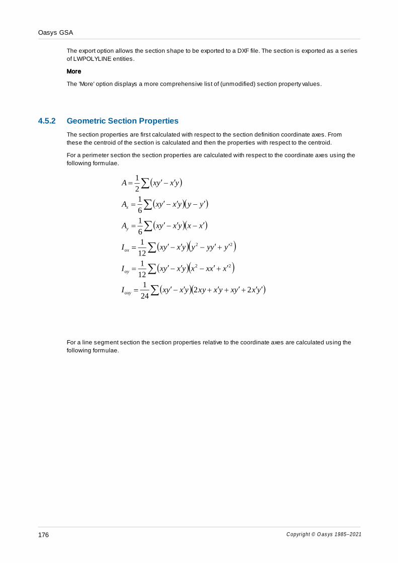
Oasys GSA

Copyright © O as ys 1985–2021176

The export option allows the section shape to be exported to a DXF file. The section is exported as a series

of LWPOLYLINE entities.

More

The 'More' option displays a more comprehensive list of (unmodified) section property values.

4.5.2 Geometric Section Properties

The section properties are first calculated with respect to the section definition coordinate axes. From

these the centroid of the section is calculated and then the properties with respect to the centroid.

For a perimeter section the section properties are calculated with respect to the coordinate axes using the

following formulae.

yxyxyxxyyxyxI

xxxxyxyxI

yyyyyxyxI

xxyxyxA

yyyxyxA

yxyxA

oxy

oy

ox

y

x

2224

1

12

1

12

1

6

1

6

1

2

1

22

22

For a line segment section the section properties relative to the coordinate axes are calculated using the

following formulae.

Oasys GSA

Copyright © O as ys 1985–2021 177

section closed singlea not isit when3

segments) line by the enclosedarea -(a

section closed singlea isit when4

412

41212

41212

2

1

2

1

2

1

3

2

2

22

22

2

222

22

2

222

ltt

l

a

J

yyxxyyxx

l

tlltI

xxyy

l

tllltI

yyxx

l

tllltI

yyltA

xxltA

ltA

oxy

oy

ox

y

x

Then, for both perimeter and line segment sections, the centroid of the section and the section properties

with respect to the centroid are calculated as follows.

ccoxyxy

coyyy

coxxx

xc

y

c

yxAII

xAII

yAII

A

Ay

A

Ax

2

2

where (x, y) are the coordinates of a point and (xc, y

c) are the coordinates of the previous point. The

summation is carried out for each point round the section if it is a perimeter section or for each segment if

it is a line segment section.

Note that the torsion constant, J of Perimeter sections, and shear factors, Ky and K

z of both perimeter and

line segment sections are not calculated and are set to zero.

Oasys GSA

Copyright © O as ys 1985–2021178

4.5.3 Reference Point

The reference point is the point where axial loads on a section are assumed to apply. By default this is the

centroid, meaning that an axial loads produces no bending. However in some situations it is better to

assume loads are applied with an eccentricity. One way to achieve this is to apply an offset to the section.

Definition

Basic Definition

The basic reference point definition allows the reference point on the section – the point at which axial

loads are assumed to apply to be moved from the centroid. This means that axial loads will introduce

bending into the section.

Offset

The basic reference point definition can then be further adjusted by applying an offset specified in terms of

a vector.

4.5.4 Point Voids

There are a number of situation where it is useful to introduce (small) voids into the section. If these are

small they can be considered as a having an area concentrated at a point.

4.5.5 Steel Design

In order to use a section in steel design, a number of steel specific parameters are required. These may

vary from one steel design code to another.

Definition

The section can be one of:

Cold formed

Hot rolled/finished

Welded

The other parameters related to various ratios and reduction factors associated with the section and used

in the design.

4.5.6 Section Modifiers

Normally the section properties are derived from the section geometry, but in some cases it is convenient

to modify some of the parameters.

Definition

Bending Axes

The section can be considered to bend about either the local (y & z) axes or the principal (u & v) axes. So

for an asymmetric section restrained by a slab it may be preferable to ignore the Iy z

term and just have

bending about the y & z axes. The subscripts 1 and 2 refer to y and z for local axes and u and v for principal

axes.

Analysis Reference Point

In defining a section the reference point may be adjusted, but this can be overridden for the analysis if

Oasys GSA

Copyright © O as ys 1985–2021 179

required.

Modifiers

Modifiers can be applied to any of the section properties. The modification can be

by – values modified by a factor

to – values modified to a value

Of significance is the special case of modifying the Ky & K

z values to 0. In this case beam elements are

considered as simple beams, rather than shear beams.

Stress Calculation

Applying modifiers to the section means that the stress calculation is not straightforward, so there are

options:

Don't calculate

Use unmodified properties

Use modified properties

Miscellaneous

The clear modifiers option returns the properties to standard properties derived from the section.

The simple beams option sets the shear factor to zero so that shear stiffness terms are not included in the

calculation.

The multiple sections option is mainly intended for situations where there are several physical sections

modelled as a single section property but where the properties are simply a multiple of the base

properties, for example a hanger which may comprise two identical bars which act together but don’t

interact with each other.

When defining the properties of a section for bending there are three second moments of area, Iy y

, Izz

, and

Iy z

, and three shear area factors, ky y

, kzz

, and ky z

, (often the first two are written as ky, k

z). The stiffness

matrix is always assembled in principal directions, or local directions ignoring the cross terms.When

the bending axes are local the modifiers apply to Iy y

, Izz

, ky y

and kzz

but when the bending axes are

principal these apply to Iuu

, Iv v

, kuu

and kv v

. So transformation of properties to appropriate axis

happens prior to applying the modifiers.

4.5.7 Section Design Pools

The section Pool is a way to group sections for use in design tasks to ensure that only suitable sections

are chosen. For example there may be one pool for beam sections and another for column sections.

For steel sections there is a steel section pool.

4.5.7.1 Steel Section Pools

The steel section pool allows sections to be grouped for design purposes. In steel design the process is

one of choosing a suitable section. If a member refers to a section in a particular pool, it can end up with

any of the sections included in that pool after the design task has been run.

Definition

Name

Oasys GSA

Copyright © O as ys 1985–2021180

Pools are given a name to make it easier to work with them.

Sections

The Sections are a list of section that are included in the pool. This attribute is set for the individual

sections.

4.6 Properties : General

4.6.1 Spring Matrices

A spring matrix allows the user to define the stiffness terms explicitly for a nodal spring. The matrix option

cannot be used with internal springs.

Definition

Name

The name is only used as a convenient way of identifying a spring matrix.

K(i,j)

The stiffness terms defining the upper triangle of the 6 x 6 stiffness matrix. The stiffness matrix must be

positive definite.

4.6.2 Spring Properties

Springs are a general type of element which can be used to model both simple springs and more

sophisticated types of behaviour. For springs connected to ground these are specified directly on a node

rather than as an element. The two simplest and most robust types of spring are the axial and rotational

springs which have only and axial or rotational stiffness respectively. The more general spring types can

violate equilibrium conditions so use be used with care. General non linear springs require material

curves to define the load deflection characteristics. A completely general linear spring connected to ground

uses a material matrix to define the stiffness, but this matrix must be positive definite. Springs follow the

same local axis definition as beam, but the exceptions are zero length springs and nodal springs. For zero

length springs the local axis is the constraint axis or the first node and for nodal springs it is the constraint

axis of the node.

Definition

Name

The name is only used as a convenient way of identifying a spring property.

Type

The type defines the spring is one of:

Axial – single translational degree of freedom

Torsional – single rotational degree of freedom

General – six degrees of freedom, linear or non-linear

Matrix – six degrees of freedom referring to a full 6 × 6 stiffness matrix

Tension only – single translational degree of freedom, only active in tension

Oasys GSA

Copyright © O as ys 1985–2021 181

Compression only – single translational degree of freedom, only active on compression

Connector – six degree of freedom coupling different parts

Lock-up – single translational degree of freedom, active when the spring reaches the lock up limit

Gap – single translational degree of freedom, active when the gap closes

Friction – three translational degrees of freedom, active when a gap closes, and generates a transverse

friction force

Material Curve and Stiffness

If it is linear spring or tension only or compression only springs, springs stiffness can be defined here

directly. Most spring types only require a single stiffness, but the general spring has six degree of freedom

and six spring stiffness need to be defined, if type is friction, three friction coefficients need to be defined. If

spring is nonlinear, the reference to the nonlinear spring curve (material curve) need to be defined here

and no stiffness definitions are needed, the relationships of force-displacement and moment-rotation of

the spring are defined by the referred nonlinear spring curve.

Material Matrix

For a spring defined by a matrix the stiffness characteristics are defined in a material matrix. This allows

for definition of the 6 × 6 stiffness matrix. This can only be referenced by nodal springs.

Lock-up

Lock up elements have no stiffness until the element locks up at the specified displacements. At this point

the element behaves as a spring with the defined stiffness. The lock up for tension and compression are

both defined as positive values.

Friction Coefficient

For a friction spring the transverse (shear) forces are limited to the by the friction coefficient × the normal

force.

Damping Ratio

The damping ratio is used during a dynamic analysis to calculate an estimate of the modal damping ratio.

Spring Properties

Spring elements define both conventional 'springs', but also other 1D elements which are not defined as

beams or bars. The characteristics of these are described below.

Tension only – uniaxial nonlinear spring element. This element have no stiffness under compressive

loading and creates penetration without any resistance.

Compression only – uniaxial nonlinear spring element. This element have no stiffness when subjected

tensile loading/displacements. Under tensile loading this element will create gap.

Connector – six degree of freedom linear spring element coupling two different parts. Program

automatically calculate the stiffness for this element using total stiffness at connecting nodes.

Lock-up – uniaxial nonlinear spring element, active when the spring displacement reaches the lock up

limit. Similar to the Connector element, program automatically calculate the stiffness for this element

using total stiffness at connecting nodes. This stiffness can be overridden by providing stiffness greater

than zero in the element property definition.

Gap – special type of compression only spring element with initial gap. Initial gap is calculated from the

element nodal positions. This element will have zero stiffness in the analysis while the displacements

are within the initial gap or element is subjected to tensile loading. Program automatically calculate the

stiffness for this element using total stiffness at connecting nodes. By default program assigns very high

stiffness. This stiffness can be overridden by providing stiffness greater than zero in the element

Oasys GSA

Copyright © O as ys 1985–2021182

property definition.

Friction – Gap element with two additional translational degrees of freedom. When axial stiffness is

active, this element will generate frictional resistance in transverse directions. This element will have

zero stiffness in the analysis while the axial displacements are within the initial gap or element is

subjected to tensile loading. Program automatically calculate the stiffness for this element using total

stiffness at connecting nodes. By default program assigns very high stiffness. This stiffness can be

overridden by providing stiffness greater than zero in the element property definition.

Tips for Convergence

Compression only and Gap elements

Usually Compression only elements subjected to tensile loading requires large number of iteration to

converge, if the stiffness is high.

To identify the elements, which creates the convergence issue, start the analysis using very low axial

stiffness and check for the convergence.

Verify the results and check if the elements are subjected to tensile loading or creates gap then leave

the stiffness of those elements as it is or reduce even further to increase the convergence.

If the results of the spring elements indicates large penetration beyond acceptable limit, then slowly

increase the axial stiffness for those elements until acceptable results obtained.

In case, the non-convergence is due to rigid body motion between the two bodies replace the elements

with friction elements.

Tension only elements

Similar to Compression only elements, use very low stiffness and check for the convergence by running

the analysis.

If the results creates large gap beyond acceptable limit, increase the axial stiffness of the elements.

Friction Element

This type of elements have the convergence issues either when they are subjected tensile loading or

when these elements are subjected lateral movement.

To avoid convergence issues due to tensile loading on the element follow similar steps defined for

Compression only elements.

To avoid non-convergence due to lateral movement, start providing transverse stiffness equal to 1/10th

stiffness in normal direction or less. Increase the stiffness gradually for the elements subjected to

compressive loadings.

Note about the property axis

If the property is used by 1D elements and the element length is not zero, the axis definition is the same as

beam elements, if the element length is zero, i.e. the two nodes of the element are coincide, the nodal

constraint axis of the first topology node of the element is used as the spring property axis.

If the property is used by a node, the nodal constraint axis of the node will be used as the spring property

axis.

Oasys GSA

Copyright © O as ys 1985–2021 183

4.6.3 Mass Properties

A node with a mass property concentrates mass and inertia at a single point. In a static analysis (linear or

non-linear), the only effect of a mass is to give a loading based on m × g when gravity loads are applied to

the structure. In a dynamic analysis both mass and inertia are used in the construction of the mass matrix

Definition

Name

The name is only used as a convenient way of identifying a mass property.

Mass, Inertia

This defines the mass and a (symmetric) inertia tensor. The terms that make up the inertia tensor are

described more fully in the theory section.

Care should be taken in defining the off-diagonal terms to ensure a positive definite matrix so that the

resulting principal inertias are positive.

Mass Modifiers

The mass modifiers allow the mass to be varied in the different directions. These can be specified as a

mass value or as proportion of the actual mass. This only applies to mass and in dynamic analysis.

Typically this is used to add mass in some directions when a structure is in contact with a fluid.

Note about the property axis

Mass property is only used to by nodes, the nodal constraint axis of the node will be used as the mass

property axis.

4.6.4 2D Element Properties

There are two different classes of 2D elements. The basic 2D element is the normal finite elements used

for structural applications included in-plane and/or out-of-plane behaviour. The load panel element is a

non-structural element used to apply load to beam elements.

Property Type

Name

The name is only used as a convenient way of identifying a 2D element property.

Color

Define the color of the elements that use this property when element coloring by property on graphic view

Element Type

The types of 2D properties available will depend on the structure type. For the 2D structure types (plane

stress, plane strain and axisymmetric) only the type corresponding to the structure type is available.

Likewise for non 2D structure types the plane strain and axisymmetric types are not available, although the

plane stress option is. The types are:

Plane Stress – in plane effects only (no out of plane stress)

Plane Strain – plane effects only (no out of plane strain), it is only active/used when the Structure Type is

"Plane strain"

Axisymmetric – in plane effects only (the out of plane direction is the hoop direction), it is only active/

used when the Structure Type is "Axisymmetric"

Fabric – in plane effects only (no thickness associated with fabrics)

Oasys GSA

Copyright © O as ys 1985–2021184

Flat Plate – out of plane effects only

Shell – in-plane and out-of-plane effects

Curved Shell – a general shell element which may be curved out of plane, Curved shell cannot be used

in GSA analysis at present, it can be used to build a GSA model and export to other software to do the

analysis

Load Panel – an element which is used only for the distribution of loads. It has no stiffness, so does not

need material or thickness parameters. For more information see 2D Loads on Load Panels

Axis

Users may assign an axis to be used to define the orientation of 2D elements. If the axis is set to

“Topological” the orientation of the element will be determined by the first two nodes of the elements and

the orientation angle. If an axis (global or user defined) is assigned here then that axis will be projected on

to the element plane to determine its orientation.

Material

The material definition breaks into three parts. The first part is the material type. it is one of:

Steel

Concrete - if it is concrete, then concrete slab property can be set for RC slab design

FRP

Aluminium

Timber

Glass

Fabric

<undefined> – not associated with any grade

The second part is material grade index that this 2D property refers to. The material grade with actual

material design properties is defined in material grade table. If material type is assigned and material

grade is defined, analysis can use this material grade as the analysis material when "from Grade" is used

in "Analysis" column.

The third part is the Analysis material index that this 2D property refers to. The analysis material property

can be defined in Analysis Material table. If analysis material is set to "from Grade", then the material

properties defined by the material grade will be used in the analysis.

Concrete Slab Property

The Concrete slab property is used in concrete slab reinforcement.area calculations

Profile/Thickness

In the simplest case this defines the thickness of the 2D elements. No thickness definition is needed if

material type is fabric, and a unit thickness is assumed for plane strain and axisymmetric structure types.

For a shell element there are four options for defining the property

Solid – just the thickness

Decking slab – a composite concrete slab based on steel decking and is defined on the next page of

the dialog

Hollow – a hollow core concrete slab and is defined on the next page of the dialog

Layered composite – a layered shell that needs to be exported to LS DYNA for analysis and is defined

on the next page of the dialog

Oasys GSA

Copyright © O as ys 1985–2021 185

Reference Surface

The reference surface is a virtual plane that the in-plane forces are assumed to act in a 2D element. If the

reference surface is the top or bottom surface, in-plane loads will also generate a bending moment. The

reference surface setting is only used by shell elements. There are two parameters to define the reference

surface, "Surface" defines top, middle or bottom of the 2D elements as the reference surface, "Offset"

defines an extra offset from the selected top, middle or bottom surface. If offset is zero, then the selected

top, middle or bottom surface will be the final reference surface.

Property Modifiers

There are four factors, three for stiffness modifications and one for volume modification. The three

stiffness modifiers are for in-plane stiffness, bending stiffness and through thickness shear stiffness, the

volume modifier is for modifying the volume that is used to calculate the mass and self-weight of the

elements. By using the property modifiers, the 2D element properties can be different from those

calculated by the given thickness which may be useful to deal with situations such as cracked concrete

slabs (reduced bending stiffness due to cracking) or hollow slabs where the stiffness of the slab in

bending and in-plane will be less than that for a solid slab.

The modifiers can be an absolute values or a percentage of the calculated values from the given

thickness. For Plane Strain, Axisymmetric or Fabric elements, these modifications are not relevant so they

are not enabled.

The stresses in 2D elements are calculated using unmodified thickness.

Additional Mass

Normally the gravity loads on a 2D element are calculated from the density and thickness or modified

volume. Fabric elements have no thickness but it may still be desirable to assign a mass, or where a slab

is modelled which has a non-structural screed that adds mass. Both of these situations are provided for

by the additional mass per unit area. This mass is in addition to the mass implied by the thickness and

density.

Support pattern & reference edge

The support pattern and reference edge are applicable only to load panel elements. The support pattern

defines the number of edges to which the load is transferred and the reference edge sets the selection of

the free/loaded edges. For more information see 2D Loads on Load Panels

4.6.4.1 Decking Slab

A composite slab consists of profiled decking and concrete. The properties are adjusted to account for the

reduced effective thickness of slab when decking is introduced. The modifiers for the 2D properties are

calculated to allow for the modified geometry and the combined steel and concrete properties.

Definition

Decking option

The decking can either be user defined, where the thickness and dimensions defining the profile must be

specified, or selected from a catalogue of standard decking profiles.

The angle of the decking determines how the slab stiffness are determined. At 0° the properties calculated

are for the slab in the slab span direction and the concrete in the trough is assumed to contribute to the

stiffness, while at 90° the troughs are ignored.

Profile

The profile description is either a reference to the selected standard profile e.g. CAT RLSD Ribdeck AL

(0.9) of a string of the form 'STD D 50 0.9 300 120 140 10 40' where the numeric values related to the

depth, thickness and profile dimensions.

Oasys GSA

Copyright © O as ys 1985–2021186

Syntax

The description of hollow slab profile is

thick(unit) D angle CAT profile (t)

thick(unit) D angle STD d t b1 b2 b3 b4 b5

where

thick – the overall thickness

unit – the units defining the profile

D – decking slab

angle – angle of decking relative to x direction

CAT or STD – catalogue or standard decking

profile – the catalogue profile

t – the decking thickness

d – the depth of the decking profile

b1, ... b5 – the dimensions which define the shape of the profile

4.6.4.2 Hollow Slab

This dialog is accessed from the 2D element property wizard and is to simplify the specification of slabs

that may contain voids.

Definition

Slab thickness

The overall thickness of the slab

Thickness of top/bottom zone

The top and bottom zones are assumed to have the same thickness and the material is assumed to be

concentrated in these zones.

Proportion of material in void zone

Typically the central part of the slab will have some material so a percentage can be specified here. A zero

percentage will give the same results as a solid slab

Syntax

The description of hollow slab profile is

Oasys GSA

Copyright © O as ys 1985–2021 187

thick(unit) H top void%

where

thick – the overall thickness

unit – the units defining the profile

H – hollow slab

top – the thickness of the top (and bottom) zones

void – the percentage of the core that is void

Effective depth

These are the effective depths for bending and in-plane stiffness calculations, based on an overall

thickness, D, top and bottom zones of thickness, t, and proportion of material in void, v

For in-plane effects the effective thickness is:

tvvDD 21ˆ

For bending effects the effective thickness that gives an equivalent second moment of area is:

3 322 81261~

tDttDvvDD

4.6.4.3 Layered Slab (LS-DYNA)

When creating a model for analysis in LS-DYNA it is useful to be able to define a composite shell. This is

defined in terms of layers of different materials.

Definition

The composite shell is defined from the bottom up in layers. Each layer is defined by an analysis material,

a thickness and an optional angle for orthotropic materials. The total thickness of the shell is determined

from the sum of the layer thicknesses.

Syntax

The description of hollow slab profile is

(unit) L (mat thick angle) ...

where

unit – the units defining the profile

L – layered slab

thick – the layer thickness

angle – the angle of the layer for an orthotropic material

The material, thickness and angle are repeated for each layer.

Oasys GSA

Copyright © O as ys 1985–2021188

4.6.5 3D Element Properties

This defines the type and properties ascribed to each 3D Element Property Number. Properties can be

edited using the “3D Property Definition”.

Definition

Name

The name is only used as a convenient way of identifying a 3D element property.

Element Type

Whether it is a solid or infinite element (infinite elements are used to model the surrounding areas in soil

modelling.

Axis

Users may assign an axis to be used to define the orientation of32D elements. If the axis is set to local the

orientation of the element will be determined from the topology (point 1 and point 2 will be taken to define

the x axis). If another axis (global or user defined) is assigned here then that axis will be projected on to the

element to determine its orientation.

Material Analysis

The material definition breaks into three parts. The first part is the material type. This is one of:

Steel – gives option to assign to various steel design properties to the section

Concrete – gives option to assign reinforcement information to the section

FRP – allows a set of properties for various grades

Glass – allows a set of properties for various grades

Aluminium – allows a set of properties for various grades

Timber – allows a set of properties for various grades

<undefined> – not associated with any grade

The grade defines the actual material design properties, which depend on the material type. New grades

can be initialized from the standard grades for the current design code. The final material attribute is the

analysis material. This defines a set of elastic properties. If a grade is specified it is possible to refer to

this for the analysis material (from Grade). In this case the required analysis properties are inferred from

the grade.

4.6.6 Link Properties

A link is unlike other elements in that it does not have stiffness, instead it created a constraint condition

between the two ends of the element. The behaviour of a link element is like a rigid constraint with just two

nodes. Degrees of freedom that are not linked have no connection at all.

Definition

Name

The name is only used as a convenient way of identifying a link property.

Type of Linkage

The type should be set to “All” to make a link completely rigid. There are however many cases in which it is

Oasys GSA

Copyright © O as ys 1985–2021 189

useful to make a link rigid in a plane (for example in modelling floor slabs). The following planes can be

specified:

Linked degrees of freedom

All x y z xx yy zz

All (pin) x y z

xy plane x y zz

yz plane y z xx

zx plane x z yy

xy plane (pin) x y

yz plane (pin) y z

zx plane (pin) x z

The “pin” linkage types do not include the rotational degrees of freedom at the constrained node in the

rigid body displacements. Note that the “pin” condition applies only to the constrained node - the rotational

degrees of freedom at the primary are always retained.

The above options can be used in both the Gss and GsRelax solvers. A further set of Links are available

for use only in the GsRelax solver; see GsRelax modelling implications for more details:

Tension – the link supports tension only

Compression – the link supports compression only

Bar – the link works in both tension and compression

There is also a general Link type, though it is not available for use in all solvers:

Custom – the link works like a joint linking the nodes in the specified coupled directions

Constraints

More details are given in Link elements and rigid constraints. Care should be taken to avoid conflicting

constraints.

Note about the property axis

The nodal constraint axis of the first topology (primary) node of the element is used as the link property

axis.

4.6.7 Cable Properties

Cable properties are most useful for GsRelax non-linear analysis, where all the cable elements with the

same property form a cable that is allowed to slide. Cable elements can also be used in the Gss solver

where they are treated in the same way as ties.

Definition

Name

The name is only used as a convenient way of identifying a cable property.

Colour

See Specifying Colour of entities for more details

Oasys GSA

Copyright © O as ys 1985–2021190

Type

Allows the cable property to be set to Normal or Sliding. Note that Sliding properties are only used in

nonlinear analysis and are treated as Normal in other analyses. See Element Types for more details.

Stiffness

The stiffness of cables is specified directly rather than through the area and Young’s modulus, which are

less clearly defined for cables. This stiffness is equivalent to AE (area × elastic modulus).

Mass

For gravity loading and dynamic analysis it is necessary to be able to associate a mass with cables. This

is specified as a mass per unit length.

Temperature Coefficient

To allow for thermal effects in cables the temperature coefficient of expansion is required. Used in the

same way as the temperature coefficient of expansion for beam and bar elements.

Damping Ratio

The damping ratio is used during a dynamic analysis to calculate an estimate of the modal damping ratio.

4.6.8 Damper Properties

Damper elements are only considered in the explicit non-linear solver. Including damper elements in a

modal dynamic analysis gives rise to a completely different problem with complex results. This is not

considered in GSA. Dampers follow the same local axis definition as beam, but the exceptions are zero

length dampers and nodal dampers. For zero length dampers the local axis is the constraint axis or the

first node and for nodal dampers it is the constraint axis of the node

Definition

Name

The name is only used as a convenient way of identifying a damper property.

Type

The type defines the damper as one of:

Axial

Torsional

General

Dashpot constant

The relevant dashpot constant must be supplied. x for an axial damper, xx for a torsional damper and all

six for a general damper.

Note about the property axis

If the property is used by 1D damper elements and the element length is not zero, the axis definition is the

same as beam elements, if the element length is zero, i.e. the two nodes of the element are coincide, the

nodal constraint axis of the first topology node of the element is used as the damper property axis.

If the property is used to by a node, the nodal constraint axis of the node will be used as the damper

property axis.

Oasys GSA

Copyright © O as ys 1985–2021 191

4.6.9 Spacer Properties

This defines the properties of a spacer chain made up of a series of spacer elements. Each individual

spacer chain has its own unique spacer property number. The properties determine how the nodes along

the spacer chain are controlled during the form-finding process.

Spacer elements are only used in form-finding analysis. They are ignore in all other solutions.

Definition

Name

The name is only used as a convenient way of identifying a spacer property.

Spacer Axis

The axis number, which is only used when the spacer leg length type is “Projected Ratio”. (Global or user

defined axis, local axis is not available.)

Type

The types are

Geodesic – Geodesic spacers will reposition the nodes in 2 directions within the tangent plane. The

tangent plane is defined by the normal vector of the node on a 2D fabric surface.

Free – Free spacers will reposition the node in only one direction; the tangent direction is defined by the

two legs of the spacer connected to the node.

Bar – Bar spacers will reposition the nodes in all three directions. Bar spacers can be imagined as Tie

elements except the spacer element length will be adjusted during form-finding analysis to meet the

nodal spacing requirement.

Spacer Leg Length Type

The spacer leg length types can be defined as

Proportional – Final spacer leg length will be proportional to the original leg length.

Ratio – Final leg length of the spacer elements will form a geometric series using the ratio defined in

the Spacer leg ratio column.

XY plane projected ratio – Final projected leg length of the spacer on the xy plane of the Spacer Axis will

form a geometric series with the ratio defined by the spacer leg ratio.

X axis projected ratio – Final projected leg length of the spacer on the x Spacer Axis will form a

geometric series with the ratio defined by the spacer leg ratio.

Spacer stiffness

If the spacer is imagined as a Tie element, the spacer stiffness is equal to EA (where E is the Young’s

modulus and A is section area). If zero is specified, a default value will be used in form-finding analysis.

Spacer leg ratio

This is only used when spacer leg length type is Ratio or Projected Ratio. For example,

where r is the Spacer leg ratio ( i = 1, 2, 3…).

Oasys GSA

Copyright © O as ys 1985–2021192

4.6.10 External Matrix

In some instances a stiffness matrix may have been determined outside GSA. This can then be included

directly onto the structure matrices during the analysis

Definition

Node and Direction

A node and direction identifies a degree of freedom (row or column in the structure matrices), so this

identifies the stiffness and mass to associate with a particular degree of freedom.

Stiffness and Mass

The is the stiffness and mass associated with the defined degree of freedom. If only static analysis is

required then the mass terms can be ignored.

Note

The terms defined for stiffness and mass should not lead to non-positive definite matrices.

4.6.11 Environmental Impact Wizard

As discussed in the Step-by-Step guide to Environmental Impact, environmental impact parameters for a

material type may be specified in the Environmental Impact Wizard. This wizard can be accessed either

from the Environmental Impact Specification dialog to specify global parameters, or from the material

grades to specify values for a particular user material.

Definition

Enter Specified values for each environmental parameter.

When the Environmental Impact Wizard is accessed from the Material Wizard for a concrete material type,

separate tabs are offered to enable environmental parameters to be specified for both concrete and rebar.

Import

The Import button will launch a connection to the Veracity carbon database, allowing the environmental

parameters to be imported for a particular material. Use the "Select" button in the material details page to

import the values for that material. Note that this feature is only available for Arup staff and requires

connection to the Arup network.

4.7 Properties : Form-finding

Form-finding is an analysis which seeks to determine the shape of a lightweight structure under a set of

boundary constraints. During a form-finding analysis with the solver will search for form finding properties

with the property number assigned to the element. If none are found, the normal beam section or 2D

element properties will be used instead.

There are two types of form finding properties: force density 1D and force density 2D for 1D and 2D

elements respectively and soap film 1D and soap film 2D for 1D and 2D elements respectively.

Oasys GSA

Copyright © O as ys 1985–2021 193

4.7.1 Force Density 1D

Definition

Name

The name is only used as a convenient way of identifying a form-finding property.

Force Density

The final axial force (f) and the final length ( l) of the element that uses this property will satisfy the following

equation

f = l × FD

where FD is the force density.

4.7.2 Soap Film 1D

Definition

Name

The name is only used as a convenient way of identifying a form-finding property.

Axis

If a local axis is used, the force in the Bar, Tie and Strut elements that use this property will be equal to that

defined in Force column.

If a user defined axis number is input, the projected element force along the X axis direction of this axis set

will be constant and equal to the force defined. This can be used to model prestressing using hanging

weights supported by inclined ties. Here the force is constant in a projected direction, and the element

force varies as the element local axis moves.

Force

The constant force (in the x-axis direction of the axis defined by column) of Bar, Tie and Strut elements that

use this property in soap-film form-finding analysis. The Young’s modulus of these elements will be set to

zero in the form-finding analysis in order to achieve constant axial force.

4.7.3 Force Density 2D

Definition

Name

The name is only used as a convenient way of identifying a form-finding property.

Force density

The final axial stress (σ) and the final area (A) of the 2D element that uses this property will satisfy the

following equation

σ = A × FD

where FD is the force density.

Oasys GSA

Copyright © O as ys 1985–2021194

4.7.4 Soap Film 2D

Definition

Name

The name is only used as a convenient way of identifying a form-finding property.

Stress in x

The constant stress in x direction of the 2D elements that use this property in soap-film form-finding

analysis. The Young’s modulus of these elements will be set to zero in the form-finding analysis in order

to achieve constant in-plane force.

Stress in y

The constant stress in y direction of the 2D elements that use this property in soap-film form-finding

analysis. The Young’s modulus of these elements will be set to zero in the form-finding analysis in order

to achieve constant in-plane force.

4.8 Properties : Concrete Slab

4.8.1 Reinforcement

There are two aspects to the reinforcement - the reinforcement material and the reinforcement layout.

Definition

Name

The name is used only as a label for the slab design property.

Grades

The grade of reinforcement. This refers to a material entry in the reinforcement grades module.

Bar Direction

The bars are aligned in two directions A and B, relative to the element x axis. Normally these will be

orthogonal, but the angle between the two directions can be adjusted to suit.

Axis to Surface Distance

These distances locate the position of the bars from the top and bottom of the slab. As no bar size is

specified these are distances to the centre of the reinforcement.

Minimum Areas of Reinforcement

The minimum area of reinforcement to be provided in the top or bottom face. A minimum area of

compression reinforcement for each face in each direction can also be specified – either according to

code or a user specified value.

4.8.2 Calculation

A number of parameters which control the calculation can be adjusted.

Definition

Solution Method

The information below presents a practical overview of the two methods. More detail on the RC Slab

analysis procedure is available in the RC Slab theory section.

Oasys GSA

Copyright © O as ys 1985–2021 195

Two solution methods are available; a ‘fast’ method and a ‘rigorous’ method.

Fas t m e thod

The ‘fast’ method selects a faster non-iterative solution method wherever the loading is considered to be

either predominately in-plane or predominately out-of-plane. For each element position where this be a

reasonable assumption, this method will yield faster analysis times. When the loading is not considered

to be predominately in-plane or out-of-plane, the method will fall-back to the slower iterative technique. The

decision is made independently for each element position, on a position by position basis.

The user may also restrict use of the non-iterative technique to any case where the total reinforcement

area is below a certain percentage of the total cross-sectional area. Should the total reinforcement

calculated by the ‘fast’ method be above this threshold, the iterative technique is used.

Any use of the non-iterative technique will typically lead to slightly more conservative results. Note that by

design, its use is limited to those cases that represent the most favourable trade-offs between analysis

time and approximation accuracy.

More detail on the non-iterative technique is available in the RC Slab theory.

R igo r ous m e thod

The ‘rigorous’ method selects the iterative solution technique in all cases. This approach will always yield

the most accurate result available, regardless of any opportunity for a performance/approximation trade-off.

A common work-flow scenario may be one that adopts the ‘fast’ method during the early stages of design,

before later switching exclusively to the ‘rigorous’ approach.

Note that the ‘rigorous’ method is equivalent to the (sole) solution technique prior to GSA version 8.7.

Design Thickness

By default the thickness used is the thickness defined in 2D element property for the analysis. If this

proves difficult to reinforce the slab, the thickness can be overridden as a trial thickness to see if a solution

can be found without the need to change 2D element property thickness and redo the analysis. Once a

suitable thickness is worked out, it can be used as the slab thickness in 2D element property, in this case,

a re-analysis should be carried out after modifying the analysis (2D element property) thickness.

Eccentricity

The minimum eccentricity to be used in the design, it is normally taken from the relevant design code, but it

can be overridden and defined explicitly.

Additional eccentricity is used to consider the second order effect (increase) on the applied moment due to

the slenderness of the slab. It is an user defined parameter to incorporate the second order moment if the

slab is slender.

Two-way spanning modifier, normally 0 should be used for for one-way spanning slab and 50 to 100% for

two-way spanning slab, see details for how to work out the two-way spanning modifier on RC slab theory

manual.

Stress/strain limits

The value of x/dmax will normally be that specified in the design code but can be overridden if required.

The design strain limit (εsu

) limits the allowable strain in the section. This may be a function of both the

concrete and reinforcement material. The crack rotation limit is specified in some of the codes, but is

normally 90°.

Oasys GSA

Copyright © O as ys 1985–2021196

4.8.3 Strength Reduction Factors

Design codes have one of two methods for introducing a factor of safety: either applying a factor to the

material properties or a reduction to the calculated strength

Strength Reduction Factors

For codes (ACI and Australian codes) which implement a strength reduction factors there is a φ factor for

in-plane compression and a φ factor for in-plane tension & bending. Depending on the forces/moment on

the section the φ value will vary between the limits for compression and tension. The actual reduction

value used will depend on the actual strain plane across the slab.

Note

Typical compression and axial tension & bending reduction values are 0.65 and 0.9 respectively.

4.9 Nodes

Nodes are used to locate points in space. Elements are located in space by referring to nodes in their

topology lists. Loads may be applied to nodes. The Node Definition dialog may be used to define node all

attributes of nodes.

Basic Definition

Node Coordinates

Coordinates are defined with respect to the current grid plane, which defaults to the global grid (i.e. global

axis directions). Coordinates are stored in global axes, regardless of the current grid plane. For structures

specified as “Plane”, only X and Z are required; for “Grid” only X and Y.

The ‘Sculpt | Node Operations | Convert Nodes to Standard’ and ‘... | Convert Nodes to Grid’ commands

may be used to convert the node status, maintaining their position in global space.

Constraint Axis

Constraint axes are used for specifying restraints, joints, constraint equations and applied displacements

and results at nodes, in non-global directions.

The constraint axes default is global, but user-defined axes can be specified by typing the axis record

number as specified in the Axes Table.

Restraint Direction

Any combination of translational and rotational restraint can be specified for each node. Restraints will be

in global or user-specified axis directions, depending on the constraint axis.

Nodal Stiffness

Nodes can be assigned a stiffness. The stiffness is specified as a property. These properties act in the

constraint axis system of the node.

Nodal Damping

Nodes can be assigned a damping. The damping is specified as a property. These properties act in the

constraint axis system of the node.

Nodal Mass

Nodes can be assigned a mass and inertia. This is specified as a property. These properties act in the

constraint axis system of the node.

The node definition dialog is used to define or modify a node. This dialog can be activated from Nodes

Oasys GSA

Copyright © O as ys 1985–2021 197

table view using the wizard button or from a Graphic View by selecting a node and then “Edit Node” from

the right-click menu.

The units are displayed in the top right corner of the dialog.

Name

The name is used only as a label for the node. (default: blank)

Coordinates

The location of the node in the global axis system in the current units. Plane structures have only x and z

coordinates; grid structures have only x and y coordinates. In these cases the coordinate that is not

relevant is greyed.

Constraints

The constraints define if the node is fixed in particular directions. This is done by selecting an axis,

normally global and selecting the directions to restrain. Directions that do not apply for that structure type

are disabled. The restraint types Free, Pin and Encastre options provide a shortcut to setting the flags for

the individual degrees of freedom. The symmetry options in the xy plane, yz plane and zx plane provide

shortcuts for applying the boundary conditions corresponding to symmetry in these planes. The symmetry

options do not unset other restraint conditions.

See also :

Axis Sets

Definition Axes

Generalised Restraints

Conflicting constraints

4.10 Members

Members are the entities that are the building block for GSA models. Members can be 1D (linear), 2D

(area), or 3D (solid) entities. Members are defined by topology, so are located with reference to nodes.

Local axis orientations are defined using orientation angles and nodes. 1D members have end fixities

defined by releases and release stiffnesses.

Members should not be confused with elements, which are used for analysis. Elements can be created

from Members and is the recommended workflow.

Each member is assigned a property number and a group number. The property number is used to

assign the section or 2D property and through that the material information.

Members, as opposed to elements, are suitable for coordination and round-tripping with BIM software

programs. In BIM oriented workflows, the design layer containing members interacts with both BIM models

as well as the GSA analysis model.

This wizard can be activated from the Members table view using the wizard button or from a Graphic View

by selecting an member and then 'Edit Member' from the right-click menu. The basic definition includes

geometry and topology. This leads to separate pages for end conditions and effective lengths for steel and

concrete members design_properties. Finally offsets can be assigned.

Member forces are required for the design calculations. Since analysis results are calculated for

elements, not members, it is necessary for there to be a relationship between elements and members.

This relationship is formed automatically by GSA when generating elements for analysis from members.

Oasys GSA

Copyright © O as ys 1985–2021198

4.10.1 Definition

The member wizard can be activated from the Members table view using the wizard button or from a

Graphic View by selecting a member and then “Edit Member” from the right-click menu.

Definition

Name

An optional identifier for the member.

Type

Members are assigned a type. This embraces both one dimensional (1D) and two dimensional (2D)

members:

1D – Generic 1D, Beam, Column, 1D void cutter

2D – Generic 2D, Slab, Wall, 2D void cutter

The ‘void cutter’ member types can be used to create voids in intersecting or coplanar 2D members.

Property

These are the properties that define the type, shape and dimensions of the section or 2D properties. Either

choose a property from the list or type in a property number.

Group

This defines the group to which the member belongs. No further information is required to define a group.

Topology

The geometry of the member is defined through the topology. The syntax for member topology depends on

the member type:

1D members

an ordered list of nodeso a straight beam member between nodes 21 and 22 would have topology ’21 22’node number preceded by A for arc through nodeo an arc member between node 21 and 22, passing through node 23 would have topology ’21 A23 22’.

Fo r 1D a rc m em b ers from ea rlie r ve rsions o f GSA, de fined with a rad ius, the m em b er is transfo rm ed to one

with a th ird node de fin ing the a rc.

2D members

an ordered list of nodeso a simple slab defined by nodes 41, 42, 43 and 44 the topology is ’41 42 43 44’node number preceded by A for an arc through a nodeo the slab above with an arc through node 43, the topology is ’41 42 A43 44’V(node list) for a voido The slab above, with a void defined by nodes 45 to 48 the topology is '41 42 43 44 V(45 46 47 48)’P(node list) for points to be includedo To include fixed points in the mesh at node 50 and 55: ’41 42 43 44 P(50 55)’L(node list) for lines to be includedo To include a fixed polyline segment in the mesh between nodes 71, 72 and 73: ’41 42 43 44 L(71 72

73)’A(node list) for additional solid areas to be includedo To include an additional area (must be coplanar with the first): ’41 42 43 44 A(45 46 47 48)’

3D members

3D members are defined by a closed boundary mesh of triangles and/or triangle strips.

To create a 3D cube, where the base is a clockwise loop of nodes 1-4 and the top is a clockwise loop of

Oasys GSA

Copyright © O as ys 1985–2021 199

nodes 5-8 the topology is: ‘1 2 4 3; 5 6 8 7; 1 5 2 6 3 7 4 8 1 5’ (where the first triangle strip is the base,second the top and third the sides of the cube).

Orientation node and angle

The orientation of 1D members is controlled by an orientation angle and an orientation node. The

orientation node along with the end nodes defines the xy plane of the member.

For 1D members the orientation angle defines the rotation of the members about its axis from the default

orientation, so for example setting an I beam to work as an H beam. For 2D members the orientation

angle relates to a rotation about an out-of-plane axis from the local x direction defined by the properties.

The angle is measured in degrees.

Releases

The releases are used when mapping members to elements to provide appropriate element releases in

the analysis model.

Member end conditions and effective length...

This specifies the member conditions that apply at the ends of a 1D member. See the design properties

for more information.

Meshing

When creating elements from members (Model | Coordination Tools | Create Elements from Members)

GSA needs to know how to create element meshes. Typically the meshing will take account of other

members, but the members can be meshed independently or excluded altogether. The resulting mesh

will be influenced by the target mesh size for the resulting elements.

Tapered 1D member

An 1D member can be tapered from one end to the next if the member refers to a section that includes two

different size sections. See section definition on how to define section for tapered members.

4.10.2 Design Properties

These options are available for 1D members when the section material is steel. They define the properties

relating to design from the interaction of the member with the rest of the structure.

End restraints

End restraints define how the end connections of the member affect the effective length calculations.

These are applicable only to 1D members.

The description specifies the degrees of freedom that are restrained by the connection. Individual

rotational and translational terms can be restrained but the most common connections can be selected

directly. These are:

Pinned – top flange laterally restrained. Nominal torsional restraint. No restraint against rotation

Fixed – encastre

Free – no restraint

Full rotational – top flange laterally restrained. Nominal torsional restraint. Both flanges fully restrained

against rotation on plan

Partial rotational – top flange laterally restrained. Nominal torsional restraint. Both flanges partially

restrained against rotation on plan

Top flange lateral

Custom – determine the detail of the particular connection. Note that inconsistent combinations of

Oasys GSA

Copyright © O as ys 1985–2021200

restraints will be automatically updated

Effective Length

The options to determine effective lengths of 1D members are

Automatic – uses only the member end conditions and the geometry of the structure to define the

effective lengths in accordance with the design specification.

Define the internal restraint on the member – both point restraints (where another member is

connected) and span restraints (such as a slab on the top flange of a beam)

Specify the effective lengths directly

The 'All Spans' drop down provides a shortcut to set the restraint condition for all spans along the member.

The Advanced option allows restraints along individual spans to be specified.

The 'All Points' drop down provides a shortcut to set the restraint condition for all points along the member.

The Advanced option allows restraints along at points to be specified.

Destabilizing Load

This is the height at which the load is assumed to act which can have a destabilizing effect on the

member. By default this is relative to the shear centre, but can be relative to the top or bottom flanges.

Note

GSA automatically detects and registers points and spans based on the nodes and elements along the

member. When a Design Task is executed, GSA automatically generates the member internal restraints to

assign point and span restraints. If the 'All Spans' member restraint is set to advanced the spans restraint

conditions can be specified for individual spans. Likewise if the 'All Points' member restraint is set to

advanced the spans restraint conditions can be specified for individual positions along the member.

4.10.2.1 Member Restraint Conditions

Member Restraints allow a member to have its restraint defined at one location along its length. They

allow specification of restraint in two different ways: by use of a relatively user-friendly dialog box, or by an

abbreviated “mnemonic” text syntax.

Some of the attributes of a restraint being set in combination with others imply other restraints are also

set, even though the user has not specifically stated that the additional restraint axes are restrained. For

example, if both the top and bottom flanges of a member are laterally restrained, then it is clear that St.

Venant torsion is also achieved at this location as well. Similarly, if the top flange is restrained and full St.

Venant torsion restraint is also manually restrained, then the bottom flange is assumed also to have been

restrained. With regard to warping restraint, a more conservative approach is taken, and minor axis

bending restraint is not assumed to imply warping restraint of the flanges, nor is warping restraint

assumed to imply any overall bending restraint of the section. This is because (using an example)

although an RHS section may have its “major-axis” flanges welded to a stiff end plate (thus achieving

flange warping restraint), the webs could be free. This would allow significant minor axis bending flexibility

in comparison to a section that had been welded all round. Inconsistent end restraints are automatically

updated to ensure that sensible conditions are set.

A table summarising the available restraint axes is shown below:

Restraint Axis Possible values Description Comments

Top Flange Warping None

Partial

Oasys GSA

Copyright © O as ys 1985–2021 201

Full

Bottom Flange Warping None

Partial

Full

Torsion None

Friction/ Bearing on

support only

Partial

Full

St. Venant torsion restraintFull restraint is assumed

if both flanges are laterally

restrained.

Major Axis Rotation None

Partial

Full

Major (stiff) axis restraint

Minor Axis Rotation None

Partial

Full

Minor (weak) axis restraint

Top Flange Lateral None

Full

Full restraint is assumed

if the bottom flange is

laterally restrained and the

full torsion restraint is also

applied.

Bottom Flange Lateral None

Full

Full restraint is assumed

if the top flange is laterally

restrained and the full

torsion restraint is also

applied.

Major Axis Shear None

Full

Restraint of shear centre

against movement in the

direction associated with

major axis bending.

Minor Axis Shear None

Full

Restraint of shear centre

against movement in the

direction associated with

minor axis bending.

Full restraint is assumed

if both flanges are laterally

restrained.

4.10.2.2 Restraints at Points

You can define restraint conditions along the length of 1D Members, which can be either be at points or

along spans. Points are marked by nodes that lie on the member whereas a span is made up of at least

one constituent element along the member.

You can specify the restraint conditions for individual points if you set the 'All Points' member restraint

option to 'Advanced'.

Internal Points

Add, Delete, Modify, +, -

Oasys GSA

Copyright © O as ys 1985–2021202

Buttons to add, delete and modify point restraints. Add and Modify invoke the Restraint Definition dialog for

points, which then allows translational and rotational modes to be set. The 'Point' field in the Restraint

Definition dialog relates the index of the node for which the restraint is being modified. For example if the

internal nodes along the member are 3, 6, and 5, point 1 edits the restraint at node 3, point 2 edits the

restraint at node 6 and so on.

The +/- allow the point numbers to be incremented or decremented.

4.10.2.3 Restraints at Spans

You can define restraint conditions along the length of 1D Members, which can be either be at points or

along spans. Points are marked by nodes that lie on the member whereas a span is made up of at least

one constituent element along the member.

You can specify the restraint conditions for individual spans if you set the 'All Spans' member restraint

option to 'Advanced'.

Spans

Add, Delete, Modify, +, -

Buttons to add, delete, and modify span restraints. Add and Modify invoke the Restraint Definition dialog for

spans. As with point restraints, the 'Span' field relates to the index of the span along the member.

The +/- allow the point numbers to be incremented or decremented.

4.10.3 Miscellaneous

Where a member may have offsets these are defined here.

Members also support ‘Automatic axial offset’. This option, when checked, applies offsets automatically

based on the geometry of the member, and that of the member(s) that connect to it. Automatic offsets are

only applied when the member has an I, rectangular, or a circular section profile. The value of the offset is

set to half the section depth (or width, as applicable) of the connecting member section when the

connecting angle is 90o (allowing for a tolerance).

Definition

Time line & exposure

The member can be assigned timing information. This includes the time the member is created and

removed (a removal time of zero means it is not removed). For concrete members there is also the option

to specify the start of drying ad the age at which it is loaded. The exposed faces can also be specified.

Fire resistance

The required fire resistance can be specified as 30 , 60, 90 , 120, 180 or 240 minutes.

Offsets for transfer to elements

Allows offsets to be specified at the nodes. Offsets are in local axis directions. Two kinds of offset are

defined

axial offsets – which are in the axial direction towards the centre of the member, and

transverse offsets – which apply to the member as a whole.

Automatic axial offsets will apply an offset to the end of a beam based on the shape and dimensions of the

column to which it is attached.

Dummy member

Oasys GSA

Copyright © O as ys 1985–2021 203

This is a member which is defined, but does not participate in the design process.

4.10.4 1D Member Axes

Member axes for linear members are defined in a similar manner to the axes of beam elements by two

nodes locating the ends of the member. The x axis of the element is along the axis of the element (taking

account of any offsets) from the first topology item to the second. For curved members the basic axis

system of linear members holds.

The definition of the member y and z axes then depends on the member's orientation, verticality,

orientation node and orientation angle. The member is considered vertical in GSA if the element is within

the “vertical element tolerance”.

Non-vertical members

If an orientation node is not specified, the member z axis of a non-vertical member defaults to lying in the

vertical plane through the member and is directed in the positive sense of the global Z direction. The

member y axis is orthogonal to the member z and x axes. The member y and z axes may be rotated out of

this default position by the orientation angle.

Vertical members

If an orientation node is not specified, the member y axis of a vertical member defaults to being parallel to

and is directed in the positive sense of the global Y axis. The member z axis is orthogonal to the member x

and y axes. The member y and z axes may be rotated out of this default position by the orientation angle.

Oasys GSA

Copyright © O as ys 1985–2021204

Orientation Node and Angle

If an orientation node is specified, the member xy plane is defined by the member x axis and a vector from

the first topology position to the orientation node, such that the node has a positive y coordinate. The

member z axis is orthogonal to the member x and y axes. Specifying an orientation node overrides the

“vertical member” and “non-vertical member” definitions described above. The member y and z axes may

be rotated out of this default position by the orientation angle.

With an orientation angle the member y and z axes are rotated from their default positions about the

member x axis by the orientation angle in the direction following the right hand screw rule. This occurs

regardless of whether or not the member is vertical and of whether or not an orientation node is specified.

4.11 Blocks

The block wizard can be activated from the Block table view using the wizard button. Blocks allow for rapid

creation of models by allow replicas of groups of members to be defined.

Definition

Name

An optional identifier for the block.

Members

The members to be assigned to this block. These can be either 1D or 2D members.

Replicate

The replicate feature allows multiple copies of a member to exist in the model. The copies (replicas)

remain linked to the geometry of the original member.

Offset spacings can be defined in the global x, y and z directions. This can be in the format "4 4 4" to define

three replicas at 4m spacing or using the shorthand "3@4" to create the same result. The syntax types can

be mixed e.g. "6 3@4 8" to expand to five replicas with spacings of "6 4 4 4 8".

Oasys GSA

Copyright © O as ys 1985–2021 205

4.12 Elements

An Element is an entity that is analysed. Its topology and position is defined using Nodes and Offsets. Its

orientation is defined by the element axis set which depends on the topology of the element and the

orientation node and angle. Its end fixity is defined partly by the behaviour of the Element Type and partly by

the element Releases.

Elements can be created via the Element wizard or via the data tables.

The types of element offered depend on the structure type specified. The definition of the element

behaviour varies with the solver chosen in the Analysis Wizard.

Each element is assigned a property number and a group number. The property number is used to assign

stiffnesses, material and other relevant properties to the element in the appropriate properties table. The

group number can be used for data management.

In general Elements are treated as individual entities. However there are two element types that are

treated as a linked set of entities during analysis. These are Spacer and Cable Elements. The GsRelax

solver will link adjacent Spacer or Cable elements together to form a chain.

Any element can be made into a dummy element to result in it being ignored during analysis. The dummy

attribute can be set in the Element Wizard or graphically using the Sculpt command to Modify Elements.

Elements should not be confused with members, which are used for design.

Definition

Element Type

Sets the element type. The element types are:

1D – Beam Bar, Rod, Tie, Strut, Cable, Spring, Damper, Link, Spacer

2D – Quad 4, Quad 8, Triangle 3, Triangle 6

3D – Brick 8, Wedge 6, Pyramid 5, Tetra 4

Dummy Element

When checked, the element is specified as a dummy element and is ignored during analysis.

Beam Section or Element Property

This item is labelled according to the element type. It specifies the properties that are used for analysis to

determine the stiffness and mass matrices. Either choose a property from the list or type in a property

number.

Property

The property number defines which properties relate to a particular element. The property table to which

this item points will depend on the element type. Each of the property tables starts with Property Number 1.

Beams, Bars, Ties and Struts reference Beam Sections

Springs reference Spring Properties

Dampers reference Damper Properties

2D elements reference 2D Element Properties

3D elements reference 3D Element Properties

Link elements reference Link Element Properties

Cable elements reference Cable Properties

Oasys GSA

Copyright © O as ys 1985–2021206

Spacers reference Spacer Properties

Note that each complete linked chain of spacer elements should have a unique spacer property

number. This number should be given to each of the individual 2-noded spacer elements that make

up the chain.

An element can have more than one property definition for form-finding analysis. These are all defined

using the same Property number.

For example if a bar is given property number 3 in the Elements Table all analysis solvers will normally

look for Property 3 in the Beam Sections property table for the required physical properties of the bar.

However, if the analysis selected is soap film form-finding, Property 3 in the 1-d soap-film form finding

properties table will be used instead if information has been input. Similarly, if the analysis selected is

force-density form-finding, Property 3 in the 1-d force-density form finding properties table will be used

instead if information has been input.

Beams, bars, ties, struts and 2D elements that require material definitions reference these through the

relevant property table.

Group

The user can split the structure into Groups of elements, which can be used to:

attribute element loads to particular group(s).

reduce the quantity of tabular output or clarify plots, when only nominated group(s) are shown.

Topology

All elements are located in space through the nodes to which they attach. The number of nodes defining

the topology depends on the element type:

beams, bars, ties, struts and springs have two topology items;

2D elements, (depending on the element type), will have 3, 4, 6 or 8 topology items;

3D elements will have 8 topology items.

For 1D elements the order in which the topology is defined will determine the local x direction. For link

elements the first node in the topology list becomes the primary node. In the Gss solver this implies a

constraint on the other (constrained) node.

For 2D elements the topology order is anti-clockwise when looking on the top surface of the element. All

the corner nodes are identified first, followed by the mid-side nodes. The local axes of a 2D element will

depend on the topology order unless overridden by the axis in the “2D Element Properties”.

For 3D elements the topology order is anti-clockwise when looking on the top surface of the element. The

four lower corner nodes are identified first, followed by the upper corner nodes. The local axes of a 2D

element will depend on the topology order unless overridden by the axis in the “2D Element Properties”.

Orientation

The orientation information is used to establish the local axes of an element. The definition of the element

axes depends on the element type, the orientation node and the orientation angle. The angle is measured

in degrees.

Both orientation node and angle are used to define the orientation of beam, bar, tie, strut and spring,

damper elements for which the spring property axis is set to local. The orientation angle is used to define

the orientation of the 2D elements, but this can be modified by the 2D element axis defined in the “2D

Element Properties”. Link, cable and spacer elements use neither orientation node or angle to define the

orientation.

Note for fabric 2D elements the warp axis aligns with the element local x axis.

Oasys GSA

Copyright © O as ys 1985–2021 207

Offsets

The flexible part of an element may be offset from the nodal positions by specifying an offset. Offsets may

be used where the flexible part of an element is less than the full length of the element or where the

centreline of the element does not coincide with the line between the nodes at each end. For example

where a beam is connected to a large column, it may be desirable to offset the flexible part of the beam by

half the column width from the node. Offsets are treated as rigid arms between the node and the flexible

part of the element.

Offsets are specified in local axis directions.

Care should be exercised before using offsets to ensure that this feature is appropriate. Offsets cannot be

used in GsRelax and attempts to use them will result in an error message.

Translational and Rotational Releases

By default, Beam and 2D elements transfer moment to nodes and adjoining elements; releases may be

applied to these elements to allow free rotational movement.

Releases may be set for each element axis direction, for each topology item.

Releases may be applied only to Beams.

A release on an offset element is located at the offset position, not at the node.

On beams:

Each degree of freedom at each end of the beam element can be released. If the degree of freedom is

released a stiffness can also be applied to connect the end of the beam to the node.

The dropdowns give shortcuts to setting up common release options.

Fully fixed – the end of the beam is not released in any direction

Release translations – the translation degrees of freedom are released, allowing the end of the element

to translate freely, but the rotations are still fixed to the rest of the structure

Release moments – the moment degrees of freedom are released for the element, but translations are

still fixed to the rest of the structure

Remove stiffness – the releases are retained but the stiffnesses are removed.

Note: care should be taken when applying releases that the resulting element does not become unstable.

Various checks for invalid restraints are carried out to prevent singularities at a later stage in the analysis.

It is invalid to:

release a translational degree of freedom at both ends of a beam

release the torsional degree of freedom at both ends of a beam

release moment degree of freedom at both ends of beam and one of the corresponding translational

releases

Note that releasing the x axis at both ends of a beam element will result in an element free to spin about

its axis. Where a fully released beam is required it is usually preferable to use a Bar element.

Tapered 1D elements

An 1D element can be tapered from one end to the next if this element refers to a section that includes two

different size sections. See section definition on how to define section for tapered elements.

Oasys GSA

Copyright © O as ys 1985–2021208

See also :

Element Types

Element Axes

Working with the Program – Element offsets

4.12.1 Element Types

Beam Elements

A beam element is a two-noded element that models axial, bending and torsional effects. Shear

deformations are included when calculating deflections, but can be excluded by setting the shear area

factors to 0. The orientation of a beam is defined by its topology, an orientation node and an orientation

angle as described in the Axes section. Releases allow some of the degrees of freedom to be treated as

pinned. If all the rotational degrees of freedom are to be considered as pins it is preferable to use a bar or

rod element. Offsets can be applied to beam elements where the flexible part of an element has to be

offset from the node position.

Bar and Rod Elements

A bar element is a two-noded element with axial stiffness only. A bar can sustain compression and

tension forces. The orientation of bars is the same as for a beam element with an orientation node and

angle. Releases and offsets are not allowed.

A rod element is similar to a bar element but also includes torsional stiffness. The orientation of rods is

the same as for a beam element with an orientation node and angle. Releases and offsets are not

allowed.

Tie and Strut Elements

A tie element is a two-noded element with axial stiffness only. A tie will have zero stiffness under

compressive forces.

A strut element is a two-noded element with axial stiffness only. A strut will have zero stiffness under

tensile forces.

If a modal analysis is requested the model must behave linearly. In this case tie and strut behaves exactly

like a bar element.

Spring Elements

A spring is a two-noded element in which stiffnesses are specified explicitly rather than derived from

geometrical properties. The orientation of a spring is defined in the same way as a beam element with the

x axis along the damper and the y and z directions defined by an orientation node and/or orientation angle.

For a zero length spring the orientation is defined by the constraint axis of the first node.

In general a spring is defined by a stiffness, but there are variants on the springs, defined by the spring

properties, that allow more specialized behaviour.

Quad and Triangle Elements

The quad and triangle elements are planar 2D elements. Quad elements can be either linear, with four

nodes, or quadratic, with 8 nodes (four corner nodes and four 'mid-side' nodes). similarly the triangle

elements can be either linear, with three nodes, or quadratic, with 6 nodes (three corner nodes and three

'mid-side' nodes). For plane stress, plain strain or axisymmetric structure types these are limited to acting

purely in the plane of the element, but in a space structure, these can act both in-plane and out of plane (in

Oasys GSA

Copyright © O as ys 1985–2021 209

bending).

For the non-linear static solver, only the linear variants can be used. In this case the solver converts each

quad element during the analysis into four triangular elements by creating an additional 'node' in the

centre of the quadrilateral.

There are two methods for their out-of-plane formulation (Mindlin or MITC) and two methods for in-plane

behaviour (Bilinear or Allman-Cook). See the Advanced Solver Settings for more details on the differences.

The in-plane variants apply only to linear elements.

The quadratic elements have greater accuracy that the linear elements, but at the expense of a larger

model. Quadrilateral element provide greater accuracy that triangular elements.

Oasys GSA

Copyright © O as ys 1985–2021210

Oasys GSA

Copyright © O as ys 1985–2021 211

Brick, Wedge, Pyramid and Tetra Elements

Brick, wedge, pyramid and tetra elements are 3D elements defined by 8, 6 5 and 4 nodes respectively.

They can be used for modelling any three dimensional item. They can be used in all analyses except non-

linear static.

Infinite brick and wedge elements are defined by one face which then stretches in an infinite direction in an

orthogonal axis.

Oasys GSA

Copyright © O as ys 1985–2021212

Oasys GSA

Copyright © O as ys 1985–2021 213

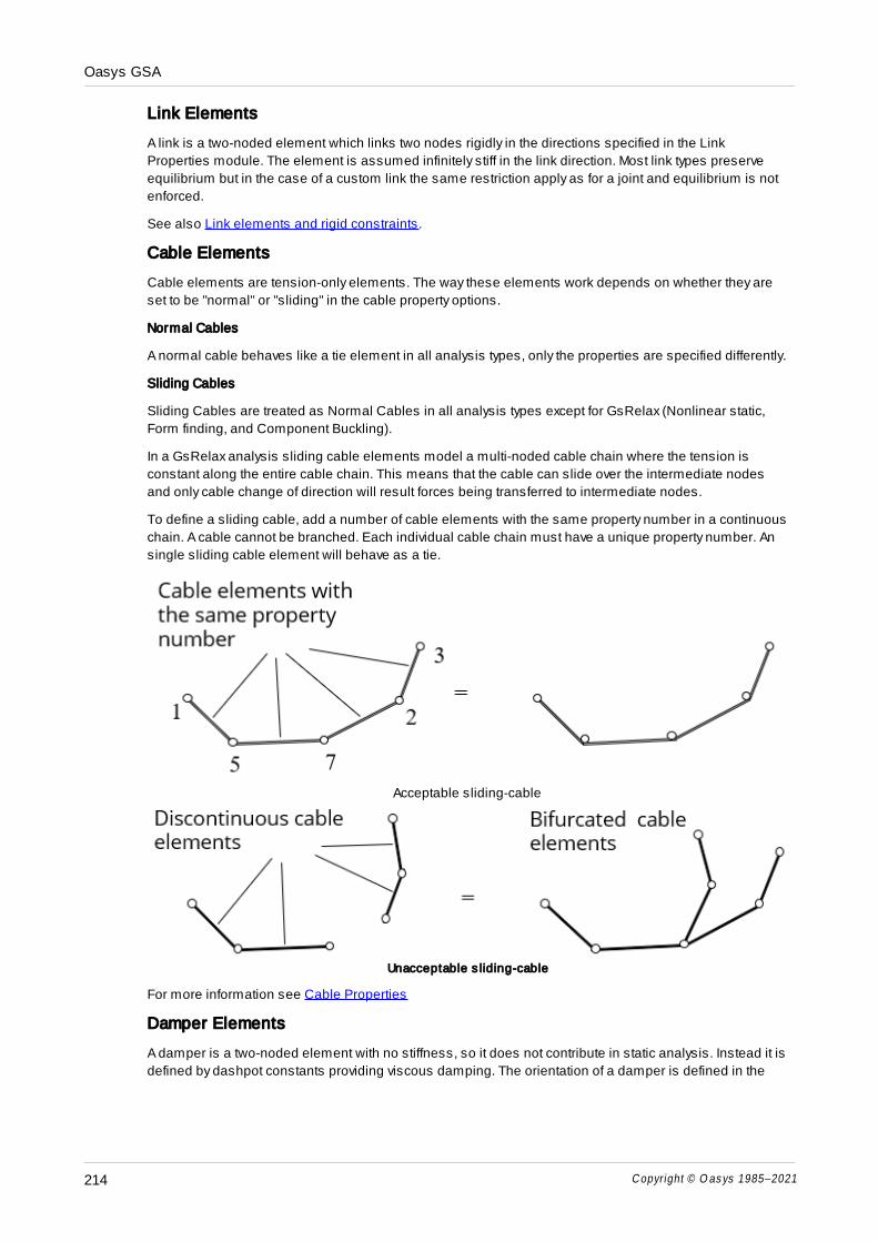
Oasys GSA

Copyright © O as ys 1985–2021214

Link Elements

A link is a two-noded element which links two nodes rigidly in the directions specified in the Link

Properties module. The element is assumed infinitely stiff in the link direction. Most link types preserve

equilibrium but in the case of a custom link the same restriction apply as for a joint and equilibrium is not

enforced.

See also Link elements and rigid constraints.

Cable Elements

Cable elements are tension-only elements. The way these elements work depends on whether they are

set to be "normal" or "sliding" in the cable property options.

Normal Cables

A normal cable behaves like a tie element in all analysis types, only the properties are specified differently.

Sliding Cables

Sliding Cables are treated as Normal Cables in all analysis types except for GsRelax (Nonlinear static,

Form finding, and Component Buckling).

In a GsRelax analysis sliding cable elements model a multi-noded cable chain where the tension is

constant along the entire cable chain. This means that the cable can slide over the intermediate nodes

and only cable change of direction will result forces being transferred to intermediate nodes.

To define a sliding cable, add a number of cable elements with the same property number in a continuous

chain. A cable cannot be branched. Each individual cable chain must have a unique property number. An

single sliding cable element will behave as a tie.

Acceptable sliding-cable

Unacceptable s liding-cable

For more information see Cable Properties

Damper Elements

A damper is a two-noded element with no stiffness, so it does not contribute in static analysis. Instead it is

defined by dashpot constants providing viscous damping. The orientation of a damper is defined in the

Oasys GSA

Copyright © O as ys 1985–2021 215

same way as a beam element with the x axis along the damper and the y and z directions defined by an

orientation node and/or orientation angle. For a zero length damper the orientation is defined by the node

constraint axis of the first node. The damper characteristics are defined in the damper properties.

Spacer Elements

Spacer elements are only for use in soap-film form-finding analysis with the GsRelax solver. Spacer

elements are ignored by the Gss solver. Each Spacer chain joins a line of nodes and is, in effect, the

opposite of the sliding Cable element. Spacer behaviour is described in detail in the Form-Finding theory

section. Spacer chains do not apply any force to their nodes in a direction normal to the surface of the

adjoining triangles and quads. Spacers therefore do not affect the surface that is form-found; they only

control the position of nodes on the surface that is formed. Spacer chains do not exert any force onto the

end nodes of the chain. Because of this, an isolated Spacer element will have no structural effect. To

define the multi-noded Spacer chain input a list of 2 noded individual spacer elements with the same

property number. Each individual spacer chain must have a unique property number. The program

connects individual elements together to form a continuous chain of linked elements by linking common

node numbers. A spacer cannot be branched.

4.12.2 Element Axes

For each element there is an element axis that is used both to establish the element stiffness relative to

the structure as a whole and to establish the direction of element loading as well as element analysis

results

The element axes are defined relative to the undeformed geometry of the structure. For linear analysis

these remain unchanged during the analysis, but for non-linear analysis, element axes will be updated

during the analysis according to the current deformed positions of the elements..

Beam Type Elements

Beam elements including bars, rods, ties and struts are defined by two nodes locating the ends of the

element. The x axis of the element is along the axis of the element (taking account of any offsets) from the

first topology item to the second.

The definition of the element y and z axes then depends on the element's orientation, verticality, orientation

node and orientation angle. The element is considered vertical in GSA if the element is within the “vertical

element tolerance”.

Non-vertical elements

If an orientation node is not specified, the element z axis of a non-vertical element defaults to lying in the

vertical plane through the element and is directed in the positive sense of the global Z direction. The

element y axis is orthogonal to the element z and x axes. The element y and z axes may be rotated out of

this default position by the orientation angle (β).

Oasys GSA

Copyright © O as ys 1985–2021216

Vertical elements

If an orientation node is not specified, the element y axis of a vertical element defaults to being parallel to

and is directed in the positive sense of the global Y axis. The element z axis is orthogonal to the element x

and y axes. The element y and z axes may be rotated out of this default position by the orientation angle.

Oasys GSA

Copyright © O as ys 1985–2021 217

Orientation Node and Angle

If an orientation node is specified, the element xy plane is defined by the element x axis and a vector from

the first topology position to the orientation node, such that the node has a positive y coordinate. The

element z axis is orthogonal to the element x and y axes. Specifying an orientation node overrides the

“vertical element” and “non-vertical element” definitions described above. The element y and z axes may

be rotated out of this default position by the orientation angle.

With an orientation angle the element y and z axes are rotated from their default positions about the

element x axis by the orientation angle in the direction following the right hand screw rule. This occurs

regardless of whether or not the element is vertical and of whether or not an orientation node is specified.

Spring and Damper Elements

For a spring (including Gap, Friction & lockup elements) or damper element with finite length, the element

axis are defined in the same way as the beam element axes. For a spring and damper element with zero

length, the element axis is the nodal constraint axis of the first topology node of this element.

Cable Elements

Cable elements act only in the axial direction, so only the x axis is defined following the same definition as

the x axis of a beam element.

Link Elements

The local axes of link elements are the same as the constraint axis of the primary node.

Quad and Triangle Elements

2D element local axis is the axis referenced by the element stiffness and forces, moments and stresses,

the xy plane of the 2D element local axis is always co-planar with the element plane. 2D element local axis

can be defined by global axis or a user defined axis or by the nodes defining the 2D element (topological),

the axis used by 2D element to determine its local axis is defined in 2D element property. User defined

axes can be Cartesian, cylindrical or spherical.

Typically using a global axis or a user defined axis to define 2D element local axis can result in consistent

local axis direction for all the elements in the mesh.

2D element local axis defined by element topology

If "topological" is used in 2D element property, 2D element local axis is defined as follows: The z axis

direction of the 2D element local axis is always perpendicular to the 2D element plane and it is defined as

n = (c3 c

1) × (c

4 c

2) for quad elements

n = (c2 c

1) × (c

3 c

1) for triangle elements

Then the three axes of the 2D element local axis are defined as:

x = c2 c

1y = n × x z = n

where c1, c

2, c

3, & c

4 are the coordinates of topology nodes 1, 2, 3 & 4 of the element, the coordinates of

the node should include any offset.

2D element local axis defined by global or user defined axis

If global or user defined axis is used in 2D element property, the x axis of 2D element local axis is the

projection of the control vector "X" onto the 2D element plane and the other two axes of the 2D element

local axis can be determined accordingly as shown below.

The control vector "X" depends on the type.of the user defined axis,

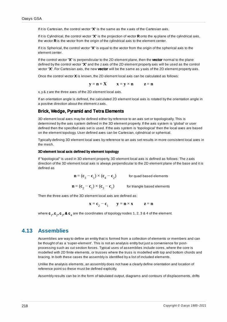
Oasys GSA

Copyright © O as ys 1985–2021218

If it is Cartesian, the control vector "X" is the same as the x axis of the Cartesian axis,

If it is Cylindrical, the control vector "X" is the projection of vector R onto the xy plane of the cylindrical axis,

the vector R is the vector from the origin of the cylindrical axis to the element center.

If it is Spherical, the control vector "X" is equal to the vector from the origin of the spherical axis to the

element center.

If the control vector "X" is perpendicular to the 2D element plane, then the vector normal to the plane

defined by the control vector "X" and the z axis of the 2D element property axis will be used as the control

vector "X". For Cartesian axis, the new vector will be the same as y axis of the 2D element property axis.

Once the control vector X is known, the 2D element local axis can be calculated as follows:

y = n × X x = y × n z = n

x, y & z are the three axes of the 2D element local axis.

If an orientation angle is defined, the calculated 2D element local axis is rotated by the orientation angle in

a positive direction about the element z axis.

Brick, Wedge, Pyramid and Tetra Elements

3D element local axes may be defined either by reference to an axis set or topologically. This is

determined by the axis system defined in the 3D element property. If the axis system is 'global' or user

defined then the specified axis set is used. If the axis system is 'topological' then the local axes are based

on the element topology. User defined axes can be Cartesian, cylindrical or spherical.

Typically defining 3D element local axes by reference to an axis set results in more consistent local axes in

the mesh.

3D element local axis defined by element topology

If "topological" is used in 3D element property, 3D element local axis is defined as follows: The z axis

direction of the 3D element local axis is always perpendicular to the 2D element plane of the base and it is

defined as

n = (c3 c

1) × (c

4 c

2) for quad based elements

n = (c2 c

1) × (c

3 c

1) for triangle based elements

Then the three axes of the 3D element local axis are defined as:

x = c2 c

1y = n × x z = n

where c1, c

2, c

3, & c

4 are the coordinates of topology nodes 1, 2, 3 & 4 of the element.

4.13 Assemblies

Assemblies are way to define an entity that is formed from a collection of elements or members and can

be thought of as a ‘super-element’. This is not an analysis entity but just a convenience for post-

processing such as cut section forces. Typical uses of assemblies include cores, where the core is

modelled with 2D finite elements, or trusses where the truss is modelled with top and bottom chords and

bracing. In both these cases the assembly is identified by a list of included elements.

Unlike the analysis elements, an assembly does not have a clearly define orientation and location of

reference point so these must be defined explicitly.

Assembly results can be in the form of tabulated output, diagrams and contours of displacements, drifts

Oasys GSA

Copyright © O as ys 1985–2021 219

and force/moments, for analysis and combination cases, including envelopes.

The ‘Model | Checking Tools | Check Assemblies’ tool checks all assemblies for missing topology items

and invalid geometry configurations.

Name

The name is used as a convenient way of referring to assemblies.

Entity

Assemblies can be defined in terms of members or elements. Only elements related to the member list or

element list are considered. Spring and damper elements are ignored.

Topology

This defines the nodes at the ends of the assembly.

Orientation Node

The plane formed by the topology items and the orientation node is the xy plane of the assembly. The

orientation node cannot be collinear with the topology nodes.

Internal Topology

This is a list of nodes that define the curve of the assembly. The order of the nodes is not important as the

nodes are ordered along a vector between ends one and two.

Curve Fit

For a curved element there is a choice of how the curve is fitted to the points. The default is to use

Lagrange interpolation to fit a curve through all the intermediate points. The other option which is only valid

if there is just a single internal topology item is for a circular arc from end one passing through the internal

node to end two.

Extents

The extents of the assembly can be specified directly as end 1 and end 2 or GSA can determine this from

the elements that define the assembly.

Point Definition

The is how the assembly is defined internally (as use for assembly forces and moments). See Assembly

Results for more information.

4.14 Constraints

4.14.1 Generalised Restraints

Generalised Restraints allow a set of restraint conditions to be applied to a list of nodes, saving the effort

of specifying restraints for individual nodes in the “Nodes | Restraints” table. The generalised restraints

and nodal restraints work together to apply restrain to the model. Car must be taken to avoid conflicting

constraints.

Definition

Name

The name is only used as a convenient way of identifying a restraint.

Stage List

This specifies a stage list using one any of the forms detailed in “Lists”. If this is set to “all” the restraint

Oasys GSA

Copyright © O as ys 1985–2021220

applies to the whole model, irrespective of stage. Otherwise it applies only to the specified stage(s).

Node List

This specifies a node list using any of the forms detailed in “Lists”. These include a list definition to select

nodes on a specified plane.

Restraints

Specifies the directions that are to be restrained. Restraints are applied in the constraint axes of each

individual node, as specified in the Nodes module.

Generalised Restraints act in addition to Nodal Restraints. The user should remain aware of this to avoid

duplication and general confusion.

Generalised restraints are not affected by the Sculpt “Modify Nodes” operation – it adjusts the Nodal

Restraints. A warning is given when the user is about to modify Nodal Restraints in Sculpt when

Generalised Restraints are specified.

In Output Views, the Nodes table reports the nodal restraints and the generalised restraints separately.

The Supports table reports the total restraints (nodal + generalised).

Restraint Hierarchy

Restraints are a constraint on the model where the displacement at a node in a particular direction is set

to zero. Restraints can be applied to a model in several ways and it is important to understand the different

restraint methods.

Implied restraint due to structure type

For a “Plane” structure type the active degrees of freedom are x, z and yy. So the remaining three degrees

of freedom are ignored in the analysis. This has the same results are restraining all the out-of-plane

degrees of freedom. This feature is set by the program when the user selects a structure type from the

“General Specification”.

Global restraints

In some it is useful to restrain all the degrees of freedom in model in a particular direction. For example

modelling a slab with plate elements, where the plate elements have no stiffness in the x and y directions,

it may be useful to apply global restraints in the x and y directions. These are also set on the “Analysis

Specification”.

Nodal restraints

Nodal restraints are the most commonly used restraint type. Here particular degrees of freedom at a node

are restrained. So, for example, to create a pinned support, the user can apply restraints to a node in the x,

y and z directions. These are set in the Restraints page of the “Nodes” table view or in the Node Wizard.

Generalised Restraints

Generalised restraints are similar to nodal restraints except that they are applied to a list of nodes. It is

therefore possible to use a list specifying all the nodes on a plane so as to apply restraint across all of the

base of a structure.

The total restraint on a node is the sum of all of the restraints acting on it.

4.14.2 Rigid Constraints

Rigid constraints define sets of nodes constrained to move as a rigid body. These are commonly use to

model rigid diaphragms, where typically the nodes are rigid in the x-y plane but not in the z direction.

Rigid constraints are similar to link elements except that the number of nodes is not limited. The

Oasys GSA

Copyright © O as ys 1985–2021 221

differences between link elements and rigid constraints is discussed elsewhere.

Unlike joints rigid constraints maintain equilibrium in the system.

Definition

Name

The name is only used as a convenient way of identifying a rigid constraint.

Stage List

This specifies a stage list using one any of the forms detailed in “Lists”. If this is set to “all” the constraint

applies to the whole model, irrespective of stage. Otherwise it applies only to the specified stage(s).

Node List

This specifies a node list using any one of the forms detailed in “Lists”. These include a list definition to

select nodes on a specified plane.

Primary

The reference node to which the “constrained” nodes are attached. The primary node may be included in

the node list.

Type of Linkage

This should be set to “All” to make the constraint completely rigid. There are however many cases in which

it is useful to make a constraint rigid in a plane (for example in modelling floor slabs) or a plate. The

following planes can be specified:

L ink age L ink ed degr ees o f f r eedom

all x, y, z, xx, yy, zz

all (pin) x, y, z

xy plane x, y, zz

yz plane y, z, xx

zx plane x, z, yy

xy plane (pin) x, y

xy plane (pin) x, y

yz plane (pin) y, z

zx plane (pin) x, z

x plate x, yy, zz

y plate y, xx, zz

z plate z, xx, yy

x plate (pin) x

y plate (pin) y

z plate (pin) z

custom any

The “pin” linkage types do not include the rotational degrees of freedom at the constrained node in the

rigid body displacements. Note that the “pin” condition applies only to the constrained node - the rotational

Oasys GSA

Copyright © O as ys 1985–2021222

degrees of freedom at the primary are always retained. The degrees of freedom linked are always in the

constraint axis of the nodes and all nodes must be assigned the same constraint axis.

Coupled directions

For most constraint types the couple directions are fixed, but for custom links they must be specified

explicitly. This can lead to behaviour that is not consistent with a ‘rigid’ condition.

4.14.3 Joints

Joints allow nodes to be tied in the specified translational or rotational directions. Unlike rigid constraints,

joints do not impose equilibrium on the model.

As with all constraints, care must be taken to avoid conflicting constraints.

Definition

Name

The name is only used as a convenient way of identifying a joint.

Stage List

This specifies a stage list using one any of the forms detailed in “Lists”. If this is set to “all” the joint

applies to the whole model, irrespective of stage. Otherwise it applies only to the specified stage(s).

Primary

The reference node to which the “constrained” node is attached.

Constrained

The node coupled to a “primary” node so that it shares the coupled degrees of freedom.

Directions

Specifies the translational and rotational directions that are linked by this joint.

If the constrained and primary nodes are coincident there are no problems with joints, however if the

constrained and primary nodes are not coincident there can be moment imbalance since forces are

transferred directly to the primary node and no account is taken of the moment implied by the force times

offset. If this is to be modelled, rigid constraints should be used instead.

Joint Limitations

Joints are a facility to allow two nodes to be coupled in particular directions. Thus to create a pin joint, two

nodes can be defined at the two parts of the structure to be joined. These are included in a joint, which is

linked in the required directions (e.g. x, y and z). In a joint as in a link element there is a constrained and

primary node and the linked degrees of freedom are simply shared between the constrained and the

primary node. The axis directions of a joint are the constraint axis directions of the constituent nodes. This

means that if a direction is linked this may be different for the two nodes in the joint; in this circumstance a

warning is given, though in the case of GsRelax analyses this is treated as an error.

While a link element or rigid constraint uses the geometrical relationship between constrained and

primary to ensure equilibrium, this is not true for joints. Thus joints in which the nodes are not coincident

will not in general be in equilibrium. To guard against this problem the user is warned if the nodes are not

coincident.

Oasys GSA

Copyright © O as ys 1985–2021 223

4.14.4 Constraint Equations

Constraint equations allow a node, in a particular direction to be constrained relative to a set of other

nodes. Constraint equations are the fundamental building block for all other constraint types.

Definition

Name

The name is only used as a convenient way of identifying a constraint equation.

Stage List

This specifies a stage list using one any of the forms detailed in “Lists”. If this is set to “all” the constraint

equation applies to the whole model, irrespective of stage. Otherwise it applies only to the specified stage

(s).

Constrained

The node coupled to a set of “primary” nodes so that it shares the coupled degrees of freedom

Direction

This is the direction in which the constrained node is constrained.

Equation

The equation is a set of factors, nodes and directions. The displacement of the “constrained” node is the

summation of the factored displacements at the primary in the specified directions.

Any linear equation can be set up and there is no requirement that the constraint equation preserves

equilibrium in model, so care should be taken that no artificial constraint is introduced into the model.

Primary – Factor, Node and Direction

The displacement of the constrained node is the summation of the factored displacements at the primary

in the specified directions. Care should be taken when mixing translational and rotational freedom.

Constraint Equations

Constraint equations are the most fundamental way of specifying a constraint on a node. This constrained

node is related to one or more primary nodes. The displacement at the constrained node in a particular

direction is a function of the displacements in a particular direction at a set of primary nodes. The basic

relationship can be specified in the form:

mjmmis uau ..

So for a node whose displacement is the average of two other nodes this is of the form

u2,x

= 0.5u0,x

+ 0.5u1,x

For primary nodes 101 and 102 the equation would be of the form 0.5N101x + 0.5N102x.

Rigid constraints and joints can be thought of as particular instances of constraint equations.

The axis directions of a constraint are the constraint axis directions of the constituent nodes. While a link

element or rigid constraint uses the geometrical relationship between constrained and primary to ensure

equilibrium, this is not true for the more general constraint equation. Thus care should be taken when

defining constraint equations to ensure that no unwanted constraint is applied to the model. Also the

factors in the constraint equation are dimensionless, so if these are to represent actual relative positions

of nodes care should be taken with units.

Oasys GSA

Copyright © O as ys 1985–2021224

4.14.5 Tied Interfaces

Tied interfaces allow two sets of elements that do not have connectivity to be joined without the need for

complex mesh refinement. Instead the elements on one side are taken as primary and the other side as

constrained. The nodes on the boundary of the constrained side are tied to the nodes on the boundary of

the primary side through a set of constraint equations.

As tied interfaces do not give proper continuity conditions across the boundary they should not be used in

area where accurate determination of stresses is required.

Definition

Name

The name is only used as a convenient way of identifying a tied interface.

Stage List

This specifies a stage list using one any of the forms detailed in “Lists”. If this is set to “all” the tied

interface applies to the whole model, irrespective of stage. Otherwise it applies only to the specified stage

(s).

Constrained Type

The constrained side of the tied interface can be defined either as nodes or elements. When elements are

selected GSA will find the nodes on the constrained side that need to be connected.

Constrained List and Primary List

The nodes in the constrained list are tied to elements in the primary list to form a continuous entity. The

primary retains all its degrees of freedom. The primary elements must be 2D elements, but the

constrained elements can be of any element type (although link elements should be avoided as these will

give rise to conflicting constraints). So for example a beam element can be connected to the face of a 2D

elements.

The primary list should contain the larger elements.

Type of Linkage

There are two options for the type of linkage if the constrained type is “nodes”:

Auto – the tied interface behaves as tied if the constrained type is element and rigid if the constrained

type is node.

Tied – the tied interface connects the node on the constrained side to the element faces on the primary

side using constraint equations.

Rigid – the tied interface take the node on the constrained side as a primary and creates a rigid

constraint making the element on the primary side rigidly connected with the node.

The third of these options is intended for situations where the node represents a line entity such as a

column that is to be attached to a slab. In this case, if the beam element cross section is a similar size to

the 2D element on the other face the effect of the connection will be to make the 2D element behave in a

manner close to being rigid. This option will not work where there are nodes to connect to the same

element face or adjacent element faces.

The rigid linkage cannot be used when the constrained type is element as this would constraint conflict.

Surface Tolerance

This is used to limit the nodes that are connected to only those along the edge. Nodes outside this

tolerance are excluded from the tied interface.

Tied Interface

Oasys GSA

Copyright © O as ys 1985–2021 225

A tied interface works by connecting the nodes associated with the constrained elements to the elements

on the primary side to form a continuous entity.

A tied interface is a way of joining two meshes with dissimilar mesh densities by establishing a set of

constraint equations to “stitch” the nodes on the constrained side to those on the primary side. The tied

interface can be used to attached elements along two edges or elements on an edge to a face, or to

connect a beam element to the face of a 2D element.

The primary elements must be 2D elements, but the constrained elements can be of any element type

(although link elements should be avoided as these will give rise to conflicting constraints). The primary

retains all its degrees of freedom.

The elements on the primary side should be of the same size as or larger than those on the constrained

side for the tied interface to work well. The accuracy of the tied interface will be controlled by the mesh size

on the primary side.

4.15 Loading

GSA provides a number of different ways to apply loads to a model. The simplest option is nodal loading

where forces are applied directly to nodes. This is not recommended for 2D and 3D elements. The next

level of loading applies loads to the elements, either beam loading, 2D element loading or 3D element

loading. In the solver these use shape functions to give loading on the nodes compatible with the

elements to which the load is applied. Grid loading is a different type of loading which is applied to a grid

surface. An algorithm then distributes this loading from the grid surface to the surrounding beam

elements. This is useful for models where floor slabs are not modelled explicitly.

Gravity is the final load type. This is different from the other load types as it is specified as an acceleration

in the z direction.

Selecting entities for loading

Node and element loads apply to lists of entities. These lists can be entered directly in the loading tables

or selections can be made graphically using the “Select Nodes” or “Select Elements” options on the

Cursor Mode toolbar. “Copy” (Ctrl+C) will copy these to the clipboard and they can then be pasted directly

into the appropriate loads table. No check is made to see if a list of elements is being pasted into a node

load table or vice versa.

Checks can be made that the loading has been applied correctly by requesting a load diagram.

Projected Loads

Irrespective of the type of loading applied all loading results in a set of forces and moments at nodes

which are assembled into a structure force vector. For a number of load types loads can be projected.

When projected the load intensity is applied to the projected length of the element as shown below.

Oasys GSA

Copyright © O as ys 1985–2021226

Locking of Loads

In general, input data may not be edited when a model has been analysed and results are present.

Loading is an exception to this rule in that loads, of any type, are only locked against editing if they are

applied in a load case which is referred to by an analysis case that has been analysed. This means that

un-analysed load cases can be edited and appended to and new load cases can always be created.

4.15.1 Load Case Specification

When loads are applied to the model they are assigned to a load case. Load cases should be assigned to

simplify the management of the data. Load cases, when referred to in lists, are prefixed with an “L” (e.g.

L2). See Lists for more details.

The Load Cases are simply titles for these load cases defined elsewhere.

Definition

Name

The name for a load case where the loads are defined elsewhere.

Case Type

Defines the type of load case. The options offered are specific to the selected load design code, but

include dead, live, snow, seismic, etc.

Oasys GSA

Copyright © O as ys 1985–2021 227

Source

A way of grouping load cases with the same action.

Category

Specified the category of loading. The options offered are specific to the selected load design code, but

include domestic office, storage, roof, etc.

Direction

For loading such as seismic the direction in which it is applied

Include

Specified if adverse (unfavourable) and/or beneficial (favourable) effects should be included.

See also:

Working with the Program – Load Cases

4.15.2 Nodal Loading

Node Loading

Three type of nodal loading are possible in GSA. Node loads are the most direct type of loading and apply

a force or moment directly to a node. Applied displacements provide a method of determining the state of

the structure given a set of fixed displacements at selected nodes. Settlements work with constraints to

also provide a way of specifying displacements at specified nodes, but in this cases these are unaffected

by any other loads on the structure. Noded to which settlements are applied must be restrained in the

settlement directions.

Load case and title

The loading is stored by case number. However it is good practice to give load cases names. The load title

gives access to the Load Case Titles wizard to simplify this procedure. The wizard is opened for the

currently displayed load case.

4.15.2.1 Node Loads

Node loads are the most fundamental type of load. A node load is a force or moment applied to a

particular node or set of nodes. Node loads can be applied in local (i.e. node constraint axis), global or

user defined axis directions. User axes can be Cartesian, cylindrical or spherical.

Definition

Name

The name is only used as a convenient way of identifying a load. Optional.

Node List

This specifies a list of nodes to be loaded using any one of the forms detailed in “Lists”. The list may be a

single item.

In sculpt: The node list is set to the current selection set. The node list cannot be edited in the dialog

Load Case

This is the load case in which the load applies. The load case gives a way of grouping load effects

together.

Oasys GSA

Copyright © O as ys 1985–2021228

Axis

The axis in which the load is applied (global by default).

Direction

The direction of the loading, in the specified axis direction.

Value

The magnitude of the load – either a force or a moment.

4.15.2.2 Applied Displacements

An applied displacement allows a fixed displacement to be applied to a node in the structure and

calculates the deformation of the structure which results in the specified displacement at the specified

degree of freedom. Thus applied displacements may be used to investigate the stiffness of a structure by

constraining certain degrees of freedom to move by a fixed amount and noting the forces involved.

Applied displacements are different to the other load types and are also distinct from settlements.

Applied displacements apply to a particular load case and the node is free in all other load cases. Warning

– applied displacements should not be used in conjunction with other loading in the same analysis case.

Applied displacements are handled by using Lagrange multipliers.

Applied displacements can be applied in local (i.e. node constraint axis), global or user defined axis

directions. User axes can be Cartesian, cylindrical or spherical.

Definition

Name

The name is only used as a convenient way of identifying a load. Optional.

Node List

This specifies a list of nodes to be displaced using any one of the forms detailed in “Lists”. The list may be

a single item.

In sculpt: The node list is set to the current selection set. The node list cannot be edited in the dialog.

Load case

This is the load case in which the displacement applies. The load case gives a way of grouping load

effects together.

Axis

The axis in which the displacement is applied (global by default).

Direction

The direction of the loading, in the specified axis direction.

Value

The magnitude of the displacement or rotation.

Oasys GSA

Copyright © O as ys 1985–2021 229

4.15.2.3 Settlements

A settlement forces a node to move a specified distance in a specified global or local direction in a

particular load case, where the node has been restrained in the relevant direction.

It has no effect on any other load cases. Note that no axis is specified for settlements are the settlement is

in the node constraint axis.

Definition

Name

The name is only used as a convenient way of identifying a load. Optional.

Node List

This specifies a list of nodes to settle using any one of the forms detailed in “Lists”. The list may be a

single item.

In sculpt: The node list is set to the current selection set. The node list cannot be edited in the dialog.

Load Case

This is the load case in which the settlement applies. The load cases give a way of grouping load effects

together.

Direction

The settlement of the loading, in the node constraint axis direction.

Value

The magnitude of the settlement – displacement or rotation.

Settlements and Constraints

Settlements are used in conjunction with restraints. A restraint fixes a node so that it is no longer free to

move and a settlement determines the displacement imposed on that node for the particular load case. In

the load cases where there are no settlements the nodes are treated as simply restrained (i.e. fixed). The

restraint must be specified explicitly by the user.

Typically settlements are used to examine differential settlement of the structure. The distortion of the

structure can be calculated by applying a series of displacements or settlements (typically in the z

direction) at the base of the structure.

Settlements should not be confused with Applied Displacements. It is useful to think of settlements as

“constraints”, and applied displacements as “loads”.

A settlement is applied in the constraint axis directions of the node to which it is applied.

4.15.3 Beam Loading

Beam Loading

Beam loading applies to beam, bar, tie and strut elements and to a more limited extent to cable elements.

There are a number of ways in which loads can be applied but in all cases the loading is resolved during

the solution into an equivalent set of nodal forces and moments. When a position along an element is

required this may be specified as an actual distance (e.g. 2.46) or as a percentage (25%).

The most commonly used option is the beam loads which applies loads at specified positions along the

elements.

Oasys GSA

Copyright © O as ys 1985–2021230

Prestress allows prestress loads to be applied to elements. Beam distortions are a different and little

used option which allows an element to have a displacement discontinuity along the element. This is only

valid for linear elements. The final load type for beam element is thermal where temperature or

temperature gradients can be applied to the elements.

Load case and title

The loading is stored by case number. However it is good practice to give load cases names. The load title

gives access to the Load Case Titles wizard to simplify this procedure. The wizard is opened for the

currently displayed load case.

4.15.3.1 Beam Loads

Beam Loads are a ways of applying load to beam elements offering the commonly used load patterns as

different types. All these loads except the Beam Loads point load type are distributed along the elements. If

the beam has offsets the load positions relate to the flexible part of the beam, not the node positions.

The various types of beam loads are illustrated as follows.

Oasys GSA

Copyright © O as ys 1985–2021 231

Oasys GSA

Copyright © O as ys 1985–2021232

Beam Loads offer the option to specify the load as a projected load. When “projected” is set the distributed

load is specified as the intensity applied to the projection of the element on the surface normal to the

direction of the load; the load intensity actually applied to the element is then

W cos θ

where θ is the angle between the element and the surface normal to the direction of the load, and W is the

specified load intensity. A typical application of projected loads is for snow loads on inclined rafters.

Beam loads can be applied in local (i.e. element axis), global or user defined axis directions. User axes

can only be Cartesian; not cylindrical or spherical.

Definition

Name

The name is only used as a convenient way of identifying a load. Optional.

Beam List

This specifies a list of beam, bar, tie, strut or link elements to load using any one of the forms detailed in

“Lists”. The list may be a single item. Note that beam loads applied to cable elements are ignored.

In sculpt: The beam list is set to the beam and bar elements in the current selection set. The beam list

cannot be edited in the dialog.

Load case

The load case in which the load applies. The load case gives a way of grouping load effects together.

Type

The user has a choice of the type of loading applied to the elements.

Point – single load at position along the element

Uniform – load applied along the length of the element

Linear – load which varies linearly along the length of the element

Patch – a load applied to a section of the element with linear variation between the end points

Tri-linear – similar to a patch load but the load tapers off to zero outside the patch

Axis

The direction of the load is with respect to this axis set. Setting this to Local implies element local axes

and Deformed local implies a element local axis that is embedded in the element as it deforms (GsRelax

only).

Projected

Normally, by default, loads are applied along the length of the element. In some cases it may be more

appropriate to project the loads on to the element, e.g. (vertical) snow loading on an inclined roof may be

considered more easily as a projected load.

Direction

The direction of the loading, with respect to the specified axis.

Position 1

This is only relevant for point loads and patch loads. For a point load this is the location of the load

measured from end 1 of the beam; for a patch load it is the start of the patch load measured from end 1 of

the beam Position 1 can be specified as a length or as a percentage of the length of the element, e.g.

either 1.2 or 15%.

Oasys GSA

Copyright © O as ys 1985–2021 233

In sculpt: When the position of a patch load is specified, in absolute terms, to extend beyond the end

of the element(s) the load is automatically “broken up” and applied to elements positioned to take the

load. A warning is given if such elements cannot be found.

Load 1

Load magnitude. For a point load this is the load value; for a uniform load this is the load intensity; for a

linear load this is the load intensity at end 1; for a patch load this is the load intensity at Position 1.

Position 2

This is only relevant for patch loads and is the end of the patch load measured from end 1 of the beam.

Position 2 can be specified as a length or as a percentage of the length of the element, e.g. either 2.4 or

85%.

Where it is intended that a position should refer to end 2 of the beam 100% should be used instead of

entering the actual length. Otherwise a rounding error in the element length calculation may result in an

error being reported for the load.

Load 2

Load magnitude. For a linear load this is the load intensity at end 2 and for a patch load this is the load

intensity at Position 2.

Beam loads in non-linear static analysis

Element loads are converted into nodal forces and moments and added to other nodal forces, GsRelax

analysis being performed for nodal forces only. Only torsion loads are converted into moments; all other

loads are converted into forces only, with pinned end connections assumed. Obviously this means that

beam loads should only be used as a convenient means of generating statically equivalent nodal loads

and not in the expectation that the analysis will treat local effects accurately.

The vector of the equivalent nodal load will not change orientation as the element deflects, even if a local

axis has been specified for the load direction. This can lead to inaccuracies in the case of large deflections

and results should be checked.

4.15.3.2 Pre-stress

Prestress is a general description covering prestress loads, initial strains and initial lengths. In all cases

the result is a prestress condition (set of forces and/or moments) in the element.

Definition

Name

The name is only used as a convenient way of identifying a load. Optional.

Beam List

This specifies a list of beam, bar, tie, strut or cable elements to load using any one of the forms detailed in

“Lists”. The list may be a single item.

In sculpt: The beam list is set to the beam and bar elements in the current selection set. The beam list

cannot be edited in the dialog.

Load Case

The load case in which the load applies. The load case gives a way of grouping load effects together.

Type

Oasys GSA

Copyright © O as ys 1985–2021234

The user has a choice of the type of loading applied to the elements.

Prestress Force – This is the force in the element with undeflected nodes, before the structure is

allowed to relax into its deflected shape. The resultant force will not necessarily be the same, since the

attached structure’s stiffness and applied loading also affect the position of the nodes. This option is

equivalent to the Initial Strain and Lack of Fit options: The three prestress types are related by the

relevant element’s stiffness and length alone. A positive prestress force is equivalent to a negative Initial

Strain or lack of Fit, and will result in a tension in the element for normal structures.

Initial Strain – This allows the natural length of an element to be longer (positive) or shorter (negative)

than the distance between its undeflected node positions. The difference in length is the initial strain

multiplied by the node-to-node distance. The eventual length of the element depends on the stiffness of

the attached structure, and the other applied loading.

Lack-of-Fit – Similar to Initial Strain, with the two being related by the element’s undeflected node-to-

node length.

Tendon Prestress – Concrete elements are commonly prestressed using tendons or wires. This option

allows the simulation of a tendon by the application of equal and opposite forces to the ends of the

element. Since the tendon’s stiffness is much lower than the beam’s, the tendon’s elastic properties do

not need to be modelled, and the tendon force is assumed to remain constant over the elastic range of

beam deflections. The tendon can be offset from the element’s centroid to induce a moment as well as

an axial force. A positive tendon prestress force causes compression in the element. The element

forces output from the model are those for the “concrete” section alone: e.g. an unloaded cantilever

element that had a prestress applied would show a negative axial force despite having no load applied

to the tip.

Prestress Force & Tendon Prestress

The magnitude of the prestressing load. This applies only to the prestress force and tendon prestress

load types. A positive force implies a tensile prestress force or a tensile tendon prestress.

Prestress Offsets

The offsets in local (y, z) directions of the tendon prestress. This allows for the introduction of prestressing

moments in addition to prestressing force. This applies only to the tendon prestress load type and can

only be applied to beam elements. Note that the prestress offset cannot be used in the static non-linear

solver.

Initial Strain

The initial strain in the element used to define a lack-of-fit. The value specified should be the factor of the

element length by which the element is too long or too short. A positive value means the element is too

long compared with the nodal distance and will induce compression in the element, a negative value will

introduce tension in the element.

Lack of Fit

The length by which the element is too long or too short. A positive value means the element is too long

compared with the nodal distance and will induce compression in the element, a negative value will

introduce tension in the element.

4.15.3.3 Distortion

Distortions are used to model the effect of introducing a cut in an element and applying a translational or

rotational displacement across the cut.

The GsRelax solver can only deal with rotational distortions (excluding torsional distortions) and only when

applied to the ends of elements.

The main application of beam distortion is to generate influence diagrams. This makes use of Muller-

Oasys GSA

Copyright © O as ys 1985–2021 235

Breslau’s principle to determine influence coefficients from the deflected shapes resulting from member

distortions.

Definition

Name

The name is only used as a convenient way of identifying a load. Optional.

Beam list

This specifies a list of beam, bar, tie or strut elements to which the distortion loads apply using any one of

the forms detailed in “Lists”. The list may be a single item. Note that distortion loads applied to cable

elements are ignored.

In sculpt: The beam list is set to the beam and bar elements in the current selection set. The beam list

cannot be edited in the dialog.

Load case

The load case in which the distortion applies. The load case gives a way of grouping load effects together.

Direction

The direction of the distortion, with respect to the specified axis.

Position

The position along the element at which the member distortion is applied. Position can be specified as a

length or as a percentage of the length of the element, e.g. either 1.2 or 15%.

Displacement

The magnitude of the distortion applied to the element – either a displacement or rotation.

4.15.3.4 Thermal

In many cases it is useful to consider the effect of thermal loading on a structure. Thermal loads can have

two effects. A uniform temperature change causes the element to expand axially but induces no bending.

However, the thermal gradient option defines a linearly varying strain through the thickness of the element

so resulting in both axial expansion and bending. The positions of the temperatures are used to define the

temperature gradient.

Either constant temperatures or temperature gradients can be applied to an element. In either case the

temperature values specified are changes in temperature from ambient.

The temperature gradient is defined by applying temperatures at notional lower and upper surfaces.

These need not coincide with the actual lower and upper surfaces of the element (which may not be

known). The temperature gradient is then calculated from the top and bottom temperatures (Ttop

and Tbot

)

and the top and bottom locations (ptop

and pbot

) as follows:

This temperature gradient applies to the section as a whole.

Definition

Oasys GSA

Copyright © O as ys 1985–2021236

Name

The name is only used as a convenient way of identifying a load. Optional.

Beam List

This specifies a list of beam, bar, tie, strut or cable elements to which the thermal loads apply using any

one of the forms detailed in “Lists”. The list may be a single item.

In sculpt: The beam list is set to the beam and bar elements in the current selection set. The beam list

cannot be edited in the dialog.

Load Case

The load case in which the thermal load applies. The load case gives a way of grouping load effects

together.

Type

The user has a choice of the type of loading applied to the elements.

Uniform – a constant temperature rise applied to the whole element

Gradient in y – a temperature gradient is applied in the element y direction

Gradient in z – a temperature gradient is applied in the element z direction

Uniform Temperature

The temperature rise relative to ambient applied to the whole element.

Lower Surface, Temperature

For temperature gradients the temperature profile is defined by the temperature at two points, referred to

as the lower and upper surfaces. This defines the location and temperature rise that applies in the

negative y or z directions relative to the neutral axis. A negative value denotes a position “below” the neutral

axis.

Upper Surface, Temperature

This defines the location and temperature rise that applies in the positive y or z directions relative to the

neutral axis.

4.15.4 2D Element Loading

2D Element Loading

2D element loads apply to 2D element types, though not all the load types can be applied to each 2D

element type.

Face loads should be used where a load distributed over the face of a 2D element is required and edge

loads where it is the edges of a 2D element. Prestress loads can be thought of either as prestress forces

or tendon prestresses applied to the element or an initial strain. Thermal loads can be applied to consider

either a uniform temperature rise or a thermal gradient on the element.

Load case and title

The loading is stored by case number. However it is good practice to give load cases names. The load title

gives access to the Load Case Titles wizard to simplify this procedure. The wizard is opened for the

currently displayed load case.

Oasys GSA

Copyright © O as ys 1985–2021 237

4.15.4.1 Face Loads

Face loads should be used where a load distributed over the face of a 2D element is required and edge

loads where it is the edges of a 2D element. Face loads can be applied in local, global or user defined

axis directions. For face loads local is interpreted as element axis directions. User axes can only be

Cartesian; not cylindrical or spherical.

Face loads cannot be used for plane stress, plane strain or axisymmetric elements.

Face loads offer the option to specify the load as a projected load. When “projected” is set the distributed

load is specified as the intensity applied to the projection of the element on the surface normal to the

direction of the load; the load intensity actually applied to the element is then

W cos θ

where θ is the angle between the element and the surface normal to the direction of the load, and W is the

specified load intensity. A typical application of projected loads is for snow loading on an inclined roof.

Definition

Name

The name is only used as a convenient way of identifying a load. Optional.

2D Element List

This specifies a list of 2D elements to load using any one of the forms detailed in “Lists”. The list may be a

single item.

In sculpt: The 2D element list is set to the 2D elements in the current selection set. The 2D element list

cannot be edited in the dialog.

Load Case

The load case in which the load applies. The load case gives a way of grouping load effects together.

Axis

The axis in which the load is applied.

The axis may be Global, Initial Local, Deformed Local or the number of an axis set specified in the Axes

module.

Loads applied in Initial Local directions are applied in the element axis directions with the element axes

being based on the undeformed state of the element.

Loads applied in Deformed Local directions are applied in the element axis directions with the element

axes being based on the deformed state of the element. Loads applied in Deformed Local directions may

only be specified for non-linear analysis.

Projected

By default, loads are applied at the specified intensity over the element. In some cases it may be more

appropriate to project the loads on to the element, e.g. (vertical) snow loading on an inclined roof may be

considered more easily as a projected load.

Type

The user has a choice of the type of loading applied to the elements.

Uniform – uniform load applied over the whole face of the element

Variable – load which varies across the face of the elements interpolating between values specified at

the corner nodes

Oasys GSA

Copyright © O as ys 1985–2021238

Point – force can be applied at a point on the face of the elements. The position of the point load on the

face can be specified in ( r , s ) coordinates. (Based on two-dimensional shape function)

If the elements to which this relates are load panels then the load type must be uniform.

Direction

The direction in which the load applies, with respect to the specified axis.

Pressure

The pressure to apply to the element. For point type load, force at the point to be specified (not pressure).

For a uniform face load a single pressure value is required and for the variable face load a value is

required for each corner node on the element. The pressure over the face is interpolated from the corner

values.

Position of load

Position of load is applicable for point load type. The position of the point load to be specified in ( r , s )

coordinates based on two-dimensional shape function.

Coordinates vary from 0 to 1 for Triangle 3 and Triangle 6.

2D loads in non-linear analysis

Element loads are converted into nodal forces and moments and added to other nodal forces, GsRelax

analysis being performed for nodal forces only. No nodal forces are applied to quad dummy nodes.

The vector of the equivalent nodal load will not change orientation as the element deflects, even if a local

axis has been specified for the load direction. This can lead to inaccuracies in the case of large deflections

and results should be checked.

4.15.4.1.1 2D Loads on Load Panels

Linear 2D elements can be defined as load panels. A load panel element is not structural and so does not

contribute to the stiffness or mass of the structure. The purpose of the load panel is to allow loads to be

defined as a face load on 2D elements and then distributed to the beam elements surrounding the 2D

element. In many ways face loads on load panels gives an alternative to grid load.

A 2D element is specified as a load panel in the properties. A load panel element does not have a

material, thickness, etc. Instead a support type and reference edge are specified. The support pattern

Oasys GSA

Copyright © O as ys 1985–2021 239

defines the number of edges to which the load is transferred and the reference edge sets the selection of

the free/loaded edges.

All edges supported - the load is distributed to the edges in proportion to the contributing areas.

Three edges supported - the load is distributed to the supporting edges so that as far a possible

equilibrium is maintained. The edge opposite the reference edge does not take any load

Two edges supported - the load spans from the sides adjacent to the reference edge.

Two adjacent edges supported - the load is taken on the reference edge and the “next” edge on the

element.

One edge supported - the load is all attributed to the reference edge. The moment due to the offset of

the load is ignored.

Cantilever support - the forces are distributed as for one edge supported but the moment is applied to

the edge so that equilibrium is achieved.

Quad 8 or tri 6 element cannot be selected for load panels.

Setting the ‘Load panels’ labelling option in the Labels and Display Methods: On Elements dialog tab

displays the load distribution pattern on load panels.

The loads from the load panels are distributed by searching for beam/bar elements that bound the panel

and attributing load to these elements based on the support condition. If the bounding beam/bar elements

are dummy elements these elements cannot take load so an appropriate support condition should be

selected to ensure that no load is attributed to the dummy elements.

For elements with rigid offsets the basic load distribution is modified to avoid loads on the rigid offsets.

4.15.4.2 Edge Loads

Edge Loads are loads applied to the edge of 2D elements. In general edge loads should be applied with

care to ensure that the loading applied to the element is in a direction in which the element is stiff. Edge

loads may not be applied to Flat Plate or Fabric type 2D elements.

Edge loads can be applied in local, global or user defined axis directions. Local is interpreted as follows:

x is the direction along the edge in the topology order direction.

y is the direction into the element, in the plane of the element and normal to the edge of the element at

Oasys GSA

Copyright © O as ys 1985–2021240

the point at which it is applied.

z is orthogonal to the x and y directions.

User axes can only be Cartesian; not cylindrical or spherical.

Definition

Name

The name is only used as a convenient way of identifying a load. Optional.

2D Element List

This specifies a list of 2D elements to load using any one of the forms detailed in “Lists”. The list may be a

single item.

In sculpt: The 2D element list is set to the 2D elements in the current selection set. The 2D element

list cannot be edited in the dialog.

Load Case

The load case in which the load applies. The load case gives a way of grouping load effects together.

Axis

The axis in which the load is applied.

The axis may be Global, Initial Local, Deformed Local or the number of an axis set specified in the Axes

module.

Loads applied in Initial Local directions are applied in a direction that relates to the element edge. The x

direction is the direction along the edge in the topology order direction. The y direction is the direction into

the element, in the plane of the element and normal to the edge of the element at the point at which it is

applied. The z direction is orthogonal to the x and y directions. The element is taken as being in its

undeformed state.

Loads applied in Deformed Local directions are in directions as described for Initial Local directions

except that the element is taken as being in its deformed state. Loads applied in Deformed Local

directions may only be specified for non-linear analysis options.

Edge

The edge of the element that is loaded. The edges as defined by the topology items are

Edge Topo logy item s

edge 1 1 2

edge 2 2 3

edge 3 3 4

edge 4 4nono 1

Direction

The direction in which the load applies, with respect to the specified axis.

Stress at Ends

The stress to apply to the element. The stress along the edge is interpolated from the end values.

2D loads in non-linear analysis

Element loads are converted into nodal forces and moments and added to other nodal forces, GsRelax

Oasys GSA

Copyright © O as ys 1985–2021 241

analysis being performed for nodal forces only. No nodal forces are applied to quad dummy nodes.

The vector of the equivalent nodal load will not change orientation as the element deflects, even if a local

axis has been specified for the load direction. This can lead to inaccuracies in the case of large deflections

and results should be checked.

4.15.4.3 Pre-stress

Prestress loads can be thought of either as prestress forces, tendon prestress applied to the element or

an initial strain. The tendon prestress option allows for the prestress to be offset by a constant distance

from the centre of the element in the thickness direction to induce bending.

The prestress or initial strain is applied in either the local x or y direction or in both directions.

An element with a positive prestress tends to contract, as in a prestressed slab.

Definition

Name

The name is only used as a convenient way of identifying a load. Optional.

2D Element List

This specifies a list of 2D elements to load using any one of the forms detailed in “Lists”. The list may be a

single item.

In sculpt: The 2D element list is set to the 2D elements in the current selection set. The 2D element

list cannot be edited in the dialog.

Load Case

The load case in which the load applies. The load case gives a way of grouping load effects together.

Type

The user has a choice of the type of loading applied to the elements.

Prestress force – an in-plane force applied to the element

Initial strain – an initial in-plane strain is specified in the element

Tendon prestress – an in-plane force is applied to the element at an offset from the neutral axis. Only

the latter option induces forces and moments in the element.

Direction

The direction in which the load applies in element local axes. This can be x, y or both x and y directions

where x and y are element local directions.

Prestress Force

The prestress force (load per unit length) to apply to the element.

Initial Strain

The initial strain in the element.

Tendon Prestress, Offset

The prestress force (load per unit length) and offset (in the local z direction) to apply to the element. When

the offset is specified the element is loaded by an in-plane force and a moment.

Oasys GSA

Copyright © O as ys 1985–2021242

4.15.4.4 Thermal

In many cases it is useful to consider the effect of thermal loading on a structure. Thermal loads can have

two effects. A uniform temperature change causes the element to expand axially but induces no bending.

However, the thermal gradient options define a linearly varying strain through the thickness of the element

so resulting in both in-plane expansion and bending.

Definition

Name

The name is only used as a convenient way of identifying a load. Optional.

2D element list

This specifies a list of 2D elements to which the thermal loads apply using any one of the forms detailed in

“Lists”. The list may be a single item.

In sculpt: The 2D element list is set to the 2D elements in the current selection set. The 2D element

list cannot be edited in the dialog.

Load Case

The load case in which the thermal load applies. The load case gives a way of grouping load effects

together.

Type

The user has a choice of the type of loading applied to the elements.

Uniform – uniform load applied over the whole of the element

Gradient in local z – load which varies through the thickness of the elements, but not across the surface

of the element

General – load which varies over the whole element

Uniform Temperature

The temperature rise relative to the background temperature applied to the whole element.

Temperature at Position

For temperature gradients the temperature profile is defined by two values, the temperature at the top and

bottom surfaces. For general temperatures the temperature is defined at the top and bottom surface for

each corner of the element.

4.15.4.4.1 2D Thermal Load Diagrams

2D element thermal loads have two diagram outputs: in-plane and gradient. Note that if the All Load

Diagrams option is chosen then both will be shown superimposed.

In these examples the four elements have the following loads:

Oasys GSA

Copyright © O as ys 1985–2021 243

2D Thermal In-plane

The in-plane diagram and contour shows the average thermal change on the element or at the nodal

locations.

2D Thermal Gradient

The gradient diagram and contour shows degrees per unit length through the thickness of the element. In

this instance the 2D thickness is 0.1 m, so the gradient from a one degree change is shown as 10.

Oasys GSA

Copyright © O as ys 1985–2021244

4.15.5 3D Element Loading

There are two loading options for loading 3D (brick) elements. Face loads apply to specified faces of the

brick element. Thermal loads allow temperatures to be applied to the elements.

Load case and title

The loading is stored by case number. However it is good practice to give load cases names. The load title

gives access to the Load Case Titles wizard to simplify this procedure. The wizard is opened for the

currently displayed load case.

4.15.5.1 Face Loads

Face loads on 3D elements are similar to face loads on 2D elements, with the additional requirement that

the face be selected. Loads are specified as a pressure across the surface.

Definition

Name

The name is only used as a convenient way of identifying a load.

3D element list

The list of elements to which the load is to be applied.

In sculpt: The 3D element list is set to the 3D elements in the current selection set. The 2D element list

Oasys GSA

Copyright © O as ys 1985–2021 245

cannot be edited in the dialog.

Load case

This is the load case in which the load applies. The load case gives a way of grouping load effects

together.

Face

The face to be loaded.

Fac e 1 2 3 4 5 6

Brick bottom top front right back left

Wedge bottom top front right left

Pyramid bottom front right back left

Tetra bottom front right left

Load type

The user has a choice of the type of loading applied to the elements.

Uniform – uniform load applied over the whole face of the element

Variable – load which varies across the face of the elements interpolating between values specified at

the corner nodes

If the elements to which this relates are load panels then the load type must be uniform.

Direction

The direction in which the load is applied, with respect to the specified axis.

Axis

The direction of the load is with respect to this axis set. Setting this to Local implies element local axes.

Projected

When set, the load is projected from onto the element to result in the magnitude of the load actually

applied to the element being the specified magnitude factored by an amount dependent on the inclination

of the element to the load direction. (E.g. for snow loading.)

Value

The magnitude of the load specified at the corner nodes of the element.

4.15.5.2 Thermal

Thermal loads on 3D elements can either be uniform giving rise to a uniform thermal strain across the

element, or variable with temperature specified at each node.

Definition

Name

The name is only used as a convenient way of identifying a load.

3D Element List

The list of elements to which the load is to be applied.

In sculpt: The 3D element list is set to the 3D elements in the current selection set. The 3D element list

Oasys GSA

Copyright © O as ys 1985–2021246

cannot be edited in the dialog.

Load Case

This is the load case in which the load applies. The load case gives a way of grouping load effects

together.

Load Type

The user has a choice of the type of loading applied to the elements.

Uniform – uniform load applied over the whole of the element

General – load which varies over the whole element

Temperature

The magnitude of the temperature change as required by the load type.

4.15.6 Grid Loading

Grid loads are loads that are not applied directly to a node or element, but are located in space or, more

precisely, on a grid surface which is located in space. Internally, the load is applied to the structure by

considering the location of the load relative to adjacent structural elements.

Grid loads can be grid point loads, grid line loads or grid area loads. In all cases these loads are

expanded to beam type elements.

The loads are not applied directly to the structure but by comparing the location of the loads relative to

elements in the structure. The advantage of grid loads is that the loads can remain unchanged if the local

definition of the structure changes, with the disadvantage that the loads are not tied to the structure.

The structure is considered as a collection of polygonal regions bounded by elements. These regions are

referred to as panels. The panel associated with the loading is found and provided a number of checks

are satisfied the load can be considered as a load on the structure. It is possible, though neither

necessary nor desirable, to expand grid loading into an equivalent set of beam loads. Alternatively the grid

loads are expanded as required by the solver.

Application of grid loading

The way in which the grid loads are applied to the structure depends on the span type associated with the

grid surface.

Loads on a one-way spanning grid surface are assumed to span from one side of the panel to the other

as is carried on a plank (or set of unconnected planks) spanning across the panel in the span direction.

Thus a point load on a one-way spanning panel produces a pair of point loads on the panel edges.

Area loads on a two-way spanning grid surface are treated in a special way if the panel is triangular or

rectangular and the simplified tributary areas option is set, otherwise two-way spanning panels are treated

in the more general way described below. For simplified tributary areas the angle at each corner is

bisected and the intersection of these lines is used to split the panel up in to three of four regions. For a

rectangular panel this leads to the typical “back of an envelope” pattern. The load on each these regions is

then assumed to be applied to the nearest edge.

Loads on two-way spanning panels are assumed to radiate in all directions from the point where the load

is applied to result in a load which varies around the edge of the panel. Line loads are considered by

dividing the line into a series of short segments each of which can be considered as an equivalent point

load. Integrating the loading from each of these points gives the loading from the line load. Area loads are

considered in a similar way but in this case a grid is superimposed on the loaded area. The cells of the

grid are trimmed (if required) for panel and load boundaries and then the load is considered as set of

equivalent point loads. As with the line loads the total load is the integral of all the point load contributions.

Oasys GSA

Copyright © O as ys 1985–2021 247

In all cases the load distributions are chosen to result in a set of loads which are in equilibrium with the

defined grid loading.

Load cases and titles

The loading is stored by case number. However it is good practice to give load cases names. The load title

gives access to the Load Case Titles wizard to simplify this procedure. The wizard is opened for the

currently displayed load case.

4.15.6.1 Grid Point Loads

These are point loads located in space or, more precisely, on a grid surface which is located in space. The

grid surface is also used to identify the elements that are considered during the grid load expansion. Refer

to Specifying Grid Loading for details.

Grid point loads must be located so as, either, to coincide with an element or to be bounded by a closed

polygon of elements. The grid loading edge tolerance is used to determine whether a load is applied

directly on an element.

If the grid surface associated with the load is 2D element type, the grid point load will be transferred as a

point load on the coincided 2D element. If the grid point load coincides with corners or edges of more than

one 2D elements, the load will be transferred to the first element that program identifies and ignore the

other elements.

Definition

Name

The name is only used as a convenient way of identifying a load. Optional.

Grid Surface

The plane in which the load is located and the plane that defines the elements that attract the load. Note

that the load is not necessarily applied in grid plane axis directions (see Axis, below).

In sculpt: The grid plane is set to the current grid. The grid plane cannot be edited in the dialog.

Grid Coordinates

The grid coordinates of the load point. Only the x and y coordinates (or r and θ if the grid plane is

cylindrical) are defined, the z axis is taken as zero.

In sculpt: A grid point load will be defined at each point on the current polyline. The grid coordinates cannot

be edited in the dialog.

Load Case

This is the load case in which the load applies. The load case gives a way of grouping load effects

together.

Axis

The axis in which the load is applied. Setting this to local specifies implies panel local axes.

Direction

The direction of the loading, in the specified axis direction.

Value

The magnitude of the load.

Oasys GSA

Copyright © O as ys 1985–2021248

4.15.6.2 Grid Line Loads

These are line loads located in space or, more precisely, on a grid surface which is located in space. The

grid surface is also used to identify the elements that are considered during the grid load expansion. Refer

to Specifying Grid Loading for details.

Grid line loads must be located so as, either, to coincide with an element or to be bounded by a closed

polygon of elements. The grid loading edge tolerance is used to determine whether a load is applied

directly on an element.

If the grid surface associated with the load is 2D element type, the grid line load will be transferred as point

loads on each of the 2D elements which intersects with the grid line load. Position of the point load is at

the centroid of the grid line segment that intersected with the 2D element. Intensity of the point load is also

calculated from the intersected grid line segment. If the grid line load coincides with edges of more than

one 2D elements, the load will be transferred to the first element that program identifies and ignores other

element.

Definition

Name

The name is only used as a convenient way of identifying a load. Optional.

Grid Surface

The surface in which the load is located and the surface that defines the elements that attract the load.

Note that the load is not necessarily applied in the underlying grid plane axis directions (see Axis, below).

In sculpt: The grid plane is set to the current grid. The grid plane cannot be edited in the dialog.

2D Polyline

Line loads are defined by a polyline. This can either be a reference to a polyline specified in the polylines

module, or the polyline can be defined explicitly in the load record. If a polygon is embedded in the load

record it should be of the form ‘(x0,y

0), (x

1,y

1), ... (x

n,y

n) (unit)’, where the ‘(unit)’ part is optional.

The polyline is defined in grid coordinates (i.e. x and y coordinates in the grid surface). Note that the

vertices are defined by Cartesian x-y coordinates even when the grid plane is cylindrical.

In sculpt: An existing 2D polyline identical to the current polyline is referenced or the current polyline is

saved as a 2D polyline and referenced. The 2D polyline cannot be edited in the dialog.

Load case

This is the load case in which the load applies. The load case gives a way of grouping load effects

together.

Axis

The axis in which the load is applied. Setting this to local implies panel local axes.

Direction

The direction of the loading, in the specified axis direction.

Projected

When the load and the structure are not orthogonal the load applied to the structure depends on whether

the load is taken as applying along the length of the polyline or the length of the polyline projected on to the

structure in the load direction.

Oasys GSA

Copyright © O as ys 1985–2021 249

Values

The magnitude of the load at the ends of the polyline. A linear variation between the ends is assumed.

4.15.6.3 Grid Area Loads

These are area loads located in space or, more precisely, on a grid surface which is located in space. The

grid surface is also used to identify the elements that are considered during the grid load expansion. Refer

to Specifying Grid Loading for details.

Grid area loads must be located so as be bounded by a closed polygon of elements.

If the grid surface associated with the load is 2D element type, the grid area load will be transferred as

point loads on each of the 2D elements which intersects with the grid area load. Position of the point load

is at the centroid of the intersected polygon between the grid area load and the 2D element. Intensity of the

point load is also calculated from the intersected grid area load polygon.

Definition

Name

The name is only used as a convenient way of identifying a load. Optional.

Grid Surface

The surface in which the load is located and the surface that defines the elements that attract the load.

Note that the load is not necessarily applied in the underlying grid plane axis directions (see Axis, below).

In sculpt: The grid plane is set to the current grid. The grid plane cannot be edited in the dialog.

Load Type

Area loads can either apply to the whole plane, in which case the load boundary is the structure boundary,

or to a polygon on the grid surface. If the loaded area is defined by a polygon this can either be a reference

to a 2D polyline defined outside the grid loading or a polygon embedded in the load record.

2D Polygon

If the area loads are applied to a reference to a polygon the polygon is defined by reference to a 2D

polyline. If a polygon is embedded in the load record it should be of the form ‘(x0,y

0), (x

1,y

1), ... (x

n,y

n) (unit)’,

where the ‘(unit)’ part is optional.

The polyline is defined in grid coordinates (i.e. x and y coordinates in the grid plane) and is assumed to

close back to the starting point – it is not necessary to explicitly close the polyline. Note that the vertices are

defined by Cartesian x-y coordinates even when the grid plane is cylindrical.

In sculpt: An existing 2D Polyline identical to the current polyline is referenced or the current polyline is

saved as a 2D Polyline and referenced. The 2D Polyline cannot be edited in the dialog.

Load Case

This is the load case in which the load applies. The load case gives a way of grouping load effects

together.

Axis

The axis in which the load is applied. Setting this to local implies panel local axes.

Direction

The direction of the loading, in the specified axis direction.

Projected

Oasys GSA

Copyright © O as ys 1985–2021250

When the load and the structure are not orthogonal the load applied to the structure depends on whether

the load is taken as applying to the area of the polygon or the area of the polygon projected on to the

structure in the load direction.

Value

The magnitude of the load.

4.15.7 Gravity

Gravity loads are a special case of body loads i.e. loads that apply internally throughout the body rather

than being applied externally to the body. Unlike the other load types, gravity loads are an acceleration

applied to mass in the structure.

Gravity loads are one way to account for the dead weight of the structural elements, but excluding any non-

structural loads. However gravity loads can be applied in any global direction so it is possible to use gravity

loads to model transverse effects as well as vertical effects. The gravity load considers all the mass of the

structure that is modelled. Non-structural elements, floor slabs etc which are not modelled explicitly are

excluded. The gravity loads are defined in terms of 'g', thus a normal gravity loading on the structure is

Normally gravity is thought of applied to the whole structure. In some cases it is convenient to look at

gravity applied to a subset of the structure. In this case gravity loads are applied to elements specified by a

list.

This is useful where design checks which require different gravity factors on different spans. So for

example if elements 1, 3, 5, … are assigned gravity loading in load case 1 and elements 2, 4, 6, … are

assigned gravity loading in load case 2. Then it is possible to examine the effects of adverse and

beneficial loading using L1 + 1.4L2 and 1.4L1 + L2.

Definition

Name

The name is only used as a convenient way of identifying a load. Optional.

Element List

This specifies a list of elements to which the gravity loads apply using any one of the forms detailed in

“Lists”. The list may be a single item, but is typically “all”.

In sculpt: The element list is set to the elements in the current selection set. The element list cannot be

edited in the dialog.

Load Case

The load case in which the gravity load applies. The load case gives a way of grouping load effects

together.

Gravity Factors

for normal static structures with the global Z-axis vertically upwards. However to model seismic effects it

may be useful to apply a static horizontal loading of, for example, 0.25g in the X direction in which case the

factors may be (0.25, 0, 0).

Application

Gravity loads apply to the following element types:

Oasys GSA

Copyright © O as ys 1985–2021 251

Beams, bars, rods, ties and struts – through the area, density and length.

Masses – through the element mass

Cables – through the mass per unit length and mass

2D Elements – through the thickness, density and area. plus the additional mass per unit area and area

3D Elements – through the volume and density

Spring, damper, link and spacer elements are considered massless, so attract no gravity load.

Load cases and titles

The loading is stored by case number. However it is good practice to give load cases names. The load title

gives access to the Load Case Titles wizard to simplify this procedure. The wizard is opened for the

currently displayed load case.

4.16 Dynamic Response

These modules are required for dynamic response analysis. The basic requirement for response

spectrum analysis is a response spectrum which can be either user defined or coded specific. In addition

to the parameters which define the spectrum other related seismic parameters are defined here. For

harmonic and time-history analysis a damping table can be used to define damping as a function of

frequency or mode. Time-history analysis requires a spatial load distribution and a load curve defining the

variation with time. Dynamic load factors are specified for periodic analysis. Footfall analysis requires a

frequency weighting curve.

4.16.1 Response Spectra

Basic Definition

Name

The name is used only as a label for the response spectrum.

Spectrum type

The user has a choice of the type of spectrum to use. This can be code defined to one of

ASCE 7-05

ASCE 7-10

AS 1170-2007

Eurocode 8 : 1994

Eurocode 8 : 2003 (draft)

Eurocode 8 : 2004

FEMA 356

GB 50011-2001

GB 50011-2010

IBC 2000

IBC 2006 (ASCE 7-05)

IBC 2009 (ASCE 7-05)

Oasys GSA

Copyright © O as ys 1985–2021252

IBC 2015 (ASCE 7-10)

IS 1893 (Part 1) : 2002

Ordinanza PCM 3274

NBCC 2015

UBC 1994

UBC 1997

or

User defined

Depending on the spectrum type a different set of information is required to define the spectrum. The

spectra are defined via the Response Spectrum Wizard.

Response spectrum wizard

The wizard takes the user through the following steps.

Select spectrum type

For code spectra

Code specific data to define spectrum

Derived code specific values

Damping associated with the spectrum

Spectrum values

For user defined spectra

Spectrum values

Damping

CQC and other double sum combination methods require a damping value to establish the coupling

coefficients between modal responses. The default option is constant 5% damping, but this can be

changed to code specified damping, modal damping values or a table of damping values.

No adjustment from

code

Newmark-Hall : 50th

percentile

Newmark-Hall : 84th

percentile

ISO 19901-2

Eurocode 8

4.16.1.1 ASCE 7 (05, 10), IBC (2006, 2009, 2015)

The ASCE 7-05 / ASCE 7-10 spectrum is defined by a set of parameters defined in the code. The IBC 2006

and IBC 2009 codes refer directly to the ASCE 7-05 code. The IBC 2015 code refer directly to the ASCE 7-

10 code.

Oasys GSA

Copyright © O as ys 1985–2021 253

Site Class

Sites are classed as one of A, B, C, D or E depending on the soil. Type F soil requires specialist

geotechnical advice and is not included as an option.

SS and S1

These are the short period response acceleration parameter and the 1s response acceleration parameter

as defined in section 11.4.3. Seismic Hazard maps for the USA are available from the U.S. Geological

Survey web site by following the USGS hyperlink.

Occupancy Category

The occupancy category from Table 1-1 is used to define the seismic design category (Tables 11.6-1 and

11.6-2) and the importance factor (I) (Table 11.5-1).

Response Modification and Deflection Amplification Factor

The response modification factor (R) and deflection amplification factor (Cd) are determined from Table

12.2-1 and section 12.9.2.

Frame Type and Building Period Coefficient

The approximate fundamental period of the building (section 12.8.2.1) is calculated from equation (12.8-7)

T = Ct(h

n)x

The building period coefficient, Ct, depends on the type of building frame. The frame types are:

Steel moment-resisting

Reinforced concrete moment-resisting

Eccentrically braced

Other

And hn is the height of the building (in feet).

Ignore Short Period Force Reduction

It may be unconservative to reduce spectral values for low periods. This option ignores the reduction and

extends the plateau to cover the low periods.

4.16.1.2 AS 1170 (07)

The AS 1170 Response Spectrum code is defined using the following parameters from the code.

Site class

Sites are classed as one of A, B, C, D or E depending on the soil.

Probability factor

The probability factor, kp, relates to the annual probability of exceedance.

Hazard design factor

The location-dependent value Z of the hazard design factor from table 3.2.

Spectrum

The spectrum could either be an elastic spectrum or a design spectrum.

Oasys GSA

Copyright © O as ys 1985–2021254

Structural performance factor and Structural ductility factor

The performance and ductility factors are based on the the structure type and the material. These are

defined in Table 6.5(A).

Additional parameters:

Frame type

The Frame type governs the value of kt for use in equation 6.2(7).

4.16.1.3 Eurocode 8 (2004)

The Eurocode 8 : 2004 spectrum is defined by a set of parameters defined in the code.

Subsoil Class

Sites are classed depending on the subsoil as A, B, C, D or E as described in Part 1-1 Table 3.1.

Ratio of Ground Acceleration to Gravity (agR)

The parameter agR

is used to characterise the seismicity of the site.

Importance factor (γ1)

The importance factor allow am amplification for topographical effects depending on the type of structure.

Spectrum

The spectrum can be either an elastic spectrum or a design spectrum.

Structure Damping Ratio (ξ )

The spectrum values to use depend on the level of damping in the structure as expressed in the damping

ratio. Elastic spectra only.

Behaviour (q, qd)

A behaviour factor is defined which adjusts the level of the spectral values. A separate value, qd, can be

applied to scale the displacements. If qd is not specified the value is q is used instead. Design Spectra

only.

Lower Bound Limit (β)

A lower bound factor sets a minimum level below which the spectrum cannot fall. Design Spectra only.

4.16.1.4 Eurocode 8 (2003)

The Eurocode 8 : 2003 spectrum is defined by a set of parameters defined in the code.

Subsoil Class

Sites are classed depending on the subsoil as A, B, C, D or E as described in Part 1-1 Table 3.1.

Ratio of Ground Acceleration to Gravity (agR)

The parameter agR

is used to characterise the seismicity of the site.

Importance Factor (γ1)

Oasys GSA

Copyright © O as ys 1985–2021 255

The importance factor allow am amplification for topographical effects depending on the type of structure.

Spectrum

The spectrum can be either an elastic spectrum or a design spectrum.

Structure Damping Ratio (ξ )

The spectrum values to use depend on the level of damping in the structure as expressed in the damping

ratio. Elastic spectra only.

Behaviour (q)

A behaviour factor is defined which adjust the level of the spectral values. Design Spectra only.

4.16.1.5 Eurocode 8 (1994)

The Eurocode 8 : 1994 spectrum is defined by a set of parameters defined in the code.

Subsoil Class

Sites are classed depending on the subsoil as A, B, or C as described in Part 1-1 Section 3.

Ratio of Ground Acceleration to Gravity (α)

The parameter α is used to characterise the seismicity of the site.

Spectrum

The spectrum can be either an elastic spectrum or a design spectrum.

Structure Damping Ratio (ξ )

The spectrum values to use depend on the level of damping in the structure as expressed in the damping

ratio. Elastic spectra only.

Behaviour (q)

A behaviour factor is defined which adjust the level of the spectral values. Design Spectra only.

4.16.1.6 FEMA 356

The FEMA 356 spectrum is defined by a set of parameters defined in the code.

Site Class

Sites are classed as one of A, B, C, D or E for the soil type as described in Table 1615.1.1. Type F soil

requires specialist geotechnical advice and is not included as an option.

SS and S1

These are the short period response acceleration parameter and the 1s response acceleration parameter

as defined in Section 1.6.1.1. Seismic Hazard maps for the USA are available from the U.S. Geological

Survey web site by following the USGS hyperlink.

Damping Ratio (β)

The damping ratio should be determined according to FEMA 356 1.6.1.5.3

Frame Type and Building Period Coefficient / Exponent

The empirical period of the building (Section 3.3.1.2.2) is calculated from equation (3-7)

T = Ct(h

n)β

Oasys GSA

Copyright © O as ys 1985–2021256

The building period coefficient, Ct, and the building period exponent, β, depend on the type of building

frame. The frame types are:

Steel moment-resisting

Reinforced concrete moment-resisting

Eccentrically braced

Wood

Other

And hn is the height of the building (in feet).

Factor for Vertical Excitation

1.6.1.5.2)

Ignore Short Period Force Reduction

It may be unconservative to reduce spectral values for low periods. This option ignores the reduction and

extends the plateau to cover the low periods. FEMA 356 1.6.1.5.1 states that “Use of spectral response

accelerations calculated using Equation (1-8) in the extreme short period range (T<T0) shall only be

permitted in dynamic analysis procedures and only for modes other that the fundamental mode”.

4.16.1.7 GB50011 (2001, 2010)

The GB 50011-2001 spectrum is defined by a set of parameters defined in the code.

Seismic Design Intensity

Seismic analysis is required when the seismic intensity in 6 or greater. If the value is greater than 9 more

detailed analysis than response spectrum analysis is required. For design intensities 7 and 8 there are

lower and higher values of design ground accelerations. Reference should be made to the code for the

appropriate intensity for a particular site.

Site Class

Sites are classed depending on the soil type and shear wave velocity. from Type I (for firm soil) to Type IV

(for weak, soft soil).

Building Category

Buildings are categorized as one of 4 types.

Ty pe Str uc tu r e

A Important structures; severe hazardous consequences

B Structures whose functionality needs to be maintained

C Structures other than types A, B or D

D Less important structures

the importance factor is 1 but this can increase to 1.5. Determine the importance factor (I) from Table 6.

Seismic Group

Three different seismic design groups (1, 2 and 3) are defined in the code. The characteristic period is a

function of this design group

Oasys GSA

Copyright © O as ys 1985–2021 257

Seismic Recurrence

Two different scenarios are considered: frequent earthquakes with a smaller ground acceleration and rare

earthquakes with a larger ground acceleration. The frequent earthquake is one with a probability of

exceedance of 63% within a design period of 50 years. The rare earthquake is one with a probability of

exceedance of 2-3% within a design period of 50 years.

Structure Damping Ratio (ζ)

The spectrum values to use depend on the level of damping in the structure as expressed in the damping

ratio. This value will adjusted the spectral accelerations.

4.16.1.8 IBC (2000)

The IBC 2000 spectrum is defined by a set of parameters defined in the code.

Site Class

Sites are classed as one of A, B, C, D or E for the soil type as described in Table 1615.1.1. Type F soil

requires specialist geotechnical advice and is not included as an option.

SS and S1

These are the short period response acceleration parameter and the 1s response acceleration parameter

as defined in Section 1615. Seismic Hazard maps for the USA are available from the U.S. Geological

Survey web site by following the USGS hyperlink.

Importance Factor

Determine the importance factor (IE) from Section 1616.2 and Table 1604.5.

Response Modification Factor

The structural system factor (R) is determined from Table 1617.6.

Frame Type and Building Period Coefficient

The approximate fundamental period of the building (Section 1617.4.2.1) is calculated from equation (16-

39)

T = Ct(h

n)¾

The building period coefficient, Ct, depends on the type of building frame. The frame types are:

Steel moment-resisting

Reinforced concrete moment-resisting

Eccentrically braced

Other

And hn is the height of the building (in feet).

Factor for Vertical Excitation

Ignore Short Period Force Reduction

It may be unconservative to reduce spectral values for low periods. This option ignores the reduction and

extends the plateau to cover the low periods.

Oasys GSA

Copyright © O as ys 1985–2021258

4.16.1.9 IS 1893 (Part 1) (2002)

The IS 1893 (Part 1) : 2002 spectrum is defined by a set of parameters defined in the code.

Seismic Zone

The seismic zones are defined as II, III, IV or V (See Fig. 1 and Annex E).

Soil Type

Sites are classed depending on the soil type as one of Type I (rock or hard soil), Type II (medium soil) or

Type III (soft soil).

Importance Factor

For most buildings the importance factor is 1 but this can increase to 1.5. Determine the importance factor

(I) from Table 6.

Response Reduction Factor

Depending on the structure type a different response reduction factor can be used. Determine the

response reduction factor (R) from Table 7.

Structure Damping Ratio (ξ )

The spectrum values to use depend on the level of damping in the structure as expressed in the damping

ratio. (See Table 3). This value will normally be adjusted during an analysis.

Factor for Vertical Excitation

Ignore Short Period Force Reduction

It may be unconservative to reduce spectral values for low periods. This option ignores the reduction and

extends the plateau to cover the low periods.

4.16.1.10 Ordinanza PCM 3274

The Ordinanza PCM 3274 (Italian) spectrum is defined by a set of parameters defined in the code.

Seismic Zone

The seismic zones are defined as 1, 2, 3 or 4.

Subsoil Class

Sites are classed depending on the subsoil as A, B, C, D or E.

Ratio of Ground Acceleration to Gravity (ag)

The parameter ag is used to characterise the seismicity of the site.

Spectrum

The spectrum can be either an elastic spectrum or a design spectrum.

Structure Damping Ratio (ξ )

The spectrum values to use depend on the level of damping in the structure as expressed in the damping

ratio. Elastic spectra only.

Behaviour (q)

A behaviour factor is defined which adjust the level of the spectral values. Design Spectra only.

Oasys GSA

Copyright © O as ys 1985–2021 259

4.16.1.11 UBC (1994)

The UBC 1994 spectrum is defined by a set of parameters defined in the code.

Zone Number

This is the Zone in which the structure is to be located and is one of 1, 2A, 2B, 3, 4 as defined in Table 23-

I).

Soil Type

Enter S1, S2 or S3 for the soil type as described in Table 23-J. Type S4 soil requires specialist

geotechnical advice.

Importance Factor

Determine the importance factor (I) from Table 23-L.

Structural System Factor

The structural system factor (Rw) is determined from Table 23-O (building structures) or 23-Q (non-

building structures).

Empirical Building Period

Enter the value of the empirical building period derived from the code. (Clause 2334(b) 2A.)

Target Base Shear

Select from 90% or 100% as determined from Clause 2335(e)3.

Factor for Vertical Excitation

Ignore Short Period Force Reduction

It may be unconservative to reduce spectral values for low periods. This option ignores the reduction and

extends the plateau to cover the low periods.

4.16.1.12 UBC (1997)

The UBC 1997 spectrum is defined by a set of parameters defined in the code.

Zone Number

This is the Zone in which the structure is to be located and is one of 1, 2A, 2B, 3, 4 as defined in Table 23-

I).

Seismic Source Type

For Zone 4 the seismic source type is categorised by types A, B or C determined form Table 16-U.

Closest Distance to Known Seismic Source

For Zone 4 the spectrum will depend on the distance to a known seismic source in the range 2km to

15km. See Table 16.

Soil Type

Enter SA, SB, SC, SD or SE for the soil type as described in Section 1636. Type SF soil requires specialist

geotechnical advice.

Importance Factor

Determine the importance factor (I) from Table 16-K.

Oasys GSA

Copyright © O as ys 1985–2021260

Structural System Factor

The structural system factor (R) is determined from Table 16-N (building structures) or 16-P (non-building

structures).

Empirical Building Period

Enter the value of the empirical building period derived from the code (Section 1630.2.2) or set to zero for

automatic calculation based on frame type.

Frame Type and Building Period Coefficient

The empirical period of the building (Section 1630.2.2 – Method A) is calculated from equation (30-8)

T = Ct(h

n)¾

The building period coefficient, Ct, depends on the type of building frame. The frame types are:

Steel moment-resisting

Reinforced concrete moment-resisting

Eccentrically braced

Other

And hn is the height of the building (in feet).

This is ignored if the building period is specified directly.

Target Base Shear

Select from 90% or 100% as determined from Section 1631.5.4.

Factor for Vertical Excitation

Ignore Short Period Force Reduction

It may be unconservative to reduce spectral values for low periods. This option ignores the reduction and

extends the plateau to cover the low periods.

4.16.1.13 User Defined Spectrum

The user-defined spectrum must be defined externally and can be imported in this dialog.

Import

The user is given a file selection dialog to select the file to import. The files supported are:

Text - tab delimited (.txt)

Text - comma delimited (.csv)

T/HIS curve file (.cur)

GFA binary file (.gfa)

The files must contain values of displacement / velocity / acceleration as a function of period / frequency.

The types for the abscissa (x-axis) should be one of:

FREQUENCY

Oasys GSA

Copyright © O as ys 1985–2021 261

PERIOD

The types for the ordinate (y-axis) should be one of:

DISP

VELOCITY

ACCELERATION

Export

The user is given the option of exporting a file. This allows a file to be modified if required and then re-

imported into GSA. The files supported are:

Text - tab delimited (.txt)

Text - comma delimited (.csv)

T/HIS curve file (.cur)

HTML files file (.htm,.html)

Modify

In many cases the imported file contains the correct data but the data needs some modification, such as

scaling so that the units are correct. See Modify Curve.

4.16.1.14 Damping

Scale response spectrum

When a constant or modal damping option has been selected the used is given the option of scaling the

spectrum to allow for different levels of damping.

Code defined scaling only – the spectrum is modified if the code allows for this, otherwise it is left

unchanged.

– this applies a scaling of ln(100/η)/ln(20) as outlined in ISO

19901-2 over the whole spectrum

Newmark-Hall : 50th percentile – the median acceleration modifiers from Newmark and Hall (1982) are

applied to the calculated spectral values

Newmark-Hall : 84th percentile – the acceleration modifiers at one standard deviation from Newmark

and Hall (1982) are applied to the calculated spectral values

4.16.2 Frequency Damping

The frequency damping table defines the critical damping ratio as a function of frequency. It is used by

harmonic analysis, time history analysis and footfall induced vibration analysis when the damping ratios

for modes vary with frequency. Values are interpolated from the table. Frequencies outside the range use

the nearest specified value.

Definition

Name

The name is used only as a label for this frequency damping table definition.

Description

Oasys GSA

Copyright © O as ys 1985–2021262

Damping table consists of a series pair of data that gives the frequency and the corresponding total critical

damping ratio. The description is a string in the form of '(f1,d

1) (f

2,d

2) (f

3,d

3) ...' to describe each pair of the

frequency and damping ratio. The description can be typed directly in the table or entered as a table in the

wizard.

Frequency damping curves can be exported and imported as text (.txt or .csv) files.

4.16.3 Mode Damping

The damping table defines the critical damping ratio for the given modes of modal dynamic analysis. It is

used by harmonic analysis, time history analysis and footfall induced vibration analysis when the damping

ratios for some modes need to be defined individually.

Definition

Name

The name is used only as a label for this damping table definition.

Default Damping

If damping ratios of any modes have not been defined in this module, the default damping ratio is used for

those modes in harmonic analysis, time-history analysis and footfall analysis.

Description

Damping table consists of a series pair of data that gives the mode number of modal dynamic analysis

and its corresponding total critical damping ratio. The description is a string in the form (m1,d

1) (m

2,d

2)

(m3,d

3) ...' to describe each pair of the mode and damping ratio. The description can be typed directly in the

table or open the wizard to input the mode and damping ratio numerically.

Mode damping curves can be exported and imported as text (.txt or .csv) files.

4.16.4 Load Curve

The load curve defines the variations of the dynamic loads or the base accelerations against time. The

load curve defines the load factor versus time and it is used by time history analysis. The load curve will be

normalized before being used in time history analysis, i.e. the magnitude of the maximum load factor in the

load curve will be unit and all other load factors on the curve are factorised accordingly.

Definition

Name

The name is used only as a label for this load curve definition.

Description

Load curve consists of a series pair of data that defines the load factor at the corresponding time. The

description is a string in the form of (t1,v

1) (t

2,v

2) (t

3,v

3) ...' to describe each pair of the load factor and time.

The description can be typed directly in the load curve table or open the wizard to input the load factor and

time numerically. When used in the analysis, if analysis time is beyond the defined range, the load factor

will be taken as zero.

Load curves can be exported as text (.txt or .csv) and imported as text (.txt or .csv) or PEER ground motion

files.

Oasys GSA

Copyright © O as ys 1985–2021 263

4.16.5 Dynamic Load Factor

This defines the dynamic load factors (DLF) for each of the harmonic components of periodic loads

against the periodic load frequencies. Dynamic load factors are used by periodic load analysis. The

dynamic load factors are limited for maximum of 4 harmonic components of the periodic loads.

Definition

Name

The name is used only as a label for this dynamic load factor definition.

Description

Dynamic load factors consists of a series points of data that defines the periodic load frequency, DLFs for

first, second, third and fourth harmonic components. The description is a string in the form

'(f1,d

1,1,d

1,2,d

1,3,d

1,4) (f

2,d

2,1,d

1,2,d

2,3,d

2,4) (f

3,d

3,1,d

3,2,d

3,3,d

3,4) ...' to describe each point of the periodic load

frequency and dynamic load factors. The description can be typed directly in the dynamic load factor table

or open the wizard to input the frequencies and dynamic load factors numerically.

4.16.6 Frequency Weighting Curve

This defines a frequency weighting curve, used for calculating response factors of footfall analysis. The

response factor is calculated using the product of root mean square (rms) acceleration response and the

frequency weighting factor from the curve, divided by 0.005 m/s2.

Definition

Name

The name is used only as a label for this frequency weighting curve.

Description

A frequency weighting curve consists of a series points of data that defines the relationship between

vibration frequency and weighting factor. The description is a string in the form of (f1,w

1) (f

2,w

2) (f

3,w

3) ...'.

The description can be typed directly in the frequency weighting curve table or open the wizard to input the

frequencies and weighting factor.

Frequency weighting curves can be exported and imported as text (.txt or .csv) files.

4.17 Raft

4.17.1 Soil

4.17.1.1 Soil Profiles

Soil profiles are vertical columns through the ground which are separated into levels of strata. A new table

is created for each soil profile.

Layers must be entered in order of decreasing level.

The lateral extent of each soil profile is specified later as a soil zone.

Definition

Name

The name is a convenient way of identifying a particular soil profile.

Oasys GSA

Copyright © O as ys 1985–2021264

Levels

The levels are defined in terms of the level at top of each stratum and the number of intermediate

displacement levels.

Displacement levels sub-divide each layer of soil into a number of sub-layers. For example the

specification of two intermediate displacement levels will divide the layer of soil into three sub-layers.

This also defines the number of stress calculation points, with depth, for the Boussinesq solution. The

stresses are calculated at the centre of each sub-layer.

Soil Material Properties

The basic soil properties are the Young’s modulus & Poisson’s ratio. Where non-linear behaviour is

required a non-linear soil curve can be assigned to individual layers of strata.

The pile-soil interaction property allows the selection of a pile-soil interaction property to be associated

with each layer of a soil profile.

Notes

The number of displacement levels calculated is determined as the larger of:

a user-specified number (N) given for each soil layer

a generated number (n) taken from the Maximum Allowable Ratio (Ra) between values of Young’s

modulus (E).

The value of n is calculated by

a

tb

R

EEn

log

log

So for the example illustrated above, if Ra = 1.5

The value of n is always taken as the next lowest integer.

The value of Ra = 1.5 is normally sufficiently accurate for most problems.

Oasys GSA

Copyright © O as ys 1985–2021 265

4.17.1.2 Soil Zones

Soil zones along with soil profiles define soil blocks. The soil profile defines the variation with depth and

the soil zones define the horizontal extents of the block.

Definition

Name

The name is a convenient way of identifying a particular soil zone.

Extents

This is defined in terms of rectangular areas specified by corner x and y co-ordinates. The soil zones are

therefore aligned with the Cartesian coordinate system.

Soil zone areas may overlap. If this occurs then the profile relating to the soil zone with highest allocated

number will be used in the calculation.

If no soil zone is specified then the first soil profile is assumed to be widespread. Similarly, if

displacements are to be calculated for locations that are wide of any soil zones then the first soil profile will

be used.

4.17.1.3 Soil Material Curves

The value of stiffness (Young's modulus or E) with depth is specified in the soil profiles. For linear

materials each specified value of E will remain constant, at the given depth, throughout the calculation for

stress, strain and thereby displacement.

For models of materials where the relationship between stress and strain is non-linear a non-linear curve

must also be specified.

Definition

Name

This is only used as a way to easily identify the soil curve.

Stiffness strain curve

The nonlinear soil curve is specified as a factor on the stiffness (Young’s modulus). This can be defined

by the specification of a curve of strain versus stiffness factor. The secant stiffness at a particular strain is

then the specified E value × factor.

4.17.1.4 Pile-Soil Interaction Properties

Pile-soil interaction properties allows for a connection between pile and soil. The soil interacts with piles

(modelled by beam elements) through nodes along the piles in 3 dimensions (x, y, z). At the base of the

pile, the z interaction is through normal bearing contact. Along the piles, z interaction is through shearing

contact between piles and soil. The normal and shearing interaction stresses are given by

for vertical shear interaction along the piles and

Oasys GSA

Copyright © O as ys 1985–2021266

ult

CB

for horizontal normal contact interaction along the piles

where: σ is the interaction stress (shear or normal as relevant),

σult

is the maximum value of the stress defined on this table,

C( ) a coefficient obtained from Pile-soil interaction coefficients/curves explained in Pile-soil

interaction coefficients table,

δ is the relative displacement explained below

D, B are geometry parameters explained below.

The values of δ represent the relative displacement between the pile and the elastic ground soil near it.

That is, δ is the non-linear deformation of the soil local to the pile, which is usually behaving in a non-linear

manner.

For circular piles D = Bx = B

y = the diameter of the pile

For rectangular piles, Bx and B

y are the side width of the rectangular section, p = 2B

x + 2B

y and D = p/π

For H & I sections, Bx is the flange width, B

y the web height + 2 × flange thickness, p the complete

perimeter (roughly 2 × web height + 4 × flange) and D = (2Bx + 2B

y)/π .

Definition

Name

name of pile-soil interaction property.

Pile-Soil Interaction Curve (coefficients) in X, Y & Z or the curve used for pile base

These define the interaction curves used for x, y and z interaction and for the pile base interaction

The maximum soil bearing/shear stress-in X, Y, Z & pile base at both top and bottom of each layers of

the soil.

These define maximum bearing/shear stresses in direction directions and locations

4.17.1.5 Pile-Soil Interaction Coefficients

This defines pile-soil interaction coefficients/curves, that are used by Pile-soil interaction properties.

Definition

Name

The name of the pile-soil interaction coefficients/curves.(PSIC)

Curve

For each PSIC, the coefficient C(d) is a function of d, d is normalised relative displacement, i.e. d = δ/B or

δ/D, δ, B & D are explained in Pile-soil interaction property table. If d is outside the defined range on

positive or negative side of PSIC curve, the last C value on positive or negative side of the curve will be

used as the corresponding C value, i.e. the curve is extended horizontally on both positive and negative

sides.

Oasys GSA

Copyright © O as ys 1985–2021 267

4.17.1.6 Soil Rectangular Loads

Normally in a raft analysis the load on the soil is from the structure, but additional soil loads can be

specified. These act in addition to the raft loading.

Definition

Name

This is just used to make it easier to identify a soil load

Loading Plane Orientation

The orientation of the loading plane. A load in the vertical plane and no rotation angle is in the XZ plane.

Angle of local x from global X

Define the rotation angle of the load about the global z axis.

Centre of loaded area

The coordinates of the centre of the rectangular loading area (x, y, & z in global axis).

Width x

The width of the area in local x.

Length y

The length of the area in local y.

Load values in normal and tangent directions

Normal load in local z direction.

Tangent load in local x direction

Tangent load in local y direction

Note that the soil loads follow the PDisp convention:

Loading plane

orientation

Angle of local x from

global x

Global direction of

local z load (normal)

Global direction of

local x load

(tangential)

Global direction of

local y load

(tangential)

Horizontal plane 0 -Z X Y

Vertical plane 0 -Y X -Z

Vertical plane 90 X Y -Z

4.17.2 Raft Interaction

The Raft interaction module defines the interface between the nodes on raft and the soil. Each raft

interaction node in the structure is assumed to interact with a rectangular area of soil.

Definition

Node List

A list of nodes that interact with soil.

Interaction Area

Oasys GSA

Copyright © O as ys 1985–2021268

A rectangular area can be defined for the interaction nodes by x and y dimensions in global axis if

"Automatic" option is not used. If 'Automatic' is selected, the interaction areas will be calculated by GSA

automatically. If an interaction node is connected to one 1D element or parallel 1D elements, the

interaction area cannot be generated. If an interaction node is connected to the middle nodes of quadratic

2D elements, the interaction area also cannot be generated, in these two cases, the interaction area has

to be defined explicitly by the x and y dimension.

Interaction Elevation

This defines the elevation of the raft nodes that interact with soil, the elevation is relative to vertical level

used in soil profile definition. If 'Automatic' is selected, the z coordinate of the interaction nodes will be

used as the interaction elevation.

Minimum & Maximum Pressure

The minimum pressure that can be exerted on the soil, with a positive value being compression.

If a negative minimum pressure is specified then this is the maximum tensile pressure the soil can

sustain.

The maximum pressure that can be exerted on the soil. If the soil pressure is higher than the maximum

pressure during raft analysis, the soil pressure will be constant and and equal to this maximum pressure.

4.17.3 Pile Interaction

The Pile interaction module defines the interface between the nodes on pile and the soil.

Definition

Node List

A list of nodes that interact with soil.

Interaction Area

If Automatic is selected, the interaction areas will be calculated by GSA automatically, otherwise, X, Y and Z

represent the dimension of the beam section of the pile covered by the interaction nodes. The perimeter is

the perimeter length of the pile section that are used by pile-soil vertical shear interaction.

Interaction Elevation

The elevation of the pile nodes interacts with soil. If Automatic is selected, the Z coordinate of the

interaction will be used as the interaction elevation. The user defined interaction elevations are relative to

elevation used in soil profile.

4.18 Bridge

4.18.1 Alignments

An alignment is the basic setting out feature for bridges, defined in terms of chainage and straights or

radii. The vehicle paths are then related back to alignments. A structure may have multiple alignments.

Definition

Name

The name is used to identify the alignments where they are referred to. The name is displayed on the tab

in the Alignment table. This can be adjusted by double clicking on the tab or right-clicking on the tab and

selecting the modify option.

Oasys GSA

Copyright © O as ys 1985–2021 269

Chainage

Distance along the Alignment from the origin. The origin of the alignment (chainage 0) is at the origin of the

axis system of the Grid Plane, see below.

Curvature

Straight, Right Curve or Left Curve (looking in the direction of increasing chainage).

Radius

The instantaneous radius curvature of the curve at that chainage. A circular curve is defined by two

chainages with the same curvature, and a transition curve by two chainages with different radii (or a radius

and a straight. Curvature varies linearly along the transition as in a standard highways transition). A typical

alignment is illustrated below.

The formulae for the transition curves are taken from the “County Surveyors’ Society” Tables.

If a change of curvature without a transition is needed then a very short transition length needs to be used.

Grid Plane

The alignment has to be positioned in space relative to the structure. The grid plane provides this

positioning with zero chainage at the origin of the grid plane and the alignment at this point aligned with

the positive x axis of the grid plane.

4.18.2 Paths

Paths define traffic lines along a bridge related to the alignments. These can be for trains, road vehicle or

pedestrians. Different path types are used for the different ways of using the tools available for bridge

loading described in Step-by-Step guide to Bridge Loading.

For highway loading, if a design code has been specified in the Bridge Loading Analysis Specification

dialogue then the full width of a carriageway between kerbs is entered (the notional width for HK

carriageways without raised kerbs), along with any footways, and the programme will automatically divide

this into lanes and vehicle paths for analysis. In all other cases the user must specify Lanes individually,

plus Vehicle paths if vehicles are not to be placed central in Lanes.

Paths must be defined before carrying out an Influence Analysis, or using the Bridge Loading table to set

up load cases, and can be used to position vehicles in the Generate Vehicle dialog. Paths are used in

conjunction with an alignment to define the road or railway track geometry.

Definition

Path Name

The name of the path will be used in the Bridge Loading table and the Generate Static Vehicle dialog to

Oasys GSA

Copyright © O as ys 1985–2021270

identify the path.

Path Type

The deck section is split up into paths. The paths can be of the following types:

Lane – for roads where automatic path generation is not available.

Footway – for pedestrians.

Track – for railways.

Vehicle – to define a vehicle path straddling lanes, or to place vehicles off centre within a lane, where

automatic path generation is not available.

Carriageway 1 way – for roads where automatic lane generation is available, carrying 1 way traffic,

minimum width 5m.

Carriageway 2 way – for roads where automatic lane generation is available, carrying 2 way traffic,

minimum width 5m.

No checks are made on whether Footway and Lane paths overlap, but a severe warning is given if Footway

and Carriageways defined from a single alignment overlap. In this case (or if there are overlaps between

carriageways defined from different alignments, which are not identified by the program) the user will need

to review the Static Bridge Loads and delete any overlapping loads. Any gaps between lanes will be

considered as central reserves and left unloaded.

Path Group

Group number is only used by the program in automatic path generation.

The deck can be considered as a series of groups of paths. Thus a two lane dual carriageway consisting

of six paths could be considered as four groups – two carriageway groups (each containing two paths),

and two footway groups. The central reserve is formed by the gap between the central lanes. Vehicle paths

should be given the same group number as the lanes they straddle.

Alignment

The Alignment which this path follows. For highways this will normally be the same for all paths.

Offsets / Gauge

The values entered here define different things depending on the path type.

For footways and lanes: offsets from the Alignment to the left and right sides of the path. Vehicles will

always be placed centrally in the path.

For tracks: offset to the centreline of the track, and track gauge (rail spacing, standard gauge – 1.435m).

For vehicle path: offset to centreline of vehicle.

A positive offset is to the right when looking along the alignment.

Left Rail Factor

When the path type is track it is possible to specify how the load will be split between the left and right rails

by specifying the percentage of the load taken on the left rail.

Number of Marked Lanes

The number of marked lanes on a 1 way or 2 way carriageway. Use for CS454 assessment only.

Oasys GSA

Copyright © O as ys 1985–2021 271

4.18.3 Vehicles

For bridge analysis a vehicle is defined as a pattern of loading based on axle and wheel positions. User

defined arrangements of wheel loads forming a vehicle are defined here for use in bridge loading or to

generate static vehicle load. Wheels are always positioned in pairs symmetrically about the central axis,

but can have different intensities of load to allow for lurching, wind loading etc.

Definition

Name

The name is used to identify the vehicles where they are referred to. The name is displayed on the tab in

the Vehicle table. This can be adjusted by double clicking on the tab or right-clicking on the tab and

selecting the modify option.

Axle Location

The position relative to vehicle origin, i.e. x coordinate.

Wheel Offset and Load

The wheel position is defined by the distance each wheel is offset from the centreline (i.e. ±y coordinate). A

wheel load is then specified for the left and right respectively looking in the direction of increasing x.

Width

This specifies the width of the vehicle used when checking vehicle paths.

4.18.4 Bridge Variable Load

To optimize bridge loading based on an influence line analysis, any uniformly distributed load to be

applied to a path needs to be specified either as a standard variable load or a user variable load.

A variable load comprises a variable uniformly distributed load (UDL) and knife-edge load (KEL).

A variable UDL is a uniformly distributed load that has a uniform intensity (force/length or force/area) for

each path, which can depend on the loaded length or loaded area.

A KEL is a line load applied over the width of the Path. If CS454 KEL is selected this will also vary

depending on the length loaded by the UDL.

A number of standard variable loads implement the requirements of specific design codes.

You can specify additional variable loads. This is most easily done using the Bridge Variable Load wizard.

Variable UDL Types

5 curve types are available for variable UDL:

Non-linear Type 1 (e.g. BS5400)

The intensity of the load is defined by a series of segments. Transition points between each segment can

be defined. Each segment of the VUDL curve between transition lengths has intensity per unit length per

path. This is defined by power-law functions to give a loading intensity which varies with loaded length:

Where the variable UDL is in kN/m, A is Factor in kN, n is index, and L is loaded length in m.

Up to three segments of variable UDL can be specified. You need to ensure the intensity matches either

Oasys GSA

Copyright © O as ys 1985–2021272

side of the transition length.

Non-linear Type 2 (e.g. EC1 UK Footway)

The load intensities are constant for the first and last segments respectively, with the intensity of the

intermediate zone defined by:

1202

Transition ParameterW

L

with L and the transition parameter in m and W in kN/m².

Non-linear Type 3 (e.g. AASHTO)

The load intensities are constant for the first and second segments respectively. The load intensity of the

third zone is a curve defined as:

55300030

50

BW

L

where: W – lb/tf²; B – ff.

Non-linear Type 4 (CS454)

The load intensity curve is a 4-segment curve defined in CS454 Table 5.19a. No user configuration is

permitted.

Loaded length, L (m) UDL (kN/m)

L 0.67

230

L

20m < L < 40m0.67

336 11.92 0.023LL

L 0.67

336

L

L > 50m0.1

36

L

Linear

The intensity of the load is defined by straight lines between transition points. The first and last straight

lines are horizontal, joined by an intermediate line.

KEL Types

None

No KEL is applied

Constant

A constant KEL is applied across the path, regardless of the length loaded by UDL. A constant UDL of 0 is

the same as type ‘None’

CS454

Varies with the length loaded by the UDL and is defined in CS454 Table 5.19a. No user configuration is

Oasys GSA

Copyright © O as ys 1985–2021 273

permitted.

Loaded length, L (m) KEL (kN)

L 82

20m < L < 40m 1201.92 0.023L

L 120

L > 50m 120

Definition

Name

The name is used to refer to a particular variable load.

UDL Curve Type

Different linear and non-linear variable UDL types can be selected.

Knife-edge Load (KEL)

Different KEL types can be selected, with a value specified where applicable.

UDL curve definition

UDL curve definition varies with Curve type. Common options include:

Number of Segments

The number of segments used to define the complete VUDL (with a maximum of three).

Transition Point

The load length up to which the previous segment applies and beyond which the next segment applies.

Graph

This provides a view of the load intensity as a function of load length (or area). This is provided as visual

confirmation of the VUDL definition.

4.18.5 Influence Effects

Influence effects give the effects on one part of the structure of a load in another part. GSA allows definition

of both node influence effects and beam influence effects.

4.18.5.1 Node Influence Effects

Node Influence Effects can be defined here for use in an influence analysis. The effect of a moving load

will be found for any of the following situations:

Displacement or rotation in the specified direction at an unrestrained node.

Reaction in the specified direction at a restrained node.

The total effect is the sum of the factored individual effects. Note that only the Effect columns in the Static

Bridge Loads table will be affected in this way. The total effect is used to find the critical load pattern but the

magnitude of the loads (and so of the moments and forces produced by analysing them) is independent of

the effect factors.

Oasys GSA

Copyright © O as ys 1985–2021274

Definition

Name

The name from the first line with a given effect number is used to identify the effect. Names from

subsequent lines with the same effect number are ignored.

Effect

The effect number will normally be the same as the line number, unless the user chooses to combine

effects (for example to maximise the sum of the reactions from a series of supports on a single column).

Node

The node number where the effect is to calculated.

Factor

The effect to be calculated can be factored, but will normally be 1. Non-unity factors can be used to

combine effects (e.g. to maximise the weighted average of a number of reactions), but note, this is an

advanced feature.

Type

Displacement – nodal displacement will be optimized.

Force – reaction will be optimized.

Axis & Direction

The axis and direction relative to that axis to be used for calculation.

Note: As the number of analysis cases in the bridge analysis task depends on the influence effects, the

editing of influence effects will be disabled if there is a bridge analysis task.

4.18.5.2 Beam Influence Effects

Beam Influence effects can be defined here for use in an influence analysis. The effect of a moving load

will be found for any of the following situations:

Displacement, rotation, force or moment in the specified direction at the specified position on any single

beam element.

The total effect is the sum of the factored individual effects. Note that only the Effect columns in the Static

Bridge Loads table will be affected in this way. The total effect is used to find the critical load pattern but the

magnitude of the loads (and so of the moments and forces produced by analysing them) is independent of

the effect factors.

Definition

Name

The name from the first line with a given effect number is used to identify the effect. Names from

subsequent lines with the same effect number are ignored.

Effect

The effect number will normally be the same as the line number, unless the user chooses to combine

effects (for example to maximise the sum of the bending moments from a series of elements across the

width of a deck).

Beam

The beam number where the effect is to be calculated.

Oasys GSA

Copyright © O as ys 1985–2021 275

Position

The point on the element where the effect is to be calculated.

Factor

The effect to be calculated can be factored, but will normally be 1. Non-unity factors can be used to

combine effects (e.g. to maximise the average moment either side of a node, two effects with factors of 0.5

could be used), but note, this is an advanced feature.

Type

Displacement – element displacement will be optimized.

Force – element force or moment will be optimized.

Direction

The direction, in the beam local axis, to be used for calculation.

Note: As the number of analysis cases in the bridge analysis task depends on the influence effects, the

editing of influence effects will be disabled if there is a bridge analysis task.

4.18.6 Path Loading

Path Loading can be used with the results of an influence line analysis to derive optimized bridge loading

load cases.

Definition

Path

The path name to be loaded. A number of restrictions apply to combinations of path and load types:

Vehicle paths can only be loaded with vehicles.

Footway paths can only be loaded with KEL or UDL loads using Variable Loads (to place accidental wheel

loads on footways use the Generate Static Vehicle dialog.)

Lane and Track paths can accept any loading.

Load Type

A number of standard path loadings implement the requirements of specific design codes.

The user can define other loading which consists of one of the following:

User Vehicle: any standard or user defined vehicle on its own.

User Vehicle + variable load: any standard or user defined vehicle combined with any standard or user

defined variable load. An exclusion length can be specified, see below.

User variable load: any standard or user defined variable load (UDL and KEL).

EC1:LM3 Generic: any standard or user defined vehicle, combined with a UDL outside the exclusion

length (see below) and a second vehicle placed within the UDL in accordance with EN 1991-2 (EC1).

Note that UDL in GSBridge is defined as kN/m/lane, while UDL in EC1 is defined in kN/m².

The components of the Standard loading can be factored independently (to allow for 25 units of HB for

example). Note that the VUDL factor specified for variable loading is applied to both UDL and KEL.

Variable Load

Details of the Variable loads (UDL and KEL) are defined in the variable load module. The factor can be

used to modify the intensity of standard variable loads (to allow for lane factors). A knife edge load (KEL) of

Oasys GSA

Copyright © O as ys 1985–2021276

the intensity specified in the variable load definition be placed at one point only on the lane.The KEL will

always be placed normal to the alignment. To place a KEL at a skew the Grid Point loads will need to be

modified after optimisation and expansion.

Standard footway loading intensity is for a unit width footway and the factor is the footway width (modified

by reduction factors for wide footways).

UDL(1kN) is a 1kN/m/lane UDL which can be factored to give any intensity of constant UDL.

Vehicle

Details of the Vehicles are defined in the Vehicle module and referred to here.

The factor can be used to modify the intensity of standard Vehicles (for example to reduce the standard 45

unit HB vehicle to a lower intensity).

The exclusion length is measured from the midpoint of the vehicle to the point where the VUDL starts on

either side of the vehicle (so an exclusion length of 0 gives an uninterrupted VUDL).

Note: As the number of analysis cases in the bridge analysis task depends on path loading data, the

editing of path loading will be disabled if there is a bridge analysis task.

4.18.7 Bridge Loading

Both user defined static bridge loads and moving bridge loads can be defined to define loading relative to

defined paths. For code based analysis there are standard bridge loads.

4.18.7.1 Static Bridge Load

This table allows the user to define static bridge loads. To apply these loads to the structure they have to

be expanded to Grid Point Loads using the “Model | Bridge Modelling | Expand Bridge Loading” menu

command.

All bridge loading defined in this table is defined relative to paths specified in the Paths table. Single

vehicle load cases can also be defined in the “Generate Static Vehicle” dialog from the “Model | Bridge

Modelling | Generate Static Vehicle Load” menu command. Note that once the load cases have been

generated changes to this table or the data to which it refers will not affect the generated load.

Definition

Name, Group

Each Group forms a single load case when expanded into grid point loads, with Name from first line in

group used as the load case title.

Path

The path name to be loaded. A number of restrictions apply to combinations of path and load types:

Vehicle paths can only be loaded with vehicles.

Footway paths can only be loaded with KEL or UDL loads (to place accidental wheel loads on footways

use the Generate Static Vehicle dialog.)

Lane and Track paths can accept any loading.

If "Bridge design loading code" is selected in "Bridge Loading Specification", the bridge analysis has to be

done first, then the carriageways paths can be populated to the path dropdown list and the static bridge

loads can be defined and expanded.

Load Type

Oasys GSA

Copyright © O as ys 1985–2021 277

This can be one of the following:

Static vehicle – standard vehicle from the list below, or a vehicle defined in the Vehicle table, placed

centrally in the path with the datum (normally the centre of the rear axle) at the chainage specified. A

single grid point load will be generated for each wheel of the vehicle. The magnitude of the wheel loads

can be factored (for example the standard 45 unit HB vehicle can be factored to represent smaller

vehicles). Note that vehicles can also be positioned in space and wheel loads represented by patches

rather than point loads using the Generate Static Vehicle dialog.

Static KEL – a series of six grid point loads (or two point loads for tracks) will be generated to simulate a

line load, equally spaced across the width of the path at the chainage specified. The intensity of the KEL

is the total line load. The KEL will always be placed normal to the alignment. To place a KEL at a skew

the Grid Point loads will need to be modified after expansion.

Static UDL – a series of grid point loads will be generated to simulate a UDL over the full width of the

path. Lines of six point loads (or two point loads for tracks) equally spaced across the path at regular

intervals will be generated in a single load case (combined with any other static loads with the same

bridge case number). The intensity of the UDL is defined per unit length of the path, not per unit area.

Start and End Chainage

Define first and last positions of the UDL on the path.

Vehicle

Selected from the standard and user defined vehicles.

Load Intensity / Load Factor

Multiplier on vehicle wheel loads.

Magnitude of KEL (positive).

Magnitude of UDL (positive) per unit length (not per unit area) along the alignment. Note that with large

offsets on curved alignments the intensity per metre of path will not correspond exactly to this value.

Effect, Group Total Effect

Effect is given where the static bridge load has been derived by the Optimiser. The effect is the magnitude

(in SI units) of the effect being optimised resulting from the current line of static bridge loading, derived

from the influence line. The group total effect is the sum of the effects for a single group of static bridge

loads, and can be used by the user to decide how to combine the different groups to maximise a particular

effect.

4.18.7.2 Moving Bridge Load

This table allows the user to define loads which move along the structure. To apply these loads to the

structure they have to be expanded using to Grid Point Loads using the “Model | Bridge Modelling | Expand

Bridge Loading” menu command.

All bridge loading defined in this table is defined relative to paths specified in the Paths table. Note that

once the load cases have been generated changes to this table or the data to which it refers will not affect

the generated load. Each entry forms a series of load cases when expanded into grid point loads.

Definition

Name

The name is used as the basis of the load case title for the expanded bridge loads. The individual load

cases are identified as title.1, title.2, etc.

Path

Oasys GSA

Copyright © O as ys 1985–2021278

The path name to be loaded. A number of restrictions apply to combinations of path and load types:

Vehicle paths can only be loaded with vehicles.

Footway paths can only be loaded with KEL or UDL loads (to place accidental wheel loads on footways

use the Generate Static Vehicle dialog.)

Lane and Track paths can accept any loading.

If "Bridge design loading code" is selected in "Bridge Loading Specification", the bridge analysis has to be

done first, then the carriageways paths can be populated to the path dropdown list and the static bridge

loads can be defined and expanded.

Load Type

This can be one of the following:

Moving vehicle – vehicle as above positioned at successive intervals along the path. Each vehicle

position appears in a separate load case.

Moving KEL – a series of six grid point loads (or two point loads for tracks) will be generated to simulate

a line load, equally spaced across the width of the path at the chainage specified, positioned at

successive intervals along the path. The intensity of the KEL is the total line load. Each KEL appears in a

separate load case. The KEL will always be placed normal to the alignment. To place a KEL at a skew

the Grid Point loads will need to be modified after expansion.

Start and End Chainage

Define first and last positions of the KEL or of the origin of the vehicle (normally the back axle) on the path.

Interval

The space between successive KEL or vehicle positions.

Vehicle

Selected from the standard and user defined vehicles.

Load Intensity / Load factor

Multiplier on vehicle wheel loads.

Magnitude of KEL (positive).

4.18.7.3 Standard Bridge Loading

Standard Vehicles, VUDLs and Path Loadings have been set up to simplify calculations for different

loading codes and types of loading.

UK or HK Highway Design Loading (HA and HB)

UIC or UK Railway Loading (UIC71, RU, RL, SW/0, SW/2)

US Highway Loading (H20-44, HS20-44, and HL-93)

Eurocode Loading (LM1 and LM3)

Australian Highway Loading (M1600, S1600)

UK Assessment Loading (SV)

Oasys GSA

Copyright © O as ys 1985–2021 279

4.18.7.3.1 UK or HK Highw ay Design Loading

To BD37/01 (UK) or HK SDM (1997 edition)

Note this loading on constant width carriageways is best dealt with by specifying the design code in the

Bridge Loading Analysis Specification dialogue when paths and loading will be generated automatically.

For varying width carriageways or local analysis where the loaded area under individual wheels is

important the following components are available:

Vehicles

HB45-6 – 45 unit HB vehicle to BD37 with 6m between central axles (to generate other weights of HB

vehicle use the load factor column).

HB45-11, HB45-16, HB45-21, HB45-26 – 45 unit HB vehicles with larger spacing between central axles.

VUDL

HA (UK) – full HA loading to BD37

HA (HK) – full HA loading to HK SDM dated 1997

Foot (UK) – full footway loading on a 1m strip to BD37

Foot (HK) – full footway loading on a 1m strip to BD37 (using HAHK)

Path Loading

HA (UK) – VUDL + 120kN KEL

HA (HK) – VUDL + 120kN KEL

HB – most onerous of the standard 45 unit vehicles HB45-6, HB45-11 … HB45-26

Foot (UK) – load on a 1m wide footway

Foot (HK) – load on a 1m wide footway

HB + HA(UK) – Vehicle+VUDL – exclusion length for HB vehicles is 25.2m from the end axles.

HB+HA(Hong Kong) – Vehicle+VUDL – exclusion length for HB vehicles is 25.2m from the end axles.

Shadow HB + HA(UK) – HA VUDL outside the exclusion length for an HB vehicle, to use when the vehicle

straddles two lanes

Shadow HB + HA(HK) – HA VUDL outside the exclusion length for an HB vehicle, to use when the vehicle

straddles two lanes

These loads should normally be applied to Lane Paths between 2.5m and 3.65m wide. Where lanes are

less than 3.5m wide then the HB vehicle does not fit entirely within a single lane. In this case vehicle paths

can be used to place the vehicle eccentrically, with Shadow HB + HA loading on the lane paths.

4.18.7.3.2 UIC or UK Railw ay Loading

Vehicles

UIC 71/RU axles – locomotive axles for RU loading to BD37. These are the same as the axles for UIC

71. Note that the UDL to be applied either side of these axles is not included.

SW/0 – works train, two 15m long UDLs 133kN/m separated by 5.3m gap.

SW/2 – works train, two 25m long UDLs 150kN/m separated by 7m gap.

Path loads

Oasys GSA

Copyright © O as ys 1985–2021280

RL – UDL [50kN/m] + KEL [200kN]

UIC71/RU – 80kN/m UDL, UIC71/RU axles, 3.2m exclusion length

These loads will normally be applied to Track Paths with the default standard gauge of 1.435m. Effects of

lurching and centrifugal effects can be modelled using the Left Rail Factor when specifying the Track Path.

Note that dynamic factors are not included in the above loads and need to be applied separately.

4.18.7.3.3 US Highw ay Loading

Loading for two different US Loading codes has been included as detailed below.

The older AASHTO 16th Edition loading, H20-44 or HS20-44 consisted of either a UDL+KEL or a Truck

load, and has been retained since it forms the basis for other load criteria. It can also be factored by 0.75

to give H15-44 or HS15-44 loading.

The newer AASHTO LRFD loading HL-93 uses the HS20-44 truck, but applies one or two trucks

simultaneously with a UDL.

In both codes the influence effect being considered affects the magnitude of loading. Enveloping different

load cases for different effects will therefore be overconservative.

To match the requirements of the codes, Lane paths for AASHTO loading should normally be 10 ft (3m)

wide and placed within 12ft (3.6m) notional lanes (central in the 12ft lanes for internal lanes with HL-93

loading).

Because the AASHTO vehicles are not symmetrical the direction of travel needs to be considered. (…+

Path Loadings take the vehicle travelling in the most onerous direction.

Vehicles

– Truck load

AASHTO Tandem – Two axle load

– Truck load. The

suffixes /14 etc. refer to the variable axle spacing, v, in feet.

– 90% of two HS20-44/14 trucks with 15m between them

VUDL

Sidewalk (AASHTO) – full sidewalk loading on a 1 foot strip (i.e. 85lb/ft for short lengths)

Path Loadings

Sidewalk (AASHTO)

H20-44 – Vehicle H20-44 or UDL + 1 or 2 KEL (magnitude and number of KEL depends on type of effect

– Moment / Shear / Hogging Moment)

HS20-44 – Worst Vehicle (HS20-44/14 or /22 or /30) or UDL + 1 or 2 KEL

HL-93 – UDL + tandem or 1 or 2 truck loads – zero exclusion length. (magnitude and number of trucks

depends on type of effect – Normal / Hogging Moment / Internal Reaction)

Note that dynamic factors are not included in the above loads and need to be applied separately.

Oasys GSA

Copyright © O as ys 1985–2021 281

4.18.7.3.4 Eurocode Loading

Load Model 1 from the Draft prEN 1991-2 dated 22/8/01 has been allowed for as follows:

Vehicles

EU-TS300 – 2 axles 300kN each

EU-TS200 – 2 axles 200kN each

EU-TS100 – 2 axles 100kN each

Path Loads

EU-LM1:Lane1 – UDL 9×(path width) kN/m + Vehicle EU-TS300, zero exclusion length

EU-LM1:Lane2 – UDL 2.5×(path width) kN/m + Vehicle EU-TS200, zero exclusion length

EU-LM1:Lane3 – UDL 2.5×(path width) kN/m + Vehicle EU-TS100, zero exclusion length

EU-LM1:Other – UDL 2.5×(path width) kN/m

These loads should normally be applied to 3m wide lanes, (except the EU-LM1-Other path loading which

can be applied to any path width).

Note that for very short spans, less than about 7m, Load Model 2 (single axle loading) may govern. Load

Model 3 (abnormal load) is defined in National Annexes to the code. These models need to be considered

separately.

4.18.7.3.5 Australian Highw ay Loading

Loading from the draft DR 00375 code dated September 2001 has been allowed for as follows:

Vehicles

M1600-3.5 – 6 axle vehicle 120kN/axle 3.5m centre spacing

M1600-5 – 6 axle vehicle 120kN/axle 5m centre spacing

S1600-3.5 – 6 axle vehicle 80kN/axle 3.5m centre spacing

S1600-5 – 6 axle vehicle 80kN/axle 5m centre spacing

Path Loading

M1600 – UDL 6kN/m + Two Vehicles, M1600-3.5 and M1600-5, at least 6.5m clear between them,

placed in worst positions, zero exclusion length

S1600 – UDL 24kN/m + Two Vehicles, S1600-3.5 and S1600-5, at least 6.5m clear between them,

placed in worst positions, zero exclusion length

4.18.7.3.6 UK Assessment Loading

To BD86/04 (UK)

Note this loading on constant width carriageways is best dealt with by specifying the design code in the

Bridge Loading Analysis Specification dialog when paths and loading will be generated automatically. For

varying width carriageways or local analysis where the loaded area under individual wheels is important

the following components are available:

Vehicles

NOTES: See BD86 for details of vehicles, Dynamic Factor has been included in axle load definition. Slow

Oasys GSA

Copyright © O as ys 1985–2021282

speed vehicles have lower axle loads but smaller exclusion lengths. Overload factor, OF, has been applied

to a particular axle in these vehicles, this can be slightly unconservative since BD requires factor to be

applied to the most onerous axle.

SV-TT-Norm-ToHighChain – Normal speed travelling in direction of increasing chainage

SV-TT-Norm-ToLowChain – Normal speed travelling in direction of decreasing chainage

SV-TT-Slow-ToHighChain – Slow speed travelling in direction of increasing chainage

SV-TT-Slow-ToLowChain – Slow speed travelling in direction of decreasing chainage

SV-Train-1.2ToHighChain – Normal speed travelling in direction of increasing chainage, 1.2m between

trailer axle groups

SV-Train-1.2ToLowChain – Normal speed travelling in direction of decreasing chainage, 1.2m between

trailer axle groups

SV-Train-5ToHighChain – Normal speed travelling in direction of increasing chainage, 5m between

trailer axle groups

SV-Train-5ToLowChain – SV-Train-9ToHighChain, SV-Train-9ToLowChain

SV150-1.2Norm, SV150-1.2Slow, SV150-5Norm, SV150-5Slow, SV150-9Norm, SV150-9Slow

SV100-1.2Norm, SV100-1.2Slow, SV100-5Norm, SV100-5Slow, SV100-9Norm, SV100-9Slow

SV80-1.2Norm, SV80-1.2Slow, SV80-5Norm, SV80-5Slow, SV80-9Norm, SV80-9Slow

VUDL

HA (UK) – full HA loading to BD37

Foot (UK) – full footway loading on a 1m strip to BD37

Path Loading

NOTES: These loadings select the most onerous of the vehicles listed, regardless of traffic direction. HA +

loadings include full HA(UK) Loading and should have VUDL factored to suit BD21 lane factors. Because

ULS factor on SV vehicles is 1.1 while on HA loading it is 1.3 an additional factor is needed to account for

this (in full carriageway optimization the SV vehicle loading is factored by 1.1/1.3

). Exclusion lengths are

measured from end axles and are 25m for normal vehicles and 5m for slow vehicles.

SV-TT, HA + SV-TT – SV-TT-Norm-ToHighChain, SV-TT-Norm-ToLowChain, SV-TT-Slow-ToHighChain,

SV-TT-Slow-ToLowChain

SV-Train, HA + SV-Train – SV-Train-1.2ToHighChain, SV-Train-1.2ToLowChain, SV-Train-

5ToHighChain, SV-Train-5ToLowChain, SV-Train-9ToHighChain, SV-Train-9ToLowChain.

SV-150, HA + SV-150 – SV150-1.2Norm, SV150-1.2Slow, SV150-5Norm, SV150-5Slow, SV150-9Norm,

SV150-9Slow

SV100, HA + SV-100 – SV100-1.2Norm, SV100-1.2Slow, SV100-5Norm, SV100-5Slow, SV100-9Norm,

SV100-9Slow

SV-80, HA + SV-80 – SV80-1.2Norm, SV80-1.2Slow, SV80-5Norm, SV80-5Slow, SV80-9Norm, SV80-

9Slow

These loads should normally be applied to Lane Paths between 2.5m and 3.65m wide. Where lanes are

less than 3.5m wide then the SV vehicles do not fit entirely within a single lane. In this case vehicle paths

can be used to place the vehicle eccentrically, Shadow HB + HA loading placed on the lane paths will

approximate to lane loading in this case, but will not give correct exclusion lengths.

Oasys GSA

Copyright © O as ys 1985–2021 283

4.19 Analysis Stages

There are situations where it is convenient to consider only part of the model or the model with different

section or analysis properties. This can be accommodated in a model through the use of analysis stages.

The basic stage definition defines the elements that participate in a stage. The properties in a particular

stage can be mapped across from the base properties defined in the model in the analysis stage

properties or the analysis stage materials.

4.19.1 Stage Definition

The basic definition of a stage is a set of element which are associate with the stage. This can be 'all'.

Definition

Stage Name

The name is used to identify the stage.

Element List

The list of elements that are included in this stage. The list syntax is described in the “Sets and Lists”

section of “Working with the Program”.

Creep Coefficient

This option allows creep to be considered for concrete materials by specifying a creep coefficient. The

properties are modified as follows:

,1 1

E GE G

Lock Releases on Elements

It may be useful to ignore releases that have been assigned to beam elements. Analysis stages allow

releases to be excluded when this is required.

4.19.2 Stage Properties

Stage properties are used to specify element properties for analysis stages where these are to differ from

the whole model element properties. The table maps from the element property number, to a property

number to be used inn the analysis stage. Properties not referenced in the analysis stage properties

retain the element property reference.

Definition

Stage

The analysis stage for which the properties are to be adjusted.

Type

The type of property, whether Beam Section, 2D Element Property, etc.

Element Property

The property number as given in the Elements table. I.e. the whole model element property number.

Element Stage Property

Oasys GSA

Copyright © O as ys 1985–2021284

The property to be mapped for this stage.

Exam p le

Stage N o. Type Elem ent Property N o. Property R ecord

1 Beam Section 2 15

Elements that have Beam Section properties (i.e. beams, bars etc.) that have property number 2 in the

Elements module (i.e. have Beam Section 2 properties in the whole model) are to have Beam Section 15

properties in analysis stage 1.

4.19.3 Stage Materials

Stage materials are used to specify analysis materials for analysis stages where these are to differ from

the whole model element materials. The table maps from the element materials (referenced by property),

to a material number to be used inn the analysis stage. Materials not referenced in the analysis stage

materials retain the material defined in the element property reference.

Definition

Stage

The analysis stage for which the properties are to be adjusted.

Element Material

The material number defined in the element properties.

Stage Material

The material to be mapped for this stage.

Creep Coefficient

The creep coefficient used for concrete materials in stage. Click C ode in the wizard to get a code-specific

creep value.

4.20 Tasks and Cases

4.20.1 Analysis Case Definition

The case description definition dialog is made available when an analysis case definition is required, it is

not invoked directly.

Definition

Name

This gives the name to identify the analysis case.

Description

This is where the description of the analysis case is entered. See Analysis Case Descriptions. The dialog

lists all the existing load cases by name, where the name exists, or by number, and all the case

descriptions. Double clicking on any of these entries adds the expanded load description to the

description field.

Oasys GSA

Copyright © O as ys 1985–2021 285

4.20.2 Analysis Wizard

4.20.2.1 Solver Option

All analysis options are controlled from the analysis wizard and depend on the selected solver option.

Definition

Task Name

This is a name to associate with this task. This is used as the basis of the analysis case name, so that if

there is more than one modal analysis the particular modes can be clearly identified.

Solution Type

The solution type breaks down into a number of main categories:

Static – linear static, static P-delta, non-linear static and non-linear static explicit analysis.

Dynamic – modal, modal P-delta and Ritz analysis.

Dynamic response – response spectrum, pseudo response spectrum, harmonic analysis, linear time

history analysis, footfall analysis and periodic load analysis

Buckling – modal or component buckling analysis.

Soil-structure – raft analysis.

Bridge – bridge optimisation analysis (pre-analysis and no analysis case should exist).

Miscellaneous – mass and LS-DYNA analysis

Lightweight structures – form finding analysis.

Post-processing – analysis envelopes.

Diagnostic – model stability and model stability P-delta analyses

Solver, Task and Initial Case

The solver option depends on the analysis requested. The task number is determined by GSA, but the

initial case can be specified by the user.

Imperfection

GSA can apply a range of imperfections in an analysis. The most commonly specified imperfection is an

imperfection which is a function of height. This option allows for an imperfection in the x or y direction as a

linear function of height. More complex imperfections are set in the Advanced options.

Analysis Stage

The analysis task will refer to the selected stage. If stages are not required the 'Whole mode' option

includes everything in the model.

4.20.2.2 Static Analysis Cases

This is where the loading associated with the analysis case is specified. In the simplest case each

analysis case will have a single, unfactored load case (e.g. case A1, description L1). For a P-delta or other

non-linear analysis results should not be combined post analysis so the factored and combined loads

must be specified for the analysis case (e.g. case A1, description 1.4L1+1.6L2 or 1.5A3 or1.6C1).

For GsRelax a blank entry is allowed for form-finding analysis. In this case the analysis will find the

equilibrium position under form-finding forces only.

Oasys GSA

Copyright © O as ys 1985–2021286

Definition

The details of the loading associated with each analysis case are displayed in a list box

Case – case identifier

Name – case name

Description – a description of the case

On entry this will be empty and as new cases are defined they are added to the list. In the list box the items

can be selected by clicking on the Name field. Normal rules for shift+click and control+click apply to this

control.

Add

Allows the user to add new cases. A Case Description Definition allows the user to enter the name and

description.

Delete

Allows the selected analysis cases to be deleted.

Modify

Allows the user to modify the name and description of the analysis case.

Create default cases

Sets up a set of default analysis cases, one for each load case.

4.20.2.3 Static P-delta

Definition

P-delta case

For a static P-delta analysis the user must specify the basis for the geometric stiffness The options are:

Each analysis case defining its own geometric stiffness

Load case definition

Result case

The basis on which the geometric stiffness is calculated. The first option requires a separate solution for

each analysis case as a new geometric (or differential) stiffness matrix is required for each analysis case,

based on the load in that case. The second option allows a load definition (e.g. 1.2L1 + 1.2L2) to be

specified. In this case GSA first analyses the structure under this load and generates a geometric stiffness

from the resulting forces/moments. In the third an analysis case or combination case is specified and the

geometric stiffness is constructed from the results in this analysis case. The combination cases must be

a simple combination (only one permutation).

4.20.2.4 Modal Dynamic

For both a 'modal dynamic' and 'modal dynamic p-delta' analysis the user is brought to this page.

Definition

Number of Modes & Start Mode

Specify the number of modes required from the eigenanalysis. Occasionally it is only higher modes that

are of interest. The start mode allows the lower modes to be excluded.

Oasys GSA

Copyright © O as ys 1985–2021 287

Maximum No. Iterations

All eigensolvers are iterative. This is used to set up the maximum number of iterations that will be allowed.

It is rare that this value will need to be increased. The maximum number of iterations can also be set in

the advanced analysis settings dialog.

Additional Restraint

For a large class of structure the horizontal and vertical modes are essentially uncoupled. In these

situations it may be better to do separate modal analysis for horizontal and vertical modes. The unwanted

degrees of freedom can be suppressed using the additional restraints; for example, setting ‘horizontal’

additional restraint will produce only vertical modes.

Frequency Shift

The frequency shift specifies the frequency around which the modes are calculated. For example, a

frequency shift of 20 will find the frequencies closest to 20 Hz.

Frequency Cut-offs

This option allows for frequencies outside the range of interest to be discarded. These natural frequencies

will still be calculated but the results are discarded rather than stored. Note that these are absolute values

and not relative to the frequency shift.

Effective Mass Ratio for Filtering Out Modes

There are often a significant number of modes which contribute little to the overall mass participation. This

option allows these modes to be filtered from the results on the basis of their effective mass contribution.

For each mode the magnitude of the effective mass is compared with the structure mass. Results for the

modes where this contribution is below the cutoff get discarded. For example, setting the filter to 0.02 will

filter out any mode whose effective mass contribution is less than 2% of the total mass.

Mass Option

This specifies how the mass of the elements is to be included in a dynamic analysis, the following three

options are available:

Lumped mass at nodes - in this option, the total element mass is assigned to the nodes of the

element and form the element mass matrix, the proportion of the total mass at each node depends

on the length (1D element), area (2D element) or volume (3D element) covered by the nodes for 1D,

2D and 3D elements respectively, e.g. the two nodes of a beam element will each have half of the

total mass of the element, the 4 nodes of a rectangular Quad4 element will each have 1/4 of the total

mass of the element. The element mass matrix from this option is a diagonal matrix, this option

should be used in most cases unless local vibration modes of the elements are interested.

Calculate mass from the element shape function - in this option, the element mass matrix, called

consistent mass matrix, will be calculated using the same shape function for element stiffness

matrix calculation. The principle of this method is that the work done by the inertia forces of the

distributed mass within the element is the same as the work done by the inertia forces of the

calculated nodal masses are equal. The element mass matrix from this option is not diagonal. This

option is normally used if element local vibration modes are interested

Ignore element mass except for nodal mass - if this option is selected, the mass of all elements

except explicitly defined nodal masses will be ignored in the dynamic analysis. The nodal masses

will be always considered in modal dynamic analysis

A scale factor can be applied to modify the element masses. This is typically used to increase the mass to

allow for connections.

Mass Derived from Loads

In addition to the mass of the elements, extra mass can be inferred from loads (Case definition) applied in

Oasys GSA

Copyright © O as ys 1985–2021288

a particular Direction, with a Scale factor if required. This is used where “dead loads” have been applied to

the structure which represent mass in the real structure. Only externally applied forces are included; the

effect of gravity (i.e. self weight) is taken into account by the mass option.

P-delta Case

This option is only present if a “modal dynamic p-delta” analysis has been requested.

This is the basis on which the geometric stiffness is calculated. This can either be a load description (e.g.

1.2L1 + 1.2L2) or an analysis or combination case (e.g. A3 or C4). When a load description is specified,

GSA first analyses the structure under this load and generates a geometric stiffness from the resulting

forces/moments. When an analysis or combination case is specified the geometric stiffness is

constructed from the results in this analysis or combination case. Combination cases can only be simple

combination cases (i.e. of the form a.Aa + b.A

b + ... )

Calculate modal (material) damping

If a damping value has been specified in materials used by elements in the analysis, this will calculate the

resulting damping effect due to the various materials. Note that if only a single material is used in the

model then the modal damping will be equal to the material damping.

Advanced options

For advanced options on buckling analysis see

Eigensolution

Geometric Stiffness

Pre-load

4.20.2.5 Explicit Time History Load

Explicit time history analysis - load definition

Analysis termination time

The analysis will start from time zero, this termination time defines the duration of the analysis, once the

analysis time reaches or passes this time, the analysis will stop.

Load curve and load description

This table is used to define the dynamic loads and their variations based on the load curves. The load

curve in the first column is used to define the variations of the load or load combination given in the second

column. There is no limit for the number of load curves and loads to be used in the analysis.

Analysis option

Two options available and they are linear and geometrically nonlinear. If linear option is selected, the

analysis will be geometrical linear analysis, i.e. geometrically nonlinear effects are ignored. If

geometrically nonlinear is selected, the analysis will be geometrically nonlinear analysis, i.e. large

deformation and element geometric stiffness are considered. If elastic-plastic material is used for some

or all elements, the elastic-plastic material properties will be considered for the relevant elements.

Initial deformation and loads

This allows the analysis to be started from the end of another analysis, e.g. the time history analysis can

start from the end of a static analysis with only self-weight loads. Once this option is defined by giving an

analysis case number that has analysis results, the analysis will start after moving all the nodes to the

deformed positions according to the given analysis case, the loads used in the given analysis case will be

included and kept constant during the explicit time history analysis.

Oasys GSA

Copyright © O as ys 1985–2021 289

4.20.2.6 Explicit Time History Mass & Damping

Explicit time history analysis - mass and damping definition

Mass scale factor on element masses

Element masses will be lumped at the element nodes, this factor can be used to magnify or reduce the

element masses used in the analysis.

Mass derived from loads

Case definition: define the load or load combination that is used to derive masses

Direction: specify which direction of the loads to be used in deriving masses

Scale factor: the factor is used to magnify or reduce the masses derived from loads

Damping option

Damper elements: check this box to include damping from damper elements. If there is no damper

element in the model, checking this box will make no difference

Rayleigh damping: define Rayleigh damping by specifying two frequencies and corresponding two critical

damping ratios. Wizard is available for defining the Rayleigh damping by giving alpha and beta parameters

directly.

4.20.2.7 Explicit Time History Results

Explicit time history analysis - analysis results

Whole model results

Whole model results can be saved at constant time interval or at variable time intervals defined in the

table. The whole model results are saved and associated with analysis cases as other analysis. Whole

model results are normally saved as larger time intervals.

Selected node and element results

Node list: define the nodes that results are saved

Element list: define the elements that results are saved

Selected node and element results can also be saved at constant time interval or related to analysis time

steps (multiple of analysis time step as the saving time interval)

Selected node and element results are saved as analysis task results, i.e. the results are associated with

the analysis task rather than analysis case, the results can be presented with chart view.

4.20.2.8 Ritz Analysis

A Ritz analysis is similar to a modal analysis but is specified in terms of Ritz vectors.

Definition

Number of Ritz Vectors

The number of Ritz vectors in each of x, y and z, and thus the number of modes required from the

eigenanalysis.

Maximum No. Iterations

All eigensolvers are iterative. This is used to set up the maximum number of iterations that will be allowed.

It is rare that this value will need to be increased. The maximum number of iterations can also be set in

Oasys GSA

Copyright © O as ys 1985–2021290

the Gss Analysis Settings dialog.

Mass Option

This specifies how the mass of the elements is to be included in a dynamic analysis.A scale factor can be

applied to modify the element masses. This is typically used to increase the mass to allow for

connections.

Mass Derived from Loads

In addition to the mass of the elements, extra mass can be inferred from loads (Case definition) applied in

a particular Direction, with a Scale factor if required. This is used where “dead loads” have been applied to

the structure which represent mass in the real structure.

P-delta Case

The basis on which the geometric stiffness is calculated. This can either be a load description (e.g. 1.2L1

+ 1.2L2) or an analysis or combination case (e.g. A3 or C4). When a load description is specified, GSA first

analyses the structure under this load and generates a geometric stiffness from the resulting forces/

moments. When an analysis or combination case is specified the geometric stiffness is constructed from

the results in this analysis or combination case. Combination cases can only be simple combination

cases (i.e. of the form a.Aa + b.A

b + ... )

This option is only present if a “Ritz p-delta” analysis has been requested.

4.20.2.9 Buckling

Buckling is an eigenanalysis to find the load factors and modes of buckling.

Definition

Number of Modes

The number of modes required from the eigenanalysis.

Maximum No. Iterations

All eigensolvers are iterative. This is used to set up the maximum number of iterations that will be allowed.

For some buckling analyses this value may need to be increased. The maximum number of iterations can

also be set in the Advanced Settings dialog.

Load Factor Shift

The load factor shift specifies the load factor around which the modes are calculated. For example, a load

factor shift of 5 will find the buckling cases closest to 5 times the applied load.

Load Factor Cut-offs

The cut-offs allows for load factors outside the range of interest to be discarded. These buckling modes

will still be calculated but the results are discarded rather than stored. A lower cutoff of zero will ensure that

negative modes (i.e. buckling due to load reversal) are ignored. Note that these are absolute values and

not relative to the load factor shift.

P-delta Case

The basis on which the geometric stiffness is calculated.. This can either be a load definition (e.g. 1.2L1 +

1.2L2) or an analysis or combination results case (e.g. A3 or C4). When a load description is specified,

GSA first analyses the structure under this load and generates a geometric stiffness from the resulting

forces/moments. When an analysis or combination case is specified the geometric stiffness is

constructed from the results in this analysis or combination case. Combination cases can only be simple

combination cases (i.e. of the form a.Aa + b.A

b + ... )

Oasys GSA

Copyright © O as ys 1985–2021 291

Advanced options

For advanced options on buckling analysis see

Eigensolution

Geometric Stiffness

Pre-load

4.20.2.10 Mass Calculation

A mass analysis calculates the mass and mass distribution in the structure.

Definition

Mass Option

This specifies how the mass of the elements is to be included. A scale factor can be applied to modify the

element masses. This is typically used to increase the mass, for example to allow for connections.

Mass Derived from Loads

In addition to the mass of the elements, extra mass can be inferred from loads (Case definition) applied in

a particular direction, with a scale factor if required.

4.20.2.11 Nonlinear Static

Non-linear static analysis uses dynamic relaxation to allow for non-linear effects and large displacements.

Definition

Element Slenderness

When checked, slenderness effects on individual beam elements are included by the use of stability

functions. These obviate the need to include intermediate nodes in beam elements to consider their

stability.

Automatic Load Increment

When checked, the magnitude of each load increment (except the first increment) will be chosen

automatically by the program. The load applied in the first increment is specified as a percentage of the

total imposed loads. During the analysis, the loading is increased until the specified limits are exceeded.

These limits can be expressed in terms of nodal displacement (translation or rotation) or load factor. They

are defined in the GsRelax Analysis Task Control page of the Analysis Wizard. The magnitude of the

automatic load increment is chosen by the program according to the likelihood of the convergence of the

analysis in the previous load increment: the easier the previous load increment was to converge, the larger

of the current load increment will be, and vice versa. If the analysis cannot converge for the current load

increment, the load increment is reduced until the analysis does converge or the specified minimum load

increment is reached. If the specified minimum load increment is reached, the analysis will stop; the

current load level is probably the ultimate capacity of the model. The records of the incremental load

factors and corresponding displacements are available after the analysis as “Global Results | Load Factor

/ Displacement Relationship” output.

Oasys GSA

Copyright © O as ys 1985–2021292

4.20.2.12 Nonlinear Static Control

This provides the control parameters for nonlinear static analysis

Definition

Load increment

In a nonlinear analysis the load can all be applied at the start - sing le load increm en t or in au tom atic load

increm en ts. If the latter then the proportion of the total loads applied in the first load increment should be

specified.

Initial load condition

There are three initial load conditions

No initial load – no initial load is considered on the structure

Load case – this load is applied at the start of the analysis and remains constant throughout the analysis.

This can be used, for example, for dead loads.

Analysis case – the analysis starts from the results of the specified analysis case - the initial analysis

case can be a linear static analysis or nonlinear analysis.

4.20.2.13 Nonlinear Static Termination

When the automatic load increment option is selected the termination criteria must be set.

Definition

Nodal displacement/rotation limit

A node need be selected which will be monitored and the analysis will terminate when the displacement/

rotation at the specified node and direction reaches the limiting displacement or rotation

Load factor limit

The analysis will terminate when the load factor has been reached or passed the specified load factor

limit. The load factor is the multiplier on all the loads defined by the load combination of this analysis case

4.20.2.14 Form Finding

Definition

Form-finding Properties

The analysis proceeds as for the single increment option except that no results are stored. Instead, the

resulting deflected coordinates and equilibrium element distortions overwrite the original data to create a

modified data file.

Soap-f ilm fo r m -f ind ing

The analysis proceeds as for the single increment option except soap-film properties are used for

elements where these have been defined. The resulting deflected coordinates and equilibrium element

forces overwrite the original data to create a modified data file.

Fo r c e -dens ity fo r m f ind ing

The analysis proceeds as for the single increment option except force density properties are used for

elements where these have been defined. The resulting deflected coordinates and equilibrium element

forces overwrite the original data to create a modified data file.

Oasys GSA

Copyright © O as ys 1985–2021 293

Post Analysis

Spacer element are used to control form-finding and avoid poor meshes. Post analysis it is possible to

save axial forces generated in spacer elements as prestress

Beam and similar element also generate load axial forces which can be stored as prestress.

4.20.2.15 Relaxation Analysis Task Control

This option is required when 'automatic load increment analysis' has been selected. The limits set here

control the automatic load increment option and can be used to define the 'capacity' of the model.

Definition

Displacement Termination

Set the maximum permitted deflection or rotation at a node. The analysis terminates when this condition is

reached.

Load Factor Termination

Set the max load factor at which the program should cease to search for the model capacity. Use this to

avoid unnecessary analysis.

Automatic Increment Limits

The program will successively increase the load factor. The size of each increment can be limited here.

4.20.2.16 Member Identification

This information is required when the “Individual component buckling” option has been selected.

In this option, the effective length of a chain of compressive Beam elements in a structure can be

estimated. Elements specified should not be Bars or Struts.

The axial load in these elements will be increased, while the rest of the model is subjected to the defined

analysis case. Thus the effective restraint offered to the member by the surrounding structure can be

investigated.

The program analyses the structure with 100% imposed loads. The program stores the equilibrium

element forces and adds a small disturbance to the member under investigation. The next step is to

reanalyse with the resultant element forces and imposed loads from the initial analysis but with a factored

axial force in the member under consideration. This is repeated until the member in question buckles.

Definition

Elements

Input a list of elements to be investigated for individual component buckling. These must be adjacent

beam elements.

4.20.2.17 Relaxation Analysis Progress

The progress of an analysis can be viewed in a progress report and Graphic View that are opened at the

start of the analysis. The Graphic View shows the deflection of the model as the analysis progresses.

Updating the graphic and progress report slows the analysis down. Therefore it is advisable to update

these views more frequently during the initial runs of the model, reducing the frequency or disabling the

views as the performance of the model becomes familiar.

If the option to save residuals to file is selected then the residual forces and moments at the last iteration

Oasys GSA

Copyright © O as ys 1985–2021294

calculated are saved in user modules in a GWA file. This GWA file can then be imported into the model

using the “File | Import | Text (GWA file)” command to make the residuals available for tabular and

contoured display.

4.20.2.18 Response Spectrum

The basic response cases are set up in the data. This page confirms which output is required. If no modal

results are present the user is warned: “There are no modal results present. This analysis will terminate”.

Definition

Modal Analysis Task

If more than one set of modal dynamic results exist GsSpec needs to know which set of results are to be

used. In this situation the task selection is enabled with a list of the available analysis tasks.

Separate or CQC3

Normally a response spectrum analysis considers each direction separately, and some rule if used to

combine the effects from different directions. a CQC3 analysis considers all three directions concurrently.

Combination Method

This determines how the modes are to be combined. The combination methods offered are

Absolute sum

Complete quadratic combination (CQC)

Modified Rosenbluth

Square root sum of squares (SRSS)

The CQC combination method requires damping value which depends on the particular analysis options.

The combination of basic responses allows for an SRSS combination across the different directions.

Axis

In general the calculation is carried out in global axes, however a different axis can be specified provided

that the z axis is aligned with the global z axis.

Source

This allows for this analysis to be included as a source for combining results.

Direction, Spectrum and Modes

Each of the x, y and z directions can be selected for inclusion in the analysis. The spectra that have been

defined are offered as options or the user may enter a spectrum number directly. The user may select

particular modes to be included in the response, although in most cases the default of “all” will be most

appropriate.

Rigorous or Fast

This option is only relevant for This gives a choice between a rigorous calculation only applies for

combination method which couple the responses in different modes (CQC and modified Rosenbluth). A

rigorous calculation calculates the coupling between all modes. A fast calculation ignores the coupling

between modes where the coupling coefficient is less than 1%.

Note

There are two combination in response spectrum analysis. The part of the calculation is for the response

in each mode. These modal responses need to be combined to get the response to excitation in that

Oasys GSA

Copyright © O as ys 1985–2021 295

direction. This can use any of the combination methods noted above but is generally CQC. Once the

response in the individual direction has been calculated these need to be combined to get overall

responses. The second combination is to combine the results for different directions. The simplest is a

linear combination where there is a full contribution from one direction and reduce combinations from the

others. This can be handled just like any other combination case. The other option is the SRSS option and

this takes the responses calculated in the first step and then combines these using SRSS.

4.20.2.19 Response Spectrum Details

Unlike most other analysis options derived results from a response spectrum analysis cannot be derived

from the basic response spectrum results. Instead the derived modal results must be calculated and then

these combined.

Definition

Storey drifts

Storey drifts can be specified at various locations. A storey drift is identified by a name, a location in the

global xy plane and a list of storeys that are included. By specifying storeys it is possible to carry out drift

calculations where storey levels may be different in different parts of the structure.

Relative nodal displacements

In a response spectrum analysis relative displacements cannot be calculated from the difference in the

response displacements at the nodes but need to be calculated from the relative modal displacements.

The relative nodal displacement is specified by a name, a pair of nodes and an axis for the output.

4.20.2.20 Response Spectrum Modes

A pseudo response spectrum analysis is based on mode shapes arrived at by static analysis. In order to

combine these for a response spectrum analysis the modal information must be supplied.

Definition

Pseudo Dynamic Details

The dynamic details must be supplied for each pseudo mode to be considered. These are the frequency,

model mass and effective mass. Only the pseudo modes for which values are not specified will be

included in the analysis

4.20.2.21 Linear Time History

This page defines the analysis parameters for linear time history analysis. If no modal dynamic analysis

results are present, this option is disabled and this page cannot be opened.

Definition

Modal Analysis Task

If more than one set of modal dynamic analysis results exist it needs to know which set of results are to be

used. If only one modal dynamic analysis task is available, it will be used by the analysis.

Excitation

Excitation can be a force excitation which requires a magnitude and locations of the dynamic loads, the

syntax of the description of the loads is the same as that for static analysis, e.g. 1.4L1+1.6L2. The other

Oasys GSA

Copyright © O as ys 1985–2021296

excitation option is base excitation where the base acceleration is defined by the load curve and the

direction of the excitation can be in global X, Y or Z direction or in any direction defined by global X, Y & Z

vectors. This direction vector only defines the direction of the base acceleration and its length is not used

in the analysis, e.g. direction vector (1, 2, 3) will be the same as direction vector (2, 4, 6) . the ground

accelerations defined by the load curve can be scaled up and down by the scaling factor that is also

defined at this page of the wizard.

Output Options

Two output options are offered; (1) "Save results at intervals of specified seconds" is to define the time

interval when the full set of analysis results are saved in the analysis cases; (2) "Interval for time-history

results" is to define the time interval for plotting analysis results (e.g. displacements and acceleration etc)

versus time curves on chart view.

Time Step

This defines the time step in the analysis, if it is too large, the analysis may diverge. Normally the

automatic time step should be used but this can be overridden if required.

4.20.2.22 Harmonic Analysis

This page defines the analysis parameters and the output requirements. If no modal dynamic analysis

results are present, this option is disabled and this page cannot be opened. The load is assumed to vary

as

f(t) = a sin(ω t)

Definition

Modal Analysis Task

If more than one set of modal dynamic analysis results exist it needs to know which set of results are to be

used. If only one modal dynamic analysis task is available, it will be used by the analysis.

Load Description

The load description defines the spatial distribution of the harmonic load. The syntax of the description is

the same as other analyses, e.g. 1.4L1+1.6L2.

Excitation Frequencies

The excitation is assumed to cover a range of frequencies: define the lowest, highest frequencies and the

frequency increment. These will be used to generate the actual frequencies to be used in the harmonic

analysis. The number of harmonic analysis cases will be equal to the number of input harmonic

frequencies determined by the lowest, highest frequencies and frequency increment.

4.20.2.23 Periodic Load Analysis

This page defines the analysis parameters for periodic load analysis. If no modal dynamic analysis

results are present, this option is disabled and this page cannot be opened.

Definition

Modal Analysis Task

If more than one set of modal dynamic analysis results exists then GSA needs to know which set of results

is to be used. If only one modal dynamic analysis task is available, it will be used by the analysis.

Load Description

This defines the magnitude and spatial distribution of the periodic loads, the syntax of the description of

Oasys GSA

Copyright © O as ys 1985–2021 297

the loads is the same as that for other analyses, e.g. 1.4L1+1.6L2

Dynamic Load Factor

This defines the dynamic load factor curves to be used for this analysis. Dynamic load factor curves are

defined in Dynamic load factor table.

Excitation Frequencies

This defines the range of the periodic load frequencies to be considered in the analysis as well as the

increment of the periodic load frequency. Smaller increment of the frequencies will give more accurate

results, but will result in a longer analysis time and vice versa.

4.20.2.24 Footfall Analysis

This page defines the analysis parameters. If no modal dynamic analysis results are present, this option

is disabled and this page cannot be opened.

Definition

Modal analysis task

If more than one set of modal dynamic analysis results exist it needs to know which set of results are to be

used. If only one modal dynamic analysis task is available, it will be used by the analysis.

Excitation Method

1. Self excitation - the excitation node will be the same as response node, i.e. only excite the response

node itself for obtaining its response (maximum response may be missed)

2. Full excitation - Rigorous - excite all the specified excitation nodes for each of the response nodes. For a

large model, this will take very long time for the analysis to complete.

3. Full excitation - Rigorous (exclude response node) - excite all the specified excitation nodes for each of

the response nodes but exclude the response node. For a large model, this will take very long time for

the analysis to complete.

4. Full excitation - Fast - use search technique to determine the nodes to be excited for each of the

response nodes in order to reduce the computing time (maximum response may be missed, but better

than self excitation)

Response Nodes

Node list to define the nodes that the responses will be calculated in the analysis. Responses will not be

available if the nodes are not included in the response node list.

Excitation Nodes

Node list to define the nodes that will be excited for evaluation of the response of the response nodes. If

search technique is used, only a selection of the nodes, that will generate large response at the response

nodes according to search technique, will be excited to evaluate the responses of the response nodes. If

self excitation method is used, the definition of excitation nodes is not required, so it will be greyed out.

Number of Footfalls

The number of footfalls to be considered in the analysis.

Walker (mass or weight)

The mass/weight representing a sample walker

Direction of Responses

Oasys GSA

Copyright © O as ys 1985–2021298

The direction of response in the GSA global axis direction. It can be in Z (vertical), X, Y or XY plane

(horizontal). Note that it is the response direction in GSA global axis, not the Basicentric axes of the human

body described in BS6472 and BS6841.

Frequency weighting curve

The Frequency Weighting Curve (FWC) is used in calculating the response factors. Standard and user

defined curves can be used.

The following standard frequency weighting curves are available in GSA: Wg, Wb and Wd. These

weightings are defined in BS 6841:1987, a document which also describes how they might be applied to

comfort, perception, health and so on. These defined weightings have been adopted and applied in

various ways in other subsequent BS documents, as summarised below in the case of the assessment of

human exposure to vibration in buildings.

Wg is the weighting adopted in BS6472:1992 for the assessment of human exposure to vertical

vibrations in buildings. It is presented as a base curve with a multiplier corresponding to the response

factor metric in the frequency range 1-80 Hz. The horizontal weighting is also presented as a base curve

which is similar to the Wd weighting and is shown in the frequency range 1-100 Hz.

Wb is the weighting specified in BS6472-1:2008 for the assessment of human exposure to vertical

vibration in buildings; Wd is the corresponding weighting for horizontal vibration. The weighting functions

are presented in the form of charts showing the weighting curves in the frequency range 0.1 to 100 Hz.

Excitation forces (DLFs)

This defines the way of the structure to be excited (the dynamic Load Factor to be used). The options are:

Walking on floor (AISC SDGS11) – AISC Steel Design Guide Series, Floor Vibration Due to Human

Activity.

Walking on floor (AISC SDGS11 2nd ed) – AISC Steel Design Guide Series, Floor Vibration Due to

Human Activity.

Walking on floor (CCIP-016) – Arup method.

Walking on floor (SCI P354) – SCI P354 – Design of Floors for Vibration: A New Approach.

Walking on stair (AISC SDGS11 2nd ed) – AISC Steel Design Guide Series, Floor Vibration Due to

Human Activity.

Walking on stairs (Arup) – Arup method.

Walking on stairs (SCI P354) – SCI P354 – Design of Floors for Vibration: A New Approach. method is

used.

Running on floor (AISC SDGS11 2nd ed) – AISC Steel Design Guide Series, Floor Vibration Due to

Human Activity.

User defined Dynamic Load Factor – from the ‘Dynamic Load Factor’ table

Walking Frequency

Defines the range (minimum & maximum) of walking frequencies to be considered in the analysis.

4.20.2.25 Soil Structure Analysis

The soil-structure analysis is a static analysis of a single analysis case including soil structure interaction.

Definition

Maximum No. of Iterations

Oasys GSA

Copyright © O as ys 1985–2021 299

The soil structure interaction is an iterative procedure so that maximum number of iterations should be

specified. If convergence has not been reached by this stage the user is prompted whether to continue or

abandon the analysis.

PDisp Analysis

For the PDisp part of the analysis the user should choose which model is used for the soil. This can be

Mindlin

Boussinesq

The user should refer to the PDisp manual for more information about these soil models.

Displacement Residual

The solution is converged when the convergence criteria are met. The convergence can be based on

either or both of the relative displacement or absolute displacement change from one iteration to the next.

Force Residual

This is only used for piled-raft analysis and it is the tolerance of the pile-soil interaction force.

4.20.2.26 Soil-Structure Progress

Definition

Progress Information

These options are to allow the user to view the progress on the solution. The options are

Progress report – a dialog reports convergence as the solution progresses.

Show stiffness contour – a Graphic View with contours of the stiffness of the 'soil springs'.

Show deformed shape – show the deformation of the structure as the solution progresses. With this

option the deformation magnification should also be specified.

Post-process Options

PDisp input data files may be written every specified number of iterations. This includes the pressure

exerted by the raft on the soil at that iteration.

Soil stiffness from the analysis can be saved in the input data at the end of the analysis. Note that this

option modifies the input data. Subsequent soil-structure analysis of any analysis case will use the saved

support stiffnesses as initial soil stiffnesses, as usual.

This option is disabled if any results exist for other than soil-structure analyses.

4.20.2.27 Bridge Analysis

Two possible methods of performing a the GSBridge Analysis are available, as described in the Step-by-

Step Guide, and the Dialog deals with these differently:

Method A – Full carriageway optimisation for UK/HK loading

The code to be used has been specified in the Bridge Specification. It is normal to carry out all stages of

this analysis in one operation, in which case all the analysis options should be on (the default). If the user

wishes to review and modify the Static Bridge Loads before carrying out the static analysis, then the last

two options can be deselected (the only other option available). Note that combination cases will not be

generated automatically if this staged option is chosen.

Oasys GSA

Copyright © O as ys 1985–2021300

Method B – Lane by lane optimisation

The code is Undefined in the Bridge Specification Table. It is normal to modify the static bridge loads

before expanding them, so the default is to do the Influence Analysis only, but some or all of the later steps

can be selected as well to give a batch analysis.

Definition

In either case the subsequent steps can be carried out using the Tools: Optimise Bridge Loading and

Expand Bridge Loading, and a final static analysis.

Retain results at influence points only

Bridge analysis can result in very large post-analysis files. This option trims the results so that only those

at the influence points are retained, resulting in significantly reduced file sizes.

4.20.2.28 Envelopes

The use of analysis envelopes is described in the Step-by-Step Guide.

Definition

Description

Enter the envelope description here, using the syntax of combination case descriptions.

1D Element Envelope Cases

Select how many analysis cases to generate for 1D element results. Choose from:

Worst along element – generate one pair of analysis cases for each result type, corresponding to the

position (as specified in 1D element results) with the greatest result value.

Per node – generate two pairs of analysis cases for each result type, corresponding to node positions 1

and 2.

1D Element Results

Opens the 1D Element Results dialog box for the specification of the positions along 1D elements at

which displacements and forces are to be calculated.

2D Element Envelope Cases

Select how many analysis cases to generate for 2D element results. Choose from:

Worst in element – generate one pair of analysis cases for each result type, corresponding to the

position (node or centre) with the greatest result value.

Centre only – generate one pair of analysis cases for each result type, corresponding to the result value

at the centre of each element.

Per node and centre – generate up to nine pairs of analysis cases for each result type, corresponding

to each node position and the centre of each element.

Tree Control

Select which results to generate envelopes for by ticking the boxes. Each nodal result type generates one

pair of analysis cases; the number of cases for each element result type depends on the element

envelope case settings.

Oasys GSA

Copyright © O as ys 1985–2021 301

4.20.2.29 Model Stability

A model stability analysis is set up identify problems arising from modelling.

Definition

Low Stiffness Modes

In most cases a handful of modes (say 5) should suffice. This will identify area of the model that have zero

(or low) stiffness. This may be due to lack of proper connectivity. The 'correct' number of modes will

depend on how ill conditioned the model is and how many errors there are. As a rule of thumb, if the result

from running the analysis returns all eigenvalues as small, double the number of modes requested.

The shift option allows highly ill conditioned models to be solved successfully. If the default value does not

work, the shift can be increased by moving the slider to the right.

High Stiffness Modes

The high stiffness modes are usually less of an issue, but these enlarge the condition number. In

particular short elements with high section properties can give rise to ill conditioning.

See stability analysis for details about the Model stability analysis.

4.20.2.30 Cases Set Up

This page confirms that all the data required for the analysis is present.

Definition

Analyse Now

The task can be analysed immediately, or kept for later analysis.

Advanced

For most analyses all the information required to specify the analysis is now ready. However, advanced

user may wish to adjust some of the solver parameters. The details of what can be adjusted will depend

on the model and the analysis options chosen.

It is generally best to use default settings for analyses, adjusting these should be done carefully as it is

possible to change parameters resulting in inaccurate solutions.

4.20.2.31 Damping

Modal analysis is carried out ignoring damping, however much of the dynamic post-processing relies on

damping to get a solution.

Definition

Damping Option

The critical damping ratio options are

Constant – a constant damping ratio is specified which is used for all modes

Damping vs Frequency – the damping ratio is calculated for the required frequency by interpolation from

the specified frequency/damping table. If the frequency is outside the range defined in the table the

damping ratio of the nearest end value is used.

Damping vs Mode – the damping ratio for the mode is determined from the specified mode/damping table.

Oasys GSA

Copyright © O as ys 1985–2021302

For modes not defined in the table the standard damping ratio will be used.

Modal (material) Damping – the damping ratios calculated for the material in a modal dynamic analysis

are used. If the damping ratio is not available from a modal dynamic analysis, the analysis cannot be

carried out.

4.20.3 Advanced Solver Settings

4.20.3.1 Stiffness Solution

For many of the solver options GSA uses a matrix solver. There are a number of options which allow

adjustments to be made to the assembly of the stiffness matrix.

Definition

Solution Details

There are three matrix solvers in GSA, each with different characteristics:

Active Column

Sparse Direct

Sparse Parallel Direct

The original GSA solver is the active column solver. This is a robust solver for both static and modal

solutions, but has largely been superseded by the sparse direct solvers. The default solver is the sparse

parallel direct solver - this is the best solver, in most cases, for medium to large modes and can be used

for both static and modal solutions. Generally the sparse parallel direct solver is significantly faster than

the active column solver.

The preconditioner is not used at present.

Global Stiffness Factor

This allows a factor to be applied to the stiffness as a whole. Either stiffening the structure (>0) or

introducing more flexibility (<0).

Lock Releases

For some analyses it may be desirable to ignore releases at the ends of beam elements and consider all

connections fully fixed

Stiffness Matrix Reduction

Limiting minimum:maximum stiffness ratio – this is the limit where Gss will trigger a warning about

possible ill-conditioning problems.

Minimum stiffness distinguished from zero – this is the limit at which a stiffness is considered. Any

stiffness value less than this value is considered to be zero.

Calculate Error Norm and Condition Number

Where there are reservations about the integrity of the model it is useful to get feedback on the solution.

The error norm gives a measure of the error in the solution and the condition number gives feedback on

the best accuracy that can be expected.These options allow for forcing of the calculation of the error norm /

condition number of the matrix.

Save System Files

The stiffness and mass/geometric stiffness matrices can be stored in matrix market format. This can then

be loaded into programs such as MATLAB for further analysis.

Oasys GSA

Copyright © O as ys 1985–2021 303

4.20.3.2 Eigensolution

Both the modal dynamic analysis and buckling analysis make use of an eigensolver. These are iterative

so it is useful to be able control the solution procedure.

Definition

Eigensolver

There are two eigensolvers available in GSA: Subspace Iteration and Spectra.

Maximum Number of Iterations

The maximum number of iterations can be set here and the associated convergence tolerance.

Number of Subspace Vectors

The number of subspace vectors (always higher than the number of modes requested) has an impact on

the progress of the iteration. Select ‘auto’ to use GSA defaults but in case convergence is slow, try a

number between 1.1 times to 2 times the number of modes requested.

Shift Strategy

The shift strategy accelerates the solution in the case of dynamic analysis (but not currently in buckling) so

it must be set to ‘None’ when doing a buckling analysis. For dynamic analysis, select ‘Aggressive’ for fast

convergence and use ‘Conservative’ or ‘None’ only if there are issues converging with aggressive. This is

only available for the Subspace Iteration option.

Normalisation

The results of a modal analysis are mode shapes which can be scaled arbitrarily. By default modes

shapes are normalised so that the maximum displacement is 1m, but different normalisation can be set

by selecting an appropriate length unit.

When the analysis is dynamic there is an alternative which is to normalise the modes shape based on the

modal mass. This option scales the mode shapes so that the modal mass is 1kg, by default, or to the

mass units selected.

Ignore Offsets

Offsets in element mass can give rise to off diagonal terms in the mass matrix. This increases the

memory footprint of the solution, and in general will have little influence on the overall solution, so these

can be ignored.

4.20.3.3 Ritz Analysis

Definition

Randomize the Load Vector

A Ritz analysis sets up load vectors for each of the required directions which correspond to a unit gravity

load. For symmetric structures this can sometimes lead to a problem in that torsional responses are not

captured. This option applies a randomization to the gravity load vector to seed a torsional response. The

same randomization is applied in each run.

4.20.3.4 2D Element Analysis

Definition

Linear Element Formulation

Available separately for both in-plane and out-of-plane problems, GSA provides a separate additional

Oasys GSA

Copyright © O as ys 1985–2021304

method for the formulation of the element’s stiffness. In each case there is an original formulation kept for

consistency with existing models, and an improved formulation based on refinements to the standard 2D

element isoparametric theory. More information is provided below on the differences between the different

options.

In general, both later formulations are driven by a desire to upgrade the performance and/or stability of

GSA’s Linear TRI / QUAD elements, admitting their use in a wider spread of applications where a

preference for linear elements is of practical concern. Both make use of changes to the element

formulation that help alleviate common problems of shear locking that is symptomatic of standard linear

TRI and QUAD elements. As a general rule, the improved formulations perform much better in bending-

type problems than their original formulations. Note however that the formulations remain as elements

based on linear approximation theory and so while improved, do not match the bending performance of

quadratic elements (but at greater computational cost).

For out of-of-plane behaviour, the formulations are named:

Mindlin – Original formulation consistent with versions of GSA v8.4 and previous. Based on Mindlin-

Reissner plate theory.

MITC – An improved formulation that both removes the inherent problems of out-of-plane shear locking

with the traditional Mindlin formulation while not reducing the number of stiff modes and the

consequential problems of hourglassing.

For in-plane behaviour, the formulations are named:

Bilinear – Original formulation consistent with versions of GSA v8.5 and previous. Uses a linear

interpolation for the dependent variable in both dimensions.

Allman-Cook – An improved formulation that makes use of the local zz ‘drilling’ degree of freedom to

add four additional stiff modes of deformation. While not required by the basic formulation, these modes

both help alleviate in-plane shear locking while also gaining the practical significance of providing

access to stiff ‘zz’ degrees of freedom.

By default both options are set to the recommended, later formulations. The default in-plane and out-of

pane formulations can be set in the preferences. This preference setting can be found in the

miscellaneous tab of the GSA Preferences.

Suppression of Non-stiff Degrees of Freedom

This governs the method by which the non-stiff degrees of freedom on 2D elements are handled. This

problem arises because the 2D elements do not have any zz stiffness. The options are

Geometry based automatic constraints, Flatness parameter – This approach removes the degrees of

freedom with no stiffness based on a geometric or pseudo stiffness criterion. The surface is planar and

the degree of freedom removed if the minimum principal pseudo stiffness is less than the flatness

parameter. This is the recommended option.

Stiffness based automatic constraints, Zero stiffness value – This approach removes the degrees of

freedom with no stiffness based on the directions of principal stiffness at the nodes. The degree of

freedom surface is removed if the minimum principal stiffness is less than the zero stiffness value.

Artificial zz stiffness in shells – This approach retains the degrees of freedom but assigned a small

artificial stiffness to shells in the zz direction. This option should be used with caution.

When tied interfaces are used with shell elements with five degrees of freedom (no drilling degree of

freedom) there can be issued in setting up the constraint equations used by the tied interface. Assigning a

full set of degrees of freedom avoids this problem.

Geometry Checks

Normally when the element geometry is poor the results are likely to be less reliable. The default

behaviour of Treat geometry check failures as Errors will cause the analysis to abort when poor

Oasys GSA

Copyright © O as ys 1985–2021 305

geometry is found. Selecting Severe warnings allows the analysis to continue despite the presence of

badly shaped elements.

This option affects geometry checks on

large internal angles in elements

warping of flat shell elements

Considerations when using the Allman-Cook formulation

The Bilinear formulation associates no stiffness with the local ‘zz’ degrees of freedom in linear 2D

elements. In this case, these rotational ‘drilling’ degrees of freedom are not activated in the solution (or are

suppressed) such that any topological connection to these local freedoms go unrestrained in the solution.

Choosing the Allman-Cook formulation activates the local ‘zz’ degrees of freedom through refinements to

the stiffness formulation that connect the local rotational ‘zz’ freedoms to the in-plane translational

stiffness of the element. The results provides a means to connect a moment applied in the ‘zz’ direction to

translational strain of the element. While this has the clear advantage in practical problems, consideration

must be made to allow for a suitably stable connection. Specifically, ‘zz’ moment connections to 2D

elements made over a single node are not recommended as these can cause unwanted local

deformations around the individual node and possible imbalances in load transfer. A warning from the

solver is provided in this case. Either use additional in-plane beams to distribute the load connection over

a local finite area or use a rigid constraint to achieve a similar effect. As an example, if tying a column to a

slab, the area under the column itself may be a suitable candidate area to use for the connection.

4.20.3.5 Convergence Control

The relaxation solution is iterative, and these parameters control the iterative process. They can be

adjusted if convergence problems are experienced, or to speed up analysis.

Definition

Number of Cycles to Check Residuals

The convergence of the solution depends on the magnitude of the residual vector, however checking the

residual takes time so it is usual to not calculate this at every time step.

Dummy Mass Update

A dynamic relaxation solution assigns dummy mass to the nodes which is updated during the solution. In

general it is best to leave the updating to the Automatic option, but the user can also take control of how

frequently this happens. IN some cases it may be better not to update the dummy mass, and instead

specify a dummy mass factor directly.

Damping

There is a choice of using viscous damping (based on the pseudo velocities) or artificial damping (based

on displacements). This can be handled automatically. or with a user defined percentage of damping.

4.20.3.6 Reduced Integration

In an explicit solution the time taken to process elements is the most significant factor in the solution time.

Reduced integration allows for a faster solution by accepting a less refined integration scheme. This

mean that the elements are not stiff in all modes of deformation so are liable to 'hourglassing'.

Consequently hourglass control is needed to stabilize the model.

Definition

Use reduced integration (this will override the 2D element formulation)

Oasys GSA

Copyright © O as ys 1985–2021306

This mean that instead of full integration of the elements a simpler integration scheme with fewer

integration points will be used leading to a faster solution.

2D elements / 3D elements

Select the appropriate hourglass control type and degree of control.

4.20.3.7 Case Control

The analysis will run for a maximum number of cycles or length of time, checking periodically to see if the

out of balance or “residual” forces are smaller than the limits set. If they are the model is said to have

converged and the analysis stops.

Definition

Residual

Set the maximum acceptable out-of-balance conditions.

The convergence of the analysis can be adjusted by selecting the “Advanced” button. This will allow you to

adjust the damping and mass, and the frequency at which the dynamic relaxation process is paused to

check residuals, and recalculate the dummy mass.

Termination

Set the maximum number of cycles or the length of time (clock time) for which the analysis should run

before terminating.

4.20.3.8 Results

GSA can calculate a large range of results. However not all these results may be required so this allows

for selection of particular results to be stored. For an explicit solver these can be selected separately for

Full Model Results and for Selected Model Results

Definition

Nodal Results

Allows the user to select which nodal results are to be retained following the calculation. Some results will

not be available depending on the solver option requested.

Element Results

Allows the user to select which element results are to be retained following the calculation. Some results

will not be available depending on the solver option requested.

Centre-only

When checked 2D element forces and stresses and 3D are stored at centre positions only, not at nodal

positions. Tabular output and diagrams will be reported at element centres only; contouring will use the

centre value at each nodal position to result in a constant contour value across each element (unless

results are averaged at nodes). When combining centre only results with results from tasks that do store

results at nodal positions the centre value will be used as the nodal value.

Oasys GSA

Copyright © O as ys 1985–2021 307

4.20.3.9 Pre-load

Definition

Element Pre-load

Allows the user to specify a pre-load to be applied to the elements. This pre-load must refer only to

prestress beam or 2D loads. The internal loads are used to calculate a geometric stiffness (Kg matrix) for

the element which is added into the normal element stiffness K. By providing an “out-of-plane” stiffness

this allows pre-tensioned bars to be analysed in the linear solver.

Use of pre-load in a modal P-delta analysis

Note that for a modal P-delta analysis, the geometric stiffness Kg is calculated as a result of solved

displacements including the effect of the pre-load. It follows that the derivation of the Kg matrix is to include

the effect of the pre-load as well as the supplied P-delta force.

4.20.3.10 Geometric Stiffness

Definition

Geometric Stiffness for Beam Elements

This allows certain terms to be excluded from the geometric stiffness matrix. The options are

Include all terms in the Kg matrix - this is the default option

Suppress torsional buckling terms in the Kg matrix - this can be useful in situations where a low torsion

constant can lead to spurious torsional modes that would be suppressed by the warping restraint that is

not included in the calculation if it is known that the end connection will act to suppress the torsional

modes.

Suppress torsional and lateral-torsional buckling terms in the Kg matrix - similar to previous option but

removing more of the destabilizing terms.

Treat the beam element as a bar for Kg terms - includes only the Euler buckling.

Elements Excluded

At times it can be useful to exclude some elements from the geometric stiffness matrix and this option

allows elements to be specified which should not contribute to the geometric stiffness matrix. if all

elements are excluded this reduces a P-∆ analysis to a linear analysis, so it should be used with care.

Element forces

When constructing the geometric stiffness element forces are required. When these are not available it is

possible to synthesize these form displacements, but this is only an approximation when these relate to a

non-linear analysis.

4.20.3.11 Imperfection

Real structures are not the perfect structure envisaged by the designed but contain imperfections. The

design codes try to ensure that imperfections are considered in the design process. This feature allows

imperfections to be included in the analysis.

Definition

Geometric imperfection

A geometric imperfection is specified by a set of equations defining how the x, y and z coordinates are

Oasys GSA

Copyright © O as ys 1985–2021308

modified for the analysis. The simplest imperfection is typically where the x (or y) coordinate is a function of

the height of the node on building

Scaled case imperfection

If for example a buckling analysis has been carried out then it may be appropriate to check an imperfection

in which the structure assumes a scaled value of one of the buckling model shapes. Select and scale a

result case as appropriate.

Random imperfection

This specifies a random imperfection

Clear imperfections

Removes any specified imperfactions

4.20.3.12 Raft

There are times when it may be difficult to achieve convergence, particularly where the soil stiffness varies

significantly over the site. Adjusting the damping and stiffness parameters may help achieve convergence.

Definition

Damping Coefficient

The damping coefficient relates to damping of the numeric solution, and is where the proportion of the old

spring stiffness that is to be retained is specified. For a damping coefficient d the new stiffness will be

x

fdkdk ii 11

Initial Support Stiffness

Raft analysis needs an initial stiffness for the soil. The closer this is to the actual soil stiffness the more

rapid the convergence is likely to be. At the start of the analysis an initial support stiffness is assigned to

the all soil interaction nodes that do not have support stiffness explicitly defined.

4.20.3.13 Explicit Solver

Definition

Time Step

The explicit solver calculates a critical time step based on the natural frequency of the mesh. For stability

the time step must be less than this. By default the time step is set as a percentage of the critical time

step, but a user defined time step can be specified. To ensure stability nodal masses can be adjusted, but

a maximum mass scaling factor should be specified to avoid too much divergence from the real inertia

characteristics of the structure.

Progress Dialog

This displays a dialog with summary information for the analysis. Note this slows the analysis, so is more

useful as a diagnostic tool.

Oasys GSA

Copyright © O as ys 1985–2021 309

4.20.3.14 LS-DYNA

This allows various key parameters to be included in the LS-DYNA export. Refer to the LS-DYNA manuals

for a detailed description of these parameters.

Definition

Command line

This specifies the command line to run on exiting the analysis wizard

Memory / Number of processors

Determine the memory and number of processors for parallel execution available to LS-DYNA when

running

Element formulation

This allows the user to specify the element formulations to be used for quad and triangle elements and for

beams.

Integration factor k

LS-DYNA assumes the sections are a collection of point areas which are integrated to get the element

forces. The parameter k determines how a section will be discretised.

Include file

This allows a pre-prepared data file to be include in the LS-DYNA keyword file.

4.20.4 Soil-Structure Analysis Progress

This dialog is opened when a soil-structure analysis is started and keeps the user informed of the

solution progress during the analysis.

Damping

This allows the user to adjust the solution damping parameter.

Residual

This allows the user to adjust the displacement residual.

Pause / Start

This allows the user to pause and restart the soil-structure analysis.

Stop

This will terminate the soil-structure analysis.

4.20.5 Combination Cases

It is often useful to combine results from more than one analysis case. This is achieved by defining

combination cases, which combine a number of factored analysis cases (e.g. 1.4A1 + 0.8A3).

Note combinations are only valid for linear solutions and should not be used to combine results from non-

linear analyses. A mode details description is given in Working with the Program – Combination cases

and Working with the Program – Enveloping in GSA

Definition

Oasys GSA

Copyright © O as ys 1985–2021310

Name

The name is only used as a convenient way of identifying a combination case.

Description

Defines the analysis cases and factors that constitute the combination case (e.g. 1.4A1 + 0.8A3). An

envelope of any number of cases can be specified as part of the combination, for example to view the

worst case results for a number of cases. See “Cases” in “Working with the Program” for details of the

syntax for combination cases.

A1, A2 …

In the case of a simple combination (e.g. 1.4A1 + 0.8A3) these are the factors that apply to the particular

analysis cases.

Note

The note is not used by the combination case but gallows a note to be stored against the combination

case.

Notes

Append to description

To assist in creating the case description the append options allow the user to select analysis cases,

other combinations cases or lists (of cases) or a list of cases to envelope and add to the description. The

cases selected are then appended to the description.

Expand

A combination case may refer to another combination case that is defined as a simple combination. If this

is the case the expand to analysis cases will convert the description to one in terms of analysis cases

only.

4.20.6 Design Wizard

Once analysis has been carried out GSA can then proceed to member design. The Design task wizard

allows you to automate section design. The design wizard can be activated by:

Selecting New Design Task from the Design menu.

Opening the Design Tasks page in the Cases and Tasks folder in the data explorer, and selecting New

Design Task from the right-click Context menu.

A Design Task is collection of specifications that guide the automated, iterative design or checking of

members. A Design Task is analogous to an Analysis Task in that there can be multiple Design Tasks all

of which are saved with the model. Design Tasks must be executed to carry out either a design or a check

based on the parameters defined in the task.

The result of a Steel Member design is a new section reference.

Results of the checks are saved as design histories in members and member utilizations that are

available for output and contouring.

4.20.6.1 Design Option

The Design task wizard allows you to automate section design.

Definition

Name

Oasys GSA

Copyright © O as ys 1985–2021 311

A name for the design task.

Option

A design task can be set up either for steel member or RC member design. The RC member design is not

currently implemented.

Member list

Design is carried out for selected members. This specifies the members that are to be included in the

design task, although the list can be 'all'. Non-steel members are ignored in steel design

4.20.6.2 Steel Member Design

Steel design works on a member-by-member basis and checks each member for strength and/or

serviceability using the combination cases specified. Sections are drawn from the Steel Section Pool that

the member refers to and these serve as possible candidates for the design. If a member fails a check, it

is assigned a fitter section from the pool. Sections are ranked based on the Design Objectives.

Definition

Strength Design

The combination case reference considered in strength design must be specified. Both an upper limit and

lower limit can be set for the target utilization. The lower limit does not alter the design, it only produces an

inefficiency warning.

Design Objectives

Select a primary and a secondary objective for design. The primary objective will control the choice of

section but where there is ambiguity the secondary objective is used to determine the design.

Section Assignment

Members can be designed on an individual or a group basis. When on an individual basis each member

can end up with a different section after the design. When grouped all members with the same pool

reference will be assigned the same section. The grouped option will generate fewer variations, but

provide a more conservative solution, as some members will be 'over-designed'. It is also possible, at

least theoretically, that grouped design may fail to converge, especially when doing strength design.

4.20.6.3 Task Option

Definition

The task can be stored for design at a later point, or the design can be run immediately. A third option

allows for a check to be carried out on the current section, to see if it has sufficient capacity. This option

does not generate new sections for the member – only reporting if the member meets the design criteria.

4.21 General Data

4.21.1 Lists

Lists (of nodes, elements, members and cases) are used, for example, when a particular load is to be

applied to one or several elements. To define a series of items the list can either specify each individually

or, if applicable, use a more concise syntax.

Lists may be pre-defined separately by name and stored in the Lists module and later referenced by that

Oasys GSA

Copyright © O as ys 1985–2021312

name in e.g. the beam loads module; alternatively they may be specified directly in that module itself.

See also List Definitions and Lists Toolbar

Definition

Name

The name is used as a convenient way of referring to lists.

Type

A list can be defined for the following entities:

Node

Element

Member

Case

Definitions

The entities that make up the list. The list syntax is described in the “Sets and Lists” section of “Working

with the Program”.

4.21.2 Case Descriptions

Case descriptions are used to store commonly used case descriptions. For example, the dead load may

have contributions from several load cases. The combination of the loads can be entered as a case

description and this can then be used when a case is required in an analysis task.

Definition

Name

The name is used as a convenient way of referring to the case description.

Description

This can be any valid case description, so will typically be of the form “1.6A1 + 1.4A2”.

The combination case dialog can be activated from Case Descriptions table view by giving the “Edit |

Wizard” menu command. “Wizard” is also available on the Data Options toolbar and on the right-click

menu for the table view. Case descriptions can be descriptions of load cases, analysis cases or

combinations cases. Case descriptions are used to store commonly used case descriptions. For

example, the dead load may have contributions from several load cases. The combination of the loads can

be entered as a case description and this can then be used when a case is required in an analysis task.

Part V

Oasys GSA

Copyright © O as ys 1985–2021314

5 Analysis in GSA

5.1 Linear Static Analysis

For most users the most common use of GSA is for linear static analysis. The Getting Started manual

guides a new user through the stages of building and carrying out a linear static analysis. In all cases a

knowledge of linear static analysis is a pre-requisite for the more advanced analysis options.

Analysis

A linear static analysis can be carried out using the A na ly s is | A na ly s e A ll menu command. (See Running

Analyses.)

Results

The results of a linear static analysis break down into three categories:

Global results – total loads and reactions

Nodal results – e.g. displacements at all nodes and reactions at restrained nodes

Element results – e.g. forces and moments in elements

Details of results available and how they can be viewed are in the Results Display Options section.

5.1.1 P-delta Analysis

For some structures it is important to be able to take account of the changes in the stiffness of a structure

due to the load. When a column is subjected to an increasing compressive axial load its ability to carry

transverse load is reduced until the Euler load is reached when it can no longer carry any transverse load.

The aim of a P-delta analysis analysis is to take account of the changes in the stiffness of he structure as

a whole due to the load.

In most cases a P-delta analysis follows on from a linear static analysis, so a model set up for skeletal

static analysis is the normal starting point. The results of P-delta analysis are similar to those for a linear

static analysis.

Analysis

In a P-delta analysis there is a geometric (or differential) stiffness in addition to the normal structure

stiffness. The geometric stiffness is derived from the forces in the structure, so within the solution there

are two passes. The first pass establishes the forces in the structure allowing the geometric stiffness to

be established for the second pass. The GSA solver handles both passes in a single solution task.

A P-delta analysis is set up using the Analysis Wizard from the A na ly s is | N ew A na ly s is Tas k menu

command. For a P-delta analysis there is then a choice

P-delta analysis with each analysis case defining its own differential stiffness

P-delta effects for all analysis cases defined by case…

P-delta effects form an analysed case...

For a true P-delta analysis the loads used to establish the geometric stiffness are then used in the

solution in the second pass (the first option above). However there are circumstances where one load

dominates, for example the dead loads in a bridge, so it is possible to base the geometric stiffness on

one set of loads and analyse for another set of loads.

Once this is selected the analysis cases are defined in the same way as for a static analysis and finally

the user is give a choice to analyse immediately or later.

Oasys GSA

Copyright © O as ys 1985–2021 315

In linear static analysis, provided the model is properly restrained, the structure should always be stable,

so a solution is always possible. In a P-delta analysis this is not necessarily the case. If the axial (or other)

forces in the element are too high the elements may be unstable so that a solution cannot be found.

Results

The same set of results is available from a P-delta analysis as for a linear static analysis. Details of

results available and how they can be viewed are in the Results Display Options section.

The effect of the geometric stiffness is to either stiffen the structure, reducing displacements, if the internal

forces are predominantly in tension or make the structure more flexible, increasing displacements, if the

internal forces are predominantly in compression.

For a true P-delta analysis the results for each analysis case are based on a different stiffness matrix so

superposition of results in combination cases should be avoided. Even scaling of analysis case results

will be incorrect, as the stiffness depends on the loading.

5.1.2 Linear 2D Element Analysis

5.1.2.1 Modelling Implications

Some structures can only be adequately modelled using 2D elements. For examples cores (where

deformations in the plane of the element dominate) or floor slabs (where deflections normal to the plane

of the element dominate). This section gives an introduction to 2D elements for linear analysis. Non-linear

analysis using 2D elements is discussed later.

Modelling using 2D elements is less intuitive than modelling with skeletal elements, and very different

results can be obtained for the same problem, by changing mesh size for example.

Structure types

There are a number of different types of 2D analysis available in GSA depending on the structure type set

in the General Specification

Space – allowing 2D elements to be combined with other element types in 3D space.

Plane stress – where a condition of plane stress (in-plane stresses only) is required, for example a

shear wall.

Plane strain – where a condition of plane strain (in-plane strains only) is required, for example a tunnel

section.

Axisymmetric – where a radial slice of an axisymmetric structure is required, for example a cylindrical

tank.

Plane stress, plane strain and axisymmetric analyses are restricted to 2 dimensions (x and y only).

Elements

There are two aspects of 2D elements that need to be considered: the geometrical aspects (element

shapes and mesh) and the appropriate properties.

In skeletal analysis the element mesh is defined by the structure, while in 2D analysis the user needs to

provide a mesh of 2D elements which will give an adequate representation of the structural behaviour in

the region. This will usually be done using the option for generating 2D element meshes.

The type of element chosen will depend on the type of structure and the analysis method that will be used.

2D elements can be either quadrilateral or triangular and linear (nodes at the corners) or quadratic (nodes

at corners and at mid-sides). The recommended elements for linear analysis are quadratic quad (Quad8)

elements. However it is often more convenient to generate a mesh of Quad4 elements and use the Modify

elements command on the Sculpt toolbar to convert the elements from linear to quadratic before analysis.

Oasys GSA

Copyright © O as ys 1985–2021316

Internally the elements are mapped onto simpler shapes, so for example, a Quad8 element regardless of

its shape is mapped to a square. The further the shape of the element departs from a square the less

accurate the elements are likely to be.

The properties of 2D elements are defined in the 2D Element Properties table. For plane stress, plane

strain and axisymmetric structures no type is required as this is implied by the structure type. For space

elements there is a choice of:

Plane stress – an element which has only in-plane stiffness

Fabric – not available for linear analysis

Flat plate – an element which has only out-of-plane stiffness

Flat shell – an element which has both in-plane and out-of-plane stiffness

Curved shell – not available at present in the solver

So to model a shear wall the plane stress type may be appropriate, while for a slab the flat shell may be

the best choice.

It is useful to be able to assign a set of axes to 2D elements that applies to a whole group of elements

irrespective of the individual orientations. This can be done by setting the axis in the property table.

The added mass allows for an extra non-structural mass, such as a screed, to be included when gravity

loads as being considered.

Loading

Loading can be applied to 2D elements in a similar way to loading on beam elements, on individual or

lists of elements. The 2D element loading modules are accessible from the 2D Element Loading table.

The loading types are:

Face Loads

Edge Loads

Prestress

Thermal

As with beam elements gravity loads can be applied to lists of 2D elements.

The loading that can be applied will depend on the type of element, so for example face loads cannot be

applied to plane stress elements and edge loads cannot be applied to flat plate elements. In general it is

preferable to apply loads to elements than to the nodes around the elements as the nodal forces resulting

from 2D loads are far from intuitive.

5.1.2.2 Analysis & Results

Analysis

Linear analysis of 2D elements is carried out in the same way as linear analysis of skeletal structures.

Results

The same set of results is available from a 2D element analysis with a number of additional results for

forces and moments, and stresses in 2D elements.

Results for 2D analysis are often most easily understood graphically. This can be done by selecting the

Gr aph ic s | D is p lay | Se t t ings | C on tou r Se t t ings or Gr aph ic s | D is p lay | Se t t ings | D iag r am Se t t ings

commands or the C on tou r s e t t ings or D iag r am s e t t ings buttons on the Graphic display toolbar. Details of

results available and how they can be viewed are in the Results Display Options section.

Oasys GSA

Copyright © O as ys 1985–2021 317

Unlike analysis with beam elements there is no requirement for continuity of stress and force results

across 2D elements so contour discontinuities are to be expected. The user may choose in the contour

settings to average the results at the nodes giving smooth contours, but this should not be done until the

user is satisfied that the discontinuities are minor, so as not to mask poor results. Large discontinuities

indicate that the mesh is too coarse. 2D elements results are discussed in more details in Interpreting

Data and Results – 2D element results.

If all results for 2D elements are stored the model can become very large, so the user may select which

force and stress results to store. This can be done from the Too ls | Pr e fe r enc es menu command; select

R esu lts and select the 2D E lem en t R esu lts that are required. This has no effect on existing results and

only affects subsequent analyses.

5.2 Nonlinear Static Analysis

There are several different types of non-linear analysis, but there are two different effects that need to be

considered.

Geometric non-linearity – where the loading causes changes in the shape of the structure which must

be taken into account in order to get an accurate solution.

Material non-linearity – where the loading causes material to behave in a non-linear manner, typically

through yielding.

Different analysis options in GSA allow these effects to be accounted for in different ways.

The simplest geometrically non-linear problem is a static P-delta analysis. This takes account of the fact

that displacements in the structure can be either beneficial or detrimental to its performance.

The simplest material non-linearity problem is static analysis with ties and struts. In this case the material

can take either no compression or no tension.

More general non-linear static analysis will model both geometrical and material non-linear effects. Non-

linear data types are made available in the data tables. The options given are the basic Non-linear static

analysis and Fabric analysis. Once a non-linear analysis preference has been set and the model defined

it can be analysed with a non-linear analysis solver.

There are two analysis solvers for non-linear analysis. One is called GsRelax and is based on Dynamic

Relaxation, the other is an explicit solver. The GsRelax solver takes a completely different approach to the

GSS solver. Because of this some data items function differently with the GSS and GsRelax solvers. Other

data items are only appropriate for use with a specific solver option. The data affected is mentioned briefly

below and is covered in detail in the relevant data definition sections.

M o re:

Modelling implications of non-linear static analysis

Non-linear static analysis of ties and struts

Non-linear static analysis using dynamic relaxation

Analysis of fabric structures

5.2.1 Modelling Implications

Cases

The principle of superposition is not valid for non-linear behaviour so unlike linear static analysis, results

from different analyses must not be added together. An analysis case can be defined as the summation of

factored load cases. This total loading is then analysed. Combination Cases formed from previously

Oasys GSA

Copyright © O as ys 1985–2021318

analysed Gss, non-linear or GsRelax results will probably contain invalid results. Combination Cases

should only be used for producing envelopes in these cases.

5.2.2 Ties and Struts

Analysis of structures with ties and struts is the simplest non-linear option. No special action is required

by the user to activate this option as it depends only on the types of elements in the model.

The effect of the geometric stiffness can be included by selecting a static P-delta analysis rather than a

static analysis.

Modelling implications of ties and struts

The following elements cause a solution to be non-linear:

Tie – tension only elements that otherwise resemble bars.

Strut – compression only elements that otherwise resemble bars.

Cables – similar to tie element but the properties are specified differently.

Non-linear behaviour is only appropriate for a static analysis and cannot be incorporated into a modal

analysis (dynamics or buckling). In these cases these elements behave as bars.

Non-linear static analysis

The analysis of ties and struts uses an iterative solution technique, which means that each load case has

to be considered separately. The number of iterations required for convergence of each task is shown in

the report view.

If the solution fails to converge or the results are insufficiently accurate (for example as indicated by a large

residual in the Total Loads and Reactions) then you can adjust the number of iterations and the

convergence tolerance in the Advanced dialog in the Analysis Wizard.

Results of non-linear static analysis

The same set of results is available from a non-linear static analysis as for a linear static analysis.

However in this case superposition of results is not valid. Details of results available and how they can be

viewed are in the Results Display Options section.

5.2.3 Dynamic Relaxation

5.2.3.1 Modelling Implications

Limitations

The following modelling options are not allowed when analysing with the dynamic relaxation non-linear

solver:

Element offsets

1D Element section profile offsets

2D Elements:

o Quad8 and Tri6 elements

o Flat Plate and Curved Shell 2D properties

o Property offsets and Reference Surface other than Centre

3D Elements

Oasys GSA

Copyright © O as ys 1985–2021 319

Links:

o custom

Rigid Constraints:

o x plate

o y plate

o z plate

o x plate (pin)

o y plate (pin)

o z plate (pin)

o custom

Properties

Materials – To take account of material non-linearity, Material Properties with a yield stress can be defined

using the materials wizard. The user defined materials are assigned to the section in the selection/

numeric material field of the Section table.

Elements - Cable elements can behave as Sliding cable elements as well as Normal with the non-linear

analysis dynamic relaxation solver. See Element Types for more information

Cases

As the principle of superposition is not valid for non-linear behaviour results from different analyses must

not be added together. To mitigate this an analysis can be performed in steps with loads being applied

incrementally during the analysis and the intermediate results stored. These incremental load options are

offered by the Analysis Wizard.

Dynamic data

Although the solver uses a method called dynamic relaxation, the non-linear options cannot be used to

study the dynamic behaviour of a structure. Any data relating to dynamic analysis included in the model will

be ignored during GsRelax analysis.

5.2.3.2 Analysis & Results

Analysis

Once the structural model is defined using the data tables and graphics, the analysis is set-up using the

Analysis Wizard. Note that the A na ly s is | C hec k D a ta menu command checks the data without knowing

which solution method is intended. Error messages may be generated which are not relevant to the

nonliner solver. The N on-linea r sta tic solver option should be selected in the Analysis Wizard. (The solver

will be reported as GsRelax and the solution option as Static.) The Wizard then prompts for the information

to define an analysis. The data is fully checked for GsRelax at the start of the analysis.

Within the wizard an Analysis Case can be defined or selected, the loading can be applied in one or many

steps and the particular non-linear analysis selected. The basic analysis option is sing le increm en t. This

will set up an analysis which most closely follows a linear static analysis in that the results are the forces

and deflections in the model for imposed loading defined as an analysis case. The loading is all imposed

on the model at the start of the analysis. Only one analysis case is analysed at a time, so for multiple

cases the solutions are sequential.

The dynamic relaxation solver uses an iterative process controlled by damping. The results and progress

of the analysis can be viewed and adjusted while it is in progress. The iterative process can be tuned in

Oasys GSA

Copyright © O as ys 1985–2021320

the analysis wizard, and the format and frequency of reporting analysis progress adjusted.

Results

Once the analysis has converged to a solution, the results are available for display in Output Views and

Graphic Views. During the analysis a report window displays the checks, and the intermediate results for

the multi-increment analyses. This report window also displays the results summary for individual

component buckling and automatic increment options.

5.2.4 Explicit Nonlinear Static Analysis

The explicit nonlinear static analysis option is also a dynamic relaxation approach. This is a new nonlinear

solver that will in time replace the existing dynamic relaxation solver. This builds on the explicit dynamic

(nonlinear time history) solver

5.2.5 Analysis of Fabric Structures

Fabric structures rely on deflection and prestress to achieve equilibrium. Also fabric material is orthotropic

with distinct warp and weft properties. The non-linear solver offers features to deal with both of these

issues.

Modelling implications

Proceed in the same way as for a non-linear static analysis using Quad 4 and Tri 3 element types to define

fabric elements. The initial geometry of the fabric surface is a function of the stress in the fabric and the

support geometry. To define the geometry prior to analysing the fabric structure, a Form-Finding Analysis

can be performed. This is the most likely method of defining a fabric model.

Enter the Fabric Material properties in the fabric materials table. The warp direction will be aligned with the

element x axis of each 2D element. It is worth considering this before starting to input fabric elements.

Then open the 2D element properties table. Set the property type to Fabric. Type the Fabric Material

property record number to assign the Material.

2D element prestress loading defines the prestress in warp and weft (element x and y) directions.

Alternatively the element prestress data (for membrane and 1D elements) will be generated during a

Form-Finding analysis.

Spacer elements will probably have been used in a Form-Finding analysis to generate the model. These

elements and associated prestress loading should be deleted prior to analysis as a real fabric structure.

Analysis and results

Once the structural model is defined, the analysis is set-up using the Analysis Wizard as described for the

basic Non-Linear static analysis. The “Non-linear static” solver option should be selected in the Analysis

Wizard. The GSS solver cannot analyse 2D elements with Fabric Properties and is not appropriate for the

large deflection behaviour of these structures. The Wizard then prompts for the data to define the analysis.

Fabric analysis is the same as Non-linear analysis except that fabric elements are enabled. Therefore the

same analysis options apply.

5.2.6 Form-Finding Analysis

This can find the geometry of an artificial structure that is in equilibrium with user defined internal and

external forces and constraints. There are two types of artificial structures available: soap-film structures to

model membranes, and force-density structures to model cable nets.

Oasys GSA

Copyright © O as ys 1985–2021 321

When a form-finding analysis converges, the nodal co-ordinate data is overwritten with the deformed

shape, and load cases are created from the equilibrium element distortions. Therefore the form-finding

analysis method is suitable for investigating construction sequences of non-linear structures using the

option “form-finding analysis – ignoring form-finding properties”.

Before embarking on a form-finding exercise consider the approximate shape and the boundary

conditions required. This should include estimating the average radii of curvature of membranes and

boundary cables, and identifying fixed high and low points. Use approximate hand calculations to estimate

the state of equilibrium prestress that will result.

5.2.6.1 Modelling Implications

Proceed in the same way as for a non-linear static analysis except that the elements can have Form-

finding Properties assigned as well as, or instead of, their true physical properties. The solver looks for the

appropriate form-finding property for each element, and if none is defined it uses the normal property.

Therefore the model can include a mixture of stiff “real” elements and form-finding elements.

Spacer elements are used to control the mesh (nodal spacing) in soap-film form-finding analysis. These

elements are ignored in all the other analysis options.

5.2.6.2 Soap Film

Membrane geometries are defined using soap-film form-finding. In this method, all or part of the structure

is modelled as having zero stiffness by assigning Soap Film Form-Finding Properties. It is useful to

visualise this as making 1D elements into elastic bands, and 2D elements a soap film.

Use Quad4 and Tri3 to define fabric elements. The initial geometry of the fabric surface only needs to be

an approximation of the final expected geometry. Therefore generating simplified flat grids of 2D Quad4 or

Tri3 elements can be a fast method of constructing a model. The edges of these simplified grids can be

modified to form the boundaries and supports as required.

During soap film form-finding, the nodes within soap film elements tend to wander and coalesce. Spacer

elements and Spacer Properties should be input to control the final node positions generated during the

form-finding process.

A state of prestress needs to be defined in fabric and boundary elements using Soap Film Properties to

give the desired geometry and boundary conditions.

Once the model is defined store the data to a new file name as the results will overwrite the original data.

Set up the analysis using the Analysis Wizard and selecting the “Form finding” solver option. An analysis

case is prompted for but external loading is not always needed for form-finding. If no external loading is to

be considered a blank entry is acceptable.

Once converged, the deflected shape represents a form that is in equilibrium with the specified soap film

forces. The resulting forces in Elements with “real” properties will be in equilibrium with their deflected

shape. These forces will differ from any prestress input for “real” elements. The option is given to overwrite

the data file with the deformed geometry and to store resulting forces as a specific prestress load case.

5.2.6.3 Force Density

Force density form-finding is a method of form-finding cable networks. The tension in each link of the

network is made proportional to its length. The form that is found is that giving the minimum strain energy

i.e. the form that minimises the sum of the squares of the lengths of the links multiplied by the stiffnesses

of the links.

Oasys GSA

Copyright © O as ys 1985–2021322

The procedure is the same as for soap film form finding, except that force density properties are defined

instead or as well as soap film and real properties. When force density form finding is selected in the

Analysis Wizard, the program uses force density properties where these exist.

5.2.6.4 Ignoring Form-finding Properties

This simply performs a non-linear analysis with the GsRelax solver using the materials and section

properties defined in the data tables (i.e. ignoring soap film or force density properties and using real

physical element properties).

The analysis is therefore identical to the static non-linear analysis. The results, however, are reported very

differently. The displaced nodal co-ordinates overwrite the original geometry and element distortions and

tensile forces are stored in the additional load case. The structure in the deformed shape plus the

additional load case is in equilibrium with the total loading applied in the form-finding analysis. So if the

deformed model is analysed with the same applied loading as before plus the new load case, negligible

further movement should occur. An exception to this occasionally arises where distributed element loading

has been used, as the equivalent nodal loads of the element loads will be generated based on the

deformed geometry. They are different from the equivalent nodal loads used in form-finding analysis that

were generated based on original undeformed geometry.

No “analysis results” will be produced from the form-finding analysis.

5.3 Dynamic Analysis

Dynamic analysis covers a range of analysis options from determining the dynamic characteristics of a

structure, through looking at linear response, to full non-linear dynamic analysis.

The dynamic characteristics of a structure are best captured through a linear modal analysis or a Ritz

analysis. A modal analysis is used to determine the natural frequencies and the accompanying mode

shapes, which represent free vibration of the structure without reference to any loads. A Ritz analysis is

similar to a modal analysis, but can better target significant modes with approximations to the real modes.

There are a number of dynamic response analysis options which follow from a modal or Ritz analysis and

which make use of these dynamic characteristics. These include seismic response using response

spectrum analysis, linear time-history and harmonic analysis and footfall analysis.

Where nonlinearity has to be considered the only option is a time history solution. This is available with

the explicit time history analysis option.

5.3.1 Modal Dynamic Analysis

5.3.1.1 Modal Analysis

A modal dynamic analysis is set up using the Analysis Wizard from the A na ly s is | N ew A na ly s is Tas k

command. The next page allow the user to specify the task name (a name to associate with this modal

analysis), the number of modes and start mode, and the maximum number of iterations. In most cases

only the number of modes needs to be changed here. The number of modes that are required will depend

on the structure and what is to be done with the modal results. For a simple structure or where all that is

required is the frequency of the fundamental mode only a few modes are required, while a large, complex

structure may require up to or in excess of 100 modes.

Modelling Implications

In most cases a dynamic analysis follows on from a linear static analysis, so a model set up for static

analysis is the normal starting point. The dynamic response should normally be considered in three

dimensions so generally global restraints should be avoided.

Oasys GSA

Copyright © O as ys 1985–2021 323

In a modal analysis there is a structure mass matrix in addition to structure stiffness matrix. This is

assembled from the element mass matrices in a similar way to the stiffness matrix. This requires some

additional specification information, which is set when setting up a modal analysis. The user must decide

how the mass is to be distributed around the structure and can derive additional mass from loading.

The three mass options allow for the mass of the structure to be accounted for in different ways.

Mass lumped at nodes – the mass of the elements (including mass properties) is lumped at the nodes

(inertias are ignored). For a beam element half of the mass is assigned to each node.

Masses calculated from the element shape function – the mass and inertia of the element are

accounted for.

Mass of mass properties only – the mass of the structural elements is ignored and the user has to

specify mass properties on nodes to distribute mass around the structure.

In general the first option will be the most useful. If the mass calculated from the element shape function is

used it may lead to modes which involve vibration of individual elements rather than the structure as a

whole.

The element mass is derived from the element properties and geometry. For beam and bar elements the

mass is not the catalogue mass per unit length but is derived from the unmodified section area, element

length and material density.

In most cases not all the mass of the structure is accounted for by the mass of the structural elements, but

some is represented in the model as loading on the structure. The option to derive mass from loads

allows for some loading to be converted to mass for the modal analysis. Loads are vectors, whereas

mass is a scalar so the direction allows the appropriate component of the loading to be selected. The

converted loads (load component divided by g) are then considered like lumped masses at the nodes.

Results

The results for a modal analysis are similar to those for a static analysis, but the interpretation of the

results is different.

The displacements represent the mode shape, rather than an actual deflected form, and are arbitrarily

scaled or normalised. The default normalisation gives a maximum displacement of 1m. The basis of

normalisation can be changed in the GSS Advanced Settings | Eigensolution dialog, both in terms of units

and whether based on mode shape or modal mass.

In addition to the modal displacements, forces and reactions there are the dynamic details results with

information such as frequency, modal mass and stiffness, participation factors and effective masses. All of

these quantities will depend on the displacement units in that they depend on the modal displacements.

Details of results available and how they can be viewed are in the Results Display Options section.

5.3.1.2 Modal P-delta Analysis

A modal P-delta analysis is similar to a modal analysis, only the deflected shape is the mode shape. The

same model (with a few changes) can be used for both. The difference in the case of P-delta analyses is

that the stiffness is modified to include geometric stiffness effects.

Modelling implications

A modal P-delta dynamic analysis is set up using the Analysis Wizard from the A na ly s is | N ew A na ly s is

Tas k menu command. Select the M oda l P-de lta option. The next page is similar to the page for a modal

analysis without P-delta effects with the difference in this case that a P-delta case should also be defined.

Results

The same set of results is available from a modal P-delta analysis as for a linear modal analysis.

Oasys GSA

Copyright © O as ys 1985–2021324

If the geometric stiffness acts to stiffen the structure the result will be that the natural frequencies are

increased, while if the geometric stiffness reduces the stiffness of the structure the result will be that the

natural frequencies are lowered.

5.3.2 Ritz Dynamic Analysis

5.3.2.1 Ritz Analysis

A Ritz analysis is a way of calculating approximations to the dynamic modes of a structure, so can appear

similar to a modal dynamic analysis, even though the calculation is quite different. A Ritz analysis is based

on a set of load dependent vectors derived from gravity loads applied in the three global axis directions.

The advantage of a Ritz analysis is that it will recover modes of vibration that are significant in all three

directions. This is the case even if the stiffness in one direction is significantly different from the other,

which is a challenge form a normal dynamic modal analysis.

Modelling implications

In a Ritz analysis there is a structure mass matrix and structure stiffness matrix, just as with the modal

analysis.

A Ritz analysis is set up using the Analysis Wizard from the A na ly s is | N ew A na ly s is Tas k menu

command. Select the R itz ana ly s is option. The next page allows the user to specify the task name (a

name to associate with this modal analysis), the number of Ritz vectors and the “load” direction, and the

maximum number of iterations. The number of Ritz vectors determines the number of approximate modes.

The number that are required will depend on the structure and what is to be done with the modal results.

Results of Ritz analysis

The results for a Ritz analysis are almost identical to those for a modal analysis. However the mode

shapes, represented by the displacements, are in this case only approximations to the true mode shapes.

The reliability of the mode shape can be checked by examining the error norm which for an exact

calculation of the true mode shape would be zero.

Details of results available and how they can be viewed are in the Results Display Options section.

5.3.2.2 Ritz P-delta Analysis

A Ritz P-delta analysis is similar to a Ritz analysis, only the deflected shape is the mode shape. The same

model (with a few changes) can be used for both. The difference in the case of P-delta analyses is that the

stiffness is modified to include geometric stiffness effects.

Modelling implications

A Ritz P-delta analysis is set up using the Analysis Wizard from the A na ly s is | N ew A na ly s is Tas k menu

command. Select the R itz P-de lta option. The next page is similar to the page for a Ritz analysis without P-

delta effects with the difference in this case that a P-delta case should also be defined.

Results

The same set of results is available from a modal P-delta analysis as for a Ritz Analysis.

If the geometric stiffness acts to stiffen the structure the result will be that the natural frequencies are

increased, while if the geometric stiffness reduces the stiffness of the structure the result will be that the

natural frequencies are lowered.

Oasys GSA

Copyright © O as ys 1985–2021 325

5.3.3 Explicit Dynamic Analysis

When the model is non-linear the only option for dynamic analysis is a time-history analysis which steps

through the solution one time step at a time. There are two basic schemes for this time stepping: implicit

and explicit. The time-history option implemented in GSA is explicit.

With an explicit time history solution the analysis time step depend on the mesh frequency, so small, stiff

elements which have a high frequency will require a small time step that can control the overall solution

computational effort.

Modelling Implications

An explicit time-history solution proceeds from a knowledge of the structure at a given time, being used to

calculate an acceleration which is then used to predict the state at the next time step. With an explicit time

history solution the analysis time step depends on the mesh frequency, so small, stiff elements (which

have a high frequency) will require a small time step. This limiting time step controls the stability of the

analysis, and so can control the overall solution computational effort.

An explicit solution can require a large number (1000s) of iterations, so results are only output at intervals

requested by the user. Unlike other analysis options an explicit solution allows two types of output –

results for the whole model and results for selected nodes and elements. The whole model results form a

(relatively small) set of analysis cases where results such as displacements, forces, etc. are stored for all

nodes and elements. The selected node and element results are normally output at a much small time

step so that significant results can be tracked as a function of time. These are stored as task results,

rather than analysis case results and are normally viewed as charts.

Analysis

An explicit time-history analysis is set up using the Analysis Wizard from the A na ly s is | N ew A na ly s is

Tas k menu command. Select the Exp lic it t im e h is to r y option. The following page allow the user to specify

the task details, including the spatial and temporal aspects of the load, and the distribution of the structure

mass and specification of the damping.

Results

The results for an explicit time history analysis fall into two sets – whole model results and time history

results. The whole model results are similar to those for a static analysis, but with the option of velocity

and acceleration results for nodes. These display the state of the model at that snapshot in time.

The selected node and element results give the variation with time and they can be viewed charts.

Details of results available and how they can be viewed are in the Results Display Options section.

5.3.4 Dynamic Response Analysis

5.3.4.2 Linear Time History Analysis

5.3.4.2 Linear Time History Analysis

Linear time history analysis is to calculate the linear responses of structures that are subjected to dynamic

loads (force excitation) or base accelerations defined by the combination of the applied loads or base

acceleration and load curve. The structure responses include nodal displacements, velocities and

accelerations as well as element forces and moments etc at the chosen time intervals. If it is force

excitation, the magnitude and locations of the dynamic loads are defined in the same way as that for static

analysis and the variation of the dynamic loads along with time is defined by load curve in the unit of time

versus load factor. If it is base acceleration, the load curve should be acceleration recordings of the ground

motions in the unit of time versus acceleration, the ground accelerations varying with time given by the load

curve can be scaled by a scaling factor that can be defined in the analysis wizard.

The initial displacements and initial velocities are assumed to be zero in GSA linear time history analysis.

Oasys GSA

Copyright © O as ys 1985–2021326

Linear time history analysis utilizes modal dynamic analysis results (frequencies, mode shapes & modal

masses etc), so at least one modal dynamic analysis must exist with results before doing linear time

history analysis.

Modelling implications

Linear time history analysis utilizes modal dynamic analysis results, so the construction of a GSA model

for linear time history analysis is the same as that for modal dynamic analysis. See the modelling

implications of Modal dynamic analysis for the requirements of building up a model for modal dynamic

analysis which also applies to linear time history analysis.

The spatial distribution and magnitude of the dynamic loads are defined in the same way as for defining

loads for static analysis. Load combinations (e.g. 1.4L1 + 1.6L2) can also be used in linear time history

analysis. The variation of the dynamic loads along with time is defined by load curve in the load curve table.

As linear time history analysis utilizes the results of modal dynamic analysis, at least one modal dynamic

analysis task must be analysed before doing linear time history analysis.

Results

The results of a linear time history analysis include nodal displacements, velocities and accelerations and

element forces and moments at the chosen time intervals. In addition, the nodal displacements, velocities

and accelerations can also be plotted against time on the output of chart views.

See also :

Analysis Wizard : Linear Time History Analysis

5.3.4.3 Harmonic Analysis

Harmonic analysis of structures is to calculate the maximum elastic response of a structure subjected to

harmonic loading at steady state. The structure responses include nodal displacements, velocities and

accelerations as well as element forces and moments etc. The harmonic loading is the load that varies

sinusoidally along with time. Harmonic analysis is based on modal dynamic analysis results

(frequencies, mode shapes and modal masses etc). It calculates the maximum structure responses for

the given harmonic loads using modal superposition method.

This analysis utilizes modal dynamic analysis results, so modal dynamic analysis must be conducted

before doing this analysis.

Modelling implications

Harmonic analysis utilizes modal dynamic analysis results and the construction of GSA model for

harmonic analysis is the same as that for modal dynamic analysis. See Modelling implications of Modal

dynamic analysis for the requirements of building up a model for harmonic analysis.

The magnitudes and locations of harmonic loads can be defined in the same way of defining a static load.

Load combination (e.g. 1.4L1 + 1.6L2) can also be used in harmonic analysis. Harmonic loads vary

sinusoidally and its frequency is defined in the ‘Harmonic Analysis’ page of the analysis wizard.

The results of modal dynamic analysis are essential for harmonic analysis, before doing harmonic

analysis, at least one modal dynamic analysis task with analysis results must exist.

Results

The results of a harmonic analysis are the same as that from Response Spectrum Analysis, they include

nodal displacements, velocities and accelerations and element forces, moments and stresses etc. The

results are not a set of results in equilibrium but the maximum values that can be expected in the whole

history of the vibration response. This means that it is not possible to calculate meaningful intermediate

forces and moments along individual elements. Any analysis cases or combination cases that include

Oasys GSA

Copyright © O as ys 1985–2021 327

harmonic analysis results will only use linear interpolation of results along the element.

The results can be viewed in the same way as those from other analyses. See section Results Display

Options section for viewing the results.

In addition to the normal node and element results mentioned above, chart views that show the nodal

responses (e.g. displacement, velocity and acceleration etc) versus harmonic load frequencies are also

available.

See also :

Analysis Wizard : Harmonic Analysis

5.3.4.4 Footfall Induced Vibration Analysis

Footfall induced vibration analysis is to evaluate the responses of structures subjected to the actions of

human footfalls. The structural responses include nodal accelerations, velocities and response factors

etc. The human footfall loads are considered as periodical loads which are represented by a number of

harmonic loads according to Fourier series theory. The detailed descriptions of human footfall loads can

be found from references 35, 29 and 1 in the Bibliography which are also listed below. Footfall induced

vibration analysis utilizes dynamic analysis results (frequencies, mode shapes & modal masses etc) to

calculate the structure responses . The outputs of footfall analysis are the maximum responses of the

structure for the given ranges of walking frequencies etc. The following three design guides of footfall

analysis can be considered:

1. Willford, M.R. & Young, P. (2006) A Design Guide for Footfall Induced Vibration of Structures, The

Concrete Centre, CCIP-016.

2. Smith, A.L., Hicks, S.J., & Devine, P.J. (2009) Design of Floors for Vibration: A New Approach, The Steel

Construction Institute, P354.

3. AISC Steel Design Guide Series, Floor Vibration Due to Human Activity.

In addition to the three design guides, user defined DLF (Dynamic Load Factor) curve can also be used in

footfall analysis if you know the Fourier coefficients of each of the harmonic components of the footfall

loads.

As footfall analysis utilizes modal dynamic analysis results, modal dynamic analysis results must be

available before doing footfall analysis.

Response factors from footfall analysis are calculated using frequency weighting curves (FWC), i.e. the

calculated RMS accelerations times the weighting factors from the chosen frequency weighting curve, then

divided by 0.005 m/s2 to get the response factors. Frequency weighting curve can be standard or user

defined, there are three standard frequency weighting curves (Wb, W

d and W

g) from BS6841 that can be

used directly by footfall analysis. User defined frequency weighting curves can also be used in footfall

analysis if it has been defined in Frequency weighting curve table, this makes it possible for GSA footfall

analysis to cope with any type of frequency weighting options.

Modelling Implications

Footfall induced vibration analysis utilizes modal dynamic analysis results and the construction of a GSA

model for footfall analysis is the same as that for modal dynamic analysis. See modelling implications of

modal dynamic analysis for the requirements of setting up a model for Footfall analysis.

The results of modal dynamic analysis are essential for footfall induced vibration analysis, before doing

footfall induced vibration analysis, at least one modal dynamic analysis task with analysis results must

exist. As the footfall analysis is only concerned with vertical excitation it may often be appropriate to

constrain the modal analysis to exclude horizontal motion by applying additional restraint.

For more details see Analysis Wizard : Footfall Induced Vibration Analysis

Oasys GSA

Copyright © O as ys 1985–2021328

Results

The results of a footfall induced vibration analysis are all nodal results and they include:

Resonant analysis

Maximum acceleration based response factors

Peak acceleration

Critical nodes

Critical walking frequencies

Transient analysis

Maximum velocity based response factors

Peak velocity

RMS (Root Mean Square) velocity

RMQ (Root Mean Quad) velocity

RMQ Critical nodes

RMQ Critical walking frequencies

These results can be viewed from contours, diagrams and output tables.

After a footfall induced vibration analysis, chart views that show the plot of response factor versus walking

frequency, velocity versus time, etc. are also available for individual response nodes.

5.3.4.5 Periodic Load Analysis

Periodic load analysis is to calculate the maximum responses of structures that are subjected to periodic

loads. The structure responses include the maximum nodal displacements, velocities and accelerations.

The periodic loads are generic and the dynamic load factors of each of the harmonic components of the

periodic loads at a given frequency are defined by the users through dynamic load factor table.

Periodic load analysis utilizes modal dynamic analysis results (frequencies, mode shapes & modal

masses etc), so at least one modal dynamic analysis must exist with results before doing periodic load

analysis.

Modelling implications

Periodic load analysis utilizes modal dynamic analysis results, so the construction of a GSA model for

linear time history analysis is the same as that for modal dynamic analysis. See the modelling

implications of Modal dynamic analysis for the requirements of building up a model for modal dynamic

analysis which also applies to periodic load analysis.

The spatial distribution and magnitude of the periodic loads are defined in the same way as for defining

loads for static analysis. Load combinations (e.g. 1.4L1 + 1.6L2) can also be used in periodic load

analysis. The dynamic load factors of each of the harmonic components of the periodic loads at a given

frequency are defined in the dynamic load factor table.

As periodic load analysis utilizes the results of modal dynamic analysis, at least one modal dynamic

analysis task must be analysed before doing periodic load analysis.

Results

The results of a periodic load analysis include the nodal displacements, velocities and accelerations. In

addition, the nodal displacements, velocities and accelerations can also be plotted against frequencies of

Oasys GSA

Copyright © O as ys 1985–2021 329

the periodic loads from chart view output.

See also :

Analysis Wizard : Periodic Load Analysis

5.4 Buckling Analysis

A buckling analysis is required where it is important to investigate the potential effects of buckling on the

structure. These effects can be significant well before a structure actually buckles.

There are two approaches to buckling – eigenvalue buckling and non-linear buckling. Eigenvalue buckling

analysis looks at buckling load factors and the corresponding buckling mode shapes, for a structure with a

particular load. Non-linear buckling analysis looks at the response of the structure to a particular load as

the load is increased and the effects of buckling begin to show. Non-linear buckling cannot, in general,

reveal higher modes.

5.4.1 Eigenvalue Buckling Analysis

An eigenvalue buckling analysis looks at the potential for buckling on a structure with a given load. Unlike

a modal dynamic analysis, which characterises the structure, a buckling analysis characterises the

structure for a given load.

When a column is subjected to an increasing compressive axial load its ability to carry transverse load is

reduced until the Euler load is reached when it can no longer carry any transverse load. For a given axial

load the ratio of the Euler load to the actual load is the load factor for that mode. If the column is supported

at its midpoint then the first mode will be suppressed and higher modes with corresponding higher loads

factors are possible. The eigenvalue buckling analysis extends this concept from a simple column to the

whole structure, to determine global modes of buckling.

Sufficient modes should be selected for the buckling analysis to ensure that all the modes of concern are

identified.

5.4.1.1 Modelling Implications

In most cases a buckling analysis follows on from a linear static analysis, so a model set up for static

analysis is the normal starting point. As buckling effects are three dimensional, it is inadvisable to define

global restraints on the structure, as this can potentially provide an artificial degree of stiffness to the

model.

Buckling analysis

In a P-delta analysis there is a geometric or differential stiffness in addition to the normal structure

stiffness. The geometric stiffness is derived from the forces in the structure, so the solution requires two

passes. The first pass establishes the forces in the structure allowing the geometric stiffness to be

established for the second pass, which solves for the modes. The GSA solver handles both passes in a

single solution procedure.

A buckling analysis is set up using the Analysis Wizard from the A na ly s is | N ew A na ly s is Tas k menu

command. Select the option to create new analysis cases, then select the Modal Buckling option. The next

page allows the user to specify the task name (a name to associate with this modal analysis), the number

of modes and start mode, and the maximum number of iterations. In most cases only the number of

modes needs to be changed here. The number of modes that are required will depend on the structure

and what is to be done with the modal results. For a simple structure or where all that is required is the

frequency of the fundamental mode only a few modes are required, while a large, complex structure may

require up to or in excess of 100 modes.

Oasys GSA

Copyright © O as ys 1985–2021330

Limitations

Eigenvalue buckling only works for linear elements. Tie and strut elements are treated as bars for buckling

analysis. In the GSA solver cable elements in general act like tie elements. For a buckling analysis cables

are assumed to act in a similar way to bar elements. So for a buckling analysis the geometric stiffness of

the tie, strut and cable elements are identical to those for a bar.

Generating an imperfect geometry

It is useful, particularly for non-linear buckling to be able to specify an imperfect geometry. The results of an

eigenvalue buckling can be scaled to give an appropriate imperfection. Using the M ode l | C oor d ina t ion

Too ls | C r ea te N ew M ode l f r om D e fo r m ed Geom etr y menu command allows the user to select an

analysis case and specify either a scale factor or maximum imperfection to apply to the displacements to

be used to update the model geometry.

5.4.1.2 Results

The results for a buckling analysis are similar to those for a static analysis, but the interpretation of the

results is different. The displacements represent the mode shape, rather than an actual deflection form,

and are arbitrarily scaled to give a maximum displacement of typically 1m. In addition to the modal

displacements, forces and reactions there are the buckling details results with information such as load

factor, modal stiffness and geometric stiffness.

Details of results available and how they can be viewed are in the Results Display Options section.

In general negative eigenvalues mean that buckling cannot occur under the loading as applied. However if

the loading is reversed so that tension and compression are reversed in the structure then the load factors

would become positive. If the magnitude of the load factors is greater than 10 then the effects of buckling

can generally be ignored. But for values between 1 and 10 further checks are required. The load factor

should not be considered as a factor of safety against buckling. It is better to think of the effects of buckling

being ever present, and it being necessary to make specific allowance for then if the load factor is less

than 10.

5.4.2 Nonlinear Buckling Analysis

Non-linear analysis is performed by the dynamic relaxation (DR) solver. Note that for some structures

buckling is not a sudden phenomenon and can be preceded by a gradual reduction in stiffness as forces

increase. The DR solver recalculates element forces and overall model stiffness based on the deformed

geometry, therefore P-de lta effects and the reduction in stiffness associated with the onset of buckling is

considered automatically for all DR analyses. In addition, the stiffness of individual beam elements is

reduced when they are in compression.

There are a number of non-linear analysis options that can be used to investigate the behaviour of a

structure as it approaches its first mode of buckling. It can be helpful to run the model through the modal

buckling analysis first to get an estimate of the buckling load factor, then create a new model with

imperfection introduced based on the first mode shape.

The automatic load increment option in non-linear static analysis should be used to search for the

collapse / buckling load of a model, starting form a predefined first increment. Note that the loads are

increased monotonically in this analysis.

Individual component buckling analysis can be used to estimate the maximum axial force capacity of an

element or a chain of elements. This option should be used to estimate the effective restraint to the

elements offered by the surrounding structure under a particular load combination.

Modelling implications for non-linear buckling analysis

Oasys GSA

Copyright © O as ys 1985–2021 331

Beam elements should be used if buckling within the element need to be considered, Bars and struts will

not buckle no matter how large of the compressive forces.

Results for non-linear buckling analysis

The results for non-linear buckling analysis will include the real deflections and element forces from the

applied loads. This differs from the modal buckling analysis, which gives displacements that represent a

scaled mode shape rather than the actual magnitude of the deflection.

The individual component buckling analysis will give axial force - deflection/rotation results for the

elements under consideration. These are reported in the A xia l Fo r c e / D is p lac em en t R e la t ions h ip Output

View option and the relationship can also be plotted using chart view.

The automatic increment analysis will give load factor deflection/rotation results per load increment for the

node under consideration. These are reported in the Load Fac to r / D is p lac em en t R e la t ions h ip Output

View option and the relationship can be plotted using chart view

5.5 Dynamic Relaxation Analysis

A number of different analyses can be performed on the same data file using the dynamic relaxation

solver. The basic analysis option is the single increment option. Using this option will generate forces and

deflections in the model resulting from the imposed loads specified in a single analysis case.

This is similar to linear elastic static analysis except that material and geometrical non-linear effects will

be considered. Also the post processing of results is different from linear static analysis as the principle of

superposition is invalid in non-linear analysis. Therefore results from single increment analysis should

not be combined and a different approach to load capacity factors and incremental loading is needed.

In order to match the loading from a linear analysis and combination cases the load ing for a nonlinear

analysis should be factored and combined. Thus the loading may be specified as 1.4L1+1.6L2. It is also

possible to use a combination case such as 1.6C1. In this case the loading implied by that combination

will be used.

Note that each dynamic relaxation run relates to a single analysis case and that results should not be

combined post analysis. Combinations of loads and factored analysis cases should be run through the

solver. If the task is form-finding with no imposed loading, a blank load case can be input. Note that in the

case of incremental load options, the solver generates analysis cases for each load stage.

Non-linear analysis can be used to show the change in stiffness of the whole model as loading increases.

This can be used to investigate near-collapse large deflection behaviour, plastic behaviour, and buckling.

Automatic load increment, and Individual component buckling analysis options are offered to investigate

these issues. With these options, the imposed loading specified is used to define the loading pattern.

Analysis cases are generated by the program using factored versions of the load pattern.

As the solver is iterative, non-convergence can occur. This may be due to inappropriate damping, or an

inadequate number of iterations. However it will also occur if the model is a mechanism (possibly due to a

modelling error), or is approaching model capacity. Non-convergence problems should be investigated.

With incremental loading options, the solver monitors the convergence rate for each analysis. If an initial

run at low load converges the program stores the information about the convergence process. This initial

run shows that the model is not inherently unstable. If convergence becomes significantly harder to

achieve as the load increases it is likely that the model has reached capacity.

Note that the model capacity is dependent on the simplifications used in the modelling process

(particularly material properties, and node positions), and may not have any relation to the ultimate

capacity of the real structure defined by codes of practice.

Another use of the nonlinear solver is for Form-finding. This process will transform a data file with

approximate geometry and prestress loading into a data file with an accurate 3 dimensional form in

Oasys GSA

Copyright © O as ys 1985–2021332

equilibrium with the boundary conditions and prestress. Selecting form finding analysis options tells the

solver to use form finding properties for the elements where these are defined, and to create new data

representing the final equilibrium geometry and prestress. This new data overwrites the original data.

5.5.1 Nonlinear Analysis Options

5.5.1.1 Incremental Analysis

Single Increment

This is the default option. In this option 100% of the loads will be applied to the structure at the start of the

analysis. The analysis will then run for the number of cycles specified or until convergence is achieved. No

intermediate results will be stored. If convergence has not been achieved after a significant number of

cycles it is possible that the structural model capacity has been exceeded and/or the model represents a

mechanism. The non-convergence can be investigated by looking at the changes in the residual forces

during analysis.

Multiple increment

In this option, the total applied loads will be divided into a number of equal or unequal increments. The first

increment will be analysed, and then the load will increase in steps one increment at a time. An analysis

case is generated with the total accumulated load for each load stage. Results are stored for each

analysis case if convergence is achieved.

Automatic Increment

In automatic increment analysis, the program is searching for the structural capacity of the model, by

successively increasing the load factor up to a maximum specified. The structural model capacity can be

defined as the load at which analysis ceases to converge, or, the load at which predefined excessive

deflections occur. This option can also be used to investigate the load factor at which serviceability criteria

(deflections or rotations at key nodes) are met.

In this option, the magnitude of each load increment (except the first increment) is automatically selected

by the program. The first load increment is specified as a percentage of the total imposed loads. Analysis

cases are generated by the program with the loading increasing until specified limits are exceeded or the

capacity of the model is found. These conditions can be limits on deflection or loading and are defined in

the Relaxation Analysis Task Control dialog. The automatic load increment scheme is as follows:

1) Do the first increment analysis (the increment level is known) and record the number (N) of cycles being

used.

2) Determine the limit of cycles allowed for the following increment analyses, 5×N is used.

3) Determine the magnitude of load increment.

a) If the previous three or more increment analyses are all converged within the limited cycles, the

current increment will be 1.328×Last_increment

b) If the previous two increment analyses are all converged within the limited cycles, the current

increment will be 1.236×Last_increment

c) If only the last increment analysis is converged within the limited cycles, the current increment will be

1.15×Last_increment

d) If the analysis cannot converge within the limited cycles, the current increment will be reduced by a

factor of 0.618, if it still cannot converge, the increment will be reduced by this factor again.

e) If the increment determined above is larger than the maximum increment allowed, the maximum

Oasys GSA

Copyright © O as ys 1985–2021 333

increment will be used.

f) If the increment determined above is smaller than the minimum increment specified, the analysis will

be terminated.

4) Do nonlinear analysis under the current load level (previous loads plus the current load increment,

previous nodal displacements are carried over from the previous loads (if converged) to speed up the

process )

5) Check displacement and/or load factor limit, if satisfied, stop the analysis, otherwise Go to Step 3.

The program uses the convergence information from each run to pin-point the load at which convergence

fails, or increases the load until the specified limits are exceeded. This is deemed to be the structural

capacity of the model.

5.5.1.2 Individual Component Buckling

In this option, the effective length of an element or a chain of compressive Beam elements in a structure

can be estimated. Elements specified should not be Bars or Struts. This is useful for estimating the

degree of restraint offered by the whole structure under a particular load condition. This is particularly

relevant to non-linear structures where the degree of restraint offered by ties and cables varies with load

case.

The program analyses the structure with 100% imposed loads. This is called the first step analysis. If this

converges, the structure is well conditioned; the number of cycles required for convergence under applied

loads is stored as a measure of the stability of the structure. The program stores the equilibrium element

forces and adds a small moment to the member under investigation. (Buckling will not occur without a

small disturbance to the member)

The next step is to reanalyse with the resultant element forces and imposed loads from the initial analysis

but with a factored axial force in the member under consideration. This is repeated until the member in

question buckles.

Buckling is deemed to occur when the analysis fails to converge within 5 times the number of cycles that

achieved the convergence in the first step analysis. If snap through occurs in the analysis, the buckling

load will not be given directly by the analysis, but the buckling load can be found out by plotting load–

deflection curve using the data given in the report view. If a load deflection curve is not output, check the

results carefully.

5.5.1.3 Form-finding

In these analyses, 100% of imposed loads are applied at the start of the analysis. However there may be

no external loading required as the form can be generated by finding equilibrium geometry for the

prestress state. If no imposed loading is required, input a blank load case.

The analysis proceeds as for the single increment option except the appropriate form-finding properties

(soap film or force density) are used for elements where these have been defined. Otherwise uses form-

finding uses normal element properties.

5.5.1.3.1 Soap Film

The commonest method of form-finding is with Triangles or Quads which have been given a uniform

pretension and whose stiffnesses have been set to zero. Because the elements have no stiffness, the

pretension is unaffected by changes of strain and so is “locked in” to the elements. They therefore behave

like a soap film. If the pressure on the elements is zero they will form the “least area” surface within their

boundary. A popular example of such a surface is the hyperbolic paraboloid; this is formed in a square in

which two opposite corners have been raised. If the elements have a uniform pressure load, they will

Oasys GSA

Copyright © O as ys 1985–2021334

simulate an inflated bubble. The elements will only converge within conditions where a soap film could be

formed; each point on their perimeter must be prevented from shifting inwards and they cannot be

restrained internally at an isolated node since this would act like a pinpoint in a soap film. Equally in a

surface that is being formed between a ring and a large base, the elements below the ring may form a

narrow neck and collapse inwards if the ring is too small or too high.

If the pressure on the elements is zero, the shape that is form found is not affected by the size of the

pretension and the pretension may be set to any reasonable value. If the elements have a pressure load,

the curvature of the surface formed depends on the pretension. The greater the pretension, the flatter will

be the form found surface. The pretension that will provide a given curvature can be estimated from the

following equations.

For a spherical surface

2

curvatureofradiuspressurepretension

For a cylindrical surface

pretension = pressure × (radius of curvature)

A problem with “soap film” form-finding is that nodes that are only attached to Triangles and Quads tend to

wander over the surface that is being formed. One method of controlling them is to put them on “greasy

poles” i.e. restrain them so that they can only move in a line. The line should be approximately normal to

the surface being formed. However Spacers offer a better means of controlling nodes. Advantages of

using Spacers are that they position nodes on smooth curves with regular spacing and that the positioning

of the nodes adapts automatically when the boundary of a surface is changed. Also if one uses a geodesic

Spacer to form the boundary of a strip from a surface that will be flattened to make a cutting pattern, the

curvature of the edges of the cutting pattern will be minimised and fabric wastage reduced.

Soap Film boundaries

In the absence of external load, the soap film surface is entirely dependent on its boundary conditions.

Sometimes the boundary is a fixed line or point representing connection to a rigid structural beam or

support point. More often, the boundary is a constant tension tie (defined using 1D soap film properties)

which controls the edges of the surface of soap film triangles and quads. In reality this represents

clamping the fabric to a cable spanning between fixed boundary points. The boundary cables should not

be confused with the sliding cable element.

In the form finding process these boundary cables can be thought of as elastic bands. They are used

when the precise length of the members they represent is not critical. They are modelled by a line of Ties

whose Young’s modulus has been set to zero using 1D soap film properties. The prestress in the ties is

set to a constant tension using 1D soap film properties. The ties’ forces are unaffected by their lengths

and their nodes will shift to a position where the ties’ forces are in equilibrium with the tension of the

surface of which they form the edge.

As with 2D soap film form finding elements, nodes in constant tension cables may need to be prevented

from wandering. They can be controlled by duplicating the Ties with a “free” spacer or by restraining them

to move in a plane approximately normal to the cable.

The required prestress in the cable depends on the desired curvature of the cable. For a boundary cable to

“soap film” Triangles and Quads

Oasys GSA

Copyright © O as ys 1985–2021 335

5.5.1.3.2 Force Density

Force density form-finding is a method of form-finding cable networks which originated over 20 years ago

in Germany. The tension in each link of the network is made proportional to its length. The resulting

stiffness matrix is valid for any displacements and so the method enables linear structural analysis

programmes to form-find. The form that is found is that giving the minimum strain energy i.e. the form

which minimises the sum of the squares of the lengths of the links multiplied by the stiffnesses of the

links.

1D elements – the force density form finding properties set the value of force/length for succeeding bars.

2D elements – force density form finding properties can be used to set the values of (force per width)/area

for triangles or for the triangles into which succeeding quads are split. This allows fabric surfaces with

different warp and weft tensions to be form-found but the shapes of the elements are generally very

irregular.

5.5.1.3.3 Normal Element Properties

This form-finding analysis is the same as normal non-linear analysis, but at the end of the analysis, there

will be no analysis results being produced, instead, the model will be modified and a new load case will

be generated to represent the state of the structure at the end of form-finding analysis. Since the deformed

geometry and the newly generated load case are representing the state of the structure at the end of form-

finding, so the actual analysis results can be obtained by analysing the deformed structure with the

original loads used in form-finding analysis plus the new load, this analysis option can be used for

continuation analysis and staged analysis. To achieve this, a form-finding analysis need to be carried out,

then modifying the structure if necessary and then do the final stage analysis. If multiple stage analysis is

required, further form-finding analysis is required after the previous form-finding analysis.

5.5.1.4 Continuation Analysis

Because dynamic relaxation is iterative, it is sometimes desirable to start the iterations from a particular

point in the analysis other than the initial position.

The initial position is the undeformed structure at rest with no forces other than prestress in the elements.

As the iterations progress, the elements deflect and their internal forces increase until the deflected shape

and internal forces are in equilibrium with the applied loads. If further loading is then to be applied, or

damping or convergence parameters adjusted, it is quicker to start iterating again from this deflected,

loaded position. This is termed continuation analysis.

A particular case of continuation analysis is form finding. After form-finding analysis, options will be given

to update the nodal coordinates and save the current member forces. In this case the nodal coordinates

will be overwritten with the coordinates of the deflected shape, the equilibrium element forces will be

saved as prestressed forces equivalent distortion loads in an extra load case.

Form finding can be used to carry out continuation analysis. For example, any model, (not only zero

stiffness form-finding models), can be analysed with the form-finding option, ignoring the form finding

properties. This will perform the same analysis as single increment analysis. Opting to modify the node

coordinates and save current member forces at the end of the form-finding analysis will guarantee that the

current deformed state of the structure has been kept. If the resulting model is re-analysed with the load

case combination used in previous form-finding analysis plus the extra load case just created, the

structure will not deform any more since it is already in the equilibrium state.

The usefulness of this option is that it allows the structure to be modified between the first step form-

finding analysis and the second stage normal analysis. For example, extra loading, elements or

constraints can be added to the structure after form-finding analysis, then the structure can be analysed

again with the extra load case being included in the load combination. This process could be used to

model the construction stage of a structure.

Oasys GSA

Copyright © O as ys 1985–2021336

5.5.2 Dynamic Relaxation Convergence & Damping

Monitoring the Iterative Process

During the analysis, the program tests the out-of-balance forces and moments (residuals) at each free

node against target values (or Control Parameters). The frequency of this test can be adjusted. To save

computing time this should not be done every cycle.

During GsRelax analysis, analysis progress information will be shown in the progress dialog box. This

allows users to assess the progress of the run. In particular they can check that the simulated damped

vibration has not become unstable and that the residuals are decreasing. There are three options for

progress information: full progress information, summary progress information and no progress

information. From the progress dialog box it is possible to reset the residual target, dummy mass factor

etc or even to stop the analysis by clicking the relevant button

Summary of the analysis progress information includes the current cycles, maximum cycles, current

residuals and residual targets.

Full analysis progress information includes the above plus, the maximum displacement and rotations.

Also a graphics view will be periodically updated to show the deflected shape as the analysis progresses.

The frequency of updating the progress dialog box and updating the graphic view can be set prior to the

analysis. The analysis speed is slightly affected by the frequency of updating the progress information, but

the speed is significantly affected by the frequency of updating the graphic view especially for large

structures. It is recommended not to update the graphic view too frequently for medium and large size

structures.

Interrupting the Analysis

GsRelax analysis can be interrupted at any time during the analysis by clicking the stop button on the

progress dialog box. When the stop button is clicked, there are three options. To continue, abandon or

terminate the analysis. Terminating the analysis will mean that the current deformed shape and internal

forces of the structure will be saved as result, even though the specified residual targets have not been

met. The terminate option should be used cautiously and make sure that the non-converged results are

not misused since they will be inaccurate. Alternatively adjust the target residual values to accept a less

accurate solution.

Optimising Convergence

By default automatic adjustment of dummy mass factors, dummy inertia factors, and damping occurs.

However if convergence problems occur, the user can override these values and disable the automatic

adjustment. This can be done before analysis in the Convergence control box accessed by selecting

“Advanced” in the Analysis wizard. It can also be done from the progress dialog box. More details on

Optimising Convergence are given below.

Termination

The user can set single target values for force and moment residuals. Alternatively the user can specify a

target Residual Percentage. These are set as GsRelax Control Parameters.

It is important not to set too rigorous target values and to monitor results. The target values may be less

than the errors that are generated by the computer. In such cases the structure does not shift significantly

as cycles repeat and the residuals do not decrease. The run should be terminated since the best possible

accuracy has been achieved.

If the analysis does not converge it will be stopped after the number of cycles, or a length of time specified

as termination controls. Non convergence should be investigated as it is possible to improve

convergence by adjusting damping, or modifying a badly conditioned model. It is also possible that an

acceptable solution can be achieved with higher out of balance forces and that the convergence criteria

should be relaxed by adjusting the residual controls.

Oasys GSA

Copyright © O as ys 1985–2021 337

In addition, limits can be set to control the automatic load increment option. With this option GsRelax is

searching for the “capacity” of the model by successively increasing the load factor. The capacity can be

defined as the load at which analysis ceases to converge, or, the load at which excessive deflections or

rotations occur. This can also be used to investigate the load factor at which certain serviceability criteria

are met.

For most structures there is a load factor beyond which the capacity becomes unimportant, as the loading

will never be achieved, even considering normal safety factors. With the automatic load increment option it

is important to set the max load factor at which the program should cease to search for the model capacity.

Use this to avoid unnecessary analysis.

5.5.2.1 Optimising Convergence

Mass and Inertia Factors

The user can modify the fictitious nodal masses and inertias used by the program by specifying Mass and

Inertia Factors. It may be possible to speed up convergence by specifying factors of less than 1.0 to reduce

the masses and inertias. However this method is less effective than adjusting the damping; the

improvement in speed of convergence is limited to a factor of about 2. Factors of less than 0.5 should not

be used and the user must be prepared for the solution process to “blow up” because the simulated

damped vibration has become unstable.

The Inertia Factor only has an effect if the structure contains nodes to which moments are applied.

The mass button on the progress dialog box is used to adjust individual mass factors and it is normally

not necessary. Setting individual mass factors is only necessary in the following circumstance. At a later

stage of the analysis, the maximum residual stays at the same node in the same direction and the

residual decreases very slowly. This may indicate that the dummy mass in that direction is too large, so

the convergence rate may be boosted by setting a small mass factor for the node in the relevant direction.

However, be aware that if the mass factor is too small, the analysis might diverge.

If the structural flexibility cannot be judged before the analysis, use the default dummy mass and inertia

factor (1.0). After the analysis starts, the dummy mass factor can be adjusted according to the residual

information shown. If the maximum residual reduces too slowly it may be necessary to reduce the dummy

mass factor. Otherwise if the maximum residual does not tend to reduce but jumps around, this may

suggest that a larger dummy mass factor or damping is needed.

Viscous Damping

There are two types of viscous damping, one is viscous damping and one is artificial viscous damping.

Viscous damping will apply the specified (or automatically selected) percentage of the critical damping to

the system and artificial viscous damping will artificially reduce the velocity at each cycle by the specified

(or automatically selected) percentage. Once artificial viscous damping is used, kinetic damping will be

disabled automatically. It is possible to modify the viscous damping applied each cycle to the linear and

angular velocities of nodes. The damping is specified as a percentage (a percentage of 2 causes

velocities to be factored by 0.98 each cycle if it is artificial viscous damping or applies 2% of the critical

damping to the system if it is viscous damping ) and is applied separately to linear and angular velocities.

The default percentages of damping is automatically selected by the program, if this does not help the

analysis to converge, a fixed percentage of damping can be specified or altered during the analysis.

Recommended percentage of damping are 0.1 to 20 percent for linear velocities and 1 to 40 percent for

angular velocities.

The more closely a structure approximates to a tuning fork, piano string, drum membrane or anything else

that has a single vibration mode, the greater the damping required for fast convergence. If such structures

are insufficiently damped they will oscillate instead of coming to rest in their position of equilibrium.

However most real structures, at least as simulated by the program, do not vibrate in a simple mode and

require little damping.

Oasys GSA

Copyright © O as ys 1985–2021338

It is possible to speed up the convergence of a typical complex structure by specifying a small damping

percentage. In particular the damping should be small if a structure has to deflect significantly to achieve

equilibrium, since the “terminal” velocity of the nodes as they shift towards their equilibrium position

depends directly on the damping. The speed of convergence can be improved by factors of 10 or more, by

reducing the damping in this case. However, the user must be prepared for the solution process to “blow

up” if this is done.

With viscous damping, the theoretical ideal for a structure that vibrates in a simple mode is to have low

damping initially and to increase the damping as the structure approaches its equilibrium position.

The damping for angular velocities will only have an effect if the structure contains beams. The damping

for angular velocities should generally be greater than the damping for linear velocities. Since typically

displacements are of a greater order than rotations, target values are met more quickly for moment

residuals than for force residuals and convergence is not significantly delayed by increasing the damping

for angular velocities.

Generally high damping (5 to 20%) should be used for soap film form-finding. If too low damping is used,

the solution process is likely to “blow up”, and even with high damping convergence is usually quite rapid.

Low damping (0.1 to 2%) should be used for force density form-finding.

Kinetic Damping

The program monitors the kinetic energy of the structure. When the maximum kinetic energy is passed, the

analysis is automatically adjusted using the principles of kinetic damping outlined in the GSA Theory

manual. The structure is brought to rest and the process restarted. If artificial viscous damping is used,

kinetic damping will be disabled.

Modelling for Optimum Convergence

The speed of convergence depends primarily on the form of the structure and how it is modelled. GsRelax

constructs the dummy mass and inertia of a node according to the stiffness of the elements to which it is

connected. If the stiffness of some elements is much higher than that of others, the dummy mass at the

relevant node will be very large. This can slow down the convergence, even causing divergence. Links and

rigid constraints do not affect the dummy masses and inertias of nodes and should be used in preference

to exceptionally stiff bars or beams.

If a GsRelax analysis “blows up” because the simulated damped vibration becomes unstable, the user

should re-run the analysis with higher damping. If there are still problems the user should attempt to

locate the spot where the forces first start to increase by watching the analysis progress dialog box. If the

user is satisfied that the data file is correct and the analysis still blows up even with high damping (20%),

the user should seek advice. The most likely causes of problems are extreme imposed displacements or

imposed rotations, or a large difference between the specified “initial length” of a bar or a beam and the

actual distance between its end nodes.

The smaller the residual target (Control Parameter) the more difficult it will be for GsRelax analysis to

converge. If a larger residual is acceptable, do not try to set too small one in the analysis.

Even layouts of element meshes make the analysis converge more easily. In the example below,

convergence will be quicker for the model with the most even mesh layout.

Oasys GSA

Copyright © O as ys 1985–2021 339

5.6 Model Stability Analysis

Model stability analysis can be helpful in detecting the causes of ill conditioning in GSA models. As

mentioned in model stability analysis theory, if a model is reported as being ill-conditioned in a static

analysis, a model stability task can be setup and run. It is best to start with the default values of low and

high stiffness modes requested. The task returns two sets of results.

Element virtual energies that can be contoured or viewed as an output table.

Eigenvalues of the stiffness matrix, which can be viewed from Globa l R es u lts | M ode l S tab ility

Sum m ar y in the Output Explorer.

Assuming the number of low stiffness modes requested was w and high stiffness modes was h, then

virtual energies for modes 1 to w represent element virtual kinetic energies whereas modes (N-h) to N

represent element virtual strain energies. Here N stands for the number of degrees of freedom in the

model.

Once the contours are generated, it can be seen that a handful of elements have relatively large energies

(compared with other elements) in either low stiffness or high stiffness modes. These are to be viewed in

conjunction with the eigenvalues reported in the Model Stability Summary output. The eigenvalues

corresponding to low stiffness modes (the first w eigenvalues) will often have a ‘gap’ in their magnitude

i.e. there is an i < w such that

.

If such a gap is not found in the w smallest eigenvalues computed, the task must be modified by

increasing w (say by doubling it) and executed again.

Elements with large relative virtual kinetic energies (low stiffness modes) are badly connected with the rest

of the model. This can happen, for example, when beam elements are free to spin about their X axis due to

insufficient restraints when moments are released or when they are connected to bars. Another common

reason is when a beam is normal to the plane of a connected QUAD8 element, it does not have restraint

against rotation about its axis.

Elements with large relative virtual strain energies (high stiffness modes) are ones that have

disproportionately large stiffnesses compared with other elements in the model. The most common

reason for this are beams with very short lengths but a large section size, which can result when a model

is imported from CAD.

In both cases, the model definition in the vicinity of the elements identified needs to be examined for the

presence of modelling errors. Once such errors are found and fixed, the task must be run again to ensure

the condition number is below the warning threshold. Thus the analysis is an iterative procedure.

Running Model Stability Analysis

Oasys GSA

Copyright © O as ys 1985–2021340

You can run a Model Stability Analysis by adding a new Analysis task and selecting Model stability (or

Model stability P-delta).

5.7 Seismic Analysis

There are many different approaches to seismic analysis. The main approaches implemented in GSA

are Equivalent Static Procedures, Response Spectrum Analysis, Linear Time History Analysis, and

Nonlinear Time History Analysis. In general the response spectrum method is recommended in the

various seismic codes as this is based on a dynamic analysis of the structure. However at times the

simpler equivalent static method which ignores the actual dynamic response of the structure may be

useful.

GSA has support for a variety of seismic codes including

ASCE 7 (USA)

Eurocode 8 (Europe)

FEMA 356 (USA)

GB50011 (China)

IBC (USA)

IS1893 (India)

Ordinanza PCM 3274 (Italy)

UBC (USA)

Modelling Implications

The basic model can be built as any other GSA model but the following points should be considered for

seismic analysis.

The vertical direction should be global Z.

Define storeys for the structure. Most codes make reference to storeys at some point and for simple

structures they can be defined automatically by the M ode l | C r ea te Sto r ey Gr id P lanes menu command. A

storey is defined by a height in the Z direction along with appropriate storey tolerances.

Codes give the situations where floors are allowed to be treated as rigid diaphragms. Where this is the

case create rigid constraints (xy-plane type) either graphically or if you have defined storeys using the

M ode l | C r ea te R ig id M em br anes f r om Sto r ey s command.

In most cases seismic design will be carried out with reference to a particular design code, GSA supports

to a lesser or greater extent UBC 1994, UBC 1997, IBC 2000, FEMA 356 (rehabilitation code) Eurocode 8

(1994 and 2003) and Ordinanza PCM 3274 (Italian). The seismic data is stored along with the response

spectrum data as the two are closely interrelated.

In all seismic analysis the first stage is to determine the levels of ground motion that are to be considered.

This can be expressed in different ways and varies from one code to another and will typically vary

depending on the type of building. When working to a particular code, the various parameters required will

be defined in the code. Values are either supplied by the code or have to be found by reference to external

sources. For example the US Geological Survey gives detailed information of SS and S

1 values for all of the

USA.

Oasys GSA

Copyright © O as ys 1985–2021 341

5.7.1 Equivalent Static Procedures

In many cases simplified analysis methods using equivalent static loading are used in seismic analysis.

The static loading to be considered will normally be defined with reference to a design code.

Equivalent Static

The equivalent static load is based on the base shear, which in turn depends on the period of the building.

This can either be specified directly or based on the code approximation. The code period is usually

defined as a function of the height of the building

T = C(h)n

The coefficients C and n are defined in the code.

GSA uses the details defined for the response spectrum along with the weight of the building and the

period to calculate the base shear, V. The base shear is then distributed over the storeys, s, in the building

based on the storey weight, w and height above ground, h.

n

iii

ssts

hw

hwFVF

1

where Ft is a concentrated force at the top defined for some of the seismic codes, but set to zero for most

codes. Fs represents the total force applied at the storey. This is then distributed across the nodes on that

storey in proportion to the nodal masses.

Accidental Torsion

The equivalent static load procedures require accidental torsion loads to be considered. These are to

represent the effect of a displacement of the centre of mass of the storeys. In GSA the accidental torsion

loads are calculated so that the moment applied to the storey is proportional to the equivalent static storey

forces Fs.

Ms = k dF

s

This depends on the building dimension d at the storey level which is determined by GSA. The factor k is

specified in the seismic code (typically 5%).

GSA generates a set of nodal forces that create a moment for the storey that satisfies the equation above

without generating any lateral force, so that this can be used n conjunction with the equivalent static load.

5.7.2 Response Spectrum Analysis

Response spectrum analysis is a method for estimating the seismic response of a structure from a set of

modal dynamic or Ritz analysis results along with a response spectrum which capture the frequency

content of an expected earthquake.

Response spectrum

A modal response spectrum analysis is a statistical approach that looks at the elastic response of the

structure taking account of the response in all the calculated modes. While this gives a good estimate of

maximum values of displacement and force/moment it effectively only produces an envelope of these

values, so it can be difficult to examine all the results of interest or combine these results with those from

other analyses.

Oasys GSA

Copyright © O as ys 1985–2021342

The modal analysis should contain sufficient modes to capture the dynamic characteristics of the

structure. In general the sum of the effective masses (in the relevant directions) should be around 90% of

the total mass of the structure. For tall structures it is typically easier to capture the effective mass in the

horizontal direction than the vertical this being a reflection of the relative greater flexibility in the horizontal

direction.

A response spectrum is a curve of the maximum acceleration response of a series of single degree of

freedom system oscillators of different natural frequencies with a given level of damping to a given

excitation.

So starting from the seismic record (acceleration time history) as shown below and a given level of

damping

The response spectrum is then the maximum acceleration response of a single degree of freedom

system to the excitation.

In practice the response spectrum is usually code defined. In this case the curve is an envelope of the

spectra that would be calculated from a series of possible earthquakes. The actual values are determined

from a selection of parameters which include such factors as the seismicity of the region, the ground

conditions, the importance of the building, etc.

Oasys GSA

Copyright © O as ys 1985–2021 343

The response of the structure in any direction for a given mode can then be determined with reference to

the frequency, participation factor and the spectral value as

i

i

ispectralii

f

fax

22

In this equation:

22 i

ispectral

if

fa

is known as the modal multiplier.

Modal combinations

Once the responses in each mode are calculated they must be combined over the modes. A number of

different combinations are provided

Absolute sum – simple combination, but overestimates the response

iiqq

Square Root Sum of Squares (SRSS) – better than the absolute sum but can underestimate the

response where there are closely spaced modes

iiqq2

Complete quadratic combination (CQC) – the most commonly used method which allows for

interaction between closely spaced modes

i jjiji qqq

where

ji,

ijr

modeindampingji

j

i

ijjiijijjiij

ijjijiji

ijrrrr

rr

,

4141

8222222

23

If the damping is the same for all modes

Oasys GSA

Copyright © O as ys 1985–2021344

1141

182222

232

ii

ijijij

ijij

jiijrrr

rr

Modified Rosenbluth – an alternative combination, similar to CQC

i jjiji qqq

where

12

12

jjii

ji

ji

ji

ijff

ff

The same combination can be used for any modal response, such as displacement, force or base shear.

Seismic total forces and moments

In addition to the code defined procedure GSA carries out some overall checks of total forces and

moments (overturning and twisting moments).

We define an origin o for our calculation which is at the centre of mass on plan (x,y) and at the base level

(z) of the structure.

Then, where the subscript i refers to nodes, j to modes and k the excitation direction

iijiiijijkjk

iijijkjk

ma

ma

θIocuM

uF

..

.

Where m is the nodal mass, I the nodal inertia, u and θ the modal displacement and rotation and c is node

coordinates and

jspecjkfacjk apa ., .

Where PFjk is the participation factor for mode j in the k direction and a

s pec , j is the spectral acceleration for

the frequency corresponding to mode j.

And

Then if k is the x direction the base shear from this calculation is Fk ,x

, the overturning moment is Mk ,y y

and

the torsional (twisting) moment is Mk ,zz

.

Oasys GSA

Copyright © O as ys 1985–2021 345

When the origin of the calculation is changed to the global origin then these calculations give total dynamic

forces moments.

Other results

The (dynamic) base shear for a given mode can be calculated from the response spectrum and the

effective mass

ispectralieffi famV ,

The storey drift is defined as

h

ui

drift

where h is the storey height.

Two useful results are the ratio of effective mass in the modes considered to the total mass and the base

shear coefficients.

tot

d

tot

d

tot

iieff

W

V

gM

V

M

m

tcoefficienshearbase

ratiomass

Limitations

The response spectrum method is essentially a statistical method which aims to give maximum

responses, so it does not provide a consistent set of results but rather an envelope of the maximum

results. This can lead to difficulties in interpreting and using the results of a response spectrum analysis.

So

Element forces results are from combining the modal forces, so these are not the same as calculating

the results from the response displacements at the nodes.

Storey drifts are not the same as the difference in response between floors.

Displacements, etc. in transformed axes will be conservative (as maximum x is combined with

maximum y).

Warning: any derived results should from a response spectrum case should be used with caution as

these will tend to over-estimate the actual effect. So for example in RC Slab in-plane forces and bending

moment will both be made positive while design may require bending moments of the opposite sign to the

in-plane forces.

Details of results available and how they can be viewed are in the Results Display Options section.

Oasys GSA

Copyright © O as ys 1985–2021346

5.8 Bridge Analysis

For bridge analysis the live load requirements are very different to those for ordinary structural analysis. A

number of tools are available in GSA to simplify the generation of these load cases. Three different ways of

using the tools are available for different design codes and different situations:

A) The most powerful tools are available for specific design codes and constant width carriageways.

B)For other design codes or more complex carriageway geometry, lane by lane optimisation is possible.

C)When an influence analysis is not appropriate, loads can be placed directly on a structure.

The steps to be carried out are described below and should normally be carried out in sequence:

Method A

For UK or HK design loading (HA and HB), assessment loading (HA and SV), EC1-UK loading (LM1 and

LM3) Australian (AS), or US (AASHTO or LRFD) only on constant width carriageways

1. Use the Bridge Specification dialog to select the design code, limit state(s) to be considered and

loading type.

2. Define a User Axis – as method B

3. Define a Grid Plane – as method B

4. Define an Alignment – as method B

5. Define a series of Paths – carriageways/footways only (otherwise as method B)

6. Define influence effects – as method B

7. Carry out a Bridge Load Optimistion analysis which will produce analysed Grid Loading load cases and

Combination Cases.

The Bridge Analysis generates data for a number of input modules. These are generally deleted

automatically when the Influence Analysis is deleted.

For large files with many Influence Effects the Bridge analysis may take a long time.

The process may be split into two stages by carrying out an Influence Analysis (which includes

Optimisation in this method) and reviewing the Influence Lines and generated Static Bridge Loads before

Expanding Bridge Loading and carrying out the final static analysis. Note that the user will then need to

create Combination Cases manually, so this is only recommended for large models where the user wants

to make manual changes to Static Bridge Loading (for example to delete cases which will not govern

design by inspection, such as sagging at supports). If the user wants to make minor alterations to the

generated loading, without deleting cases, the recommended approach is to carry out a full Bridge

Analysis first, then delete the static Analysis Cases (using the Analysis Wizard, not Delete All Results

which will delete the Carriageway Paths and Static Bridge Loads as well) and Grid Loading (using the

Delete Grid Loads Tool), then modify the Static Bridge Loading, and follow steps 11 and 12 of method B.

Method B

To optimise on a lane by lane basis for any design code

1. Use the Bridge Specification dialog to set the design code to "U nde fined".

2. Define a User Axis with origin at the start of the alignment, chainage 0 and the x axis in direction of

increasing chainage (or arrange the model so that the alignment starts at global (0,0,0) in the Global X

direction).

3. Define a Grid Surface on which the load is to be applied. Note that all bridge loading is applied in the

Grid Surface, and that the elements selected in this plane need to either all be 2D elements or all form a

Oasys GSA

Copyright © O as ys 1985–2021 347

simple grillage with 1D elements only that meet at nodes. Further details of these restrictions are given

under Grid Point Loads.

4. Define an Alignment, defined by a series of curvatures at chainages and the Grid Plane.

5. Define a series of Paths – lanes/footways/tracks/vehicle path (defined by offsets from the Alignment,

note that positive offsets are to the right of the alignment, looking in the direction of increasing chainage,

not in the direction of positive local y) along which bridge loading is to be moved. Paths need to be within

closed panels of the structure (or within the 2D element mesh), except at the ends of the structure.

6. Define a series of Node Influence Effects or Beam Influence Effects that are to be maximised/minimised

by the optimiser. To optimise for stresses in 2D elements, add small beams joining adjacent nodes.

For axial stress a single beam is sufficient, for bending stresses a straight line of beams is needed.

7. Define a series of Path Loads that are to be applied to Paths.

8. Carry out an Influence Analysis using the Bridge option in the Ana lysis W iz a rd. Tip: It is often useful to

save the results at this stage to allow a quick return to this point.

9. Use the Optimize Path Loading Tool to derive Static Bridge Loads for each Path Load and each

Influence Effect. Tip: increase the default group number by one to allow the group number and load case

number to be made identical to the analysis case number, see step 12.

10.Use the Expand Bridge Loading Tool to convert Static Bridge Loads (or Moving Bridge Loads) to Grid

Loads. Note that only the Grid Loads form part of the input data to a static analysis, and changes to the

other data described above will not have any effect on subsequent analysis unless the old Grid Point

Loads are deleted and new ones generated using this tool.

11.Carry out a Static Analysis of the Grid Load cases using the analysis wizard. Tip: create default analysis

cases then delete the dummy load case created at step 10 to make analysis case numbers identical to

load case numbers.

12.Using the Total Effect information in the Static Vehicle Loads module as a guide, set up Combination

Cases to give the worst effect due to simultaneous loading on several Paths.

Having gone through these steps once for a model it is sometimes useful to use the GSBridge dialog box

to carry out steps 9 to 12 in one operation. Expanding Bridge Loads generates Grid Loading and 2D

Polylines. The Delete Grid Loading Tool allows these to be deleted quickly before carrying out another

analysis.

Note that generated Static Bridge Loads are not deleted automatically with the Influence Analysis Results

in this method, and should normally be deleted before carrying out another Influence Analysis.

Method C

Placing load directly on the structure

1. Enable Bridge Analysis – as method B.

2. Use the Bridge Specification dialog to set the design code to “Other”.

3. Define a User Axis – as method B

4. Define a Grid Plane – as method B

5. The Generate Static Vehicle Loading tool can be used to place a vehicle directly on the Grid Plane,

otherwise:

6. Define an Alignment – as method B

7. Define a series of Paths – as method B

8. The Generate Static Vehicle Loading tool can also be used to place a vehicle directly on a path, or offset

from an alignment, otherwise:

Oasys GSA

Copyright © O as ys 1985–2021348

9. Vehicles can be moved along Paths at regular intervals as Moving Bridge Loads and Static Bridge

Loads can be placed directly on paths.

10.Not used

11.Expand bridge loading – as method B.

5.8.1 Modelling Implications

Defining the structure

Different models are usually needed to determine global effects on the main structural members, and

local effects (local bending of slabs/plates). The main bridge analysis features are designed for

determining global effects. Grillage models of complete bridges are unlikely to be sufficiently refined to

give a reasonable estimate of local effects, which also depend on wheel contact areas etc. These effects

on local parts of bridges can be investigated using fine grillage meshes for short lengths of bridge, and

using the Generate Static Vehicle tool to model critical wheel loads as patches.

Bridge loading is applied to Grid Planes in GSA, and the results from a Bridge Load Optimisation analysis

will depend on the type of grid plane chosen. The Technical Note on Grid Loading describes in detail how

the loads are distributed to elements and defines some of the terms used below. Some knowledge of how

the load is transferred from space on to the structure will avoid some of the potential problems associated

with bridge analysis.

Structure edges

When checking the paths a pass is made along the path checking where the path first crosses and where

it last leaves the structure and looks for any positions between these where the path fa lls o ff the edge of

the structure. The method of doing this relies on identifying the edge of the structure. If no edge can be

found the checks will fail.

Note: Where a bridge deck is constructed from longitudinal beams with transverse beams that cantilever

out from the main beams, the resulting comb like sides cannot be interpreted as edges of the structure.

This problem can be avoided by adding dummy elements between the tips of the cantilever elements.

These elements are ignored in the analysis but they allow the identification of the structure edge and

panels for loading.

Tolerances

When checking which elements lie in the grid plane and thus those forming the deck the Grid p lane

to le rance is used. If the deck is not flat the tolerance may be adjusted to include all deck elements, but if

panels are significantly out of the grid plane a solution is unlikely to be found.

When checking for the start and end chainages for bridge analysis the Grid load ing edge to le rance is

used. This may require adjustment if the path is reported as crossing the edge of the structure.

Grid plane span direction

There is no difference between two-way spanning and multi-way spanning unless a Grid Area Load

completely covers a lot of simple rectangular panels, in which case two-way spanning will give quicker

results. One way spanning, because the span direction is related to the grid plane definition axes, will only

give meaningful results for straight bridges. Normally it is recommended to use multiway spanning onto a

list of elements (defined with the grid plane) which only includes the longitudinal beams and end

diaphragms. This will model the spreading effect of the slab without confusing global and local effects.

Influence line interval

During an Influence Analysis, values of effects are calculated at a number of regularly spaced points along

the length of the structure (provided the alignment extends over the full length). By default the program will

Oasys GSA

Copyright © O as ys 1985–2021 349

try to provide approximately 100 points. Where the structure is very long and an effect is very local (e.g.

bending of a transverse element) there may not be sufficient calculation points in this local area to

accurately position the load to pick up the maximum effect. If this is a concern then the number of influence

calculation points can be increased in the Bridge Specification dialog.

Note: Increasing the number of points will increase the analysis time, so the number of points should be

chosen to be sufficient but not excessive.

5.8.2 Delete Grid Loading Tool

Bridge Analysis generates Grid Point Loads, Grid Line Loads, Grid Area Loads, and 2D Polylines. These

are not deleted automatically before carrying out a further bridge analysis, because there are

circumstances where keeping these might be appropriate, but often it is appropriate for all grid loading to

be deleted. The Delete Grid Loading Tool does this in a single operation, giving the option to delete 2D

polylines at the same time.

5.8.3 Automatic Path Generation

Automatic UK/HK Path Generation

Carriageway paths are first split into Lane Paths between 2.5m and 3.65m wide in accordance with BD37.

Next Vehicle Paths along the division between lanes are defined. Influence analysis is carried out on these

key paths. Additional Vehicle Paths are then set up at 1.75m from the edge of each lane and at 4.25m

(1.75m + 2.5m) from the edge of each lane. Influence lines on these paths are determined by linear

interpolation. These will then be used during carriageway optimisation.

Automatic EC1 Path Generation

Carriageway paths are first split into Lane Paths 3m wide starting at first the extreme left then from the

extreme right of the carriageway in accordance with EC1. Next Vehicle Paths along the division between

lanes are defined. Influence analysis is carried out on these key paths. Additional Vehicle Paths are then

set up at 4m from the edge of each lane. Influence lines on these paths are determined by linear

interpolation. These will then be used during carriageway optimisation.

Carriageway Path load optimisation is performed automatically after the influence analysis. Basic Bridge

Loads are derived as for lane by lane optimisation and then combined in accordance with the rules in the

UK NA to EN1991-2 to give a single maximum (most positive) and minimum (most negative) Static Bridge

Load case for each influence effect. The lane factors for each possible transverse position of the SV/SOV

vehicle and the effect of each case are available in the EC1 Optimisation Summary output table.

5.8.4 Analysis

Bridge load optimisation is selected in the Analysis Wizard.

Analysis of bridge structures consists of a number of stages:

Influence analysis

Optimization

Expansion

Static analysis

For method A as described in the Step-by-Step guide to Bridge Loading all these stages are usually

carried out in a single operation, while for method B it is more likely that only the influence analysis will be

carried out initially and the other operations will be done using the tools described.

Oasys GSA

Copyright © O as ys 1985–2021350

The influence analysis is carried out by applying a unit load across the width of the path at a series of

positions along each path, the result for each influence effect being extracted for each load position. As

this involves solving for many sets of loads the influence analysis can be quite slow.

The influence analysis is selected in the Analysis Wizard. The influence analysis is carried out by applying

a unit load across the width of the path at a series of positions along each path, the result for each

influence effect being extracted for each load position. As this involves solving for many sets of loads the

influence analysis can be quite slow.

The optimization uses the path loading and the influence results to determine the most onerous load

positions (those that maximise the response at the positions of the influence effects) and creates a set of

static bridge loads.

The third stage in the bridge analysis is to carry out a static analysis of the structure subject to the static

bridge loads determined by the optimizer. The first stage in this analysis is to expand the bridge loads

Model | Bridge Modelling | Expand Bridge Loading menu command. This converts the bridge loads defined

in the “Bridge Loads” table into loads on the structure. The static analysis is then selected in the “Analysis

Wizard”.

Influence Analysis

For bridge loading, where large concentrated loads move across a structure, it is often useful to plot

influence lines to determine the optimum position of a load to maximise an effect.

Each point on an influence line is the magnitude of a specified effect (eg moment, displacement, reaction

etc) at a specified point on the structure (node or position on element) of a unit load, plotted at the point of

application of the load. An influence line is the line joining these points along the line of travel of the load.

The influence analysis option in GSA produces influence lines along the centre of every path specified in

the Paths module (or on key automatically generated paths), for each effect specified in the Node Influence

Effect and Element Influence Effect modules.

The influence lines are produced by analysing the effect of a knife edge load (KEL) at approximately 100

points along each path, and storing the specified effects only.

All the influence lines produced by this analysis are stored in a single analysis case, and can be viewed in

graphical or tabular form. As an aid to optimisation, details of each lobe of an influence line, where a lobe

is generally the section of the influence line between points of zero influence, can also be tabulated. For

Lane Paths only, lobes are split where the effective lobe length (the base length of a triangle with the same

maximum value as the lobe) would be less than 90% of the actual lobe length.

No other results are available for this analysis case.

Lane by Lane Path Optimisation

The path load optimisation tool uses the results of an influence analysis to generate a series of Static

Bridge Loads, based on the loading information specified in the Path Loading module.

For each influence effect and each entry in the Path Loading module, the optimiser produces two groups of

static bridge loading, to give the maximum (most positive) and minimum (most negative) effect.

Path loading can be a standard (code dependant) load type, or a user defined load type. For details of the

application of standard type loading the user should refer to the relevant code, details of the versions of

codes used are given in the description of Path Loading. User defined path loading can be made up of

vehicles, KELs, and VUDLs.

The following rules are used for optimisation, these are based on the UK loading code (BD37) but are

generally applicable:

Unless noted otherwise in the definition of Standard Bridge Loading only one KEL or vehicle will be

placed in each path, across the width of the path.

Oasys GSA

Copyright © O as ys 1985–2021 351

VUDLs will always be applied over complete lobes of an influence line (except when placed outside a

vehicle exclusion length, see below) and over the full width of the path.

For Vehicle + VUDL loading, the VUDL will be placed starting at the specified exclusion length either

side of the midpoint of the Vehicle (if effect at this point is adverse, or at the start of the next adverse lobe

if not). Loaded length for calculating intensity of VUDL is the total length of adverse lobes, including each

adverse lobe in the exclusion length.

Intensity of VUDL will be calculated for the sum of the lengths of the adverse lobes. The worst case from

1, 2 or more lobes loaded will be determined.

5.9 Raft & Piled-raft Analysis

The raft analysis option analyses vertical soil-structure interaction for raft and both vertical and horizontal

soil-structure interaction for piles. It provides a means of linking the GSA static analysis of a structural

model (typically a raft or piled-raft) with PDisp soil settlement analysis. PDisp is a program which

calculates the soil settlements (and stresses if Boussinesq analysis method is used) under the normal

and/or shear pressure loads on vertical and/or horizontal planes within the soil. PDisp has been

embedded in GSA as the soil settlement analysis engine, so standalone PDisp program is not needed in

GSA raft and piled-raft analysis. The data modules in GSA relating to soil properties and analysis can be

imported from or exported to the PDisp program.

An alternative modelling option is to create a solid finite element (FE) mesh using the M ode l | R a f t

M ode lling | C r ea te So il FE M es h command. With an FE mesh representing the soil the analysis can be

run as a normal static analysis.

5.9.1 Data Requirements

The input data for a raft and piled-raft analysis can be divided into three categories:

Raft and piled-raft structure data

The structural model of the raft or piled-raft is modelled in GSA in the usual way as other structure models

except that the nodes that will interact with soil should be kept free in vertical direction for the raft interaction

nodes and kept free in all three directions for pile interaction nodes.

Vertical support stiffness for the soil interaction nodes may be specified in which case the specified

stiffness are used as the initial stiffness for the interaction nodes, if the specified initial support spring

stiffness are closer to the real soil stiffness, the analysis speed can be enhanced, but it has no effect on

the analysis results. If nodal support stiffness are not defined, default initial nodal support stiffness will be

used, the default initial nodal support stiffness can be modified on the Analysis Wizard when setting up the

raft & piled-raft analysis.

Raft can be modelled by grillage using beam elements or modelled by 2D elements. For piled-raft model,

the piles need to be modelled by a number of beam elements and the beams must be vertical (in global Z

direction).

Soil property and soil zone data

These data are the same as those used in the standalone PDisp program. Refer to PDisp program user

manual which is in GSA installation folder for guidance. The input tables for these data can be opened

either from M ode l | D a ta M odu les | R a f t | So il | ... command or from the Data explorer using the R a f t | So il |

... option.

The loading to the soil from raft and/or piles is generated automatically during raft or piled-raft analysis and

Oasys GSA

Copyright © O as ys 1985–2021352

they should not be included in PDisp rectangular load table. Only additional loads, i.e. extra to the loads

from raft and piles should be defined in PDisp rectangular load table.

Soil-raft interaction and soil-pile interaction data

Soil-raft and soil-pile interactions are defined by the nodes on raft and piles. The Raft Interaction table

defines the nodes on the raft to interact with soil. This table is opened from the M ode l | D a ta M odu les |

R a f t | R a f t In te r ac t ion command or from the Data explorer using the D a ta | R a f t | R a f t In te r ac t ion option.

The interaction area of the raft interaction nodes can be defined on this table or choose Automatic to allow

GSA to calculate the interaction areas automatically. The elevation of the interaction can also be defined

explicitly or choose Automatic to take the nodal z coordinate as the interaction elevation. Minimum and

maximum soil pressure can also be defined in this table. Zero minimum soil pressure means that soil will

not take any tensile stresses. If a negative minimum soil pressure is defined, it will be used as the soil

tensile strength. The maximum soil pressure is the compressive strength of soil. If this pressure is

reached during the analysis, the soil-raft contact pressure will not increase any more to allow soil local

yield effect to be considered.

The Pile Interaction table defines the nodes on the piles to interact with soil. This table is opened from the

M ode l | D a ta M odu les | R a f t | P ile In te r ac t ion menu command or from the Data explorer using the D a ta |

R a f t | P ile In te r ac t ion option. The pile-soil interaction areas (dimensions of X, Y, Z & perimeter) of the pile

interaction nodes can be defined on this table or choose Automatic to allow GSA to calculate the

interaction areas automatically. The same as raft interaction nodes, the elevation of the interaction can

also be defined explicitly or choose Automatic to take the nodal z coordinate as the interaction elevation.

The graphical display of raft and pile interaction nodes and/or raft and pile interaction areas are available

from Graphic View label options.

5.9.2 Solution Method

Raft & piled-raft analysis is an iterative process linking the linear static analysis solver for the structure

analysis with the PDisp analysis solver for the soil settlement analysis. The process iterates until the

difference of the nodal displacements and soil settlements for all the interaction nodes are smaller than

the specified tolerance.

The first stage in a raft analysis is a linear static analysis. The soil is represented by support springs of the

interaction nodes. For raft nodes, only vertical interaction is considered and for pile nodes, the interaction

in all three directions will be considered.

After linear static analysis, the support spring forces are known, so the pressures on soil can be

calculated using the nodal interaction areas. Then, a PDisp soil settlement analysis is carried out to obtain

soil settlements. From these settlements and the spring forces, new support stiffness can be calculated

for the interaction nodes. For pile interaction nodes, the reaction forces from soil will be calculated based

on the differences of pile displacements and soil settlements using the data defined in Pile-soil interaction

table and Pile-Soil Interaction Coefficient (PSIC) curves. This iteration continues until the raft and pile

displacements and soil settlements are compatible, i.e. differences of soil settlements and raft

displacements are smaller than the predefined tolerance.

If maximum pressure of soil has been specified for the raft interaction nodes and the maximum pressure

has been reached, the check of the compatibility of raft displacements and soil settlements will be

ignored, i.e. the raft displacements and the soil settlements are allowed to be different.

By default, the temporary support springs used during the analysis will be deleted after the analysis is

converged or cancelled. However, if Sav e s o il s t if fnes s box is checked in the analysis wizard, the support

spring stiffness at the last iteration will be kept, therefore the Raft model will be modified.

Oasys GSA

Copyright © O as ys 1985–2021 353

5.9.3 Raft Analysis Steps

The following are the main steps required for doing a raft analysis.

1. Build up a raft model, the raft can be modelled by a grillage using beam elements or by a horizontal

plate using 2D elements.

2. Define loads on the raft in the same way as for doing other GSA analysis.

3. Open R a f t A na ly s is Spec if ic a t ion dialog box from the Data explorer or from menu M ode l | D a ta

M odu les | Spec if ic a t ion | R a f t A na ly s is Spec if ic a t ion ... to define rigid boundary level etc soil settlement

analysis parameters

4. Open So il Pr o f iles table from the Data explorer or from menu M ode l | D a ta M odu les | R a f t | So il | So il

Pr o f ile to define soil properties. One soil profile defines the soil properties in a vertical line from the top

surface of the soil to the rigid boundary level below. One soil profile may include soil properties of many

layers depending on the real soil conditions. There is no limit for the number of soil profiles to be

defined and the number of soil profiles depends on the actual site requirements. Soil profiles are then

assigned to rectangular areas called soil zones.

5. Open So il Zones table from the Data explorer or from menu M ode l | D a ta M odu les | R a f t | So il | So il

Zones to assign soil profiles (properties) to relevant rectangular areas called soil zones. If soil zones

are overlapped, the overlapped areas will use the soil-profile defined later in the soil zone table.

6. Open R a f t In te r ac t ion table from the Data explorer or from menu M ode l | D a ta M odu les | R a f t | R a f t

In te r ac t ion to define the nodes on raft to interact with soil. The interaction areas of the raft interaction

nodes can be defined on this table or choose Automatic to allow GSA to calculate the interaction areas

automatically. The elevation of the interaction can also be defined here or choose Automatic to take the

nodal z coordinate as the interaction elevation. Minimum and maximum soil pressure can also be

defined in this table. Zero minimum soil pressure means that soil will not take any tensile stresses. If a

negative minimum soil pressure is defined, it will be used as the soil tensile strength. The maximum

soil pressure is the compressive strength of soil. If this pressure is reached during the analysis, the

soil-raft contact pressure will not increase any more to allow soil local yield effect to be considered.

7. Now we are ready to do raft analysis by going through the analysis wizard start from menu A na ly s is |

N ew A na ly s is Tas k ... in the same way as doing other GSA analysis.

Note:

The data described above are the data always required for doing raft analysis. There are also some other

PDisp data which are not always required and necessary in most of the raft analysis. If they are required,

they can be defined as explained below:

1. N on-linea r C ur v e – If soil non-linearity needs to be considered and the soil strain - Young’s modulus

(or Young’s modulus reduction factor) relationship is known, the non-linear curve defining the strain -

Young’s modulus reduction factor can be defined and then referred to by the relevant soil profile. Once

this has been done, the soil Young’s modulus will be changing according to the current soil strain so

non-linear properties is considered. This is non-linear curve is only used when Boussinesq is selected

for soil settlement analysis.

2. So il r ec tangu la r load – The loads defined in the “Soil rectangular load” table are the loads acting

directly on the soil in addition to the loads on soil come from the raft. Normally, these loads are not

required as the soil loads from raft are defined as raft loads. The loads on raft will be transferred to soil

through the interaction nodes during the analysis. If there are really some extra loads directly on the soil,

e.g. construction loads acting on directly on soil outside the building, they can be defined here to

increase the flexibility of GSA raft analysis.

See also :

Notes on raft analysis

Oasys GSA

Copyright © O as ys 1985–2021354

Iteration scheme in section Raft Analysis

5.9.4 Piled-raft Analysis Steps

The following are the main steps required for doing a piled-raft analysis.

1. Build up a piled-raft model, the raft can be modelled by a grillage using beam elements or by a

horizontal plate using 2D elements. A pile should be model by a number of vertical beam elements,

since pile-soil interaction is defined by the nodes on the pile, the number of beam elements used to

model a pile depends on the length and section sizes of the pile. Normally, 10 beam elements may be

required to model a single pile.

2. Define loads on the raft in the same way as for doing other GSA analysis. If there are loads acting on

pile directly, they can also be defined.

3. Open R a f t A na ly s is Spec if ic a t ion dialog box from the Data explorer or from menu M ode l | D a ta

M odu les | Spec if ic a t ion | R a f t A na ly s is Spec if ic a t ion ... to define rigid boundary level and other soil

settlement analysis parameters.

4. Open So il Pr o f iles table from the Data explorer or from menu M ode l | D a ta M odu les | R a f t | So il | So il

Pr o f ile to define soil properties. One soil profile defines the soil properties in a vertical line from the top

surface of the soil to the rigid boundary level below it. One soil profile may include soil properties of

many layers depending on the real soil conditions. There is no limit for the number of soil profiles to be

defined and the number of soil profiles depends on the actual site requirements. Soil profiles are then

assigned to rectangular areas called soil zones.

5. Open So il Zones table from the Data explorer or from menu M ode l | D a ta M odu les | R a f t | So il | So il

Zones to assign soil profiles (properties) to relevant rectangular areas called soil zones. If soil zones

are overlapped, the overlapped areas will use the soil-profile defined later in the soil zone table.

6. Open Pile -s o il in te r ac t ion p r oper t ies table from the Data explorer or from menu M ode l | D a ta M odu les |

R a f t | So il | P ile -So il In te r ac t ion Pr oper t ies to define the pile-soil interaction properties. The properties

include the maximum soil stresses (strengths) at the top and bottom of each soil layer in X, Y & Z

directions as well as at the pile base. The interaction in X, Y & base are normal contact strength and the

interaction in Z is shear strength between pile surface and soil in vertical direction. A Pile -s o il

in te r ac t ion p r oper ty is referred to by one or more soil layers in soil profile table. The pile-soil

interactions are non-linear and the non-linear relationships are defined by P ile -s o il in te r ac t ion

c oe f f ic ien ts which is a curve defining the relationship between normalized relative soil-pile

displacements and the reduction factor of the soil strength. Which Pile -s o il in te r ac t ion c oe f f ic ien ts

(c u r v es ) to be used for this pile-soil interaction in X, Y, Z & base need to be defined in this table as a

reference to the Pile -s o il in te r ac t ion c oe f f ic ien ts table.

7. Open Pile -s o il in te r ac t ion c oe f f ic ien ts table from the Data explorer or from menu M ode l | D a ta

M odu les | R a f t | So il | P ile -So il In te r ac t ion C oe f f ic ien ts to define the pile-soil interaction coefficients

(curves). These coefficients (curves) define the relationship between the normalized relative soil-pile

displacements and the reduction factor of the soil strength. It is used (referred to) by the Pile-soil

interaction properties.

8. Open R a f t In te r ac t ion table from the Data explorer or from menu M ode l | D a ta M odu les | R a f t | R a f t

In te r ac t ion to define the nodes on raft to interact with soil. The interaction areas of the raft interaction

nodes can be defined on this table or choose Automatic to allow GSA to calculate the interaction areas

automatically. The elevation of the interaction can also be defined here or choose Automatic to take the

nodal z coordinate as the interaction elevation. Minimum and maximum soil pressure can also be

defined in this table. Zero minimum soil pressure means that soil will not take any tensile stresses. If a

negative minimum soil pressure is defined, it will be used as the soil tensile strength. The maximum

soil pressure is the compressive strength of soil. If this pressure is reached during the analysis, the

soil-raft contact pressure will not increase any further to allow soil local yield effect to be considered.

Oasys GSA

Copyright © O as ys 1985–2021 355

9. Open Pile In te r ac t ion table from the Data explorer or from menu M ode l | D a ta M odu les | R a f t | P ile

In te r ac t ion to define the nodes on piles to interact with soil. The interaction areas of the pile interaction

nodes can be defined on this table or choose Automatic to allow GSA to calculate the interaction areas

automatically. The elevation of the interaction can also be defined here or choose Automatic to take the

nodal z coordinate as the interaction elevation. Normally the elevation of soil-pile interaction should be

automatic as pile interaction nodes are not at the same level.

10.Now we are ready to do piled-raft analysis by going through the analysis wizard start from menu

A na ly s is | N ew A na ly s is Tas k ... in the same way as doing other GSA analysis.

See also the section on raft analysis steps and the iteration scheme in section Raft Analysis

5.9.5 Results

Raft & piled-raff analysis results

Results of raft and piles

They are the same as from other GSA analysis, e.g. the nodal displacements and element forces/

moments etc.

Interaction results

The interaction results include the contact pressures between raft interaction nodes & soil as well as the

contact pressure and shear pressure between pile interaction nodes and soil. These results can be

contoured on graphic or viewed from tabular outputs.

The total reaction at all soil supports can be viewed from To ta l Loads & R eac t ions ou tpu t.

See also The Generate New Structural Model Tool.

5.9.6 Notes

Combination of Raft analysis results

In general, raft analysis results cannot be combined as it is non-linear analysis if not all raft interaction

nodes are in contact with soil or piles are included. However, if it is a pure raft analysis and all the

interaction nodes are in contact with soil (not separated from soil) in the raft analysis cases to be

combined, the combination of those raft analysis cases can be used since in this case the results are

linear.

Export and Import of PDisp data

PDisp data files (*.pdd) can be imported into GSA using the File | Im por t | PD is p (PD D f ile ) command. The

analysis results in PDisp data will be ignored in the import since they are meaningless in GSA.

The PDisp data created in GSA can also be exported to PDisp data file. The export can be done from the

File | Expor t | PD is p (PD D f ile ) command. If Raft results exist when exporting PDisp data the equivalent

soil loads will be calculated and they will be exported along with the other PDisp data.

The Create New Raft Model Tool

After the completion of a converged raft analysis it is possible to generate a new raft model in which

support stiffness equivalent to the soil reactions are added to the current raft model.

This is done using the M ode l | R a f t M ode lling | C r ea te N ew R a f t M ode l menu command.

Creating a new model in this way will modify the current model so it is recommended that the current

model be saved before running this command.

Oasys GSA

Copyright © O as ys 1985–2021356

The support stiffness are derived from the soil reaction forces and the nodal displacements. If raft analysis

results exist for several analysis cases then an analysis case must be selected for the calculation.

Continuation runs

The C r ea te N ew R a f t M ode l tool can be used to restart a raft analysis since the preserved support

stiffnesses will be used as initial stiffnesses in subsequent raft analyses.

It is sometimes useful to do an initial analysis with coarse convergence criteria to examine the potential for

convergence. The raft analysis can then be continued by using the C r ea te N ew R a f t M ode l tool to

generate a model with revised initial support stiffnesses and then analysing with more demanding

convergence criteria.

Soil settlement (PDisp) analysis methods (Mindlin or Boussinesq) to be used

If soil stresses are not interested from raft analysis, it is recommended to use Mindlin analysis method

since it is generally faster and less sensitive to “number of intermediate displacement levels” defined for

soil layers compared with Boussinesq analysis method. However, Mindlin analysis method is not able to

consider soil non-linearity, therefore if soil non-linearity (defined by non-linear curves) need to be

considered, Boussinesq analysis method should be used as the non-linear curves will be ignored in

Mindlin analysis. For piled-raft analysis, only Mindlin analysis method can be used since Boussinesq

method is not able to consider horizontal loads and horizontal displacements in the soil that are required

by pile-soil interactions. In piled-raft analysis, the soil non-linearity is considered by the “Pile-soil

interaction coefficient” through the non-linear springs used to connect piles and soil. The followings are a

summary of the recommended soil settlement analysis methods:

Pure raft analysis:

If soil stresses are not interested and soil non-linearity is not considered, use Mindlin method.

If soil stresses are required or soil non-linearity need to be considered, use Boussinesq method.

Piled-raft analysis:

Only Mindlin analysis method can be used.

5.10 Analysis Stages

5.10.1 Modelling Implications

The analysis stage facility allows the elements, element properties, restraints and constraint conditions to

be specified for particular analysis cases. It is provided to allow the results from models differing in these

ways to be combined (e.g. for the analysis of construction stages).

The model is set up in the usual way. In the context of staged analysis the model that is set up without

reference to an analysis stage is referred to as the whole model. The following should be considered

when setting up the whole model.

The elements that constitute an analysis stage will be a list of elements from the whole model so the

whole model must be the superset of all analysis stage elements.

The element properties used in an analysis stage default to the whole model properties. The properties

for a given property number may be replaced for specific stages (see below) so whole model element

property numbers should be organised accordingly.

Nodal restraints and nodal springs are applied in all stages in which the nodes to which they are

applied are active. If it is required that a node be restrained in some stages but not in others then this

must be done in the Generalised Restraints module (see below), not in the Nodes module.

Analysis stages are defined in the Stage Definition module. A stage has a name and a list of elements that

Oasys GSA

Copyright © O as ys 1985–2021 357

are to be active for the stage. Other data that contributes to the definition of the stage is as follows.

If the properties associated with an element property number are to be different for a specific analysis

stage the required property record may be mapped on to the element property number for the stage in

the Analysis Stage Properties module. This module does distinguish between different property types

so mapping Beam Sections record 10 on to element property number 5 will only affect elements that

refer to Beam Section property 5. Note that the element local axes may not vary from stage to stage so,

for example, changing the 2D Element Property axis from that specified for the whole model will result in

an error.

Generalised restraints may be associated with a particular stage. When the stage is set to zero the

restraint condition is applied to the nodes in the whole model, irrespective of stage. Otherwise it is

applied just in the specified stage. If it is required to apply a restraint to a stage made up of all the

elements in the whole model but not to all stages then a stage must be set up containing all of the

elements.

Rigid constraints may be associated with a particular stage, as for Generalised Restraints. Note that it

is valid for the constrained node list to identify nodes that are not active for the stage; a warning is given

in this circumstance. The primary node is implicitly active for the stage.

Joints may be associated with a particular stage, as for Generalised Restraints. The joint is ignored if

either the constrained or primary node is not active for the stage.

Constraint equations may be associated with a particular stage, as for Generalised Restraints. The

equation is ignored if either the constrained or any primary node is not active for the stage.

Note that when specifying element lists references to element properties in the list (to identify elements

with a specified property) are always interpreted as whole model element properties. For example, beam

loads applied to elements PB5 are applied to beam and bar elements that have element property number

5 in the whole model even if the analysis of that load case is of a stage for which the beam section

property has been mapped to a different record.

Analysis stages are not available for raft analysis.

5.10.2 Analysis of Stages

The analysis of a stage is set up using the Analysis Wizard from the A na ly s is | N ew A na ly s is Tas k

command. Select the option to create a new analysis and select the analysis stage. The remainder of the

data in the wizard is entered in the usual way.

The elements that are included in the analysis are those defined in the stage definition. Any other

elements are inactive in this analysis and are ignored.

The properties and materials can be modified from the base properties for an analysis stage using either

the analysis stage properties or analysis stage materials. If an element has a property that is modified for

an analysis stage, e.g. beam property 1 is mapped to property 7, then the properties used as those of

property 7. It is an error if the material type changes between the property definitions, so if section 1 is

concrete then section section should also be concrete if it is to be used in the analysis stage. The

materials can also be mapped. e.g. is the element references concrete material 1 but for the analysis

stage this maps to material 5 then the material properties used for this element are those of material 5.

The definition of an analysis stage material will always override the material implied by an analysis stage

property which in turn will override the material implied in the base element definition.

The other change that can be applied in an analysis stage is creep. Creep can only be applied to concrete

elements. If a creep is defined for the analysis stage that creep value is applied to all the concrete

elements in that analysis stage, it is ignored if the elements are not concrete. If the creep is specified in

the analysis stage materials then this can only be specified if the material is concrete and this creep value

Oasys GSA

Copyright © O as ys 1985–2021358

will override the value specified for the analysis stage as a whole. The effect of creep is to modify the E and

G values of the material.

,1 1

E GE G

5.10.3 Results

Results are produced for analysis stages in the same way as for whole model analysis. Values of zero are

stored for nodes and elements that are inactive for the stage.

Results are not output for inactive nodes and elements where this is reasonable, though records

representing that data are reported if, say, output is requested for several cases and the node or element

is active in some of the cases.

When combining results from different analysis stages there are circumstances in which it is

inappropriate to output the combined values. The following restrictions apply.

Combined element stress and force results (and results derived from these) are not output when the

geometric properties of the element differ for any of the analysis cases being combined. For this

purpose geometric properties are deemed to differ:

If any Beam Section description differs or if any modification factor, other than a shear factor modification

factors, differs.

If any 2D Element Property thickness differs.

If any Link Property linkage differs.

respectively. Properties for other element types are not checked for consistency and are deemed not to

differ. Note that the material is not checked for consistency so these results will be combined even if any

material differs.

Combined reactions are not output when the restraint condition differs for any of the analysis cases

being combined.

Combined rigid constraint, joint and constraint equation forces are always output regardless of whether

the constraint condition for the node differs for the analysis cases being combined.

Result envelopes are not output when the result for any contributing permutation is not calculated for any of

the reasons stated above.

In staged analysis combined 2D element stresses and forces are not averaged across elements when

the geometric property (i.e. thickness) or material differs for either element being considered for any of the

analysis cases being combined.

5.10.4 Stages and Graphic Views

Graphic Views can be set to display a specific stage. The stage is specified on the Lists toolbar for the

Graphic View by first setting the Display Option to Stages and then selecting the required stage in the

Display List. The Stages Display Option is not offered when no stages are present in the model. The stage

can also be set in the in the Graphic Settings dialog box.

Setting the current stage to other than whole model has the following affect.

Elements not in the current stage are either not drawn or drawn in wire-frame style, depending on

whether “Draw inactive elements” is set on the Display Methods page of the Labels and Display

methods dialog box.

Oasys GSA

Copyright © O as ys 1985–2021 359

Element properties, restraints, rigid constraints, joints and constraint equations displayed are those

relating to the current stage.

When edges are highlighted the edge calculation is based on the elements that are active for the current

stage.

The display of results is independent of the current stage. Results are produced by the analysis of a stage

so it is the stage that relates to the analysis case that determines whether or not results are available for a

node or element and the analysis stage properties are used in calculating beam stresses, etc.

The analysis stage in which an element first appears can be labelled by setting the In itia l stage option on

the On Elements page of the Labels and Display methods dialog box. Elements can be coloured

according to the analysis stage in which they first appear by setting C o lou r E lem en ts | By in it ia l s tage on

the Display Methods page of the Labels and Display methods dialog box.

References to element properties in the element list on the Lists toolbar (to identify elements with a

specified property) are always interpreted as whole model element properties regardless of the current

stage.

5.11 Analysis Envelopes

An analysis envelope is a sto red envelope of results produced in way similar to other analysis options. I.e

Analysis envelopes are requested by setting up an appropriate analysis task via the Analysis Wizard and

then analysing this. The envelope is produced by comparing results from cases described in the syntax of

a standard enveloping combination case. Since it is stored it is very much quicker to display than the

alternative combination envelope that is produced by examining all effected analysis case results at the

time of display. The disadvantage of analysis envelopes is that derivation of other results from those

stored is not possible.

The specification of an analysis envelope includes a case description, that describes which cases are to

be compared, and the result types for which envelopes are required. In the case of element results it is

also necessary to specify whether an envelope is required at each node on the element or just at the worst

position. Setting up an analysis envelope task produces several analysis cases: a case each for the

maximum and minimum values for each position for each data type selected. Performing the analysis

determines which permutation causes the maximum or minimum value for the data type at the position at

each node or element.

Having produced the analysis envelope the results to which the envelope permutation refers plus

coexistent values can be output in Graphic Views, as contours or diagrams, and in Output Views as tables

of results.

Analysis envelope cases may be referred to by combination cases.

5.12 Environmental Impact

The Environmental Impact feature enables environmental impact parameters to be assigned to the

structure, and for the environmental impact of the structure to be reported both as a summary and to be

represented graphically.

Environmental Impact Parameters

The following environmental impact parameters can be assigned:

Embodied energy (eE)

Embodied carbon (eCO2)

Recycled content (%RC)

Oasys GSA

Copyright © O as ys 1985–2021360

a user defined parameter

A set of environmental impact parameters can be assigned to the structure for each material type: Steel,

Concrete, Rebar, FRP, Aluminium, Timber, Glass, and Fabric. These global values are assigned in the

Environmental Impact Specification dialog.

The global environmental impact parameters can be overridden by parameters assigned to material

grades via the Grade wizards.

Note that the parameters are based on material type. Elements and members must be assigned to

materials of a defined type to accrue environmental impact.

Where an element refers to a concrete material type, the parameters assigned to the element are both the

concrete and rebar parameters in the specified proportion.

Environmental Impact Wizard

Environmental impact parameters are assigned via the Environmental Impact Wizard.

Output of Environmental Impact

Environmental impact can be output as follows:

In Output Views: the ‘Environmental Impact Summary’ output reports environmental impact to ta ls per

property, per material property and for the whole structure. Recycled content is proportioned by the quantity

of total material, resulting in total recycled content for the structure. The user should judge whether the

summation of the user defined impact is valid.

In Graphic Views: environmental impact parameters can be contoured on elements, for the current stage,

and on members.

5.13 Wave loading

The wave loading tool calculates wave loads on 1D elements using Morison’s equation. Wave loading is

an option on the Tools menu. The wave profile is supplied by ASCII input file (wave profile data file). The

calculated wave loads are represented by beam loads. The wave loads can be calculated according to

either Airy linear theory or Stokes’s Fifth Order theory that can be set in the wave profile data file.

Wave loading has the following capabilities:

1. A choice of two wave theories:

· Linear Airy theory.

· Fifth Order Stokes’s theory.

2. A series of phase angles can be specified.

3. A wave profile can be specified.

4. A drag and inertia coefficients profile can be specified.

5. A marine growth profile can be specified.

6. Skip level (whole elements below this level are not considered in the wave load generation).

7. Skipped elements list (elements in this list are not considered in the wave load generation).

8. Option to define the number of points along elements for the generated poly-loads.

9. A summary file (*.sum) will be generated after running Wave Loading which summarizes the wave

profile data and the total wave loads.

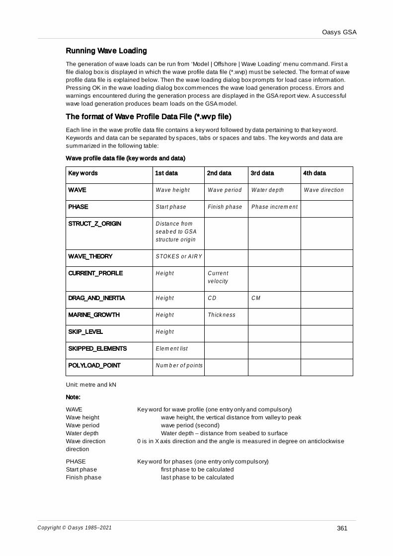
Oasys GSA

Copyright © O as ys 1985–2021 361

Running Wave Loading

The generation of wave loads can be run from ‘Model | Offshore | Wave Loading’ menu command. First a

file dialog box is displayed in which the wave profile data file (*.wvp) must be selected. The format of wave

profile data file is explained below. Then the wave loading dialog box prompts for load case information.

Pressing OK in the wave loading dialog box commences the wave load generation process. Errors and

warnings encountered during the generation process are displayed in the GSA report view. A successful

wave load generation produces beam loads on the GSA model.

The format of Wave Profile Data File (*.wvp file)

Each line in the wave profile data file contains a key word followed by data pertaining to that key word.

Keywords and data can be separated by spaces, tabs or spaces and tabs. The key words and data are

summarized in the following table:

Wave profile data file (key words and data)

Key words 1st data 2nd data 3rd data 4th data

WAVE Wave he igh t Wave pe riod Wate r dep th Wave d irection

PHASE Sta rt phase Fin ish phase Phase increm en t

STRUCT_Z_ORIGIN D istance from

seab ed to GSA

structu re o rig in

WAVE_THEORY STOKES o r AIR Y

CURRENT_PROFILE H e igh t C urren t

ve locity

DRAG_AND_INERTIA H e igh t C D C M

MARINE_GROWTH H eigh t Th ick ness

SKIP_LEVEL H e igh t

SKIPPED_ELEMENTS Elem en t list

POLYLOAD_POINT N um b er o f po in ts

Unit: metre and kN

Note:

WAVE Key word for wave profile (one entry only and compulsory)

Wave height wave height, the vertical distance from valley to peak

Wave period wave period (second)

Water depth Water depth – distance from seabed to surface

Wave direction 0 is in X axis direction and the angle is measured in degree on anticlockwise

direction

PHASE Key word for phases (one entry only compulsory)

Start phase first phase to be calculated

Finish phase last phase to be calculated

Oasys GSA

Copyright © O as ys 1985–2021362

Phase increment phase angle increment

STRUCT_Z_ORIGIN Key word for GSA structure origin (one entry only, if omitted zero is assumed)

Distance from seabed to GSA structure origin, e.g. .if sea-bed is at –60 on GSA coordinates,

STRUCT_Z_ORIGIN should be 60.

WAVE_THEORY Key word for wave theory (one entry only and compulsory)

Either STOKES or AIRY

CURRENT_PROFILE Key word for current profile (as many entries as needed and optional)

Height distance to seabed

Current velocity current velocity at the above given water level

DRAG_AND_INERTIA Key word for drag and inertia coefficients (as many entries as needed and

compulsory)

Height distance to seabed

CD Drag coefficient at the given water depth

CM Inertia coefficient at the above given water level

MARINE_GROWTH Key word for marine growth, radium growth of the tubular members (as

many entries as needed and optional)

Height distance to seabed

Thickness growth thickness at the above given water level

SKIP_LEVEL Key word for elements skip level (one entry only and optional)

Height distance to seabed, elements below this level will be skipped in wave

load calculation

SKIPPED_ELEMENTS Key word for skipped elements (as many entries as needed and optional)

Element list list of the element number that to be skipped in wave load calculation

(refer to the GSA documentation for details of valid element list syntax)

POLYLOAD_POINT Key word for the number of points of the poly-loads (one entry only and optional,

default is 8)

Number of points the number of the generated poly-load points

Example Wave Profile file

!Lines starting with - Lines start with ! are comment lines

!

!Wave wave_height wave_period water_depth direction_angle

WAVE 17.5 13.4 60 90

!

!Phase start_phase end_phase phase_step

PHASE 0 180 45

!

!Struct_Z_origin distance_from_sea_bed_to_GSA_structure_origin

STRUCT_Z_ORIGIN 60

!

!Wave_theory STOKES or AIRY

WAVE_THEORY STOKES

!

! Current profile height current_velocity

CURRENT_PROFILE 0 0.55

CURRENT_PROFILE 100 0.55

!

! Drag and Inertia Height CD and CM

DRAG_AND_INERTIA 0 1 2

DRAG_AND_INERTIA 60 1 2

DRAG_AND_INERTIA 60.1 0.7 2

DRAG_AND_INERTIA 100 0.7 2

!

! Marine_Growth Height Thickness

Oasys GSA

Copyright © O as ys 1985–2021 363

MARINE_GROWTH 0 0.05

MARINE_GROWTH 60 0.05

MARINE_GROWTH 60.1 0

MARINE_GROWTH 100 0

!

SKIP_LEVEL 10

SKIPPED_ELEMENTS 1 to 5

POLYLOAD_POINT 15

5.14 LS-DYNA Analysis

The GSA analysis options are focused on linear and mildly non-linear problems. In some cases it is

necessary to use a more advanced analysis. This can be provided by LS-DYNA. This analysis option

allows the GSA model to be used to create an LS-DYNA analysis

Modelling implications

The key idea is that the GSA model should form the reference model and that the extra data required for an

LS-DYNA model should be included as part of the GSA data. Normally the different attributes required for a

DYNA analysis are assigned by use of an analysis stage.

The key area where LS-DYNA requires more detail is in the material models. To achieve this a number of

LS-DYNA specific material models are included. These are defined in the material wizard, by checking the

DYNA material option

Once the task is created an LS-DYNA keyword file is written and opened in the selected LS-DYNA

environment.

Results

The LS-DYNA results are not copied back to GSA for post-processing.

5.15 Results

5.15.1 Static Analysis Results

The basic results of an analysis are the displacements and rotations at nodes, generally referred to as

displacements. All other results are derived from the displacements. The forces or stresses in elements

depend on the loading on the elements and the displacements at nodes. The force and stress results

available will depend on the element types. The other results at nodes are the reactions. Reactions at

nodes are calculated by looking at all the element forces and the load applied to the node. For an

unrestrained node these should be in equilibrium but for a restrained node the out-of-balance force must

be balanced by the reaction force.

5.15.2 Modal Analysis Results

In a static analysis there is a unique set of displacement results. By contrast, in a modal analysis the

displacements are mode shapes and so can be scaled by any constant and still represent a solution of

the eigenproblem. Some method is required to decide on the scaling of the results and in GSA the results

are scaled so that the maximum translational displacement at any node in the mode is 1m. (If there are no

translation the results are scaled so that the maximum rotation at any node in 1 rad.)

Once the scaling for the modes is fixed there are a number of other results specific to modal analysis.

These are described below.

Dynamic Analysis

Oasys GSA

Copyright © O as ys 1985–2021364

The motivation for a modal dynamic analysis is to characterise the dynamic response of a structure in

discrete modes. Along with the mode shape (the eigenvectors) are the load factors (the natural

frequencies). The “Global Results – Buckling Details” reports the following data:

Frequency

Modal mass

Modal stiffness

Total mass and inertia of structure

Centre of mass

Effective mass and inertia

Participation factors

These terms are defined in the GSA Theory Manual section.

The natural frequencies (f), modal stiffness (k) and modal mass (m) are related as follows:

m

kf

2

1

The effective masses can be used to check that sufficient modes have been chosen to capture the

dynamic behaviour of the structure. In the limit the sum of the effective masses for each of the global

direction should approach the total mass of the structure.

Buckling Analysis

The motivation for a buckling analysis is to characterise the response of a structure, to the given loading, in

discrete modes. Along with the mode shape (the eigenvectors) are the load factors (the eigenvalues). The

“Global Results – Buckling Details” reports the following data:

Load factor

Modal stiffness

Modal geometric stiffness

These terms are defined in the GSA Theory Manual section.

The load factor (λ), modal stiffness (k) and modal geometric stiffness (kg) are related as follows:

gk

k

Note that load factors may be positive or negative. Negative load factors are not a cause for concern,

however if the loads leading to a negative load factor can be reversed the factor will become positive.

5.15.3 Displacements

Displacements (or mode shapes) are calculated at the nodes. When viewing results graphically it is

useful to be able to see deflections at intermediate points on elements. The displacements at these

intermediate points are not stored by calculated as required, from the end conditions on the element and

any load on the element. The number of intermediate points at which these are calculated can be selected

by the user, but GSA will add points that are significant e.g. points at which distortion loads are applied.

Oasys GSA

Copyright © O as ys 1985–2021 365

The magnitude of the displacements in a mode shape is not significant, only the relationship between the

displacements and the modal details.

Displacements can be viewed in a number of ways. The most direct way is to display the deformed

geometry using the D e fo r m ed im age command on the Graphical Display toolbar, but the displacements

can also be displayed as diagrams or contours.

5.15.4 Reactions

Reactions are calculated at constrained nodes. The constraint can be due to a restraint or a spring

support.

Total Loads & Reactions

‘Total loads’ and ‘Total reactions’ represent a sum of all loads and reactions observed in a model.

Moments are reported about the global origin. It is a useful check to monitor that the total loads reported in

a model are approximately in equilibrium with the total reactions. If it is judged that the total loads and

reactions differ significantly, this may in general be a result of two types of error:

1. A load is applied to a degree of freedom that is not active in the model. For example, from applying a

moment to the end of a bar element. In this case the load is reported as being applied, but is ignored by

the solver.

2. The imbalance is as a result of the numerical solution itself. This may be evidence of ill-conditioning.

You can run a model stability analysis to check for disproportionately large stiffnesses.

To help differentiate the difference within a model, an entry ‘Ignored loads’ is reported that accounts for the

first type of error above.

5.15.5 Soil Contact Bearing Pressure

The soil contact bearing pressure is available for output during or after a raft analysis. It is calculated as

the vertical reaction at a node divided by the area of foundation as specified in the Soil Interaction table.

The pressure is reported as zero if the node is restrained in the vertical direction. After the analysis this

situation will only arise if the node has been restrained explicitly. Note, however, that during raft analysis a

temporarily restraint may be applied to a node in order to impose a settlement during the iterative process,

to result in the bearing pressure being reported as zero at that stage in the analysis.

5.15.6 Beam Element Results

5.15.6.1 Displacements and Rotations

Displacements reported are element displacements; element end values may differ from nodal

displacements when the element has end releases or is offset. Such differences are reported in the Beam

End Relative Displacement output, contours, and diagrams.

Element rotations are calculated by interpolation from the element end rotations. The end rotations for an

element are those of the node unless the element end has degrees of freedom that are released. In these

situations the rotation at the end of the element has to be calculated.

The basic equation relating force and displacement for the element if

{f} = [K]{u}

This can be partitioned depending on whether a degree of freedom is released on not.

Oasys GSA

Copyright © O as ys 1985–2021366

f

r

fffr

rfrr

f

r

u

u

KK

KK

f

f

where the subscripts r and f refer to released and fixed respectively. Knowing the forces that result from the

loads on the element and the displacements at the fixed degrees of freedom we can extract the following

equation for the displacements at the released degrees of freedom.

{ur} = [K] ({f

rK

rf]{u

f})

5.15.6.2 Forces

Forces are calculated at the end of beam, bar, tie, strut, cable and spring elements, from the

displacements at the nodes.

Beam element forces may only be output in Local axis directions.

The most commonly used beam force results: Fx axial force diagram, F

z shear force diagram and M

y y

bending moment diagram are available from the Diagrams toolbar.

Intermediate Forces

Forces, and other force based results, along elements are calculated from the end conditions on the

element and any load on the element. The positions at which intermediate forces are reported can be

specified either in terms of a number of equidistant points or by selecting intermediate forces at interesting

points.

Interesting points are determined from the applied loading, as follows.

For moments: an interesting point is located at every point load on the beam and at the ends of every

distributed load. It also places points at a number of equidistant points along distributed loads. In Graphic

Views the number of equidistant points along distributed loads is dependent on the number of elements

currently being displayed: if more than 50 elements are displayed then the number is 3, if less than 5

elements are being displayed (even if there are many more in the whole model) then the number is 19. In

Output Views the number is always 3.

For shear forces: an interesting point is located immediately to either side of every point load on the beam

and of each end of every distributed load.

Sign Convention

The force in the beam at any point is the force required to maintain equilibrium if the beam is cut at that

point and the end 2 part of the beam is discarded. Thus:

Axial forces and stresses are positive when tensile.

For a beam viewed horizontally with its Z-axis pointing vertically up, a positive My y

is hogging.

For a beam viewed horizontally with its Y-axis pointing vertically down, a positive Mzz

is hogging.

This is demonstrated for the following two beams:

Oasys GSA

Copyright © O as ys 1985–2021 367

Drawing a graph of the numerical output of moment and shear force gives:

Drawing bending moment and shear force diagrams in graphics gives:

Sign Convention Definitions

Moment: positive/negative depending on direction of moment relative to axis direction (rotational

direction).

Force: positive/negative depending on direction of force relative to axis direction.

Bending moment diagram: drawn on tension side

Shear force diagram: positive corresponds to negative slope of bending moment diagram where a

bending moment diagram reads from left to right (as viewed) or bottom to top, if vertical.

5.15.6.3 Beam Stresses

Beam stresses are calculated from the forces, moments and the shape of the section. The assumption is

that the stresses are linear through the thickness, so the stresses are incorrect for elements in which yield

has taken place.

Oasys GSA

Copyright © O as ys 1985–2021368

Where beam section properties have been modified from the base values the properties used in the

stress calculation depend on the Stress C a lc. Basis setting for the property. The Stress C a lc. Basis

determines whether the modified or unmodified properties are used and can also be set to result in the

stresses not being calculated.

The beam stresses are as follows:

A – Axial stress

B – Bending stress

C – Combined stress

S – Shear stress

Only axial stresses are output for sections that have properties explicitly defined.

The axial stress is:

area

FA x

For symmetric sections the bending stresses are:

y

zz

zzzz

yy

yyy D

I

MBD

I

MB ,

For non-symmetric sections there is an interaction between the two directions. So a bending stress about

one axis will depend on the moments about both axes. In this case the bending stresses are:

yzzyyyyyz

yzzzyy

z

zzzyzyyzz

yzzzyy

y

DMIMIIII

B

DMIMIIII

B

2

2

1

,1

The combined stresses are:

C1 is the maximum extreme fibre longitudinal stress due to axial forces and transverse bending

C2 is the minimum extreme fibre longitudinal stress due to axial forces and transverse bending

The shear stresses are:

The shear stresses are of most use for steel structures so the shear stresses are calculated based on

the shear area (a reay and a rea z) in BS 5950-1:2000 cl.4.2.3, and they depend on the section shape and if

the section is rolled or welded. The section dimensions are shown below:

Oasys GSA

Copyright © O as ys 1985–2021 369

and a rea is the area of the section. The shear areas are calculated as follows:

Concrete Steel: welded Steel: rolled, formed, etc.

z y z y z y

I section0.8 × D ×t

1.6 × B ×T

d × t 1.8 × B ×T

D × t 1.8 × B × T

Channel 0.8 × D ×t

1.6 × B ×T

d × t 1.8 × B ×T

D × t 1.8 × B × T

Rectang

ular

hollow

1.6 × D ×t

1.6 × B ×T

2 × d × t 1.8 × B ×T BD

Darea

BD

Barea

Rectang

ular

solid

0.8 × area

0.8 × area

0.9 × area

0.9 × area

0.9 × area 0.9 × area

Angle 0.8 × D ×t

0.8 × B ×T

0.9 × d ×t

0.9 × B ×T

0.9 × D × t 0.9 × B × T

Tee 0.8 × D ×t

0.8 × B ×T

d × t 0.9 × B ×T

D × t 0.9 × B × T

Circular

hollow- - 0.6 ×

area0.6 × area

0.6 × area 0.6 × area

Circular

solid0.7 × area

0.7 × area

0.9 × area

0.9 × area

0.9 × area 0.9 × area

Oasys GSA

Copyright © O as ys 1985–2021370

Welded sections are assumed to have weld positions as shown above.

Sections not specified as steel or concrete

For sections not specified as steel or concrete the areas are

zzyy kareaareakareaarea ,

In the case of simple beams where the shear area factor is set to zero the actual area is used giving an

average shear stress value.

Stress measures in beams

The derived stress values output from GSA for beam elements are:

maximum torsional stress

maximum shear stress (y and z)

von Mises stress

for the following section shapes:

rectangular

RHS

circular

CHS

I

Tee

channel

angle

oval

A new property – CT (or W

T) the torsion modulus – is loaded or calculated for these sections.

Torsional stress

Torsional stress is calculated ignoring warping of the section by using the torsion modulus CT (or W

T). We

then get the maximum torsional stress from

Oasys GSA

Copyright © O as ys 1985–2021 371

The values for CT are calculated from "Bautabellen für Ingenieure", Klaus-Jürgen Schneider, (pp 4.30 &

4.31) and "Roark's Formulas for Stress and Strain" (Table 10.7)

Shear Stress

The calculation of the shear stresses SEy

and SEz

are calculated as described in the Technical Note:

Calculation of Shear Areas with the exception of ovals which are calculated from the equation:

n

ba

K 3

2

where K is the shear area factor, n = 1.75 for a<b and 1.5 for a>b, with load being applied in the b direction.

The maximum shear stress = shear force / [K(stress) × total area]. The expression gives a that tends to 2/3

(as for rectangles) for tall, narrow ellipses where b>>a.

von Mises Stress

A precise calculation of the von Mises stress is difficult so a number of simplifications have been made.

The von Mises stress depends on the axial forces, the bending moments, the through thickness shear

forces and the torsional moment.

The axial force and bending moments combine to give σxx

. The shear stresses are a combination of the

through thickness shear + torsion. To combine the shear stresses the through thickness shear stresses

are rotated into components parallel and perpendicular to the surface of the section and the torsional

shear stress is added to the component parallel to the surface.

0~

~T

xz

xy

xz

xy T

The von Mises stress is then calculated from

222 ~3~3 xzxyxxvM

Note: in most cases this is an over estimate of the von Mises stress.

5.15.6.4 Strain Energy Density

The strain energy density for a beam is a measure of how hard the beam is working. Strain energy density

may be output for Beam, Bar, Tie and Strut element types.

The definition of strain energy density is:

For a linear material this is equivalent to:

which represents the strain energy density at a point in the material. For beam elements it is more

Oasys GSA

Copyright © O as ys 1985–2021372

convenient to integrate this over the area (whole or partial) of the section and express the result as strain

energy per unit length. So considering the axial stresses only the extensional (e) and bending (b) strain

energies per length for the section are:

EI

MSE

EA

FSE

b

e

2

22

2

Values of strain energy density may be output for the Web, the Flange or the Total value, though Web and

Flange values are only output for I section and rectangular hollow sections with unmodified section

properties. In the case of rectangular hollow sections “Web” refers to the sides of the section and “Flange”

refers to the top and bottom of the section.

The average strain energy density is the average density along the element or member.

5.15.6.5 Cross Strain Energy Density

The strain energy density for a beam is a measure of how hard the beam is working. The definition of

strain energy density is:

dSED

For a linear material this is equivalent to:

ESED

2

2

A related quantity is the cross strain energy density. The cross terms are calculated from the forces in one

analysis case (i) and the displacements in a different analysis case (j). This can be used to provide

information about how to optimise a structure by indicating where stiffening will be most effective.

The definition of cross strain energy density is:

ji dcSED

This quantity is useful only for linear materials where this is equivalent to:

EcSED

ji

2

For beam elements it is more convenient to integrate this over the area (whole or partial) of the section and

express the result as cross strain energy per unit length. So considering the axial stresses only the

extensional (e) and bending (b) cross strain energies per length for the section are:

Oasys GSA

Copyright © O as ys 1985–2021 373

EI

MMSE

EA

FFSE

ji

b

ji

e

2

2

Values of cross strain energy density may be calculated for the Web, the Flange or the Total value, though

Web and Flange values are only output for I section and rectangular hollow sections with unmodified

section properties. In the case of rectangular hollow sections “Web” refers to the sides of the section and

“Flange” refers to the top and bottom of the section.

Note that unlike strain energy density which must always be a positive value the cross strain energy

density may be negative.

These results differ from most GSA results in that they are not specific to a single analysis case so they

are stored as an Element User Module. Use the “Tools | Cross Strain Energy Density Results” command

to generate the user modules.

5.15.6.6 Torce Lines

Torce lines are identical to thrust lines in plane frames, but in generalising thrust lines for space frames it

is necessary to combine the effects of torsion with the effects of axial force (hence the name).

Eccentricities of the torce, ty and t

z, are given by

x

xyxyz

x

xzxzy

F

FFMMt

F

FFMMt

/ .

/ .

For more details refer to the GSA theory manual.

5.15.7 2D Element Results

5.15.7.1 2D Element Displacements

The element displacements are the displacements of the flexible part of the element. In GSA

displacements are calculated at degrees of freedom which for 2D elements are at nodes. However when

elements are offset the nodal displacements need a transformation to the flexible part of the element.

Element rotations are not reported.

5.15.7.2 2D Element Stress Results

The method of calculating the stresses and forces in 2D elements depends to a certain extent on the

solution method. The stresses are based on the strains, which in turn are based on the displacement

gradients in the element. The stresses are calculated at the Gaussian integration points and then

extrapolated to the nodes. Depending on the solution GSA either calculates the force and moment results

from the stresses or by direct integration through the thickness of the element.

2D element results (forces and stresses) are most conveniently viewed as contours or diagrams.

Oasys GSA

Copyright © O as ys 1985–2021374

Diagrams may be more useful in principal stresses with the direction information are required.

Sign Convention

Membrane stresses are positive when tensile (i.e. positive direct strain).

Positive shear stresses result from positive shear strain.

This is illustrated as follows.

2D Element Stress Sign Convention

Projected and derived stresses

Stresses are a tensor value so there are six possible stress components that can be reported for any

position on the element – three direct stresses and three shear stresses. The x and y stresses are in the

plane of the element and z in the through thickness direction. When a user axis is selected the stresses

are projected on to the plane of the element so that z remains normal to the element surface.

The derived stresses are useful ways of understanding how the element responds to the loading. The

derived stress options are:

principal stresses – stresses rotated so that there no shear stresses showing flow of stress in metals,

concrete

maximum shear

von Mises – a measure of the distortional stress used in yield functions to see how close the material is

to yield ( σy ield

v m

= 0 )

average – checking if material is in overall compression/tension

Details of these are given in the GSA Theory manual.

Limitations of the stress calculation

The stress calculations show more clearly than the displacement calculation the approximate nature of the

finite element method. In particular it should be noted that the stresses are calculated by interpolation

involving an extrapolation from the Gauss points to the nodes. This means that for element with high

stress gradients the interpolated values will be less accurate than for elements with low stress gradients.

It is important to check to see what variation of stress exists over the element and if it is large it may be

necessary to refine the mesh locally to overcome this problem.

Oasys GSA

Copyright © O as ys 1985–2021 375

The stress is calculated on an element by element basis (unlike the displacement) so it is possible, and

in fact very likely, that the stresses at a node in one element will not match up with the stress at the same

node in an adjacent element. In some cases, where there is a discontinuity in the material properties or

the thickness of the elements, it is correct that there is a local stress discontinuity, however in other cases

this stress difference will be a measure of the error in the solution.

When contour plots of the stresses are required, or when a stress value is required for further calculation it

is better to have a single value. The values from all the elements at a node can be averaged to give a

single value at the node. However it should be remembered that the stresses which look smooth and

continuous on the plots are in fact calculated as a series of discontinuous stress patches.

Checking 2D elements stresses

It is useful to be able to carry out some quick checks on the stresses to get an idea of the accuracy of the

analysis. There is no simple answer as to how good an analysis is, but a number of qualitative rules can

be established.

check that the stress gradients are low within the elements, particularly in regions of high stress

check that the stress discontinuities between elements are small — look at the stress errors

5.15.7.3 2D Element Force and Moment Results

When dealing with elements with no thickness (such as fabrics) or composite materials (such as

reinforced concrete) it is more useful to work with stress resultants or forces, than with stresses. For

concrete the stress values are based on the properties of an equivalent isotropic material. The checks

used for stress results noted above can also be applied to force results. For fabric elements the force

resultants are calculated directly but for elements with thickness they are calculated from the in-plane and

bending stresses and the element thickness. Details of these are given in the GSA Theory manual.

The moment per unit length results are a tensor

Mx, My, Mxy

and the force results are a tensor (in-plane forces per unit length)

Nx, Ny, Nxy

and a vector (through-thickness shears per unit length)

Qx, Qy

The Wood-Armer results are derived from the moment terms as follows

M*x = Mx + sgn(Mx ) |Mxy | and

M*y = My + sgn(My) | Myx |

Note that the moment terms follow the Timoshenko convention in which the moment Mx is based on the

stress in the x direction. With the Timoshenko convention if a slab is in compression on the top face in

both the x and y directions the moments are both negative.

Sign Convention

Positive in-plane forces result from positive in-plane stresses.

Positive bending moments result from positive top surface stresses relative to the bottom surface

stress. (This corresponds to the Timoshenko (1964) sign convention.)

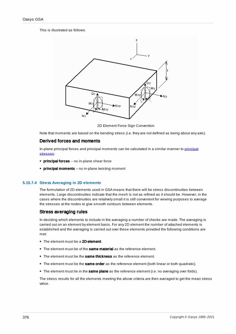
Oasys GSA

Copyright © O as ys 1985–2021376

This is illustrated as follows.

2D Element Force Sign Convention

Note that moments are based on the bending stress (i.e. they are not defined as being about any axis).

Derived forces and moments

In-plane principal forces and principal moments can be calculated in a similar manner to principal

stresses:

principal forces – no in-plane shear force

principal moments – no in-plane twisting moment

5.15.7.4 Stress Averaging in 2D elements

The formulation of 2D elements used in GSA means that there will be stress discontinuities between

elements. Large discontinuities indicate that the mesh is not as refined as it should be. However, in the

cases where the discontinuities are relatively small it is still convenient for viewing purposes to average

the stresses at the nodes to give smooth contours between elements.

Stress averaging rules

In deciding which elements to include in the averaging a number of checks are made. The averaging is

carried out on an element by element basis. For any 2D element the number of attached elements is

established and the averaging is carried out over these elements provided the following conditions are

met:

The element must be a 2D element.

The element must be of the same material as the reference element.

The element must be the same thickness as the reference element.

The element must be the same order as the reference element (both linear or both quadratic).

The element must lie in the same plane as the reference element (i.e. no averaging over folds).

The stress results for all the elements meeting the above criteria are then averaged to get the mean stress

value.

Oasys GSA

Copyright © O as ys 1985–2021 377

Notes on stress averaging

The stress averaging can be used to get the “best” approximation to the stress at the node. However,

stress averaging can also mask poor stress results.

The stress averaging ignores the complexities of the stress field that results from having other elements

attached to the reference element, for example beam framing elements, or 2D stiffening elements.

Stress error

It is useful to be able to quantify the error in the different stress values at nodes. This can be done by

contouring the stress error based on the von Mises stress in the elements meeting at a node. The stress

error is the standard deviation of the element stresses:

n

n

eav

n

22

where n is the number of elements meeting at the node and the summation is over the n elements. The

error reported at the centre of the element is the average of the nodal errors.

5.15.8 3D Element Results

Enter topic text here.

5.15.8.1 3D Element Displacements

The element displacements are the displacements at each node on the element. 3D elements have only

translational degrees of freedom so there are no element rotations.

5.15.8.2 3D Element Stress Results

The stresses in 3Delements are based on the strains, which in turn are based on the displacement

gradients in the element. The stresses are calculated at the Gaussian integration points and then

extrapolated to the nodes.

Derived stresses

Stresses are a tensor value so there are six possible stress components that can be reported for any

position on the element – three direct stresses and three shear stresses. The x and y stresses are in the

plane of the element and z in the through thickness direction. When a user axis is selected the stresses

are projected on to the plane of the element so that z remains normal to the element surface.

The derived stresses are useful ways of understanding how the element responds to the loading. The

derived stress options are:

principal stresses – maximum, minimum and intermediate stresses rotated so that there no shear

stresses showing flow of stress in metals, concrete

maximum shear

von Mises – a measure of the distortional stress used in yield functions to see how close the material is

to yield ( σy ield

v m

= 0 )

average – checking if material is in overall compression/tension

Details of these are given in the GSA Theory manual.

Oasys GSA

Copyright © O as ys 1985–2021378

Limitations of the stress calculation

The stress calculations show more clearly than the displacement calculation the approximate nature of the

finite element method. In particular it should be noted that the stresses are calculated by interpolation

involving an extrapolation from the Gauss points to the nodes. This means that for element with high

stress gradients the interpolated values will be less accurate than for elements with low stress gradients.

It is important to check to see what variation of stress exists over the element and if it is large it may be

necessary to refine the mesh locally to overcome this problem.

The stress is calculated on an element by element basis (unlike the displacement) so it is possible, and

in fact very likely, that the stresses at a node in one element will not match up with the stress at the same

node in an adjacent element. In some cases, where there is a discontinuity in the material properties or

the thickness of the elements, it is correct that there is a local stress discontinuity, however in other cases

this stress difference will be a measure of the error in the solution.

When contour plots of the stresses are required, or when a stress value is required for further calculation it

is better to have a single value. The values from all the elements at a node can be averaged to give a

single value at the node. However it should be remembered that the stresses which look smooth and

continuous on the plots are in fact calculated as a series of discontinuous stress patches.

Checking 3D elements stresses

It is useful to be able to carry out some quick checks on the stresses to get an idea of the accuracy of the

analysis. There is no simple answer as to how good an analysis is, but a number of qualitative rules can

be established.

check that the stress gradients are low within the elements, particularly in regions of high stress

check that the stress discontinuities between elements are small – look at the stress errors

5.15.9 Assembly Results

There are many cases where the modelling requires a single component to be built using many elements

to get the required analysis accuracy, but results are required for the component as a whole. Examples of

this include building cores and trusses.

An Assembly allows a component to considered as a stick and be defined as a collection of elements (a

list), orientation information and result positions.

An assembly can be either straight of curved. A curved assembly can either be defined with a third node on

the arc or by a curve using Lagrange interpolation through a set of nodes. The line or curve joining the

topology items defines the x axis of assembly. An orientation node defines the xy plane of the assembly,

and the local z axis is normal to the x axis and xy plane.

As well as defining the basic assembly it is important to specify where results are required. GSA offers a

number of options for this:

Number of points – the internal result positions are spaced evenly along the assembly.

Spacing of points – the internal result positions are set at the specified spacing.

By storey – the internal result positions correspond to the storeys (for Vertical axis only)

Explicit – the internal result positions are specified directly along the x axis of the assembly.

The results for an assembly are broadly in two categories: displacements and forces. In both cases the

results are calculated for each of the internal positions. At each of these positions a cutting plane is

specified which is normal to the x axis of the assembly. A check is made to see which elements are cut by

Oasys GSA

Copyright © O as ys 1985–2021 379

this plane. These results are then reported or displayed in the graphics for the assembly as a whole.

5.16 Displaying Data and Results

Data and results are displayed in the following formats:

In Output Views, as tables of data.

In Graphic Views, as diagram, contours or labels.

In Chart Views, as graphs.

The topics within this section indicate how different data may be displayed.

5.16.1 Model Data Display Options

Data Type Components (“ all”

unless noted)

Default

axes (n/a

unless

noted)

Axes may

be

transform

ed

Output

Views

Diagram

s

Contours Labels

Titles and Model

Statistics

*

Analysis Task

Details

*

Combination Case

and Envelope

Details

*

Axes *

Global Axes *

Output Axes *

User Axes *

Nodes Global * *

Dots *

Node Numbers *

Constraint Axis

Numbers

*

Restraints and

Supports

* *

Joints * *

Rigid Constraints * *

Constraint

Equations

* *

Tied Interfaces * *

Elements *

Element Numbers *

Oasys GSA

Copyright © O as ys 1985–2021380

Property Numbers *

Group Numbers *

Section Descriptions *

Section Shapes *

Orientation Node Dots *

Orientation Node

Numbers

*

Orientation Angle (total) *

Element Lengths *

Element Releases *

Element x axis *

Element Axes *

Element Principal Axes *

Element Direction

Cosines

Global * *

Members *

Member Numbers *

Property Numbers *

Design Property

Numbers

*

Restraint Property

Numbers

*

Group Numbers *

Section Descriptions *

Section Shapes *

Orientation Node Dots *

Orientation Node

Numbers

*

Orientation Angle (total) *

Member Lengths *

Member Restraints *

Member x axis *

Member Axes *

2D Element Shape

Checks

*

2D Element

Projected Axes

*

Nodal Spring

Property

*

Oasys GSA

Copyright © O as ys 1985–2021 381

RC Beams *

Grid Planes *

Grid Plane Axes *

Standard Materials * * *

User Defined

Materials

* * *

Fabric Materials

Beam Sections *

Area * *

Moment of Inertia, Iy y

Local * *

Moment of Inertia, Izz

Local * *

Torsion Constant, J * *

Shear Factor, Ky

Local * *

Shear Factor, Kz

Local * *

A × Ky

Local * *

A × Kz

Local * *

E × A * *

E × Iy y

Local * *

E × Izz

Local * *

G × J * *

G × A × Ky

Local * *

G × A × Kz

Local * *

Section Descriptions *

Section Shape *

Beam Section

Summary

*

Beam Design

Properties

*

Spring Properties *

Non-linear Spring

Properties

*

Mass Properties *

Mass * *

2D Element

Properties

*

Thickness *

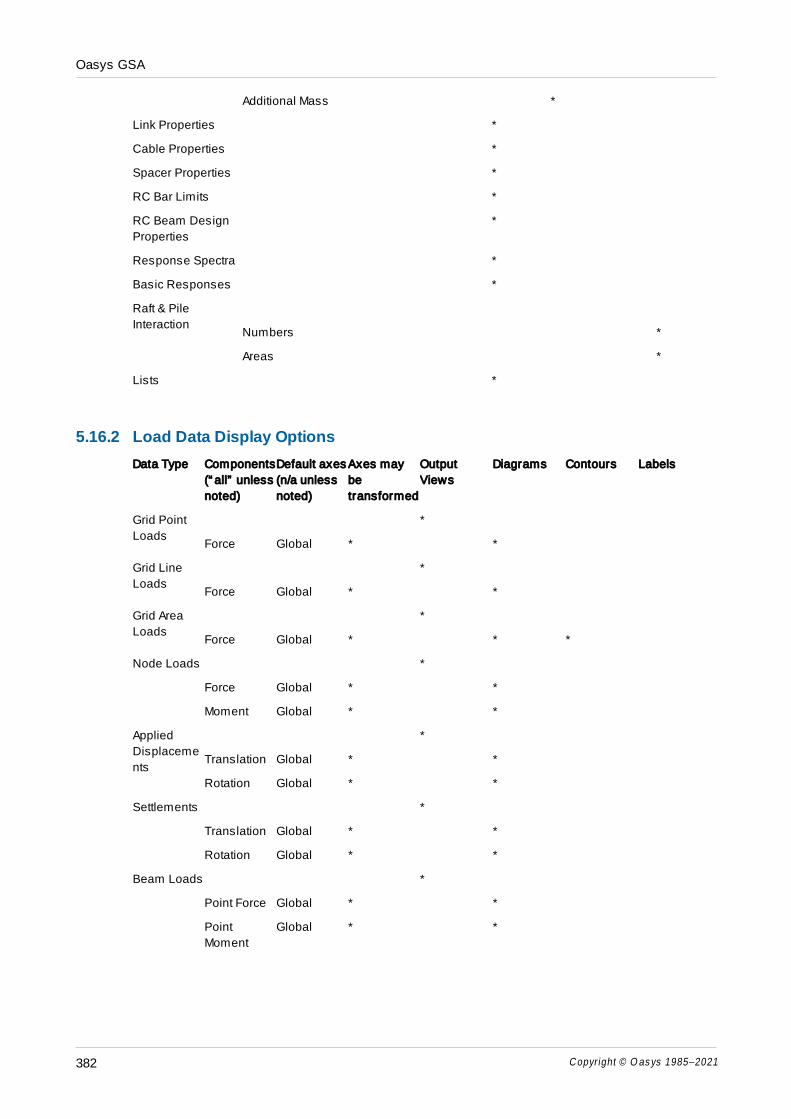
Oasys GSA

Copyright © O as ys 1985–2021382

Additional Mass *

Link Properties *

Cable Properties *

Spacer Properties *

RC Bar Limits *

RC Beam Design

Properties

*

Response Spectra *

Basic Responses *

Raft & Pile

InteractionNumbers *

Areas *

Lists *

5.16.2 Load Data Display Options

Data Type Components

(“ all” unless

noted)

Default axes

(n/a unless

noted)

Axes may

be

transformed

Output

Views

Diagrams Contours Labels

Grid Point

Loads

*

Force Global * *

Grid Line

Loads

*

Force Global * *

Grid Area

Loads

*

Force Global * * *

Node Loads *

Force Global * *

Moment Global * *

Applied

Displaceme

nts

*

Translation Global * *

Rotation Global * *

Settlements *

Translation Global * *

Rotation Global * *

Beam Loads *

Point Force Global * *

Point

Moment

Global * *

Oasys GSA

Copyright © O as ys 1985–2021 383

Patch Force Global * *

Patch

Moment

Global * *

Member

Distortions

*

Translation Global * *

Rotation Global * *

Prestress

Loads

*

Force Global * *

Moment Global * *

Beam

Thermal

Loads

*

Temperature *

Temperature

Gradient

*

2D Element

Face Loads

* * *

2D Element

Edge Loads

* * *

2D Element

Prestress

Loads

*

Force Global * * *

Moment Global * * *

2D Element

Thermal

Loads

*

Temperature * *

Gradient * *

Gravity

Loading

* *

5.16.3 Results Display Options

Data Type Components

(“ all” unless

noted)

Default axes

(n/a unless

noted)

Axes may

be

transformed

Output

Views

Diagrams Contours Labels

Mass Details *

Dynamic

Details

*

Dynamic

Summary

*

Buckling

Details

*

Response *

Oasys GSA

Copyright © O as ys 1985–2021384

Spectrum

Details

Steel Design

Summary

*

Load Factor /

Displaceme

nt

Relationship

*

Axial Force /

Displaceme

nt

Relationship

*

Total Loads

and

Reactions

*

Deformed

Elevation

*

Nodal

Displaceme

nts

Global * * * *

Nodal

Velocities

Global * * (on nodes

& elements)

* * (on nodes

& elements)

Nodal

Acceleration

s

Global * * (on nodes

& elements)

* * (on nodes

& elements)

Reactions Global * * * *

Rigid

Constraint

and Joint

Forces and

Moments

Global * * * *

Nodal

Forces and

Moments

Global * *

Nodal Mass * *

Soil Nodal

Results

(on nodes

& elements)

* (on nodes

& elements)

Footfall

Induced

Vibration

Results

Global (on nodes

& elements)

* (on nodes

& elements)

Nodal Spring

& Mass

Displaceme

nts

Global * * * *

Nodal Spring Global * * * *

Oasys GSA

Copyright © O as ys 1985–2021 385

Forces and

Moments

Beam and

Spring

Displaceme

nts

Local * * * *

Beam End

Relative

Displaceme

nts

Local * *

Beam and

Spring

Forces and

Moments

Local * * *

Beam

Stresses

Local * * *

Beam

Derived

Stresses

Local * * *

Beam

Strains

Local *

Beam Strain

Energy

Density

n/a * * *

Average

Beam Strain

Energy

Density

n/a * * *

Steel

Utilisation

* * *

Torce Lines *

2D Element

Displaceme

nts

* * *

2D Element

Derived

Forces and

Moments

Principal 2D

Moments

*

Principal 2D

Forces

*

Maximum 2D

Moment,

Mmax

* *

Minimum 2D

Moment,

Mmin

* *

Angle to *

Oasys GSA

Copyright © O as ys 1985–2021386

Mmax

Maximum 2D

Force, Nmax

* *

Minimum 2D

Force, Nmin

* *

Angle to

Nmax

*

2D Element

Projected

Moments

2D Moment * *

2D Moment,

Mx

* * *

2D Moment,

My

* * *

2D Moment,

Mxy

* * *

2D Moment, |

Mx|+|Mxy|

* * *

2D Moment, |

My|+|Myx|

* * *

2D Element

Projected

Forces

2D Force * *

2D Through-

Thickness

Shear

*

2D Force, Nx * * *

2D Force, Ny * * *

2D Force,

Nxy

* * *

2D Through-

Thickness

Shear, Qx

* *

2D Through-

Thickness

Shear, Qy

* *

2D Element

Derived

Stresses

2D Stress,

Principal

*

2D Stress,

Max

* *

2D Stress,

Min

* *

Oasys GSA

Copyright © O as ys 1985–2021 387

2D Stress,

Angle to Max

Global * *

2D Stress,

Max Shear

* *

2D Stress,

Von Mises

* *

2D Stress,

Average

* *

2D Element

Projected

Stresses

2D Projected

Stress, xx

Global * * * *

2D Projected

Stress, yy

Global * * * *

2D Projected

Stress, zz

Global * * * *

2D Projected

Stress, xy

Global * * * *

2D Projected

Stress, yz

Global * * * *

2D Projected

Stress, zx

Global * * * *

2D Element

Stress Error

* *

Soil 2D

Element

Contact

Bearing

Pressure

* *

RC Slab

Reinforceme

nt

* * *

Element

Strain

Energy

* *

Assembly

Displaceme

nts

* * *

Assembly

Forces and

Moments

* * *

5.16.4 Bridge Data Display Options

Data Type Components

(“ all” unless

noted)

Default axes

(n/a unless

noted)

Axes may

be

transformed

Output

Views

Diagrams Contours Labels

Oasys GSA

Copyright © O as ys 1985–2021388

Alignments * *

Paths * *

Standard

Vehicles

*

User

Vehicles

*

Standard

Bridge VUDL

*

User Bridge

VUDL

*

Node

Influence

Effects

* *

Beam

Influence

Effects

* *

Path

Loading

*

Static Bridge

Load

*

Moving

Bridge Load

*

5.16.5 Bridge Results Display Options

Data Type Components

(“ all” unless

noted)

Default axes

(n/a unless

noted)

Axes may

be

transformed

Output

Views

Diagrams Contours Labels

Node

Influence

Results

*

Beam

Influence

Results

*

Node

Influence

Lobe Details

*

Beam

Influence

Lobe Details

*

Influence

Lines

*

Oasys GSA

Copyright © O as ys 1985–2021 389

5.16.6 Analysis Stage Data Display Options

Data Type Components

(“ all” unless

noted)

Default axes

(n/a unless

noted)

Axes may

be

transformed

Output

Views

Diagrams Contours Labels

Stage

Definition

*

Stage

Properties

*

5.16.7 User Modules Display Options

Data Type Components

(“ all” unless

noted)

Default axes

(n/a unless

noted)

Axes may

be

transformed

Output

Views

Diagrams Contours Labels

Nodal User

Modules

Nodal User

Modules on

Elements

Element

User

Modules

5.16.8 Analysis Diagnostics: Error norm

Static analysis

In a static analysis the error norm is calculated only when ill-conditioning is suspected. The calculation is

as follows:

Calculate the residual and solver for residual displacements

{fR} = {f u}

{uR} = [K] {f

R}

and then the error is

where

These error norms are reported in the Analysis Details output.

Modal analysis

Oasys GSA

Copyright © O as ys 1985–2021390

In a modal analysis the error norm is always calculated. The calculation for a dynamic analysis is as

follows:

}{

}]{[}{

uK

uMuKe

and for a buckling analysis:

}]{[

}]{[}]{[

uK

uKuKe

g

These are reported in the Analysis Details output.

5.16.9 Numeric formats

The numeric format governs the way that numbers are output in GSA. This is best illustrated by an

example of output of E, ν and ρ for a standard material in the three different formats.

E (N/m²) ν ρ (t/m³)

Engineering 3 sig. figures 205.E+9 7.85

Decimal 2 decimal places 2.0E+11 0.30 7.85

Scientific 4 sig. figures 2.050E+11 7.850

The preferred numeric format is set in the Miscellaneous Preferences. This can be adjusted locally for

Output Views using the Numeric Format button on the Data Options toolbar.

Part VI

Oasys GSA

Copyright © O as ys 1985–2021392

6 Design in GSA

6.1 Concrete Design

All RC calculations are code dependent. Select the appropriate concrete design code via M ode l | D a ta

M odu les | Spec if ic a t ion | D es ign C ode.

6.1.1 RC Slab Reinforcement Design

The RC slab reinforcement design process calculates reinforcement areas for RC slabs modelled using

2D elements of uniform thickness, subject to any combination of in-plane compression and/or shear force

and out-of-plane bending moment and torsion. The process ignores through thickness shear.

Two directions of reinforcement are specified; these need not be orthogonal. Reinforcement areas per unit

width are calculated for each direction at the top and bottom of the slab.

To use these features, reinforcement grade needs to be defined which is referred to by concrete slab

property, concrete slab property should be referred by 2D element property that include concrete material

grade. Concrete design code need to be defined in design specification.

Theory

The input data for calculating reinforcement areas at a node of 2D elements include: forces and moments,

reinforcement directions, section depth and concrete and reinforcement material properties.

RC slab design arrives at a solution by dividing the section into 3 layers each with a certain state of in-

plane stresses. These layered stresses are in equilibrium with the applied loads. The reinforcement

requirements for each layer are then calculated and apportioned to the user specified reinforcement

positions.

The results consist of areas of reinforcement for the top and the bottom of the point in the two specified

directions, if reinforcements cannot be calculated, empty results will be produced that indicates failure due

to inappropriate input data..

Modelling Implications

RC slab reinforcement design is carried out directly on a 2D element model that represents a slab or a

wall. The data required additional to the analysis model data are the Concrete Slab Properties,

reinforcement grade, concrete grade and the selection of an RC Slab design code. Concrete slab property

may be designed before or after analysis.

The design p roperty number in the 2D e lem en ts p roperties table identifies the Concrete Slab Design

Property record associated with the element. Reinforcement is not calculated for elements that do not have

Concrete Slab Design Properties. Refer to Concrete Slab Properties wizard for details of Reinforcement

definition and Calculation definition.

Results

There is no stage at which the user requests a design to be processed. Instead, when the data is correctly

specified to enable the design calculations to be carried out the design results options become available.

The design results are calculated only at the time they are needed for display. The D es ign | C hec k D es ign

D a ta menu command may be used at any stage to establish whether the data has been correctly

specified for RC slab design.

Reinforcement areas can be shown in Graphic Views as contours and diagrams, and in Output Views as

tables of RC Slab Reinforcement. Areas shown with positive values represent tension reinforcement.

Areas shown with negative values represent compression reinforcement.

Occasionally the process fails to produce a result for a particular point in a slab. The reason for such a

Oasys GSA

Copyright © O as ys 1985–2021 393

failure is given in the Output View RC Slab Reinforcement table. Such failures are displayed in contoured

output as out-of-range values, typically displayed black.

6.2 Steel Design

For design to work, it is necessary for Member definitions to be complete and consistent. The

recommended approach for creating a GSA model is to define members first, and then to create elements

from them. This approach is also more efficient when coordinating the GSA model with a BIM model. The

Create Elements from Members tool (under Model | Coordination menu) generates elements from

Members.

Before starting to design members, the following must be ensured.

Restraint Conditions must be defined appropriately.

Members and the corresponding element definitions must be in-sync with each other. The ‘Highlight

inconsistent elements’ display under Graphic settings highlights Members and Elements that are out of

sync.

Steel Members must be appropriately restrained along their length.

Design Task

A Design Task must be set up and executed for designing Members.

Prior to setting to a Design Task, the following must be ensured.

1. The Design code must be specified from ‘Specification | Design Specification’.

2. Design grades available to the project must be populated under ‘Material | Material Grades | Steel’.

3. Populate the Section Library. The ‘Add Catalogue Sections’ and ‘Add Standard Sections’ tool under

‘Model | Section Tools’ can be used to add several section sizes to the library at once.

4. Group Members and assign each group to a Pool. Add Sections into the relevant Pools from the Pool

definition wizard.

5. Set up combination cases.

6. Set up a Design Task.

7. From the Design Task view | Right click menu, choose to either design or check the task.

The Design Task uses a code checker as specified in the Design Specification. The ‘Notes on Code

Checks’ section outlines the checks, design code references and assumptions for each code of practice.

The analysis capabilities allow the user to determine forces and stresses in elements. The steel design

option checks these against the capacity of the members. Steel design is integrated within GSA so that the

design model coexists with the analysis model. Steel design is carried out on the design model using

analysis results to establish the steel utilisation to the selected design code.

M o re:

Tools

Results for steel design

Oasys GSA

Copyright © O as ys 1985–2021394

6.2.1 Generating Steel Member Restraints

In addition to member ends, Steel Members must have either internal restraints or effective lengths

defined to carry out buckling checks across member subspans. There are two ways of assigning Steel

Member Internal restraints.

Manually, by editing them from the Steel Properties page for a given Member. These can then be

propagated to other Members using the Property Pane

Automatically, while a Design Task is executed. When generating restraints automatically, GSA uses the

parameters defined in the Design Specifications.

6.2.2 Member Results

Results returned from checks of members come in a variety of forms.

Verbose text

During the member checks, much of the calculation is written to this part of the result. This is the place to

look if you do not understand any of the other results a member is getting.

Brief text

Contains a summary of the exceptional (bad and interesting) things that have happened during the check.

Summary text

Textual summary of the utilisation ratios and flags that have been set.

M o re:

Steel Member Design: Utilisation ratios

Steel Member Design: Flags

6.2.2.1 Utilisation Ratios

Measures of the utilisation of the member’s capacity. Remember that their values will not be directly

comparable from design code to design code, and that the calculation of some of them is highly non-

linear. If any of them is greater than 1, then the member has failed.

All of the utilisations are the worst of their kind encountered along the member’s length.

Envelopes of utilisation ratios are the maximum and minimum of the utilisation ratios calculated for each

permutation in the envelope.

The ratios available are:

Ratio Comment

Overall worst of all the other utilisation ratios

Local Combined local force/capacity interaction

Local Axial

Local Moment Major local major axis moment

Local Moment Minor local minor axis moment

Local Shear Major

Oasys GSA

Copyright © O as ys 1985–2021 395

Local Shear Minor

Local Torsion

Buckling Combined buckling interaction

Buckling LT lateral torsional buckling

Buckling Axial Major

Buckling Axial Minor

6.2.2.2 Flags

These can give a quick indication of what has happened in the member’s check.

The flags that can be set are:

Flag Name Comments

NOTIFY

WARNING causes NOTIFY to be set

FAIL causes WARNING to be set

NOT CHECKED causes WARNING to be set

FAIL LOCAL cause FAIL to be set

FAIL BUCKLE

FAIL BUCKLE LAT_TORS

FAIL BUCKLE AXIAL MAJOR

FAIL BUCKLE AXIAL MINOR

FAIL LOCAL AXIAL

FAIL LOCAL BENDING MAJOR

FAIL LOCAL BENDING MINOR

FAIL LOCAL SHEAR MAJOR

FAIL LOCAL SHEAR MINOR

FAIL LOCAL TORSION

INFO LOCAL SLENDER cause NOTIFY to be set

INFO LOCAL SLENDER WEB

INFO LOCAL SLENDER FLANGE

INFO MEMBER SLENDER causes WARNING to be set

By necessity, the structure of member results is not design code specific.

Oasys GSA

Copyright © O as ys 1985–2021396

6.2.3 Steel Checks to AISC LRFD

The steel design check supports the AISC LRFD 3rd edition. See Steel Checks to AISC 360 for later

versions.

The input data requirements are the same as for BS5950-1:2000.

The effect sway of frame on the effective length of members has not been considered in member buckling

check.

6.2.4 Steel Checks to AISC 360

The steel design check supports the ANSI/AISC 360-05 and 360-10 ASD and LRFD versions.

All cases provided to the checker are assumed to be factored loads including second order small p-delta

effects. All cases provided to the checker are assumed to be ultimate limit state (i.e. the member forces

are fully factored). Any non ULS cases – e.g. unfactored wind load – will be treated as if they are ULS, and

so will result in non-conservative utilizations.

Definition

Section Classification

Section is classified as Compact, Non-compact and Slender in accordance with AISC360-05 Clause B4

and Table B4.1.

Tension

Section is checked at the ends of every sub-span of the member for the moments and forces acting on it.

Tension capacity at a section is calculated in accordance with AISC360-05 clause D2. Sections in tension

uses the user defined ‘Net Area Ratio’ to compute Net Area and ‘Effective net area factor (Beta)’ to

compute Effective Net Area.

Compression

Compression force is checked in accordance with AISC360-05 Chapter E. Checker uses appropriate

equations depending upon the section shape and local buckling class. Effective length factor for the

members under compression is taken in accordance with the AISC360-05 Table C-C2.2.

Bending

Section is checked for bending in accordance with AISC360-05 Chapter F using appropriate equations.

Shear

Shear is checked according to AISC360-05 Chapter G using appropriate equations. While calculating the

shear strength steel checker assumes that the section web is unstiffened.

Torsion

At present, any significant torsional moment (greater than 5% of the torsional capacity) causes a warning.

Interaction checks

The section is checked against all the applied forces in accordance with AISC360-05 Clause H1 and H2.

Any torsion on the section is ignored from the interaction checks.

Moments used in the interaction check includes the moments due to eccentricity in axial force. Eccentricity

may be due to end connection and due to shift in neutral axis in case of Unsymmetrical slender sections.

Limitations

Limitations are the similar to for BS5950-1:2000. See BS5950-1:2000 Limitations for more details.

Oasys GSA

Copyright © O as ys 1985–2021 397

6.2.5 Steel Checks to AS 4100

The steel design check supports the AS 4100-1998 version

Input data

All cases provided to the checker are assumed to be ultimate limit state (i.e. the member forces are fully

factored). Any non ULS cases – e.g. unfactored wind load – will be treated as if they are ULS, and so will

result in non-conservative utilizations.

Effective Section Properties

Members subjected to bending are classified as Compact, Non-compact and Slender sections in

accordance with AS4100:1998 clause 5.2 and Table 5.2. The effective section modulus is computed using

the appropriate clause from AS4100:1998 5.2.3, 5.2.4 and 5.2.5.

Members subjected to axial compression are classified as Compact, Non-compact and Slender sections

in accordance with AS4100:1998 clause 6.2.3

Local Checks

Sections are checked at the ends of every sub-span of the member for the moments and forces acting on

it.

Shear

Shear is checked according to AS4100:1998 clause 5.11. While calculating the shear strength steel

checker assumes that the section web is unstiffened.

The shear area is calculated based on clear web depth between flanges for the welded sections, and

based on full web depth for rolled section. For RHS and Box sections the shear area is based on two clear

web depths.

Shear capacities are reduced to account for moment in the direction of shear force according to

AS4100:1998 5.12.3

Bending moment

Moment capacity at a section is calculated in accordance AS4100:1998 clause 5.2.1. See Effective Section

Properties for details on calculation of effective section modulus.

Axial Force

Compression capacity at a section is calculated in accordance with AS4100:1998 clause 6.2.1. See

Effective Section Properties for details on calculation of effective area of section.

Tension capacity at a section is calculated in accordance with AS4100:1998 clause 7.2 and 7.3. Sections

in tension use the user defined ‘Net Area Ratio’.

Torsion

At present, any significant torsional moment (greater than 5% of the torsional capacity) produces a

warning.

Combined local effects

The section is checked against all the applied forces using the equations in AS4100:1998 clause 8.3.4.

The choice of equations used depends on the section shape and the section’s local buckling class.

Moments used in the local interaction check include the moments due to eccentricity in axial force.

Eccentricity may be due to end connection and to shift in neutral axis in case of Unsymmetrical slender

sections.

Buckling Checks

Oasys GSA

Copyright © O as ys 1985–2021398

Axial Buckling

The member is checked along its length for major axis axial buckling and minor axis axial buckling

according to AS4100:1998 clause 6.3.3.

Unsymmetrical sections are also checked for torsional and flexural torsional buckling according to

AS4100:1998 clause 6.3.3. Lambda value will be computed in accordance with clause 6.3.4.

At present the effective length of the member is calculated from the factors available in AS4100:1998

Figure 4.6.3.2.

Lateral Torsional Buckling

Members with full lateral restraint are checked for Lateral torsional buckling in according to AS4100:1998

clause 5.3. Lateral restraints are verified in accordance with AS4100:1998 clause 5.3.2.

Lateral torsional buckling is checked in accordance with AS4100:1998 clause 5.6.1 and 5.6.2(i) for the

member without continuous restraints. Effective lengths for lateral torsional buckling are calculated

according to AS4100:1998 clause 5.6.3.

Buckling Interaction

Interaction checks are carried out according to AS4100:1998 clause 8.4.5.1 and 8.4.5.2 for compression

and tension members respectively. Reduced moments used in compression member checks are

calculated using the simplified equations in AS4100:1998 clause 8.4.2.2 and 8.4.4.1.

6.2.6 Steel Checks to BS 5950-1

The steel design check supports the BS 5950-1:2005 edition.

Input data

All cases provided to the checker are assumed to be ultimate limit state (i.e. the member forces are fully

factored). Any non ULS cases – e.g. unfactored wind load – will be treated as if they are ULS, and so will

result in non-conservative utilizations.

This section explains particular (non-obvious) significances of input data to the BS5950-1:2000 member

checker. See Step By Step Guide: Steel Design and the Steel Member Design chapter for general steel

design input requirements.

Max Plastic/Elastic Ratio

In order to limit the effects of plasticity at the serviceability limit state (SLS), the design code limits the

maximum benefit that can be obtained at the ultimate limit state from allowing the section to become

plastic in bending. To comply with BS5950-1:2000 4.2.5.1, the limit should be set to 1.2 for simply

supported members and cantilevers, and 1.5 for members with moment continuity between spans. If the

ratio is set to 0, the checker will assume 1.2 (which is the more conservative choice available).

Single Angle Struts

BS5950-1:2000 4.7.10.2 and Table 25 make reference to the A-A, B-B and V-V axes in relation to axial

buckling. The V-V axis is the minor principal axis. The AA and BB axes are the X-X and Y-Y axes, but which

is which depends on the design of the connections of the member to the rest of the structure. The checker

only knows about the applied member restraints.

The rotational restraint applied by a two bolt group in clearance holes in one leg ( clause 4.7.10.2 (a) )

should be represented by restraining the section:

Oasys GSA

Copyright © O as ys 1985–2021 399

fully about the axes of the bolts, and

partially about an axis perpendicular to the bolts and the member.

The rotational restraints applied by a two bolt group, one of which uses a kidney shaped hole should be

represented by restraining the section:

partially about an axis perpendicular to the bolts and the member.

The rotational restraint applied by a single bolt group should be represented by leaving the member free

about both the X-X and Y-Y axes.

The local capacity check needs to know which legs are connected at the location of the check ( clause

4.6.3.1 ). This information is partly provided by the rotational restraints if they are applied as above. In

cases of ambiguity, the connection restraint settings are used. Restraint settings “A” and “B” imply that

legs A and B respectively are connected. Where both legs are connected, both “A” and “B” should be set.

Even if “A” and/or “B” are not set, the checker can often make assumptions using the rotational restraints

alone. Examples of connections requiring use of “A” and “B” include all those consisting of a single bolt

through either leg.

Local Checks

At each end of each subspan (LH and RH), the member’s section is checked for the moments and forces

applied to it.

Plastic, compact. semi-compact and slender sections are supported.

Allowance for slenderness is made by the use of effective section properties, and the full design stress,

which is considerably less conservative than the adoption of a lowered design stress in conjunction with

the gross section properties (as used by the Blue Book [19]).

Depending on the section’s properties, the method of checking may vary. For example, if the section is

doubly-symmetric and compact or plastic, biaxial bending may be checked using the Mrx

and Mry

method

which reduces the moment capacities with increasing axial load.

Shear

Shear is checked only if the section’s web(s) are not slender. Warning is given if the section is slender in

shear.

Bending moments

Moments are conservatively enhanced if slenderness leads to the effective centroid of the section moving,

and axial force is present.

Mcx

and Mcy

are always calculated (reduced by coincident shears in either direction), and compared with

the applied moments. The interaction of transverse shear is not covered by BS5950-1:2000 (which is

therefore potentially non-conservative). This deficiency is rectified by the use of a Von Mises type capacity

reduction. Shear force parallel to webs in bending is considered in accordance with BS5950-1:2000.

Mrx

and Mry

(moment capacities with coincident axial force) are calculated for plastic and compact doubly

symmetric sections, and compared with the applied moments. They are not reduced by coincident shears.

For this reason, their use is inhibited by “high” shears: (Fv>0.6P

v) in either direction.

Axial force

Sections in tension use the user controllable Net Area Ratio to determine net area.

Slenderness is calculated differently for sections in overall tension, than for sections in compression.

Torsion

Oasys GSA

Copyright © O as ys 1985–2021400

At present, any significant torsional moment (greater than 5% of the torsional capacity) causes a warning,

because torsion is not explicitly catered for by the code. The torsional capacity is calculated as follows: (1)

CHS - thin wall theory is used; (2) RHS - thin wall theory is used but warping restraint is ignored; (3) I

section - based on formulas in Table 10.7 in the book of “Roark’s Formulas for Stress and Strain”.

Combined local effects

The section is checked against all the applied forces (except torsion) using the appropriate equations in

BS5950-1:2000 4.8.2 and 4.8.3. The choice of equations depends on the section shape and the section’s

local buckling class.

Buckling Checks

The member is checked along its length for major axis axial buckling, minor axis axial buckling and LT

buckling in turn. Once complete, relevant interactions of the buckling modes are considered.

Individual buckling mode checks

Each buckling mode check searches for appropriate buckling spans using the design restraints that have

been applied to the member. Each buckling span is checked individually. Cantilever spans at either end of

members are recognized and catered for.

The effective buckling length calculated can be overridden to either a multiple of the member length or to

an absolute length. If this is done, the whole member length is used for determination of buckling

parameters, such as equivalent uniform moment factors and applied axial forces.

Buckling interaction

During checks for the simple buckling modes (axial/major axis, axial minor axis, and LT) note is made of

various parameters needed later when the buckling interaction check is carried out. These parameters are

stored for each sub-span of the member. (See BS5950-1:2000 4.8.3.3)

The parameters are:

Fcx

– maximum axial compression in the major axis buckling span

Fcy

– maximum axial compression in the minor axis buckling span

Mb1

– major axis bending moment capacity in the LT span

Mb2

– opposite sense moment capacity in the LT span (for reverse curvature spans)

MLT1

– maximum applied major axis bending moment in the LT span

MLT2

– opposite sense major axis bending moment in the LT span (for reverse curvature spans)

Mx – maximum major axis moment in the major axis buckling span

My – maximum minor axis moment in the minor axis buckling span

Pcx

– major axis axial buckling capacity

Pcy

– minor axis axial buckling capacity

Zx – section modulus about major axis

Zy – section modulus about minor axis

mLT

– equivalent uniform moment factor for major axis moment in relevant LT span

Oasys GSA

Copyright © O as ys 1985–2021 401

mx – equivalent uniform moment factor for major axis moment in the major axis axial span

my – equivalent uniform moment factor for minor axis moment in the minor axis axial span

my x

– equivalent uniform moment factor for minor axis moment in the major axis axial span

py – design stress for the section

The checker steps through the sub-spans looking at this interaction data. It only carries out an interaction

check once for each permutation of buckling spans, to reduce the volume of output.

Interaction is carried out according to clauses BS5950-1:2000 4.8.3.3.1, 4.8.3.3.2 and 4.8.3.3.3 depending

on the section shape. The variant (c) that allows biaxial bending moments is always used, even when

there is only bending about a single axis.

Limitations

Torsion not fully considered.

Unsymmetrical sections not yet supported.

Mixed steel grades in single section not yet supported.

Weld material disregarded in assessment of section properties.

Web high-shear buckling treated conservatively in respect of web capacity.

Whole structure stability issues are not considered, since the checker only knows about one member at

a time. Users must construct their models to account for these effects if appropriate.

6.2.7 Steel checks to CSA S16

The steel design check supports the CSA S16-09 and S16-14 editions.

6.2.8 Steel Checks to EN 1993

The steel design check supports the EN 1993-1-1:2005 edition. EN 1993 or Eurocode 3 provides the basic

code and is supplemented by National Annexes to allow for variations from one country to another.

Input data

All cases provided to the checker are assumed to be ultimate limit state (i.e. the member forces are fully

factored). Any non ULS cases – e.g. unfactored wind load – will be treated as if they are ULS, and so will

result in non-conservative utilizations.

Effective net area factor (β)

For angles connected through one leg, the tensile strength of a section is affected by shear lag. To comply

with EN 1993-1-8:2005 3.10.3 the Effective net area factor (Beta) is used to compute the design tensile

strength. This factor is calculated for a single bolt. The effect of shear lag in tension is ignored for

members with other section shapes.

Single Angle Struts

Oasys GSA

Copyright © O as ys 1985–2021402

When considering Member Restraints for angle sections EC3 interprets restraint settings “A” and “B” as

relating to the longer and shorter leg respectively. Where both legs are connected, both “A” and “B” should

be set.

Local Checks

Sections are checked at the ends of every sub-span of the member for the moments and forces acting on

it.

Checks are carried out for Class 1, Class 2, Class 3 and Class 4 sections. Local buckling effects for

Class 4 sections are included by an effective width in accordance with EN 1993-1-5.

For Class 4 CHS sections a reduced yield stress is used to account for local buckling.

For Channel and Tee sections elastic section verification is used.

Shear

Shear is checked according to EN 1993-1-1:2005 clause 6.2.6 if the section’s web(s) are not slender. A

warning is given if the section is slender in shear.

Bending moment

Moment capacity is calculated in accordance with EN 1993-1-1:2005 clause 6.2.5 and compared with the

applied moments. Allowance is made for shear and torsion in moment capacity according to EN 1993-1-

1:2005 6.2.8.

Moment capacities are reduced for Class 1 and Class 2 sections to account for axial force as per EN

1993-1-1:2005 6.2.9.1.

Axial force

Compression and tension capacities are calculated in accordance with EN 1993-1-1:2005 6.2.4 and 6.2.3

respectively and compared with the applied axial force. For sections in tension the user defined ‘Net Area

Ratio’ and ‘Effective net area factor (Beta)’ are used to determine tension capacity.

Torsion

At present, any significant torsional moment (greater than 5% of the torsional capacity) produces a

warning. See BS5950-1:2000 for more details.

Combined local effects

The section is checked against all the applied forces using the equations in EN 1993-1-1:2005 6.2.9 and

6.2.10. The choice of equations depends on the section shape and the section’s local buckling class.

Buckling Checks

The member is checked along its length for major axis axial buckling, minor axis axial buckling, torsional

buckling, flexural torsional buckling and lateral torsional buckling. Interaction checks are carried out

according to EN 1993-1-1:2005 6.3.3; see National Annexes for interaction factors. See BS5950-1:2000 for

more details on buckling checks.

Limitations

Section classification is based on axial force and major axis bending moment. Minor axis bending

moment is disregarded.

Shear lag effects are not considered in bending.

Elastic critical moment for lateral-torsion buckling is calculated in accordance with Annex I of EN 1999-1-

1:2007. When the loads on the member are not found in the appropriate table of Annex I of EN 1999-1-

1:2007, the worst values of C1, C2 and C3 are taken from the appropriate table assuming the ends are

pinned.

Oasys GSA

Copyright © O as ys 1985–2021 403

Transverse load checks not yet supported.

Slender Angle sections not yet supported.

Refer BS5950-1:2000 for other limitations.

6.2.8.1 EN 1993 National Annexes

The following nationally defined parameters are used.

EN 1993-1-1:2005 Eurocode 3 (generic):

The following parameters are used for design checks to EN 1993-1-1:2005 Eurocode 3.

Clause 6.1 (1)

γM0

= 1.00, γM1

= 1.00 and γM2

= 1.25

Clause 6.3.2.2.

Table 6.3 is used for imperfection factors.

Clause 6.3.2.3 (1)

λLT,0

= 0.4, β = 0.75 and table 6.5 of EN 1993-1-1:2005 are used for the lateral torsional

buckling curve. For the sections not available in the table, buckling curve d is used.

Clause 6.3.2.3 (2)

f = 1-0.5(1-kc)[1-2.0(λ

LT-0.8)2] and f <= 1.0; Table 6.6 are used for the correction

factor kc.

Interaction factors:

Annex B is used for interaction factors. For other than doubly symmetric sections, the λ

value used for calculating interaction factors in any direction (say λx or λ

y) is the largest

value of the following three

1) λx or λ

y depending on the direction.

2) λT for torsion.

3) λTF

for flexural torsion.

Table B.3 is used for equivalent uniform moment factors; steel checker assumes that the

spans are loaded with uniform loading.

Effective Length:

Effective buckling lengths for flexural buckling are calculated in accordance with Table 22

of BS5950-1:2000.

BS EN 1993-1-1:2005 Eurocode 3 (GB):

The following parameters are used for design checks to the UK National Annex to EN 1993-1-1:2005

Eurocode 3.

Clause 6.1 (1)

Oasys GSA

Copyright © O as ys 1985–2021404

γM0

= 1.00, γM1

= 1.00 and γM2

= 1.10

Clause 6.3.2.2.

Table 6.3 is used for imperfection factors.

Clause 6.3.2.3 (1)

For rolled sections and hot-finished and cold-formed hollow sections:

λLT,0

= 0.4 and β = 0.75

Welded sections:

λLT,0

= 0.2 and β = 1.00

Table in clause 2.17 of UK NA to EN 1993-1-1:2005 is used for the lateral torsional

buckling curve. For the sections not available in the table, buckling curve d is used.

Clause 6.3.2.3 (2)

Clause NA 2.18 is used to calculation modification factor, f.

Interaction factors:

As for Eurocode 3 (generic).

Effective Length:

Effective buckling lengths for flexural buckling are calculated in accordance with Table 22

of BS5950-1:2000.

BS EN 1993-1-2:2005 (fire) Eurocode 3 (GB):

The following parameters are used for design checks to the UK National Annex to EN 1993-1-1:2005

Eurocode 3.

...

DIN EN 1993-1-1:2005 Eurocode 3 (DE):

The following parameters are used for design checks to the German National Annex to EN 1993-1-1:2005

Eurocode 3.

Clause 6.1 (1)

γM0 = 1.00, γM1 = 1.10 and γM2 = 1.25

Clause 6.3.2.3 (2)

The coefficient f is calculated as for Eurocode 3 (generic).

I.S. EN 1993-1-1:2005 Eurocode 3 (IE)

The following parameters are used for design checks to the UK National Annex to EN 1993-1-1:2005

Eurocode 3.

...

Oasys GSA

Copyright © O as ys 1985–2021 405

NEN-EN 1993-1-1:2005 Eurocode 3 (NL):

The following parameters are used for design checks to the Netherlands National Annex to EN 1993-1-

1:2005 Eurocode 3.

Clause 6.1 (1)

γM0

= 1.00, γM1

= 1.00 and γM2

= 1.25

Clause 6.3.2.2.

Table 6.3 is used for imperfection factors.

Clause 6.3.2.3 (1)

λLT,0

= 0.4, β = 0.75 and table 6.5 of EN 1993-1-1:2005 are used for the lateral torsional

buckling curve. For the sections not available in the table, buckling curve d is used.

Clause 6.3.2.3 (2)

f = 1-0.5(1-kc)[1-2.0(λ

LT-0.8)2] and f <= 1.0; Table 6.6 are used for the correction

factor kc.

Interaction factors:

As for Eurocode 3 (generic) .

Effective Length:

Effective buckling lengths for flexural buckling are calculated in accordance with clause

12.1.1.3 of NEN 6770.

Other checks:

In addition to the EN 1993-1-1:2005 checks, the following checks are performed.

1) Combined bending, axial and shear force is checked in accordance with the

clause 11.3.1.1 to 11.3.1.3 of NEN 6770

2) Biaxial bending interaction is checked in accordance with the clause 11.3.2.1 to

11.3.2.3 of NEN 6770.

NF EN 1993-1-1:2005 Eurocode 3 (FR):

The following parameters are used for design checks to the French National Annex to EN 1993-1-1:2005

Eurocode 3.

Clause 6.1 (1)

γM0

= 1.00, γM1

= 1.00 and γM2

= 1.25

Clause 6.3.2.2.

Table 6.3 is used for imperfection factors.

Clause 6.3.2.3 (1)

For rolled sections (I or H sections):

λLT,0

= 0.2+0.1(b/h), αLT

= 0.4-0.2(b/h)λLT

2 >= 0 and β = 1.0

Welded sections (doubly symmetric I sections):

Oasys GSA

Copyright © O as ys 1985–2021406

λLT,0

= 0.3(b/h), αLT

= 0.5-0.25(b/h)λLT

2 >=0 and β = 1.0

Clause 6.3.2.3 (2)

The coefficient f is calculated as for Eurocode 3 (generic).

Note: The coefficient f is only applicable to the members without intermediate lateral

restraints and no warping at the ends.

Interaction factors:

Annex A is used for interaction factors.

For other than doubly symmetric sections:

a) The χ value used in interaction equations in any direction (say χx or χ

y) is the

smallest value of the following three

1) χx or χ

y depending on the direction.

2) χT for torsion.

3) χTF

for flexural torsion.

b) Elastic verification is used in the interaction

c) The equivalent uniform moment factor is limited to Cmi,0

>= 1-(NEd

/Ncr,i

)

Effective Length:

Effective buckling lengths for flexural buckling are calculated in accordance with Table 22

of BS5950-1:2000.

Elastic Critical Moment (Mcr):

For doubly symmetric I sections:

Mcr is calculated in accordance with the Annex MCR of NF EN 1993-1-1:2005.

The factors C1 and C2 are taken from Table1 and Table2 of the Annex MCR.

Mcr is calculated in accordance with clause 6.2.1.4 of “The behaviour and

design of steel structures to EC3” by Trahair et al. for the loading types not

specified in the Annex MCR.

For other sections:

Elastic critical moment for lateral-torsion buckling is calculated in accordance

with Annex I of EN 1999-1-1:2007

SS EN 1993-1-1:2010 Eurocode 3 (SG)

The Singapore N.A. to Eurocode 3 i.e. “EN 1993-1-1:2010 Eurocode 3 (SS)” is identical to UK National

Annex to EN 1993-1-1:2005 Eurocode 3.

Oasys GSA

Copyright © O as ys 1985–2021 407

6.2.9 Steel Checks to HKSUOS

The steel design check supports the Hong Kong Code of Practice 2005 and 2011 editions.

Input data

All cases provided to the checker are assumed to be ultimate limit state (i.e. the member forces are fully

factored). Any non ULS cases – e.g. unfactored wind load – will be treated as if they are ULS, and so will

result in non-conservative utilizations.

Effective Section Properties

Members are classified as Class 1, Class 2, Class 3 and Class 4 sections in accordance with

HKSUOS:05 Table 7.1 and 7.2. The channel webs are classified according to BS5950-1:2000 Table 11

since HKSUOS:05 does not specify the same. Effective section properties are calculated according to the

appropriate clause from HKSUOS:05 clause 11.3.4. For flanges with non-uniform compression the

effective width of the plate is calculated according to EN 1993-1-5:2006 clause 4.4.

Effective Plastic Modulus

Class 3 semi-compact sections subjected to bending are designed using effective plastic modulus

according HKSUOS:05 clause 7.5.

Local Checks

Sections are checked at the ends of every sub-span of the member for the moments and forces acting on

it.

Shear

Shear is checked according to HKSUOS:05 clause 8.2.1. Shear is checked only if the section’s web(s) are

not slender. A warning is given if the section is slender in shear.

Bending moment

Moment capacity at a section is calculated in accordance with HKSUOS:05 clause 8.2.2. See Effective

Section Properties for details on calculation of effective section modulus.

Moments are conservatively enhanced if slenderness or end connection leads to the effective centroid of

the section moving, and axial force is present.

Moment capacities are reduced to take account of high shear according to HKSUOS:05 clause 8.2.2.2 and

compared with the applied moments.

Axial Force

Compression capacity at a section is calculated in accordance with HKSUOS:05 clause 8.9.1. See

Effective Section Properties for details on calculation of effective area of section.

Tension capacity at a section is calculated in accordance with HKSUOS:05 clause 8.6. Sections in tension

use the user defined ‘Net Area Ratio’.

Torsion

At present, any significant torsional moment (greater than 5% of the torsional capacity) produces a

warning.

Combined local effects

The section is checked for interaction of axial, shear and moments using the equations in HKSUOS:05

clause 8.9.1 and 8.2.1.

Moments used in the local interaction check include the moments due to eccentricity in axial force.

Eccentricity may be due to end connection and to shift in neutral axis

Oasys GSA

Copyright © O as ys 1985–2021408

Buckling Checks

Axial Buckling

The member is checked along its length for major axis axial buckling and minor axis axial buckling

according to HKSUOS:05 clause 8.7. Unsymmetrical sections are checked for torsional and flexural

torsional buckling according to the HKSUOS:05 clause 8.10. At present the effective length of the member

is calculated from the factors available in HKSUOS:05 Table 8.6 based on the restraints on the member;

this value can be overridden from the steel design properties.

Torsional and Flexural-Torsion Buckling

Unsymmetrical sections are checked for torsional and flexural torsional buckling according to the

HKSUOS:05 clause 8.10

Lateral Torsional Buckling

Lateral torsional buckling is checked in accordance with HKSUOS:05 clause 8.3, Appendix 8.1.and

Appendix 8.2.

Appendix 8.2 provide guidance to calculate λLt

for uniform I, H and channel with equal flanges. It also

suggested to use recognized buckling analysis for other section shapes. Currently BS5950-1:2000

formulations are using to calculate λLt

for RHS and T sections.

Buckling Interaction

Interaction checks are carried out according to HKSUOS:05 clause 8.9.2. Since it is assumed that the

analysis results are inclusive of second order p - small delta analysis, the amplification factor is ignored

for non-sway frame members.

6.2.10 Steel Checks to IS 800

The steel design check supports the IS 800 1984 and 2007 working stress method editions.

Input data and requirements

All cases provided to the checker are assumed to be working loads.

IS800:1984 does not use Max Plastic/Elastic Ratio specified in the design property.

For Member Restraints, IS800:1984 interprets connection A and B in the following manner.

For angle sections A and B stand for longer, shorter leg respectively. Where both legs are connected,

both A and B should be set.

For I and RHS sections, A stands for the web and B for flange.

Local Checks

Following Local checks or Section checks are carried out at each end of each subspan.

Shear strength check

Shear is checked only for unstiffened webs. A warning is generated if the web is slender as per

IS800:1984 6.7.3.1. Shear is check to Clause 6.4.1 and 6.4.2.

Torsion checks

At present, any significant torsional moment (greater than 5% of the torsional capacity) causes a warning,

because torsion is not explicitly catered for by the code. See BS5950-1:2000 local checks for details.

Oasys GSA

Copyright © O as ys 1985–2021 409

Bearing capacity checks

At present, bearing capacity checks are ignored.

Axial and bending strength checks

Axial tensile, compressive and bending strength checks are carried as per section 4, 5 and 6 of

IS800:1984 respectively without considering the effect of buckling (only local).

Combined local effects

The section is checked against all the applied forces (except bearing) using the appropriate equations in

IS800:1984 7.1.1.b, 7.1.2 and 7.1.4.

Buckling Checks

Following Buckling checks or member checks are carried out at for every member. See BS5950-1:2000

buckling checks for details.

Major and Minor axis axial buckling strength check

Axial compression strength checks will be carried along major axis and minor axis as per the section 5 of

IS800:1984.

Lateral Torsion buckling strength check

The member is checked against lateral torsion buckling strength as per IS800:1984 6.2.3 and 6.2.4.

Buckling interaction strength check

These checks are carried out for the appropriate equations stipulated in section 7 of IS800:1984.

IS800:2007 (Working stress method)

The input data requirements and checks that are the similar to for BS5950-1:2000. See BS5950-1:2000 for

more details

Effective Net Area Factor (β)

The rupture strength of a section connected through one or more elements of section is affected by shear

lag. To comply with IS800:2007 6.3.3 and 6.3.4, the Effective net area factor (Beta) is used to compute the

design tensile strength of such sections to account for tearing of net section.

6.2.11 Steel Checks to SANS 10162-1

The steel design check supports the SANS 10162-1:2011 edition.

Input data

All cases provided to the checker are assumed to be ultimate limit state (i.e. the member forces are fully

factored). Any non ULS cases – e.g. unfactored wind load – will be treated as if they are ULS, and so will

result in non-conservative utilizations.

Effective Section Properties

Members are classified as Class 1, Class 2, Class 3 and Class 4 sections in accordance with SANS

10162-1:2011 Table 3 and 4.

Effective section area is calculated in accordance with SANS 10162-1:2011 clause 13.3.3.

Oasys GSA

Copyright © O as ys 1985–2021410

Effective section modulus for the section with class 3 or better web and class 4 flange is calculated in

accordance with SANS 10162-1:2011 clause 13.5. If the web is class 4 and flange is class 3 or better then

the revised factored moment of resistance is calculated in accordance with SANS 10162-1:2011 clause

14.3.4. Checker doesn’t support the section if both the flange(s) and web are class 4.

Local Checks

Sections are checked at the ends of every sub-span of the member for the moments and forces acting on

it.

Members with Angle sections are treated as strut and tie only member and the shear and moment

capacities are assumed as zero.

Shear

For the webs of section with two flanges shear capacity is calculated using elastic analysis in accordance

with SANS 10162-1:2011 clause 13.4.1.1. This clause applies for I,Channel sections with shear acting

along the web and also for RHS sections.

For all other cases maximum shear stress is calculated in the section and compared with 0.66*phi*fy. The

effect of shear buckling is not considered and this is non-conservative.

Bending moment

Moment capacity at a section is calculated in accordance with SANS 10162-1:2011 clause 13.5 and clause

14.3.4. See Effective Section Properties for details on calculation of effective section modulus. Moment

capacity of a section is assumed as zero whose flanges and web are class 4

Moments are conservatively enhanced if slenderness or end connection leads to the effective centroid of

the section moving, and axial force is present.

Axial force

Compression capacity at a section is calculated in accordance with SANS 10162-1:2011 clause 13.3.1

and 13.3.4 and assuming member length as zero. See Effective Section Properties for details on

calculation of effective area of section.

Tension capacity at a section is calculated in accordance with SANS 10162-1:2011 clause 13.2. Sections

in tension use the user defined ‘Net Area Ratio’.

Torsion

At present, any significant torsional moment (greater than 5% of the torsional capacity) produces a

warning.

Combined local effects

The section is checked for interaction of axial and moments in accordance with SANS 10162-1:2011

clause 13.8.2 (b) and 13.8.3 (b).

Moments used in the local interaction check include the moments due to eccentricity in axial force.

Eccentricity may be due to end connection and to shift in neutral axis.

Buckling Checks

Axial buckling

The member is checked along its length for major axis axial buckling and minor axis axial buckling

according to SANS 10162-1:2011 clause 13.3.1

Singly symmetric and unsymmetrical sections are also checked for torsional and flexural torsional

buckling according to SANS 10162-1:2011 clause 13.3.2. Doubly symmetric sections are checked for

torsional buckling in accordance with SANS 10162-1:2011 clause 13.3.2 (a).

Oasys GSA

Copyright © O as ys 1985–2021 411

SANS 10162-1:2011 Annex E (Figure E.1) is referred to estimate effective length factor using the restraint

condition.

Bending laterally unsupported members

Lateral torsional buckling is checked in accordance with SANS 10162-1:2011 clause 13.6.

Buckling interaction

Interaction checks are carried out according to SANS 10162-1:2011 clause 13.8.2 and 13.8.3

Limitations

Clause 15.3.4 suggest that “The factored resistances of the first compression web member and its

connection shall be determined with their respective resistance factors, ?, multiplied by 0.85”. To

account for this user should explicitly enter the reduced yield strength in the steel design property.

Web buckling, yielding and crippling checks are not implemented.

Section with class 4 flange and class 4 webs are not supported.

Design of cold formed sections are not supported.

Refer to BS5950-1:2000 for other limitations.

6.2.12 Results

Running a Design Task produces the following results and output

A report in the Report Pane as the task executes.

Member Design History – accessed from Output Explorer | Member Results. This outline the design

history for each member, recorded over multiple runs of Design Tasks.

Member User Modules – accessed from Output Explorer | User Modules. These contain the utilizations

of each Member in the Design Task post-design.

Apart from the above, GSA also presents force and displacements results for Members. These are

accessed from Outpu t Exp lo r e r | M em ber R es u lts.

Results are available for any valid analysis case or combination. There is no stage at which the user

requests a design to be processed. Instead, when the data is correctly specified to enable the design

calculations to be carried out the design results options become available. The design results are

calculated only at the time they are needed for display.

The “Design | Check Design Data” menu command may be used at any stage to establish whether the

data has been correctly specified for steel design. The details of any problems appear in a message box

that is displayed after this command is given.

A convenient way of inspecting results for individual members in rapid succession is to use the Result

Pane.

Select the type of results to be shown from the dropdown menu at the top of the window. Once the Object

Viewer window is set to display member results (for example: brief results), the member to be inspected is

selected by clicking on the relevant member in any graphic view that is showing any members. The view

could usefully be displaying a contour of member utilization, so that members of particular interest could

be picked.

Steel utilisation factors can be output in the same way as stress results, i.e. they may be shown in Graphic

Views as contours or diagrams, in Output Views as tables of steel utilisation, or in the Result Pane.

Oasys GSA

Copyright © O as ys 1985–2021412

Steel design summaries, brief calculations, verbose calculations and effective lengths are also available

in Output Views and the Result Pane.

6.2.13 Tools

Various menu items are available to assist you in the construction and maintenance of design models.

These are accessible from the Model | Coordination menu:

Menu Item Description

Create Elements from Members Automates the construction of an analysis model,

given an existing design model.

Create Members from Elements Automates the creation of members, given an

existing analysis model.

Generate Steel Member Restraints Automates the generation of member internal

restraints

Synchronize Members and Elements Updates member data from elements or elements

from members.

6.3 Member Results

The following Results are available for Members. Note that Members are also associated with results from

a Design Task run. These are described under Steel Design | Results.

Result Description

Member Displacements Aggregate of Element displacements along the Member

Member Forces and Moments Aggregate of Element forces and moments along the Member

Steel Utilisation Worst utilisation from Member local strength and buckling checks

Steel Design Calcs (Verbose) Detailed steel design calculation output for buckling checks and local

strength along the member

Steel Design Calcs (Brief) Detailed steel design calculation output for buckling checks and local

strength at critical points along the member

Steel Member effective lengths Member effective lengths calculated for each buckling sub-span along the

member

Member deflection Member displacement relative to support, as defined by restraint

conditions at ends and internal points

Member span to max. deflection

ratio

Ratio of deflection over the span that carries that deflection

Mem b er D e flection and Mem b er Span to Max. D e flection R a tio results require member end conditions to

be set and are only applicable to members with no intermediate supports.

Part VII

Oasys GSA

Copyright © O as ys 1985–2021414

7 GSA Tools

7.1 Welcome to GSA dialog

The Welcome to GSA dialog is displayed on entry to GSA and is designed to assist the user to get started

quickly.

Start

New Model: Takes the user to the New Model Wizard to allow simple structures to be defined with the

minimum effort.

Open Model: Browse for an existing file.

Recent Model: Open a recent file.

Help links (and Preferences)

Go to the Oasys website.

Hide this dialog

The “Welcome to GSA” dialog can be disabled if required. This can also be switched from the

Miscellaneous page of the Preferences dialog.

7.2 Undo and Redo

In GSA it is possible to undo both edits to the data and view settings. Undoing an edit results in the last

edit carried out on the data being cancelled, regardless of the view in which that edit was carried out.

Undoing a view results in the view reverting to the previously displayed view in that window. Undoing views

is only possible in Graphic Views and Output Views. The undo edit and undo view mechanisms operate

independently. Redo is available in both.

Undoing Edits

The Ed it | U ndo (Ctrl+Z) menu command undoes the last edit on the data.

The Ed it | R edo (Ctrl+Y) menu command redoes edits that have been undone.

Data edits are preserved in an undo buffer (i.e. remembered) regardless of how the edits were applied

(i.e. whether via tables, sculpt or batch operation).

Edits that are undone are preserved in a redo buffer.

The undo buffer is cleared when the file is closed. It is frozen when an analysis is done and only unfrozen

when all results are deleted.

The redo buffer is cleared when any edits are carried out on the data and when the file is closed.

Edits are preserved in the undo and redo buffers as individual edit operations, though several edit

operations may be associated with one undo step. So, for example, modifying 10,000 elements in one

sculpt command constitutes 10,000 undo operations but just one undo step. The Undo command undoes

one step.

Multiple undo and redo steps are possible.

Undo Edit Limit

There is a limit to the number of operations that are preserved in the undo and redo buffers. This limit may

be adjusted in the Input Data Preferences. GSA preserves at least one undo step and one redo step if

called upon to do so. In our example, even if the maximum number of preserved undo operations is set to

Oasys GSA

Copyright © O as ys 1985–2021 415

5,000, the 10,000 modified elements will be preserved in the undo buffer and one Undo command will

undo all of the element modifications.

Undoing Analysis and Design Tasks

The option to undo analysis and design task results may be set in the Input Data Preferences. When this

is set, an analysis or design task becomes an undo step and the first undo after an analysis will cause the

results and any analysis cases generated during the analysis to be deleted. A subsequent undo will undo

the last edit done before the analysis, etc. Redo is not available for an analysis.

When the undo analysis preference is not set, undoing an analysis is not available and the undo and redo

buffers are cleared upon commencing any analysis.

Enabling / Disabling Undo

Undo for edits may be enabled or disabled in the Advanced Preferences. When Undo is disabled then the

undo and redo buffers are cleared and no edits are preserved in the undo buffer until Undo is enabled

again.

Undo Buffer and Computer Memory

The undo and redo buffers reside in the memory of the computer. The larger these buffers are, the greater

the demand will be on the memory resources. This should be considered when adjusting the undo limit

and undo analysis preferences, especially when working on a machine with limited memory available.

Note that:

Setting the undo limit preference to a huge number will result in data for that many operations being

preserved in the undo buffer.

Switching the undo analysis preference on will result in the undo and redo buffers coexisting in memory

with the results generated during the analysis.

Undoing Views

The V iew | U ndo V iew (Ctrl+Alt+Z) menu command undoes the last change in view settings in the current

Graphic View or Output View. Undo View is also available on the Standard toolbar.

The V iew | R edo V iew (Ctrl+Alt+Y) menu command redoes the last Undo View.

All changes to the view settings are preserved in the undo view buffer. In the case of a Graphic View this

means changes in orientation (e.g. dragging to rotate), scale (e.g. zoom), content (e.g. volume and entity

list), adornments (e.g. labels, diagrams and contours), case list etc.

View settings that are undone are preserved in a redo view buffer.

The undo view buffer is associated with the view. Each Graphic View and each Output View has its own

undo view buffer which is cleared when the view is closed.

The redo view buffer is cleared when any changes are made to the view settings and when the view is

closed.

Multiple undo view and redo view steps are possible, currently set at 32 steps. The limit is not adjustable.

Oasys GSA

Copyright © O as ys 1985–2021416

7.3 New Model Wizard

7.3.1 Titles

This allows the user to enter the job details. By default the job details of the previous job are used.

Definition

Job Number

This is the job number, which can be any alphanumeric string.

Initials

The initials of the user used on printed output.

Job Title, Subtitle & Calc Heading

The title of the job, the subtitle that this model relates to, and calculations specific to this model.

Notes

Notes on the model can be stored here. This is a text field that can be appended to as required.

7.3.2 Structure

This page sets up the basic details of the structure. Cancelling at any time will result in no new document.

Definition

Structure Type

The structure type describes the type of structural model to be considered. The options are

Space – 3D structure type. This is the most general structure type, and all the other can be considered

as subsets of this.

Plane stress – 2D analysis option with plane stress conditions.

Plane strain – 2D analysis option with plane strain conditions.

Axisymmetric – 2D analysis option with axisymmetric conditions.

Previous versions of GSA offered ‘Plane’ and ‘Grid’ structure types. These have been removed as structure

types but the same conditions can be achieved with a Space structure and setting the appropriate global

restraints.

Units

Opens the Units dialog to allow the user to set a default set of units for the structure. The current units are

reported on the page.

Grid Data

Grid lines and grid planes can be assigned to give a framework for subsequent model generation.

7.3.3 Properties

Definition

Design Codes

Selects the steel and concrete design codes. These can be changed later, but code changes require

Oasys GSA

Copyright © O as ys 1985–2021 417

mapping of some of the data, so it is useful to settle on the appropriate design code at an early stage.

Material Grades

In general steel and concrete grades will be needed when creating a model. This allows steel and

concrete grade to be selected based on the selected design codes. You can also define the default

reinforcement grade for use in the RC Slab Reinforcement Design table.

Sections

Sections are one of the key items in many GSA models. If there are a set of sections that relate to the

current project it is convenient to be able to set these up as group of sections, rather than have to set up

each individually. Options are provided for catalogue sections and standard sections. Along with this a

standard slab profile can be defined.

Generate Data

Selecting 'Generate data for the selected structure type' closes the New Model Wizard and opens the Data

Generation Wizard to allow the definition of simple structural forms.

7.4 Data Generation Wizard

7.4.1 Structure Types

For space and plane structures the user is able to select the type of structure to generate. The full set of

options is:

Portal

Grid

Orthogonal frame

Truss

Vierendeel

Pratt truss

Pitched portal

Roof truss

2D element orthogonal mesh

2D element grid

2D element circular grid

3D element orthogonal mesh

Selecting one of these will lead directly to the page to define this structure.

7.4.2 Portal Frame

The information supplied on these pages provides a description of a portal frame, which is subsequently

used to generate the structural model. The units of length are reported on the dialog, alongside a sketch of

the structural form.

Definition

Generation

Oasys GSA

Copyright © O as ys 1985–2021418

The user can choose to create analysis and/or design models with

Generate members

Generate elements

Bay Width, Number of Bays

The width of the structure is defined by the number of bays of equal bay width.

Storey Height, Number of Storeys

The height of the structure is defined by the number of storeys of equal storey height.

Column

Opens the Section Wizard to allow the column section to be selected. This is marked as unspecified until

a section is assigned when the actual section will be displayed.

Beam

Opens the Section Wizard to allow the beam section to be selected. This is marked as unspecified until a

section is assigned, when the actual section will be displayed. On the Orthogonal Frame page, there are

separate buttons for the beams spanning in the x direction and for the beams spanning in the y direction.

Include supports

Encastre supports are created at the base of the columns. By default no restraints are applied to the

model.

Include self weight

A gravity load is set up in load case 1 applied to all elements. By default no loading is applied to the model.

.

7.4.3 Grid

The information supplied on this page provides a description of a grid, which is subsequently used to

generate the structural model. The units of length are reported on the dialog, alongside a sketch of the

structural form.

Definition

Generation

The user can choose to create analysis and/or design models with

Generate members

Generate elements

Bay Width, Number of Bays, Skew Angle

The plan layout is defined by the number of bays of equal bay width in each of the two directions, with the

option of including a skew of the elements or members in the y direction.

Beams

Opens the Section Wizard to allow the section to be selected for the beams spanning in the x and y

directions. This is marked as unspecified until a section is assigned when the actual section will be

displayed.

Include Self Weight

Oasys GSA

Copyright © O as ys 1985–2021 419

A gravity load is set up in load case 1. By default no loading is applied to the model.

Generate Grid Planes

If this box is ticked, generate a grid plane at each level.

7.4.4 Orthogonal Frame

The information supplied on these pages provides a description of an orthogonal frame, which is

subsequently used to generate the structural model. The units of length are reported on the dialog,

alongside a sketch of the structural form.

Definition

Generation

The user can choose to create analysis and/or design models with

Generate members

Generate slabs for floors

Generate elements

Bay Width, Number of Bays

The width of the structure is defined by the number of bays of equal bay width.

Storey Height, Number of Storeys

The height of the structure is defined by the number of storeys of equal storey height.

Column

Opens the Section Wizard to allow the column section to be selected. This is marked as unspecified until

a section is assigned when the actual section will be displayed.

Beam

Opens the Section Wizard to allow the beam section to be selected. This is marked as unspecified until a

section is assigned, when the actual section will be displayed. On the Orthogonal Frame page, there are

separate buttons for the beams spanning in the x direction and for the beams spanning in the y direction.

Slab

Open the 2D Property Wizard to allow definition of the slab properties to apply to floor members.

Include Supports

Encastre supports are created at the base of the columns. By default no restraints are applied to the

model.

Include Self Weight

A gravity load is set up in load case 1 applied to all elements. By default no loading is applied to the model.

Generate Grid Planes & Storeys

If this box is ticked, generate a storey grid plane at each level.

Oasys GSA

Copyright © O as ys 1985–2021420

7.4.5 Truss

The information supplied on these pages provides a description of a truss, a Vierendeel truss, or a Pratt

truss, which is subsequently used to generate the structural model. The units of length are reported on the

dialog, alongside a sketch of the structural form.

Definition

Generation

The user can choose to create analysis and/or design models with

Generate members

Generate elements

Width, Number of Bays

Specify the width of the truss and the number of bays between supports.

Depth

The distance between the neutral axes of the top and bottom chords.

End Style

The end style of the truss can be selected from

Cornice – overhanging.

Facia – vertical.

Mansard – sloping.

Use Bars for Bracing

Bar elements should be used for bracing. By default beam elements will be used.

Top & Bottom Chords, Diagonals & Verticals

Opens the Section Wizard to allow the top and bottom chord, bracing and vertical sections to be selected.

This is marked as unspecified until a section is assigned when the actual section will be displayed.

The verticals are only relevant if the facia option is selected, otherwise this item is disabled.

Include Supports

Pin supports are created at the ends of the span. By default no restraints are applied to the model.

Include Self Weight

A gravity load is set up in load case 1 applied to all elements. By default no loading is applied to the model.

7.4.6 Vierendeel

The information supplied on these pages provides a description of a truss, a Vierendeel truss, or a Pratt

truss, which is subsequently used to generate the structural model. The units of length are reported on the

dialog, alongside a sketch of the structural form.

Definition

Generation

The user can choose to create analysis and/or design models with

Generate members

Oasys GSA

Copyright © O as ys 1985–2021 421

Generate elements

Width, Number of Bays

Specify the width of the truss and the number of bays between supports.

Depth

The distance between the neutral axes of the top and bottom chords.

Top & Bottom Chord & Verticals

Opens the Section Wizard to allow the top and chord and vertical sections to be selected. This is marked

as unspecified until a section is assigned when the actual section will be displayed.

Include Supports

Pin supports are created at the ends of the span. By default no restraints are applied to the model.

Include Self Weight

A gravity load is set up in load case 1 applied to all elements. By default no loading is applied to the model.

7.4.7 Pratt Truss

The information supplied on these pages provides a description of a truss, a Vierendeel truss, or a Pratt

truss, which is subsequently used to generate the structural model. The units of length are reported on the

dialog, alongside a sketch of the structural form.

Definition

Generation

The user can choose to create analysis and/or design models with

Generate members

Generate elements

Width, Number of Bays

Specify the width of the truss and the number of bays between supports.

Depth

The distance between the neutral axes of the top and bottom chords.

Use Bars for Bracing

Bar elements should be used for bracing. By default beam elements will be used.

Top & Chord, Diagonals & Verticals

Opens the Section Wizard to allow the top and bottom chord, diagonal and vertical sections to be selected.

This is marked as unspecified until a section is assigned when the actual section will be displayed.

Include Supports

Pin supports are created at the ends of the span. By default no restraints are applied to the model.

Include Self Weight

A gravity load is set up in load case 1 applied to all elements. By default no loading is applied to the model.

Oasys GSA

Copyright © O as ys 1985–2021422

7.4.8 Pitched Portal

The information supplied on this page provides a description of a pitched portal frame, which is

subsequently used to generate the structural model. The units of length are reported on the dialog,

alongside a sketch of the structural form.

Definition

Generation

The user can choose to create analysis and/or design models with

Generate members

Generate elements

Bay Width, Number of Bays

The width of the structure is defined by the number of bays of equal bay width.

Eaves & Eaves-ridge Height

Specify the height from ground to the eaves and the height from the eaves to the ridge.

Frame Spacing, Number of Frames

The length of the structure is defined by the number of frames of equal frame spacing.

Column, Rafter & Beams

Opens the Section Wizard to allow the column, rafter and beam section to be selected. This is marked as

unspecified until a section is assigned when the actual section will be displayed.

Include Supports

Encastre supports are created at the base of the columns. By default no restraints are applied to the

model.

Include Self Weight

A gravity load is set up in load case 1. By default no loading is applied to the model.

7.4.9 Roof Truss

The information supplied on this page provides a description of a roof truss, which is subsequently used

to generate the structural model. The units of length are reported on the dialog, alongside a sketch of the

structural form.

Definition

Generation

The user can choose to create analysis and/or design models with

Generate members

Generate elements

Width & Depth

Specify the width of the truss between supports and the depth of the truss at the ridge.

Use Bars for Bracing

Bar elements should be used for bracing. By default beam elements will be used.

Oasys GSA

Copyright © O as ys 1985–2021 423

Rafter, Ties & Bracing

Opens the Section Wizard to allow the rafter, tie and bracing section to be selected. This is marked as

unspecified until a section is assigned when the actual section will be displayed.

Include Supports

Pin supports are created at the ends of the span. By default no restraints are applied to the model.

Include Self Weight

A gravity load is set up in load case 1. By default no loading is applied to the model.

7.4.10 2D Element Orthogonal Mesh

The information supplied on this page provides a description of a regular grid of 2D elements, which is

subsequently used to generate the structural model. The units of length are reported on the dialog,

alongside a sketch of the structural form.

Definition

Width, Number of Elements

Specify the overall width of the grid in the two directions. This width is subdivided by the number of

elements in the two directions.

2D Property

Opens the 2D Element Property dialog to allow the element properties to be defined. This is marked as

unspecified until a section is assigned when the actual section will be displayed.

Include Spacers

This generates spacer elements along the 2D element edges for use in form finding.

Internal & Edge

If spacers are to be generated this opens the spacer properties wizard to allow properties to be defined for

internal spacer elements (those between 2D elements) and around the edge.

Generate Edge Elements

This generates 1D elements around the edge of the grid of the type selected.

Section

If edge elements are to be generated this allows the properties for the edge elements to be specified.

7.4.11 2D Element Skew Mesh

The information supplied on this page provides a description of a regular warped grid of 2D elements,

which is subsequently used to generate the structural model. The units of length are reported on the

dialog, alongside a sketch of the structural form.

Definition

Coordinates

Specify the coordinates of the four corners of the grid. The program will generate a mesh with in the

boundary defined by straight lines between the corners, but the resulting mesh may be warped since the

corner nodes are not required to lie in a plane.

Mesh Density

Oasys GSA

Copyright © O as ys 1985–2021424

This width is subdivided by the number of elements in the two directions.

2D Property

Opens the 2D Element Property dialog to allow the element properties to be defined. This is marked as

unspecified until a section is assigned when the actual section will be displayed.

Include Spacers

This generates spacer elements along the 2D element edges for use in form finding.

Internal & Edge

If spacers are to be generated this opens the spacer properties wizard to allow properties to be defined for

internal spacer elements (those between 2D elements) and around the edge.

Generate Edge Elements

This generates 1D elements around the edge of the grid of the type selected.

Section

If edge elements are to be generated this allows the properties for the edge elements to be specified.

7.4.12 2D Element Elliptical Mesh

The information supplied on this page provides a description of a regular warped grid of 2D elements,

which is subsequently used to generate the structural model. The units of length are reported on the

dialog, alongside a sketch of the structural form.

Definition

Bottom, Top and Height

Specify the major and minor axis dimensions at the bottom and top of the mesh. If height is non-zero the

mesh will be 3D , and if zero it will form a planar 2D mesh.

Blend to Square

If selected, the bottom or top of a frustum or outside edge of a planar grid is square.

Mesh Density

This width is subdivided by the number of elements in the two directions. To create a solid or hollow

polygon, pyramid or pyramidal frustum, set the circumferential density equal to the number of sides in the

polygon.

2D Property

Opens the 2D Element Property dialog to allow the element properties to be defined. This is marked as

unspecified until a section is assigned when the actual section will be displayed.

Include Spacers

This generates spacer elements along the 2D element edges for use in form finding.

Internal & Edge

If spacers are to be generated this opens the spacer properties wizard to allow properties to be defined for

internal spacer elements (those between 2D elements) and around the edge.

Generate Edge Elements

This generates 1D elements around the edge of the grid of the type selected.

Oasys GSA

Copyright © O as ys 1985–2021 425

Section

If edge elements are to be generated this allows the properties for the edge elements to be specified.

7.4.13 3D Element Orthogonal Mesh

The information supplied on this page provides a description of a regular warped grid of 2D elements,

which is subsequently used to generate the structural model. The units of length are reported on the

dialog, alongside a sketch of the structural form.

Definition

Geometry

Specify the coordinates for left-right, front-back and bottom-top surfaces

Number

Specify the number of elements to generate in the three primary directions.

7.4.14 Generate

This page confirms that you have entered the data to generate a model if you select Finish, the model will

be generated.

7.5 Preferences & Settings

7.5.1 Preferences

7.5.1.1 Basic

Basic preferences are those that apply across the program.

Definition

Company Information, Language, File Locations, Page Setup

The company logo, specified as a bitmap and name can be adjusted as required.

GSA has limited support for languages other than English. Select the language as appropriate.

The file locations specifies the Preferred Files and Folders where GSA will look for various data and

temporary files

Page setup controls the appearance of printed output - borders, logos, etc.

Tolerances, Units, Section, Design

GSA models hold a set of tolerances. Preferred values for these can be stored for creation of new models.

The units set up a preferred set of units for use when creating a new model.

GSA has a number of section catalogues available. This allows a preferred catalogue to be selected. The

section wizard will then default to this catalogue.

The design option allows preferred design codes to be selected.

Data IDs

Oasys GSA

Copyright © O as ys 1985–2021426

When there are references between modules it is possible to reference by number, name or name and

number. This sets the preferred option.

Labels

Set preferences for labelling restraints, releases and rigid constraints. For restraints and releases the

choice is between “Text” labelling or “Symbol” to indicate the type of restraint or release. For rigid

constraints the option is to include or exclude dots at the constrained and primary nodes.

Refer to Labels for more details.

Property Tips

Property tips can be displayed alongside the cursor when the cursor hovers over an entity (node, element,

member, ...). “Brief” displays the reference of the entity plus some other key properties (e.g. topology of

elements). “Full” displays the full properties for that entity (i.e. the same properties as are displayed on the

Message Pane when an entity is clicked on).

Saved Image Settings

Set the preferred saved image settings that govern the output of graphic images. This option opens the

Saved Image Settings.

7.5.1.2 Graphics

This page handles preferences that relate to Graphic Views.

Definition

Scaling, Auto-scale margin

Scaling to fit produces a scale that will result in the image fitting within this margin within the picture area.

The margin is expressed as a percentage of the picture dimension.

Scaling, Recalculate displayed data scales on change of case

When checked, an auto-scale is calculated for each diagram and contour specified whenever the Cases

list is changed for a Graphic View.

Scaling, Recalculate extents of displayed data on change of case

When checked, the maximum and minimum values for each diagram and contour specified are calculated

whenever the Cases list is changed for a Graphic View. This has impact on contours when default contour

values are used or when contours are specified in terms of percentage of extents and on diagrams when

diagram extents are expressed in terms of percentage of extents.

Mouse operation, Mouse sensitivity when dragging

The sensitivity of the mouse can be adjusted in terms of the affect that 1mm of mouse movement has on

the operation in question. The operations that may be tuned in this way are:

Horizontal and vertical rotational increment – the number of degrees of rotation per mm of mouse

movement in the Rotate cursor mode.

Zoom increment – the amount the scale is factored per mm of mouse movement in the Rotate cursor

mode.

Eye distance increment – the amount the eye distance is factored per mm of mouse movement in the

Rotate cursor mode.

Pan increment – the amount the image is panned in picture mm per mm of mouse movement in the

Oasys GSA

Copyright © O as ys 1985–2021 427

Rotate cursor mode.

Mouse operation, Limit before ghost image drawn when dragging

When using the mouse in the Rotate cursor mode to rotate, zoom, pan or adjust the eye distance the

image is drawn as a ghost image if the number of elements being drawn is larger than the number set

here. Note that the “number of elements being drawn” is affected by the current Volume and entity list.

Keyboard operation, Rotational increment per arrow key stroke

When using the arrow keys to rotate the image rotate by this many degrees per arrow key stroke.

Keyboard operation, Zoom to engineering scale

When checked, the “Graphics | Orientation | Zoom In” (Ctrl+Up) and “… | Zoom Out” (Ctrl+Dn) menu

commands change the scale up or down to the next engineering scale instead of factoring the scale by the

zoom factor.

Keyboard operation, Zoom factor

When “zoom to engineering scale” is not set, the “Graphics | Orientation | Zoom In” (Ctrl+Up) and “… |

Zoom Out” (Ctrl+Dn) menu commands factor the scale by this amount.

Shrink factor

When shrink elements is set reduce the size of drawn elements by this amount.

7.5.1.3 Sculpting

This page handles preferences that relate to sculpting and to entity selection in Graphic Views.

Definition

Reference point of selection items

This setting defines the reference point of entities for entity selection and for determining whether an entity

is within a volume. It does not affect the identification of point entities, i.e. nodes and grid points.

Any part – If any topological point or the centre of the entity is in the selection area then the entity is

selected. Click on any part to select a single entity.

All – If all topological points and the centre of the entity are in the selection area then the entity is

selected. Click on any part to select a single entity.

Drag to right – all, drag to left – any part – If the selection area has been formed by dragging the

mouse from left to right then the selection is as “All” otherwise it is as “Any part”.

At centre – If the centre of the entity is in the selection area then the entity is selected. Click on the centre

to select a single entity.

Append to selection with click

When checked, previous selections are not emptied by a plain click or drag. Otherwise the shift key must

be used while selecting, to append to the selection.

Highlight selected elements by line

When checked, selected entities are highlighted by a line along or around the entity. Otherwise highlighting

is done by a symbol at the entity centre.

Snap to grid points

When checked, the position of the cursor on the construction grid is deemed to be at the nearest grid point.

Otherwise the position is the actual position of the cursor, to an accuracy dependent on the structure scale

Oasys GSA

Copyright © O as ys 1985–2021428

and the screen resolution: the larger the scale and the finer the resolution, the greater is the accuracy of

the position.

The coordinates of this position (the grid coordinates) are displayed in the status bar.

Copy list expanded

Lists are normally copied collapsing ranges to condense the string. This option permits list to be copied

with each item included explicitly. The separator can be select to suit.

Pick tolerance

When selecting entities by clicking, an entity is selected if it is found within the pick tolerance of the cursor

position. The pick tolerance is expressed in mm as measured on the screen, regardless of the structure

scale.

Tolerance for coincidence

Two entities are deemed to be coincident if they lie within this tolerance of each other. The tolerance for

coincidence is expressed in m as measured on the model.

Various operations, especially sculpt operations, use this setting as a default and then allow this default to

be adjusted before the operation is carried out. Other operations use this setting directly.

Straightness tolerance

When selecting entities that must form a straight line the straightness tolerance is used to check the angle

between pairs of entities to decide if they lie on a straight line. The straightness tolerance is expressed in °

.

7.5.1.4 Input

This page handles preferences that relate to the input data.

Definition

Precision

Defined the precision to which new nodes are located.

Show Drop-down Lists

When tables require a selection from a set of options this can either be displayed as a conventional drop-

down, or can be an edit file which matches the options as the user types.

Number of analysis case factors in combination tables

For simple combinations of analysis cases it can be convenient to specify analysis case factors directly in

a spreadsheet style, but the number of fields depends on the number of analysis cases in the model. Set

the number of analysis cases to be accommodated in the combination cases table, here.

Undo – Number of undo steps

The limit to the number of operations that are preserved in the undo and redo buffers. Refer to Working

with the Program – Undo and Redo for more details.

Undo analysis and design task results

Enables the option to undo analysis and design. Refer to Working with the Program – Undo and Redo for

more details.

Material models

GSA has a limited number of material models which can be used in analysis, however it has links to other

Oasys GSA

Copyright © O as ys 1985–2021 429

programs which include many more material models. This provides an option to offer material models

specific to LS-DYNA and OpenSees.

7.5.1.5 Result

This page affects the way output is presented.

Definition

Numeric Format

The numeric format governs the way that numbers are output. The settings in the preferences form the

default for output and apply to any new output views or diagram. Existing output views and diagrams are

not updated but the numeric format can be adjusted for each diagram or output view.

The options are

Engineering – numbers are output to the specified number of significant figures with exponents which

are multiples of 3

Decimal – a number of decimal places is specified

Scientific – numbers are output to the specified number of significant figures in exponent form.

Units

The unit separator when outputting dimensional units

Facet Angle

When results for 2D elements are averaged some checks have to be made that stresses should be

averaged across elements. When the boundary between elements is not flat but an edge the averaging

should not take place. This is determined by the “Facet angle”.

Entity Output

Selecting text output for a large model with many cases can be slow. To speed up the output it can be

limited by default to a set number of entities when the total number of entities exceed the user defined

limit. This can be adjusted/overridden in the output specification.

2D/3D element analysis results

Full results for 2D and 3D elements (i.e. results at all topology items ) can use lots of memory and this

level of detail is often not required, so the results at centre only allows the user to only keep one set of

results per element - the values at the element centre.

Selecting text output for a large model with many cases can be slow. To speed up the output it can be

limited by default to a set.

7.5.1.6 Miscellaneous

This page handles miscellaneous preferences that do not fit clearly into any other category.

Definition

Messages

It is often useful to be able to limit the number of error and warning messages that are be displayed.

Limiting the number of messages is achieved by setting the number of messages. Selecting 'omit lists in

notes' reduces the amount of output by giving the details but not a list of entities to which that applies.

Timed Backup Interval

Oasys GSA

Copyright © O as ys 1985–2021430

GSA will write a backup file either on demand (a manual backup) or at a timed interval (a timed backup)

The timed backup interval set here is used to determine the frequency of the timed backups. Setting the

timed backup interval to zero disables the timed backup mechanism. Other options allow tailoring of what

is included in the backup .

Startup

The ‘Welcome’ dialog when opening GSA is optional and is controlled by the Show Welcome dialog

option. When opening a file initial graphic and output views can be activated.

Batch Output

Batch ‘save to file’ options for Saved Graph ic V iews and Saved Ou tpu t V iews will be saved in the format

specified here.

COM Objects

When using the GSA COM interface it can be beneficial to create a new GSA instance for each COM object.

Solver options

The LS-DYNA environment to launch when setting up an LS-DYNA task can be specified. Also it is

possible to set the D3PLOT version to be used when exporting from GSA. More recent versions of

D3PLOT provide better support for files from GSA, but these features will be regarded as a corrupt

database by earlier versions. LS-DYNA plot files store displaced coordinates rather than displacements.

For linear static analysis these can be small compared with the coordinates so this option allows the

displacements to be autoscaled to provide more accuracy and better visuals in D3PLOT.

LS-DYNA – GSA can be used to create analysis tasks for LS-DYNA, but has no direct link with LS-DYNA.

The user can set up a link to the LS-DYNA shell environment to provide a direct connection from GSA.

Advanced – The advanced preferences allow threading to be controlled and diagnostic information to be

requested.

7.5.2 Miscellaneous Preferences

Enter topic text here.

7.5.2.1 Saved Image Settings

The Saved Image Settings dialog box allows the parameters that govern the output of graphic images to

be specified.

Open this dialog box from the Basic page of the 'Preferences'.

Definition

The resolution of images is set to the screen resolution.

Image size

Adjust the image size based on the window size or specify a size directly.

Oasys GSA

Copyright © O as ys 1985–2021 431

7.5.2.2 Preferred Section

The Preferred Section dialog is available from the Basic page of the Preferences.

Definition

The default steel section catalogue is selected. The other catalogues remain available for selection in the

Section Wizard.

7.5.2.3 Preferred Folders

The preferred folders dialog is available from the Basic page of the Preferences. This is where the user

can select locations for files.

Definition

Section Database

Pathname for the database where characteristics of catalogue sections are stored. The user may choose

to specify and use a particular location for this file, or may choose to use the default location. The default

location is that of the installed section database file in the program directory.

The choice of default or specified location is stored in the system registry for the current user, together with

the pathname of the specified location. Hence these options may vary depending on which user is running

the program.

Temporary Files

Folder for manual and timed backup files, and for temporary files used during analysis. The user may

choose to specify and use a particular folder, or may choose to use the default folder. The default folder is

the system temporary folder.

The choice of default or specified folder is stored in the system registry for the current machine, along with

the pathname of the specified location. These are picked up whichever user is logged in there.

Mappings Database

Pathname for the file holding the section mappings for the GSA to Revit link.

The choice of default or specified location is stored in the system registry for the current user, together with

the pathname of the specified location. Hence these options may vary depending on which user is running

the program.

7.5.2.4 Advanced Preferences

The Advanced Preferences dialog is available from the Miscellaneous page of the Preferences. This is

where various low level settings can be set including those relating to threading and the behaviour of

various view types.

Graphic View Options

Render Graphic Views in a separate thread – when checked, Graphic Views are rendered in a separate

thread allowing other GSA activity to continue during graphics rendering, and the graphics rendering to be

interrupted. Note that animation is disabled when this option is not set.

Enforce old OpenGL in Graphic Views – <TO-DO>.

GDI overlay in Graphic Views – when checked, the legend, selection marks and rubber-banding are

drawn using GDI. Otherwise these items are drawn using OpenGL or GDI depending on the ‘Crude

graphics rendering in Graphic Views’ setting.

Oasys GSA

Copyright © O as ys 1985–2021432

Antialiased fonts in Graphic Views – <TO-DO>.

Output View Options

Render Output Views in a separate thread – when checked, the content of Output Views is prepared in a

separate thread allowing other GSA activity to continue during output preparation, and the output

preparation to be interrupted.

Analysis Options

Perform analysis in a separate thread – when checked, analysis is performed in a separate thread

allowing other GSA activity to continue during analysis, and analysis to be interrupted.

Number of threads for parallel solver – specifies the number of cores/processors that are to be used by

the parallel solver. When set to ‘auto’ all cores/processors available will be used.

Debug Diagnostics

These should normally be unchecked, but can be useful for tracking down problems in the GSA code.

General Options

Enable undo for model data – when checked, undo is enabled for edits carried out on the model. Refer to

Working with the Program – Undo and Redo for more details.

Use whole model undo logic – changes the way that data is saved to support undoing sculpting and bulk

tool edits.

7.6 Sculpting

Editing the model in a Graphic View is referred to as sculpting. Generally sculpting is done either by using

the mouse directly on the image in one of the Sculpt Geometry Cursor Modes or by executing a sculpt

command on a selection set or polyline.

All sculpt commands are accessible from the Sculpt menu. Sculpt Geometry Cursor Modes are also

accessible from the Sculpt toolbar. Other frequently used sculpt commands are accessible from the Sculpt

toolbar by selecting the required command in the Sculpt Command field and then executing this by clicking

the Execute Sculpt Command button. The Sculpt Command field is initialised with a list of commonly used

sculpt options. However this list is dynamic in that the most recently used command is placed at the top of

the list, whether the command has been picked from the Sculpt menu or from the Sculpt Command field.

Several 2D element sculpt commands are appended to the list when 2D elements are present in or added

to the model. This functionality allows rapid repetition of a sculpt operation and easier access to all sculpt

commands used frequently within a session. The Sculpt toolbar may be switched on and off from the

Cursor Mode toolbar as well as by giving the “View | Toolbars | Sculpt” menu command.

To abort an operation, press Escape or click outside the Graphic View. This will not undo operations

already carried out on nodes or elements but will abort the current operation. The “Edit | Undo” command

can be used to undo operations.

Many of the sculpt operations apply default values to the attributes of the entities that are being sculpted.

The default values used for this purpose are the data defaults for the model. These may be edited in the

Property Pane.

Oasys GSA

Copyright © O as ys 1985–2021 433

7.6.1 Sculpt Dialogs

7.6.1.1 Create User Axes

The Create User Axes dialog box is used to create a user axis set which may either overwrite an existing

axis set or become a new one.

Some nodes or grid points must be selected prior to opening this dialog box. These nodes or grid points

are used to define the origin, x vector and xy vector of the axis set. The xy vector need only be defined for

space structures so three nodes or grid points must be selected for space structures; otherwise two.

Open this dialog box by giving the “Sculpt | Create User Axes” menu command or from the Sculpt toolbar

when the current view is a Graphic View.

New axis set | Overwrite set

New axis set – The defined axis set will be appended to the current module of user axis sets.

Overwrite set – The defined axis set will overwrite the existing set specified here.

Name

The name of this axis set.

Type

Whether the axis set is Cartesian, Cylindrical or Spherical.

Axes Definition

Use the spin control to select the required axes from the various axes that can be defined by the selected

nodes or grid points. The origin, x vector and xy vector identified by the current selection are displayed in

the dialog box and the axes are displayed on the Graphic View.

See also :

Creating user axes graphically

7.6.1.2 Connect 1D Elements

This one dialog box is used to connect 1D elements or members, depending on the context in which it is

opened.

The Connect 1D Elements dialog box is used to connect beams, bars etc. that intersect, maintaining

element releases and offsets as originally defined. The standard case is where two elements that cross

are connected. Sculpt creates a new node at the point of intersection and replaces the two original

elements with four elements meeting at the new node. Also, a 1D element aligned with the edge of a 2D

element will be split at each 2D element node.

The elements that are to be connected must be selected prior to opening this dialog box. Two or more

elements must be selected.

Open this dialog box by giving the “Sculpt | 1D Element Operations | Connect 1D Elements” menu

command when the current view is a Graphic View.

Offset tolerance

The offset tolerance defines the maximum separation of two elements at the point at which they “cross” for

the elements to be deemed to be intersecting.

Trim tolerance

If an element crosses another within “trim tolerance” of the element end then the element is trimmed to

Oasys GSA

Copyright © O as ys 1985–2021434

end at the crossing point.

Coincident nodes, Use existing nodes where present

When checked, wherever a new node is required during the execution of this operation the program

searches existing nodes for one that lies within the Coincidence tolerance of the required position, and

uses the first node found instead of creating a new node. Otherwise new nodes are always created.

Split loads and replace references to old elements with references to new

When checked, loads applied to original elements are mapped onto new elements and, other than in

loading records, references to the original elements in element lists are replaced by references to the new

elements. Note that the splitting of loads does not occur where a load is applied to an element because

that element is included in a saved list or grid surface that is referred to by the loading record rather than

being referred to directly in the loading record list. See Connecting 1D elements graphically for more

details.

7.6.1.3 Split 1D Elements

This one dialog box is used to split 1D elements or members, depending on the context in which it is

opened.

The Split 1D Elements dialog box is used to split beams, bars etc. into a number of parts maintaining

element releases and offsets as originally defined.

The elements that are to be split must be selected prior to opening this dialog box. Non-1D elements will

be ignored.

Open this dialog box by giving the “Sculpt | 1D Element Operations | Split 1D Elements” menu command

or from the Sculpt toolbar when the current view is a Graphic View.

The split may be specified in one of the following ways:

Split in n equal parts – The selected elements will be split into this many equal parts.

Split at n [length] – The selected elements will be split into two parts at this many model units of length

from the end of the elements. The length can be specified from end 1 or from end 2.

Split at n % – The selected elements will be split into two parts at this percentage of the way along from

end one of the elements.

Split at existing nodes – The selected elements will be split at every node found within the specified

coincidence tolerance along its length. If the align nodes option is checked then found nodes are moved

onto the line of the original element.

Split at plane – The selected elements will be split where they intersect the specified plane. The plane

may be specified by a grid plane or by three nodes. To define the plane by three nodes, first select the

three nodes that define the plane; then select the elements that are to be split; then open this dialog box.

Selected elements that do not intersect the plane will be ignored.

Coincident nodes, Use existing nodes where present

When checked, wherever a new node is required during the execution of this operation the program

searches existing nodes for one that lies within the Coincidence tolerance of the required position, and

uses the first node found instead of creating a new node. Otherwise new nodes are always created.

Split loads and replace references to old elements with references to new

When checked, loads applied to original elements are mapped onto new elements and, other than in

loading records, references to the original elements in element lists are replaced by references to the new

elements. Note that the splitting of loads does not occur where a load is applied to an element because

Oasys GSA

Copyright © O as ys 1985–2021 435

that element is included in a saved list or grid plane that is referred to by the loading record rather than

being referred to directly in the loading record list. See Splitting elements graphically for more details.

Preview

Display the consequences of this operation in the current Graphic View without committing to applying the

operation. Exiting this dialog box by “Cancel” will “undo” the preview.

7.6.1.4 Split Quad Elements

The Split Quad Elements dialog box is used to split Quad4 and Quad8 elements into a number of

elements of the same type maintaining element releases and offsets as originally defined. The split is

specified in terms of an equal number of elements along edges 1 and 3 and an equal number along

edges 2 and 4.

The original elements are deemed to be of a shape as defined by the shape function of the elements. So

splitting a non-planar Quad8 element, which is a quadratic element, will result in a mesh fitting a

paraboloid surface.

The Quad elements that are to be split must be selected prior to opening this dialog box. Non-Quad

elements will be ignored.

Open this dialog box by giving the “Sculpt | 2D Element Operations | Split Quad Elements” menu

command when the current view is a Graphic View.

Split along edge

Specify the split along edges 1 and 3 and 2 and 4.

Coincident nodes, Use existing nodes where present

When checked, wherever a new node is required during the execution of this operation the program

searches existing nodes for one that lies within the Coincidence tolerance of the required position, and

uses the first node found instead of creating a new node. Otherwise new nodes are always created.

Replace references to old elements with references to new

When checked, references to the original elements in element lists are replaced by references to the new

elements so, for example, a loading record that applied to the original element will apply to each of the

new elements after the split. Note: This will have a bizarre effect if, say, a variable face load is applied to

the original element: the same variable face load will be applied to each new element to produce a rasp-

like load pattern.

Preview

Display the consequences of this operation in the current Graphic View without committing to applying the

operation. Exiting this dialog box by “Cancel” will “undo” the preview.

See also :

Splitting elements graphically

Oasys GSA

Copyright © O as ys 1985–2021436

7.6.1.5 Refine Quad Elements

The Refine Quad Elements dialog box is used to refine Quad4 and Quad8 elements at a specified corner

by splitting the elements in the following manner:

New elements of the same type are created and the original element releases and offsets are maintained.

The original elements are deemed to be of a shape as defined by the shape function of the elements. So

refining a non-planar Quad8 element, which is a quadratic element, will result in a mesh fitting a

paraboloid surface.

The Quad elements that are to be refined must be selected prior to opening this dialog box. Non-Quad

elements will be ignored.

Open this dialog box by giving the “Sculpt | 2D Element Operations | Refine Quad Elements” menu

command when the current view is a Graphic View.

Refined corner

Select the corner at which the refinement is to occur.

Coincident nodes, Use existing nodes where present

When checked, wherever a new node is required during the execution of this operation the program

searches existing nodes for one that lies within the Coincidence tolerance of the required position, and

uses the first node found instead of creating a new node. Otherwise new nodes are always created.

Replace references to old elements with references to new

When checked, references to the original elements in element lists are replaced by references to the

original elements in element lists are replaced by references to the new elements so, for example, a

loading record that applied to the original element will apply to each of the new elements after the split.

Note: This will have a bizarre effect if, say, a variable face load is applied to the original element: the same

variable face load will be applied to each new element to produce a rasp-like load pattern.

Preview

Display the consequences of this operation in the current Graphic View without committing to applying the

operation. Exiting this dialog box by “Cancel” will “undo” the preview.

See also :

Splitting elements graphically

Oasys GSA

Copyright © O as ys 1985–2021 437

7.6.1.6 Split Tri Elements

The Split Tri Elements dialog box is used to split Tri3 and Tri6 elements into either Tri or Quad elements

maintaining element releases and offsets as originally defined.

The original elements are deemed to be of a shape as defined by the shape function of the elements. So

splitting a non-planar Tri6 element, which is a quadratic element, will result in a mesh fitting a paraboloid

surface.

The Tri elements that are to be split must be selected prior to opening this dialog box. Non-Tri elements

will be ignored.

Open this dialog box by giving the “Sculpt | 2D Element Operations | Split Tri Elements” menu command

when the current view is a Graphic View.

The split may be specified in one of the following ways:

Split into Tri elements – The selected elements will be split into Split along each edge Tri elements per

edge.

Split into Quad elements – The Split along edge is specified for each edge, abiding by the following

rule:

When splitting Tri elements into Quads there must be an equal split along two of the edges. The split

along the other edge must be an even number and not greater than the equal split plus 2.

If the two equal splits are into 2 then the split along the other edge must also be 2.

The split is carried out in the following manner:

The Kite diagonal : Skirt height ratio may be specified to adjust the mesh.

Coincident nodes, Use existing nodes where present

When checked, wherever a new node is required during the execution of this operation the program

searches existing nodes for one that lies within the Coincidence tolerance of the required position, and

uses the first node found instead of creating a new node. Otherwise new nodes are always created.

Replace references to old elements with references to new

When checked, references to the original elements in element lists are replaced by references to the

original elements in element lists are replaced by references to the new elements so, for example, a

loading record that applied to the original element will apply to each of the new elements after the split.

Note: This will have a bizarre effect if, say, a variable face load is applied to the original element: the same

variable face load will be applied to each new element to produce a rasp-like load pattern.

Preview

Oasys GSA

Copyright © O as ys 1985–2021438

Display the consequences of this operation in the current Graphic View without committing to applying the

operation. Exiting this dialog box by “Cancel” will “undo” the preview.

See also :

Splitting elements graphically

7.6.1.7 Disconnect Elements

The Disconnect Elements dialog box is used to disconnect elements from the existing structure at a

specified nodal position. New nodes are created at the original positions and the selected elements are

then attached to the new nodes. Joints may be created to join the original nodes with the new.

The elements that are to be disconnected must be selected prior to opening this dialog box.

Where several elements are to be disconnected from a particular node it may be necessary to flip some of

the elements to result in the particular node appearing at the same nodal position for all selected

elements, prior to opening this dialog box.

Open this dialog box by giving the “Sculpt | Disconnect Elements” menu command when the current view

is a Graphic View.

Topology

The selected elements will be disconnected at the specified nodal position.

Connect new node to existing by Joint

When checked, a joint is created for every new node, joining it with the existing node. Default joint

directions are applied to the new joints.

See also :

Disconnecting elements graphically

7.6.1.8 Move Entities / Copy Entities

This dialog box is presented in several guises depending on the context in which it is opened; it is used to

move or copy nodes, elements or members.

The entities that are to be moved or copied must be selected prior to opening this dialog box.

In describing the operation of the move or copy, below, the term “subject node” is used. When moving

nodes the “subject nodes” are the selected nodes. When moving other entities the “subject nodes” are the

nodes attached to the selected entities. When copying nodes the initial set of “subject nodes” is the

selected nodes; when making multiple copies “subject nodes” of subsequent sets is the previous copy

set. When copying, say, elements the initial set of “subject nodes” is the nodes attached to selected

elements, etc.

Open this dialog box by giving the “Sculpt | Move Selection” menu command or the “Sculpt | Copy

Selection” menu command when the current view is a Graphic View.

Axes

Opens the Axes dialog box. The move or copy performs coordinate transformations with respect to the

current axes. Axes default to the axis set defined for the current grid (not adjusted by the grid plane

elevation).

The move or copy may be specified in one of the following ways:

Shift – The specified coordinates are transformed from the definition axis set to global. The shift ‘by’

Oasys GSA

Copyright © O as ys 1985–2021 439

coordinates are added to the respective coordinates of the “subject” nodes; the shift ‘to’ coordinates

overwrite the respective coordinates of the “subject” nodes.

Shift ‘to’ is only available when ‘moving, not ‘copying’. Shift ‘to’ x, y, and z (all three) is only available

when moving nodes.

The default ‘shift by’ vector is the vector from 1st current polyline point to the 2nd point, if specified.

The default ‘shift to’ coordinates are the coordinates of the first selected entity.

Rotate – The coordinates of the subject nodes are rotated about the specified axis of the definition axes

by the specified number of degrees. A positive rotation is as defined by the “right hand screw” rule.

Reflect – The coordinates of the subject nodes are reflected through the specified plane of the definition

axes.

Number of copies

Specifies the number of copies to be made. This is disabled when moving entities or when copying by

reflecting.

Node number increment

When checked, the new node numbers are the “subject node” number plus the specified increment.

Otherwise new nodes are appended to the nodes module with no attempt to form a constant increment.

This is disabled when moving nodes or elements.

Entity number increment

When checked, the new element or member numbers are the “subject entity” number plus the specified

increment. Otherwise new entities are appended to the respective module with no attempt to form a

constant increment. This is disabled when moving entities or copying nodes.

Coincident nodes, Use existing nodes where present

When checked, wherever a new node is required during the execution of this operation the program

searches existing nodes for one that lies within the Coincidence tolerance of the required position. Of the

nodes found within the tolerance the closest is used instead of creating a new node; the restraint condition

of the existing node is retained. Otherwise new nodes are always created.

Copy references

When checked, where copied nodes/elements are referred to in data modules references to the new

nodes/elements are added.

The references are copied in the Lists module first, if in lists is checked, and are not repeated in

subsequent modules if the copy has been done in the Lists module to a list that is referred to in the

subsequent module. However, in the case where in lists is not checked and, say, in loading is checked

and a load is applied by reference to a list in the Lists module then the load will be “copied” by appending

to the list field in the loading module.

Where both nodes in a Joint are copied, the Joint is copied.

Where at least two nodes in a Rigid Constraint are copied a new Rigid Constraint is created for the new

nodes.

Node references in Generalised Restraints are not copied.

This option is disabled when moving nodes or elements.

Preview

Display the consequences of this operation in the current Graphic View without committing to applying the

Oasys GSA

Copyright © O as ys 1985–2021440

operation. Exiting this dialog box by “Cancel” will “undo” the preview.

Further options for moving and copying can be in found in Moving and copying entities graphically and

Definition Axes

7.6.1.9 Extrude

A set of nodes, elements or members must be selected prior to opening this dialog box, to serve as the

basis of the extrusion.

The extrude operation copies a set of nodes by a specified number of increments and increment length

either along a specified Axis of a specified axis set or along a specified Alignment, if any Alignments are

defined. The option is given to Include Beam elements along extrusion and to Include Quad4 elements

along extrusion during the extrusion process.

If the selected elements (or members) have the same local axes then selecting the ‘local’ axis option

specifies the local element axis set as the axis for the extrude; otherwise, similarly, if the selected nodes

have the same constraint axes then these will be the local axis directions. Note that the entity type used for

local axis interpretation is independent of the type of entities being extruded. E.g. When extruding nodes, it

is possible first to select the element that is to define the local axis directions, then to select the nodes that

are to be extruded before opening the Extrude dialog.

Assignment of Property and Group numbers to new elements

For extrusions that are based on a selection of elements, the copies of the selected elements at each

increment are assigned the same property and group number as the original element. Otherwise the

default property is assigned as it is assumed that the property numbers will have to be adjusted manually.

To facilitate selection for the purpose of the assignment of property numbers, unique group numbers are

assigned to the group of new longitudinal beam elements, to the group of new 2D elements and to the

group of new transverse beam elements, respectively.

Extruding a set of nodes

If the extrusion is based on a set of nodes and the Include Quad4 elements along extrusion option is

selected then the nodes are ordered geometrically for the purpose of connecting nodes with Quad4

elements along the extrusion. This can lead to bizarre element generation if the nodes cannot be ordered

sensibly; this can be overcome by carrying out the extrusion in several steps.

Extruding a set of elements

If the extrusion is based on a set of elements then copies of the selected elements are included at each

increment. If the Include Quad4 elements along extrusion option is selected a Quad4 element is created

between each increment for each 1D element selected.

Extruding a set of members

If the extrusion is based on a set of members then copies of the selected members are included at each

increment. If the Include 2D members along extrusion option is selected a 2D member is created

between each increment for each 1D member selected.

Coincident nodes

The option is given to check for an existing node within the coincidence tolerance of the position of a

required node before creating a new node.

The extrusion can be previewed before committing to the creation of nodes and elements.

See also :

Extruding nodes and elements graphically

Oasys GSA

Copyright © O as ys 1985–2021 441

7.6.1.10 Flex

The nodes that are to be flexed must be selected prior to opening this dialog box.

The flex operation moves a set of nodes, that are initially approximately in a line, into a specified shape.

The shape can be linear, circular, elliptical or parabolic. The new position of one of the nodes is specified;

this node is referred to as the shift node. A more complete description of the flex operation is given in the

“Flexing lines of nodes graphically” section of the Working With GSA chapter.

Open this dialog box by giving the “Sculpt | Flex Line of Nodes” menu command when the current view is a

Graphic View. “Flex Line of Nodes” is also available on the right-click menu that is displayed when the

cursor mode is set to Select Nodes. Invoking Flex via the “Sculpt | Flex Line of Nodes” menu command

assumes the middle node as the node to be explicitly shifted; Flex via the right-click menu requires that a

node has been right-clicked and this node is assumed as the shift node. Either way the shift node can be

re-selected from within the Flex dialog box.

Axes

Opens the Axes dialog box. The shift coordinates are expressed with respect to the current axes. Axes

default to the axis set defined for the current grid (not adjusted by the grid plane elevation).

Shift node

The node that is shifted to the shift coordinates. The shift node must be one of the current selection of

nodes. Nodes at the ends of the line of nodes may be selected as the shift node only when flexing linearly.

Note that the current shift node is highlighted on the Graphic View.

Shift coordinates

The shift coordinates specify the new position of the shift node. Note that Shift By vector specifies a shift

relative to the initial position and Shift To position is an absolute position. In both cases the coordinates

are with respect to the defined axes for the flex. Note also the special case of a circular flex with specified

radius, described below.

Flex shape

The flex may be specified in one of the following ways:

Linear – The nodes are arranged linearly between the end nodes and the shift node. The shift node may

be an end node. Shifting an internal node results in two lines of nodes meeting at the shift node. This

option may be used to align or evenly distribute a set of nodes.

Circular – The nodes are arranged on a circular arc that goes through the end points and the new

position of the shift node.

Elliptical – The nodes are arranged on an ellipse or a sheared-ellipse that goes through the end points

and the new position of the shift node. If the shift node is shifted normal to the line between the end

nodes then a true ellipse is formed. If the shift node is also shifted parallel to the line then the ellipse is

sheared to result in the shift node being positioned at its shift coordinates.

Parabolic – The nodes are arranged on a parabola or a sheared-parabola that goes through the end

points and the new position of the shift node. If the shift node is shifted normal to the line between the

end nodes then a true parabola is formed. If the shift node is also shifted parallel to the line then the

parabola is sheared to result in the shift node being positioned at its shift coordinates.

When the flex shape is set to circular the Circle radius may be specified. Note that when the circle radius

is specified the shifted position of the shift node is used only to indicate the general direction of the flex; the

shift node is shifted onto the circle defined by the end points and radius (which is not necessarily the

specified shift position).

Spacing of nodes

Oasys GSA

Copyright © O as ys 1985–2021442

The spacing of nodes can be one of:

Space evenly – The nodes are spaced evenly between the end nodes and the shift node.

Space proportionally – The spacing of the nodes between the end nodes and the shift node remain at

the same proportion as their initial spacing along the line of nodes.

This spacing is only true for linear and circular flexes. Elliptical and parabolic flexes use this spacing to

distribute the nodes along the line of nodes before projecting them onto the ellipse or parabola. So, for

elliptical and parabolic flexes, the spacing is a basis for the final positioning of the nodes, not an actual

spacing.

Coincident nodes, Use existing nodes where present

When checked, wherever a flexed node is shifted to within the Coincidence tolerance of an existing node

the flexed node is replaced by the existing node. Otherwise the flexed node is always retained even when it

is coincident with another node.

Preview

Display the consequences of this operation in the current Graphic View without committing to applying the

operation. Exiting this dialog box by “Cancel” will “undo” the preview.

See also :

Definition Axes

7.6.2 Sculpt Geometry Cursor Modes

There are several cursor modes available for sculpting the geometry of a model. New nodes and

elements can be created, the attributes of existing nodes can be modified and existing nodes can be

moved (resulting in elements attached to these moving). These operations are carried out by first selecting

the appropriate sculpt tool cursor mode and then using the cursor on the graphical image. The sculpt tools

may be selected from the Sculpt toolbar or the “Sculpt | Sculpt Geometry Cursor Modes” menu.

7.6.2.1 Drag Nodes Sculpt Tool

Dragging an existing node results in the node being moved to the new grid coordinates. Nodes are moved

within a plane parallel to the construction grid. This is achieved by the program temporarily adjusting the

grid elevation to the elevation of the node while it is being dragged.

If the drag is on to another existing node then the operation takes into account the existing node,

depending on the current ‘drag on node’ setting:

Drag on node – Collapse – the dragged node is deleted and references to the dragged node are replaced

with references to the target node. So, for example, an element attached to the dragged node will end up

being attached to the target node.

Drag on node – Joint – the dragged node is moved to the same position as the target node and a joint is

created to connect the dragged and target nodes. The target node is made the primary of the joint and the

default linkage is applied.

Drag on node – Co-locate – the dragged node is moved to the same position as the target node.

Drag on node – Ignore – the target node is ignored.

The current ‘drag on node’ setting may be set via the ‘Sculpt | Sculpt Geometry Cursor Modes’ menu, or the

right-click menu when in the Drag Nodes Sculpt Tool.

Oasys GSA

Copyright © O as ys 1985–2021 443

7.6.2.2 Add Nodes Sculpt Tool

Click at the position the new node is required. If an existing node is selected the option to create a new

coincident node is offered. Otherwise if the construction grid is switched on a new node is created at the

grid coordinates. The attributes of the new node are set to the Node data defaults in the Property Pane.

The new node is displayed as an unattached node.

7.6.2.3 Add Elements Sculpt Tool

The type of element created by this tool is as set in the Property Pane. Any element type can be created by

this method. Click on nodes in the desired topological sequence for the new element. The new element is

created when the number of nodes required for the element type have been selected. Ctrl+Click when

selecting the last node for an element will cause that node also to be the first node of the next new

element.

When the construction grid is switched on clicking somewhere where there is no node causes a new

node to be created at the grid coordinates with default attributes. This new node then becomes the next

item in the topology sequence of the new element.

When creating 1D elements a new node can be created for end 2 on the line of an existing 1D element by

clicking on the existing element. The position of the new node is determined by the current ‘snap’ setting:

Snap - Centre – the new node is located at the centre of the existing element.

Snap - Perpendicular – the new node is located such that the new element is normal to the existing.

Snap - Align with Grid Axis – the new node is located such that the new element is parallel to the most

appropriate axis of the current grid plane.

The current ‘snap’ setting may be set via the ‘Sculpt | Sculpt Geometry Cursor Modes’ menu, or the right-

click menu when in the Add Element Sculpt Tool.

To achieve the expected connectivity the existing element is split at the new node. In some circumstances

the new node will be located beyond the end of the existing element, in which case the existing element is

not split and a new element is created along the ‘extension’ of the existing element.

7.6.3 Creating User Axes Graphically

New axes can be created or existing axes overwritten using the “Sculpt | Create User Axes” menu

command. Two methods are available, as follows:

Create User Axes from Selected Points

Before giving the command two nodes or grid points must have been selected (or three for Space

structures). These will be used to define the required axis set. Selected items will be used to define:

The origin of the axis set.

The x axis vector.

The xy vector. (This is only required for Space structure types.)

Giving the Create User Axes command displays the Create User Axes dialog box in which the number,

name and type of the axis set are specified and the nodes or grid points defining the origin, x axis and xy

vector are identified. The user axis set is then created.

Create User Axes from Selected Elements

Select one or more elements before giving the command. New user axis sets will be created based on the

element axes and the position of the first node of each of the selected elements.

Oasys GSA

Copyright © O as ys 1985–2021444

7.6.4 Creating Grid Planes Graphically

The “Set Grid Plane to This” command and clicking on a node when forming a polyline will both offer the

option to set up a new grid plane if an appropriate one is not available. Otherwise, new grid planes can be

created using the “Sculpt | Create Grid Plane” menu command. The procedure is as follows.

1. Set the cursor mode to Select Nodes or Select Elements.

2. Select some items to define the location of the plane.

3. Give the “Create Grid Plane” command.

4. If an existing grid plane is found upon which the selected items lie, the option is given to simply set that

as the current grid.

5. If an existing axis set with an xy plane parallel to the plane on which the selected items lie is found, this

is identified as the grid axis for the new grid plane. Otherwise an appropriate axis set is defined.

6. If elements have been selected then those elements are identified as the element list for the new grid

plane.

7. The Grid Plane Definition dialog box opens. Edit as required.

8. On pressing OK the new grid plane is created and so to is the new axis, if required. The option is given

to set this new grid plane as the current grid.

7.6.5 Adding Nodes Graphically

Nodes may be created one at a time using the Add Nodes Sculpt Tool, or a number of nodes can be

created at once using the “Sculpt | Add Nodes” menu command. The procedure is as follows.

1. The attributes assigned to new nodes are taken from the data defaults as set in the Property Pane.

2. Switch the construction grid on.

3. Adjust the construction grid such that grid points occur at desired nodal positions.

4. Set the cursor mode to Select Grid Points.

5. Select grid points where new nodes are required.

6. Give the “Add Nodes” command.

7.6.6 Modifying Nodes Graphically

The coordinates of individual nodes may be changed using the Drag Nodes Sculpt Tool and of multiple

nodes using the move nodes command.

The right-click menu that is displayed when the cursor is pointing at a node offers commands to view the

current attributes of the node, to open the Node Wizard for that node and to open the Nodes Table View at

that node.

The support conditions and constraint axes of nodes can be modified using the Property Pane when the

cursor mode is set to Select Nodes. “Modify” is also available on the right-click menu when the cursor

mode is set to Select Nodes. The procedure is as follows.

1. Set the cursor mode to Select Nodes.

2. Select the nodes to be modified.

3. Give the “Modify Selection” command.

Oasys GSA

Copyright © O as ys 1985–2021 445

4. Specify the required changes to the attributes in the Nodes dialog.

7.6.7 Collapsing Coincident Nodes

Coincident nodes can be collapsed using the “Sculpt | Collapse Coincident Nodes” menu command. The

procedure is as follows.

1. Set the cursor mode to Select Nodes.

2. Select the nodes to be collapsed. Note that only coincident nodes will be collapsed so there is no harm

in selecting nodes that are not coincident.

3. Give the “Collapse Coincident Nodes” command.

4. Specify the coincidence tolerance, i.e. the tolerance used to establish whether two nodes are coincident.

(This value defaults to the tolerance for coincidence specified on the Sculpting page of the Preferences

dialog box.)

Nodes that are connected by a Joint are not collapsed.

Note that bizarre modifications to the topology of the model will occur if the coincidence tolerance is too

coarse.

Note also that various other sculpt commands offer the option to collapse coincident nodes created during

that sculpt operation.

7.6.8 Rounding Nodal Coordinates Graphically

Nodal coordinates can be rounded to the nearest specified length using the “Sculpt | Node Operations |

Round Coordinates” menu command. The procedure is as follows.

1. Set the cursor mode to Select Nodes.

2. Select the nodes to be rounded.

3. Give the “Round Coordinates” command.

4. Specify the length to which coordinates are to be rounded.

Note that a “Round Coordinates” command is also offered on the right-click menu when the Nodes table

is displayed. This rounds coordinates for all nodes in the model.

7.6.9 Adding Elements Graphically

The most direct way of sculpting in individual new elements is to use the Add Elements Sculpt Tool. New

elements can also be created in sculpt by copying and splitting existing elements. The Adding a string of

1D elements also allows for simple sculpting of elements.

Other non-graphical tools are also available for constructing a model.

7.6.9.1 Adding a String of 1D Elements

A string of 1D elements can be created using the “Sculpt | 1D Element Operations | Add String of 1D

Elements” menu command. The procedure is as follows.

1. The element type and other attributes assigned to new elements are taken from the data defaults as set

in the Property Pane.

2. Set the cursor mode to Select Grid Points or Select Nodes.

Oasys GSA

Copyright © O as ys 1985–2021446

3. If selecting grid points then new nodes will be created at the grid point positions. The attributes

assigned to the new nodes are taken from the data defaults as set in the Property Pane.

4. Select grid points or nodes. New elements will be strung generally along the line of the items selected.

If the selected items do not lie vaguely along a line then the sequence in which the items are connected

by elements may not be as expected.

5. Give the “Add String of 1D Elements” command.

7.6.10 Connecting 1D Elements Graphically

1D elements that intersect, within a defined tolerance, can be connected by being split at the point of

intersection and joined to a common node using the “Sculpt | 1D Element Operations | Connect 1D

elements” menu command.

The standard case is where two elements that cross are connected. Sculpt creates a new node at the

point of intersection and replaces the two original elements with four elements meeting at the new node.

An offset tolerance is specified for the operation. This defines the maximum separation of two elements at

the point at which they “cross” for the elements to be deemed to be intersecting.

A trim tolerance is also specified. If an element crosses another within “trim tolerance” of the element end

then the element is trimmed to end at the crossing point.

A 1D element aligned with the edge of a 2D element will be split at each 2D element node.

Generally the attributes of the original elements are adopted by the new elements and the local directions

of the new elements generally align with those of the original. However, the element releases in the new

elements are established to result in releases at only the existing positions; a release at end one of the

original element results in a release at end one of only the element at that position.

The option is given to split loads and replace references to original elements with references to new

elements. Note that the splitting of loads does not occur where a load is applied to an element because

that element is included in a saved list or grid surface that is referred to by the loading record rather than

being referred to directly in the loading record list. In this circumstance references to the old element in the

saved list or grid surface are replaced by references to the new split elements. For example:

Element 12 has a linearly varying load applied to it and is split. If the element list for the beam load

record is “12” then that load will be split correctly, whereas if the element list is “#1” and element 12 is

included in saved list 1 then that load will not be split. However, in list 1 reference to element 12 will be

replaced by the numbers of the new split elements, resulting in a saw-tooth load pattern along the

new elements. (The “Delete Displayed Loading” command may be helpful in rectifying such

problems.)

The procedure is as follows.

1. Set the cursor mode to Select Elements. Two or more elements must be selected.

2. Select the elements to be connected. Elements that are not 1D or 2D will be ignored by this operation

and no action will be taken if only 2D elements are selected.

3. Give the “Connect 1D Elements” command.

4. Specify how the elements are to be split in the Connect 1D Elements dialog box.

Oasys GSA

Copyright © O as ys 1985–2021 447

7.6.11 Splitting Elements Graphically

1D and 2D elements can be split. Various methods are available for doing this, as described below.

Generally the attributes of the existing element are adopted by the new elements and the local directions of

the new elements generally align with those of the existing. However, the element releases in the new

elements are established to result in releases at only the existing positions; a release at end one of the

existing element results in a release at end one of only the element at that position.

Note that bizarre modifications to the topology of the model will occur if coincident nodes are collapsed

during the operation and the coincidence tolerance is too coarse.

Splitting 1D Elements

1D elements can be split using the “Sculpt | 1D Element Operations | Split 1D Elements” menu command.

The option is given to split loads and replace references to original elements with references to new

elements. Note that the splitting of loads does not occur where a load is applied to an element because

that element is included in a saved list or grid plane that is referred to by the loading record rather than

being referred to directly in the loading record list. In this circumstance references to the old element in the

saved list or grid plane are replaced by references to the new split elements. For example:

Element 12 has a linearly varying load applied to it and is split. If the element list for the beam load

record is “12” then that load will be split correctly, whereas if the element list is “#1” and element 12 is

included in saved list 1 then that load will not be split. However, in list 1 reference to element 12 will be

replaced by the numbers of the new split elements, resulting in a saw-tooth load pattern along the

new elements.

A warning is given when this circumstance arises (though it’s always worth checking). The “Delete

Displayed Loading” command may be helpful when rectifying such problems.

The procedure is as follows.

1. Set the cursor mode to Select Elements.

2. Select the elements to be split. Elements that are not 1D will be ignored by this operation.

3. Give the “Split 1D Elements” command.

4. Specify how the elements are to be split in the Split 1D Elements dialog box.

Splitting 2D Elements

The 2D element splitting options described below are sometimes used as a means of generating a 2D

element mesh. Note that an option for generating 2D element meshes is also available in GSA.

In each of the 2D element splitting options the shape of the existing element is interpolated recognising

the shape function of the element. Thus splitting a Quad 8 element, which is a quadratic element, results

in new elements fitting the implied quadratic surface.

The option is given to split loads and replace references to original elements with references to new

elements. Note that the splitting of loads does not occur where a load is applied to an element because

that element is included in a saved list or grid plane that is referred to by the loading record rather than

being referred to directly in the loading record list. In this circumstance references to the old element in the

saved list or grid plane are replaced by references to the new split elements, which may have bizarre

consequences. A warning is given when this circumstance arises (though it’s always worth checking). The

“Delete Displayed Loading” command may be helpful when rectifying such problems.

Splitting Quad elements

Quad 4 and Quad 8 elements can be split into an equal number of elements along opposite edges using

the “Sculpt | 2D Element Operations | Split Quad Elements” menu command. The procedure is as follows.

Oasys GSA

Copyright © O as ys 1985–2021448

1. Set the cursor mode to Select Elements.

2. Select the elements to be split. Elements that are not Quad 4 or Quad 8 will be ignored by this operation.

3. Give the “Split Quad Elements” command.

4. Specify how the elements are to be split in the Split Quad Elements dialog box.

Refining Quad and Tri elements

2D elements meeting at a node (or a selection of nodes) can be split to result in a mesh refinement at the

node(s). The procedure is as follows.

1. Set the cursor mode to Select Nodes.

2. Select the node at which attached 2D elements are to be refined. Non-2D elements will be ignored by

this operation.

3. Give the “Refine Mesh at Nodes” command.

Understandably, refining the mesh at more than one node on an element will have bizarre consequences.

Alternatively, Quad 4 and Quad 8 elements can be split into two elements along adjacent edges using the

“Sculpt | 2D Element Operations | Refine Quad Elements” menu command. This may be used to bring

about a mesh refinement at a corner of the existing element. The procedure is as follows.

4. Set the cursor mode to Select Elements.

5. Select the elements to be refined. Elements that are not Quad 4 or Quad 8 will be ignored by this

operation.

6. Give the “Refine Quad Elements” command.

7. Specify corner at which the elements are to be refined in the Refine Quad Elements dialog box.

Split Quad to Tri elements

Quad 4 and Quad 8 element can be split into Triangle 3 and Triangle 6 elements respectively using the

“Sculpt | 2D Element Operations | Split Quad to Tri Elements” menu command. Each quad element is split

into two tri elements such that the split occurs at across the corner with largest internal angle. The

procedure is as follows.

1. Set the cursor mode to Select Elements.

2. Select the elements to be split. Elements that are not Quad 4 or Quad 8 will be ignored by this operation.

3. Give the “Split Quad to Tri Elements” command.

Splitting Tri elements

Triangle 3 and Triangle 6 elements can be split using the “Sculpt | 2D Element Operations | Split Tri

Elements” menu command. The elements can be split into either Triangle or Quad elements. When

splitting into Triangle elements the split must be into an equal number of elements along each edge. The

split options available when splitting into Quad elements are described in the documentation for the Split

Tri Elements dialog box. The procedure is as follows.

1. Set the cursor mode to Select Elements.

2. Select the elements to be split. Elements that are not Triangle 3 or Triangle 6 will be ignored by this

operation.

3. Give the “Split Tri Elements” command.

4. Specify how the elements are to be split in the Split Tri Elements dialog box.

Oasys GSA

Copyright © O as ys 1985–2021 449

7.6.11.1 Splitting 1D Elements

1D elements can be split using the “Sculpt | 1D Element Operations | Split 1D Elements” menu command.

The option is given to split loads and replace references to original elements with references to new

elements. Note that the splitting of loads does not occur where a load is applied to an element because

that element is included in a saved list or grid plane that is referred to by the loading record rather than

being referred to directly in the loading record list. In this circumstance references to the old element in the

saved list or grid plane are replaced by references to the new split elements. For example:

Element 12 has a linearly varying load applied to it and is split. If the element list for the beam load

record is “12” then that load will be split correctly, whereas if the element list is “#1” and element 12 is

included in saved list 1 then that load will not be split. However, in list 1 reference to element 12 will be

replaced by the numbers of the new split elements, resulting in a saw-tooth load pattern along the

new elements.

A warning is given when this circumstance arises (though it’s always worth checking). The “Delete

Displayed Loading” command may be helpful when rectifying such problems.

The procedure is as follows.

1. Set the cursor mode to Select Elements.

2. Select the elements to be split. Elements that are not 1D will be ignored by this operation.

3. Give the “Split 1D Elements” command.

4. Specify how the elements are to be split in the Split 1D Elements dialog box.

7.6.11.2 Splitting 2D Elements

The 2D element splitting options described below are sometimes used as a means of generating a 2D

element mesh. Note that an option for generating 2D element meshes is also available in GSA.

In each of the 2D element splitting options the shape of the existing element is interpolated recognising

the shape function of the element. Thus splitting a Quad 8 element, which is a quadratic element, results

in new elements fitting the implied quadratic surface.

The option is given to split loads and replace references to original elements with references to new

elements. Note that the splitting of loads does not occur where a load is applied to an element because

that element is included in a saved list or grid plane that is referred to by the loading record rather than

being referred to directly in the loading record list. In this circumstance references to the old element in the

saved list or grid plane are replaced by references to the new split elements, which may have bizarre

consequences. A warning is given when this circumstance arises (though it’s always worth checking). The

“Delete Displayed Loading” command may be helpful when rectifying such problems.

Splitting Quad elements

Quad 4 and Quad 8 elements can be split into an equal number of elements along opposite edges using

the “Sculpt | 2D Element Operations | Split Quad Elements” menu command. The procedure is as follows.

1. Set the cursor mode to Select Elements.

2. Select the elements to be split. Elements that are not Quad 4 or Quad 8 will be ignored by this operation.

3. Give the “Split Quad Elements” command.

4. Specify how the elements are to be split in the Split Quad Elements dialog box.

Oasys GSA

Copyright © O as ys 1985–2021450

Refining Quad and Tri elements

2D elements meeting at a node (or a selection of nodes) can be split to result in a mesh refinement at the

node(s). The procedure is as follows.

1. Set the cursor mode to Select Nodes.

2. Select the node at which attached 2D elements are to be refined. Non-2D elements will be ignored by

this operation.

3. Give the “Refine Mesh at Nodes” command.

Understandably, refining the mesh at more than one node on an element will have bizarre consequences.

Alternatively, Quad 4 and Quad 8 elements can be split into two elements along adjacent edges using the

“Sculpt | 2D Element Operations | Refine Quad Elements” menu command. This may be used to bring

about a mesh refinement at a corner of the existing element. The procedure is as follows.

4. Set the cursor mode to Select Elements.

5. Select the elements to be refined. Elements that are not Quad 4 or Quad 8 will be ignored by this

operation.

6. Give the “Refine Quad Elements” command.

7. Specify corner at which the elements are to be refined in the Refine Quad Elements dialog box.

Split Quad to Tri elements

Quad 4 and Quad 8 element can be split into Triangle 3 and Triangle 6 elements respectively using the

“Sculpt | 2D Element Operations | Split Quad to Tri Elements” menu command. Each quad element is split

into two tri elements such that the split occurs at across the corner with largest internal angle. The

procedure is as follows.

1. Set the cursor mode to Select Elements.

2. Select the elements to be split. Elements that are not Quad 4 or Quad 8 will be ignored by this operation.

3. Give the “Split Quad to Tri Elements” command.

Splitting Tri elements

Triangle 3 and Triangle 6 elements can be split using the “Sculpt | 2D Element Operations | Split Tri

Elements” menu command. The elements can be split into either Triangle or Quad elements. When

splitting into Triangle elements the split must be into an equal number of elements along each edge. The

split options available when splitting into Quad elements are described in the documentation for the Split

Tri Elements dialog box. The procedure is as follows.

1. Set the cursor mode to Select Elements.

2. Select the elements to be split. Elements that are not Triangle 3 or Triangle 6 will be ignored by this

operation.

3. Give the “Split Tri Elements” command.

4. Specify how the elements are to be split in the Split Tri Elements dialog box.

7.6.12 Joining 1D Elements Graphically

1D elements that form a linear string, within the straightness tolerance (ref. Preferences | Sculpting |

Straightness Tolerance), can be joined up into one element using the “Sculpt | 1D Element Operations |

Join String of 1D elements” menu command. (This documentation is also applicable to the “Sculpt |

Geometric Entity Operations | Join String of Lines” menu command.)

Oasys GSA

Copyright © O as ys 1985–2021 451

The string is broken by:

a node that is connected to more than two elements,

a node that is restrained or otherwise constrained,

a node that is loaded,

a change in element property or group.

The attributes of the first element in the string are applied to the new element. The new element is offset by

the offset amount at each end of the string of elements.

References to the original string of elements are replaced by with references to the new element.

Loads applied to the string of elements are transferred to the new element. Note that the transfer of loads

does not occur where a load is applied to an element because that element is included in a saved list or

grid plane that is referred to by the loading record rather than being referred to directly in the loading record

list. In this circumstance references to the old element in the saved list or grid plane are replaced by

references to the new split elements.

7.6.13 Convert Orientation Node to Angle

The C onv er t Or ien ta t ion N ode to A ng le command may be used to replace specified orientation nodes

with orientation angles that result in unchanged orientations for a set of beam (etc.) elements or

members.

This command may be found in the Sc u lp t | 1D E lem en t Oper a t ions menu.

The entities that are to be modified must be selected prior to giving this command.

7.6.14 Modifying 2D Elements From Linear To Quadratic

Linear 2D elements (i.e. Tri3 and Quad4) can be converted to quadratic (i.e. Tri6 and Quad8, respectively)

using the “Sculpt | 2D Element operations | Modify Linear 2D to Quadratic” menu command. The

procedure is as follows.

1. Set the cursor mode to Select Elements.

2. Select the 2D elements that are to be converted.

3. Give the “Modify Linear 2D to Quadratic” command.

7.6.15 Modifying 2D Elements from Quadratic to Linear

Quadratic 2D elements (i.e. Tri6 and Quad8) can be converted to linear (i.e. Tri3 and Quad4, respectively)

using the “Sculpt | 2D Element operations | Modify Quadratic 2D to Linear” menu command. The

procedure is as follows.

1. Set the cursor mode to Select Elements.

2. Select the 2D elements that are to be converted.

3. Give the “Modify Quadratic 2D to Linear” command.

Oasys GSA

Copyright © O as ys 1985–2021452

7.6.16 Moving and Copying Entities Graphically

The sculpt move and copy commands operate similarly. Both can operate on nodes, elements or

members. Both operate by shifting, rotating or reflecting the selected items. The amount of shift can be

specified by a polyline.

When moving nodes, the selected nodes are moved. When moving other entities, the associated nodes

are moved if they are associated only with entities that are being moved; if the associated nodes also have

entities (of the same type) attached that are not being moved then new nodes are created at the new

topology positions.

When copying nodes, only copies of the nodes are created. When copying other entities, copies of the

entities and attached nodes are created.

When copying, the option is given to copy references to the copied entities to result in constraints and

loading etc. being copied.

Existing entities can be moved and copied using the “Sculpt | Move Selection” and “Sculpt | Copy Selection”

menu commands, respectively. The procedure is as follows.

1. If the shift vector is to be specified by a polyline:

1a.Set the cursor mode to Polyline.

1b.Form a polyline to define the shift vector; – the vector from the first point to the second point is

used.

2. Set the cursor mode to the required selection mode.

3. Select the items to be moved or copied.

4. Give the “Move Selection” or “Copy Selection” command.

5. Specify the action to be taken in the respective Move or Copy dialog box.

Note that bizarre modifications to the topology of the model will occur if coincident nodes are collapsed

during the operation and the coincidence tolerance is too coarse.

7.6.17 Extruding Nodes and Elements Graphically

The sculpt extrude command generates nodes and elements by a specified number and length of

increments. The extrusion is based on either a polyline or a set of nodes or elements and is generated

along an axis of a specified axis set or along an alignment, if any exist.

An extrusion can be formed using the “Sculpt | Extrude Selection” menu commands. The procedure is as

follows.

1. Ensure that an appropriate axis set or alignment exists.

2. Set the cursor mode to Select Nodes or Select Elements or Polyline.

3. Select the nodes or elements or polyline to form the basis of the extrusion.

4. Give the “Extrude Selection” command.

5. Specify the action to be taken in the Extrude dialog box.

Note that the generated nodes and elements may be bizarre if either coincident nodes are collapsed

during the operation and the coincidence tolerance is too coarse or if the extrusion is based on a set of

nodes that cannot be ordered sensibly along a line.

Oasys GSA

Copyright © O as ys 1985–2021 453

7.6.18 Transforming Nodes Graphically

The sculpt transform geometry command moves selected nodes to positions expressed as a function of

the original positions of the nodes. Normal mathematical notation is used in expressions. For example:

z + abs( sin(x) ) * pi

Operations may be with respect to standard (e.g. global) or user defined axis sets.

Existing nodes can be transformed using the “Sculpt | Node Operations | Transform Geometry” menu

command. The procedure is as follows.

1. Set the cursor mode to Select Nodes.

2. Select the nodes to be transformed.

3. Give the “Transform Geometry” command.

4. Specify the action to be taken in the Transform Geometry dialog box.

7.6.19 Flexing Lines of Nodes Graphically

The flex command flexes a set of nodes into a specified shape. Typically the nodes are originally in a line,

though this need not necessarily be the case. One of the set of nodes is identified as being the one to be

shifted explicitly and the new position of this node is specified. The flex shape can be specified as linear,

circular, elliptical or parabolic. When flexing linearly any node can be selected as the shift node; otherwise,

the nodes at the ends of the line of nodes may not be shifted. End nodes are not flexed except when an

end node is explicitly shifted in a linear flex. The flex operation moves the nodes to result in the specified

shape, anchored by the end nodes and the explicitly shifted node.

Nodes can be flexed using the “Sculpt | Flex Line of Nodes” menu command. “General commands | Flex

Line of Nodes” is also available on the right-click menu that is displayed when the cursor mode is set to

Select Nodes. Invoking Flex via the “Sculpt | Flex Line of Nodes” menu command assumes the middle

node as the node to be explicitly shifted; Flex via the right-click menu requires that a node has been right-

clicked and this node is assumed as the shift node. Either way the shift node can be re-selected from

within the Flex dialog box. Since right-clicking on the shift node is the quicker method, that method is

described in the following procedure.

1. Set the cursor mode to Select Nodes.

2. Select the nodes to be flexed.

3. Right-click on the node to be shifted explicitly.

4. Click on the “Flex Selection” command on the floating menu.

5. Specify the flex in the Flex dialog box.

Flex is a high level operation designed to cope with a wide variety of circumstances. Understanding the

internal processes will help determine the outcome of some, apparently less predictable, flex requests.

The following notes describe some of the internal flex processes.

1. On entry to the Flex dialog box the current set of nodes is organised, internally, into a line, referred to as

the flex line. The flex line is established as follows.

o The nodes are ordered along a vector pointing from the most extreme node to the centre of the set of

nodes.

o The end nodes are identified.

o Nodes are re-ordered along a vector stretching between the end nodes.

Oasys GSA

Copyright © O as ys 1985–2021454

2. This internal organisation of the nodes is the starting point of any flex operation. So, flexing a set of

randomly dispersed nodes linearly by shifting an end node by nothing will result in that set of nodes

being dispersed along the line between end nodes.

3. When flexing linearly:

o Any of the set of nodes may be selected as the shift node.

o The nodes to be flexed are dispersed along the line(s) formed between the end nodes and the shifted

node.

o “Even” spacing results in separate, even spacing on either side of the shifted node.

o “Proportional” spacing results in spacing that is proportional to the position of the nodes on the flex

line.

4. When flexing in circular shape:

o Only internal nodes (not end nodes) of the set of nodes may be selected as the shift node.

o If the circle radius is not specified the centre and radius of the circle are established from the three

points on the circle: the two end nodes and the shifted node.

o If the circle radius is specified the centre of the circle is established from the two end nodes and the

radius. Note that the shifted position of the shift node is used only to indicate the general direction of

the flex. The circular arc is formed in the plane of the end nodes and the shifted position of the shift

node, arcing towards the shifted position. The shift node is then flexed onto the circle, which is not

necessarily the specified shift position.

o Spacing is then based upon angles around the centre.

o “Even” spacing results in separate, even angles on either side of the shift node.

o “Proportional” spacing results in angles that are proportional to the position of the nodes on the flex

line.

5. The methods for flexing in elliptical and parabolic shapes are similar, as follows.

o Only internal nodes (not end nodes) of the set of nodes may be selected as the shift node.

o An ellipse/parabola is established symmetrical about a line normal to the flex line, through the end

nodes and the position of the shift node shifted by only the component normal to the flex line.

o The nodes to be flexed are dispersed along the flex line.

o “Even” spacing results in separate, even spacing on either side of the shift node along the flex line.

o “Proportional” spacing results in spacing undisturbed from the ordered position on the flex line.

o The nodes are then flexed normal to the flex line onto the parabola.

o If the shift node has been shifted by a component parallel to the flex line then the ellipse/parabola is

sheared to result in the shift node arriving at its shifted position.

o Note that this method does not result in flexed nodes that are actually evenly or proportionally spaced.

6. Use the “Preview” command in the Flex dialog box to confirm the consequence of a Flex operation

before committing to the operation.

Note that bizarre modifications to the topology of the model will occur if coincident nodes are collapsed

during the operation and the coincidence tolerance is too coarse.

Oasys GSA

Copyright © O as ys 1985–2021 455

7.6.20 Straightening Lines of Nodes Graphically

Ragged lines of nodes can be straightened using the “Sculpt | Node Operations | Straighten Spacing

Proportionally” and “Sculpt | Node Operations | Straighten Spacing Evenly” menu commands. The

“Straighten Spacing Proportionally” command maintains the nodal positions as projected onto the line

between the two extreme nodes; the “Straighten Spacing Evenly” spaces the nodes at equidistant

positions along that line. The procedure is as follows.

1. Set the cursor mode to Select Nodes.

2. Select the nodes to be straightened.

3. Give the “Straighten Spacing Proportionally” or “Straighten Spacing Evenly” command.

7.6.21 Flipping Elements Graphically

Flipping a 1D element has the effect of reversing the direction of the local x axis. Flipping a 2D element

turns that element upside-down. The flip operation adjusts the position of any element releases or offsets

with respect to the element topology to result in these remaining at the same position in space.

Elements can be flipped using the “Sculpt | Flip Elements” menu command. The procedure is as follows.

1. Set the cursor mode to Select Elements.

2. Select the elements to be flipped.

3. Give the “Flip Elements” command.

Note that this operation only affects data in the elements module, namely element topology, releases and

offsets. E.g. it does not adjust loading data therefore loads are effectively flipped with the elements.

7.6.22 Spinning 2D Elements Graphically

Spinning a 2D element has the effect of rotating the element about its z axis such that the second edge

becomes the first etc. The spin operation adjusts the position of any element releases or offsets with

respect to the element topology to result in these remaining at the same position in space.

Elements can be spun using the “Sculpt | 2D Element Operations | Spin 2D Elements” menu command.

The procedure is as follows.

1. Set the cursor mode to Select Elements.

2. Select the elements to be spun.

3. Give the “Spin 2D Elements” command.

Note that this operation only affects data in the elements module, namely element topology, releases and

offsets. E.g. it does not adjust loading data therefore loads are effectively spun with the elements.

7.6.23 Modifying Elements Graphically

The right-click menu that is displayed when the cursor is pointing at an element offers commands to view

the current attributes of the element, to open the Element, Property and Material Wizards for that element

and to open the Elements, Property and Materials Table Views at the record that relates to that element.

The attributes of elements, including the element type, can be modified using the Property Pane when the

cursor mode is set to Select Elements. “Modify” is also available on the right-click menu when the cursor

mode is set to Select Elements. The procedure is as follows.

Oasys GSA

Copyright © O as ys 1985–2021456

1. Set the cursor mode to Select Elements.

2. Select the elements to be modified.

3. Give the “Modify Selection” command.

4. Specify the required changes to the attributes in the Modify Entities dockable pane.

7.6.24 Disconnecting Elements Graphically

Elements can be disconnected from the existing structure at a specified nodal position using the “Sculpt |

Disconnect Elements” menu command.

An element is disconnected by the creation of a new node, located at the same position as the original and

with the same attributes (constraint axis, restraints, etc.) as the original. The topology of the selected

element is then adjusted to refer to the new node instead of the original. The option is given to create a

joint of default linkage that joins the new and original nodes.

Several elements can be disconnected in one operation. Where several are disconnected from the same

node in one operation they are connected to the same new node.

In the situation where several elements are to be disconnected from the same node but the node appears

at different nodal positions in the topology lists for some of the elements the “Flip Elements” command

may be used to orientate the elements appropriately for the disconnect operation. The elements may be

“re-flipped” following the disconnection to return to the original orientation.

The procedure is as follows.

1. Set the cursor mode to Select Elements.

2. Select the elements to be disconnected.

3. Give the “Disconnect Elements” command.

4. Specify the nodal position at which the elements are to be disconnected and whether joints are to be

created in the Disconnect Elements dialog box.

7.6.25 Deleting Nodes and Elements Graphically

Nodes and elements can be deleted using the “Edit | Delete” (Del) menu command.

Unused nodes (i.e. nodes drawn red) can be deleted. When attempting to delete nodes that are in joints,

rigid constraints or constraint equations but otherwise unused, the option to delete these is given. Nodes

that are attached to any element or referred to as an orientation node or a grid plane elevation node cannot

be deleted graphically.

The procedure is as follows.

1. Set the cursor mode to Select Nodes or Select Elements, depending on whether nodes or elements are

to be deleted.

2. Select the nodes or elements that are to be deleted.

3. Give the “Delete” command.

Note that the option to delete references to the entity is offered.

Oasys GSA

Copyright © O as ys 1985–2021 457

7.6.26 Create Wall/Core Assembly

A single assembly of a wall or core can be created using the “Sculpt | Assembly Operations | Create Wall/

Core Assembly” menu command. This operates on the current element or member selection.

The assembly will have spacing defined by storey so if storeys are not present GSA will ask if these should

be generated.

The assembly will be aligned with the vertical (global z) axis. The bounding box for the selected entities is

calculated and the x axis of the assembly is defined at the centre of this bounding box. A node is created at

the bottom and top of the bounding box to define the assembly topology. An orientation node is created at a

1m offset from the bottom node.

7.6.27 Creating Rigid Constraints Graphically

Rigid constraints can be created using the “Sculpt | Constraint Operations | Create Rigid Constraint” menu

command. The procedure is as follows.

1. Set the cursor mode to Select Nodes.

2. Select the nodes that are to form a rigid constraint.

3. Give the “Create Rigid Constraint” command.

4. Open the Rigid Constraints table and set the type of linkage as required.

Note that this process results in all selected nodes being included in the rigid constraint node list and the

highest numbered of these being the primary. The fact that the primary is also represented in the node list

is not a problem.

7.6.28 Creating Joints Graphically

Joints can be created using the “Sculpt | Constraint Operations | Create Joints” menu command. The

procedure is as follows.

1. Set the cursor mode to Select Nodes.

2. Select the nodes that are to form joints. Note that only coincident nodes will be joined; non-coincident

nodes will be ignored. The tolerance used for establishing coincidence in this operation is the tolerance

for coincidence on the Sculpt page of the Preferences dialog box.

3. Give the “Create Joints” command.

4. Open the Joints table and set the direction of the joint as required.

7.6.29 Creating Nodal Loading Graphically

The following nodal load types can be created using the respective commands in the “Sculpt | Create

Nodal Loading” menu:

Node loads

Applied displacements

Settlements

The “Create Nodal Loading” menu is also available on the right-click menu that is displayed when the

cursor mode is set to Select Nodes. The procedure is broadly the same for creating each load type and is

as follows.

Oasys GSA

Copyright © O as ys 1985–2021458

1. Set the cursor mode to Select Nodes.

2. Select the nodes that are to be loaded.

3. Give the respective Create Nodal Loading command.

4. Specify the load in the respective nodal load definition dialog box.

Mapping Node Loads on Nodes

The sculpt “Map Node Loads on Nodes” command allows node loads to be applied to selected nodes

with loading values expressed as a function of the coordinates of the nodes. Normal mathematical

notation is used in expressions. For example:

z + abs( sin(x) ) * pi

Operations may be with respect to standard (e.g. global) or user defined axis sets.

Node loads can be mapped on nodes using the “Sculpt | Create Nodal Loading | Map Node Loads on

Nodes” menu command. The procedure is as follows.

1. Set the cursor mode to Select Nodes.

2. Select the nodes to be loaded.

3. Give the “Map Node Loads on Nodes” command.

4. Specify the action to be taken in the Map Node Loads dialog box.

7.6.30 Creating Element Loading Graphically

The following element load types can be created using the respective commands in the “Sculpt | Create

Element Loading” menu:

Beam Loading

o Beam Loads (note the extended patch load feature described below)

o Prestress

o Distortions

o Thermal

2D Element Loading (only offered when 2D element analysis is enabled)

o Face Loads

o Edge Loads

o Prestress

o Thermal

Gravity

The “Create Element Loading” menu is also available on the right-click menu that is displayed when the

cursor mode is set to Select Elements. The procedure is broadly the same for creating each load type and

is as follows.

1. Set the cursor mode to Select Elements.

2. Select the elements that are to be loaded.

3. Give the respective Create Element Loading command.

Oasys GSA

Copyright © O as ys 1985–2021 459

4. Specify the load in the Beam Load Definition, Beam Prestress Definition, Beam Distortion Definition,

Beam Thermal Load Definition, 2D Element Face Load Definition, 2D Element Edge Load Definition, 2D

Element Prestress Load Definition, 2D Element Thermal Load Definition or Gravity Load Definition

dialog box respectively.

Extended Beam Patch Loads

When using the Create Beam Load command to apply a patch load, specifying the position of the load as

beyond the element end will result in the patch load being “broken up” appropriately with the parts of the

load that extend beyond the element being applied to the aligned and attached string of elements

following. The straightness tolerance preference is used to determine whether a following element is

aligned. A message is given if the load is not fully resolved.

Mapping Beam Loads on 1D elements and Face Loads on 2D elements

The sculpt load mapping commands allow beam loads and face loads to be applied to selected 1D and

2D elements, respectively, with loading values expressed as a function of the coordinates of the element

topologies. Normal mathematical notation is used in expressions. For example:

z + abs( sin(x) ) * pi

Operations may be with respect to standard (e.g. global) or user defined axis sets.

Beam and face loads can be mapped on elements using the “Sculpt | Create Element Loading | Map

Beam Loads on 1D Elements” and “Sculpt | Create Element Loading | Map Face Loads on 2D Elements”

menu commands, respectively. The procedure is as follows.

1. Set the cursor mode to Select Elements.

2. Select the elements to be loaded.

3. Give the respective Map Loads command.

4. Specify the action to be taken in the Map Beam Loads or Map Face Loads dialog box, respectively.

7.6.31 Creating Grid Loading Graphically

Grid point, line and area loads can be created using the respective commands in the “Sculpt | Create Grid

Loading” menu. The “Create Grid Loading” menu is also available on the right-click menu that is displayed

when the cursor mode is set to Polyline. The procedure is broadly the same for creating each grid load

type and is as follows.

1. Set the cursor mode to Polyline.

2. Define a polyline to locate the loading. The polyline will be used according to the grid load type being

created.

o Grid point loads will be created at each point on the polyline. A single point polyline will suffice.

o A grid line load will be created along the polyline. At least two polyline points are required.

o A grid area load will be created within the closed polyline or across the plane defined by the first three

polyline points. Either way at least three polyline points are required.

3. Give the “Create Grid Point Loads”, “Create Grid Line Load” or “Create Grid Area Load” command.

4. Specify the grid load in the respective grid load definition dialog box.

Oasys GSA

Copyright © O as ys 1985–2021460

7.6.32 Deleting Loading Graphically

Any loading applied to nodes or elements can be deleted using the “Sculpt | Delete Displayed Loading”

menu command. The procedure is as follows.

1. Set the Cases list to the load case(s) in which the loads that are to be deleted are specified. Make sure

that none of the load cases in the list have been analysed; the program will not allow cases referred to

by analysed, analysis cases to be deleted.

2. Display diagrams of the loads that are to be deleted.

3. Give the “Delete Displayed Loading” command.

The consequence of this operation is that the lists in the affected loading records have “not (<deleted

entities>)” appended unless the resulting list is empty, in which case the loading record is deleted.

7.7 File Tools

7.7.1 Import GWA Data

The “File | Import | Text (GWA file)” menu command allows GWA data to be imported into the existing

model. Before the data is imported the GWA Import Options dialog box is displayed to offer the selection of

GWA data to be imported and to give the option to append nodes, elements and load cases.

When the option to “append” is not selected data records that are identified by record number (and often

referred to by that number) such as nodes, elements and properties, overwrite existing data; other data

append to existing data. When “append” is selected, the node numbers, element numbers and load cases

numbers, and references to these, are renumbered in the imported data to follow on from the existing

data.

7.7.2 Footfall Response Data

This dialog can be accessed from the “File | Export | Footfall Response (CSV file)” menu command. This

allows control of the data written for analysis in the Footfall Response spreadsheet.

Definition

Nodes to export

This is the list of nodes whose modal responses are written for use by the footfall response spreadsheet.

The program offers “all”, “<current selection>” if any and the stored node lists.

Excitation node set

This is the sets of nodes that comprise a path. These are defined by GSA lists. The user may select none

or select one or more of the node lists. Any nodes defined in these lists are automatically added to the

nodes exports in the node list.

Modal analysis task

Where there is more than one modal analysis task, the user must select the task to output.

Direction of mode shape output (Z if it is for footfall analysis)

Check one of the mode shape directions to be used in the export.

Oasys GSA

Copyright © O as ys 1985–2021 461

7.8 Output View Dialogs

7.8.1 Wizard: Output Settings

The Wizard: Output Settings dialog box allows the parameters that govern the format and content of Output

Views to be specified. All Output View settings can be specified either in this Output Settings dialog box or

in dialog boxes accessible from this.

The default Output View settings are stored as preferences. Refer to Working with the Program: – Default

View Settings for details.

Open this dialog box by giving the “Output | Output Settings” (Ctrl+W) menu command or the Wizard button

on the Data Options toolbar when the current view is an Output View.

Definition

Data (tree control)

The selected data will be output. Many of the items are tables containing several components.

Multiple selection can be made by holding down the Ctrl or Shift key while selecting.

Output of 2D Element Results, Stress layer

Select whether top, middle, bottom or bending stresses are to be contoured.

This is enabled only when a 2D element result is selected.

Output of 2D Element Results, Centre values only

When checked, results are output for the centre position on the element only and not the nodal positions.

This is enabled only when a 2D element result is selected.

Output of 2D Element Results, Average stresses and forces at nodes

When checked, results are averaged across elements at common nodes. (See stress averaging in 2D

elements for details.)

This is enabled only when a 2D element result is selected and when ‘Centre values only’ is not selected.

By Case

When checked, data that is output in table format and per case is output in several tables, each table being

the output for one case in the cases list. Otherwise each case is output on consecutive lines per entity.

By Property

When checked, data that is output in table format and per element or member is output in several tables,

each table being the output for one property represented in the element or member list. Otherwise all

entities in the corresponding list are output in one table.

In separating the elements into properties heed is taken of the property type, so beam elements with

property one will appear in a different table to spring elements with property one.

By Group

When checked, data that is output in table format and per element or member is output in several tables,

each table being the output for one group represented in the element or member list. Otherwise all entities

in the corresponding list are output in one table.

Output Table | Output Summary

The table is the table of data specified. The summary is a short table of maxima and minima encountered

per component of data in the table and, in some cases, the total accumulated in the table. Checking

Oasys GSA

Copyright © O as ys 1985–2021462

“Output Table” and “Output Summary” switches the output of the table and summary on.

Case list | Node list | Element list | Member list

Specifies the list of cases, nodes, elements or members to be represented in the output. This is ignored

for data that is case, node, element or member independent.

Refer to the list syntax for details.

The lists may also be specified on the Lists toolbar associated with the view.

Apply

Applies the current settings to the image without exiting the dialog box.

Reset

Resets all settings except the data type to the default view settings.

Copy

Copy all of the current view settings to the clipboard in text format, GWA syntax.

Paste

Paste the view settings from the clipboard. The view settings must be in text format, GWA syntax.

Export

Write the currently specified output to file in tab delimited, comma delimited or HTML format. The output

need not have been displayed previously in the Output View and neither does exporting the output to file

cause the output to be displayed to the Output View.

Copy Output

Write the currently specified output to the clipboard in tab delimited format. The output need not have been

displayed previously in the Output View and neither does copying the output to the clipboard cause the

output to be displayed to the Output View.

Gen. User Mod.

Generate user modules for each case of each component of currently specified output. User modules are

only generated for data that are per node or per element. E.g. not properties or modal frequencies.

1D Elem Results

Opens the 1D Element Results dialog box for the specification of the positions along 1D elements at

which displacements and forces are to be output for this view.

Units

Opens the Units dialog box for the specification of the units in which the data are to be expressed for this

view.

Numeric Format

Opens the Numeric Format dialog box for the specification of the numeric format in which the data are to

be expressed for this view.

Axes

Opens the Axis dialog box for the specification of the axes in which the data are to be transformed for this

view.

Further Options

Opens the Output Wizard: Further Options dialog box.

Oasys GSA

Copyright © O as ys 1985–2021 463

See also :

Working with Output Views

Working with Saved Views and Preferred Views

Working with Sets and Lists

7.8.2 Output Wizard: Further Options

The Output Wizard: Further Options dialog box allows less frequently used parameters that govern the

output to be specified.

Open this dialog box from the Wizard: Output Settings dialog box.

Definition

Subject Component (tree control)

The selected component is identified as being the “subject component”. For this to be useful it must be a

component of the data that has been selected for output in the Wizard: Output Settings dialog box.

The “subject component” is used in the “Data Extents of ‘Subject Component’ ” and “Envelope ‘Subject

Component’ only” options described below.

Data Extents of “ Subject Component” , Activate Extents

When checked, a range of interest, or extents, can be specified. Records in the output in which the “subject

component” does not lie within the specified extents are disregarded, both in the table and in assessing

the maxima and minima for the summary.

See “subject component”, above, for details on specifying what this is.

This is ignored for non-tabular output.

Data Extents of “ Subject Component” , Min. and Max.

These specify the minimum and maximum extents.

Data Extents of “ Subject Component” , Magnitude | Signed

into account.

Data Extents of “ Subject Component” , Inclusive | Exclusive

When “Exclusive” is selected values within the extents are deemed to be out of range. Otherwise values

within extents are within range.

Envelope “ Subject Component” only

When checked and when the case being output is an enveloping combination case only the “subject

component” is enveloped; coexistent values are output for other components. Otherwise each component

is enveloped.

See “subject component”, above, for details on specifying what this is.

Summary, Summarise worst n values

Specifies the number of records of maxima and minima per component to be output in the summary.

Output in spreadsheet format

When checked output for a given entity is concatenated into one line.

Oasys GSA

Copyright © O as ys 1985–2021464

Data references

Data references, such as constraint axis references, may be reported either by number, by name or by

name and number. If no name is given then the reference is by number, regardless of this setting.

See also:

Enveloping in GSA

7.9 Graphic View Dialogs

7.9.1 Wizard: Graphic Settings

The Wizard: Graphic Settings dialog box allows the parameters that govern the format and content of

Graphic Views to be specified. All Graphic View settings can be specified either in this Graphic Settings

dialog box or in dialog boxes accessible from this.

The default Graphic View settings are stored as preferences. Refer to Working with the Program: – Default

View Settings for details.

Open this dialog box by giving the “Graphics | Graphic Settings” (Ctrl+W) menu command or the Wizard

button on the Data Options toolbar when the current view is a Graphic View.

Definition

View name

When specified and when the legend is displayed, this text appears at the top of the legend, both on the

screen and on printed output.

This is also the saved view name.

Structure scale, Scale

Specifies the scale at which the structure is to be drawn. This is disabled when “Do scale to fit” is checked.

Structure scale, Lock Scale

When checked the specified scale is not affected by changing the window size or sending the image to a

printer. This setting is overridden by any scale to fit or zoom operation.

Structure scale, Do scale to fit

When checked a scale to fit is done. This operation modifies the scale, eye to object distance, object point

and mid-point.

The “Scale to fit” option on the Orientation toolbar may also be used to do this.

Structure scale, Engineering scale

When checked any scaling to fit produces an engineering scale.

Structure scale, Printed image

When the printed image scale method is set to Auto, the scale used for printing is based on the current

scale on the screen and whether this was scaled to fit, zoomed or explicitly defined. When the printed

image scale is specified then this is used for printed output regardless of the current scale on the screen.

Refer to “Scaling for printed output (and changed window sizes)” for details.

Shrink elements

When checked the size of drawn elements is reduced by the preferred shrink factor. Details are given in

Oasys GSA

Copyright © O as ys 1985–2021 465

Shrinking elements.

This may also be set using the “Graphics | Display | Shrink” menu command or via the Display toolbar.

Shade surfaces

When checked the shade of colour filled surfaces is adjusted according to the current lighting settings.

Details are given in Shading surfaces.

This may also be set via the Display toolbar.

Highlight edges

When checked, intended and unintended edges of the structure are highlighted. Details are given in

Highlighting element edges.

This may also be set using the “Graphics | Display | Highlight Edges” menu command or via the Display

toolbar.

Case list

Specifies the list of cases, nodes, elements or members to be represented in diagrams, contours and the

deformed shape. This is ignored for data that is case independent.

Note that, while typically a single case will be specified, a list of cases can be specified to result in

diagrams and deformations being superimposed for all cases. Contours are only displayed for one of the

cases in the list.

Refer to the list syntax for details.

The cases may also be specified on the Lists toolbar associated with the view.

Print by case

When checked, diagrams and contours for each case specified in the case list are printed separately. See

Printing from Graphic Views. This also affect the saving of the image file.

Note that when “Recalculate extents of displayed data on change of case” in the Graphics Preferences is

checked and the data scale is not locked in the Further Options dialog box for the contour or diagram the

data scale will be recalculated for each case.

Entities, Node list | Element list | Member list

Specifies the list of nodes, elements or members that are to be drawn.

When the Analysis layer is being displayed only elements that are connected to nodes in the node list and

included in the element list are drawn.

When the Design layer is being displayed only members that are connected to nodes in the node list and

included in the member list are drawn.

Refer to the list syntax for details.

The entities may also be specified on the Lists toolbar associated with the view. Selecting All on this

toolbar resets all entity lists to “All” (and deletes any specified volumes).

Entities, Clear all volumes

When checked, any specified volumes are deleted. A description of the use of volumes is given in Volume

clipping.

Note that selecting All on the Lists toolbar associated with the view also has the effect of deleting any

specified volumes (and resets all entity lists to “All”).

Oasys GSA

Copyright © O as ys 1985–2021466

Entities, Display excluded faint

When checked, entities excluded from display, whether by exclusion by volume or display list, are drawn

faint, rather than not at all. (Auto-scaling ignores excluded entities regardless of this setting.)

Layer, Analysis (elements) | Design (members)

Select Analysis to display the analysis model and Design to display the design model.

Refer to Analysis and Design Layers for details.

Stage

Select the analysis stage to be displayed.

Refer to Analysis Stages for a discussion on this topic.

Legend, Show legend panel

When checked, the legend is displayed.

This may also be set using the “Graphics | Display | Legend Display” (Ctrl+Alt+L) menu command.

Note that the same information may be displayed in a message box by giving the “Graphics | View Legend”

menu command. In this circumstance the contour colour panel is excluded.

Legend, Width of legend panel

The width of the legend panel is set to this size in mm on the picture.

Legend, Picture area to exclude legend panel

When checked, the picture area used for the legend is used exclusively for the legend and that used for the

display of the image is reduced by the width of the legend panel. Otherwise the legend is superimposed

on the image.

Automatic scaling is based on the picture area, – excluding the legend panel when this option is checked.

Apply

Applies the current settings to the image without exiting the dialog box.

Copy

Copy all of the current view settings to the clipboard in text format, GWA syntax).

Paste

Paste the view settings from the clipboard. The view settings must be in text format, GWA syntax.

Reset display

Resets all settings except the data type to the default view settings.

Refer to Working with the Program: – Resetting the display for details.

This may also be set using the “Graphics | Display | Reset Display” menu command or via the Display

toolbar.

Other settings

All of the options in this group open the respective settings dialog box. Other ways of accessing these

settings are as follows.

Labels – “Graphics | Display | Labels and Display Methods” menu command or via the Display toolbar.

Oasys GSA

Copyright © O as ys 1985–2021 467

Commonly used labelling options are available on the Labels toolbar.

Deformation – “Graphics | Display | Settings | Deformation Settings” menu command. The deformed

image may be switched on or off via the Display toolbar.

Contour – “Graphics | Display | Settings | Contour Settings” menu command or via the Display toolbar.

Commonly used contour options are available on the Contours toolbar.

Diagram – “Graphics | Display | Settings | Diagram Settings” menu command or via the Display toolbar.

Commonly used diagram options are available on the Diagrams toolbar.

Animation – “Graphics | Display | Settings | Animation Settings” menu command.

Orientation – “Graphics | Orientation | Orientation Settings” menu command.

Lighting – “Graphics | Orientation | Lighting Settings” menu command.

Unwrap – “Graphics | Orientation | Unwrap Settings” menu command.

Further details can also be found in Working with Graphic Views, Working with Saved Views and Preferred

Views and Working with Sets and Lists.

7.9.2 Labels and Display Methods

The Labels and Display Methods dialog box allows labels to be switched on and off and the method by

which entities are represented to be adjusted.

Some of the more frequently used labelling options may also be switched from the Labels toolbar.

Open this dialog box by giving the “Graphics | Display | Labels and Display Methods” menu command or

from the Graphic Display toolbar when the current view is a Graphic View. This dialog box may also be

opened from the Graphic Settings dialog box.

See also:

Graphic Settings dialog box

M o re:

Labels and Display Methods: Axes

Labels and Display Methods: Nodes

Labels and Display Methods: Elements / Members

Labels and Display Methods: Other Labels

Labels and Display Methods: Display Methods

7.9.2.1 Axes

The Axes page of the Labels and Display Methods dialog box is where various types of axes may be

switched on for display in the current Graphic View. All axis sets are displayed as colour coded axes triads.

Options are as follows.

Global axes

Output axes – display all axis sets referred to by all diagram and contour displays in the current Graphic

View

User axes – display all user axes for which the origin lies within all currently defined volumes

Grid plane axes – display all grid plane axes at the grid elevation

Oasys GSA

Copyright © O as ys 1985–2021468

Storey grid plane IDs

Due north – display a north arrow in the legend axes triad

Data IDs, such as axis or grid plane references, may be labelled either by number, by name or by name

and number. If no name is given then the reference is by number, regardless of this setting.

Reset Page

Resets the label settings on this page to the default view settings.

Apply

Applies the current settings to the image without exiting the dialog box.

See also: Graphic Settings dialog box

7.9.2.2 Nodes

The Nodes page of the Labels and Display Methods dialog box is where various types of node related

labels may be switched on for display in the current Graphic View.

Node label options are as follows.

Dots at nodes

Node IDs

Constraint axis IDs are labelled in the format “a” followed by the axis set number, only at nodes for

which the constraint axes are not global

Restraints and Supports – restraints are represented either by symbol or by text label, depending on

the Data Display Preference; spring supports are labelled in the format “SprSpt.” followed by the

direction codes

Joints – primary nodes are labelled in the format “Jt” followed by the direction codes. A line is drawn

from each constrained node to its primary

Rigid constraints – primary nodes are labelled in the format “Rgd” followed by the direction codes. A

line is drawn from each constrained node to its primary

Constraint equations – constrained nodes are labelled in the format “CEq” followed by the direction

codes. A line is drawn from each primary node to its constrained

Tied interfaces – each node that is part of an interface has a brown dot

Raft interaction numbers are labelled in the format “R” followed by the interaction number

Raft interaction area is drawn in orange over the raft

Pile interaction numbers are labelled in the format “P” followed by the interaction number

Pile interaction area is drawn in brown to the depth of the pile

Data IDs, such as constraint axis references, may be labelled either by number, by name or by name and

Oasys GSA

Copyright © O as ys 1985–2021 469

number. If no name is given then the reference is by number, regardless of this setting.

The Apply to group of options determines which nodes in the current Graphic View are to have the node

labels applied. They are as follows:

Apply to, All

Apply to, Selection – the labels are to be applied to the currently selected nodes; this is only enabled

when the cursor mode is “Select Nodes” and some nodes are selected

Apply to, Current set – the labels are to be applied to the same set of nodes to which labels are

currently applied, regardless of the current cursor mode and selection set; this is only enabled when

node labels were previously applied to a selection set

Reset Page

Resets the label settings on this page to the default view settings.

Apply

Applies the current settings to the image without exiting the dialog box.

See also: Graphic Settings dialog box

7.9.2.3 Elements / Members

The Elements / Members page of the Labels and Display Methods dialog box is where various types of

element related labels may be switched on for display in the current Graphic View.

Element label options are as follows.

Element IDs

Property IDs – labelled in the format “pb” (etc. depending on element type) followed by the number

Pool IDs – labelled in the format “p” followed by the number

Group numbers – labelled in the format “g” followed by the number

Analysis material IDs – labelled with the material name; analysis material names are preceded by “m”

followed by the number

Material grade IDs – labelled with the grade name; grade names are preceded by “st”, “c”, “a”, “g”, “frp”,

“r” or “t” followed by the number

Section descriptions – beam section descriptions are labelled for all beams and bars, etc.

Section shapes – outlines of cross-sections are drawn for all beams and bars, etc.

Orientation node dots – node dots are drawn at all nodes that are referenced as orientation nodes by

the currently displayed elements

Orientation nodes – labelled in the format “n” followed by the number

Orientation angle (total) – the angles are labelled in the format “o” followed by the angle in degrees; the

angle is the orientation angle required to achieve the orientation without the influence of an orientation

node or property axis set

Element edges – an arrow aligned with edge one is drawn from the first node to the second node of

Oasys GSA

Copyright © O as ys 1985–2021470

each 2D element

Initial stage IDs – labelled in the format “s” followed by the number of the first analysis stage in which

the element appears

Element lengths – labelled for 1D elements only

Element releases – lines are drawn for each release to represent the release axis at the position the

release is specified

Member restraints – drawn with a symbol which is a stylized representation of the restraint

Element x axis – arrow-heads pointing in the direction of the element x direction are drawn at the centre

of each element

Element axes – axes triads representing the element axes are drawn at the centre of each element

Principal axes – axes triads representing the element principal axes are drawn at the centre of each

element for which the principal axes are not aligned with the element axes

Load panels – on 2D load elements the reference edge is identified and lines are drawn to indicate the

load pattern

2D member reinforcement

This allows the displace of reinforcement resulting from Concrete 2D member design.

Data IDs, such as property references, may be labelled either by number, by name or by name and

number. If no name is given then the reference is by number, regardless of this setting.

The Apply to group of options determines which elements in the current Graphic View are to have the

element labels applied. They are as follows:

Apply to, All

Apply to, Selection – the labels are to be applied to the currently selected elements; this is only enabled

when the cursor mode is “Select Elements” and some elements are selected

Apply to, Current set – the labels are to be applied to the same set of elements to which labels are

currently applied, regardless of the current cursor mode and selection set; this is only enabled when

element labels were previously applied to a selection set

Reset Page

Resets the label settings on this page to the default view settings.

Apply

Applies the current settings to the image without exiting the dialog box.

See also: Graphic Settings dialog box

Oasys GSA

Copyright © O as ys 1985–2021 471

7.9.2.4 Other Labels

The other Labels page of the Labels and Display Methods dialog box is where various types of geometric

entity related labels may be switched on for display in the current Graphic View.

On Assemblies

Assembly IDs – displays both numbers and names

Assembly axes – axis triads representing the assembly axes are drawn at the assembly axis origin for

each assembly, plus the assembly name

Assembly shapes - when the assembly has defined extents, this shows them at each calculation point

On Polylines

Polyline IDs

Polyline names

The Data IDs setting is ignored for polylines as the names and numbers are displayed explicitly.

Data IDs, such as assembly IDs, may be labelled either by number, by name or by name and number. If no

name is given then the reference is by number, regardless of this setting.

The Apply to group of options determines which entities in the current Graphic View are to have the entity

labels applied. They are as follows.

Apply to, All

Apply to, Current set – The labels are to be applied to the same set of geometric entities to which

labels are currently applied, regardless of the current cursor mode and selection set. This is only

enabled when entity labels were previously applied to a selection set

Reset Page

Resets the label settings on this page to the default view settings.

Apply

Applies the current settings to the image without exiting the dialog box.

See also: Graphic Settings dialog box

7.9.2.5 Display Methods

The Display Methods page of the Labels and Display Methods dialog box is where the form and colour of

the various element types may be specified and where the drawing of unattached nodes may be specified.

Nodal Springs & Dampers may be drawn as follows:

Symbol

Oasys GSA

Copyright © O as ys 1985–2021472

Coil

Off – nodal springs are not drawn

Nodal Masses may be drawn as follows:

Symbol

Weight

Off – nodal masses are not drawn

Section entities (beams) and bars may be drawn as follows:

Line

Section Outline – the edges of the section are drawn; the hidden lines are not removed

Section Filled – the faces of the section are drawn

Outline & Filled – the edges and faces of the section are drawn; only the faces are coloured according to

the Colour Elements setting

Outline & Filled Background – the edges of the section are drawn; the faces are drawn in the

background colour to simulate the removal of the hidden lines

Off – beams and bars are not drawn

An equivalent solid rectangular section is calculated for elements that have explicitly defined beam section

properties. In this context bar refers to all generic bar elements.

Springs and damper entities may be drawn as follows:

Line

Coil

Off – 1D springs are not drawn

2D entities may be drawn as follows:

Outline

Outline & Filled

Outline, Filled & Thickness

Outline Edges

Outline Edges & Filled

Outline Edges, Filled & Thickness

Filled

Filled & Thickness

Off – 2D elements are not drawn

When the elements are drawn “filled” only the faces are coloured according to the Colour Elements

setting.

Oasys GSA

Copyright © O as ys 1985–2021 473

When the thickness is drawn the top and bottom surfaces are drawn offset from the plane of the element

by half the thickness.

3D entities may be drawn as follows:

Outline

Outline & Filled

Outline Edges

Outline Edges & Filled

Filled

Off – 3D elements are not drawn

Links, Cables and Spacers may be drawn as follows:

On

Off – links, cables, and spacers elements are not drawn

Soil zones and profiles may be drawn as follows:

Outline

Outline & Filled

Filled

Off – Soil zones and profiles are not drawn

Colour Entities

The options are as follows:

By type – elements are drawn in their standard colour. Note that 2D elements are coloured differently on

the top (positive z) and bottom (negative z) surfaces

By property - GSA assigns colours by dividing a colour spectrum into as many parts as there are

properties in the model

By group - GSA assigns colours by dividing a colour spectrum into as many parts as there are groups in

the model

By pool - GSA assigns colours by dividing a colour spectrum into as many parts as there are pools in

the model

By material type - entities are coloured:

o Steel - light blue

o Concrete - green

o FRP - magenta

o Aluminium - light grey

o Timber - brown

Oasys GSA

Copyright © O as ys 1985–2021474

o Glass - lilac

o Fabric - dark grey

o Rebar - dark blue

By material grade - GSA assigns colours by dividing a colour spectrum into as many parts as there are

materials in the model

By initial stage - the program assigns colours by dividing a colour spectrum into as many parts as there

are analysis stages in the model. An element is coloured according to the first analysis stage it appears

in

Draw options

Inactive elements - elements that are flagged as being dummy (non-analysed) elements and elements

that are not included in the current stage are drawn as a wire-frame; otherwise such inactive elements

are not drawn

Offset marks - lines are drawn from the node to the flexible part of the element for elements that are

offset to represent the rigid arm of the offset

Load panel edges - highlights beam elements that are identified as forming an edge to a load panel

element. For loading to be transferred from a load panel to the surrounding beam elements the load

panel must be completely bounded by beam elements

Current grid panels - draws panels on the current grid surface: an area bounded by beam, bar, strut, tie,

or rod elements, some of which can be set to dummy; in the process of expanding grid loading valid

panels are identified for the grid surface to which the load is applied

Nodes at shrunk position - shifts the position at which nodes are displayed to the average of half-way

towards the shrunk end of attached elements; this is useful for identifying coincident nodes and their

attachments (e.g. at joints or tied interfaces)

Member Mesh - displays the mesh of analysis elements that will be created when using the command

Create Elements from Members

Highlight Edges - highlights the 1D entity ends and 2D entity edges that are not connected to another

such entity

The Draw unattached nodes group of options is as follows.

Unused – draw dots at nodes that have not been referenced

Orientation – draw dots at nodes that have been referenced as orientation nodes (but not as an

element topology)

Constrained – draw dots at nodes that have been referenced by a constraint, e.g. a Rigid Constraint,

Joint, Constraint Equation or Tied Interface (but not as an element topology)

Reset Page

Resets the display method settings to the default view settings.

Apply

Applies the current settings to the image without exiting the dialog box.

Oasys GSA

Copyright © O as ys 1985–2021 475

See also: Graphic Settings dialog box

7.9.3 Deformation Settings

The Deformation Settings dialog box allows the parameters that govern the drawing of the deformed

image to be specified.

Open this dialog box by giving the “Graphics | Display | Settings | Deformation Settings” menu command

when the current view is a Graphic View. This dialog box may also be opened from the Graphic Settings

dialog box.

Draw deformed shape

When checked, the deformed shape is drawn for each case specified in the Cases list on the Lists

toolbar.

The deformed shape may also be switched on and off from the Graphic Display toolbar.

Draw initial state (undeformed)

When checked, the undeformed shape is drawn feint whenever the deformed shape is drawn. Otherwise

the undeformed shape is not drawn when the deformed shape is drawn.

Scaling, Magnification

Specifies the amount by which the displacements are magnified in the deformed image (but see also

“Factor by” below). This is disabled when “Do auto-scale” is checked.

Scaling, Factor by

The calculated or specified magnification value is factored by this amount to arrive at the total

magnification factor used when magnifying the displacements for the deformed image.

The “Double size of diagrams” and “Halve size of diagrams” options on the Graphic Display toolbar adjust

this value.

Scaling, Lock scale

When checked the specified scale is not affected by any auto-scaling.

Scaling, Do auto-scale

When checked, an auto-scale is done. See Scaling of diagrams, contours and deformations for details.

The “Rescale data” option on the Graphic Display toolbar may also be used to do this.

Scaling, Engineering scale

When checked any auto-scaling produces an engineering scale. (Defaults to the preference setting for

each new Graphic View.)

1D Elem Results

Opens the 1D Element Results dialog box for the specification of the positions along 1D elements at

which displacements and forces are to be calculated.

Note that as well as specifying the number of points at which the deformed shape is calculated, the 1D

Elem Results settings offered here are also the default settings for all new contour and diagram settings

for the current Graphic View.

Oasys GSA

Copyright © O as ys 1985–2021476

Apply

Applies the current settings to the image without exiting the dialog box.

For additional information see Deformed image and Scaling of diagrams, contours and deformations

7.9.4 Contour Settings

The Contour Settings dialog box allows the parameters that govern the display of contours to be specified.

Open this dialog box by giving the “Graphics | Display | Settings | Contour Settings” menu command or

from the Graphic Display toolbar when the current view is a Graphic View. This dialog box may also be

opened from the Graphic Settings dialog box.

Definition

Data (tree control)

The selected data will be contoured for the first case only in the Cases list on the Lists toolbar.

RC Slab Reinforcement

This contour setting will be offered in the tree control if RC Slab design is enabled and if the RC Slab

design code has been set to a valid code, or to “undefined”.

Reset

Resets all settings except the data type to the default view settings.

Clear

Clears the current contour settings to produce no contouring.

Envelope method

When the case being contoured is an enveloping combination case, this setting determines what values

of the envelope are output. Select whether to contour the Minimum, Maximum, Absolute (i.e. the greater of

the absolute Min and absolute Max) or Signed Absolute (i.e. as Absolute but keeping the original sign)

values.

Output of 2D/3D Element Results, Stress layer

Select whether top, middle, bottom or bending stresses are to be contoured.

This is enabled only when a 2D element result is selected.

Output of 2D/3D Element Results, Centre values only

When checked, the centre value is applied to the nodal positions per element to result in constant

contouring values for each element.

This is enabled only when a 2D element result is selected.

Output of 2D/3D Element Results, Average stresses and forces at nodes

When checked, results are averaged across elements at common nodes. (See stress averaging in 2D

elements for details.)

This is enabled only when a 2D element result is selected and when ‘Centre values only’ is not selected.

Number of contours

Specifies the number of contours.

The number of contour intervals is one less than this number.

Oasys GSA

Copyright © O as ys 1985–2021 477

This field is disabled when the contour values are specified in terms of a “constant interval”.

Automatic Contour Values

Contours based on rounded range – contours are dispersed at rounded intervals between the

minimum and maximum extents of data values being contoured, rounded down and up, respectively.

o Set middle contour to zero – the middle contour is set at zero and contours are assigned at different

rounded intervals above and below zero to cover the rounded range. Where all data being contoured

is +ve the lowest contour is set at zero (and vice versa for all -ve data).

Equal +ve and -ve contour intervals – the middle contour is set at zero and contours are

assigned at the same rounded intervals above and below zero to cover the rounded range.

For example, if the range being contoured is -25.2 to 14.1:

o “Contours based on rounded range” produces contours from -30 to +15 in intervals of 5.

o “... - Set middle contour to zero” produces contours at -30 -20 -10 zero +5 +10 +15.

o “... - Equal +ve and -ve contour intervals” produces contours from -30 to +30 in intervals of 5.

When contours are based on a rounded range the specified number of contours is used only as a

guide.

Contours based on actual values – the specified number of contours is evenly dispersed between the

minimum and maximum extents of data values being contoured.

Specify constant interval – contours are spaced at the specified interval, based at zero or a multiple of

ten if zero is not within the range being contoured.

Note that these options use the automatically calculated data extents. These may or may not be

recalculated upon a change of case, depending on the current preferences but will be recalculated upon a

“Rescale data”. (See scaling of diagrams, contours and deformations for details.)

See the section on ‘Graded by value’ for the behaviour of ‘Automatic Contour Values’ in that circumstance.

Specify contour values and colours

When “Specify contour values and colours” is selected clicking the adjacent “Specify” button opens the

Contour Values dialog. In this, contour values (or percentages) and colours may be specified for some or

all contours. The values of contours for which no value is specified are interpolated between known

contour values, where the lowest contour defaults to the minimum extent and the highest to the maximum

extent. The colours of contours for which no colour is specified are also interpolated. For filled contours the

colour relates to the contour interval between “this” contour and the next. The lowest contour is numbered

zero.

Labels may also be specified in the Contour Values dialog. These are displayed in the legend against the

respective contour interval.

Constant size on nodes and 1D entities

When set, the size of contour blobs at nodes and the thickness of the displayed contour barrels is

determined by the “Node and 1D entity contour size” setting in the “Graphic Fonts and Styles” dialog and

not scaled according to the value being contoured. The scaling factor is applied.

Don’t paint white contours

When set, contour intervals that would have been painted white are left unpainted. This includes out-of-

range values and intervals for which the colour has been manually set to white.

Contours: Line | Filled | Graded by value

Contours may be displayed as lines along the contours or as filled intervals.

Oasys GSA

Copyright © O as ys 1985–2021478

The ‘Graded by value’ option contours only data at the specified contour values; data at other values are

treated as out of range. When contour values are calculated automatically for this option a contour value is

set for every discrete data value encountered in the part of the structure being contoured, and colours are

assigned automatically. ‘Graded by value’ is only available for some data types, e.g. properties, grid

loading, ...

Apply

Applies the current settings to the image without exiting the dialog box.

Value | Percent

When “Percent” is selected the contour values specified are interpreted as a percentage of the extents of

the data being contoured. Otherwise the values are interpreted as being data values in the current contour

setting units.

This field is disabled when “Contours based on rounded range” or “Contours based on actual values” is

set.

Magnitude | Signed

contour range is positive. Otherwise the sign is taken into account.

1D Elem Results

Opens the 1D Element Results dialog box for the specification of the positions along 1D elements at

which displacements and forces are to be calculated.

Units

Opens the Units dialog box for the specification of the units in which the contour values are to be

expressed.

Numeric Format

Opens the Numeric Format dialog box for the specification of the numeric format in which the contour

values are to be expressed.

Axes

Opens the Axis dialog box for the specification of the axes in which the contour values are to be

transformed.

Further Options

Opens the Further Options dialog box.

For more information see Contours, Scaling of diagrams, contours and deformations and Displaying Data

and Results

7.9.5 Diagram Settings

The Diagram Settings dialog box allows the parameters that govern the display of diagrams to be

specified.

This is a multi-paged dialog box. Each page holds the settings for one diagram. On entry, each currently

specified diagram appears on a separate page and the last page is named “New Diagram”. The “New

Diagram” page may be used to specify another diagram in addition to what is already displayed.

Alternatively existing diagrams may be re-specified.

Some of the more frequently used diagrams may also be switched from the Diagrams toolbar.

Oasys GSA

Copyright © O as ys 1985–2021 479

Open this dialog box by giving the “Graphics | Display | Settings | Diagram Settings” menu command or

from the Graphic Display toolbar when the current view is a Graphic View. This dialog box may also be

opened from the Graphic Settings dialog box.

Definition

Data (tree control)

The selected data will be represented as a diagram for all cases in the Cases list on the Lists toolbar.

Reset

Resets all settings except the data type to the default view settings.

Clear

Clears the current diagram.

Draw loads as components in output axes directions

When checked, loading diagrams are drawn as three components in output axes directions. Otherwise

loading is shown in the direction in which it is applied. (Beam loading is always broken down into

components in output axes directions.)

Output of 2D Element Results, Stress layer

Select whether diagrams are to be of top, middle, bottom or bending stresses.

This is enabled only when a 2D element result is selected.

Output of 2D Element Results, Centre values only

When checked, diagrams are drawn at the centre position on the element only and not the nodal positions.

This is enabled only when a 2D element result is selected.

Output of 2D Element Results, Average stresses and forces at nodes

When checked, results are averaged across elements at common nodes. (See stress averaging in 2D

elements for details.)

This is enabled only when a 2D element result is selected and when ‘Centre values only’ is not selected.

Data Extents, Activate extents

When checked, a range of interest, or extents, can be specified. Portions of diagrams that do not lie within

the specified extents are drawn faint (but see “Hide excluded diagrams”, below).

Data Extents, Min. and Max.

These specify the minimum and maximum extents.

Data Extents, Value | Percent

When “Percent” is selected the extents specified are interpreted as a percentage of the extents of the

diagram data. Otherwise the values are interpreted as being data values in the current diagram units.

Data Extents, Magnitude | Signed

taken into account.

When “Exclusive” is selected values within the extents are deemed to be out of range. Otherwise values

within extents are within range.

Data Extents, Hide excluded diagrams

Oasys GSA

Copyright © O as ys 1985–2021480

When checked the out of range portions of diagrams are not displayed. Otherwise the out of range

portions of diagrams are drawn feint.

Annotate envelope

When annotating envelope diagrams select whether to annotate the Minimum and Maximum, Minimum

only or Maximum only values.

Draw diagrams in plane of picture

When checked, all diagrams are drawn in the plane of the picture regardless of the direction associated

with the data being represented. This allows diagrams to be displayed when the orientation of the image

would otherwise cause the diagram to be invisible; for example, when drawing vertical (global Z direction)

loads on a plan view.

Draw simple diagrams

When checked, diagrams are drawn in their simplest state. Normally diagrams along 1D elements are

drawn with bars at points along the element at which values have been calculated. Simple diagrams

exclude these bars.

Bridge Options

Opens the Bridge Options dialog box. The button is enabled only when a relevant data option is selected.

1D Elem Results

Opens the 1D Element Results dialog box for the specification of the positions along 1D elements at

which displacements and forces are to be calculated.

Units

Opens the Units dialog box for the specification of the units in which the diagram values are to be

expressed.

Numeric Format

Opens the Numeric Format dialog box for the specification of the numeric format in which the diagram

values are to be expressed.

Axes

Opens the Axis dialog box for the specification of the axes in which the diagram values are to be

transformed.

Further Options

Opens the Further Options dialog box.

Apply

Applies the current settings to the image without exiting the dialog box.

See also :

Diagrams

Scaling of diagrams, contours and deformations

7.9.6 Bridge Options

The Bridge Options dialog box allows parameters that relate specifically to bridge analysis diagrams to be

specified.

Oasys GSA

Copyright © O as ys 1985–2021 481

Open this dialog box from the Diagram Settings dialog box. It is only accessible when a relevant diagram

data option is selected.

Definition

Alignments

Specify the list of alignments that are to be included. This option is disabled when it is not relevant to the

current diagram.

Paths

Specify the list of paths that are to be included.

Influence effect

Specify the Node Influence Effect or Beam Influence Effect that is to be considered. This option is disabled

when it is not relevant to the current diagram.

Draw centre line

When checked the centre lines of paths are drawn.

Draw edges

When checked the edges of paths are drawn. This option is disabled when it is not relevant to the current

diagram.

Label centre lines

When checked alignment and path centre lines are labelled.

7.9.7 Further Options

The Further Options dialog box allows less frequently used parameters that govern the display of contours

and diagrams to be specified.

Open this dialog box from the Contour Settings or Diagram Settings dialog box.

Definition

Scaling, Scale

Specifies the scale at which the contour or diagram is to be drawn (but see also “Factor by” below). This is

disabled when “Do auto-scale” is checked.

When contouring the scale is used in the contouring of nodal data for the diameter of the balloons and 1D

element data for the diameter of the barrels. Scaling does not come into the contouring of 2D element

data.

Scaling, Factor by

The calculated or specified scale is factored by this amount to arrive at the total scale used.

The “Double size of diagrams” and “Halve size of diagrams” options on the Graphic Display toolbar adjust

this value.

Scaling, Lock scale

When checked the specified scale is not affected by any auto-scaling.

Scaling, Do auto-scale

When checked, an auto-scale is done. See Scaling of diagrams, contours and deformations for details.

Oasys GSA

Copyright © O as ys 1985–2021482

The “Rescale data” option on the Graphic Display toolbar may also be used to do this.

Scaling, Engineering scale

When checked any auto-scaling produces an engineering scale. (Defaults to the preference setting for

each new contour or diagram specified.)

Annotation

Specify for which entities this contour or diagram is to be annotated, as follows.

Annotation, All – This contour or diagram is annotated for all entities regardless of whether they are

selected in the “Select for annotation” cursor mode.

Annotation, By Selection – This contour or diagram is annotated for entities selected in the “Select for

annotation” cursor mode.

Annotation, None – This contour or diagram is not annotated for any entities regardless of whether they

are selected in the “Select for annotation” cursor mode.

Usually it is convenient to leave the annotation setting set at “by selection” and use the “Select for

annotation” cursor mode to interactively interrogate the image. When working with contouring and multiple

diagrams it is sometime useful to specify which are to be annotated.

Annotation, Full annotation

For 1D element diagrams, when checked diagrams are annotated at each point along the element at

which values have been calculated. Otherwise annotation appears at element ends and where the

gradient of the diagram changes sign or at the middle of the element if the diagram is constant along the

element.

For 2D element contours, when checked annotation is displayed at the element centre and at each node.

Otherwise annotation is displayed at the element centre and, if space permits, at each node.

This setting does not switch annotation on. It does affect how annotation is displayed when it is switched

on. Refer to Annotating diagrams and contours for more details.

Apply to

The Apply to group of options determines which entities in the current Graphic View are to have this

contour or diagram applied. They are as follows.

Apply to, All

Apply to, Selection – This contour or diagram is to be applied to the currently selected entities. This is

only enabled when the cursor mode is “Select Nodes” when the data is nodal or “Select Elements”

when the data is per element, and some entities are selected.

Apply to, Current set – This contour or diagram is to be applied to the same set of entities as it is

currently, regardless of the current cursor mode and selection set. This is only enabled when this

contour or diagram was previously applied to a selection set.

7.9.8 Animation Settings

The Animation Settings dialog box allows the parameters that govern animation to be specified.

Open this dialog box by giving the “Graphics | Display | Settings | Animation Settings” menu command.

This dialog box may also be opened from the Graphic Settings dialog box.

(Animation may be switched on by giving the “Graphics | Display | Animate” menu command or from the

Orientation toolbar.)

Definition

Oasys GSA

Copyright © O as ys 1985–2021 483

Period of animation

Specifies the approximate time to be taken to animate from the undeformed position through to maximum

deformation and back to undeformed. Mode shapes are animated from positive deformation to negative

deformation; in this case the period is for a half animation cycle.

When animation is by stepping through the cases in the cases list the period of animation specifies the

approximate time to step through all of the cases.

When Override with modal period if animating mode shape is checked and a mode shape is being

animated the period of animation is automatically set to the modal period and the specified value is

ignored. However the specified period of animation is used if ( 0.1s < modal period < 60s ).

Animate diagrams and contours with deformation

When checked the scales of diagrams and contours are reduced with the deformation.

This assumes a linear relationship between diagram / contour data and deformation, which may not be

appropriate. This feature is only offered for visualisation purposes.

Rotation, Period of complete rotation about model

Specifies the approximate time to be taken to rotate the model through 360°. Rotation only occurs when

“Do rotate when animating” is set.

Rotation mode

Don’t rotate – The model is not rotated.

Do rotate – The model is rotated about the object point when animated.

Rotate if undeformed – The model is rotated about the object point when animated if the image is

undeformed. No rotation occurs if the image is deformed.

See also:

Animation

7.9.9 Orientation Settings

The Orientation Settings dialog box allows the orientation, projection and associated data to be explicitly

specified. There are many higher level operations that modify these settings indirectly.

Open this dialog box by giving the “Graphics | Orientation | Orientation Settings” menu command. This

dialog box may also be opened from the Graphic Settings dialog box.

Definition

Projection, Perspective view

When checked the image is drawn in a perspective projection. Otherwise the image is drawn

orthographically.

Projection, Eye to object distance

Specifies the distance from the object point to the point at which the model is viewed. The shorter this

distance is the greater the effect of a perspective projection.

Direction of view, Longitude

Specifies the longitudinal position of the eye point, about a vertical axis through the object point. By default,

zero longitude produces a view looking in the positive Y direction. 90° longitude produces a view looking in

the negative X direction.

Oasys GSA

Copyright © O as ys 1985–2021484

Direction of view, Latitude

Specifies the latitude of the eye point, about a horizontal axis through the object point in the picture plane.

By default, zero latitude produces an elevation. 90° latitude produces a plan.

Object point, X, Y, Z

Specifies the object point in global axes and metres.

Mid-point, X, Y, Z

Specifies the mid-point in picture axes and metres.

Picture rotation

Specifies the rotation of the display about the line of sight in degrees. Clockwise rotation is specified by a

negative value.

Apply

Applies the current settings to the image without exiting the dialog box.

See also:

Changing the orientation of the image

7.9.10 Graphic Fonts and Styles

The Fonts and Styles dialog box allows the fonts and styles of Graphic View entities to be adjusted.

Open this dialog box by giving the “Window | Settings | Fonts and Styles” menu command when the current

view is a Graphic View.

In this context “Print” applies to WMF output as well as printed output and print previews; “Screen” applies

to bitmap output and the screen image.

Definition

Colour over-rides

Over-ride the default colours to produce Grey in-fill, Black lines, Black text, Black symbols or White

background on Print or Screen.

Negative colours

Inverts the default colours on screen to produce, for example, the image on a black background.

Scaling factors

Factor the default Font height or Symbol size on Print or Screen.

Feature size

Specify the Spring coil radius size in mm as drawn. This is used when drawing spring elements.

Specify the Node and 1D entity contour size in mm as drawn. This is used as the contour blob size and

barrel width when “Constant thickness size on nodes and 1D entities” is set in the “Contour Settings”

dialog and when values of “Infinity” or “no value” are being contoured.

Oasys GSA

Copyright © O as ys 1985–2021 485

7.10 Chart View Dialogs

Chart views are the plots showing the relationship as a graph. The values on the ordinate (y) are a function

of the values on the abscissa (x) of Y versus X, e.g. Nodal response factor versus Walking frequency,

Nodal velocity versus Time and Nodal acceleration versus Harmonic load frequency etc. Most of the chart

options depend on some previous analysis being carried out.

The following chart views are available:

Non-linear analysis

Modal analysis

Harmonic analysis

Periodic load analysis

Linear time history analysis

Footfall analysis

Storey displacements and forces

Forces on 2D element cut

7.10.1 Non-linear Analysis

Non-linear analysis chart views are for the following two analyses:

1. Automatic load increment analysis. For this analysis, the chart view will plot the curve of overall load

factor versus nodal displacement (rotation) used in the analysis.

2. Component buckling analysis. For this analysis, the chart view will plot the curve of axial force of the

member versus the nodal displacement (rotation)

After opening the non-linear analysis chart view setting dialog box, just select the analysis cases from the

list box and click OK, the chart views will be presented.

7.10.2 Modal Analysis Details

This dialog is accessible from the “View | New Chart View | Mode Details” menu command. This allows

the user to plot various modal properties as a function of mode number.

Task

This identifies the task from which the results are to be extracted. This must be either a modal or Ritz

analysis or a response spectrum analysis.

Output option

The output from this is a bar chart with the result as a function of mode. The options that can be output are

selected from:

Participation factor

Rotational participation factor

Effective mass

Effective inertia

And if the task is a response spectrum task:

Oasys GSA

Copyright © O as ys 1985–2021486

Modal multiplier

Spectral acceleration

Elastic base shear

Participation factors and effective mass/inertia are plotted for all three directions (X, Y and Z). The modal

multiplier, spectral acceleration and elastic base shear are plotted for each response case.

7.10.3 Harmonic Analysis

Harmonic analysis chart view shows the plots of nodal responses versus harmonic load frequencies for

the chosen nodes. The settings include:

Items to be plotted (tree control)

The selected items will be plotted in the chart views. Multiple selection can be made and it will result in

multiple chart views to be opened.

Harmonic analysis task

If more than one Harmonic analysis task exist, choose the one to be used in generating the chart views. If

only one harmonic analysis task is available, it will be used in generating the chart views.

Output nodes

Node list to define the output nodes in the chart views.

7.10.4 Periodic Load Analysis

Periodic load analysis chart view shows the plots of nodal responses versus periodic load frequencies for

the chosen nodes. The settings include:

Items to be plotted (tree control)

The selected items will be plotted in the chart views. Multiple selection can be made and it will result in

multiple chart views to be opened.

Periodic load analysis task

If more than one Periodic load analysis task exist, choose the one to be used in generating the chart

views. If only one harmonic analysis task is available, it will be used in generating the chart views.

Output nodes

Node list to define the output nodes in the chart views.

7.10.5 Linear Time-history Analysis

Time history analysis chart view shows the plots of nodal responses (displacements, velocities and

accelerations) versus time for the chosen nodes. The settings include:

Items to be plotted (tree control)

The selected items will be plotted in the chart views. Multiple selection can be made and it will result in

multiple chart views to be opened.

Linear time history analysis task

Oasys GSA

Copyright © O as ys 1985–2021 487

If more than one linear time history analysis tasks exist, choose the one to be used in generating the chart

views. If only one linear time history analysis task is available, it will be used in generating the chart views.

Output nodes

Node list to define the output nodes in the chart views.

Modal contributions

Check this box if the contributions from a particular mode or a number of modes need to be plotted. If this

box is Unchecked, the total responses will to be plotted.

Mode list

List of the modes to be plotted for their contributions to total responses, it is only available if ‘Modal

contributions’ box is checked.

7.10.6 Footfall Analysis

Footfall induced vibration analysis chart view shows the plots of responses factor versus Walking

frequency, Velocity versus Time and Participation factor versus modes etc for the selected response node

and excitation node. The settings include:

Items to be plotted (tree control)

The selected items will be plotted in the opened chart views. Multiple selection can be made and it will

result in multiple chart views being opened.

Footfall analysis task

If more than one set of Footfall analysis results (tasks) exist it needs to know which set of results are to be

used. If only one footfall analysis task is available, it will be used in generating the chart views.

Response node

The response node number used for the plot. It can be typed in or selected from the list. It must be a single

node number.

Excitation node

The excitation node number used for the plot. It can be typed in or selected from the list. It must be a single

node number.

Criteria of response factor

This is used for comparison with the calculated responses of “Acceleration v. Harmonic forcing frequency”

and “Velocity response v. Walking frequency” in the chart views. Two criteria can be selected which can be

response factors or selected from standard criteria. The selected criteria will be represented by two curves

on the chart views. The two criteria curves can be used to tell how far/close of the calculated responses

from the criteria. It will not be used for other plots, so it is disabled if these two plots are not selected on the

tree control.

Walking frequency

The walking frequency to be used in “Velocity v. Time” plot. It will not be used for other plots, so it is

disabled if “Velocity v. Time” plot is not selected on the tree control.

Oasys GSA

Copyright © O as ys 1985–2021488

7.10.7 Storey Displacements and Forces

This dialog is accessible from the “Tools | Storey Displacements and Forces” and “View | New Chart View

| Storey Displacements and Forces” menu commands. When accessed from the Tools menu tabular

output of storey displacements, drifts or forces is produced; when accessed from the View menu, storey

output is displayed on charts. Output is in global axis directions.

Storey Displacements

This option calculates the displacements of the each storey and reports in-plane displacements and

rotation about the global z axis.

Storey Drifts

This option calculates the relative displacements of the each storey and reports in-plane displacements

and rotation about the global z axis.

Storey Forces

The storey forces are calculated at mid-storey height. The structure is cut at this level and the force

summed on the cutting plane.

Force Calculation

To provide more control over the force calculation the elements to be considered can be specified (for

example to select a single core in a building). By default the force/moment calculations are about the

global origin, but this can be offset if this is convenient. Where the model contains 2D elements there is an

option to use averaged 2D stresses to calculate storey forces, otherwise unaveraged stresses are used.

Result case

This allows any analysis or combination case (provided it has a single permutation) to be selected for

which the displacements of forces will be calculated.

Storey drift and displacement calculations are calculated from the average of all the selected nodes on that

storey. Rotations are about the centre of mass of the storey.

If the selected case is a response spectrum cases, the displacement/drift will be calculated for each mode

individually and these results combined using the appropriate combination method for that case.

7.10.8 Forces on 2D Element Cut

This dialog is accessible from the “View | New Chart View | Forces on 2D Element Cut” menu command.

This allows the user to calculate the force and moment (per unit length) along the cut. Output is in the local

axis defined by the grid plane and cut.

Grid plane

This identifies the grid plane on which the element lie that are to be cut.

Line defining cut

The line defining the cut can be either a polyline or defined explicitly by a start and end point. If the polyline

is associated with a grid plane the elements on this grid plane will be cut. If the polyline is a 2D polyline or

if a line is specified the current grid plane will be used.

Output selection

The output from this is a chart, or set of charts, with the variation of force/moment per unit length along the

cut. These results are defined in a local axis for each segment of the polyline where z is the grid plane z

axis, y is the direction along the cut (for the current segment) and x is in the outward normal direction from

Oasys GSA

Copyright © O as ys 1985–2021 489

the cut. Thus the in-plane forces on the cut are Nx, and the bending moment about the cut are M

x, and the

through thickness shear forces are Qx. Stresses may be averaged or unaveraged.

When output “By Case” is selected a new chart is created for each case. When “By Component” is

selected a new chart is created for each selected component. If both “By Case” and “By Component” are

selected then there is a new chart for each case and component.

Result case

This allows any analysis or combination case (provided it has a single permutation) to be selected for

which the displacements of forces will be calculated.

7.11 Model Tools

Manage Data

Current Grid Definition

Grid Layout Definition

History

Coordination

Create Elements from Members

Create Members from Elements

Synchronise Members and Elements

Section Tools

Add Catalogue Sections

Add Standard Sections

BIM Utilities

Rationalise Sections for BIM Coordination

Manipulate Model

Create a New Model from Deformed Geometry

Generate 3D Orthogonal Frame

Flip Upside-Down 2D Elements

Apply Offsets

Split Warped 2D Elements

Create Mass from Loads

Create Mass from Grid Loads

Create Grid Loads from Element Weight

Mesh Generation

Generate Mesh from Soil Zones/Profiles

Contact Constraints

Create 2D Face to Ground Contact

Oasys GSA

Copyright © O as ys 1985–2021490

Create 2D Edge to Ground Contact

Create a Joint in Disparate Axes

Create a Node/Beam to 2D Element Constraint

Investigate Model

Extract Sub-model

Check Entity Lists for Completeness

Comparing models

Building Modelling

Create Storey Grid Planes

Create Rigid Membranes from Storeys

Create Load Panels on Surface

Create Facade List

Create Patterned Loads

Create Patterned Load Combinations

Raft Modelling

Create a New Raft Model

Bridge Modelling

Generate Static Vehicle Load

Wheel Patch Definition

Optimise Path Loading

Expand Bridge Loading

Dynamics

Create CEAP Modal Damping File

Effective Mass by Part

Seismic

Equivalent Static / Accidental Torsion Load

Response Spectrum Generator

Time-History Load Curves

Storey Masses

Spectrum Scaling of Modes

Offshore

Wave Loading

Manage User Modules

Miscellaneous Tools

Expand Grid Loading

Oasys GSA

Copyright © O as ys 1985–2021 491

Storey Displacements and Forces

7.11.1 Manage Data

This dialog is accessible from the 'Model | Manage Data' menu command. It is only enabled when results

are not present.

Offered in this dialog are options to manipulate the data for the model as a whole. Any data management

operation that causes nodes or elements to be renumbered also renumbers references to these items in

other modules. (This can take a long time for large models.)

Data management of nodes, elements and load cases can be selected for execution in one pass.

Nodes

Delete blank nodes

Deletes all blank nodes, renumbering subsequent nodes and the references to these in other modules.

References to blank nodes are also deleted.

Delete references to blank nodes

Deletes any references to blank nodes. E.g. node loads applied to blank nodes.

Renumber nodes incrementally

Renumbers all nodes in a specified range by a constant increment. The increment can be negative but

cannot be such that a node will be renumbered to less than one. If the specified renumbering results in a

node being renumbered to the number of an existing node the renumbered node will overwrite the

existing. References to renumbered nodes in other modules are also renumbered.

Renumber list of nodes

Renumbers a specified list of nodes. The nodes that are to be renumbered can specified as:

an ordered list of nodes – the ‘to’ field must also be an ordered list of the same number of items. E.g.

from "11 13 15" to "21 3 25" renumbers node 11 to node 21, 13 to 3 and 15 to 25.

a GSA node list – the ‘to’ field must be the new number of the first item in the node list; other node

numbers are incremented by the same amount, thereby preserving gaps. E.g. from "2 to 6 step 2" to

"102" renumbers node 2 to node 102, 4 to 104 and 6 to 106.

Renumber nodes along vector

Renumbers all nodes progressively along the direction of a specified vector. The vector is specified in

global axes. References to renumbered nodes in other modules are also renumbered.

Delete list of nodes

Deletes nodes in the specified list. Nodes that are referenced by elements or members are not deleted.

References to deleted nodes in other modules are also deleted.

Elements

Delete blank elements

Deletes all blank elements, renumbering subsequent elements and the references to these in other

modules. References to blank elements are also deleted.

Delete references to blank elements

Deletes any references to blank elements. E.g. beam loads applied to blank elements.

Renumber elements incrementally

Oasys GSA

Copyright © O as ys 1985–2021492

Renumbers all elements in a specified range by a constant increment. The increment can be negative but

cannot be such that an element will be renumbered to less than one. If the specified renumbering results

in an element being renumbered to the number of an existing element the renumbered element will

overwrite the existing. References to renumbered elements in other modules are also renumbered.

Renumber list of elements

Renumbers a specified list of elements. The elements that are to be renumbered can specified as:

an ordered list of elements – the ‘to’ field must also be an ordered list of the same number of items. E.g.

from "11 13 15" to "21 3 25" renumbers element 11 to element 21, 13 to 3 and 15 to 25.

a GSA element list – the ‘to’ field must be the new number of the first item in the element list; other

element numbers are incremented by the same amount, thereby preserving gaps. E.g. from "PB1" to

"102" renumbers the lowest numbered element that references beam section 1 to element and other

elements that reference beam section 1 are incremented by the same amount.

Renumber elements along vector

Renumbers all elements progressively along the direction of a specified vector. The vector is specified in

global axes. References to renumbered elements in other modules are also renumbered.

Delete list of elements

Deletes elements in the specified list. References to deleted elements in other modules are also deleted.

Properties and materials

Blank unused properties and materials

Deletes unused properties and materials without renumbering anything. If ‘Exclude sections’ is ticked no

beam sections are deleted.

Delete blank properties and materials

Deletes all blank properties and materials, renumbering subsequent records and the references to these

in other modules. References to blank records are also deleted.

Loading

Renumber list of load cases

Renumbers a specified list of load cases. The load cases that are to be renumbered can specified as:

an ordered list of load cases – the ‘to’ field must also be an ordered list of the same number of items.

E.g. from "11 13 15" to "21 3 25" renumbers load case 11 to load case 21, 13 to 3 and 15 to 25.

a GSA case list – the ‘to’ field must be the new number of the first item in the case list; other load case

numbers are incremented by the same amount, thereby preserving gaps. E.g. from "2 to 6 step 2" to

"102" renumbers load case 2 to load case 102, 4 to 104 and 6 to 106.

Delete loads for a list of load cases

Deletes all loads applied in any of the load cases specified in the list of load cases.

7.11.2 Current Grid Definition

The current grid definition dialog is used to modify the current grid. This dialog can be activated from the

'Define Current Grid' (Ctrl+Alt+W) menu command on the 'Edit' and 'Sculpt' menus and on the Graphic View

right-click menu.

The current grid is used as follows:

Oasys GSA

Copyright © O as ys 1985–2021 493

GSA reports coordinates transformed to the (elevated) axes of the current grid plane.

Grid points are displayed in Graphic Views in the xy plane of the current grid plane and according to the

current grid layout.

Grid lines are displayed in Graphic Views projected onto the xy plane of the current grid plane

See Grid axes and the current grid for details of the axes of the current grid.

Definition

Grid Plane

A reference to a grid plane. If the grid plane does not exist the “Global grid” is assumed.

Click the Grid Plane... button to edit the currently selected grid plane, or a copy of it, if the current one is a

standard grid plane, or a new grid plane if “<new>” is selected.

Grid Layout

A reference to a grid layout. If the grid layout does not exist the “Default” layout is assumed.

Set the grid layout to <disabled> to remove the option from the Draw Grid command.

Click the Grid Layout... button to edit the currently selected grid layout, or a copy of it, if the current one is a

standard grid layout, or a new grid layout if “<new>” is selected.

Grid Lines

Click the Grid Lines... button to edit the grid lines for the model.

7.11.3 Grid Layout Definition

The grid layout definition dialog is used to define or modify a grid layout. This dialog can be activated from

the Current Grid Definition dialog.

A grid layout defines a distribution of grid points. Grid layouts are referred to by the current grid and are

positioned with respect to the axes of the current grid plane at z=0 elevation. Grid layouts can be displayed

in Graphic Views and can be operated on using sculpt commands.

Definition

Name

The name (or number) may be used to refer to the grid layout.

Spacing

The spacing of grid points, defined separately for the x and y directions.

Automatic Extents

When “automatic extents” is not set, the minimum and maximum x and y extents of the region of grid

points.

7.11.4 History

This dialog is accessed from the 'Model | History' menu command.

Definition

A history of automatically recorded events is displayed in chronological order. An event is an occasion

when the model has been opened in GSA and saved. The date, time, duration of each event is reported

Oasys GSA

Copyright © O as ys 1985–2021494

together with the name of the user.

Notes

A note can be added to existing items and new items to record significant stages in the model history.

New

Creates a new history record.

Delete, Delete All

These delete individual or all records. This might be of use is an old model is to become the basis of a

new model.

7.11.5 Coordination

7.11.5.1 Create Elements from Members

If a model is defined in the design layer then it is relatively straightforward to create an analysis model from

this. For the selected members the 'Model | Coordination Tools | Create Elements from Members' option

the properties of the members allow the generation of appropriate 1D elements and 2D elements or rigid

diaphragms as appropriate.

A check allows existing elements to be retained or overwritten with new elements based on the member

definition.

7.11.5.2 Delete Elements from Members

The idea is that models are generated and edited in the design layer. To allow for rapid adjustment of the

model the 'Model | Coordination Tools | Delete Elements from Members' option allows for rapid removal of

the elements associated with a member, to allow the member to be updated prior to regeneration of the

analysis model.

7.11.5.3 Synchronise Members and Elements

The process of design can leave members being assigned new sections, leading to incompatibility

between the sections assigned to members and those assigned to the corresponding elements.

In addition it is possible for other attributes such as orientation and offsets to get out of sync.

The 'Model | Coordination Tools | Synchronise Members and Elements' option allows either elements to

be updated from members or vice versa.

7.11.5.4 Set Member Timeline

A timeline for members can be defined to determine the presence or absence of elements for the duration

of the project

Members

Select the members for which a timeline is to be created.

Adjust

The adjustment allow times to be set for creation of the member, start of drying, age at loading and

Oasys GSA

Copyright © O as ys 1985–2021 495

removal of the member. The start of drying and age at loading are only applied to concrete members and

are for use in determining creep and shrinkage effects.

7.11.5.5 Create Analysis Stage from Timeline

This allows a 'construction stage' to be defined using analysis stages for the times specified (in days). The

dialog reports the earliest and latest dates defined in the members. A stage is created including the

members that are active at the time specified.

7.11.5.6 Extract Sub-model

The 'Model | Coordination Tools | Extract Sub-model' feature allows a sub-model to be extracted from GSA,

so that the sub-model can be investigated in more detail. There are two aspects to the sub-model: the

elements that form the sub-model and the tasks that are to be associated with the sub-model.

The nodes that form the sub-model and the nodes that form the boundary between the sub-model and the

remainder of the model are identified. A new model is then created for the sub-model. Nodes on the

boundary are fully restrained. Properties are copied directly. Constraints and loading are updated to

include only those associated with the sub-model. Tasks are updated based on the tasks selected for the

sub-model.

Definition

Titles

The titles and job details to include in the new model

Sub-model & Tasks

This selects the part of the model to be extracted, and the analysis tasks whose results are required. For

dynamic tasks there are option for global versus local treatments See below.

Options

There are a number of options to guide the creation of the sub-model. The most significant is the option to

trim rigid constraints that cross the boundary introduced by the sub-model.

Static analysis tasks

For static analysis tasks the displacements at the boundary nodes are extracted for each analysis case.

These are then applied in a new load case as settlements, and the analysis cases updated to include

these settlements.

Modal dynamic and Ritz analysis cases

For dynamic tasks there is the option of Local or Global response.

Local

If the mode is predominantly local it may be more appropriate to consider the boundary of the sub model

as fixed and to carry out a modal analysis of the sub-model. In this case the model extraction is

straightforward. In this case the analysis task is copied directly

Global

It is not possible to carry out a sub-model modal analysis when the mode is global. In this case the modal

results are used to create a set of static loads

The modal analysis of the full model gives us eigenvalues and eigenvectors which satisfy

Kφi

iMφ

i = 0

Oasys GSA

Copyright © O as ys 1985–2021496

This can be rearranged in the form

Kφi = λ

iMφ

i

Which we can consider as a static (pseudo modal) analysis of

Kφi = p

i

where

pi = λ

iMφ

i

When extracting the sub-model the frequency (eigenvalue) and mode shape (eigenvector) can be used to

create a set of node loads:

npi = λ

i nM nφ

i

npi = (2πf

i)2.

nM nφ

i

The modal task in the full model is mapped to a static task in the sub-model. As for the static analysis the

displacements at the boundary nodes are used to determine settlements at the boundary nodes and the

inertia loads are saved as node loads. The static analysis of these loads will then recover the mode

shapes of the original model.

Response spectrum analysis

Response spectrum analysis is a combination of modal results scaled to match a given response

spectrum. Extracting the modal results are static load cases means that the dynamic details are lost to the

sub-model. To overcome this problem the response spectrum tasks are mapped to pseudo response

spectrum tasks. A pseudo response spectrum task assumes that a static analysis case represents a

mode shape. The dynamic details are supplied directly to the task in the form of frequency, modal mass

and effective masses. When a response spectrum task is extracted from the full model these details are

recovered from the modal analysis and included in the pseudo response spectrum analysis task.

Given a shape from a pseudo modal analysis the scaling for each mode i, for excitation in the j direction is:

2

,2 i

spectral

jiif

au

Where

m

ji

ji ~,

,

If the pseudo modal analysis is carried out using the static procedure above, and the frequency and

participation factor are known from the primary model, then the modal contribution to the response

spectrum analysis can be estimated. Thereafter the combination is just as for any normal modal analysis.

7.11.5.7 Generate 3D Orthogonal Frame

The information supplied on these pages provides a description of an portal or orthogonal frame, which is

subsequently used to generate the structural model. The units of length are reported on the dialog,

alongside a sketch of the structural form. This is available from the 'Model | Coordination Tools | Generate

3D Orthogonal Frame' option.

Oasys GSA

Copyright © O as ys 1985–2021 497

Definition

Generation

The user can choose to create analysis and/or design models with

Generate elements

Generate members

Bay Width, Number of Bays

The width of the structure is defined by the number of bays of equal bay width.

Storey Height, Number of Storeys

The height of the structure is defined by the number of storeys of equal storey height.

Column

Opens the Section Wizard to allow the column section to be selected. This is marked as unspecified until

a section is assigned when the actual section will be displayed.

Beam

Opens the Section Wizard to allow the beam section to be selected. This is marked as unspecified until a

section is assigned, when the actual section will be displayed. On the Orthogonal Frame page, there are

separate buttons for the beams spanning in the x direction and for the beams spanning in the y direction.

Location

This is used to locate the new frame with respect to the existing structure. This is done by identifying the

corner of the new structure that relates to a specific position or node on the existing structure.

Include Supports

Encastre supports are created at the base of the columns. By default no restraints are applied to the

model.

Merge with Existing Nodes

The generation tool initially creates a new set of nodes and elements. This option allows new nodes co-

located with existing nodes to be removed and the new structure to connect with the existing.

7.11.5.8 Rationalize Sections for BIM Coordination

GSA does not in general make any significant distinction between beams, columns and braces, and this

can result in difficulty when coordinating with BIM models. The 'Model | Coordination Tools | Rationalize

Sections for BIM Coordination' option to allows for sections to be separated into distinct sections for

vertical and non-vertical elements or members.

7.11.5.9 Create Members from Elements

This dialog can be accessed from the 'Model | Coordination Tools | Create Members from Elements' menu

command.

The Create Members from Elements command generates members from 1D elements.

Definition

Element List

You can select which elements are available for “conversion” using the combo-box at the top of the dialog

Oasys GSA

Copyright © O as ys 1985–2021498

box. You can either use a predefined list by using the pull down part of the box, use the current selection

set by pressing the button below, or type in your own list of elements. The default list is All.

Elements already covered by a member will not be used even if they are in the element list. This means

that you can create members from elements in several stages (possibly with different settings each time)

without worrying that you are going to end up with coincident members.

Creation Options

The options are:

One element = one member

Many elements = one member

Restrictions on member construction

This group of settings allows you finer control over how members are generated:

Setting Description

Divide members at change of elements’ group If this checkbox is set, then all the elements in a

member must have the same group, otherwise the

member construction tool ignores elements’ groups.

Divide members at intersections with columns You select which direction “columns” run in using the

x,y,z list box. This causes members to be broken at

columns. Tip: This feature can be used to

differentiate secondary beams from primary beams

by setting the “column” direction to the direction of the

primary beams. The secondary beams will be

broken (discontinuous) where they meet the primary

beams, even if they are continuous in alignment.

Member straightness tolerance All steel members are assumed in their check

calculations to be straight, however, the analysis

model may not be exactly aligned. Use this setting to

allow definition of members from elements that

aren’t exactly in line with each other (though they

must all be connected together). Be careful not to be

too generous with this setting, because although the

members will be created without complaint, the

resulting calculations may be invalid.

7.11.6 Section Tools

7.11.6.1 Add Catalogue Sections

This allows selection of a group of sections from a catalogue which are added to the section library.

Definition

Member Type & Material

Depending on the context the member type can be preset and a material grade is then chosen for the

section. An analysis material can be assigned or the option to derive properties from the grade can be

selected.

Catalogue & Type

A catalogue and type are selected and then the corresponding sections are listed and can be selected.

Oasys GSA

Copyright © O as ys 1985–2021 499

Name

Normally each section should be assigned a unique name, so the name specified is a template that can

be expanded for the individual sections.

<g> – material grade

<t> – member type

<d> – section description

# – section number

So for example for a steel section with a grade S450 and a profile UB457x191x89 and a name 'Steel <g>

<d>' would result in a name Steel S450 CAT UB UB457x191x89'.

Steel Design Attributes

Details for steel design, such as net : gross area ratio can be specified.

7.11.6.2 Add Standard Sections

This allows creation of a group of sections from standard shapes which are added to the section library.

Definition

Member Type & Material

Depending on the context the member type can be preset and a material grade is then chosen for the

section. An analysis material can be assigned or the option to derive properties from the grade can be

selected.

Section & Dimensions

This only provide a limited number of section types - those most commonly used: rectangular, circular, tee

and I sections.

The dimensions required change depending on the chosen profile. The dimensions are specified as lists,

so the depth can be for example '400 500 600' for discrete sizes or '400 to 600 step 50' for ranges.

Name

Normally each section should be assigned a unique name, so the name specified is a template that can

be expanded for the individual sections.

<g> – material grade

<t> – member type

<d> – section description

# – section number

So for example for a concrete section with a grade C40/50 and a rectangular profile 400 × 400 and a name

'Concrete <g> <d>' would result in a name 'Concrete C40/50 STD R 400 400'.

7.11.6.3 Modify Section Properties

In many models, particularly when targeting steel design, there can be a large number of sections. It is

convenient to be able to make bulk changes to groups of sections, e.g. the material grades and analysis

materials, or adding sections to pools.

Oasys GSA

Copyright © O as ys 1985–2021500

7.11.7 Checking Tools

7.11.7.1 Identify Structures

It is possible to create models in GSA which contain multiple structures. This can lead to problems with

some of the solvers. This is more likely to be an issue when there are analysis stages as it is then easier

to leave parts of the model unconnected. This tool allows a stage to be selected and list created with the

elements in the different structures within the model.

7.11.7.2 Check Incompatible Elements for Stages

It is possible to use analysis stages to reassign properties between different analysis stages. This option

check for such incompatibilities. For example if an element has a property mapping for an analysis stage

the stress calculation may not be consistent between analysis cases. In such a case there is no valid way

to determine stresses for a combination case.

7.11.7.3 Check Assemblies

This is a check that the assemblies are properly defined. The check are for definition nodes existing and

unique.

7.11.7.4 Check Tied Interfaces

Tied interfaces are a complex feature and it is easy to have a conflict between constrained and primary

definitions. This check highlights inconsistent definitions, for example where a node might be included in

both constrained and primary surfaces.

7.11.7.5 Check Grid Load Expansion

This is a check that the grid load expansion is correct for analysis cases and combination cases.

7.11.7.6 Check Element End Rotations

This option allows the element end rotations for the selected case to be calculated and reported

7.11.7.7 Check Member End Rotations

This option allows the member end rotations for the selected case to be calculated and reported

7.11.7.8 Check Entity Lists for Completeness

This gives a check across multiple lists to see if the give a complete description of the model.

Definition

Check

This gives a selection of the entities to be checked, such as nodes or elements.

Lists

Normally multiple lists will be selected and checked. If any entities are missing or duplicated these are

added to new lists.

Oasys GSA

Copyright © O as ys 1985–2021 501

7.11.7.9 Comparing Models

There are two ways to compare models. The option 'Model | Checking Tools | Compare with Reference

Model…' prompts for a reference model and then lists some aspects that are different to the current

model:

Titles

Specification

Grid lines

Planes

Polylines

Nodes

Elements

Members

Sections

2D Properties

3D Properties

Spring Properties

Link Properties

It does not list what the differences are, only that there are additions, modifications, or deletions.

The recommended method for finding the differences between two versions of the same structure is to

use the “File | Export | Input Data (GWA file)” menu command to save the input data for each model in GWA

format. Then use a proprietary file-difference analysis tool such as CSDiff to highlight the differences. (At

the time of writing, CSDiff is available as a free download.)

7.11.7.10 Check Model Suitability for BIM Coordination

This carries out check to ensure a successful coordination between analysis and design layers to ensure

the greatest chance of data integrity when transferring to BIM. Checks include section coordianteion

between members and elements and check of grid planes.

7.11.7.11 Check Member-Element Relationships

When working with the model it is possible to lose the linkage between the member and elements.

Topologies can be changes, or properties reassigned. This option reports on discrepancies on the

mapping between the members and elements.

7.11.7.12 Check Concrete 2D Design Data

Check the data specified for and analysis of the Concrete 2D Design . This check completeness of the

data.

Oasys GSA

Copyright © O as ys 1985–2021502

7.11.8 Model Tools

7.11.8.1 Create Nodal Mass

There are cases where the masses associated with the structure and that which it supports are created

as Loads. In some instances, particularly for exporting to other programs for dynamic analyses that do not

have the facility to include the effects of applied loads, it can be useful to convert the loads to masses on

nodes. It is possible to vary these masses between stages

At each node where a load is applied, a new mass property that matches that load is created and applied

to that node.

7.11.8.1.1 Create Mass from Loads

This dialog can be accessed from the “Model | Model Tools | Create Nodal Mass | From Loads” menu

command.

This command creates a set of mass properties that give a nodal mass corresponding to a specified load

in a given direction.

If the tool is run before properties have been assigned to 2d elements, the additional mass is assumed to

be zero.

Definition

Case Definition

The load definition that is to be used to generate equivalent masses.

Direction

This specifies the direction of load to be used in the conversion of the force (a vector) to mass (a scalar).

This will in most cases be the z direction.

Scale Factor

The loads are scaled by this factor before being assigned mass.

Element Group

This specifies the group number for the generated mass elements. This should be chosen so that these

elements can be accessed as a unique group.

Analysis Stage

This specifies which analysis stage is to be considered in the creation of mass, defaulting to the whole

model.

7.11.8.1.2 Create Mass from Grid Loads

This dialog can be accessed from the “Model | Model Tools | Create Nodal Mass | From Grid Loads” menu

command.

This command creates a set of mass properties that give a nodal mass corresponding to a specified load

in a given direction.

Definition

Case Definition & Scale

The case definition allow the loading to be specified – either a single analysis case (e.g. A2) or a

combined case (e.g. 1.4A1 + A2). The overall case description cane also be scaled by the scaling factor.

Oasys GSA

Copyright © O as ys 1985–2021 503

Expansion

There is choice of expansion of grid point loads, grid line loads and grid area loads. Any loads that do not

map on to the structure are ignored. Only the vertical component of load is considered and loads in the

positive z direction will result in negative masses.

Elements

To make this work for stages it is possible to define a list of elements that will be excluded. This can be

used to ensure that secondaries are not considered when determining where mass can be placed.

7.11.8.1.3 Create Mass from Element/Member Mass

These dialogs can be accessed from the “Model | Model Tools | Create Nodal Mass | From Element Mass”

and “Model | Model Tools | Create Nodal Mass | From Member Mass” menu commands.

The tools allow the mass of 1D elements and members to be converted to nodal mass properties at the

ends. Once these have been created the mass of the original elements should be ignored.

7.11.8.2 Explode Blocks to Members

The blocks are an attribute of members but it can be useful to separate blocks from the parent member(s).

This creates a member corresponding to each instance in the selected blocks.

7.11.8.3 Create 3D Members from Soil Zones

Raft models are typically set up to include soil zones and soil profiles. The alternative way to analyse the

raft-soil interaction is to create a finite element model of the soil using 3D elements. This tool loops

though the soil zones and soil profiles creating a 3D member for each stratum in the soil profile bounded

by the soil zones. An isotropic elastic material is created for each member with an elastic modulus

corresponding to the value at the mid-height of the stratum.

7.11.8.4 Update Superseded Sections

With time sections can be superseded - this allow old sections to be replaced with the new/updated

sections. This should make minimal impact on the model

7.11.8.5 Collapse Joint Nodes

This allows for the nodes defining joints to be collapsed - effectively removing the joint.

7.11.8.6 Flip Upside-Down 2D Elements

Swaps the top and bottom faces of 2D elements.

Definition

An element list specifies the 2D elements to be flipped.

Oasys GSA

Copyright © O as ys 1985–2021504

7.11.8.7 Apply Offsets

Typically models are built with beam elements connecting at nodes, but this implies an overlap as it

ignores the dimensions of the elements modelled as lines.

Definition

Element List

Specifies the elements to be considered.

Offset

There are a number of offset options available. Beams can be offset to element faces (offset in xy plane),

beams can be offset to be level with column nodes (offset in z), or alternatively the reference point of the

section can be modified. The most general option allows offsets to be assigned to elements by individual

section.

7.11.8.8 Trim Overlapping Members

The allows members to be trimmed where there is a small overlap due to tolerance issues.

7.11.8.9 Split Warped 2D Elements

This dialog can be accessed from the “Model | Manipulate | Split Warped 2D Elements” menu command.

The Split Warped 2D Elements command splits each non-planar Quad element that is currently selected

into two Tri elements.

7.11.8.10 Straighten Edges on Grid Planes

Grid load expansion can have problem if the edges of panels are not straight. This refines the geometry

between corners to ensure that the grid load expansion algorithms work smoothly.

7.11.8.11 Create Grid Loads from Element Weight

This creates a set of grid loads from the element weight.

Definition

Load Case

Specifies a load case to which these loads are assigned.

Elements & Properties

The elements that will provide grid loading from their weight. This can be based on the specified

properties of the elements or the analysis properties.

7.11.8.12 Clean Combination Cases

As models evolve it is possible to get combination cases which refer to non-existent analysis cases. This

option allows combinations cases to be cleaned by purging references to non-existent cases.

Oasys GSA

Copyright © O as ys 1985–2021 505

7.11.8.13 Create New Model for Fire Analysis

This tool extracts a floor for fire analysis. Along with the floor the columns above and below the selected

floor are extracted to a distance of one and a help storeys. Appropriate translational restraints are applied

at a distance of one storey and rotational restraints at the one and a half storey distance.

7.11.8.14 Create New Model from Deformed Geometry

Using a deformed shape from analysis and new model is created reflecting the deformed geometry using

the 'Model | Coordination Tools | Create a New Model from Deformed Geometry' option

Definition

Case

The deformed geometry is specified as an analysis case.

Scaling

The deformed geometry can be scaled by a factor or to a predefined maximum displacement.

Orientation

The orientation angle can be adjusted to take account of the deformation.

7.11.8.15 Create New Model from Raft Analysis

This dialog can be accessed from the “Model | Raft Modelling | Create New Raft Model” menu command.

This command creates a new model from the existing model by taking the geometry and updating it with

nodal support stiffnesses based on the soil stiffnesses calculated for the specified raft analysis case.

Raft analysis case

The raft analysis case upon which the new support stiffnesses are to be based.

7.11.9 Contact Constraints

7.11.9.1 Create 2D Face to Ground Contact

It can be convenient to model a foundation stiffness under a mesh of 2D elements. This tool creates a set

of springs and constraint equations to model this interaction

Definition

Elements

For each 2D element in the element list, a node will be created at the element centre and that node will be

connected to the 2D element by a constraint equation.

Stage

The stages to which this constraint should apply.

Springs

The centre node will optionally have a soil spring specified by a nodal stiffness property.

Raft Interaction

If this is to be used for a soil-structure interaction the relevant raft interaction areas can be determined.

Oasys GSA

Copyright © O as ys 1985–2021506

7.11.9.2 Create 2D Edge to Ground Contact

It can be convenient to model a foundation stiffness under a mesh of 2D elements. This tool creates a set

of springs and constraint equations to model this interaction

Definition

Nodes

For each 2D element edge represented in the node list, a node will be created at the element edge centre

and that node will be connected to the 2D element by a constraint equation.

Stage

The stages to which this constraint should apply.

Springs

The centre node will optionally have a soil spring specified by a nodal stiffness property.

7.11.9.3 Create a Joint in Disparate Axes

Joints work in the constraint axis of the nodes, but at times there may be a need to create 'joints' where the

nodes have disparate axes. This can be achieved through a set of constraint equations.

Definition

Stage List

The stages to which this constraint should apply.

Primary & Constrained

The two nodes to be joined.

Coupled directions

The directions to be coupled referred to the local directions of the constrained node.

7.11.9.4 Create a Node/Beam to 2D Element Constraint

It can be convenient to connect a node or beam element to a 2D element mesh where there is no

topological connectivity. This can be achieved through a set of constraint equations.

Definition

Node/Beam

The node or beam element to be connected to the face of the 2D element.

2D Element

The 2D element which forms the other half of the connection

Link Type

The link can be either a tied or rigid constraint. The rigid option constrains the 2D element to which the

node is tied.

Stages

The stages to which this constraint should apply.

Tolerance

Oasys GSA

Copyright © O as ys 1985–2021 507

If there is a node on the 2D element within this tolerance, the node will be linked directly to this node rather

than a set of constraint equation connecting the whole face.

7.11.10 Create Grid Lines

Normally a set of grid lines will be defined prior to building a GSA model. This option tries to generate a

series of grid lines base4d on the geometry defined in the model.

This has a reasonable chance of success for a simple model but may give unexpected results for a mode

complex model.

7.11.11 Building Modelling

7.11.11.1 Create Storey Grid Planes

This is available from the “Model | Create Storey Grid Planes” menu command, when no storeys are

defined in the structure. The process works using the default storey tolerance properties. The program

scans through the nodes. If no storey exists for a node a new storey is created. At the end of the procedure

the storeys are sorted into ascending order (of elevation).

7.11.11.2 Create Rigid Constraints from Storeys

This is available from the “Model | Create Rigid Membranes from Storeys” menu command. A rigid

constraint is created that corresponds to each storey. The constraint type is set to xy plane so that the

“floor” is considered rigid in-plane but can deform in the out-of-plane direction.

7.11.11.3 Create Load Panels on Surface

If a floor is modelled as a rigid diaphragm it is useful to be able to apply loads in a convenient way. This

can be achieved in different ways but one method is to create load panels

Definition

Grid planes and tolerance

The grid planes are used to define the floors, but to ensure that the correct beam elements are considered

there are three options

all elements – picks up any beam elements that lie within the given tolerance of the grid planes

element on grid surface – the grid surfaces on the grid planes are used and the elements considered

are those that exist on the grid surface

element list – this is similar to the first option with the exception that only the elements in the selected

list are considered

2D Property

Choose either an existing property to assign to the mesh or create a new 2D property.

7.11.11.4 Create Base Dummy Elements

Models are typically generated with columns attached to ground. In order to use load panels it is

necessary to close loops of beam (or 1D) elements. Create Base Dummy Elements creates a set of

dummy beam elements to form enclosed areas. The base level is considered to be z elevation value

specified in the specification.

Oasys GSA

Copyright © O as ys 1985–2021508

7.11.11.5 Create Facade List

There are a set of tools to manipulate the model and create facades. The simpler tools allow creation of

facades on the north, south east and west extremes of the structure. This is useful for simple rectangular

structures but does not cope with more complex geometries.

The more general tool creates facades on the whole model, with out as a list of ‘Exterior Nodes’ and

‘Exterior Elements’.

These are normally used in conjunction with the Create Load Panels on Surface to skin a structure.

7.11.11.6 Create Load Panels on Surface

This tool gives a quick route to creating load panels on a surface.

The Create Facade List tool can be useful in identifying the nodes on facades.

Definition

Element List

An element list is used to define the surface - either the current selection, a saved list or a user defined list

of beam elements.

Group

Sets a group for the load panel elements which will be created.

Properties

Properties are assigned for simple load panels (triangular and rectangular panels) and compound load

panels (general polygonal panels) - typically the support conditions will be different for the two.

Panel List

A new list can be created to make it easier to identify the load panels.

Tolerance

Specifies the tolerance used to determine if edges are straight.

7.11.11.7 Create Load Panels for Facade

This provides a shortcut way to apply load panel elements to the facade of a structure. The operation

consists of

Create Dummy Base Elements – ensure that ground level can accept load panels -

Create Facade List – creating a list of elements on the exterior of the structure

Create Load Panels for Element List – based on the list of elements on the exterior of the structure

create a set of load panels (but with default properties)

7.11.11.8 Create Patterned Loads

In most design codes there is a need to consider different load factors on different parts of the structure.

This dialog assists in creating the loading that needs to be considered. Details of this methodology are

covered in the technical note Patterned Load Analysis.

Definition

Elements

Oasys GSA

Copyright © O as ys 1985–2021 509

Only these elements will be considered for pattern loading. This allows the technique to be applied to one

part of the model, for example a single floor.

Dead and Imposed Load Factors

This specifies the adverse and beneficial factors (γG,sup

and γG,inf

) for dead and the adverse and beneficial

factors (γQ,sup

and γQ,inf

) imposed loads. These are used to set up mean and difference loads

QQQ

GGG

mean fff22

,infsup,,infsup,

Qi

QQ

iG

GG

i fff22

inf,sup,

,

inf,sup,

Case Descriptions for Dead/Imposed Loads

These are the descriptions of the loads cases that specify the dead and imposed load patterns. This

allows for the specification of the spatial distribution of these loads.

Include Loads

Determines which loads should be included in the load patterns. Only beam force/moment loads, face

loads on load panels and gravity loads are considered.

The loads specified in the relevant load cases are factored according to the equations above. One load

case for the mean loads and one load case for each element considered for pattern loading. A set of load

case titles are set up for these with the title “Mean load” for the means load and “Difference load L#” for the

difference loads when # is the element number. These new load cases should then be included in the

analysis task.

See also Create Patterned Load Combinations.

7.11.11.9 Create Patterned Load Combinations

In most design codes there is a need to consider different load factors on different parts of the structure.

This dialog assists in creating the combination cases that needs to be considered. Details of this

methodology are covered in the technical note Patterned Load Analysis.

Definition

Analysis Case for Mean Loads

This is the analysis case that contains the mean loads (fmean

)

Analysis Cases for Load Differences

These are the analysis case that contains the difference loads (∆fi). These are assumed to be contiguous.

Description of Other Cases

This allows any other cases to be added to the description.

The combination cases to be considered are:

Oasys GSA

Copyright © O as ys 1985–2021510

iimeanA

iimeanA

fff

fff

min

max

This will set up a series of combination cases that correspond to the ∆fi analysis cases. The absolute

value of these are then combined with the analysis case corresponding to the mean loads to give the

maximum and minimum cases. So for example if the mean case is A3 and the difference cases are A4 to

A8. Then assuming no other cases the combination cases will be defined as follows:

C1 A4

C2 A5

C3 A6

C4 A7

C5 A8

C6 A3 + (C1abs + C2abs +C3abs + C4abs +C5abs)

C7 A3 - (C1abs + C2abs +C3abs + C4abs +C5abs)

See also Create Patterned Load.

7.11.11.10Create Member Timeline

When considering the construction stages of a model, particularly when creep and shrinkage are a

concern it is useful to be able to assign a timeline to a member or set of members. This is not used

directly by GSA at present.

Definition

Members

Select the list of members to be updated. Any existing timeline for these members will be overwritten.

Timeline

The timeline specifies when the seleced members are created, and for concrete members when they start

drying and age at which they are loaded.

7.11.12 Bridge Modelling

7.11.12.1 Generate Static Vehicle Load

This dialog is accessible from the “Model | Bridge Modelling | Generate Static Vehicle Load” menu

command. This allows the user to generate a set of loads for a statically positioned vehicle. The origin of

the vehicle (normally the centre of the back axle) is positioned is this dialog.

Definition

Vehicle

The vehicle which contributes the load. This can be either a standard vehicle or a user defined vehicle.

Load Case

Oasys GSA

Copyright © O as ys 1985–2021 511

The load case in which the vehicle load will be generated.

In Space

The vehicle is positioned in space. The vehicle is located at coordinates (x, y, 0) in the axis set and the

vehicle is rotated by the angle about the z axis. Loads are dispersed onto elements included in the

element list; other elements are ignored in the load expansion process.

By Alignment

The vehicle is positioned at a chainage and offset relative to an alignment curve. An alignment curve is

defined by a set of chainage and curvature values in the Alignment and Alignment Curve tables. Loads are

dispersed onto elements included in the element list; other elements are ignored in the load expansion

process.

By Path

Vehicles can also be positioned in Paths. In this case the offset is from the centre of the path instead of

Oasys GSA

Copyright © O as ys 1985–2021512

from the alignment, and will normally be zero.

Advanced

Normally each wheel load is represented by a single grid point load. The advanced button gives access to

the Wheel Patch Definition dialog which allows the user to specify that each vehicle wheel load should be

represented by a series of grid point loads in a rectangular patch.

7.11.12.1.1 Wheel Patch Definition

The wheel patch definition dialog is accessed from the “Generate Static Vehicle Load” dialog and allows

the user to specify that each vehicle wheel load should be represented by a series of grid point loads in a

rectangular patch. This will only affect the analysis if the patch size is large compared to the panel size of

the grillage. The patch size will generally be determined from loading code requirements for the contact

area of the wheel with the road surface and the spread of load down to the neutral axis.

Definition

Axle Number

The user selects the axle number to define.

Contact Area

The length of the contact area along the length of the vehicle and the width of the contact area across the

width of the vehicle.

Spread to Neutral Axis

The amount by which the surface patch has spread before the load reaches the neutral axis of the beam

elements. This forms a uniform width border around the contact patch, giving a patch length of contact

area length plus twice spread and a patch width of contact area width plus twice spread.

Number of Point Loads

This allows the user to influence the number of point loads to be used to represent the wheel patch.

Unless the patch will cover several panels of the grillage, requesting more than 4 point loads across the

width of a patch is unlikely to affect the results.

7.11.12.2 Optimise Path Loading

This dialog is available from the “Model | Bridge Modelling | Optimise Path Loading” menu command. This

allows the user to generate a series of Static Bridge Loads, based on the results of an Influence Analysis

and the data in the Path Loading module. For each Node Influence Effect and Beam Influence Effect and

each entry in the Path Loading table, two groups of Static Bridge Loads are generated, to give the most

positive and most negative Effect (force/displacement/reaction). Each of these groups can then be used to

generate a load case comprising Grid Point Loads using the Expand Bridge Loading Tool.

Definition

Optimisation

The Static Bridge Loads module contains two types of load, optimised loads and user defined loads. The

user can edit optimised loads, which converts them to user defined loads. Three options are given for

what should happen to existing Static Bridge Loads when a new optimisation is carried out:

Delete all existing static bridge loads,

Delete existing optimised bridge loads only (user defined loads retained)

Oasys GSA

Copyright © O as ys 1985–2021 513

Append to existing static bridge loads (all existing optimised loads converted to user defined loads).

Start Group Number

The first group number to be generated. If existing Static Bridge Loads are to be retained this needs to be

greater than the largest existing group number.

7.11.12.3 Expand Bridge Loading

This dialog is accessible from the “Model | Bridge Modelling | Expand Bridge Loading” menu command.

This allows the user to generate a series of grid point load equivalent to the static bridge loads and/or

moving bridge loads defined in Static Bridge Load and Moving Bridge Load tables. Load cases are created

in the order of the Bridge Loads appear in the table. For Static Bridge Loads, the grid point loads

generated from each group will have the same load case number. For Moving Bridge Loads, the grid point

loads generated by each increment of the moving bridge load will have a new load case number. Note that

changes to the bridge loading table, or to the vehicles and alignments referred to in it will not change the

Grid Point Loads already generated. The load case title for the newly generated grid point loads are the

same as the name of Static/Moving Bridge Loads but with a suffix of “(i)” where i equals the order of this

operation, i.e. first expansion is 1 and second is 2 and so on. Ideally, Grid Point Loads already generated

should be deleted manually before generating new ones through Expand Bridge Loading.

Definition

Expand Bridge Loading

Static bridge loads, if checked, static bridge loads will be expanded.

Moving bridge loads, if checked, moving bridge loads will be expanded.

Initial Load Case

The first load case number to be generated. This must always be greater than the largest existing load

case.

7.11.12.4 Delete Grid Loads

The process of bridge analysis creates grid loading. This allows the model to be cleaned by deleting the

auto generated bridge grid loads.

7.11.12.5 Extrude Along Alignment

A bridge model is typically built to follow an alignment. It is convenient therefore to be able to generate a

model by specifying an extrusion along an alignment.

Definition

Alignment and Chainage

Choose the alignment along which to extrude a model and the start and end chainages for the extrusion.

This defines the basic geometry of the model.

Target Element and Section

The extrusion places a set of elements along the alignment. This controls both the element size and the

section to apply to the bridge deck.

Oasys GSA

Copyright © O as ys 1985–2021514

7.11.13 Dynamics

7.11.13.1 Modal Forces

In a modal analysis the structure can be considered as a series of single degree of freedom (spring /

mass) oscillators. To carry out post-processing for effect of loading using the modal results requires

construction of the corresponding modal forces. These are defined as the dot product of the load vector

and the mode shape.

The output is reported in the message pane.

Definition

Analysis Task

Specify the analysis task that provides the mode shapes

Load Cases

Specify the load cases that are to provide modal forces.

7.11.13.2 Create CEAP Modal Damping File

This dialog can be accessed from the “Model | Dynamics | Create CEAP Modal Damping File” menu

command. This command creates a modal damping file for use in Oasys CEAP (Civil Engineering

Application Package).

Definition

Node List

This is the list of nodes whose modal responses are written for use by CEAP.

Mode List

The list of modes that are exported to the modal damping file.

Damping

This specifies the percentage damping that is to be specified. This value is output for all modes. Any

variation of damping from one mode to another must be made by editing the modal damping file.

7.11.13.3 Effective Mass by Part

This allows for a breakdown of the effective mass of the structure by part where the parts are defined by

element lists.

The effective mass for mode i in direction j is defined as

This gives information about the mass mobilised in a particular direction for a particular mode, but gives

no indication as to which part of the structure this is associated with. The effective mass by part modifies

this equation to work for the elements, k, in the list so that

Oasys GSA

Copyright © O as ys 1985–2021 515

m

um

m kjkk

T

ik

partij ˆ~

2

,

Normally we are interested in the summation over all the modes so we arrive at his value by summing the

modal participation factors to report

ipartijsumpartj mm ,,

~~

Definition

Parts

These are the lists of elements that are to be considered that are to be considered.

Analysis Task

This is the dynamic analysis (modal or Ritz) for which the effective masses are to be calculated.

Target Value

Most seismic code require that a target percentage of the mass is recovered. Values that do not meet the

target will be highlighted. This can be compared with either total mass or unrestrained mass.

Include Modal Details

By default only the summation of the effective masses over the modes is reported but mode by mode

results can be provided if required.

7.11.13.4 Create Model Principal Axes

This determines from an analysis task the centre of mass principal axes of the particular analysis model.

These results are used to generate a new axis set.

7.11.14 Seismic

7.11.14.1 Equivalent Static / Accidental Torsion Load

This dialog can be accessed from the “Model | Seismic | Equivalent Static / Accidental Torsion Load” menu

command. This command creates a load case corresponding to either an equivalent static load or an

accidental torsion load to a selected seismic code.

Definition

Load Type

The same dialog is used for both Lateral load (equivalent static load) and Accidental torsion.

Dynamic Response Analysis and Base Shear

A list of the dynamic response cases allows the particular case to be selected. The base shear calculated

in this analysis will then be used.

Seismic Code Procedure

To calculate either equivalent static or accidental torsion loads requires a seismic code to be selected and

a set of code related parameters (e.g. peak accelerations, importance factors, etc.). The required seismic

Oasys GSA

Copyright © O as ys 1985–2021516

parameters are defined in the response spectrum, so either an existing can be used or a new spectrum

defined. The appropriate procedure from the code is followed. Both the fundamental period and base

shear are code values by default, but can be overridden.

Where the static procedures are used the program has to calculate the weight (or mass) of the structure.

In most cases the dead load should be included in the seismic weight along with a component of live

load. This uses the normal load syntax e.g. 1.4L1 +0.25L2. Leave blank if none.

Details

The direction of loading will be generated for either the X or Y direction. Z is assumed to be vertical. The

mass offset is required for accidental torsion calculations. This is the percentage of the building

dimension used in the accidental torsion case. By default this is 5% to satisfy the codes, but can be

adjusted if required. GSA determines the building dimension by looking at the nodes that comprise the

storey. Both the base level and number of storeys can be controlled by the user.

Output

The output from this is a set of node loads. These are created for the load case specified. A title can be

used to identify this case.

7.11.14.2 Generate Time History

This tool will create a new seismic time history curve by taking an existing curve and adjusting it so that it is

based on a target response spectrum.

To use this tool you must first have a Response Spectra and Load Curve defined in the appropriate table.

The output time history field sets the name of the resulting load curve. The curve will still be added to the

table if this field is blank.

7.11.14.3 Generate Response Spectrum

In most cases a code based response spectrum is what is required, but on occasions it is useful to be

able to generate a spectrum from a given time history. When selecting this option a time history must first

be selected. This is a text file either in tab of comma separated form, or a PEER file.

Definition

Time History Curve

If the file contains more than one time-history record select the appropriate record.

Spectrum Details

Specify the details such as title, number of spectral values and acceleration option to be used in the new

spectrum.

Damping

Set the level of damping for use in the spectrum calculation. This must be greater than zero.

Peak Acceleration

By default the peak acceleration is derived from the input time history but the user can override this value

and set a desired maximum acceleration.

Oasys GSA

Copyright © O as ys 1985–2021 517

7.11.14.4 Spectrum Broadening

When a response spectrum is generated from a time history it can be have sharp peaks. A response

spectrum analysis may have modes which are just off these peaks and so the response may be

underestimated.

Definition

Reference spectrum

The spectrum to be broadened

Broadening factor (∆f)

Each peak is smeared across bu the broadening factor to avoid unrealistic dips.

Overwrite reference / create new spectrum

The existing spectrum can be updated with the broadened spectrum or a new spectrum can be generated

from the reference spectrum.

7.11.14.5 Time-History Load Curves

In general the load curves used in seismic analysis are from reference curves or a database of ground

motions. When selecting this option a time history must first be selected. This is a text file either in tab or

comma separated form, or a PEER file.

Definition

Time History Curve & Title

Select the appropriate time history curve from those in the file, and set a title as appropriate.

7.11.14.6 Storey Masses

In seismic analysis there is often a need to extract mass and (torsional) inertia data for each storey of a

structure. This option looks at the structure, storey by storey, summing the mass and Izz

inertia across all

the nodes in that storey. The results are output to a csv file which can be opened in Excel.

This dialog can be accessed from the “Model | Seismic | Storey Masses” menu command. In order to use

this option the model must contain storeys and there must be at least one dynamic analysis task.

Definition

Analysis Task

A list of dynamic analysis tasks are displayed. The mass calculation is based on the mass specification

for the modal analysis (including additional mass).

SI or User Units

Output can either be in SI or the current model units.

7.11.14.7 Spectrum Scaling of Modes

When a modal dynamic analysis is carried out the results are normalised to either a unit displacement or

unit modal mass depending on the selection made by the user when creating the task. For response

spectrum analysis these mode shapes are scaled to predict displacement values but the CQC

combination procedure then combines these results across all the modes. It is useful to be able to

Oasys GSA

Copyright © O as ys 1985–2021518

recover directly the scaled modal values. This dialog creates a set of combination cases that correspond

to the modal case scaled by the modal multiplier.

22 f

af spectral

iparti

So that for each mode there is a combination case of the form αiAm.

Response spectrum

The response spectrum is used to define the spectral acceleration. This may be different for horizontal and

vertical excitation, and will be affected by the participation factor, so the direction must also be specified.

Modal task

Any dynamic modal (or Ritz) task with results is made available. The process will then generate a set of

combination cases which scale the modal values according to the response spectrum and direction.

7.11.14.8 Create Positive Result Set

A set of results can be converted to a positive only set of results. This can be useful for combining results

with a response spectrum analysis.

7.11.14.9 Rationalize Spring Properties for LS-DYNA

The way in which GSA defines spring properties is different to the way that they are defined in LS-DYNA. If

the model is to be transferred to LS_DYNA this can be run to ensure that the spring will transfer properly.

7.11.15 Offshore

7.11.15.1 Wave loading

The wave loading tool calculates wave loads on 1D elements using the Morison equation. Wave loading is

an option on the Tools menu. The wave profile is supplied in a text input file (wave profile data file). The

calculated wave loads are represented by beam loads. The wave loads can be calculated according to

either Airy linear theory or Stokes’s Fifth Order theory that can be set in the wave profile data file.

Wave loading has the following capabilities:

1. A choice of two wave theories:

o Linear Airy theory.

o Fifth Order Stokes’s theory.

2. A series of phase angles can be specified.

3. A wave profile can be specified.

4. A drag and inertia coefficients profile can be specified.

5. A marine growth profile can be specified.

6. Skip level (whole elements below this level are not considered in the wave load generation).

7. Skipped elements list (elements in this list are not considered in the wave load generation).

8. Option to define the number of points along elements for the generated poly-loads.

Oasys GSA

Copyright © O as ys 1985–2021 519

9. A summary file (*.sum) will be generated after running Wave Loading which summarizes the wave

profile data and the total wave loads.

Running Wave Loading

The generation of wave loads can be run from ‘Tools | Offshore | Wave Loading’ menu command. First a

file dialog box is displayed in which the wave profile data file (*.wvp) must be selected. The format of wave

profile data file is explained below. Then the wave loading dialog box prompts for load case information.

Pressing OK in the wave loading dialog box commences the wave load generation process. Errors and

warnings encountered during the generation process are displayed in the GSA report view. A successful

wave load generation produces beam loads on the GSA model.

The format of Wave Profile Data File (*.wvp file)

Each line in the wave profile data file contains a key word followed by data pertaining to that key word.

Keywords and data can be separated by spaces, tabs or spaces and tabs. The key words and data are

summarized in the following table:

Wave profile data file (key words and data)

Key words 1st field 2nd field 3rd field 4th field

WAVE Wave he igh t Wave pe riod Wate r dep th Wave d irection

PHASE Sta rt phase Fin ish phase Phase increm en t

STRUCT_Z_ORIGIN D istance from

seab ed to GSA

structu re o rig in

WAVE_THEORY STOKES o r AIR Y

CURRENT_PROFILE H e igh t C urren t ve locity

DRAG_AND_INERTIA H e igh t C D C M

MARINE_GROWTH H eigh t Th ick ness

SKIP_LEVEL Wate r leve l

SKIPPED_ELEMENTS Elem en t list

POLYLOAD_POINT N um b er o f po in ts

Units: m, kN and ° (degree)

WAVE Key word for wave profile (one entry only and compulsory)

Wave height wave height, the vertical distance from valley to peak. If wave height is zero, the

wave loads generated will be from current only and phase angle will be ignored

Wave period wave period (second)

Water depth water depth – distance from seabed to surface

Wave direction 0 is in X axis direction and the angle is measured in degree on anticlockwise

direction

PHASE Key word for phases (one entry only compulsory) in unit of degree

Start phase first phase to be calculated

Oasys GSA

Copyright © O as ys 1985–2021520

Finish phase last phase to be calculated

Phase increment phase angle increment

STRUCT_Z_ORIGIN Key word for GSA structure origin (one entry only, if omitted zero is assumed)

Distance from seabed to GSA structure origin (i.e. GSA global Z axis origin), e.g. .if sea-bed is at –60 on

GSA global coordinate system, STRUCT_Z_ORIGIN should be 60.

WAVE_THEORY Key word for wave theory (one entry only and compulsory)

Either STOKES or AIRY

CURRENT_PROFILE Key word for current profile (as many entries as needed and optional)

Height distance from seabed

Current velocity the current velocity at above water 'Height' level

DRAG_AND_INERTIA Key word for drag and inertia coefficients (as many entries as needed and

compulsory)

Height distance from seabed

CD drag coefficient at above water 'Height' level

CM inertia coefficient at above water 'Height' level

MARINE_GROWTH Key word for marine growth, radium growth of the tubular members (as many

entries as needed and optional)

Height distance from seabed

Thickness growth thickness at above water 'Height' level

SKIP_LEVEL Key word for elements skip level (one entry only and optional)

Water level GSA Z coordinate, elements below this level will be skipped in wave load

calculation

SKIPPED_ELEMENTS Key word for skipped elements (as many entries as needed and optional)

Element list list of the element number that to be skipped in wave load calculation (refer to

the GSA documentation for details of valid element list syntax)

POLYLOAD_POINT Key word for the number of points of the poly-loads (one entry only and optional,

default is 8)

Number of points the number of the generated poly-load points

Oasys GSA

Copyright © O as ys 1985–2021 521

Example Wave Profile file

!Lines starting with - Lines start with ! are comment lines

!

!Wave wave_height wave_period water_depth direction_angle

WAVE 17.5 13.4 60 90

!

!Phase start_phase end_phase phase_step

PHASE 0 180 45

!

!Struct_Z_origin distance_from_sea_bed_to_GSA_structure_origin

STRUCT_Z_ORIGIN 60

!

!Wave_theory STOKES or AIRY

WAVE_THEORY STOKES

!

! Current profile height current_velocity

CURRENT_PROFILE 0 0.55

CURRENT_PROFILE 100 0.55

!

! Drag and Inertia Height CD and CM

DRAG_AND_INERTIA 0 1 2

DRAG_AND_INERTIA 60 1 2

DRAG_AND_INERTIA 60.1 0.7 2

DRAG_AND_INERTIA 100 0.7 2

!

! Marine_Growth Height Thickness

MARINE_GROWTH 0 0.05

MARINE_GROWTH 60 0.05

MARINE_GROWTH 60.1 0

MARINE_GROWTH 100 0

!

SKIP_LEVEL -30

SKIPPED_ELEMENTS 1 to 5

Oasys GSA

Copyright © O as ys 1985–2021522

POLYLOAD_POINT 15

7.11.16 Manage User Modules

These dialogs can be accessed from the “Model | Manage User Modules” menu command and from the

right-click menu displayed by right-clicking on ‘Nodal User Modules’, or ‘Element User Modules’ or

‘Member User Modules’ on the Output Explorer pane.

Definition

User modules can be:

deleted

renamed

exported

generated

These operations may be carried out for individual user modules by first selecting the required user

module.

Modify

Open the Modify User Module dialog for the selected user module to allow that module to be deleted,

undeleted or renamed.

Delete

Flag the selected user module for deletion. If already flagged for deletion then this button switches off that

flag.

Export

Export the selected user modules to GWA file.

Generate

Create a new user module by applying the one of the following functions to the values in the selected user

modules.

min()

max()

abs()

signabs()

sum()

srss()

Export All

Export all user modules to GWA file..

Reset All

Resets settings for all (nodal / element) user modules to the state on entry to this dialog box.

Delete All

Flags all (nodal / element) user modules for deletion.

Oasys GSA

Copyright © O as ys 1985–2021 523

7.11.17 Result Map

This provides a breakdown of results stored for each an analysis case. See example below.

Result Map

Case Disp. Vel. Acc. React. MassElem.

Disp.

Force

1DForce 2D

Stress

2D

Stress

3DEnergy

1 yes yes yes yes

2 yes yes yes yes

3 yes yes yes yes

4 yes yes yes yes

5 yes yes yes yes

7.11.18 Miscellaneous Tools

7.11.18.1 Expand Grid Loading

This dialog is accessible from the “Tools | Grid/Face Loading | Expand Grid/Face Loading” menu

command. This expands grid loads and maps them to beam loads. Expanding grid loads is not

necessary for grid loads to be used in the solution.

This operation does not report any errors or failure to identify elements on which to place the load, however

a check can be made using the “Analysis | Check Data” menu command before carrying out this operation.

Definition

Grid Loading Case

The load case that is to be expanded. All grid loads in this case are expanded.

Overwrite Grid Loading with Expanded Loads

The grid loads are expanded in the same load case. The expanded loads are retained and the grid loads

deleted.

Create New Load Case for Expanded Loads

The grid loads are expanded and the expanded grid loads are save in a new load case. The grid loads are

retained.

New Load Case

The load case for expanded grid loads, if the grid loads do not overwrite the grid loads.

See also:

Tolerances Specification

7.11.18.2 Storey Displacements and Forces

This dialog is accessible from the “Tools | Storey Displacements and Forces” and “View | New Chart View

| Storey Displacements and Forces” menu commands. When accessed from the Tools menu tabular

output of storey displacements, drifts or forces is produced; when accessed from the View menu, storey

Oasys GSA

Copyright © O as ys 1985–2021524

output is displayed on charts. Output is in global axis directions.

Definition

Storey Displacements

This option calculates the displacements of the each storey and reports in-plane displacements and

rotation about the global z axis.

Storey Drifts

This option calculates the relative displacements of the each storey and reports in-plane displacements

and rotation about the global z axis.

Storey Forces

The storey forces are calculated at mid-storey height. The structure is cut at this level and the force

summed on the cutting plane.

Force Calculation

To provide more control over the force calculation the elements to be considered can be specified (for

example to select a single core in a building). By default the force/moment calculations are about the

global origin, but this can be offset if this is convenient. Where the model contains 2D elements there is an

option to use averaged 2D stresses to calculate storey forces, otherwise unaveraged stresses are used.

Result Case

This allows any analysis or combination case (provided it has a single permutation) to be selected for

which the displacements of forces will be calculated.

Storey drift and displacement calculations are calculated from the average of all the selected nodes on that

storey. Rotations are about the centre of mass of the storey.

If the selected case is a response spectrum cases, the displacement/drift will be calculated for each mode

individually and these results combined using the appropriate combination method for that case.

7.12 Miscellaneous Dialogs

7.12.1 Find

The find dialog is available from the “Edit | Find” (Ctrl+F) menu command and from the Find option on the

Data options toolbar. This is used to find values in tables.

Find what

This is the string that is to be searched for in the table.

Match case

Check this box if the match is to be case sensitive.

Find in

The search can either be in the selected text or the whole file.

Direction

The search can be either up or down through the table.

Find Next

This will continue the search for the string.

Oasys GSA

Copyright © O as ys 1985–2021 525

Close

This finishes the search and closes the dialog.

7.12.2 Replace

The replace dialog is available from the “Edit | Replace” (Ctrl+H) menu command and from the Replace

option on the Data options toolbar. This is used to find values in tables and replace with another value.

Find what

The string that is to be searched for in the table.

Replace with

The string that will replace the found string in the table.

Match case

The match is to be case sensitive. By default the match is case insensitive.

Replace in

The search can either be in the selected text or the whole file.

Find Next

Continue the search for the string.

Replace

Confirms that you want to replace the found string with the new string.

Replace All

Confirms that you want to replace all occurrences of the old string with the new string.

7.12.3 Modify

The modify dialog is available from the “Edit | Modify” (Ctrl+M) menu command and from the Modify option

on the Data options toolbar. This is used to modify numeric values in tables. It does not apply to text or list

fields.

Modify by

This is the numeric value that applies to the modification.

Add

The value will be added to the existing table values.

Factor

The existing table values will be factored by the numeric value.

Power

The existing table values will be raised to the power of the specified value.

Absolute

The existing table values are all made positive.

Modify in

Oasys GSA

Copyright © O as ys 1985–2021526

The modification can either be in the selected text of the whole file.

7.12.4 Go To

The go to dialog is available from the “Edit | Go To” (Ctrl+G) menu command and from the Go To option on

the Data options toolbar. This is used to go to a particular line in a table.

Go to what

In multipage tables, choose to go to a record or a page.

Record number

Specifies the record or page to go to in the table.

7.12.5 Modify Curve

This dialog is made available when a response curve is selected for modification. The units that apply are

displayed.

Factor curve by

The user can choose to apply a factor to the curve to scale the values.

Normalise curve to

The user can choose to scale the curve so that the maximum value is as specified.

7.12.6 Curve Data Selection

When reading some file formats it is possible to have more than one set of data in a file. The curve data

selection allows the user to choose the values to be read.

Abscissa

Select the value to be used for the abscissa (x axis).

Ordinate

Select the value to be used for the ordinate (y axis).

7.12.7 GWA Import Options

This dialog is accessed from the “File | Import | Text (GWA File)” menu command or from the Data explorer

Paste Special command and specifies the options to be applied to the GWA import. Data is imported

either from file or from the clipboard in text format, GWA syntax into the existing model. For details of the

GWA syntax see GSA Text (ASCII) File. Options that would invalidate existing analysis results are disabled.

The default behaviour for the importing of GWA data is that data records that are identified by record

number (and often referred to by that number) such as nodes, elements and properties overwrite existing

data; other data, such as constraints and loading, append to existing data.

Data options

Data records relating to data options that are not checked will be ignored by the import.

Import mode

The import mode setting only affects the handling of node, element, load case and analysis task and case

Oasys GSA

Copyright © O as ys 1985–2021 527

numbering. Other imported data always overwrites existing data.

Import mode, Overwrite – When overwrite is selected, imported nodes and elements overwrite

original nodes and elements of the same number and imported loads are imported into their

respective loading modules, with no adjustment to the load case numbers.

Import mode, Append – When append is selected, imported nodes, elements and load case

numbers are renumbered so as to follow on from the existing data. Items in the imported model are

incremented by the highest number in the original model; gaps in item numbering in both the original

and imported model are preserved. For example, model A has two nodes: 2 4, as does model B;

model B is appended to model A to result in model A having 4 nodes: 2 4 6 8. References to the

renumbered nodes and elements in the imported data are renumbered.

Note that the following data are overwritten, even when the import mode is set to Append:

All properties

Materials

Analysis cases

Combination cases

- existing data will be overwritten.

7.12.8 CAD Export Options

AutoCAD version

This allows the user to select the target version of AutoCAD. The model can be exported to AutoCAD 2.5

through AutoCAD 2004.

Units of exported data

All data in GSA is stored internally as SI. However, this may not be the most useful option for AutoCAD, so

the user can specify the units in which the dimensions are to be output.

Entity colours

Entity colours in the CAD file can be assigned in 3 different ways.

Colour by layer: Elements will be exported to layers based on their respective property numbers. In this

case, the entities are coloured by layer, and so inherit the layer colour, which in turn is based on the

element property.

Apply GSA element colours to CAD entities: Elements will be exported to the same layer in the CAD file,

with colours corresponding to the element type in the GSA model.

Apply colours based on GSA element groups: Elements will be exported to the same layer and their

colours will be based on the GSA element group numbers.

Export

The user can choose to export the “Analysis” layer or the “Design” layer, exporting respectively elements

and members.

Export 3D sections

If this is checked 3D representations of beams will be exported as well as a wireframe representation. The

3D sections lie on a separate layer, whose name is based on the element property name by prefixing

“3D_”.

Oasys GSA

Copyright © O as ys 1985–2021528

Export element offsets

If this is checked then element offsets will be considered when exporting the 3D sections.

Transform node coordinates

If this is checked and a grid plane is specified then coordinates will be transformed so as to be with

respect to the grid plane axes.

7.12.9 CAD Import Options

CAD Import: Select Layers to Import

CAD Import: Map layers to properties

CAD Import: Import Options

CAD Import: Post import options

7.12.9.1 Select Layers to Import

This page enables selection of layers in the drawing that need to be imported.

Select layers to import

This will list all the layers in the AutoCAD drawing, and the user can select the ones that have to be

imported.

Base element property names on layer names

Names of the element properties will be based on names of the layers in AutoCAD.

Edit relationship layers and element properties

Enables the property page where the relationship between layers and property names/property numbers

can be edited.

Base element group numbers on entity colours

Element group numbers will be based on entity colours.

7.12.9.2 Map layers to properties

This page is enabled only when the “Edit relationship between layers and element properties” option in

the previous page is checked. The table on this page specifies the relationships between the selected

layers and the property names and numbers they are assigned, in addition to the section description, if

applicable.

Tip: To automatically assign sections to the given property, the section description must be enclosed

within curly braces { and } as a part of the layer name.

Tip: The default attributes of all the properties will correspond to the defaults in the property tables of the

current model.

Note: The property numbering will start from the highest section property number in the model. Changing

the property number to a value already present in the property tables will overwrite it without any warning.

Oasys GSA

Copyright © O as ys 1985–2021 529

7.12.9.3 Import Options

The data can be imported to the

Analysis layer – creating elements.

Design layer – creating members.

Point

Specifies how AutoCAD points are to be treated in GSA.

Line

Specifies how AutoCAD lines are to be treated in GSA.

Arc / Circle / Ellipse

Specifies how AutoCAD arc, circle and ellipse entities are to be treated in GSA. The user provides either a

minimum arc angle for splitting the arcs or a number of equal segments.

Poly Line

Specifies how AutoCAD polylines (LWPolyLine, 2DPolyLine and 3DPolyLine entities) are to be treated in

GSA. The user can specify if curve fitting is to be used for curved polylines.

Polygon Mesh

Specifies how AutoCAD polygon meshes are to be treated in GSA. This allows the user to specify two

entities, so for example the mesh may be modelled in GSA as quad elements stiffened by a beam mesh.

3D Face / Poly Face Mesh

Specifies how AutoCAD 3D Faces and Poly Face meshes are to be treated in GSA.

7.12.9.4 Post import options

Units of length in CAD model

Extents of the CAD model: Specifies the geometrical bounding box extents of the AutoCAD model. There

are no units for the extents, and this is provided merely to provide a cue to what the model units cou ld be.

Suggested units of length

This is the unit of length guessed by GSA.

Units of length and Position of the model

Import units of length: Specifies the unit of length chosen for importing the drawing.

Note: If the units selected do not correspond to the units in which the drawing was made, import may not

behave as expected. For example, if a CAD drawing of a roof truss is in meters, and it is imported in mm,

the element sizes could be too small in the GSA model and/or the nodes can get collapsed since they

would be too close to each other.

Shift the origin of the model to…: Specifies the coordinates of the new origin (in metres, with respect to

the CAD origin) which all model coordinates are transformed to. When the origin is shifted a grid plane is

created at the CAD origin, enabling coordinates to be viewed with respect to the CAD origin, despite the

shift in origin.

Importing CAD models created with coordinates that are offset a long distance away from global origin

results in nodal coordinates with high order of magnitude. This can lead to rounding and precision errors.

To avoid such a situation, the coordinates can be transformed to a point closer to the model. (In

Oasys GSA

Copyright © O as ys 1985–2021530

determining whether the model is offset away from the global origin, GSA only uses entities from the layers

selected on the ‘Select Layers to Import’ page.)

Rounding Tolerance

Same as rounding tolerance.

Connect 1D elements

Same as Connect 1D elements.

Auto Offset

Sets element offsets for horizontal beam elements automatically.

Coincident nodes

Sets tolerance for collapsing coincident nodes. See collapse coincident nodes.

7.12.10 Nastran Export Options

This dialog is accessed from the “File | Export | Nastran (Bulk data file)” menu command. For more details

on Nastran export see Nastran Export.

Bulk data format: Small field, Large field

Nastran data can be written in either small or large fields. In general large field format is preferable.

Solution method / Number of modes

This determines if items such as loading should be written (static) or the user asked for the number of

modes (dynamic or buckling).

Analysis stage

The model corresponding to the particular analysis stage will be exported.

Export section shape information

Some versions of Nastran (e.g. MSC/Nastran) support section shape information. If this option is selected

the section dimensions are exported otherwise only the section properties (area, second moments of area

etc) are exported.

Export modified section properties

If this is ticked section modifiers are taken into account when writing section properties, otherwise they are

ignored.

7.12.11 OpenSees Export Options

This dialog is accessed from the “File | Export | OpenSees (.tcl file)” menu command. For more details on

OpenSees export see OpenSees Export.

Analysis stage

The model corresponding to the particular analysis stage will be exported.

Cases

Choose which load case to export loads for.

Export bars as:

Oasys GSA

Copyright © O as ys 1985–2021 531

Choose whether to export GSA bars as OpenSees Truss or Corotational Truss elements.

Export steel beams as:

Export concrete beams as:

Choose whether to export GSA beams as OpenSees elasticBeamColumn, nonlinearBeamColumn or

dispBeamColumn elements. You can choose different element models for beams with steel and concrete

materials.

Export beam sections as:

Choose whether to export GSA beam sections as OpenSees Elastic or Fiber sections.

Rectangular fiber sections

Input the number of subdivisions in the Y and Z directions of rectangular sections when Fiber sections are

selected.

Circular fiber sections

Input the number of subdivisions around the circumference and in the radial direction of rectangular

sections when Fiber sections are selected.

General fiber sections

Input the number of subdivisions along and across the flanges and webs of I, T, channel, double channel,

angle, double angle, taper, general I, taper T, taper angle and taper I sections when Fiber sections are

selected.

7.12.12 ADC AdBeam Export

This dialog is accessed from the “File | Export | ADC (AdBeam file)” menu command. The data exported

Design code

Selected concrete design code in project specification.

RC beam list

The list of RC beams (members defined as concrete beams) to export. The defaults is all.

Loading and results

Select load combination for which result will be exported.

Save File

Browse path to save exported file.

Open AdBeam on completion

If this option is checked GSA will try to open AdBeam with the first file exported.

7.12.13 AdSec Export

This dialog is accessed from the “File | Export | AdSec Section (ADS file)” menu command. This allows a

section from the model to be exported with optionally the forces and moments to AdSec. The concrete

design code in GSA will be used in the export.

There may, at times, be a mismatch in the design codes supported by GSA and those supported by

AdSec, so it may be that AdSec cannot open the file generated by GSA.

Oasys GSA

Copyright © O as ys 1985–2021532

Section List

This gives a choice of exporting a list of section "all" or specific section.

Members List

This gives a choice of exporting a list of members. If the member option is chosen, one section will be

generated for each of the positions.

Cases

Specific analysis or combination results can be exported as AdSec loads.

Save File

Browse path to save exported file.

Open AdSec on completion

If this option is checked GSA will try to open AdSec with the first file exported.

7.12.14 Export Member Input Data to CSV

This dialog allows export of comma separated variable (CSV) data that describes the information

conveyed to the code checking DLLs. It can be used with the companion program SteelDesign.exe. The

data in the csv file can be manipulated with a text editor or within SteelDesign.

The format of the file is not guaranteed to be stable, so do not rely on older versions of this data to be

compatible with future editions of SteelDesign.

Members

Specify any valid list of members (including named lists)

Cases

Specify any valid case or list of cases (including named) lists.

The exported file contains a member definition for each member/case combination specified. Each

member is titled so as to identify the GSA model, member number and case.

7.12.15 1D Element Results

The 1D Element Results dialog is accessible from the “Analysis Wizard : Envelopes”, “Diagram Settings”,

“Contour Settings” and “Output Settings” dialogs.

During analysis, displacements and forces are calculated for 1D elements at the element ends.

Intermediate results can then be calculated during post-processing, as needed. These results can be

calculated at any position along the elements. The positions at which 1D element intermediate results are

calculated depend on these settings.

Note that these settings are not exclusive; intermediate results can be calculated at both interesting points

and a number of equidistant points.

At interesting points

When checked: intermediate results are calculated at positions that are interesting, based on the result

being output and the applied loading in the case being considered.

For example:

An interesting point for displacements is where there is a displacement discontinuity.

Oasys GSA

Copyright © O as ys 1985–2021 533

An interesting point for shear forces is immediately to either side of a point load.

An interesting point for moments is at point loads, and along UDLs. (The number of interesting points

along a UDL is set arbitrarily by the program, depending on context.)

Number of equidistant points

Intermediate results are calculated at the specified number of points evenly spaced along elements.

Include intermediate results on bars

When checked: intermediate results, including displacements, forces and results derived from these are

calculated for bar elements. Otherwise only end values are reported for bars.

7.12.16 Numeric Format

The Numeric Format dialog is accessible from the “Diagram Settings”, “Contour Settings” and “Wizard:

Output Settings” dialog boxes, and the Numeric format button on the “Data Options” toolbar.

The numeric format allows the user to adjust the format of numeric output. The default settings are set in

the Miscellaneous page of the Preferences.

The options are

Engineering – numbers are output to the specified number of significant figures with exponents that are

multiples of 3.

Decimal – a number of decimal places is specified.

Scientific – numbers are output to the specified number of significant figures in exponent form.

See also:

Numeric Formats

7.12.17 Axes

The Axes dialog is accessible from the “Diagram Settings”, “Contour Settings” and “Wizard: Output

Settings” dialogs: various Sculpt dialog boxes, and the axis button on the “Data Options” toolbar.

This allows the user to choose the appropriate axis system from:

Global

X-elevation

Y-elevation

Local

User – the user can then select a user defined axis from the list.

Default for data

Not all of the axis options may be enabled depending on the context.

See also:

Axis Sets

Part VIII

Oasys GSA

Copyright © O as ys 1985–2021 535

8 GSA Text Files

8.1 Text Data File Format

The format of the text data file is a record by record file with fields separated by tabs or commas. Three

different versions of this file can be used:

gwa - default text file

csv - comma separated text file

txt - tab separated text file

With the default (.gwa) file extension the file is read/written in an international format. This is

recommended where files have to be transferred between offices in different countries. The alternative

options read/write files using the local settings for decimal points and list separators (see 'Windows

Settings') for ease of importing the files into spreadsheets.

Each record consists of a keyword and a number of fields each separated with a tab (comma or

semicolon if in CSV format). There may only be one record per line, but a record may be continued on

more than one line. To spread a record over several lines a continuation marker (a \) should be placed in

the next field position on that line. Comments can be included in the file on any line after a comment

marker (an !) character. The \ should precede any comments and anything after the continuation marker

will be treated as a comment. Both comments and continuation characters should be separated from the

fields by a tab. Blank lines (no space or tab characters) are acceptable. A blank field is interpreted as a null

string for string fields and a zero for numeric fields.

With any of the text file formats the files can be written in either SI or model units. In any file the units

assumed to be SI until a UNIT_ record is encountered. This then changes the units for all subsequent

records.

Each record is of the form:

KEY_WORD, value, value, value, value

Where a table is referred to this represents the following input

n, x1, y

1, … x

n, y

n

where n is the number of points, xi is the value of the abscissa and y

i is the value of the ordinate.

The syntax of all aspects are described in detail in the Text File Format document.

Units

GSA data is stored in SI units both in GWB files and in the program. In text files, however, data units are set

by UNIT_DATA records, defaulting to SI.

When reading a GWA file GSA registers the current unit for each unit type, defaulting to SI. Units may be

adjusted several times in one GWA file. For example, for NODE records that precede any UNIT_DATA

LENGTH records coordinates will be read as being in metres; after any UNIT_DATA LENGTH records

coordinates in NODE records will be taken as being in the last specified unit of LENGTH.

For clarity, all length related values in GWA records use the LENGTH option and not DISP etc., regardless

of the dimension option implemented elsewhere in the program.

When writing GWA files GSA offers the option to export in SI units or model units. When the option to export

in model units is taken a set of UNIT_DATA records is written at the top of the file, specifying the current

model units, and all data are written in those units.

When used from the COM interface(GwaCommand), the default units while reading the file are model units.

Oasys GSA

Copyright © O as ys 1985–2021536

It’s worth noting that when using GET GwaCommand, GSA is actually writing a GWA file and while using SET,

GSA is reading it in.

Names

Whenever records have a field for the object name it may be entered in double quotes "..." to specify that

any characters forming part of the name are not field separators. GSA outputs names surrounded by

quotes whenever a field separator character is part of the name.

String Ids

Most GSA objects can have an associated string ID (sID). In text files sIDs are assigned as follows:

For sIDs to be recognised for any object a sID must first be assigned to the model by a SID record.

Then a sID is defined for an object by appending a colon (‘:’) to the keyword; the text following the colon

specifies the sID.

Having assigned a model sID it is not necessary to assign sIDs to every object.

sIDs may not be assigned to subsidiary records such as SEC_MOD records.

Examples of sID usage in GWA files:

SID, {Mesh:assigned}

- assigns the sID "{Mesh:assigned}" to the model.

NODE:{Mesh:1}, 8, 1.4, 0.0, 4.4, 0

- assigns the sID "{Mesh:1}" to node 8

Refer to string ids for information on sID formatting.

Format

The format of the specific records is as follows:

8.2 Reinforcement Template File

In order to simplify the creation of reinforced concrete sections, it is possible to create a reinforcement

template file. This allows several templates to be defined which can be selected when template

reinforcement is selected in the section wizard.

Rebar Template

This file is delimited by a <rebar> </rebar> pair of tags. Inside these tags the following tags define the

different types of reinforcement

<beam> </beam> – beam template

<col-rect> </col-rect> – rectangular column template

<col-circ> </col-circ> – circular column template

<col-perim> <col-perim> – perimeter template

Comments can be included by starting the line with an exclamation mark.

Beam Template

The beam template is of the form

<beam>

Oasys GSA

Copyright © O as ys 1985–2021 537

Name, Cover, Grade

<<link>>

<<layer>>

<<layer>>

<<layer>>

<<layer>>

</beam>

where

Name – is a name used to identify this template

Cover – is the cover in mm

Grade – is the name of the reinforcement grade

<<link>> – is the link definition

<<layer>> – is the layer definition (one for top & bottom, and middle & ends)

Rectangular Column Template

The rectangular column template is of the form

<col-rect>

Name,Cover,Number,Arrange,Size,Grade,Bundle

<<link>>

</col-rect>

where

Name – is a name used to identify this template

Cover – is the cover in mm

Number – is the number of bars

Arrange – is the arrangement number

Size – is the bar size

Grade – is the name of the reinforcement grade

Bundle – is the number of bars per bundle (default 1)

<<link>> – is the link definition

<<layer>> – is the layer definition ( one for end-top, end-bottom, mid-top, mid-bottom)

Circular Column Template

The circular column template is of the form

<col-circ>

Name,Cover,Grade,Bundle

<<link>>

<<layer>>

Oasys GSA

Copyright © O as ys 1985–2021538

<<layer>>

</col-circ>

where

Name – is a name used to identify this template

Cover – is the cover in mm

Grade – is the name of the reinforcement grade

Bundle – is the number of bars per bundle (default 1)

<<link>> – is the link definition

<<layer>> – is the layer definition ( one for outer, inner)

Perimeter Column Template

The perimeter column template is of the form

<col-perim>

Name,Cover,Grade,Spacing,Size,Bundle

<<link>>

</col-perim>

where

Name – is a name used to identify this template

Cover – is the cover in mm

Grade – is the name of the reinforcement grade

Spacing – is the bar centre to centre spacing

Size – is the bar size in mm

Bundle – is the number of bars per bundle (default 1)

<<link>> – is the link definition

<<layer>> – is the layer definition ( one for outer, inner)

Link Template

The link template is of the form

<link>

Size,Legs

</link>

where

Size – is the bar size in mm

Legs – is the number of link legs

Layer Template

The perimeter column template is of the form

<layer>

Oasys GSA

Copyright © O as ys 1985–2021 539

Pos,Number,Size,Rows,Bundle

where

Pos – is the position of the layer

Number – is the number of bars in the layer

Size – is the bar size in mm

Rows – is the number of rows

Bundle – is the number of bars per bundle (default 1)

The position options for beams are

end-top

end-bottom

mid-top

mid-bottom

and for circular columns

inner

outer

Example

!

! rebar template

!

<rebar>

<beam>

Beam C-1,0.025,500B

<link>

0.02,2

</link>

<layer>

end-top,4,0.02,1,1

</layer>

<layer>

end-bottom,2,0.012,1,1

</layer>

<layer>

mid-top,2,0.02,1,1

</layer>

<layer>

mid-bottom,4,0.020,2,1

</layer>

</beam>

<col-rect>

Rect A-1,0.025,8,2,0.032,500B,2

<link>

0.02,2

</link>

</col-rect>

<col-rect>

Oasys GSA

Copyright © O as ys 1985–2021540

Rect B-1,0.020,4,1,0.025,500B,2

<link>

0.02,2

</link>

</col-rect>

<col-circ>

Circ D-1,0.025,500B

<link>

0.02,2

</link>

<layer>

outer,4,0.02,1,3

</layer>

</col-circ>

<col-perim>

Perim E-1,0.027,0.15,0.016,500A,3

<link>

0.02,,2

</link>

</col-perim>

</rebar>

8.3 Curve File

Curve files are used to store tables of data, and are widely used in the LS-DYNA peripheral programs

supplied by Oasys. A curve file is a text file with tabs, commas or spaces separating fields.

Curve File

The format of the file is as follows:

TitleX label <TYPE/FACTOR>Y label <TYPE/FACTOR>Curve identifierx0, y1x1, y1…CONTINUETitleX label <TYPE/FACTOR>Y label <TYPE/FACTOR>Curve identifierx0, y1x1, y1…

By default TYPE is undefined and the FACTOR is 1. This is to allow backwards compatibility in that old

programs reading curve files would not require any modification: the labels would just give some

additional information. Newer versions would be able to read this information and give tighter control over

the data.

Unit Types

The current options for TYPE are:

Oasys GSA

Copyright © O as ys 1985–2021 541

UNDEFINED 1ST_MOMENT_AREA ANGULAR_ACCELERATION

FORCE 2ND_MOMENT_AREA FLOW_RATE

LENGTH VOLUME FREQUENCY

MASS PER_LENGTH ANGULAR_FREQUENCY

TIME PER_AREA PERIOD

TEMPERATURE PER_VOLUME THERMAL_EXPANSION

DISP CS_AREA TEMPERATURE_GRADIENT

PRESSURE CS_AREA_PER_LENGTH IMPULSE

ACCEL INERTIA MOMENTUM

WORK DENSITY ANGULAR_MOMENTUM

MOMENT AREA_DENSITY DAMPING

STRESS WEIGHT_DENSITY ENERGY

FORCE_PER_LENGTH MASS_PER_LENGTH ENERGY_DENSITY

MOMENT_PER_LENGTH PER_MASS DEGREE

MOMENT_PER_ROTATION VELOCITY PERCENT

STRAIN ROTATION

AREA ANGULAR_VELOCITY

The FACTOR is the value by which the data values should be multiplied to convert to SI units (e.g. 0.01 for

cm).

Example

Test curveTime <TIME>Relative acceleration <ACCELERATION/0.001>Reference point 10, 01, 12, 43, 94, 16

8.4 Tab and Comma Separated Files

These are text files that can be assembled in a spreadsheet or a text editor. The files can be either tab

delimited (with the extension .txt) or comma delimited (with the extension .csv).

The text files are of the form

Title

…

Oasys GSA

Copyright © O as ys 1985–2021542

The axis types are as defined for Curve Files.

Part IX

Oasys GSA

Copyright © O as ys 1985–2021544

9 API and Command Line Interface

There are two methods by which GSA can be driven as a non-interactive application. These are through

the GSA API or by using a command file.

The API uses COM automation to allow commands to be issued from a separate process via a set of VBA

or C++ instructions. The separate process could be a separate program or, indeed, a VBA script in a

spreadsheet.

In the Command File method a series of instructions are listed in a text file. This is then submitted to GSA

as a command line instruction. For example:

GSA commands.gwc

9.1 GSA API

The GSA API uses COM automation to allow other programs to access to GSA operations by creating an

instance of GSA class "ComAuto" and calling the exported functions of this class. A log file will be created

to record the execution of each of the functions. The available COM export functions are listed below.

Note that function names are case sensitive.

The COM interface is ‘versioned’, i.e. each minor and major release of GSA has COM classes specific tothat release. (N.b. COM was unversioned in GSA 8.3.1 and earlier.) Instantiating these classes willspecifically invoke the version of GSA they correspond to. Whilst this gives the flexibility to bind to aparticular release of GSA, it is also possible to “always” bind to the latest release. The choice of whether aprogrammer wants to bind to a version specific COM class or version independent COM depends on hows/he invokes GSA COM (see the section ‘Early and Late Binding’ in the GSA COM API Reference).

For early binding code:

Dim gsaObj As Gsa_8_4.ComAuto

Set gsaObj = New Gsa_8_4.ComAuto

Early binders will always need to refer to a version specific COM class.

For late binding code

Dim gsaObj As Object

Set gsaObj = CreateObject("Gsa_8_4.ComAuto.1")

... will invoke a version specific class, whereas,

Dim gsaObj As Object

Set gsaObj = CreateObject("Gsa.ComAuto")

invokes to the current version of GSA. (To make an older version “current”, simply run the GSA.exe in the

program files folder of the particular version.)

Further details are available in the GSA COM API Reference Manual.

9.2 Command File

The command file allows access to certain (basic) GSA operations by specifying these in a text file called a

command file, identified by a GWC extension. The command file can then be run from the Windows “Run”

command by typing

gsa <filename>

On machines that have access to several versions of GSA it is necessary to be explicit in specifying the

version of GSA that is to be run. For example:

Oasys GSA

Copyright © O as ys 1985–2021 545

"c:\program files\oasys\gsa 8.1\gsa" c:\data\ex.gwc

The double quotes are necessary when the path includes spaces.

Alternatively the command file can be run when in GSA by selecting a GWC file in the “File | Open”

command.

A log file will be created to record the execution of each of the commands in the GWC file.

The rules for a command file are as follows:

The command file consists of a series of records, each record consisting of a command followed by any

required arguments in parenthesis and separated by commas.

There may only be one command per line and only one line per command.

The commands are not case sensitive.

Text following a comment marker, //, is ignored.

Commands can optionally finish with a semi-colon character.

White spaces are ignored except within quoted strings.

Blank lines (no space or tab characters) are acceptable.

Where command arguments are strings these should be enclosed in double quotes (e.g. "test.gwb")

Command File Commands

The GWC file commands are listed as either core commands or view commands.

Core commands

{

Special command to mark the start of a command sequence.

}

Special command to mark the end of a command sequence.

Open (filename)

Open a GWB, GWA or CSV file.

f ilenam e – the name of the file to be opened, including path and extension.

Save ()

Save the data to the default file (i.e. overwriting the file that was opened or last saved).

SaveAs (filename)

Save the data to GWB, GWA or CSV file.

f ilenam e – the name of the file to be saved, including path and extension.

Close ()

Close the current file.

Exit ()

Close the file and exit GSA.

Analyse ()

If task exists, analyse the task.

Oasys GSA

Copyright © O as ys 1985–2021546

If no task is specified(or task is 0), analyse all unanalysed tasks if analysis tasks exist;

otherwise do linear static analysis of each specified load case.

Delete (option)

Delete results.

op t ion – valid settings are:

RESULTS – delete all results but not analysis cases.

RESULTS_AND_CASES – delete all results and analysis cases.

View commands

PrintView (option)

Print saved or preferred Graphic Views or Output Views.

op t ion – valid settings are:

ALL_PGV – print all preferred Graphic Views.

ALL_SGV – print all saved Graphic Views.

ALL_POV – print all preferred Output Views.

ALL_SOV – print all saved Output Views.

ALL_LST – print all View Lists.

TAGGED_PGV – print tagged preferred Graphic Views.

TAGGED_SGV – print tagged saved Graphic Views.

TAGGED_POV – print tagged preferred Output Views.

TAGGED_SOV – print tagged saved Output Views.

TAGGED_LST – print tagged View Lists.

<name> – print the first view or view list found with the specified name.

SaveViewToFile (option, filetype)

Save saved or preferred Graphic Views or Output Views to file.

op t ion – valid settings are:

ALL_PGV – save all preferred Graphic Views.

ALL_SGV – save all saved Graphic Views.

ALL_POV – save all preferred Output Views.

ALL_SOV – save all saved Output Views.

ALL_LST – save all View Lists.

TAGGED_PGV – save tagged preferred Graphic Views.

TAGGED_SGV – save tagged saved Graphic Views.

TAGGED_POV – save tagged preferred Output Views.

TAGGED_SOV – save tagged saved Output Views.

TAGGED_LST – save tagged View Lists.

Oasys GSA

Copyright © O as ys 1985–2021 547

<name> – save the first view or view list found with the specified name.

f ile ty pe – valid settings are:

WMF – save Graphic Views to WMF file.

PNG – save Graphic Views to PNG file.

JPG – save Graphic Views to Jpeg file.

TXT – save Output View to tab delimited TXT file.

CSV – save Output View to comma delimited CSV file.

HTM – save Output View to HTML file.

Part X

Oasys GSA

Copyright © O as ys 1985–2021 549

10 Interaction with Other Software

GSA is only one of the programs that an engineer will use so it is important to be able to exchange

information between GSA and other software tools such as spreadsheets, CAD programs, etc. for both

model creation and manipulation, and for result post-processing and design. The options cover export of

data and/or results from GSA, import of data into GSA and links with Revit and through IFC files.

10.1 Analysis in LS-DYNA

GSA provides most of the analysis capabilities for structural models, however for advanced analysis there

is an option to create an LS-DYNA analysis task.

This feature is provided to make it simpler to maintain a single reference model and analyse in the

appropriate tool.

Mapping between GSA and LS-DYNA

Some features available in GSA are not available in LS-DYNA and other features have been added to GSA,

to facilitate LS-DYNA analysis, but which are not available for analysis in GSA. Analysis stages provide a

way of coordinating between the GSA and LS-DYNA models. Using the analysis stages non-linear (LS-

DYNA) materials can be assigned to the model while retaining the linear materials used by GSA.

Analysis Parameters

The Analysis Wizard allows an LS-DYNA keyword file to be created, generally for a selected analysis stage.

The analysis parameters for specification of timings, excitation and elements formulations. Termination

and output times (whole model and time history) can be set. Excitation can be selected as a force

excitation or base excitation. Assemblies can be specified – these are exported as cross sections.

In addition to the mass of the structure additional mass can be added for the LS-DYNA analysis. This is

selected as a loading which is converted to a mass elements when creating the LS-DYNA model.

The final stage in the analysis task selects a keyword file for output and the environment to launch. A

default environment can be set in the Preferences.

Materials

GSA is used primarily for materially linear problems, while LS-DYNA generally uses non-linear materials.

To accommodate this a number of LS-DYNA material models can be defined in GSA. The following

models are available for LS-DYNA:

Concrete EC2

General Nonlinear Beam

Hysteretic Beam

Hysteretic Reinforcement

Park Ang Beam

Plastic Kinematic

Seismic Isolator

Some of these material models refer to Load Curves in LS-DYNA. These are defined as Material Curves in

GSA, and transferred as load curves.

Spring/damper elements

LS-DYNA considers some spring elements as variants of beam elements and in general regards springs

Oasys GSA

Copyright © O as ys 1985–2021550

as single degree of freedom entities. These simple springs are written as *ELEMENT_DISCRETE. For

simple springs the orientation option (VID) is set to 0 so the spring acts along the axis between the nodes.

For more general springs the GSA element is written as a DYNA element for each stiff direction. In this

case the orientation option is set to the number of an *DEFINE_SD_ORIENTATION record with option

(IOP) set to 1 and a vector defining the direction of action (XT,YT,ZT). Springs and dampers are

differentiated by using different material definitions. For a spring the element relates to a *MAT_SPRING_

definition and a damper refers to a *MAT_DAMPER_VISCOUS definition.

The properties for a linear elastic spring are written as *MAT_SPRING_ELASTIC defining the stiffness (K).

A non-linear spring is written as *MT_SPRING_NONLINEAR_ELASTIC with the spring curve written as a

load curve referred to by LCD. Tension and compression only springs are written as

*MAT_SPRING_INELASTIC and a load curve is generated for the stiffness (LCFD) and the compression

tension flag is set (CTF) as required

GSA springs

Linear spring in x - This is written as a *ELEMENT_DISCRETE with a *MAT_SPRING_ELASTIC for the

stiffness

Linear spring in all 6 dof - This is written as a *ELEMENT_BEAM with ELFORM set to 6 with a

*MAT_LINEAR_ELASTIC_DISCRETE_BEAM defining the stiffness in all 6 dof

Non-linear spring in all 6 dof - This is written as a *ELEMENT_BEAM with ELFORM set to 6 with a

*MAT_NONLINEAR_ELASTIC_DISCRETE_BEAM defining the material curves of stiffness in all 6 dof. If

some of the dof are linear these must be converted to (non-linear) material curves

Tension-only and compression only springs - These must be converted to a nonlinear spring and can then

be written as *ELEMENT_DISCRETE with material *MAT_SPRING_INELASTIC

Lockup elements - These must be converted to a nonlinear spring and can then be written as

*ELEMENT_DISCRETE with material *MAT_SPRING_INELASTIC

Connector elements - These are exported as *ELEMENT_BEAM with ELFORM set to 6 with a

*MAT_LINEAR_ELASTIC_DISCRETE_BEAM defining a stiffness in all 6 dof of 1e10.

Gap elements - These are not exported at present

Friction elements - These are not exported at present

GSA Damper

Linear damper in x - This is written as a *ELEMENT_DISCRETE with a *MAT_DAMPER_VISCOUS for the

damping

Linear damper in all 6 dof - This is written as a *ELEMENT_BEAM with ELFORM set to 6 with a

*MAT_LINEAR_ELASTIC_DISCRETE_BEAM defining the stiffness in all 6 dof.

Rayleigh damping

In addition to damper elements , Rayleigh damping can be specified. Rayleigh damping is written as α

and β in the *DAMPER_GLOBAL record and *DAMPING_PART_STIFFNESS respectively.

Composite shells

GSA does not provide options to analyse composite shells. To allow for this in LS-DYNA there is an option

in the 2D element properties wizard to define a composite shell. This allow a series of layers to be

specified in terms of a material, a thickness and an angle. If these are specified the element thickness is

the sum of the thicknesses of the layers.

Oasys GSA

Copyright © O as ys 1985–2021 551

10.2 Text output

Text output is available from Table Views and Output views. There are three file formats supported for text

output

TXT – tab delimited file for import to spreadsheets

CSV – comma delimited file for import to spreadsheets

HTML – web pages for display in browsers

These output the data displayed in the current view, in the selected file format.

For output views the export options is also available from the “Output Wizard”. This allows the data or

results to be exported without generating the output view first. (The option to copy output directly to the

clipboard is also offered in the “Output Wizard”.)

The layout of the information exported from an output view can be changed to “spreadsheet format” from

the “Further Options” dialog in the Output Wizard. In this form the results for all positions on an element are

output on one line per case, rather than the normal style of one line for each element position.

10.3 Export options

The export options are available from the “File | Export” menu command.

Input data

SAP2000

Nastran

OpenSees

AutoCAD

PDisp

ADC

AdSec

Steel Member(s)

Footfall Response

Text output

10.3.1 Input data

The input data can be exported as a GWA file – the GSA ASCII file format. This file can contain all the input

data for the model in a tab separated file. Each record starts with a keyword which defines the content of

the record. The option is given to export data in either SI or model units.

Three different file extensions can be used:

GWA - this is used as a means of transferring data from GSA in one version or on one machine to

another. These files are tab separated and country independent.

TXT - this is used to transfer data from GSA to other programs such as spreadsheets. These files are

tab separated and the decimal point is determined from the Windows regional settings. So for example

in the UK the decimal point will be a "." but in France this would be a ",".

Oasys GSA

Copyright © O as ys 1985–2021552

CSV - this is similar to the TXT option and is normally used to transfer data from GSA to other programs

such as spreadsheets. These files use the list separator and the decimal point as determined from the

Windows regional settings. So for example in the UK the decimal point and list separator would be a "."

and "," respectively but in France these would be a "," and ";" respectively.

10.3.2 ADC

This exports RC beam data for design in ADC/AdBeam.

The GSA model must contain RC beams (members defined as concrete beams) and analysis results for

this option to work.

Having set up RC beams corresponding properties the “ADC AdBeam Export” dialog allows the user to

select a list of beams for selected load combinations. The export creates an AdBeam model for each

beam.

The following restrictions apply:

Each member must be oriented to point in the same direction with the x axes pointing along the beam.

The result is exported for selected load combination only.

Minor axis bending and shear, axial loads and torsion in the beams are ignored.

The beam member properties in the design layer may differ from the corresponding element properties

in the analysis layer.

10.3.3 AdSec

This exports section data for design in AdSec.

The GSA model must contain either concrete beam or column members for this option to work. If results

are present forces and moment can be extracted from these and set as loads in AdSec. If members are

chosen, one file is created for each member. For beam members three sections are exported (left, middle

and right) and for columns a single section is exported.

The following restrictions apply:

The export may fail if materials are not specified as concrete or steel.

The combination cases must contain only a single permutation.

The design code in GSA may at time be unsupported in AdSec leading to a failure to read the file.

10.3.4 PDisp

This exports the PDisp data (compatible with PDisp 17.7.2) used in a raft model in the PDisp format. If raft

results exist when exporting PDisp data the equivalent soil loads will be calculated and they will be

exported along with the other PDisp data.

10.3.5 Steel Member(s)

Steel member input data can be exported to a csv file using this option. The input data comprises all the

information supplied to the member code checking modules in text form. The resulting file can be opened

by the Steel Design application, and the members checked.

Oasys GSA

Copyright © O as ys 1985–2021 553

10.3.6 Footfall Response

This exports data for use in the Footfall Response spreadsheet. The user is prompted for the nodes to

export. The data is exported as a csv file containing sets of frequency, modal mass and nodal z

displacements for each mode in a form that can be interpreted by the spreadsheet.

This will only work where there is at least one set of modal results.

10.3.7 AutoCAD

GSA can export DWG/DXF files that can be read by CAD packages such as AutoCAD and Microstation.

The CAD Export Options dialog allows the user to specify the content of the exported CAD file. A target

version of AutoCAD may be selected; depending on the version selected there will be some variation in the

way in which the GSA details are exported. GSA data is stored in SI units, but these may not be convenient

units for the CAD program, so the user may select appropriate length units. The user can also choose to

export from either the GSA Analysis Layer or the GSA Design Layer. Beam elements or members may be

exported either as lines or as lines and 3D sections.

The model can be exported as either a wire-frame model or as wire-frame with 3D sections. Each property

can be assigned to a different layer and the 3D sections can be written to separate layers from the wire-

frame model. The restraints on a model are exported to a Restraint layer. The 3D sections are written as

blocks consisting of 3D faces. Alternatively, elements can be exported based on their group numbers,

wherein entities created from those elements will have colours based on the element group.

If a section property in GSA is named "Main Beam" and has the description "CAT%UC%UC152x152x23%

19860501" then the elements with this property will be represented in wire-frame style in a layer named

"Main_Beam{CAT%UC%UC152x152x23%19860501}", the elements will be represented as 3D in a layer

named "3D_Main_Beam" and a block will be created with the section information called BM_MAIN_BEAM.

10.3.8 SAP2000

The model data can be exported to a SAP2000 S2K file.

The user can select:

To export sections as defined, section shapes or section properties.

The following restrictions apply:

The S2K file is written in SAP2000 v6 format.

Only geometry, properties and loading are exported.

Spacer elements are not exported.

Standard materials are appended to user materials.

Additional mass on 2D elements is ignored.

Pinned conditions on rigid constraints are ignored.

This option is not thoroughly tested and should be used with caution. Any problems should be reported to

Oasys.

Oasys GSA

Copyright © O as ys 1985–2021554

10.3.9 Nastran

The model data can be exported to a a Nastran bulk data file.

Export

The user can select:

Small or large field format.

Static, modal dynamic or buckling solution options and number of modes for eigenvalue solutions.

Which analysis stage should be exported.

To export section properties or section shapes.

Restrictions

The following restrictions apply:

Spacer elements not exported.

Spring elements in non-global directions are approximate. The spring is assumed to act in the closest

global direction.

In spring elements non-axial/torsional effects are ignored.

No distinction is made between applied displacements and settlements.

The axis is ignored for applied displacements.

Beam loads in user axes are transferred in global axes.

Face load axes are ignored and pressure assumed normal to surface.

Edge loads on 2D elements are ignored.

Prestress and in-plane loads are converted to equivalent thermal loads.

CBAR & CBEAM elements

The principal difference between CBARs and CBEAMs is that the shear centre, neutral axis and centre of

mass are all coincident for a CBAR element, but can be defined separately for a CBEAM.

Also, for SOL106 – Pδ analysis – only CBEAM elements may be used.

CBAR elements will generally take PBAR or PBARL property cards, CBEAM elements will generally take

PBEAM or PBEAML property cards. The ‘L’ suffix indicates that the property is defined by its dimensions,

rather than defining the section properties explicitly. This is useful when element stress output is required,

as Nastran automatically chooses the main stress recovery points of the section, or if you want to optimize

on a particular dimension. See the Nastran manual for further information.

When converting GSA models into Nastran models the option is given writing either of the four property

formats mentioned above. Using the PBEAML card is the only way to ensure that the shear centre, centre

of mass and neutral axis are correctly defined for sections that do not have two axes of symmetry, such as

angles, channels or tees. Sections that are defined explicitly in GSA are written as PBEAM or PBAR cards,

regardless of whether section shape information is requested.

The disadvantage of using PBEAML cards is that some pre-processors may not be able to read and

rewrite them.

Oasys GSA

Copyright © O as ys 1985–2021 555

10.3.10 OpenSees

The model data can be exported to an OpenSees TCL file.

Export

The user can select:

Which analysis stage should be exported.

Which case loads ere exported in.

To export bars as OpenSees trusses or corotational trusses.

To export steel and concrete beams (as separate choices) as OpenSees elastic, nonlinear or

displacement beam columns.

To export section properties or section shapes.

Restrictions

The following restrictions apply:

Spacer elements not exported.

Spring elements in non-global directions are approximate. The spring is assumed to act in the closest

global direction.

In spring elements non-axial/torsional effects are ignored.

No distinction is made between applied displacements and settlements.

The axis is ignored for applied displacements.

Beam loads in user axes are transferred in global axes.

Face load axes are ignored and pressure assumed normal to surface.

Edge loads on 2D elements are ignored.

Prestress and in-plane loads are converted to equivalent thermal loads.

10.4 Import options

The import options are available from the “File | Import” menu command.

Text

AutoCAD

PDisp

10.4.1 Text files

Three different file extensions can be used:

GWA - this is used as a means of transferring data from GSA in one version or on one machine to

another. These files are tab separated and country independent.

TXT - this is used to transfer data to GSA from other programs such as spreadsheets. These files are

tab separated and the decimal point is determined from the Windows regional settings. So for example

in the UK the decimal point will be a "." but in France this would be a ",".

Oasys GSA

Copyright © O as ys 1985–2021556

CSV - this is similar to the TXT option and is normally used to transfer data to GSA from other programs

such as spreadsheets. These files use the list separator and the decimal point as determined from the

Windows regional settings. So for example in the UK the decimal point and list separator would be a "."

and "," respectively but in France these would be a "," and ";" respectively.

10.4.2 AutoCAD

GSA allows you to open/import CAD drawings stored in DWG or DXF formats.

The way in which AutoCAD features are interpreted will depend on the user selections in the CAD Import

wizard. The following points should be noted:

Layers – Layers can be mapped to element properties in the property tables.

Sections – Sections can be set up from layers. The section description must be given in the layer name

enclosed in curly braces: { }.

Entity colours – Entity colours can be used to map to element group numbers.

Lines – These can be used to create 1D (two-noded) elements such as beams bars, ties, struts, etc.

Points – These can either be used to create nodal mass or spring support properties or specify pinned

restraints.

Arc / Circle / Ellipse – These can be interpreted in the same way as lines, but are subdivided either by

specifying an angle or a number of segments.

Polygon Mesh – These can be interpreted as 2D or 1D elements. Two options are allowed for the

polygon mesh; this allows, for example, quad elements to be stiffened by beam elements on the grid

lines.

3D Face / Poly Face Mesh – These are interpreted as 2D (3-noded triangle or four-noded quad)

elements.

Note: when importing from a Polygon Mesh or 3D Face / Poly Face Mesh and ‘Quad4’ is selected:

where two of the four vertices are coincident, a Tri3 element is created; where more than two

vertices are coincident an error is reported.

Other options – Other post-import options such as selecting units for import, tolerance for collapsing

coincident nodes, tolerance for rounding node coordinates etc can also be specified.

CAD files can be imported into your model in 2 ways.

1. Open a DWG/DXF file – Give the ‘File | Open’ command and, in the Open dialog, set ‘Files of type’ to

‘CAD Files (*.dwg, *.dxf)’. (note that the .dwg or .dxf file must not be

2. Import an CAD file into an existing model – Give the ‘File | Import | AutoCAD (DWG/DXF files)’ menu

command and, in the Import CAD dialog set ‘Files of type’ to DWG or DXF.

Selecting a DWG or DXF file will then open the CAD Import wizard. Follow the wizard instructions to import

the drawing into a new GSA model.

10.4.3 PDisp

PDisp data (PDD) files from Windows PDisp 17.7.2 or earlier version can be imported into GSA. The

analysis results in PDisp data will be ignored in the importation since they are meaningless when

imported into GSA.

Oasys GSA

Copyright © O as ys 1985–2021 557

10.5 Links With 3D Modelling Packages

10.5.1 Revit

The link between Revit Structure and GSA is provided by the Revit plug-in, GsRevit, that is installed with

GSA. After successful GsRevit registration, several GSA / Revit Structure link options are offered on the

R evit S tructu re ‘Tools | External Tools’ menu. (The options are named from the Revit perspective.)

The following options are provided:

Export to Oasys GSA – create a new GSA model from a Revit model or synchronise an existing GSA

model with changes from a Revit model.

Update from Oasys GSA – synchronise an existing Revit model with changes from a GSA model.

Import from Oasys GSA – create a new Revit model from a GSA model.

Following the Recommended Practice will improve coordination between the GSA and Revit models.

10.5.1.1 Export to Oasys GSA

You are prompted to enter the name of the GWB file that is to be written. If the GWB file exists then you

must choose whether to update the existing file or to overwrite with a new file.

GSA Layer

You must select which GSA layer to export to.

Design Layer – GSA members are created. These will then have to be converted to elements within

GSA.

Analysis Layer – GSA elements are created. These will then have to be checked for connectivity within

GSA.

See ‘Recommended Practice’ for the pros and cons of each option.

Entities

The option is given to export the whole model or, if a selection has been made in Revit, just the selection.

Properties and Materials

The option is given to export all sections (and associated materials), 2D Element properties or just those

that are referenced by entities that are being exported. If ‘Export all sections, 2D element properties and

materials’ is selected then all Structural Columns, Structural Framing types, wall and floor types are

exported.

See ‘Recommended Practice’ for information on why you might want to export all properties.

Open GSA session

If checked then the model is opened in GSA upon completion of the export.

Clear Log

The log is saved automatically on completion of the operation. The folder and filename of the log file is the

same as the specified GWB file but with the extension RTF.

If ‘Clear Log’ is checked the log file associated with the GWB file being exported to is deleted at the start of

the operation.

Notes on the Export Operation – writing a new GWB file

Oasys GSA

Copyright © O as ys 1985–2021558

Revit levels are written as GSA grid planes.

o The GSA grid plane name is assigned the name of the level.

Revit grids are written as GSA grid lines

o The GSA grid line name is assigned the name of the grid.

Each Revit column, beam and brace is written as GSA a member or element, depending on whether

‘design layer’ or ‘analysis layer’ is selected (see above).

o If existing nodes are not found at the required locations then new nodes are created.

Each Revit Structural Floor and wall is written as a GSA 2D member.

o A Revit Floor is deemed structural if the “Structural” option in its properties is checked.

o A Revit Wall is considered structural if it has the “Enable Analytical Model” option checked in its

properties and provided its structural usage is not “non-bearing”.

o Walls/Floors with openings may not translate to GSA 2D members accurately. The user may require

manual editing of the said members.

When exporting to the analysis layer, the Analytical Projection Plane is handled as follows:

o For beams,

1. if set to ‘Center of Beam’ the GSA element is offset downwards by half the beam depth.

2. if set to ‘Top of Beam’ then no offset is applied.

3. Other settings are not handled

o For columns

1. Only ‘Top of Column’ at the top and ‘Bottom of Column’ at the bottom are handled. No offset is

applied.

2. Revit materials associated with written columns, beams and braces are written as GSA

materials.

o The GSA material name is assigned the name of the material.

o For steel materials:

1. the Revit ‘Minimum Yield Stress’ is translated to the GSA ‘Yield Stress’ and

2. the Revit ‘Minimum Tensile Strength’ is translated to the GSA ‘Ultimate Stress’.

o For concrete materials the Revit ‘Concrete Compression’ is translated to both the GSA ‘Yield Stress’

and ‘Ultimate Stress’.

Revit family types associated with written columns, beams and braces are written as GSA sections.

o GsRevit attempts to find a valid GSA section basing the section description on:

1. the description entered in the Revit symbol ‘Type Comments’ field.

2. the Revit symbol name.

o The search for a matching GSA section is as follows:

1. Is the section description an exact GSA section description?

2. Does the section description approximate to a catalogue section name, whether with the type at

the beginning or end of the name?

o If no matching section name is found then an attempt is made to create a standard section based on

Oasys GSA

Copyright © O as ys 1985–2021 559

the Revit symbol properties, as follows:

1. If a depth, width and thickness are defined then a standard rectangular hollow section is

created.

2. If a depth and width are defined then a standard rectangular section is created.

o The GSA section name is assigned the Revit section description, whether the symbol ‘Type

Comment’ or symbol name.

Revit Floor and Wall types are written as 2D Element properties, with the same thickness and name as

the Revit types. The materials associated with these types will not exported, hence the 2D element

properties will carry a dummy material reference of 99.

Notes on the Export Operation – updating an existing GWB file

For any Revit object that is handled by GsRevit (except floors and walls), the related object is searched for

in the GSA model. The search is for the first occurrence of a reference to the Revit object in the GSA model,

basing the search on the Revit object ID reference stored in the GSA objects.

If a related GSA object is found then only the data controlled by Revit for that object is updated. Extra data

is not affected.

If a related GSA object is not found then a new object is written.

Other data in the GSA model is not affected by the update.

Please note that this does not apply to Floors and Walls and their types.

Known Issues

Restraints are not handled.

Translational releases are not handled.

GSA objects that relate to deleted Revit objects are not deleted.

10.5.1.2 Update from Oasys GSA

You are prompted to enter the name of the GWB file from which the Revit model is to be updated.

GSA Layer

This updates from the selected GSA layer. It’s best to keep this in line with the layer the model was

originally exported to.

Notes on the Update Operation

When updating a Revit Model from GSA:

Grid Planes / Levels: Any changes to the elevations of GSA grid planes will reflect as changes in the

elevation of the related Revit levels.

Grid Lines / Revit Grids: Changes to grid line start point will be transferred.

GSA Beam elements/Members related to Structural Columns:

o Columns can be moved horizontally, but not vertically.

o Columns can be vertical or slanted.

o Column lengths can be altered.

o Orientation can be altered.

Oasys GSA

Copyright © O as ys 1985–2021560

o Revit offsets are changed as necessary to accommodate changes in the elevation of reference levels.

GSA Beam elements/Members related to Structural Framing: Beams/Braces

o Beams can be moved horizontally.

o Beam lengths can be changed.

o Orientation can be altered.

o Revit offsets are changed as necessary to accommodate changes in the elevation of reference levels.

o Changes in beam orientations can be translated – although this may not necessarily yield useful

results.

o Changes in beam releases can be translated.

Element property references: Element property references may be changed but the references must be

to properties that are either a. related to Revit family types (i.e. a section that has been exported from

Revit to GSA.) An element referring to a “Framing Section” must refer only to other Framing Sections.

See ‘Recommended Practice’ OR b. If referencing new section property, the section in question must be

imported into Revit as new Family.

Sections properties:

o Newly created section properties can be imported into Revit. A new section can only be referenced by

columns or by Framing. If it is referenced by both, it will be ignored for the import.

o Changes to existing section properties is not reflected in the corresponding Revit Families.

Materials: Properties of materials can be edited. However, creating new materials is not allowed since

this is not supported by Revit. See ‘Recommended Practice’.

Known Issues

Changes made to GSA 2D members will not be translated, yet.

There may be unexpected results while trying to update Revit beam systems, if their coordinates have

been changed inside GSA or while updating Revit levels whose elevations have been changed via GSA

grid planes that have Revit beam systems defined on them.

When a beam is ‘hosted’ on a column or where two or more beams are ‘joined’, changing their

coordinates inside GSA may result in unexpected behaviour such as the Revit elements becoming

disjointed.

10.5.1.3 Import from Oasys GSA

You are prompted to enter the name of the GWB file that is to be imported. Until a valid GWB file is found,

other controls on the form will stay disabled.

Map Sections

Click ‘Map Sections’ to begin mapping GSA section properties to the corresponding Revit Family types.

This may take a little long depending on the number of sections in the GSA model. During this, GsRevit

tries to load the new family types into the Revit model. If prompted for overwriting a pre-loaded Family Type,

please choose ‘Yes’.

GSA - Revit section mapping

This table displays the Revit Family types that will be used for the corresponding GSA sections. Please

note that a given GSA section can either be a Revit Family for Structural columns or for Structural framing

but not both. Sections referred to by both GSA columns and beams/braces will be ignored.

Oasys GSA

Copyright © O as ys 1985–2021 561

Note: If a GSA section maps to ‘N/A’ for a Revit Family type, it signifies that GsRevit has not been able to

find a suitable match for the section among the Family Types loaded in the project. If a family type refers to

N/A, elements referring to the corresponding section will not be imported.

The section mapping utility currently works only for catalogue steel sections. For standard sections and for

concrete sections, load the appropriate Family Type into the model before starting the import process. See

‘Recommended Practice’ for more information on this.

Import from (GSA Layer)

You must select which GSA layer to import from.

Design Layer – GSA members are read and imported.

Analysis Layer – GSA elements are read and imported.

Levels

Use GSA grid planes – GsRevit will create levels at elevations corresponding to GSA’s grid planes.

Use existing levels – All elements created will be based on the existing levels in the model.

Coordination

Vertical GSA 1D members/elements can be imported as Revit columns or braces.

Inclined GSA 1D members/element can be imported as Revit beams, braces or slanted columns.

Horizontal 1D members can be imported as Revit beams or braces.

GSA 2D Member can be imported as a wall or slab in Revit as per the section

Determine Revit element type from GSA member type. This is applicable when importing GSA from

the design layer and it overrides the setting above, except where a horizontal GSA member is

specified in GSA as a column member type; in this case the member will be imported as a Revit

beam or brace according to the setting above.

Option to delete Revit entities where there is no matching of GSA entities.

Option to map Revit entities using GSA entity id shared parameter where there is no mapping by

'unique ID' : 'SID'

Filter

The filter allows selective import of entities

10.5.1.4 Import from Oasys GSA - Example

Importing a GSA model into Revit

This tutorial contains a step by step guide on importing a GSA model into Revit using the GsRevit

‘Import from Oasys GSA’ tool. The procedure followed for importing this model is specific to the

example and the approach can differ depending on the model in hand.

The model used in this tutorial, "TrGen_10.gwb" can be found under the Sam p les fo lde r in the

GSA insta lla tion fo lde r, typ ica lly <C :\Prog ram Files\Oasys\GSA 10 .1 /Sam p les\Tra in ing_Genera l >.

Oasys GSA

Copyright © O as ys 1985–2021562

1. Open the file in GSA 8.7, or later.

2. From Model | Checking Tools, run ‘Check Model Suitability for BIM Coordination' Command

3. GSA produces the following output in the Report Pane after checking model suitability for BIM

coordination:

4. ‘Warning: Members are not present in this model’: It’s advisable to coordinate with the GSA Design

layer. Use ‘Model | Coordination Tools | Create Members From Elements...’ to automatically

generate members.

Oasys GSA

Copyright © O as ys 1985–2021 563

Note: If the Automatic tool does not split members at the correct locations, try changing the

elements list and Column direction options in tandem. Alternatively you could also use the sculpt

options to create members manually wherever needed.

Oasys GSA

Copyright © O as ys 1985–2021564

5. Error: Some sections are referred by both vertical and non-vertical elements. GSA Sections that are

referred to by vertical and non-vertical members cannot be imported. However, vertical and slanted

column can refer to same GSA section. Use ‘Tools | BIM Utilities | Rationalize sections for BIM

Coordination’ to correct these.

6. Warning: Check Grid Plane definitions and ensure they represent structure levels.Grid planes

elevations in GSA model should represent levels elevations. To graphically iterate through the grid

planes in the model, first turn on the grid display from ‘Sculpt | Draw Grid’ or the toolbar option,

then switch to ‘Cur Grid’ in the Display drop down in the graphics view.

You can now loop through all grid planes in the model by using the buttons. More on

grid planes is in the manual under ‘GSA concepts | Grid Planes’.

7. Creating new grid planes: Change to ‘Select Node’ cursor mode and select 3 nodes lying on the

proposed plane. ‘Sculpt | Create Grid Plane’ will create a grid plane if one doesn’t exist. See

‘Sculpting | Creating grid planes graphically’ in the manual.

8. Section Mapping: The section property table contains cross sections of members used in the

model. These need to be mapped to Revit Families. This can be done in two ways, one by editing

‘Mappings.db3’ file using SqLite or by editing mapping table (Section 10) in mapping section

wizard.

Open ‘Mappings.db3’ from <C:\Program Files\Oasys\GSA 10.1\mappings.db3> in SqLite

personal (http://www.sqliteexpert.com/) and ensure all entries in the section property table are

present in Framing or Columns table as the case may be:

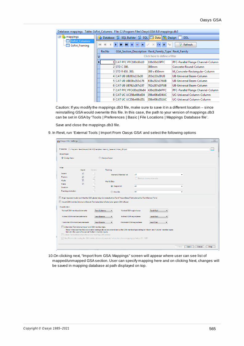
Oasys GSA

Copyright © O as ys 1985–2021 565

Caution: If you modify the mappings.db3 file, make sure to save it in a different location – since

reinstalling GSA would overwrite this file. In this case, the path to your version of mappings.db3

can be set in GSA by ‘Tools | Preferences | Basic | File Locations | Mappings Database file’.

Save and close the mappings.db3 file.

9. In Revit, run ‘External Tools | Import From Oasys GSA’ and select the following options

10.On clicking next, “Import from GSA: Mappings” screen will appear where user can see list of

mapped/unmapped GSA section. User can specify mapping here and on clicking Next, changes will

be saved in mapping database at path displayed on top.

Oasys GSA

Copyright © O as ys 1985–2021566

11.When mapping sections, make sure no sections are <Unmapped>. Sections mapped INVALID will

not be imported.

Oasys GSA

Copyright © O as ys 1985–2021 567

Select ‘Unjoin Elements’ if Revit throws up warnings.

10.5.1.5 Recommended Practice

Update From GSA and Import From GSA

The suitability of a GSA model for coordination with Revit can be examined using the tool ‘Check Model

suitability for BIM coordination’ from the tools menu.

Oasys GSA

Copyright © O as ys 1985–2021568

Mapping GSA Sections

Mapping section properties to Revit Family types is the most crucial step in the import. GsRevit

can try to find suitable matches for most steel catalogue sections, but for the rest, the best option

is to manually load the desired (equivalent) family type before starting the import. During the

import process, one can then select the appropriate family type in the drop-downs.

Section Property References

For each section property in GSA, it must be ensured the section is not referred to by elements/

members that are both vertical and non-vertical. Sections referred to by both will not be imported.

GSA has a tool that facilitates splitting section properties into Beam(non-vertical) sections and

Column(vertical) sections. The command ‘Rationalize sections for BIM coordination’ in the Tools

menu examines all sections in the section property table. If any of them is referred to by both

vertical and non-vertical entities, the tool creates a new section property and gets the vertical

entities to refer to the new section.

Each Revit column, beam and brace is reflected in GSA as a single member or beam element,

depending on whether Design Layer or Analysis Layer is selected. Note the following:

Member - Element coordination

It is recommended that the design layer(GSA Members) be used for coordinating with BIM

models.

The commands ‘Model | Manipulate | Create Elements from Members’ and ‘Model | Manipulate |

Create Members from Elements’ can be used to initially create Members from Elements and vice-

versa but subsequent coordination(between the design and analysis layer) will need to be done

manually. To assist in checking consistency of section property references, the tools ‘Update

Element sections’ or ‘Reset Member sections’ in the Design menu might be helpful.

Creating levels

All the new entities created by GsRevit will map to the nearest level available. Since Revit

Columns span between 2 valid levels, it’s important for the levels to properly reflect elevations of

the column ends. GsRevit can try and create levels from GSA’s grid planes, but the user can also

create them manually before invoking the import.

Preparing for the import/update

1. Ensure if model is fit to be coordinated with Revit by running the ‘Check Model Suitability for BIM

coordination’ command. Make modifications to the model if necessary.

2. Open a new Revit model from one of the templates for Metric or for Imperial.

3. If you plan to use grid planes for creating levels, for best results, ‘Level 1’ in the Revit model

may be deleted. If not, levels may be defined at appropriate elevations manually.

4. Load the appropriate family types which are used in the GSA model. If a particular section is

being used both as a column and as a beam in GSA, make sure to load them separately in the

Revit model, under Structural Column Family types and Structural Framing Family types.

5. It’s best to start the import from an ‘Elevation’ view rather than the default 3D view.

The Revit model is now ready for receiving the GSA model file.

Note: After the import process, Revit may display warnings against errors in the models. Choose

‘Unjoin Elements’ in such a situation.

Oasys GSA

Copyright © O as ys 1985–2021 569

10.5.1.6 Registering GsRevit

Revit needs to be told that the Revit / GSA link plug-in (GsRevit) is available, where it resides on disk and

what options are provided, before Revit will offer the GsRevit options. If Revit is installed at the time GSA is

installed then the GSA installation will automatically register GsRevit with Revit. Successful registration is

indicated by the presence of the GSA options in the Revit ‘Tools | External Tools’ menu (and that they

work!).

GsRevit can be registered interactively by running GsaRegister.exe, which may be found in the GSA

program folder.

Possible reasons for failure in the registration process are:

Revit Structure is not installed in the default location. The automated install-time registration assumes

that Revit is installed in its default location, <C:\Program Files\Autodesk Revit Structure x>. When

running GsaRegister.exe interactively there is an opportunity to specify the location of Revit.

The version of Revit Structure that you have installed is not supported.

Refer to file GsRevit_ReadMe.pdf (installed in the Docs folder beneath the GSA program folder) for the

latest information on GsRevit, including supported versions.

10.5.1.7 Section Mappings File

The Mappings file, Mappings.db3, is a SQLite database that contains mappings between GSA Sections

and Revit Column and Framing Family Types. This file is installed at a default location in the GSA

installation Program Files folder, typically, <C:\Program Files\Oasys\GSA x.y> where x and y and version

numbers. The location of this file can be changed in GSA preferences.

Note: The Mappings.db3 file will be overwritten whenever a new version of GSA is installed. Before making

changes, copy the mappings file to a different folder and change GSA Preferences to reflect the new

location.

The tables GsRvt_Framing and GsRvt_Columns contain section mappings for Revit Framing Family

Types and Column Family Types respectively. A brief description of the fields -

GSA_Section_Description: Use the section description from GSA Section Property table. See Section

Profile.

Revit_Family_Type: The name of the family type. This name must either be contained in the text file

accompanying the family rfa file(as in the case of Steel Catalogue families) or they must be ‘defined’

in the rfa file.

Revit_Family: The name of the family file on the disk, without the extension.

GsRevit searches for family files in locations listed in Revit ‘Options | File Locations | Places’.

10.5.2 IFC

The IFC file format is a widely-used format supported by variety of software for civil engineers. It describes

building and construction data. It is not meant to replace proprietary formats of any particular software but

to provide a universally recognized general format, even if the functionality to interchange data is limited.

Oasys GSA includes both IFC Import and Export with some limitations.

Export from Oasys GSA to IFC: exports the whole GSA model into a new IFC file.

Import from IFC to Oasys GSA: imports IFC objects into the current GSA project. Not all objects are

transferred into Oasys GSA. A log of the import process is available to users.

Update from IFC to Oasys GSA: applying changes onto current GSA objects from a modified IFC file is not

Oasys GSA

Copyright © O as ys 1985–2021570

currently implemented.

Credit: the implementation uses IfcOpenShell library which depends on Open Cascade library.

10.5.2.1 Export from Oasys GSA to IFC

The export is intended for:

viewing a GSA model in IFC graphical viewers

transferring GSA models into Tekla Structures..

There may be other applications that have not been tested. Note that exporting to Autodesk Revit is

recommended to be done primarily by GSA Revit plugin (GsRevit), not via IFC.

All entities will be exported to IFC, i.e. the user has no option to reduce the export to part of a model. The

user can choose whether to export the design layer, analysis layer or both layers.

The following options are available:

Generate assemblies for Tekla

If ON, IFC objects are augmented with additional properties to facilitate import into Tekla Structures. It has

no compatibility impact on importing to another software package. This switch can always be turned ON

unless you aim to reduce the file size. The default is ON.

Layer(s) to export

1. Design layer: members are exported. Elements are skipped during export (default).

2. Analysis layer: elements are exported. Members are skipped during export. The IFC file will be typically

larger than if the design layer is exported since each GSA element has to be represented as one IFC

object.

3. Both: both design and analysis layer are exported to IFC file. This is not recommended.

Colors

GSA lets you decide how the IFC objects are colored.

1. None: in case you want to keep the IFC file small.

2. By type: different entity types within GSA are assigned different colors. (default)

3. By property: according to assigned property number within GSA.

4. By group: according to assigned group number within GSA.

Shell elements

There are several ways how to represent shell surfaces in IFC.

1. As shells with no thickness (a plane shell). The thickness information is lost.

2. As faces (e.g. a box consists of six faces so the thickness is determined). Not an efficient setting.

3. As solids (an area is extruded by thickness, i.e. usually by thickness of a slab or a wall). This is the

default setting and the format expected by Tekla Structures.

Beams

The cross-sections of beams can be represented in two ways.

Oasys GSA

Copyright © O as ys 1985–2021 571

1. By perimeter. Every section behaves as a user section. (default)

2. As standard sections. IFC format supports basic standard sections as L, U, C, I shapes.

Which option to select depends on the target software.

10.5.2.2 Import from IFC to Oasys GSA

IFC is a loose format: a physical object (e.g. a beam or a slab) can be described in many ways (the same

shape can use different representations). Not all possible IFC representations are supported when an IFC

file is opened in GSA. Therefore it is likely that some entities will be lost or not transferred neatly. This

behaviour can be improved in the future.

IFC files are imported into the current GSA document (typically a blank document). The smaller the IFC file

is, the faster the process.

The recommended settings when exporting from Tekla Structures are:

(optional) select the objects to export,

select File format: IFC,

select Export type: Coordination view,

for Tekla Structures rev. <= 20, unselect Pour objects in “Advanced tab” (other settings in the Advanced

tab are not known to have a functional impact on import into GSA).

Part XI

Oasys GSA

Copyright © O as ys 1985–2021 573

11 Bibliography

1. AISC Steel Design Guide Series, Floor Vibration Due to Human Activity.

2. ASCE 4-09, Seismic Analysis of Safety-Related Nuclear Structures and Commentary, ASCE 2010 (Draft)

3. ASCE 7-05, Loads for Buildings and Other Structures Seismic Loads, ASCE, 2005

4. ASCE 7-10, Loads for Buildings and Other Structures Seismic Loads, ASCE, 2010

5. Bathe K-J, Finite Element Procedures in Engineering Analysis, Prentice Hall, 1982

6. Bathe, K. J. and Dvorkin, E. N., A four-node plate bending element based on Mindlin/Reissner plate

theory and a mixed interpolation, International Journal for Numerical Methods in Engineering, Vol 21,

367-383, 1985

7. Bell W.W, Matrices for Scientists and Engineers, Van Nostrand Reinhold, 1975

8. BS6841 - 1987, Measurement and evaluation of human exposure to whole-body mechanical vibration

and repeated shock.

9. Budynass R.G. & Sadegh A.M., Roark's Formulas for Stress and Strain, 2020

10.Structural Use of Concrete, BS 8110-1:1997, BSI, 1997

11.CEN, ENV 1998-1-1, Eurocode 8 – Design Provisions for Earthquake Resistance of Structures – Part 1-

1: General Rules – Seismic actions and general requirements for structures, 1994.

12.Chopra A.K, Dynamics of Structures – Theory and Applications to Earthquake Engineering, Prentice

Hall, 1995

13.Clough R.W & Penzien J, Dynamics of Structures, 2nd Edition, McGraw-Hill, 1993

14.Coates R.C, Coutie M.G & Kong F.K, Structural Analysis, Nelson, 2nd edition, 1980

15.Criswell H, Highway Spirals, Superelevation and Vertical Curves, County Surveyors’ Society / The

Carriers Publishing Co. 1969

16.Eurocode 8: Design of structures for earthquake resistance- Part 1: General rules, seismic actions and

rules for buildings, EN1998-1, 2004, European Committee for Standardization

17.FEMA, Prestandard and Commentary for the Seismic Rehabilitation of Buildings, FEMA 356, ASCE/

FEMA, 2000.

18.Ghali A. & Neville A.M, Structural Analysis, Chapman and Hall, 1978

19.Higham N. J., Accuracy and Stability of Numerical Algorithms, Second edition, SIAM, 2002.

20. Higham N. J. and Tisseur F, A Block Algorithm for Matrix 1-Norm Estimation, with an Application to 1-

Norm Pseudospectra. SIAM Journal of Matrix Anal. Appl., 21(4): 1185-1201, 2000. http://

dx.doi.org/10.1137/S0895479899356080

21.Horne M.R., Merchant W, The Stability of Frames, Pergamon 1965

22.Indian Standard – Criteria for Earthquake Resistant Design of Structures, IS 1893 (Part1) : 2002,

Bureau of Indian Standards

23.International Conference of Building Officials, Uniform Building Code UBC-94, Whittier, CA, 1994

24.International Conference of Building Officials, Uniform Building Code UBC-97, Whittier, CA, 1997

25.International Conference of Building Officials, International Building Code 2000, Whittier, CA, 2000

26.Levy R & Spillers W.R, Analysis of Geometrically Nonlinear Structures, Chapman and Hall, 1994

27.Newmark N.M & Hall W.J, Earthquake Spectra and Design, Earthquake Engineering Research Institute,

Oasys GSA

Copyright © O as ys 1985–2021574

Berkeley, Calif., 1982

28.Ove Arup Partnership, Structural Guidance Notes, Volume 2, 1983

29.Schneider K.J., Bautabellen für Ingenieure

30.SI units and recommendations for the use of their multiples and of certain other units BS5555:1993,

ISO 1000:1992(E)

31.Smith, A.L., Hicks, S.J., & Devine, P.J. (2009) Design of Floors for Vibration: A New Approach, The Steel

Construction Institute, P354

32.Steel Construction Institute & BCSA, Steelwork Design Guide to BS5950-1:2000 Volume 1 Section

Properties Member Capacities 6th Edition (2001)

33.Timoshenko S.P & Woinowsky-Krieger S, Theory of Plates and Shells, McGraw Hill, 1964

34.Timoshenko S.P & Goodier J.N, Theory of Elasticity, McGraw Hill, 1970

35.Wilson E.L, Three Dimensional Dynamic Analysis of Structures – With Emphasis on Earthquake

Engineering, Computers and Structures Inc., 1997

36.Wilson E.L, der Kiureghian A & Bayo E, Earthquake Engineering and Structural Dynamics, Vol. 9, 187–

194 (1981)

37.Willford, M.R. & Young, P. (2006) A Design Guide for Footfall Induced Vibration of Structures, The

Concrete Centre, CCIP-016.

Part XII

Oasys GSA

Copyright © O as ys 1985–2021576

12 Glossary

1D elements

Beam, Bar, Tie, Strut, Spring, Damper, Link and Cable are all 1D elements.

2D elements

Quad 4, Quad 8, Triangle 3 and Triangle 6 are all 2D elements.

3D elements

Brick 8, Wedge 6, Pyramid 5, Tetra 4

AASHTO

Acronym for “American Association of State Highway and Transportation Officials”.

Alignment

An alignment defines a line in space, relative to a grid plane, from which lanes tracks or vehicle are

positioned.

Analysis layer

The analysis layer is a view of elements in a Graphic View.

Applied displacement

A degree of freedom where the displacement is known at the beginning of the analysis, rather than being

solved for.

Axes triad

Axis sets are displayed in Graphic Views as colour coded triads. The red, green and blue lines represent

the x, y and z axes respectively.

Bandwidth

The width of array required to store a matrix clustered around the diagonal, with the diagonal elements

along the first column. A small bandwidth will be more efficient in the storage required.

Bar element

A particular type of finite element used to model elements designed to take only axial load, e.g. truss

members.

Beam element

A particular type of finite element used to model beam, column and bracing structural elements. GSA uses

a linear beam element with 2 nodes.

Beta angle

The angle used to define the orientation of beam elements in space and the local axis directions of 2D

elements. Also called Orientation angle.

Buckling analysis

An analysis to determine the buckling response of a structure. This can be either an eigenvalue analysis

for linear structures or a non-linear buckling analysis.

Cable element

Oasys GSA

Copyright © O as ys 1985–2021 577

Cable elements are primarily used in fabric analysis. Cables are similar to tie elements but are defined by

a stiffness and mass per unit length, rather than a cross section.

Click

Clicking is the action of pressing and immediately releasing the left mouse button.

Coincident nodes

Coincident nodes are two or mode nodes that are positioned within a defined distance of each other.

Collapsing coincident nodes

Collapsing coincident nodes is the operation that results in all but the lowest numbered node in a set of

coincident nodes to be deleted and all references to these deleted nodes to be changed to references to

the remaining node.

Constraint

A constraint on a degree of freedom, such as an applied displacement, rigid link, repeat freedom or

restraint.

Current grid

A reference to a grid plane. Coordinates are defined and reported in the current grid axes. The grid drawn

in Graphic Views is defined by the grid layout of the current grid.

Cycle

This is a single time step in the dynamic relaxation solution process. During a cycle the model is

assumed to be a set of linked nodal masses accelerating through space. At the end of each cycle the

position, velocity and forces acting on the nodes are calculated, the resulting accelerations calculated, and

the process repeated.

Degree of freedom

A freedom of a node to move in a particular direction this may be either a translational or rotational

direction.

Design layer

The design layer is a view of members in a Graphic View.

Diagonal array

An array which has non-zero elements only on the diagonal.

Direction cosine array

The array relating local and global coordinate system, and used to transform vectors and tensors between

different coordinate systems.

Displacement vector

The calculated displacements at all the degrees of freedom in the structure.

Drag

Dragging is the action of pressing the left mouse button down and moving the mouse before releasing the

mouse button.

Dummy element

An element that has its dummy attribute set. Dummy elements are ignored during analysis. Certain results

Oasys GSA

Copyright © O as ys 1985–2021578

can be output for dummy elements.

Dynamic analysis

An analysis to determine the dynamic response of a structure. A modal analysis gives the dynamic

characteristics of the structure while a time-history analysis or response spectrum analysis gives the

structural response.

Eigenvalue

Part of the solution of an eigenproblem. A dynamic analysis is an example of an eigenproblem and the

natural frequencies correspond to the eigenvalues.

Element

An element is an entity that is analysed. An analysis model is made up of elements.

Engineering scale

An engineering scale is a scale of 1, 1.25, 2, 2.5 or 5 multiplied by a power of 10.

Entity

A node, element or member.

Eye distance

The eye distance in a Graphic View is the distance from the eye point to the object point.

Eye point

The eye point in a Graphic View is the position from which the model is being viewed.

Finite element

A mathematical representation of a piece of the structure located by nodes and contributing to the

stiffness/inertia of the structure.

Finite element method

The method for analysis of structure by dividing the structure into a collection of connected finite elements.

Force vector

The collection of forces applied to an element or to the structure as a whole. Normally the force vector for

the structure is known and we wish to calculate the displacements. Once the displacements at the nodes

are calculated we then want to calculate the internal forces in the elements.

Form-finding

A process by which the natural shape of a fabric structure is established.

Full image

The full image is a Graphic View image that displays all aspects of the currently specified view.

Gaussian elimination

A method for solving large systems of linear equations by successively removing degrees of freedom.

Generic bar elements

Bars, ties and struts are all generic bar elements.

Geometric stiffness

Oasys GSA

Copyright © O as ys 1985–2021 579

The additional stiffness of an element that results from the load in the element.

Ghost image

The ghost image is a Graphic View image that displays a cuboid representing the global extents of the

image. A triad representing the global directions is drawn at the object point. A dashed triad is drawn at the

mid-point of the view.

Global axes

The global axes are the axis set to which all other axes relate. The datum axis set for the model.

Grid axes

The axes referred to by a grid plane. Commonly used to refer to the axes of the current grid.

Grid layout

Defines the distribution of grid points or grid lines as drawn in Graphic Views.

Grid plane

A grid plane is a way of defining a plane for loading etc by reference to an axis set and elevation.

Grid structure

A Grid structure is one modelled in the global XY (horizontal) plane. Global restraints are applied to the

model to force it to deform only in the Z direction.

Hourglassing

Hourglassing arises with under-integrated elements where there are insufficient stiffness terms to fully

represent the stiffness of the element and is noticeable in the results by an hourglass pattern in the mesh.

Increment

Used in non-linear, GsRelax analysis to define a single load stage. An increment represents the total

imposed loads that are deemed to be present at the time of analysis. It is equivalent to an analysis case

generated internally by the GsRelax Solver. For example with single increment analysis a single analysis

case is created and all loads are applied at the start of analysis. Whereas with a 2-stage multiple

increment analysis, the first increment could be an analysis case with half the load applied and the

second increment is an analysis case with the total load applied.

Inertia matrix

Same as mass matrix.

Influence analysis

An analysis that calculates the effect at a point due to load at a series of points along the structure.

Joint

A joint is a constraint which links two nodes together in specified directions and is used for modelling

features such as pinned connections.

Lagrange multiplier method

A technique that is used to impose constraints on a model; in particular applied displacements.

Legend

The legend is the panel of information that describes the content of a Graphic View. The legend may be

displayed either on the Graphic View or in a message box.

Oasys GSA

Copyright © O as ys 1985–2021580

Linear element

A finite element with a low order shape function and no mid-side nodes.

Linear shape function

2-D elements without mid-side nodes interpolate strains linearly between nodes. This can lead to

significant stress and strain discontinuities across element boundaries.

Link element

A link element is a two node element that is rigid in the specified directions, and transfers forces and

moments through the structure.

List field

This is a field that allows the user to enter a list. The syntax of the list is then checked before the field is

accepted.

Lumped mass

A mass (and inertia) at a node. A lumped mass is treated as a one node element.

Mass matrix

The relationship between force and acceleration in a linear system. In finite element analysis we consider

the inertia of the element as represented by the element mass matrix and the inertia of the whole structure

as represented by the structure mass matrix.

Member

A member is an entity that is designed. Typically a member relates to one or more elements.

Mid-point

The mid-point is a 3D vector used to specify the pan in a Graphic View. The mid-point vector is the position

of the mid-point of the picture relative to the object point in picture axes.

Modal analysis

Modal analysis solves an eigenvalue problem either for a dynamic or buckling analysis of the structure.

Node

A point in space. Nodes are used to define the location of the elements.

Normalisation

A way of scaling a vector or matrix. For example the displacement vector for a node can be normalised,

producing a displacement magnitude of one at that node.

Numeric field

A numeric field allows the user to enter a number. Depending on the context this will be either a real

number (e.g. a coordinate) or a whole number (e.g. a load case).

Numeric format

The format used for the display of numbers. The choice is engineering, to a number of significant figures,

decimal, to a number of decimal places, or scientific, to a number of significant figures.

Numeric/percentage field

This is a field that allows the user to enter either a number or a percentage. These fields are used to allow

Oasys GSA

Copyright © O as ys 1985–2021 581

the user to specify position in either an absolute sense (number e.g. 0.25) or a relative sense (percentage

e.g. 10%).

Object point

The object point is the point about which rotations occur in a Graphic View. Also, in perspective views the

position of the eye is measured from the object point.

Object to eye distance

See eye distance.

Orientation angle

The angle used to define the orientation of beam elements in space and the local axis directions of 2D

elements.

Orientation axes

The axes about which orientations occur in Graphic Views.

Orientation node

The node used to define the xy-plane for orientation of beam elements.

Panel

A panel is an area bounded by beam elements.

Path

A path is the line across a structure followed by a lane, track or vehicle.

Picture axes

The picture axes in a Graphic View are x, left to right, y upwards and z out of the plane of the picture.

Plane structure

A Plane structure is one modelled in the global XZ (vertical) plane. Global restraints are applied to the

model to force it to deform only in the XZ plane.

Prescribed displacement

See “Applied displacement” and “Settlement”.

Quad element

A linear or quadratic element used in two dimensional analyses with 4 sides and 4 or 8 nodes defining the

element.

Quadratic element

A finite element with a higher order shape function – usually with mid-side nodes.

Quadratic shape function

2D elements with mid-side nodes (quad8 and tri6) interpolate strains using a fitted quadratic function.

This provides more realistic stresses and strains than elements with linear shape functions.

Reaction

Force which is generated at restraint.

Restraint

Oasys GSA

Copyright © O as ys 1985–2021582

A degree of freedom that is fixed so that it is no longer free. Special cases of restraints are pins and

encastré supports. (See also: Member Restraint and Restraint Property.)

Section definition axes

The axis system used for defining beam sections.

Selection field

This is a field that allows the user to choose from a list of options.

Selection/numeric field

This is a field that allows the user to either choose from a list of options or enter a number (e.g. when

specifying a material either a standard material can be selected or a user defined material specified).

Settlement

A degree of freedom which is restrained and given a fixed displacement prior to analysis.

Shear beam

A particular type of finite element similar to a beam element but taking account of shear deformations.

Skyline array

A storage scheme which only holds the entries in the stiffness or mass matrix which are on and above the

diagonal. Its name derives from the outline of the array elements that are stored.

Space structure

A Space structure is one that may be modelled in 3 dimensions.

Spacer element

A spacer element is used to control the mesh during a form-finding analysis.

Spring element

An element which is defined by stiffnesses in each of the translational and rotational directions. Used to

model springs and features such as elastic supports.

Static analysis

A static analysis loads at how the structure responds to loads which do not vary with time.

Stiffness matrix

The relationship between force and displacement in a linear system. In finite element analysis we

consider the stiffness of the element as represented by the element stiffness matrix and the stiffness of

the whole structure as represented by the structure stiffness matrix.

Structure scale

The structure scale is the scale at which the structure is drawn in a Graphic View.

Strut element

A strut element is similar to a bar element in that it has axial stiffness only, but will only take compressive

forces. Note that since this is a non-linear element, post-analysis combining of results is inappropriate.

Subspace iteration

A technique for solving for eigenvalues and eigenvectors iteration of large systems, by projecting the

Oasys GSA

Copyright © O as ys 1985–2021 583

system of equations on to a smaller “subspace”.

Text field

A text field allows the user to enter a string of text and is normally used for names.

Thread

Threads are a way for a computer program to fork (or split) itself into two or more simultaneously running

tasks.

Tie element

A tie element is similar to a bar element in that it has axial stiffness only, but will only take tensile forces.

Note that since this is a non-linear element, post-analysis combining of results is inappropriate.

Topology

The list of nodes which define an element or member.

Torce lines

Torce lines are generalised thrust lines for two or three dimensions. In 2D (plane frame analysis) they are

synonymous with thrust lines (i.e. they show the line of action of axial load) but in three dimensions they

can contain both torque and force components, hence the name.

Tree control

A tree control is a standard Windows control that offers options via expandable branches. Click on the “+”

Sometimes multiple selection of items is possible. This is achieved by holding the control key down to

continue selection or the shift key to include all items between the currently selected and the item Shft-

Clicked.

Triangular element

A linear or quadratic element used in two dimensional analyses with 3 sides and 3 or 6 nodes defining the

element.

Unattached node

An unattached node is one that is not referenced in the topology list of an element.

Variable UDL

A variable UDL is a uniformly distributed load whose intensity varies depending on the loaded length. This

is used in bridge analysis.

Vehicle

A vehicle is defined as a list of axle positions and loadings along with an overall width for use in bridge

analyses.

VUDL

See Variable UDL.

Wireframe image

The wireframe image is a Graphic View image that represents 1D elements as lines and 2D elements as

outlines and displays nothing else, regardless of the current settings for the view.

X elevation axes

Oasys GSA

Copyright © O as ys 1985–2021584

The X elevation axis set is a standard axis set that has its xy plane in the global YZ plane.

Y elevation axes

The Y elevation axis set is a standard axis set that has its xy plane in the global XZ plane.

Index 585

Copyright © Oasys 1985–2021

Index

- * -*= command

in tables 45

- / -/= command

in tables 45

- + -+= command

in tables 45

- = -= command 45

- - --= command

in tables 45

- = -== command

in tables 45

- 1 -1D Element Results Dialog 532

- 2 -2D circular mesh

data generation 424

2D derived force results

output options 375

2D element

axis 215

2D element displacements

output options 373

2D element edge loads

create dialog 239

definition dialog 239

2D element face loads

create dialog 237

definition dialog 237

2D element facet angle

change default 429

2D element loads

load panel fundamentals 238

2D element pre-stress loads

create dialog 241

definition dialog 241

2D element stresses

output options 373

2D element thermal loads

create dialog 242

definition dialog 242

2D elements

Allman-Cook 303

centre-only results 306

convert Quad4 to Quad8 451

convert Quad8to Quad4 451

convert Tri6 to Tri3 451

geometry checks 303

linear analysis introduction 316

linear to parabolic 451

load panels 183, 238

loading data 236

MITC 303

modelling and loading introduction 315

parabolic to linear 451

properties 183

settings 303

split warped 504

2D elliptical mesh

data generation 424

2D orthogonal mesh

data generation 423

2D polylines

check for validity 151

definition dialog 151

2D properties

decking slab 185

hollow slab 186

2D skew mesh

Oasys GSA586

Copyright © Oasys 1985–2021

2D skew mesh

data generation 423

- 3 -3D element

axis 215

3D element displacements

output options 377

3D element face loads

create dialog 244

definition dialog 244

3D element stresses

output options 377

3D element thermal loads

create dialog 245

definition dialog 245

3D elements

properties 188

3D orthogonal mesh

data generation 425

- A -AASHTO 21

abs combination case operator 109

accelerators 130

Accidental Torsion Load 515

ACI 19, 21

Acknowledgements 23

ADC

export options 552

add elements sculpt tool 443

Add Nodes command 444

add nodes sculpt tool 443

Add String of 1D Elements command 445

adornments

apply to selection 70

advanced preferences 431

AISC LRFD checker

documentation 396

AISC360 checker

documentation 396

align

beams and columns 504

alignment

extrude 513

alignments

data 268

extrude geometry along 440

Allman-Cook 303

aluminium

material grade 155

Analyse All command 90

Analyse All Marked Tasks command 103

analysis

bridge step by step 346

bridge structures 349

buckling step by step 329

damping 301

dynamic step by step 322

Elements 83

explicit time history 325

explicit time-history 363

footfall analysis 327

harmonic analysis 326

imperfection 307

introduction 89

linear static step by step 314

LS-DYNA 309

non-linear step by step 317

P-delta 314

periodic load analysis 328

piled-raft analysis 351

raft 144

raft analysis 351

response spectrum 341

seismic step by step 340

step by step summary 90

Tasks & Cases 82

threading 431

Time history analysis 325

Types 87

analysis cases

definition dialog 284

fundamentals 107

analysis envelopes

Analysis Wizard 300

step by step 359

analysis features 16

Analysis Layer in graphic views 75

analysis materials

data 158

analysis options

Analysis Wizard 285

Index 587

Copyright © Oasys 1985–2021

Analysis Progress Dialog

GsRaft 309

analysis specification

dialog 142

Analysis Stage

Timeline 495

analysis stages 357

colour elements by 471

creep 283

data 283

definition data 283

in graphic views 358

introduction to analysis 357

introduction to analysis results 358

long term analysis 283

material map 357

modelling implications 356

property data 283

property map 357

results introduction 358

analysis tasks

fundamentals 107

analysis tasks and cases

Analysis Wizard 105

copy and paste 105

Analysis Wizard

analysis envelopes 300

analysis options 285

buckling parameters 290

cases set up 301

footfall analysis parameters 297

form finding options 292

generic dynamic analysis parameters 296

GsBridge control 299

GsRaft control 298

GsRaft progress 299

GsRelax analysis progress information 293

GsRelax analysis task control 293

GsRelax member identification 293

harmonic analysis parameters 296

linear time history analysis parameters 295

mass calculation 291

modal dynamic parameters 286

non-linear static options 291

pseudo response spectrum analysis 295

response spectrum analysis 294

Ritz analysis parameters 289

static analysis cases 285

static p-delta 286

working with 105

angle between nodes 34

Animate 76

Animate command 76

animation

Animation Settings Dialog 482

in graphics 76

settings for graphics 482

Animation Settings command 76

Annotate Selection command 71

annotating graphic diagrams etc 71

annotation of diagrams options 481

Append GWA data 460

from Data Explorer pane 32

applied displacements

create dialog 228

data 228

definition dialog 228

Apply Adornments to Selection command 70

areas

copy / move graphically 452

Copy Areas Dialog 438

labels in graphic views 471

Move Areas Dialog 438

AS 19, 21

AS4100 checker 397

Buckling checks 397

documentation 397

Local checks 397

ASCE 7 -05

ASCE7-05 spectrum 252

ASCII (GWA) file

syntax 535

Assemblies

Check 500

data 218

definition dialog 218

labels in graphic views 471

assembly

wall/core 457

auto views

details 101

AutoCAD

export options 553

import options 556

automatic constraints

Oasys GSA588

Copyright © Oasys 1985–2021

automatic constraints

fundamentals 118

automatic increment

dynamic relaxation analysis 332

axes 94

coordinates, non-global definition fundamentals 97

Create User Axes Dialog 433

creating user graphically 443

cylindrical and spherical fundamentals 96

data 146

definition dialog 146

global cylindrical 94

grid fundamentals 97

grid planes 150

grid surfaces 150

in table views 49

joint in disparate axes 506

labels in graphic views 467

Member 203

modify axis 146

output 50

projected fundamentals 96

sets fundamentals 94

use of fundamentals 96

vertical 94

x elevation 94

y elevation 94

Axes command

in graphic views 71

Axes Dialog 533

axis

elements 215

axismmetric

new model wizard 416

- B -backup

set time interval 429

backups

working with 119

bar

axis 215

base

create dummy elements 507

basic concepts in GSA 30

Batch Analysis command 103

batch output file formats 429

batch printing views and view lists 102

beam

axis 215

offset 504

beam cross strain energy density

output options 372

beam derived stresses

output options 367

beam displacements

output options 365

beam distortion loads

create dialog 234

definition dialog 234

beam forces

output options 366

beam loads

create dialog 230

definition dialog 230

beam pre-stress loads

create dialog 233

definition dialog 233

beam sections

modifiers 178

simple beams 178

beam strain energy density

output options 371

beam stresses

output options 367

beam thermal loads

create dialog 235

definition dialog 235

Beams

Influence effects 274

load data 230

loading data 229

bearings

data 222

beta angle

beam axis 215

BIM 567

constructing a model 27

BIM Compatibility

Check 501

blank in tables 47

block 204

Index 589

Copyright © Oasys 1985–2021

block 204

definition 204

replica 204

Blocks

Explode to Members 503

bricks

properties 188

bridge

analysis 349

Expand Bridge Loading 513

Generate Static Vehicle Load 510

influence analysis 349

lane-by-lane path optinisation 349

Optimise Path Loading 512

bridge analysis

modelling implications 348

step by step 346

bridge analysis specification 145

bridge beams 173

bridge modelling

delet grid loads 513

Bridge Options Dialog 480

bridges

bridge loading data 276

broadening

response spectrum 517

BS 19, 21

BS5950 checker 398

buckling checks 398

buckling interaction check 398

combined local check 398

documentation 398

limitations 398

local axial check 398

local bending check 398

local checks 398

local shear check 398

local torsion check 398

buckling analysis

step by step 329

buckling analysis results

output options 363

Buckling checks

AS4100 397

buckling parameters

Analysis Wizard 290

building

create storeys 507

- C -cables

properties 189

case description

definition dialog 312

case descriptions 312

cases 309

Analysis Case Definition Dialog 284

analysis case fundamentals 107

Case Description 312

combination case data 309

combination case fundamentals 108

Combination Cases dialog 309

data 310

fundamentals 106

load case data 226

load case fundamentals 106

Load Case Titles dialog 226

output by 53

selected for output 52

selecting for graphic views 70

syntax of combination descriptions 109

cases set up

Analysis Wizard 301

catalogue

section 167

CEAP Modal Damping 514

cell operators

in tables 45

centre-only results 306

chart view

chart view settings 485

chart views

Footfall analysis 487

Forces on 2D Element Cut 488

Generic periodic load analysis 486

Harmonic analysis 486

Linear time history analysis 486

Modal analysis details 485

non-linear analysis 485

Check

Assemblies 500

BIM Compatibility 501

Concrete 2D Data 501

Oasys GSA590

Copyright © Oasys 1985–2021

Check

Element End Rotations 500

Grid Load Expansion 500

Incompatible Elements 500

MemberEnd Rotations 500

Tied Interfaces 500

Check Data command 103

check for completeness

entity lists 500

Chinese Standards

GB 50011-20012 spectrum 256

clean

combination cases 504

Clear Colour Modifications command 72

clipboard

copy graphic image to 79

copy output to 461

Codes

Design 19, 21

coexistent values in envelopes

specifying 463

coexistent values in output view envelopes 52

coincidence tolerance

changing 427

coincident elements

deleting graphically 63

highlighting in graphics 75

selecting 63

coincident nodes

collapsing graphically 445

deleting graphically 63

highlighting in graphics 74

selecting 63

Collapse Coincident Nodes command 445

colour

in graphics 72

in tables 49

colour elements by property etc. 471

colours

assigning to entities 61

colours in graphic views 484

COM interface 544

COM numeric precision

change default 429

COM units 535

COM version 544

combination cases 309

clean 504

data 309

definition dialog 309

fundamentals 108

syntax of descriptions 109

Combine model 460

command file (GWC)

run by 544

command line interface 544

Command Toolbar 126

company information 425

company name

setting 429

Comparing models 501

Concrete

Check 2D Data 501

Design Codes 19, 21

material grade 153

concrete beam

dialog 531

export 531

concrete beam design 531

concrete slab

calculation properties 194

reinforcement properties 194

strength reduction properties 196

condition number 302

conflicting constraints

fundamentals 118

Connect 1D Elements command 446

Connect 1D Elements Dialog 433

connecting 1D elements graphically 446

constraint equations

data 223

definition dialog 223

constraints

automatic fundamentals 118

axes fundamentals 97

conflicting fundamentals 118

constraint equation data 223

creating rigid graphically 457

fundamentals 116

joint data 222

rigid constraint data 220

rigid fundamentals 117

tied interface data 224

constructing a model

Index 591

Copyright © Oasys 1985–2021

constructing a model

introduction 27

construction (analysis) stages

in graphic views 358

introduction to analysis 357

introduction to analysis results 358

modelling implications 356

results introduction 358

construction grid

in graphic views 62

contact

edge to ground 506

face to ground 505

node to 2D element 506

contour barrel widths in graphic views 484

Contour Settings command 68

Contour Settings Dialog 476

Contour Values Dialog 476

contours

apply to selection 70

contours on graphic views 68

Contours Toolbar 127

control

nonlinear analysi 292

Convert Nodes to Grid command 196

Convert Nodes to Standard command 196

convert orientation node to angle 451

coordinates

axes, non-global definition fundamentals 97

grid fundamentals 97

rounding graphically 445

copy 46

Copy Areas Dialog 438

Copy Elements Dialog 438

Copy Lines Dialog 438

Copy Members Dialog 438

Copy Nodes Dialog 438

Copy Regions Dialog 438

graphic image to clipboard 79

nodes, elements, members, lines, areas, regionsgraphically 452

output to clipboard 461

copy and paste analysis tasks and cases 105

Copy command 53, 65, 79

copy GWA data

from Data Explorer pane 32

Copy Selection command 452

copying

cutting and pasting in tables 46

Copying between tables and spreadsheets 48

create

base dummy elements 507

grid lines 507

rigid membranes from storeys 507

Create 2D Edge Load command 458

Create 2D Face Load command 458

Create 2D Pre-stress command 458

Create 2D Thermal Load command 458

create a new raft model 505

Create Applied Displacement command 457

Create Beam Distortion command 458

Create Beam Load command 458

Create Beam Thermal Load command 458

Create Facade List 508

Create Footfall Response Data command 460

Create Gravity Load command 458

Create Grid Area Load command 459

Create Grid Line Load command 459

Create Grid Plane command 444

Create Grid Point Load command 459

Create Joints command 457

create load panels on element list 508

create load panels on facade 508

create mass from grid loads 502

create mass from loads 502

Create Members from Elements 497

create nodal mass 503

from element mass 503

from member mass 503

Create Node Load command 457

Create Patterned Load Combinations 509

Create Patterned Loads 508

Create Pre-stress command 458

Create Rigid Constraints command 457

Create Settlement command 457

create storeys 507

Create User Axes command 443

Create User Axes Dialog 433

creep

analysis stages 283, 357

cross strain energy density

output options 372

Oasys GSA592

Copyright © Oasys 1985–2021

Cross Strain Energy Density Results command 372

CSA 19, 21

CSV

batch saving saved views to 102

CSV (GWA) file

syntax 535

CSV file

export options 551

import options 555

current grid

definition dialog 492

fundamentals 97

in graphic views 62

current polyline in Graphic Views 65

Cursor Mode Toolbar 128

cursor modes

in Graphic Views fundamentals 77

Curve Data Selection Dialog 526

curves

alignment data 268

extrude geometry along alignment 440

Modify Curve Dialog 526

custom links

fundamentals 117

properties 188

cut 46

Forces on 2D Element Cut 488

Cut section forces

Assemblies 218

cutting

copying and pasting in tables 46

cutting 1D elements graphically 446

cylindrical axes fundamentals 96

- D -dampers

properties 190

damping 289

analysis wizard 301

CEAP Modal Damping 514

frequency damping table 261

mode damping table 262

settings 305

soil-structure analysis 308

data

delete from Data Explorer pane 32

extents in output views 52

Manage Data Dialog 491

selecting what to output 51

Data Explorer pane 32

data generation

2D elliptical mesh 424

2D orthogonal mesh 423

2D skew mesh 423

3D orthogonal mesh 425

constructing a model 27

grid 418

orthogonal frame 419

pitched portal frame 422

portal frame 417

Pratt truss 421

roof truss 422

structure types 417

truss 420

Vierendeel 420

Data Management

comparing models 501

import GWA data 460

Data Options Toolbar 125

data preferences 428

data scaling unreliable message 56

decking slab

2D properties 185

Decrease Precision command

in graphic views 71

default view settings

details 99

introduction 99

Define Current Grid command 62

defining current grid

in graphic views 62

definition

2D properties 183

block 204

environmental Impact 192

grid layouts 493

links 188

masses 183

material curve 162

material wizard 158

member 198

non-linear spring curve 162

section 163

Index 593

Copyright © Oasys 1985–2021

definition

springs 180

definition axes

fundamentals 97

definition dialogs

2D element edge loads 239

2D element face loads 237

2D element pre-stress loads 241

2D element thermal loads 242

2D polylines 151

3D element face loads 244

3D element thermal loads 245

Analysis Case 284

applied displacements 228

assemblies 218

axes 146

beam distortion loads 234

beam loads 230

beam pre-stress loads 233

beam thermal loads 235

constraint equations 223

Current Grid 492

Element Wizard 205

generalised restraints 219

gravity loads 250

grid area loads 249

grid line loads 248

grid lines 149

grid planes 150

grid point loads 247

grid surfaces 150

joints 222

node loads 227

polylines 151

Response Spectrum Wizard 251

rigid constraints 220

settlements 229

tied interfaces 224

Variable Load Wizard 271

Deformation Settings command 69

Deformation Settings Dialog 475

deformed geometry

new model 505

Deformed Image command 69

deformed image on graphic views 69

delete

data from Data Explorer pane 32

Delete All Polyline command 66

Delete All Results command 90

Delete command 47, 456

Delete Displayed Loading command 460

Delete Element command 75

Delete Element Loading command 75

delete in tables 47

Delete Member command 75

Delete Nodal Loading command 75

Delete Node command 75

Delete Polyline Point command 66

delete results 89

Delete Results From Files command 119

deleting nodes and elements

data management 491

derived stress output

beams 367

descriptions

cases 312

design

section 116

steel design results step by step 411

steel design step by step 393

steel design tools step by step 412

design codes 19, 21

preferred 425

design features 17

Design Layer in graphic views 75

design pools

steel 179

design specification 144

Design Task 393

members 310

option 310

run 311

steel 311

destabilizing load

member 199

Diagram Settings command 68

diagrams

annotation options 481

apply to selection 70

change scale on change of case switch 426

Diagram Settings Dialog 478

simple/detailed & draw in plane of pictureswitches 478

diagrams on graphic views 68

Diagrams Toolbar 127

Oasys GSA594

Copyright © Oasys 1985–2021

dialogs

1D Element Results 532

2D Element Edge Load Definition 239

2D Element Face Load Definition 237

2D Element Pre-stress Load Definition 241

2D Element Thermal Load Definition 242

2D polyline definition 151

3D Element Face Load Definition 244

3D Element Thermal Load Definition 245

Advanced Preferences 431

Analysis Case Definition 284

analysis specification 142

Animation Settings 482

Applied Displacement Definition 228

Axes 533

axis definition 146

Beam Distortion Definition 234

Beam Load Definition 230

Beam Pre-stress Definition 233

Beam Thermal Load Definition 235

bridge analysis specification 145

Bridge Options 480

CEAP Modal Damping 514

Combination Cases 309

concrete beam 531

Connect 1D Elements 433

Constraint Equation Definition 223

Contour Settings 476

Contour Values 476

Copy Areas 438

Copy Elements 438

Copy Lines 438

Copy Members 438

Copy Nodes 438

Copy Regions 438

create 2D element edge load 239

create 2D element face load 237

create 2D element pre-stress load 241

create 2D element thermal load 242

create 3D element face load 244

create 3D element thermal load 245

create a new raft model 505

create applied displacement 228

create beam distortion load 234

create beam load 230

create beam pre-stress load 233

create beam thermal load 235

create gravity load 250

create grid loading 247, 248, 249

create node load 227

create settlement 229

Create User Axes 433

Current Grid Definition 492

Curve Data Selection 526

Deformation Settings 475

design specification 144

Diagram Settings 478

Disconnect Elements 438

Display Methods 471

Element Wizard 205

environmental impact definition 146

Export Member Input Data to CSV 532

Extrude 440

Find 524

Flex 441

Footfall Response Data 460

Further Options 481

Further Options (output) 463

Generalised Restraint Definition 219

Go To 526

Graphic Fonts and Styles 484

Graphic Settings Wizard 464

Gravity Load Definition 250

Grid Area Load Definition 249

grid line definition 149

Grid Line Load Definition 248

grid plane definition 150

Grid Point Load Definition 247

grid surface definition 150

GsRaft Analysis Progress 309

GWA Import Options 526

Joint Definition 222

Labels and Display Methods 467

Lighting Settings 73

Load Case Titles 226

material curve 162

Material Wizard 158

Modify 525

modify axis 146

Modify Curve 526

Move Areas 438

Move Elements 438

Move Lines 438

Move Members 438

Move Nodes 438

Move Regions 438

Index 595

Copyright © Oasys 1985–2021

dialogs

NASTRAN Export Options 530

Node Load Definition 227

non-linear spring curve 162

Numeric Format 533

OpenSees Export Options 530

Orientation Settings 483

Output Settings Wizard 461

Path Loading 275

polyline definition 151

preferred folders 431

RC beam 531

Refine Quad Elements 436

Replace 525

Response Spectrum Wizard 251

Rigid Constraint Definition 220

Settlement Definition 229

Split 1D Elements 434

Split Quad Elements 435

Split Tri Elements 437

Storey Displacements and Forces 488, 523

Tied Interface Definition 224

titles 139

Unwrap Settings 73

Variable Load Wizard 271

View List 120

Welcome to GSA 414

Disconnect Elements command 456

Disconnect Elements Dialog 438

disconnecting elements graphically 456

displacements

applied displacement data 228

intermediate results 532

output options 364

Storey Displacements and Forces Dialog 488,523

Display Methods Dialog 471

display methods in graphic views 67

display options 379

analysis stage data 389

bridge data 387

bridge results 388

error norm 389

load data 382

model data 379

numeric formats 390

results 383

user modules 389

distance between nodes 34

distortion loads

data 234

documentation 19

Double size of diagrams command 70

drag nodes sculpt tool 442

Drag on node - Collapse command 442

Drag on node - Co-locate command 442

Drag on node - Ignore command 442

Drag on node - Joint command 442

Draw Selection command 60

drawing part of the model 59

drilling degrees of freedom

Allman-Cook 303

dummy elements

draw 471

dummy mass

settings 305

Dynamic analysis

scaling of modes 517

step by step 322

dynamic analysis results

output options 363

dynamic load

dynamic load factor 263

load curve 262

dynamic load factor

data 263

dynamic relaxation

incremental analysis 332

dynamic response

data 251

- E -EC3 checker

National Annexes 403

edge

contact to ground 506

edge loads

data 239

edges of elements

highlighting in graphics 74

Edit Design Property command 75

Edit Element command 75

Edit Material command 75

Edit Member command 75

Oasys GSA596

Copyright © Oasys 1985–2021

Edit Node command 75

Edit Property command 75

Edit Restraint Property command 75

Edit Section Property command 75

editing models in graphics 432

effective lengths

member 199

steel members 411

Effective mass

by part 514

eigensolver 303

convergence 303

settings 303

shifting 303

Sturm sequence check 303

subspace iteration 303

eigenvalue

introduction to buckling analysis 329

model stability 339

eigenvalue buckling analysis 329

modelling implications 329

eigenvalue buckling results

introduction 330

Element

axis 215

End Rotations 500

element formulation

LS-DYNA 309

element properties

Object Viewer 34

Element Properties command 75

element user modules 119

elements

2D element release 205

add/modify one by one sculpting 442

adding graphically introduction 445

adding string of 1D graphically 445

Beam release 205

colour in graphics 72

Connect 1D Elements Dialog 433

connecting 1D graphically 446

convert Quad4 to Quad8 451

convert Quad8 to Quad4 451

convert Tri3 to Tri6 451

convert Tri6 to Tri3 451

copy / move graphically 452

Copy Elements Dialog 438

create members 497

data 205

delete from members 494

deleting 491

deleting graphically 456

Disconnect Elements Dialog 438

disconnecting graphically 456

dummy 205

End stiffness 205

Extrude Dialog 440

extrude graphically 452

flip 503

flipping graphically 455

from members 494

highlighting coincident in graphics 75

highlighting edges in graphics 74

Incompatibility Check 500

joining 1D graphically 450

labels in graphic views 469

length of selection 34

link fundamentals 117

manage user modules 522

mass of selection 34

modifying graphically 455

Move Elements Dialog 438

offset fundamentals 117

orientation node, convert to angle 451

parabolic to linear 451

Refine Quad Elements Dialog 436

renumbering 491

selecting for output 52

shrinking in graphics 72

spinning 2D graphically 455

Split 1D Elements Dialog 434

Split Quad Elements Dialog 435

Split Tri Elements Dialog 437

splitting 1D and 2D graphically 447

surface area of selection 34

synchronise from members 494

upside-down 503

wizard 205

EN1993

Eurocode 3 401

EN1993 checker 401

limitations 401

EN19933 checker

buckling checks 401

buckling interaction check 401

Index 597

Copyright © Oasys 1985–2021

EN19933 checker

combined local check 401

documentation 401

local axial check 401

local bending check 401

local checks 401

local shear check 401

local torsion check 401

End condition

members 202

End stiffness

Beam element 205

Engineering Scale command 56

engineering scale for structure

default switch 464

entities

check for completeness 500

Entity Selection Mode 63

envelope subject component

specifying 463

enveloping

fundamentals 108

operator fundamentals 109

optimising fundamentals 109

permutations 109

stored step by step 359

syntax of combination descriptions 109

enveloping in output views 52

environmental impact

specification dialog 146

step by step 359

wizard 192

environmental impact specification

dialog 146

Equivalent Static Load 515

seismic 341

error messages

limit numbers 429

error norm 302

Eurocode 19, 21

Eurocode 8 - 1994 spectrum 255

Eurocode 8 - 2003 spectrum 254

Eurocode 3

EN1993 401

Evaluating expressions 121

Expand Bridge Loading 513

Expand Grid Loading 523

Explicit 288, 289

explicit solver

settings 308

time step 308

explicit time history

analysis 325

modelling implications 325

results 325

explicit time-history

analysis 363

Explode

Blocks to members 503

Explorer Panes

working with 32

export

ADC 552

AutoCAD 553

footfall response 553

GWA 551

input data 551

NASTRAN 554

NASTRAN Export Options Dialog 530

OpenSees 555

OpenSees Export Options Dialog 530

output views 551

Pdisp 552

Revit 557

SAP2000 553

steel members 552

Export command 46, 48

Export Member Input Data to CSV Dialog 532

export options 551

Expressions 121

Map beam loads on 1D elements 458

Map node loads on nodes 457

Map pressures on 2D elements 458

extents of output

specifying 463

external matrix 192

extract

sub-model 495

extrude

alignment 513

nodes and elements graphically 452

Extrude Dialog 440

Extrude Selection command 452

Eye Distance In command 58

Oasys GSA598

Copyright © Oasys 1985–2021

Eye Distance Out command 58

- F -fabric

material grade 157

fabric structures

step by step 320

fabricated

section 174

facade

create load panels 508

facade list

create 508

face

contact to ground 505

face IDs 244

face loads

data 237

facet angle of 2D elements

change default 429

FEMA

FEMA 356 spectrum 255

field types

in tables 44

file backups

working with 119

file locations

change default 429

find

in tables 47

Find command 47, 65

Find Dialog 524

find in Graphic Views 65

fire analysis

new model 505

Flex Dialog 441

Flex Selection command 453

flexing lines of nodes graphically 453

flip

elements 503

Flip Elements command 455

folders

preferred folders dialog 431

font

in graphic views 76

in table views 49

fonts

Graphic Fonts and Styles Dialog 484

footfall analysis

chart view 487

modelling 327

results 327

step by step 327

footfall analysis parameters

Analysis Wizard 297

footfall response

export options 553

Footfall Response Data Dialog 460

force density

1D properties 193

2D properties 193

force density form-finding 321

forces

intermediate results 532

Storey Displacements and Forces Dialog 488,523

Forces on 2D Element Cut command 488

form finding options

Analysis Wizard 292

format

Numeric Format Dialog 533

format of numeric output

change default 429

formats

numeric fundamentals 390

form-finding

by force density method 321

by soap film method 321

modelling implications of analysis 321

properties 192

structures step by step 320

frequency damping table

data 261

FRP

material grade 154

Further Options Dialog 481

Further Options Dialog (output) 463

- G -GB 50011-2001

GB 50011-2001 spectrum 256

generalised restraints

Index 599

Copyright © Oasys 1985–2021

generalised restraints

data 219

definition dialog 219

generate

new model wizard 425

orthogonal frame 496

generate member restraints

points 201

spans 202

Generate Static Vehicle Load 510

generate steel member restraints 144

Generate User Modules command 119

generating an imperfect geometry 329

generic dynamic analysis parameters

Analysis Wizard 296

Generic periodic load analysis

chart view 486

geometric section

properties 176

geometric stiffness

options 307

pre-load 307

geometry

generating imperfect 329

geometry checks

settings 303

Getting started with GSA 27

glass

material grade 156

global cylindrical

axes 94

go to

in tables 47

Go To command 45, 47

Go to Design Property Data command 75

Go To Dialog 526

Go to Element Data command 75

Go to Material Data command 75

Go to Member Data command 75

Go to Node Data command 75

Go to Property Data command 75

Go to Restraint Property Data command 75

Go to Section Property Data command 75

graft GWA data

from Data Explorer pane 32

Graft model 460

Graphic Display Toolbar 129

Graphic Fonts and Styles Dialog 484

Graphic Settings command 54

graphic view

save to file preferred format 429

Graphic view settings 54

Graphic view wizard 54

graphic views

animation 76

annotating diagrams etc 71

axes 71

axes label settings 467

case list 70

colour in 72

colours 484

contour barrel widths 484

contour settings 476

contour values 476

contours 68

current grid 62

cursor mode fundamentals 77

defining current grid 62

deformation settings 475

deformed image 69

diagram settings 478

diagrams 68

display method settings 471

display methods 67

double-clicking 54

drawing part of the model 59

element label settings 469

formatting of numbers 71

highlighting coincident elements 75

highlighting coincident nodes 74

highlighting edges of elements 74

labels 67

layer 75

lighting settings 73

node label settings 468

Object Viewer 34

polylines in 65

printing from 77

properties 34

rendering quality 431

resetting adornments 75

resetting entities 59

right click menus 75

scaling diagrams etc 70

scaling for printing 58

Oasys GSA600

Copyright © Oasys 1985–2021

graphic views

sculpting (editing) models in 432

Settings Wizard 464

shrinking elements in 72

storey label settings 467

surface shading 73

symbol sizes 484

threading 431

units 71

unreliable data scaling 56

unwrap settings 73

working with 54

graphics

graphic view preferences 426

sculpting preferences 427

Graphics Palettes

working with 35

gravity

data 250

gravity loads

create dialog 250

definition dialog 250

grid

in graphic views 62

in table views 49

grid area loads

data 249

definition dialog 249

grid axes

fundamentals 97

Grid command 51

grid coordinates

fundamentals 97

grid frame

data generation 418

grid layouts

definition 493

disabling 492

grid line loads

data 248

definition dialog 248

grid lines 98

create 507

definition dialog 149

grid load

Check 500

straighten edges 504

grid loading

create dialog 247, 248, 249

create graphically 459

data 246

graphical display 114

grid loads

delete bridge loads 513

from weight 504

tolerance data 143

grid nodes

definition 196

Grid output view

opening 51

grid planes 98

creating graphically 444

data 150

definition 150

graphical display 114

grid point loads

data 247

definition dialog 247

grid points

disabling 492

grid surfaces 98

data 150

definition dialog 150

Grid Window command 51

grids

Expand Grid Loading 523

Ground View command 55

group

output by 53

GSA

analysis features 16

basic concepts 30

design features 17

documentation 19

overview 15

program features 18

where do I start? 27

working with the program 30

GSA Dialog

Welcome to 414

GSA Toolbar 125

GsBridge control

Analysis Wizard 299

GsRaft Analysis Progress Dialog 309

Index 601

Copyright © Oasys 1985–2021

GsRaft control

Analysis Wizard 298

GsRaft progress

Analysis Wizard 299

GsRelax analysis progress information

Analysis Wizard 293

GsRelax analysis task control

Analysis Wizard 293

GsRelax member identification

Analysis Wizard 293

GsRevit 557

GWA file

export options 551

import options 555

string IDs (sID) 535

syntax 535

units 535

GWA Import Options Dialog 526

GWA numeric precision

change default 429

GWA, TXT, CSV 551, 555

GwaCommand units 535

GWC command file

run by 544

- H -Halve size of diagrams command 70

Harmonic analysis

chart view 486

step by step 326

harmonic analysis parameters

Analysis Wizard 296

Hide Areas command 59

Hide Contours command 68

Hide Diagrams command 68

Hide Elements command 59

Hide Labels command 67

Hide Lines command 59

Hide Members command 59

Hide Regions command 59

Highlight Coincident Elements command 75

Highlight Coincident Nodes command 74

Highlight Edges command 74

history 493

HKSUOS checker 407

Buckling checks 407

documentation 407

Local checks 407

hollow slab

2D properties 186

Hong Kong 19, 21

bridge analysis 349

hourglass control 305

How do I get started? 27

HTML

batch saving saved views to 102

- I -IBC

IBC 2000 spectrum 257

IBC 2006 (ASCE 7-05) spectrum 252

IBC 2009 (ASCE 7-05) spectrum 252

Identify

Structures 500

ill conditioning

model stability 339

imperfect geometry

generating 329

imperfection 307

import

AutoCAD 556

CSV 555

GWA 555

GWA Import Options Dialog 526

Pdisp 556

Revit 557

TXT 555

Import GWA data 460

import options 555

Incompatible

Elements 500

Increase Precision command

in graphic views 71

Indian Standards

IS 1893 - 2002 spectrum 258

influence analysis

bridge 349

Influence effects

Beams 274

Nodes 273

initial pre-load 307

input data

Oasys GSA602

Copyright © Oasys 1985–2021

input data

export options 551

input preferences 428

Insert command 47

insert in tables 47

intermediate beam forces

output options 366

intermediate displacements and forces 532

introduction

constructing a model 27

Introdution to GSA 27

Invert Selection command 63, 71

IRS 19, 21

IS 19, 21

IS 1893

IS 1893 - 2002 spectrum 258

IS800 checker

documentation 408

Isometric command 55

Itailian

Ordinanza PCM 3274 spectrum 258

- J -Join String of 1D Elements command 450

Join String of Lines command 450

joining strings of 1D elements graphically 450

joining strings of lines graphically 450

joint

as constraint equation 506

joints

adding by disconnecting elements graphically 456

collpase node 503

creating graphically 457

data 222

definition dialog 222

JPEG

batch saving saved views to 102

- K -keyboard accelerators 130

keyboard shortcuts 130

keystrokes in graphics

changing sensitivity 426

Kg

settings 307

- L -labels

apply to selection 70

Labels and Display Methods command 67

Labels and Display Methods Dialog 467

Labels in graphic views 67

Labels Toolbar 126

lane-by-lane path optinisation

bridge 349

legend panel in graphics

changing 464

length of element selection 34

lighting settings

in graphics 73

Lighting Settings command 73

line segment

section 174

line segnment section

properties 176

linear static analysis

step by step 314

Linear time history analysis

chart view 486

linear time history analysis parameters

Analysis Wizard 295

lines

copy / move graphically 452

Copy Lines Dialog 438

Grid 98

joining graphically 450

labels in graphic views 471

Move Lines Dialog 438

link

node to 2D element 506

links

fundamentals 117

properties 188

Lists

check for completeness 500

data 311

effective mass 514

embedded 91

working with 90

Lists Toolbar 130

Index 603

Copyright © Oasys 1985–2021

load cases

data 226

deleting 491

fundamentals 106

renumbering 491

titles dialog 226

load curve 288

data 262

time history 517

load panels

2D element fundamentals 238

2D properties 183

create on facade 508

create on surface 508

loading

2D Element Edge Load Definition dialog 239

2D Element Face Load Definition dialog 237

2D Element Pre-stress Load Definition dialog 241

2D Element Thermal Load Definition dialog 242

3D Element Face Load Definition dialog 244

3D Element Thermal Load Definition dialog 245

Applied Displacement Definition dialog 228

Beam Distortion Definition dialog 234

Beam Load Definition dialog 230

Beam Pre-stress Definition dialog 233

Beam Thermal Load Definition dialog 235

create 2D element edge load dialog 239

create 2D element face load dialog 237

create 2D element pre-stress load dialog 241

create 2D element thermal load dialog 242

create 3D element face load dialog 244

create 3D element thermal load dialog 245

create applied displacement dialog 228

create beam distortion load dialog 234

create beam load dialog 230

create beam pre-stress load dialog 233

create beam thermal load dialog 235

create element load graphically 458

create gravity load dialog 250

create grid load graphically 459

create grid loading dialog 247, 248, 249

create nodal load graphically 457

create node load dialog 227

create settlement dialog 229

delete from Data Explorer pane 32

Gravity Load Definition dialog 250

grid Definition dialog 247, 248, 249

map loading graphically 458

Node Load Definition dialog 227

Settlement Definition dialog 229

Types 225

loads

2D element loading data 236

applied displacement data 228

beam load data 230

beam loading data 229

beam pre-stress load data 233

create mass from grid loads 502

create mass from loads 502

deleting graphically 460

distortion load data 234

edge load data 239

Expand Bridge Loading 513

Expand Grid Loading 523

face load data 237

Generate Static Vehicle Load 510

gravity data 250

grid area loads data 249

grid line loads data 248

grid loading data 246

grid point loads data 247

nodal loading data 227

node load data 227

Optimise Path Loading 512

pre-stress 2D load data 241

settlement data 229

thermal 2D load data 242

thermal beam load data 235

local axes

constraint axes fundamentals 97

Local checks

AS4100 397

LS-DYNA 363

control parameters 309

layered shell 187

spring properties 518

- M -Manage Tasks command 103

manage user modules 522

manual backup

working with 119

Manual Backup command 119

Map Beam Loads on 1D Elements command 458

Oasys GSA604

Copyright © Oasys 1985–2021

Map beam loads on beam elements

Expressions 121

Map Face Loads on 2D Elements command 458

Map node loads on nodes

Expresisons 121

Map Node Loads on Nodes command 457

Map pressures on 2D elements

Expressions 121

mapping file 569

margin around image

changing 426

Mark Task For Analysis command 103

marking views and view lists for printing and saving tofile 102

mass 135

axis 215

create mass from grid loads 502

create mass from loads 502

mass calculation

Analysis Wizard 291

mass matrix

external 192

mass of element selection 34

masses

properties 183

storeys 517

Material | Material Grades | Steel 393

material grade

aluminium 155

concrete 153

fabric 157

FRP 154

glass 156

reinforcement 157

steel 152

timber 156

material map

analysis stages 357

material properties

data 158

materials

analysis data 158

wizard 158

matrix

external 192

sping 180

matrix singularity

model stability 339

matrix solver

settings 302

max combination case operator 109

measure distance between nodes 34

member

Axes 203

definition 198

destalilizing load 199

End Rotations 500

steel 199

timeline 510

member properties

Object Viewer 34

Member Properties command 75

member restraints

points 201

spans 202

steel restraint description 200

member user modules 119

members 197

copy / move graphically 452

Copy Members Dialog 438

create elements 494

create from elements 497

delete elements 494

design task 310

end conditions 202

Explode Blocks 503

From soil zones 503

labels in graphic views 469

length of selection 34

manage user modules 522

mass of selection 34

Move Members Dialog 438

orientation node, convert to angle 451

selecting for output 52

steel design step by step 393

straightness tolerance 143

surface area of selection 34

synchronise from elements 494

Timeline 494

trim 504

Message Pane

working with 34

Message Pane command 34

messages in report

limit numbers 429

Index 605

Copyright © Oasys 1985–2021

methods

Display Methods Dialog 471

min combination case operator 109

Miscellaneous

deleting results from files 119

file backups 119

unlocking files 119

MITC 303

Modal analysis details

chart view 485

modal analysis results

output options 363

modal damping

CEAP Modal Damping 514

modal dynamic parameters

Analysis Wizard 286

modal dynamics

introduction to analysis 322

modal force 514

modal P-delta analysis

step by step 323

mode damping table

data 262

model

create a new raft model 505

generate orthogonal frame 496

Identify Structures 500

principal axes 515

units fundamentals 141

Model comparison 501

model construction

introduction 27

model stability 339

modelling

footfall analysis 327

for analysis (construction) stages 356

for bridge analysis 348

for eigenvalue buckling analysis 329

for form-finding analysis 321

for non-linear static analysis 318

for seismic analysis 340

RC slab reinforcement design 392

using 2D elements 315

modelling implications

explicit time history 325

modify

in tables 47

Modify Colour command 49

Modify Colour of Selection command 72

Modify Colour of This command 72

Modify command 47

Modify Curve Dialog 526

Modify Dialog 525

Modify Elements command 455

modify linear 2D to parabolic 451

Modify Nodes command 444

modify properties

section 499

modifylparabolic 2D to linear 451

Morison

Wave loading 518

mouse sensitivity preferences

changing 426

move

Move Areas Dialog 438

Move Elements Dialog 438

Move Lines Dialog 438

Move Members Dialog 438

Move Nodes Dialog 438

Move Regions Dialog 438

nodes by expression graphically 453

nodes, elements, members, lines, areas, regionsgraphically 452

Move Selection command 452

multi-page tables 44

multiple increment

dynamic relaxation analysis 332

- N -NASTRAN

export options 554

NASTRAN Export Options Dialog 530

New Analysis Task command 103

New Graphic View (main thread) command 54

New Graphic View command 54

new model

deformed geometry 505

fire analysis 505

new model wizard

generate 425

properties 416

structure type 416

titles 416

Oasys GSA606

Copyright © Oasys 1985–2021

New Output View command 49, 53

New users introduction 27

nodal user modules 119

Nodal User Modules command 522

node loads

create dialog 227

definition dialog 227

node properties

Object Viewer 34

Node Properties command 75

node to 2D element

contact 506

nodes

add more than one graphically 444

add/modify/drag one by one sculpting 442

adding graphically 444

collapsing coincident graphically 445

coordinates, non-global definition fundamentals 97

copy / move graphically 452

Copy Nodes Dialog 438

definition 196

deleting 491

deleting graphically 456

draw shrunk 471

Extrude Dialog 440

extrude graphically 452

Flex Dialog 441

flexing lines graphically 453

highlighting coincident in graphics 74

Influence effects 273

labels in graphic views 468

load data 227

loading data 227

manage user modules 522

modifying attributes graphically 444

Move Nodes Dialog 438

Node Grid Settings 196

Node Grid Settings Definition dialog 196

Node Mesh Attribute 196

Node Mesh Attribute Definition dialog 196

Node Stiffness 196

Node Stiffness Definition dialog 196

renumbering 491

rounding coordinates graphically 445

selecting for output 52

shrink 471

straightening lines graphically 455

transform graphically 453

non-linear

combination fundamentals 108

termination time 306

nonlinear analysis 292

control 292

damping 305

load factor 292

termination 292

non-linear analysis

chart view 485

step by step 317

non-linear buckling analysis 330

non-linear spring

material curve 162

non-linear static

introduction to analysis 319

non-linear static analysis 318

modelling implications 318

non-linear static options

Analysis Wizard 291

non-stiff degrees of freedom 303

numeric format

in preferred and saved views 102

output 50

Numeric Format command

in graphic views 71

Numeric Format Dialog 533

numeric formats

fundamentals 390

numeric output format

change default 429

- O -offset

section 178

offsets

apply 504

draw 471

draw marks 471

element fundamentals 117

members 202

open command file (GWC) 544

OpenSees

export options 555

OpenSees Export Options Dialog 530

Index 607

Copyright © Oasys 1985–2021

operations

in tables 45

operators

abs 109

combination case descriptions 109

in tables 45

max 109

min 109

signabs 109

Optimise Path Loading 512

optimising enveloping

fundamentals 109

options

Bridge Options Dialog 480

Further Options Dialog 481

GWA Import Options Dialog 526

NASTRAN Export Options Dialog 530

OpenSees Export Options Dialog 530

Orientation

Member 203

orientation angle

beam axis 215

orientation node

beam axis 215

Orientation Settings Dialog 483

Orientation Toolbar 128

orthogonal frame

data generation 419

generate 496

output

case and entity lists 52

change default numeric format 429

data extents 52

enveloping 52

grid view 51

of data on a selection set 52

selecting what to 51

summary 53

tabbed tables 51

to spreadsheets 53

totals 53

working with views 49

Output command 53

Output Explorer pane 33

output options 379

2D element derived force results 375

2D element displacements 373

2D element stresses 373

3D element displacements 377

3D element stresses 377

analysis stage data 389

beam cross strain energy density 372

beam derived stresses 367

beam displacements 365

beam force sign convention 366

beam forces 366

beam strain energy density 371

beam stresses 367

bridge data 387

bridge results 388

buckling analysis results 363

cross strain energy density 372

displacements 364

dynamic analysis results 363

error norm 389

intermediate beam forces 366

load data 382

modal analysis results 363

model data 379

numeric formats 390

reactions 365

results 383

SED 371

static analysis results 363

strain energy density 371

stress averaging 376

torce lines 373

user modules 389

Output Panes

working with 34

output preferences 429

output view

change spacing 51

save to file preferred format 429

output view settings

axes 50

numeric format 50

units 50

output views

by case/property/group 53

export options 551

printing from views 53

Settings Wizard 461

threading 431

overview 15

Oasys GSA608

Copyright © Oasys 1985–2021

- P -page setup

preferred 425

Page Setup command 77

output 53

Pan Down command 57

Pan Left command 57

Pan Right command 57

Pan Up command 57

panels

draw 471

graphical display 114

Paste 46

Paste command 46, 65

paste GWA data

from Data Explorer pane 32

paste special Dialog 526

pasting in tables 46

path generation

Hong Kong 349

UK 349

Path Loading dialog 275

paths

data 269

Optimise Path Loading 512

patterned load

Create Patterned Load Combinations 509

Create Patterned Loads 508

fundamentals 134

P-delta analysis

step by step 314

P-delta modal dynamic analysis

step by step 323

P-delta results

introduction 314

P-delta Ritz analysis

step by step 324

Pdisp

export options 552

import options 556

perimeter

section 173

periodic load analysis

step by step 328

permutations

fundamentals 109

Pick Colour of This command 72

pick tolerance

changing 427

piled-raft

introduction to analysis 354

piled-raft analysis

step by step 351

pitched portal frame

data generation 422

Plan command 55

plane strain

new model wizard 416

plane stress

new model wizard 416

Planes

Grid 98

PNG

batch saving saved views to 102

point voids

section 178

points

member restraints 201

Polyline Properties command 65

polylines

check for validity 151

data 151

definition dialog 151

draw 471

in Graphic Views 65

length 65

selecting within 63

pools

section 179

portal frame

data generation 417

pitched 422

positive result 518

post-analysis 89

Prat truss

data generation 421

precision 339

preferences

basic 425

steel catalogue 431

preferred folders 431

preferred units

Index 609

Copyright © Oasys 1985–2021

preferred units

fundamentals 141

preferred views

batch printing 102

batch saving to file 102

details 100

introduction 99

opening 33

units and numeric format 102

pre-load 307

pre-stress 2D loads

data 241

pre-stress beam loads

data 233

principal axes

model 515

print

page setup 429

print by case

changing 464

printing 77

Print command 77

output 53

Print Preview command 77

output 53

printing

view lists 102

views and view lists remotely 102

printing from graphic views 77

printing from output views 53

profile

component 165

section 165, 166

sections 115

program features 18

programming interface 544

Progress Dialog

GsRaft Analysis 309

projected axes

fundamentals 96

properties

2D elements 183

3D elements 188

analysis stage property data 283

cables 189

concrete slab calculation 194

concrete slab reinforcement 194

concrete slab strength reduction 196

dampers 190

force density 1D 193

force density 2D 193

form-finding properties 192

links 188

masses 183

material data 158

new model wizard 416

non-linear spring curve 162

Object Viewer 34

output by 53

RC slab calculation 194

RC slab reinforcement 194

RC slab strength reduction 196

section modifiers 178

section profile 175

soap film 1D 193

soap film 2D 194

spacers 191

spring curves data 162

spring matrix 180

springs 180

property map

analysis stages 357

Property Pane

working with 37

property tables

changing number of points 428

Pseudo response spectrum analysis

dynamic details 295

Pseudo response spectrum parameters

Analysis Wizard 295

- Q -quads

properties 183

Refine Quad Elements Dialog 436

Split Quad Elements Dialog 435

- R -raft

Boussinesq 144

create a new raft model 505

introduction to analysis 353

Mindlin 144

Oasys GSA610

Copyright © Oasys 1985–2021

raft analysis

specification 144

step by step 351

raft analysis data requirements 351

raft analysis notes 355

raft results

introduction 355

raft solution method 352

randomized load vector

Ritz analysis 303

rationalise sections 567

rationalize

section for BIM 497

RC beam

dialog 531

export 531

RC beam design 531

RC slab

calculation properties 194

reinforcement properties 194

strength reduction properties 196

RC slab reinforcement design

introduction 392

modelling implications 392

negative areas 392

step by step 392

reactions

error norm 365

output options 365

redo

summary 414

reduced integration 305

reference point

offset 504

section 178

Refine Mesh at Nodes command 447, 449

Refine Quad Elements command 447, 449

Refine Quad Elements Dialog 436

Regenerate command 56

regions

copy / move graphically 452

Copy Regions Dialog 438

labels in graphic views 471

Move Regions Dialog 438

reinforcement

material grade 157

Reinforcement Template 536

Release

2D element 205

Beam element 205

renumbering

elements 491

nodes 491

repeated freedoms

data 222

replace

in tables 47

Replace command 47

Replace Dialog 525

replica

block 204

Report Pane

working with 35

Report Pane command 35

Rescale Data command 70

Reset Display Adornments command 75

Reset Pan command 57

Reset Preferences command 33

Reset to All Entities command 52, 75

resetting graphics display adornments 75

resetting graphics entities 59

residual

settings 306

response

dynamic response data 251

Footfall Response Data Dialog 460

response spectrum

ASCE 7-05 252

broadening 517

Eurocode 8 - 1994 255

Eurocode 8 - 2003 254

FEMA 356 255

GB 50011-2001 256

generate 516

IBC 2000 257

IBC 2006 252

IBC 2009 252

IS 1893 - 2002 258

Ordinanza PCM 3274 258

UBC 1994 259

UBC 1997 259

user defined 260

response spectrum analysis

combination method 294

Index 611

Copyright © Oasys 1985–2021

response spectrum analysis

dynamic details 295

rigorous or fast 294

seismic 341

spectrum 294

Response spectrum parameters

Analysis Wizard 294

response spectrums

data 251

wizard 251

Restore Manual Backup command 119

Restore Timed Backup command 119

restraints

generalised restraint data 219

steel member restraint description 200

result

steel design results step by step 411

Result Pane

working with 35

Result Pane command 35

results

change output view type 51

explicit time history 325

footfall analysis 327

selection 306

steel design 394

Revit link

export from Revit to GSA 557

import to Revit from GSA 560

introduction 557

Model suitability for BIM Coordination 557, 559,560, 567

recommended practice 567

registration 569

update Revit from GSA 559

right click menu 75

right click menus in graphic views 75

rigid constraints

data 220

definition dialog 220

fundamentals 117

Rigorous or fast

response spectrum analysis 294

Ritz analysis

randomized load vector 303

settings 303

Ritz analysis parameters

Analysis Wizard 289

Ritz P-delta analysis

step by step 324

rods

axis 215

roof truss

data generation 422

Round Coordinates command 445

rounding coordinates graphically 445

run by command file (GWC) 544

- S -SANS10162 checker

buckling checks 409

buckling interaction check 409

documentation 409

limitations 409

local checks 409

SAP2000

export options 553

Save Default View Settings 99

Save Graphic View 101

Save Output View 101

Save Selection As 2D Polyline command 66

Save Selection As List command 64

saved image settings 430

saved view

save to file preferred format 429

saved views

batch printing 102

batch saving to file 102

details 101

introduction 99

opening 33

units and numeric format 102

saving to file

view lists 102

views and view lists remotely 102

scale

diagrams change scale on change of case switch 426

structure to engineering scale default switch 464

Scale to fit command 56

scaling

graphic diagrams etc 70

Oasys GSA612

Copyright © Oasys 1985–2021

scaling

printed graphic image 58

Scaling of modal results 517

sculpt

adding elements introduction 445

adding string of 1D elements 445

collapsing coincident nodes 445

connecting 1D elements 446

copy / move nodes, elements, members, lines,areas, regions 452

create element loading 458

create grid loading 459

create joints 457

create nodal loading 457

create rigid constraints 457

delete elements 456

delete nodes 456

deleting loading 460

disconnecting elements 456

extrude nodes and elements 452

flex lines of nodes 453

flipping elements 455

geometry cursor modes 442

grid planes 444

highlighting 427

joining lines 450

joining strings of 1D elements 450

map loading on elements 458

map loading on nodes 457

models in graphics 432

modify node attributes 444

modifying elements 455

nodes adding more than one 444

nodes/elements one by one 442

references 427

rounding nodal coordinates 445

spinning 2D elements 455

splitting 1D and 2D elements 447

straightening lines of nodes 455

transform nodes 453

user axes 443

sculpt tool

add elements 443

add nodes 443

drag nodes 442

Sculpt Toolbar 126

sculpting

coincidence tolerance 427

constructing a model 27

pick tolerance 427

reference point for selection 427

straightness tolerance 427

section

catalogue 167

definition 163, 166

design parameters 116

fabricated 174

line segment 174

modify properties 499

offset 178

perimeter 173

point voids 178

pools 179

preferred catalogue 425

profile 165, 166

property calculation 176

reference point 178

standard shspe 167

steel design 178

section analysis properties

modifiers 178

section design pools

steel 179

Section Display command 67

section mapping, Revit

mappings 569

section profile

properties 175

sections

design parameters 114

material types 114

member types 114

modifiers 178

preferred catalogue 431

profile 115

rationalize for BIM 497

sorting into vertical and non-vertical 567

superseded 503

working with 114

SED

output options 371

seismic

Equivalent Static / Accidental Torsion Load 515

equivalent static load 341

Response Spectrum Generator 516

Storey Masses 517

Index 613

Copyright © Oasys 1985–2021

seismic

tme history 517

Seismic analysis 340

modelling implications 340

scaling of modes 517

step by step 340

Select 2D Polyline command 66

Select All command 63, 71

Select Clost To Vertical 1D Elements command 63

Select Highest Coincident command 63

Select List command 64

Select None command 63, 71

Select Out-Of-Range command 63

Select Polyline command 66

Select String command

elements and members 63

for polyline points 66

selecting entities in sculpt

Entity Selection Mode 63

forming selection sets 63

selecting topologies 63

selecting within polylines 63

selection

Curve Data Selection Dialog 526

selection properties

Object Viewer 34

Selection Properties command 34

serviceability

steel design 311

Set Current Grid to This

in graphic views 62

Set Current Grid to This command 75

sets

working with 90

settings

2D element analysis 303

Animation Settings Dialog 482

Contour Settings Dialog 476

Contour Values Dialog 476

damping 305

Deformation Settings Dialog 475

Diagram Settings Dialog 478

dummy mass 305

eigensolver 303

explicit solver 308

geometric stiffness 307

Graphic view 54

lighting settings 73

matrix solver 302

Orientation Settings Dialog 483

Output Settings Wizard 461

output view 50

pre-load 307

results 306

Ritz analysis 303

Saved Image 430

soil-structure analysis 308

termination time 306

unwrap settings 73

settlements

create dialog 229

data 229

definition dialog 229

shade surfaces

changing 464

Shade Surfaces command 73

shading surfaces

in graphics 73

shell 187

layered 187

LS-DYNA 187

Shine Light From Here command 73

shortcuts 130

show in Graphic Views 65

Shrink command 72

shrinking elements

in graphics 72

sIDs

convention 136

format 136

fundamentals 136

GWA 535

signabs combination case operator 109

simple beams

section modifiers 178

simple static analysis

introduction 89

single increment

dynamic relaxation analysis 332

single tables 44

size columns to fit

in table views 49

size rows to fit

in table views 49

Oasys GSA614

Copyright © Oasys 1985–2021

Skew View command 55

slab reinforcement design

modelling implications 392

step by step 392

sliding joints

data 222

Snap - Align with Grid Axis command, addingelements 443

Snap - Centre command, adding elements 443

Snap - Perpendicular command, adding elements 443

Snap to Grid Points command 62

soap film

1D properties 193

2D properties 194

soap film form-finding 321

soil

interaction data 267, 268

rigid boundary 144

zones and profiles display 471

soil interaction

data 267, 268

Soil zones

Members 503

soil-structure analysis 308

damping 308

settings 308

solid sections in graphic views 67

solver options

Analysis Wizard 285

solver preferences 428

space

new model wizard 416

structure type 416

spacers

2D elliptical mesh 424

2D orthogonal mesh 423

2D skew mesh 423

properties 191

spans

member restraints 202

sparse direct solver 302

specification

analysis specification definition 142

bridge analysis specification 145

design specification definition 144

environmental impact definition 146

Output Settings Wizard 461

unit data 139

spectrums

response spectrum data 251

spherical axes fundamentals 96

Spin 2D Elements command 455

Split 1D Elements command 449

Split 1D Elements Dialog 434

Split Quad Elements command 447, 449

Split Quad Elements Dialog 435

Split Quad to Tri elements command 447, 449

Split Tri Elements command 447, 449

Split Tri Elements Dialog 437

split warped 2D elements 504

splitting elements 447

Spreadsheet Format command 53

spreadsheets

copying to and from tables 48

data from output views 53

spreadsheets & CAD

constructing a model 27

spring

axis 215

non-linear spring curve 162

spring properties

LS-DYNA 518

spring support 196

springs

curves data 162

matrix 180

non-linear spring curve definition 162

properties 180

stages

analysis stage data 283

definition data 283

property data 283

standard shape

section 167

Standard Toolbar 124

starting to construct a model 27

Starting to use GSA 27

startup

show welcome dialog 429

static analysis

introduction 89

non-linear 318

step by step 314

Index 615

Copyright © Oasys 1985–2021

static analysis cases

Analysis Wizard 285

static analysis results

output options 363

static p-delta

Analysis Wizard 286

steel

Design Codes 19, 21

design task 311

material grade 152

member restraint description 200

section pools 179

steel design

results step by step 411

section 178

step by step 393

tools step by step 412

steel design results

effective lengths 411

introduction 411

steel member

design results step by step 411

steel member restraints

description 200

generate 144

steel members

export options 552

restraint description 200

step by step

analysis envelopes 359

analysis summary 90

bridge analysis 346

buckling analysis 329

dynamic analysis 322

environmental impact 359

footfall analysis 327

harmonic analysis 326

linear static analysis 314

modal P-delta analysis 323

non-linear analysis 317

P-delta analysis 314

periodic load analysis 328

piled-raft analysis 351

raft analysis 351

RC slab reinforcement design 392

response spectrum analysis 341

Ritz P-delta analysis 324

seismic analysis 340

steel design 393

Time history analysis 325

Wave loading 360

Step by step guide

introduction 27

stiffness matrix

external 192

model stability 339

stiffness options

matrix solver 302

Stop 76

Stop command 76

Storey Displacements and Forces command 488,523

storey masses 517

storey views

details 101

storeys

Displacements and Forces command 488, 523

Displacements and Forces Dialog 488, 523

Storey Displacements and Forces Dialog 488,523

straighten edges

grid load 504

Straighten Spacing Evenly command 455

Straighten Spacing Proportionally command 455

straightening lines of nodes graphically 455

straightness tolerance

preferred 427

strain energy density

output options 371

strength

steel design 311

stress averaging

output options 376

stress output

2D elements 373

3D elements 377

beam derived stresses 367

beams 367

string IDs

convention 136

format 136

fundamentals 136

GWA 535

structure

default to engineering scale switch 464

Oasys GSA616

Copyright © Oasys 1985–2021

Structure comparison 501

structure types

data generation 417

styles

Graphic Fonts and Styles Dialog 484

in graphic views 76

subject component in output view envelopes 52

sub-model

extraction 495

subspace iteration

convergence 303

shifting 303

Sturm sequence check 303

summary output 53

superseded

sections 503

surface

create load panels 508

surface area of element selection 34

surface shading

changing 464

in graphics 73

Surfaces

Grid 98

sustainainability 359

Switch Layer in graphic views 75

symbol sizes in graphic views 484

synchronise

elements from members 494

members from elements 494

syntax

combination case descriptions 109

- T -Tab Separate Tables command 51

table views

colour in 49

data display in 49

Object Viewer 34

properties 34

working with views 44

tables

basic operations 45

cell operators 45

copying cutting and pasting in 46

copying to and from spreadsheets 48

delete blank and insert in 47

field types 44

find replace go to and modify in 47

from Data Explorer pane 32

navigation and editing 45

operators 45

single and multi-page 44

task view

working with 103

task view right-click menu

working with 103

tasks

Analysis Wizard 105

copy and paste 105

fundamentals 107

tasks (analysis) and cases

fundamentals 106

Template

Reinforcement 536

tendon

position 178

tendon positions 173

termination

nonlinear analysis 292

termination time

settings 306

Text (GWA) file

syntax 535

thermal 2D loads

data 242

thermal beam loads

data 235

Tied Interfaces

Check 500

data 224

definition dialog 224

timber

material grade 156

time history 288, 289

select 517

Time history analysis

step by step 325

time step

explicit solver 308

timed backup

set interval 429

working with 119

Index 617

Copyright © Oasys 1985–2021

timeline

Analysis Stages 495

member 510

Members 494

titles

definition 139

new model wizard 416

tolerances 143

preferred 425

preferred model 428

toolbars 123

Command 126

Contours 127

Cursor Mode 128

Data Options 125

Diagrams 127

Graphic Display 129

GSA 125

Labels 126

Lists 130

Orientation 128

Sculpt 126

Standard 124

tools

create rigid membranes from storeys 507

steel design step by step 412

torce lines

output options 373

totals in output 53

touch gestures

generally 123

in Graphic Views 123

touch screen 123

Transform geometry

Expressions 121

Transform Geometry command 453

triangles

properties 183

Split Tri Elements Dialog 437

trim

overlapping members 504

trimming 1D elements graphically 446

truss

data generation 420

Pratt 421

Vierendeel 420

TXT

batch saving saved views to 102

TXT file

export options 551

import options 555

- U -UBC

UBC 1994 spectrum 259

UBC 1997 spectrum 259

UK

bridge analysis 349

undo

enable/disable undo, preference 431

summary 414

undo steps

change default 428

units

change default 428

GWA 535

in model fundamentals 141

in preferred and saved views 102

in table views 49

output 50

preferred 425

preferred fundamentals 141

specification data 139

Units command

in graphic views 71

Unlock File command 119

unreliable data scaling 56

unwrap mode

in graphics 73

Unwrap Settings command 73

update

sections 503

user axes

Create User Axes Dialog 433

creating graphically 443

user modules 119

manage 522

user-defined materials

data 158

USNRC

spectrum broadening 517

utilization

steel design results step by step 411

Oasys GSA618

Copyright © Oasys 1985–2021

- V -variable Loads

wizard 271

variable UDLs

wizard 271

VBA interface 544

vehicles

data 271

Generate Static Vehicle Load 510

vertical

axes 94

Vierendeel

data generation 420

View Explorer pane 33

View List Dialog 120

view lists

details 102

introduction 99

view settings 99

View settings painter

Graphic view 54

Output view 50

views

auto view details 101

batch printing 102

batch saving to file 102

default view settings details 99

saved and preferred 99

saved view details 101

storey view details 101

Visual Basic interface 544

volume clipping 59

- W -wall/core

assembly 457

warped 2D elements

split 504

Wave loading 518

step by step 360

Weight 135

Welcome to GSA Dialog 414

wheel

patch definition 512

Wheel Patch Definition 512

Where do I start? 27

wizard

Graphic view 54

Output view 50

Wizard command 54

wizards

element 205

environmental impact 192

Graphic Settings 464

material 158

Output Settings 461

Response Spectrum 251

tables 44

Variable Load 271

WMF

batch saving saved views to 102

working with

section 114

working with GSA 30

- X -X Elevation command 55

- Y -Y Elevation command 55

- Z -Zoom In command 57

Zoom Out command 57

Endnotes 2... (after index)

619

Copyright © Oasys 1985–2021

Back Cover