Taylor J. R. Introduction To Error Analysis 2ed
349
Principal Formulas in Part I Notation (Chapter 2) (Measured value of jc) = jc^est ± ^Jc, (p- 13) where -*best ~ estimate for jc, Sx ~ uncertainty or error in the measurement. Sx Fractional uncertainty = -. r. (p. 28) \x> best! Propagation of Uncertainties (Chapter 3) If various quantities x w are measured with small uncertainties 8x, . . . , 8w, and the measured values are used to calculate some quantity q, then the uncertainties in X VI' cause an uncertainty in q as follows: If q is the sum and difference, q = x + • * + z — (m + • + w), then Sq , for independent random errors; Sx • • + 8z + 8u + • • + 8w always. If q is the product and quotient, q x X X z u X X w , then 8x ^ j- for independent random errors; Sw 8z 8u ^ j_ \z\ \u\ always. if q = Bx, where B is known exactly, then Sq = \B\Sx, If ^ is a function of one variable, q(x\ then «9 = i dx I If is a power, q ~ x", then Sq Sx (p. 60) (p. 61) (p. 54) (p. 65) (p. 66)
-
Upload
khangminh22 -
Category
Documents
-
view
1 -
download
0
Transcript of Taylor J. R. Introduction To Error Analysis 2ed

Principal Formulas in Part I
Notation (Chapter 2)
(Measured value of jc) = jc^est ± ^Jc, (p- 13)
where
-*best~ estimate for jc,
Sx ~ uncertainty or error in the measurement.
SxFractional uncertainty = -. r. (p. 28)
\x>best!
Propagation of Uncertainties (Chapter 3)
If various quantities x w are measured with small uncertainties 8x, . .. , 8w,
and the measured values are used to calculate some quantity q, then the uncertainties
in X VI' cause an uncertainty in q as follows:
If q is the sum and difference, q = x + • * + z — (m + • + w), then
Sq ,
for independent random errors;
Sx • • + 8z + 8u + • • + 8w
always.
If q is the product and quotient, qx X X z
u X X w, then
8x^ j-
for independent random errors;
Sw8z 8u^ j_
\z\ \u\
always.
if q = Bx, where B is known exactly, then
Sq = \B\Sx,
If ^ is a function of one variable, q(x\ then
«9 =i dx I
If is a power, q ~ x", then
Sq Sx
(p. 60)
(p. 61)
(p. 54)
(p. 65)
(p. 66)

If q is any function of severaJ variables x, . .. , z, then
(for independent random errors).
Statistical Definitions (Chapter 4)
if JC| Xfy, denote A'^ separate measurements of one quantity jc, then we define:
X = ~ S -^i~ mean; (p. 98)
~ x)^ ~ Standard deviation, or SD (p. 100)
cro"j = ~~= ~ standard deviation of mean, or SDOM. (p. i02)
The Normal Distribution (Chapter 5)
For any limiting distribution f(x) for measurement of a continuous variable jc:
f(x) dx ~ probability that any one measurement will
give an answer between x and x + dx; (p. 128)rb
I fix)dx = probability that any one measurement will
" give an answer between x = « and x ~ b; (p. 128)
If(x)dx = I is the normalization condition. (p. 128)
The Gauss or normal distribution is
G^^ix) = -1= ^"'(-^)^/2.^(p. 133)
ay2n
where
X ~ center of distribution ~ true value of x
~ mean after many measurements,
cr ~ width of distribution
== standard deviation after many measurements.
The probability of a measurement within t standard deviations of X is
Pro/>(within fcr) = —=j e~^^''^ dz = normal error integral; (p. 136)
in particular
Pmbimthin la) = 68%.
AN INTRODUCTION TO
Error AnalysisTHE STUDY OF UNCERTAINTIESIN PHYSICAL MEASUREMENTS
SECOND EDITION
John R.TaylorPROFESSOR OF PHYSICS
UNIVERSITY OF COLORADO
University Science Books
Sausailto, California

University Science Books
55D Gate Five Road
Sausalito, CA 94965
Fax: (415) 332-5393
Production manager: Susanna Tadlock
Manuscript editor; Ann McGuire
Designer; Robert Ishi
Illustrators: John and Judy Waller
Compositor; Maple-Vail Book Manufacturing Group
Printer and binder: Maple-Vail Book Manufacturing Group
This book is printed on acid-free paper.
Copyright © 1982, 1997 by University Science Books
Reproduction or translation of any part of this work beyond that
permitted by Section 107 or 108 of the 1976 United States Copy-
right Act without the permission of the copyright owner is unlaw-
ful. Requests for permission or further information should be ad-
dressed to the Permissions Department, University Science Books.
Library of Congress Cata!oging-in-Publication Data
Taylor, John R. (John Robert), 1939-
An introduction to error analysis / John R. Taylor.—2nd ed.
p. cm.
Includes bibliographical references and index.
ISBN 0-935702-42-3 (cioth).—ISBN 0-935702-75-X (pbk.)
1. Physical measurements. 2. Error analysis (Mathematics)
3. Mathematical physics, i. Title.
QC39.T4 1997
530.1'6~-dc20 96-953
CIP
Printed in the United States of America
10 987654321

To My Wife


Contents
Preface to the Second Edition xi
Preface to the First Edition xv
Part I
Chapter I. Preliminary Description of Error Analysis 3
I . I Errors as Uncertainties 3
i .2 inevitability of Uncertainty 3
1 .3 importance of Knowing the Uncertainties S
t.4 More Examples 6
f .5 Estimating Uncertainties When Reading Scales 8
1.6 Estimating Uncertainties in Repeatabie Measurements 10
Chapter 2. How to Report and Use Uncertainties i 3
2.1 Best Estimate ± Uncertainty 13
2.2 Significant Figures 1
4
2.3 Discrepancy 16
2.4 Comparison of Measured and Accepted Values 18
2.5 Comparison of Two Measured Numbers 20
2.6 Checking Relationships with a Graph 24
2.7 Fractional Uncertainties 28
2.8 Significant Figures and Fractional Uncertainties 30
2.9 Multiplying Two Measured Numbers 3
1
Problems for Chapter 2 35
Chapter 3. Propagation of Uncertainties 45
3.1 Uncertainties in Direct Measurements 46
3.2 The Square-Root Rule for a Counting Experiment 48
3.3 Sums and Differences; Products and Quotients 49
3.4 Two Important Special Cases 54
3.5 Independent Uncertainties in a Sum 57
3.6 More About Independent Uncertainties 60
3.7 Arbitrary Functions of One Variable 63
3.8 Propagation Step by Step 66
3.9 Examples 68
3. 1 0 A More Complicated Example 7
1
3.1 1 General Formula for Error Propagation 73
Problems for Chapter 3 79
Chapter 4. Statistical Analysis of Random Uncertainties 93
4.1 Random and Systematic Errors 94 vii

Introduction to Error Anal/sis
4.2 The Mean and Standard Deviation 97
4.3 The Standard Deviation as the Uncertainty in a Single
Measurement 1 0 i
4.4 The Standard Deviation of the Mean 1 02
4.5 Examples 1 04
4.6 Systematic Errors 106
Problems for Chapter 4 MO
Chapter 5. The Normal Distribution 1 2
1
5.1 Histograms and Distributions f22
5.2 Limiting Distributions i26
5.3 Tile Norma! Distribution !29
5.4 The Standard Deviation as 68% Confidence Limit 135
5.5 Justification of the Mean as Best Estimate 137
5.6 justification of Addition in Quadrature i 4
1
5.7 Standard Deviation of the Mean 147
5.8 Acceptability of a Measured Answer 149
Problems for Chapter 5 1 54
Part II
Chapter 6. Rejection of Data 1 65
6. ! The Problem of Rejecting Data f 65
6.2 Chauvenet's Criterion 166
6.3 Discussion 169
Problems for Chapter 6 1 70
Chapter 7. Weighted Averages 1 73
7. } The Problem of Combining Separate Measurements 173
7.2 The Weighted Average 1 74
7.3 An Example 176
Problems for Chapter 7 1 78
Chapter 8. Least-Squares Fitting 1 8
1
8. ? Data That Should Fit a Straight Line 18!
8.2 Calculation of the Constants A and B 1 82
8.3 Uncertainty in the Measurements of y 1 86
8.4 Uncertainty in the Constants A and B 188
8.5 An Example 190
8.6 Least-Squares Fits to Other Curves 1 93
Problems for Chapter 8 f 99
Chapter 9. Covariance and Correiation 209
9. 1 Review of Error Propagation 209
9.2 Covariance in Error Propagation 21 I
9.3 Coefficient of Linear Correlation 2 1
5
9.4 Quantitative Significance of r 218
9.5 Examples 220
Problems for Chapter 9 222

Contents jx
Chapter 10. The Binomial Distribution 227
! 0. 1 Distributions 227
!0.2 Probabilities in Dice Throwing 228
10.3 Definition of the Binomial Distribution 228
} 0.4 Properties of the Binomial Distribution 23
!
iO.5 The Gauss Distribution for Random Errors 235
! 0.6 Applications; Testing of Hypotheses 236
Problems for Chapter 10 24
1
Chapter 1 1 . The Poisson Distribution 245
i I.! Deftnttion of the Potsson Distribution 245
1 1 .2 Properties of the Poisson Distribution 249
1 1.3 Applications 252
\ 1.4 Subtracting a Background 254
Problems for Chapter \ \ 256
Chapter 12. The Chl-Squared Test for a Distribution 261
1 2. i Introduction to Chi Squared 26
1
1 2.2 General Definition of Chi Squared 265
12.3 Degrees of Freedom and Reduced Chi Squared 268
12.4 Probabilities for Chi Squared 271
12.5 Examples 274
Problems for Chapter 12 278
Appendixes 285
Appendix A. Normal Error Integral, I 286
Appendix B. Normal Error Integral, II 288
Appendix C. Probabilities for Correlation Coefficients 290
Appendix D. Probabilities for Chi Squared 292
Appendix E. Two Proofs Concerning Sample Standard Deviations 294
Bibliography 299
Answers to Quicic Checks and Odd-Numbered Problems 301
index 323


Preface to the Second Edition
I first wrote An huroduction to Error Analysis because my experience teaching
introductory laboratory classes for several years had convinced me of a serious need
for a book that truly introduced the subject to the college science student. Several
fine books on the topic were available, but none was really suitable for a student
new to the subject. The favorable reception to the first edition confirmed the exis-
tence of that need and suggests the book met it.
The continuing success of the first edition suggests it still meets that need.
Nevertheless, after more than a decade, every author of a college textbook must
surely feel obliged to improve and update the original version. Ideas for modifica-
tions came from several sources: suggestions from readers, the need to adapt the
book to the wide availability of calculators and personal computers, and my own
experiences in teaching from the book and finding portions that could be improved.
Because of the overwhelmingly favorable reaction to the first edition, I have
maintained its basic level and general approach. Hence, many revisions are simply
changes in wording to improve clarity. A few changes are major, the most important
of which are as follows:
(1) The number of problems at the end of each chapter is nearly doubled to
give users a wider choice and teachers the ability to vary their assigned problems
from year to year. Needless to say, any given reader does not need to solve any-
where near the 264 problems offered; on the contrary, half a dozen problems from
each chapter is probably sufficient.
(2) Several readers recommended placing a few simple exercises regularly
throughout the text to let readers check that they really understand the ideas just
presented. Such exercises now appear as "Quick Checks," and I strongly urge stu-
dents new to the subject to try them all. If any Quick Check takes much longer than
a minute or two, you probably need to reread the preceding few paragraphs. The
answers to all Quick Checks are given in the answer section at the back of the book.
Those who find this kind of exercise distracting can easily skip them.
(3) Also new to this edition are complete summaries of all the important equa-
tions at the end of each chapter to supplement the first edition's brief summaries
inside the front and back covers. These new summaries list all key equations from
the chapter and from the problem sets as well.
(4) Many new figures appear in this edition, particularly in the earlier chapters.
The figures help make the text seem less intimidating and reflect my conscious xi

introduction to Error Analysis
effort to encourage students to think more visually about uncertainties. I have ob-
served, for example, that many students grasp issues such as the consistency of
measurements if they think visually in terms of error bars.
(5) I have reorganized the problem sets at the end of each chapter in three ways.
First, the Answers section at the back of the book now gives answers to ai! of
the odd-numbered problems, (The first edition contained answers only to selected
problems.) The new arrangement is simpler and more traditional. Second, as a rough
guide to the level of difficulty of each problem, I have labeled the problems with a
system of stars: One star (if) indicates a simple exercise that should take no more
than a couple of minutes if you understand the material. Two stars (*•) indicate a
somewhat harder problem, and three stars() indicate a really searching prob-
lem that involves several different concepts and requires more time. I freely admit
that the classification is extremely approximate, but students studying on their own
should find these indications helpful, as may teachers choosing problems to assign
to their students.
Third, I have arranged the problems by section number. As soon as you have
read Section N, you should be ready to try any problem listed for that section.
Although this system is convenient for the student and the teacher, it seems to be
currently out of favor, I assume this disfavor stems from the argument that the
system might exclude the deep problems that involve many ideas from different
sections, I consider this argument specious; a problem listed for Section N can, of
course, involve ideas from many earlier sections and can, therefore, be just as gen-
eral and deep as any problem listed under a more general heading.
(6) T have added problems that call for the use of computer spreadsheet pro-
grams such as Lotus 123 or Excel. None of these problems is specific to a particular
system; rather, they urge the student to learn how to do various tasks using whatever
system is available. Similarly, several problems encourage students to learn to use
the built-in functions on their calculators to calculate standard deviations and the
like.
(7) I have added an appendix (Appendix E) to show two proofs that concern
sample standard deviations: first, that, based on N measurements of a quantity, the
best estimate of the true width of its distribution is the sample standard deviation
with (A^—l) in the denominator, and second, that the uncertainty in this estimate is
as given by Equation (5.46). These proofs are surprisingly difficult and not easily
found in the literature.
It is a pleasure to thank the many people who have made suggestions for this
second edition. Among my friends and colleagues at the University of Colorado, the
people who gave most generously of their time and knowledge were David Alexan-
der, Dana Anderson, David Bartlett, Barry Bruce, John Cumalat, Mike Dubson, Bill
Ford, Mark Johnson, Jerry Leigh, Uriel Nauenberg, Bill O' Sullivan, Bob Ristinen,
Rod Smythe, and Chris Zafiratos, At other institutions, I particularly want to thank
R. G, Chambers of Leeds, England, Sharif Heger of the University of New Mexico,
Steven Hoffmaster of Gonzaga University, Milliard Macomber of the University of
Northern Iowa, Mark Semon of Bates College, Peter Timbie of Brown University,
and David Van Dyke of the University of Pennsylvania, I am deeply indebted to all
of these people for their generous help. I am also most grateful to Bruce Armbruster

Preface to the Second Edition xiii
of University Science Books for his generous encouragement and support. Above
a!l, I want to thank my wife Debby; I don't know how she puts up with the stresses
and strains of book writing, but I am so grateful she does.
J. R. Taylor
September 1996
Boulder, Colorado


Preface to the First Edition
All measurements, however careful and scientific, are subject to some uncertainties.
Error analysis is the study and evaluation of these uncertainties, its two main func-
tions being to allow the scientist to estimate how large his uncertainties are, and to
help him to reduce them when necessary. The analysis of uncertainties, or "errors,"
is a vital part of any scientific experiment, and error analysis is therefore an im-
portant part of any college course in experimental science. It can also be one of the
most interesting parts of the course. The challenges of estimating uncertainties and
of reducing them to a level that allows a proper conclusion to be drawn can turn a
dull and routine set of measurements into a truly interesting exercise.
This book is an introduction to error analysis for use with an introductory col-
lege course in experimental physics of the sort usually taken by freshmen or sopho-
mores in the sciences or engineering. I certainly do not claim that error analysis is
the most (let alone the only) important part of such a course, but 1 have found that
it is often the most abused and neglected part. In many such courses, error analysis
is "taught" by handing out a couple of pages of notes containing a few formulas,
and the student is then expected to get on with the job solo. The result is that error
analysis becomes a meaningless ritual, in which the student adds a few lines of
calculation to the end of each laboratory report, not because he or she understands
why, but simply because the instructor has said to do so.
I wrote this book with the conviction that any student, even one who has never
heard of the subject, should be able to learn what error analysis is, why it is interest-
ing and important, and how to use the basic tools of the subject in laboratory reports.
Part I of the book (Chapters 1 to 5) tries to do all this, with many examples of the
kind of experiment encountered in teaching laboratories. The student who masters
this material should then know and understand almost all the error analysis he or
she would be expected to learn in a freshman laboratory course: error propagation,
the use of elementary statistics, and their justification in terms of the normal distri-
bution.
Part II contains a selection of more advanced topics: least-squares fitting, the
correlation coefficient, the }^ test, and others. These would almost certainly not be
included officially in a freshman laboratory course, although a few students might
become interested in some of them. However, several of these topics would be
needed in a second laboratory course, and it is primarily for that reason that I have
included them.

<vi Introduction to Error Analysis
I am well aware that there is al! too little time to devote to a subject like error
analysis in most laboratory courses. At the University of Colorado we give a one-
hour lecture in each of the first six weeks of our freshman laboratory course. These
lectures, together with a few homework assignments using the problems at the ends
of the chapters, have let us cover Chapters 1 through 4 in detail and Chapter 5
briefly. This gives the students a working knowledge of error propagation and the
elements of statistics, plus a nodding acquaintance with the underlying theory of the
normal distribution.
From several students' comments at Colorado, it was evident that the lectures
were an unnecessary luxury for at least some of the students, who could probably
have learned the necessary material from assigned reading and problem sets. I cer-
tainly believe the book could be studied without any help from lectures.
Part 11 could be taught in a few lectures at the start of a second-year laboratory
course (again supplemented with some assigned problems). But, even more than
Part I, it was intended to be read by the student at any time that his or her own needs
and interests might dictate. Its seven chapters are almost completely independent of
one another, in order to encourage this kind of use.
I have included a selection of problems at the end of each chapter; the reader
does need to work several of these to master the techniques. Most calculations of
errors are quite straightforward. A student who finds himself or herself doing many
complicated calculations (either in the problems of this book or in laboratory re-
ports) is almost certainly doing something in an unnecessarily difficult way. In order
to give teachers and readers a good choice, 1 have included many more problems
than the average reader need try. A reader who did one-third of the problems would
be doing well.
Inside the front and back covers are summaries of all the principal formulas. I
hope the reader will find these a useful reference, both while studying the book and
afterward. The summaries are organized by chapters, and will also, I hope, serve as
brief reviews to which the reader can turn after studying each chapter.
Within the text, a few statements—equations and rules of procedure—have been
highlighted by a shaded background. This highlighting is reserved for statements
that are important and are in their final form (that is, will not be modified by later
work). You will definitely need to remember these statements, so they have been
highlighted to bring them to your attention.
The level of mathematics expected of the reader rises slowly through the book.
The first two chapters require only algebra; Chapter 3 requires differentiation (and
partial differentiation in Section 3.11, which is optional); Chapter 5 needs a knowl-
edge of integration and the exponential function. In Part II, I assume that the reader
is entirely comfortable with all these ideas.
The book contains numerous examples of physics experiments, but an under-
standing of the underlying theory is not essential. Furthermore, the examples are
mostly taken from elementary mechanics and optics to make it more likely that the
student will already have studied the theory. The reader who needs it can find an
account of the theory by looking at the index of any introductory physics text.
Error analysis is a subject about which people feel passionately, and no single
treatment can hope to please everyone. My own prejudice is that, when a choice
has to be made between ease of understanding and strict rigor, a physics text should

Preface to the First Edition xvii
choose the former. For example, on the controversiai question of combining errors
in quadrature versus direct addition, I have chosen to treat direct addition first, since
the student can easily understand the arguments that lead to it.
In the last fevv' years, a dramatic change has occurred in student laboratories
with the advent of the pocket calculator. This has a few unfortunate consequences
—
most notably, the atrocious habit of quoting ridiculously insignificant figures just
because the calculator produced them—^but it is from almost every point of view a
tremendous advantage, especially in error analysis. The pocket calculator allows one
to compute, in a few seconds, means and standard deviations that previously would
have taken hours. It renders unnecessary many tables, since one can now compute
functions like the Gauss function more quickly than one could find them in a book
of tables. I have tried to exploit this wonderful tool wherever possible.
It is my pleasure to thank several people for their helpful comments and sugges-
tions. A preliminary edition of the book was used at several colleges, and I amgrateful to many students and colleagues for their criticisms. Especially helpful were
the comments of John Morrison and David Nesbitt at the University of Colorado,
Professors Pratt and Schroeder at Michigan State, Professor Shugart at U.C. Berke-
ley, and Professor Semon at Bates College. Diane Casparian, Linda Frueh, and Con-
nie Gurule typed successive drafts beautifully and at great speed. Without mymother-in-law, Frances Kretschmann, the proofreading would never have been done
in time. I am grateful to all of these people for their help; but above all I thank
my wife, whose painstaking and ruthless editing improved the whole book beyond
measure.
j. R. Taylor
November 1, 1981
Boulder, Colorado


AN INTRODUCTION TO
Error Analysis


Part I
1 . Preliminary Description of Error Analysis
2. How to Report and Use Uncertainties
3. Propagation of Uncertainties
4. Statistical Analysis of Random Uncertainties
5. The Normal Distribution
Part I introduces the basic ideas of error analysis as tliey are needed in a typical
first-year, college physics laboratory. The first two chapters describe what error anal-
ysis is, why it is important, and how it can be used in a typical laboratory report.
Chapter 3 describes error propagation, whereby uncertainties in the original mea-
surements "propagate" through calculations to cause uncertainties in the calculated
final answers. Chapters 4 and 5 introduce the statistical methods with which the so-
called random uncertainties can be evaluated.
I


Chapter I
Preliminary Description
of Error Analysis
Error analysis is the study and evaluation of uncertainty in measurement. Experience
has shown that no measurement, however carefully made, can be completely free
of uncertainties. Because the whole structure and application of science depends on
measurements, the ability to evaluate these uncertainties and keep them to a mini-
mum is crucially important.
This first chapter describes some simple measurements that illustrate the inevita-
ble occurrence of experimental uncertainties and show the importance of knowing
how large these uncertainties are. The chapter then describes how (in some simple
cases, at least) the magnitude of the experimental uncertainties can be estimated
realistically, often by means of little more than plain common sense.
i . I Errors as Uncertainties
In science, the word error does not carry the usual connotations of the terms mistake
or blunder. Error in a scientific measurement means the inevitable uncertainty that
attends all measurements. As such, errors are not mistakes; you cannot eliminate
them by being very careful. The best you can hope to do is to ensure that errors are
as small as reasonably possible and to have a reliable estimate of how large they
are. Most textbooks introduce additional definitions of error, and these are discussed
later. For now, error is used exclusively in the sense of uncertainty, and the two
words are used interchangeably.
1.2 inevitability of Uncertainty
To illustrate the inevitable occurrence of uncertainties, we have only to examine any
everyday measurement carefully. Consider, for example, a carpenter who must mea-
sure the height of a doorway before installing a door. As a first rough measurement,
he might simply look at the doorway and estimate its height as 210 cm. This crude
"measurement" is certainly subject to uncertainty. If pressed, the carpenter might
express this uncertainty by admitting that the height could be anywhere between
205 cm and 215 cm. 3

4 Chapter I: Preliminary Description of Error Analysis
If he wanted a more accurate measurement, he would use a tape measure and
might find the height is 211.3 cm. This measurement is certainly more precise than
his original estimate, but it is obviously still subject to some uncertainty, because it
is impossible for him to know the height to be exactly 211.3000 cm rather than
211.3001 cm, for example.
This remaining uncertainty has many sources, several of which are discussed in
this book. Some causes could be removed if the carpenter took enough trouble. For
example, one source of uncertainty might be that poor lighting hampers reading of
the tape; this problem could be corrected by improving the lighting.
On the other hand, some sources of uncertainty are intrinsic to the process of
measurement and can never be removed entirely. For example, let us suppose the
carpenter's tape is graduated in half-centimeters. The top of the door probably will
not coincide precisely with one of the ha If-centimeter marks, and if it does not, the
carpenter must estimate just where the top lies between two marks. Even if the top
happens to coincide with one of the marks, the mark itself is perhaps a millimeter
wide; so he must estimate just where the top lies within the mark. In either case,
the carpenter ultimately must estimate where the top of the door lies relative to the
markings on the tape, and this necessity causes some uncertainty in the measure-
ment.
By buying a better tape with closer and finer markings, the carpenter can reduce
his uncertainty but cannot eliminate it entirely. If he becomes obsessively deter-
mined to find the height of the door with the greatest precision technically possible,
he could buy an expensive laser interferometer. But even the precision of an interfer-
ometer is limited to distances of the order of the wavelength of light (about
0.5 X 10""^ meters). Although the carpenter would now be able to measure the height
with fantastic precision, he still would not know the height of the doorway exactly.
Furthermore, as our carpenter strives for greater precision, he will encounter an
important problem of principle. He will certainly find that the height is different in
different places. Even in one place, he will find that the height varies if the tempera-
ture and humidity vary, or even if he accidentally rubs off a thin layer of dirt. In
other words, he will find that there is no such thing as the height of the doorway.
This kind of problem is called a problem of definition (the height of the door is not a
well-defined quantity) and plays an important role in many scientific measurements.
Our carpenter's experiences illustrate a point generally found to be true, that is,
that no physical quantity (a length, time, or temperature, for example) can be mea-
sured with complete certainty. With care, we may be able to reduce the uncertainties
until they are extremely small, but to eliminate them entirely is impossible.
In everyday measurements, we do not usually bother to discuss uncertainties.
Sometimes the uncertainties simply are not interesting. Tf we say that the distance
between home and school is 3 miles, whether this means "somewhere between 2.5
and 3.5 miles" or "somewhere between 2.99 and 3.01 miles" is usually unimportant.
Often the uncertainties are important but can be allowed for instinctively and with-
out explicit consideration. When our carpenter fits his door, he must know its height
with an uncertainty that is less than 1 mm or so. As long as the uncertainty is this
small, the door will (for all practical purposes) be a perfect fit, and his concern with
error analysis is at an end.

Section 1 .3 importance of Knowing the Uncertainties 5
1 .3 Importance of Knowing the Uncertainties
Our example of the carpenter measuring a doorway illustrates how uncertainties are
always present in measurements. Let us now consider an example that illustrates
more dearly the crucial importance of knowing how big these uncertainties are.
Suppose we are faced with a problem like the one said to have been solved by
Archimedes. We are asked to find out whether a crown is made of 18-karat gold, as
claimed, or a cheaper alloy. Following Archimedes, we decide to test the crown's
density p knowing that the densities of 18-karat gold and the suspected alloy are
Pgoid = 15.5 gram/cm-"*
and
p^u^y = 13,8 gram/cm-''.
If we can measure the density of the crown, we should be able (as Archimedes
suggested) to decide whether the crown is really gold by comparing p with the
known densities p^^y^ and Patioy
Suppose we summon two experts in the measurement of density. The first ex-
pert, George, might make a quick measurement of p and report that his best estimate
for p is 15 and that it almost certainly lies between 13.5 and 16.5 gram/cm-*. Our
second expert, Martha, might take a little longer and then report a best estimate of
13,9 and a probable range from 13.7 to 14.1 gram/cm"*. The findings of our two
experts are summarized in Figure 1,1.
George
Martha
Density p(gram/cm'*)
17
i6
15
14
13
gold
alloy
Figure l.f . Two measurements of the density of a supposedly gold crown. The two black dots
show George s and Martha s best estimates for the density; the two vertical error bars show their
margins of error, the ranges within which they believe the density probably lies. George's uncer-
tainty is so large that both gold and the suspected alloy fall within his margins of error; there-
fore, his measurement does not determine which metal was used. Martha's uncertainty is appreci-
ably smaller, and her measurement shows clearly that the crown is not made of gold.

6 Chapter !; Preliminary Description of Error Analysis
The first point to notice about these results is that although Martha's measure-
ment is much more precise, George's measurement is probably also correct. Each
expert states a range within which he or she is confident p lies, and these ranges
overlap; so it is perfectly possible (and even probable) that both statements are
correct.
Note next that the uncertainty in George's measurement is so large that his
results are of no use. The densities of 18-karat gold and of the alloy both lie within
his range, from 13.5 to 16.5 gram/cm-'; so no conclusion can be drawn from
George's measurements. On the other hand, Martha's measurements indicate clearly
that the crown is not genuine; the density of the suspected alloy, 13.8, lies comtbrt-
ably inside Martha's estimated range of 13.7 to 14.1, but that of 18-karat goid,
15.5, is far outside it. Evidently, if the measurements are to allow a conclusion, the
experimental uncertainties must not be too large. The uncertainties do not need to be
extremely small, however. In this respect, our example is typical of many scientific
measurements, for which uncertainties have to be reasonably small (perhaps a few
percent of the measured value) but for which extreme precision is often unnecessary.
Because our decision hinges on Martha's claim that p lies between 13.7 and
14.1 gram/cm^, she must give us sufficient reason to believe her claim. In other
words, she must justify her stated range of values. This point is often overlooked by
beginning students, who simply assert their uncertainties but omit any justification.
Without a brief explanation of how the uncertainty was estimated, the assertion is
almost useless.
The most important point about our two experts' measurements is this: Like
most .scientific measurements, they would both have been useless if they had not
included reliable statements of their uncertainties. In fact, if we knew only the two
best estimates (15 for George and 13.9 for Martha), not only would we have been
unable to draw a valid conclusion, but we could actually have been misled, because
George's result (15) seems to suggest the crown is genuine.
1.4 More Examples
The examples in the past two sections were chosen, not for their great importance,
but to introduce some principal features of error analysis. Thus, you can be excused
for thinking them a little contrived, ft is easy, however, to think of examples of
great importance in almost any branch of applied or basic science.
In the applied sciences, for example, the engineers designing a power plant
must know the characteristics of the materials and fuels they plan to use. The manu-
facturer of a pocket calculator must know the properties of its various electronic
components. In each case, somebody must measure the required parameters, and
having measured them, must establish their reliability, which requires error analysis.
Engineers concerned with the safety of airplanes, trains, or cars must understand the
uncertainties in drivers' reaction times, in braking distances, and in a host of other
variables; failure to carry out error analysis can lead to accidents such as that shown
on the cover of this book. Even in a less scientific field, such as the manufacture of
clothing, error analysis in the form of quality control plays a vital part.

Section I A More Examples 7
In the basic sciences, error analysis has an even more fundamental role. Whenany new theory is proposed, it must be tested against older theories by means of
one or more experiments for which the new and old theories predict different out-
comes. In principle, a researcher simply performs the experiment and lets the out-
come decide between the rival theories. In practice, however, the situation is compli-
cated by the inevitable experimental uncertainties. These uncertainties must all be
analyzed carefully and their effects reduced until the experiment singles out one
acceptable theory. That is, the experimental results, with their uncertainties, must be
consistent with the predictions of one theory and inconsistent with those of all
known, reasonable alternatives. Obviously, the success of such a procedure depends
critically on the scientist's understanding of error analysis and ability to convince
others of this understanding.
A famous example of such a test of a scientific theory is the measurement of
the bending of light as it passes near the sun. When Einstein published his general
theory of relativity in 1916, he pointed out that the theory predicted that light from
a star would be bent through an angle a ~ 1.8" as it passes near the sun. The
simplest classical theory would predict no bending (a - 0), and a more careful
classical analysis would predict (as Einstein himself noted in 1911) bending through
an angle a = 0.9". In principle, all that was necessary was to observe a star when
it was aligned with the edge of the sun and to measure the angle of bending a. If
the result were a ~ 1.8", general relativity would be vindicated (at least for this
phenomenon); if a were found to be 0 or 0.9", general relativity would be wrong
and one of the older theories right.
In practice, measuring the bending of light by the sun was extremely hard and
was possible only during a solar eclipse. Nonetheless, in 1919 it was successfully
measured by Dyson, Eddington, and Davidson, who reported their best estimate as
a = T, with 95% confidence that it lay between 1.7" and 2.3"} Obviously, this
result was consistent with general relativity and inconsistent with either of the older
predictions. Therefore, it gave strong support to Einstein's theory of general rela-
tivity.
At the time, this result was controversial. Many people suggested that the uncer-
tainties had been badly underestimated and hence that the experiment was inconclu-
sive. Subsequent experiments have tended to confirm Einstein's prediction and to
vindicate the conclusion of Dyson, Eddington, and Davidson. The important point
here is that the whole question hinged on the experimenters' ability to estimate
reliably all their uncertainties and to convince everyone else they had done so.
Students in introductory physics laboratories are not usually able to conduct
definitive tests of new theories. Often, however, they do perform experiments that
test existing physical theories. For example, Newton's theory of gravity predicts that
bodies fall with constant acceleration g (under the appropriate conditions), and stu-
dents can conduct experiments to test whether this prediction is correct. At first, this
kind of experiment may seem artificial and pointless because the theories have obvi-
'This simplified account is based on the originai paper of F. W. Dyson, A. S. Eddington, and C. Davidson
(Philosophical Transactions of the Royal Society, 220A, 1920, 291). I have converted the probable error
originally quoted into the 95% confidence limits. The precise significance of such confidence limits will be
established in Chapter 5.

8 Chapter 1 : Preliminary Description of Error Analysis
ously been tested many times with much more precision than possible in a teaching
laboratory. Nonetheless, if you understand the crucial role of error analysis and
accept the challenge to make the most precise test possible with the available equip-
ment, such experiments can be interesting and instructive exercises.
1 .5 Estimating Uncertainties When Reading Scales
Thus far, we have considered several examples that illustrate why every measure-
ment suffers from uncertainties and why their magnitude is important to icnow. Wehave not yet discussed how we can actually evaluate the magnitude of an uncer-
tainty. Such evaluation can be fairly complicated and is the main topic of this book.
Fortunately, reasonable estimates of the uncertainty of some simple measurements
are easy to make, often using no more than common sense. Here and in Section
1.6, I discuss examples of such measurements. An understanding of these examples
will allow you to begin using error analysis in your experiments and will form the
basis for later discussions.
The first example is a measurement using a marked scale, such as the ruler in
Figure 1,2 or the voltmeter in Figure 1.3, To measure the length of the pencil in
Figure 1.2, we must first place the end of the pencil opposite the zero of the ruler
and then decide where the tip comes to on the ruler's scale. To measure the voltage
in Figure 1.3, we have to decide where the needle points on the voltmeter's scale.
If we assume the ruler and voltmeter are reliable, then in each case the main prob-
0
Figure t .2. Measuring a length with a ruler.
volts
5
Figure 1 .3. A reading on a voltmeter.

SecutHi t.5 Estimating Uncmainties When Reading Scaies 9
lem is to decide where a certain point lies in relation to the scale markings. (Of
course, if there is any possibility the ruler and voltmeter are not reliable, we will
have to take this uncertainty into account as well.)
The markings of the ruier in Figure i.2 are fairly close together (i mm apart).
We might reasonably decide that the length shown is undoubtedly closer to 36 mmthan it is to 35 or 37 mm but that no more precise reading is possible. In this case,
we would state our conclusion as
best estimate of length ~ 36 mm,{W)
probable range: 35.5 to 36.5 mm
and would say that we have measured the length to the nearest millimeter.
This type of conclusion—that the quantity lies closer to a given mark than to
either of its neighboring marks—is quite common. For this reason, many scientists
introduce the convention that the statement "/ = 36 mm" without any qualification
is presumed to mean that / is closer to 36 than to 35 or 37; that is,
/ = 36 mm
means
35.5 mm =s Z =s 36.5 mm.
In the same way, an answer such as x ~ 1.27 without any stated uncertainty would
be presumed to mean that x lies between 1.265 and 1.275. In this book, I do not
use this convention but instead always indicate uncertainties explicitly. Nevertheless,
you need to understand the convention and know that it applies to any number
stated without an uncertainty, especially in this age of pocket calculators, which
display many digits. If you unthinkingly copy a number such as 123.456 from your
calculator without any qualification, then your reader is entitled to assume the num-
ber is definitely correct to six significant figures, which is very unlikely.
The markings on the voltmeter shown in Figure 1.3 are more widely spaced
than those on the ruler. Here, most observers would agree that you can do better
than simply identify the mark to which the pointer is closest. Because the spacing
is larger, you can realistically estimate where the pointer lies in the space between
two marks. Thus, a reasonable conclusion for the voltage shown might be
best estimate of voltage = 5.3 volts,^^^^
probable range: 5.2 to 5.4 volts.
The process of estimating positions between the scale markings is called interpola-
tion. It is an important technique that can be improved with practice.
Different observers might not agree with the precise estimates given in Equa-
tions (1.1) and (1.2). You might well decide that you could interpolate for the length
in Figure 1.2 and measure it with a smaller uncertainty than that given in Equation
(1.1). Nevertheless, few people would deny that Equations (1.1) and (1.2) are rea-
sonable estimates of the quantities concerned and of their probable uncertainties.
Thus, we see that approximate estimation of uncertainties is fairly easy when the
only problem is to locate a point on a marked scale.

10 Chapter I : Pretiminary Description of Error Anai/sts
1 .6 Estimating Uncertainties in Repeatable Measurements
Many measurements involve uncertainties that are much harder to estimate than
those connected with locating points on a scale. For example, when we measure a
time interval using a stopwatch, the main source of uncertainty is not the difficulty
of reading the dial but our own unknown reaction time in starting and stopping the
watch. Sometimes these kinds of uncertainty can be estimated reliably, if we can
repeat the measurement several times. Suppose, for example, we time the period of
a pendulum once and get an answer of 2.3 seconds. From one measurement, wecan't say much about the experimental uncertainty. But if we repeat the measure-
ment and get 2.4 seconds, then we can immediately say that the uncertainty is
probably of the order of 0.1 s. If a sequence of four timings gives the results (in
seconds),
then we can begin to make some fairly realistic estimates.
First, a natural assumption is that the best estimate of the period is the average^
value, 2.4 s.
Second, another reasonably safe assumption is that the correct period lies be-
tween the lowest value, 2.3, and the highest, 2.5. Thus, we might reasonably con-
clude that
Whenever you can repeat the same measurement several times, the spread in
your measured values gives a valuable indication of the uncertainty in your mea-
surements, in Chapters 4 and 5, I discuss statistical methods for treating such re-
peated measurements. Under the right conditions, these statistical methods give a
more accurate estimate of uncertainty than we have found in Equation (1.4) using
just common sense. A proper statistical treatment also has the advantage of giving
an objective value for the uncertainty, independent of the observer's individual judg-
ment.-^ Nevertheless, the estimate in statement (1.4) represents a simple, realistic
conclusion to draw from the four measurements in (1.3).
Repeated measurements such as those in (1.3) cannot always be relied on to
reveal the uncertainties. First, we must be sure that the quantity measured is really
the same quantity each time. Suppose, for example, we measure the breaking
strength of two supposedly identical wires by breaking them (something we can't
do more than once with each wire). If we get two different answers, this difference
may indicate that our measurements were uncertain or that the two wires were not
really identical. By itself, the difference between the two answers sheds no light on
the reliability of our measurements.
vvil! prove in Chapter 5 that the best estimate based on several measurements of a quantity is almost
always the average of the measuremcTits.
^Also, a proper statistical treatmcTit usually gives a smaller uncerlaiTity than the Ml range from the lowest
to the highest observed value. Thus, upon looking at the. four timings in (1.3), we liave judged that the period
is "probably" somewhere between 2.3 atid 2.5 s. The statistical methods of Chapters 4 and 5 let us state with
70% confidence that the period lies in the smaller range of 2.36 to 2.44 s.
!2^*3j Hi2t«^^ (1.3)
best estimate = average = 2,4 s,
probable range: 2.3 to 2.5 s.
(1.4)

Secticm 1.6 Estimating Uncertainties in Repeatabte Measurements I i
Even when we can be sure we are measuring the same quantity each time,
repeated measurements do not always reveal uncertainties. For example, suppose
the clock used for the timings in (1.3) was running consistently 5% fast. Then, all
timings made with it will be 5% too long, and no amount of repeating (with the
same clock) will reveal this deficiency. Errors of this sort, which affect all measure-
ments in the same way, are called systematic errors and can be hard to detect, as
discussed in Chapter 4. In this example, the remedy is to check the clock against a
more reliable one. More generally, if the reliability of any measuring device is in
doubt, it should clearly be checked against a device known to be more reliable.
The examples discussed in this and the previous section show that experimental
uncertainties sometimes can be estimated easily. On the other hand, many measure-
ments have uncertainties that are not so easily evaluated. Also, we ultimately want
more precise values for the uncertainties than the simple estimates just discussed.
These topics will occupy us from Chapter 3 onward. In Chapter 2, 1 assume tempo-
rarily that you know how to estimate the uncertainties in all quantities of interest,
so that we can discuss how the uncertainties are best reported and how they are
used in drawing an experimental conclusion.


Chapter 2
How to Report and Use
Uncertainties
Having read Chapter 1, you should now have some idea of the importance of experi-
mental uncertainties and how they arise. You should also understand how uncertain-
ties can be estimated in a few simple situations. In this chapter, you will learn some
basic notations and rules of error analysis and study examples of their use in typical
experiments in a physics laboratory. The aim is to familiari2£ you with the basic
vocabulary of error analysis and its use in the introductory laboratory. Chapter 3
begins a systematic study of how uncertainties are actually evaluated.
Sections 2.1 to 2.3 define several basic concepts in error analysis and discuss
general rules for stating uncertainties. Sections 2.4 to 2,6 discuss how these ideas
could be used in typical experiments in an introductory physics laboratory. Finally,
Sections 2.7 to 2.9 introduce fractional uncertainty and discuss its significance.
2. 1 Best Estimate ± Uncertainty
We have seen that the correct way to state the result of measurement is to give a
best estimate of the quantity and the range within which you are confident the
quantity lies. For example, the result of the timings discussed in Section 1.6 was
reported as
Here, the best estimate, 2.4 s, lies at the midpoint of the estimated range of probable
values, 2.3 to 2.5 s, as it has in all the examples. This relationship is obviously
natural and pertains in most measurements. It allows the results of the measurement
to be expressed in compact form. For example, the measurement of the time re-
corded in (2.1) is usually stated as follows:
best estimate of time = 2.4 s,
probable range: 2.3 to 2.5 s.
(2.1)
measured value of time = 2.4 ± 0.1 s. (2.2)
This single equation is equivalent to the two statements in (2.1).
In general, the result of any measurement of a quantity x is stated as
(2.3) 13

14 Chapter 2: How to Report wnd Use Uncertainaes
This statement means, first, that the experimenter's best estimate for the quantity
concerned is the number JCbest* second, that he or she is reasonably confident the
quantity Hes somewhere between Xi,^^^~ bx and x^^^ + 8x. The number 8x is called
the uncertainty, or error, or margin of error in the measurement of x. For conve-
nience, the uncertainty &c is always defined to be positive, so that Xj^^t + Sjc is
always the highest probable value of the me^ured quantity and x^es, — &c the
lowest.
I have intentionally left the meaning of the range Xi^^^^ — &c to jCbesj + Sx some-
what vague, but it can sometimes be made more precise. In a simple measurement
such as that of the height of a doorway, we can easily state a range .v^,^,; -- 8x
to Xbes, + dx within which we are absolutely certain the measured quantity lies.
Unfortunately, in most scientific measurements, such a statement is hard to make.
In particular, to be completely certain that the measured quantity Hes between
jCbest~" ^ si^d JCbest + fix, we usually have to choose a value for 8x that is too large
to be usefiil. To avoid this situation, we can sometimes choose a value for dx that
lets us state with a certain percent confidence that the actual quantity lies within the
range Xy^^^ ± 8x. For instance, the public opinion polls conducted during elections
are traditionally stated with margins of error that represent 95% confidence limits.
The statement that 60% of the electorate favor Candidate A, with a margin of error
of 3 percentage points (60 ± 3), means that the pollsters are 95% confident that the
percent of voters favoring Candidate A is between 57 and 63; in other words, after
many elections, we should expect the correct answer to have been inside the stated
margins of error 95% of the times and outside these margins only 5% of the times.
Obviously, we cannot state a percent confidence in our margins of error until
we understand the statistical laws that govern the process of measurement. I return
to this point in Chapter 4. For now, let us be content with defining the uncertainty
dx so that we are "reasonably certain" the measured quantity lies between Xj^^j Bx
and x^^ + 8x.
Quick Check' 2.1. (a) A student measures the length of a simple pendulum
and reports his best estimate as 110 mm and the range in which the length
probably lies as 108 to 112 mm. Rewrite this result in the standard form (2.3).
Ob) if another student reports her measurement of a current as / = 3.05 ± 0.03
amps, what is the range within which / probably lies?
2.2 Significant Figures
Several basic rules for stating uncertainties are worth emphasizing. First, because
the quantity 8x is an estimate of an uncertainty, obviously it should not be stated
'These "Quick Checks" appear at inten'als through the text to give you a chance to check yoiir understand-
ing of the concept just introduced. They are straightforward exercises, and many can be done in your head. 1
urge you to take a moment to make sure you can do them; if you cannot, you shouid reread the preceding
few paragraphs.

SectiCMi 2.2 S^niflcant Figures 15
with too much precision. If we measure the acceleration of gravity g, it would be
absurd to state a result like
(measured g) = 9.82 ± 0.02385 m/s\ (2.4)
The uncertainty in the measurement cannot conceivably be known to four significant
figures. In high-precision work, uncertainties are sometimes stated with two signifi-
cant figures, but for our purposes we can state the following rule:
Rule for Stating Uncei^aihtiie^:'
Expeririiental uncertainties should atoost always be
rounded to one significant figure.
(2.5)
Thus, if some calculation yields the uncertainty Sg ~ 0.02385 m/s^, this answer
should be rounded to bg = 0.02 m/s^, and the conclusion (2.4) should be rewritten
as
(measured g) - 9.82 ± 0,02 m/s^. (2.6)
An important practical consequence of this rule is that many error calculations can
be carried out mentally without using a calculator or even pencil and paper.
The rule (2.5) has only one significant exception, if the leading digit in the
uncertainty 8x is a 1, then keeping two significant figures in 8x may be better. For
example, suppose that some calculation gave the uncertainty bx ~ 0.14, Rounding
this number to 6r = 0,1 would be a substantia! proportionate reduction, so we could
argue that reteining two figures might be less misleading, and quote 8x = 0.14. The
same argument could perhaps be applied if the leading digit is a 2 but certainly not
if it is any larger.
Once the uncertainty in a measurement has been estimated, the significant fig-
ures in the measured value must be considered. A statement such as
measured speed = 6051,78 ± 30 m/s (2.7)
is obviously ridiculous. The uncertainty of 30 means that the digit 5 might really be
as small as 2 or as large as 8. Clearly the trailing digits 1, 7, and 8 have no signifi-
cance at all and should be rounded. That is, the correct statement of (2,7) is
measured speed = 6050 ± 30 m/s. (2.8)
The general rule is this:
Rule for Stating Answers
The last significant figure in any stated answer should
usually be of the same order of magnitude (in the
same decimal position) as the uncertainty.

16 Chapter 2: How to Report and Use Uncertainties
For example, the answer 92.81 with an uncertainty of 0.3 should be rounded as
92.8 ± 0.3.
If its uncertainty is 3, then the same answer should be rounded as
93 ± 3,
and if the uncertainty is 30, then the answer should be
90 ± 30.
An important qualification to rules (2.5) and (2.9) is as follows: To reduce
inaccuracies caused by rounding, any numbers to be used in subsequent calculations
should normally retain at least one significant figure more than is finally justified.
At the end of the calculations, the final answer should be rounded to remove these
extra, insignificant figures. An electronic calculator will happily carry numbers with
far more digits than are likely to be significant in any calculation you make in a
laboratory. Obviously, these numbers do not need to be rounded in the middle of a
calculation but certainly must be rounded appropriately for the final answers.^
Note that the uncertainty in any measured quantity has the same dimensions as
the measured quantity itself. Therefore, writing the units (m/s^, cm^, etc.) after both
the answer and the uncertainty is clearer and more economical, as in Equations
(2.6) and (2.8). By the same token, if a measured number is so large or small that
it calls for scientific notation (the use of the form 3 X instead of 3,000, for
example), then it is simpler and clearer to put the answer and uncertainty in the
same form. For example, the result
measured charge = (1.61 ± 0.05) X 10"^^ coulombs
is much easier to read and understand in this form than it would be in the form
measured charge = 1.61 X 10"^^ ± 5 X 10"^' coulombs.
Quick Check 2.2. Rewrite each of the following measurements in its most
appropriate form:
(a) V - 8.123456 ± 0.0312 m/s
(b) X - 3.1234 X 10^ ± 2 m(c) m = 5.6789 X 10~'^ ± 3 X 10"^ kg.
2.3 Discrepancy
Before I address the question of how to use uncertainties in experimental reports, a
few important terms should be introduced and defined. First, if two measurements
^RuJe (2.9) has one more small exception. If the leading digit in the uncertainty is small (a 1 or, perhaps,
a 2), retaining one extra digit in the final answer may be appropriate. For example, an answer such as 3.6 ± 1
is quite acceptable because one couid argue that rounding it to 4 ± 1 would waste information.

Section 2.3 Discrepsmcy
of the same quantity disagree, we say there is a discrepancy. Numerically, we define
the discrepancy between two measurement as their difference:
difference between two measi^dsi(2.10)
More specificaUy, each of the two measurements consists of a best estimate and an
uncertainty, and we define the discrepancy as the difference between the two best
estimates. For example, if two students measure the same resistance as follows
Student A: 15 ± 1 ohms
and
Student B: 25 ± 2 ohms,
their discrepancy is
discrepancy = 25-15 = 10 ohms.
Recognize that a discrepancy may or may not be significant. The two measure-
ments just discussed are illustrated in Figure 2.1(a), which shows clearly that the
discrepancy of 10 ohms is significant because no single value of the resistance is
compatible with both measurements. Obviously, at least one measurement is incor-
rect, and some careful checking is needed to find out what went wrong.
30
20
^ 10
r Al-
discrepancy = 10
(a)
O
30
20 ~
10
discrepancy = 10
<b)
Figure 2. i . (a) Two measurements of the same resistance. Eadi measurement includes a best
estimate, shown by a block dot, and a range of probable values, shown by a vertical error bar.
The discrepancy (difference between the two best estimates) is 10 ohms and is significant be-
cause it is much larger than the (»mbined uncertainty in the two measurements. Almost cer-
tainly, at least one of the experimenters made a mistake, (b) Two different measurements of the
same resistance. The discrepancy is again 10 ohms, but in this case it is insignificant because the
stated margins of error overlap. There is no reason to doubt either measurement (although they
could be criticized for being rather imprecise).

18 Chapter 2: How to Report and Use Uncertainties
Suppose, on the other hand, two other students had reported these results:
Student C: 16 ± 8 ohms
and
Student D: 26 ± 9 ohms.
Here again, the discrepancy is 10 ohms, but in this case the discrepancy is insignifi-
cant becaiBe, as shown in Figure 2.1(b), the two students' margins of error overlap
comfortably and both measurements could well be correct. The discrepancy between
two measurements of the same quantity should be assessed not just by its size
but, more importantly, by how big it is compared with the uncertainties in the
measurements.
In the teaching laboratory, you may be asked to measure a quantity that has
been measured carefully many times before, and for which an accurate accepted
value is known and published, for example, the electron's charge or the universal
g^ constant. This accepted value is not exact, of course; it is the result of measure-
ments and, like all measurements, has some uncertainty. Nonetheless, in many cases
the accepted value is much more accurate than you could possibly achieve yourself.
For example, the currently accepted value of the universal gas constant R is
(accepted /?) = 8.31451 ± 0.00007 J/(mol-K). (2.11)
As expected, this value is uncertain, but the uncertainty is extremely small by the
standards of most teaching laboratories. Thus, when you compare your measured
value of such a constant with the accepted value, you can usually treat the accepted
value as exact.^
Although many experiments call for me^urement of a quantity whose accepted
value is known, few require me^urement of a quantity whose true value is known."^
In fact, the true value of a measured quantity can almost never be known exactly
and is, in fact, hard to define. Nevertheless, discussing the difference between a
measured value and the corresponding true value is sometimes useful. Some authors
call this difference the true error.
2.4 Comparison of Measured and Accepted Values
Performing an experiment without drawing some sort of conclusion has little merit.
A few experiments may have mainly qualitative resulte—the appearance of an inter-
ference pattern on a ripple tank or the color of light transmitted by some optical
system—but the vast majority of experiments lead to quantitative conclusions, that
is, to a statement of numerical results. It is important to recognize that the statement
of a single measured number is completely uninteresting. Statements that the density
^This is not always so. For exaoipie, if you look up the refractive index of glass, you fitid values ranging
from 15 to 1.9, depending on the composition of the glass, in an experiment to measure the refractive index
of a piece of glass whose composidon is unknown, the accepted value is therefore no more than a rough guide
to the expected answer.
"'Here is an e.xample: If you measure the ratio of a circle's cirtaimference to its diameter, the true answer is
exactly n. (Obviously such an experiment is rather contrived.)

Section 2.4 CtHnparison of Measured and Accepted Values 19
•a
340
330
320
-
' A
B
I'
accepted value
Figure 2.2. Three measurements of the speed of sound at standard temperature and pressure.
Because the accepted value (331 m/s) is within Student A's margins of error, her result is satis-
factory. The accepted value is just outside Student B's margin of error, but his measurement is
nevertheless acceptable. The accepted value is far outside Student C's stated margins, and bis
measurement is definitely unsatisfactory.
of some metal was measured as 9.3 ± 0.2 gram/cm-^ or that the momentum of a
cart was measured as 0.051 ± 0.004 kg-m/s are, by themselves, of no interest. An
interesting conclusion must compare two or more numbers: a measurement with
the accepted value, a measurement with a theoreticaUy predicted value, or several
measurements, to show that they are related to one another in accordance with some
physical law. It is in such comparison of numbers that error analysis is so important.
This and the next two sections discuss three typical experiments to illustrate how
the estimated uncertainties are used to draw a conclusion.
Perhaps the simplest type of experiment is a measurement of a quantity whose
accepted value is known. As discussed, this exercise is a somewhat artificial experi-
ment peculiar to the teaching laboratory. The procedure is to measure the quantity,
estimate the experimental uncertainty, and compare these values with the accepted
value. Thus, in an experiment to measure the speed of sound in air (at standard
temperature and pressure). Student A might arrive at the conclusion
A's measured speed = 329 ± 5 m/s, (2.12)
compared with the
accepted speed = 331 m/s. (2.13)
Student A might choose to display this result graphically as in Figure 2.2. She
should certainly include in her report both Equations (2.12) and (2.13) next to each
other, so her readers can clearly appreciate her result. She should probably add an
explicit statement that because the accepted value lies inside her margins of error,
her measurement seems satisfactory.
The meaning of the uncertainty Sx is that the correct value of x probably lies
between X|,est ^ and x^^^^ + 8x; it is certainly possible that the correct value lies
slightly outside this range. Therefore, a measurement can be regarded as satisfactory
even if the accepted value lies slightly outside the estimated range of the measured

Chapter 2: How to Rej>ort md Use Uncertaindes
value. For example, if Student B found the value
B's measured speed = 325 ± 5 m/s,
he could certainly claim that his measurement is consistent with the accepted value
of 331 m/s.
On the other hand, if the accepted value is well outside the margins of error
(the discrepancy is appreciably more than twice the uncertainty, say), there is reason
to think something has gone wrong. For example, suppose the unlucky Student Cfinds
C's measured speed = 345 ± 2 ra/s (2.14)
compared with the
accepted speed = 331 ra/s. (2.15)
Student C's discrepancy is 14 ra/s, which is seven times bigger than his stated
uncertainty (see Figure 2.2). He will need to check his measurements and calcula-
tions to find out what has gone wrong.
Unfortunately, the tracing of C's mistake may be a tedious business because of
the numerous possibilities. He may have made a mistake in the measurements or
calculations that led to the answer 345 m/s. He may have estimated his uncertainty
incorrectly. (The answer 345 ± 15 ra/s would have been acceptable,) He also might
be comparing his measurement with the wrong accepted value. For example, the
accepted value 331 m/s is the speed of sound at standard temperature and pressure.
Because standard temperature is O^C, there is a good chance the measured speed in
(2.14) was not taken at standard temperature. In fact, if the measurement was made
at 20°C (that is, normal room temperature), the correct accepted value for the speed
of sound is 343 m/s, and the measurement would be entirely acceptable.
Finally, and perhaps most likely, a discrepancy such as that between (2.14) and
(2.15) may indicate some undetected source of systematic error (such as a clock
that runs consistently slow, as discussed in Chapter 1). Detection of such systematic
errors (ones that consistently push the result in one direction) requires careful check-
ing of the calibration of all instruments and detailed review of all procedures.
2.5 Comparison of Two Measured Numbers
Many experiments involve measuring two numbers that theory predicts should be
equal. For example, the law of conservation of momentum states that the total rao-
mentum of an isolated system is constant. To test it, we might perform a series of
experiments with two carts that collide as they move along a frictionless track. Wecould measure the total momentum of the two carts before (p) and after (q) they
collide and check whether p = q within experimental uncertainties. For a single pair
of measurements, our results could be
initial momentum p = 1.49 ± 0.03 kg m/s
and
final momentum q = 1.56 ± 0.06 kg m/s.

SecticHi 2.5 Comparison of Tvro Measured Numbers
eo
1,6
1.5
1.4
Figure 2.3. Measured values of the total momentum of two carts before (p) and after (q) a col-
lision. Because the margins of error for p and q overlap, these measurements are certainly consis-
tent with a>n5ervaiion of momentum (which implies that p and q should be equal).
Here, the range in which p probably lies (1.46 to 1.52) overlaps the range in which
q probably lies (i.50 to 1.62). (See Figure 2.3.) Therefore, these measurements are
consistent with conservation of momentum. If, on the other hand, the two probable
ranges were not even close to overlapping, the measurements would be inconsistent
with conservation of momentum, and we would have to check for mistakes in oih*
measurements or calculations, for possible systematic errors, and for the possibility
that some external forces (such as gravity or friction) are causing the momentum of
the system to change.
If we repeat similar pairs of measurements several times, what is the best way
to display our results? First, using a table to record a sequence of similar measure-
ments is usually better than listing the results as several distinct statements. Second,
the uncertainties often differ little from one measurement to the next. For example,
we might convince ourselves that the uncertainties in all measurements of the initial
momentum p are about 8p 0.03 kg m/s and that the uncertainties in the final qare all about Sq ~ 0.06 kg-m/s. If so, a good way to display our measurements
would be as shown in Table 2.1.
Table 2.1. Measured momenta (kg m/s).
Trial Initial momentum p Final momentum qnumber (aii ±0.03) (aii ±0.06)
1 1.49 1.56
2 3.10 3.12
3 2.16 2.05
etc.
For each pair of measurements, the probable range of values for p overlaps (or
nearly overlaps) the range of values for q. If this overlap continues for all measure-
ments, our results can be pronounced consistent with conservation of momentum.
Note that our experiment does not prove conservation of momentum; no experiment
can. The best you can hope for is to conduct many more trials with progressively

22 Ch^>ter 2: How to Report and Use Uncertainties
smaller uncertainties and that all the results are consistent with conservation of
momentum.
In a real experiment, Table 2.1 might contain a dozen or more entries, and
checking that each final momentum q is consistent with the corresponding initial
momentum p could be tedious. A better way to display the results would be to add
a fourth column that lists the differences p - q. If momentum is conserved, these
values should be consistent with zero. The only difficulty with this method is that
we must now compute the uncertainty in the difference p ~- q. This computation is
performed as follows. Suppose we have made measurements
(measured = p^e^, ± Sp
and
(measured q) = q^^, ± 8q.
The numbers p(,est ^besi our best estimates for p and q. Therefore, the best
estimate for the difference (p - q) is (jPf^^, - ^best)- To find the uncertainty in
(p " 4)^ we must decide on the highest and lowest probable values of {p — q). The
highest value for (p — q) would result if p had its largest probable value,
Pbest + ^P^ 3* *he same time that q had its smallest value <?best Thus, the
highest probable value for p — ^ is
highest probable value = (p^esi-
^best) + + S<?). (2.16)
Similarly, the lowest probable value arises when p is smallest (Pbest™^)' but q is
largest (^^esi + Thus,
lowest probable value = (Pbest"
^best)~ + 8q). (2.17)
Combining Equations (2.16) and (2.17), we see that the uncertainty in the difference
ip ~~ q)\% the sum ^ + Sqofthe original uncertainties. For example, if
p = 1.49 ± 0.03 kg m/s
and
q = L56 ± 0.06 kg m/s,
then
p - q = -0.07 ± 0.09 kg m/s.
We can now add an extra column for p - ^ to Table 2.1 and arrive at Table
2.2.
TaMe 2.2. Measured momenta (kg-m/s).
Trial Initial p Final q Difference p~~qnumber (all ±0.03) (all ±0.06) (ail ±0.09)
1 1.49 1.56 ™0.07
2 3.10 3.12 "0.02
3 2.16 2.05 o.n
etc.

Section 2.5 Comparison of Two Measured Numbers
0.20
0.10
0.10
-0.20
expected value (zero)
Figure 2.4. Hiree trials in a test of the conservation of momentum. The student has measured
the total momentum of two carts before and after they collide (p and q, respectively). If momen-
tum is conserved, the differences p ~ q shoiild all be zero. The plot shows the value oi p - qwith its error bar for each trial. The expected value 0 is inside the margins of error in trials 1
and 2 and only slightly outside in trial 3. Therefore, these results are consistent with Uie conser-
vation of momentum.
Whether our results are consistent with conservation of momentum can now be seen
at a glance by checking whether the numbers in the final column are consistent with
zero (that is, are less than, or comparabie with, the uncertainty 0.09). Aiternativeiy,
and perhaps even better, we could plot the results as in Figure 2.4 and check visu-
ally. Yet another way to achieve the same effect would be to calculate the ratios
q/p, which should all be consistent with the expected value q/p — 1. (Here, wewould need to calculate the uncertainty in q/p, a problem discussed in Chapter 3.)
Our discussion of the uncertainty inp ~~ q applies to the difference of any two
measured numbers. If we had measured any two numbers x and y and used our
measured values to compute the difference x — y,hy the argument just given, the
resulting uncertainty in the difference would be the sum of the separate uncertainties
in X and y. We have, therefore, established the following provisional rule:
Uncertainty in a Difference
(Provisional Ftuie)
If two quantities x and y are measured with uncertainties 8x
and 8y, and if the measured values x and y are used to calculate
the difference q = x — y, the uncertainty in q is the sum of
the uncertainties in x and y:
~ Sx + dy. (2.18)
I call this rule "provisional" because we will find in Chapter 3 that the uncertainty
in the quantity q ~ x — y is often somewhat smaller than that given by Equation

Ch^ter 2: How to Report and Use Uncertainti^
(2.18). Thus, we will be replacing the provisional rule (2.18) by an "improved"
ru!e—in which the uncertainty in ^ = x - }^ is given by the so-called quadratic
sum of 8x and 5y, as defined in Equation (3.13). Because this improved rule gives
a somewhat smaller uncertainty for q, you will want to use it when appropriate. For
now, however, let us be content with the provisional rule (2.18) for three reasons:
(1) The rule (2.18) is easy to understand—much more so than the improved rule of
Chapter 3. (2) In most cases, the difference between the two rules is small. (3) The
rule (2.18) always gives an upper bound on the uncertainty in ^ = x — y\ thus, we
know at least that the uncertainty in x — y is never worse than the answer given in
(2.18).
The result (2.18) is the first in a series of rules for the propagation of errors.
To calculate a quantity q in terms of measured quantities x and y, we need to know
how the uncertainties in x and y "propagate" to cause uncertainty in q. A complete
discussion of error propagation appears in Chapter 3.
Quick Check 2.3. In an experiment to measure the latent heat of ice, a student
adds a chunk of ice to water in a styrofoam cup and observes the change in
temperature as the ice melts. To determine the mass of ice added, she weighs
the cup of water before and after she adds the ice and then takes the difference.
If her two measurements were
(mass of cup & water) = = 203 ± 2 grams
and
(mass of cup, water, & ice) — m2 = 246 ± 3 grams,
find her answer for the mass of ice, — m,, with its uncertainty, as given by
the provisional rule (2.18).
2.6 Checking Relationships with a Graph
Many physical laws imply that one quantity should be proportional to another. For
example, Hooke's law states that the extension of a spring is proportional to the
force stretching it, and Newton's law says that the acceleration of a body is propor-
tional to the total applied force. Many experiments in a teaching laboratory are
designed to check this kind of proportionality.
If one quantity y is proportional to some other quantity x, a graph of y against
jc is a straight line through the origin. Thus, to test whether y is proportional to x,
you can plot the measured values of y against those of x and note whether the
resulting points do lie on a straight line through the origin. Because a straight line
is so easily recognizable, this method is a simple, effective way to check for propor-
tionality.
To illustrate this use of graphs, let us imagine an experiment to test Hooke's
law. This law, usually written as F ^ kx, asserts that the extension a' of a spring is
proportional to the force F stretching it, so x = F/k, where k is the "force constant"

Section 2.6 Checldng Relationships with a Gnph
of the Spring. A simple way to test this law is to hang the spring vertically and
suspend various masses m from it. Here, the force F is the weight mg of the load;
so the extension should be
The extension x should be proportional to the load m, and a graph of x against mshould be a straight line through the origin.
If we measure x for a variety of different loads m and plot our measured values
of X and m, the resuidng points almost certainly wiii not lie exactly on a straight
line. Suppose, for example, we measure the extension x for eight different bads mand get the results shown in Table 2.3. These values are plotted in Figure 2.5(a),
T^le 2.3. Load and extension.
Load m (grams) 200 300 400 500 600 700 800 900
(Sm negligible)
Extension a: (cm) LI L5 L9 2.8 3.4 3.5 4.6 5.4
(aU ±0.3)
which also shows a possible straight line that passes through the origin and is rea-
sonably close to al! eight points. As we should have expected, the eight points do
not He exactly on any line. The question is whether this result stems from experi-
mental uncertainties (as we would hope), from mistakes we have made, or even
from the possibility the extension x is not proportional to m. To answer this question,
we must consider our uncertainties.
As usual, the measured quantities, extensions x and masses m, are subject to
uncertainty. For simplicity, let us suppose that the masses used are known very
accurately, so that the uncertainty in m is negligible. Suppose, on the other hand,
that all measurements of x have an uncertainty of approximately 0.3 cm (as indi-
cated in Table 2.3). For a load of 200 grams, for example, the extension would
probably be in the range LI ± 0,3 cm. Our first experimental point on the graph
thus lies on the vertical line m = 200 grams, somewhere between x = 0.8 and
x~ 1.4 cm. This range is indicated in Figure 2.5(b), which shows an error bar
through each point to indicate the range in which it probably lies. Obviously, weshould expect to find a straight line that goes through the origin and passes through
or close to all the error bars. Figure 2.5(b) has such a line, so we conclude that the
data on which Figure 2.5(b) is based are consistent with x being proportional to m.
We saw in Equation (2.19) that the slope of the graph of x against m is g/k. By
measuring the slope of the line in Figure 2.5(b), we can therefore find the constant
k of the spring. By drawing the steepest and least steep lines that fit the data reason-
ably well, we could also find the uncertainty in this value for k. (See Problem 2.18.)
If the best straight line misses a high proportion of the error bars or if it misses
any by a large distance (compared with the length of the error bars), our results
(2.19)

Chs^ter 2: How to Report and Use Uncertainties
0 500 i,000
m (grams)—
^
(a)
0 500 1,000 0 500 1,000
m (grams)— m (grams)—
(b) (c)
Figure 2.5. Three plots of extension .v of a spring against the load m. (a) The data of Table 2.3
with<MJt error bars, (b) The same data with error bars to show the uncertainties in a. (The uncer-
tainties in m are assumed to be negligible.) These data are consistent witii the expected propor-
tionality of X and m. (c) A different set of data, which are inconsistent with x being proportional
to m.
would be inconsistent with x being proportional to m. This situation is illustrated in
Figure 2.5(c). With the results shown there, we would have to recheck our measure-
ments and calculations (including the calculation of the uncertainties) and consider
whether x is not proportional to m for some reason. [In Figure 2.5(c), for instance,
the first five points can be fitted to a straight line through the origin. This situation
suggests that x may be proportional to m up to approximately 600 grams, but that
Hooke's law breaks down at that point and the spring starts to stretch more rapidly.]
Thus far, we have supposed that the uncertainty in the mass (which is plotted
along the horizontal axis) is negligible and that the only uncertainties are in x, as
shown by the vertical error bars. If both x and m are subject to appreciable uncer-
tainties the simplest way to display them is to draw vertical and horizontal error
bars, whose lengths show the uncertainties in x and m respectively, as in Figure 2.6.

Section 2.6 Checking Reiationsliips with a Graph
j„„^.„,j
Figure 2.6. Measurements that have uncertainties in both variables can be shown by crosses
made up of one error bar for each variable.
Each cross in this plot corresponds to one measurement of x and m, in which a-
probabiy lies in the interval defined by the vertical bar of the cross and m probably
in that defined by the horizontal bar.
A slightly more complicated possibility is that some quantity may be expected
to be proportional to a power of another. (For example, the distance traveled by a
freely falling object in a time t is d - kgt~ and is proportional to the square of t.)
Let us suppose that y is expected to be proportional to x^. Then
y = Ax^, (2.20)
where A is some constant, and a graph of y against x should be a parabola with the
general shape of Figure 2.7(a). If we were to measure a series of values for y and x
and plot y against x, we might get a graph something like that in Figure 2.7(b).
Unfortunately, visually judging whether a set of points such as these fit a parabola
(or any other curve, except a straight line) is very hard. A better way to check that
y oc is to plot y against x squared. From Equation (2.20), we see that such a plot
should be a straight line, which we can check easily as in Figure 2.7(c).
y y y
Figure 2.7. (a) If y is proportional to;c^, a graph of >' against ,v should be a parabola with this
general shape, (b) A plot of y against x for a set of measured values is hard to check visually for
fit with a parabola, (c) On the other hand, a plot of y against x^ should be a straight line through
the origin, which is easy to check. (In the case shown, we see easily that the points do fit a
straight line through the origin.)

Chapter 2: How to R^>orc md Use Uncertainties
In the same way, if y ~ Axf* (where n is any power), a graph of y against jc"
should be a straight line, and by plotting the observed values of y against a:", we
can check easily for such a fit. There are various other situations in which a nonlin-
ear relation (that is, one that gives a curved—^nonlinear—^graph) can be converted
into a linear one by a clever choice of variables to plot. Section 8.6 discusses an
important example of such "linearization," which is worth mentioning briefly here.
Often one variable y depends exponentionally on another variable x:
y - Ae^\
(For example, the activity of a radioactive sample depends exponentially on time.)
For such relations, the natural logarithm of y is easily shown to be linear in x\ that
is, a graph of in(y) against x should be a straight line for an exponential relationship.
Many other, nongraphical ways are available to check the proportionality of two
quantities. For example, if y oc x, the ratio y/x should be constant. Thus, having
tabulated the measured values of y and x, you could simply add a column to the
table that shows the ratios y/x and check that these ratios are constant within their
experimental uncertainties. Many calculators have a built-in function (called the
correlation coefficient) to show how well a set of measurements fits a straight line.
(This function is discussed in Section 9.3.) Even when another method is used to
check thaty x, making the graphical check as well is an excellent practice. Graphs
such as those in Figures 2.5(b) and (c) show clearly how well (or badly) the mea-
surements verify the predictions; drawing such graphs helps you understand the
experiment and the physical laws involved.
2.7 Fractional Uncertainties
The uncertainty in a measurement,
(measured x) — x^^i ± Sx,
indicates the reliability or precision of the measurement. The uncertainty Sx by itself
does not tell the whole story, however. An uncertainty of one inch in a distance of
one mile would indicate an unusually precise measurement, whereas an uncertainty
of one inch in a distance of three inches would indicate a rather crude estimate.
Obviously, the quality of a measurement is indicated not just by the uncertainty
&c but also by the ratio of dx to x^^^^i, which leads us to consider the fractional
uncertainty,
iiiiillillii (2.2 1
)
iiiSiiiSIB^
(The fractional uncertainty is also called the relative uncertainty or the precision.)
In this definition, the symbol \x^,^J denotes the absolute value ^ of x^egf The uncer-
-^The absolute vaiue \x\ of a numiwr x is equal to x when ;i; is positive but is obtained by omitting the minus
Sign if X is negative. We use the absolute value in (2.21) to guarantee that the fractional uncertainty, like the
uncertainty 8x itself, is aiways positive, whether x^^^ is positive or negative. In practice, you can often arrange
matters so that measured numbers are positive, and the absolute-value signs in (2.21) can then be omitted.

Section 2.7 Fractionat Uncertainties 29
tainty 8ix is sometimes called the absolute uncertainty to avoid confusion with the
fractional uncertainty.
In most serious measurements, the uncertainty 8x is much smaller than the
measured value A^est- Because the fractional uncertainty &/|xbestl is therefore usually
a smaii number, multiplying it by 100 and quoting it as the percentage uncertainty
is often convenient. For example, the measurement
length / = 50 ± i cm (2.22)
has a fractional uncertainty
JL = i£5L = 0.02
l/besci 50 cm
and a percentage uncertainty of 2%. Thus, the result (2.22) could be given as
length / 50 cm ± 2%.
Note that although the absolute uncertainty SI has the same units as I, the fractional
uncertainty 5//|/bestl dimensionless quantity, without units. Keeping this differ-
ence in raind can help you avoid the common mistake of confusing absolute uncer-
tainty with fractional uncertainty.
The fractional uncertainty is an approximate indication of the quality of a mea-
surement, whatever the size of the quantity measured. Fractional uncertainties of
10% or so are usually characteristic of fairly rough measurements. (A rough mea-
surement of 10 inches might have an uncertainty of 1 inch; a rough measurement
of 10 miles might have an uncertainty of 1 mile.) Fractional uncertainties of 1 or
2% are characteristic of reasonably careful measurements and are about the best to
hope for in many experiments in the introductory physics laboratory. Fractional
uncertainties much less than 1% are often hard to achieve and are rather rare in the
introductory laboratory.
These divisions are, of course, extremely rough. A few simple measurements
can have fractional uncertainties of 0,1% or less with little trouble. A good tape
measure can easily measure a distance of 10 feet with an uncertainty ofifeinch, or
approximately 0.1%; a good timer can easily measure a period of an hour with an
uncertainty of less than a second, or 0.03%. On the other hand, for many quantities
that are very hard to measure, a 10% uncertainty would be regarded as an experi-
mental triumph. Large percentage uncertainties, therefore, do not necessarily mean
that a measurement is scientifically useless. In fact, many important measurements
in the history of physics had experimental uncertainties of 10% or more. Certainly
plenty can be learned in the introductory physics laboratory from equipment that
has a minimum uncertainty of a few percent.
Quick Check 2.4. Convert the errors in the following measurements of the
velocities of two carts on a track into fractional errors and percent errors: (a)
i; = 55 ± 2 cm/s; (b) « = -20 ± 2 cm/s. (c) A cart's kinetic energy is mea-
sured d&K- 4.58 J ± 2%; rewrite this finding in terms of its absolute uncer-
tainty. (Because the uncertainties should be given to one significant figure, you
ought to be able to do the calculations in your head.)

Chapter 2: How to Report and Use Uncert^ndes
2.8 Significant Figures and Fractional Uncertainties
The concept of fractional uncertainty is closely related to the familiar notion of
significant figures. In fact, the number of significant figures in a quantity is an
approximate indicator of the firactional uncertainty in that quantity. To clarify this
connection, let us review briefly the notion of significant figures and recognize that
this concept is both approximate and somewhat ambiguous.
To a mathematician, the statement that j: = 21 to two significant figures means
unambiguously that x is closer to 21 than to either 20 or 22; thus, the number 21,
with two significant figures, means 21 ± 0.5. To an experimental scientist, most
numbers are numbers that have been read off a meter (or calculated from numbers
read off a meter). In particular, if a digital meter displays two significant figures and
reads 21, it may mean 21 ± 0.5, but it may also mean 21 ± 1 or even something
like 21 ± 5. (Many meters come with a manual that explains the actual uncertaint-
ies.) Under these circumstances, the statement that a measured number has two
significant figures is only a rough indicator of its uncertainty. Rather than debate
exactly how the concept should be defined, I will adopt a middle-of-the-road defini-
tion that 21 with two significant figures means 21 ± 1, and more generally that a
number with N significant figures has an uncertainty of about 1 in the N^^ digit.
Let us now consider two numbers,
X — 21 and y ~ 0.21,
both of which have been certified accurate to two significant figures. According to
the convention just agreed to, these values mean
jc = 21 ± 1 and y 0.21 ± 0.01.
Although the two numbers both have two significant figures, they obviously have
very different uncertainties. On the other hand, they both have the same fractional
uncertainty, which in this case is 5%:
Sx Sy 1 0.01 ^„- = f = - -rr - 0.05 or 5%.X y 21 0.21
Evidently, the statement that the numbers 21 and 0.21 (or 210, or 2.1, or 0.0021,
etc.) have two significant figures is equivalent to saying that they are 5% uncertain.
In the same way, 21.0, with three significant figures, is 0.5% uncertain, and so on.
Unfortunately, this useful connection is only approximate. For example, the
statement that s = 10, with two significant figures, means
s = 10 ± 1 or 10 ± 10%.
At the opposite extreme, t = 99 (again with two significant figures) means
r ^ 99 ± 1 or 99 ± 1%.
Evidently, the fractional uncertainty associated with two significant figures ranges
from 1% to 10%, depending on the first digit of the number concerned.
The approximate correspondence between significant figures and fractional un-
certainties can be summarized as in Table 2.4.

Section 2.9 Multiplying Two Measured Numbers 3!
Table 2.4. Approximate correspondence
between significant figures and fractional
uncertainties.
Corresponding fractional
Number of uncertainty is
significant
figures between or roughly
1 10% and m% 50%
2 i% and 10% 5%3 0.1% and 1% 0.5%
2.9 Multiplying Two Measured Numbers
Perhaps the greatest importance of fractional errors emerges when we start multi-
plying measured numbers by each other. For example, to find the momentum of a
body, we might measure its mass m and its velocity v and then multiply them to
give the momentum p ~ mv. Both m and v are subject to uncertainties, which we
will have to estimate. The problem, then, is to find the uncertainty in p that results
from the known uncertainties in ni and v.
First, for convenience, let us rewrite the standard form
(measured value of x) = x^^^i ± Sx
in terms of the fractional uncertainty, as
(measured value of x) ~ x^^Il ± \. (2.23)
For example, if the fractional uncertainty is 3%, we see from (2.23) that
(measured value oix) ~ -t^best^^ ~ 1^)'
that is, 3% uncertainty means that x probably lies between x^^^i times 0.97 and JCbest
times 1,03,
(0.97)Xj:besi ^ X ^ (L03) X jcj^,^.
We will find this a useful way to think about a measured number that we will have
to multiply.
Let us now return to our problem of calculating p — mv, when m and v have
been measured, as
8m(measured m) = nii^Il ± — (2.24)
and
(measured v) = v^^Jl ± (2.25)

Chapter 2: How to Report and Use Uncertainties
Because m^^^ and v^^^ are our best estimates for m and v, our best estimate for
p = my is
(best estimate for p) =p^est
= m^iV^^i.
The largest probable values of m and v are given by (2.24) and (2.25) with the plus
signs. Thus, the largest probable value for p = my is
/ Sfn \ ( Sv \(largest value forp) - /«besA,estM +
]
—^ ] U'^'^'^^^
The smallesi: probable value for p is given by a similar expression with two minus
signs. Now, the product of the parentheses in (2.26) can be multiplied out as
^ \/. ^ \ . ^ Sv &n 8v(. «w \/ av \ ^ Sm bv cm bvI _|.
jI 4.
1= 1 + + + ~ (2.27)
Because the two fractional uncertainties &nl\m^^ and Sy/jyi^sJ are small numbers
(a few percent, perhaps), their product is extremely small. Therefore, the last term
in (2.27) can be neglected. Returning to (2.26), we find
, ^ 6m 5y \(largest value of/?) - /«besti^bes.{ 1 + ; : + \
[•
^ Fbesii PbestK
The smallest probable value is given by a similar expression with two minus signs.
Our measurements of m and y, therefore, lead to a value ofp = mv given by
(value of p) = mbes,ybestfl ± + ^^]\
Comparing this equation with the general form
(value of p) - p^Jl ±^ IPbesfK
we see that the best estimate for p is p^.^^,=
W[,esiybest (^^ we already knew) and that
the fractional uncertainty in p is the sum of the fractional uncertainties in m and y,
bp ^ ^ dv
kcsti WbestI It^bes.l
If, for example, we had the following measurements for m and y,
m = 0.53 ± 0.01 kg
and
y = 9.1 ± 0.3 m/s,
the best estimate for p = my is
Pbest ^ mj^eAst = (0-53) X (9.1) - 4.82 kg-m/s.

Section 2,9 Muttipl^ng Two Measured Numbers
To compute the uncertainty in p, we would first compute the fractional errors
8m
m
and
best
8v
'best
0.01
0.53
03
9,1
0.02 = 2%
0.03 =
The fractional uncertainty in p is then the sum:
5/7
Pbes
2% + 3% 5%.
If we want to know the absolute uncertainty in p, we must multiply by Pbest-
8p8p
Pbes
0.05 X 4.82 = 0.241.
We then round Sp and p^^i to give us our final answer
(value of p) = 4,8 ± 0.2 kg m/s.
The preceding considerations apply to any product of two measured quantities.
We have therefore discovered our second general rule for the propagation of errors.
If we measure any two quantities x and y and form their product, the uncertainties
in the original two quantities "propagate" to cause an uncertainty in their product.
This uncertainty is given by the following rule:
Uncertainty in a Product
(Provisional Rule)
If two quantities x and y have been measured with small frac-
tional uncertainties &:/|jCj,esJ and ^/(ybestk measured
values of x and y are used to calculate the product q = xy,
then the fractional uncertainty in q is the sum oj the fractional
uncertainties in x and y,
i'?besf
8x
'-best!
Sy
bestl
(2,28)
I call this rule "provisional," because, just as with the rule for uncertainty in a
difference, I will replace it with a more precise rule later on. Two other features of
this rule also need to be emphasized. First, the derivation of (2.28) required that the
fractional uncertainties in x and y both be small enough that we could neglect their
product. This requirement is almost always true in practice, and I will always as-
sume it. Nevertheless, remember that if the fractional uncertainties are not much
smaller than 1, the rule (2.28) may not apply. Second, even when x and y have
different dimensions, (2.28) balances dimensionally because all fractional uncertain-
ties are dimensionless.

CK^ter 2: How to Report and Use Uncertainties
In physics, we frequently multiply numbers together, and the rule (2.28) for
finding the uncertainty in a product will obviously be an important tool in error
analysis. For the moment, our main purpose is to emphasize that the uncertainty in
any product q — xy is expressed most simply in terms of fractional uncertainties, as
in (2.28).
Quick Check 2.5. To find the area of a rectangular plate, a student measures
its sides as / = 9.1 ± 0.1 cm and 6 == 3.3 ± 0.1 cm. Express these uncertainties
as percent uncertainties and then find the student's answer for the area A ~ lb
with its uncertainty. (Find the latter as a percent uncertainty first and then con-
vert to an absolute uncertainty. Do all error calculations in your head.)
Principal Definitions and Equations of Chapter 2
STANDARD FORM FOR STATING UNCERTAINTIES
The standard form for reporting a measurement of a physical quantity x is
(measured value of x) = jc^esi ~ ^>
where
^best ~ (best estimate for x)
and
Sx ~ (uncertainty or error in the measurement). [See (2.3)]
This statement expresses our confidence that the correct value of x probably lies in
(or close to) the range from x^^i ~ fir to x^^^
DISCREPANCY
The discrepancy between two measured values of the same physical quantity is
discrepancy = difference between two measured
values of the same quantity. [See (2.10)]
FRACTIONAL UNCERTAINTY
If X is measured in the standard form x^^^ ± Sx, the fractional uncertainty in x
is
fractional uncertainty = . [See (2.21)]

Problems for Chapter 2
The percent uncertainty is just the fractional uncertainty expressed as a percentage
(that is, multiplied by 100%).
We have found two provisional rules, (2.18) and (2.28), for error propagation
that show how the uncertainties in two quantities x and y propagate to cause uncer-
tainties in calculations of the difference jc ~ y or the product xy. A complete discus-
sion of error propagation appears in Chapter 3, where I show that the rules (2.18)
and (2.28) can frequently be replaced with more refined rules (given in Section 3.6).
For this reason, I have not reproduced (2.18) and (2.28) here.
Problems for Chapter 2
Notes: The problems at the end of each chapter are arranged by section number. Aproblem listed for a specific section may, of course, involve ideas from previous
sections but does not require knowledge of later sections. Therefore, you may try
problems listed for a specific section as soon as you have read that section.
The approximate difficulty of each problem is indicated by one, two, or three
stars. A one-star problem should be straightforward and usually involves a single
concept. Two-star problems are more difficult or require more work (drawing a
graph, for instance). Three-star problems are the most difficult and may require
considerably more labor.
Answers to the odd-numbered problems can be found in the Answers Section at
the back of the book.
For Section 2.1: Best Estimate ± Uncertainty
2.1. * In Chapter 1, a carpenter reported his measurement of the height of a door-
way by stating that his best estimate was 210 cm and that he was confident the
height was between 205 and 215 cm. Rewrite this result in the standard form
x^^i ± 8x. Do the same for the measurements reported in Equations (1.1), (1.2),
and (1.4).
2.2. T*r A student studying the motion of a cart on an air track measures its posi-
tion, velocity, and acceleration at one instant, with the results shown in Table 2.5.
Rewrite these results in the standard form Xj^,, ± Boc.
Table 2.5. Measurements of position, velocity, and
acceleration; for Problem 2.2.
Variable Best estimate Probable range
Position, X 53.3 53.1 to 53.5 (cm)
Velocity, v -13.5 -14.0 to -13.0 (cm/s)
Acceleration, a 93 9Q to 96 (cm/s^)

Ch^ter 2: How to Report and Use Uncertainties
For Secticm 2.2: Si^rftcant Fibres
23, * Rewrite the following results in their clearest forms, with suitable numbers
of significant figures:
(a) measured height = 5.03 ± 0.04329 m(b) measured time = 1.5432 ± 1 s
(c) measured chaise = -3.21 X 10~*' ± 2.67 X 10~^ C(d) measured wavelength - 0.000,000,563 ± 0.000,000,07 m(e) measured momentum = 3.267 X lO'^ ± 42 g-cm/s.
2.4. * Rewrite the following equations in their clearest and most appropriate
forms:
(a) X ~ 3.323 ± 1 .4 mm(b) t = 1,234,567 ± 54,321 s
(c) \ = 5.33 X 10-^ ± 3.21 XiO~^ ra
(d) r = 0.000,000,538 ± 0.000,000,03 mm
For Section 2.3: Discrepancy
2.5. Two students measure the length of the same rod and report the results
135 ± 3 mm and 137 ± 3 mm. Draw an illustration like that in Figure 2.1 to repre-
sent these two measurements. What is the discrepancy between the two measure-
ments, and is it significant?
2.6. * Each of two research groups discovers a new elementary particle. The two
reported masses are
mj = (7.8 ± 0.1) X 10-27 |j.g
and
m2 ^ (7.0 ± 0.2) X 10-2' kg.
Draw an illustration like that in Figure 2.1 to represent these two measurements.
The question arises whether these two measurements could actually be of the same
particle. Based on the reported masses, would you say rhey are likely to be the same
particle? In particular, what is the discrepancy in the two measurements (assuming
they really are measurements of the same mass)?
For Section 2.4: Comparis(»i of Measured and Accepted Values
2.7. T*r (a) A student measures the density of a liquid five times and gets the results
(all in gram/cm^^) 1.8, 2.0, 2.0, 1.9, and 1.8. What would you suggest as the best
estimate and uncertainty based on these measurements? (b) The student is told that
the accepted value is 1.85 gram/cm^. What is the discrepancy between the student's
best estimate and the accepted value? Do you think it is significant?
2.8. * Two groups of students measure the charge of the electron and report their
results as follows:
Group A: e = (1.75 ± 0.04) X 10~^^ C

Problems for Chapter 2
and
Group B: e = (1.62 ± 0.04) X 10"^'' C.
What should each group report for the discrepancy between its value and the ac-
cepted value,
e - 1.60 X IQ-^^C
(with negligible uncertainty)? Draw an illustration similar to that in Figure 2.2 to
show these results and the accepted value. Which of the results would you say is
satisfactory?
For Section 2.5: Comparison of Two Measured Numbers
2.9. * In an experiment on the simple pendulum, a student uses a steel ball sus-
pended from a light string, as shown in Figure 2.8. The effective length / of the
/ X
Figure 2.8, A simple pendulum; for Problem 2.9,
pendulum is the distance from the top of the string to the center of the ball, as
shown. To find /, he first measures the distance x from the top of the string to the
bottom of the ball and the radius r of the ball; he then subtracts to give / = x - k
If his two measurements are
X = 95.8 ± 0.1 cm and r == 2.30 ± 0.02 cm,
what should be his answer for the length / and its uncertainty, as given by the
provisional rule (2.18)?
2.10. * The time a carousel takes to make one revolution is measured by noting
the starting and stopping times using the second hand of a wrist watch and sub-
tracting. If the starting and stopping times are uncertain by ± 1 second each, what
is the uncertainty in the time for one revolution, as given by the provisional rule
(2.18)?
2.11. * In an experiment to check conservation of angular momentum, a student
obtains the results shown in Table 2.6 for the initial and final angular momenta {L
and I') of a rotating system. Add an extra column to the table to show the difference
L ~- L' and its uncertainty. Are the student's results consistent with conservation of
angular momentum?

Chj^Jter 2: How to Report and Use Uncertainties
Table 2.6. Initial and final
angular momenta (in
kg-m"/s); for Problems
2.11 and 2.14.
Initial L Final V
3.0 ± 0.3 2.7 ± 0.6
7,4 ± 0.5 8.0 ± 1
14.3 ± 1 16.5 ± 1
25 ± 2 24 ± 2
32 ± 2 31 ± 2
37 ± 2 41 ± 2
2.12. * The acceleration a of a cart sliding down a frictionless incline with slope
0 is expected to be g^ind. To test this, a student measures the acceleration a of a
cart on an incline for several different values of 9\ she also calculates the corres-
ponding expected accelerations ^sin B for each 0 and obtains the results shown in
Table 2.7. Add a column to the table to show the discrepancies a ~ gsin^ and their
uncertainties. Do the results confirm that a is given by gsin^ If not, can you
suggest a reason they do not?
Table 2.7. Measured and expected accelerations;
for Problem 2.12.
Trial Acceleration Expected acceleration
number a (m/s^) gsin 0 (m/s^)
1 2,04 ± 0.04 2,36 ± 0.1
2 3.58 ± 0.06 3.88 ± 0.08
3 4.32 ± 0.08 4.57 ± 0.05
4 4.85 ± 0.09 5.05 ± 0.04
5 5.53 ± 0.1 5.72 ± 0.03
2.13. itcir An experimenter measures the separate masses M and m of a car and
trailer. He gives his results in the standard form A/best ~ m^^^^ ± 8m. What
would be his best estimate for the total mass M + m? By considering the largest
and smallest probable values of the total mass, show that his uncertainty in the total
mass is just the simi of 8M and 8m. State your arguments clearly; don't just write
down the answer. (This problem provides another example of error propagation: The
uncertainties in the measured numbers, M and m, propagate to cause an uncertainty
in the sum M + m.)
For SecticHt 2.6: Checldng Relattonshtps witii a Graph
2.14. Using the data of Problem 2.11, make a plot of final angular momentum
V against initial angular momentum L for the experiment described there. (Include

Problems for Chapter 2 39
vertical and horizontal error bars, and be sure to include the origin. As with all
graphs, label your axes, including units, use squared paper, and choose the scales
so that the graph fills a good proportion of the page.) On what curve would you
expect the points to He? Do they He on this curve within experimental uncertainties?
2.15. According to the ideal gas law, if the volume of a gas is kept constant,
the pressure P should be proportional to the absolute temperature T. To check this
proportionality, a student measures the pressure of a gas at five different tempera-
tures (always with the same volume) and gets the results shown in Table 2.8. Plot
these results in a graph ofP against T, and decide whether they confirm the expected
proportionality of P and 7.
Table 2.8. Temperature and pressure
of a gas; for Problem 2.15.
Temperature (K)
(negligibie uncertainty)
Pressure (atm)
(ali ±0.04)
100 0.36
150 0.46
200 0.71
250 0.83
300 1.04
2.16. You have learned (or will learn) in oplics that certain lenses (namely,
thin spherical lenses) can be characterized by a parameter called the focal length /and that if an object is placed at a distance p from the lens, the lens forms an image
at a distance r/, satisfying the lens equation, l/f~ (\/p) + (l/<7), where /always has
the same value for a given lens. To check if these ideas apply to a certain lens, a
student places a small light bulb at various distances p from the lens and measures
the location q of the corresponding images. She then calculates the corresponding
values of /from the lens equation and obtains the results shown in Table 2.9. Make
a plot of / against p, with appropriate error bars, and decide if it is true that this
particular lens has a unique focal length /.
Table 2.9. Object distances p (in cm)and corresponding focal lengths / (in
cm); for Problem 2.16.
Object distance p(negligible uncertainty)
45
55
65
75
85
Focal length /(ail ±2)
28
34
33
37
40

40 Chs^ter 2: How to Report and Use Uncemindes
2.17, "A-* The power P delivered to a resistance /? by a current / is supposed to
be given by the relation P = RI^. To check this relation, a student sends several
different currents through an unknown resistance immersed in a cup of water and
measures the power delivered (by measuring the water's rise in temperature). Use
the results shown in Table 2.10 to make plots of P against / and P against
including error bars. Use the second plot to decide if this experiment is consistent
with the expected proportionality of P and
TaNe 2.10. Current / and power P; for
Problem 2.17.
Current / (amps)
(negligible uncertainty)
Power P (watts)
(all ±50)
1.5 270
2.0 380
2.5 620
3.0 830
3.5 1280
4.0 1600
2,18, *T*r* If a stone is thrown vertically upward with speed v, it should rise to a
height h given by = 2gh, In particular, should be proportional to h. To test
this proportionality, a student measures and h for seven different throws and gets
the results shown in Table 2.U. (a) Make a plot of against h, including vertical
and horizontal error bars. (As usual, use squared paper, label your axes, and choose
your scale sensibly,) Is your plot consistent with the prediction that « ^? (b) The
slope of your graph should be 2g. To find the slope, draw what seems to be the best
straight line through the points and then measure its slope. To find the uncertainty
in the slope, draw the steepest and least steep lines that seem to fit the data reason-
ably. The slopes of these lines give the largest and smallest probable values of the
slope. Are your results consistent with the accepted value 2g — 19.6 m/s^?
Table 2.1 1. Heights and
speeds of a stone thrown
vertically upward; for
Problem 2.18.
h (m)
all ±0.05 (m^/s^)
0.4 7 ± 3
0.8 17 ± 3
1.4 25 ± 3
2.0 38 ± 4
2.6 45 ± 5
3.4 62 ± 5
3.8 72 ± 6

Problems for Chapter 2
2.19. iric* In an experiment with a simple pendulum, a student decides to check
whether the peri{)d T is independent of the amplitude A (defined as the largest angle
that the pendulum makes with the vertical during its oscillations). He obtains the
Table 2.12. Amplitude and period
of a pendulum; for Problem 2.19.
Amplitude A (deg) Period T (s)
5 ± 2 i.932 ± 0.005
17 ± 2 L94 ± 0.01
25 ± 2 1.96 ± 0.01
40 ± 4 2.01 ± 0.01
53 ± 4 2.04 ± 0.01
67 ± 6 2.12 ± 0.02
results shown in Table 2.12. (a) Draw a graph of T against .A. (Consider your choice
of scales carefully. If you have any doubt about this choice, draw two graphs, one
including the origin, A ~ T ~ 0, and one in which only values of 2' between 1.9
and 2.2 s are shown.) Should the student conclude that the period is independent of
the amplitude? (b) Discuss how the conclusions of part (a) would be affected if all
the measured values of T had been uncertain by ± 0.3 s.
For Section 2.7: Fractional Uncertainties
2.20. -k Compute the percentage uncertainties for the five measurements reported
in Problem 2.3. (Remember to round to a reasonable number of significant figures.)
2.21. * Compute the percentage uncertainties for the four measurements in Prob-
lem 2.4.
2.22. ic Convert the percent errors given for the following measurements into ab-
solute uncertainties and rewrite the results in the standard form x^est ± &c rounded
appropriately.
(a) X = 543.2 m ± 4%(b) V - -65.9 m/s ± 8%(c) X = 671 X 10~^ m ± i%
2.23. -k A meter stick can be read to the nearest millimeter; a traveling microscope
can be read to the nearest 0.1 mm. Suppose you want to measure a length of 2 cmwith a precision of 1%. Can you do so with the meter stick? Is it possible to do so
with the microscope?
2.24. -A- (a) A digital voltmeter reads voltages to the nearest thousandth of a volt.
What will be its percent uncertainty in measuring a voltage of approximately 3
volts? (b) A digital balance reads masses to the nearest hundredth of a gram. What
will be its percent uncertainty in measuring a mass of approximately 6 grams?
2.25. -kic To find the acceleration of a cart, a student measures its initial and final
velocities, and Vf, and computes the difference (i^f- i;;). Her data in two separate

Chs^ter 2: How to Report and Use Uncertainties
T^le 2.13. Initial and final
velocities (all in cm/s and all
± 1%); for Problem 2.25.
First run 14.0 18.0
Second run 19.0 19.6
trials are shown in Table 2.13. All have an uncertainty of ±1%. (a) Calculate the
absolute uncertainties in all four measurements; find the change (Vf ~ Uj) and its
uncertainty in each run. (b) Compute the percent uncertainty for each of the two
values of (v^ — v{). Your answers, especially for the second run, illustrate the disas-
trous results of finding a small number by taking the difference of two much larger
numbers.
For Section 2.8: Significant Fibres and Fractional Uncertainties
2.26. * (a) A student's calculator shows an answer 123.123. If the student decides
that this number actually has only three significant figures, what are its absolute and
fractional uncertainties? (To be definite, adopt the convention that a number with Nsignificant figures is uncertain by ±1 in the N^^ digit.) (b) Do the same for the
number 1231.23. (c) Do the same for the number 321,321. (d) Do the fractional
uncertainties lie in the range expected for three significant figures?
2.27. (a) My calculator gives the answer x = 6.1234, but I know that x has a
fractional uncertainty of 2%. Restate my answer in the standard form jc^est ± &properly rounded. How many significant figures does the answer really have? (b)
Do the same for y = 1.1234 with a fractional uncertainty of 2%. (c) Likewise, for
2 = 9.1234.
For Section 2.9: Multiplying Two Measured Numbers
2.28. * (a) A student measures two quantities a and b and obtains the results
a = 11.5 ± 0.2 cm and b - 25.4 ± 0.2 s. She now calculates the product q = ab.
Find her answer, giving both its percent and absolute uncertainties, as found using
the provisional rule (2.28). (b) Repeat part (a) using a = 5.0 m ±7% and b = 3.0
N ± 1%.
2.29. it: (a) A student measures two quantities a and b and obtains the results
a = 10 ± 1 N and h = 272 ± 1 s. He now calculates the product q =^ ah. Find his
answer, giving both its percent and absolute uncertainties, as found using the provi-
sional rule (2.28). (b) Repeat part (a) using a = 3.0 ft ± 8% and = 4.0 lb ± 2%.
2.30. -k-k A well-known rule states that when two numbers are multiplied together,
the answer will be reliable if rounded to the number of significant figures in the less
precise of the original two numbers, (a) Using our rule (2.28) and the f^ct that
significant figures correspond roughly to fractional uncertainties, prove that this rule

Problems for Chapter 2
is approximately valid. (To be definite, treat the case that the less precise number
has two significant figures.) (b) Show by example that the answer can actually be
somewhat less precise than the ''well-known" rule suggests. (This reduced precision
is especially true if several numbers are multiplied together.)
2.31. (a) A student measures two numbers x and y as
.r = 10 ± 1 and y = 20 ± 1.
What is her best estimate for their product q - xy? Using the largest probable values
for X and y (11 and 21), calculate the largest probable value of q. Similarly, find the
smallest probable value of q, and hence the range in which q probably lies. Compare
your result with that given by the rule (2.28). (b) Do the same for the measurements
X == 10 ± 8 and y = 20 ± 15.
[Remember that the rule (2.28) was derived by assuming that the fractional uncer-
tainties are much less than 1.]


Chapter 3
Propagation of Uncertainties
Most physical quantities usually cannot be measured in a single direct measurement
but are instead found in two distinct steps. First, we measure one or more quantities
that can be measured directly and from which the quantity of interest can be calcu-
lated. Second, we use the measured values of these quantities to calculate the quan-
tity of interest itself. For example, to find the area of a rectangle, you actually
measure its length / and height h and then calculate its area A as .4 = !h. Similarly,
the most obvious way to find the velocity v of an object is to measure the distance
traveled, d, and the time taken, t, and then to calculate u as u = d/t. Any reader
with experience in an introductory laboratory can easily think of more examples. In
fact, a little thought will show that almost all interesting measurements involve these
two distinct steps of direct measurement followed by calculation.
When a measurement involves these two steps, the estimation of uncertainties
also involves two steps. We must first estimate the uncertainties in the quantities
measured directly and then determine how these uncertainties "propagate" through
the calculations to produce an uncertainty in the final answer.^ This propagation of
errors is the main subject of this chapter.
In hct, examples of propagation of errors were presented in Chapter 2. In Sec-
tion 2.5, 1 discussed what happens when two numbers x and y are measured and the
results are used to calculate the difference = x ~ y. We found that the uncertainty
in q is just the sum 8q Sx + 8y of the uncertainties in x and y. Section 2.9 dis-
cussed the product q = xv, and Problem 2.13 discussed the sum g ~ x + y. I review
these cases in Section 3.3; the rest of this chapter is devoted to more general cases
of propagation of uncertainties and includes several examples.
Before I address error propagation in Section 3.3, I will briefly discuss the
estimation of uncertainties in quantities measured directly in Sections 3.1 and 3.2.
The methods presented in Chapter 1 are reviewed, and further examples are given
of error estimation in direct measurements.
Starting in Section 3.3, I will take up the propagation of errors. You will learn
that almost ail problems in error propagation can be solved using three simple rules.
'In Chapter 4, I discuss another way in which the final uncertainty can sometimes be estimated. If at!
measurements can be repeated several times, and if aii uncertainties are known to be random in character,
then the uncertainty in the quantity of interest can be estimated by examining the spread in answers. Evenwhen this method is possible, it is usually best used as a check on the two-step procedure discussed in this
chapter.

Chapter 3: Propagation of Uncertainties
A single, more complicated, rule will also be presented that covers al! cases and
from which the three simpler rules can be derived.
This chapter is long, but its length siniply reflects its great importance. Error
propagation is a technique you will use repeatedly in the laboratory, and you need
to become familiar with the methods described here. The only exception is that the
material of Section 3.11 is not used again until Section 5.6; thus, if the ideas of this
chapter are all new to you, consider skipping Section 3.11 on your first reading.
3. 1 Uncertainties in Direct Measurements
Almost all direct measurements involve reading a scale (on a ruler, clock, or voltme-
ter, for example) or a digital display (on a digital clock or voltmeter, for example).
Some problems in scale reading were discussed in Section 1.5. Sometimes the main
sources of uncertainty are the reading of the scale and the need to interpolate be-
tween the scale markings. In such situations, a reasonable estimate of the uncertainty
is easily made. For example, if you have to measure a clearly defined length / with
a ruler graduated in millimeters, you might reasonably decide that the length could
be read to the nearest millimeter but no better. Here, the uncertainty 81 would be
81 = 0,5 mm. If the scale markings are farther apart (as with tenths of an inch), you
might reasonably decide you could read to one-fifth of a division, for example. In
any case, the uncertainties associated with the reading of a scale can obviously be
estimated quite easily and realistically.
Unfortunately, other sources of uncertainty are frequently much more important
than difficulties in scale reading. In measuring the distance between two points, your
main problem may be to decide where those two points really are. For example, in
an optics experiment, you may wish to measure the distance q from the center of a
lens to a focused image, as in Figure 3.1. In practice, the lens is usually several
millimeters thick, so locating its center is hard; if the lens comes in a bulky mount-
ing, as it often does, locating the center is even harder. Furthermore, the image may
appear to be well-focused throughout a range of many millimeters. Even though the
apparatus is mounted on an optical bench that is clearly graduated in millimeters,
the uncertainty in the distance from lens to image could easily be a centimeter or
so. Since this uncertainty arises because the two points concerned are not clearly
defined, this kind of problem is called a problem of definition.
image focused
on this screen lens bulb
Figure 3.1. An image of the light bulb on the right is focused by the lens onto the screen at
the left.

Section 3.1 Uncertainties in Direct Measurements
This example illustrates a serious danger in error estimation. If you look only
at the scales and forget about other sources of uncertainty, you can badly underesti-
mate the total uncertainty. In fact, the beginning student's most common mistake is
to overlook some sources of uncertainty and hence underesiimaie uncertainties, of-
ten by a factor of 10 or more. Of course, you must also avoid overestimating errors.
Experimenters who decide to play safe and to quote generous uncertainties on all
measurements may avoid embarrassing inconsistencies, but their measurements may
not be of much use. Clearly, the ideal is to find all possible causes of uncertainty
and estimate their effects accurately, which is often not quite as hard as it sounds.
Superficially, at least, reading a digital meter is much easier than a conventional
analog meter. Unless a digital meter is defective, it should display only significant
figures. Thus, it is usually safe to say that the number of significant figures in a
digital reading is precisely the number of figures displayed. Unfortunately, as dis-
cussed in Section 2.8. the exact meaning of significant figures is not alv/ays clear.
Thus, a digital voltmeter that tells us that V = 81 microvolts could mean that the
uncertainty is anything from SV = 0.5 to 5^ = 1 or more. Without a manual to tell
you the uncertainty in a digital meter, a reasonable assumption is that the uncertainty
in the final digit is ± 1 (so that the voltage just mentioned is V =81 ± 1).
The digital meter, even more than the analog scale, can give a misleading im-
pression of accuracy. For example, a student might use a digital timer to time the
fall of a weight in an Atwood machine or similar device. If the timer displays 8.01
seconds, the time of fall is apparently
t - 8.01 ± 0.01 s. (3.1)
However, the careful student who repeats the experiment under nearly identical
conditions might find a second measurement of 8.41 s; that is,
t - 8.41 ± 0.01 s.
One likely explanation of this large discrepancy is that uncertainties in the starting
procedure vary the initial conditions and hence the time of fall; that is, the measured
times really are different. In any case, the accuracy claimed in Equation (3.1) clearly
is ridiculously too good. Based on the two measurements made, a more realistic
answer would be
^ = 8.2 ± 0.2 s.
In particular, the uncertainty is some 20 times larger than suggested in Equation
(3.1) based on the original single reading.
This example brings us to another point mentioned in Chapter 1: Whenever a
measurement can be repeated, it should usually be made several times. The resulting
spread of values often provides a good indication of the uncertainties, and the aver-
age of the values is almost certainly more trustworthy than any one measurement.
Chapters 4 and 5 discuss the statistical treatment of multiple measurements. Here, 1
emphasize only that if a measurement is repeatable, it should be repeated, both to
obtain a more reliable answer (by averaging) and, more important, to get an estimate
of the uncertainties. Unfortunately, as also mentioned in Chapter 1, repeating a mea-
surement does not always reveal uncertainties. If the measurement is subject to a
systematic error, which pushes all results in the same direction (such as a clock that

Chapter 3: Propagation of Uncertainties
runs siow), the spread in results will not reflect this systematic error. Eliminating
such systematic errors requires careful checks of calibration and procedures.
3.2 The Square-Root Rule for a Counting Experiment
Another, different kind of direct measurement has an uncertainty that can be esti-
mated easily. Some experiments require you to count events that occur at random
but have a definite average rate. For example, the babies born in a hospital arrive
in a fairly random way, but in the long run births in any one hospital probably occur
at a definite average rate. Imagine that a demographer who wants to know this rate
counts 14 births in a certain two-week period at a local hospital. Based on this
result, he would naturally say that his best estimate for the expected number of
births in two weeks is 14. Unless he has made a mistake, 14 is exactly the number
of births in the two-week period he chose to observe. Because of the random way
births occur, however, 14 obviously may not equal the actual average number of
births in all two-week periods. Perhaps this number is 13, 15, or even a fractional
number such as 13.5 or 14.7.
Evidently, the uncertainty in this kind of experiment is not in the observed
number counted (14 in our example). Instead, the uncertainty is in how well this
observed number approximates the true average number. The problem is to estimate
how large this uncertainty is. Although 1 discuss the theory of these counting experi-
ments in Chapter 11, the answer is remarkably simple and is easily stated here: The
uncertainty in any counted number of random events, as an estimate of the true
average number, is the square root of the counted number. In our example, the
demographer counted 14 births in a certain two-week period. Therefore, his uncer-
tamty is and his final conclusion would be
(average births in a two-week period) = 14 ± 4.
To make this statement more general, suppose we count the occurrences of any
event (such as the births of babies in a hospital) that occurs randomly but at a
definite average rate. Suppose we count fbr a chosen time interval T (such as two
weeks), and we denote the number of observed events by the Greek letter v. (Pro-
nounced "nu," this symbol is the Greek form of the letter n and stands for number.)
Based on this experiment, our best estimate for the average number of events in
time T is, of course, the observed number p, and the uncertainty in this estimate is
the square root of the number, that is, V*'- Therefore, our answer for the average
number of events in time T is
(average ntober of events in ti^^^ — v i -^v^ (3.2)
I refer to this important result as the Square-Root Rule for Counting Experiments.
Counting experiments of this type occur frequently in the physics laboratory.
The most prominent example is in the study of radioactivity. In a radioactive mate-
rial, each nucleus decays at a random time, but the decays in a large sample occur
at a definite average rate. To find this rate, you can simply count the number p of

Section 3.3 Sums and Differences; Products and Quotients
decays in some convenient time interval T\ the expected number of decays in time
r, with its uncertainty, is then given by the square-root rule, (3.2),
Quick Check 3. 1 . (a) To check the activity of a radioactive sample, an inspec-
tor places the sample in a liquid scintillation counter to count the number of
decays in a two-minute interval and obtains 33 counts. What should he report
as the number of decays produced by the sample In two minutes? (b) Suppose,
instead, he had monitored the same sample for 50 minutes and obtained 907
counts. What would be his answer for the number of decays in 50 minutes? (c)
Find the percent uncertainties in these two measurements, and comment on the
usefulness of counting for a longer period as in part (b).
3.3 Sums and Differences; Products and Quotients
For the remainder of this chapter, I will suppose that we have measured one or
more quantities x, y, . ..
, with corresponding uncertainties 8x, By, ... , and that we
now wish to use the measured values of x, y, , ..
, to calculate the quantity of real
interest, q. The calculation of q is usually straightforward; the problem is how the
uncertainties, dy\ . ,. ,
propagate through the calculation and lead to an uncer-
tainty 8q in the final value of q.
SUMS AND DIFFERENCES
Chapter 2 discussed what happens when you measure two quantities x and yand calculate their sum, x -I- y, or their difference, x ~ y. To estimate the uncertainty
in the sum or difference, we had only to decide on their highest and lowest probable
values. The highest and lowest probable values of x are ± fit, and those of yare y^^ ± dy. Hence, the highest probable value of x + y is
+ ^best + (fi^ + fiy),
and the lowest prob^le value is
Thus, the best estimate for ^ = jc y is
^best ~ -"-best ^be^'
and its uncertainty is
8q ^ 8x -¥ Siy. (3.3)
A similar argument (be sure you can reconstruct it) shows that the uncertainty in
the difference jc — y is given by the same formula (3.3). Hiat is, the uncertainty in
either the sum x 4- y or the difference x — y'ls the sum fie -I- Sy of the uncertainties
in X and y.

Chapter 3: Propagation of Uncertainties
If we have several numbers x, . ..
, w to b& added or subtracted, then repeated
application of (3.3) gives the following provisional rule.
Uncertainty in Sums and Differences
(Provisional Rule)
If several quantities . .,
, w are measured with uncertain-
ties Sx, . ,. ,
8w, and the measured values used to compute
q = X -f •' + z ~ (« + '• + w),
then the uncertainty in the computed value of q is the sum,
Sq 6x; + -- +&-fSM+-*-f 8w,
of all the original uncertainties.
In other words, when you add or subtract any number of quantities, the uncertainties
in those quantities always add. As before, I use the sign to emphasize that this
rule is only provisional.
Example: Adding and Subtracting Masses
As a simple example of rule (3.4), suppose an experimenter mixes together the
liquids in two flasks, having first measured their separate masses when full and
empty, as follows:
= mass of first flask and contents - 540 ± 10 grams
mj = mass of first flask empty ~ 72 ± 1 grams
M2 ~ mass of second flask and contents = 940 ± 20 grams
m2 = mass of second flask empty = 97 ± 1 grams
He now calculates the total mass of liquid as
M = Mj — mj + M2 ~ m2== (540 ~ 72 + 940 ~ 97) grams - 1,311 grams.
According to rule (3.4), the uncertainty in this answer is the sum of all four uncer-
tainties,
8M ^ 8My + 6mj + 6M2 + - (10 + 1 + 20 + 1) grams
~ 32 grams.
Thus, his final answer (properly rounded) is
total mass of liquid = 1,310 ± 30 grams.

Section 3.3 Sums and Differences; Products and Quotients 51
Notice how the much smaller uncertainties in the masses of the empty flasks
made a negligible contribution to the final uncertainty. This effect is important, and
we will discuss it later on. With experience, you can learn to identify in advance
those uncertainties that are negligible and can be ignored from the outset. Often,
this can greatly simplify the calculation of uncertainties.
PRODUCTS AND QUOTIENTS
Section 2.9 discussed the uncertainty in the product q — xy of two measured
quantities. We saw that, provided the fractional uncertainties concerned are small,
the fractional uncertainty in q - xy is the sum of the fractional uncertainties in x
and y. Rather than review the derivation of this result, I discuss here the similar
case of the quotient q = x/y. As you will see, the uncertainty in a quotient is given
by the same rule as for a product; that is, the fractional uncertainty in q = x/y is
equal to the sum of the fractional uncertainties in x and y.
Because uncertainties in products and quotients are best expressed in terms of
fractional uncertainties, a shorthand notation for the latter will be helpful. Recall
that if we measure some quantity x as
(measured value of x) - x^^^ ± 8x
in the usual way, then the fractional uncertainty in x is defined to be
8x(fractional uncertainty in x) - ——
.
(The absolute value in the denominator ensures that the fractional uncertainty is
always positive, even when x^^^i is negative.) Because the symbol Sr/jxij^stj is clumsy
to write and read, from now on 1 will abbreviate it by omitting the subscript "best"
and writing
Sx(fractional uncertainty in x) ~ —
.
\x\
The result of measuring any quantity x can be expressed in terms of its frac-
tional error Sxl\x\ as
(value of x) ~ -^bestCl — Sx/\x\),
Therefore, the value of q = x/y can be written as
JCbest i ± Sx/\x\(value of q)
yhest 1 ± Sy/\y\
Our problem now is to find the extreme probable values of the second factor on the
right. This factor is largest, for example, if the numerator has its largest value,
1 + 8x/\x\, and the denominator has its smallest value, 1 — dy/\y\. Thus, the largest

Chapter 3: Propagation of Uncertainties
probable value for q — xly is
(largest value of q) — 1 + ^l\x\^ ^^^^
3'best 1-
The last factor in expression (3.5) has the form (1 + a)l{\ - b), where the
numbers a and b are normally small (that is, much less than 1). It can be simplified
by two approximations. First, because b is small, the binomial theorem^ implies
that
1 -i- 6. (3.6)
Therefore,
1 + a ^ (I + aXl + b) = 1 + a + b + ab1 - b
« 1 + a + b,
where, in the second line, we have neglected the product ab of two small quantities.
Returning to (3.5) and using these approximations, we find for the largest probable
value of q = x/y
(largest value of ^) = ^ (l + ~ +Vbesi V |a-| [y|/
A similar calculation shows that the smallest probable value is given by a similar
expression with two minus signs. Combining these two, we find that
(value of ^) = ^^fl ± [^ + ^1V
Comparing this equation with the standard form,
(value of q) = ^^est - TT )'
we see that the best value for q is q^^^ = ^best/ybesp ^ would expect, and that
the fractional uncertainty is
^ . ^ + ^. (3.7)
kl kl \y\
We conclude that when we divide or multiply two measured quantities x and y,
the fractional uncertainty in the answer is the sum of the fractional uncertainties in
.V and V, as in (3.7). If we now multiply or divide a series of numbers, repeated
application of this result leads to the following provisional rule.
^The binomiai theorem expresses 1/(1 - b) as the infinite series I + b + br + •. If b is much less than
1, then 1/(1 ~b) « 1 + 6 as in (3.6). If you are unfamiiiar with the binomial theorem, you can find more
details in Vrchlem 3.8.

Section 3.3 Sums and DHFerences; Products and Quotients
Uncertainty in Products and Quotients
(Provisional Rule)
If several quantities x, . . . , w are measured with small un-
certainties dx, . . . , 8w, and the measured values are used
to compute
9 = X X X Z
U X X w
then the fractional uncertainty in the computed value of qis the sum.
+8q ^ 8x
\q\ W \z\ |«l
of the fractional uncertainties in jc.
6z Su-\ 1 h
8w
, w.
Briefly, when quantities are multiplied or divided ihc fractional uncertainties add.
Example: A Probiem in Surveying
In surveying, sometimes a value can be found for an inaccessible length I (such as
the height of a tall tree) by measuring three other lengths /j, I2, in terms of which
h'
Suppose we perform such an experiment and obtain the following results (in feet):
/, - 200 ±2, /2 = 5.5 ± 0.1, ^3 = 10.0 ± 0.4.
Our best estimate for / is
200 X 5.5
'- = "ToJ~ = ^^^^-
According to (3.8), the fractional uncertainty in this answer is the sum of the frac-
tional uncertainties in and l^, which are 1%, 2%, and 4%, respectively. Thus
81 8L 8I2 81^ ^^ ^ ^ ^ + ^ = (1+2 + 4)%/ ii It i-i
= 7%,
and our final answer is
/ = 110 ± 8 ft.

Chapter 3; Propagation of Uncertainties
Quick Check 3.2. Suppose you measure the three quantities x, y, and z as
follows:
x = 8.0 ± 0,2, y = 5.0 ± 0.1, 2 - 4.0 ± 0,1.
Express the given uncertainties as percentages, and then calculate q ~ xylz with
its uncertainty 8q [as given by the provisional rule (3.8)].
3.4 Two Important Special Cases
Two important special cases of the rule (3.8) deserve mention. One concerns the
product of two numbers, one of which has no uncertainty; the other involves a
power (such as x^) of a measured number.
MEASURED QUANTITY TIMES EXACT NUMBER
Suppose we measure a quantity x and then use the measured value to calculate
the product q ~ Bx, where the number B has no uncertainty. For example, we might
measure the diameter of a circle and then calculate its circumference, c ~ n X d;
or we might measure the thickness T of 200 identical sheets of paper and then
calculate the thickness of a single sheet as t == (1/200) X T. According to the rule
(3.8), the fractional uncertainty in q - Bx is the sum of the fractional uncertainties
in B and x. Because SB = 0, this implies that
dq _^ 8x
That is, the fractional uncertainty m q =^ Bx (with B known exactly) is the same as
that in x. We can express this result differently if we multiply through by \q\= \Bx\
to give 8q ~ \B\dx, and we have the following useful rule:-*
Measured Quantity Times Exact Number if
If the quantity is .me^ured with uncertainty Sx aii|;:
has no uncertainty, then the uncertainly in qis jttSt.jiS| times that in x.
(3.9)
^This rule (3.9) was derived from the ruie (3.8), which is provisional and wili be replaced by the morecomplete rules {3.18) and (3.19). Fortunately, the same conclusion (3.9) follows from these improved rules.
Thus (3.9) is already in its final form.

Section 3.4 Two Important Special Cases
This rule is especially useful in measuring something inconveniently small but
available many times over, such as the thickness of a sheet of paper or the time for
a revolution of a rapidly spinning wheel. For example, if we measure the thickness
T of 200 sheets of paper and get the answer
(thickness of 200 sheets) = T - 1.3 ± 0.1 inches,
it immediately follows that the thickness £ of a single sheet is
(thickness of one sheet) = t = X T
= 0.0065 ± 0.0005 inches.
Notice how this technique (measuring the thickness of several identical sheets and
dividing by their number) makes easily possible a measurement that would other-
wise require quite sophisticated equipment and that this technique gives a remark-
ably small uncertainty. Of course, the sheets must be known to be equally thick.
Quick Check 3.3. Suppose you measure the diameter of a circle as
rf = 5.0 ± 0.1 cm
and use this value to calculate the circumference c = Tcd. What is your answer,
with its uncertainty?
POWERS
The second special case of the rule (3.8) concerns the evaluation of a power of
some measured quantity. For example, we might measure the speed v of some object
and then, to find its kinetic energy hmv^, calculate the square v^. Because is just
vXv,it follows from (3.8) that the fractional uncertainty in is twice the fractional
uncertainty in v. More generally, from (3.8) the general rule for any power is clearly
as follows.
Uncertainty in a Power
If the quantity x is measured with uncertainty Sx and the
measured value is used to compute the power
q ~ xf',
then the fractional uncertainty in ^ is n times that in x,
8q
\q\ \x\

Chapter 3; Propagation of Uncertainties
The derivation of this rule required that « be a positive integer. In fact, however,
the rule generalizes to include any exponent n, as we wil! see later in Equation
(3.26).
Quick Check 3.4. To find the volume of a certain cube, you measure its side
as 2.00 ± 0.02 cm. Convert this uncertainty to a percent and then find the
volume with its uncertainty.
Example: Measurement of g
Suppose a student measures g, the acceleration of gravity, by measuring the time t
for a stone to fall from a height h above the ground. After making several timings,
she concludes that
t = 1.6 ± 0.1 s,
and she measures the height h as
h = 46.2 ± 0.3 ft.
Because h is given by the well-known formula h = igt^, she now calculates g as
82k
2 X 46.2 ft
(1.6 sf36.1 ft/s^.
What is the uncertainty in her answer?
The uncertainty in her answer can be found by using the rules just developed.
To this end, we need to know the fractional uncertainties in each of the factors in
the expression g = 2hlf- used to calculate g. The factor 2 has no uncertainty. The
fractional uncertainties in h and t are
Sh 0.3
h 46.2
and
f"
1.6
0.7%
6.3%.
According to the rule (3.10), the fractional uncertainty of is twice that of/. There-
fore, applying the rule (3.8) for products and quotients to the formula g = 2hlf-, wefind the fractional uncertainty
g " h t
= 0.7% + 2 X (6.3%) = 13.3%, (3.11)

Section 3.5 Independent Uncertainties in a Sum
and henc^ the uncertainty
8g = (36.1 ft/s^) X - 4.80 ft/s\
Thus, our student's final answer (properly rounded) is
g = 36 ± 5 ft/sl
This example illustrates how simple the estimation of uncertainties can often
be. It also illustrates how error analysis tells you not only the size of uncertainties
but also how to reduce them. In this example, (3.11) shows that the largest contribu-
tion comes from the measurement of the time. If we want a more precise value of
g, then the measurement of t must be improved; any attempt to improve the mea-
surement of h will be wasted effort.
Finally, the accepted value of g is 32 ft/s^, which lies within our student's
margins of error. Thus, she can conclude that her measurement, although not espe-
cially accurate, is perfectly consistent with the known value of g.
3.5 Independent Uncertainties in a Sum
The rules presented thus far can be summarized quickly: When measured quantities
are added or subtracted, the uncertainties add; when measured quantities are
multiplied or divided, the fractional uncertainties add. In this and the next section,
I discuss how, under certain conditions, the uncertainties calculated by using these
rules may be unnecessarily large. Specifically, you will see that if the original uncer-
tainties are independent and random, a more realistic (and smaller) estimate of the
final uncertainty is given by similar rules in which the uncertainties (or fi-actional
uncertainties) are added in quadrature (a procedure defined shortly).
Let us first consider computing the sum, q — x + of two numbers x and ythat have been measured in the standard form
(measured value of x) = X;,^.^, ± 8x,
with a similar expression for y. The argument used in the last section was as follows:
First, the best estimate for q ~ x + y is obviously q^^i = jc^es, + y^^^^i. Second, since
the highest probable values for x and y are x^^ + Sx and y^^^ + 5y, the highest
probable value for q is
+ y^,, -^Sx + 8y, (3.12)
Similarly, the lowest probable value of q is
J^best + ^best- &C- 5y.
Therefore, we concluded, the value of q probably lies between these two numbers,
and the uncertainty in q is
dq Sx + Sy.

Chs^er 3: Prc^>agati<xi of UncertMnties
To see why this formula is likely to overestimate dq, let us consider how the
actual value of q could equal the highest extreme (3.12). Obviously, this occurs if
we have underestimated x by the full amount 8x and underestimated y by the full
8y, obviously, a fairly unlikely event. If x and y are measured independently and our
errors are random in nature, we have a 50% chance that an underestimate of x is
accompanied by an overestimate of y, or vice versa. Clearly, then, the probability
we will underestimate both x and y by the full amounts 8x and 8y is fairly small.
Hierefore, the value Sq'^ 8x + Sy overstates our probable error.
What constitutes a better estimate of dq7 The answer depends on precisely what
we mean by uncertainties (that is, what we mean by the statement that q is "proba-
bly" somewhere between q^^i — 8q and ^^est + ^Iso depends on the statistical
laws governing our errors in measurement. Chapter 5 discusses the normal, or
Gauss, distribution, which describes measurements subject to random uncertainties.
It shows that if the measurements of x and y are made independently and are both
governed by the normal distribution, then the uncertainty in q = x + y is given by
8q = ^i8xf + (5y)2 (3.13)
When we combine two numbers by squaring them, adding the squares, and
taking the square root, as in (3.13), the numbere are said to be added in quadrature.
Thus, the rule embodied in (3.13) can be stated as follows: If the measurements of
X and y are independent and subject only to random uncertainties, then the uncer-
tainty 8q in the calculated value of ^ = a: + y is the sum in quadrature or quadratic
sum of the uncertainties Sx and dy.
Compare the new expression (3,13) for the uncertainty in q~x + y with our
old expression,
8q ^ 8x+ 8y. (3.14)
First, the new expression (3.13) is always smaller than the old (3.14), as we can see
from a simple geometrical argument: For any two positive numbers a and 6, the
numbers a, b, and + are the three sides of a right-angled triangle (Figure
3.2). Because the length of any side of a triangle is always less than the sum of the
h
a
Figure 3.2. Because any side of a triangle is less than the sum of the other
two sides, the inequality ^ja^ + )r < a + b is always true.
Other two sides, it follows that -sja^ -i- b^ < a + b and hence that (3,13) is always
less than (3.14).
Because expression (3.13) for the uncertainty in q ~x + y is always smaller

Section 3.5 Independent Uncertainties in a Sum
than (3.14), you should always use (3.13) when it is applicable. It is, however, not
always applicable. Expression (3.13) reflects the possibility that an overestimate of
X can be offset by an underestimate of v or vice versa, but there are measurements
for which this cancellation is not possible.
Suppose, for example, that ^ = jc + y is the sum of two lengths x and y mea-
sured with the same steel tape. Suppose further that the main source of uncertainty
is our fear that the tape was designed for use at a temperature different from the
present temperature. If we don't know this temperature (and don't have a reliable
tape for comparison), we have to recognize that our tape may be longer or shorter
than its calibrated length and hence may yield readings under or over the correct
length. This uncertainty can be easily allowed for,"^ The point, however, is that if
the tape is too long, then we underestimate both x and y; and if the tape is too short,
we overestimate both x and y. Thus, there is no possibility for the cancellations that
justified using the sum in quadrature to compute the uncertainty in q - x 4 y.
I wi!i prove later (in Chapter 9) that, whether or not our errors are independent
and random, the uncertainty in g = jc + ^ is certainly no larger than the simple sum
&c + By:
Sq ^ Sx+ 8y. (3.15)
That is, our old expression (3.14) for Sq is actually an upper bound that holds in all
cases. If we have any reason to suspect the errors in x and y are not independent
and random (as in the example of the steel tape measure), we are not justified in
using the quadratic sum (3.13) for Sq. On the other hand, the bound (3.15) guaran-
tees that Sq is certainly no worse than Sx + 8y, and our safest course is to use the
old rule
Sq Sx + 8y.
Often, whether uncertainties are added in quadrature or directly makes little
difference. For example, suppose that x and y are lengths both measured with uncer-
tainties Sx ~ 8y — 2 mm. If we are sure these uncertainties are independent and
random, we would estimate the error in + 3? to be the sum in quadrature,
^l{Sxf + {Syf = V4T4 mm = 2.8 mm 3 mm,
but if we suspect that the uncertainties may not be independent, we would have to
use the ordinary sum,
Sx + 8y == (2 + 2) mm = 4 mm.
In many experiments, the estimation of uncertainties is so crude that the difference
between these two answers (3 mm and 4 mm) is unimportant. On the other hand,
sometimes the sum in quadrature is significantly smaller than the ordinary sum.
Also, rather surprisingly, the sum in quadrature is sometimes easier to compute than
the ordinary sum. Examples of these effects are given in the next section.
^Suppose, for exampie, that the tape has a coefficient of expansion a = 10~* per degree and that we decide
that the difference between its calibration temperature and the present temperature is unlikeiy to be more than
10 degrees. The tape is then unlikely to be more than lO"*, or 0.01%, away from its c»rre<S length, and our
uncertainty is therefore 0.01%.

Chapter 3: Propagation of Uncertainties
Quick Check 3.5. Suppose you measure the volumes of water in two beakers
as
= 130 ± 6 ml and V2 = 65 ± 4 mi
and then carefully pour the contents of the first into the second. What is your
prediction for the total volume V — V2 with its uncertainty, 8% assuming
the original uncertainties are independent and random? What would you give
for dV if you suspected the original uncertainties were not independent?
3.6 More About Independent Uncertainties
In the previous section, I discussed how independent random uncertainties in two
quantities x and y propagate to cause an uncertainty in the sum jc + y. We saw that
for this type of uncertainty the two errors should be added in quadrature. We can
naturally consider the corresponding problem for differences, products, and quo-
tients. As we will see in Section 5.6, in ail cases our previous rules (3.4) and (3.8)
are modified only in that the sums of errors (or fractional errors) are replaced by
quadratic sum^. Further, the old expressions (3.4) and (3.8) will be proven to be
upper bounds that always hold whether or not the uncertainties are independent and
random. Thus, the final versions of our two main rules are as follows:
Uncertainty In Sums„aft4jP<^^^6nc^s
Suppo-sc Jhii Y.^. . . u- ar*.- [neasurcd^wiili u.KtJi.n.iiiLs 6\.
iiili Jl the nftccrtaimies in a, w aic known to be indepen-
dent aitd random, then the uncertainty in q is the quadratic
of the original uncertainties. In ;:;j> cisc, dqis never larger
(3.16)
(3.17)
and

Section 3.6 More About Independent Uncertainties
Uncertainties in Products and Quotients
Suppose that X,..., \v arc mciisurcd with uncertainilics
hx, .,.,Sw, and the nieasuicd values arc used to compute
A- X • X
H X - • • X w'
If the unccrtainlies in x w arc independem and ran^\ "'
dom, then the fractional unccrt;iinty. in q is the sum in
p^atwa of tfee 100^1^rjOrilj^ '""v-l ;,|
y ^ vul lif .17/ "^,7'^ wr'[n any ca-^e, it is never larger than ihcir ordinary sum.
.. ,1 A .nail.
(3.18)
(3.19)
Notice that I have not yet justified the use of addition in quadrature for indepen-
dent random uncertainties. I have argued only that when the various uncertainties
are independent and random, there is a good chance of partial cancellations of errors
and that the resulting uncertainty (or fractional uncertainty) should be smaller than
the simple sum of the original uncertainties (or fractional uncertainties); the sum in
quadrature does have this property. I give a proper justification of its use in Chapter
5. The bounds (3.17) and (3.19) are proved in Chapter 9.
Example: Straight Addition vs Addition In Quadrature
As discussed, sometimes there is no significant difference between uncertainties
computed by addition in quadrature and those computed by straight addition. Often,
however, there is a significant difference, and—surprisingly enough—the sum in
quadrature is often much simpler to compute. To see how this situation can arise,
consider the following example.
Suppose we want to find the efficiency of a D.C. electric motor by using it to
lift a mass m through a height h. The work accomplished is mgh, and the electric
energy delivered to the motor is Vlt, where V is the applied voltage, / the current,
and t the time for which the motor runs. The efficiency is then
^ . work done by motor mghefaciency, e =
; = -77;-
•
energy delivered to motor Vlt
Let us suppose that m, h, K and / can all be measured with 1% accuracy.
(fractional uncertainty for m, V, and /) = 1%,

62 Ch^ter 3: Prapagation of Uncertainties
and that the time t has an uncertainty of 5%,
(fractional uncertainty for t) = 5%.
(Of course, g is known with negligible uncertainly.) If we now compute the effi-
ciency then according to our old rule ("fractional errors add"), we have an uncer-
tainty
8e Bm 8h SV 81 8t
e m h V I t
= (1 + I + I + I + 5)% ^ 9%.
On the other hand, if we are confident that the various uncertainties are independent
and random, then we can compute Se/e by the quadratic sum to give
Se l/8m\2 /5h\2 /8V\2 /8I\2 /8t\2
7 = yy ^ (t) ^ (t) ^ (t) ^ (t)
=^ « 5%.
Clearly, the quadratic sum leads to a significantly smaller estimate for Se. Further-
more, to one significant figure, the uncertainties in m, /?, V' and / make no contribu-
tion at all to the uncertainty in e computed in this way; that is, to one significant
figure, we have found (in this example)
e t
'
This striking simplification is easily understood. When numbers are added in quad-
rature, they are squared first and then summed. The process of squaring greatly
exaggerates the importance of the larger numbers. Thus, if one number is 5 times
any of the others (as in our example), its square is 25 times that of the others, and
we can usually neglect the others entirely.
This example illustrates how combining errors in quadrature is usually better
and often easier than computing them by straight addition. The example also illus-
trates the type of problem in which the errors are independent and for which addi-
tion in quadrature is justified. (For the moment I take for granted that the errors are
random and will discuss this more difficult point in Chapter 4.) The five quantities
measured (m, h, V, /, and 0 are physically distinct quantities with different units and
are measured by entirely different processes. For the sources of en-or in any quantity
to be correlated with those in any other is almost inconceivable. Therefore, the
errors can reasonably be treated as independent and combined in quadrature.
Quick Check 3.6. Suppose you measure three numbers as follows:
jf - 200 ± 2, y = 50 ± 2, ^ = 20 ± 1,
where the three uncertainties are independent and random. What would you
give for the values of q = x + y - z and r = xyfz with their uncertainties?

Section 3.7 Arbitrary Functions of One Variable
3.7 Arbitrary Functions of One Variable
You have now seen how uncertainties, both independent and otherwise, propagate
through sums, differences, products, and quotients. However, many calculations re-
quire more complicated operations, such as computation of a sine, cosine, or square
root, and you will need to know how uncertainties propagate in these cases.
As an example, imagine finding the refractive index n of glass by measuring
the critical angle 0. We know from elementary optics that n ~ 1/sinR Therefore, if
we can measure the angle 0, we can easily calculate the refractive index n, but wemust then decide what uncertainty Sn in n = 1/sin 9 results from the uncertainty 86
in our measurement of 0.
More generally, suppose we have measured a quantity x in the standard form
x^gsi ~ ^ want to calculate some known function q{x), such as q{x) = 1/sin
^
or q(x) ~ a/x. a simple way to think about this calculation is to draw a graph of
q{x) as in Figure 3.3. The best estimate for q{x) is, of course, q^^^^ ~ q{x^^^i), and
the values x^^^ and q^^^t are shown connected by the heavy lines in Figure 3.3.
To decide on the uncertainty dq, we employ the usual argument. The largest
probable value of x is x^^^^ + 5r; using the graph, we can immediately find the
largest probable value of q, which is shown as ^^a^- Similarly, we can draw in the
smallest probable value, q^i„, as shown. If the uncertainty Sx is small (as we always
suppose it is), then the section of graph involved in this construction is approxi-
mately straight, and q^^^^ and q^^^^ are easily seen to be equally spaced on either
side of(g^bes,.
The uncertainty Sq can then be taken from the graph as either of the
lengths shown, and we have found the value of q in the standard form q^^^i ± dq.
Occasionally, uncertainties are calculated from a graph as just described. (See
Problems 3.26 and 3.30 for examples.) Usually, however, the function q{x) is known
Figure 3.3. Graph of q{x) vs x. Ux is measured as Xf^^^ ± Sx, then the best estimate for q{x)
is <?best™
^C^bcss)- The largest and smallest probable values of q(x) correspond to the values
Jtbest ±Sxofx.
X

Chapter 3: Prc^agatton of Uncert^rrties
explicitly
—
q(x) ~ s'mx or q{x) ~ six, for example— and the uncertainty dq can be
calculated analytically. From Figure 3.3, we see that
= 9(Xbest + &C) - ^Xbest). (3.20)
Now, a fundamental approximation of calculus asserts that, for any function q(x)
and any sufficiently small increment u,
, ^ , ^ dq+ w) - 4x) -^u.
Thus, provided the uncertainty 8x is small (as we always assume it is), we can
rewrite the difference in (3.20) to give
= (3.21)dx
Thus, to find the uncertainty Sq, we just calculate the derivative dq/dx and multiply
by the uncertainty dx.
The rule (3.21) is not quite in its final form. It was derived for a function, like
that of Figure 3.3, whose slope is positive. Figure 3.4 shows a function with nega-
tive slope. Here, the maximum probable value g^^^ obviously corresponds to the
minimum value of x, so that
S, = -i^- (3.22)
Because dq/dx is negative, we can write —dq/dx as \dq/dx\, and we have the follow-
ing general rule.

Section 3.7 Arbitrary Functions of One Variable
If X is meas
.calculate the
ity in Any 1
ured with u
functioTi q{
hcert^inty '
&ir and is used to
x), then the uncertainty 5g is
8c/~ \dq
\ (ix (3.23)
This rule usually allows us to find Sq quickly and easily. Occasionally, if q(x)
is very complicated, evaluating its derivative may be a nuisance, and going back to
(3.20) is sometimes easier, as we discuss in Problem 3.32. Particularly if you have
programmed your calculator or computer to find q(x\ then finding qix^^^^ + Sx) and
<?(-*^best)*heir difference may be easier than differentiating q{x) explicitly.
Example: Uncertainty in a Cosine
As a simple application of the rule (3.23), suppose we have measured an angle 6 as
e 20 ±3"^
and that we wish to find cos$. Our best estimate of cosB is, of course,
cos 20° = 0.94, and according to (3.23), the uncertainty is
S(cose)dcosO
86t do
sin 9I89 (in rad). (3.24)
We have indicated that 80 must be expressed in radians, because the derivative of
cos <? is — sin $ only if 0 is expressed in radians. Therefore, we rewrite 8$ = 3" as
86 ^ 0.05 rad; then (3.24) gives
S(cose) == (sin 20°) x 0.05
= 0.34 X 0.05 - 0.02.
Thus, our final answer is
cos e - 0,94 ± 0.02.
Quick Check 3.7. Suppose you measure jc as 3.0 ± 0.1 and then calculate
q ~ e^. What is your answer, with its uncertainty? (Remember that the deriva-
tive of is e^.)
As another example of the rule (3.23), we can rederive and generalize a result
found in Section 3.4. Suppose we measure the quantity x and then calculate the

Chapter 3: fVop^tion of Uncertainties
power q(x) — x", where n is any known, fixed number, positive or negative. Ac-
cording to (3.23), the resuhing uncertainty in q is
dgdq
dx8x == Inxf HSx.
(3.25)
If we divide both sides of this equation by \q\= we find that
Sq.
that is, the fractional uncertainty in ^ = is \n\ times that in x. This result (3.25) is
Just the rule (3.10) found earlier, except that the result here is more general, because
n can now be any number. For example, if n - 1/2, then q - -six, and
6q ^ I Sx
that is, the fractional uncertainty in ^fx is half that in x itself. Similarly, the fractional
uncertainty in 1/x = x~^ is the same as that in x itself.
The result (3,25) is just a special case of the rule (3.23). It is sufficiently im-
portant, however, to deserve separate statement as the following general rule.
,
Uncertainty in a Power
if X is measured with uncpitaiiity Bx and is used to
calculate : the jibwer q -^'s^' (where « is a fixed,
teowii numbeOs^^t^^^ frabtipnaii iinceitainty in q
iillliilliii^^(3.26)
Quick Check 3.8. If you measure x as 100 ± 6, what should you report for
-\/r, with its uncertainty?
3.8 Propagation Step by Step
We now have enough tools to handle almost any problem in the propagation of
errors. Any calculation can be broken down into a sequence of steps, each involving
just one of the foiiowing types of operation: (1) sums and differences; (2) products
and quotients; and (3) computation of a function of one variable, such as x", sinx,

Section 3.8 Propagation Step by Step
e^, or in jc. For example, we could calculate
q ~ x(y — z sinu) (3.27)
from the measured quantities x, y, z, and u in the following steps: Compute the
function sinw, then the product of z and sinu, next the difference of y and z sinu,
and finally the product of .v and (v - z sXmi).
We know how uncertainties propagate through each of these separate opera-
tions. Thus, provided the various quantities involved are independent, we can calcu-
late the uncertainty in the final answer by proceeding in steps from the uncertainties
in the original measurement. For example, if the quantities x, y, z. and u in (3.27)
have been measured with corresponding uncertainties 5a, we could calcu-
late the uncertainty in q as follows. First, find the uncertainty in the function sinw;
knowing this, find the uncertainty in the product z sin w, and then that in the differ-
ence y ~ z sinw; finally, find the uncertainty in the complete product (3.27).
Quick Check 3.9. Suppose you measure three numbers as follows:
X = 200 ± 2, y = 50 ± 2, z - 40 ± 2,
where the three uncertainties are independent and random. Use step-by-step
propagation to find the quantity q = x/(y - z) with its uncertainty. [First find
the uncertainty in the difference y ~ z and then the quotient x({y - z).]
Before I discuss some examples of this step-by-step calculation of errors, let
me emphasize three general points. First, because uncertainties in sums or differ-
ences involve absolute uncertainties (such as &c) whereas those in products or quo-
tients involve fractional uncertainties (such as the calculations will require
some facility in passing from absolute to fractional uncertainties and vice versa, as
demonstrated below.
Second, an important simplifying feature of all these calculations is that (as
repeatedly emphasized) uncertainties are seldom needed to more than one significant
figure. Hence, much of the calculation can be done rapidly in your head, and many
smaller uncertainties can be completely neglected. In a typical experiment involving
several trials, you may need to do a careful calculation on paper of all error propa-
gations for the first trial. After that, you will often find that all trials are sufficiently
similar that no further calculation is needed or, at worst, that for subsequent trials
the calculations of the first trial can be modified in your head.
Finally, you need to be aware that you will sometimes encounter functions q{x)
whose uncertainty cannot be found reliably by the stepwise method advocated here.
These functions always involve at least one variable that appears more than once.
Suppose, for example, that in place of the function (3.27), we had to evaluate
(? = y ~ A;siny.

Chaypter 3: Propa^tion of Uncertainties
This function is the difference of two terms, y and x sin but these two terms are
definitely not independent because both depend on y. Thus, to estimate the uncer-
tainty, we would have to treat the terms as dependent (that is, add their uncertainties
directly, not in quadrature). Under some circumstances, this treatment may seriously
overestimate the true uncertainty. Faced with a function like this, we must recognize
that a stepwise calculation may give an uncertainty that is unnecessarily big, and
the only satisfactory procedure is then to use the general formula to be developed
in Section 3.11.
3.9 Examples
In this and the next section, I give three examples of the type of calculation encoun-
tered in introductory laboratories. None of these examples is especially complicated;
in fact, few real problems are much more complicated than the ones described here.
Example: Measurement of g with a Simple Pendulum
As a first example, suppose that we measure the acceleration of gravity, using a
simple pendulum. The period of such a pendulum is well known to be T = Iny l/g,
where / is the length of the pendulum. Thus, if / and T are measured, we can find
g as
g = 4nH/Tl (3.28)
This result gives g as the product or quotient of three factors, 4jc^, /, and T^. If
the various uncertainties are independent and random, the fractional uncertainty in
our answer is just the quadratic sum of the fractional uncertainties in these factors.
The factor 4ji^ has no uncertainty, and the fractional uncertainty in is twice that
in T:
Thus, the fractional uncertainty in our answer for g will be
Suppose we measure the period T for one value of the length / and get the
results^
/ = 92.95 ± 0.1 cm,
T = 1.936 ± 0.004 s.
^Although at first sight an uncertainty ST = 0.004 s may seem unrealisticaiiy smail, you can easiiy achieve
it by timing several osciliations. If you can measure with an accuracy of 0.1 s, as is certainiy possible with a
stopwatdi, then by timing 25 osciliations you will find T within 0.004 s.

Section 3.9 Examples
Our best estimate for g is easily found from (3.28) as
4it^ X (92.95 cm)^best
(1.936 s)=
979 cm/s^.
To find our uncertainty in g using (3.29), we need the fractional uncertainties in /
and T. These are easily calculated (In the head) as
5/
/
0.1% andST
T0.2%.
Substituting into (3.29), we find
8g
8
from which
- V(O.l)- + (2 X 0.2)- % 0.4%;
Sg = 0.004 X 979 cm/s^ - 4 cm/s^.
Thus, based on these measurements, our final answer is
^ = 979 ± 4 cm/s^.
Having found the measured value of g and its uncertainty, we would naturally com-
pare these values with the accepted value of g. If the latter has its usual value of
981 cm/s^, the present value is entirely satisfactory.
If this experiment is repeated (as most such experiments should be) with differ-
ent values of the parameters, the uncertainty calculations usually do not need to be
repeated in complete detail. We can often easily convince ourselves that all uncer-
tainties (in the answers for g) are close enough that no further calculations are
needed; sometimes the uncertainty in a few representative values of g can be calcu-
lated and the remainder estimated by inspection. In any case, the best procedure is
almost always to record the various values of /, T, and g and the corresponding
uncertainties in a single table. (See Problem 3.40.)
Example: Refractive Index Using Snell's Law
If a ray of light passes from air into glass, the angles of incidence i and refraction
r are defined as in Figure 3.5 and are related by Snell's law, sin/ = n sinr, where
n is the refractive index of the glass. Thus, if you measure the angles / and r, you
Air
Glass
Figure 3,5. The angles of incidence i and refraction r
when a ray of light passes from air into glass.

Chapter 3: Propagation of Uncertainties
can calculate the refractive index n as
n = (3.30)sinr
The uncertainty in this answer is easily calculated. Because « is the quotient of
s'mi and sinr, the fractional uncertainty in n is the quadratic sum of those in sini
and sinr:
— = a/ -r— + (-T— . (3.31)n V V sin* / V smr /
To find the fractional uncertainty in the sine of any angle 0^ we note that
. Idsineosm $ ~ —7~-" 86
! dO
= (cos ^1 86 (in rad).
Thus, the fractional uncertainty is
Isin 6\
|cot0( 80 (in rad). (3.32)
Suppose we now measure the angle r for a couple of values of i and get the
results shown in the first two columns of Table 3.1 (with all measurements judged
to be uncertain by ±1% or 0.02 rad). The calculation of « ~ sin //sinr is easily
carried out as shown in the next three columns of Table 3.1. The uncertainty in n
can then be found as in the last three columns; the fractional uncertainties in sin i
and sinr are calculated using (3.32), and finally the fractional uncertainty in n is
found using (3.31).
Table 3. 1 . Finding the refractive index.
( (deg) r (deg) dsini 5sinr dn
all ±1 all ±1 sin I sinr n jsinij Isinrj n
20 13 0.342 0.225 1.52 5% 8% 9%40 23.5 0.643 0.399 1.61 2% 4% 5%
Before making a series of measurements like the two shown in Table 3.1, you
should think carefully how best to record the data and calculations. A tidy display
like that in Table 3.1 makes the recording of data easier and reduces the danger of
mistakes in calculation. It is also easier for the reader to follow and check.
If you repeat an experiment like this one several times, the error calculations
can become tedious if you do them for each repetition, if you have a programmable
calculator, you may decide to write a program to do the repetitive calculations auto-
matically. You should recognize, however, that you almost never need to do the error
calculations for all the repetitions; if you find the uncertainties in n corresponding to
the smallest and largest values of /" (and possibly a few intermediate values), then
these uncertainties suffice for most purposes.

Section 3.10 A More Complicated Example 71
3.10 A More Complicated Example
The two examples just given are typical of many experiments in the introductory
physics laboratory. A few experiments require more compiicated calculations, how-
ever. As an example of such an experiment, I discuss here the measurement of the
acceleration of a cart rolling down a slope.^
Example: Acceleration of a Cart Down a Slope
Let us consider a cart rolling down an incline of slope 6 as in Figure 3.6. The
expected acceleration is gsinO and, if we measure we can easily calculate the
expected acceleration and its uncertainty (Problem 3.42). We can measure the actual
acceleration a by timing the cart past two photocells as shown, each connected to a
timer, if the cart has length / and takes time to pass the first photocell, its speed
there is yj = //fj. In the same way, = ///o. {Strictly speaking, these speeds are
the cart's average speeds while passing the two photocells. However, provided / is
small, the difference between the average and instantaneous speeds is unimportant.)
If the distance between the photocells is 5, then the well-known formula
— + 2as implies that
(3.33)
Using this formula and the measured values of /, s, ti, and we can easily find the
observed acceleration and its uncertainty.
"'If you wish, you could omit this .section without loss of continuity or return to study it in connection with
Problem 3.42.

Chapter 3: Propagation of Uncertainties
One set of data for this experiment, including uncertainties, was as follows (the
numbers in parentheses are the corresponding percentage uncertainties, as you can
easily check):
/ = 5.00 ± 0.05 cm (1%)
s = 100.0 ± 0.2 cm (0.2%)
f j= 0.054 ± 0.001 s (2%)
t2 = 0.031 ± 0.001 s (3%).
From these values, we can immediately calculate the first factor in (3.33) as
fl2s = 0.125 cm. Because the fractional uncertainties in / and s are 1% and 0.2%,
that in lV2s is
(fractional uncertainty in r/2s) ~Y\'^yj
^ \—
j
= V(2 X 1%)2 + (0.2%f = 2%.
(Note how the uncertainty in s makes no appreciable contribution and could have
been ignored.) Therefore,
P/2s = 0.125 cm ± 2%. (3.35)
To calculate the second factor in (3.33) and its uncertainty, we proceed in steps.
Because the fractional uncertainty in is 2%, that in l/t^^ is 4%. Thus, since
= 0.054 s,
l/t{^ = 343 ± 14 s~\
In the same way, the fractional uncertainty in l/t2' is 6% and
l/t^2 = 1041 ± 62 s~^.
Subtracting these (and combining the errors in quadrature), we find
± „ A 698 ± 64 s~2 (or 9%). (3.36)h h
Finally, according to (3.33), the required acceleration is the product of (3.35)
and (3.36). Multiplying these equations together (and combining the fractional un-
certainties in quadrature), we obtain
a = (0.125 cm ± 2%) X (698 s"^ ± 9%)
= 87.3 cm/s2 ± 9%
or
a = 87 ± 8 cm/s\ (3.37)
This answer could now be compared with the expected acceleration gsinO, if the
latter had been calculated.
When the calculations leading to (3.37) are studied carefully, several interesting
features emerge. First, the 2% uncertainty in the factor fi/Zs is completely swamped

Section 3. 1 1 General Fwrnula for Error Propagation
by the 9% uncertainty in (l/?2^) — (lAi^)- If further calculations are needed for
subsequent trials, the uncertainties in / and 5 can therefore be ignored (so long as a
quick check shows they are still just as unimportant).
Another important feature of our calculation is the way in which the 2% and
3% uncertainties in ti and (2 grow when we evaluate l/t2^, and the difference
(l//2~) ~~ SO that the final uncertainty is 9%. This growth results partly from
taking squares and partly from taking the difference of large numbers. We could
imagine extending the experiment to check the constancy of a by giving the cart an
initial push, so that the speeds Uj and V2 are both larger. If we did, the times fj and
t2 would get smaller, and the effects just described would get worse (see Problem
3.42).
3. 1 1 General Formuia for Error Propagation ^
So far, we have established three main rules for the propagation of errors: that for
sums and differences, that for products and quotients, and that for arbitrary functions
of one variable. In the past three sections, we have seen how the computation of a
complicated function can often be broken into steps and the uncertainty in the fiinc-
tion computed stepwise using our three simple rules.
In this final section, I give a single general formuia from which ail three of
these rules can be derived and with which any problem in error propagation can be
solved. Although this formula is often rather cumbersome to use, it is useful theoret-
ically. Furthermore, there are some problems in which, instead of calculating the
uncertainty in steps as in the past three sections, you will do better to calculate it in
one step by means of the general formula.
To illustrate the kind of problem for which the one-step calculation is prefera-
ble, suppose that we measure three quantities jc, y, and z and have to compute a
function such as
, = (3.38)
in which a variable appears more than once (jc in this case). If we were to calculate
the uncertainty Sq in steps, then we would first compute the uncertainties in the two
sums X + y and x + z, and then that in their quotient. Proceeding in this way, we
would completely miss the possibility that errors in the numerator due to errors in
X may, to some extent, cancel errors in the denominator due to errors in x. To
understand how this cancellation can happen, suppose that x, y, and z are all positive
numbers, and consider what happens if our measurement of x is subject to error. If
we overestimate x, we overestimate both x + y and x + z, and (to a large extent)
these overestimates cancel one another when we calculate (x + y)/(x + z). Simi-
larly, an underestimate of x leads to underestimates of both x + y and jc + 2, which
again cancel when we form the quotient. In either case, an error in x is substantially
^You can postpone reading this section without a serious loss of continuity. Hie material covered here is
not used again until Section 5.6.

Oi^ter 3: Propagation of Uncertainties
canceled out of the quotient (x + y)f(x + z), and our stepwise calculation com-
pletely misses these cancellations.
Whenever a function involves the same quantity more than once, as in (3.38),
some errors may cancel themselves (an effect sometimes called compensating er-
rors). If this cancellation is possible, then a stepwise calculation of the uncertainty
may overestimate the final uncertainty. The only way to avoid this overestimation is
to calculate the uncertainty in one step by using the method I will now develop.'^
Let us suppose at first that we measure two quantities x and y and then calculate
some function q ~ q(x, y). This function could be as simple as q - x + y or some-
thing more complicated such as q = (x^ + y) sin(,ic>'). For a function q(x) of a single
variable, we argued that if the best estimate for x is the number x^f,^i, then the best
estimate for q{x) is q{x^^i). Next, we argued that the extreme (that is, largest and
smallest) probable values of x are JCbest ~ ^ ^^^^ corresponding extreme
values of q are therefore
^^best ± (3-39)
Finally, we used the approximation
q(x -f m) « q{x) + ~ M (3.40)ax
(for any small increment u) to rewrite the extreme probable values (3.39) as
^(•^bes,)
dq
dx8x, (3.41)
where the absolute value is to allow for the possibility that dq/dx may be negative.
The result (3.41) means that 8q = \dq/dx\8x.
When ^ is a function of two variables, q{x, y% the argument is similar. If x^^i
and >'{^s, are the best estimates for x and y, we expect the best estimate for q to be
^best ~ ^-^besn ybest)
in the usual way. To estimate the uncertainty in this result, we need to generalize
the approximation (3.40) for a function of two variables. The required generalization
is
q{x + u,y + v) « q{x,y) + + ^ v, (3.42)ax ay
where u and v are any small increments in x and y^ and dqjdx and dq/dy are the so-
called partial derivatives of q with respect to x and y. That is, dq/dx is the result of
differentiating q with respect to x while treating y as fixed, and vice versa for dq/dy.
[For further discussion of partial derivatives and the approximation (3.42), see Prob-
lems 3.43 and 3.44.]
The extreme probable values for x and y are jf^est — ^ ybesi ~ ^>'- we
insert these values into (3.42) and recall that dq/dx and dq/dy may be positive or
^Somelimes a function that involves a variable more than once can be rewritten in a different form that
does not. For example, q ~ xy ~ xz can be rewritten -as q ~ x(y — z). In the second fomi, the uncertainty
Sq can be calculated in steps without any danger of overestimation.

Section 3.t i Gener^ FormuJa for Error Propa|^tion 75
negative, we find, for the extreme values of
dq
(^(^best> >'best)
This means that the uncertainty in ^x, y) is
Sq -
& + j^ 5y
dx\ \dy\J
dq
dxSx +
dq8y. (3.43)
Before I discuss various generalizations of this new rule, let us apply it to rederive
some familiar cases. Suppose, for instance, that
q{x, y) ^ x + y;
that is, q is just the sum of x and y. The partial derivatives are both one,
and so, according to (3.43),
dx dy
Sq ^ Six + Sy.
(3.44)
(3.45)
(3.46)
This is just our original provisional rule that the uncertainty in ;c -f is the sum of
the uncertainties in x and y.
In much the same way, if q is the product q ~ xy, you can check that (3.43)
implies the familiar rule that the fractional uncertainty in ^ is the sum of the frac-
tional uncertainties in x and y (see Problem 3.45).
The rule (3.43) can be generalized in various ways. You will not be surprised
to learn that when the uncertainties Sx and Sy are independent and random, the sum
(3.43) can be replaced by a sum in quadrature. If the function q depends on more
than two variables, then we simply add an extra term for each extra variable. In this
way, we arrive at the following general rule (whose full justification will appear in
Chapters 5 and 9).
mmmffm
Uncertainty in a Function of Several Variables
(% . , . , dz and the measured values are used to compute
iiiljijSlBftilji^ case, it is never larger than the ordinary sum
Sx + +
(3.47)
(3.48)

Chapter 3: Propagation of Uncertainties
Although the formulas (3.47) and (3.48) look fairly complicated, they are easy
to understand if you think about them one term at a time. For example, suppose for
a moment that among ail the measured quantities, x, y, . .. ,
z, only x is subject to
any uncertainty. (That is, Sy ==... = & = 0.) Then (3.47) contains only one term
and we would find
dxSx (if §y; . 5Z = 0). (3.49)
In other words, the term \dq/dx\Sx by itself is the uncertainty, or partial uncertainty,
in q caused by the uncertainty in x alone. In the same way, \dq/dy\8y is the partial
uncertainty in q due to 8y alone, and so on. Referring back to (3.47), we see that
the total uncertainty in q is the quadratic sum of the partial uncertainties due to each
of the separate uncertainties Sx, Sy, . ..
, Sz (provided the latter are independent).
This is a good way to think about the result (3.47), and it suggests the simplest way
to use (3.47) to calculate the total uncertainty in q: First, calculate the partial uncer-
tainties in q due to Sy, . ..
, Sz separately, using (3.49) and its analogs for y, ...
,
z; then simply combine these separate uncertainties in quadrature to give the total
uncertainty as in (3.47).
In the same way, whether or not the uncertainties Sx, 8y, . ..
, Sz are indepen-
dent, the rule (3.48) says that the total uncertainty in q never exceeds the simple
sum of the partial uncertainties due to each of Sx^ Sy, . ..
, Sz separately.
Example; Using the General Formula (3.47)
To determine the quantity
q ^ x^ - xy^,
a scientist measures x and y as follows:
jc - 3.0 ± 0.1 and y = 2.0 ± 0.1.
What is his answer for q and its uncertainty, as given by (3.47)?
His best estimate for q is easily seen to be <7;,„5= 6.0. To find 8q, we follow
the steps just outlined. The uncertainty in q due to Sx alone, which we denote by
Sq^^ is given by (3.49) as
Sx (3.50)
== (error in q due to Sx alone)
dx
= \2xy - y^\dx - |12 - 4| X 0.1 - 0.8.
Similarly, the uncertainty in q due to 8y is
= (error in q due to Sy alone)
dq
dy
^ ~ 2xy\Sy - |9 ™ 12| X 0.1 - 0.3.
Sy (3.51)

Principai Definitions and Equations of Chapter 3
Finally, according to (3.47), the total uncertainty in q is the quadratic sum of these
two partial uncertainties:
Sq = ^iSq,)^ + (Sq/ (3.52)
- V(0.8)2 + (0.3)2 ^
Thus, the final answer for q is
^ == 6.0 ± 0.9,
The use of (3,47) or (3.48) to calculate uncertainties is reasonably straightfor-
ward if you follow the procedure used in this example; that is, first calculate each
separate contribution to Sq and only then combine them to give the total uncertainty.
This procedure breaks the problem into calculations small enough that you have a
good chance of getting them right. It has the further advantage that it lets you see
which of the measurements a\ v z are the main contributors to the final uncer-
tainty, (For instance, in the example above, the contribution Sq^, == 0,3 was so small
compared with S<y^ = 0.8 that the former could almost be ignored.)
Generally speaking, when the stepwise propagation described in Sections 3.8 to
3.10 is possible, it is usually simpler than the general rules (3.47) or (3.48) discussed
here. Nevertheless, you must recognize that if the function qix, . .. , z) involves any
variable more than once, there may be compensating errors; if so, a stepwise calcu-
lation may overestimate the final uncertainty, and calculating Sq in one step using
(3.47) or (3.48) is better.
Principal Definitions and Equations of Chapter 3
THE SQUARE-ROOT RULE FOR A COUNTINGEXPERIMENT
If we observe the occurrences of an event that happens at random but with a
definite average rate and we count v occurrences in a time T, our estimate for the
true average number is
(average number of events in time T) ^ v ± -sfv. [See (3.2)]
RULES FOR ERROR PROPAGATION
The rules of error propagation refer to a situation in which we have found
various quantities, x, . . . ,w with uncertainties 8x, . ,.
, Sw and then use these values
to calculate a quantity q. The uncertainties in x, . . . , w "propagate" through the
calculation to cause an uncertainty in q as follows:

Chapter 3: Propagation of Uncertainties
Sums and Differences: If
q = jc + • - + 2 — (h + • + w),
then
8q = -sliSxf 4- • • • + {Bzf + {6uf + • • • + {8wf(provided al! errors are independent and random)
and
8q ^ St + ••* + & + 5« + ••• + 6^
(always). [See (3.16) & (3.17)]
Products and Quotients: If
Jt X - • X 2q =
« X • • • X w
then
(provided all errors are independent and random)
and
8q Sx 8z 8u dw
\q\ \k\ \z\ \u\ \w\
(always). [See (3.18) & (3.19)]
Measured Quantity Times £xact Number: If B is known exactly and
q ~ Bx,
then
8q ^ or, equivalently, S = [See (3.9)]
Unceiiainty in a Power: If n is an exact number and
q = yr,
then
g=Hg. [See (3.26)]
Uncertainty In a Function of One Variable: If ^ = ^x) is any function of x,
then
d^
dx&. [See (3.23)1
Sometimes, if q{x) is complicated and if you have written a program to calculate
qix) then, instead of differentiating q{x)^ you may find it easier to use the equivalent

ProlMems for Chapter 3
formula,
^ = kfesi + &) -'^/(^'best)!- [See Problem 3.32]
General Formula for Error Propagation: If ^ = q{x, . .. , z) is any function of
X, . . . ,z, then
(provided all erroi^ are independent and random)
and
Sq^^7
&- + • Bzdx 1 dz
(always). [See (3.47) & (3.48)]
Problems for Chapter 3
For Section 3.2: The Square-Root Rule for a Counting Experiment
3.1. * To measure the activity of a radioactive sample, two students count the
alpha particles it emits. Student A watches for 3 minutes and counts 28 particles;
Student B watches for 30 minutes and counts 310 particles, (a) What should Student
A report for the average number emitted in 3 minutes, with his uncertainty? (b)
What should Student B report for the average number emitted in 30 minutes, with
her uncertainty? (c) What are the fractional uncertainties in the two measurements?
Comment.
3.2. * A nuclear physicist studies the particles ejected by a beam of radioactive
nuclei. According to a proposed theory, the average rates at which particles are
ejected in the forward and backward directions should be equal. To test this theory,
he counts the total number ejected forward and backward in a certain 10-hour inter-
val and finds 998 forward and 1,037 backward, (a) What are the uncertainties asso-
ciated with these numbers? (b) Do these results cast any doubt on the theory that
the average rates should be equal?
3.3. * Most of the ideas of error analysis have important applications in many
different fields. This applicability is especially true for the square-root rule (3.2)
for counting experiments, as the following example illustrates. The normal average
incidence of a certain kind of cancer has been established as 2 cases per 10,000
people per year. The suspicion has been aired that a certain town (population
20,000) suffers a high incidence of this cancer because of a nearby chemical dump.
To test this claim, a reporter investigates the town's records for the past 4 years and
finds 20 cases of the cancer. He calculates that the expected number is 16 (check
this) and concludes that the observed rate is 25% more than expected. Is he justified
in claiming that this result proves that the town has a higher than normal rate for
this cancer?

Cha|>ter 3: Propagation of Uncertainties
3.4. ** As a sample of radioactive atoms decays, the number of atoms steadily
diminishes and the sample's radioactivity decreases in proportion. To study this
effect, a nuclear physicist monitors the particles ejected by a radioactive sample for
2 hours. She counts the number of particles emitted in a 1 -minute period and repeats
the me^urement at half-hour intervals, with the foUowing results:
Time elapsed, t (hours): 0.0 0.5 1.0 1.5 2.0
Number counted, v, in 1 mini 214 134 101 61 54
(a) Plot the number counted against elapsed time, including error bars to show the
uncertainty in the numbers. (Neglect any uncertainty in the elapsed time,)
(b) Theory predicts that the number of emitted particles should diminish exponen-
tially as v~ v„ exp(— r/), where (in this case) = 200 and r = 0.693 h~^ On the
same graph, plot this expected curve and comment on how well the data seem to fit
the theoretical prediction.
For Section 3.3: Sums smd Differences; Products and Quotients
3.5. -k Using the provisional rules (3.4) and (3.8), compute the following;
(a) (5 ± 1) + (8 ± 2) - (10 ± 4)
(b) (5 ± 1) X (8 ± 2)
(c) (10 ± l)/(20 ± 2)
(d) (30 ± 1) X (50 ± l)/(5.0 ± 0.1)
3.6. * Using the provisional rules (3.4) and (3.8), compute the following:
(a) (3.5 ± 0.1) + (8.0 ± 0.2) - (5,0 ± 0.4)
(b) (3.5 ± 0.1) X (8.0 ± 0.2)
(c) (8,0 ± 0,2)/(5,0 ± 0.4)
(d) (3.5 ± 0.1) X (8.0 ± 0.2)/(5.0 ± 0.4)
3.7. if A student makes the following measurements:
= 5 ± 1 cm, b = 18 ± 2 cm, c = 12 ± 1 cm,
r 3.0 ± 0.5 s, m = 18 ± 1 gram
Using the provisional rules (3.4) and (3.8), compute the following quantities with
their uncertainties and percentage uncertainties: (a) a + b + c, (b) a + b ~ c, (c)
ct, and (d) mb/t.
3.8. -kir The binomial theorem states that for any number n and any x with
W < h
^ 1-2 1-2-3
(a) Show that if /z is a positive integer, this infinite series terminates (that is, has
only a finite number of nonzero terms). Write the series down explicitly for the
cases n - 2 and n — 3. (b) Write down the binomial series for the case n ^ —1.
This case gives an infinite series for 1/(1 + x), but when x is small, you get a good
approximation if you keep just the first two terms;

Problems for CJrapter 3 81
as quoted in (3.6). Calculate both sides of this approximation for each of the values
X == 0.5, 0.1, and 0.01, and in each case find the percentage by which the approxi-
mation (I -~ x) differs from the exact value of 1/(1 + x).
For Section 3.4: Two tmportant Special Cases
3.9. * I measure the diameter of a circular disc as d - 6.0 ±0.1 cm and use
this value to calculate the circumference c ~ nd and radius r = d/2. What are
my answers? [The rule (3.9) for "measured quantity X exact number" applies to
both of these calculations. In particular, you can write r as d X 1/2, where the
number 1/2 is, of course, exact.]
3.10. * I have a set of callipers that can measure thicknesses of a few inches with
an uncertainty of ±0.005 inches. I measure the thickness of a deck of 52 cards and
get 0.590 in. (a) If I now calculate the thickness of 1 card, what is my answer
(including its uncertainty)? (b) I can improve this result by measuring several decks
together. If I want to know the thickness of 1 card with an uncertainty of only
0.00002 in, how many decks do I need to measure together?
3.11. * With a good stopwatch and some practice, you can measure times ranging
from approximately 1 second up to many minutes with an uncertainty of 0.1 second
or so. Suppose that we wish to find the period r of a pendulum with t = 0.5 s. If
we time 1 oscillation, we have an uncertainty of approximately 20%; but by timing
several oscillations together, we can do much better, as the following questions
illustrate:
(a) If we measure the total time for 5 oscillations and get 2.4 ± 0.1 s, what is
our final answer for r, with its absolute and percent uncertainties? [Remember the
rule (3.9).j
(b) What if we measure 20 oscillations and get 9.4 ± 0.1 s?
(c) Could the uncertainty in t be improved indefinitely by timing more oscilla-
tions?
3.12. * If X has been measured as 4.0 ±0.1 cm, what should I report for and
x^2 Give percent and absolute uncertainties, as determined by the rule (3.10) for a
power.
3.13. * If I have measured the radius of a sphere as r = 2.0 ± 0.1 m, what should
I report for the sphere's volume?
3.14. * A visitor to a medieval castle measures the depth of a well by dropping a
stone and timing its fall. She finds the time to fall is r = 3.0 ± 0.5 sec and calcu-
lates the depth as d ~ kgt^. What is her conclusion, if she takes g = 9.80 m/s^ with
negligible uncertainty?
3.15. ifif Two students are asked to measure the rate of emission of alpha particles
from a certain radioactive sample. Student A watches for 2 minutes and counts 32
particles. Student B watches for 1 hour and counts 786 particles. (The sample de-
cays slowly enough that the expected rate of emission can be assumed to be constant
during the measurements.) (a) What is the uncertainty in Student A's result, 32, for
the number of particles emitted in 2 minutes? (b) What is the uncertainty in Student
B's result, 786, for the number of particles emitted in 1 hour? (c) Each student now

Chapter 3: Prqpagatiw of Uncertainties
divides his count by his number of minutes to find the rate of emission in particles
per minute. Assuming the times, 2 min and 60 min, have negligible uncertainty,
what are the two students' answers for the rate, with their uncertainties? Comment.
For Section 3.5: Independent Uncertainties in a Sum
3.16- if A student measures five lengths:
= 50 ± 5, Z? - 30 ± 3, c = 60 ± 2, d 40 ± 1, e = 5.8 ± 0.3
(all in cm) and calculates the four sums a + b, a + c, a + d, a + e. Assuming the
original errors were independent and random, find the uncertainties in her four an-
swere [rule (3.13), "errors add in quadrature"]. If she has reason to think the original
errors were not independent, what would she have to give for her final uncertainties
[rule (3.14), "errors add directly"]? Assuming the uncertainties are needed with only
one significant figure, identify those cases in which the second uncertainty (that in
b, c, d, e) can be entirely ignored. If you decide to do the additions in quadrature
on a calculator, note that the conversion from rectangular to polar coordinates auto-
matically calculates + for given x and y.
3.17. * Evaluate each of the following:
(a) (5.6 ± 0.7) + (3.70 ± 0.03)
(b) (5.6 ± 0.7) + (2.3 ± 0.1)
(c) (5.6 ± 0.7) + (4.1 ± 0.2)
(d) (5.6 ± 0.7) + (1.9 ± 0.3)
For each sum, consider both the case that the original uncertainties are independent
and random ("errors add in quadrature") and that they are not ("errors add directly").
Assuming the uncertainties are needed with only one significant figure, identify
those cases in which the second of the original uncertainties can be ignored entirely.
If you decide to do the additions in quadrature on a calculator, note that the conver-
sion from rectangular to polar coordinates automatically calculates '^x^ + y^ for
given X and y.
For Section 3.6: More About independ^t Uncertainties
3.18. -k If you have not yet done it, do Problem 3.7 (assuming that the original
uncertainties are not independent), and repeat each calculation assuming that the
original uncertainties are independent and random. Arrange your answers in a table
so that you can compare the two different methods of propagating errors.
3.19. * If you have not yet done it, do Problem 3.5 (assuming that the original
uncertainties are not independent) and repeat each calculation assuming that the
original uncertainties are independent and random. Arrange your answers in a table
so that you can compare the two different methods of propagating errors.
3.20. * If you have not yet done it, do Problem 3.6 (assuming that the original
uncertainties are not independent) and repeat each calculation assuming that the
original uncertainties are independent and random. Arrange your answers in a table
so that you can compare the two different methods of propagating errors.

ProWems for Chapter 3
3.21. * (a) To find the velocity of a cart on a horizontal air track, a student mea-
sures the distance d it travels and the time taken t as
d == 5.10 ± 0.01 m and f ^ 6.02 ± 0.02 s.
What is his result for v — d/t, with its uncertainty? (b) If he measures the cart's
mass as ni ~ 0.711 ± 0.002 kg, what would be his answer for the momentum
p = mv — md/t'l (Assume all errors are random and independent.)
3.22. * A student is studying the properties of a resistor. She measures the current
flowing through the resistor and the voltage across it as
/ = 2.10 ± 0.02 amps and V = 1.02 ± 0.01 volts.
(a) What should be her calculated value for the power delivered to the resistor,
P ~ IV, with its uncertainty? (b) What for the resistance R = Vfll (Assume the
original uncertainties are independent. With / in amps and V in volts, the power Pcomes out in watts and the resistance R in ohms.)
3.23. * In an experiment on the conservation of angular momentum, a student
needs to find the angular momentum X of a uniform disc of mass M and radius Ras it rotates with angular velocity £u She makes the following measurements:
M = 1.10 ± 0.01 kg,
R == 0.250 ± 0.005 m,
io == 21.5 ± 0.4 rad/s
and then calculates Z, as L ~ iA/Zf^ftx (The factor \MR^ is Just the moment of inertia
of the uniform disc.) What is her answer for L with its uncertainty? (Consider the
three original uncertainties independent and remember that the fractional uncertainty
in R^ is twice that in /?.)
3.24. In his famous experiment with electrons, J.J. Thomson measured the
"charge-to-mass ratio" r — elm, where e is the electron's charge and m its mass. Amodern classroom version of this experiment finds the ratio r by accelerating elec-
trons through a voltage V and then bending them in a magnetic field. The ratio
r = elm is given by the formula
125 D^V^
2 Ar2 j272- (3.53)
In this equation, /n^ is the permeability constant of the vacuum (equal to
47C X 10 " '^NIPs} exactly) and is the number of turns in the coil that produces the
magnetic field; D is the diameter of the field coils, V is the voltage that accelerates
the electrons, d is the diameter of the electrons* curved path, and / is the current in
the field coils. A student makes the following measurements:
N = 72 (exactly)
D = 661 ± 2 mmV = 45.0 ± 0.2 volts
d 91.4 ± 0.5 mm/ - 2.48 ± 0.04 amps

Chapter 3: Propagation of Uncertainties
(a) Find the student's answer for the charge-to-mass ratio of the electron, with its
uncertainty. [Assume all uncertainties are independent and random. Note that the
first factor in (3.53) is known exactly and can thus be treated as a single known
constant, A'. The second factor is a product and quotient of four numbers, D^, V, rf^,
and l\ so the fractional uncertainty in the final answer is given by the rule (3.18).
Remember that the fractional uncertainty in is twice that in D, and so on.] (b)
How weii does this answer agree with the accepted value r — 1.759 X 10^^ C/kg?
(Note that you don't actually need to understand the theory of this experiment to do
the problem. Nor do you need to worry about the units; if you use SI units for all
the input quantities, the answer automatically comes out in the units given.)
3.25. We know from the rule (3.10) for uncertainties in a power that if
q = x\ the fractional uncertainty in q is twice that in x;
Consider the following (fallacious) argument. We can regard as x times x; so
This conclusion is wrong. In a few sentences, explain why.
For Section 3.7: Art)ftrary Functions of One Variable
3.26. * In nuclear physics, the energy of a subatomic article can be measured in
various ways. One way is to measure how quickly the particle is stopped by an
obstacle such as a piece of lead and then to use published graphs of energy versus
stopping rate. Figure 3.7 shows such a graph for photons (the particles of light) in
lead. The vertical axis shows the photons' energy E in MeV (millions of electron
volts), and the horizontal axis shows the corresponding absorption coefficient /jl in
cm^/g. (The precise definition of this coefficient need not concern us here; /a is
simply a suitable measure of how quickly the photon is stopped in the lead.) From
this graph, you can obviously find the energy £ of a photon as soon ds you know
its absorption coefficient fi,
(a) A student observes a beam of photons (ail with the same energy, E) and finds
that their absorption coefficient in lead is = 0.10 ± 0.01 cm^/gram. Using the
graph, find the energy E and the uncertainty 8E. (You may find it helpful to draw
on the graph the lines connecting the various points of interest, as done in Figure
3.3.) (b) What answer would the student have found if he had measured
iLt = 0.22 ± 0.01 cm^/gram?
3.27. T*r A student finds the refractive index n of a piece of glass by measuring the
critical angle $ for light passing ftom the glass into air as ^ = 41 ± l**. The relation
q = X X x;
therefore, by the rule (3.18),

Problems for Chapter 3
0 O.i 0.2 0.3 0.4
fL (cmVgram)—>
Figure 3.7. Energy E against absorption coefftcient fL for photons in lead; for Problem 3.26.
between these is known to be « ~ l/sin 0. Find the student's answer for n and use
the rule (3.23) to find its uncertainty. (E)on't forget to express 86 in radians.)
3.28. T*r (a) According to theory, the period T of a simple pendulum is J =
ZlvsjUg, where L is the length of the pendulum. If L is measured as
L = 1.40 ± 0.01 m, what is the predicted value of T? (b) Would you say that a
measured value of T == 2.39 ± 0.01 s is consistent with the theoretical prediction of
part (a)?
3.29. (a) An experiment to measure Planck's constant h gives it in the form
h = A'X^^^ where K is n constant known exactly and X. is the measured wavelength
emitted by a hydrogen lamp. If a student has measured A. with a fractional uncer-
tainty she estimates as 0.3%, what will be the fractional uncertainty in her answer
for h7 Comment, (b) If the student's best estimate for h is 6.644 X lO"-'* J-s, is her
result in satisfactory agreement with the accepted value of 6.626 X 10"^* J*s?
3.30. A spectrometer is a device for separating the different wavelengths in a
beam of light and measuring the wavelengths. It deflects the different wavelengths
through different angles $, and, if the relation between the angle 0 and wavelength
K is known, the experimenter can find X by measuring $. Careful measurements
with a certain spectrometer have established the calibration curve shown in Figure
3.8; this figure is simply a graph of X (in nanometers, or nm) against 8, obtained by
measuring 8 for several accurately known wavelengths X. A student directe a narrow
beam of light from a hydrogen lamp through this spectrometer and finds that the

light consiste of just three well-defined wavelengths; that is, he sees three narrow
beams (one red, one turquoise, and one violet) emerging at three different angles.
He measures these angles as
0, = 51.0 ± 0.2°
$2 = 52.6 ± 02''
63 = 54.0 ± 0.2°
(a) Use the calibration curve of Figure 3.8 to find the corresponding wavelengths
Xj, ^3 with their uncertainties, (b) According to theory, these wavelengths
should be 656, 486, and 434 nm. Are the student's measurements in satisfactory
agreement with these theoreticai values? (c) If the spectrometer has a vernier scale
to read the angles, the angles can be measured with an uncertainty of 0.05'* or even
less. Let us suppose the three measurements above have uncertainties of ±0.05".
Given this new, smaller uncertainty in the angles and without drawing any more
lines on the graph, use your answers from part (a) to find the new uncertainties in
the three wavelengths, explaining clearly how you do it. (Hint: the calibration curve
is nearly straight in the vicinity of any one measurement.) (d) To take advantage of
more accurate measurements, an experimenter may need to enlarge the calibration
curve. The inset in Figure 3.8 is an enlargement of the vicinity of the angle 62. Use
this graph to find the wavelength X.2 *f ^2 been measured as 52.72 ± 0.05°;
check that your prediction for the uncertainty of X2 in part (c) was correct.
331. (a) An angle 0 is measured as 125 ± 2°, and this value is used to com-
pute &m9. Using the rule (3.23), calculate sin^ and its uncertainty, (b) If a is mea-
sured as flbest ~ ^» value used to compute f{a) == e", what are/jjj.s{
and

f^c^i^s for Ch^ter 3
3/? If a — 3.0 ± 0.1, what are ^ and its uncertainty? (c) Repeat part (b) for the
function f(a) = In a.
3.32. The rule (3.23), Sq ~ \dq/dx\Sx, usually allows the uncertainty in a
function q{x) to be found quickly and easily. Occasionally, if q(x) is very compli-
cated, evaluating its derivative may be a nuisance, and going back to (3.20), from
which (3.23) was derived, is sometimes easier. Note, however, that (3.20) was de-
rived for a function whose slope was positive; if the slope is negative, the signs
need to be reversed, and the general form of (3.20) is
5g = kiXbesi + 8x) - ^(Xbest)!- (3-54)
Particularly if you have programmed your calculator or computer to find (^x), then
finding qix^^^^^ + &c) and ^(j^best) ^^^^^ difference will be easy,
(a) If you have a computer or programmable calculator, write a program to calculate
the function
+ cotx
Use this program to find q(x) if x = 0.75 ± 0.1, using the new rule (3,54) to find
8q. (b) If you have the courage, differentiate q(x) and check your value of 8q using
the rule (3.23).
3.33. Do Problem 3.32 but use the function
q(x) ^ (1 -x^)cos^^^
and the measured value x = 1.70 ± 0.02.
For Section 3.8: FVopagation Step by Step
3.34 -k Use step-by-step propagation to find the following quantities (assuming
that all given uncertainties are independent and random):
(a) (20 ± 1) + [(5.0 ± 0.4) x (3.0 ± 0.2)]
(b) (20 ± l)/[(5.0 ± 0.1) - (3.0 ± 0.1)]
(c) (1.5 ± 0,1) - 2 sin(30 ± 6°)
[In part (c), the number 2 is exact,]
3.35. * Use step-by-step propagation to find the following quantities (turning
that all given uncertainties are independent and random):
(a) (20 ± 1) + [(50 ± l)/(5.0 ± 0.2)]
(b) (20 ± 1) X [(30 ± 1) - (24 ± 1)]
(c) (2.0 ± 0.1) X tan (45 ± 3**)
3.36. * Calculate the following quantities in steps as described in Section 3.8,
Assume all uncertainties are independent and random,
(a) (12 ± 1) X [(25 ± 3) - (10 ± 1)]
(b) Vl6 ± 4 + (3.0 ± 0Af(2.0 ± 0.1)
(c) (20 ± 2)e-(^-° - '^•'>

Ch^ter 3: iVop^tton of Uncmainties
3.37. * (a) To find the acceleration of a glider moving down a sloping air track, 1
measure its velocities (i;, and V2) at two points and the time t it takes between them,
as follows:
Vi = 0.21 ± 0.05, V2 = 0.85 ± 0.05
(both in m/s) and
r === 8.0 ± 0.1 s.
Assuming all uncertainties are independent and random, what should I report for
the acceleration, a ~ (vj"" v^)lt and its uncertainty? (b) I have calculated theoreti-
cally that the acceleration should be 0.13 ± 0.01 m/s^ Does my measurement agree
with this prediction?
3.38. -k (a) As in Problem 3.37, I measure the velocities, v-^ and Vj, of a glider at
two points on a sloping air track with the results given there. Instead of measuring
the time between the two points, 1 measure the distance as
d = 3.740 ± 0.002 m.
If I now calculate the acceleration as a = {V2 — v^^yid, what should be my answer
with its uncertainty? (b) How well does it agree with my theoretical prediction that
a - 0.13 ± 0.01 m/s^?
3.39. ** (a) The glider on a horizontal air track is attached to a spring that causes
it to oscillate back and forth. The total energy of the system is £ ~ hmv^ + kkx^
where m is the glider's mass, v is its velocity, k is the spring's force constant, and
X is the extension of the spring from equilibrium. A student makes the following
measurements;
m - 0.230 ± 0.001 kg, v = 0,89 ± 0.01 m/s,
k - 1.03 ± 0.01 N/m, x = 0.551 ± 0.005 m.
What is her answer for the total energy El (b) She next measures the position Xj^^x
of the glider at the extreme end of its oscillation, where y = 0, as
^max = 0-698 ± 0.002 m.
What is her value for the energy at the end point? (c) Are her results consistent with
conservation of energy, which requires that these two energies should be the same?
For Section 3.9: Examples
3.40. T*-* Review the discussion of the simple pendulum in Section 3.9. In a real
experiment, one should measure the period T for several different lengths / and
hence obtain several different values of g for comparison. With a little thought, you
can organize all data and calculations so that they appear in a single convenient
tabulation, as in Table 3.2. Using Table 3.2 (or some other arrangement that you
prefer), calculate g and its uncertainty dg for the four pairs of data shown. Are your
answers consistent with the accepted value, 980 cm/s^? Comment on the variation
of 8g as / gets smaller. (The answers given for the first pair of data will let you
check your method of calculation.)

Problems for Chapter 3
Table 3.2. Finding g with a pendulum; for Probiem 3.40.
/ (cm) r (sec) 8 mi ST/T answer
all ±0.1 all ±0.001 (cm/s^) (%) (%) (%) g ± Sg
93.8 1.944 980 0.1 0.05 0.14 980 ± 1.4
70.3 1.681
45.7 1.358
21.2 0.922
3.41. Review the measurement of the refractive index of glass in Section 3.9.
Using a table similar to Table 3.1, calculate the refractive index n and its fractional
uncertainty for the data in Table 3.3. Are your answers consistent with the manufac-
turer's claim that n - 1.50? Comment on the variation in the uncertainties. (All
angles are in degrees, i is the angle of incidence, r that of refraction.)
Table 3.3. Refractive index data (in degrees);
for Problem 3.41.
/ (all ±1) 10 20 30 50 70
r (an ±1) 7 13 20 29 38
For Section 3. i 0: A More Complicated Example
3.42. **T*r Review the experiment in Section 3.10, in which a cart is rolled down
an incline of slope B. (a) If the cart's wheels are smooth and light, the expected
acceleration is gsiwQ, If Q is measured as 5.4 ± 0.1 degrees, what are the expected
acceleration and its uncertainty? (b) If the experiment is repeated giving the cart
various pushes at the top of the slope, the data and all calculations can be recorded
as usual, in a single tabulation like Table 3.4. Using Equation (3.33) for the acceler-
Tabie 3.4. Acceleration data; for Probiem 3.42.
h (s) h (s) 1 1 1 1 a
all ±0.001 an ±0.001 / 2*! (cm/s^)
0.054 ± 2% 0.031 ± 3% 343 ± 14 1040 ± 62 698 ± 64 87 ± 8
0.038 0.027
0.025 0.020
ation (and the same values /-/2s = 0.125 cm ± 2% as before), calculate a and 8a
for the data shown. Are the results consistent with the expected constancy of a and
with the expected value g?>mB of part (a)? Would pushing the cart harder to check
the constancy of a at even higher speeds be worthwhile? Explain.

Chapter 3: Propagation of Uncertainties
For Section 3.M: General Formula for Error FVopagation
3.43. T*r The partia! derivative dqibx of q{x, y) is obtained by differentiating q with
respect to x while treating y as a constant. Write down the partial derivatives dqidx
and dqldy for the three functions:
(a) q{x, y) = x + y, (b) q{x, y) = xy, (c) q(x, y) = xY,
3.44. The crucial approximation used in Section 3.11 relates the value of the
function q at the point (x + u, y + v) to that at the nearby point (x, y):
q(x + u,y + v) ^ q(x,y) + ^u + ^v (3.55)
when u and v are small. Verify explicitly that this approximation is good for the
three fiinctions of Problem 3.43. That is, for each function, write both sides of
Equation (3.55) exactly, and show that they are approximately equal when u and v
are small. For example, if q(x, y) = jcy, then the left side of Equation (3,55) is
{x + + v) = xy + uy + XV + uv.
As you will show, the right side of (3.55) is
xy + yu + XV,
If u and V are small, then uv can be neglected in the first expression, and the two
expressions are approximately equal.
3.45. * (a) For the function q(x, y) = .r\', write the partial derivatives Bq/dx and
dq/dy. Suppose we measure x and y with uncertainties dx and Sy and then calculate
q{x, y). Using the general rules (3.47) and (3.48), write the uncertainty Sq both for
the case when Sx and 8y are independent and random, and for the case when they
are not. Divide through by \q\= jxyj, and show that you recover the simple rules
(3.18) and (3.19) for the fractional uncertainty in a product, (b) Repeat part (a) for
the function q{x, y) = xfy^, where « and m are known fixed numbers, (c) What do
Equations (3.47) and (3.48) become when q(x) depends on only one variable?
3.46. itcir If you measure two independent variables as
X ^ 6.0 ± 0.1 and y = 3.0 ± 0.1,
and use these values to calculate q = xy + xVy, what will be your answer and its
uncertainty? [You must use the general rule (3.47) to find 8q. To simplify your
calculation, do it by first finding the two separate contributions Sq^ and Sqy as
defined in (3.50) and (3.51) and then combining them fai quadrature.]
3.47. T*n*r The Atwood machine consists of two m^es M and m (with M> m)
attached to the ends of a light string that passes over a light, frictionless pulley.
When the masses are released, the mass M is easily shown to accelerate down with
an acceleration
M — ma = e .*M + m

ProWems for Chapter 3 91
Suppose that M and m are measured as M = 100 ± 1 and m = 50 ± 1, both in
grams. Use the general rule (3.47) to derive a formula for the uncertainty in the
expected acceleration Sa in terms of the masses and their uncertainties and then find
da for the given numbers.
3.48. ^•*'i*r If we measure three independent quantities x, y, and z and then calcu-
late a function such as q = (x + y)/{x + z), then, as discussed at the beginning of
Section 3.11, a stepwise calculation of the uncertainty in q may overestimate the
uncertainty Sq. (a) Consider the measured values ;c = 20 ± l,y~2, and z ~ 0, and
for simplicity, suppose that 8y and & are negligible. Calculate the uncertainty 8q
correctly using the general rule (3.47) and compare your result with what you would
get if you were to calculate Sq in steps, (b) Do the same for the values x = 20 ± I,
y = —40, and z = 0. Explain any differences between parts (a) and (b).
3.49. If an object is placed at a distance p from a lens and an image is
formed at a distance q from the lens, the lens's focal length can be found as
' - ^ (3.56)p + q
[This equation follows from the "lens equation," Iff = (l/p) + (Ifq).] (a) Use the
general rule (3.47) to derive a formula for the uncertainty Sf in terms of p, q, and
their uncertainties, (b) Starting from (3.56) directly, you cannot find 6f in steps
because p and q both appear in numerator and denominator. Show, however, that /can be rewritten as
/ =(Vp) + {Vq)
Starting from this form, you can evaluate 8f in ste{». Do so, and verify that you get
the same answer as in part (a).
3.50. Suppose you measure three independent variables as
;c = 10 ± 2, y == 7 ± 1, 0 = 40 ± 3^
and use these values to compute
^ x + 2
^ X + y cos(4e)'
What should be your answer for q and its uncertainty? Note that you cannot do the
error propagation in steps here because the variable x appears in both numerator
and denominator; therefore, you must v&it the general rule (3.47).


Chapter 4
Statistical Analysis of RandomUncertainties
We have seen that one of the best ways to assess the reliability of a measurement
is to repeat it several times and examine the different values obtained. In this chapter
and Chapter 5, I describe statistical methods for analyzing measurements in this
way.
As noted before, not ail types of experimental uncertainty can be assessed by
statistical analysis based on repeated measurements. For this reason, uncertainties
are classified into two groups: the random uncertainties, which can be treated statis-
tically, and the systematic uncertainties, which cannot. This distinction is described
in Section 4.1. Most of the remainder of this chapter is devoted to random uncertain-
ties. Section 4,2 introduces, without formal justification, two important definitions
related to a series of measured values x^, . . . , %, all of some single quantity x.
First, I define the average or mean x of x^, . .. , x^. Under suitable conditions, x is
the best estimate of x based on the measured values A j, , . . , a> 1 then define the
standard deviation of aj , Xfj, which is denoted cr^ and characterizes the average
uncertainty in the separate measured values Xj, Section 4.3 gives an exam-
ple of the use of the standard deviation.
Section 4.4 introduces the important notion of the standard dexiation of the
mean. This parameter is denoted o-j and characterizes the uncertainty in the mean x
as the best estimate for x Section 4.5 gives examples of the standard deviation of
the mean. Finally, in Section 4.6, 1 return to the vexing problem of systematic errors.
Nowhere in this chapter do I attempt a complete justification of the methods
described. The main aim is to introduce the basic formulas and describe how they
are used. In Chapter 5, I give proper justifications, based on the important idea of
the normal distribution curve.
The relation of the material of this chapter (statistical analysis) to the material
of Chapter 3 (error propagation) deserves mention. From a practical point of view,
these two topics can be viewed as separate, though related, branches of error analy-
sis (somewhat as algebra and geometry are separate, though related, branches of
mathematics). Both topics need to be mastered, because most experiments require
the use of both.
In a few kinds of experiments, the roles of error propagation and of statistical
analysis are complementary. That is, the experiment can be analyzed using either

Chapter 4: Statistica! ^atysis of Random Uncertainties
error propagation or statistical methods. Consider an example: Suppose you decide
to measure the acceleration of gravity, g, by measuring the period, T, and the length,
/, of a simple pendulum. Since T ™ Inyllg, you can find ^ as - 4n^I/T'^. You
might decide to repeat this experiment using several different values of / and mea-
suring the corresponding period T for each. In this way, you would arrive at several
values for g. To find the uncertainty in these values of you could proceed in
either of two ways. If you can estimate realistically the uncertainties in your mea-
surements of 7 and T, you could propagate these uncertainties to find the uncertaint-
ies in your values of g. Allernatively, given your several values of g, you could
analyze them statistically; in particular, their standard deviation will be a good mea-
sure of their uncertainty. Unfortunately, you do not truly have a choice of how to
find the uncertainty. If the uncertainty can be found in these two ways, you really
ought to do so both ways to check that Uiey do give, at least approximately, the
same answer,
4. 1 Random and Systematic Errors
Experimental uncertainties that can be revealed by repeating the measurements are
called random errors; those that cannot be revealed in this way are called systematic.
To illustrate this distinction, let us consider some examples. Suppose first that we
time a revolution of a steadily rotating turntable. One source of error will be our
reaction time in starting and stopping the watch. If our reaction time were always
exactly the same, these two delays would cancel one another. In practice, however,
our reaction time will vary. We may delay more in starting, and so underestimate
the time of a revolution; or we may delay more in stopping, and so overestimate
the time. Since either possibility is equally likely, the sign of the effect is random.
If we repeat the measurement several times, we will sometimes overestimate and
sometimes underestimate. Thus, our variable reaction time will show up as a varia-
tion of the answers found. By analyzing the spread in results statistically, we can
get a very reliable estimate of this kind of error.
On the other hand, if our stopwatch is running consistendy slow, then all our
times will be underestimates, and no amount of repetition (with the same watch)
will reveal this source of error. This kind of error is called systematic, because it
always pushes our result in the same direction. (If the watch runs slow, we always
underestimate; if the watch runs fast, we always overestimate.) Systematic errors
cannot be discovered by the kind of statistical analysis contemplated here.
As a second example of random versus systematic errors, suppose we have to
measure some well-defined length with a ruler. One source of uncertainty will be
the need to interpolate between scale markings; and this uncertainty is probably
random, (When interpolating, we are probably just as likely to overestimate as to
underestimate,) But there is also the possibility that our ruler has become distorted;
and this source of uncertainty would probably be systematic. (If the ruler has
stretched, we always underestimate; if it has shrunk, we always overestimate.)
Just as in these two examples, almost all measurements are subject to both
random and systematic uncertainties. You should have no difficulty finding more
examples. In particular, notice that common sources of random uncertainties are

Section 4. 1 Random and Systematic Errors
Random: small Random; smalt
Systematic; small Systematic: large
(a) (b)
Random: large Random: large
Systematic: small Systematic: large
(c) (d)
Figure 4. 1 . Random and systematic errors in target practice, (a) Because all shots arrived close
to one another, we can tell the randotii errors are small. Because the distribution of shots is cen-
tered on the center of the target, the systematic errors are also small, (b) The random errors are
still small, but the systematic ones are much larger—the shots are "systematically" off-center to-
ward the right, (c) Here, the random errors are large, hut the systematic ones are small—the
shots are widely scattered but not systematically off-center, (d) Here, both random and system-
atic errors are large.
small errors of judgment by the observer (as when interpolating), small disturbances
of the apparatus (such as mechanical vibrations), problems of definition, and several
others. Perhaps the most obvious cause of systematic error is the miscalibration of
instruments, such as the watch that runs slow, the ruler that has been stretched, or a
meter that is improperly zeroed.
To get a better feel for the difference between random and systematic errors,
consider the analogy shown in Figure 4.1. Here the "experiment" is a series of shots
fired at a target; accurate "measurements" are shots that arrive close to the center.
Random errors are caused by anything that makes the shots arrive at randomly
different points. For example, the marksman may have an unsteady hand, or fluctu-
ating atmospheric conditions between the marksman and the target may distort the
view of the target in a random way. Systematic errors arise if anything makes the
shots arrive off-center in one "systematic" direction, for instance, if the gun's sights
are misaligned. Note from Figure 4.1 how the results change according to the vari-
ous combinations of small or large random or systematic errors.
Although Figure 4.1 is an excellent illustration of the effects of random and
systematic errors, it is, nonetheless, misleading in one important respect. Because
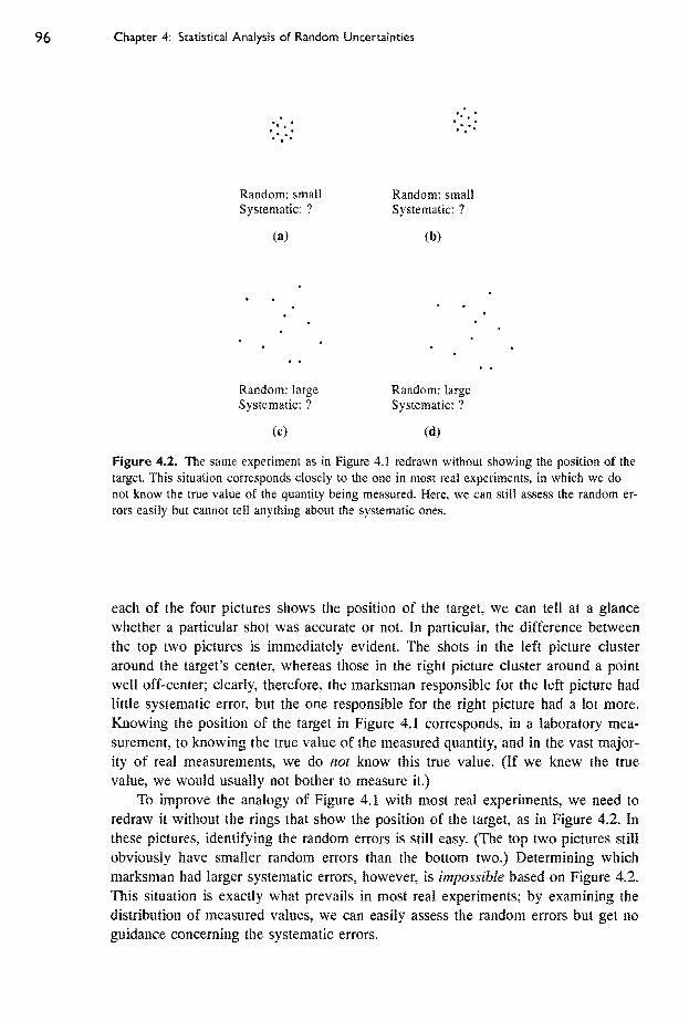
Ch^ter 4: Statistical Analysis of R<uidom Uncertainties
Random: small Random: small
Systematic: ? Systematic: ?
(a) (b)
Random: large Random: large
Systematic: ? Systematic: ?
(c) (d)
Figure 4.2. The same experiment as in Figure 4.1 redrawn without showing the position of the
target. This situation corresponds closely to the one in most real experiments, in which we do
not know the true value of the quantity being measured. Here, we can still assess the random er-
rors easily but cannot tell anything about the systematic ones.
each of the four pictures shows the position of the target, we can teil at a glance
whether a particular shot was accurate or not. In particular, the difference between
the top two pictures is immediately evident. The shots in the left picture cluster
around the target's center, whereas those in the right picture cluster around a point
well off-center; clearly, therefore, the marksman responsible for the left picture had
little systematic error, but the one responsible for the right picture had a lot more.
Knowing the position of the target in Figure 4.1 corresponds, in a laboratory mea-
surement, to knowing the true value of the measured quantity, and in the vast major-
ity of real measurements, we do not know this true value. (If we knew the true
value, we would usually not bother to measure it.)
To improve the analogy of Figure 4.1 with most real experiments, we need to
redraw it without the rings that show the position of the target, as in Figure 4.2. In
these pictures, identifying the random errore is still easy. (The top two pictures still
obviously have smaller random errors than the bottom two.) Determining which
marksman had larger systematic errors, however, is impossible based on Figure 4.2.
This situation is exactly what prevails in most real experiments; by examining the
distribution of measured values, we can easily asse^ the random errors but get no
guidance concerning the systematic errois.

Section 4.2 The Mean and Standard Deviation
The distinction between random and systematic errors is not always clear-cut,
and a problem that causes random errors in one experiment may produce systematic
errors in another. For example, if you position your head first to one side and then
to another to read a typical meter (such as an ordinary clock), the reading on the
meter changes. This effect, called parallax, means that a meter can be read correctly
only if you position yourself directly in front of it. No matter how careful you are,
you cannot always position your eye exactly in front of the meter; consequently,
your measurements will have a small uncertainty due to parallax, and this uncer-
tainty will probably be random. On the other hand, a careless experimenter who
places a meter to one side of his seat and forgets to worry about parallax will
introduce a systematic error into ail his readings. Thus, the same effect, parallax, can
produce random uncertainti^ in one case, and systematic uncertainties in another.
The treatment of random errors is different from that of systematic errors. The
statistical methods described in the following sections give a reliable estimate of the
random uncertainties, and, as we shall see, provide a well-defined procedure for
reducing them. For the reasons just discussed, systematic uncertainties are usually
hard to evaluate and even to detect. The experienced scientist has to learn to antici-
pate the possible sources of systematic error and to make sure that all systematic
errors are much less than the required precision. Doing so will involve, for example,
checking the meters against accepted standards and correcting them or buying better
ones if necessary. Unfortunately, in the first-year physics laboratory, such checks are
rarely possible, so the treatment of systematic errors is often awkward. This concept
is discussed further in Section 4.6. For now, I will discus experiments in which all
sources of systematic error have been identified and made much smaller than the
required precision.
4.2 The Mean and Standard Deviation
Suppose we need to measure some quantity x, and we have identified all sources of
systematic error and reduced them to a negligible level. Because all remaining
sources of uncertainty are random, we should be able to detect them by repeating
the measurement several times. We might, for example, make the measurement five
times and find the results
71, 72, 72, 73, 11 (4.1)
(where, for convenience, we have omitted any units).
The first question we address is this: Given the five measured values (4.1), what
should we take for our best estimate JC|^^^t of the quantity xl Reasonably, our best
estimate would seem to be the average or mean x of the five values found, and in
Chapter 5, 1 will prove that this choice is normally best. Thus,
-"best ~ ^
71 + 72 -H 72 -H 73 -H 71
5
= 71.8. (4.2)

Chapter 4: Statistical Anal/sis of Random Uncertainties
Here, the second line is simply the definition of the mean x for the numbers at
hand/
More generally, suppose we make N raeasureinents of the quantity x (all using
the same equipment and procedures) and find the N values
Xi,X2,..., Xj^. (4.3)
Once again, the best estimate for x is usually the average of x^^ . .. ,
X/^. That is,
"-best (4.4)
where
(4.5)
In the last line, I have introduced the useful sigma notation, according to which
^Xj — ^Xf — ^Xj — Xi -i- X2 + + Xpj;
1 = 1
the second and third expressions here are common abbreviations, which I will use
when there is no danger of confusion.
The concept of the average or mean is almost certainly familiar to most readers.
Our next concept, that of the standard deviation, is probably less so. The standard
deviation of the measurements Xj, . ..
, is an estimate of the average uncertainty
of the measurements x^, . . .,
x^,, and is determined as follows.
Given that the mean x is our best estimate of the quantity x, it is natural to
consider the difference x^ — x = dj. This difference, often called the deviation (or
residual) of a', from x, tells us how much the /"^ measurement differs from the
average x. If the deviations ~ x^ — x are all very small, our measurements are ail
close together and presumably very precise. If some of the deviations are large, our
measurements are obviously not so precise.
To be sure you understand the idea of the deviation, let us calculate the devia-
tions for the set of five measurements reported in (4.1). These deviations can be
listed as shown in Table 4.1. Notice that the deviations are not (of course) all the
same size; dj is small if the ith measurement jc, happens to be close to x, but d^ is
large if x, is far from x. Notice also that sorae of the d^ are positive and some
negative because some of the a,- are bound to be higher than the average x, and
some are bound to be lower.
To estimate the average reliability of the measurements x,, . . .,x^, we might
naturally try averaging the deviations rf,. Unfortunately, as a glance at Table 4.1
shows, the average of the deviations is zero. In fact, this average will be zero for
^ tn this age of pocket calculators, it is worth pointing out that an average such as (4.2) is easily calculated
in your head. Because ail the numbers are in the seventies, the same must be true of the average. All that
remains is to average the numbers 1, 2, 2, 3, 1 in the units place. These numbers obviously average to
9/5 = 1.8, and our answer is J = 71.8.

Secti<m 4.2 The Mean and Standard DeviatKXi
Table 4.1. Calculation of deviations.
Trial numlwr Measured value Deviation
/ = Xi ~ X
1 71 -0.8
2 72 0.2
3 72 0.2
4 73 1.2
5 71 -0.8
Ix^ = 359 Id, = 0.0
mean, X = L>Ci/N = 359/5 = 71.8
any set of measurements x^, . . . ,Xff because the definition of the average x ensures
that dj — Xf —x is sometimes positive and sometimes negative in just such a way
that d is zero (see Problem 4.4). Obviously, then, the average of the deviations is
not a useful way to characterize the reliability of the measurements JCj, . .. , x^.
The best way to avoid this annoyance is to square all the deviations, which will
create a set of positive numbers, and then average these numbers.^ If we then take
the square root of the result, we obtain a quantity with the same units as x itself.
Hiis number is called the standard deviation of JCj, . . . , jc^, and is denoted cr^:
With this definition, the standard deviation can be described as the mot mean square
(or RMS) deviation of the measurements JCj, . . . , Xf^. It proves to be a useful way
to characterize the reliability of the measurements. [As we will discuss shortly, the
definition (4.6) is sometimes modified by replacing the denominator N hy N ~ 1,]
To calculate the standard deviation as defined by (4.6), we must compute the
deviations r/,-, square them, average these squares, and then take the square root of
the result. For the data of Table 4.1, we start this calculation in Table 4.2.
Table 4.2. Calculation of the standard deviation.
Trial number Measured value Deviation Deviation squared
i di = Xi-x d,'
1 71 -0.8 0.64
2 72 0.2 0.04
3 72 0.2 0.04
4 73 1.2 1.44
5 71 -0.8 0.64
Ix, = 359 I4i = 0.0 = 2.80
X = 359/5 = 71.8
^Another possibility would be to take the absolute values |^,-| and average them, but the average of the d,^
proves more useful. The average of the \di\ is sometimes (misieadingly) called the average deviation.

Chapter 4: Statistical Anal/sis of Random Uncertainties
Summmg the numbers m the fourth column of Table 4.2 and dividing by 5,
we obtain the quantity (r^ (often called the variance of the measurements),
o-/ = ^24^ = ^ = 0-56. (4.7)
Taking the square root, we find the standard deviation
^ 0.7. (4.8)
Thus the average uncertainty of the five measurements 71, 72, 72, 73, 71 is approxi-
mately 0.7,
Unfortunately, the standard deviation has an alternative definition. There are
theoretical arguments for replacing the factor N in (4.6) by (AT — 1) and defining
the standard deviation tr^ of jCj, . .. , jc^ as
(4.9)
I will not try here to prove that definition (4.9) of cr^ is better than (4.6), except to
say that the new "improved" definition is obviously a iittie larger than the old one
(4.6) and that (4.9) corrects a tendency for (4.6) to understate the uncertainty in the
measurements Xj, . .. , %, especially if the number of measurements is small.
This tendency can be understood by considering the extreme (and absurd) case that
N = \ (that is, we make only one measurement). Here, the average x is equal to
our one reading Xj, and the one deviation is automatically zero. Therefore, the defi-
nition (4.6) gives the absurd result = 0. On the other hand, the definition (4.9)
gives 0/0; that is, with definition (4.9), (x^ is undefined, which correctly reflects our
total ignorance of the uncertainty after just one measurement. The definition (4.6) is
sometimes called the population standard deviation and (4.9) the sample standard
deviation.
The difference between the two definitions (4.6) and (4.9) is almost always
numerically insignificant. You should always repeat a measurement many times (at
least five, and preferably many more). Even if you make only five measurements
(A^ = 5), the difference between -^N ~ 2.2 and y[N~-~~i ~ 2 is, for most purposes,
insignificant. For example, if we recalculate the standard deviation (4,8) using the
improved definition (4.9), we obtain cr^ = 0.8 instead of cr, ~ 0.7, not a very
important difference. Nevertheless, you need to be aware of both definitions. In the
physics laboratory, using the more conservative (that is, larger) definition (4.9) is
almost always best, but in any case, your laboratory report should state clearly
which definition you are using so that your readere can check the calculations for
themselves.
Quick Check 4.1. You measure the time for a cart to roll down the same
length of track four times and get the following results:
21, 24, 25, 22

Section 4.3 The Standard Deviation as the Uncertainty in a Single Measurement
(in seconds). Find the average time and the standard deviation as given by the
improved definition (4.9).
To understand the notion of the standard deviation, you must be able to calcu-
late it yourself for simple cases such as that in Quick Check 4.1. Most scientific
calculators, however, have a built-in function to do the caJcuiatioii automatically,
and you will certainly want to use this function for real experiments that involve
numerous measurements. If you are not sure how to use your calculator to obtain
standard deviations, take the time to learn, and then use the function to check your
answer to Quick Check 4.1. Some calculators give you a choice of the definitions
(4.6) or (4.9); some use just (4.9). Make sure you know what yours does.
4.3 The Standard Deviation as the Uncertainty
m a Single Measurement
Recall the claim that the standard deviation cr^ characterizes the average uncertainty
of the measurements ,r,, .... % from which it was calculated. In Chapter 5, I will
justify this claim by proving the following more precise statement, if you measure
the same quantity x many times, always using the same method, and if ail your
sources of uncertainty are small and random, then your results will be distributed
around the true value Xi^^ in accordance with the so-called normal, or bell-shaped,
curve. In particular, approximately 68% of your results-^ will fall within a distance
CTjj. on either side of x^^^^ that is, 68% of your measurements will fall in the range
X *+ <T
In other words, if you make a single measurement (using the same method), the
probability is 68% that your result will be within cr^ of the correct value. Thus, wecan adopt to mean exactly what we have been calling "uncertainty." If you make
one measurement of x^ the uncertainty associated with this measurement can be
taken to be
Sx = a-j.;
with this choice, you can be 68% confident that the measurement is within 8x of
the correct answer.
To illustrate the application of these ideas, suppose we are given a box of
similar springs and told to measure their spring constants k. We might measure the
spring constants by loading each spring and observing the resulting extension or,
perhaps better, by suspending a mass from each spring and timing its oscillations.
Whatever method we choose, we need to know k and its uncertainty 8k for each
spring, but it would be hopelessly time-consuming to repeat our measurements many
times for each spring. Instead we reason as follows; If we measure k for the first
'As we will see, the exact number is 68,27 . . .%, but stating this kind of number so precisely is obviousJy
absurd, in fact, it is often best to think of this number as "about two thirds."
Ch^ter 4: Statistical ^aiysis of Random Uncertainties
Spring several (say, 5 or 10) tim^, then the mean of these measurements should
give a good estimate of k for the first spring. More important for now, the standard
deviation cr^ of these 5 or 10 measurements provides us with an estimate of the
uncertainty in our method for measuring k. Provided our springs are aii reasonably
similar and we use the same method to measure each one, we can reasonably expect
the same uncertainty in each measurement.'* Thus, for each subsequent spring we
need to make only one measurement, and we can immediately state that the uncer-
tainty St is the standard deviation cr^ measured for the first spring, with a 68%confidence that our answer is within of the correct value.
To illustrate these ideas numerically, we can imagine making 10 measurements
on the first spring and obtaining the following measured values of k (in newtons/
meter):
86, 85, 84, 89, 85, 89, 87, 85, 82, 85. (4.10)
From these values, we can immediately calculate k ~ 85.7 N/m and, using the
definition (4.9),
ojt = 2.16 N/m (4.11)
^ 2 N/m. (4.12)
The uncertainty in any one measurement of k is therefore approximately 2 N/m. If
we now measure the second spring once and obtain the answer k — 1\ N/m, we can
without further ado take 8k = cr^ = 2 N/m and state with 68% confidence that k lies
in the range
{k for second spring) = 71 ± 2 N/m. (4.13)
4.4 The Standard Deviation of the Mean
If Xj, . .. , jc^ are the results of measurements of the same quantity then, as we
have seen, our best estimate for the quantity x is their mean x. We have also seen
that the standard deviation cr^ characterizes the average uncertainty of the separate
measurements Xj, . . . ,jc^. Our answer x^^^^^ — x, however, represents a judicious
combination of all N measurements, and we have every reason to think it will be
more reliable than any one of the measurements taken alone, in Chapter 5, I will
prove that the uncertainty in the final answer x^est = ^ is given by the standard
deviation cr^ divided by Tliis quantity is called the standard deviation of the
mean, or SDOM, and is denoted oj:
liisiHii'i^iiBiiiiiilliiii!^
(Other common names are standard error and standard error of the mean.) Thus,
based on the A'^ measured values x^, . .. ,
x^, we can state our final answer for the
''If some springs are very different from the first, our uncertainty in measuring them may be different. Thus,
if the springs differ a lot, we would tieed to check our uncertainty by making several measurements for each
of two or three different springs.

Section 4,4 The Standard Deviation of the Mean 103
value of X as
(value of x) = x^,^^^ ± dx,
where A^est ~ ^» mean of x^, . .. , x^, and Sx is the standard deviation of the
mean,
8x ^ aJ-jN, (4.15)
As an example, wc can consider the 10 measurements reported in (4.10) of the
spring constant k of one spring. As we saw, the mean of these values isk = 85.7
N/m, and the standard deviation is = 2.2 N/m. Therefore, the standard deviation
of the mean is
(T^ = o-^/a/To - 0.7 N/m, (4.16)
and our final answer, based on these 10 measurements, would be that the spring has
k = 85.7 ± 0.7 newtons/meter. (4.17)
When yoi! give an answer like this, you must state clearly what the numbers are
—
namely, the mean and the standard deviation of the mean—^so your readers can
judge their significance for themselves.
An important feature of the standard deviation of the mean, = aJ-\lN, is
the factor -\[n in the denominator. The standard deviation cr^ represents the average
uncertainty in the individual measurements x^, . .. , Xjy. Thus, if we were to malce
some more measurements (using the same technique), the standard deviation cr^
wouid not change appreciably. On the other hand, the standard deviation of the
mean, cr^/>//V, would slowly decrease as we increase N, This decrease is just what
we would expect. If we make more measurements before computing an average, wewould naturally expect the final result to be more reliable, and this improved relia-
bility is just what the denominator a/zV in (4.15) guarantees. This conclusion pro-
vides one obvious way to improve the precision of our measurements.
Unfortunately, the factor a/zV grows rather slowly as we increase N. For exam-
ple, if we wish to improve our precision by a factor of 10 simply by increasing the
number of measurements N, we will have to increase A'^ by a factor of TOO—
a
daunting prospect, to say the least! Furthermore, we are for the moment neglecting
systematic errors, and these are not reduced by increasing the number of measure-
ments. Thus, in practice, if you want to increase your precision appreciably, you
will probably do better to improve your technique than to rely merely on increased
numbers of measurements.
Quick Check 4.2. A student makes five measurements of e, the magnitude of
the electron's charge, as follows:
15, 17, 18, 14, 16,
all in units of 10 coulombs. Find her best estimate for e (as given by the
mean) and its uncertainty (as given by the SDOM),

Chapter 4: Statistic^ Anat/sis of Random Uncertainties
4.5 Examples
In this section, ] discuss two examples of simple experiments that make use of the
ideas of the past three sections.
Example: Area of a Rectangle
As a first, simple application of the standard deviation of the mean, imagine that we
have to measure very accurately the area A of a rectangular plate approximately 2.5
cm X 5 cm. We first find the best available measuring device, which might be a
vernier caliper, and then make several measurements of the length / and breadth b
of the plate. To allow for irregularities in the sides, we make our measurements at
several different positions, and to allow for small defects in the instrument, we use
several different calipers (if available). We might make 10 measurements each of /
and b and obtain the results shown in Table 4.3.
T^le 4.3. Length and breadth (in mm).
Measured values Mean SD SDOM
/ 24.25, 24.26, 24.22, 24.28, 24.24 7 = 24.245 or, = 0.019 aj ^ 0.006
24.25, 24.22, 24.26, 24.23, 24.24
b 50.36, 50.35, 50.41, 50.37, 50.36 b = 50.368 CFf, = 0.024 ai = 0.008
50.32, 50.39, 50.38, 50.36, 50.38
Using the 10 observed values of /, you can quickly calculate the mean /, the
standard deviation cr^, and the standard deviation of the mean orj, as shown in the
columns labeled mean, SD, and SDOM. In the same way you can calculate 6, cr^,
and (Tg. Before doing any further calculations, you should examine these results to
see if they seem reasonable. For example, the two standard deviations cr^ and cr^ are
supposed to be the average uncertainty in the measurements of / and b. Because /
and b were measured in exactly the same way, <J/ and cr^ should not differ signifi-
cantly from each other or from what we judge to be a reasonable uncertainty for
the measurements.
Having convinced yourself that the results so far are reasonable, you can
quickly finish the calculations. The best estimate for the length is the mean / and
the uncertainty is the SDOM (J/; so the final value for / is
/ = 24.245 ± 0.006 mm (or 0.025%);
the number in parenthesis is the percentage uncertainty. Similarly, the value for b is
b = 50.368 ± 0.008 mm (or 0.016%).
Finally, the best estimate for the area A = lb is the product of these values, with a
fractional uncertainty given by the quadratic sum of those in / and b (assuming the

Section 4.5 Examples
errors are independent):
A - (24.245 mm ± 0.025%) X (50.368 mm ± 0.016%)
^ 1221.17 mm^ ± 0.03%
== 1221.2 ± 0.4 mm^ (4.18)
To arrive at the answer (4.18) for A, we calculated the averages I and 6, each
with an uncertainty equal to the standard deviation of its mean. We then calculated
the area A as the product of 7 and h and found the uncertainty by propagation of
errors. We could have proceeded differently. For instance, we could have multiplied
the first measured value of / by the first value of b to give a first answer for A.
Continuing in this way we could have calculated 10 answers for A and {hen have
subjected these 10 answers to statistical analysis, calculating A, and finally aj.
If, however, the errors in / and b are independent and random, and if we make
enough measurements, this alternative procedure will produce the same result as the
first one.''
Example: Another Spring
As a second example, consider a case in which a statistical analysis cannot be
applied to the direct measurements but can to the final answers. Suppose we wish
to measure the spring constant A: of a spring by timing the oscillations of a mass mfixed to its end. We know from elementary mechanics that the period for such
oscillations is T = Iw^mlk. Thus, by measuring T and m, we can find k as
The simplest way to find k is to take a single, accurately known mass m and make
several careful measurements of T. For various reasons, however, timing T for sev-
eral dijferent masses m may be more interesting. (For example, in this way, wecould check that T « as well as measure k) We might then get a set of readings
such as those in the first two lines of Table 4.4.
Table 4.4. Measurement of spring constant k.
Mass/n(kg) 0.513 0.581 0.634 0.691 0.752 0.834 0.901 0.950
Period r(s) 1.24 1.33 1.36 1.44 1.50 1.59 1.65 1.69
jt = AiT^mlt^ 13.17 12.97 etc.
It obviously makes no sense to average the various different masses in the top
line (or the times in the second line) because they are not different measurements
of the same quantity. Nor can we learn anything about the uncertainty in our mea-
surements by comparing the different values of m. On the other hand, we can com-
-""Thc second procedure has a certain illogic because there is no particular reason to associate the first
measurement of / with the first measurement of b. indeed, we might have measured / eight times and b twelve
times; then we couldn't pair off vaiues. Thus, our first procedure is iogically preferable.
k = An^mjT^, (4.19)

Chapter 4: Statistical Anal/sis of Random Uncertainties
bine each value of m with its corresponding period T and calculate k, as in the final
line of Table 4.4. Our answers for k in the bottom line are all measurements of the
same quantity and so can be subjected to statistical analysis. In particular, our best
estimate for k is the mean, k = 13.16 N/m, and our uncertainty is the standard
deviation of the mean, crj = 0.06 N/m (see Problem 4.20), Thus, the final answer,
based on the data of Table 4.4, is
spring constant k = 13.16 ± 0.06 N/m. (4.20)
If we had formed reasonable estimates of the uncertainties in our original mea-
surements of m and T, we could also have estimated the uncertainty in A by using
error propagation, starting from these estimates for dm and 8T. In this case, it would
be a good idea to compare the final uncertainties in k obtained by the two methods.
4.6 Systematic Errors
In the past few sections, I have been taking for granted that all systematic errors
were reduced to a negligible level before serious measurements began. Here, I take
up again the disagreeable possibility of appreciable systematic errors. In the example
just discussed, we may have been measuring m with a balance that read consistently
high or low, or our timer may have been running consistently fast or slow. Neither
of these systematic errors will show up in the comparison of our various answers
for the spring constant k. As a result, the standard deviation of the mean cr^ can be
regarded as the random component 8k of the uncertainty 8k but is certainly not
the total uncertainty 8k, Our problem is to decide how to estimate the systematic
component dk^yg and then how to combine Sfe^a^ and SAgyj- to give the complete
uncertainty
No simple theory tells us what to do about systematic errors. In fact, the only
theory of systematic errors is that they must be identified and reduced until they are
much less than the required precision. In a teaching laboratory, however, this goal
is often not attainable. Students often cannot check a meter against a better one to
correct it, much less buy a new meter to replace an inadequate one. For this reason,
some teaching laboratories establish a rule that, in the absence of more specific
information, meters should be considered to have some definite systematic uncer-
tainty. For example, the decision might be that all stopwatches have up to 0.5%
systematic uncertainty, all balances up to 1%, all voltmeters and ammeters up to
3%, and so on.
Given rules of this kind, there are various possible ways to proceed. None can
really be rigorously justified, and we describe just one approach here. (Problems
4.23 to 4.28 contain more examples.) In the last example in Section 4.5, the spring
constant k ~ Ai^mlT^ was found by measuring a series of values of m and the
corresponding values of T, As we have seen, a statistical analysis of the various
answers for k gives the random component of Sk as
S^raii ^ <ri ^ 0.06 N/m. (4.21)
Suppose now we have been told that the balance used to measure m and the clock
used for T have systematic uncertainties up to 1% and 0.5%, respectively. We can

Section 4.6 Systmatic Errors
then find the systematic component of Sfe by propagation of errors; the only question
is whether to combine the errors in quadrature or directly. Because the errors in mand T are surely independent and some cancellation is therefore possible, using the
quadratic sum is probably reasonable*^; this choice gives
= + {\%f - 1.4% (4,23)
and hence
Sfcsys = X (1.4%) (4.24)
= (13.16 N/'m) X 0.014 - 0.18 N/m.
Now that we have estimates for both the random and systematic uncertainties
in k, we must decide how to state our final conclusion for the spring constant k with
its overall uncertainty. Because the method for combining Sfe^aH ^nd Bk^^^ is not
completely clear, many scientists leave the two components separate and state a
final answer in the form
(measured value of k) = /c^est ± ^ran ± ^^sys (4.25)
- 13.16 ± 0.06 ± 0.18 N/m
(all of which should probably be rounded to one decimal place). Alternatively, a
case can be made that 8k^^^ and dk^y^ should be combined in quadrature, in which
case we could state a single, total uncertainty
Sfe = <{^K..f + i^Kysf (4.26)
= V(0.06)2 + (0.18)2 ^ 0.19 N/m
and replace the conclusion (4.25) by
(measured value of k) — /c^^g^j ± 8k
= 13.16 ± 0.19 N/m
or, probably better, 13.2 ± 0.2 N/m.
The expression (4.26) for 8k cannot really be rigorously justified. Nor is the
significance of the answer clear; for example, we probably cannot claim 68% confi-
dence that the true answer lies in the range k ± 8k. Nonetheless, the expression
does at least provide a reasonable estimate of our total uncertainty, given that our
apparatus has systematic uncertainties we could not eliminate. In particular, there is
one important respect in which the answer (4.26) is realistic and instructive. We saw
in Section 4.4 that the standard deviation of the mean aj approaches zero as the
number of measurements N is increased. This result suggested that, if you have the
^Whether we should use the quadratic or ordinary sum really depends on what is meant by the statement
that the balance has "up to 1% systematic uncertainty." If it means the error is certainly no more than 1%(and likewise for the clock), then direct addition is appropriate, and dk^^^ is then certainly no more than 2%.
On the other hand, perhaps an analysis of all balances in the laboratory has shown that they follow a normal
distribution, with 68% of them better than 1% reliable (and likewise for the clocks). In this case, we can use
addition in quadrature as in (4.22) with the usual significance of 68% confidence.

Chapter 4: Statistic^ AnaE/sis of Random Uncertainti^
patience to make an enonnous number of measurements, you can reduce the uncer-
tainties indefinitely without having to improve your equipment or technique. We can
now see that this suggestion is incorrect. Increasing jV can reduce the random com-
ponent = ai indefinitely. But any given apparatus has some systematic uncer-
tainty, which is not reduced as we increase M From (4.26) we clearly see that little
is gained from further reduction of Sk^.^^, once 8k^.^^ is smaller than SA'^ys- particu-
lar, the total 8k can never be made less than &c^ys- This fact simply confirms what
we already guessed, that in practice a large reduction of the uncertainty requires
improvements in techniques or equipment to reduce both the random and systematic
errors in each single measurement.
As discussed in Chapter 2, a peculiar feature of the teaching laboratory is that
you will probably be asked to measure quantities, such as the acceleration of gravity,
for which an accurate, accepted value is already known. In this kind of experiment,
the logic of the error analysis is a bit confusing. Probably the most honest course is
to ignore the known accepted value until after you have done all calculations of
your measured value, q^^^^, and its uncertainty. Then, of course, you must ask
whether the accepted value lies inside (or at least close to) the range q^,^^^ ± 8q. If
it does, you can simply record this agreement in your report. If the accepted value
lies well outside the range ^^g^, ± 8g, however, you have to examine the possible
causes of the excessive discrepancy. For example, you might measure the acceler-
ation of gravity, and get the results (all in m/s^),
gbest = 9.97, (4.27)
with uncertainties
Sg,3„ = 0.02 and 8g,y, = 0.03,
and hence a total uncertainty, as in (4.26), of
Sg ^ 0.04.
Clearly, the accepted value of
g = 9.80 m/s^
lies far outside the measured range, 9.97 ± 0.04. (More specifically, the discrepancy
is 0.17, which is four times the uncertainty.) This result is definitely not satisfactory
and further analysis is required.
The first thing to check is the possibility that you made a downright mistake in
calculating g^^^^ or one of the uncertainties S^^^n and Sgjys- Y^^ ca^ convince
yourself that all your calculations were correct, the next possibility is that the ac-
cepted value is wrong. In the case of g = 9.80 m/s^ this possibility is rather unlikely,
but it is entirely possible for plenty of other cases. For example, suppose you were
measuring the density of air; because this is strongly dependent on the temperature
and pressure, you could easily have looked up the wrong accepted value for this
parameter.
Once you have eliminated these suspects, only one possibility is left; You must
have overlooked some systematic error so that your value of dg^y^ is too small.
Ideally, you should try to find the culprit, but this search can be hard because of the
many possibilities:

Principal Definitions and Equations of Chapter 4
(1) Perhaps one of your meters had larger systematic errors than you had al-
lowed for when you calculated Sg^yg- You can investigate this possibility by de-
termining how large a systematic error in your clock (or voltmeter, or whatever)
would be needed to account for the offending discrepancy. If the needed error is not
unreasonably large, you have one possible explanation of your difficulty,
(2) Another possible cause of systematic error is that you used an incorrect
vaiue for some parameter needed in your calculations. A celebrated example of this
was Miilikan's famous measurement of the electron's charge, e. Millikan's method
depended on the viscosity of air, for which he used a value that was 0.4% too small.
This discrepancy caused all of his values of e to be 0.6% too small, an error that
was not noticed for nearly 20 years. This kind of mistake sometimes arises in a
teaching laboratory when a student uses a value that has too few significant figures.
For example, suppose you do an experiment with protons and you expect to have
an accuracy better than T%. If you take the proton's mass to be 1.7 X 10 ^ ~^ kg
(instead of tlie more exact 1.67 X 10 ^ kg), you will have introduced a 2% sys-
tematic error, which will almost certainly frustrate your hope for 1% results.
(3) Much harder to analyze is the possibility of a flaw in the design of the
experiment. For example, if you had measured g by dropping an object from a great
height, air resistance could introduce an appreciable systematic error. [Note, how-
ever, that this error would not account for the large value of g in (4.27) because air
resistance would cause an acceleration that was too small.] Similarly, if you try to
measure the half-life of a radioactive material and your sample is contaminated with
another material of shorter half-life, you will get an answer that is systematically
too short.
Obviously, tracking down the source of systematic errors is difficult and has
defied the best efforts of many great scientists. In all probability, your instructors
are not going to penalize you too severely if you fail to do so. Nevertheless, they
will expect an intelligent discussion of the problem and at least an honest admission
that there appear to have been systematic errors that you were unable to identify.
Principal Definitions and Equations of Chapter 4
Suppose that we make N measurements, x^, X2, . ..
, of the same quantity jc,
all using the same method. Provided ail uncertainties are random and small, we
have the following results:
THE MEAN
The best estimate for x, based on these measurements, is their mean:
X - [See (4.5)]

Chapter 4: Statistical Analysis of Random Uncertainties
THE STANDARD DEVIATION
The average uncertainty of the individual measurements x^^ X2, . . . , is given
by the standard deviation, or SD:
cr, = ^j~jl(x,-xf, [See (4.9)]
This definition of the SD, often called the sample standard deviation, is the most
appropriate for our purposes. The population standard deviation is obtained by re-
placing the factor (N — 1) in the denominator by N. You will usually want to calcu-
late standard deviations using the built-in function on your calculator; be sure you
know which definition it uses.
The detailed significance of the standard deviation cr^ is that approximately 68%
of the measurements of x (using the same method) should lie within a distance cr^.
of the true value. (This claim is justified in Section 5.4.) This result is what allows
us to identify cr^ as the uncertainty in any one measurement of x,
and, with this choice, we can be 68% confident that any one measurement will fall
within cr^ of the correct answer.
THE STANDARD DEVIATION OF THE MEAN
As long as systematic uncertainties are negligible, the uncertainty in our best
estimate for x (namely x) is the standard deviation of the mean, or SDOM,
a, = [See (4.14)]
If there are appreciable systematic errors, then o-j gives the random component of
the uncertainty in our best estimate for x:
If you have some way to estimate the systematic component Sx^ys' a reasonable (but
not rigorously justified) expression for the total uncertainty is the quadratic sum of
^ran ^nd 8x,^.^:
- V(6x,,j2 + (a^ [See (4.26)]
Problems for Chapter 4
For Section 4.2: The Mean and Standard Deviation
4.1. * You measure the time for a ball to drop from a second-floor window three
times and get the results (in tenths of a second):

Problems for Chapter 4 III
(a) Find the mean and the standard deviation. For the latter, use both the "im-
proved" definition (4.9) (the sample standard deviation) and the original definition
(4.6) (the population standard deviation). Note how, even with only three measure-
ments, the difference between the two definitions is not very big. (b) If you don't
yet know how to calculate the mean and standard deviation using your calculator's
built-in functions, take a few minutes to learn. Use your calculator to check your
answers to part (a); in particular, find out which definition of the standard deviation
your calculator uses.
4.2. * A student measures g, the acceleration of gravity, five times, with the results
(all in m/s^):
9.9, 9.6, 9.5, 9.7, 9.8.
(a) Find her mean and the standard deviation [as defined by (4.9) j. Do the calcula-
tion yourself using a layout similar to that in Table 4,2. (b) Check your value for
the SD using the built-in function on your calculator. (If you don't yet know how
to calculate the mean and standard deviation using your calculator's built-in func-
tions, take a few minutes to learn.)
4.3. * Find the mean and standard deviation of the 10 measurements reported in
(4.10). If you haven't done either of the two previous problems, be sure to do this
calculation yourself, then check it using the built-in functions on your calculator.
4.4. * The mean of quantities .Y|, . .. , % is defined as their sum divided by N;
that is, X = The deviation of is the difference dj = Xj — x. Show clearly
that the mean of the deviations d^, , .,
, is always zero.
If you are not used to the £ notation, you might want to do this problem
both without and with the notation. For example, write out the sum X(jc, — 3c) as
(x^ - x) + (x2 - x) + ... + (xjy ~- x) and regroup the terms.
4.5. -kir (a) Computing the standard deviation or. of measurements jcj, . ., , %
of a single quantity x requires that you compute the sum X(JCf - x)^. Prove that this
sum can be rewritten as
I[(x,: - xf] = im'] - i [I(x,)]l (4.28)
This problem is a good exercise in using the £ notation. Many calculators use the
result to compute the standard deviation for the following reason: To use the expres-
sion on the left, a calculator must keep track of all the data (which uses a lot of
memory) to calculate x and then the sum indicated; to use the expression on the
right, the machine needs only to keep a running total of Z(x,-^) and X(a-,), which
uses much less memory, (b) Verify the identity (4.28) for the three measurements
of Problem 4,1.
4.6. In Chapter 3, you learned that in a counting experiment, the uncertainty
associated with a counted number is given by the "square-root rule" as the square
root of that number. This rule can now be made more precise with the following
statements (proved in Chapter 11): If we make several counts
V], 1/2, . . . ,

Chapter 4: Statistical Analysis of Random Uncertainties
of the number v of random events that occur in a time T, then; (1) the best estimate
for the true average number that occur in time T is the mean v — Y^v-JN of our
measurements, and (2) the standard deviation of the observed numbers should be
approximately equal to the square root of this same best estimate; that is, the uncer-
tainty in each measurement is V^. In particular, if we make on!y one count i/, the
best estimate is just v and the uncertainty is the square root this result is just
the square-root rule of Chapter 3 with the additional information that the "uncer-
tainty" is actually the standard deviation and gives the margins within which we can
be approximately 68% confident the true answer lies. This problem and Problem 4.7
explore these ideas.
A nuclear physicist uses a Geiger counter to monitor the number of cosmic-ray
particles arriving in his laboratory in any two-second interval. He counts this num-
ber 20 times with the following results:
10, 13, 8, 15, 8, 13, 14, 13, 19, 8,
13, 13, 7, 8, 6, 8, 11, 12, 8, 7.
(a) Find the mean and standard deviation of these numbers, (b) The latter shouid be
approximately equal to the square root of the former. How well is this expectation
borne out?
4.7. *** Read the first paragraph of Problem 4.6 and then do the following prob-
lem: A health physicist is testing a new detector and places it near a weak radioac-
tive sample. In five separate lO-second intervals, the detector counts the following
numbers of radioactive emissions:
16, 21, 13, 12, 15.
(a) Find the mean and standard deviation of these five numbers, (b) Compare the
standard deviation with its expected value, the square root of the average number,
(c) Naturally, the two numbers in part (b) do not agree exactly, and we would like
to have some way to assess their disagreement. This problem is, in fact, one of error
propagation. We have measured the number v. The expected standard deviation in
this number is just a/^, a simple function of p. Thus, the uncertainty in the standard
deviation can be found by error propagation. Show, in this way, that the uncertainty
in the SD is 0.5, Do the numbers in part (b) agree within this uncertainty?
4.8. Spreadsheet programs, such as Lotus 123 or Excel, provide an excellent
way to find the standard deviation of a set of measurements (and to record and
process many kinds of data in general), (a) If you have access to one of these
programs, create a spreadsheet to calculate the SD of any set of 10 measurements
using the layout of Table 4.2. The first column should list {he trial number z, and
the second column should be where the user will enter the data x^. The mean x will
be calculated by a formula that gives
(sum of data entries)/(number of data entries),
which you can place to the side of the main table. In the third column, put a formula
to calculate the deviation, x^ — 3c, and in the fourth, a formula to calculate the devia-
tion squared. Finally, somewhere to the side of the main table, write a formula to

Problems for Chapter 4
find the SD as
_ /sum of squared deviations
(Most spreadsheet programs can caicuiate standard deviations automatically, but the
point here is for you to create your own program to do it, not to use the buiit-in
functions.) (b) Test your spreadsheet on the data of Equation (4.10). (c) (The hard
part.) Most simple solutions to part (a) have two irritating drawbacks. First, as you
enter each of the data, the spreadsheet will calculate answers for the mean and SD,
but these answers will probably be incorrect (even for the data entered so far) until
you have entered all the data. Second, your spreadsheet will probably need some
modification before you can use it to find the mean and SD of a different number
of data. If you can, modify your spreadsheet so that it does not suffer these defects
and can find the mean and SD of any numher of data (up to some convenient
maximum, say 30). (d) Test your new spreadsheet using the data of Problem 4.6,
and convince yourself that as you enter the data the program gives the correct
answer at each stage.
For Section 4.3: The Standard Deviation as the Uncertainty in a Single Measurement
4.9. * A student measures the period of a pendulum three times and gets the
answers 1.6, 1.8, and 1.7, all in seconds. What are the mean and standard deviation?
[Use the improved definition (4.9) of the standard deviation.] If the student decides
to make a fourth measurement, what is the probability that this new measurement
will fall outside the range of 1.6 to 1.8 s? (The numbers here were chosen to "come
out right." In Chapter 5, I will explain how to do this kind of problem even when
the numbers don't come out right.)
4.10. * After several measurements of a quantity x, we expect to find that approxi-
mately 68% of the measurements fall within the range of x ± cr^.. (The exact num-
ber is 68.27 . . . %, but the difference is usually insignificant.) If you have not
already done so, check the mean and standard deviation of the 10 measurements in
(4.10). How many of the measurements should we expect to fall within the range
of jc ± cr^? How many do?
4.11. A student has to measure several unknown charges ^ on a capacitor by
discharging it through a ballistic galvanometer. The discharge kicks the galvanome-
ter's needle, whose resulting maximum swing tells the student the value of Q, Be-
fore making all her measurements, the student wants to know how reliably she can
read the maximum displacement of the swinging needle. Therefore, she arranges to
charge the capacitor to exactly the same voltage (and hence the same charge) five
times and to measure the resulting charge. Her results (in microcoulombs) are:
1.2, 1.4, 1.6, 1.6, 1.2.
Based on these results, what would you suggest she take for the uncertainty SQ in
her subsequent measurements of the charge Q, assuming she wants to be 68% con-
fident that the correct value is within ±dQ of her measurement?

Ch^ter 4: Statistical Andysis of RandcHn Uncertainties
4.12. T*r To calibrate a prism spectrometer, a student sends light of 10 different
known wavelengths X through the spectrometer and measures the angle $ by which
each beam is deflected. Using these resuUs, he makes a calibration curve like Figure
3.8 showing A. as a function of 0. For the first value of X, he measures 6 six times
and obtains these results (in degrees):
52.5, 523, 52.6, 52.5, 52.7, 52.4.
For each of the nine remaining values of X, he measures the corresponding value of
Q just once. What should he take for the uncertainty in each of these nine measure-
ments of ff>
4.13. -kin (a) Calculate the mean and standard deviation for the following 30 mea-
surements of a time t (in seconds):
8.16, 8.14, 8.12, 8.16, 8.18, 8.10, 8.18, 8.18, 8.18, 8.24,
8.16, 8.14, 8,17, 8.18, 8.21, 8.12, 8.12, 8.17, 8.06, 8.10,
8.12, 8.10, 8.14, 8.09, 8.16, 8.16, 8.21, 8.14, 8.16, 8.13.
(You should certainly use the built-in functions on your calculator (or the spread-
sheet you created in Problem 4.8 if you did), and you can save some button pushing
if you drop all the leading 8s and shift the decimal point two places to the right
before doing any calculation.) (b) We know that after several measurements, we can
expect about 68% of the observed values to be within cr^ of t (that is, inside the
range t ± a>). For the measurements of part (a), about how many would you expect
to lie outside the range ? ± cr,? How many do? (c) In Chapter 5, I will show that
we can also expect about 95% of the values to be within 2(r, of t (that is, inside the
range t ± 2cr,). For the measurements of part (a), about how many would you ex-
pect to lie outside the range t ± 2<jp. How many do?
4.14. ** (a) If you have not yet done it, do Problem 4.6. (b) About how many of
the measurements of this problem should you expect to He outside the range
p ± cTj,? How many do? (c) In Chapter 5, I will show that we can expect about
95% of the measurements to be within 2cr^ of v (that is, inside the range i> ± 2ov).
For the measurements of part (a), about how many would you expect to lie outside
the range v ± 2ct^7 How many do?
For Section 4.4: The Standard Deviation of the Mean
4.15. it; Given the three measurements in Problem 4.1, what should you state for
your best estimate for the time concerned and its uncertainty? (Your answer will
illustrate how the mean can have more significant figures than the original measure-
ments.)
4.16. (a) Based on the five measurements of g reported in Problem 4.2, what
should be the student's best estimate for g and its uncertainty? (b) How well does
her result agree with the accepted value of 9.8 m/s^?
4.17. -Ar (a) Based on the 30 measurements in Problem 4.13, what would be your
best estimate for the time involved and its uncertainty, assuming all uncertainties

Problems for Chapter 4
are random? (b) Comment on the number of significant digits in your best estimate,
as compared with the number of significant digits in the data.
4.18. * After measuring the speed of sound u several times, a student concludes
that the standard deviation (t„ of her measurements is cr„ = 10 m/s. If all uncer-
tainties were truly random, she could get any desired precision by making enough
measurements and averaging, (a) How many measurements are needed to give
a final uncertainty of ±3 m/s? (b) How many for a final uncertainty of only
±0.5 m/s?
4.19. *** (a) The data in Problem 4.6 are 20 measurements of the number of
cosmic-ray particles counted by a Geiger counter in 2 seconds. By averaging these
numbers, find the best estimate for the number of particles that arrive in 2 seconds
and the uncertainty in that number (as given by the SDOM). (b) Another way to do
this problem is as follows: If you add all the data, you will have the number counted
in 40 seconds (with an uncertainty given by the square root of that number). If you
now divide this result by 20, you should get the number of particles that arrive in 2
seconds and its uncertainty. Check that your answers in (b) and (c) agree, at least
approximately. (Assume that that the 2-second time intervals are measured with
negligible uncertainty.) (c) Prove that these two methods should, ideally, give the
same answers. (Your proof should be general; that is, you should work in terms of
algebraic symbols, not the specific numbers of Problem 4.6. Remember that the SDof any counted number should be the square root of that number.)
For Section 4.S: Examples
4.20. * Complete the calculations of the spring constant k in Table 4.4. Then
compute k and its uncertainty (the SDOM, o-j).
4.21. Table 4.3 records 10 measurements each of the length / and breadth h of
a rectangle. These values were used to calculate the area A = lb. If the measure-
ments were made in pairs (one of / and one of b), it would be natural to multiply
each pair together to give a value of A—the first / times the first h to give a first
value of A, and so on. Calculate the resulting 10 values of A, the mean A, the SD(T^, and the SDOM crj. Compare the answers for A and a-j with the answer (4.18)
obtained by calculating the averages T and b and then taking A to be T b, with an
uncertainty given by error propagation, (For a large number of measurements, the
two methods should agree.)
4.22.* This problem is an example of an experiment for which the error analy-
sis can be done in either of two ways: by propagating the estimated errors in the
original measurements or by doing a statistical analysis of the various answers. Astudent wants to measure g, the acceleration of gravity, using a simple pendulum,
as described briefly in the introduction to this chapter. Because the period is known
to be r = In^^Jljg, where / is the length of the pendulum, she can find g as ^ =
At^lIT'^. She measures T for five different values of / and obtains the following
results:
Length, / (cm): 57.3 61.1 73.2 83.7 95.0
Time, r(s): 1.521 1.567 1.718 1.835 1.952

Chapter 4: ^tistica! Anat^is of Random Uncertainties
(a) Copy the table of data and add a row in which you list her five computed values
of g. (b) She estimates she can read the lengths 1 within about 0,3% (that is, two
or three millimeters). Similarly, she estimates that all of the times are within
± 0,2%. Use error propagation to find the uncertainty in her values for g, (c) Be-
cause her values of g are five measurements of the same quantity, we can analyze
them statistically. In particular, their standard deviation should represent the uncer-
tainty in any one of her answers. What is the SD, and how does it compare with
the uncertainty found by error propagation in part (b)? [You should not expect the
agreement to be especially good because we don't know the exact nature of her
original estimated uncertainties (nor, probably, does she). Nevertheless, the two
methods should agree roughly^ and a large disagreement would be a clear signal that
something had gone wrong.] (d) What is her final answer for g with its uncertainty?
[Use the statistical analysis of part (c), and remember that the final uncertainty is
the SDOM. How does her answer compare with the accepted value (in her labora-
tory) of 979.6 cm/s^?
For Section 4.6: Systematic Errors
if A famous example of a systematic error occurred in Millikan's historic
measurement of the electron's charge e. He worked on this experiment for several
years and had reduced all random errors to a very low level, certainly less than
0.1%. Unfortunately, his answer for e depended on the viscosity of air (denoted 17),
and the value of 17 that he used was 0.4% too low. His value for e had the form
e — Krf^^, where K stands for a complicated expression involving several measured
parameters but not tj. Therefore, the systematic error in 17 caused a systematic error
in e. Given that all other errors (random and systematic) were much less than 0.4%,
what was his error in e? (This example is typical of many systematic errors. Until
the errors are identified, nothing can be done about them. Once identified, the errors
can be eliminated, in this case by using the right value of 17.)
4J!4. ifk In some experiments, systematic errors can be caused by the neglect of
an effect that is not (in the situation concerned) negligible, for example, neglect of
heat losses from a badly insulated calorimeter or neglect of friction for a poorly
lubricated cart. Here is another example: A student wants to measure the accelera-
tion of gravity g by timing the fall of a wooden ball (3 or 4 inches across) dropped
from four different windows in a tall building. He assumes that air resistance is
negligible and that the distance fallen is given by d — hgt. Using a tape measure
and an electric timer, he measures the distances and times of Che four separate drops
as follows:
Distance, d (meters): 15.43 17.37 19.62 21.68
Time, t (seconds): 1.804 1.915 2.043 2.149
(a) Copy these data and add a third row in which you put the corresponding acceler-
ations, calculated as ^ = 2d/t^. (b) Based on these results, what is his best estimate
'Although the percent uncertainties in the five measurements of / are probably not exactly the same, it is
appropriate (and time saving) in many experiments fo assume they are at least approximately so. In other
words, instead of doing five separate error propagations, you may often approfwiateiy do just one for a repre*
sentative case and assume that all five cases are reasonably similar.

Problems for Chapter 4
for g, assuming that all errors are random? Show that this answer is inconsistent
with the accepted value of g = 9.80 rn/s^. (c) Having checked his calculations, tape
measure, and timer, he concludes (correctly) that there must be some systematic
error causing an acceleration different from 9.80 m/s", and he suggests that air
resistance is probably the culprit. Give at least two arguments to support this sugges-
tion, (d) Suggest a couple of ways he could modify the experiment to reduce the
effect of this systematic error.
4.25. ** (a) A student measures the speed of sound as « = fk, where / is the
frequency shown on the dial of an audio oscillator, and k is the wavelength mea-
sured by locating several maxima in a resonant air column. Because there are sev-
eral measurements of k, they can be analyzed statistically, and the student concludes
that A. = 1 1 .2 ± 0.5 cm. Only one measurement has been taken of / = 3,000 Hz
(the setting on the oscillator), and the student has no way to judge its reliability.
The instructor says that the oscillator is "certainly 1% reliable"; therefore, the stu-
dent allows for a 1% systematic error in / (but none in X). What is the student's
answer for u with its uncertainty? Is the possible i% systematic error from the
oscillator's calibration important? (b) If the student's measurement had been
\ ~ 11.2 ± 0.1 cm and the oscillator calibration had been 3% reliable, what would
the answer have been? Is the systematic error important in this case?
4.26. ** A student wants to check the resistance of a resistor by measuring the
voltage across it (V) and the resulting current through it (/) and then calculating the
resistance as /? = V/I. He measures four different values of V and the corresponding
currents /, as follows;
Voltage, V (volts): 11.2 13.4 15.1 17,7
Current, / (amps): 4.67 5.46 6.28 7.22
(a) Calculate the four corresponding values of R (which will come out in ohms).
What is his best estimate for R, and what is the random component of its uncertainty
(SR^^Jl (b) The resistor is rated at 2.50 ohms, which does not lie within the range
± so he considers the possibility that the voltmeter and ammeter suffer
some systematic error. The laboratory technician states that many of the meters in
the laboratory have up to 2% systematic error. Use error propagation to find the
possible systematic error in R, and then combine the systematic and random errors
to give the total uncertainty. (In both calculations, combine the errors in quadrature.)
What is his final answer and how does it compare with the given value?
4.27. ick Some experiments require calibration of the equipment before the mea-
surements can be made. Any random errors in the calibration will usually become
systematic errors in the experiment itself. To illustrate this effect, consider an exper-
iment on the Zeeman effect, in which a magnetic field causes a tiny shift in the
frequency of light given out by an atom. This shift can be measured using a Fabry-
Perot interferometer, which consists of two parallel reflecting surfaces a distance d
apart (where d is typically a couple of millimeters). To use the interferometer, one
must know the distance d; that is, one must calibrate the instrument by measuring
d. A convenient way to make this measurement is to send light of an accurately
known wavelength k through the interferometer, which produces a series of interfer-

Ch^ter 4: Statist^l Analysis of Random Uncenainties
fringes reference marks
Figure 4.3. When light of one wavelength is sent through a Fabry-Perot interferometer, it pro-
duces a pattern of alternating light and dark fringes. If the air is pumped out of the interferome-
ter, the whole pattern shifts sideways, and the number of complete fringes (light-dark-light) that
pass the reference marks can be counted; for Problem 4.27.
ence fringes like those depicted in Figure 4.3. If all the air is then pumped out of
the chamber that houses the interferometer, the interference pattern slowly shifts
sideways, and the number of fringes that move past the reference marks is
N = 2{n — l)d/\, where n denotes the refractive index of air. Because n and \ are
known accurately, d can be found by counting N, Because N is not necessarily an
integer, the fractions of complete fringes that pass the reference marks must be
estimated, and this estimation introduces the only serious source of uncertainty,
(a) In one such experiment, a student measures N five times as follows:
What is her best estimate for N and its uncertainty? What is the resulting percent
uncertainty in d? (b) The uncertainty you Just found is purely random. Nevertheless,
in ail subsequent measurements using the interferometer, she will be using the same
value of d she found in part (a), and any error in that value will cause a systematic
error in her final answers. What percent value should she use for this systematic
error in d7
4.28. Systematic errors sometimes arise when the experitiienter unwittingly
measures the wrong quantity. Here is an example: A student tries to measure g using
a pendulum made of a steel ball suspended by a light string. (See Figure 4.4.) He
values of 3.0, 3.5, 3.2, 3.0, 3.2.
length of
stringlength of
pendulum
Figure 4.4. A pendulum consists of a metal ball suspended by a string. The effective length of
the pendulum is the length of the string plus the radius of the ball; for Problem 4.28.

Problems for Chapter 4
records five different lengths of the pendulum / and the corresponding periods T as
follows:
Length, / (cm): 51.2 59.7 68.2 79.7 88.3
Period, r(s): 1,448 1.566 1,669 1,804 1,896.
(a) For each pair, he calculates g ?ls g - AkHIT'^. He then calculates the mean of
these five values, their SD, and their SDOM. Assuming all his errors are random,
he takes the SDOM as his final uncertainty and quotes his answer in the standard
form of mean ± SDOM. What is his answer for g> (b) He now compares his an-
swer with the accepted value g ~ 979.6 cm/s^ and is horrified to realize that his
discrepancy is nearly 10 times larger than his uncertainty. Confirm this sad conclu-
sion, (c) Having checked all his calculations, he concludes that he must have over-
looked some systematic error. He is sure there was no problem with the measure-
ment of the period T, so he asks himself the question: How large would a systematic
error in the length / have to be so that the margins of the total error just included
the accepted value 979.6 cm/s^? Show that the answer is approximately 1.5%. (d)
This result would mean that his length measurements suffered a systematic error of
about a centimeter
—
a conclusion he first rejects as absurd. As he stares at the
pendulum, however, he realizes that 1 cm is about the radius of the ball and that
the lengths he recorded were the lengths of the string. Because the correct length of
the pendulum is the distance from the pivot to the center of the ball (see Figure
4.4), his measurements were indeed systematically off by the radius of the ball. He
therefore uses callipers to find the ball's diameter, which turns out to be 2.00 cm.
Make the necessary corrections to his data and compute his final answer for g with
its uncertainty.


Chapter 5
The Normal Distribution
This chapter continues our discussion of the statistical analysis of repeated measure-
ments. Chapter 4 introduced the important ideas of the mean, the standard deviation,
and the standard deviation of the mean; we saw their significance and some of their
uses. This chapter supplies the theoretical justification for these statistical ideas and
gives proofs of several results stated without proof in earlier chapters.
The first problem in discussing measurements repeated many times is to find a
way to handle and display the values obtained. One convenient method is to use a
distribution or histogram, as described in Section 5.1. Section 5.2 introduces the
notion of the limiting distribution, the distribution of results that would be obtained
if the number of measurements become infinitely large, in Section 5.3, I define the
normal distribution, or Gauss distribution, which is the limiting distribution of re-
sults for any measurement subject to many small random errors.
Once the mathematical properties of the normal distribution are understood, we
can proceed to prove several important results quite easily. Section 5.4 provides
proof that, as anticipated in Chapter 4, about 68% of all measurements (a!! of one
quantity and ail using the same technique) should lie within one standard deviation
of the true value. Section 5.5 proves the result, used back in Chapter 1, that if we
make measurements JCj, • • • J X/if of some quantity x, then our best estimate x^^^^f
based on these values is the mean x == ^x^/N. Section 5.6 Justifies the use of addi-
tion in quadrature when propagating errors that are independent and random. In
Section 5.7, I prove that the uncertainty of the mean x, when used as the best
estimate of x, is given by the standard deviation of the mean ctj = cr^/V^, as stated
in Chapter 4, Finally, Section 5.8 discusses how to assign a numerical confidence to
experimental results.
The mathematics used in this chapter is more advanced than used thus fer. In
particular, you will need to understand the basic ideas of integration—the integral
as the area under a graph, changes of variables, and (occasionally) integration by
parts. However, once you have worked through Section 5.3 on the normal distribu-
tion (going over calculations with a pencil and paper, if necessary) you should be
able to follow the rest of the chapter without much difficulty.

122 Chapter 5: The Nomi^ Distribution
5. 1 Histograms and Distributions
It should be clear that the serious statistical analysis of an experiment requires us to
make many measurements. Thus, we first need to devise methods for recording and
displaying large numbers of measured values. Suppose, for instance, we were to
make 10 measurements of some length x. For example, x might be the distance from
a lens to an image formed by the lens. We might obtain the values (all in cm)
Written this way, these 10 numbers convey fairly little information, and if we were
to record many more measurements this way, the result would be a confusing jungle
of numbers. Obviously, a better system is needed.
As a first step, we can reorganize the numbers (5.1) in ascending order.
Next, rather than recording the three readings 24, 24, 24, we can simply record that
we obtained the value 24 three times; in other words, we can record the different
values of x obtained, together with the number of times each value was found, as
in Table 5.1.
Table 5. 1 . Measured lengths x and their numbers of occurrences.
Different values, jc^ 23 24 25 26 27 28
Number of times found, «t 1 3 2 3 0 1
Here, 1 have introduced the notation a-^ {k — 1,2,...) to denote the various differ-
ent values found: = 23, Xj = 24, jcg = 25, and so on. And n^ (k = 1, 2, . . .)
denotes the number of times the corresponding value x,^ was found: Wj = 1, «2 = 3,
and so on.
If we record measurements as in Table 5.1, we can rewrite the definition of the
mean x in what proves to be a more convenient way. From our old definition, weknow that
26, 24, 26, 28, 23, 24, 25, 24, 26, 25. (5.1)
23, 24, 24, 24, 25, 25, 26, 26, 26, 28. (5.2)
23 -f 24 + 24 + 24 + 25 + . . . + 28
10X
N (5.3)
This equation is the same as
X — 23 + (24 X 3) + (25 X 2) + . . . + 28
10
or in general
k(5.4)X =
N

Section 5. i Histograms and Distributions
In the original form (5.3), we sum over all the measurements made; in (5.4) we
sum over all different values obtained, multiplying each value by the number of
nmes it occurred. These two sums are obviously the same, but the form (5.4) proves
more useful when we make many measurements. A sum like that in (5.4) is some-
times called a weighted sum; each value X/^ is weighted by the number of times it
occurred, For later reference, note that if we add up all the numbers ri/^y we
obtain the total number of measurements made, N. That is,
N. (5.5)
k
(For example, for Table 5.1 this equation asserts that the sum of the numbers in the
bottom line is 10.)
Quick Check 5.L In his first two years at college, Joe takes 20 courses (ail
with the same number of credits) and earns 7 As, 4 Bs, 7 Cs, and 2 Fs. For the
purpose of computing a grade point average (GPA), each letter grade is assigned
a numerical score in the usual way, as follows:
Letter grade: F D C B AScore, s,^: ~ 0 ^2 ~ 1 S3 == 2 ^4 == 3 5^ — 4
Set up a table like Table 5.1 showing the different possible scores Sj^. and the
number of times Hj^. they were obtained. Use Equation (5.4) to compute Joe's
GPA, s.
The ideas of the past two paragraphs can be rephrased in a way that is often
more convenient. Instead of saying that the result x = 24 was obtained three times,
we can say that == 24 was obtained in 3/10 of ail our measurements. In other
words, instead of using n^, the number of times the result occurred, we introduce
the fraction
N'-(5.6)
which is the fraction of our N measurements that gave the result Xf.. The fractions
are said to specify the distribution of our results because they describe how our
measurements were distributed among the different possible values.
In terms of the fractions F/^, we can rewrite the formula (5.4) for the mean x in
the compact form
(5.7)
That is, the mean .\' is just the weighted sum of all the different values X/^ obtained,
with each x^ weighted by the fraction of times it occurred, Fi^.

Ch^ter 5: The Norma! Distrilnition
The result (5.5) implies that
(5.8)
That is, if we add up the fractions Ff^ for all possible results a:^, we must get i. Any
set of numbe!^ whose sum is I is said to be normalized, and the relation (5.8) is
therefore called the normalization condition.
The distribution of our measurements can be displayed graphically in a histo-
gram, as in Figure 5.1. This figure is just a plot of against jc^^, in which the
0.3
0.2
O.i
022 23 24 25 26 27 28
Figure 5. 1 . Histogram for 10 measufements of a length x. The vertical axis shows the fraction
of times f^ that each value was observed.
different measured values jc^ are plotted along the horizontal axis and the fraction
of times each X;^ was obtained is indicated by the height of the vertical bar drawn
above Xi^. (We can also plot against x^, but for our purposes the plot of against
is more convenient.) Data displayed in histograms like this one can be compre-
hended quickly and easily, as many writers for newspapers and magazines are
aware.
A histogram like that in Figure 5.1 can be called a bar histogram because the
distribution of results is indicated by the heights of the vertical bars above the Xf^.
This kind of histogram is appropriate whenever the values x^. are tidily spaced, with
integer values. (For example, students' scores on an examination are usually integers
and are displayed conveniently using a bar histogram.) Most measurements, how-
ever, do not provide tidy integer results because most physical quantities have a
continuous range of possible values. For example, rather than the 10 lengths re-
ported in Equation (5.1), you are much more likely to obtain 10 values like
26.4, 23,9, 25.1, 24.6, 22.7, 23.8, 25.1, 23.9, 25.3, 25.4. (5.9)
A bar histogram of these 10 values would consist of 10 separate bars, all the same
height, and would convey comparatively little information. Given measurements like
those in (5.9), the best couree is to divide the range of values into a convenient
number of intervals or "bins," and to count how many values fall into each "bin."
For example, we could count the number of the measurements (5.9) between jc ~ 22
and 23, between x~23 and 24, and so on. The results of counting in this way are

Section 5. i Histograms and Distributions
shown in Table 5.2. (If a measurement happens to fall exactly on the boundary
between two bins, you must decide where to place it. A simple and reasonable
course is to assign half a measurement to each of the two biiK.)
Tabie 5.2. The 10 measurements (5.9) grouped in bins.
Bin 22 to 23 23 to 24 24 to 25 25 to 26 26 to 27 27 to 28
Observations
in bin 1 3 1 4 1 0
The results in Table 5.2 can be plotted in a form we can call a bin histogram,
as shown in Figure 5.2. In this plot, the fraction of measurements that fall in each
bin is indicated by the area of the rectangle drawn above the bin. Thus, the shaded
0.4
0.3
0,2
0.1
iV~10
22 23 24 25 26 27 28
—
H
Bin size Ai
Figure 5.2. Bin histogram showing the fraction of the 10 measurements (5.9) of x that fail in
the "bins" 22 to 23, 23 to 24, and so on. The area of the rectangle above each interval gives the
fraction of measurements that fa!! in that inter\'al. Thus, the area of the shaded rectangle is 0.3,
indicating that -Vio of alt measurements he between 23 and 24.
rectangle above the interval from jc = 23 to jh: - 24 has area 0.3 X 1 = 0.3, indi-
cating that 3/10 of all the measurements fell in this interval. In general, we denote
the width of the kth bin by A^. (These widths are usually all the same, though they
certainly don't have to be.) The height of the rectangle drawn above this bin is
chosen so that the area/^A^t is
/fcAjt== fraction of measurements in kth bin.
In other words, in a bin histogram the area /^A^ of the A:*** rectangle has the same
significance as the height of the k^^ bar in a bar histogram.
Some care is needed in choosing the width A^ of the bins for a histogram. If
the bins are made much too wide, then all the readings (or almost all) will fall in
one bin, and the histogram will be an uninteresting single rectangle. If the bins are
made too narrow, then few of them will contain more than one reading, and the
histogram will consist of numerous narrow rectangles almost all of the same height.

Chapter 5: The Normal Distribution
Clearly, the bin width must be chosen so several readings fall in each of severa!
bins. Thus, when the total number of measurements N is small, we have to choose
our bins relatively wide, but if we incre^e iV, then we can usually choose narrower
bins.
Quick Check 5.2. A class of 20 students takes an exam, which is graded out
of 50 points, and obtains the following results:
26, 33, 38, 41, 49, 28, 36, 38, 47, 41,
32, 37, 48, 44, 27, 32, 34, 44, 37, 30
(These scores were taken from an alphabetical list of the students.) On a piece
of square-ruled paper, draw a bin histogram of the scores, using bin boundaries
at 25, 30, 35, 40, 45, and 50. Label the vertical scale so that the area of each
rectangle is the fraction of students in the corresponding bin.
5.2 Limiting Distributions
In most experiments, as the number of measurements increases, the histogram be-
gins to take on a definite simple shape. This evolving shape is clearly visible in
Figures 5.3 and 5.4, which show 100 and 1,000 measurements of the same quantity
as in Figure 5.2. After 100 measurements, the histogram has become a single peak,
which is approximately symmetrical. After 1,0{X) measurements, we have been able
to halve the bin size, and the histogram has become quite smooth and regular. These
three graphs illustrate an important property of most measurements. As the number
of measurements approaches infinity, their distribution approaches some definite,
continuous curve. When this happens, the continuous curve is called the limiting
distrifmtion} Thus, for the measurements of Figures 5.2 through 5.4, the limiting
0.4 -
0.3
0.2
O.I
0
Af = IOO
22 23 24 25 26 27 28
Fi^re 5.3. Histogram for 100 measurements of the same quantity as in Figure 5.2.
'Some common synonyms (or approximaie synonyms) for the limiting distribution are: parent distribution,
inlinite parent distribution, universe distribution, and parent population.

Section 5.2 Limiting Distributions
distribution appears to be close to the symmetric be!l-shaped curve superimposed
on Figure 5.4.
Note that the limiting distribution is a theoretical construct that can never itself
be measured exactly. The more measurements we maice, the closer our histogram
approaches the limiting distribution. But only if we were to make an infinite number
of measurements and use infinitesimaily narrow bins would we actually obtain the
limiting distribution itself. Nevertheless, there is good reason to believe that every
measurement does have a limiting distribution to which our histogram approaches
ever cioser as we make more and more measurements.
A limiting distribution, such as the smooth curve in Figure 5.4, defines a func-
tion, which we call j{x). The significance of this function is shown by Figure 5.5.
As we make more and more measurements of the quantity x, our histogram will
eventually be indistinguishable from the limiting curve f{x). Therefore, the fraction
of measurements that fall in any small interval x io x + dx equals the area f{x) dx
of the shaded strip in Figure 5.5(a):
fix) dx ~ fraction of measurements that
fall between x and x + dx. (5.10)
More generally, the fraction of measurements that fall between any two values a
and b is the total area under the graph between x = a and x = b (Figure 5.5b).
Figure 5.5. A limiting distribution f(x). (a) After very many measurements, the fraction that
falls between x and x + dx is the medf(x)dx of the narrow strip, (b) The fraction that falls be-
tween X = a and x = b is the shaded area.

Chapter 5: The Normal Discributk>n
This area is just tiie definite integral of fix). Thus, we have the important result that
la ^^"^^ ^ " fraction of measurements that
fall between x = a and x — b. (5.11)
Understanding the meaning of the two statements (5.10) and (5.11) is important.
Both tell us the fraction of measurements expected to lie in some interval after wemake a very large number of measurements. Another, very useful, way to say this
is that f{x) dx is the probability that a single measurement of x will give an answer
between x and x -¥ dx.
lilillllW^^^ dx.(5.12)
Similarly, the integralJj'
f{x) dx tells us the probability that any one measurement
will fall between x~ a and x-b.^Nt have arrived at the following important con-
clusion: If we knew the limiting distribution f{x) for the measurement of a given
quantity x with a given apparatus, then we would know the probability of obtaining
an answer in any interval b.
Because the total probability of obtaining an answer anywhere between
and +c<. must be one, the limiting distribution /(jc) must satisfy
(5.13)
This identity is the natural analog of the normalization sum (5.8), SjtFjt ~ h and a
function X-'^) satisfying (5.13) is said to be normalized.
The limits ±«o in the integral (5.13) may seem puzzling. They do not meanthat we really expect to obtain answers ranging all the way from -cxd to oo. Quite
the contrary. In a real experiment, the measurements all fall in some fairly small
finite interval. For example, the measurements of Figure 5.4 aii lie between x ~ 21
and X = 29. Even after infinitely many measurements, the fraction lying outside
A- = 21 to A = 29 would be entirely negligible. In other words, f(x) is essentially
zero outside this range, and it makes no difference whether the integral (5.13) runs
from -«o to -i-oo or 21 to 29. Because we generally don't know what these finite
limits are, for convenience we leave them as ±«>.
If the measurement under consideration is very precise, all the values obtained
will be close to the actual value of x, so the histogram of results, and hence the
limiting distribution, will be narrowly peaked like the solid curve in Figure 5,6. If
the measurement is of low precision, then the values found will be widely spread
and the distribution will be broad and low like the dashed curve in Figure 5.6.
The limiting distribution f{x) for measurement of a given quantity x using a
given apparatus describes how results would be distributed after many, many mea-
surements. Thus, if we knew /(a), we could calculate the mean value jc that would
be found after many measurements. We saw in (5.7) that the mean of any number

Section 5.3 The Norma! Distribution
Figure S.6. Two Umiting distributions, one for a high-precision measurement, the other for a
low-precision measurement.
of measurements is the sum of aii different values Xj^, each weighted by the fraction
of times it is obtained:
^ == 2 ^kPk- (5.14)k
In the present case, we have an enormous number of measurements with distribution
f(x). If we divide the whole range of values into small intervals x,^ to Xf^ + dx,^, the
fraction of values in each interval is ~ f{x^) dx^ and in the limit that ail intervals
go to zero, (5.14) becomes
(5.15)
Remember that this formula gives the mean x expected after infinitely many trials.
Similarly, we can calculate the standard deviation cr^ obtained after many mea-
surements. Because we are concerned with the limit A^-^ =« , it makes no difference
which definition of we use, the original (4.6) or the "improved" (4.9) with Nreplaced by - 1. In either case, when N-~>oo^ a-/ is the average of the squared
deviation {x ~~ xf. Thus, exactly the argument leading to (5.15) gives, after manytrials,
o-/ -I
{x~'xff(x)dx (5.16)
(see Problem 5.10).
5.3 The Normal Distribution
Different types of measurements have different limiting distributions. Not all lim-
iting distributions have the symmetric bell shape illustrated in Section 5.2. (For

Chapter 5: The Normal Distributicm
true value
of X
Figure 5.7. The limiting distribution for a measurement subject to many small random errors.
The distribution is bell-shaped and centered on the true value of the measured quantity x.
example, the binomial and Poisson distributions discussed in Chapters 10 and 11
are usually not symmetric.) Nevertheless, many measurements are found to have a
symmetric bell-shaped curve for their limiting distribution. In fact, I will prove in
Chapter 10 that if a measurement is subject to many small sources of random error
and negligible systematic error, the measured values will be distributed in accor-
dance with a be 11-shaped curve and this curve will be centered on the true value of
X, as in Figure 5.7. In the remainder of this chapter, 1 will confine my attention to
measurements with this property.
If our measurements have appreciable systematic errors, we would not expect
the limiting distribution to be centered on the true value. Random errors are equally
likely to push our readings above or below the true value. If all errors are random,
after many measurements the number of observations above the true value will be
the same as that below it, and our distribution of results will therefore be centered
on the true value. But a systematic error (such as that caused by a tape measure that
is stretched or a clock that runs slow) pushes ail values in one direction and so
pushes the distribution of observed values off center from the true value. In this
chapter, I will assume that the distribution is centered on the true value. This is
equivalent to assuming that all systematic errors have been reduced to a negligible
level.
I now turn briefly to a question we have avoided discussing so far: What is the
"true value" of a physical quantity? This question is a hard one that has no satisfac-
tory, simple answer. Because no measurement can exactly determine the true value
of any continuous variable (a length, a time, etc.), whether the true value of such a
quantity exists is not even clear. Nevertheless, I will make the convenient assump-
tion that every physical quantity does have a true value.
We can think of the true value of a quantity as that value to which one ap-
proaches closer and closer as increasing numbers of measurements are made with
increasing care. As such, the true value is an idealization similar to the mathemati-
cian's point with no size or line with no width; like the point or line, it is a useful
idealization. I will often denote the true values of measured quantities x, y, . .. ,
by
their corresponding capital letters X,Y,.., . if the measurements of x are subject to
many small random errors but negligible systematic errors, their distribution will be
a symmetric bell-shaped curve centered on the true value X.

Section 5.3 The Normal Distribution
X
0 0
Figure 5.8. The Gauss function (5.17) is bell-shaped and centered on ,v = 0. The bell cun-e is
wide if (T is large and narrow if a is small. Although for now we will view <t as just a parameter
that characterizes the belt curve's width, cr can be shown (as in Problem 5.13) to be the distance
from the center of the curve to the point where the curvature changes sign. This distance is
shown in the two graphs.
The mathematical function that describes the beii-shaped curve is called the
normal distribution, or Gauss function.^ The prototype of this function is
^-xyia^^(5.17)
where cr is a fixed parameter I will call the width parameter. It is important that you
become familiar with the properties of this function.
When X - 0, the Gauss function (5.17) is equal to one. The function is symmet-
ric about x~ 0, because it has the same value for x and ~~x, Asx moves away from
zero in either direction, x^/lcr^ increases, quickly if a is small, more slowly if cr is
large. Therefore, as x moves away from the origin, the function (5.17) decreases
toward zero. Thus, the genera! appearance of the Gauss function (5.17) is as shown
in Figure 5.8. The graphs illustrate the name "width parameter" for a because the
beii shape is wide if a is large and narrow if a is small.
The Gauss function (5.17) is a bell-shaped curve centered on x == 0. To obtain
a bell-shaped curve centered on some other point x ~ X, we merely replace x in
(5.17) by jc ~ X Thus, the function
g-(^-A)2/2cr2^5
has its maximum atx ~X and falls off symmetrically on either side oix - X, as in
Figure 5.9.
Figure 5.9. The Gauss function (5.18) is bell-shaped and centered on jc = X
^ Other common names for the Gauss function are the Gaussian function (or just "Gaussian"), the normai
density function, and the normal error function. The last of these names is rather unfortunate because the
name "error function" is often used for the integral of the Gauss function (as discussed in Section 5.4).

Chapter 5: The Normai Distribution
The function (5.18) is not quite in its finai form to describe a limiting distribu-
tion because any distribution must be normalized; that is, it must satisfy
f{x)dx = 1. (5.19)
To arrange this normalization, we set
f{x) = Ne-~^^-~^i^''\ (5.20)
(Multiplication by the factor N does not change the shape, nor does it shift the
maximum at .v - X.) We must then choose the "normalization factor" N so that f{x)
is normalized as in (5.19), This involves some elementary manipulation of integrals,
which i give in some detail:
If{x)dx =
INe-^""-^''^^' dx. (5.21)
in evaluating this kind of integral, changing variables to simplify the integral is
always a good idea. Thus, we can set x - X - y (in which case dx = dy) and get
= iVJ
e-y-^^^ dy. (5.22)
Next, we can set y/a = z (in which case dy = adz) and get
= Nar( e-''^^ dz. (5.23)
The remaining integral is one of the standard integrals of mathematica! physics. It
can be evaluated by elementary methods, but the details are not especially illuminat-
ing, so i will simply quote the result;^
-'^^^dz = (5,24)
Returning to (5.21) and (5.23), we find that
f{x)dx •= A?^crV27C.
Because this integral must equal 1, we must choose the normalization factor N to
be
N
With this choice for the normalization factor, we arrive at the final form for the
Gauss, or normal, distribution function, which we denote by Gx^Jx):
'For a derivation, see, for cxampJe, H. D. Young, Statistical Treatment of Experimental Data {McGraw-Hill, 1962), Appendix D.

Section 5,3 The Normal Distribution
llljlljlllie Ga
/,A Jiiiiiiiiipiiiiiiifi (5.25)
Notice that I have added subscripts X and cr to indicate the center and width of the
distribution. The function Cv^X^) describes the limiting distribution of results in a
measurement of a quantity x whose true value is X, if the measurement is subject
on!y to random errors. Measurements whose limiting distribution is given by the
Gauss function (5.25) are said to be normally distributed.
The significance of the width parameter a will be explored shortly. We have
already seen that a small value of a gives a sharply peaked distribution, which
corresponds to a precise measurement, whereas a large value of a gives a broad
distribution, which corresponds to a low-precision measurement. Figure 5.10 shows
two examples of Gauss distributions with different centers X and widths a. Note
Figure 5.10. Two norma), or Gauss, distributions.
how the factor a in the denominator of (5.25) guarantees that a narrower distribution
(a- smaller) is automatically higher at its center, as it must be so that the total area
under the curve equals 1.
Quick Check 5.3. On square-ruled paper, sketch the Gauss function Gx^Jx)
for A" = 10 and cr = 1. Use your calculator to find the values at Jtr = 10, 10.5,
11, 11.5, 12, and 12.5. You don't need to calculate the values for a: < 10 because
you know the function is symmetric about x ~ 10.
We saw in Section 5.2 that knowledge of the limiting distribution for a measure-
ment lets us compute the average value x expected after numerous trials. According

Chaf>ter 5: The Normal Distribution
to (5.15), this expected average for the Gauss distribution /(jc) = Gx^Jx) is
X — j X Gx,Jx) dx. (5.26)
Before we evaluate this integral, we should note that the answer almost obviously
will be X, because the symmetry of the Gauss function about X implies that the
same number of results will fall any distance above X as will fail an equal distance
below X. Thm, the average should be X.
We can calculate the integral (5.26) for the Gauss distribution as follows:
=j_
xGx,a(x)dx
J";cc-<*-^*'^*^<fe. (5.27)
1
If we make the change of variables y = x — X, then dx dy and x = y + X. Thus,
the integral (5.27) becomes two terms.
1
(r ye~>''^^^ dy -¥Xr e->-'/2<^ dy\ (5.28)
The first integral here is exactly zero because the contribution from any point y is
exactly canceled by that from the point ~y. The second integral is the normalization
integral encountered in (5.22) and has the value a^lln. This integral cancels with
the o"\l2n in the denominator and leaves the expected answer that
X = X, (5.29)
after many trials. In other words, if the measurements are distributed according to
the Gauss distribution Gx^Jx), then, after numerous trials, the mean value x is the
true value X, on which the Gauss function is centered.
The result (5.29) would be exactly true only if we could make infinitely many
measuremenfe. Its practical usefulness is that if we make a large (but finite) number
of trials, our average will be close to XAnother interesting quantity to compute is the standard deviation cr^ after a
large number of trials. According to (5.16), this quantity is given by
a-/ = j°^Jx-xfGxA^)dx. (5.30)
This integral is evaluated easily. We replace x by X, make the substitutions
X ~ X ~ y and y/cr = z, and finally integrate by parts to obtain the result (see Prob-
lem 5.16)
<t/ - (5.31)
after many trials. In other words, the width parameter a of the Gauss function
Gx^Jx) is just the standard deviation we would obtain after making many measure-
ments. This is, of course, why the letter o- is used for the width parameter and
explains why cr is often called the standard deviation of the Gauss distribution
Gx^Jx). Strictly speaking, however, cr is the standard deviation expected only after

Section 5.4 The Standard Deviation as 68% Confidence Limit
infinitely many trials. If we make some finite number of measurements (10 or 20,
say) of X, the observed standard deviation should be some approximation to cr, but
we have no reason to think it will be exactly a. Section 5.5 addresses what more
can be said about the mean and standard deviation after a finite number of trials.
5.4 The Standard Deviation as 68% Confidence Limit
The limiting distribution /(x) for measurement of some quantity x tells us the proba-
bility of obtaining any given value of x. Specifically, the integral
[ f{x)dxJa
is the probability that any one measurement gives an answer in the range a x^b.If the limiting distribution is the Gauss function Gx^Jix), this integral can be evalu-
ated. In particular, we can now calculate the probability (discussed in Chapter 4)
that a measurement will fall within one standard deviation cr of the true value X.
This probability is
Jrx+a-GxJ(X)dx (5.32)
^ ™__L^ ^-ix-xw dx. (5.33)
a"V2Jt Jx-fT
This integral is illustrated in Figure 5.11. It can be simplified in the now familiar
X
Figure 5. 1 1 . The shaded area between X ± a-'is the probability of a measurement within one
standard deviation ofX
way by substituting {x ~ X)/a — z. With this substitution, dx ~ adz, and the limits
of integration become z = ±1. Therefore,
Prob{within o) = —= e~^^^ dz. (5.34)
Before discussing the integral (5.34), let me remark that we could equally have
found the probability for an answer within 2<j of X or within l.Scr of X. More
generally, we could calculate Pra6(within to), which means "the probability for an

Chapter 5: The Normal Distribution
G,Jx)
Figure 5.12. The shaded area between X ± tir is the probabiiity of a measurement within (
standard deviations of X.
answer within tcr of X," where t is any positive number. This probabiiity is given
by the area in Figure 5.12, and a calculation identical to that leading to (5.34) gives
(as in Problem 5.22)
Frobiy^'ithm to) (5.35)
The integral (5.35) is a standard integral of mathematical physics, and it is often
called the error function^ denoted erf(/), or the normal error integral It cannot be
evaluated analytically but is easily calculated on a computer (or even many calcula-
tors). Figure 5.13 shows this integral plotted as a function of t and tabulates a few
values. A more complete tabulation can be found in Appendix A (see a!so Appendix
B, which shows a different, but closely related, integral).
We first note from Figure 5.13 that the probability that a measurement will fall
99,7% 99.99%
0.674
t 0 0.25 0.5 0.75 1.0 1.25 1.5 1.75 2.0 2.5 3.0 3.5 4.0
Prob (%) 0 20 38 55 68 79 87 92 95.4 98.8 99.7 99.95 99.99
Figure 5.13. The probability Probiyfiihin to) that a measurement of x will fall within t stan-
dard deviations of the true value x~X. Two common names for this function are the normal er-
ror integral and the error fimction, erf{t).

Secticm 5.5 jusaflcation of the Mean as Best Estimate
within one standard deviation of the true answer is 68%, as anticipated in Chapter
4. If we quote the standard deviation as our uncertainty in such a measurement (that
is, write x = x,,^^; ± 8x\ and take Sx ~ a), then we can be 68% confident that we
are within a of the correct answer.
We can also see in Figure 5.13 that the probability Profe(within to) rapidly
approaches 100% as t increases. The probability that a measurement will fall inside
2cr is 95.4%; that for 3cr is 99.7%. To put these results another way, the probability
that a measurement will fail outside one standard deviation is appreciable (32%),
that it will lie outside 2tr is much smaller (4.6%), and that it will lie outside 3cr is
extremely small (0.3%).
Of course, nothing is sacred about the number 68%; it just happens to be the
confidence associated with the standard deviation cr. One alternative to the standard
deviation is called the probable error, or PE, and is defined as that distance for
which there is a 50% probability of a measurement between X ± PE. Figure 5.13
shows that (for a measurement that is normally distributed) the probable error is
PE 0.67O".
Some experimenters like to quote the PE as the uncertainty in their measurements.
Nonetheless, the standard deviation tr is the most popular choice because its proper-
ties are so simple.
Quick Check 5.4. The measurements of a certain distance x are distributed
normally with X = 10 and a - 2. What is the probability that a single measure-
ment will lie between x ~ 1 and x = 13? What is the probability that it will lie
outside the range from a: = 7 to 13?
5.5 Justification of the Mean as Best Estimate
The past three sections have discussed the limiting distrilmtion f(x% the distribution
obtained from an infinite number of measurements of a quantity x. If /(,v) were
known, we could calculate the mean x and standard deviation o obtained after infi-
nitely many measurements, and (at least for the norma! distribution) we would also
know the true value X. Unfortunately, we never do know the limiting distribution.
In practice, we have a finite number of measured values (5, 10, or perhaps 50),
Xj, X2, • •, Xff,
and our problem is to arrive at best estimates ofZ and 0 based on these N measured
values.
If the measurements follow a norma! distribution Gx^Jix) and if we knew the
parameters X and a-, we could calculate the probability of obtaining the values
Xyy . ., , Xjsj that were actually obtained. Thus, the probability of getting a reading

Ch^ter 5: The Norma! C^stributkin
near x^, in a small interval dxi, is
Prohix between JCj and Xy + dx^ ~ —^j=. e"^^'~x)y2<T^
In practice, we are not interested in the size of the interval dx^ (or the factor V^Jt),
so we abbreviate this equation to
Prob{x{) oc (5.36)a
1 will refer to (5.36) as the probability of getting the value although strictly
speaking it is the probability of getting a value in an interval near Xi as in the
preceding equation.
The probability of obtaining the second reading X2 is
Prob{x2) « ~e~(^2"^>'/2a2^ ^,- 3^^cr
and we can similarly write down all the probabilities ending with
Prob{Xf^) a ie-(^'^-^>'/2*^'. (5.38)
Equations (5.36) through (5.38) give the probabilities of obtaining each of the
readings Xj, . ..
, calculated in terms of the assumed limiting distribution Gx,a{x)'
The probability that we observe the whole set of readings is just the product of
these separate probabilities,*
Probx^Jx^, ...,%) = Prob(x^) X Prob(x2) X ... X Prob{Xf^)
or
cr
Understanding the significance of the various quantities in (5.39) is most important.
The numbers x^, . .. , X;^ are the actual results of N measurements; thus Xj, . .
. , %are known, fixed numbers. The quantity ProZ?Y^^(.\ j, . . . , x^) is the probability for ob-
taining the results -t,, . . ., %, calculated in terms of X and cr, the true value of x
and the width parameter of ite distribution. The numbers X and cr are not known; wewant to find best estimates for X and a based on the given observations .Vj, . . . , x^,.
I have added subscripts X and cr to the probability (5.39) to emphasize that it de-
pends on the (unknown) values ofX and cr.
Because the actual values ofX and a are unknown, we might imagine guessing
values X' and cr' and then using those guessed values to compute the probability
Probx\a'{xi, . .. ,
x^). if we next guessed two new values, X" and cr" and found
that the corresponding probability Probx"^^<'{x^, . .. , %) was larger, we would natu-
''We are using the well-known result thai the prohahiiity for several independent events is the product of
their separate probabililies. For exatnpie, the probability of throwing a "heads" with a coin is 1/2 and that
of throwing a "six" with a die is 1/6. Therefore, the probability of throwing a "heads" and a "six" is
(1/2) X (1/6) = 1/12.

Section 5.5 justifKiadcm of the Mew as Best Estimate i 39
raiiy regard the new values X" and a-" as better estimates for X and cr. Contin-
uing in this way, we could imagine hunting for the values of X and cr that make
Prohx cr{^\ i:,v) as large as possible, and these values would be regarded as the
best estimates for X and cr.
This plausible procedure for finding the best estimates for X and cr is called by
statisticians the principle of maximum likelihood. It can be stated briefly as follows:
Given the observed measurements . ..
, the best estimates for X and cr
are those values for which the observed jCi, . .. , % are most likely. That is, the best
estimates for X and a are those values for which Prob^ Jxi, . ,. , x^f) is maximum,
given that here
Prob^^Jx,, . . , x^) a 1 (5,40)
Using this principle, we can easily find the best estimate for the true value X.
Obviously (5.40) is maximum if the sum in the exponent is minimum. Thus, the best
estimate for X is that value ofX for which
A*
2 (x,-Xf/cr^ (5.41)
is minimum. To locate this minimum, we differentiate with respect to X and set the
derivative equal to zero, giving
N
2 (X, ~X) = 0
or
(5.42)
That is, the best estimate for the true value X is the mean of our measurements,
X ~ Xa';/A'\ a result we have been assuming without proof since Chapter 1.
Finding the best estimate for a, the width of the limiting distribution, is a little
harder, because the probability (5.40) is a more complicated function of a. We must
differentiate (5.40) with respect to a and set the derivative equal to zero. (I leave
the details to you; see Problem 5.26.) This procedure gives the value of or that
maximizes (5.40) and that is therefore the best estimate for cr, as
(best estimate for cr)
N
2 Qci - xf (5.43)
The true value X is unknown. Thus, in practice, we have to replace X in (5.43) by
our best estimate for X, namely the mean x. This replacement yields the estimate

Chapter 5: The Normal Distrtbutjon
In Other words, our estimate for the width a of the limiting distribution is the
standard deviation of the N observed values, x^, . . . , %, as originally defined in
(4.6).
You may have been surprised lhat the estimate (5.44) is the same as our original
definition (4.6), using iV, of the standard deviation, instead of our "improved" defi-
nition, using - I. In fact, in passing from the best estimate (5.43) to the expres-
sion (5.44), we have glossed over a rather elegant subtlety. The best estimate (5.43)
involves the true value X, whereas in (5.44) we have replaced X by x (our best
estimate for X). Now, these numbers are generally not the same, and you can easily
see that the number (5.44) is always less than, or at most equal to, (5.43).^ Thus, in
passing from (5.43) to (5.44), we have consistently underestimated the width a.
Appendix E shows that this underestimation is corrected by replacing the denomina-
tor N in (5.44) by N — 1. That is, the best estimate for the width a is precisely the
"improved," or "sample," standard deviation of the measured values JCi, JC2, . .. , x^^,
with {N - 1) in its denominator,
ilipiliiMii8ilii^
Now is a good time to review the rather complicated story that has unfolded so
far. First, if the measurements of x are subject only to random errors, their limiting
distribution is the Gauss function Gx^J^x) centered on the true value X and with
width or. The width a is the 68% confidence limit, in that there is a 68% probability
that any measurement will fall within a distance a of the true value X. In practice,
neither X nor cr is known. Instead, we know our A'^ measured values Xj, . .. ,
x^^
where N is as large as our time and patience allowed us to make it. Based on these
N measured values, our best estimate of the true value X has been shown to be the
mean x ~ and our best estimate of the width cr is the standard deviation
cr^oix^ A y as defined in (5.45).
Two further questions now arise. First, what is the uncertainty in x as an esti-
mate of the true value of This question is discussed in Section 5.7, where the
uncertainty in x is shown to be the standard deviation of the mean, or SDOM, as
defined in Chapter 4. Second, what is the uncertainty in cr^ as an estimate of the
true width or? The formula for this "uncertainty in the uncertainty" or "standard
deviation of the standard deviation" is derived in Appendix E; the result proved
there is that the fractional uncertainty in tr^ is
(fractional uncertainty in aS\ =^
=. (5.46)
^2iN - 1)
^If we regard (5.43) as a function of X, we have just seen that this function is minimum at = 3c. Thus
(5.44) is always less than or equal to (5.43).

Section 5.6 Justtftcation of Ad(fition in Quadrature
This result makes clear the need for numerous measurements before the uncertainty
can be known reliably. For example, with just three measurements of a quantity
(N ~ 3), the result (5.46) implies that the standard deviation is 50% uncertain!
Quick Check 5.5. To test the reliability of a ballistic galvanometer, a student
discharges a capacitor (charged to a fixed voltage) through the galvanometer
three times and measures the resulting charge q in microcoulombs. From his
three measurements, he calculates the standard deviation to be cr^ = 6 fiC. Use
(5.46) to find the uncertainty 5(t^ in this parameter. The true value of the stan-
dard deviation could easily be as small as cr^ ~ 5cr^ or as large as + 5cr^.
What are these two values for this experiment? Note well how unreliable is
after only three measurements.
The results of the past two sections depend on the assumption that our measure-
ments are normally distributed.^ Although this assumption is reasonable, it is diffi-
cult to verify in practice and is sometimes not exactly true. This being the case, I
should emphasize that, even when the distribution of measurements is not normal,
it is almost always approximately normal, and you can safely use the ideas of this
chapter, at least as good approximations.
5.6 Justification of Addition in Quadrature
Let us now return to the topic of Chapter 3, the propagation of errors. I stated there,
without formal proof, that when errors are random and independent, they can be
combined in quadrature according to certain standard rules, either the "simple rules"
in (3.16) and (3.18), or the general rule in (3.47), which includes the "simple" rules
as special cases. This use of addition in quadrature can now be justified.
The problem of error propagation arises when we measure one or more quanti-
ties X, . .. ,
z, all with uncertainties, and then use our measured values to calculate
some quantity q{x, . .. , z). The main question is, of course, to decide on the uncer-
tainty in our answer for q. If the quantities x, . ..
, z are subject only to random
errors, they will be normally distributed with width parameters^ cr^, . .. ,
cr,, which
we take to be the uncertainties associated with any single measurement of the cor-
responding quantities. The question to be decided now is this: Knowing the distribu-
tions of measurements of x, . , . , z, what can we say about the distribution of values
for cf? In particular, what will be the width of the distribution of values of q7 This
question is answered in four steps, numbered I to IV.
''And that systematic errors have been reduced to a negligible level.
'When discussing several difCerem measured quantities x, . . . , z, i use subscripts x,.,.,zto distinguish
the width parameters of their limiting distributions. Thus denotes the width of the Gauss distribution
Gji( ^^{x) for the measurements of jc, and so on.

Chapter 5: The Normaf Distributicm
I. MEASURED QUANTITY PLUS FIXED NUMBER
First, consider two simpie, special cases. Suppose we measure a quantity x and
proceed to calculate the quantity
q = X A, (5.47)
where A is a fixed number witii no uncertainty (such as A = 1 or Jt). Suppose also
that the measurements of x are normally distributed about the true value X, with
width <r.
(b)
g = x+A (calculated)
Figure 5.14. If the measured values of .v are normally distributed with center x = X and width
(T^, the calculated values of ^ = ;c 4- >4 (with A fixed and known) will be normally distributed
with center q = X + A and the same width tr^.
width a^, as in Figure 5,14(a). Then the probability of obtaining any value x (in a
small interval dx) is Gx^^X^) dx or
(probability of obtaining value x) « (5.48)
Our problem is to deduce the probability of obtaining any value q of the quantity
defined by (5.47). Now, from (5.47) we see that x = q - A and hence that
(probability of obtaining value q) — (probability of obtaining x = q - A),
The second probability is given by (5.48), and so
(probability of obtaining value ^) a g-K^-^)-^}-'^*^
= g-k-(Ar+>»)]2/2<r^^5^^^
The result (5.49) shows that the calculated values of q are normally distributed
and centered on the value X + A, with width cr^, as shown in Figure 5.14(b). In
particular, the uncertainty in q is the same (namely, cr^) as that in x, just as the rule
(3.16) would have predicted.

Section 5.6 Justification of Addition in Quadrauire
II. MEASURED QUANTITY TIMES FIXED NUMBER
As a second simple example, suppose that we measure x and calculate the
quantity
q = Bjc,
where 5 is a fixed number (such as 5 = 2 or 5 = n). If the measurements of x are
normaiiy distributed, then, arguing exactly as before, we conclude that^
(probability of obtaining value q) a (probability of obtaining x = q/B)
== &xp[~{q - BXyyiB^l (5.50)
In other words, the values of q ~ Bx will be normally distributed, with center at
q = BX and width Baj^, as shown in Figure 5.15. In particular, the uncertainty in
q — Bx i& B times that in x, just as our rule (3.18) would have predicted.
X
y width Ba^
q-BxBX
Figure S.I 5. If the measured values of jc are normaiiy distributed with centerx—X and width
flTj., then the calculated values of g = Bx (with B fixed and known) wi!! be nonnaUy distributed
with center BX and width Btr,.
III. SUM OF TWO MEASURED QUANTITIES
As a first nontrivial example of error propagation, suppose we measure two
independent quantities x and y and calculate their sum x + y. We suppose that the
measurements of x and y are normally distributed about their true values X and Y,
with widths and o-y as in Figures 5.16(a) and (b), and we will try to find the
distribution of the calculated values ofx + y. We will find that the values of a: + y
**Here I introduce the alternative iKitation exp(z) for the exponential function, exp(z) = e^. When the expo-
nent z becomes complicated, the "exp" notation is more convenient to type or print.

Chapter 5: The Normal Dls&ibution
width <T,
width (T^
width ^cr^" + ay
x-¥y
Figure 5.16. If the measurements of -v and >' are independent and normally distributed with cen-
ters X and y and widths o-^ and a-y, then the caiailated values of x+y are normaiiy distributed
with center Z + 7 and width -^a^ + a^-
are normally distributed, that their center is the true value X -¥ Y, and that the width
of their distribution is
as in Figure 5.16(c). In particular, this result justifies the rule of Chapter 3 that if .\-
and y are subject to independent random uncertainties only, then the uncertainty in
X + y is the quadratic sum of the separate uncertainties in x and y.
To simplify our algebra, we assume at first that the true values X and Kare both
zero. In this case, the probability of getting any particular value of x is
Pwb{x) a exp(^) (5.51)
and that of y is
Prob{y) cc exp^^j. (5.52)
Our problem now is to calculate the probability of obtaining any particular value of
j: + y. We first observe that because x and y are independently measured, the proba-
bility of obtaining any given jc and any given y is just the product of (5.51) and
(5.52):
Prob{x, y) a exp[~i + ^)], (5.53)
Knowing the probability of obtaining any x and any y, we can now calculate the
probability for any given value of x + y. The first step is to rewrite the exponent in
(5.53) in terms of the variable of interest, x+y. This step can be done using the

Section 5.6 JustificatiOT of Addition in Quadrature
identity (which you can easily verify)
4- v\~ (Ry ~ Av\^(5.54)
+ z\ (5.55)
^ t. - + >')" (fix - Ayfa'^ B ~ A + B ^ AB{A + B)
_ (X + yfA B
In the second line I have introduced the abbreviation z~ for the second term on the
right of (5.54) because its value does not interest us anyway.
If we substitute (5.55) into (5.53), replacing A with aj^ and B with or^,-, we
obtain
{x + yf _ ^2(o:,2 + a-/) 2.
Prob{x, y) oc exp| ~:~'-rT^ " Tl- (5-56)
This probability for obtaining given values of x and y can just as well be viewed as
the probability of obtaining given values oix + y and z. Thus, we can rewrite (5.56)
as
ProKx + y, cc exp[^^^±^]exp[^]. (5.57)
Finally, what we want is the probability of obtaining a given value of x + y,
irrespective of the value of z. This probability is obtained by summing, or rather
integrating, (5.57) over ail possible values of z\ that is,
Proh{x + y) =I
Prob{x + y, z) dz. (5.58)
When we integrate (5.57) with respect to 2, the factor exp(~z^/2) integrates to
-\/27t, and we find
Pmb{x + y) oc exp — ^ . (5.59)
This result shows thai the values of jc + y are normally distributed with width
+ o'y^ as anticipated.
Our proof is complete for the case when the true values of x and y are both
zero, X ~ Y = 0. IfX and Y are nonzero, we can proceed as follows: We first write
x + y = (x ~ X) + (y ~ Y) + (X + Y). (5.60)
Here, the first two terms are centered on zero, with widths cr^ and o-y, by the result
from step I. Therefore, by the result just proved [Equation (5.59)], the sum of the
first two terms is normally distributed with width ^[cr^+o^. The third term in
(5.60) is a fixed number; therefore, by the result of step I again, it simply shifts the
center of the distribution to(X + Y) but leaves the width unchanged. In other words,
the values of (x + y) as given by (5.60) are normally distributed about (X+Y)with width V^?"/ + o"/' This is the required result.

Ch^ter 5: The Norma! Disuibution
IV. THE GENERAL CASE
Having justified the error-propagation formula for the special case of a sum
x + y, we can justify the general formula for error propagation surprisingly simply.
Suppose we measure two independent quantities x and y whose observed values are
normally distributed, and we now calculate some quantity q{x, y) in terms of x and
y. The distribution of values of q{x, y) is found easily by using the results from
steps 1 through III as follows:
First, the widths and cr,, (the uncertainties in x and y) must, as always, be
small. This requirement means that we are concerned only with values of x close to
X and y close to Y, and we can use the approximation (3.42) to write
q{x, y) - q{X, Y) + {^^ {x - X) + (y - K). (5.61)
This approximation is good because the only values of x and y that occur signifi-
cantly often are close to X and Y. The two partial derivatives are evaluated at X and
Kand are, therefore, fixed numbers.
The approximation (5.61) expresses the desired quantity q{x, y) as the sum of
three terms. The first term q{X, Y) is a fixed number, so it merely shifts the distribu-
tion of answers. The second term is the fixed number dqidx times {x ~ X), whose
distribution has width o-^., so the values of the second term are centered on zero,
with width
Similarly, the values of the third term are centered on zero with width
Combining the three terms in (5.61) and invoking the results already established,
we conclude that the values of q{x, y) are normally distributed about the true value
q{X, Y) with width
If we identify the standard deviations cr^ and ay as the uncertainties in x and y,
the result (5.62) is precisely the rule (3.47) for propagation of random errors, for
the case when ^ is a function of just two variables, q(x, y). If q depends on several
variables, q(x, y, . .. , 2), the preceding argument can be extended immediately to
establish the general rule (3.47) for functions of several variables. Because the rules
of Chapter 3 concerning propagation of random errors can be derived from (3.47),
they are all now justified.

Section 5.7 Standard Deviation of the Mean
5.7 Standard Deviation of the Mean
One more important result, quoted in Chapter 4, remains to be proved. This result
concerns the standard deviation of the mean aj. i proved (in Section 5.5) that if we
make N measurements j^j, . .. , % of a quantity x (that is normaUy distributed), the
best estimate of the true value X is the mean x of X|, . .. , In Chapter 4, 1 stated
that the uncertainty in this estimate is the standard deviation of the mean,
ff^ ^ aJslN. (5.63)
Let us now prove this result. The proof is so surprisingly brief that you need to
follow it very carefully.
Suppose that the measurements of x are normally distributed about the true
value X with width parameter cr^^. We now want to know the reliability of the aver-
age of the N measurements. To answer this, we naturally imagine repeating our
measurements many times; that is, we imagine performing a sequence of experi-
ments, in each of which we make N measurements and compute the average. Wenow want to find the distribution of these many determinations of the average ofNmeasurements.
in each experiment, we measure N quantities jtj, . . . , and then compute the
function
X = ^—^ a. (5.64)
Because the calculated quantity (x) is a simple function of the measured quantities
X|, . .. , %, we can now find the distribution of our answers for 3c by using the error-
propagation formula. The only unusual feature of the function (5.64) is that all the
measurements x^, . .. , % happen to be measurements of the same quantity, with the
same true value X and the same width cr^.
We first obsen'C that, because each of the measured quantities .\'}, . . . , % is
normally distributed, the same is true for the function x given by (5.64). Second,
the true value for each of x^, . .. ,
Xj^ is X; so the true value of x as given by (5.64)
is
Thus, after making many determinations of the average ^ of measurements, our
many results for x will be normally distributed about the true value X. The only
remaining (and most important) question is to find the width of our distribution of
answers. According to the error-propagation formula (5.62), rewritten for N vari-
ables, this width is

Chs^ter 5: The Normal Dtsu*ibution
Because jc^, , . . , Xj^ are a!! measurements of the same quantity x, their widths are
all the same and are all equal to a^.
We also see from (5.64) that all the partial derivatives in (5.65) are the same:
dx_^ _ _ 1
dXi dXj^ N'
Therefore, (5.65) reduces to
(5.66)
as required.
We have arrived at the desired result (5.66) so quickly that we probably need
to pause and review its significance. We imagined a large number of experiments,
in each of which we made N measurements of x and then computed the average x
of those N measurements. We have shown that, after repeating this experiment many
times, our many answers for x will be normally distributed, that they wiJ] be cen-
tered on the true value X, and that the width of their distribution is o~ = (tJ-\[n, as
shown in Figure 5.17 for N — 10. Hiis width ctj^ is the 68% confidence limit for our
experiment. If we find the mean ofN measurements once, we can be 68% confident
that our answer lies within a distance ctj of the true value X. This result is exactly
what should be signified by the uncertainty in the mean. It also explains clearly
why that uncertainty is called the standard deviation of the mean.
With this simple and elegant proof, all the results quoted in earlier chapters
concerning random uncertainties have now been Justified.
X
Figure S.I 7. The individual measurements of jc are normally distributed about X with width <t^
(dashed curve), if we use the same equi|Hnent to make many determinations of the average of 10
measurements, the results jc will be normally distributed about X with width a~ = crJylQ
(solid curve).

Secdon 5.8 Acceptability of a Measured Answer
5.8 Acceptability of a Measured Answer
We can now return to two questions first raised but not completely answered in
Chapter 2. First, what is meant by the now-familiar statement that we are "reason-
ably confident" that a measured quantity lies in the range x^^^i ± fiy? Second, when
we compare our value jC{,e<,t with an expected value x^^^ (the latter based on some
theory, or just someone else's measurement), how do we decide whether or not the
agreement between our vaiue and the expected value is acceptable?
For the first question, the answer should by now be clear: If we measure a
quantity x several times (as we usually would), the mean jc of our measurements is
the best estimate for x, and the standard deviation of the mean «7j is a good measure
of its uncertainty. We would report the conclusion that
(value of .r) = x ± a^,
meaning that, based on our observations, we expect 68% of any measurements of
JC, made in the same way, to fall in the range x ± o-^.
We could choose to characterize our uncertainty differently. For example, we
might choose to state our conclusion as
(value of jc) = x ± lo-^;
here, we would be stating the range in which we expect 95% of all comparable
measurements to fail. Clearly, the essential point in stating any measured value is
to state a range (or uncertainty) and the confidence level corresponding to that
range. The most popular choice is to give the standard deviation of the answer, with
its familiar significance as the 68% confidence limit.
As emphasized in Chapter 2, almost all experimental conclusions involve the
comparison of two or more numbers. With our statistical theory, we can now give a
quantitative significance to many such comparisons. Here, I will consider just one
type of experiment, in which we arrive at a number and compare our result with
some known, expected answer. Notice that this general description fits many inter-
esting experiments. For instance, in an experiment to check conservation of momen-
tum, we may measure initial and final momenta, p and p' , to verify that p ~ p'
(within uncertainties), but we can equally well regard this experiment as finding a
value for (p — p') to be compared with the expected answer of zero. More gener-
ally, when we want to compare any two measurements that are supposedly the same,
we can form their difference and compare it with the expected answer of zero. Any
experiment that involves measuring a quantity (such as g, the acceleration of grav-
ity), for which an accurate accepted value is known, is also of this type, and the
expected answer is the known accepted value.
Ixt us suppose that a student measures some quantity x (such as the difference
of two momenta that are supposedly equal) in the form
(value of 4 = Xt,est ±
where a denotes the standard deviation of his answer (which would be the SDOMif Xbest was the mean of several measurements). He now wants to compare this
answer with the expected answer x^^„.

Ch^ter 5: The Normal DiscributiOT
In Chapter 2, I argued that if the discrepancy Ix^^ - x^^^\ is less than (or only
slightly more than) cr, then the agreement is satisfactory, but if \x\^^^ — Xg^pj is much
greater than a, it is not satisfactory. These criteria are correct as far as they go, but
they give no quantitative measure of how good or bad the agreement is. They also
do not tell us where to draw the boundary of acceptability. Would a discrepancy of
1.5a have been satisfactory? Or 2a?
We can now answer these questions if we assume that our student's measure-
ment was governed by a normal distribution (as is certainly reasonable). We start
by making two working hypotheses about this distribution:
(1) The distribution is centered on the expected answer x^^p.
(2) The width parameter of the distribution is equal to the student's estimate a.
Hypothesis (i) is, of course, what the student hopes is true. It assumes that all
systematic errors were reduced to a negiigibJe level (so that the distribution was
centered on the true value) and that the true value was indeed x^^^ (that is, that the
reasons for expecting x^^^ were correct). Hypothesis (2) is an approximation because
cr must have been an estimate of the standard deviation, but it is a reasonable
approximation if the number of measurements on which cr is based is large.^ Taken
together, our two hypotheses are the same as assuming that the student's procedures
and calculations were essentially correct.
We must now decide whether the student's value jc^est was a reasonable one to
obtain if our hypotheses were correct. If the answer is yes, there is no reason to
doubt the hypotheses, and all is well; if the answer is no, the hypotheses must be
doubted, and the student must examine the possibilities of mistakes in the measure-
ments or calculations, of undetected systematic errors, and of the expected answer
•^exp being incorrect.
We first determine the discrepancy, [xbest~ x^xpl and then
kbestt = '-^— (5.67)
the number of standard deviations by which x^^^^ differs from x^.^^. (Here, a denotes
the standard deviation appropriate to Xy^{, if x^^^ is the mean of several measure-
ments, then cr is the standard deviation of the mean.) Next, from the table of the
normal error integral in Appendix A, we can find the probability (given our hypothe-
ses) of obtaining an answer that differs from x^^^ by t or more standard deviations.
This probability is
Prob{o\Ms\dc to) ~ 1 - ProZ?(within ta). (5.68)
If this probability is large, the discrepancy |x^,p^j — x^^J^ is perfectly reasonable, and
the result x^^^^ is acceptable; if the probability in (5.68) is ^'unreasonably small," the
''We are going to judge the reasonableness of our measurement, x^^^, by comparing j^:;^,;,,— x^^^l with tr,
our estimate of the width of the norma! distribution concerned. If the number of measurements on which tr
was based is small, this estimate may be fairly unreliable, and the confidence levels wili be correspondingly
inaccurate {although stiii a useful rough guide). With a small number of measurements, the accurate calculation
of confidence limits requires use of the so-caiied "student's t distribution," which allows for the probable
variations in our estimate a of the width. See H, L. Alder and E. B. Roller, Introduction to Probability and
Statistics, 6th ed. (W. H. Freeman, 1977), Chapter 10.

Section 5.8 Acc^tability of a Measured Answer
discrepancy must be judged significant (that is, unacceptable), and our unlucky stu-
dent must try to find out what has gone wrong.
Suppose, for example, the discrepancy \x^^^^ - x^^^ is one standard deviation.
The probability of a discrepancy this large or larger is the familiar 32%, Clearly, a
discrepancy of one standard deviation is quite likely to occur and is, therefore,
insignificant. At the opposite extreme, the probability Pro/>(outside 3a-) is just 0,3%,
and, if our hypotheses are correct, a discrepancy of 3cr is most unlikely. Turning
this statement around, if our student's discrepancy is 3cr, our hypotheses were most
unlikely to be correct.
The boundary between acceptability and unacceptability depends on the level
below which we judge a discrepancy is unreasonably improbable. This level is a
matter of opinion, to be decided by the experimenter. Many scientists regard 5% a
fair boundary for "unreasonable improbability." If we accept this choice, then a
discrepancy of 2(r would be just unacceptable, because /•/•©^(outside 2a) ^ 4.6%.
in fact, from the table in Appendix A, we see that any discrepancy greater than
1.96cr is unacceptable at this 5% level, and discrepancies this large are sometimes
called "significant." Similarly, at the 1% level, any discrepancy greater than 2.58cr
would be unacceptable, and discrepancies this large are sometimes called "highly
significant"
Quick Check 5.6. A student measures the electron charge e and notes that her
answer is 2.4 standard deviations away from the accepted value. Is this discrep-
ancy significant at the 5% level? What about the 2% level? Or 1%?
We still do not have a clear-cut answer that a certain measured value x^^^^ is, or
is not, acceptable. Our theory of the normal distribution, however, has given us a
clear, quantitative measure of the re^onableness of any particular answer, which is
the best we can hope for.
Most physicists do not spend a lot of time debating precisely where the bound-
ary of acceptability lies. If the discrepancy is appreciably less than 2cr (\.8a, say),
then by almost any standard the result would be judged acceptable. If the discrep-
ancy is appreciably more than 2.5cr, then by any standard it is unacceptable. If the
discrepancy falls in the gray region between about 1.9i7 and about 2.6cr, the experi-
ment is simply inconclusive. If the experiment is sufficiently important (as a test of
a new theory, for example), it needs to be repeated (preferably with improved tech-
niques) until a conclusive result is obtained.
Of course, some experiments are more complicated and require correspondingly
more involved analyses. Most of the basic principles, however, have been illustrated
by the simple, important case discussed here. Further examples can be found in Part
II.

Chapter S: The Nortnai DistriiHttion
Principal Definitions and Equations of Chapter 5
LIMITING DISTRIBUTIONS
If f{x) is the limiting distribution for measurement of a continuous variable x,
then
and
f(x) dx ~ probability that any one measurement will
give an answer between x and x + dx.
rI f{x) dx — probability that any one measurement will
" give an answer between jc = aandx — b. (See (5.12)]
[See (5.13)]
[See (5.15)]
Hie normalization condition is
[_J{x)dx - 1.
TTie mean value of x expected after many measurements is
x =J
xf(x)dx,
THE GAUSS. OR NORMAL, DISTRIBUTION
If the measurements of x are subject to many small random errors but negligible
systematic error, their limiting distribution will be the normal, or Gauss, distribu-
tion:
""'^^<r^& [See (5.25)]
where
X ~ true value of x
= center of distribution
— mean value after many measurements.
and
(T — width parameter of distribution
= standard deviation after many measurements.
The probability of a single measurement falling within t standard deviations ofX is
PwMwithin ta) = ~4=I
dz.^^-^ [See (5.35)]

Principal Definitions and Equations of Chapter S
This integral is often called the error ftinction or the norma! error integral. Its value
as a function of t is tabulated in Appendix A, In particular,
Prob(wiMn a) = 68.27%.
EST IHATlNGXANDo-FROMNMEASURED VALUES
After N measurements of a normally distributed quantity x,
the best estimate for the true value X is the mean of our measurements,
(best estimate for X) = x = —^ ^ N ' [See (5,42)]
and the best estimate for the width a is the standard deviation of the measurements.
(best estimate for cr) = cr,-
(N- 1) [See (5.45)]
The uncertainties in these estimates are as follows: The uncertainty in x as an esti-
mate of X is
_ or
(uncertainty in x) ~ SDOM =a/S [See (5.66)]
and the uncertainty in cr^ as the estimate of the true width cr is given by
1(fractional uncertainty in o-J =
V2(JV - 1) [See (5.46)J
ACCEPTABILITY OF A MEASURED ANSWERSuppose we measure a quantity x in the standard form
(value of x) = x^^,^ ± <j,
where a is the appropriate standard deviation. Suppose also that, based on some
theory or on someone else's measurements, we expected the value x^^^. We say that
x^^ differs from x^^^ by t standard deviations, where
a
Assuming x is normally distributed about x^^^ with width a-, we can find from
Appendix A the probability Fro/3(outside ta) of a discrepancy as large as ours or
larger. If this probability is less than some chosen level (1%, for example), we judge
the agreement to be unacceptable at that level. [For example, if Pro/^outside to) is
less than 1%, the agreement is unacceptable at the 1% level.]

Chapter 5: The Normal Distribution
Problems for Chapter 5
For Section 5. 1 : Histograms and Distributions
5.1. Draw a bar histogram for Joe's grades, as given in Quick Check 5.1. The
horizontal axis should show the five possible grades (or, better, the corresponding
scores s^;. = 0, 1, . .. , 4) and the vertical axis, the fractions jF^. Compute his average
grade as J^f,fk-
5.2. * A health physicist places a weak radioactive sample in a liquid scintillation
counter and records the number of decays in 10-minute intervals, starting at t — 0.
His resuhs are as follows (with / in minutes):
Interim! for t: 0 to 10 10 to 20 20 to 30 30 to 40 40 to 50
Number: 9 6 3 1 1
and none beyond t - 50 min. Make a bin histogram of these events. Show / on the
horizontal axis, and choose the vertical scale so that the area of each rectangle is
the fraction of the decays that occurred in the corresponding bin.
5.3. A student measures the angular momenta 1; and of a rotating system
before and after adding an extra mass. To check the conservation of angular momen-
tum, he calculates - L, (expecting the answer zero). He repeats the measurement
50 times and collects his answers into bins as in Table 5.3, which shows his results
Table 5.3. Occurrences of values of £j — L^; for Problem 5.3.
Bin
After (--9, -7) (--7, --5) (-5,-3) 3, -I) (-1, i) (1,3) (3, 5) (5, 7) a 9)
5 trials 0 1 2 0 1 0 I 0 0
10 trials 0 1 2 2 3 1 1 0 0
50 trials 1 3 7 8 10 9 6 4 2
(in some unspecified units) after 5, 10, and 50 trials. Draw a bin histogram for each
of these three cases. (Be careful to choose your scales so that the area of each
rectangle is the fraction of events in the corresponding bin.)
5.4. A student makes 20 measurements of the time for a ball bearing to fail
from the top to the bottom of a vertical cylinder of oil. She arranges her results in
increasing order and counts how many times she got each different value, as follows
(with the times in tenths of a second):
Time, f: 71 72 73 74 75 76 77 78 79 80
Occurrences: 2 0 3 5 4 1 3 1 0 1
(a) Draw a bin histogram of these results using bins of width 1, starting at 70.5.
(Notice that, with bins of width 1, this bin histogram gives essentially the same

Problems for Chapter 5
result as a bar histogram.) (b) Redraw the histogram with a bin width of 2, again
starting at 70.5. (c) Notice how the wider bins in part (b) give a smoother histogram.
If the chosen bins are too wide, however, information starts to be lost. To illustrate
this loss, redraw the histogram with a bin width of 10, again starting at 70,5.
For Section 5.2: Limiting Distributions
5.5. T*r The limiting distribution for the resuhs in some hypothetical measurement
is given by the triangular function shown in Figure 5.18, where the value of /(O) is
Figure 5.18. A triangular distribution; for Probiem 5.5.
called C. (a) What is the probability of a measurement outside the range between
X = —a and x = a? (b) What is the probability of a measurement with jc > 0?
(c) Use the normalization condition (5.13) to find C in terms of a. (d) Sketch this
function for the cases that a = 1 and a = 2.
5.6. * Consider an experiment similar to the one described in Problem 5.2, in
which the experimenter counts the number of decays from a radioactive sample in a
short time interval from a radioactive source, starting at time / = 0. The limiting
distribution for this kind of experiment is the exponential distribution,
fit) = ^ (5,69)T
where t is a positive constant, (a) Sketch this function. (The distribution is zero for
/ < 0 because the experiment begins only at t = 0.) (b) Prove that this function
satisfies the normalization condition (5,13). (c) Find the mean time f at which the
decays occur, as given by Equation (5.15). (Your answer here shows the significance
of the parameter r: It is the mean time at which the atoms in a large sample decay.)
5.7. * For the exponential distribution of Problem 5.6, what is the probability for
a result / > r? What for / > 2t? (Notice that these probabilities also give the fraction
of the original atoms that live longer than r and 2r.)
5.8. The physicist of Problem 5.2 decides that the limiting distribution for his
experiment is the exponential distribution (5.69) (from Problem 5.6) with the param-
eter T = 14.4 rain. If you have not already done so, draw the histogram for the data
of Probiem 5.2, and then draw the supposed limiting distribution on the same plot.
How well does It seem to match? (You have no quantitative way to measure the
agreement, so you can decide only if it looks satisfactory.)
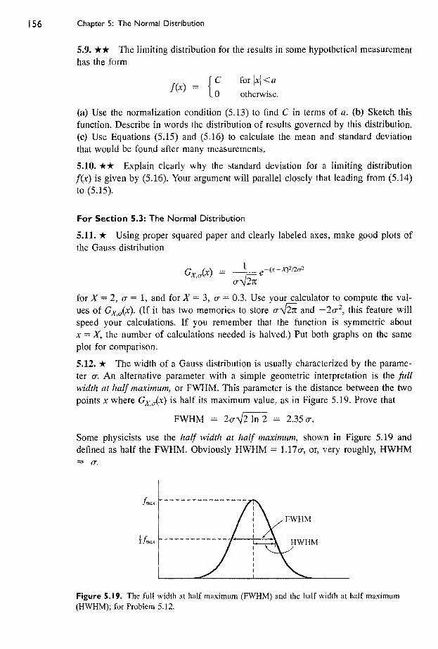
Chapter 5: The Normal Distribution
5.9. The limiting distribution for the results in some hypotheticai measurement
has the form
1 0 otherwise.
(a) Use the normalization condition (5.13) to find C in terms of a. <b) Sketch this
function. Describe in words the distribution of results governed by this distribution,
(c) Use Equations (5.15) and (5.16) to calculate the mean and standard deviation
that would be found after many measurements.
5.10. i*r* Explain clearly why the standard deviation for a limiting distribution
f{x) is given by (5.16). Your argument will parallel closely that leading from (5.14)
to (5.15).
For Section 5.3: The Normal Distribution
5.11. ir Using proper squared paper and clearly labeled axes, make good plots of
the Gauss distribution
for Z = 2, <r = 1, and for X = 3, a - 0.3. Use your calculator to compute the val-
ues of Gx^tAx). (If it has two memories to store o"\/2ii and ~-2cr'^, this feature will
speed your calculations. If you remember that the function is symmetric about
x = X, the number of calculations needed is halved.) Put both graphs on the same
plot for comparison.
5,12. T*r Hie width of a Gauss distribution is usually characterized by the parame-
ter or. An alternative parameter with a simple geometric interpretation is the fidl
width at half maximum, or FWHM. This parameter is the distance between the two
points X where Gx^J^) is half its maximum value, as in Figure 5.19. Prove that
FWHM = 20-V2 In 2 = 2.35(7.
Some physicists use the half width at half maximum, shown in Figure 5.19 and
defined as half the FWHM. Obviously HWHM = XAla, or, very roughly, HWHM= cr.
Figure 5.19. The full width at half maximum (FWHM) and the half width at half maximum(HWHM); for Problem 5.12.

FVdaiems for Chs^ter 5
XX
Figure 5.20. The points X ± traxc the points of inflection of
the Gauss curve; for Problem 5.13.
5.13. T*r One way to define the width a of the Gauss distribution is that the points
X ± cr are the two points of inflection (Figure 5.20), where the curvature changes
sign; that is, where the second derivative is zero. Prove this claim.
5.14. ** Make careful sketches of the normal distributions Gx^M for the three
cases;
(a) X = 0, o- = 1
(b) X - 0, (7 = 2
(c) X = 5, o- - 1
Describe in words the differences among the three curves.
5.15. ** If you have not yet done so, plot the third histogram of Problem 5.3.
The student of that problem decides that the distribution of his results is consistent
with the Gauss distribution Gx^Jx) centered on X = 0 with width a — 3.4. Draw
this distribution on the same graph and compare it with your histogram. (Read the
hints to Problem 5.11. Note that you have no quantitative way to assess the fit; all
you can do is see if the Gauss function seems to fit the histogram satisfactorily.)
5.16. Give in detail the steps leading from (5.30) to (5.31) to show that the
standard deviation cr^ of many measurements normally distributed with width pa-
rameter <7 is = cr.
For Section 5.4: The Standard Deviation as 68% Confidence Limit
5.17. * Some statisticians speak of a "68-95 rule." What do you suppose this rule
is? What is the "68-95-99.7 rule"?
5.18. ir We often say that the probability of a measurement in the range X ± 2cr
is about 95%. What is this probability to four significant figures? What range
X ± tcr actually has probability equal to 95.00%? (Give t to three significant figures.
The needed probabiliti^ can be found in Appendix A.)
5.19. -A-* A student measures a quantity y many times and calculates his mean as
y = 23 and his standard deviation as cr^, = I. What fraction of his readings would
you expect to find between
(a) 22 and 24? (d) 21 and 23?
(b) 22.5 and 23.5? (e) 24 and 25?
(c) 21 and 25?

Chapter 5: The Normal Distributicm
Finally, (f) within what limits (equidistant on either side of the mean) would you
expect to find 50% of his readings? (The necessary information for al! parts of this
question is in Figure 5.13. More detailed information on these kinds of probabilities
is in Appendixes A and B.)
5.20. An extensive survey reveals that the heights of men in a certain country
are normally distributed, with a mean h = 69" and standard deviation cr = 2". In a
random sample of 1,000 men, how many would you expect to have a height
(a) between 67" and 71"?
(b) more than 71"?
(c) more than 75"?
(d) between 65" and 67"?
5.21. T*r* The Giraffe Club of Casterbridge is a club for young adults (18-24
years) who are unusually tall. There are 2,000 women between the ages of 18 and
24 in Castert>ridge, and the heights of women in this age range are distributed
normally with a mean of 5'5V2" and standard deviation of IVi". (a) If the Giraffe
Club initially sets its minimum height for women at 5 '10", approximately how many
women are eligible to join? (b) A year or so later, the club decides to double its
female membership by lowering the minimum height requirement; what would you
recommend that the club set as its new minimum height for women (to the nearest
half inch)?
5.22. If the measurements of a quantity x are governed by the Gauss distribu-
tion Gj^ „(x), the probability of obtaining a value between X — to- and X + to is
With each change of variables, check carefully what happens to your limits of inte-
gration. Hie integral (5.70) is often called the error function, denoted erf(/), or the
normal error integral.
5.23. We have seen that for the normal distribution, the standard deviation
gives the 68% confidence range. This result is not necessarily true for other distribu-
tions, as the following problem illustrates: Consider the exponential distribution of
Problem 5.6, /(/) = (I/t)^"'^^ (for t ^ 0; f(t) = 0 for r < 0). The parameter t is the
mean value of t (that is, after many measurements, T ™ r). (a) Use the integral
(5.16) to prove that t is also the standard deviation, ~ r. (This result is a note-
worthy property of this distribution—that the mean value is equal to the standard
deviation.) (b) By doing the necessary integral, find the probability that any one
value would fall in the range F ± a^.
For Section 5.5: Justification of liie Mean as Best Estirrate
5.24. * Suppose you have measured a quantity x six times, as follows:
Prove carefully, showing ail the necessary changes of variables, that
(5.70)
51, 53, 54, 55, 52, 53.

Problems for Chapter 5
(a) Assuming these measurements are normally distributed, what should be your
best estimates for the true value X and the standard deviation cr? (b) Based on these
estimates, what is the probability that a seventh measurement would fall outside the
range of the first six? (Given that your results are rounded to the nearest integer,
this probability is that for a result x ^ 50.5 or a: > 55.5.)
5.25. * A student measures a time t eight times with the following results (in
tenths of a second):
Value, t^. 75 76 77 78 79 80
Occurrences, Wj^: 2 3 0 0 2 1
(a) Assuming these measurements are normally distributed, what should be your
best estimates for the true value and the standard deviation? (b) Based on these
estimates, what is the probability that a ninth measurement would be 81 or more?
(Because the measurements are rounded to the nearest integer, this probability is
that for a value t > 80.5.)
5.26. ** Suppose we have N measurements x, , . ..
, of the same quantity x,
and we believe that their limiting distribution should be the Gauss function Gx Jx),
with X and a unknown. The principle of maximum likelihood asserts that the best
estimate for the width is the value of a for which the probability Probx^J^Xi, , .. , %)
of the observed values .i,, . . . , jc^ is largest. Differentiate Proby^^{x^, . . . , a'v) in
(5.40) with respect to <t, and show that the maximum occurs when cr is given by
(5.43). [As discussed after (5.43), this result means that the best estimate for the
true width cr is the standard deviation of the N observed values Xj, . .. ,
jc^^. In
practice, the true value X must be replaced with its best estimate x, which requires
replacement of N by N — 1, as proved in Appendix E.]
5.27. ** (a) Based on the data of Problem 5.24, find the mean, the standard
deviation, and the uncertainty of your value for the SD [the last using Equation
(5.46)]. (b) Recalculate the probability asked for in part (b) of Problem 5.24 assum-
ing the true value of <t is cr^ ~ 8cr^., and, once again, assuming a is really <t^ 4- 8a^.
Comment on the difference in your two answers here.
5.28. T*n*r Based on several measurements of the same quantity x normally distrib-
uted about X with width cr, we can estimate X and cr. (a) Approximately how many
measurements must we make to know cr within 30%? (b) Within 10%? (c) Within
3%?
Section 5.6: justification of Addition in Quadrature
5.29. * The measurements of a certain quantity x are distributed according to the
Gauss function G^ Jx) with X = 10 and a = 2. Sketch this distribution and the
distributions for = j: + 5 and for ^' = x / 2, all on the same graph.
5.30. if Verify the identity (5.54) used in Justifying addition in quadrature when
propagating random errors.

Chapter 5: The Normal Disoibution
For Section 5.7: Standard Deviation of Mean
531. Listed here are 40 measurement tj, . . . ^ of the time for a stone to
fall from a window to the ground (all in hundredths of a second).
63 58 74 78 70 74 75 82 68 69
76 62 72 88 65 81 79 77 66 76
86 72 79 77 60 70 65 69 73 77
72 79 65 66 70 74 84 76 80 69
(a) Compute the standard deviation o-, for the 40 measurements, (b) Compute the
means /i, . ., , ?}() the four measurements in each of the 10 columns. You can
think of the data as resulting from 10 experiments, in each of which you found the
mean of four timings. Given the result of part (a), what would you expect for the
standard deviation of the 10 averages . ..
, What is it? (c) Plot histograms
for the 40 individual measurements t^, . ..
, and for the 10 averages t^, . .. , I^q,
[Use the same scales and bin sizes for both plots so they can be compared easily.
Bin boundaries can be chosen in various ways; perhaps the simplest is to put one
boundary at the mean of all 40 measurements (72.90) and to use bins whose width
is the standard deviation of the 10 averages fj, . .. , tiQ.]
5.32. In Problem 4.13 are listed 30 measurements of a certain time t. (a) If
you haven't already done so, find the standard deviation of these 30 values, (b)
Now think of the 30 data as 10 columns, each representing an experiment consisting
of three measurements, and compute the 10 averages, ^i, . .. , t^Q, for these 10 exper-
iments, (c) Given the result of part (a), what would you expect for the standard
deviation of the 10 means of part (b)? What is it? (d) Draw histograms for the 30
separate measurements and for the 10 means,?io- (Use the same scale for
both. A good way to choose your bin boundaries is to put one at the mean of ail 30
measurements and to use the SD of the 10 means as the bin width.)
5.33. T^r* Based on the data of Problem 5.25, what would you give for the best
estimate for the time t and its uncertainty? What is the uncertainty in your value for
the uncertainty in t7 [The uncertainty in / is the SDOM, <Tj = a-J'^. You can find
the uncertainty in the SD from (5.46), and from this result you can find the
uncertainty in the SDOM by error propagation.]
For Section 5.8: Acceptability of a Measure ^swer
534. * According to a proposed theory, the quantity x should have the value jCfj,.
Having measured x in the usual form x^^^ ± <j (where <7 is the appropriate SD), wewould say that the discrepancy between x^^^^ and x^^ is t. standard deviations, where
t ™ l^bes,-
-VtiJ/o-. How large must t be for us to say the discrepancy is significant
at the 5% level? At the 2% level? At the 1% level?
535. * A student measures g, the acceleration of gravity, repeatedly and carefully
and gets a final answer of 9.5 m/s^ with a standard deviation of 0.1. If his measure-
ments were normally distributed with center at the accepted value 9.8 and with
width 0.1, what would be the probability of his getting an answer that differs from

Problems for Chapter S
9.S by as much as (or more than) his? Assuming he made no actual mistakes,
do you think his experiment may have suffered from some undetected systematic
errors?
5.36. Two students measure the same quantity x and get final answers
a;^ = 13 ± 1 and % = 15 ± 1, where the quoted uncertainties are the appropriate
standard deviations, (a) Assuming all errors are independent and random, what is
the discrepancy x,^ ~ and what is its uncertainty? (b) Assuming all quantities
were normally distributed as expected, what would be the probability of getting a
discrepancy as large as they did? Do you consider their discrepancy significant (at
the 5% level)?
5.37. A nuclear physicist wants to check the conservation of energy in a cer-
tain nuclear reaction and measures the initial and final energies as £; ™ 75 ± 3
MeV and f'f = 60 ± 9 MeV, where both quoted uncertainties are the standard devia-
tions of the answers. Is this discrepancy significant (at the 5% level)? Explain your
reasoning clearly.


Part II
6. Rejection of Data
7. Weighted Averages
8. Least-Squares Fitting
9. Covariance and Correlation
10. The Binomial Distribution
1 1 . The Poisson Distribution
! 2. The Chi-Squared Test for a Distribution
If you have read and understood Chapter 5, you are now ready, with surprisingly
little difficulty, to study a number of more advanced topics. The chapters of Part li
present seven such topics, some of which are applications of the statistical theory
already developed, and others of which are further extensions of that theory. All are
important, and you will probably study them sooner or later. Because you might not
necessarily want to learn them all at once, these topics have been arranged into
independent, short chapters that can be studied in any order, as your needs and
interests dictate.


Chapter 6
Rejection of Data
Hiis chapter discusses the awkward question of whether to discard a measurement
that seems so unreasonable that it looks like a mistake. This topic is controversial;
some scientists would argue that discarding a measurement just because it looks
unreasonable is never justified. Nevertheless, there is a simple test you could at least
consider applying if you find yourself confronted with this situation. The test is
called Chauvenet's criterion and is a nice application of the statistical ideas devel-
oped in Chapters 4 and 5.
6. 1 The Problem of Rejecting Data
Sometimes, one measurement in a series of measurements appears to disagree strik-
ingly with all the others. When this happens, the experimenter must decide whether
the anomalous measurement resulted from some mistake and should be rejected or
was a bona fide measurement that should be used with all the others. For example,
imagine we make six measurements of the period of a pendulum and get the results
(all in seconds)
3.8, 3.5, 3.9. 3.9, 3.4, 1.8. (6.1)
In this example, the value 1.8 is startlingly different from all the others, and we
must decide what to do with it.
We know from Chapter 5 that a legitimate measurement may deviate signifi-
cantly from other measurements of the same quantity. Nevertheless, a legitimate
discrepancy as large as that of the last measurement in (6,1) is very improbable, so
we are inclined to suspect that the time 1.8 s resulted from some undetected mistake
or other external cause. Perhaps, for example, we simply misread the last time or
our electric timer stopped briefly during the last measurement because of a momen-
tary power failure.
If we have kept very careful records, we may sometimes be able to establish
such a definite cause for the anomalous measurement. For example, our records
might show that a different stopwatch was used for the last timing in (6.1), and a
subsequent check might show that this watch runs slow. In this case, the anomalous
measurement should definitely be rejected.

Chapter 6: Rejection of Data
Unfortunately, establishing an external cause for an anomalous result is usually
not possible. We must then decide whether or not to reject the anomaly simply by
examining the results themselves, and here our knowledge of the Gauss distribution
proves useful.
The rejection of data is a controversial question on which experts disagree. It is
also an important question. In our example, the best estimate for the period of the
pendulum is significantly affected if we reject the suspect 1.8 s. The average of all
six measurements is 3.4 s, whereas that of the first five is 3.7 s, an appreciable
difference.
Furthermore, the decision to reject data is ultimately a subjective one, and the
scientist who makes this decision may reasonably be accused by other scientists of
"fixing" the data. The situation is made worse by the possibility that the anomalous
result may reflect some important effect. Indeed, many important scientific discover-
ies first appeared as anomalous measurements that looked like mistakes. In throwing
out the time 1.8 s in the example (6.1), we just might be throwing out the most
interesting part of the data.
In fact, faced with data like those in (6.1), our only really honest course is to
repeat the measurement many, many times. If the anomaly shows up again, we will
presumably be able to trace its cause, either as a mistake or a real physical effect.
If it does not recur, then by the time we have made, say, 100 measurements, there
will be no significant difference in our final answer whether we include the anomaly
or not.
Nevertheless, repeating a measurement lOQ times every time a result seems
suspect is frequently impractical (especiaMy in a teaching laboratory). We therefore
need some criterion for rejecting a suspect result. There are various such criteria,
some quite complicated. Chauvenet's criterion provides a simple and instructive
application of the Gauss distribution.
6.2 Chauvenet's Criterion
Let us return to the six measurements of the example (6.1):
3.8, 3.5, 3.9, 3.9, 3.4, 1.8.
If we assume for the moment that these are six legitimate measurements of a quan-
tity X, we can calculate the mean x and standard deviation
I = 3.4 s (6.2)
and
(T^ = 0.8 s. (6.3)
We can now quantify the extent to which the suspect measurement, 1.8, is anoma-
lous. It differs from the mean 3.4 by 1.6, or two standard deviations. If we assume
the measurements were governed by a Gauss distribution with center and width
given by (6.2) and (6.3), we can calculate the probability of obtaining measurements
that differ by at least this much from the mean. According to the probabilities shown

Section 6.2 Chauvenet's Criterion
in Appendix A, this probability is
Probiput&ide 2a) = 1 - ProMyfiihin 2a)
= 1 - 0.95
= 0.05.
In other words, assuming that the values (6.2) and (6.3) for x and cTj^ are legitimate,
we would expect one in every 20 measurements to differ from the mean by at least
as much as the suspect 1.8 s does. If we had made 20 or more measurements, we
should actually expect to get one or two measurements as deviant as the 1.8 s, and
we would have no reason to reject it. But we have made only six measurements, so
the expected number of measurements as deviant as 1.8 s was actually
(expected number as deviant as 1.8 s)
= (number of measurements) X PTOi>(outside 2a)
= 6 X 0.05 = 0.3.
That is, in six measurements we would expect (on average) only one-third of a
measurement as deviant as the suspect 1.8 s.
This result provides us with the needed quantitative measure of the "reasonable-
ness" of our suspect measurement. If we choose to regard one-third of a measure-
ment as "ridiculously improbable," then we will conclude that the value 1.8 s was
not a legitimate measurement and should be rejected.
The decision of where to set the boundary of "ridiculous improbability" is up
to the experimenter. Chauvenet's criterion, as normally given, states that if the ex-
pected number of measurements at least as deviant as the suspect measurement is
less than one-half, then the suspect measurement should be rejected. Obviously, the
choice of one-half is arbitrary, but it is also reasonable and can be defended.
The application of Chauvenet's criterion to a general problem can now be de-
scribed easily. Suppose you have made N measurements
of a single quantity x. From all N measurements, you calculate x and a^. If one of
the measurements (call it x^^^^) differs from x so much that it looks suspicious, then
find
the number of standard deviations by which x^^^ differs from x. Next, from Appendix
A you can find the probability
Prob{outsi6& t^^isO)
that a legitimate measurement would differ from x by t^^J^ or more standard devia-
tions. Finally, multiplying by A^, the total number of measurements, gives
n = (expected number as deviant as jCgyJ
= X PTO6(outside fgusO-).

Chapter 6: Rejection of Data
If this expected number n is less than one-half, then, according to Chauvenet's
criterion, you can reject x^us-
If you do decide to reject x^^^, you would naturally recalculate I and ar^ using
just the remaining data; in particular, your final answer for x would be this new
mean, with an uncertainty equal to the new SDOM.
Ex^ple: 1en Measurements of a Length
A student makes 10 measurements of one length x and gets the results (all in mm)
46, 48, 44, 38, 45, 47, 58, 44, 45, 43.
Noticing that the value 58 seems anomalously large, he checks his records but can
find no evidence that the result was caused by a mistake. He therefore applies
Chauvenet's criterion. What does he conclude?
Accepting provisionally all 10 measurements, he computes
X ™ 45.8 and cr^ = 5.1.
The difference between the suspect value x^^^^ — 58 and the mean x ~ 45.8 is
12.2, or 2A standard deviations; that is,
= ^sus - ^ ^ 58 - 45.8 ^<T, 5.1
Referring to the table in Appendix A, he sees that the probability that a measurement
will differ from jc by 2.4cr^ or more is
/*roi>(outside 2.4a-) = 1 - Pro6(within 2.4o-)
= 1 - 0.984
= 0.016.
In 10 measurements, he would therefore expect to find only 0.16 of one measure-
ment as deviant as his suspect result. Because 0.16 is less than the number 0.5 set
by Chauvenet's criterion, he should at least consider rejecting the result.
If he decides to reject the suspect 58, then he must recalculate x and as
X ~ 44.4 and ~ 2.9.
As you would expect, his mean changes a bit, and his standard deviation drops
appreciably.
Quick Check 6. L A student makes 20 measurements of a certain voltage Vand computes her mean and standard deviation as V = 51 and a^ — 2 (both in
microvolts). The evening before the work is due, she starts to write her report
and realizes that one of her measured values was V^^^ == 56. What is the proba-
bility of her getting a measurement this deviant from V? If she decides to use
Chauvenet's criterion, should she reject the suspect value?

Section 6.3 Discussion
6.3 Discussion
You should be aware that some scientists believe that data should never be rejected
without external evidence that the measurement in question is incorrect. A reason-
able compromise is to use Chauvenet's criterion to identify data that could be con-
sidered for rejection; having made this identification, you could do all subsequent
calculations twice, once including the suspect data and once excluding them, to see
how much the questionable values affect your final conclusion.
One reason many scientists are uncomfortable with Chauvenet's criterion is that
the choice of one-half as the boundary of rejection (in the condition that n < |) is
arbitrary. Perhaps even more important, unless you have made a very large number
of measurements (A'^ 50, say), the value of cTj^ is extremely uncertain as an esti-
mate for the true standard deviation of the measurements. (See Problem 6.7 for an
example.) This means in turn that the number t^^^ in (6.4) is very uncertain. Because
the probability of a measurement outside t standard deviations is very sensitive to
a large error in t^^ causes a very large error in this probability and casts serious
doubt on the whole procedure. For both of these reasons, Chauvenet's criterion
should be used only as a last resort, when you cannot check your measurements by
repeating them.
So far, we have assumed that only one me^urement is suspect. What should
you do if you have several? Given that the use of Chauvenet's criterion to reject
one measurement is open to doubt, clearly its use to reject several measurements is
even more problematic. Nevertheless, if there is absolutely no way you can repeat
your measurements (because you have rashly dismantled your equipment before
writing your report, for example), you may have to confront this question.
Suppose first that you have two measurements that deviate from the mean by
the same large amount. In this case, you could calculate the expected number of
measurements this deviant, and if this number is less than one (that is, two times
one-half), then both measurements could be considered candidates for rejection. If
you have two suspect measurements, Xi and X2, with X2 more deviant than x^, you
should first apply Chauvenet's criterion using the value x^. If the expected number
this deviant is less than one, you could reject both values. If this expected number
is more than one, you certainly should not reject both but instead reapply Chauve-
net's criterion using X2 and, if the expected number this deviant is less than one-
half, you could reject just X2.
Having rejected any measurements that fail Chauvenet's criterion, you would
naturally recalculate x and cr^ using just the remaining data. The resulting value of
cTj^ will be smaller than the original one, and with the new ffj., some more measure-
ments may fail Chauvenet's criterion. However, agreement seems widespread that
Chauvenet's criterion should not be applied a second time using the recalculated
values of x and cr^..

Cha[>ter 6: Rejection of Data
Principal Definitions and Equations of Chapter 6
CHAUVENET'S CRITERION
If you make measurements x^, . .. ,
x^j of a single quantity x, and if one of
the measurements (x^^^ say) is suspiciously different from all the others, Chauve-
net's criterion gives a simple test for deciding whether to reject this suspect value.
First, compute the mean and standard deviation of all measurements and then find
the number of standard deviations by which x^^^ differs from x,
t — i^sus ~ -^i
^sus „
Next, find the probability (assuming the measurements are normally distributed
about X with width o-J of getting a result as deviant as x^^^, and, hence, the number
of measurements expected to deviate this much,
n = N X Frofe(outside t^^^cr).
If n < i, then according to Chauvenet's criterion, you can reject the value Xg^^^,
Because there are several objections to Chauvenet's criterion (especially if A'^ is
not very large), it should be used only as a last resort, when the measurements of x
cannot be checked. The objections to Chauvenet's criterion are even greater if two
or more measurements are suspect, but the test can be extended to this situation, as
described in Section 6.3.
Problems for Chapter 6
For Section 6.2: Chauvenet's Criterion
6,1. * An enthusiastic student makes 50 measurements of the heat Q released in
a certain reaction. Her average and standard deviation are
Q ^ 4.8 and Og = 0.4,
both in kilocalories. (a) Assuming her measurements are governed by the normal
distribution, find the probability that any one measurement would differ from Q by
0.8 kcal or more. How many of her 50 measurements should she expect to differ
from Q by 0.8 kcal or more? If one of her measurements is 4.0 kcal and she decides
to use Chauvenet's criterion, would she reject this measurement? (b) Would she
reject a measurement of 6.0 kcal?
6J. it The Franck-Hertz experiment involves measuring the differences between
a series of equally spaced voltages that cause the maximum current through a tube
of mercury vapor. A student measures 10 such differences and obtains these results
(all in volts):
0.48, 0.45, 0.49, 0.46, 0.44, 0.57, 0.45, 0.47, 0.51, 0.50.

Problems for Chapter 6
(a) Calculate the mean and standard deviation of these results. (By ail means,
use the built-in functions on your calculator.)
(b) If he decides to use Chauvenet's criterion, should he reject the reading of
0.57 volts? Explain your reasoning clearly.
6.3. * A student makes 14 measurements of the period of a damped oscillator and
obtains these results (in tenths of a second):
7, 3, 9, 3, 6, 9, 8, 7, 8, 12, 5, 9, 9, 3.
Believing that the result 12 is suspiciously high, she decides to apply Chauvenet's
criterion. How many results should she expect to find as far from the mean as 12
is? Should she reject the suspect result?
6.4. A physicist makes 14 measurements of the density of tracks on an emul-
sion exposed to cosmic rays and obtains the following results (in tracks/cm^):
11, 9, 13, 15, 8, 10, 5, 11, 9, 12, 12, 13, 9, 14.
fa) What are his mean and standard deviation? (Use the built-in functions on your
calculator.) (b) According to Chauvenet's criterion, would he be justified in rejecting
the measurement of 5? Explain your reasoning clearly, (c) If he does reject this
measurement, what does he get for his new mean and standard deviation? (Hint:
You can almost certainly recalculate the mean and standard deviation by editing the
contents of your calculator's statistical registers rather than re-entering ai! the data.
If you don't know how to do this editing, take a moment to learn.)
6.5. In the course of a couple of hours, a nuclear engineer makes 12 measure-
ments of the strength of a long-lived radioactive source with the following results,
in millicuries:
12, 34, 22, 14, 22, 17, 24, 22, 18, 14, 18, 12.
(Because the source has a long life, its activity should not change appreciably during
the time ail the measurements are made.)
(a) What are his mean and standard deviation? (Use the built-in functions on your
calculator.) (b) According to Chauvenet s criterion, would he be justified in rejecting
the value 34 as a mistake? Explain your reasoning clearly, (c) If he does reject this
measurement, what does he get for his new mean and standard deviation? (Read the
hint to Problem 6.4.)
6.6. ** Chauvenet's criterion defines a boundary outside which a measurement is
regarded as rejectable. If we make 10 measurements and one differs from the mean
by more than about two standard deviations (in either direction), that measurement
is considered rejectable. For 20 measurements, the corresponding boundary is ap-
proximately 2.2 standard deviations. Make a table showing the "boundary of reject-
ability" for 5, 10, 15, 20, 50, 100, 200, and 1,000 measurements of a quantity that
is normally distributed.
6.7. ** Based on N measurements of a normally distributed quantity x, the best
estimate of the width or is the standard deviation or^ of the N measured values.
Unfortunately, if is small, this estimate is fairly uncertain. Specifically, the frac-
tionai uncertainty in as an estimate of a is given by (5.46) as l/-\j2(N — 1). If

Chapter 6: Rejection of Data
N = 6, for example, our estimate for cr is about 30% uncertain. This large uncer-
taimy in a means you should regard Chauvenet's criterion with considerable skepti-
cism when is small, as the foiiowing example illustrates.
An experimenter measures a certain current six times and obtains the foiiowing
results (in milliamps):
28, 25,29, 18,29,24.
(a) Find the mean x and standard deviation cr^ of these measurements, (b) If he
decided to apply Chauvenet's criterion, would the experimenter reject the value 18?
(c) Find the uncertainty— call it cScr^.— in cr,.. (d) The true value of a may well be
as small as tr^ — Scr^ or as large as o-j^ + 6cr^. Re-apply Chauvenet's criterion, using
each of these two values for a. Comment on the results.

Chapter 7
Weighted Averages
This chapter addresses the problem of combining two or more separate and indepen-
dent measurements of a single physical quantity. We will find that the best estimate
of that quantity, based on the several measurements, is an appropriate weighted
average of those measurements,
7.1 The Problem of Combining Separate Measurements
Often, a physical quantity is measured several times, perhaps in several separate
laboratories, and the question arises how these measurements can be combined to
give a single best estimate. Suppose, for example, that two students, A and jB, mea-
sure a quantity x carefully and obtain these results:
Student i4: x = ± o*^ (7.1)
and
Student B: x = % ± tr^ . (7.2)
Each result will probably itself be the result of several measurements, in which case
will be the mean of all .4's measurements and cr^ the standard deviation of that
mean (and similarly for Xq and cr^). The question is how best to combine x^ and x^
for a single best estimate of x.
Before examining this question, note that if the discrepancy \x..^ ~ Xq\ between
the two measurements is much greater than both uncertainties cr^ and cr^, we should
suspect that something has gone wrong in at least one of the measurements. In this
situation, we would say that the two measurements are inconsistent, and we should
examine both measurements carefully to see whether either (or both) was subject to
unnoticed systematic errors.
Let us suppose, however, that the two measurements (7.1) and (7.2) are consis-
tent; that is, the discrepancy Ix^ - x^j is not significantly larger than both a;,^ and
0^- We can then sensibly ask what the best estimate x^^ is of the true value X,
based on the two measurements. Your first impulse might be to use the average
(x^ + Xg)/2 of the two measurements. Some reflection should suggest, however, that
this average is unsuitable if the two uncertainties o*^ and oj^ are unequal. The simple

Chapter 7: Wei^ted Averages
average {x^ + ^bV^ gives equal importance to both measurements, whereas the more
precise reading should somehow be given more weight.
Throughout this chapter, I will assume ail systematic errors have been identified
and rcduced to a negligible level. Thus, all remaining errors are random, and the mea-
surements ofX are distributed normally around the true value X.
7.2 The Weighted Average
We can solve our problem easily by using the principle of maximum likelihood,
much as we did in Section 5.5. We are assuming that both measurements are gov-
erned by the Gauss distribution and denote the unknown true value of x by XTherefore, the probability of Student ^'s obtaining his particular value X4 is
Probj^x^) ^ -le-(-*^^-^)'/2o-^^ (7.3)
and that of B's getting his observed is
The subscript X indicate explicitly that these probabilities depend on the unknown
actual value.
The probability that A finds the value and B the value Xg is just the product
of the two probabilities (7.3) and (7.4). In a way that should now be familiar, this
product will involve an exponential function whose exponent is the sum of the two
exponents in (7.3) and (7.4), We write this as
Prob;^XA,XB) = PTvb^XA)Probj^XB)
oc --i-^-Ar2/2^ (7,5)
where 1 have introduced the convenient shorthand (chi squared) for the exponent
- XV /x« - Z\2
This important quantity is the sum of the squares of the deviations from X of the
two measurements, each divided by its corresponding uncertainty.
The principle of maximum likelihood asserts, just as before, that our best esti-
mate for the unknown true value X is that value for which the actual observations
Xj^, Xg are most likely. That is, the best estimate for is the value for which the
probability (7.5) is maximum or, equivalently, the exponent minimum. (Be-
cause maximizing the probability entails minimizing the "sum of squares" *his
method for estimating X is sometimes called the "method of least squares.") Thus,
to find the best estimate, we simply differentiate (7.6) with respect to X and set the
derivative equal to zero,
^ Xa X _ Xa "*~ X _2
A + 2 ^ = 0.ota Ob

Section 7.2 The Weighted Average
The solution of this equation for X is our best estimate and is easily seen to be
(best estimate for JT) = (i + i)/ (-1, + -i^).(7.7)
Ttiis rather ugly result can be made tidier if we define weights
m'a = ™2 and :72- U'^)
With this notation, we can rewrite (7.7) as the weighted average (denoted x^^^)
(best estimate for A-) - x^^, - + ^b^b^ ^
If the original two measurement are equally uncertain (cr^ = cr^ and hence
- Wg), this answer reduces to the simple average (x^ + Xb)/2. In general, when
^ Wq, the weighted average (7.9) is not the same as the ordinary average; it is
similar to the formula for the center of gravity of two bodies, where and Wg are
the actual weights of the two bodies, and and Xg their positions. In (7.9), the
"weights" are the inverse squares of the uncertainties in the original measurements,
as in (7.8). If A's measurement is more precise than B% then < cr^ and hence
> Wg, so the best estimate jc^est is closer to x^ than to x^, just as it should be.
Quick Check 7. 1 . Workers from two laboratories report the lifetime of a cer-
tain particle as 10.0 ± 0.5 and 12 ± 1, both in nanoseconds. If they decide to
combine the two results, what will be their respective weights as given by (7.8)
and their weighted average as given by (7.9)?
Our analysis of two me^urements can be generalized to cover any number of
measurements. Suppose we have N separate measurements of a quantity Xy
Xi ± ffi, X2± Xjv ± av,
with their corresponding uncertainties cr^, a-j, . .. ,
o*^. Arguing much as before, wefind that the best estimate based on these measurements is the weighted average
Mm(7.10)
where the sums are over all N measurements, /' = 1, . .. , iV, and the weight w^ of
each measurement is the reciprocal square of the corresponding uncertainty.
iWJiiiiiiiliiM^^^(7.11)
for / = 1, 2, . . . , iV.

Chapter 7: Wei^ted Averages
Because the weight = l/o^^ associated with each measurement involves the
square of the corresponding uncertainty o;-, any measurement that is much less pre-
cise than the others contributes very much less to the final answer (7.10). For exam-
ple, if one measurement is four times less precise than the rest, its weight is 16
times less than the other weights, and for many purposes this measurement could
simply be ignored.
Because the weighted average x^,^^ is a function of the original measured values
Xi, X2, . .J^A', the uncertainty in x^^^ can be calculated using error propagation. As
you can easily check (Problem 7.8), the uncertainty in x^^v is
(7,12)
This rather ugly result is perhaps a little easier to remember if we rewrite (7.11) as
1= -=L . (7.13)
Paraphrasing Equation (7.13), we can say that the uncertainty in each measurement
is the reciprocal square root of its weight. Returning to Equation (7.12), we can
paraphrase it similarly to say that the uncertainty in the grand answer x^.^^ is the
reciprocal square root of the sum of all the individual weights; in other words, the
total weight of the final answer is the sum of the individual weights w,-.
Quick Check 7.2. What is the uncertainty in your final answer for Quick
Check 7.1?
7.3 An Example
Here is an example involving three separate measurements of the same resistance.
Example: Three Measurements of a Resistance
Each of three students measures the same resistance several times, and their three
final answers are (all in ohms);
Student 1: /? - 11 ± 1
Student 2: = 12 ± 1
Student 3: /? = 10 ± 3
Given these three results, what is the best estimate for the resistance R7
The three uncertainties cti, Oj, 03 are 1, 1, and 3. Therefore, the corresponding
weights ~ l/cr^ are
Wj - 1, W2 = 1, 1V3 = 5.

Principal Definitions and Equations of Chapter 7 (77
The best estimate for R is the weighted average, which according to (7.10) is
. (1 X U) H- (1 X 12) + ft X 10) ^ ^^ ^^^^^^1 + 1 + 1
The uncertainty in this answer is given by (7.12) as
1 1ar^^^ = -== =
.- 0.69.
VS ^|l + I + i
Thus, our final conclusion (properly rounded) is
R = 11.4 ± 0.7 ohms.
For interest, let us see what answer we would get if we were to ignore com-
pletely the third student's measurement, which is three times less accurate and hence
nine times less important. Here, a simple calculation gives ij^est ~ H-^O (compared
with 11.42) with an uncertainty of 0.71 (compared with 0.69). Obviously, the third
measurement does not have a big effect.
Principal Definitions and Equations of Chapter 7
If jcj, X2, . . . ,xj^ are measurements of a single quantity x, with known uncertain-
ties cTj, 0-2, ... , Ojv, then the best estimate for the true value of x is the weighted
average
""^^^ I IV,' [See (7.10)]
where the sums are over all N measurements, / = 1, . .. ,
AT, and the weights
are the reciprocal squares of the corresponding uncertainties,
1
The uncertainty in x^^^ is
1
™fSee (7.12)]
where, again, the sum runs over all of the measurements i ~ 1, 2, . ..
, M

Chapter 7: Weighted Averages
Problems for Chapter 7
For Section 7.2: The Weighted Average
7.1. * Find the best estimate and its uncertainty based on the following four mea-
surements of a certain voltage;
1.4 ± 0.5, 1.2 ± 0.2, 1.0 ± 0.25, 1.3 ± 0.2.
7.2. * Three groups of particle physicists measure the mass of a certain elemen-
tary particle with the results (in units of MeV/c^):
1,967.0 ± 1.0, 1,969 ± 1.4, 1,972.1 ± 2.5.
Find the weighted average and its uncertainty.
7.3. if (a) Two measurements of the speed of sound « give the answers 334 ± 1
and 336 ± 2 (both in m/s). Would you consider them consistent? If so, calculate
the best estimate for u and its uncertainty, (b) Repeat part (a) for the results 334 ± 1
and 336 ± 5. Is the second measurement worth including in this case?
7.4. Four measurements are made of the wavelength of light emitted by a
certain atom. The results, in nanometers, are:
503 ± 10, 491 ± 8, 525 ± 20, 570 ± 40.
Find the weighted average and its uncertainty. Is the last measurement worth in-
cluding?
7.5. ifir Two students measure a resistance by different methods. Each makes 10
measurements and computes the mean and its standard deviation, and their final
results are as follows:
Student A: /? = 72 ± 8 ohms
Student B: R = IS ± 5 ohms.
(a) Including both measurements, what are the best estimate of R and its uncer-
tainty? (b) Approximately how many measurements (using his same technique)
would student A need to make to give his result the same weight as B's? (Remember
that each student's final uncertainty is the SDOM, which is equal to the SD/a/Jv.)
7.6. Two physicists measure the rate of decay of a long-lived radioactive
source. Physicist A monitors the sample for 4 hours and observes 412 decays; physi-
cist B monitors it for 6 hours and observes 576 decays, (a) Find the uncertainties in
these two counts using the square-root rule (3.2). (Remember that the square-root
rule gives the uncertainty in the actual counted number.) (b) What should each
physicist report for the decay rate in decays per hour, with its uncertainty? (c) What
is the proper weighted average of these two rates, with its uncertainty?
7.7. Suppose that N separate measurements of a quantity x all have the same
uncertainty. Show clearly that in this situation the weighted average (7.10) reduces
to the ordinary average, or mean, x ~ ^x^/N, and that the uncertainty (7.12) re-
duces to the familiar standard deviation of the mean.

Pfxsbiems for Chapter 7
7.8, T*r* The weighted average (7.10) of N separate measurements is a simple
function of x^,X2,..., Xjy. Therefore, the uncertainty in x^^^ can be found by error
propagation. Prove in this way that the uncertainty in x^^^ is as claimed in (7.12).
7.9. ir-kir (a) If you have access to a spreadsheet program such as Lotus 123 or
Excel, create a spreadsheet to calculate the weighted average of three measurements
Xf with given uncertainties o^. In the first column, give the trial number i, and use
columns 2 and 3 to enter the data x, and the uncertainties o;. in columns 4 and 5,
put ftmctions to calculate the weights and the products w^xf, at the bottoms of
these columns, you can calculate the sums "Zw^ and Xw^ji;,. Finally, in some conve-
nient position, place functions to calculate x^^^ and its uncertainty (7.12). Test your
spreadsheet using the data of Secdon 7.3. (b) Try to modify your spreadsheet so
that it can handle any number of measurements up to some maximum (20 say).
(The main difjficulty is that you will probably need to use some logical functions to
make sure that empty cells in column 3 don't get counted as zeros and cause trouble
with the function that calculates vv, = l/o^^.) Test your new spreadsheet using the
data in Section 7.3 and in Problem 7.1.


Chapter 8
Least-Squares Fitting
Our discussion of the statistical analysis of data has so far focused exclusively on
the repeated measurement of one single quantity, not because the analysis of many
measurements of one quantity is the most interesting problem in statistics, but be-
cause this simple problem must be well understood before more general ones can
be discussed. Now we are ready to discuss our first, and very important, more
general problem.
8. 1 Data That Should Fit a Straight Line
One of the most common and interesting types of experiment involves the measure-
ment of several values of two different physical variables to investigate the mathe-
matical relationship between the two variables. For instance, an experimenter might
drop a stone from various different heights A,, . . . , /ly and measure the correspond-
ing times of fall t^, . .. ,
t^^ to see if the heights and times are connected by the
expected relation h = hgt^-
Probably the most important experiments of this type are those for which the
expected relation is linear. For instance, if we believe that a body is falling with
constant acceleration g, then its velocity u should be a linear function of the time t,
V v,,-h gt.
More generally, we will consider any two physical variables x and y that we suspect
are connected by a linear relation of the form
y = y4 + Bx, (8.1)
where A and B are constants. Unfortunately, many different notations are used for a
linear relation; beware of confusing the form (8.1) with the equally popular
y = ax + b.
If the two variables y and x are linearly related as in (8.1), then a graph of yagainst x should be a straight line that has slope B and intersects the y axis at y = ^,
if we were to measure N different values jCj, . ..
, and the corresponding values
yi, . .. , yjv and if our measurements were subject to no uncertainties, then each of
the points (jc„ y,) would lie exactly on the line y = ^4 4- JSx, as in Figure 8.1(a). In

Chapter 8: Least-Squares Fitting
>' y
(a) (b)
Figure 8J. (a) If the two variables y and x are lineariy reiated as in Equation (8.1), and if
there were no experimental uncertainties, then the measured points (x^, y,) would ail lie exactly
on the line y A + Bx. (b) In practice, there always are uncertainties, which can be shown by
error bars, and the points (jCj, can be expected only to lie reasonably close to the line. Here,
only y is shown as subject to appreciable uncertainties.
practice, there are uncertainties, and the most we can expect is that the distance of
each point {xi, y^) from the line will be reasonable compared with the uncertainties,
as in Figure 8.1(b).
When we make a series of measurements of the kind just described, we can ask
two questions. First, if we take for granted that y and x are lineariy related, then the
interesting problem is to find the straight line y =A + Bx that best fits the measure-
ments, that is, to find the best estimates for the constants A and B based on the data
(jcj, y^), . .. , (xjv, >'^). This problem can be approached graphically, as discussed
briefly in Section 2.6. It can also be treated analytically, by means of the principle
of maximum likelih{X)d. This analytical method of finding the best straight line to
fit a series of experimental points is called linear regression, or the least-squares fit
for a line, and is the main subject of this chapter.
The second question that can be asked is whether the measured values (xj, y^,
. .. , (%, yi^) do really bear out our expectation that y is linear in x. To answer this
question, we would first find the line that best fits the data, but we must then devise
some measure of how well this line fits the data. If we already know the uncertain-
ties in our measurements, we can draw a graph, Uke that in Figure 8.1(b), that
shows the best-fit straight line and the experimental data with their error bars. Wecan then judge visually whether or not the best-fit line passes sufficiently close to
all of the error bars. M we do not know the uncertainties reliably, we must Judge
how well the points fit a straight line by examining the distribution of the points
themselves. We take up this question in Chapter 9.
8.2 Calculation of the Constants A and B
Let us now return to the question of finding the best straight line y = A ^ Bx to
fit a set of measured points {x^, y{}, . .. , (%, jy). To simplify our discussion, we
will suppose that, although our measuremente of y suffer appreciable uncertainty,
the uncertainty in our measurements of x is negligible. This assumption is often
reasonable, because the uncertainties in one variable often are much larger than

Section 8.2 CakuEation of the Constants A and 6
those in the other, which we can therefore safely ignore. We will further assume
that the uncertainties in y all have the same magnitude. (This assumption is also
reasonable in many experiments, but if the uncertainties are different, then our anal-
ysis can be generalized to weight the measurements appropriately; see Problem 8.9.)
More specifically, we assume that the measurement of each y,- is governed by the
Gauss distribution, with the same width parameter for all measurements.
If we knew the constants A and B, then, for any given value (which we are
assuming has no uncertainty), we could compute the true value of the correspond-
ing yi>
(true value for y^) = A + fix,. (8.2)
The measurement of is governed by a normal distribution centered on this true
value, with width parameter Therefore, the probability of obtaining the observed
value is
Pr^^^y, oc (8.3)
where the subscripts A and B indicate that this probability depends on the (unknown)
values of A and B, The probability of obtaining our complete set of measurements
..
, is the product
Pj'obAj.yi. -^.yN) = Prob^Ayi) ' ^^^^AAy^f)
« ™A?^"^''^ (8-4)
where the exponent is given by
x'-i ": (8.5)
In the now-fami!iar way, we will assume that the best estimates for the unknown
constants A and B, based on the given measurements, are those values of A and Bfor which the probability Pfobj^^{y^^ . . . , y^j) is maximum, or for which the sum of
squares in (8-5) is a minimum. (This is why the method is known as least-
squares fitting.) To find these values, we differentiate with respect to A and Band set the derivatives equal to zero:
= 2 (3^^- A - Ba:,) - 0 (8.6)
and
dA ay
dB (Ty ,.^1
(8.7)
These two equations can be rewritten as simultaneous equations for A and B:
AN + Blxf = ly,. (8.8)
and
Alx, + B^xl - Ijc,y,. (8.9)

Chapter 8: Least-Squares FHting
Here, 1 have omitted the limite i - I to N from the summation signs E. In the
foiiowing discussion, I also omit the subscripts / when there is no serious danger of
confusion; thus, X-V; V/ is abbreviated to Y.xy and so on.
The two equations (8.8) and (8,9), sometimes called normal equations, are eas-
ily solved for the least-squares estimates for the constants A and B,
(8.10)
and
(8.11)
where I have introduced the convenient abbreviation for the denominator.
(8.12)
The results (8.10) and (8.11) give the best estimates for the constants A and Bof the straight line y = A + Bx, based on the N measured points (jc,,^]), . .
.
,
{Xff, yjv)- The resulting line is called the least-squares fit to the data, or the line of
regression of y on x.
Example: Length versus Mass for a Spring Balance
A student makes a scale to measure masses with a spring. She attaches its top end
to a rigid support, hangs a pan from its bottom, and places a meter stick behind the
arrangement to read the length of the spring. Before she can use the scale, she must
calibrate it; that is, she must find the relationship between the mass in the pan and
the length of the spring. To do this calibration, she gets five accurate 2~kg masses,
which she adds to the pan one by one, recording the corresponding lengths 1^ as
shown in the first three columns of Table 8.1. Assuming the spring obeys Hooke's
law, she anticipates that / should be a linear function of m.
I = A + Bm. (8.13)
(Here, the constant A is the unloaded length of the spring, and B is g/k, where k is
the usual spring constant.) The calibration equation (8.13) will let her find any
unknown mass m from the corresponding length /, once she knows the constants Aand B. To find these constants, she uses the method of least squares. What are her
answers for A and ^? Plot her calibration data and the line given by her best fit
(8.13). If she puts an unknown mass m in the pan and observes the spring's length
to be / = 53.2 cm, what is m?

Section 8.2 CaicuEation of the Constants A and B
Table 8.1. Masses m,- (in kg) and lengths (in cm) tor a spring balance.
The "x" and "j" in quotes indicate which variables play the roles of x and
y in this example.
Trial number
{ Load, nil Length, /,
2
1 2 42.0 4 84
2 4 48.4 16 194
3 6 51.3 36 308
4 8 56.3 . 64 450
5 10 58.6 100 586
iV= 5 Hi = 256.6 Sffii^ = 220 Im,/, = 1,622
As often happens in such problems, the two variables are not called x and y,
and one must be careful to identify which is which. Comparing (8.13) with the
standard form, y ~A + Bx,wq see that the length / plays the role of the dependent
variable y, while the mass m plays the role of the independent variable x. The
constants A and B are given by (8.10) through (8.12), with the replacements
X, «-> ffij and y^ <-> l^.
(This correspondence is indicated by the headings "jc" and "y" in Table 8.1.) To find
A and B, we need to find the sums Xm„ S/,, Xm,^, and Xw,/,; therefore, the last two
columns of Table 8.1 show the quantities and m^/,, and the corresponding sum
is shown at the bottom of each column.
Computing the constants A and B is now straightforward. According to (8.12),
the denominator A is
^ = NYjir - (Lmf= 5 X 220 ~ 30^ = 200.
Next, from (8.10) we find the intercept (the unstretched length)
A ^ ^
220 X 256.6 - 30 X 1622
200
Finally, from (8.11) we find the slope
Nl.ml - I,ml,l
= 39.0 cm.
A
5 X 1622 - 30 X 256.6 ^200
^

A plot of the data and the !nie (8.13) using these values of A and B is shown in
Figure 8.2. If the mass m stretches the spring to 53.2 cm, then according to (8.13)
the mass is
I ~ A (53.2 - 39,0) cm
2.06 cm/kg^
Quick Check 8. 1 . Find the least-squares best-fit line y ~ A •¥ Bx through the
three points (x, y) = (-]. 0). (0, 6), and (1, 6), Using squared paper, plot the
points and your line. [Note that because the tliree values of x (— 1, 0, and 1) are
symmetric about zero, ~ 0, which simplifies the calculation of A and B. In
some experiments, the values of x can be arranged to be symmetrically spaced
in this way, which saves some trouble.]
Now that we know how to find the best estimates for the constants A and B,
we naturally ask for the uncertainties in these estimates. Before we can find these
uncertainties, however, we must discuss the uncertainty o\, in the original measure-
ments of yj, . . . , y^-
8.3 Uncertainty in the Measurements of y
In the course of measuring the values >'!,. Va" we have presumably formed some
idea of their uncertainty. Nonetheless, knowing how to calculate the uncertainty by
analyzing the data themselves is important. Remember that the numbers , . .. , y^y
are not N measurements of the same quantity. (They might, for instance, be the
times for a stone to fail from N different heights.) Thus, we certainly do not get an
idea of their reliability by examining the spread in their values.
Nevertheless, we can easily estimate the uncertainty o-y in the numbers >i, . . ,
,
The measurement of each y, is (we are assuming) normally distributed about its
true value A + Bx^, with width parameter or,. Thus the deviations y^ - A ~ Bx^ are

Section 8.3 Uncertainty in the Measurements of /
normally distributed, ail with the same central value zero and the same width o-y.
This situation immediately suggests that a good estimate for a^, would be given by
a sum of squares with the familiar form
<T, = ^j~l(y, ~ A - Bxd^, (8.14)
In fact, this answer can be confirmed by means of the principle of maximum likeli-
hood. As usual, the best estimate for the parameter in question (o;, here) is that
value for which the probability (8.4) of obtaining the observed values y^, . .,
, is
maximum. As you can easily check by differentiating (8.4) with respect to o-y and
setting the derivative equal to zero, this best estimate is precisely the answer (8.14).
(See Problem 8.12.)
Unfortunately, as you may have suspected, the estimate (8.14) for ay is not
quite the end of the story. The numbers A and B in (8.14) are the unknown true
values of the constants A and B, In practice, these numbers must be replaced by our
best estimates for A and B, namely, (8.10) and (8.11), and this replacement slightly
reduces the value of (8.14). It can be shown that this reduction is compensated for
if we replace the factor N in the denominator by (N - 2). Thus, our final answer
for the uncertainty in the measurements yj, , ..
, is
with A and B given by (8.10) and (8.11). If we already have an independent estimate
of our uncertainty in Vj, . .. , y^y, we would expect this estimate to compare with ay
as computed from (8.15).
I will not attempt to justify the factor of (A^ ~ 2) in (8.15) but can make some
comments. First, as long as is moderately large, the difference between N and
{N - 2) is unimportant anyway. Second, that the factor (A'' - 2) is reasonable be-
comes clear if we consider measuring just two pairs of data (Aj, y^) and (^2, y-2).
With only two points, we can always find a line that passes exactly through both
points, and the least-squares fit wiH give this line. That is, with just two pairs of
data, we cannot possibly deduce anything about the reliability of our measurements.
Now, since both points lie exactly on the best line, the two terms of the sum in
(8,14) and (8.15) are zero. Thus, the formula (8.14) (with A^ = 2 in the denominator)
would give the absurd answer a^. ~ 0; whereas (8.15), with N — 2 - 0 m the de-
nominator, gives ay ~ 0/0, indicating correctly that cr^, is undetermined after only
two measurements.
The presence of the factor (Ai^ — 2) in (8.15) is reminiscent of the (A^ ~ 1) that
appeared in our estimate of the standard deviation of A^ measurements of one quan-
tity X, in Equation (5.45). There, we made N measurements Aj, . .. , % of the one
quantity x. Before we couid calculate a^, we had to use our data to find the mean
X. In a certain sense, this computation left only (A^ - 1) independent measured val-
ues, so we say that, having computed x, we have only {N ~ \) degrees offreedom
left. Here, we made A^ measurements, but before calculating ay we had to compute
the two quantities A and B. Having done this, we had only {N ~ 2) degrees of

Chapter 8: L^st-Squares Rtdng
freedom left. In general, we define the number of degrees offreedom at any stage
in a statistical calculation as the number of independent measurements minus the
number of parameters calculated from these measurements. We can show (but will
not do so here) that the number of degrees of freedom, not the number of measure-
ments, is what should appear in the denominator of formulas such as (8.15) and
(5.45). This fact explains why (8,15) contains the factor (N - 2) and (5.45) the
factor (A^ - 1).
8.4 Uncertainty In the Constants A and B
Having found the uncertainty <jy in the measured numbers y^, . ., , y^, we can easily
return to our estimates for the constants A and B and calculate their uncertainties.
The point is that the estimates (8.10) and (8.11) for A and B are well-defined func-
tions of the measured numbers jj, • • , ^a^- Therefore, the uncertainties in A and Bare given by simple error propagation in terms of those in y^, . .
. , yf^. I leave it as
an exercise for you to check (Problem 8.16) that
(8.16)
and
iiillililliillllll^
where A is given by (8.12) as usual.
The results of this and the previous two sections were based on the assumptions
that the measurements of y were all equally uncertain and that any uncertainties in
X were negligible. Although these assumptions often are justified, we need to discuss
briefly what happens when they are not. First, if the uncertainties in y are not all
equal, we can use the method of weighted least squares, as described in Problem
8.9. Second, if there are uncertainties in x but not in y, we can simply interchange
the roles ofx and y in our analysis. The remaining case is that in which both x and
y have uncertainties—a case that certainly can occur. The least-squares fitting of a
general curve when both x and j have uncertainties is rather complicated and even
controversial. In the important special case of a straight line (which is all we have
discussed so far), uncertainties in both jc and j make surprisingly little difference,
as we now discuss.
Suppose, first, that our measurements of x are subject to uncertainty but those
of y are not, and we consider a particular measured point (x, y). This point and the
true line y =^ A 4- Bx are shown in Figure 8.3. The point (x, y) does not lie on the
line because of the error—call it Ajc—in our measurement of x. Now, we can see

Section 8.4 Uncertainty in the Constants A and B
I ^ X
Figure 8.3. A measured point (x, y) and the line y ^ A + Bxon which the point is supposed
to lie. The error Ax in x, with y exact, produces the same effect as an error Aj(equiv)
= {dyfdx)Ax in >», with jc exact. (Here, dyfdx denotes the slope of the expected line.)
easily from the picture that the error Ax in x, with no error in y, produces exactly
the same effect as if there had been no error in x but an error in y given by
Ay(equiv) = (8-18)
(where "equiv" stands for "equivalent"). The standard deviation a^. is just the root-
mean-square value of Ax that would result from repeating this measurement many
times. Thus, according to (8.18), the problem with uncertainties cr^ in x can be
replaced with an equivalent problem with uncertainties in y, given by
a>(equiv) = ^(t,. (8.19)
The result (8.19) is true whatever the curve of y vs x, but (8.19) is especially
simple if the curve is a straight line, because the slope dy/dx is just the constant B,
Therefore, for a straight line
a-^(equiv) = Ba^. (8.20)
In particular, if all the uncertainties a^^ are equal, the same is true of the equivalent
uncertainties (r^(equiv). Therefore, the problem of fitting a line to points {x^, y^) with
equal uncertainties in x but no uncertainties in y is equivalent to the problem of
equal uncertainties in y but none in x. This equivalence means we can safely use
the method already described for either problem. [In practice, the points do not lie
exactly on the line, and the two "equivalent" problems will not give exactly the
same line. Nevertheless, the two lines should usually agree within the uncertainties
given by (8.16) and (8.17). See Problem 8.17,]
We can now extend this argument to the case that both x and y have uncertain-
ties. The uncertainty in x is equivalent to an uncertainty in y as given by (8.20). In
addition, y is already subject to its own uncertainty These two uncertainties are

Chapter 8: Least-Squares Rtting
independent and must be combined in quadrature. Thus, the original problem, with
uncertainties in both x and y, can be replaced with an equivalent problem in which
only y has uncertainty, given by
cr^(equiv) ^ ^ja/ + (BaJ^. (8.21)
Provided all the uncertainties cr^ are the same, and likewise all the uncertainties cr^,
the equivalent uncertainties (8.21) are all the same, and we can safely use the formu-
las (8.10) through (8.17),
If the uncertainties in x (or in y) are not all the same, we can still use (8.21),
but the resulting uncertainties will not all be the same, and we will need to use the
method of weighted least squares. If the curve to which we are fitting our points is
not a straight line, a further complication arises because the slope dy/dx is not a
constant and we cannot replace (8.19) with (8.20). Nevertheless, we can still use
(8.21) (with dy/dx in place of ^) to replace the original problem (with uncertainties
in both X and y) by an equivalent problem in which only y has uncertainties as given
by (8.21).^
8.5 An Example
Here is a simple example of least-squares fitting to a straight line; it involves the
constant-volume gas thermometer.
Example: Measurement of Absolute Zero with a Constant-Volume Gas
Thermometer
If the volume of a sample of an ideal gas is kept constant, its temperature T is a
linear function of its pressure P,
T A+ BP. (8.22)
Here, the constant A is the temperature at which the pressure P would drop to zero
(if the gas did not condense into a liquid first); it is called the absolute zero of
temperature, and has the accepted value
A = ~-273.15"C
The constant B depends on the nature of the gas, its mass, and its volume,^ By
measuring a series of values for T and F, we can find the best estimates for the
constants A and B. In particular, the value ofA gives the absolute zero of tempera-
ture.
One set of five measurements of P and T obtained by a student was as shown
in the first three columns of Table 8.2. The student judged that his measurements of
^This procedure is quite compiicated in practice. Before we can use (8.21) to find the uncertainty cr^.(equiv),
we need to know tiie slc^ B (or, more generally, dy/dx), which is not known until we have solved the
prc^iem! Nevertheless, we can get a reasonable first approximation for the slc^e using the method of un-
weighted least squares, ignoring ali of the complications discussed here. Hits method gives an approximate
value for the slope B, which can then be used in (8.21) to give a reasonable approximation for (ry(equiv).
^The difference T - A is called the absolute tenyjerature. Thus (8.22) can be rewritten to say that the
absolute temperature is proportional to the pressure (at con^nt volume).

Section 8.5 An Example
Table 8,2. Pressure (in mm of mercury) and temperature
("C) of a gas at constant volume.
Trial iiunibcr
/
Pressure
Pi
Temperature
T A + JSP,
1 65 -20 -22.2
2 75 17 14.9
3 85 42 52.0
4 95 94 89.1
5 105 127 126.2
P had negligible uncertainty, and those of T were all equally uncertain with an
uncertainty of "a few degrees." Assuming his points should fit a straight line of the
form (8.22), he calculated his best estimate for the constant A (the absolute zero)
and its uncertainty. What should have been his conclusions?
All we have to do here is use formulas (8.10) and (8.16), with replaced by
and by 7^, to calculate all the quantities of interest. This requires us to compute
the sums £P, £P^, X^, JJPT. Many pocket calculators can evaluate all these sums
automatically, but even without such a machine, we can easily handle these calcula-
tions if the data are properly organized. From Table 8.2, we can calculate
IP = 425,
IP2 37,125,
ir - 260,
IPT = 25,810,
A = NJJ"^ ~ {JjPf - 5,000.
In this kind of calculation, it is important to keep plenty of significant figures be-
cause we have to take differences of these large numbers. Armed with these sums,
we can immediately calculate the best estimates for the constants A and B:
I^P^I^T - "LP^PT
and
= -263.35
n = : = J. /I.
This calculation already gives the student's best estimate for absolute zero,
A - ~263°CKnowing the constants A and B, we can next calculate the numbers A + BP^,
the temperatures "expected" on the basis of our best fit to the relation T = A + BP.
These numbers are shown in the far right column of the table, and as we would
hope, all agree reasonably well with the observed temperatures. We can now take
the difference between the figures in the last two columns and calculate
ctt = yj—Ti - ^ - ^^«)' = 6.7.

Chapter 8: Least-Squares Fitdng
100
f
100
•200
300
_
1 ! 1 ... y^... ! 1
20 40 60 5y 80 100
P (mm of mercury)—-
ft Student's value, ~ 260 ± 20
Fi^re 8.4. Graph of temperature T vs pressure P for a gas at constant volume. The error bars
extend one standard deviation, oy, on each side of the five experimental points, and the line is
the least-squares best fit. The absoiute zero of temperature was found by extrapolating the line
back to its intersection with the T axis.
This result agrees reasonably with the student's estimate that his temperature mea-
surements were uncertain by "a few degrees."
Finally, we can calculate the uncertainty in>l using (8.16):
ox = o-WXP^/A = 18.
Thus, our student's final condition, suitably rounded, should be
absolute zero, = -260 ± 20''C,
which agrees sat^factorily with the accepted value, ~273''C.
As is often true, these results become much clearer if we graph them, as in
Figure 8.4. The five data points, with their uncertainties of ± T in 7', are shown
on the upper right. The best straight line passes through four of the error bars and
close to the fifth.
To find a value for absolute zero, the line was extended beyond all the data
points to its intersection with the T axis. This process of extrapolation (extending a
curve beyond the data points that determine it) can introduce large uncertainties, as
is clear from the picture. A very small change in the line's slope will cause a large
change in its intercept on the distant T axis. Thus, any uncertainty in the data is
greatly magnified if we have to extrapolate any distance. This magnification explains
why the uncertainty in the value of absolute zero ( ± 18**) is so much larger than
that in the original temperature measurements ( ± 7**).

Section 8.6 Least-Squares Fits to Other Curves
8.6 Least-Squares Fits to Other Curves
So far in this chapter, we have considered the observation of two variables satisfying
a linear relation, y ~ A + Bx, and we have discussed the calculation of the constants
A and B. This important problem is a special case of a wide class of curve-fitting
problems, many of which can be solved in a similar way. In this section, I mention
briefly a few more of these problems.
FiTTiNG A POLYNOMIAL
Often, one variable, y, is expected to be expressible as a polynomial in a second
variable, x,
y - ^ + + Cr2 + • • • + Hx\ (8.23)
For example, the height y of a failing body is expected to be quadratic in the time t,
y =^ yo^ VqI ~ Igf,
where v„ and are the initial height and velocity, and g is the acceleration of
gravity. Given a set of observations of the two variables, we can find best estimates
for the constants A, B, . ..
, H m (8.23) by an argument that exactly parallels that of
Section 8.2, as I now outline.
To simplify matters, we suppose that the polynomial (8.23) is actually a qua-
dratic,
y = A + + Cxi (8.24)
(You can easily extend the analysis to the general case if you wish.) We suppose,
as before, that we have a series of measurements (x„ _y,), / == 1, . .. , A/', with the
all equally uncertain and the x, all exact. For each x^, the corresponding true value
of y, is given by (8.24), with .4, and C as yet unknown. We assume that the
measurements of the y^ are governed by normal distributions, each centered on the
appropriate true value and all with the same width (Xy This assumption lets us
compute the probability of obtaining our observed values yj, . .. , yjv in the familiar
formProb{y„.,.,y^) a e'>^'^\ (8,25)
where now
[This equation corresponds to Equation (8.5) for the linear case.] The best estimates
for A, B, and C are those values for which Prob{y^, . .. , y^) is largest, or is
smallest. Differentiating with respect to A, B, and C and setting these derivatives
equal to zero, we obtain the three equations (as you should check; see Problem
8.21):
AN -f 5lx + Clx^ = ly,
Alx + 51x2 + Clx^ - Ixy, (8,27)
Alx^ + Blx^ + Clx^ - Ix^y.

Ch^^>ter 8: Least-Squares Ficdng
For any given set of measurements (xi, y^), these simultaneous equations for A, B,
and C (known as the normal equations) can be solved to find the best estimates for
Ay B, and C. With A, B, and C calculated in this way, the equation
y ~ A + Bx + Cx^ is called the least-squares polynomial fit, or the polynomial
regression, for the given measurements. (For an example, see Problem 8.22.)
The method of polynomial regression generalizes easily to a polynomial of any
degree, although the resulting normal equations become cumbersome for polynomi-
als of high degree. In principle, a similar method can be applied to any function
y ~ f{x) that depends on various unknown parameters A, B, . . . . Unfortunately,
the resulting normal equations that determine the best estimates for A, B, . . . can
be difficult or impossible to solve. However, one large class of problems can always
be solved, namely, those problems in which the function y = f{x) depends linearly
on the parameters A, B, . , . . These include all polynomials (obviously the polyno-
mial (8.23) is linear in its coefficients A, B, . . .) but they also include many other
functions. For example, in some problems y is expected to be a sum of trigonometric
:^nctions, such as
y = Asinx + B cos x. (8.28)
For this ftmction, and in fact for any function that is linear in the parameters A,
B, . . ., the normal equations that determine the best estimates for >i, B, . . .are si-
multaneous linear equations, which can always be solved (see Problems 8.23 and
8.24).
EXPONENTIAL FUNCTIONS
One of the most important Actions in physics is the exponential function
y = (8.29)
where A and B are constants. The intensity / of radiation, after p^ing a distance x
through a shield, falls off exponentially:
where /q is the original intensity and /x characterizes the absorption by the shield.
The charge on a short-circuited capacitor drains away exponentially:
where <2o is the original charge and X = l/(i?C), where R and C are the resistance
and capacitance.
If the constants A and B in (8.29) are unknown, we naturally seek estimates of
them based on measurements of x and y. Unfortunately, direct application of our
previous arguments leads to equations for A and B that cannot be conveniently
solved. We can, however, transform the nonlinear relation (8.29) between y and x
into a linear relation, to which we can apply our least-squares fit.
To effect the d^ired "linearization," we simply take the natural logarithm of
(8.29) to give
Iny = InA + Bx. (8.30)

Section 8.6 Least-Squares Fits to Odier Curves
We see that, even though y is not linear in x. In y is. This conversion of the nonlinear
(8.29) into the linear (8.30) is useful in many contexts besides that of least-squares
fitting. If we want to check the relation (8.29) graphically, then a direct plot of y
against .v will produce a curve that is hard to identify visually. On the other hand, a
plot of In y against x (or of log y against x) should produce a straight line, which
can be identified easily. (Such a plot is especially easy if you use "semilog" graph
paper, on which the graduations on one axis are spaced logarithmically. Such paper
lets you plot log y directly without even calculating it.)
The usefulness of the linear equation (8.30) in least-squares filling is readily
apparent. If we believe that v and x should satisfy y = Ae^^, then the variables
z = ln_y and x should satisfy (8.30), or
z - In A + 5x. (8.31)
If we have a series of measurements (x^, yi), then for each y- we can calculate z-,~
Iny^. Then the pairs (a;,, 2^) should lie on the line (8,31). This line can be fitted by
the method of least squares to give best estimates for the constants \nA (from which
we can find A) and B.
Example; A Population of Bacteria
Many populations (of people, bacteria, radioactive nuclei, etc.) tend to vary
exponentially over time. If a population is decreasing exponentially, we write
AT = NQe-'^\ (8.32)
where t is called the population's mean life [closely related to the half-life, ty2, i^
fact, ~ (In 2)t]. A biologist suspects that a population of bacteria is decreasing
exponentially as in (8.32) and me^ures the population on three successive days; he
obtains the results shown in the first two columns of Table 8.3. Given these data,
what is his best estimate for the mean life t?
Table 8.3. Population of bacteria.
Time t, (days) Population N, 2, = InJV,
0 153,000 11.94
1 137,000 11.8.3
2 128,000 11.76
IfN varies as in (8.32), then the variable z ~ \nN should be linear in t:
2 = InAT = \nNo - -. (8,33)T
Our biologist therefore calculates the three numbers ~ bjV, (/ = 0, 1, 2) shown
in the third column of Table 8.3. Using these numbers, he makes a least-squares fit
to the straight line (8.33) and finds as best estimates for the coefficients IhNq and
(-l/T),
IniVo = 11.93 and (~1/t) -0.089 day"
^

Ch^tsr 8: teast-Sqiares Fining
The second of these coefficients implies that his best ^timate for the mean life is
T ^ 11.2 days.
The method just described is attractively simple (especially with a calculator
that performs linear regression automatically) and is frequently used. Nevertheless,
the method is not quite logically sound. Our derivation of the least-squares fit to a
straight line y =A + Bx was based on the a^umption that the measured values
^1, . .. , y^- were ail equally uncertain. Here, we are performing our least-squares fit
using the variable z ~ In y. Now, if the measured values y, are all equally uncertain,
then the values z, = In y, are not. In fact, from simple error propagation we know
that
dz
Jyor, - ^. (834)
Thus, if OTy is the same for a!! me^urements, then cr^ varies (with cr^ larger when yis smaller). Evidently, the variable z = In y does not satisfy the requirement of equal
uncertainties for all measurements, if y itself does.
The remedy for this difficulty is straightforward. The least-squares procedure
can be modified to allow for different uncertainties in the measurements, provided
the various uncertainties are known. (This method of weighted least squares is out-
lined in Problem 8.9). If we know that the measurements of y^, . .. ,
really are
equally uncertain, then Equation (834) tells us how the uncertainties in Zj, . .. , Zjv
vary, and we can therefore apply the method of weighted least square to the equa-
tion z - InA + Bx.
In practice, we often cannot be sure that the uncertainties in y^, . .. , y^ really
are constant; so we can perhaps argue that we could just as well assume the uncer-
tainties in Z[, .... Zy be constant and use the simple unweighted least squares.
Often the variation in the uncertainties is small, and which method is used makes
little difference, as in the preceding example. In any event, when the uncertainties
are unknown, straightforward application of the ordinary (unweighted) least-squares
fit is an unambiguous and simple way to get reasonable (if not best) estimates for
the constants A and B in the equation y = A^^, so it is frequently used in this
way.
MULTIPLE REGRESSION
Finally, we have so far discussed only observations of two variables, x and y,
and their relationship. Many real problems, however, have more than two variables
to be considered. For example, in studying the pressure P of a gas, we find that it
depends on the volume V and temperature T, and we must analyze f* as a function
of V and r. The simplest example of such a problem is when one variable, z, de-
pends linearly on two others, x and y:
z = A+ Bx + Cy. (835)

Principe Definitions ajnd Equations of Chapter 8
This problem can be analyzed by a very straightforward generalization of our two-
variable method. If we have a series of measurements (x;, y,-, z,), i ~ 1, . . . , (with
the z, ail equally uncertain, and the and y, exact), then we can use the principle
of maximum likelihood exactly as in Section 8.2 to show that the best estimates for
the constants A, B, and C are determined by normal equations of the form
AN + BZx + Cly = Iz,
Alx + Blx" + C'Lxy = Ixz, (8.36)
Aly + Blxy + CS/ = I.yz.
The equations can be solved for A, B, and C to give the best fit for the relation
(8.35). This method is called multiple regression ("multiple" because there are more
than two variables), but we will not discuss it further here.
Principal Definitions and Equations of Chapter 8
Throughout this chapter, we have considered N pairs of measurements (x^, y^), . . .
,
(xj^, ^A/) two variables x and y. The problem addressed was finding the best values
of the parameter of the curve that a graph of y vs a: is expected to fit. We assume
that only the measurements of y suffered appreciable uncertainties, whereas those
for jc were negligible. [For the case in which both x and y have significant uncertain-
ties, see the discussion following Equation (8.17).] Various possible curves can be
analyzed, and there are two different assumptions about the uncertainties in y. Some
of the more important cases are as fbllows;
A STRAIGHT LINE, y = A + Bx; EQUAL WEIGHTS
If y is expected to lie on a straight line y =A + Bx, and if the measurements
of y all have the same uncertainties, then the best estimates for the constants A and
B are:
. Sjt l^y - hx Ixy^ = A
and
NJjcy - zjcz.y* = A '
where the denominator, A, is
A = iVljc^ ~ (142 j-3gg (8 JO) to (8.12)]
Based on the observed points, the best estimate for the uncertainty in the mea-
surements of y is
1"
[See (8.15)]

198 Ch£^>ter 8: Least-Squares Fitting
The uncertainties in A and B are:
and
In
Va' [See (8.16) & (8.17)]
STRAIGHT LINETHROUGHTHEORIGIN (y=Bx);EQUAL WEIGHTS
If y is expected to lie on a straight line through the origin, y = Bx, and if the
measurements of y ail have the same uncertainties, then the best estimate for the
constant B is:
Tx^' [See Problem 8.5]
Based on the measured points, the best estimate for the uncertainty in the mea-
surements of y is:
Bx,y
and the uncertainty in B is:
[See Problem 8.18]
WEIGHTED FITFORASTRAIGHTLINE,y = A + Bx
If y is expected to lie on a straight line y = A + Bx, and if the measured values
y^ have different, known uncertainties a-,, then we introduce the weights ~ Xla^,
and the best estimates for the constants A and B are:
^ ~ A
and
* = A •
where
A = Ewlwjc^ - (Itwc)l [See Problem 8.9]
The uncertainties in A and B are:

Problems for Chapter 8
and
[See Problem 8.19]
OTHER CURVES
If y is expected to be a polynomial in that is,
y ^ A + Bx + ... + HxT,
then an exactly analogous method of least-squares fitting can be used, although the
equations are quite cumbersome if n is large. (For examples, see Problems 8.21 and
8.22.) Curves of the form
y = Af{x) + Bg{x) + . . . + Hk{x),
where /{x), . . . , k{x) are known functions, can also be handled in the same way.
(For examples, see Problems 8.23 and 8.24.)
if y is expected to be given by the exponential function
y ^ A^*,
then we can "linearize" the problem by using the variable z = In(y), which should
satisfy the linear relation
z = ln(y) = ln(A) + Bx. [See (8.31)]
We can then apply the linear least-square fit to z as a function of x. Note, however,
that if the uncertainties in the measured values of y are all equal, the same is cer-
tainly not true of the values of z. Then, strictly speaking, the method of weighted
least squares should be used. (See Problem 8.26 for an example.)
Problems for Chapter 8
For Section 8.2: Calculation <^ ilie Constants A and 6
8.1. Use the method of least squares to find the line v ~ A ~\' Bx that best fits
the three points (1, 6), (3, 5), and (5, 1). Using squared paper, plot the three points
and your line. Your calculator probably h^ a built-in Unction to calculate A and B;
if you don't know how to use it, take a moment to learn and then check your own
answers to this problem.
8.2. * Use the method of least squares to find the line y — A + Bx that best fits
the four points (—3, 3), (~1, 4), (1, 8), and (3, 9). Using squared paper, plot the four
points and your line. Your calculator probably has a built-in function to calculate Aand B; if you don't know how to use it, take a moment to learn and then check
your own answers to this problem.

Chapter 8: Least-Squares Fitting
8.3. ic The best estimates for the constants A and B are determined by Equations
(8.8) and (8.9). The solutions to these equations were given in Equations (8.10)
through (8.12). Verify that these are indeed the solutions of (8.8) and (8.9).
8.4. * Prove the following useful fact: The least-squares fit for a line through any
set of points (Xj, ji), . .. , {Xj^, yj^) always passes through the "center of gravity"
(jc, y) of the points, where the bar denotes the average of the N values concerned.
[Hint: You know that A and B satisfy Equation (8.8).]
8.5. Line Through the Origin. Suppose two variables x and v are known to
satisfy a relation y ~ Bx. That is, y ^ x, and a graph of y vs x is a line through the
origin. (For example. Ohm's law, V ~ RI, tells us that a graph of voltage V vs
current / should be a straight line through the origin.) Suppose further that you have
N measurements (x,, and thai the uncertainties in x are negligible and those in yare all equal. Using arguments similar to those of Section 8.2, prove that the best
estimate for B is
8.6- For measurements of just two points Vj) and (as, y-^. the line that
best fits the points is obviously the line through the points. Prove that the least-
squares line for two points does indeed pass through both points. [One way to do
this is to use Equations (8.8) and (8.9) to show that either of the points does satisfy
the equation y = A 4- Bx.]
8.7. To find the spring constant of a spring, a student loads it with various
masses M and measures the corresponding lengths /. Her results are shown in Table
8.4. Because the force mg ~ k{l - Q, where is the unstretched length of the
Table 8-4. Length versus load for a spring; for Problem 8.7.
"x": Load m (grams) 200 300 400 500 600 700 800 900
"v": Length / (cm) 5.1 5.5 5.9 6.8 7.4 7.5 8,6 9.4
spring, these data should fit a straight line, / = 4- (g/k)m. Make a least-squares fit
to this line for the given data, and find the best estimates for the unstretched length
/(, and the spring constant k. Do the calculations yourself, and then check your
answers using the built-in functions on your calculator.
8.8. A student measures the velocity of a glider on a horizontal air track. She
uses a multiflash photograph to find the glider's position s at five equally spaced
times as in Table 8.5. (a) One way to find v would be to calculate v ~ A^/Ar for
each of the four successive two-second intervals and then average them. Show that
this procedure gives ^==(55- 5i)/(f5 — ti), which means that the middle three
measurements are completely ignored by this method. Prove this without putting in
numbers; then find a numerical answer, (b) A better procedure is to make a least-

Problems for Chapter 8
Table 8.5. Position versus time data; for Problem 8.8.
'V: Time, r (s) -4 -2 0 2 4
'y': Position, s (cm) 13 25 34 42 56
squares fit to the equation s ~ vt using all five data points. Follow this proce-
dure to find the best estimate for v and compare your result with that from part (a).
Do the calculations yourself and check your answers using the built-in functions on
your calculator. (The five times have negligible uncertainty; the positions are all
equaiiy uncertain.)
8.9.* Weighted Least Squares. Suppose we measure pairs of values (x„ y^)
of two variables x and y that are supposed to satisfy a linear relation y = A + Bx.
Suppose the have negligible uncertainty and the yi have different uncertainties 0-^.
(That is, yi has uncertainty o-^, while y2 has uncertainty 0-2, and so on.) As in
Chapter 7, we can define the weight of the /th measurement as tv, = l/o-/. Review
the derivation of the least-squares fit in Section 8.2 and generalize it to cover this
situation, where the measurements of the y^ have different weights. Show that the
best estimates ofA and B are
(8.37)
and
B ^liliSiiiBSliiiiiBiiji(8.38)
where
(8.39)
Obviously, this method of weighted least squares can be applied only when the
uncertainties cr^ (or at least their relative sizes) are known.
8.10. Suppose y is known to be linear in x, so that y ~ A Bx, and wehave three measurements of {x, y):
(1, 2 ± 0.5), (2, 3 ± 0.5), and (3, 2 ± 1).
(The uncertainties in x are negligible.) Use the method of weighted least squares.
Equations (8.37) to (8,39), to calculate the best estimates forA and B. Compare your
results with what you would get if you ignored the variation in the uncertainties, that
is, used the unweighted fit of Equations (8.10) to (8.12). Plot the data and both
lines, and try to understand the differences.

Chapter 8: Least-Squares Fitting
8.11. (a) If you have access to a spreadsheet program such as Lotus 123 or
Excel, create a spreadsheet that will calculate the coefficients A and B for the least-
squares fit for up to 10 points (a- 5, Vj), . . . . Use the layout of Table 8.1. (b) Test
your spreadsheet with the data of Problems 8.1 and 8.7.
For Section 8.3: Uncertainty in the Measurements of y
8.12. Use the principle of maximum likelihood, as outlined in the discussion
of Equation (8.14), to show that (8.14) gives the best estimate for the uncertainty
cTy in y in a series of measurements (jc^, y,), . .. ,
(x^, y^) that are supposed to lie
on a straight line. [Note that in (8.14), A and B are the true values of these two
constants. When we replace these true values by our best estimates, as given by
(8.10) and (8.11), the expression is decreased, and the M in the denominator must
be replaced by N - 2 to get the best estimate, as in (8.15).]
8.13. If you have a reliable estimate of the uncertainty 8y in the measure-
ments of y, then by comparing this estimate with ay as given by (8.15), you can
assess whether your data confirm the expected linear relation y - A + Bx. The quan-
tity is roughly the average distance by which the points (jc^, y,) fail to He on the
best-fit line. If cr^ is about the same as the expected uncertainty 8y, the data are
consistent with the expected linear relation; if o-y is much larger than 5y, there is
good reason to doubt the linear relation. The following problem illustrates these
ideas.
A student measures the velocity of a glider coasting along a horizontal air track
using a multiftash photograph to find its position s at four equally spaced times, as
shown in Table 8.6. Assuming the glider moves with constant velocity, he fits these
Table 8.6. Positions and times of a coasting glider; for
Problem 8.13.
"x": Time, MS) -3 -1 1 3
"y": Position, s (cm) 4.0 7.5 10.3 1.2.0
data to a line s ~ + vt. (a) Use the method of least squares to find his best
estimates for a and v and for the standard deviation ar^ in the measurements of s.
(b) Suppose the quality of his photograph was poor and he believed his measure-
ments of s were uncertain by & ~ 1 cm. By comparing this value of Ss with cr,,
decide If his data are consistent with his assumption that the velocity was constant.
Draw a graph of s vs f, with error bars showing his uncertainties 5* 1 cm, to
confirm your conclusion, (c) Suppose, instead, that he was confident his measure-
ments were good within 0.1 cm. In this case, are his measurements consistent with
a constant velocity? After examining your graph of the data and best line, can you
suggest an explanation?
For Section 8.4: Uncertainty in the Constants >^ and 8
8.14. -k Use the method of least squares to find the student's best estimate for the
velocity v of the glider in Problem 8.8 and the uncertainty in v. (By all means, use
the built-in functions on your calculator to find the best-fit line; unfortunately, most

Problems for Chapter 8
calculators do not have built-in functions to find the uncertainty in A and B, so you
wiii probably have to do this part of the calculation yourself.)
8.15. Kundt's tube is a device for measuring the wavelength X. of sound. The
experimenter sets up a standing wave inside a glass tube in which he or she has
sprinkled a light powder. The vibration of the air causes the powder to move and
eventually to collect in small piles at the displacement nodes of the standing wave,
as shown in Figure 8.5. Because the distance between the nodes is \/2, this lets the
a/2
Node1 2 3 4 5 6
5 1 $2 i'3 .S4 S —*-
Figure 8.5. Kundt's tube, with small piles of powder at the nodes of a standing wave;
for Problem 8.15.
experimenter find \. A student finds six nodes (numbered n ~ 1, . .. , 6) as shown
in Table 8.7. Because the nodes should be equal distances \/2 apart, their positions
should satisfy 5„ ~ j4 + Bn, where B = \/2. Use the method of least squares to fit
the data to this line and find the wavelength and its uncertainty.
Table 8.7. Positions of nodes in Kundt's tube; for Problem 8.15.
"jc": Node number n 1 2 3 4 5 6
Position s„ (cm) 5.0 14.4 23.1 32.3 41.0 50.4
8.16. in-k Use error propagation to verify that the uncertainties in the parameters
of a straight line y ~ A + Bx are given by (8.16) and (8.17). [Hint: Use the general
error propagation formula (3.47) and remember that, by assumption, only the y, are
subject to uncertainty. When you differentiate a sum like with respect to y,,
writing the sum out as + ... f may help. Any quantity, such as the denomi-
nator A, that involves only the has no uncertainty.]
8.17, ** The least-squares fit to a set of points {x^, yj, . . . , (%, y^) treats the
variables x and y unsymmetrically. Specifically, the best fit for a line y == ^ + Bjc is
found on the assumption that the numbers y^, . ..
, are all equally uncertain,
whereas x^, . . . , % have negligible uncertainty. If the situation were reversed, the
roles of X and y would have to be exchanged and x and y fitted to a line
X = A' + B'y. The resulting two lines, y ~ A '\~ Bx and = A' + B'y, would be the
same if the N points lay exactly on a line, but in general the two lines will be
slightly different. The following problem illustrates this small difference.
(a) Find the best fit to the line y =A Bx for the data of Problem 8.1 and the
uncertainties in A and B. (b) Now reverse the roles of x and y and fit the same data
to the line x — A' + B'y. If you solve this equation for y in terms of x, you can find
values for A and B based on the values of A' and B' , Comment on the difference
between the two approaches.

Chapter 8: Least-Squares Fitting
8.18. -A^* Uncertainties for a Line Through the Origin. Consider the situation
described in Problem 8.5, in which it is known that y ~ Bx [that is, the points
(x, y) lie on a straight line known to pass through the origin]. The best value for the
slope B is given in Problem 8.5. Arguing as in Section 8.3, we can show that the
uncertainty ay in the measurements of v is given by
Following the argument sketched m Problem 8.16, prove that the uncertainty in the
constant B is given by
1- ! I IIKW II I IIII J IIII Il iril l llll llL |)!l|
^
8.19. -kiric Uncertainties in Weiglited Least-Squares Fits. Consider the method
of weighted least squares outlined in Problem 8.9. Use error propagation to prove
that the uncertainties in the constants ,4 and B are civen by
I
and
— —^—^If
L:::-.i.,-^.::..= :.,..!.......:;j..:,.-:;..i.=.=.;. .:.;^:;:KLU(^i!y.jai!;hli:i^
For Section 8.5: An Example
8.20. ic A student measures the pressure P of a gas at five different temperatures
T, keeping the volume constant. His results are shown in Table 8.8, His data should
Table 8.8. Temperature (in *C) versus Pressure (in mmof mercury); for Problem 8.20.
V: Pressure P 79 82 85 88 90
'Y- Temperature T 8 17 30 37 52
fit a straight line of the form T = A + BP, where A is the absolute zero of tempera-
ture (whose accepted value is -273*0). Find the best fit to the student's data and
hence his best estimate for absolute zero and its uncertainty.

Problems for Chapter 8
For Section 8.6: Least-Squares Fits to Other Curves
8.21. ** Consider the problem of fitting a set of measurements (jc^, y^), with
/ = I , . .. , j¥, to the polynomial y - A ¥ Bx + Cx^. Use the principle of maxi-
mum likelihood io show that the best estimates for A, B, and C based on the data
are given by Equations (8.27). Follow the arguments outlined between Equations
(8.24) and (8.27).
8.22. ** One way to measure the acceleration of a freely falling body is to mea-
sure its heights at a succession of equally spaced times t, (with a multiflash
photograph, for example) and to find the best fit to the expected polynomial
y = y„ -H v,t " kgt^. (8.40)
Use the equations (8.27) to find the best estimates for the three coefficients in (8.40)
and hence the best estimate for g, based on the five measurements in Table. 8.9.
Table 8.9. Height (in cm) versus time (in tenths of a
second) for a falling body; for Problem 8.22.
"x":T\mtt -2 ™1 0 1 2
Height y 131 113 89 51 7
(Note that we can name the times however we like. A more natural choice might
seem to be f = 0, 1, . ..
, 4. When you solve the problem, however, you will see
that defining the times to be symmetrically spaced about t 0 causes approxi-
mately half of the sums involved to be zero and greatly simplifies the algebra.
This trick can be used whenever the values of the independent variable are equally
spaced.
8.23. Suppose y is expected to have the form y = Af{x) + Bg{x), where Aand B are unknown coefficients and / and g are fixed, known functions (such as
f~x and g~ j^.ox f - cos x and g ~ sin x). Use the principle of maximum likeli-
hood to show that the best estimates for A and B, based on data {x^, y^), i = 1, . ..
,
N, must satisfy
Ai.mg{^^ + Bngixdf = ^y£{xd-
8.24. A weight oscillating on a vertical spring should have height given by
y = j4 cos 4- sin o>t.
A student measures w to be 10 rad/s with negligible uncertainty. Using a multiflash
photograph, she then finds y for five equally spaced times, as shown in Table 8.10.
Table 8. 1 0. Positions (in cm) and times (in tenths of a
second) for an oscillating mass; for Problem 8.24.
"jc": Time t -4 ™2 0 2 4
Position y 3 -16 6 9 -8

Chapter 8: Least-Squares Fitting
Use Equations (8.41) to find best estimates for A and B. Plot the data and your best
fit. (If you plot the data first, you will have the opportunity to consider how hard it
would be to choose a best fit without the least-squares method.) If the student judges
that her measured values of y were uncertain by "a couple of centimeters," would
you say the data are an acceptable fit to the expected curve?
8.25. The rate at which a sample of radioactive material emits radiation de-
creases exponentially as the materia! is depleted. To study this exponential decay, a
student places a counter near a sample and records the number of decays in 15
seconds. He repeats this five times at 10-minute intervals and obtains the results
shown in Table 8.11. (Notice that, because it takes nearly 10 minutes to prepare the
equipment, his first measurement is made at / = 10 rain.)
Table 8.M . Number v(t) of emissions in a 15-second interval
versus total time elapsed t (in minutes); for Problem 8.25,
'V: Elapsed time t 10 20 30 40 50
Number v{t) 409 304 260 192 170
If the sample does decay exponentially, the number p(t) should satisfy
p(t) - v^e~'^ (8.42)
where r is the (unknown) mean life of the material in question and is another
unknown constant. To find the mean life r, the student takes the natural log of
Equation (8.42) to give the linear relation
z - ln{v) - \n{vj - t/T (8.43)
and makes a least-squares fit to this line. What is his answer for the mean life t?
How many decays would he have counted in 15 seconds at t — 0?
8.26. ir-kic The student of Problem 8.25 decides to investigate the exponential
character of radioactive decay further and repeats his experiment, monitoring the
decays for a longer total time. He decides to count the decays in 15-second periods
as before but makes six measurements at 30-minute intervals, as shown in Table
8.12.
Table 8.12. Number i'{t) of emissions in a 15-second interval versus
total time elapsed t (in minutes); for Problem 8.26.
"x":Timet 10 40 70 100 130 160
Number f(0 188 102 60 18 16 5
According to the square-root rule of Section 3.2, the uncertainty in each of the
counts V is -^jv, which obviously varies widely during this experiment. Therefore,
he decides to make a weighted least-squares fit to the straight line (8.43). (a) To this
end, he must first calculate the logs, 2, = In(iA), and their uncertainties. Use error
propagation to show that the uncertainty in Z; is l/'^i, which means that the weight

Problems for Chapter 8
of 2j is just v^, (b) Now make the weighted least-squares fit to the line (8.43), What
is his answer for the material's mean life r and its uncertainty? [The best values for
the coefficients A and B are given in Equations (8.37) and (8.38) of Problem 8.9,
and their uncertainties are given in Problem 8.19. Make a table showing t, v,
z ~ in(v), and the various sums in (8.37) to (8.39).] (c) Draw a graph of z == \n{v)
vs f, showing the best-fit straight line and the data with error bars. Is your graph
consistent with the expectation that the decay rate should decrease exponentially?


Chapter 9
Covariance and Correlation
This chapter introduces the important concept of covariance. Because this concept
arises naturally in the propagation of errors. Section 9.1 starts with a quick review
of error propagation. This review sets the stage for Section 9.2, which defines covar-
iance and discusses its role in the propagation of errors. Then, Section 9.3 uses the
covariance to define the coefficient of linear correlation for a set of measured points
(xj, yj), . .. , (%, y^). This coefficient, denoted r, provides a measure of how well
the points fit a straight line of the form y ~ A + Bx; its use is described in Sections
9.4 and 9.5.
9. 1 Review of Error Propagation
This and the next section provide a final look at the important question of error
propagation. We first discussed error propagation in Chapter 3, where we reached
several conclusions. We imagined measuring two quantities x and y to calculate
some function q(x\ y), such as q =^ x + v or q = A"sin>'. [In fact, we discussed a
function q{x, . .. ,
z) of an arbitrary number of variables x, . .. ,
z; for simplicity, wewill now consider just two variables.] A simple argument suggested that the uncer-
tainty in our answer for q is just
Sqdq
Sx +dq
dx dy
We first derived this approximation for the simple special cases of sums, differences,
products, and quotients. For instance, if q is the sum q ™ x + y, then (9.1) reduces to
the familiar &c + Sy. The general result (9.1) was derived in Equation (3.43).
We next recognized that (9.1) is often probably an overstatement of because
there may be partial cancellation of the errors in x and y. We stated, without proof,
that when the errors in x and y are independent and random, a better value for the

Chapter 9: Covariance and Correlation
uncertainty in the calculated value of q{x, y) is the quadratic sum
We aiso stated, without proof, that whether or not the errors are independent and
random, the simpler formula (9.1) always gives an upper bound on Sq; that is, the
uncertainty 8q is never any worse than is given by (9.1).
Chapter 5 gave a proper definition and proof of (9.2). First, we saw that a good
measure of the uncertainty 8x in a measurement is given by the standard deviation
(X^; in particular, we saw that if the measurements of x are normally distributed, wecan be 68% confident that the measured value lies within cr^ of the true value.
Second, we saw that if the measurements of x and y are governed by independent
normal distributions, with standard deviations o-_^ and (ly, the values of q{x, y) are
also normally distributed, with standard deviation
This result provides the justification for the claim (9.2).
in Section 9.2, I will derive a precise formula for the uncertainty in q that
applies whether or not the errors in x and y are independent and normally distrib-
uted. In particular, I will prove that (9.1) always provides an upper bound on the
uncertainty in q.
Before I derive these results, let us first review the definition of the standard
deviation. The standard deviation cr^ of N measurements Xj, . .. ,
jc^ was originally
defined by the equation
N
-li^i-xf. (9.4)
If the measurements of x are normally distributed, then in the limit that N is large,
the definition (9.4) is equivalent to defining or^ as the width parameter that appears
in the Gauss function
that governs the measurements of x. Because we will now consider the possibility
that the errors in x may not be normally distributed, this second definition is no
longer available to us. We can, and will, still define a^^ by (9.4), however. Whether
or not the distribution of errors is normal, this definition of gives a reasonable
measure of the random uncertainties in our measurement of x. (As in Chapter 5, 1
will suppose all systematic errors have been identified and reduced to a negligible
level, so that all remaining errors are random.)
The usual ambiguity remains as to whether to use the definition (9.4) of cr^ or
the "improved" definition with the factorN in the denominator replaced by (A^ ~ 1).
Fortunately, the discussion that follows applies to either definition, as long as weare consistent in our use of one or the other. For convenience, I will use the defini-
tion (9.4), with N in the denominator throughout this chapter.

Section 9.2 Covariance in Error Propagati<»i 211
9.2 Covariance in Error Propagation
Suppose lhat to find a value for the function q(x, y), we measure the two quantities
X and y several times, obtaining N pairs of data, (x^, yj), ...» (x^, y^). From the
measurements we can compute the mean 3c and standard deviation in
the usual way; similarly, from yi, . . . , y^, we can compute y and cr^ . Next, using
the N pairs of mesusurements, we can compute N values of the quantity of interest
% = gixi,yi), (i = 1,...,A^).
Given <7^, . . . , we can now calculate their mean q, which we assume gives our
best estimate for q, and their standard deviation a^, which is our measure of the
random uncertainty in the values q^,
I will assume, as usual, that all our uncertainties are sma!! and hence that all
the numbers Xj^, . .. ,x^ are close to x and that ail the ^i, • , are close to y. We
can then make the approximation
- q(x, y) + g (X, - J^) + I (yi - n (9.5)
In this expression, the partial derivatives dq/dx and dq/dy are taken at the point
x = X, y = y, and are therefore the same for all i = 1, . ..
, N. With this approxima-
tion, the mean becomes
1^
This equation gives q as the sum of three terms. Hie first term is just y), and
the other two are exactly zero. [For example, it follows from the definition of x that
^(jCi - x) ~ 0.] Thus, we have the remarkably simple result
q = q(x,y); (9.6)
that is, to find the mean q we have only to calculate the function q{x, y) at the point
X = x and y = y.
The standard deviation in the N values ^j, . ..
, is given by
1cr,^ - <?)^
Substituting (9.5) and (9.6), we find that

2 1 2 Ch^er 9: Covartance and Correlation
The sums in the first two terms are those that appear in the definition of the standard
deviations cr^ and ov The final sum is one we have not encountered before. It is
called the covariance^ of x and v and is denoted
(9.8)
With this definition. Equation (9.7) for the standard deviation a becomes
(9.9)
This equation gives the standard deviation cr^, whether or not the measurements of
X and y are independent or normally distributed.
If the measurements of x and y are independent, we can easily see that, after
many measurements, the covariance a^y should approach zero: Whatever the value
of yi, the quantity jc, -xh just as likely to be negative as it is to be positive. Thus,
after many measurements, the positive and negative terms in (9.8) should nearly
balance; in the limit of infinitely many measurements, the factor UN in (9.8) guaran-
tees that cr^ is zero. (After a finite number of measurements, will not be exactly
zero, but it should be small if the errors in x and y really are independent and
random.) With o-^ zero, Equation (9.9) for reduces to
(9.10)
the familiar result for independent and random uncertainties.
If the measurements of x and y are not independent, the covariance need
not be zero. For instance, it is easy to imagine a situation in which an overestimate
of x will always be accompanied by an overestimate of y, and vice versa. Thenumbers (a^ - x) and (y,
- y) will then always have the same sign (both positive
or both negative), and their product will always be positive. Because all terms in
the sum (9.8) are positive, cr^ will be positive (and nonzero), even in the limit that
we make infinitely many measurements. Conversely, you can imagine situations in
which an overestimate of x is always accompanied by an underestimate of y, and
vice versa; in this case (jc, - x) md (y.^ - y) will always have opposite signs, and
a^y will be negative. This case is illustrated in the example below.
When the covariance <x^ is not zero (even in the limit of infinitely many mea-
surements), we say that the errors in x and y are correlated. In this case, the uncer-
tainty in q{x, y) as given by (9,9) is not the same as we would get from the
formula (9.10) for independent, random errors.
' The name covariance for <r,,, (for two variables x, y) parallels the name variance ftw cr^ (for one variable
x). To emphasize this parallel, the covariance (9.8) is sometimes denoted (r^, not an especially apt notation,
because the c»variance can be negative. A convenient feature of the definition (9.8) is that cr^, has the dimen*sicms of Jty, just as tr, has the dimensions of x.

Section 9.2 Covuiance in Error f^pagation 2 1
3
Example: Two Angles with a Negative Covariance
Each of five students measures the same two angles a and jS and obtains the results
shown in the first three columns of Table 9.1.
Table 9.1. Five measurements of two angles a and /3
(in degrees).
Student a (a — a) (a - - /3)
A 35 50 2 -2 -4
B 31 55 ~2 3 -6
C 33 51 0 -1 0
D 32 53 -1 1 -1
E 34 51 1 -1 -1
Find the average and standard deviation for each of the two angles, and then find
the covariance cr,^ as defined by (9.8). The students now calculate the sum
q ~ a + j8. Find their best estimate for q as given by (9.6) and the standard
deviation cr^ as given by (9.9). Compare the standard deviation with what you would
get if you assumed (incorrectly) that the errors in a and j3 were independent and
that cr^ was given by (9.10).
The averages are immediately seen to be a = 33 and ^ ~ 52. With these
values, we can find the deviations (a — a) and (^ — j8), as shown in Table 9.1, and
from these deviations we easily find
aj^ = 2.0 and cr/ = 3.2.
[Here I have used the definition (9.4), with the N in the denominator.]
You can see from Table 9.1 that high values of a seem to be correlated with
low values of (3 and vice versa, because (a - a) and (/S — /S) always have opposite
signs. (For an experiment in which this kind of correlation arises, see Problem 9.6.)
This correlation means that the products (a - a)(/8 - j8) shown in the last column
of the table are all negative (or zero). Thus, the covariance cr„^ as defined by (9.8)
is negative,
cr„^ = ^^(« - - a = 5 X (-12) = -2.4.
The best estimate for the sum q = a + jS h given by (9.6) as
<?be,s{ ^ = « + ^ - 33 + 52 85.
To find the standard deviation using (9.9), we need the two partial derivatives, which
are easily seen to be dq/da = dq/d^ = 1. Therefore, according to (9.9),
cr^ = ^JaJ + o-/ + 2tr^p
= ^|2.0 + 3.2 ~ 2 X 2.4 = 0.6.
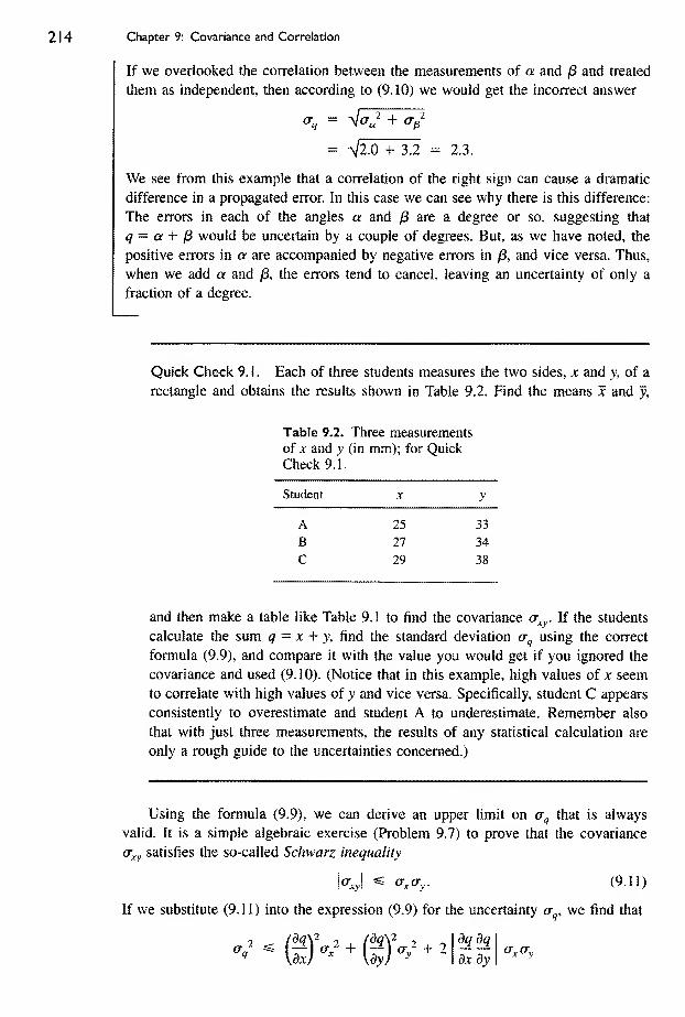
214 Chapter 9: Covartance and Correiation
If we overlooked the correiation between the measurements of a and /3 and treated
them as independent, then according to (9.10) we would get the incorrect answer
= V2.O + 3.2 ^ 2.3.
We see from this example that a correlation of the right sign can cause a dramatic
difference in a propagated error. In this case we can see why there is this difference:
The errors in each of the angles a and ^ are a degree or so. suggesting that
q ^ a + (3 would be uncertain by a couple of degrees. But, as we have noted, the
positive errors in a are accompanied by negative errors in j8, and vice versa. Thus,
when we add a and j8, the errors tend to cancel, leaving an uncertainty of only a
fraction of a degree.
Quick Check 9. i . Each of three students measures the two sides, x and v, of a
rectangle and obtains the results shown in Table 9.2. Find the means x and y.
Table 9.2. Three measurements
of X and y (in mm); for Quick
Check 9.1.
Student X >
A 25 33
B 27 34
C 29 38
and then make a table like Table 9.1 to find the covariance a^.. If the students
calculate the sum q ~ x + y. find the standard deviation cr^^ using the correct
formula (9.9), and compare it with the value you would get if you ignored the
covariance and used (9.10). (Notice that in this example, high values of x seem
to coiTelate with high values of _v and vice versa. Specifically, student C appears
consistently to overestimate and student A to underestimate. Remember also
that with just three measurements, the results of any statistical calculation are
only a rough guide to the uncertainties concerned.)
Using the formula (9.9), we can derive an upper limit on cr^ that is always
valid. It is a simple algebraic exercise (Problem 9.7) to prove that the covariance
(Tj^y satisfies the so-called Schwarz inequality
Wxy\ ^ (^x<^y (9.11)
If we substitute (9.11) into the expression (9.9) for the uncertainty ct-^, we find that
^2 ^ m\-^2 + {^\~^i^2 eraW^' dxdy^"^y

Section 9.3 Coefficient of Linear Correlation
dq
dx+
dq
dy
-.2
that is.
pliiIHIIIIlfll iliBlllil (9,12)
With this result, we have finally established the precise significance of our origi-
nal, sinniple expression
SgBq
8x +dq
dyay (9.13)
for the uncertainty 8(]. If we adopt the standard deviation ct-^ as our measure of the
uncertainty in q, then (9.12) shows that the old expression (9.13) is reaiiy the upper
limit on the uncertainty. Whether or not the errore in x and y are independent and
normally distributed, the uncertainty in q wiii never exceed the right side of (9.13).
If the measurements of x and y are correlated in just such a way that jor^yj = cr^.o-y,
its largest possible value according to (9.11), then the uncertainty in q can actually
be as large as given by (9.13), but it can never be any larger.
In an introductory physics laboratory, students usually do not make measure-
ments for which the covariance cr^^, can be estimated reliably. Thus, you will proba-
bly not have occasion to use the result (9.9) explicitly. If, however, you suspect that
two variables x and y may be correlated, you should probably consider using the
bound (9.12) instead of the quadratic sum (9.10). Our next topic is an application
of covariance that you will almost certainly be able to use.
9.3 Coefficient of Linear Correlation
The notion of covariance cr^v introduced in Section 9.2 enables us to answer the
question raised in Chapter 8 of how well a set of measurements (x^, y{), . . .
,
(%» of ^wo variables supports the hypothesis that x and >' are linearly related.
Let us suppose we have measured N pairs of values (jCi, yi% . .. , (jc^, yj^) of
two variables that we suspect should satisfy a linear relation of the form
y = A + Bx.
Note that Xj, . . . , are no longer measurements of one single number, as they
were in the past two sections; rather, they are measurements of N different values
of some variable (for example, N different heights from which we have dropped a
stone). The same applies to >'i, . .. , y^f.
Using the method of least squares, we can find the values of A and B for the
line that best fits the points (aj, y^), .
.
(x^, y^). If we already have a reliable
estimate of the uncertainties in the measurements, we can see whether the measured
points do lie reasonably close to the line (compared with the known uncertainties).
If they do, the measurements support our suspicion that x and y are linearly related.

2 1 6 Ch(^}ter 9: Covanance and Coiretation
iOO
t
oS 50
aat
0 50 iOO
Homework score x—
Figure 9.1. A "scatter plot" showing students' scores on exams and homework. Each of the 10
points {x„ shows a student's homework score, x„ and exani score, y,.
Unfortunately, in many experiments, getting a reliable estimate of the uncertain-
ties in advance is hard, and we must use the data themselves to decide whether the
two variables appear to be linearly related. In particular, there is a type of experi-
ment for which knowing the size of uncertainties in advance is impossible. This
type of experiment, which is more common in the social than the physical sciences,
is best explained by an example.
Suppose a professor, anxious to convince his students that doing homework will
help them do well in exams, keeps records of their scores on homework and exams
and plots the scores on a "scatter plot" as in Figure 9.1. In this figure, homework
scores are plotted horizontally and exam scores vertically. Each point (x,, y,) shows
one student's homework score, x^, and exam score, The professor hopes to show
that high exam scores tend to be correlated with high homework scores, and vice
versa (and his scatter plot certainly suggests this is approximately so). This kind of
experiment has no uncertainties in the points; each student's two scores are known
exactly. The uncertainty lies rather in the extent to which the scores are correlated;
and this has to be decided from the data.
The two variables x and y (in either a typical physics experiment or one like
that just described) may, of course, be related by a more complicated relation than
the simple linear one, y — A + Bx, For example, plenty of physical laws lead to
quadratic relations of the form y ~ A + 5x + Cx^. Nevertheless, I restrict my dis-
cussion here to the simpler problem of deciding whether a given set of points sup-
ports the hypothesis of a linear relation y = A + Bx.
The extent to which a set of points {x^, j'j), - , (jcjv, yfi) supports a linear
relation between x and y is measured by the linear correlation coefficient, or just
correlation coefficient,
r = (9.14)

Section 9.3 Coeffident of Linear Correiation 2 1
7
where the covariance cr^ and standard deviations cr^ and a-y are defined exactly as
before, in Equations (9.8) and (9.4).^ Substituting these definitions into (9.14), wecan rewrite the correlation coefficient as
(9.15)
As I will show directly, the number r is an indicator of how well the points (jc^, y^)
fit a straight line. It is a number between -1 and 1. If r is close to ± 1, the points
lie close to some straight line; if r is close to 0, the points are uncorrected and have
little or no tendency to lie on a straight line.
To prove these assertions, we first observe that the Schwarz inequality (9.11),
\(^xy\ ^ <^x<^yy impHes immediately that |r| 1 or
-1 ^ r ^ 1
as claimed. Next, let us suppose that the points (x„ >y) lie exactly on the line
y ~ A + Bx. In this case y, ^ A + Bx^ for all and hence y =A + Bx, Subtracting
these two equations, we see that
y,~~y^B(x,- X)
for each /. Inserting this result into (9.15), we find that
B S (Xi ~ xf Br =
. : =: ™- = ±1. (9.16)sll,{x,~xfB^1{x^~xf \B\
That is, if the points (x^, Vj) , (x^,, lie perfectly on a line, then r = ± 1, and
its sign is determined by the slope of the line (r = 1 for B positive, and r = - 1 for
B negative).-^ Even when the variables x and y really are linearly related, we do not
expect our experimental points to lie exactly on a line. Thus, we do not expect r to
be exactly ±1. On the other hand, we do expect a value of r that is close to ±\,if we believe that x and y are linearly related.
Suppose, on the other hand, there is no relationship between the variables x and
y. Whatever the value of y^, each x^ would then be just as likely to be above x as
below X, Thus, the terms in the sum
1{Xi ~ J)(y,. - y)
in the numerator of r in (9.15) are just as likely to be positive as negative. Mean-while, the terms in the denominator of r are all positive. Thus, in the limit that N,
the number of measurements, approaches infinity, the correlation coefficient r will
'Notice, however, that their significance is slightly different. For example, in SeOion 9.2 x^,...,Xf^ weremeasurements of one number, and if these measurements were precise, tr should be small, in llie present case
X,, . . . , Xy are measurements of different values of a variable, and even if the measurements are precise, there
is no reason to think er^ will be small. Note also that some authors use the number r\ called the coefficient ofdelennination.
^If the !ine is exactiy horizontal, then J5 - 0, and (9.16) gives r ~ 0/0; that is, r is undefined. Fortunately,
this special case is not important in praaice, because it corresponds to y being a constant, independent of x.

218 Chapter 9: Covartcmce and Correlation
be zero. With a finite number of data points, we do not expect r to be exactly zero,
but we do expect it to be small (if the two variables really are unrelated).
If two variables x and y are such that, in the limit of infinitely many measure-
ments, their covariance cr^ is zero (and hence r = 0), we say that the variables are
uncorrelated. If, after a finite number of measurements, the correlation coefficient
r = d^Jcr^cr^, is small, the hypothesis that JC and y are uncorrelated is supported.
As an example, consider the exam and homework scores shown in Figure 9.1.
These scores are given in Table 9.3. A simple calculation (Problem 9.12) shows that
Table 9.3. Students' scores.
Student / 1 2 3 5 6 7 8 9 10
Homework x^ 90 60 45 100 15 23 52 30 71 88
Exam >», 90 71 65 too 45 60 75 85 100 80
the correlation coefficient for these 10 pairs of scores is r = 0,8. The professor
concludes that this value is "reasonably close" to 1 and so can announce to next
year's class that, because homework and exam scores show good correlation, it is
important to do the homework.
If our professor had found a correlation coefficient r close to zero, he would
have been in the embarra^ing position of having shown that homework scores have
no bearing on exam scores. If r had turned out to be close to -1, then he would
have made the even more embarrassing discovery that homework and exam scores
show a negative correlation; that is, that students who do a good Job on homework
tend to do poorly on the exam.
Quick Check 9,2. Find the correlation coefficient for the data of Quick Check
9.1. Note that these measurements show a positive correlation; that is, high
values of x correlate with high values of and vice versa.
9.4 Quantitative Significance of r
The example of the homework and exam scores clearly shows that we do not yet
have a complete answer to our original question about how well data points support
a linear relation between x and y. Our professor found a correlation coefficient
r == 0.8, and Judged this value "reasonably close" to 1. But how can we decide
objectively what is "reasonably close" to 1? Would r = 0.6 have been reasonably
close? Or r = 0.4? These questions are answered by the following argument.
Suppose the two variables x and y are in reality uncorrelated; that is, in the
limit of infinitely many measurements, the correlation coefficient r would be zero.

Section 9.4 Quantitative Significance of r
After a finite number of measurements, r is very unlikely to be exactly zero. Onecan, in fact, calculate the probability that r will exceed any specific value. We will
denote by
Prob^(\r\ ^ r,)
the probability that A'' measurements of two uncorrelated variables x and y will give
a coefficient r larger"* than any particular r^. For instance, we could calculate the
probability
Proh^(\r\ ^ 0.8)
that, after A' measurements of the uncorrelated variables x and y, the correlation
coefficient would be at least as large as our professor's 0.8. The calculation of these
probabilities is quite complicated and will not be given here. The results for a few
representative values of the parameters are shown in Table 9.4, however, and a more
complete tabulation is given in Appendix C.
Table 9.4. The probability Probfj(\r\ 5= r^) that N measurements of two uncorrelated
variables .y and y would produce a correlation coefficient with
kl ^ ''o-Values given are percentage probabilities, and blanks indicate values
less than 0.05%,
N 0 0.1 0.2 0.3 0.4 0.5 0.6 0.7 0.8 0.9 1
3 100 94 87 81 74 67 59 51 41 29 0
6 100 85 70 56 43 31 21 12 6 1 0
10 100 78 58 40 25 14 7 2 0.5 0
20 100 67 40 20 8 2 0.5 0.1 0
50 100 49 16 3 0.4 0
Although we have not shown how the probabilities in Table 9.4 are calculated,
we can understand their general behavior and put them to use. The first column
shows the number of data points j^V. (In our example, the professor recorded 10
students' scores, so A' = 10.) The numbers in each succeeding column show the
percentage probability that measurements of two uncorrelated variables would
yield a coefficient r at least as big as the number at the top of the column. For
example, we see that the probability that 10 uncorrelated data points would give
jrj ^ 0.8 is only 0.5%, not a large probability. Our professor can therefore say it is
very unlikely that uncorrelated scores would have produced a coefficient with \r\
greater than or equal to the 0.8 that he obtained. In other words, it is very likely
that the scores on homework and examinations really are correlated.
Several features of T^ible 9.4 deserve comment. All entries in the first column
are 100%, because \r\ is always greater than or equal to zero; thus, the probability
''Because a correJation is indicated if /* is cJose to +1 or to -1, we consider the probability of getting the
absolute value \r\

Chapter 9: Covariance and Correlation
of finding jrj ^ 0 is always 100%. Similarly, the entries in the last column are all
zero, because the probability of finding \r\ 3= 1 is zero.^ The numbers in the interme-
diate columns vary with the number of data points N, This variation also is easily
understood. If we make just three measurements, the chance of their having a corre-
lation coefficient with jrj ^ 0.5, say, is obviously quite good (67%, in fact); but if
we make 20 measurements and the two variables really are uncorrelated, the chance
of finding jrj > 0.5 is obviously very small (2%).
Armed with the probabilities in Table 9.4 (or in the more complete table in
Appendix C), we now have the most complete possible answer to the question of
how well A'' pairs of values (.v^, y,) support a linear relation between x and y. From
the measured points, we can first calculate the observed correlation coefficient
(the subscript o stands for "observed"). Next, using one of these tables, we can
find the probability Probi^(jr\ ^ \rj) that N uncorrelated points would have given a
coefficient at least as large as the observed coefficient /;,. If this probability is "suf-
ficiently small," we conclude that it is very improbable that x and y are uncorrelated
and hence very probable that they really are correlated.
We still have to choose the value of the probability we regard as "sufficiently
small." One fairly common choice is to regard an observed correlation as "sig-
nificant" if the probability of obtaining a coefficient r with |r| ^ |r,J from uncorre-
lated variables is less than 5%. A correlation is sometimes called "highly significant"
if the corresponding probability is less than 1%. Whatever choice we make, we do
not get a definite answer that the data are, or are not, correlated; instead, we have a
quantitative measure of how improbable it is that they are uncorrelated.
Quick Check 9.3. The professor of Section 9.3 teaches the same course the
following year and this time has 20 students. Once again, he records homework
and exam scores and this time finds a correlation coefficient r = 0.6. Would
you describe this correlation as significant? Highly significant?
9.5 Examples
Suppose we measure three pairs of values (x^, y^) and find that they have a correla-
tion coefficient of 0.7 (or -0.7). Does this value support the hypothesis that jc and
y are linearly related?
Referring to Table 9.4, we see that even if the variables x and y were completely
uncorrelated, the probability is 51% for getting |r| ^ 0.7 when N ~ 3. In other
words, it is entirely possible that x and y are uncorrelated, so we have no worthwhile
evidence of correlation. In fact, with only three measurements, getting convincing
evidence of a correlation would be very difficult. Even an observed coefficient as
large as 0.9 is quite insufficient, because the probability is 29% for getting \r\ ^ 0.9
from three measurements of uncorrelated variables.
•''Although it is impossible that jrj > 1, it is, in principle, possible that jrj = 1. However, r is a continuous
variable, and the probability of getting jrj exactly equal to 1 is zero. Thus Prohf/(}r\ ^ l) ™ 0.

Principd Definitions and Equations of Chapter 9 22!
If we found a correlation of 0.7 from six measurements, the situation would be
a little better but still not good enough. With N - 6, the probability of getting
jrj ^ 0.7 from uncorrelated variables is 12%. This probability is not small enough
to rule out the possibility that x and y are uncorrelated.
On the other hand, if we found r = 0.7 after 20 measurements, we would have
strong evidence for a correlation, because when = 20, the probability of getting
\r\ ^ 0.7 from two uncorrelated variables is only 0.1%. By any standards this is
very improbable, and we could confidently argue that a correlation is indicated. In
particular, the correlation could be called "highly significant," because the probabil-
ity concerned is less than 1%.
Principal Definitions and Equations of Chapter 9
COVARIANCE
Given N pairs of measurements (jcj, ^'i), . . . , (jc^, y/^) of two quantities x and y,
we define their covariance to be
o-^ = - - x)iyi - y).j^^^ ^^^^^
If we now use the measured values to calculate a function q(Xj y), the standard
deviation of q is given by
^ W; by) y dxdy'
[See (9.9)]
If the errors in x and y are independent, then cr^ = 0, and this equation reduces to
the usual formula for error propagation. Whether or not the errors are independent,
the Schwarz inequality (9,11) implies the upper bound
[See (9.12)]
CORRELATION COEFFICIENT
Given N measurements {x^, y^), . . . , (jc^, y^) of two variables x and y^ we define
the correlation coefficient r as
dq
dx dy
_ X (x,-~~ x) (y- - y)
^^^y il{x, - xf I (>',~ yf [See (9.15)]
An equivalent form, which is sometimes more convenient, is
Ixjyj ~ Nxy
V(Sjc,-^ - Nx^){I.y^ ~ Nf) [See Problem 9.10]

Chapter 9: Covariance and Correlation
Values of r near 1 or -l indicate strong linear correlation; values near 0 indicate
little or no correlation. The probability Probj^{\r\ > r,,) that N measurements of two
uncorrected variables would give a value of r larger than any observed value r^ is
tabulated in Appendix C. The smaller this probability, the better the evidence that
the variables x and y really are correlated. If the probability is less than 5%, we say
the correlation is significant; if it is less than 1%, we say the correlation is highly
significant.
Problems for Chapter 9
For Section 9.2: Covariance in Error Propagation
9.1, * Calculate the covariance for the following four measurements of two quan-
tities X and y.
x: 20 23 23 22
y: 30 32 35 31
9.2. T*r Each of five students measures the two times (/ and T) for a stone to fall
from the third and sixth floors of a tall building. Their results are shown in Table
9.5. Calculate the two averages t and T, and find the covariance cr^j^ using the layout
of Table 9.1.
Table 9.5. Five measurements of
two times, t and T (in tenths of a
second); for Problem 9.2.
Student t r
A 14 20
B 1.2 18
C 13 18
D 15 22
E 16 22
[As you examine the data, note that students B and C get lower-than-average
answers for both times, whereas D's and E's answers are both higher than average.
Although this difference could be just a chance fluctuation, it suggests B and C mayhave a systematic tendency to underestimate their times and D and E to overesti-
mate. (For instance, B and C could tend to anticipate the landing, whereas D and Ecould tend to anticipate the launch.) Under these conditions, we would expect to get
a correlation of the type observed.]
9.3 (a) For the data of Problem 9.1, calculate the variances <r^^ and a^^ and
the covariance . (b) If you now decide to calculate the sum q ^ x + y, what will
be its standard deviation according to (9.9)? (c) What would you have found for the
standard deviation if you had ignored the covariance and used Equation (9.10)?

Problems for Chapter 9 223
(d) In a simple situation like this, an easier way to find the standard deviation of q
is just to calculate four values of q [one for each pair {x, y)] and then find cr^ from
these four values. Show that this procedure gives the same answer as you got in
part (b).
9.4. -k-k (a) For the data of Problem 9.2, calculate the variances cr," and (t-j? and
the covariance cr^j . (b) If the students decide to calculate the difference T ~ ty what
will be its standard deviation according to (9.9)? (c) What would they have found
for the standard deviation if they had ignored the covariance and used Equation
(9.10)? (d) In a simple situation like this, an easier way to find the standard devia-
tion of r ~ MS just to calculate five values of T ~ t [one for each pair (r, T)] and
then find the standard deviation of these five values. Show that this procedure gives
the same answer as you got in part (b).
9.5. Imagine a series of measurements of two fixed lengths x and y that
were made to find the value of some function q(x, y). Suppose each pair is measured
with a different tape; that is, the pair (jcj, is measured with one tape, (^2, ^2) is
measured with a second tape, and so on. (a) Assuming the main source of errors is
that some of the tapes have shrunk and some stretched (uniformly, in either case),
show that the covariance cr^^, is bound to be positive, (b) Show further, under the
same conditions, that ~<^x^y'^ ^^^^ ^xy large as permitted by the Schwarz
inequality (9.11).
[Hint: Assume that the ith tape has shrunk by a factor X,, that is, present
length ~ (design length)/\j, so that a length that is really X will be measured as
Xj = \,X. The mora! of this problem is that there are situations in which the covari-
ance is certainly not negligible.]
9.6. if* Here is an example of an experiment in which we would expect a nega-
tive correlation between two measured quantities (high values of one correlated with
low values of the other). Figure 9.2 represents a photograph taken in a bubble
chamber, where charged subatomic particles leave clearly visible tracks. A positive
particle called the K ^ has entered the chamber at the bottom of the picture. At
point A, it has collided with an invisible neutron (n) and has undergone the reaction
+ n ~-> + p.
The proton's track (p) is clearly visible, going off to the right, but the path of the
K° (shown dotted) is really invisible because the K° is uncharged. At point B, the
K° decays into two charged pions,
K'' jc-" + n~,
whose tracks are again clearly visible. To investigate the conservation of momentum
in the second process, the experimenter needs to measure the angles a and (j be-
tween the paths of the two pions and the invisible path of the K*', and this measure-
ment requires drawing in the dotted line that joins A and B. The main source of
error in finding a and /3 is in deciding on the direction of this line, because A and
B are often close together (less than a cm), and the tracks that define A and B are
rather wide. For the purpose of this problem, let us suppose that this is the only
source of error.

224 Chapter 9: Covartance and Correiation
Figure 9.2. Tracks of charged particles in a bubble chamber. The dotted line shows the
direction of an invisible K°, which was formed at A and decayed at B; for Problem 9.6.
Suppose several students are given copies of Figure 9.2, and each draws in his
best estimate for the line AB and then measures the two angles a and /3. The
students then combine their results to find the means a and (3, the standard devia-
tions (T^^ and o-^, and the covariance a^^^^. Assuming that the only source of error is in
deciding the direction of the line AB, explain why an overestimate of a is inevitably
accompanied by an underestimate of /3. Prove that ~ cr^ and that the covariance
cr^^ is negative and equal to the largest value allowed by the Schwartz inequality,
(Hint: Suppose that the iih student draws his line AB to the right of the true
direction by an amount A^. Then his value for a will be a, ~ cttrue + Write the
corresponding expression for his value jS,- and compute the various quantities of
interest in terms of the A, and A.)
9.7. Prove that the covariance cr^y defined in (9.8) satisfies the Schwarz in-
equality (9.11),
\a,y\ ^ a,a,. (9.17)
[Hint: Let t be an arbitrary number and consider the function
A{t) = |l[(x, ~x) + t{y, ~ y)f ^ 0. (9.18)
Because A{t) ^ 0 whatever the value of t, even its minimum A^^^ ^ 0. Find the
minimum A^,,,, and set A^-,^ ^ 0.]
For Section 9.3: Coefficient of Linear Correiation
9.8. * Calculate the correlation coefficient r for the following five pairs of mea-
surements:
X 1 2 3 4 5
y - 8 8 5 6 3

Probiems for Chapter 9
Do the calculations yourself, but if your calculator has a built-in function to compute
r, make sure you know how it works, and use it to check your value.
9.9. Calculate the correlation coefficient r for the following six pairs of mea-
surements:
a: = 1 2 3 5 6 7
j-566889Do the calculations yourself, but if your calculator has a built-in function to compute
r, make sure you know how it works, and use it to check your value.
9.10. -kit: (a) Prove the identity
l{Xi - x){y, -y)^ - Nxy.
(b) Hence, prove the correlation coefficient r defined in (9. 15) can be written as
r ^ ^==ML^m===. (9.19)
Many calculators use this result to find r because it avoids the need to store all the
data before calculating the means and deviations.
For Section 9.4: Quantitative Significance of r
9.11. In the photoelectric effect, the kinetic energy K of electrons ejected from
a metal by light is supposed to be a linear function of the light's frequency /,
K ^ hf~~ 0, (9.20)
where h and 0 are constants. To check this linearity, a student measures K for
different values of /and calculates the correlation coefficient /• for her results, (a) If
she makes five measurements (A'' = 5) and finds r = 0.7, does she have significant
support for the linear relation (9.20)? (b) What if A'^ = 20 and r — 0.5?
9.12. T*r (a) Check that the correlation coefficient r for the 10 pairs of test scores
in Table 9.3 is approximately 0.8. (By all means, use the built-in function on your
calculator, if It has one.) (b) Using the table of probabilities in Appendix C, find the
probability that 10 uncorrelated scores would have given |r| > 0.8. Is the correla-
tion of the test scores significant? Highly significant?
9.13. * A psychologist, investigating the relation between the intelligence of fa-
thers and sons, measures the Intelligence Quotients of 10 fathers and sons and ob-
tains the following results:
Father: 74 83 85 96 98 100 106 107 120 124
Son: 76 103 99 109 111 107 91 101 120 119
Do these data support a correlation between the intelligence of fathers and sons?
9.14. Eight aspiring football players are timed in the 100-meter dash and the
l,500~meter run. Their times (in seconds) are as follows:
Dash: 12 11 13 14 12 15 12 16
Run: 280 290 220 260 270 240 250 230

226 Chapter 9: Covariance and Correlation
Calculate the correlation coefficient r. What kind of correlation does your result
suggest? Is there, in fact, significant evidence for a correlation?
9.15. Draw a scatter plot for the six data pairs of Probiem 9.9 and the least-
squares line that best fits these points. Find their correlation coefficient r. Based on
the probabilities listed in Appendix C, would you say these data show a significant
linear correlation? Highly significant?
9.16. *T*r (a) Draw a scatter plot for the five data pairs of Problem 9.8 and the
least-squares line that best fits these points. Find their correlation coefficient r.
Based on the probabilities listed in Appendix C, would you say these data show a
significant linear correlation? Highly significant? (b) Repeat for the following data:
jc - 1 2 3 4 5
y = 4 6 3 0 2

Chapter 10
The Binomial Distribution
The Gauss, or normal, distribution is the only example of a distribution we have
studied so far. We will now discuss two other important examples, the binomial
distribution (in this chapter) and the Poisson distribution (in Chapter U).
i 0. i Distributions
Chapter 5 introduced the idea of a distribution, the function that describes the pro-
portion of times a repeated measurement yields each of its various possible answers.
For example, we couid make N measurements of the period T of a pendulum and
find the distribution of our various measured values of F, or we could measure
the heights h of N Americans and find the distribution of the various measured
heights h.
I next introduced the notion of the limiting distribution, the distribution that
would be obtained in the limit that the number of measurements N becomes very
large. The limiting dislrtbution can be viewed as telling us the prohahility that one
measurement will yield any of the possible values: the probability that one measure-
ment of the period will yield any particular value T; the probability that one Ameri-
can (chosen at random) will have any particular height h. For this reason, the lim-
iting distribution is also sometimes called the prohabilit)' distribufion.
Of the many possible limiting distributions, the only one we have discussed is
the Gauss, or normal, distribution, which describes the distribution of answers for
any measurement subject to many sources of error that are all random and small.
As such, the Gauss distribution is the most important of all limiting distributions
for the physical scientist and amply deserves the prominence given it here. Never-
theless, several other distributions have great theoretical or practical importance, and
this and the next chapter present two examples.
This chapter describes the binomial distribution, which is not of great practical
importance to the experimental physicist. Its simplicity, however, makes it an excel-
lent introduction to many properties of distributions, and it is theoretically important,
because we can derive the all-important Gauss distribution from it.

Chapter 10: The Binomia! Distribution
10.2 Probabilities in Dice Throwing
The binomial distribution can best be described by an example. Suppose we under-
take as our "experiment" to throw three dice and record the number of aces show-
ing. The possible results of the experiment are the answers 0, 1, 2, or 3 aces, if we
repeat the experiment an enormous number of times, we will find the limiting distri-
bution, which will tell us the probability that in any one throw (of all three dice)
we get p aces, where v 0,1, 2, or 3.
This experiment is sufficiently simple that we can easily calculate the probabil-
ity of the four possible outcomes. We observe first that, assuming the dice are true,
the probability of getting an ace when throwing one die is i Let us now throw all
three dice and ask first for the probability of getting three aces (i^ — 3). Because
each separate die has probability g of showing an ace, and because the three dice
roii independently, the probability for three aces is
Calculating the probability for two aces (i' = 2) is a little harder because we
can throw two aces in several ways. The first and second dice could show aces and
the third not (A, A, not A), or the first and third could show aces and the second not
(A, not A, A), and so on. Here, we argue in two steps. First, we consider the proba-
bility of throwing two aces in any definite order, such as (A, A, not A). The probabil-
ity that the first die will show an ace is i and likewise for the second. On the other
hand, the probability that the last die will not show an ace is §. Thus, the probability
for two aces in this particular order is
The probability for two aces in any other definite order is the same. Finally, there
are three different orders in which we could get our two aces: {A, A, not A), or {A,
not A, A), or (not A, A, A). Thus, the total probability for getting two aces (in any
order) is
Similar calculations give the probabilities for one ace in three throws (34.7%)
and for no aces in three throws (57.9%). Our numerical conclusions can be summa-
rized by drawing the probability distribution for the number of aces obtained when
throwing three dice, as in Figure 10.1. This distribution is an example of the bino-
mial distribution, the general form of which we now describe.
1 0.3 Definition of the Binomial Distribution
Prob(3 aces in 3 throws)
Prob{2 aces in 3 throws) (10.1)
To describe the general binomial distribution, i need to introduce some terminology.
First, imagine making n independent irials, such as throwing n dice, tossing n coins,
or testing n firecrackers. Each trial can have various outcomes: A die can show any

Section 10.3 Definition of i^e Binomial Distributi<»i 229
f57.9%
34.7%
6.9%
0.5%
0 2 3
Figure 10. 1. Probability of getting v aces when throwing three dice. This function is the bino-
mial distribution B„ Jiy), with n = 3 andp= lit.
face from 1 to 6, a coin can show heads or tails, a firecracker can explode or fizzle.
We refer to the outcome in which we happen to be interested as a success. Thus
"success" could be throwing an ace on a die, or a head on a coin, or having a
firecracker explode. We denote by p the probability of success in any one trial, and
by q — \ — p that of "failure" (that is, of getting any outcome other than the one
of interest). Thus, p = g for getting an ace on a die, p = 2 for heads on a coin, and
p might be 95% for a given brand of firecracker to explode properly.
Armed with these definitions, we can now ask for the probability of getting v
successes in // trials. A calculation I will sketch in a moment shows that this proba-
bility is given by the so-called binomial distribution:
Pro/>(j^ successes in « trials) - ^n,p{^)
Here the letter B stands for "binomial"; the subscripts n and p on B„p{v) indicate
that the distribution depends on n, the number of trials made, and /?, the probability
of success in one trial.
The distribution (10.2) is called the binomial distribution because of its close
connection with the well-known binomial expansion. Specifically, the fraction in
(10.2) is the binomial coefficient, often denoted
n{n — \)' •' {n — v + 1)
\ XlX • X Vp^<t~\ (10.2)
(10.3)
(10.4)i'!(/7 -- I')!
'
where we have introduced the useful factorial notation.
n\ = 1 X 2 X • • • X /I.

Chapter 10: The Binomiai Distribution
|By convention, 0! == 1, and so (g) = 1.] The binomiai coefficient appears in the
binomiai expansion
(10.5)
which holds for any two numbers p and q and any positive integer n (see Problems
10.5 and 10.6).
With the notation (10.3), we can rewrite the binomial distribution in the more
compact form
The Binomial Distribalion
i!||||||iii|:j^;succ^p Mmm&'-•"'''•1:/^'
iiiiiii
(10.6)
where, as usual, p denotes the probability of success in one trial and ^7~ 1 - p.
The derivation of the result (10.6) is similar to that of the example of the dice
in (10.1),
Prob(2 aces in 3 throws) = 3 Xer
X(D-
(10,7)
In fact, if we set J/ = 2, « = 3, /? ~ |, and <? = § in (10.6), we obtain precisely (10.7),
as you should check. Furthermore, the significance of each factor in (10.6) is the
same as that of the corresponding factor in (10.7). The factor p" is the probability
of getting all successes in any definite v trials, and q" "is the probability of failure
in the remaining n - v trials. The binomiai coefficient (^) is easily shown to be the
number of different orders in which there can be i' successes in // trials. This estab-
lishes that the binomial distribution (10.6) is indeed the probability claimed.
Example: Tossing Four Coins
Suppose we toss four coins (« = 4) and count the number of heads obtained, v.
What is the probability of obtaining the various possible values p-Q, 1, 2, 3, 4?
Because the probability of getting a head on one toss is p =|, the required
probability is simply the binomial distribution B„J^v), with n - 4 m6 p ~ q - I,
^4\/l\4Prob{v heads in 4 tosses)
These probabilities are easily evaluated. For example,
Prob{0 heads in 4 tosses) = 1 x{2)
0.0625.

Section 1 0.4 Properties of the Binomial Distribution
50%
37.5%
25%
6.25%
25%
6.25%
0 12 3 4
V—-
Figure 1 0.2. The binomial distribution B„Jy) with n - 4, p=-\.
This gives the probability of getting v heads when throwing four coins.
AJI five probabilities are shown in Figure 10.2.
We see that the most probable number of heads is v~2, as we would expect.
Here, the probabilities are symmetric about this most probable value. That is, the
probability for three heads is the same as that for one, and the probability for four
heads is the same as that for none. As we will see, this symmetry occurs only when
P =
Quick Check i 0. i . If you draw one card at random from a full deck of 52
playing cards, the probability of drawing any particular suit is \. If you draw
three times, replacing your card after each draw, what is the probability of
drawing three hearts? Of drawing exactly two hearts? Of drawing two or more
hearts?
! 0.4 Properties of the Binomial Distribution
The binomial distribution B„p(i') gives the probability of having "successes" in n
trials, when p is the probability of success in a single trial. If we repeat our whole
experiment, consisting of n trials, many times, then it is natural to ask what our
average number of successes p would be. To find this average, we just sum over all
possible values of each multiplied by its probability. That is,
and is easily evaluated (Problem 10,14) as
V - np. (10.9)

Chapter iO: The &nomi<d Disuibution
Hiat is, if we repeat our series of n trials many times, the average number of
successes will be just the probability of success in one trial (p) times n, as youwould expect. We can similarly calculate the standard deviation in our numberof successes (Problem 10.15). The result is
(10.10)
When p = 3 (as in a coin-toeing experiment), the average number of successes
is just n/2. Furthermore, it is easy to prove for p = i that
Bn,iM = - V) (10.11)
(see Problem 10.13). That is, the binomial distribution with p = | is symmetric
about the average value «/2, as we noticed in Figure 10.2.
In general, when p I, the binomial distribution B^J^v) is not symmetric. For
example, Figure 10.1 is clearly not symmetric; the most probable number of suc-
cesses is J' = 0, and the probability diminishes steadily for v=l,2, and 3. Also,
the average number of successes {v = 0.5) here is not the same as the most probable
number of successes (p = 0).
It is interesting to compare the binomial distribution B„j{p) with the more fa-
miliar Gauss distribution G^ J^x). Perhaps the biggest difference is that the experi-
ment described by the binomial distribution has outcomes given by the discrete^
values V ~ 0, I, 2, . .. , n, whereas those of the Gauss distribution are given by the
continuous values of the measured quantity x. The Gauss distribution is a symmetric
peak centered on the average value x ^ X, which means that the average value X is
also the most probable value [that for which Gj^ jix) is maximum]. As we have seen,
the binomial distribution is symmetric only when p =|, and in general the average
value does not coincide with the most probable value.
GAUSSIAN APPROXIMATION TO THEBINOMIAL DISTRIBUTION
For all their differences, the binomial and Gauss distributions have an important
connection. If we consider the binomial distribution B„j^{ p) tor any fixed value of
p, then when n is large B„p{v) is closely approximated by the Gauss distribution
^x,M same mean and same standard deviation; that is,
Sn,piid ^ (« large) (10.12)
with
JT = np and cr = V«p(l - p)- (10.13)
We refer to (10.12) as the Gaussian approximation to the binomial distribution.
'The word discrete (not to be confused with discreet) means "detadied from one another" and is theopposite of continuous.

Section 1 0.4 Properties of the Binomia! Distribution
0 12 3
V—-
0 2 4 6 8
0 4 8 12 !6 20
p—
Figure 10.3. The binomial distributions for p = 1/4 and n = 3, 12, and 48. The continuous
curve superimposed on each picture is the Gauss function with the same mean and same stan-
dard deviation.
I will not prove the result here,^ but its truth is clearly illustrated in Figure 10.3,
which shows the binomial distribution for /? - | and for three successively larger
values of « (« = 3, 12, 48). Superimposed on each binomial distribution is the
Gaussian distribution with the same mean and standard deviation. With just three
trials (n = 3), the binomial distribution is quite different from the corresponding
Gaussian. In particular, the binomial distribution is distinctly asymmetric, whereas
the Gaussian is, of course, perfectly symmetric about its mean. By the time n = 12,
the asymmetry of the binomial distribution is much less pronounced, and the two
distributions are quite close to one another. When n — 48, the difference between
the binomial and the corresponding Gauss distribution is so slight that the two are
almost indistinguishable on the scale of Figure 10.3(c).
^For proofs, see S. L. Meyer, Data Analysis for Scientists and Engineers (John Wiley, 1975), p. 226, or
H. D. Young, Statistical Treatment of Experimental Data (McGraw-Hiil, 1962), Appendix C.

Chapter 10: The Binomta! Distribution
That the binomial distribution can be approximated by the Gauss function when
n is large is very useful in practice. Calculation of the binomial function with n
greater than 20 or so is extremely tedious, whereas calculation of the Gauss function
is always simple whatever the values of X and a. To illustrate this, suppose we
wanted to know the probability of getting 23 heads in 36 tosses of a coin. This
probability is given by the binomial distribution B^Q y2(^) because the probability of
a head in one toss is /? = i Thus
Prob(23 heads in 36 tosses) == y^i^ (10.14)
which a fairly tedious calculation ^ shows to be
jPra/>(23 heads) = 3.36%.
On the other hand because the mean of the distribution is np ~ 18 and the standard
deviation is a = ynp{}~p) ~ 3, we can approximate (10.14) by the Gauss func-
tion Gjg 3(23), and a simple calculation gives
/>raf>(23 heads) Gi8,3(23) = 3.32%.
For almost all purposes, this approximation is excellent.
The usefulness of the Gaussian approximation is even more obvious if we want
the probability of several outcomes. For example, the probability of getting 23 or
more heads in 36 tosses is
Prob{2i or more heads) = Prob{23 heads) + Prob{24 heads) + • ••
+ Prob (36 heads),
a tedious sum to calculate directly. If we approximate the binomial distribution by
the Gaussian, however, then the probability is easily found. Because the calculation
of Gaussian probabilities treats i' as a continuous variable, the probability for
v~ 23, 24, . . . is best calculated as ProbQ^^jl^v^ 22.5), the probability for any
22.5. Now, V = 22.5 is 1.5 standard deviations above the mean value, 18. (Re-
member, (T = 3, so 4.5 ™ 1.5(7.) The probability of a result more than 1.5cr above
the mean equals the area under the Gauss function shown in Figure 10.4. It is easily
calculated with the help of the table in Appendix B, and we find
L5a
Figure 10.4. The probability of a result more than l.So- above the mean
is the shaded area under the Gauss curve.
-''Some hand calculators are preprogrammed to compute n! automatically, and with such a calculator compu-
tation of (10.15) is easy. In most such calculators, however, n! overflows when n s= 70, so for n 3= 70 this
preprogrammed function is no help.

Section iO.5 The Gauss Distribution for Random Errors
Pra6(23 or more heads) « ProbQ^^^^v-^ X ^ 1. 5a) ^ 6.7%.
This value compares well with the exact result (to two significant figures) 6.6%.
10.5 The Gauss Distribution for Random Errors
In Chapter 5, I claimed that a measurement subject to many small random errors
will be distributed normally. We are now in a position to prove this claim, using a
simple model for the kind of measurement concerned.
Let us suppose we measure a quantity x whose true value is X. We assume our
measurements are subject to negligible systematic error but there are n independent
sources of random error (effects of parallax, reaction times, and so on). To simplify
our discussion, suppose further that all these sources produce random errors of the
same fixed size £. That is, each source of error pushes our result upward or down-
ward by e, and these two possibilities occur with equal probability, /? == i For exam-
fa) (b) (c)
Figure 10.5. Distribution of measurements subject to n random erron* of magnitude e, for
n = 1, 2, and 32. The continuous curves superimposed on (b) and (c) are Gaussians with the
same center and width. (The vertical scales differ in the three graphs.)
p!e, if the true value is X and there is just one source of error, our possible answers
are x~ X ~ e and x ~ X + e, both equally likely. If there are two sources of error,
a measurement could yield .v = A' - 2e (if both errors happened to be negative), or
X ~ X (if one was negative and one positive), or x =^ X + 2s (if both happened to
be positive). These possibilities are shown in Figures 10.5(a) and (b).
In general, if there are n sources of error, our answer could range from
X ~ X ~ ne to X ~ X ne. In a given measurement, if v sources happen to give
positive errors and (n — v) negative errors, our answer will be
X ^ X + m~{n~v)e^^^^^^
= X + (2v ~ n)e.
The probability of this result occurring is just the binomial probability
Pm/:>( j^ positive errors) = B^^ ^^^v). (10.17)
Thus, the possible results of our measurement are symmetrically distributed around
the true value X, and the probabilities are given by the binomial function (10.17).

236 Chapter 10: The ^nomia! Distribution
This distribution is illustrated in Figure 10.5 for « = 1, 2, and 32.
I now claim that if the number of sources of error, n, is large and the size of
the individual errors, is small, then our measurements are normally distributed.
To be more precise, we note that the standard deviation of the binomial distribution
is cr^ = V«/K1 ~ P) - Therefore, according to (10.16), the standard deviation
of our measurements of x is cr,. = 2sa^,= s-\jn. Accordingly, we let n and
e 0 in such a way that cr^ = s^^n remains fixed. Two things happen as a result.
First, as discussed in the previous section, the binomial distribution approaches the
Gauss distribution with center X and width <x^. This approach is clearly visible
in Figures 10.5(b) and (c), on which the appropriate Gauss functions have been
superimposed. Second, as e 0, the possible results of our measurement move
closer together (as is also clear in Figure 10.5), so that the discrete distribution
approaches a continuous distribution that is precisely the expected Gauss distribu-
tion.
1 0.6 Applications; Testing of Hypotheses
Once we know how the results of an experiment should be distributed, we can ask
whether the actual results of the experiment were distributed as expected. This kind
of test of a distribution is an important technique in the physical sciences and per-
haps even more so in the biological and social sciences. One important, general test,
the chi-squared test, is the subject of Chapter 12. Here, I give two examples of a
simpler test that can be applied to certain problems involving the binomial distribu-
tion.
TESTING A NEW SKI WAX
Suppose a manufacturer of ski waxes claims to have developed a new wax that
greatly reduces the friction between skis and snow. To test this claim, we might take
10 pairs of skis and treat one ski from each pair with the wax. We could then hold
races between the treated and untreated members of each pair by letting them slide
down a suitable snow-covered incline.
If the treated skis won all 10 races, we would obviously have strong evidence
that the wax works. Unfortunately, we seldom get such a clear-cut result, and even
when we do, we would like some quantitative measure of the strength of the evi-
dence. Thus, we have to address two questions. First, how can we quantify the
evidence that the wax works (or doesn't work)? Second, where would we draw the
line? If the treated skis won nine of the races, would this result be conclusive? What
if they won eight races? Or seven?
Precisely these same questions arise in a host of similar statistical tests. If wewanted to test the efficacy of a fertilizer, we would organize "races" between treated
and untreated plants. To predict which candidate is going to win an election, we
would choose a random sample of voters and hold "races" between the candidates
among the members of our sample.
To answer our questions, we need to decide more precisely what we should

Section 10.6 Appiicaaons; Testing of Hypotheses
expect from our teste. In the accepted terminology, we must formulate a statistical
hypothesis. In the example of the ski wax, the simplest hypothesis is the null hypoth-
esis, that the new wax actually makes no difference. Subject to this hypothesis, we
can calculate the probability of the various possible results of our test and then
judge the significance of our particular result.
Suppose we take as our hypothesis that the ski wax makes no difference. In any
one race, the treated and untreated skis would then be equally likely to win; that is,
the probability for a treated ski to win is p ~ I. The probability that the treated skis
wiii win v of the 10 races is then the binomial probability:
Prob{v wins in 10 races) ==^lo.i/aC*')
i/!(io - v)\ b;*
According to (10.18), the probability that the treated skis would win all 10 races is
Prob{\0 wins in 10 races) =^ {\f^ 0.1%. (10.19)
That is, if our null hypothesis is correct, the treated skis would be very unlikely to
win all 10 races. Conversely, if the treated skis did win all 10 races, the null hypoth-
esis is very unlikely to be correct. In fact, the probability (10.19) is so small, we
could say the evidence in favor of the wax is "highly significant," as we will discuss
shortly.
Suppose instead that the treated skis had won eight of the 10 races. Here, wewould calculate the probability of eight or more wins:
Proh(S or more wins in 10 races)
- Pm/)(8 wins) + Prad(9 wins) + Pro6(10 wins) « 5.5%. (10.20)
For the treated skis to win eight or more races is still quite unlikely but not nearly
as unlikely as their winning all 10.
To decide what conclusion to draw from the eight wins, we must recognize that
there are really just two alternatives. Either
(a) our null hypothesis is correct (the wax makes no difference), but by chance,
an unlikely event has occurred (the treated skis have won eight races)
or
(b) our null hypothesis is false, and the wax does help.
In statistical testing, by tradition we pick some definite probability (5%, for exam-
ple) to define the boundary below which an event is considered unacceptably im-
probable. If the probability of the actual outcome (eight or more wins, in our case)
is below this boundary, we choose alternative (b), reject the hypothesis, and say the
result of our experiment was significant.
By common practice, we call a result significant if its probability is less than
5% and caii it highly significant if its probability is less than 1%. Because the

CKapter tO: The Binomial Distribution
probability (10.20) is 5.5%, we see that eight wins for the waxed skis are Just not
enough to give significant evidence that the wax worlds. On the other hand, we saw
that the probability of 10 wins is 0.1%. Because this value is less than 1%, we can
say that 10 wins would constitute highly significant evidence that the wax heips."*
GENERAL PROCEDURE
The methods of the example just described can be applied to any set of n similar
but independent tests (or "races"), each of which has the same two possible out-
comes, "success" or "failure." First, a hypothesis is formulated, here simply an
assumed value for the probability p of success in any one test. This assumed value
of p determines the expected mean number of successes, v = np, in n trials.'' If the
actual number of successes, v, in our n trials is close to np, there is no evidence
against the hypothesis. (If the waxed skis win five out of 10 races, there is no
evidence the wax makes any difference.) If v is appreciably larger than np, we
calculate the probability (given our hypothesis) of getting v or more successes. If
this probability is less than our chosen significance level (for example, 5% or 1%),
we argue that our observed number is unacceptably improbable (if our hypothesis
is correct) and hence that our hypothesis should be rejected. In the same way, if our
number of successes v is appreciably less than np, we can argue similarly, except
that we would calculate the probability of getting v or less successes.^
As you should have expected, this procedure does not provide a simple answer
that our hypothesis is certainly tme or certainly false. But it does give a quantitative
measure of the reasonableness of our results in light of the hypothesis, so we can
choose an objective, if arbitrary, criterion for rejection of the hypothesis. Whenexperimenters state conclusions based on this kind of reasoning, they must state
clearly the criterion used and the calculated probability so that readers can judge
the reasonableness of the conclusion for themselves.
AN OPINION POLL
As a second example, consider an election between two candidates, A and B.
Suppose candidate A claims that extensive research has established that he is favored
by 60% of the electorate, and suppose candidate B asks us to check this claim (in
the hope, of course, of showing that the number favoring A is significantly less than
60%).
Here, our statistical hypothesis would be that 60% of voters favor A, so the
probability that a randomly selected voter will favorA would be p = 0.6. Recogniz-
ing that we cannot poll every single voter, we carefully select a random sample of
'^Note the great simpiicity of the test just described. We couJd have measured various additional parameters,
such as the time tal^en by each ski, the maximum speed of each ski, and so on. Instead, we simply recorded
which ski won each race. Tests that do not use such additional parameters are called nonparametric tests.
They have the ^eat advantages of sinipHcity and wide applicability.
^As usual, V ~ is the mean number of successes expected if we were to repeat our whole set of n trials
many times.
*As we discuss below, in some experiments the relevant probability is the "two-tailed" probabiiisy of getting
a value of v that deviates in either direction from flp by as much as, or more than, the value actually obtained.

Section 10.6 ^^lications; Testir^g of Hypodieses
600 and ask their preferences. If 60% really favor A, the expected number in our
sample who favor A'lsnp- 600 x 0.6 ™ 360. If in fact 330 state a preference for
A, can we claim to have cast significant doubt on the hypothesis that 60%favor >l?
To answer this question, we note that (according to the hypothesis) the probabil-
ity that V voi&m will favor A is the binomial probability
voters favor A) = B^Jiy) (10.21)
with n = 600 and p ~ 0.6. Because n is so large, it is an excellent approximation to
replace the binomial function by the appropriate Gauss function, with center at
np ~ 360 and standard deviation (t^, = ^np{l — p) =12.
Pra6(i^ voters favor /i) « O36o,i2(^')' (10.22)
The mean number expected to favor A is 360. Thus, the number who actually
favored y4 in our sampie (namely 330) is 30 less than expected. Because the standard
deviation is 12, our result is 2,5 standard deviations below the supposed mean. The
probability of a result this low or lower (according to the table in Appendix B) is
0.6%7 Thus, our result is highly significant, and at the 1% level we can confidently
reject the hypothesis that A is favored by 60%.
This example illustrates two general features of this kind of test. First, having
found that 330 voters favored A (that is, 30 less than expected), we calculated the
probability that the number favoring A would be 330 or less. At first thought, you
might have considered the probability that the number favoring A is precisely
v~ 330. This probability is extremely small (0.15%, in fact) and even the most
probable result (p~ 360) has a low probability (3.3%). To get a proper measure of
how unexpected the result y ~ 330 is, we have to include v ~ 330 and any result
that is even further below the mean.
Our result p ~ 330 was 30 less than the expected result, 360. The probability
of a result 30 or more below the mean is sometimes called a "one-taiied probabil-
ity," because it is the area under one tail of the distribution curve, as in Figure
10.6(a). In some tests, the relevant probability is the "two-tailed probability" of
getting a result that differs from the expected mean by 30 or more in either direc-
j-i Hi •l-i
30 30 30
{a) (b)
Figure 10.6. (a) The "one-tailed" probability for getting a result 30 or more below the mean,
(b) The "two-tailed" probabiiity for getting a result that differs from the mean by 30 or more in
either direction. (Not to scale.)
^Stricsly speaking, we should have compuied ihe probabiiity for v ^ 330.5 because the Gauss distribution
treafs r- as a consinuous variabie. This number is 2.46(:r below the mean, SO the correct prc^ability is actually
0.7%, but this small a difference does not affect our conclusion.

Chapter iO: The BInomtd t^s^bution
tion, that is, the probability of getting p =^ 3^ or 390, as in Figure 10.6(b).
Whether you use the one-tailed or two-tailed probability in a statistical test depends
on what you consider the interesting alternative to the original hypothesis. Here, we
were concerned to show that candidate A was favored by less than the claimed 60%,
so the one-tailed probability was appropriate. If we were concerned to show that the
number favoring A was different from 60% (in either direction), the two-tailed prob-
ability would be appropriate. In practice, the choice of which probability to use is
usually fairly clear. In any case, the experimenter always needs to state clearly the
probability and significance level chosen and the calculated value of the probability.
With this information readers can judge the significance of the results for them-
selves.
Quick Check 10.2. If I toss a coin 12 times and get 11 heads, do I have
significant evidence that the coin is loaded in favor of heads? (Hint: Assuming
the coin is true, the probability of getting heads in a single throw is p = |.
Making this assumption, find the probability that I would have obtained U or
more heads in 12 tosses.
Principal Definitions and Equations of Chapter 1
0
THE BINOMIAL DISTRIBUTION
We consider an experiment with various possible outcomes and designate the
particular outcome (or outcomes) in which we are interested as a "success." If the
probability of success in any one trial is p, then the prcrf>abiiity of v successes in n
trials is given by the binomial distribution;
Prob{v successes in n trials) = B„p{v)
where denotes the binomial coefficient,
/n\ _ n\
\v}" v\{n- v)\'
if we repeat the whole set of n trials many times, the expected mean number of
successes is
V ^ np [See (10,9)]
and the standard deviation of v is

FVobiems for Chapter iO
[See (10.10)]
THE GAUSSIAN APPROXIMATION TO THEBINOMIAL DISTRIBUTION
When n is large, the binomial distribution B„^,(f) is well approximated by the
Gauss function with the same mean and standard deviation; that is,
- OVeX^), [See (10.12)1
where X= np and cr = '\jnp{l ~~p).
Problems for Chapter 1
0
For Section 10.2: Probabilities tn Dice Throwing
10.1. T*r Consider the experiment of Section 10.2 in which three dice are thrown.
Derive the probabilities for throwing no aces and one ace. Verify all four of the
probabilities shown in Figure 10.1.
10.2. * Compute the probabilities Prob{ v aces in two throws) for = 0, 1, and 2
in a throw of two dice. Plot them in a histogram.
10.3. i*r* Compute the probabilities Prob{v aces in four throws) for = 0,
1, . .. , 4 in a throw of four dice. Plot them in a histogram. You will need to think
carefully about the number of different ways in which you can get two aces in a
throw of four dice.
For Section 10.3: Definition of the Binomiai Distribution
10.4. (a) Compute 5!, 6!, and 25!/23! (Please think for a moment before you
do the last one.) (b) Explain why we traditionally define 0! = 1. [Hint: According to
the usual definition, for w == 1, 2, . ..
, the factorial function satisfies «! = (« + !)!/
(n + 1).] (c) Prove that the binomial coefficient defined by Equation (10.3) is equal
to
10.5. T*r Compute the binomiai coefficients (J) for v~ 0, 1, 2, and 3. Hence, write
the binomial expansion (10.5) of {p + qf.
10.6. * Compute the binomial coefficients (^) for v = 0, I, 2, 3, and 4. Hence,
write the binomial expansion (10.5) of (p + qf.
10.7. T*r Compute and plot a histogram of the binomial distribution function B„p(v)
for « = 4, p == 1/2, and all possible v.
10.8. * Compute and plot a histogram of the binomial distribution function B„p{v)
for n = 4, p ~ 1/5, and all possible v.

Chapter iCh The ^nomlal Dis^bution
10.9. * I draw six times from a deck of 52 playing cards, replacing each card
before making the next draw. Find the probabilities, Prob(p hearts), that I would
draw exactly v hearts in six draws, for = 0, 1, . ..
, 6.
10.10. if: A hospital admits four patients suffering from a disease for which the
mortality rate is 80%. Find the probabilities of the following outcomes: (a) None of
the patients survives, (b) Exactly one survives, (c) Two or more survive.
10.11. In the game of Yahtzee, a player throws five dice simultaneously, (a)
Find the probabilities of throwing i' aces, for v - Q, 1, . .. , 5. (b) What is the
probability of throwing three or more aces? (c) What is the probability of throwing
five of a kind?
10.12. Prove that the binomial coefficient (") is the number of different orders
in which v successes could be obtained in n trials.
For Section 1 0.4: Properties of the Binomial Distribution
10.13. * Prove that for p = 1/2, the binomial distribution is symmetric about
V = n/2; that is,
10.14. T*n*r Prove that the mean number of successes,
n
for the binomial distribution is just np. [There are many ways to do this, of which
one of the best is this: Write the binomial expansion (10.5) for {p + qy\ Because
this expansion is true for any p and you can differentiate it with respect to p. If
you now set /? + g = 1 and multiply the result by p, you will have the desired
result.]
10.15. T*n*r (a) The standard deviation for any limiting distribution f{v) is defined
by
o-i? = (v ~ pf.
Prove that this definition is the same as ~ (p)^. (b) Use this result to prove that,
for the binomial distribution,
0-^2 = «p(l - P).
(Use the same trick as in Problem 10.14, but differentiate twice.)
10.16. The Gaussian approximation (10,12) to the binomial distribution is ex-
cellent for n large and surprisingly good for n small (especially if /? is close to i).
To illustrate this claim, calculate ^4 i aC^^) (for v~0, 1, . .. , 4) both exactly and
using the Gaussian approximation. Compare your results.
10.17. ifir Use the Gaussian approximation (10.12) to find the probability of get-
ting 15 heads if you throw a coin 25 times. Calculate the same probability exactly
and compare answers.

Problems for Ch^ter 10
10.18. Use the Gaussian approximation to find the probability of getting 18
or more heads in 25 tosses of a coin. (In using the Gauss probabilities, you should
find the probability for v 3= 17.5.) Compare your approximation with the exact an-
swer, which is 2.16%.
For Section 10.6: Applications; Testing of Hypotheses
10.19. T*r In the test of a ski wax described in Section 10.6, suppose the waxed
skis had won 9 of the 10 races. Assuming the wax makes no difference, calculate
the probability of 9 or more wins. Do 9 wins give significant (5% level) evidence
that the wax is effective? Is the evidence highly significant (1% level)?
10.20. *T*r To test a new fertilizer, a gardener selects 14 pairs of similar plants
and treats one plant from each pair with the fertilizer. After two months, 12 of the
treated plants are healthier than their untreated partners (and the remaining 2 are
less healthy). If, in fact, the fertilizer made no difference, what would be the proba-
bility that pure chance led to 12 or more successes? Do the 12 successes give
significant (5% level) evidence that the fertilizer helps? Is the evidence highly sig-
nificant (1% level)?
10.21. ** Of a certain kind of seed, 25% normally germinates. To test a new
germination stimulant, 100 of these seeds are planted and treated with the stimulant.
If 32 of them germinate, can you conclude (at the 5% level of significance) that the
stimulant helps?
10.22. ** In a certain school, 420 of the 600 students pass a standardized mathe-
matics test, for which the national passing rate is 60%. If the students at the school
had no special aptitude for the test, how many would you expect to pass, and what
is the probability that 420 or more would pass? Can the school claim that its stu-
dents are significantly well prepared for the test?


Chapter 1
1
The Poisson Distribution
This chapter presents a third example of a limiting distribution, the Poisson distribu-
tion, which describes the results of experiments in which we count events that occur
at randojn but at a definite average rate. Examples of this kind of counting experi-
ment crop up in almost every area of science; for instance, a sociologist might count
the number of babies born in a hospital in a three-day period. An important example
in physics is the counting of the decays of a radioactive sample; for instance, a
nuclear physicist might decide to count the number of alpha particles given off by
a sample of radon gas in a ten-second interval.
This kind of counting experiment was discussed in Section 3.2, where I stated
but did not prove the "square-root rule": If you count the occurrences of an event
of this type in a chosen time interval T and obtain v counts, then the best estimate
for the true average number in time T is, of course, v, and the uncertainty in this
estimate is -\^.
In Sections 11.1 and 11.2, 1 introduce the Poisson distribution and explore someof its properties. In particular, I prove in Section 11.2 that the standard deviation of
the Poisson distribution is the square root of the expected number of events. This
result Justifies the square-root rule of Section 3.2. Sections 11.3 and 11.4 describe
some applications of the Poisson distribution.
i I . i Definition of tlie Poisson Distribution
As an example of the Poisson distribution, suppose we are given a sample of radio-
active material and use a suitable detector to find the number v of decay particles
ejected in a two-minute interval. If the counter is reliable, our value of v will have
no uncertainty. Nevertheless, if we repeat the experiment, we will almost certainly
get a different value for v. This variation in the number v does not reflect uncertain-
ties in our counting; rather, it refleas the intrinsically random character of the radio-
active decay process.
Each radioactive nucleus has a definite probability for decaying in any two-
minute interval. If we knew this probability and the number of nuclei in our sample,
we could calculate the expected average number of decays in two minutes. Never-
theless, each nucleus decays at a random time, and in any given two-minute interval,
the number of decays may be different from the expected average number.

Chapter I i : The Pbisson Distribution
Obviously the question we should ask is this: If we repeat our experiment manytimes (replenishing our sample if it becomes significantly depleted), what distribu-
tion should we expect for the number of decays v observed in two-minute intervals?
If you have studied Chapter 10, you will recognize that the required distribution is
the binomial distribution. If there are n nuclei and the probability that any one
nucleus decays is p, then the probability of p decays is just the probability of v
"successes" in n "trials," or B^J^v). In the kind of experiment we are now dis-
cussing, however, there is an important simplification. The number of "trials" (that
is, nuclei) is enormous (« ~ 10^**, perhaps), and the probability of "success" (decay)
for any one nucleus is tiny (often as small as p ~ lO"^*'). Under these conditions (;i
large and p small), the binomial distribution can be shown to be indistinguishable
from a simpler function called the Poisson distribution. Specifically, it can be shownthat
Prob{v counte in any definite interval)
where the Poisson distribution, PfJiv), is given by
(11.1)
The Poisson Distribution
ilBIIIIBill(11.2)
In this definition, /x is a positive parameter (^t > 0) that, as I will show directly, is
just the expected mean number of counts in the time interval concerned, and v\
denotes the factorial function (with 0! = 1).
SIGNIFICANCE OF ^ AS THE EXPECTED MEAN COUNTI will not derive the Poisson distribution (11.2) here but simply assert that it li-
the appropriate distribution for the kind of counting experiment in which we are
interested.^ To establish the significance of the parameter /x in (11.2), we have only
to calculate the average number of counts, expected if we repeat our counting
experiment many times. This average is found by summing over ail possible values
of V, each multiplied by its probability:
The first term of this sum can be dropped (because it is zero), and v/p\ can be
replaced by l/{v - 1)!. If we remove a common factor of fie'*^, we get
^For derivations, see, for exampie, H. D, Young, Statistical Treatment of Experimental Data (McGraw-Hill,1962), Section 8, or S. L. Meyer, Data Analysis for Scientists and Engineers (John Wiiey, 1975), p. 207.

Section I Lf Definition of the PoisscHi Distribution
The infinite sum that remains is
(11.5)
which is just the exponential function e** (as indicated). Thus, the exponential
in (11.4) is exactly canceled by the sum, and we are left with the simple conclusion
that
That is, the parameter ju, that characterizes the Poisson distribution PfJ^v) is just the
average number ofcounts expected if we repeat the counting experiment many times.
Sometimes, we may know in advance the average rate 7? at which the events
we are counting should occur. In this case, the expected average number of events
in a time T is just
Conversely, if the rate R is unknown, then by counting the number of events in a
time T, we can get an estimate for fi and hence for the rate R as R^^f = ti^t/T.
Example: Counting Radioacdve Decays
Careful measurements have established that a sample of radioactive thorium emits
alpha particles at a rate of 1.5 per minute. If I count the number of alpha particles
emitted in two minutes, what is the expected average result? What is the probability
that I would actually get this number? What is the probability for observing v parti-
cles for P = 0, 1, 2, 3, 4, and for p ^ 5?
The expected average count is just the average rate of emissions (R ~ 1.5 per
minute) multiplied by the time during which I make my observations (1 = 2 min-
utes):
This result does not mean, of course, that I should expect to observe exactly three
particles in any single trial. On the contrary, the probabilities for observing any
number (v) of particles are given by the Poisson distribution
In particular, the probability that 1 would observe exactly three particles is
(11.6)
fi = rate X time = RT.
(expected average number) = fi = 3.
Pro6(v particles) = Pj,{v) = e
Prob(3 particles) == P^{3) = = 0.22 22%.
Notice that although the expected average result is = 3, we should expect to get
this number only about once in every five trials.

Chsq^ter 1 1 : The Bc»sson Distribution
20%
t 10%
0*-
fi = 3
X0 12 3 5 6 7 8 9
Figure I i.l. The Poisson distribution P^{v) gives the probabiiities of observing v
events in a counting experiment fof which the expected average count is 3.
The probabilities for any number v can be calculated in the same way and are
(as you might want to check):
Number v: 0 12 3 4
Probability: 5% 15% 22% 22% 17%
These probabilities (up to p=^9) are plotted in Figure li.i. The simplest way to
find the probability for getting 5 or more counts is to add the probabilities for
= 0, . . . , 4 and then subtract the sum from 100% to give^
Pwb(v ^ 5) ^ 100% - (5 + 15 + 22 + 22 + 17)%
= 19%.
Quick Check i !.!. On average, each of the 18 hens in my henhouse lays 1
egg per day. If I check the hens once an hour and remove any eggs that have
been laid, what is the average number, ix, of eggs that I lind on my hourly
visits? Use the Poisson distribution PJiv) to calculate the probabilities that I
would find V eggs for j/ ™ 0, 1, 2, 3, and v ~ 4 or more. What is the most
probable number? What is the probability that 1 would find exactly /u, eggs?
Verify the probabilities shown in Figure 11.2.
50%
0 L0 1
fi = 0.75
2 3 4
Fi^re 1 1.2. The Poisson distribution Po^jsiv)
gives Uie probabilities of observing v events in
a counting experiment for which the expected
average count is 0.75.
^The cwect answer is M;aia!ly 18.48%, as you can check by Iceeping a couple of extra decimal piaces in
all the probabilities.

Sectifxi f t .2 Properdes of die Poisson Distributj<»i
1 .2 Properties of the Poisson Distribution
THE STANDARD DEVIATION
The Poisson distribution P^{v) gives the probability of getting the result v in an
experiment in which we count events that occur at random but at a definite average
rate. We have seen that the parameter /x is precisely the expected average count p.
The natural next question is to ask for the standard deviation of the counts v whenwe repeat the experiment many times. The standard deviation of any distribution
(after a large number of trials) is just the root-mean-square deviation from the mean.
That is,
<T,. {v - v)\
or, using the result of Problems 10.15(a) or 4.5(a),
(11.7)
For the Poisson distribution, we have already found that v= fi&nda similar calcu-
lation (Problem 11.9) gives = /j? + fi. Therefore, Equation (11.7) implies that
fi or
!}!.(11.8)
That is, the Poisson distribution with mean count jjl has standard deviation Vm-The result (1 1.8) justifies the square-root rule of Section 3.2. If we carry out a
counting experiment once and get the answer we can easily see (using the princi-
ple of maximum iikelihood, as in Problem M.U) that the best estimate for the
expected mean count is /x^est = v- From (11.8), it immediately follows that the best
estimate for the standard deviation is just ^fv. In other words, if we make one
measurement of the number of events in a time interval T and get the answer v, our
answer for the expected mean count in time T is
p ± -sfp. (U.9)
This answer is precisely the square-root rule quoted without proof in Equation (3.2).
Example: More Radioactive Decays
A student monitors the thorium sample of the previous example for 30 minutes and
observes 49 alpha particles. What is her answer for the number of particles emitted
in 30 minutes? What is her answer for the rate of emission, R, in particles per
minute?
According to (11.9), her answer for the number of particles emitted in 30 min-
utes is
(number emitted in 30 minutes) = 49 ± ^49 = 49 ± 7.

250 Chapter 1 1: The Poisson Distribution
To find the rate in particles per minute, she must divide by 30 minutes. Assuming
this 30 minutes has no uncertainty, we find
49 ± 7/; = —_g— = 1,6 ± 0.2 particies/min. (ll.iO)
Notice that the square-root rule gives the uncertainty in the actual counted number
(or,, - a/?/ — 7, in this case). A common mistake is to calculate the rate of decay
R ~ vlT and then to take tiie uncertainty in R to be A glance at (11.10) should
convince you that this procedure is simply not correct. The square-root rule applies
only to the actual counted number and the uncertainty in /? = vlT must be found
from that in v using error propagation as in (11.10).
Quick Check i 1.2. The farmer of Quick Check 11.1 observes that in a certain
ten-hour period his hens lay 9 eggs. Based on this one observation, what would
you quote for the number of eggs expected in ten hours? What would you give
for the rate R of egg production, in eggs per hour? (Give the uncertainties in
both your answers.)
GAUSSIAN APPROXIMATION TO THEPOISSON DISTRIBUTION
In Chapter 10, we compared the Gauss distribution with the binomial distribu-
tion. We saw that in most ways, the two distributions are very different; neverthe-
less, under the right conditions, the Gauss distribution gives an excellent, extremely
useful, approximation to the binomial distribution. As we will now see, almost ex-
actly the same can be said about the Gauss and Poisson distributions.
The Gauss distribution Gx,J<x) gives the probabilities of the various values of a
continuous variable x\ by contrast, the Poisson distribution Pixiv), like the binomial
B„p(v), gives the probabilities for a discrete variable v~ 0, 1, 2, 3 Another
important difference is that the Gauss distribution Gx^M is specified by two param-
eters, the mean X and the standard deviation <j, whereas the Poisson distribution
PJ^v) is specified by a single parameter, the mean yit. because the width of the
Poisson distribution is automatically determined by the mean (namely, cr^ ^ ^JJl).
Finally, the Gauss distribution is always bell shaped and symmetric about its meanvalue, whereas the Poisson distribution has neither of these properties in general.
This last point is especially clear in Figure 11.2, which shows the Poisson distribu-
tion for IX = 0.75; this curve is certainly not bell shaped, nor is it even approxi-
mately symmetric about its mean, 0.75.
Figure U.l showed the Poisson distribution for fx - 3. Although this curve is
obviously not exactly bell shaped, it is undeniably more nearly so than the curve
for jLt = 0.75 in Figure 11.2. Figure 11.3 shows the Poisson distribution for /x = 9;
this curve is quite nearly bell shaped and close to symmetric about its mean ~ 9).
In fact, it can be proved that as /a -> «>, the Poisson distribution becomes progres-

Section I i .2 Properties of the Poisson Distribution
15%
10%
5% //// N M = 9
\\\
10 15
Figure i ) .3. The Poisson distribution for /x = 9. The dashed curve is the Gauss distribution
with the same mean and standard deviation (X = 9 and a = 3). As —> «>, the two distribu-
tions become indistinguishable; even when fJt.~ 9, they are very close.
sively more bell shaped and approaches the Gauss distribution with the same mean
and standard deviation.'' That is.
where
^/t(^) ^x,Jjd^ (when ^ is large)
X = fi and <T = Vm-
(11.11)
in Figure 11.3, the dashed curve is the Gauss function with X ~ 9 and cr = 3. You
can see clearly how, even when ^ is only 9, the Poisson distribution is remarkably
close to the appropriate Gauss function; the slight discrepancy reflects the remaining
asymmetry in the Poisson function.
The approximation (11.11) is called the Gaussian approximation to the Poisson
distribution. It is analogous to the corresponding approximation for the binomial
distribution (discussed in Section 10.4) and is useful under the same conditions,
namely, when the parameters involved are large.
Example: Gaussian Approximation to a Poisson Distribution
To illustrate the Gaussian approximation to the Poisson distribution, consider the
Poisson distribution with ju, = 64. The probability of 72 counts, for example, is
(64)72Prob{72 counts) ^ Pe4U2) =
which a tedious calculation gives as
^^6(72 counts) = 2,9%.
-64
72!(11.12)
'For proof, see S. L. Meyer, Data Analysis for Scientists and Engineers (John Wiley, 1975), p. 227.

Chapter 1 1 : The Poisson Distribution
According to (11.11), however, the probability (11.12) is we!! approximated by the
Gauss function
Prob(72 counts) §(72),
which is easi!y evaluated to give
/'ra/>(72 counts) 3.0%.
If we wanted to ca!culate directly the probability of 72 or more counts in the
same experiment, an extremely tedious calculation would give
Prob{v^l2) - PJJ2) + ^64(73) + . .
.
- 17.3%.
If we use the approximation (11.11), then we have only to calculate the Gaussian
probabilily for getting 71.5 (because the Gauss distribution treats v as a contin-
uous variable). Because 71.5 is 7,5, or QMcr, above the mean, the required probabil-
ity can be found quickly from the table in Appendix B as
Frob{v^l2) « ProbQ{v^l\.S) = Prob^Jiv^ X + 94a)
= 17.4%,
by almost any standard an excellent approximation.
1 1 .3 Applications
As I have emphasized, the Poisson distribution describes the distribution of results
in a counting experiment in which events are counted that occur at random but at a
definite average rate. In an introductory physics laboratory, the two most commonexamples are counting the disintegrations of radioactive nuclei and counting the
arrival of cosmic ray particles.
Another very important example is an experiment to study an expected limiting
distribution, such as the Gauss or binomial distributions, or the Poisson distribution
itself. A limiting distribution tells us how many events of a particular type are
expected when an experiment is repeated several times. (For example, the Gaussian
Gx Jx) tells us how many measurements of x are expected to fall in any interval
from jc == fl to jc = fe.) In practice, the observed number is seldom exactly the ex-
pected number. Instead, it fluctuates in accordance with the Poisson distribution. In
particular, if the expected number of events of some type is n, the observed number
can be expected to differ from « by a number of order sjn. We will make use of
this point in Chapter 12.
In many situations, it is reasonable to expect numbers to be distributed approxi-
mately according to the Poisson distribution. The number of eggs laid in an hour on
a poultry farm and the number of births in a day at a hospital would both be
expected to follow the Poisson distribution at least approximately (though they
would probably show some seasonal variations as well). To test this assumption,

Section 1 1.3 AppNcatlons
you would need to record the number concerned many times over. After plotting the
resulting distribution, you could compare it with the Poisson distribution to see how
close the fit is. For a more quantitative test, you would use the chi~squared test
described in Chapter 12.
Example: Cosmic Ray Counting
As another example of the Poisson distribution, let us consider an experiment with
cosmic rays. These "rays" originate as charged particles, such as protons and alpha
particles, that enter the Earth's atmosphere from space. Many of these primary parti-
cles collide with atoms in the atmosphere and create further, secondary particles,
such as mesons and positrons. Some of the particles (both primary and secondary)
travel all the way to ground level and can be detected (with a Geiger counter, for
example) in the laboratory. In the following problem, I exploit the fact that the
number of cosmic rays hitting any given area in a given time should follow the
Poisson distribution.
Student A asserts that he has measured the number of cosmic rays hitting a
Geiger counter in one minute. He claims to have made the measurement repeatedly
and carefully and to have found that, on average, 9 particles hit the counter per
minute, with "negligible" uncertainty. To check this claim. Student B counts how
many particles arrive in one minute and gets the answer 12. Does this answer cast
serious doubt on A's claim that the expected rate is 9? To make a more careful
check. Student C counts the number of particles that arrive in ten minutes. From
A's claim, she expects to get 90 but actually gets 120, Does this value cast signifi-
cant doubt on A's claim?
Let us consider B's result first. If A is right, the expected mean count is 9.
Because the distribution of counts should be the Poisson distribution, the standard
deviation is Student B's result of 12 is, therefore, oniv one standard devia-
tion away from the mean of 9. This amount is certainly not far enough away to
contradict A's claim. More specifically, knowing that the probability of any answer
V is supposed to be Pg{v), we can calculate the total probability for getting an
answer that differs from 9 by 3 or more. This probability turns out to be 40% (see
Problem 11.7). Obviously B's result is not at all surprising, and A has no reason to
worry.
Student C's result is quite a different matter. If A is right, C should expect to
get 90 counts in ten minutes. Since the distribution should be Poisson, the standard
deviation should be ^|90 = 9.5. Thus, C's result of 120 is more than three standard
deviations away from A's prediction of 90. With these large numbers, the Poisson
distribution is indistinguishable from the Gauss function, and we can immediately
find from the table in Appendix A that the probability of a count more than three
standard deviations from the mean is 0.3%. That is, if A is right, it is extremely
improbable that C would have observed 120 counts. Turning this statement around,
we can say something almost certainly has gone wrong. Perhaps A was just not as
careful as he claimed. Perhaps the counter was malfunctioning for A or C, introduc-
ing systematic errors into one of the results. Or perhaps A made his measurements
at a time when the flux of cosmic rays was truly less than normal.

Chapter 1 1; The Poisson Distribution
1 1 .4 Subtracting a Background
To conclude this chapter, I discuss a problem that complicates many counting exper-
iments. Often, the events we want to study are accompanied by other "background"
events that cannot be distinguished from the events of interest. For example, in
studying the disintegrations of a radioactive source, we usually cannot prevent the
detector from registering particles from other radioactive materials in the vicinity or
from cosmic rays. This means that the number we count includes the events of
interest plus these background events, and we must somehow subtract out the un-
wanted background events. In principle at least, the remedy is straightforward; Hav-
ing found the total counting rate (due to source and background), we must remove
the source and find the rate of events due to the background alone; the rate of events
from the source is then just the difference of these two measured rates.
In practice, it is surprisingly easy to make a mistake in this procedure, espe-
cially in the error analysis. It is usually convenient to measure the total and back-
ground counts using different time intervals. Suppose we count a total of Vi^^^ events
(source plus background) in a time Tjot, and then v^^^ background events in a time
^bgd- Obviously, we do not simply subtract I'^gd ^^"^ "tot because they refer to
different time intervals, instead, we must first calculate the rates
^tot " '^^^ ^bgd ~ (11.13)•* tot * bgd
and then calculate the rate from the source as the difference
^sce ''^tot~^bgd- (lil4)
In estimating the uncertainties in the quantities involved, you must remember that
the square-root rule gives the uncertainties in the counted numbers v^^^ and i^^gdj
uncertainties in the corresponding rates must be found by error propagation, as in
the following example.
Example: Radioactive Decays with a Background
A student decides to monitor the activity of a radioactive source by placing it in a
liquid scintillation detector. In the course of 10 minutes, the detector registers 2,540
total counts. To allow for the possibility of unwanted background counts, she re-
moves the source and notes that in 3 minutes, the detector registers a further 95
counts. To find the activity of the source, she calculates the two rates of counting,
/fto, and /?bgjj (in counts per minute) and their difference R^ct = /ftot~ ^bgd- What
are her answers with their uncertainties? (Assume the two times have negligible
uncertainty.)
According to the square-root rule, the two counted numbers with their uncer-
tainties are
v,^, ^ 2,540 ± V2,540 = 2,540 ± 50
and
i^bgd - 95 ± a/95 = 95 ± 10.

Principal Deftnitions and Equations of Chapter I
!
Dividing these numbers by their corresponding times, we find the rates
„ not 2,540 ± 50 . ^ . , , .
"tot ~ ^ ~ ^7; ~ 254 ± 5 counts/mm-'tot
and
J^bgd 95 ± 10 ^^bgd " ~ n ~ 32 ± 3 counts/mm.
^bgd 3
Finally, the rate due to the source alone is
^sce ^tot~
'^bgd = (254 ± 5) - (32 ± 3) = 222 ± 6 counts/min.
Notice that, in the last step, the errors are combined in quadrature, because they are
certainly independent and random.
Principal Definitions and Equations of Chapter I \
THE POfSSON DISTRIBUTION
The Poisson distribution describes experiments in which you count events that
occur at random but at a definite average rate. If you count for a chosen time
interval T, the probability of observing v events is given by the Poisson function
Pro6( counts in time T) == PJ,v) ~ e
where the parameter ju- is the expected average number of events in
V ~ IX {after many trials)
= RT,
where R is the mean rate at which the events occur.
The standard deviation of the observed number v is
THE GAUSSIAN APPROXIMATION TO THEPOiSSON DISTRIBUTION
When IX is large, the Poisson distribution P^^{i') is well approximated by the
Gauss function with the same mean and standard deviation; that is,
[See (11.2)]
time T; that is,
[See (11.6)]
[See (11.8)]
where X = fi and cr ~ -sffi. [See (11.11)]

256 Chaptffl- I \: The Poisson Distribution
SUBTRACTING A BACKGROUNDThe events produced by a source subject to an unavoidable background can be
counted in a three-step procedure:
(1) Count the total number v^^^ (source plus background) in a time T^^i, and
calculate the total rate R^f^^ ~ ^toi^^tot-
(2) Remove the source, and measure the number of background events in a
time Tbgd; then calculate the background rate /f^gd = J'bgd/^bgd-
(3) Calculate the rate of the evente from the source as the difference R^^ =
Finally, the uncertainties in the numbers and i^^^j are given by the square-
root rule, and, from these values, the uncertainties in the three rates can be found
using error propagation.
Problems for Chapter 1
1
For Section 11 . i : Definition of the Poisson Distribution
11.1. * Compute the Poisson distribution P^{v) for fju= 0.5 and v~0, 1, . .
., 6.
Plot a bar histogram of /'o.sC'^) against v.
11.2. -k (a) Compute the Poisson distribution PfJiv) for /a = 1 and == 0, 1, . ..
,
6, and plot your results as a bar histogram, (b) Repeat part (a) but for /u, = 2.
113. A radioactive sample contains 5.0 X 10^^ atoms, each of which has a
probability p — 3.0 X 10^^'* of decaying in any given five-second interval, (a) What
is the expected average number, (jl, of decays from the sample in five seconds? (b)
Compute the probability Pf^v) of observing v decays in any five-second interval,
for V = 0, 1, 2, 3. (c) What is the probability of observing 4 or more decays in any
five-second interval?
11.4. In the course of four weeks, a farmer finds that between 10:00 and i0:30
A.M., his hens lay an average of 2.5 eggs. Assuming the number of eggs laid follows
a Poisson distribution with fx = 2.5, on approximately how many days do you sup-
pose he found no eggs laid between 10:00 and 10:30 A.M.? On how many days do
you suppose there were 2 or less? 3 or more?
11.5. A certain radioactive sample is expected to undergo three decays per
minute. A student observes the number v of decays in 100 separate one-minute
intervals, with the results shown in Table 11.1. (a) Make a histogram of these re-
Tabfe I I.I. Occurrences of numbers of decays in one-minute intervals; for
Problem 11.5.
No. of decays v 0 123456789Times observed 5 19 23 21 14 12 3 2 1 0

Problems for Chapter ! i
suits, plotting (the fraction of times the result v was found) against v. (b) On the
same plot, show the expected distribution P^{v), Do the data seem to fit the expected
distribution? (For a quantitative measure of the fit, you could use the chi-squared
test, discussed in Chapter 12.)
11.6. -kif-k (a) The Poisson distribution, like all distributions, must satisfy a "nor-
malization condition,"
i P^(f) - 1. (11.15)
This condition asserts that the total probability of observing all possible values of v
must be one. Prove it. [Remember the infinite series (11.5) for e^.\ (b) Differentiate
(11.15) with respect to /it, and then multiply the result by to give an alternative
proof that, after infinitely many trials, v~ ixd&m Equation (11.6).
For Section 1 1 .2: Properties of the Poisson Distribution
11.7. * (a) What is the standard deviation (after a large number of trials) of
the observed counts v in a counting experiment in which the expected average count
is ju, = 9? (b) Compute the probabilities ^^9(1^) of obtaining v counts for v~l,8, . .
., 11. (c) Hence, find the probability of getting a count v that differs from the
expected mean by one or more standard deviations, (d) Would a count of 12 cause
you to doubt that the expected mean really is 9?
11.8. * A nuclear physicist monitors the disintegrations of a radioactive sample
with a Geiger counter. She counts the disintegrations in 15 separate five-second
intervals and gets the following numbers:
7, 11, 10, 7, 5, 7, 6, 12, 12, 7, 18, 12, 13, 12, 6.
(a) Her best estimate yu^^^^ for the true mean count fx is the average of her 15 counts.
(For a proof of this claim, see Problem 11.15.) What is her value for ju-besr ^) The
standard deviation (T,, of her 15 counts should be close to Vm-- What is her standard
deviation and how does it compare with V^beM?
11^. (a) Prove that the average value of for the Poisson distribution PJj^)
is = ^ fjL. [The easiest way to do this is probably to differentiate the identity
(11.15) twice with respect to fi.] (b) Hence, prove that the standard deviation of v
is CTj, ~ ^[fl. [Use the identity (11.7).]
11.10. The average rate of disintegrations from a certain radioactive sample
is known to be roughly 20 per minute. If you wanted to measure this rate within
4%, for approximately how long would you plan to count?
11.11. Consider a counting experiment governed by the Poisson distribution
PfJ,v), where the mean count (jl is unknown, and suppose that I make a single count
and get the value v. Write down the probability Prob{v) for getting this value v.
According to the principle of maximum likelihood, the best estimate for the un-
known /Lt is that value of ju for which Prob(v) is largest. Prove that the best estimate
Mbest precisely the obseived count p as you would expect. (In this calculation, the
unknown fji is the variable and i> is the fixed value I obtained in my one experiment.)

Chapter 1 1 : The Poisson Distribution
11.12. Tfr* The expected mean count in a certain counting experiment is ju = 16.
(a) Use the Gaussian approximation (11.11) to estimate the probability of getting a
count of 10 in any one trial. Compare your answer with the exact value P^^f lO). (b)
Use the Gaussian approximation to estimate the probability of getting a count of 10
or less. (Remember to compute the Gaussian probability for v ^ 10.5 to allow for
the fact that the Gauss distribution treats as a continuous variable.) Calculate the
exact answer and compare.
Note how, even with ju, as small as 16, the Gaussian approximation gives quite
good answers and—at least in part (b)—is significantly less trouble to compute than
an exact calculation using the Poisson distribution.
11.13. The expected mean count in a certain counting experiment is = 400.
Use the Gaussian approximation to tind the probability of getting a count anywhere
in the range 380 ^ =^ 420. Compare your answer with the exact answer, which is
69.47%. Discuss the feasibility of finding this exact probability using your calcu-
lator.
11.14. In the experiment of Problem 11.5, the expected mean count was
known in advance to be /it — 3. Therefore, the mean of the data should be close to
3 and the standard deviation should be close to ^3- Find the mean and standard
deviation of the data and compare them with their expected values.
11.15. Consider a counting experiment governed by the Poisson distribution
P^{v), where the mean count /a is unknown, and suppose that you make separate
trials and get the values
Write the probability Prob{Vi, . .. , v^) for getting this particular set of values. Ac-
cording to the principle of maximum likelihood, the best estimate for the unknown
fx is that value of ix for which Prob{vi, . .. ,
Vp^ h largest. Prove that the best
estimate fjL^^^ is the average of the observed numbers
1
Mhest " 7? 2y'V
1 = 1
as you would expect. (In this calculation, the unknown ji is the variable, and
1^1, ... , are fixed at the values you obtained in your trials.)
For Section I 1 .3: Appiications
11.16. * Using a Geiger counter, a student records 25 cosmic-ray particles in 15
seconds, (a) What is her best estimate for the true mean number of particles in 15
seconds, with its uncertainty? (b) What should she report for the rate (in particles
per minute) with its uncertainty?
11.17. A student counts 400 disintegrations from a radioactive sample in 40
seconds, (a) What is his best estimate for the true mean number of disintegrations
in 40 seconds, with its uncertainty? (b) What should he report for the rate of disinte-
grations (per second) with its uncertainty?

Probiems for Chapter i t
11.18. Sean and Maria monitor the same radioactive sample. Sean counts for
one minute and gets 121 counts. Maria counts for six minutes and gets 576 counts.
Each then calculates the rate in counts per minute. Do their results agree satisfac-
torily?
For Section 1 1 ,4: Subtracting a Background
11.19. icif A heating duct at a nuclear plant is suspected of being contaminated
with radioactive dust. To check this suspicion, a health physicist places a detector
inside the duct and records 7,075 particles of radiation in 120 minutes. To check for
background radiation, he moves his detector some distance from the duct and shields
it from any radiation coming from the duct; in this new position, he records 3,015
particles in 60 minutes. What is his final answer for the radiation rate (in particles
per minute) due to the contents of the duct alone? Does he have significant evidence
for radioactive material in the duct?
11.20. TAr-A- To measure the activity of a rock thought to be radioactive, a physicist
puts the rock beside a detector and counts 225 particles in 10 minutes. To check for
background, she removes the rock and then records 90 particles in 6 minutes. She
converts both these answers into rates, in particles per hour, and takes their differ-
ence to give the activity of the rock alone. What is her final answer, in particles per
hour, and what is its uncertainty? Does she have significant evidence that the rock
is radioactive?
11.21. A physicist needs an accurate measurement of the activity of a radio-
active source. To plan the best use of his time, he first makes quick approximate
measurements of the total counting rate (source plus background) and the back-
ground rate. These approximations give him rough values for the true rates, }\^^ and
''bgd- (Notice that I have used lower-case r for the true rates; this will let you use
upper-case R for the values he measures in the main experiment.) To get more
accurate values, he plans to count the total number j^,,,, (source plus background) in
a long time 7^^, and the background number v^^^ in a long time T^,^^. From these
measurements, he will calculate the rates R^^^^ and jR(,gd and finally the rate R^ due
to the source aione.
The detector he is using is available only for a time T, so that the two times Jjq,
and jTbgd are constrained not to exceed
Therefore, he must choose the two times T^^^ and T^^^ to minimize the uncertainty
in his final answer for R^^^.
(a) Show that his final uncertainty will be minimum if he chooses the two times
such that
(11.17)
[Hint: Write the expected numbers v^^^ and v^^^ in terms of the true rates, r,(,( and
rjjgtj, and the corresponding times. From these calculate ail the uncertainties in-

Chapter ! I : The l^iss<»i DistritHidtm
volved. To minimize the uncertainty in R^^, eliminate T^^^ using (11.16), and then
differentiate with respect to 7,0^ and set the derivative equal to zero.] Because his
preliminary measurements of /(oj
and r^^^ tell him the approximate value of the ratio
on the right side, (11.17) tells him how to apportion the available time between T^^^^
and Tbgd*
(b) If the available time t is two hours and his preliminary measurements have
shown that rtoj/rj,gd 9, how should he choose Jtot and Tbgd?
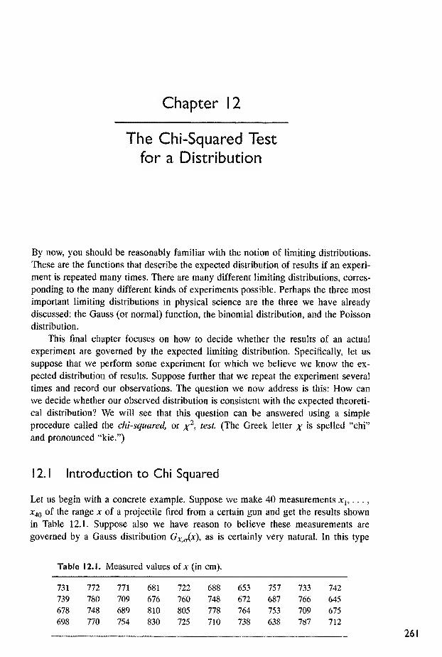
Chapter 12
The Chi-Squared Test
for a Distribution
By now, you should be reasonabiy familiar with the notion of limiting distributions.
These are the functions that describe the expected distribution of results if an experi-
ment is repeated many times. There are many different limiting distributions, corres-
ponding to the many different kinds of experiments possible. Perhaps the three most
important limiting distributions in physical science are the three we have already
discussed: the Gauss (or norma!) function, the binomial distribution, and the Poisson
distribution.
This final chapter focuses on how to decide whether the results of an actual
experiment are governed by the expected limiting distribution. Specifically, let us
suppose that we perform some experiment for which we believe we know the ex-
pected distribution of results. Suppose further that we repeat the experiment several
times and record our observations. The question we now address is this: How can
we decide whether our observed distribution is consistent with the expected theoreti-
cal distribution? We will see that this question can be answered using a simple
procedure called the chi-squared, or ^^^i- (The Greek letter x is spelled "chi"
and pronounced "kie.")
12.1 Introduction to Chi Squared
Let us begin with a concrete example. Suppose we make 40 measurements Xj, . . .
,
x^Q of the range x of a projectile fired from a certain gun and get the results shown
in Table 12.1. Suppose also we have reason to believe these measurements are
governed by a Gauss distribution Gx^j(x), as is certainly very natural. In this type
Table 12.1. Measured values of jc (in cm).
731 772 771 681 722 688 653 757 733 742
739 780 709 676 760 748 672 687 766 645
678 748 689 810 805 778 764 753 709 675
698 770 754 830 725 7iO 738 638 787 712

Ch(q>ter 1 2: The Chi-Squ»^ lest for a Distrtbucion
of experiment, we usually do not know in advance either the center X or the width
(T of the expected distribution. Our first step, therefore, is to use our 40 measure-
ments to compute best estimates for these quantities:
(best estimate for = x ^ =^ = 730.1 cm (12J )4U
and
(best estimate for a) =^ 39
^^6.8 cm. (12.2)
Now we can ask whether the actual distribution of our results a-j, . . .,x^(^ is
consistent with our hypothesis that our measurements were governed by the Gauss
distribution G^ Jx) with X and cr as estimated. To answer this question, we must
compute how we would expect our 40 results to be distributed if the hypothesis is
true and compare this expected distribution with our actual observed distribution.
The first difficulty is that x is a continuous variable, so we cannot speak of the
expected number of measurements equal to any one value of x. Rather, we must
discuss the expected number in some interval a < x < b. That is, we must divide
the range of possible values into bins. With 40 measurements, we might choose bin
boundaries dXX — a, X, and X + giving four bins as in Table 12.2.
Table 12.2. A possible choice of bins for the data of Table 12.1. The final
column shows the number of observations that fell into each bin.
Bin number
k Values of x in bin
Observations
0,
I X < X ~~ (J (otx < 683.3) 8
2 X - a < X < X (or 683.3 < x < 730.1) 10
3 X < X < X -h a (or 730.1 < X < 776.9) 16
4 X + cr < X (or 776.9 < x) 6
We will discuss later the criteria for choosing bins, in particular, they must be
chosen so that ail bins contain several measured values x,. In general, I will denote
the number of bins by n; for this example with four bins, n ~ 4,
Having divided the range of possible measured values into bins, we can now
formulate our question more precisely. First, we can count the number of measure-
ments that fail into each bin k,^ We denote this number by (where O stands for
"observed number"). For the data of our example, the observed numbers Oj, Oj,
O3, O4 are shown in the last column of Table 12.2. Next, assuming our measure-
ments are distributed normally (with X and a as estimated), we can calculate the
expected number E/, of measurements in each bin k. We must then decide how well
the observed numbers O^t compare with the expected numbers E/^.
^If a measurement foils exactly on the boundary between two bins, we can assign half a measurement to
each bin.

Section ! 2. 1 introduction to Chi Squared
Probi,
X~(T X X + o-
Figure I2J. The probabilities Prob^ that a measurement faiis into each of the bins, A = 1, 2,
3, 4, of Table 12.2 are the four areas shown under the Gauss function.
The calculation of the expected numbers Ej. is quite straightforward. The proba-
bility that any one measurement fails in an interval a <x < b is just the area under
the Gauss function between x ~ a and x = b. In this example, the probabilities
Prob^, Prob2, Prob^, Prob^ for a measurement to fall into each of our four bins are
the four areas indicated m Figure 12.1. The two equal areas Prob^ and Prob^ to-
gether represent the well-known 68%, so the probability for failing into one of the
two central bins is 34%; that is, Prob2 ~ Prob^ ~ 0.34. The outside two areas com-
prise the remaining 32%; thus Prob^ ~ Prob^ ~ 0.16. To find the expected numbers
E(^, we simply multiply these probabilities by the total number of measurements,
N - 40. Therefore, our expected numbers are as shown in the third column of Table
12.3. That the numbers are not integers serves to remind us that the "expected
number" is not what we actually expect in any one experiment; it is rather the
expected average number after we repeat our whole series of measurements many
times.
Our problem now is to decide how well the expected numbers f"^ do represent
the corresponding observed numbers Oi^ (in the last column of Table 12.3). We
Table 1 2.3. The expected numbers £"^. and the observed numbers
for the 40 measurements of Table 12.1, with bins chosen as in Table
12.2.
Bin number Probability Expected number Observed numberk Prob^ Ej, = NProbf, o,
1 16% 6.4 8
2 34% 13.6 10
3 34% 13.6 16
4 16% 6.4 6
would obviously not expect perfect agreement between Ej. and after any finite
number of measurements. On the other hand, if our hypothesis that our measure-
ments are normally distributed is correct, we would expect that, in some sense, the
deviations
O, ~ E, (12.3)
would be small. Conversely, if the deviations — E^ prove to be large, we would
suspect our hypothesis is incorrect.

264 CK^ter 1 2: Hie Chi-Squared Test for a DisiributiCHi
To make precise the statements that the deviation Oj^ — is "small" or "large,"
we must decide how large we would expect Of^ — f^. to be if the measurements
really are normally distributed. Fortunately, this decision is easily made. If we imag-
ine repeating our whole series of 40 measurements many times, then the number O^.
of measurements in any one bin k can be regarded as the result of a counting
experiment of the type described in Chapter 11. Our many different answers for
should have an average value of and would be expected to fluctuate around E^
with a standard deviation of order ^Je^. Thus, the two numbers to be compared are
the deviation ~ E,^ and the expected size of its fluctuations "v/fi*.
These considerations lead us to consider the ratio
5^=^. (12.4)
SE,
For some bins k, this ratio will be positive, and for some negative; for a few k, it
may be appreciably larger than one, but for most it should be of order one, or
smaller. To test our hypothesis (that the measurements are normally distributed), it
is natural to square the number (12.4) for each k and then sum over all bins
k~ 1, . ..
, n (here n = 4), This procedure defines a number called chi squared,
- 1 <£l^_ (12.5)
This number x'^ clearly a reasonable indicator of the agreement between the
observed and expected distributions. If x^ = 0» the agreement is perfect; that is,
~Ef, for all bins A, a situation most unlikely to occur. In general, the individual
terms in the sum (12.5) are expected to be of order one, and there are n terms in
the sum. Thus, if
X"" ^ n
(X^ of order n or less), the observed and expected distributions agree about as well
as could be expected. In other words, if x^ ^ «> we have no reason to doubt that
our measurements were distributed as expected. On the other hand, if
X^ » n
(X^ significantly greater than the number of bins), the observed and expected num-
bers differ significantly, and we have good reason to suspect that our measurements
were not governed by the expected distriburion.
In our example, the numbers observed and expected in the four bins and their
differences are shown in Table 12.4, and a simple calculation using them gives
^ (--3.6)^ + ei£ + ("Q-^)
6.4 13.6 13.6 6.4
1.80. (12.6)

Section 12.2 Genera! Definition of Chi Squared
Table 12.4. The data of Table 12.1, shown here with the differences
Bin numberk
Observed number
Ok
Expected number
E/^ = NProbfc
Difference
Oi. — Et
1 8 6.4 1.6
2 10 13.6 -3.6
3 16 13.6 2.4
4 6 6,4 -0.4
Because the value of 1.80 for less than the number of terms in the sum
(namely, 4), we have no reason to doubt our hypothesis that our measurements were
distributed normally.
Quick Check 1 2. 1 . Each of the 100 students in a class measures the time for
a ball to fall from a third-story window. They calculate their mean t and stan-
dard deviation cr, and then group their measurements into four bins, chosen as
in the example just discussed. Their results are as follows:
less than (t - a,): 19
between (/ - cr,) and h 30
between 't and (f + cr,): 37
more than {i + <t,): 14.
Assuming their measurements are normally distributed, what are the expected
numbers of measurements in each of the four bins? What is x^-> is there
reason to doubt that the measurements are distributed normally?
1 2.2 General Definition of Chi Squared
The discussion so far has focused on one particular example, 40 measurements of a
continuous variable x, which denoted the range of a projectile fired from a certain
gun. We defined the number and saw that it is at least a rough measure of
the agreement between our observed distribution of measurements and the Gauss
distribution we expected our measurements to follow. We can now define and use
in the same way for many different experiments.
Let us consider any experiment in which we measure a number x and for which
we have reason to expect a certain distribution of results. We imagine repeating the
measurement many times (AT) and, having divided the range of possible results x
into n bins, Jk = 1, ...,«, we count the number of observations that actually fall
into each bin k. Assuming the measurements really are governed by the expected

Chapter 1 2: The Chi-Squared Test for a Disoibution
distribution, we next calculate the expected number £^ of measurements in the kth
bin. Finally, we calculate exactly as in (12.5),
(12.7)
The approximate significance of is always the same as in our previous example.
That is, if x^ ^ n, the agreement between our observed and expected distributions
is acceptable; if x^ » n, there is significant disagreement.
The procedure for choosing the bins in terms of which x^ is computed depends
somewhat on the nature of the particular experiment. Specijficaiiy, it depends on
whether the measured quantity x is continuous or discrete. I wUl discuss these two
situations in turn.
MEASUREMENTS OF A CONTINUOUS VARIABLE
The example discussed in Section 12.1 involved a continuous variable x, and
little more needs to be said. The only limiting distribution we have discussed for a
continuous variable is the Gauss distribution, but there are, of course, many different
distributions that can occur. For example, in many atomic and nuclear experiments,
the expected distribution of the measured variable x (actually an energy) is the
Lorentzian distribution
fipc) ~ _^
{x ~ X) +
where X and y are certain constants. Another example of a continuous distribution,
mentioned in Problem 5.6, is the exponential distribution ~e~ which gives the
probability that a radioactive atom (whose expected mean life is t) will live for a
time t.
Whatever the expected distribution f{x), the total area under the graph of f{x)
against x is one, and the probability of a measurement between x = a and x = b is
just the area between a and 6,
Prob{a<x<b) ^ \^fix)dx.Ja
Thus, if the ^th bin runs from x = to = a^^ + i, the expected number of measure-
ments in the ^h bin (after iV measurements in a!!) is
£a = AT X Prob{a^ <x< a^^{)
ak
f(x)dx. (12.8)
When we discuss the quantitative use of the chi-squared test in Section 12.4,
we will see that the expected numbers £^ should not be too small. Although there
is no definite lower limit, £^ should probably be approximately five or more,
£, ^ 5. (12.9)

Section 1 22 Genera! Deftnttton of Cht Squared
We must therefore choose bins in such a way that J?^ as given by (12.8) satisfies
this condition. We will also see that the number of bins must not be too small. For
instance, in the example of Section 12.1, where the expected distribution was a
Gauss distribution whose center X and width a were not known in advance, the chi-
squared test cannot work (as we will see) with less than four bins; that is, in this
example we needed to have
n ^ 4. (12.10)
Combining (12.9) and (12.10), we see that we cannot usefully apply the chi-squared
test to this kind of experiment if our total number of observations is less than about
20.
MEASUREMENT OF A DISCRETE VARIABLE
Suppose we measure a discrete variable, such as the now-familiar number of
aces when we throw several dice. In practice, the most common discrete variable is
an integer (such as the number of aces), and we will denote the discrete variable by
V instead of x (which we use for a continuous variable). If we throw five dice, the
possible values of v are v = 0, 1, . .. , 5, and we do not actually need to group the
possible results into bins. We can simply count how many times we got each of the
six possible results. In other words, we can choose six bins, each of which contains
just one result.
Nonetheless, it is often desirable to group several different results into one bin.
For instance, if we threw our five dice 200 times, then (according to the probabilities
found in Problem 10.11) the expected distribution of results is as shown in the first
two columns of Table 12.5. We see that here the expected numbers of throws giving
four and five aces are 0.6 and 0.03, respectively, both much less than the five or so
occurrences required in each bin if we want to use the chi-squared test. This diffi-
culty is easily remedied by grouping the results v = 3, 4, and 5 into a single bin.
This grouping leaves us with four bins, A: == 1, 2, 3, 4, which are shown with their
corresponding expected numbers E,^, in the last two columns of Table 12.5.
Table 12.5. Expected occurrence of i^aces (v ~ 0,
1, . .. , 5) after throwing five dice 200 times.
Result
Expected
occurrences
Bin
number A
Expected
number E^.
No aces 80.4 1 80.4
One 80.4 2 80.4
Two 32.2 3 32.2
Three 6.4
1
Four 0.6[
4 7.0
Five 0.03 J
Having chosen bins as just described, we could count the observed occurrences
O/. in each bin. We could then compute ^v"^ ^'"^d see whether the observed and ex-
pected distributions seem to agree. In this experiment, we know that the expected
distribution is certainly the binomial distribution ^5 ^^(v) provided the dice are true

Chapter 1 2: The Chi-Squared Test for a Distribution
(so that p really is g). Thus, our test of the distribution is, in this case, a test of
whether the dice are true or loaded.
In any experiment involving a discrete variable, the bins can be chosen to con-
tain just one result each, provided the expected number of occurrences for each bin
is at least the needed five or so. Otherwise, several different results should be
grouped together into a single larger bin that does include enough expected occur-
rences.
OTHER FORMS OF CHI SQUARED
The notation lias been used earlier in the book, in Equations (7.6) and (8.5);
it could also have been used for the sum of squares in (5.41). In all these cases,
is a sum of squares with the general form
2 V /Observed value - expected value\2
^ ^ \ standard deviation /'
In all cases, x"^ is an indicator of the agreement between the observed and expected
values of some variable. If the agreement is good, x'^ will be of order «; if it is
poor, x'^ will be much greater than n.
Unfortunately, we can use x^ ^ test this agreement only if we know the ex-
pected values and the standard deviation, and can therefore calculate (12.11). Per-
haps the most common situation in which these values are known accurately enough
is the kind of test discussed in this chapter, namely, a test of a distribution, in which
is given by the distribution, and the standard deviation is -\/£^. Nevertheless, the
chi-squared test is of very wide application. Consider, for example, the problem
discussed in Chapter 8, the measurement of two variables and >, where y is ex-
pected to be some definite function of x,
y = fix)
(such asy ~ A + Bx). Suppose we have measured pairs (xi, y,), where the Xi have
negligible uncertainty and the y, have known uncertainties o^- Here, the expected
value of y, is /(x^), and we could test how well y fits the function f{x) by calculating
All our previous remarks about the expected value of x^ would apply to this num-
ber, and the quantitative tests described in the following sections could be used.
This important application will not be pursued here, because only rarely in the
introductory physics laboratory would the uncertainties cr, be known reliably enough
(but see Problem 12.14).
i 2.3 Degrees of Freedom and Reduced Chi Squared
I have argued that we can test agreement between an obser\^ed and an expected
distribution by computing x^ and comparing it with the number of bins used in

Section 1 2.3 Degrees of Freedom and Reduced Chi Squared
collecting the data. A slightly better procedure, however, is to compare x^-> ^o*
the number of bins n, but instead with the number of degrees offreedom, denoted
d. The notion of degrees of freedom was mentioned briefly in Section 8.3, and wemust now discuss it in more detail.
In general, the number of degrees of freedom in a statistical calculation is
defined as the number of observed data minus the number of parameters computed
from the data and used in the calculation. For the problems considered in this chap-
ter, the observed data are the numbers of observations Oj^ in the n bins, /c = 1, . ..
,
«. Thus, the number of observed data is just «, the number of bins. Therefore, in
the problems considered here,
where n is the number of bins and c is the number of parameters that had to be
calculated from the data to compute the expected numbers E^.. The number c is
often called the number of constraints, as I will explain shortly.
The number of constraints c varies according to the problem under consider-
ation. Consider first the dice-throwing experiment of Section 12.2. If we throw five
dice and are testing the hypothesis that the dice are true, the expected distribution
of numbers of aces is the binomial distribution B5 ^^(v), where v 0, . ..
, 5 is the
number of aces in any one throw. Both parameters in this function—the number of
dice, five, and the probability of an ace, I—are known in advance and do not have
to be calculated from the data. When we calculate the expected number of occur-
rences of any particular v, we must multiply the binomial probability by the total
number of throws (in our example. A'' " 200). This parameter does depend on the
data. Specifically, N is just the sum of the numbers O^,
- i O,. (12.12)
Thus, in calculating the expected results of our dice experiment, we have to calcu-
late just one parameter (AT) from the data. The number of constraints is, therefore,
c = 1,
and the number of degrees of freedom is
d = n - \.
In Table 12.5, the results of the dice experiment were grouped into four bins (that
is, n = 4), so that experiment had 3 degrees of freedom.
The equation (12.12) illustrates well the curious terminology of constraints and
degrees of freedom. Once the number A^ has been determined, we can regard (12.12)
as an equation that "constrains" the values of O^, . .. , 0„. More specitically, we can
say that, because of the constraint (12.12), only « — 1 of the numbers O^, . .. , 0„
are independent. For instance, the first « - 1 numbers 0„ . .. , 0„ _ , could take
any value (within certain ranges), but the last number 0„ would be completely
determined by Equation (12.12). in this sense, only « ~ 1 of the data are free to
take on independent values, so we say there are only « — 1 independent degrees of
freedom.
In the first example in this chapter, the range x of a projectile was measured 40

270 Chapter 1 2: The Chi-Squared Test for a Distribution
times (A'' = 40). The results were collected into four bins (n ~ 4) and compared
with what we would expect for a Gauss distribution Gx^Jx). Here, there were three
constraints and hence only one degree of freedom,
if = n~c = 4- 3 = l.
The first constraint is the same as (12.12): The total number of observations is
the sum of the observations in all the bins. But here there were two more con-
straints, because (as is usual in this kind of experiment) we did not know in advance
the parameters X and a of the expected Gauss distribution Gx^Jx). Thus, before wecould calculate the expected numbers E^, we had to estimate X and cr using the data.
Therefore, there were three constraints in all, so in this example
= « - 3. (12.13)
Incidentally, this result explains why we had to use at least four bins in this experi-
ment. We will see that the number of degrees of freedom must always be one or
more, so, from (12.13), we clearly had to choose n ^ 4.
The examples considered here will always have at least one constraint (namely,
the constraint N ~ ZO^, involving the total number of measurements), and there
may be one or two more. Thus, the number of degrees of freedom, d, will range
from - 1 to ~ 3 (in our examples). When n is large, the difference between n
and d is fairly unimportant, but when n is small (as it often is, unfortunately), there
is obviously a significant difference.
Armed with the notion of degrees of freedom, we can now begin to make our
chi-squared test more precise. It can be shown (though I will not do so) that the
expected value of is precisely d, the number of degrees of freedom,
(expected average value of x^) ~ (12.14)
This important equation does not mean that we really expect to find ~ ^ ^ft^J"
any one series of measurements. It means instead that if we could repeat our whole
series of measurements infinitely many times and compute x^ ^^^h time, the average
of these values of x^ would be d. Nonetheless, even after just one set of measure-
ments, a comparison of x^ with d is an indicator of the agreement. In particular, if
our expected distribution was the correct distribution, x^ would be very unlikely to
be a lot larger than d. Turning this statement around, if we fiind x^^ we can
assert that our expected distribution was most unlikely to be correct.
We have not proved the result (12.14), but we can see that some aspects of the
result are reasonable. For example, because d — n — c, sve can rewrite (12.14) as
(expected average value of x^) ~ n ~ c. (12.15)
That is, for any given n, the expected value of x^ will be smaller when c is larger
(that is, if we calculate more parameters from the data). This result is just what weshould expect. In the example of Section 12.1, we used the data to calculate the
center X and width a of the expected distribution G^Jpc). Naturally, because X and
a were chosen to fit the data, we would expect to find a somewhat better agreement
between the observed and expected distributions; that is, these two extra constraints
would be expected to reduce the value of x'^- This reduction is just what (12.15)
implies.

Section ! 2.4 Probabiittjes for Chi Squared
The result (12.14) suggests a slightly more convenient way to thinic about our
chi-squared test. We introduce a reduced chi squared (or chi squared per degree of
freedom), which we denote by x ~ and define as
(12.16)
Because the expected value of is d, we see that the
(12.17)
Thus, whatever the number of degrees of freedom, our test can be stated as follows:
If we obtain a value of x'^ of order one or less, then we have no reason to doubt
our expected distribution; if we obtain a value of much larger than one, our
expected distribution is unlikely to be correct.
Quick Check !2.2. For the experiment of Quick Check 12.1, what is the num-
ber of degrees of freedom, and what is the value of the reduced chi squared,
12.4 Probabilities for Chi Squared
Our test for agreement between observed data and their expected distribution is still
fairly crude. We now need a quantitative measure of agreement. In particular, weneed some guidance on where to draw the boundary between agreement and dis-
agreement. For example, in the experiment of Section 12.1, we made 40 measure-
ments of a certain range x whose distribution should, we believed, be Gaussian. Wecollected our data into four bins, and found that ~ ^-80. With three constraints,
there was only one degree of freedom {d = 1), so the reduced chi squared, =
X^/d, is also 1.80,
^ 1.80.
The question is now: Is a value of = 1.80 sufficiently larger than one to rule out
our expected Gauss distribution or not?
To answer this question, we begin by supposing that our measurements were
governed by the expected distribution (a Gaussian, in this example). With this as-
sumption, we can calculate the probability of obtaining a value of as large as,
or larger than, our value of 1.80. Here, this probability turns out to be
Prob(x^ ^ l.SO) ^ 18%,
as we will soon see. That is, if our results were governed by the expected distribu-
tion, there would be an 18% probability of obtaining a value of greater than or

Chapter 12: The Chi-Squared Test for a Distribution
equal to our actual value 1.80. In other words, in this experiment a value of as
large as 1.80 is not at all unreasonable, so we would have no reason (based on this
evidence) to reject our expected distribution.
Our general procedure should now be reasonably clear. After completing any
series of measurements, we calculate the reduced cht squared, which we now denote
by Xc^ (where the subscript o stands for "observed," because Xo^ value actu-
ally observed). Next, assuming our measurements do follow the expected distribu-
tion, we compute the probability
Probix^^X^) (12-18)
of finding a value of x'^ greater than or equal to the observed value x^^- 1*
probability is high, our value perfectly acceptable, and we have no reason to
reject our expected distribution. If this probability is unreasonably low, a value of
as large as our observed x^^ is very unlikely (if our measurements were distrib-
uted as expected), and our expected distribution is correspondingly unlikely to be
correct.
As always with statistical tests, we have to decide on the boundary between
what is reasonably probable and what is not. Two common choices are those already
mentioned in connection with correlations. With the boundary at 5%, we would say
that our observed value Xo^ indicates a significant disagreement if
Probix^^X.^) < 5%,
and we would reject our expected distribution at the 5% significance level. If we
set the boundary at 1%, then we could say that the disagreement is highly significant
if Prob{x^^Xo) < 1*^ a'^d reject the expected distribution at the 1% signifi-
cance level.
Whatever level you choose as your boundary for rejection, the level chosen
should be stated. Perhaps even more important, you should state the probability
Prob{x^ ^ XoX so that your readers can judge its reasonableness for themselves.
Ttie calculation of the probabilities Proi^x^ ^ ^o^) *s too complicated to de-
scribe in this book. The results can be tabulated easily, however, as in Table 12.6 or
in the more complete table in Appendix D. The probability of getting any particular
values of ^ ^ depends on the number of degrees of freedom. Thus, we will write the
probability of interest as Probj{x ^ x^) to emphasize its dependence on d.
The usual calculation of the probabilities Proh^jix^ ^o") treats the observed
numbers O^. as continuous variables distributed around their expected values E,^
according to a Gauss distribution. In the problems considered here, O^^ is a discrete
variable distributed according to the Poisson distribution.^ Provided all numbers
involved are reasonably large, the discrete character of the O/, is unimportant, and
the Poisson distribution is well approximated by the Gauss function. Under these
conditions, the tabulated probabilities Prob^{x^ > Xt^) can be used safely. For this
reason, we have said the bins must be chosen so that the expected count E^. in each
bin is reasonably large (at least five or so). For the same reason, the number of bins
should not be too small.
^! have argued that finding the number Oj^ amounts to a counting experiment and hence that should
follow a Poisson distribution. If the bin ^ is too large, then this argumeut is not strictly correct, because the
probability of a measurement in the bin is not mudi} less than one (which is one of the conditions for the
Poisson distribution, as mentioned in Section 11.1), so we must have a reason£d}le nun^r of bins.

Section 1 2.4 Probabiiities for Chi Squared
Table 12.6. The percentage probability Prob^(x'^ ^ Xo'^) of obtaining a value of
greater than or equal to any particular value xj, assuming the measurements
concerned are governed by the expected distribution. Blanks indicate probabilities
less than 0.05%. For a more complete table, see Appendix D.
d 0 0.25 0.5 0.75 1.0 1.25 1.5 1.75 2 3 4 5 6
I 100 62 48 39 32 26 22 19 16 8 5 3 1
100 78 61 47 37 29 22 17 14 5 2 0.7 0.2
3 1.00 86 68 52 39 29 21 15 11 3 0.7 0.2
5 100 94 78 59 42 28 19 12 8 1 0.1
io 100 99 89 68 44 25 13 6 3 0.1
1.5 100 100 94 73 45 23 10 4 1
With these warnings, we now give the calcuiated probabilities Prob^(x^ ^ Xo^)
for a few representative values of d and Xo^ Table 12.6. The numbers in the left
column give six choices of d, the number of degrees of freedom {d = 1, 2, 3, 5, 10,
15). Those in the other column heads give possible values of the observed Xo^- E^ch
cell in the table shows the percentage probability Prob^i{x^ > x^^^) as a function of
^ and x.i'- example, with 10 degrees of freedom {d = 10), we see that the
probability of obtaining ^ ^ ^ 2 is 3%,
/>m/7,,(^2^2) = 3%.
Thus, if we obtained a reduced chi squared of 2 in an experiment with 10 degrees
of freedom, we could conclude that our observations differed significantly from the
expected distribution and reject the expected distribution at the 5% significance level
(though not at the 1% level).
The probabilities in the second column of Table 12.6 are all 100%, because x^is always certain to be greater than or equal to 0. As Xo^ increases, the probability
of getting x^ ^ diminishes, but it does so at a rate that depends on d. Thus,
for 2 degrees of freedom {d - 2), Proh^{x^^ 1) is 37%, whereas for 15,
Pmb^{X^ > 1) is 45%. Note that ProbJ^x^ ^ 1) is always appreciable (at least
32%, in fact), so a value for Xo^ of 1 ^^ss is perfectly reasonable and never
requires rejection of the expected distribution.
The minimum value of Xo^ that does require questioning the expected distribu-
tion depends on d. For 1 degree of freedom, we see that Xo~ can be as large as 4
before the disagreement becomes significant (5% level). With 2 degrees of freedom,
the corresponding boundary is Xo^ = 3; for d = 5, it is closer to 2 (Xo^ ~ 2.2, in
fact), and so on.
Armed with the probabilities in Table 12.6 (and Appendix D), we can now
assign a quantitative significance to the value of Xo^ obtained in any particular
experiment. Section 12.5 gives some examples.
Quick Check 1 2.3. Each student in a large class times a glider on an air track
as it coasts the length of the track. They calculate their mean time and standard
deviation and then divide their data into six bins. Assuming their measurements

Chs^ter 1 2: The Chi-Squared Test for a DiswibLrtaOT
ought to be normally distributed, they calculate the numbers of measurements
expected in each bin and the reduced chi squared, for which they get 4.0. If
their measurements really were normally distributed, what would have been the
probability of getting a value of this large? Is there reason to think the
measurements were not normally distributed?
1 2.5 Examples
We have already analyzed rather completely the example of Section 12.1. In this
section, we consider three more examples to illustrate the application of the chi-
squared test.
Ex^pie: Another Example of the Gauss Distribution
The example of Section 12.1 involved a measurement for which the results were
expected to be distributed normally. The normal, or Gauss, distribution is so com-
mon that we consider briefly another example. Suppose an anthropologist is inter-
ested in the heights of the natives on a certain island. He suspects that the heights
of the adult males should be normally distributed and measures the heights of a
sample of 200 men. Using these measurements, he calculates the mean and standard
deviation and uses these numbers as best estimates for the center X and width pa-
rameter or of the expected normal distribution Gj^ Jx). He now chooses eight bins,
as shown in the first two columns of Table 12.7, and groups his observations, with
the results shown in the third column.
Table 12.7. Measurements of the heights of 2{X) adult males.
Bin Heights Observed Expected
number k in bin number number E^.
1 less than X ~ 1.5
a
14 13.4
2 between X — 1.5<r and X - a 29 18.3
3 between X — a and X — 0.5a 30 .30.0
4 between X - 0.5(r and X 27 38.3
5 between X and X + 0.5a 28 38.3
6 between X + 05a and X + a 31 30.0
7 between X + a and X + 1.5a 28 18.3
8 more than X + 1 .5a 13 13.4
Our anthropologist now wants to check whether these results are consistent with
the expected normal distribution Gx^Jx). To this end, he first calculates the probabil-
ity Probf^ that any one man has height in any particular bin k (assuming a normal
distribution). This probability is the integral of G^^Jx) between the bin boundaries
and is easily found from the table of integrals in Appendix B. The expected number
in each bin is then Prob,^ times the total number of men sampled (200). These
numbers are shown in the final column of Table 12.7.

Section 12.5 Examples 275
To calculate the expected numbers the anthropoiogist had to use three pa-
rameters calculated from his data (the total number in the sample and his estimates
for X and a). Thus, although there are eight bins, he had three constraints; so the
number of degrees of freedom is d = S - 3 ~ 5. A simple calculation using the data
of Table 12.7 gives for his reduced chi squared
Because this value is appreciably larger than one, we immediately suspect that the
islanders' heights do not follow the normal distribution. More specifically, we see
from Table 12.6 that, if the islanders' heights were distributed as expected, then the
probability Probs{x^^3.5) of obtaining ^^^^^=3.5 is approximately 0.5%. By
any standards, this value is very improbable, and we conclude that the islanders'
heights are very unlikely to be normally distributed. In particular, at the 1% (or
highly significant) level, we can reject the hypothesis of a normal distribution of
heights.
Example: More Dice
In Section 12.2, we discussed an experiment in which five dice were thrown many
times and the number of aces in each throw recorded. Suppose we make 200 throws
and divide the results into bins as discussed before. Assuming the dice are true, wecan calculate the expected numbers E/, as before. These numbers are shown in the
third column of Table 12.8.
Table 1 2.8. Distribution of numbers of aces in 200 throws
of 5 dice.
Bin Results Expected Observed
number k in bin number number 0/,
1 no aces 80.4 60
2 one ace 80.4 88
3 two aces 32.2 39
4 3, 4, or 5 aces 7.0 13
In an actual test, five dice were thrown 200 times and the numbers in the last
column of Table 12.8 were observed. To test the agreement between the observed
and expected distributions, we simply note that there are three degrees of freedom
(four bins minus one constraint) and calculate
X' = \t ^^V^ = 4.16.
Referring back to Table 12.6, we see that with three degrees of freedom, the proba-
bility of obtaining x" ^ 4.16 is approximately 0.7%, //the dice are true. We con-
clude that the dice are almost certainly not true. Comparison of the numbers and
Of^ in Table 12.8 suggests that at least one die is loaded in favor of the ace.
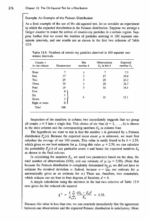
Chapter 1 2: The Chi-Squared Test for a Distribution
Example: An Example of the Poisson Distribution
As a final example of the use of the chi-squared test, let us consider an experiment
in which the expected distribution is the Poisson distribution. Suppose we arrange a
Geiger counter to count the arrival of cosmic-ray particles in a certain region. Sup-
pose further that we count the number of particles arriving in 100 separate one-
minute intervals, and our results are as shown in the first two columns of Table
12.9.
Table 1 2.9. Numbers of cosmic-ray particles observed in 100 separate one-
minute intervals.
Counts V Bin Obser\'ations Expected
in one minute Occurrences number k 0^ in bin A: number E/,
None 7 I 7 7.5
One 1.7 2 17 19.4
Two 29 3 29 25.2
Three 20 4 20 21.7
Four 16 5 16 14.1
Five 8^
Six
Seven
1
2• 6 11 12.1
Eight or more 0.
Total ioo
Inspection of the numbers in column two immediately suggests that we group
aU counts 5 into a single bin. This choice of six bins (A: = 1, . .. , 6) is shown
in the third column and the corresponding numbers in column four.
The hypothesis we want to test is that the number p is governed by a Poisson
distribution Pfjiv). Because the expected mean count fi is unknown, we must first
calculate the average of our 100 counts. This value is easily found to be P = 2.59,
which gives us our best estimate for fi. Using this value (i ~ 2.59, we can calculate
the probability P^{p) of any particular count v and hence the expected numbers
as shown in the final column.
In calculating the numbers E^, we used two parameters based on the data, the
total number of observations (100), and our estimate of /a (/x = 2.59). (Note that
because the Poisson distribution is completely determined by /x, we did not have to
estimate the standard deviation cr. Indeed, because a = yji, our estimate for /x
automatically gives us an estimate for cr.) There are, therefore, two constraints,
which reduces our six bins to four degrees of freedom, d ~ 4.
A simple calculation using the numbers in the last two columns of Table 12.9
now gives for the reduced chi squared
= -.2 ^2lZ_E£ = 0.35.
Because this value is less than one, we can conclude immediately that the agreement
between our observations and the expected Poisson distribution is satisfactory. More

Principal Definitions and Equations of Chapter 12
Specifically, we see from the table in Appendix D that a value of ^ ^ as large as 0,35
is very probable; in fact
Prob^iX^ ^ 0.35) ^ 85%.
Thus, our experiment gives us absolutely no reason to doubt the expected Poisson
distribution.
The value of = 0.35 found in this experiment is actually appreciably less
than one, indicating that our observations fit the Poisson distribution very weil This
small value does no% however, give stronger evidence that our measurements are
governed by the expected distribution than would a value x'^'=^\. If the results
really are governed by the expected distribution, and if we were to repeat our series
of measurements many times, we would expect many different values of x fluctu-
ating about the average value one. Thus, if the measurements are governed by the
expected distribution, a value of - 0.35 is just the result of a large chance fluc-
tuation away from the expected mean value. In no way does it give extra weight to
our conclusion that our measurements do seem to follow the expected distribution.
If you have followed these three examples, you should have no difficulty
applying the chi-squared test to any problems likely to be found in an elementary
physics hiboratory. Several further examples are included in the problems below.
You should certainly test your understanding by trying some of them.
Principal Definitions and Equations of Chapter 1
2
DEFINITION OF CHI SQUARED
If we make n measurements for which we know, or can calculate, the expected
values and the standard deviations, then we define x^ as
2 ~ V /observed value — expected valuey^
1 V standard deviation / [See 12.11)]
In the experiments considered in this chapter, the n measurements were the numbers,
Oj, . .. , 0„. of times that the value of some quantity x was observed in each of n
bins. In this case, the expected number E^^ is determined by the assumed distribu-
tion of X, and the standard deviation is just V^E^; therefore,
ifi [See (12.7)]
If the assumed distribution of x is correct, then x^ should be of order «. If
X^ » «, the assumed distribution is probably incorrect.

Ch^ter 12: The Chi>Squared Test for a DtstrilHition
DEGREES OF FREEDOM AND REDUCED CHI SQUARED
If we were to repeat the whole experiment many dmes, the mean value of
should be equal to 4 the number of degrees offreedom, defined as
d = n ~ c,
where c is the number of constraints, the number of parameters that had to be
calculated from the data to compute x^-
The reduced is defined as
- X^/d. [See (12.16)]
If the assumed dislribution is correct, should be of order 1; if » 1, the data
do not fit the assumed distribution satisfactorily.
PROBABILITIES FOR CHI SQUARED
Suppose you obtain the value Xo^ for the reduced chi squared in an experiment.
If Xn~ appreciably greater than one, you have reason to doubt the distribution on
which your expected vaiues were based. From the table in Appendix D, you can
find the probability,
Prob,(x^^Xo^),
of getting a value x ^ large as x^,^, assuming the expected distribution is correct.
If this probability is small, you have reason to reject the expected distribution; if it
is less than 5%, you would reject the assumed distribution at the 5%, or significant,
level; if the probability is less than 1%, you would reject the distribution at the 1%,
or highly significant, level.
Problems for Chapter 1
2
For Section 12.1: Inmsducdon to Chi Squared
12,1. * Each member of a class of 50 students is given a piece of the same metal
(or what is said to be the same metal) and told to find its density p. From the 50
results, the mean p and standard deviation o-p are calculated, and the class decides
to test whether the results are normally distributed. To this end, the measurements
are grouped into four bins with boundaries at p - cr^^ p, and p + cr^, and the
results are shown in Table 12.10.
Tat^ 12.10. Observed densities of 50 pieces of metal
arranged in four bins; for Problem 12.1.
Bin number k Range of bin Observed number 0^
1 less than p — <Tp 12
2 between p — Op and p 13
3 between p and p + <Tp 11
4 more than p 14

Problems for Chapter 12
Assuming the measurements were normaUy distributed, with center p and width
CTp, calculate the expected number of measurements E,^ in each bin. Hence, calculate
X^. Do the measurements seem to be normally distributed?
12.2. Problem 4.13 reported 30 measurements of a lime t, with mean ? = 8.15
sec and standard deviation ^ 0.04 sec. Group the values of l into four bins with
boundaries at f — o-^, and f + cr^, and count the observed number in each bin
A' — 1, 2, 3, 4. Assuming the measurements were normally distributed with center at
t and width 07, find the expected number E^. in each bin. Calculate x^- Is there any
reason to doubt the measurements are normally distributed?
For Section i 2.2: General Definition of Chi Squared
12.3. -k A gambler decides to test a die by throwing it 240 times. Each throw has
six possible outcomes, A: ~ 1, 2, . . . , 6, where k is the face showing, and the
distribution of his throws is as shown in Table 12.11. If you treat each possible
Table 12.11. Number of occurrences of each face showing on
a die thrown 240 times; for Problem 12.3.
Face showing k: 1 2 3 4 5 6
Occurrences O^: 20 46 35 45 42 52
result k as a separate bin, what is the expected number E,. in each bin, assuming
that the die is true? Compute x'^. Does the die seem likely to be loaded?
12.4. *T*r I throw three dice together a total of 400 times, record the number of
sixes in each throw, and obtain the results shown in Table 12,12. Assuming the dice
Table MAI, Number of occurrences for each result
for three dice thrown together 400 times; for Problem
12.4.
Resuh Bin number k Occurrences 0^
No sixes 1 217
One six 2 148
Two or three sixes 3 35
are true, use the binomial distribution to find the expected number Ef^ for each of
the three bins and then calculate x^- Do I have reason to suspect the dice are
loaded?
12.5. As a radioactive specimen decays, its activity decreases exponentially as
the number of radioactive atoms diminishes. Some radioactive species have mean
lives in the millions, and even billions, of years, and for such species the exponential
decay of activity is not readily apparent. On the other hand, many species have
mean lives of minutes or hours, and for such species the exponential decay is easily
observed. The following problem illustrates this latter case.

Chapter i 2: l^ve Chi-Squared Test for a Distribution
A student wants to verify the exponential decay law for a raateriai with a known
mean life of r. Starling at lime / - 0, she counts the decays from a sample in
successive intervals of length 7'; thai is, she establishes bins with 0 < / < T, and
T < t< IT, and so on, and she counts the number of decays in each bin. (a) Ac-
cording to the exponential decay law, the number of radioactive atoms that remain
after lime t is N{t) = iV^e"'^^, where A^^ the number of atoms at t ~ 0. Deduce
that the number of decays expected in the kih time bin {{k ~ 1)T <t< kT\ is
E,, - A^(e^'"""l)e-^^^^ (12.19)
(b) For convenience, the student chooses her lime interval 7' equal to the known
value of r, and she gets the results shown in Table 12.13. What are the expected
TaMe 12.13. Observed number of decays in successive
time intervals of a radioactive sample. Note that all
decays that occurred after t~ AT have been included in
a single bin; for Problem 12.5.
Bin number k Time interval Observed decays O,^
1 0 < t < T 528
2 T t < 2T 180
3 IT < t < 3T 71
4 3T < t < 4T 20
5 AT < t 16
numbers f'^, according to (12.19), and what is her value for x'^'^ Are her results
consistent with the exponential decay law? (Note that the initial number Nq is easily
found from the data, because it must be equal to the total number of decays after
f = 0.)
For Section 1 2.3: Degrees of Freedom and Reduced Chi Squared
12.6. if (a) For the experiment of Problem 12.1, find the number of constraints c
and the number of degrees of freedom d, (b) Suppose now that the accepted value
Pace of density was known and that the studenis decided to test the hypothesis
that the results were governed by a normal distribution centered on pa^c- For this
test, how many constraints would there be, and how many degrees of freedom?
12.7. For each of Problems 12.2 to 12.4, find the number of constraints c and
the number of degrees of freedom d.
For Sections 1 2.4 and 1 2.5: Probabilities for Chi Squared and Examples
12.8. If we observe the distribution of results in some experiment and know the
expected distribution, we can calculate the observed Xo^ probability
ProbJj(^ ^ Xo^)' th*s prc^ability is less than 5%, we can then reject the expected
distribution at the 5% level. For example, with two degrees of freedom (d ~ 2),

Problems for Chapter ! 2
any value of Xo greater than 3.0 would justify rejection of the expected distribution
at the 5% level; that is, for d~2, ~ 3.0 is the critical value above which wecan reject Ihe distribution at the 5% level. Use the probabilities in Appendix D to
malce a table of the corresponding critical values (5% level) of Xq-> fof <i = 1, 2, 3,
4, 5, 10, 15, 20, 30.
12.9. As in Problem 12.8, make a table of the critical values of Xo for rejection
of the expected distribution, but this time at the 1% level, for ~ 1, 2, 3, 4, 5, 10,
15, 20, 30.
12.10. For the data of Problem 12.1, compute x~- the measurements were
normally distributed, what was the probability of getting a value of x^ this large or
larger? At the 5% significance level, can you reject the hypothesis that the measure-
ments were normally distributed? At the \% level? (See Appendix D for the needed
probabilities.)
12.11. ** In Problem 12.3, find the value of x^. Can we conclude that the die
was loaded at the 5% significance level? At the 1% level? (See Appendix D for the
necessary probabilities.)
12.12. In Problem 12.4, find the value of x!^. If the dice really are true, what
is the probability of getting a value of this large or larger? Explain whether the
evidence suggests the dice are loaded. (See Appendix D for the necessary probabili-
ties.)
12.13. Calculate x^ for the data of Problem 11.5, assuming the observations
should follow the Poisson distribution with mean count yit~ 3. (Group all values
into a single bin.) How many degrees of freedom are there? (Don't forget
that /X was given in advance and didn't have to be calculated from the data.) What
is x^l Are the data consistent with the expected Poisson distribution?
12.14. The chi-squared test can be used to test how well a set of measure-
ments (x,-, of two variables fits an expected relation y ~ /(x), provided the uncer-
tainties are known reliably. Suppose y and x are expected to satisfy a linear relation
(For instance, y might be the length of a metal rod and x its temperature.) Suppose
that A and B are predicted theoretically to be A — 50 and B ~ 6, and that five
measurements have produced the values shown in Table 12.14. The uncertainty in
y fix) A + Bx, (12.20)
Table 12.14. Five measurements of two variables
expected to fit the relation y^A +Bx; for Problem
12.14.
X (no uncertainty):
y (all ± 4): 60
2
56
3
71
4
66
5
86
the measurements of x is negligible; all the measurements of y have the same stan-
dard deviation, which is known to be o- = 4.

Chapter ! 2: The Oii-Squared Test for a Distribution
(a) Make a table of the oteerved and expected vaiues of y^-, and calculate as
(b) Because no parameters were calculated from the data, there are no con-
straints and hence five degrees of freedom. Calculate and use Appendix D to
find the probability of obtaining a value of this large, assuming y does satisfy
(12.20). At the 5% level, would you reject the expected relation (12.20)? (Note that
if the constants A and B were not known in advance, you would have to calculate
them from the data by the method of least squares. You would then proceed as
before, except that there would now be two constraints and only three degrees of
freedom.)
12.15. ifkic Two dice are thrown together 360 times, and the total score is re-
corded for each throw. The possible totals are 2, 3, ... , 12, and their numbers of
occurrences are as shown in Table 12.15. (a) Calculate the probabilities for each
Table 1 2. 1 5. Observed occurrences of total scores for two dice thrown together 360
times; for Problem 12.15.
Tola! score: 2 3 4 5 6 7 8 9 10 11 12
Occurrences: 6 14 23 35 57 50 44 49 39 27 16
total and hence the expected number of occurrences (assuming the dice are true).
(b) Calculate ^"^^ ~A'^/'^- Assuming the dice are true, what is the
probability of getting a value of this large or larger? (d) At the 5% level of
significance, can you reject the hypothesis that the dice are true? At the 1% level?
12.16. -k-k-k A certain long-lived radioactive sample is alleged to produce an aver-
age of 2 decays per minute. To check this claim, a student counts the numbers of
decays in 40 separate one-minute intervals and obtains the results shown in Table
12.16. (The mean life is so long that any depletion of the sample is negligible over
Table 12.16, Observed number of decays in one-minute intervals of a
radioactive sample; for Problem 12.16.
Number of decays v. 0 1 2 3 4 5 or more
Times observed: 11 12 I I 4 2 0
the course of all these measurements.) (a) If the Poisson distribution that governs
the decays really does have fi- 2, what numbers should the student expect to
have found? (Group all observations with 3 into a single bin.) Calculate
and = x^^d- (Don't forget that /x was not calculated from the data.) At the 5%significance level, would you reject the hypothesis that the sample follows the Pois-
son distribution with ju, = 2? (b) Ttie student noti(%s that the actual mean of his
results is P= 1.35, and he therefore decides to test whether the data fit a Poisson
distribution with /i = 1.35. In this case, what are d and ^^? Are the data consistent
with this new hypothesis?

Problems for Chapter t2
12.17. Chapter 10 described a test for fit to the binomial distribution. Weconsidered n trials, each with two possible outcomes: "success" (with probability p)
and "failure" (with probability 1 - p). We then tested whether the observ^ed number
of successes, was compalibie with some assumed value of p. Provided the num-
bers involved are reasonably large, we can also treat this same problem with the
chi-squared test, with just two bins
—
k — 1 for successes and k — 2 for failures—and one degree of freedom. In the following problem, you will use both methods
and compare results. When the numbers are large, you will find the agreement is
excellent; when they are small, it is less so but still good enough that chi squared
is a useful indicator.
(a) A soup manufacturer believes he can introduce a different dumpling into
his chicken dumpling soup without noticeably affecting the flavor. To test this hy-
pothesis, he makes 16 cans labeled "Style that contain the old dumpling and 16
cans labeled "Style y" that contain the new dumpling. He sends one of each type
to 16 tasters and asks them which they prefer. If his hypothesis is correct, we should
expect eight tasters to prefer X and eight to prefer Y. In the actual test, the number
who favored X was v = 11. Calculate probability of getting a value this
large or larger. Does the test indicate a significant difference between the two kinds
of dumpling? Now, calculate the corresponding probability exactly, using the bino-
mial distribution, and compare your results. (Note that the chi-squared test includes
deviations away from the expected numbers in both directions. Therefore, for this
comparison you should calculate the two-tailed probability for values of v that devi-
ate from 8 by 3 or more in either direction; that is, = 11, 12, . . . , 16 and v~ 5,
4, . . . , 1.)
(b) Repeat part (a) for the next test, in which the manufacturer makes 400 cans
of each style and the number of tasters who prefer X is 225. (In calculating the
binomial probabilities, use the Gaussian approximation.)
(c) In part (a), the numbers were small enough that the chi-squared test was
fairly crude. (It gave a probability of 13%, compared with the correct value of 21%.)
With one degree of freedom, you can improve on the chi-squared test by using an
adjusted chi-squared, defined as
(adjusted x') = i
Calculate the adjusted for the data of part (a) and show that the use of this value,
instead of the ordinary in the table of Appendix D gives a more accurate value
of the probability.-^
•'We have not justified the use of the adjusted chi squared here, but this example does iilustrate its superior-
ity. For more details, see H. L. Alder and E. B. Roessler, Introduction to Probability and Statistics, 6th ed.
(W. H. Freeman, 1977), p. 263.


Appendixes

Appendix A
Norma! Error Integral, I
If the measurement of a continuous variable x is subject to many small errors, all
of them random, the expected distribution of results is given by the normal, or
Gauss, distribution,
where X is the true value of x, and a is the standard deviation.
The integral of the normal distribution function, J* Gx^J^x)dx^ is called the nor-
mal error integral, and is the probability that a measurement falls between x~ a
and x~b^
ProHa^x^b) - Tg;,,^.Ja
'x)dx.
Table A shows this integral fox a=X — t(T and b=X-^ ta. This gives the probabil-
ity of a measurement within t standard deviations on either side of X,
Prof>(within fa) = Prob(X ~~ tcr^ x ^X + to)
JrX+ur Jrt
Jx) dx ~ —=I
dz.
This function is sometimes denoted erf(/), but this notation is also used for a slightly
different function.
The probability of a measurement outside the same interval can be found by
subtraction;
jProi<outside to) = 100% - Pro^within tcr).
For further discussions, see Section 5.4 and Appendix B.

Appendix A: Norma! Error Integra!, I
Table A. The percentage probability,
Prob(withm ta) ~ \^x^%Ox^Xx)dx,
as a function of t,X tv X X-^tfj
t 0.00 0.01 0.02 0.03 0.04 0.05 0.06 0.07 0.08 0.09
0.0 0.00 0.80 1.60 2.39 3.19 3.99 4.78 J..Do 6.38 7.17
0.1 7.97 8.76 9.55 10.34 11.13 11.92 12.71 1 1IJ .50 14.28 15.07
0.2 15.85 16.63 17.41 18.19 18.97 19.74 20.51 .Z.O 22.05 22.82
0.3 23.58 24.34 25.10 25.86 26.61 27.37 28.12 28,.86 29.61 30.35
0.4 31.08 31.82 32.55 33.28 34.01 34.73 35.45 36.16 36.88 37.59
0.5 38.29 38.99 39.69 40.39 41.08 41.77 42.45 4J..1
J
43.81 44.48
0.6 45.15 45.81 46.47 47.13 47.78 48.43 49.07 '71 50.35 50.98
0.7 51.61 52.23 52.85 53.46 54.07 54.67 55.27 JJ..O / 56.46 57.05
0.8 57.63 58.21 58.78 59.35 59.91 60.47 61.02 61 .57 62.11 62.65
0.9 63.19 63.72 64.24 64.76 65.28 65.79 66.29 66.80 67.29 67.78
1.0 68.27 68.75 69.23 69.70 70.17 70.63 71.09 I 1
,
71.99 72.43
1.1 72.87 73.30 73.73 74.15 74.57 74.99 75.40 ID.on,oU 76.20 76.60
1.2 76.99 77.37 77.75 78.13 78.50 78.87 79.23 TO 79.95 80.29
1.3 80.64 80.98 81.32 81.65 81.98 82.30 82.62 82.,93 83.24 83.55
1.4 83.85 84.15 §4.44 84.73 85.01 85.29 85.57 85..84 86.11 86.38
1.5 86.64 86.90 87.15 87.40 87.64 87.89 88.12 ciiS..JO 88.59 88.82
1.6 89.04 89.26 89.48 89.69 89.90 90.11 90.31 onyu..31 90.70 90.90
1.7 91.09 91.27 91.46 91.64 91.81 91.99 92.16 .3J 92.49 92.65
1.8 92.81 92.97 93.12 93.28 93.42 93.57 93.71 93,,85 93.99 94.12
1.9 94.26 94.39 94.51 94.64 94.76 94.88 95.00 95..12 95.23 95.34
2.0 95.45 95.56 95.66 95.76 95.86 95.96 96.06 96..15 96.25 96.34
2.1 96.43 96.51 96.60 96.68 96.76 96.84 96.92 97..00 97.07 97.15
2.2 97.22 97.29 97.36 97.43 97.49 97.56 97,62 97..68 97.74 97,80
2.3 97.86 97.91 97.97 98,02 98.07 98.12 98.17 98..22 98.27 98.32
2.4 98.36 98.40 98.45 98.49 98.53 98.57 98.61 98..65 98.69 98.72
2.5 98.76 98.79 98.83 98.86 98.89 98.92 98.95 98,.98 99.01 99.04
2.6 99.07 99.09 99.12 99.15 99.17 99.20 99.22 99..24 99.26 99.29
2.7 99.31 99.33 99.35 99.37 99.39 99.40 99.42 99.,44 99.46 99.47
2.8 99.49 99.50 99.52 99.53 99.55 99.56 99.58 99.,59 99.60 99.61
2.9 99.63 99.64 99.65 99.66 99.67 99.68 99.69 99,.70 99.71 99.72
3.0 99.73
3.5 99.95
4.0 99.994
4.5 99.9993
5.0 99.99994

Appendix B
Norma! Error Integral, II
In certain calculations, a convenient form of the normal error integral is
Jrx+ta
X
(This integral is, of course, just half the integral tabulated in Appendix A.) The
probability Prob(a ^ b) of a measurement in any interval a b can be
found from Q(t) by a single subtraction or addition. For example,
Prob{X + a^x^X + 2(r) = Q{2) - Q(l).
X X+cf X+la
Similarly,
Pwb{X-2cr^x^X-^(T) = Q{2) + Q(l).
X"2(T X X+(T
The probability of a measurement greater than any X + ta is just 0.5 — Q(t).
For example,
Prob(x^X + o) = 50% - Q{1).
X X+a-

Appendix B: Normal Error integral, H 289
Table B. The percentage probability,
Q(t) = lx^'''Gx^Jx)dx,
as a function of t X+ta
0.00 0.01 0.02 0.03 0.04 0.05 0.06 0.07 0.08 0.09
0.0 0.00
0.1 3.98
0.2 7.93
0.3 11.79
0.4 15.54
0.5 19.15
0.6 22.57
0.7 25.80
0.8 28.81
o.y ji.Dy
1.0 34.13
1.1 36.43
1.2 38.49
1.3 40.32
1 A1.4 41.VZ
1.5 43.32
1.6 44.52
1.7 45.54
1.8 46.41
/IT 1 14 /.Li
2.0 47.72
2.1 48.21
2.2 48.61
2.3 48.93
2.4 49.18
2.5 49.38
2.6 49.53
2.7 49.65
2.8 49.74
2.9 49.81
3.0 49.87
3.5 49.98
4.0 49.997
4.5 49.9997
5.0 49.99997
4.38
8.32
12.17
15.91
19.50
22.91
26.11
29.10
31.86
34.38
36.65
38.69
40.49
42.07
43.45
44.63
45.64
46.49
47.19
47.78
48.26
48.64
48.96
49.20
49.40
49.55
49.66
49.75
49.82
0.80 1.20 1.60 1.99 2.39 2.79 3.19 3.59
4.78 5.17 5.57 5.96 6.36 6.75 7.14 7.53
8.71 9.10 9.48 9.87 10.26 10.64 11.03 11.41
12.55 12.93 13.31 13.68 14.06 14.43 14.80 15.17
16.28 16,64 17.00 17.36 17.72 18.08 18.44 18.79
19.85 20.19 20.54 20.88 21.23 21.57 21.90 22.24
23.24 23.57 23.89 24.22 24.54 24.86 25.17 25.49
26.42 26.73 27.04 27.34 27.64 27.94 28.23 28.52
29.39 29.67 29.95 30.23 30.51 30.78 31.06 31.33
32.12 32.38 32.64 32.89 33.15 33.40 33.65 33.89
34.61 34.85 35.08 35.31 35.54 35.77 35.99 36.21
36.86 37.08 37.29 37.49 37.70 37.90 38.10 38.30
38.88 39.07 39.25 39.44 39.62 39.80 39.97 40.15
40.66 40.82 40.99 41.15 41.31 41.47 41,62 41.77
42.22 42.36 42.51 42.65 42.79 42.92 43.06 43.19
43.57 43.70 43.82 43.94 44.06 44.18 44.29 44.41
44.74 44.84 44.95 45.05 45.15 45.25 45.35 45.45
45.73 45.82 45.91 45.99 46.08 46.16 46.25 46.33
46.56 46.64 46.71 46.78 46.86 46.93 46.99 47.06
47.26 47.32 47.38 47.44 47.50 47.56 47.61 47.67
47.83 47.88 47.93 47.98 48.03 48.08 48.12 48.17
48.30 48.34 48.38 48.42 48.46 48.50 48,54 48.57
48.68 48.71 48.75 48.78 48.81 48.84 48.87 48.90
49.98 49.01 49.04 49.06 49.09 49.11 49.13 49.16
49.22 49.25 49.27 49.29 49.31 49.32 49.34 49.36
49.41 49.43 49.45 49.46 49.48 49.49 49.51 49.52
49.56 49.57 49.59 49.60 49.61 49.62 49.63 49.64
49.67 49.68 49,69 49.70 49.71 49.72 49.73 49,74
49.76 49.77 49.77 49.78 49.79 49.79 49.80 49.81
49.82 49.83 49.84 49.84 49.85 49.85 49.86 49.86

Appendix C
Probabilities for Correlation Coefficients
The extent to whichN points (x^, y^), . .. , (jc^, y^y) fit a straight line is indicated by
the linear correlation coefficient
^ ^ l(x, - x){y, - v)
which always lies in the interval ~1 ^ r ^ 1. Values of r close to ± 1 indicate a
good linear correlation; values close to 0 indicate little or no correlation.
A more quantitative measure of the fit can be found by using Table C. For any
given observed value r^,, Probf,4}r\ ^ is the probability that N measurements of
two uncorrelated variables would give a coefficient r as large as r^. Thus, if we
obtain a coefficient r^, for which Probj^i^r\ ^ is small, it is correspondingly
unlikely that our variables are uncorrelated; that is, a correlation is indicated. In
particular, if Prob}^r\ ^ \rj^ ^ 5%, the correlation is called significant; if it is less
than 1%, the correlation is called highly significant.
For example, the probability that 20 measurements (A^ = 20) of two uncorre-
lated variables would yield jrj ^ 0.5 is given in the table as 2.5%. Thus, if 20 mea-
surements gave / == 0.5, we would have significant evidence of a linear correlation
between the two variables. For further discussion, see Sections 9.3 to 9.5.
The values in Table C were calculated from the integral
Prob^{\T\ ^ |rj) = ^^^^ " ^^^^^(1 - r^f^'^'y^dr.
V7rr[(iV ~ 2)/2] -'kol
See, for example, E. M. Pugh and G. H. Winsiow, The Analysis of Physical Mea-
surements (Addison-Wesley, 1966), Section 12-8.

Appendix C: Probabiltties for Correlation Coefficients 291
Table C, The percentage probability Prob^{\r\ ^ r^) that N measurements of two
uncorreiated variables give a correlation coefficient with |r| ^ r^, as a function ofNand Tq, (Blanks indicate probabilities less than 0.05%.)
ly 0u ft 1 ft ? ft '\ ft d ft sU.J 0 fi ft 7 ft s ft Q 1±
3 100 94 87 81 74 67 59 51 41 29 0
4 100 90 80 70 60 50 40 30 20 10 0
5 100 87 75 62 50 39 28 19 10 3.7 0
6 100 85 70 56 43 31 21 12 5.6 1.4 0
7 100 83 67 51 37 25 15 8.0 3.1 0.6 0
8 100 81 63 47 33 21 12 5.3 1.7 0.2 0
9 100 80 61 43 29 17 8.8 3.6 1.0 0.1 0
10 100 78 58 40 25 14 6.7 2.4 0.5 0
11 100 77 56 37 22 12 5.1 1.6 0.3 0
12 100 76 53 34 20 9.8 3.9 1.1 0.2 0
13 100 75 51 32 18 8.2 3.0 0.8 0.1 0
14 100 73 49 30 16 6.9 2.3 0.5 0.1 0
15 100 yy 47 28 14 5.8 1.8 0.4 0
16 100 71 46 26 12 4.9 1.4 0.3 0
17 100 70 44 24 11 4.1 1.1 0.2 0
18 100 69 43 23 10 3.5 0.8 0.1 0
19 100 68 41 21 9.0 2.9 0.7 0.1 0
20 100 67 40 20 8.1 2.5 0.5 0.1 0
ZD inn oj 1LD d R't.O 1 1 ft 9 ft
30 100 60 29 11 2.9 0.5 0
35 100 57 25 8.0 1.7 0.2 0
40 too 54 22 6.0 1.1 0.1 0
45 100 51 19 4.5 0.6 0
0 0.05 0.1 0.15 0.2 0.25 0.3 0.35 0.4 0.45
50 100 73 49 30 16 8.0 3.4 1.3 0.4 0.1
60 100 70 45 25 13 5.4 2.0 0.6 0.2
70 100 68 41 9.7 3.7 1.2 0.3 0.1
80 100 66 38 18 7.5 2.5 0.7 0.1
90 100 64 35 16 5.9 1.7 0.4 0.1
100 100 62 32 14 4.6 1.2 0.2

Appendix D
Probabilities for Chi Squared
If a series of measurements is grouped into bins /r 1, we denote by
the number of measurements observed in the bin k. The number expected (on the
basis of some assumed or expected distribution) in the bin k is denoted by The
extent to which the observations fit the assumed distribution is indicated by the
reduced chi squared, x ^ defined as
where d is the number of degrees of freedom, d ~ n — c, and c is the number of
constraints (see Section 12.3). The expected average value of ^ is 1, If ^ ^ » 1,
the observed results do not fit the assumed distribution; if ^ ^ ^ 1, the agreement
is satisfactory.
This test is made quantitative with the probabilities shown in Table D. Let
denote the value of ^ ^ actually obtained in an experiment with d degrees of free-
dom. The number ProbJ^x ^ ^ -^o"^) the probability of obtaining a veilue of ^as large as the observed xJ"-) measurements really did follow the assumed
distribution. Thus, if ProbJJ( ^ > Xo") ^ l^g^? observed and expected distribu-
tions are consistent; if it is small, they probably disagree. In particular, if Proba{x ^
^ X^ is less than 5%, we say the disagreement is significant and reject the
assumed distribution at the 5% level. If it is less than 1%, the disagreement is called
highly significant, and we reject the assumed distribution at the 1% level.
For example, suppose we obtain a reduced chi squared of 2.6 (that is,
X^ — 2.6) in an experiment with six degrees of freedom {d = 6). According to
Table D, the probability of getting ^ ^ ^ 2.6 is 1.6%, if the measurements were
governed by the ^umed distribution. Thus, at the 5% level (but not quite at the
1% level), we would reject the assumed distribution. For further discussion, see
Chapter 12.

Appendix D: Probabilities for Chi Squared
Table D. The percentage probability Prob^ix ^ ^ Xo^) of obtaining a value of
Xq'^ an experiment with d degrees of freedom, as a function of d and Xq'^-
(Blanks indicate probabilities less than 0.05%.)
d 0 0.5 1.0 1.5 2.0 2.5 3.0 3.5 4.0 4.5 5.0 5.5 6.0 8.0 10.0
1 100 48 32 22 16 11 8.3 6.1 4.6 3.4 2.5 1.9 1.4 0.5 0.2
2 100 61 37 22 14 8.2 5.0 3.0 1.8 1.1 0.7 0.4 0.2
3 100 68 39 21 11 5.8 2.9 1.5 0.7 0.4 0.2 0.1
4 100 74 41 20 9.2 4.0 1.7 0.7 0.3 0.1 0.1
5 100 78 42 19 7.5 2.9 1.0 0.4 0.1
0 0.2 0.4 0.6 0.8 1.0 1.2 1.4 1.6 1.8 2.0 2.2 2.4 2.6 2.8 3.0
1 100 65 53 44 37 32 27 24 21 18 16 14 12 11 9.4 8.3
2 100 82 67 55 45 37 30 25 20 17 14 11 9.1 7.4 6.1 5.0
3 100 90 75 61 49 39 31 24 19 14 11 8.6 6.6 5.0 3.8 2.9
A 1 AniUU y4 01ol DO dZ A 141 31 Zd 1 / 13 y.z 0.0 A C4.0 1 A3.4 ZA I. /
<;J lUU vo TA/U DD An42 11 zz io 1
1
11 1 .J<: 1r>. i 3.3 Z.3 1 Ai.O 1 nI.U
6 100 98 88 73 57 42 30 21 14 9.5 6.2 4.0 2.5 1.6 1.0 0.6
7 100 99 90 76 59 43 30 20 13 8.2 5.1 3.1 1.9 1.1 0.7 0.4
8 100 99 92 78 60 43 29 19 12 7.2 4.2 2.4 1.4 0.8 0.4 0.2
1AAIUU yy y4 QAoU OA A A44 Zy 1
1
11 0.3 3.CI1 Qi.y 1 Ai.U A CU.3 A 1U.3 A 1U.l
f fxiU 1AAIUU inAIUU yj 03 AA44 1 1i /
iniU z.y 1 ^1.3 A QU.O n AU.4 A TU.Z n 1U.I
11 100 100 96 83 64 44 28 16 9.1 4.8 2.4 1.2 0.6 0.3 0.1 0.1
12 100 100 96 84 65 45 28 16 8.4 4.2 2.0 0.9 0.4 0.2 0.1
13 100 100 97 86 66 45 27 15 7.7 3.7 1.7 0.7 0.3 0.1 0.1
1
A
1 AAiUU 1 AAiUU Qfiyo Of 0/ A^i43 1 A14 T 1 3.3 1 A1.4 AU.O A '>u.z A 1U.I
1 AAIUU 1 AnIUU yo Do A<Z43 na 1 A14 O.J 1 TI.Z A ^U.3 A TU.Z A 1U.l
16 100 100 98 89 69 45 26 13 6.0 2.5 1.0 0.4 0.1
17 100 100 99 90 70 45 25 12 5.5 2.2 0.8 0.3 0.1
18 100 100 99 90 70 46 25 12 5.1 2.0 0.7 0.2 0.1
19 100 100 99 91 71 46 25 11 4.7 1.7 0.6 0.2 0.1
20 100 100 99 92 72 46 24 11 4.3 1.5 0.5 0.1
22 100 100 99 93 73 46 23 10 3.7 1.2 0.4 0.1
24 100 100 100 94 74 46 23 9.2 3.2 0.9 0.3 0.1
26 100 100 100 95 75 46 22 8.5 2.7 0.7 0.2
28 100 100 100 95 76 46 21 7.8 2.3 0.6 0.1
30 100 100 100 96 77 47 21 7.2 2.0 0.5 0.1
The values in Table D were calculated from the integral
ProbAx-^X^) - -rr-? -| x^-^f-'^'^'^dx,d\\ Ac)2*2r(rf/2)4,.
See, for example, E. M. Pugh and G. H. Winslow, The Analysis of Physical Mea-
surements (Addison-Wesley, 1966), Section 12-5.

Appendix £
Two Proofs Concerning Sample Standard Deviations
In Chapter 5, 1 quoted without proof two important results concerning measurements
of a quantity x normally distributed with width a: (1) The best estimate of or based
on N measurements of x is the sample standard deviation, cr^, of the N measure-
ments, as defined by (5.45) with the factor of (A^ — 1) in the denominator. (2) The
fractional uncertainity in cr^ as an estimate of a is as in (5,46). The
proofs of these two results are surprisingly awkward and were omitted from Chapter
5. For those who like to see proofs, 1 give them here.
Consider an experiment that consists of N measurements (all using the same
method) of a quantity x, with the results
The sample standard deviation of these N measurements is defined by
2 _ ^(^( ~ ^)
N - 1
SS(El)N - r
where I have introducwi the notation SS for the Sian of Squares,
SS = Sum of Squares
= Tt^, -^= 2^W-^(lf4 (E2)
In writing the last line of (E2), I have used the identity (4,28) from Problem 4.5.
Equation (El) actually defines squared, which is called the sample variance of
the N measurements. To avoid numerous square root signs, I will work mostly with
the variance rather than the standard deviation itself.
Our proofs will be simplified by noting that neither the true width cr nor the
sample standard deviation cr^ is changed if we subtract any fixed constant from our
measured quantity x. In particular, we can subtract from x its true value X, which
gives a quantity normally distributed about a true value of zero. In other words, we
can (and will) assume that the true value of our measured quantity x isX ~ 0.

Appendix E: Two Proofs Concerning Sample Standard Deviations
To discuss our best estimate for o- and its uncertainty, we must imagine re-
peating our whole experiment an enormous ("infinite") number of times a ~ 1, 2,
3, .... In this way we generate an immense array of measurements, which we can
display as in Table El.
Tabie El. Results of a large number of experiments, a ~ 1, 2, 3, ... , each of
which consists of N measurements of a quantity x. The ith measurement in the ath
experiment is denoted by x^, and is shown in the ith column of the ath row.
Experiment
number
1st
measurement
2nd
measurement
ith
measurement
Nth
measurement
1
2
a ^a2 • • ^ai '
For each of the infinitely many experiments, we can calculate the mean and
variance. For example, for the ath experiment (or ath "sampling"), we find the
sample mean by adding all the numbers in the row of the ath experiment and
dividing by N. To find the corresponding sample variance, we compute the sum of
squares
N
and divide by (N — i). Here again, the sum runs over ail entries in the appropriate
row of data.
We use the usual symbol of a bar, as in x,^, to indicate an average over ail
measurements in one sample (that is, in one row of our data). We also need to
consider the average of ai! numbers in a given column of our data (that is, an
average over all a — 1, 2, 3, . . .), and we denote this kind of average by two
brackets (. .). For example, we denote by (x^i), or just <x>,-, the average of all the
measurements in the rth column. Because this value is the average of infinitely many
measurements of it equals the true value X, which we have arranged to be zero.
Thus,
<^), = X = 0.
Similarly, if we average the squares of all the values in any column, we will get the
true variance
{x^\ - (E3)
[Remember that X ~ 0, so that (a-), is the same as {(x — Xf)i, which is just o^.]
Armed with these ideas, we are ready for our two proofs.

introduction to Error Anal/sis
I Best Estimate for the Width cr
We want to show that, based on A' measurements of x, the best estimate for the true
width cr is the sample standard deviation of the N measurements. We do this by
proving the following proposition: If we calculate the sum of squares 5'5'„ for each
sample a and then average the sums over ail a = 1, 2, 3, . ..
, the result is (iV ~ 1)
times the true variance <t^:
{SS) = (iV - l)o^. (E4)
Dividing (E4) by (N ~ 1), we see the true variance is ~ {SS)/(N ~ 1), Here,
(SS) is the average of the sums of squares from infinitely many sets of N measure-
ments. This, in turn, means that the best estimate for based on a single set of JV
measurements is just SS/(N — 1), where SS is the sum of squares for that single set
of measurements. This is just the variance given in Equation (El), Thus, if we can
prove (E4), we will have established the desired result.
To prove Equation (E4), we start with the sum of squares SS^ for the ath
sample. Using (E2), we can write this sum as
^^a ™ 2) i^ad'^*~ S S ^ai^aj (E5)
This equation differs from (E2) only in that I have added the subscripts a and have
written out the square in the last term of (E2) as a product of two sums. The double
sum in (E5) consists of two parts: First, there are N terms with i = which can be
combined with the single sum in (E5). This leaves N{N ~ 1) terms with i 4^ j. Thus,
we can rewrite (E5) as
The expression (E6) is the sum of squares for a single sample a. To find {SS), wehave only to average (E6) over all values of a. Because the average of any sum
equals the sum of the corresponding averages, (E6) implies that
The N terms in the first sum are all the same, and each is equal to [as in (E3)].
Therefore, the first sum is Just Na^. With / ^ /, the terms of the double sum in (E7)
are all zero, {x^^x^j) ~ 0. (Remember that x is normally distributed about X ~ 0.
Thus, for each possible value of x^^, positive and negative values of x^j are equally
likely and cancel each other out.) Thus, the whole second sum is zero, and we are
left with
{SS} - (AT - l)o^,
which is precisely the result (E4) we needed to prove.

Appendix E; Two Proofs Concerning Sample Standard Deviations
2 Uncertainty In the Estimate for the Width or
We have shown that, based on N measurements of x, the best estimate for the true
variance cP- is the sample variance of the N measurements, as defined in (El),
SSI{N - 1). Therefore, the fractiona! uncertainty in (p- is the same as that in the
sum of squares SS:
(fractiona! uncertainty in estimate for a^) ~ (fractional uncertainty in SS). (E8)
Because cr is the square root of o-^, the fractional uncertainty in a is just half of
this:
(fractiona! uncertainty in estimate for tr)
~I
(fractional uncertainty in SS), (E9)
To find the uncertainty in SS, we use the result (1.1.7) that the uncertainty in
any quantity q is ^{q^) ~ {q}^, where, as usual, the brackets (. .) denote the average
of the quantity concerned after an infinite number of measurements. Therefore, the
uncertainty in the sum of squares SS is
(uncertainty in 5S) = V(SSV^^"CSS)^. (ElO)
We already know [Equation (E4)] that the second average in this square root is
{SS) = (N - so all that remains is to find the first term {SS~).
For any one set of N measurements, the sum of squares SS is given by (E6).
Squaring this expression, we find that (I omit a!! subscripts a to reduce the clutter)
- 2-^2. (^/)^2. Zj Xj^k (Ell)
1
j k¥^j m n^m
= A + 5 + C.
To find the average value of (Ell), we need to evaluate each of the three aver-
ages {A), {B), and <C). The double sum in A contains N terms with i — /, each of
which averages to (jc"*), and N{N ~1) terms with i ¥= j, each of which averages to
(a~)^. Because x is distributed normally about X ~ 0, (x^) = cr^ (as we already
knew), and a straightforward integration shows that (x*) ~ So-"*. Thus, the double
sum in A averages to 3Na^ + N{N - l)cr'* = N{N + 2)cr^, and
iV
Every term in the sum of B can easily be seen to contain an odd power of X/^ (either
Xf, or X/^^). Because x is normally distributed about 0, the average of any odd power

IntroducticMi to Error Anat^is
is zero, so
(B) - 0.
The quadruple sum in the term C contains N{N — 1) terms in which j ~ m and
k ^ n, each of which averages to {jp-Y — There is the same number of terms in
which ~ n and k = m, each of which also averages to a'^. Ml the remaining terms
contain an odd power of x and average to zero. Thus, the quadruple sum in Caverages to 2N(N — 1)(t\ and
<Q - a.
Adding together the last three equations and inserting the result into (Ell), we
conclude that
Inserting this result into (ElO) [and replacing (55) by (N - l)cr^], we find that
(uncertainty in 55) = ^{N^ - i) - {N - if = ^]2(N ~ 1) cr^.
If we divide through by (55) = {N — l)o^, this result implies that the fractional
uncertainty in 55 is ^l2/{N - 1). Finally, we know [from (E9)] that the fractional
uncertainty in our value of a is half of that in 55. So,
1
(fractional uncertainty in estimate for cr)
V2(iV " 1)'
which is the required result.

Bibliography
I have found the following books useful. They are arranged approximately according
to their mathematical level and the completeness of their coverage.
A beautifully clear introduction to statistical methods that contrives to use no
calculus is O, L. Lacy, Statistical Methods in Experimentation (Macmillan, 1953).
A more advanced book on statistics that is also very clear and uses no calculus
is H. L. Alder and E. B. Roessler, Introduction to Probability and Statistics, 6th ed.
(W. H. Freeman, 1977).
Four books at approximately the level of this book that cover many of the same
topics are:
D. C. Baird, Experimentation; An Introduction to Measurement Theory and Experi-
ment Design, 2nd ed. (Prentice Hall, 1988);
N. C. Barford, Experimental Measurements; Precision, Error, and Truth (Addison-
Wesley, 1967);
G. L. Squires, Practical Physics (Cambridge, 1985).
H. D. Young, Statistical Treatment of Experimental Data (McGraw-Hill, 1962).
Numerous further topics and derivations can be found in the following more
advanced books:
P. R. Bevington and K. D. Robinson, Data Reduction and Error Analysis for the
Physical Sciences (McGraw-Hill, 1992);
S. L. Meyer, Data Analysis for Scientists and Engineers (John Wiley, 1975);
E. M. Pugh and G. H. Winsiow, The Analysis of Physical Measurements (Addison-
Wesley, 1966),


ANSWERSto
Quick Checksand
Odd-Numbered Problems
Chapter 2
QUICK CHECKS
QC2.1. (a) 110 ± 2 mm. (b) between 3.02 and 3.08 amps.
QC2.2. (a) 8.12 ± 0.03 m/s. (b) 31,234 ± 2 m or (3.1234 ± 0.0002) X 10^ m.
(c) (5.68 ± 0.03) X 10-^ kg.
QC2.3. 43 ± 5 grams.
QC2.4. (a) 0.04 - 4%. (b) 0.1 - 10%. (c) 4.58 ± 0.09 J.
QC2.5. Percent uncertainties are 1% and 3%; area ~ 30 cm^ ± 4% = 30
± 1 cm-^.
PROBLEMS
2.1. 210 ± 5 cm; 36.0 ± 0.5 mm; 5.3 ± 0.1 V; 2.4 ± 0.1 s.
2.3. (a) 5.03 ± 0.04 m. (b) There is a strong case for retaining an extra digit and
quoting 1.5 ± 1 s, (c) (-3.2 ± 0.3) X lO"^'* C (d) (5.6 ± 0.7) X 10"^ m.
(e) (3.27 ± 0.04) X 10^ grams • cm/s.
2.5. Discrepancy = 2 mm, which is not significant.
c
140
135
130
Figure A 2.5.
2.7. (a) Probably the only reasonable conclusion at this stage is 1.9 ± 0.1 gram/
cm^. (b) The discrepancy is 0.05 gram/cm^; because this value is less than the
uncertainty, it is not significant.
2.9. Length, / = 93.5 ± 0.1 cm.

ANSWERS to Quick Checks and Odd-Numbered Problems
2.11. The column headed I - L' should read: 0.3 ± 0.9, -0.6 ± 1.5, -2.2
± 2 (which could be rounded to - 2 ± 2), 1 ± 4, 1 ± 4, - 4 ± 4. The dif-
ference L — V should theoretically be zero. In all cases but one, the measured
value of Z, — V is smaller than its uncertainty. In the one exceptional case
(- 2.2 ± 2), it is only slightly larger. Therefore, the observed values are con-
sistent with the expected value zero.
2.13. (Best estimate for M + m) — Mbest + '"best-'^^^^ largest probable value for
M 4- m is (A^bes! ^ "*besJ + + ^"0- ^^d the smallest probable value is
the same expression except for a minus sign. Therefore, the answer for
M + m is (Mjjest + ffibest) ± {8M + 5m).
2.15. The straight line shown in Figure A2.15 passes through the origin and
through, or close to, all error bars. Therefore, the data are consistent with Pbeing proportional to T.
2.17. The graph of P against / in Figure A2.17 looks as if it would fit a parabola,
but it is hard to be sure. The plot of P against clearly fits a straight line
through the origin and is, therefore, consistent with P being proportional to P.
/(amps) —* P
Figure A 2. 1 7.

Answers to Chapter 2
2.19. (a) In Figure A2, 19(a), which includes the origin, it is impossible to say
whether T varies with A, Figure A2. 19(b) has a much enlarged vertical scale
and clearly shows that T does vary with A. Obviously, the best choice of scale
for the purpose at hand must be considered carefully, (b) If either picture were
redrawn with error bars of 0.3s (up and down), there would be no evidence for
variation of T with A.
2.21. (a) 40%. (b) 4%. (c) 0.6%. (d) 6%.
2,23, For the meter stick, 5/ == 0.5 mm and 8111 ~ 2.5%, which is not precise
enough, for the microscope, 6/ ~ 0.05 mm and Sill ~ 0.25%, which is pre-
cise enough.
2.25. (a) The answers for Vf — Vi are 4.0 ± 0.3 cm/s and 0.6 ± 0.4 cm/s. (b)
The percent uncertainties are 8% and 70%.
2.27. (a) 6.1 ± 0.1, which has two significant figures, (b) 1.12 ± 0.02. This value
has three figures with at least some significance, (c) 9.1 ± 0.2, which has two
significant figures.
2,29. (a) q 2,700 N s, with an uncertainty of 10% or 270 (or approximately
300) N-s. (b) ^ = 12 ftTb, with an uncertainty of 10% or 1 ftTb.
2.31. (a) ^best= 10 X 20 =^ 200; (highest probable value of ^) = 11 X 21
^ 231; (lowest probable value of <?)== 9 X 19 = 171. The rule (2.28) gives
q ~ 200 ± 30, which agrees well, (b) (Highest probable value of q) = 18
X 35 630; (lowest probable value of ^) = 2 X 5 - 10. The rule (2.2S)
gives ^ = 200 ± 300 (that is, ^^^x = 500 and q^^^, ^ - 100). The reason
this result is so badly incorrect is that the rule (2.28) applies only when all
fractional uncertainties are small compared with 1. This condition (which is
usually met in practice) is not met here.

ANSWERS to Quick Checks and Odd-Numbered Problems
Chapter 3
QUICK CHECKS
QC3.1. (a) 33 ± 6. (b) 910 ± 30. {c} The percent uncertainty is 18% in part (a)
but only 3% in part (b). His patience in counting for a longer time has been
rewarded by a smaller fractional uncertainty.
QC3.2. Percent uncertainties in x, y, and z are 2.5%, 2%, and 2.5%. Hence,
q = 10.0 ± 7% - 10.0 ± 0,7.
QC3.3. 15.7 ± 0.3 cm.
QC3.4. The percent uncertainty in / is 1%; V == 8.0 cm^ ± 3% = 8.0 ± 0.2
cm^.
QC3.5. V ~ 195 mi; 8V ~ 1 ml if tlie uncertainties are independent and random,
and bV ~ 10 ml otherwise.
QC3.6. ^ = 230 ± 3; r - 500 ± 6.5% ^ 500 ± 30.
QC3.7. <? === 20 ± 2,
QC3.8. q = 10.0 ± 0.3.
QC3.9. ^ - 20 ± 6.
PROBLEMS
3.1. (a) 28 ± 5. (b) 310 ± 20. (c) The fractional uncertainty is 18% for A, 6%for B. B's absolute uncertainty is larger, but her patience has been rewarded
with a smaller fractional uncertainty.
3.3. The observation is that the number of cases in four years is 20 ± ^20 == 20
± 4.5. This value is consistent with the expected number 16, and there is no
significant evidence that the rate is abnormally high.
3.5. (and 3.19)
Problem 3.5 Problera 3.19
Straight sum Quadratic sum
(a) 3 ± 7 3 ± 5
(b) 40 ± 18 40 ± 13
(0 0.5 0.1 0.50 ± 0,07
(d) 300 ± 21 300 ± 12
3.7. (a) 35 ± 4 cm - 35 cm ± 10%. (b) 11 ± 4 cm = 11 ± 40%. (c) 36 ± 9
cm = 36 cm ± 25%. (d) 110 ± 40 grams -cm/s -110 grams -cm/s ± 30%.
3.9. c - 18.8 ± 0.3 cm; r = 3.00 ± 0.05 cm.
3.11. (a) 0.48 ± 0.02 s (or 4%). (b) 0.470 ± 0.005 s (or 1%). (c) No. In the first
place, the pendulum will eventually stop, unless it is driven. Even if it is
driven, other effects will eventually become important and thwart our quest for

Answers to Chapter 3
greater accuracy. For example, if we time for several hours, the reliability of
the stopwatch may become a limiting factor, and the period t may vary be-
cause of changing temperature, humidity, and other variables.
3.13. Volume = 34 ± 4 m^.
3.15. (a) Student A: 32 ± 6. (b) Student B: 790 ± 30. (c) A's rate is 16 ± 3
counts/min, and B's is 13.1 ± 0.5 counts/min. These two measurements are
compatible, but B has been rewarded with a smaller uncertainty.
3.17. Those cases in which the second uncertainty could be ignored are indicated
with an asterisk.
Uncertainty
Case Answer Quadratic sum Straight sum
a 9.3 0.7* 0.7*
b 7.9 0.7* 0.8
c 9.7 0.7* 0.9
d 7.5 0.8 1
3.19, See answer to Problem 3.5.
3.21. (a) i; ^ 0.847 ± 0.003 m/s. (b) p = 0.602 ± 0.003 kg-m/s.
3.23. L === 0.74 ± 0.03 kg-m^/s.
3.25. The rule (3.18) holds only if the uncertainties in the various factors are inde-
pendent. When we write x" as x X x, it is certainly not true that the two fac-
tors (x and a) are independent, and the rule (3.18) does not hold.
3.27, Refractive index, n - 1.52 ± 0.03.
3.29, (a) 6h/h ~ 0.1%. Because h is proportional to a fractional power of X, the
percent uncertainty in h is smaller than that in \. (b) The measure value of
6.644 X 10"^"^ J s has an uncertainty of 0.1%, or 0.007 X lO"^'' J s. The dis-
crepancy is 0.018 X 10 -^"^ and is more than twice the uncertainty. Therefore,
the result is somewhat unsatisfactory,
3.31. (a) sin{6) = 0.82 ± 0.02. [Don't forget that 86 must be expressed in radians
when using 8sm(d) = |cos(^l)|5a] (b) f^^^i= e^'"''\ Sf = fi^^^Sa, ef = 20
± 2. (c)/,,,, - in(«bestX 5/ - Sa/a^,^, ln(«) = 1.10 ± 0.03.
3.33. (a) q ^ -1.38 and 8q - 0.0791 ^ 0.08. (b) Sq = 0.0787 ^ 0.08. The two
methods agree to two significant figures.
3.35, (a) 30 ± 1. (b) 120 ± 30. (c) 2.0 ± 0.2.
3.37. (a) 0.08 ± 0.01 m/s". (b) This measurement does not agree at all well with
the predicted value 0.13 ± 0.01 m/s^.
3.39, (a) E = 0.247 ± 0.004 J. (b) E = 0.251 ± 0.003 J. (c) The margins of er-
ror for the two measurements overlap, and they are, therefore, consistent with
conservation of energy.

ANSWERS to Quick Checks and Odd-Numbered Probiems
3.41.
/ (deg) n SnIn dn
10 1.42 17% 0.2
20 1.52 9% 0.14
30 1.46 6% 0.09
50 1.58 3% 0.05
70 1.53 2% 0.03
Ali but one of the measurements straddle the given value, 1.50. The only ex-
ception is tor i ~ 50 deg (n = 1.58 ± 0.05), and even here the given value,
1.50, is only slightly outside the margins of error. Therefore, the measurements
are consistent with the given value.
As the angle / increases, the fractional uncertainty in n decreases; this de-
crease occurs mainly because the absolute uncertainties are constant, so the
fractional uncertainties decrease as the angles increase.
3.43. (a) 1 and 1. (fo) y and x. (c) 2xf and 3jc^/,
3.45. (a) lfq~xy, the two partial derivatives are y and x. The rule (3.47) gives
Sq = ^|f&FTl^^.
Dividing the equation by \q\ produces exactly the rule (3.18) for the fractional
uncertainty in xy. In a similar way, (3.48) gives
8q ^\y\Sx + \x\ 8y,
and, when divided by j^j, gives the rule (3.19) for the fractional uncertainty in
xy. (b) If ^ ™ xf^y", then, after division by \ql the rules (3.47) and (3.48) be-
come
8q / &\2 / 8y\2, 8q , , 8x
t , 8y
y(«7)^[mj) and
m y\ X/ \ y; \q\ \x\ \y\
These equations agree exactly with the answers from our old rules, (c) If q de-
pends only on x, then both (3.47) and (3.48) reduce to the old rule (3.23) for a
function of one variable,
3.47. Uncertainty, 8a = ^ ^m\8Mf + M\8mf; a = 3.3 ± 0.1 m/s^.{.M nt)
'\I<i^(8d')^ + dHBqS^3.49. Either method gives the uncertainty as S/ ~ ~^ ^ ^
Chapter 4
QUICK CHECKS
QC4.1. Mean - 23 s; SD == 1.8 s.
QC4.2. 16.0 ± 0.7.

Answers to Chapter 4
PROBLEMS
12; (sample SD) ~ 1; (population SD) ~ 0.8.
85.7; SD (sample) = 2.2.
£(jC; ~ xf ™ "Lix?- - 2xxi + x^)
=== Ix/^ - 2xiVl + iV^^
(b) With the data of Problem 4.1, either side of (4.28) gives 2.
4.7. (a) Mean = 15,4; SD = 3.5. (b) Expected SD = ^|l5A = 3,9, compared
with observed SD - 3.5. (c) By the rule (3.26) for the uncertainty in a power,
the fractional uncertainty in ^fv is
8r\lv _ I8v „ 1 __ JL
Therefore, 8-\fi' - i This result means the expected value of the SD is
3.9 ± 0.5, which is consistent with the obsen'ed 3.5.
4.9. Mean = 1.7 s; SD — 0.1 s; probability = 32%.
4.11. Uncertainty in any single measurement = SD = 0.2 ^C.
4.13. (a) Mean ^ 8.149 sec; SD = 0.039 sec. (b) Outside one SD, we expect to
find 32% of the measurements, or 9.6, and we got 8. (c) Outside two SD, weexpect to find 5% of the measurements, or 1.5, and we got 2.
4.15, The best estimate is the mean = 12.0, and uncertainty in this estimate is the
SDOM - 0.6.
4.17 (a) (Final answer for time) = mean ± SDOM = 8.149 ± 0.007 s. (b) The
data have three significant figures, whereas the final answer has four; this re-
sult is what we should expect with a large number of measurements because
the SDOM is then much smaller than the SD.
4.19. (a) (Mean of 20 counts) = 10.70; (uncertainty in this answer) = SDOM= 0.76. (b) (Total count in 40 s) ^ 214 ± ^214 = 214 ± 14.6; dividing
by 20, we get (mean count in 2 s) = 10.70 ± 0.73. (c) Suppose we make Ncounts, J^i, . . . , i^v- of the particles in time T. Then, using either argument
gives approximately
I I.
(best estimate for count in time T) ™ -^X^i ± —'VXi'j.
4.21. (Mean of Ai, . .. ,A^) - 1,221.2; SD = 0.88; SDOM = 0.29. Thus, the
final answer this way is 1,221.2 ± 0.3 mm-*, compared with 1,221.2 ± 0.4
mm^ the other way.
4.23. By the rule (3.26) for the uncertainty in a power.
4,1. Mean ==
4.3. Mean ~
4.5. (a)

ANSWERS to Quick Checks and Odd-Numbered Probiems
4.25. (a) 336 ± 15 ra/s; the 1% systematic uncertainty in /is negligible beside the
4,5% uncertainty in X. (b) 336 ± 11 m/s; here, the systematic uncertainty
dominates.
4.27. (a) = 3.18 ± 0.09 (or 3%); fractional uncertainty in d is 3%. (b) 3%.
Chapter 5
QUICK CHECKS
QC5.1.
Grade: F D c B
0 1 2 3 4
2 0 4 7
s = 2.7.
QC5.2. See Figure AQC5.2.
/
0.05
20 30 40 50
Figure AQC 5.2.
QC5.3. See Figure AQC5.3.
r-n_
J L
Figure AQC 5.3

Answers to Chapter 5
QC5.4. /*rofe(between 7 and 13) = 87%; Prob(ontside 7 to 13) = 13%.
QC5.S. (Answer for a^) = 6 ± 3 fiC; ~ Sa^ = 3 ju-C; cr^ + 8a^ = 9 fxC.
QC5.6. fra^>(outside lAo) ~ 1.64%; therefore, a discrepancy of lAcr is signifi-
cant at the 5% and 2% levels but not at the 1% level.
PROBLEMS
5.1. See Figure A5.1. s = 2.7.
0.4
0.2
0 12 3 4
Figure AS.).
5.3. (and 5.15.) See Figure A5.3. The broken curve in part (c) is the Gauss func-
tion for Problem 5.15.
0.2 - iV=5
/a-
0.2
j .! L t J L9 -7 -5 -3 -1 1 3 5 7 9 -9-7-5-3-1 1 3 5 7 9
(a) (b)
N = 50
Figure A 5.3.

ANSWERS to Quick Checks and Odd-Numbered Problems
5.5. (a) fra6(outside -a to a) = 0. (b) Prob(x > 0) = 1/2. (c) C = l/a.
(d) See Figure AS.5.
fix)
-2-1 0 i 2
Figure A 5.5.
5.7. Proh{t > t) = l/e - 37%; ProbU > 2t) = l/e^ - 14%.
5.9. (a) C - l/(2a). (b) See Figure A5.9. All values between -« and a ai
equally likely; no measurements fall outside this range, (c) Mean
SD ^ a/^J3.
0
Figure A 5.9.
5.11. See Figure A5.n.
Figure A 5.1 i.

Answers to Chapter 5
5,13. Ignoring uninteresting constants,
This vanishes when x ~ X ± a.
5,15. See answer to Problem 5.3.
5.17. The 68-95 rule states that, for normaily distributed measurements, 68% is
the probability of a result within Icrof X and 95% is that of a result within
2o-ofX The 68-95-99.7 rule is the same but includes 99.7% as the probabil-
ity of a result within 3o- ofX5.19. (a) 68%. (b) 38%. (c) 95%. (d) 48%. (e) 14%. (f) Between y = 22.3 and
23.7.
5.21. (a) 72. (b) 5'9".
5.23. (a) After two integrations by parts, the integral (5.16) reduces to r^; there-
fore o> — T. (b) The required probability is given by the integral of the distri-
bution function over the range t ± <T(, that is, from ? = 0 to 2t. This integral
is 1 - ^ 0.86 - 86%.
5.25. (a) Best estimate = 77, SD == 2. (b) 4%.
5.27. (a) Mean = 53, o- — 1.41 ± 0.45; that is, a could well be anywhere from
0.96 to 1.86. 0>) If cr = 1.41, the probability asked for is 7%; if o" = 0.96,
the same probability is only 0.9%; if cr == 1.86, the probability is 18%. Proba-
bilities of this kind are very sensitive to the value of cr; after a small number
of measurements (like 6), our estimate for a is very uncertain, and calculated
probabilities of this kind are, therefore, very unreliable.
5.29. See Figure A5.29.
0.4
0.2 .
0 5 !0 15 20
Figure A 5.29.
5.31. (a) SD = 7.04. (b) = 74.25; ?2 = 67.75, etc. If } denotes the average of
any group of four measurements, we should expect cr^ = aj"^ = 3.52; in
fact, the SD of the 10 means is 3.56. <c) See Figure A5.31.

ANSWERS to Quick Checks and Oeki-Numbered Problems
~I0 means of four
measurements each
r—
_ jt
1 > ,
•— 1
1
— 11
i-i 'M) separate
measurements
;
,
t t i
mean =72.90 ^bin size = 3.56
Figure A 5.3 i
.
533, (Best estimate) = 77.0; uncertainty ~ 0.7; (uncertainty in uncertainty)
- 0.2; that is, t - 77.0 ± (0.7 ± 0.2).
5.35. The student's answer is 3a away from the expected answer; the probability
for a result this deviant is 0.3%. His discrepancy is highly significant, and
there is very likely some undetected systematic error.
537. The observed energy change, Ef ~~ E^, is —15 MeV, with a standard devia-
tion of 9,5 MeV. If the measurement was normally distributed around 0, with
a == 9.5, then the observed value differs from the true value by 15/9.5, or 1.6,
standard deviations. Because P/TO&(outside 1.6<r) = 11%, the observed value is
perfectly re^onable, and there is no reason to doubt conservation of energy.
Chapter 6
QUICK CHECKS
QC6.1. Prob = 1.24%; the number expected to be this deviant is 1.24% x 20
= 0.25, and according to Chauvenet's criterion, she should reject the suspect
value.
PROBLEMS
6,1. (a) Prob ~ 4.5%; (expected number) ~ 2.3; no, she should not reject it.
(b) Yes.
63. (Expected number) = 0.9; no, she should not reject it.
6.5. (a) Mean = 19.1; SD ^ 6.3. (b) Reject, (c) New mean = 17.7; SD = 4.3,
6.7. (a) Mean ^ 25.5; SD = 4.23, (b) Yes, reject; (expected number = 0.46).
(c) 8a^ ~ 1.34. (d) If cr = — 5cr^, the expected number is 0.05, and he
would definitely reject the measurement. If cr = cr^ + Sa^, the expected num-
ber is 1.06, and he would definitely Tiot reject the measurement. The range of
possible values of spans from "definitely reject" to "definitely don't reject."
In other words with this few measurements (6), Chauvenet's criterion is ambig-
uous and should be avoided, if possible.

Answers to Chapter 7
Chapter 7
QUICK CHECKS
QC7,1. Weights == 4 and 1; weighted average ~ 10.4 ns.
QC7.2. Uncertainty ~ 0.4 ns.
PROBLEMS
7.;. Voltage = 1.2 ± 0.1.
7.3. (a) Yes, the two measurements are consistent; their weighted average is 334.4
± 0.9 m/s. (b) These results are also consistent (more so, in fact); their
weighted average is 334.08 ± 0,98, which should be rounded to 334 ± 1.
The second measurement is not worth including.
7.5. (a) = 76 ± 4 ohms, (b) Approximately 26 measurements.
7.7. If c/j =. . , = (r^r = cj, say, then iv, =
. . . = vv ^ V<^^ ~ say. With
all the w's equal. Equation (7.10) for x^^^ reduces to Xwx^/Zw = wJ,Xi/Nw;
the factors of w cancel to give the ordinary average. According to (7.12), cr^^^
= 1/VSw = 1/'>/a/vv; because w = l/cr^, this result reduces to cr^^^ ~ cr/^fS,
which is the ordinary SDOM.
7.9. (a) The details of your spreadsheet will depend on what program you use, but
its general appearance should be something like this:
Trial
1 11 1 LOO 11.00
2 1 1.00 12.00
3 io 3 0.11 1.11
I 2.11 24.11
11.42 0.69
The cells in the fourth column contain a formula to calculate w- as l/o-^^. Simi-
larly, the fifth column has a formula to give w^x^. The cell for x^^^ (11.42 here)
has a formula to calculate jc^g^ as shown, and the cell for has a formula
to calculate cr^av
(b) Making a similar spreadsheet with 20 rows is easy. If you put in just three
data, however, the blank cells for cr^ will be treated as zeros when the program
tries to evaluate w, as , and the program will return an error message. To
avoid this difficulty, the formula for Wi needs a conditional command that re-
turns 1 /cTf if the cell for cr^ contains an entry but returns a blank if the cell for
cr^ is blank.

314 ANSWBIS to Quick Checfa and Odd-Numbered ProU^s
Chapter 8
QUICK CHECKS
QC8.1. The best fit is 3; = 4 + 3x, as shown in Figure AQC8.1.
y
X-1 0 1
Figure AQC 8.
1
PROBLEMS
8.1. The best fit is = 7,75 - 1.25a-, as shown by the solid line in Figure A8.1.
(The dashed line is for Problem 8.17.)
>'
0 1 2 3 4 5
Figure A 8. f
.
83. If you multiply (8.8) by Xx^^ and (8.9) by and then subtract, you will get
the given solution for A. Similarly, (8.8) times Xoc;, minus (8.9) times N gives
the solution for B.
8.5. The argument parallels closely that leading from (8.2) to (8.12) in Section 8.2;
the only important change is that A ~ 0 throughout. Thus, Prol^y^, - • - ^yN)a exp(-,Y^/2) as in (8.4), and x~ is given by (8.5), except that A ~ 0. Differ-
entiation with respect to B gives (8.7) (again with A = 0), and the solution is
8.7. = 3.69 cm; k = 162 N/m.
8.9. As in Problem 8.5, the argument closely parallels that leading from (8.2) to
(8.12). As in Equation (8.4), Prohiyi, • • • - >W) ^ exp(-;^^/2), but because the
measurements have different uncertainties, ™ ^^iiyt-- A ~ Bx^^.
(Remember that = l/o-j^-) The argument then continues as before.

Answers to Chapter 8
8.11. The details depend on the program and layout you choose, but the general ap-
pearance of the worksheet for the data of Problem 8.1 will be as follows: (To
save space, my spreadsheet accommodates only six data.)
Trial
1 1 6 1 6
2 3 5 9 15
3 5 1 25 5
4 0 0
5 0 0
6 0 0
s 9 12 35 26
A = .4 - B =(N'Zxy ~ 'Lx'Zy)/^
3 24 7.75 -1.25
Notice that the blank entries in the and columns get treated as zeros; thus
(unless you take precautions to prevent this effect), the formulas in columns 4
and 5 return zeros in rows that have no data. Fortunately, these zeros do not af-
fect the answers. The cell for A'' (3 in this example) contains an instruction to
count the number of entries in the Xi column. The ceils for A, A, and B contain
formulas to calculate the appropriate numbers,
8.13. (a) 5o 8.45 cm; v = 1.34 cm/s; o-^ = 0.64 cm. (b) If 5s 1 cm, then 8s
and are roughly the same, and the data are consistent with a straight line, as
shown in Figure A8.13. (c) If & ~ 0.1 cm (approximately the size of the dots
on the graph), then the data are not consistent with a straight line, (a^ is ap-
proximately 6 times bigger than 8s.) From the graph, the glider appears to be
slowing down. (Friction?)
s (cm)
Figure A 8. 1 3.

ANSWERS to Quick Checks and Odd-Numbered Problems
8.15. A = -3.90; B = 9.03; \ = 18.1 ± 0.1 cm.
8.17. (a) As in Problem 8.1, A = 7.8 ± 1.5; 5 = -1.25 ± 0.4. (b) If we fit to x
~A'+ B'y\ then we gQi A' - 5.86 and B' == —0.714; rewriting this equation
2&y —A-k- Bx, we get A = 8.2 and B = —1.4, These results are consistent with
the answers in part (a), as we would expect, based on the discussion of Sec-
tion 8.4. See Figure A8.1.
8.19. The constant A depends on ai! of the x^ and y^, but only the have uncertain-
ties (denoted oi). Therefore, by the error propagation formula (3.47),
If you substitute the second equation into the first and have the courage to
wade through some algebra, this process should give the advertised answer for
a.y [Remember the definition (8.39) of A and that == I/cT;"^.] A similar argu-
ment gives <T^.
8.21. The probability of obtaining the observed vaiues is given by (8.25), with x'^
given by (8.26). The maximum probability corresponds to the minimum value
of x^- The derivatives of with respect toA,B, and C are (~2/o^)'£(yi - A~ BXi - Cxi^l (- 2/(r^)E ( ~ A - Bx, ~~ Cx,V,, and ( - 2/(r^)E -A- BXi
— Cx?)x^. Setting these three derivatives equal to zero gives the three equa-
tions (8.27).
8.23. The argument closely parallels that of Section 8.2. The probability of getting
the observed values>'i,
. .. , yjv is proportional to exp(~ X'^l'^)-> where
The probability is largest when minimum. To find this minimum, we dif-
ferentiate x^ with respect to A and B and set the derivatives equal to zero.
This process gives the required (8.41).
8.25. T = 45.1 min; = 494.
Chapter 9
QUICK CHECKS
QC9.1. == 3.7, including covariance; but cr^ = 2.7, ignoring covariance.
QC9.2. r = 0.94.
QC9.3. Because Prob2Q(\r\ ^ 0.6) == 0.5%, the correlation is both significant and
highly significant.
The required derivative is
dA ^ (IwjJ^/)Wf " (Lw^Xj)WiXi
By," A
X"- - Ibi ~ Am - Bg(x,)f/cr',

^swers to Ot^ster i 0
PROBLEMS
9.1. - 1.75.
9.3. (a) a/ = 1.5; o-/ = 3.5; = 1.75. (b) 2.92. (c) 2.24. (d) 2.92.
9.5. (a) If tape i has shrunk (compared to the average), both answers and will
be greater than average; if the tape has stretched, both will be less than aver-
age. Either way, the product (Xf ~ x)(y, ~- y) wiii be positive. Because every
term in the sum that defines cr^, is positive, the same is true of o-^ itself, (b)
Because = k^X for every measurement (, it follows that x = \X and then
that cr^ — <T^. In the same way, = o\F and, finally, cr^ ~ <t^XY
9.7. This calculation is simplest if you note that the function A{f) is the same as
9.9. r = 0.9820 either way.
9.11. (a) Proh^i^r\ ^ 0.7) = 19%, so the evidence for a linear relation is not sig-
nificant, (b) Prc»/?2()(l'i ^ 0-5) = 2%, so the evidence for a linear relation ^significant at the S% level.
9.13. Because r = 0.73 and Pra6io({r{ ^ 0.73) ^ 1.5%, the correlation is signifi-
cant at the 5% level.
9.15. See Figure A9.15. Because r = 0.98 and Froh^^r\ > 0.98) ^ 0.3%, the cor-
relation is both significant and highly significant.
012345678Figure A 9.15.
Chapter 10
QUICK CHECKS
QC10.1. i»rafe(3 hearts) = 1.56%; ProZ>(2 hearts) = 14.06%; ProhQ. or 3
hearts) = 15.62%.
QCIOJI. ProU}X or 12 heads) == 0.32%, and there is significant (even highly sig-
nificant) evidence that the coin is loaded toward heads.

ANSWERS to Quick Checks and Odd-Numbered fhx>biems
PROBLEMS
10.1. Prob(0 aces) = 57.87%; Pwb(l ace) ^ 34.72%.
103. Prob{v aces in 4 throws) ^ 48.23. 38.58, 11.57, 1.54, and 0.08% for v = 0,
1, . ..
, 4. See Figure A10.3.
50%
-C)
£CL.
0"-
0.08%>
Figure A 10.3.
10.5. The binomial coefficients (l) are 1, 3, 3, 1 for = 0, 1, 2, 3.
10.7. B4^y2(id = 6.25, 25, 37.5, 25, 6.25% for p = 0, 1, . . . , 4. See Figure 10.2.
10.9, Prob(vheait& in 6 draws) = 17.8, 35.6, 29.7, 13.2, 3.3, 0.4, 0.02% for
V = 0, 1, . .. , 6.
10.11. (a) 40, 40, 16, 3.2. 0.3, 0.01%. (b) 3.5%. (c) 0.08%.
10.13.
^n,V2(n = _ _ (5)"
^vKn - {2)
-^^'-y^^""^-
10.15. (a)
cr^ = (v ~ Vf
= X/(x^)(x^ ~ P)' = lf{v){v^ - 2vv + v^)
(b) We already know that v - np. To find v^, we observe that for any values
of p and q,

Answers to Chapter 1
1
If you differentiate this equation twice with respect to p, multiply through by
p^^ and set p + ^ = 1, you will find that
n{n ~ l)p" = liii^ - l}QpV~*'
Because v ~ np, this result tells us that = n(n — l)p^ + np. Substitution
into the result of part (a) gives crj' as rtp(l — p).
10.17. 9.68% (Gaussian approximation); 9.74% (exact).
10.19. Because Pmb{9 or 10 wins) == 1.07%, the evidence is significant but just
not highly significant.
10.21. i'ro/?(t' germinations) == B^qq ^J^v) G'25.4.33(^)- Therefore,
ProbQl or more germinations) ProbQ^^^J^v ^ 31.5)
== ProhQ^y.^ (more than 1.5cr above mean) = 6.7%.
The test is just not significant.
Chapter 1
1
QUICK CHECKS
QCll.l. Average number in 1 hour is, ix — 0.75. Prob{v eggs in 1 hour) = 47.2,
35.4, 13.3, 3.3% for = 0, . ..
, 3. Prob{A or more eggs) = 0.7%. The most
probable number is 0; the probability of getting exactly 0.75 eggs is 0.
QC11.2. The mean number expected in 10 hours is 9 ± 3. The rate R ~ 0.9
± 0.3 eggs/hour.
PROBLEMS
11.1. P^Jiv) 60.65, 30.33, 7.58, 1.26, 0.16, 0.02, 0.001 for v - 0, 1, . .. , 6, as
shown in Figure Al 1 . 1
.
0 1
Figure A H . I
.

ANSV^RS to Quick Checks and Odd-Numbered RDblems
113. (a) fi = 1.5. (b) Pi^siv) = 22.3, 33.5, 25.1, 12.6%, for v = 0, 1, 2, 3. (c)
Prob{4 or more decays) = 6.6%.
11.5. The vertical bars in Figure All.5 show the observed distribution. The ex-
pected Poisson distribution, P^iv), has been connected by a continuous curve
to guide the eye. The fit seems very good.
V
10
Figure A M .5.
11.7. (a) 3. (b) PgC?) = 11.7%, etc. (c) Frob{v ^ 6 or ^ 12) = 40.3%. (d) Aresult as deviant as 12 is not surprising and gives no reason to question that
M == 9.
11.9. (a) If you differentiate (11.15) twice with respect to /i and multiply the result
by /A^, you get the following:
= fX^ ~ 2fJLl> + (P^ — = —fji^
-~fXy
from which the desired result follows, (b) Substituting into (11.7), you should
get
as claimed.
11.11. Prob{v) ~ e'~^ix^'lv\. This value is maximum when its derivative with re-
spect to /A is 0. The derivative is (f — fx)e~'*ti^^~^ViAj which vanishes when
fi = V, as claimed.
11.13. Because the SD is 20, P4qq(i') ~ G^^^Q^uiv)- simplest argument approxi-
mates Prob{380 ^ V ^ 420) by the corresponding Gaussian probability; this is
just the probability for a result within one SD of the mean and is well known
to be 68.27%. This value compares quite well with the exact 69.47%. We do
even better if we calculate the Gaussian probability for 379.5 =^ v 420.5 (to
take account that the Gauss distribution treats as a continuous variable); this
value is easily found with the help of Appendix A to be close to 69.46%, in re-
markable agreement. The exact distribution is e^'^^'^HiW/i'l- most calculators
overflow when calculating any one of these three factors with v in the range
from 380 to 420.

Answers to Ch^ter 12
11.15. The prcA)ability of getting the observed values is
,,in+ - +fN)
To find the value of fi for which this probability is a maximum, differentiate it
with respect to fx and note that the derivative is zero at /a ~ "Lpi/N.
11.17. (a) 400 ± 20. (b) 10.0 ± 0.5 events/second.
11.19. 8.75 ± 1.1 particles/min. This value is strong evidence that the duct is con-
taminated.
11.21. (a) The number he will count in time Tt^t is approximately i/j^, = r^^T^Q^,
and its uncertainty wi!! be 8p^^^^ = V^W V^'tot^tot- He next calculates R^^^^ as
*'tot/^tot> so its uncertainty is SR^^i = ^t^uytfTiox ^f\ox^^ m- exactly the
same way, he finds J?bgd» ^^d its uncertainty is SR^gd - a/t^^^/T^- finally, he
calculates the source's rate as — /fjoj- /f^gj, with an uncertainty given
by
(5i?sce)' - mod' + (Si^bgdf = ^ +* tot * bgd
To make the uncertainty as small as possible, he substitutes T^,^^ ~ T -7;^,
and then differentiates the equation with respect to Tjot- The resulting deriva-
tiye is - r,JT,J- + r^dglTh^?^ and this derivative is 0 when T^JT^^^ -
V^'toi/^'bgd. as claimed, (b) r^t = 1.5 h; T^^^ = 0.5 h.
Chapter 12
QUICK CHECKS
QC12.1. Expected numbers = 16, 34, 34, 16; ~ There is no reason to
doubt the measurements are normally distributed.
QC12.2. d ^ 1\ X' = 1-6.
QC12.3. 0,7%. The evidence is highly significant that the measurements were not
normally distributed.
PROBLEMS
12.1. Expected numbers = 7.9, 17.1, 17.1, 7.9; ~ ^O-^^- Because »the measurements were unlikely to be normally distributed.
12.3. Expected number = 40 in each bin; x' == 15.85. Because x' » n, the die
is probably loaded.
12.5. (a) The number of decays in the ^th bin is the number that decay between
times {k — 1)7' and kT; this should be
Ef, = N{[k - 1]7) - N{kT)

ANSWERS to Quick Checks and Odd-Numbered Prdilems
(b) Expected numbers = 515.2, 189.5, 69.7, 25.6, 15.0; = 1-8. Her re-
sults are consistent with the exponential decay law.
12.7. For Problem 12.2, c = 3, = 1; for Problem 12.3, c = 1, = 5; for Prob-
lem 12.4, c = l,d = 2.
12.9.
d: 1 2 3 4 5 10 15 20 30
Xcn?: 6.6 4.6 3.8 3.3 3.0 2.3 2.0 1.9 1.7
12.11. X'^== 3.17, The probability of getting a value of this large is 0.7%, so we
can conclude that the die is loaded at both the 5% and 1% levels.
12.13. x^ ~ 2.74; d = 6; x^ = 0.46. The data are consistent with the expected
Poisson distribution.
12.15. (a) The probabilities for totals of 2, 3, . . . , 12 are ~, |:, . .. , |-, . . . , |-.
(b) x^ = 19.8; = 10; jp^ = 1.98. (c) The probability of getting a value of
X^ this large or larger is 3.1%. (d) At the 5% level, we can conclude that the dice
are loaded; at the 1% level, we cannot.
12.17. (a) x^ = 2.25; Probix~ ^ 2.25) = 13%, and the difference is not signifi-
cant. The exact calculation gives Prob{v 5= 11) + Prob{v ^ 5) = 21%. The
two methods agree only very approximately, (b) x^ ~ 6.25; Prob(x^ ^ 6.25)
~ 1.2%, and the difference is significant at the 5% level. The "exact" cal-
culation (using the Gaussian approximation) gives Prob{v ^ 224.5)
+ Prob{p ^ 175.5) = 1.4%. The two methods agree quite well, (c) The
adjusted x^ is 1.56, and Prob(x^ ^ 1.56) = 21.2%, in excellent agreement
with the exact answer 21.0%.

Index
For definitions of important symbols and summaries of principal formulas,
see the insides of the front and back covers.
Absolute uncertainty, 29
Absolute zero of temperature, 190
Absorption coefficient and photon energy,
84
Acceleration of cart on slope, 71-73, 89
Accepted value, 18
compared with measured value, 18-20
Addition in quadrature, 58
can give smaller answer, 62
for independent random errors, 57-62
justification of, 141-146
Adjusted chi squared, 283
see aha Chi squared
Archimedes' problem, 5-6
Area of a rectangle, 104-105, 115
Average, see Mean and Weighted average
Average deviation, 99
Background events, subtraction of, 254-
255
Bar histogram, 124
Bell-shaped curve, 129-130
see also Normal distribution
Bending of light by sun, 7
Best estimate, x^^^, 14
Bin, 124
choice of, 125-126, 262, 266-268, 272
Bin histogram, 125
Binomial coefficient, 229
Binomial distribution, 228-235
compared with Gaussian, 232-235
definition, 230
mean for, 231, 242
standard deviation of, 232
symmetry when p = I, 232
Binomial expansion, 230
Binomial series, 52, 80
B^piy\ binomial distribution, 230
see also Binomial distribution
Bubble chamber, 223
Cart on slope, 71-73, 89
Chauvenet's criterion, 166-169
to reject several data, 169
Chi squared, x^i 266, 268
adjusted, 283
as indicator of agreement, 264
per degree of freedom, 271
probabilities for, 271-273
reduced, x'^'< ^^l
table of probabilities for, 292-293
Chi -squared test, 261^278
for dice experiment, 267-268, 275
for Gauss distribution, 261-265, 274-
275
for Poisson distribution, 276-277
Coefficient of correlation, see Correlation
coefficient
Coefficient of determination, 217
see also Correlation coefficient
Coefficient of expansion, 59
Comparison,
of measured and accepted values, 18-
20, 149-151
of two measured numbers, 20-23, 149-
151
Compensating errors, 74
Confidence level for uncertainty, 149
see also Significance level
Consistent measurements, 173
Constraints, 269-270
Correlation,
negative, 218

index
Correlation, (continued)
of I.Q., 225
significant, 220
Correlation coefficient, 216-217
probabilities for, 219-220
table of probabilities for, 290-291
Cosmic rays, 253
Counting experiments,
uncertainty in, 48-49, 249
see also Poisson distribution
Covariance, 212
and correlation coefficient, 216-217
in error propagation, 211-215
Critical angle, 63
Decay, radioactive, 245
Definition, problems of, 4, 46
Degrees of freedom, 188, 269-271
8x, uncertainty in x, 14
see also Uncertainty and Error
Density of gold, 5
Determination, coefficient of, 217
see also Correlation coefficient
Deviation, 98
average, 99
mean of is zero, 111
see also Standard deviation
Dice experiment, 228
and chi-squared test, 267-268, 275
Difference of measured numbers, 22-24,
41-42, 49-50, 60
Digital displays, 47
Discrepancy, 16-18
significant and insignificant, 17-18,
150-151
Discrete distributions, 232
Distribution, 123
binomial, see Binomial distribution
discrete, 232
exponential, 155, 158
Gauss, see Normal distribution
limiting, see Limiting distribution
Lorentzian, 266
normal, see Normal distribution
parent, 126
Poisson, see Poisson distribution
universe, 126
see also Limiting distribution
Dividing measured numbers, 51-53,
61
Door, measurement of, 3-4
Erf(f), see Normal error integral
Error, 3, 14
compensating, 74
in target practice, 95-96
probable, 137
random, 94-97
systematic, 11, 94-97, 106-109
true, 18
see also Uncertainty
Error bar, 5, 25-27
Error function, see Normal error integral
Error of the mean, 102
see also Standard deviation of mean
Error propagation, 45-91, 209-215
covariance in, 211-215
for fiinction of one variable, 63-65
for function of several variables, 74—77
for independent errors, 57-62
for powers, 55-56, 66
for products and quotients, 51—54, 61
for sums and differences, 49-50, 60
general formula, 73-77
proof of general formula, 146
step-by-step, 66-68
upper bound for, 214-215
with graphs, 63, 84
Exponential distribution, 155, 158
Extrapolation, 192
Factorial function, «!, 229
Fractionai uncertainty, 28-31
and significant figures, 30-31
in products, 31-34
see also Uncertainty
Full width at half maximum, 156
Function of one variable, uncertainty in,
65
Function of several variables, uncertainty
in, 75
FWHM, 156
g, measurement with pendulum, 68-69,
88
Gauss distribution, see Normal
distribution
Gauss function, 133
see also Normal distribution
Gaussian approximation,
to binomial distribution, 232-235
to Poisson distribution, 250-251
General relativity, test of, 7

Index 325
Gold, density of, 5
Graphs, 24-28
and error propagation, 63, 84
error bars on, 25-27, 39
slope of, 25, 40
straight-line, 24-27, 181-182
see also Least-squares fit to a iine and
Least -squares fit to curves
GxJx\ Gauss function, 133
see also Normal distribution
Half width at half maximum, 156
Highly significant test (1%), 237, 272
Histogram, 124
bar, 124
bin, 125
HWHM, 156
.Hypotheses, 237, 238
null, 237
Hypothesis testing, 236-240
Inconsistent measurements, 173
Independent errors, propagation of, 57-62
Interpolation, 9
Least squares, 174
see also ]!xast-squares fit to a iine and
Ixast-squares fit to curves
Least-squares fit to a line, 182-192
estimates for A and B, 184
line through origin, 200, 204
uncertainty in A and 188
uncertainty o^, 186-188
weighted, 201, 204
when both x and y are uncertain, 188-
190
Least-squares fit to curves, 193-196
exponential, 194-196
polynomial, 193-194
Light, bending by sun, 7
Limiting distribution, 126-129, 227
as probability, 128
mean of, 129
normalization of, 128
standard deviation of, 129
see also Distribution
Line of regression, 184
Linear correlation, see Correlation
coefficient
Linear graphs, 24—27, 181-182
slope of, 25, 40
see also ]!xast-squares fit to a line
Linear regression, 182
see also Least-squares fit to a line
Linearization, 194
Lorenzian distribution, 266
Margin of error, 14
see also Uncertainty
Maximum iikeiihood, see Principle of
maximum iikeiihood
Mean,
as best estimate, 97-98, 137-139
of binomial distribution, 231, 242
of limiting distribution, 129
of normal distribution, 134
of Poisson distribution, 247
standard deviation of, see Standard
deviation of mean
Method of least squares, 174
see also Least-squares fit to a line and
Least-Squares fit to curves
MilUkan's measurement of e, 109, 116
Multiple regression, 196-197
Multiplying measured numbers, 31-34,
53, 61
Negative correlation, 218
Nonparametric tests, 238
Normal density function, 131
Normal distribution, 129-135
as limit of binomial, 232-236
as limit of Poisson distribution, 250-
chi-squared test for, 261-265, 274-275
compared with binomial, 232-235
compared with Poisson, 250
definition, 133
mean of, 134
normalization of, 132
points of inflection of, 157
proof of for random errors, 235-236
standard deviation of, 134
width parameter of, 131
Normal equations, 184, 194, 197
Normal error function, 131
Normal error integral, 136-137
tables of, 286-289
Normalization condition, 124, 128
for normal distribution, 132
for Poisson distribution, 257
Normally distributed measurements, 133
Null hypothesis, 237

index
One-tailed probability, 239
Opinion poll, 238-239
Parallax, 97
Parent population, 126
see also Limiting distribution
Partial differentiation, 74, 90
Partial uncertainty, 76
Pendulum, 68-69, 88
Percent uncertainty, 29
see also Fractional uncertainty
Photoelectric effect, 225
F^(v'), Poisson distribution, 246
see also Poisson distribution
Points of inflection of Gauss function,
157
Poisson distribution, 245-260
approximate symmetry for /u, large, 250
as limit of binomial, 246
chi-squared test for, 276-277
compared with Gaussian, 250-251
definition, 246
for cosmic rays, 253
mean of, 247
normalization of, 257
standard deviation of, 249
Polynomial regression, 194
Population standard deviation, 100
Precision, 28
see also Fractional uncertainty
Principle of maximum likelihood, 139
applied to Poisson distribution, 257,
258
in least-squares fits, 182, 202
in weighted averaging, 174
Probability, one- and two-tailed, 239
Probability distribution, 227
see also Limiting distribution
Probable error, 137
Problems of definition, 4, 46
Product of measured numbei^, 31-34, 42-
43, 53, 61
Propagation of errors, see Error
propagation
Quadratic sum, 58
see also Addition in quadrature
Quotient of measured numbers, 51-53, 61
r, correlation coefficient, 216-217
see also Correlation coefficient
Radioactive decay, 245
Random component of error, 106
Random errors, 94-97
can become systematic, 117
Reduced chi squared, x^, 271
see also Chi squared
Refractive index,
from critical angle, 63
using Snell's law, 69-70, 89
Regression,
line of, 184
linear, 182
multiple, 196-197
polynomial, 194
see also Least-squares fit to a line and
Least-squares fit to curves
Rejection of data, 165-169
Relative uncertainty, 28
see also Fractional uncertainty
Relativity, test of, 7
Residual, 98
see also IDeviation
RMS deviation, 99
Sample standard deviation, 100
as best estimate for width a, 296
Scatter plot, 216
Schwarz inequality, 214, 224
SD, see Standard deviation
SDOM, see also Standard deviation of
mean
Sigma notation, X, 98
cr, width of Gauss distribution, 131
see also Normal distribution
a^, standard deviation, 99-101
see also Standard deviation
a^, standard deviation of mean, 102
see also Standard deviation of mean
cr^, covariance of x and y, 212
see also Covariance
Significance level, 238, 272
Significant correlation, 220
Significant discrepancy, 151
Significant figures, 14-16, 30
and fractional uncertainty, 30-31
in products, 42-43
need to keep extra, 16
Significant test (5%), 237, 272
Simple pendulum, 68-69, 88
Ski wax, tests of, 236-238
Snell's law, 69-70, 89

Index 327
Spreadsheets, 112, 179, 202
Spring constant, k, 101-103, 105-106,
200
Square root, uncertainty in, 66
Square-root rule, 48, 249
Standard deviation, 98-101
as 68% confidence limit, 135-137
as uncertainty in one measurement,
101-102
definition, 99-100
"improved" definition, 100
of binomial distribution, 232
of Gauss function, 134
of iimiting distribution, 129
of measurements as estimate of width
of distribution, 139-140
of Poisson distribution, 249
of the standard deviation, 140, 297-298
population, 100
sample, 100, 294-298
Standard deviation of mean, 102-103
justification of, 147-148
Standard error, 102
see also Standard deviation of mean
Statistical liypothesis, 237, 238
Step-by-step propagation of errors, 66—68
Straight-line graphs, 24-27, 181-182
slope of, 25, 40
see also Least-squares fit to a line
Student's t distribution, 150
Subtracting background events, 254-255
Sum in quadrature, 58
see also Addition in quadrature
Sum of measured numbers, 38, 49-50, 60
Systematic component of error, 106
Systematic error, 11, 94-97, 106-109
Target practice and error, 95-96
Testing,
of hypotheses, 236-240
of ski wax, 236-238
True error, 18
True value, 130
Two-tailed probability, 239
Uncertainty, 14
absolute, 29
fractional, 28-31
in counting experiments, 48-49, 249
in differences, 22-24, 41-42, 49-50, 60
in direct measurements, 46-49
in functional of one variable, 65
in function of several variables, 75
in least-squares parameters A and B,
188
in mean, see Standard deviation of
mean
in measured quantity times exact
number, 54-55
in powers, 55-56, 66
in products, 31-34, 53, 61
in quotients, 53, 61
in reading scales, 8-9
in repeatabie measurements, 10-11
in square root, 66
in sums, 38, 49-50, 60
in the standard deviation, 140, 297-298
in the uncertainty, 140, 297-298
in weighted average, 176
independent, 57-62
meaning of, 14, 149
partial, 76
percent, 29
propagation of, see Error propagation
relative, 28
units of, 16, 29
when not stated, 9
see also Error
Uncorrelated variables, 218
Universe distribution, 126
see also Limiting distribution
Upper bound for propagated error, 214-
215
Variance, 100
see also Standard deviation
Weighted average, 174-177
definition, 175
uncertainty in, 176
Weighted least-squares fit to a line, 201
uncertainties for, 204
Weighted sum, 123
Width parameter a of normal distribution,
131
%est' estimate for x, 14
^wav; weighted average, 175

Principal Formulas in Part II
Weighted Averages (Chapter 7)
If Xi, . . . , % are measurements of the same quantity x, with known uncertainties
, . . . , o-^, then the best estimate for x is the weighted average
{p. 175)"•wav'^W-
'
where the weight w, = I/cTj^.
Least-Squares Fit to a Straight Line (Chapter 8)
If (j:j,>'j), . .. , (xi^, V/v) are measured pairs of data, then the best straight line
y = A -h Bx to fit these N points has
A = [(lA-r)(I>v) - (Ia-,)(Ijc,j,.)]/A,
B = [iV(Sx,j,-) ~ (Ix,)(I);,)]/A,
where
A = A^(Za:,-2) - (p. 184)
Covariance and Correlation (Chapter 9)
The covariance a^y of A'^ pairs (x^, y^)^ . . . , y^y) is
= - x)(yi ~ y). (p. 212)
The coefficient of linear correlation is
~x)(yi~y)(p. 217)
Values of r near 1 or ~ 1 indicate strong linear correlation; values near 0 indicate
little or no correlation. (For a table of probabilities for n see Appendix C.)
Binomial Distribution (Chapter 10)
If the probability of "success" in one trial is p, then the probability of p successes
in n trials is given by the binomial distribution
PmWp successes m n trials) ~ B„Jv) - — — p\\ ~ pf
(p. 230)

After many sets of n trials, the mean number of successes is
np,
and the standard deviation is
- ~ P)- (P- 232)
Poisson Distribution (Chapter 1 1)
In counting radioactive decays (and other similar random events), the probability of
V counts (in some definite time interval) is given by the Poisson distribution
Pm£)(i' counts) = PJv) = (p. 246)V;
where jx is the expected average count in the time interval concerned.
V ~ fji (after many experiments). (p. 247)
The standard deviation is
o-^ - (p. 249)
Chi Squared (Chapter 1 2)
The results of any repeated measurement can be grouped in bins, k ~ I, . . . , n.
Let denote the number of results ohsen'ed in bin k. Similarly, Ej^. denotes the
number expected in bin k, based on some assumed distribution (Gauss, binomial,
Poisson. etc.). We define chi squared as
at' = i (O, - E,f/E„ (p. 266)
and the reduced chi squared as
= X^fd, (p. 271)
where d is the number of degrees of freedom.
If X'^ » 1 , the agreement between Oi^ and E/^ is unacceptable, and we reject the
assumed distribution. If ^ 1, the agreement is satisfactory, and the observed and
expected distributions are compatible. (For a table of probabilities for x'^, see Ap-
pendix D.)