Tax Policy Design in the Presence of Social Preferences: Some Experimental Evidence
39
ANDREW Y OUNG SCHOOL OF POLICY STUDIES
Transcript of Tax Policy Design in the Presence of Social Preferences: Some Experimental Evidence
ANDREW YOUNG SCHOOL O F P O L I C Y S T U D I E S
Tax Policy Design in the Presence of Social Preferences: Some Experimental Evidence
February 2006
Lucy F. Ackert* Michael J. Coles College of Business
1000 Chastain Road Kennesaw State University
Kennesaw, GA 30144 ph: (770) 423-6111 fax: 770-499-3209
e-mail: [email protected] and
Research Department Federal Reserve Bank of Atlanta
1000 Peachtree Street NE Atlanta, Georgia 30309-4470
Jorge Martinez-Vazquez
Andrew Young School of Policy Studies Georgia State University
P.O. Box 3992 Atlanta, GA 30302-3992
ph: (404) 651-3989 e-mail: [email protected]
Mark Rider
Andrew Young School of Policy Studies Georgia State University
P.O. Box 3992 Atlanta, GA 30302-3992
ph: (404) 651-3986 e-mail: [email protected]
* Corresponding author
Tax Policy Design in the Presence of Social Preferences: Some Experimental Evidence
Abstract: This paper reports the results of an experiment designed to examine whether a taste for fairness affects people’s preferred tax structure. Using the Fehr and Schmidt (1999) model we devise a simple test for the presence of social preferences in voting for alternative tax structures. The experimental results show that individuals demonstrate concern for their own payoff and inequality aversion in choosing between alternative tax structures. However, concern for redistribution decreases as the deadweight losses from progressive taxation increase. Our findings have important implications for tax policy design. (JEL C92, D63, H21, H23; tax policy, social preferences, fairness.)
This paper examines whether a taste for fairness influences people’s
preferences among alternative tax structures. Using an experimental approach,
we devise a simple test for social preferences in voting for alternative tax
structures. We find that accounting for social preferences helps explain the
choices among alternative tax structures of some individuals. However, we find
that the willingness to accept a smaller payoff for greater distributional equity
decreases as the deadweight loss from progressive taxation increases.
These findings have important implications for tax policy design. If, for
example, individuals are averse to income inequality, tax structures that increase
inequality may reduce individual utility. According to Alm (1998) and Andreoni,
Erard, and Feinstein (1998) among others, the perceived fairness of a tax system
also may influence voluntary tax compliance. Thus, a fundamental issue in

2
optimal tax theory is whether individual utility is based exclusively on one’s own
payoff.1
Outside the context of tax policy design the existence of social
preferences is now well established [Frohlich and Oppenheimer (1992), Ledyard
(1995), Camerer (1997), Bolton and Ockenfels (2000), and Charness and Rabin
(2002)].2 Within the context of tax policy design, the most direct evidence bearing
on the fundamental issue examined in this paper comes from the path breaking
work of Frohlich and Oppenheimer (1992) and Engelmann and Strobel (2004).3
Frohlich and Oppenheimer (FO) use laboratory experiments to investigate which
principle of distributive justice people choose, absent knowledge of their position
in the income distribution. More specifically, they ask subjects to express a
preference for a principle of distributive justice among several stylized principles,
such as the maximin principle [Rawls (1971)] and the efficiency principle
1 Optimal tax policy prescriptions are derived from the maximization of a social welfare function of individual utilities subject to a tax revenue constraint [see, for example, Ramsey (1927), Mirrlees (1971), Diamond and Mirrlees (1971), Martinez-Vazquez and Rider (1996), and McCaffery and Slemrod (2004)]. 2 There is substantial evidence suggesting that social preferences influence behavior in a variety of environments including firm pricing policies [Kahneman, Knetsch, and Thaler (1986)], ultimatum bargaining games [Gϋth, Schmittenberger, and Tietz (1990)], and public goods experiments [Bagnoli and McKee (1991)] to name just a few. To be fair, there is some evidence suggesting that fairness considerations may not be important in other environments [e.g., Roth, Parsnikar, Okuno-Fujiwara, and Zamir (1991) and Fehr and Schmidt (1999)]. 3 Lewis (1978) and Gemmell, Morrissey, and Pinar (2004) use survey data to uncover individual preferences for progressive tax structures. Other studies use experiments to investigate preferences for the degree of tax progressivity [Hite and Roberts (1991)] and framing effects on preferences for progressive taxation [McCaffery and Baron (2004)]. Sheffrin (1994) provides a comprehensive review of papers in this area.
3
[Harsanyi (1953, 1955)] among others.4 FO find that most groups choose a
mixed principle: they prefer to maximize average income as suggested by
Harsanyi constrained by an income floor for the worst-off individual as suggested
by Rawls.
FO do not directly address the choice of tax structure; rather their results
imply that people care about both the efficiency and distributional consequences
of tax policy. Though very instructive, their experiments do not provide
quantitative evidence on the nature of the trade offs among the potentially
conflicting goals of maximizing one’s own payoff, maximizing the sum of
individual payoffs, and maximizing the payoff of the worst off individual. In a
related paper, Engelmann and Strobel (ES) use one-shot, distribution
experiments to compare the performance of several behavioral models, including
theories reflecting social preferences. Consistent with FO, ES conclude that
theories of inequality aversion have no additional explanatory power in their data
beyond what can be explained by the mixed rule of efficiency and maximin. They
also conclude that theories of inequality aversion perform poorly in cases where
a distribution with less inequality is Pareto dominated by another distribution.
The focus of the current paper is on the relevance of fairness motives in
the choice of tax structures. We use Fehr and Schmidt’s (1999) model of
inequality aversion to test whether people are willing to choose a distribution with
a smaller own payoff to achieve a more equitable distribution of after-tax payoffs.
In the experiments reported below, we present participants with a simple task.
4 By efficiency we mean maximizing the sum of individual payoffs, rather than Pareto efficiency.
4
We randomly assign nine participants in each experimental session with a payoff
that is uniformly distributed between $10 and $50, in increments of $5. Then, the
participants are asked to vote for either a uniform head tax or a progressive tax.
The vote of the majority determines the tax structure and consequently the
distribution of after-tax payoffs to the subjects. Thus, the laboratory experiments
are designed to elicit individually held social preferences for redistributive
taxation. Our central finding is that some people are willing to accept a smaller
own after-tax payoff to reduce payoff inequality, but this apparent demand for
fairness decreases as the cost of reducing inequality increases.
Our experiments differ from those of FO and ES in a number of ways. In
particular, our experimental design allows us to gauge whether participants are
willing to sacrifice in terms of a smaller after-tax payoff to reduce payoff
inequality. ES’s canonical experiments do not.5 This is a crucial difference
because, in our view, a decision reflects a taste for fairness when the preferred
outcome requires the decision-maker to sacrifice by reducing their own after-tax
payoff to achieve a more equitable distribution of payoffs.
The paper proceeds as follows. In the next section, we describe a model
that formalizes our notion of fairness. Section Three presents a summary of
voting behavior, and Section Four discusses an econometric model and presents
additional results. Section Five offers concluding comments.
5 Engelman and Strobel provide some evidence based on sessions in which the subjects know their position in the income distribution and are required to sacrifice to achieve greater equity and/or efficiency. However, these experiments are mentioned only in passing to test the robustness of results obtained from their canonical experiments with role uncertainty and the decision maker’s own payoff is unaffected by the choice of distribution.
5
I. A Model of Social Preferences
As reviewed in the previous section, there is growing empirical evidence of
social preferences. Although theoretical work continues on the form of such
preferences, from our perspective, three recent models are particularly relevant
in framing the way people vote for different tax structures. First, Charness and
Rabin (2002) develop a model that combines social preferences, efficiency
concerns, and reciprocity to predict behavior in economic experiments. In their
two-person formulation, a player’s utility is the weighted average of one’s own
payoff and the other player’s payoff where the weight of the other player depends
on payoff inequality and whether the other player has behaved fairly. Second,
Bolton and Ockenfels (2000) argue that own payoff and relative standing can
explain observed behavior in many economic games. In their formulation,
however, players do not care about inequality among other players or efficiency.
Finally, Fehr and Schmidt (1999) develop a model where own payoff and
inequality aversion play key roles.
Several considerations are pertinent in choosing a theoretical framework
to explain individual preferences among alternative tax structures. First, we are
not concerned here with reciprocity because voting processes are often
anonymous, which prevents participants from observing one another’s voting
behavior and rules out the ability to punish unfair play. Second, the choice of tax
structure may be affected not only by income inequality aversion but also
concerns about efficiency. Third, social preferences may take varied and
complex forms in the population. An approach that allows some people to be
6
concerned with their own payoff and income inequality aversion is, we believe,
sufficiently flexible to account for different possible voting behaviors. Fourth,
people may be more apt to show social preferences in “low cost” voting
environments when their decisions tend to matter less, as compared to “high
cost” private choice environments, with the latter being the context of the three
models summarized above.6
Fehr and Schmidt’s model provides a basis for our examination of social
preferences. In their model, a player’s utility is a linear sum of one’s own payoff
and the losses from disadvantageous and advantageous inequality.7 In Fehr and
Schmidt’s model with n players, an individual’s utility depends on one’s own
payoff and inequity aversion as follows:
{ } { }.0,max1
10,max1
1),...,( 2121 ∑ ∑≠ ≠
−⎟⎠⎞
⎜⎝⎛
−−−⎟
⎠⎞
⎜⎝⎛
−−=
ji jijiijin nn
ππδππδππππiU
In this model πi is the monetary payoff to player i; δ1 is a parameter measuring
the degree of disadvantageous inequality aversion; and δ2 is a parameter
measuring the degree of advantageous inequality aversion. The first term on the
right-hand-side reflects player i’s concern for his own payoff. The next two terms
reflect i’s utility loss from disadvantageous and advantageous inequality,
respectively. Following Fehr and Schmidt, we assume that a player’s inequity
aversion is self-centered, so that he does not care about inequities among other 6 Eichenberger and Oberholzer-Gee (1998) provide experimental evidence that is consistent with the argument that behavior is fairer in a political sphere because social norms can be observed through voting behavior, which is nearly costless to observe. 7 Inequality is disadvantageous when a reference individual earns more than the person evaluating the outcome. Advantageous inequality arises when the reference individual makes less than the evaluator.

7
players. Finally, we normalize the disutility from inequity aversion by n -1 in order
to ensure that the effect of inequity aversion is independent of the number of
players. As discussed below, this model of individual utility can be adapted to
predict an individual’s vote between two tax structures and our experimental
design allows us to test for social motives.8
II. Experimental Design and Method
The choice of tax structure in a democratic country is a complex process,
but ultimately it can be reduced to voters supporting different political platforms
with tax proposals that differ in terms of the associated efficiency losses and the
distribution of tax burdens. In our experimental setting individuals may express a
preference for distributional equity by voting for a progressive tax, some of which
involve efficiency losses.
There are nine experimental sessions, each consisting of a series of five
trials or rounds.9 Nine university students participate in each session, which are
completed in approximately 30 minutes.10 The average age of participants is 22.0
8 One feature of this model is the potential for high correlation among the three terms. We discuss the empirical implications of this correlation below. 9 Since learning may occur, we perform a statistical test for ‘round’ effects. As discussed below, the test rejects round effects at conventional levels of significance. However, repeated game effects, such as “cooperative” choices, should not be of concern because the nine participants in each of our experimental sessions vote anonymously. Further to ensure that cooperation is not a determinant of behavior we include Treatment 3, as described subsequently. In this treatment participants do not know the outcome of the majority vote each round until the conclusion of the session. 10 To establish a consistent pre-tax payoff distribution across the nine sessions, it is necessary to choose a fixed number of participants for each session. We eliminate the possibility of a split majority or 50-50 vote by requiring an odd
8
years, and no participant takes part in more than one session.11 After they arrive
for the experiment, participants receive a set of instructions and follow along as
an experimenter reads aloud. The instructions are provided in Appendix 1. The
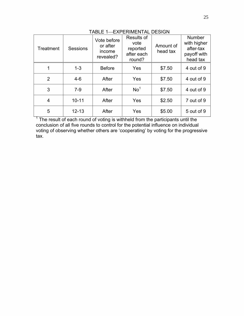
experimental design is summarized in Table 1 and described below.
In all sessions, participants are endowed with an income or pre-tax payoff
that is theirs to keep for participating in the study except that they must pay a tax.
Each participant’s pre-tax payoff or experimental income is determined by
drawing a card from a set of nine cards. The following incomes are recorded on
the cards: $10, $15, $20, $25, $30, $35, $40, $45 and $50. They also are
reminded that because each income is equally likely, the average pre-tax payoff
across participants is $30.12 Within each period income cards are drawn without
replacement and participants are instructed that their income is private
information that should not be revealed at any time during the session.
In all treatments the tax is one of two types. As Table 2 reports, Tax 1 is a
lump-sum head tax of $7.50, and Tax 2 is a progressive income tax. Notice from
Panel A of Table 2 that the sum of after-tax payoffs in Treatments 1 through 3 is
number of subjects. We settled on nine participants in order to provide anonymity among the participants on the one hand and to limit the total cost of the experiments on the other. 11 Some critics question the relevance of insight provided by experiments with student subject pools. If the average person behaves differently from university students, we should be cautious in drawing inferences about the general population. However, there is some evidence that the behavior of subjects drawn from other populations is not markedly different from the behavior of student subjects [Davis and Holt (1993, page 17)]. 12 Of course, people may behave differently when their income is earned rather than endowed. In particular, people may be more predisposed to fairness when endowed. Hoffman, McCabe, Shachat, and Smith (1994) provide experimental evidence that first movers in dictator and ultimatum games offer less when the first mover is decided by the higher score on a general knowledge test.
9
$202.50 for both the head tax and the progressive tax. In other words, the two
tax regimes are revenue neutral.13 For Treatments 1 through 3, four of the nine
participants receive a higher after-tax payoff under the head tax, as noted in
Table 1. Four (4) low-income participants receive a higher after-tax payoff under
the progressive tax; whereas, the median participant with a pre-tax payoff of $30
receives the same after-tax payoff under both tax structures.14 If the participants
care only about their after-tax payoff, high-income participants (i.e., pre-tax
payoff > $30) prefer the head tax; low-income participants (i.e., pre-tax payoff <
$30) prefer the progressive tax; and the median income participant (i.e., pre-tax
payoff = $30) is indifferent between the two.
The subjects’ after-tax payoffs are determined by the vote of the majority
in the choice between the head tax (Tax 1) and the progressive tax (Tax 2).15
Participants are given 5 minutes to indicate the preferred tax. In Treatments 1
and 2, the votes are tallied; the chosen tax structure is publicly announced after
each round of voting; and participants are reminded that their after-tax payoff is
private information that should not be disclosed at any time. In Treatment 3 the
result of each round of voting is withheld from the participants until the conclusion
13 In Treatments 4 and 5, we simulate the excess burden of progressive taxation by using two tax regimes that are not revenue neutral, as discussed below. 14 During the experiments, we used the more neutral terms Tax 1 and Tax 2 rather than lump-sum tax and progressive tax to refer to the two tax regimes in order to avoid unintentionally biasing the responses. 15 Clearly, we are concerned in this paper with outcome fairness. There is a related literature that examines process fairness. By using majority voting to decide the outcome, we have invoked a process, which we believe to be widely accepted as process fair. However, it would be interesting in future research to examine the sensitivity of the results reported here to alternative decision rules such as super majority or weighted voting schemes.

10
of all five rounds to control for the potential influence on individual voting of
observing whether others are ‘cooperating’ by voting for the progressive tax.
These procedures are repeated five times in each session. As the
instructions indicate, participants are told at the outset that they will be paid
according to the results of only one of the trials, and this trial will be chosen by a
card draw at random by one of the participants from a set of cards labeled 1-5.
Since ex ante the students have no way of knowing which trial is the payout trial,
it is in their interest to treat all trials with equal seriousness.16
Treatment 1 differs from Treatments 2 and 3 in that participants in
Treatment 1 vote for a tax structure before they draw an income card. In other
words, participants in Treatment 1 vote before they know their pre-tax payoff.
Since they do not know their place in the income distribution when they vote,
they have no way of knowing whether the chosen tax regime increases or
decreases their after-tax payoff, and, in that sense, they vote ‘as if behind a veil
of ignorance,’ to use a phrase coined by Rawls (1971). In Treatments 2 and 3
participants vote after drawing an income card; so they know their standing in the
income distribution when they vote. These treatments allow us to see if
knowledge of one’s position in the income distribution, and thus the effect of the
vote on their own after-tax payoff, changes the outcome of the vote.
At the conclusion of each session, participants complete a post-
experiment questionnaire, designed to collect demographic information.
Consideration of demographic information does not indicate any notable
16 As part of the empirical analysis described subsequently, we include dummy variables for the rounds and find no evidence of a round effect.
11
differences between participants across all sessions (1-10), as expected given
that all subjects are recruited from the same pool. In addition, their responses on
the questionnaire indicate that they found the experiment interesting and the
monetary incentives motivating. Participants respond on an eleven-point scale as
to how interesting they found the experiment, where 1 = not very interesting and
11 = very interesting. The mean response across all treatments is 9.0.
Participants also respond on an 11-point scale as to how they would characterize
the amount of money earned for taking part in the experiment, where 1 = nominal
amount and 11 = considerable amount. The mean response across all
treatments is 10.0.17
III. Summary of Voting Behavior
A. Revenue Neutral Treatments
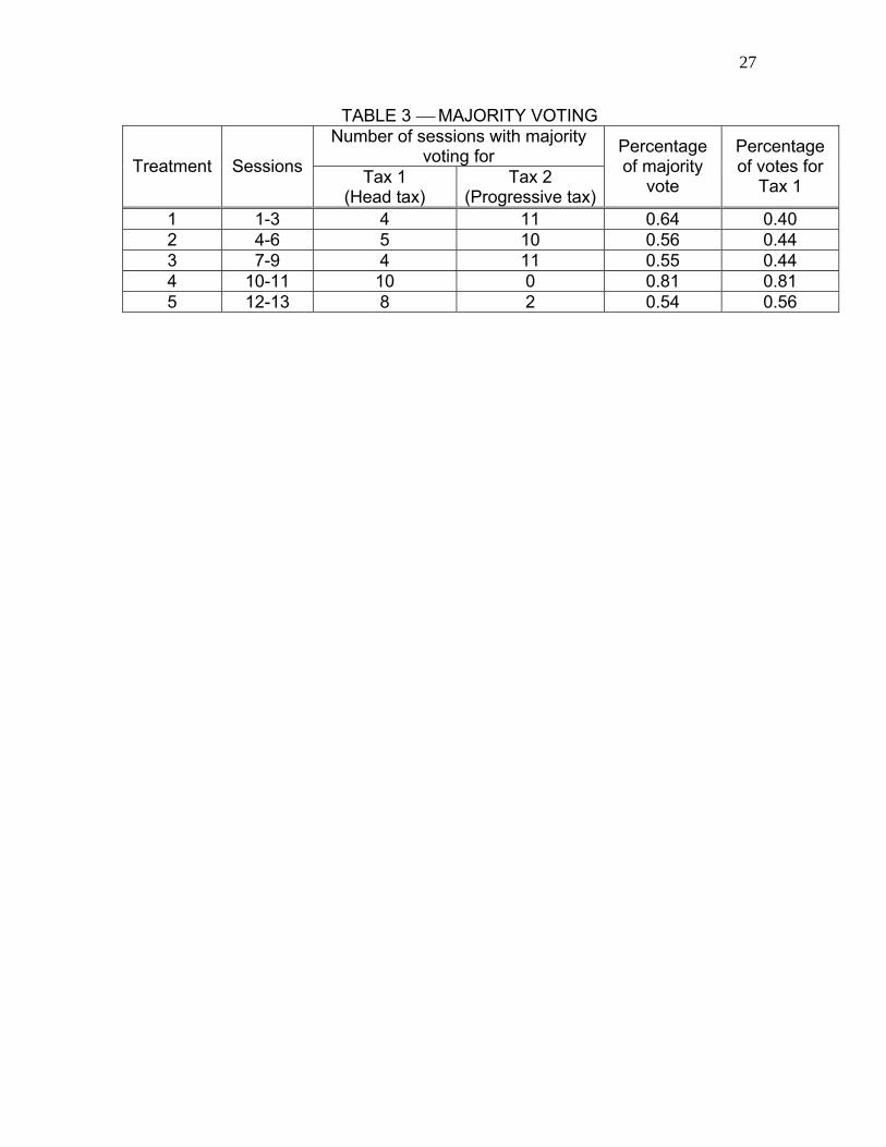
Table 3 summarizes the preferences of participants as revealed by their
voting behavior. In Treatment 1, the majority vote for Tax 2 (the progressive tax)
in 11 of 15 trials. In these sessions, participants do not know their income level
when they cast their votes, and the majority chooses the progressive tax. This
result supports the view that people care about the distributional consequences
of taxation and not simply their own payoff. Since the participants do not know
their pre-tax payoff, however, some may be attempting to pool payoff risk by
17 Participants are paid $2 for timely arrival to the experimental session and $2 for completion of a post-experiment questionnaire. Thus, while the average after-tax earnings in the revenue-neutral treatments are $22.50, the average compensation is $26.50 with a range of $6.50 to $46.50.
12
voting for the progressive tax, reflecting risk aversion rather than payoff inequality
aversion.
To control for this potential confound, we allow participants to observe
their pre-tax payoff before voting.18 This experimental design also allows us to
observe whether participants are willing to sacrifice income to satisfy a taste for
fairness; if in fact a taste for fairness drives the previous finding. In Treatment 2,
the majority votes for the progressive tax (Tax 2) in 10 of 15 trials. As we will see,
it is not necessarily the median participant with a pre-tax payoff of $30 who is
decisive. Thus, some participants vote for the progressive tax even though they
suffer in terms of their own after-tax payoff. In other words, it appears that some
participants are prepared to pay or sacrifice income in order to satisfy a taste for
fairness. In contrast, some median income participants vote against the
progressive tax even though their after-tax payoff is unaffected by their choice of
distribution. This evidence of heterogeneity in the population may play an
important role in distribution experiments and may explain ES’s conclusion that
theories of inequality aversion do not provide additional explanatory power
beyond that afforded by the efficiency and maximin principles.
An additional concern about the experimental design described above
may stem from participants attempting to play cooperative strategies. When
participants know their income before they vote and the majority vote is revealed
18 In a strict sense, removing the “veil of ignorance” only removes the uncertainty regarding one’s income. Uncertainty remains as to how others will vote, and we cannot rule out an effect on voting from this type of uncertainty. However, uncertainty regarding how others will vote is equally present behind the “veil of ignorance.”
13
after each round, high-income participants in a given round may attempt to
‘signal’ a cooperative strategy by voting for the progressive tax, even though
doing so reduces their after-tax payoff in that round. In this manner, they may try
to elicit cooperation to ‘insure’ against the risk of being low income in subsequent
rounds. A solution to this potential confound is a treatment in which participants
receive no information about the majority vote in each round until the end of the
session. Thus, in Treatment 3 we withhold the result of each voting round until
the conclusion of the experiment to control for the potential influence of
‘cooperation’ on individual voting. The results of Treatment 3 are reported in
Table 3 and indicate that the majority votes for the progressive tax (Tax 2) in 11
of 15 trials. Since these results are very similar to those obtained with Treatment
2 (10 of 15), votes by high income participants for the progressive tax do not
appear to reflect attempts to signal a cooperative strategy.
Table 4 provides additional insight into the behavior of our experimental
participants. As one might expect, in Treatment 1 where the participants vote
‘behind a veil of ignorance,’ voting for either Tax 1 or Tax 2 shows no pattern
across payoffs. Interestingly, however, we observe approximately the same
proportion of total votes for the progressive tax (Tax 2) in Treatment 2 (56
percent or 76/135), in which pre-tax payoffs are known before voting as when
they are not, as in Treatment 1 (60 percent or 81/135).
In Treatment 2, we observe a clear pattern in voting behavior with low
(high) payoff individuals showing a strong preference for the progressive tax
(head tax). It is impossible to infer whether low payoff individuals are voting for
14
the progressive tax out of concern for their own payoff and/or due to
disadvantageous inequality aversion because the two motives are congruent.
However, we also see that the median-income participant whose pre-tax payoff is
$30 votes only slightly more often for Tax 2 (53 percent or 8/15).19 Significantly in
terms of our hypothesis, some individuals vote for the progressive tax (Tax 2)
even when it is clearly not in their monetary self-interest to do so. In fact, we
observe more votes for Tax 2 by high-income participants (15.0 percent or 9/60
votes) as compared to votes for Tax 1 (head tax) by low-income participants (1.6
percent or 1/60 votes).
For Treatment 3 in which participants do not know the results of previous
rounds of voting, the results are very similar. As in Treatment 2, we observe a
strong preference for the progressive tax (56 percent or 75/135) and more high-
income participants vote for Tax 2 (15.0 percent or 9/60 votes) as compared to
votes for Tax 1 by low-income participants (0 percent or 0/60 votes).
Table 4 also provides further insight into voting behavior. For each of
Treatments 2 and 3 (pre-tax income is known before voting), nine out of a
possible 60 votes cast are for the progressive tax by participants with a pre-tax
payoff greater than the median and therefore risk a smaller own payoff by voting
19 The median voter hypothesis predicts that the decisive voter should be the median payoff participant as long as preferences are monotonic over the issue in question. In Treatment 2, the median payoff participant is decisive in 80 percent of the trials and only 55 percent of the trials in Treatment 3. Since tastes for redistribution may be heterogeneous, preferences are not necessarily monotonic. Therefore, the median voter hypothesis may not be applicable in redistribution settings. This observation may have important implications for ES’s experimental design in which the median payoff participant is the sole decision maker. We would like to thank an anonymous referee for bringing this issue to our attention.

15
for the progressive tax (Tax 2). Eight participants cast these eighteen votes and
no more than two participate in any session. We refer to these subjects as
fairness-minded. Six of the eight always vote for the progressive tax (Tax 2),
regardless of their income level.
Demographic information indicates the following. The median participant is
in the third year of university study. Three fairness-minded participants are in
their first year at the university, two are in their third year, and three are in their
fourth year. Four fairness-minded participants are men, and four are women. The
median participant in our experiment and the median fairness-minded participant
both report income in the $25,001 to $50,000 range. Thus, there is no apparent
demographic link across participants who are fairness-minded. Overall the
results support the hypothesis that some subjects exhibit social preferences and
prefer a more equitable distribution of after-tax payoffs, even if it is personally
costly to do so.
B. Treatments with a Distortionary Progressive Tax
Because previous experimental evidence suggests that some people care
about efficiency or maximizing the sum of payoffs, we conduct two additional
treatments. In Treatments 4 and 5, we require participants to choose between
two tax regimes that are not revenue neutral. In other words, the sum of the after-
tax payoffs from the ‘distortionary’ progressive tax is less than that of the lump-
sum head tax. Notice from Panel B of Table 2 that in Treatment 4, the sum of the
after-tax payoffs is $247.50 with the head tax; whereas the sum of the after-tax
payoff with the progressive tax is $202.50. With the exception of the two lowest
16
pre-tax payoff participants ($10 and $15), all the subjects have an economic
incentive – absent inequality aversion - to vote for the head tax (Tax 1).
Turning to Treatment 5, the after-tax payoffs are summarized in Panel C
of Table 2. Again, the tax regimes are not revenue neutral. The sum of after-tax
payoffs with the lump-sum head tax is $225.00; whereas the sum of after-tax
payoffs with the distortionary progressive tax is $202.50. Now, five of nine
participants have an economic incentive – again absent inequality aversion – to
vote for the head tax (Tax 1). In short, the tax regimes in Treatments 4 and 5 are
not revenue neutral; otherwise the procedures are identical to those described
above for Treatment 2.
Table 3 reports the voting behavior of the majority in Treatments 4 and 5.
In contrast to the behavior observed in Treatments 2 and 3, the majority of
participants votes against the progressive tax. In Treatment 4, the majority votes
for the lump-sum head tax in every trial. In Treatment 5, the majority votes for the
lump-sum head tax in eight out of ten trials. In other words, when the tax is not
revenue neutral, fewer people are willing to sacrifice in terms of a smaller own
after-tax payoff to reduce payoff inequality. This result is suggestive: Individuals
care about distributional equity, but they also care about the total size of the pie
or efficiency.20
Votes by income level, reported in Table 4, support this interpretation. Few
people with high incomes (i.e., pre-tax payoff > $30) vote for the progressive tax.
20 As the excess burden of the distortionary progressive tax increases, we observe the number of people voting for the progressive tax (Tax 2) decreases. This suggests that there may be a downward sloping demand for fairness. This is an interesting issue for further study.
17
In Treatment 4, all participants with incomes greater than or equal to $20 have an
economic incentive – absent distributional considerations - to vote for the head
tax (Tax 1). We observe only 2.0 percent (1/50 votes) of high-income votes for
the progressive tax (Tax 2) in Treatment 4. Similarly, in Treatment 5 only 4.0
percent (2/50) of high-income voters (pre-tax payoff ≥ $30) choose the
progressive tax (Tax 2).
However, the votes of participants with pre-tax payoffs less than $20 in
Treatment 4 are particularly suggestive regarding social preferences assuming
the form of a taste for efficiency. Low-income participants (pre-tax payoffs < $20)
in Treatment 4 benefit in terms of own payoff from the progressive tax (Tax 2).
Yet, as Table 4 shows, 20 percent (5/20) of these participants vote for the lump-
sum tax, which results in a smaller own payoff.
Turning to a similar analysis of Treatment 5, those with pre-tax payoffs
less than $30 benefit in terms of own payoff under the progressive tax (Tax 2). In
contrast to Treatment 4, now, only 13 percent (2/15) vote for the lump-sum tax
and against their self interest in terms of own payoff. As Table 4 shows, however,
the benefit in terms of the increase in the sum of total payoffs of voting for the
lump-sum tax is smaller, and the cost in terms of own payoff is larger for these
low-income participants in Treatment 5 than in Treatment 4. In other words, the
price of fairness has increased for these low-income participants in Treatment 5
relative to the price facing them in Treatment 4. The increasing price of fairness
may account for the smaller percentage of low-income participants willing to vote
for the efficient, lump-sum tax in Treatment 5.
18
In short, there is evidence that some participants exhibit social
preferences among tax structures in the form of inequality aversion and concern
for efficiency. This is evidenced by those who vote for tax structures that impose
a sacrifice in terms of a smaller own payoff with the only apparent compensating
benefits being reduced payoff inequality in the case of high-income participants
and a more efficient tax in the case of some low income participants in
Treatments 4 and 5. Finally, the percentage of fairness-minded votes decreases
as the cost of achieving these social goals increase in terms of a reduced own
payoff. This suggests a downward sloping demand for fairness.
IV. Statistical Model and Results
The foregoing discussion provides a number of interesting insights.
Generally speaking, the results are consistent with the predictions of the Fehr-
Schmidt model of inequality aversion. Yet, we recognize that preferences may
take varied and complex forms. An approach that allows some people to be
concerned with their own payoff, efficiency (e.g, the sum of total after-tax
payoffs), and income inequality aversion provides flexibility to account for a
variety of possible voting behaviors.21 However, an examination of these three
motives in a single empirical model is problematic because, as shown in
Appendix 2, there is an exact linear relationship between the sum of total payoffs,
own payoff, disadvantageous inequality, and advantageous inequality.22 Thus, to
21 As described previously, efficiency is measured by the sum of the individual payoffs. 22 Appendix 2 includes a proof of the proposition that the change in the sum of total payoffs is a linear combination of changes in own payoff, disadvantageous inequality, and advantageous inequality.
19
perform a more rigorous test of the observations reported in the previous
sections, we evaluate two models relative to the Fehr-Schmidt model, as
described subsequently.
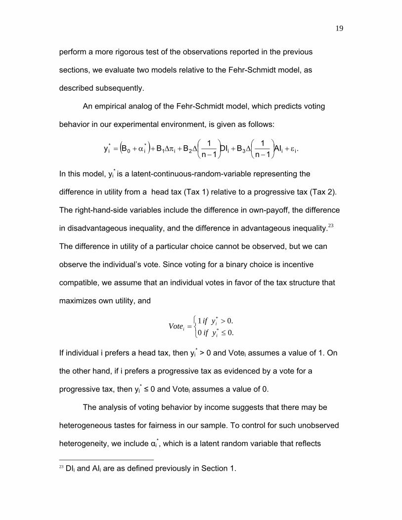
An empirical analog of the Fehr-Schmidt model, which predicts voting
behavior in our experimental environment, is given as follows:
( ) .AI1n
1BDI1n
1BBBy ii3i2i1*i0
*i ε+⎟
⎠⎞
⎜⎝⎛
−Δ+⎟
⎠⎞
⎜⎝⎛
−Δ+πΔ+α+=
In this model, yi* is a latent-continuous-random-variable representing the
difference in utility from a head tax (Tax 1) relative to a progressive tax (Tax 2).
The right-hand-side variables include the difference in own-payoff, the difference
in disadvantageous inequality, and the difference in advantageous inequality.23
The difference in utility of a particular choice cannot be observed, but we can
observe the individual’s vote. Since voting for a binary choice is incentive
compatible, we assume that an individual votes in favor of the tax structure that
maximizes own utility, and
⎩⎨⎧
≤>
=.00.01
*
*
i
ii yif
yifVote
If individual i prefers a head tax, then yi* > 0 and Votei assumes a value of 1. On
the other hand, if i prefers a progressive tax as evidenced by a vote for a
progressive tax, then yi* ≤ 0 and Votei assumes a value of 0.
The analysis of voting behavior by income suggests that there may be
heterogeneous tastes for fairness in our sample. To control for such unobserved
heterogeneity, we include αi*, which is a latent random variable that reflects
23 DIi and AIi are as defined previously in Section 1.
20
unobserved idiosyncratic tastes for fairness. Finally, the random error of the
structural model is given by εi.
To provide insight into the relative ability of the Fehr-Schmidt model to
predict observed voting behavior in our experiments, we estimate two additional
models. The conventional model of purely selfish preferences which is given as
follows:
( ) .BBy ii1*i0
*i ε+πΔ+α+=
In this model the difference in own after-tax payoffs is the only explanatory
variable. To account for social preferences assuming the form of a concern for
efficiency, irrespective of distributional concerns, we estimate a model that
accounts for the difference in own payoff and the difference in the sum of after-
tax payoffs or the S/E model which is given as follows:
( ) .21*
0 iiii EBBB επα +Δ+Δ++=*iy
This model reflects concern for own payoff and efficiency, where ΔEi is the
difference in the sum of after-tax payoffs in the two tax regimes. 24 We test
whether the purely selfish or the S/E model provides a superior fit to the
experimental data than the Fehr-Schmidt model.
In estimating the three models, we are confident that αi* is statistically
independent of the other regressors, as required by the random effects probit
specification. Our confidence is based on the fact that the regressors for each
observation depend on pre-tax income, which is randomly assigned to
24 We also used as an alternative measure of efficiency a dummy variable taking the value of 1 for Treatments 4 and 5, which are not revenue neutral. Inferences are similar to those reported subsequently.
21
participants by the draw of a card. We also include a constant in each regression;
therefore, αi* measures deviations from a common mean. Lacking any
information about the distribution of αi*, it seems reasonable to assume that
deviations from a common mean are normally distributed in the student
population from which we draw our sample.
Accordingly, we assume αi* ~ N(0,σα2) and E[αi
*|πt,Ei,DIi,AIi,εi] = E[αi*],
where DIi and AIi are the indices of disadvantageous and advantageous
inequality, respectively. By further assuming the error term εi has a standard
normal distribution, it follows that our specification is a multivariate probit model.25
Therefore, we estimate the three empirical models using random effects probit.26
Our experimental design elicits repeated binary choices by 90 subjects.
The resulting data include 450 votes from Treatments 2, 3, 4 and 5.27 Our results
are very similar to those reported subsequently whether we estimate random-
25 The assumption of unit variance is an innocent normalization [see, for example, Greene (2002)]. Also, Hsiao (2003) provides an excellent discussion of discrete choice as well as fixed and random effects models. 26 For the random-effects model, the likelihood (for an independent unit i) is expressed as an integral, which is computed in STATA using Gauss-Hermite quadrature. STATA recommends that the fitted model be evaluated for sensitivity to the chosen number of quadrature points. As a rule of thumb, if the coefficients do not change by more than a relative difference of 0.01 percent, then the choice of quadrature points does not significantly affect the outcome and the results may be confidently interpreted. When we change the number of quadrature points by ±4 points, our estimates do not change by more than the indicated 0.01 percent. 27 The results of Treatment 1 are not used to estimate these models. To calculate the regressors in these models, we need a reference payoff. Since the pre-tax income is unknown to the subjects before voting in Treatment 1, the choice of reference income for the calculations of the regressors is not obvious. In any event, the regressors would be identical for any choice of reference income. For example, the expected payoff is an obvious candidate to serve as the reference income. However, the regressors would be identical for every observation for this or any other choice of reference income in Treatment 1.
22
effects or fixed-effects linear probability (logit) models. In contrast to ES’s one
shot design, our experimental design allows us to control for individual effects,
which Charness and Rabin (2002) and the analysis of voting behavior in the
previous section suggest may be important in experiments designed to elicit
tastes for distributional equity.
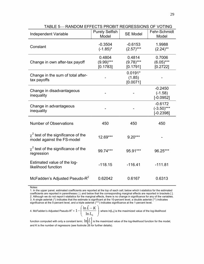
Table 5 reports estimated coefficients, t-statistics in parentheses, and
marginal effects in brackets for the three specifications. Recall that the estimated
coefficients of a probit equation indicate the direction of change due to a vote for
a head tax (Tax 1); whereas the marginal effects show the change in the
probability of a vote for the head tax due to a unit change in the corresponding
independent variable.28 Below the number of observations, the table reports a χ2
statistic for a test of the linear restriction among the coefficients implied by the
model with respect to the Fehr-Schmidt model. The implied linear restrictions are
described in Appendix 2. Finally, the table reports goodness of fit measures,
including Wald’s χ2 test statistic for the significance of the regression, the
estimated value of the log-likelihood function, and McFadden’s Adjusted Pseudo-
R2.29
28 To test for learning or order effects, we include individual dummy variables for each round, dropping the dummy variable for round 5. This vector of estimated coefficients is statistically insignificant, and the other results are virtually identical to those in Table 5. We also estimate the regressions in Table 5 with a dummy variable for gender (female = 1). This estimated coefficient is statistically insignificant at conventional levels. These results are available from the authors upon request. 29 Like a conventional R2 in the context of ordinary least squares, McFadden’s Pseudo-R2 increases as the number of regressors in the model increases. Accordingly, we adjust the likelihood ratio index by subtracting K, the number of
23
In general, the estimated coefficients of the three models take the
expected signs and are statistically significant at conventional levels, except for
the measure of disadvantageous inequality, which is statistically insignificant (p-
value = 0.115).30 In the purely selfish model, a vote for a head tax is positively
related to the change in own payoff. In the S/E model, a subject is more likely to
vote for a head tax as the deadweight loss from the progressive tax increases.
Finally, as predicted by the FS-model of social preferences, subjects are averse
to payoff inequality as evidenced by the negative and statistically significant,
estimated coefficient of the difference in the index of advantageous inequality.31
The likelihood ratio tests reject the linear restrictions implied by the purely selfish
and S/E models in favor of the unrestricted FS-model; both models are rejected
with a p-value less than 0.01. The values of the χ2 test statistics (degrees of
freedom = 2) are reported in Table 5.
regressors in the model, from the numerator of the index. See McFadden (1984) and note number 4 of Table 5 for further details. 30 We estimate variants of the regressions reported in Table 4 by including a dummy variable for Treatment 3. The estimated coefficient of this dummy variable is statistically insignificant at conventional levels. We also estimate all three models on the 315 observations from Treatments 2, 4 and 5. Again, these estimates are nearly identical to those reported in Table 5. This supports our conclusion in the previous section that there does not appear to be any attempt to signal cooperation in Treatments 2, 4 and 5 when the majority vote is announced after each trial. These results are available from the authors upon request. 31 As previously discussed, there is nearly exact multicollinearity among the regressors of the FS model. A recommended remedy for near exact multicollinearity is to increase the sample size. Tellingly, the significance level of the estimated coefficient of DI increases when the sample size increases from 315 observations (p-value = 0.312) to 450 observations (p-value = 0.115). This suggests that a further increase in the sample size may result in a statistically significant estimate. These results are available from the authors upon request.
24
In summary, our evidence suggests that the FS model of social
preferences best explains the decisions made by our experimental participants.
Though we cannot separate the impacts of own payoff, efficiency, and inequity
aversion, the empirical analysis supports the assertion that social preferences
matter.
V. Conclusion
We report results of a simple experiment designed to examine individual
preferences among tax structures. We find that some individuals may possess
social preferences or concern for one’s own payoff as well as the payoff of
others. This finding may have important implications for tax policy design. For
example, ours is a cautionary message for advocates of substituting a
consumption tax for the current federal income tax. Proponents of this policy
ostensibly believe that the potential benefit of efficiency gains from substituting a
consumption tax for the current federal income tax more than compensate for the
potential cost of greater after-tax income inequality. Our experimental evidence
suggests that at least some individuals may be far more concerned with the
distributional consequences of tax policy design than generally recognized by
some economists and policymakers. In short, economic models that do not
account for social preferences may provide a faulty guide to tax policy design.
25
TABLE 1⎯EXPERIMENTAL DESIGN
Treatment Sessions
Vote before or after income
revealed?
Results of vote
reported after each
round?
Amount of head tax
Number with higher
after-tax payoff with head tax
1 1-3 Before Yes $7.50 4 out of 9
2 4-6 After Yes $7.50 4 out of 9
3 7-9 After No1 $7.50 4 out of 9
4 10-11 After Yes $2.50 7 out of 9
5 12-13 After Yes $5.00 5 out of 9 1 The result of each round of voting is withheld from the participants until the conclusion of all five rounds to control for the potential influence on individual voting of observing whether others are ‘cooperating’ by voting for the progressive tax.

26
TABLE 2⎯TAX STRUCTURES
Panel A: Treatments 1 through 3 (Sessions 1-9) Tax 1: Head tax Tax 2: Progressive tax Pre-Tax
Income Tax After-tax payoff Tax After-tax payoff $10.00 $7.50 $2.50 $0 $10.00 $15.00 $7.50 $7.50 $2.00 $13.00 $20.00 $7.50 $12.50 $3.00 $17.00 $25.00 $7.50 $17.50 $4.00 $21.00 $30.00 $7.50 $22.50 $7.50 $22.50 $35.00 $7.50 $27.50 $11.00 $24.00 $40.00 $7.50 $32.50 $12.00 $28.00 $45.00 $7.50 $37.50 $13.00 $32.00 $50.00 $7.50 $42.50 $15.00 $35.00 Total $67.50 $202.50 $67.50 $202.50
Panel B: Treatment 4 (Sessions 10-11)
Tax 1:Head tax Tax 2: Progressive tax Pre-Tax Income Tax After-tax payoff Tax After-tax payoff $10.00 $2.50 $7.50 $0 $10.00 $15.00 $2.50 $12.50 $2.00 $13.00 $20.00 $2.50 $17.50 $3.00 $17.00 $25.00 $2.50 $22.50 $4.00 $21.00 $30.00 $2.50 $27.50 $7.50 $22.50 $35.00 $2.50 $32.50 $11.00 $24.00 $40.00 $2.50 $37.50 $12.00 $28.00 $45.00 $2.50 $42.50 $13.00 $32.00 $50.00 $2.50 $47.50 $15.00 $35.00 Total $22.50 $247.50 $67.50 $202.50
Panel C: Treatment 5 (Sessions 12-13)
Tax 1: Head tax Tax 2: Progressive tax Pre-Tax Income Tax After-tax payoff Tax After-tax payoff $10.00 $5.00 $5.00 $0 $10.00 $15.00 $5.00 $10.00 $2.00 $13.00 $20.00 $5.00 $15.00 $3.00 $17.00 $25.00 $5.00 $20.00 $4.00 $21.00 $30.00 $5.00 $25.00 $7.50 $22.50 $35.00 $5.00 $30.00 $11.00 $24.00 $40.00 $5.00 $35.00 $12.00 $28.00 $45.00 $5.00 $40.00 $13.00 $32.00 $50.00 $5.00 $45.00 $15.00 $35.00 Total $45.00 $225.00 $67.50 $202.50
27
TABLE 3 ⎯ MAJORITY VOTING Number of sessions with majority
voting for Treatment Sessions Tax 1 (Head tax)
Tax 2 (Progressive tax)
Percentage of majority
vote
Percentage of votes for
Tax 1
1 1-3 4 11 0.64 0.40 2 4-6 5 10 0.56 0.44 3 7-9 4 11 0.55 0.44 4 10-11 10 0 0.81 0.81 5 12-13 8 2 0.54 0.56
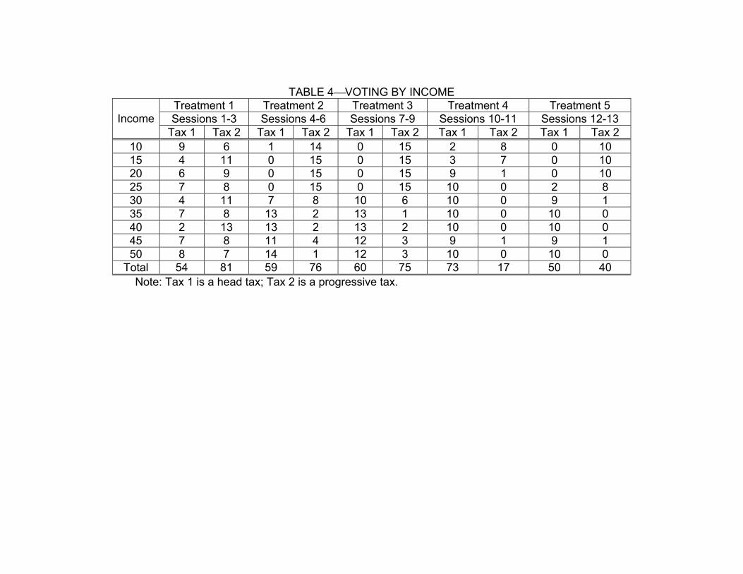
TABLE 4⎯VOTING BY INCOME Treatment 1 Treatment 2 Treatment 3 Treatment 4 Treatment 5 Sessions 1-3 Sessions 4-6 Sessions 7-9 Sessions 10-11 Sessions 12-13 Income
Tax 1 Tax 2 Tax 1 Tax 2 Tax 1 Tax 2 Tax 1 Tax 2 Tax 1 Tax 2 10 9 6 1 14 0 15 2 8 0 10 15 4 11 0 15 0 15 3 7 0 10 20 6 9 0 15 0 15 9 1 0 10 25 7 8 0 15 0 15 10 0 2 8 30 4 11 7 8 10 6 10 0 9 1 35 7 8 13 2 13 1 10 0 10 0 40 2 13 13 2 13 2 10 0 10 0 45 7 8 11 4 12 3 9 1 9 1 50 8 7 14 1 12 3 10 0 10 0
Total 54 81 59 76 60 75 73 17 50 40 Note: Tax 1 is a head tax; Tax 2 is a progressive tax.
29
TABLE 5⎯ RANDOM EFFECTS PROBIT REGRESSIONS OF VOTING
Independent Variable Purely Selfish Model SE Model Fehr-Schmidt
Model
Constant -0.3504 (-1.85)*
-0.6153 (2.57)***
1.9988 (2.24)**
Change in own after-tax payoff 0.4804
(9.99)*** [0.1783]
0.4814 (9.78)*** [0.1791]
0.7006 (6.05)*** [0.2722]
Change in the sum of total after- tax payoffs -
0.0191*
(1.85) [0.0071]
-
Change in disadvantageous inequality - -
-0.2450 (-1.58)
[-0.0952]
Change in advantageous inequality - -
-0.6172 (-3.50)*** [-0.2398]
Number of Observations 450 450 450
χ2 test of the significance of the model against the FS-model 12.69*** 9.20*** -
χ2 test of the significance of the regression 99.74*** 95.91*** 96.25***
Estimated value of the log-likelihood function -118.15 -116.41 -111.81
McFadden’s Adjusted Pseudo-R2 0.62042 0.6167 0.6313
Notes: 1. In the upper panel, estimated coefficients are reported at the top of each cell; below which t-statistics for the estimated coefficients are reported in parentheses ( ); and below that the corresponding marginal effects are reported in brackets [ ]. 2. Although we do not report t-statistics for the marginal effects, there is no change in significance for any of the variables. 3. A single asterisk (*) indicates that the estimate is significant at the 10-percent level, a double asterisk (**) indicates significance at the 5-percent level, and a triple asterisk (***) indicates significance at the 1-percent level.
4. McFadden’s Adjusted Pseudo-R2 = ⎟⎟⎠
⎞⎜⎜⎝
⎛ −−
0ln
ˆln1L
KL; where ln[L0] is the maximized value of the log-likelihood
function computed with only a constant term; [ ]L̂ln is the maximized value of the log-likelihood function for the model, and K is the number of regressors (see footnote 26 for further details).
30
Acknowledgements: The views expressed here are those of the authors and not
necessarily those of the Federal Reserve Bank of Atlanta or the Federal Reserve
System. The authors gratefully acknowledge the financial support of the Federal
Reserve Bank of Atlanta and the International Studies Program of Georgia State
University. The authors thank Aye Chatupromwong and Budina Naydenova for
research assistance and Francisco Arze, Ann Gillette, Bryan Church, Govind
Hariharan, Luc Noiset, and Roy Wada for helpful discussions and comments.
31
REFERENCES
Alm, James, 1998. Tax compliance and administration. In: Hildreth, W. Bartley, Richardson, James A. (Eds.), Handbook on Taxation, Marcel Dekker, Inc., New York, pp. 741-768.
Andreoni, James, Erard, Brian, Feinstein, Jonathan, 1998. Tax compliance.
Journal of Economic Literature 36(2), 818-60. Bagnoli, Mark, McKee, Michael, 1991. Voluntary contribution games: efficient
provision of public goods. Economic Inquiry 29(2), 351-66. Bolton, Gary E., Ockenfels, Axel, 2000. ERC: a theory of equity, reciprocity, and
competition. The American Economic Review 90(1), 166-93. Camerer, Colin F., 1997. Progress in behavioral game theory. Journal of
Economic Perspectives 11(4). 167-88. Charness, Gary, Rabin, Matthew, 2002. Understanding social preferences with
simple tests. The Quarterly Journal of Economics 117(3), 817-69. Davis, Douglas D., Holt, Charles A., 1993. Experimental Economics, Princeton
University Press, Princeton, New Jersey. Diamond, Peter A., Mirrlees, James A, 1971. Optimal taxation and public
production: I – production efficiency. The American Economic Review 61(1), 8-27.
Eichenberger, Reiner, Oberholzer-Gee, Felix, 1998. Rational moralists: the role
of fairness in democratic economic politics. Public Choice 94(1-2), 191-210.
Engelmann, Dirk, Strobel, Martin, 2004. Inequality aversion, efficiency, and
maximin preferences in simple distribution experiments. The American Economic Review 94 (4), 857-69.
Fehr, Ernst, Schmidt, Klaus M., 1999. A theory of fairness, competition, and
cooperation. The Quarterly Journal of Economics 114(3), 817-68. Frohlich, Norman, Oppenheimer, Joe A., 1992. Choosing Justice: An
Experimental Approach to Ethical Theory. University of California Press, Berkeley.
Gemmell, Norman, Morrissey, Oliver, Pinar, Abuzer, 2004. Tax perceptions and
preferences over tax structure in the United Kingdom. The Economic Journal 114, 117-38.

32
Greene, William H., 2002. Econometric Analysis. Fifth Edition, Prentice-Hall, New
York. Gϋth, Werner; Schmittenberger, Rolf, Tietz, Reinhard, 1990. Ultimatum
bargaining behavior – a survey and comparison of experimental results. Journal of Economic Psychology 11(3), 417-49.
Harsanyi, John, 1953. Cardinal Utility and the Theory of Risk-Taking. The Journal
of Political Economy 61, 434-35. Harsanyi, John, 1955. Cardinal Utility, Individualistic Ethics, and Interpersonal
Comparisons of Utility in Welfare Economics.” The Journal of Political Economy 63, 302-21.
Hite, P.A., Roberts, M.L., 1991. An experimental investigation of taxpayer
judgments on rate structure in the individual income tax system. Journal of the American Taxation Association 13(2), 47-63.
Hoffman, Elizabeth, McCabe, Kevin, Shachat, Keith, Smith, Vernon, 1994.
Preferences, property rights, and anonymity in bargaining games. Games and Economic Behavior 7(3), 346-380.
Hsiao, Cheng, 2003. Analysis of Panel Data. Second Edition, Cambridge
University Press, New York. Johansson-Stenman, Olof, Carlsson, Fredrik, and Daruvala, D., 2002. Measuring
future grandparents’ preferences for equality and relative standing. Economic Journal 112(479), 362-83.
Kahneman, Daniel, Knetsch, Jack L., Thaler, Richard, 1986. Fairness as a
constraint on profit seeking: entitlements in the market. The American Economic Review, September 76(4), 728-41.
Ledyard, John, 1995, Public goods: A survey of experimental research. In: Kagel,
John H., Roth, Alvin E. (Eds.), Handbook of Experimental Economics. Princeton University Press, Princeton, pp. 111-94.
Lewis, A., 1978. Perceptions of tax rates. British Tax Review, 358-66. Martinez-Vazquez, Jorge, Rider, Mark, 1996. A revelation approach to optimal
taxation. Public Finance Quarterly 24(4), 439-63. McCaffery, Edward J., Baron, Jonathan, 2004. Masking redistribution (or its
absence). Institute for Law and Economics, Research Paper No. 04-09, University of Pennsylvania Law School.

33
McCaffery, E. J., Slemrod, J., 2004. Toward an agenda for behavioral public
finance. USC CLEO Research paper No. C04-22. McFadden, Daniel, 1984. Econometric analysis of qualitative response models.
In: Griliches, Zvi and Intriligator, Michael (Eds.), Handbook of Econometrics, Vol. 2, North-Holland, Amsterdam.
Mirrlees, James A., 1971. An exploration in the theory of optimum income
taxation. Review of Economic Studies 38(114), 175-208. Ramsey, Frank P., 1927, A contribution to the theory of taxation. Economic
Journal 37(145), 47-61. Rawls, John, 1971. A Theory of Justice. Harvard University Press, Cambridge,
Massachusetts. Roth, Alvin E., Parsnikar, Vesna, Okuno-Fujiwara, Masahiro, Zamir, Shmuel,
1991. Bargaining and market behavior in Jerusalem, Ljubljana, Pittsburgh, and Tokyo: an experimental study. The American Economic Review 81(5), 1068-1095.
Sheffrin, Steven M., 1994. Perceptions of fairness in the crucible of tax policy. In:
Slemrod, Joel (Ed.), Tax Progressivity and Income Inequality. Cambridge University Press, Cambridge, 309-334.
34
APPENDIX 1: EXPERIMENTAL INSTRUCTIONS The experimental instructions for Treatment 2 follow. Changes in the instructions for other treatments are noted in brackets.
General Instructions
This experiment is concerned with the economics of decision-making. The instructions are simple, and if you follow them carefully and make good decisions, you might earn a considerable amount of money that will be paid to you in cash.
In this experiment you will be given an endowment of cash. This
endowment is your income for participating in the experiment today except that you must pay a tax.
A Record Sheet is included with these instructions. You will keep track of
your decisions on this sheet.
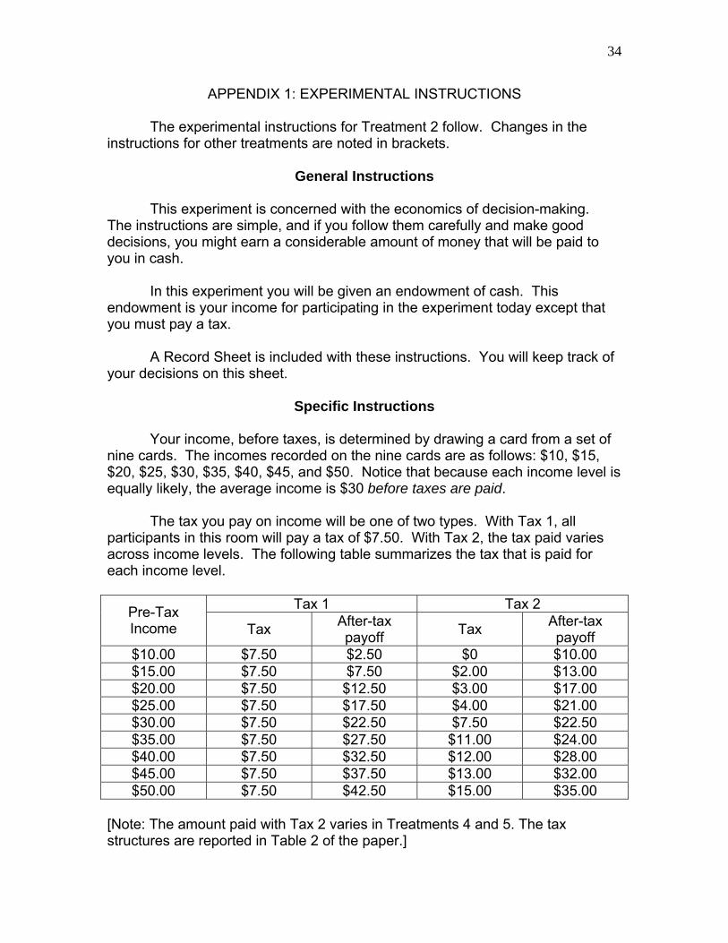
Specific Instructions Your income, before taxes, is determined by drawing a card from a set of nine cards. The incomes recorded on the nine cards are as follows: $10, $15, $20, $25, $30, $35, $40, $45, and $50. Notice that because each income level is equally likely, the average income is $30 before taxes are paid. The tax you pay on income will be one of two types. With Tax 1, all participants in this room will pay a tax of $7.50. With Tax 2, the tax paid varies across income levels. The following table summarizes the tax that is paid for each income level.
Tax 1 Tax 2 Pre-Tax Income Tax After-tax
payoff Tax After-tax payoff
$10.00 $7.50 $2.50 $0 $10.00 $15.00 $7.50 $7.50 $2.00 $13.00 $20.00 $7.50 $12.50 $3.00 $17.00 $25.00 $7.50 $17.50 $4.00 $21.00 $30.00 $7.50 $22.50 $7.50 $22.50 $35.00 $7.50 $27.50 $11.00 $24.00 $40.00 $7.50 $32.50 $12.00 $28.00 $45.00 $7.50 $37.50 $13.00 $32.00 $50.00 $7.50 $42.50 $15.00 $35.00
[Note: The amount paid with Tax 2 varies in Treatments 4 and 5. The tax structures are reported in Table 2 of the paper.]

35
Whether the tax you pay is Tax 1 or Tax 2 will be determined by majority vote. After the experimenter distributes the income cards, you will be given 5 minutes to indicate which tax you prefer. When all participants have recorded their votes on their Record Sheets, the experimenter will tally the votes and report on the outcome. Please record the tax paid and your after-tax payoff on your Record Sheet. Your income is your private information and should not be disclosed to other participants at any time. [Note: In Treatment 1 income cards are distributed after votes are recorded.]
We will repeat these steps 5 times. At the end of each trial, the tax chosen by the majority vote is announced. However, only one of the five trials will be binding. A number from one to five will be randomly selected to determine the binding trial. Your after-tax payoff from the binding trial is yours to keep and will be paid to you in cash. [Note: In Treatment 3 the outcome of voting each round is not revealed until the conclusion of the session.] Please do not confer with other participants in making your decisions at any time. Please remember that once you record your vote in each trial, you cannot change it.
Record Sheet
Trial Your vote (Tax 1 or Tax 2)
Majority vote (Tax 1 or Tax 2)
Your pre-tax payoff (from your income card) Your after-tax payoff
1
2
3
4
5

36
APPENDIX 2: PROOF OF LINEAR DEPENDENCE
This appendix shows that an exact linear relationship exists between changes in own payoff, disadvantageous inequality, advantageous inequality, and the sum of total payouts. Proposition 1: The change in the sum of total payoffs (ΔE) is an exact linear function of the sum of a change in own payoff, a change in the index of disadvantageous inequality, and a change in the index of advantageous inequality under any two tax regimes, or iii AInDInnE Δ−−Δ−+Δ=Δ −− 11 )1()1(π for
all i. Where ( )∑=
−=Δn
iiiE
121 ππ is the difference in the sum of the after-tax payoffs
under tax regimes 1 and 2.
Before proceeding with the proof of this proposition, it is helpful to establish our notation and re-write some familiar expressions. Let πki be the after-tax payoff of individual i = 1, … , n under tax regime k = 1,2. Further, assume that the after-tax payoffs are ranked in ascending order such that πk1 ≤ πk2 ≤ … ≤ πki ≤ … ≤ πkn.
This allows us to re-write DIki and AIki as follows: ∑>∀
− −−=n
ijkikjki nDI )()1( 1 ππ and
∑<
=
− −−=ij
jkjkiki nAI
1
1 )()1( ππ . With these definitions in hand, we proceed to a proof
of our proposition.
Proof: We begin by writing the FS-model as follows:
.)1()1( 11
kikiki AInDInnS −− −−−+
Now, we re-write the model and re-arrange terms.
∑∑<
=>
−− −−−+=−−−+ij
jkjki
n
ijkikjkikikiki nAInDInnS
1
11 )()()1()1( πππππ
.,)()()()()1(111
iEn k
N
iki
n
ijki
ij
jki
n
ijkj
ij
jkjki ∀==⎥
⎦
⎤⎢⎣
⎡+−⎥
⎦
⎤⎢⎣
⎡++−= ∑∑∑∑∑
=>
<
=>
≤
=
ππππππ
Since Δ is a linear operator, this completes the proof.
37
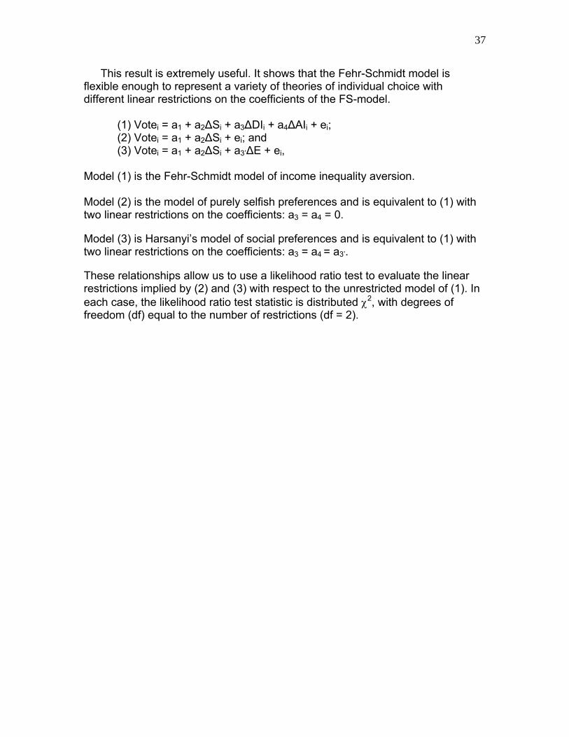
This result is extremely useful. It shows that the Fehr-Schmidt model is flexible enough to represent a variety of theories of individual choice with different linear restrictions on the coefficients of the FS-model.
(1) Votei = a1 + a2ΔSi + a3ΔDIi + a4ΔAIi + ei; (2) Votei = a1 + a2ΔSi + ei; and (3) Votei = a1 + a2ΔSi + a3’ΔE + ei,
Model (1) is the Fehr-Schmidt model of income inequality aversion. Model (2) is the model of purely selfish preferences and is equivalent to (1) with two linear restrictions on the coefficients: a3 = a4 = 0.
Model (3) is Harsanyi’s model of social preferences and is equivalent to (1) with two linear restrictions on the coefficients: a3 = a4 = a3’.
These relationships allow us to use a likelihood ratio test to evaluate the linear restrictions implied by (2) and (3) with respect to the unrestricted model of (1). In each case, the likelihood ratio test statistic is distributed χ2, with degrees of freedom (df) equal to the number of restrictions (df = 2).