Tarnopolsky M. Room air distribution calculation. 2014
35
Tarnopolsky M. Room air distribution calculation. 2014 Page 1 of 35 Room air distribution calculation M. Tarnopolsky, Ph.D. Abstract The objectives of this task are to evaluate the performance of airflow simulation techniques and to establish their viability as design tools. This paper outlines a semi- empirical method for calculating the velocity and temperature fields in the room. The method takes into consideration interaction between the various jets in the room, the walls of the room and the counter flow between jet and enclosure. Effect of the walls is calculated by the mirror method. To explore impact of initial velocity and temperature difference profiles, inlet is divided to increments of elementary jets. The velocity and temperature difference at point considered are determined by adding momentum flux and excess heat, as supplied from all real, mirror, and elementary jets. Then this solution has corrections of the velocity field for deviations from the equations of continuity and momentum flux, taking into consideration the counter flow between jet and enclosure. Similarly, the temperature field is calculated so that the heat balance equation is preserved. The results of the calculations are shown to be in good agreement with measurements in scaled models. The reliable, practical, and efficient method can be used both in the preliminary stages of the development of jet-supplying products and in room air distribution design. Introduction. The ability to accurately predict air movement and temperature distribution in spaces offers the potential for design engineers to evaluate and optimize room air distribution systems at an early stage, leading to improved thermal comfort and ventilation effectiveness. The purpose of this work is to create a reliable, practical, and efficient method, which can be used both in the preliminary stages of the development of jet-supplying products and in room air distribution design. -- ----------------------------------------------------------------------------------------------------------- Dr. Moshe Tarnopolsky is with Department of Civil and Environmental Engineering, Technion, Haifa, Israel ([email protected])
-
Upload
independent -
Category
Documents
-
view
1 -
download
0
Transcript of Tarnopolsky M. Room air distribution calculation. 2014

Tarnopolsky M. Room air distribution calculation. 2014 Page 1 of 35
Room air distribution calculation
M. Tarnopolsky, Ph.D.
Abstract
The objectives of this task are to evaluate the performance of airflow simulation
techniques and to establish their viability as design tools. This paper outlines a semi-
empirical method for calculating the velocity and temperature fields in the room. The method
takes into consideration interaction between the various jets in the room, the walls of the
room and the counter flow between jet and enclosure.
Effect of the walls is calculated by the mirror method. To explore impact of initial
velocity and temperature difference profiles, inlet is divided to increments of elementary jets.
The velocity and temperature difference at point considered are determined by adding
momentum flux and excess heat, as supplied from all real, mirror, and elementary jets. Then
this solution has corrections of the velocity field for deviations from the equations of
continuity and momentum flux, taking into consideration the counter flow between jet and
enclosure. Similarly, the temperature field is calculated so that the heat balance equation is
preserved.
The results of the calculations are shown to be in good agreement with measurements
in scaled models. The reliable, practical, and efficient method can be used both in the
preliminary stages of the development of jet-supplying products and in room air distribution
design.
Introduction.
The ability to accurately predict air movement and temperature distribution in spaces
offers the potential for design engineers to evaluate and optimize room air distribution
systems at an early stage, leading to improved thermal comfort and ventilation effectiveness.
The purpose of this work is to create a reliable, practical, and efficient method, which
can be used both in the preliminary stages of the development of jet-supplying products and
in room air distribution design. --
-----------------------------------------------------------------------------------------------------------
Dr. Moshe Tarnopolsky is with Department of Civil and Environmental Engineering, Technion, Haifa, Israel

Tarnopolsky M. Room air distribution calculation. 2014 Page 2 of 35
We expect that some expensive laboratory tests could be avoided if airflows in rooms
should become possible to predict using calculation with a certain degree of confidence.
Recent developments in measurement techniques open new possibilities to study these
phenomena, while calculation methods haven been produced in an attempt to describe this
flow.
The most fundamental research on jets has been performed using contoured nozzles
which produce a nearly uniform ‘‘top hat’’ velocity profile at the nozzle exit (Crow [1] and
Becker [2]).
There has been increasing evidence that the impact of initial conditions on the
downstream development of a flow is significant even in the far field (Wygnanski [3] and
George [4]).
Papers of Deo et al. [5], [6] report the statistical behavior of a plane jet discharging
into a large space by exploring the impacts of varying nozzle contraction profile. The nozzle-
exit profile varied by changing orifice-plates with different exit nozzle’s inner-wall
contraction radii. The results reveal consistent differences throughout the flow, extending
from the exit velocity profiles, through the near field, and into the far field. The exit velocity
profiles were found to depend systematically upon radii, with a gradual transition from being
saddle-backed for the case small radii to closely approximate a ‘‘top hat’’ for the cases of
large radii. In the self-similar far field, the rates of centerline velocity decay and jet spread
decreased in an asymptotic-like manner with an increase in radii.
Quinn et al. [7] compared sharp-edged and smoothly contoured round nozzles with
the same exit area. The experimental results showed the existence of distinct off-center peaks
in the mean stream wise velocity in the very near flow field of the jet from the sharp-edged
round nozzle. Stream wise velocity off-center peaks were absent in the smoothly contoured
nozzle jet flow which was found to spread faster than the sharp-edged slot jet flow in the
initial region.
The focus of the study by Quinn [8] was the relationship between speed of mixing in
the near flow field and slot aspect ratio in flows of turbulent free jets issuing from sharp-
edged rectangular jets. The results indicate that the speed of mixing in the very near flow
field increases as the slot aspect ratio increases.
The objective of the study by Cao et al. [9], [10], [11], and [12]) was to identify the
airflow patterns of attached plane non-isothermal jets after its impingement with the corner in
a room. After impingement in the corner, the jet flow reattached to the wall surface and the
flow directed parallel to the vertical wall, with the jet thickness growing downwards. Smith

Tarnopolsky M. Room air distribution calculation. 2014 Page 3 of 35
[13] and Cao [9] found that the air velocity distribution in the ceiling-wall and wall-floor
corners is nearly symmetric and flow after impingement was as jet continuation. This means
that the reattached distance assumes approximately equal to separation distance in the
impinging zone and the maximum jet velocity at the separation point is approximately equal
to the jet velocity at the reattachment point after its impingement.
In experiments of Nielsen et al. [15], [16] and [16] attached plane isothermal jet was
discharged horizontally near the ceiling into a model space and removed from the model near
the floor in opposite wall. Corresponding results were obtained in an idealized wall-jet
configuration by Sehwarz and Cosart [17]. After impingement in the ceiling-wall and wall-
floor corners, the jet flow reattached to the floor surface and the flow directed parallel to the
floor backwards.
In experiments of Pelfrey and Liburdy [18], Pramanik and Das [19] plane isothermal
jet discharged from a nozzle adjacent to a plate parallel to the axis of the nozzle. Then jet
bended and attached to the solid boundary due to lower pressure region created between the
jet axis and the nearest solid boundary (Coanda effect). The downward curving jet, the nozzle
plate and the oblique wall formed a recirculation zone.
The air-jet discharged from a ceiling slot inlet in an isothermal ventilated enclosure in
experiments of Yu et al. [20]. Two geometrically similar scale models represented a model
and a prototype with ratio of 1:2. Velocity measurements provided by the same relative exit
velocity profile U/U0 but different Reynolds numbers. In experiments of Yu et al. [21] the
same models were used for non-isothermal conditions.
Shepelev [22] has performed the most fundamental research on jets, what we use in
our analysis.
Room flow analysis.
The objective of this task is to evaluate the performance of airflow calculation
techniques. Analysis assumes a jet supplying from a rectangular inlet to the room with the
rectangular cross-section (see Figure 1).
Initially, the effect of the sidewalls, ceiling and floor is taken into consideration by the
mirror method using virtual jets symmetrical to real jet (ignoring friction in the boundary
layer). The real jet is shown by solid lines and the virtual jets are shown by dotted lines in
cross-section 1 - 1 of Figure 1 (total number of jets are My and Mz along axes Y and Z,

Tarnopolsky M. Room air distribution calculation. 2014 Page 4 of 35
respectively). The velocity field obtained in this step will be denoted as current by the index c
(Uc).
Then, this solution has corrections taking into consideration the counter flow between
jet and enclosure. The velocity field in the room (U) is calculated using a correction denoted
as a velocity shift by the index s (Us):
sc U - U = U , (1)
To explore impact of initial velocity and temperature difference profiles, inlet is
divided to Ny and Nz increments of elementary jets along axes Y and Z, respectively.
B0*H0
1
η
δ
Y
Z
Z
U
Xr
X 1
Cross-section 1-1
Hβ c
Be*He
U0
Ue
-2*Hr+2*H+Z
2*H+Z
B B Br-B BBr-BBr-B
-2*Br+2*B+Y
Hr
H
Hr-H
H
Hr-H
H
Hr-H
2*B+Y
B0*H0
1
η
δ
Y
Z
Z
U
Xr
X 1
Cross-section 1-1
Hβ c
Be*He
U0
Ue
-2*Hr+2*H+Z
2*H+Z
B B Br-B BBr-BBr-B
-2*Br+2*B+Y
Hr
H
Hr-H
H
Hr-H
H
Hr-H
2*B+Y
1
η
δ
Y
Z
Z
U
Xr
X 1
Cross-section 1-1
Hβ c
Be*He
U0
Ue
-2*Hr+2*H+Z
2*H+Z
B B Br-B BBr-BBr-B
-2*Br+2*B+Y
Hr
H
Hr-H
H
Hr-H
H
Hr-H
2*B+Y
Figure 1. Room jet interaction diagramme.

Tarnopolsky M. Room air distribution calculation. 2014 Page 5 of 35
The current velocity (Uc) and temperature difference (Tc) at point considered are
determined by adding momentum flux and excess heat, as supplied from all real and mirror
jets jy and jz, and all inlet increments Ky and Kz, along axes Y and Z (see Tarnopolsky [23]):
d dU
HB g
=
gU
i
k
k
k
k
Nz
1=kz
Mz
1=jz
Ny
1=ky
My
1=jyoo
c 2112 1
, (2)
and
d dT U
HB
C = T U C ii
k
k
k
k
Nz
1=kz
Mz
1=jz
Ny
1=ky
My
1=jyoo
hcch 11
, (3)
where is the specific weight of the air at a given point:
T + T
T =
a
aa , (4)
Ui and Ti are air velocity and temperature difference induced by elementary jet i in
inlet with coordinates δ and η along axes Y and Z, respectively (according to Shepelev [22]):
]S C 2
) +(Z )+(Y[- U =U
22
2j
2j
mi
Exp (5)
and
)U
U(T =T
m
imi
, (6)
Yj and Zj are coordinates of a point in real and virtual jets jy and jz, m:
) - Y) + (-) - B() - M - (-j
= BY jyjy
yrj 11
2
1 (7)
and
Z- )(-1 + H(1 -2
)(-1 - (M - jH =Zj jz
jzz
r , (8)
The values of air velocity Um and temperature difference Tm on axis of i - elementary
jet have to be calculated by assuming conservation of momentum flux and excess heat of cell
made by increments ky and kz:
g
U =
g
dYdZU kkkkk
2i2H-Hr
H-
B-Br
B-
11 , (9)
and
kkkkkkhiih
H-Hr
H-
B-Br
B-
T U C = dYdZ T U C 11 , (10)
Taking into consideration Equations 4 through 6 and after further integration, we obtain:

Tarnopolsky M. Room air distribution calculation. 2014 Page 6 of 35
kkkkk2
m2
a U SCU 1122 , (11)
and
kkkkkkhtmmah T U C = SCT U C 1122 , (12)
Empirical values of velocity profile constant C = 0.082 and turbulent Prandtl number
σ = 0.5 are used here. Ct is the temperature profile constant: 095.01
25.0
+ C = Ct , (13)
Equations 11 and 12 can be used to find air velocity Um and temperature difference Tm
on axis of i - elementary jet. After substitution of Equations 4, 5, 11, and 12 into Equations 2
and 3 and further integration, current velocity and temperature difference can be presented as:
zy0.5
ooa
cc U U )
H B
I g(=U (14)
and
zy0.5oocah
cc T T
)H B I (g C
Q = T , (15)
where Uy and Uz are the no dimensional components of the current velocity:
)]CS
YErf[-]CS
+Y(Erf[
U
U =U 0.5ijij
Ny
1=ky
My
1=jyy
o
k
1
2
5.0 , (16)
and
)]CS
-ZErf[-]
CS
+Z(Erf[
U
U=U 0.5ijij
Nz
1=kz
Mz
1=jzz
o
k 1
2
5.0
. (17)
Similarly Ty and Tz are given by:
])SC
-YErf[-]
SC
+Y(Erf[
UTU
TU=Tt
ij
t
ij
yoo
kkNy
1=ky
My
1=jyy
15.0
, (18)
and
])SC
-ZErf[-]
SC
+Z(Erf[
UTU
TU=Tt
ij
t
ij
zoo
kkNz
1=kz
Mz
1=jzz
15.0 , (19)
where Ic and Qc are the initial momentum flux and excess heat of the current calculated as the
product of sums of increments of momentum flux and excess heat in the inlet along the axes
Y and Z:

Tarnopolsky M. Room air distribution calculation. 2014 Page 7 of 35
g
U =I kkkkk
2Nz
1=kz
Ny
1=kyc
11 , (20)
and
kkkkkkh
Nz
1=kz
Ny
1=kyc T U C=Q 11 . (21)
This solution have to be corrected taking into consideration the velocity “shift” (Us),
which is determined by the equation of continuity:
G = dZ dY U H-Hr
H-
B-Br
B-
, (22)
where G is the quantity of air in cross-section of the room. Accordingly, we obtain the
following from Equations 1, 14, and 22:
,U - H B
G = U e
rra
cs (23)
where Gc is the current quantity of air in considered cross-section of the room:
zy0.5
cooac L L )I H B (g = G ; (24)
where Ly and Lz are no dimensional discharge factors:
dY B
U = L
o
yB-Br
B-
y (25)
dZ H
U = L
o
zH-Hr
H-
z . (26)
Ue is the air-removal velocity in considered cross-section of the room:
rrae H B
G = U ; (27)
If distance from the inlet to the cross-section considered is less than the distance to the
outlet (X < Xe), the total quantity of the air in this cross-section of the room G equals to the
total quantity of the air in the inlet Go, and in another case (X = Xe or X > Xe) G equals to
zero.
To determine the trajectory of the jet, we have to calculate the effect of the
momentum flux and the buoyancy flux. The momentum flux in the cross-section of the room
is:
dZ dY gU = I
2H-Hr
H-
B-Br
B-
u
,

Tarnopolsky M. Room air distribution calculation. 2014 Page 8 of 35
(28)
Taking into consideration Equations 1, 23 through 27 and after integration, we obtain:
ez2
y2
rr
oocu I+ ) L L
H B
H B - (1I = I , (29)
where Ie is momentum flux of air-removal in considered cross-section of room:
H Bg
U =I rr
e2
ae
. (30)
The buoyancy force, created by temperature-density difference between elementary
volume of current and ambient air, is:
dX dZ dY )-( = dI a
H-Hr
H-
B-Br
B-
t , (31)
Using Equations 4 and 15, and after approximate integration, Equation 31 becomes:
dX Q Q I g
H B
C T
Q=dI zy
0.5
c
ooa
ha
ct
, (32)
where Qy and Qz are no dimensional components of the excess heat:
dY B
T = Q
o
yB-Br
B-
y (33)
and
dZ H
T = Q
o
zH-Hr
H-
z . (34)
The components and the resultant momentum flux in a cross-section of room will be:
xycux I = I coscos , (35)
cxy I = I tan , (36)
t
X
0
cxz dI + I = I tan , (37)
and
)I + I + I( = I 0.5z
2y
2
x2 , (38)
The coordinates of the current trajectory can now be calculated:
dS I
I = X x
S
0 , (39)
and

Tarnopolsky M. Room air distribution calculation. 2014 Page 9 of 35
dS I
I = B y
S
0 , (40)
and
dS I
I = H z
S
0 . (41)
Now ratios of the coordinates of current trajectory X
B and
X
H can be used as
tangents to find the angles of current trajectory αc and c along axes Y and Z.
The static pressure in cross-section of the room is given from the momentum flux
equation for closed space:
X
o rr
xos H B
dI P = P , (42)
Influence of the exit nozzle profile.
Deo et al. [5] and [6] studied influence of geometric profile of a long slot nozzle on
the properties of a jet. The nozzle facility, shown schematically in Figure 2, consists of an
open circuit wind tunnel, flow-straightening elements including a honeycomb and screens,
and a smooth contraction exit.
The jet was discharged horizontally at the midpoint into a laboratory space of
dimensions Xr =14 m (long) · Br=0.72 m (wide) · Hr =2.04 m (high). The nozzle-exit profile
of Bo = 0.72 m (width) and Ho = 0.01 m (height) was varied by changing orifice-plates with
different exit contraction radii over the range of 0 < rc / Ho < 3.6 (Ho = h and rc = r in Figure
2). The measurements were made at a slot-height based Reynolds number (Re) of 18000 and
a slot aspect ratio (span/height) of 72.

Tarnopolsky M. Room air distribution calculation. 2014 Page 10 of 35
Figure 2. Schematic view of the wind tunnel and nozzle attachment in experiments of
Deo [5] and [6].
Calculated U using Equation 1 (solid lines) and measured (Deo [5], symbols) exit
vertical velocity profiles at relative distance of X / Ho =0.25 for rc / Ho= 0.45–3.60 and at X/
Ho = 1.25 for rc / Ho =0 compared in Figure 3, where Ux is the centerline mean velocity (rc /
Ho= r* in Figures 3 and 4).
Figure 3. Calculated (solid lines) and measured (Deo [5], symbols) exit velocity
profiles U/Ux at X/Ho = 0.25 for rc/Ho= 0.45–3.60 and at X/Ho = 1.25 for rc/Ho = 0.
Clearly, the exit velocity profiles depend on rc/Ho and specifically undergo a
substantial transition from being saddle-backed for rc/Ho= 0 to closely approximate a ‘‘top
hat’’ profile for rc/Ho = 1.80 and 3.60 (Figure 3).
One can see in Figure 4 satisfactory coincidence between measured axial jet velocity
(Deo [5], symbols) and calculated values Ux using Equation 1 by Y = 0 and Z = 0 (solid
Vertical velocity profiles.
0.00
0.20
0.40
0.60
0.80
1.00
1.20
0.0 0.1 0.2 0.3 0.4 0.5 0.6
Z / H0
U / U
x
0
0.45
0.9
1.8
3.6
Calculated rc / H0
X/Ho
Velocity of jet.
0.4
0.6
0.8
1.0
1.2
0 5 10 15 20X / H0
Ux /
U0
0
0.45
0.9
1.8
3.6
Calculated rc / H0
X/Ho

Tarnopolsky M. Room air distribution calculation. 2014 Page 11 of 35
lines), where Uo is the mean exit velocity.
Figure 4. Calculated (solid lines) and measured (Deo [5], symbols) evolution of the
axial jet velocity Ux/Uo for various cases of investigation.
The results of measurements and calculations obtained show that both the initial flow
and the downstream flow are dependent upon the ratio rc/Ho. As expected, there is a
consistent dependence of Ux/Uo on rc/Ho, in particular, the case of rc/Ho =0 being discernibly
different from that for other cases. A hump in Ux/Uo (at vena contracta about X/ Ho =2.0 for
the cases of rc/Ho <1.8) becomes obvious, although its magnitude tends to decrease as rc/Ho is
increased. For X/ Ho > 6, the decay rate of the axial velocity depends on rc/Ho, and for the
case of rc/Ho=0 decaying was at the highest rate. Overall, the effect of rc/Ho on the mean and
turbulence fields decreases as rc/Ho increases. In other words, even in the fully developed
state, a plane jet does not ‘forget’ its origin.
The focus of the study by Quinn et al. [7], [8] was the relationship between speed of
mixing in the near flow field and slot aspect ratio AR in flows of turbulent free jets issuing
from sharp-edged rectangular and round slots. Four slot aspect ratios (2, 5, 10, and 20), with
the same exit plane area of 0.00161 m2, were used. The exit plane equivalent diameter (De =
0.0453 m) of the slot was same as the diameter of a round slot with the same exit area as the
rectangular slot in all the flows considered. The exit plane equivalent diameter (De = 0.0453
m) of the rectangular slots was same as the diameter of a round slot with the same exit area as
the rectangular slot in all the flows considered. The mean stream wise velocity and stream
wise turbulence intensity at the center of the slot exit plane were at U0 = 60 m/s and 0.5%,
respectively, in all the jets.
The jets issue from flow facility (see Figure 5) into a cage, which extends Xr = 3.0 m
downstream and fitted with a Br=2.44 m (wide) · Hr =2.44 m (high). The downstream end of
the cage is open.

Tarnopolsky M. Room air distribution calculation. 2014 Page 12 of 35
Figure 5. Plane view sketch of the flow facility in experiments of Quinn et al. [7] and
[8]
Calculated using Equation 1 by Z = 0 (solid lines) and measured (Quinn et al. [7],
symbols) mean radial velocity profiles for the sharp-edged and contoured round slots at
downstream location X/De = 2.66 compared in Figure 6.
Figure 6. Calculated (solid lines) and measured (Quinn et al. [7], symbols) mean
velocity profiles for the sharp-edged and contoured round slots in the central XY plane at X/De
= 2.66.
The four rectangular jets calculated U using Equation 1 by Y = 0 or Z = 0 (solid lines)
and measured (Quinn [8], symbols) mean velocity profiles in the central XY and XZ planes at
downstream location X/De= 10, are presented in Figures 7 and 8, respectively. Y0.5 and Z0.5
are the half-velocity width in the central XY and XZ planes, correspondingly.
Velocity profiles.
0.0
0.2
0.4
0.6
0.8
1.0
-3 -2 -1 0 1 2 3Y / Y0.5
U / U
x 1s
1c
Calculated AR

Tarnopolsky M. Room air distribution calculation. 2014 Page 13 of 35
Figure 7. Calculated (solid lines) and measured (Quinn [8], symbols) mean stream
wise velocity profiles for the four rectangular jets in the central XY plane at X/De = 10.
Figure 8. Calculated (solid lines) and measured (Quinn [8], symbols) mean stream
wise velocity profiles for the four rectangular jets in the central XZ plane at X/De = 10.
Calculated using Equation 1 by Y = 0 and Z = 0 (solid lines) and measured (Quinn [8],
symbols) mean stream wise velocity along the jet centerline Ux is shown in Fig. 9 for round
jets issuing from a sharp-edged slot and from a contoured nozzle and for the four rectangular
jets.
Vertical velocity profiles.
0.0
0.4
0.8
1.2
-2.5 -1.5 -0.5 0.5 1.5 2.5
Z/Z0.5
U /
Ux 2
5
10
20
Calculated AR
Horizontal velocity profiles.
0.0
0.2
0.4
0.6
0.8
1.0
1.2
-2.5 -1.5 -0.5 0.5 1.5 2.5
Y/Y0.5
U / U
x
2
5
10
20
Calculated AR
Velocity of jet.
0.0
0.4
0.8
1.2
1.6
0 2 4 6X / De
Ux /
U0
1s
1c
2
5
10
20
Calculated AR

Tarnopolsky M. Room air distribution calculation. 2014 Page 14 of 35
Figure 9. Calculated (solid lines) and measured (Quinn [8], symbols) mean stream
wise velocity along the jet centerline
Attached plane jet after its impingement with the corner.
The objective of the study by Cao et al. [9], [10], [11], and [12] was the indoor
airflow of an attached plane jet after its impingement with the corner in a room (see Figure
10). To avoid a high air velocity in the occupied zone, the maximum air velocity, V1, of the
attached plane jet should be predictable and designed accurately before the air enters the
occupied zone in room conditions.
The jet was discharged horizontally close to ceiling into a laboratory space of
dimensions Br=2.0 m (wide) · Hr =4.3 m (high) through the slot of Bo = 2.0 m (width) and Ho
= 0.03 m (height).
The experiment used initial jet velocities (U0) 1.0, and 2.0 m/s by three initial
temperature differences (T0) of 0, -3, and -6 0C.
The distance between the slot and impinging wall (Xr) was 1.5 m, and 2.0 m. Before
the impingement of an attached plane jet in the ceiling-wall corner, the jet was bound by the
ceiling surface on its upper side in room conditions.
Figure 10. Application of an attached plane jet in a room (Cao [9])
The above analysis can also be used to calculate the air distribution for the case of a
plane jet by Bo = Br. The stream wise mean velocity distributions are presented in Figure 11,
where the calculated U using Equation 1 (solid lines) and measured (Cao [9], symbols)
velocity profiles are normalized by the local maximum velocity Ux, and by the jet half-width
distance Z0.5.

Tarnopolsky M. Room air distribution calculation. 2014 Page 15 of 35
Figure 11. Calculated (solid lines) and measured (Cao [9], symbols) mean stream
wise velocity profiles for attached plane jet in the central XZ plane by U0=1.0 m/s.
The profiles express similarity to some extent in each case by the mean exit velocity
Uo =1.0 m/s. Most of the data could fit the calculating curves using Equation 18 quite well,
except very close to the jet slot.
Figure 12 shows comparison of calculated values Ux using Equation 1 by Y = 0 and Z = 0
(solid lines) and measured ([9], filled symbols) maximum jet velocity by U0=1.0 m/s and
T0=0 0C.
Figure 12. Comparison of calculated (solid lines) and measured (Cao [9], symbols)
maximum jet velocity by U0=1.0 m/s and T0=00C.
After impingement in the corner, the jet flow reattached to the wall surface and the
flow directed parallel to the vertical wall, with the jet thickness growing downwards.
Earlier studies of Cao [9] revealed that the air velocity distribution in the ceiling-wall
and wall-floor corners is nearly symmetric and flow can be considered as jet continuation.
This means that the reattached distance assumes approximately equal to separation distance
in the impinging zone and the maximum jet velocity at the separation point is approximately
equal to the jet velocity at the reattachment point after its impingement.
Vertical velocity profiles.
0.0
0.2
0.4
0.6
0.8
1.0
1.2
0.0 0.5 1.0 1.5 2.0 2.5 3.0
Z/Z0.5
U/U
x2
4
6
10
14
22
30
Calculated X/H0
Velocity of jet.
0.00
0.25
0.50
0.75
1.00
1.25
1.50
1.75
2.00
0.0 0.2 0.4 0.6 0.8 1.0 1.2 1.4 1.6X, m
Ux, m
/s
1.0 0
Calculated U0 T0

Tarnopolsky M. Room air distribution calculation. 2014 Page 16 of 35
Analyzing earlier studies of Smith [13] and Cao [9], the separation distance in the
corner can be expressed as jet thickness at the distance from the jet slot to the corner.
Then the distance from the slot to the separation point in the ceiling-wall corner (Scw),
and to the measured sections of jet near vertical wall (Xw) can be calculated as:
,ZXS cwrcw (43)
and
ZZSX cwcww (44)
where Zcw is the jet thickness at the distance from the jet slot to the ceiling-wall corner (Xa).
At the distance to the wall Xr = 2.0 m the jet thickness was calculated as Zcw = 0.44 m, and
the distance to the separation point Scw = 1.56 m.
The distance from the slot to the wall-floor corner (Xwf), and to the separation point in
the wall-floor corner (Swf), can be calculated as:
ZHXX cwrcwwf , (45)
and
ZXS wfwfwf , (46)
where Zwf is the jet thickness at the distance from the jet slot to the wall-floor corner (Xwf). At
the distance to the the wall Xr = 2.0 m the distance from the jet slot to the wall-floor corner
floor Xwf = 5.42 m the jet thickness was calculated as Zcw = 0.95 m, and the distance to the
separation point Scw = 4.47 m.
Comparison of calculated using Equation 1 by Y = 0 and Z = 0 (solid lines) and
measured (Cao [10], symbols) maximum jet velocity after impingement in the ceiling-wall
corner (by X = Xw, initial jet velocity U0 =1.0 m/s, and three initial temperature differences T0
of 0, -3, and -6 0C) are presented in Figures 13, 14, and15, correspondingly.

Tarnopolsky M. Room air distribution calculation. 2014 Page 17 of 35
Figure 13. Comparison of calculated (solid lines) and measured (Cao [10], symbols)
maximum jet velocity after impingement in the ceiling-wall corner by U0=1.0 m/s and T0=0 0C.
Figure 14. Comparison of calculated (solid lines) and measured (Cao [10], symbols)
maximum jet velocity after impingement in the ceiling-wall corner by U0=1.0 m/s and T0=-3 0C.
Figure 15. Comparison of calculated (solid lines) and measured (Cao [10], symbols)
maximum jet velocity after impingement in the ceiling-wall corner by U0=1.0 m/s and T0=-6 0C.
Velocity of jet.
0.5
1.0
1.5
2.0
2.5
3.0
3.5
4.0
4.5
0.0 0.5 1.0 1.5 2.0Uz, m/s
Hr
- Z
, m
1 -6
Calculated U0 T0
Velocity of jet.-3.0
-2.5
-2.0
-1.5
-1.0
-0.5
0.0
0.0 0.5 1.0 1.5Uz, m/s
Z, m
1 0
Calculated U0 T0
Velocity of jet.
0.5
1.0
1.5
2.0
2.5
3.0
3.5
4.0
4.5
0.0 0.5 1.0 1.5 2.0Uz, m/s
Hr -
Z, m
1 -3
Calculated U0 T0

Tarnopolsky M. Room air distribution calculation. 2014 Page 18 of 35
The flow directed parallel to the vertical wall influenced by buoyancy force and the
corresponding air velocity is higher than in the isothermal ones by T0 = -3 0C and is the
highest by T0 = -6 0.
The results show the similar maximum velocity decay trend in three cases and
indicate that the calculated maximum velocity can obtain a certain agreement compared with
all measured cases except the ceiling-wall corner and the wall-floor corner region
Attached isothermal jet in a room.
In experiments of Nielsen et al. [15], [16], and [16] the jet was discharged
horizontally near the ceiling into a model space of dimensions Xr = 9 m (long) · Br = 3.0 m
(wide) · Hr = 3.0 m (high) with inlet velocity U0 = 0.455 m/s and inlet temperature difference
To = 0°C (see Figure 16). The inlet Reynolds number is 5,000 and the turbulence intensity 4
%. The room is specified by ratios of H0/Hr = 0.056, He/Hr = 0.16, where H0 is the inlet slot
height, He the exhaust height. (Xr = L, Hr = H, Br = W, X = x, Z = y, Ho = h, and He = t in
Figures 15 - 21)
Figure 16. Model of the room in experiments of Nielsen [16].
The aim is to compare the calculated results with this data (Nielsen [15], [16], and
[16]). In particular the inlet profiles and profiles on two vertical locations X = Hr and X = 2
Hr.
Two values of the width of the inlet slot (B0/Br = 0.5 and 1.0) were used to assist the
determination of the extent of influence of a three dimensional inlet flow on the velocity
characteristics of the room. The inlet was preceded by a smooth, plane contraction of area
ratio 2 and resulted in the initial profiles shown on Figures 17 and 18. As can be seen, the
mean profiles are symmetric about axis. Transverse profiles along the centerline of the slot
indicate, over the central 80 percent of both slots, differences of less than two percent of the

Tarnopolsky M. Room air distribution calculation. 2014 Page 19 of 35
bulk velocity. Measurements show that, within experimental uncertainty, no dimensional
profiles are independent of Reynolds number.
Calculated U using Equation 1 (solid lines) and measured (Nielsen [15], symbols)
mean velocity profiles in the central XY plane and two XZ planes for B0/Br = 1.0, Y / Br = 0
and 0.4 at downstream location X/ Hr= 0.05, are presented in Figures 17 and 18, respectively.
Figure 17. Calculated (solid lines) and measured (Nielsen [15], symbols) inlet
velocity profile U/U0 in the central XY plane for B0/Br = 1.0, at downstream section X/Hr=
0.05.
Figure 18. Calculated (solid lines) and measured (Nielsen [15], symbols) inlet
velocity profiles U/U0 in two XZ planes for B0/Br = 1.0, Y/Br = 0 and 0.4 at downstream
section X/Hr= 0.05.
The profiles were unfortunately influenced by the inlet geometry, which had a
contraction in Y – direction and constant height.
Vertical velocity profiles.
-0.50
-0.25
0.00
0.25
0.50
0.0 0.5 1.0
U/U0
Z/H
0
0.05 0
0.05 0.4
Calculated X/Hr Y/Br
Horizontal velocity profile.
-0.50
-0.25
0.00
0.25
0.50
0.0 0.5 1.0 1.5
U/U0
Y/B
0
0.05 0
Calculated X/Hr Z/Hr

Tarnopolsky M. Room air distribution calculation. 2014 Page 20 of 35
The flow near the floor can be considered as jet continuation. After impingement in
the wall-floor corner, the jet flow reattached to the floor surface and the flow directed parallel
to the floor backwards.
Then the distance from the slot to the measured sections of the back flow near floor
(Xb) can be calculated as:
XZXSX wfrwfb , (47)
Flow in the room can be calculated taking into consideration the superposition of the
jet and the backward flow near floor, by adding the velocity components at each point and
later correcting the velocity field for deviations from the equations of continuity and
momentum flux. To correct the velocity field for deviation from the equation of continuity the air-
removal velocity in considered cross-section of the flow near floor (Uef) should be equal to
zero. To correct the velocity field for deviation from the equation of momentum flux the
momentum flux of the flow near floor (Ib) at distance from the slot to considered cross-
section (Xb) should be:
rrsab H )BP(PI = I , (48)
and the initial momentum flux of the jet (I by X = 0) should be recalculated as follows:
bc I I = I . (49)
Figures 19 and 20 show comparison between calculated using Equations 1, 43
through 49 (solid lines), and measured (Nielsen [15], symbols) mean velocity profiles at
sections X=Hr and X=2Hr in XZ planes for B0/Br = 1.0, Y/Br = 0 and Y/Br = 0.4,
correspondingly.
Vertical velocity profiles.
0.0
0.2
0.4
0.6
0.8
1.0
-0.5 -0.3 -0.1 0.1 0.3 0.5 0.7 0.9 1.1 1.3 1.5 1.7
U/U0
Z/H
r
0.0
0.2
0.4
0.6
0.8
1.0
-1.5 -1.3 -1.1 -0.9 -0.7 -0.5 -0.3 -0.1 0.1 0.3 0.5 0.7
U/U0
Z/H
r
1 02 0
Calculated X/Hr Y/Br
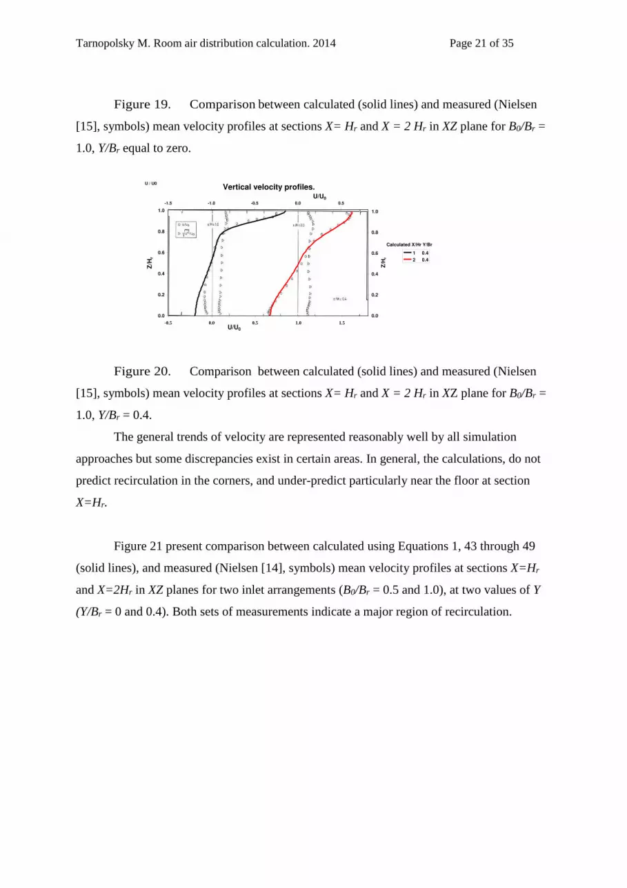
Tarnopolsky M. Room air distribution calculation. 2014 Page 21 of 35
Figure 19. Comparison between calculated (solid lines) and measured (Nielsen
[15], symbols) mean velocity profiles at sections X= Hr and X = 2 Hr in XZ plane for B0/Br =
1.0, Y/Br equal to zero.
Figure 20. Comparison between calculated (solid lines) and measured (Nielsen
[15], symbols) mean velocity profiles at sections X= Hr and X = 2 Hr in XZ plane for B0/Br =
1.0, Y/Br = 0.4.
The general trends of velocity are represented reasonably well by all simulation
approaches but some discrepancies exist in certain areas. In general, the calculations, do not
predict recirculation in the corners, and under-predict particularly near the floor at section
X=Hr.
Figure 21 present comparison between calculated using Equations 1, 43 through 49
(solid lines), and measured (Nielsen [14], symbols) mean velocity profiles at sections X=Hr
and X=2Hr in XZ planes for two inlet arrangements (B0/Br = 0.5 and 1.0), at two values of Y
(Y/Br = 0 and 0.4). Both sets of measurements indicate a major region of recirculation.
Vertical velocity profiles.
0.0
0.2
0.4
0.6
0.8
1.0
-0.5 0.0 0.5 1.0 1.5U/U0
Z/H
r
0.0
0.2
0.4
0.6
0.8
1.0
-1.5 -1.0 -0.5 0.0 0.5
U/U0
Z/H
r
1 0.4
2 0.4
Calculated X/Hr Y/Br
U / U0

Tarnopolsky M. Room air distribution calculation. 2014 Page 22 of 35
Figure 21, Comparison between calculated (solid lines), and measured (Nielsen [14],
two inlet for planes XZin r2H=Xand rH=X sat section svelocity profilemean s) symbol
.)0.4and 0= rBY/( Yat two values of ,)0.5 and 1.0= rB/0B( arrangements
, 43 using Equation 1 xUalculated cbetween show comparison 22 Figure
through 49 by Z = 0 (solid lines) and measured (Nielsen [15], symbols) axial velocity in XZ
.)0.4and 0= rBY/( Yat two values of ,)0.5 and 1.0= rB/0B( two inlet arrangements forplanes
These measurements are compared with the corresponding results obtained in an idealized
wall-jet configuration by Sehwarz and Cosart [17]
Figure 22. Comparison between calculated Ux (solid lines) and measured
(Nielsen [15], symbols) axial velocity in XZ planes for two inlet arrangements (B0/Br = 0.5
and 1.0), at two values of Y (Y/Br = 0 and 0.4).
The calculation of velocity decay corresponded quite well with measurements except
that the measured recirculation in the corner was not predicted.
0.0
0.2
0.4
0.6
0.8
1.0
-1.6 -1.4 -1.2 -1.0 -0.8 -0.6 -0.4 -0.2 0.0 0.2 0.4 0.6
0.0
0.2
0.4
0.6
0.8
1.0
-0.8 -0.6 -0.4 -0.2 0.0 0.2 0.4 0.6 0.8 1.0 1.2 1.4
Z/H
r
U/U0
Z/H
r
U/U0
Vertical velocity profiles.
0.5 1 0
0.5 1 - 0.4
0.5 2 0
0.5 2 - 0.4
1 2 0
1 2 - 0.4
Calculated Bo/Br X/Hr Y/Br
0.01
0.02
0.04
0.08
0.16
0.32
0.64
2 4 8 16 32 64 128
Ux/
U0
X/H0
Velocity of jet.
0.5 0
0.5 -0.4
1 0
1 -0.4
Calculated Bo/Br Y/Br

Tarnopolsky M. Room air distribution calculation. 2014 Page 23 of 35
Offset plane jet.
It should be noted that plane jets are greatly affected by the ceiling or floor, as a result
of the Coanda effect. The static pressure difference between the lower and upper regions of
the current (relative to the current axis) creates a vertical pressure force:
PBrdX = IX
0
p , (50)
where ΔP is elementary static pressure difference between the lower and upper regions of the
current and calculated as momentum flux difference between these current regions:
B
dY )
H
dZU
g -
H - H
dZ U
g( = P
r
20
H-r
2H-Hr
0
B-Br
B-
. (51)
The jet trajectory can be calculated using Equations 41 and 49:
dX I
I + I = H pzX
0 . (52)
If jet attaches to the plate, after impingement, it creates forward and backward flows
near plate, which can be considered as jet continuation. The momentum fluxes of forward If
and backward Ib flows can be determined from preservation of momentum flux before
impingement I and its projection on the plate:
bf I I = I , (53)
bfc I - I = I cos , (54)
accordingly, we obtain the following from Equations 52 and 53:
2/)cos1( cf I I , (55)
2/)cos1( cb I I . (56)
In experiments of Pelfrey and Liburdy [18] and Pramanik and Das [19] a plane jet is
discharged from a nozzle adjacent to a plate parallel to the axis of the nozzle, it bends and
attaches to the plate due to low pressure region created between the jet axis and the solid
boundary (Coanda effect) as shown in Figure 23. The nozzle width was fixed at 12.5 mm and
the span at 150 mm (aspect ratio of 12). The flow exiting the nozzle discharged above a
horizontal plate by an offset ratio 7.0 and was contained by two Plexiglas sidewalls.

Tarnopolsky M. Room air distribution calculation. 2014 Page 24 of 35
Figure 23. Offset jet flow geometry in experiments of Pelfrey and Liburdy [18].
All data presented were for an offset ratio (H/H0) of seven and nozzle Reynolds
number (Re) of 15000 and inlet temperature difference T0 = 0°C. At the nozzle exit the
velocity profile was essentially flat (U0=17.5 m/s). However, a slight skewness was found
(see Figure 23).
Figure 23. Comparison between calculated (solid lines) and measured (Pelfrey
and Liburdy [18], symbols) nozzle exit velocity profile.
Figure 24 shows comparison between calculated using Equation 1, 43 through 48 by Y
= 0 (solid lines) and measured (Pelfrey and Liburdy [18], symbols) the jet development from
the nozzle exit to seventeen nozzle widths (H0) downstream. It is obvious that the flow was
immediately affected by the secondary recirculation in the lower left corner. The attachment
distance along the plate was found to be 13 H0.
Exit velocity profile
-0.50
-0.40
-0.30
-0.20
-0.10
0.00
0.10
0.20
0.30
0.40
0.50
0.92 0.94 0.96 0.98 1.00 1.02U/U0
Z/H
0
Z/Ho
Calculated U/U0
Vertical velocity profiles.
0
1
2
3
4
5
6
7
8
0 1 2 3 4 5 6 7 8 9 10 11 12 13 14 15 16 17 18
X/H0
Z/H
0
0.1
1
2
3
4
5
6
7
8
9
10
11
12
13
14
15
16
17
Calculated U m/s, X/H0

Tarnopolsky M. Room air distribution calculation. 2014 Page 25 of 35
Figure 24. Comparison between calculated (solid lines) and measured (Pelfrey
and Liburdy [18], symbols) vertical mean velocity profiles.
Figure 25 shows comparison between calculated jet trajectory using Equation 44
(solid red line) and back flow (dashed blue line) and measured mean velocity vectors (Pelfrey
and Liburdy [18], arrows).
Figure 25. Comparison between calculated jet trajectory (solid line) and measured
(Pelfrey and Liburdy [18], arrows) mean velocity vectors. One can see satisfactory
coincidence between these measurements and calculated using Equation 1 by Y = 0 velocity
contours in Figure 26.
Figure 26. Calculated jet velocity contours.
Reasonable agreement between the experimental results and calculations has been
observed. For further validation of the calculation result, a comparison between calculated
Velocity vectors and trajectory of jet.
0
1
2
3
4
5
6
7
8
0 1 2 3 4 5 6 7 8 9 10 11 12 13 14 15 16 17 18
X/H0
Z/H
0 Z/Ho
Zb/Ho
Calculated Z/H0
0 2 4 6 8 10 12 14 160
2
4
6
8 Calculated U/U0
X/H0
Z/H0
Velocity contours
0.9-1.0
0.8-0.9
0.7-0.8
0.6-0.7
0.5-0.6
0.4-0.5
0.3-0.4
0.2-0.3
0.1-0.2
0.0-0.1
-0.1-0.0
-0.2--0.1
-0.3--0.2

Tarnopolsky M. Room air distribution calculation. 2014 Page 26 of 35
using Equation 1 by Y = 0 and Z = 0 (solid lines) and measured (Pramanik and Das [19] and
Pelfrey and Liburdy [18], symbols) jet axial velocity is presented in Figure 27. The
calculated centerline velocity decay matches well in the potential core region barring a small
region near the impingement distance about 15 H0.where the experimental results show a
sudden dip in the pattern.
Figure 27. Comparison between calculated (solid lines) and measured (Pramanik
and Das [19], symbols) jet axial velocity.
Non-isothermal attached plane jet in a room.
The air-jet discharged from a ceiling slot inlet in a non-isothermal ventilated enclosure in
experiments of Yu et al. [20]. Two geometrically similar scale models representing a model
and a prototype with ratio of 1:2 (see Figure 28). Both models had an exhaust plenum
between the test room and exhaust duct to reduce the effect of exhaust airflow from the slot
outlet (Xr = L, Hr = H, Br = W, Ho = h, and He = d in Figure 28). In experiments of Yu et al.
[21] the same models were used for isothermal conditions.
Axial velocity of jet.
0.00
0.20
0.40
0.60
0.80
1.00
0 5 10 15 20 25
X/H0
Ux/U
0
Calculated Ux/U0

Tarnopolsky M. Room air distribution calculation. 2014 Page 27 of 35
Figure 28. The scheme and dimensions (prototype/model) of test chambers in
experiments of Yu et al. [20].
Typical vertical velocity profiles of a plane wall isothermal jet (T0 = 0°C) at values for
X of 0.25 Xr, 0.5 Xr, and 0.75 Xr with inlet airspeed of U0=3.41 and U0=3.56 m/s for the
model and prototype respectively in experiments of Yu et al. [21] are compared with
calculated values using Equation 1 by Y = 0 (solid lines) in Figure 29. In calculations, relative
exit velocity profile U/U0 for the model and prototype was the same.
Figure 29. Comparison between calculated (solid lines) and measured (Yu, et al.
[21], symbols o for prototype, and x for model) vertical velocity profiles with inlet airspeed
of U0=3.41 and U0=3.56 m/s for the model and prototype respectively and inlet temperature
difference T0 = 0°C, (U=u, air-jet velocity).
The measured peak velocities of the isothermal jet (Yu et al. [21], empty symbols for
prototype, and filled symbols for model) at specific distances from the inlet are compared
with calculated values using Equation 1 by Y = 0 and Z = 0 (solid lines for prototype, and
dashed lines for model) as a function of Reynolds number Re (based on U0 and H0) in Figure
30.
Vertical velocity profiles.
0.55
0.60
0.65
0.70
0.75
0.80
0.85
0.90
0.95
1.00
1.05
0.00 0.25 0.50 0.75 1.00
X/Xr
Z/H
r
0.25 0.5
0.50 0.5
0.75 0.5
0.25 1.0
0.50 1.0
0.75 1.0
Calculated X/Xr Hr, m

Tarnopolsky M. Room air distribution calculation. 2014 Page 28 of 35
Figure 30. Comparison between calculated (solid lines for prototype, and dashed
lines for model) and measured (Yu et al. [21], empty symbols for prototype, and filled
symbols for model) peak velocities by T0 = 0°C.
One can see satisfactory coincidence between these measurements and calculated
velocities of the isothermal jets by the same relative exit velocity profile U/U0 but different
Reynolds numbers Re for model and prototype.
In experiments of Yu [20] the floor of the prototype was fitted with insulated heat
panels to simulate occupied region surface temperature the airflow patterns were observed
from the contours of velocity and temperature in the chamber.
Figures 31 and 32 shows comparison between calculated trajectory of jet using
Equation 44 by Y = 0 (solid red line) and back flow (dashed blue line) with measured velocity
and temperature contours (Yu [20], contours) by initial jet velocities U0= 0.78 m/s and
temperature difference T0 = -20°C.
Axial velocity of jet.
0
1
2
3
4
5
6
0 1000 2000 3000 4000 5000
Re
Ux,
m/s 0.25 0.5
0.50 0.5
0.75 0.5
0.25 1.0
0.50 1.0
0.75 1.0
Calculated X/Xr Hr, m

Tarnopolsky M. Room air distribution calculation. 2014 Page 29 of 35
Figure 31. Comparison between calculated trajectory of jet (solid red line) and
back flow (dashed blue line) with measured velocity contours (Yu [20], contours) by initial
jet velocities U0= 0.78 m/s and temperature difference T0 = -20°C,
Figure 32. Comparison between calculated trajectory of jet (solid red line) and
back flow (dashed blue line) with measured temperature contours (Yu [20], contours) by
initial jet velocity U0= 0.78 m/s and temperature difference T0 = -20°C.
One can see satisfactory coincidence between these measurements (see Figures 31
and 32) and calculated velocity using Equation 1 by Y = 0 and temperature using Equation 15
by Y = 0 contours (see Figures 33 and 34), correspondingly.
Figure 33. Calculated velocity contours by initial jet velocity U0= 0.78 m/s and
temperature difference T0 = -20°C.
0.0 0.2 0.4 0.6 0.8 1.0 1.2 1.4 1.6 1.8
0.0
0.2
0.4
0.6
0.8
1.0
Z, m
X, m
Calculated Ux/U0
Velocity contours.
1.0-1.1
0.9-1.0
0.8-0.9
0.7-0.8
0.6-0.7
0.5-0.6
0.4-0.5
0.3-0.4
0.2-0.3
0.1-0.2
0.0-0.1
-0.1-0.0
-0.2--0.1
-0.3--0.2
-0.4--0.3
0.0
0.2
0.4
0.6
0.8
1.0
0.0 0.2 0.4 0.6 0.8 1.0 1.2 1.4 1.6 1.8 2.0
H, m
X, m
Temperature contours and trajectory of jet.
H
Hb
Calculated H, m

Tarnopolsky M. Room air distribution calculation. 2014 Page 30 of 35
Figure 34. Calculated temperature contours by initial jet velocity U0= 0.78 m/s
and temperature difference T0 = -20°C.
The trajectory, velocity, and temperature of jet predicted by calculation matches well
barring a small region near the floor at impingement distance about 1.0, m.
Conclusions.
This study presents basic concepts of a semi-empirical method for calculating the
velocity and temperature fields in rooms. The method takes into consideration the interaction
between the various jets in the room, the boundaries of the room and the counter flow
between jet and enclosure by adding the momentum flux of all jets at each point.
To explore impact of initial velocity and temperature difference profiles, inlet divided
to increments of elementary jets. The effect of the walls is calculated by the mirror method.
The velocity and temperature difference at point considered are determined by adding
momentum flux and excess heat, as supplied from all real, mirror, and elementary jets. Then
this solution has corrections of the velocity field for deviations from the equations of
continuity and momentum flux, taking into consideration the counter flow between jet and
enclosure. Similarly, the temperature field is calculated so that the heat balance equation is
preserved.
Two- and three-dimensional calculations compared with measurements performed
under isothermal and buoyant conditions. Almost all the calculations can predict the
isothermal airflow patterns with an acceptable degree of realism. In many cases, the predicted
occupied zone air velocities are within a band indicating general compliance with
expectation. Small recirculation areas in the corners of the room were usually not predicted
though their impact is believed small.
0.0 0.2 0.4 0.6 0.8 1.0 1.2 1.4 1.6 1.8
0.0
0.2
0.4
0.6
0.8
1.0
Z, m
X, m
Calculated T, deg
Temperature contours.
40-41
39-40
38-39
37-38
36-37
35-36
34-35
33-34
32-33
31-32
30-31
29-30
28-29
27-28
26-27
25-26
24-25
23-24
22-23
21-22

Tarnopolsky M. Room air distribution calculation. 2014 Page 31 of 35
In buoyant flow, it has been shown that calculations can predict flow pattern, velocity
and temperature distribution, although with a reliability reduced from that demonstrated for
isothermal flow.
After impingement in the corner, the jet flow reattached to the wall surface and the
flow directed parallel to the wall, with the jet thickness growing downwards. Experiments and
calculations revealed that the air velocity distribution in the ceiling-wall and wall-floor
corners is nearly symmetric and flow after impingement can be considered as jet
continuation.
Calculation of the supply jet characteristics from number of models (approaches) by
dividing inlet to increments of elementary jets reveal consistent differences throughout the
near field. In the self-similar far field, the rates of centerline velocity and temperature decay
decreased in an asymptotic-like manner. It would be helpful if the manufacturers of air
diffusers would publish some near field data (e.g. profiles in front of the device) with their
technical specifications.
NOMENCLATURE.
AR slot aspect ratio
B, H coordinates of current trajectory along axes Y and Z (given by Equations 40, 41, and
52), m
Bo, Ho width and height of inlet, respectively, along axes Y and Z, m
Br, Hr, Xr width, height, and length of room, respectively, along axes Y, Z, and X, m
C empirical constant (a value of C = 0.082 is used here)
Ch specific heat of air (at constant pressure), kJ//kg/ oK
Ct, temperature profile constant (given by Equation 13)
De equivalent diameter of the rectangular slot, m
dIt buoyancy force, created by temperature-density difference between elementary volume
of current and ambient air (given by Equation 32), N
Do, diameter of round inlet, m
G quantity of air moving trough cross-section considered of room (given by Equation 22),
N s-1
g acceleration due to gravity, m/s2
Gc quantity of air in current cross-section considered (given by Equation 24),
N s-1

Tarnopolsky M. Room air distribution calculation. 2014 Page 32 of 35
I, Ix, Iy, Iz components and resultant momentum flux in cross-section of room (given by
Equations 35-38, 49, and 53), N
Ib the momentum flux of the backward flow near floor (given by Equation 48, 5655), N
Ic initial momentum flux of the current (given by Equation 20), N
Ie momentum flux of air removal in ross-section considered (given by Equation 30), N
If the momentum flux of the forward flow near floor (given by Equation 55), N
Ip vertical pressure force created by static pressure difference between the lower and
upper regions of the current (relative to the axis) and (given by Equation 42, 50), N
Iu momentum flux in cross-section of room (given by Equation 29), N
i ordinal number of elementary jet
Jy, My ordinal and total numbers of real and virtual jets interacted, respectively, along axis Y
Jz, Mz ordinal and total numbers of real and virtual jets interacted, respectively, along axis Z
Ky, Ny ordinal and total numbers of increments, respectively, in inlet along axis Y
Kz, Nz ordinal and total numbers of increments, respectively, in inlet along axis Z
Ly, Lz no dimensional discharge factors (given by Equations 25, 26)
Pa static pressure in the cross-section of outlet (by X=Xa), Pa
Po static pressure in the cross-section of inlet (by X=0), Pa
Ps static pressure in current cross-section considered of room (given by Equation 42), Pa
Qc inlet excess heat (given by Equation 21), W
Qy, Qz no dimensional factors of excess heat (given by Equations 33, 34)
r orifice radius, m
S distance from inlet to cross section considered of current along jet axis, m
Scw distance from the slot to the separation point in the ceiling-wall corner (given by
Equation 43), m
Swf distance from the slot to the to the separation point in the wall-floor corner (given by
Equation 46), m
T temperature difference at point considered, oC
Ta absolute temperature of ambient air, oK
Tc current temperature difference (given by Equation 15), oC
Ti temperature difference induced by i - elementary jet, (given by Equation 6), oC
Tk inlet temperature difference of cell made by increments Ky and Kz, oC
Tm temperature difference on axis of i - elementary jet (selected from Equations
11 and 12), oC
To inlet axial temperature difference, oC

Tarnopolsky M. Room air distribution calculation. 2014 Page 33 of 35
Ty, Tz no dimensional factors of current temperature difference (given Equations 18, 19)
U velocity at point considered (given by Equation 1), m/s
Uc current velocity at point considered (given by Equation 14), m/s
Ue air-removal velocity in cross-section considered of room (given by Equations 27), m/S
Ui air velocity induced by i - elementary jet (given by Equation 5), m/s
Uk inlet velocity of cell made by increments Ky and Kz, m/s
Um air velocity on axis of i - elementary jet (selected from Equations 11), m/s
Uo inlet axial velocity, m/s
Us velocity “shift” (given by Equation 23), m/s
Ux axial velocity (given by Equation 1, Y = 0, and Z = 0), m/s
Uy, Uz no dimensional factors of current velocity (given by Equations 16, 17)
X, Y, Z coordinates of point considered, m
Xa distance from inlet to outlet position, m
Xb distance from inlet to the measured sections of the back flow near floor, m
Xw distance from slot to the measured sections of jet near vertical wall (given by
Equation 44), m
Xwf distance from the jet slot to the wall-floor corner (given by Equation 45), m
Y0.5, Z0.5 no dimensional half-velocity width in the central XY and XZ planes,
correspondingly
Yj, Zj coordinates of point considered in jet j (given by Equations 7, 8), m
Zcw jet thickness at the distance from the jet slot to the ceiling-wall corner (Xr), m
Zwf jet thickness at the distance from the jet slot to the wall-floor corner (Xwf), m
αc angle between current trajectory projection in XY plane and X axis, degrees
c angle between current trajectory projection in XZ plane and X axis, degrees
xy angle between current trajectory and XY plane [ xy = atan(cosαc tan c)], degrees
δ, η coordinates of elementary jet i in inlet along axes Y and Z, m
δk, δk+1 start and end of increment Ky, respectively, in inlet along axis Y, m
ΔP elementary static pressure difference between the lower and upper current parts (given
by Equation 51), Pa
specific weight of the air at point considered (given by Equation 4), N m
a specific weight of ambient air, N m
ηk ,ηk+1 start and end of increment Kz, respectively, in inlet along axis Z, m
σ turbulent Prandtl number (a value of σ = 0.5 is used here)

Tarnopolsky M. Room air distribution calculation. 2014 Page 34 of 35
REFERENCES
1. Crow, S. C., and Champagne, F. H., 1971, Orderly Structure in Jet Turbulence. J.
Fluid Mech., 48, pp. 547–591.
2. Becker, H. A., Hotel, H. C., and Williams, G. C., 1967. The Nozzle-Fluid
Concentration Field of the Round, Turbulent, Free Jet. J. Fluid Mech., 30, pp.
285–303.
3. Wygnanski, I., Champagne, F., and Marasli, B., 1986, ‘‘On the Large-Scale
Structures in Two Dimensional, Small-Deficit, Turbulent Wakes,’’ J. Fluid
Mech., 168, pp. 31–71.
4. George, W. K., 1989. The Self-Similarity of Turbulent Flows and Its Relation to
Initial Conditions and Coherent Structures. Recent Advances in Turbulence,
R. E. A. Arndt and W. K. George, eds., Hemisphere, New York, pp.39–73.
5. R.C. Deo, 2005. Experimental investigations of the influence of Reynolds number and
boundary conditions on a plane air jet, Ph.D. Thesis, School of Mechanical
Engineering, The University of Adelaide, South Australia 5005.
6. R. C. Deo , Jianchun Mi , Graham J. Nathan, 2007. The influence of nozzle-exit
geometric profile on statistical properties of a turbulent plane jet. Experimental
Thermal and Fluid Science 32, pp.545–559
7. W.R. Quinn, J., Militzer,1989. Effects of nonparallel exit flow on round turbulent free
jets International Journal of Heat and Fluid Flow, Volume 10, Issue 2, June, pp. 139-
145
8. W. R. Quinn, 1992. Flows Issuing from Sharp-Edged Rectangular Slots: The
Influence of Slot Aspect Ratio. Fluid Science , 5, pp.203-215
9. Guangyu Cao, 2009. MODELLING THE ATTACHED PLANE JET IN A ROOM.
Doctoral Dissertation. Helsinki University of Technology, Faculty of Engineering and
Architecture, Department of Energy Technology
10. Guangyu Cao, Mika Ruponen, Jarek Kurnitski, 2010. Experimental investigation of
the velocity distribution of the attached plane jet after impingement with the corner in
a high room. Energy and Buildings 42, pp. 935–944
11. Yushui, Guangyu Cao, Mika Ruponen3and, Kim Hagström. 2010. Experimental study
of the non-isothermal attached plane jet after impinging the corner in a high room.
IAQVEC, Paper ID , pp.218-220

Tarnopolsky M. Room air distribution calculation. 2014 Page 35 of 35
12. Guangyu Cao, Mika Ruponen, Risto Paavilainen, Jarek Kurnitski, 2011. Modelling
and simulation of the near-wall velocity of a turbulent ceiling attached plane jet
after its impingement with the corner. Building and Environment 46, pp. 489-500
13. T. Smith, P.W. Duck, 1977. Separation of jets of thermal boundary layers from a wall.
Quarterly Journal of Mechanics and Applied Mathematics 30, pp.143–156.
14. P. V. Nielsen, A. Restivo and J. H. Whitelaw. 1978. The Velocity Characteristics of
Ventilated Rooms. Fluids Eng. 100(3), 291-298
15. Nielsen, P. V., 1990. Specification of a Two-Dimensional Test Case. International
Energy Agency, Annex 20. Aalborg: Institut for Bygningsteknik, Aalborg Universitet.
Gul serie; No. 8, Vol. R9040. 15 p.
16. Q. Chen, M. Ewert, J. Heikkinen, C. A. Moser, P.V. Nielsen, G. Whittle, 1993. Room
Air and Contaminant Flow, Evaluation of Computational Methods. Energy
Conservation in Buildings and Community Systems, Annex 20: Air Flow Patterns
within Buildings.pp.1-95
17. Schwarz, W. H., and Cosart, W. P., "The Two-Dimensional Turbulent Wall-Jet," J.
Fluid Mech., Vol. 10, 1961, p. 481.
18. J. R. R. Pelfrey and J. A. Liburdy 1986. Mean Flow Characteristics of a Turbulent
Offset Jet. J. Fluids Eng. 108(1), pp.82-88
19. Shantanu Pramanik, Manab Kumar Das, 2013. Numerical characterization of a planar
turbulent offset jet over an oblique wall. Computers & Fluids 77, pp.36–55
20. Hsin Yu, 2006. A Modified Estimation of a Plane Wall Jet Trajectory Horizontally
diffused from a Ceiling Slot in Non-isothermal Ventilated Enclosures. Biosystems
Engineering (2006) 95 (2), pp.255–269
21. Hsin Yu,; Li-John Jou2; Huei-Tau Ouyang1; Huang-Min Liang3; Chung-Min Liao,
2006. Similitude Criteria for a Two-dimensional Wall Jet in an Isothermal
Mechanically Ventilated Enclosure. Bio systems Engineering, 93 (4), 415–425
22. I. A. Sheplev, 1978. Airflow room aerodynamics. Stroyizdat, Moscow, 145 p.
23. Tarnopolsky, M. 1994. Improved calculation of air distribution in an auditorium.
ASHRAE Transactions.100, pp.1195-1209.