arX

iv:1

303.

6732

v1 [

hep-

th]

27

Mar

201

3

ITP–UH–06/13CBPF-NF-001/13

Target duality in N=8 superconformal mechanics

and the coupling of dual pairs

Marcelo Gonzales†, Sadi Khodaee∗, Olaf Lechtenfeld× and Francesco Toppan∗

†Carrera de FısicaUniversidad Autonoma Tomas Frıas

Av. Del Maestro s/n, Casilla 36, Potosı, BoliviaEmail: marcbino@gmail.com

∗TEO, CBPFRua Dr. Xavier Sigaud 150 (Urca)

Rio de Janeiro (RJ), cep 22290-180, BrazilEmails: khodaee@cbpf.br, toppan@cbpf.br

×Institut fur Theoretische Physik and Riemann Center for Geometry and PhysicsLeibniz Universitat Hannover

Appelstraße 2, 30167 Hannover, GermanyEmail: lechtenf@itp.uni-hannover.de

Centre for Quantum Engineering and Space-Time ResearchLeibniz Universitat Hannover

Welfengarten 1, 30167 Hannover, Germany

Abstract

We couple dual pairs of N=8 superconformal mechanics with conical targets of dimension dand 8−d. The superconformal coupling generates an oscillator-type potential on each of the twotarget factors, with a frequency depending on the respective dual coordinates. In the case ofthe inhomogeneous (3,8,5) model, which entails a monopole background, it is necessary to addan extra supermultiplet of constants for half of the supersymmetry. The N=4 analog, joiningan inhomogeneous (1,4,3) with a (3,4,1) multiplet, is also analyzed in detail.

1 Introduction and summary

N -extended superconformal mechanics (for a review, see [1]) is defined on off-shell supermultipletscontaining propagating bosons, fermions and auxiliary fields and, following the conventions of [2],being denoted by (d,N ,N−d). Their associated invariant actions define one-dimensional sigmamodels with a d-dimensional conical target manifold. The case of N=8 has been studied lessextensively than those with N=2 or N=4. However, in the literature one finds invariant actionsfor the supermultiplets (1,8,7) [3, 4], (3,8,5) [5, 6] and (5,8,3) [5, 7]. The (2,8,6) model is free.

In this paper, we make use of a d ↔ N−d duality observed in [8] to couple for the first timetwo dually related superconformal mechanics. Depending on the target dimension d, for N=8 thecoupled systems are invariant under one of the four one-dimensional finite superconformal algebrasA(3, 1), D(4, 1), D(2, 2) or F (4). Their target manifold is a product of two asymptotically flatcones of dimension d and 8−d over the spheres Sd−1 and S7−d, respectively.

The possibility of consistently coupling dually related supermultiplets was first observed, forhomogeneous supersymmetry transformations, in [9]. This produces N=8 superconformal systemswith targets of dimension d = 1+7, 2+6 or 3+5 (the 4-dimensional system is degenerate, andthe dual of the 8-dimensional system is empty). However, for the particular cases of (N=4, d=1)and (N=8, d=3), an inhomogeneous deformation of the supersymmetry is admissible (see, e.g., [10]and [8], respectively). The presence of an inhomogeneity parameter is responsible for the appearanceof a Calogero potential in the N=4, A(1, 1)-invariant, (1,4,3) model and of a Dirac monopole in theN=8, D(2, 1)-invariant, (3,8,5) model, as will be reviewed below. In these instances, a consistentsuperconformal coupling of the inhomogeneous supermultiplet with its (homogeneous) dual is non-trivial, as will be shown here. It requires the introduction of an extra supermultiplet of constantsfor half of the supersymmetries and leads to new superconformal interactions in the presence of aCalogero potential or a monopole. In particular, in all cases (homogeneous or not), an oscillatorpotential on each of the two cones is generated, with a frequency depending on the mutually dualcoordinate.

The description of the models is given in a Lagrangian framework. By setting all fermionicfields to zero and eliminating the auxiliary fields, we are led to the dynamics of two interactingbosonic sigma models whose parameters are fixed by superconformal invariance. Passing to conicalradial variables then reveals the geometry and the physical content of the coupled model. In thisfashion, our results provide an extension of the class of known superconformal models.

Some interesting questions are left for future investigations. In particular, it seems quite plausi-ble that the bosonic sector of the dually coupled models, whose parameters are fixed by supercon-formal invariance, turn out to be integrable, as a remnant of the off-shell invariant transformations.

The paper is structured as follows. After reviewing general features of (d, 8, 8−d) supermulti-plets in Section 2, we present in Section 3 the superconformal pairing of dually related multipletsand work out the coupled Lagrangian in the case of homogeneous supersymmetry, ending up withthe general bosonic potential on the cone product in the presence of Fayet-Iliopoulos terms. Sec-tions 4 and 5 deal with the inhomogeneous (3,8,5) supermultiplet, its Dirac monopole backgroundand the corresponding gauge transformations. In Section 6, the dual (5,8,3) supermultiplet is dis-played, before Section 7 couples it to the inhomogeneous (3,8,5) model. Here one finds the centralresults of the paper. In Section 8 we reduce the coupled system back to the (5,8,3) supermultiplet.Complete actions and the N=4 coupling of the inhomogeneous (1,4,3) supermultiplet with its dual(3,4,1) partner are presented in detail in three Appendices.

1

2 Generalities for (d,8,8−d) supermultiplets

N=8 superconformal mechanical systems realize the one-dimensional global supersymmetry algebra

Qi, Qj

= 2δijH with i, j = 1, . . . , 8 and H = ∂t , (2.1)

where t parametrizes the particle worldline. The corresponding supermultiplets are denoted by(d,8,8−d), indicating d propagating bosonic, 8 propagating fermionic and 8−d auxiliary bosoniccoordinate functions for the superparticle, which thus moves on some d-dimensional target spaceparametrized by x = xa | a = 1, . . . , d.

In the construction of N=8 superconformal actions we can make manifest at most four of theeight supersymmetries. Picking by convention Q1, Q2, Q3 and Q8, an N=4 invariant action reads

Sd =

∫dt Ld =

∫dt Q8Q1Q2Q3F (x) , (2.2)

where F (x) is a yet unconstrained function of all coordinates. The restriction to the manifest N=4superalgebra splits the N=8 supermultiplet,

(d, 8, 8−d) −→ (d1, 4, 4−d1) ⊕ (d2, 4, 4−d2) with d1, d2 ≤ 4 and d1 + d2 = d (2.3)

and opposite chiralities.1 It turns out that the action depends only on two combinations of secondderivatives of F , namely 2

Φ1 = −∆d1F ≡ −F1 1 − . . .− Fd1d1 and Φ2 = ∆d2F ≡ Fd1+1 d1+1 + . . .+ Fd d , (2.4)

where we grouped the coordinates according to the decomposition above.

To enhance to N=8 invariance, we must impose

QℓLd = ∂tWℓ for ℓ = 4, 5, 6, 7 . (2.5)

This produces a harmonicity condition on F ,

∆dF ≡ δabFab = 0 . (2.6)

As a consequence, we have

Φ1 = Φ2 =: Φ with ∆dΦ = 0 . (2.7)

Clearly, for d ≤ 5, we may take d2 = 1 so that Φ = Fdd, singling out the last coordinate. Hence,taking F to be harmonic, we obtain an N=8 sigma model, with a conformally flat target space forthe propagating bosonic coordinates,

ds2 = Φ(x) δabdxadxb . (2.8)

The remaining generators of the conformal sl(2) algebra are realized as

K = −t2∂t − 2t λϕ and D = −t ∂t − λϕ (2.9)

1The construction fails if d1 = 0 or d2 = 0. There exists, however, a different method which works in all cases [11].2Except for d=3, where an inhomogeneous deformation yields a background gauge potential, see below.

2

on functions ϕ with engineering dimension [ϕ] = λϕ. They give rise to 8 superconformal genera-tors [10, 8]

Qi = [K,Qi] . (2.10)

Superconformal symmetry is imposed by also demanding that 3

DLd = ∂tMD and K Ld = ∂tMK , (2.11)

which yields two conditions on Φ, namely

[Φ] = −1− 2λx and Φ = Φ(r) with r2 = δabxaxb . (2.12)

The closure of the D-module representation for the N=8 superconformal algebra determines acritical value for the engineering dimension of x,

λx = 1d−4 ⇒ [Φ] = −1− 2

d−4 = d−24−d = (2−d)λx . (2.13)

As a consequence, the conformal factor is indeed fixed to the proper harmonic expression,

Φ(r) = r2−d . (2.14)

Introducing the spherical line element dΩd−1 on Sd−1 and changing the radial coordinate via

ρ = 2|4−d|r

(4−d)/2 , (2.15)

the metric reads

ds2 = r2−d(dr2 + r2dΩ2

d−1

)= dρ2 + 1

4 (4−d)2ρ2dΩ2

d−1 . (2.16)

It reveals the target space to be a specific cone over Sd−1, asymptotically flat with a linear relativedeficit of |4−d|/2. Its scalar curvature comes out as

R = 14(d−1)(d−2)

2(d−6)rd−4 = (d−1)(d−2)2(d−6)(d−4)−2ρ−2 , (2.17)

which is negative for d = 3, 5 and positive for d = 7, 8. At d = 2, 6 we encounter flat space.

In any dimension d up to 8, the manifest N=4 superconformal algebra must be a particularmember of the D(2, 1;α) family. It turns out that the value of α is determined (up to an S3automorphism) by the relation

α = −12 |4−d| = − 1

2|λx|. (2.18)

In fact, only for the special values

α ∈−3,−2,−3

2 ,−1,−23 ,−

12 ,−

13 , 0,

12 , 1, 2, ∞

(2.19)

attained via (2.18) (and its S3 orbit) is D(2, 1;α) extendable to an N=8 superconformal algebra.

3The ‘D condition’ actually follows from the ‘K condition’.

3

3 Duality and coupling in the homogeneous case

From the results of the previous section, an obvious duality relates

d ↔ 8−d ⇔ λx ↔ −λx ⇔r↔ 1

r and Sd−1 ↔ S7−d. (3.1)

The self-dual point at d=4, however, represents a degenerate case, and the case of d=0 is empty.We summarize the values for all dimensions in the following table, which displays also the manifestN=4 superalgebra G4 and the full N=8 superalgebra G8 for each case.

d 0 1 2 3 4 5 6 7 8

Φ r2 r 1 r−1 r−2 r−3 r−4 r−5 r−6

λx −14 −1

3 −12 −1 ∞ +1 +1

2 +13 +1

4

α −2 −32 −1 −1

2 0 −12 −1 −3

2 −2

G4 D(2, 1) D(2, 1; 12) A(1, 1) D(2, 1) A(1, 1) D(2, 1) A(1, 1) D(2, 1; 1

2) D(2, 1)

G8 D(4, 1) F (4) A(3, 1) D(2, 2) − D(2, 2) A(3, 1) F (4) D(4, 1)

The duality map indicated in (3.1) is easily performed by interchanging propagating and aux-iliary bosons and flipping the direction of the supersymmetry transformations. If we summarilydenote the propagating bosons, fermions and auxiliary bosons by xa, ψi and fα, respectively, andindicate the components of the dual multiplet by overtildes and lowered indices, the structureschematically takes the following form,

xaQ−→ ψi Q

−→ (fα, xa)Q−→ ψi

l l l˙ψi

Q←− ( ˙xa, fa)

Q←− ψi

Q←− xα

where the horizontal arrows encode the various supersymmetry transformations and the verticalarrows depict the duality relations.

We have essentially three different cases of such a duality for N=8 superconformal theories:

(1, 8, 7) ↔ (7, 8, 1) , (2, 8, 6) ↔ (6, 8, 2) , (3, 8, 5) ↔ (5, 8, 3) . (3.2)

The two members of each pair have different target dimensions but share the same superconformalalgebra. For this reason, they can be coupled together in a Lagrangian

Ld+(8−d) = Ld + L8−d + γ Ld,(8−d) , (3.3)

with a coupling of dimensionless strength γ provided by a canonical pairing,

Ld,(8−d) = xafa + ψiψi − fαxα . (3.4)

Note that the dimensions in each pairing add up to one, and the duality guarantees the N=8 su-perconformal invariance of the coupling term, as long as the transformations remain homogeneous.This is the case for d=1 and d=2. In three dimensions, there exists an inhomogeneous deformation

4

of the (3,8,5) multiplet. When this is turned on, the coupling to the dual (5,8,3) becomes lessobvious. We will dwell on this point later on.

Let us take a look at the bosonic part of the Lagrangian in the homogeneous case. It takes theform

Ld+(8−d)

∣∣ = Φ(r)(xaxa + fαfα

)+ Φ(r)

(˙xα ˙xα + fafa

)+ γ

(xafa − f

αxα). (3.5)

We may add Fayet-Iliopoulos terms with dimensionful parameters µα and µa to get

L′d+(8−d)

∣∣ = Ld+(8−d)

∣∣+ µαfα − µafa . (3.6)

Eliminating the auxiliary components by their equations of motion,

fα = 12Φ

−1(γxα − µα

)and fa = −1

2Φ−1

(γxa − µa

), (3.7)

we arrive at

L′′d+(8−d)

∣∣ = Φ xaxa + Φ ˙xα ˙xα −14Φ

−1(γxα−µα

)(γxα−µα

)− 1

4Φ−1

(γxa−µa

)(γxa−µa

), (3.8)

which features a very specific potential in the joint target space of both multiplets.

For a physical interpretation, it is useful to fix Φ(r) = r2−d and Φ = rd−6 and pass to standardradial coordinates (up to a factor of 1

2),

ρ(r) = 2|4−d|r

(4−d)/2 and ρ(r) = 2|4−d| r

(d−4)/2 . (3.9)

Introducing total angular momenta ℓ and ℓ for the d- and (8−d)-dimensional targets and unitvectors via xa = rea and xα = reα, one arrives at

Lconed+(8−d)

∣∣ = ρ2 + 4ℓ2

|d−4|2ρ−2 + ˙ρ

2+ 4ℓ2

|d−4|2ρ−2 − 1

4Φ−1

(γr~e− ~µ

)2− 1

4Φ−1

(γr~e− ~µ

)2, (3.10)

where r = r(ρ) and r = r(ρ) is understood. Apart from the standard angular momentum ‘barriers’,

the potential for the coordinates r and r is of oscillator type, centered around ~r = ~µ/γ and ~r = ~µ/γand with (position-dependent) frequencies ω = γ

2 Φ−1/2 and ω = γ

2Φ−1/2, respectively.

4 D-module representation of the (3,8,5) supermultiplet

Let us adopt a convenient notation for the components of the (3,8,5) multiplet:

bosons xa: x, y, z or x1, x2, x3

fermions ψi: ψ0, ψ1, ψ2, ψ3, ξ0, ξ1, ξ2, ξ3

auxiliaries fα: f1, f2, g, g1, g2

. (4.1)

For simplicity, we lower all indices. According to the relations of Section 2, we have λx = −1and α = −1

2 , so the N=4 algebra D(2, 1;−12 ) ≃ D(2, 1; 1) ≃ osp(4|2) should get enlarged to an

D(2|2) ≃ osp(4|4) algebra. For the conformal factor we expect Φ = 1r .

A unique feature specific to d=3 is the option to deform the homogeneous superconformaltransformations by a constant shift in some transformations of fermions to auxiliaries. Without

5

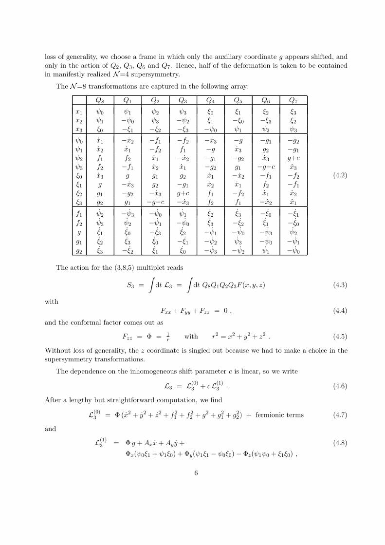
loss of generality, we choose a frame in which only the auxiliary coordinate g appears shifted, andonly in the action of Q2, Q3, Q6 and Q7. Hence, half of the deformation is taken to be containedin manifestly realized N=4 supersymmetry.

The N=8 transformations are captured in the following array:

Q8 Q1 Q2 Q3 Q4 Q5 Q6 Q7

x1 ψ0 ψ1 ψ2 ψ3 ξ0 ξ1 ξ2 ξ3x2 ψ1 −ψ0 ψ3 −ψ2 ξ1 −ξ0 −ξ3 ξ2x3 ξ0 −ξ1 −ξ2 −ξ3 −ψ0 ψ1 ψ2 ψ3

ψ0 x1 −x2 −f1 −f2 −x3 −g −g1 −g2ψ1 x2 x1 −f2 f1 −g x3 g2 −g1ψ2 f1 f2 x1 −x2 −g1 −g2 x3 g+cψ3 f2 −f1 x2 x1 −g2 g1 −g−c x3ξ0 x3 g g1 g2 x1 −x2 −f1 −f2ξ1 g −x3 g2 −g1 x2 x1 f2 −f1ξ2 g1 −g2 −x3 g+c f1 −f2 x1 x2ξ3 g2 g1 −g−c −x3 f2 f1 −x2 x1

f1 ψ2 −ψ3 −ψ0 ψ1 ξ2 ξ3 −ξ0 −ξ1f2 ψ3 ψ2 −ψ1 −ψ0 ξ3 −ξ2 ξ1 −ξ0g ξ1 ξ0 −ξ3 ξ2 −ψ1 −ψ0 −ψ3 ψ2

g1 ξ2 ξ3 ξ0 −ξ1 −ψ2 ψ3 −ψ0 −ψ1

g2 ξ3 −ξ2 ξ1 ξ0 −ψ3 −ψ2 ψ1 −ψ0

(4.2)

The action for the (3,8,5) multiplet reads

S3 =

∫dt L3 =

∫dt Q8Q1Q2Q3F (x, y, z) (4.3)

withFxx + Fyy + Fzz = 0 , (4.4)

and the conformal factor comes out as

Fzz = Φ = 1r with r2 = x2 + y2 + z2 . (4.5)

Without loss of generality, the z coordinate is singled out because we had to make a choice in thesupersymmetry transformations.

The dependence on the inhomogeneous shift parameter c is linear, so we write

L3 = L(0)3 + cL

(1)3 . (4.6)

After a lengthy but straightforward computation, we find

L(0)3 = Φ(x2 + y2 + z2 + f21 + f22 + g2 + g21 + g22) + fermionic terms (4.7)

and

L(1)3 = Φ g +Axx+Ayy + (4.8)

Φx(ψ0ξ1 + ψ1ξ0) + Φy(ψ1ξ1 − ψ0ξ0)− Φz(ψ1ψ0 + ξ1ξ0) ,

6

where we introducedAx = Fzy and Ay = −Fzx . (4.9)

The complete expression of L(0)3 is displayed in Appendix A. Setting all fermions to zero, we extract

the bosonic part

L3∣∣ = Φ(x2 + y2 + z2 + f21 + f22 + g2 + g21 + g22) + c (Φ g +Axx+Ay y) . (4.10)

We remark that only the z derivative of F appears, so it makes sense to define a prepotential

G := Fz ⇒ Gx = −Ay , Gy = Ax , Gz = Φ , (4.11)

which inherits the harmonicity from F .

It is admissible to slightly deform our model by adding Fayet-Iliopoulos terms. This extendsthe bosonic Lagrangian to

L′3∣∣ = L3

∣∣+ µαfα + ζg + ζαgα with α = 1, 2 (4.12)

and five real parameters µα, ζ and ζα.

We solve the equations of motion for the auxiliary fields,

fα = −µα2Φ

, g = −ζ + cΦ

2Φ, gα = −

ζα2Φ

, (4.13)

and eliminate them from the Lagrangian to arrive at

L′′3∣∣ = Φ(x2 + y2 + z2) − 1

4Φ−1(µ2α + ζ2 + ζ2α) −

12c ζ −

14c

2Φ + c (Axx+Ay y) . (4.14)

Apparently, there is not only a magnetic but also an electric field, together

Bx = cGxz , By = cGyz , Bz = −c(Gxx+Gyy) = cGzz and Ea = −14c

2Gza , (4.15)

both being simply proportional to the gradient of Gz = Φ. With Φ = 1r , we identify a magnetic

monopole, while for the interpretation of the electric field we better pass to the conical coordinates,

r = 14ρ

2 ⇒ ds2 = dρ2 + 14ρ

2dΩ22 and A0 = c2ρ−2 . (4.16)

The bosonic dynamics of this theory has been analyzed for general values of α in [12].

5 Gauge freedom

In order to explicitly write down the Lagrangian, we must ‘integrate’ Φ to find the prepotential G,from which the gauge potential A is obtained. The answer is not unique, due to abelian gaugeinvariance,

δAa = ∂au and δG = v (5.1)

with a priori arbitrary harmonic gauge functions u and v. However, the invariance of Φ=Gz enforcesvz = 0, and the relation between G and Aa connects the two functions,

ux = vy and uy = −vx . (5.2)

7

The (local) solution introduces another function h(x, y) via

u = hy(x, y) + u(z) and v = hx(x, y) with hxx + hyy = 0 . (5.3)

The harmonicity of u implies that u is at most linear in z. Alternatively, we may interpret theabove relation as Cauchy-Riemann equations for the real and imaginary part of a holomorphicfunction of w = x+ iy,

v − i(u−u) = E(w) =: ∂wH(w) ⇒ h = H(w) +H(w) , (5.4)

where H and h are determined up to a constant. Therefore, the gauge freedom for the prepotentialis encoded in a single holomorphic function E.

For the magnetic monopole there does not exist a globally regular gauge potential; we must becontent with configurations on a ‘northern’ (N) and on a ‘southern’ (S) patch, related by a regulargauge transformation in the equatorial overlap. The standard expressions obtained from Gz = 1

rread

GN = + ln(r+z) ⇒ ANx = GN

y = yr(z+r) and AN

y = −GNx = − x

r(z+r) ,(5.5)

GS = − ln(r−z) ⇒ ASx = GS

y = yr(z−r) and AS

y = −GSx = − x

r(z−r) ,(5.6)

so that indeed (for a = x, y)

GN −GS = ln(x2+y2) =: hx ⇒ ANa −A

Sa = −2∂a arctan

yx =: ∂ahy , (5.7)

and the holomorphic combination

E = ln(x2+y2) + 2i arctan yx = lnw2 (5.8)

gives rise to the correct ‘pre-gauge’ function

H = 2w(lnw−1) ⇒ h = x ln(x2+y2)− 2x− 2y arctan yx (5.9)

in the class described above and regular away from the poles. The singularity of the northernfunctions along the negative z-axis and likewise for the southern patch signify the would-be Diracstring in a global configuration.

6 The dual (5,8,3) supermultiplet

Applying the duality reflection to the (3,8,5) multiplet, we obtain a (5,8,3) multiplet. However,we must first put the inhomogeneous deformation parameter c to zero, since such a deformationdoes not exist for d=5. Section 2 tells us that λx = +1 and Φ = r−3, and we again realize anD(2, 2) ≃ osp(4|4) superalgebra. Naming the components as follows,

bosons xα: v1, v2, w,w1, w2

fermions ψi: χ0, χ1, χ2, χ3, λ0, λ1, λ2, λ3

auxiliaries fa: h1, h2, h3

, (6.1)

8

the array (4.2) gets transformed into the N=8 transformations for the (5,8,3) multiplet:

Q8 Q1 Q2 Q3 Q4 Q5 Q6 Q7

v1 λ2 −λ3 −λ0 λ1 χ2 χ3 −χ0 −χ1

v2 λ3 λ2 −λ1 −λ0 χ3 −χ2 χ1 −χ0

w χ1 χ0 −χ3 χ2 −λ1 −λ0 −λ3 λ2w1 χ2 χ3 χ0 −χ1 −λ2 λ3 −λ0 −λ1w2 χ3 −χ2 χ1 χ0 −λ3 −λ2 λ1 −λ0

χ0 h3 w w1 w2 h1 −h2 −v1 −v2χ1 w −h3 w2 −w1 h2 h1 v2 −v1χ2 w1 −w2 −h3 w v1 −v2 h1 h2χ3 w2 w1 −w −h3 v2 v1 −h2 h1λ0 h1 −h2 −v1 −v2 −h3 −w −w1 −w2

λ1 h2 h1 −v2 v1 −w h3 w2 −w1

λ2 v1 v2 h1 −h2 −w1 −w2 h3 wλ3 v2 −v1 h2 h1 −w2 w1 −w h3

h1 λ0 λ1 λ2 λ3 χ0 χ1 χ2 χ3

h2 λ1 −λ0 λ3 −λ2 χ1 −χ0 −χ3 χ2

h3 χ0 −χ1 −χ2 −χ3 −λ0 λ1 λ2 λ3

(6.2)

The full Lagrangian L5 is found in Appendix B. Its bosonic part is obvious,

L5∣∣ = Φ (v2α + w2 + w2

α + h2a) , (6.3)

where the prepotential function is

Φ = Fv1v1 + Fv2υ2 = −(Fww + Fw1w1+ Fw2w2

) . (6.4)

7 Coupling (3,8,5) to (5,8,3)

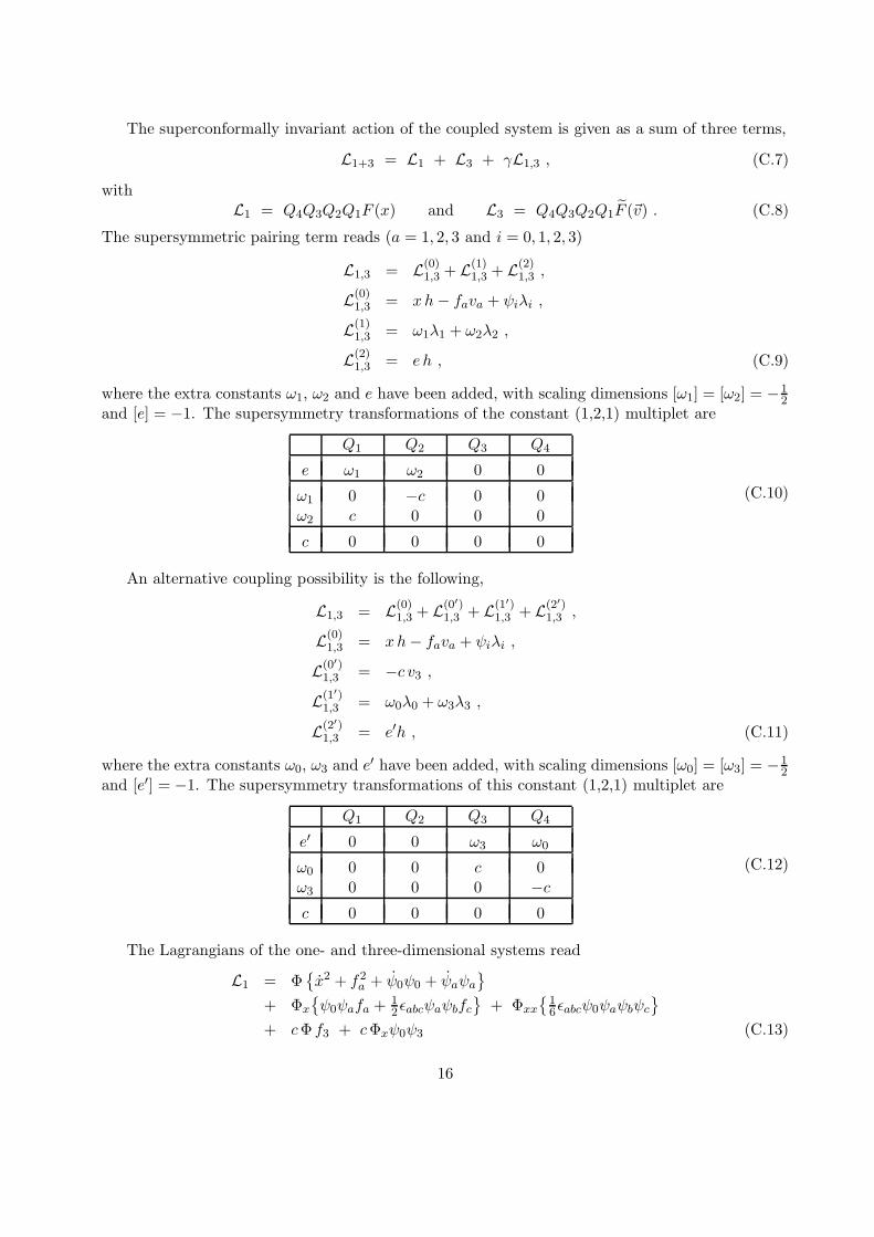
Since both (3,8,5) and (5,8,3) multiplets represent the same D(2, 2) superalgebra, it is natural to

couple them. The duality provides a canonical interaction term L(0)3,5 in the joint Lagrangian

L(0)3 + L5 + γL

(0)3,5 (7.1)

of the form

L(0)3,5 = xaha − fαvα − g w − gαwα + ψiλi + ξiχi with a = 1, 2, 3 , α = 1, 2 , i = 0, 1, 2, 3 ,

(7.2)

with some dimensionless coupling constant γ. It is easy to check that L(0)3,5 is invariant (up to

total time derivatives) under all eight supersymmetries and their conformal partners, because thedimensions of any two duality partners add up to one.

The superscript (0) reminds us that we turned off the inhomogeneous deformation in the(3,8,5) multiplet. So the question arises as to whether it is possible to extend this coupling to

9

the deformed multiplet as well, and what this entails for the dual (5,8,3) multiplet. To answer this,we first observe that

L3 + L5 + γL(0)3,5 (7.3)

is indeed invariant (up to total time derivatives) under Q8, Q1, Q4 and Q5, but

Q2L(0)3,5 = −cχ3 , Q3L

(0)3,5 = cχ2 , Q6L

(0)3,5 = −cλ3 , Q7L

(0)3,5 = cλ2 (7.4)

do not vanish. Yet, since c is a constant, these terms are linear and may be cancelled by addingother linear terms to the interaction. To achieve this feat, however, one must view the deformationparameter c as the highest component of an N=4 multiplet of type (3,4,1) involving the super-charges Qj for j = 2, 3, 6, 7. Denoting the components of dimension −1, −1

2 and 0 by ea, ωi and c,respectively, the transformation table takes the form

Q8 Q1 Q2 Q3 Q4 Q5 Q6 Q7

e1 0 0 ω2 ω3 0 0 ω0 ω1

e2 0 0 ω3 −ω2 0 0 −ω1 ω0

e3 0 0 −ω0 −ω1 0 0 ω2 ω3

ω0 0 0 0 −c 0 0 0 0ω1 0 0 c 0 0 0 0 0ω2 0 0 0 0 0 0 0 −cω3 0 0 0 0 0 0 c 0

c 0 0 0 0 0 0 0 0

(7.5)

It is important to realize that all these components are constants, i.e. time independent, otherwisethere could not be zeros in this table. For the same reason, it is admissible to have this multipletannihilated by the other four supercharges, Qk for k = 8, 1, 4, 5. If we add to our interactionLagrangian two extra pieces,

L(1)3,5 = ω0χ2 + ω1χ3 + ω2λ2 + ω3λ3 and L

(2)3,5 = e1h1 + e2h2 + e3h3 , (7.6)

it is not hard to check that all unwanted terms get cancelled, and only total time derivatives remain.In other words,

L3+5 := L3 + L5 + γL3,5 (7.7)

is fully N=8 superconformally invariant for

L3,5 = (xa+ea)ha − fαvα − g w − gαwα (7.8)

+ ξ0χ0 + ξ1χ1 + (ξ2+ω0)χ2 + (ξ3+ω1)χ3 + ψ0λ0 + ψ1λ1 + (ψ2+ω2)λ2 + (ψ3+ω3)λ3 ,

which adds to the pairings (7.2) a term linear in a (1,4,3) submultiplet (w;χ2, χ3, λ2, λ3;ha) insideour dual (5,8,3) multiplet. Another interpretation is that the (1,8,5) components with inhomo-geneous transformation receive constant shifts which cancel the inhomogeneity produced in thecanonical coupling term.

Interestingly, there is another way to cancel the non-invariant terms (7.4). Observing that

QjL(0)3,5 = cQjw for j = 2, 3, 6, 7 (7.9)

10

suggests repairing the deficit by adding

L(0′)3,5 = −cw (7.10)

to the interaction. While QjL(0′)3,5 indeed just cancels the unwanted terms, now the other four

supersymmetries are compromised, however, as

Q8L(0′)3,5 = −c χ1 , Q1L

(0′)3,5 = −c χ0 , Q4L

(0′)3,5 = c λ1 , Q5L

(0′)3,5 = c λ0 . (7.11)

Comparing with (7.4), we see that the deficiency has simply been shifted from the Qj to the Qk

with k = 8, 1, 4, 5, and the relevant fermionic components carry indices 0 and 1 instead of 2 and 3.Hence, adding a suitable constant (3,4,1) multiplet for those supersymmetries and the appropriate

terms L(1′)3,5 and L

(2′)3,5 to the interaction will accomplish the job just as well. The only difference for

the bosonic Lagrangians is an additional term of −γcw.

Sticking with the first resolution and adding Fayet-Iliopoulos terms for all auxiliary components,the bosonic part of the total action reads

L′3+5

∣∣ = Φ(x2a + f2α + g2 + g2α

)+ c ~A·~x+ Φ

(v2α + w2 + w2

α + h2a)

−(γvα−µα

)fα −

(γw−ζ−cΦ

)g −

(γwα−ζα

)gα +

(γ(xa+ea)−µa

)ha , (7.12)

and elimination of the auxiliary components produces

L′′3+5

∣∣ = Φ x2a + c ~A·~x+ Φ(v2α + w2 + w2

α

)

− 14Φ

−1((γvα−µα)

2 + (γw−ζ−cΦ)2 + (γwα−ζα)2)− 1

4Φ−1

(γ(xa+ea)− µa

)2.(7.13)

The constant Lagrange multipliers ea serve to eliminate the zero modes of the ha. For convenience,we relabel wα = v2+α and w = v5 and define v2 = vαvα +w2 +wαwα. In conical radial coordinatesρ = 2r1/2 and σ = 2v−1/2, the bosonic action then takes the form

Lcone3+5

∣∣ = ρ2 + 4ℓ2ρ−2 + σ2 + 4ℓ2σ−2 + c ~A·~x

− 116ρ

2(4γσ−2~eσ − ~µ− 4cρ−2~e5

)2− σ−6

(γ(ρ2~eρ+4~e)− 4~µ

)2, (7.14)

where we introduced the angular momenta ℓ and ℓ in the three- and five-dimensional targets, andthe vectors in the first and second brackets are five- and three-dimensional, respectively.

8 A deformed (5,8,3) supermultiplet

If in (7.7) we set to zero the complete (5,8,3) multiplet, we simply come back to the original deformed(3,8,5) theory. Let us then try the opposite and see whether we recover the (5,8,3) model. However,due to (7.4) it is not consistent to put the (3,8,5) components to zero completely, but we must keepthe zero modes of xa, ψ2, ψ3, ξ2, ξ3 and g, which we denote by an overbar. With this provision,the full Lagrangian (7.7) reduces to

L5 = L5 + γ((xa+ea)ha + (ξ2+ω0)χ2 + (ξ3+ω1)χ3 + (ψ2+ω2)λ2 + (ψ3+ω3)λ3 − (g+c)w

)

=: L5 + γ(e′aha + ω′

0χ2 + ω′1χ3 + ω′

2λ2 + ω′3λ3 − c

′w), (8.1)

11

and to the transformations (7.5) of the constants we must add

Q8 Q1 Q2 Q3 Q4 Q5 Q6 Q7

x1 0 0 ψ2 ψ3 0 0 ξ2 ξ3x2 0 0 ψ3 −ψ2 0 0 −ξ3 ξ2x3 0 0 −ξ2 −ξ3 0 0 ψ2 ψ3

ξ2 0 0 0 g+c 0 0 0 0

ξ3 0 0 −g−c 0 0 0 0 0

ψ2 0 0 0 0 0 0 0 g+c

ψ3 0 0 0 0 0 0 −g−c 0

g 0 0 0 0 0 0 0 0

(8.2)

which is what remains of (4.2). We see that only the four Qj are effective. The upshot is adeformation of the original (5,8,3) Lagrangian by linear terms in a (1,4,3) submultiplet. The linearcoefficients (e′a, ω

′i, c

′) are just the sum of the (3,4,1) zero-mode submultiplet (8.2) of the original(3,8,5) multiplet and the constant auxiliary (3,4,1) multiplet (7.5). This combination transformsas follows,

Q8 Q1 Q2 Q3 Q4 Q5 Q6 Q7

e′1 0 0 ω′2 ω′

3 0 0 ω′0 ω′

1

e′2 0 0 ω′3 −ω′

2 0 0 −ω′1 ω′

0

e′3 0 0 −ω′0 −ω′

1 0 0 ω′2 ω′

3

ω′0 0 0 0 −c′ 0 0 0 0ω′1 0 0 c′ 0 0 0 0 0ω′2 0 0 0 0 0 0 0 −c′

ω′3 0 0 0 0 0 0 c′ 0

c′ 0 0 0 0 0 0 0 0

(8.3)

Hence, the coupling of the (5,8,3) multiplet to a dual inhomogeneous (3,8,5) multiplet leads to adeformation of the former, which consists of the coupling of a (1,4,3) submultiplet to an auxiliaryconstant (3,4,1) dual multiplet. The deformation is parametrized by γ and contains the (3,8,5)inhomogeneity c as part of it. Of course, we may also add standard Fayet-Iliopoulos terms.

12

A Appendix: Action for the (3,8,5) supermultiplet

The complete Lagrangian for the (3,8,5) multiplet reads

L(0)3 = Φ(x2 + y2 + z2 + f21 + f22 + g2 + g21 + g22) + (A.1)

Φ (ψ0ψ0 + ψ1ψ1 + ψ2ψ2 + ψ3ψ3 + ξ0ξ0 + ξ1ξ1 + ξ2ξ2 + ξ3ξ3) +

Φx((yξ0ξ1 + f1ξ0ξ2 + f2ξ0ξ3) + (yψ0ψ1 + f1ψ0ψ2 + f2ψ0ψ3)

+(gψ0ξ1 + g1ψ0ξ2 + g2ψ0ξ3) + (gψ1ξ0 + g1ψ2ξ0 + g2ψ3ξ0)

−(yξ2ξ3 + f1ξ3ξ1 + f2ξ1ξ2) + (yψ2ψ3 + f1ψ3ψ1 + f2ψ1ψ2)

+(gξ3ψ2 + g1ξ1ψ3 + g2ξ2ψ1)− (gξ2ψ3 + g1ξ3ψ1 + g2ξ1ψ2)

+z(ψ0ξ0 + ξ1ψ1 + ξ2ψ2 + ξ3ψ3)) +

Φy((−xξ0ξ1 − f1ξ0ξ3 + f2ξ0ξ2) + (xψ1ψ0 − f1ψ3ψ0 + f2ψ2ψ0)

−(zξ1ψ0 − g1ξ3ψ0 + g2ξ2ψ0)− (zξ0ψ1 + g1ξ0ψ3 − g2ξ0ψ2)

+g(ξ0ψ0 − ξ1ψ1 + ξ2ψ2 + ξ3ψ3)

+x(ξ2ξ3 − ψ2ψ3)− z(ξ3ψ2 − ξ2ψ3)

+g1(ψ1ξ2 − ξ1ψ2) + g2(ψ1ξ3 − ξ1ψ3)) +

Φz((gξ0ξ1 + g1ξ0ξ2 + g2ξ0ξ3) + (gψ0ψ1 + g1ψ0ψ2 + g2ψ0ψ3)

−(yψ0ξ1 + f1ψ0ξ2 + f2ψ0ξ3)− (yψ1ξ0 + f1ψ2ξ0 + f2ψ3ξ0)

+(gξ2ξ3 + g1ξ3ξ1 + g2ξ1ξ2) + (gψ2ψ3 + g1ψ3ψ1 + g2ψ1ψ2)

+(yξ3ψ2 + f1ξ1ψ3 + f2ξ2ψ1)− (yξ2ψ3 + f1ξ3ψ1 + f2ξ1ψ2)

+x(ψ0ξ0 + ξ1ψ1 + ξ2ψ2 + ξ3ψ3)) +

Φxx(ψ3ψ1ξ2ξ0 + ψ3ψ0ξ2ξ1 − ψ2ψ1ξ3ξ0 − ψ2ψ0ξ3ξ1) +

Φyy(ψ2ψ0ξ2ξ0 + ψ3ψ0ξ3ξ0 − ψ2ψ1ξ2ξ1 − ψ3ψ1ξ3ξ1) +

Φzz(−ξ3ξ2ξ1ξ0 + ψ3ψ2ξ1ξ0 − ψ1ψ0ξ3ξ2 + ψ3ψ2ψ1ψ0) +

Φxy(ψ2ψ0ξ3ξ0 − ψ2ψ0ξ2ξ1 + ψ3ψ1ξ2ξ1 − ψ3ψ0ξ2ξ0

−ψ2ψ1ξ3ξ1 − ψ3ψ0ξ3ξ1 − ψ2ψ1ξ2ξ0 − ψ3ψ1ξ3ξ0)−

Φxz(ψ2ξ3ξ1ξ0 + ψ2ψ1ψ0ξ3 − ψ3ψ1ψ0ξ2 + ψ3ψ2ψ1ξ0

+ψ3ξ2ξ1ξ0 − ψ0ξ3ξ2ξ1 + ψ3ψ2ψ0ξ1 − ψ1ξ3ξ2ξ0)−

Φyz(ψ0ξ3ξ2ξ0 + ψ2ξ2ξ1ξ0 + ψ3ξ3ξ1ξ0 − ψ1ξ3ξ2ξ1

−ψ3ψ2ψ0ξ0 + ψ3ψ1ψ0ξ3 + ψ2ψ1ψ0ξ2 + ψ3ψ2ψ1ξ1)

and

L(1)3 = Φ g +Axx+Ayy + (A.2)

Φx(ψ0ξ1 + ψ1ξ0) + Φy(ψ1ξ1 − ψ0ξ0)− Φz(ψ1ψ0 + ξ1ξ0) .

13

B Appendix: Action for the (5,8,3) supermultiplet

The complete Lagrangian for the (5,8,3) multiplet reads

L5 = Φ(v21+ v2

2+ w2 + w2

1+ w2

2+ h2

1+ h2

2+ h2

3) +

Φ(λ0λ0 + λ1λ1 + λ2λ2 + λ3λ3 + χ0χ0 + χ1χ1 + χ2χ2 + χ3χ3) +

Φv1[v2(λ0λ1 + λ2λ3 + χ1χ0 + χ2χ3) + h1(λ1λ3 + λ2λ0 + χ3χ1 + χ2χ0)

+h2(λ2λ1 + λ3λ0 + χ0χ3 + χ2χ1) + h3(λ0χ2 + λ3χ1 + λ2χ0 + χ3λ1)] +

Φv2[v1(λ1λ0 + λ3λ2 + χ0χ1 + χ3χ2) + h1(λ2λ1 + λ3λ0 + χ1χ2 + χ3χ0)

+h2(λ0λ2 + λ3λ1 + χ3χ1 + χ2χ0) + h3(χ1λ2 + λ3χ0 + λ1χ2 + λ0χ3)] +

Φw[w1(λ3λ0 + λ1λ2 + χ0χ3 + χ1χ2) + w2(λ0λ2 + λ3λ1 + χ2χ0 + χ1χ3)

+h1(χ2λ3 + χ1λ0 + χ0λ1 + λ2χ3) + h2(χ1λ1 + λ2χ2 + λ0χ0 + λ3χ3)

+h3(λ1λ0 + λ2λ3 + χ1χ0 + χ3χ2)] +

Φw1[w(λ0λ3 + λ2λ1 + χ2χ1 + χ3χ0) + w2(λ2λ3 + λ1λ0 + χ0χ1 + χ2χ3)

+h1(λ3χ1 + χ3λ1 + χ2λ0 + χ0λ2) + h2(χ1λ2 + χ2λ1 + λ0χ3 + χ0λ3)

+h3(λ2λ0 + λ3λ1 + χ1χ3 + χ2χ0)] +

Φw2[w(λ3λ1 + λ2λ0 + χ0χ2 + χ3χ1) + w1(λ0λ1 + λ3λ2 + χ1χ0 + χ3χ2)

+h1(χ0λ3 + λ1χ2 + χ3λ0 + χ1λ2) + h2(χ3λ1 + λ2χ0 + χ2λ0 + χ1λ3)

+h3(λ3λ0 + λ1λ2 + χ3χ0 + χ2χ1)] +

Φww(λ0χ0λ1χ1 + λ2χ2λ3χ3 + χ0χ1χ2χ3) +

Φv1v1(λ0χ0χ2λ2 + λ1χ1λ3χ3 + λ0χ1χ2λ3 − χ0λ1λ2χ3 + λ0λ1λ2λ3) +

Φv2v2(λ0χ0χ3λ3 + λ1χ1λ2χ2 + λ0χ1λ2χ3 − χ0λ1χ2λ3 + λ0λ1λ2λ3) +

Φw1w1(λ0χ0χ2λ2 + λ1χ1λ3χ3 − λ0λ1χ2χ3 + λ0χ1λ2χ3 + χ0χ1λ2λ3 +

−χ0λ1χ2λ3 + χ0χ1χ2χ3) +

Φw2w2(λ0χ0χ3λ3 + λ1χ1λ2χ2 − λ0λ1χ2χ3 + λ0χ1χ2λ3 + χ0χ1λ2λ3 +

−χ0λ1λ2χ3 + χ0χ1χ2χ3) +

Φv1v2(λ0χ0χ2λ3 − λ0χ0λ2χ3 − λ0χ1χ2λ2 + λ0χ1χ3λ3 + χ0λ1λ2χ2

+χ0λ1χ3λ3 + λ1χ1χ2λ3 − λ1χ1λ2χ3) +

Φv1w(−λ0χ0λ1λ2 − λ0χ0χ1χ2 + λ0λ3λ1χ1 + λ0λ3χ2λ2 + χ0χ3χ1λ1

+χ0χ3λ2χ2 + λ1λ2χ3λ3 + χ1χ2χ3λ3) +

Φv1w1(λ0λ1χ2λ3 − λ0χ1λ2λ3 − χ0λ1λ2λ3 − λ0λ1λ2χ3 − χ0λ1χ2χ3

+χ0χ1λ2χ3 − χ0χ1χ2λ3 − λ0χ1χ2χ3) +

Φv1w2(λ0χ0χ2χ3 + λ0χ0λ2λ3 + χ0χ1χ2λ2 + χ0χ1λ3χ3 + λ0λ1λ2χ2 +

λ0λ1χ3λ3 + λ1χ1λ2λ3 + λ1χ1χ2χ3) +

Φv2w(λ0χ0χ3χ1 + λ0χ0λ3λ1 + χ0χ2λ1χ1 + χ0χ2χ3λ3 + λ0λ2χ1λ1

+λ0λ2λ3χ3 + λ2χ2λ3λ1 + χ2λ2χ1χ3) +

Φv2w1(−λ0χ0χ2χ3 − λ0χ0λ2λ3 + χ0χ1χ2λ2 + χ0χ1λ3χ3 + λ0λ1λ2χ2

+λ0λ1χ3λ3 + λ1χ1λ3λ2 + λ1χ1χ3χ2) +

Φv2w2(−χ0λ1λ2λ3 + λ0λ1λ2χ3 − λ0λ1χ2λ3 − λ0χ1λ2λ3 − χ0χ1λ2χ3

−λ0χ1χ2χ3 + χ0χ1χ2λ3 − χ0λ1χ2χ3) +

Φww1(−λ0χ0λ1χ2 + λ0χ0χ1λ2 − χ0λ3λ1χ1 + χ0λ3λ2χ2 − λ0χ3λ1χ1

+λ0χ3λ2χ2 − λ3χ3λ1χ2 + λ3χ3χ1λ2) +

Φww2(λ0χ0χ3λ1 − λ0χ0λ3χ1 − χ0λ2χ1λ1 + χ0λ2χ3λ3 + λ0χ2λ1χ1

+λ0χ2χ3λ3 + λ1χ3χ2λ2 − χ1λ3χ2λ2) +

Φw1w2(λ0χ0χ2λ3 − λ0χ0λ2χ3 + χ0λ1χ2λ2 + χ0λ1λ3χ3 + λ0χ1χ2λ2

+λ0χ1λ3χ3 + χ2λ3λ1χ1 + λ2χ3χ1λ1) . (B.1)

14

C Appendix: N=4 duality

It is instructive to display the simpler case of N=4 duality. Since only the (1,4,3) multiplet allowsfor an inhomogeneous deformation, we concentrate on the d=1 / d=3 duality and the coupling ofthese two multiplets.

Like in the N=8 cases, the N=4 Lagrangians have the form

Ld = Φ δabxaxb + . . . . (C.1)

Scale (D) and special conformal (K) invariance require

Φ = rβ Y (angles) and Φ r2 = ddtZ for r2 = xaxa , (C.2)

with some exponent β and functions Y and Z. It follows that Z = cc+2r

β+2Y and Y = constant.

Let us denote the components of the two multiplets by

(1, 4, 3) : x;ψ0, ψ1, ψ2, ψ3; f1, f2, f3

(3, 4, 1) : v1, v2, v3;λ0, λ1, λ2, λ3;h(C.3)

and assign scaling dimensions (i = 0, 1, 2, 3 and a = 1, 2, 3)

[x, ψi, fa] = −1,−12 , 0 and [va, λi, h] = 1, 32 , 2 , (C.4)

so that the conformal factors for a dimensionless action become

Φ = x−1 and Φ = v−3 with v2 = vava . (C.5)

The bosonic target space is therefore the product of a (half) line with a three-dimensional cone.The supersymmetry transformations are given by

Q1 Q2 Q3 Q4

x ψ1 ψ2 ψ3 ψ0

ψ0 f1 f2 f3 xψ1 x f3+c −f2 −f1ψ2 −f3−c x f1 −f2ψ3 f2 −f1 x −f3

f1 ψ0 −ψ3 ψ2 −ψ1

f2 ψ3 ψ0 −ψ1 −ψ2

f3 −ψ2 ψ1 ψ0 −ψ3

Q1 Q2 Q3 Q4

v1 λ0 −λ3 λ2 −λ1v2 λ3 λ0 −λ1 −λ2v3 −λ2 λ1 λ0 −λ3

λ0 v1 v2 v3 hλ1 h v3 −v2 −v1λ2 −v3 h v1 −v2λ3 v2 −v1 h −v3

h λ1 λ2 λ3 λ0

(C.6)

with inhomogeneous parameter c. The transformations can be written in terms of the quaternionicstructure constants δab and ǫabc (with ǫ123 = 1). We note that the two multiplets must have thesame chirality to be coupled. Therefore, the overall sign of ǫ123 in the second multiplet is fixed inorder to allow the supersymmetric pairing of the multiplets.

15

The superconformally invariant action of the coupled system is given as a sum of three terms,

L1+3 = L1 + L3 + γL1,3 , (C.7)

withL1 = Q4Q3Q2Q1F (x) and L3 = Q4Q3Q2Q1F (~v) . (C.8)

The supersymmetric pairing term reads (a = 1, 2, 3 and i = 0, 1, 2, 3)

L1,3 = L(0)1,3 + L

(1)1,3 + L

(2)1,3 ,

L(0)1,3 = xh− fava + ψiλi ,

L(1)1,3 = ω1λ1 + ω2λ2 ,

L(2)1,3 = e h , (C.9)

where the extra constants ω1, ω2 and e have been added, with scaling dimensions [ω1] = [ω2] = −12

and [e] = −1. The supersymmetry transformations of the constant (1,2,1) multiplet are

Q1 Q2 Q3 Q4

e ω1 ω2 0 0

ω1 0 −c 0 0ω2 c 0 0 0

c 0 0 0 0

(C.10)

An alternative coupling possibility is the following,

L1,3 = L(0)1,3 + L

(0′)1,3 + L

(1′)1,3 + L

(2′)1,3 ,

L(0)1,3 = xh− fava + ψiλi ,

L(0′)1,3 = −c v3 ,

L(1′)

1,3 = ω0λ0 + ω3λ3 ,

L(2′)1,3 = e′h , (C.11)

where the extra constants ω0, ω3 and e′ have been added, with scaling dimensions [ω0] = [ω3] = −

12

and [e′] = −1. The supersymmetry transformations of this constant (1,2,1) multiplet are

Q1 Q2 Q3 Q4

e′ 0 0 ω3 ω0

ω0 0 0 c 0ω3 0 0 0 −c

c 0 0 0 0

(C.12)

The Lagrangians of the one- and three-dimensional systems read

L1 = Φx2 + f2a + ψ0ψ0 + ψaψa

+ Φx

ψ0ψafa +

12ǫabcψaψbfc

+ Φxx

16ǫabcψ0ψaψbψc

+ cΦ f3 + cΦxψ0ψ3 (C.13)

16

and

L3 = Φv2a + h2 + λ0λ0 + λaλa

+ Φa

λaλbvb + ǫabc(

12λbλch− λ0λbvc)

+ 1

6∆Φ ǫabcλ0λaλbλc , (C.14)

whereΦ = Fxx and Φ = ∆F ≡ Faa , (C.15)

respectively.

Finally we add Fayet-Iliopoulos terms which are superconformal (not just supersymmetric)invariants and introduce dimensionful constants µa and ν,

LFI = µafa − ν h , (C.16)

with [µa] = 1 and [ν] = −1. The supersymmetry transformations act trivially on µa and ν.

Setting all fermions to zero, the total bosonic Lagrangian based on (C.7) with (C.9) becomes

L′1+3

∣∣ = Φ(x2 + f2a) + Φ (v2a + h2)− (γva − µa − cδa3Φ) fa + (γx+ γe− ν)h . (C.17)

If we use (C.11) instead, an additional term −γc v3 appears. Eliminating the auxiliary fields via

fa = 12Φ

−1(γva − µa − cδa3Φ) and h = −12Φ

−1(γx+ γe− ν), (C.18)

we arrive at

L′′1+3

∣∣ = Φ x2 + Φ v2a −14Φ

−1(γva − µa − cδa3Φ

)2− 1

4 Φ−1

(γ(x+e)− ν

)2, (C.19)

where the Lagrange multiplier e only ensures that the zero mode h vanishes. Hence, its value is

e = −(Φ−1x− ν/γ)/Φ−1. Specializing to Φ = x−1 and Φ = v−3, one gets

L′′1+3

∣∣ = x−1x2 + v−3v2a −14x

(γva − µa − cδa3x

−1)2− 1

4v3(γ(x+e)− ν

)2. (C.20)

In order to interpret this Lagrangian, we pass to standard kinetic terms (up to a factor of 12) by

changing the radial coordinates via

x = 14ρ

2 and v = 4σ−2 with [ρ] = [σ] = −12 (C.21)

and arrive at

Lcone1+3

∣∣ = ρ2 + σ2 + 4ℓ2σ−2 − 116ρ

2(γσ−2~eσ − ~µ− 4cρ−2~e3

)2− σ−6

(γ(ρ2+4e)− 4ν

)2, (C.22)

where ℓ is the angular momentum in σ space, and ~eσ and ~e3 denote unit vectors in the σ and3 directions, respectively. We find a rather complicated potential in the four-dimensional target.If one employs the option (C.11), then linear terms −γc v3 and −4γc σ−2~e3 have to be added to(C.20) and (C.22), respectively.

Acknowledgments

This work was partially supported by CNPq and by the Deutsche Forschungsgemeinschaft undergrant LE 838/12. M.G. and O.L. acknowledge a PCI-BEV grant and hospitality at CBPF.

17

References

[1] S. Fedoruk, E. Ivanov and O. Lechtenfeld,“Superconformal mechanics”,J. Phys. A: Math. Theor. 45 (2012) 173001 [arXiv:1112.1947[hep-th]].

[2] A. Pashnev and F. Toppan,“On the classification of N-extended supersymmetric quantum mechanical systems”,J. Math. Phys. 42 (2001) 5257 [arXiv:hep-th/0010135].

[3] Z. Kuznetsova, M. Rojas and F. Toppan,“Classification of irreps and invariants of N-extended supersymmetric quantum mechanics”,JHEP 0603 (2006) 098 [arXiv:hep-th/0511274].

[4] F. Delduc and E. Ivanov,“New model of N=8 superconformal mechanics”,Phys. Lett. B 654 (2007) 200 [arXiv:0706.2472[hep-th]].

[5] S. Bellucci, E. Ivanov, S. Krivonos and O. Lechtenfeld,“N=8 superconformal mechanics”,Nucl. Phys. B 684 (2004) 321 [arXiv:hep-th/0312322].

[6] S. Bellucci, E. Ivanov, S. Krivonos and O. Lechtenfeld,“ABC of N=8, d=1 supermultiplets”,Nucl. Phys. B 699 (2004) 226 [arXiv:hep-th/0406015].

[7] D.-E. Diaconescu and R. Entin,“A nonrenormalization theorem for the d=1, N=8 vector multiplet,”Phys. Rev. D 56 (1997) 8045 [arXiv:hep-th/9706059].

[8] S. Khodaee and F. Toppan,“Critical scaling dimension of D-module representations of N=4,7,8 superconformal algebrasand constraints on superconformal mechanics”,J. Math. Phys. 53 (2012) 103518 [arXiv:1208.3612[hep-th]].

[9] F. Toppan,“Critical D-module reps for finite superconformal algebras and their superconformalmechanics”, Talk given at XXIXth ICGTMP, Tianjin 2012,to appear in the proceedings [arXiv:1302.3459[math-ph]].

[10] Z. Kuznetsova and F. Toppan,“D-module representations of N=2,4,8 superconformal algebras and their superconformalmechanics”,J. Math. Phys. 53 (2012) 043513 [arXiv:1112.0995[hep-th]].

[11] M. Gonzales, S. Khodaee and F. Toppan,“On non-minimal N=4 supermultiplets in 1D and their associated sigma models”,J. Math. Phys. 52 (2011) 013514 [arXiv:1006.4678[hep-th]].

[12] E. Ivanov, S. Krivonos and O. Lechtenfeld,“New variant of N=4 superconformal mechanics,”JHEP 0303 (2003) 014 [arXiv:hep-th/0212303].

18