arX

iv:2

112.

1216

9v2

[he

p-th

] 1

4 M

ar 2

022

Superconformal blocks in diverse dimensions

and BC symmetric functions

Francesco Aprile1 and Paul Heslop2

1 Instituto de Fisica Teorica, UNESP, ICTP South American Institute for Fundamental Research

Rua Dr Bento Teobaldo Ferraz 271, 01140-070, Sao Paulo, Brazil

2Mathematics Department, Durham University,

Science Laboratories, South Rd, Durham DH1 3LE

Abstract

We uncover a precise relation between superblocks for correlators of superconformal fieldtheories (SCFTs) in various dimensions and symmetric functions related to the BC root sys-tem. The theories we consider are defined by two integers (m,n) together with a parameter θand they include correlators of all half-BPS correlators in 4d theories with N = 2n supersym-metry, 6d theories with (n, 0) supersymmetry and 3d theories with N = 4n supersymmetry,as well as all scalar correlators in any non SUSY theory in any dimension, and conjecturallyvarious 5d, 2d and 1d superconformal theories. The superblocks are eigenfunctions of thesuper Casimir of the superconformal group whose action we find to be precisely that of theBCm|n Calogero-Moser-Sutherland Hamiltonian. When m = 0 the blocks are polynomials,and we show how these relate to BCn Jacobi polynomials. However, differently from BCn

Jacobi polynomials, the m = 0 blocks possess a crucial stability property that has not beenemphasised previously in the literature. This property allows for a novel supersymmetricuplift of the BCn Jacobi polynomials, which in turn yields the (m,n; θ) superblocks. Su-perblocks defined in this way are related to Heckman-Opdam hypergeometrics and are nonpolynomial functions. A fruitful interaction between the mathematics of symmetric functionsand SCFT follows, and we give a number of new results on both sides. One such example isa new Cauchy identity which naturally pairs our superconformal blocks with Sergeev-Veselovsuper Jacobi polynomials and yields the CPW decomposition of any free theory diagram inany dimension.

Contents

1 Introduction 3

2 Overview 5

2.1 Superconformal blocks . . . . . . . . . . . . . . . . . . . . . . . . . . . . . . . 6

2.2 Solving the Casimir equation . . . . . . . . . . . . . . . . . . . . . . . . . . . 9

2.3 Superblocks as dual super Jacobi functions . . . . . . . . . . . . . . . . . . . 12

2.4 Binomial coefficient and Cauchy identities . . . . . . . . . . . . . . . . . . . . 15

2.5 Superblock to block decomposition: a conjecture . . . . . . . . . . . . . . . . 17

3 Supergroups, physical theories, and beyond 18

3.1 List of theories and their superconformal blocks . . . . . . . . . . . . . . . . . 18

3.2 Coset space formalism . . . . . . . . . . . . . . . . . . . . . . . . . . . . . . . 20

4 Rank-one invitation 28

4.1 Rank-one bosonic blocks . . . . . . . . . . . . . . . . . . . . . . . . . . . . . . 28

4.2 Relation with the Heckman-Opdam hypergeometrics . . . . . . . . . . . . . . 30

5 Superconformal blocks (I): recursion 32

5.1 Derivation of the recursion and higher order Casimirs . . . . . . . . . . . . . 33

5.2 Explicit formulae for the recursion . . . . . . . . . . . . . . . . . . . . . . . . 37

5.3 Special solutions: the half-BPS superconformal block . . . . . . . . . . . . . . 40

5.4 General features and non-trivial γ-dependence . . . . . . . . . . . . . . . . . . 42

6 Superconformal blocks (II): analytic continuation 43

6.1 Row-type representation on the east . . . . . . . . . . . . . . . . . . . . . . . 44

6.2 Column-type representation on the south . . . . . . . . . . . . . . . . . . . . 45

6.3 Supersymmetric representation . . . . . . . . . . . . . . . . . . . . . . . . . . 45

7 SCFT perspective on the binomial coefficient 47

7.1 The binomial coefficient . . . . . . . . . . . . . . . . . . . . . . . . . . . . . . 48

7.2 Binomial representation of the Jack→Block matrix . . . . . . . . . . . . . . . 49

7.3 Inverse Jack→Block matrix and complementation . . . . . . . . . . . . . . . . 52

8 Generalised free theory from a Cauchy identity 56

8.1 Super Cauchy identity . . . . . . . . . . . . . . . . . . . . . . . . . . . . . . . 56

8.2 Proof of the super Cauchy identity . . . . . . . . . . . . . . . . . . . . . . . . 58

8.3 Free theory block coefficients . . . . . . . . . . . . . . . . . . . . . . . . . . . 61

9 Decomposing superblocks 63

9.1 General decomposition of blocks . . . . . . . . . . . . . . . . . . . . . . . . . 64

1

9.2 Superblock to block decomposition . . . . . . . . . . . . . . . . . . . . . . . . 66

9.3 Examples of the superblock to block decomposition . . . . . . . . . . . . . . . 66

10 Conclusions and outlook 69

10.1 Outlook on the q-deformed superblocks . . . . . . . . . . . . . . . . . . . . . 73

A Super/conformal/compact groups of interest 75

A.1 θ = 1: SU(m,m|2n) . . . . . . . . . . . . . . . . . . . . . . . . . . . . . . . . 75

A.2 θ = 2 : OSp(4m|2n) . . . . . . . . . . . . . . . . . . . . . . . . . . . . . . . . 76

A.3 θ = 12 : OSp(4n|2m) . . . . . . . . . . . . . . . . . . . . . . . . . . . . . . . . 77

A.4 Non-supersymmetric conformal and internal blocks . . . . . . . . . . . . . . . 79

B From CMS Hamiltonians to the superblock Casimir 81

B.1 Deformed CMS Hamiltonians. . . . . . . . . . . . . . . . . . . . . . . . . . . . 81

B.2 A-type Hamiltonians and Jack polynomials . . . . . . . . . . . . . . . . . . . 83

B.3 BC-type Hamiltonians and superblocks . . . . . . . . . . . . . . . . . . . . . 84

C Symmetric and supersymmetric polynomials 87

C.1 Symmetric polynomials . . . . . . . . . . . . . . . . . . . . . . . . . . . . . . 87

C.2 Jack polynomials . . . . . . . . . . . . . . . . . . . . . . . . . . . . . . . . . . 90

C.3 Interpolation polynomials . . . . . . . . . . . . . . . . . . . . . . . . . . . . . 93

C.4 Supersymmetric polynomials . . . . . . . . . . . . . . . . . . . . . . . . . . . 94

C.5 Super Jack polynomials . . . . . . . . . . . . . . . . . . . . . . . . . . . . . . 96

C.6 Properties of Super Jack polynomials . . . . . . . . . . . . . . . . . . . . . . . 97

C.7 Super interpolation polynomials . . . . . . . . . . . . . . . . . . . . . . . . . . 100

D More properties of analytically continued superconformal blocks 101

D.1 Shift symmetry of the supersymmetric form of the recursion . . . . . . . . . . 101

D.2 Truncations of the superconformal block . . . . . . . . . . . . . . . . . . . . . 103

E Revisiting known blocks with the binomial coefficient 105

E.1 The half-BPS solution . . . . . . . . . . . . . . . . . . . . . . . . . . . . . . . 106

E.2 Rank-one and rank-two . . . . . . . . . . . . . . . . . . . . . . . . . . . . . . 107

E.3 Revisiting the θ = 1 case and determinantals . . . . . . . . . . . . . . . . . . 110

2

1 Introduction

In this paper we will obtain conformal and superconformal blocks for four-point functions ofhalf-BPS scalar operators in diverse dimensions. Our construction is based on a single unifiedformalism, which uses analytic superspace [1–10] as its starting point, but includes variousgeneralisations. In particular, a parameter θ which allows us to move across dimensions.By varying the value of θ, we will find superconformal blocks for theories in 1,2,3,4,6 andconjecturally 5 dimensions.

The superconformal blocks that we present have a beautiful interpretation in the theory ofsymmetric functions: they are in one-to-one correspondence with a natural supersymmetricextension of a class of stable polynomials that we call dual BC Jacobi polynomials. Whilethe appearance of the BC root system in this context is not new,1 the results here set theseobservations in a much more general context and apply them directly to the supersymmetriccase as well as the bosonic CFT case.

In a quantum field theory, correlation functions can be decomposed by using the opera-tor product expansion (OPE). If the theory is a Conformal Field Theory (CFT), it is wellknown that the OPE can be organised further by collecting the contribution of a primaryoperator with all its infinite descendants [18–21]. The object representing the common OPEbetween pairs of external operators in a four-point correlator is the conformal block. It can berepresented as the solution of a Casimir operator (for the correlation function under consid-eration) with given boundary conditions [11,22–25]. The conformal block encodes an infinitesum and is closely related to hypergeometric functions. We will show, more precisely, thatthe mathematics underlying the physics of superconformal blocks is that of the multivariate

hypergeometric functions developed by Heckman-Opdam (applied to the BC root system).

The Heckman-Opdam (HO) hypergeometrics are rigorously defined as eigenfunctions of asystem of differential equations [16,17]. In the case of positive weights it was shown [26] thatthe A- and BC-type solutions reduced to Jack and Jacobi polynomials. These polynomials,on the other hand, were particularly well known in the literature because of their definition asorthogonal polynomials associated to root systems [27–29]. In fact, the study of orthogonalpolynomials had its own independent trajectory, perhaps culminating with the introduction ofthe Koornwinder polynomials [30–32] and the proof of evaluation symmetry by Okounkov [33].In this framework, supersymmetry makes its first appearance in [34–36], where Sergeev andVeselov used the Am−1|n−1 root system to construct a supersymmetric version of Jack andMacdonald polynomials, i.e. super Jack and super Macdonald polynomials, which reduce tothe bosonic family for the An−1 root system.

The idea of expanding superconformal blocks in terms of super Jack polynomials wasdeveloped in [7–9,11]. In particular the work of [9] showed that 4d superconformal blocks onthe super Grassmannian Gr(m|n, 2m|2n) admit a simple representation as a sum over superSchur polynomials [37], the latter being a particular (θ=1) case of super Jack polynomials. Inthis representation each super Schur polynomial contributes with a simple coefficient built outof gamma functions. Quite nicely, the whole series was shown to re-sum into a determinantof a matrix of Gauss hypergeometric functions.

1It was pointed out already in the foundational work [11], and more recently in [12–15], that bosonicconformal blocks solve BC2-type differential equations.

3

An essential property of the construction in [9] is stability, which states that the (m,n)superconformal block reduces to the (m−1, n) or (m,n−1) superconformal block when one ofits m x-variables, or n y-variables, is switched off. This property is crucial. It implies that thecoefficients of a block expanded in super Schur polynomials are independent on m,n! Thus,they can be obtained by examining the (m, 0) bosonic conformal blocks, or even simpler, the(0, n) compact analogues, which are just polynomials. This simple property then leads to aprecise formula of all superblocks (in particular those of short or atypical representations) ofhalf BPS correlators in 4d N = 4, 2 supersymmetric theories.

As we will show here, it turns out that the (0, n) polynomial of [9] is actually a rewritingof the BCn Jacobi polynomial Jλ with the parameter θ = 1. A BCn Jacobi polynomial isa polynomial in n variables defined by a Young diagram λ = [λ1, .., λn] with row lengthsλi ≥ λi+1 ∈ Z≥0. We will use the recent definition given by Koornwinder in [41]. Then, theprecise relation between the (0, n) block and a Jacobi polynomial is quite interesting as itinvolves taking a complementary Young diagram, βn\λ = [β−λn, .., β−λ1] and inverting theoriginal variables. Based on this observation we introduce a new class of polynomials, whichwe call the dual Jacobi polynomials. These are defined by

Jβ,λ(y1, . . . , yn) ≡ (y1 . . . yn)βJβn\λ(

1y1, . . . , 1

yn) (1.1)

where the new parameter β here is an arbitrary integer, sufficiently large to ensure the Ja-cobi in inverse variables is again polynomial. Remarkably, unlike the Jacobi polynomialsthemselves, the dual Jacobi polynomials are stable! This surprisingly simple fact is a keyobservation,2 and opens up the way towards the more general definition of superconformalblocks in diverse dimensions that we give below. In fact, the above discussion was for θ = 1but can be repeated for any value of θ by going from Schur to Jack polynomials.

We can now define a natural supersymmetric extension of Jβ,λ using stability in a crucial

way: We simply have to replace the expansion in Jack polynomials of Jβ,λ with super Jackpolynomials, keeping the same expansion coefficients. The sum over super Jack polynomialsnow is no longer cut off, and becomes infinite in the direction of the conformal subgroup,since the latter is non compact. We define in this way the BCn|m dual Jacobi functions.

The key claim then is that superconformal blocks Bγ,λ(x|y) in any (m,n; θ) theory aregiven by these dual super Jacobi functions through a trivial redefinition, normalisation andtransposition

Bγ,λ(x|y) =(∏

i xθi∏

j yj

)γ2

(−1)|λ′|Πλ′(1θ ) Jβ,λ′(y|x) . (1.2)

The parameter θ will be related to the spacetime dimension in the four-point correlator,and β is given in terms of the parameter γ, related to the scaling dimension of the operatorappearing in the block. Here and throughout the paper we use primed Young diagrams todenote transposed Young diagrams, i.e. the row lengths of λ′ are the column lengths of λ andviceversa. The factor Πλ′(1θ ) is an explicit known function of θ given later.

The dual Jacobi functions so constructed interpolate between the dual Jacobi polynomialsfor m = 0, the (infinite series) bosonic conformal blocks of [11] for n = 0 and arbitrary θ, and

2The importance of stability for the construction of BC symmetric functions from BC polynomials wasdiscussed by E.Rains in [32].

4

reproduce the θ = 1 (m,n) superconformal blocks in 4d. Quite remarkably, another class ofsupersymmetric Jacobi polynomials was constructed by Sergeev and Veselov in [38], howeverthese are polynomial in both directions and are explicitly different from the super Jacobifunctions we defined above.

The correlators in this formalism, which are defined entirely by specifying (m,n; θ) andcharges for the external operators, include many cases of interest, for example 3d and 6d halfBPS superconformal blocks which are notoriously difficult to study. Importantly, it will treatlong and short representations on the same footing.

The use of symmetric polynomials, in relation with stability, has important payoffs forboth the study of CFT and the theory of symmetric functions. The first one is that we willexhibit a formula for the expansion coefficients of our superconformal blocks, over the basisof super Jack polynomials, in terms of a (super) binomial coefficient [38], after a physicallymotivated redefinition of the external parameters. The second one, which is perhaps themost beautiful, is that we will able to prove, and indeed generalise, a superconformal Cauchyidentity, which once properly interpreted yields the conformal partial wave expansion of anyfree theory propagator structures within the formalism. The objects paired in this Cauchyidentity are, on the one side the superconformal blocks, on the other side the super Jacobipolynomials of Sergeev and Veselov [38], which we mentioned above. Another pay off is that wecan read off and generalise explicit results derived for Heckman Opdam hypergeometrics withθ = 1, allowing us to write down all higher order super Casimir operators for the superblocks.Finally we will find an interpretation of the coefficients occurring in the decomposition ofsuperblocks into blocks as structure constants for dual Jacobi polynomials.

In the next section we will give a detailed outline of the whole paper before proceeding tothe main body.

2 Overview

We would like to facilitate the reading of our paper, by presenting an extended overview ofour results.

From a physics perspective, we will begin by presenting superconformal blocks in theformalism of analytic superspace as eigenfunctions of the superconformal Casimir operatorwhich remarkably we will see is equivalent to a BCm|n CMS operator. This will anticipatethe more detailed discussion in section 3. Then, we will outline a practical method to solvethe differential equation associated to the BCm|n Casimir, by using a recursion relation. Thisrecursion is very important in our story. Full details will be given in section 5, and an extendeddiscussion about its analytic properties will be given in section 6.

From a more mathematically oriented point of view, we will motivate in section 2.3 ourconstruction of dual BCn Jacobi polynomials, and their supersymmetric extension to dualsuper Jacobi functions. We will show that superblocks are essentially dual super Jacobi func-tions. Properties of these functions, which parallel physical properties of the superconformalblocks, will be reviewed in sections 2.4 and 2.5, and proved later on in the correspondingsections. These have to do with the action of complementation, the Cauchy identity, and thestructure constants for superconformal blocks.

5

2.1 Superconformal blocks

We will consider four-point functions of scalar operators living on certain coset spaces of appro-priate superconformal groups with coordinates X. These operators include a number of casesof interest including half-BPS correlators in many superconformal field theories in 1, 2, 3, 4, 6and conjecturally 5 dimensions, as well as (non-supersymmetric) scalars on Minkowski spaceof any dimension, as well as scalars in non supersymmetric CFTs and analogous reps onpurely internal (ie compact) spaces. These cases all belong to the more general family of the-ories indexed by three parameters (m,n; θ) with m,n non-negative integers. The above grouptheory interpretation exists only for certain values of (m,n; θ) and when there is such a grouptheory interpretation, the complexified coset space in question will be a maximal (possiblysuper and/or orthosymplectic) Grassmannian. They will all be given by a flag manifold whichcan be denoted by a (super) Dynkin diagram with a single marked node (see section 3 formore details, in particular section 3.1 gives a list of the physical CFTs to which the formalismapplies). Scalar operators in this space have a weight, p, under a C∗ subgroup.3 We denotethem by Op, and the four point functions by

〈Op1(X1)Op2(X2)Op3(X3)Op4(X4)〉. (2.1)

The operatorO1 is the basic representation, and corresponds to a representation whose highestweight state is a scalar operator of scaling dimension θ = d−2

2 and internal charge 1. Thenthe scaling dimension of Op is p θ with internal charge p. In the supersymmetric cases Op isa half BPS multiplet. Full details of all theories that fit into this (m,n, θ) classification canbe found in section 3 and appendix A.

In a CFT we can bring two operators close to each other and replace their coincident limitwith a sum over operators at a single point, as follows,

Opi(X1)Opj (X2) =∑

Oγ,λ

CpipjOγ,λ g12(pi+pj−γ)

12 Dγ,λ(X12, ∂2) Oγ,λ(X2) . (2.2)

Formula (2.2) is known as the Operator Product Expansion or OPE. As an equality in grouptheory, the OPE corresponds to decomposing the tensor product of two (possibly infinitedimensional) representations into its irreducible primary representations, denoted above withOγ,λ, when X1 → X2. In the (m,n; θ) theories that we consider here, the coordinates Xi canalways be written as a square (super)-matrix, and the propagator, i.e. the two point functionof two basic O1 operators, is4

gij = 〈O1(Xi)O1(Xj)〉 = sdet(Xi−Xj)−# . (2.3)

The operator D appearing in (2.2) generates descendants of the exchanged primary operatorsOγ,λ, and CpipjOγ,λ is the OPE coefficient of Oγ,λ w.r.t. the external fields Opi(X1)Opj (X2).

In the OPE of two scalars, as is the case here, the primaries exchanged can always be

3This is the complexification of either a U(1) subgroup of the internal subgroup or the group of dilatationswhen there is no internal subgroup (i.e. n = 0) and it corresponds to the single marked Dynkin node.

4The power # here is defined so that O1 has dimension θ and/or internal charge 1. It depends on thetheory in question: for θ = 1, 2 we will have # = 1 whereas for θ = 1

2we will have # = 1

2. This precise value

won’t play any further role in the following.

6

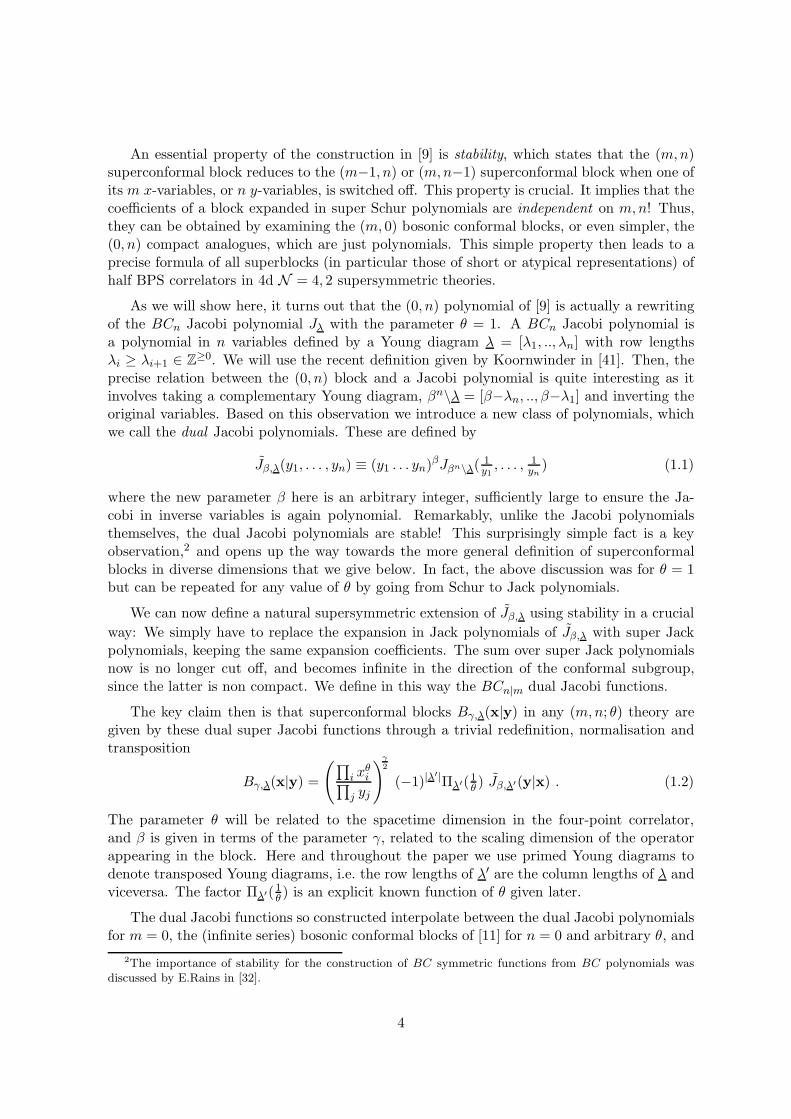
specified by a weight under the afore-mentioned C∗, which we denote by γ, together with therepresentation of the remaining isotropy group, λ, so Oγ,λ (and also the external operatorsO can be specified in this way but with λ trivial). In a free theory,5 γ varies over therange max(p1−p2, p4−p3) ≤ γ ≤ min(p1 + p2, p3 + p4) in steps ∈ 2Z where we will assumep1 > p2, p4 > p3 without loss of generality. The representation of the isotropy group isspecified via a Young diagram λ, which will encode the various quantum numbers, for examplespin and twist, of the operator exchanged. The Young diagram will be consistent with thatdescribing an SL(m|n) representation, meaning it will have at most m rows longer than nand at most n columns taller than m. Furthermore the overall height of the Young diagrammust be smaller than β ≡ min

(12(γ−p12), 12(γ−p43)

). So a valid Young diagram λ must fit

inside the red area here

mβ

n

λ

(2.4)

Superconformal representations are conventionally specified via the dilation weight, ∆,various conformal quantum numbers or Dynkin labels (e.g. Lorentz spin), and quantumnumbers or Dynkin labels describing the internal representation, whereas we specify the therepresentation by the Young diagram λ and the parameter γ. The dilation weight is then∆ =

∑mi=1max(λi−n, 0) +mθ γ2 and the other conformal quantum numbers are specified by

differences of the first m row lengths λi − λi+1. The internal group quantum numbers aregiven as differences of Young diagram column heights λ′i − λ′i+1 as well as the special markedDynkin label b = γ− 2λ′1. We refer to section 3 for a more detailed explanation about how toread the Young diagram and relate it to conformal group representations. For now note thatwhilst all parameters are integers in the free theory, in an interacting quantum theory ∆ alonecan become non integer, with all other quantum numbers remaining integer. In particular,this means we can allow for anomalous dimensions by deforming the row lengths λi → λi + τfor i = 1, ..,m, arbitrary real τ and/ or λ′j → λ′j + τ ′ for j = 1, .., n, arbitrary real τ ′ aslong as we also have γ → γ + 2τ ′ to ensure that b = γ − 2λ′1 remains integer. Furthermoredeforming thus, with τ = −θτ ′ leaves the representation unchanged. We will return to this‘shift symmetry’.

The conformal structure of the theory and the use (twice) of the OPE, imply that we candecompose a four-point function as follows:

〈Op1(X1)Op2(X2)Op3(X3)Op4(X4)〉 =

gp1+p2

212 g

p3+p42

34

(g14g24

)p122(g14g13

)p432 ∑

γ,λ

(∑

O

COp1p2CO p2p3

)B(m,n)

γ,λ (Xi; θ, p12, p43) (2.5)

5We will focus initially on the case where all parameters are integers as for example occurs in a (generalised)free conformal field theory. However the analytic continuation to non integer values (for example to includeanomalous dimensions) is considered in detail in section 6.

7

where Bγ,λ(Xi) is called the (super)conformal block.

The (super)conformal block Bγ,λ is the main subject of this paper. It represents thecontribution of an exchanged primary operator Oγ,λ with its tail of descendants, which iscommon to the OPE of Op1Op2 and Op3Op4 .Thus the block depends on the particular theoryof interest (m,n; θ), as well as the external operators through the quantities

p12 ≡ p1−p2 ; p43 ≡ p4−p3. (2.6)

Furthermore, because of conformal invariance, Bγ,λ(Xi) only depends on cross ratios builtout of the four coordinates Xi=1,2,3,4.

The Xi=1,2,3,4 are square (super) matrices, and the cross ratios are the m+n independenteigenvalues of the (super)-matrix Z = X12X

−124 X43X

−131 where Xij = Xi−Xj . These m+n

independent cross-ratios zi split into two types, corresponding to whether they arise from thenon-compact conformal group or the compact internal group, which we denote by xi and yjrespectively, so

Bγ,λ(Xi) = Bγ,λ(z)

z = (z1, . . . , zm|zm+1, . . . , zm+n), zi = xi, zj+m = yj . (2.7)

The details in all cases of physical interest will be given in section 3. For now note that

sdet(Z)# =g24g13g12g34

=

∏mi=1 x

θi∏n

j=1 yjsdet(1− Z)# =

g14g23g12g34

=

∏mi=1(1− xi)

θ

∏nj=1(1− yj)

, (2.8)

where # is the power in (2.3).

We can characterise Bγ,λ(z) group theoretically, as eigenfunctions of the quadratic Casimiracting at points 1 and 2 on the correlator. Pulling the Casimir through the prefactor of (2.5)to act on the block itself, it becomes a differential operator in z. This differential operator,denoted hereafter by C, has been computed explicitly in a number of cases6 and we find,quite remarkably, that in all these cases it is equivalent to the BCm|n operator of the type ofCalogero-Moser-Sutherland. We give the details of this identification in appendix B. We areled to conjecture that such an identification is true for all cases. Under this assumption wedefine superconformal blocks group theoretically through the eigenvalue equation:

C(θ,− 12p12,− 1

2p43,0)Bγ,λ(z) = E(m,n;θ)

γ,λ Bγ,λ(z) . (2.9)

The Casimir C(θ,a,b,c) is a second order differential operator in the variables z given explicitlyin (5.5). It depends on θ, a, b, c and implicitly on m,n. The eigenvalue is

E(m,n;θ)γ,λ = h(θ)λ + θγ|λ|+

[γθ|mn|+ h

(θ)[em] − θh

( 1θ)

[sn]

](2.10)

6The cases are: (m,n) = (2, 0) and (0, 2) in [11]. Then, θ = 1, m,n ∈ Z+, in [9], by using a supermatrixformalism, and partially in the case of θ = 2, m,n ∈ Z+ in [39]

8

where e = + θγ2 , s = −γ

2 , and

h(θ)λ =∑

i

λi(λi−2θ(i−1)−1) ; |λ| =∑

i

λi (2.11)

with λ = [λ1, . . .] denoting the row lengths of the Young diagram, and

h(θ)[em] = mθ γ2 ((

γ2 + 1−m)θ − 1) ; θh

( 1θ)

[sn] = nγ2 (θ(

γ2 + 1)− 1 + n) (2.12)

In particular, [em] and [sn] are the diagrams with m rows of ‘length’ + θγ2 , and n columns of

‘height’ −γ2 .

What is important about (2.10) is that h(θ)λ + θγ|λ| does not depend on m,n but only de-pends on the Young diagram λ, whereas the other terms clearly have explicitm,n dependence.We will revisit this key point shortly.

2.2 Solving the Casimir equation

From OPE considerations, it has been shown in a number of cases7 that in the limit z → 0

Bγ,λ(z) =

(∏i x

θi∏

j yj

)γ2

×(Pλ(z; θ) + . . .

)(2.13)

where Pλ is the super Jack polynomial of Young diagram λ. (Jack and super Jack polynomialsare reviewed in appendix C). The physics behind (2.13) is quite simple to understand: Whenthere is a group theory interpretation, the prefactor corresponds to the limit zi → 0 of a four-point propagator structure in which an operator of twist θγ is the first operator exchanged,and Pλ accounts for the corresponding superprimary operator in Bγ,λ(z).

The eigenvalue equation (2.9), together with the asymptotics (2.13), gives a unique defi-nition of the superblocks Bγ,λ(z).

For θ = 1, 2 the whole superblock is known to be representable as a series over super Jackpolynomials [7–9]. Thus for arbitrary θ we will seek a representation of Bγ,λ(z) as such aseries, explicitly as,

Bγ,λ(z) =

(∏i x

θi∏

j yj

)γ2

Fγ,λ(z) ; Fγ,λ(z; θ, p12, p43) =∑

µ⊇λ

(Tγ;θ,p12,p43)µλ Pµ(z) , (2.14)

where the sum is over all Young diagrams µ which contain λ, i.e. λ ⊆ µ. The expansioncoefficients (Tγ)

µλ will be sometimes referred to as the Jack→Block matrix. These coefficients

depend on (θ, p12, p43) as well as γ and the two Young tableaux λ, µ. In principle they shoulddepend also on (m,n), but as we will see quite remarkably they in fact don’t! The superJacks themselves vanish if the Young diagram is not of SL(m|n) shape (ie if the mth row

7For a direct derivation of this limit from the OPE see the discussion around eq. (20) in [9] for the θ = 1case and the discussion around (33)-(35) of [8] for θ = 2. This limit is also implicit in earlier work for θ = 1 [6]as well as in the bosonic case [11] for any θ.

9

is bigger than n, λm+1 > n). Furthermore we will see that the coefficients Tγ vanish if theheight of the Young digram is larger than β. So the non-vanishing contributions to the sumare only from Young diagrams µ which fit inside the red area of (2.4).

From the defining Casimir for the blocks (2.9) we obtain a differential equation for Fγ,λ(z)by conjugating the original Casimir in (2.9) by the γ-prefactor in (2.14). It turns out that theresult can be written in terms of a shifted version of the same differential operator C, with amodified eigenvalue:

C(θ,α,β,γ)Fγ,λ(z) = (h(θ)λ + γ|λ|)Fγ,λ(z) , (2.15)

where

α ≡ max(12 (γ−p12), 12(γ−p43)

), β ≡ min

(12(γ−p12), 12(γ−p43)

). (2.16)

A remarkable outcome of conjugating the Casimir is that the eigenvalue of Fγ,λ does notdepend explicitly on (m,n), since the m,n dependent term of the original eigenvalue (2.10),the one in [. . .], is now missing. In other words, the eigenvalue of Fγ,λ depends only on λ andγ. This fact underlies a property known as ‘stability’ in the maths literature, which meansthat Fγ,λ depends only on the number of non-vanishing variables of each type. So the Fγ,λ

of type (m + 1, n) in which one of the x’s is set to zero reduces to the Fγ,λ of type (m,n).Similarly if one of the ys is set to zero. In formulae

Fγ,λ(x1, . . . xm, 0|y1, . . . yn) = Fγ,λ(x1, . . . xm|y1, . . . yn, 0) = Fγ,λ(x1, . . . xm|y1, . . . yn) .(2.17)

Stability is clear when there is a (super) matrix interpretation for the superconformal block(as for θ = 1

2 , 1, 2), but the generalisation to arbitrary θ is non-trivial.

The next observation is that since super Jack polynomials are also stable,8 the expansioncoefficients (Tγ)

µλ must be independent of (m,n)! Indeed this was the main insight of [9],

which reduces the study of (Tγ)µλ for m,n superconformal blocks to the study of the simpler

generalised bosonic conformal blocks.

The representation of the super blocks Bγ,λ(z) as a sum over super Jack polynomials,(2.14), is not accidental. In fact, building on the observation that the Casimir is a differentialoperator for the BCm,n root system, as mentioned above, we are led to consider writing it interms of operators H and

∑i zi∂i, the Am−1,n−1 differential operators for which super Jack

polynomials are eigenfunctions.9 The corresponding decomposition takes the form,

C(θ,a,b,c) = H(θ) + θc

m+n∑

i=1

zi∂i

− θ(a+ b)m+n∑

i=1

z2i ∂i − 12

[H(θ),

m+n∑

i=1

z2i ∂i

]− θ2ab

m+n∑

i=1

zi(−θ)−πi . (2.18)

The operators on the first line thus map Jack polynomials to themselves whereas those onthe second line take a Jack polynomial to another Jack polynomial with an additional box in

8Notice also that the eigenvalue for Fγ,λ is the same as for Pλ, since HPλ = hλPλ and∑

i zi∂iPλ = |λ|Pλ.9More precisely, H is the supersymmetric version of the Calogero-Moser-Sutherland (CMS) Hamiltonian

found in [34,35]. A- and BC-type differential operators are reviewed in appendix B.

10

its Young diagram and will thus be interpreted as one-box raising operators. The action ofthe Casimir on the sum of super Jack polynomials, decomposed as in (2.18), thus turns thedifferential equation (2.15) into a recursion relation on the coefficients (Tγ)

µλ. A particularly

convenient representation of this recursion is

(Tγ)µλ =

∑i=1 (µi−1−θ(i−1−α)) (µi−1−θ(i−1−β)) f (i)µ−�i

(Tγ)µ−�iλ(

hµ−hλ+θγ (|µ|−|λ|)) . (2.19)

Here µ−�i represents a Young diagram obtained by removing the last box at row i fromµ, when allowed, and f is a simple function given in (5.30). Let us emphasise that therecursion (2.19) is straightforward to implement on a computer, and very efficient up to highorder.

The recursion (2.19) actually depends only on objects which can be defined combinato-rially, and admits different equivalent representations, depending on whether we read theYoung diagram just along the rows, or the columns, or we mix rows and columns as it is moreappropriate in the supersymmetric theory. By the (m,n) independence, the value of (Tγ)

µλ

does not depend on the chosen representation. This is particularly useful when construct-ing superconformal blocks for short (protected) representations, a case which is notoriouslydifficult to study with other methods.

As mentioned the above discussion is true for (generalised) free theory blocks where allquantum numbers are integers. In an interacting CFT however, the dilation weight canbecome non integer. Further it is interesting to consider analytic continuations of otherquantum numbers such as spin. We then study possible analytic continuations of the recursionin the variables that describe the Young diagrams. We do so by promoting the external λto complex values, and taking µ = λ + ~n with ~n ∈ Z+. It turns out that each one of thefollowing representations of the recursion, either row type, column type, or supersymmetricone, now gives a distinct analytic continuation (thus analytic continuation breaks the m,nindependence), which however coincide with the others when λ reduces to a valid Youngdiagram.

For long (non protected) representations we show in section 6 that a suitable (m,n)analytic continuation of (Tγ)

µλ exists, such that the following shift,

λi → λi − θτ ′

µi → µi − θτ ′

i = 1, . . . m

;

λ′j → λ′j + τ ′

µ′j → µ′j + τ ′

j = 1, . . . n

; γ → γ + 2τ ′ . (2.20)

is a symmetry of the solution. For integer values this shift symmetry corresponds to the wellunderstood equivalence of different Young diagrams describing SL(m|n) reps for θ = 1 andsimilarly for the other group theoretic cases (e.g. when n = 0 you can see it as the fact thatfull m columns correspond to the trivial SL(m) rep and thus can be deleted). It can also beseen directly from the relation between the Young diagram and Dynkin labels (see (3.16)) thatthere is a redundancy in the Young diagram description of representations which is preciselythis shift.

11

2.3 Superblocks as dual super Jacobi functions

In this section we start from scratch and motivate, from a purely mathematical point of view,the introduction of a certain supersymmetric generalisation of BC Jacobi polynomials [31,41].More precisely, we will define a family of polynomials that we call dual Jacobi polynomials.These are closely related to the BC Jacobi polynomials of Koornwinder [41], but differentlyfrom those, they are stable, and thus allow a straightforward supersymmetric generalisation.The supersymmetric generalisation of a dual Jacobi polynomial is however not polynomial, ingeneral. We will denote them as dual super Jacobi functions. It will turn out that superblocksare equivalent to these dual super Jacobi functions.

This section can be read largely independently of the previous sections (up to the pointwhere we make the identification with blocks).

Dual Jacobi polynomials

Consider the following operation: take a BCn Jacobi polynomial Jλ() in inverse variablesy−1i , and multiply by a sufficiently high power of (y1...yn)

β for β ∈ N in order to ensure theresult is polynomial again in the yi. We will call this a dual Jacobi polynomial.

Note that when the above operation is performed on a Jack polynomial the result is againa Jack polynomial of the complementary Young diagram βn\λ:

(y1 . . . yn)βPλ(

1y1, . . . , 1

yn) = Pβn\λ(y1, . . . , yn) , (2.21)

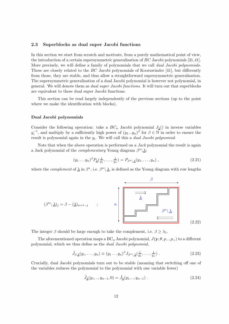
where the complement of λ in βn, i.e. βn\λ, is defined as the Young diagram with row lengths

n

β

λ

βn\λ(βn\λ)j = β − (λ)n+1−j ;

(2.22)

The integer β should be large enough to take the complement, i.e. β ≥ λ1.

The aforementioned operation maps a BCn Jacobi polynomial, J(y; θ, p−, p+) to a differentpolynomial, which we thus define as the dual Jacobi polynomial,

Jβ,λ(y1, . . . , yn) ≡ (y1 . . . yn)βJβn\λ(

1y1, . . . , 1

yn) . (2.23)

Crucially, dual Jacobi polynomials turn out to be stable (meaning that switching off one ofthe variables reduces the polynomial to the polynomial with one variable fewer)

Jλ(y1, .., yn−1, 0) = Jλ(y1, .., yn−1) . (2.24)

12

This is the same stability property possessed by Jack polynomials, Pλ(y, 0) = Pλ(y), butwhich is absent for the original Jacobi polynomials themselves: Jλ(y, 0) 6= Jλ(y).

This stability property is key to a direct supersymmetric uplift of the dual Jacobi poly-nomials to BCn|m functions. As we will see, this uplift lands precisely on our superconformalblocks!

The BCn Jacobi polynomial has as an explicit expansion in Jack polynomials (just likethe blocks)10

Jλ(y; θ, p−, p+) =

∑

µ⊆λ

(S(n)θ,p−,p+

)µλ Pµ(y; θ) . (2.25)

The coefficients, (S(n))µλ are not stable, meaning they have explicit n dependence and don’tjust depend on the Young diagrams λ, µ. Indeed, this is what prevents stability of the Jacobipolynomial J . Let us note that the (S(n))µλ can be computed quite explicitly, either througha recursion, investigated by Macdonald [28], or independently by using a binomial formuladue to Okounkov [33,40,41]. In the latter case, S(n), is written in terms of BCn interpolationpolynomials (IPs). We will discuss this in much more detail in section 7.

We can understand the stability of the dual Jacobi polynomials by considering their defin-ing differential equation. The original eigenvalue equation for the Jacobi polynomials, trans-lated to the dual Jacobi polynomials, can be written in terms of the Casimir (2.18) as

C( 1θ,a,b,c)(|y) Jβ,λ(y1, . . . yn; θ, p−, p+) = e

(θ)β,λ Jβ,λ(y1, . . . yn; θ, p

−, p+) (2.26)

a = β ; b = β + p− ; c = 2β + p− + p+ .

where the eigenvalue is

e(θ)β,λ = −1

θh(θ)λ + 1

θ (2β + p− + p+)|λ| (2.27)

Both h(θ)λ and |λ|, given already in (2.11), are functions of the Young diagram λ only, (unlikethe corresponding eigenvalue for the Jacobi polynomial which has explicit n dependence) andstability (2.24) follows. In our conventions, the normalisation of J will be chosen so that theleading term of Jβ,λ is Pλ.

Dual Jacobi polynomials depend on θ, p±, as the Jacobi polynomials do, and in additiondepend on β, which sets the boundary for the Young diagram in (2.22). From the definitionof Jβ,λ, in terms of the Jacobi polynomials (2.23), the expansion of Jacobi polynomials (2.25),and the relation (2.21), we obtain the following expansion of the dual Jacobi polynomials inJack polynomials with coefficients given by binomial coefficients, S, in complemented Youngdiagrams

Jβ,λ(y1, . . . , yn) =∑

µ:λ⊆µ

(Sβ)µλPµ(y1, . . . , yn) ;

(Sβ)µλ=(S(n)

)βn\µβn\λ . (2.28)

Note that if the Young diagram µ is wider than β (ie µ1 > β) the coefficient S will vanish

10We have momentarily suppressed the parameters in Jλ(; θ, p−, p+), since they do not play an immediate

role. Note that Pµ(y1, . . . , yn) here is P (n,0)µ (y1, . . . , yn|; θ) in supersymmetric notation, not to be confused

with the P (0,n)µ (|y1, . . . , yn; θ) polynomials. See appendix C and C.5 for further details.

13

and so the sum is finite, µ ⊆ βn giving a polynomial.

Stability of dual Jacobi polynomials implies that the coefficients (Sβ)µλ are independent

of n. Looking at the way this is related to S(n) (2.28), we see that even though S(n) is ndependent, remarkably it becomes independent of n when specified by complemented Youngdiagrams as is the case for (Sβ)

µλ.

Dual super Jacobi functions

The supersymmetric extension of the dual Jacobi polynomial which we call dual super Jacobi

functions is now immediate from stability: replace the expansion over Jack polynomials withsuper Jack polynomials, keeping the same expansion coefficients S. This operation definesthe n|m dual super Jacobi function

Jβ,λ(y|x) =∑

µ⊇λ

(Sβ)µλ Pµ(y|x) . (2.29)

When m > 0, the sum is over all Young diagrams µ such that λ ⊆ µ. As before, if µ is widerthan βn, the coefficient S will vanish and so µ1 ≤ β. But now µ can have arbitrary height,unlike in the non supersymmetric case (2.28) where it was naturally cut-off by n since theJack polynomials would vanish for µ′1 > n. This means that the sum is infinite in the verticalYoung diagram direction, and this is why we call Jβ,λ a function rather than a polynomial.

As a result, the dual Jacobi functions Jβ,λ are explicitly different from the super Jacobipolynomials introduced in [38]. The latter also provide a supersymmetric generalisations ofJacobi polynomials but the generalisation is polynomial in both x and y variables and notstable. We will have something to say about these other supersymmetric Jacobi polynomialsin section 7.

Blocks as dual super Jacobi functions

The claim is then that the dual super Jacobi functions are precisely the superconformal blocksup to changes of conventions. Explicitly the relation is

Fγ,λ(x|y; θ, p12, p43) = (−1)|λ′|Πλ′(1θ ) Jβ,λ′(y|x; 1θ , p−, p+) (2.30)

where11

γ = 2β + p+ + p− ; p± = 12 |p12 ± p43| (2.31)

then Π(θ) is a numerical factor, given explicitly later on in (7.10), and p43 and p12 can besolved as linear combinations of p+ and p−. Specialising to the internal case (0, n) we have adirect relation between internal blocks and Jacobi polynomials

n∏

i=1

y12(p++p−)

i ×Bγ=2β+p++p−, λ(y; θ, p12, p43) = (−)|λ|Πλ′(1θ )× Jβn−λ′

(1y; 1θ , p

−, p+)

(2.32)

11In other words, β = min(

12(γ−p12),

12(γ−p43)

)

.

14

where the original Jacobi polynomial J appears on the RHS with complemented, transposedYoung diagram.

Equation (2.32), is an equation purely between symmetric polynomials, and provides thecleanest way to prove the more general supersymmetric relation (2.30). Indeed it was thediscovery of this relation which lead us to dual Jacobi polynomials and their supersymmetricgeneralisation. This polynomial identification (2.32) can be proved by simply showing theyobey the same Casimir equation. Then the general supersymmetric relation (2.30) followsdirectly because both sides can be uplifted supersymmetrically in the same way, i.e. by ex-panding in Jack polynomials, and uplifting the bosonic polynomials to super Jack polynomialsthanks to stability.

The relation between dual super Jacobi functions and superconformal blocks gives a way ofseeing why there must be an infinite expansion in the x variable, at least in cases where thereis a supergroup interpretation. This infinite sum is a consequence of the non compactness ofthe conformal subgroup.

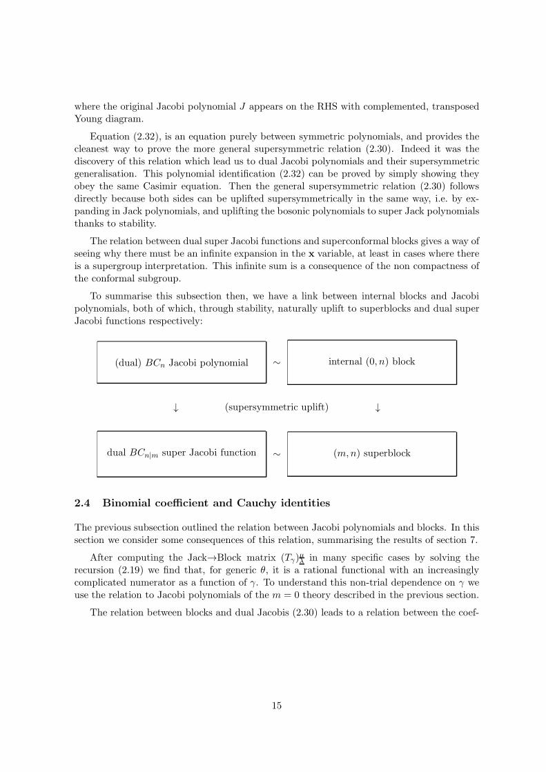
To summarise this subsection then, we have a link between internal blocks and Jacobipolynomials, both of which, through stability, naturally uplift to superblocks and dual superJacobi functions respectively:

(dual) BCn Jacobi polynomial ∼ internal (0, n) block

↓ (supersymmetric uplift) ↓

dual BCn|m super Jacobi function ∼ (m,n) superblock

2.4 Binomial coefficient and Cauchy identities

The previous subsection outlined the relation between Jacobi polynomials and blocks. In thissection we consider some consequences of this relation, summarising the results of section 7.

After computing the Jack→Block matrix (Tγ)µλ in many specific cases by solving the

recursion (2.19) we find that, for generic θ, it is a rational functional with an increasinglycomplicated numerator as a function of γ. To understand this non-trial dependence on γ weuse the relation to Jacobi polynomials of the m = 0 theory described in the previous section.

The relation between blocks and dual Jacobis (2.30) leads to a relation between the coef-

15

ficients, S and Tγ in their respective Jack expansions (2.14),(2.28), explicitly:12

(Tγ;θ,p12,p43)µλ = (Sβ; 1

θ,p−,p+)

µ′

λ′ ×(−1)|µ|Πµ(θ)

(−1)|λ|Πλ(θ). (2.34)

Hence from (2.28) the coefficients Tγ are related to the binomial coefficients S (2.25)

(Tγ;θ,p12,p43)µλ =

(−)|µ|Πµ(θ)

(−)|λ|Πλ(θ)× (S

(n)1θ; p−,p+

)βn\µ′

βn\λ′ , (2.35)

where β, p± are read off γ, p12, p43 through (2.31).

Now the BCn Jacobi polynomials are very well studied objects. In particular, the co-efficients in the expansion over Jack polynomials can be computed by Okounkov binomial

formula. Okounkov’s binomial formula for S(n) (see [32, 33, 40, 41]) is computed via objectscalled BC interpolation polynomials (IPs) evaluated on partitions. The combinatorics isthus completely different from the combinatorics induced by the recursion and so the aboverewriting of Tγ (2.35) is quite non trivial.

In fact, a very non trivial feature of this relation (2.35) is the way the RHS depends onγ. In the binomial coefficient we have γ = 2β + p+ + p− where β is an integer specifying thecomplemented Young diagram. On the other hand in the recursion, γ is a free parameter, andthe solution of the recursion is a rational function of γ and thus straightforwardly analyticallycontinued. This should also be the case for the binomial coefficient then. In the process ofunderstanding how this works we find that the complicated γ dependence of (Tγ)

µλ is precisely

captured by the interpolation polynomial. We also find that the inverse of the Jack→Blockmatrix (i.e. the Block→Jack matrix) T−1

γ , has an even more direct characterisation in termsof the binomial coefficient.

Note that since (Tγ)µλ does not depend on (m,n), for integer quantum numbers, the above

characterisation via the binomial coefficient, through the (0, n) case, can be used to computeany superconformal block for arbitrary (m,n). However, from this insight we understand thatthe binomial coefficient can also be upgraded to a super binomial coefficient which uses thesuper interpolation polynomials introduced by Sergeev and Veselov [38]. We will investigatethis whole story in detail in section 7, and then in appendix E we collect a number of explicitsolutions for Tγ found by solving the recursion, and we show explicitly how the two sides of(2.35) match.

We will conclude the main body of the paper by giving two nice applications of the relationbetween blocks and Jacobi polynomials, together with stability. Firstly, in section 8 we seehow upon re-interpreting a Cauchy identity for Jacobi polynomials, given by Mimachi in [42],we can obtain (essentially with no effort) a formula for the conformal partial wave expansionof any generalised free theory within the class analysed here, i.e. whose supergroup descrip-tion fits (m,n, θ) for specific values. In the process of investigating this we discover a new

12To derive this relation one also needs to use the fact that super Jack polynomials are well behaved undertransposition

Pλ′(y|x; 1θ) = (−1)|λ|Πλ(θ)Pλ(x|y; θ) (2.33)

For more details see the discussion around (C.47).

16

non-trivial double uplift of Mimachi’s Cauchy identity to a doubly supersymmetric Cauchyidentity involving both dual super Jacobi functions and Sergeev and Veselov’s super Jacobipolynomials. Secondly in section 5.1 we use results from the study of BC hypergeometricfunctions in the special θ = 1 case of Shimeno [43] to give simple explicit formulae for allhigher order super Casimirs.

2.5 Superblock to block decomposition: a conjecture

Our formalism for constructing superconformal blocks might be classified as top-down, becausewe start from a supergroup perspective in which superconformal symmetry is built-in, andwe derive its consequences for the superconformal blocks. Instead, a bottom-up approachconstructs superconformal blocks starting from an ansatz made of a sum of products ofconformal and internal blocks, and afterwards imposes the constraints of superconformalsymmetry, i.e. the superconformal Ward identity and the Casimir equation [44–51].

The top-down and the bottom-up approaches should obviously give the same final result.However, the two paths are quite different, and the crucial point is that decomposing asuperconformal blocks, say for example on a basis of conformal and internal blocks, is quitehard. In fact, we will now show that all the nice properties about stability and the Jack→Blockmatrix, explained in the previous sections, become hidden in the details.

From the top-down approach we are able to provide an implicit formula for decomposinga (m,n) superconformal in subgroups. Mathematically, this formula is the equivalent ofdecomposing a super Jack polynomial (m+m′, n+n′) into sum of products of two super Jackpolynomials for (m,n) and (m′, n′). This decomposition is achieved by using the structureconstants for super Jack polynomials (S)µνλ ,

J (m+m′,n+n′)λ =

∑

µ,ν

(S)µνλ J (m,n)µ J (m′,n′)

ν (2.36)

which by stability are the same as those for bosonic Jack polynomials. For θ = 1 these are theLittlewood-Richardson coefficients. Combining (2.36) with the expansion of superconformalblocks in super Jack polynomials we arrive at

F (m+m′,n+n′)γ,λ =

∑

µ,ν

F (m,n)γ,µ (Sγ)

µνλ F (m′,n′)

γ,ν , (2.37)

where the block structure constants Sγ depend on θ, p12, p43 and are related to the Jackstructure constants via the matrices Tγ and T−1

γ ,

(Sγ)µνλ =

∑

λ⊇λµ⊆µν⊆ν

S µνλ (Tγ)

λλ(T

−1γ )

µµ(T

−1γ )

νν . (2.38)

Let us point out that [52–54] obtained a recursive formula for the Jack structure constantsS, but we are not aware of a more explicit formula, and to the best of our knowledge thereis no closed formula expression for it, and therefore for Sγ . The bottom-up construction ofsuperblocks in terms of conformal and internal blocks mentioned above is a special case of

17

the more general decomposition (2.37) when m′ = n = 0, and the ignorance about S is whatmakes it complicated.

Not only is S not known explicitly, but a very non-obvious fact about (2.38) is the fol-lowing: the Jack→Block matrix and its inverse are infinite size triangular matrices, however(Sγ)

µνλ should truncate, because, for example, superconformal group theory for specific values

of θ = 12 , 1, 2 tells us that (2.37) is a finite sum. Consider again the case of conformal block

× internal block decomposition, m′ = n = 0. Whilst a truncation in the number of rows ofν is expected, since Fγ,λ is polynomial in the y, the truncation over finitely many conformalblock Fγ,µ is not at all manifest.

We conjecture that the subgroup decomposition in (2.37) is a finite sum. In section9 we discuss in more detail various aspects of this conjecture, relating it to a more specificconjecture for a general decomposition and providing a number of examples. We have checkedthe conjecture with computer algebra, in many cases, and find that it holds for generic θ,even beyond the cases θ = 1

2 , 1, 2 related to superconformal groups. Perhaps the connectionwith the binomial coefficient will provide a simple mechanism to prove it in the future.

That concludes our extended outline of the paper. The methods employed throughout thepaper strongly rely on the use of Young diagrams and symmetric polynomials. To help thereader familiarise themself with the relevant mathematics, we have summarised in appendixC a number of results on the theory of symmetric polynomials.

3 Supergroups, physical theories, and beyond

In this section we detail the theories and the external operators for which we are computingsuperconformal blocks, as a function of (m,n; θ). We also explain the field theory interpreta-tion of the labels assigned to the superconformal block Bγ,λ, namely γ and λ.

A unified description of all relevant theories can be achieved by using the formalismbased on harmonic/analytic superspace, and building on previous literature. In particular,4d superconformal theories with θ = 1 discussed in [1–3, 6–10, 55, 56], 6d superconformalfield theories with θ = 2 discussed in [5, 8, 57], and 3d superconformal field theories withθ = 1

2 discussed in some detail in [4,57]. This is explained in section 3.2, with supplementarymaterial given in appendix A.

Let us emphasise that we will be able to construct Bγ,λ for any (m,n; θ) (for m,n positiveinteger), but only some values of (m,n; θ) appear to have a group theoretic meaning (andeven fewer will correspond to a physical CFT). The spacetime dimension d and the parameterθ are identified as θ = d−2

2 , apart for special cases, that we will explicitly mention. A usefulsummary of the different cases is given here below.

3.1 List of theories and their superconformal blocks

The main examples to have in mind are three complete families of supergroups with θ = 1, 2, 12and arbitrary m,n. These include the cases of four-point functions of half-BPS operators in4d,6d,3d superconformal field theories respectively:

18

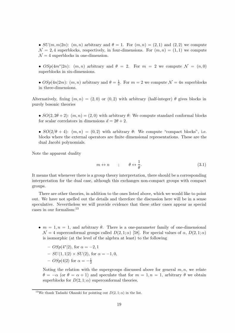
• SU(m,m|2n): (m,n) arbitrary and θ = 1. For (m,n) = (2, 1) and (2, 2) we computeN = 2, 4 superblocks, respectively, in four-dimensions. For (m,n) = (1, 1) we computeN = 4 superblocks in one-dimension.

• OSp(4m∗|2n): (m,n) arbitrary and θ = 2. For m = 2 we compute N = (n, 0)superblocks in six-dimensions.

• OSp(4n|2m): (m,n) arbitrary and θ = 12 . For m = 2 we compute N = 4n superblocks

in three-dimensions.

Alternatively, fixing (m,n) = (2, 0) or (0, 2) with arbitrary (half-integer) θ gives blocks inpurely bosonic theories

• SO(2, 2θ + 2): (m,n) = (2, 0) with arbitrary θ: We compute standard conformal blocksfor scalar correlators in dimensions d = 2θ + 2.

• SO(2/θ + 4): (m,n) = (0, 2) with arbitrary θ: We compute “compact blocks”, i.e.blocks where the external operators are finite dimensional representations. These are thedual Jacobi polynomials.

Note the apparent duality

m↔ n ; θ ↔ 1

θ. (3.1)

It means that whenever there is a group theory interpretation, there should be a correspondinginterpretation for the dual case, although this exchanges non-compact groups with compactgroups.

There are other theories, in addition to the ones listed above, which we would like to pointout. We have not spelled out the details and therefore the discussion here will be in a sensespeculative. Nevertheless we will provide evidence that these other cases appear as specialcases in our formalism:13

• m = 1, n = 1, and arbitrary θ. There is a one-parameter family of one-dimensionalN = 4 superconformal groups called D(2, 1;α) [58]. For special values of α, D(2, 1;α)is isomorphic (at the level of the algebra at least) to the following

– OSp(4∗|2), for α = −2, 1

– SU(1, 1|2) × SU(2), for α = −1, 0,

– OSp(4|2) for α = −12

Noting the relation with the supergroups discussed above for general m,n, we relateθ = −α (or θ = α + 1) and speculate that for m = 1, n = 1, arbitrary θ we obtainsuperblocks for D(2, 1;α) superconformal theories.

13We thank Tadashi Okazaki for pointing out D(2, 1;α) in the list.

19

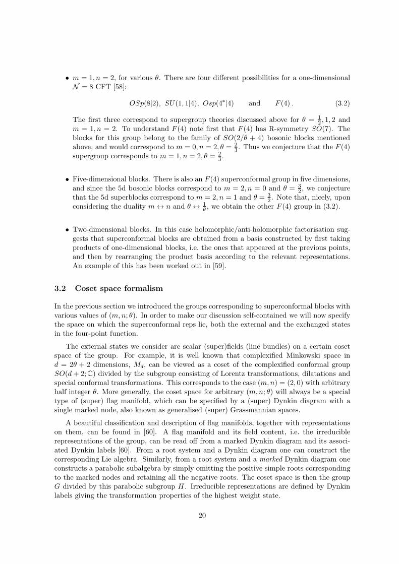
• m = 1, n = 2, for various θ. There are four different possibilities for a one-dimensionalN = 8 CFT [58]:

OSp(8|2), SU(1, 1|4), Osp(4∗|4) and F (4) . (3.2)

The first three correspond to supergroup theories discussed above for θ = 12 , 1, 2 and

m = 1, n = 2. To understand F (4) note first that F (4) has R-symmetry SO(7). Theblocks for this group belong to the family of SO(2/θ + 4) bosonic blocks mentionedabove, and would correspond to m = 0, n = 2, θ = 2

3 . Thus we conjecture that the F (4)supergroup corresponds to m = 1, n = 2, θ = 2

3 .

• Five-dimensional blocks. There is also an F (4) superconformal group in five dimensions,and since the 5d bosonic blocks correspond to m = 2, n = 0 and θ = 3

2 , we conjecturethat the 5d superblocks correspond to m = 2, n = 1 and θ = 3

2 . Note that, nicely, uponconsidering the duality m↔ n and θ ↔ 1

θ , we obtain the other F (4) group in (3.2).

• Two-dimensional blocks. In this case holomorphic/anti-holomorphic factorisation sug-gests that superconformal blocks are obtained from a basis constructed by first takingproducts of one-dimensional blocks, i.e. the ones that appeared at the previous points,and then by rearranging the product basis according to the relevant representations.An example of this has been worked out in [59].

3.2 Coset space formalism

In the previous section we introduced the groups corresponding to superconformal blocks withvarious values of (m,n; θ). In order to make our discussion self-contained we will now specifythe space on which the superconformal reps lie, both the external and the exchanged statesin the four-point function.

The external states we consider are scalar (super)fields (line bundles) on a certain cosetspace of the group. For example, it is well known that complexified Minkowski space ind = 2θ + 2 dimensions, Md, can be viewed as a coset of the complexified conformal groupSO(d+ 2;C) divided by the subgroup consisting of Lorentz transformations, dilatations andspecial conformal transformations. This corresponds to the case (m,n) = (2, 0) with arbitraryhalf integer θ. More generally, the coset space for arbitrary (m,n; θ) will always be a specialtype of (super) flag manifold, which can be specified by a (super) Dynkin diagram with asingle marked node, also known as generalised (super) Grassmannian spaces.

A beautiful classification and description of flag manifolds, together with representationson them, can be found in [60]. A flag manifold and its field content, i.e. the irreduciblerepresentations of the group, can be read off from a marked Dynkin diagram and its associ-ated Dynkin labels [60]. From a root system and a Dynkin diagram one can construct thecorresponding Lie algebra. Similarly, from a root system and a marked Dynkin diagram oneconstructs a parabolic subalgebra by simply omitting the positive simple roots correspondingto the marked nodes and retaining all the negative roots. The coset space is then the groupG divided by this parabolic subgroup H. Irreducible representations are defined by Dynkinlabels giving the transformation properties of the highest weight state.

20

The generalisation of Dynkin diagrams to the supersymmetric case is well known (we rec-ommend [61] for a nice introduction) and the generalisation of the flag manifold techniquesof [60] to supergroups proceeds fairly straightforwardly and has been considered in the θ = 1, 2cases explicitly in [6–8, 56]. We should point out that, compared to the bosonic cases, whendealing with supergroups there is no longer a unique (super) Dynkin diagram.14 A superDynkin diagram will have even (black) and odd (white) nodes, and then the coset space ofthis superspace will be indicated by marked nodes (represented by crosses). Remarkably allunitary superconformal representations of the superconformal group are obtained as uncon-

strained analytic superfields on the the coset superspaces we use here. This is proven for4d superconformal theories θ = 1,m = 2 in [7] and is conjectured in other supersymmetriccases.15

Various details about the coset construction for the specific cases listed in section 3.1 aregiven in appendix A. We repeat the main points here.

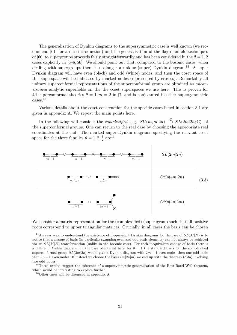
In the following will consider the complexified, e.g. SU(m,m|2n) C−→ SL(2m|2n;C), ofthe superconformal groups. One can return to the real case by choosing the appropriate realcoordinates at the end. The marked super Dynkin diagrams specifying the relevant cosetspace for the three families θ = 1, 2, 12 are16

m− 1 n− 1 n− 1 m− 1

SL(2m|2n)

2m− 1 n− 1

OSp(4m|2n)

m− 1 2n− 2

OSp(4n|2m)

(3.3)

We consider a matrix representation for the (complexified) (super)group such that all positiveroots correspond to upper triangular matrices. Crucially, in all cases the basis can be chosen

14An easy way to understand the existence of inequivalent Dynkin diagrams for the case of SL(M |N) is tonotice that a change of basis (in particular swapping even and odd basis elements) can not always be achievedvia an SL(M |N) transformation (unlike in the bosonic case). For each inequivalent change of basis there isa different Dynkin diagram. In the case of interest here, for θ = 1 the standard basis for the complexifiedsuperconformal group SL(2m|2n) would give a Dynkin diagram with 2m − 1 even nodes then one odd nodethen 2n− 1 even nodes. If instead we choose the basis (m|2n|m) we end up with the diagram (3.3a) involvingtwo odd nodes.

15These results suggest the existence of a supersymmetric generalisation of the Bott-Borel-Weil theorem,which would be interesting to explore further.

16Other cases will be discussed in appendix A.

21

such that (super)coset space H\G has the following block 2× 2 structure

G =

{(aAB bAB′

cA′B d B′

A′

)}H =

{(aAB 0

cA′B d B′

A′

)}. (3.4)

where a, b, c, d, a, c, d are square (super-)matrices of equal dimensions (in general they willhave some constraints). For θ = 1 they are (m|n) × (m|n) matrices; for θ = 2 they are(2m|n)× (2m|n) matrices; for θ = 1

2 they are (m|2n)× (m|2n) matrices.17 For example, thespecial case (m,n; θ) = (2, 0; 1) corresponds to 4d Minkowski space viewed as the coset spaceof the complexified conformal group SL(4) modded out by dilatations, Lorentz and specialconformal transformations. Here the 2× 2 matrices a, b give Lorentz and dilatations whereasc represents special conformal transformations.

Fields living on the coset space transform non-trivially under the block diagonal partof the parabolic subgroup H (known as the Levi subgroup, L). This subgroup consists ofthe matrices a, d (e.g. in the Minkowski space example these correspond to Lorentz anddilatations under which conformal operators transform). The Levi subgroup is read off fromthe same Dynkin diagrams (3.3) upon deleting the marked node (and replacing it with C∗).In the above cases they are as follows,

θ 1 2 12

G SL(2m|2n) Osp(4m|2n) Osp(4n|2m)

L SL(m|n)⊗ SL(m|n)⊗ C∗ SL(2m|n)⊗ C∗ SL(m|2n)⊗ C∗

(3.5)

There is an overall constraint to take into account: for h ∈ H, sdet(h) = sdet(a) sdet(d) = 1.The C∗ subgroup of the parabolic group is then identified with sdet(a) = 1/(sdet(d)).

The coset space H\G is finally the collection of all the orbits under the equivalence g ∼ hgfor g ∈ G and h ∈ H. A representative for each orbit is18

g ∼ s(X) =

(1 XAA′

0 1

). (3.6)

17More precisely, the second half of the basis is reversed compared to the first half. Taking θ = 1 as theillustrative example, then a is (m|n)× (m|n), X is (m|n)× (n|m), c is (n|m)× (m|n) and d is (n|m)× (n|m).However when referring to a, c, d,X we will consider them with the bases rearranged, so they all have the samedimensions (m|n)× (m|n).

18A toy model for the coset construction, corresponding to (m,n; θ) = (0, 1; 1) is just the Riemann sphere,

realised by taking g =(

a bc d

)

in SL(2,C) and h =(

a 0c d

)

. Then(

1 x0 1

)

is the coset representative and(

1 x0 1

)

g =

h( 1 f(x)0 1

)

∼( 1 f(x)0 1

)

where f(x) = (dx+ b)/(cx+ a) and a = a+ xc, c = c, d = d− cf(x). From f we recogniseMobius transformations acting on the Riemann sphere as the coset H\SL(2,C). By taking just the top rowof the coset representative, (1, x), we recognise this construction to be completely equivalent to the projectivespace P 1. Similarly, the general (m,n; θ) construction is equivalent to a Grassmannian space.

22

This supermatrix X are then coordinates for the coset space, which we write as

X =

(x ρ

ρ y

). (3.7)

For θ = 1, x is m×m, y is n×n and both are bosonic, whereas ρ is m×n, ρ is n×m and theyare fermionic. The other cases are similar except m → 2m when θ = 2 and n → 2n whenθ = 1

2 (and the supermatrix is generalised (anti-)symmetric in its indices, see appendix Afor more details). For θ = 1 the cosets are equivalent to super Grassmannians which canbe seen by considering the upper half of the group matrix (1,X) ∼ a(1,X), which is indeedGr(m|n, 2m|2n), the space of m|n planes in 2m|2n dimensions. Then the θ = 2, 12 casesare generalised Grassmannians. For θ = 1, 2, 12 note that xαα represents coordinates forMinkowski space in dimensions Md=4,6,3 respectively written in a (Weyl) spinor notation.

Now we can connect with the superblocks. The four-point superconformal invariant com-binations of four coordinates X1,X2,X3,X2 can be viewed as the independent eigenvalues ofthe cross-ratio matrix:

Z = X12X−123 X34X

−141 ; Xij = Xi −Xj . (3.8)

These independent eigenvalues then correspond to the arguments of the blocks, z (2.7). Fur-ther the building block two-point function gij in (2.3) is

gij = sdet−#(Xi−Xj). (3.9)

where sdet is the superdeterminant (Berezinian) and the exponent # is discussed in footnote 4.

The external representations appearing in the four-point function (2.5) are scalars, Op(X),on this coset space, thus they transform non-trivially, with a certain weight p under C∗ andare invariant under the rest of the parabolic group (3.5). In terms of the Dynkin labels,the label above a marked node gives the weight under the C∗ subgroup of the parabolicsubgroup associated with that node. The Dynkin labels next to the unmarked nodes givethe representation under non-trivial subgroups of the parabolic subgroup.19 The external

19Although we will be dealing with infinite dimensional representations, the representation of the parabolicsubgroup itself will always be finite dimensional.

23

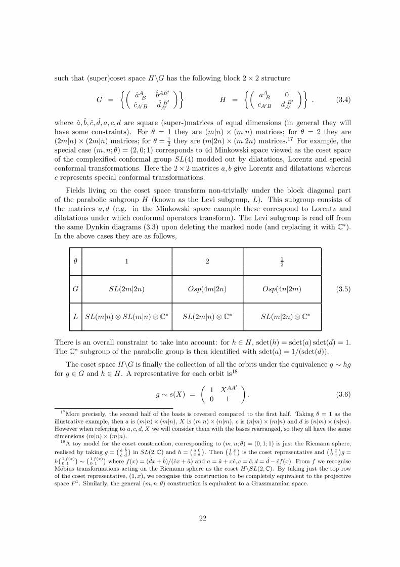
operators Op are therefore written as,

pSL(2m|2n)

pOSp(4m|2n)

p

OSp(4n|2m)

(3.10)where all unlabelled nodes are understood to have the label 0. These fields transform undera general superconformal transformation g as follows:

s(X) g = h s(X ′) Op(X) → O′p(X

′) = sdet(a)pOp(X) . (3.11)

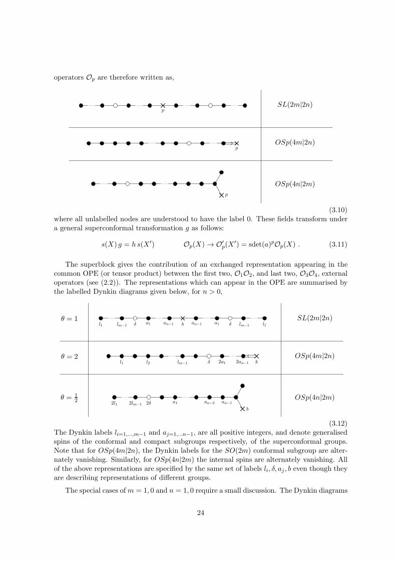
The superblock gives the contribution of an exchanged representation appearing in thecommon OPE (or tensor product) between the first two, O1O2, and last two, O3O4, externaloperators (see (2.2)). The representations which can appear in the OPE are summarised bythe labelled Dynkin diagrams given below, for n > 0,

l1 lm−1 δ a1 an−1 b an−1 a1 δ lm−1 l1SL(2m|2n)

l1 l2 lm−1 δ 2a1 2an−1 bOSp(4m|2n)

2l1 2lm−1 2δ a1 an−2 an−1

b

OSp(4n|2m)

θ = 1

θ = 2

θ = 12

(3.12)The Dynkin labels li=1,...,m−1 and aj=1,...n−1, are all positive integers, and denote generalisedspins of the conformal and compact subgroups respectively, of the superconformal groups.Note that for OSp(4m|2n), the Dynkin labels for the SO(2m) conformal subgroup are alter-nately vanishing. Similarly, for OSp(4n|2m) the internal spins are alternately vanishing. Allof the above representations are specified by the same set of labels li, δ, aj , b even though theyare describing representations of different groups.

The special cases ofm = 1, 0 and n = 1, 0 require a small discussion. The Dynkin diagrams

24

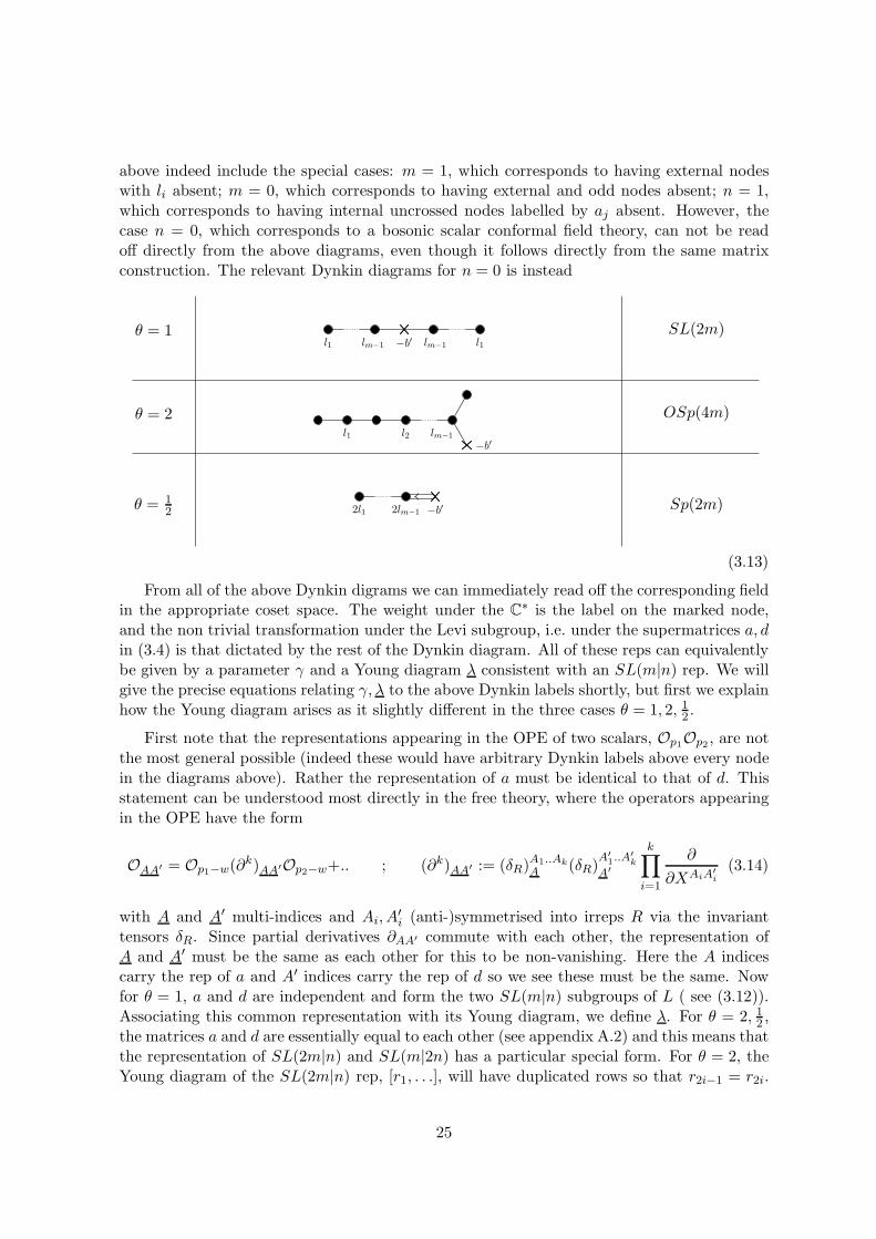
above indeed include the special cases: m = 1, which corresponds to having external nodeswith li absent; m = 0, which corresponds to having external and odd nodes absent; n = 1,which corresponds to having internal uncrossed nodes labelled by aj absent. However, thecase n = 0, which corresponds to a bosonic scalar conformal field theory, can not be readoff directly from the above diagrams, even though it follows directly from the same matrixconstruction. The relevant Dynkin diagrams for n = 0 is instead

l1 lm−1 −b′ lm−1 l1SL(2m)

l1 l2 lm−1

−b′

OSp(4m)

2l1 2lm−1 −b′ Sp(2m)

θ = 1

θ = 2

θ = 12

(3.13)

From all of the above Dynkin digrams we can immediately read off the corresponding fieldin the appropriate coset space. The weight under the C∗ is the label on the marked node,and the non trivial transformation under the Levi subgroup, i.e. under the supermatrices a, din (3.4) is that dictated by the rest of the Dynkin diagram. All of these reps can equivalentlybe given by a parameter γ and a Young diagram λ consistent with an SL(m|n) rep. We willgive the precise equations relating γ, λ to the above Dynkin labels shortly, but first we explainhow the Young diagram arises as it slightly different in the three cases θ = 1, 2, 12 .

First note that the representations appearing in the OPE of two scalars, Op1Op2 , are notthe most general possible (indeed these would have arbitrary Dynkin labels above every nodein the diagrams above). Rather the representation of a must be identical to that of d. Thisstatement can be understood most directly in the free theory, where the operators appearingin the OPE have the form

OAA′ = Op1−w(∂k)AA′Op2−w+.. ; (∂k)AA′ := (δR)

A1..AkA (δR)

A′1..A

′k

A′

k∏

i=1

∂

∂XAiA′i

(3.14)

with A and A′ multi-indices and Ai, A′i (anti-)symmetrised into irreps R via the invariant

tensors δR. Since partial derivatives ∂AA′ commute with each other, the representation ofA and A′ must be the same as each other for this to be non-vanishing. Here the A indicescarry the rep of a and A′ indices carry the rep of d so we see these must be the same. Nowfor θ = 1, a and d are independent and form the two SL(m|n) subgroups of L ( see (3.12)).Associating this common representation with its Young diagram, we define λ. For θ = 2, 12 ,the matrices a and d are essentially equal to each other (see appendix A.2) and this means thatthe representation of SL(2m|n) and SL(m|2n) has a particular special form. For θ = 2, theYoung diagram of the SL(2m|n) rep, [r1, . . .], will have duplicated rows so that r2i−1 = r2i.

25

Thus, the only relevant information is given in a Young diagram λ defined by λi = r2i,i.e. half the height, and this λ will label the blocks. Furthermore since the Young diagram[r1, . . .] is consistent with SL(2m|n) the resulting Young diagram λ will be consistent withSL(m|n). For θ = 1

2 on the other hand, the resulting SL(m|2n) Young diagram will alwayshave duplicated columns so r′2j−1 = r′2j . Thus,we will label the blocks with the Young diagramλ defined to have column lengths λ′j = r′2j .

Summarising: In all cases with a group theory interpretation we have specified a represen-tation exchanged in the OPE of two scalars, through a Young diagram, λ. Thus λ, togetherwith a parameter γ, is the data we will use to specify the superconformal blocks Bγ,λ. It willturn out that this same data is very natural from the point of view of BCm|n functions!

A closing remark regarding the non-supersymmetric degeneration for either n = 0 orm = 0, which we discuss in appendix A. This has a group theory interpretation for any halfinteger (or inverse of a half integer) θ, and it is interesting to mention that the group theoreticinterpretation we give here meshes closely with a previously understood interpretation ofthe BCn Heckman Opdam hypergeometric functions as spherical functions on certain cosetspaces [62]. The latter are Grassmannians in SU(p, q), SO(p, q) and Sp(p, q), for θ = 1, 2, 12respectively. Upon setting p = q = m (or n) they look very reminiscent of the ones that weare using and it would be interesting to pursue this connection further.

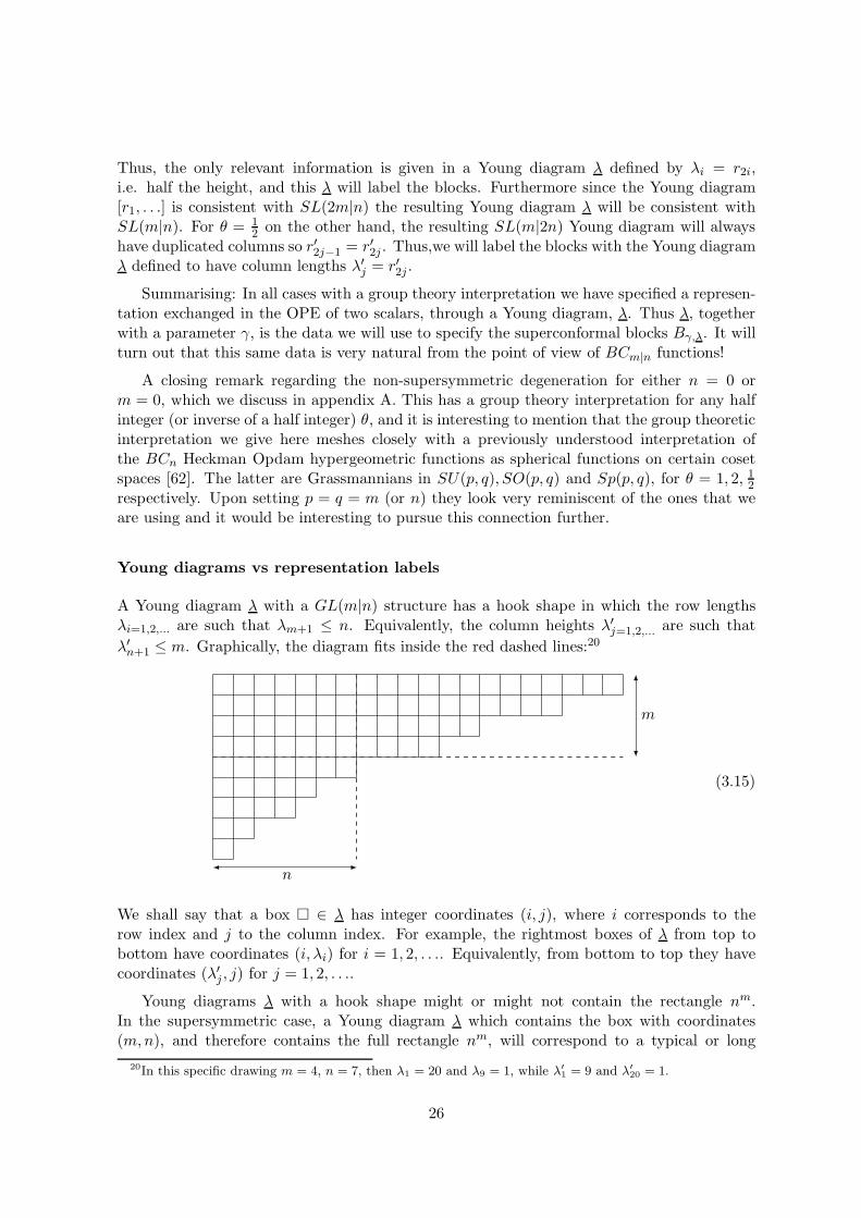
Young diagrams vs representation labels

A Young diagram λ with a GL(m|n) structure has a hook shape in which the row lengthsλi=1,2,... are such that λm+1 ≤ n. Equivalently, the column heights λ′j=1,2,... are such that

λ′n+1 ≤ m. Graphically, the diagram fits inside the red dashed lines:20

n

m

(3.15)

We shall say that a box � ∈ λ has integer coordinates (i, j), where i corresponds to therow index and j to the column index. For example, the rightmost boxes of λ from top tobottom have coordinates (i, λi) for i = 1, 2, . . .. Equivalently, from bottom to top they havecoordinates (λ′j , j) for j = 1, 2, . . ..

Young diagrams λ with a hook shape might or might not contain the rectangle nm.In the supersymmetric case, a Young diagram λ which contains the box with coordinates(m,n), and therefore contains the full rectangle nm, will correspond to a typical or long

20In this specific drawing m = 4, n = 7, then λ1 = 20 and λ9 = 1, while λ′1 = 9 and λ′

20 = 1.

26

representation. Otherwise the representation is atypical. We will discuss concrete examplesrelated to physical theories later on (see discussion around (C.40) and (C.41) for examplesand a fuller description).

The Dynkin labels given in (3.12) (and (3.13) for the case n = 0) translate to the dataspecifying a Young diagram λ, and a parameter γ, for θ = 1, 2, 12 as follows

lm−i = (λi−n)+ − (λi+1−n)+ i = 1, . . . ,m− 1 ; δ = (λ1−n)+ + θλ′n

an−i = (λ′i−λ′i+1) i = 1, . . . , n− 1 ; b = γ − 2λ′1

b′ = γ + 2θλ1

(3.16)

where (x)+ = max(x, 0). In physical applications it is useful to read off the dilation weight,especially as this is the only quantum number which can become non integer in an interactingCFT. The following equality gives the dilation weight in terms of the Dynkin labels, and thenγ, λ

∆ = −m−1∑

i=1

ili +m

δ + θ

n−1∑

j=1

aj + θ b2

=

m∑

i=1

(λi−n)+ +mθ γ2 . (3.17)

Note now that for long representations (those for which the box with coordinates (m,n) liesin the Young diagram λ) the dictionary (3.16) is invariant under

λi → λi − θτ ′

i = 1, . . . ,m;

λ′j → λ′j + τ ′

j = 1, . . . , n; γ → γ + 2τ ′ . (3.18)

We will refer to this redundancy as the shift invariance.

The shift invariance (3.18) arises from the fact that SL(m|n) reps are not uniquely specifiedby a Young diagram. This is very familiar in the bosonic case n = 0. In fact, for SL(m)reps one can add arbitrarily many height m columns to a Young diagram without changingthe rep. This leads directly to (3.18) for n = 0. In the same way, SL(n) reps have a shiftinvariance, and therefore when m = 0 one can add arbitrarily many length n rows (since theYoung diagram in SL(0|n) is transposed w.r.t. SL(n)). For the supergroup SL(m|n) whathappens is that if there is a full width n row below the nm rectangle in the Young diagram,this can be removed and replaced by a full height m column to the right of the rectanglewithout changing the representation. The presence of θ in the shift (3.18) reflects the factthat this shift applies to the reps of SL(2m|n) or SL(m|2n) with double numbers of rows orcolumns around (3.14). The implications of this shift for λ then give the θ dependence in(3.18).

Let us exemplify the relevant Young diagrams in some cases of physical interest. Blocksfor maximally supersymmetric theories

N = 4, 4d for θ = 1

N = (2, 0), 6d for θ = 2

N = 8, 3d for θ = 12

all correspond to m = 2, n = 2 (3.19)

These blocks are labelled by γ and a Young diagram with at most two rows of length λ1, λ2

27

and two columns of length λ′1, λ′2. There are two quantum numbers for the conformal group,

dilation weight ∆ = (λ1−2)+ + (λ2−2)+ + θγ and spin l1 = (λ1−2)+ − (λ2−2)+ (onlysymmetrised Lorentz indices appear in these four-point functions) and two analogous quantumnumbers for the internal subgroup a1, b.

21 When λ2 ≥ 2 the representation exchanged in theOPE (assuming integer dilation weight) is long or typical . If λ2 = 1, 0 the diagram is a thinhook, with at most a single row and a single column, and the representation is short. Whenthe Young diagram is empty it is half BPS. We emphasise that in our formalism there is noneed to distinguish the different shortening conditions!

Another case of physical interest is given by blocks with m = 2, n = 1, which includesN = 2 superconformal theories in 4d, the N = (0, 1) superconformal theories in 6d, andalso N = 4 in 3d. In this case the Young diagram has at most a single long column λ′1 andtherefore a single integer classifies the internal representations that can appear in the OPE.The reps are often defined by ∆, l and b. This time the atypical diagrams can only be thesingle row diagrams, since these do not contain the rectangle [12]. The rest of the alloweddiagrams, [λ1, λ2, 1

λ′1−2], are necessarily long/typical.

4 Rank-one invitation

Before presenting the most general (m,n) superconformal block, we describe in some detailthe bosonic (1, 0) and (0, 1) blocks, since these are simple enough to familiarise with theformalism based on super Jack polynomials.

4.1 Rank-one bosonic blocks

(1, 0) blocks

Consider first the (1, 0) blocks, i.e. a single x variable and no y variables. The only allowedYoung diagrams have a single row shape λ = [λ]. The Casimir (5.5) reduces to a one-variableGauss hypergeometric equation, from which follows the solution (normalised according to(2.13)),

CBγ,[λ](x|) = (λ+ θγ2 )(λ+ θγ

2 −1)Bγ,λ(x|)

Bγ,[λ](x|) = xθγ2+λ

2F1

(λ+θα, λ+θβ; 2λ + θγ;x

) (4.1)

where recall α = max(12(γ−p12), 12(γ−p43)

), β = min

(12(γ−p12), 12(γ−p43)

)(2.16). The

Casimir and the solution is symmetric in α and β. Furthermore, let us point out that out ofthe five parameters λ, γ, θ, p12, p43 only the three quantities λ+ θγ

2 , p12θ and p43θ appear.22

Writing the (1, 0) block as a series over superJack polynomials is very simple since the(1, 0) Jack is simply P[λ](x|) = xλ, therefore the Jack→Block matrix is just the coefficient in

21It might be instructive to compare with [45], which also treats all maximally supersymmetric cases together.They use internal labels (athere, bthere) where athere = 1

2γ−λ′

2, bthere = 12γ−λ′

1.22The combination λ+ θγ

2appears in the Dynkin diagram (A.14) for the (1, 0) bosonic theory.

28

the Taylor expansion of the Gauss hypergeometric:

Bγ,[λ](x|) = xθγ2

∞∑

µ=λ

(Tγ)[µ][λ]P[µ](x|) , (Tγ)

[µ][λ] =

(λ+ θα)µ−λ(λ+ θβ)µ−λ

(µ−λ)!(2λ + θγ)µ−λ. (4.2)

(0, 1) blocks

Consider now the (0, 1) blocks, i.e. no x variables and a single y variable. Here the onlyallowed Young diagrams have a single column shape λ = [1λ

′]. The Casimir reduces again to

a hypergeometric equation, and is solved by:

CBγ,[1λ′ ](|y) = −θ(λ′−γ2 )(λ

′−γ2−1)Bγ,[1λ′ ](|y)

Bγ,[1λ′ ](|y) =(−1)λ

′( 1θ)λ′

λ′! y−γ2+λ′

2F1

(λ′−α, λ′−β; 2λ′−γ; y

).

(4.3)

Notice that the entries of the 2F1 this time are independent of θ. Then, λ′ and γ only enterthrough the combination γ

2 − λ′.23

The normalisation of Bγ,[1λ′ ](|y) has been chosen as for the the (0, 1) superJack polyno-

mials (in agreement with (2.13)). In fact, the series expansion in superJack polynomials thistime reads

Bγ,[1λ′ ]

(|y) = y−γ2

∞∑

µ′=λ′

(Tγ)[1µ

′]

[1λ′ ]P[1µ′ ]

(|y) , P[1µ′ ]

(|y) = (1θ )µ′

µ′!(−y)µ′

(4.4)

where

(Tγ)[1µ

′]

[1λ′ ]=

(λ′−α)µ′−λ′(λ′−β)µ′−λ′

(µ′ − λ′)!(2λ′−γ)µ′−λ′

µ′!(1θ )λ′

λ′!(1θ )µ′

(−1)µ′−λ′

, (4.5)

An important observation to make at this point is that this series truncates when the ar-guments of the Pochhammers are negative. Thus it truncates for values of µ′ greater thanβ.

Properties of Tγ

We can already with this information perform do a very rudimentary check that the coefficientsTγ are (m,n) independent i.e. they only depend on the Young diagrams, θ, and p12, p43. Thisimplies that when the Young diagrams coincide, evaluating (4.2) and (4.4) should give thesame result. In the (1, 0) case the Young diagram has a single row, and in (0, 1) case a singlecolumn, thus they can only be compared when the Young diagram is empty or consists of asingle box i.e. the cases (λ, µ) = ([0], [0]), ([1], [1]), ([0], [1]). We indeed see that for both (1, 0)

23This combination is the value appearing in (A.15) sitting on crossed through Dynkin node.

29

and (0, 1) we obtain:

([0], [0]) ; (Tγ)[0][0] = 1

([1], [1]) ; (Tγ)[1][1] = 1

([0], [1]) ; (Tγ)[1][0] = θαβγ .

(4.6)

The above computation is limited, but nevertheless it is nice to see that (4.2) and (4.4) doindeed give the same results where they overlap. This illustrates the more general (m,n)independence of Tγ which we will consider further in section 5.

4.2 Relation with the Heckman-Opdam hypergeometrics

Despite the fact that both (1, 0) and (0, 1) blocks are given by the same building block, aGauss hypergeometric, there is an important difference, which we emphasised already: the(0, 1) block is a polynomial, while the (1, 0) block is an infinite series. However, since bothexternal and internal blocks are based on the same 2F1, comparing the two expressions (4.1)and (4.3), we read off the following formal relation between them:

B(1,0)γ, [λ](y|; θ, p12, p43) =

λ!

(−1)λ(θ)λB

(0,1)

−θγ, [1λ](|y; 1θ ,−θp12,−θp43) . (4.7)

So the (1, 0) and (0, 1) blocks can be viewed as analytic continuations of each other. Inparticular, if α, β, γ are assumed to be positive on the (1, 0) side, they become negative onthe (0, 1) side, specifically, (α, β, γ) → −θ(α, β, γ). This can be also understood from thegeneral relation satisfied by the defining Casimir

C(θ,a,b,c)(x|y) = −θC( 1θ,−aθ,−bθ,−cθ)(y|x) . (4.8)

Let us then try and understand this analytic continuation in the parameters and relate it tothe Heckman Opdam hypergeometric function.

In section 2.3 we identified the internal (0, n) block with the dual BCn Jacobi polynomial,up to a normalisation, and we showed how the latter is obtained from the BCn Jacobi poly-nomial (in particular see (2.32)). Now the BCn Jacobi polynomials are also Heckman Opdam(HO) hypergeometric functions for positive weights [26], but the BCn HO hypergeometric aredefined more generally for arbitrary parameters. It is therefore interesting to compare thesefunctions with our (1, 0) and (0, 1) blocks, and discuss in this context the analytic continuationw.r.t. the external parameters.

Both the BC1 Jacobi polynomial and the dual Jacobi polynomial can be given explicitly

30

in terms of 2F1 Hypergeometrics as follows,24

J[λ](y; θ, p−, p+) =

(−)λ(1 + p−)λ(1 + λ+p++p−)λ

2F1(1 + λ+p++p−,−λ; 1+p−; y) λ ∈ Z≥0 (4.9)

Jβ,[λ](y; θ, p−, p+) = yλ 2F1(λ−β−p−,−(β − λ); 2(λ−β)−p+−p−; y) β−λ ∈ Z≥0

= yλ2F1(λ−α, λ−β; 2λ−γ; y) (4.10)

where α = β + p− and γ = 2β + p+ + p−. The use of the Gauss hypergeometric to writethe polynomials has the bonus that they give a natural analytic continuation to arbitraryvalues of the parameters, i.e. away from the polynomial restriction λ ∈ Z+ for J and β−λ ∈Z+ for J . The key point here is that even though the Jacobi polynomial and the dualJacobi polynomial are directly related to each other, the above expressions in terms of Gausshypergeometrics yield two inequivalent analytic continuations of the parameters. The first isthe HO hypergeometric, the second is the one relevant for blocks. In both cases the analyticcontinuation gives a function that is regular at y = 0 with a branch cut between y = 1 andy = ∞.

Let us explore how this works in more detail. The point is that when β − λ ∈ Z+, thehypergeometrics are polynomial and there is a hypergeometric identity [63]

(−1)λ−β

c(α, β, γ, λ)2F1(1−λ+γ−β,−(β − λ); 1−β+α; 1y ) = yλ−β

2F1(λ−α,−(β − λ); 2λ−γ; y) ,(4.11)

where

c(α, β, γ, λ) =Γ[1+α−β]Γ [1 + γ−2λ]

Γ [1 + α−λ] Γ [1−β+γ−λ] . (4.12)

This is precisely the identity between the Jacobi and dual Jacobi polynomials J[β−λ](1/y) =

y−βJβ,[λ](y).

But as soon as we continue away from β − λ ∈ Z+, the above identity relaxes to a threeterm identity [64]:

2F1(1−λ+γ−β, λ−β; 1−β+α; 1y ) = (−1)λ−βc(α, β, γ, λ) × yλ−β2F1 (λ−α, λ−β; 2λ−γ; y)

+ (−1)λ−βc(α, β, γ, λ)× yλ−β2F1(λ−α, λ−β; 2λ−γ; y)

(4.13)

where α = α − γ, β = β − γ, γ = −γ, λ = 1 − λ. This is a well know connection formula forthe 2F1. Notice in particular that c(α, β, γ, λ) → 0, as β − λ→ n ∈ Z+, therefore we recoverthe previous identity (4.11).

Now the combination on the RHS of (4.13) is precisely the expression for the BC1 HOhypergeometric (in 1/y) given as a specific sum of independent solutions of its defining equa-tion (which is equivalent to the Casimir equation). In general the BCn HO hypergeometric

24These can be obtained by solving their defining differential equations. In the dual case this is (2.26). Forthe Jacobi polynomial we refer to [28]. Alternatively, the 1d combinatorial formula in [41] straightforwardlygives the result. The normalisation of the Jacobi is taken such that J[λ] = yλ+ . . ., and this gives the prefactorw.r.t. to the 2F1 series.

31

is defined as a sum over W = Sn ⋉ (Z2)n of building block functions called Harish Chandra

functions [16,17] each of which are independent solutions of the same defining equation. ForBC1 this sum is just a sum over Z2 and the two functions on the RHS of (4.13) are pre-cisely these building block Harish Chandra functions (the normalisations are known as theHarish-Chandra c functions). More details for this BC1 case can be found for example in [43].

In our context however on the RHS of (4.13), the first contribution is (up to a normal-isation) the (1, 0) block in (4.1) with parameters B−θγ, [λ](y|; 1θ ,−θp12,−θp43). The secondcontribution is B−θγ;[1−λ], and corresponds to an independent solution of the same Casimirequation (4.1), with different properties in the small y expansion. In the CFT context this isalso an important object known as the shadow block.

So we see therefore that the block and the shadow block are both Harish-Chandra func-tions25. The blocks have different analyticity properties to the Heckman Opdam hyperge-ometrics, explaining why they are not the same even though they are trivially related forcertain integer values of their parameters. In particular, in the variables we are using theblocks are regular at y → 0, whereas instead the Heckman Opdam hypergeometrics are regu-lar at 1/y → 0. For a more detailed analysis of the analytic structure of the standard bosonicconformal m = 2, n = 0 blocks and the relation to Harish Chandra functions see [12,14].

Summarising. The BC1 HO hypergeometric is the analytic continuation of the BC1 Jacobipolynomial when β − λ ∈ C which is regular when its argument approaches zero. The dualJacobi polynomials however have a different natural analytic continuation which is regularwhen its argument (which is the inverse of that of that of the Jacobi polynomial) approacheszero. This latter analytic continuation gives the Harish Chandra functions, the building blocksin the sum over W = ±1 giving the HO hypergeometric. Furthermore this latter analyticcontinuation interpolates between the (1, 0) or (0, 1) blocks as we vary the parameters.

This story would appear to have a natural generalisation to higher n. The BCn Jacobipolynomials have a natural analytic continuation in their parameters as BCn HO Hyperge-ometrics. The dual Jacobi polynomials (internal (0, n) blocks) however will have a naturalanalytic continuation as Sn ⊂ W = Sn × (Z2)

n invariant combinations of Harish Chandrafunctions. This combination will then coincide with external (n, 0) blocks for certain valuesof their parameters. Indeed this latter story can be seen explicitly in the θ = 1 case fromthe results of [9] where both external and internal blocks are given in terms of a determinantof Gauss Hypergeometric functions which indeed coincide on mapping the parameters appro-priately. It is then interesting to consider the generalisation to the supersymmetric (m,n)case and if there is a relation between the dual super Jacobi functions and super Jacobipolynomials via analytic continuation. We consider (m,n) analytic continuations further insection 6

5 Superconformal blocks (I): recursion

Having considered in detail the (1, 0) and (0, 1) blocks in the previous section we return tothe general case. In this section we explain how to solve the Casimir equation (2.9) for the

25In fact twisted Harish Chandra functions since we exclude the (−1)λ−β in the definition of the block.

32

superconformal blocks, defined via the expansion

Bγ,λ =

(∏i x

θi∏

j yj

)γ2

Fγ,λ ; Fγ,λ =∑

µ⊇λ

(Tγ)µλ Pµ(z) ; (5.1)

for any values of the m|n variables z as well as any θ, p12, p43 and γ. We will use a recur-sion, as anticipated in section 2, and to find it we will first derive the representation of theCasimir (2.18) suited for acting on the basis of super Jack polynomials, Pµ and then use thisto turn the differential equation into a recurrence relation for the coefficients (Tγ)

µλ.

We will write the recursion in a way which is manifestly independent of the dimensionof the blocks, and the m,n labels for the super Jack polynomials, purely in terms of theYoung diagram (5.16). Later this is made very explicit in a manner prepared for differentpossible analytic continuations, see for example (5.35), (5.36). Appendix C provides a concisesummary of properties and definitions of Jack and super Jack polynomials which might serveas a helpful guide for the reader.

Various properties of the recursion, and therefore of its solution, the Jack→Block matrixTγ , will then be discussed. First we will exemplify the special case of the half-BPS blockλ = [∅], which admits a simple hypergeometric solution. This is instructive because thedetails are still quite non trivial, despite the final simplicity of the solution. Then, we willconsider the most general case. We do not obtain an explicit solution for the general case,however, it is very efficient to implement the recursion on a computer, and we use this toexplore properties of (Tγ)

µλ, for example its dependence on θ, γ, p12 and p43. The most

intriguing is the dependence on γ, which becomes highly non-trivial and takes the form ofa more and more complicated mostly non factorisable polynomial. In section 7 we will finda surprising interpretation for the γ dependence, by elaborating on the connection betweensuperconformal blocks and Jacobi polynomials.

5.1 Derivation of the recursion and higher order Casimirs

Recall briefly our construction. Superconformal blocks as eigenfunctions of the Casimir op-erator introduced in (2.9)-(2.10). On Fγ,λ, the eigenvalue problem reduces to

C(θ,α,β,γ)Fγ,λ = (h(θ)λ + θγ|λ|)Fγ,λ , (5.2)

whereh(θ)λ =

∑

i

λi(λi−2θ(i−1)−1) (5.3)

and |λ| = ∑i λi, with λ = [λ1, . . .]. As highlighted already, the eigenvalue for Fγ,λ does notdepend explicitly on (m,n) unlike the original eigenvalue for Bγ,λ in (2.10). Recall also thedefinitions of α and β in terms of p12, p43, γ given in (2.16)

α ≡ max(12(γ−p12), 12 (γ−p43)

), β ≡ min

(12 (γ−p12), 12(γ−p43)

)(5.4)

As discussed above (2.9), the Casimir can be nicely related to the BCm|n CMS operator,

33

and we do so in appendix B. The explicit result in our notation takes the form,

C(θ,a,b,c) =

m+n∑

I=1

(−θ)πID(θ,a,b,c)I + 2θ

m+n∑

I=1

∑

J 6=I

zIzJzI − zJ

(−θ)−πJdI (5.5)

where the two operators dI and DI are defined as

dI = (1− zI)∂I (5.6)

D(θ,a,b,c)I = z2I∂I(1− zI)∂I − (−θ)1−πI (c− (a+ b)zI)zI∂I − (−θ)2−2πIabzI . (5.7)

We use the vector z = (z1, . . . , zm|zm+1, . . . , zm+n) to label the variables zi = xi=1,...m andzm+j = yj=1,...n. The parity πi = 0 is assigned to the non-compact direction i = 1, ..,m,otherwise πj = 1 is assigned to the compact direction j = m+ 1, ..,m + n.

The identification of the Casimir with a BCm|n differential operator helps deducing thedecomposition (2.18) of the Casimir into operators with well defined actions on Pµ:

C(θ,a,b,c) =H(θ) + θcm+n∑

i=1

zI∂I

− θ(a+ b)m+n∑

I=1

z2I∂I − 12

[H(θ),

m+n∑

I=1

z2I∂I

]− θ2ab

m+n∑

I=1

zI(−θ)−πI (5.8)

where H(θ) is the Am|n CMS Hamiltonian (see appendix B)26

H(θ) =

m+n∑

I=1

(−θ)πIz2I∂2I + 2θ

∑

I 6=J

zIzJzI − zJ

(−θ)−πJ∂I . (5.9)

The operator decomposition in (5.8) is perfectly suited to acting on the expansion Fγ,λ =∑(Tγ)

µλPµ because super Jack polynomials are eigenfunctions of both

∑I zI∂I (reflecting

the fact that they are homogeneous polynomials) and H(θ),27 and moreover, the other twooperators are themselves related to the simplest one-box super Jack polynomial, P�

∑

I

zI(−θ)−πI = P�(z), and∑

I

z2I∂I =12 [H

(θ), P�(z)] . (5.10)

The action of all the operators zI∂I , H, P� on super Jack polynomials yields a linearcombination of Jack polynomials whose coefficients are independent of m,n. This will implythat the recursion for Tγ , which we derive from the Casimir, will be independent of m,n atevery stage.

26Notice that H shows up directly in (5.8), since it is found by replacing DI → z2I∂2I and dI → ∂I . Terms

of the Casimir in which DI → −z3I∂2I and dI → −zI∂I , are generated by the commutator.

27Indeed these are the first two Hamiltonians of a tower found in [34], which establishes the classical inte-grability of the system.

34

Let us begin with the simplest operator in (5.8), i.e. the momentum operator,

m+n∑

I=1

zI∂I Pµ(z) = |µ|Pµ(z) . (5.11)

The eigenvalue here simply counts the number of boxes of the Young diagram µ (whichobviously does not depend on (m,n)). This operator just reflects the fact that super Jackpolynomials are homogeneous functions of the zI of degree |µ|.

For the Hamiltonian, we have

H(θ) Pµ(z) = h(θ)µ Pµ(z) . (5.12)

This equation is part of the standard definition of the super Jack polynomials and the eigen-value h(θ)µ in (5.3) has no explicit dependence on (m,n).

Next, the two ‘off-diagonal’ operators in (5.10). The first of the two is simply the multi-plicative operator acting with P�. In general the product Pµ1

Pµ2gives a linear combination

of super Jacks whose coefficients, Cµ3µ1µ2

(θ), known as structure constants, are independent ofm,n. When θ = 1 Jack polynomials reduce to Schur polynomials and the structure constantsbecome precisely the standard Littlewood-Richardson coefficients. Finding an explicit for-mula for the structure constants for general θ however is a difficult problem/task in modernmathematics [54]. Here however we only need the case in which one of the Young diagramsis a single box. This case reduces to the simplest case of the Pieri rule for Jack and superJack polynomials, and Cν

�µ is known combinatorially [65, 66]. It is perhaps less known thatthis combinatorial formula can be made fully explicit, as we will show shortly.

So the action of the first off-diagonal operator in (5.10) coincides with the product P�Pµ

and returnsP�(z)Pµ(z) =

∑

ν∈{µ+�}Cν�µPν(z) . (5.13)

where the RHS spans all polynomials labelled by the Young diagram ν obtained by addingan extra box to the Young tableau µ, in all possible ways.

The action of the second off-diagonal operator in (5.10),∑

i z2i ∂i, can then be obtained

straightforwardly from its representation as a commutator together with (5.12),(5.13). Wehave

∑

I

z2I∂IPµ(z) =12 [H

(θ), P�(z)]Pµ(z) =∑

ν∈{µ+�}

12(hν − hµ)Cν

�µPµ+�i(z) . (5.14)

Having understood the action of all the operators appearing in the operator decompositionof the Casimir, and having observed that all of them decompose into Jack polynomials withcoefficients which only depend on the Young diagram, we can now write the representation ofthe Casimir itself in the basis of superJack polynomials. The result is quite neat and nicely

35

generalises the structure noticed for θ = 1 in [9],

C(θ,a,b,c)Pµ =(hµ + θc|µ|

)Pµ −

∑

ν∈{µ+�}

(12(hν−hµ) + θa

) (12 (hν−hµ) + θb

)Cν�µ Pν .

(5.15)

From this and the definition Fγ,λ =∑

µ(Tγ)µλPµ, then the Casimir equation (5.2) gives the

following recursion equation for the coefficients Tγ

(Tγ)µλ =

∑ν∈{µ−�}

(12(hµ−hν) + θα

) (12(hµ−hν) + θβ

)Cµ� ν (Tγ)

νλ(

hµ−hλ+θγ (|µ|−|λ|)) (5.16)

with α, β as defined earlier in terms of γ, p12, p43 (5.4). Here we see that the recursioninitiates from the Young diagram µ (which contains λ) and goes back to λ (for which weknow (Tγ)

λλ = 1) recursively by subtracting boxes. Thus if µ is compatible with the (m,n)

structure (i.e. µm+1 ≤ n) then ν ∈ {µ − �} is also compatible with it and the recursionalways remains inside the (m,n) Young diagram. This means the recursion can be solvedquite efficiently on a computer.

It is also interesting to consider the inverse of Tγ , i.e. the Block→Jack matrix, T−1γ . This

gives Jack polynomials as a sum of blocks, via the inverse of (5.1),

Pλ =∑

µ

(T−1γ )µλ Fγ,µ. (5.17)

Note that Fγ,µ, when m > 0 is an infinite series, and the sum, an infinite sum. Many nontrivial cancellations take place in order to recover a polynomial. From (5.15) and (5.2) weobtain a recursion for T−1

γ which is very similar looking to that of Tγ

(T−1γ )µλ =

∑ν∈{λ+�}

(12 (hν−hλ) + θα

) (12 (hν−hλ + θβ

)Cν� λ (T

−1γ )µν(

hλ−hµ+θγ (|λ|−|µ|)) (5.18)

The main difference is that here the recursion gives (T−1γ )µλ in terms of (T−1

γ )µλ+�

, obtained

by adding boxes to λ, whereas the recursion for (Tγ)µλ is in terms of (Tγ)

µ−�λ , is obtained by

subtracting boxes from µ.

We will return to the relation between T and T−1 later on in section 7.3.

Higher order Casimirs for θ = 1

Before considering the recursion in more detail we would like to discuss higher order Casimirsin the CFT. These arise from the relation between the Casimir and CMS system with BCroot system. In fact, higher order Casimirs correspond to the defining higher order differential

36

operators of the Heckman Opdam BC hypergeometric functions. This is a general statement,but here we will specialise to θ = 1, where formulae are both explicit and simple. Generalisingthe work of [43] (who focussed on the purely bosonic case n = 0) we now show that higherorder Casimirs in the supersymmetric case are given by simply replacing the variables zI in asuper Schur with the corresponding second order operator DI of (5.7) and conjugating withthe Vandermonde (super-) determinant

C(θ=1,a,b,c)µ = V −1(zI)Pµ

(D

(θ=1;a,b,c)I ; θ = 1

)V (zI) (5.19)

where the super van der Monde determinant is

V (zI) =

∏1≤i<j≤m(x−1

i − x−1j )

∏1≤i<j≤n(y

−1i − y−1

j )∏

1≤i≤m1≤j≤n

(x−1i − y−1

j ), (5.20)

and where DI is given in (5.7). The quadratic Casimir of (5.5) correspond to the above forthe one-box super Schur, i.e. µ = �. The latter is simply the sum

∑i xi −

∑j yj.

The superblocks Bγ,λ are eigenvalues of C(θ,− 12p12,− 1

2p43,0)

λ for all Young diagrams µ

Cµ(θ,− 1

2p12,− 1

2p43,0)Bγ,λ(z) = (Eµ)

(m,n;θ=1)γ,λ Bγ,λ(z) , (5.21)

The corresponding eigenvalue is

(Eµ)(m,n;θ=1)γ,λ = Pµ((EI)γ,λ)− 1

3(m− n− 1)3 (5.22)

obtained by replacing zI by EI in the corresponding Schur polynomial Pµ where

(EI)(m,n;θ=1)γ,λ =

{(λi − i+ 1

2γ + 1)(λi − i+ 12γ) I = i = 1, ..,m

(λ′j − j − 12γ + 1)(λ′j + j − 1

2γ) I −m = j = 1, .., n. (5.23)

The case µ = � is the one we discussed in our overview: one can check that putting the singlebox Young diagram, this agrees with (2.10) for θ = 1.

Note that an eighth order super Casimir in N = 4 SYM considered in [70] correspondsto (5.19) withm=n=2 and µ=[2, 2] for which Pµ(zI)=(x1−y1)(x1−y2)(x2−y1)(x2−y2). Higherorder Casimirs both in 1d CFTs (m=n=θ=1) and inN=4 SYM (m=n=2, θ=1) are consideredin [73].

5.2 Explicit formulae for the recursion

So far the recursion (5.16) is entirely combinatoric, written in terms of Young diagrams, andour main concern has been to emphasize this property, that it depends only on objects that are(m,n) independent. We will now make the discussion more concrete by considering explicitformulae. Remarkably, there are different explicit forms that the recursion can take. Thedifference is simply a preference for rows over columns when reading the Young diagrams, orvice-versa, or even mixing rows and columns as is more natural in the supersymmetric (m,n)case.

37

Eigenvalue

Let us begin from h(θ)λ which in (5.3) we wrote as

h(θ)λ =∑

i=1,2,..

λi(λi−2θ(i−1)−1) . (5.24)

It is simple to see that it admits an equivalent representation in which instead we take thesum to run over columns,

h(θ)λ = −θ∑

j=1,2,..

λ′j(λ′j − 1− 2

θ (j − 1)) = −θh(1θ)

λ′ , (5.25)

or if λ is a typical (m,n) Young diagram (ie it has λm ≥ n, λn+1 ≤ n see (C.40)) then it canbe rewritten as a combination of these row and column formulae:

h(θ)λ =m∑

i=1

λi(λi−2θ(i−1)−1)− θn∑

j=1

λ′j(λ′j − 1− 2

θ (j − 1))− h(θ)nm . (5.26)

where h(θ)nm = nm((n− 1)− θ(m− 1)). All these forms for the eigenvalue can be easily derived

from the following combinatoric formula

h(θ)λ = 2∑

(i,j)∈λ

((j−1)− θ(i−1)

). (5.27)

where the eigenvalue is given as a sum over boxes in the Young tableau where each box isunderstood to have row i column j. Then one obtains the equivalent formulae (5.3) or (5.25)by simply performing the first sum in each of the following ways of writing the sum overYoung diagram boxes explicitly

∑

(i,j)∈λ=

∑

i=1,2,..

λi∑

j=1

=∑

j=1,2,..

λ′i∑

i=1

=m∑

i=1

λi∑

j=1

+n∑

j=1

λ′i∑

i=1

−m∑

i=1

n∑

j=1

. (5.28)

with the last formula for typical (long) (m,n) Young diagrams only.

In the numerator of the recursion (5.16) we have the expression

(12 (hµ−hν) + θα

) (12(hµ−hν) + θβ

)ν ∈ {λ−�} . (5.29)

Since ν is related to µ by subtracting a box in position (i, j), clearly from (5.27) we have12(hµ − hν) = (j−1)− θ(i−1).

38

Structure constants

Let us come to Cµ+�

�µ in (5.16). The corresponding combinatorial formula is well known and

can be found in [65]. It can be rearranged quite explicitly and we find28

Cµ+�ij

�µ = f (i)µ (θ) =

i−1∏

k=1

(θ(i−k+1)−1+µk−µi) (θ(i−k−1)+µk−µi)(θ(i−k)−1+µk−µi) (θ(i−k)+µk−µi)

. (5.30)

where we are using the notation µ+�ij to mean that we add a box to row i and column j ofthe Young tableau so that we have j = µi+1 and i = µ′j +1. The above formula is written in

terms of Young diagram row lengths µi. Alternatively, we might prefer a rewriting of Cµ+�ij

�µ

over columns.

To do so we define first, g(i)µ , obtained by multiplying f (i)µ by the following normalisation

in terms of C symbols (defined more generally later in (7.9))

g(i)µ (θ) ≡ Πµ(θ)

Πµ+�ij(θ)f (i)µ (θ) (5.31)

Πκ(θ) =C−κ (θ; θ)

C−κ (1; θ)

=

∏(ij)∈κ

(κi−j + θ(κ′j−i) + θ

)

∏(ij)∈λ

(κi−j + θ(κ′j−i) + 1

) . (5.32)

Note that this can be rewritten as an explicit function of the row lengths µi (i = 1, .., n)only29

g(i)µ (θ) =

µi − µi+1 + 1

µi − µi+1 + θ

n∏

k=i+1

(θ(k − i+ 1) + µi − µk)(θ(k − i) + µi − µk+1 + 1)

(θ(k − i+ 1) + µi − µk+1)(θ(k − i) + µi − µk + 1)

(5.33)

(with µn+1 defined to vanish).

The structure constant (5.30) then has an alternative writing in terms of column lengths

using g(j)µ′ as follows30

Cµ+�ij

�µ = f (i)µ (θ) = 1θ g

(j)µ′ (

1θ ) , µ′j = i− 1 , µi = j − 1 . (5.34)

28See also [66]. We actually first derived this formula using computed algebra, by seeking a generalisationof the formula for two-row polynomials, which can be derived with pencil and paper. Then, we confirmed itsexpression by rewriting the combinatorial formula coming from the Pieri rule [29].

29To do this we use explicit formulae for C−κ (w; θ)from [26],

C−µ (θ; θ) =

∏µ′

1

k=1(µk+θ(µ′

1−k)+θ−1)!

(θ−1)!∏

1≤k1<k2≤µ′

1

(µk1−µk2

+θ(k2−k1))θC−

µ (1; θ) =

∏µ′

1

k=1(µk + θ(µ′1 − k))!

∏

1≤k1<k2≤µ′

1

(µk1−µk2

+θ(k2−k1)− (θ−1))θ.

after which the majority of contributions to Πµ(θ)/

Πµ+�ij(θ) simplify in the ratio.

30A posteriori, f can also be written in terms of the A-type binomial coefficient, built out of the A-typeinterpolation polynomials of Okounkov [67], which can be seen as the limit u = ∞ in (C.30). The dualityf ↔ g can be proven using the identification with the A-type binomial coefficient.

39

where recall that (i, j) are the coordinates of �ij.

Equivalent forms of the recursion

Choosing all row-type formulae is the most natural from a bosonic CFT point of view, sincein a physical theory with conformal symmetry, we would be summing over Pµ with a finitenumber of rows but an arbitrary number of columns such that λ ⊆ µ, in order to constructBγ,λ. With this choice then we use (5.24) and (5.30) to write the recursion (5.16) in terms ofrow lengths explicitly as

(Tγ)µλ =

∑i (µi−1−θ(i−1−α)) (µi−1−θ(i−1−β)) f (i)µ−�i

(θ) (Tγ)µ−�iλ∑

i(µi − λi)(λi + µi + θγ − 2θ(i− 1)− 1)(5.35)

where µ−�i := [µ1, .., µi−1, µi−1, µi+1, ...]. Note that f imposes that µi > µi+1 automatically.In fact if it was the case that µi = µi−1 + 1 for some i, then second term in the denominator

of f(i)µ−�i

in (5.30) would vanish for k = i− 1.

If instead we choose all column-type explicit formulae then using (5.25) and (5.31) wewrite the recursion (5.16) in terms of column lengths explicitly as

(Tγ)µλ =

∑j

(µ′j−1−α− j−1

θ

)(µ′j−1−β− j−1

θ

)g(j)µ′−�j

(1θ )(Tγ)(µ′−�j)′λ

∑j(λ

′j − µ′j)(λ

′j + µ′j − γ − 2

θ (j − 1)− 1)(5.36)

where µ′−�j := [µ′1, .., µ′j−1, µ

′j − 1, µ′j+1, ...].

Finally we could also split the sum∑

ν∈{µ−�} in (5.16) into east and south part arbi-trarily. The outcome for (Tγ)

µλ will remain unchanged. This is most natural for an (m,n)

supersymmetric theory and indeed is crucial if we wish to analytically continue consistentlywith the (m,n) structure. We will discuss this supersymmetric splitting in the section 6.

5.3 Special solutions: the half-BPS superconformal block

There is a special case in which we can solve the recursion for all coefficients explicitly witha particularly simple solution. It is the case corresponding to an empty diagram λ = [∅],and therefore corresponding to a half-BPS superconformal block exchanged in a propagatorstructure with γ propagators going from Op1Op2 to Op3Op4 . The solution is

(Tγ)µ[∅] =

C0µ(θα; θ)C

0µ(θβ; θ)

C0µ(θγ; θ)

1

C−µ (1; θ)

(5.37)

40

where the combinatorial symbols are

C0λ(w; θ) =

∏

(ij)∈λ(j−1− θ(i−1) + w)

C−λ (w; θ) =

∏

(ij)∈λ

(λi−j + θ(λ′j−i) + w

). (5.38)

Let us verify that this solution indeed satisfies the recursion using the row-type recur-sion (5.35). We will see that despite the final simplicity of the result, the recursion is solvedin a very non trivial way. Afterwards we will present a more direct argument based on thefact that the Casimir annihilates the half-BPS superconformal block, therefore it can be splitinto simpler independent hypergeometric equations studied by Yan in [68].

Consider the recursion (5.35) with λ = [∅]

(Tγ)µ[∅] =

∑i (µi−1−θ(i−1−α)) (µi−1−θ(i−1−β)) f (i)µ−�i

(θ) (Tγ)µ−�i

[∅](hµ + θγ |µ|

) . (5.39)

Inserting the solution (5.37) the terms (µi−1−θ(i−1−α)) and C0µ−�i

(θα; θ) combine and

simplify with the LHS C0µ(θα; θ). Similarly for the terms with β. We are left with needing to

prove the non trivial statement

1 =1(

hµ + θγ |µ|)∑

i

(f(i)µ−�i

C−µ (1; θ)

C−µ−�i

(1; θ)

)((µi − 1)− θ(i− 1) + θγ) . (5.40)

We can deal with C−µ by using the explicit formulae of footnote 29 and find that

f(i)µ−�i

C−µ (1; θ)

C−µ−�i

(1; θ)= (µi + θ(µ′1 − i))

∏

k 6=i

µi − µk + θ(k − i− 1)

µi − µk + θ(k − i). (5.41)

Proving the recursion is now equivalent to proving that

∑

i

(µi + θ(µ′1 − i))∏

k 6=i

µi − µk + θ(k − i− 1)

µi − µk + θ(k − i)= |µ| (5.42)

∑

i

(µi + θ(µ′1 − i))∏

k 6=i

µi − µk + θ(k − i− 1)

µi − µk + θ(k − i)(µi − θi) = 2

∑

(ij)∈µ(j − 1

2)− θ(i− 12)

where the RHS corresponds to a decomposition of hµ + θγ. Note that even the first one ofthese relations is quite non trivial, since the common denominator in the LHS has to cancelout in the end, and this only happens after taking the sum. These two relations are provenin a beautiful way in [69] by using the Lagrange Lemma for alphabets.

The superconformal block Bγ,[∅] itself is now obtained by summing up (Tγ)µ[∅] with super

41

Jack polynomials. It takes the form of a multivariate 2F1 series,

Bγ,[∅] =

(∏i x

θi∏

j yj

)γ2 ∑

µ

C0µ(θα; θ)C

0µ(θβ; θ)

C0µ(θγ; θ)

Pµ(z; θ)

C−µ (1; θ)

. (5.43)

In the bosonic (m, 0) theory this is indeed equal to a well known multivariate hypergeometricfunction [68].31 In particular, it is known to satisfy a set of m hypergeometric equations,which in our notation take the formz−1

I D(θ,α,β,γ)I −θ(m−1)(1−zI)+θ

∑

J 6=I

zI(1−zI)∂I−zJ(1−zJ )∂JzI−zJ

Bγ,[∅] = 0 ; I = 1, . . . m

(5.44)where DI is the same operator introduced in (5.7). The trick to recover our Casimir C is tosum

∑I zI × (5.44) and put together −(m− 1)+

∑J 6=I

zIzI−zJ

= +∑ zJ

zI−zJ.

Since h∅ + γ|∅| = 0, the half-BPS block is annihilated by the Casimir, and therefore thesystem of equations (5.44) is equivalent to the original Casimir eigenvalue problem.

5.4 General features and non-trivial γ-dependence

The solution of the recursion for Tγ reveals many non trivial features. In order to systematisethe discussion, let us first show that the α and β dependence of (Tγ)

µλ always takes the

following form(Tγ)

µλ = C0

µ/λ(θα; θ)C0µ/λ(θβ; θ)× (T rescaled

γ )µλ (5.45)

with (T rescaledγ )µλ then independent of α, β. Here by definition C0

µ/λ ≡ C0µ/C

0λ, thus

32

C0µ/λ(θα; θ)C

0µ/λ(θβ; θ) =

∏

(ij)∈µ/λ

(j−1−θ(i−1−α))(j−1−θ(i−1−β)). (5.46)

The proof of (5.45) is immediate. In fact, the ratio of C0 satisfies the relation

C0µ/λ(θw; θ) = (µi − 1− θ(i− 1− w))C0

µ−�i/λ(θw; θ) (5.47)

and therefore in the row-type formulae (5.35) for the recursion, the α and β dependence drops.This is indeed the same argument we saw at work in the half-BPS solution, around (5.39),with λ = [∅]. Then, it follows from (5.45) that (T rescaled

γ )µλ satisfies a simpler recursion,

(T rescaledγ )µλ =

∑i f

(i)µ−�i

(θ) (T rescaledλ )µ−�i

λ∑i(µi − λi)(λi + µi + θγ − 2θ(i− 1)− 1)

, (5.48)

and (T rescaledγ )µλ is only a function of γ, θ and the Young diagrams µ and λ.

The recursion for (T rescaledγ )µλ can be turned into column or mixed type formulae, exactly

31As discussed at the end of section 4.2 we believe this is also a certain Sn combination of Harish Chandracontributions to the corresponding Heckman-Opdam hypergeometric.

32The C0µ(w; θ) was defined in (5.38). Here we are giving the final result for C0

µ/λ(θα; θ)C0µ/λ(θβ; θ).

42

as for (Tγ)µλ itself, as we did in section 5.2. The C0 rescaling will change accordingly, see in

particular section D.2.

Given the various explicit formulae provided in the previous section 5.2, it is not difficultto implement the recursion on a computer and solve it in many cases. Let us look at a coupleof examples to illustrate the general features:

(T rescaledγ )

[5,3][3,1] =

162 + 222θ + 67γθ − 168θ2 + 109γθ2 + 7γ2θ2 + 24θ3 − 36γθ3 + 13γ2θ3

2(1 + θ)(3 + θ)2(6 + γθ)2(2− 2θ + γθ)2(4− θ + γθ)2(5.49)

The dependence on γ in the denominator as a product of linear factors in γ is simple tounderstand: it can only come from putting together all denominators encountered uponsolving the recursion, and these are all of the form (θγ − θN+ N) with integers coming fromYoung diagrams. The numerator on the other hand is fairly complicated, degree two in γ anddegree three in θ. This degree depends on the Young diagrams. Another example shows thismore clearly,

(T rescaledγ )

[6,5,3][3,2,1] ∼ + 21208 + 6(1861γ + 7012)θ +

(1943γ2 + 26524γ − 56312

)θ2

+(111γ3 + 5312γ2 − 17918γ + 11112

)θ3

+(339γ3 − 965γ2 − 796γ + 2560

)θ4

+(66γ3 − 410γ2 + 800γ − 480

)θ5 . (5.50)

(we only display the complicated polynomial factor, and we omitted the various linear factorsof the form (θγ − θN+ N).)

The point is that guessing the γ dependence of (Tγ)µλ, for arbitrary λ, µ, and θ, would

be quite challenging. However, as anticipated in the introduction, due to the relation withJacobi polynomials we will find in section 7.2 an alternative description for this complicatedfactor as an interpolation polynomial.

6 Superconformal blocks (II): analytic continuation

We have understood in the previous section how to construct a superconformal block Bγ,λ

given a Young diagram λ for which e.g. its row lengths λi ∈ N with λi ≥ λi+1.

For physical applications in an interacting CFT however, non-protected operators ex-changed in the OPE acquire an anomalous dimension and thus it is crucial to be able tounderstand non-integer quantum numbers, at least for the dilation weight. Even though theother quantum numbers remain integer in a unitary CFT, it is nevertheless also very usefulto consider analytically continuing these too (for example the spin, see [70] for example).

For general θ, we do not have explicit solutions for either Bγ,λ or (Tγ)µλ to look at, in

order to discuss analytic continuation beyond Young diagrams. In fact, only the case θ = 1has been solved for both Bγ,λ and (Tγ)

µλ in [9]. We will then have to look at the recursion.

The combinatorial form given in (5.16) is not immediately useful, since does not lend itselfto analytic continuation. However, from the explicit forms of the recursion (5.35),(5.36) wecan obtain analytic results for the coefficients Tγ as rational functions of the row lengths λior column lengths λ′i respectively.

43

The logic will be quite simple. For the row type recursion (5.35) we will think of (Tγ)µλ as

a function of λ ∈ C, with µ given by µ = λ+~n with ni ∈ Z+. The recursion takes µ and goesback to λ by negative integer shifts, regardless of whether the λi are integer or not. In thisframework, the various representations of the recursion, i.e. whether row-type or vertical-typeor a mixed one, lead to different ways of analytically continuing the (Tγ)

µλ in the variables

describing the Young diagrams. Crucially we know that all these analytic continuations ofTγ must coincide in the cases when λ and µ return to values such that they represent a validYoung diagrams.

6.1 Row-type representation on the east

The row-type representation of the recursion on the east, which we derived in the previoussection using Young diagrams technology, is given in (5.35). This has the following (m, 0)analytic continuation in the row lengths λi,

(Tγ)µλ =

∑mi=1 (µi−1−θ(i−1−α)) (µi−1−θ(i−1−β)) f (i)µ−ei

(θ) (Tγ)µ−eiλ∑m

i=1(µi − λi)(λi + µi + θγ − 2θ(i− 1)− 1)(6.1)

λi ∈ C, µi = λi + ni, ni ∈ Z+, (Tγ)λλ = 1, (Tγ)

µλ = 0 if ni < 0

Here µ and λ are parameters such that µi − λi = ni is a positive integer, but λi ∈ C and eiis the usual basis vector with a 1 in position i and zeroes elsewhere. As we discussed below(5.35) this recursion automatically gives (Tγ)

µλ = 0 if µi = µi−1+1. Thus if λ corresponds to a

Young diagram, meaning that λi−λi−1 ∈ Z+, then (Tγ)µλ = 0 unless µ also corresponds to the

row lengths of a Young diagram. This is a key point which allows the analytic continuationaway from the Young diagram: if this was not the case, then the solution to the aboverecursion would not recover the correct solution when λ becomes a Young diagram. Theexpression for f (i)µ (θ) is given in (5.30) and is rational in λi and θ. For fixed, integer µi − λi,the recursion (6.1) has a solution which is manifestly rational in λi, θ, α, β, γ. We can thusview the solution of (6.1) as an analytic continuation of the solution of (5.35) which is validonly when λi are the row lengths of Young diagrams.

An important bonus of the solution of (6.1) is the manifest shift symmetry (2.20) (for anyvalue of θ)

λi → λi−θτ ′ , µi → µi − θτ ′ , γ → γ + 2τ ′ , i = 1, . . . m . (6.2)

We can see this invariance immediately. First, the combinations (µi + θα), (µi + θβ), aremanifestly invariant, since both α and β have the form

γ−pij2 . Then, the combination of

eigenvalues appearing in the denominator, i.e. (µi − λi)(λi + µi + θγ − 2θ(i− 1)− 1), is alsomanifestly invariant. Finally, fµ−ei only depends on differences µi − µj and so is invariant.

The simplest analytic continuation we can think of is the (1, 0) solution given in section4.1, which we repeat here for convenience,

(Tγ)[µ][λ]

=(λ+ θα)µ−λ(λ+ θβ)µ−λ

(µ−λ)!(2λ+ θγ)µ−λ. (6.3)

We see that indeed, for fixed integer µ − λ this is a rational function of λ, θ, α, β, γ. (Of

44

course, having an explicit solution we can now also see how to analytically continue in µ ifwe desired, just by changing the Pochhammers to Gamma functions.)

Summarising, we have shown that defining (Tγ)µλ via (6.1) produces a rational (and hence)

analytic function of λ, θ, α, β, γ, which is also invariant under the shift symmetry (6.2).

6.2 Column-type representation on the south

An alternative analytic continuation of (Tγ)µλ can be obtained by viewing the Young diagram

as function of the column lengths λ′j, rather than the row lengths λi. The column-typerepresentation of the recursion on the south was derived in (5.36). It has the following (0, n)analytic continuation,

(Tγ)µλ =

∑nj=1

(µ′j−1−α− j−1

θ

)(µ′j−1−β− j−1

θ

)g(j)µ′−ej

(1θ )(Tγ)(µ′−ej)

′

λ∑n

j=1(λ′j − µ′j)(λ

′j + µ′j − γ − 2

θ (j − 1)− 1)(6.4)

λ′j ∈ C, µ′j = λ′j + n′j, n′j ∈ Z+, (Tγ)λλ = 1, (Tγ)

µλ = 0 if n′j < 0

where the explicit formula for g was given already in (5.33) Similarly to the recursion on theeast, for fixed integer µ′j − λ′j, the solution is clearly a rational function of λ′j , θ, α, β, γ.

The simplest solution of (6.4) we can look at is the (0, 1) solution studied in section 4.1.Namely

(Tγ)[1µ

′]

[1λ′ ]= (−1)µ

′−λ′ (λ′−α)µ′−λ′(λ′−β)µ′−λ′

(µ′ − λ′)!(2λ′−γ)µ′−λ′

(λ′ + 1)µ′−λ′

(λ′ + 1θ )µ′−λ′

. (6.5)

Comparing with the row-type solution from (6.1) there is one small difference, which canappreciated also in (6.5). This (Tγ)

µλ is not quite invariant under the n = 1 case of the shift

symmetry (6.2)

λ′j → λ′j+τ′ , µ′j → µ′j+τ

′ , γ → γ + 2τ ′ , j = 1, . . . n . (6.6)

The problem is a simple normalisation issue, due to the fact that we are expanding in BC0,n

super Jack polynomials rather than directly in BCn Jack polynomials. These two are essen-tially equal but have a different normalisation, (e.g see (C.47) with m = 0)

P(n)λ′ (y; 1θ ) = (−1)|λ|Πλ(θ)P

(0,n)λ (|y; θ) . (6.7)

Thus the combination of superJack × coefficient Tγ does satisfy shift invariance.

6.3 Supersymmetric representation

We now come to a form of the recursion which gives analytic (indeed rational) results in thevariables λi, λ

′j , the first m row lengths and first n column lengths, for long (or typical, the

see discussion around (C.40) for these meanings) (m,n) Young diagrams λ. This is suited forsupersymmetric theory described by a (m,n) theory. It includes the previous cases as specialcases by taking m = 0 or n = 0.

45

We first give a version of the recursion (5.16) for long reps λ in the (m,n) theory, whichgives rational results in λi, λ

′j . To do this we split the RHS of the recursion into south and

east components and define it as follows,

(hµ−hλ+θγ (|µ|−|λ|)

)(Tγ)

µλ =

m∑

i=1

(µi−1−θ(i−1−α)) (µi−1−θ(i−1−β)) f (i)µ−ei(θ)(Tγ)

µ−eiλ +

+θ

n∑

j=1

(µ′j−1−α− j−1

θ

)(µ′j−1−β− j−1

θ

)g(j)µ′−ej

(1θ )(Tγ)(µ′−ej)

′

λ (6.8)

λi, λ′j ∈ C, µ′j = λ′j + n′j, µi = λi + ni ni, n

′j ∈ Z+, (Tγ)

λλ = 1, (Tγ)

µλ = 0 if ni, n

′j < 0

where (5.26) is used for hµ, hλ in the above. As in previous cases, for given integers ni, n′j

this recursion yields a solution which is manifestly rational in λi, λ′j , θ, α, β, γ and therefore

gives a supersymmetric-type analytic continuation in the variables λi, λ′j of Tγ .

For example the explicit solution for the (1, 1) theory (relevant for 1d and 2d supersym-metric theories) is

(Tγ)µλ =

(µ′1 − 1)!(1θ )λ′1−1

(λ′1 − 1)!(1θ )µ′1−1

θ2λ′1−2µ′

1 C0µ/λ(θα; θ)C

0µ/λ(θβ; θ)

(µ′1 − λ′1)!(µ1 − λ1)!×

(λ1 + θλ′1 − θ)(µ1 + θµ′1 − 1) + (1− θ)(λ1 − µ1)(θγ+λ1−θµ′

1)(θγ+λ1−θλ′

1)

(λ1 + θλ′1 − 1)(µ1 + θµ′1 − θ)(2λ1 + θγ)µ1−λ1(2λ′1 − γ)µ′

1−λ′1(−1)µ

′1−λ′

1(6.9)

where µ = [µ1, 1µ′1−1] and λ = [λ1, 1

λ′1−1]. Note that this (1, 1) coefficient reduces to the (1, 0)

case for µ′1 = λ′1 = 1 and to the (0, 1) case for µ1 = λ1 = 1.

In appendix D we discuss in detail the shift symmetry of this form of the recursion relationand various other features.

We conclude with some comments.

Note that the recursion has been explicitly solved analytically for arbitrary λi and/or λ′j

in only a few cases: using both row and column variables, the determinantal formula of [9]for θ = 1, which we repeat in appendix E.3, and the (1, 1) solution presented above, witharbitrary θ. In this latter case the solution is precisely a formula depending on one row lengthand one column height.

In the next section 7 we will give a completely different description of the coefficients Tγand T−1

γ , closely related to the BC binomial formula of Okounkov [33] involving evaluatingBC interpolation polynomials at partitions arising via the identification between (0, n) blocksand BCn Jacobi polynomials. It is tempting to speculate that this form should also have asupersymmetric representation, more suited for a (m,n) theory and indeed we will find thatthe super interpolation polynomials of Sergeev and Veselov [38] do the job, but only for T−1

γ

not Tγ itself.

46

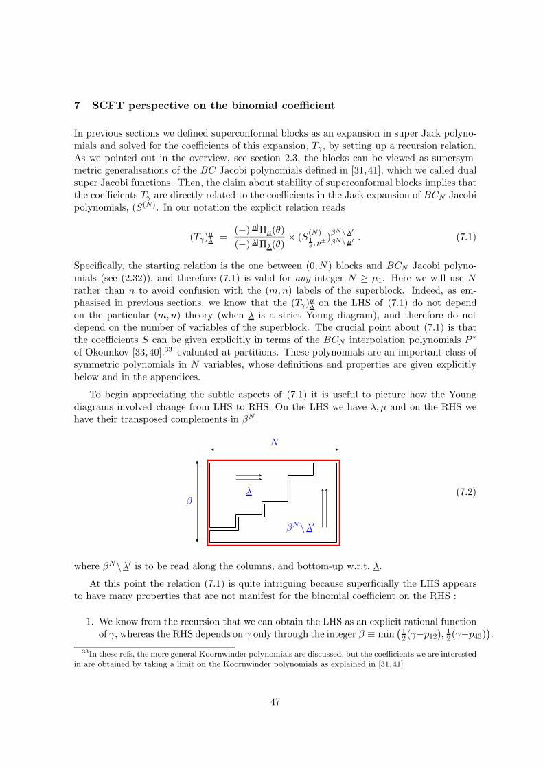
7 SCFT perspective on the binomial coefficient

In previous sections we defined superconformal blocks as an expansion in super Jack polyno-mials and solved for the coefficients of this expansion, Tγ , by setting up a recursion relation.As we pointed out in the overview, see section 2.3, the blocks can be viewed as supersym-metric generalisations of the BC Jacobi polynomials defined in [31,41], which we called dualsuper Jacobi functions. Then, the claim about stability of superconformal blocks implies thatthe coefficients Tγ are directly related to the coefficients in the Jack expansion of BCN Jacobipolynomials, (S(N). In our notation the explicit relation reads

(Tγ)µλ =

(−)|µ|Πµ(θ)

(−)|λ|Πλ(θ)× (S

(N)1θ; p±

)βN\λ′

βN\µ′ . (7.1)

Specifically, the starting relation is the one between (0, N) blocks and BCN Jacobi polyno-mials (see (2.32)), and therefore (7.1) is valid for any integer N ≥ µ1. Here we will use Nrather than n to avoid confusion with the (m,n) labels of the superblock. Indeed, as em-phasised in previous sections, we know that the (Tγ)

µλ on the LHS of (7.1) do not depend

on the particular (m,n) theory (when λ is a strict Young diagram), and therefore do notdepend on the number of variables of the superblock. The crucial point about (7.1) is thatthe coefficients S can be given explicitly in terms of the BCN interpolation polynomials P ∗

of Okounkov [33,40].33 evaluated at partitions. These polynomials are an important class ofsymmetric polynomials in N variables, whose definitions and properties are given explicitlybelow and in the appendices.

To begin appreciating the subtle aspects of (7.1) it is useful to picture how the Youngdiagrams involved change from LHS to RHS. On the LHS we have λ, µ and on the RHS wehave their transposed complements in βN

β

N

λ

βN\λ′

(7.2)

where βN\λ′ is to be read along the columns, and bottom-up w.r.t. λ.

At this point the relation (7.1) is quite intriguing because superficially the LHS appearsto have many properties that are not manifest for the binomial coefficient on the RHS :

1. We know from the recursion that we can obtain the LHS as an explicit rational functionof γ, whereas the RHS depends on γ only through the integer β ≡ min

(12 (γ−p12), 12(γ−p43)

).

33In these refs, the more general Koornwinder polynomials are discussed, but the coefficients we are interestedin are obtained by taking a limit on the Koornwinder polynomials as explained in [31,41]

47

2. To obtain superblocks we sum over Young diagrams with arbitrarily large width µ1. Onthe RHS this translates to arbitrarily large N and so we need interpolating polynomialswith arbitrarily large number of variables which is very inefficient.

3. Moreover, the LHS depends mostly on the skew diagram µ/λ (indeed the recursion ofthe previous sections is solved along this skew diagram), the RHS instead depends onthe increasing large (as N gets large, and also when β is large) Young diagrams βN\λ′and βN\µ′. Again this looks very inefficient.

From the above considerations we expect the binomial coefficient, S(N), to have various non-trivial hidden properties, in order to recover those of (Tγ)

µλ.

Our plan is thus the following: After giving a detailed definition of the binomial coeffi-cient in terms of interpolating polynomials we will examine the above properties from thisperspective. In the process we will obtain a rewriting of the binomial coefficient which dealswith the first two of these points. Furthermore we will find that the inverse coefficient (T−1

γ )µλi.e. the coefficient in the expansion of a super Jack polynomial in terms of blocks, has a formwhich deals with all three points.

7.1 The binomial coefficient

Recall (2.25), we wrote the coefficients of a BCN Jacobi polynomial, expanded in terms ofJack polynomials,

Jλ(y1, . . . , yN ; θ, p−, p+) =∑

µ⊆λ

(S(N)θ,p−,p+

)µλ Pµ(y; θ) . (7.3)

Now these binomial coefficients S(N) have been well studied and are known to be given, upto normalisations, by BCN interpolation polynomials P ∗

µ evaluated on λ. The interpolationpolynomials themselves are symmetric polynomials, depending on a single parameter u, andare uniquely defined [32,33] by the property that they vanish when evaluated on a partitionλ which is strictly contained in µ, i.e.

P ∗µ(λ; θ, u) = 0 if λ ⊂ µ . (7.4)

Quite remarkably, the interpolation polynomials admit a combinatorial definition which gen-eralises the one of Jack polynomials in a simple way. See appendix C.3.

Now for some normalisation of the Jacobi polynomial, say Jλ(y) = Jλ(y)/Nλ, and some

normalisation of the Jack polynomials, say Pµ(y) = Pµ(y)/Mµ, the corresponding binomial

coefficients in the expansion of Jλ in the Pµ really are simply interpolating polynomials withthe variables taking the values of the Young diagram λ

Jλ(y1, . . . , yN ; θ,A1, A2) =∑

µ⊆λ

P ∗(N)µ (λ; A1+A2+1

2 ) Pµ(y; θ) . (7.5)

Returning to the standard choice of normalisations (such that the coefficient of Pλ in theexpansion (2.25) is 1 and that Pµ(0) = δµ,∅) we can see that the normalisation of S will have

48

the more complicated looking form:

(S(N)

θ, ~A)µλ =

Jλ(0; θ,A1, A2)

Jµ(0; θ,A1, A2)

P ∗(N)µ (λ; θ, u)

P ∗(N)µ (µ; θ, u)

∣∣∣∣∣u=

A1+A2+12

. (7.6)

However, the only non trivial part of (7.6) is still P ∗(N)µ (λ; θ, u)! The remaining objects

entering this formula are explicitly known formulae which are all products of linear factors inthe parameters

P ∗(N)µ (µ; θ, u) = C+

µ (2u−1+2θN ; θ)C−µ (1; θ) (7.7)

J (N)λ (0; θ,A1, A2) =

(−)|λ| C0λ(A1+1+θ(N − 1); θ)C0

λ(θN ; θ)

P ∗λ (λ; θ, u)Πλ(θ)

∣∣∣∣∣u=

A1+A2+12

, (7.8)

where the combinatorial symbols C0,± are

C0λ(w; θ) =

∏

(ij)∈λ(j−1− θ(i−1) + w)

C−λ (w; θ) =

∏

(ij)∈λ

(λi−j + θ(λ′j−i) + w

)

C+λ (w; θ) =

∏

(i,j)∈λ(λi + j − θ(λ′j + i) +w), (7.9)

andΠλ(θ) ≡ C−

λ (θ; θ)/C−λ (1; θ) ; Πλ(

1θ ) = 1

/Πλ′(θ). (7.10)

Although these evaluation formulae may look complicated at first sight, they consist simplyof products of linear factors. For later use we will sometimes use the notation C0

λ(A,B; θ) =

C0λ(A; θ)C

0λ(B; θ) and and C0

µ/λ ≡ C0µ/C

0λ whenever λ ⊆ µ.

Putting the above definitions in we arrive at the expression for the binomial coefficient

(S(N)

θ, ~A

)µλ= (−)|λ|−|µ|Πµ(θ)

Πλ(θ)C0λ/µ(A1+1+θ(N−1), θN ; θ)×

P ∗(N)µ (λ; θ, u)

P ∗(N)λ (λ; θ, u)

∣∣∣∣∣u=

A1+A2+12

.

(7.11)Note that the P ∗ in the denominator now involves P ∗

λ .

7.2 Binomial representation of the Jack→Block matrix

From this expression (7.11) we can obtain an expression for Tγ in terms of interpolationpolynomials via (7.1). Manipulating this with the help of some identities for interpolationpolynomials of Rains [32] (the details will be given shortly), we obtain:

(Tγ)µλ = (N )µλ ×

P∗(M)

NM \µ(NM \λ; θ, u)

P∗(M)

NM \λ(NM \λ; θ, u)

∣∣∣∣∣u=

12−θ

γ2−N

. (7.12)

49

The normalisation is

(N )µλ = C0µ/λ (θα, θβ; θ)×

(−)|µ|Πµ(θ)

(−)|λ|Πλ(θ)

C0µ/λ(1+θ(M − 1); θ)

C0µ/λ

(Mθ; θ)(7.13)

where α, β are as defined in (D.2), and the symbols Π and C0 are given in (7.9).

Crucially the whole expression is independent of M,N as long as the rectangle NM con-tains the Young diagram µ (which in turn contains λ). For practical computations we wouldalways choose the minimal case M = µ′1 and N = µ1.

Note that the manipulations we performed have produced a formula which solves thefirst two problems listed on page 47. Firstly, the non factorisable γ dependence of Tγ nowappears entirely in the parameter of P ∗

NM \µ(NM \λ; θ, u), and can thus be continued to

arbitrary non-integer values. This polynomial is precisely the complicated polynomial in γ in(Tγ)

µλ discussed in section 5.4. Secondly, when the Young diagrams λ and µ are arbitrarily

wide with limited height, i.e. less than or equal to β for superblocks, the dimension of theinterpolating polynomials M is limited (since we can choose M = β for example) and doesnot grow indefinitely as for the original formula.

Finally, note that the bosonic (m, 0) case of the shift symmetry (D.1) is manifest in thisformula: choosing N = µ1, we see that γ only appears through the combination µ1 + θ γ2 andthe row lengths λi, µi only appear as differences with µ1 via µM1 \λ and µM1 \µ all of whichleave the shift invariant.

Proof of (7.12)

To show that (7.1) is equivalent to (7.12) we will need two formulae which can both befound in [32], by taking the appropriate classical limits. The first relates BCN interpolationpolynomials with a Young diagram κ to one with a Young diagram with additional ν full (ieheight N) columns

P∗(N)

κ+νN(w1 . . . wN ; θ, s) =

N∏

i=1

ν∏

j=1

(w2i − (s+ j − 1)2) P ∗(N)

κ (w1 . . . wN ; θ, s+ ν) . (7.14)

The second relation is an identity between a BCN interpolation polynomial with Young dia-gram µ evaluated on a Young diagram κ and a BCM interpolation polynomial with transposedYoung diagram µ′ evaluated on the transposed Young diagram κ′. Here M,N can be arbi-trary (this freedom to choose M,N in fact arises from the previous relation) as long as theyare big enough to contain the relevant Young diagrams, so M ≥ µ′1 and N ≥ µ1. It reads

P ∗(N)µ (κ; θ, u)

P ∗(N)µ (µ; θ, u)

=P

∗(M)µ′ (κ′; 1θ , u

′)

P∗(M)µ′ (µ′; 1θ , u

′)(7.15)

where θu′ + (M − 12) = −u− θ(N − 1

2) .

50

We can now use (7.14) to remove the explicit β dependence in the Young diagram of thenon-trivial P ∗ term in (7.1) with (7.11). Taking ν =M − β positive we find

P∗(N)

βN\µ′(βN\λ′; θ−1, 12(p++p−+1)) = P

∗(N)

MN\µ′(MN\λ′; θ−1, 12(γ + 1)−M)×N1 (7.16)

where we recalled the relation between β, γ, p± in (2.31) to get this. Note however that thisequation is true for both ν positive or negative and indeed is valid for any M ≥ µ1. Thenormalisation N1 is given in terms of the known evaluation formula (7.7) for P ∗

µ(µ) as

N1 =P

∗(N)

βN\λ′(βN\λ′; 1θ , 12(p++p−+1))

P∗(N)

MN\λ′(MN\λ′; 1θ , 12(γ + 1)−M)(7.17)

Next we use the relation (7.15) to transpose the Young diagrams. Thus obtaining

P∗(N)

MN\µ′(MN\λ′; 1

θ ,12(γ+1)−M) = P

∗(M)

NM\µ(NM\λ; θ, 12(1−γθ)−N)×N2 , (7.18)

with the normalisation N2 also given in terms of explicitly known formulae as

N2 =P

∗(N)

MN\µ′(MN\µ′; 1

θ ,12 (γ+1)−M)

P∗(M)

NM\µ(NM\µ; θ, 12(1−γθ)−N)

. (7.19)

So inserting these into the formula for Tγ (7.1) using the definition of the binomial coeffi-cient (7.6) we obtain (7.12) with the normalisation:

(N )µλ =(−)|µ|Πµ(θ)

(−)|λ|Πλ(θ)×JβN\λ′(0; 1θ , p

−, p+)

JβN\µ′(0; 1θ , p−, p+)

×N1N2 ×P

∗(M)

NM \λ(NM \λ; θ, 12(1− γθ)−N)

P∗(N)

βN\µ′(βN\µ′; 1θ , 12(p++p−+1))).

(7.20)

This normalisation, despite its complicated appearance, is just made of known linear factors.Moreover, it dramatically simplifies!! We know this in advance because it is clear from therecursion for Tγ that only the γ dependence is non factorisable and complicated. In particularall factors of C+ occurring in the evaluation formulae for (7.7) appear in ratios with transposedYoung diagrams and appropriate parameters such that they cancel using the relations

C0µ(x; θ) = (−θ)|µ| C0

µ′(−xθ ;

1θ ) (7.21)

C−µ (x; θ) = (+θ)|µ| C−

µ′(+xθ ;

1θ )

C+µ (x; θ) = (−θ)|µ| C+

µ′(−xθ ;

1θ ) ,

together with the identities

C0NM\µ(x; θ)

C0NM (x; θ)

=(−)|µ|

C0µ(1−N + θ(M−1)− x; θ)

, (7.22)

51

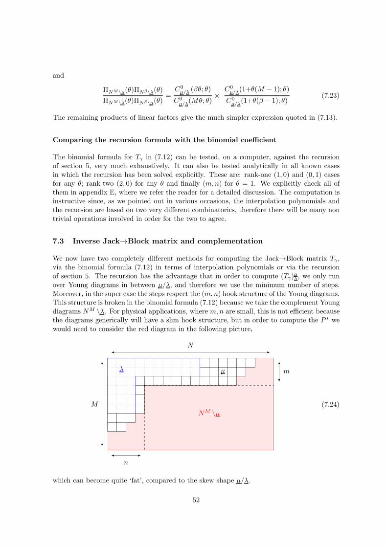
and

ΠNM\µ(θ)ΠNβ\λ(θ)

ΠNM\λ(θ)ΠNβ\µ(θ)=

C0µ/λ (βθ; θ)

C0µ/λ

(Mθ; θ)×

C0µ/λ(1+θ(M − 1); θ)

C0µ/λ

(1+θ(β − 1); θ)(7.23)

The remaining products of linear factors give the much simpler expression quoted in (7.13).

Comparing the recursion formula with the binomial coefficient

The binomial formula for Tγ in (7.12) can be tested, on a computer, against the recursionof section 5, very much exhaustively. It can also be tested analytically in all known casesin which the recursion has been solved explicitly. These are: rank-one (1, 0) and (0, 1) casesfor any θ; rank-two (2, 0) for any θ and finally (m,n) for θ = 1. We explicitly check all ofthem in appendix E, where we refer the reader for a detailed discussion. The computation isinstructive since, as we pointed out in various occasions, the interpolation polynomials andthe recursion are based on two very different combinatorics, therefore there will be many nontrivial operations involved in order for the two to agree.

7.3 Inverse Jack→Block matrix and complementation

We now have two completely different methods for computing the Jack→Block matrix Tγ ,via the binomial formula (7.12) in terms of interpolation polynomials or via the recursionof section 5. The recursion has the advantage that in order to compute (Tγ)

µλ, we only run

over Young diagrams in between µ/λ, and therefore we use the minimum number of steps.Moreover, in the super case the steps respect the (m,n) hook structure of the Young diagrams.This structure is broken in the binomial formula (7.12) because we take the complement Youngdiagrams NM \λ. For physical applications, where m,n are small, this is not efficient becausethe diagrams generically will have a slim hook structure, but in order to compute the P ∗ wewould need to consider the red diagram in the following picture,

λ µ

M

N

m

n

NM \µ(7.24)

which can become quite ‘fat’, compared to the skew shape µ/λ.

52

In a number of applications, (T−1γ ), the inverse of the Jack→Block matrix, shows up and

plays an important role. This matrix is such that

Pλ(z) =∑

µ:λ⊆µ

(T−1γ )µλ Fγ,µ(z) (7.25)

where as usual we understand the dependence on θ, p12, p43 in Fγ,µ. Note that when m > 0the Jack polynomials is represented as an infinite sum. We will now see that the inverse ofthe Jack→Block matrix, the Block→Jack matrix, has a very nice interpretation in terms ofinterpolation polynomials, and avoids the above mentioned problems with complementation.

An illuminating way of obtaining the Block→Jack matrix is to apply the Casimir (5.15)and obtain a recursion very similar to the recursions for Tγ , see (5.18). By carefully examiningand comparing the two recursions (5.16) and (5.18), in particular the denominator term ineach, one can deduce that there is a direct relation between T−1

γ and Tγ with complementedYoung diagrams. This complementation then accounts for the difference that in (5.16) wesum over Young diagrams with one subtracted box, whereas in (5.18) we sum over Youngdiagrams with one added box. The precise relation is then

(T−1γ

)µλ(θ, p12, p43) =

C0(NM\λ)/(NM \µ)(Mθ; θ)

C0(NM\λ)/(NM \µ)(1 + θ(M − 1); θ)

×ΠNM\µ(θ)

ΠNM\λ(θ)(Tγ)

NM\µNM\λ (θ,−p12,−p43)

(7.26)

whereγ = −γ + 2(M − 1)− 2

θ (N − 1) . (7.27)

This identity is valid for any γ, p12, p43 and N ≥ µ1, M ≥ µ′1. The intuition behind (7.26)is that µ/λ and (NM\λ)/(NM\µ) represent the same skew diagram, seen from differentorientations. Then, the map γ → γ is the only real non trivial transformation in going fromleft to right in (7.26), since the γ dependence is the non factorisable one. Analyticity in γ ofTγ is also crucial, since γ might be an integer but γ is certainly not. The factors of C0 can beeventually rewritten/simplified by using (7.22)-(7.23).34 The form given above is useful forthe computation that follows.

Now notice that the binomial formula for the Jack→Block matrix, Tγ (7.12) involvescomplemented Young diagrams, as does the RHS formula (7.26) for T−1

γ in terms of Tγ .We thus conclude that the inverse matrix T−1

γ is very naturally computed by a binomialcoefficient, given by interpolation polynomials directly in µ and λ! In fact, by using (7.12)on the RHS of (7.26), a number of simplifications take place,35 and the final formula is very

34For example, the RHS can be transposed by using

(T−θγ)µ′

λ′ (1θ,−θp12,−θp43) =

(−)|λ|Πλ(θ)

(−)|µ|Πµ(θ)(Tγ)

µλ(θ, p12, p43)

which follows from C(θ,a,b,c)(x|y) = −θC( 1

θ,−aθ,−bθ,−cθ)(y|x), and properties of the (super) Jack polynomials

under transposition.35Upon writing (Tγ)

NM \µ

NM \λ(θ,−p12,−p43) note that C0

µ/λ (θα, θβ; θ) is recovered by using (7.22).

53

clean and reads:

(T−1γ )µλ =

(−)|µ|

(−)|λ|C0µ/λ (θα, θβ; θ)

P ∗(M)λ (µ; θ, v)

P ∗(M)µ (µ; θ, v)

∣∣∣∣∣v=−1

2+θγ2−θ(M−1)

(7.28)

where P ∗λ are BCM interpolation polynomials with any M ≥ µ′1 and α, β, as always, given

by (D.2). Note, the formula above is independent of M with the minimal choice M = µ′1.One can also deduce this relation from formulae in Rains [32], together with the identification(7.12), where it is seen that both the binomial coefficient and its inverse are given by inter-polation polynomials with complemented Young diagrams (see [32] (4.1),(4.2),(4.22),(4.23)).Observe that this expression for T−1

γ is very similar to the expression for the binomial coeffi-cients S written in (7.11). We will make use of this observation when examining the Cauchyidentity in the next section.

The nice feature of (7.28) is that the Young diagrams labelling the interpolation polyno-mials are now λ and µ rather than their complements. As a result, computing T−1

γ by usingthe binomial coefficient is also quite efficient. Finally, the evaluation of the interpolationpolynomial in the numerator, P ∗

λ (µ; θ, v), is again the only term not involving products oflinear factors, and depends non trivially on γ.

Even though (7.28) has nice properties, it still has the inconvenience that the numberof variables in the interpolation polynomials grows with M . Therefore, if we are consideringblocks with large β, since µ1 ≤ β andM ≥ µ′1, withM = µ′1 being the minimal choice, we willwill have to consider interpolation polynomials with fixed but large number of variables. Infact, (7.28) is still a bosonic formula, which reads the Young diagram only by rows, whereasin the super block the typical Young diagram is a (m,n) hook. We can then ask if thereis an interpolation polynomial type formula which respects the (m,n) structure. Nicelyenough, this problem has a simple solution which is suggested by the independence of thedimension of the interpolation polynomials, M , of the expression T−1 (7.28). This stabilityproperty immediately suggests that one might be able to replace the bosonic interpolationpolynomials with super-interpolation polynomials, where the latter have a natural hook-typeparametrisation of their variables.

Sergeev and Veselov introduced the BCM |N super interpolation polynomials in [38] thatwe need. They first modified the free parameter on which the interpolation polynomialsdepend, to h = v + θM and defined the modified interpolation polynomial P ∗(M)

λ as

P ∗(M)λ (x; θ, h) := P ∗(M)

λ (x; θ, h−θM) . (7.29)

They then showed that these modified IPs have a natural supersymmetric generalisation, de-noted by P ∗(M |N)

λ (x|y; θ, h), where taking N = 0 returns the bosonic interpolation polynomial

P ∗(M)λ (x; θ, h) = P ∗(M |0)

λ (x| ; θ, h) . (7.30)

We spell out the conventions [38] in appendix C.7.

In [38] these super polynomials were used to obtain super binomial coefficients, i.e. thecoefficients of the expansion of super Jacobi polynomials in terms of super Jacks. We willreturn to this point in the next section. Here we notice that stability of T−1

γ in (7.28) gives

54

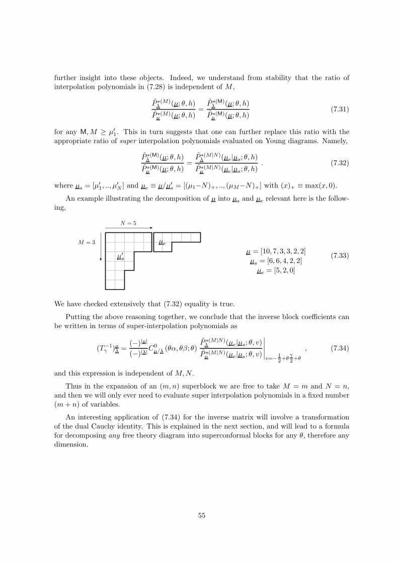
further insight into these objects. Indeed, we understand from stability that the ratio ofinterpolation polynomials in (7.28) is independent of M ,

P ∗(M)λ (µ; θ, h)

P ∗(M)µ (µ; θ, h)

=P ∗(M)λ (µ; θ, h)

P ∗(M)µ (µ; θ, h)

(7.31)

for any M,M ≥ µ′1. This in turn suggests that one can further replace this ratio with theappropriate ratio of super interpolation polynomials evaluated on Young diagrams. Namely,

P ∗(M)λ (µ; θ, h)

P ∗(M)µ (µ; θ, h)

=P ∗(M |N)λ (µe|µs; θ, h)P ∗(M |N)µ (µe|µs; θ, h)

. (7.32)

where µs = [µ′1, .., µ′N ] and µe ≡ µ/µ′s = [(µ1−N)+, .., (µM−N)+] with (x)+ ≡ max(x, 0).

An example illustrating the decomposition of µ into µs and µe relevant here is the follow-ing,

µ = [10, 7, 3, 3, 2, 2]

µs = [6, 6, 4, 2, 2]

µe = [5, 2, 0]

µ′s

µe

N = 5

M = 3

(7.33)

We have checked extensively that (7.32) equality is true.

Putting the above reasoning together, we conclude that the inverse block coefficients canbe written in terms of super-interpolation polynomials as

(T−1γ )µλ =

(−)|µ|

(−)|λ|C0µ/λ (θα, θβ; θ)

P ∗(M |N)λ (µe|µs; θ, v)P ∗(M |N)µ (µe|µs; θ, v)

∣∣∣∣∣v=−1

2+θγ2+θ

, (7.34)

and this expression is independent of M,N .

Thus in the expansion of an (m,n) superblock we are free to take M = m and N = n,and then we will only ever need to evaluate super interpolation polynomials in a fixed number(m+ n) of variables.

An interesting application of (7.34) for the inverse matrix will involve a transformationof the dual Cauchy identity. This is explained in the next section, and will lead to a formulafor decomposing any free theory diagram into superconformal blocks for any θ, therefore anydimension.

55

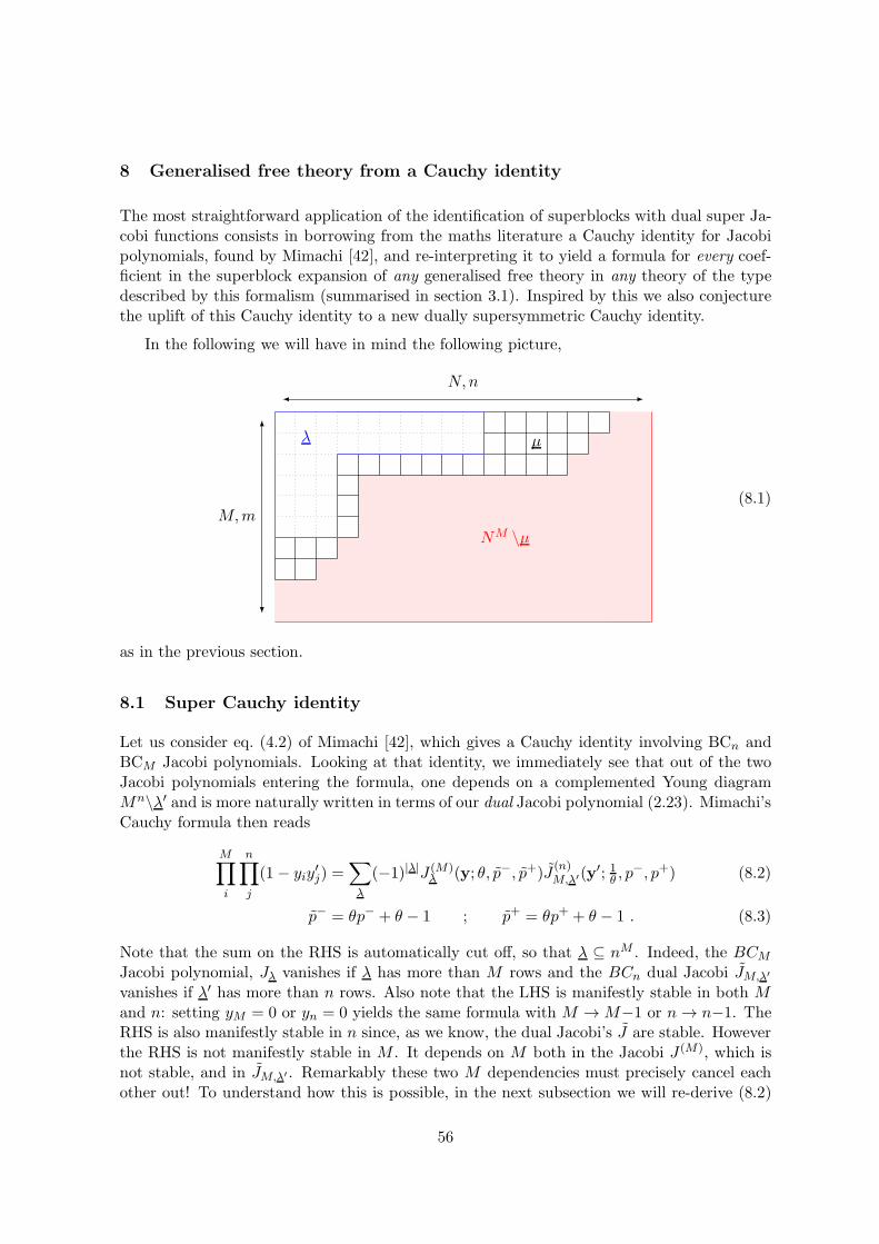
8 Generalised free theory from a Cauchy identity

The most straightforward application of the identification of superblocks with dual super Ja-cobi functions consists in borrowing from the maths literature a Cauchy identity for Jacobipolynomials, found by Mimachi [42], and re-interpreting it to yield a formula for every coef-ficient in the superblock expansion of any generalised free theory in any theory of the typedescribed by this formalism (summarised in section 3.1). Inspired by this we also conjecturethe uplift of this Cauchy identity to a new dually supersymmetric Cauchy identity.

In the following we will have in mind the following picture,

λ µ

M,m

N,n

NM \µ

(8.1)

as in the previous section.

8.1 Super Cauchy identity

Let us consider eq. (4.2) of Mimachi [42], which gives a Cauchy identity involving BCn andBCM Jacobi polynomials. Looking at that identity, we immediately see that out of the twoJacobi polynomials entering the formula, one depends on a complemented Young diagramMn\λ′ and is more naturally written in terms of our dual Jacobi polynomial (2.23). Mimachi’sCauchy formula then reads

M∏

i

n∏

j

(1− yiy′j) =

∑

λ

(−1)|λ|J (M)λ (y; θ, p−, p+)J (n)

M,λ′(y′; 1θ , p

−, p+) (8.2)

p− = θp− + θ − 1 ; p+ = θp+ + θ − 1 . (8.3)

Note that the sum on the RHS is automatically cut off, so that λ ⊆ nM . Indeed, the BCM

Jacobi polynomial, Jλ vanishes if λ has more than M rows and the BCn dual Jacobi JM,λ′

vanishes if λ′ has more than n rows. Also note that the LHS is manifestly stable in both Mand n: setting yM = 0 or yn = 0 yields the same formula with M →M−1 or n→ n−1. TheRHS is also manifestly stable in n since, as we know, the dual Jacobi’s J are stable. Howeverthe RHS is not manifestly stable in M . It depends on M both in the Jacobi J (M), which isnot stable, and in JM,λ′ . Remarkably these two M dependencies must precisely cancel eachother out! To understand how this is possible, in the next subsection we will re-derive (8.2)

56

starting from the simpler and well known Cauchy identity involving Jack polynomials. Thederivation will then explain the stability property in N and also explain the appearance ofthe modified parameters p±.

But first let us motivate various supersymmetric generalisations of this Jacobi Cauchyidentity which we will explicitly prove in the next section. Through stability, we know thatdual Jacobi polynomials have a natural uplift to dual super Jacobi functions. Thus we can

uplift J(n)M,λ′(y′) on the RHS of the previous formula (8.2) to (n,m) variables. Regarding the

LHS of (8.2), the eigenvalue interpretation of the variables in the super matrix formalismfor θ = 1, 2, 12 (see appendix A) provides intuition for the corresponding uplift. Namely, weinterpret the LHS as the product of determinants

∏i det(1 − yiZ) where Z is the diagonal

matrix with eigenvalues y′j, and therefore we simply lift the matrix Z to the supermatrix(see (A.1),(A.6),(A.11)).

This then leads to propose the following supersymmetric Jacobi Cauchy identity

M∏

i

∏nj (1− yiy

′j)∏m

k (1− yix′k)θ=∑

λ

(−1)|λ|J (M)λ (y; θ, p−, p+)J (n|m)

M,λ′ (y′|x′; 1θ , p

−, p+) , (8.4)

involving BCN Jacobi polynomials and BCn|m super dual Jacobi functions.

Now, the dual super Jacobi functions on the RHS of (8.4) are simply superblocks (2.30).Thus, redefining variables this becomes

β∏

r=1

∏nj=1(1− sryj)∏mi=1(1− srxi)θ

=∑

λ

J (β)λ (s; θ, p−, p+) Πλ(θ)Fγ,λ(z; θ, p12, p43) , (8.5)

where M = β and therefore γ = 2β + p+ + p−, as usual. Upon setting sr=1,...,β to the values0 or 1, the LHS of this formula can be interpreted as a diagram contributing to a generalisedfree theory correlator in a (m,n, θ) SCFT as we show in section 8.3. The RHS then givesthe expansion in superconformal blocks of this diagram and we see that the coefficients in asuperblock decomposition of any generalised free theory diagram are simply bosonic Jacobipolynomials J (β)

λ (s; θ, p−, p+) evaluated on 0s and 1s, (up to multiplication by an explicitlyknown factor Πλ(θ)).

Indeed, if we now specialise back to m = 0, the coefficients of this expansion don’t changeand we get

β∏

r=1

n∏

j=1

(1− sryj) =∑

λ

J (β)λ (s; θ, p−, p+) Πλ(θ)Fγ,λ(|y; θ, p12, p43) . (8.6)

which is just Mimachi’s formula (8.2). The above is a formula involving only polynomials!Nevertheless it gives the same information, the superblock coefficients i.e. J (β)

λ (s; θ, p−, p+)Πλ,as (8.5), which instead contains the full (infinite series) superconformal blocks.

But before discussing this generalised free CFT interpretation of the Cauchy formula letus try to first generalise the formula further. Having lifted the dual Jacobi polynomials tosupersymmetric functions, it is natural to also lift the Jacobi polynomials! We will do soin two steps. By looking at (8.4), we first consider that BCM Jacobi polynomials have an

57

uplift to BCM |N super Jacobi polynomials, J (M |N)λ (y|x) discussed below (7.29). Once we

disentangle the various pieces, we arrive at the doubly supersymmetric Cauchy identity:

∏M,ni,j (1− yiy

′j).∏N,m

l,k (1− xlx′k)∏M,m

i,k (1− yix′k)θ.∏N,n

l,j (1− xly′j)

1θ

= (8.7)

∑

λ

(−1)|λ|J (M |N)λ (y|x; θ, p−, p+)J (n|m)

M− 1θN,λ′(y

′|x′; 1θ , p−, p+)

which is therefore the master formula for all Cauchy identities previously discussed.

In the next section we will prove the supersymmetric Cauchy identities (8.4) and (8.7)and in the process, illuminate the appearance of the parameters p± as well as explaining howstability manifests in all parameters.

8.2 Proof of the super Cauchy identity

The idea of the proof is to start from analogous super Cauchy identities involving superJackpolynomials [71] and by using properties of the Jack→Block matrix and its inverse, derivefrom them the super Jacobi Cauchy identities (8.4) and (8.7). We will first use formulaeinvolving interpolation polynomials, in order to have a direct connection with mathematics.Then we will give a perspective based on our Jack→Block matrix T and its inverse T−1.

It is useful to begin with the internal case, namely derive (8.2), the Jacobi Cauchy identityin Mimachi [42], from the Cauchy identity for Jack polynomials,

M∏

i=1

n∏

j=1

(1− yiy′j) =

∑

λ

(−)|λ|P (M)λ (y; θ)P

(n)λ′ (y′; 1θ ) . (8.8)

The rough idea is to change basis from Jacks to Jacobis and dual Jacobis, noting that thechange of basis matrices are inverses of each other.

So to convert this into (8.2) recall first the relevant definitions for S, S (2.28),

J (M)µ =

∑

λ⊆µ

(S(M)θ,p−,p+

)λµ Pλ(y1, . . . , yM ; θ) (8.9)

J(n)β,λ =

∑

λ⊆µ

(Sβ;θ,p−,p+

)µλPµ(y1, . . . , yn; θ) ;

(Sβ)µλ=(S(n)

)βn\µβn\λ . (8.10)

We will proceed by using the observation that the inverse of the dual Jacobi coefficient S−1β ,

once written via interpolation polynomials is very similar to the binomial coefficient S forJacobi polynomials. Given the precise relation S ∼ S−1, we will use it in (8.8) to obtain thedesired identity (8.2).

Let us go into details. Continuing from (7.28), with the P given in (7.29)-(7.31), and

58

using (2.34), we find

(S−1β; 1

θ,p−,p+

)µ′

λ′ =Πλ(θ)

Πµ(θ)C0µ/λ (θα, θβ; θ)

P ∗(M)λ (µ; θ, v)

P ∗(M)µ (µ; θ, v)

∣∣∣∣∣v=− 1

2+θ(p

++p−

2+1+β)

(8.11)

where on the RHS we are assuming the usual relations

α = max(12(γ−p12), 12(γ−p43)

), β = min

(12(γ−p12), 12 (γ−p43)

), p± = 1

2 |p12 ± p43|,

and therefore γ = 2β + p+ + p− and α = β+p−.

Recall that M is arbitrary in (8.11) as long as M ≥ µ′1. Now compare this with thebinomial coefficient for the Jacobi polynomial (7.11)

(S(M)

θ, ~A

)λµ= (−)|µ|−|λ|Πλ(θ)

Πµ(θ)C0µ/λ(A1+1+θ(M−1), θM ; θ)×

P ∗(M)λ (µ; θ, u)

P ∗(M)µ (µ; θ, u)

∣∣∣∣∣u=

A1+A2+12

+θM

.(8.12)

where the M-dimensional P are introduced to display the same M independence as (8.11).Comparing (8.12) with (8.11) we see that if we match the parameters as

β ↔M ; A1 ↔ p− ; A2 ↔ p+ (8.13)

as defined in (8.3), i.e. p± = θp± + θ − 1, there is a precise matching (up to a sign) betweenS(M) and S−1

M , namely

(S(M)θ,p−,p+

)λµ= (−)|µ|−|λ|(S−1

M ; 1θ,p−,p+

)µ′

λ′ . (8.14)

If we now expand the Jack polynomial P(n)λ′ (y, 1θ ) on the RHS of the Cauchy identity (8.8)

in terms of dual Jacobi polynomials, and then use the relation (8.14), we will recognize aJacobi polynomial (7.3), for specific values of the parameters. Let us explain the reasoningstep by step: First

M∏

i=1

n∏

n=1

(1− yiy′j) =

∑

λ

(−)|λ|P (M)λ (y; θ)P

(n)λ′ (y′, 1θ )

=∑

λ

(−)|λ|P (M)λ (y; θ)

∑

µ

(S−1β; 1

θ,p−,p+

)µ′

λ′ J(n)β,µ′(y

′; 1θ , p−, p+) (8.15)

where β is still arbitrary, since it was not entering the Cauchy identity for Jack polynomialswe started with. Then, we fine tune β =M and A1,2 as in (8.13), so to use (8.14)

M∏

i=1

n∏

n=1

(1− yiy′j) =

∑

µ

∑

λ

(−)|µ|(S(M)θ,p−,p+

)λµP (M)λ (y; θ) J

(n)M,µ′(y

′; θ−1, p−, p+)

=∑

µ

(−)|µ|J (M)µ (y; θ, p−, p+) J (n)

M,µ′(y′; 1θ , p

−, p+) . (8.16)

59

To obtain the second line we recognised that the sum over λ gives the Jacobi polynomial.36

Our proof of (8.2) is thus concluded. Our derivation here explains both the appearance ofthe parameter combinations p± in the Cauchy identity, needed to obtain the relation (8.14), aswell as its stability inM . The latter follows because the Cauchy identity for Jack polynomialswe started with is manifestly stable in M .

A bonus of our discussion is that following the logic that leads to (8.16) we can prove othersupersymmetric generalisations of the Cauchy identity for Jacobi and dual Jacobi polynomials,starting from known Cauchy identity involving supersymmetric Jack polynomials [71].

There is an immediate supersymmetrisation of P (n)(y′) → P (n|m)(y′|x′) that we canperform and will lead to (8.4). The known Cauchy identity for this case is [71]

M∏

i

∏nj (1− yiy

′j)∏m

k (1− yix′k)θ=∑

λ

(−1)|λ|P (M)λ (y; θ)P

(n|m)λ′ (y′|x′; 1θ ) , (8.17)

The key point is that the super expansion of P(n|m)λ′ in terms of J

(n|m)M,λ′ depends exactly on

the same coefficients (S−1M )

µ′

λ′ as in the bosonic case, because J is stable. Thus, by the very

same manipulations as in (8.16), we arrive at (8.4),

M∏

i

∏nj (1− yiy

′j)∏m

k (1− yix′k)θ=∑

µ

(−1)|µ|J (M)µ (y; θ, p−, p+)J (n|m)

M,µ′ (y′|x′; 1θ , p

−, p+) . (8.18)

For completeness we point out that the sum over µ is now unbounded on the east, since itonly truncates to M rows due to J (M). The J (n|m) is instead an infinite series in small x′, asit is the LHS.

Next, we want to supersymmetrise P (M)(y) → P (M |N)(y|x) and obtain the doubly super-symmetric Cauchy identity (8.7). As before, the starting point is the doubly supersymmetricCauchy identity for super Jack polynomials [71]

∏M,ni,j (1− yiy

′j).∏N,m

l,k (1− xlx′k)∏M,m

i,k (1− yix′k)θ.∏N,n

l,j (1− xly′j)

1θ

=∑

λ

(−1)|λ|P (M |N)λ (y|x; θ)P (n|m)

λ′ (y′|x′; 1θ ) . (8.19)

and the initial step is the same as (8.15), for arbitrary β. But this time we will need tocarefully understand how to fine tune β with both M and N .

In [38] super Jacobi polynomials were defined and shown to have an expansion in termsof super Jacks with coefficients given in terms of super interpolation polynomials:

J (M |N)µ (y|x; θ, p−, p+) =

∑

λ⊆µ

(S(M |N)θ,p−,p+

)λµ P(M |N)λ (y|x; θ) , (8.20)

36The sum over λ in (8.15) we kept unbounded (since it automatically truncates to Mn) will now alsoautomatically truncate since (S(M))λµ = 0 when µ ⊂ λ. The result is therefore a polynomial, i.e. the Jacobipolynomial.

60

where

(S(M |N)θ,A1,A2

)λµ= (−)|µ|−|λ|Πλ(θ)

Πµ(θ)C0µ/λ(a, b; θ)×

P ∗(M |N)λ (µe|µs; θ, u)P ∗(M |N)µ (µe|µs; θ, u)

a = A1+1+θ(M−1)−N, b = θM−N, u = A1+A2+12 +θM−N , (8.21)

with µs, µe defined below (7.32).

In the above formula the dimensions of the interpolation polynomials (M |N) is tied di-rectly to the dimension of the super Jacobi. However in (7.32) we saw that the dimensionsof the interpolation polynomials can be arbitrary (as long as they are big enough to containthe corresponding Young diagram). So we can write the more general expression:

(S(M |N)θ,A1,A2

)λµ= (−)|µ|−|λ|Πλ(θ)

Πµ(θ)C0µ/λ(a, b; θ)×

P ∗(M|N)λ (µe|µs; θ, u)P ∗(M|N)µ (µe|µs; θ, u)

∣∣∣∣∣u=

A1+A2+12 +θM−N

(8.22)

with a, b as above, any M|N. (In particular, we could choose N = 0 and obtain the superJacobi coefficients in terms of non supersymmetric interpolation polynomials).

Compare (8.22) with S−1β , in which we use the analogue of the supersymmetric for-

mula (7.34) for T−1γ , namely,

(S−1β; 1

θ,p−,p+

)µ′

λ′ =Πλ(θ)

Πµ(θ)C0µ/λ (θα, θβ; θ)

P ∗(M|N)λ (µs|µe; θ, v)P ∗(M|N)µ (µs|µe; θ, v)

∣∣∣∣∣v=− 1

2+θ(p

++p−

2+1+β)

(8.23)

we see that

(S(M |N)θ,p−,p+

)λµ= (−)|µ|−|λ|(S−1

M− 1θN ; 1

θ,p−,p+

)µ′

λ′ . (8.24)

We can now apply manipulations similar to the ones performed in (8.16) to derive the doublysupersymmetric Jacobi Cauchy (8.7) from the doubly supersymmetric Jack Cauchy (8.19).

8.3 Free theory block coefficients

We now turn to our main interest in the Cauchy formulae, namely, we will compute conformalpartial wave (CPW) coefficients, in generalised free theories, with no effort, just using Cauchyidentities and nothing else.

Four-point functions of generalised free theories are given simply as sums of products ofpropagators with the correct weights:

〈Op1Op2Op3Op4〉free =∑

{bij}a{bij}

∏

1≤i<j≤4

gbijij ,

∑

i

bij = pj . (8.25)

61

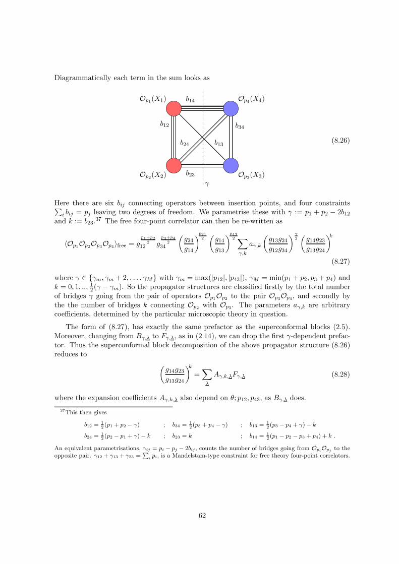
Diagrammatically each term in the sum looks as

γ

Op1(X1)

Op2(X2) Op3(X3)

Op4(X4)

b12 b34

b14

b23

b24 b13 (8.26)

Here there are six bij connecting operators between insertion points, and four constraints∑i bij = pj leaving two degrees of freedom. We parametrise these with γ := p1 + p2 − 2b12

and k := b23.37 The free four-point correlator can then be re-written as

〈Op1Op2Op3Op4〉free = gp1+p2

212 g

p3+p42

34

(g24g14

)p212(g14g13

)p432 ∑

γ,k

aγ,k

(g13g24g12g34

) γ2(g14g23g13g24

)k

(8.27)

where γ ∈ {γm, γm + 2, . . . , γM} with γm = max(|p12|, |p43|), γM = min(p1 + p2, p3 + p4) andk = 0, 1, .., 12(γ − γm). So the propagator structures are classified firstly by the total numberof bridges γ going from the pair of operators Op1Op2 to the pair Op3Op4 , and secondly bythe the number of bridges k connecting Op2 with Op3 . The parameters aγ,k are arbitrarycoefficients, determined by the particular microscopic theory in question.

The form of (8.27), has exactly the same prefactor as the superconformal blocks (2.5).Moreover, changing from Bγ,λ to Fγ,λ, as in (2.14), we can drop the first γ-dependent prefac-tor. Thus the superconformal block decomposition of the above propagator structure (8.26)reduces to

(g14g23g13g24

)k=∑

λ

Aγ,k,λFγ,λ (8.28)

where the expansion coefficients Aγ,k,λ also depend on θ; p12, p43, as Bγ,λ does.

37This then gives

b12 = 12(p1 + p2 − γ) ; b34 = 1

2(p3 + p4 − γ) ; b13 = 1

2(p3 − p4 + γ)− k

b24 = 12(p2 − p1 + γ)− k ; b23 = k ; b14 = 1

2(p1 − p2 − p3 + p4) + k .

An equivalent parametrisations, γij = pi − pj − 2bij , counts the number of bridges going from OpiOpj to theopposite pair. γ12 + γ13 + γ23 =

∑

i pi, is a Mandelstam-type constraint for free theory four-point correlators.

62

The LHS of (8.28) is simple to understand, using from (2.8) we have that:

(g14g23g13g24

)k= sdet(1−Z)−k# =

β∏

r=1

∏nj=1(1− sryj)∏mi=1(1− srxi)θ

;si=1,...,k = 1

si=k+1,...,β = 0(8.29)

where β = 12 min(γ − p43, γ − p12) as usual. We recognise here the LHS of the supercon-

formal Cauchy identity (8.5). Thus comparing (8.28) with this Cauchy identity (8.5) wecan immediately identify the CPW coefficients Aγ,k,λ as an evaluation formula for a Jacobipolynomial:

Aγ,k,λ;θ,p12,p43 = Πλ(θ)J(β)λ (s; θ, p−, p+)|

s=(1k ,0β−k) (8.30)

with p± defined in the same way, i.e. p± = θp± + θ − 1 and p± = 12 |p12 ± p43|.

Finally then, through Okounkov’s binomial formula (7.3), the free theory CPW coeffi-cients, Aγ,k,λ, can be written as a sum over interpolation polynomials evaluated at partitionsmultiplied by Jack polynomials evaluated at 1 and 0, Pµ(1

k, 0β−k; θ). Note that such aJack polynomial, Pµ(1

k, 0β−k; θ), truncates to a Young diagram with just k rows out of β,P[µ1,...,µk ](1

k; θ), from stability. The latter is a known explicit evaluation formula due to Stan-ley [65]. Putting this together then we arrive at an explicit formula for the CPW coefficientsas a sum of binomial coefficients,

Aγ,k,λ;θ,p12,p43 = Πλ(θ)∑

µ⊆λ

(S(β)θ,p−,p+

)µλ ×∏

1≤i<j≤k

(θ(j−i+1))µi−µj

(θ(j−i))µi−µj

. (8.31)

This formula provides the decomposition of any free theory diagram in superconformal blocks.It depends on γ, k, then θ and the external charges p12 and p43. It does not of course depend on(m,n) by stability of the super Cauchy identity. Indeed, because of stability, the derivationof (8.31) doesn’t rely on any supersymmetry at all, and can be derived directly from theoriginal bosonic Cauchy identity of Mimachi (8.2).

We will investigate this formula for free theory CPW coefficients further in a separatepublication [72] giving even simpler and completely explicit formulae for the θ = 1 case.

9 Decomposing superblocks

The superconformal block (or equivalently dual super Jacobi functions) Bγ,λ has been so fardefined as the multivariate series

Bγ,λ =

(∏i x

θi∏

j yj

)γ2

Fγ,λ , Fγ,λ =∑

µ⊇λ

(Tγ)µλ Pµ(z; θ) (9.1)

with (Tγ)µλ computed either from the recursion of section 5 or by the binomial coefficient of

section 7.

In this section we want to relate this to a more common approach where instead Bγ,λ isdecomposed into its constituent bosonic blocks. It is useful to view this in a more general

63

context of decomposing superblocks into smaller superblocks,

(m+m′|n+ n′) → (m|n)⊗ (m′|n′) . (9.2)

Then we will specialise to the case of decomposing into bosonic blocks an internal blocks byconsidering m′ = n = 0.

9.1 General decomposition of blocks

The analogous decomposition (9.2) for superJack polynomials is given in (C.59), and it in-volves the structure constants S. Note that these structure constants are independent of thedimensions m,n,m′, n′, because of stability! Combining this with the expansion of Blocksinto Jacks (9.1) we arrive at the decomposition of superblocks as

F (m+m′,n+n′)γ,λ =

∑

µ,ν

F (m,n)γ,µ (Sγ)

µνλ F (m′,n′)

γ,ν , (9.3)

where the block structure constants Sγ depend on θ, p12, p43 and are related to the Jackstructure constants via the (inverse) block to Jack matrices Tγ as

(Sγ)µνλ =

∑

λ⊇λµ⊆µν⊆ν

S µνλ (Tγ)

λλ(T

−1γ )

µµ(T

−1γ )

νν . (9.4)

Note we distinguish the Jack structure constants S from the block structure constants Sγ

purely by the presence of the subscript for the latte.r Since we know Tγ infinite triangularmatrices, the issue in this formula is to understand when and how the Sγ are non vanishing.

For the structure constants of Jack polynomials, since these are homogeneous, we clearlyrequire |λ| = |µ|+|ν| for S µν

λ 6= 0. A stronger statement conjectured by Stanley (conjecture 8.4in [65]) is that the Jack structure constants are non vanishing if and only if the correspondingSchur structure constants (given by the Littlewood-Richardson rule) are non vanishing

S µνλ (θ) 6= 0 ⇔ S µν

λ (1) 6= 0 . (9.5)

In any case, clearly for a given λ there are only a finite number of non vanishing Jack structureconstants S µν

λ and thus a finite number of terms in the decomposition of Pλ into smaller Jacks.

What about the block structure constants? Since the Jack→Block matrix Tγ is triangular

we see that (9.4) gives the (Sγ)µνλ in terms of S µν

λ with λ ⊇ λ. Thus λ can become arbitrarilylarge and the decomposition of a superblock into smaller superblocks might involve an infinitenumber of terms. However let us consider more carefully the structure of the Young diagramswhich can survive.

First note that the decomposition (9.3) has a vertical cut-off: the height of the Youngdiagram λ can be no larger than β = min

(12 (γ−p12), 12(γ−p43)

), since Tγ has such a vertical

cut-off (see discussion above (D.20)).

Now we claim that if µ is much wider than λ (i.e. µ1 >> λ1 ) then ν will also have to be

64

very wide in order for (Sγ)µνλ 6= 0. More precisely we make the following conjecture:

(Sγ)µνλ 6= 0 ⇒ ∃ µ, ν, κ, such that S µν

λ 6= 0, S µκµ 6= 0, S νκ

ν 6= 0 . (9.6)

To get a feel for this claim, consider the case λ = ∅ (corresponding to half BPS operatorsin a superconformal theory). Then the above conditions will require µ = ν = ∅ and soµ = ν(= κ). Therefore the conjecture implies the following in this case

(Sγ)µν∅ 6= 0 ⇒ µ = ν , (9.7)

so the decomposition of a superblock with a trivial Young diagram is diagonal. This is notobvious from (9.4) and requires non trivial relations between the Jack structure constants Sand the block to Jack matrix Tγ .

More generally, the conjecture (9.6) can be proven in the case θ = 1 where there is a group

theory interpretation. In the θ = 1 case the decomposition of the superblock F(m+m′|n+n′)γ,λ

in (9.3) has the group theoretic interpretation of decomposing reps of U(2m+2m′|2n+2n′) →U(2m|2n)⊗U(2m′|2n′) and taking only the states which are diagonal under the decompositionU(2m+2m′|2n+2n′) → U(m+m′|n+n′)⊗U(m+m′|n+n′) ( equivalently taking only thosereps whose Dynkin labels are symmetric as only such states contribute to the block).38 Letus perform this decomposition U(2m + 2m′|2n + 2n′) → U(2m|2n) ⊗ U(2m′|2n′) for theinduced U(2m + 2m′|2n + 2n′) representations Oγ,λ(X

AA′) (described in section 3.2. We

must first decompose the U(m+m′|n+n′) rep λ into U(m|n) ⊗ U(m′|n′) reps. In fact wedo this decomposition twice but then take the same reps for both copies of U(m+m′|n+n′).Under the decomposition let the U(m+m′|n+n′) index A split into the U(m|n) indices (α, a)and similarly A′ → (α, a′). So

Oγ,λ(A)λ(A′)(XAA′

) →⋃

µν

Oγ,µ(α)ν(a)µ(α)ν(a′)(XAA′

)

(this decomposition is dictated by S µνλ and explains the appearance of this in (9.6)). We

must now also consider the derivatives ∂AA′ acting on these. In particular the off-diagonalderivatives ∂αa′ and ∂aα will yield new induced representations of the subgroup U(2m|2n)⊗U(2m′|2n′). Since the derivatives commute (and we again project onto the diagonal rep) wearrive at

Oγ,µ(α)µ(α)ν(a)ν(a′)(XAA′

) →⋃

κ

∂|κ|κ(α)κ(α)κ(a)κ(a′)Oγ,µ(α)µ(α)ν(a)ν(a′)(X

αα,Xaa′) ,

and arrive at the tensor products κ ⊗ µ and κ ⊗ ν which explains the structure constantsS µκµ ,S νκ

ν appearing in (9.6).

We believe a similar argument for (9.6) can be made for the other group theoretic casesθ = 2, 12 although we haven’t gone carefully through the details.

38Note the difference with the corresponding group theory interpretation of the Jack decomposition (C.59)which is instead equivalent to decomposing reps of U(m+m′|n+ n′) → U(m|n)⊗U(m′|n′) in the θ = 1 case.

65

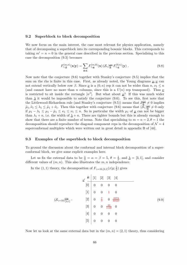
9.2 Superblock to block decomposition

We now focus on the main interest, the case most relevant for physics application, namelythat of decomposing a superblock into its corresponding bosonic blocks. This corresponds totaking m′ = n = 0 in the general case described in the previous section. Specialising to thiscase the decomposition (9.3) becomes

F (m,n)γ,λ (x|y) =

∑

µ,ν

F (m,0)γ,µ (x) (Sγ)

µνλ F (0,n)

γ,ν (y) . (9.8)

Now note that the conjecture (9.6) together with Stanley’s conjecture (9.5) implies that thesum on the rhs is finite in this case. First, as already noted, the Young diagrams µ, ν cannot extend vertically below row β. Since ν is a (0, n) rep it can not be wider than n, ν1 ≤ n(and cannot have no more than n columns, since this is a U(n) rep transposed). Thus νis restricted to sit inside the rectangle [nβ]. But what about µ? If this was much widerthan λ it would be impossible to satisfy the conjecture (9.6). To see this, first note thatthe Littlewood-Richardson rule (and Stanley’s conjecture (9.5)) means that S µν

λ 6= 0 impliesµ1, ν1 ≤ λ1 ≤ µ1 + ν1. Then this together with conjecture (9.6) means that (Sγ)

µνλ 6= 0 only

if µ1 − λ1 ≤ µ1 − µ1 ≤ κ1 ≤ ν1 ≤ n. So in particular the width µ1 of µ can not be biggerthan λ1 + n, i.e. the width of λ+ n. There are tighter bounds but this is already enough toshow that there are a finite number of terms. Note that specialising to m = n = 2, θ = 1 thedecomposition should reproduce the diagonal component reps in the decomposition of N = 4superconformal multiplets which were written out in great detail in appendix B of [44].

9.3 Examples of the superblock to block decomposition

To ground the discussion about the conformal and internal block decomposition of a super-conformal block, we give some explicit examples here.

Let us fix the external data to be γ2 = α = β = 5, θ = 1

2 , and λ = [3, 1], and considerdifferent values of (m,n). This also illustrates the m,n independence.

In the (1, 1) theory, the decomposition of Fγ=10,[3,1](x|y; 12) gives

(Sγ=10)νµ[3,1] :

[1] [2] [3] [4]

[0]

[1]

[2]

[3]

[4]

[5]

µν ′

0 0 0 0

0 0 1 0

0 79 0 1573

40320

0 0 391120 0

0 0 0 0

0 0 0 0

(9.9)

Now let us look at the same external data but in the (m,n) = (2, 1) theory, thus considering

66

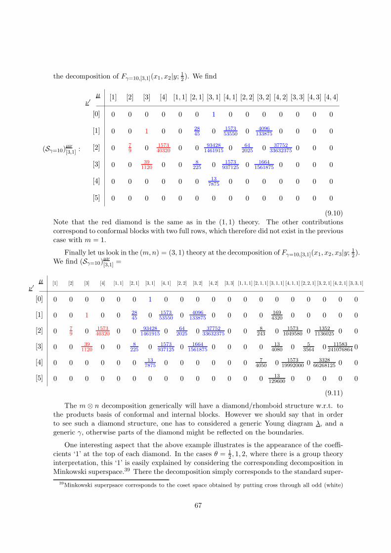
the decomposition of Fγ=10,[3,1](x1, x2|y; 12 ). We find

(Sγ=10)µν[3,1] :

[1] [2] [3] [4] [1, 1] [2, 1] [3, 1] [4, 1] [2, 2] [3, 2] [4, 2] [3, 3] [4, 3] [4, 4]

[0]

[1]

[2]

[3]

[4]

[5]

µν ′

0 0 0 0 0 0 1 0 0 0 0 0 0 0

0 0 1 0 0 2845 0 1573

53550 0 4096133875 0 0 0 0

0 79 0 1573

40320 0 0 934281461915 0 64

2025 0 3775233632375 0 0 0

0 0 391120 0 0 8

225 0 1573937125 0 1664

1561875 0 0 0 0

0 0 0 0 0 0 137875 0 0 0 0 0 0 0

0 0 0 0 0 0 0 0 0 0 0 0 0 0

(9.10)Note that the red diamond is the same as in the (1, 1) theory. The other contributionscorrespond to conformal blocks with two full rows, which therefore did not exist in the previouscase with m = 1.

Finally let us look in the (m,n) = (3, 1) theory at the decomposition of Fγ=10,[3,1](x1, x2, x3|y; 12).We find (Sγ=10)

µν[3,1] =

[1] [2] [3] [4] [1, 1] [2, 1] [3, 1] [4, 1] [2, 2] [3, 2] [4, 2] [3, 3] [1, 1, 1] [2, 1, 1] [3, 1, 1] [4, 1, 1] [2, 2, 1] [3, 2, 1] [4, 2, 1] [3, 3, 1]

[0]

[1]

[2]

[3]

[4]

[5]

µν ′

0 0 0 0 0 0 1 0 0 0 0 0 0 0 0 0 0 0 0 0

0 0 1 0 0 2845 0 1573

53550 0 4096133875 0 0 0 0 169

4320 0 0 0 0 0

0 79 0 1573

40320 0 0 934281461915 0 64

2025 0 3775233632375 0 0 8

243 0 15731049580 0 1352

1136025 0 0

0 0 391120 0 0 8

225 0 1573937125 0 1664

1561875 0 0 0 0 134080 0 5

3564 0 11583241076864 0

0 0 0 0 0 0 137875 0 0 0 0 0 0 7

4050 0 157319992000 0 3328

66268125 0 0

0 0 0 0 0 0 0 0 0 0 0 0 0 0 13129600 0 0 0 0 0

(9.11)

The m ⊗ n decomposition generically will have a diamond/rhomboid structure w.r.t. tothe products basis of conformal and internal blocks. However we should say that in orderto see such a diamond structure, one has to considered a generic Young diagram λ, and ageneric γ, otherwise parts of the diamond might be reflected on the boundaries.

One interesting aspect that the above example illustrates is the appearance of the coeffi-cients ‘1’ at the top of each diamond. In the cases θ = 1

2 , 1, 2, where there is a group theoryinterpretation, this ‘1’ is easily explained by considering the corresponding decomposition inMinkowski superspace.39 There the decomposition simply corresponds to the standard super-

39Minkowski superpsace corresponds to the coset space obtained by putting cross through all odd (white)

67

space expansion of the corresponding superfield over Grassmann odd variables and the firstterm in the expansion (the term obtained by switching off all Grassmann odd variables) hascorresponding coefficient ‘1’. We can view this superspace expansion for different values of(m,n), thus giving different ‘1’ coefficients. So for example in the (1, 1) theory this gives thered ‘1’ in (9.10) and in the (2, 1) theory it gives the blue ‘1’. But of course stability meansthe red ‘1’ remains there even for the (2, 1) theory.

It is interesting to see how to recover the “1 at the top of the diamond”, i.e. the leadingconformal block in the decomposition of a superblock from the formula (9.4) and show thatit is true for all θ regardless of whether there is a group theory interpretation. This followsdirectly from the observation that the Jack structure constants are ‘1’ whenever the largeYoung diagram is built from the smaller ones put on top of each other (C.27). A similarresult then follows for the block structure constants

(Sγ)µνλ (θ) = 1 if λ = [µ, ν] . (9.12)

since S and Sγ are simply related via a triangular change of (infinite) basis with 1’s on thediagonal (9.4) (recall (Tγ)

λλ = 1).

Testing the conjecture (9.6) in general turns into a sophisticated computation, because theJack structure constants S themselves are non-trivial and explicit formulae are not known.The works [52–54] obtain a recursive formulation which can be used to carry out the com-putation, but we are not aware of a more explicit formula. A naive approach we used, forgeneric number of rows, which nevertheless gives the desired result, is to start from the defi-nitions, and use computer algebra. But we point out that the remarkable consequence of theconjecture (9.6) is that even though Sγ involves infinite matrices Tγ , the result always hasonly finitely many non zero values. In particular if we keep α, β, γ arbitrary in the recursionrelation for Tγ this truncation does not occur, but only takes place when β (or α) is an integerlarger than the height of λ. To help clarify these points we now give some explicit results forthe two row case.

Explicit formulae for two-rows

For Young diagrams with two rows we can give alternative explicit (i.e. non combinatorial)formulae for the building blocks of the block structure constants (9.4). Indeed, the Jackstructure constants for two-row diagrams are known thanks to a result quoted in [100],

C[µ1,µ2][κ1,κ2] [ω1,ω2]

=(θ, 2θ + µ−, ω2 + κ1 − µ2 + 1, ω1 + κ2 − µ2 + 1)µ2−κ2−ω2

(1, 1 + θ + µ−, ω2 + κ1 − µ2 + θ, ω1 + κ2 − µ2 + θ)µ2−κ2−ω2

(9.13)

and

Sκωµ =

Πκ(θ)Πω(θ)

Πµ(θ)Cµκω . (9.14)

(Where (a, b, c)n represents a product of Pochhammers anbncn.) Note this formula is man-ifestly symmetric in κ ↔ ω. It is also clear that for θ = 1 the value of C collapse to unity,when it is non vanishing.

nodes in the relevant super Dynkin diagram rather than the crossed through nodes of analytic superspace (3.3).

68

Now, we assemble the block structure constants Sγ in (9.4). The two-row Jack→Blockmatrix Tγ can be taken from (E.18), and the inverse T−1

γ is given by the formula (7.28), interms of the interpolation polynomials in (E.22). Putting them together then gives the blockstructure constants Sγ .

In the recursion we may leave all variables α, β, γ unspecified in Tγ and T−1γ . We find that

in this case there is actually no truncation and there are infinitely many non-zero structureconstants (Sγ)

µνλ (θ) for given λ. However one finds that for arbitrary α, β, γ, for ν large

enough they always appear with a factor of (α − 2)(β − 2). So for any λ, µ exists a ν∗ suchthat

(Sγ)µνλ (θ) = (α− 2)(β − 2)

[. . .]

∀ ν ⊃ ν∗ (9.15)

where the terms understood in[. . .]might be cumbersome, but their knowledge is not needed

to understand the truncation. It is then clear from (9.15) that upon specifying either β orα to be the value of the maximal number of rows of the Young diagram, in the case of thissection β = 2, the block structure constants Sγ will truncate. We checked explicitly that thevery same mechanism generalises to any number of rows.

Them⊗n decomposition then can be carried out in practice for arbitrary Young diagramsand theories (m,n; θ). It depends on the Young diagrams and θ through rational functions.For example, consider the (2, 2) theory and Bγ=4,[λ1,λ2]. Then, we know that

Bγ=4,[λ1,λ2] =

(∏2i=1 x

θi∏2

j=1 yj

)γ2 (

F(2,0)γ,[λ1,λ2]

(x)× F(0,2)γ,∅ (y) + . . .

). (9.16)

The coefficients of the next terms beyond Fγ=4,[λ1,λ2] × Fγ=4,∅, with p12 = p43 = 0, are

(Sγ=4)[λ1,λ2−1],�[λ1,λ2]

= θλ2λ2+θ−1

(Sγ=4)[λ1−1,λ2],�[λ1,λ2]

= θ(λ1+θ)(λ1−λ2)(λ1−λ2+2θ−1)(λ1+2θ−1)(λ1−λ2+θ−1)(λ1−λ2+θ)

(Sγ=4)[λ1+1,λ2],�[λ1,λ2]

= θ(λ1+2θ)(λ1+3θ−1)(λ1+λ2+2θ)(λ1+λ2+4θ−1)4(2λ1+4θ−1)(2λ1+4θ+1)(λ1+λ2+3θ−1)(λ1+λ2+3θ)

(Sγ=4)[λ1,λ2+1],�[λ1,λ2]

= θ(λ1−λ2)(λ1−λ2+2θ−1)(λ2+θ)(λ2+2θ−1)(λ1+λ2+2θ)(λ1+λ2+4θ−1)4(λ1−λ2+θ−1)(λ1−λ2+θ)(λ1+λ2+3θ−1)(3θ+λ1+λ2)(2λ2+2θ−1)(2λ2+2θ+1)

(9.17)The complexity of these rational functions comes both from the complexity of the struc-ture constants and the solution of the recursion, equivalently the complexity of interpolationpolynomials evaluated at partitions.

10 Conclusions and outlook

Let us summarise our findings and conclude with an outlook.

In this paper we have uncovered a non trivial connection between the theory of con-formal and superconformal blocks for four-point correlators of scalar fields, and the the-ory of symmetric functions (as well as Heckman Opdam hypergeometric functions, CalogeroSutherland Moser wave functions and supersymmetric generalisations of all of these). Thisconnection generalises previous work done in [9] for theories defined on a super Grassman-

69

nian Gr(m|n, 2m|2n), corresponding to the case (m,n; θ = 1), where the connection betweensymmetric functions and superconformal blocks passed through the use of super Schur poly-nomials [37]. It also generalises the connection between bosonic external/internal blocks andBC2 hypergeometric functions/Jacobi polynomials uncovered in [11–15]. The starting pointhas been to consider four-point functions of scalar operators on certain special generalised(m,n) analytic superspaces in 3,4 and 6 dimensions following [1–10]. We then looked at thevery concrete problem of solving a Casimir eigenvalue differential equation, and we have foundthat:

• The Casimir operator for these theories coincides with the BCm|n CMS operator for

special values of a parameter θ (θ = 12 , 1, 2). This then immediately suggests to define

(m,n; θ) analytic superspaces for more general θ as discussed in section 3.1.

• The eigenfunctions of the BCm|n Casimir admit a representation as a multivariate seriesover super Jack polynomials,

Bγ,λ(z) =

(∏i x

θi∏

j yj

)γ2

Fγ,λ(z) , Fγ,λ(z) =∑

µ⊇λ

(Tγ)µλ Pµ(z) , (10.1)

with expansion coefficients Tγ enjoying special properties.

• The expansion coefficients (Tγ)µλ do not depend on m,n as long as λ, µ are Young

diagrams. Since super Jack polynomials are themselves stable, by construction, oursuperconformal blocks are stable!

• Although the coefficients Tγ do not depend on (m,n) when λ, µ are Young diagrams,the recursion (and its solution) can non-the-less be represented in various forms, interms of the row lengths of the Young diagram, the column lengths, or a mixture ofthe two. All representations give the same result, as shown in section 5.2, when theparameters coincide with those of a Young diagram. However, the different choicesyield inequivalent analytic continuations (section 6). A mixed representation consistentwith the (m,n) Young diagram structure is then most appropriate for superblocks inan (m,n; θ) theory and will give the correct superblocks for operators with non-integer(anomalous) dimensions. Such an (m,n) representation satisfies the shift symmetry (2.20)for arbitrary θ (which is a manifest symmetry for the physical cases θ = 1

2 , 1, 2).

• We exemplified this (m,n) analytic continuation in the simplest (1, 1) theory, forarbitrary θ. This shows, in a concrete case, that the recursion can be solved by using amixed, or supersymmetric, representation where the Young diagrams are read both alongrows and columns.

The above results find immediate application for superconformal theories not only in di-mensions 3,4,6, but also in 1,2 and possibly also 5 dimensions, as well as ordinary bosonictheories in any dimension, as explained in section 3.1. The superconformal block understand-ing is particularly important for theories that have a gravity dual through the AdS/CFT

70

correspondence, where we expect the SCFT to provide important insights towards the questfor a theory of quantum gravity. The simplest examples which have made full use of this(m,n; θ) formalism have been so far AdS5 × S5 [74–76]. There has been some use of theformalism also for AdS7×S4 but restricted to the lowest charge correlators [8,78].40 It wouldbe interesting to extend this further and consider other AdS×S backgrounds. An interestingcase that has not been attacked yet is AdS3 ×S3×S3, which realises a one-parameter familyof two-dimensional superconformal theories with D(2, 1;α) ×D(2, 1;α) symmetry.41

The connection between (super)conformal blocks and symmetric functions, that we haveuncovered, yielded in turn a number of mathematical results, providing further inspirationon the mathematics of BCn|m symmetric functions, as well as further insights for the super-conformal blocks themselves. In this context, we found that:

• The reduction our blocks from BCm|n to BCn produces the dual Jacobi polynomials

Jβ,λ(; θ, p±) in n variables, which are stable, and were not noticed before. From the

knowledge of these polynomials (in particular their stability), we showed that they admita natural supersymmetric extension which give superconformal blocks.

• Jacobi polynomials Jλ(; θ, p±) have a binomial formula due to Okounkov [32,33,41], and

so do the dual Jacobi polynomials. The difference is the way the Young diagrams enterthe interpolation polynomials P ∗. For the dual Jacobi polynomials, the Young diagramsare complemented and transposed w.r.t. a given rectangle R. This manipulation stabilisesthe binomial formula for the Jacobi polynomials.

• The dependence on the variables of the interpolation polynomialsP ∗NM \µ(N

M \λ; θ, u=12−θ

γ2−N), provides the highly non-trivial γ dependence of

(Tγ)µλ, which was quite challenging to understand from the point of view of the recursion.

• Elaborating on the way complementation works on the Jack→Block matrix, we showedthat its inverse, the Block→Jack matrix, Tγ , has a natural representation in terms ofinterpolation polynomials, which we upgraded to super interpolation polynomials ofSergeev and Veselov [36]. Thus, whenever an identity pairs a Young diagram with itscomplement, we can use the Jack→Block and the Block→Jack matrix to uplift thatidentity to an identity for superconformal blocks.

40More recent work has considered superblocks for higher charge correlators in the AdS7×S4 case using theWard identity approach discussed at the start of section 2.5 [51,79]

41In the context of integrability this has been studied in, e.g. [80].

71

• From the (m,n) Cauchy identity for superJack polynomials we proved a superconformalCauchy identity,

β∏

r=1

∏nj=1(1− sryj)∏mi=1(1− srxi)θ

=∑

λ

Jλ(s; θ, p−, p+) Πλ(θ)Fγ,λ(z; θ, p12, p43) (10.2)

Then we showed that the LHS becomes a propagator structure when s = (1k, 0β−k), upto the overall prefactor (

∏i,j x

θi /yj)

γ2 , which distinguishes Bγ,λ from Fγ,λ. It follows that,

with no effort, the above Cauchy identity provides the decomposition of any (generalised)free theory diagram within our formalism.

• The physics understanding of the (m,n) super Cauchy identity allowed us to provea new doubly supersymmetric Cauchy identity (8.7) involving superconformal blocks(dual super Jacobi functions) and the super Jacobi polynomial of Sergeev and Veselov [36].

• Finally we could read off known results on higher order operators for Heckman Opdamhypergeometrics to obtain all higher order Casimirs in θ = 1 theories (in particular N = 4SYM).

Overall, we showed in section 7 and 8 that the connection between superconformal blocksand symmetric functions comes with a non trivial exchange of information, which is fruitfulfor both sides. The superconformal Cauchy identity is a beautiful example of this exchange.On one side the understanding of stability clarifies the proofs greatly, on the other side, theCauchy formula allows us to read off, with no effort, the superconformal block decompositionof any free theory diagram.

There are a number of topics one could investigate further. There is still more to beunderstood about the analytic properties of the superblocks. In [12, 14] bosonic blocks wereidentified with twisted versions of the Harish Chandra functions giving Heckman Opdamhypergeometric functions. We give here two new viewpoints on this. Both viewpoints startwith the much simpler BCn Jacobi polynomials or more accurately the dual BCn Jacobipolynomials which are stable. This stability then leads immediately to a family of (n,m)supersymmetric dual Jacobi functions, and then specialising to n = 0 we obtain the conformalblocks (which are certain Sn symmetric combinations of Harish Chandra functions). But therank one considerations suggest another viewpoint, namely that the analytic continuation,regular at the origin, of the dual Jacobi polynomials to negative row lengths also yield theconformal blocks. We then expect similarly that analytic continuation of the super dualJacobi functions to negative row lengths for the infinite non compact direction will give thesuper Jacobi polynomials of [36].

Besides the immediate relevance of our work for theories that have a generalised freelimit, the superconformal block expansion has a non perturbative nature, and recent workin [81–85] has shown that a fully non perturbative reconstruction of a four-point correlatorcan be given within the framework of the inversion formula [70]. A prominent role is playedby the Polyakov-Regge block.We think that this discussion should have a counterpart in thetheory of symmetric functions worth investigating.42

42For similar reasons, it would be interesting to investigate the diagonal limit [86] of the superconformal

72

It would be interesting to try to adapt our story beyond scalar representations, as well asfor higher points, possibly by adapting the techniques of [88–91].

10.1 Outlook on the q-deformed superblocks

Finally, it would be fascinating to find a place for a possible q-deformation of the superblocks,since the various group theoretic objects that we have been discussing, i.e. Jack, Jacobi,interpolation polynomials etc., have well known q-deformed generalisations. In particular,the expansion coefficients (7.12) of the superblocks

(Tγ)µλ = (N )µλ ×

P∗(M)

NM \µ(NM \λ; θ, u)

P∗(M)

NM \λ(NM \λ; θ, u)

∣∣∣∣∣u=

12−θ

γ2−N

. (10.3)

written as binomial coefficient has such a q-deformation. A simple question to ask is whetherthe q-deformed binomial coefficient plays a role in physical theories.43 For example, is there anotion of q-deformed CFTs in any dimension? In these theories, how do q-deformed conformalblocks compare to our multivariate series? For applications within the AdS/CFT correspon-dence, is it possible to investigate the field theory dual to the q-deformed world-sheet σ-modelon AdS5 × S5 [96–98].

In a little more detail, the q-deformed binomial coefficient can be used to define theKoornwinder polynomialsKλ(z, q, t; ai=1,2,3,4), as shown by Okounkov [33]. The latter are BCorthogonal (Laurent) polynomials in the bosonic variables z, and for a choice of parameters~a, the q → 1 defines the BC Jacobi polynomials (see e.g. [41]):

limq→1

Kλ(z) = (−4)|λ|Jλ(−1

4(√zi − 1√

zi)2). (10.4)

An obvious proposal to build the q-deformed generalisation of the (0, n) internal block wouldbe to start from the Koornwinder polynomials. Koornwinder polynomials have a binomialexpansion, but the polynomials involved are themselves q-deformed BC interpolation poly-nomials.44 One might have expected the generalisation of the internal block would rathercorrespond to a series over Macdonald polynomials, instead of BC interpolation polynomi-als. After all the super Jack polynomials, which provided the relevant basis for the (m,n)superconformal blocks, admit a natural generalisation to the super Macdonald operators ofSergeev and Veselov [36]. On the other hand, there is a fundamental reason why Koornwinderpolynomials sum over BC interpolation polynomials, and this is evaluation symmetry, i.e. theproperty that evaluating Kµ at partition λ is invariant under µ↔ λ. This property is mani-fest in the binomial coefficient formalism [33], precisely because the expansion coefficients onthe basis of BC interpolation polynomials are again BC interpolation polynomial evaluatedat a partition, and therefore evaluation symmetry “swaps” the two.

A proposal for the q-deformed generalisation of the (0, n) internal block can be read from

blocks, as well as the change of variables to the radial coordinate proposed in [87].43In this paper, we used the limit q → 1 and t → qθ, in the notation of [32].44The limit to the Jacobi polynomials is designed to degenerate the BC interpolation polynomials to Jack

polynomials and the q-deformed binomial coefficient to its classical counterpart [41].

73

E.Rains’ results in [32].45 It is the virtual Koornwinder “polynomial” KQ,λ (see Definition 7and Theorem 7.13 in [32]). This is a stable Sn (rather than BCn) function which provides a1-parameter, Q, generalisation of Koornwinder polynomials K(n)

λ in the following sense,

KQ,λ(. . . , zn; q, t;~a)∣∣∣Q=qm

=∏

i

zmi K(n)mn\λ(z; q, t,~a) . (10.5)

In more detail, KQ,λ is defined by a binomial formula that sums over Young diagrams µ suchthat λ ⊆ µ, and uses the equivalent of the q-deformed Jack→Block matrix, as in our dualJacobi function Jβ,λ(y| ) in (2.29), analytically continued in β (see the discussion in section6 and appendix D.2.) The similarity is even more precise because when Q = qm the sumtruncates to the polynomial on the r.h.s. of (10.5), which indeed has the same characteristicsas dual Jacobi polynomials:

Jβ,λ(y| )∣∣∣β=m

≡∏

i

ymi Jmn\λ(. . . ,1yn) . (10.6)

We can see now that by taking the limit from Koornwinder polynomials to Jacobi polynomialsin (10.5), and re-expressing the result in terms of our dual Jacobi polynomials we find that

limq→1

KQ,λ(z)∣∣∣Q=qm

=∏

i

(1− zi)2mJm,λ

( −4zi(1− zi)2

)(10.7)

The argument of J might be surprising at first, but Z(z) = −4z/(1 − z)2 is just a conformalmapping which sends the unit disk in the z plane to Z ∈ C\(1,+∞). Stability of the r.h.s. of(10.7) then follows from that of KQ,λ, and coincides with the stability of Jβ,λ which we

discussed in this paper (since that of∏

i(1 − zi)2m is obvious). We thus conclude that KQ,λ

is the q-generalisation of our Jβ,λ(y| ) where Q = qβ.

From stability, following the same logic that led us from dual Jacobi polynomials to superJacobi function Jβ(y|x) in section 2.3, we infer that there is a supersymmetric uplift of the

virtual K to a “super virtual Koornwinder” KQ(y|x) obtained by supersymmetrising the

expansion polynomials that define K, called virtual P ∗ for reference, but keeping the sameexpansion coefficients, i.e. the q-deformed Jack→Block matrix. It is crucial here that suchvirtual P ∗ are again Sn stable polynomials, the “super virtual” P ∗ will then generalise thesuper Macdonald polynomials of [36]. The super virtual Koornwinder KQ(y|x) would thengive the q-generalisation of our superconformal blocks. Following our general motivations,it would be fascinating to study in more detail the properties of the super KQ(y|x) andunderstand their role in the context of q-deformed CFTs.

Acknowledgements

We would like to thank Ole Warnaar for very illuminating conversations about BC symmetricfunctions, and guidance into the literature. With great pleasure we would like to thankReza Doobary for collaboration at an initial stage of this work, and James Drummond,

45We thank Ole Warnaar for pointing out this to us.

74

Arthur Lipstein, and Hynek Paul, Michele Santagata for collaboration on related projectsover the years. We also thank Chiung Hwang, Gleb Arutunov, Pedro Vieira, Sara Pasquetti,Volker Schomerus and other members of the DESY theory group for discussions on relatedtopics. FA is supported by FAPESP grant 2016/01343-7, 2019/24277-8 and 2020/16337-8, andwas partially supported by the ERC-STG grant 637844-HBQFTNCER. PH is supported bySTFC Consolidated Grant ST/P000371/1 and the European Union’s Horizon 2020 researchand innovation programme under the Marie Sklodowska-Curie grant agreement No.764850“SAGEX”.

A Super/conformal/compact groups of interest

Here we give details about the supercoset construction of section 3, and in particular showhow the general formalism ties in with the more standard approach in the case of non-supersymmetric conformal blocks.

A.1 θ = 1: SU(m,m|2n)

The SU(m,m|2n) is the simplest family of theories with a supergroup interpretation for anyvalue of m,n positive integers. This corresponds to the case θ = 1.

The supercoset here is the most straightforward of the three general classes: Firstly viewthe complexified group SU(m,m|2n) = SL(2m|2n;C) as the set of (m|2n|m) × (m|2n|m)matrices (this is a straightforward change of basis of the more standard (2m|2n) × (2m|2n)matrices). Then the supercoset space we consider has the 2× 2 block structure of (3.4) witheach block being a (m|n)× (m|n) matrix (or rearrangement thereof - see footnote 17.) Theseblocks are unconstrained beyond the overall unit superdeterminant condition: sdet(G) =sdet(H) = 1. So in particular the coordinates XAA′

of (3.6) are unconstrained (m|n)× (m|n)matrices. Here A and A′ are both superindices carrying the fundamental representation of twoindependent SL(m|n) subgroups. This supercoset corresponds to the super GrassmannianGr(m|n, 2m|2n). For more details see [2, 3, 6, 7, 56].

Then a four point function (and in particular the superconformal blocks) can be writtenin terms of a function of the four points X1,X2,X3,X4 invariant under the action of G. Thisin turn boils down to a function of the (m|n)× (m|n) matrix Z invariant under conjugation(see [7] for more details)

Z = X12X−123 X34X

−141 ∼ diag(x1, .., xm|y1, .., yn) . (A.1)

The m+ n eigenvalues xi, yi then yield the m+ n arguments of the superblocks Bγ,λ.

Thus any function of Z invariant under conjugation will automatically solve the super-conformal Ward identities associated with the four point function. As first pointed out in thiscontext in [7] the simplest way to construct a basis of all such polynomials associated with aYoung diagram λ naturally yields (super) Schur polynomials (which are just the Jack poly-nomials with θ = 1). The construction is as follows. Take |λ| copies of ZB

A and symmetrisethe upper (B) indices according to the Young symmetriser of λ. Then contract all upper and

75

lower indices. For example

λ = → ZAA = Tr(Z) = Pλ(z; θ=1)

λ = → Z(A1

A1Z

A2)A2

= 12

(Tr(Z)2 +Tr(Z2)

)= Pλ(z; θ=1)

λ = → Z[A1

A1Z

A2]A2

= 12

(Tr(Z)2 − Tr(Z2)

)= Pλ(z; θ=1) (A.2)

Inputting the eigenvalues of Z (A.1) into these we obtain (up to an overall normalisation)precisely the corresponding Schur polynomials i.e. Jack polynomials with θ = 1, Pλ(z; θ = 1).This correspondence works for any Young diagram λ.

A.2 θ = 2 : OSp(4m|2n)

Details of this supercoset construction can be found (specialised to the m = 2 case) in [5, 8].We summarise here.

When θ = 2 the relevant (complexified) supergroup is OSp(4m|2n) which has bosonicsubgroup SO(4m) × Sp(2n) with SO(4m) non-compact and Sp(2n) compact. Of physicalinterest is the case m = 2 in which SO(8) is the complexification of the 6d conformal groupSO(2, 6) and Sp(2n) is the internal symmetry group for (0, n) superconformal field theories.

The supercoset space is defined by the marked Dynkin diagram (3.12)b (or (3.13)b ifn = 0) and can be realised in the block 2 × 2 matrix form of (3.4). To see this one needs torealise the group osp(4m|2n) as the set of supermatrices orthogonal wrt the metric J :

osp(4m|2n) =

M ∈ C(2m|2n|2m)×(2m|2n|2m) :MJMT = J =

12m1n

−1n12m

.

(A.3)InputtingM = H in the block form of (3.4) into this we find that a is related to d but is itselfunconstrained. Thus the Levi subgroup (under which the operators transform explicitly) isisomorphic to GL(2m|n). Similarly, inputting M = s(X) in the form of (3.6), we find thatthe coordinates are (2m|n)× (2m|n) antisymmetric supermatrices

X = −XT . (A.4)

Note that here and elsewhere XT denotes the supertranspose (XAB)T = XBA(−1)AB . Four-point functions are written in terms of a function of four such Xs, X1,X2,X3,X4 invariantunder OSp(4m|2n). We can use the symmetry to set X3 → 0 and then X−1

2 → 0. Then wecan use the remaining symmetry to set

X1 → K =

1m−1m

1n

. (A.5)

Finally we end up with the problem of finding a function of X4 which is invariant under X4 →AX4A

T where AKAT = K. The group of matrices satisfying AKAT = K is OSp(n|2m). Soletting Z = X4K we seek functions of Z invariant under conjugation under OSp(n|2m) ⊂

76

GL(2m|n). Ultimately, an invariant function of X1,X2,X3,X4 will be a function of theeigenvalues of this matrix Z. The eigenvalues of the m×m piece of the matrix Z (3.8) arerepeated

Z = X12X−123 X34X

−141 ∼ diag(x1, x1, x2, x2, .., xm, xm|y1, .., yn) . (A.6)

As always the independent ones yield the m|n arguments of the superblocks (2.7).

This construction again provides a completely manifest way of solving the superconformalWard identities. Fascinatingly the simplest way to construct a basis of functions solving theseWard identities yields the super Jack polynomials! To construct a basis of such functions in 1-1 correspondence with Young diagrams λ proceed as follows. Take |λ| copies of W = X4, andsymmetrise all indices according to the Young symmetriser of λ the Young diagram obtainedfrom λ by duplicating all rows. Then contract all indices with |λ| copies of K.

Let us illustrate this with the simplest examples:

λ = ⇒ λ = AB

→ WABKAB = Tr(Z) = Pλ(z; θ=2)

λ = ⇒ λ = ACBD

→ −WB(AWC)DKABKCD = 12

(Tr(Z)2 +Tr(Z2)

)= Pλ(z; θ=2)

λ = ⇒ λ =ABCD

→ W [ABWCD]KABKCD = 13

(Tr(Z)2 − 2Tr(Z2)

)= Pλ(z; θ=2)

(A.7)

Inputting the eigenvalues of Z (A.6) into these we obtain (up to an overall normalisation)precisely the corresponding Jack polynomial with θ = 2, Pλ(z; θ = 2). This correspondencecontinues for any Young diagram λ.

Note that this derivation of superblocks and super Jacks from group theory makes manifestthe stability in m,n of both, since they arise from formulae derived from matrices Z ofarbitrary dimensions. A combinatoric description of (super)Jack polynomials with θ = 2along these lines has also been discussed in [92].

A.3 θ = 12: OSp(4n|2m)

The other value of θ for which there is a supergroup interpretation for any m,n is θ = 12 .

Here the relevant (complexified) supergroup is OSp(4n|2m), the same complexified group aspreviously but with the roles of m,n reversed. This has bosonic subgroup Sp(2m)× SO(4n)but now with Sp(2m) non-compact (for m = 2 this is the complexified 3d conformal groupSp(4) ∼ SO(5) ∼ SO(2, 3)) and SO(4n) compact the internal subgroup.

The following is then essentially identical to the θ = 2 case but with the role of Grassmannodd and even exchanged. The supercoset space defined by the marked Dynkin diagram (3.12)c(or (3.13)c if n = 0) can also be realised in the block 2× 2 matrix form of (3.4) by realising

77

the group osp(4n|2m) in the following form46:

osp(4n|2m) =

M ∈ C(m|4n|n)×(m|4n|m) :MJMT = J =

1m12n

12n−1m

(A.8)

The Levi subgroup (under which the operators transform explicitly) is isomorphic toGL(m|2n)and the coordinates are (m|2n)× (m|2n) symmetric supermatrices

X = XT . (A.9)

Four-point functions are written in terms of a function of four such Xs, X1,X2,X3,X4 in-variant under OSp(4n|2m). We can use the symmetry to set X3 → 0 and then X−1

2 → 0.Then we can use the remaining symmetry to set

X1 → K =

1m1n

−1n

. (A.10)

We then are left with a function ofX4 which invariant underX4 → AX4AT where AKAT = K

i.e. under OSp(m|2n). Letting Z = X4K we seek functions of Z invariant under conjugationunder OSp(m|2n) ⊂ GL(m|2n). Thus ultimately, an invariant function of X1,X2,X3,X4 willbe a function of the eigenvalues of this matrix Z. The eigenvalues of the internal n× n pieceof the matrix Z (3.8) are repeated and the independent eigenvalues yield the m|n argumentsof the superblocks (2.7)

Z = X12X−123 X34X

−141 ∼ diag(x1, .., xm|y1, y1, y2, y2, .., yn, yn) . (A.11)

As for θ = 2 this construction provides a completely manifest way of solving the super-conformal Ward identities naturally giving θ = 1

2 super Jack polynomials! Take |λ| copies ofW = X4, and symmetrise all indices according to the Young symmetriser of λ which is thistime the Young diagram obtained from λ by duplicating all columns rather than rows. Thencontract all indices with |λ| copies of K.

In the simplest examples:

λ = ⇒ λ = AB → WABKAB = Tr(Z)

λ = ⇒ λ = ABCD → W (ABWCD)KABKCD = 13

(Tr(Z)2 + 2Tr(Z2)

)

λ = ⇒ λ = ABCD

→ W (B[AWC]DKABKCD = 12

(Tr(Z)2 − Tr(Z2)

)

(A.12)

Inputting the eigenvalues of Z (A.11) into these we obtain (up to an overall normalisation)precisely the corresponding Jack polynomials with θ = 1

2 , Pλ(z; θ = 12). This correspondence

works for any Young diagram λ.

46This is a change of basis of the matrix form in (A.3)

78

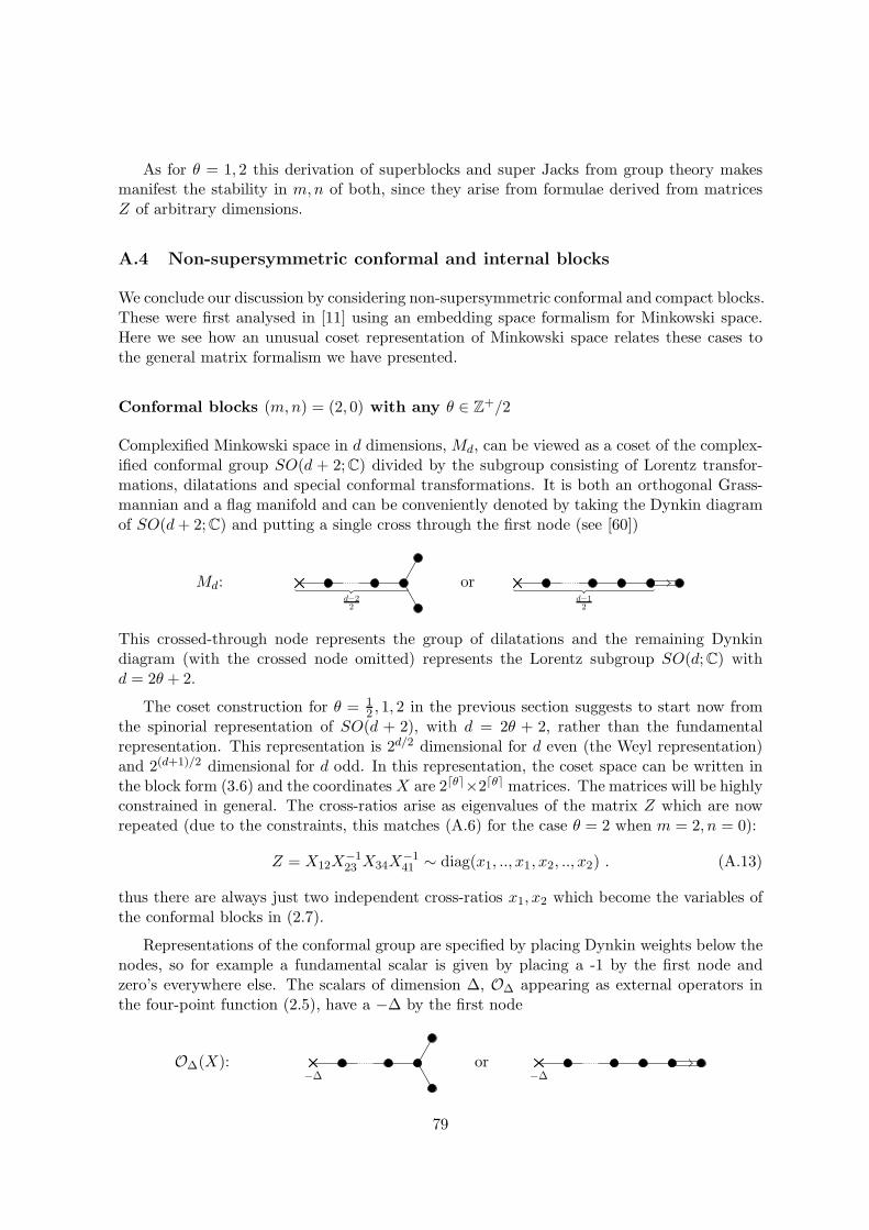
As for θ = 1, 2 this derivation of superblocks and super Jacks from group theory makesmanifest the stability in m,n of both, since they arise from formulae derived from matricesZ of arbitrary dimensions.

A.4 Non-supersymmetric conformal and internal blocks

We conclude our discussion by considering non-supersymmetric conformal and compact blocks.These were first analysed in [11] using an embedding space formalism for Minkowski space.Here we see how an unusual coset representation of Minkowski space relates these cases tothe general matrix formalism we have presented.

Conformal blocks (m,n) = (2, 0) with any θ ∈ Z+/2

Complexified Minkowski space in d dimensions, Md, can be viewed as a coset of the complex-ified conformal group SO(d + 2;C) divided by the subgroup consisting of Lorentz transfor-mations, dilatations and special conformal transformations. It is both an orthogonal Grass-mannian and a flag manifold and can be conveniently denoted by taking the Dynkin diagramof SO(d+ 2;C) and putting a single cross through the first node (see [60])

Md:d−22

ord−12

This crossed-through node represents the group of dilatations and the remaining Dynkindiagram (with the crossed node omitted) represents the Lorentz subgroup SO(d;C) withd = 2θ + 2.

The coset construction for θ = 12 , 1, 2 in the previous section suggests to start now from

the spinorial representation of SO(d + 2), with d = 2θ + 2, rather than the fundamentalrepresentation. This representation is 2d/2 dimensional for d even (the Weyl representation)and 2(d+1)/2 dimensional for d odd. In this representation, the coset space can be written inthe block form (3.6) and the coordinatesX are 2⌈θ⌉×2⌈θ⌉ matrices. The matrices will be highlyconstrained in general. The cross-ratios arise as eigenvalues of the matrix Z which are nowrepeated (due to the constraints, this matches (A.6) for the case θ = 2 when m = 2, n = 0):

Z = X12X−123 X34X

−141 ∼ diag(x1, .., x1, x2, .., x2) . (A.13)

thus there are always just two independent cross-ratios x1, x2 which become the variables ofthe conformal blocks in (2.7).

Representations of the conformal group are specified by placing Dynkin weights below thenodes, so for example a fundamental scalar is given by placing a -1 by the first node andzero’s everywhere else. The scalars of dimension ∆, O∆ appearing as external operators inthe four-point function (2.5), have a −∆ by the first node

O∆(X):−∆

or−∆

79

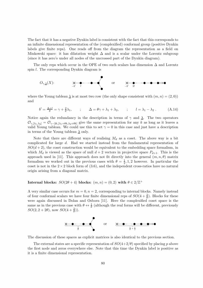
The fact that it has a negative Dynkin label is consistent with the fact that this corresponds toan infinite dimensional representation of the (complexified) conformal group (positive Dynkinlabels give finite reps). One reads off from the diagram the representation as a field onMinkowski space: it has dilatation weight ∆ and is a scalar under the Lorentz subgroup(since it has zero’s under all nodes of the uncrossed part of the Dynkin diagram).

The only reps which occur in the OPE of two such scalars has dimension ∆ and Lorentzspin l. The corresponding Dynkin diagram is

Oγ,λ(X):−b′ l

or−b′ 2l

where the Young tableau λ is at most two row (the only shape consistent with (m,n) = (2, 0))and

b′ = ∆+lθ = γ + 2

θλ1, ; ∆ = θγ + λ1 + λ2, ; l = λ1 − λ2 . (A.14)

Notice again the redundancy in the description in terms of γ and λ. The two operatorsOγ,[λ1,λ2] = Oγ−2k,[λ1+θk,λ2+θk] give the same representation for any k as long as it leaves avalid Young tableau. We could use this to set γ = 0 in this case and just have a descriptionin terms of the Young tableau λ only.

Note that there are different ways of realising Md as a coset. The above way is a bitcomplicated for large d. Had we started instead from the fundamental representation ofSO(d+ 2), the coset construction would be equivalent to the embedding space formalism, inwhich Md is viewed as the space of null d + 2 vectors in projective space Pd+1. This is theapproach used in [11]. This approach does not fit directly into the general (m,n, θ) matrixformalism we worked out in the previous cases with θ = 1

2 , 1, 2 however. In particular thecoset is not in the 2× 2 block form of (3.6), and the independent cross-ratios have no naturalorigin arising from a diagonal matrix.

Internal blocks: SO(2θ + 4) blocks: (m,n) = (0, 2) with θ ∈ 2/Z+

A very similar case occurs for m = 0, n = 2, corresponding to internal blocks. Namely insteadof four conformal scalars we have four finite dimensional reps of SO(4 + 2

θ ). Blocks for thesewere again discussed in Dolan and Osborn [11]. Here the complexified coset space is thesame as in the previous case with θ ↔ 1

θ (although the real forms will be different, previouslySO(2, 2 + 2θ), now SO(4 + 2

θ )).

1θ

or1θ + 1

2

The discussion of these spaces as explicit matrices is also identical to the previous section.

The external states are a specific representation of SO(4+2/θ) specified by placing p abovethe first node and zeros everywhere else. Note that this time the Dynkin label is positive asit is a finite dimensional representation.

80

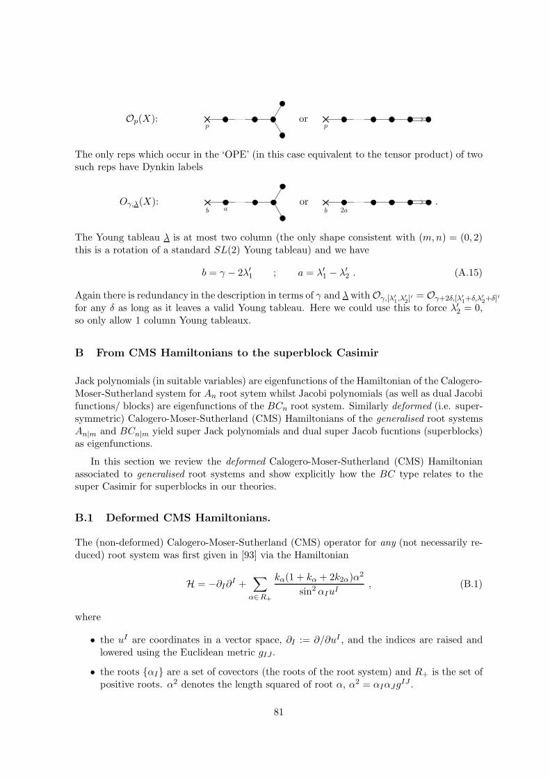
Op(X):p

orp

The only reps which occur in the ‘OPE’ (in this case equivalent to the tensor product) of twosuch reps have Dynkin labels

Oγ,λ(X):b a

orb 2a

.

The Young tableau λ is at most two column (the only shape consistent with (m,n) = (0, 2)this is a rotation of a standard SL(2) Young tableau) and we have

b = γ − 2λ′1 ; a = λ′1 − λ′2 . (A.15)

Again there is redundancy in the description in terms of γ and λ withOγ,[λ′1,λ

′2]

′ = Oγ+2δ,[λ′1+δ,λ′

2+δ]′

for any δ as long as it leaves a valid Young tableau. Here we could use this to force λ′2 = 0,so only allow 1 column Young tableaux.

B From CMS Hamiltonians to the superblock Casimir

Jack polynomials (in suitable variables) are eigenfunctions of the Hamiltonian of the Calogero-Moser-Sutherland system for An root sytem whilst Jacobi polynomials (as well as dual Jacobifunctions/ blocks) are eigenfunctions of the BCn root system. Similarly deformed (i.e. super-symmetric) Calogero-Moser-Sutherland (CMS) Hamiltonians of the generalised root systemsAn|m and BCn|m yield super Jack polynomials and dual super Jacob fucntions (superblocks)as eigenfunctions.

In this section we review the deformed Calogero-Moser-Sutherland (CMS) Hamiltonianassociated to generalised root systems and show explicitly how the BC type relates to thesuper Casimir for superblocks in our theories.

B.1 Deformed CMS Hamiltonians.

The (non-deformed) Calogero-Moser-Sutherland (CMS) operator for any (not necessarily re-duced) root system was first given in [93] via the Hamiltonian

H = −∂I∂I +∑

α∈R+

kα(1 + kα + 2k2α)α2

sin2 αIuI, (B.1)

where

• the uI are coordinates in a vector space, ∂I := ∂/∂uI , and the indices are raised andlowered using the Euclidean metric gIJ .

• the roots {αI} are a set of covectors (the roots of the root system) and R+ is the set ofpositive roots. α2 denotes the length squared of root α, α2 = αIαJg

IJ .

81

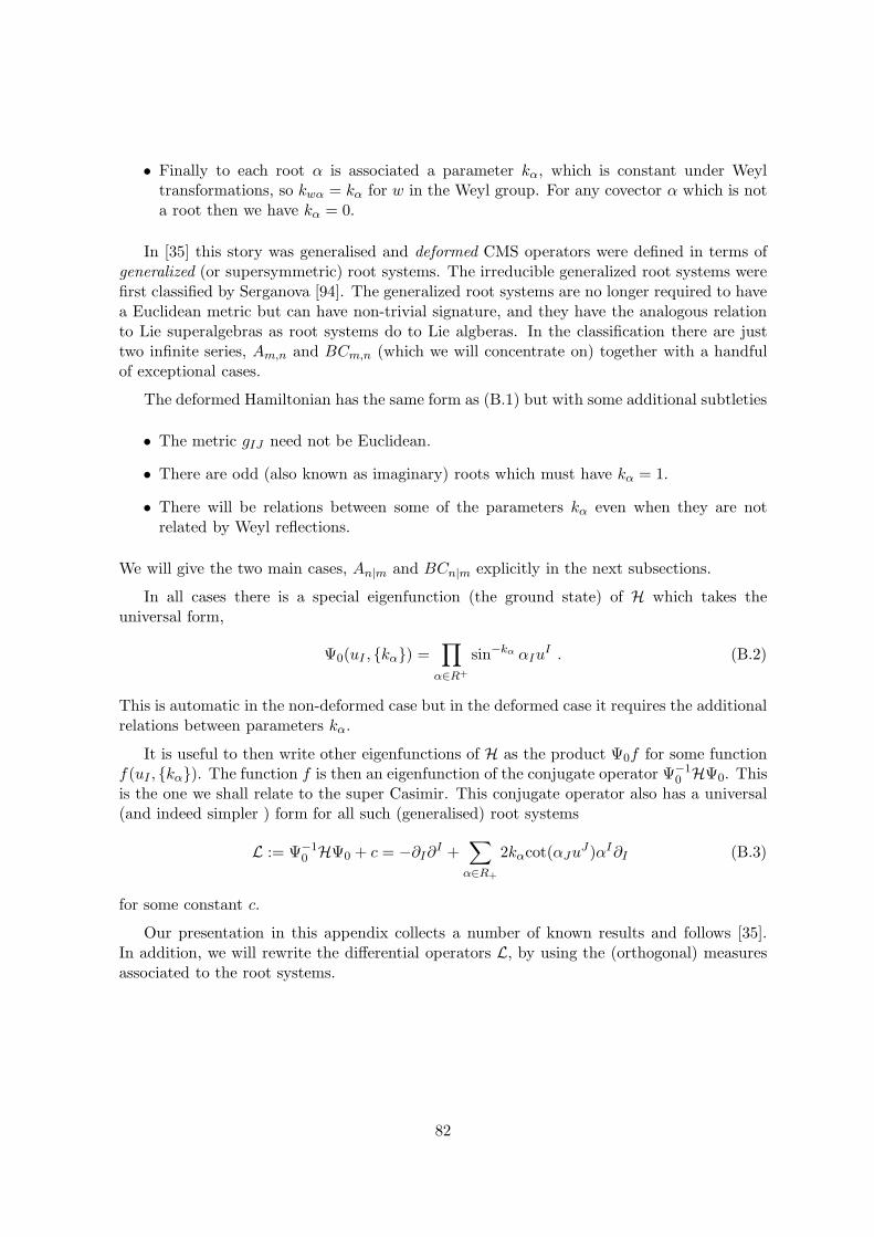
• Finally to each root α is associated a parameter kα, which is constant under Weyltransformations, so kwα = kα for w in the Weyl group. For any covector α which is nota root then we have kα = 0.

In [35] this story was generalised and deformed CMS operators were defined in terms ofgeneralized (or supersymmetric) root systems. The irreducible generalized root systems werefirst classified by Serganova [94]. The generalized root systems are no longer required to havea Euclidean metric but can have non-trivial signature, and they have the analogous relationto Lie superalgebras as root systems do to Lie algberas. In the classification there are justtwo infinite series, Am,n and BCm,n (which we will concentrate on) together with a handfulof exceptional cases.

The deformed Hamiltonian has the same form as (B.1) but with some additional subtleties

• The metric gIJ need not be Euclidean.

• There are odd (also known as imaginary) roots which must have kα = 1.

• There will be relations between some of the parameters kα even when they are notrelated by Weyl reflections.

We will give the two main cases, An|m and BCn|m explicitly in the next subsections.

In all cases there is a special eigenfunction (the ground state) of H which takes theuniversal form,

Ψ0(uI , {kα}) =∏

α∈R+

sin−kα αIuI . (B.2)

This is automatic in the non-deformed case but in the deformed case it requires the additionalrelations between parameters kα.

It is useful to then write other eigenfunctions of H as the product Ψ0f for some functionf(uI , {kα}). The function f is then an eigenfunction of the conjugate operator Ψ−1

0 HΨ0. Thisis the one we shall relate to the super Casimir. This conjugate operator also has a universal(and indeed simpler ) form for all such (generalised) root systems

L := Ψ−10 HΨ0 + c = −∂I∂I +

∑

α∈R+

2kαcot(αJuJ)αI∂I (B.3)

for some constant c.

Our presentation in this appendix collects a number of known results and follows [35].In addition, we will rewrite the differential operators L, by using the (orthogonal) measuresassociated to the root systems.

82

B.2 A-type Hamiltonians and Jack polynomials

The An−1|m−1 generalised root system can be placed inside an n + m dimensional vectorspace. The positive roots will be parametrised as

An−1|m−1 : R+ =

ei−ejei−ej′ei′−ej′

; 1 ≤ i < j ≤ n, n+ 1 ≤ i′ < j′ ≤ m+ n

(B.4)

where eI=1,...m+n give the basis of unit vectors. The (inverse) metric is

gIJ =

{δij i, j = 1, .., n

−θδi′j′ i′, j′ = n+1, ..,m+n(B.5)

R+ splits into three separate Weyl orbits (therefore there will be three distinct kα) and thethree families of roots are

α = ei−ej : α2 = 2, kα = −θα = ei−ej′ : α2 = 1− θ, kα = 1

α = ei′−ej′ : α2 = −2θ, kα = −1θ

(B.6)

Plugging in these, the CMS operator (B.1) thus becomes

HA = −∑

i

∂2i + θ∑

i′

∂2i′ −∑

i<j

2θ(1− θ)

sin2 uij+∑

i

∑

j′

2(1 − θ)

sin2(ui−uj′)+∑

i′<j′

2(1 − 1/θ)

sin2 ui′j′

= −n+m∑

I=1

(−θ)πI∂2i + 2(1 − θ)∑

1≤I<J≤n+m

(−θ)1−πI−πJ

sin2(uI − uJ)(B.7)

where the parity assignment is πi=1,...n = 0 and πi′=n+1,...n+m = 1.

The ground state is given by

Ψ0 =

∏i<j sin

θ(ui−uj)∏

i′<j′ sin1θ (ui′−uj′)∏

i

∏j′ sin(ui−uj′)

(B.8)

and the conjugated operator (B.3) is

LA = Ψ−10

(HA − |ρθ|2

)Ψ0 =−

n+m∑

I=1

(−θ)πI∂2I + 2∑

i,j′

cot(ui−uj′)(∂i + θ∂j′)

− 2θ∑

i<j

cot(ui−uj)(∂i − ∂j) + 2∑

i′<j′

cot(ui−uj)(∂i′ − ∂j′)

where ρθ =∑

α kαα =∑

I<J(−θ)1−πI−πJ (eI − eJ ), and |ρθ|2 is the norm of ρθ under gIJ .

Notice that LA contains in principle all terms coming from∑

I(−θ)πI∂2IΨ0 and in partic-ular the terms

∑β

∑α6=β kαkβ (αIg

IJβJ) cot(αIuI) cot(βIu

I), which have mixed nature and

83

do not cancel immediately with the ones from HA. However these can be replaced in favourof a θ dependent constant, −∑β

∑α6=β kαkβ (αIg

IJβJ), because of the following relation

∑

β

∑

α6=β

kαkβ (αIgIJβJ)

(cot(αIu

I) cot(βIuI) + 1

)= 0 (B.9)

This condition is automatically satisfied by the kα assignment of the roots, and can be un-derstood as a consistency condition on Ψ0 being the ground state.

Finally, by changing variables to zI = e2iuI , we find cot(uI − uJ) = i(zI + zJ)/(zI − zJ )and ∂uI

= 2izI∂zI . Therefore,

14LA =

n+m∑

I=1

(−θ)πI (zI∂I)2 + θ

n+m∑

I<J

zI + zJzI − zJ

((−θ)−πJzI∂I − (−θ)−πIzJ∂J ) . (B.10)

and one can check that

14LA = H + (θ(m− 1)− (n− 1))

∑

I

zI∂I (B.11)

where H is defined in (5.9) and is the defining operator of super Jacks (5.12) .

At this point it is also interesting to note that superJack operators are orthogonal in anA(m,n) measure [95]

S(m,n)(z; θ) =∏

I

∏

J 6=I

(1− zI

zJ

)−(−θ)1−πI−πJ

(B.12)

(where the parity assignment is πi=1,...n = 0 and πi′=n+1,...n+m = 1) and the A-type CMSoperator (B.10) can be rewritten in a very simple way in terms of this measure as

14LA = S−1

∑

I

(−θ)πIzI∂I [SzI∂I ] . (B.13)

Finally, we point out that Jack polynomials are also eigenfunctions of the one-parameterfamily of Sekiguchi differential operators [67].

B.3 BC-type Hamiltonians and superblocks

We now move on to the CMS operator for the generalised BC root system and relate it tothe Casimir which give superblocks.

The positive roots of the BCn|m root system live in an m + n dimensional vector spaceand are as follows

RBC+ =

eiei′

;2ei2ei′

;ei ± ejei ± ej′

ei′ ± ej′; 1 ≤ i < j ≤ n, n+ 1 ≤ i′ < j′ ≤ m+ n

(B.14)

84

where again eI=1,...m+n are the basis of unit vectors and the inverse metric is the same as inthe An|m case (B.5). The parameters are assigned as follows,

α = ei±ej : α2 = 2, kα = −θα = ei±ej′ : α2 = 1− θ, kα = 1

α = ei′±ej′ : α2 = −2θ kα = −1θ

(B.15)

and

α = ei : α2 = 1, kα = p

α = ei′ : α2 = −θ, kα = r;

α = 2ei : α2 = 4, kα = q

α = 2ei′ : α2 = −4θ, kα = s(B.16)

Plugging these values into the general formula (B.1) we obtain the Hamiltonian

HBC =−n+m∑

I=1

(−θ)πI∂2I + 2(1 − θ)∑

1≤I<J≤n+m

(−θ)1−πI−πJ

sin2(uI ± uJ)(B.17)

+n∑

i=1

(p(p+ 2q + 1)

sin2 ui+

4q(q + 1)

sin2 2ui

)− θ

(n+m∑

i′=n+1

r(r + 2s+ 1)

sin2 ui′+

4s(s+ 1)

sin2 2ui′

)

where the first line is a trivial modification of (B.7).

The ground state (B.2) becomes

Ψ0 =

∏i<j sin

θ(ui ± uj)∏

i′<j′ sin1θ (ui′ ± uj′)∏n

i=1

∏m+nj′=n+1 sin(ui ± uj′)

∏ni=1(sin

p(ui) sinq(2ui))

∏n+mi′=n+1(sin

r(ui′) sins(2ui′))

(B.18)

and the conjugated operator is

LBC = Ψ−10

(HBC − |ρθ|2

)Ψ0 =−

n+m∑

I=1

(−θ)πIDI∂I + 2∑

i,j′

cot(ui±uj′)(∂i ∓ θ∂j′)

− 2θ∑

i<j

cot(ui ± uj)(∂i ± ∂j) + 2∑

i′<j′

cot(ui′ ± uj′)(∂i′ ± ∂j′)

where ρθ =∑

α kαα and DI = (∂I + 2cot(2uI))− 2(−θ)−πI (p cot uI + (2q + 1) cot(2uI)).

Going through the computation notice that for the ground state to be so, the followingrelation had to be satisfyied

∑

β

∑

β≁α

kαkβ (αIgIJβJ)

(cot(αIu

I) cot(βIuI) + 1

)= 0 ;

p = −θr2q + 1 = −θ(2s+ 1)

(B.19)

This was not automatic for the kα assignment but puts a constraint which we used to solvefor r and s. The summation over β ≁ α excludes roots which are parallel in the vector space.The origin of this constraint again can be understood as a rewriting of the potential terms

85

arising from∑

(−θ)πI∂2IΨ0 coming from mixed products which do not cancel immediatelyagainst the potential terms in HBC .

We now change variables to exponential coordinates zI = e2iuI , and we get

14LBC =

n+m∑

I=1

((−θ)πI

(zI ∂I +

z2I + 1

z2I − 1

)−(pzI + 1

zI − 1+ (2q + 1)

z2I + 1

z2I − 1

))(zI ∂I)

+ θ

n+m∑

I<J

zI + z±JzI − z±J

((−θ)−πJ zI ∂I ∓ (−θ)−πI zJ ∂J ) (B.20)

We can rearrange the sum over many-body interactions as a sum over I 6= J , then for a single

derivative we can add up the two termszI+z±JzI−z±J

to find2zJ(1−z2I )

(zI−zJ )(1−zizJ ).

Finally we need to change variables again to47

zI =1

2− 1

4

(zI +

1

zI

)(B.21)

and we obtain

14LBC(z, θ) =

n+m∑

I=1

((−θ)πI∂IzI(zI − 1)∂I −

(p(zI − 1) + (2q + 1)

(zI − 1

2

))∂I

)

− 2θ∑

I 6=J

(−θ)−πJ

zI − zJzI(1− zI)∂I (B.22)

At this point we can understand the relation between the super Casimir C, defining thesuperblocks, and LBC . One can check that they are closely related after conjugation and ashift

(∏mi=1 x

θi∏n

j=1 yj

)−β

14LBC( 1

x1. . . 1

xm; 1y1. . . 1

yn; θ)

(∏mi=1 x

θi∏n

j=1 yj

)+β

=

C(θ, 12(γ−p12),

12(γ−p43),γ) −

[β(n −mθ)((n− 1)− (m− 1)θ + (γ − β)θ)

](B.23)

with β = min(12(γ−p12), 12(γ−p43)

). We have thus shown that the differential operator

corresponding to BC root system is equivalent to our Casimir operator.

Before concluding this section however, we point that there is an analogue of the measurebased relation (B.13) in the super BC case which we have not seen in the literature previously.

47Note the following useful relations

zI = − 14

(

1√zI

−√zI

)2

zI − 1 = − 14

(

1√zI

+√zI

)2 ;

zI∂zI∂zI

= 14

(1−z2I )

zI=

√

zI(zI − 1)

14

(1+z2I )

zI= −(zI − 1

2)

86

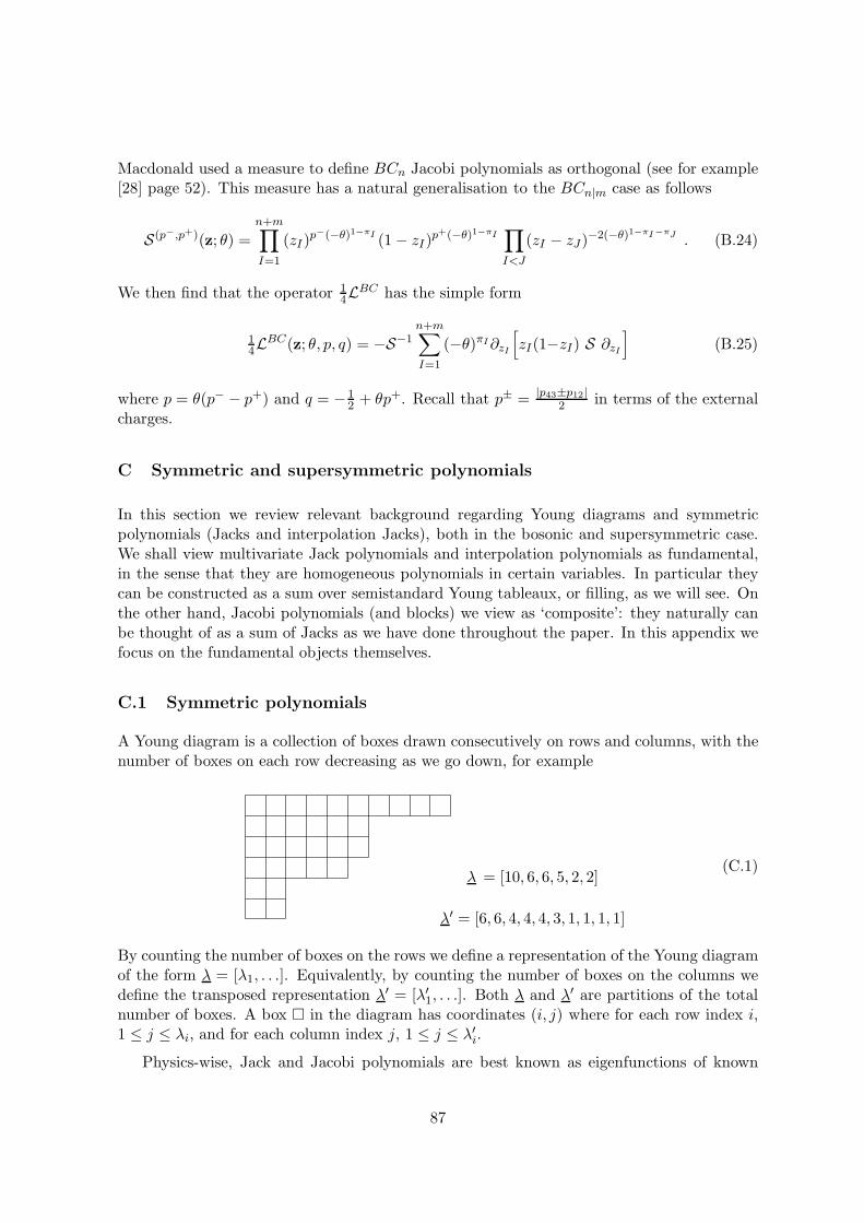
Macdonald used a measure to define BCn Jacobi polynomials as orthogonal (see for example[28] page 52). This measure has a natural generalisation to the BCn|m case as follows

S(p−,p+)(z; θ) =

n+m∏

I=1

(zI)p−(−θ)1−πI (1− zI)

p+(−θ)1−πI∏

I<J

(zI − zJ)−2(−θ)1−πI−πJ . (B.24)

We then find that the operator 14LBC has the simple form

14LBC(z; θ, p, q) = −S−1

n+m∑

I=1

(−θ)πI∂zI

[zI(1−zI) S ∂zI

](B.25)

where p = θ(p− − p+) and q = −12 + θp+. Recall that p± = |p43±p12|

2 in terms of the externalcharges.

C Symmetric and supersymmetric polynomials

In this section we review relevant background regarding Young diagrams and symmetricpolynomials (Jacks and interpolation Jacks), both in the bosonic and supersymmetric case.We shall view multivariate Jack polynomials and interpolation polynomials as fundamental,in the sense that they are homogeneous polynomials in certain variables. In particular theycan be constructed as a sum over semistandard Young tableaux, or filling, as we will see. Onthe other hand, Jacobi polynomials (and blocks) we view as ‘composite’: they naturally canbe thought of as a sum of Jacks as we have done throughout the paper. In this appendix wefocus on the fundamental objects themselves.

C.1 Symmetric polynomials

A Young diagram is a collection of boxes drawn consecutively on rows and columns, with thenumber of boxes on each row decreasing as we go down, for example

λ = [10, 6, 6, 5, 2, 2]

λ′ = [6, 6, 4, 4, 4, 3, 1, 1, 1, 1]

(C.1)

By counting the number of boxes on the rows we define a representation of the Young diagramof the form λ = [λ1, . . .]. Equivalently, by counting the number of boxes on the columns wedefine the transposed representation λ′ = [λ′1, . . .]. Both λ and λ′ are partitions of the totalnumber of boxes. A box � in the diagram has coordinates (i, j) where for each row index i,1 ≤ j ≤ λi, and for each column index j, 1 ≤ j ≤ λ′i.

Physics-wise, Jack and Jacobi polynomials are best known as eigenfunctions of known

87

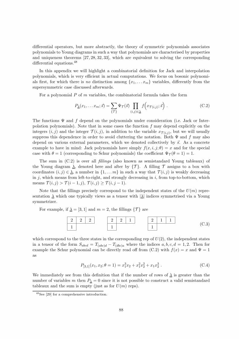
differential operators, but more abstractly, the theory of symmetric polynomials associatespolynomials to Young diagrams in such a way that polynomials are characterised by propertiesand uniqueness theorems [27, 28, 32, 33], which are equivalent to solving the correspondingdifferential equations.48

In this appendix we will highlight a combinatorial definition for Jack and interpolationpolynomials, which is very efficient in actual computations. We focus on bosonic polynomi-als first, for which there is no distinction among {x1, . . . xm} variables, differently from thesupersymmetric case discussed afterwards.

For a polynomial P of m variables, the combinatorial formula takes the form

Pλ(x1, . . . xm;~s) =∑

{T }ΨT (~s)

∏

(i,j)∈λf(xT (i,j);~s

). (C.2)

The functions Ψ and f depend on the polynomials under consideration (i.e. Jack or Inter-polation polynomials). Note that in some cases the function f may depend explicitly on theintegers (i, j) and the integer T (i, j), in addition to the variable xT (i,j), but we will usuallysuppress this dependence in order to avoid cluttering the notation. Both Ψ and f may alsodepend on various external parameters, which we denoted collectively by ~s. As a concreteexample to have in mind: Jack polynomials have simply f(x, i, j; θ) = x and for the specialcase with θ = 1 (corresponding to Schur polynomials) the coefficient ΨT (θ = 1) = 1.

The sum in (C.2) is over all fillings (also known as semistandard Young tableaux) ofthe Young diagram λ, denoted here and after by {T }. A filling T assigns to a box withcoordinates (i, j) ∈ λ, a number in {1, . . . m} in such a way that T (i, j) is weakly decreasingin j, which means from left-to-right, and strongly decreasing in i, from top-to-bottom, whichmeans T (i, j) > T (i− 1, j), T (i, j) ≥ T (i, j − 1).

Note that the fillings precisely correspond to the independent states of the U(m) repre-sentation λ which one typically views as a tensor with |λ| indices symmetrised via a Youngsymmetrizer.

For example, if λ = [3, 1] and m = 2, the fillings {T } are

2 2 2

1

2 2 1

1

2 1 1

1(C.3)

which correspond to the three states in the corresponding rep of U(2), the independent statesin a tensor of the form Sabcd = T(abc)d − T(dbc)a where the indices a, b, c, d = 1, 2. Then forexample the Schur polynomial can be directly read off from (C.2) with f(x) = x and Ψ = 1as

P[3,1](x1, x2; θ = 1) = x31x2 + x21x22 + x1x

32 . (C.4)

We immediately see from this definition that if the number of rows of λ is greater than thenumber of variables m then Pλ = 0 since it is not possible to construct a valid semistandardtableaux and the sum is empty (just as for U(m) reps).

48See [29] for a comprehensive introduction.

88

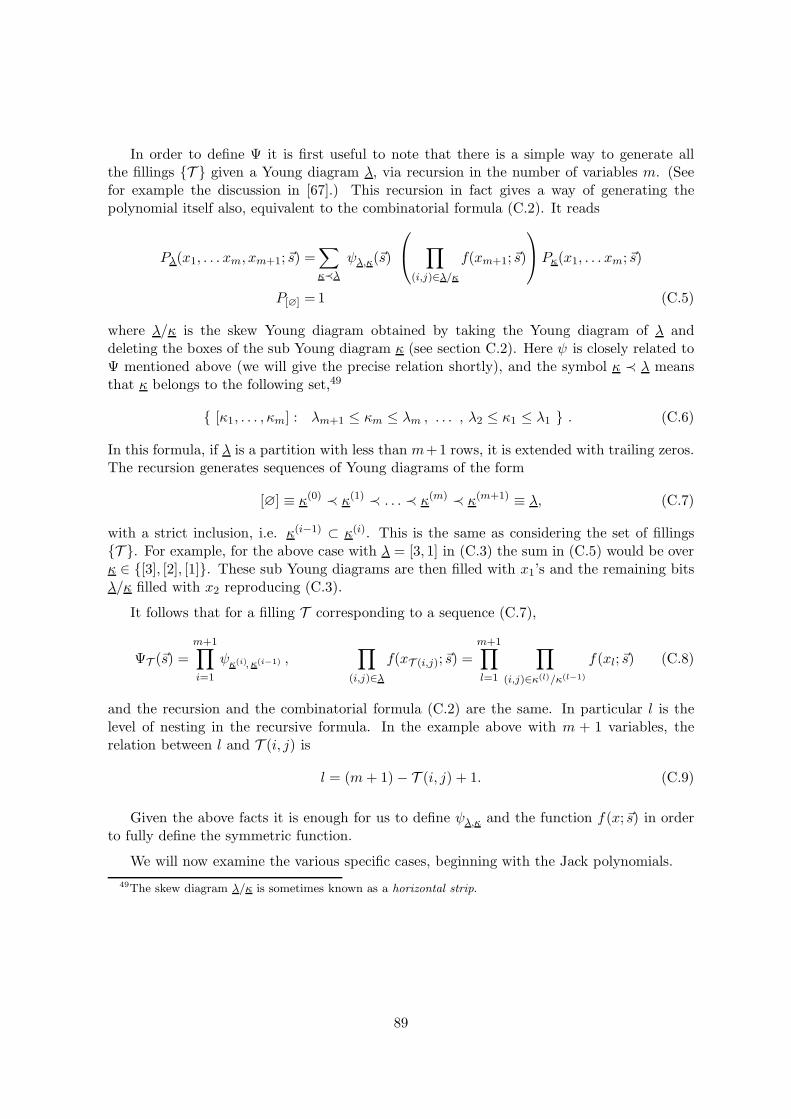
In order to define Ψ it is first useful to note that there is a simple way to generate allthe fillings {T } given a Young diagram λ, via recursion in the number of variables m. (Seefor example the discussion in [67].) This recursion in fact gives a way of generating thepolynomial itself also, equivalent to the combinatorial formula (C.2). It reads

Pλ(x1, . . . xm, xm+1;~s) =∑

κ≺λ

ψλ,κ(~s)

∏

(i,j)∈λ/κf(xm+1;~s)

Pκ(x1, . . . xm;~s)

P[∅] =1 (C.5)

where λ/κ is the skew Young diagram obtained by taking the Young diagram of λ anddeleting the boxes of the sub Young diagram κ (see section C.2). Here ψ is closely related toΨ mentioned above (we will give the precise relation shortly), and the symbol κ ≺ λ meansthat κ belongs to the following set,49

{ [κ1, . . . , κm] : λm+1 ≤ κm ≤ λm , . . . , λ2 ≤ κ1 ≤ λ1 } . (C.6)

In this formula, if λ is a partition with less than m+1 rows, it is extended with trailing zeros.The recursion generates sequences of Young diagrams of the form

[∅] ≡ κ(0) ≺ κ(1) ≺ . . . ≺ κ(m) ≺ κ(m+1) ≡ λ, (C.7)

with a strict inclusion, i.e. κ(i−1) ⊂ κ(i). This is the same as considering the set of fillings{T }. For example, for the above case with λ = [3, 1] in (C.3) the sum in (C.5) would be overκ ∈ {[3], [2], [1]}. These sub Young diagrams are then filled with x1’s and the remaining bitsλ/κ filled with x2 reproducing (C.3).

It follows that for a filling T corresponding to a sequence (C.7),

ΨT (~s) =m+1∏

i=1

ψκ(i), κ(i−1) ,∏

(i,j)∈λf(xT (i,j);~s) =

m+1∏

l=1

∏

(i,j)∈κ(l)/κ(l−1)

f(xl;~s) (C.8)

and the recursion and the combinatorial formula (C.2) are the same. In particular l is thelevel of nesting in the recursive formula. In the example above with m + 1 variables, therelation between l and T (i, j) is

l = (m+ 1)− T (i, j) + 1. (C.9)

Given the above facts it is enough for us to define ψλ,κ and the function f(x;~s) in orderto fully define the symmetric function.

We will now examine the various specific cases, beginning with the Jack polynomials.

49The skew diagram λ/κ is sometimes known as a horizontal strip.

89

C.2 Jack polynomials

Jack polynomials depend on one parameter, θ. The defining function is (for example [67])

ψλ,κ(θ) =∏

1≤i≤j<m+1

(κi − λj+1 + 1 + θ(j − i))λi−κi

(κi − λj+1 + θ(j − i+ 1))λi−κi

(κi − κj + θ(j − i+ 1))λi−κi

(κi − κj + 1 + θ(j − i))λi−κi

. (C.10)

with,

f(x; θ) = x (C.11)

Considering the top-left Pochhammer symbol, notice that ψλ,κ vanishes when,

(κi − λi+1 + 1)λi−κi= (κi + 1− λi+1) . . . (λi − λi+1) = 0 (C.12)

i.e. when one of the terms vanishes. This happens precisely when κ ⊀ λ.

As a simple example then consider P[2,1](x1, x2; θ). The case with θ = 1 (Schur polynomial)is given in (C.4). For arbitrary θ we need the coefficient ΨT (θ) for the three fillings T in (C.3).The first and third filling have Ψ = 1 whereas the second has Ψ = 2θ

1+θ and we thus obtain

P[3,1](x1, x2; θ) = x31x2 +2θ1+θx

21x

22 + x1x

32 . (C.13)

Notice that Jack polynomials are stable, i.e. Pλ(x1, . . . xm, 0; θ) = Pλ(x1, . . . xm; θ) as canbe shown directly from the combinatorial formula (as well as from their definition as the uniquepolynomial eigenfunctions of the differential equation (5.12) with eigenvalues and differentialoperator independent of m, and with the same normalisation).

Also note that Jack polynomials have the following property

Pλ+τm = (x1 . . . xm)τPλ . (C.14)

It is instructive to prove (C.14) by showing again that both RHS and LHS are eigenfunctions ofthe An CMS operator H in (5.12). Applying H on the LHS we simply find the correspondingeigenvalue hλ+τm . On the RHS we need to consider what happens upon conjugation,

(x1 . . . xm)−τ ·H · (x1 . . . xm)τ = H+ 2τ∑

i

xi∂i + h(θ)τm (C.15)

Thus applying H· to (C.14) we find

h(θ)λ+τm = h(θ)λ + 2τ |λ|+ h

(θ)τm (C.16)

which is an identity, and proves (C.14), since both RHSand l.h.s have the same small variableexpansion.

Remark. When there is an ambiguity in the notation, in relation to the supersymmetriccase, we will specify P (m,0)(z; θ) to mean the bosonic Jack polynomial.

90

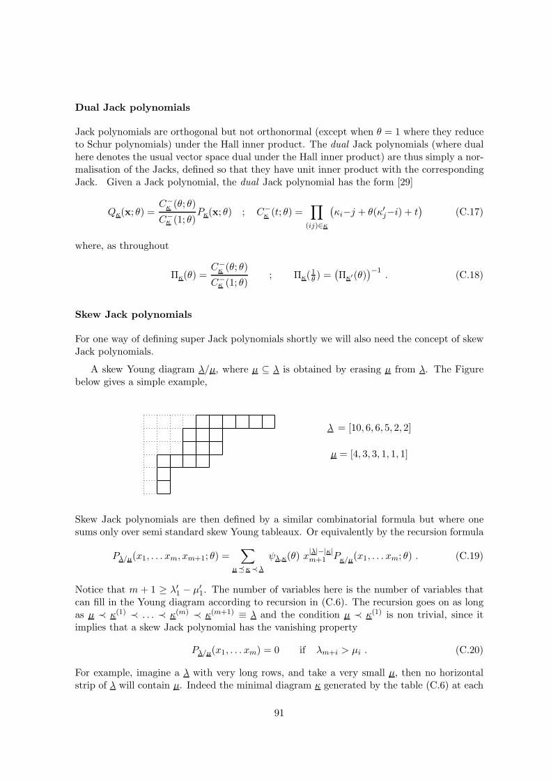
Dual Jack polynomials

Jack polynomials are orthogonal but not orthonormal (except when θ = 1 where they reduceto Schur polynomials) under the Hall inner product. The dual Jack polynomials (where dualhere denotes the usual vector space dual under the Hall inner product) are thus simply a nor-malisation of the Jacks, defined so that they have unit inner product with the correspondingJack. Given a Jack polynomial, the dual Jack polynomial has the form [29]

Qκ(x; θ) =C−κ (θ; θ)

C−κ (1; θ)

Pκ(x; θ) ; C−κ (t; θ) =

∏

(ij)∈κ

(κi−j + θ(κ′j−i) + t

)(C.17)

where, as throughout

Πκ(θ) =C−κ (θ; θ)

C−κ (1; θ)

; Πκ(1θ ) =

(Πκ′(θ)

)−1. (C.18)

Skew Jack polynomials

For one way of defining super Jack polynomials shortly we will also need the concept of skewJack polynomials.

A skew Young diagram λ/µ, where µ ⊆ λ is obtained by erasing µ from λ. The Figurebelow gives a simple example,

λ = [10, 6, 6, 5, 2, 2]

µ = [4, 3, 3, 1, 1, 1]

Skew Jack polynomials are then defined by a similar combinatorial formula but where onesums only over semi standard skew Young tableaux. Or equivalently by the recursion formula

Pλ/µ(x1, . . . xm, xm+1; θ) =∑

µ�κ≺λ

ψλ,κ(θ) x|λ|−|κ|m+1 Pκ/µ(x1, . . . xm; θ) . (C.19)

Notice that m + 1 ≥ λ′1 − µ′1. The number of variables here is the number of variables thatcan fill in the Young diagram according to recursion in (C.6). The recursion goes on as longas µ ≺ κ(1) ≺ . . . ≺ κ(m) ≺ κ(m+1) ≡ λ and the condition µ ≺ κ(1) is non trivial, since itimplies that a skew Jack polynomial has the vanishing property

Pλ/µ(x1, . . . xm) = 0 if λm+i > µi . (C.20)

For example, imagine a λ with very long rows, and take a very small µ, then no horizontalstrip of λ will contain µ. Indeed the minimal diagram κ generated by the table (C.6) at each

91

step of the recursion is given by components of λ properly shifted upwards.

An example of a skew Jack polynomial is

P[3,1,1]/[1](x1, x2; θ) = x31x2 + x1x32 +

2θ

1 + θx21x

22 (C.21)

Skew polynomials have the property that

Pλ(x; θ) =∑

µ⊂λ

Pµ(x1, . . . xm−n; θ)Pλ/µ(xm−n+1, . . . xm; θ) (C.22)

Structure constants and decomposition formulae for Jacks

The Jack structure constants Cνλµ(θ) are defined as follows

PλPµ =∑

ν

Cνλµ(θ)Pν . (C.23)

For θ = 1 they are just the Littlewood-Richardson coefficients.

Then there are related coefficients Sλµν (θ) obtained from decomposing skew Jack polyno-

mials into Jack polynomials

Pν/λ =∑

µ

Sλµν (θ)Pµ . (C.24)

The property (C.22) then yields the decomposition formula for decomposing higher dimen-sional Jacks into sums of products of lower dimensional Jacks

Pλ(x1, .., xm+n) =∑

µ,ν

Pµ(x1, .., xm)Sµνλ (θ)Pν(xm+1, .., xm+n) . (C.25)

For θ = 1 these decomposition coefficients are also the Littlewood-Richardson coefficients,Cνλµ(1) = Sλµ

ν (1), but for general θ they are related via normalisation:

Sµνλ (θ) =

Πµ(θ)Πν(θ)

Πλ(θ)Cλµν(θ) . (C.26)

Note that the structure constants Cνλµ(θ) and Sλµ

ν (θ) do not depend on the dimensions ofthe Jack polynomials in any of the above formulae.

Also note that if the Young diagram λ is built from two Young diagrams µ, ν on top ofeach other then the corresponding structure constant is 1:

Sµνλ (θ) = 1 if λ = [µ, ν] . (C.27)

This can be seen by (C.24) noting that the Jack polynomial of dimension equal to the height

92

of µ is equal to the skew Jack

Pµ(x1, .., xµ′1) = Pλ/ν(x1, .., xµ′

1) if λ = [µ, ν] . (C.28)

This can be verified from the respective combinatoric formulae.

C.3 Interpolation polynomials

The interpolation polynomials of relevance here (i.e. the BC-type which appear in section 7)depend on two parameters, θ, and a new one denoted here by u. They can be defined ina very similar way to the Jack polynomials and we will denote them P ip(x; θ, u). They aresymmetric polynomials in the variables x = (x1, .., xm). Generically P ip is a complicated, nonfactorisable polynomial and it is uniquely defined by the following vanishing property

P ipκ (ν + θδ + u; θ, u) = 0 if λ ⊂ µ (C.29)

where δ = (m−1, .., 1, 0). This idea generalises what happens for the Pochhammer symbol(−z)λ = (−z)(−z + 1) . . . (−z + λ− 1) which vanishes if 0 ≤ z < λ.50

The interpolation polynomial is defined via the combinatorial formula (C.2) (or the equiv-alent recursion (C.5)) with ψ exactly the same as for the Jacks (C.10), but with a morecomplicated x dependence arising from a modified f

ψλ,κ(θ, u) = ψλ,κ(θ) (C.30)

f(xl, i, j, l; θ, u) = x2l − ((j−1)−θ(i− 1) + θ(l − 1) + u)2 (C.31)

where ψλ,κ(θ) is the defining function for Jack polynomials (C.10). Instead, note that f heredepends explicitly on (i, j) and l. As in (C.7) the index l labels the nesting and is related toT (i, j) via (C.9).

One can see an example of the vanishing property from the above definition: take the lastvariable xm and the last row i = m in (C.31), this contributes with terms which vanish forall xm = j − 1 + u, where j = 1, . . . κm.

Because of the various shifts in the vanishing property (C.29), it is useful to define thenon-symmetric version of the interpolation polynomial P ∗(x; θ, u) by

P ∗(x; θ, u) ≡ P ip(x+ θδ + u; θ, u) δ = (m−1, .., 1, 0) (C.32)

So the vanishing property (C.29) takes the form

P ∗µ(λ; θ, u) = 0 if λ ⊂ µ . (C.33)

(Recalling however that P ∗µ here is no longer symmetric in its variables z.)

This interpolation polynomial is Z2 invariant under xi ↔ −xi. It was introduced byOkounkov [33], and re-obtained by Rains [32], using a different approach.

50Indeed the Pochhammer symbol (−z)k is precisely a case of interpolating polynomial, giving the standard

one-variable binomial expansion (1 + x)n =∑

k(nk )x

k =∑

k(−n)k(−k)k

xk.

93

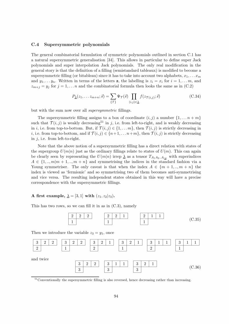
C.4 Supersymmetric polynomials

The general combinatorial formulation of symmetric polynomials outlined in section C.1 hasa natural supersymmetric generalisation [34]. This allows in particular to define super Jackpolynomials and super interpolation Jack polynomials. The only real modification in thegeneral story is that the definition of a filling (semistandard tableaux) is modified to become asupersymmetric filling (or bitableau) since it has to take into account two alphabets, x1, . . . xmand y1, . . . yn. Written in terms of the letters z, the labelling is zi = xi for i = 1, . . . m, andzm+j = yj for j = 1, . . . n and the combinatorial formula then looks the same as in (C.2)

Pλ(z1, . . . zm+n;~s) =∑

{T }ΨT (~s)

∏

(i,j)∈λf(zT (i,j);~s) (C.34)

but with the sum now over all supersymmetric fillings.

The supersymmetric filling assigns to a box of coordinate (i, j) a number {1, . . . n +m}such that T (i, j) is weakly decreasing51 in j, i.e. from left-to-right, and is weakly decreasingin i, i.e. from top-to-bottom. But, if T (i, j) ∈ {1, . . . m}, then T (i, j) is strictly decreasing ini, i.e. from top-to-bottom, and if T (i, j) ∈ {n+1, . . . n+m}, then T (i, j) is strictly decreasingin j, i.e. from left-to-right.

Note that the above notion of a supersymmetric filling has a direct relation with states ofthe supergroup U(m|n) just as the ordinary fillings relate to states of U(m). This can againbe clearly seen by representing the U(m|n) irrep λ as a tensor TA1A2..A|λ|

with superindicesA ∈ {1, ..,m|m + 1, ..,m + n} and symmetrising the indices in the standard fashion via aYoung symmetriser. The only caveat is that when the index A ∈ {m + 1, ..,m + n} theindex is viewed as ‘fermionic’ and so symmetrising two of them becomes anti-symmetrisingand vice versa. The resulting independent states obtained in this way will have a precisecorrespondence with the supersymmetric fillings.

A first example, λ = [3, 1] with (z1, z2|z3).

This has two rows, so we can fill it in as in (C.3), namely

2 2 2

1

2 2 1

1

2 1 1

1(C.35)

Then we introduce the variable z3 = y1, once

3 2 2

2

3 2 2

1

3 2 1

2

3 2 1

1

3 1 1

2

3 1 1

1

and twice3 2 2

3

3 1 1

3

3 2 1

3(C.36)

51Conventionally the supersymmetric filling is also reversed, hence decreasing rather than increasing.

94

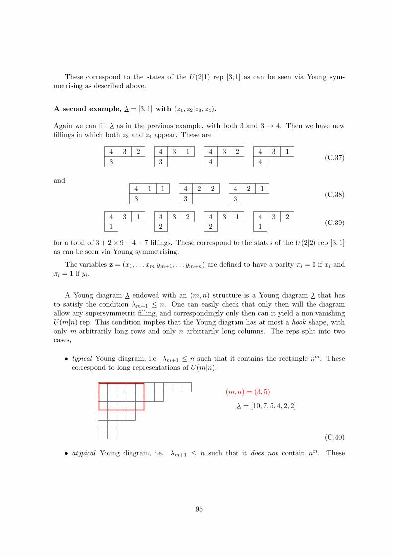
These correspond to the states of the U(2|1) rep [3, 1] as can be seen via Young sym-metrising as described above.

A second example, λ = [3, 1] with (z1, z2|z3, z4).

Again we can fill λ as in the previous example, with both 3 and 3 → 4. Then we have newfillings in which both z3 and z4 appear. These are

4 3 2

3

4 3 1

3

4 3 2

4

4 3 1

4(C.37)

and4 1 1

3

4 2 2

3

4 2 1

3(C.38)

4 3 1

1

4 3 2

2

4 3 1

2

4 3 2

1(C.39)

for a total of 3 + 2× 9 + 4 + 7 fillings. These correspond to the states of the U(2|2) rep [3, 1]as can be seen via Young symmetrising.

The variables z = (x1, . . . xm|ym+1, . . . ym+n) are defined to have a parity πi = 0 if xi andπi = 1 if yi.

A Young diagram λ endowed with an (m,n) structure is a Young diagram λ that hasto satisfy the condition λm+1 ≤ n. One can easily check that only then will the diagramallow any supersymmetric filling, and correspondingly only then can it yield a non vanishingU(m|n) rep. This condition implies that the Young diagram has at most a hook shape, withonly m arbitrarily long rows and only n arbitrarily long columns. The reps split into twocases,

• typical Young diagram, i.e. λm+1 ≤ n such that it contains the rectangle nm. Thesecorrespond to long representations of U(m|n).

(m,n) = (3, 5)

λ = [10, 7, 5, 4, 2, 2]

(C.40)

• atypical Young diagram, i.e. λm+1 ≤ n such that it does not contain nm. These

95

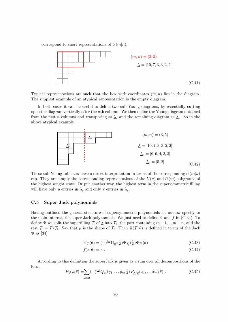
correspond to short representations of U(m|n).

(m,n) = (3, 5)

λ = [10, 7, 3, 3, 2, 2]

(C.41)

Typical representations are such that the box with coordinates (m,n) lies in the diagram.The simplest example of an atypical representation is the empty diagram.

In both cases it can be useful to define two sub Young diagrams, by essentially cuttingopen the diagram vertically after the nth column. We then define the Young diagram obtainedfrom the first n columns and transposing as λs and the remaining diagram as λe. So in theabove atypical example:

(m,n) = (3, 5)

λ = [10, 7, 3, 3, 2, 2]

λs = [6, 6, 4, 2, 2]

λe = [5, 2]

λ′s

λe

(C.42)

These sub Young tableaux have a direct interpretation in terms of the corresponding U(m|n)rep. They are simply the corresponding representations of the U(n) and U(m) subgroups ofthe highest weight state. Or put another way, the highest term in the supersymmetric fillingwill have only y entries in λs and only x entries in λe.

C.5 Super Jack polynomials

Having outlined the general structure of supersymmetric polynomials let us now specify tothe main interest, the super Jack polynomials. We just need to define Ψ and f in (C.34). Todefine Ψ we split the superfilling T of λ into T1, the part containing m+1, ..,m+ n, and therest T0 = T /T1. Say that µ is the shape of T1. Then Ψ(T ; θ) is defined in terms of the JackΨ as [34]

ΨT (θ) = (−)|µ|Πµ′(1θ )ΨT ′1(1θ )ΨT0(θ) (C.43)

f(z; θ) = z . (C.44)

According to this definition the superJack is given as a sum over all decompositions of theform

Pλ(z; θ) =∑

µ⊆λ

(−)|µ|Qµ′(y1, . . . yn,1θ )Pλ/µ(x1, . . . xm; θ) . (C.45)

96

where the sum can also be restricted to µ such that max(λ′j−m, 0) ≤ µ′j ≤ λ′j with j = 1, . . . n.

Note also that we could construct the superJacks directly from Jack polynomials via theirdecomposition into U(m) and U(n) reps following [34] (see also [95] for a nice review). Quitenicely [34] showed that this decomposition can be brought to (C.45). From this point of viewit might be useful to compare this with the bosonic decomposition (C.22).

Remark. A super Jack polynomial is denoted by P (m,n)λ (z; θ). However, the (m,n) depen-

dence can be read off the variables z, when there are no ambiguities in the notation. Whenthis is the case, we will simply use Pλ(z; θ).

Some simple observations which can be seen directly from this formula:

1) If λ fails to have an (m,n) structure, so (i, j) = (m+1, n+1) is in the Youngdiagram λ, then the superJack vanishes. For any µ in the summation, either the box(m+1, n+1) is in µ, in which case Qµ′ = 0 as µ′ will have n+1 rows, or (m+1, n+1)is in λ/µ in which case Pλ/µ = 0 as λ/µ will have a full column with m+ 1 elements.

2) When m = 0 the sum localises on µ = λ, and since Pλ/λ = P∅ = 1, the superJack

polynomial reduces to a (normalised) dual Jack polynomial (−)|λ′|Qλ′(y; 1θ ). When

n = 0 the sum localises on µ = ∅ and the superJack polynomials reduces to Pλ(x; θ).

C.6 Properties of Super Jack polynomials

Stability

The combinatorial formula makes stability of superJacks manifest. Alternatively, from thefact that the eigenvalue of the A-type CMS differential depends only on the Young diagram,and the uniqueness of the polynomial solution for given Young diagram, we also infer thatthe super Jack polynomials are stable.

The m and n switch

From the bosonisation of the eigenvalue and a property of the differential operator H, namely

h(θ)λ = −θ∑

j=1

λ′j(λ′j − 1− 2

θ (j − 1)) = −θh(1θ)

λ′ ; H( 1θ)(y|x) = −1

θH(θ)(x|y) (C.46)

we deduce that Pλ′(y|x; 1θ ) has to be proportional to Pλ(x|y; θ). Looking at the precisenormalisations we arrive at

P(m,n)λ (x|y; θ) = (−1)|λ

′|Πλ′(1θ )P(n,m)λ′ (y|x; 1θ ) (C.47)

We can also show this more directly from either the combinatorial formula or the de-composition formula (where we further decompose the skew Jacks into Jacks via structureconstants, and use some known properties of the structure constants).

97

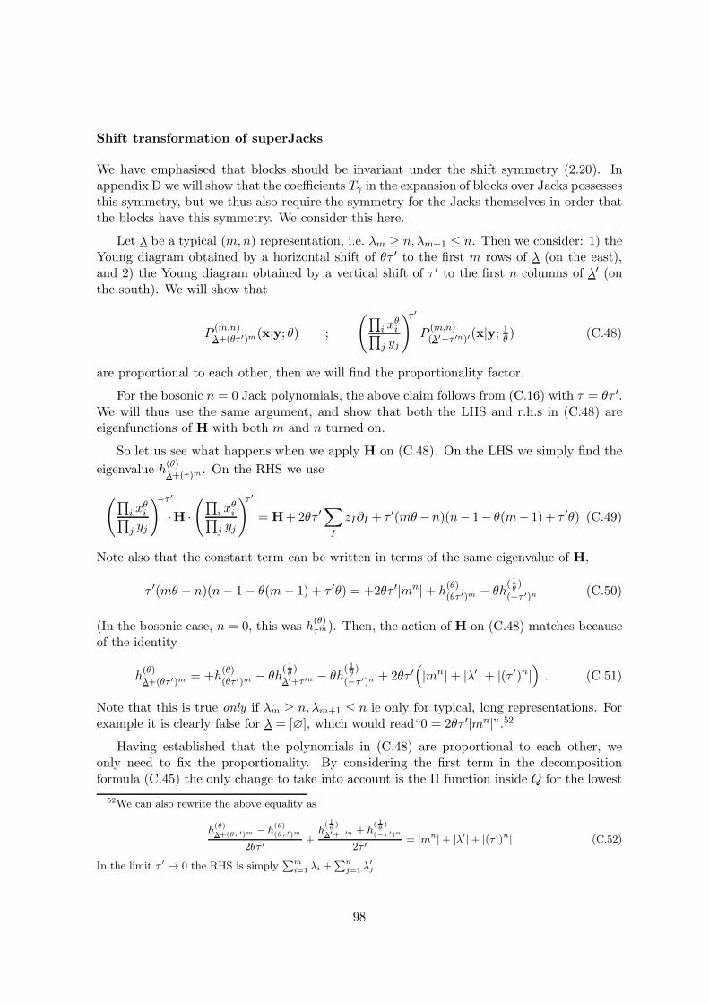
Shift transformation of superJacks

We have emphasised that blocks should be invariant under the shift symmetry (2.20). Inappendix D we will show that the coefficients Tγ in the expansion of blocks over Jacks possessesthis symmetry, but we thus also require the symmetry for the Jacks themselves in order thatthe blocks have this symmetry. We consider this here.

Let λ be a typical (m,n) representation, i.e. λm ≥ n, λm+1 ≤ n. Then we consider: 1) theYoung diagram obtained by a horizontal shift of θτ ′ to the first m rows of λ (on the east),and 2) the Young diagram obtained by a vertical shift of τ ′ to the first n columns of λ′ (onthe south). We will show that

P(m,n)λ+(θτ ′)m(x|y; θ) ;

(∏i x

θi∏

j yj

)τ ′P

(m,n)(λ′+τ ′n)′(x|y; 1θ ) (C.48)

are proportional to each other, then we will find the proportionality factor.

For the bosonic n = 0 Jack polynomials, the above claim follows from (C.16) with τ = θτ ′.We will thus use the same argument, and show that both the LHS and r.h.s in (C.48) areeigenfunctions of H with both m and n turned on.

So let us see what happens when we apply H on (C.48). On the LHS we simply find the

eigenvalue h(θ)λ+(τ)m . On the RHS we use

(∏i x

θi∏

j yj

)−τ ′

·H ·(∏

i xθi∏

j yj

)τ ′= H+2θτ ′

∑

I

zI∂I + τ ′(mθ−n)(n− 1− θ(m− 1) + τ ′θ) (C.49)

Note also that the constant term can be written in terms of the same eigenvalue of H,

τ ′(mθ − n)(n− 1− θ(m− 1) + τ ′θ) = +2θτ ′|mn|+ h(θ)(θτ ′)m − θh

( 1θ)

(−τ ′)n (C.50)

(In the bosonic case, n = 0, this was h(θ)τm). Then, the action of H on (C.48) matches because

of the identity

h(θ)λ+(θτ ′)m = +h

(θ)(θτ ′)m − θh

( 1θ)

λ′+τ ′n − θh( 1θ)

(−τ ′)n + 2θτ ′(|mn|+ |λ′|+ |(τ ′)n|

). (C.51)

Note that this is true only if λm ≥ n, λm+1 ≤ n ie only for typical, long representations. Forexample it is clearly false for λ = [∅], which would read“0 = 2θτ ′|mn|”.52

Having established that the polynomials in (C.48) are proportional to each other, weonly need to fix the proportionality. By considering the first term in the decompositionformula (C.45) the only change to take into account is the Π function inside Q for the lowest

52We can also rewrite the above equality as

h(θ)λ+(θτ ′)m − h

(θ)(θτ ′)m

2θτ ′+

h( 1

θ)

λ′+τ ′n + h( 1

θ)

(−τ ′)n

2τ ′= |mn|+ |λ′|+ |(τ ′)n| (C.52)

In the limit τ ′ → 0 the RHS is simply∑m

i=1 λi +∑n

j=1 λ′j .

98

representation. Following this through we arrive at the shift formula (D.8)

Π(λs−mn)′(θ)P(m,n)λ+(θτ ′)m(x|y; θ) = Π(λs−mn+τ ′n)′(θ)

(∏i x

θi∏

j yj

)τ ′P

(m,n)(λ′+τ ′n)′(x|y; θ) (C.53)

where we are using Π−1ν (1θ ) = Πν′(θ), and we introduced

λs = [λ′1, . . . λ′n] (C.54)

as in (C.42).

Super Jacks and the superconformal Ward identity

The uplift of Jack to superJack polynomials follows from a characterisation theorem, cf.Theorem 2 of [34]. In particular, a superJack polynomial Pλ(x|y; θ) is generated by the mapϕ(m,n) which acts on the power sum decomposition of Pλ(z; θ) as

ϕ(m,n)

pr ≡

∑

j

zr

=

m∑

j=1

xrj − 1θ

n∑

j=1

yrj → Pλ,(m,n)(; θ) = ϕ(m,n)(Pλ(z; θ)) (C.55)

Note that this map is very easy to understand in the cases θ = 1, 2, 12 where there is a grouptheoretic interpretation. For example, when θ = 1 we consider the symmetric polynomials asfunctions of the n× n matrix Z, invariant under conjugation f(Z) = f(G−1ZG), with zi theeigenvalues of Z. Then the supersymmetric case just corresponds to the case where Z is a(m|n) × (m|n) supermatrix and the map ϕ is just taking the supertrace (see (A.1) and thefollowing discussion). So for example the power sums

pr = tr(Zr) =∑

j

zr → str(Zr) =

m∑

i=1

xri −n∑

j=1

yrj . (C.56)

A similar discussion also follows in the cases θ = 2 and θ = 12 (which is dual under the

m,n swap) with the only real difference as far as power sums is concerned being that thereare repeated eigenvalues of Z in these cases, which accounts for the factors of θ appearing.(See (A.6) and the following for the θ = 2 case and (A.11) for the θ = 1

2 case.)

The characterisation (C.55) implies that superJack polynomials satisfy the condition

[(∂

∂xi+ θ

∂

∂yi

)P (z; θ)

]

xi=yi

= 0 (C.57)

From the point of view of the four point functions invariant under the superconformal group,this condition is a consequence of the super-conformal Ward identity. We understand in thisway that our construction of the superconformal blocks, as given by the series over super Jackpolynomials, automatically satisfy the super-conformal Ward identity. Our approach here isalternative to various other approaches which instead use the superconformal Ward identityto fix the superblock, given an ansatz of m⊗n bosonic blocks. We will consider this approach

99

in appendix 9.

Structure constants and decomposition formulae for super Jacks

The super Jacks (from stability) have exactly the same structure constants as the Jacks.So (C.23) is true for superJacks

PλPµ = Cνλµ(θ)Pν . (C.58)

and furthermore so is the decomposition formula for decomposing higher dimensional superJacks into sums of products of lower dimensional super Jacks

P (m+m′|n+n′)λ =

∑

µ,ν

P (m|n)µ Sµν

λ (θ)P (m′|n′)ν . (C.59)

Here the arguments of the superJack on the LHS are split between the two superJacks onthe RHS e.g. P (m|n)

µ (x1, .., xm|y1, .., yn) and P (m′|n′)ν (xm+1, .., xm+m′ |yn+1, .., yn+n′). The co-

efficients Sµνλ (θ) are completely independent of m,m′, n, n′ and are related to the structure

constants just as before (C.26)

Sµνλ (θ) =

Πµ(θ)Πν(θ)

Πλ(θ)Cλµν(θ) . (C.60)

Indeed the definition of superJacks itself in terms of Jacks (C.45) is just an example ofthis decomposition with n = m′ = 0 (after using (C.47) with n = 0).

Note that in the θ = 1 case this corresponds to the decomposition of U(m+m′|n+n′) →U(m|n)⊗ U(m′|n′) for which the coefficients are the Littlewood Richardson coefficients.

C.7 Super interpolation polynomials

The last polynomials we review are the super interpolation polynomials which we first discussbelow (7.29). These were first introduced in [38], and we will repeat below the definitiongiven in [38] following our conventions.

Introduce the bosonic polynomial,

I(m)λ (x1, . . . xm; θ, h) = P ip

λ (. . . , xi − θi+ h, . . . ; θ, h− θm) (C.61)

= P ∗λ (x; θ, h− θm) (C.62)

where the corresponding function f follows from (C.31), i.e.

f(xl, i, j, l; θ, h) = (xl − θl + h)2 − ((j − 1)− θ(i− 1) + h− θT (i, j))2 (C.63)

where T (i, j) = 1 +m− l. In the main text, see (7.29), we wrote

P ∗(m)λ (x; θ, h) ≡ I(m)

λ (x; θ, h) = P ∗(m)λ (x; θ, h− θm) . (C.64)

100

The supersymmetrised version of I has the same structure as (C.45), simply reflecting theunderlying sum over superfillings, and it is simply

I(m,n)λ (x|y; θ, h) =

∑

µ⊆λ

(−)|µ|[(θ2)|µ

′|Πµ′(1θ )Iµ′(y1, . . . yn;1θ ,

12 +

12θ − h

θ +m)]Iλ/µ(x1, . . . xm; θ, h)

(C.65)

In particular, we find I(0,n)λ (|y; θ, h) = (−θ2)|λ|Πλ′(1θ )P∗(n)λ′ (. . . yn;

1θ ,

12 +

12θ − h

θ ), and for n = 0

we obvious recover I(m)λ . Note that if we take the scaling limit z → ǫz and we look at the

leading contribution as ǫ→ ∞, that polynomial is a superJack, i.e.

lead . contr .[I(m,n)λ (x|y; θ, h)

]= P (m,n)

λ (. . . , x2m| . . . , θ2y2n; θ) (C.66)

Following Veselov and Sergeev, we now define

I(m,n)λ (x|y; θ, h) = (−θ2)|λ|Πλ′(1θ )I

(n,m)λ′ (y|x; 1θ , 12 + 1

2θ − hθ ) (C.67)

This object is such that

I(m,0)λ = P ∗(m)

λ (. . . xm; θ, h) ; I(m,n)λ (µe|µs; θ, h) = 0 if µ ⊂ λ (C.68)

where µs = [µ′1, .., µ′N ] and µe ≡ µ/µ′s = [(µ1−N)+, .., (µM−N)+] where (x)+ ≡ max(x, 0).

Note also that the leading contribution of I now gives a superJack polynomial through therelation in (C.47). In the main text, see (7.30), we wrote

P (m,n)λ (z; θ, h) ≡ I(m,n)

λ (z; θh) (C.69)

with I being the supersymmetrisation we were looking for. Finally

I(m,n)λ (λe|λs; θ, h) =

∏

(i,j)∈λ(1 + λi − j + θ(λ′j − i))(2h − 1 + λi + j − θ(λ′j + i)) (C.70)

The r.h.s. of course does not depend on (m,n) and it becomes (7.7) upon matching theparameters.

D More properties of analytically continued superconformal blocks

D.1 Shift symmetry of the supersymmetric form of the recursion

We would like the supersymmetric recursion (6.8) to be invariant under the supersymmetricshift:

λi → λi − θτ ′

µi → µi − θτ ′

i = 1, . . . m

;

λ′j → λ′j + τ ′

µ′j → µ′j + τ ′

j = 1, . . . n

; γ → γ + 2τ ′ . (D.1)

This is almost the case for (6.8). The issue is to do with normalisation and we will fix itbelow. Let us emphasise first that this shift symmetry arises directly from the group theoryin all cases with a group theory interpretation, θ = 1

2 , 1, 2 (see (3.18)) but we expect it for any

101

θ. Note that in writing (D.1), we are implicitly assuming that the Young diagram, prior toanalytic continuation, contains the box with coordinates (m,n). Thus in a supersymmetrictheory we are looking at typical or long representations.

We claim that the following normalisation of Tγ gives a shift invariant result:

(T longγ )

[µs;µe][λs;λe]

=Πµs−mn(1θ )

Πλs−mn(1θ )(Tγ)

µλ ;

λs = [λ′1, . . . λ′n] ; λe = [λ1, . . . λm]

µs = [µ′1, . . . µ′n] ; µe = [µ1, . . . µm]

(D.2)

where we split the diagrams into east and south components by taking the corresponding firstm rows and first n columns. We might consider λe → λe−nm, however this is not importanthere.

So the claim is that Tlongγ is invariant under the shift (D.1). In particular, it solves the

following recursion

(hµ−hλ+θγ (|µ|−|λ|)

)(T long

γ )[µs;µe]

[λs;λe]=

m∑

i=1

(µi−1−θ(i−1−α)) (µi−1−θ(i−1−β)) f (i)µe−�i(θ)(T long

γ )[µs;µe−�i][λs;λe]

+

+θ

n∑

j=1

(µ′j−1−α− j−1

θ

)(µ′j−1−β− j−1

θ

)f(j)µs−�j

(1θ )c(j)µ−�j

(1θ )(Tlongγ )

[µs−�j ;µe]

[λs;λe](D.3)

where

c(j)µ (1θ ) =

m∏

i=1

(µi − j + 1 + θ(µ′j − i)

)(µi − j + θ(µ′j − i+ 2)

)

(µi − j + 1 + θ(µ′j − i+ 1)

)(µi − j + θ(µ′j − i+ 1)

) (D.4)

Note that c(j)µ (θ) is built out of arm and leg length symbols, cν(i, j) = νi − j + (ν ′j − i+ 1)/θ

and c′ν(i, j) = νi − j +1+ (ν ′j − i)/θ for ν = µ, (µ′ +�j)′. This c(j)µ (θ) is now invariant under

(D.1) since it mixes rows and columns coherently, i.e.

µi + θµ′j is invariant under (D.1) if 1 ≤ i ≤ m ; 1 ≤ j ≤ n. (D.5)

The origin of the normalisation in (D.2) can be understood starting from the Casimirdifferential equations and the super Jack polynomials. Indeed, a quick way to see the invari-ance of the superblocks under (D.1) is to consider that the eigenvalue of the original Casimiroperator on Bγ,λ (2.11)

E(m,n;θ)γ,λ = h(θ)λ + θγ|λ|+

[γθ|mn|+ h

(θ)[em] − θh

( 1θ)

[sn]

](D.6)

with e = + θγ2 and s = −γ

2 , is indeed invariant under (D.1). To see this, the hybrid formof the RHS is useful, therefore |γ| = ∑m

i=1 λi +∑n

j=1 λ′j − nm, and for hλ(θ) the expression

given in (5.26).

102

The precise statement about shift invariance of the long superconformal blocks is

Π(λs−mn)′(θ)Bγ,λ+(θτ ′)m = Π(λs−mn+(τ ′)n)′(θ)Bγ+2τ ′,(λ′+(τ ′)n)′ (D.7)

The Π factors follow from the fact that we normalise our blocks so that the coefficient of theleading superJack Pλ is unity, i.e. Bγ,λ = (

∏xθi/∏

j yj)γ2

(Pλ + . . .

), and from the analogous

relation proved in appendix C.6 for super Jack polynomials, namely

Π(λs−mn)′(θ)P(m,n)λ+(θτ ′)m = Π(λs+(τ ′)n−mn)′(θ)

(∏i x

θi∏

j yj

)τ ′P

(m,n)(λ′+(τ ′)n)′ . (D.8)

From (D.7) and (D.8) we find the corresponding transformation on the coefficients

(Tγ)µ+(θτ ′)m

λ+(θτ ′)m = (Tγ+2τ ′)(µ′+(τ ′)n)′

(λ′+(τ ′)n)′ ×Πλs−mn(1θ )

Πλs−mn+(τ ′)n(1θ )

Πµs−mn+(τ ′)n(1θ )

Πµs−mn(1θ ). (D.9)

This gives the normalisation of Tlongγ in (D.2), so that it is invariant under the shift

(T longγ )

[µs;µe+(θτ ′)m]

[λs;λe+(θτ ′)m] = (T longγ )

[µs+(τ ′)n;µe]

[λs+(τ ′)n; λe]. (D.10)

We could then define normalised long super Jack polynomial P longλ so that (T

longγ ) gives the

expansion coefficients and all formulae are manifestly shift symmetric.

Finally, let us point out that the ratio of Π functions in (D.9) should simplify because itdoes not depend on γ. Indeed, by using a property of C− under shifts53 and rearranging theexpression we obtain

(Tγ)µ+(θτ ′)m

λ+(θτ ′)m = (Tγ+2τ ′)(µ′+(τ ′)n)′

(λ′+(τ ′)n)′ ×C0µs/λs

(τ ′ + nθ −m)C0

µs/λs(1 + n−1

θ −m)

C0µs/λs

(nθ −m)C0µs/λs

(τ ′ + 1 + n−1θ −m)

(D.11)

As expected the ratio of Π functions above is more explicitly just a function of the skewdiagrams.

D.2 Truncations of the superconformal block

An (m,n) superconformal block Bγ,λ has been so far defined as the multivariate series

Bγ,λ =

(∏i x

θi∏

j yj

)γ2 ∑

µ⊇λ

(Tγ)µλ Pµ(z; θ) . (D.12)

In this section we discuss how the infinite sum over µ depends effectively on the externalparameters α, β and λ. Let us recall indeed that the α and β dependence of Tγ is solved by

53This is

C−κ+(τ ′)n(w; θ)

/

C−κ (w; θ) = C−

(τ ′)n(w; θ)× C0κ(w + τ ′ + θ(n− 1); θ)

/

C0κ(w + θ(n− 1); θ)

103

the C0 factors, as we pointed out already in section 5.4. Thus

(Tγ)µλ = C0

µ/λ(θα; θ)C0µ/λ(θβ; θ)× (T rescaled

γ )µλ (D.13)

where T rescaledγ is α, β independent. The observation we will elaborate on is that the C0

factors have certain vanishing properties which in practise truncate the sum.

Given the various forms of the recursions, spelled out in previous sections, it is useful toput the C0 factors accordingly. To do so consider the equivalent rewritings54

C0µ/λ(w; θ) = (−θ)|µ|−|λ|C0

µ′/λ′(−wθ ;

1θ ) (D.14)

= (−θ)|µs|−|λs|C0µe/λe

(w; θ)C0µ′s/λ

′s(−w

θ ;1θ ) (D.15)

which follow from the definition in (5.38). Then, let us note that C0 has the following analyticcontinuation,

C0[κ1,...,κℓ]

(w; θ) =

ℓ∏

i=1

(w − θ(i− 1))κi (D.16)

therefore, if we consider the (m, 0) analytic continuation of section 6, we are keeping fixed thenumber of rows of λ, µ, as for the Young diagrams, and we find that C0

µ/λ(w; θ) has the correct

(m, 0) analytic continuation. If instead we consider the (0, n) analytic continuation, we arekeeping fixed the number of columns of λ, µ, and thus it is C0

µ′/λ′(−wθ ;

1θ ) on the RHS of (D.14)

the one with the correct (0, n) analytic continuation. Finally, the rewriting on the RHS of(D.15) is the one with the correct (m,n) analytic continuation.

To appreciate the vanishing properties of the C0 factors in (D.13), consider for exampleC0µ/λ(θα; θ). It will vanish when

(λi + θα− θ(i− 1)) . . . (µi − 1 + θα− θ(i− 1)) = 0 (D.17)

and similarly for C0µ/λ(θβ; θ). In particular, it is enough that only one factor becomes zero.

This of course depends on the values of α, β, θ, as well as λ. The general situation issummarised by the following tables. On the east

truncation

if ∃ i ≤ m such that (i− 1)− w ≥ λiθ ∈ Z µi = θ(i− 1− w)

(D.18)

with w here being either β or α. This means that when the condition is satisfied on a rowindex i, by progressively increasing µi = λi + ni by integers ni we will hit a vanishing point.Similarly on the south

truncation

if ∃ j ≤ n such that (j − 1) + θw ≥ θλ′j ∈ Z µ′j =(j−1)

θ + w

(D.19)

where again w is either β or α.

54For the last rewriting consider that ((µs −mn)′)i = µm+i ∀i ≥ 1.

104

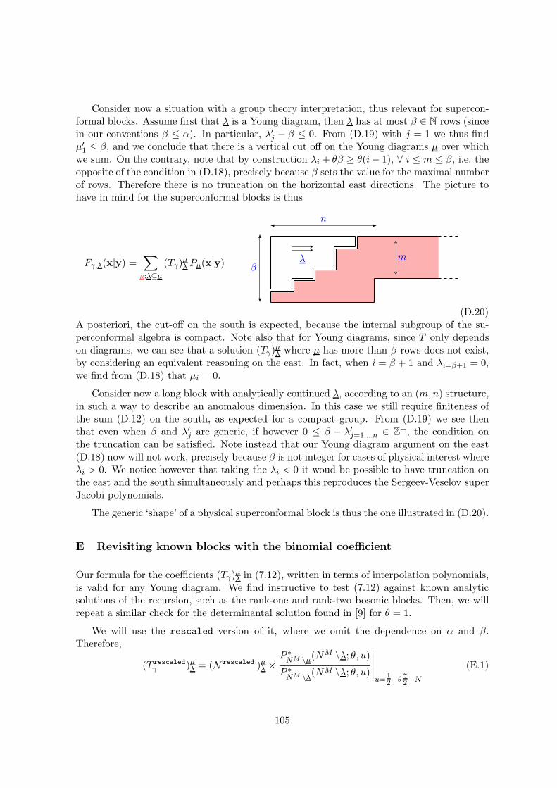
Consider now a situation with a group theory interpretation, thus relevant for supercon-formal blocks. Assume first that λ is a Young diagram, then λ has at most β ∈ N rows (sincein our conventions β ≤ α). In particular, λ′j − β ≤ 0. From (D.19) with j = 1 we thus findµ′1 ≤ β, and we conclude that there is a vertical cut off on the Young diagrams µ over whichwe sum. On the contrary, note that by construction λi + θβ ≥ θ(i− 1), ∀ i ≤ m ≤ β, i.e. theopposite of the condition in (D.18), precisely because β sets the value for the maximal numberof rows. Therefore there is no truncation on the horizontal east directions. The picture tohave in mind for the superconformal blocks is thus

mβ

n

λFγ,λ(x|y) =∑

µ:λ⊆µ

(Tγ)µλ Pµ(x|y)

(D.20)A posteriori, the cut-off on the south is expected, because the internal subgroup of the su-perconformal algebra is compact. Note also that for Young diagrams, since T only dependson diagrams, we can see that a solution (Tγ)

µλ where µ has more than β rows does not exist,

by considering an equivalent reasoning on the east. In fact, when i = β + 1 and λi=β+1 = 0,we find from (D.18) that µi = 0.

Consider now a long block with analytically continued λ, according to an (m,n) structure,in such a way to describe an anomalous dimension. In this case we still require finiteness ofthe sum (D.12) on the south, as expected for a compact group. From (D.19) we see thenthat even when β and λ′j are generic, if however 0 ≤ β − λ′j=1,...n ∈ Z+, the condition onthe truncation can be satisfied. Note instead that our Young diagram argument on the east(D.18) now will not work, precisely because β is not integer for cases of physical interest whereλi > 0. We notice however that taking the λi < 0 it woud be possible to have truncation onthe east and the south simultaneously and perhaps this reproduces the Sergeev-Veselov superJacobi polynomials.

The generic ‘shape’ of a physical superconformal block is thus the one illustrated in (D.20).

E Revisiting known blocks with the binomial coefficient

Our formula for the coefficients (Tγ)µλ in (7.12), written in terms of interpolation polynomials,

is valid for any Young diagram. We find instructive to test (7.12) against known analyticsolutions of the recursion, such as the rank-one and rank-two bosonic blocks. Then, we willrepeat a similar check for the determinantal solution found in [9] for θ = 1.

We will use the rescaled version of it, where we omit the dependence on α and β.Therefore,

(T rescaledγ )µλ = (N rescaled )µλ ×

P ∗NM \µ(N

M \λ; θ, u)P ∗NM \λ(N

M \λ; θ, u)

∣∣∣∣∣u=

12−θ

γ2−N

(E.1)

105

where

(N rescaled )µλ =(−)|µ|Πµ(θ)

(−)|λ|Πλ(θ)

C0µ/λ(1−θ+Mθ; θ)

C0µ/λ

(Mθ; θ)(E.2)

As pointed out already, the interpolation polynomials encode the non-factorisable γ depen-dence of (Tγ)

µλ, which we saw emerging experimentally from the recursion. However, the way

the interpolation polynomials are evaluated is quite different compared with the recursion.In fact, in order to match (Tγ)

µλ we will need to compute P ∗ of NM\µ, rather than looking

recursing over µ/λ, as we do in the recursion. Our exercise here will show in simple caseshow these two combinatorics actually produce the same result.

Through this section, we shall take the minimal choice for N andM in the above formulae,i.e.

N = µ1 ; M = β (E.3)

where β as usual fixes the maximal height of both λ and µ.

E.1 The half-BPS solution

The simplest case to start with is the derivation from (E.1) of the half-BPS solution in (5.37),

(T rescaledγ )

µ[∅] =

1

C0µ(θγ; θ)

1

C−µ (1; θ)

. (E.4)

To obtain the γ dependence we need consider the ratio of interpolation polynomials in (E.1)

and since λ = [∅], the numerator P ∗ is evaluated on µβ1 , which is a “constant” Young diagram.This evaluation is known. From [32] we find

P ipκ (c+ θδℓ + u; θ, u) = (−)|λ|C0

κ(c+ 2u+ θ(ℓ− 1),−c; θ)C0κ(ℓθ; θ)

C−κ (θ; θ)

(E.5)

which we need here for c = µ1 and ℓ = β. For what concerns the denominator instead, thisis always factorised for any λ and it is given by (7.7). Putting together we find,

P ∗

µβ1 \µ

(µ1+θδβ+u;θ,u)

C+

µβ1

(−2µ1−θγ+2θβ)C−

µβ1

(1;θ)=

C0

µβ1 \µ

(−θγ−(µ1−1)+θ(β−1);θ)

C0

µβ1

(−θγ−(µ1−1)+θ(β−1);θ)×

C0

µβ1 \µ

(−µ1;θ)C0

µβ1 \µ

(βθ;θ)

(−)|µ|−βµ1C−

µβ1

(1;θ)C−

µβ1\µ

(θ;θ)

(E.6)where we rewrote C+ in terms of C0 using the explicit definition (7.9), and the fact that the

Young diagram involved is a rectangle µβ1 . At this point, the 1/C0(θγ; θ) comes out thanksto the identity,

C0µ(w − (µ1 − 1) + θ(β − 1); θ)C0

µβ1−µ

(−w; θ)C0µβ1

(−w; θ) = (−1)|µ| ; ∀w (E.7)

taken with w = −θγ, and the (−1)|µ| cancels against the one in (E.2). Finally, the contribution1/C−

µ (1; θ) comes from Πµ(θ) in (E.2). The remaining terms in the binomial coefficient

106

necessarily have to simplify to unity. When we collect them all,55 upon using another identity

C−µ (w; θ)

C0µβ1

(θ(β − 1) + w; θ)C−µβ1 \µ

(w; θ)=C0µ(−w − (µ1 − 1); θ)

(−)|µ|C−µβ1

(w; θ); ∀w (E.8)

we finally obtain our desired result.

Already in this simple example we needed several identities between C±,0 coefficients.This shows that the rewriting of T in terms of interpolation polynomials is quite non trivial.

E.2 Rank-one and rank-two

After the half-BPS solution, we will consider the rank-one cases, since these are fully fac-torised. Next, the rank-two case, which involves a 4F3 and has non trivial dependence on γ.Thus it is the most interesting case for our purpose. Our task will be to revisit the solutionfound by Dolan and Osborn in [11].

Rank-one (1, 0)

For the single row case β = 1, with µ = [µ] and λ = [λ], we find

(N reduced )µλ =(−)|µ|Πµ(θ)

(−)|λ|Πλ(θ)× C0

µ/λ(1;θ)

C0µ/λ

(θ;θ)

=(−)µ(θ)µ(1)λ(−)λ(1)µ(θ)λ

× (λ+1)µ−λ

(λ+θ)µ−λ

(E.9)

which simplifies to a sign. Then, for the interpolation polynomials we find

P ∗[∅](µ − λ; θ, u)

P ∗[µ−λ](µ− λ; θ, u)

=1

(−)µ−λ(2λ+ θγ)µ−λ(1)µ−λ(E.10)

in particular, the numerator is trivial, and the denominator follows straightforwardly from(7.7) and (7.9). Putting together the two results above we obtain the formula

(T rescaledγ )

[µ][λ] =

1

(µ−λ)!(2λ + θγ)µ−λ(E.11)

which coincides with the one derived in section 4.1.

This case was quite immediate and the reason is that the formula for the P ∗ is orientedon the east, as the (1, 0) theory. We will see now what happens in the (0, 1) theory.

55These terms are

(−)|µ|+βµ1C−µ (θ; θ)

C0µ(βθ; θ)C

−

µβ1\µ(θ; θ)

×C0

µβ1\µ(βθ; θ)

C−

µβ1

(1; θ)×C0

µβ1\µ(−µ1; θ)C

0µ(1 + θ(β − 1); θ) = 1

using w = θ in (E.8) and w = µ1 in (E.7), then again w = −βθ in (E.7). Finally (−)βµ1C0

µβ1

(−µ1; θ)/C−

µβ1

(1; θ) =

1 and C0

µβ1

(βθ; θ)/C−

µβ1

(θ; θ) = 1, directly from their definitions.

107

Rank-one (0, 1)

For the single column case, the diagrams are λ = [1λ′] and µ = [1µ

′]. This is a case in

which λ′, µ′ ≤ β. Let us proceed with a direct computation starting with (E.1). Thenormalisation (E.2) becomes

(N rescaled )µλ =(−)|µ|Πµ(θ)

(−)|λ|Πλ(θ)× C0

µ/λ(1+(β−1)θ;θ)

C0µ/λ

(βθ;θ)

=(−)µ

′(1)µ′ (

1θ)λ′

(−)λ′ ( 1θ)µ′ (1)λ′

× ( 1θ+β−µ′)µ′−λ′

(1+β−µ′)µ′−λ′

(E.12)

For the ratio of interpolation polynomials the diagrams are µβ1\µ = [1β−µ′] and µβ1\λ = [1β−λ′

]and the polynomials have β variables. This time the numerator involves a non trivial Youngdiagram, which however has less than β rows. To simplify the result we use the non-trivialreducibility property for the interpolation polynomials, which reads

P ip[κ1,...κs]

(. . . , ws, u, u+ θ, . . . u+ (r − 1)θ︸ ︷︷ ︸variables

; θ, u) = P ip[κ1,...κs]

(. . . , ws; θ, u+ rθ) (E.13)

where r is counting the excess between the number of variables β and the non zero parts ofκ.56 In our case, the above result gives back an evaluation formula to

P ip

[1β−µ′ ](1β−λ′

+ δβ−λ′ + u′; θ, u′)

∣∣∣∣∣u′=u+λ′θ

=(µ′−λ′+1)β−µ′

(1)β−µ′(θ)2(β−µ′)(1θ )β−µ′(λ′ + µ′ − γ)β−µ′

(E.14)and in fact the RHS follows from (E.5). Thus, the ratio of interpolation polynomials con-tributes as,

P ∗[1β−µ′ ]

(1β−λ′; θ, u)

P ∗[1β−λ′ ]

(1β−λ′ ; θ, u)=

(θ)2(β−µ′)(λ′ + µ′ − γ)β−µ′(1θ )β−µ′

(θ)2(β−λ′)(2λ′ − γ)β−λ′(1θ )β−λ′

. (E.15)

Putting it all together, the final result for T rescaledγ (defined in (5.45)) is

(T rescaledγ )

[1µ′]

[1λ′ ]=

(θ)2(λ′−µ′)

(µ′ − λ′)!(2λ′−γ)µ′−λ′

µ′!(1θ )λ′

λ′!(1θ )µ′

(−1)µ′−λ′

. (E.16)

This coincides precisely with the one derived in section 4.1 for (Tγ)[1µ

′]

[1λ′ ]when we re-insert

C0µ/λ

(θ(γ−p12)

2 , θ(γ−p43)2 ; θ

)= (−θ)2(µ′−λ′)

(λ′ − (γ−p12)

2 , λ′ − (γ−p43)2

)µ′−λ′ (E.17)

properly oriented towards the south.

56Of course the same is true for a symmetric permutation of all variables on the LHS

108

Rank-two (2, 0)

In the rank-one cases there is no room for any non trivial polynomial in γ. The first non trivialcase in this sense is then rank-two, corresponding to Tγ for two row Young diagrams. Therecursion (5.35) for this case was solved explicitly by Dolan and Osborn [11]. They did thisfirst on a case by case basis in dimensions d = 2, 4, 6, then for general θ by using propertiesof the 4F3 function, and manipulations inspired by those in [99].57 We will show here howthis relates to the interpolation polynomial of (7.12).

In our conventions the solution of [11] reads

(T rescaledγ )µλ =

(θ)θ(µ− + θ)θ

× (Drescaled)µ+ θ

2γ

λ+ θ2γ

(E.18)

with

(Drescaled)µλ =(2θ)λ−(2θ)µ−

(θ)λ−(θ)µ−

(µ−+1)θ(µ1−λ2+1)θ

(µ1 − λ1)!(µ2 − λ2)!× (E.19)

(λ+−2θ)θ(λ2+µ2−2θ)θ

(2λ1)µ1−λ1(2λ2 − 2θ)µ2−λ2

4F3

[−µ− , θ , −λ− , λ+ − 1

−(µ1 − λ2) , λ2 + µ2 − θ , 2θ; 1

]

where λ = [λ1, λ2], µ = [µ1, µ2], and κ± = κ1 ± κ2, for κ = λ, µ.

The contribution denoted by D is the translation to our conventions of the result of [11],where we implemented the shift symmetry and slightly rewrote some Pochhammers. Notethat the 4F3 has a series expansion which truncates at min(λ−, µ−) and can thus be writtenas the explicit finite sum

(Drescaled)µλ =

min(λ−,µ−)∑

n=0

(−λ−)nn!

(2θ)λ−(θ)n(2θ)µ−

(θ)λ−(2θ)n(θ)µ−

(µ− − n+ 1)n+θ

(µ1 − λ2 − n+ 1)n+θ(E.20)

(λ+ − 1)n(λ+ − 2θ)θ(µ1 − λ1)!(µ2 − λ2)!(2λ1)µ1−λ1(2λ2 − 2θ)µ2−λ2+n+θ

.

Now compare this expression with our expression for Tγ written in terms of interpolationpolynomials (7.12) (with N = µ1, M = 2):

(Tγ)µλ = (N )µλ ×

P ip[µ1−µ2]

(w1, w2; θ,12 − θ γ2 − µ1)

P ip[µ1−λ2,µ1−λ1]

(w1, w2; θ,12 − θ γ2 − µ1)

∣∣∣∣∣wi=

12−θ(γ

2−i+1)−λi

(E.21)

(Note that the shift symmetry shows up nicely in this formula since we can always put to-gether combinations of the form κi+

θ2γ, and N is automatically invariant.) All contributions

in (E.21) coming from the denominator and the normalisation, can be straightforwardly com-puted, and written as product of Pochhammers or Gamma functions. The BC2 interpolation

57In [11], see formulae (3.11), (3.18) and (3.19).

109

polynomial in the numerator is also known explicitly, and described by a 4F3 [41],

P ipκ (w1, w2; θ, u) =(−)|κ|(u± w1, u± w2)κ2(κ2 + θ + u± w1)κ−×

× 4F3

[−κ− , θ , κ2 + u± w2

1− θ − κ− , κ2 + θ + u± w1; 1

](E.22)

Although similar, this 4F3 is not identical to that of (E.19). Also note that it is not manifestlyw1 ↔ w2 invariant even though the polynomial is symmetric under this interchange. We thushave two possibilities leading to the same result. Using P ip

[µ1−µ2](w2, w1) we find

numerator of (Tγ=0)µλ → 4F3

[−µ− , θ , 1− λ1 − µ1 , λ1 − µ1

λ2 − µ1 , 1− θ − µ1 + µ2, 1 + 2θ − λ2 − µ1; 1

](E.23)

which becomes the same hypergeometric as in (E.19) upon using the Whipple identity

4F3

[−n , a , b , cd , e , f

; 1

]=

(e− a)n(f − a)n(e)n(f)n

4F3

[−n , a , d− b , d− c

d , a− e+ 1− n , a− f + 1− n; 1

]

(E.24)Similarly had we chosen P ∗

[µ1−µ2](w1, w2) a different 4F3 identity will give the same final result.

Thus we see how the 4F3 of [11] arises directly from the interpolation polynomial.

It is quite spectacular to implement on a computer the above representation of Tγ andthe one arising directly from the recursion and check that they agree over many examples.

E.3 Revisiting the θ = 1 case and determinantals

The superconformal blocks for the case θ = 1 and any (m,n) were obtained in [9]. One of themain outcomes of that derivation is an explicit expression for the coefficients in an expansionover super Schur polynomials, that we quote here below,

(Rγ)µλ =

∑

σ

(−)|σ|m∏

i=1

(λi − i+ 1 + γ−p12

2

)µσ(i)+i−σ(i)−λi

(λi − i+ 1 + γ−p43

2

)µσ(i)+i−σ(i)−λi

(µσ(i) + i− σ(i) − λi)!(2λi − 2i+ 2 + γ)µσ(i)+i−σ(i)−λi

We can also conveniently rewrite the above formula for the coefficients as a determinant

(Rγ)µλ = det

((λi − i+ γ−p12

2 + 1)µj−j−λi+i(λi − i+ γ−p432 + 1)µj−j−λi+i

(µj − j − λi + i)!(2λi − 2i+ 2 + γ)µj−j−λi+i

)

1≤i,j≤β

(E.25)In this section we want to directly show how (Rγ)

µλ also arises from the interpolation polyno-

mials via (7.12), namely we want to show

(Rγ)µλ = (Tγ)

µλ

∣∣∣∣∣θ=1

= (N )µλ ×P ∗NM \µ(N

M \λ; θ, u)P ∗NM \λ(N

M \λ; θ, u)

∣∣∣∣∣u=

12−θ

γ2−N

∣∣∣∣∣θ=1

(E.26)

110

Notice that for θ = 1 the normalisation simplifies massively,

(N )µλ

∣∣∣∣∣θ=1

= C0µ/λ

((γ−p12)

2 , (γ−p43)2 ; 1

)(E.27)

and only the ratio of interpolation polynomials is important.

Let us begin by improving the expression of the determinant in such a way as to extractthe same normalisation. Using (a)x = Γ[a + x]/Γ[a], it is simple to realise that variouscontributions depend solely on either row or column index, therefore can be factored out, andrearranged. We arrive at the expression

(Rγ)µλ = (N )µλ × (Rrescaled

γ )µλ (E.28)

(Rrescaledγ )µλ =

(β∏

i=1

Γ[2− 2i+ γ + 2λi]

)det

(Γ[1 + i− j − λi + µj ]

−1

Γ[2− i− j + γ + λi + µj]

)

1≤i,j≤β

(E.29)

Our formula for Tγ in terms of interpolation polynomials can be manipulated quite ex-plicitly when θ = 1, since the BC interpolation polynomials for θ = 1 themselves also have adeterminantal representation [40],

P ip[κ1,...κℓ]

(w; θ = 1, u) =det(P ip[κj+ℓ−j](wi;u)

)1≤i,j≤ℓ∏

i<j(w2i − w2

j )(E.30)

The entries of the matrix are single-variable interpolation polynomials P ipκ (wi, u). These do

not depend on θ and are given by a pair of Pochhammers,

P ipκ (w;u) = (−)k(u+ w)k(u− w)k = (−w − u− k + 1)k(u− w)k

= (−)k(−w − u− k + 1)k(w − u− k + 1)k (E.31)

The denominator of (E.30) is the Z2 invariant Vandermonde determinant.

We can now proceed and compute (Tγ)µλ for θ = 1. Since we already identified the

normalisation, we will focus on (Rrescaledγ )µλ. This has to agree with

(T rescaledγ )µλ ≡ (−)|µ|

(−)|λ|

P ip

µβ1−µ

(12 − γ2 + i− 1− λi; 1,

12 − γ

2 − µ1)

P ip

µβ1−λ

(12 − γ2 + i− 1− λi; 1,

12 −

γ2 − µ1)

(E.32)

The idea is simple: we need to recognise the matrix in (E.29). To do so, we first use theexpression of the BC1 interpolation polynomials given in (E.31), and pass from Pochhammersto Γ functions. The result is

(T rescaledγ )µλ =

(−)|µ|

(−)|λ|

(−)βµ1−|µ|+ 12β(β−1) det

(Γ[i−λi+µ1]Γ[1−i+γ+λi−µ1]

Γ[1+i−J−λi+µJ ]Γ[2−i−J+γ+λi+µJ ]

)1≤i,j≤β

(−)βµ1−|λ|+ 12β(β−1) det

(Γ[i−λi+µ1]Γ[1−i+γ+λi−µ1]

Γ[1+i−J−λi+λJ ]Γ[2−i−J+γ+λi+λJ ]

)1≤i,j≤β

(E.33)

111

where J = β+1− j and the signs have been factored out since only depended on the columnindex. For the same reason we can factor out Γ[i− λi + µ1]Γ[1− i+ γ + λi − µ1] and cancelit between numerator and denominator. Moreover we can reverse the columns and switchj ↔ J . We arrive at the simple formula

(T rescaledγ )µλ =

det(

Γ[1+i−j−λi+µj ]−1

Γ[2−i−j+γ+λi+µj ]

)1≤i,j≤β

det(

Γ[1+i−j−λi+λj ]−1

Γ[2−i−j+γ+λi+λj ]

)1≤i,j≤β

(E.34)

Comparing this result with (E.29) we are left with the statement

β∏

i=1

Γ[2− 2i+ γ + 2λi] =1

det(

Γ[1+i−j−λi+λj ]−1

Γ[2−i−j+γ+λi+λj ]

)1≤i,j≤β

(E.35)

But notice that Γ[1 + i− j − λi + λj]−1, because λi ≥ λi+1, makes the matrix on the r.h.s a

triangular matrix, and the identity follows. Thus (T rescaledγ )µλ = (Rrescaled)µλ and our proof

is concluded.

References

[1] A. Galperin, E. Ivanov, S. Kalitsyn, V. Ogievetsky and E. Sokatchev, “Uncon-strained N=2 Matter, Yang-Mills and Supergravity Theories in Harmonic Superspace,”Class. Quant. Grav. 1 (1984), 469-498 [erratum: Class. Quant. Grav. 2 (1985), 127]doi:10.1088/0264-9381/1/5/004

[2] P. S. Howe and G. G. Hartwell, “A Superspace survey,” Class. Quant. Grav. 12 (1995),1823-1880 doi:10.1088/0264-9381/12/8/005

[3] G. G. Hartwell and P. S. Howe, “(N, p, q) harmonic superspace,” Int. J. Mod. Phys. A10 (1995), 3901-3920 doi:10.1142/S0217751X95001820 [arXiv:hep-th/9412147 [hep-th]].

[4] P. S. Howe and M. I. Leeming, “Harmonic superspaces in low dimensions,” Class. Quant.Grav. 11 (1994), 2843-2852 doi:10.1088/0264-9381/11/12/004 [arXiv:hep-th/9408062[hep-th]].

[5] P. S. Howe, “Aspects of the D = 6, (2,0) tensor multiplet,” Phys. Lett. B 503 (2001),197-204 doi:10.1016/S0370-2693(00)01304-6 [arXiv:hep-th/0008048 [hep-th]].

[6] P. J. Heslop, “Superfield representations of superconformal groups,” Class. Quant. Grav.19 (2002), 303-346 doi:10.1088/0264-9381/19/2/309 [arXiv:hep-th/0108235 [hep-th]].

[7] P. J. Heslop and P. S. Howe, “Four point functions in N=4 SYM,” JHEP 01 (2003), 043doi:10.1088/1126-6708/2003/01/043 [arXiv:hep-th/0211252 [hep-th]].

[8] P. J. Heslop, “Aspects of superconformal field theories in six dimensions,” JHEP 07(2004), 056 doi:10.1088/1126-6708/2004/07/056 [arXiv:hep-th/0405245 [hep-th]].

[9] R. Doobary and P. Heslop, “Superconformal partial waves in Grassmannian field theo-ries,” JHEP 12 (2015), 159 doi:10.1007/JHEP12(2015)159 [arXiv:1508.03611 [hep-th]].

112

[10] P. S. Howe and U. Lindstrom, “Notes on Super Killing Tensors,” JHEP 03 (2016), 078doi:10.1007/JHEP03(2016)078 [arXiv:1511.04575 [hep-th]].

[11] F. A. Dolan and H. Osborn, “Conformal partial waves and the operator productexpansion,” Nucl. Phys. B 678 (2004), 491-507 doi:10.1016/j.nuclphysb.2003.11.016[arXiv:hep-th/0309180 [hep-th]].

[12] M. Isachenkov and V. Schomerus, “Superintegrability of d-dimensional ConformalBlocks,” Phys. Rev. Lett. 117 (2016) no.7, 071602 doi:10.1103/PhysRevLett.117.071602[arXiv:1602.01858 [hep-th]].

[13] H. Y. Chen and J. D. Qualls, “Quantum Integrable Systems from ConformalBlocks,” Phys. Rev. D 95 (2017) no.10, 106011 doi:10.1103/PhysRevD.95.106011[arXiv:1605.05105 [hep-th]].

[14] M. Isachenkov and V. Schomerus, “Integrability of conformal blocks. Part I. Calogero-Sutherland scattering theory,” JHEP 07 (2018), 180 doi:10.1007/JHEP07(2018)180[arXiv:1711.06609 [hep-th]].

[15] H. Y. Chen and J. i. Sakamoto, “Superconformal Block from Holographic Geometry,”JHEP 07 (2020), 028 doi:10.1007/JHEP07(2020)028 [arXiv:2003.13343 [hep-th]].

[16] G. J. Heckman, “Root systems and hypergeometric functions II”, Compositio Math. 64(1987), 329-352.

[17] G. J. Heckman, “Root systems and hypergeometric functions I”, Compositio Math. 64(1987), 353-373.

[18] S. Ferrara, A. F. Grillo, G. Parisi, and R. Gatto. “Covariant expansion of the conformalfour-point function”. Nucl. Phys. B, 49:77, 1972.

[19] S. Ferrara, A. F. Grillo, R. Gatto. “Tensor representations of conformal algebra andconformally covariant operator product expansions”. Ann.Phys.(N.Y.), 76:161, 1973.

[20] V. K. Dobrev, G. Mack, V. B. Petkova, S. G. Petrova, and I.T. Todorov. “On ClebschGordan expansions for the Lorentz group in n dimensions”. Reports on MathematicalPhysics, 9:219, 1976.

[21] G. Mack, “D-independent representation of Conformal Field Theories in D dimen-sions via transformation to auxiliary Dual Resonance Models. Scalar amplitudes”,[arXiv:0907.2407 [hep-th]].

[22] F. A. Dolan and H. Osborn, “Conformal four point functions and the operator prod-uct expansion,” Nucl. Phys. B 599 (2001), 459-496 doi:10.1016/S0550-3213(01)00013-X[arXiv:hep-th/0011040 [hep-th]].

[23] F. A. Dolan and H. Osborn, “Superconformal symmetry, correlation functions andthe operator product expansion,” Nucl. Phys. B 629 (2002), 3-73 doi:10.1016/S0550-3213(02)00096-2 [arXiv:hep-th/0112251 [hep-th]].

[24] M. Nirschl and H. Osborn, “Superconformal Ward identities and their solution,” Nucl.Phys. B 711 (2005), 409-479 doi:10.1016/j.nuclphysb.2005.01.013 [arXiv:hep-th/0407060[hep-th]].

113

[25] F. A. Dolan and H. Osborn, “Conformal partial wave expansions for N=4 chiral four pointfunctions,” Annals Phys. 321 (2006), 581-626 doi:10.1016/j.aop.2005.07.005 [arXiv:hep-th/0412335 [hep-th]].

[26] R. J. Beerends and E. M. Opdam “Certain hypergeometric series related to the rootsystem BC”, Transactions of the AMS volume 339, Number 2, 1993.

[27] I. G. Macdonald, “Orthogonal polynomials associated with root systems”, Unpublishedmanuscript, 1987; Sem. Lothar. Combin. 45 (2000), B45a, 40 pp.

[28] I. G. Macdonald, “Hypergeometric functions I”, Unpublished manuscript, 1987;arXiv:1309.4568 [math.CA], 2013.

[29] I. G. Macdonald, “Symmetric functions and Hall polynomials”, Oxford University Press,Second edition, 1994.

[30] T. H. Koornwinder, “Askey-Wilson polynomials for root systems of type BC”, in: “Hy-pergeometric functions on domains of positivity, Jack polynomials, and applications”,Contemp. Math. 138, Amer. Math. Soc., 1992, pp. 189–204.

[31] J. V. Stokman and T. H. Koornwinder, “Limit transitions for BC type multivariableorthogonal polynomials”, Canad. J. Math. 49 (1997), 373–404.

[32] E. M. Rains, “BCn-symmetric polynomials”, Transform. Groups 10 (2005), 63–132.

[33] A. Okounkov, “BC-type interpolation Macdonald polynomials and binomial formula forKoornwinder polynomials”Transform. Groups 3 (1998), 181–207.

[34] A. N. Sergeev, A. P. Veselov, “Generalised discriminats, deformed CMS operators andsuper-Jack polynomials”, Adv. Math. 192 (2005), 341-375.

[35] A.N. Sergeev and A.P. Veselov, “Deformed quantum Calogero-Moser problems and Liesuperalgebras”, Commun. Math. Phys. 245 (2004), 249–278.

[36] A. N. Sergeev and A. P. Veselov “Deformed Macdonald-Ruijsenaars operators and superMacdonald polynomials” arXiv:0707.3129 [math.QA] (2008)

[37] E.M. Moens and Joris Van der Jeugt. “A determinantal formula for supersymmetricSchur polynomials”. Journal of Algebraic Combinatorics, 17(3):283-307, 2003.

[38] A.N. Sergeev and A.P. Veselov, “BC∞ Calogero-Moser operator and super Jacobi polyno-mials.” Advances in Mathematics 222.5 (2009): 1687-1726. [arXiv: 0807.3858 [math-ph]]

[39] R. Doobary, Unpublished notes (2016).

[40] A. Okounkov and G. Olshanski “Limits of BC orthogonal polynomials as the number ofvariables goes to infinity”. Contemp. Math., 417, 281?318, Amer. Math. Soc., Providence,RI, 2006. arXiv:math/0606085 [math.RT].

[41] T. H. Koornwinder, “Okounkov’s BC type interpolation Macdonald polynomials andtheir q=1 limit”. Seminaire Lotharingien de Combinatoire, B72a (2015), 27 pp.arXiv:1408.5993 [math.CA].

114

[42] K. Mimachi, “A duality of Macdonald-Koornwinder polynomials and its application tointegral representations”, Duke Mathematical Journal 107.2 (2001): 265-281.

[43] N. Shimeno, “A formula for the hypergeometric function of type BCn”arXiv:0706.3555[math.RT], Pacific Journal of Mathematics Vol. 236, No. 1, 2008

[44] F. A. Dolan and H. Osborn, “On short and semi-short representations forfour-dimensional superconformal symmetry,” Annals Phys. 307 (2003), 41-89doi:10.1016/S0003-4916(03)00074-5 [arXiv:hep-th/0209056 [hep-th]].

[45] F. A. Dolan, L. Gallot and E. Sokatchev, “On four-point functions of 1/2-BPS opera-tors in general dimensions,” JHEP 09 (2004), 056 doi:10.1088/1126-6708/2004/09/056[arXiv:hep-th/0405180 [hep-th]].

[46] C. Beem, M. Lemos, P. Liendo, L. Rastelli and B. C. van Rees, “The N = 2 superconfor-mal bootstrap,” JHEP 03 (2016), 183 doi:10.1007/JHEP03(2016)183 [arXiv:1412.7541[hep-th]].

[47] S. M. Chester, J. Lee, S. S. Pufu and R. Yacoby, “TheN = 8 superconformal bootstrap inthree dimensions,” JHEP 09 (2014), 143 doi:10.1007/JHEP09(2014)143 [arXiv:1406.4814[hep-th]].

[48] C. Beem, L. Rastelli and B. C. van Rees, “More N = 4 superconformal bootstrap,” Phys.Rev. D 96 (2017) no.4, 046014 doi:10.1103/PhysRevD.96.046014 [arXiv:1612.02363 [hep-th]].

[49] M. Lemos, P. Liendo, C. Meneghelli and V. Mitev, “BootstrappingN = 3 superconformaltheories,” JHEP 04 (2017), 032 doi:10.1007/JHEP04(2017)032 [arXiv:1612.01536 [hep-th]].

[50] P. Liendo, C. Meneghelli and V. Mitev, “Bootstrapping the half-BPS line defect,” JHEP10 (2018), 077 doi:10.1007/JHEP10(2018)077 [arXiv:1806.01862 [hep-th]].

[51] L. F. Alday, S. M. Chester and H. Raj, “6d (2,0) and M-theory at 1-loop,” JHEP 01(2021), 133 doi:10.1007/JHEP01(2021)133 [arXiv:2005.07175 [hep-th]].

[52] M.Lassalle “Explicitation des polynomes de Jack et de Macdonald en longueur trois”,C.R.Acad.Sci. Paris Ser. I Math. 333 (2001), 505–508.

[53] M.Lassalle, M. Schlosser “Inversion of the Pieri formula for Macdonald polynomials”,arXiv:math/0402127 (2014). Adv. Math 202 (2006) 289-325

[54] M. Schlosser “Explicit computation of the q,t Littlewood-Richardson coefficients”,Contemp. Math. 417, Amer. Math. Soc. Providence RI 2006. available athttps://www.mat.univie.ac.at/~schlosse/qtlr.html

[55] P. S. Howe and P. C. West, “AdS / SCFT in superspace,” Class. Quant. Grav. 18 (2001),3143-3158 doi:10.1088/0264-9381/18/16/305 [arXiv:hep-th/0105218 [hep-th]].

[56] P. J. Heslop and P. S. Howe, “Aspects of N=4 SYM,” JHEP 01 (2004), 058doi:10.1088/1126-6708/2004/01/058 [arXiv:hep-th/0307210 [hep-th]].

115

[57] P. S. Howe, “On harmonic superspace,” Lect. Notes Phys. 524 (1999), 68doi:10.1007/BFb0104588 [arXiv:hep-th/9812133 [hep-th]].

[58] T. Okazaki, “Superconformal Quantum Mechanics from M2-branes,” [arXiv:1503.03906[hep-th]].

[59] F. Aprile and M. Santagata, “Two-particle spectrum of tensor multiplets coupled toAdS3 × S3 gravity,” [arXiv:2104.00036 [hep-th]].

[60] R. J. Baston and M. G. Eastwood, “The Penrose transform: Its interaction with repre-sentation theory,”

[61] John F. Cornwell, “Group theory in physics vol. 3”. Academic press (1984).

[62] M. Rosler, “Positive convolution structure for a class of Heckman-Opdam hypergeo-metric functions of type BC”, Journal of Functional Analysis 258.8 (2010): 2779-2800[arXiv:0907.2447]

[63] https://functions.wolfram.com/HypergeometricFunctions/Hypergeometric2F1/17/02/05/0003/

[64] https://functions.wolfram.com/HypergeometricFunctions/Hypergeometric2F1/17/02/07/0005/

[65] R. P. Stanley, “Some combinatorial properties of Jack symmetric functions”, Adv. Math.77 (1989), 76–115.

[66] M. Lassalle, “Une formule du binome generalisee pour les polynomes de Jack”, C. R.Acad. Sci. Paris Ser. I Math. 310 (1990), 253–256.

[67] A. Okounkov and G. Olshanski, “Shifted Jack polynomials, binomial formula, and ap-plications”, Math. Res. Lett. 4 (1997), 69–78.

[68] Z. Yan, “A class of generalized hypergeometric functions in several variables”, Canad. J.Math. 44 (1992), 1317–1338.

[69] M.Lassalle “Jack polynomials and some identities for partitions”. Trans. Amer. Math.Soc. 356 (2004) 3455-3476. arXiv:math/0306222v2[math.CO]

[70] S. Caron-Huot, “Analyticity in Spin in Conformal Theories,” JHEP 09 (2017), 078doi:10.1007/JHEP09(2017)078 [arXiv:1703.00278 [hep-th]].

[71] Sho Matsumoto, “Averages of ratios of characteristic polynomials in circular beta-ensembles and super-Jack polynomials,” arXiv:0805.3573

[72] F. Aprile, J. M. Drummond, P. Heslop, M. Santagata “Free theory OPE data from aCauchy identity”, In preparation.

[73] T. Abl, P. Heslop and A. E. Lipstein, “Higher-Dimensional Symmetry of AdS2×S2 Cor-relators,” [arXiv:2112.09597 [hep-th]].

[74] F. Aprile, J. M. Drummond, P. Heslop and H. Paul, “Quantum Gravity from ConformalField Theory,” JHEP 01 (2018), 035 doi:10.1007/JHEP01(2018)035 [arXiv:1706.02822[hep-th]].

116

[75] F. Aprile, J. M. Drummond, P. Heslop and H. Paul, “Loop corrections forKaluza-Klein AdS amplitudes,” JHEP 05 (2018), 056 doi:10.1007/JHEP05(2018)056[arXiv:1711.03903 [hep-th]].

[76] F. Aprile, J. Drummond, P. Heslop and H. Paul, “One-loop amplitudes in AdS5×S5

supergravity from N = 4 SYM at strong coupling,” JHEP 03 (2020), 190doi:10.1007/JHEP03(2020)190 [arXiv:1912.01047 [hep-th]].

[77] P. Heslop and A. E. Lipstein, “M-theory Beyond The Supergravity Approximation,”JHEP 02 (2018), 004 doi:10.1007/JHEP02(2018)004 [arXiv:1712.08570 [hep-th]].

[78] T. Abl, P. Heslop and A. E. Lipstein, “Recursion relations for anomalous dimen-sions in the 6d (2, 0) theory,” JHEP 04 (2019), 038 doi:10.1007/JHEP04(2019)038[arXiv:1902.00463 [hep-th]].

[79] C. Beem, M. Lemos, L. Rastelli and B. C. van Rees, “The (2, 0) superconformalbootstrap,” Phys. Rev. D 93 (2016) no.2, 025016 doi:10.1103/PhysRevD.93.025016[arXiv:1507.05637 [hep-th]].

[80] A. Babichenko, B. Stefanski, Jr. and K. Zarembo, “Integrability and the AdS(3)/CFT(2)correspondence,” JHEP 03 (2010), 058 doi:10.1007/JHEP03(2010)058 [arXiv:0912.1723[hep-th]].

[81] J. Penedones, J. A. Silva and A. Zhiboedov, “Nonperturbative Mellin Amplitudes: Ex-istence, Properties, Applications,” JHEP 08 (2020), 031 doi:10.1007/JHEP08(2020)031[arXiv:1912.11100 [hep-th]].

[82] C. Sleight and M. Taronna, “The Unique Polyakov Blocks,” JHEP 11 (2020), 075doi:10.1007/JHEP11(2020)075 [arXiv:1912.07998 [hep-th]].

[83] D. Carmi and S. Caron-Huot, “A Conformal Dispersion Relation: Correlations from Ab-sorption,” JHEP 09 (2020), 009 doi:10.1007/JHEP09(2020)009 [arXiv:1910.12123 [hep-th]].

[84] S. Caron-Huot, D. Mazac, L. Rastelli and D. Simmons-Duffin, “Dispersive CFT SumRules,” JHEP 05 (2021), 243 doi:10.1007/JHEP05(2021)243 [arXiv:2008.04931 [hep-th]].

[85] R. Gopakumar, A. Sinha and A. Zahed, “Crossing Symmetric Dispersion Re-lations for Mellin Amplitudes,” Phys. Rev. Lett. 126 (2021) no.21, 211602doi:10.1103/PhysRevLett.126.211602 [arXiv:2101.09017 [hep-th]].

[86] M. Hogervorst, H. Osborn and S. Rychkov, “Diagonal Limit for Conformal Blocks ind Dimensions,” JHEP 08 (2013), 014 doi:10.1007/JHEP08(2013)014 [arXiv:1305.1321[hep-th]].

[87] M. Hogervorst and S. Rychkov, “Radial Coordinates for Conformal Blocks,” Phys. Rev.D 87 (2013), 106004 doi:10.1103/PhysRevD.87.106004 [arXiv:1303.1111 [hep-th]].

[88] V. Schomerus and E. Sobko, “From Spinning Conformal Blocks to MatrixCalogero-Sutherland Models,” JHEP 04 (2018), 052 doi:10.1007/JHEP04(2018)052[arXiv:1711.02022 [hep-th]].

117

[89] I. Buric, V. Schomerus and E. Sobko, JHEP 01 (2020), 159doi:10.1007/JHEP01(2020)159 [arXiv:1904.04852 [hep-th]].

[90] I. Buric, M. Isachenkov and V. Schomerus, “Conformal Group Theory of Tensor Struc-tures,” JHEP 10 (2020), 004 doi:10.1007/JHEP10(2020)004 [arXiv:1910.08099 [hep-th]].

[91] I. Buric, V. Schomerus and E. Sobko, JHEP 10 (2020), 147doi:10.1007/JHEP10(2020)147 [arXiv:2005.13547 [hep-th]].

[92] Nantel Bergeron and Adriano M Garsia, “Zonal polynomials and domino tableaux,”Discrete mathematics(1992) 99, 1-3, pp 3-15.

[93] M. A. Olshanetsky and A. M. Perelomov, “Quantum Integrable Systems Related to LieAlgebras,” Phys. Rept. 94 (1983), 313-404 doi:10.1016/0370-1573(83)90018-2

[94] V. Serganova, “On generalizations of root systems”, Commun. in Alg. 24.13 (1996),4281–4299.

[95] F. Atai, M. Hallnas, E. Langmann, “Orthogonality of super-Jack polynomials and Hilbertspace interpretation of deformed CMS operators”, arXiv:1802.02016 [math.QA], (2018).

[96] F. Delduc, M. Magro and B. Vicedo, “An integrable deformation of theAdS5 × S5 superstring action,” Phys. Rev. Lett. 112 (2014) no.5, 051601doi:10.1103/PhysRevLett.112.051601 [arXiv:1309.5850 [hep-th]].

[97] F. Delduc, M. Magro and B. Vicedo, “Derivation of the action and symmetries of theq-deformed AdS5×S5 superstring,” JHEP 10 (2014), 132 doi:10.1007/JHEP10(2014)132[arXiv:1406.6286 [hep-th]].

[98] G. Arutyunov, S. Frolov, B. Hoare, R. Roiban and A. A. Tseytlin, “Scale invariance of theη-deformed AdS5×S5 superstring, T-duality and modified type II equations,” Nucl. Phys.B 903 (2016), 262-303 doi:10.1016/j.nuclphysb.2015.12.012 [arXiv:1511.05795 [hep-th]].

[99] T. Koornwinder and I. Sprinkhuizen-Kuyper, “Generalized Power Series Expansions fora Class of Orthogonal Polynomials in Two Variables”, Siam J. on Mathematical Analysis,9 (1978) 457.

[100] S.Ole Warnaar “Bisymmetric functions, Macdonald polynomials and sl3 basic hyperge-ometric series”. Compos. Math. 144 (2008) 271-303. arXiv:math/0511333v1

[101] E. M. Rains, “A difference-integral representation of Koornwinder polynomials”, inJack, Hall-Littlewood and Macdonald Polynomials. Contemporary Mathematics. No.417AMS. arXiv:math/0409437 [math.CA] (2004).

118