Prepared for submission to JHEP

2d small N=4 Long-multiplet superconformal block

Filip Kos1, Jihwan Oh1,2

1Department of Physics, University of California, Berkeley, CA 94720, U.S.A.2Perimeter Institute for Theoretical Physics, 31 Caroline St. N., Waterloo, ON N2L 2Y5, Canada

E-mail: filip.kos@berkeley.edu, jihwanoh@berkeley.edu

Abstract: We study 2d N=4 superconformal field theories, focusing on its application

on numerical bootstrap study. We derive the superconformal block by utilizing the global

part of the super Virasoro algebra and set up the crossing equations for the non-BPS

long-multiplet 4-point function. Along the way, we build global N=4 superconformal short

and long multiplets and compute all possible 2,3-point functions of long-multiplets that

are needed to construct the superconformal blocks and the crossing equations. Since we

consider a long-multiplet 4-point function, the number of crossing equations is huge, and

we expect it to give a strong constraint than the usual superconformal bootstrap analysis,

which relies on BPS 4-point functions. In addition, we present an alternative way to derive

crossing equations using N=4 superspace and comment on a puzzle.

arX

iv:1

810.

1002

9v3

[he

p-th

] 2

4 Ja

n 20

19

Contents

1 Introduction 2

2 2d small N = 4 superconformal algebra 3

2.1 N = 4 superconformal algebra 3

2.2 Long-multiplets 4

2.3 Short-multiplets 7

2.4 Decomposition of the Long-multiplets into the Short-multiplets 8

3 Superconformal block computation 10

3.1 Selection rules 11

3.2 2-point functions 12

3.3 3-point functions 14

3.4 4-point functions 16

3.5 Crossing equations 18

4 N = 4 superspace approach 19

4.1 N = 4 superspace and 3-point invariants 20

4.2 4-point invariants and their limits 20

4.3 Nilpotent invariants and their independent combinations 21

4.4 Crossing Equations 23

4.5 Casimir equation 24

4.6 The puzzle 25

5 Discussion 26

A 3-point invariants of N = 4 superspace 27

B 2-point function normalization 30

B.1 L0 30

B.2 L1 30

B.3 L2 31

C 3-point function normalizations 32

C.1 〈φL0L0〉 32

C.2 〈φL0L1〉 33

C.3 〈φL0L2〉 34

D Sample crossing equations 35

– 1 –

1 Introduction

For a decade, there has been extensive work on solving various conformal field theories

using only first principles – unitarity, associativity of the operator product algebra, and

the so called conformal bootstrap program. First introduced by [1, 2] and revived through

[3], there were many attempts to solve theories with no supersymmetry [4–6] and differ-

ent amount of supersymmetries in various dimensions [7, 8] from two dimensions to six

dimensions [9–17].

With this paper, we wish to fill a gap in the literature – CFT in two dimensions

with (0, 4) or (4, 4) supersymmetry [18], which seems to be the last remaining family of

supersymmetric CFTs that has not been explored extensively.1At first glance, the infinite

dimensional super-Virasoro symmetry [19] can be very constraining and provides a lot of

information by itself. However, we are not aware of any literature that worked out the

super-Virasoro conformal blocks for N = 2 or higher [20–22], and this makes it difficult to

use the full power of the N = 4 super-Virasoro algebra in the bootstrap analysis.

Still, one can try to use a global part of the superconformal algebra to construct

‘smaller’ superconformal blocks. More precisely, we will use the fact that the 4-point

correlation function of conformal primaries in the long-multiplet is decomposed into bosonic

Virasoro conformal blocks, not the super-Virasoro conformal blocks. Since the coefficients

placed in front of each decomposed Virasoro blocks are independent, the set of crossing

equations is distinguished from non-supersymmetric 2d CFT 4-point functions and at the

same time captures structure of N = 4. This fact was used in [9] to do the N = 2

long-multiplet bootstrap analysis. Our goal is to generalize this result to N = 4. As we

will find in this paper, the number of crossing equations is larger than check that of any

numerical bootstrap literature that we are aware of, which makes us confident about the

level of precision in using only such small superconformal blocks. Moreover, different from

previous approaches that only analyzed particular BPS sectors of the theory, we set up

the crossing equations using generic long-multiplets. Hence, we expect the resulting set of

crossing equations to be more comprehensive, constraining the spectrum of the theory.

2d (0, 4) or (4, 4) superconformal field theories are interesting in their own right. There

are many interesting examples that have N = 4 superconformal symmetry in 2-dimensions.

Some of these include K3 (4, 4) theory [17], IR limits of (0, 4) E-string worldsheet theories

[23–25], a family of (0, 4) theories [27] that originate from class-S theory [28, 29], and lastly

a huge class of (0, 4) theories from brane-box model [30]. Lastly, it is worth mentioning

that the 2d small N = 4 chiral algebra appears in the subsector of 4d N = 4 SYM [31–

33], which is at the same time superconformal field theory with the algebra psu(2, 2|4).

Although we have not attempted to study the implication of our analysis on 4d N = 4

superconformal field theory, it would be very interesting to pursue such direction.

Our paper is organized as follows. In §2, we review the 2d small N = 4 superconformal

algebra and construct the supermultiplet using the global part of the superVirasoro alge-

bra. In addition, we analyze short-multiplets and decompositions of long-multiplets into

1[17] solved the K3 (4, 4) SCFT, using a special relation between super-Virasoro block and Virasoro

block available for this specific case.

– 2 –

short-multiplets. In §3, we compute superconformal blocks, starting from basic building

blocks, such as 2-point functions and 3-point functions. A heavy amount of computation

is simplified using R-symmetry and Fermion number selection rules. The solution of the

system of linear equations for 3-point functions is unique and is expressed in terms of

10 independent constants that match with the counting using the superspace. This pro-

vides a strong consistency check of our calculation. With the superconformal blocks, we

obtain crossing equations that can be used in the numerical analysis. In §4, an alterna-

tive approach to compute superconformal blocks, using N = 4 superspace [35, 36, 41], is

presented. We compute 3-point and 4-point invariants and construct Nilpotent invariants

for superconformal block expansion using them. Our goal is to use Casimir differential

equation to solve the superconformal block, but N = 4 superspace does not seem to fully

represent small N = 4 superconformal algebra. As it is not a complete treatment, we point

out some limitations that we encountered. We conclude the paper with future directions §5.

Since 2-point and 3-point function data is huge, we include a part of them in Appendices

§B, §C, §D, and this submission is also accompanied by a separate Mathematica file that

contains all the data.

2 2d small N = 4 superconformal algebra

In this section, we introduce basic elements that will be used to calculate long-multiplet

n-point functions of 2d small N = 4 global long-multiplets. In §2.1, we review 2d small

N = 4 superconformal algebra, focusing on the global part of the super Virasoro algebra.

Following the general analysis that was done for d ≥ 3 in [42, 43], we build long- and

short-multiplets in §2.2, along with the decomposition of the long-multiplet into various

short-multiplets. It is essential to do the short-multiplet analysis even though we compute

long-multiplet 4-point functions, since the stress energy tensor lies in one of the short-

multiplets. The identification of the multiplet that contains the stress energy tensor is

crucial in the bootstrap analysis of central charges, as one needs to compute the 4-point

function with stress energy tensor exchanged. Furthermore, we have identified the short-

multiplets that contain the flavor current operator, which can be used in the bootstrap

analysis for 2d CFT with a global symmetry.

2.1 N = 4 superconformal algebra

Let us review small N = 4 superconformal algebra following [37–39]. Other than the

usual Virasoro algebra generators, due to enhanced supersymmetry, the superconformal

algebra contains supersymmetry generators Gar , superconformal symmetry generators Gar ,

and SU(2)R R-symmetry current algebra generators T im, where a, b are SU(2)R spinor

indices, i is SO(3)R vector index, m ∈ Z, and r ∈ Z/2, as we restrict ourselves in the

NS sector. The super-Virasoro algebra generators satisfy the following (anti-)commutation

– 3 –

relations.[Lm, Ln

]= (m− n)Lm+n +

1

2km(m2 − 1)δm+n,0,

{Gar , Gbs} = {Gar , Gbs} = 0, {Gar , Gbs} = 2δabLr+s − 2(r − s)σiabT ir+s +1

2k(4r2 − 1)δr+s,0δ

ab,[T im, T

jn

]= iεijkT km+n +

1

2kmδm+n,0δ

ij ,[T im, G

ar

]= −1

2σiabG

bm+r,

[T im, G

as

]=

1

2σi∗abG

bm+s,[

Lm, Gar

]= (

1

2m− r)Gam+r,

[Lm, G

as

]= (

1

2m− s)Gam+s,

[Lm, T

in

]= −nT im+n

In the following discussion, we only use the global part of the superconformal algebra to

compute 2-point, 3-point, and 4-point functions. It would be far more constraining to use

the infinite dimensional super-Virasoro algebra when one tries to bootstrap two dimensional

conformal field theories, but unfortunately, the full recursion relation that leads to the

approximate expression for conformal block for extended supersymmetry has not been

worked out in the literature. For now, after Zamoldchikov derived the recursion relation

for Virasoro conformal block [20], only N = 1 super-Virasoro conformal block recursion

relation was obtained [21]. In spite of this limitation to use full super-Virasoro symmetry,

we expect that the use of global part of super-Virasoro symmetry and Zamolodchikov

recursion relation on conformal blocks should be sufficient to constrain the system and

study spectrum.

Non-trivial (anti-)commutation relations for the global part of small N = 4 algebra

are[L+1, L−1

]= 2L0,

[L+1, L0

]= L+1,

[L0, L−1

]= L−1

{Ga± 12

, Gb± 12

} = {Ga± 12

, Gb± 12

} = 0, {Ga12

, Gb− 12

} = 2δabL0 − 2σiabTi0, {Ga± 1

2

, Gb± 12

} = 2δabL±1[T i0, T

j0

]= iεijkT k0 ,

[T i0, G

a± 1

2

]= −1

2σiabG

b± 1

2

,[T i0, G

a± 1

2

]=

1

2σi∗abG

b± 1

2

,[L0, G

a± 1

2

]= ∓1

2Ga± 1

2

,[L0, G

a± 1

2

]= ∓1

2Ga± 1

2

,[L±1, G

a∓ 1

2

]= ±Ga± 1

2

,[L±1, G

a∓ 1

2

]= ±Ga± 1

2

(2.1)

2.2 Long-multiplets

Given the algebra, we want to construct N = 4 long-multiplets labeled by superconformal

primary at the bottom of the multiplets. First of all, we define superconformal primary

operator Oh,r or corresponding state |Oh,r〉 to be those annihilated by all positive Fourier

modes of super-Virasoro algebra and eigenstates of zero modes of the algebra:

Ln>0|Oh,r〉 = Gam>0|Oh,r〉 = Gam>0|Oh,j〉 = T ia>0|Oh,r〉 = 0, L0|Oh,r〉 = h|Oh,r〉, T i0|Oh,r〉 = (ti)|Oh,r〉(2.2)

where h is holomorphic weight, and r indicates spin r/2 representation of SU(2)R. We will

use operator Oh,r and state |Oh,r〉 interchangeably.

Acting Gα− 12

, Gα− 12

repeatedly on superconformal primary Oh,r until it annihilates, one

can obtain global long-multiplet Lr. Note that by definition of a long-multiplet, there is

no null-state in the multiplet. Hence, the length of a long-multiplet is purely determined

– 4 –

by the Fermi-statistics of raising operators. The general structure of the long-multiplet is

as follows:

Lr =

[O(0)h,r,⊕ri

O(1)

h+ 12,ri,⊕ri

O(2)h+1,ri

,⊕ri

O(3)

h+ 32,ri,O(4)

h+2,ri

](2.3)

Here the superscript (n) on each component indicates the number that G or G acts on Oh,r;we will call half of this number as level k = n/2. As Gα−1/2 and Gα−1/2 are fermionic gener-

ators, they annihilate any states after acting twice, hence the level of highest component

in the long-multiplet is 4/2 = 2.

To make sure all the components O(n)h,r of the long-multiplet to be (quasi)conformal pri-

maries, one should modify them properly, checking the (quasi)conformal primary condition:

L+1|O(n)h,r 〉 = 0. To illustrate this point clearly, let us explicitly work out the long-multiplet

built on φh,0, calling it L0:

Following diagram shows how to act G−1/2 and G−1/2 until they annihilate supercon-

formal primary and complete the multiplet.

Here, Gα− 12

acts along ↖,↙ directions, and Gα− 12

acts along ↗,↘ directions.

In other words, each of component operator can be expressed as

ψα = Gαφ, χα = Gαφ, τ = GαGβφεαβ, τ = GαGβφεαβ, t0 = GαGβφεαβ, tit = Gα(σi)αβG

βφ,

Cα = GαGβGγφεβγ , Cα = GαGβGγφεβγ , d = GαGβGγGδφεαβεγδ

(2.4)

Note that we present the action of the Gα− 12

and Gα− 12

as an ordered action on the state

|φ〉 in radial quantization using state/operator correspondence. We will stick to this con-

vention throughout this paper. Some of the operators in the diagram do not satisfy the

(quasi)conformal primary condition: L+1|O(n)h,r 〉 = 0, hence one needs to correct the defini-

tion of those operators so that they become conformal primaries for later use. Below, we

only present the operators that are modified, while other operators remain same.

δt0[0] = +2L[−1] · φ[0], δC[0] = −2h+ 2

2h+ 1L−1ψ[0], δC[0] = +

2h+ 2

2h+ 1L−1χ[0],

δd[0] = −L−1t0[0] +2h+ 2

2h+ 1L−1L−1φ[0]

(2.5)

Here O[0] means that it is the bottom component of SU(2)R multiplet O, if O is charged

under SU(2)R; otherwise, O[0] simply means O. Other components of SU(2)R multi-

plet can be completed by successively acting SU(2)R raising operator T−1 with a proper

– 5 –

normalization. For instance,

Or[n] =1

r − (n− 1)T−1Or[n− 1] (2.6)

Similarly, we write down Lr for higher r. For r = 1, we have

In other words, each of component operator can be expressed as

φα, ψαβ = Gαφβ, ψ = Gαφβεαβ, χαβ = Gαφβ, χ = Gαφβεαβ,

τα = GβGγεβγφα, τα = GβGγεβγφ

α, tα1 = GβGγεβγφα, tα2 = G(1G2)φα, tαβγt = GαGβφγ ,

Cαβ = GαGγGδφβεγδ, C = GαGγGδφβεαβεγδ, Cαβ = GαGγGδφβεγδ, C = GαGγGδφβεαβεγδ

dα = GβGδGσGρεβδεσρφα

(2.7)

Next, (quasi)conformal primary condition should be imposed. For simplicity, we will

drop [0] assuming all the fields shown below are bottom components of SU(2)R multiplets.

δtα1 =2h+ 3

2hL−1φ

α, δtα2 =−2h+ 3

2hL−1φ

α, δCαβ = −2h+ 3

2h+ 1L−1ψ

αβ,

δC = −2h− 1

2h+ 1L−1ψ, δC

αβ = −2h+ 3

2h+ 1L−1χ

αβ, δC = +2h− 1

2h+ 1L−1χ

δdα = − 2h+ 1

2(h+ 1)L−1t

α1 +

2h+ 3

2(h+ 1)L−1t

α2

(2.8)

Other components of SU(2)R multiplet can be completed by successively acting SU(2)Rraising operator as before.

Now, let us write down the most general Lr; here we include all the corrections, so all

the operators below are (quasi)conformal primaries. To clearly illustrate SU(2)R tensor

selection rules, we adopt a new convention for each operator F [r][n], where F is name of

an operator(e.g. φ, ψ, . . .), r represents the rank of SU(2)R representation, and n indicates

the component of SU(2)R multiplet. We denote n = 0 as its bottom component, as before.

– 6 –

Rather than writing down the whole SU(2)R multiplet, we will only present the SU(2)Rbottom component of each operator for simplicity. Finally, note that Gα and Gα are both

r = 1; we omit subscript −1/2 on these generators.

ψ[r − 1][0] = G1φ[r][1]−G2φ[r][0], ψ[r + 1][0] = G1φ[r][0],

χ[r − 1][0] = G1φ[r][1]− G2φ[r][0], χ[r + 1][0] = G1φ[r][0],

τ [r][0] = G1G2φ[r][0], τ [r][0] = G1G2φ[r][0],

tt[r − 2][0] = G1G1φ[r][2]−G1G2φ[r][1]−G2G1φ[r][1] +G2G2φ[r][0],

t1[r][0] = G1G1φ[r][1]−G1G2φ[r][0] +2h+ r + 2

2hL−1φ[r][0],

t2[r][0] = G1G1φ[r][1]−G2G1φ[r][0] +−2h+ r + 2

2hL−1φ[r][0],

tt[r + 2][0] = G1G1φ[r][0],

C[r − 1][0] = G1G1G2φ[r][1]− G2G1G2φ[r][0]− 2h− r2h+ 1

L−1ψ[r − 1][0],

C[r + 1][0] = G1G1G2φ[r][0]− 2h+ 2 + r

2h+ 1L−1ψ[r + 1][0],

C[r − 1][0] = G1G1G2φ[r][1]−G2G1G2φ[r][0] +2h− r2h+ 1

L−1χ[r − 1][0],

C[r + 1][0] = G1G1G2φ[r][0] +2h+ r + 2

2h+ 1L−1χ[r + 1][0],

d[r][0] = G1G2G1G2φ[r][0] +2∑i=1

(−1)i2 + 2h+ (−1)ir

2(h+ 1)L−1ti[r][0] +

4h+ 4h2 − 2r − r2

2h(1 + 2h)L−1L−1φ[r][0]

(2.9)

2.3 Short-multiplets

Superconformal algebra determines a shortening condition for the long-multiplet. General

analysis was done in [42, 43] for higher dimension 3 ≤ d ≤ 6. We will use their insights to

analyze our case and sometimes adopt their conventions.

Recall

{Ga12

, Gb− 12

} = 2δabL0 − 2σabi Ti0 (2.10)

By sandwiching between two superconformal primary states |φh,r〉 and imposing unitarity,

one gets

〈φh,r|{Ga12

, Gb− 12

}|φh,r〉 = 〈φh,r|2δabL0 − 2σabi Ti0|φh,r〉 = 2(h− r

2) ≥ 0 (2.11)

This implies that the multiplet is shortened when the superconformal primary satisfies the

h = r2 condition. By looking at the algebra, one can easily see that only this specific type

of the anti-commutator gives the non-trivial shortening condition that gives zero in the

norm of descendants, as it is clear in the explicit calculation given in Appendix §B.

Let us apply this to L0, L1, and Lr≥2 separately. For L0, as h[φ]→ 0, only supercon-

formal primary that survives is

φ = 1 (2.12)

– 7 –

This is the unit operator of CFT. Let us denote it as A0.

For L1, as h[φα] → 12 , there is one short-multiplet, as shown below. φα is a two-

component fermion, and ψ, χ are bosons. We denote it as A1.

This multiplet should be the one that contains a flavor current operator. The reason is

the following. As a flavor symmetry commutes with the superconformal symmetry, the

superconformal multiplet that contains the flavor current operator should place it at the

top of the multiplet. One can see the top component of this short-multiplet does not carry

SU(2)R index, consistent with the flavor symmetry current operator being R-symmetry

neutral. Furthermore, we know that the conformal weight of {ψ, χ} is 1, which is the

correct dimension of flavor current operator. Also, flavor symmetry current operator can

not reside in the long-multiplet, as the top-component of any long-multiplet should have

conformal weight 2, at least.

For Lr≥2, as h[φ[r ≥ 2]]→ r2 , there is one short-multiplet that appears at the bottom

corner. We denote it as Ar.

For r = 2, it is natural to think that the holomorphic stress-energy tensor lives in this

short-multiplet as a top component. First, the top component has the desired quantum

number: (h, r) = (2, 0). Second, as the stress energy tensor should commute with global

super(conformal)symmetry generators Gα− 12

and Gα− 12

, it should be on top of multiplet.

Furthermore, other components of the multiplet reproduce the desired content of the stress-

energy multiplet: SU(2)R R-symmetry current operator with SU(2)R rank-2 at the bottom

and the global super(conformal) currents with SU(2)R rank-1 in the middle. Of course,

each operator in the multiplet has expected conformal dimension: 1, 32 , and 2.

In N = 2 superconformal field theory, a stress energy tensor lives in N = 2 long-

multiplet [9]. The N = 2 long-multiplet is a short-multiplet in the point of view of N = 4

theory. Above analysis shows that in N = 4 theory, the stress energy tensor should live in

the short-multiplet, different from N = 2 case.

2.4 Decomposition of the Long-multiplets into the Short-multiplets

Similar to that of higher dimensional superconformal field theories, 2dN = 4 long-multiplet

has a decomposition into the short-multiplets. We could see all 2d N = 4 short-multiplets

that appear in the decomposition of the long-multiplet are ‘Short-multiplet at Threshold’,

in the terminology of [43].

Let us illustrate this point with L0, L1 long-mutiplets.

– 8 –

The green threshold short-multiplets of L0, L1 first decouple, as h[φ[0]]→ 0 and h[φ[1]]→12 . Moreover, red and yellow operators form L1, L2 short-multiplets that were called as A1,

A2. Finally, it can be checked that the top blue short-multiplets are the short-multiplets

of L2, L3 at threshold. Hence, the long-multiplets L0, L1 decompose when superconformal

primaries saturate the unitarity bound as

limh→0L0[h]→ A0[0]⊕A1[

1

2]⊕ A1[

1

2]⊕A2[1]

limh→ 1

2

L1[h]→ A1[1

2]⊕A2[1]⊕ A2[1]⊕A3[

3

2]

(2.13)

where we used convention Fr[h] for long or short multiplet with rank-r su(2)R representa-

tion and conformal weight h.

More generally,

limh→ r

2

Lr[h]→ Ar[r

2]⊕Ar+1[

r + 1

2]⊕ Ar+1[

r + 1

2]⊕Ar+2[

r + 2

2] (2.14)

From this, we can see the shortening condition in 2d N = 4 superconformal algebra, and

the kind of short-multiplet that could appear is simpler compared to higher dimension

analogue [43]. This is not surprising as there is no non-trivial Lorentz symmetry index,

unless combined with Left-moving non-SUSY side, and the R-symmetry algebra is simple

in 2d superconformal field theory.

The short-multiplet structures can also be read off from the direct calculation of two-

point function. We sketch the calculation in the next section and present the results in

the appendix §B. In short, two-point functions constructed from L0, L1, and L2 have zero

at h = 0, h = 12 , h = 1, respectively. They are unique zeros for each multiplet and the

highest degree is 2, as the G, G anti-commutator can at most appear twice when we build

a long-multiplet, due to the grassmann nature of the supersymmetry generators.

– 9 –

3 Superconformal block computation

The main object to study is 4-point function of identical rank-0 long-multiplet L0. From

now, we will interchangeably use L0 and Φi(Zi) to denote rank-0 long-multiplet. In super-

space, Φi(Zi) has the following expansion with proper SU(2)R index contraction assumed:

Φ(Z) = φ(z) + ψθ + χθ + τθθ + τ θθ + t0θθ + ttθσθ + Cθθθ + Cθθθ + dθθθθ (3.1)

One way to study 4-point function is to work in the superspace, as it provides a natural

framework to use the superconformal algebra to fix the structure of 4-point function and

selection rules to classify non-trivial component 4-point functions, such as 〈φ1φ2φ3φ4〉,〈ψ1χ2φ3φ4〉, and 〈τ1φ2φ3φ4〉. However, we found N = 4 superspace has a subtlety that

prevented us to use it to compute the superconformal blocks. Still, we could proceed to

compute component 4-point functions by classical method in computing n-point function

and superconformal algebra that we will describe in this section. We will separately discuss

N = 4 superspace in the next section, up to the point that we could reach and comment

on the subtle point.

We will compute all possible 4-point functions of component operators in L0:

{φ, ψα, χα, τ, τ , t0, tt, Cα, Cα, d} (3.2)

If we treat different SU(2)R index α = 1, 2 separately, in principle there are 164 possible

4-point functions to compute. The number grows tremendously if we include 〈L0L0Lr〉three point functions. Of course, Fermion number and SU(2)R symmetry selection rules

help to restrict the set to a reasonably small subset.

Let us start with the simplest one 〈φ1φ2φ3φ4〉 to illustrate the strategy to get the

conformal block decomposition of general 4-point functions. Here, φi are identical super-

conformal primaries of long-multiplet L0. Note that although we used different indices

to distinguish their positions in the superspace for the operators φi, they are essentially

identical superconformal primaries with same h:

〈φ1(x1)φ2(x2)φ3(x3)φ4(x4)〉 =∑O,O′

fφ1φ2Ofφ3φ4O′Ca(x12, ∂2)Cb(x34, ∂4)〈Oa(x2)O′b(x4)〉

=∑OfφφOfφφO′Ca(x12, ∂2)Cb(x34, ∂4)

fOO′

x2hO24

=1

x2hφ12 x

2hφ34

∑O

fφφOfφφO′

fOOghO(z)

(3.3)

where z is the standard bosonic cross-ratio z = x12x34x13x24

, and we used

〈O(x1)O′(x2)〉 =fOO′

x2hO12

〈φ1(x1)φ2(x2)O(x0)〉 =fφ1φ2O

xh1+h2−h012 xh2+h0−h1

20 xh1+h0−h210

gh(z) ≡ xh12xh34Ca(x12, ∂2)Cb(x34, ∂4)

f2OO′

x2h24

(3.4)

– 10 –

Here xij = xi − xj and xi are holomorphic coordinates. 2

We can decompose each of 4-point functions into bosonic blocks:

〈φ1(x1)φ2(x2)φ3(x3)φ4(x4)〉 =1

x2hφ12 x

2hφ34

( ∑{O1}

fφφO1fφφO′1

fO1O′1

ghO1(z) + . . .+

∑{O5}

fφφO5fφφO′5

fO5O′5

ghO5(z)

)(3.5)

where Oi represents a conformal primary in the long-multiplet Lr that appears in the OPE

of φ and φ. Here, i is 2k + 1, where k is the level of the conformal primary in Lr. This

decomposition is the essential property for the long-multiplet 4-point function analysis,

since it provides a detour from the use of the unknown N = 4 super-Virasoro conformal

blocks. One might think that the coefficients in front of ghOi may be dependent, but this

is not the case as can be seen in the explicit computation of 3-point functions shown in

the subsequent sub-sections. The independence of the coefficients in the 4-point function

decomposition indicates the novelty of our N = 4 study, distinguished from the bootstrap

of non-supersymmetric 2d CFT.

Due to Zamolodchikov [20], approximate expression for gh(z) is known and it can be

recursively deduced from sl(2) bosonic conformal block

gh12,h34h (z) = zh2F1(h− h12, h+ h34, 2h, z) (3.6)

Hence, what remains to compute is 3-point function coefficients fφφOn and 2-point function

normalization fOnO′n.

Similarly, it is easy to generalize to any component 4-point functions, 〈p1p2p3p4〉. In

general,

〈p1p2p3p4〉 =1

x2hp112 x

2hp334

( ∑{O1}

fp1p2O1fp3p4O′1

fO1O′1

ghO1(z) + . . .+

∑{Oi}

fp1p2Onfp3p4O′n

fOnO′n

ghOn (z)

)(3.7)

Note that the exchange operators Oi,O′i can belong to any rank-r supermultiplet Lr, not

just L0 where all 4 external operators belong to. We can classify blocks shown in (3.7) in

terms of what super-multiplet {Oi} belongs to. There are three possible supermultiplets

that participate in (3.7); they are L0, L1, and L2. As before, the necessary computation

reduces to figuring out non-trivial fp1p2O, fO′p3p4 and fOO′ .

3.1 Selection rules

There are two selection rules that we will use frequently in the subsequent sections: 1.

Fermion number selection rule, 2. R-symmetry selection rule. For the first selection rule,

we assign Fermion number to each operator in L0, L1, and L2:

L0 φ ψα χα τ τ t0 tit Cα Cα d

F 0 1 1 0 0 0 0 1 1 0

L1 φα ψ ψαβ χ χαβ τα τα tα1 tα2 tαβγt C Cαβ C Cαβ dα

F 1 0 0 0 0 1 1 1 1 1 0 0 0 0 12The factorization of correlation functions does not hold in general. So, by this we assume that the

factorization holds for our case. We thank an anonymous referee of JHEP, who pointed out this subtlety

that we were not aware of.

– 11 –

L2 φαβ ψα ψαβγ χα χαβγ ταβ ταβ t tαβ1 tαβ2 tαβγδ Cα Cαβγ Cα Cαβγ dαβ

F 0 1 1 1 1 0 0 0 0 0 0 1 1 1 1 0

For n-point function 〈F1 . . .Fn〉 not to vanish, the sum of fermion number should be even.

n∑i=1

F [Fi] = 0 mod 2 (3.8)

Next, in describing the R-symmetry selection rules, we will take the general notations

that were used in illustrating the primary operators in the general Lr multiplet. There

are two rules: U(1)R ⊂ SU(2)R charge conservation rule and SU(2)R selection rule. For

3-point function 〈F1[r1][n1]F2[r2][n2]F3[r3][n3]〉, the first rule is

r1 + r2 + r3

2− (n1 + n2 + n3) = 0 (3.9)

and the second rule is

|r1 − r2| ≤ r3 ≤ r1 + r2 (3.10)

For 4-point function 〈F1[r1][n1]F2[r2][n2]F3[r3][n3]F4[r4][n4]〉, the first rule is

r1 + r2 + r3 + r4

2− (n1 + n2 + n3 + n4) = 0 (3.11)

and the second rule is

min[r1 + r2, r3 + r4] ≥ max[|r1 − r2|, |r3 − r4|] (3.12)

3.2 2-point functions

Let us start with the simplest case: 2-point function normalization fOO′ . A simple fact that

super(conformal) symmetry generator annihilates vacuum leads to the following equation

〈0|F1F2Gα|0〉 = 0, 〈0|F1F2G

α|0〉 = 0 (3.13)

where Fi ∈ {φ, ψ, τ, τ, τ , t0, t1, t2, tt, C, C, d} are component primary operators in super-

multiplets L0, L1, and L2.

Commuting Gα, Gα to the left generates a set of linear equations for each pair {F1,F2}.

(−1)f2〈F1[Gα,F2]〉+ (−1)f1+f2〈[Gα,F1]F2〉 = 0

(−1)f2〈F1[Gα,F2]〉+ (−1)f1+f2〈[Gα,F1]F2〉 = 0,(3.14)

where factors of (−1) is due to the commutation of Fi and fermionic operator Gα. fi is 0

for Fi boson, and 1 for Fi fermion. Here, GαFi or GαFi can be computed by utilizing the

superconformal algebra and is equal to a linear combination of Fj with known proportion-

ality constants cαj,k, cαj,k with possible corrections L−1Fi, L−1L−1Fi, which we have seen in

the definitions of conformal primaries above.

GαFi =

ni∑k=1

cαi,kFk, GαFi =

ni∑k=1

cαi,kFk (3.15)

– 12 –

As 2-point functions are fixed up to normalization constants

〈FiFj〉 =fFiFj

(z1 − z2)2hi, (3.16)

the above equations (3.14) become

(−1)f2n2∑i=1

c2,ifF1Fi(z1 − z2)2h1

+ (−1)f1+f2

n1∑i=1

c1,ifFiF2

(z1 − z2)2h2= 0

(−1)f2n2∑i=1

c2,ifF1Fi(z1 − z2)2h1

+ (−1)f1+f2

n1∑i=1

c1,ifFiF2

(z1 − z2)2h2= 0

(3.17)

By factoring out the common denominators, (3.17) becomes

(−1)f2n2∑i=1

c2,ifF1Fi(z1 − z2)2h2 + (−1)f1+f2

n1∑i=1

c1,ifFiF2(z1 − z2)2h1 = 0

(−1)f2n2∑i=1

c2,ifF1Fi(z1 − z2)2h2 + (−1)f1+f2

n1∑i=1

c1,ifFiF2(z1 − z2)2h1 = 0

(3.18)

from which one can read off the coefficients of zI1zJ2 that is a linear system of fF1Fi , fFiF2 .

We can easily solve the linear system to fix all fFiFj up to three independent constants.

Each of the three constants comes from L0, L1, and L2, respectively. The three constants

can be fixed to 1 in the later computation.

We should obtain all non-trivial 2-point functions of L0, L1, and L2. The reason that

we do not consider higher rank Lr with r > 2 will become clear in the next subsection §3.3

where we discuss 3-point function. In practical computation, because of the large number

of operators in L0, L1, and L2, it would be better to first restrict the set of non-trivial two-

point functions by using the 2-point function definition and SU(2)R symmetry selection

rules.

For instance,

1. 〈φφGα〉 = 〈φψα〉 + 〈ψαφ〉 will not give any non-trivial condition as both 〈φψα〉 and

〈ψαφ〉 vanish since φ and ψα have different conformal weight.

2. Equations from 〈φψ1G1〉 are trivial, since they are equal to 〈φ0〉+ 〈ψ1ψ1〉, and 〈ψ1ψ1〉vanishes due to the SU(2)R selection rules.

It would be instructive to explicitly work out one non-trivial example that passed

the two simple tests above, as we will use this procedure to construct higher n-point

functions. Start from 〈χ2τG1〉, where both χ and τ are in L0 built from conformal weight

h superconformal primary φ.

0 = 〈χ2τG1〉 = 〈χ2[G1, τ ]〉 − 〈[G1, χ2]τ〉 (3.19)

From the superconformal algebra, we know

G1τ = −C2 +2 + 2h

1 + 2h∂χ2, G1χ2 = −t3t (3.20)

– 13 –

So, (3.19) becomes

0 = 〈χ2τG1〉 = −〈χ2C2〉+2 + 2h

1 + 2h∂z2〈χ2χ2〉+ 〈t3t τ〉 (3.21)

〈χ2C2〉 vanishes due to the R-symmetry selection rules. For the next two terms, we sub-

stitute explicit 2-point function formula (3.16) and get

0 = 0 +2 + 2h

1 + 2h∂z2

fχ2χ2

(z1 − z2)1+2h+

ft3t τ

(z1 − z2)2+2h

0 = (2 + 2h)fχ2χ2 + ft3t τ

(3.22)

So, we obtained one linear equation that relates two 2-point function normalizations. Sim-

ilarly, we can do the same thing for 〈χ2τG2〉, 〈χ2τ G1〉, and 〈χ2τ G2〉. We automated this

procedure in Mathematica to compute all non-trivial 2-point function normalizations fFiFj .

For simplicity, let us only present those of L0. They are fixed up to one constant denoted

as fφφ. Of course, most of them vanish by the definition of a 2-point function.

fφφ, fψ1χ2 = fχ2ψ1 = −2hfφφ, fψ2χ1 = fχ1ψ2 = −2hfφφ, fτ τ = fτ τ = −4h(1 + h)fφφ,

ft0t0 = 8h(1 + h)fφφ, ft1t t3t = ft3t t1t = −4h2fφφ, ft2t t2t = 2h2fφφ, fC1C2 = fC2C1 = −16h2(h+ 1)2

1 + 2hfφφ

fC2C1 = −fC1C2 =16h2(1 + h)2

1 + 2hfφφ, fdd =

16h2(1 + h)2(3 + 2h)

1 + 2hfφφ

(3.23)

Similarly, 2-point functions that consist of L1 and L2 are fixed up to one constant respec-

tively.

3.3 3-point functions

We want to compute 3-point function OPE coefficients fF1F2F3 , where F1,F2 ∈ L0,

F3 ∈ L0,L1,L2,L3,L4,L5, as F1,F2 are two of external primary operators in the 4-point

function and F3 is an exchanged primary operator that can in principle be in any of Fi,although we will find out 3-point function with F3 ∈ L3,L4,L5 vanishes.

n−point correlator calculation becomes extremely complicated from n ≥ 3, as the

total number of possible 3 point combination increases tremendously compared to that of

2-point function case.

F3 ∈ L0 L1 L2 L3 L4 L5

# of fF1F2F3 163 163 × 2 163 × 3 163 × 4 163 × 5 163 × 6

Hence, we need to introduce more systematic way of selecting non-trivial equations by

refining SU(2)R selection rules. We used the rules to construct a linear system of 2-point

functions, but as it starts to impose non-trivial constraints starting from 3-point function,

we describe an additional procedure here.

Before deriving a system of equations from Gα, Gα commutation, it may be more

efficient to use SU(2)R generators T+0 to obtain an extra set of equations that prepares a

– 14 –

smaller subset of the entire set on which we apply Gα, Gα commutation procedure. The

method is essentially the same as before with T+0 replacing Gα, Gα that leads

〈0|F1F2F3T+0 |0〉 = 0 (3.24)

where Fi ∈ {φ, ψ, τ, τ, τ , t0, t1, t2, tt, C, C, d} are component primary operators in the su-

permultiplets L0, L1, L2.

By commuting T+0 to the left, we get a set of linear equations

〈F1F2[T+0 ,F3]〉+ 〈F1[T+

0 ,F2]F3〉+ 〈F1F2[T+0 ,F3]〉 = 0 (3.25)

As T+0 is a raising operator of SU(2)R R-symmetry algebra, it is a map from one operator to

the same operator with different SU(2)R index. For instance, T+0 : ψ1 → ψ2. As a result,

it will not be as powerful as the constraints from the equations of Gα, Gα commutation;

however, it completely reduces SU(2)R degeneracy and enables us to only consider one

component of each SU(2)R multiplet. Especially, this procedure helps us to reduce a

significant number of degrees of freedom in higher rank representations in L1 and L2.

Following table shows how much the number of operators in each Lr is reduced after using

T+0 .

Rank 0 1 2 3 4 5

Before 16 32 48 64 80 96

After 10 15 16 16 16 16

Let us work out explicitly, for example, 〈χ1C2t2tT+0 〉.

0 = 〈ψ2C2t2tT+0 〉 = 〈ψ2C2[T+

0 , t2t ]〉+ 〈ψ2[T+

0 , C2]t2t 〉+ 〈[T+

0 , ψ2]C2t2t 〉

= 〈ψ2C2t1t 〉+ 〈ψ2C1t2t 〉+ 〈ψ1C2t2t 〉(3.26)

As three terms in the last line of (3.26) share the same set of conformal weights, (h+ 12 , h+

32 , h+ 1), zi dependence is gone and the above equation becomes a linear equation of three

3-point coefficients.

fψ2C2t1t+ fψ2C1t2t

+ fψ1C2t2t= 0 (3.27)

In this way, we can reduce the number of 3-point functions that we need to treat in

G, G commutation equations. Following table shows the reduction of the number of the

independent 3-point functions 〈L0L0Li〉 after using Fermion number, R-symmetry selection

rules, and T+0 commutation.

i 0 1 2 3 4 5

Before 4096 8192 12288 16384 20480 24576

Fermion Number 2048 4096 6144 8192 10240 12288

R-symmetry 1364 1364 1315 840 341 84

T+0 429 572 429 208 64 12

– 15 –

Next, let us work out one simple case from G, G commutations.

0 = 〈φφχ1G1〉 = −〈φφG1χ1〉 − 〈φG1φχ1〉 − 〈G1φφχ1〉

= 〈φφt2t 〉+1

2〈φφt0〉 − ∂z3〈φφφ〉 − 〈φψ1χ1〉 − 〈ψ1φχ1〉

=fφφt2t

zh−112 zh+1

23 zh+131

+1

2

fφφt0zh−1

12 zh+123 zh+1

31

− ∂z3fφφφ

zh12zh23z

h31

−fφψ1χ1

zh12zh+123 zh31

−fψ1φχ1

zh12zh23z

h+131

(3.28)

Here, fφφt2t vanishes due to U(1)R selection rule. By change of variables t = z13/z12, (3.28)

reduces to

(−fφφt0 − 2fψ1φχ2 + 2fφφφ(h1 − h2 + h3)) + t(−2fφψ1χ2 + 2fψ1φχ2 − 4fφφφh3) = 0 (3.29)

As this should be satisfied for all t > 0, (3.29) is equivalent to

−fφφt0 − 2fψ1φχ2 + 2fφφφ(h1 − h2 + h3) = 0, −2fφψ1χ2 + 2fψ1φχ2 − 4fφφφh3 = 0

(3.30)

In this way, by constructing a linear system using all possible non-trivial 3-point function

equations, we can solve all fF1F2F3 in terms of 10 independent constants. 5 come from

F3 ∈ L0: {fφφφ, fφφτ , fφφτ , fφφt0 , fφφd}, 4 from F3 ∈ L1: {fφφψ, fφφχ, fφφC , fφφC} and

1 from F3 ∈ L2: {fφφt}. This means that all 3-point OPE coefficients can be expressed in

terms of fφφf , where φ is a superconformal primary, and f ∈ Lr. The counting matches

with superspace computation in §4.2. Moreover, the solution set is unique. This provides

a strong consistency check of this rather tedious computation. We could check explicitly

that all 3-point functions with F3 ∈ Lr with r > 2 vanish, which is not surprising due to

the R-symmetry selection rule. We have seen this pattern in the short-multiplet analysis

(2.14) too. Hence, we can focus on F3 ∈ {L0,L1,L2} from now on.

3.4 4-point functions

From the above computation, we have gathered all information to construct 4-point func-

tion defined in (3.7). It remains then to find the independent set of external 4-points.

The strategy is the same as that of lower correlators. Instead, we stop after solving T+0

equations, which give a set of independent 4-point functions. We could proceed to solve

G, G equations to produce crossing equations, but we can equivalently construct all the

4-point functions as described at the beginning of this section §3 only using 2-point and

3-point functions and also crossing equations that we will describe in the next subsection

§3.5.

We construct a linear system of equation commuting T+0 inside 4-point functions.

0 = 〈F1F2F3F4T+0 〉 = 〈F1F2F3[T+

0 ,F4]〉+ 〈F1F2[T+0 ,F3]F4〉+ 〈F1[T+

0 ,F2]F3F4〉+ 〈[T+

0 ,F1]F2F3F4〉(3.31)

with

〈F1F2F3F4〉 =f1234[z]

zh1+h212 zh3+h4

34

(z24

z14

)h1−h2(z14

z13

)h3−h4(3.32)

– 16 –

Note that different from before, 4-point function coefficient f1234[z] is not a constant, but

a function of cross-ratio z = z12z34z13z24

. However, it will not make things complicated, as T+0

action does not generate any zi dependence C(∂zi , zi). After solving all T+0 equations, we

get 4826 4-point functions that will give non-trivial equations from G or G commutations.

By using superconformal invariance, we can fix 4-point function of long-multiplet

〈L0L0L0L0〉 with first two to be L0 but last two operators to be superconformal pri-

mary φ ∈ L0. In other words, in a particular frame: z3 → 0, z4 → ∞, θ3, θ4, θ3, θ4 → 0,

〈Φ1Φ2Φ3Φ4〉 reduces to 〈Φ1Φ2φ3φ4〉. If expanded in components, it is a linear combina-

tion of 16 × 16 = 256 different component 4-point functions. However, they are not all

independent, due to the superconformal symmetry.

With the above T+0 equations, the 256 equations reduce into 42 independent 4-point

functions that are

Total Level 0: {f0 = 〈φφφφ〉},Total Level 1: {f1 = 〈ψ1χ2φφ〉, f2 = 〈χ1ψ2φφ〉, f3 = 〈φt0φφ〉, f4 = 〈t0φφφ〉, f5 = 〈ψ1ψ2φφ〉,f6 = 〈φτφφ〉, f7 = 〈τφφφ〉, f8 = 〈χ1χ2φφ〉, f9 = 〈φτφφ〉, f10 = 〈τφφφ〉},Total Level 2: {f11 = 〈t0t0φφ〉, f12 = 〈t0τφφ〉, f13 = 〈t0τφφ〉, f14 = 〈τt0φφ〉, f15 = 〈ττφφ〉f16 = 〈τ τφφ〉, f17 = 〈φτt0φ〉, f18 = 〈τ τφφ〉, f19 = 〈τ τφφ〉, f20 = 〈ψ1C2φφ〉,f21 = 〈ψ1C2φφ〉, f22 = 〈χ1C2φφ〉, f23 = 〈χ1C2φφ〉, f24 = 〈C1ψ2φφ〉, f25 = 〈C1ψ2φφ〉f26 = 〈C1χ2φφ〉, f27 = 〈C1χ2φφ〉, f28 = 〈dφφφ〉, f29 = 〈φdφφ〉, f30 = 〈t1t t3tφφ〉}Total Level 3: {f31 = 〈dt0φφ〉, f32 = 〈dτφφ〉, f33 = 〈Dτφφ〉, f34 = 〈t0dφφ〉, f35 = 〈τdφφ〉,f36 = 〈τ dφφ〉, f37 = 〈C1

1C2φφ〉, f38 = 〈C1C2φφ〉, f39 = 〈C1C2φφ〉, f40 = 〈C1C2φφ〉},Total Level 4: {f41 = 〈ddφφ〉}

(3.33)

Here, we classified 4-point functions by the sum of level of 4 external operators. The

same set of 42 independent 4-point function will appear in the superspace derivation

(4.11),(4.13),(4.15),(4.16).

As described earlier in the section, with the above 2-point, 3-point function data, one

can compute the conformal block expansion of one of 4-point functions fi. Before that, let

us rename 10 independent 3-point coefficients {fφφF} as

F ∈ L0, {fφφφ, fφφτ , fφφτ , fφφt0 , fφφd} = {a[1], a[2], a[3], a[4], a[5]}F ∈ L1, {fφφψ, fφφχ, fφφC , fφφC} = {a[6], a[7], a[8], a[9]}F ∈ L2, {fφφt} = {a[10]}

(3.34)

and choose 2-point function normalization fφφ = 1.

– 17 –

Consider for example, 〈τφφφ〉. By (3.3), it is

〈τφφφ〉 = (1− z)2h

[(fτφφfφφφfφφ

g1,00 [z] +

fτφτfφφτfτ τ

g1,01 [z] +

fτφτfτφφfτ τ

g1,01 [z] +

fτφt0ft0φφft0t0

g1,01 [z]

+fτφdfdφφfdd

g1,02 [z]

)0

+

(fτφψfχφφfψχ

g1,012

[z] +fτφχfψφφfχψ

}g1,012

[z] +fτφCfCφφfCC

g1,032

[z] +fτφCfCφφ

fCCg1,0

32

[z]

)1

+

(fτφtftφφftt

g1,01 [z]

)2

](3.35)

where the subscripts under the big parenthesis denote the rank r of Lr to which the ex-

change primary operator belongs. By using the 3-point, 2-point function solution, it can

be expressed in terms of {a[1], . . . , a[10]}:

〈τφφφ〉 = (1− z)2h+1

(a[1]a[2](g1,0

0 [z] +1 + h

2(1 + 2h)g1,0

1 [z]) + a[2]a[5](− 1

4h(h+ 1)g1,0

1 [z]

− h+ 2

8h(h+ 1)(3 + 2h)g1,0

2 [z]) + a[6]21

4g1,0

12

[z] + a[6]a[8](1

2(3 + 2h)g1,0

12

[z]− 1

16(1 + h)g1,0

32

[z])

+ a[8]21

8(3 + 5h+ 2h2g1,0

32

[z]

)(3.36)

3.5 Crossing equations

By exchanging F1 and F3 in 〈F1F2F3F4〉, we get crossing channel 〈F3F2F1F4〉. As we

know all possible 〈F3F2O〉, 〈O′F1F4〉, 〈OO′〉, we can compute all 42 crossing channel

superconformal blocks that correspond to (3.33).

〈F1F3F2F4〉 =1

x2∆F113 x

2∆F224

( ∑{O1}

fF1F3O1fF2F4O′1

fO1O′1

ghO1(1− z) + . . .+

∑{Oi}

fF1F3OnfF2F4O′n

fOnO′n

ghOn (1− z))

(3.37)

For instance, 1↔ 3 crossing channel of (3.36) is

〈φφτφ〉 = z1+2h

(a[1]a[2](g1,0

0 [1− z] +1 + h

2 + 4hg1,0

1 [1− z])− a[2]a[5](6 + 4h

8h(1 + h)(3 + 2h)g1,0

1 [1− z]

+2 + h

8h(1 + h)(3 + 2h)g1,0

2 [1− z])− a[6]2(1

4g1,0

12

[1− z]) + a[6]a[8](1

6 + 4hg1,0

12

[1− z]

+1

16(1 + h)g1,0

32

[1− z]) + a[8]2(1

8(3 + 5h+ 2h2)g1,0

32

[1− z]))

(3.38)

We have dropped anti-holomorphic part of equations until now, and now we want to restore

it. Since we assume that only right moving part is N = 4 supersymmetric, we can simply

replace z dependent factors or functions with following rules:

zi+2h → zi+2hz2h, g∆12,∆34

hex[z]→ g∆12,∆34

hex[z, z], g∆12,∆34

hex[1− z]→ g∆12,∆34

hex[1− z, 1− z]

(3.39)

where ∆ = h+h2 .

– 18 –

By equating 〈F1F2F3F4〉n and 〈F3F2F1F4〉n for each n = 1, . . . , 42, we arrive at a

system of 42 linear equations that can be represented by fourty two 10× 10 block diagonal

Fnij matrices.10∑

i,j=1

a[i]Fnij(z)a[j] = 0, n = 1, . . . , 42 (3.40)

Most of the matrix component of Fnij are zero, as one can see in (3.36), (3.38). There are

195 independent crossing equations that we need to solve using SDPB. We provide selected

few in the Appendix and the complete set of crossing equations is available in the separate

Mathematica file.

4 N = 4 superspace approach

In this section, we explain a separate approach to analyze N = 4 long-multiplet 4-point

functions using the superspace and the Casimir differential equations, generalizing the

N = 2 superspace approach that was introduced in [9]. We have obtained 3-point, 4-point

superconformal invariants, and Nilpotent invariants that are used in the long-multiplet 4-

point function expansion and the Casimir differential operator that can be used to get the

conformal block expansion. Due to a subtle problem in N = 4 superspace, we could not

get the final expression for superconformal blocks, but we proceeded as much as possible

and pointed out the problem.

In this section, we heavily used Mathematica package ‘grassmann.m’ developed by

Matthew Headrick [40]. For concise presentation, we will drop left-moving non-supersymmetric

part of 4-point functions consistently throughout the section and re-introduce in the ap-

propriate place.

We want to study long-multiplet L0 4-point function 〈Φ1(Z1)Φ2(Z2)Φ3(Z3)Φ4(Z4)〉,with Zi = (zi, θi, θi). In N = 4 superspace, a generic long multiplet is represented as

Φ(x, θα, θα) = φ(x) + θψ(x) + θχ(x) + θθt0(x) + θθτ + θθτ + θσiθtit + θθθC + θθCθ + (θθ)2d

(4.1)

with SU(2)R index all contracted. Quantum numbers for each element are (h, 0)φ, (h +

1/2, 1/2)ψα,χα , (h+1, 0)τ,τ ,t0 , (h+1, 1)tit ,(h+3/2, 1/2)Cα,Cα , (h+2, 0)D. With the explicit

superspace expansion (4.1), one can expand the 4-point function in terms of nilpotent

superconformal invariants {Ii,Jj ,Kk} that we will derive in this section, as

〈Φ1(Z1)Φ2(Z2)Φ3(Z3)Φ4(Z4)〉 =∑i,j,k

gn(Ii,Jj ,Kk)Fn(z) (4.2)

where gn is a monomial of {Ii,Jj ,Kk} and Fn(z) is component 4-point function such as

〈ψ1χ2φφ〉. By studying N = 4 superspace 3-point invariants U123 and 4-point invariants

{Ii,Jj ,Kk}, one can systematically deduce the expansion.

Each of 4-point function Fn(z) can be decomposed into Virasoro conformal blocks

labeled by the exchanged conformal primary in one of three long-multiplets: L0, L1, L2.

Fn(z) =5∑i=1

cingh12,h34hiex

(z) (4.3)

– 19 –

Here, h12 = h1 − h2, h34 = h3 − h4, and hex is weight of exchange primary. Note that we

sum 5 terms as there are 5 different levels in a given long-multiplet Lr– see the diamond

graphs 2.2. gh12,h34hiex

(z) is the Virasoro block, derived recursively from sl(2) block.

So, in the superspace approach, there are two things to compute to get crossing equa-

tions eventually: 1. the superspace expansion of long-multiplet 4-point function in terms

of the superconformal invariants. 2. expansions of each of 4-point functions into Virasoro

blocks; in other words we need to get the coefficients cin.

4.1 N = 4 superspace and 3-point invariants

2d N = 4 superspace has 4 pairs of grassmann coordinates θ1,2,3,4, θ1,2,3,4 along with the

usual spacetime coordinates (z, z). The symmetry that rotates θi’s is thenO(4). Restricting

R-symmetry as su(2)R subalgebra of o(4) leads to SU(2)−extended N = 4 superspace

where small N = 4 superconformal algebra is properly embedded. Coordinate of the

superspace is then Z = (z, θα, θα), where θα and θα are 2 and 2 under SU(2)R. One

can then introduce (super-)translation invariants that are building blocks for n−point

invariants.

Zij = zi − zj − θj θi + θiθj , θij = θi − θj , θij = θi − θj (4.4)

We derived 3-point superspace invariants that are function of three superspace coor-

dinates, and are invariant under all superconformal transformations. If one starts from

ansatz that only depends on (super)translation invariants, the main task is to impose an

inversion invariance that guarantees conformal invariance. We present the detail of the

derivation in Appendix §A. The 3-point invariants are

U123 =Z2

23θ13θ13 − (θ13θ13 + θ23θ23 − θ12θ12)Z13Z23 + θ23θ23Z213

Z13Z23Z12

V123 =Z2

23θ13θ13 − (θ13θ13 + θ23θ23 − θ12θ12)Z13Z23 + θ23θ23Z213

Z13Z23Z12

W123 =Z2

23θ13θ13 − (θ13θ13 + θ23θ23 − θ12θ12)Z13Z23 + θ23θ23Z213

Z13Z23Z12

(4.5)

4.2 4-point invariants and their limits

Nine 4-point invariants that consist of fermionic bilinears are obtained by replacing indices

{123} of (4.5), to {124}, {134}, {234}. With the usual bosonic 4-point invariant U1 and

its fermionic partner U5, we complete eleven 4-point invariants. From now, we will use

following definitions.

U1 :=Z13Z24

Z23Z14, U2 := U124, U3 := U134, U4 := U234, U5 =

Z12Z34

Z23Z14,

V2 := V124, V3 := V134, V4 := V234,

W2 := W124, W3 := W134, W4 := W234

(4.6)

Hence, there are 10 four-point invariants constructed from fermionic bilinears and 1 four-

point invariant from usual bosonic coordinates in N = 4 superspace. The number 10

– 20 –

matches with the number of independent 3-point OPE coefficients obtained in the previous

section §3.3.

Due to grassmann nature, {Ui, Vj ,Wk} are nilpotent. This is the reason that one can

use those invariants when expanding long-multiplet 4-point functions as it guarantees finite

truncation in the superspace expansion. To obtain clear nilpotency relations, we want to

convert the basis into a special form. To guess the form of the nilpotent invariants, first let

us take following limits of the 4-point invariants: x4 →∞, x3 → 0, θ3, θ4 → 0, θ3, θ4 → 0.

U1 →z1

z2, U2 →

θ1θ1 − θ1θ2 − θ2θ1 + θ2θ2

z1 − z2 − θ1θ2 + θ2θ1, U3 →

θ1θ1

z1, U4 →

θ2θ2

z2, U5 →

z1 − z2 − θ1θ2 + θ2θ1

z2

V2 →θ1θ1 − θ1θ2 − θ2θ1 + θ2θ2

z1 − z2 − θ1θ2 + θ2θ1, V3 →

θ1θ1

z1, V4 →

θ2θ2

z2

W2 →θ1θ1 − θ1θ2 − θ2θ1 + θ2θ2

z1 − z2 − θ1θ2 + θ2θ1, W3 →

θ1θ1

z1, W4 →

θ2θ2

z2(4.7)

4.3 Nilpotent invariants and their independent combinations

From (4.7), we get some hint to construct the good basis of the nilpotent invariants

{Ii,Ji,Ki}. The invariants defined in (4.7) should combine to produce simple limits.

Hence, we can guess following combinations and compute their limit in the convenient

frame.I0 = U1 → I0 :=

z1

z2

I1 = −U5 + U1 − 1 → I1 :=θ1θ2 − θ2θ1

z2

I2 = −U2U5 + U3U1 + U4 → I2 :=θ1θ2 + θ2θ1

z2

I3 = U4 → I3 :=θ2θ2

z2

I4 = U3U1 → I4 :=θ1θ1

z2

J2 = −V2U5 + V3U1 + V4 → J2 :=θ1θ2 + θ2θ1

z2=

2θ1θ2

z2

J3 = V4 → J3 :=θ2θ2

z2

J4 = V3U1 → J4 :=θ1θ1

z2

K2 = −W2U5 +W3U1 +W4 → K2 :=θ1θ2 + θ2θ1

z2=

2θ1θ2

z2

K3 = W4 → K3 :=θ2θ2

z2

K4 = W3U1 → K4 :=θ1θ1

z2

(4.8)

As the nilpotency condition preserves under the conformal transformations, we can use

{Ii,Ji,Ki} to figure out the whole expansion of the long-multiplet 4-point function. In

– 21 –

this frame, (4.2) reduces to

〈Φ1Φ2φ3φ4〉 =∑i,j,k

gn(Ii,Jj ,Kk)Fn(z) (4.9)

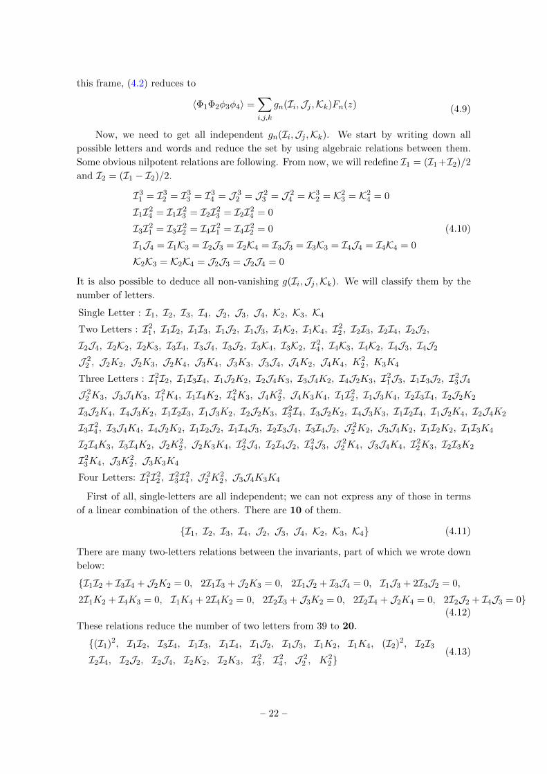
Now, we need to get all independent gn(Ii,Jj ,Kk). We start by writing down all

possible letters and words and reduce the set by using algebraic relations between them.

Some obvious nilpotent relations are following. From now, we will redefine I1 = (I1 +I2)/2

and I2 = (I1 − I2)/2.

I31 = I3

2 = I33 = I3

4 = J 32 = J 2

3 = J 24 = K3

2 = K23 = K2

4 = 0

I1I24 = I1I2

3 = I2I23 = I2I2

4 = 0

I3I21 = I3I2

2 = I4I21 = I4I2

2 = 0

I1J4 = I1K3 = I2J3 = I2K4 = I3J3 = I3K3 = I4J4 = I4K4 = 0

K2K3 = K2K4 = J2J3 = J2J4 = 0

(4.10)

It is also possible to deduce all non-vanishing g(Ii,Jj ,Kk). We will classify them by the

number of letters.

Single Letter : I1, I2, I3, I4, J2, J3, J4, K2, K3, K4

Two Letters : I21 , I1I2, I1I3, I1J2, I1J3, I1K2, I1K4, I2

2 , I2I3, I2I4, I2J2,

I2J4, I2K2, I2K3, I3I4, I3J4, I3J2, I3K4, I3K2, I24 , I4K3, I4K2, I4J3, I4J2

J 22 , J2K2, J2K3, J2K4, J3K4, J3K3, J3J4, J4K2, J4K4, K

22 , K3K4

Three Letters : I21I2, I1I3I4, I1J2K2, I2J4K3, I3J4K2, I4J2K3, I2

1J3, I1I3J2, I23J4

J 22 K3, J3J4K3, I2

1K4, I1I4K2, I24K3, J4K

22 , J4K3K4, I1I2

2 , I1J3K4, I2I3I4, I2J2K2

I3J2K4, I4J3K2, I1I2I3, I1J3K2, I2J2K3, I23I4, I3J2K2, I4J3K3, I1I2I4, I1J2K4, I2J4K2

I3I24 , I3J4K4, I4J2K2, I1I2J2, I1I4J3, I2I3J4, I3I4J2, J 2

2 K2, J3J4K2, I1I2K2, I1I3K4

I2I4K3, I3I4K2, J2K22 , J2K3K4, I2

2J4, I2I4J2, I24J3, J 2

2 K4, J3J4K4, I22K3, I2I3K2

I23K4, J3K

22 , J3K3K4

Four Letters: I21I2

2 , I23I2

4 , J 22 K

22 , J3J4K3K4

First of all, single-letters are all independent; we can not express any of those in terms

of a linear combination of the others. There are 10 of them.

{I1, I2, I3, I4, J2, J3, J4, K2, K3, K4} (4.11)

There are many two-letters relations between the invariants, part of which we wrote down

below:

{I1I2 + I3I4 + J2K2 = 0, 2I1I3 + J2K3 = 0, 2I1J2 + I3J4 = 0, I1J3 + 2I3J2 = 0,

2I1K2 + I4K3 = 0, I1K4 + 2I4K2 = 0, 2I2I3 + J3K2 = 0, 2I2I4 + J2K4 = 0, 2I2J2 + I4J3 = 0}(4.12)

These relations reduce the number of two letters from 39 to 20.

{(I1)2, I1I2, I3I4, I1I3, I1I4, I1J2, I1J3, I1K2, I1K4, (I2)2, I2I3

I2I4, I2J2, I2J4, I2K2, I2K3, I23 , I2

4 , J 22 , K2

2}(4.13)

– 22 –

Using three-letters relations

(I1)2I2 + 2I1I3I4 = I1(I2)2 + 2I2I3I4 = 2I1I2I3 + I23I4 = 2(I2)2I4 + I3I2

4 = 0 (4.14)

we can also reduce the number of three letters from 56 to 10 that are

(I1)2I2, (I1)2J3, (I1)2K4, I1(I2)2, I1I2I3, I1I2I4, I1I2J2, I1I2K2, (I2)2J4, (I2)2K3

(4.15)

Trivially, there is 1 independent four-letter:

I21I2

2 (4.16)

Hence, including the bosonic single letter I0, the total number of the independent combi-

nations of the nilpotent invariants is 1 + 10 + 20 + 10 + 1 = 42, which matches the counting

from the previous section §3, (3.33). It must be the linearly independent set, since each of

42 combinations has different number of (θ1, θ2, θ1, θ2). We further checked those of V are

all independent. Let us call the set of 42 combinations of invariants S and their general

element Si

4.4 Crossing Equations

To write down the crossing equations, we first need to derive the crossing transformed

invariants. The crossing acts on {Ii,Jj ,Kj} by exchanging (z1, z1, θ1, θ1) and (z3, z3, θ3, θ3).

The crossing symmetry imposes following constraint:∑i

SiFi(z) ∝∑i

StiFi(1− z) (4.17)

The RHS of (4.17) can be rearranged into an expansion with the same set of parameters of

LHS, since we have seen 41 combinations of the nilpotent invariants are linearly independent

and span the set of possible 4-point invariants. We could find ItI , J tj , Ktk.

It0 = − I0

I1 + I2 + 1− I0, It1 = − I1 + I2

I1 + I2 + 1− I0, It2 =

−I1 + I2 + 2I4

I1 + I2 + 1− I0, It4 =

I4

I1 + I2 + 1− I0

It3 =I4 + I2 + I3 − I1

I1 + I2 + 1− I0, J t2 =

2J4 − J2

I1 + I2 + 1− I0, J t4 =

J4

I1 + I2 + 1− I0, J t3 =

J4 + J3 − J2

I1 + I2 + 1− I0

Kt2 =2K4 −K2

I1 + I2 + 1− I0, Kt4 =

K4

I1 + I2 + 1− I0, Kt3 =

K3 +K4 −K2

I1 + I2 + 1− I0(4.18)

From this, one can deduce the crossing transformed set of the nilpotent invariants {Sti}.Given the above information, we are ready to write down the crossing equations,

starting from 1− 2, 3− 4 channel 4-point function:

〈Φ(Z1, z1)Φ(Z2, z1)Φ(Z3, z3)Φ(Z4, z4)〉 =1

Z2h12

1

Z2h34

1

z2h12 z

2h34

(g0(I0, z) +

41∑i=1

Sigi(I0, z))

(4.19)

– 23 –

where Si ∈ S. Here we coupled with a left-moving non-supersymmetric conformal block

that adds z dependence. The crossing channel is

〈Φ(Z3, z3)Φ(Z2, z2)Φ(Z1, z1)Φ(Z4, z4)〉 =1

Z2h32

1

Z2h14

1

z2h32 z

2h14

(g0(St0, z) +

41∑i=1

Stigi(St0, z))

(4.20)

The crossing equation is then

g0(I0, z) +41∑i=1

Sigi(I0, z) = (I0 − I1 − I2 − 1)2h

(z

z − 1

)2h(g0(St0, 1− z) +

41∑i=1

Stigi(St0, 1− z))

(4.21)

4.5 Casimir equation

Now, it remains to solve gn(z, z) that take following form.

gn(z) = c1ng

h12,h34h (z) + c2

ngh12,h34h+ 1

2

(z) + c3ng

h12,h34h+1 (z) + c4

ngh12,h34h+ 3

2

(z) + c5ng

h12,h34h+2 (z) (4.22)

The reason for this particular decomposition is explained around (4.3). By solving gn(z, z),

we mean that we solve for cni with n = 1, . . . , 42, i = 1, . . . , 5 using following set of coupled

differential equations [44], which are called Casimir differential equations:

C(2)

g0

g1

. . .

g40

= D[I0]

g0

g1

. . .

g40

= c2

g0

g1

. . .

g40

(4.23)

where D[I0] is a matrix of differential operators with respect to I0 and c2 is a 42 × 42

matrix with constant that depends on h.

We derived the quadratic Casimir for N = 4.

C2 =(L2

0 −1

2{L1, L−1}

)−((T 3

0 )2 +1

2{T+

0 , T−0 })

+1

4εαβ(−Gα− 1

2

Gβ12

− Gα− 12

Gβ12

+Gα12

Gβ− 12

+ Gα12

Gβ− 12

)(4.24)

The way to derive it is to start from the most general ansatz C2 =∑

i∈b∪f ciGi that is a

linear combination of all possible quadratic global generators that are invariant under the

global N = 4 superconformal algebra and fix the coefficients using the algebra, where

Quadratic Bosonic Generators: b = {L∓L±, L0L0, T∓T±, T 0T 0, L0T 0}

Quadratic Fermionic Generators: f = {Gi− 12

Gj12

, Gi− 12

Gj12

, Gi12

Gj− 12

, Gi12

Gj− 12

}, i, j = 1, 2

(4.25)

After moving to the convenient frame x3 → 0, x4 →∞, θ3, θ4, θ3, θ4 → 0, the Casimir

operators only act on first two operators of 4-point function 〈Φ1Φ2φ3φ4〉. Hence, we need

– 24 –

to get the two particle Casimir operator, similar to [45].

C(2)12 =

(L

(1)0 + L

(2)0

)2 − 1

2{(L(1)

−1 + L(2)−1), (L

(1)+1 + L

(2)+1)} − 1

4

((T

(1)0 + T

(2)0

)2 − 1

2{(T (1)−1 + T

(2)−1 ), (T

(1)+1 + T

(2)+1 )}

)+

1

2

[(G

(1)12

+ G(2)12

),(G

(1)

− 12

+G(2)

− 12

)]+

1

2

[(G

(1)12

+G(2)12

),(G

(1)

− 12

+ G(2)

− 12

)]= 2c2 + 2L

(1)0 L

(2)0 − L

(1)−1L

(2)+1 − L

(1)+1L

(2)−1 −

1

4

(2T

(1)0 T

(2)0 − T (1)

−1 T(2)+1 − T

(1)+1 T

(2)−1

)+ G

(1)12

G(2)

− 12

−G(1)

− 12

G(2)12

+G(1)12

G(2)

− 12

− G(1)

− 12

G(2)12

(4.26)

Here, the superscripts (1), (2) in the parenthesis refer to first two long-multiplets Φ1, Φ2.

4.6 The puzzle

To solve the Casimir equation, we need to know the superspace representation of N = 4

superconformal algebra generators that consist of the quadratic Casimir operator (4.24).

For simple notation, let us re-introduce small N = 4 superconformal algebra with the

outer-automorphism manifest. The global N = 4 superconformal algebra is

[Lm, Ln] = (m− n)Lm+n, [T i0, Tj0 ] = iεijkT k0 ,

[Lm, GαAr ] =

(m2− r)GαAm+r, [T i0, G

αAr ] = −1

2(σi)β

αGβAr .

{GαA− 12

, GβB− 12

} = 2εαβεABL−1,

{GαA− 12

, GβB12

} = 2εαβεABL0 + 2εAB(σa)αβT a0 ,

{GαA12

, GβB12

} = 2εαβεABL−1,

(4.27)

for i = 1, 2, 3, m,n = 0,±1 and r = ±12 . Here, α, β indices are that of SU(2)F outer-

automorphism of small N = 4 superconformal algebra.

To find the superspace representation of each generator, we start with the most general

ansatz and fix the coefficients {p, q, r, s, t, u, v, w, y} in front of each term.

L−1 = ∂z, L0 = z∂z + pθ∂θ, L1 = z2∂z + qzθ∂θ,

T a0 = rθγC(σa)γδ∂θδC ,

GαA− 12

= sεαβεAB∂θβB + tθαA∂z,

GαA12

= uεαβεABz∂θβB + vθαAθβB∂θβB + wθβAθαB∂θβB + yθαAz∂z.

(4.28)

By using (4.27), we can try to fix the coefficients. However, there is no non-trivial set of

solution for the coefficients.3 As we did not have a superspace representation of each gen-

erator, we could not set up the Casimir differential equation that would solve to coefficients

in the conformal block expansions.

3We thank Carlo Meneghelli for explaining that this problem can be resolved by using more general

algebra than (4.28).

– 25 –

5 Discussion

In this paper, we initiated general 2d N = 4 superconformal bootstrap study, using the

long-multiplets. As we have not specified any other properties of theory, other than N = 4

superconformal symmetry, our analysis is general, but at the same time lack of decorations

that could arise from global symmetries and analysis of BPS 4-point functions. This study

provides the starting point for the numerical bootstrap analysis using the standard methods

[46, 47]. Also, since our superspace analysis is incomplete, it would be interesting to resolve

the problem that we pointed out. Other than these obvious directions, there are several

ways to use this set-up by imposing more input depending on the specific theories that

preserve N = 4 superconformal symmetry.

Different from N = 2 theories, N = 4 theory has the stress energy tensor in short-

multiplet. Rather than considering the long-multiplet 4-point function 〈L0L0L0L0〉, we can

consider the short-multiplet 4-point function of L2 that contains the stress energy tensor

at the top. Because the stress energy tensor is a universal ingredient of any CFT [48], this

will also provide a general information on N = 4 CFTs. Moreover, we expect a L2 4-point

function, though it is BPS, may give a different restriction that L0 4-point function could

not impose. Since the length of the multiplet and the number of components are reduced

significantly in the BPS multiplet, we expect efficient numerical analysis here.

CFTs with a global symmetry will give more stringent bounds, since there is a non-

trivial relation between the level of Kac-Moody algebra and total central charge. Especially,

there is a series of interesting (0, 4) theories with E8 global symmetry that arises from IR

limit of E-string worldsheet gauge theories [23, 24]. The gauge theory lives on N D2 brane

worldvolume(012 direction); it has finite length(L) in direction 2 and extends between NS5

brane and D8/O8 complex. By taking L small, there appears 2d O(N) supersymmetric

gauge theory with SO(16) global symmetry. Flowing into deep IR(semi-classical limit or

Higgs branch [25]), one expects to get 2d (0, 4) superconformal theory with a central charge

(cL, cR) = (6N, 12N) and a global symmetry E8. It would be interesting to study this series

of CFT labeled by the number of E-strings and it would be also very interesting to see if

there is another IR limit that comes from a different choice of IR R-symmetry, which was

once suggested in [24]. Other big family of (0, 4) theories [26, 27] comes from a twisted

compactification4 of class-S theory, and [30] from the brane box model, which are another

interesting models to study using the bootstrap technique.

Lastly, our analysis can be used to study 4d N = 4 SYM or SCFT, as 2d small N = 4

chiral algebra appears in a particular twisted Q−cohomology of 4d N = 4 SCFT [31]. [32]

mentioned this fact in their 4d N = 4 numerical bootstrap analysis, but did an honest 4d

superconformal block computation to construct 4-point functions and crossing equations.

It would be interesting to use our result to study the 4d N = 4 SCFT as we have much

more crossing equations that can give more stringent bounds.

4We thank an anonymous referee of JHEP, who pointed out the original reference [26] for this topological

twisting.

– 26 –

Acknowledgements

We thank Chi-Ming Chang for his collaboration in early stage of the project, especially his

observation on the subtlety of N = 4 superspace. We are also grateful to Ori Ganor for

comments on the draft, and crucial advice in various stages of this project. We thank the

organizers and participants in the 2017, 2018 Simons Bootstrap conference, where a part of

the work was done. We especially thank Carlo Meneghelli for his comment on our paper,

pointing out the possible resolution of our puzzle. This research was supported in part

by the Berkeley Center of Theoretical Physics. The research of JO was supported in part

by Kwanjeong Educational Foundation and by the Visiting Graduate Fellowship Program

at the Perimeter Institute for Theoretical Physics. Research at the Perimeter Institute is

supported by the Government of Canada through Industry Canada and by the Province

of Ontario through the Ministry of Economic Development & Innovation.

A 3-point invariants of N = 4 superspace

The idea is to start with arbitrary 3 superspace coordinates (zi, θi, θi), with i = 1, 2, 3, and

perform superconformal transformations 5 to set

z2 = 0, z3 =∞, θ2 = θ3 = 0, θ2 = θ3 = 0,

then, construct the dilatation invariant θ′1θ′1/z′1 from the resulting (z′1, θ

′1, θ′1). The details

are below.

We use following conventions (for α, β = 1, 2 and a = 1, 2, 3):

θα = εαβθβ, θα = εαβ θβ, σa := (σa)αβ, (σi)α

β = εαα′εββ′(σa)α

′β′ , εαβ = −εαβ (A.1)

For two doublets ψα and χα,

ψχ := ψαχα = εαβψαχβ = −χαψα = χαψα = χψ

Inversion acts on the superspace coordinates by

I : (z, θ, θ) → (−1/z, θ/z, θ/z) (A.2)

Also, as usual, rigid SUSY with parameters εα acts as

δzi = −εθi + εθi , δθi = ε , δθi = ε (A.3)

Denote

zij := zi − zj , θij := θi − θj , θij := θi − θj .

Then θij , θij , and

Zij := zij + θiθj − θj θi5We are grateful to Ori Ganor for sharing his unpublished notes that show preliminary result for the

3-point invariant of N = 4 superspace [49]

– 27 –

are invariant under (A.3).

A noninfinitesimal SUSY transformation with parameters η and η acts as

z → z − ηθ + ηθ , θ → θ + η , θ → θ + η

Then we construct a large superconformal transformation from a translation by (ζ1, η1, η1)

followed by inversion, followed by translation by (ζ2, η2, η2), followed by dilatation by λ

(the dilatation will be implicit).

z → z−η1θ+η1θ+ζ1 → −1

z − η1θ + η1θ + ζ1, θ → θ + η1

z − η1θ + η1θ + ζ1, θ → θ + η1

z − η1θ + η1θ + ζ1

Next,

θ + η1

z − η1θ + η1θ + ζ1→ θ + η1

z − η1θ + η1θ + ζ1+η2 ,

θ + η1

z − η1θ + η1θ + ζ1→ θ + η1

z − η1θ + η1θ + ζ1+η2 ,

− 1

z − η1θ + η1θ + ζ1→

− 1

z − η1θ + η1θ + ζ1− η2

(θ + η1

z − η1θ + η1θ + ζ1

)+ η2

(θ + η1

z − η1θ + η1θ + ζ1

)+ ζ2

So, altogether

z → z′ := ζ2 +−η2θ + η2θ − η2η1 + η1η2 − 1

z − η1θ + η1θ + ζ1

θ → θ′ :=θ + η1

z − η1θ + η1θ + ζ1+ η2 , θ → θ′ :=

θ + η1

z − η1θ + η1θ + ζ1+ η2

Now we start with three superspace coordinates (zi, θi, θi) with i = 1, 2, 3. Let us first set

z′3 =∞ by setting

ζ1 = −z3 + η1θ3 − η1θ3 .

Next, we require θ′3 and θ′3 to be finite (and therefore zero after inversion) by setting

η1 = −θ3, η1 = −θ3

Thus,

ζ1 = −z3 + η1θ3 − η1θ3 = −z3 − θ3θ3 + θ3θ3 = −z3

Next, we require z′2 = 0 by setting

ζ2 =η2θ2 − η2θ2 + η2η1 − η1η2 + 1

z2 − η1θ2 + η1θ2 + ζ1=η2θ2 − η2θ2 − η2θ3 + θ3η2 + 1

z23 + θ3θ2 − θ3θ2=η2θ23 − η2θ23 + 1

Z23

We also require θ′2 = θ′2 = 0 by setting

0 =θ2 + η1

z2 − η1θ2 + η1θ2 + ζ1+ η2

– 28 –

and

0 =θ2 + η1

z2 − η1θ2 + η1θ2 + ζ1+ η2

Thus

η2 = − θ2 + η1

z2 − η1θ2 + η1θ2 + ζ1= − θ23

Z23(A.4)

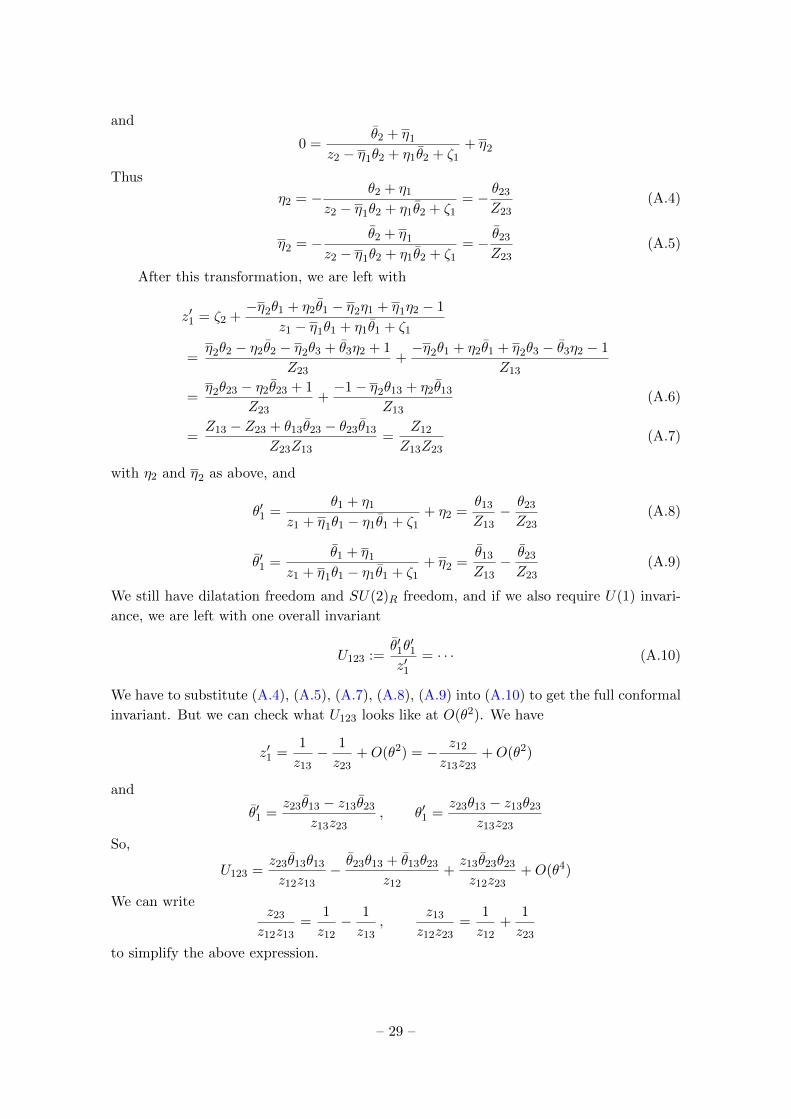
η2 = − θ2 + η1

z2 − η1θ2 + η1θ2 + ζ1= − θ23

Z23(A.5)

After this transformation, we are left with

z′1 = ζ2 +−η2θ1 + η2θ1 − η2η1 + η1η2 − 1

z1 − η1θ1 + η1θ1 + ζ1

=η2θ2 − η2θ2 − η2θ3 + θ3η2 + 1

Z23+−η2θ1 + η2θ1 + η2θ3 − θ3η2 − 1

Z13

=η2θ23 − η2θ23 + 1

Z23+−1− η2θ13 + η2θ13

Z13(A.6)

=Z13 − Z23 + θ13θ23 − θ23θ13

Z23Z13=

Z12

Z13Z23(A.7)

with η2 and η2 as above, and

θ′1 =θ1 + η1

z1 + η1θ1 − η1θ1 + ζ1+ η2 =

θ13

Z13− θ23

Z23(A.8)

θ′1 =θ1 + η1

z1 + η1θ1 − η1θ1 + ζ1+ η2 =

θ13

Z13− θ23

Z23(A.9)

We still have dilatation freedom and SU(2)R freedom, and if we also require U(1) invari-

ance, we are left with one overall invariant

U123 :=θ′1θ′1

z′1= · · · (A.10)

We have to substitute (A.4), (A.5), (A.7), (A.8), (A.9) into (A.10) to get the full conformal

invariant. But we can check what U123 looks like at O(θ2). We have

z′1 =1

z13− 1

z23+O(θ2) = − z12

z13z23+O(θ2)

and

θ′1 =z23θ13 − z13θ23

z13z23, θ′1 =

z23θ13 − z13θ23

z13z23

So,

U123 =z23θ13θ13

z12z13− θ23θ13 + θ13θ23

z12+z13θ23θ23

z12z23+O(θ4)

We can writez23

z12z13=

1

z12− 1

z13,

z13

z12z23=

1

z12+

1

z23

to simplify the above expression.

– 29 –

More explicitly, the U123 is

U123 =θ′1θ′1

z′1=Z13Z23

Z12

(θ13

Z13− θ23

Z23

)(θ13

Z13− θ23

Z23

)=

(θ13Z23 − θ23Z13)(θ13Z23 − θ23Z13)

Z12Z13Z23

=θ13θ13Z

223 + θ23θ23Z

213 − Z13Z23(θ13θ23 + θ23θ13)

Z12Z13Z23.

(A.11)

B 2-point function normalization

Here, we collected all relevant 2-point function normalization. We also submitted Mathe-

matica files that have the same information.

B.1 L0

We order and number each component fields of L0 from bottom component to top compo-

nent.

L0 = {φ, ψ1, ψ2, χ1, χ2, τ, τ , t0, t1t , t

2t , t

3t , C

1, C2, C1, C2, d} = {F1,F2, . . . ,F16} (B.1)

Below, fi,j refers to 〈FiFj〉 normalization constant.

f1,1 = F0, f2,5 = f5,2 = 2hF0, f3,4 = f4,3 = 2hF0, f6,7 = f7,6 = 4h(1 + h)F0, f8,8 = 8h(1 + h)F

f9,11 = f11,9 = 4h2F0, f10,10 = 2h2F0, f12,15 = f15,12 =16h2(1 + h)2

1 + 2hF0,

f13,14 = f14,13 =16h2(1 + h)2

1 + 2hF0, f16,16 =

16h2(1 + h)2(3 + 2h)

1 + 2hF0

(B.2)

In other words, all the normalization constants are determined up to a constant F0.

B.2 L1

We first fix the order and number the components

L1 ={φ[1], ψ[0], ψ[2], χ[0], χ[2], τ [1], τ [1], t1[1], t2[1], t[3], C[0], C[2], C[0], C[2], d[1]} = {F1,F2, . . . ,F32}(B.3)

Here, for non-trivial representations of su(2)R, such as φ[1], we aligned from bottom

component to top component of R-symmetry multiplet. For instance, φ[1] = {F1,F2},ψ[0] = {F3}, ψ[2] = {F4,F5,F6}. Below, fi,j refers to 〈FiFj〉 normalization constant.6

f1,2 = −f2,1 = F1, f3,7 = f7,3 = −2(3 + 2h)f1,2, f4,10 = −f10,4 = (1− 2h)F1, f5,9 = −f9,5 =1− 2h

2F1,

f6,8 = f8,6 = (1− 2h)F1, f11,14 = −f14,11 = (1− 2h)(3 + 2h)F1, f12,13 = −f13,12 = (2h− 1)(3 + 2h)F1,

6In practical use in numerics, one needs positive normalization. Since the - signs in some of fi,j come

from our definitions of operators, they further need to be re-defined.

– 30 –

f15,16 = −f16,15 =(1− 2h)(3 + 2h)

2hF1, f15,18 = −f18,15 =

(1− 2h)(3 + 2h)(3 + 4h)

2hF1,

f16,17 = −f17,16 =(2h− 1)(3 + 2h)(3 + 4h)

2hF1, f17,18 = −f18,17 =

(1− 2h)(3 + 2h)2

2hF1,

f19,22 = −f22,19 = −(1− 2h)2F1, f20,21 =(1− 2h)2

3F1, f23,27 = −f27,23 =

4(1 + h)(1− 2h)(3 + 2h)2

1 + 2hF1,

f24,30 = −f30,27 = −2(1− 2h)2(1 + h)(3 + 2h)

1 + 2hF1, f25,29 = −f29,25 =

(1− 2h)2(1 + h)(3 + 2h)

1 + 2hF1,

f31,32 = −f32,31 =(1− 2h)2(3 + 2h)3

1 + 2hF1

(B.4)

Similar to above, all the 2-point normalizations are fixed up to a constant F1.

B.3 L2

We first fix the order and number the components

L2 ={φ[2], ψ[1], ψ[3], χ[1], χ[3], τ [2], τ [2], t[0], t1[2], t2[2], t[4], C[1], C[3], C[1], C[3], d[2]}={F1, . . . ,F48}

(B.5)

Similarly, we pick the same order in the R-symmetry multiplet as above.

f1,3 = F2, f2,2 =1

2F2, f4,11 = f11,4 = 3(2 + h)F2, f5,10 = f10,5 = 3(2 + h)F2,

f6,15 = f15,6 = 2(h− 1)F2 f7,14 = f14,7 =2(−1 + h)

3F2, f8,13 = f13,8 =

2(1− h)

3F2,

f9,12 = f12,9 = 2(−1 + h)F2, f16,21 = f21,16 = 4(1− h)(2 + h)F2,

f17,20 = f20,17 = 2(h− 1)(2 + h)F, f18,19 = f19,18 = 4(1− h)(2 + h)F2, f22,22 = 12(2 + h)2F2,

f23,25 = f25,23 =2(1− h)(2 + h)2

hF2, f23,28 =

2(1− h)(4 + 8h+ 3h2)

hF2,

f24,24 =(h− 1)(2 + h)2

hF2, f24,27 = f27,24 =

(−1 + h)(2 + h)(2 + 3h)

hF2,

f25,26 = f26,25 =2(1− h)(4 + 8h+ 3h2)

hF2, f26,28 = f28,26 =

2(1− h)(2 + h)2

hF2,

f29,33 = 4(h− 1)2F2, f30,32 = f32,30 = (h− 1)2F2, f31,31 =2

3(h− 1)2F,

f34,41 = f41,34 =24(1− h)(1 + h)(2 + h)2

1 + 2hF2, f35,40 = f40,35 =

24(h− 1)(1 + h)(2 + h)2

1 + 2hF2,

f36,45 = f45,36 =16(h− 1)2(2 + 3h+ h2)

1 + 2hF2, f37,44 = f44,37 =

16(h− 1)2(2 + 3h+ h2)

3 + 6hF2,

f38,43 = f43,38 =16(h− 1)2(2 + 3h+ h2)

3 + 6hF2, f39,42 = f42,39 =

16(−1 + h)2(2 + 3h+ h2)

1 + 2hF2,

f46,48 = f48,46 =16(3 + 2h)(−2 + h+ h2)2

1 + 2hF2, f47,47 =

8(3 + 2h)(−2 + h+ h2)2

1 + 2hF2

(B.6)

– 31 –

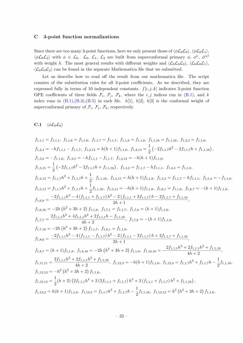
C 3-point function normalizations

Since there are too many 3-point functions, here we only present those of 〈φL0L0〉, 〈φL0L1〉,〈φL0L2〉 with φ ∈ L0. L0, L1, L2 are built from superconformal primary φ, φα, φαβ

with weight h. The most general results with different weights and 〈L0L0L0〉, 〈L0L0L1〉,〈L0L0L2〉 can be found in the separate Mathematica file that we submitted.

Let us describe how to read off the result from our mathematica file. The script

consists of the substitution rules for all 3-point coefficients. As we described, they are

expressed fully in terms of 10 independent constants. f [i, j, k] indicates 3-point function

OPE coefficients of three fields Fi, Fj , Fk, where the i, j indices run in (B.1), and k

index runs in (B.1),(B.3),(B.5) in each file. h[1], h[2], h[3] is the conformal weight of

superconformal primary of Fi, Fj , Fk, respectively.

C.1 〈φL0L0〉

f1,1,1 = f1,1,1, f1,1,6 = f1,1,6, f1,1,7 = f1,1,7, f1,1,8 = f1,1,8, f1,1,16 = f1,1,16, f1,2,3 = f1,1,6,

f1,2,4 = −hf1,1,1 − f1,1,7, f1,2,13 = h(h+ 1)f1,1,6, f1,2,14 =1

2

(−2f1,1,7h

2 − 2f1,1,7h+ f1,1,16

),

f1,3,2 = −f1,1,6, f1,3,5 = −hf1,1,1 − f1,1,7, f1,3,12 = −h(h+ 1)f1,1,6,

f1,3,15 =1

2

(−2f1,1,7h

2 − 2f1,1,7h+ f1,1,16

), f1,4,2 = f1,1,7 − hf1,1,1, f1,4,5 = f1,1,8,

f1,4,12 = f1,1,7h2 + f1,1,7h+

1

2, f1,1,16, f1,4,15 = h(h+ 1)f1,1,8, f1,5,3 = f1,1,7 − hf1,1,1, f1,5,4 = −f1,1,8,

f1,5,13 = f1,1,7h2 + f1,1,7h+

1

2f1,1,16, f1,5,14 = −h(h+ 1)f1,1,8, f1,6,1 = f1,1,6, f1,6,7 = −(h+ 1)f1,1,6,

f1,6,8 =−2f1,1,1h

3 − 4 (f1,1,1 + f1,1,7)h2 − 2 (f1,1,1 + 3f1,1,7)h− 2f1,1,7 + f1,1,16

2h+ 1,

f1,6,16 = −2h(h2 + 3h+ 2

)f1,1,6, f1,7,1 = f1,1,7, f1,7,6 = (h+ 1)f1,1,6,

f1,7,7 =2f1,1,1h

3 + 4f1,1,1h2 + 2f1,1,1h− f1,1,16

4h+ 2, f1,7,8 = −(h+ 1)f1,1,8,

f1,7,16 = −2h(h2 + 3h+ 2

)f1,1,7, f1,8,1 = f1,1,8,

f1,8,6 =−2f1,1,1h

3 − 4 (f1,1,1 − f1,1,7)h2 − 2 (f1,1,1 − 3f1,1,7)h+ 2f1,1,7 + f1,1,16

2h+ 1,

f1,8,7 = (h+ 1)f1,1,8, f1,8,16 = −2h(h2 + 3h+ 2

)f1,1,8, f1,10,10 = −2f1,1,1h

3 + 2f1,1,1h2 + f1,1,16

4h+ 2,

f1,11,11 =2f1,1,1h

3 + 2f1,1,1h2 + f1,1,16

4h+ 2, f1,12,3 = −h(h+ 1)f1,1,6, f1,12,4 = f1,1,7h

2 + f1,1,7h−1

2f1,1,16,

f1,12,13 = −h2(h2 + 3h+ 2

)f1,1,6,

f1,12,14 =1

2(h+ 2)

(2f1,1,1h

4 + 2 (2f1,1,1 + f1,1,7)h3 + 2 (f1,1,1 + f1,1,7)h2 + f1,1,16

),

f1,13,2 = h(h+ 1)f1,1,6, f1,13,5 = f1,1,7h2 + f1,1,7h−

1

2f1,1,16, f1,13,12 = h2

(h2 + 3h+ 2

)f1,1,6,

– 32 –

f1,13,15 =1

2(h+ 2)

(2f1,1,1h

4 + 2 (2f1,1,1 + f1,1,7)h3 + 2 (f1,1,1 + f1,1,7)h2 + f1,1,16

),

f1,14,2 = −f1,1,7h2 − f1,1,7h−

1

2f1,1,16, f1,14,5 = −h(h+ 1)f1,1,8,

f1,14,12 =1

2(h+ 2)

(2f1,1,1h

4 + (4f1,1,1 − 2f1,1,7)h3 + 2 (f1,1,1 − f1,1,7)h2 + f1,1,16

),

f1,14,15 = −h2(h2 + 3h+ 2

)f1,1,8, f1,15,3 = −f1,1,7h

2 − f1,1,7h−1

2f1,1,16, f1,15,4 = h(h+ 1)f1,1,8,

f1,15,13 =1

2(h+ 2)

(2f1,1,1h

4 + (4f1,1,1 − 2f1,1,7)h3 + 2 (f1,1,1 − f1,1,7)h2 + f1,1,16

),

f1,15,14 = h2(h2 + 3h+ 2

)f1,1,8, f1,16,1 = f1,1,16, f1,16,6 = −2h

(h2 + 3h+ 2

)f1,1,6,

f1,16,7 = −2h(h2 + 3h+ 2

)f1,1,7, f1,16,8 = −2h

(h2 + 3h+ 2

)f1,1,8,

f1,16,16 = 2(h2 + 5h+ 6

) (2f1,1,1h

4 + 4f1,1,1h3 + 2f1,1,1h

2 + f1,1,16

)(C.1)

C.2 〈φL0L1〉

f1,1=,3 = f1,1,3, f1,1,7 = f1,1,7, f1,1,23 = f1,1,23, f1,1,27 = f1,1,27, f1,2,2 =1

2f1,1,3,

f1,2,14 =2(2h+ 1)f1,1,27 − (−2h− 1)(2h− 1)f1,1,7

8h+ 4, f1,2,16 = f1,1,23 −

(−2h− 1)(4h2 + 4h− 3

)f1,1,3

8h(2h+ 1),

f1,2,18 =1

2f1,1,23 −

(−2h− 1)(8h2 + 2h− 3

)f1,1,3

8h(2h+ 1), f1,2,32 = −(−2h− 3)(2h− 1)f1,1,23

8(h+ 1),

f1,4,2 =1

2f1,1,7, f1,4,12 =

(−2h− 1)(2h− 1)f1,1,3 + 2(2h+ 1)f1,1,23

8h+ 4,

f1,4,16 = −(−2h− 1)

(8h2 + 2h− 3

)f1,1,7

8h(2h+ 1)− 1

2f1,1,27, f1,4,18 = −

(−2h− 1)(4h2 + 4h− 3

)f1,1,7

8h(2h+ 1)− f1,1,27,

f1,4,32 =(−2h− 3)(2h− 1)f1,1,27

8(h+ 1), f1,6,7 =

2(2h+ 1)f1,1,23 − (−2h− 1)(2h+ 3)f1,1,3

4h+ 2,

f1,6,27 = −(−2h− 3)(2h− 1) ((−2h− 1)(2h+ 3)f1,1,3 − 2(2h+ 1)f1,1,23)

4(2h+ 1)2,

f1,7,3 =(−2h− 1)(2h+ 3)f1,1,7 + 2(2h+ 1)f1,1,27

4h+ 2,

f1,7,23 = −(−2h− 3)(2h− 1) ((−2h− 1)(2h+ 3)f1,1,7 + 2(2h+ 1)f1,1,27)

4(2h+ 1)2,

f1,8,3 =2(2h+ 1)f1,1,23 − (−2h− 1)(2h+ 3)f1,1,3

4h+ 2, f1,8,7 =

(−2h− 1)(2h+ 3)f1,1,7 + 2(2h+ 1)f1,1,27

4h+ 2,

f1,8,23 =(−2h− 3)(2h− 1) ((−2h− 1)(2h+ 3)f1,1,3 − 2(2h+ 1)f1,1,23)

4(2h+ 1)2,

f1,8,27 =(−2h− 3)(2h− 1) ((−2h− 1)(2h+ 3)f1,1,7 + 2(2h+ 1)f1,1,27)

4(2h+ 1)2,

f1,9,6 = −(−2h− 1)(2h− 1)f1,1,3 + 2(2h+ 1)f1,1,23

8h+ 4, f1,9,10 =

2(2h+ 1)f1,1,27 − (−2h− 1)(2h− 1)f1,1,7

8h+ 4,

– 33 –

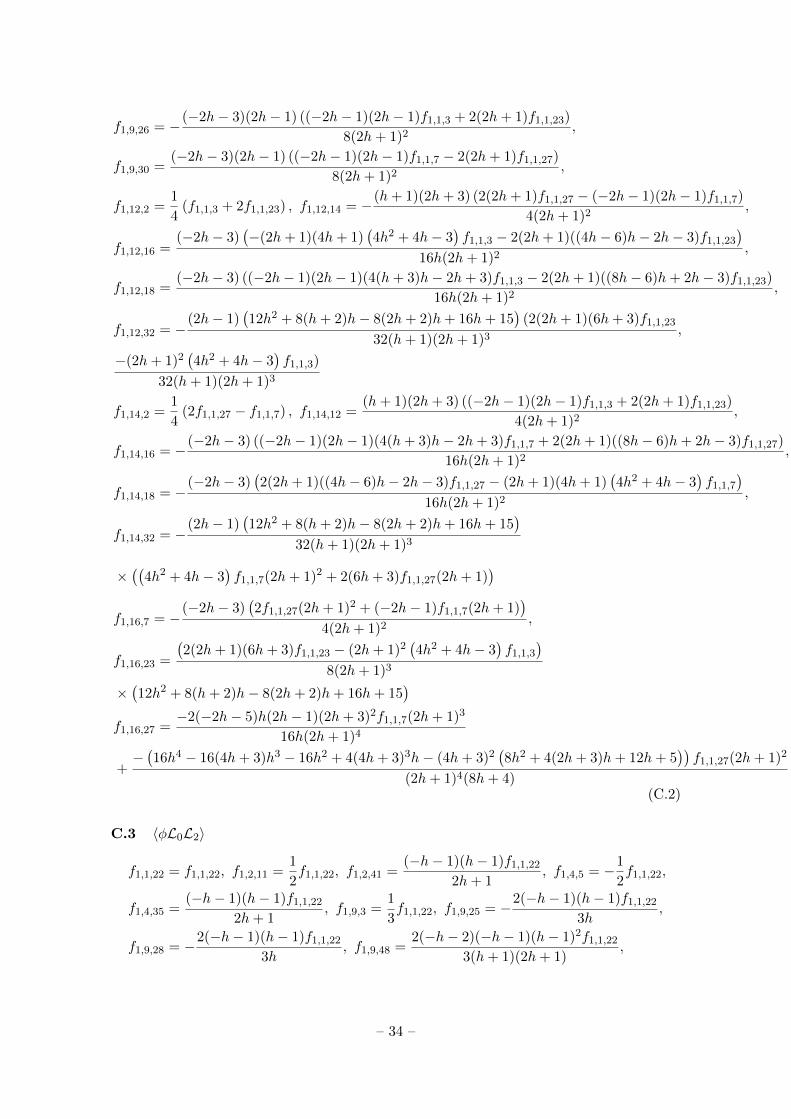
f1,9,26 = −(−2h− 3)(2h− 1) ((−2h− 1)(2h− 1)f1,1,3 + 2(2h+ 1)f1,1,23)

8(2h+ 1)2,

f1,9,30 =(−2h− 3)(2h− 1) ((−2h− 1)(2h− 1)f1,1,7 − 2(2h+ 1)f1,1,27)

8(2h+ 1)2,

f1,12,2 =1

4(f1,1,3 + 2f1,1,23) , f1,12,14 = −(h+ 1)(2h+ 3) (2(2h+ 1)f1,1,27 − (−2h− 1)(2h− 1)f1,1,7)

4(2h+ 1)2,

f1,12,16 =(−2h− 3)

(−(2h+ 1)(4h+ 1)

(4h2 + 4h− 3

)f1,1,3 − 2(2h+ 1)((4h− 6)h− 2h− 3)f1,1,23

)16h(2h+ 1)2

,

f1,12,18 =(−2h− 3) ((−2h− 1)(2h− 1)(4(h+ 3)h− 2h+ 3)f1,1,3 − 2(2h+ 1)((8h− 6)h+ 2h− 3)f1,1,23)

16h(2h+ 1)2,

f1,12,32 = −(2h− 1)

(12h2 + 8(h+ 2)h− 8(2h+ 2)h+ 16h+ 15

)(2(2h+ 1)(6h+ 3)f1,1,23

32(h+ 1)(2h+ 1)3,

−(2h+ 1)2(4h2 + 4h− 3

)f1,1,3)

32(h+ 1)(2h+ 1)3

f1,14,2 =1

4(2f1,1,27 − f1,1,7) , f1,14,12 =

(h+ 1)(2h+ 3) ((−2h− 1)(2h− 1)f1,1,3 + 2(2h+ 1)f1,1,23)

4(2h+ 1)2,

f1,14,16 = −(−2h− 3) ((−2h− 1)(2h− 1)(4(h+ 3)h− 2h+ 3)f1,1,7 + 2(2h+ 1)((8h− 6)h+ 2h− 3)f1,1,27)

16h(2h+ 1)2,

f1,14,18 = −(−2h− 3)

(2(2h+ 1)((4h− 6)h− 2h− 3)f1,1,27 − (2h+ 1)(4h+ 1)

(4h2 + 4h− 3

)f1,1,7

)16h(2h+ 1)2

,

f1,14,32 = −(2h− 1)

(12h2 + 8(h+ 2)h− 8(2h+ 2)h+ 16h+ 15

)32(h+ 1)(2h+ 1)3

×((

4h2 + 4h− 3)f1,1,7(2h+ 1)2 + 2(6h+ 3)f1,1,27(2h+ 1)

)f1,16,3 = −

(2h+ 3)(2(2h+ 1)2f1,1,23 − (−2h− 1)(2h+ 1)f1,1,3

)4(2h+ 1)2

,

f1,16,7 = −(−2h− 3)

(2f1,1,27(2h+ 1)2 + (−2h− 1)f1,1,7(2h+ 1)

)4(2h+ 1)2

,

f1,16,23 =

(2(2h+ 1)(6h+ 3)f1,1,23 − (2h+ 1)2

(4h2 + 4h− 3

)f1,1,3

)8(2h+ 1)3

×(12h2 + 8(h+ 2)h− 8(2h+ 2)h+ 16h+ 15

)f1,16,27 =

−2(−2h− 5)h(2h− 1)(2h+ 3)2f1,1,7(2h+ 1)3

16h(2h+ 1)4

+−(16h4 − 16(4h+ 3)h3 − 16h2 + 4(4h+ 3)3h− (4h+ 3)2

(8h2 + 4(2h+ 3)h+ 12h+ 5

))f1,1,27(2h+ 1)2

(2h+ 1)4(8h+ 4)(C.2)

C.3 〈φL0L2〉

f1,1,22 = f1,1,22, f1,2,11 =1

2f1,1,22, f1,2,41 =

(−h− 1)(h− 1)f1,1,22

2h+ 1, f1,4,5 = −1

2f1,1,22,

f1,4,35 =(−h− 1)(h− 1)f1,1,22

2h+ 1, f1,9,3 =

1

3f1,1,22, f1,9,25 = −2(−h− 1)(h− 1)f1,1,22

3h,

f1,9,28 = −2(−h− 1)(h− 1)f1,1,22

3h, f1,9,48 =

2(−h− 2)(−h− 1)(h− 1)2f1,1,22

3(h+ 1)(2h+ 1),

– 34 –

f1,12,11 = −(h+ 1)2f1,1,22

2h+ 1,

f1,12,41 =2(h− 1)(h+ 1)

(3h2 + (2h+ 3)h− (4h+ 3)h+ 3h+ 2

)f1,1,22

(2h+ 1)2, f1,14,5 = −(h+ 1)2f1,1,22

2h+ 1,

f1,14,35 = −2(h− 1)(h+ 1)

(3h2 + (2h+ 3)h− (4h+ 3)h+ 3h+ 2

)f1,1,22

(2h+ 1)2,

f1,16,22 =2(h+ 1)

(3h2 + (2h+ 3)h− (4h+ 3)h+ 3h+ 2

)f1,1,22

2h+ 1(C.3)

D Sample crossing equations

In this appendix, we collect sample crossing equations obtained from 〈ψ1χ2φφ〉, 〈φφφφ〉and 〈ψ2C2φφ〉. We will use following notation for Virasoro conformal block:

g[z, z, h12, h34, hex − h] = gh12,h34hex(z)gh12,h34

hex(z)

gh12,h34hex(z) = zhex2F1(hex − h12, hex + h34, 2hex, z)

(D.1)

where h is the conformal weight for superconformal primary of L0,L1,L2, and hex is the

conformal weight for exchanged operator.

In the mathematica file, we showed all the crossing equations that were obtained by

studying long-multiplet 4-point function of L0. H is the conformal weight of the supercon-

formal primary of L0.

Crossing equations obtained from 〈ψ1χ2φφ〉 are

1. − 96h3(6 + 13h+ 9h2 + 2h3

)2 (−3− 4h+ 12h2 + 16h3)

×(z1+2hz2hg

[1− z, 1− z 1

2,1

2,1

2

]+ 2(1− z)

12

+2h(1− z)2hg[z, z, 0, 0, 0]

)= 0

2. −24h(6 + 7h+ 2h2

)2 (−3− h+ 10h2 + 8h3)(

2(1 + 3h+ 2h2

)z1+2hz2hg

[1− z, 1− z, 1

2,1

2,1

2

]−

h

((1 + h)z1+2hz2hg

[1− z, 1− z, 1

2,1

2,3

2

]+ 4(1 + 2h)(1− z)

12

+2h(1− z)2hg[z, z, 0, 0, 1]))

= 0

3. 12(2 + 5h+ 2h2

)2 (−9 + 28h2 + 16h3)(

(3 + 2h)z1+2hz2hg

[1− z, 1− z, 1

2,1

2,3

2

]−

(1 + 3h)(1− z)12

+2h(1− z)2hg[z, z, 0, 0, 2])

= 0

4. 8h2(3 + 5h+ 2h2

)2 (−3 + 2h+ 8h2)(

2(2 + 5h+ 2h2

)z1+2hz2hg

[1− z, 1− z, 1

2,1

2,1

2

]−

(−1 + h2

)z1+2hz2hg

[1− z, 1− z, 1

2,1

2,3

2

]+ 2(1 + 2h)2(1− z)

12

+2h(1− z)2hg[z, z, 0, 0, 1])}

= 0

The crossing equations obtained from 〈φφφφ〉 are

1. z2hz2hg[1− z, 1− z, 0, 0, 0]− (1− z)2h(1− z)2hg[z, z, 0, 0, 0] = 0

2. z2hz2hg[1− z, 1− z, 0, 0, 1]− (1− z)2h(1− z)2hg[z, z, 0, 0, 1] = 0

3. z2hz2hg[1− z, 1− z, 0, 0, 2]− (1− z)2h(1− z)2hg[z, z, 0, 0, 2] = 0

(D.2)

– 35 –

The crossing equations obtained from 〈ψ2C2φφ〉 are

1. 96h3(1 + h)3(−18− 9h+ 56h2 + 60h3 + 16h4

)(2(1 + 2h)z2+2hz2hg

[1− z, 1− z, 1

2,3

2,1

2

]+ (2 + h)z2+2hz2hg

[1− z, 1− z, 1

2,3

2,3

2

]+

2(1− z)32

+2h(1− z)2h((2 + 4h)g[z, z,−1, 0, 0] + hg[z, z,−1, 0, 1]))

= 0

2. 96h2(1 + h)2(−6− 11h+ 20h2 + 44h3 + 16h4

)(2(3 + 8h+ 4h2

)z2+2hz2hg

[1− z, 1− z, 1

2,3

2,1

2

]−(6 + 7h+ 2h2

)z2+2hz2hg

[1− z, 1− z, 1

2,3

2,3

2

]+

(1− z)32

+2h(1− z)2h(4(3 + 8h+ 4h2

)g[z, z,−1, 0, 0]− h(2 + h)g[z, z,−1, 0, 2]

))= 0

3. −192h2(1 + h)2(−18− 9h+ 56h2 + 60h3 + 16h4

)(2(1 + 3h+ 2h2

)z2+2hz2hg

[1− z, 1− z, 1

2,3

2,1

2

]−

h(2 + h)z2+2hz2hg

[1− z, 1− z, 1

2,3

2,3

2

]−2(1 + 2h)(1− z)

32

+2h(1− z)2hg[z, z,−1, 0, 1])

= 0

4. 48h(−6− 17h+ 9h2 + 64h3 + 60h4 + 16h5

)(2(3 + 11h+ 12h2 + 4h3

)z2+2hz2hg

[1− z, 1− z, 1

2,3

2,1

2

]+(6 + 13h+ 9h2 + 2h3

)z2+2hz2hg

[1− z, 1− z, 1

2,3

2,3

2

]−(1− z)

32

+2h(1− z)2h

(2(3 + 11h+ 15h2 + 6h3

)g[z, z,−1, 0, 1] + h

(4 + 8h+ 3h2

)g[z, z,−1, 0, 2]

))= 0

5. −96(2 + 5h+ 2h2

)2 (−3 + 2h+ 8h2)(

(3 + 2h)z2+2hz2hg

[1− z, 1− z, 1

2,3

2,3

2

]+ h(1− z)

32

+2h(1− z)2hg[z, z,−1, 0, 2]

)= 0

6. −24h(1 + h)2(−6− 7h+ 22h2 + 28h3 + 8h4

)(−2h

(3 + 10h+ 8h2

)z2+2hz2hg

[1− z, 1− z, 1

2,3

2, 0

]+

(−9− 33h+ 28h2 + 116h3 + 64h4

)z2+2hz2hg

[1− z, 1− z, 1

2,3

2, 1

]+

2h(1 + 2h)2(3 + 4h)(1− z)32

+2h(1− z)2hg

[z, z,−1, 0,

1

2

])= 0

7. −3

2h2(−2− h+ 8h2 + 4h3

)(64(1 + h)3

(9 + 45h+ 22h2

)z2+2hz2hg

[1− z, 1− z, 1

2,3

2, 1

]−

(3 + 10h+ 8h2

)((−15 + 14h+ 28h2 + 8h3

)z2+2hz2hg

[1− z, 1− z, 1

2,3

2, 2

]+

24(1 + h)(1− z)32

+2h(1− z)2h

(8(1 + h)2g

[z, z,−1, 0,

1

2

]− h(3 + 2h)g

[z, z,−1, 0,

3

2

])))= 0

8. −12h(1 + h)2(−2− h+ 8h2 + 4h3

)(8h(9 + 36h+ 44h2 + 16h3

)z2+2hz2hg

[1− z, 1− z, 1

2,3

2, 0

]−

4(−27− 117h− 108h2 + 26h3 + 44h4

)z2+2hz2hg

[1− z, 1− z, 1

2,3

2, 1

]+

h(3 + 10h+ 8h2

)(1− z)

32

+2h(1− z)2h

(8hg

[z, z,−1, 0,

1

2

]− (3 + 2h)g

[z, z,−1, 0,

3

2

]))= 0

– 36 –

9. 3h2(2 + 5h+ 2h2

)(64(1 + h)3

(−9− 18h+ 32h2

)z2+2hz2hg

[1− z, 1− z, 1

2,3

2, 1

]+

3(−3− 4h+ 12h2 + 16h3

)((5 + 2h)z2+2hz2hg

[1− z, 1− z, 1

2,3

2, 2

]−

8(1 + 3h+ 2h2

)(1− z)

32

+2h(1− z)2hg

[z, z,−1, 0,

3

2

]))= 0

References

[1] A. M. Polyakov, “Nonhamiltonian approach to conformal quantum field theory,” Zh. Eksp.

Teor. Fiz. 66, 23 (1974) [Sov. Phys. JETP 39, 9 (1974)].

[2] S. Ferrara, A. F. Grillo and R. Gatto, Annals Phys. 76, 161 (1973).

doi:10.1016/0003-4916(73)90446-6

[3] R. Rattazzi, V. S. Rychkov, E. Tonni and A. Vichi, “Bounding scalar operator dimensions in

4D CFT,” JHEP 0812, 031 (2008) doi:10.1088/1126-6708/2008/12/031 [arXiv:0807.0004

[hep-th]].

[4] F. Kos, D. Poland, D. Simmons-Duffin and A. Vichi, “Bootstrapping the O(N) Archipelago,”

JHEP 1511, 106 (2015) doi:10.1007/JHEP11(2015)106 [arXiv:1504.07997 [hep-th]].

[5] F. Kos, D. Poland and D. Simmons-Duffin, “Bootstrapping the O(N) vector models,” JHEP

1406, 091 (2014) doi:10.1007/JHEP06(2014)091 [arXiv:1307.6856 [hep-th]].

[6] F. Kos, D. Poland and D. Simmons-Duffin, “Bootstrapping Mixed Correlators in the 3D Ising

Model,” JHEP 1411, 109 (2014) doi:10.1007/JHEP11(2014)109 [arXiv:1406.4858 [hep-th]].

[7] N. Bobev, S. El-Showk, D. Mazac and M. F. Paulos, “Bootstrapping SCFTs with Four

Supercharges,” JHEP 1508, 142 (2015) doi:10.1007/JHEP08(2015)142 [arXiv:1503.02081

[hep-th]].

[8] N. Bobev, E. Lauria and D. Mazac, “Superconformal Blocks for SCFTs with Eight

Supercharges,” JHEP 1707, 061 (2017) doi:10.1007/JHEP07(2017)061 [arXiv:1705.08594

[hep-th]].

[9] M. Cornagliotto, M. Lemos and V. Schomerus, “Long Multiplet Bootstrap,” JHEP 1710,

119 (2017) doi:10.1007/JHEP10(2017)119 [arXiv:1702.05101 [hep-th]].

[10] S. M. Chester, J. Lee, S. S. Pufu and R. Yacoby, “The N = 8 superconformal bootstrap in

three dimensions,” JHEP 1409, 143 (2014) doi:10.1007/JHEP09(2014)143 [arXiv:1406.4814

[hep-th]].

[11] C. Beem, L. Rastelli and B. C. van Rees, “The N = 4 Superconformal Bootstrap,” Phys.

Rev. Lett. 111, 071601 (2013) doi:10.1103/PhysRevLett.111.071601 [arXiv:1304.1803

[hep-th]].

[12] C. Beem, M. Lemos, P. Liendo, L. Rastelli and B. C. van Rees, “The N = 2 superconformal

bootstrap,” JHEP 1603, 183 (2016) doi:10.1007/JHEP03(2016)183 [arXiv:1412.7541

[hep-th]].

[13] C. M. Chang, M. Fluder, Y. H. Lin and Y. Wang, “Spheres, Charges, Instantons, and

Bootstrap: A Five-Dimensional Odyssey,” JHEP 1803, 123 (2018)

doi:10.1007/JHEP03(2018)123 [arXiv:1710.08418 [hep-th]].

– 37 –

[14] C. Beem, M. Lemos, L. Rastelli and B. C. van Rees, “The (2, 0) superconformal bootstrap,”

Phys. Rev. D 93, no. 2, 025016 (2016) doi:10.1103/PhysRevD.93.025016 [arXiv:1507.05637

[hep-th]].

[15] C. M. Chang and Y. H. Lin, “Carving Out the End of the World or (Superconformal

Bootstrap in Six Dimensions),” JHEP 1708, 128 (2017) doi:10.1007/JHEP08(2017)128

[arXiv:1705.05392 [hep-th]].

[16] Y. H. Lin, S. H. Shao, Y. Wang and X. Yin, “(2, 2) superconformal bootstrap in two

dimensions,” JHEP 1705, 112 (2017) doi:10.1007/JHEP05(2017)112 [arXiv:1610.05371

[hep-th]].

[17] Y. H. Lin, S. H. Shao, D. Simmons-Duffin, Y. Wang and X. Yin, “N = 4 superconformal

bootstrap of the K3 CFT,” JHEP 1705, 126 (2017) doi:10.1007/JHEP05(2017)126

[arXiv:1511.04065 [hep-th]].

[18] M. Ademollo et al., “Supersymmetric Strings and Color Confinement,” Phys. Lett. 62B, 105

(1976). doi:10.1016/0370-2693(76)90061-7

[19] A. A. Belavin, A. M. Polyakov and A. B. Zamolodchikov, “Infinite Conformal Symmetry in

Two-Dimensional Quantum Field Theory,” Nucl. Phys. B 241, 333 (1984).

doi:10.1016/0550-3213(84)90052-X

[20] A. B. Zamolodchikov, “Conformal Symmetry In Two-dimensions: An Explicit Recurrence

Formula For The Conformal Partial Wave Amplitude,” Commun. Math. Phys. 96, 419

(1984). doi:10.1007/BF01214585

[21] V. A. Belavin, “N=1 supersymmetric conformal block recursion relations,” Theor. Math.

Phys. 152, 1275 (2007) [Teor. Mat. Fiz. 152, 476 (2007)] doi:10.1007/s11232-007-0112-2

[hep-th/0611295].

[22] L. Hadasz, Z. Jaskolski and P. Suchanek, “Recursion representation of the Neveu-Schwarz

superconformal block,” JHEP 0703, 032 (2007) doi:10.1088/1126-6708/2007/03/032

[hep-th/0611266].

[23] O. J. Ganor and A. Hanany, Small E(8) instantons and tensionless noncritical strings, Nucl.

Phys. B474 (1996) 122–140, [hep-th/9602120].

[24] J. Kim, S. Kim, K. Lee, J. Park and C. Vafa, Elliptic Genus of E-strings, 1411.2324.

[25] E. Witten, “On the conformal field theory of the Higgs branch,” JHEP 9707, 003 (1997)

doi:10.1088/1126-6708/1997/07/003 [hep-th/9707093].

[26] A. Kapustin, “Holomorphic reduction of N=2 gauge theories, Wilson-’t Hooft operators, and

S-duality,” hep-th/0612119.

[27] P. Putrov, J. Song and W. Yan, “(0,4) dualities,” JHEP 1603, 185 (2016)

doi:10.1007/JHEP03(2016)185 [arXiv:1505.07110 [hep-th]].

[28] D. Gaiotto, “N=2 dualities,” JHEP 1208, 034 (2012) doi:10.1007/JHEP08(2012)034

[arXiv:0904.2715 [hep-th]].

[29] D. Gaiotto, G. W. Moore and A. Neitzke, “Wall-crossing, Hitchin Systems, and the WKB

Approximation,” arXiv:0907.3987 [hep-th].

[30] A. Hanany and T. Okazaki, “(0,4) brane box models,” arXiv:1811.09117 [hep-th].

[31] C. Beem, M. Lemos, P. Liendo, W. Peelaers, L. Rastelli and B. C. van Rees, “Infinite Chiral

– 38 –

Symmetry in Four Dimensions,” Commun. Math. Phys. 336, no. 3, 1359 (2015)

doi:10.1007/s00220-014-2272-x [arXiv:1312.5344 [hep-th]].

[32] C. Beem, L. Rastelli and B. C. van Rees, “More N = 4 superconformal bootstrap,” Phys.

Rev. D 96, no. 4, 046014 (2017) doi:10.1103/PhysRevD.96.046014 [arXiv:1612.02363

[hep-th]].

[33] F. Bonetti, C. Meneghelli and L. Rastelli, “VOAs labelled by complex reflection groups and

4d SCFTs,” arXiv:1810.03612 [hep-th].

[34] S. M. Chester, S. Giombi, L. V. Iliesiu, I. R. Klebanov, S. S. Pufu and R. Yacoby,

“Accidental Symmetries and the Conformal Bootstrap,” JHEP 1601, 110 (2016)

doi:10.1007/JHEP01(2016)110 [arXiv:1507.04424 [hep-th]].

[35] P. Bouwknegt, “Extended Conformal Algebras,” Phys. Lett. B 207, 295 (1988).

doi:10.1016/0370-2693(88)90578-3

[36] K. Schoutens, “O(n) Extended Superconformal Field Theory in Superspace,” Nucl. Phys. B

295, 634 (1988). doi:10.1016/0550-3213(88)90539-1

[37] T. Eguchi and A. Taormina, “Unitary Representations of N = 4 Superconformal Algebra,”

Phys. Lett. B 196, 75 (1987). doi:10.1016/0370-2693(87)91679-0

[38] T. Eguchi and A. Taormina, “On the Unitary Representations of N = 2 and N = 4

Superconformal Algebras,” Phys. Lett. B 210, 125 (1988). doi:10.1016/0370-2693(88)90360-7

[39] T. Eguchi and A. Taormina, “Character Formulas for the N = 4 Superconformal Algebra,”

Phys. Lett. B 200, 315 (1988). doi:10.1016/0370-2693(88)90778-2

[40] M. Headrick, http://people.brandeis.edu/ headrick/Mathematica.

[41] S. Matsuda and T. Uematsu, “Chiral Superspace Formulation of N = 4 Superconformal

Algebras,” Phys. Lett. B 220, 413 (1989). doi:10.1016/0370-2693(89)90896-4

[42] C. Cordova, T. T. Dumitrescu and K. Intriligator, “Deformations of Superconformal

Theories,” JHEP 1611, 135 (2016) doi:10.1007/JHEP11(2016)135 [arXiv:1602.01217

[hep-th]].

[43] C. Cordova, T. T. Dumitrescu and K. Intriligator, “Multiplets of Superconformal Symmetry

in Diverse Dimensions,” arXiv:1612.00809 [hep-th].

[44] A. L. Fitzpatrick, J. Kaplan, Z. U. Khandker, D. Li, D. Poland and D. Simmons-Duffin,

“Covariant Approaches to Superconformal Blocks,” JHEP 1408, 129 (2014)

doi:10.1007/JHEP08(2014)129 [arXiv:1402.1167 [hep-th]].

[45] J. Murugan, D. Stanford and E. Witten, “More on Supersymmetric and 2d Analogs of the

SYK Model,” JHEP 1708, 146 (2017) doi:10.1007/JHEP08(2017)146 [arXiv:1706.05362

[hep-th]].

[46] D. Simmons-Duffin, “The Conformal Bootstrap,” doi:10.1142/97898131494410001

arXiv:1602.07982 [hep-th].

[47] D. Simmons-Duffin, “A Semidefinite Program Solver for the Conformal Bootstrap,” JHEP

1506, 174 (2015) doi:10.1007/JHEP06(2015)174 [arXiv:1502.02033 [hep-th]].

[48] A. Dymarsky, F. Kos, P. Kravchuk, D. Poland and D. Simmons-Duffin, “The 3d

Stress-Tensor Bootstrap,” JHEP 1802, 164 (2018) doi:10.1007/JHEP02(2018)164

[arXiv:1708.05718 [hep-th]].

[49] O. Ganor, “Unpublished notes”.

– 39 –