
TARA (tcd.ie) - Trinity College Dublin
228
Trinity College Dublin The University of Dublin Hydropower Energy Recovery from Water Supply Networks Using Pump-As-Turbines: Optimal Selection, Prediction of Global Efficiency, Economic Viability and Large-Scale Resource Assessment Dorde Mitrovic Thesis submitted for the fulfilment of the requirements for the Degree of Doctorate of Philosophy in Engineering to the University of Dublin, Trinity College. January 2021 Supervisor: Prof. Aonghus McNabola Co-Supervisors: Prof. Juan Antonio Rodríguez Díaz & Prof. Jorge García Morillo Department of Civil, Structural & Environmental Engineering, University of Dublin, Trinity College, Dublin
-
Upload
khangminh22 -
Category
Documents
-
view
0 -
download
0
Transcript of TARA (tcd.ie) - Trinity College Dublin
Trinity College Dublin
The University of Dublin
Hydropower Energy Recovery from Water Supply Networks
Using Pump-As-Turbines: Optimal Selection, Prediction of
Global Efficiency, Economic Viability and Large-Scale Resource
Assessment
Dorde Mitrovic
Thesis submitted for the fulfilment of the requirements for the Degree of Doctorate of
Philosophy in Engineering to the University of Dublin, Trinity College.
January 2021
Supervisor: Prof. Aonghus McNabola
Co-Supervisors: Prof. Juan Antonio Rodríguez Díaz & Prof. Jorge García Morillo
Department of Civil, Structural & Environmental Engineering, University of
Dublin, Trinity College, Dublin

i
Declaration
I declare that this thesis has not been submitted as an exercise for a degree at this or any other
university and it is entirely my own work.
I agree to deposit this thesis in the University’s open access institutional repository or allow
the library to do so on my behalf, subject to Irish Copyright Legislation and Trinity College
Library conditions of use and acknowledgement.
Djordje Mitrović
January 2021
ii
Summary
It is well documented in the literature that the drinking water sector is among the most energy intensive
sectors in developed countries. This is because all processes involved in their operation such as
extraction, treatment and distribution of water to consumers, require significant amounts of energy.
Moreover, all predictions suggest that the energy consumption of the sector is only going to increase in
the future, with the increase in population, urbanisation and wealth.
Consequently, researchers and practitioners from the field are constantly exploring new technical
solutions to reduce the energy dependency of water supply networks (WSNs). Since the beginning of
the last decade, a concept that gained particular interest among the researchers is the concept of
hydropower energy recovery (HPER). Namely, this concept assumes installation of different kinds of
hydroelectric converters at sites within WSNs with excess pressure, aiming to exploit this excess energy
for electricity generation. Nevertheless, majority of the sites from WSNs have small installed powers
(usually less than 100kW), which usually makes them not economically viable for installation of the
traditional custom-made hydro turbines.
An unconventional type of hydro converters that has been extensively investigated by researchers to be
used as a low cost HPER technology at sites within WSNs is so called pump-as-turbine (PAT)
technology. PATs are conventional water pumps utilized in reverse as turbines. Their most important
advantage and the one that makes PAT technology relevant in comparison to the traditional turbines is
their several times lower cost, which originates from their mass production. As these are not intended
to work as turbines these of course have their disadvantages as well. Some of the most pronounced are
lower part load efficiency and particularly absence of flow regulation device. These disadvantages are
particularly relevant for their application in WSNs whose sites are characterized with large flow and
head variability
The present PhD dissertation focused on addressing several gaps that have been identified in the
literature in the area of application of PATs as HPER devices in WSNs, aiming to foster the HPER
concept as a means to reduce the energy dependency of the sector.
After studying the problem of PAT selection to be used as HPER device at locations of existing PRVs,
characterized by large variation of flow and head operating conditions, the first part of the thesis
describes development of a novel optimisation-based methodology for addressing this problem. The
novelties of the presented methodology includes application of a derivative free heuristic optimisation
algorithm, a new formulation of the constraints imposed to solution space defined with the boundaries
of PATs available on the market, and implementation of the PAT’s operation limits using the values of
the mechanical power. This part of the thesis also applies the developed methodology to several real-
world PRV case studies to investigate two literature gaps: 1) Can the selection of different objectives
iii
lead to the selection of different commercially available PAT families? and 2) Can different operational
limits lead to the selection of different commercially available PAT families?
As the selection of an optimal PAT for a particular PRV site and assessment of the HPER plant’s global
efficiency is not very straightforward, the second part of this thesis investigates if the global efficiency
of the plant could be predicted using only the statistical parameters of PRV operating conditions. For
this purpose, a large database with high resolution recordings at 38 PRVs from Dublin and Seville was
compiled. Statistical metrics representing centrality and dispersion of these samples were than
quantified and used as predictor variables in subsequent regression analysis to predict the global
efficiency of the HPER plants equipped with PATs. The results of the regression analysis showed the
global efficiency of these plants could be predicted with an accuracy of around 0.89 (expressed with R2
adjusted), using only the statistical parameters of the recorded PRV operating conditions. Another aim
of this part of the thesis was to define the minimal average operating conditions at PRV sites so their
upgrade to PAT based HPER plants is expected to have a positive NPV after 10 years.
The high resolution recordings from 38 PRV sites mentioned previously were also used in the third part
of this thesis to investigate the ratio between their average operating flow and head conditions and the
BEP flow and head of their theoretically optimal PATs. The aim of this part of the thesis was to
investigate if this ratio could be generalised regardless of dispersion of the operating conditions of a
considered site, its size and optimal operating limits of the selected PAT.
The previously described parts of this thesis present different solutions on how to assess HPER potential
of PRV site within a WSN when the information about its operating conditions are available. However,
it was found that in many cases these are not available. Thus, the forth part of this thesis conducts a
spatial regression analysis to investigate if the potential of PRV sites could be estimated with reasonable
accuracy using only population and topography data in their proximity.
The fifth and the final part of this thesis addresses the problem of assessment of HPER potential within
WSNs on a multi-country scale. For this purpose, a large database of several thousands potential sites
across Ireland and the UK was complied. The methodology developed in this part of the thesis utilizes
the findings from the second part of the thesis to determine the economically viable sites and the
prediction model derived in the same part to assess their global efficiency and thus their potential. To
extrapolate the potential to areas without the data the methodology defines a coefficient, which
designates the average power potential per 1000 people. Finally, the extrapolated values of the total
potential in the investigated countries are compared to the total energy consumption of their drinking
water sectors, thus evaluating the percentage of the possible energy savings using HPER concept.

iv
Acknowledgements
First and foremost, I would like to thank my supervisor Professor Aonghus McNabola for his immense
support, patience and guidance throughout this PhD degree. By providing promptly feedbacks to all of
my questions and doubts, he has given a fundamental contribution to my research. Without his help the
research work presented in this thesis would not be completed.
I am also very grateful to my co-supervisors Professors Jorge Garcia Morillo and Juan Antonio
Rodrigruez Diaz for their support, patience and constructive feedbacks whenever it was needed.
Special thanks to all my Red Brick Building Allstars. Thank you for all lunches, dinners, barbecues,
coffees, cycling, bouldering and so many other things we have done together. It was really privilege
sharing the office with you people. In no particular order: Nilki Aluthge Dona, Szu-Hsin Wu, Ana De
Almeida Kumlien, Irene Fernandez Garcia, Himanshu Nagpal, Danielle Novara, Jan Spriet and Miguel
Crespo. I am particularly grateful to Miguel and Jan, my Irish family, for all unforgettable moments we
shared together in our homes in Terenure and Kilmainham.
I am also very thankful towards the other academics from the REDAWN project team that I had a
chance to collaborate with: John Gallagher, Paul Coughlan, Oreste Fecarotta, Helena Ramos and
Armando Carravetta.
I must not forget to mention my friends from Serbia, whose Skype calls helped me to feel less homesick
so far from home.
Last but not least, I want especially to thank my parents, my grandparents, my brother Aleksandar and
my girlfriend Milica for their unconditional love and support from the distance.

v
List of abbreviations
ANN – Artificial Neural Networks
AOP – Average Operating Point
BEP – Best Efficiency Point
BPT- Break Pressure Tank
CFD – Computational Fluid Dynamics
CR – Cost Ratio
CV – Control Valve
DEMs – Digital Elevation Model
DMA – District Metered Area
ER – Electric Regulation
FIT - Feed-In-Tariff
GA – Genetic Algorithms
HER – Hydraulic-Electric Regulation
HPER – Hydropower Energy Recovery
HR – Hydraulic Regulation
LLSR – Linear Least-Squares Regression
LP – Linear Programming
LUR – Land Use Regression
MINLP – Mixed Integer Nonlinear Programming
NLP – Nonlinear Programming
NMSDS – Nedler-Mead Simplex Direct Search
NPV- Net Present Value
OMC – Operation and Management Cost
PAT – Pump As Turbine

vi
PP – Payback Period
PRV – Pressure Reducing Valve
PSO – Particle Swarm Optimisation
RQ – Research Question
SR – Service Reservoir
TCD – Trinity College Dublin
TIC – Total Installation Cost
VOS – Variable Operating Strategy
WDN – Water Distribution Network
WSN – Water Supply Network
WTP – Water Treatment Plant
WWN – Wastewater Network
WWTP – Wastewater Treatment Plant
vii
Nomenclature
‖𝑄𝐻‖2 [-] – Average Euclidean distance of dimensionless PRV samples
ℎ𝐵𝐸𝑃 [-] – optimal relative BEP head
𝐶𝑃𝐴𝑇+𝑔𝑒𝑛 [€] – Cost of PAT and generator assembly
�̅� [-] – Average operating head of a PRV sample
𝐻𝐵𝐸𝑃 [m] – BEP head of a PAT
𝑁𝑠 [rpm (m3s-1)0.5 m-0.75] – specific speed based on flow
𝑃𝑔𝑒𝑛 [kW] – Installed power of generator
𝑃𝑔𝑟𝑜𝑠𝑠 [kW] – Gross hydraulic power of a PRV site
𝑃𝑚𝑒𝑐ℎ [kW] – mechanical power of PAT shaft
𝑃𝑟𝑒𝑙 [-] – relative mechanical power of PAT shaft
�̅� [-] - Average operating flow of a PRV sample
𝑄𝐵𝐸𝑃 - BEP flow of a PAT
𝑄𝑟𝑒𝑙 [-] – relative part load flow of a PAT
𝑒𝑢𝑝 [€/MWh] = 90 – electricity unit price
𝑞𝐵𝐸𝑃 [-] – optimal relative BEP flow
𝜂𝐴𝑃𝑚𝑎𝑥 [-] – maximal efficiency of a hypothetical plant with BEP equal to AOP of a PRV site
𝜂𝑒𝑙𝑒𝑐 [-] – efficiency of generator
𝜂𝑔𝑙𝑜𝑏𝑎𝑙 [-] – global efficiency of HPER plant
𝜂𝑚𝑒𝑐ℎ [-] – mechanical efficiency of a PAT
𝜎𝐻 [-] – standard deviation of dimensionless recorded PRV head
𝜎𝑄 [-] - standard deviation of dimensionless recorded PRV flow
Δ𝑡 [-] – time step
𝐶𝑅 [-] – ratio between 𝐶𝑃𝐴𝑇+𝑔𝑒𝑛 and 𝑇𝐼𝐶

viii
𝐷 [m] – diameter of PAT impeller
𝐸 [MWh year-1] – Energy recovered using HPER devices per year
𝑁 [-] - number of operating points
𝑁𝑃𝑉 [€] – Net present value of installation
𝑂𝐼𝐶 [€] – Other installation cost
𝑂𝑀𝐶 [€] – Operation and management cost
𝑃𝑔𝑙𝑜𝑏𝑎𝑙 [kW] – Global power of a site
𝑃𝑃 [€] – Payback period
𝑇 [Nm] – torque moment
𝑎, 𝑏, 𝑐 [-]– polynomial coefficients of head loss curves model adopted from Novara et al. (2018)
𝑑 [m] – shaft diameter
𝑑, 𝑒, 𝑓 [-] - polynomial coefficients of power curves model adopted from Novara et al. (2018)
𝑔 [m s-2] – gravitational acceleration
𝑘𝑊1000𝑝𝑒 – power potential of an area in kW per 1000 people
𝑛 [rpm] – rotational speed of PAT impeller
𝑝𝑝 [-] – number of magnetic pole pairs of induction generators
𝑟 [-]= 0.05 – discount rate
𝑨 – shape matrix of ellipse
𝒄 – center of ellipse
𝜌 [m kg-3] – water density
𝜔 [rad s-1] – angular rotational speed of PAT impeller

ix
Contributors and Funding Sources
This thesis was part funded by the European Regional Development Fund (ERDF) through the Interreg
Atlantic Area Programme 2014-2020, as part of the REDAWN project (Reducing the Energy
Dependency in the Atlantic Area from Water Networks).

x
Table of Contents Declaration ............................................................................................................................................... i
Summary ................................................................................................................................................. ii
Acknowledgements ................................................................................................................................ iv
List of abbreviations ............................................................................................................................... v
Nomenclature ........................................................................................................................................ vii
Contributors and Funding Sources ......................................................................................................... ix
1 Introduction ..................................................................................................................................... 1
1.1 Research Context .................................................................................................................... 1
1.2 The REDAWN Project............................................................................................................ 2
1.3 Research questions .................................................................................................................. 3
1.4 Research structure ................................................................................................................... 4
2 Literature Review ............................................................................................................................ 6
2.1 Introduction ............................................................................................................................. 6
2.2 WSN basics ............................................................................................................................. 7
2.3 Conventional pressure management for leakage reduction in WSNs ................................... 10
2.3.1 Negative consequences of excessive pressure .............................................................. 10
2.3.2 Pressure management methods ..................................................................................... 14
2.4 Hydropower .......................................................................................................................... 19
2.4.1 Hydropower classification by size and type .................................................................. 19
2.4.2 Turbomachinery generalities ......................................................................................... 20
2.4.3 Mini and micro hydropower become more attractive ................................................... 22
2.5 PAT technology .................................................................................................................... 24
2.5.1 Design types and application range............................................................................... 24
2.5.2 Performance prediction methods................................................................................... 28
2.5.3 Advantages and disadvantages in comparison to conventional turbines ...................... 34
2.6 HPER in WSNs ..................................................................................................................... 36
2.6.1 Potential site locations .................................................................................................. 36
2.6.2 Design challenges related to HPER in WSN settings ................................................... 38
xi
2.6.3 Studies that consider traditional turbines as HPER devices .......................................... 39
2.6.4 Studies that consider PATs as HPER devices ............................................................... 40
2.7 Summary ............................................................................................................................... 47
3 Research Approach ....................................................................................................................... 49
4 Optimisation-Based Methodology for Selection of a PAT in WDNs ........................................... 53
4.1 Introduction ........................................................................................................................... 53
4.2 Methodology ......................................................................................................................... 54
4.2.1 Design variables ............................................................................................................ 54
4.2.2 Constraints on the solution space .................................................................................. 55
4.2.3 Energy recovery objective function .............................................................................. 56
4.2.4 PAT’s operation limits based on its relative mechanical power ................................... 59
4.2.5 NPV and Payback Period Objective Functions ............................................................. 61
4.2.6 Optimisation algorithm ................................................................................................. 62
4.3 Validation .............................................................................................................................. 64
4.4 Results and discussion .......................................................................................................... 67
4.4.1 PRV database ................................................................................................................ 67
4.4.2 Effects of different objectives on the optimal BEP ....................................................... 68
4.4.3 Effects of different PAT’s operation limits on the optimal BEP and energy recovery . 72
4.4.4 Benchmarks ................................................................................................................... 74
4.5 Conclusions ........................................................................................................................... 75
5 Prediction of Global Efficiency and Economic Viability Bounds in PATs within WDNs ........... 77
5.1 Introduction ........................................................................................................................... 77
5.2 Methodology ......................................................................................................................... 78
5.2.1 Methodology Overview ................................................................................................ 78
5.2.2 Assessment of energy recovery and NPV ..................................................................... 78
5.2.3 Model for Prediction of Global Plant Efficiency using Sample Statistics .................... 85
5.2.4 Bound of economically viable sites .............................................................................. 87
5.3 Results ................................................................................................................................... 89
5.3.1 Model for Prediction of Global Plant Efficiency using Sample Statistics .................... 89
xii
5.3.2 Bound of economically viable sites .............................................................................. 95
5.4 Discussion ............................................................................................................................. 98
5.5 Conclusions ......................................................................................................................... 100
6 Generalization of the Optimal Relative BEP .............................................................................. 102
6.1 Introduction ......................................................................................................................... 102
6.2 Methodology ....................................................................................................................... 103
6.2.1 New design variable .................................................................................................... 103
6.2.2 Constraints .................................................................................................................. 104
6.2.3 NPV objective function ............................................................................................... 107
6.2.4 Optimisation problem and algorithms ......................................................................... 108
6.3 Results ................................................................................................................................. 110
6.3.1 Comparison between NMSDS and PSO algorithms ................................................... 110
6.3.2 Generalized ratio ......................................................................................................... 114
6.3.3 Regression analysis ..................................................................................................... 118
6.4 Discussion ........................................................................................................................... 118
6.5 Conclusions ......................................................................................................................... 123
7 Spatial Regression Analysis ........................................................................................................ 125
7.1 Introduction ......................................................................................................................... 125
7.2 Methodology ....................................................................................................................... 125
7.2.1 Studied sites ................................................................................................................ 125
7.2.2 Calculating Potential Energy ...................................................................................... 126
7.2.3 Spatial Regression Analysis ........................................................................................ 127
7.3 Results and Discussion ....................................................................................................... 131
7.3.1 Estimation of the power potential ............................................................................... 131
7.3.2 Regression with Population Data ................................................................................ 132
7.3.3 Regression with Topography Data .............................................................................. 133
7.4 Conclusion .......................................................................................................................... 135
8 Large-Scale Resource Assessment .............................................................................................. 136
8.1 Introduction ......................................................................................................................... 136
xiii
8.2 Methodology ....................................................................................................................... 137
8.2.1 Data acquisition........................................................................................................... 137
8.2.2 Existing Energy Resource Assessment ....................................................................... 139
8.2.3 Resource extrapolation ................................................................................................ 142
8.3 Results ................................................................................................................................. 146
8.3.1 Existing Energy Resource Assessment ....................................................................... 146
8.3.2 Resource extrapolation ................................................................................................ 154
8.4 Discussion ........................................................................................................................... 157
8.5 Conclusions ......................................................................................................................... 160
9 Discussion ................................................................................................................................... 161
9.1 Chapter 4: Optimisation-Based Methodology for Selection of a PAT in WDNs ............... 161
9.2 Chapter 5: Prediction of Global Efficiency and Economic Viability Bounds .................... 164
9.3 Chapter 6: Generalization of the optimal relative BEP ....................................................... 166
9.4 Chapter 7: Spatial Regression Analysis .............................................................................. 168
9.5 Chapter 8: Large-Scale Resource Assessment .................................................................... 169
10 Conclusions and Future Work ................................................................................................. 172
10.1 Addressing the research questions ...................................................................................... 172
10.2 Impact of research ............................................................................................................... 175
10.3 Future research .................................................................................................................... 176
References ........................................................................................................................................... 178
Appendices .......................................................................................................................................... 192
Appendix A: Chapter 4 Further Details .......................................................................................... 192
Appendix B: Chapter 5 Further Details .......................................................................................... 195
Appendix C: Chapter 6 Further Details .......................................................................................... 207
Appendix D: Chapter 8 Further Details .......................................................................................... 213

Chapter 1. Introduction
1
1 Introduction
1.1 Research Context
Water supply networks (WSNs) are a core infrastructure on which modern society depends. Processes
involved in their operation are very energy intensive. Globally, 2-3% of energy usage is associated with
the production, distribution and treatment of water (Kwok et al., 2010). In the United States 5% of
national energy consumption is associated with water services, while this value rises up to 60% at city
level (Kwok et al., 2010). In the United Kingdom, the water industry is the fourth most energy intensive
sector responsible for 5 million tonnes of CO2 emissions and 7.9 TWh of energy consumption annually
(Ainger et al., 2009). These figures are expected to increase in the future with the increase in population,
urbanisation and wealth. This coupled with the rapidly rising cost of energy will adversely affect the
operation of water services. There is consensus among water service providers around the world on the
need to identify new, more sustainable and carbon free technologies for producing energy (Gaius-
obaseki, 2010).
In addition, the agreements made by the conference of the parties of the United Nations Climate Change
Conference (Kyoto 1992 and Paris 2015) have prompted the EU to impose the “20-20-20” targets for
2020. The “20-20-20” targets aim at improving energy efficiency by 20%, reducing the GHG emissions
by 20% and reaching a share of 20% renewable energy sources in the energy mix (EU2015.LV, 2015).
For 2030, these targets are 27%, 40% and 27% respectively (Commission-Energy, n.d.).
WSNs are complex systems whose purpose is to deliver water to consumers at sufficient pressure and
quality in an economically efficient manner. The location of water sources, predefined topography, and
the requirement to deliver the water with sufficient pressure to all parts of the networks usually result
in some parts of the networks having excess pressure. This especially refers to the networks that are
characterized with hilly topography and there is a large difference in elevation between a source and
the rest of a network (McNabola et al., 2014). The consequences of high pressure are more frequent
pipe bursts, increased leakage and maintenance costs. Current practice in the industry to prevent and
mitigate these negative effects of excess pressure is to install special water network infrastructure such
as pressure reducing valves (PRVs) or break pressure tanks (BPTs).
Chapter 1. Introduction
2
Nevertheless, the energy dissipated at PRVs is lost. To further improve the energy efficiency of WSNs,
researchers have started to explore the technological and economic feasibility of replacing the valves
with different kinds of hydroelectric converters. While the concept of energy recovery from WSNs
using hydropower is not new (Afshar et al., 1991), since the beginning of the last decade the area has
experienced growing research interest (Mc Nabola et al., 2011). As most of the potential of larger sites
within the transmission part of WSNs have already been exploited, the focus has shifted to the smaller
sites of micro (<100 kW) and pico (<10 kW) scale within the distribution part of the networks (Pérez-
Sánchez et al., 2017a). This is partly due to advances in the area of the conventional pumps being used
in reverse as turbines, or so called Pump-As-Turbines (PATs) (Derakhshan and Nourbakhsh, 2008),
due to their lower cost making the smaller sites more economically attractive (Novara et al., 2019).
However, PATs have some disadvantages in comparison to conventional turbines as well. Some of the
most pronounced are lower part load efficiency and particularly absence of flow regulation devices.
These disadvantages are particularly relevant for their application in WSNs whose sites are
characterized with large flow and head variability. Hence, this thesis attempts to address some technical
challenges related to implementation of PAT technology as hydropower energy recovery (HPER)
devices in WSNs.
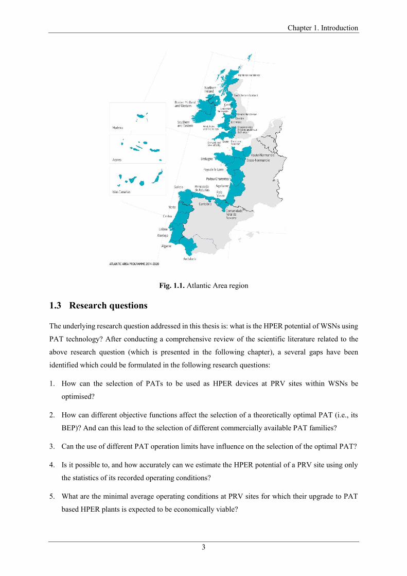
1.2 The REDAWN Project
This research is part of multidisciplinary REDAWN project (“Reducing Energy Dependency of the
Atlantic area Water Networks”, www.redawn.eu ). Its main target is to improve the energy efficiency
of water networks in the Atlantic Area (see Fig. 1.1) water networks through the assessment,
development and installation of innovative micro-hydropower technology. It presents a collaboration
between 9 partners including academic institutions, water networks operators, public energy agencies
and private companies. The project is part funded under the ERDF INTERREG Atlantic Area
programme 2014-2020 (www.atlanticarea.eu).
Trinity College Dublin (TCD) is the leader of one of the eight work packages that comprise REDAWN,
but it also participates in some of the other seven. TCD is the project leader of the work page 4, whose
main objectives are to gather data on flow, pressure and location of water network infrastructure that
could be potential sites for energy recovery and assess the existing potential at these sites. Another aim
was to try to perform a spatial extrapolation of the existing potential to areas where the data about the
potential sites were unavailable.
Chapter 1. Introduction
3
Fig. 1.1. Atlantic Area region
1.3 Research questions
The underlying research question addressed in this thesis is: what is the HPER potential of WSNs using
PAT technology? After conducting a comprehensive review of the scientific literature related to the
above research question (which is presented in the following chapter), a several gaps have been
identified which could be formulated in the following research questions:
1. How can the selection of PATs to be used as HPER devices at PRV sites within WSNs be
optimised?
2. How can different objective functions affect the selection of a theoretically optimal PAT (i.e., its
BEP)? And can this lead to the selection of different commercially available PAT families?
3. Can the use of different PAT operation limits have influence on the selection of the optimal PAT?
4. Is it possible to, and how accurately can we estimate the HPER potential of a PRV site using only
the statistics of its recorded operating conditions?
5. What are the minimal average operating conditions at PRV sites for which their upgrade to PAT
based HPER plants is expected to be economically viable?

Chapter 1. Introduction
4
6. Can the ratio between BEPs of the theoretically optimal PATs and the average operating condition
of the considered PRV sites be generalized?
7. Can the HPER potential at the site level be predicted using population and topography data in the
site's proximity?
8. How can the HPER potential be assessed on a country scale? Which percentage of the energy
consumed by the drinking water sector can be recovered using the HPER concept?
The main objective of the presented thesis is to address the above research questions.
1.4 Research structure
The subsequent content of this thesis is distributed as per the following chapters’ structure:
Chapter 2 presents a critical review of the state of the art literature in two main fields, WSNs and
hydropower technology. Firstly, WSN basics and conventional pressure management literature are
discussed helping to understand WSN settings and pressure management requirements. The chapter
then presents and overview of hydropower technology with particular focus on PAT technology and its
advantages and disadvantages in comparison to traditional turbines. The chapter ends with an in-depth
overview of the research to date dealing with the HPER concept in WSNs.
Chapter 3 introduces the overall research approach adopted in the thesis. It describes different work
stages in which the thesis is divided and how each of the stages addresses the previously defined
research questions.
Upon describing the adopted research approach in Chapter 3, the next five chapters present the research
work carried out during this PhD program, attempting to address the research gaps.
Chapter 4 develops a new optimisation-based methodology for the selection of a PAT from the market
that can be used as HPER devices at PRV sites in WSNs. It then applies the developed methodology to
several case study sites using different objective functions and different PAT operation limits to address
some of the set research questions.
Chapter 5 consists of two parts. The analysis presented in the first part of the chapter derives a model
for the prediction of the global efficiency of a HPER plant equipped with a PAT, whose predictor
variables are only the statistics of a considered PRV operating conditions. The second part of the chapter
performs an analysis that identifies the minimal average operating conditions at PRV sites so their
upgrade to HPER plants equipped with a PAT are estimated to have positive NPV after 10 years.
By applying an improved variant of the methodology developed in Chapter 4 to 38 PRV sites with high
resolution data, Chapter 6 investigates the ratios between the theoretically optimal PATs and the
average operating points of the examined PRVs.

Chapter 1. Introduction
5
Chapter 7 conducts another correlation analysis. Namely, it investigates whether the HPER potential
at the site level could be predicted using variables designating population and topography in their
proximity.
Finally, Chapter 8 develops a 7-step methodology for assessment of the HPER potential within WSNs
on a country scale. The developed methodology utilized the findings from Chapter 5 to determine the
economically viable sites and the prediction model derived in the same chapter to assess their global
efficiency and thus their potential. The methodology extrapolates the potential to areas of the examined
countries without data by considering several scenarios for a coefficient that links the power potential
to the number of people residing in these areas.
Chapter 9 discusses the main results and findings exhibited in the previous five chapters, pointing out
their potential impact in the field and their limitations.
Chapter 10 concludes the thesis by providing the answers to the research questions defined in the
previous subsection of this chapter drawn from the research findings in Chapters 4-8. In addition, it
gives references to the journal and conference papers that emerged from the research presented in this
thesis and indicates areas that require further research.
Chapter 2. Literature Review
6
2 Literature Review
2.1 Introduction
This chapter presents a critical review of the state of the art literature in the fields of pressure
management in WSNs and hydropower with a focus on PAT technology and its potential to be used as
a hydropower energy recovery (HPER) device at the locations of pressure management infrastructure.
Figure 2.1 graphically illustrates the areas covered in the remaining subsections of this chapter,
suggesting their intersections. Firstly, the basic notions and laws important for understanding the
context and operation principles of WSNs have been discussed. The role of HPER concept in WSNs
could be regarded as a novel technical solution for more efficient pressure management. Thus, the
literature in the area of conventional pressure management has been reviewed, focusing on pressure
management infrastructure, its control and optimal deployment for minimization of water losses. The
review of the literature proceeds with the studies examining hydropower technology in general, with
special attention to the mini and micro segments. Previous research suggested PAT technology as
particularly attractive for these hydropower segments because of its lower cost. Hence, this review
discusses types of PATs suitable for WSNs settings, their advantages and disadvantage in comparison
to conventional turbines, focusing on the problem of performance uncertainty and models for its
prediction. The review ends with an in-depth overview of the research dealing with the HPER concept
in WSNs. This part firstly discusses the potential installation locations and design challenges for
hydropower installations posed by WSN settings. Then it discusses a few studies that used traditional
turbines as HPER devices. The final part compares different studies for the selection of PATs to be used
as HPER devices and discusses how these addressed the main challenges related to this technology for
the application in WSNs.
The main driver for this research is the provision of solutions for innovative pressure management
alternatives that incorporate PATs as HPER devices, thus improving energy efficiency of WSNs by
recovering a portion of the energy solely dissipated using conventional solutions.

Chapter 2. Literature Review
7
Fig. 2.1. Literature review subsections and their interconnections.
2.2 WSN basics
The idea to convey the water from its source to the place where it is needed via a system of channels or
pipes is several millennia old. The first water distribution pipes originate from the period 1500 B.C. on
the island of Crete (Greece), where the Minoan civilization developed a water distribution system that
uses rectangular terracotta conduits to convey water to Knossos palace, see Fig. 2.2 (Angelakis et al.,
2013). Since then the advancement of water distribution technology went in parallel with the
advancement of human civilization. Today WSNs are one of the most important urban infrastructure
without which the modern life cannot be imagined.
Fig. 2.2. Minoan water distribution projects: (left) pipes of rectangular shape from Myrtos-Pyrgos and
(b) closed terracotta pipes at Knossos palace (adopted from Angelakis et al. 2013).
Chapter 2. Literature Review
8
Although the modern WSNs vary greatly in size and complexity the purpose remains the same as in the
ancient time and that is to convey the water from the source to the customers. The untreated or raw
water can be extracted from either ground water sources or surface water sources such as lakes, rivers
or even seas. The untreated water is then transmitted to the water treatment plants (WTPs) where it is
treated to defined water quality standards. In general, the ground water has better quality than the
surface water, and thus requires less intensive treatment. Once the water is treated, it is then transported
to the storage reservoirs whose main function is to store water in the periods of low consumption for
the periods of high consumption. Thus serving as a buffer between the WTPs and the distribution
systems, resulting in cheaper WTPs that can be designed for an average consumption rather than the
peak one. Besides the storage function, these reservoirs also provide contact time for disinfectants such
as chlorine that are added near the end of the treatment process. In addition, the reservoirs can serve as
a source for backwash water for cleaning WTPs filters using high rate flows for a short period of time
(Walski et al., 2003).
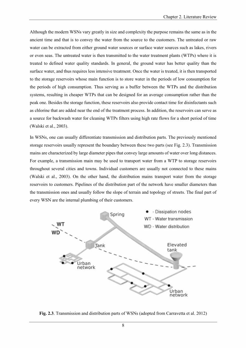
In WSNs, one can usually differentiate transmission and distribution parts. The previously mentioned
storage reservoirs usually represent the boundary between these two parts (see Fig. 2.3). Transmission
mains are characterized by large diameter pipes that convey large amounts of water over long distances.
For example, a transmission main may be used to transport water from a WTP to storage reservoirs
throughout several cities and towns. Individual customers are usually not connected to these mains
(Walski et al., 2003). On the other hand, the distribution mains transport water from the storage
reservoirs to customers. Pipelines of the distribution part of the network have smaller diameters than
the transmission ones and usually follow the slope of terrain and topology of streets. The final part of
every WSN are the internal plumbing of their customers.
Fig. 2.3. Transmission and distribution parts of WSNs (adopted from Carravetta et al. 2012)

Chapter 2. Literature Review
9
Customers of a WSN can be homeowners, hospital, factories, golf courses etc. The customers’ water
usage patterns determine the behaviour of a WSN, hence the network has to be designed to fulfil their
needs.
The configuration or topology of WDNs can be either looped or branched. The looped configuration
imposes that the water can reach customer by more than one path, while in the branched configuration
there is only one water path to each of the customers (see Fig. 2.4). WDNs located in densely populated
areas are mostly looped for improved reliability (redundancy). The advantage of the looped
configuration can be best perceived after a failure event. As it can be seen from Fig. 2.4 much fewer
customers stay without the service during failure events within the networks with looped configuration,
as there are alternative paths for the water to reach the customers. Another advantage of the looped
configuration are lower velocities within the pipes. However, in the rural areas the branched
configuration prevails because of the monetary reasons.
Fig. 2.4. Looped and branched networks after network failure (adopted from Walski et al. (2003))
Pressurized fluid flowing through the pipes of a WSN possesses two types of energy, namely potential
and kinetic energy. The potential energy can be divided on the part due to elevation and the part due to
pressure. In hydraulic engineering practice, the energy possessed by a fluid is usually expressed as
energy per unit weight of fluid also known as hydraulic head. The hydraulic head is expressed in the
length units (Kapor, 2011):
𝐸 = 𝑍 +𝑝
𝜌𝑔+
𝑉2
2𝑔= Π +
𝑉2
2𝑔 (2.1),
Chapter 2. Literature Review
10
where E [m] is total energy of the fluid; Z [m] is elevation; p [Pa] is pressure; 𝜌 [kg m-3] is water density;
𝑔 [m s-2] is gravitational acceleration; and V [m s-1] is velocity at a cross section of a pipe. The potential
energy, i.e., the elevation and pressure terms are usually sum and expressed as piezometric head Π [m].
When a fluid flows through a pipe it experience two types of losses. The first are friction losses, which
are caused by shear stress developed between the fluid and the wall of the pipe. The friction losses are
function of the properties of the fluid, its velocity and properties of the pipes, inner roughness, diameter
and length. Their magnitude can be quantified using some of the formulas defined in the literature such
as Darcy-Weisbach’s, Hazen-Williams’ or Manning’s (Ivetic, 1996). The second type of losses are local
or minor losses and these are the result of turbulence due to changes in streamlines through obstacles
such as valves, bends, tees etc. The local losses could be assessed as a product of the local loss
coefficient and the velocity head (𝑉2/2𝑔). The values of the local loss coefficient are assessed
experimentally and are known for the most common obstacles such as 90o bend, while the value of the
coefficient for valves could be found in valve manufacturers datasheets.
2.3 Conventional pressure management for leakage reduction in WSNs
2.3.1 Negative consequences of excessive pressure
Why is there excess pressure within WSNs in the first place? WSNs are either gravity-fed, pump-fed or
mixed systems (Mamade et al., 2018). Whenever it is possible, it is desired to have a gravity-fed system
to reduce the costs related to the energy consumed for pumping. In a gravity-fed system, there can be
large elevation differences between the source and some parts of a WDN resulting in excess pressure
in those parts of the network. On the other hand, when a system is mixed or completely pump-fed there
is still a possibility for excess pressure, especially in the areas with hilly terrain. This is because of the
predefined topography of WDNs and the requirement to deliver the water with sufficient pressure to all
parts of the networks. For the pumped systems, it is also important if pumping is centralized or high-
rise buildings have their own pumping stations. In other words, the minimum value of pressure available
in a WDN which is usually defined by legislation, also influences the value of excess pressure. Figure
2.5 presents the values for the minimum pressure for some countries in the world. For example, Smith
and Liu (2020) examined 82 case cities in China to judge whether China’s recommended minimum
pressure regulation leads to unnecessarily high-energy use in certain cities. Results showed that 63 of
these cities could save energy by reducing the minimum and average pressure used to distribute water,
with energy savings of up to 28% of the total energy for the water distribution.
The primary negative consequence of high pressure is excessive leakage. Water loss occurs in every
water distribution system during its overall operational lifetime. For perspective, on the level of EU the
values of water losses span from single digit values in Germany, Denmark and Netherlands up to around
45% in Ireland, with an average of 23%, see Fig. 2.6.

Chapter 2. Literature Review
11
Fig. 2.5. Minimum pressure guidelines (non-binding) and regulations (binding) for countries around
the world (adopted from Smith and Liu (2020).
Fig. 2.6. Average distribution losses in percentages (adopted from The European Federation of
National Water Services (2017))
Relationship between the leakage and pressure is well established. A leak in a pipe through a hole or
crack can be considered as flow through an orifice. Orifice hydraulics is well understood and the orifice

Chapter 2. Literature Review
12
equation describes the flow rate 𝑄[m3s-1] through an orifice as a function of the orifice area 𝐴[m2] and
pressure head ℎ[m] as (Van Zyl, 2014):
𝑄 = 𝐶𝑑𝐴√2𝑔ℎ (2.2),
where 𝐶𝑑[-] is the discharge coefficient, accounting for energy losses and jet contraction, and 𝑔[ms-2]
is acceleration due to gravity. May (1994) introduced the FAVAD (fixed and variable area discharge)
concept where the authors assumed that the orifice area increases linearly with an increase of pressure,
which was later proven by Cassa et al. (2010) in a finite element study that examined pipes of various
materials:
𝐴(ℎ) = 𝐴0 + 𝑚ℎ (2.3),
where 𝐴0 [m2] is initial area; 𝑚 [-] is pressure-head area slope and ℎ[m] is pressure head. Introducing
Eq. 2.3 in Eq. 2.2, one can get the FAVAD equation:
𝑄 = 𝐶𝑑√2𝑔(𝐴0ℎ0.5 + 𝑚ℎ1.5) (2.4).
However, the leakage practitioners usually use a more general form of the equation to describe the
relationship between pressure and leakage based on 𝑁1 exponent (Thornton and Lambert, 2005):
𝑄 = 𝐶ℎ𝑁1 (2.5).
Based on more than 100 field tests, Thornton and Lambert (2005) found that the 𝑁1 exponent lies within
the range 0.5–1.5 and occasionally reaches 2.5. Four factors that are the possible causes for this variation
of the leakage exponent include: pipe material elastic behaviour, leak hydraulics, soil hydraulics and
water demand.
Another negative consequence of high pressure within WDNs is the increased frequency of pipes bursts.
Unlike in the case of the pressure head-leakage relationship, establishing an accurate relationship
between new pipe burst frequency and pressure head is quite challenging (Lambert, 2002). Thornton
and Lambert (2005) proposed a method based on a pressure head exponent N2, similarly to N1 used for
leakage assessment. This method suggests that the new burst occurrences will decrease exponentially
as a function of the N2 exponent from B0 to B1 if the pressure head within a network is decreased from
P0 to P1:
𝐵0
𝐵1= (
𝑃0
𝑃1)
𝑁2 (2.6).
The study suggested that the value of the N2 exponent can range from 0.5 up to 6.5. The same authors
published new results of their research two years later, suggesting that the new burst frequency
relationship depends largely to the break frequency rate before implementation of pressure management
strategies (Thornton and Lambert, 2007). Namely, if the pipe breaks rate prior to pressure management
Chapter 2. Literature Review
13
is high then even a small reduction of pressure can lead to a significant reduction of the break frequency.
Conversely, if the break frequency before pressure management is relatively low, then any percentage
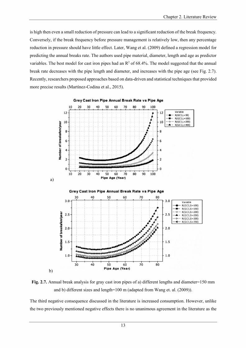
reduction in pressure should have little effect. Later, Wang et al. (2009) defined a regression model for
predicting the annual breaks rate. The authors used pipe material, diameter, length and age as predictor
variables. The best model for cast iron pipes had an R2 of 68.4%. The model suggested that the annual
break rate decreases with the pipe length and diameter, and increases with the pipe age (see Fig. 2.7).
Recently, researchers proposed approaches based on data-driven and statistical techniques that provided
more precise results (Martínez-Codina et al., 2015).
a)
b)
Fig. 2.7. Annual break analysis for gray cast iron pipes of a) different lengths and diameter=150 mm
and b) different sizes and length=100 m (adapted from Wang et. al. (2009)).
The third negative consequence discussed in the literature is increased consumption. However, unlike
the two previously mentioned negative effects there is no unanimous agreement in the literature as the

Chapter 2. Literature Review
14
relationship between pressure and consumption is very complex (Vicente et al., 2016). The studies
dealing with this topic are generally based on disaggregation of the demand components. Thus one can
differentiate pressure-dependant consumption elements such as irrigation systems, showers and taps,
and pressure-independent elements such as toilet tanks, dishwashers, washing machines etc. (Gomes et
al., 2011). Lambert and Fantozzi (2010) proposed an N3 pressure exponent following the analogy with
the previously mentioned N1 exponent defined for pressure-leakage relationship. The study proposed
the exponent values between 0.4-0.5 for the outside pressure-dependant elements, and between 0.02-
0.04 for the indoor pressure-independent elements. Liu et al. (2011) argued that only when there is
insufficient pressure in the network that the consumption depends on pressure while it is independent
otherwise. Giustolisi and Walski (2012) carried out one of the most comprehensive studies on this topic.
In the presented study, the authors disaggregated demand into four components: human based demand
(e.g., taps and showers); volume based demand (e.g., dishwashers, washing machines, toilet tanks etc.);
uncontrolled orifice demand (fire protection hydrants and irrigation systems); and leakage based
demand. The study concluded that solely demand-driven (pressure-independent) analysis should be
used only for specific purposes like calibration or design of a network, or specific assumptions for in-
door demands.
2.3.2 Pressure management methods
To tackle these negative consequences of excess pressure, in the last 30 years researchers, engineers
and water practitioners have been implementing pressure management by means of PRVs, among other
methods. Hence, many PRVs have been deployed around the world within WDNs for pressure
management purposes. PRVs are usually installed at the entrance of district metered areas (DMAs)
(Gomes et al., 2012). DMAs are the sectors of WDNs with defined boundaries where the flow that
comes in and leaves is constantly metered for leakage monitoring. For perspective, in the United
Kingdom (UK) some of the main water utilities operate in the range of 2000 DMAs, where 50-60% are
pressure managed (Vicente et al., 2016).
2.3.2.1 Types of PRV regulation
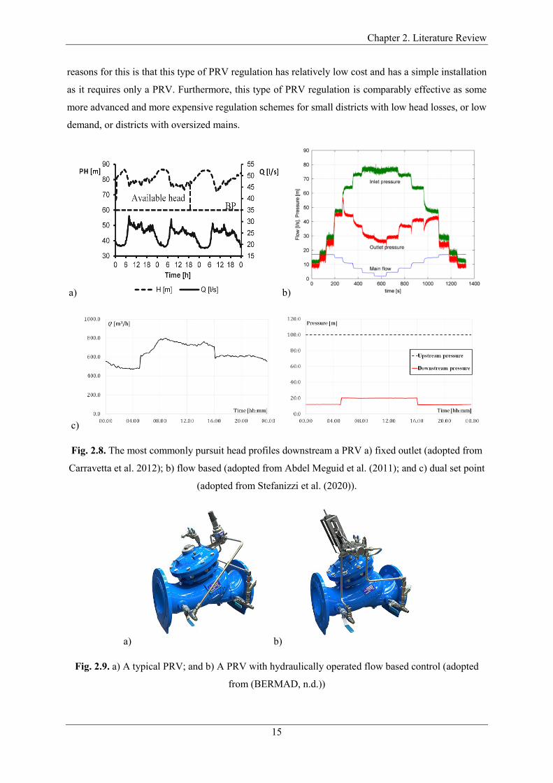
In general, there are three types of head profiles that are most commonly present downstream of PRVs.
These are: 1) fixed outlet profile - the head profile downstream a PRV is constant regardless of the
upstream head and flow; 2) dual set point profile – different downstream heads are set for day and night
regimes; and 3) Flow based or proportional discharge profile – downstream head varies according to a
predefined flow-pressure relationship curve. These three profiles are presented in Fig. 2.8.
When the fixed outlet head profile is present, the control is usually attained using a hydraulically
operated autonomous pilot valve (see Fig. 2.9a). This type of downstream head profile and control is
the most frequently used by water utilities. For perspective, out of the previously mentioned DMAs that
implement pressure management in the UK, 80% use this type regulation (Vicente et al. 2016). The
Chapter 2. Literature Review
15
reasons for this is that this type of PRV regulation has relatively low cost and has a simple installation
as it requires only a PRV. Furthermore, this type of PRV regulation is comparably effective as some
more advanced and more expensive regulation schemes for small districts with low head losses, or low
demand, or districts with oversized mains.
a) b)
c)
Fig. 2.8. The most commonly pursuit head profiles downstream a PRV a) fixed outlet (adopted from
Carravetta et al. 2012); b) flow based (adopted from Abdel Meguid et al. (2011); and c) dual set point
(adopted from Stefanizzi et al. (2020)).
a) b)
Fig. 2.9. a) A typical PRV; and b) A PRV with hydraulically operated flow based control (adopted
from (BERMAD, n.d.))
Chapter 2. Literature Review
16
The dual set point profiles are referred also as time-based profiles, although time-based regulation does
not need to have only two downstream head settings. This type of downstream head profile can be
attained either using hydraulically or electronically operated controls (Charalambous and
Kanellopoulou, 2010; Lambert and Fantozzi, 2010). The hydraulically operated control can be achieved
using two pilot valves set at different heads, a solenoid and a time controller. On the other hand, the
electronically operated control includes a local electronic controller with an internal timer which is
connected to controlling pilot of a PRV. This type of regulation is recommended when advanced head
regulation is desired but the cost is an issue. It is suitable for stable repetitive demand patterns (on daily
or weekly basis) and districts with low head losses. It is not recommended when sudden emergency
requirements are needed such as firefighting.
The flow-based profile is usually attained electronically using closed loop control, where the flow-head
relationship is a part of the controller. For this type of regulation, a flow meter gauge is necessary.
Although nowadays some valve manufactures provide even PRVs with hydraulically operated flow-
based control (see Fig. 2.9b). The main advantage of this type of regulation is the ability to adapt to
demand profile in real time, which results in more effective pressure management and leakage
reduction. This type of regulation is recommended for DMAs with variable non-deterministic demand,
and/or large head losses, and/or for districts where sudden unexpected demand such firefighting is very
important (Vicente et al. 2016).
Another type of PRV regulation that has gained a lot of interest in the literature lately is remote node
regulation (Burrows, 2014; Wyeth and Chalk, 2012). The downstream head profile generated by this
type is the closest to the flow-based regulation profile but it cannot be classified as any of the profiles
presented in Fig. 2.8. This type of regulation is always electronically operated as it uses data from a
remote sensor located usually at a critical node (the lowest head) within a DMA to regulate the head
profile downstream a PRV. The head drop at the PRV is regulated so that the head at the critical node
never falls below the minimal pre-set value. This type of regulation is recommended when an effective
flow-downstream head curve is difficult to calculate, e.g., when there is a large consumer with stochastic
demand within a district. However, as this type of regulation requires a communication system that can
receive remote signal, it is the most expensive.
2.3.2.2 Optimal PRV locations
To support the decision making process and to find optimal locations for the deployment of pressure
management valves that will minimize excess pressure and reduce leakage but also minimize
installation costs, researchers and engineers have developed many algorithms. These algorithms were
usually based on traditional or heuristic optimisation techniques, or a combination of heuristic
procedures and optimisation techniques.

Chapter 2. Literature Review
17
Firstly, traditional linear programing (LP) was used to optimise control valves to reduce leakage
(Germanopoulos, 1995; Jowitt and Xu, 1990; Sterling and Bargiela, 1984; Vairavamoorthy and
Lumbers, 1998), but in recent decades optimisation of WSNs switched to heuristic techniques inspired
by nature primarily by Genetic Algorithms (GAs) (Araujo et al., 2006; Giugni et al., 2014). Heuristic
techniques allow multi objective optimisation, but do not guarantee a global optimum (Fontana et al.,
2012; Nicolini and Zovatto, 2009). Eck et al.(2012) used the open-source BONMIN solver, whose
algorithm is based on the Mix Integer Nonlinear Programming (MINLP) technique, to find optimal
locations and settings of PRVs in WSNs.
In mathematical models, the leakage is simulated as additional pressure-driven demand allocated to
network nodes (Araujo et al., 2006). This requires augmentation of the mass balance equations that are
written for nodes with an additional term which represents the leakage:
𝑄𝑙 = ∑ 𝑞𝑖𝑙𝑛
𝑖=1 (2.7),
where n is the number of nodes and 𝑞𝑖𝑙 is the leaked discharge through the ith node, that can be assessed
as:
𝑞𝑖𝑙 = 𝑓𝑖 ∙ 𝑝𝑖
𝛽 (2.8),
where pi is the pressure head (in meters) of the ith node, β an exponent depending on the material of the
pipe and on the shape of the orifice (Greyvenstein and Van Zyl, 2007). The leakage coefficient, fi, is
constant for each node and is estimated as:
𝑓𝑖 = 𝑐 ∙ ∑ 0.5 ∙ 𝐿𝑖,𝑗𝐾𝑖𝑗=1 (2.9),
where c is a coefficient equal to 0.00001 l/(s∙m1+β) (Araujo, 2005) and Ki is the number of pipes
approaching the ith node and connecting the nodes i and j , whose lengths are Li,j.
All of the above-mentioned literature used similar approaches, i.e., objective function to find optimal
locations and settings of PRVs, which represent minimization of the mean square difference between
the actual and the target pressure at each node, according to the general formulation:
𝑂𝐹 = ∑ [𝛼 ∙ (𝑃𝑖 − 𝑃𝑚𝑖𝑛)2]𝑁𝑖=1 (2.10),
where N is the number of nodes, and the constant α is a penalty coefficient for pressure violation, which
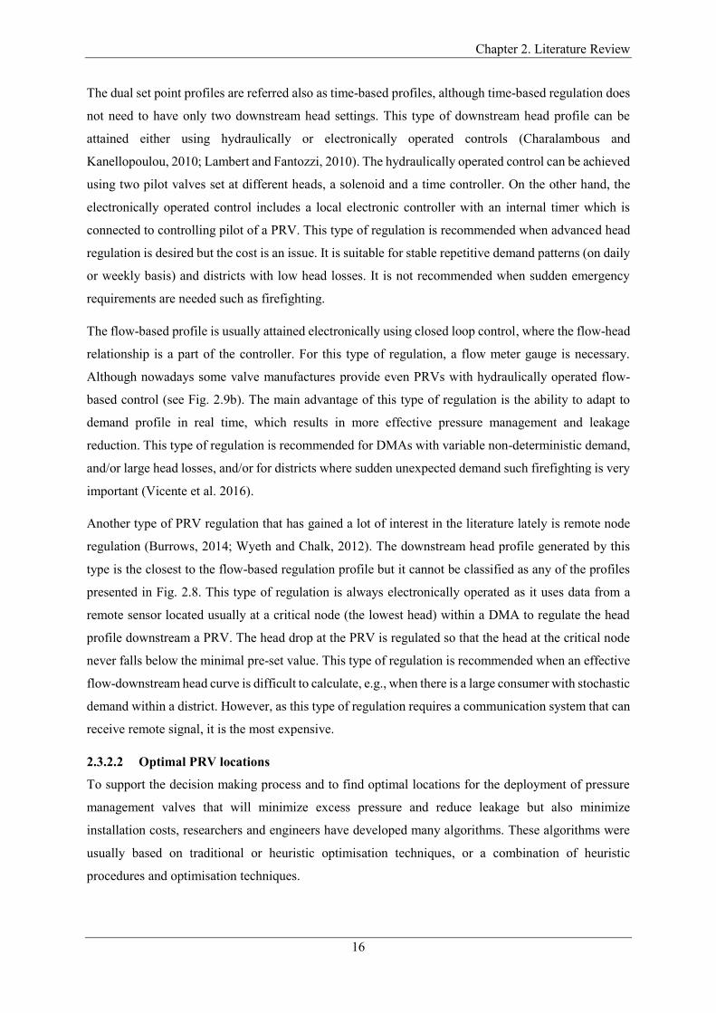
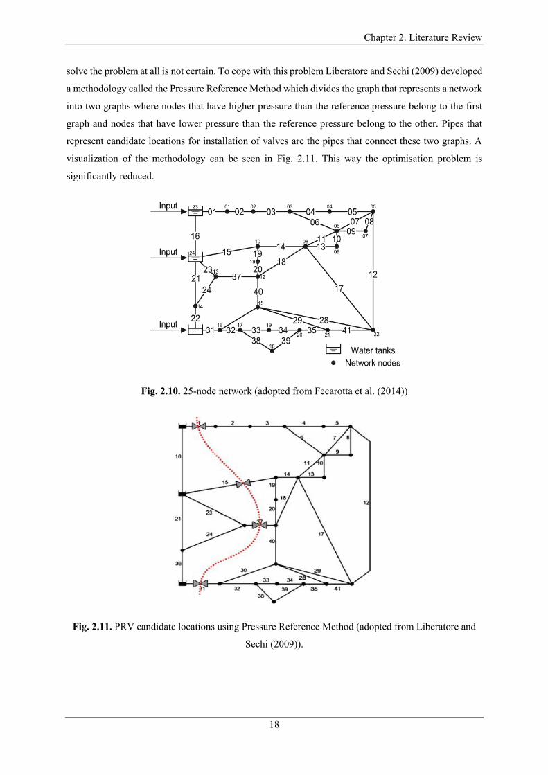
ensures that the targeted pressure is larger or equal to Pmin at all demand nodes. In addition, most of
these algorithms were tested on a small synthetic 25-node network, presented on Fig. 2.10.
One more thing in common for previous studies is that the optimisation problem was defined in a way
that all pipes in the network are considered as candidate locations for installation of valves. The same
formulation of the problem for larger networks would take too much computational time and if it could
Chapter 2. Literature Review
18
solve the problem at all is not certain. To cope with this problem Liberatore and Sechi (2009) developed
a methodology called the Pressure Reference Method which divides the graph that represents a network
into two graphs where nodes that have higher pressure than the reference pressure belong to the first
graph and nodes that have lower pressure than the reference pressure belong to the other. Pipes that
represent candidate locations for installation of valves are the pipes that connect these two graphs. A
visualization of the methodology can be seen in Fig. 2.11. This way the optimisation problem is
significantly reduced.
Fig. 2.10. 25-node network (adopted from Fecarotta et al. (2014))
Fig. 2.11. PRV candidate locations using Pressure Reference Method (adopted from Liberatore and
Sechi (2009)).

Chapter 2. Literature Review
19
2.4 Hydropower
Hydropower is energy derived from flowing water. More than 2,000 years ago, the ancient Greeks used
waterpower to run wheels for grinding grain. Today, hydropower is the most well established renewable
energy source worldwide with around 60% (4222.21 out of 7027.73 TWh per year) share of all
renewable energy and around 16% of all electricity produced in the world (Rittchie and Roser, 2017).
Furthermore, hydropower has lower environmental impact and more stable energy supply compared to
other renewable sources, such as solar or wind (Gaudard and Romerio, 2014) Gaudard. The largest
hydropower plants are located in China, the United States, Brazil and Canada. Currently, China has the
largest installed capacity exceeding 240 GW with an average growth of capacity of 20 GW per year
(Hennig et al., 2013). Spänhoff (2014) performed a worldwide projection of the installed capacity for
the renewable energies. According to this projection, the installed capacity of hydropower in 2035
should exceed 1400 GW, being three times higher than wind energy capacity and 15 times higher than
solar energy capacity.
2.4.1 Hydropower classification by size and type
According to the classification proposed by the International Energy Agency, hydropower plants can
be classified by their installed power capacity as presented in Tab. 2.1:
Tab. 2.1. Classification of hydropower plants according to their installation capacity
Category Power range
Pico 0-5 kW
Micro 5-100 kW
Mini 100 kW - 1 MW
Small 1 - 10 MW
Median 10 - 100 MW
Large above 100 MW
By type, hydraulic machines can be classified based on the settings where these are installed on the
ones installed in open channels systems and in pressurized systems (Pérez-Sánchez et al., 2017a). In
open channels, all types of hydraulic wheels have been installed to exploit the energy of waterfalls.
Thus, one can differentiate gravitational (e.g. Archimedes screw), hydrostatic (e.g. hydrostatic pressure
wheel) and kinetic (e.g. undershot waterwheel) machines. On the other hand, in pressurized systems
there are action and reaction turbines. The classification was made based on the type of energy that is
used within a turbine runner for transformation of the energy of water stream into the mechanical energy
of the turbine’s shaft (Đorđević, 1989). During the energy transformation in runners of reaction
turbines, all three components of the energy of the water stream (potential energy due elevation,
potential energy due pressure and kinetic energy) are changed. The energy exchange is carried out in
pressurized flow. On the other hand, the action turbines use only the kinetic energy of the water stream,
while the energy exchange is carried out on the atmospheric pressure. Hence, the action turbines can be

Chapter 2. Literature Review
20
installed only at specific locations in pressurized systems, such break pressure tanks (BPTs) or
consumption nodes (Sitzenfrei and Rauch, 2015; Sitzenfrei and Von Leon, 2014).
Over the years, in attempt to improve the energy transformation efficiency for different flow and
hydraulic head operating conditions at installation sites, different types of action and reaction turbines
have been developed. The most renowned action turbines are Pelton, Turgo and Crossflow. On the other
hand, the most widely used conventional reaction turbines are Francis, Kaplan, Bulb turbines and PATs
(Pérez-Sánchez et al., 2017a). Figure 2.12 presents the application domain boundaries for the selection
of the aforementioned turbines based on flow and hydraulic head operating conditions at a considered
site. Gordon (2001) analysed the efficiency of 107 hydropower plants built since 1908, aiming to
evaluate the improvement in the performance over time. Increases in the performance of the machines
were obtained, rising from efficiencies lower than 50% in 1920 to above 96% in current cases.
Fig. 2.12. Application domain boundaries for selection of the conventional turbines based on flow and
hydraulic head operating conditions: large (left); and small (right) hydropower (Pérez-Sánchez et al. 2017a).
2.4.2 Turbomachinery generalities
The power output of a hydraulic turbine can be defined using the following equation (Corcoran et al.
2013):
𝑃 = 𝜌𝑔𝑄𝐻𝜂 (2.11),
where 𝑃 [W] is power output; 𝜌 [kg m-3] is fluid density; 𝑔 [m s-2] is gravitational acceleration; 𝑄 [m3
s-1] is nominal flow rate; H [m] is net hydraulic head, i.e., head drop imposed by turbine; and 𝜂 [-] is
turbine efficiency.
Besides nominal flow and hydraulic head of a turbine, another important variable is the impeller
rotational speed 𝑛 [rpm]. These three variables are combined into a variable called specific speed, which
can be expressed using the following equation (Carravetta et al., 2012):
Chapter 2. Literature Review
21
𝑁𝑠𝑞
= 𝑛𝑄0.5
𝐻0.75 (2.12),
where 𝑁𝑠𝑞
[rpm (m3 s-1)0.5 m-0.75] is specific speed based on flow; 𝑛 [rpm] is rotational speed of turbine
impeller; 𝑄 [m3 s-1] is nominal flow rate; H [m] is net hydraulic head of turbine. Besides specific speed
based on flow there is also specific speed based on power:
𝑁𝑠𝑝
= 𝑛𝑃0.5
𝐻1.25 (2.13),
where 𝑁𝑠𝑝
[rpm W0.5 m-1.25] is specific speed based on power; 𝑃 [W] is nominal power generated by
turbine; while the other terms are the same as in Eq. 2.12. In the remaining of the manuscript 𝑁𝑠 will
refer to the specific speed based on flow.
The specific speed has been being used for comparison of turbines of different hydraulic characteristics.
In other words, 𝑁𝑠 has been being used to distinguish families of hydraulically similar turbines, i.e.,
turbines with similar impeller geometry (Djordjevic 1989). Thus, Pelton turbines are characterized with
the smallest specific speeds (high hydraulic head – low flow). Contrary Bulb turbines are characterized
with the highest specific speeds (low hydraulic head – high flow).
For families of hydraulically similar turbines (having the same specific speed) it is possible to express
relationship between their main performance characteristics using affinity laws. The main performance
characteristics are best efficiency flow and hydraulic head, impeller diameter, impeller rotational speed,
and power output. The affinity laws are defined with the following mathematical expressions:
𝑄1
𝑄2=
𝑛1
𝑛2(
𝐷1
𝐷2)
3 (2.14),
𝐻1
𝐻2= (
𝑛1
𝑛2)
2(
𝐷1
𝐷2)
2 (2.15),
𝑃1
𝑃2= (
𝑛1
𝑛2)
3(
𝐷1
𝐷2)
5 (2.16).
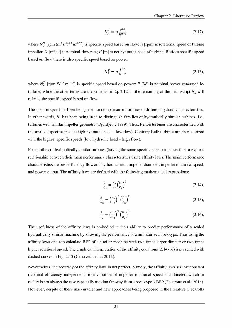
The usefulness of the affinity laws is embodied in their ability to predict performance of a scaled
hydraulically similar machine by knowing the performance of a miniaturized prototype. Thus using the
affinity laws one can calculate BEP of a similar machine with two times larger dimeter or two times
higher rotational speed. The graphical interpretation of the affinity equations (2.14-16) is presented with
dashed curves in Fig. 2.13 (Carravetta et al. 2012).
Nevertheless, the accuracy of the affinity laws in not perfect. Namely, the affinity laws assume constant
maximal efficiency independent from variation of impeller rotational speed and dimeter, which in
reality is not always the case especially moving faraway from a prototype’s BEP (Fecarotta et al., 2016).
However, despite of these inaccuracies and new approaches being proposed in the literature (Fecarotta
Chapter 2. Literature Review
22
et al. 2016), the affinity laws remain the most widely used tool for performance prediction of similar
turbines.
Fig. 2.13. Affinity laws presented with dashed curves (adapted from Carravetta et al. (2012))
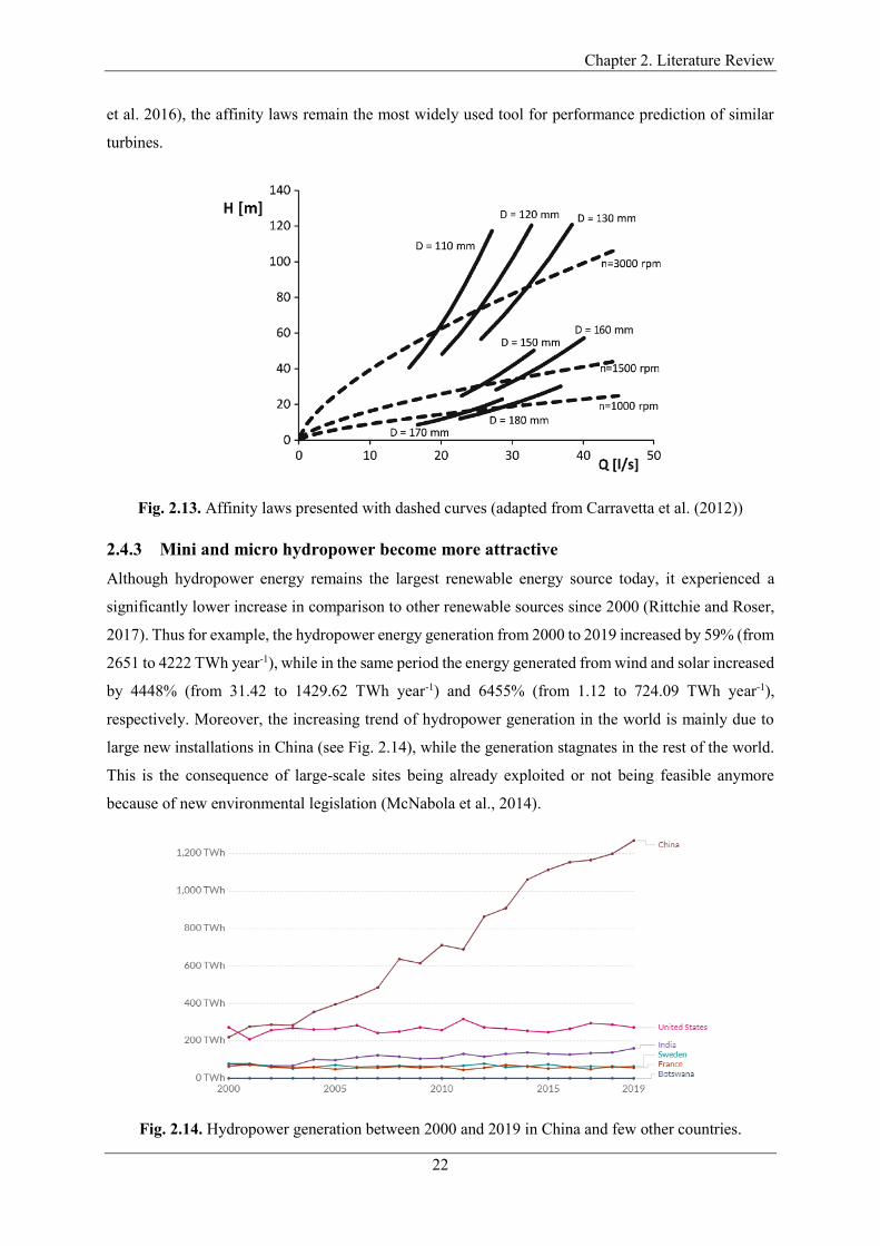
2.4.3 Mini and micro hydropower become more attractive
Although hydropower energy remains the largest renewable energy source today, it experienced a
significantly lower increase in comparison to other renewable sources since 2000 (Rittchie and Roser,
2017). Thus for example, the hydropower energy generation from 2000 to 2019 increased by 59% (from
2651 to 4222 TWh year-1), while in the same period the energy generated from wind and solar increased
by 4448% (from 31.42 to 1429.62 TWh year-1) and 6455% (from 1.12 to 724.09 TWh year-1),
respectively. Moreover, the increasing trend of hydropower generation in the world is mainly due to
large new installations in China (see Fig. 2.14), while the generation stagnates in the rest of the world.
This is the consequence of large-scale sites being already exploited or not being feasible anymore
because of new environmental legislation (McNabola et al., 2014).
Fig. 2.14. Hydropower generation between 2000 and 2019 in China and few other countries.

Chapter 2. Literature Review
23
Given this, sites of mini and micro scale are becoming more attractive like those occurring in drinking
water (McNabola et al., 2014), irrigation (Chacón et al., 2019) and wastewater (Bousquet et al., 2017)
networks. However, it is well documented in the literature that the installation cost of hydropower
schemes per unit power increases with a decrease of the installation capacity (Ramos and Ramos, 2010).
Figure 2.15 from Ramos and Ramos (2010) presents the relationship between the installation cost of
water turbines and their installation capacity. In other words, scaling down the conventional turbines to
be used for the sites of mini and micro scale was usually found to be non-economically viable. Thus in
recent years many researchers have been exploring other cheaper hydropower technologies to be used
for these smaller sites.
Fig. 2.15. Curves for the hydropower equipment initial cost (adopted from Ramos and Ramos, 2010).
a)
Chapter 2. Literature Review
24
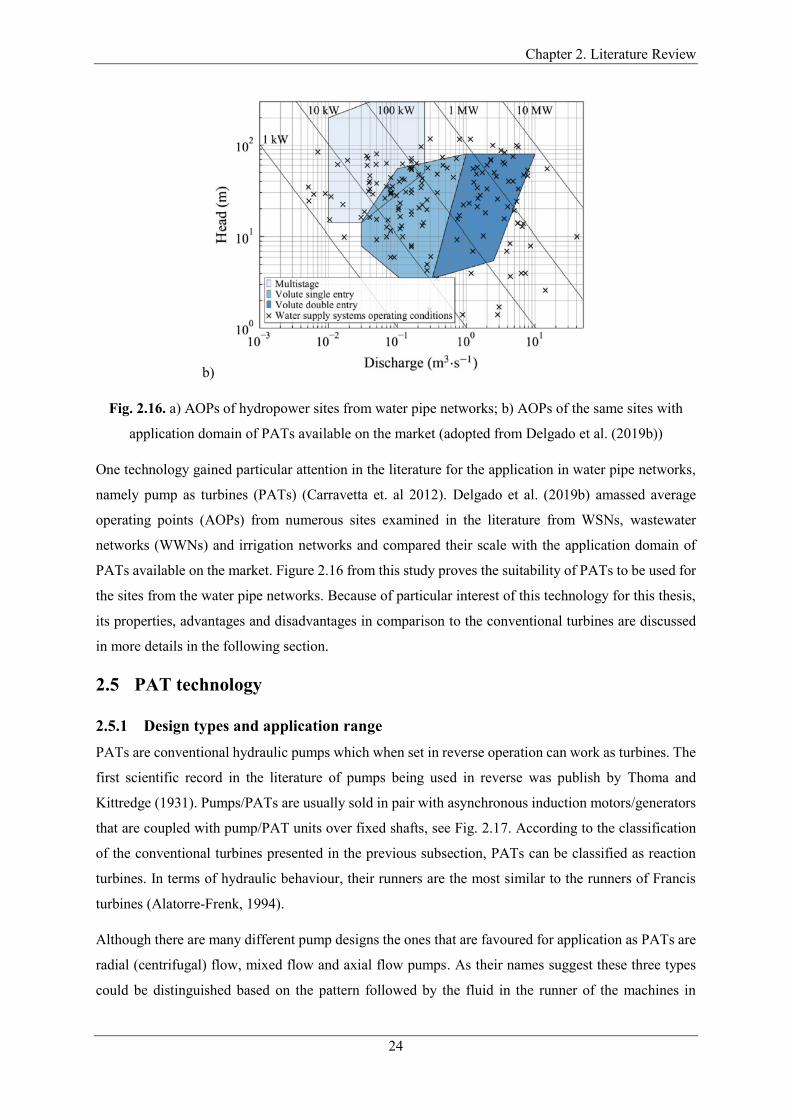
b)
Fig. 2.16. a) AOPs of hydropower sites from water pipe networks; b) AOPs of the same sites with
application domain of PATs available on the market (adopted from Delgado et al. (2019b))
One technology gained particular attention in the literature for the application in water pipe networks,
namely pump as turbines (PATs) (Carravetta et. al 2012). Delgado et al. (2019b) amassed average
operating points (AOPs) from numerous sites examined in the literature from WSNs, wastewater
networks (WWNs) and irrigation networks and compared their scale with the application domain of
PATs available on the market. Figure 2.16 from this study proves the suitability of PATs to be used for
the sites from the water pipe networks. Because of particular interest of this technology for this thesis,
its properties, advantages and disadvantages in comparison to the conventional turbines are discussed
in more details in the following section.
2.5 PAT technology
2.5.1 Design types and application range
PATs are conventional hydraulic pumps which when set in reverse operation can work as turbines. The
first scientific record in the literature of pumps being used in reverse was publish by Thoma and
Kittredge (1931). Pumps/PATs are usually sold in pair with asynchronous induction motors/generators
that are coupled with pump/PAT units over fixed shafts, see Fig. 2.17. According to the classification
of the conventional turbines presented in the previous subsection, PATs can be classified as reaction
turbines. In terms of hydraulic behaviour, their runners are the most similar to the runners of Francis
turbines (Alatorre-Frenk, 1994).
Although there are many different pump designs the ones that are favoured for application as PATs are
radial (centrifugal) flow, mixed flow and axial flow pumps. As their names suggest these three types
could be distinguished based on the pattern followed by the fluid in the runner of the machines in
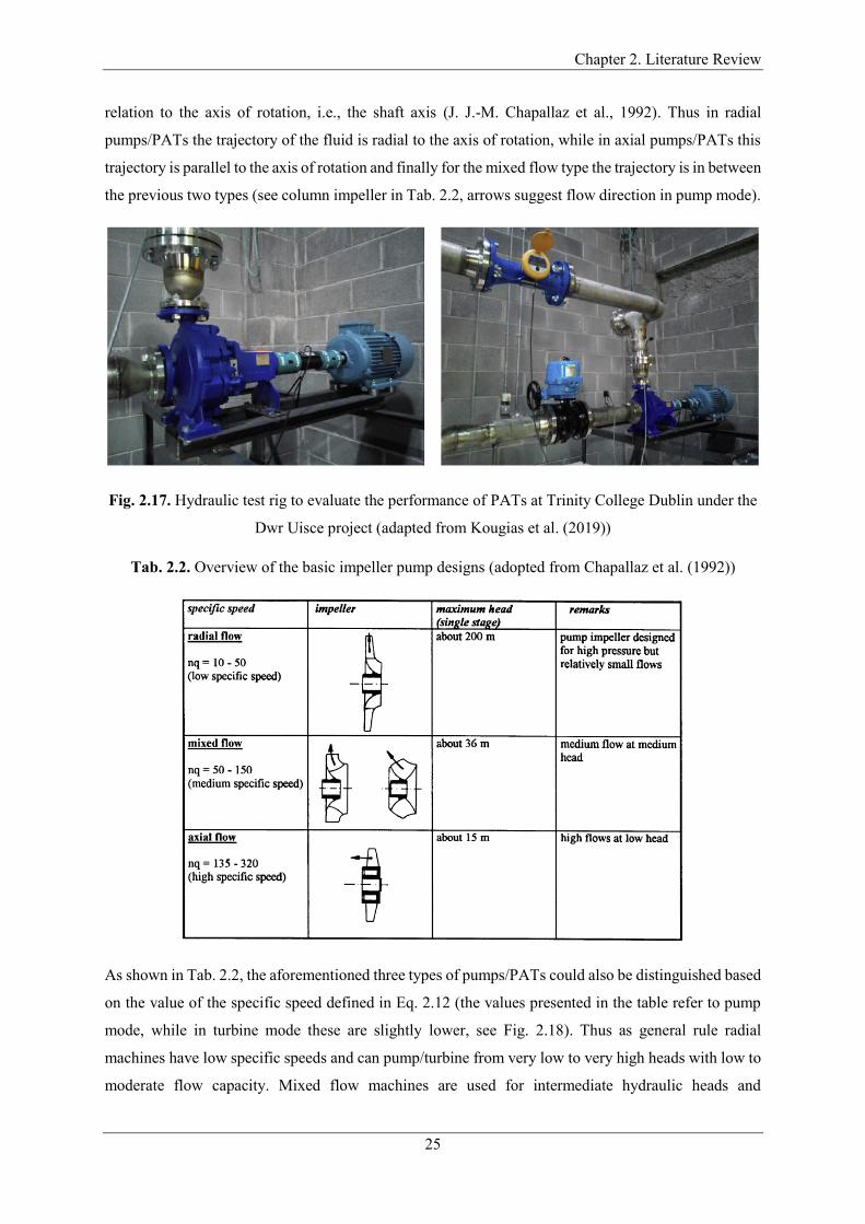
Chapter 2. Literature Review
25
relation to the axis of rotation, i.e., the shaft axis (J. J.-M. Chapallaz et al., 1992). Thus in radial
pumps/PATs the trajectory of the fluid is radial to the axis of rotation, while in axial pumps/PATs this
trajectory is parallel to the axis of rotation and finally for the mixed flow type the trajectory is in between
the previous two types (see column impeller in Tab. 2.2, arrows suggest flow direction in pump mode).
Fig. 2.17. Hydraulic test rig to evaluate the performance of PATs at Trinity College Dublin under the
Dwr Uisce project (adapted from Kougias et al. (2019))
Tab. 2.2. Overview of the basic impeller pump designs (adopted from Chapallaz et al. (1992))
As shown in Tab. 2.2, the aforementioned three types of pumps/PATs could also be distinguished based
on the value of the specific speed defined in Eq. 2.12 (the values presented in the table refer to pump
mode, while in turbine mode these are slightly lower, see Fig. 2.18). Thus as general rule radial
machines have low specific speeds and can pump/turbine from very low to very high heads with low to
moderate flow capacity. Mixed flow machines are used for intermediate hydraulic heads and
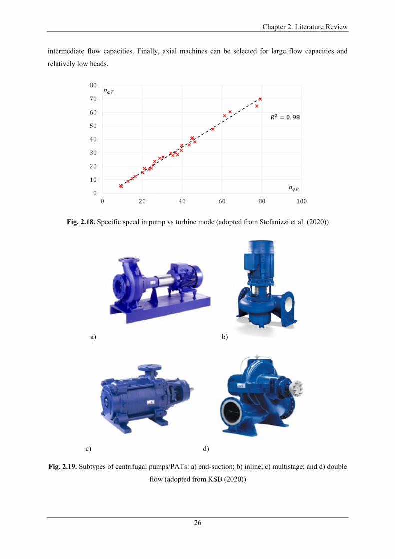
Chapter 2. Literature Review
26
intermediate flow capacities. Finally, axial machines can be selected for large flow capacities and
relatively low heads.
Fig. 2.18. Specific speed in pump vs turbine mode (adopted from Stefanizzi et al. (2020))
a) b)
c) d)
Fig. 2.19. Subtypes of centrifugal pumps/PATs: a) end-suction; b) inline; c) multistage; and d) double
flow (adopted from KSB (2020))

Chapter 2. Literature Review
27
The most widely used type worldwide are centrifugal pumps/PATs (Novara et al., 2019). This type of
machine has its subtypes, which enable to expand its application range. Beside the most common end-
suction design that is presented in Fig. 2.17 and Fig. 2.19a, there are also inline (Fig. 2.19b), multistage
(Fig. 2.19c) and double flow (Fig. 2.19d) designs. The inline type has very similar application range as
the end-suction type in terms of flow capacity and hydraulic heads and it has slightly lower maximal
efficiency (KSB, 2020), however it is suitable for sites where construction space is limited. For instance
when it is not possible to maintain 90 degrees angle between the inlet and outlet pipes. To achieve a
higher head drop across a PAT multiple impellers can be assembled in series forming a multistage unit.
Conversely, the double flow type allows processing higher flow rates than standard radial type by
having radially split casing with two impellers in parallel.
Chapallaz et al. (1992) proposed an application chart of the aforementioned PAT designs, which is
presented in Fig. 2.20. The application boundaries of different PAT types match reasonably well with
the ones suggested by Andritz Hydro (Fig. 2.16b), presented in a study carried out by Delgado et al.
(2019). Chapallaz et al. (1992) also suggested that the potential cost advantage of PATs over
conventional turbines is limited to mini and micro hydropower schemes under 500kW, as for larger
power outputs the pumps are no longer standard, mass produced units but purpose-built machines like
conventional turbines (and no longer retain their low-cost advantage).
Fig. 2.20. PAT application chart (adopted from Chapallaz et al (1992))
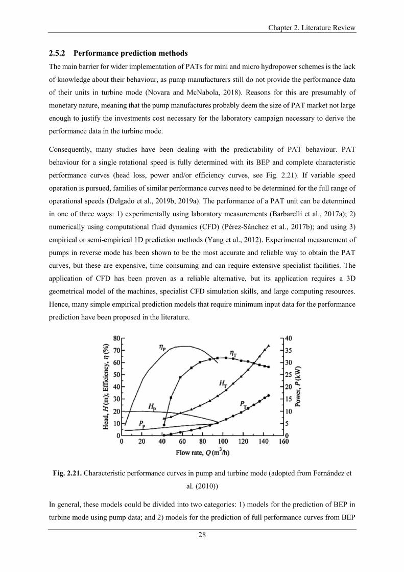
Chapter 2. Literature Review
28
2.5.2 Performance prediction methods
The main barrier for wider implementation of PATs for mini and micro hydropower schemes is the lack
of knowledge about their behaviour, as pump manufacturers still do not provide the performance data
of their units in turbine mode (Novara and McNabola, 2018). Reasons for this are presumably of
monetary nature, meaning that the pump manufactures probably deem the size of PAT market not large
enough to justify the investments cost necessary for the laboratory campaign necessary to derive the
performance data in the turbine mode.
Consequently, many studies have been dealing with the predictability of PAT behaviour. PAT
behaviour for a single rotational speed is fully determined with its BEP and complete characteristic
performance curves (head loss, power and/or efficiency curves, see Fig. 2.21). If variable speed
operation is pursued, families of similar performance curves need to be determined for the full range of
operational speeds (Delgado et al., 2019b, 2019a). The performance of a PAT unit can be determined
in one of three ways: 1) experimentally using laboratory measurements (Barbarelli et al., 2017a); 2)
numerically using computational fluid dynamics (CFD) (Pérez-Sánchez et al., 2017b); and using 3)
empirical or semi-empirical 1D prediction methods (Yang et al., 2012). Experimental measurement of
pumps in reverse mode has been shown to be the most accurate and reliable way to obtain the PAT
curves, but these are expensive, time consuming and can require extensive specialist facilities. The
application of CFD has been proven as a reliable alternative, but its application requires a 3D
geometrical model of the machines, specialist CFD simulation skills, and large computing resources.
Hence, many simple empirical prediction models that require minimum input data for the performance
prediction have been proposed in the literature.
Fig. 2.21. Characteristic performance curves in pump and turbine mode (adopted from Fernández et
al. (2010))
In general, these models could be divided into two categories: 1) models for the prediction of BEP in
turbine mode using pump data; and 2) models for the prediction of full performance curves from BEP
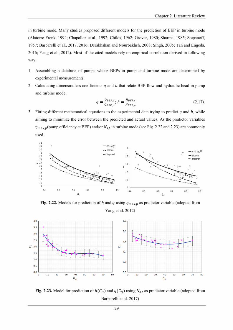
Chapter 2. Literature Review
29
in turbine mode. Many studies proposed different models for the prediction of BEP in turbine mode
(Alatorre-Frenk, 1994; Chapallaz et al., 1992; Childs, 1962; Grover, 1980; Sharma, 1985; Stepanoff,
1957; Barbarelli et al., 2017, 2016; Derakhshan and Nourbakhsh, 2008; Singh, 2005; Tan and Engeda,
2016; Yang et al., 2012). Most of the cited models rely on empirical correlation derived in following
way:
1. Assembling a database of pumps whose BEPs in pump and turbine mode are determined by
experimental measurements.
2. Calculating dimensionless coefficients 𝑞 and ℎ that relate BEP flow and hydraulic head in pump
and turbine mode:
𝑞 =𝑄𝐵𝐸𝑃,𝑡
𝑄𝐵𝐸𝑃,𝑝; ℎ =
𝐻𝐵𝐸𝑃,𝑡
𝐻𝐵𝐸𝑃,𝑝 (2.17).
3. Fitting different mathematical equations to the experimental data trying to predict 𝑞 and ℎ, while
aiming to minimize the error between the predicted and actual values. As the predictor variables
𝜂𝑚𝑎𝑥,𝑝(pump efficiency at BEP) and/or 𝑁𝑠,𝑡 in turbine mode (see Fig. 2.22 and 2.23) are commonly
used.
Fig. 2.22. Models for prediction of ℎ and 𝑞 using 𝜂𝑚𝑎𝑥,𝑝 as predictor variable (adopted from
Yang et al. 2012)
Fig. 2.23. Model for prediction of ℎ(𝐶𝐻) and 𝑞(𝐶𝑄) using 𝑁𝑠,𝑡 as predictor variable (adopted from
Barbarelli et al. 2017)

Chapter 2. Literature Review
30
The prediction parameters defined in Eq. 2.17 assume that the impeller rotational speed is the same in
pump and turbine mode. In general, the prediction parameters have values higher than one, meaning
that BEP flow and hydraulic head in turbine mode are higher than in pump mode (see Fig. 2.21). The
literature also agrees that the efficiency at BEP in both operating modes is very similar, thus the
efficiency in turbine mode was usually considered equal to the efficiency of the same unit in pump
mode, or slightly lower (Alatorre-Frenk, 1994). Using this assumption and one of the models for
prediction of BEP in turbine mode from BEP in pump mode, Novara et al. (2017) derived an equation
for prediction of the efficiency at BEP in turbine mode. Namely, the authors recalculated new values
for the coefficients a-e, for an equation originally proposed by Anderson (1977) used for prediction of
BEP efficiency in pump mode:
𝜂𝑚𝑎𝑥 = 𝑎 −𝑏
𝑄𝐵𝐸𝑃𝑐 − 𝑑 (𝑒 + ln (
𝑁𝑠
52.933))
2 (2.18).
In the original publications that proposed the models for prediction of BEP in turbine mode, the errors
in the predictions of the coefficients 𝑞 and ℎ (calculated on the set of pumps based on which the models
were derived), were acceptable for engineering practice. The inventors of the models usually claimed
superiority of their models, i.e., that their models reduce the prediction errors in comparison to
previously proposed models. However, the analyses usually included different sets of pumps and
usually these sets comprised a quite small number of units. Recently, Novara (2020) conducted the most
comprehensive cross comparison of the prediction models to date. The comparison included 119
commercial pumps of different design types and manufactures. Figure 2.21 shows the average relative
prediction error 𝐸 across the set of 119 pumps for each of the analysed models. For each of the
pump/PAT unit from the set, the relative prediction error was calculated using the following
expressions:
𝐸𝑞 =𝑞𝑝−𝑞𝑎
𝑞𝑎; 𝐸ℎ =
ℎ𝑝−ℎ𝑎
ℎ𝑎; 𝐸 = (𝐸𝑞
2 + 𝐸ℎ2)
0.5 (2.19),
where indices 𝑝 and 𝑎 designate predicted and actual experimental value respectively. In Fig. 2.21 the
results were divided in two parts, i.e., the pump set was divided in two subsets depending on the value
of 𝑁𝑠, because of the applicability limits of some models. As it can be seen from the figure, some models
even had average error across the set of up to 100%. The model proposed by Yang et al. (2012)
performed the best overall, with the average relative error of 16.2% for 𝑁𝑠<60 and 18.8% for 𝑁𝑠 > 60.
These results are a bit surprising, considering that the model proposed by Yang et al. (2012) has one of
the simplest formulations among the considered models (see also Fig. 2.22):
𝑞 =1.2
𝜂𝑝0.55 ; ℎ =
1.2
𝜂𝑝1.1 (2.20).
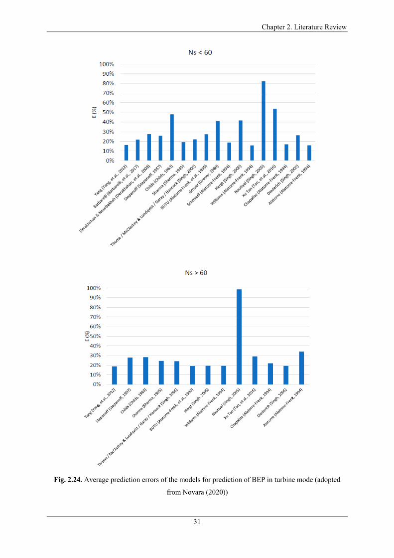
Chapter 2. Literature Review
31
Fig. 2.24. Average prediction errors of the models for prediction of BEP in turbine mode (adopted
from Novara (2020))
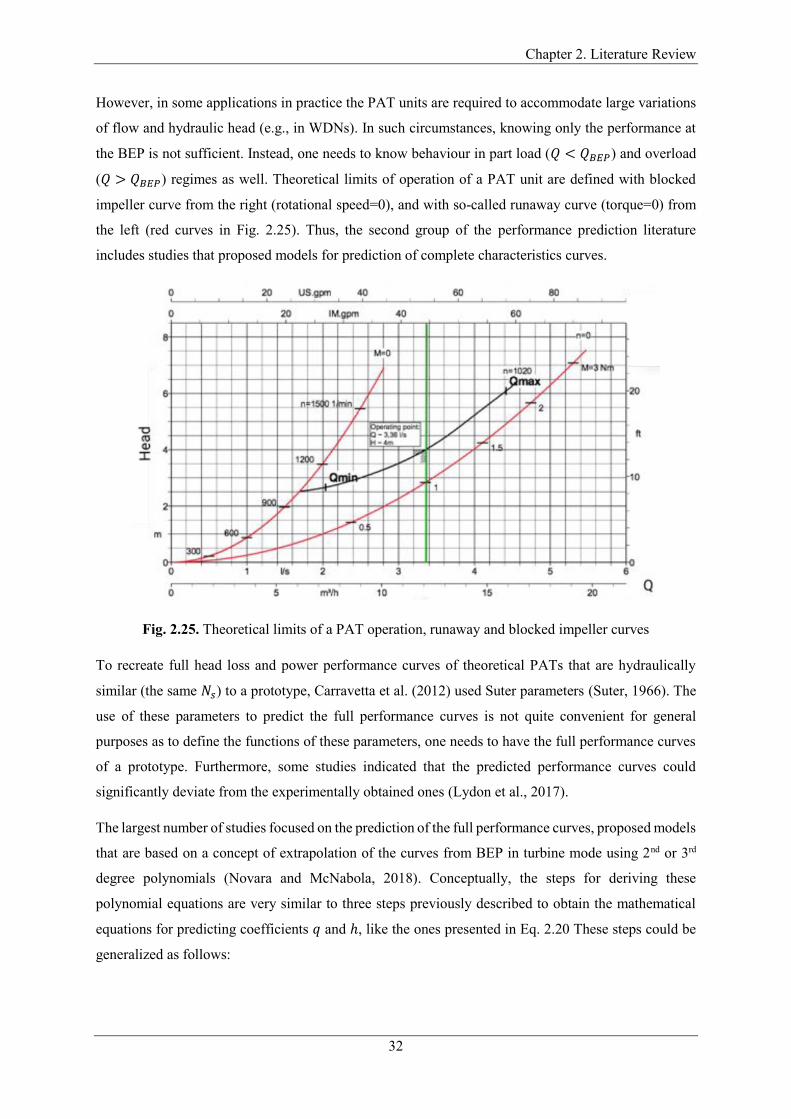
Chapter 2. Literature Review
32
However, in some applications in practice the PAT units are required to accommodate large variations
of flow and hydraulic head (e.g., in WDNs). In such circumstances, knowing only the performance at
the BEP is not sufficient. Instead, one needs to know behaviour in part load (𝑄 < 𝑄𝐵𝐸𝑃) and overload
(𝑄 > 𝑄𝐵𝐸𝑃) regimes as well. Theoretical limits of operation of a PAT unit are defined with blocked
impeller curve from the right (rotational speed=0), and with so-called runaway curve (torque=0) from
the left (red curves in Fig. 2.25). Thus, the second group of the performance prediction literature
includes studies that proposed models for prediction of complete characteristics curves.
Fig. 2.25. Theoretical limits of a PAT operation, runaway and blocked impeller curves
To recreate full head loss and power performance curves of theoretical PATs that are hydraulically
similar (the same 𝑁𝑠) to a prototype, Carravetta et al. (2012) used Suter parameters (Suter, 1966). The
use of these parameters to predict the full performance curves is not quite convenient for general
purposes as to define the functions of these parameters, one needs to have the full performance curves
of a prototype. Furthermore, some studies indicated that the predicted performance curves could
significantly deviate from the experimentally obtained ones (Lydon et al., 2017).
The largest number of studies focused on the prediction of the full performance curves, proposed models
that are based on a concept of extrapolation of the curves from BEP in turbine mode using 2nd or 3rd
degree polynomials (Novara and McNabola, 2018). Conceptually, the steps for deriving these
polynomial equations are very similar to three steps previously described to obtain the mathematical
equations for predicting coefficients 𝑞 and ℎ, like the ones presented in Eq. 2.20 These steps could be
generalized as follows:
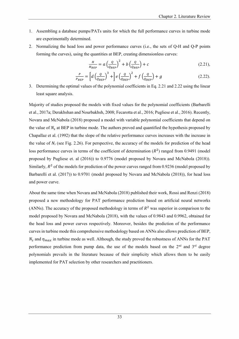
Chapter 2. Literature Review
33
1. Assembling a database pumps/PATs units for which the full performance curves in turbine mode
are experimentally determined.
2. Normalizing the head loss and power performance curves (i.e., the sets of Q-H and Q-P points
forming the curves), using the quantities at BEP, creating dimensionless curves:
𝐻
𝐻𝐵𝐸𝑃= 𝑎 (
𝑄
𝑄𝐵𝐸𝑃)
2+ 𝑏 (
𝑄
𝑄𝐵𝐸𝑃) + 𝑐 (2.21),
𝑃
𝑃𝐵𝐸𝑃= [𝑑 (
𝑄
𝑄𝐵𝐸𝑃)
3+] 𝑒 (
𝑄
𝑄𝐵𝐸𝑃)
2+ 𝑓 (
𝑄
𝑄𝐵𝐸𝑃) + 𝑔 (2.22).
3. Determining the optimal values of the polynomial coefficients in Eq. 2.21 and 2.22 using the linear
least square analysis.
Majority of studies proposed the models with fixed values for the polynomial coefficients (Barbarelli
et al., 2017a; Derakhshan and Nourbakhsh, 2008; Fecarotta et al., 2016; Pugliese et al., 2016). Recently,
Novara and McNabola (2018) proposed a model with variable polynomial coefficients that depend on
the value of 𝑁𝑠 at BEP in turbine mode. The authors proved and quantified the hypothesis proposed by
Chapallaz et al. (1992) that the slope of the relative performance curves increases with the increase in
the value of Ns (see Fig. 2.26). For perspective, the accuracy of the models for prediction of the head
loss performance curves in terms of the coefficient of determination (𝑅2) ranged from 0.9491 (model
proposed by Pugliese et. al (2016)) to 0.9776 (model proposed by Novara and McNabola (2018)).
Similarly, 𝑅2 of the models for prediction of the power curves ranged from 0.9236 (model proposed by
Barbarelli et al. (2017)) to 0.9701 (model proposed by Novara and McNabola (2018)), for head loss
and power curve.
About the same time when Novara and McNabola (2018) published their work, Rossi and Renzi (2018)
proposed a new methodology for PAT performance prediction based on artificial neural networks
(ANNs). The accuracy of the proposed methodology in terms of 𝑅2 was superior in comparison to the
model proposed by Novara and McNabola (2018), with the values of 0.9843 and 0.9962, obtained for
the head loss and power curves respectively. Moreover, besides the prediction of the performance
curves in turbine mode this comprehensive methodology based on ANNs also allows prediction of BEP,
𝑁𝑠 and 𝜂𝑚𝑎𝑥 in turbine mode as well. Although, the study proved the robustness of ANNs for the PAT
performance prediction from pump data, the use of the models based on the 2nd and 3rd degree
polynomials prevails in the literature because of their simplicity which allows them to be easily
implemented for PAT selection by other researchers and practitioners.
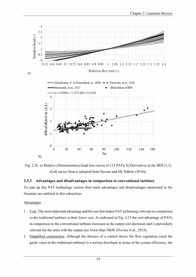
Chapter 2. Literature Review
34
a)
b)
Fig. 2.26. a) Relative (Dimensionless) head loss curves of 113 PATs; b) Derivatives at the BEP (1,1)
of all curves from a (adopted from Novara and Mc Nabola (2018)).
2.5.3 Advantages and disadvantages in comparison to conventional turbines
To sum up this PAT technology section their main advantages and disadvantages mentioned in the
literature are outlined in this subsection:
Advantages
1. Cost. The most important advantage and the one that makes PAT technology relevant in comparison
to the traditional turbines is their lower cost. As indicated in Fig. 2.15 the cost advantage of PATs
in comparison to the conventional turbines increases as the output size decreases and is particularly
relevant for the units with the output size lower than 50kW (Novara et al., 2019).
2. Simplified construction. Although the absence of a control device for flow regulation (such the
guide vanes at the traditional turbines) is a serious drawback in terms of the system efficiency, the

Chapter 2. Literature Review
35
simpler design of PATs can be regarded as an advantage in terms of their manufacture and simpler
installation (J. J.-M. Chapallaz et al., 1992).
3. Availability. Because of their mass production and widespread application in many fields,
pumps/PATs are usually readily available with short delivery times. The same refers to the
availability of the spare parts.
Disadvantages
1. Lower peak and part load efficiency. In general, compared to most of the traditional turbine designs
PATs have lower part load mechanical efficiency. From Fig. 2.24 it can be observed that PATs
exhibit lower part and over load efficiency compared to Pelton, Crossflow or Kaplan turbines, while
their part load efficiency is comparable to the part load efficiency of Francis turbines. Furthermore,
the peak efficiency of the sophisticated turbines from renowned manufacturers, which reaches over
90% is higher than the one of PATs. However, the peak efficiency of PAT units can be comparable
if not superior to locally manufactured Cross Flow and Pelton turbines (J. J.-M. Chapallaz et al.,
1992).
Fig. 2.27. Relative mechanical efficiency of PATs and traditional turbines (adopted from Novara
and McNabola (2018))
2. No hydraulic regulation device. Regardless of values of their peak efficiencies, the comparison of
just mechanical part load efficiencies between the traditional turbines and PATs like presented in
Fig. 2.27 is not appropriate. Instead, the global system efficiency should be compared. The global
system efficiency of PATs would match the mechanical efficiency from Fig. 2.27 only if the flow-
head pattern at a considered site would follow the head loss curve of a PAT unit (like in Fig. 2.21
or Fig. 25). However, in reality this is never the case, instead available flow-head patterns usually
follow the opposite pattern (low flow-high head and high flow-low head) because of the relationship
Chapter 2. Literature Review
36
between flow and hydraulic head losses. Thus, for 𝑄 < 𝑄𝐵𝐸𝑃 in the absence of a control device
PATs can exploit only partial available head, which significantly reduced their global efficiency.
On the other head, for 𝑄 > 𝑄𝐵𝐸𝑃 a partial flow usually have to be bypassed to avoid excessive head
drops by a PAT, which again significantly reduces the global efficiency of a hydropower plant
equipped with a PAT (see Fig. 2.25).
Fig. 2.28. Global system efficiency of PATs and traditional turbines (adopted from Novara and
McNabola (2018))
3. Performance uncertainty. Probably the main disadvantage of PATs is their performance uncertainty.
As it was thoroughly discussed in the previous subsection, the pump manufacturers do not provide
the performance curves of their units in turbine mode and some 1D selection methodologies have
been unreliable.
4. Vibration and excessive noise. Another disadvantage of PATs could be potential large vibration
and excessive noise recorded at some of the previous installations in practice (Zeropex, 2012),
which led to failures and poor reputation.
To conclude, a PAT unit has to be selected very carefully to avoid poor performance that can offset the
cost advantage of PATs in comparison to the traditional turbines. This particularly pertains to sites with
large recurrent variation of flow and head like the ones occurring in WDNs.
2.6 HPER in WSNs
2.6.1 Potential site locations
The idea of using WSNs as a setting for hydropower generation is not new (Afshar et al., 1991).
However, in the past the installations were almost exclusively restricted to large sites located in
transmission parts of the networks. It is only recently that because of the imperative to reduce the energy
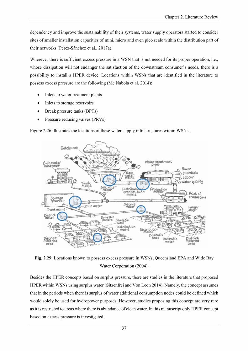
Chapter 2. Literature Review
37
dependency and improve the sustainability of their systems, water supply operators started to consider
sites of smaller installation capacities of mini, micro and even pico scale within the distribution part of
their networks (Pérez-Sánchez et al., 2017a).
Wherever there is sufficient excess pressure in a WSN that is not needed for its proper operation, i.e.,
whose dissipation will not endanger the satisfaction of the downstream consumer’s needs, there is a
possibility to install a HPER device. Locations within WSNs that are identified in the literature to
possess excess pressure are the following (Mc Nabola et al. 2014):
Inlets to water treatment plants
Inlets to storage reservoirs
Break pressure tanks (BPTs)
Pressure reducing valves (PRVs)
Figure 2.26 illustrates the locations of these water supply infrastructures within WSNs.
Fig. 2.29. Locations known to possess excess pressure in WSNs, Queensland EPA and Wide Bay
Water Corporation (2004).
Besides the HPER concepts based on surplus pressure, there are studies in the literature that proposed
HPER within WSNs using surplus water (Sitzenfrei and Von Leon 2014). Namely, the concept assumes
that in the periods when there is surplus of water additional consumption nodes could be defined which
would solely be used for hydropower purposes. However, studies proposing this concept are very rare
as it is restricted to areas where there is abundance of clean water. In this manuscript only HPER concept
based on excess pressure is investigated.
Chapter 2. Literature Review
38
2.6.2 Design challenges related to HPER in WSN settings
Regardless of turbine type, all turbines are designed to work optimally (with the highest efficiency) at
particular operating condition, i.e., particular flow rate and hydraulic head. These values of flow rate
and hydraulic head are designated as BEP of the machines. Any deviation from this condition will lead
to lower mechanical efficiency.
It is well documented in the literature that locations within WSNs are characterised by large variation
of flow and hydraulic head (Colombo and Kleiner, 2011). Consequently, many studies indicated large
variations of the hydraulic conditions as one of the main challenges for selection of appropriate HPER
devices and assessment of economic viability. Corcoran et al. (2017) studied 10 years long high-
resolution historical data of the recorded hydraulic conditions at potential HPER sites in Irish and UK
WSNs. The aim of the study was to derive a model that forecasts long-term demand variations. The
historical data recorded in the period between 2002-2012 showed that at some valves the average yearly
demand varied as much as 350%. For one of the valves from the study (V2), the conducted statistical
analysis showed the highest correlation of the demand with population data and new households built.
Using the forecasted data from CSO (Central Statistics Office) for these two predictor variables
Corcoran et al. (2017) estimated that the theoretical HPER potential would have changed in the period
between 2003 and 2020 from 71.83 MWh to 381.06 MWh per year. Although, these values indicated
the scale of demand change, the real potential would not change this much because the real machines
have limitations of their operational range. For instance, if a design flow of the selected machine would
match the average yearly flow from 2003 than the maximal energy that could be recovered per year
would be around that value, as the rest of the flow would need to be bypassed because of the operational
limits of the selected machine. However, if the demand would decrease to a similar scale it would
probably make the selected turbine completely unsuitable to recover energy from the considered site.
Similarly, Brady et al. (2017) investigated the influence of variation of flow and hydraulic head recorded
at PRVs in Dublin WSN on HPER potential, by studying 20 years long historical data. The study
observed demand variations of similar magnitude as presented in study by Corcoran et al. (2017), but
indicated that the hydraulic head varied to a significantly smaller degree. This can be explained with
the fact that water supply operator are obligated to maintain satisfactory level of pressure in the
networks, while flow rate is solely driven by the consumers’ demand. Nevertheless, the study found
that for sites of small installation power potential (12.5 kW) with such magnitudes of demand variations,
the only economically viable solution is to install two PATs in parallel.
Another important design challenge recurring in the literature that is characteristic for WSN settings is
the requirement to maintain downstream head (A. Carravetta et al., 2014). As the primary function of
WSNs is to supply water to consumers with satisfactory quality and quantity, which implies maintaining
the minimal hydraulic head within the networks. The value of the minimal hydraulic head can vary

Chapter 2. Literature Review
39
significantly from network to network (see Fig. 2.5) and usually depends on the height of buildings in
supplied area.
In conventional hydropower settings there is no such requirement. In conventional hydropower settings
it is only sometimes (if reaction turbine is used) necessary to maintain a few meters of back head , in
order to prevent occurrence of cavitation (J. J.-M. Chapallaz et al., 1992). The requirement to maintain
downstream head at certain level also leads to only reaction turbines being suitable for majority of
potential locations.
Maintaining downstream head is a particular challenge when PATs are used as HPER devices (Fontana
et al., 2018, 2016). Namely, as PATs do not possess flow control devices and are not able to adjust their
head loss curve to match operating conditions at sites, several installation schemes have been proposed
in the literature to address this problem. These installation schemes will be discussed in more details in
subsection 2.6.4 and in other chapters of the thesis.
2.6.3 Studies that consider traditional turbines as HPER devices
Although a minority, a few studies examined the energy recovery potential and economic feasibly of
replacing pressure management infrastructure such as BPTs and PRVs, with traditional turbines.
McNabola et al. (2014) examined HPER potential of 10 BPTs in Ireland. The study concluded that the
economic viability of BPT sites greatly depend on value of Feed-In-Tarriffs (FITs) in differing country,
purchase price of electricity and variations in flow conditions, and that 13 kW were minimum for
economic viability in the best circumstances. In addition, FITs are no longer available for hydropower
in Europe.
Corcoran et al. (2013) performed an analysis of HPER potential at 95 sites, including BPTs, PRVs and
valves at inlet pipes of storage reservoirs in WSNs in Ireland and the UK. Firstly, a preliminary analysis
was carried out on all sites using average values of flow, pressure and turbine efficiency, shortlisting
the most promising sites. For the most promising sites, a detailed sensitivity analysis was carried out
with focus on effects of flow and pressure variations and choice of turbine type on the energy recovery.
The results obtained using actual flow and hydraulic head with part load-turbine efficiency, compared
with assuming average values showed a significant overestimate of the power outputs in some cases.
The study of Gallagher et al. (2015) proposed a structured 4 step methodology for finding the most
promising HPER sites including both water supply and wastewater networks. The study examined the
set of 238 sites, including valves at service reservoirs, BPTs, PRVs and outlets of WWTPs. 80 out of
238 sites had power potential bigger than 5 kW and potential to recovery 17.9 GWh per annum. The
study also outlined bottom thresholds of power potentials in Ireland and Wales for each type of
infrastructure to be economically viable.
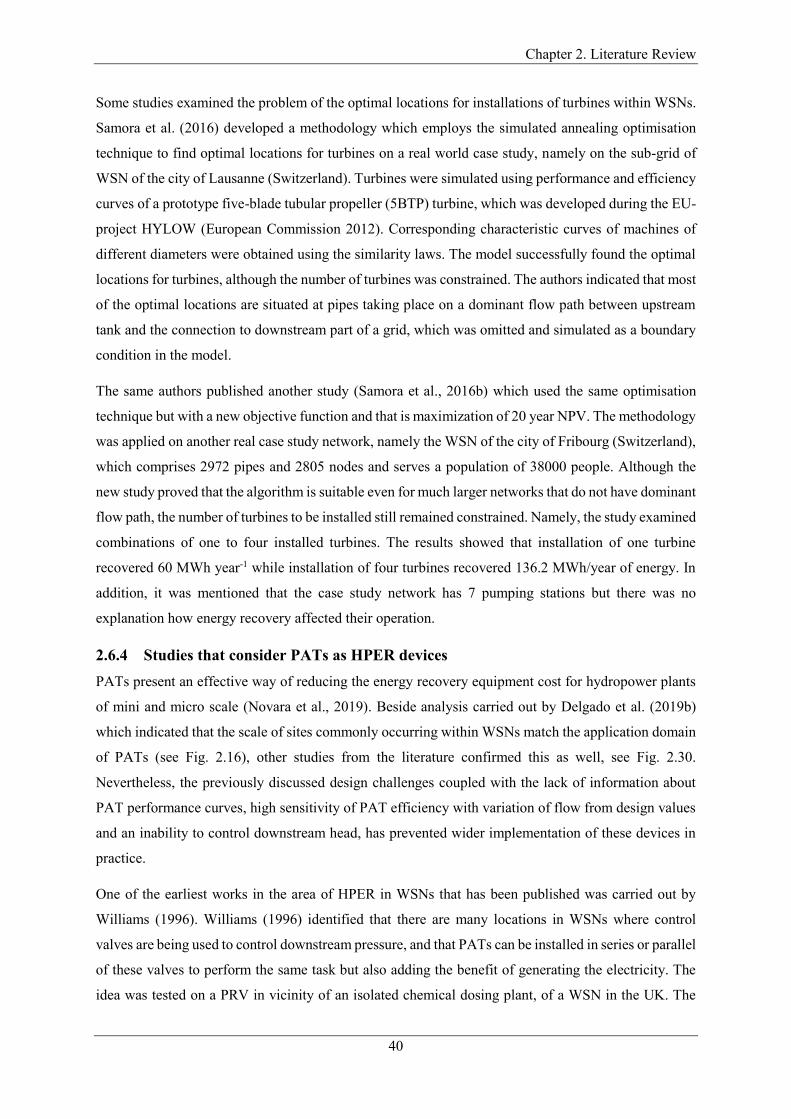
Chapter 2. Literature Review
40
Some studies examined the problem of the optimal locations for installations of turbines within WSNs.
Samora et al. (2016) developed a methodology which employs the simulated annealing optimisation
technique to find optimal locations for turbines on a real world case study, namely on the sub-grid of
WSN of the city of Lausanne (Switzerland). Turbines were simulated using performance and efficiency
curves of a prototype five-blade tubular propeller (5BTP) turbine, which was developed during the EU-
project HYLOW (European Commission 2012). Corresponding characteristic curves of machines of
different diameters were obtained using the similarity laws. The model successfully found the optimal
locations for turbines, although the number of turbines was constrained. The authors indicated that most
of the optimal locations are situated at pipes taking place on a dominant flow path between upstream
tank and the connection to downstream part of a grid, which was omitted and simulated as a boundary
condition in the model.
The same authors published another study (Samora et al., 2016b) which used the same optimisation
technique but with a new objective function and that is maximization of 20 year NPV. The methodology
was applied on another real case study network, namely the WSN of the city of Fribourg (Switzerland),
which comprises 2972 pipes and 2805 nodes and serves a population of 38000 people. Although the
new study proved that the algorithm is suitable even for much larger networks that do not have dominant
flow path, the number of turbines to be installed still remained constrained. Namely, the study examined
combinations of one to four installed turbines. The results showed that installation of one turbine
recovered 60 MWh year-1 while installation of four turbines recovered 136.2 MWh/year of energy. In
addition, it was mentioned that the case study network has 7 pumping stations but there was no
explanation how energy recovery affected their operation.
2.6.4 Studies that consider PATs as HPER devices
PATs present an effective way of reducing the energy recovery equipment cost for hydropower plants
of mini and micro scale (Novara et al., 2019). Beside analysis carried out by Delgado et al. (2019b)
which indicated that the scale of sites commonly occurring within WSNs match the application domain
of PATs (see Fig. 2.16), other studies from the literature confirmed this as well, see Fig. 2.30.
Nevertheless, the previously discussed design challenges coupled with the lack of information about
PAT performance curves, high sensitivity of PAT efficiency with variation of flow from design values
and an inability to control downstream head, has prevented wider implementation of these devices in
practice.
One of the earliest works in the area of HPER in WSNs that has been published was carried out by
Williams (1996). Williams (1996) identified that there are many locations in WSNs where control
valves are being used to control downstream pressure, and that PATs can be installed in series or parallel
of these valves to perform the same task but also adding the benefit of generating the electricity. The
idea was tested on a PRV in vicinity of an isolated chemical dosing plant, of a WSN in the UK. The
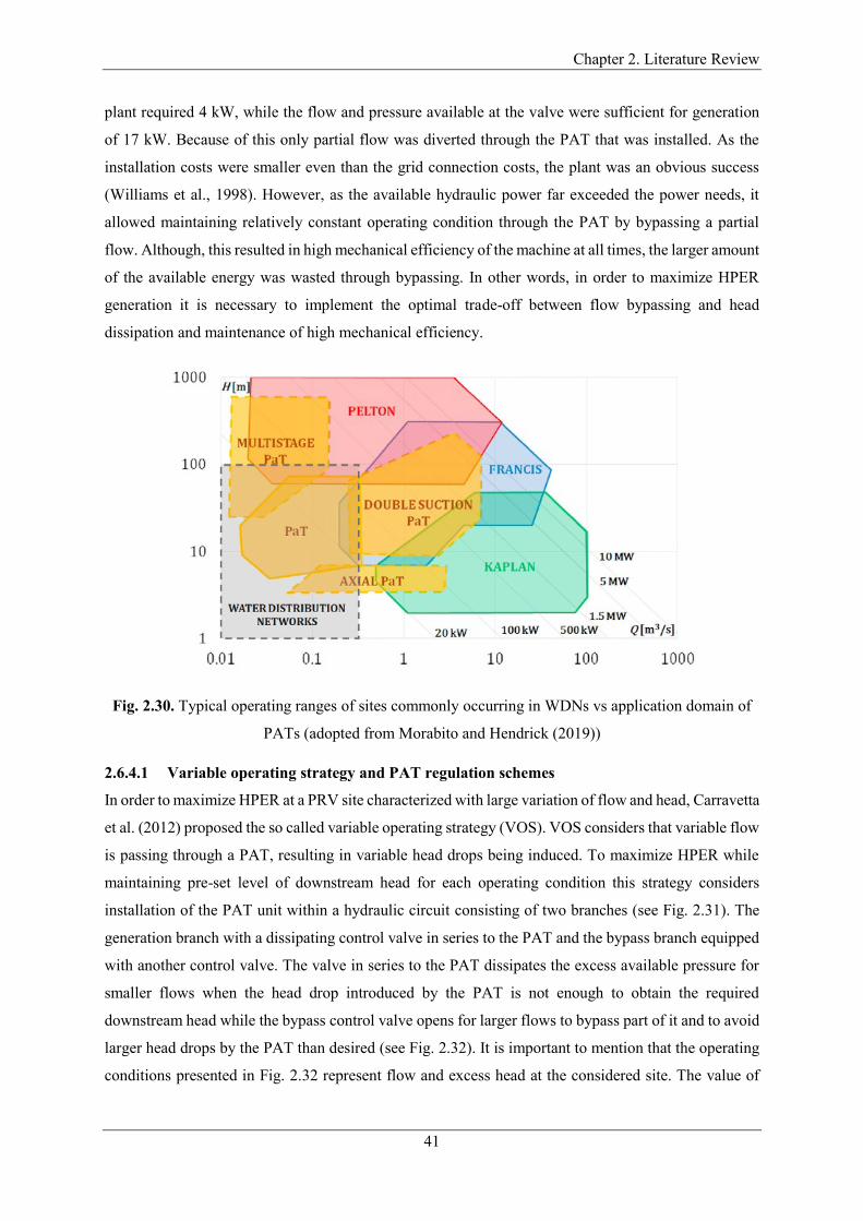
Chapter 2. Literature Review
41
plant required 4 kW, while the flow and pressure available at the valve were sufficient for generation
of 17 kW. Because of this only partial flow was diverted through the PAT that was installed. As the
installation costs were smaller even than the grid connection costs, the plant was an obvious success
(Williams et al., 1998). However, as the available hydraulic power far exceeded the power needs, it
allowed maintaining relatively constant operating condition through the PAT by bypassing a partial
flow. Although, this resulted in high mechanical efficiency of the machine at all times, the larger amount
of the available energy was wasted through bypassing. In other words, in order to maximize HPER
generation it is necessary to implement the optimal trade-off between flow bypassing and head
dissipation and maintenance of high mechanical efficiency.
Fig. 2.30. Typical operating ranges of sites commonly occurring in WDNs vs application domain of
PATs (adopted from Morabito and Hendrick (2019))
2.6.4.1 Variable operating strategy and PAT regulation schemes
In order to maximize HPER at a PRV site characterized with large variation of flow and head, Carravetta
et al. (2012) proposed the so called variable operating strategy (VOS). VOS considers that variable flow
is passing through a PAT, resulting in variable head drops being induced. To maximize HPER while
maintaining pre-set level of downstream head for each operating condition this strategy considers
installation of the PAT unit within a hydraulic circuit consisting of two branches (see Fig. 2.31). The
generation branch with a dissipating control valve in series to the PAT and the bypass branch equipped
with another control valve. The valve in series to the PAT dissipates the excess available pressure for
smaller flows when the head drop introduced by the PAT is not enough to obtain the required
downstream head while the bypass control valve opens for larger flows to bypass part of it and to avoid
larger head drops by the PAT than desired (see Fig. 2.32). It is important to mention that the operating
conditions presented in Fig. 2.32 represent flow and excess head at the considered site. The value of
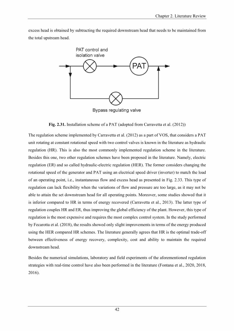
Chapter 2. Literature Review
42
excess head is obtained by subtracting the required downstream head that needs to be maintained from
the total upstream head.
Fig. 2.31. Installation scheme of a PAT (adopted from Carravetta et al. (2012))
The regulation scheme implemented by Carravetta et al. (2012) as a part of VOS, that considers a PAT
unit rotating at constant rotational speed with two control valves is known in the literature as hydraulic
regulation (HR). This is also the most commonly implemented regulation scheme in the literature.
Besides this one, two other regulation schemes have been proposed in the literature. Namely, electric
regulation (ER) and so called hydraulic-electric regulation (HER). The former considers changing the
rotational speed of the generator and PAT using an electrical speed driver (inverter) to match the load
of an operating point, i.e., instantaneous flow and excess head as presented in Fig. 2.33. This type of
regulation can lack flexibility when the variations of flow and pressure are too large, as it may not be
able to attain the set downstream head for all operating points. Moreover, some studies showed that it
is inferior compared to HR in terms of energy recovered (Carravetta et al., 2013). The latter type of
regulation couples HR and ER, thus improving the global efficiency of the plant. However, this type of
regulation is the most expensive and requires the most complex control system. In the study performed
by Fecarotta et al. (2018), the results showed only slight improvements in terms of the energy produced
using the HER compared HR schemes. The literature generally agrees that HR is the optimal trade-off
between effectiveness of energy recovery, complexity, cost and ability to maintain the required
downstream head.
Besides the numerical simulations, laboratory and field experiments of the aforementioned regulation
strategies with real-time control have also been performed in the literature (Fontana et al., 2020, 2018,
2016).
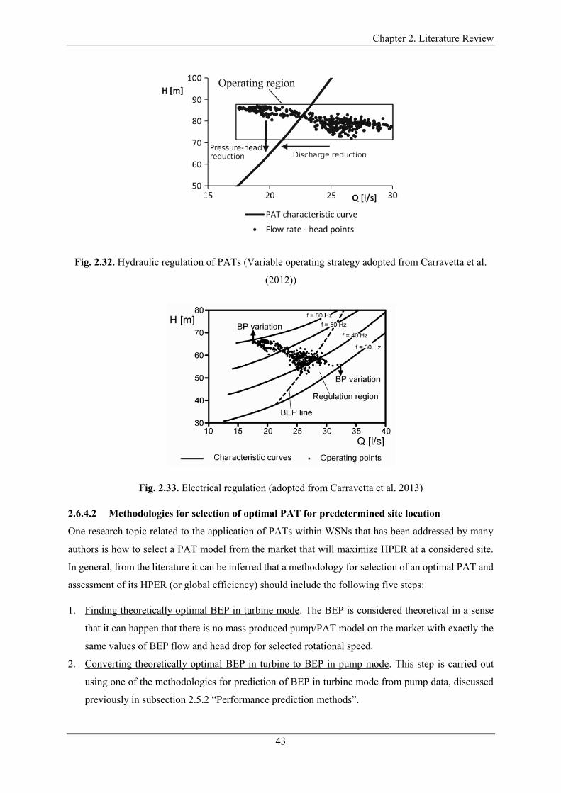
Chapter 2. Literature Review
43
Fig. 2.32. Hydraulic regulation of PATs (Variable operating strategy adopted from Carravetta et al.
(2012))
Fig. 2.33. Electrical regulation (adopted from Carravetta et al. 2013)
2.6.4.2 Methodologies for selection of optimal PAT for predetermined site location
One research topic related to the application of PATs within WSNs that has been addressed by many
authors is how to select a PAT model from the market that will maximize HPER at a considered site.
In general, from the literature it can be inferred that a methodology for selection of an optimal PAT and
assessment of its HPER (or global efficiency) should include the following five steps:
1. Finding theoretically optimal BEP in turbine mode. The BEP is considered theoretical in a sense
that it can happen that there is no mass produced pump/PAT model on the market with exactly the
same values of BEP flow and head drop for selected rotational speed.
2. Converting theoretically optimal BEP in turbine to BEP in pump mode. This step is carried out
using one of the methodologies for prediction of BEP in turbine mode from pump data, discussed
previously in subsection 2.5.2 “Performance prediction methods”.
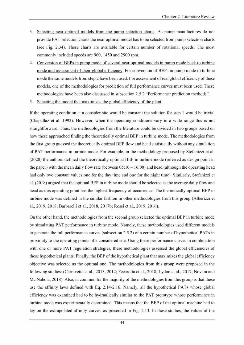
Chapter 2. Literature Review
44
3. Selecting near optimal models from the pump selection charts. As pump manufactures do not
provide PAT selection charts the near optimal model has to be selected from pump selection charts
(see Fig. 2.34). These charts are available for certain number of rotational speeds. The most
commonly included speeds are 960, 1450 and 2900 rpm.
4. Conversion of BEPs in pump mode of several near optimal models in pump mode back to turbine
mode and assessment of their global efficiency. For conversion of BEPs in pump mode to turbine
mode the same models from step 2 have been used. For assessment of real global efficiency of these
models, one of the methodologies for prediction of full performance curves must been used. These
methodologies have been also discussed in subsection 2.5.2 “Performance prediction methods”.
5. Selecting the model that maximizes the global efficiency of the plant.
If the operating condition at a consider site would be constant the solution for step 1 would be trivial
(Chapallaz et al. 1992). However, when the operating conditions vary in a wide range this is not
straightforward. Thus, the methodologies from the literature could be divided in two groups based on
how these approached finding the theoretically optimal BEP in turbine mode. The methodologies from
the first group guessed the theoretically optimal BEP flow and head statistically without any simulation
of PAT performance in turbine mode. For example, in the methodology proposed by Stefanizzi et al.
(2020) the authors defined the theoretically optimal BEP in turbine mode (referred as design point in
the paper) with the mean daily flow rate (between 05:10 – 16:00) and head (although the operating head
had only two constant values one for the day time and one for the night time). Similarly, Stefanizzi et
al. (2018) argued that the optimal BEP in turbine mode should be selected as the average daily flow and
head as this operating point has the highest frequency of occurrence. The theoretically optimal BEP in
turbine mode was defined in the similar fashion in other methodologies from this group (Alberizzi et
al., 2019, 2018; Barbarelli et al., 2018, 2017b; Rossi et al., 2019, 2016).
On the other hand, the methodologies from the second group selected the optimal BEP in turbine mode
by simulating PAT performance in turbine mode. Namely, these methodologies used different models
to generate the full performance curves (subsection 2.5.2) of a certain number of hypothetical PATs in
proximity to the operating points of a considered site. Using these performance curves in combination
with one or more PAT regulation strategies, these methodologies assessed the global efficiencies of
these hypothetical plants. Finally, the BEP of the hypothetical plant that maximizes the global efficiency
objective was selected as the optimal one. The methodologies from this group were proposed in the
following studies: (Carravetta et al., 2013, 2012; Fecarotta et al., 2018; Lydon et al., 2017; Novara and
Mc Nabola, 2018). Also, in common for the majority of the methodologies from this group is that these
use the affinity laws defined with Eq. 2.14-2.16. Namely, all the hypothetical PATs whose global
efficiency was examined had to be hydraulically similar to the PAT prototype whose performance in
turbine mode was experimentally determined. This means that the BEP of the optimal machine had to
lay on the extrapolated affinity curves, as presented in Fig. 2.13. In these studies, the values of the
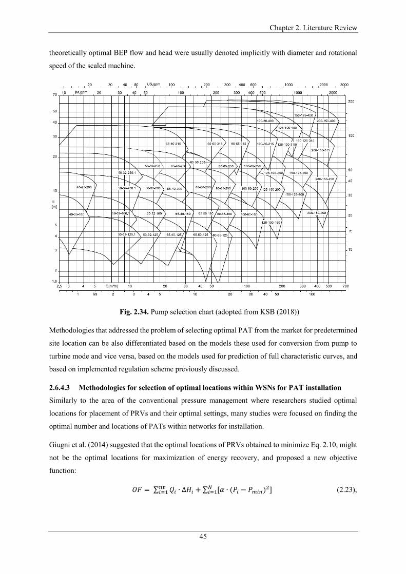
Chapter 2. Literature Review
45
theoretically optimal BEP flow and head were usually denoted implicitly with diameter and rotational
speed of the scaled machine.
Fig. 2.34. Pump selection chart (adopted from KSB (2018))
Methodologies that addressed the problem of selecting optimal PAT from the market for predetermined
site location can be also differentiated based on the models these used for conversion from pump to
turbine mode and vice versa, based on the models used for prediction of full characteristic curves, and
based on implemented regulation scheme previously discussed.
2.6.4.3 Methodologies for selection of optimal locations within WSNs for PAT installation
Similarly to the area of the conventional pressure management where researchers studied optimal
locations for placement of PRVs and their optimal settings, many studies were focused on finding the
optimal number and locations of PATs within networks for installation.
Giugni et al. (2014) suggested that the optimal locations of PRVs obtained to minimize Eq. 2.10, might
not be the optimal locations for maximization of energy recovery, and proposed a new objective
function:
𝑂𝐹 = ∑ 𝑄𝑖 ∙ ∆𝐻𝑖𝑛𝑣𝑖=1 + ∑ [𝛼 ∙ (𝑃𝑖 − 𝑃𝑚𝑖𝑛)2]𝑁
𝑖=1 (2.23),
Chapter 2. Literature Review
46
in which the first term represents the HPER potential, whereas the second is a penalty term to prevent
node pressure being lower than the target value. Unlike in Eq. 2.10, in this case the penalty coefficient
α=0 for P ≥ Pmin was used. Numerical tests were carried out on the same benchmark network presented
in Fig. 2.10, and the results showed that some of the optimal locations differed. The set of new locations
give significant increase of power output with slight increases in the average pressure. The results also
pointed out that unlike in the case of installation of PRVs where the installation of an additional valve
always decreased the average pressure in a network, the installation of an additional turbine did not
guarantee an increase of energy recovery.
Corcoran et al. (2016) used the same objective function as Giugni et al. (2014) to find optimal locations
for installation of turbines. The authors tested performance of three different optimisation techniques
namely NLP, MINLP and GA. The highest value of the objective function was obtained using MINLP.
Both Corcoran et al. (2016) and Giugni et al. (2014) did not include cost analysis in their models, which
can be very relevant especially in cases of sites with smaller power potentials.
In order to test the influence of cost on the energy recovery, Fecarotta and McNabola (2017) proposed
a new objective function and that is maximization of 10 year NPV of all installations. The developed
model used the MINLP algorithm and was tested for average and daily flow pattern conditions. These
two conditions had three scenarios. The first scenario considered the theoretical situation of zero
leakage, while the other two included leakage. The difference between the second and the third scenario
was that the third scenario took into account the economic value of water. An important novelty of this
model comparing to the previous models is also that the number of PATs to be installed was not
constrained. The results showed that NPV values obtained for daily flow pattern decreased from 4.8%
to 7.5% comparing to the average flow pattern. The proposed model also showed an 11% increase of
NPV and a 13% increase of energy production compared to the model proposed by Corcoran et al.
(2016). Comparing to the model proposed by Giugni et al. (2014), the model showed higher or
comparable values of energy production and higher values of water savings.
The studies presented by Giugni et al. (2014), Corcoran et al. (2016) and Fecarotta and McNabola
(2017), all simulated the presence of turbines as a simple head drop in the hydraulic model (a
simplification of real PAT behaviour). In addition, these were applied on the benchmark network of 25
nodes and 37 pipes, presented in Fig. 2.10.
Recently Tricarico et al. (2018) proposed a methodology for optimal WSN management using
Evolutionary Algorithms. Unlike previously mentioned studies in this area, whose main aim was only
energy recovery and its maximization, this study examined the installation of PATs for energy recovery
only as one part of a more holistic WSN management. Namely, this methodology examined optimal
locations for installation of PATs in combinations with optimal scheduling of existing pumps. Design
variables were locations and types of PATs to be installed and the related pump schedules and initial
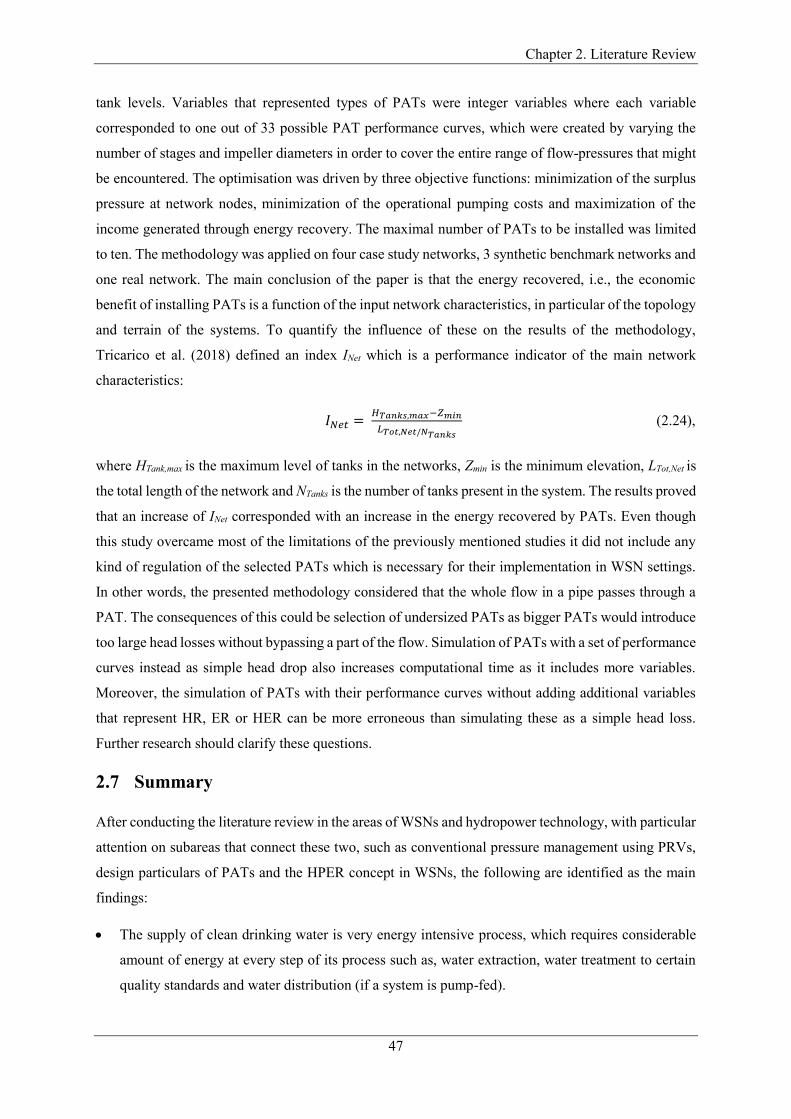
Chapter 2. Literature Review
47
tank levels. Variables that represented types of PATs were integer variables where each variable
corresponded to one out of 33 possible PAT performance curves, which were created by varying the
number of stages and impeller diameters in order to cover the entire range of flow-pressures that might
be encountered. The optimisation was driven by three objective functions: minimization of the surplus
pressure at network nodes, minimization of the operational pumping costs and maximization of the
income generated through energy recovery. The maximal number of PATs to be installed was limited
to ten. The methodology was applied on four case study networks, 3 synthetic benchmark networks and
one real network. The main conclusion of the paper is that the energy recovered, i.e., the economic
benefit of installing PATs is a function of the input network characteristics, in particular of the topology
and terrain of the systems. To quantify the influence of these on the results of the methodology,
Tricarico et al. (2018) defined an index INet which is a performance indicator of the main network
characteristics:
𝐼𝑁𝑒𝑡 = 𝐻𝑇𝑎𝑛𝑘𝑠,𝑚𝑎𝑥−𝑍𝑚𝑖𝑛
𝐿𝑇𝑜𝑡,𝑁𝑒𝑡/𝑁𝑇𝑎𝑛𝑘𝑠
(2.24),
where HTank,max is the maximum level of tanks in the networks, Zmin is the minimum elevation, LTot,Net is
the total length of the network and NTanks is the number of tanks present in the system. The results proved
that an increase of INet corresponded with an increase in the energy recovered by PATs. Even though
this study overcame most of the limitations of the previously mentioned studies it did not include any
kind of regulation of the selected PATs which is necessary for their implementation in WSN settings.
In other words, the presented methodology considered that the whole flow in a pipe passes through a
PAT. The consequences of this could be selection of undersized PATs as bigger PATs would introduce
too large head losses without bypassing a part of the flow. Simulation of PATs with a set of performance
curves instead as simple head drop also increases computational time as it includes more variables.
Moreover, the simulation of PATs with their performance curves without adding additional variables
that represent HR, ER or HER can be more erroneous than simulating these as a simple head loss.
Further research should clarify these questions.
2.7 Summary
After conducting the literature review in the areas of WSNs and hydropower technology, with particular
attention on subareas that connect these two, such as conventional pressure management using PRVs,
design particulars of PATs and the HPER concept in WSNs, the following are identified as the main
findings:
The supply of clean drinking water is very energy intensive process, which requires considerable
amount of energy at every step of its process such as, water extraction, water treatment to certain
quality standards and water distribution (if a system is pump-fed).
Chapter 2. Literature Review
48
Excessive pressure within WSNs can have severe negative consequences that can jeopardize their
functioning and increase operational costs. The main negative consequences are increased water
losses, increased frequency of pipe bursts and sometimes increased water consumption. The
traditional way to reduce excessive pressure and to mitigate its negative consequences on operation
of WSNs is deployment of PRVs at entrances of DMAs.
PRVs are usually controlled hydraulically using autonomous piston valves and sometimes using
electronic controllers when more advanced control in necessary. Depending on the characteristics
of DMAs, three types of downstream head profile are usually pursued: 1) fixed point head profile;
2) dual set point head profile and 3) flow based head profile.
Many studies identified hydropower as a viable renewable energy source at locations of excess
pressure that can reduce the energy dependency and improve sustainability of WSNs. The new
HPER concept was seen as a new technological solution for more efficient pressure management.
However, the most sites in WSNs are of mini and micro hydropower scale. Downsizing the
traditional turbines to this scale increases their cost per kilowatt significantly, making a lot of sites
not economically viable.
In attempt to reduce the equipment cost and make mini and micro scale sites more economically
attractive, researchers and practitioner explored alternative technologies. Many researchers pointed
out PAT technology as a promising low-cost solution. Mass production of pump/PAT units and
their widespread implementation not only reduce their cost but also provide their off-the-shelf
availability which made these particularly attractive. However, PATs have their disadvantages
which prevented wider adoption of this technology. The most significant are low part-load
efficiency, absence of flow regulation device that would allow them adjustment of their head loss
curves, and probably the most important their performance uncertainty.
The most promising locations for installation of HPER devices within WSNs identified by the
literature were: inlets to water treatment plants, inlets to storage reservoirs, BPTs and locations of
PRVs.
As the main technical challenges for installation of HPER within WSNs the literature recurrently
pointed out large flow and head fluctuations in combination with requirement to maintain
downstream head.
Several literature gaps were identified as well. These were summarised in the form of the research
questions and presented in section 1.3 of the Introduction chapter.
Chapter 3. Research Approach
49
3 Research Approach
To address the research questions defined in the section 1.3 of Chapter 1, the research work that will be
presented in the following chapters of this thesis had to incorporate a combination of PAT hydraulic
performance analysis, optimisation analysis, statistical analysis of PRV data samples, spatial analysis
and different kinds of regression analysis. The complete research work could be compartmentalised into
the following five stages: 1) Optimal PAT selection; 2) Prediction of global plant efficiency & economic
viability bounds; 3) Generalization of the optimal relative BEP; 4) Spatial regression analysis using
GIS; and 5) Assessment of the HPER potential in the Irish and the UK’s WSNs. Detailed methodologies
and obtained results from these stages can be found in Chapters 4-8 of this thesis. In addition, these five
stages and their parts are graphically illustrated in Fig. 3.1. The numbers within red circles presented
under “RQs” headings, signify the aforementioned research questions (RQs) addressed in each of the
stages. The subsequent lines of this chapter briefly outline the research work conducted in each of five
stages with reference to Fig. 3.1.
Chapter 4: Optimal PAT selection
The research work conducted in this chapter focuses on the problem of the selection of a PAT available
on the market that can be used as a HPER device at locations of existing PRVs, characterized by large
variation of operating conditions. The chapter firstly elaborates how the aforementioned problem could
be defined as an optimisation problem. In other words, which PAT performance parameters could be
used as the design variables, what are the problem constraints and how these could be defined, and what
are the pursued objectives. Based on the characteristics of the optimisation problem the Nedler-Mead
Simplex Direct Search (NMSDS) algorithm has been adapted for its solving. The chapter also described
novelties introduced related to the constraints on the solution space and the operation limits for the
variable PAT performance. As it can be seen from Fig. 3.1, this chapter considered three objective
functions, namely maximisation of energy recovery, maximisation of net present value (NPV) and
minimisation of payback period (PP). The chapter investigated their influence on the selection of the
optimal PAT family from the market. In addition, the chapter also investigates whether differently
defined operation limits can have an influence on the selection of the optimal PAT family on the market.
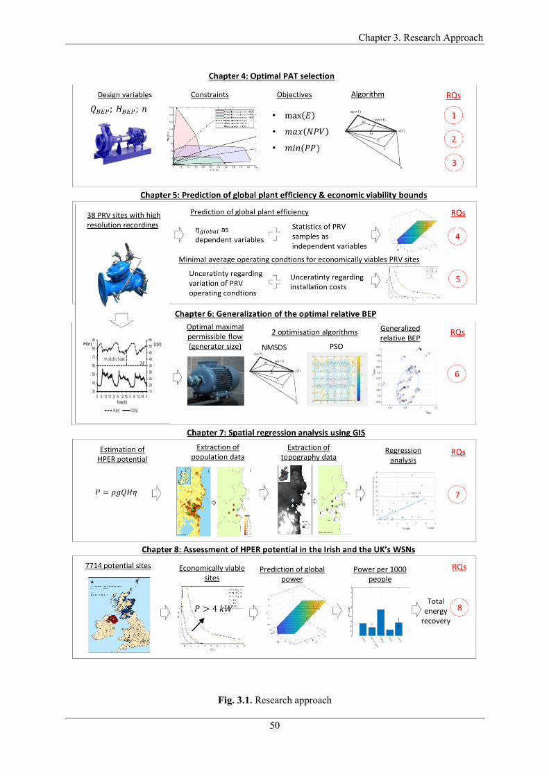
Chapter 3. Research Approach
50
Fig. 3.1. Research approach
Chapter 3. Research Approach
51
Chapter 5: Prediction of global plant efficiency & economic viability bounds
The research work conducted in Chapter 5 consisted of two parts. The first part derived a regression
model able to accurately predict the global efficiency of a HPER plant equipped with a PAT and HR
regulation scheme at PRV sites, using only the statistical parameters of the PRV operating conditions.
Thus, addressing the 4th research question. The dependant variables in the regression analysis were the
global efficiencies of 38 HPER plants equipped with an optimal PAT based on maximisation of the
NPV function. On the other hand, the independent variables were the statistical parameters of PRV
samples designating centrality and dispersion of the recorded operating conditions.
The aim of the second part was to address the 5th research question by defining a curve in Q-H space
that designates the set of the minimal average operating conditions at PRV sites so their upgrade to
HPER plants equipped with a PAT is expected to have a positive NPV after 10 years. The analysis first
assessed the optimal NPV for a set of hypothetical PRV sites whose average operating conditions were
uniformly distributed within the Q-H domain common for sites occurring in WSNs. The analysis also
considered different levels of variation of PRV operating conditions and different installation cost
scenarios. The curves designating the bounds of the economic viability were identified as zero contours
on the NPV surfaces generated across the investigated Q-H domain.
Chapter 6: Generalization of the optimal relative BEP
The optimal relative BEP designates the ratio between the BEP of a theoretically optimal PAT for a
considered PRV site and the site’s average operating conditions. The hypothesis that this ratio could be
generalized meaning that it varies in a narrow range regardless of dispersion of PRV sites’ operating
conditions and their size was tested in Chapter 6 by finding the optimal theoretical PATs for the same
38 PRV sites presented in previous chapter. To find the optimal theoretical solution the methodology
presented in Chapter 6 employed an improved variant of the methodology developed in Chapter 4 by
introducing another design variable representing maximal operating flow of a PAT unit. By optimising
the maximal operating flow, the methodology implicitly optimises the size of the generator to be
coupled to a PAT. Besides, the NMSDS algorithm used in Chapter 4, the analysis conducted in Chapter
6 applied another global heuristic optimisation algorithm, namely particle swarm optimisation (PSO).
The reasons for this will be explained the chapter. This chapter answers on the 6th research question.
Chapter 7: Spatial regression analysis using GIS
From the correspondence with water supply operators in Ireland the UK it was discovered that there are
many PRVs whose existence and location are known, but that their operating conditions such as flow
and head necessary for estimation of their HPER potential were not available. This disclosure led to
formulation of the 7th research question that was addressed in this chapter. Namely, the aim of the
research work carried out in this chapter was to examine whether population and topography data in
Chapter 3. Research Approach
52
proximity to the potential HPER sites could be used for prediction of their potential. Thus, firstly for
the sites from Ireland and Wales for which the data about the average annual flow and head were
available, the average power potential was estimated. Subsequently, a spatial buffer analysis was
conducted in a GIS based software to extract the information about the population and terrain variability
in proximity to considered sites. Finally, a regression analysis was performed to see if an accurate
prediction model could be derived.
Chapter 8: Assessment of the HPER potential within the Irish and the UK’s WSNs
The main aim of the research work conducted in Chapter 8 was to address the literature gap by
conducting a large multi-country scale assessment of HPER potential in WSNs and thus quantifying
the percentage of the energy consumption by the sector that could be recovered. Hence, since the
beginning of this PhD program, numerous water utilities and public organisations across Ireland and
the UK have been contacted in an attempt to obtain the data necessary for conducting such analysis.
Based on the data that the water supply operators were in position to share, a 7-step methodology has
been defined. Two main stages of the methodology were the assessment of HPER potential of the sites
whose data was available, while the second stage used the population estimates to extrapolate the
potential to areas where the data about the sites was not available. The most important steps in the first
stage of the methodology were the determination of the economic viability of the available sites and
prediction of their global power as displayed in Fig. 3.1. On the other hand, the most important step in
the second stage of the methodology was the calculation of a coefficient which quantifies HPER
potential per 1000 people of a region.
Chapter 4. Optimisation-Based Methodology for Selection of a PAT in WDNs
53
4 Optimisation-Based
Methodology for Selection of a
PAT in WDNs
4.1 Introduction
Pressure management together with the rehabilitation of the infrastructure has proven to be one of the
most efficient strategies for water losses reduction. In addition to the reduction of leakages, pressure
management can also reduce the burst frequency of pipes (Vicente et al., 2016). Although the pressure
management using conventional PRVs has many positive effects on the functioning of WDNs, the
dissipated energy at the valves is irreversibly lost. In the last few years, a lot of researchers have been
investigating technological and economic feasibility of replacing these valves with micro turbines or
PATs (Fernández Garcia and Mc Nabola, 2020; Gallagher et al., 2015; Mc Nabola et al., 2014). The
literature indicated large diurnal and seasonal flow and pressure variability, and the pressure
management requirements, as the main technical challenges for replacing conventional valves with
HPER plants (Fecarotta et al., 2018; Lydon et al., 2017).
There are studies which examined the use of conventional turbines (Coelho and Andrade-Campos,
2018; Corcoran et al., 2013) or specific hydropower devices (Sinagra et al., 2017) for this purpose,
however the use of PATs prevails. Mainly this is due to the power output size of PRV sites within
WDNs which is usually up to 100 kW (Delgado et al., 2019b) and their significantly lower cost in this
range comparing to the conventional turbines (Novara et al., 2019).
The problem analysed in this chapter is the problem of selecting an optimal PAT for a predetermined
site within a WDN, which is characterized with large variation of flow and head operating conditions.
Although other criterions for the classification of the methodologies that addressed this problem could
be established, the one relevant for this chapter is how these approached finding the theoretically
optimal BEP in turbine mode. As discussed in section 2.6.4.2 of this thesis, based on the criterion the
methodologies could be divided into two groups. The methodologies from the first group practically

Chapter 4. Optimisation-Based Methodology for Selection of a PAT in WDNs
54
guessed the theoretically optimal BEP flow and head statistically without any simulation of PAT
performance in turbine mode. For example, some methodologies defined this point with average flow
and head during the daytime (Stefanizzi et al., 2020). As discussed, the methodologies from the second
group selected the optimal BEP in turbine mode by simulating PAT performance in turbine mode. The
methodology developed in this chapter is from the second group.
The developed optimisation-based methodology employs the classical hydraulic regulation scheme
with two control valves and a single-stage centrifugal PAT whose performance curves and maximal
efficiency were predicted using the state of art models defined by Novara and Mc Nabola (2018) and
Novara et al. (2017), respectively. This regulation scheme is selected over other schemes proposed in
the literature because of the reasons discussed in subsection 2.6.4.1 “Variable operating strategy and
PAT regulation schemes”. To guide the model towards the optimal solution the Nelder-Mead simplex
direct search (NMSDS) optimisation algorithm was used (Lagarias et al., 1998). Besides the
optimisation method used, the novelties of the proposed methodology are also reflected in the
constraints imposed to the solution space which are defined only by the boundaries of the available
single-stage centrifugal PATs on the market, and new formulation of the PAT’s operation limits that
are based on its relative mechanical power. The accuracy of the model was validated using 23
experimental curves collected from the literature.
The analysis presented in this chapter also carried out two tests that have not previously been conducted
in the literature. The first test examines the effects of using three independent single-objective functions
on the optimal PAT, namely: maximization of energy recovery, maximization of NPV after 10 years
and minimization of the payback period, respectively. The second test investigated the effects of using
different operation limits on the optimal PAT. The both tests were performed on three case study sites
from a compiled database of 38 PRV sites with yearly recordings at time step of 15 min or less. The
goal of the conducted tests was to find out how much the theoretically optimal BEPs obtained using
different objectives and different maximal operation limits differ from each other and if this can result
in the selection of different commercially available pump families.
The proposed methodology was also applied to six real-world sites previously used in the literature to
demonstrate the improvements introduced.
4.2 Methodology
4.2.1 Design variables
The performance characteristics of different centrifugal pumps or PATs can be defined with their BEPs,
and the nominal impeller rotational speed (n). The aim of the proposed optimisation model was to find
the optimal values of the related three design variables for the considered sites. The rotational speed
was considered a discrete variable with possible values of 1005, 1510, and 3020 rpm. The set of the

Chapter 4. Optimisation-Based Methodology for Selection of a PAT in WDNs
55
rotational speeds was predetermined by the fact that the centrifugal pumps or PATs are usually coupled
with asynchronous electric generators with either 3, 2 and 1 magnetic pole pairs. These generators are
operating at constant speed to produce the electric current with synchronous frequency of 50 Hz. Also,
the pump manufacturers usually provide the pump performance curve only for these speeds. In order to
have the rotational speed different from these, additional equipment is needed such as a mechanical
speed multiplier or an electrical speed driver (inverter) (Fecarotta et al., 2018) which complicate the
installation and increase the cost. The discharge and the head drop at the BEP were considered
continuous variables. This also means that the optimal solution is theoretical as there is a possibility
that there is no commercial PAT with exactly the same values of BEP for considered n. However, the
function of the theoretically optimal solution is to serve as a benchmark for identifying the most suitable
commercial PATs in its proximity.
4.2.2 Constraints on the solution space
The methodologies available in the literature all followed the traditional approach where the most
suitable machine for the selected site was obtained by scaling the prototype machine whose performance
curves were available to the respective authors. In the optimisation terminology this would mean that
the constraints defined by the affinity equations are imposed on the solution space, i.e., that the BEP of
the optimal scaled machines has to fall on the affinity curves. While this approach is adequative when
the final machine is custom built like in the case of large turbines, in the case of HPER plants like the
ones within WDNs, the final machine will be the one from a finite set of pumps/PATs’ families
available on the market for which the mass production cost can be availed. The PATs from this set are
not all hydraulically similar meaning that these do not have the same value of turbine specific speed
(Ns) based on either unit flow or unit power. Moreover, it is hard to anticipate the optimal value of the
PAT’s Ns for a PRV site where large flow and head variations are present and there is a regulation
scheme. Even if this value is known, the characteristic curves of hydraulically similar machines
probably are not available.
In the presented methodology the solution space of the PAT’s BEP was constrained only with the
boundaries that represent the available mass produced centrifugal PATs on the market for each
rotational speed. The illustration of this concept is presented in Fig. 4.1. The boundaries for each
available speed were defined by creating a database of centrifugal pumps from the catalogues of
Etanorm and Etanorm-R models, that are classical end-suction centrifugal pumps (KSB, 2018a). Their
BEPs as PAT were converted using the model defined by Yang et al. (2012) and affinity laws to adjust
the speed to the turbine mode (e.g. from 1450 to 1510). The database included 58 different pump
families and 150 different BEPs for three rotational speeds. Only the full impellers of these families
were considered. The minimal values of BEP flow, head and specific speed amounted 1.49 l s-1, 3.62 m
and 3.74 rpm (m3 s-1)0.5(m)-0.75 while the maximal values were 513.1 l s-1, 398.06 m and 102.89 rpm
(m3 s-1)0.5 (m)-0.75 respectively.
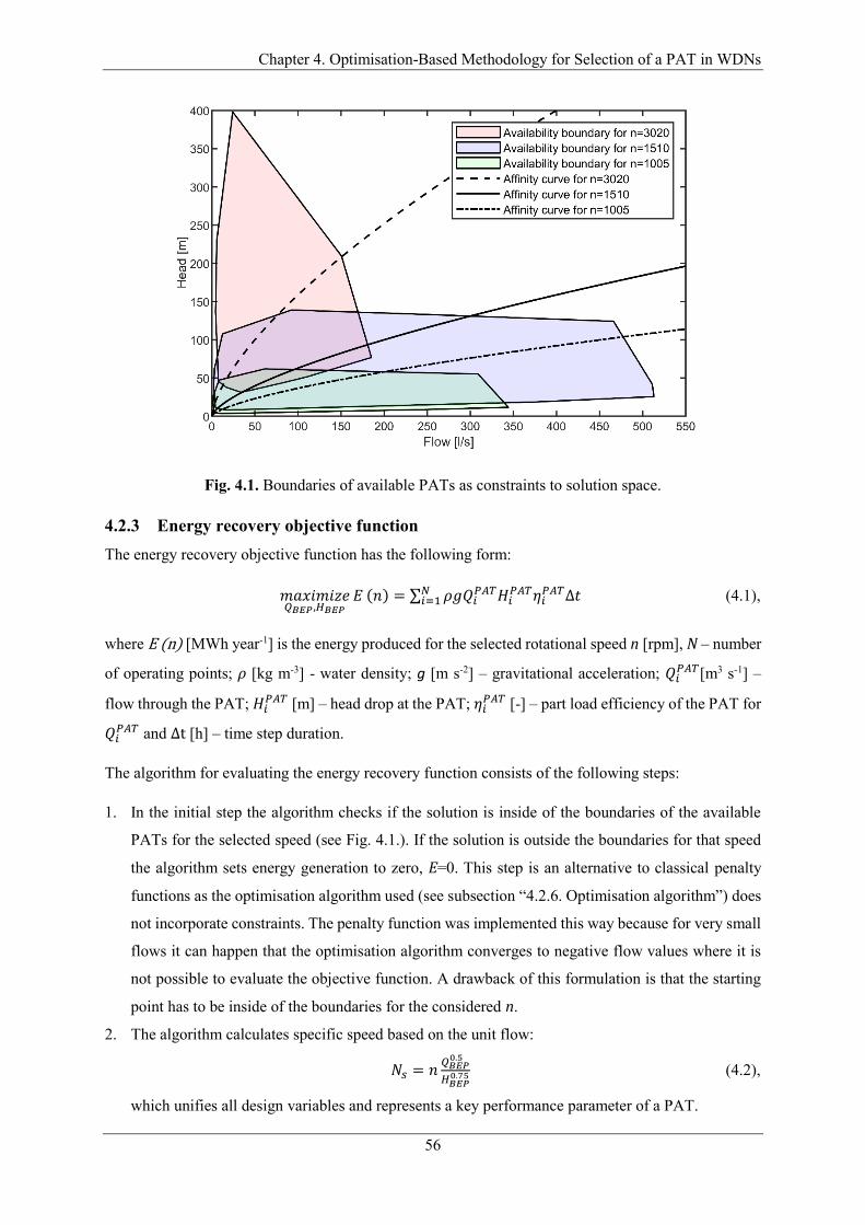
Chapter 4. Optimisation-Based Methodology for Selection of a PAT in WDNs
56
Fig. 4.1. Boundaries of available PATs as constraints to solution space.
4.2.3 Energy recovery objective function
The energy recovery objective function has the following form:
𝑚𝑎𝑥𝑖𝑚𝑖𝑧𝑒𝑄𝐵𝐸𝑃,𝐻𝐵𝐸𝑃
𝐸 (𝑛) = ∑ 𝜌𝑔𝑄𝑖𝑃𝐴𝑇𝐻𝑖
𝑃𝐴𝑇𝜂𝑖𝑃𝐴𝑇Δ𝑡𝑁
𝑖=1 (4.1),
where E (n) [MWh year-1] is the energy produced for the selected rotational speed n [rpm], N – number
of operating points; ρ [kg m-3] - water density; g [m s-2] – gravitational acceleration; 𝑄𝑖𝑃𝐴𝑇[m3 s-1] –
flow through the PAT; 𝐻𝑖𝑃𝐴𝑇 [m] – head drop at the PAT; 𝜂𝑖
𝑃𝐴𝑇 [-] – part load efficiency of the PAT for
𝑄𝑖𝑃𝐴𝑇 and ∆t [h] – time step duration.
The algorithm for evaluating the energy recovery function consists of the following steps:
1. In the initial step the algorithm checks if the solution is inside of the boundaries of the available
PATs for the selected speed (see Fig. 4.1.). If the solution is outside the boundaries for that speed
the algorithm sets energy generation to zero, E=0. This step is an alternative to classical penalty
functions as the optimisation algorithm used (see subsection “4.2.6. Optimisation algorithm”) does
not incorporate constraints. The penalty function was implemented this way because for very small
flows it can happen that the optimisation algorithm converges to negative flow values where it is
not possible to evaluate the objective function. A drawback of this formulation is that the starting
point has to be inside of the boundaries for the considered n.
2. The algorithm calculates specific speed based on the unit flow:
𝑁𝑠 = 𝑛𝑄𝐵𝐸𝑃
0.5
𝐻𝐵𝐸𝑃0.75 (4.2),
which unifies all design variables and represents a key performance parameter of a PAT.
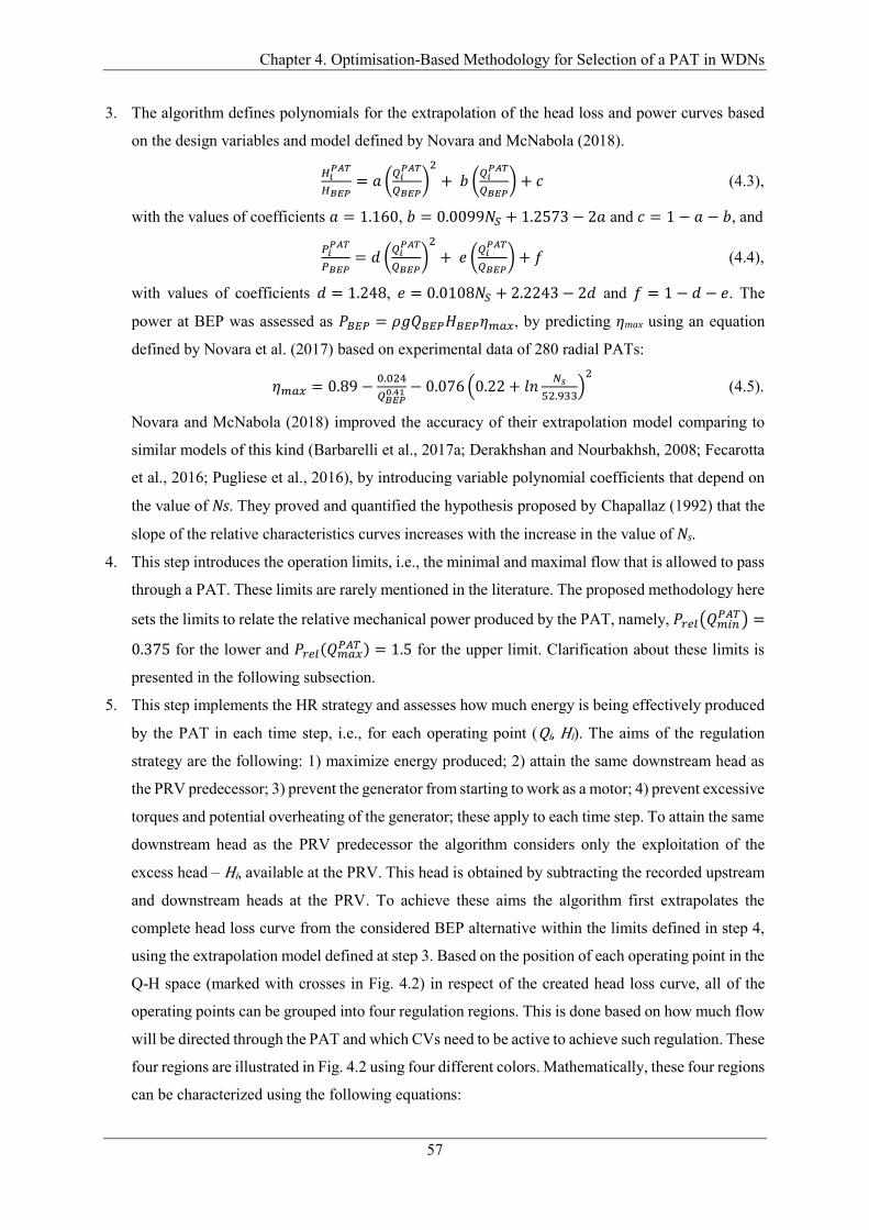
Chapter 4. Optimisation-Based Methodology for Selection of a PAT in WDNs
57
3. The algorithm defines polynomials for the extrapolation of the head loss and power curves based
on the design variables and model defined by Novara and McNabola (2018).
𝐻𝑖
𝑃𝐴𝑇
𝐻𝐵𝐸𝑃= 𝑎 (
𝑄𝑖𝑃𝐴𝑇
𝑄𝐵𝐸𝑃)
2
+ 𝑏 (𝑄𝑖
𝑃𝐴𝑇
𝑄𝐵𝐸𝑃) + 𝑐 (4.3),
with the values of coefficients 𝑎 = 1.160, 𝑏 = 0.0099𝑁𝑆 + 1.2573 − 2𝑎 and 𝑐 = 1 − 𝑎 − 𝑏, and
𝑃𝑖
𝑃𝐴𝑇
𝑃𝐵𝐸𝑃= 𝑑 (
𝑄𝑖𝑃𝐴𝑇
𝑄𝐵𝐸𝑃)
2
+ 𝑒 (𝑄𝑖
𝑃𝐴𝑇
𝑄𝐵𝐸𝑃) + 𝑓 (4.4),
with values of coefficients 𝑑 = 1.248, 𝑒 = 0.0108𝑁𝑆 + 2.2243 − 2𝑑 and 𝑓 = 1 − 𝑑 − 𝑒. The
power at BEP was assessed as 𝑃𝐵𝐸𝑃 = 𝜌𝑔𝑄𝐵𝐸𝑃𝐻𝐵𝐸𝑃𝜂𝑚𝑎𝑥, by predicting ηmax using an equation
defined by Novara et al. (2017) based on experimental data of 280 radial PATs:
𝜂𝑚𝑎𝑥 = 0.89 −0.024
𝑄𝐵𝐸𝑃0.41 − 0.076 (0.22 + 𝑙𝑛
𝑁𝑠
52.933)
2 (4.5).
Novara and McNabola (2018) improved the accuracy of their extrapolation model comparing to
similar models of this kind (Barbarelli et al., 2017a; Derakhshan and Nourbakhsh, 2008; Fecarotta
et al., 2016; Pugliese et al., 2016), by introducing variable polynomial coefficients that depend on
the value of Ns. They proved and quantified the hypothesis proposed by Chapallaz (1992) that the
slope of the relative characteristics curves increases with the increase in the value of Ns.
4. This step introduces the operation limits, i.e., the minimal and maximal flow that is allowed to pass
through a PAT. These limits are rarely mentioned in the literature. The proposed methodology here
sets the limits to relate the relative mechanical power produced by the PAT, namely, 𝑃𝑟𝑒𝑙(𝑄𝑚𝑖𝑛𝑃𝐴𝑇) =
0.375 for the lower and 𝑃𝑟𝑒𝑙(𝑄𝑚𝑎𝑥𝑃𝐴𝑇 ) = 1.5 for the upper limit. Clarification about these limits is
presented in the following subsection.
5. This step implements the HR strategy and assesses how much energy is being effectively produced
by the PAT in each time step, i.e., for each operating point (Qi, Hi). The aims of the regulation
strategy are the following: 1) maximize energy produced; 2) attain the same downstream head as
the PRV predecessor; 3) prevent the generator from starting to work as a motor; 4) prevent excessive
torques and potential overheating of the generator; these apply to each time step. To attain the same
downstream head as the PRV predecessor the algorithm considers only the exploitation of the
excess head – Hi, available at the PRV. This head is obtained by subtracting the recorded upstream
and downstream heads at the PRV. To achieve these aims the algorithm first extrapolates the
complete head loss curve from the considered BEP alternative within the limits defined in step 4,
using the extrapolation model defined at step 3. Based on the position of each operating point in the
Q-H space (marked with crosses in Fig. 4.2) in respect of the created head loss curve, all of the
operating points can be grouped into four regulation regions. This is done based on how much flow
will be directed through the PAT and which CVs need to be active to achieve such regulation. These
four regions are illustrated in Fig. 4.2 using four different colors. Mathematically, these four regions
can be characterized using the following equations:

Chapter 4. Optimisation-Based Methodology for Selection of a PAT in WDNs
58
Fig. 4.2. Yearly Q-H operating points at Site 13 within Dublin WDN, coloured based on
regulation regions.
𝑄𝑖 < 𝑄min𝑃𝐴𝑇 𝑜𝑟 𝐻𝑖 < 𝐻𝑚𝑖𝑛
𝑃𝐴𝑇 → 𝐸𝑖 = 0 (4.6),
𝑄𝑚𝑖𝑛𝑃𝐴𝑇 ≤ 𝑄𝑖 < 𝑄𝑚𝑎𝑥
𝑃𝐴𝑇 𝑎𝑛𝑑 𝐻𝑖 ≥ 𝐻𝑃𝐴𝑇(𝑄𝑖) → 𝐸𝑖 = 𝜌𝑔𝑄𝑖𝐻𝑃𝐴𝑇(𝑄𝑖)𝜂𝑖𝑃𝐴𝑇(𝑄𝑖)𝛥𝑡 (4.7),
𝐻𝑚𝑖𝑛𝑃𝐴𝑇 ≤ 𝐻𝑖 < 𝐻𝑚𝑎𝑥
𝑃𝐴𝑇 𝑎𝑛𝑑 𝑄𝑖 > 𝑄𝑃𝐴𝑇(𝐻𝑖) → 𝐸𝑖 = 𝜌𝑔𝑄𝑃𝐴𝑇(𝐻𝑖)𝐻𝑖𝜂𝑃𝐴𝑇(𝑄𝑃𝐴𝑇(𝐻𝑖))𝛥𝑡 (4.8),
𝑄𝑖 ≥ 𝑄𝑚𝑎𝑥𝑃𝐴𝑇 𝑎𝑛𝑑 𝐻𝑖 ≥ 𝐻𝑚𝑎𝑥
𝑃𝐴𝑇 → 𝐸𝑖 = 𝜌𝑔𝑄𝑚𝑎𝑥𝑃𝐴𝑇 𝐻𝑚𝑎𝑥
𝑃𝐴𝑇 𝜂𝑃𝐴𝑇(𝑄𝑚𝑎𝑥𝑃𝐴𝑇 )Δ𝑡 (4.9).
For the operating points that satisfy one of the inequalities defined in Eq. 4.6 (green crosses in Fig.
4.2), the entire flow needs to be bypassed and consequently there is no electricity generation. If the
flow is too low (𝑄𝑖 < 𝑄min𝑃𝐴𝑇), it needs to be bypassed to prevent the potential operation of the
generator as a motor as the shaft mechanical power is not sufficient even to create the nominal
electromagnetic flux. For the operating points with the larger flows but with excess head lower than
𝐻𝑚𝑖𝑛𝑃𝐴𝑇, the necessary bypassing to avoid the excessive head drops at the PAT would lead to the same
phenomena. For the operating points that satisfy both inequalities defined in Eq. 4.7 (blue crosses
in Fig. 4.2), the entire flow is directed through the generation line in the PAT, creating head loss at
the PAT according to its head loss curve (𝐻𝑃𝐴𝑇(𝑄𝑖)), while the excess head is dissipated by the CV
in series (𝐻𝑖 − 𝐻𝑃𝐴𝑇(𝑄𝑖)). For all the operating points that satisfy both inequalities defined in Eq.
4.8 (red crosses in Fig. 4.2), a part of flow needs to be bypassed to avoid head drops larger than the
excess head. The exact flow that should be directed through the PAT to maximize the energy
recovery and avoid excessive head drops is the flow from the PAT head loss curve that corresponds
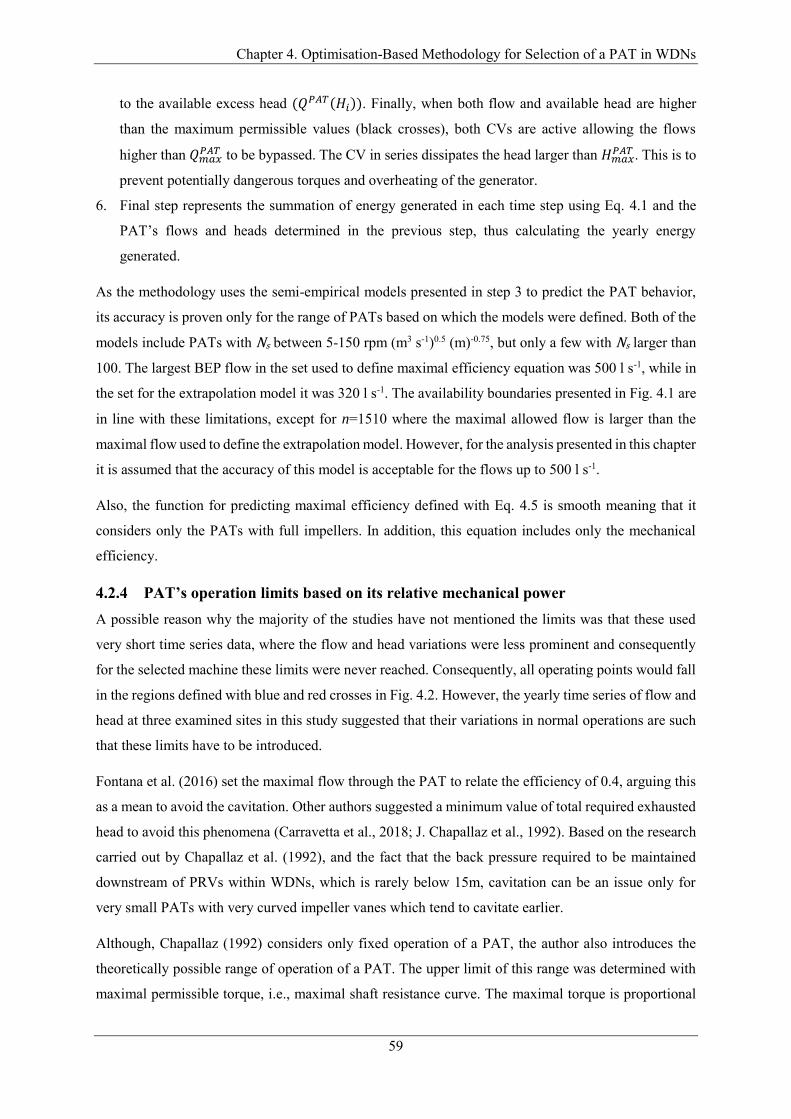
Chapter 4. Optimisation-Based Methodology for Selection of a PAT in WDNs
59
to the available excess head (𝑄𝑃𝐴𝑇(𝐻𝑖)). Finally, when both flow and available head are higher
than the maximum permissible values (black crosses), both CVs are active allowing the flows
higher than 𝑄𝑚𝑎𝑥𝑃𝐴𝑇 to be bypassed. The CV in series dissipates the head larger than 𝐻𝑚𝑎𝑥
𝑃𝐴𝑇 . This is to
prevent potentially dangerous torques and overheating of the generator.
6. Final step represents the summation of energy generated in each time step using Eq. 4.1 and the
PAT’s flows and heads determined in the previous step, thus calculating the yearly energy
generated.
As the methodology uses the semi-empirical models presented in step 3 to predict the PAT behavior,
its accuracy is proven only for the range of PATs based on which the models were defined. Both of the
models include PATs with Ns between 5-150 rpm (m3 s-1)0.5 (m)-0.75, but only a few with Ns larger than
100. The largest BEP flow in the set used to define maximal efficiency equation was 500 l s-1, while in
the set for the extrapolation model it was 320 l s-1. The availability boundaries presented in Fig. 4.1 are
in line with these limitations, except for n=1510 where the maximal allowed flow is larger than the
maximal flow used to define the extrapolation model. However, for the analysis presented in this chapter
it is assumed that the accuracy of this model is acceptable for the flows up to 500 l s-1.
Also, the function for predicting maximal efficiency defined with Eq. 4.5 is smooth meaning that it
considers only the PATs with full impellers. In addition, this equation includes only the mechanical
efficiency.
4.2.4 PAT’s operation limits based on its relative mechanical power
A possible reason why the majority of the studies have not mentioned the limits was that these used
very short time series data, where the flow and head variations were less prominent and consequently
for the selected machine these limits were never reached. Consequently, all operating points would fall
in the regions defined with blue and red crosses in Fig. 4.2. However, the yearly time series of flow and
head at three examined sites in this study suggested that their variations in normal operations are such
that these limits have to be introduced.
Fontana et al. (2016) set the maximal flow through the PAT to relate the efficiency of 0.4, arguing this
as a mean to avoid the cavitation. Other authors suggested a minimum value of total required exhausted
head to avoid this phenomena (Carravetta et al., 2018; J. Chapallaz et al., 1992). Based on the research
carried out by Chapallaz et al. (1992), and the fact that the back pressure required to be maintained
downstream of PRVs within WDNs, which is rarely below 15m, cavitation can be an issue only for
very small PATs with very curved impeller vanes which tend to cavitate earlier.
Although, Chapallaz (1992) considers only fixed operation of a PAT, the author also introduces the
theoretically possible range of operation of a PAT. The upper limit of this range was determined with
maximal permissible torque, i.e., maximal shaft resistance curve. The maximal torque is proportional
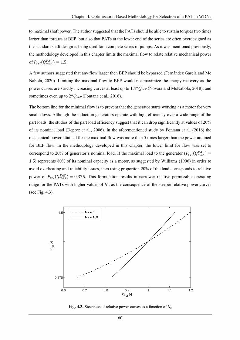
Chapter 4. Optimisation-Based Methodology for Selection of a PAT in WDNs
60
to maximal shaft power. The author suggested that the PATs should be able to sustain torques two times
larger than torques at BEP, but also that PATs at the lower end of the series are often overdesigned as
the standard shaft design is being used for a compete series of pumps. As it was mentioned previously,
the methodology developed in this chapter limits the maximal flow to relate relative mechanical power
of 𝑃𝑟𝑒𝑙(𝑄𝑚𝑎𝑥𝑃𝐴𝑇 ) = 1.5
A few authors suggested that any flow larger then BEP should be bypassed (Fernández Garcia and Mc
Nabola, 2020). Limiting the maximal flow to BEP would not maximize the energy recovery as the
power curves are strictly increasing curves at least up to 1.4*QBEP (Novara and McNabola, 2018), and
sometimes even up to 2*QBEP (Fontana et al., 2016).
The bottom line for the minimal flow is to prevent that the generator starts working as a motor for very
small flows. Although the induction generators operate with high efficiency over a wide range of the
part loads, the studies of the part load efficiency suggest that it can drop significantly at values of 20%
of its nominal load (Deprez et al., 2006). In the aforementioned study by Fontana et al. (2016) the
mechanical power attained for the maximal flow was more than 5 times larger than the power attained
for BEP flow. In the methodology developed in this chapter, the lower limit for flow was set to
correspond to 20% of generator’s nominal load. If the maximal load to the generator (𝑃𝑟𝑒𝑙(𝑄𝑚𝑎𝑥𝑃𝐴𝑇 ) =
1.5) represents 80% of its nominal capacity as a motor, as suggested by Williams (1996) in order to
avoid overheating and reliability issues, then using proportion 20% of the load corresponds to relative
power of 𝑃𝑟𝑒𝑙(𝑄𝑚𝑎𝑥𝑃𝐴𝑇 ) = 0.375. This formulation results in narrower relative permissible operating
range for the PATs with higher values of Ns, as the consequence of the steeper relative power curves
(see Fig. 4.3).
Fig. 4.3. Steepness of relative power curves as a function of 𝑁𝑠
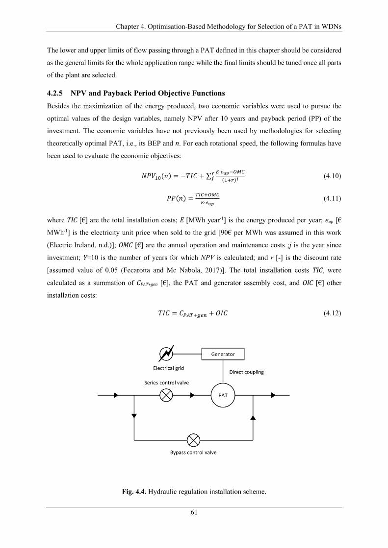
Chapter 4. Optimisation-Based Methodology for Selection of a PAT in WDNs
61
The lower and upper limits of flow passing through a PAT defined in this chapter should be considered
as the general limits for the whole application range while the final limits should be tuned once all parts
of the plant are selected.
4.2.5 NPV and Payback Period Objective Functions
Besides the maximization of the energy produced, two economic variables were used to pursue the
optimal values of the design variables, namely NPV after 10 years and payback period (PP) of the
investment. The economic variables have not previously been used by methodologies for selecting
theoretically optimal PAT, i.e., its BEP and n. For each rotational speed, the following formulas have
been used to evaluate the economic objectives:
𝑁𝑃𝑉10(𝑛) = −𝑇𝐼𝐶 + ∑𝐸∙𝑒𝑢𝑝−𝑂𝑀𝐶
(1+𝑟)𝑗𝑌𝑗 (4.10)
𝑃𝑃(𝑛) =𝑇𝐼𝐶+𝑂𝑀𝐶
𝐸∙𝑒𝑢𝑝 (4.11)
where TIC [€] are the total installation costs; E [MWh year-1] is the energy produced per year; eup [€
MWh-1] is the electricity unit price when sold to the grid [90€ per MWh was assumed in this work
(Electric Ireland, n.d.)]; OMC [€] are the annual operation and maintenance costs ;j is the year since
investment; Y=10 is the number of years for which NPV is calculated; and r [-] is the discount rate
[assumed value of 0.05 (Fecarotta and Mc Nabola, 2017)]. The total installation costs TIC, were
calculated as a summation of CPAT+gen [€], the PAT and generator assembly cost, and OIC [€] other
installation costs:
𝑇𝐼𝐶 = 𝐶𝑃𝐴𝑇+𝑔𝑒𝑛 + 𝑂𝐼𝐶 (4.12)
Fig. 4.4. Hydraulic regulation installation scheme.
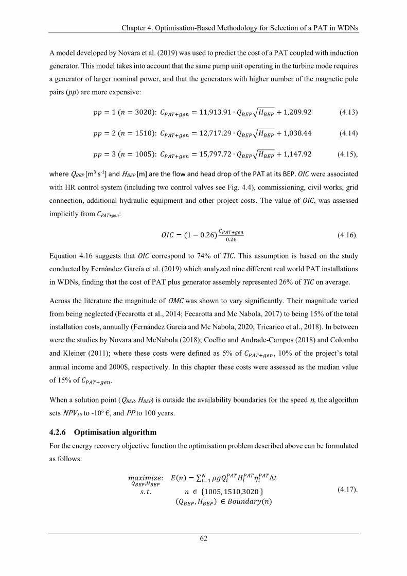
Chapter 4. Optimisation-Based Methodology for Selection of a PAT in WDNs
62
A model developed by Novara et al. (2019) was used to predict the cost of a PAT coupled with induction
generator. This model takes into account that the same pump unit operating in the turbine mode requires
a generator of larger nominal power, and that the generators with higher number of the magnetic pole
pairs (pp) are more expensive:
𝑝𝑝 = 1 (𝑛 = 3020): 𝐶𝑃𝐴𝑇+𝑔𝑒𝑛 = 11,913.91 ∙ 𝑄𝐵𝐸𝑃√𝐻𝐵𝐸𝑃 + 1,289.92 (4.13)
𝑝𝑝 = 2 (𝑛 = 1510): 𝐶𝑃𝐴𝑇+𝑔𝑒𝑛 = 12,717.29 ∙ 𝑄𝐵𝐸𝑃√𝐻𝐵𝐸𝑃 + 1,038.44 (4.14)
𝑝𝑝 = 3 (𝑛 = 1005): 𝐶𝑃𝐴𝑇+𝑔𝑒𝑛 = 15,797.72 ∙ 𝑄𝐵𝐸𝑃√𝐻𝐵𝐸𝑃 + 1,147.92 (4.15),
where QBEP [m3 s-1] and HBEP [m] are the flow and head drop of the PAT at its BEP. OIC were associated
with HR control system (including two control valves see Fig. 4.4), commissioning, civil works, grid
connection, additional hydraulic equipment and other project costs. The value of OIC, was assessed
implicitly from CPAT+gen:
𝑂𝐼𝐶 = (1 − 0.26)𝐶𝑃𝐴𝑇+𝑔𝑒𝑛
0.26 (4.16).
Equation 4.16 suggests that OIC correspond to 74% of TIC. This assumption is based on the study
conducted by Fernández García et al. (2019) which analyzed nine different real world PAT installations
in WDNs, finding that the cost of PAT plus generator assembly represented 26% of TIC on average.
Across the literature the magnitude of OMC was shown to vary significantly. Their magnitude varied
from being neglected (Fecarotta et al., 2014; Fecarotta and Mc Nabola, 2017) to being 15% of the total
installation costs, annually (Fernández Garcia and Mc Nabola, 2020; Tricarico et al., 2018). In between
were the studies by Novara and McNabola (2018); Coelho and Andrade-Campos (2018) and Colombo
and Kleiner (2011); where these costs were defined as 5% of 𝐶𝑃𝐴𝑇+𝑔𝑒𝑛, 10% of the project’s total
annual income and 2000$, respectively. In this chapter these costs were assessed as the median value
of 15% of 𝐶𝑃𝐴𝑇+𝑔𝑒𝑛.
When a solution point (QBEP, HBEP) is outside the availability boundaries for the speed n, the algorithm
sets NPV10 to -106 €, and PP to 100 years.
4.2.6 Optimisation algorithm
For the energy recovery objective function the optimisation problem described above can be formulated
as follows:
𝑚𝑎𝑥𝑖𝑚𝑖𝑧𝑒:𝑄𝐵𝐸𝑃,𝐻𝐵𝐸𝑃
𝐸(𝑛) = ∑ 𝜌𝑔𝑄𝑖𝑃𝐴𝑇𝐻𝑖
𝑃𝐴𝑇𝜂𝑖𝑃𝐴𝑇Δ𝑡𝑁
𝑖=1
𝑠. 𝑡. 𝑛 ∈ {1005, 1510,3020 }
(𝑄𝐵𝐸𝑃 , 𝐻𝐵𝐸𝑃) ∈ 𝐵𝑜𝑢𝑛𝑑𝑎𝑟𝑦(𝑛)
(4.17).
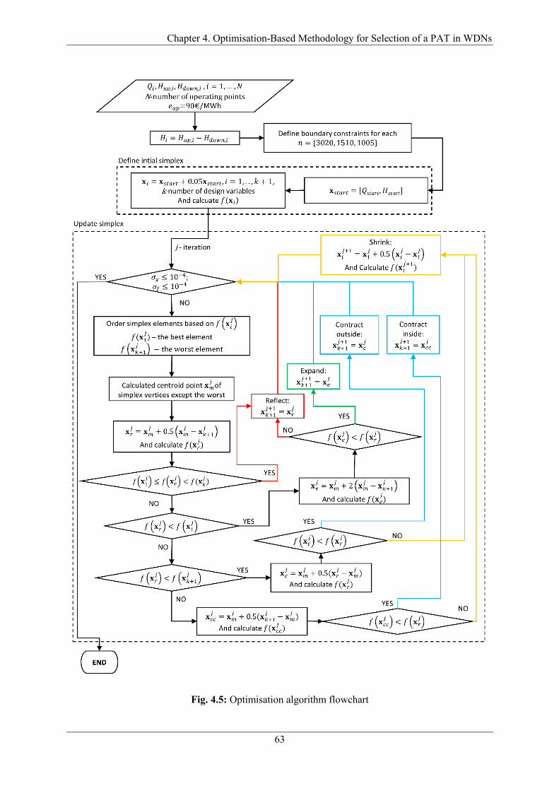
Chapter 4. Optimisation-Based Methodology for Selection of a PAT in WDNs
63
Fig. 4.5: Optimisation algorithm flowchart
Chapter 4. Optimisation-Based Methodology for Selection of a PAT in WDNs
64
The problem formulation for the other two objectives is the same as in Eq. 4.17 except in the case of
the PP objective for which the goal is to minimize PP. For a single rotational speed n, the problem
formulated in Eq. 4.17 is nonlinear subject to linear constraints defined using availability boundaries.
Because of the piecewise nature of the energy recovery function defined in Eq. 4.6-9 and due to the
discrete nature of the PRV operating points, the objective functions are discontinuous and hence non-
differentiable. As it will be seen in the result section, the described problem is a local problem.
Considering the problem characteristics, the Nelder-Mead Simplex Direct Search (NMSDS) algorithm
has been chosen to solve the optimisation problem (Lagarias et al., 1998). The NMSDS algorithm is
derivative-free heuristic search method suitable for nonlinear non-smooth problems. It belongs to the
class of direct search methods whose convergence is based on function comparison. As the algorithm
does not incorporate constraints, the boundary constraints are implemented through the penalty function
defined in step 1 of the energy recovery function.
The method uses the concept of a three-point simplex for a 2D-problem. The flowchart of the algorithm
is presented in Fig. 4.5. The starting point (Qstart, Hstart) can be anywhere within the availability boundary
for the selected rotational speed. The average operating point is a good initial guess if it is within the
boundary. As can be seen in the chart, the algorithm tries to replace the worst element of the simplex
(xk+1), with a better solution by reflecting and contracting through the centroid (xm) of the remaining
simplex points. If none of the alternatives is better that the worst point of the simplex, the algorithm
shrinks the simplex towards the best point. The advantage of the NMSDS algorithm is that it requires
less function evaluation in each iteration then some other heuristic methods. However, it is not suitable
for global optimisation problems.
All the simulations were carried out in the MATLAB programming environment.
4.3 Validation
As the pump manufacturers do not provide the information about pumps behaviour in turbine mode,
researchers and practitioners have to rely on some of the prediction models developed in the literature.
All PAT performance prediction models induce certain errors. To quantify the errors of their models
the developers usually use the accuracy metrics such as root mean square error (RMSE) and coefficient
of determination (R2) (Barbarelli et al., 2017a; Derakhshan and Nourbakhsh, 2008; Fecarotta et al.,
2016; Novara and McNabola, 2018; Pugliese et al., 2016). These metrics do not provide an explicit
answer about the magnitude of error in the assessment of energy produced. Furthermore, the
methodologies that are focused on selecting a PAT to replace a PRV which would operate with variable
flow and head conditions, usually couple several of these models where each embeds its error. Previous
methodologies in this field omitted to quantify this cumulative error.
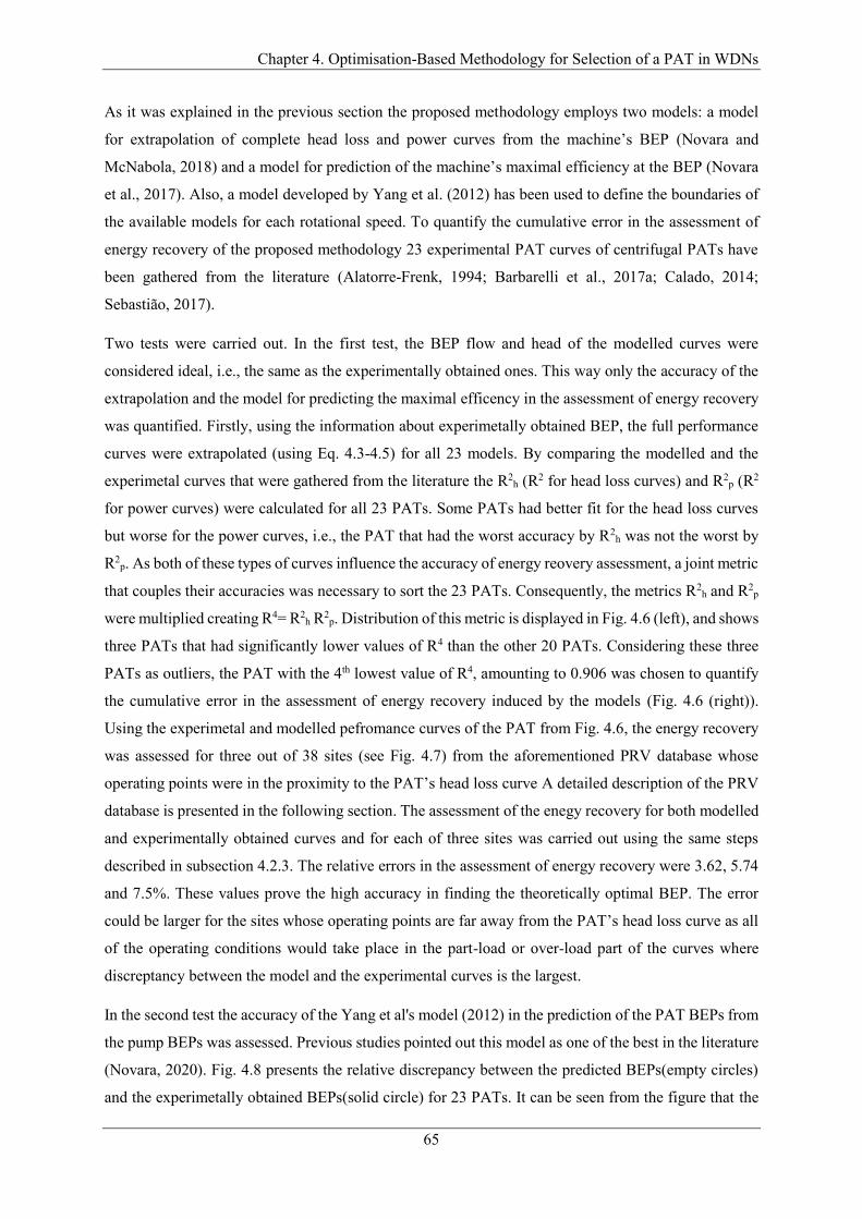
Chapter 4. Optimisation-Based Methodology for Selection of a PAT in WDNs
65
As it was explained in the previous section the proposed methodology employs two models: a model
for extrapolation of complete head loss and power curves from the machine’s BEP (Novara and
McNabola, 2018) and a model for prediction of the machine’s maximal efficiency at the BEP (Novara
et al., 2017). Also, a model developed by Yang et al. (2012) has been used to define the boundaries of
the available models for each rotational speed. To quantify the cumulative error in the assessment of
energy recovery of the proposed methodology 23 experimental PAT curves of centrifugal PATs have
been gathered from the literature (Alatorre-Frenk, 1994; Barbarelli et al., 2017a; Calado, 2014;
Sebastião, 2017).
Two tests were carried out. In the first test, the BEP flow and head of the modelled curves were
considered ideal, i.e., the same as the experimentally obtained ones. This way only the accuracy of the
extrapolation and the model for predicting the maximal efficency in the assessment of energy recovery
was quantified. Firstly, using the information about experimetally obtained BEP, the full performance
curves were extrapolated (using Eq. 4.3-4.5) for all 23 models. By comparing the modelled and the
experimetal curves that were gathered from the literature the R2h (R2 for head loss curves) and R2
p (R2
for power curves) were calculated for all 23 PATs. Some PATs had better fit for the head loss curves
but worse for the power curves, i.e., the PAT that had the worst accuracy by R2h was not the worst by
R2p. As both of these types of curves influence the accuracy of energy reovery assessment, a joint metric
that couples their accuracies was necessary to sort the 23 PATs. Consequently, the metrics R2h and R2
p
were multiplied creating R4= R2h R2
p. Distribution of this metric is displayed in Fig. 4.6 (left), and shows
three PATs that had significantly lower values of R4 than the other 20 PATs. Considering these three
PATs as outliers, the PAT with the 4th lowest value of R4, amounting to 0.906 was chosen to quantify
the cumulative error in the assessment of energy recovery induced by the models (Fig. 4.6 (right)).
Using the experimetal and modelled pefromance curves of the PAT from Fig. 4.6, the energy recovery
was assessed for three out of 38 sites (see Fig. 4.7) from the aforementioned PRV database whose
operating points were in the proximity to the PAT’s head loss curve A detailed description of the PRV
database is presented in the following section. The assessment of the enegy recovery for both modelled
and experimentally obtained curves and for each of three sites was carried out using the same steps
described in subsection 4.2.3. The relative errors in the assessment of energy recovery were 3.62, 5.74
and 7.5%. These values prove the high accuracy in finding the theoretically optimal BEP. The error
could be larger for the sites whose operating points are far away from the PAT’s head loss curve as all
of the operating conditions would take place in the part-load or over-load part of the curves where
discreptancy between the model and the experimental curves is the largest.
In the second test the accuracy of the Yang et al's model (2012) in the prediction of the PAT BEPs from
the pump BEPs was assessed. Previous studies pointed out this model as one of the best in the literature
(Novara, 2020). Fig. 4.8 presents the relative discrepancy between the predicted BEPs(empty circles)
and the experimetally obtained BEPs(solid circle) for 23 PATs. It can be seen from the figure that the
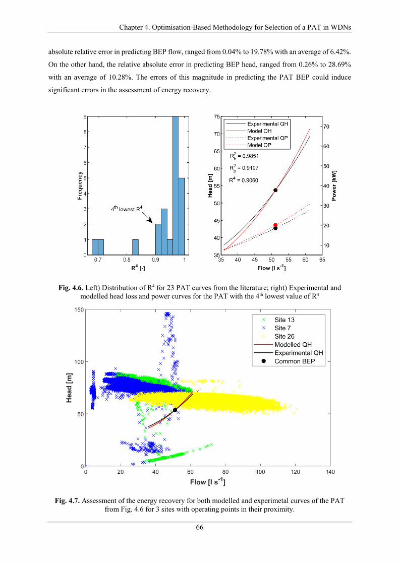
Chapter 4. Optimisation-Based Methodology for Selection of a PAT in WDNs
66
absolute relative error in predicting BEP flow, ranged from 0.04% to 19.78% with an average of 6.42%.
On the other hand, the relative absolute error in predicting BEP head, ranged from 0.26% to 28.69%
with an average of 10.28%. The errors of this magnitude in predicting the PAT BEP could induce
significant errors in the assessment of energy recovery.
Fig. 4.6. Left) Distribution of R4 for 23 PAT curves from the literature; right) Experimental and
modelled head loss and power curves for the PAT with the 4th lowest value of R4
Fig. 4.7. Assessment of the energy recovery for both modelled and experimetal curves of the PAT
from Fig. 4.6 for 3 sites with operating points in their proximity.
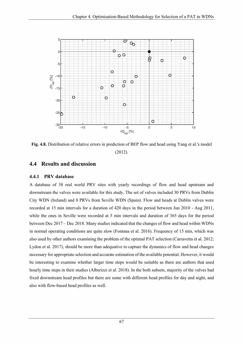
Chapter 4. Optimisation-Based Methodology for Selection of a PAT in WDNs
67
Fig. 4.8. Distribution of relative errors in prediction of BEP flow and head using Yang et al.'s model
(2012).
4.4 Results and discussion
4.4.1 PRV database
A database of 38 real world PRV sites with yearly recordings of flow and head upstream and
downstream the valves were available for this study. The set of valves included 30 PRVs from Dublin
City WDN (Ireland) and 8 PRVs from Seville WDN (Spain). Flow and heads at Dublin valves were
recorded at 15 min intervals for a duration of 420 days in the period between Jun 2010 - Aug 2011,
while the ones in Seville were recorded at 5 min intervals and duration of 365 days for the period
between Dec 2017 – Dec 2018. Many studies indicated that the changes of flow and head within WDNs
in normal operating conditions are quite slow (Fontana et al. 2016). Frequency of 15 min, which was
also used by other authors examining the problem of the optimal PAT selection (Carravetta et al. 2012;
Lydon et al. 2017), should be more than adequative to capture the dynamics of flow and head changes
necessary for appropriate selection and accurate estimation of the available potential. However, it would
be interesting to examine whether larger time steps would be suitable as there are authors that used
hourly time steps in their studies (Alberizzi et al. 2018). In the both subsets, majority of the valves had
fixed downstream head profiles but there are some with different head profiles for day and night, and
also with flow-based head profiles as well.
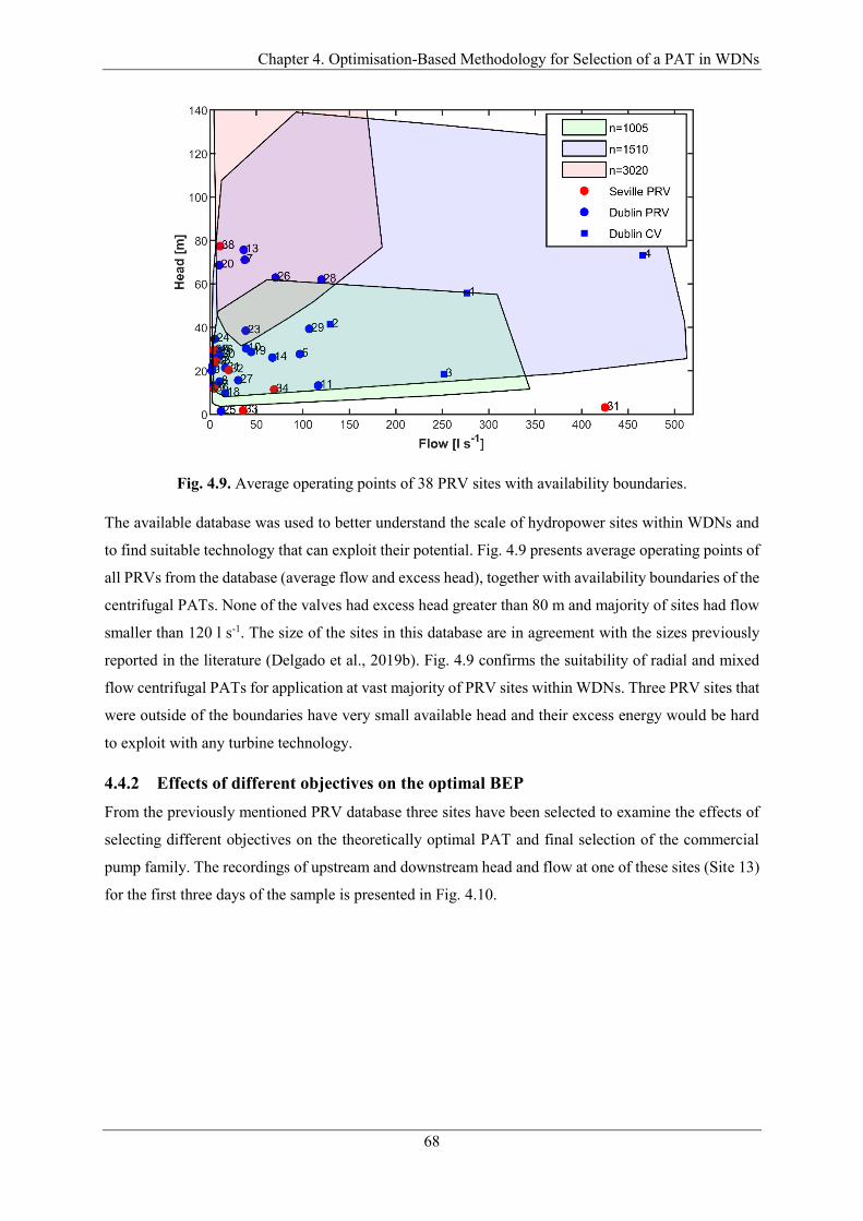
Chapter 4. Optimisation-Based Methodology for Selection of a PAT in WDNs
68
Fig. 4.9. Average operating points of 38 PRV sites with availability boundaries.
The available database was used to better understand the scale of hydropower sites within WDNs and
to find suitable technology that can exploit their potential. Fig. 4.9 presents average operating points of
all PRVs from the database (average flow and excess head), together with availability boundaries of the
centrifugal PATs. None of the valves had excess head greater than 80 m and majority of sites had flow
smaller than 120 l s-1. The size of the sites in this database are in agreement with the sizes previously
reported in the literature (Delgado et al., 2019b). Fig. 4.9 confirms the suitability of radial and mixed
flow centrifugal PATs for application at vast majority of PRV sites within WDNs. Three PRV sites that
were outside of the boundaries have very small available head and their excess energy would be hard
to exploit with any turbine technology.
4.4.2 Effects of different objectives on the optimal BEP
From the previously mentioned PRV database three sites have been selected to examine the effects of
selecting different objectives on the theoretically optimal PAT and final selection of the commercial
pump family. The recordings of upstream and downstream head and flow at one of these sites (Site 13)
for the first three days of the sample is presented in Fig. 4.10.

Chapter 4. Optimisation-Based Methodology for Selection of a PAT in WDNs
69
Fig. 4.10. Flow and head recordings at Site 13 for the first three days of the sample.
Fig. 4.11 presents the contour plots of the three examined objectives for each examined speed, for Site
13. The contour plots indicate that the examined optimisation problem defined with Eq. 17 and
analogues problems with NPV10 and PP objectives are indeed local problems, thus proving the suitability
for usage of Nelder-Mead algorithm. The numerical values of theoretically optimal solutions for all
three sites are presented in Tab. 4.1. The theoretical solutions can be regarded as upper bounds in the
cases of energy recovery and NPV10 objectives and lower bound in the case of PP objective.
Surprisingly, not many studies on this topic relate their optimal solution to the average operation point,
i.e., average flow and excess head at the examined sites. In the study carried out by Stefanizzi et
al.(2019), the authors suggested that the BEP of a PAT (in the alternative with 1 PAT) should be as
close as possible to the average point to maximize energy recovery. The authors supported this
hypothesis with the fact that this point has the highest frequency of occurrence. On the other hand, the
results of the study by Lydon et al. (2017) suggested that the design flow which will maximize energy
recovery should be between 10% and 30% smaller than the average flow depending on the site (in the
alternative with 1 PAT). They explained that the design flow should be small enough to have a high
frequency of larger flows occurrence but big enough to capture most of the available energy. In the
methodology developed in this chapter the theoretically optimal BEPs that will maximize the objectives
are the result of the optimisation procedure. The results presented in Tab. 4.1 indicate that the average
BEP flow and available head, across the three considered valves, that would maximize the energy
recovery, NPV and PP objectives, amounted 92% and 85%, 87% and 78% and 64% and 75% of the
valves’ average operating points, respectively. It can be also noticed that these ratios do not change

Chapter 4. Optimisation-Based Methodology for Selection of a PAT in WDNs
70
much across the valves except in the case of QBEP/Qave ratio for the minimization of PP, which seems to
decrease with the increase of the average operation flow at the valves.
Tab. 4.1. Effects of different objective functions on the optimal BEPs for three PRV case studies
Site 13 Site 28 Site 1
Objective max(E) max(NPV10) mini(PP) max(E) max(NPV10) min(PP) max(E) max(NPV10) min(PP)
QBEP [l s-1] 33.25 32.10 26.08 111.98 105.05 77.77 250.63 232.78 151.08
HBEP [m] 62.21 59.20 56.82 55.34 50.06 46.20 46.39 42.41 41.64
n [rpm] 3020 3020 3020 3020 3020 3020 1510 1510 1510
Ns [rpm (m3 s-1)0.5
m-0.75] 24.86 25.35 23.56 49.81 52.01 47.53 42.53 43.84 35.80
ηmax [-] 0.77 0.77 0.76 0.83 0.83 0.82 0.85 0.85 0.84
PBEP [kW] 15.65 14.38 11.00 50.41 42.64 28.93 96.68 81.96 51.57
ηglobal [-] 0.62 0.61 0.55 0.66 0.65 0.55 0.66 0.66 0.51
E [MWh year-1]
143.81 143.31 129.28 416.51 412.87 350.26 874.15 866.93 664.74
NPV10 [€ year-1]
77854 78413 71672 233338 236156 205444 493662 500800 394722
PP [years] 1.36 1.31 1.25 1.20 1.09 0.96 1.16 1.04 0.90
QBEP/Qave
[-] 0.92 0.89 0.72 0.93 0.88 0.65 0.91 0.84 0.55
HBEP/Have
[-] 0.82 0.78 0.75 0.89 0.81 0.74 0.83 0.76 0.75
Optimal commercial family
50-160, n=3020, D=174
50-160, n=3020, D=174
50-160, n=3020, D=174
100-160, n=3020, D=185
100-160, n=3020, D=185
80-160, n=3020, D=174
200-330, n=1510, D=330
200-330, n=1510, D=330
150-315, n=1510, D=334
As the PAT selection charts do not exist, to find the best commercial pump family alternative for the
considered site, the theoretically optimal BEP in turbine mode should be converted into related BEP in
pump mode using Yang et al.'s (2012) model or any similar conversion models. Using the obtained BEP
in pump mode from the pump selection charts the near optimal commercial pump families can be
selected. The BEPs of the pumps in proximity to the theoretically optimal BEP should be converted in
turbine mode to assess the exact values of the objectives. The BEPs of the commercial Etanorm pumps
that were in proximity to the optimal BEP for three considered sites are presented in Tab. A.1-3. For
Site 13, these BEPs are also presented as empty circles on contour plots in Fig. 4.11.

Chapter 4. Optimisation-Based Methodology for Selection of a PAT in WDNs
71
Fig. 4.11. Contour plots of Site 13: a) max(E) n=1005; b) max(E) n=1510; c) max(E) n=3020; d)
max(NPV) n=1005; e) max(NPV) n=1510; f) max(NPV) n=3020; g) min(PP) n=1005; h) min(PP)
n=1510; i) min(PP) n=3020; j) - l) Optimal BEPs of the objectives with available commercial families
for each rotational speed.
Table 4.1 indicates that in case of Site 13 the best commercial family was the same regardless of the
objective. On the other hand, in the cases of Sites 28 and 1 the best solutions obtained based on energy
recovery and NPV10 objectives differed from the solution obtained using PP objective. Although, the
best commercial alternatives in the cases of all examined sites and objectives, all were of the optimal
speed, from Tab. A.1-3 it can be seen that the second best solution was of a different speed, which
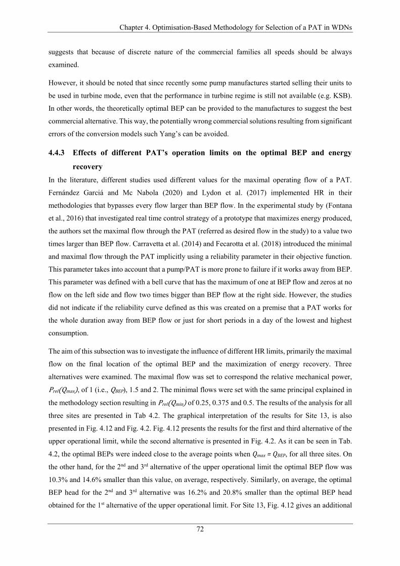
Chapter 4. Optimisation-Based Methodology for Selection of a PAT in WDNs
72
suggests that because of discrete nature of the commercial families all speeds should be always
examined.
However, it should be noted that since recently some pump manufactures started selling their units to
be used in turbine mode, even that the performance in turbine regime is still not available (e.g. KSB).
In other words, the theoretically optimal BEP can be provided to the manufactures to suggest the best
commercial alternative. This way, the potentially wrong commercial solutions resulting from significant
errors of the conversion models such Yang’s can be avoided.
4.4.3 Effects of different PAT’s operation limits on the optimal BEP and energy
recovery
In the literature, different studies used different values for the maximal operating flow of a PAT.
Fernández Garciá and Mc Nabola (2020) and Lydon et al. (2017) implemented HR in their
methodologies that bypasses every flow larger than BEP flow. In the experimental study by (Fontana
et al., 2016) that investigated real time control strategy of a prototype that maximizes energy produced,
the authors set the maximal flow through the PAT (referred as desired flow in the study) to a value two
times larger than BEP flow. Carravetta et al. (2014) and Fecarotta et al. (2018) introduced the minimal
and maximal flow through the PAT implicitly using a reliability parameter in their objective function.
This parameter takes into account that a pump/PAT is more prone to failure if it works away from BEP.
This parameter was defined with a bell curve that has the maximum of one at BEP flow and zeros at no
flow on the left side and flow two times bigger than BEP flow at the right side. However, the studies
did not indicate if the reliability curve defined as this was created on a premise that a PAT works for
the whole duration away from BEP flow or just for short periods in a day of the lowest and highest
consumption.
The aim of this subsection was to investigate the influence of different HR limits, primarily the maximal
flow on the final location of the optimal BEP and the maximization of energy recovery. Three
alternatives were examined. The maximal flow was set to correspond the relative mechanical power,
Prel(Qmax), of 1 (i.e., QBEP), 1.5 and 2. The minimal flows were set with the same principal explained in
the methodology section resulting in Prel(Qmin) of 0.25, 0.375 and 0.5. The results of the analysis for all
three sites are presented in Tab 4.2. The graphical interpretation of the results for Site 13, is also
presented in Fig. 4.12 and Fig. 4.2. Fig. 4.12 presents the results for the first and third alternative of the
upper operational limit, while the second alternative is presented in Fig. 4.2. As it can be seen in Tab.
4.2, the optimal BEPs were indeed close to the average points when Qmax = QBEP, for all three sites. On
the other hand, for the 2nd and 3rd alternative of the upper operational limit the optimal BEP flow was
10.3% and 14.6% smaller than this value, on average, respectively. Similarly, on average, the optimal
BEP head for the 2nd and 3rd alternative was 16.2% and 20.8% smaller than the optimal BEP head
obtained for the 1st alternative of the upper operational limit. For Site 13, Fig. 4.12 gives an additional

Chapter 4. Optimisation-Based Methodology for Selection of a PAT in WDNs
73
insight and that is that for the 3rd alternative the maximal flow through the PAT was never reached,
meaning the two CVs were never active at the same time (there are not black crosses), unlike in the first
two alternatives.
Tab. 4.2. Effects of PAT’s operation limits on the optimal BEPs for three PRV case studies
Site 13 Site 28 Site 1
Prelmax [-] 1 1.5 2 1 1.5 2 1 1.5 2
Qmax [l s-1] 37.74 39.35 41.87 121.99 130.82 139.07 278.82 293.86 323.77
QBEP [l s-1] 37.74 33.25 31.20 121.99 111.98 105.67 278.82 250.63 244.70
HBEP [m] 75.82 62.21 57.79 64.05 55.34 52.30 55.68 46.39 44.69
n [rpm] 3020 3020 3020 3020 3020 3020 1510 1510 1510
Ns [rpm (m3 s-1)0.5
m-0.75] 22.83 24.86 25.45 46.59 49.81 50.48 39.12 42.53 43.21
ηmax [-] 0.77 0.77 0.77 0.83 0.83 0.83 0.85 0.85 0.85
PBEP [kW] 21.58 15.65 13.63 63.81 50.41 44.86 129.29 96.68 90.89
ηglobal [-] 0.61 0.62 0.60 0.65 0.66 0.65 0.67 0.66 0.65
E [MWh year-1] 143.35 143.81 140.61 414.25 416.51 411.26 876.29 874.15 855.95
NPV10 [€ year-1] 70284 77854 78134 217052 233338 235555 456731 493662 497327
PP [years] 1.67 1.36 1.29 1.42 1.20 1.12 1.43 1.16 1.11
QBEP/Qave [-] 1.04 0.92 0.86 1.02 0.93 0.88 1.01 0.91 0.89
HBEP/Have [-] 1.00 0.82 0.76 1.03 0.89 0.84 1.00 0.83 0.80
Optimal commercial
family
65-200, n=3020, D=219
50-160, n=3020, D=174
50-160, n=3020, D=174
150-500-1, n=1005, D=500
100-160, n=3020, D=185
125-315, n=1510, D=334
300-500, n=1005, D=520
200-330, n=1510, D=330
200-330, n=1510, D=330
Fig. 4.12. Influence of PAT’s operation limits on the optimal BEP a) Prel(Qmax) = 1 b) Prel(Qmax) = 2.
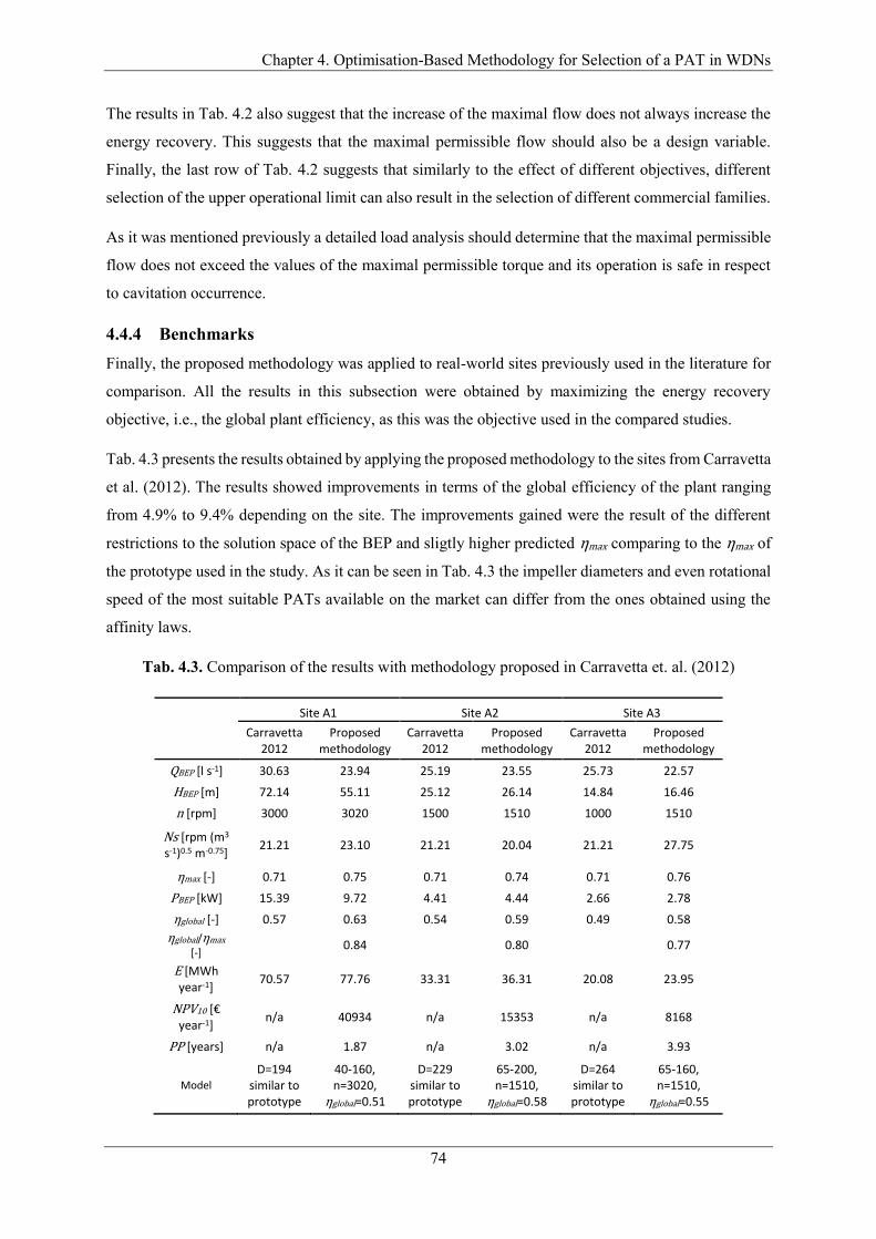
Chapter 4. Optimisation-Based Methodology for Selection of a PAT in WDNs
74
The results in Tab. 4.2 also suggest that the increase of the maximal flow does not always increase the
energy recovery. This suggests that the maximal permissible flow should also be a design variable.
Finally, the last row of Tab. 4.2 suggests that similarly to the effect of different objectives, different
selection of the upper operational limit can also result in the selection of different commercial families.
As it was mentioned previously a detailed load analysis should determine that the maximal permissible
flow does not exceed the values of the maximal permissible torque and its operation is safe in respect
to cavitation occurrence.
4.4.4 Benchmarks
Finally, the proposed methodology was applied to real-world sites previously used in the literature for
comparison. All the results in this subsection were obtained by maximizing the energy recovery
objective, i.e., the global plant efficiency, as this was the objective used in the compared studies.
Tab. 4.3 presents the results obtained by applying the proposed methodology to the sites from Carravetta
et al. (2012). The results showed improvements in terms of the global efficiency of the plant ranging
from 4.9% to 9.4% depending on the site. The improvements gained were the result of the different
restrictions to the solution space of the BEP and sligtly higher predicted ηmax comparing to the ηmax of
the prototype used in the study. As it can be seen in Tab. 4.3 the impeller diameters and even rotational
speed of the most suitable PATs available on the market can differ from the ones obtained using the
affinity laws.
Tab. 4.3. Comparison of the results with methodology proposed in Carravetta et. al. (2012)
Site A1 Site A2 Site A3
Carravetta 2012
Proposed methodology
Carravetta 2012
Proposed methodology
Carravetta 2012
Proposed methodology
QBEP [l s-1] 30.63 23.94 25.19 23.55 25.73 22.57
HBEP [m] 72.14 55.11 25.12 26.14 14.84 16.46
n [rpm] 3000 3020 1500 1510 1000 1510
Ns [rpm (m3 s-1)0.5 m-0.75]
21.21 23.10 21.21 20.04 21.21 27.75
ηmax [-] 0.71 0.75 0.71 0.74 0.71 0.76
PBEP [kW] 15.39 9.72 4.41 4.44 2.66 2.78
ηglobal [-] 0.57 0.63 0.54 0.59 0.49 0.58
ηglobal/ηmax [-]
0.84 0.80 0.77
E [MWh year-1]
70.57 77.76 33.31 36.31 20.08 23.95
NPV10 [€ year-1]
n/a 40934 n/a 15353 n/a 8168
PP [years] n/a 1.87 n/a 3.02 n/a 3.93
Model D=194
similar to prototype
40-160, n=3020,
ηglobal=0.51
D=229 similar to prototype
65-200, n=1510,
ηglobal=0.58
D=264 similar to prototype
65-160, n=1510,
ηglobal=0.55
Chapter 4. Optimisation-Based Methodology for Selection of a PAT in WDNs
75
Regardless the improvements comparing to Carravetta et al. (2012) the selected prototype, i.e., its
similarity curves (as in Fig. 4.1) matched well to the examined sites. Tab. A.4, which presents the results
of comparison with Lydon et al. (2017), indicates that the improvements can be significantly higher if
a non-optimal prototype is selected. The improvements gained in terms of ηglobal ranged from 24% to
36% comparing to design points and from 45% to 58% comparing to BEPs of machines similar to
prototype. The improvements of this magnitude, especially in case of the machines similar to prototype,
can be explained with the efficiency of the prototype which was around 20% lower than the predicted
values and the fact that the prototype’s affinity curve for n = 900 rpm was very far away from the
operating points of all three considered sites. Although the PRV sites are the same it has to be pointed
out that the measurements have not been recorded for the same year. However the gross powers of the
sites presented in the study were similar.
As it was indicated by the results in Tab. 4.3 and Tab. A.4, the non-optimal choice of the prototype and
its speed can seriously dimish the results of the energy recovery. Selection of the prototype, i.e., the
specific speed which is a good fit for a site within WDNs which are characterized with large variations
of flow and head is not straighforward. Additionally the characteristic curves of the such prototype
could be unavailable. The main advantage of the proposed methodology is that it does not depend on
the choice of the prototype and that it will always provide the upper bound of the energy recovery for
the examined site.
Some of the previous studies suggested ηglobal = 0.6 as maximal global efficiency of a hydro plant within
a WDN equiped with a PAT (Carravetta et al., 2014; Fecarotta et al., 2018). The results of the six
examined sites presented in Tab. 4.3 and A.4 provide a different definition of the upper bound of the
energy recovery using hydraulic regulation. The results suggest that the maximal global efficiency of a
plant is around 80% of the ηmax of the optimal PAT.
4.5 Conclusions
This chapter presents a novel methodology for the selection of a PAT from the market to replace a PRV
located within WDNs, which are characterized by large flow and head fluctuations. The presented
methodology implements the classical hydraulic regulation scheme with two control valves and a
single-stage centrifugal PAT for maintenance of required downstream head pattern. It also employs the
NMSDS optimisation algorithm to find the optimal BEP. Besides the optimisation algorithm used, the
novel methodology differs from previous approaches in restriction of the solution space. Unlike
traditional approaches which are based on scaling a prototype data by affinity curves and thus restricting
the solution space to these curves, the proposed methodology restricts the solutions space only with the
availability boundaries of market centrifugal PATs.

Chapter 4. Optimisation-Based Methodology for Selection of a PAT in WDNs
76
Using the proposed methodology, this study examined the effects of different objectives, namely
maximization of energy recovery, maximization of NPV10 and minimization of PP on the selection of
the optimal PAT. The results of three real world PRV case studies from Dublin WDN showed that the
optimal BEPs for the three objectives correspond to 92%, 87% and 64% of the sites’ average operating
flow and 85%, 78% and 75% of the sites’ average operating head, on average across three sites,
respectively. The results also showed that the former differences in the theoretically optimal BEPs can
result in selection of different commercial pump families. Although the selection of commercial
families should be regarded with caution as the validation section presented in this chapter indicated
that even the most accurate models for predicting the BEP in turbine mode can result in errors of around
30%.
The methodology developed in this chapter also suggested new formulation for the limits of variable
PAT operation based on its relative mechanical power (Prel). Varying the upper operational limit the
analysis conducted in this chapter investigated how it can affect the selection of the optimal PAT and
the maximization of energy recovery. The results of the same three PRV case studies showed that the
increase of the maximal permissible flow results in a theoretically smaller PAT but it does not always
increase the maximal value of the energy recovery. Similarly to the effect of the selection of different
objectives the results showed that the selection of different upper operational limit can also result in
selection of different commercial pump family. This indicates that the upper operation limit should also
be one of the designed variables.
The methodology was also applied to sites previously used in the literature resulting in improvements
in terms of the global plant’s efficiency of 4.9% to 9.4% comparing with Carravetta et al. (2012) and
24% to 58% comparing to Lydon et al. (2017). The results of the maximal global efficiency for the six
sites from these 2 studies suggest that the upper bound of the energy recovery is around 80% of the ηmax
of the optimal PAT.
The future work will be focused on studying the flow and head patterns of the PRV database in order
to find out what are the minimal flow and head characteristics of a PRV which would result in
economically viable replacement.
Chapter 5. Prediction of Global Efficiency and Economic Viability Bounds in PATs within WDNs
77
5 Prediction of Global Efficiency
and Economic Viability
Bounds in PATs within WDNs
5.1 Introduction
To conduct a preliminary analysis of the potential of a site within a WDN, researchers often estimate
the average operating condition at the valve, i.e., the average operating flow and excess head and
multiply these values with the expected average global efficiency of the plant, usually estimated as 65%
𝑃 = 9.81 ∙ 𝑄 ∙ 𝐻 ∙ 0.65 [𝑘𝑊] (Corcoran et al., 2013). In addition, many studies pointed out the
variations of the real-time operating conditions as an influential factor that can diminish the energy
recovery potential thus making the installation of HPER plants non-viable. However, to the candidate’s
knowledge there has been no study that quantified their influence. Therefore, this chapter makes a novel
contribution by directly assessing whether it is possible to accurately estimate the energy recovery
potential of a PRV site using only the statistics of the recorded operating conditions (the 4th research
question of the thesis).
Consideration of the economic viability of a PAT installation at a PRV site, this upgrade is often deemed
viable if it is expected to have positive NPV after 10 years, or payback period less than 10 years
(Fernández Garcia and Mc Nabola, 2020). For two sites with similar average operating conditions, the
uncertainties that can make a difference between one being viable and the other not, are related to the
level of variation of the hydraulic operating conditions occurring at the sites, and the variation in total
installation costs (TIC) of their upgrades. Namely, the site with larger variation of the hydraulic
conditions is expected to have a lower value of NPV as a consequence of lower energy generation due
to larger head dissipation and flow bypassing, and more operating points being further away from the
PAT’s BEP or even outside of its permissible operating range. Therefore this chapter makes another
novel contribution by addressing whether a bound of economically viable upgrades of PRV sites into
PAT based HPER plants can be defined (the 5th research question of the thesis).
Chapter 5. Prediction of Global Efficiency and Economic Viability Bounds in PATs within WDNs
78
5.2 Methodology
5.2.1 Methodology Overview
To address the identified research questions, the database of 38 PRVs with yearly high temporal
resolution recordings of flow and head upstream and downstream from the valves described in the
previous chapter was used. However, unlike in the analysis presented in the previous chapter, where
only three sites were analysed, the analysis conducted in this chapter analysed all sites from the
database. To assess the energy recovery of the considered valves an improved variant of the energy
recovery algorithm defined in the previous chapter was developed. The improvements include
optimisation of the operational limits of the considered PAT alternative to optimally suit the operating
conditions of the considered valve, thus implicitly optimising the size of the generator to be coupled
with the considered PAT. The optimality criteria for selection of a PAT from a PAT database was the
maximization of the NPV after 10 years.
The first part of the analysis addressed the first research question of this chapter (the 4th overall) by
carrying out a linear least-squares regression analysis, where different measures of centrality and
dispersion of the PRV samples were defined to be used as predictor variables, while the response
variable was the assessed global efficiency of the HPER plants.
The second research question of this chapter (the 5th overall) was addressed in the second part of the
study that started with investigation of the domain of average operating conditions commonly occurring
at PRVs within WDNs. Following the definition of the domain, distribution of a variable defined to
quantify the variation of the operating conditions recorded at 38 PRV samples was studied to define its
confidence interval. The possible range of values of the TIC was adopted from the study carried out by
Fernández García et al. (2019). Then, the optimal NPV was calculated for all hypothetical PRV sites
evenly distributed across the whole domain by including both types of uncertainty. Finally, the expected
bound of economically viable sites and its confidence interval were defined by extracting the zero
contours from the previously assessed NPV surfaces.
5.2.2 Assessment of energy recovery and NPV
To assess the potential for energy recovery at each valve, a PAT database was compiled. This database
was mention in Chapter 4, but there it was used only to define the boundaries of the PATs available on
the market. The methodology presented in Chapter 4 does not use the PAT database to find the
theoretically optimal solution. In other words, for application of the methodology presented in Chapter
4, a potential user does not need to possess the information about the PATs from database. Instead, the
user can find the near optimal solution from the pump selection charts by converting the theoretically
optimal solution obtained in turbine mode to pump mode. Contrary, the user of the methodology
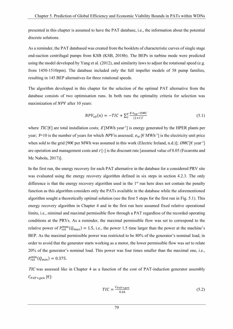
Chapter 5. Prediction of Global Efficiency and Economic Viability Bounds in PATs within WDNs
79
presented in this chapter is assumed to have the PAT database, i.e., the information about the potential
discrete solutions.
As a reminder, the PAT databased was created from the booklets of characteristic curves of single stage
end-suction centrifugal pumps from KSB (KSB, 2018b). The BEPs in turbine mode were predicted
using the model developed by Yang et al. (2012), and similarity laws to adjust the rotational speed (e.g.
from 1450-1510rpm). The database included only the full impeller models of 58 pump families,
resulting in 145 BEP alternatives for three rotational speeds.
The algorithm developed in this chapter for the selection of the optimal PAT alternative from the
database consists of two optimisation runs. In both runs the optimality criteria for selection was
maximization of 𝑁𝑃𝑉 after 10 years:
𝑁𝑃𝑉10(𝑛) = −𝑇𝐼𝐶 + ∑𝐸∙𝑒𝑢𝑝−𝑂𝑀𝐶
(1+𝑟)𝑗𝑌𝑗 (5.1)
where TIC [€] are total installation costs; E [MWh year-1] is energy generated by the HPER plants per
year; Y=10 is the number of years for which NPV is assessed; eup [€ MWh-1] is the electricity unit price
when sold to the grid [90€ per MWh was assumed in this work (Electric Ireland, n.d.)]; OMC [€ year-1]
are operation and management costs and r [-] is the discount rate [assumed value of 0.05 (Fecarotta and
Mc Nabola, 2017)].
In the first run, the energy recovery for each PAT alternative in the database for a considered PRV site
was evaluated using the energy recovery algorithm defined in six steps in section 4.2.3. The only
difference is that the energy recovery algorithm used in the 1st run here does not contain the penalty
function as this algorithm considers only the PATs available in the database while the aforementioned
algorithm sought a theoretically optimal solution (see the first 5 steps for the first run in Fig. 5.1). This
energy recovery algorithm in Chapter 4 and in the first run here assumed fixed relative operational
limits, i.e., minimal and maximal permissible flow through a PAT regardless of the recorded operating
conditions at the PRVs. As a reminder, the maximal permissible flow was set to correspond to the
relative power of 𝑃𝑟𝑒𝑙max(𝑄𝑚𝑎𝑥) = 1.5, i.e., the power 1.5 time larger than the power at the machine’s
BEP. As the maximal permissible power was restricted to be 80% of the generator’s nominal load, in
order to avoid that the generator starts working as a motor, the lower permissible flow was set to relate
20% of the generator’s nominal load. This power was four times smaller than the maximal one, i.e.,
𝑃𝑟𝑒𝑙min(𝑄𝑚𝑖𝑛) = 0.375.
TIC was assessed like in Chapter 4 as a function of the cost of PAT-induction generator assembly
𝐶𝑃𝐴𝑇+𝑔𝑒𝑛 [€]:
𝑇𝐼𝐶 =𝐶𝑃𝐴𝑇+𝑔𝑒𝑛
0.26 (5.2)
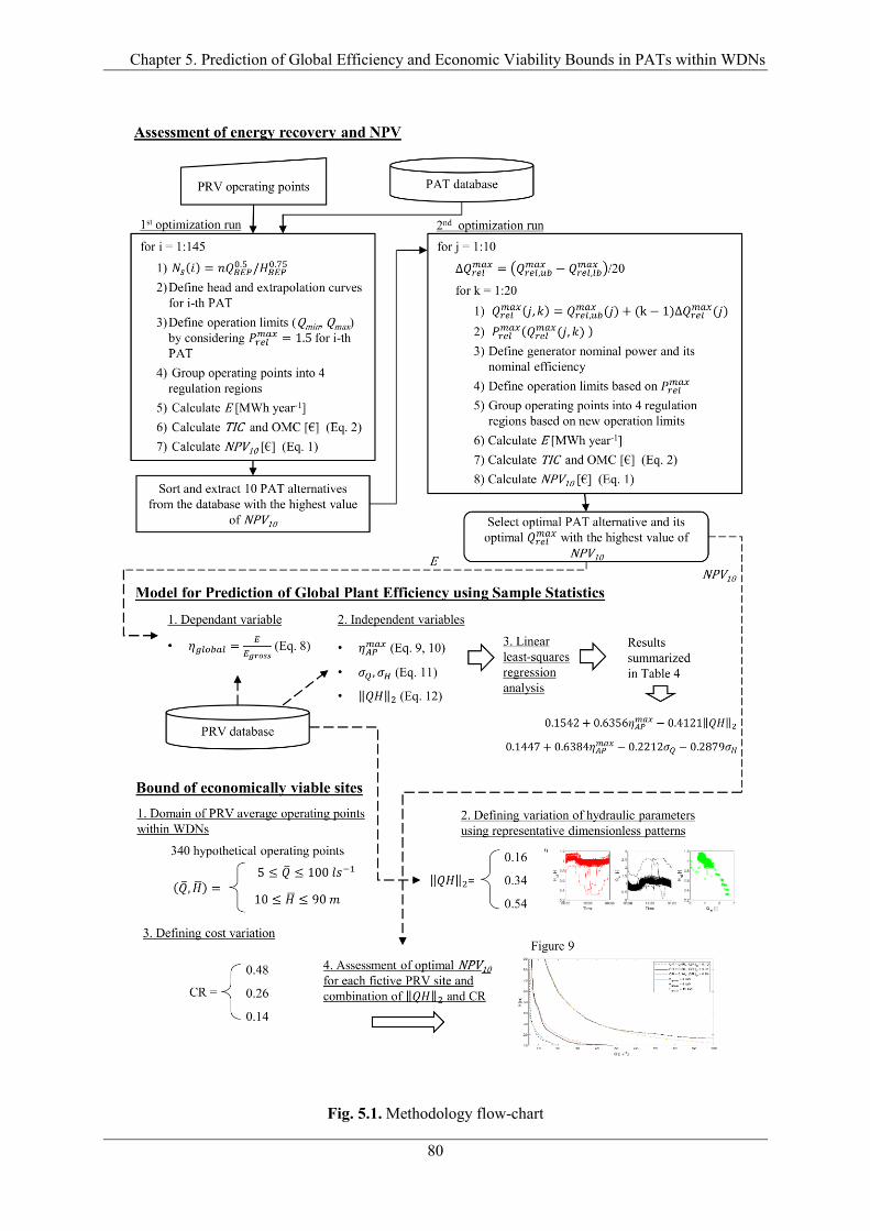
Chapter 5. Prediction of Global Efficiency and Economic Viability Bounds in PATs within WDNs
80
Fig. 5.1. Methodology flow-chart
Chapter 5. Prediction of Global Efficiency and Economic Viability Bounds in PATs within WDNs
81
Eq. 5.2 suggests that 𝐶𝑃𝐴𝑇+𝑔𝑒𝑛 represents 26% of TIC. This assumption was based on the study carried
out by Fernández García et al. (2019) that examined 9 real-world PAT installations within WDNs. The
other 74% of the installation costs were associated with hydraulic regulation control system,
commissioning, civil works, grid connection, additional hydraulic equipment and other project costs.
To assess the cost of 𝐶𝑃𝐴𝑇+𝑔𝑒𝑛, the methodology developed in Chapter 4 used a model defined by
Novara et al. (2019). This model considers that a PAT is always coupled with a generator whose
nominal power is 20% higher than the power of the PAT generated at its BEP. In this chapter, the
𝐶𝑃𝐴𝑇+𝑔𝑒𝑛 cost model is modified to consider the true size of the coupled generator. The modification
is attained by subtracting the cost of the generator with default size from the original cost of the
assembly and by adding the cost of a generator of a true size:
𝑝𝑝 = 1: 𝐶𝑃𝐴𝑇+𝑔𝑒𝑛 = 11913.91 ∙ 𝑄𝐵𝐸𝑃𝐻𝐵𝐸𝑃0.5 + 1289.92 + 40.03 ∙ 𝑃𝐵𝐸𝑃
100
80(𝑃𝑟𝑒𝑙
𝑚𝑎𝑥 − 1) (5.3)
𝑝𝑝 = 2: 𝐶𝑃𝐴𝑇+𝑔𝑒𝑛 = 12717.29 ∙ 𝑄𝐵𝐸𝑃𝐻𝐵𝐸𝑃0.5 + 1038.44 + 40.51 ∙ 𝑃𝐵𝐸𝑃
100
80(𝑃𝑟𝑒𝑙
𝑚𝑎𝑥 − 1) (5.4)
𝑝𝑝 = 3: 𝐶𝑃𝐴𝑇+𝑔𝑒𝑛 = 15797.72 ∙ 𝑄𝐵𝐸𝑃𝐻𝐵𝐸𝑃0.5 + 1289.92 + 60.19 ∙ 𝑃𝐵𝐸𝑃
100
80(𝑃𝑟𝑒𝑙
𝑚𝑎𝑥 − 1) (5.5)
where 𝑝𝑝 [-] is the number of magnetic pole pairs of the generator; 𝑄𝐵𝐸𝑃 [m3 s-1] is flow at BEP; 𝐻𝐵𝐸𝑃
[m] is head at BEP; 𝑃𝐵𝐸𝑃 [kW] is the mechanical power of the shaft; and 𝑃𝑟𝑒𝑙𝑚𝑎𝑥 = 𝑃𝑚𝑎𝑥/𝑃𝐵𝐸𝑃 [-] is the
relative permissible maximal power as explained previously. The last term in Eq. 5.3-5.5 represents the
cost difference between the generator of true size 𝑃𝑔𝑒𝑛𝑡𝑟𝑢𝑒 = 𝑃𝐵𝐸𝑃𝑃𝑟𝑒𝑙
𝑚𝑎𝑥100/80 and the generator of
default size 𝑃𝑔𝑒𝑛𝑑𝑒𝑓
= 𝑃𝐵𝐸𝑃100/80. The linear relationship between the generators’ cost and their
nominal size was also defined in Novara et al. (2019).
Besides the upgrade of the cost model, in comparison to the methodology from Chapter 4 the current
methodology has been upgraded to include the nominal efficiency of the generator. The value of the
generator’s nominal efficiency as a function of its size has been assessed using a power model that has
been obtained by fitting a power model to a curve that relates the nominal efficiency of the induction
generator of IE3 efficiency class with their nominal sizes, see Fig. B.1 (ABB Motors and Generators,
2014):
𝜂𝑒𝑙𝑒𝑐𝑚𝑎𝑥 = −15.3864 ∙ 𝑃𝑔𝑒𝑛
−0.3312 + 98.7780 (5.6)
The best 10 PAT alternatives according to the value of NPV proceeded to the second run. Although,
the methodology developed in Chapter 4 used the fixed operational limits the analysis indicated that
different upper operation limit can lead to the selection of different commercial PAT for the same site.
In other words, the operating limits should also be a design variable and be optimised. This was the
main reason for the upgrade of the cost model to include the generator of a true size, as the change of
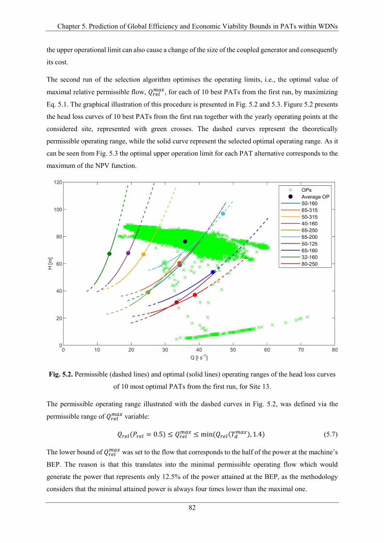
Chapter 5. Prediction of Global Efficiency and Economic Viability Bounds in PATs within WDNs
82
the upper operational limit can also cause a change of the size of the coupled generator and consequently
its cost.
The second run of the selection algorithm optimises the operating limits, i.e., the optimal value of
maximal relative permissible flow, 𝑄𝑟𝑒𝑙𝑚𝑎𝑥, for each of 10 best PATs from the first run, by maximizing
Eq. 5.1. The graphical illustration of this procedure is presented in Fig. 5.2 and 5.3. Figure 5.2 presents
the head loss curves of 10 best PATs from the first run together with the yearly operating points at the
considered site, represented with green crosses. The dashed curves represent the theoretically
permissible operating range, while the solid curve represent the selected optimal operating range. As it
can be seen from Fig. 5.3 the optimal upper operation limit for each PAT alternative corresponds to the
maximum of the NPV function.
Fig. 5.2. Permissible (dashed lines) and optimal (solid lines) operating ranges of the head loss curves
of 10 most optimal PATs from the first run, for Site 13.
The permissible operating range illustrated with the dashed curves in Fig. 5.2, was defined via the
permissible range of 𝑄𝑟𝑒𝑙𝑚𝑎𝑥 variable:
𝑄𝑟𝑒𝑙(𝑃𝑟𝑒𝑙 = 0.5) ≤ 𝑄𝑟𝑒𝑙𝑚𝑎𝑥 ≤ min (𝑄𝑟𝑒𝑙(𝑇𝑑
𝑚𝑎𝑥), 1.4) (5.7)
The lower bound of 𝑄𝑟𝑒𝑙𝑚𝑎𝑥 was set to the flow that corresponds to the half of the power at the machine’s
BEP. The reason is that this translates into the minimal permissible operating flow which would
generate the power that represents only 12.5% of the power attained at the BEP, as the methodology
considers that the minimal attained power is always four times lower than the maximal one.
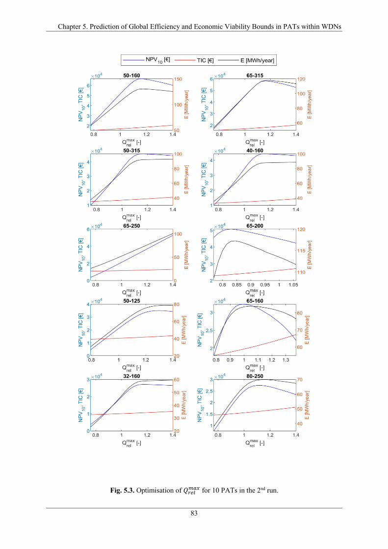
Chapter 5. Prediction of Global Efficiency and Economic Viability Bounds in PATs within WDNs
83
Fig. 5.3. Optimisation of 𝑄𝑟𝑒𝑙𝑚𝑎𝑥 for 10 PATs in the 2nd run.
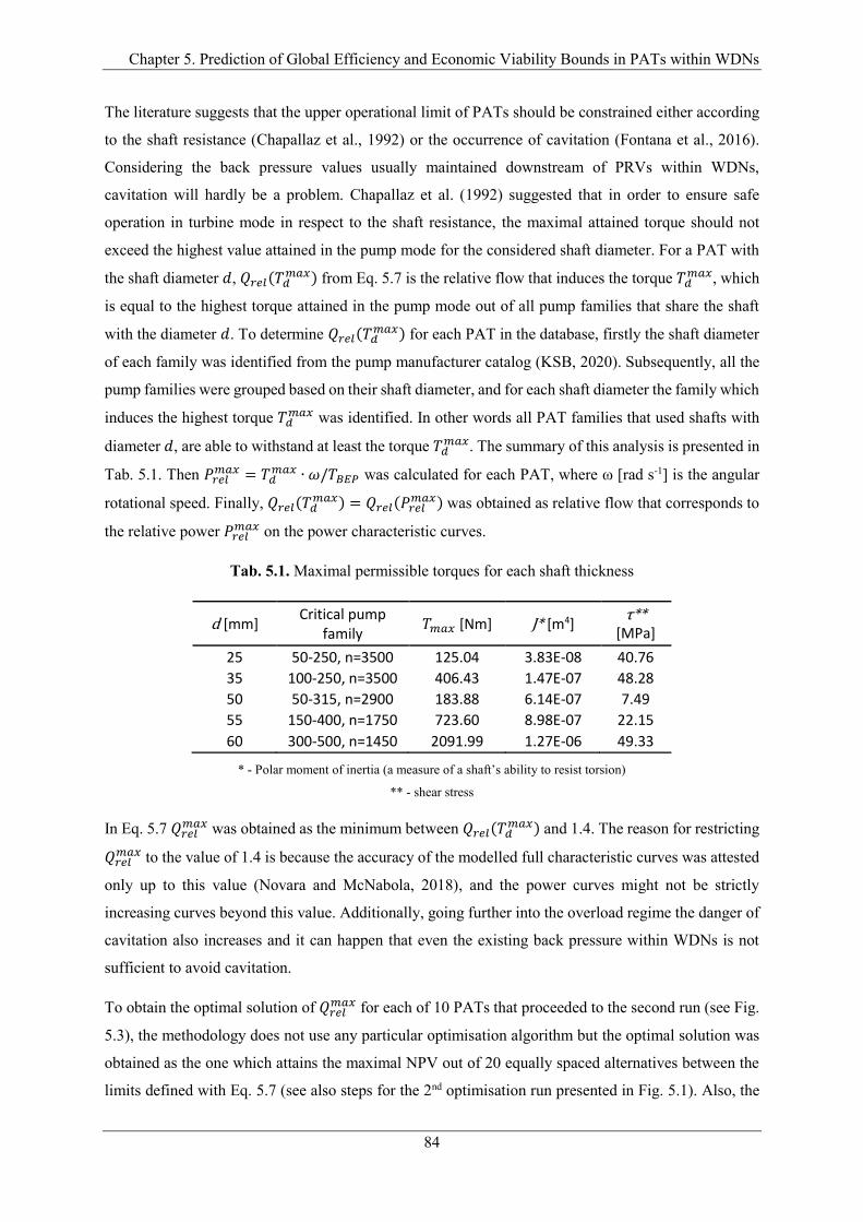
Chapter 5. Prediction of Global Efficiency and Economic Viability Bounds in PATs within WDNs
84
The literature suggests that the upper operational limit of PATs should be constrained either according
to the shaft resistance (Chapallaz et al., 1992) or the occurrence of cavitation (Fontana et al., 2016).
Considering the back pressure values usually maintained downstream of PRVs within WDNs,
cavitation will hardly be a problem. Chapallaz et al. (1992) suggested that in order to ensure safe
operation in turbine mode in respect to the shaft resistance, the maximal attained torque should not
exceed the highest value attained in the pump mode for the considered shaft diameter. For a PAT with
the shaft diameter 𝑑, 𝑄𝑟𝑒𝑙(𝑇𝑑𝑚𝑎𝑥) from Eq. 5.7 is the relative flow that induces the torque 𝑇𝑑
𝑚𝑎𝑥, which
is equal to the highest torque attained in the pump mode out of all pump families that share the shaft
with the diameter 𝑑. To determine 𝑄𝑟𝑒𝑙(𝑇𝑑𝑚𝑎𝑥) for each PAT in the database, firstly the shaft diameter
of each family was identified from the pump manufacturer catalog (KSB, 2020). Subsequently, all the
pump families were grouped based on their shaft diameter, and for each shaft diameter the family which
induces the highest torque 𝑇𝑑𝑚𝑎𝑥 was identified. In other words all PAT families that used shafts with
diameter 𝑑, are able to withstand at least the torque 𝑇𝑑𝑚𝑎𝑥. The summary of this analysis is presented in
Tab. 5.1. Then 𝑃𝑟𝑒𝑙𝑚𝑎𝑥 = 𝑇𝑑
𝑚𝑎𝑥 ∙ 𝜔/𝑇𝐵𝐸𝑃 was calculated for each PAT, where ω [rad s-1] is the angular
rotational speed. Finally, 𝑄𝑟𝑒𝑙(𝑇𝑑𝑚𝑎𝑥) = 𝑄𝑟𝑒𝑙(𝑃𝑟𝑒𝑙
𝑚𝑎𝑥) was obtained as relative flow that corresponds to
the relative power 𝑃𝑟𝑒𝑙𝑚𝑎𝑥 on the power characteristic curves.
Tab. 5.1. Maximal permissible torques for each shaft thickness
d [mm] Critical pump
family 𝑇𝑚𝑎𝑥 [Nm] J* [m4]
τ** [MPa]
25 50-250, n=3500 125.04 3.83E-08 40.76
35 100-250, n=3500 406.43 1.47E-07 48.28
50 50-315, n=2900 183.88 6.14E-07 7.49
55 150-400, n=1750 723.60 8.98E-07 22.15
60 300-500, n=1450 2091.99 1.27E-06 49.33
* - Polar moment of inertia (a measure of a shaft’s ability to resist torsion)
** - shear stress
In Eq. 5.7 𝑄𝑟𝑒𝑙𝑚𝑎𝑥 was obtained as the minimum between 𝑄𝑟𝑒𝑙(𝑇𝑑
𝑚𝑎𝑥) and 1.4. The reason for restricting
𝑄𝑟𝑒𝑙𝑚𝑎𝑥 to the value of 1.4 is because the accuracy of the modelled full characteristic curves was attested
only up to this value (Novara and McNabola, 2018), and the power curves might not be strictly
increasing curves beyond this value. Additionally, going further into the overload regime the danger of
cavitation also increases and it can happen that even the existing back pressure within WDNs is not
sufficient to avoid cavitation.
To obtain the optimal solution of 𝑄𝑟𝑒𝑙𝑚𝑎𝑥 for each of 10 PATs that proceeded to the second run (see Fig.
5.3), the methodology does not use any particular optimisation algorithm but the optimal solution was
obtained as the one which attains the maximal NPV out of 20 equally spaced alternatives between the
limits defined with Eq. 5.7 (see also steps for the 2nd optimisation run presented in Fig. 5.1). Also, the

Chapter 5. Prediction of Global Efficiency and Economic Viability Bounds in PATs within WDNs
85
selection algorithm is split into two runs only to reduce the computational time by avoiding optimising
𝑄𝑟𝑒𝑙𝑚𝑎𝑥 for all PAT alternatives from the database.
5.2.3 Model for Prediction of Global Plant Efficiency using Sample Statistics
The aim of the regression analysis presented in this subsection was to derive a model that would allow
practitioners to accurately estimate the amount of energy that can be recovered at their PRVs using only
the statistical parameters of the recorded samples of flow and excess head. Additionally, the presented
analysis intended to quantify how different magnitudes of flow and excess head variability affect energy
recovery using PATs.
The dependent variable in the regression analysis was the global efficiency of the HPER plants installed
at 38 PRV sites, which are equipped with the optimal PATs and generators, obtained using the
optimisation methodology described in the previous subsection:
𝜂𝑔𝑙𝑜𝑏𝑎𝑙 =𝐸 [𝑀𝑊ℎ]
𝐸𝑔𝑟𝑜𝑠𝑠 [𝑀𝑊ℎ]=
𝐸 [𝑀𝑊ℎ]
10−6 ∑ 𝜌𝑔𝑄𝑖𝐻𝑖Δ𝑡𝑖𝑁𝑖
(5.8)
where 𝜂𝑔𝑙𝑜𝑏𝑎𝑙 [-] is global plant efficiency; 𝐸 [MWh] is the energy recovered using the optimal PAT
and generator pair; 𝑁 [-] is the number of the recorded operating points; 𝜌 [kg m-3] is the water density;
𝑔 [m s-2] is the gravitational acceleration; 𝑄𝑖 [m3 s-1] is the flow recorded in each time step and 𝐻𝑖 [m]
is the excess head recorded in each time step. The excess head 𝐻𝑖 was obtained by subtracting the heads
recorded upstream and downstream of the PRVs.
The independent variables used in the regression analysis for predicting 𝜂𝑔𝑙𝑜𝑏𝑎𝑙 can be divided into two
groups. The first group describes the centrality of the recorded operating conditions, while the other
describes its dispersion.
Regardless of variation of flow and excess head at a PRV site, the predominant effect on the global
efficiency of a HPER plant will be the maximal efficiency of the selected PAT and the maximal
efficiency of the selected generator. Although, many methodologies for the assessment of energy
recovery using PATs used a constant value for their maximal mechanical efficiency regardless of the
PAT’s flow and head at the BEP (Carravetta et al., 2012; Fecarotta and Mc Nabola, 2017; Fernández
García et al., 2019; Fernández Garcia and Mc Nabola, 2020; Lydon et al., 2017), it is documented in
the literature that the maximal mechanical efficiency of the PATs can vary considerably across their Q-
H domain (Novara et al., 2017). As the maximal efficiency of a pump unit is similar in the pump and
turbine modes, Novara et al. (2017) recalculated coefficients of an equation initially proposed by
Anderson et al. (1977) for predicting the maximal efficiency in pump mode to refer to the PAT domain:
𝜂𝑚𝑒𝑐ℎ𝑚𝑎𝑥 = 0.89 −
0.024
𝑄𝐵𝐸𝑃0.41 − 0.076 (0.22 + 𝑙𝑛
𝑁𝑠
52.933)
2 (5.9)

Chapter 5. Prediction of Global Efficiency and Economic Viability Bounds in PATs within WDNs
86
where 𝜂𝑚𝑒𝑐ℎ𝑚𝑎𝑥 [-] is the mechanical efficiency of a PAT at its BEP for a selected rotational speed n [rpm];
QBEP [m3 s-1] is BEP flow and Ns [rpm (m3 s-1)0.5 (m)0.75] is the specific speed based on a unit flow of the
selected PAT. Using Eq. 5.9 the maximal mechanical efficiency of the PATs from the database ranges
from 32% to 86%.
A statistic that was used to describe the centrality of the sample was its average operating point (�̅�, �̅�).
As suggested by the results presented in Chapter 4, the BEP of a theoretically optimal PAT should be
relatively close to the average operating point of the sample when the objective is to maximize the NPV.
Hence, the function of the centrality statistic was to mimic the maximal efficiency of the selected PAT.
A derived predictor variable was created by substituting the BEP with the average operating point in
Eq. 5.9:
𝜂𝐴𝑃𝑚𝑎𝑥 = max {𝜂𝑚𝑒𝑐ℎ
𝑚𝑎𝑥 (3020), 𝜂𝑚𝑒𝑐ℎ𝑚𝑎𝑥 (1510), 𝜂𝑚𝑒𝑐ℎ
𝑚𝑎𝑥 (1005)} ∙ 𝜂𝑒𝑙𝑒𝑐𝑚𝑎𝑥 (5.10)
where 𝜂𝑚𝑒𝑐ℎ𝑚𝑎𝑥 (𝑛) is a theoretical mechanical efficiency for the average operating point calculated using
Eq. 5.9. 𝜂𝑚𝑒𝑐ℎ𝑚𝑎𝑥 (𝑛) is calculated using Eq. 5.9 only if the average operating point is within the availability
boundary of PATs from the database for the selected speed 𝑛, presented in Fig. 5.4, otherwise it is zero.
The availability boundary for each speed was defined as a convex hull for the set of BEPs from the PAT
database for the speed 𝑛; and 𝜂𝑒𝑙𝑒𝑐𝑚𝑎𝑥 is a theoretical electrical efficiency calculated using Eq. 5.6 where
the nominal generator power was assumed to be 20% higher than the theoretical mechanical power at
the average operating point, i.e., 𝑃𝑔𝑒𝑛 = 𝑃𝐴𝑃100/80.
Fig. 5.4. Average operating points of 38 PRVs with the availability boundaries.
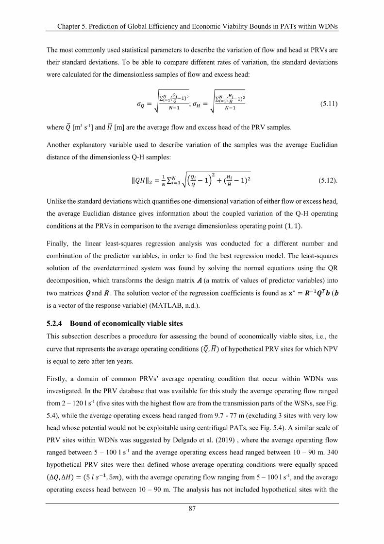
Chapter 5. Prediction of Global Efficiency and Economic Viability Bounds in PATs within WDNs
87
The most commonly used statistical parameters to describe the variation of flow and head at PRVs are
their standard deviations. To be able to compare different rates of variation, the standard deviations
were calculated for the dimensionless samples of flow and excess head:
𝜎𝑄 = √∑ (
𝑄𝑖�̅�
−1)2𝑁𝑖=1
𝑁−1; 𝜎𝐻 = √∑ (
𝐻𝑖�̅�
−1)2𝑁𝑖=1
𝑁−1 (5.11)
where �̅� [m3 s-1] and �̅� [m] are the average flow and excess head of the PRV samples.
Another explanatory variable used to describe variation of the samples was the average Euclidian
distance of the dimensionless Q-H samples:
‖𝑄𝐻‖2 =1
𝑁∑ √(
𝑄𝑖
�̅�− 1)
2+ (
𝐻𝑖
�̅�− 1)2𝑁
𝑖=1 (5.12).
Unlike the standard deviations which quantifies one-dimensional variation of either flow or excess head,
the average Euclidian distance gives information about the coupled variation of the Q-H operating
conditions at the PRVs in comparison to the average dimensionless operating point (1, 1).
Finally, the linear least-squares regression analysis was conducted for a different number and
combination of the predictor variables, in order to find the best regression model. The least-squares
solution of the overdetermined system was found by solving the normal equations using the QR
decomposition, which transforms the design matrix A (a matrix of values of predictor variables) into
two matrices Q and R . The solution vector of the regression coefficients is found as 𝐱∗ = 𝑹−1𝑸𝑇𝒃 (b
is a vector of the response variable) (MATLAB, n.d.).
5.2.4 Bound of economically viable sites
This subsection describes a procedure for assessing the bound of economically viable sites, i.e., the
curve that represents the average operating conditions (�̅�, �̅�) of hypothetical PRV sites for which NPV
is equal to zero after ten years.
Firstly, a domain of common PRVs’ average operating condition that occur within WDNs was
investigated. In the PRV database that was available for this study the average operating flow ranged
from 2 – 120 l s-1 (five sites with the highest flow are from the transmission parts of the WSNs, see Fig.
5.4), while the average operating excess head ranged from 9.7 - 77 m (excluding 3 sites with very low
head whose potential would not be exploitable using centrifugal PATs, see Fig. 5.4). A similar scale of
PRV sites within WDNs was suggested by Delgado et al. (2019) , where the average operating flow
ranged between 5 – 100 l s-1 and the average operating excess head ranged between 10 – 90 m. 340
hypothetical PRV sites were then defined whose average operating conditions were equally spaced
(Δ𝑄, Δ𝐻) = (5 𝑙 𝑠−1, 5𝑚), with the average operating flow ranging from 5 – 100 l s-1, and the average
operating excess head between 10 – 90 m. The analysis has not included hypothetical sites with the
Chapter 5. Prediction of Global Efficiency and Economic Viability Bounds in PATs within WDNs
88
average operating flow higher than 100 l s-1 as it was deemed that sites characterized with such operating
conditions would certainly be economically viable.
There are two main uncertainties that can affect the economic viability of the installations. The first
uncertainty is related to the level of variation in the hydraulic operating conditions at PRV sites. Two
sites with the same average operating point but different levels of flow and excess head variations would
result in different values of NPV. The site with larger variation of the operating conditions is expected
to have lower value of NPV as a consequence of lower energy generation due to larger head dissipation
and flow bypassing, and more operating points being further away from the PAT’s BEP or even outside
of its permissible operating range. To assess the span of the variation magnitudes, the examined valves
were sorted according to the value of ‖𝑄𝐻‖2 parameter and its distribution. The average Euclidian
distance was chosen as it unifies the variations of flow and excess head into a single parameter. Once
the distribution of ‖𝑄𝐻‖2 parameter was detected, its parameters such as mean and 95% confidence
interval bounds were calculated. Finally, dimensionless patterns whose values of ‖𝑄𝐻‖2 parameter
were the closest to the mean, lower and upper confidence bounds were identified. The selected
dimensionless patterns were then applied to each of 340 average operating points to generate the
complete flow and excess head patterns.
The second uncertainty in the assessment of NPV of an installation refers to the assessment of TIC. For
a site of particular average condition the cost of the PAT-generator assembly (𝐶𝑃𝐴𝑇+𝑔𝑒𝑛) should not
vary a lot, however the other installation costs associated with civil works, hydraulic regulation control
system, grid connection, additional hydraulic equipment, commissioning, and engineering design can
vary significantly. Consequently, 𝐶𝑃𝐴𝑇+𝑔𝑒𝑛 can represent smaller or large percentage of TIC. As it can
be seen from Eq. 5.2, TIC was assessed implicitly via 𝐶𝑃𝐴𝑇+𝑔𝑒𝑛 by assuming that 𝐶𝑃𝐴𝑇+𝑔𝑒𝑛 amounts
26% of TIC. This assumption was based on the study conducted by Fernández García et al. (2019),
which investigated 9 real-world PAT installations within WDNs. However, the value of 26% was the
average cost ratio (CR) across 9 considered sites with the minimal value of 14% and the maximal of
48%. The sizes of the considered sites ranged from 9 up to 120 kW of electric power, but still no
correlation between the ratio and the size of the sites was indicated.
Considering that the distribution of CR was unknown for this analysis and with a reasonable assumption
that ‖𝑄𝐻‖2 and CR are uncorrelated, the average value of ‖𝑄𝐻‖2 was paired with the average value of
CR to assess the expected bound of economically viable sites, while the values of ‖𝑄𝐻‖2 that signify
its 95% confidence interval were paired with the extreme values adopted from Fernández García et al.
(2019). Finally, the optimal NPV was assessed using the methodology described in subsection
“Assessment of energy recovery and NPV” for each of three alternatives of ‖𝑄𝐻‖2-CR pair, for each
of 340 hypothetical sites, thus creating three NPV surfaces across the considered PRV domain. The
Chapter 5. Prediction of Global Efficiency and Economic Viability Bounds in PATs within WDNs
89
expected bound of the economically viable sites and its confidence interval were identified as the zero
contours from the previously created NPV surfaces.
Another important factor for the economic viability of an installation is eup. Regardless if it was
considered that the generated electricity was sold to the grid or used at the site, the value of eup used in
the literature ranged from 83.81 €/MWh (Irish Renewable Energy Feed-In-Tariff (REFIT) ceased in
2015) used by Corcoran et al. (2013) up to 260 €/MWh (the UK REFIT for the hydropower sites smaller
than 15kW) used in the same study. The studies carried out by Carravetta et al., (2014), (2013); Coelho
and Andrade-Campos, (2018); Fecarotta and Mc Nabola, (2017); Fernández Garcia and Mc Nabola,
(2020); Fontana et al., (2012); Tricarico et al., (2018) used the values in between. The influence of
different values of eup on the bound of economically viable sites was not examined, however the
conservative value of 90 €/MWh used in this chapter is almost the minimum value used in the literature.
5.3 Results
Long time series recordings of the hydraulic parameters such as the ones used in this chapter often
contain some missing or erroneous data, caused by power outages or wrongly calibrated gauges.
Consequently, the raw samples were filtered to exclude such data. Except time periods for which the
recordings were missing, several valves contained periods with “negative” excess head, i.e., the periods
when the recorded downstream head was larger than the upstream one. For most of the valves such
recordings were very short and the consequence of a sudden closure or opening of the valves. In case
of one valve this identified a long period of the valve being inactive. The daily patterns which contained
any missing data or any abnormal behaviour such as periods of sudden opening and closure, or periods
of inactivity, were excluded from the samples.
5.3.1 Model for Prediction of Global Plant Efficiency using Sample Statistics
Table 5.2 presents the results of the optimisation procedure described in subsection “5.2.2 Assessment
of energy recovery and NPV” for all 38 valves. For each of the valves the algorithm selects the optimal
family from the PAT database and its speed, as well as the optimal maximal permissible flow 𝑄𝑟𝑒𝑙𝑚𝑎𝑥, by
maximizing the NPV objective. The last column of Tab 5.2 presents the results of the global efficiency
of the HPER plants, 𝜂𝑔𝑙𝑜𝑏𝑎𝑙, calculated by dividing the energy recovered by the plants with their gross
hydraulic energy available at the PRV sites, as described in Eq. 5.8. 𝜂𝑔𝑙𝑜𝑏𝑎𝑙 which was used as the
dependent variable in the regression analysis, ranged from 0.07 for valve 9 up to 0.64 for valve 1, with
a mean of 0.4.
The previously mentioned ranges do not consider three valves whose energy recovery and consequently
𝜂𝑔𝑙𝑜𝑏𝑎𝑙 were zero. The excess head of these valves was so low that none of the centrifugal PATs from
the database were suitable for them, see Tab. 5.2 and Fig. 5.4. Besides these three valves, valves 9, 15,
17 and 36 were excluded from the regression analysis in order to avoid potentially erroneous

Chapter 5. Prediction of Global Efficiency and Economic Viability Bounds in PATs within WDNs
90
generalizations as their 𝑃𝑒𝑙𝑒𝑐𝑚𝑎𝑥 were lower than 400 W, and the accuracies of the models for performance
curve extrapolation (Novara and McNabola, 2018) and the TIC (Novara et al., 2019) were not validated
for PATs below this threshold.
Tab. 5.2. Results of the assessment of 𝜂𝑔𝑙𝑜𝑏𝑎𝑙, used as dependant variable in the regression analysis.
Site ID
Family n [rpm] 𝑄𝑟𝑒𝑙
𝑚𝑎𝑥 [-]
𝑃𝑒𝑙𝑒𝑐𝐵𝐸𝑃
[kW] 𝑃𝑒𝑙𝑒𝑐
𝑚𝑎𝑥 [kW]
NPV [€] E [MWh year-1]
𝜂𝑔𝑙𝑜𝑏𝑎𝑙
[-]
1 200-330 1510 1.178 84.28 128.24 461667 837.0 0.635
2 125-250 1510 1.240 23.00 39.45 123988 244.5 0.555
3 150-200 1510 1.308 18.75 38.05 14425 90.2 0.327
4 250-400 1510 1.093 189.57 238.20 952956 1659.8 0.583
5 125-200 1510 1.179 13.52 20.77 54916 126.6 0.555
6 32-160_1 1510 1.162 0.37 0.52 -5121 2.0 0.209
7 50-160 3020 1.137 14.45 19.75 64059 126.1 0.556
8 40-125 1510 1.301 0.48 0.90 -3390 5.2 0.395
9 32-125_1 1510 0.761 0.19 0.10 -5889 0.2 0.068
10 80-200 1510 1.236 6.02 10.03 15443 47.6 0.504
11 150-200 1005 1.400 5.40 12.86 19005 70.1 0.503
12 32-125_1 1510 1.400 0.22 0.47 -4957 1.7 0.162
13 50-160 3020 1.170 14.47 21.15 66659 130.4 0.561
14 100-200 1510 1.207 9.09 14.49 23521 67.8 0.465
15 32-125_1 1510 1.030 0.21 0.22 -5575 0.7 0.151
16 32-160 1510 1.400 0.64 1.38 -1796 7.9 0.347
17 32-125_1 1510 1.097 0.21 0.26 -5346 1.1 0.290
18 40-125 1510 1.235 0.48 0.79 -4167 4.1 0.306
19 80-200 1510 1.171 6.00 8.81 14787 46.2 0.460
20 32-125_1 3020 1.333 1.92 3.70 2119 17.4 0.317
21 40-160 1510 1.367 0.96 1.97 -1124 9.9 0.343
22 32-160_1 1510 1.366 0.38 0.76 -3762 4.0 0.269
23 50-125 3020 1.144 7.57 10.68 23338 60.2 0.473
24 32-160_1 1510 1.298 0.38 0.68 -3559 4.3 0.294
25 32-125_1 1510 0.761 0.19 0.10 -6044 0.0 0.000
26 65-125 3020 1.400 10.94 25.01 112272 198.1 0.524
27 65-160 1510 1.335 2.09 4.18 2795 19.9 0.493
28 100-160 3020 1.117 44.30 59.56 215849 394.1 0.621
29 125-315 1005 1.400 12.61 27.73 90527 187.3 0.520
30 32-160 1510 1.400 0.64 1.38 -689 9.5 0.368
31 32-125_1 1510 0.761 0.19 0.10 -6044 0.0 0.000
32 50-160 1510 1.203 1.70 2.65 -369 13.5 0.404
33 32-125_1 1510 0.761 0.19 0.10 -6044 0.0 0.000
34 125-200 1005 1.211 3.83 6.27 7779 41.4 0.611
35 32-125_1 1510 1.400 0.22 0.47 -4093 3.0 0.246
36 32-125_1 1510 1.030 0.21 0.22 -5406 1.0 0.244
37 32-160_1 1510 1.196 0.37 0.56 -4916 2.3 0.244
38 32-125_1 3020 1.400 1.92 4.14 11678 31.4 0.445
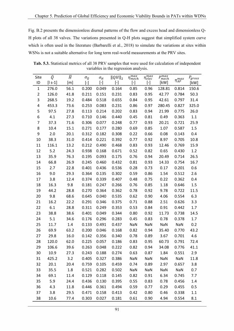
Chapter 5. Prediction of Global Efficiency and Economic Viability Bounds in PATs within WDNs
91
Fig. B.2 presents the dimensionless diurnal patterns of the flow and excess head and dimensionless Q-
H plots of all 38 valves. The variations presented in Q-H plots suggest that simplified system curve
which is often used in the literature (Barbarelli et al., 2018) to simulate the variations at sites within
WSNs is not a suitable alternative for long term real-world measurements at the PRV sites.
Tab. 5.3. Statistical metrics of all 38 PRV samples that were used for calculation of independent
variables in the regression analysis.
Site ID
�̅� [l s-1]
�̅� [m]
𝜎𝑄
[-] 𝜎𝐻 [-]
‖𝑄𝐻‖2 [-]
𝜂𝑚𝑒𝑐ℎ𝑚𝑎𝑥 [-]
𝜂𝑒𝑙𝑒𝑐𝑚𝑎𝑥 [-]
𝑃𝑚𝑒𝑐ℎ𝑚𝑎𝑥
[kW] 𝜂𝐴𝑃
𝑚𝑎𝑥 𝑃𝑔𝑟𝑜𝑠𝑠
[kW]
1 276.0 56.1 0.200 0.049 0.164 0.85 0.96 128.81 0.814 150.6
2 126.0 41.8 0.211 0.151 0.231 0.83 0.95 42.77 0.784 50.3
3 268.5 19.2 0.484 0.518 0.655 0.84 0.95 42.61 0.797 31.4
4 453.3 73.6 0.253 0.083 0.231 0.86 0.97 280.45 0.827 325.0
5 97.5 27.8 0.113 0.214 0.202 0.83 0.94 21.99 0.775 26.0
6 4.1 27.3 0.710 0.146 0.440 0.45 0.81 0.49 0.363 1.1
7 37.3 71.6 0.306 0.077 0.248 0.77 0.93 20.21 0.721 25.9
8 10.4 15.1 0.271 0.177 0.280 0.69 0.85 1.07 0.587 1.5
9 2.0 20.1 0.312 0.182 0.308 0.22 0.66 0.08 0.143 0.4
10 38.3 31.0 0.414 0.221 0.392 0.77 0.92 8.97 0.705 10.8
11 116.1 13.2 0.212 0.490 0.468 0.83 0.93 12.46 0.769 15.9
12 5.2 24.3 0.938 0.168 0.671 0.52 0.82 0.65 0.430 1.2
13 35.9 76.3 0.195 0.093 0.175 0.76 0.94 20.49 0.714 26.5
14 66.8 26.9 0.245 0.460 0.432 0.81 0.93 14.33 0.754 16.7
15 2.7 22.8 0.401 0.436 0.536 0.28 0.73 0.17 0.201 0.6
16 9.0 29.3 0.364 0.135 0.302 0.59 0.86 1.54 0.512 2.6
17 3.8 12.4 0.374 0.339 0.407 0.48 0.75 0.22 0.362 0.4
18 16.3 9.8 0.181 0.247 0.266 0.76 0.85 1.18 0.646 1.5
19 44.2 28.8 0.270 0.364 0.362 0.78 0.92 9.78 0.722 11.5
20 9.8 68.6 0.645 0.040 0.535 0.62 0.90 4.06 0.554 6.3
21 16.2 22.2 0.291 0.346 0.375 0.71 0.88 2.51 0.626 3.3
22 6.1 28.8 0.311 0.249 0.353 0.53 0.84 0.91 0.442 1.7
23 38.8 38.6 0.401 0.049 0.344 0.80 0.92 11.73 0.738 14.5
24 5.1 34.6 0.176 0.296 0.283 0.45 0.83 0.78 0.378 1.7
25 11.7 1.4 0.133 0.491 0.437 NaN NaN NaN NaN 0.2
26 69.9 63.2 0.200 0.046 0.168 0.82 0.94 35.40 0.770 43.2
27 29.8 16.0 0.142 0.356 0.340 0.78 0.89 3.67 0.701 4.6
28 120.0 62.0 0.225 0.057 0.186 0.83 0.95 60.73 0.791 72.4
29 106.6 39.6 0.263 0.048 0.222 0.82 0.94 34.08 0.776 41.1
30 10.9 27.3 0.243 0.188 0.274 0.63 0.87 1.84 0.551 2.9
31 425.2 3.2 0.405 0.327 0.386 NaN NaN NaN NaN 11.8
32 20.1 20.4 0.759 0.105 0.459 0.74 0.89 2.97 0.657 3.8
33 35.5 1.8 0.521 0.282 0.502 NaN NaN NaN NaN 0.7
34 69.1 11.4 0.129 0.118 0.145 0.82 0.91 6.34 0.745 7.7
35 5.9 24.4 0.436 0.130 0.395 0.55 0.83 0.78 0.456 1.4
36 4.3 11.8 0.446 0.361 0.494 0.59 0.77 0.29 0.455 0.5
37 3.8 29.5 0.471 0.158 0.413 0.42 0.80 0.46 0.338 1.1
38 10.6 77.4 0.303 0.027 0.181 0.61 0.90 4.94 0.554 8.1
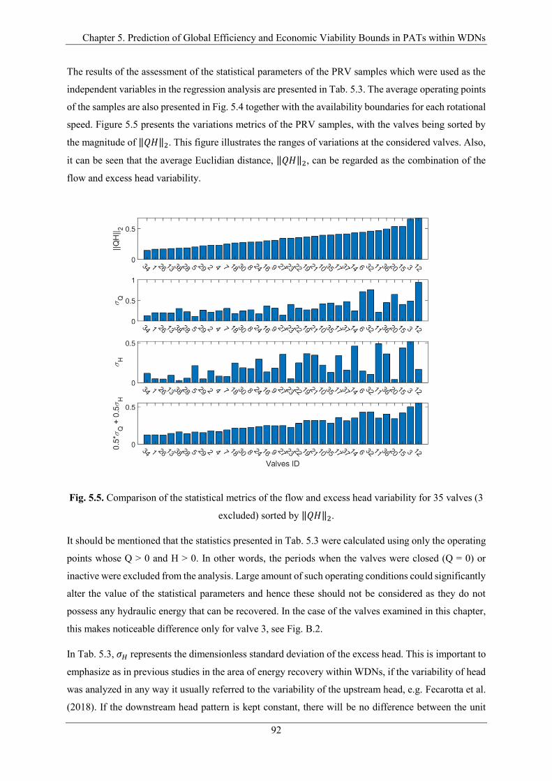
Chapter 5. Prediction of Global Efficiency and Economic Viability Bounds in PATs within WDNs
92
The results of the assessment of the statistical parameters of the PRV samples which were used as the
independent variables in the regression analysis are presented in Tab. 5.3. The average operating points
of the samples are also presented in Fig. 5.4 together with the availability boundaries for each rotational
speed. Figure 5.5 presents the variations metrics of the PRV samples, with the valves being sorted by
the magnitude of ‖𝑄𝐻‖2. This figure illustrates the ranges of variations at the considered valves. Also,
it can be seen that the average Euclidian distance, ‖𝑄𝐻‖2, can be regarded as the combination of the
flow and excess head variability.
Fig. 5.5. Comparison of the statistical metrics of the flow and excess head variability for 35 valves (3
excluded) sorted by ‖𝑄𝐻‖2.
It should be mentioned that the statistics presented in Tab. 5.3 were calculated using only the operating
points whose Q > 0 and H > 0. In other words, the periods when the valves were closed (Q = 0) or
inactive were excluded from the analysis. Large amount of such operating conditions could significantly
alter the value of the statistical parameters and hence these should not be considered as they do not
possess any hydraulic energy that can be recovered. In the case of the valves examined in this chapter,
this makes noticeable difference only for valve 3, see Fig. B.2.
In Tab. 5.3, 𝜎𝐻 represents the dimensionless standard deviation of the excess head. This is important to
emphasize as in previous studies in the area of energy recovery within WDNs, if the variability of head
was analyzed in any way it usually referred to the variability of the upstream head, e.g. Fecarotta et al.
(2018). If the downstream head pattern is kept constant, there will be no difference between the unit
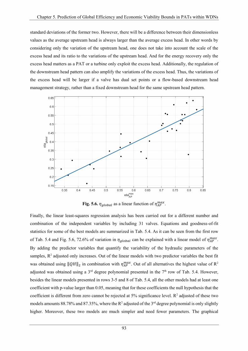
Chapter 5. Prediction of Global Efficiency and Economic Viability Bounds in PATs within WDNs
93
standard deviations of the former two. However, there will be a difference between their dimensionless
values as the average upstream head is always larger than the average excess head. In other words by
considering only the variation of the upstream head, one does not take into account the scale of the
excess head and its ratio to the variations of the upstream head. And for the energy recovery only the
excess head matters as a PAT or a turbine only exploit the excess head. Additionally, the regulation of
the downstream head pattern can also amplify the variations of the excess head. Thus, the variations of
the excess head will be larger if a valve has dual set points or a flow-based downstream head
management strategy, rather than a fixed downstream head for the same upstream head pattern.
Fig. 5.6. 𝜂𝑔𝑙𝑜𝑏𝑎𝑙 as a linear function of 𝜂𝐴𝑃𝑚𝑎𝑥.
Finally, the linear least-squares regression analysis has been carried out for a different number and
combination of the independent variables by including 31 valves. Equations and goodness-of-fit
statistics for some of the best models are summarized in Tab. 5.4. As it can be seen from the first row
of Tab. 5.4 and Fig. 5.6, 72.6% of variation in 𝜂𝑔𝑙𝑜𝑏𝑎𝑙 can be explained with a linear model of 𝜂𝐴𝑃𝑚𝑎𝑥.
By adding the predictor variables that quantify the variability of the hydraulic parameters of the
samples, R2 adjusted only increases. Out of the linear models with two predictor variables the best fit
was obtained using ‖𝑄𝐻‖2 in combination with 𝜂𝐴𝑃𝑚𝑎𝑥. Out of all alternatives the highest value of R2
adjusted was obtained using a 3rd degree polynomial presented in the 7th row of Tab. 5.4. However,
besides the linear models presented in rows 3-5 and 8 of Tab. 5.4, all the other models had at least one
coefficient with p-value larger than 0.05, meaning that for these coefficients the null hypothesis that the
coefficient is different from zero cannot be rejected at 5% significance level. R2 adjusted of these two
models amounts 88.78% and 87.35%, where the R2 adjusted of the 3rd degree polynomial is only slightly
higher. Moreover, these two models are much simpler and need fewer parameters. The graphical
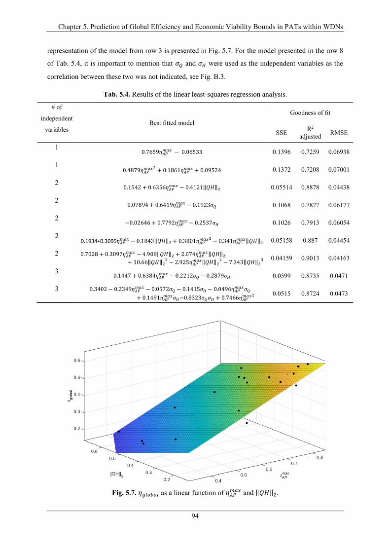
Chapter 5. Prediction of Global Efficiency and Economic Viability Bounds in PATs within WDNs
94
representation of the model from row 3 is presented in Fig. 5.7. For the model presented in the row 8
of Tab. 5.4, it is important to mention that 𝜎𝑄 and 𝜎𝐻 were used as the independent variables as the
correlation between these two was not indicated, see Fig. B.3.
Tab. 5.4. Results of the linear least-squares regression analysis.
# of
independent
variables Best fitted model
Goodness of fit
SSE R2
adjusted RMSE
1 0.7659𝜂𝐴𝑃
𝑚𝑎𝑥 − 0.06533 0.1396 0.7259 0.06938
1 0.4879𝜂𝐴𝑃
𝑚𝑎𝑥2+ 0.1861𝜂𝐴𝑃
𝑚𝑎𝑥 + 0.09524 0.1372 0.7208 0.07001
2 0.1542 + 0.6356𝜂𝐴𝑃
𝑚𝑎𝑥 − 0.4121‖𝑄𝐻‖2 0.05514 0.8878 0.04438
2 0.07894 + 0.6419𝜂𝐴𝑃
𝑚𝑎𝑥 − 0.1923𝜎𝑄 0.1068 0.7827 0.06177
2 −0.02646 + 0.7792𝜂𝐴𝑃
𝑚𝑎𝑥 − 0.2537𝜎𝐻 0.1026 0.7913 0.06054
2 0.1934+0.3095𝜂𝐴𝑃
𝑚𝑎𝑥 − 0.1843‖𝑄𝐻‖2 + 0.3801𝜂𝐴𝑃𝑚𝑎𝑥2
− 0.341𝜂𝐴𝑃𝑚𝑎𝑥‖𝑄𝐻‖2 0.05158 0.887 0.04454
2 0.7028 + 0.3097𝜂𝐴𝑃𝑚𝑎𝑥 − 4.908‖𝑄𝐻‖2 + 2.074𝜂𝐴𝑃
𝑚𝑎𝑥‖𝑄𝐻‖2
+ 10.66‖𝑄𝐻‖22
− 2.925𝜂𝐴𝑃𝑚𝑎𝑥‖𝑄𝐻‖2
2− 7.343‖𝑄𝐻‖2
3
0.04159 0.9013 0.04163
3 0.1447 + 0.6384𝜂𝐴𝑃
𝑚𝑎𝑥 − 0.2212𝜎𝑄 − 0.2879𝜎𝐻 0.0599 0.8735 0.0471
3 0.3402 − 0.2349𝜂𝐴𝑃𝑚𝑎𝑥 − 0.0572𝜎𝑄 − 0.1415𝜎𝐻 − 0.0496𝜂𝐴𝑃
𝑚𝑎𝑥𝜎𝑄
+ 0.1491𝜂𝐴𝑃𝑚𝑎𝑥𝜎𝐻−0.8323𝜎𝑄𝜎𝐻 + 0.7466𝜂𝐴𝑃
𝑚𝑎𝑥2
0.0515 0.8724 0.0473
Fig. 5.7. 𝜂𝑔𝑙𝑜𝑏𝑎𝑙 as a linear function of 𝜂𝐴𝑃𝑚𝑎𝑥 and ‖𝑄𝐻‖2.
Chapter 5. Prediction of Global Efficiency and Economic Viability Bounds in PATs within WDNs
95
5.3.2 Bound of economically viable sites
Figure 5.8 presents the normal probability plots of ‖𝑄𝐻‖2. The normal probability plot is a graphical
method to test if the examined sample comes from a normally distributed population. Figure 5.8a
includes the complete set of the examined valves (excluding three valves with very low excess head).
As it can be seen from the figure the discrete values of ‖𝑄𝐻‖2 follow the theoretical straight line quite
well except at the ends of the range. It can also be noticed that extreme values of ‖𝑄𝐻‖2 parameter at
both ends belong to the valves with very specific flow patterns that do not follow the characteristic
household pattern (red crosses in Fig. 5.8a). The dimensionless flow patterns of all examined valves
can be observed in Fig. B.2. The valves with non-household flow patterns with potential for energy
recovery are usually located upstream of large water consumers with very particular flow determined
by the consumers’ needs. Therefore, drawing generalizations based on their variations could lead to
incorrect conclusions. Consequently, the non-household patterns were excluded from the sample and
the distribution of the household patterns was examined separately. The normal probability plot of 28
household patterns is presented in Fig. 5.8b. As can be seen from Fig. 5.8b the discrete points follow
the straight line and the extreme values deviate less. It should also be mentioned that the normality of
the samples’ distribution has been tested using Kolmogorov-Smirnof and Chi-square goodness-of-fit
tests, and in both cases the results showed that the null hypothesis that the samples come from normally
distributed population cannot be rejected at 5% significance level.
The mean, lower and upper 95% confidence interval bounds of the household set were subsequently
evaluated amounting to 0.3388, 0.1311 and 0.5464, respectively. In the absence of a synthetic pattern
generator that could produce patterns with exact values of ‖𝑄𝐻‖2, the dimensionless patterns of the
valves whose value of ‖𝑄𝐻‖2 were closest to the aforementioned values were selected. The selected
dimensionless patterns are presented in Fig. 5.9.
As mentioned in the methodology section, the cost uncertainty of the HPER projects within WDNs was
simulated using the CR value. As the distribution of this ratio was not indicated in the referenced study
by Fernández García et al. (2019), in the analysis conducted in this chapter the minimal, average and
maximal values of CR were used to evaluate the span of its possible values. The variation levels of the
installation costs were coupled with the dimensionless patterns selected based on their value of ‖𝑄𝐻‖2,
creating three different scenarios. Figure 5.10 presents the zero contours extracted from the NPV
surfaces generated by calculating the optimal NPV for the whole domain of the average operating points
for each of the three scenarios. Additionally, three curves that represent 2, 4 and 12 kW of gross
hydraulic power were plotted together with the zero contours as a benchmark of the results.

Chapter 5. Prediction of Global Efficiency and Economic Viability Bounds in PATs within WDNs
96
a)
b)
Fig. 5.8. Normal probability plot of ‖𝑄𝐻‖2 a) all 35 PRV patterns; b) 28 household patterns

Chapter 5. Prediction of Global Efficiency and Economic Viability Bounds in PATs within WDNs
97
Fig. 5.9. Three characteristic dimensionless samples a) lower confidence bound of ‖𝑄𝐻‖2; b) average
‖𝑄𝐻‖2; and 3) upper confidence bound of ‖𝑄𝐻‖2.
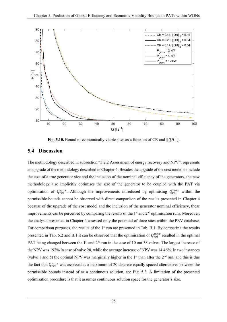
Chapter 5. Prediction of Global Efficiency and Economic Viability Bounds in PATs within WDNs
98
Fig. 5.10. Bound of economically viable sites as a function of CR and ‖𝑄𝐻‖2.
5.4 Discussion
The methodology described in subsection “5.2.2 Assessment of energy recovery and NPV”, represents
an upgrade of the methodology described in Chapter 4. Besides the upgrade of the cost model to include
the cost of a true generator size and the inclusion of the nominal efficiency of the generators, the new
methodology also implicitly optimises the size of the generator to be coupled with the PAT via
optimisation of 𝑄𝑟𝑒𝑙𝑚𝑎𝑥. Although the improvements introduced by optimising 𝑄𝑟𝑒𝑙
𝑚𝑎𝑥 within the
permissible bounds cannot be observed with direct comparison of the results presented in Chapter 4
because of the upgrade of the cost model and the inclusion of the generator nominal efficiency, these
improvements can be perceived by comparing the results of the 1st and 2nd optimisation runs. Moreover,
the analysis presented in Chapter 4 assessed only the potential of three sites within the PRV database.
For comparison purposes, the results of the 1st run are presented in Tab. B.1. By comparing the results
presented in Tab. 5.2 and B.1 it can be observed that the optimisation of 𝑄𝑟𝑒𝑙𝑚𝑎𝑥 resulted in the optimal
PAT being changed between the 1st and 2nd run in the case of 10 out 38 valves. The largest increase of
the NPV was 192% in case of valve 20, while the average increase of NPV was 14.46%. In two instances
(valve 1 and 5) the optimal NPV was marginally higher in the 1st than after the 2nd run, and this is due
the fact that 𝑄𝑟𝑒𝑙𝑚𝑎𝑥 was assessed as a maximum of 20 discrete equally spaced alternatives between the
permissible bounds instead of as a continuous solution, see Fig. 5.3. A limitation of the presented
optimisation procedure is that it assumes continuous solution space for the generator’s size.
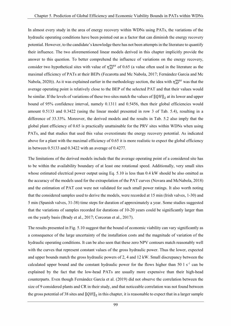
Chapter 5. Prediction of Global Efficiency and Economic Viability Bounds in PATs within WDNs
99
In almost every study in the area of energy recovery within WDNs using PATs, the variations of the
hydraulic operating conditions have been pointed out as a factor that can diminish the energy recovery
potential. However, to the candidate’s knowledge there has not been attempts in the literature to quantify
their influence. The two aforementioned linear models derived in this chapter implicitly provide the
answer to this question. To better comprehend the influence of variations on the energy recovery,
consider two hypothetical sites with value of 𝜂𝐴𝑃𝑚𝑎𝑥 of 0.65 (a value often used in the literature as the
maximal efficiency of PATs at their BEPs (Fecarotta and Mc Nabola, 2017; Fernández Garcia and Mc
Nabola, 2020)). As it was explained earlier in the methodology section, the idea with 𝜂𝐴𝑃𝑚𝑎𝑥 was that the
average operating point is relatively close to the BEP of the selected PAT and that their values would
be similar. If the levels of variations of these two sites match the values of ‖𝑄𝐻‖2 at its lower and upper
bound of 95% confidence interval, namely 0.1311 and 0.5456, then their global efficiencies would
amount 0.5133 and 0.3422 (using the linear model presented in row 3 of Tab. 5.4), resulting in a
difference of 33.33%. Moreover, the derived models and the results in Tab. 5.2 also imply that the
global plant efficiency of 0.65 is practically unattainable for the PRV sites within WDNs when using
PATs, and that studies that used this value overestimate the energy recovery potential. As indicated
above for a plant with the maximal efficiency of 0.65 it is more realistic to expect the global efficiency
in between 0.5133 and 0.3422 with an average of 0.4277.
The limitations of the derived models include that the average operating point of a considered site has
to be within the availability boundary of at least one rotational speed. Additionally, very small sites
whose estimated electrical power output using Eq. 5.10 is less than 0.4 kW should be also omitted as
the accuracy of the models used for the extrapolation of the PAT curves (Novara and McNabola, 2018)
and the estimation of PAT cost were not validated for such small power ratings. It also worth noting
that the considered samples used to derive the models, were recorded at 15 min (Irish valves, 1-30) and
5 min (Spanish valves, 31-38) time steps for duration of approximately a year. Some studies suggested
that the variations of samples recorded for durations of 10-20 years could be significantly larger than
on the yearly basis (Brady et al., 2017; Corcoran et al., 2017).
The results presented in Fig. 5.10 suggest that the bound of economic viability can vary significantly as
a consequence of the large uncertainty of the installation costs and the magnitude of variation of the
hydraulic operating conditions. It can be also seen that these zero NPV contours match reasonably well
with the curves that represent constant values of the gross hydraulic power. Thus the lower, expected
and upper bounds match the gross hydraulic powers of 2, 4 and 12 kW. Small discrepancy between the
calculated upper bound and the constant hydraulic power for the flows higher than 50 l s-1 can be
explained by the fact that the low-head PATs are usually more expensive than their high-head
counterparts. Even though Fernández García et al. (2019) did not observe the correlation between the
size of 9 considered plants and CR in their study, and that noticeable correlation was not found between
the gross potential of 38 sites and ‖𝑄𝐻‖2 in this chapter, it is reasonable to expect that in a larger sample
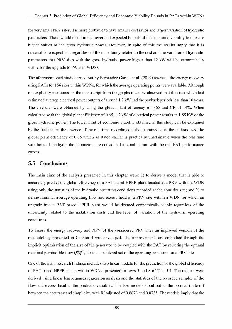
Chapter 5. Prediction of Global Efficiency and Economic Viability Bounds in PATs within WDNs
100
for very small PRV sites, it is more probable to have smaller cost ratios and larger variation of hydraulic
parameters. These would result in the lower and expected bounds of the economic viability to move to
higher values of the gross hydraulic power. However, in spite of this the results imply that it is
reasonable to expect that regardless of the uncertainty related to the cost and the variation of hydraulic
parameters that PRV sites with the gross hydraulic power higher than 12 kW will be economically
viable for the upgrade to PATs in WDNs.
The aforementioned study carried out by Fernández García et al. (2019) assessed the energy recovery
using PATs for 156 sites within WDNs, for which the average operating points were available. Although
not explicitly mentioned in the manuscript from the graphs it can be observed that the sites which had
estimated average electrical power outputs of around 1.2 kW had the payback periods less than 10 years.
These results were obtained by using the global plant efficiency of 0.65 and CR of 14%. When
calculated with the global plant efficiency of 0.65, 1.2 kW of electrical power results in 1.85 kW of the
gross hydraulic power. The lower limit of economic viability obtained in this study can be explained
by the fact that in the absence of the real time recordings at the examined sites the authors used the
global plant efficiency of 0.65 which as stated earlier is practically unattainable when the real time
variations of the hydraulic parameters are considered in combination with the real PAT performance
curves.
5.5 Conclusions
The main aims of the analysis presented in this chapter were: 1) to derive a model that is able to
accurately predict the global efficiency of a PAT based HPER plant located at a PRV within a WDN
using only the statistics of the hydraulic operating conditions recorded at the consider site; and 2) to
define minimal average operating flow and excess head at a PRV site within a WDN for which an
upgrade into a PAT based HPER plant would be deemed economically viable regardless of the
uncertainty related to the installation costs and the level of variation of the hydraulic operating
conditions.
To assess the energy recovery and NPV of the considered PRV sites an improved version of the
methodology presented in Chapter 4 was developed. The improvements are embodied through the
implicit optimisation of the size of the generator to be coupled with the PAT by selecting the optimal
maximal permissible flow 𝑄𝑟𝑒𝑙𝑚𝑎𝑥, for the considered set of the operating conditions at a PRV site.
One of the main research findings includes two linear models for the prediction of the global efficiency
of PAT based HPER plants within WDNs, presented in rows 3 and 8 of Tab. 5.4. The models were
derived using linear least-squares regression analysis and the statistics of the recorded samples of the
flow and excess head as the predictor variables. The two models stood out as the optimal trade-off
between the accuracy and simplicity, with R2 adjusted of 0.8878 and 0.8735. The models imply that the

Chapter 5. Prediction of Global Efficiency and Economic Viability Bounds in PATs within WDNs
101
large variations could reduce the global plant efficiency up to 33,33%. Additionally, the derived models
suggest that the global efficiency of 0.65 used for the preliminary analysis of the potential in some of
the previous studies is not realistically attainable and that the value of 0.4277 should be used instead.
Another important finding are the zero contours of the NPV function presented in Fig. 5.10, calculated
for the different ratios of the plants’ installation costs and different levels of variations of the hydraulic
operating conditions expressed via CR and ‖𝑄𝐻‖2. The contours indicate the minimal average
operating conditions (�̅�, �̅�) at PRV sites so their upgrade into PAT based HPER plants is considered
economically viable. The results presented in Fig. 5.10 suggest that there is a high probability that PRV
sites with the gross hydraulic power higher than 12 kW will be economically viable for upgrade. The
results pertain only to the sites with the characteristic household flow patterns.
There are many practical applications where the derived models for prediction of the global efficiency
and the bound of economic viability could be used. For instance, the prediction models could be used
instead the constant values for the global efficiency to improve the accuracy of the assessment of energy
recovery in the methodologies for selection of the optimal number and location of PATs within WDNs
(Corcoran et al., 2016; Fecarotta and Mc Nabola, 2017). Additionally, the bound of economic viability
could be used to further reduce the computational time of these models by disregarding the locations
whose average operating conditions are below the defined threshold.
Future work will be focused on using the presented research findings for a preliminary assessment of
the energy recovery potential on country levels by evaluating the potential of a large number of sites
where only the average operating conditions are available.

Chapter 6. Generalization of the Optimal Relative BEP
102
6 Generalization of the Optimal
Relative BEP
6.1 Introduction
The final output of the methodologies for selection of an optimal PAT for installation at any given site
within WDNs is to find a BEP of a theoretical machine which will maximize the chosen objective
(Carravetta et al., 2012; Fecarotta et al., 2018; Lydon et al., 2017). Although for the methodologies that
are based on the similarity laws the theoretically optimal BEP can be expressed implicitly via the
impeller diameter and speed of a theoretical machine similar to the prototype (Lydon et al., 2017). The
PAT selection charts analogous to the ones available for the pump mode are not available up to this
date. Consequently, the theoretically optimal BEP in turbine mode has to be converted using one of the
methodologies that relate turbine and pump domain (Yang et al., 2012), and thus the near optimal pump
family can be found from the pump charts (KSB, 2018b).
When the operating condition at a considered site is constant or experiences small variations, e.g. in
transmission part of a network, the problem of finding the theoretically optimal BEP is trivial, i.e., the
BEP should match the constant operating condition to gain the most efficient conversion of the
hydraulic energy (J. Chapallaz et al., 1992). On the other hand, when large variation of operating
conditions is occurring at consider sites, e.g. at PRVs within WDNs, the problem of finding the
theoretically optimal BEP becomes significantly more complex. The main reason for this is that for
maximization of energy recovery a variable operation of the PAT is necessary, meaning that the PAT
unit is expected to turbine a wide range of flows and that complete PAT performance curves have to be
included in the analysis as described in Chapter 4. Furthermore, for the PRV sites additional complexity
pertains to the requirement for the maintenance of downstream head. Regardless of the occurrence of
large variation of the hydraulic parameters it is still reasonable to expect that the theoretically optimal
BEP of the machine will be in relative proximity or at least be related to the average operating condition
of the considered valve. Nevertheless, the ratio of these two points is rarely identified in the studies on
this topic.
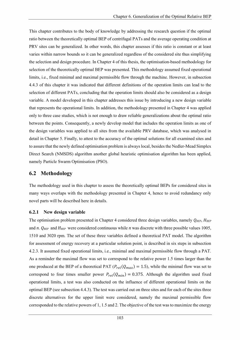
Chapter 6. Generalization of the Optimal Relative BEP
103
This chapter contributes to the body of knowledge by addressing the research question if the optimal
ratio between the theoretically optimal BEP of centrifugal PATs and the average operating condition at
PRV sites can be generalized. In other words, this chapter assesses if this ratio is constant or at least
varies within narrow bounds so it can be generalized regardless of the considered site thus simplifying
the selection and design procedure. In Chapter 4 of this thesis, the optimisation-based methodology for
selection of the theoretically optimal BEP was presented. This methodology assumed fixed operational
limits, i.e., fixed minimal and maximal permissible flow through the machine. However, in subsection
4.4.3 of this chapter it was indicated that different definitions of the operation limits can lead to the
selection of different PATs, concluding that the operation limits should also be considered as a design
variable. A model developed in this chapter addresses this issue by introducing a new design variable
that represents the operational limits. In addition, the methodology presented in Chapter 4 was applied
only to three case studies, which is not enough to draw reliable generalizations about the optimal ratio
between the points. Consequently, a newly develop model that includes the operation limits as one of
the design variables was applied to all sites from the available PRV database, which was analysed in
detail in Chapter 5. Finally, to attest to the accuracy of the optimal solutions for all examined sites and
to assure that the newly defined optimisation problem is always local, besides the Nedler-Mead Simplex
Direct Search (NMSDS) algorithm another global heuristic optimisation algorithm has been applied,
namely Particle Swarm Optimisation (PSO).
6.2 Methodology
The methodology used in this chapter to assess the theoretically optimal BEPs for considered sites in
many ways overlaps with the methodology presented in Chapter 4, hence to avoid redundancy only
novel parts will be described here in details.
6.2.1 New design variable
The optimisation problem presented in Chapter 4 considered three design variables, namely QBEP, HBEP
and n. QBEP and HBEP were considered continuous while n was discrete with three possible values 1005,
1510 and 3020 rpm. The set of these three variables defined a theoretical PAT model. The algorithm
for assessment of energy recovery at a particular solution point, is described in six steps in subsection
4.2.3. It assumed fixed operational limits, i.e., minimal and maximal permissible flow through a PAT.
As a reminder the maximal flow was set to correspond to the relative power 1.5 times larger than the
one produced at the BEP of a theoretical PAT (𝑃𝑟𝑒𝑙(𝑄𝑚𝑎𝑥) = 1.5), while the minimal flow was set to
correspond to four times smaller power 𝑃𝑟𝑒𝑙(𝑄𝑚𝑖𝑛) = 0.375. Although the algorithm used fixed
operational limits, a test was also conducted on the influence of different operational limits on the
optimal BEP (see subsection 4.4.3). The test was carried out on three sites and for each of the sites three
discrete alternatives for the upper limit were considered, namely the maximal permissible flow
corresponded to the relative powers of 1, 1.5 and 2. The objective of the test was to maximize the energy

Chapter 6. Generalization of the Optimal Relative BEP
104
recovery objective. The results presented in Tab. 4.2 showed that in the cases of two out of three
examined sites the maximal value of objective was attained when the upper operational limit
corresponded to the relative power of 1.5, while the third site attained the maximum for 𝑃𝑟𝑒𝑙 = 1. Thus
suggesting that the optimal upper limit cannot be predefined. As it can be seen from Tab. 4.2, the
optimal values of the energy recovery objective vary only slightly across three alternatives. However
differently defined upper operational limits had a larger effect on the theoretically optimal BEP flow
and head which varied up to 18% and 24% respectively, in respect of the average operating conditions
at the considered PRVs.
To address this limitation, the model developed in this chapter introduces the fourth design variable,
representing the upper operational limit. The upper operational limit can be defined using either relative
power or flow, or their absolute values. Unlike in the model defined in Chapter 4, which used the relative
power to define the upper limit, in this chapter the relative permissible flow is chosen:
𝑄𝑟𝑒𝑙𝑚𝑎𝑥 =
𝑄𝑚𝑎𝑥
𝑄𝐵𝐸𝑃 (6.1).
The relative flow is chosen because of the convenience related to the constraints imposed for this
variable, which will be explained in the following subsection.
The idea of optimising the upper operational limit, i.e., 𝑄𝑟𝑒𝑙𝑚𝑎𝑥, to optimally fit the operating points of a
considered site was already introduced in Chapter 5 as a part of the second run of the procedure for
selection of the optimal alternative from the PAT database, described in subsection 5.2. As mentioned
there in practical terms the optimisation of 𝑄𝑟𝑒𝑙𝑚𝑎𝑥 could be regarded as an optimisation of the size of the
generator to be coupled with the PAT. In mathematical terms, the difference between the problem being
solved in Chapter 5 and that in this chapter is that in the former the operation limits were optimised
only for a subset of discrete solutions of the PATs that belong to the database, while in the latter the
solution space for PATs is considered continuous. When the solution space is continuous, there is an
infinite number of possible solutions. Hence, the optimal solution cannot be found as a simple maximum
out of the considered set of PAT alternatives but an optimisation algorithm has to be used to guide the
model towards the optimal solution.
6.2.2 Constraints
As in the model described in Chapter 4, the rotational speed n of the theoretical PAT can have one of
the three possible values. The solution space for the BEP of the theoretical PAT is constrained with the
same boundaries of available PATs on the market as in Chapter 4, defined for each rotational speed as
a convex hull that encloses the set of BEPs of the PATs from the database (see Fig. 4.1).
As previously discussed in Chapters 4 and 5 according to the literature the upper operational limit of a
PAT should be constrained either based on the maximal permissible torque in respect to the shaft

Chapter 6. Generalization of the Optimal Relative BEP
105
resistance (J. Chapallaz et al., 1992) or based on the risk of cavitation (Fontana et al., 2016). Considering
the back pressure required to be maintained downstream of the sites within WDNs it is reasonable to
assume that the cavitation will rarely be an issue in these settings.
Figure 6.1 presents the BEPs of all PATs from the database for the speeds n=1510 rpm and n=3020
rpm, together with the availability boundaries for these speeds.
b)
Fig. 6.1. Shaft diameters of the PATs from the available database and maximal permissible torque
𝑇𝑑𝑚𝑎𝑥: a) n=3020; b) n=1510.
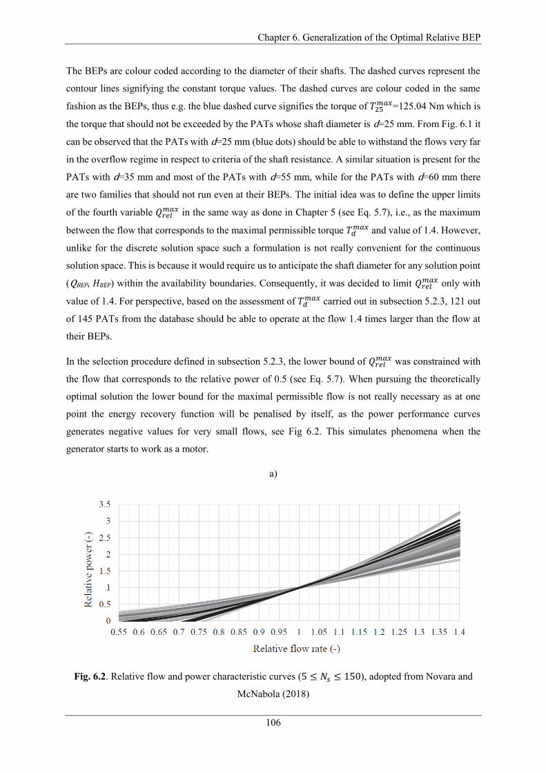
Chapter 6. Generalization of the Optimal Relative BEP
106
The BEPs are colour coded according to the diameter of their shafts. The dashed curves represent the
contour lines signifying the constant torque values. The dashed curves are colour coded in the same
fashion as the BEPs, thus e.g. the blue dashed curve signifies the torque of 𝑇25𝑚𝑎𝑥=125.04 Nm which is
the torque that should not be exceeded by the PATs whose shaft diameter is d=25 mm. From Fig. 6.1 it
can be observed that the PATs with d=25 mm (blue dots) should be able to withstand the flows very far
in the overflow regime in respect to criteria of the shaft resistance. A similar situation is present for the
PATs with d=35 mm and most of the PATs with d=55 mm, while for the PATs with d=60 mm there
are two families that should not run even at their BEPs. The initial idea was to define the upper limits
of the fourth variable 𝑄𝑟𝑒𝑙𝑚𝑎𝑥 in the same way as done in Chapter 5 (see Eq. 5.7), i.e., as the maximum
between the flow that corresponds to the maximal permissible torque 𝑇𝑑𝑚𝑎𝑥 and value of 1.4. However,
unlike for the discrete solution space such a formulation is not really convenient for the continuous
solution space. This is because it would require us to anticipate the shaft diameter for any solution point
(QBEP, HBEP) within the availability boundaries. Consequently, it was decided to limit 𝑄𝑟𝑒𝑙𝑚𝑎𝑥 only with
value of 1.4. For perspective, based on the assessment of 𝑇𝑑𝑚𝑎𝑥 carried out in subsection 5.2.3, 121 out
of 145 PATs from the database should be able to operate at the flow 1.4 times larger than the flow at
their BEPs.
In the selection procedure defined in subsection 5.2.3, the lower bound of 𝑄𝑟𝑒𝑙𝑚𝑎𝑥 was constrained with
the flow that corresponds to the relative power of 0.5 (see Eq. 5.7). When pursuing the theoretically
optimal solution the lower bound for the maximal permissible flow is not really necessary as at one
point the energy recovery function will be penalised by itself, as the power performance curves
generates negative values for very small flows, see Fig 6.2. This simulates phenomena when the
generator starts to work as a motor.
a)
Fig. 6.2. Relative flow and power characteristic curves (5 ≤ 𝑁𝑠 ≤ 150), adopted from Novara and
McNabola (2018)

Chapter 6. Generalization of the Optimal Relative BEP
107
6.2.3 NPV objective function
In Chapter 4 three separate single objectives have been used, namely maximization of energy recovery,
maximization of NPV and minimization of payback period. The results of three examined sites
presented in Tab. 4.1 showed that different objectives can lead to different optimal BEPs. Thus
maximization of energy recovery objective led to the largest theoretically optimal PAT, the
minimization of payback period led to theoretically smallest machine, and the BEP of the theoretically
optimal PAT according NPV was in between but much closer to the optimal based on maximization of
energy recovery.
In the candidate’s opinion, the NPV objective is the most suitable objective for the investigated problem
as it includes the monetary term while maintaining very high level of energy recovery. Hence, in this
chapter the generalization of the theoretically optimal BEP was investigated only for this objective.
The same updated variant of the NPV function described in subsection 5.2.2, that includes the updated
cost model by considering a generator of a true size and its nominal efficiency was used in this chapter.
As the result of the inclusion of the new variable and the generator’s nominal efficiency, the part of the
NPV objective function that assesses the energy recovery has slightly changed in comparison to the six
steps defined in subsection 4.2.3.
Firstly, the penalty function defined in step 1 that penalizes the BEP solutions that are outside of the
availability boundaries for the selected speed is expanded. An additional term is incorporated to
penalize the solutions with 𝑄𝑟𝑒𝑙𝑚𝑎𝑥 > 1.4.
Secondly, because of the inclusion of the nominal efficiency of the generator step 3 had to be broken
into three parts:
3.1. First part defines just the coefficients of the second degree polynomials used for extrapolation of
the full head loss and power curves from the BEP. In other words it defines only the dimensionless
extrapolation models (Novara and McNabola, 2018):
head loss: 𝑎 = 1.160; 𝑏 = 0.0099𝑁𝑆 + 1.2573 − 2𝑎; 𝑐 = 1 − 𝑎 − 𝑏 (6.2)
power: 𝑑 = 1.248; 𝑒 = 0.0108𝑁𝑆 + 2.2243 − 2𝑑; 𝑓 = 1 − 𝑑 − 𝑒 (6.3).
3.2. After defining the coefficients of the extrapolation models, the relative permissible power (𝑃𝑟𝑒𝑙𝑚𝑎𝑥)
can be evaluated using the value of new design variable 𝑄𝑟𝑒𝑙𝑚𝑎𝑥. The relative permissible power is
necessary to define the nominal size of the generator and its nominal efficiency:
𝑃𝑟𝑒𝑙𝑚𝑎𝑥 = 𝑑(𝑄𝑟𝑒𝑙
𝑚𝑎𝑥)2 + 𝑒𝑄𝑟𝑒𝑙𝑚𝑎𝑥 + 𝑓 (6.4)
𝜂𝑚𝑒𝑐ℎ𝑚𝑎𝑥 = 0.89 −
0.024
𝑄𝐵𝐸𝑃0.41 − 0.076 (0.22 + 𝑙𝑛
𝑁𝑠
52.933)
2 (6.5)

Chapter 6. Generalization of the Optimal Relative BEP
108
𝑃𝑚𝑒𝑐ℎ𝐵𝐸𝑃 = 𝜌𝑔𝑄𝐵𝐸𝑃𝐻𝐵𝐸𝑃𝜂𝑚𝑒𝑐ℎ
𝑚𝑎𝑥 (6.6)
𝑃𝑔𝑒𝑛 = 𝑃𝑚𝑒𝑐ℎ𝐵𝐸𝑃 𝑃𝑟𝑒𝑙
𝑚𝑎𝑥 100
80 (6.7)
𝜂𝑒𝑙𝑒𝑐𝑚𝑎𝑥 = −15.3864 ∙ 𝑃𝑔𝑒𝑛
−0.3312 + 98.7780 (6.8)
𝑃𝑒𝑙𝑒𝑐𝐵𝐸𝑃 = 𝑃𝑚𝑒𝑐ℎ
𝐵𝐸𝑃 𝜂𝑒𝑙𝑒𝑐𝑚𝑎𝑥 (6.9)
where 𝑃𝑟𝑒𝑙𝑚𝑎𝑥 [-] is the relative permissible power; 𝜂𝑚𝑒𝑐ℎ
𝐵𝐸𝑃 [-] is the maximal mechanical efficiency
(predicted using Eq. 6.5 proposed by Novara et al. (2017), previous discussed in Chapter 4); 𝑃𝑚𝑒𝑐ℎ𝐵𝐸𝑃
[kW] is the mechanical power of the shaft at BEP; 𝑃𝑔𝑒𝑛 [kW] is the nominal power of the theoretical
generator which is suggested to be 20% larger than the maximal permissible power of the plant
(Williams, 1996); 𝜂𝑒𝑙𝑒𝑐𝑚𝑎𝑥 [-] is the nominal efficiency of the generator (predicted using Eq. 6.8
which is previously introduced in Chapter 5, see Eq. 5.6); and 𝑃𝑒𝑙𝑒𝑐𝐵𝐸𝑃 [kW] is the electrical power
produced by the plant when PAT operates at its BEP.
3.3.Finally, unit extrapolation models can be defined:
𝐻𝑖𝑃𝐴𝑇 = 𝐻𝐵𝐸𝑃 (𝑎 (
𝑄𝑖𝑃𝐴𝑇
𝑄𝐵𝐸𝑃)
2
+ 𝑏 (𝑄𝑖
𝑃𝐴𝑇
𝑄𝐵𝐸𝑃) + 𝑐) (6.10)
𝑃𝑖𝑃𝐴𝑇 = 𝑃𝑒𝑙𝑒𝑐
𝐵𝐸𝑃 (𝑑 (𝑄𝑖
𝑃𝐴𝑇
𝑄𝐵𝐸𝑃)
2
+ 𝑒 (𝑄𝑖
𝑃𝐴𝑇
𝑄𝐵𝐸𝑃) + 𝑓) (6.11)
where 𝑄𝑖𝑃𝐴𝑇 [m3s-1], 𝐻𝑖
𝑃𝐴𝑇 [m] and 𝑃𝑖𝑃𝐴𝑇 are the flow, head drop and generated electrical power of
the plant in i-th time step.
In step 4 the operational limits of the PAT, i.e., the minimal and maximal permissible flow are not fixed
to relate 𝑃𝑟𝑒𝑙 of 1.5 and 0.375 but are being optimised to optimally fit the considered site.
Conceptually, the NPV objective defined in this chapter is similar to the second run of the procedure
defined in subsection 5.2.2. However as the function defined in this section needs to be passed to the
optimisation solvers the implementation differs.
6.2.4 Optimisation problem and algorithms
The modified optimisation problem described above can be formulized as follows:
𝑚𝑎𝑥𝑖𝑚𝑖𝑧𝑒:𝑄𝐵𝐸𝑃,𝐻𝐵𝐸𝑃,𝑄𝑟𝑒𝑙
𝑚𝑎𝑥𝑁𝑃𝑉10(𝑛) = −𝑇𝐼𝐶 + ∑
𝐸∙𝑒𝑢𝑝−𝑂𝑀𝐶
(1+𝑟)𝑗𝑌𝑗
𝑠. 𝑡. 𝑛 ∈ {1005, 1510,3020 }
(𝑄𝐵𝐸𝑃 , 𝐻𝐵𝐸𝑃) ∈ 𝐵𝑜𝑢𝑛𝑑𝑎𝑟𝑦(𝑛)
𝑄𝑟𝑒𝑙𝑚𝑎𝑥 ≤ 1.4
(6.12).
Chapter 6. Generalization of the Optimal Relative BEP
109
In Chapter 4, it was assumed that the optimisation problem defined with Eq. 4.17 is always local and
hence the NMSDS algorithm that is local optimiser has been used. For three examined sites, the locality
was proven by plotting the contour plots of the objective functions, as presented in Fig. 4.10. However,
it was not proven that the problem is local for a general case. Even that the modified optimisation
problem defined with Eq. 6.12 considers three design variables (for constant rotational speed n),
theoretically it would be still feasible to generate contour plots similar to the ones presented in Fig. 4.10
and to prove the locality of the modified problem. This could be done by discretizing (𝑄𝐵𝐸𝑃 , 𝐻𝐵𝐸𝑃)
solution space and then maximizing 𝑄𝑟𝑒𝑙𝑚𝑎𝑥 for each (𝑄𝐵𝐸𝑃 , 𝐻𝐵𝐸𝑃) alternative. However, this would
require immense amount of computational time, especially for 35 sites. Instead, it was decided that it is
more efficient to verify the local nature of the modified optimisation problem and the accuracy of the
optimal solutions by applying another global optimisation algorithm. Because of discontinuous nature
of the energy recovery function only derivative free algorithms were considered. Finally, the particle
swarm optimisation algorithm (PSO) was chosen. This algorithm was chosen instead some other global
heuristic algorithms (e.g. genetic algorithms), because it more suitable for optimisation problems with
continuous variables.
As the NMSDS algorithm was described in detail in Chapter 4 only the PSO algorithm is elaborated in
this Chapter. The PSO is a nature inspired algorithm whose search pattern is designed to mimic a swarm
of birds and their collective search pattern in pursuit for food (Kennedy and Eberhart, 1995). It is a
population-based algorithm, meaning that the algorithm maintains a group of candidate solutions, where
each solution represents a unique point in the search space. In this sense, it is similar to genetic
algorithms.
As the PSO is a global optimisation algorithm, the objective function defined with Eq. 6.12 was solved
as maximum of the three speed alternatives instead as separate optimisation runs for each rotational
speed, like in the case of the NMSDS algorithm. The PSO algorithm allows to define the bounds for
each of the design variables, thus the upper and lower bounds for 𝑄𝐵𝐸𝑃 and 𝐻𝐵𝐸𝑃 were defined with the
minimal operating values larger than zero and maximal operating values recorded at a considered PRV
sites. For 𝑄𝑟𝑒𝑙𝑚𝑎𝑥 only the upper bound of 1.4 was defined. Hence, unlike in the case of the NMSDS the
additional term that penalizes the solutions with 𝑄𝑟𝑒𝑙𝑚𝑎𝑥>1.4 is not necessary.
The search starts by initializing a population (swarm) of particles (solution points), which are randomly
distributed between the bounds. It also initializes velocity vectors used for the update of the location of
the particles. The most important step in each iteration is the update of the velocity vectors that guide
the particles towards the optimal solution:
𝐯𝒊 = 𝑊𝐯𝑖−1 + 𝑦1𝐮1(𝐩𝑖−1 − 𝐱𝑖−1) + 𝑦2𝐮2(𝐠𝑖−1 − 𝐱𝑖−1) (6.13),
𝐱𝒊 = 𝐱𝑖−1 + 𝐯𝑖 (6.14),
Chapter 6. Generalization of the Optimal Relative BEP
110
where 𝐱 = [𝑄𝐵𝐸𝑃; 𝐻𝐵𝐸𝑃; 𝑄𝑟𝑒𝑙𝑚𝑎𝑥] is the vector of the design variables; v is the velocity vector of a
particle; W is inertia used to maintain the particle’s current direction; y1 is self adjustment weight ; y2
is social adjustment weight; p is a vector of the best location (solution) that each particle has seen; and
g is a vector of the best solution in the current neighbourhood of a particle.
The algorithm iterates until it reaches the stopping criteria defined as relative change of the best value
of the objective function within the entire swarm over the last stall iterations. The algorithm stops when
the relative change is less than the function tolerance set as 10-6. The stall iterations means that the value
of the inertia has not increased, which depends on whether the best solution within the swarm has
improved or not.
The algorithm is implement in MATLAB programming environment using their particleswarm solver
which is based on the algorithm described in (Kennedy and Eberhart, 1995), using the modification
suggested by Mezura-Montes and Coello Coello (2011), and Pedersen (2010).
6.3 Results
6.3.1 Comparison between NMSDS and PSO algorithms
The PRV database described in Chapter 5 contains 38 valves. The optimisation problem defined in the
previous subsection has been solved for 35 out 38 valves and the results are presented in Tab. 6.1 and
6.2. Table 6.1 presents the results obtained using the NMSDS algorithm while Tab. 6.2 presents the
results obtained using PSO algorithm. Similarly, to the analysis presented in Chapter 5, three sites
namely valves 25, 31 and 33, have been excluded from the analysis because of their extremely low
excess hydraulic heads, which made these unsuitable for application of centrifugal or mixed-flow
PATs as energy recovery devices.
As explained in the previous subsection the PSO algorithm allows the definition of the bounds for the
design variables, and the particles of the initial swarm are randomly distributed within the bounds. For
the initial simulations using the PSO algorithm only the upper bound of 1.4 was defined for 𝑄𝑟𝑒𝑙𝑚𝑎𝑥 while
the variable was unbounded from below. However, with such formulation the PSO algorithm was not
able to converge to the accurate solutions presented in Tab. 6.2. Consequently, the lower bound of 0.7
was defined and this led to solutions presented in Tab. 6.2. The value of 0.7 was chosen as according
to the model used for the extrapolation of the performance curves (Novara and McNabola, 2018), at
this value the relative power curves with the mildest slope (the lowest value of Ns) attain the value of
0.5, see Fig. 6.2.
From Tab. 6.1 and 6.2 it can be observed that the differences between the optimal solutions obtained
with the two algorithms are negligible for vast majority of the sites. However, there were a few sites
with noticeable differences, namely sites 9, 12, 32 and 35, see Fig. 6.3. In Fig. 6.3, the sites were sorted
according to their gross hydraulic power from the smallest to the largest. The largest difference of the
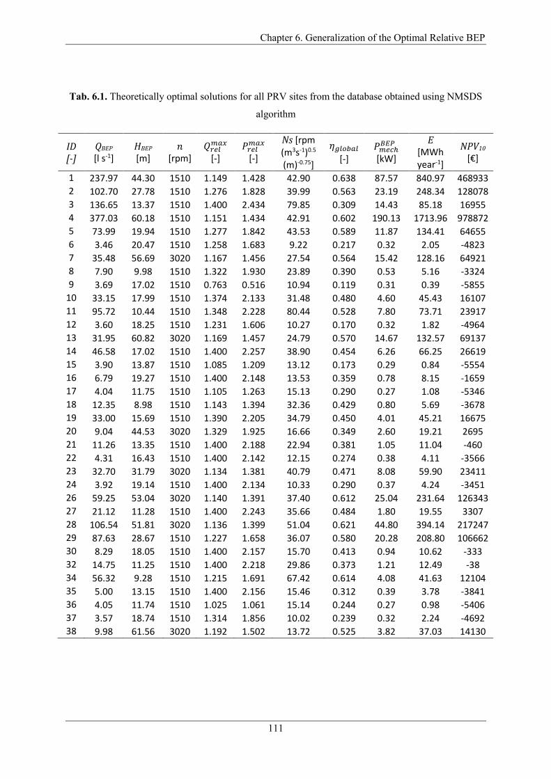
Chapter 6. Generalization of the Optimal Relative BEP
111
Tab. 6.1. Theoretically optimal solutions for all PRV sites from the database obtained using NMSDS
algorithm
ID [-]
QBEP [l s-1]
HBEP [m]
𝑛 [rpm]
𝑄𝑟𝑒𝑙𝑚𝑎𝑥 [-]
𝑃𝑟𝑒𝑙𝑚𝑎𝑥 [-]
Ns [rpm (m3s-1)0.5 (m)-0.75]
𝜂𝑔𝑙𝑜𝑏𝑎𝑙
[-] 𝑃𝑚𝑒𝑐ℎ
𝐵𝐸𝑃 [kW]
E [MWh year-1]
NPV10 [€]
1 237.97 44.30 1510 1.149 1.428 42.90 0.638 87.57 840.97 468933
2 102.70 27.78 1510 1.276 1.828 39.99 0.563 23.19 248.34 128078
3 136.65 13.37 1510 1.400 2.434 79.85 0.309 14.43 85.18 16955
4 377.03 60.18 1510 1.151 1.434 42.91 0.602 190.13 1713.96 978872
5 73.99 19.94 1510 1.277 1.842 43.53 0.589 11.87 134.41 64655
6 3.46 20.47 1510 1.258 1.683 9.22 0.217 0.32 2.05 -4823
7 35.48 56.69 3020 1.167 1.456 27.54 0.564 15.42 128.16 64921
8 7.90 9.98 1510 1.322 1.930 23.89 0.390 0.53 5.16 -3324
9 3.69 17.02 1510 0.763 0.516 10.94 0.119 0.31 0.39 -5855
10 33.15 17.99 1510 1.374 2.133 31.48 0.480 4.60 45.43 16107
11 95.72 10.44 1510 1.348 2.228 80.44 0.528 7.80 73.71 23917
12 3.60 18.25 1510 1.231 1.606 10.27 0.170 0.32 1.82 -4964
13 31.95 60.82 3020 1.169 1.457 24.79 0.570 14.67 132.57 69137
14 46.58 17.02 1510 1.400 2.257 38.90 0.454 6.26 66.25 26619
15 3.90 13.87 1510 1.085 1.209 13.12 0.173 0.29 0.84 -5554
16 6.79 19.27 1510 1.400 2.148 13.53 0.359 0.78 8.15 -1659
17 4.04 11.75 1510 1.105 1.263 15.13 0.290 0.27 1.08 -5346
18 12.35 8.98 1510 1.143 1.394 32.36 0.429 0.80 5.69 -3678
19 33.00 15.69 1510 1.390 2.205 34.79 0.450 4.01 45.21 16675
20 9.04 44.53 3020 1.329 1.925 16.66 0.349 2.60 19.21 2695
21 11.26 13.35 1510 1.400 2.188 22.94 0.381 1.05 11.04 -460
22 4.31 16.43 1510 1.400 2.142 12.15 0.274 0.38 4.11 -3566
23 32.70 31.79 3020 1.134 1.381 40.79 0.471 8.08 59.90 23411
24 3.92 19.14 1510 1.400 2.134 10.33 0.290 0.37 4.24 -3451
26 59.25 53.04 3020 1.140 1.391 37.40 0.612 25.04 231.64 126343
27 21.12 11.28 1510 1.400 2.243 35.66 0.484 1.80 19.55 3307
28 106.54 51.81 3020 1.136 1.399 51.04 0.621 44.80 394.14 217247
29 87.63 28.67 1510 1.227 1.658 36.07 0.580 20.28 208.80 106662
30 8.29 18.05 1510 1.400 2.157 15.70 0.413 0.94 10.62 -333
32 14.75 11.25 1510 1.400 2.218 29.86 0.373 1.21 12.49 -38
34 56.32 9.28 1510 1.215 1.691 67.42 0.614 4.08 41.63 12104
35 5.00 13.15 1510 1.400 2.156 15.46 0.312 0.39 3.78 -3841
36 4.05 11.74 1510 1.025 1.061 15.14 0.244 0.27 0.98 -5406
37 3.57 18.74 1510 1.314 1.856 10.02 0.239 0.32 2.24 -4692
38 9.98 61.56 3020 1.192 1.502 13.72 0.525 3.82 37.03 14130
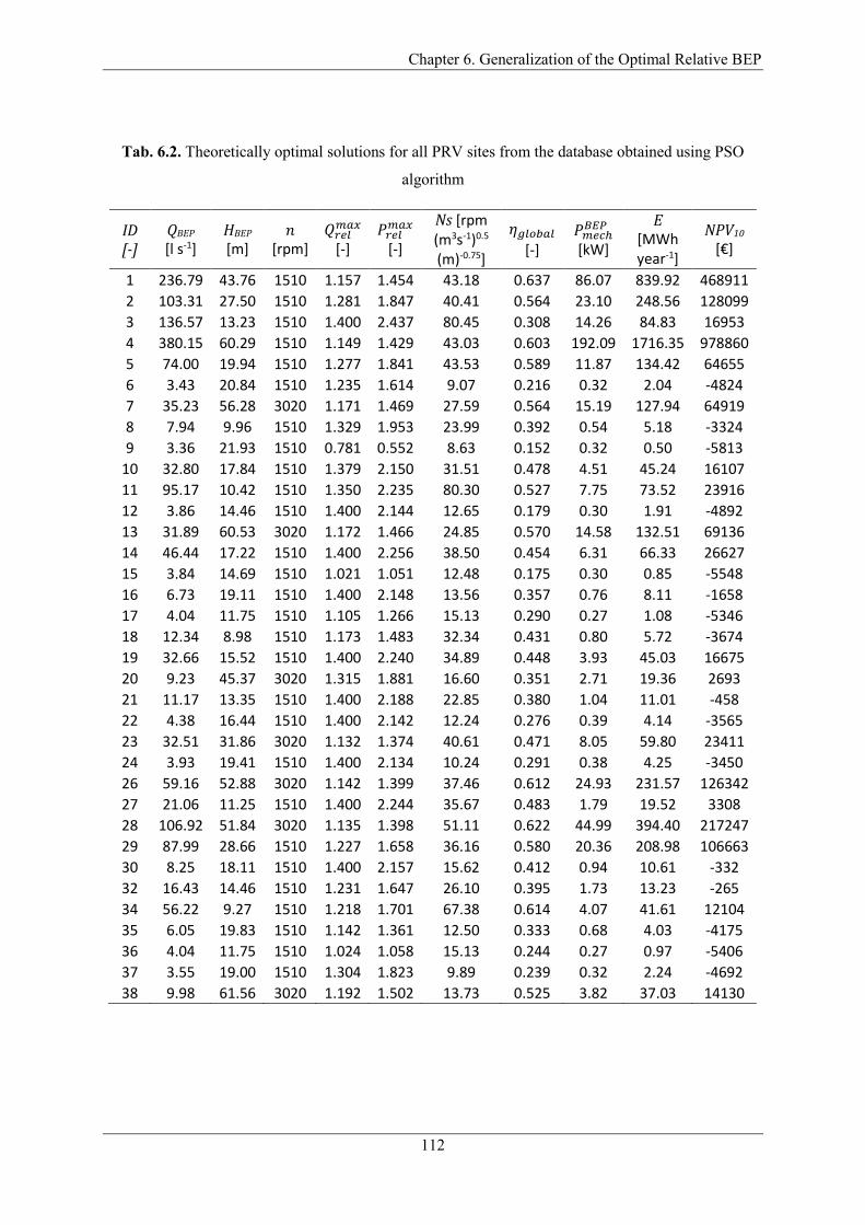
Chapter 6. Generalization of the Optimal Relative BEP
112
Tab. 6.2. Theoretically optimal solutions for all PRV sites from the database obtained using PSO
algorithm
ID [-]
QBEP [l s-1]
HBEP [m]
𝑛 [rpm]
𝑄𝑟𝑒𝑙𝑚𝑎𝑥 [-]
𝑃𝑟𝑒𝑙𝑚𝑎𝑥 [-]
Ns [rpm (m3s-1)0.5 (m)-0.75]
𝜂𝑔𝑙𝑜𝑏𝑎𝑙
[-] 𝑃𝑚𝑒𝑐ℎ
𝐵𝐸𝑃 [kW]
E [MWh year-1]
NPV10 [€]
1 236.79 43.76 1510 1.157 1.454 43.18 0.637 86.07 839.92 468911
2 103.31 27.50 1510 1.281 1.847 40.41 0.564 23.10 248.56 128099
3 136.57 13.23 1510 1.400 2.437 80.45 0.308 14.26 84.83 16953
4 380.15 60.29 1510 1.149 1.429 43.03 0.603 192.09 1716.35 978860
5 74.00 19.94 1510 1.277 1.841 43.53 0.589 11.87 134.42 64655
6 3.43 20.84 1510 1.235 1.614 9.07 0.216 0.32 2.04 -4824
7 35.23 56.28 3020 1.171 1.469 27.59 0.564 15.19 127.94 64919
8 7.94 9.96 1510 1.329 1.953 23.99 0.392 0.54 5.18 -3324
9 3.36 21.93 1510 0.781 0.552 8.63 0.152 0.32 0.50 -5813
10 32.80 17.84 1510 1.379 2.150 31.51 0.478 4.51 45.24 16107
11 95.17 10.42 1510 1.350 2.235 80.30 0.527 7.75 73.52 23916
12 3.86 14.46 1510 1.400 2.144 12.65 0.179 0.30 1.91 -4892
13 31.89 60.53 3020 1.172 1.466 24.85 0.570 14.58 132.51 69136
14 46.44 17.22 1510 1.400 2.256 38.50 0.454 6.31 66.33 26627
15 3.84 14.69 1510 1.021 1.051 12.48 0.175 0.30 0.85 -5548
16 6.73 19.11 1510 1.400 2.148 13.56 0.357 0.76 8.11 -1658
17 4.04 11.75 1510 1.105 1.266 15.13 0.290 0.27 1.08 -5346
18 12.34 8.98 1510 1.173 1.483 32.34 0.431 0.80 5.72 -3674
19 32.66 15.52 1510 1.400 2.240 34.89 0.448 3.93 45.03 16675
20 9.23 45.37 3020 1.315 1.881 16.60 0.351 2.71 19.36 2693
21 11.17 13.35 1510 1.400 2.188 22.85 0.380 1.04 11.01 -458
22 4.38 16.44 1510 1.400 2.142 12.24 0.276 0.39 4.14 -3565
23 32.51 31.86 3020 1.132 1.374 40.61 0.471 8.05 59.80 23411
24 3.93 19.41 1510 1.400 2.134 10.24 0.291 0.38 4.25 -3450
26 59.16 52.88 3020 1.142 1.399 37.46 0.612 24.93 231.57 126342
27 21.06 11.25 1510 1.400 2.244 35.67 0.483 1.79 19.52 3308
28 106.92 51.84 3020 1.135 1.398 51.11 0.622 44.99 394.40 217247
29 87.99 28.66 1510 1.227 1.658 36.16 0.580 20.36 208.98 106663
30 8.25 18.11 1510 1.400 2.157 15.62 0.412 0.94 10.61 -332
32 16.43 14.46 1510 1.231 1.647 26.10 0.395 1.73 13.23 -265
34 56.22 9.27 1510 1.218 1.701 67.38 0.614 4.07 41.61 12104
35 6.05 19.83 1510 1.142 1.361 12.50 0.333 0.68 4.03 -4175
36 4.04 11.75 1510 1.024 1.058 15.13 0.244 0.27 0.97 -5406
37 3.55 19.00 1510 1.304 1.823 9.89 0.239 0.32 2.24 -4692
38 9.98 61.56 3020 1.192 1.502 13.73 0.525 3.82 37.03 14130
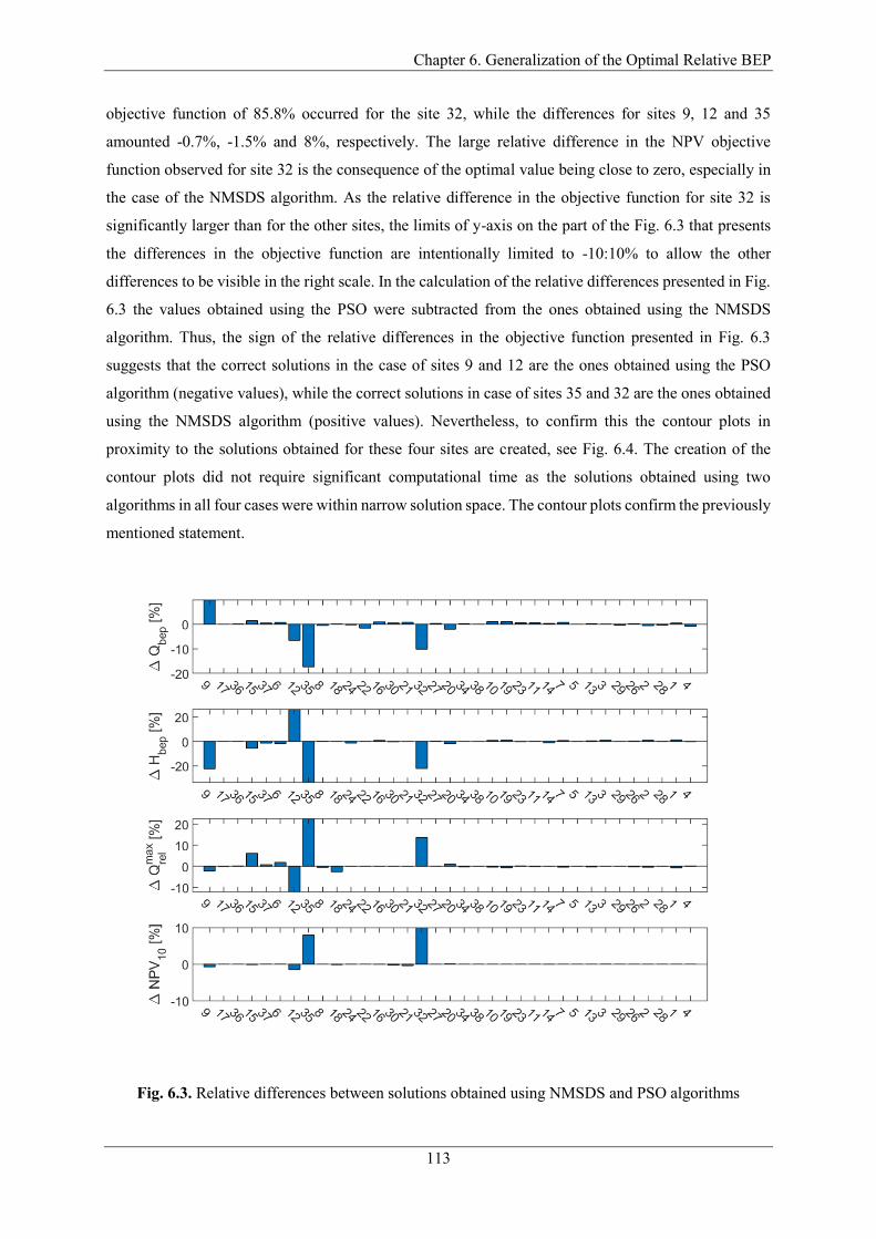
Chapter 6. Generalization of the Optimal Relative BEP
113
objective function of 85.8% occurred for the site 32, while the differences for sites 9, 12 and 35
amounted -0.7%, -1.5% and 8%, respectively. The large relative difference in the NPV objective
function observed for site 32 is the consequence of the optimal value being close to zero, especially in
the case of the NMSDS algorithm. As the relative difference in the objective function for site 32 is
significantly larger than for the other sites, the limits of y-axis on the part of the Fig. 6.3 that presents
the differences in the objective function are intentionally limited to -10:10% to allow the other
differences to be visible in the right scale. In the calculation of the relative differences presented in Fig.
6.3 the values obtained using the PSO were subtracted from the ones obtained using the NMSDS
algorithm. Thus, the sign of the relative differences in the objective function presented in Fig. 6.3
suggests that the correct solutions in the case of sites 9 and 12 are the ones obtained using the PSO
algorithm (negative values), while the correct solutions in case of sites 35 and 32 are the ones obtained
using the NMSDS algorithm (positive values). Nevertheless, to confirm this the contour plots in
proximity to the solutions obtained for these four sites are created, see Fig. 6.4. The creation of the
contour plots did not require significant computational time as the solutions obtained using two
algorithms in all four cases were within narrow solution space. The contour plots confirm the previously
mentioned statement.
Fig. 6.3. Relative differences between solutions obtained using NMSDS and PSO algorithms

Chapter 6. Generalization of the Optimal Relative BEP
114
Fig. 6.4. Contour plots of 4 sites with notable difference between the optimal solutions obtained with
NMSDS and PSO algorithms a) site 9; b) site 12; c) site 32 and d) site 35
6.3.2 Generalized ratio
Once the correct theoretically optimal BEPs were confirmed for all sites, the ratios between these and
the average operating conditions recorded at the considered sites were assessed. The pair of these two
ratios could be regarded as the relative BEP (𝑞𝐵𝐸𝑃, ℎ𝐵𝐸𝑃):
𝑞𝐵𝐸𝑃 =𝑄𝐵𝐸𝑃
�̅�; ℎ𝐵𝐸𝑃 =
𝐻𝐵𝐸𝑃
�̅�; (6.15).
The results are presented in Tab. 6.3 and Fig. 6.5. As it can be seen from Fig. 6.5, the relative optimal
BEPs for vast majority of sites (29 out of 35) are clustered within a relatively small area (within the
ellipse), except for six outliers, namely sites 3, 18, 36, 17, 15 and 9. By examining the possible reasons
for the outliers, it is found out that for five out of six sites, the theoretically optimal BEP was located at
the availability boundary defined for the selected optimal speed. In other words, the “natural” optimal
solution (within the ellipse) was not feasible because of the constraints imposed to the solution space.
The notable discrepancy for the sixth outlier, i.e., Site 3, whose optimal solution was not constrained
by the availability boundaries can be partially explained with the fact that it has one of the largest and
the most irregular variations of the operating conditions among the considered sites, see Fig. 6.6. By
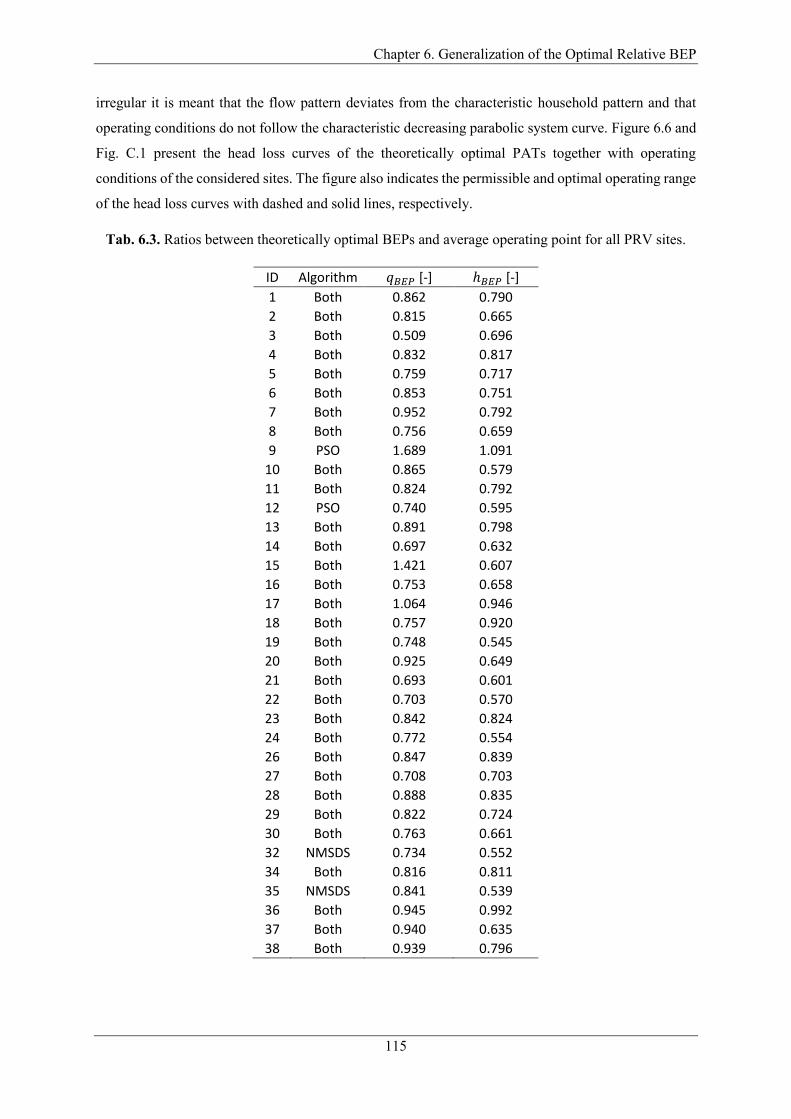
Chapter 6. Generalization of the Optimal Relative BEP
115
irregular it is meant that the flow pattern deviates from the characteristic household pattern and that
operating conditions do not follow the characteristic decreasing parabolic system curve. Figure 6.6 and
Fig. C.1 present the head loss curves of the theoretically optimal PATs together with operating
conditions of the considered sites. The figure also indicates the permissible and optimal operating range
of the head loss curves with dashed and solid lines, respectively.
Tab. 6.3. Ratios between theoretically optimal BEPs and average operating point for all PRV sites.
ID Algorithm 𝑞𝐵𝐸𝑃 [-] ℎ𝐵𝐸𝑃 [-]
1 Both 0.862 0.790
2 Both 0.815 0.665
3 Both 0.509 0.696
4 Both 0.832 0.817
5 Both 0.759 0.717
6 Both 0.853 0.751
7 Both 0.952 0.792
8 Both 0.756 0.659
9 PSO 1.689 1.091
10 Both 0.865 0.579
11 Both 0.824 0.792
12 PSO 0.740 0.595
13 Both 0.891 0.798
14 Both 0.697 0.632
15 Both 1.421 0.607
16 Both 0.753 0.658
17 Both 1.064 0.946
18 Both 0.757 0.920
19 Both 0.748 0.545
20 Both 0.925 0.649
21 Both 0.693 0.601
22 Both 0.703 0.570
23 Both 0.842 0.824
24 Both 0.772 0.554
26 Both 0.847 0.839
27 Both 0.708 0.703
28 Both 0.888 0.835
29 Both 0.822 0.724
30 Both 0.763 0.661
32 NMSDS 0.734 0.552
34 Both 0.816 0.811
35 NMSDS 0.841 0.539
36 Both 0.945 0.992
37 Both 0.940 0.635
38 Both 0.939 0.796

Chapter 6. Generalization of the Optimal Relative BEP
116
Fig. 6.5. Rations between the BEPs of the optimal PATs and the average operating conditions of the
considered PRV sites
Considering, that the reason for almost all outliers (5 out of 6) was the constraints imposed to the Q-H
solution space, it could be said that unless the operating points of a PRV site are in immediate proximity
to the availability boundaries, its relative optimal BEP should reside within the cluster. To generalize
the location and the shape of the cluster a minimal enclosing ellipse was created around the points
forming the cluster. The minimum area enclosing ellipse around the set of 29 points was found by
solving the following optimisation problem (Moshtagh, 2020):
𝑚𝑖𝑛𝑖𝑚𝑖𝑧𝑒:𝑨,𝒄
𝑙𝑜𝑔 (𝑑𝑒𝑡 (𝑨))
𝑠. 𝑡. (𝑷𝑖 − 𝒄)𝑇𝑨(𝑷𝑖 − 𝒄) ≤ 1 , 𝑖 = 1, … , 29
𝑨 > 0
(6.16).
In Eq. 6.16, the equation of the ellipse is defined in centred matrix form, where c is a vector containing
the coordinates of the centre of ellipse; A is a matrix containing information about the shape of ellipse;
and Pi is the i-th point within the cluster. The centre c and matrix A of the ellipse presented in Fig. 6.5
have the following values:
𝒄 = [0.830.68
] ; 𝑨 = [59.43 −17.80
−17.80 43.72] (6.17).
The radii and orientation of the ellipse can be obtained using singular value decomposition (Moshtagh,
2020).

Chapter 6. Generalization of the Optimal Relative BEP
117
Fig. 6.6. Head loss curves of the theoretically optimal PATs with optimal operating range: Valves 1-6
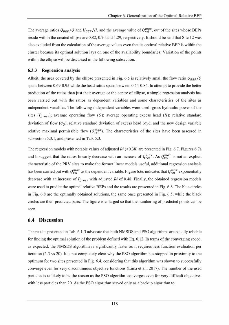
Chapter 6. Generalization of the Optimal Relative BEP
118
The average ratios 𝑄𝐵𝐸𝑃/�̅� and 𝐻𝐵𝐸𝑃/�̅�, and the average value of 𝑄𝑟𝑒𝑙𝑚𝑎𝑥, out of the sites whose BEPs
reside within the created ellipse are 0.82, 0.70 and 1.29, respectively. It should be said that Site 12 was
also excluded from the calculation of the average values even that its optimal relative BEP is within the
cluster because its optimal solution lays on one of the availability boundaries. Variation of the points
within the ellipse will be discussed in the following subsection.
6.3.3 Regression analysis
Albeit, the area covered by the ellipse presented in Fig. 6.5 is relatively small the flow ratio 𝑄𝐵𝐸𝑃/�̅�
spans between 0.69-0.95 while the head ratios spans between 0.54-0.84. In attempt to provide the better
prediction of the ratios than just their average or the centre of ellipse, a simple regression analysis has
been carried out with the ratios as dependent variables and some characteristics of the sites as
independent variables. The following independent variables were used: gross hydraulic power of the
sites (𝑃𝑔𝑟𝑜𝑠𝑠); average operating flow (�̅�); average operating excess head (�̅�); relative standard
deviation of flow (𝜎𝑄); relative standard deviation of excess head (𝜎𝐻); and the new design variable
relative maximal permissible flow (𝑄𝑟𝑒𝑙𝑚𝑎𝑥). The characteristics of the sites have been assessed in
subsection 5.3.1, and presented in Tab. 5.3.
The regression models with notable values of adjusted R2 (>0.38) are presented in Fig. 6.7. Figures 6.7a
and b suggest that the ratios linearly decrease with an increase of 𝑄𝑟𝑒𝑙𝑚𝑎𝑥. As 𝑄𝑟𝑒𝑙
𝑚𝑎𝑥 is not an explicit
characteristic of the PRV sites to make the former linear models useful, additional regression analysis
has been carried out with 𝑄𝑟𝑒𝑙𝑚𝑎𝑥 as the dependent variable. Figure 6.6c indicates that 𝑄𝑟𝑒𝑙
𝑚𝑎𝑥 exponentially
decrease with an increase of 𝑃𝑔𝑟𝑜𝑠𝑠 with adjusted R2 of 0.48. Finally, the obtained regression models
were used to predict the optimal relative BEPs and the results are presented in Fig. 6.8. The blue circles
in Fig. 6.8 are the optimally obtained solutions, the same once presented in Fig. 6.5, while the black
circles are their predicted pairs. The figure is enlarged so that the numbering of predicted points can be
seen.
6.4 Discussion
The results presented in Tab. 6.1-3 advocate that both NMSDS and PSO algorithms are equally reliable
for finding the optimal solution of the problem defined with Eq. 6.12. In terms of the converging speed,
as expected, the NMSDS algorithm is significantly faster as it requires less function evaluation per
iteration (2-3 vs 20). It is not completely clear why the PSO algorithm has stopped in proximity to the
optimum for two sites presented in Fig. 6.4, considering that this algorithm was shown to successfully
converge even for very discontinuous objective functions (Lima et al., 2017). The number of the used
particles is unlikely to be the reason as the PSO algorithm converges even for very difficult objectives
with less particles than 20. As the PSO algorithm served only as a backup algorithm to
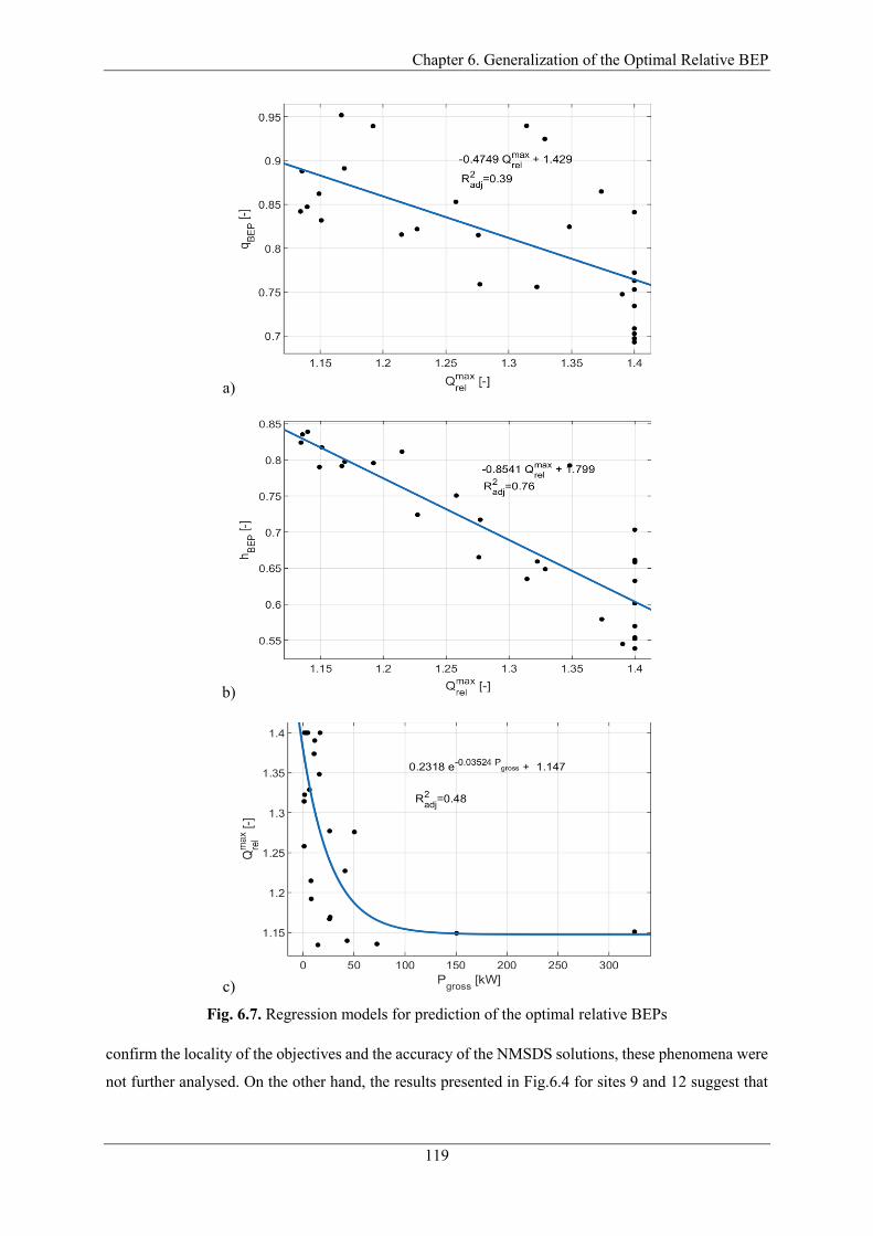
Chapter 6. Generalization of the Optimal Relative BEP
119
a)
b)
c)
Fig. 6.7. Regression models for prediction of the optimal relative BEPs
confirm the locality of the objectives and the accuracy of the NMSDS solutions, these phenomena were
not further analysed. On the other hand, the results presented in Fig.6.4 for sites 9 and 12 suggest that
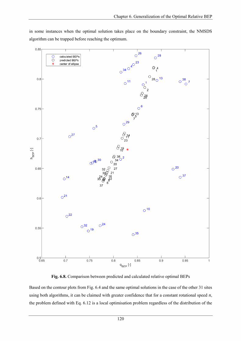
Chapter 6. Generalization of the Optimal Relative BEP
120
in some instances when the optimal solution takes place on the boundary constraint, the NMSDS
algorithm can be trapped before reaching the optimum.
Fig. 6.8. Comparison between predicted and calculated relative optimal BEPs
Based on the contour plots from Fig. 6.4 and the same optimal solutions in the case of the other 31 sites
using both algorithms, it can be claimed with greater confidence that for a constant rotational speed n,
the problem defined with Eq. 6.12 is a local optimisation problem regardless of the distribution of the
Chapter 6. Generalization of the Optimal Relative BEP
121
operating points of a considered site. And this is true even after inclusion of additional design variable
𝑄𝑟𝑒𝑙𝑚𝑎𝑥, the nominal efficiency of generators, and the update of the cost function.
Based on the spread of the theoretically optimal BEPs of 35 examined sites, it could be said that the
answer to the research question addressed in this Chapter is that the optimal relative BEP can be
generalized. In other words, the optimal relative BEP resides within the narrow range defined with the
ellipse presented in Fig. 6.5, with centre c and matrix A, see Eq. 6.17. This stands regardless of the
distribution of the operating points of the consider site, its size and optimal operating limits. The
distributions of the operating points for Sites 1-6 are presented in Fig. 6.6, while for the rest of the sites
these are presented in Fig. C.1.
Another important finding can be observed from Fig. 6.6 and Fig. C.1. Namely, if Fig. 6.6 is closely
observed it can be seen that for the majority of sites their average operating point matches, or is in the
immediate proximity, to the optimal maximal operating point (𝑄𝑃𝐴𝑇𝑚𝑎𝑥, 𝐻𝑃𝐴𝑇
𝑚𝑎𝑥) of the theoretically optimal
PAT. The optimal maximal operating points of the PATs on Fig. 6.6 and Fig. C.1 are located at the end
of the optimal range of their head loss curves (end of the solid lines and beginning of the dashed lines).
The operating flow at the sites higher than 𝑄𝑃𝐴𝑇𝑚𝑎𝑥 is always bypassed, while the excess head higher than
𝐻𝑃𝐴𝑇𝑚𝑎𝑥 is always dissipated.
This is in agreement with the relationships captured with the regression models presented in Fig. 6.7a
and b, and the locations of the optimal relative BEPs. Namely, as the average operating points of the
sites match with the maximal operating points, with an increase of 𝑄𝑟𝑒𝑙𝑚𝑎𝑥 the flow and head, the BEPs
are “moved further back” along the head loss curves, thus their ratios to the average points are
decreasing. On the other hand, the model in Fig. 6.7c suggests that for the sites with small power
potential, 𝑄𝑟𝑒𝑙𝑚𝑎𝑥 is high so that a cheaper machine is selected. As the power potential of the sites
increases, the cost of machine is less and less important so 𝑄𝑟𝑒𝑙𝑚𝑎𝑥 exponentially decreases until reaching
a value of 1.15 below which it does not go, as it would decrease the energy recovery. For perspective,
the value of 𝑄𝑟𝑒𝑙𝑚𝑎𝑥=1.15 correspond to 𝑃𝑟𝑒𝑙
𝑚𝑎𝑥 of around 1.45 using the relative power model defined by
Novara and McNabola (2018) and an average value of Ns = 50 rpm(m3/s)0.5(m)0.75.
In Figure 6.7 it could be also seen that except the relationship between ℎ𝐵𝐸𝑃 and 𝑄𝑟𝑒𝑙𝑚𝑎𝑥, the other two
relationships are not particularly strong in terms of R2. The low values of R2 of these models are
probably the major reason why the predicted BEPs (black circles in Fig. 6.8) obtained using these
models deviated considerably from the calculated BEPs (blue circles in Fig. 6.8). Moreover, as can be
seen from Fig. 6.8, the use of these regression models does not even improve the prediction for all sites
in comparison to the average BEP (e.g., sites 2 and 29).
Chapter 6. Generalization of the Optimal Relative BEP
122
If there is a regression model that could accurately explain the variation of the theoretically optimal
BEPs within the cluster (which is unlikely), this model would be possible to obtain by solving an
optimisation problem similar to the following one:
𝑚𝑖𝑛𝑖𝑚𝑖𝑧𝑒: ∑ 𝐸𝐷𝑖
𝑝𝑟𝑒𝑑𝑁𝑖
𝑠. 𝑡. 𝐸𝐷𝑖𝑝𝑟𝑒𝑑
− 𝐸𝐷𝑖𝑎𝑣𝑒 ≤ 0, 𝑖 = 1, … , 𝑁
(6.18)
where 𝐸𝐷𝑖𝑝𝑟𝑒𝑑
is Euclidean Distance between the predicted and calculated optimal BEP for i-th site;
and 𝐸𝐷𝑖𝑎𝑣𝑒 is Euclidean Distance between the average BEP (or the centre of the ellipse) and the optimal
BEP for i-th site. However, this analysis is beyond the scope of this chapter.
The most obvious implication of the results presented in this chapter is that the procedure for selection
of the optimal PAT to be installed at a PRV site could be hugely simplified. Namely, instead of using
an optimisation procedure for selection of the BEP of the theoretically optimal PAT, the BEP could be
predicted as the simple ratio to the average operating point of a considered site. Thus, the simplified
selection procedure would include the following steps:
1. Calculate the average operating point of a considered site.
2. Calculate the BEP of the theoretically optimal PAT by using the average optimal ratios
(𝑄𝐵𝐸𝑃/�̅�,𝐻𝐵𝐸𝑃/�̅�) = (0.82, 0.70). The ratios that define the centre of the ellipse could be used
as well. As the derived regression models did not improve the prediction for all sites, their use
is not recommended.
3. Select the optimal rotational speed. In theory, all three rotational speeds should be always
considered because of the discrete nature of the available pump families. However, in most
cases the optimal PAT from the market will be of the speed that gives the highest value of the
efficiency calculated using Eq. 6.5, at the predicted BEP in step 2.
4. Conduct a slight adjustment of the theoretically optimal BEP using the similarity laws so it
corresponds the analogous speed in pump mode for which the pump selection charts are
available (Carravetta et al., 2012).
5. Convert the adjusted BEP into the pump domain using the Yang et al.'s (2012) conversion
methodology.
6. Select near optimal pump/PAT family from the pump selection charts.
Another useful application of the derived optimal relative BEP or the ellipse equation would be to
reduce the computational time of the optimisation procedures for the selection of the optimal number
and locations of PATs within WDNs. Namely, consider the optimisation strategy proposed by Tricarico
Chapter 6. Generalization of the Optimal Relative BEP
123
et al. (2018) where a PAT database is available. The PATs available in the database are considered as
integer variables in the strategy. Instead of considering all PATs for each considered pipe location, the
solution set for i-th pipe could be narrowed down to only a few whose BEPs are within the ellipse whose
equation would be defined based on the average operating condition at the pipe. Alternatively, instead
calculating if the BEPs are within the ellipse, the solution set could be narrowed down to a few
alternatives with the shortest Euclidean Distances from the centre of the ellipse.
For the improvement of the selection of a PAT based on the Euclidean Distance calculated from its BEP
to the theoretically optimal BEP it would be useful to study the contour plots of the objective function
for the examined sites, such as the ones presented in Fig. 6.4. Namely, the calculation of the simple
unweighted distance would be valid if the contours would be concentric circles around the optimal
point. The contours presented in Fig. 6.4 obviously do not follow this pattern. Thus, it would be
interesting to analyse if a generalized vector of weight coefficients could be defined. This vector would
adjust the Euclidean Distance based on the angle between x-axis and a line defined between the optimal
and the BEP of the considered PAT family.
6.5 Conclusions
The main aim of the research presented in this chapter was to address the hypothesis that the ratio
between the average operating points of PRV sites and the BEPs of their theoretically optimal PATs in
terms of maximization of the NPV objective, can be generalized. In other words, it was examined
whether this ratio is constant or at least varies within narrow range, regardless of the differences among
the considered sites.
The optimisation problem definition has been modified in comparison to Chapter 4 to include the
operation limits as a design variable, as it was shown that these can influence the optimal solution.
Additionally, the model for assessment of the NPV has been updated to include the nominal efficiency
of the coupled generator and its true cost defined as a function of its size, like in Chapter 5.
To find the BEPs of the theoretically optimal PATs two heuristic optimisation methods have been used,
namely the NMSDS and PSO algorithms. The reason for using the PSO algorithm besides the
previously used NMSDS algorithm was to verify the local nature of the modified optimisation problem
as the PSO is global algorithm, and to validate the accuracy of the optimal solutions. The results of the
simulations conducted on 35 PRV sites suggest that both algorithms are reliable for solving the set
optimisation problem. The same results for 31 valves and the contour plots of the ones with moderate
differences suggest that the examined problem is local for the general case, regardless of the distribution
of the operating points at considered sites.
The results obtained for the ratios (𝑄𝐵𝐸𝑃/�̅�, 𝐻𝐵𝐸𝑃/�̅�), i.e., the optimal relative BEP suggest that it is
not constant but it varies within narrow range. The location and shape of the cluster of the optimal

Chapter 6. Generalization of the Optimal Relative BEP
124
relative BEPs have been determined by creating the minimal area-enclosing ellipse around the cluster
points. The obtained ellipse is defined with the centre vector c = [0.83 0.69] and matrix A that contains
information about its shape, see Eq. 6.17. The average relative optimal BEP is almost the same as the
centre of the ellipse and amounts (0.82 0.7), while the average value of the new design variable is
𝑄𝑟𝑒𝑙𝑚𝑎𝑥 = 1.29.
Another important finding has been observed from the graphs of the head loss curves of the theoretically
optimal PATs presented in Fig. 6.6 and Fig. C.1. These graphs suggest that the optimal maximal
operating points of the theoretical PATs match with the average operating points for majority of the
examined sites.
Although, the area of the defined ellipse is relatively small, a regression analysis has been carried out,
to investigate if the characteristics of the sites can explain the variation of the optimal relative BEPs
within the ellipse, and thus improve its prediction. The analysis determined that 𝑞𝐵𝐸𝑃 and ℎ𝐵𝐸𝑃 linearly
decrease with an increase of 𝑄𝑟𝑒𝑙𝑚𝑎𝑥, with R2 adjusted of 0.39 and 0.76 respectively. Subsequent
regression analysis of 𝑄𝑟𝑒𝑙𝑚𝑎𝑥 as the dependant variable determined its exponential relationship with Pgross
of the sites, with R2 adjusted of 0.48. As it can be seen from Fig. 6.8, the use of these models did improve
the overall prediction in comparison to the simple average, however it also makes the prediction worse
for some of the valves. Hence, their use is not recommended for general application.
The future work will be focused on implementation of the findings presented in this Chapter in an
algorithm for the selection of the optimal number and locations of PATs within a WDN, aiming to
reduce the computational time needed.
Chapter 7. Spatial Regression Analysis
125
7 Spatial Regression Analysis
7.1 Introduction
The previous part of this thesis presents methodologies how to assess the energy recovery potential of
sites within WSNs when the operating flow and excess head conditions at the considered valves are
available as input data. Even if the operating conditions at a considered site are available in very low
resolution, for example as yearly average values, these data can serve to give a raw estimate of the site’s
potential. However, what if the operating conditions at a potential site are not available even in the low
resolution. In the early stage of this PhD program from the correspondence with water supply operators
in Ireland and the UK it was discovered that there are many PRVs whose existence and location are
known, but that their operating conditions such as flow and head necessary for estimation of HPER
potential are not available. Because PRVs have been installed at these locations, it is reasonable to
assume that these sites possess at least some excess pressure.
Estimating the HPER potential of these sites with reasonable accuracy would be very relevant for large
scale assessments, e.g., when the goal is to estimate the potential of a whole network or larger
geographical coverage. Hence, the idea of the analysis presented in this chapter was to investigate if the
potential of HPER sites from WSNs could be estimated using some publicly available data in their
proximity (e.g., radius of 1-5 km), that are available for the whole area of interest. By examining the
publicly available data that could serve as proxy indicators of HPER potential at PRV sites, two groups
of data have been identified, namely population and topography. Thus, the following sections of this
chapter present results of a regression analysis, where the estimated power potential of HPER sites was
used as a dependant variable, while the extracted population and topography data in their proximity
were used as independent variables.
7.2 Methodology
7.2.1 Studied sites
In the analysis presented in this chapter, the same set of the potential energy recovery sites is used as in
the study of Gallagher et al. (2015). The set includes 51 potential energy recovery sites in Ireland and
187 sites in Wales. These sites represent WSN infrastructures such as PRVs in the first place, control

Chapter 7. Spatial Regression Analysis
126
valves (CVs), break pressure tanks (BPTs) and service reservoirs (SRs). Most of the Irish sites are
situated in Dublin County, 36 out of 51 sites, while the Welsh sites are more uniformly deployed across
Wales. The locations of all the sites are displayed in Fig. 7.1. For each of the sites the following data
was available: mean annual flow and pressure data, for the year 2011; site type (e.g. PRV, CVs, BPT,
SR); place name, county and country; longitude and latitude coordinates. The data for this study was
obtained from Dublin City Council, for Irish sites, and from Dwr Cymru/Welsh Water for the Welsh
ones.
Fig. 7.1. Locations of potential micro-hydropower energy recovery site in Ireland and Wales
7.2.2 Calculating Potential Energy
As discussed in previous part of the thesis, many factors can influence the energy recovery potential of
a site within a WSN. In the first place, these are flow and pressure variations that occur at the site which
are mainly determined by the demand of downstream consumers of the network. The diurnal flow and
pressure patterns were available for only a few previously mentioned sites, thus the mean annual flow
and pressure values were used to assess the power potential of all sites. Also, the selection of turbine
type can influence the potential significantly. In order to be able to compare the influence of spatial
geographical data on the power potential of the sites (the spatial regression analysis described in the
next subsection) the global efficiency of the hypothetical plants was estimated as a constant, 𝜂=0.65.
The energy recovery potential of the considered sites was quantified using the following equation:
Chapter 7. Spatial Regression Analysis
127
𝑃 = 𝜌𝑔𝑄𝐻𝜂 (7.1),
where 𝑃[kW] - power output; 𝑄 [m3s-1] - flow rate through the turbine; 𝜌 [kg m-3] - fluid density; 𝑔 [m
s-2] - acceleration due to gravity; 𝐻 [m] - hydraulic head (potential energy per unit of water weight)
available at the turbine; 𝜂 [-] - overall efficiency of the system, estimated at 0.65.
7.2.3 Spatial Regression Analysis
The use of spatial regression models is common in other fields such as air quality modelling (Hoek et
al., 2008). The methodology called Land Use Regression (LUR) is used to explain variations in the
concentrations of the air pollutants. The basic concept of this methodology is that concentrations of
pollutants are measured at a set of monitoring sites, which are used as the dependent variables in the
regression model. LUR uses buffering (if vector-based model is used) to determine the proximity of
pollution sources such as roads or industrial lands etc., to the monitoring sites. The obtained values are
used as the independent variables in a regression model to explain the variation of pollutant
concentrations at the monitoring sites. The built regression model is then used to evaluate the
concentrations of pollutants at other locations of interest.
Upon analogy with the air quality models, the dependant variables in our case would be the power
potential quantified using Eq. 7.1, at the sites presented in Fig 1. Apart from this analogy and the general
concept of spatial regression analysis, everything else is different. Phenomena that influence the
potential for energy recovery in WSNs are of course completely different from the ones that influence
the air pollution. The real challenge in the case of the potential for energy recovery in WSN is finding
the spatial variables which would explain the variations of the power potential without having the
hydraulic model of networks to which these sites belong. As it can be seen in the Eq. 7.1 the two
variables that dictate the potential of a site are the flow in a pipe and excess head that can be exploited.
7.2.3.1 Population
The total flow of a WSN corresponds to the number of people for whom the network supplies the water.
The same way flow in a pipe where a PRV or a SR are situated corresponds to the number of consumers
downstream from the pipe. Of course, without having the hydraulic model of the network we cannot
know which part of the network, i.e., areas of land are downstream of the pipe. Which type of WDN
infrastructure is in place at a pipe can somewhat explain the quantity of the flow in the pipe. Thus pipes
where SRs are in place, will have much larger flow than the ones where PRVs are installed, because
the SRs are commonly situated in the most upstream part of a network, and their flow corresponds to a
much bigger population than the one which passes through a PRV. In this study, the buffer analysis is
used to extract population in a proximity to the potential sites to see if it can explain the variations in
their potential for energy recovery. A model is created using model builder wizard, within ArcMap for
this purpose. The extraction procedure is illustrated in Fig 7.2. The population within the grid cells
which just partially intersect the buffers is calculated by using Eq. 2:

Chapter 7. Spatial Regression Analysis
128
𝑃𝑎𝑟𝑡 𝑜𝑓 𝑡ℎ𝑒 𝑐𝑒𝑙𝑙 𝑜𝑣𝑒𝑟𝑙𝑎𝑖𝑑 𝑤𝑖𝑡ℎ 𝑡ℎ𝑒 𝑏𝑢𝑓𝑓𝑒𝑟
𝐴𝑟𝑒𝑎 𝑜𝑓 𝑡ℎ𝑒 𝑐𝑒𝑙𝑙(1𝑥1𝑘𝑚)× 𝑝𝑜𝑝𝑢𝑙𝑎𝑡𝑖𝑜𝑛 𝑤𝑖𝑡ℎ𝑖𝑛 𝑡ℎ𝑒 𝑐𝑒𝑙𝑙 (7.2),
In order to use the same reference system for both, Irish and Welsh sites the European Terrestrial
Reference System (ETRS89) was used as it is the EU-recommended frame of reference for geodata for
Europe. The highest resolution for the population data that was found, is in the form of a grid, with a
cell size of 1x1 km2. The source of the population shapefile was the Eurostat website, which is the
statistical office of the European Union (ec.europa.eu). The buffer analysis was conducted for a few
buffer sizes to investigate which size gives the best correlation with the HPER potential of the sites.
The buffers of 1km, 3km and 5km in diameter were used. Besides the buffer-based scale for the
population variables in the regression analysis, one more scale was used and that is a 1x1km population
grid cell in which a site takes place (see Fig. 7.2).
Fig. 7.2. Extraction of the population data within the 3km buffers for 4 sites in Dublin
7.2.3.2 Topography
It is well documented in the literature that the terrain variability of a WDN is one of the causes for
excess pressures in it, and therefore the potential for energy recovery therein may be related to
topography. In WDNs which are characterised by hilly terrain the most critical point with the minimum
pressure does not need to be the one which is the furthest away from the source, unlike in networks
which are situated on a flat terrain (see Fig. 7.3). Also in a network which has a large difference in
elevation between its source and the rest of the network there is a large potential for energy recovery
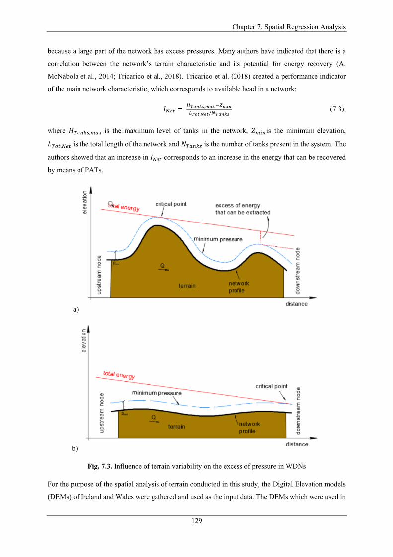
Chapter 7. Spatial Regression Analysis
129
because a large part of the network has excess pressures. Many authors have indicated that there is a
correlation between the network’s terrain characteristic and its potential for energy recovery (A.
McNabola et al., 2014; Tricarico et al., 2018). Tricarico et al. (2018) created a performance indicator
of the main network characteristic, which corresponds to available head in a network:
𝐼𝑁𝑒𝑡 = 𝐻𝑇𝑎𝑛𝑘𝑠,𝑚𝑎𝑥−𝑍𝑚𝑖𝑛
𝐿𝑇𝑜𝑡,𝑁𝑒𝑡/𝑁𝑇𝑎𝑛𝑘𝑠 (7.3),
where 𝐻𝑇𝑎𝑛𝑘𝑠,𝑚𝑎𝑥 is the maximum level of tanks in the network, 𝑍𝑚𝑖𝑛is the minimum elevation,
𝐿𝑇𝑜𝑡,𝑁𝑒𝑡 is the total length of the network and 𝑁𝑇𝑎𝑛𝑘𝑠 is the number of tanks present in the system. The
authors showed that an increase in 𝐼𝑁𝑒𝑡 corresponds to an increase in the energy that can be recovered
by means of PATs.
a)
b)
Fig. 7.3. Influence of terrain variability on the excess of pressure in WDNs
For the purpose of the spatial analysis of terrain conducted in this study, the Digital Elevation models
(DEMs) of Ireland and Wales were gathered and used as the input data. The DEMs which were used in

Chapter 7. Spatial Regression Analysis
130
the analysis were acquired from the United States Geological Survey website (USGS, n.d.). These
DEMs have the resolution of 1x2 arc second which is around 30x60m. Similar to the extraction of the
population variables, a model was created in model builder wizard within ArcMap to perform the buffer
analysis. This model clipped the DEMs using the buffers created around the sites, as it is illustrated in
Fig. 7.4.
The model also calculated the standard deviation of each newly created DEM (products obtained by
clipping the original DEM of Ireland and Wales using the buffers created around the sites, see Fig. 7.4),
which was used as the measure of terrain variability in the regression analysis. Similar to the extraction
of the population data, different buffer sizes are used, namely 0.5km, 1km, 3km and 5km in diameter.
The hydraulic head conditions at a site of course depend on the hydraulic conditions in the upstream
part of a network. However, without network drawings (which are not publically available), it is not
feasible to anticipate which area of the land represents the upstream part of the network. As majority of
the sites were PRVs and these are usually placed at entrances of district metered areas, the hypothesis
was that the higher excess heads are a result of larger elevation difference between these areas and that
this could be captured with the buffers of the selected sizes. On the other hand, using larger buffers for
the terrain variability variable would result that all sites have very similar values for this variable.
Besides the standard deviation of DEM buffers, one more variable was used to represent the terrain
variability and that was the slope of terrain at the locations of energy recovery sites. For this purpose,
the DEMs of Ireland and Wales were transformed to slope raster files and the slope values were
extracted for each site.
Fig. 7.4. Extraction of the DEM within the 3km buffers for 4 sites located in Dublin

Chapter 7. Spatial Regression Analysis
131
The results of regression analysis between the energy recovery potential of the considered sites and the
variables that represented the population or the terrain variability are presented in section 7.3.
7.3 Results and Discussion
7.3.1 Estimation of the power potential
The distribution of the potential for energy recovery of the Irish and Welsh sites is presented in the Fig.
5a and b, respectively. This figure can give us better insight into the potential of the sites and better
explain why some filters were applied in the following subsections on the set of sites in an attempt to
improve the regression model.
a)
b)
Fig. 7.5: Distribution of the potential for energy recovery, a) Irish sites; b) Welsh sites

Chapter 7. Spatial Regression Analysis
132
7.3.2 Regression with Population Data
The data about population inside the buffers of different sizes was extracted in the way explained in the
subsection 7.2.3.1 and correlated with the potential of the sites. Linear Least-Squares Regression
(LLSR) analysis was undertaken to examine how good the population variables explain the variations
in the potential of the sites. The results of the analysis are presented in Tab. 7.1. The initial dataset
where all sites were included did not show almost any correlation with the population data inside the
buffers, especially in the case of Welsh sites (see Tab. 1, row 1). The reason why the initial set of the
Welsh sites includes 165 out of 187 sites is that the rest take place in rural areas without data about the
population. Consequently, some filters were applied to see if the correlation would improve. Firstly, the
SRs were excluded from the sets. The reasoning that this filter might improve the correlation is that
these sites take place in the most upstream part of the WDNs and consequently their pipes carry a large
volume of the water, and buffers of 1 to 5 km are not appropriate in this case.
As it can be seen in Fig. 7.5 all four CV sites in Ireland had very high flows so these were also excluded.
There is only one BPT site with a very small potential, which takes place in Ireland so it was also
excluded. As the result of filtering the LLSR analysis was undertaken only for the PRV sites, but PRV
sites represent 2/3 of all sites in the dataset. The buffers of 1 to 5 km were most logical in their case
because PRVs are usually located at inlets of District Meter Areas (DMAs) which represent smaller
parts of a WDN, to reduce pressure in that part of a network and consequently leakage. In Tab. 7.1, it
can be seen that R2 has increased 2 to 5 times depending on the buffer diameter for the Irish sites, while
in the case of Welsh sites R2 underwent insignificant increase (see Tab. 7.1, row 2). This somewhat can
be explained with that the Welsh set of PRVs is much bigger than the Irish one (152 versus 28), and
that the Welsh set includes PRVs from multiple WDNs while 26 out of 28 of Irish PRVs take place in
Dublin County. Because almost all Irish PRVs are located in Dublin County which is very densely
populated area their average population density in the 1km buffer is 3507, while it is 1351 in case of
Welsh sites. Therefore, the Welsh PRV sites were filtered to include only those which take place in
Cardiff County. As the result, we got the set of 15 PRV sites with the average population density in the
1km buffer of 3810, but the correlation did not improve. A few more filters were applied as it can be
seen in Tab. 1, but the R2 has not been improved. It can be also noticed from the results in the Tab. 7.1,
that in 4 out of 5 alternatives R2 decreases with the increase of size of the buffer for the Irish sites.
With a visual examination of the sites, it was noticed that there are several PRVs which are located very
close to each other, e.g., in the same grid cell. Consequently, these have almost the same population
within the buffers but that their potentials can differ significantly. Taking this into account the sites
which are located in the same grid cell were grouped and the sum of their potential was correlated with
the population of the cell. The result of this regression analysis for the Irish set of PRVs is presented in
Fig. 7.6. As it can be seen from the Fig. 7.6 the correlation has slightly improved from R2=0.214 (row

Chapter 7. Spatial Regression Analysis
133
2, Tab. 7.1) to R2=0.26. The same analysis was undertaken for the Welsh sites but it gave insignificant
improvements.
Tab. 7.1. Results of Linear Least-Squares Regression analysis of energy recovery potential of the
sites with population inside buffers of 1,3 and 5km in diameter, for Irish and Welsh sites
Row Filters applied
R squared
Ireland Wales
1km 3km 5km # of sites
1km 3km 5km # of sites
1 none 0.063 0.038 0.023 51 0.01 0.011 0.009 165
2 type=PRV 0.214 0.193 0.148 28 0.002 0.003 0.008 152
3 type=PRV &
County=Dublin/Cardiff 0.183 0.161 0.118 26 0.016 3E-04 0.044 15
4 type=PRV & P<15kW 0.003 0.019 0.061 22 0.015 0.014 0.022 147
5 type=PRV & 2<P<50kW 0.216 0.185 0.157 14 0.004 0.001 2E-04 89
Fig. 7.6. Energy recovery potential as the function of population within 1km buffer for the set of Irish
PRV sites
7.3.3 Regression with Topography Data
The procedure explained in the subsection 7.2.3.2 was undertaken to obtain variables which describe
terrain variability. After extracting the variables, the LLSR analysis was carried out to assess their
correlation with the energy recovery potential of the sites. The Tab. 7.2 displays the results of the
analysis. As it was mentioned in the subsection 7.2.3.2, two types of variables which were chosen to
represent the terrain variability are: standard deviation of DEM buffers and slope at the locations of the
sites (see Tab. 7.2). As in the case of the regression analysis with the population variables, the R2 for
the initial dataset when all sites are included was insignificant (see Tab. 7.2, row 1). Unlike in the

Chapter 7. Spatial Regression Analysis
134
regression analysis with the population variables, the data filtering here did not bring any improvements
of the R2. Furthermore, almost all regression lines had negative slope, like in Fig. 7.7, which is
completely opposite from the expectations.
It should be pointed out that other nonlinear regression models were considered in the cases of both
types of variables (population and terrain variability), but the datasets were too scattered and did not
show any nonlinear trend. In addition, the regression curves are expected to have positive slopes
(𝑑𝑃𝑜𝑤𝑒𝑟/𝑑𝑃𝑜𝑝𝑢𝑙𝑎𝑡𝑖𝑜𝑛 > 0 and 𝑑𝑃𝑜𝑤𝑒𝑟/𝑑𝑇𝑒𝑟𝑟𝑎𝑖𝑛 𝑣𝑎𝑟𝑖𝑎𝑏𝑙𝑖𝑡𝑖𝑡𝑦 > 0) in the whole range as it is
expected for the power potential to increase with an increase in population and terrain variability.
Tab. 7.2. Results of Linear Least-Squares Regression analysis between the energy recovery potential
of the sites and terrain variability
Row
Filters applied
Ireland # of sites
Wales # of sites 0.5km 1km 3km 5km 0.5km 1km 3km 5km
SD o
f D
EM b
uff
ers
1 none 0.011 0.002 0.007 0.001 51 0.026 0.040 0.045 0.037 186
2 type=PRV 0.057 0.006 0.045 0.042 28 0.004 0.004 0.006 0.014 173
3 type=PRV & P<15kW
0.000 0.003 0.027 0.039 22 0.001 0.001 0.001 0.000 168
4 type=PRV
& 2<P<50kW
0.005 0.060 0.000 0.000 14 0.002 0.000 0.001 0.013 81
5 P<50 0.003 0.008 0.007 0.007 46 0.002 0.003 0.007 0.010 182
Slo
pe
1 none 0.069 51 0.044 186
2 PRV 0.058 28 0.000 173
3 P<50 0.044 46 0.000 182
4 PRV &
2<P<50 0.001 14 0.005 81
Fig. 7.7. Regression analysis between the energy recovery potential and standard deviation of the 1km
DEM buffer for the set of PRV sites in Ireland.

Chapter 7. Spatial Regression Analysis
135
7.4 Conclusion
The spatial regression analysis was performed in this chapter to assess the correlation between the
HPER potential of the sites in WSNs and the geographical data, in Ireland and Wales. The geographical
data whose correlation with the potential was examined are the population and terrain variability. The
results of the LLSR analysis presented in chapter showed that neither population nor topography
variables can explain a significant amount of the variation of the potential at the considered sites. The
only somewhat notable correlation of R2=0.26 was obtained for the set of Irish PRV sites when the
potential of sites located in one population grid cell is summarised and correlated with the population
of the grid cell.
There are many potential reasons why the conducted regression analysis was unsuccessful, one of which
is that the created buffer areas did not match the DMAs at whose entrances the considered PRVs were
installed. Then different areas could have significantly different rate of water consumptions per
inhabitant, which could be caused by presence of a large water consumer for example. The overall
conclusion of the study is that geographical variables such as population and terrain variability in the
proximity to the sites (up to 5 km) sites are not sufficient to accurately predict their potential.

Chapter 8. Large-Scale Resource Assessment
136
8 Large-Scale Resource
Assessment
8.1 Introduction
Significant proportions of water resources in the EU are consumed by the domestic drinking water
sector (14%) (EEA, 2018). The energy consumption associated with pressurized water networks is
estimated to represent 2-3% of global energy consumption (Nogueira Vilanova and Perrella Balestieri,
2015). The consumption of energy inherent in the extraction, treatment, and distribution of drinking
water is a well-publicised area of concern for water utilities and their respective governments
(McNabola et al., 2014; Venkatesh and Brattebø, 2011).
Significant focus in recent years has been placed on hydropower energy recovery (HPER) as an energy
saving technique (Fecarotta and Mc Nabola, 2017). Numerous case studies have been conducted
assessing the potential impacts of HPER in water supply networks (WSNs) mostly at site or local
network scale and seldom on regional scales. Gallagher et al. (2015) outlined the potential for the
recovery of 17.9 GWh yr-1 from 80 existing pressure reducing valves (PRVs) and other network
infrastructure, in water supply networks (WSNs) in Ireland and Wales.
However, the potential impact of HPER in WSNs across a large geographical scale has not been
assessed to date, owing in part to the difficulty in obtaining the required water network data to conduct
such an assessment. This data is often missing or unavailable from water authorities. As a result, the
full potential impact of this technological intervention on energy consumption and CO2 emissions in
the sector is unknown. Therefore, limited exploitation of the resources to date has occurred due to a
combination of inertia within the water sector, a lack of knowledge about its potential impacts and lack
of incentives from government, who are also largely unaware of its potential owing to the lack of
regional or country scale assessments.
The work presented in this chapter addresses this gap by carrying out one of the largest assessments of
this potential conducted to date, using a large dataset amassed across Ireland and the UK. The results
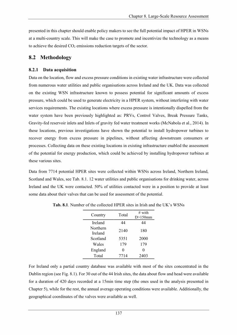
Chapter 8. Large-Scale Resource Assessment
137
presented in this chapter should enable policy makers to see the full potential impact of HPER in WSNs
at a multi-country scale. This will make the case to promote and incentivize the technology as a means
to achieve the desired CO2 emissions reduction targets of the sector.
8.2 Methodology
8.2.1 Data acquisition
Data on the location, flow and excess pressure conditions in existing water infrastructure were collected
from numerous water utilities and public organisations across Ireland and the UK. Data was collected
on the existing WSN infrastructure known to possess potential for significant amounts of excess
pressure, which could be used to generate electricity in a HPER system, without interfering with water
services requirements. The existing locations where excess pressure is intentionally dispelled from the
water system have been previously highlighted as: PRVs, Control Valves, Break Pressure Tanks,
Gravity-fed reservoir inlets and Inlets of gravity fed water treatment works (McNabola et al., 2014). In
these locations, previous investigations have shown the potential to install hydropower turbines to
recover energy from excess pressure in pipelines, without affecting downstream consumers or
processes. Collecting data on these existing locations in existing infrastructure enabled the assessment
of the potential for energy production, which could be achieved by installing hydropower turbines at
these various sites.
Data from 7714 potential HPER sites were collected within WSNs across Ireland, Northern Ireland,
Scotland and Wales, see Tab. 8.1. 12 water utilities and public organisations for drinking water, across
Ireland and the UK were contacted. 50% of utilities contacted were in a position to provide at least
some data about their valves that can be used for assessment of the potential.
Tab. 8.1. Number of the collected HPER sites in Irish and the UK’s WSNs
Country Total # with
D>150mm
Ireland 44 44
Northern
Ireland 2140 180
Scotland 5351 2000
Wales 179 179
England 0 0
Total 7714 2403
For Ireland only a partial country database was available with most of the sites concentrated in the
Dublin region (see Fig. 8.1). For 30 out of the 44 Irish sites, the data about flow and head were available
for a duration of 420 days recorded at a 15min time step (the ones used in the analysis presented in
Chapter 5), while for the rest, the annual average operating conditions were available. Additionally, the
geographical coordinates of the valves were available as well.

Chapter 8. Large-Scale Resource Assessment
138
Fig. 8.1. Distribution of all collected sites
For Wales, the full country database was available (see Fig. 1), but only the annual average operating
flow and excess head were available for all sites. The geographical coordinates of the Welsh valves
Chapter 8. Large-Scale Resource Assessment
139
were also provided. In addition, the diameters of the pipe mains where the valves are installed were
known as well. PRVs with diameters less than 150mm were not considered.
As it can be seen from Tab. 8.1, the Irish and Welsh sites together make only around 3% of the total
number of collected sites while the rest comes from Northern Ireland (27.7%) and Scotland (69.4%).
This is because the Irish and Welsh databases include only the valves installed at the pipes with dimeters
of 150 mm or greater. Like in the case of Welsh database, the valves provided for Northern Ireland and
Scotland also cover the entire area of those countries (see Fig 8.1). However, unlike in the cases of
Ireland and Wales the data about flow and excess head was not available for all sites.
Thus for the Northern Irish sites the annual average flow and excess head were available only for a
small part of the set. Diameters of the pipes where the valves were installed were available for the vast
majority of the dataset and the maximal and minimal heads upstream and downstream the valves were
known for a part of the dataset from the valves settings. Additionally, the geographical coordinates were
available for all valves.
Everything said for the Northern Irish set stands for the Scottish set as well. A difference was that for a
portion of the sites the number of properties supplied by a particular valve was also known.
8.2.2 Existing Energy Resource Assessment
The methodology for the assessment of multi-country HPER potential presented in this chapter was
tailored to the data that the water companies in the investigated region were willing to share. It facilitates
an assessment of the potential at existing infrastructure, however it fails to assess the total or optimal
potential. This is the case as while PRVs for example exist in WSNs to reduce pressure, their presence
is not optimal in terms of maximization of energy recovery in every region (Giugni et al., 2014) and
excess pressure can exist in WSNs where PRVs are not present to reduce it. As such, the current
approach can only assess the potential of replacing or coupling existing infrastructure with hydropower
turbines. To obtain an assessment of the full optimal HPER potential in WSNs would require hydraulic
models of every network to be assessed, which is not feasible at a multi-country scale.
Considering that the flow and excess head data for the vast majority of amassed sites were available at
low temporal resolution (annual average), even the sites with longer records of the hydraulic parameters
were first converted to their annual average values and the subsequent multi-country assessment was
conducted in the following steps:
1. Estimation of average operating points (AOPs) for Northern Irish and Scottish sites. As mentioned
in the previous subsection only a small number of sites in Northern Ireland and Scotland had data
about the annual average flow and excess head. Considering the data provided from the water
utilities in these two countries their average annual flow and excess head were estimated using the
following algorithms:

Chapter 8. Large-Scale Resource Assessment
140
�̅� – Algorithm
IF annual average flow is available
�̅� = annual average flow; % confidence level A
ELSEIF Total property coverage is available
�̅� = 𝑇𝑜𝑡𝑎𝑙 𝑝𝑟𝑜𝑝𝑒𝑟𝑡𝑦 𝑐𝑜𝑣𝑒𝑟𝑎𝑔𝑒 ∙ 800𝑙
𝑝𝑟𝑜𝑝𝑟𝑒𝑡𝑦∙𝑑𝑎𝑦/24/3600
𝑠
𝑑𝑎𝑦; % confidence level B
ELSEIF diameter (D) is available
�̅� = (𝐷
2
1000 )
2
𝜋 ∙ 𝑉; % confidence level C
ELSE
�̅� = 0; % confidence level D
END
where �̅� [ls-1] is the estimated average annual flow at a site; Total property coverage is the number
of properties supplied downstream a considered valve; 𝐷 [mm] is the diameter of a pipe main where
a valve is installed ; 𝑉 [ms-1] is the average annual estimated flow velocity in the pipe.
The above algorithm first checks if the flow can be estimated using the highest confidence level
data, which is in this case the metered average annual flow, and if it is not available proceeds to the
data of the lower confidence.
�̅� – Algorithm
IF annual average excess head is available
�̅� = annual average excess head; % confidence level A
ELSEIF maximal and minimal heads upstream and downstream of a valve is available
�̅� = (𝐻𝑢𝑝
𝑚𝑎𝑥−𝐻𝑢𝑝𝑚𝑖𝑛
2) − (
𝐻𝑑𝑜𝑤𝑛𝑚𝑎𝑥 −𝐻𝑑𝑜𝑤𝑛
𝑚𝑖𝑛
2) ; % confidence level B
ELSEIF Scenario = 1
�̅� = 0; % confidence level C
ELSE % Scenario = 2
�̅� = �̅�𝑎𝑣𝑒; % confidence level C
END
where �̅� [m] is the estimated average annual excess head; �̅�𝑎𝑣𝑒 [m] – is the average excess head in
a network estimated as an average out of the sites whose excess heads were assessed using the data
with confidence levels A and B.
The same concept based on the confidence level of the available data, used for the assessment of
the flow, was used for assessment of the excess head at the sites. Unlike in the case of the algorithm
for the estimation of flow, the algorithm for estimation of the average annual excess head considers
Chapter 8. Large-Scale Resource Assessment
141
two scenarios for the sites that are missing data for estimation of the excess head (confidence level
C). The reasoning for this decision will be explained in the results section. According to Scenario
1, the average annual excess heads of these sites are set to zero. Meaning that the potential of these
sites is neglected. In Scenario 2, the average excess head of these sites was set to �̅�𝑎𝑣𝑒. In the
subsequent steps these two scenarios will represent the lower and upper bound of the estimated
potential in these two countries.
2. Finding economically viable sites. The methodology presented in this chapter considers only
exploitation of the economically viable potential, i.e., only the potential of the valves whose
replacement/coupling with hydropower turbines are expected to result in positive NPV after 10
years of the investment are considered. In this chapter, a HPER site within a WSN is considered
economically viable if it is estimated gross hydraulic power (𝑃𝑔𝑟𝑜𝑠𝑠 = 𝜌𝑔�̅��̅�) is larger than 4 kW.
The potential of the sites with 𝑃𝑔𝑟𝑜𝑠𝑠 below this threshold is neglected. The threshold of 4 kW was
adopted based on the findings of the analysis conducted in Chapter 5. Namely, in subsection 5.2.5
“Bound of economically viable sites”, the optimal market PAT and its operational limits were
selected for each of the hypothetical PRV sites uniformly distributed across the domain, by
maximizing NPV of the installations. Three scenarios were assessed to consider the uncertainties
related to the level of variation of the hydraulic parameters and related to the total installation costs.
As it can be seen from Fig. 5.10 the obtained expected zero NPV contour (average ‖𝑄𝐻‖2 and CR)
matched reasonably well with the curve representing 𝑃𝑔𝑟𝑜𝑠𝑠 = 4 𝑘𝑊.
3. Determining whether a site’s AOP is within the limits of a model used for prediction of the plant’s
global efficiency (𝜂𝑔𝑙𝑜𝑏𝑎𝑙). The model for prediction of 𝜂𝑔𝑙𝑜𝑏𝑎𝑙, derived also in Chapter 5, will be
used to assess the energy recovery potential of the available sites in the following step. The
application limits of this model are defined with the same convex hulls presented in Fig. 5.4, used
to represent the Q-H domain of the centrifugal PATs available on the market. As mentioned before
in this thesis, besides representing the domain of the centrifugal PATs available on the market, the
defined boundaries also adhere to the limits of the models used for extrapolation of the full PAT
curves (Novara and McNabola, 2018) and estimation the total installation cost (Fernández García
et al., 2019; Novara et al., 2019), used in the analysis in Chapter 5.
4. Assessment of the global power potential of the available HPER sites. The global power (𝑃𝑔𝑙𝑜𝑏𝑎𝑙)
of a HPER plant is lower than its installed power (nominal power of the generator) and is obtained
by multiplying its gross hydraulic power with the plant’s global efficiency. As mentioned in the
previous step, whether an average operating point is within at least one of the boundaries defined
for three rotational speeds determines the type of turbine considered for installation at particular
site and procedure for assessment of its 𝑃𝑔𝑙𝑜𝑏𝑎𝑙. Thus if the AOP of a considered site is within the
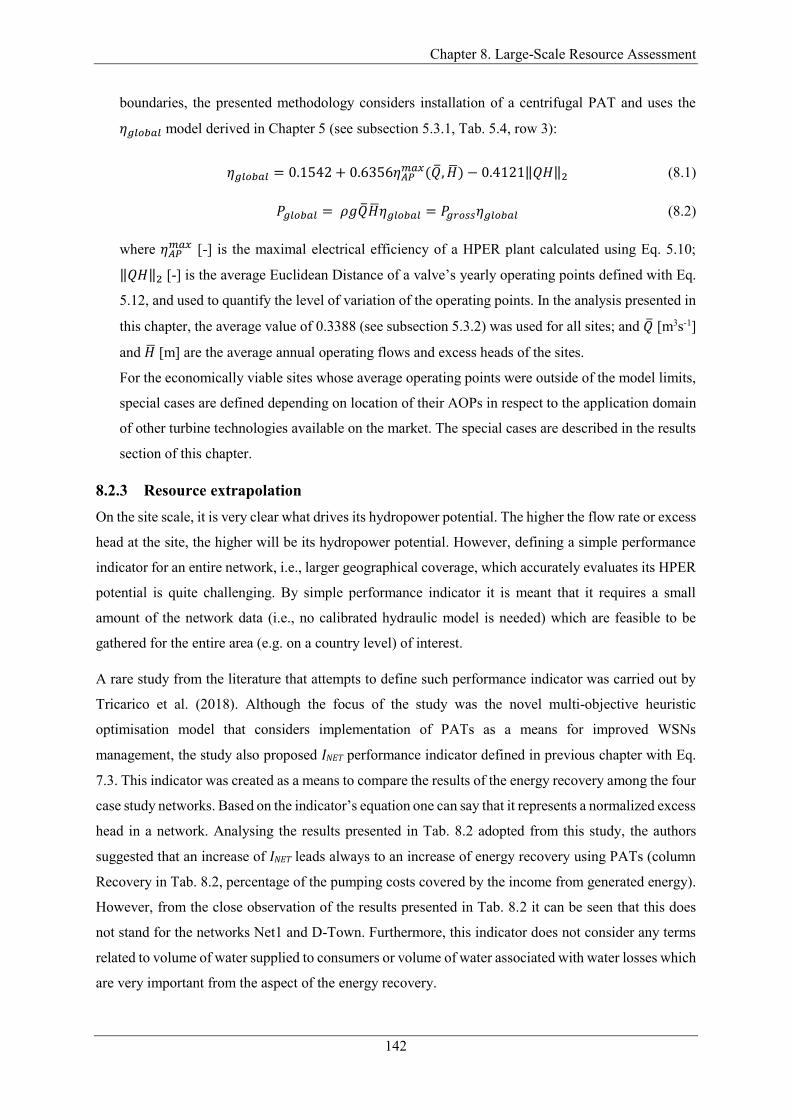
Chapter 8. Large-Scale Resource Assessment
142
boundaries, the presented methodology considers installation of a centrifugal PAT and uses the
𝜂𝑔𝑙𝑜𝑏𝑎𝑙 model derived in Chapter 5 (see subsection 5.3.1, Tab. 5.4, row 3):
𝜂𝑔𝑙𝑜𝑏𝑎𝑙 = 0.1542 + 0.6356𝜂𝐴𝑃𝑚𝑎𝑥(�̅�, �̅�) − 0.4121‖𝑄𝐻‖2 (8.1)
𝑃𝑔𝑙𝑜𝑏𝑎𝑙 = 𝜌𝑔�̅��̅�𝜂𝑔𝑙𝑜𝑏𝑎𝑙 = 𝑃𝑔𝑟𝑜𝑠𝑠𝜂𝑔𝑙𝑜𝑏𝑎𝑙 (8.2)
where 𝜂𝐴𝑃𝑚𝑎𝑥 [-] is the maximal electrical efficiency of a HPER plant calculated using Eq. 5.10;
‖𝑄𝐻‖2 [-] is the average Euclidean Distance of a valve’s yearly operating points defined with Eq.
5.12, and used to quantify the level of variation of the operating points. In the analysis presented in
this chapter, the average value of 0.3388 (see subsection 5.3.2) was used for all sites; and �̅� [m3s-1]
and �̅� [m] are the average annual operating flows and excess heads of the sites.
For the economically viable sites whose average operating points were outside of the model limits,
special cases are defined depending on location of their AOPs in respect to the application domain
of other turbine technologies available on the market. The special cases are described in the results
section of this chapter.
8.2.3 Resource extrapolation
On the site scale, it is very clear what drives its hydropower potential. The higher the flow rate or excess
head at the site, the higher will be its hydropower potential. However, defining a simple performance
indicator for an entire network, i.e., larger geographical coverage, which accurately evaluates its HPER
potential is quite challenging. By simple performance indicator it is meant that it requires a small
amount of the network data (i.e., no calibrated hydraulic model is needed) which are feasible to be
gathered for the entire area (e.g. on a country level) of interest.
A rare study from the literature that attempts to define such performance indicator was carried out by
Tricarico et al. (2018). Although the focus of the study was the novel multi-objective heuristic
optimisation model that considers implementation of PATs as a means for improved WSNs
management, the study also proposed INET performance indicator defined in previous chapter with Eq.
7.3. This indicator was created as a means to compare the results of the energy recovery among the four
case study networks. Based on the indicator’s equation one can say that it represents a normalized excess
head in a network. Analysing the results presented in Tab. 8.2 adopted from this study, the authors
suggested that an increase of INET leads always to an increase of energy recovery using PATs (column
Recovery in Tab. 8.2, percentage of the pumping costs covered by the income from generated energy).
However, from the close observation of the results presented in Tab. 8.2 it can be seen that this does
not stand for the networks Net1 and D-Town. Furthermore, this indicator does not consider any terms
related to volume of water supplied to consumers or volume of water associated with water losses which
are very important from the aspect of the energy recovery.
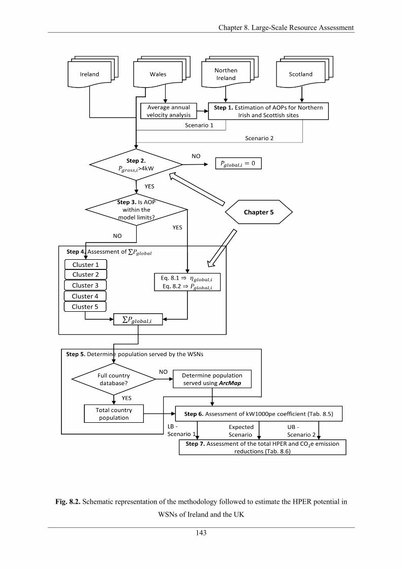
Chapter 8. Large-Scale Resource Assessment
143
Fig. 8.2. Schematic representation of the methodology followed to estimate the HPER potential in
WSNs of Ireland and the UK
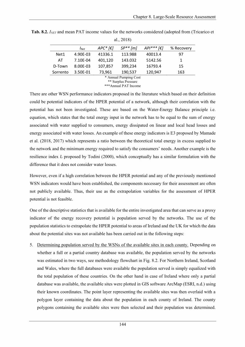
Chapter 8. Large-Scale Resource Assessment
144
Tab. 8.2. INET and mean PAT income values for the networks considered (adopted from (Tricarico et
al., 2018)
INet APC* [€] SP** [m] API*** [€] % Recovery
Net1 4.90E-03 41336.1 113.988 40013.4 97
AT 7.10E-04 401,120 143.032 5142.56 1
D-Town 8.00E-03 107,857 399,234 16793.4 15
Sorrento 3.50E-01 73,961 190,537 120,947 163 * Annual Pumping Cost
** Surplus Pressure
***Annual PAT Income
There are other WSN performance indicators proposed in the literature which based on their definition
could be potential indicators of the HPER potential of a network, although their correlation with the
potential has not been investigated. These are based on the Water-Energy Balance principle i.e.
equation, which states that the total energy input in the network has to be equal to the sum of energy
associated with water supplied to consumers, energy dissipated on linear and local head losses and
energy associated with water losses. An example of these energy indicators is E3 proposed by Mamade
et al. (2018, 2017) which represents a ratio between the theoretical total energy in excess supplied to
the network and the minimum energy required to satisfy the consumers’ needs. Another example is the
resilience index Ir proposed by Todini (2000), which conceptually has a similar formulation with the
difference that it does not consider water losses.
However, even if a high correlation between the HPER potential and any of the previously mentioned
WSN indicators would have been established, the components necessary for their assessment are often
not publicly available. Thus, their use as the extrapolation variables for the assessment of HPER
potential is not feasible.
One of the descriptive statistics that is available for the entire investigated area that can serve as a proxy
indicator of the energy recovery potential is population served by the networks. The use of the
population statistics to extrapolate the HPER potential to areas of Ireland and the UK for which the data
about the potential sites was not available has been carried out in the following steps:
5. Determining population served by the WSNs of the available sites in each county. Depending on
whether a full or a partial country database was available, the population served by the networks
was estimated in two ways, see methodology flowchart in Fig. 8.2. For Northern Ireland, Scotland
and Wales, where the full databases were available the population served is simply equalized with
the total population of these countries. On the other hand in case of Ireland where only a partial
database was available, the available sites were plotted in GIS software ArcMap (ESRI, n.d.) using
their known coordinates. The point layer representing the available sites was then overlaid with a
polygon layer containing the data about the population in each county of Ireland. The county
polygons containing the available sites were then selected and their population was determined.
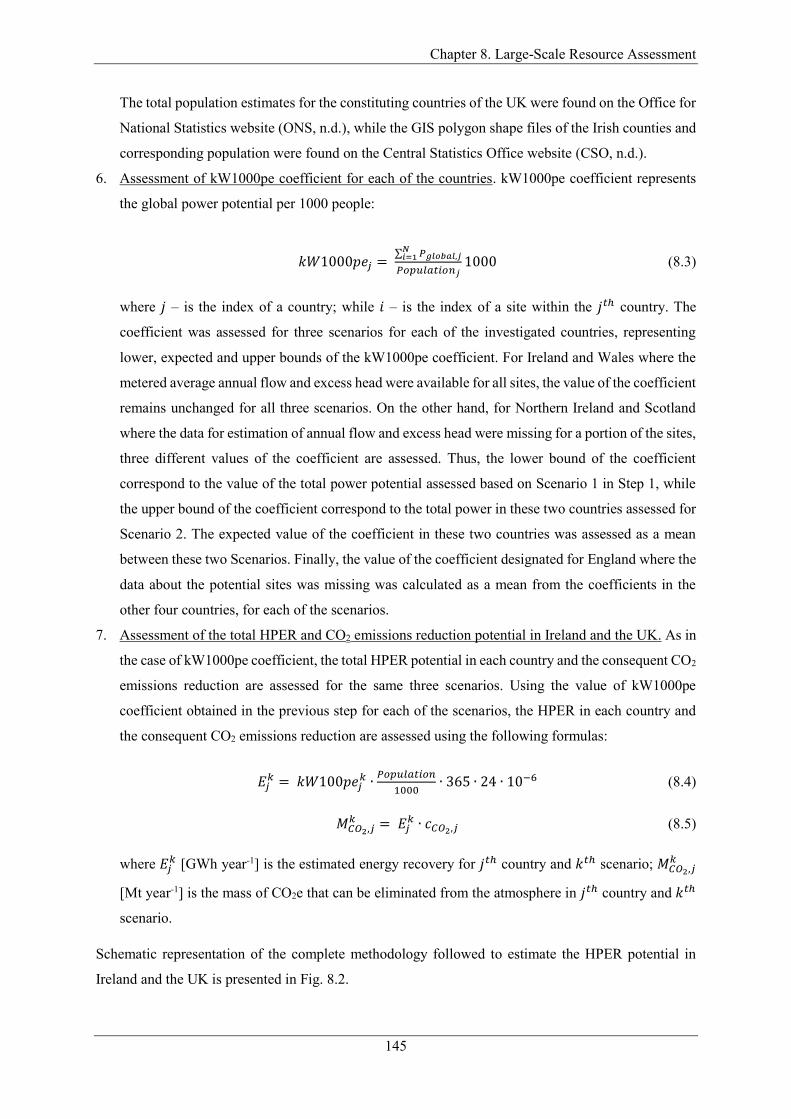
Chapter 8. Large-Scale Resource Assessment
145
The total population estimates for the constituting countries of the UK were found on the Office for
National Statistics website (ONS, n.d.), while the GIS polygon shape files of the Irish counties and
corresponding population were found on the Central Statistics Office website (CSO, n.d.).
6. Assessment of kW1000pe coefficient for each of the countries. kW1000pe coefficient represents
the global power potential per 1000 people:
𝑘𝑊1000𝑝𝑒𝑗 = ∑ 𝑃𝑔𝑙𝑜𝑏𝑎𝑙,𝑗
𝑁𝑖=1
𝑃𝑜𝑝𝑢𝑙𝑎𝑡𝑖𝑜𝑛𝑗1000 (8.3)
where 𝑗 – is the index of a country; while 𝑖 – is the index of a site within the 𝑗𝑡ℎ country. The
coefficient was assessed for three scenarios for each of the investigated countries, representing
lower, expected and upper bounds of the kW1000pe coefficient. For Ireland and Wales where the
metered average annual flow and excess head were available for all sites, the value of the coefficient
remains unchanged for all three scenarios. On the other hand, for Northern Ireland and Scotland
where the data for estimation of annual flow and excess head were missing for a portion of the sites,
three different values of the coefficient are assessed. Thus, the lower bound of the coefficient
correspond to the value of the total power potential assessed based on Scenario 1 in Step 1, while
the upper bound of the coefficient correspond to the total power in these two countries assessed for
Scenario 2. The expected value of the coefficient in these two countries was assessed as a mean
between these two Scenarios. Finally, the value of the coefficient designated for England where the
data about the potential sites was missing was calculated as a mean from the coefficients in the
other four countries, for each of the scenarios.
7. Assessment of the total HPER and CO2 emissions reduction potential in Ireland and the UK. As in
the case of kW1000pe coefficient, the total HPER potential in each country and the consequent CO2
emissions reduction are assessed for the same three scenarios. Using the value of kW1000pe
coefficient obtained in the previous step for each of the scenarios, the HPER in each country and
the consequent CO2 emissions reduction are assessed using the following formulas:
𝐸𝑗𝑘 = 𝑘𝑊100𝑝𝑒𝑗
𝑘 ∙𝑃𝑜𝑝𝑢𝑙𝑎𝑡𝑖𝑜𝑛
1000∙ 365 ∙ 24 ∙ 10−6 (8.4)
𝑀𝐶𝑂2,𝑗𝑘 = 𝐸𝑗
𝑘 ∙ 𝑐𝐶𝑂2,𝑗 (8.5)
where 𝐸𝑗𝑘 [GWh year-1] is the estimated energy recovery for 𝑗𝑡ℎ country and 𝑘𝑡ℎ scenario; 𝑀𝐶𝑂2,𝑗
𝑘
[Mt year-1] is the mass of CO2e that can be eliminated from the atmosphere in 𝑗𝑡ℎ country and 𝑘𝑡ℎ
scenario.
Schematic representation of the complete methodology followed to estimate the HPER potential in
Ireland and the UK is presented in Fig. 8.2.
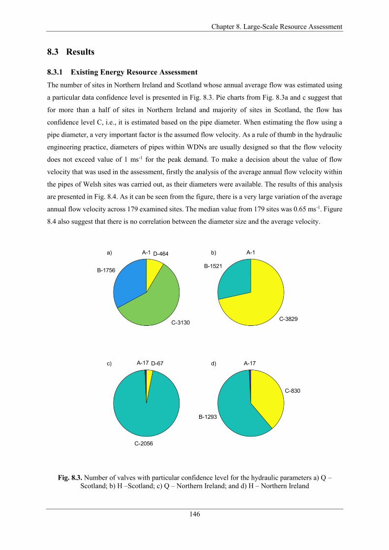
Chapter 8. Large-Scale Resource Assessment
146
8.3 Results
8.3.1 Existing Energy Resource Assessment
The number of sites in Northern Ireland and Scotland whose annual average flow was estimated using
a particular data confidence level is presented in Fig. 8.3. Pie charts from Fig. 8.3a and c suggest that
for more than a half of sites in Northern Ireland and majority of sites in Scotland, the flow has
confidence level C, i.e., it is estimated based on the pipe diameter. When estimating the flow using a
pipe diameter, a very important factor is the assumed flow velocity. As a rule of thumb in the hydraulic
engineering practice, diameters of pipes within WDNs are usually designed so that the flow velocity
does not exceed value of 1 ms-1 for the peak demand. To make a decision about the value of flow
velocity that was used in the assessment, firstly the analysis of the average annual flow velocity within
the pipes of Welsh sites was carried out, as their diameters were available. The results of this analysis
are presented in Fig. 8.4. As it can be seen from the figure, there is a very large variation of the average
annual flow velocity across 179 examined sites. The median value from 179 sites was 0.65 ms-1. Figure
8.4 also suggest that there is no correlation between the diameter size and the average velocity.
Fig. 8.3. Number of valves with particular confidence level for the hydraulic parameters a) Q –
Scotland; b) H –Scotland; c) Q – Northern Ireland; and d) H – Northern Ireland

Chapter 8. Large-Scale Resource Assessment
147
Fig. 8.4. Average flow velocity assessment for Welsh sites.
Fig. 8.5. Cumulative frequency distributions (CDF) of maximum diurnal velocity per pipe length
(adopted from Abraham et al. (2018)).

Chapter 8. Large-Scale Resource Assessment
148
Because of the very large variation of the average annual flow velocity among 179 Welsh sites, the
literature was further consulted to inform the final decision. Abraham et al. (2018) proposed an
algorithm for decreasing the risk of discoloration of drinking WDNs through optimisation of topological
changes and optimal flow velocity control. The proposed algorithm increases the flow velocity within
the pipes by isolating particular branches and making a more branched network in peak hours, thus
improving self-cleaning capacity of the network. Figure 8.5, adopted from that study presents the
cumulative distribution function of the maximal diurnal velocity per pipe length in the analysed Dutch
network. As it can be seen from the figure in the ordinary or looped state (black curve) the maximal
diurnal velocity does not exceed value of 0.5 ms-1 for any of the pipes, while for the modified branch
topologies the pipes with the highest flow velocities reach values of around 1 ms-1 in the peak hours.
Mamade et al. (2018) carried out another study that observed flow velocity within WSNs. This paper
proposed Top-Down (simplified, requires less input data) and Bottom-Up (detailed, requires a hydraulic
network model) approaches for the assessment of water-energy balance components. The study
investigated 20 WSNs in Portugal, finding that the average velocity weighted by pipe length ranged
between 0.02 and 0.2 ms-1, with a median of 0.08 ms-1. The authors claimed that the very low velocities
in the Portuguese networks (even below the national legislation) are the consequence of the
overdesigned systems due to firefighting requirements and overestimation of population.
Considering all of these findings, and assuming that the Scottish and Northern Irish networks are more
similar to the Welsh ones, it was decided to use a value of 0.6 ms-1.
From Fig. 8.3 it can be also seen that in both countries much larger portion of the sites are missing data
for estimation of the excess head (confidence level C - yellow part of the pie charts b and d) than for
estimation of the flow (confidence level D – yellow part of pie charts a and c). This was the main reason
for considering two scenarios for the estimation of the excess head available at the sites with missing
head data. The values of �̅�𝑎𝑣𝑒 calculated to be used in Scenario 2 amounted 31.88m and 32.90m for
Northern Irish and Scottish sites, respectively.
Tab. 8.3. Assessment of ∑𝑃𝑔𝑙𝑜𝑏𝑎𝑙 per country for Scenario 1
Country
# of
included
sites
# with
D>150mm
# of
economically
viable sites
% of
economically
viable
# outside
𝜂𝑔𝑙𝑜𝑏𝑎𝑙
model
limits
𝜂𝑔𝑙𝑜𝑏𝑎𝑙̅̅ ̅̅ ̅̅ ̅̅ ̅
[-]
∑𝑃𝑔𝑙𝑜𝑏𝑎𝑙
[kW]
Ireland 44 44 26 59.09 3 0.51 742.33
Northern
Ireland 1300 53 52 2.43 6 0.42 350.06
Scotland 1514 773 344 6.43 9 0.42 1986.55
Wales 179 179 75 41.90 2 0.44 751.74
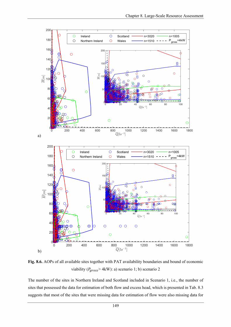
Chapter 8. Large-Scale Resource Assessment
149
a)
b)
Fig. 8.6. AOPs of all available sites together with PAT availability boundaries and bound of economic
viability (𝑃𝑔𝑟𝑜𝑠𝑠> 4kW): a) scenario 1; b) scenario 2
The number of the sites in Northern Ireland and Scotland included in Scenario 1, i.e., the number of
sites that possessed the data for estimation of both flow and excess head, which is presented in Tab. 8.3
suggests that most of the sites that were missing data for estimation of flow were also missing data for
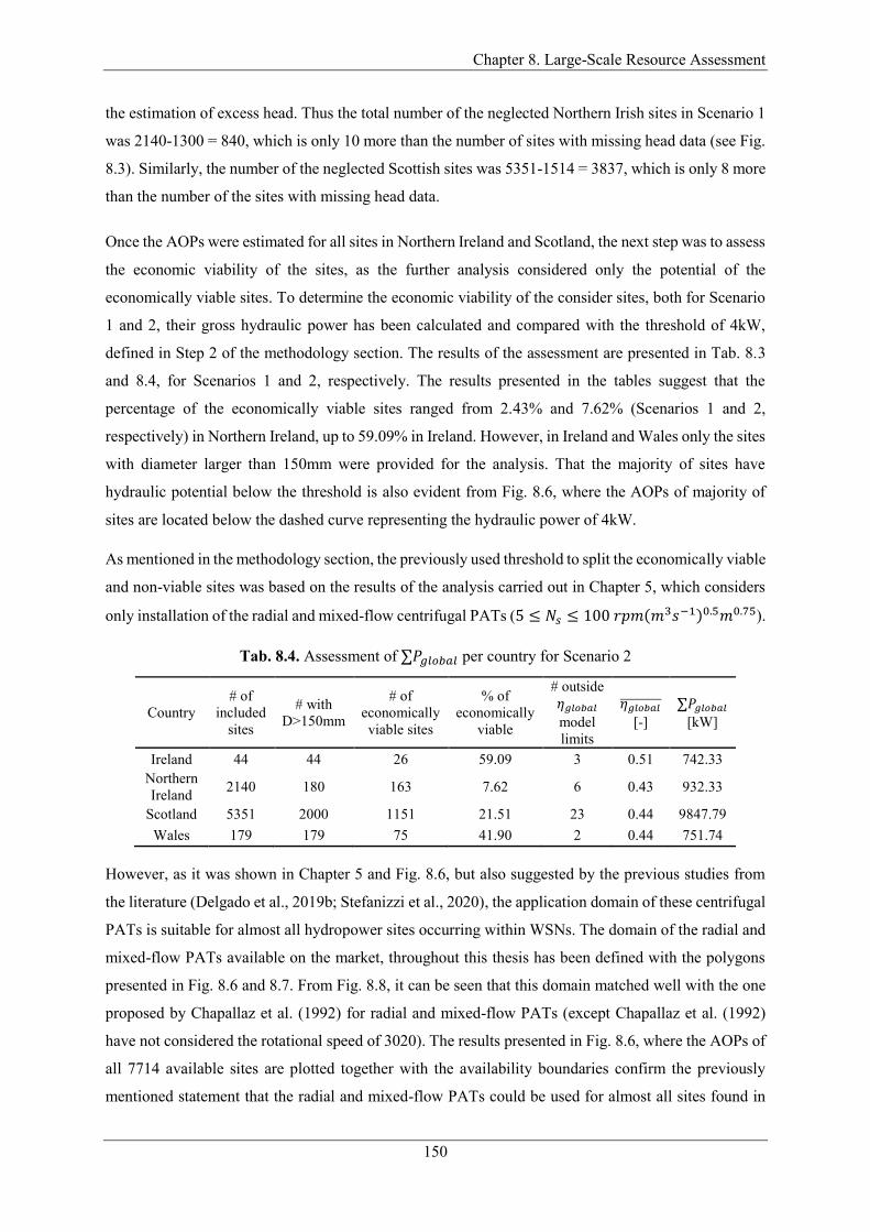
Chapter 8. Large-Scale Resource Assessment
150
the estimation of excess head. Thus the total number of the neglected Northern Irish sites in Scenario 1
was 2140-1300 = 840, which is only 10 more than the number of sites with missing head data (see Fig.
8.3). Similarly, the number of the neglected Scottish sites was 5351-1514 = 3837, which is only 8 more
than the number of the sites with missing head data.
Once the AOPs were estimated for all sites in Northern Ireland and Scotland, the next step was to assess
the economic viability of the sites, as the further analysis considered only the potential of the
economically viable sites. To determine the economic viability of the consider sites, both for Scenario
1 and 2, their gross hydraulic power has been calculated and compared with the threshold of 4kW,
defined in Step 2 of the methodology section. The results of the assessment are presented in Tab. 8.3
and 8.4, for Scenarios 1 and 2, respectively. The results presented in the tables suggest that the
percentage of the economically viable sites ranged from 2.43% and 7.62% (Scenarios 1 and 2,
respectively) in Northern Ireland, up to 59.09% in Ireland. However, in Ireland and Wales only the sites
with diameter larger than 150mm were provided for the analysis. That the majority of sites have
hydraulic potential below the threshold is also evident from Fig. 8.6, where the AOPs of majority of
sites are located below the dashed curve representing the hydraulic power of 4kW.
As mentioned in the methodology section, the previously used threshold to split the economically viable
and non-viable sites was based on the results of the analysis carried out in Chapter 5, which considers
only installation of the radial and mixed-flow centrifugal PATs (5 ≤ 𝑁𝑠 ≤ 100 𝑟𝑝𝑚(𝑚3𝑠−1)0.5𝑚0.75).
Tab. 8.4. Assessment of ∑𝑃𝑔𝑙𝑜𝑏𝑎𝑙 per country for Scenario 2
Country
# of
included
sites
# with
D>150mm
# of
economically
viable sites
% of
economically
viable
# outside
𝜂𝑔𝑙𝑜𝑏𝑎𝑙
model
limits
𝜂𝑔𝑙𝑜𝑏𝑎𝑙̅̅ ̅̅ ̅̅ ̅̅ ̅
[-]
∑𝑃𝑔𝑙𝑜𝑏𝑎𝑙
[kW]
Ireland 44 44 26 59.09 3 0.51 742.33
Northern
Ireland 2140 180 163 7.62 6 0.43 932.33
Scotland 5351 2000 1151 21.51 23 0.44 9847.79
Wales 179 179 75 41.90 2 0.44 751.74
However, as it was shown in Chapter 5 and Fig. 8.6, but also suggested by the previous studies from
the literature (Delgado et al., 2019b; Stefanizzi et al., 2020), the application domain of these centrifugal
PATs is suitable for almost all hydropower sites occurring within WSNs. The domain of the radial and
mixed-flow PATs available on the market, throughout this thesis has been defined with the polygons
presented in Fig. 8.6 and 8.7. From Fig. 8.8, it can be seen that this domain matched well with the one
proposed by Chapallaz et al. (1992) for radial and mixed-flow PATs (except Chapallaz et al. (1992)
have not considered the rotational speed of 3020). The results presented in Fig. 8.6, where the AOPs of
all 7714 available sites are plotted together with the availability boundaries confirm the previously
mentioned statement that the radial and mixed-flow PATs could be used for almost all sites found in

Chapter 8. Large-Scale Resource Assessment
151
WSNs. Namely, Tab. 8.3 and 8.4 show that only 20 and 34 sites have their AOPs outside of the defined
boundaries for Scenarios 1 and 2, respectively.
a)
b)
Fig. 8.7. Cluster of sites outside the prediction model limits. a) Scenario 1 b) scenario 2
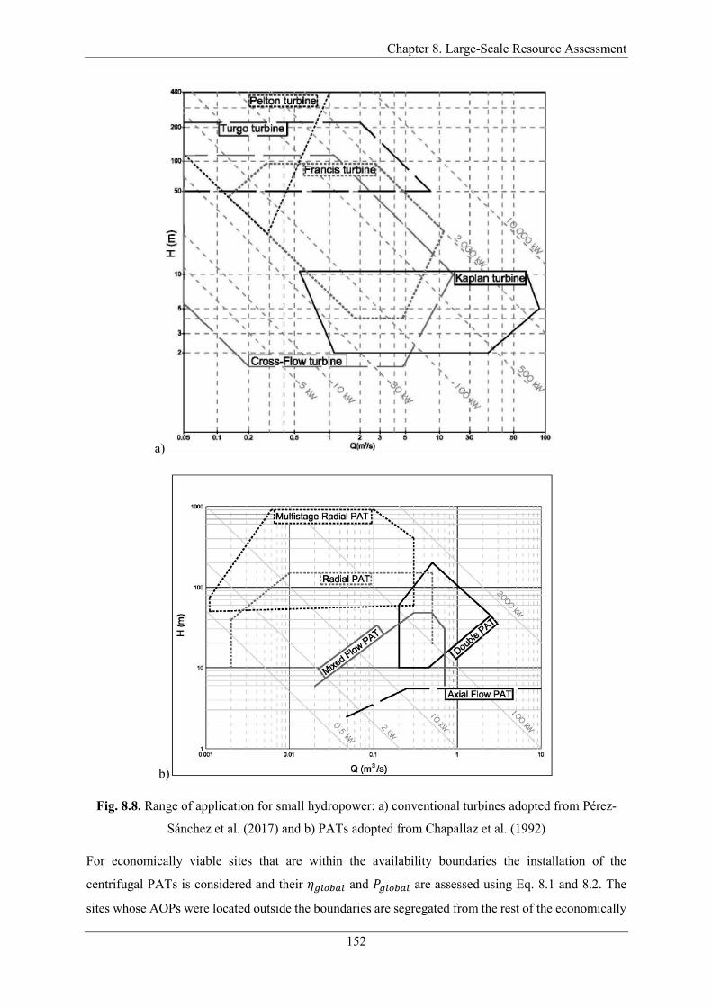
Chapter 8. Large-Scale Resource Assessment
152
a)
b)
Fig. 8.8. Range of application for small hydropower: a) conventional turbines adopted from Pérez-
Sánchez et al. (2017) and b) PATs adopted from Chapallaz et al. (1992)
For economically viable sites that are within the availability boundaries the installation of the
centrifugal PATs is considered and their 𝜂𝑔𝑙𝑜𝑏𝑎𝑙 and 𝑃𝑔𝑙𝑜𝑏𝑎𝑙 are assessed using Eq. 8.1 and 8.2. The
sites whose AOPs were located outside the boundaries are segregated from the rest of the economically
Chapter 8. Large-Scale Resource Assessment
153
viable sites and presented in Fig. 8.7. In Fig. 8.7, four different clusters can be differentiated for Scenario
1 and five for Scenario 2. Clusters 1, 2, 4 and 5 include the same sets of sites in both Scenarios. The
location of the identified clusters in Q-H space were compared with the application domain of the
turbines available on the market and their potentials were assessed in the following ways:
Cluster 1 and 2. Considering the proximity of the AOPs from Clusters 1 and 2 to the availability
boundaries of the centrifugal PATs, i.e., the limits of the application of the model defined with
Eq. 8.1, it was decided to use the same model for these sites as well. However, to calculate 𝜂𝐴𝑃
in Eq. 8.1 only one rotational speed whose boundary was the closest to the considered AOP
was used.
Cluster 3. This cluster consists of three sites, two Scottish and one Irish. All of these sites have
an available excess head less than 6m and thus these are not suitable for the radial or mixed-
flow centrifugal PATs. The gross hydraulic power of these sites is above the theoretical limits
of 4 kW defined in Chapter 5, however this analysis does not consider sites below 10m.
According to Fig. 8.8b, there is a possibility that the potential of these sites could be exploited
with the axial PATs. Nevertheless, as this cluster included only small number of sites whose
potential would not make a significant difference in the overall potential of the considered
countries, the potential of these sites is neglected.
Cluster 4. This cluster includes 14 Scottish sites (some points overlap), which are only
considered in Scenario 2, meaning that these are missing head data. Comparing the AOPs of
the sites with the application domain of the PATs available on the market (see Fig. 8.8b) it
seems that double-flow PATs would be suitable for installation at these sites. Although for the
smallest site in the cluster the radial or mixed-flow PATs would probably be a good fit as well.
Considering the size of the potential of these sites, it is reasonable to assume that the installation
of the conventional turbines would be economically viable as well. From the application
domain of the conventional turbines from small hydropower schemes presented in Fig. 8.8a,
one can conclude that Francis and Cross-flow turbines would be suitable for installation at these
sites. Finally, it was decided to select Francis turbines for installation at these sites, whose peak
efficiency is estimated as 0.94 according to ESHA (2004). 𝜂𝑔𝑙𝑜𝑏𝑎𝑙 of these sites is assessed by
multiplying the turbine peak efficiency with a coefficient of 0.8 to consider the influence of the
variation of flow and excess head. A potential alternative for exploitation of the entire potential
available at these sites would be installation of two or three radial or mixed-flow PATs in
parallel.
Cluster 5. This cluster includes two Irish sites characterized with very high flow and low head,
see Fig. 8.7. According to Fig. 8.8 none of the PAT types suit well to these sites, while out of
the conventional turbines the suitable types are Francis, Cross-flow and Kaplan. Because of the
low excess head of these sites, Kaplan turbines are selected. According to ESHA (2004), the
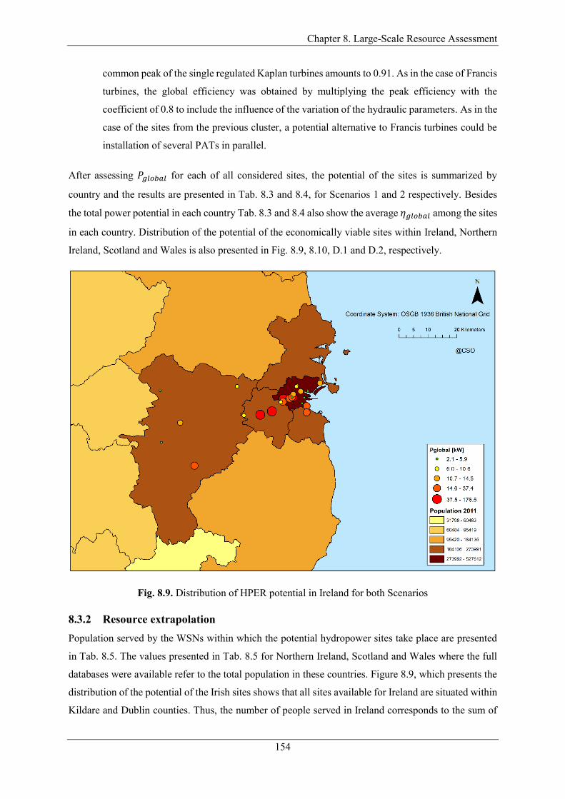
Chapter 8. Large-Scale Resource Assessment
154
common peak of the single regulated Kaplan turbines amounts to 0.91. As in the case of Francis
turbines, the global efficiency was obtained by multiplying the peak efficiency with the
coefficient of 0.8 to include the influence of the variation of the hydraulic parameters. As in the
case of the sites from the previous cluster, a potential alternative to Francis turbines could be
installation of several PATs in parallel.
After assessing 𝑃𝑔𝑙𝑜𝑏𝑎𝑙 for each of all considered sites, the potential of the sites is summarized by
country and the results are presented in Tab. 8.3 and 8.4, for Scenarios 1 and 2 respectively. Besides
the total power potential in each country Tab. 8.3 and 8.4 also show the average 𝜂𝑔𝑙𝑜𝑏𝑎𝑙 among the sites
in each country. Distribution of the potential of the economically viable sites within Ireland, Northern
Ireland, Scotland and Wales is also presented in Fig. 8.9, 8.10, D.1 and D.2, respectively.
Fig. 8.9. Distribution of HPER potential in Ireland for both Scenarios
8.3.2 Resource extrapolation
Population served by the WSNs within which the potential hydropower sites take place are presented
in Tab. 8.5. The values presented in Tab. 8.5 for Northern Ireland, Scotland and Wales where the full
databases were available refer to the total population in these countries. Figure 8.9, which presents the
distribution of the potential of the Irish sites shows that all sites available for Ireland are situated within
Kildare and Dublin counties. Thus, the number of people served in Ireland corresponds to the sum of
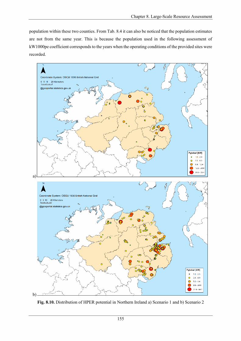
Chapter 8. Large-Scale Resource Assessment
155
population within these two counties. From Tab. 8.4 it can also be noticed that the population estimates
are not from the same year. This is because the population used in the following assessment of
kW1000pe coefficient corresponds to the years when the operating conditions of the provided sites were
recorded.
a)
b)
Fig. 8.10. Distribution of HPER potential in Northern Ireland a) Scenario 1 and b) Scenario 2
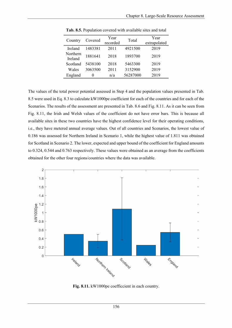
Chapter 8. Large-Scale Resource Assessment
156
Tab. 8.5. Population covered with available sites and total
Country Covered Year
recorded Total
Year
extrapolated
Ireland 1483381 2011 4921500 2019
Northern
Ireland 1881641 2018 1893700 2019
Scotland 5438100 2018 5463300 2019
Wales 3063500 2011 3152900 2019
England 0 n/a 56287000 2019
The values of the total power potential assessed in Step 4 and the population values presented in Tab.
8.5 were used in Eq. 8.3 to calculate kW1000pe coefficient for each of the countries and for each of the
Scenarios. The results of the assessment are presented in Tab. 8.6 and Fig. 8.11. As it can be seen from
Fig. 8.11, the Irish and Welsh values of the coefficient do not have error bars. This is because all
available sites in these two countries have the highest confidence level for their operating conditions,
i.e., they have metered annual average values. Out of all countries and Scenarios, the lowest value of
0.186 was assessed for Northern Ireland in Scenario 1, while the highest value of 1.811 was obtained
for Scotland in Scenario 2. The lower, expected and upper bound of the coefficient for England amounts
to 0.324, 0.544 and 0.763 respectively. These values were obtained as an average from the coefficients
obtained for the other four regions/countries where the data was available.
Fig. 8.11. kW1000pe coefficcient in each country.
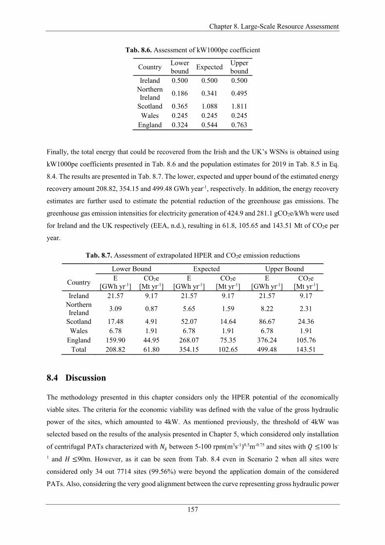
Chapter 8. Large-Scale Resource Assessment
157
Tab. 8.6. Assessment of kW1000pe coefficient
Country Lower
bound Expected
Upper
bound
Ireland 0.500 0.500 0.500
Northern
Ireland 0.186 0.341 0.495
Scotland 0.365 1.088 1.811
Wales 0.245 0.245 0.245
England 0.324 0.544 0.763
Finally, the total energy that could be recovered from the Irish and the UK’s WSNs is obtained using
kW1000pe coefficients presented in Tab. 8.6 and the population estimates for 2019 in Tab. 8.5 in Eq.
8.4. The results are presented in Tab. 8.7. The lower, expected and upper bound of the estimated energy
recovery amount 208.82, 354.15 and 499.48 GWh year-1, respectively. In addition, the energy recovery
estimates are further used to estimate the potential reduction of the greenhouse gas emissions. The
greenhouse gas emission intensities for electricity generation of 424.9 and 281.1 gCO2e/kWh were used
for Ireland and the UK respectively (EEA, n.d.), resulting in 61.8, 105.65 and 143.51 Mt of CO2e per
year.
Tab. 8.7. Assessment of extrapolated HPER and CO2e emission reductions
Lower Bound Expected Upper Bound
Country E
[GWh yr-1]
CO2e
[Mt yr-1]
E
[GWh yr-1]
CO2e
[Mt yr-1]
E
[GWh yr-1]
CO2e
[Mt yr-1]
Ireland 21.57 9.17 21.57 9.17 21.57 9.17
Northern
Ireland 3.09 0.87 5.65 1.59 8.22 2.31
Scotland 17.48 4.91 52.07 14.64 86.67 24.36
Wales 6.78 1.91 6.78 1.91 6.78 1.91
England 159.90 44.95 268.07 75.35 376.24 105.76
Total 208.82 61.80 354.15 102.65 499.48 143.51
8.4 Discussion
The methodology presented in this chapter considers only the HPER potential of the economically
viable sites. The criteria for the economic viability was defined with the value of the gross hydraulic
power of the sites, which amounted to 4kW. As mentioned previously, the threshold of 4kW was
selected based on the results of the analysis presented in Chapter 5, which considered only installation
of centrifugal PATs characterized with 𝑁𝑠 between 5-100 rpm(m3s-1)0.5m-0.75 and sites with 𝑄 ≤100 ls-
1 and 𝐻 ≤90m. However, as it can be seen from Tab. 8.4 even in Scenario 2 when all sites were
considered only 34 out 7714 sites (99.56%) were beyond the application domain of the considered
PATs. Also, considering the very good alignment between the curve representing gross hydraulic power
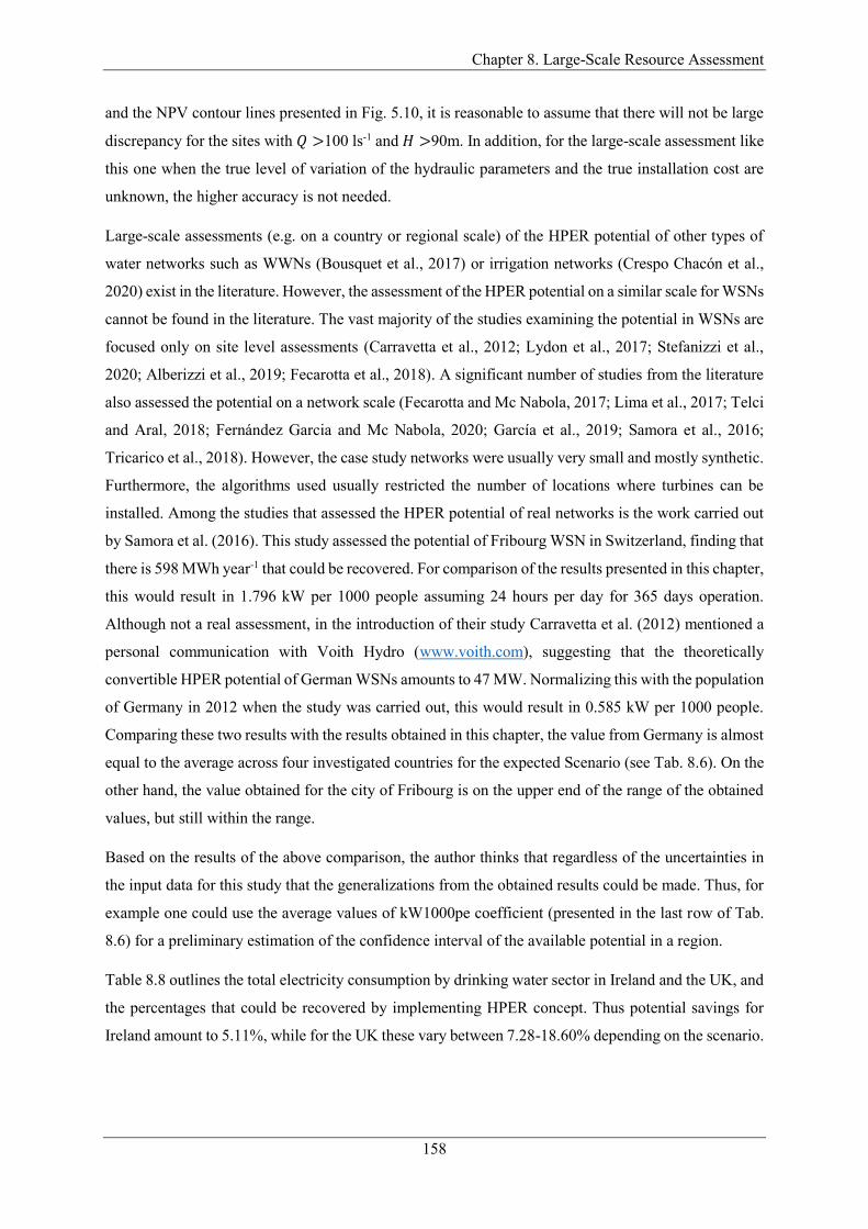
Chapter 8. Large-Scale Resource Assessment
158
and the NPV contour lines presented in Fig. 5.10, it is reasonable to assume that there will not be large
discrepancy for the sites with 𝑄 >100 ls-1 and 𝐻 >90m. In addition, for the large-scale assessment like
this one when the true level of variation of the hydraulic parameters and the true installation cost are
unknown, the higher accuracy is not needed.
Large-scale assessments (e.g. on a country or regional scale) of the HPER potential of other types of
water networks such as WWNs (Bousquet et al., 2017) or irrigation networks (Crespo Chacón et al.,
2020) exist in the literature. However, the assessment of the HPER potential on a similar scale for WSNs
cannot be found in the literature. The vast majority of the studies examining the potential in WSNs are
focused only on site level assessments (Carravetta et al., 2012; Lydon et al., 2017; Stefanizzi et al.,
2020; Alberizzi et al., 2019; Fecarotta et al., 2018). A significant number of studies from the literature
also assessed the potential on a network scale (Fecarotta and Mc Nabola, 2017; Lima et al., 2017; Telci
and Aral, 2018; Fernández Garcia and Mc Nabola, 2020; García et al., 2019; Samora et al., 2016;
Tricarico et al., 2018). However, the case study networks were usually very small and mostly synthetic.
Furthermore, the algorithms used usually restricted the number of locations where turbines can be
installed. Among the studies that assessed the HPER potential of real networks is the work carried out
by Samora et al. (2016). This study assessed the potential of Fribourg WSN in Switzerland, finding that
there is 598 MWh year-1 that could be recovered. For comparison of the results presented in this chapter,
this would result in 1.796 kW per 1000 people assuming 24 hours per day for 365 days operation.
Although not a real assessment, in the introduction of their study Carravetta et al. (2012) mentioned a
personal communication with Voith Hydro (www.voith.com), suggesting that the theoretically
convertible HPER potential of German WSNs amounts to 47 MW. Normalizing this with the population
of Germany in 2012 when the study was carried out, this would result in 0.585 kW per 1000 people.
Comparing these two results with the results obtained in this chapter, the value from Germany is almost
equal to the average across four investigated countries for the expected Scenario (see Tab. 8.6). On the
other hand, the value obtained for the city of Fribourg is on the upper end of the range of the obtained
values, but still within the range.
Based on the results of the above comparison, the author thinks that regardless of the uncertainties in
the input data for this study that the generalizations from the obtained results could be made. Thus, for
example one could use the average values of kW1000pe coefficient (presented in the last row of Tab.
8.6) for a preliminary estimation of the confidence interval of the available potential in a region.
Table 8.8 outlines the total electricity consumption by drinking water sector in Ireland and the UK, and
the percentages that could be recovered by implementing HPER concept. Thus potential savings for
Ireland amount to 5.11%, while for the UK these vary between 7.28-18.60% depending on the scenario.

Chapter 8. Large-Scale Resource Assessment
159
Tab. 8.8. Electricity consumption estimates by the sector in Ireland and the UK, compared with
extrapolated HPER potential
Electricity
Consumption
E [GWh yr-1] Savings [%]
Lower
bound
Upper
bound
Lower
bound
Upper
bound
Ireland 422.0 21.6 21.6 5.1 5.1
UK 2570.0 187.2 477.9 7.3 18.6
The large-scale analysis conducted here presents some limitations and results should be treated in light
of the methodology used. Firstly, some sites found to be economically viable could prove to be non-
viable on detailed assessment, due to the unknown variability of the operating conditions and
uncertainty about the installation costs. Secondly, as outlined in the methodology section the analysis
also only considered the HPER potential from existing locations with excess head and not all possible
locations, which would have required access to numerous hydraulic models.
In examining the distribution of potential installation sizes across 7714 sites, it was found that only 18%
of all sites are economically viable. In other words the entire energy recovery potential comes only from
18% of sites, see Fig. 8.12. Moreover, the installations with a gross hydraulic power over 30 kW
represented only around 2% of the total number of sites. Nevertheless, it was found that these could
produce around 52% of the total energy recovery potential available in the examined WSNs. Figure
8.12 highlights that a significant proportion of the energy potential estimated in this study could be
exploited by installing HPER plants in only a small number of the sites. The values presented in Fig.
8.12 correspond to Scenario 2, i.e., when the average networks’ excess heads were assumed for the
Northern Irish and Scottish sites that are missing head data. The values obtained for Scenario 1 go even
more in favor of this statement.
Fig. 8.12. Distribution of (a) number of available sites and (b) their HPER estimates; between the pre-
defined ranges of plant power sizes
Chapter 8. Large-Scale Resource Assessment
160
The potential HPER installations identified here could cumulatively make a valuable contribution to
net energy efficiency gains and CO2 emission reductions in the EU’s water sector. This is also
significant as it demonstrates cost-effective, value-added, multi-country benefits to policy makers,
establishing the case to promote and incentivize HPER installations to help achieve the desired CO2
emissions reduction targets in the sector.
8.5 Conclusions
The aim of this chapter was to develop a methodology for assessment of the HPER potential within
WSNs on a country or multi-country scale, and to use this methodology for estimation of the potential
in Ireland and the UK. To estimate the potential of the areas where the data about potential sites was
not available, the methodology defines kW1000pe coefficient which represents the available power
potential per 1000 people. Depending on country and scenario the value of the coefficient ranged from
0.186 up to 1.811, see Tab. 8.6. The total annual potential for energy production using the HPER
concept in the Irish and the UK’s WSNs was estimated in the range 208.8 to 499.48 GWh, depending
on the scenario. This energy was shown to represent a potential reduction in the electricity demand of
the sector by 5.11% and 7.28-18.60% (depending on the extrapolation scenario), in Ireland and the UK,
respectively. The results also suggest that more than a half of the potential from the available sites could
be captured by replacing (or coupling) only around 2% of the valves whose gross hydraulic power is
greater than 30 kW. The potential HPER installations identified here at existing WSN infrastructure,
could make a valuable contribution to improving the sustainability of the EU’s drinking water sector.
Incentivization and regulation of installations of this kind could prove to be a valuable mechanism in
achieving the desired CO2 emissions reduction targets in the sector.
The future work will be focused on defining a simple performance indicator of WSNs that could be
used to accurately estimate the HPER potential of WSNs. Components needed to define such an
indicator will probably never be able to be gathered for a larger geographical coverage because of the
confidentiality issues. However, it should allow water utilities to accurately estimate their HPER
potential in a simple manner.
Chapter 9. Discussion
161
9 Discussion
This chapter briefly recapitulates the main aims of Chapters 4, 5, 6, 7 and 8, their methods and case
studies used. Then it briefly summaries their main results and findings, continuing with their discussion,
outlining the relevance and impact that these are expected to have in the field.
9.1 Chapter 4: Optimisation-Based Methodology for Selection of a PAT in
WDNs
The main aim of Chapter 4 was to develop a novel comprehensive optimisation-based methodology for
the selection of a PAT available on the market that can be used as HPER device at locations of existing
PRVs, characterized by large variation of operating conditions. The comprehensiveness of the
methodology refers to its suitability to be applied for PRV sites of any operating conditions commonly
occurring within WDNs. The methodology implements a HR scheme with two control valves equipped
with a single-stage centrifugal or mixed-flow PAT whose performance is predicted using the equations
proposed by Novara and McNabola (2018) and Novara et al. (2017). The novelties of the presented
methodology include the application of NMSDS heuristic optimisation algorithm to converge through
the solution space, which is constrained with the availability limits of the single-stage centrifugal and
mixed-flow PATs on the market. In addition, an important novelty of the methodology is the restriction
of the PAT’s operation limits using the values of the generated mechanical power.
Because of the novel features of the proposed methodology (optimisation-based and operation limits
defined based on relative mechanical power), it was particularly suitable for addressing the following
two questions: Can the selection of different objectives lead to the selection of different commercially
available PAT families? And can different operational limits lead to the selection of different
commercially available PAT families? The results presented in Chapter 4 gave positive answers to both
of these questions.
The influences of the objective function and PAT operational limits on the selection of the optimal PAT
were both examined on three Irish sites that were previously used in the literature (Lydon et al., 2017)
and whose operating conditions were recorded for the period of 420 days with recording step of 15min.

Chapter 9. Discussion
162
In the test examining the influence of the objective function, the following three objectives have been
used: maximization of energy recovery, maximization of NPV after 10 years and minimization of PP.
The obtained results suggested that the maximization of energy recovery leads to the selection of the
theoretically largest PAT and that the minimization of PP leads to selection of the theoretically smallest
machine, while the solutions obtained by maximizing NPV objective were in between. For perspective,
the average ratios (𝑄𝐵𝐸𝑃/𝑄𝐴𝑂𝑃; 𝐻𝐵𝐸𝑃/𝐻𝐴𝑂𝑃) across three examined sites had the following values:
(0.92; 0.85), (0.87, 0.78) and (0.64, 0.75), for maximization of energy recovery, maximization of NPV
and minimization of PP, respectively. The results also suggested that regardless of the optimal speed of
the theoretically optimal solutions, all available rotational speeds should be considered because of the
discrete nature of the commercial families available on the market.
Surprisingly, the operation limits of PATs are not always indicated in the studies that investigated the
installation of PATs in WSNs, and their influence on the selection of the optimal commercially available
solution has never been discussed in the literature. In studies that indicated the operation limits, the
maximal permissible flow ranged from 𝑄𝐵𝐸𝑃 to twice this value. For perspective, for some PAT units
the power generated at 2𝑄𝐵𝐸𝑃 can be up to five times larger than the power generated at 𝑄𝐵𝐸𝑃. Going
too far into overload regime also increases the risk of cavitation and excessive torque values. In the test
presented in Chapter 4 that investigated the influence of the upper operation limit on the selection of
the optimal PAT from the market, the maximisation of energy recovery was used as the objective. The
results of the test showed that the increase of the upper operational limit leads to selection of a
theoretically smaller PAT. For perspective, for three considered values of the upper operation limit that
corresponded to relative mechanical powers of 1, 1.5 and 2, the average ratio between the theoretically
optimal BEPs and the AOPs (𝑄𝐵𝐸𝑃/𝑄𝐴𝑂𝑃; 𝐻𝐵𝐸𝑃/𝐻𝐴𝑂𝑃) across the considered sites amounted: (1.02;
1.01), (0.92; 0.85) and (0.88; 0.80) respectively. However, the results also showed that the increase of
the upper operational limit does not always lead to the increase of energy recovery. In addition, different
values of the upper operational limit were optimal for different sites which lead to a conclusion that the
operational limits should also be considered as a design variable.
As discussed in subsection 2.6.4.2 of the literature review chapter and in the introduction of Chapter 4,
the methodologies previously proposed in the literature could be divided into two groups based on how
these define the theoretically optimal BEP in turbine mode, i.e., design point for the plant equipped with
a PAT. The methodologies from the first group defined the design point statistically (e.g., as datetime
average flow and head), without any previous simulation of the PAT performance. On the other hand,
the methodologies from the second group defined the design point by simulating PAT performance
using the performance curves in combination with one of the regulation strategies. The optimality of
the design point can be proven only by simulating PAT performance. Thus, two methodologies from
the second group were chosen for the comparison. Namely, methodologies proposed by Carravetta et
al. (2012) and Lydon et al. (2017). The methodology proposed in Chapter 4 was applied to six case
Chapter 9. Discussion
163
study sites used in these studies by using maximization of energy recovery as the objective, as this
objective was used in the compared studies. The improvements in terms of the values of energy recovery
(i.e., the global efficiency of the plants) were observed across all six sites, ranging from 4.9% to 58%.
The improvement of 58% for the PAT hydraulically similar to the prototype used in Lydon et al. (2017),
proved that the selection of the optimal prototype (i.e., its 𝑁𝑠) is not straightforward once the large
variations of flow and head are present at the considered site. Hence, it could be said that the major
advantage of the proposed methodology is that it does not depend on the choice of the prototype, as it
always guarantees the optimal value of the selected objective. The results obtained for the six case
studies also suggested a new definition for the upper bound of the global efficiency that could be
attained for a HPER plant equipped with a PAT and HR. Namely, the results suggested that this value
amounts around 80% of the maximal efficiency of the optimal PAT. The more general definition was
later defined in Chapter 5 with the model for prediction of global plant efficiency.
Chapter 4 also includes the validation section, which confirmed the accuracy of the proposed
methodology for the determination of the theoretically optimal BEP in turbine mode. As discussed in
the section 4.3, the statistical metrics that are generally used for assessment of the accuracy of the
models for PAT performance prediction do not give an explicit measure of the error in assessment of
energy recovered. Furthermore, the methodologies for the determination of the design point in turbine
mode usually couple several models for PAT performance prediction where each embeds an error. The
results showed that the error in the assessment of energy recovered is between 3.6% and 7.5% even for
the model with one of the lowest (4th lowest) qumulative accuracy. Although it was already performed
in the literature, the validation section included the second part which tested the accuracy of the Yang
et al.’s (2012) model for conversion of the design points between turbine and pump mode. The obtained
results were in line with the previous assessments suggesting that several near optimal commercial
families should be considered as even the most accurate conversion models such as Yang et al.’s (2012)
could have errors of up to 28.69%. The potential errors in the selection of the optimal commerical family
from the market caused by the error of the conversion models, since recently could be avoided by
provding the design point in turbine mode directly to pump manufactures as some of them like KSB
started selling their units in turbine mode.
The proposed methodology is particulary relevant for the field as it can assess the optimal energy
recovery and corresponding design point in turbine mode for a large number of sites with very different
operating conditions in a very fast and automatic way. For comparison, if one of the methodologies that
rely on the application of the affinity laws would need to be applied to many sites, for each of the sites
a suitable 𝑁𝑠 would need to be determined first and then checked if the perormance curves of a prototype
with such an 𝑁𝑠 are available. Instead, for the proposed methodology it is only necessary to define the
starting design point (e.g. AOP) and the optimisation algorithm will always converge to the optimal
solution. The full advantage of this feature is realized in Chapter 6.
Chapter 9. Discussion
164
In the future, it would be interesting to couple the proposed methodology with one of the models for
long-term predictions of flow and head at a considered site, similar to one proposed by Corcoran et al.
(2017). If the average yearly flow demand can change up to 350% in the period of 20 years, it would
be interesting to see how the optimal design point in turbine mode would relate to the AOP in this
scenario. Because of the uncertainty related to future flow demand it might also be suitable to consider
including a reliability factor which would give larger weight to operating conditions which are more
probable.
9.2 Chapter 5: Prediction of Global Efficiency and Economic Viability
Bounds
Chapter 5 had two main aims. The first was to derive a statistical model that would be able to accurately
predict the global efficiency of a HPER plant equipped with a PAT and HR scheme at PRV sites, using
only the statistical parameters of the PRV operating conditions. Using this model, it would be also
possible to quantify the influence of the level of variation of flow and head on the plant’s global
efficiency. The second aim was to define a curve in Q-H space that designates the set of the minimal
average operating conditions at PRV sites to be economically viable. This analysis included the
uncertainties related to the level of flow and hydraulic head variation and the variation of the installation
costs.
An upgrade from a PRV to a HPER plant was considered economically viable if NPV after 10 years of
the installation is positive. To assess the optimal NPV for each of the considered sites a large PAT
database of 145 different solutions was compiled. For a considered site, the HPER in the first
optimisation run for each of 145 PAT solutions was assessed using steps 2-6 of the energy recovery
function defined in Chapter 4. In mathematical terms, one could say that the methodology from Chapter
5 had a discrete solution space, while the methodology from Chapter 4 had a continuous solution space.
There were two reasons for using discrete instead continuous solution space: 1) to avoid overestimation
of NPV; 2) in Chapter 5 the maximal permissible flow was restricted based on the value of the maximal
permissible torque, which was assessed for each PAT from database based its shaft thickness. The
second reason is particularly in relation to the improvements introduced in the methodology applied in
the Chapter 5 in the second run. Namely, for 10 suboptimal solutions from the first run, the methodology
proposed in Chapter 5 in the second run optimises the maximal operating flow through a PAT and thus
implicitly optimises the size of the generator that is the most suitable to be coupled with the PAT for
the considered site.
For both parts of the analysis conducted in Chapter 5, the knowledge about the level of variation at a
PRV site was gained from yearly recordings at 38 PRVs from Ireland and Spain. The models for
prediction of the global efficiency of a HPER plant equipped with a PAT were derived using LLSR
Chapter 9. Discussion
165
analysis. The dependent variable in the regression analysis was the global efficiency of the plants
equipped with the optimal PAT alternatives from the database based on the NPV objective. On the other
hand, there were two groups of the independent variables, one designated the centrality and other the
dispersion of the PRV samples. The results of the LLSR analysis indicated two linear models with two
and three independent variables as the optimal trade-off between the simplicity and accuracy, with R2adj
of 88.78% and 87.35%, respectively.
The results of the analysis presented in Chapter 5 also showed that the levels of variation assessed for
PRVs with household demand patterns follow the normal distribution. The discussion section of
Chapter 5 assumed a hypothetical scenario to illustrate the influence of flow and head variations on the
global efficiency. Namely, two PRV sites were considered with the same AOPs while their levels of
variations corresponded to the values at the lower and upper bound of 95% confidence interval. As the
sites had the same AOPs it was assumed that the same PAT alternative would be selected for both sites
and thus the difference in their global efficiencies would be only the result of their different levels of
variation of the operating conditions. Using the stated assumptions and the one of the derived prediction
models it was obtained that the difference in the global efficiency of these two sites would amount to
33%.
To determine the bound of the economically viable PRV sites within WDNs, the analysis presented in
Chapter 5 considered 340 hypothetical PRV sites with their AOPs uniformly distributed within the Q-
H domain common for sites occurring within WDNs (5 ≤ 𝑄 ≤ 100 ls-1; 10 ≤ 𝐻 ≤ 90 m). For each
of the hypothetical sites three scenarios were considered by varying their level of dispersion of the
operating conditions and the ratio of PAT cost to TIC. Calculating the optimal NPV after 10 years for
each hypothetical site and each (dispersion of operating conditions)-(PAT cost/TIC ratio) scenario three
NPV surfaces were created across the investigated domain. The lower, mean and upper bound of the
economic viability were found by extracting the zero contours from these surfaces. By plotting, the
constant hydraulic power curves together with three zero NPV contours it was observed that the zero
contours match reasonably well with the curves corresponding to the hydraulic powers of 2, 4 and 12
kW. Based on these results it can be concluded that there is very high probability that a PRV site with
hydraulic power equal or higher than 12 kW will be economically viable regardless of the uncertainties
related to the variation of hydraulic conditions and the installation costs.
The analysis presented in Chapter 5 also showed that that the value of NPV could be further increased
by optimising the size of the generator to be coupled with a considered PAT alternative. Namely, the
results presented in Chapter 5 showed the increase of 14.46% on average across 38 investigated sites.
Moreover, the results showed that the optimisation of the generator size, i.e., the operation limits can
lead to selection of a different PAT alternative as well. This was the case for 10 out 38 sites. The
Chapter 9. Discussion
166
limitation of the proposed methodology is that it considered continuous solution space for the generator
size, while in reality only discrete solutions are available.
The impact on the field of the findings presented in Chapter 5 are numerous. Firstly, the derived
prediction models resolve the well-known problem regarding the quantification of the influence of the
variation of operating conditions on the global efficiency of HPER plants equipped with PATs.
Secondly, the derived prediction models allow an accurate prediction of the potential without any
complex hydraulic simulations, and consequently could be used for assessment of PP or NPV of the
installations. And thirdly, the determined bounds of the economic viability should provide an easy tool
for water supply operators to indicate their economically viable sites (at least in the preliminary
assessment) and thus quantify the total potential of their networks.
9.3 Chapter 6: Generalization of the optimal relative BEP
The idea for the analysis presented in Chapter 6 emerged upon the results obtained in Chapter 4.
Namely, as it can be seen from the results presented in Tab. 4.1, the 𝑄𝐵𝐸𝑃/𝑄𝐴𝑂𝑃 and 𝐻𝐵𝐸𝑃/𝐻𝐴𝑂𝑃 ratios
varied in a very narrow range across the examined sites for each of the considered objective functions.
However, these ratios were obtained using the methodology that considered fixed relative operation
limits, while the results in Chapter 4 also showed that different definition of these limits can have as
much influence on the relative BEP as different objective functions (see Tab. 4.2). Furthermore, the
methodology presented in Chapter 4 was applied to only three sites, while the statistical analysis
conducted in Chapter 5 showed that these three sites had one of the smallest levels of variation of the
operating conditions among the 38 PRV sites. Thus the aim of this chapter was to test the hypothesis
that the relative BEP (𝑞𝐵𝐸𝑃, ℎ𝐵𝐸𝑃) could be generalized regardless of the level of variation of operating
conditions at sites and even with variable operation limits considered.
Consequently, the optimisation model from Chapter 4 was modified to consider the new design variable
representing the upper operation limit (implicitly generator size). In addition, the cost model was
modified to consider the true size of generators and the algorithm for assessment of energy recovery
was upgraded to include the nominal efficiency of generators which was defined as a function of their
size. In this chapter, only the NPV objective was considered as it includes the installations costs but
does not lead to undersized solutions as with the PP objective. To solve the modified optimisation
problem the NMSDS algorithm was again used as in Chapter 4. However, in this chapter an additional
global heuristic optimisation algorithm has been applied, namely PSO. This has been done for the
following two reasons: 1) to attest to the accuracy of the optimal solutions for all 38 examined sites, as
the convergence of the heuristic methods could be sensitive to the stopping criteria; 2) to assure that the
newly defined optimisation problem is always local.
Chapter 9. Discussion
167
The optimal solutions obtained using both NMSDS and PSO algorithms showed negligible difference
for almost all examined valves (31 out of 35), proving that the modified optimisation problem is a local
optimisation problem. Although, it should be pointed out that the new design variable (the upper
operation limit) has to be constrained from both sides when using PSO algorithm while this is not
necessary when NMSDS is used. Thus, it could be said that both optimisation algorithms are equally
reliable to solve the set optimisation problem. The NMSDS algorithm showed much faster convergence
speed as expected, as it needed 2 or 3 function evaluations per iteration while PSO needed 20. However,
it was not investigated whether the PSO algorithm could converge with less than 20 particles in the
swarm.
The optimal solutions were divided with the values of the AOPs of the examined sites to obtain the
relative BEPs (𝑞𝐵𝐸𝑃 , ℎ𝐵𝐸𝑃). After plotting the relative BEPs for all examined sites together, it could be
observed that almost all relative BEPs were grouped within a cluster (29 out of 35) except for a few
outliers. After studying the outliers it was found that the optimal solutions of 5 out of 6 outliers were
taking place at the linear constraints defining the boundaries for the available PATs on the market. Thus
it was concluded that unless the operating points of a PRV site are in immediate proximity to the
availability boundaries, the optimal solution should reside within the cluster. For the relative BEPs
within the cluster, 𝑞𝐵𝐸𝑃 ranged from 0.69-0.95 with an average of 0.82, while ℎ𝐵𝐸𝑃 ranged from 0.54-
0.84 with an average of 0.7. To further generalize the location and shape of the cluster, an additional
optimisation procedure was carried out to define the minimal area enclosing an ellipse for the points
within the cluster. The centre of this ellipse was point c = [0.83; 0.68] while the shape was defined with
a 2 by 2 matrix A. The average optimal value of the maximal relative operating flow (𝑄𝑟𝑒𝑙𝑚𝑎𝑥) for the
sites whose relative BEPs resided within the cluster was 1.29.
Another important observation has been detected from the figures (see Fig. 6.S1) that presented the
optimal head loss curves together with all operating conditions and AOPs at the examined valves.
Namely, it was found that for majority of the examined sites the maximal operating points
(𝑄𝑚𝑎𝑥; 𝐻𝑚𝑎𝑥) of the optimal PATs matched with the AOPs of the sites.
To try to further to explain the variation of the optimal relative BEPs within the cluster, a regression
analysis has been carried out in Chapter 6. The regression analysis found that 𝑞𝐵𝐸𝑃 (R2adj=0.39) and
ℎ𝐵𝐸𝑃 (R2adj=0.76) linearly decreased with an increase of 𝑄𝑟𝑒𝑙
𝑚𝑎𝑥. The previously mentioned observation
that the maximal operating points of the optimal PATs match with the AOPs of the considered sites
gives an explanation for these trends. Namely, as the value of the optimal 𝑄𝑟𝑒𝑙𝑚𝑎𝑥 increases it “moves”
the optimal BEP further back along the head loss curve, thus the BEP/AOP ratio decreases. The analysis
also found that 𝑄𝑟𝑒𝑙𝑚𝑎𝑥(R2
adj=0.48) exponentially decreases with an increase of the gross hydraulic power
of the examined sites. However, a further comparison between the relative BEPs obtained with
optimisation and the predicted ones using the derived regression equations concluded that these
Chapter 9. Discussion
168
equations should not be used for general prediction purposes. This is because, although the average
prediction error in comparison to the simple average relative BEP (𝑞𝐵𝐸𝑃=0.82; ℎ𝐵𝐸𝑃=0.7) for the whole
set of sites decreased, the application of the regression equation led to worse prediction for some of the
sites than the simple average relative BEP (see Fig. 6.7).
The findings presented in Chapter 6 are of relevance to the field as the ratios defining the optimal
relative BEP could be used to simplify the selection of the optimal PAT to be install at a PRV site.
Furthermore, the derived optimal ratios (or the equation of the ellipse) could be implemented as a part
of the optimisation procedures for the selection of the optimal number and locations of PATs within
WSNs to reduce the solution space at each examined location and thus significantly reduce the
computational time. This could have particular impact to the field as the current optimisation procedures
in literature were applied mostly to small synthetic networks because of the size of the optimisation
problem and the computational time necessary for its solving.
9.4 Chapter 7: Spatial Regression Analysis
In the early stage of this PhD program from the correspondence with water supply operators in Ireland
and the UK, it was discovered that there are many PRVs whose existence and location are known, but
that their operating conditions such as flow and head necessary for estimation of HPER potential are
not available. Consequently, the idea for the analysis presented in Chapter 7 was to try to derive a
regression model that could predict their HPER potential using some geographical data in their
proximity which are publicly available for the whole area of interest. By examining the publicly
available data that could serve as proxy indicators of HPER potential at PRV sites, two groups of data
have been identified, namely population and topography.
The regression analysis conducted in Chapter 7 included two stages. The first stage included estimation
of HPER power potential of the sites from Ireland and Wales for which the annual average flow and
excess head data were available. The estimated values of the power potential served as the dependent
variable in the regression analysis. The second stage of the analysis involved a spatial buffer analysis
carried out in the GIS based software ArcMap. The aim of this part of the analysis was to extract
population and topography data in proximity to the considered sites which could then be used as
independent variables in the regression analysis. The data about population in the investigated regions
was represented in the form of a grid with the cell size of 1 by 1 km. The idea with the population data
was that it could be correlated with the flow rates at the considered sites (a demand proxy) and hence
with HPER potential as well. On the other hand, the topography data was represented with DEMs.
Namely, the variables that were used to quantify the level of the terrain variability in proximity of the
considered sites were the standard deviation of the extracted DEM buffers and the average slopes. The
idea was that higher levels of terrain variability or slopes will have positive correlation with higher
values of excess head at the considered sites. The buffers created around the sites had diameters of 1, 3
Chapter 9. Discussion
169
and 5 km. Besides these buffers the population data was also extracted for the cells where the analysed
sites were taking place.
Unfortunately, the results of the LLSR analysis presented in Chapter 7 showed that neither population
nor topography variables can explain a significant amount of the variation of the potential at the
considered sites. The only somewhat notable correlation of R2=0.26 was observed for a subset of PRV
sites in Ireland. There are many potential reasons why the conducted regression analysis was
unsuccessful, one of which is that the created buffer areas did not match the DMAs at whose entrances
the considered PRVs were installed. Then different areas could have significantly different rate of water
consumptions per inhabitant, which could be caused by presence of a large water consumer for example.
The final conclusion of the analysis presented in this chapter is that the population and topography data
in proximity to potential HPER sites are not sufficient to accurately predict their potential.
9.5 Chapter 8: Large-Scale Resource Assessment
The main aim of Chapter 8 was to address the literature gap by conducting a large multi-country scale
assessment of HPER potential in WSNs and thus quantifying the percentage of the energy consumption
by the sector that could be recovered. In addition, the intention was to showcase how the findings from
Chapter 6 could be used to facilitate a large-scale assessment.
A common problem when carrying out any kind of research in the area of WSNs is obtaining the
necessary data from water supply operators. The operators are usually not willing to share their data
justifying this with confidentiality related issues. Hence, since the beginning of this PhD program,
numerous water utilities and public organisations across Ireland and the UK have been contacted in an
attempt to obtain the data necessary for conducting the analysis. 50% utilities contacted in Ireland and
the UK were in a position to provide at least some data about their pressure management infrastructure
known to possess the potential for HPER. The following type of data were usually available for the
potential sites: geographical coordinates, annual average flow and excess head, pipe diameter and PRV
settings.
Chapter 8 outlined 7-step methodology for assessment of HPER potential in Ireland and the UK, which
was tailored based on the available input data. Two main stages of the methodology could be
established. The first stage of the methodology assessed HPER potential of the sites whose data was
available, while the second stage used the population data to extrapolate the potential to areas where
the data was not available. The most important steps in the first stage of the methodology were the
determination of the economic viability of the available sites and calculation of their global efficiency.
The economic viability of the sites was determined based on the value of their gross hydraulic power
using a 4 kW threshold. This threshold was based on the results of the analysis conducted in Chapter 6.
Similarly, for vast majority of economically viable sites for which the installation of PATs was
Chapter 9. Discussion
170
considered, the global efficiency was predicted using the model derived in Chapter 5 and considering
the mean level of variation of flow and head operating conditions. On the other hand, the most important
step in the second stage of the methodology was the calculation of kW1000pe coefficient which
quantifies HPER potential per 1000 people of a region. Although, the previous chapter indicated that
the population in proximity to the considered sites (in radius 1-5km) cannot explain the variation on the
site level, the population is without a doubt an indicator of the HPER potential within WSNs considering
their main consumers. Because the HPER potential depends on many other factors except the population
estimates three scenarios were considered for kW1000pe coefficient. Subsequently, the potential was
extrapolated for these three scenarios corresponding to lower, expected (mean) and upper bound of the
energy recovered. Using the extrapolated values of the energy recovered the corresponding values of
CO2e emissions reduction were also evaluated.
The results of the analysis presented in Chapter 8 showed that the percentage of the economically viable
varied from 2.43% to 59.09% depending on region and scenario. The value of kW1000pe coefficient
varied from 0.186 up to 1.811 also depending on region and scenario, with expected (mean) value of
0.544. These values are in line with some literature records (Carravetta et al., 2012; Samora et al.,
2016b) from which the similar coefficients were possible to be derived for the comparison. The sum of
the extrapolated potential in Ireland and the UK ranged from 208.8 to 499.48 GWh per year depending
on the extrapolation scenario, which corresponded to reduction of 61.80 and 143.51 Mt of CO2e per
year, respectively. By comparing the extrapolated values of the energy recovered with the total energy
consumption of the drinking water sector in each of the countries it was found that the potential energy
savings amounted to 5.11% and between 7.28-18.60% depending on the scenario, in Ireland and the
UK respectively.
The results of the analysis also showed that more than a half of this potential could be captured from
only around 2% of the total number of sites whose gross hydraulic power potential is higher than 30
kW. The fact that such a large part of the potential comes from such a small number of sites could be
an opportunity for the turbine manufactures to target this market. However, in the author’s opinion this
is not very likely for at least two reasons. Firstly, the robust design of the conventional turbines that
enables these to have higher efficiency (e.g., spiral casing and guide vanes) could require enlargement
of the underground chambers, which would significantly increase the civil work costs and thus
undermine advantages in terms of efficiency. Secondly, and probably more importantly the familiarity
of the water sector with the pump technology and its maintenance (including the availability of spare
parts) gives these an edge over the traditional turbines.
One limitation of the methodology proposed in Chapter 8 is that some sites found to be economically
viable could prove to be non-viable on detailed assessment once the real level of variation of hydraulic
conditions and the real installation costs are determined. As it was shown in Chapter 6, the threshold of

Chapter 9. Discussion
171
4 kW represents only the expected limit of the economic viability while these limits can range from 2
kW to 12 kW depending on the operating conditions and the installation costs uncertainties.
Furthermore, on detailed assessment many practical reasons could rule sites out, like access, grid
connection, no local energy demand, space restrictions, water hammer concerns, etc. In addition, the
methodology considered only the potential at the already existing pressure management infrastructure
known to possess the potential while there could be WSNs where this infrastructure is not yet
implemented or at least not in the full scale, but there is excess of pressure.
The results presented in this chapter proved that the HPER concept could make valuable contributions
to reduction of the energy dependency of the drinking water sector in the investigated countries. Further
incentivization and regulation of installations of this kind could prove to be a valuable mechanism in
achieving the desired CO2 emissions reduction targets in the sector worldwide.

Chapter 10.Conclusions and Future Work
172
10 Conclusions and Future Work
This chapter summarises the key contributions to the body of knowledge and main research findings of
this thesis through answers provided to the research questions posed in the introduction section. In
addition, it provides the references to journal papers and conferences proceedings that have been
produced from the research presented in this thesis and disseminated in relevant water supply network
platforms. Finally, this chapter also outlines areas that require further research.
10.1 Addressing the research questions
1. How can the selection of PATs to be used as HPER devices at PRV sites within WSNs be
optimised?
After studying the problem of selection of theoretically optimal PATs that could be used as HPER
devices at PRV sites in WSNs, it was found that this problem could be defined as a nonlinear
optimisation problem. Namely, because of the piecewise nature of the energy function it was found
that a derivative free heuristic method has to be used for solving this problem. Consequently, the
optimisation-based selection methodology that implements Nedler-Mead Simplex Direct Search
(NMSDS) algorithm has been developed. Among others algorithms suitable for this problem
NMSDS algorithm was chosen because of its suitability for nonlinear non-smooth functions but
also because of its speed as it requires less function evaluation per iteration than some other
algorithms suitable for these types of problems.
2. How can different objective functions affect the selection of a theoretically optimal PAT (i.e.,
its BEP)? And can this lead to the selection of different commercially available PAT families?
Using the developed optimisation-based methodology and by considering three different objective
functions, namely maximization of energy recovery, maximization of NPV after 10 years and
minimization of PP it was found that these resulted in different theoretically optimal solutions that
can lead to the selection of different commercial PAT families. Namely, it was found that the
maximization of energy recovery always led to the selection of the theoretically largest PAT
solution, while the minimization of PP led to the selection of the smallest theoretical PAT unit, and

Chapter 10.Conclusions and Future Work
173
the solutions obtained by maximization of NPV objective were always in between but closer to the
solutions obtained using the energy recovery function. The theoretically optimal solutions led to
selection of the same commercial families for the energy recovery and the NPV objectives for all
three considered sites, while the PP objective led to the selection of different commercial families
for two PRV sites. Another interesting finding was that all the theoretically optimal solutions had
lower BEP flow and head than the average operating flow and head of the considered PRV samples.
3. Can the use of different PAT operation limits have influence on selection the optimal PAT?
After finding out that many studies used different PAT operation limits in their methodologies, one
of the aims of this thesis was to test if these can have influence on the selection of the optimal PAT.
As it was indicated multiple times throughout this thesis, a new formulation of PAT operation limits
has been proposed based on its relative mechanical power (𝑃𝑟𝑒𝑙). The analysis presented in this
thesis found that the increase of the maximal permissible flow results in a theoretically smaller PAT
but it does not always increase the maximal value of the energy recovery. For perspective, the
optimal BEP flow and head decreased by 14.6% and 20.8% respectively (on average across three
considered sites), after the increase of the maximal permissible operating flow from the value that
corresponds to 𝑃𝑟𝑒𝑙=1 (i.e., 𝑄𝐵𝐸𝑃) to the value that corresponds to 𝑃𝑟𝑒𝑙=2. Similarly, to the effect
of the selection of different objectives it was found that the selection of different maximal
permissible operating flow could also result in selection of a different commercial pump family.
Further analysis presented in Chapter 5 of this thesis found that the optimal selection of the maximal
permissible operating limits, which can be regarded as the optimisation of the generator size to be
coupled to a PAT resulted in the average increase of NPV of 14.46% in comparison to the fixed
maximal permissible flow strategy.
4. Is it possible to, and how accurately can we estimate the HPER potential of a PRV site using
only the statistics of its recorded operating conditions?
The analysis presented in Chapter 5 addressed this research question. The analysis firstly assessed
the global efficiency of 38 HPER plants equipped with the PATs optimally selected from the PAT
database, based on the maximization of NPV objective. Then the analysis studied the recorded
samples of 38 PRV sites and defined two groups of the samples’ statistics designating centrality
and dispersion, respectively. Finally, the linear least-squares regression (LLSR) analysis was
conducted using the assessed global efficiencies as dependent and the calculated statistics as
independent variables. The regression analysis indicated two linear models as the optimal trade-off
between the accuracy and simplicity, with R2 adjusted of 0.8878 and 0.8735. Thus, it could be said
that the answer on the set research question is positive, while the prediction accuracy expressed
with R2 adjusted amounts 88.78%.
Chapter 10.Conclusions and Future Work
174
5. What are the minimal average operating conditions at PRV sites for which their upgrade to
PAT based HPER plants is expected to be economically viable?
In this thesis, a PRV site was considered economically viable for an upgrade to a PAT based HPER
plant only if the installation is estimated to have positive NPV after 10 years. The analysis
conducted in Chapter 5 of this thesis found that the bound representing the minimal average
operating conditions at PRV sites that lead to the economically viable upgrade could vary
significantly. This was the consequence of the large uncertainty related to the installation costs and
the magnitude of variation of flow and head operating conditions. The same analysis also found
that the economic viability bounds represented with zero NPV contours matched reasonably well
with the curves representing constant values of the gross hydraulic power. Namely, it was found
that the lower, expected (mean) and upper bounds matched the curves representing the gross
hydraulic powers of 2, 4 and 12 kW. Thus, it could be said that there is a high probability that a
PRV site whose average operating hydraulic power is rated to 12 kW or above will be economically
viable regardless of the uncertainties related to the cost and the variation of flow and head operating
conditions.
6. Can the ratio between BEPs of the theoretically optimal PATs and the average operating
condition of the considered PRV sites be generalized?
The results of the analysis conducted in Chapter 6 provided a positive answer to this research
question. Namely, the analysis conducted in Chapter 6 concluded that the problem of selecting the
optimal PAT for a considered PRV site is always a local optimisation problem and that the optimal
relative BEP will reside (except if restricted with the availability constraints) within the narrow
range defined with the ellipse defined with the centre c=[0.83; 0.68] and the ellipse shape matrix
A=[59.43, -17.80; -17.80, 47.72]. This stands regardless of the dispersion of the operating
conditions of a considered site, its size and optimal operating limits of the selected PAT.
Another important finding of the results presented in Chapter 6 related to this research question is
that the average operation point of a considered PRV site will rather match the optimal maximal
operating point of its theoretically optimal PAT than the PAT’s BEP, as assumed by some of the
previous studies in the literature.
7. Can the HPER potential at the site level be predicted using population and topography data
in the site's proximity?
As discussed in Chapter 7 this research question was formulated after finding out that there are
many potential HPER sites whose existence and location are known but their flow and head
operating conditions are not. The aim was to try to predict the potential of these sites using some
publically available data. The results of the spatial regression analysis presented in Chapter 7
Chapter 10.Conclusions and Future Work
175
suggested that population and terrain variability data in proximity to considered sites were not
sufficient to explain the variation of their HPER potential. As discussed, there are many possible
reasons for these results one of which is that the created buffer areas did not match to the DMAs of
the considered PRV sites.
8. How can the HPER potential be assessed on a country scale? Which percentage of the energy
consumed by drinking water sector can be recovered using the HPER concept?
To address the literature gap formulated in this research question, a 7-step methodology was
developed and presented in Chapter 8. The methodology utilized the findings from Chapter 5 to
determine the economically viable sites and the prediction model derived in the same chapter to
assess their global efficiency and thus their potential. Using this methodology the HPER potential
of the Irish and the UK’s WSNs was assessed. To extrapolate the potential to areas without the data
the methodology defined a kW1000pe coefficient, which designated the average power potential
per 1000 people. Using different values of this coefficient it was estimated that the replacement of
the pressure management infrastructure with the HPER devices (mainly PATs) in the Irish and the
UK’s WSNs can result in savings of 200.8-499.48 GWh per annum. It was also found that around
50% of this potential could be exploited from only around 2% of the sites whose gross hydraulic
power is larger than 30 kW. Finally, it was found that these amounts of the recovered energy could
reduce the electricity demand of the drinking water sector by 5.11% and 7.28-18.60% in Ireland
and the UK, respectively.
10.2 Impact of research
The research presented in this thesis has been disseminated in relevant scientific platforms dealing with
water supply networks, through the following journal and conference papers:
Journal Publications
Djordje Mitrovic; Jorge García Morillo; Juan Antonio Rodríguez Díaz; Aonghus Mc Nabola. 2020.
“Optimization-Based Methodology for Selection of a Pump-as-Turbine in Water Distribution
Networks: Effects of Different Objectives & Machine Operation Limits on Best Efficiency Point”. J.
Water Resour. Plann. Manage. https://doi.org/10.1061/(ASCE)WR.1943-5452.0001356
Djordje Mitrovic; Daniele Novara; Jorge García Morillo; Juan Antonio Rodríguez Díaz; Aonghus Mc
Nabola. “Prediction of Global Efficiency and Economic Viability Bounds in Pump-As-Turbines within
Water Distribution Networks”. J. Water Resour. Plann. Manage. (Under review).
Conference Publications
Djordje Mitrovic; Juan Antonio Rodriguez Diaz; Jorge Garcia Morillo; Paul Coughlan; John
Gallagher; Aonghus Mc Nabola. 2018. “Hydropower energy recovery in water pipe networks: spatial
Chapter 10.Conclusions and Future Work
176
regression analysis using GIS, assessing the correlation between energy recovery potential and
geographical data”. 5th Annual Water Efficiency Conference: “Future of Water in Europe”. University
of Aveiro, Portugal, 5-7 September 2018.
Djordje Mitrovic; Jorge García Morillo; Juan Antonio Rodríguez Díaz; Aonghus Mc Nabola. 2020.
“Optimization based methodology for selection of a PAT to replace a PRV in water distribution
networks: Theoretical upper bound of energy recovery & comparison of three different objective
functions.” 6th IAHR Europe Congress, June 30th – July 2nd, 2020, Warsaw, Poland.
Aonghus Mc Nabola; Aida Merida Garcia, Djordje Mitrovic, Miguel Crespo Chacon, Jorge Garcia
Morillo, Juan Antonio Rodriguez Diaz, Kemi Adeyeye, Helena M. Ramos. “Assessment of the Existing
Energy Recovery Potential in Drinking and Wastewater Networks in Ireland, Scotland, Northern Ireland
and Wales, using Micro-hydropower”. 6th Annual Water Efficiency Conference: “Moving Towards
Water Resilient Communities”. Virtual Conference, University of West of England, Bristol, 3-4
September 2020.
10.3 Future research
In the process of developing the methodologies presented in this thesis and based upon the insights
gained from the results obtained from the specific case studies, several ideas were gained on how the
presented work could be upgraded and utilized in future research.
The longest duration of PRV operating condition recordings used in this thesis was 420 days. However,
some studies that investigated the long-term demand changes at PRV sites found that the average yearly
demand at these sites could change by up to 350%. As the average lifespan of PAT units is around 25
years, it would be interesting to implement the methodologies for long-term demand prediction as an
integral part of the methodologies for the selection of the optimal PATs, i.e., their optimal design point.
In addition, the robustness of the upgraded methodology could be further increased by assigning larger
weights to operating conditions which are more probable.
With variation of the operating conditions of the previously mentioned magnitude, no matter how good
the selection of the optimal PAT alternative is, it would not be feasible to attain a high global efficiency
of the plant. This is because of the operation limits of PATs, it would be inevitable to bypass a large
portion of high flows, while a lot of operating conditions will also have their flows below the minimal
operating flow of the selected machine and thus will not be feasible for exploitation. Hence, the
variations of this magnitude are an opportunity to test the installation of two or more PATs in parallel.
One of the findings of the presented thesis is the generalized optimal relative BEP, i.e., the ratio between
the BEP of a theoretically optimal PAT and the average operating point of a considered PRV site.
Namely, Chapter 6 of this thesis derived the equation of the ellipse that should enclose the BEPs of the
theoretically optimal PATs for any considered PRV site. A potential use case of this finding is to be
Chapter 10.Conclusions and Future Work
177
implemented as a part of the optimisation procedures for the selection of the optimal number and
locations of PATs within WDNs in order to reduce their computational time. To be specific, instead of
considering all PATs for each considered pipe location, the solution set for ith pipe could be narrowed
down to only a few whose BEPs are within the ellipse. If successfully implemented this improvement
has potential to enable the selection of the optimal installation locations even for very large WDNs.
Assessment of the maximal HPER potential of a WSN by application of the optimisation algorithms
that investigate the optimal number and locations for PAT installation is a very complex and
computationally intensive task. Thus, one of the aims of the future work should be to try to define
simple performance indicator(s) of WSNs that could be used to accurately estimate their maximal HPER
potential.
All analyses presented in this thesis consider that the recovered energy by means of PATs is sold to the
grid. However, considering the increasing trend of the electrification of the transportation sector, a
feasibility study should be conducted in the future to examine building the renewable charging stations
for the electric vehicles at the locations of HPER plants.
References
178
References
ABB Motors and Generators, 2014. Low voltage Process performance motors according to EU MEPS.
Abdel Meguid, H., Skworcow, P., Ulanicki, B., 2011. "Mathematical modelling of a hydraulic
controller for PRV flow modulation". J. Hydroinformatics 13, 374–389.
https://doi.org/10.2166/hydro.2011.024
Abraham, E., Blokker, M., Stoianov, I., 2018. "Decreasing the Discoloration Risk of Drinking Water
Distribution Systems through Optimized Topological Changes and Optimal Flow Velocity
Control". J. Water Resour. Plan. Manag. 144, 04017093. https://doi.org/10.1061/(asce)wr.1943-
5452.0000878
Afshar, A., Ben Jemaa, F., Marino, M.A., 1991. "OPTIMIZATION OF HYDROPOWER PLANT
INTEGRATION IN WATER SUPPLY SYSTEM". J. Water Resour. Plan. Manag. 116, 665–675.
Ainger, C., Butler, D., Caffor, I., Crawford-Brown, D., Helm, D., Stephenson, T., 2009. "A low carbon
water industry in 2050". Environ. Agency.
Alatorre-Frenk, C., 1994. Cost Minimisation in Micro-Hydro Systems Using Pumps-As-Turbines.
University of Warwick.
Alberizzi, J.C., Renzi, M., Nigro, A., Rossi, M., 2018. "Study of a Pump-as-Turbine (PaT) speed control
for a Water Distribution Network (WDN) in South-Tyrol subjected to high variable water flow
rates". Energy Procedia 148, 226–233. https://doi.org/10.1016/j.egypro.2018.08.072
Alberizzi, J.C., Renzi, M., Righetti, M., Pisaturo, G.R., Rossi, M., 2019. "Speed and pressure controls
of pumps-as-turbines installed in branch of water-distribution network subjected to highly variable
flow rates". Energies 12. https://doi.org/10.3390/en12244738
Anderson, H.H., 1977. "Statistical Records of Pump and Water Turbine Efficiencies", in: Institution of
Mechanical Engineers Conference, Paper C172.
Angelakis, A.N., De Feo, G., Laureano, P., Zourou, A., 2013. "Minoan and etruscan Hydro-
References
179
Technologies". Water (Switzerland) 5, 972–987. https://doi.org/10.3390/w5030972
Araujo, A.S.R., Ribeiro, M.F.M., Enzveiler, A., Schenkel, P., Fernandes, T.R.G., Partata, W.A.,
Irigoyen, M.C., Llesuy, S., Belló-Klein, A., 2006. "Myocardial antioxidant enzyme activities and
concentration and glutathione metabolism in experimental hyperthyroidism". Mol. Cell.
Endocrinol. 249, 133–139. https://doi.org/10.1007/s11269-006-4635-3
Araujo, L., 2005. "Controlo de perdas na gestão sustentável dos sistemas de abastecimento de água".
Araujo, L.S., Ramos, H., Coelho, S.T., 2006. "Pressure Control for Leakage Minimisation in Water
Distribution Systems Management". Water Resour. Manag. 20, 133–149.
https://doi.org/10.1007/s11269-006-4635-3
Barbarelli, S., Amelio, M., Florio, G., 2018. "Using a statistical-numerical procedure for the selection
of pumps running as turbines to be applied in water pipelines: Study cases". J. Sustain. Dev.
Energy, Water Environ. Syst. 6, 323–340. https://doi.org/10.13044/j.sdewes.d5.0181
Barbarelli, S., Amelio, M., Florio, G., 2017a. "Experimental activity at test rig validating correlations
to select pumps running as turbines in microhydro plants". Energy Convers. Manag. 149, 781–
797. https://doi.org/10.1016/j.enconman.2017.03.013
Barbarelli, S., Amelio, M., Florio, G., 2016. "Predictive model estimating the performances of
centrifugal pumps used as turbines". Energy 107, 103–121.
https://doi.org/10.1016/j.energy.2016.03.122
Barbarelli, S., Amelio, M., Florio, G., Scornaienchi, N.M., 2017b. "Procedure Selecting Pumps
Running as Turbines in Micro Hydro Plants". Energy Procedia 126, 549–556.
https://doi.org/10.1016/j.egypro.2017.08.282
BERMAD, n.d. Water Control Solutions - Bermad [WWW Document]. URL
https://www.bermad.com/ (accessed 1.28.21).
Bousquet, C., Samora, I., Manso, P., Rossi, L., Heller, P., Schleiss, A.J., 2017. "Assessment of
hydropower potential in wastewater systems and application to Switzerland". Renew. Energy 113,
64–73. https://doi.org/10.1016/j.renene.2017.05.062
Brady, J., Gallagher, J., Corcoran, L., Coughlan, P., Mc Nabola, A., McNabola, A., 2017. "Effects of
Long-Term Flow Variation on Microhydropower Energy Production in Pressure Reducing Valves
in Water Distribution Networks". J. Water Resour. Plan. Manag. 143, 04016076.
https://doi.org/10.1061/(asce)wr.1943-5452.0000731
Burrows, A., 2014. "Advanced pressure management Durban - South Africa case study", in: Proc., IWA
Int. Specialized Conf. Water Loss. IWA, Hague, the Netherlands.
References
180
Calado, T.V.R., 2014. Micro-produção de energia: caso de Loures. Universidade de Lisboa.
Carravetta, A., del Giudice, G., Fecarotta, O., Ramos, H.M., 2013. "PAT design strategy for energy
recovery in water distribution networks by electrical regulation". Energies 6, 411–424.
https://doi.org/10.3390/en6010411
Carravetta, A., Del Giudice, G., Fecarotta, O., Ramos, H.M., 2012. "Energy Production in Water
Distribution Networks: A PAT Design Strategy". Water Resour. Manag. 26, 3947–3959.
https://doi.org/10.1007/s11269-012-0114-1
Carravetta, A., Fecarotta, O., Del Giudic, G., Ramos, H., 2014. "Energy recovery in water systems by
PATs: A comparisons among the different installation schemes". Procedia Eng. 70, 275–284.
https://doi.org/10.1016/j.proeng.2014.02.031
Carravetta, Armando, Fecarotta, O., Sinagra, M., Tucciarelli, T., 2014. "Cost-benefit analysis for
hydropower production in water distribution networks by a pump as turbine". J. Water Resour.
Plan. Manag. 140, 1–8. https://doi.org/10.1061/(ASCE)WR.1943-5452.0000384
Carravetta, A., Houreh, S.D., Ramos, H.M., 2018. Pump as Turbines Fundamentals and Applications.
Springer, Cham, Switzerland. https://doi.org/10.1007/978-3-662-48465-4
Cassa, A.M., Van Zyl, J.E., Laubscher, R.F., 2010. "A numerical investigation into the effect of pressure
on holes and cracks in water supply pipes". Urban Water J. 7, 109–120.
Chacón, M.C., Díaz, J.A.R., Morillo, J.G., McNabola, A., 2019. "Pump-as-turbine selection
methodology for energy recovery in irrigation networks: Minimising the payback period". Water
(Switzerland) 11. https://doi.org/10.3390/w11010149
Chapallaz, J., Eichenberg, P., Fisher, G., 1992. Manual on Pumps Used as Turbines, Manual on pumps
used as turbines. (GTZ) GmbH, Germany.
Chapallaz, J.J.-M., Eichenberger, P., Ficher, G., Eichenberg, P., Fisher, G., 1992. Manual on Pumps
Used as Turbines, Manual on pumps used as turbines. (GTZ) GmbH, Germany. https://doi.org/3-
528-02069-5
Charalambous, B., Kanellopoulou, S., 2010. "Applied pressure management techniques to reduce
control leakage", in: Proc., IWA Int. Specialized Conf. Leakage 2010.
Childs, S.M., 1962. "Convert pumps to turbines and recover HP". Hydrocarb. Process. Pet. Refin. 41,
173–174.
Coelho, B., Andrade-Campos, A.A., 2018. "Energy recovery in water networks: Numerical decision
support tool for optimal site and selection of micro turbines". J. Water Resour. Plan. Manag. 144,
04018004. https://doi.org/10.1061/(ASCE)WR.1943-5452.0000894

References
181
Colombo, A., Kleiner, Y., 2011. "Energy recovery in water distribution systems using microturbines".
Probabilistic Methodol. water wastewater Eng. (in honour Prof. Barry Adams, Univ. Toronto) 1–
9.
Corcoran, L., Coughlan, P., Mc Nabola, A., 2013. "Energy recovery potential using micro hydropower
in water supply networks in the UK and Ireland". Water Sci. Technol. Water Supply 13, 552–560.
https://doi.org/10.2166/ws.2013.050
Corcoran, L., McNabola, A., Coughlan, P., 2016. "Optimization of water distribution networks for
combined hydropower energy recovery and leakage reduction". J. Water Resour. Plan. Manag.
142, 1–8. https://doi.org/10.1061/(ASCE)WR.1943-5452.0000566
Corcoran, L., McNabola, A., Coughlan, P., Mc Nabola, A., Coughlan, P., 2017. "Predicting and
quantifying the effect of variations in long-term water demand on micro-hydropower energy
recovery in water supply networks". Urban Water J. 14, 676–684.
https://doi.org/10.1080/1573062X.2016.1236136
Crespo Chacón, M., Rodríguez Díaz, J.A., García Morillo, J., McNabola, A., 2020. "Estimating regional
potential for micro-hydropower energy recovery in irrigation networks on a large geographical
scale". Renew. Energy 155, 396–406. https://doi.org/10.1016/j.renene.2020.03.143
CSO, n.d. Census 2011 Boundary Files - CSO - Central Statistics Office [WWW Document]. URL
https://www.cso.ie/en/census/census2011boundaryfiles/ (accessed 12.9.20).
Delgado, J., Andolfatto, L., Covas, D.I.C., Avellan, F., 2019a. "Hill chart modelling using the Hermite
polynomial chaos expansion for the performance prediction of pumps running as turbines". Energy
Convers. Manag. 187, 578–592. https://doi.org/10.1016/j.enconman.2019.02.051
Delgado, J., Ferreira, J.P., Covas, D.I.C., Avellan, F., 2019b. "Variable speed operation of centrifugal
pumps running as turbines. Experimental investigation". Renew. Energy 142, 437–450.
https://doi.org/10.1016/j.renene.2019.04.067
Deprez, W., Dexters, A., Driesen, J., Belmans, R., 2006. "Energy efficiency of small induction
Machines: Comparison between Motor and Generator Mode", in: In Proceedings of ICEM 2006:
XVII International Conference on Electrical Machines. IEEE, p. 6.
Derakhshan, S., Nourbakhsh, A., 2008. "Experimental study of characteristic curves of centrifugal
pumps working as turbines in different specific speeds". Exp. Therm. Fluid Sci. 32, 800–807.
https://doi.org/10.1016/j.expthermflusci.2007.10.004
Đorđević, B., 1989. Korišćenje vodnih snaga: objekti hidroelektrana. Gradjevinski fakultet.
Eck, B.J., Mevissen, M., Mevissen, M., 2012. "IBM Research Report Non-Linear Optimization with
References
182
Quadratic Pipe Friction" 25307.
EEA, 2018. Use of freshwater resources in Europe — European Environment Agency [WWW
Document]. URL https://www.eea.europa.eu/data-and-maps/indicators/use-of-freshwater-
resources-3/assessment-4 (accessed 12.16.20).
EEA, n.d. CO2 emission intensity — European Environment Agency [WWW Document]. URL
https://www.eea.europa.eu/data-and-maps/daviz/co2-emission-intensity-5#tab-
googlechartid_chart_11_filters=%7B%22rowFilters%22%3A%7B%7D%3B%22columnFilters
%22%3A%7B%22pre_config_ugeo%22%3A%5B%22European Union (current
composition)%22%5D%7D%7D (accessed 12.1.20).
Electric Ireland, n.d. Electric Ireland Micro-Generation Pilot Scheme [WWW Document]. URL
https://www.electricireland.ie/residential/help/efficiency/electric-ireland-micro-generation-pilot-
scheme (accessed 4.2.20).
ESHA, 2004. Guide on How to Develop a Small hydropower Plant. ESHA, Brussels, Belgium.
ESRI, n.d. ArcMap | Documentation [WWW Document]. URL https://desktop.arcgis.com/en/arcmap/
(accessed 12.1.20).
Fecarotta, O., Aricò, C., Carravetta, A., Martino, R., Ramos, H.M., 2014. "Hydropower Potential in
Water Distribution Networks: Pressure Control by PATs". Water Resour. Manag. 29, 699–714.
https://doi.org/10.1007/s11269-014-0836-3
Fecarotta, O., Carravetta, A., Ramos, H.M., Martino, R., 2016. "An improved affinity model to enhance
variable operating strategy for pumps used as turbines". J. Hydraul. Res. 54, 332–341.
https://doi.org/10.1080/00221686.2016.1141804
Fecarotta, O., Mc Nabola, A., 2017. "Optimal Location of Pump as Turbines (PATs) in Water
Distribution Networks to Recover Energy and Reduce Leakage". Water Resour. Manag. 31, 5043–
5059. https://doi.org/10.1007/s11269-017-1795-2
Fecarotta, O., McNabola, A., 2017. "Optimal Location of Pump as Turbines (PATs) in Water
Distribution Networks to Recover Energy and Reduce Leakage". Water Resour. Manag. 31, 5043–
5059. https://doi.org/10.1007/s11269-017-1795-2
Fecarotta, O., Ramos, H.M., Derakhshan, S., Del Giudice, G., Carravetta, A., 2018. "Fine tuning a PAT
hydropower plant in a water supply network to improve system effectiveness". J. Water Resour.
Plan. Manag. 144, 1–12. https://doi.org/10.1061/(ASCE)WR.1943-5452.0000961
Fernández Garcia, I., Mc Nabola, A., 2020. "Maximizing Hydropower Generation in Gravity Water
Distribution Networks: Determining the Optimal Location and Number of Pumps as Turbines". J.
References
183
Water Resour. Plan. Manag. 146, 1–12. https://doi.org/10.1061/(ASCE)WR.1943-5452.0001152
Fernández García, I., Novara, D., Nabola, A.M., 2019. "A model for selecting the most cost-effective
pressure control device for more sustainable water supply networks". Water (Switzerland) 11.
https://doi.org/10.3390/w11061297
Fernández, J., Barrio, R., Blanco, E., Parrondo, J.L., Marcos, A., 2010. "Numerical investigation of a
centrifugal pump running in reverse mode". Proc. Inst. Mech. Eng. Part A J. Power Energy 224,
373–381. https://doi.org/10.1243/09576509JPE757
Fontana, N., Giugni, M., Glielmo, L., Marini, G., 2016. "Real time control of a prototype for pressure
regulation and energy production in water distribution networks". J. Water Resour. Plan. Manag.
142. https://doi.org/10.1061/(ASCE)WR.1943-5452.0000651
Fontana, N., Giugni, M., Glielmo, L., Marini, G., Zollo, R., 2020. "Use of Hydraulically Operated PRVs
for Pressure Regulation and Power Generation in Water Distribution Networks". J. Water Resour.
Plan. Manag. 146, 1–13. https://doi.org/10.1061/(ASCE)WR.1943-5452.0001234
Fontana, N., Giugni, M., Glielmo, L., Marini, G., Zollo, R., 2018. "Hydraulic and electric regulation of
a prototype for real-time control of pressure and hydropower generation in a water distribution
network". J. Water Resour. Plan. Manag. 144, 1–11. https://doi.org/10.1061/(ASCE)WR.1943-
5452.0001004
Fontana, N., Giugni, M., Portolano, D., 2012. "Losses Reduction and Energy Production in Water-
Distribution Networks". J. Water Resour. Plan. Manag. 138, 237–244.
https://doi.org/10.1061/(asce)wr.1943-5452.0000179
Gaius-obaseki, T., 2010. "Hydropower opportunities in the water industry". Int. J. Environ. Sci. 1, 392–
402. https://doi.org/10.6088/ijessi.00103010011
Gallagher, J., Harris, I.M., Packwood, A.J., McNabola, A., Williams, A.P., 2015. "A strategic
assessment of micro-hydropower in the UK and Irish water industry: Identifying technical and
economic constraints". Renew. Energy 81, 808–815. https://doi.org/10.1016/j.renene.2015.03.078
García, I.F., Ferras, D., Nabola, A.M., 2019. "Potential of energy recovery and water saving using
micro-hydropower in rural water distribution networks". J. Water Resour. Plan. Manag. 145, 1–
11. https://doi.org/10.1061/(ASCE)WR.1943-5452.0001045
Gaudard, L., Romerio, F., 2014. "Reprint of “The future of hydropower in Europe: Interconnecting
climate, markets and policies”". Environ. Sci. Policy 43, 5–14.
https://doi.org/10.1016/j.envsci.2014.05.005
Germanopoulos, G., 1995. "Valve Control Regulation for Reducing Leakage" 1, 165–188.
References
184
https://doi.org/10.1007/978-94-017-1841-7_7
Giugni, M., Fontana, N., Ranucci, A., 2014. "Optimal location of PRVs and turbines in water
distribution systems". J. Water Resour. Plan. Manag. 140, 1–6.
https://doi.org/10.1061/(ASCE)WR.1943-5452.0000418
Giustolisi, O., Walski, T.M., 2012. "Demand Components in Water Distribution Network Analysis". J.
Water Resour. Plan. Manag. 138, 356–367. https://doi.org/10.1061/(asce)wr.1943-5452.0000187
Gomes, R., Marques, A.S., Sousa, J., 2011. "Estimation of the benefits yielded by pressure management
in water distribution systems". Urban Water J. 8, 65–77.
https://doi.org/10.1080/1573062X.2010.542820
Gomes, R., Sá Marques, A., Sousa, J., 2012. "Identification of the optimal entry points at District
Metered Areas and implementation of pressure management". Urban Water J. 9, 365–384.
https://doi.org/10.1080/1573062X.2012.682589
Gordon, J.L., 2001. "Hydraulic turbine efficiency". Can. J. Civ. Eng. 28, 238–253.
https://doi.org/10.1139/l00-102
Greyvenstein, B., Van Zyl, J.E., 2007. "An experimental investigation into the pressure-leakage
relationship of some failed water pipes". J. Water Supply Res. Technol. 56, 117–124.
Grover, K.M., 1980. "Conversion of pumps to turbines". GSA Inter corp., Katonah, New York.
Hennig, T., Wang, W., Feng, Y., Ou, X., He, D., 2013. "Review of Yunnan’s hydropower development.
Comparing small and large hydropower projects regarding their environmental implications and
socio-economic consequences". Renew. Sustain. Energy Rev.
https://doi.org/10.1016/j.rser.2013.07.023
Hoek, G., Beelen, R., De Hoogh, K., Vienneau, D., Gulliver, J., Fischer, P., Briggs, D., 2008. "A review
of land-use regression models to assess spatial variation of outdoor air pollution". Atmos. Environ.
42, 7561–7578.
Ivetic, M., 1996. Racunska Hidraulika Tecenje u Cevima. Gradjevinski fakultet Univerziteta u
Beogradu, Belgrade.
Jowitt, B.P.W., Xu, C., 1990. "Optimal valve control in water distribution networks" 116, 455–472.
Kapor, R., 2011. Hidraulika, second rev. ed. Građevinski fakultet, Univerzitet u Beogradu, Beograd,
Belgrade.
Kennedy, J., Eberhart, R., 1995. "Particle Swarm Optimization", in: Proceedings of the IEEE
International Conference on Neural Networks. Perth, Australia, pp. 1942–1948.
References
185
https://doi.org/10.1002/9780470612163
Kougias, I., Aggidis, G., Avellan, F., Deniz, S., Lundin, U., Moro, A., Muntean, S., Novara, D., Pérez-
Díaz, J.I., Quaranta, E., Schild, P., Theodossiou, N., 2019. "Analysis of emerging technologies in
the hydropower sector". Renew. Sustain. Energy Rev. 113, 109257.
https://doi.org/10.1016/j.rser.2019.109257
KSB, 2020. Etanorm, Type Series Booklet [WWW Document]. URL
https://shop.ksb.com/ims_docs/00/00215A9B03CE1EDA99949DD64453A09B.pdf (accessed
10.6.20).
KSB, 2018a. Etanorm Characteristic Curves Booklets 50 Hz [WWW Document]. URL
https://shop.ksb.com/ims_docs/00/00215A9B0E3D1EEABB91CFF769126DF9.pdf (accessed
10.6.20).
KSB, 2018b. Etanorm Characteristic Curves Booklet 50 Hz [WWW Document]. URL
https://shop.ksb.com/ims_docs/00/00215A9B0E3D1EEABB91CFF769126DF9.pdf (accessed
10.6.20).
Kwok, S.C., Lang, D.H., O’Callaghan, P., Stiff, M., 2010. Water technology markets 2010: Key
opportunities and emerging trends. Media Analytics Limited.
Lagarias, J.C., Reeds, J.A., Wright, M.H., Wright, P.E., 1998. "Convergence properties of the Nelder--
Mead simplex method in low dimensions". SIAM J. Optim. 9, 112–147.
https://doi.org/10.1137/S1052623496303470
Lambert, A.O., 2002. "International Report: Water losses management and techniques". Water Sci.
Technol. Water Supply 2, 1–20.
Lambert, A.O., Fantozzi, M., 2010. "Recent developments in pressure management", in: IWA
Conference" Water Loss 2010.
Liberatore, S., Sechi, G.M., 2009. "Location and calibration of valves in water distribution networks
using a scatter-search meta-heuristic approach". Water Resour. Manag. 23, 1479–1495.
https://doi.org/10.1007/s11269-008-9337-6
Lima, G.M., Luvizotto, E., Brentan, B.M., 2017. "Selection and location of Pumps as Turbines
substituting pressure reducing valves". Renew. Energy 109, 392–405.
https://doi.org/10.1016/j.renene.2017.03.056
Liu, J., Yu, G., Savic, D., 2011. "Deficient-network Simulation Considering Pressure-dependent
Demand".
Lydon, T., Coughlan, P., McNabola, A., Mc Nabola, A., 2017. "Pressure management and energy
References
186
recovery in water distribution networks: Development of design and selection methodologies
using three pump-as-turbine case studies". Renew. Energy 114, 1038–1050.
https://doi.org/10.1016/j.renene.2017.07.120
Mamade, A., Loureiro, D., Alegre, H., Covas, D., 2018. "Top-down and bottom-up approaches for
water-energy balance in Portuguese supply systems". Water (Switzerland) 10, 1–14.
https://doi.org/10.3390/w10050577
Mamade, A., Loureiro, D., Alegre, H., Covas, D., 2017. "A comprehensive and well tested energy
balance for water supply systems". Urban Water J. 14, 853–861.
https://doi.org/10.1080/1573062X.2017.1279189
Martínez-Codina, Á., Cueto-Felgueroso, L., Castillo, M., Garrote, L., 2015. "Use of Pressure
Management to Reduce the Probability of Pipe Breaks: A Bayesian Approach". J. Water Resour.
Plan. Manag. 141, 04015010. https://doi.org/10.1061/(asce)wr.1943-5452.0000519
MATLAB, n.d. Solve systems of linear equations Ax = B for x - MATLAB mldivide \ - MathWorks
United Kingdom [WWW Document]. URL
https://uk.mathworks.com/help/matlab/ref/mldivide.html (accessed 10.22.20).
May, J., 1994. "Pressure dependent leakage". World water Environ. Eng. 17, 10.
Mc Nabola, A., Coughlan, P., Williams, A.P., 2011. "The technical & economic feasibility of energy
recovery in water supply networks", in: Renewable Energy and Power Quality Journal. pp. 1123–
1127. https://doi.org/10.24084/repqj09.569
McNabola, A., Coughlan, P., Corcoran, L., Power, C., Williams, A.P., Harris, I., Gallagher, J., Styles,
D., 2014. "Energy recovery in the water industry using micro-hydropower: An opportunity to
improve sustainability". Water Policy 16, 168–183. https://doi.org/10.2166/wp.2013.164
McNabola, A., Coughlan, P., Williams, A.P., 2014. "Energy recovery in the water industry: An
assessment of the potential of micro-hydropower". Water Environ. J. 28, 294–304.
https://doi.org/10.1111/wej.12046
McNabola, A., Coughlan, P., Williams, A.P., 2014. "Energy recovery in the water industry: An
assessment of the potential of micro-hydropower". Water Environ. J. 28, 294–304.
https://doi.org/10.1111/wej.12046
Mezura-Montes, E., Coello Coello, C.A., 2011. "Constraint-handling in nature-inspired numerical
optimization: Past, present and future". Swarm Evol. Comput. 1, 173–194.
https://doi.org/10.1016/j.swevo.2011.10.001
Mitrovic, D., Morillo, J.G., Rodríguez Díaz, J.A., Mc Nabola, A., 2021. "Optimization-Based
References
187
Methodology for Selection of Pump-as-Turbine in Water Distribution Networks: Effects of
Different Objectives and Machine Operation Limits on Best Efficiency Point". J. Water Resour.
Plan. Manag. 147, 04021019. https://doi.org/10.1061/(ASCE)WR.1943-5452.0001356
Morabito, A., Hendrick, P., 2019. "Pump as turbine applied to micro energy storage and smart water
grids: A case study". Appl. Energy 241, 567–579. https://doi.org/10.1016/j.apenergy.2019.03.018
Moshtagh, N., 2020. Minimum Volume Enclosing Ellipsoid - File Exchange - MATLAB Central
[WWW Document]. URL https://uk.mathworks.com/matlabcentral/fileexchange/9542-
minimum-volume-enclosing-ellipsoid (accessed 11.4.20).
Nicolini, M., Zovatto, L., 2009. "Optimal location and control of pressure reducing valves in water
networks". J. Water Resour. Plan. Manag. 135, 178–187. https://doi.org/10.1061/(ASCE)0733-
9496(2009)135:3(178)
Nogueira Vilanova, M.R., Perrella Balestieri, J.A., 2015. "Exploring the water-energy nexus in Brazil:
The electricity use forwater supply". Energy 85, 415–432.
https://doi.org/10.1016/j.energy.2015.03.083
Novara, D., 2020. Hydropower Energy Recovery Systems: Development of Design Methodologies for
Pumps As Turbines in Water Networks. University of Dublin, Trinity College Dublin.
Novara, D., Carravetta, A., McNabola, A., Ramos, H.M., Mc Nabola, A., Ramos, H.M., 2019. "Cost
Model for Pumps as Turbines in Run-of-River and In-Pipe Microhydropower Applications". J.
Water Resour. Plan. Manag. 145, 04019012. https://doi.org/10.1061/(ASCE)WR.1943-
5452.0001063
Novara, D., Derakhshan, S., McNabola, A., Ramos, H., 2017. "Estimation of unit cost and maximum
efficiency for Pumps as Turbines", in: Young Water Professionals. IWA, Budapest.
Novara, D., Mc Nabola, A., 2018. "The Development of a Decision Support Software for the Design of
Micro-Hydropower Schemes Utilizing a Pump as Turbine". Proceedings 2, 678.
https://doi.org/10.3390/proceedings2110678
Novara, D., McNabola, A., 2018. "A model for the extrapolation of the characteristic curves of Pumps
as Turbines from a datum Best Efficiency Point". Energy Convers. Manag. 174, 1–7.
https://doi.org/10.1016/j.enconman.2018.07.091
ONS, n.d. Population estimates - Office for National Statistics [WWW Document]. URL
https://www.ons.gov.uk/peoplepopulationandcommunity/populationandmigration/populationesti
mates (accessed 12.9.20).
Pedersen, M.E.H., 2010. Good Parameters for Particle Swarm Optimization. Luxembourg.
References
188
Pérez-Sánchez, M., Sánchez-Romero, F.J., Ramos, H.M., López-Jiménez, P.A., 2017a. "Energy
recovery in existing water networks: Towards greater sustainability". Water (Switzerland) 9, 1–
20. https://doi.org/10.3390/w9020097
Pérez-Sánchez, M., Simão, M., López-Jiménez, P.A., Ramos, H.M., 2017b. "CFD Analyses and
experiments in a pat modeling: pressure variation and system efficiency". Fluids 2, 1–17.
https://doi.org/10.3390/fluids2040051
Pugliese, F., De Paola, F., Fontana, N., Giugni, M., Marini, G., 2016. "Experimental characterization
of two Pumps As Turbines for hydropower generation". Renew. Energy 99, 180–187.
https://doi.org/10.1016/J.RENENE.2016.06.051
Ramos, J.S., Ramos, H.M., 2010. "Multi-criterion optimization of energy management in drinking
systems". Water Sci. Technol. Water Supply 10, 129–144. https://doi.org/10.2166/ws.2010.011
Rittchie, H., Roser, M., 2017. Renewable Energy - Our World in Data [WWW Document]. URL
https://ourworldindata.org/renewable-energy (accessed 1.28.21).
Rossi, M., Renzi, M., 2018. "A general methodology for performance prediction of pumps-as-turbines
using Artificial Neural Networks". Renew. Energy 128, 265–274.
https://doi.org/10.1016/j.renene.2018.05.060
Rossi, M., Righetti, M., Renzi, M., 2016. "Pump-as-turbine for Energy Recovery Applications: The
Case Study of An Aqueduct". Energy Procedia 101, 1207–1214.
https://doi.org/10.1016/j.egypro.2016.11.163
Rossi, M., Righetti, M., Renzi, M., Alberizzi, J.C., Renzi, M., Righetti, M., Pisaturo, G.R., Rossi, M.,
Nigro, A., Rossi, M., Nigro, A., Pisaturo, G.R., Renzi, M., 2019. "Study of a Pump-as-Turbine
(PaT) speed control for a Water Distribution Network (WDN) in South-Tyrol subjected to high
variable water flow rates". Energy Procedia 101, 226–233.
https://doi.org/10.1016/j.egypro.2016.11.163
Samora, I., Franca, M.J., Schleiss, A.J., Ramos, H.M., 2016a. "Simulated Annealing in Optimization of
Energy Production in a Water Supply Network". Water Resour. Manag. 30, 1533–1547.
https://doi.org/10.1007/s11269-016-1238-5
Samora, I., Manso, P., Franca, M.J., Schleiss, A.J., Ramos, H.M., 2016b. "Energy recovery using micro-
hydropower technology in water supply systems: The case study of the city of Fribourg". Water
(Switzerland) 8. https://doi.org/10.3390/w8080344
Sebastião, A.F.F., 2017. A platform for assessment of energy recovery technologies by pressure
reduction in water distribution networks. NOVA Univeristy of Lisbon.
References
189
Sharma, K., 1985. "Small hydroelectric project-use of centrifugal pumps as turbines". Kirloskar Electr.
Co., Bangalore, India.
Sinagra, M., Sammartano, V., Morreale, G., Tucciarelli, T., 2017. "A new device for pressure control
and energy recovery in water distribution networks". Water (Switzerland) 9, 1–14.
https://doi.org/10.3390/w9050309
Singh, P., 2005. "Optimization of the internal hydraulic and of system design in pumps as turbines with
field implementation and evaluation".
Sitzenfrei, R., Rauch, W., 2015. "Optimizing small hydropower systems in water distribution systems
based on long-time-series simulation and future scenarios". J. Water Resour. Plan. Manag. 141,
1–8. https://doi.org/10.1061/(ASCE)WR.1943-5452.0000537
Sitzenfrei, R., Von Leon, J., 2014. "Long-time simulation of water distribution systems for the design
of small hydropower systems". Renew. Energy 72, 182–187.
https://doi.org/10.1016/j.renene.2014.07.013
Smith, K., Liu, S., 2020. "Methodology for evaluating city-level energy footprint for water distribution
systems". J. Clean. Prod. 104743. https://doi.org/10.1016/j.jclepro.2020.125463
Spänhoff, B., 2014. "Current status and future prospects of hydropower in Saxony (Germany) compared
to trends in Germany, the European Union and the World". Renew. Sustain. Energy Rev. 30, 518–
525. https://doi.org/10.1016/j.rser.2013.10.035
Stefanizzi, M., Capurso, T., Balacco, G., Binetti, M., Camporeale, S.M., Torresi, M., 2020. "Selection,
control and techno-economic feasibility of Pumps as Turbines in Water Distribution Networks".
Renew. Energy 162, 1292–1306. https://doi.org/10.1016/j.renene.2020.08.108
Stefanizzi, M., Capurso, T., Balacco, G., Torresi, M., Binetti, M., Piccinni, A.F., Fortunato, B.,
Camporeale, S.M., 2018. "Preliminary assessment of a pump used as turbine in a water distribution
network for the recovery of throttling energy", in: Proceedings of 12th European Conference on
Turbomachinery Fluid Dynamics & Thermodynamics. Lausanne, Switzerland.
Stepanoff, A.J., 1957. Centrifugal and axial flow pumps: Theory, Design, and Application. Wiley.
Sterling, M.J.H., Bargiela, A., 1984. "Leakage reduction by optimised control of valves in water
networks.". Trans. Inst. Meas. Control 6, 293–298. https://doi.org/10.1177/014233128400600603
Suter, P., 1966. "Representation of pump characteristics for calculation of water hammer". Sulzer Tech.
Rev 4, 45–48.
Tan, X., Engeda, A., 2016. "Performance of centrifugal pumps running in reverse as turbine: Part Ⅱ-
systematic specific speed and specific diameter based performance prediction". Renew. Energy
References
190
99, 188–197. https://doi.org/10.1016/j.renene.2016.06.052
Telci, I.T., Aral, M.M., 2018. "Optimal energy recovery fromwater distribution systems using smart
operation scheduling". Water (Switzerland) 10. https://doi.org/10.3390/w10101464
The European Federation of National Water Services, 2017. Europe’s water in figures.
Thoma, D., Kittredge, C.P., 1931. "Centrifugal pumps operated under abnormal conditions". J. Power
Sources 73, 881–884.
Thornton, J., Lambert, A., 2005. "Progress in practical prediction of pressure: leakage, pressure: burst
frequency and pressure: consumption relationships", in: … of IWA Special Conference’Leakage.
pp. 1–10.
Thornton, J., Lambert, A.O., 2007. "Pressure management extends infrastructure life and reduces
unnecessary energy costs", in: IWA Conference’Water Loss. pp. 1–10.
Todini, E., 2000. "Looped water distribution networks design using a resilience index based heuristic
approach". Urban Water 2, 115–122. https://doi.org/10.1016/s1462-0758(00)00049-2
Tricarico, C., Morley, M.S., Gargano, R., Kapelan, Z., Savić, D., Santopietro, S., Granata, F., de
Marinis, G., 2018. "Optimal energy recovery by means of pumps as turbines (PATs) for improved
WDS management". Water Sci. Technol. Water Supply 18, 1365–1374.
https://doi.org/10.2166/ws.2017.202
USGS, n.d. United States Geological Survey website [WWW Document]. URL
https://earthexplorer.usgs.gov/
Vairavamoorthy, K., Lumbers, J., 1998. "Leakage reduction in water distribution systems: Optimal
valve control". J. Hydraul. Eng. 124, 1146–1154. https://doi.org/10.1061/(ASCE)0733-
9429(1998)124:11(1146)
Van Zyl, J.E., 2014. "Theoretical modeling of pressure and leakage in water distribution systems", in:
16th Conference on Water Distribution System Analysis. Elsevier B.V., pp. 273–277.
https://doi.org/10.1016/j.proeng.2014.11.187
Venkatesh, G., Brattebø, H., 2011. "Energy consumption, costs and environmental impacts for urban
water cycle services: Case study of Oslo (Norway)". Energy 36, 792–800.
https://doi.org/10.1016/j.energy.2010.12.040
Vicente, D.J., Garrote, L., Sánchez, R., Santillán, D., 2016. "Pressure management in water distribution
systems: Current status, proposals, and future trends". J. Water Resour. Plan. Manag. 142, 1–13.
https://doi.org/10.1061/(asce)wr.1943-5452.0000589
References
191
Walski, T.M., Chase, D. V., Savic, D.A., Grayman, W., Beckwith, S., Koelle, E., 2003. ADVANCED
WATER DISTRIBUTION MODELING AND MANAGEMENT, 5th ed. Haestad Methods, Inc,
Waterbury, CT, USA.
Wang, Y., Zayed, T., Moselhi, O., 2009. "Prediction Models for Annual Break Rates of Water Mains".
J. Perform. Constr. Facil. 23, 47–54. https://doi.org/10.1061/(asce)0887-3828(2009)23:1(47)
Williams, A.A., 1996. "Pumps as turbines for low cost micro hydro power". Renew. Energy 9, 1227–
1234. https://doi.org/10.1016/0960-1481(96)88498-9
Williams, A.A., Smith, N.P.A., Bird, C., Howard, M., 1998. "Pumps as turbines and induction motors
as generators for energy recovery in water supply systems". Water Environ. J. 12, 175–178.
https://doi.org/10.1111/j.1747-6593.1998.tb00169.x
Wyeth, G., Chalk, R., 2012. "Delivery of 30 Ml/d leakage reduction through intelligent pressure
control", in: Proceedings of the IWA International Specialized Conference Water Loss, Hague,
The Netherlands. pp. 26–29.
Yang, S.S., Derakhshan, S., Kong, F.Y., 2012. "Theoretical, numerical and experimental prediction of
pump as turbine performance". Renew. Energy 48, 507–513.
https://doi.org/10.1016/j.renene.2012.06.002
Zeropex, 2012. Difgen Datasheet [WWW Document]. URL
https://uniregistry.com/market/domain/zeropex.com (accessed 1.28.21).

Appendices
192
Appendices
Appendix A: Chapter 4 Further Details
Tab. A.1. Five commercial pump families with the highest values of energy recovery for Site 13.
Family 50-160 65-315 65-200 50-315 40-160
D [mm] 174 320 219 323 174
QBEP [l s-1] 34.32 34.20 47.05 23.62 19.12
HBEP [m] 59.03 60.39 96.79 66.82 67.76
n [rpm] 3020 1510 3020 1510 3020
Ns [rpm (m3 s-1)0.5 m-0.75]
26.27 12.89 21.23 9.93 17.68
ηmax [-] 0.78 0.69 0.77 0.62 0.71
PBEP [kW] 15.44 13.90 34.37 9.57 9.02
ηglobal [-] 0.61 0.55 0.49 0.42 0.40
E [MWh year-1] 141.63 127.99 114.36 99.14 94.20
NPV10 [€ year-1]
76247 66836 45426 51413 49625
PP [years] 1.39 1.53 2.64 1.56 1.49

Appendices
193
Table A.2. Five commercial pump families with the highest values of energy recovery for Site 28.
Family 100-160 125-315 150-500-1 80-160 100-200
D [mm] 185 334 500 174 219
QBEP [l s-1] 110.92 109.16 109.44 84.39 112.75
HBEP [m] 51.70 53.00 56.61 44.29 85.28
n [rpm] 3020 1510 1005 3020 3020
Ns [rpm (m3 s-1)0.5 m-0.75]
52.16 25.40 16.11 51.10 36.14
ηmax [-] 0.83 0.81 0.76 0.82 0.83
PBEP [kW] 46.56 45.99 46.14 30.11 78.22
ηglobal [-] 0.65 0.65 0.61 0.57 0.52
E [MWh year-1] 415.14 412.36 386.54 362.22 332.38
NPV10 [€ year-1]
234498 230800 197782 211786 162454
PP [years] 1.15 1.20 1.63 0.98 1.83
Table A.3. Five commercial pump families with the highest values of energy recovery for Site 1.
Family 200-330 250-500 300-500 250-400 200-400
D [mm] 330 520 520 405 405
QBEP [l s-1] 248.81 261.53 309.05 349.96 241.70
HBEP [m] 42.47 51.31 55.15 67.16 72.86
n [rpm] 1510 1005 1005 1510 1510
Ns [rpm (m3 s-1)0.5 m-0.75]
45.27 26.81 27.61 38.07 29.77
ηmax [-] 0.85 0.83 0.84 0.85 0.84
PBEP [kW] 87.83 109.56 139.96 196.50 144.68
ηglobal [-] 0.66 0.66 0.62 0.55 0.53
E [MWh year-1] 867.54 865.59 813.96 728.28 700.07
NPV10 [€ year-1]
494511 447698 378465 318395 350014
PP [years] 1.11 1.58 2.04 2.29 1.73

Appendices
194
Tab. A.4. Comparison of the results with methodology proposed by Lydon et. al. (2017)
B
HB
(Site 1) P
op
lar (Site 13) R
ialto (Site 28)
Lydo
n 2017
Design
p
oin
t)
Lydo
n 2017
(Similar to
p
roto
ype)
Pro
po
sed
meth
od
olo
gy
Lydo
n 2017
(Design
p
oin
t)
Lydo
n 2017
(Similar to
p
roto
ype)
Pro
po
sed
meth
od
olo
gy
Lydo
n 2017
(Design
p
oin
t)
Lydo
n 2017
(Similar to
p
roto
ype)
Pro
po
sed
meth
od
olo
gy
QB
EP [l s
-1] 168.00
158.00 250.64
27.00 27.00
33.25 97.00
110.00 111.98
HB
EP [m
] 69.00
37.00 46.39
95.00 12.00
62.21 76.00
30.00 55.34
n [rpm
] n
/a 900
1510 n
/a 900
3020 n
/a 900
3020
Ns [rpm
(m3
s-1) 0.5 m
-0.75] n
/a 23.85
42.51 n
/a 22.94
24.86 n
/a 23.29
49.81
ηm
ax [-] 0.62
0.62 0.85
0.62 0.62
0.77 0.62
0.62 0.83
PB
EP [kW
] 70.50
35.56 96.76
15.60 1.97
15.65 44.84
20.07 50.41
ηglobal [-]
0.30 0.21
0.66 0.35
0.04 0.62
0.42 0.15
0.66
ηglobal /η
max
[-]
0.78
0.80
0.79
E [M
Wh
year
-1] 392.91
274.50 874.15
101.12 11.41
143.81 345.38
123.03 416.51
NP
V1
0 [€ year
-1] n
/a n
/a 493662
n/a
n/a
77854 n
/a n
/a 233338
PP
[years] n
/a n
/a 1.16
n/a
n/a
1.36 n
/a n
/a 1.20
Mo
del
n/a
D=450m
m,
similar to
p
roto
type
200-330, n
=1510,
ηglobal =0.66
n/a
D=250m
m,
similar to
p
roto
type
50-160, n
=3020,
ηglobal =0.61
n/a
D=400m
m,
similar to
p
roto
type
100-160, n
=3020,
ηglobal =0.65

Appendices
195
Appendix B: Chapter 5 Further Details
Fig. B.1. Perfomance of induction motors according to rated power and efficiency class (ABB, 2014)
Fig. B.2. PRV Sites 1-2: (left) Diurnal excess head pattern; (middle) Diurnal flow pattern; and (right)
Q-H plot.
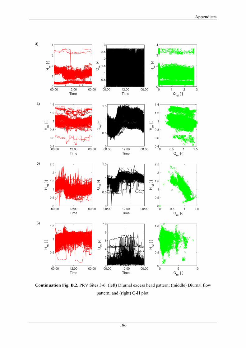
Appendices
196
Continuation Fig. B.2. PRV Sites 3-6: (left) Diurnal excess head pattern; (middle) Diurnal flow
pattern; and (right) Q-H plot.

Appendices
197
Continuation Fig. B.2. PRV Sites 7-10: (left) Diurnal excess head pattern; (middle) Diurnal flow
pattern; and (right) Q-H plot.
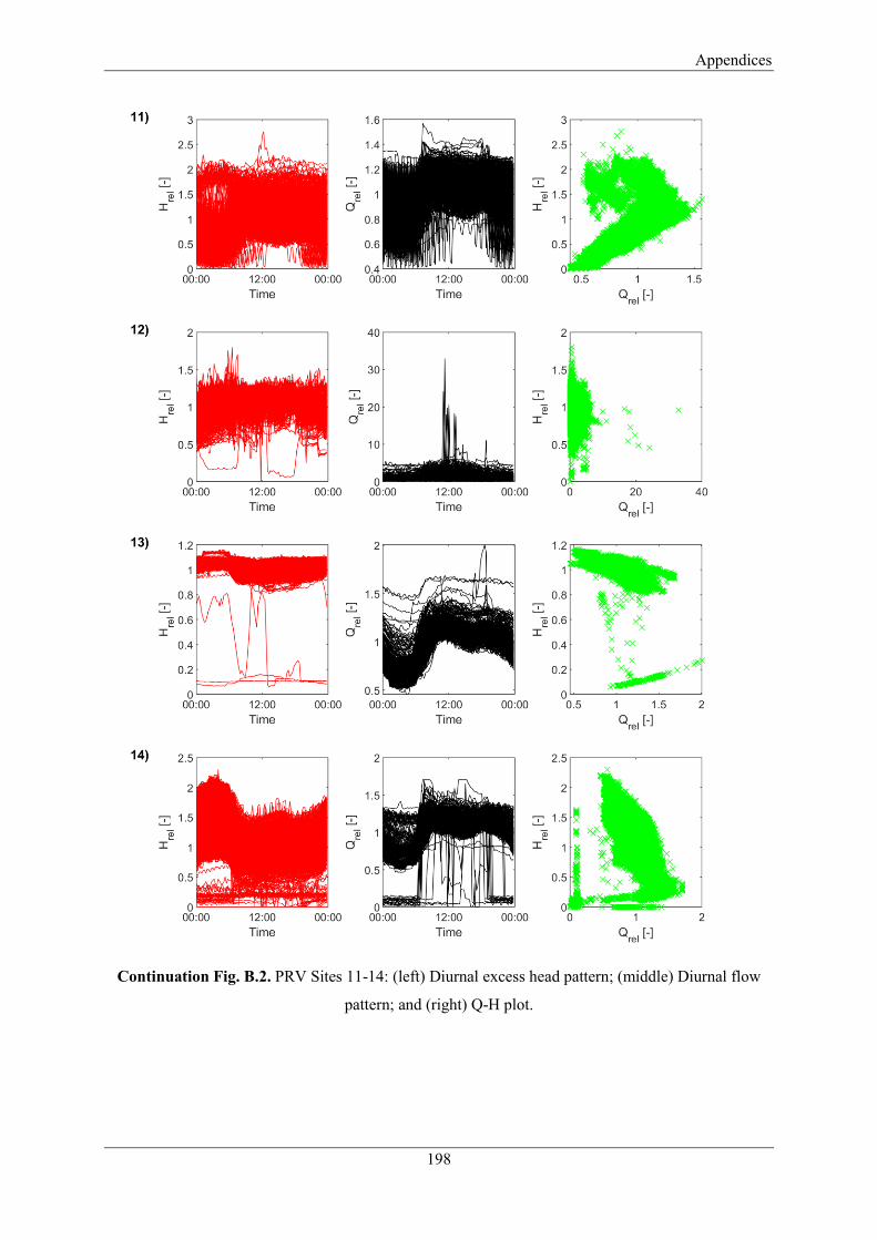
Appendices
198
Continuation Fig. B.2. PRV Sites 11-14: (left) Diurnal excess head pattern; (middle) Diurnal flow
pattern; and (right) Q-H plot.
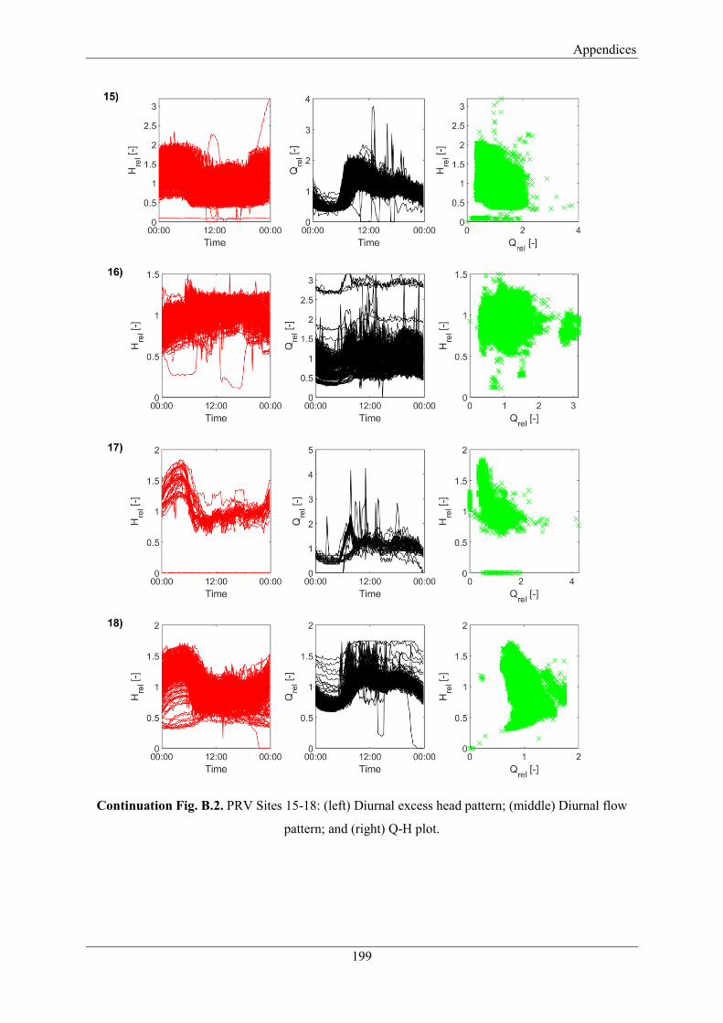
Appendices
199
Continuation Fig. B.2. PRV Sites 15-18: (left) Diurnal excess head pattern; (middle) Diurnal flow
pattern; and (right) Q-H plot.

Appendices
200
Continuation Fig. B.2. PRV Sites 19-22: (left) Diurnal excess head pattern; (middle) Diurnal flow
pattern; and (right) Q-H plot.

Appendices
201
Continuation Fig. B.2. PRV Sites 23-26: (left) Diurnal excess head pattern; (middle) Diurnal flow
pattern; and (right) Q-H plot.
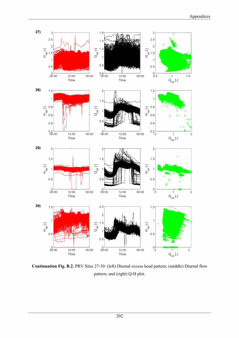
Appendices
202
Continuation Fig. B.2. PRV Sites 27-30: (left) Diurnal excess head pattern; (middle) Diurnal flow
pattern; and (right) Q-H plot.
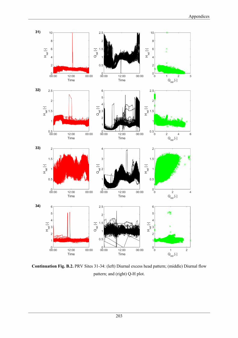
Appendices
203
Continuation Fig. B.2. PRV Sites 31-34: (left) Diurnal excess head pattern; (middle) Diurnal flow
pattern; and (right) Q-H plot.
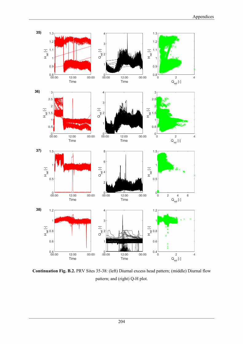
Appendices
204
Continuation Fig. B.2. PRV Sites 35-38: (left) Diurnal excess head pattern; (middle) Diurnal flow
pattern; and (right) Q-H plot.
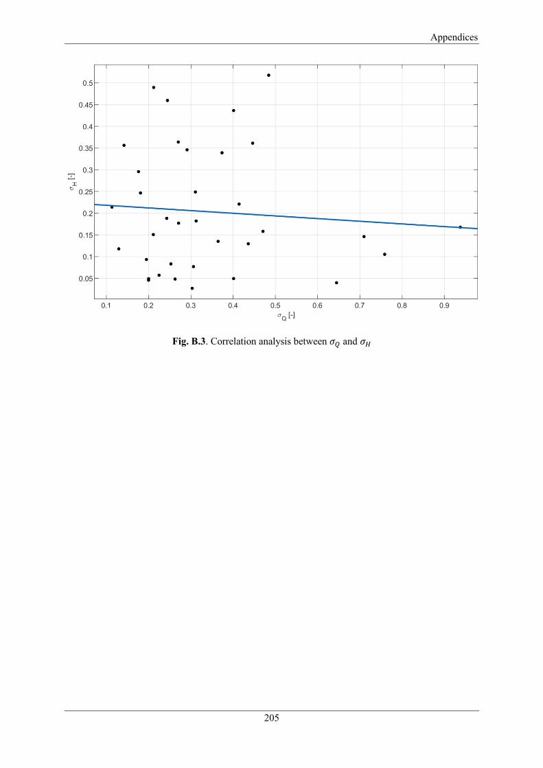
Appendices
205
Fig. B.3. Correlation analysis between 𝜎𝑄 and 𝜎𝐻

Appendices
206
Tab. B.1. Optimal solutions from the first optimisation run for all 38 PRV sites
Site ID
Family n [rpm] 𝑄𝑟𝑒𝑙
𝑚𝑎𝑥 [l s-1]
𝑃𝑒𝑙𝑒𝑐𝐵𝐸𝑃
[kW] 𝑃𝑒𝑙𝑒𝑐
𝑚𝑎𝑥 [kW]
NPV [€] E [MWh year-1]
𝜂𝑔𝑙𝑜𝑏𝑎𝑙
[-]
1 200-330 1510 1.171 84.27 126.40 462186 837.04 0.635
2 125-250 1510 1.173 22.96 34.43 119566 236.27 0.536
3 150-200 1510 1.158 18.66 28.00 10059 80.05 0.291
4 250-400 1510 1.175 189.82 284.74 945758 1666.84 0.586
5 125-200 1510 1.168 13.52 20.28 54937 126.39 0.554
6 32-160_1 1510 1.194 0.37 0.56 -5129 1.98 0.210
7 50-160 3020 1.183 14.47 21.71 63843 126.56 0.557
8 40-125 1510 1.183 0.48 0.71 -3656 4.76 0.360
9 32-125_1 1510 1.190 0.21 0.32 -6049 0.09 0.028
10 80-200 1510 1.181 6.00 9.00 15321 47.06 0.498
11 150-250 1005 1.167 9.51 14.26 15013 74.38 0.533
12 32-125_1 1510 1.190 0.21 0.32 -5154 1.38 0.129
13 50-160 3020 1.183 14.47 21.71 66465 130.33 0.561
14 100-200 1510 1.176 9.08 13.62 23315 67.18 0.460
15 32-125_1 1510 1.190 0.21 0.32 -5611 0.72 0.149
16 32-160 1510 1.190 0.63 0.94 -2615 6.52 0.287
17 32-125_1 1510 1.190 0.21 0.32 -5364 1.08 0.290
18 40-125 1510 1.183 0.48 0.71 -4180 4.00 0.302
19 80-200 1510 1.181 6.00 9.00 14764 46.26 0.460
20 32-125 3020 1.188 3.02 4.53 725 17.34 0.315
21 40-160 1510 1.189 0.95 1.42 -1495 9.19 0.317
22 32-160_1 1510 1.194 0.37 0.56 -3898 3.75 0.250
23 50-125 3020 1.173 7.58 11.36 23204 60.23 0.474
24 32-160_1 1510 1.194 0.37 0.56 -3843 3.83 0.262
25 25-160 1510 1.198 0.14 0.21 -6102 0.00 0.000
26 65-160 3020 1.179 17.42 26.12 104614 190.86 0.505
27 65-160 1510 1.179 2.07 3.11 2144 18.57 0.460
28 100-160 3020 1.167 44.36 66.54 215040 395.53 0.623
29 80-160 3020 1.167 28.53 42.79 85586 186.05 0.516
30 40-160 1510 1.189 0.95 1.42 -1461 9.24 0.359
31 25-160 1510 1.198 0.14 0.21 -6102 0.00 0.000
32 50-160 1510 1.183 1.70 2.55 -393 13.44 0.402
33 25-160 1510 1.198 0.14 0.21 -6102 0.00 0.000
34 125-200 1005 1.168 3.82 5.72 7622 40.84 0.603
35 32-160 1510 1.190 0.63 0.94 -4352 4.02 0.333
36 32-125_1 1510 1.190 0.21 0.32 -5430 0.98 0.246
37 32-160_1 1510 1.194 0.37 0.56 -4916 2.29 0.244
38 32-125 3020 1.188 3.02 4.53 6365 25.46 0.361
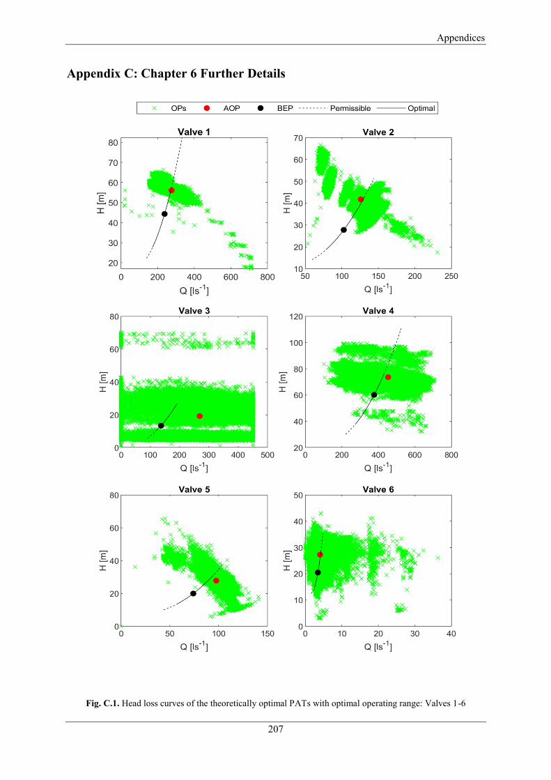
Appendices
207
Appendix C: Chapter 6 Further Details
Fig. C.1. Head loss curves of the theoretically optimal PATs with optimal operating range: Valves 1-6
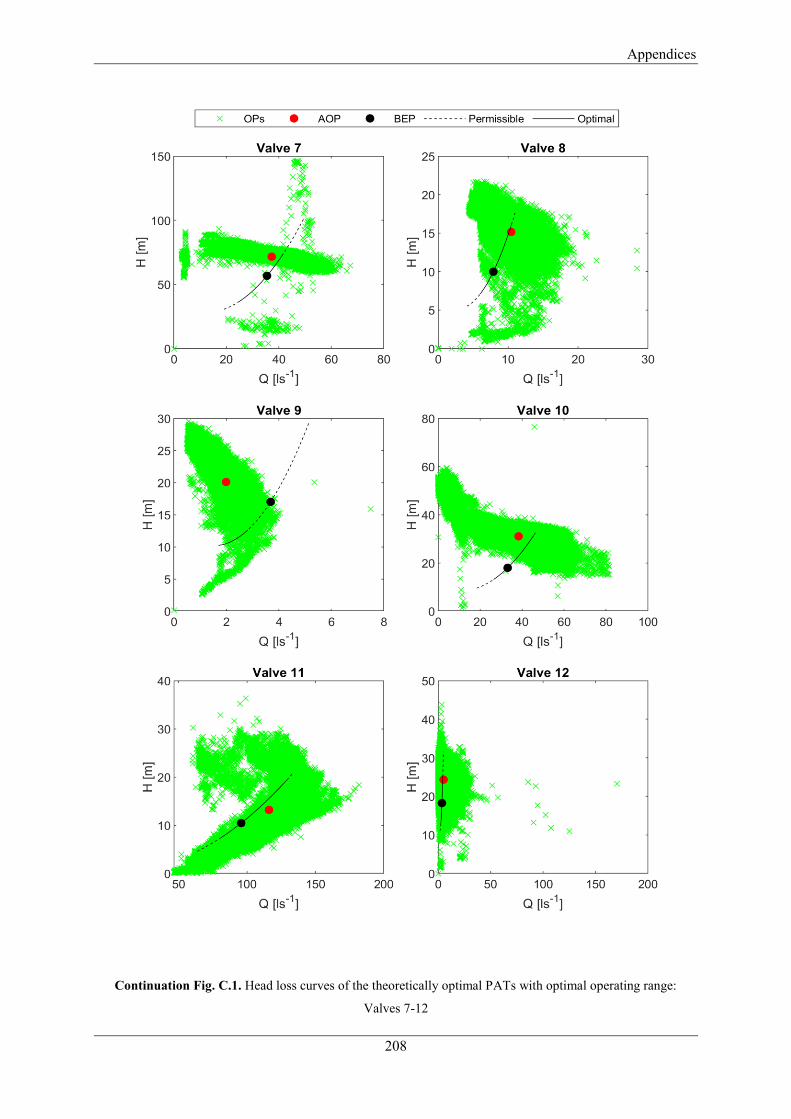
Appendices
208
Continuation Fig. C.1. Head loss curves of the theoretically optimal PATs with optimal operating range:
Valves 7-12
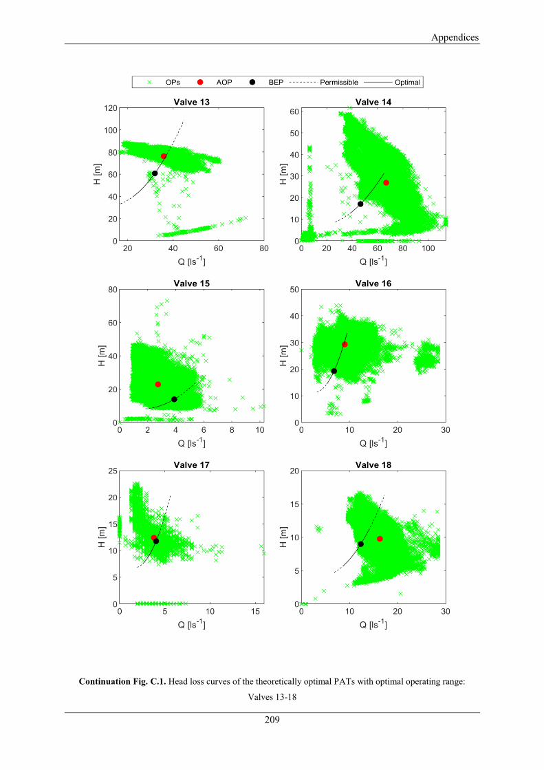
Appendices
209
Continuation Fig. C.1. Head loss curves of the theoretically optimal PATs with optimal operating range:
Valves 13-18

Appendices
210
Continuation Fig. C.1. Head loss curves of the theoretically optimal PATs with optimal operating range:
Valves 19-24
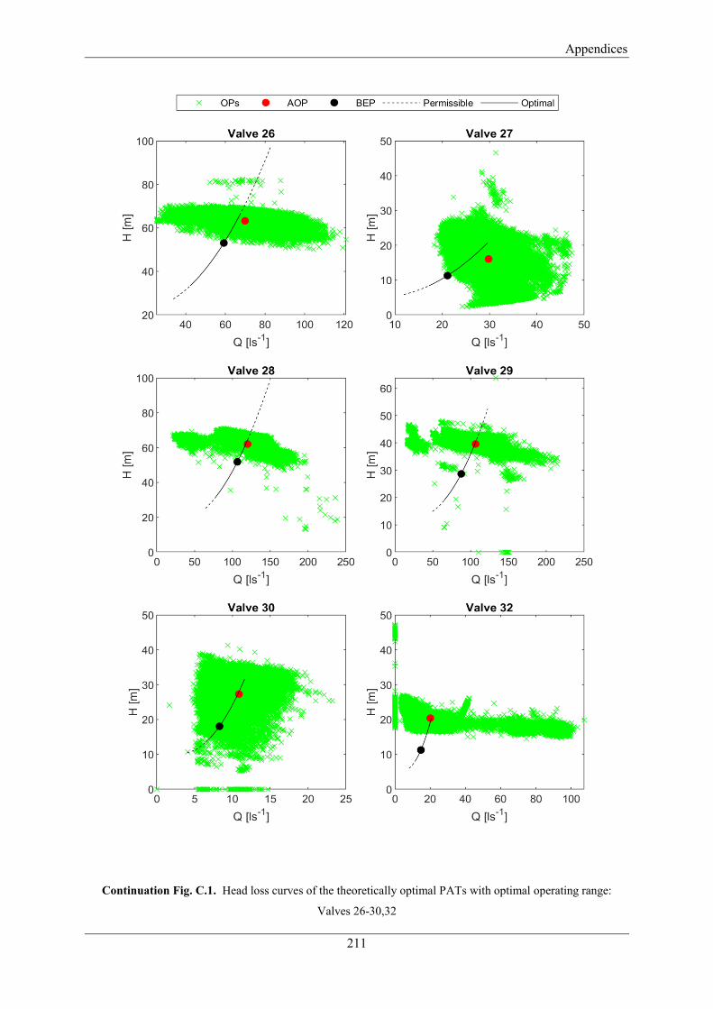
Appendices
211
Continuation Fig. C.1. Head loss curves of the theoretically optimal PATs with optimal operating range:
Valves 26-30,32

Appendices
212
Continuation Fig. C.1. Head loss curves of the theoretically optimal PATs with optimal operating range:
Valves 34-38

Appendices
213
Appendix D: Chapter 8 Further Details
a)
b)
Fig. D.1. Distribution of HPER potential in Scotland a) Scenario 1 and b) Scenario 2
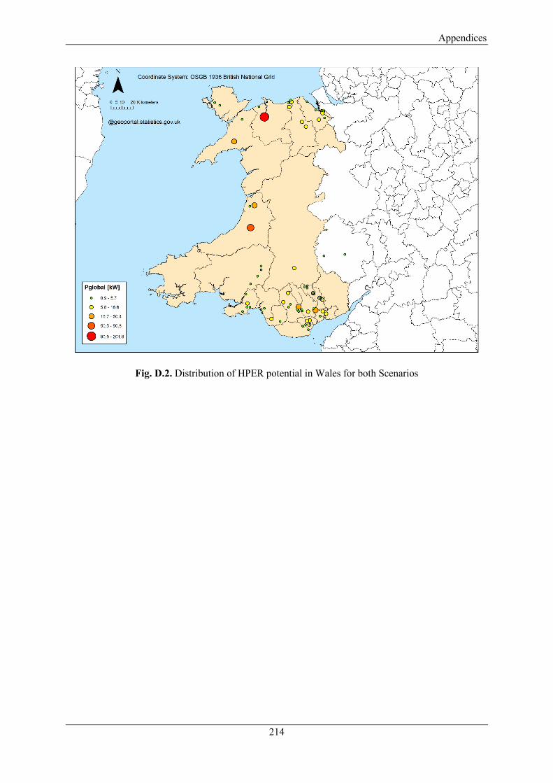
Appendices
214
Fig. D.2. Distribution of HPER potential in Wales for both Scenarios