System-Level Optimization and Code Generation for Graphics ...
203
System-Level Optimization and Code Generation for Graphics Processors using a Domain-Specific Language Optimierung auf System-Ebene und Code-Generierung für Grafikprozessoren miels einer domänenspezifischen Sprache Der Technischen Fakultät der Friedrich-Alexander-Universität Erlangen-Nürnberg zur Erlangung des Doktorgrades Dr.-Ing. vorgelegt von Bo Qiao aus Heilongjiang
-
Upload
khangminh22 -
Category
Documents
-
view
0 -
download
0
Transcript of System-Level Optimization and Code Generation for Graphics ...

System-Level Optimization and CodeGeneration for Graphics Processorsusing a Domain-Specific Language
Optimierung auf System-Ebene und Code-Generierungfür Grafikprozessoren mittels einer
domänenspezifischen Sprache
Der Technischen Fakultätder Friedrich-Alexander-Universität
Erlangen-Nürnbergzur
Erlangung des Doktorgrades Dr.-Ing.
vorgelegt von
Bo Qiao
aus Heilongjiang

Als Dissertation genehmigtvon der Technischen Fakultätder Friedrich-Alexander-Universität Erlangen-NürnbergTag der mündlichen Prüfung: 14. Dezember 2021
Vorsitzender des Promotionsorgans: Prof. Dr.-Ing. habil. Andreas Paul Fröba
Gutachter: PD Dr.-Ing. Frank HannigProf. Dr.-Ing. Marc Stamminger

This thesis is dedicated to my family and my girlfriend Zhaohanwith love and gratitude.
iii


Abstract
As graphics processing units (GPUs) are being used increasingly for general purposeprocessing, efficient tooling for programming such parallel architectures becomesessential. Despite the continuous effort of programmability improvement in CUDAand OpenCL, they remain relatively low-level languages and require in-depth archi-tecture knowledge to achieve high-performance implementations. Developers haveto perform memory management manually to exploit the multi-layered computeand memory hierarchy. This type of hand-tuned expert implementations suffersfrom performance portability, namely, existing implementations are not guaranteedto be efficient on new architectures, and developers have to perform the tedioustuning and optimization repeatedly for every architecture. To circumvent this issue,developers can choose to utilize high-performance libraries offered by hardwarevendors as well as open-source communities. Utilizing libraries is performanceportable as it is the library developer’s job to maintain the implementation. However,it lacks programmability. Library functions are provided with pre-defined APIs,and the level of abstraction may not be sufficient for developers of a certain do-main. Furthermore, using library-based implementations precludes the possibilityof applying system-level optimizations across different functions. In this thesis, wepresent a domain-specific language (DSL) approach that can achieve both perfor-mance portability and programmability within a particular domain. This is possibleby exploiting domain-specific abstractions and combining them with architecture-specific optimizations. The abstractions enable programmability and flexibility fordomain developers, and the compiler-based optimization facilitates performanceportability across different architectures. The core of such a DSL approach is itsoptimization engine, which combines algorithm and hardware knowledge to explorethe optimization space efficiently. Our contributions in this thesis target system-leveloptimizations and code generations for GPU architectures.
Today’s applications such as in image processing and machine learning growin complexity and consist of many kernels in a computation pipeline. Optimizingeach kernel individually is no longer sufficient due to the rapid evolution of modernGPU architectures. Each architecture generation reveals higher computing poweras well as memory bandwidth. Nevertheless, the computing power increase is
v

generally faster than the memory bandwidth improvement. As a result, good localityis essential to achieve high-performance implementations. For example, the inter-kernel communications within an image processing pipeline are intensive and exhibitmany opportunities for locality improvement. As the first contribution, we presenta technique called kernel fusion to reduce the number of memory accesses to theslow GPU global memory. In addition, we automate the transformation in oursource-to-source compiler by combining domain knowledge in image processingand architecture knowledge of GPUs.
Another trend we can observe following recent architecture development is theincreasing number of CUDA cores and streaming multiprocessors (SMs) for compu-tation. Traditionally, GPU programming is about exploring data-level parallelism.Following the single instruction, multiple threads (SIMTs) execution model, data canbe mapped to threads to benefit from the massive computing power. Nevertheless,small images that were considered costly on older architectures can no longer occupythe device fully on new GPUs. It becomes important to explore also kernel-levelparallelism that can efficiently utilize the growing number of compute resourceson the GPU. As the second contribution, we present concurrent kernel executiontechniques to enable fine-grained resource sharing within the compute SMs. Inaddition, we compare different implementation variants and develop analytic modelsto predict the suitable option based on the algorithmic and architecture knowledge.
After considering locality and parallelism, which are the two most essential op-timization objectives on modern GPU architectures, we can start examining thepossibilities to optimize the computations within an algorithm. As the third contri-bution in this thesis, we present single-kernel optimization techniques for the twomost commonly used compute patterns in image processing, namely local and globaloperators. For local operators, we present a systematic analysis of an efficient borderhandling technique based on iteration space partitioning. We use the domain andarchitecture knowledge to capture the trade-off between occupancy and instructionusage reduction. Our analytic model assists the transformation in the source-to-source compiler to decide on the better implementation variant and improves theend-to-end code generation. For global operators, we present an efficient approachto perform global reductions on GPUs. Our approach benefits from the continuouseffort of performance and programmability improvement by hardware vendors, forexample, by utilizing new low-level primitives from Nvidia.
The proposed techniques cover not only multi-kernel but also single-kernel opti-mization, and are seamlessly integrated into our image processing DSL and source-to-source compiler called Hipacc. In the end, the presented DSL framework can dras-tically improve the productivity of domain developers aiming for high-performanceGPU implementations.
vi

Acknowledgments
I would like to express my sincere gratitude to my supervisor Frank Hannig for hiscontinuous support throughout the last four years. I want to thank Prof. JürgenTeich for creating such an excellent research environment in the chair of Hardware/-Software Co-Design. I also want to thank Prof. Marc Stamminger for agreeing to bethe co-examiner of this work.
My special thank goes to Oliver Reiche, who was always available for help duringthe initial phase of my research. I want to thank Jorge and Akif for the interestingdiscussions as well as the fruitful collaborations in the office. Thanks Behnaz andMartin for the lunch walk and the beer during the weekends. I am extremely gratefulfor being in the chair of Hardware/Software Co-Design and being around all mycolleagues during my stay in Erlangen.
Finally, I want to thank my family for their support. Especially my girlfriendZhaohan, without her support none of these achievements would have been possible.
vii


Contents
1 Introduction 11.1 Rise of Multi-Core and Domain-Specific Architectures . . . . . . . . 11.2 Improving Productivity in Parallel Programming . . . . . . . . . . . 41.3 Domain-Specific Language Approach . . . . . . . . . . . . . . . . . 71.4 Contributions . . . . . . . . . . . . . . . . . . . . . . . . . . . . . . 101.5 Outline . . . . . . . . . . . . . . . . . . . . . . . . . . . . . . . . . . 13
2 Background 152.1 Graphics Processing Units (GPUs) . . . . . . . . . . . . . . . . . . . 15
2.1.1 Architectures . . . . . . . . . . . . . . . . . . . . . . . . . . 162.1.2 Optimization Objectives . . . . . . . . . . . . . . . . . . . . 192.1.3 Programming Models . . . . . . . . . . . . . . . . . . . . . . 23
2.2 Domain-Specific Languages and Compilers . . . . . . . . . . . . . . 272.2.1 Programming with High-Level Abstractions . . . . . . . . . 272.2.2 Hipacc: A DSL and Compiler for Image Processing . . . . . 28
3 Exploiting Locality through Kernel Fusion 373.1 Introduction . . . . . . . . . . . . . . . . . . . . . . . . . . . . . . . 373.2 From Loop Fusion to Kernel Fusion . . . . . . . . . . . . . . . . . . 39
3.2.1 Loop Fusion . . . . . . . . . . . . . . . . . . . . . . . . . . . 393.2.2 Kernel Fusion . . . . . . . . . . . . . . . . . . . . . . . . . . 403.2.3 Benefits and Costs . . . . . . . . . . . . . . . . . . . . . . . 42
3.3 The Fusion Problem . . . . . . . . . . . . . . . . . . . . . . . . . . . 443.3.1 Problem Statement . . . . . . . . . . . . . . . . . . . . . . . 443.3.2 Legality . . . . . . . . . . . . . . . . . . . . . . . . . . . . . 45
3.4 Trade-off Estimation . . . . . . . . . . . . . . . . . . . . . . . . . . 483.4.1 Compute Pattern Definition . . . . . . . . . . . . . . . . . . 493.4.2 Hardware Model . . . . . . . . . . . . . . . . . . . . . . . . 503.4.3 Fusion Scenarios . . . . . . . . . . . . . . . . . . . . . . . . 503.4.4 Putting it all Together . . . . . . . . . . . . . . . . . . . . . 57
ix

Contents
3.5 Fusibility Exploration . . . . . . . . . . . . . . . . . . . . . . . . . . 583.5.1 Search along Edges . . . . . . . . . . . . . . . . . . . . . . . 583.5.2 Search based on Minimum Cut . . . . . . . . . . . . . . . . 62
3.6 Compiler Integration . . . . . . . . . . . . . . . . . . . . . . . . . . 663.6.1 Point-Consumer Fusion . . . . . . . . . . . . . . . . . . . . 663.6.2 Point-to-Local Fusion . . . . . . . . . . . . . . . . . . . . . . 673.6.3 Local-to-Local Fusion . . . . . . . . . . . . . . . . . . . . . 67
3.7 Evaluation and Results . . . . . . . . . . . . . . . . . . . . . . . . . 703.7.1 Environment . . . . . . . . . . . . . . . . . . . . . . . . . . 703.7.2 Applications . . . . . . . . . . . . . . . . . . . . . . . . . . . 713.7.3 Results . . . . . . . . . . . . . . . . . . . . . . . . . . . . . . 71
3.8 Related Work . . . . . . . . . . . . . . . . . . . . . . . . . . . . . . . 763.9 Summary . . . . . . . . . . . . . . . . . . . . . . . . . . . . . . . . . 78
4 Improving Parallelism via Fine-Grained Resource Sharing 794.1 Introduction . . . . . . . . . . . . . . . . . . . . . . . . . . . . . . . 80
4.1.1 Multiresolution Filters . . . . . . . . . . . . . . . . . . . . . 804.1.2 CUDA Graph . . . . . . . . . . . . . . . . . . . . . . . . . . 81
4.2 Unveiling Kernel Concurrency in Multiresolution Filters . . . . . . 844.2.1 An Efficient Recursive Description in Hipacc . . . . . . . . 85
4.3 Performance Modeling . . . . . . . . . . . . . . . . . . . . . . . . . 874.3.1 Scheduling Basics . . . . . . . . . . . . . . . . . . . . . . . . 874.3.2 Single-Stream Modeling . . . . . . . . . . . . . . . . . . . . 894.3.3 Multi-Stream Modeling . . . . . . . . . . . . . . . . . . . . . 904.3.4 Model Fidelity . . . . . . . . . . . . . . . . . . . . . . . . . . 954.3.5 Intermediate Summary . . . . . . . . . . . . . . . . . . . . . 97
4.4 Execution Model in CUDA Graph . . . . . . . . . . . . . . . . . . . 984.4.1 Graph Definition . . . . . . . . . . . . . . . . . . . . . . . . 984.4.2 Graph Instantiation . . . . . . . . . . . . . . . . . . . . . . . 984.4.3 Graph Execution . . . . . . . . . . . . . . . . . . . . . . . . 100
4.5 Kernel Execution with Complementary Resource Usage . . . . . . . 1004.5.1 Intra-SM Resource Sharing . . . . . . . . . . . . . . . . . . 1004.5.2 Example Application . . . . . . . . . . . . . . . . . . . . . . 1024.5.3 Kernel Pipelining . . . . . . . . . . . . . . . . . . . . . . . . 1044.5.4 Scalability and Fidelity . . . . . . . . . . . . . . . . . . . . . 1044.5.5 Intermediate Summary . . . . . . . . . . . . . . . . . . . . . 106
4.6 Combining CUDA Graph with an Image Processing DSL . . . . . . 1074.6.1 Benefits Inherited from Hipacc . . . . . . . . . . . . . . . . 108
4.7 Evaluation and Results . . . . . . . . . . . . . . . . . . . . . . . . . 1094.7.1 Applications . . . . . . . . . . . . . . . . . . . . . . . . . . . 1094.7.2 Environment . . . . . . . . . . . . . . . . . . . . . . . . . . 1114.7.3 Results and Discussions . . . . . . . . . . . . . . . . . . . . 111
x

Contents
4.8 Related Work . . . . . . . . . . . . . . . . . . . . . . . . . . . . . . . 1184.9 Conclusion . . . . . . . . . . . . . . . . . . . . . . . . . . . . . . . . 119
5 Efficient Computations for Local and Global Operators 1215.1 Introduction . . . . . . . . . . . . . . . . . . . . . . . . . . . . . . . 122
5.1.1 Image Border Handling for Local Operators . . . . . . . . . 1225.1.2 Global Reductions on GPUs . . . . . . . . . . . . . . . . . . 123
5.2 Iteration Space Partitioning . . . . . . . . . . . . . . . . . . . . . . . 1255.2.1 Border Handling Patterns . . . . . . . . . . . . . . . . . . . 1255.2.2 Index-Set Splitting . . . . . . . . . . . . . . . . . . . . . . . 1275.2.3 Partitioning on GPUs . . . . . . . . . . . . . . . . . . . . . . 128
5.3 Performance Modeling . . . . . . . . . . . . . . . . . . . . . . . . . 1305.3.1 Demystify the Benefits . . . . . . . . . . . . . . . . . . . . . 1305.3.2 Cost Model . . . . . . . . . . . . . . . . . . . . . . . . . . . 1345.3.3 Intermediate Summary . . . . . . . . . . . . . . . . . . . . . 137
5.4 Hipacc Integration of Warp-grained Partitioning . . . . . . . . . . . 1375.4.1 Warp-Grained Partitioning . . . . . . . . . . . . . . . . . . 138
5.5 Parallel Reduction on GPUs . . . . . . . . . . . . . . . . . . . . . . 1395.5.1 Global Reduction in Hipacc . . . . . . . . . . . . . . . . . . 1405.5.2 Global Memory Load . . . . . . . . . . . . . . . . . . . . . . 1405.5.3 Intra-block Reduce . . . . . . . . . . . . . . . . . . . . . . . 1425.5.4 Inter-block Reduce . . . . . . . . . . . . . . . . . . . . . . . 143
5.6 Evaluation and Results . . . . . . . . . . . . . . . . . . . . . . . . . 1445.6.1 Environment and Implementation Variant . . . . . . . . . . 1445.6.2 Discussions . . . . . . . . . . . . . . . . . . . . . . . . . . . 150
5.7 Related Work . . . . . . . . . . . . . . . . . . . . . . . . . . . . . . . 1535.8 Conclusion . . . . . . . . . . . . . . . . . . . . . . . . . . . . . . . . 154
6 Conclusion and Future Directions 1556.1 Summary . . . . . . . . . . . . . . . . . . . . . . . . . . . . . . . . . 1556.2 Future Directions . . . . . . . . . . . . . . . . . . . . . . . . . . . . 158
A Appendix 161A.1 Kernel Fusion Artifact Evaluation . . . . . . . . . . . . . . . . . . . 161
A.1.1 Artifact Check-list . . . . . . . . . . . . . . . . . . . . . . . 161A.1.2 Description . . . . . . . . . . . . . . . . . . . . . . . . . . . 162A.1.3 Datasets . . . . . . . . . . . . . . . . . . . . . . . . . . . . . 163A.1.4 Installation . . . . . . . . . . . . . . . . . . . . . . . . . . . 163A.1.5 Experiment Workflow . . . . . . . . . . . . . . . . . . . . . 163A.1.6 Evaluation and Expected Result . . . . . . . . . . . . . . . . 164A.1.7 Notes . . . . . . . . . . . . . . . . . . . . . . . . . . . . . . . 164
xi

Contents
A.2 Fusibility Exploration Algorithm Complexity . . . . . . . . . . . . . 165A.2.1 Worst-Case Running Time . . . . . . . . . . . . . . . . . . . 165
German Part 167
Bibliography 173
Author’s Own Publications 187
Acronyms 189
xii

1Introduction
Computer architectures have evolved through generations of innovations in the pastdecades. Driven by the continuous advancement in the design and manufacture ofcomplementary metal oxide semiconductor (CMOS) technology, transistors keepgetting smaller and the total number that can be put on a single chip keeps growing.The trend has been predicted by GordenMoore [Moo65], who suggested a doubling intransistor density every two years. Nevertheless, as the current CMOS technology isreaching its physical limits, an increasing gap between processor density andMoore’sprediction can be observed [HP19]. In parallel with Moore’s law, another well-knownprediction is Dennard’s scaling [DGY+74]. It observed that as the transistor sizeshrinks, the power density on a single chip stays constant, and transistors will getincreasingly power-efficient. This trend had been held until 2005, when transistor sizeshrank below 65 nanometers. After that, the current leakage became heat dominantthat prevents transistors from getting more power-efficient. As a result, the scalingof single-core frequency started to saturate, hitting the so-called power wall.
1.1 Rise of Multi-Core and Domain-SpecificArchitectures
The breakdown of Dennard’s scaling triggered the paradigm shift towards multi-corearchitectures. Instead of raising the clock frequency as in the single-core era, morecores have been added onto the same chip to keep the raw computing power scalingcontinuously. Nevertheless, this switch to multi-core architectures did not mitigateaway from the power problem. As more cores are being crammed into a single chip,the thermal design power (TDP) becomes the bottleneck. Processor cores on thesame chip cannot be powered on at the same time, resulting in the so-called darksilicon [EBA+11]. The projection is that more than 50% of a fixed-size chip mustbe powered-off at 8 nanometers transistors size. Therefore, more power-efficientarchitectures must be explored. For this reason, domain-specific architectures (DSAs)have emerged due to their power efficiency and good performance scalability [HP19].DSAs are often referred to as accelerators, which are tailored to compute patterns
1

1 Introduction
within a specific domain. In general, DSAs are less flexible than the general-purposearchitectures such as single- and multi-core central processing units (CPUs), but aremore programmable than architectures that are customized for specific functionssuch as application-specific integrated circuits (ASICs). One prominent example ofdomain-specific architectures is graphics processing units (GPUs).
GPUs were developed originally for computer graphics workload, driven by thedemand in the gaming industry. Graphics workload is compute-intensive and in-herently parallel. GPU architectures employ a SIMT execution model to exploitparallelism in a power-efficient yet still flexible manner. Compared to the singleinstruction, multiple data (SIMD) execution model used in modern CPU’s vectorprocessing units, SIMT is more flexible since threads have their own register files,and can better support different conditional control-flow path during execution.Compared to the multiple instructions, multiple data (MIMD) technique used inmulti-core architectures where each processor core can compute its own data usingdifferent instructions, SIMT is more power-efficient, since only one single instruc-tion stream needs to be fetched and decoded. The massively parallel computingcapability of GPUs started drawing attention from other domains beyond computergraphics. Nevertheless, early efforts to perform general-purpose computing on GPUs(GPGPU) suffered from the highly specialized hardware, such as the lack of integerdata operands [OLG+05]. As GPU architectures rapidly have evolved, the limitationshave been identified and lifted gradually. With the introduction of Compute UnifiedDevice Architecture (CUDA) in 2007 by Nvidia [Nvi07] and the ratification of theOpen Computing Language (OpenCL) from the Khronos Group [Khr09], GPGPUhas become feasible for non-graphics programmers to benefit from the fast-growingcomputing power.
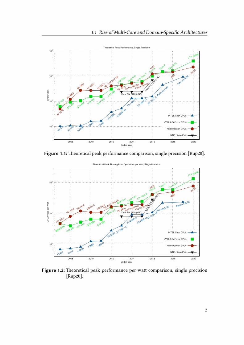
The historic performance boost in GPUs has promoted the emergence of today’smany data-intensive applications in a variety of domains such as medical imaging,artificial intelligence, computer graphics, and scientific computing. In turn, the de-velopment in those domains continues to demand more computing power and drivesthe development of GPU architectures at a stunning pace. Most high-performancesystems today use highly parallel architectures such as GPUs. More than 50% of thetop 500 supercomputers use many-core architectures and more than 20% of them areGPU accelerators [Str20]. Figure 1.1 and Figure 1.2 depict the performance gap be-tween high-end CPUs and GPUs on the market. As can be observed, compared to thehighest performance CPUs from Intel, the latest Nvidia GPUs can achieve more than4 times single-precision peak performance and more than 5 times single-precisionpeak performance per watt, respectively.
The performance and power efficiency have promoted GPUs as the de factoraccelerator option for many data-intensive computations such as medical imagingregistration and convolutional neural networks (CNNs) training. Nevertheless, it isnot easy to exploit the different levels of parallelism efficiently for GPU architectures.
2
1.1 Rise of Multi-Core and Domain-Specific Architectures
102
103
104
105
2008 2010 2012 2014 2016 2018 2020
HD 3870
HD 4870
HD 5870
HD 6970
HD 6970
HD 7970 G
Hz Ed.
HD 8970FirePro W9100
FirePro S9150
MI2
5
MI6
0M
I100
X5482
X5492
W5590 X5680
X5690
E5-2690
E5-2697 v
2
E5-2699 v
3
E5-2699 v
3
E5-2699 v
4Pla
tinum
8180
Platin
um 9
282
8800 GTS
GTX 2
80
GTX 2
85 GTX 5
80
GTX 5
80
GTX 6
80
GTX T
itan
Tesla K
40
GTX T
itan X
Titan X Tita
n V
Titan R
TX
RTX A6000
Xeon Phi 7120 (KNC)
Xeo
n Phi
729
0 (K
NL)
GF
LO
P/s
ec
End of Year
Theoretical Peak Performance, Single Precision
INTEL Xeon CPUs
NVIDIA GeForce GPUs
AMD Radeon GPUs
INTEL Xeon Phis
Figure 1.1: Theoretical peak performance comparison, single precision [Rup20].
100
101
102
2008 2010 2012 2014 2016 2018 2020
HD 3870
HD 4870 HD 5870
HD 6970
HD 6970
HD 7970 GHz Ed.
HD 8970FirePro W9100
FirePro S9150
MI25
MI60
MI1
00
X5482X5492 W5590
X5680X5690
E5-2690E5-2697 v2
E5-2699 v3
E5-2699 v3 E5-2699 v4Platinum 8180 Platinum 9282
8800 GTS
GTX 280 GTX 285GTX 580
GTX 580
GTX 680
GTX Titan
Tesla K40
GTX Titan X
Titan X
Titan V
Titan R
TX
RTX A6000
Xeon Phi 7120 (KNC)
Xeo
n Phi
729
0 (K
NL)
GF
LO
P/s
ec p
er
Wa
tt
End of Year
Theoretical Peak Floating Point Operations per Watt, Single Precision
INTEL Xeon CPUs
NVIDIA GeForce GPUs
AMD Radeon GPUs
INTEL Xeon Phis
Figure 1.2: Theoretical peak performance per watt comparison, single precision[Rup20].
3

1 Introduction
GPU programming today remains a challenging task and is mastered only by asmall group of experts. Even for experts with deep architecture knowledge, theimplementations often suffer from the performance portability issue. Code tunedfor one architecture is not guaranteed to be efficient on another architecture, whichleads to low productivity during application development.
1.2 Improving Productivity in ParallelProgramming
In software engineering, productivity can be consensually defined as a ratio betweenoutput and input [WD19]. There exist different notations and metrics to captureoutput and input within different fields. In the scope of this thesis, we define outputas the quality of implementations (e.g., execution time, resource utilization) for alltargets of interest across the software evolution, namely the continuous improvementand feature enhancement of the target applications. Input can be defined as thecost of human effort (e.g., lines of codes (LoCs) written). In other words, increasingproductivitymeansminimizing the effort required to obtain efficient implementationson the target platforms. Next, we highlight the challenges to achieve this goal, anddescribe two commonly seen approaches employed by programmers today.
Challenges in Programming Parallel Architectures Accompanied by the tran-sition to parallel architectures, the free lunch of performance improvement benefitingfrom frequency scaling in the single-core era was over [SL05]. Today programmersand compiler developers are responsible for performance optimization by exploringparallelism at different levels for multi-core architectures. At a fine-grained level,instruction-level parallelism (ILP) can be explored efficiently by modern proces-sors and compilers with relatively little human effort by using techniques such asinstruction pipelining and register renaming. Furthermore, data-level parallelism(DLP) can be explored to utilize the vector processing units equipped on modernprocessors. Although certain compilers such as GCC are able to perform vector-ization automatically, they can only detect a fixed set of code patterns (e.g., loopstructure). For loops with irregular patterns and complex dependencies, programmerintervention is needed to rewrite the code in a more compiler-friendly manner toassist these optimizations. This manual effort becomes a burden when coarse-grainedlevel parallelism such as thread-level parallelism (TLP) needs to be explored. Pro-grammers often have to explicitly manage the computing threads, as well as theirshared memory accesses and synchronizations.
The challenge grows significantly when programming for accelerators such asGPUs, where the multi-level memory hierarchy and compute units all require explicitmanagement by the programmer. Since GPU devices are used to accelerate parallel
4

1.2 Improving Productivity in Parallel Programming
workload, it is generally combined with a host CPU to form a heterogeneous system.The host is responsible for initializing and offloading parallel tasks to the device. Inthis case, programmers need to manually partition their applications into sequentialand parallel parts, which can be executed on the host and device, respectively. In thehost code, programmers need to take care of the task such as device initialization,buffer allocation, host and device communication, and kernel launch. For multi-kernel concurrent executions, programmers also need to control the asynchronouskernel launch as well as memory read and write synchronizations. In the device code,programmers need to optimize the computations for the multi-layered compute andmemory hierarchy, and take care of registers and shared memory usage. ModernGPUs have an array of SMs that can each process thousands of hardware-supportedcompute threads. Programmers cannot control all the threads explicitly. Instead,they write kernels with specific instructions that can be recognized by each threadduring execution. The most used programming APIs for GPUs today are ComputeUnified Device Architecture (CUDA) and Open Computing Language (OpenCL).Theyshare similar syntax and both provide effective abstractions for the underlying GPUarchitecture.
Hand-Tuned Expert Implementation To tackle the challenge of mapping algo-rithms to modern parallel architecture such as GPUs, experienced programmerswith deep architecture knowledge are hired to manually tune and optimize eachimplementation for different target platforms. A typical workflow is as follows:First, the programmer works out some reference implementations to guarantee thecorrectness of the algorithm. Then, he or she starts to tune and optimize the codefor a given architecture, for example, by replacing some instructions to utilize thevector processing units or by unrolling some loops for better ILP. After extensiveeffort has been made, an optimized implementation can be achieved that executesefficiently on the given platform. Problems arise when a new platform arrives, whichcould be another architecture with an upgraded specification. The code obtainedpreviously is not guaranteed to run efficiently on this new platform. Consequently,the programmer has to go back to the reference implementation and performs thetedious tuning and optimization work again for the new architecture. This work mustbe conducted for not only every new platform but also every algorithm change in thefuture in case of a function upgrade or a feature enhancement. Therefore, this kind ofhand-tuned approach is performance non-portable [Per21]. Performance portabilityis an important concept in high-performance computing, and it can be defined asfollows: To achieve a consistent level of performance across all target platforms,(a) hard portability denotes that no code changes are needed. Here, hard meansgenerally applicable to all platforms. (b) software portability denotes no algorithmicchanges are needed. It means the software of the implementation requires no change.(c) non-portable denotes both algorithmic and non-algorithmic changes are needed.
5

1 Introduction
To achieve high productivity, we expect an approach that requires minimal codechanges, namely hard portability. For this reason, many programmers choose toturn towards high-performance library-based implementations.
High-PerformanceLibraries One approach to circumvent the performance porta-bility issue is by employing high-performance libraries. Hardware vendors as wellas open source communities provide highly efficient implementations for commonlyused applications across many domains. For example, CUDA-X from Nvidia for AIand HPC [Nvi21e], MKL from Intel for Math [Int21a], OpenCV for image processingand computer vision [Bra00], and OpenBLAS for scientific computing [Xia21]. Forprogrammers without deep architecture knowledge and aiming for high-performanceimplementations, utilizing external libraries is the easiest way to employ the hard-ware. The library-based approach is performance portable: Since users only needto link the library into their implementations and call the desired function appli-cation programming interface (API). When porting for a new architecture, littlemodifications are needed in the software since it is the library maintainer’s job tooptimize for different architectures. Nevertheless, utilizing library implementationsalso incurs several disadvantages: First, the implementations typically have a rigidlydefined function interface that lacks programmability. We consider programmabilityessential for high productivity during software evolution: Domain experts and algo-rithm developers often want to implement and fast prototype new functionalitiesthat are likely not yet available in a stable library implementation, because librarymaintainers always give high priorities to the most commonly used functions. It ispossible to construct new algorithms using simple, primitive operators offered by thelibraries. However, doing so precludes the possibility of cross-function optimizations.Each function in a library is a standalone implementation, and the behavior is definedby its interface. For example, when using the CUDA Basic Linear Algebra Subroutine(cuBLAS) library [Nvi21a], the input and output buffers to the functions should beallocated on device memory. This prevents potential inter-kernel optimizations suchas locality improvement. For architectures such as GPUs, the inter-kernel optimiza-tions at the system level can significantly boost the application performance. Ingeneral, the more strict a function interface is defined, the less programmable animplementation becomes.
Performance Portability and Programmability Trade-off By comparing thehand-tuned approach with the library-based approach, we can observe a trade-offbetween performance portability and programmability. In the hand-tuned approach,the programmer has the flexibility to decide what to implement and how to optimize,hence it is highly programmable. Nevertheless, the efforts have to be repeated for eacharchitecture, hence it is performance non-portable. In the library-based approach,the user cannot change the behavior of the provided functions, hence it is not
6

1.3 Domain-Specific Language Approach
Programmability
PerformancePortabilityNon-
PortableSoftwarePortability
HardPortability
Low
Medium
HighHand-tuned
Library
DSL
High Productivity
Figure 1.3: Performance portability and programmability trade-off.
programmable. Nevertheless, the user does not need to worry about porting to newarchitectures, hence it is performance portable. Figure 1.3 depicts the trade-off spaceand the corresponding position each approach fits into. To achieve high productivity,we need an approach that is both performance portable and programmable. In thisthesis, we present a domain-specific language (DSL) approach that can bring togetherthe best of both worlds.
1.3 Domain-Specific Language Approach
Algorithms in the same domain generally exhibit common properties such as com-pute patterns, memory access patterns, or data structures. These properties canbe exploited as domain knowledge to formulate a DSL approach. A DSL approachseparates the concerns of what to compute (algorithm) from how and where tocompute (optimization). It consists of a DSL and a domain-specific compiler. TheDSL provides programmability within a specific domain by exposing the commonproperties to programmers as domain-specific abstractions (high-level operators).These abstractions provide the flexibility of specifying user-defined functions, whilealso capturing a sufficient amount of domain-specific information. This informationcan be subsequently combined with architecture-specific knowledge to facilitatea compiler-based architecture-specific optimization. The optimization is the key toachieve performance portability.
7

1 Introduction
Domain-Specific Abstractions DSLs allow programmers to specify their algo-rithms using simple and concise descriptions. The descriptions focus on the algo-rithms and contain no details on optimizations. In the scope of this thesis, imageprocessing (in particular medical imaging and computer vision) is our primary do-main of interest. Image processing functions can be categorized according to whatinformation contributes to the output [Ban08]. Subsequently, three commonly usedpatterns can be identified: To compute each pixel of the output image, (a) a pixeloperator (also called point operator) uses one pixel from the input image. (b) a localoperator uses a window of pixels from the input image. (c) the operation with oneor more images (also called global operator) uses the entire input images. Thoseoperators can be offered to programmers via language constructs in the DSL. It isimportant to observe that, in contrast to the library-based approach where the inter-face rigidly defines all the behavior within an implementation, these domain-specificoperators specify only compute patterns in a declarative manner, not the concretefunction implementations. For example, programmers can use the pixel operator toimplement a color conversion function, or a tone mapping function. Similarly, thelocal operator can be used to implement a Gaussian blur function, or a bilateral filterfor image smoothing. Furthermore, it is easy to construct complex image processingpipelines by simply connecting multiple patterns. Figure 1.4 depicts a graph represen-tation of the Harris corner detector [HS88]. The application consists of nine kernels:{3G,3~} are local operators that compute the derivation of an input image in x- andy-direction. {BG, B~, BG~} are point operators that compute the square of the image.{6G,6~, 6G~} are local operators that approximate the Gaussian convolution of theimage. Finally, {ℎ2} is a point operator that measures the corner response of theimage. Those nine kernels are connected by ten edges. As can be seen, programmershave the flexibility to implement and experiment with their new algorithms as longas they can be represented using the compute patterns.
Architecture-Specific Optimizations In addition to the DSL, a domain-specificcompiler is employed to perform optimizations by combining both domain- andarchitecture-specific knowledge. The quality of the optimization is crucial to the levelof achieved performance portability. A compiler-based approach typically imitatesthe actions of a human expert. Therefore, the compiler should have the knowledgeof both the algorithm and architecture. The algorithm information can be providedby the domain-specific abstractions as introduced previously. In the scope of thisthesis, our target architecture is the heterogeneous system that consists of a hostCPU and a GPU accelerator. For data-intensive applications such as medical imaging,the computing power and memory bandwidth of multi-core CPUs can no longerfulfill the increasing demand. GPU architectures are evolving at a stunning pace,and each new generation of GPUs from Nvidia reveals more CUDA cores alongsidean increased number of SMs. The rapid development of GPU architectures makes
8

1.3 Domain-Specific Language Approach
img
dx dy
img img
sxysx sy
imgimg img
gxygx gy
imgimg img
hc
img
Point Operator
Local Operator
Memory Access
Harris Corner Detector
Figure 1.4: Harris corner detector [HS88] consists of point and local operatorsconnected by edges in the graph. Edges represent data dependencies.Adapted from [QRH+18].
the optimization a challenging task for compiler developers: Efficient optimizationtechniques should be tailored to each architecture specifications. For example, thelatest Nvidia GPUs with Ampere architecture have a much higher number of SMsthan earlier GPUs. This means both SIMT and single program, multiple data (SPMD)parallelism should be exploited at different levels, in order to better utilize thecompute resource. The implementations optimized for older architectures are nolonger efficient for the latest GPUs architectures. In addition to the architecture,challenges also emerge from the applications. Image processing algorithms typicallyconsist of multiple or many function stages that formulate an image processingpipeline. Each function stage could be a simple operator such as a noise removingfilter or another pipeline. It is not sufficient to perform local optimizations onlywithin each function stage, which is similar to the library-based approach. Thesystem-level optimization must be exploited to efficiently manage the computationsand memory communications across all functions (kernels). Our contributions inthis thesis address these system-level optimization and code generation challenges.
9

1 Introduction
1.4 Contributions
In this thesis, we present a DSL approach that focuses on system-level optimizationsand code generations for GPU architectures. Our proposed optimization techniquesare achieved by exploring domain-specific and architecture-specific knowledge.The employed programming framework is called Hipacc [MRH+16a]: An imageprocessing DSL and a source-to-source compiler. The Hipacc framework has beendeveloped [Mem13; Rei18] to support a broad range of image processing applicationsand target multiple architectures, including hardware accelerators such as GPUs andfield-programmable gate arrays (FPGAs) [RSH+14; RÖM+17]. For the GPU backend,previous work focuses on basic single-kernel optimizations and code generations,which precludes many inter-kernel optimization opportunities that can improve theperformance significantly. In addition, GPU programming models such as CUDAkeep evolving to provide better programmability and performance support. Theoptimization strategies incorporated in earlier work lack efficient support for recentGPUs. In general, optimizing an image processing pipeline for GPU architecturesincurs a trade-off among locality, parallelism, and redundant computations, as depictedin Figure 1.5. Our contributions target these optimization objectives at the systemlevel for the whole application, as well as enhanced single-kernel optimizations forthe latest architectures.
Exploiting Locality Image processing pipelines are growing in complexity andconsist of an increasing number of function stages (kernels). The data communicationamong the kernels is intensive and dominates the overall execution time. By default,
Locality
Computation Parallelism
Trade-off
Figure 1.5: GPU optimization trade-off.
10

1.4 Contributions
each kernel executed on the GPU reads and writes data to the device global memory.Regardless of how efficient each kernel is optimized individually, the communicationoverhead is directly proportional to the number of kernels in the pipeline. Thisamount of overhead becomes orders of magnitude higher when any intermediatedata needs to be transferred to the host CPU. To achieve the peak performanceoffered by modern GPU architectures, the computation data should be available inthe registers that can be accessed in a single clock cycle. This is a very challenging taskdue to the multi-layered memory hierarchy in the architecture. Therefore, efficientmemory management for better locality is the first optimization objective in ourcontributions. In this thesis, we present a technique called kernel fusion [QRH+18;QRH+19]. It works by identifying fusible kernels from an application dependencegraph, and performing transformation and code generation automatically usingthe Hipacc compiler. Our goal is to maximize the usage of fast memory, such asregisters for the intermediate data communicated among kernels. To search forfusible kernels, the data dependence among kernels can be modeled using a directedacyclic graph (DAG). Two kernels that share a producer-consumer relationship canonly be fused when their intermediate data is not required by other kernels. Wepropose a basic search strategy that detects linearly dependent kernel pairs, whichcan already contribute significant speedups for many applications. Nevertheless,there exist scenarios where multiple consumer kernels share the same input image,which is ignored by the linearly dependent search strategy. As a remedy, we alsoproposed a graph-based partitioning algorithm that covers more fusion candidates,together with an analytic model that can evaluate the fusion cost quantitatively bycombining domain- and architecture-specific knowledge. In the end, the automatedcode transformation and generation are performed by the Hipacc source-to-sourcecompiler based on the compute pattern combinations.
Improving Parallelism GPU architectures are designed for applications that areintrinsically parallel to compute. To access the full performance, the parallelismshould be exploited efficiently at both the thread-level as well as the task-level withinand among the SMs. The performance of modern GPU architecture continues toscale, alongside an increasing number of SMs equipped on the device. When a kernelis executed, the input data is divided into a fixed number of threadblocks basedon the user-defined size and dimension. Then, the threadblocks are dispatched tothe SMs for execution. Threads in the same block always execute the same ker-nel, whereas different threadblocks can execute different kernels. This involves acombination of SPMD and multiple programs, multiple data (MPMD) executionmodel. The kernel execution schedules affect the resource usage efficiency. Forcertain applications, such as multiresolution filters [KEF+03] that are widely usedin medical imaging, kernels can be executed in parallel to improve the executionand resource utilization. Our first contribution here is a compiler-based approach
11

1 Introduction
to improve parallelism and resource utilization for multiresolution filters [QRT+20].We combine the operator dependence information (domain-specific knowledge) inthe applications with GPU-specific knowledge such as memory size to construct ananalytic model that can estimate and compare the performance of both single- andmulti-stream implementations, for sequential and parallel execution, respectively.The model is able to suggest the better implementation variant among the options.To improve parallelism, the data dependence of the kernels in the applications mustbe exploited. Nvidia recently released a task-graph programming model called CUDAGraph, which can automatically detect and schedule parallel kernels using concurrentstreams. For the multiresolution filter application, using CUDA Graph can lead tothe same execution schedule as the multi-stream implementation in our approach.However, there exist applications that consist of kernels with complementary re-source usage. In this scenario, CUDA graph fails to generate an efficient schedulesince it has no knowledge of the underlying kernels. Our second contribution hereis an approach that combines CUDA graph and DSL-based optimization and codegeneration [QÖT+20]. We incorporated CUDA graph as a new backend in the Hipaccframework to benefit from the best of both worlds: The presented approach hasnot only the advantages of a DSL such as simple algorithm representations andautomatically generated CUDA kernels, but also the advantages of CUDA graph suchas reduced work launch overhead and interoperability with other CUDA libraries. Inthis way, our DSL approach is able to extend its system-level optimization scope to awider range of image processing applications with better performance and resourceutilization support.
Efficient Kernel Computations In addition to the multi-kernel optimizations,our contributions also include the improvement of existing single-kernel compu-tations. In particular, we target two most commonly used compute patterns inimage processing, namely local and global operators. Local operators such as imagefiltering is a fundamental operation in image processing. Such operators requireborder checks during computation to prevent out-of-bounds memory accesses. Wepresent an efficient border handling approach based on iteration space partitioning[QTH21]. By dividing the iteration space of the input image into multiple regions,the computations of each region can be specialized to reduce the overhead of therequired border checks. We present a systematic analysis that combines domainknowledge such as windows size with architecture knowledge such as warp sizeto estimate any potential speedup by partitioning the iteration space. In the end,the approach is implemented in the Hipacc compiler for local operator optimiza-tion and code generations. Our second contribution here targets reduction kernels[QRÖ+20]. Reduction is a global operator and a critical building block of many widelyused image processing applications. The Hipacc framework already has an efficientGPU implementations with optimizations such as sequential addressing and warp
12

1.5 Outline
unrolling. Nevertheless, the recent development in programming models such asCUDA has provided new optimization opportunities for easier programmability andperformance. Our approach improves the reduction implementation with upgradedprogramming intrinsics such as shuffle instructions and atomic functions. In addition,we highlight the advantage of employing a source-to-source compiler such as Hipacc,namely it is easy to benefit from the continuous development of low-level driversand programming models in NVCC and CUDA.
1.5 Outline
The remainder of this thesis is structured as follows: Chapter 2 introduces thebackground information on GPU architectures, the optimization objectives to be con-sidered, and commonly used programming models. Moreover, the DSL programmingframework employed in this thesis is described in detail. Chapter 3 presents our firstcontribution package: Locality improvement through kernel fusion. The proposedfusible kernel searching strategy as well as the analytic model that combines domain-and architecture-specific knowledge are introduced. Chapter 4 presents our secondcontribution to improve parallelism in image processing pipelines. The proposedconcurrent kernel execution technique for multiresolution filters is introduced. Then,a combined approach between Hipacc and CUDA graph is presented, which includesa technique called kernel pipelining to improve the execution of kernels with comple-mentary resource usage in the applications. Chapter 5 presents our contributions tosingle-kernel optimization techniques. First, we present an efficient border handlingapproach for local operators in image processing. Then, an efficient implementationto perform global reductions on GPUs is introduced. In the end, we draw a conclusionin Chapter 6 and also give recommendations for future work.
13


2Background
This chapter lays out the background information needed to understand the remain-der of this thesis. We start by presenting the fundamentals of GPU architectures, theoptimization objectives to be considered during implementations, and commonlyused programming models. Then, we introduce the properties of state-of-the-art im-age processing DSLs and compilers. After that, we present Hipacc, the programmingframework employed in this thesis. The DSL abstractions will be introduced, togetherwith the compiler infrastructure and tool flow. In the end, the basic single-kerneloptimization techniques developed in previous works are briefly mentioned.
2.1 Graphics Processing Units (GPUs)
GPUs are throughput-oriented architectures optimized for parallel workloads suchas in computer graphics and image processing. In comparison to latency-orientedarchitectures such as CPUs, GPUs feature a much higher number of computingcores as well as extensive hardware multithreading [GK10]. Nevertheless, the GPUcomputing cores are less complex compared to the ones in CPUs. The trade-off hereis determined by the optimization objectives: CPUs have fewer cores, but all of themare equipped with techniques such as out-of-order execution to minimize the latencyof sequential tasks. On the other hand, GPUs utilize the transistors on the chip toincrease the total number of computing cores to maximize the throughput of paralleltasks. The latest high-end GPU from Nvidia, such as the A100, has 6912 CUDA coresand can achieve a peak single-precision performance of 19.49 TFLOPs [Nvi21d],compared to the latest CPU from Intel, such as the Xeon Platinum 9282, with 56cores and a peak performance of 9.32 TFLOPs [Int21b]. The throughput-optimizedperformance promotes GPUs as de factor architecture option for an increasingnumber of parallel applications today.
GPUs can be categorized as either integrated or discrete. Integrated GPUs arecommonly seen in small form factor systems in the embedded world, while discreteGPUs are widely used for high-performance systems where the raw computing powermatters the most. An integrated GPU shares the system main memory with the host
15

2 Background
CPU [GKK+18], which has better power efficiency by shortening the data movementbetween the host and the device. In contrast, discrete GPUs have their own devicememory and independent power source, which can deliver higher performance, andboth device and host computations do not affect each other. This thesis focuses ondiscrete GPUs, since we target medical imaging and computer vision applicationsthat demand high-throughput performance. The discrete GPU market today ispredominantly shared by two hardware vendors: Nvidia and AMD [Uja21]. Inparticular, Nvidia dominates with more than 80% of the market share. Nvidia GPUsand its proprietary CUDA programmingmodel are widely used today in both industryand academic research. Throughout this thesis, we mostly employ Nvidia-specificterminologies considering architectural properties and optimizations. Nevertheless,our contributions, such as locality improvement, are generally applicable to all GPUarchitectures. First, we introduce the GPU architectures in detail.
2.1.1 Architectures
Figure 2.1 depicts a high-level overview of a heterogeneous system consisting of a hostCPU and a discrete GPU. The host is responsible for initializing and offloading worksto the GPU device using a PCIe bus, which also includes the transfer of image data.The GPU architecture is a multi-layered compute and memory hierarchy. We identifytwo main components in modern GPU architectures: streaming multiprocessor (SM)for computation and global memory for storage. Next, we introduce each of themindividually.
StreamingMultiprocessors (SMs) With the release of Tesla architecture in 2006,Nvidia replaced their old graphics-specific vertex and pixel processors with a unifiedgraphics/computing architecture based on an array of SMs [LNO+08]. After that,each architecture generation from Nvidia came with changes and improvementstowards general-purpose computing to better support an increasing number of targetapplication domains. For example, the Fermi architecture provided upgraded supportfor double precision floating point operations [Nvi21g]. The Turing architecturereleased in 2018 is equipped with dedicated tensor cores to further accelerate machinelearning applications [Nvi21f]. Despite the continuous change throughout differentarchitecture generations, the basic SM-based structure largely remains the same.Typically, each SM is equipped with compute resources such as CUDA cores, specialfunctions units (SFUs), and memory resources such as register files, shared memory,L1 cache. CUDA cores are used by threads to perform arithmetic operations withboth integer and floating-point data types, which is an improvement to the oldgraphics-specific floating-point shader units. In addition, each SM has a number ofSFUs to help with the costly transcendental computations such as sine, cosine, orsquare root.
16

2.1 Graphics Processing Units (GPUs)
Discrete GPU
SM
Thread Thread Thread Thread…Register Register Register Register
Shared/Cache
SM
Thread Thread Thread Thread…Register Register Register Register
Shared/Cache
SM
Thread Thread Thread Thread…Register Register Register Register
Shared/Cache
…
GlobalCache
CPU RAM
PCIe
Cache
Figure 2.1: Heterogeneous system with a host CPU and a discrete GPU.
Threads are the basic computing units used by GPU programmers. The key toefficient GPU computing is to have an oversubscribed number of threads availableduring execution. This is achieved as follows: The input data, such as an image, isdivided into threadblocks. A threadblock is a group of threads, the size of whichis given by the programmer, typically it is a multiple of 32 (warp size). Then, thethreadblocks are dispatched to the SMs for execution. Each SM has multiple warpschedulers to further divide the threadblock into warps. A warp is a group of 32threads that uses the CUDA cores and SFUs to perform computations in a SIMTfashion. The reason to have a sufficient number of threads is that GPU architecturesare designed to be highly efficient in thread creation and warp scheduling. Wheneverawarp is stalled due to certain reasons such as execution dependency, the SM is able toinstantly select another eligible warp for execution with zero-overhead. The previouswarp can resume its execution later when the data becomes available. The goal of GPUarchitectures is to compute as many works as possible (throughput-oriented), insteadof computing each work as fast as possible (latency-oriented) as CPUs. In order toachieve close to the peak performance offered by the SMs, the computing data shouldbe kept in registers as much as possible. In contrast to CPUs, GPUs facilitate a largenumber of register files within each SM to serve the massive parallel threads and to
17

2 Background
improve the locality during computation. Nevertheless, registers are private to eachcomputing thread, which implies one thread cannot access the data from the registersof another thread. Whenever threads need to communicate with each other, sharedmemory should be used. Shared memory is a piece of on-chip scratchpad memorywith low latency, and can be accessed by all threads within the same threadblock oneach SM. Accessing shared memory requires explicit data movement managementsuch as index remapping and synchronizations. Recent architectures from Nvidiatypically combine L1 cache with the shared memory [Nvi21b]. The partition size canbe configured by the programmer using CUDA. In contrast to CPUs, GPU cache sizeis much smaller per thread, and it is not intended to be the primary concern duringoptimization. Instead, programmers should focus on explicit memory managementfor registers and shared memory to achieve good locality and different levels ofparallelism.
Global Memory As part of the off-chip device memory, global memory can beaccessed by the device GPU as well as the host CPU. Data needs to be transferredbetween the host and the device both before and after computations. Data residein global memory can be accessed by all compute threads across different SMs onthe GPU. Compared to the on-chip memory such as registers and shared memory,global memory access incurs a much longer latency (400-800 cycles), which can be15 times slower than accessing the shared memory and L1 cache [Ste21]. Generally,all accesses to global memory go through the L2 cache, which is a piece of on-chipmemory managed by the hardware that aims to reduce the costly global memoryaccess overall.
First, we introduce two commonly used global memories in modern GPU archi-tectures: graphics double data rate (GDDR) memory and high-bandwidth memory(HBM). In recent architecture development, the computing power improvementspeed for SMs (generally measured in GFLOPs/s) is much faster than the memoryperformance improvement speed (generally measured in GB/s). As a result, ap-plications are expected to have a high compute intensity to achieve the so-calledmachine balance. For example, if we divide the peak floating-point performance(19.49 TFLOPS/s) of the Nvidia A100 GPU [Nvi21d] by its peak memory bandwidth(1555 GB/s), the resulting number is 50 FLOPs per byte being transferred, namelythe machine balance of A100. This is a very high compute intensity, and there arerarely any real-world algorithms that can achieve such implementations. Therefore,GPU hardware vendors such as Nvidia and AMD attempt to improve the memorysubsystems in order to keep up with the computing power scaling. Table 2.1 depictsthe memory type and bandwidth used across recent architecture generations fromNvidia. One trend we can observe is that new architectures are shifting from GDDRmemory to HBM. Compared to GDDR, HBM is able to achieve higher bandwidthwhile consuming less power. The idea is to have a wider bus width with a slower
18

2.1 Graphics Processing Units (GPUs)
Table 2.1: GPU global memory type and bandwidth (Nvidia).
GPU Year Architecture Memory Type Bandwidth (GB/s)
M2090 2011 Fermi GDDR5 177.4K40c 2013 Kepler GDDR5 288.4M40 2015 Maxwell GDDR5 288.4P100 2016 Pascal HBM2 732.2V100 2017 Volta HBM2 897.0TITAN RTX 2018 Turing GDDR6 672.0A100 2020 Ampere HBM2e 1555.0
memory clock instead of a narrower bus width with a faster memory clock. Similarto the architecture transition from single-core to multi-core, keep scaling memoryclock for higher bandwidth is not attainable in modern systems. HBM allows a lowerboard TDP as well as a smaller form factor due to its 3D-stacked layout.
Alongside global memory, today’s GPU hardware also provides constant memoryas well as texture memory as part of the device’s off-chip DRAM. Both are small-sized,read-only, and cached memory that can be accessed by all threads to reduce theglobal memory traffic. Constant memory is efficient at broadcasting certain globalvariables used in the kernel, while texture memory is efficient at irregular addressingby a group of threads.
2.1.2 Optimization Objectives
The CUDA programming guide outlines three basic strategies for performance op-timization on GPUs [Nvi21b]: (a) Optimize memory usage to achieve maximummemory throughput. (b) Optimize instruction usage to achieve maximum instruc-tion throughput. (c) Maximize parallel execution to achieve maximum utilization.These three strategies tackle three types of application performance limitations,namely memory-bound, compute-bound, and latency-bound, respectively. Kernel opti-mization on GPUs is an iterative process involving repeated efforts of profiling andtuning [Nvi21c]. Applications can be memory-bound at the beginning and becomecompute-bound later after some optimizations. For memory-bound kernels, commonoptimization strategies include memory access coalescing, utilizing shared memory(avoid bank conflicts), and utilizing constant and texture memory. When a kernelis compute-bound, it is common to examine whether branch divergence occurswithin warps, and maximize the use of high throughput instructions. Often a kernelbecomes latency-bound when there is not a sufficient number of threadblocks beingexecuted on the device. In this case, it is common to check the achieved occupancyand increase the block-level parallelism.
19

2 Background
While the mentioned strategies target single-kernel optimizations, an increasingnumber of applications today are built on top of multiple or many small kernels.For example, image processing applications typically have a sequence of kernelsto formulate a processing pipeline. Such applications can be modeled using DAGs,where vertices represent individual kernels and edges represent data dependenciesamong kernels. When optimizing for such applications as a whole (system-level), thepreviously mentioned strategies need to be adapted to accommodate the inter-kernelcommunications as well as the data dependencies. Often this leads to exploiting atrade-off space among locality, parallelism, and computations.
Locality GPU architecture consists of SMs for computation and global memoryfor data storage. Each generation reveals an upgraded specification with highercomputing power and bandwidth. Table 2.2 depicts the peak computing power(single-precision floating-point) as well as the peak bandwidth of some high-endNvidia GPUs from different architecture generations.
As can be seen in Table 2.2, the peak performance delivered by the SMs of eachgeneration keeps increasing alongside the peak global memory bandwidth. In addi-tion, we computed the machine balance (MB) ratio of each GPU device in the table.Machine balance indicates that, in order to achieve both the peak compute perfor-mance and the peak bandwidth, the number of floating-point operations needed tobe performed for each byte being transferred. In other words, an implementation isexpected to achieve a compute intensity close to the machine balance ratio in order toutilize the GPU device optimally. For example, on a TITAN RTX, an implementationshould compute 97 floating-point operations per byte transferred. It is importantto realize that 97 FLOP/B is extremely difficult to achieve for most applications. Incomparison, the level 1 BLAS function 0G?~ that computes UG + ~ has a computeintensity of only 0.25, since 2 operations are performed for every 8 bytes beingloaded (consider only the load of G and ~). We can observe in Table 2.2 that it is
Table 2.2: Nvidia GPU peak single-precision floating-point computing power (Perf),peak bandwidth (BW), and machine balance ratio (MB).
GPU Year Architecture Perf (GFLOP/s) BW (GB/s) MB (FLOP/B)
M2090 2011 Fermi 1332 177.4 30K40c 2013 Kepler 5046 288.4 70M40 2015 Maxwell 6844 288.4 95P100 2016 Pascal 9526 732.2 52V100 2017 Volta 14130 897.0 63TITAN RTX 2018 Turing 16310 672.0 97A100 2020 Ampere 19490 1555.0 50
20

2.1 Graphics Processing Units (GPUs)
easier for hardware vendors such as Nvidia to increase the computing power ratherthan the memory bandwidth on each architecture generation. The high machinebalance ratio leads to a major challenge in optimization, namely locality is becomingincreasingly important. Data should be kept in fast memories such as shared mem-ory or registers as much as possible in order to feed the SM computations. This isespecially important for image processing applications where a pipeline of kernels iscomputed on the device. The data communication among the kernels is intensive anddominates the overall execution time. By default, each kernel executed on the GPUreads and writes data to the global memory. Regardless of how efficiently each kernelcan be optimized individually, the communication overhead is directly proportionalto the number of kernels in the pipeline. Since image processing algorithms aregrowing in complexity, the amount of overhead quickly dominates the executiontime. Therefore, it is essential to efficiently exploit locality among kernels at thesystem level to achieve close to the peak performance offered by the GPUs.
Parallelism Traditionally, GPU computing is primarily about exploiting data-levelparallelism to take advantage of the massive number of computing threads, whichdates back to the acceleration of graphics-specific workload that is inherently data-parallel. The SPMD execution model is employed when implementing GPU kernels.Nevertheless, the rapid evolution of GPU architectures today enables another layer ofoptimization opportunities, namely kernel-level parallelism with MPMD executions.Recent architecture generations from Nvidia are equipped with a growing numberof CUDA cores and SMs, as depicted in Table 2.3. The advancement in CMOStechnology enables hardware vendors to cram more transistors into the chip. As aresult, each new GPU architecture generation has an increasing amount of resourcesfor computation.
When kernels are executed, the input data is divided into a fixed number ofthreadblocks based on the user-defined size and dimension. Then, the threadblocksare dispatched to the SMs for execution. Threads in the same block always execute
Table 2.3: Nvidia GPU number of CUDA cores and SMs.
GPU Year Arch. Process (nm) Transistors CUDA Core SM
M2090 2011 Fermi 40 3.00 ·109 512 16K40c 2013 Kepler 28 7.08 ·109 2880 15M40 2015 Maxwell 28 8.00 ·109 3072 24P100 2016 Pascal 16 1.53 ·1010 3584 56V100 2017 Volta 12 2.11 ·1010 5120 80TITAN RTX 2018 Turing 12 1.86 ·1010 4608 72A100 2020 Ampere 7 5.42 ·1010 6912 108
21

2 Background
the same kernel (SPMD), whereas different threadblocks can execute different kernels(MPMD). This involves a combination of the SPMD and MPMD execution models.One optimization example of MPMD is concurrent kernel execution, where differentkernels are enqueued into concurrent streams. The main benefit is the fine-grainedresource sharing on the growing number of SMs, which otherwise may not be fullyutilized by sequential kernel executions. Therefore, it is increasingly important toexplore the MPMD parallelism among kernels (system-level) in addition to the SPMDparallelism on modern GPU architectures.
Computations The continuous evolution of GPU architecture brings new featuresevery generation for better programmability and computing power improvement.Figure 2.2 depicts some example features in recent architecture and CUDA releases.Modern GPU hardware has been transformed to be increasingly general-purpose.For example, Nvidia released the Volta architecture in 2017 that features concurrentinteger and floating-point computations with independent arithmetic pipelines. Thisfeature primarily benefits high performance computing (HPC) applications such asstencil computations, which consist of integer address calculation (loop index) andfloating-point computation (loop body). The computation of the loop body can beperformed in parallel with the address calculation of the next loop, which can lead to35% additional throughput for the floating-point pipelines [Nvi21f]. Other examplesinclude the tensor cores equipped in Turing architecture that was released in 2018,which target deep learning applications with training and inferencing workloads.
Alongside the hardware update in each architecture generation, new languageconstructs have also been offered in CUDA. For example, CUDA 9 has providedthe concept of cooperative groups that allows fine-grained thread scheduling andsynchronization, which utilizes the independent program counter per thread avail-able in the Volta architecture. This new feature provides more flexibility and better
2013
Kepler
• Dynamicparallelism
• Hyper Q
CUDA 6
• Concurrentstreams
• Warpshuffles
…
…
…
2015
Maxwell
• Dedicatedshared mem
• Atomic
CUDA 7
• C++ 11
• NVRTC
2016
Psacal
• FP64 cudacores
• NVLink
CUDA 8
• Unified mem• FP16arithmetic
2017
Volta
• INT/FPpipeline
• Thread PC
CUDA 9
• Cooperativegroups• C++ 14
2018
Turing
• Tensorcores
• RT cores
CUDA 10
• CUDA graph• Nsightsystems
2020
Ampere
• Asyncbarrier
• PCIe 4.0
CUDA 11
• Multi-inst.GPU
• Asyncmemcpy
Figure 2.2: Nvidia’s new GPU features over time.
22

2.1 Graphics Processing Units (GPUs)
programmability for certain applications such as global reductions. Another exampleis CUDA graph, an asynchronous task graph programming model introduced inCUDA 10. The core idea is to decouple the execution of kernels from the initialization,which shifts the traditional eager execution to the so-called lazy execution. The mainbenefit is the additional optimizations on scheduling and kernel launch overhead,which can contribute significant speedups for applications with many small kernels.Such applications tend to under-utilize the GPU when the schedule is not carefullyoptimized. All the depicted features are developed to enable more efficient computa-tions as well as better programmability for the architecture. Our work also focuseson utilizing available new features in our code generation, but in a way that is trans-parent to the programmer. This increases productivity and relieves the programmersfrom manually selecting and performing architecture-specific implementations.
Intermediate Summary As GPU architectures and applications co-evolve, theoptimization objectives also need to be adapted to utilize the provided compute andmemory performance fully. Recent Nvidia architectures expose new challenges aswell as opportunities in GPU programming that requires increased attention to local-ity, parallelism, and efficient computations. Our work focuses on GPU optimizationsat the system level, and exploit inter-kernel optimizations within applications suchas fusion, concurrent executions, etc. Instead of isolating system-level optimizationfrom the traditional single-kernel optimization, we view the system-level optimiza-tions as a generalization of the single-kernel scenarios: For any application consistingof multiple kernels: (a) When the inter-kernel communication dominates the execu-tion time, the system as a whole is memory-bound and can be optimized for betterlocality. (b) When there are not enough blocks to utilize the GPU device fully, thesystem (all kernels together) is latency-bound and can be optimized for parallelism.(c) When the kernels have inefficient computations, the system is compute-boundand can be optimized for efficient computations. Our contributions in this thesis arecategorized based on each of the three objectives. Next, we introduce the commonlyused programming models in GPU computing to achieve the described optimizationobjectives.
2.1.3 Programming Models
There are three methods widely used nowadays to accelerate applications on GPUs:Library-based, directive-based, and language-based [Jer15]. The easiest way to reachthe hardware is by using libraries. As introduced in Chapter 1, library-based ap-proaches are performance portable, but lack programmability. On the other hand,directive-based approaches such as Open Multi-Processing (OpenMP) [Ope18] andOpen Accelerators (OpenACC) [Ope11] provide directives to annotate the sourcecode. One benefit of such approaches is that the directives or pragmas can be safely
23

2 Background
ignored by compilers if they cannot be recognized, thus has no impact on the origi-nal source code execution. However, compilers today are still struggling to applyin-depth optimizations based on directives for architectures such as GPUs. One rea-son is that the general-purpose programming languages such as C and C++ providemainly abstractions for the old generation, single-core era hardware. For example,variables in C/C++ provide abstractions for registers, and control statements provideabstractions for branches. In recent years, C++ has been slowly adapted for parallelarchitectures with new features such as the execution policy in C++ 17. Nevertheless,the compiler support is still challenging, and the optimizations often fail to exploreeven thread-level parallelism. This can be alleviated to some extent with the directive-based approach, which requires programmers with deep architecture knowledge toannotate certain regions in the source code. However, for domain-specific architec-tures such as GPUs, the opportunities to execute low-level optimizations such asensuring global memory coalesced access are still much limited.
Themost commonly usedmethod today to performGPU computing is the language-based approach, which employs a certain programming model to specify algorithmsand perform custom optimizations. Two mostly seen GPU programming models areCUDA [Nvi07] and OpenCL [Khr09]. CUDA is Nvidia’s proprietary programmingframework that supports Nvidia GPUs only. Due to Nvidia’s market dominance,CUDA is also the most used GPU programming model in academia and industry.Nvidia also supports OpenCL on their GPUs as part of the CUDA package distribution.Other hardware vendors such as AMD employ OpenCL as the programming modelfor their GPUs. In addition, AMD also provides a CUDA-like C++ programminginterface called Heterogeneous-computing Interface for Portability (HIP), whichenables portability across AMD hardware (through HCC compiler) and Nvidia hard-ware (through NVCC compiler). Throughout this thesis, we mostly employ CUDAterminologies and Nvidia GPUs to avoid redundancy. Nevertheless, these program-ming models share similar abstractions and support both C and C++ as programminglanguage options with architecture-specific extensions. Those extensions provideabstractions for the underlying GPU hardware. Table 2.4 depicts the mappings fromsome language extensions to the Nvidia hardware.
Table 2.4: Language abstractions for Nvidia GPU architectures.
Hardware CUDA OpenCL HIP
Device Grid N-Dimensional range GridSM Threadblock/Block Work group BlockProcessing block Warp Wavefront WarpCUDA core Thread Work item Thread
24

2.1 Graphics Processing Units (GPUs)
A Simple CUDA Example: VectorAdd To illustrate how to use CUDA to pro-gram a heterogeneous architecture consisting of both CPU and GPU, we use a simpleexample that computes vector addition = � + � consisting of a typical sequenceof operations within a CUDA program. Listing 2.1 depicts the source code for theexample. The source code can be divided into host code and device code. The hostcode (lines 10–38) is executed on the CPU, which is responsible for the followingoperations: (1) Declare and allocate host (lines 11–15) and device (lines 18–22) mem-ories. (2) Initialize the input buffers on the host memory (line 17). (3) Copy the inputdata from the host to the device (lines 24–26). (4) Launch the kernel for execution(lines 28–29). (5) Copy the computed output data back from the device to the host(lines 31–32). (6) Clean up and maybe also continue to the next computation (lines34–37). In addition to the mentioned operations, the host can also control concurrentkernel executions by using streams and events, or employ APIs such as CUDA graphfor initialization and execution.
The kernel code (device code) is depicted in lines 1–7. CUDA kernels are declaredwith the __global__ specifier, which implies an entry kernel that can only be invokedfrom the host. Kernels executed on the device can invoke other kernels, which thenshould be declared with the __device__ specifier. CUDA kernels are seen by all thecomputing elements to reflect the GPU architecture’s SIMD execution model. Withinthe kernel, each computing thread and threadblock is identified by its correspondingID with threadIdx and blockIdx. Those variables can be declared as 1, 2, or 3-dimensional, and are given in the host code during kernel launch. The size of athreadblock can be queried from the blockDim variable. Similarly, the size of a gridcan be queried from the gridDim variable. There are also other variables, such ascooperative groups proposed in recent CUDA releases, which are not discussed indetail here. In addition to these predefined variables in CUDA, we can define customvariables in the device code for computation. Declaring a variable without using anyspecifier is assumed local to each thread and is stored on registers. When sharedmemory is required for the threadblock, the __shared__ specifier must be used toprefix the variable. The size of the memory can be defined at either compile time orrun time. In general, variables residing in global memory are passed as parametersto the kernel. Global memory should be accessed as minimum as possible to keep agood locality during computation. However, it is also possible to declare a variable inglobal memory directly from the kernel code by prefixing the __device__ specifier.
As can be observed in Listing 2.1, GPU computing requires explicit memorymanagement, which includes host and device communications, shared memory al-locations, and synchronizations. The simple vectorAdd example shows only theminimal boilerplate code for a CUDA implementation. It is common to see morecomplex device code structures to achieve some of the optimization objectives men-tioned in the previous section. Obtaining high-performance implementations onGPU architectures remains a challenging, tedious task and can only be performed
25

2 Background
Listing 2.1: VectorAdd CUDA example.
1 __global__2 void vectorAdd(float *K, const float *X, const float *Y, int
numElements) {
3 int gid = blockIdx.x*blockDim.x + threadIdx.x;4 if (gid < numElements) {
5 K[i] = X[i] + Y[i];
6 }
7 }
8
9 int main() {
10 int N = 1<<20;
11 // allocate host memory
12 float *h_x , *h_y , *h_k;
13 h_x = (float *) malloc(N*sizeof(float));14 h_y = (float *) malloc(N*sizeof(float));15 h_k = (float *) malloc(N*sizeof(float));16
17 // initialize x and y... (omitted)
18 // allocate device memory
19 float *d_x , *d_y , *d_k;
20 cudaMalloc (&d_x , N*sizeof(float));21 cudaMalloc (&d_y , N*sizeof(float));22 cudaMalloc (&d_k , N*sizeof(float));23
24 // copy the input data from host to device
25 cudaMemcpy(d_x , h_x , N*sizeof(float), cudaMemcpyHostToDevice);26 cudaMemcpy(d_y , h_y , N*sizeof(float), cudaMemcpyHostToDevice);27
28 // perform vectorAdd on 1M elements with block size of 256
29 vectorAdd <<<(N+255)/256 , 256 >>>(d_k , d_x , d_y , N);
30
31 // copy the output data from device to host
32 cudaMemcpy(h_k , d_k , N*sizeof(float), cudaMemcpyDeviceToHost);33
34 // check the output... (omitted)
35 // clean up
36 cudaFree(d_x); cudaFree(d_y); cudaFree(d_k);37 free(h_x); free(h_y); free(h_k);
38 return EXIT_SUCCESS;
39 }
by a small group of architecture experts. To improve productivity, abstractionsshould be raised to a higher level that can hide those architecture details from theprogrammer. One way to achieve this is by using domain-specific languages andcompilers.
26

2.2 Domain-Specific Languages and Compilers
2.2 Domain-Specific Languages and Compilers
In contrast to general-purpose language, domain-specific language trades gener-ality for expressiveness within a certain domain [MHS05]. A natural tension inprogramming languages exists between productivity (the level of abstraction) andperformance. In general, the closer a language maps to hardware, the easier forcompilers to achieve high performance, and the harder for programmers to use thelanguage. General-purpose languages such as C and C++ are generally consideredlow-level and require expert knowledge to obtain high-performance implementa-tions. Similarly, parallel programming models today, such as CUDA and OpenCL,can also be considered as general-purpose languages, since they are being employedin an increasing number of domains across machine learning, image processing,scientific computing, and computer graphics, etc. Although CUDA and OpenCLprovide abstractions for parallel architectures such as GPUs, the level of abstractionis still relatively low and requires deep architecture knowledge to obtain efficientimplementations. Therefore, raising the level of abstractions for parallel program-ming models can significantly benefit programmers for porting their applications toGPU architectures. In this section, we introduce some recent efforts in DSL program-ming. Then, we present a programming framework called Hipacc that is employedthroughout our contributions in this thesis.
2.2.1 Programming with High-Level Abstractions
The benefit of abstractions within a DSL is twofold: Providing flexibility to domaindevelopers as well as capturing domain-specific knowledge that is useful to compilersfor later optimizations. The abstractions are generally offered to programmers aslanguage constructs in the DSL. For example, the programmer can specify a stenciloperation executed on a grid, without mentioning how to map the operation to thehardware. DSLs can be categorized as either external or internal [Fow10]. ExternalDSLs have their own syntax, which can be designed concisely to fit a particularapplication domain. Nevertheless, developing an external DSL requires additionalefforts, including lexer, parser, and other tooling support. Examples of external DSLsinclude StructuredQuery Language (SQL) for databasemanagement orMake for buildsystems. An internal DSL is embedded inside a host language (typically a general-purpose language), hence also called embedded DSL. The benefits of embedding in ahost language include reusing the lexer and parser of the host, which can bypass lotsof implementation efforts. But one disadvantage is that the syntax is limited withinthe host language.
Thanks to the ability to improve productivity while providing domain programma-bility, DSL research has drawn much attention in recent years. In the domain ofimage processing, Halide is an internal DSL in C++ designed for image and tensor
27

2 Background
processing that targets multiple backends such as multi-core CPUs, GPUs, and FP-GAs [RBA+13]. PolyMage is another internal DSL embedded in Python and optimizesimage processing pipelines for multi-core CPUs [MVB15a]. LIFT is a functional DSLwith an emphasize on rewrite rules for OpenCL code generation [SRD17a]. Hipaccis an internal DSL and source-to-source compiler for image processing applica-tions [MRH+16b]. All the mentioned works are embedded DSLs. Within the world ofembedded DSLs, two flavors can be further identified: deep embedding and shallowembedding [GW14]. Deep embedding means the DSL program is a data structurewithin the user input source code, which is being overloaded. One example is Halide,which is a C++ library that optimizes the user input Halide code. On the other hand,shallow embedding does not take the program as a data structure. Instead, the hostcompiler is modified to recognize the user input syntax, based on which subsequenttransformations can be performed. One example is Hipacc, which hijacks the Clangcompiler to traverse the input DSL code. Despite the differences in compilations,all the mentioned DSLs share the same end goal, namely reducing the efforts forprogrammers to obtain high-performance implementations. Users can be domainexperts who focus on functionality rather than architecture optimization and codegeneration. It is the compiler’s job to extract domain-specific knowledge from theuser input and combine it with architecture-specific information to perform opti-mization. The benefits of a compiler-based automated approach increase with thecomplexity of the application. For simple applications with small kernels, it is doablefor programmers to perform optimization manually. However, for complex imageprocessing pipelines or deep learning models that consist of tens or hundreds ofkernels, the design space is too large for manual optimization. In this case, compilersthat can combine domain- and architecture-specific knowledge are able to explorethe optimization space more efficiently.
2.2.2 Hipacc: A DSL and Compiler for Image Processing
The Hipacc framework consists of an open-source1 image processing DSL embed-ded into C++ and a source-to-source compiler based on Clang/LLVM [MHT+12a;MRH+16b]. It supports code generation for a variety of backend targets rangingfrom multi-core CPUs, GPUs to FPGAs. An overview of the framework and itssupported architectures is depicted in Figure 2.3. In this subsection, we first in-troduce the domain-specific abstractions offered in Hipacc. Then, we describe theend-to-end workflow in the framework. Finally, we briefly mention some existingGPU optimizations proposed by previous works.
1http://hipacc-lang.org
28

2.2 Domain-Specific Languages and Compilers
C++embedded DSL
Source-to-SourceCompiler
Clang/LLVM
DomainKnowledge
ArchitectureKnowledge
CUDA(GPU)
OpenCL(x86/GPU)
C/C++(x86)
Renderscript(x86/ARM/GPU)
OpenCL(Intel FPGA)
Vivado C++(Xilinx FPGA)
CUDA/OpenCL/Renderscript Runtime Library AOCL Vivado HLS
Figure 2.3: Overview of the Hipacc framework and its target architectures. GPUtargets considered in this thesis are highlighted in orange. Adaptedfrom [Rei18].
input image output image
(a) Point operator
input image output image
(b) Local operator
input image output image
(c) Global operator
Figure 2.4: Common compute patterns in image processing. Adapted from [Rei18].
29

2 Background
Abstractions and Language Constructs
Hipacc targets image processing applications. In image processing, based on whatinformation is required to compute the output [Ban08], we can identify three commoncompute patterns: To compute each pixel of the output image, (a) a pixel operatoruses one pixel from the input image. (b) a local operator uses a window of pixelsfrom the input image. (c) the operation with one or more images uses the entireinput images. Those operators can be offered to programmers as domain-specificabstractions in the DSL. In Hipacc, those operators are named point, local, and globaloperators, respectively, as depicted in Figure 2.4. They can be implemented via auser-defined class. The class is derived from the Kernel base class in the Hipacc DSL,which provides a virtual kernel() function to be overloaded. Next, we present someexample kernels for each of these three operator types.
Point Operator Example 2.1 depicts an example of a point operator in Hipacc. Theuser-defined class ColorConversion can be initialized with two parameters: An inputAccessor and an output IterationSpace. Both are language constructs availablein Hipacc. The computation of the color conversion algorithm is implemented bythe kernel() member function, where the input is read from in() and the output isstored to output(). The kernel() function can be implemented by any algorithm aslong as the element-wise pixel-to-pixel mapping fits the algorithm compute pattern.
Example 2.1: Color ConversionHere we present a simple color conversion kernel that maps each input pixel incolor to an output pixel in gray. The data type for the input image is uchar4,which can be unpacked, and each channel is computed with the correspondingweight:
class ColorConversion : public Kernel <uchar > {
private:Accessor <uchar4 > ∈
public:ColorConversion(IterationSpace <uchar > &iter , Accessor <uchar4 >&acc)
: Kernel(iter), in(acc) {
add_accessor (&in);
}
void kernel () {
uchar4 pixel = in();
output () = .3f*pixel.x + .59f*pixel.y + .11f*pixel.z;
}
};
30

2.2 Domain-Specific Languages and Compilers
Local Operator Example 2.2 depicts a local operator example in Hipacc. Sim-ilar to the previous point operator example, an input Accessor and an outputIterationSpace are required as part of the parameters. In addition, a local op-erator requires a window of pixels as input, which is defined by the domain dom
together with the window size. What identifies the kernel as a local operator is theuse of the reduce() function inside the kernel() implementation. The reduce()
operator automatically performs an aggregation, specified by the reduction mode. Ifa kernel does not need an aggregation, Hipacc also offers more flexible extensionssuch as the iterate() operator [Rei18].
Example 2.2: Box BlurThis local kernel computes a box blur filter for the input image. For each outputpixel, a window of pixels of size size_x by size_y is accumulated and thendivided by the window size (number of pixels within the window):
class BlurFilter : public Kernel <uchar > {
private:Accessor <uchar > ∈
Domain &dom;
int size_x , size_y;
public:BlurFilter(IterationSpace <uchar > &iter , Accessor <uchar > &in,
Domain &dom , int size_x , int size_y)
: Kernel(iter), in(in), dom(dom), size_x(size_x), size_y(
size_y) {
add_accessor (&in);
}
void kernel () {
output () = reduce(dom , Reduce ::SUM , [&] () -> int {
return in(dom);
}) / (float)(size_x*size_y);}
};
Global Operator Example 2.3 depicts a global operator example in Hipacc. Thestructure of the user-defined class, as well as the input and output, are similar tothe other examples. One major difference is the implementation of the reduce()
function. For global operators such as a reduction, Hipacc employs the definitionfrom Blelloch [Ble90], and requires the user to implement the reduce() functionrather than the kernel() function. The function takes two pixels as inputs anddescribes the operation applied to the entire input image. The final result can beretrieved using a reduce_data() method of the base class.
31

2 Background
Example 2.3: Reduction Max
This example computes a global reduction for the entire input image. Morespecific, the maximal pixel is determined, which denotes the highest illuminancevalue (peak) of the image. The transitive operation max is implemented in thereduce() function:
class Reduction : public Kernel <float > {
private:Accessor <float > ∈
public:Reduction(IterationSpace <float > &iter , Accessor <float > &in)
: Kernel(iter), in(in) {
add_accessor (&in);
}
void kernel () {
output () = in();
}
float reduce(float left , float right) const {
return max(left ,right);
}
};
DSL Code Invocation After kernels have been defined, Hipacc users can declarethe parameters used to invoke the kernels for execution. The required steps aresimilar regardless of the operator type. As an example, Listing 2.2 depicts the sourcecode to invoke the box filter defined in Example 2.2. First, the input and output imageare declared (lines 12–14). The input image can be initialized directly from memory.For point operators, the Accessor can be declared directly with the input image.Whereas for local operators, a domain (lines 16–17) or a mask should be declared todefine the sliding window in the function. In addition, the local operator shouldalso declare a BoundaryCondition (line 20), which defines the pattern to handleout-of-bounds memory accesses during computation. The IterationSpace can besimply declared with the output image (lines 23–24). After that, the kernel can beinitialized with the parameters (line 27). Then, the computation can start by invokingthe execute() function (line 28). Finally, when the execution is finished, the outputdata can be queried from the data() method (lines 30–31).
It is important to observe that the above steps do not have to be invoked fromthe main() function. In earlier versions of Hipacc code, the steps must be calledfrom the main() function. However, we removed this restriction by implementing acustom attribute HIPACC_CODEGEN. Instead of visiting the main() function to searchfor kernel invocations, current Hipacc works by searching all function calls that are
32

2.2 Domain-Specific Languages and Compilers
Listing 2.2: Hipacc DSL source code to invoke a local operator.
1 // ...
2
3 HIPACC_CODEGEN int main(int argc , const char **argv) {
4 // const int width = ...
5 // const int height = ...
6 // const int size_x = ...
7 // const int size_y = ...
8
9 // host memory for image of width x height pixels
10 uchar *input = load_data <uchar >(width , height , 1, IMAGE);
11
12 // input and output image of width x height pixels
13 Image <uchar > in(width , height , input);
14 Image <uchar > out(width , height);
15
16 // declare Domain for blur filter
17 Domain dom(size_x , size_y);
18
19 // declare accessor and border handling pattern
20 BoundaryCondition <uchar > bound(in, dom , Boundary :: CLAMP);21 Accessor <uchar > acc(bound);
22
23 // declare iteration space
24 IterationSpace <uchar > iter(out);
25
26 // kernel invocation
27 BlurFilter filter(iter , acc , dom , size_x , size_y);
28 filter.execute ();29
30 // get pointer to result data
31 uchar *output = out.data();
32
33 // free memory
34 delete [] input;
35 return EXIT_SUCCESS;
36 }
declared with the HIPACC_CODEGEN attribute, which is defined as the entry function,and the visit continues inside this entry point.
As can be seen, the DSL code from Listing 2.2 is pretty simple and straightforwardto use. The source code is pure C++ code and has good interoperability with otherC++ functions that the programmer may want to use. DSL users can declare anddefine as many kernels as needed, as long as the required parameters have beendefined. What is important here is what is not shown in the DSL code, namely theoptimizations on the algorithm. The DSL code is intended to be concise and focuson the algorithm, instead of the architecture-specific implementation details. The
33

2 Background
Hipacc compiler is responsible for the subsequent lowering, optimization, and codegenerations. Next, we present the compiler workflow that translates the DSL codeto optimized implementations.
The Source-to-Source Compiler Workflow
The Hipacc compiler is based on Clang2, the C language family frontend for LLVM.The DSL code (in C++) is parsed by Clang to generate the Clang abstract syntaxtree (AST). Then, the Hipacc compiler traverses the AST and performs source-to-source transformations using two internal libraries: Analyze gathers informationfor analysis and optimizations, e.g., domain knowledge such as the compute pattern,operator window size, kernel register usage, kernel data dependence, or deviceinformation such as the compute capability and number of available registers. Basedon the obtained knowledge, optimizations such as kernel fusion or concurrent kernelexecution are exploited. After the analysis, the transformations and code generationsare performed by the other library Rewrite. It uses the runtime API to launch thekernels. In the end, the optimized implementation is pretty printed to host and devicecode. An overview of the workflow is depicted in Figure 2.5.
HipaccDSL
ClangFront-end
Analyze Rewrite PrettyPrint
Hostand
DeviceCode
C++ AST AST AST CUDA
Figure 2.5: Hipacc source-to-source compiler workflow [QRT+20].
One prominent feature that distinguishes Hipacc from other DSLs is its source-to-source compilation. The primary benefit is the ability to emit low-level source code,which is human-readable and can be further integrated into other projects to achieveCUDA interoperability. Another advantage to generate source code such as CUDAis the ability to benefit from the continuous development of Nvidia intrinsics andcompiler support. The source-to-source compiler can be adapted to utilize the newfeatures available in each CUDA release and architecture upgrade, as depicted beforein Figure 2.2. In contrast to source-to-source compilation, DSLs such as Halide utilizethe LLVM backend, and the DSL code is lowered to LLVM’s intermediate represen-tation (IR). This has the advantage of benefiting from the extensive optimizationsavailable in the LLVM workflow without the need to reinvent the wheel. In thiscase, the backend must utilize NVRTC [Nvi21h] to target Nvidia GPUs. NVRTC is aruntime compilation library for the LLVM backend supported by Nvidia. Generally,new features in Nvidia GPU architectures are first supported in CUDA, then gradually2https://clang.llvm.org/
34

2.2 Domain-Specific Languages and Compilers
being ported to NVRTC. Nevertheless, despite the different approaches taken in theworkflow, all DSLs face the same challenge of optimizing kernels for increasinglycomplex GPU architectures. In Hipacc, some basic single-kernel GPU optimizationtechniques have been developed in previous works [MRH+16b; Mem13].
Single-Kernel Optimizations on GPUs
In this subsection, we introduce some optimization techniques targeting GPUs thathave been proposed in previous works. There have been mainly four optimizationsteps performed for targeting GPUs: (a) Memory layout alignment for images. (b)Usage of shared memory. (c) Multiple pixels per thread computation. (d) Imageborder handling. These optimizations focus on locality and efficient computationsat the kernel level. For example, when computing point operators, in order to mapthe iteration space points to the memory efficiently, the memory access of a warpshould be properly aligned with the memory transactions. This is especially the casewhen a subregion of the input image is computed with a certain offset. For localoperators, when the window size is large, the on-chip cache cannot accommodatethe required pixels per computation. In this case, it is beneficial to first stage ablock of pixels onto the shared memory. Then, each thread can read the windowpixels from the shared memory multiple times, which incurs a much shorter latencycompared to global memory. Hipacc is able to decide the shared memory size basedon the specified block size and window size. Nevertheless, some existing techniques,such as memory alignment for shared memory, are no longer beneficial for recentarchitectures. One of our contributions is to remove this alignment transformationfor new architectures. Another technique developed in previous work is threadcoarsening, namely multiple pixels per thread computation. This efficiently increasesthe compute intensity during computation, which improves locality for memory-bound kernels. Finally, previous work also explored an efficient border handlingtechnique that divides the iteration space into specialized regions, such that the totalnumber of border checks can be reduced. Nevertheless, this is only beneficial forlarge images with small window-sized kernels. One of our contributions presentedlater is to refine this approach to take into consideration of both beneficial andnon-beneficial scenarios.
As GPU architectures evolve, the system-level, inter-kernel optimization becomesincreasingly important for modern applications, which motivates most of our con-tributions. The remainder of this thesis discusses our contributions in detail withrespect to the optimization objectives on GPU architectures.
35


3Exploiting Locality through
Kernel Fusion
The intrinsic data parallelism in many image processing applications demands hetero-geneous architectures with accelerators such as GPUs for execution. Nevertheless,modern parallel computing architectures exhibit complex memory hierarchies ina variety of ways. Close-to-compute memories are generally fast but scarce, andthey might not be shared globally. For example, registers are local per thread andshared memory is local per threadblock on GPUs. Whereas large, global memoryis often costly to access. Achieving good performance requires efficient memorymanagement, and incurs the trade-off among locality, parallelism, and the numberof redundant computations. In this chapter, we present a technique called kernelfusion for locality optimization at the system level on GPUs.
3.1 Introduction
Data-intensive applications are gaining importance across multiple domains today,including computer vision, medical imaging, machine learning, computer graphics,and autonomous driving. For example in image processing, new algorithms withincreased complexity are arising, which are generally composed of multiple or manykernels in a compute pipeline. The inter-kernel communications are intensive andexhibit many opportunities for locality improvement at the system level. In general-purpose compiler optimizations, one well-known optimization technique to improvelocality is loop fusion. Loop fusion and other loop transformation techniques suchas loop tiling [GOS+93; IT88] target locality optimization, and have been proveneffective in multiple domains such as linear algebra, machine learning, and imageprocessing [MAS+16; ATB+15]. GPU kernels can be regarded as nested loops thatexecute in parallel. Inspired by loop fusion, we present a kernel fusion techniquethat optimizes for data locality on GPU architectures. In order to enable automatictransformation, we analyze the fusibility of each kernel pair in an application basedon domain-specific knowledge such as data dependencies, resource utilization, and
37

3 Exploiting Locality through Kernel Fusion
parallelism granularity. We present a formal description of the problem by definingan objective function for locality optimization. By translating the fusion problemto a graph partitioning problem, we provide a solution based on the minimum cuttechnique to search fusible kernels recursively. In addition, we develop an analyticmodel to quantitatively estimate potential locality improvement by incorporatingdomain-specific knowledge and architecture details. Programming image process-ing algorithms on hardware accelerators such as GPUs often exhibits a trade-offbetween software portability and performance portability. DSLs have proven to bea promising remedy, which enable optimizations and generation of efficient codefrom a concise, high-level algorithm representation. Therefore, we implement theproposed technique in Hipacc to achieve automated compiler-based code generation.
Kernel fusion has been investigated in a number of research efforts across multipledomains [WLY10; WDW+12; FMF+15]. Our work is novel by solving the kernelfusion problem with the combination of a graph partitioning technique used in loopfusion with domain-specific and architecture knowledge. The contributions in thischapter are as follows:
1. A formal description of the kernel fusion problem. Inspired by the loop fusiontechniques, we define an objective function that represents an overall fusionbenefit in terms of the execution cycles being saved. The goal of fusion is tomaximize the benefit based on data dependency, resource usage, and threadgranularity information.
2. An analytic model for benefit estimation. The model combines domain-specificknowledge with architecture information to estimate potential locality im-provement. Our model is able to explore the trade-off between locality andredundant computation.
3. Two algorithms to explore fusible kernels in the application: A simple approachby searching along edges and an advanced algorithm to maximize the fusionbenefit by employing a weighted minimum cut technique to search fusiblekernels recursively. All steps are illustrated by an image processing exampleapplication.
4. An index exchange method to guarantee the correctness of fusing the haloregions for stencil-based kernels.
5. Implementation of the proposed approach in Hipacc. Programmers only needto specify their algorithms using the DSL. Without any additional efforts, theimplementation details are transparent to the programmer. The optimizationcan be enabled/disabled by simply passing a flag (-fuse on/off) before Hipacccompilation.
38

3.2 From Loop Fusion to Kernel Fusion
The remainder of this chapter is organized as follows1: Section 3.2 gives a briefintroduction to loop fusion and highlights the similarities as well as the differencesbetween loop fusion and kernel fusion on GPUs. In addition, the benefits and poten-tial cost of kernel fusion are introduced. Section 3.3 presents a formal descriptionof the kernel fusion problem. An objective function is defined to quantify the ben-efit that can be achieved by applying kernel fusion. To guarantee the legality offusion, data dependency and resource constraints are examined. We also mentionthe granularity constraints imposed by the GPU architecture. Section 3.4 addressesthe details in our analytic model that captures the benefit and cost. We define precisemachine models that quantitatively estimate the number of cycles being saved bythe transformation. Section 3.5 presents two methods to search fusible kernels: Abasic linear search and a graph-based algorithm that uses min-cut. We also use areal-world application to illustrate the steps of the proposed solution. Section 3.6describes our kernel fusion implementations in the context of Hipacc. We alsopresent the challenge of fusing two local operators and our implementation solutionusing an index exchange method. Section 3.7 presents the evaluation outcome anddiscussions. Finally, Section 3.8 introduces some related work before conclude ourwork in Section 3.9.
3.2 From Loop Fusion to Kernel Fusion
3.2.1 Loop Fusion
The basic idea of loop fusion is to aggregate multiple loops into one, reduce thereuse distance, and increase the opportunity for small intermediate data to reside incache. Consider two loops in a program that share a producer-consumer relationship:
do i=1,n
a[i] = i
enddo
do i=1,n
b[i] = a[i]
enddo
Where the first loop initializes an array a[] and the second loop copies a[] to anotherarray b[]. When the array size n is large, the intermediate data a[] can no longer fitin the cache after the first loop finishes. If this happens, the overall execution will becostly due to the low cache hit rate and frequent accesses to the main memory. Loopfusion optimizes this scenario by merging the two loops as follows:1The contents of this chapter are based on and partly published in [QRH+18] which has appeared in
the Proceedings of the 21th International Workshop on Software and Compilers for EmbeddedSystems (SCOPES), and [QRH+19] which has appeared in the Proceedings of the IEEE/ACMInternational Symposium on Code Generation and Optimization (CGO).
39

3 Exploiting Locality through Kernel Fusion
do i=1,n
a[i] = 1
b[i] = a[i]
enddo
In this case, the intermediate data is only one element instead of the whole array,which fits in the cache and can be accessed much faster. Moreover, the additionalmemory allocation required by a[] can be saved and replaced by registers. Forsimple programs as this, it is easy for human programmers to spot the inefficiencyand apply manual optimizations. While real-world programs can have more complexloop structures with different kinds of dependencies such as loop-carried and loop-independent dependencies. Loop fusion is typically one of the first steps among anumber of loop optimizations since it leverages the optimization scope and increasesthe opportunity for parallelism and locality exploration [MCT96].
3.2.2 Kernel Fusion
Image processing pipelines typically consist of multiple or many kernels. Each kernelis a processing stage that takes one or more images as input and produces one outputimage. Inspired by loop fusion, we can reduce the reuse distance of any interme-diate image that is produced and consumed by different kernels. Assume we havethree simple CUDA kernels, the output of the source kernel is used by the intermedi-ate kernel, and the output of the intermediate kernel is used by the destination kernel:
__global__ void KernelSrc (float *OutSrc , float *InSrc){
... = InSrc;
// source kernel body ...
OutSrc = ...;
}
__global__ void KernelIntmd (float *OutIntmd , float *InIntmd){
... = InIntmd;
// intermediate kernel body ...
OutIntmd = ...;
}
__global__ void KernelDest (float *OutDest , float *InDest){
... = InDest;
// destination kernel body ...
OutDest = ...;
}
Given the execution configurations, i.e., index space, are the same for all three kernels.Kernel fusion can merge those three kernels into one fused kernel as follows:
40

3.2 From Loop Fusion to Kernel Fusion
__global__ void KernelFused (float *OutDest , float *InSrc){
... = InSrc;
// source kernel body ...
// intermediate kernel body ..
// destination kernel body ...
OutDest = ...;
}
Similar to loop fusion, kernel fusion preserves the original execution order. Afterfusion, the new kernel executes three fusible kernel bodies in the original sequence.Furthermore, kernel fusion eliminates the data for inter-kernel communications,namely the two temporal images between the source and intermediate kernel andbetween the intermediate and destination kernel. On GPU architectures, this meansglobal memory buffers can be replaced by registers. After fusion, only the input ofthe source kernel and the output of the destination kernel are required.
The benefits of fusion are obvious for the simple examples we just presented.Nevertheless, fusion becomes a much challenging problem when applications growin complexity, and data dependency and resources need to be managed [KM94].To answer the question of which kernels can be fused, efficient search strategiesshould be explored based on the application graph. One simple method to searchfusible candidates is by greedy fusion, namely fusing along the heaviest edge. Mulla-pudi, Vasista, and Bondhugula [MVB15c] presented PolyMage, an image processingdomain-specific language (DSL) and compiler that performs automatic fusion andtiling of image processing pipelines. The grouping step in their algorithm is essen-tially a pair-wise greedy fusion, expanding the fusion scope while accounting for thefusion profitability. This simple grouping approach can already be useful for manyapplications. Halide’s auto-scheduler employs a similar approach [MAS+16]. Earlyresearch efforts, e.g., Gao et al. [GOS+93] proposed a fusion strategy for array contrac-tion based on graph cutting, i.e., max-flow min-cut algorithm. Their representationmodel is a loop dependency graph that represents a single-entry single-exit basicblock of the program, where all the edges have the same unit weight for partitioning.Kennedy et al. [KM94] proposed two fusion algorithms, targeting both data localityand parallelism. They distinguish two types of loops, parallel and sequential, whichis important for minimizing loop synchronization. Singhai et al. [SM97] studied amore restricted case of loop fusion by considering locality with register pressure.This posed a leap forward to start considering resource usage.
Our kernel fusion approach is inspired by those traditional loop fusion techniquesyet differs in significant ways. First, kernel fusion targets locality improvement atthe system level and emphasizes inter-kernel locality improvement. Applicationssuch as image processing consist of deep pipelines that communicate intensivelyhigh-resolution images. This exhibits an opportunity for locality improvement.Second, we combine techniques from graph theory with domain-specific knowledge,which enables us to quantitatively and accurately estimate the degree of locality
41

3 Exploiting Locality through Kernel Fusion
improvement. Consequently, the previously mentioned optimization trade-off canbe explored efficiently. Next, let us take a deeper look at the potential benefits andcosts of kernel fusion for GPU architectures.
3.2.3 Benefits and Costs
The primary goal of kernel fusion on GPU architectures is to improve the temporallocality during execution by eliminating unnecessary communications via globalmemory. Figure 3.1 illustrates the transformation of kernel fusion: Given two kernels5 and 6 with a producer-consumer data dependency, the result of 5 is written to theglobal memory and later read by 6, no extra modifications are made on the result.Kernel fusion identifies such intermediate memory accesses as being unnecessaryand composes 5 into 6 to create a new fused kernel 6 ◦ 5 , reducing the amount ofunnecessary global memory transfers. We highlight three key fusion benefits that
img
img
img
Memory
f
g
Load
Compute
Store
Load
Compute
Store
img
img
Memory
g ◦ f
Load
Compute
Store
Figure 3.1: GPU kernel fusion [QRH+18].
are particular and are important for GPU architectures:
• Faster execution: Accessing global memory on a GPU device requires a latencyof hundreds of cycles, which is very costly compared to arithmetic compu-tations and easily yields memory bandwidth bottleneck. If two kernels canbe fused, the intermediate data can be moved to fast memories with shorteraccess latency, such as shared memory or registers. Therefore, the expensivememory accesses are eliminated, and the implementation can have a fasterexecution.
• Larger optimization scope: Compared with the kernels before fusion, thefused kernel typically has a larger code body, which offers more opportunities
42

3.2 From Loop Fusion to Kernel Fusion
for optimization. Larger optimization scope is well understood as a general-purpose compiler technique [ALS+06]. For source-to-source compilers such asHipacc, CUDA code is generated and passed to NVCC for further compilation.By kernel fusion, the generated CUDA code has a larger code body. Thus,certain optimization passes in NVCC (or GCC that is used internally by NVCC),such as common sub-expression elimination, might be further applied afterkernel fusion. Potentially, the final code is more efficient.
• Smaller data footprint: Without kernel fusion, the intermediate image needs tobe allocated on global memory. Nevertheless, if every pixel of an intermediateimage can be directly produced and consumed by the same computation unit,e.g., a thread, kernels can be fused, and the intermediate image can be replacedby intermediate pixels that can be stored directly on registers. Thus, no bufferneeds to be allocated in global memory during the whole execution. This isalso beneficial from the energy perspective.
Accompanied by the benefits of kernel fusion, certain potential costs that are par-ticular and important for GPU architectures should also be taken into consideration.Existing works focus mostly on fusion benefit and lack of enough attention on thecost of this transformation:
• Increased resource usage: Kernel fusion potentially increases the utilization ofregisters and shared memory. If a fusible kernel list contains many kernels, itmight not be beneficial to fuse them all without considering resource usage.The absolute resource usage of a CUDA kernel, such as the number of usedregisters, can only be checked by inspecting the binary executable from NVCC.Doing so requires that the kernel has already been translated and code hasbeen generated by the compiler. If we want to make decisions ahead-of-time(AOT) during compilation, we can either compile the kernel to a CUDA binaryon the fly to get an estimation, or try to estimate the resource utilization fromthe domain-specific information extracted from the DSL code.
• Saturated computing pipeline: When individual kernels are expensive in com-putation and fully utilize certain compute resources on the GPU device suchas the arithmetic pipeline. Then, fusing such kernels result in no benefits sincethe memory access is not the performance limiter. Moreover, fusion undersuch scenarios could over-saturate the pipeline and lead to a slow down in theoverall execution.
• Redundant computations: Depending on the compute patterns of the kernel,it can be beneficial to achieve kernel fusion by performing redundant compu-tations. The trade-off can be evaluated analytically, which is discussed later inthis chapter. The cost of this redundant computation depends on a number of
43

3 Exploiting Locality through Kernel Fusion
parameters, and it is possible to outweigh the benefits in terms of executioncycles. In this case, fusion should be disabled during optimization.
3.3 The Fusion Problem
Kernel fusion is a transformation technique that aggregates multiple fusible kernelsinto one. Target applications are represented in the form of DAG� = (+ , �), where+is the set of vertices and � is the set of edges. Vertices in the graph represent kernelsin the algorithm, and edges represent the data dependency among the kernels. If anedge connects two kernels (E8, E 9 ) ∈ �, this indicates kernel E 9 consumes the outputproduced by kernel E8 .
A partition block % of � is a subset of � , where all vertices in % are connected. Ifboth the source and destination vertex of an edge 4 are in % , we say the edge 4 is in % .Moreover, assume each edge 4 ∈ � has a weightF4 , which is a positive number andrepresents the benefit gained by fusing the source and destination kernel of edge 4 .Then, the weight of a partition block % is the sum of all the edge weights in % . In theremainder of this section, we first present the objective function and then discussthe legality of a graph partition.
3.3.1 Problem Statement
Given an application graph� = (+ , �) as input, withF4 : � ↦→ ℝ>0 assigned to eachedge 4 ∈ � in the graph as weight, find a partition ( with a set of partition blocks( = {%1, ..., %:}, %8 = (+8, �8), 1 ≤ 8 ≤ : and +8 ⊆ + , �8 ⊆ � where:
• All the partition blocks in ( are legal. A partition block is legal if all the kernelsinside can be fused to one, with data dependency being preserved and resourceconstraints being satisfied. (Discussed in Section 3.3.2)
• ( is pairwise disjoint, namely any two partition blocks in ( do not share vertices,i.e., ∀8≠ 9 ,+8 ∩+9 = ∅.
• ( covers � , namely the union of all the partition blocks in ( equals to � , i.e.,+1 ∪+2 ∪ ... ∪+: = + .
such that Eq. (3.1) is maximized.
V =
:∑8=1
F%8 (3.1)
whereF%8 denotes the weight of a partition block %8 = (+8, �8), i.e.,F%8 =∑4∈�8 F4 .
44

3.3 The Fusion Problem
Eq. (3.1) is our objective function for kernel fusion and V represents the benefit wereceive by applying kernel fusion to an input application graph � . V is representedas the number of execution cycles being saved. Each partition block may containone or more kernels and is one fusion transformation. Therefore, all the kernels inthe same partition block will be fused into one kernel. The benefit we gain from thistransformation is the weight of the partition block. The goal is to maximize the totalbenefit of all the obtained partition blocks. For example, if � is a partition block andall the kernels can be fused into one, we receive the maximum benefit in� . However,this situation rarely happens due to the dependency and resource constraints, whichare discussed in the following subsection.
3.3.2 Legality
We consider the legality of kernel fusion from three aspects: Data dependency,resource usage, and header compatibility. They are particularly important for im-plementations on GPU architectures, due to the multi-level compute and memoryhierarchy.
Data Dependency
Consider an arbitrary partition block % within an application graph � , assume itconsists of a source kernel EB , a destination kernel E3 , and zero or more intermediatekernels. We identify four scenarios to analyze the data dependency, as depicted inFigure 3.2. Fusing a partition block is legal if the fused kernel body has no externaldependency. Figure 3.2a shows a true dependency among kernels in the partitionblock, which is legal and straightforward to fuse. Figure 3.2b shows another legalscenario where the inputs of EB are shared by other kernels in the partition block.Fusion becomes illegal whenever an external dependency is introduced within the
B
3
…
...
(a) True
B
3
…
...
(b) Input
B
3
…
...
(c) External output
B
3
…
...
(d) External input
Figure 3.2: Dependency scenarios [QRH+19].
45

3 Exploiting Locality through Kernel Fusion
block, as depicted in Figure 3.2c and Figure 3.2d. Since kernel fusion preserves onlythe input of the source kernel and the output the destination kernel. Therefore, anyattempt to read or write another external memory location will introduce fusionpreventing dependency. Hence, a partition block is legal to fuse only if no externaldependencies are introduced.
Resource Usage
Kernel fusion aims at locality improvement, which eliminates inter-kernel communi-cated data from the slow global memory and replaces it with fast on-chip memoriessuch as registers or shared memory on GPUs. In GPU computing, resources such asregisters, shared memory, and threads are shared within each SM. For example, ifone threadblock uses too many resources, such as shared memory, the number ofthreadblocks that can be executed on an SM in parallel will reduce. Kernel fusion canpotentially increase the amount of resource usage in the fused kernel body, whichmight cost parallelism. If many kernels with high resource usage are fused into one,the loss of parallelism might outweigh the benefit of locality improvement.
In addition to data dependency, we consider resource usage as another importantconstraint for legality. Good performance is achieved on GPUs by latency hidingcombined with massive parallelism. The number of threadblocks that can run con-currently is limited by the resource usage of the kernel, namely register and sharedmemory utilization. In terms of registers, the usage only increases when redundantcomputations are performed during fusion. For example, when a point kernel isfollowed by a local kernel, we need to explore the fusion trade-off by inlining thepoint computation into the local computations. In this case, the register usage of thefused kernel may increase. We capture this trade-off using an analytic model, whichwill be discussed in the next section. On the other hand, the story is a bit differentwhen a point kernel is followed by another point kernel. Despite the fact that thefused kernel has a larger kernel body, the new body is concatenated from the fusiblekernel bodies. There exists no data dependency carried among them in the originalcode, except the input and output. In this case, we did not observe any increase inregister pressure during kernel fusion.
In addition to registers, the shared memory usage may also increase during kernelfusion. For statically allocated shared memory, the size typically depends on thegiven work-group configuration, local operator size, and the size of the output image.When fusible kernel bodies are concatenated to formulate the fused body, the sharedmemory can be reused for all kernels. In this case, the size of the shared memory ofthe fused kernel is the maximum shared memory size used among all fusible kernels.Nevertheless, when fusible kernel bodies are inlined to perform any redundantcomputations, for example, one local kernel is followed by another local kernel. The
46

3.3 The Fusion Problem
shared memory of the fused kernel becomes the sum (instead of the max) of allshared memory used among all fusible kernels.
In conclusion, either the register or shared memory utilization may increaseafter fusion, which may lead to a reduction of threadblock parallelism (occupancydecrease) for the fused kernel. Given a partition block % consists of a set of kernels{E8 ∈ %, 1 ≤ 8 ≤ =}, and fusion tends to merge those = kernels into one kernel E% . Let$ (E) represent the theoretical occupancy2 of kernel E imposed by the resource usage,which can be limited by either register, shared memory, or the number of threads.We define a partition block % as legal if Eq. (3.2) is satisfied for all the kernels in % .
$ (E% )max({$ (E8) : E8 ∈ %})
≥ �>22 (3.2)
In Eq. (3.2), % is the set of kernels. �>22 is a user-given threshold to constrain theoccupancy of the fused kernel. For example, when�>22 = 0.5, the fused kernel shouldnot decrease the original kernels’ occupancy by more than 50 %. Eq. (3.2) preventsany dramatic increase of resource usage due to kernel fusion.
Header Compatibility
In traditional loop fusion optimizations, there are many requirements to guaranteethe feasibility. One example is the loop header, namely the number of iterations.Analogous to loop fusion, kernel fusion needs to examine the iteration space size ofthe fusible kernels. All fusible kernels should have a compatible access granularity.One important concern for fusion on GPUs is the granularity of parallelism: In thecontext of kernel fusion, granularity indicates the number of threads that is usedby the producer and consumer kernel to write and read the intermediate buffer.Figure 3.3 depicts three possible scenarios of a point-to-point kernel pair. In general,the access pattern for output images is identical among kernels, as can be seen inthe producer threads in the figure. The scenarios in Figure 3.3 are distinguished bythe access pattern of the consumer kernel. Scenario (a) illustrates the basic use casewhere the fused kernels share the same granularity. In this case, registers can beused to buffer the intermediate data. Scenarios (b) and (c) depict the situations inwhich the user input requires an offset or stride access pattern. In these cases, theintermediate data is produced and consumed by different threads. Shared memorycan be used to store the data, but further analysis is required to detect for example ifall the accessing threads are in the same work-group. Moreover, whenever a bufferin shared memory is written and read by different threads, we have a race condition.Hence synchronization is required among the threads. For scenario (c), if the threeactive threads are in the same warp with the other four inactive threads, if-statements
2Theoretical occupancy can be calculated using the CUDA Occupancy Calculator from Nvidia. InSection 4.3.1, we present the definition of the occupancy calculation in detail.
47

3 Exploiting Locality through Kernel Fusion
(a) Same (b) Offset (c) Stride
Figure 3.3: Granularity scenarios for point operator pairs. Top threads computethe producer kernel, and bottom threads compute the comsumer ker-nel [QRH+18].
are needed to explicitly disable the execution of the inactive threads. This introducesbranch divergence and greatly degrades the performance of the fused kernel. In thiswork, we constrain our granularity analysis to scenario (a). Eq. (3.3) expresses ourgranularity constraint definition �gl for a partition block % .
�gl(%) =∧E8 ,E 9∈%
(E8, E 9 ) ∈ � =⇒ AccPattern0 (E 9 ) (3.3)
Here, AccPattern0 (E 9 ) evaluates to true if the access pattern of the consumerkernel E 9 adheres to pattern (a) as shown in Figure 3.3. This requirement is nottoo restrictive, since image processing pipelines typically operate on constant-sizeimages. Therefore, we define a partition block % as legal if all the kernels havecompatible headers, namely the same iteration space size and access granularity.
3.4 Trade-off Estimation
For each kernel pair, namely each edge 4 ∈ � in the application graph� , we assign aweight F4 that represents the benefit gained by fusing the source and destinationkernel of this edge. The value captures the trade-off between locality improvementand the cost of re-computation. It can be estimated with the help of domain-specificknowledge as well as architecture knowledge. For example, on a GPU, we estimatethe number of cycles being saved by relocating an intermediate image from globalmemory to shared memory or registers. After the relocation, we need to guaranteethe fused kernel memory reading and writing from the desired location. One ofthe reasons that makes kernel fusion challenging on GPUs is that all the memorymanagement tasks must be handled explicitly, which requires the programmer toknow the behavior as well as the compute pattern in the target domain. In the
48

3.4 Trade-off Estimation
remainder of this section, we first introduce the compute patterns of interest and theproposed hardware model. Then, we present formulas for the benefit calculation.
3.4.1 Compute Pattern Definition
As mentioned in Section 2.2.2, one of the methods to categorize compute patternsin image processing is based on what information is used to map one image toanother [Ban09]. To compute each output pixel, (a) if one pixel is required as input, itis an element-wise operation, namely a point operator. Example functions are globaloffset correction, gamma expansion, tone mapping, etc. (b) if a region of pixels isrequired as input, it is a stencil-based operation, namely a local operator. Examplefunctions are Gaussian filter, convolution filter, median filter, etc. (c) if one or moreimages are required as input, it is a reduction operation, namely a global operator.Example functions are histogram estimation, peak detection, etc. Figure 3.3 depictsthe memory access patterns for each of these three operators on GPUs.
…. ….
…. ….
…. ….
(a) Point Operator (b) Local Operator
…. ….
…. ….
…. ….
(c) Global Operator
Figure 3.4: Memory access patterns. Top: Input image; middle: SIMD processing;bottom: Output image [QRH+18].
Point operators are the most straightforward to be mapped on GPUs. Each pixel iscomputed by one thread and typically requires no shared memory usage. Local oper-ators are more costly to compute, and each thread requires multiple pixels as input.Since each pixel is accessed multiple times, shared memory is generally employed toreduce the traffic to global memory. The global operator is different from the othertwo types since it computes a scalar output from the entire image. Inlining kernelsfor a global operator is too costly, since the amount of redundant computationsgrows quadratically with the image size. Therefore, we exclude scenarios wherethe consumer kernel in a fusion pair is a global operator. In the remainder of this
49

3 Exploiting Locality through Kernel Fusion
subsection, we first present a simplified GPU memory model, and then provide ananalysis technique for point and local operator combinations.
3.4.2 Hardware Model
We consider a simplified GPU memory model that consists of registers, sharedmemory, and global memory. Global memory has the longest access latency andis used by default. Assume C6 is the expected number of cycles to access a pixelfrom global memory, CB is the expected number of cycles to access a pixel fromshared memory, �( (8) represents the iteration space size of an image 8 . The localityimprovement can be defined as:
XMshared (8) = �( (8) ·C6
CB(3.4)
XA46 (8) = �( (8) · C6 (3.5)
where XMshared (8) represents the locality improvement by moving an image 8 fromglobal memory to shared memory. XA46 (8) represents the locality improvement bymoving an image 8 from global memory to registers. The cost of global memoryaccess on a GPU depends on many conditions such as memory access patterns, andcan be hidden to some extent by the massive number of threads for computation. Inthis work, we consider the global memory access latency (typically 400–800 cycles)to perform a conservative estimation. The cost of shared memory access is muchlower compared with global memory, typically in a few cycles. However, it is stillslower than registers, which can be accessed in a single cycle. Those access latencyvariables are parameters and can be adapted for new architectures.
3.4.3 Fusion Scenarios
Assume an edge 4 = (EB, E3) ∈ �, where EB is the source kernel and E3 is the destinationkernel. Further, assume EB has = input images as {8B1, ..., 8B=}, = ≥ 1. 84 is the imagethat is produced by EB and consumed by E3 . Replacing the storage of 84 is the goal ofkernel fusion. Assume the benefit of fusing EB and E3 isF , we identify four scenariosas follows:
Illegal When EB and E3 are illegal to fuse due to an external data dependency,resource constraint, or header incompatibility, as presented in the previous subsectionby Eqs. (3.2) and (3.3). In this case, we do not get any benefit improvement. Insteadof defining the benefitF zero, we assign an arbitrarily small positive number Y toF .The proposed fusibility search algorithm in this work, which is introduced in Section
50

3.4 Trade-off Estimation
3.5, requires all edges having a positive weight. Therefore, the fusion improvementfor this illegal scenario is simply given as
F = Y (3.6)
Point-based When EB and E3 are legal to fuse, and the consumer kernel E3 is a pointkernel, we refer to this scenario as a point-based fusion. As previously introduced,a point kernel requires only one pixel for each output. On GPUs, this pixel can becomputed by the same thread from the producer kernel EB , regardless of the computepattern. This is guaranteed by the granularity requirement in the header check.Therefore, each pixel can be kept in the register of each thread. In this scenario,we receive the best possible improvement by moving the intermediate image fromglobal memory to registers. The fusion improvement is given as:
F = XA46 (84) (3.7)
We can further distinguish the point-based scenario by the type of the producerkernel. When the producer kernel EB is also a point operator, the temporal localitycan be significantly improved by using registers to buffer the intermediate data, asdepicted in Figure 3.5. The left side shows the memory access pattern before fusion.Initially, three buffers need to be allocated in the global memory, and the red regionsillustrate image pixels that are read or written.
.... ....
.... ....
.... ....
.... ....
.... ....
.... ....
.... ....
.... ....
.... ....
.... ....
Figure 3.5: Point-to-point kernel fusion [QRH+18].
51

3 Exploiting Locality through Kernel Fusion
The locality of the intermediate data (pixels) is determined based on the threadsthat produce them and the consuming threads. In Figure 3.5, we can observe thateach pixel in the intermediate image is produced and consumed by the same thread.This indicates that registers should be used to improve locality. Thereby, the costlyglobal memory access can be replaced by local register access. The right-hand side ofFigure 3.5 depicts the memory access pattern after fusion. We can observe that theintermediate read and store actions have been eliminated. In addition, we can performa worst-case estimation of the number of global memory accesses and computationsbefore and after kernel fusion. Assume two kernels execute point-wise operations onan image of size # . Without considering caching and memory coalescing, Table 3.1depicts the estimation result. Note that we count all the operations to produce oneoutput pixel as one computation.
Table 3.1: Computation and global memory access estimation for point-to-pointfusion for an image with # pixels.
Memory load Memory store Computations
Before fusion 2 · # 2 · # 2 · #After fusion # # 2 · #
.... ....
.... ....
.... ....
.... ....
.... ....
.... ....
.... ....
.... ....
.... ....
.... ....
Figure 3.6: Local-to-point kernel fusion with local operator of width FG =
3 [QRH+18].
52

3.4 Trade-off Estimation
Another scenario in point-based fusion is when the producer kernel EB is a localoperator, which becomes a local-to-point fusion. Local-to-point fusion closely re-sembles the previous point-to-point scenario. Figure 3.6 depicts the memory accesspattern before and after fusion. Although the local operator requires more pixels asinput, the intermediate pixel remains produced and consumed by the same thread.Hence, the point-to-point analysis on locality still applies, namely the global memoryaccess can be replaced by local register access. Moreover, the procedures for fusionare also analogous for both scenarios since both employ registers for the intermediatestorage.
Table 3.2 presents the estimation results for this scenario. For 1D local filter, weassume a filter of widthFG = 3 for the local operator, which indicates the producerkernel needs 3 loads per pixel. Consequently, after fusion, the fused kernel also needs3 loads per pixel. All other estimations remain the same. For 2D local filter, onlythe filter size is updated with F2. Overall, we can observe that the percentage ofmemory accesses saved is less compared to the point-to-point scenario. Nevertheless,the gain can be significant for large images.
Table 3.2: Computation and global memory access estimation for local-to-pointfusion for an image with # pixels.
Local filter Memory load Memory store Computations
Before fusion 1D (FG + 1) · # 2 · # 2 · #After fusion FG · # # 2 · #Before fusion 2D (F2 + 1) · # 2 · # 2 · #After fusion F2 · # # 2 · #
Point-to-local Kernel fusion becomes more complex when the consumer kernelE3 is a local operator. When the producer kernel EB is a point operator, we have apoint-to-local fusion scenario. Figure 3.7 depicts the memory access pattern beforeand after fusion. On the left side, it can be observed that the intermediate pixels are nolonger produced and consumed by the same thread. For every three pixels as depictedin the intermediate buffer, they are produced by three threads but consumed by themiddle thread only. This prohibits the use of registers for buffering since registersin GPUs are private per thread. The middle thread cannot access the registers ofits neighboring threads, thereby cannot execute the filter operation. The next bestcandidate for locality improvement is shared memory. Buffering data in sharedmemory enables multiple thread accesses but is limited to the same threadblock.Threads in one threadblock cannot access the shared memory of another threadblock.Thereby, the boundary threads in any threadblock are likely to stall execution dueto data unavailability. Using shared memory only for certain threads easily yields
53

3 Exploiting Locality through Kernel Fusion
branch divergence, and synchronization is required. These constraints disqualify theshared memory option and leave no room to directly improve locality.
Due to the characteristics of GPU’s SIMD execution and memory hierarchy, thereis an opportunity to trade redundant computations for better temporal locality. Ascan be observed in Figure 3.7, to produce one pixel in the output image, each threadexecuting the local operator (consumer kernel) demands three pixels as input. Insteadof fetching them from an intermediate buffer, the thread can load the required threepixels from the input image, which are used to produce these intermediate pixels, asshown on the right side in Figure 3.7. After fusion, each thread executes not only thecomputation of the original local operator but also three times the computation ofthe original point operator. In this way, all the intermediate pixels are computed andstored in the same thread. Consequently, all the intermediate pixels can be bufferedin registers.
Assume kernel EB and E3 are legal to fuse, EB is a point kernel, and E3 is a localkernel. Whenever a local kernel is used as the consumer kernel, we need to explorethe trade-off between locality and redundant computation. As explained earlier, thepixels required by the local kernel E3 are computed by different threads from theproducer kernel EB on GPUs. As a remedy, each required pixel is recomputed in E3 ,essentially trading the cheap computation for the costly memory access. In additionto the locality improvement X , we introduce the term q as the redundant computation
.... ....
.... ....
.... ....
.... ....
.... ....
.... ....
.... ....
.... ....
.... ....
.... ....
Figure 3.7: Point-to-local kernel fusion with local operator widthFG = 3 [QRH+18].
54

3.4 Trade-off Estimation
cost of the fused kernel. Assume 2>BC>? represents the arithmetic computation costof EB given as:
2>BC>? = 2ALU · =ALU + 2SFU · =SFU (3.8)
Where 2ALU represents the average cost (in cycles) of the arithmetic logic units (ALUs)operations, e.g., additions. =ALU is the estimated number of ALU operations for theproducer kernel EB , 2SFU represents the average cost of the SFU operations, such astranscendental functions, e.g., sine, exponential. =SFU denotes the estimated numberof SFU operations. Furthermore, we define �(EB as the sum of the iteration spacesize of all input images for EB . BI (E3) represents the convolution mask size of theconsumer kernel E3 , for example, 3×3. Thus the redundant computation cost q isgiven as:
q = 2>BC>? · �(EB · BI (E3) (3.9)
The redundant computation is performed to trade locality at the register level.Therefore, the locality improvement in this scenario is the same as in the previousscenario. The combined benefit of this scenario is given as:
F = XA46 (84) − q (3.10)
As shown in Eq. (3.10), an expensive producer kernel that has many costly opera-tions or loads many input images will increase the computation cost q . Subsequently,the total benefit will be reduced. If the producer kernel is too expensive to compute,the cost q might outweigh the locality improvement. In this case, the fusion shouldbe disabled.
For the computation and global memory access estimation, we can compare withthe previous local-to-point scenario. Before fusion, both scenarios have a pointoperator and a local operator. Thereby, the number of load, store, and computeoperations before fusion are the same in both scenarios, as can be seen in Tables 3.2and 3.3. After fusion, the load and store patterns for both scenarios are also the
Table 3.3: Computation and global memory access estimation for point-to-localfusion for an image with # pixels.
Local filter Memory load Memory store Computations
Before fusion 1D (FG + 1) · # 2 · # 2 · #After fusion FG · # # (FG + 1) · #Before fusion 2D (F2 + 1) · # 2 · # 2 · #After fusion F2 · # # (F2 + 1) · #
55

3 Exploiting Locality through Kernel Fusion
same, as depicted by the right side in Figures 3.6 and 3.7. Regarding computation, aspreviously explained, each thread in the current scenario executes one computationfrom the consumer kernel and three other computations for the producer kernel.Therefore, the number of computations is doubled after fusion. Since the bottleneckin image processing is usually the available amount of memory bandwidth, the costfor executing additional arithmetic instructions can almost be neglected, and we canstill gain a large improvement, which is shown later in the results section.
Local-to-local Finally, we consider the situation when kernel EB and E3 are bothlocal operators and are legal to fuse. The memory access pattern before and afterfusion is shown in Figure 3.8. Note that local kernels use shared memory to reduceglobal memory communication, the intermediate shared memory staging step is notshown explicitly. Here, we focus on replacing the costly global memory accesses,and the locality improvement is from global to shared memory, namely XMshared (84),which can be marginal compared to the other scenarios. Regarding the computation,the definition of 2>BC>? and �(EB remain the same as in the point-to-local scenario.The convolution size BI () must be refined. For example, a 3×3 local operator requiresa window of 9 pixels as input, and 9 computations are required to produce one pixel.Nevertheless, if two 3×3 local kernels are fused, a window of 5×5 is required toproduce one pixel. For the sake of simplicity, we assume square-shaped convolutionmask sizes such as 3×3 or 5×5. The local-to-local fusion algorithm requires specialhandling of the pixel indices at the border region, which will be discussed in detaillater in Section 3.6. Here, we provide the mathematical description only (for squareregions):
6(BI (EB), BI (E3)) =(√BI (E3) +
⌊(√BI (EB)/2)
⌋· 2) 2
(3.11)
In Eq. (3.11), 6 represents the convolution size of the fused kernel. BI (EB) and BI (E3)denote the original convolution size of the source and destination kernels, respec-tively. For example, fusing a 3×3 source kernel with a 5×5 destination kernel yieldsa convolution size of 7×7 for the fused kernel. In this scenario, the computation costq is defined as:
q = 2>BC>? · �(EB · 6(BI (EB), BI (E3)) (3.12)
and the total fusion benefit for this scenario is defined as:
F = XMshared (84) − q (3.13)
56

3.4 Trade-off Estimation
.... ....
.... ....
.... ....
.... ....
.... ....
.... ....
.... ....
.... ....
.... ....
.... ....
Figure 3.8: Local-to-local kernel fusion with local operator widthFG = 3.
3.4.4 Putting it all Together
We just discussed how F is computed depending on different compute patterncombinations, which represents the benefit of fusing two kernels in terms of theexpected execution cycles being saved. In general, kernel pairs with point operatorsas consumers can yield higher performance improvements than those with localoperators. Nevertheless, by exploring the trade-off between locality and redundantcomputation, local operators as consumer kernels with a small window size canalso benefit from fusion. Additionally, kernel fusion introduces other benefits. Forexample, reducing kernel launch overhead, and enlarging the scope for furtheroptimizations such as common sub-expression elimination. In the following, wedefine an independent term W to give an overall estimation of these additional gains.We combine all the benefits, and clamp the value by setting a minimal number Y,which is also the benefit assigned to illegal fusions, to guarantee that all weights arepositive. If any fusion indicates a benefit equal or smaller than zero, we should notfuse the kernels and can treat them as illegal scenarios. In the end, Eq. (3.14) definesthe final valueF4 assigned to each edge 4:
F4 = max(F + W, Y) (3.14)
After computing the weight of each edge, we can start considering how to searchdifferent kernels to maximize the total fusion benefit.
57

3 Exploiting Locality through Kernel Fusion
3.5 Fusibility Exploration
So far, we have formulated the fusion problem as an objective function and haveanalytically estimated potential benefit and cost for different combinations. Thereare two questions that remain to be answered at this point: Which kernels canbe fused? And how to fuse them automatically by the compiler? In this section,we present our solutions to the first question. We propose two search strategiesthat are used to identify fusible kernels in the application graph: A basic searchalgorithm by fusing along edges, and an advanced approach based on a minimumcut algorithm of the application graph. The fine-grained benefit estimation modelderived in previous sections is required by the advanced searching strategy. Thebasic searching algorithm does not require edge weights in the model. Next, weintroduce each of the two search strategies individually.
3.5.1 Search along Edges
A basic approach to identify fusible kernels is by searching along edges. In this sub-section, we first briefly introduce the employed graph-based internal representationfor applications. Then, we present the data dependency requirement imposed bythe searching along edges approach. The requirement is restricted to only linearlydependent kernel pairs during searching. Finally, the underlying search algorithm ispresented.
Internal Graph Representation
Given an internal representation as a DAG� = (+ , �), where+ is the set of vertices3and � is the set of edges. The next step is to generate an initial set, the fusible kernellist ( , by analyzing the dependency information of the DAG. This can be achievedby taking the representation of the input algorithm and performing an in-ordertraversal, which tracks kernel executions, memory accesses, and buffer allocations.During the traversal, dependencies between buffers and kernels can be recorded.Then, a DAG is built based from the obtained AST information. In the DAG, kernelsand buffers are the vertices, represented as processes and spaces, respectively. Datadependencies are captured by edges. Figure 3.9 depicts such a representation (leftsubfigure) for a Harris corner detector [HS88], which is a classic filter for imagepreprocessing or low-level feature extraction.
3For notation simplicity, we regard each process and its output image as a single vertex. Thus, theDAG only has one type of vertex. Generally, image processing algorithms take one or more inputimages and produce one output image.
58

3.5 Fusibility Exploration
img
dx dy
img img
sxysx sy
imgimg img
gxygx gy
imgimg img
hc
img
img
dx dy
img img
KbKa Kc
imgimg img
hc
img
Domain-specificfusion
Figure 3.9: Procedure from left to right: Our simple search algorithm identifiesfusible kernels and generates a set of fusible kernel lists, as indicatedby the red-dashed rectangles. Subsequently, the compiler takes the listsof fusible kernels, combines with domain and architecture knowledge,and executes fusion for each of these lists. The outcome of fusion is onefused kernel per list. Adapted from [QRH+18].
Dependency Constraint
First, we generate an initial set (′ of fusible kernel lists by examining the datadependencies in � . Fusing multiple kernels can be seen as a reduction operation on
img
5
6
(a) None
img
5
6
img… …
…
(b) External Input
img
5
6 :… …
…
(c) External Output
Figure 3.10: Dependency scenarios for kernel pairs [QRH+18].
59

3 Exploiting Locality through Kernel Fusion
fusing pairs of kernels in a DAG. For example, fusing three kernels means two fusiontransformations: First fusing two kernels, then fusing the fused kernel with thethird remaining kernel. Therefore, we can examine any two kernels in � that sharea producer-consumer dependency. Three scenarios can be identified as depictedby Figure 3.10. Given 5 as the producer kernel, the result of which is used by theconsumer kernel 6. Scenario (a) is identical to the introductory example presented inFigure 3.1, where no external dependency exists. Hence, it is safe to execute fusion.If the consumer kernel 6 demands other input images in addition to the producerresult, as depicted in scenario (b), i.e., an external dependency exists, fusing 5 with 6in this case might not improve temporal locality. Furthermore, if the producer result8<6 is consumed by other kernels in addition to the consumer kernel 6, as depicted inscenario (c), then fusing 5 with 6 is prohibited because kernels are assumed to onlyproduce a single output image. For this simple searching approach, we restrict ourdependency constraint to scenario (a) only. Eq. (3.15) gives a dependency constraintdefinition for our basic search algorithm:
�dep(E8, E 9 ) = ((E8, E 9 ) ∈ � ∧ 346+(E8) = 1 ∧ 346−(E 9 ) = 1) (3.15)
Where�dep (boolean variable) denotes the dependency constraint on a pair of kernels.346− and 346+ denote the indegree and outdegree of a node, respectively.
Subsequently, we examine every pair of kernels in � according to Eq. (3.15). Pairsthat satisfy�dep are put in a temporal set of fusible kernel pairs (′. After all the pairshave been examined in � , we visit the collected kernel pairs in (′, and concatenateall the dependent pairs into new lists. For example, given two pairs of kernels in (′ as(?, @) and (@, A ). The consumer kernel @ in the first pair is also the producer kernel inthe second pair. Subsequently, these two pairs are concatenated into one list ! withthree kernels, namely ! = {?, @, A }. This step is executed in-place, and recursivelyin (′ for all the pairs. Finally, (′ is updated and becomes a set that contains one ormore fusible kernel lists. Assume the obtained set (′ consists of = fusible kernel lists{!1, !2, ..., !=}, each of these lists !8 for 1 ≤ 8 ≤ = has the following properties:
• !8 = (+8, �8) ∧ +8 ⊆ + , �8 ⊆ �. Namely, !8 is also a DAG, which is a subgraphof � . All vertices in !8 are connected.
• |+8 | ≥ 2. Namely, !8 should contain at least two kernels. There should be atleast a start kernel and an end kernel in each fusible kernel list.
• !8 ∩ ! 9 = ∅, 8 ≠ 9 . Namely, neither kernels nor edges can be shared amongdifferent lists. Each list can later be fused independently and resulting in onefused kernel.
Figure 3.9 depicts the dependency analysis outcome of the internal representationfor the Harris corner application. As can be seen from the figure, three fusible kernel
60

3.5 Fusibility Exploration
lists are obtained for this application, each of which consists of two kernels. In ourfusibility analysis, the number of kernels in each list is not limited. A list can havemany kernels that satisfy the dependency constraint and that are fused to a singlekernel. Nevertheless, fusing more kernels does not always guarantee performanceimprovement, due to the limited amount of resources and the possible differentgranularity of kernels. Next, we combine the data dependency requirement withresource constraints, and present the algorithm for the basic search strategy.
Algorithm
Together with the dependency requirement, we take into consideration the previouslyintroduced resource constraint in Eq. (3.2) and the header compatibility analysis inEq. (3.3). These constraints are imposed to guarantee the performance improvementin our fusible kernel list, before the actual fusion starts. For example, for the resourceconstraint Eq. (3.2), each fusible kernel list ! is evaluated to guarantee sufficientresources during kernel fusion. If a list utilizes more shared memory than available,the end kernel in the list will be removed from this list. Then, the new list is re-evaluated. The steps are repeated until Eq. (3.2) is evaluated to true. The droppedkernels from the same list are re-concatenated to formulate another new list, whichmust also be evaluated and satisfy the resource constraint. These are evaluated onthe fusible kernel lists. All the fusible kernel pairs in a list must evaluate true for allthree constraints.
The overall procedure is summarized as follows: First,� is traversed in the analysisphase. Processes and spaces that satisfy the dependency constraint �dep (Eq. (3.15))are recorded and used to construct an initial set (′ of fusible kernel lists. Then, for eachlist ! in the set (′, the resource constraint �rc (Eq. (3.2)) and granularity constraint
Algorithm 1: Simple algorithm to search along edges.input : � = (+ , �)output : Set of fusible kernel lists (
1 function FusibilityAnalysis(�)
2 (′← DependencyAnalysis(�) // Dependency constraint, Eq. (3.15)
3 ( ← {} // Set of fusible kernel lists
4 forall ; ∈ (′ do5 ;′← '4B>DA24�=0;~B8B (;) // Eq. (3.2)
6 ;′′← ;′ ∩�A0=D;0A8C~�=0;~B8B (;) // Eq. (3.3)
7 ( ← ( ∪ {;′′}8 end9 return (
10 end
61

3 Exploiting Locality through Kernel Fusion
�gl (Eq. (3.3)) are examined to further reduce the fusible kernels, if applicable. Finally,the lists that go through all the constraints are passed to our domain-specific fusionalgorithm, resulting in one fused kernel per list. The steps are summarized inAlgorithm 1.
3.5.2 Search based on Minimum Cut
The previous discussed basic fusion strategy works well for simple linear dependentkernels within an application. Nevertheless, it cannot explore the trade-off betweenlocality and redundant computations, neither it utilizes our previous computed edgeweights. In this subsection, we present a more sophisticated approach that is basedon a graph minimum cut algorithm to enhance the searching strategy. The proposedapproach enlarges the fusion scope and covers more fusion scenarios.
Back to our established problem statement for kernel fusion: To maximize Eq. (3.1),we need to find the partition ( , which is a set of partition blocks that maximizesthe overall weight. Maximizing the weights inside all the partition blocks equals tominimizing the weights connecting the partition blocks. Assume � is partitionedinto two blocks %( and %) . All edges in � can have three possible locations: (a)Within block %( . (b) Within block %) . (c) Connecting %( and %) . We assume the totalweight of all edges in � isF� , the weight of %( and %) isF%( andF%) , respectively.Let F� denotes the sum of weights of edges crossing %( and %) . Then, the totalweight of the partitioned graph is:
F� = F%( +F%) +F� (3.16)
Since the edges in � are fixed, the total weight F� is a constant. Therefore,maximizingF%( +F%) equals minimizingF� , which is a set of connecting edges thathave a minimum total weight. This can be seen as a weighted minimum cut problem,and the set of edges can be found by applying a minimum cut algorithm. There existextensive research efforts in graph theory on the minimum cut problem, includingdeterministic and randomized algorithms. We choose a well-known algorithm calledthe Stoer-Wagner algorithm to compute the minimum cut [SW97]. The algorithmfinds theminimum cut of an undirected edge-weighted graph, which is also applicableto directed graphs as in our case. The algorithm is deterministic, efficient, and has asimple proof of correctness.
Our proposed algorithm works as follows: Given� , we assign a weight to eachedge in � . The edge weight is computed as presented in the previous trade-offestimation section. Then, we initialize a ready set (A and a working set (? . (A storesthe legal partition blocks and (? contains all generated blocks during fusion. (?is initialized with � as one single partition block. In each iteration, we inspect allpartition blocks in (? . If a partition block is legal or it contains only one kernel, it isput into the ready set (A . If a partition block is illegal, we further divide it into two
62

3.5 Fusibility Exploration
Algorithm 2:Algorithm to search for fusible kernels based on graph min-cut.1 function GetLegalPartitions(�)
2 forall 4 ∈ � do3 F4 ← EstimateBenefit(4) // Assign weight
4 end5 (A ← ∅ // ready set
6 (? ← {�} // working set
7 repeat8 forall ? ∈ (? do9 if ( |? | == 1) ‖ IsLegal(?) then
// single kernel or legal
10 (A ← (A ∪ {?}11 (? ← (? \ {?}12 else
// partition is illegal
13 {?1, ?2} ← MinCut(?)
14 (? ← (? ∪ {?1, ?2}15 end16 end17 until (? = ∅18 return (A19 end
smaller partition blocks by cutting the block along its minimum edges. If there existmultiple sets of edges that have the same weight, the algorithm selects the first oneencountered. The new partition blocks are added to the working set (? . The steps areperformed iteratively until the working set becomes empty and all the kernels are inthe ready set. Finally, each partition block in the ready set is fused into one kernel.Obviously, for partition blocks consisting of a single kernel, no transformation hasto be applied. The algorithm is shown in Algorithm 2.
Example
We employ again the Harris corner detector [HS88] to illustrate the proposed al-gorithm, as depicted in Figure 3.11. Assume a constant-size image throughout thepipeline.
Step one is the weight computation and assignment, as shown in lines 2–4 inAlgorithm 2. Using our benefit estimation model, each edge is checked for itsfusibility and categorized into one of the previously mentioned scenarios. Threeedges are identified as legal: {(BG, 6G), (BG~, 6G~), (B~, 6~)}. The other seven edges
63

3 Exploiting Locality through Kernel Fusion
3G 3~
BG~BG B~
6G~6G 6~
ℎ2
Y Y YY
328 328256
Y YY
(a)
3G 3~
BG~BG B~
6G~6G 6~
ℎ2
Y Y Y
328 328256
Y Y
(b)
3G 3~
BG~BG B~
6G~6G 6~
ℎ2
Y Y
328 328256
Y Y
(c)
3G 3~
BG~BG B~
6G~6G 6~
ℎ2
Y Y
328 328256
(d)
3G 3~
BG~BG B~
6G~6G 6~
ℎ2
Y
328 328256
(e)
3G 3~
BG~BG B~
6G~6G 6~
ℎ2
328 328256
(f)
Figure 3.11: Searching fusible kernels in the Harris corner detector [QRH+19].
are identified as illegal. For example, {(3G, BG)} cannot be fused due to an existingexternal output dependency. {(6G, ℎ2)} is illegal to fuse due to two external inputdependencies in kernel {ℎ2}. Therefore, those edges are assigned the minimumweight Y. Next, we categorize the three legal edges as point-to-local fusion, based onthe compute pattern of the kernels. We assume C6 is 400 cycles, 2ALU is 4 cycles, =ALUis 2 for {BG, BG~, B~}, BI () is 9 for {6G,6G~,6~}. Note that �( is not important here dueto the constant-size image. �( can be simply replaced by the number of input images.Furthermore, we omit the insignificant term W for simplicity. Finally, we insert thesenumbers into Eqs. (3.5), (3.8) to (3.10) and (3.14). We obtain and assign a weight of328 to edge {(BG, 6G), (B~, 6~)} and 256 to {(BG~, 6G~)}, as depicted in Figure 3.11.
Step two is partitioning: We start by initializing a ready set (A , a working set(? , and assigning the DAG to (? , as shown in lines 5–6 in Algorithm 2. In the firstiteration, the legality of fusing the whole DAG is examined. No external dependencyis detected but the resource usage does not satisfy Eq. (3.2), since {6G,6~, 6G~, 3G, 3~}are local kernels that use shared memory. Assume they all employ a convolutionmask of size 3×3, based on our previous analysis, fusing two such kernels requires
64

3.5 Fusibility Exploration
a convolution mask of size 5×5. There are three consumer kernels 6G , 6~, and 6G~,which triples the memory usage. In total, the memory usage increases five times ifall those kernels would be fused to one. We limit 2Mshared to 2 in order to obtain highresource utilization. Therefore, the partition block is defined illegal and a min-cutof the graph must be found. As shown in lines 13-14 in Algorithm 2, we find themin-cut of the graph using the Stoer-Wagner algorithm. 3G is used as the requiredstarting vertex. We omit the detail of the intermediate steps during graph execution.After eight minimum-cut-phases of the algorithm, we obtain a global minimum cutof weight 2 · Y, as depicted in Figure 3.11a. The two generated partition blocks are putinto the working set (? . In the second iteration, the two blocks in (? are examined.The smaller block {B~, 6~} is identified as legal and is put into the ready set (A . Theother block has an external output dependency from 3~ to B~; hence, it is illegal anda min-cut needs to be found. The result of this iteration is shown in Figure 3.11b.Next, the steps are repeated until (? becomes empty. Those iterations are depicted inFigures 3.11c to 3.11f.
Complexity and Optimality
Given a dependency graph � = (+ , �), the weight calculation step visits all theedges. Computing each edge weight takes constant time. Hence the whole weightcomputation has a running time of O(|� |). The second step is to recursively cut thepartition blocks into smaller parts. Assume a worst-case as follows: No kernel in thegraph can be fused. To get each kernel into the ready set, the graph needs to be cutuntil all the kernels are left in their own partition block. Moreover, each iterationonly cuts one vertex from the partition block such that the partition blocks in theworking set always have the highest number of vertices possible. For this worst case,the Stoer-Wagner algorithm has to be applied for a maximum number of |+ | steps.Within each step, |+ | is reduced by one. The complexity of the Stoer-Wagner algo-rithm is O(|�′| |+ ′| + |+ ′|2 log |+ ′|) for any graph �′ = (+ ′, �′) [SW97]. Given thoseconditions, we derive a worst-case running time of O(|� | |+ |2 + |+ |2 log( |+ |!) + |� |)for Algorithm 2. The intermediate steps of the complexity analysis are documentedin the appendix A.2.
The output of our algorithm is a set of partition blocks, i.e. {%1, ..., %:}, each ofwhich can be legally fused to one kernel and the sum of their connecting edges hasminimum weight. The problem can be seen as a minimum weight :-cut problem.When : is undetermined, the problem has been proven NP-complete [GH94]. Hence,an exhaustive search is prohibited for applications with a large number of kernels.Moreover, compared with the previous basic searching strategy, the proposed al-gorithm can explore fusion opportunities in a larger scope and detect beneficialscenarios that have been precluded. For example, in Figure 3.11a, if all the kernelsare point operators and no shared memory is used, the proposed algorithm wouldidentify a legal fusion at the beginning, and the whole graph would be fused into
65

3 Exploiting Locality through Kernel Fusion
one kernel. Whereas in the previous approach, this opportunity would not be de-tected because only pair-wise fusion opportunities are considered, and kernels areprecluded as long as any constraint is encountered.
3.6 Compiler Integration
After the previous fusibility exploration step, we have identified fusible kernels in theapplication. The only problem left is how to perform the transformation. Manuallyapplying kernel fusion is tedious, error-prone, and not portable at all. In this section,we present the integration of kernel fusion into Hipacc, which facilitates automaticoptimization and end-to-end code generation from a single DSL source code. Hipaccalso offers three operators based on what information contributes to an output,namely point, local, and global operators. Since our proposed technique is tailoredto the point and local compute patterns, it can be fully automated in Hipacc. Thecompiler uses Clang AST as its intermediate representation. Kernel fusion has beenimplemented as an independent optimization pass within Hipacc. Regarding theHipacc implementations, we also distinguish three scenarios: First, the easiest toimplement is point-consumer kernels that includes point-to-point and local-to-pointfusion. In this case, the correctness is guaranteed by our granularity constraint.For example, to replace an input image with the output of a producer kernel, weonly need to replace it with a register and inline the body of the producer kernel.The transformation is more challenging for local-consumer kernels. When a pointoperator is fused with a local operator, namely the point-to-local scenario. The pointproducer body needs to be inlined for re-computations as well. The most challengingscenario is the local-to-local fusion, which requires additional support to ensurefusion correctness due to the exchange of pixels along the border between kernels.We propose an index exchange function to solve this problem, which is introducedin this section.
Our implementation in this work has been archived as a research artifact. It hasbeen evaluated and reproduced independently by external reviewers at the CGOconference 2019. The artifact is freely available at Zenodo4. We provide an instructionof how to use the software in appendix A.1.
3.6.1 Point-Consumer Fusion
The procedure to execute point-consumer fusion, namely point-to-point and local-to-point scenarios, is relatively straightforward and works as follows: First, the producerkernel is encountered during AST traversal. The body of the kernel is cloned and theoutput image assignment is replaced by register assignment. Second, the consumer
4Artifact available at: https://doi.org/10.5281/zenodo.2240193
66

3.6 Compiler Integration
kernel is encountered. The kernel body is cloned, and the input image assignment isreplaced with the previous register assignment. Third, the bodies of both kernelsare extracted from their AST nodes and are concatenated to formulate the newlyfused kernel body. Forth, the entire fused kernel body is traversed, and variables arerenamed to avoid repeated declaration errors. Finally, a new AST node is created byconstructing a new kernel with the fused body and the corresponding argument list.The procedures are similar to inlining. Nevertheless, the whole process is automatedat AST level.
3.6.2 Point-to-Local Fusion
The steps to execute local-consumer fusion is more complex than the point-consumercases due to the required re-computations. For the point-to-local fusion: First, theproducer kernel is encountered during AST traversal. The AST of the kernel body iscloned and both the input and output image assignments are replaced by registerassignments. Second, the consumer kernel is encountered. The kernel body AST iscloned, and the input image assignment that uses an intermediate buffer is replacedby another input image assignment that uses the input buffer. Third, the AST of theproducer kernel is inserted after the just replaced input assignment. At this location,the original intermediate image load should be replaced with the input image loadplus a point operator execution. Fourth, the result of previous assignments is put inanother register and is concatenated with the rest of the consumer kernel. Fifth, thewhole consumer kernel body AST is traversed, and variables are renamed to avoidrepeated declaration errors. Finally, a new AST node is created by creating a newkernel with this fused AST and the corresponding argument list. The whole processis automated by an AST fuser class implemented in Hipacc at the AST level.
3.6.3 Local-to-Local Fusion
The most challenging part of our compiler integration is the local-to-local scenariodue to the iterative border handling computations. A local kernel in Hipacc takes aregion of input pixels to produce one output pixel. Assume a producer kernel :? and aconsumer kernel:2 , both of which are local kernels and perform a 3×3 convolution onan image. Before fusion, :? requires 9 pixels to compute each intermediate pixel and:2 requires 9 intermediate pixels to compute one output pixel. To improve locality,all the required pixels can be loaded at once, hence trading redundant computationsfor locality, as discussed in the previous section. We use a 2D Gaussian kernel anda randomly generated 2D integer matrix as an example depicted in Figure 3.12a.To compute one output pixel, the fused kernel requires 25 pixels input, as a 5×5matrix. It is convolved with the Gaussian kernel to generate a 3×3 matrix. Thisintermediate data can be saved in the shared memory, where the accessing cost is
67

3 Exploiting Locality through Kernel Fusion
13545
37412
79322
76214
68122
826643
986134
935132
992
[1 2 12 4 21 2 1
] [1 2 12 4 21 2 1
](a) Body fusion: conv+conv
11135
11135
11135
33374
77793
162448
243457
566882
648
[1 2 12 4 21 2 1
] [1 2 12 4 21 2 1
](b) Border fusion incorrect: clamp+conv+conv
1135
1135
3374
7793
343457
343457
686882
763
[1 2 12 4 21 2 1
] [1 2 12 4 21 2 1
](c) Border fusion correct: clamp+conv+clamp+conv
Figure 3.12: Local-to-local fusion [QRH+19].
reduced compared to the global memory. Finally, the 3×3 matrix is convolved withthe Gaussian kernel to produce the output.
Border Fusion
The previous mentioned computations are only applicable to the body of the pro-cessed image where all the accessed indices are valid, namely neither smaller thanzero nor larger than the dimension size. Whenever the required pixels containout-of-border indices, the iterative convolution method produces invalid results.Figure 3.12b shows the output value computed using the previous method at thetop-left border position. Here, we use Clamp as an example border handling mode.Nevertheless, the proposed technique also supports other modes such as mirror andrepeat. First, images are padded based on the clamp mode and any out-of-borderindex is recomputed. The first pixel of the output image is computed by loading25 pixels from the input. However, the result is wrong compared with the unfusedimplementation, as depicted in Figure 3.12c. In an unfused version, the input imageis padded and convolved for the first kernel. After convolution, the intermediate datais stored back to the global memory. Then, it is loaded and padded again for the next
68

3.6 Compiler Integration
kernel convolution. The padding for the second kernel is the reason for the incorrectresult. The out-of-border pixels of the intermediate image should be recomputedbefore the second convolution starts. Whereas, in Figure 3.12b, those pixels are un-changed throughout the computations. As a remedy, we propose an index exchangealgorithm to handle the halo region at image borders for local-to-local kernel fusion.
Index Exchange
Border handling is required only for a small region of pixels in the whole image,depending on the mask size. We identify three regions for an image: (a) The interiorregion is the body of the image where no border handling is required, which isgenerally the largest region among the three and accounts for majority executiontime. (b) The halo region is the border of the image where out-of-border accesseshappen. The size of this region depends on the mask size. (c) The exterior regionis not part of the image and is where padding is applied. Figure 3.13 depicts thoseregions on three images. The outer gray region is the exterior region, the inner whitesquare is the interior region, and the region in between is the halo region.
… … …[ ... ] [ ... ]
Figure 3.13: Index exchange for pixels in the halo region [QRH+19].
Two steps are required for local-to-local fusion to guarantee the correctness. First,the interior region of the fused kernel needs to be identified. Second, the computationfor the halo region needs to be adapted. For simplicity, we assume square-shapedimages and convolution masks. The width of the image isF8 , the width of the maskisF: . Without fusion, the width of the interior region isF8 − b(F:/2)c · 2. The restof the image is the halo region. For two kernels with mask size F:? and F:2 , thewidth of the fused interior region becomesF8 −
⌊(max(F:? ,F:2 )/2)
⌋· 2. We develop
an index exchange method for local-to-local fusion. Figure 3.13 depicts an example.To compute the output pixel in the rightmost matrix, we need a 5×5 window fromthe middle matrix, assuming the convolution mask size of the first kernel is 3×3and second kernel is 5×5. Each of those 25 pixels is examined with respect to itsbelonging region. If the pixel is in the interior region or the halo region, we do notchange its index. If a pixel is in the exterior region, we exchange its index basedon the border handling specified in the second kernel, as illustrated in the middlematrix in Figure 3.13, where Clamp mode is applied, and the exterior pixels are
69
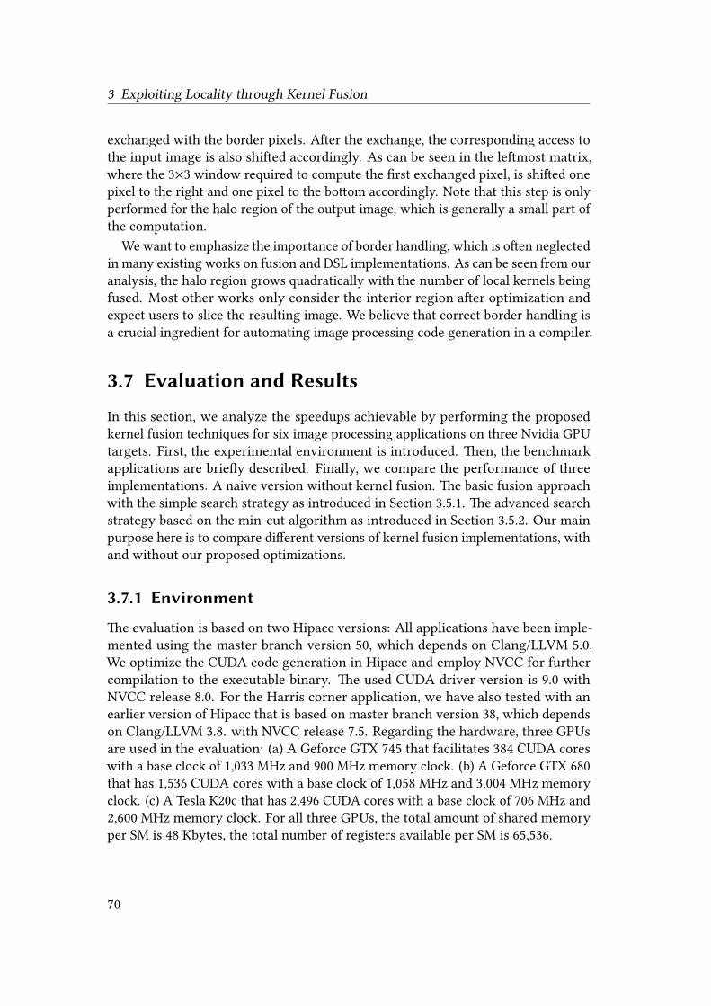
3 Exploiting Locality through Kernel Fusion
exchanged with the border pixels. After the exchange, the corresponding access tothe input image is also shifted accordingly. As can be seen in the leftmost matrix,where the 3×3 window required to compute the first exchanged pixel, is shifted onepixel to the right and one pixel to the bottom accordingly. Note that this step is onlyperformed for the halo region of the output image, which is generally a small part ofthe computation.
We want to emphasize the importance of border handling, which is often neglectedin many existing works on fusion and DSL implementations. As can be seen from ouranalysis, the halo region grows quadratically with the number of local kernels beingfused. Most other works only consider the interior region after optimization andexpect users to slice the resulting image. We believe that correct border handling isa crucial ingredient for automating image processing code generation in a compiler.
3.7 Evaluation and Results
In this section, we analyze the speedups achievable by performing the proposedkernel fusion techniques for six image processing applications on three Nvidia GPUtargets. First, the experimental environment is introduced. Then, the benchmarkapplications are briefly described. Finally, we compare the performance of threeimplementations: A naive version without kernel fusion. The basic fusion approachwith the simple search strategy as introduced in Section 3.5.1. The advanced searchstrategy based on the min-cut algorithm as introduced in Section 3.5.2. Our mainpurpose here is to compare different versions of kernel fusion implementations, withand without our proposed optimizations.
3.7.1 Environment
The evaluation is based on two Hipacc versions: All applications have been imple-mented using the master branch version 50, which depends on Clang/LLVM 5.0.We optimize the CUDA code generation in Hipacc and employ NVCC for furthercompilation to the executable binary. The used CUDA driver version is 9.0 withNVCC release 8.0. For the Harris corner application, we have also tested with anearlier version of Hipacc that is based on master branch version 38, which dependson Clang/LLVM 3.8. with NVCC release 7.5. Regarding the hardware, three GPUsare used in the evaluation: (a) A Geforce GTX 745 that facilitates 384 CUDA coreswith a base clock of 1,033 MHz and 900 MHz memory clock. (b) A Geforce GTX 680that has 1,536 CUDA cores with a base clock of 1,058 MHz and 3,004 MHz memoryclock. (c) A Tesla K20c that has 2,496 CUDA cores with a base clock of 706 MHz and2,600 MHz memory clock. For all three GPUs, the total amount of shared memoryper SM is 48 Kbytes, the total number of registers available per SM is 65,536.
70

3.7 Evaluation and Results
3.7.2 Applications
We chose six image processing applications to benchmark the kernel fusion tech-niques: The Sobel filter [DH73] as a well-known edge emphasizing operator appliedin many edge detection algorithms. It uses two local operators to derive edge in-formation along the x- and y-direction, which are then combined to produce thegradient magnitude. The Harris corner detector [HS88] and the Shi-Tomasi featureextractor [ST94] are classic filters for low-level feature extraction. Both algorithmsinvolve the computation of a Hermitian matrix but interpret the Eigenvalues indifferent ways. The Harris corner detector [HS88] is a classic filter for image pre-processing. The Hipacc implementation requires a combination of point and localoperators to form the whole pipeline, as depicted by Figure 3.11a. Overall, ninekernel invocations are needed to process one input image. The local operators inHipacc require accessing neighboring pixels, which would need boundary handling.In this evaluation, we specify clamp as the boundary handling mode in Hipacc. Fur-thermore, the filter is computed on a gray-scale image. The unsharp filter [Ram98]is a technique for image sharpening, in contrast to its name. The implementationconsists of a local kernel that blurs the image followed by three point kernels toamplify the high-frequency components. The Night filter [JPS+00] [She92] is chosenas a representation of a popular post-processing filter. First, it executes bilateralfiltering by iteratively applying the Atrous (with holes) algorithm of different size(3x3, 5x5 in our example). Then, the actual tone mapping curve is applied. The Hipaccimplementation of this filter is straightforward. It consists of three kernels Atrous0,Atrous1, and Scoto, which are linearly dependent and are executed in sequentialorder. Furthermore, the filter is computed on RGB images. Finally, we study an imageenhancement algorithm [SHM+14] used in medical imaging for wireless capsuleendoscopy. It uses a geometric mean filter and gamma correction for de-noisingand enhancement. Through the above mix of applications, we want to illustrate thatour technique is widely applicable in image processing including multiple domainssuch as computer vision and medical imaging. Throughout the experiment, we usea constant-size image of 2,048 by 2,048 pixels. Note that an exception is the Nightfilter, which uses an image of 1,920 by 1,200 pixels in RGB format. The other fiveapplications process in gray-scale.
3.7.3 Results
Figures 3.14 to 3.16 depict the execution times in milliseconds. We implementedthree versions for comparison: A baseline implementation. A basic kernel fusionimplementation based on the simple searching strategy. And finally, an optimizedimplementation based on the proposed advanced searching method. We performed500 runs for each implementation on each GPU. To cover the uncertainties in theexecutions, we visualize the results as a box plot overlay shown in the graph. The
71

3 Exploiting Locality through Kernel Fusion
whiskers cover the entire range of the obtained execution times, including theminimum, the maximum, the 25 percentile, and the 75 percentile values. The boxitself contains the intermediate 50% of all the results with a line in the middlerepresenting the median. In most cases, the box is not visible due to only smallvariations in the obtained result. In addition, Table 3.4 summarizes the achievedspeedups for three comparisons: the optimized version over the baseline version,the basic version over the baseline version, and the optimized version over thebasic version, respectively. Next, we discuss the performance improvement for eachapplication.
Harris Sobel Unsharp ShiTomasi Enhance Night0
4
8
12
16
20
24
28
Executiontim
e[m
s]
Baseline Basic Fusion Optimized Fusion
Figure 3.14: Execution times in<B (GTX 745).
Harris Sobel Unsharp ShiTomasi Enhance Night0
4
8
12
Executiontim
e[m
s]
Baseline Basic Fusion Optimized Fusion
Figure 3.15: Execution times in<B (GTX 680).
72

3.7 Evaluation and Results
Harris Sobel Unsharp ShiTomasi Enhance Night0
4
8
12Ex
ecutiontim
e[m
s]
Baseline Basic Fusion Optimized Fusion
Figure 3.16: Execution times in<B (k20c).
Table 3.4: Speedup comparison.
Optimized Fusion over Baseline
Harris Sobel Unsharp ShiTomasi Enhance Night
GTX745 1.344 1.377 3.438 1.357 1.920 1.020GTX680 1.145 1.108 2.025 1.138 1.760 1.000K20c 1.146 1.048 2.304 1.149 1.809 1.000
Basic Fusion over Baseline
Harris Sobel Unsharp ShiTomasi Enhance Night
GTX745 1.266 0.987 1.001 1.287 1.785 1.020GTX680 1.044 1.002 1.007 1.046 1.413 1.001K20c 1.094 1.002 0.999 1.099 1.490 1.000
Optimized Fusion over Basic Fusion
Harris Sobel Unsharp ShiTomasi Enhance Night
GTX745 1.061 1.394 3.435 1.055 1.076 1.000GTX680 1.097 1.106 2.011 1.088 1.245 0.999K20c 1.047 1.046 2.304 1.046 1.214 1.000
Enhance Filter Among all the applications, Enhance received the highest perfor-mance improvement due to its chain operations consisting of a local operator and
73

3 Exploiting Locality through Kernel Fusion
two point operators. There are no redundant computations required in the fusedkernel. A speedup of up to 1.92 can be achieved as can be seen in Table 3.4.
Sobel and Unsharp Filter Nevertheless, the basic fusion failed in optimizingthe filters Sobel and Unsharp. The Sobel filter consists of a local-to-local scenarioand the Unsharp filter has shared input, both of which are rejected by the basickernel fusion algorithm. The optimized fusion technique with the advanced searchalgorithm has all the power of the basic fusion with larger fusion scopes and moreoptimizations. The Unsharp filter consists of four kernels. The shape of its DAG issimilar to Figure 3.2b where all four kernels require the source input image. Thebasic fusion will regard these dependencies as external and invalid. In the optimizedfusion, we can detect this shared dependency on input image in a larger optimizationscope and aggregate them into a single kernel. A significant speedup of up to 3.4is achieved for this application. Furthermore, the Sobel operator computes bothhorizontal and vertical gradients, which is detected as local-to-local scenario and aspeedup of up to 1.377 is achieved in the optimized fusion.
Harris and Shi-Tomasi Corner Detector As for the Harris and the Shi-Tomasialgorithms, the point-to-local scenarios are detected and the basic fusion is able tocontribute speedups ranging from 1.04 to 1.28. The data dependency informationof these two applications is similar. We take the Harris operator as an example toprovide a detailed analysis of the amount of speedup obtained. We executed theHarris corner using the simple searching strategy on the Geforce 745 GPU, withHipacc (master branch) version 38, Clang/LLVM 3.8, and NVCC 7.5. The median of atotal of 50 executions is depicted in Figure 3.17. We execute the algorithm with aninput image of size 2048 by 2048, and a filter of size 3 by 3.
Figure 3.17 compares the execution time of the non-fused and the fused kernels.Table 3.5 presents the detailed execution times for all the kernels as well as the wholepipeline. Note that kernel dx, dy, and hc are categorized as unfusible, hence not shownin Figure 3.17. The execution times of those three kernels remains approximatelyunchanged compared to the unfused version, as shown in Table 3.5. The other kernelsin the Harris corner detector pipeline are identified as fusible and are grouped intothree fusible kernel lists, respectively. From Figure 3.17 and Table 3.5, we achieve aspeedup of 1.6 by fusing sx with gx, and sy with gy. By applying kernel fusion, weare able to speed up the entire Harris corner detector by a factor of 1.23.
Another observation is that fusing kernel sxy with kernel gxy yields less improve-ment. This is because kernel sxy requires two input images, as can be seen fromFigure 3.9. In the worst-case global memory access estimation, the extra input imagereduces the improvement for kernel fusion. Here, we further extend the analysis inTable 3.3 as follows: before fusion, the number of global memory loads is (FG + 1) ·#for a single input image. If an additional input image is required, the first point
74

3.7 Evaluation and Results
sx+gx sy+gy sxy+gxy0
1
2
3
4
5Ex
ecutiontim
e[m
s]Non-fusedFused
Figure 3.17: Execution time breakdown for the fusible kernels of the Harris corner.
Table 3.5: Execution time breakdown for the pipeline of Harris corner detector
Kernels Time before fusion (ms) Time after fusion (ms) Speedup
dx 2.18 2.16 -dy 2.16 2.19 -sx + gx 3.79 2.38 1.59sy + gy 3.80 2.37 1.60sxy + gxy 4.49 3.90 1.15hc 2.95 2.79 -
Overall 19.37 15.80 1.23
operator should load two images. Hence, the number of loads becomes (FG + 2) · # .After fusion, this number isFG ·# for single image input, and 2 ·FG ·# for two inputimages. Now, assume the employed filter has a width of 3, the number of globalmemory loads before and after fusion is 4 · # and 3 · # , respectively. Hence, 25% ofthe original global memory loads can be saved. Whereas for the two-input-imagecase, the number of global memory loads before and after fusion is 5 · # and 6 · # ,respectively. Without considering optimizations or caching effects, fusion mightincrease the number of global memory loads, but the number of stores is still reducedby half. Depending on image size and whether other memory optimizations areapplied, memory loads might be cached and the actual number might differ from theabove analysis. Nevertheless, we can conclude that the number of input images canpotentially degrade the performance. Fusion might not always be beneficial for thepoint-to-local scenario. The number of input images for the producer kernel shouldbe considered during fusibility analysis.
75

3 Exploiting Locality through Kernel Fusion
Night Filter One observation from Table 3.4 is the optimization of the night filterdoes not speedup. Among all the experimental results, only a maximal speedup of1.02 is achieved, which is marginal compared to other algorithms. The reason is thehigh computation cost of the kernels. Night filter consists of three kernels, Atrous0,Atrous1, and Scoto. The atrous (with holes) algorithm is applied two times (3×3, 5×5)to execute bilateral filtering. Those two local kernels are very expensive to compute.The number of ALU operations in the Hipacc implementation is 68 per thread. Usingour benefit estimation model, the cost of redundant computation outweighs thelocality improvement. Hence, the first two local kernels are not fused. The last kernelScoto is a point operator, which applies a tone mapping curve that uses 89 ALUoperations in the implementation. Kernel fusion detects a local-to-point scenario forAtrous1 and Scoto, and fuses both into one kernel. The amount of speedup we receivefrom the fusion is much smaller compared to the computation cost of the kernels.Hence, compute-bound applications benefit less from kernel fusion. Nevertheless,most image processing algorithms consist of a complex pipeline of small operatorsrather than a few very complicated functions. Kernel fusion targets algorithmsexpressed using common compute patterns, which are often memory-bound.
In the end, we provide an overview of all the speedups by computing the geometricmean across all three GPUs, as depicted in Table 3.6.
Table 3.6: Geometric mean of speedups across all GPUs.
Harris Sobel Unsharp ShiTomasi Enhance Night
Optm over Base 1.208 1.169 2.522 1.211 1.829 1.007Basic over Base 1.131 1.000 1.002 1.139 1.555 1.007Optm over Basic 1.068 1.173 2.516 1.063 1.176 1.000
3.8 Related Work
In the context of kernel fusion, accelerators such as GPUs are used extensively beyondimage processing. Our work is also motivated by DSLs from other domains. Wanget al. [WLY10] initiated kernel fusion as an alternative to loop fusion for power opti-mization on GPUs. Here, energy consumption can be reduced by balancing resourceutilization, which is achieved by fusing two or more kernels. The goal is to reducepower consumption rather than execution time. Wu et al. [WDW+12] enrichedthe benefits of kernel fusion with a smaller data footprint and larger optimizationscope. Nevertheless, the proposed fusion method is dedicated to data warehousingapplications. Filipovič et al. [FMF+15] attempted to harness the existing benefits,with a focus on inter-kernel communications. They established a source-to-source
76

3.8 Related Work
compiler in which kernel fusion is implemented as an optimization step for linearalgebra applications. The employed technique is closely related to our work, but thetarget is on different domains. It is well-known in GPU programming that frequentdata movement between host and device deteriorates the performance. Therefore,techniques such as kernel fusion have become an important optimization step onthe system level.
In the context of image processing DSLs: Halide [RBA+13] demonstrates the bene-fits of decoupling the algorithm from its schedule. Here, algorithms are specified ina functional manner. A scheduler determines the evaluation order, storage, mappinginformation, etc. PolyMage [MVB15c] employs a similar algorithm representationbut focuses on tiling techniques using the polyhedral model for scheduling. The func-tional description of algorithms in those DSLs effectively shields programmers fromhardware implementation details, which yields a much more concise description.Nevertheless, such representations capture merely data flow information from theprogram. The burden of optimization is entirely offloaded to the scheduler. A sched-uler is key for DSLs to generate efficient code. It can be specified by an architectureexpert, which is costly, error-prone, and not easily portable. A better approach isto generate a schedule from the source description automatically. For example, theHalide auto-scheduler [MAS+16] performs locality and parallelism-enhancing opti-mizations automatically by using techniques such as inlining, grouping, and tiling.It partitions the algorithm into groups and applies optimizations within each group.Subsequently, a schedule can be generated in seconds with reasonable performance.Nevertheless, the auto-scheduler might require user assists for providing functionbounds. Also, these optimizations are generic such that all SIMD machines withcaching behavior can benefit. If the target back end is a GPU, the communicationamong the partitioned groups still happens via the main memory.
Optimizations in DSLs are accomplished by combining domain-specific knowledgewith architecture knowledge. To gain this knowledge, the compiler needs to analyzethe programmer-specified algorithm description as well as the target hardware ar-chitecture information. Afterward it needs to extract information such as input size,data dependencies, memory size, and available computational resources. Finally, bycombining the gained knowledge with certain metrics, such as minimizing execu-tion time by reducing communication via global memory on a GPU, the compilerderives the optimized execution pattern and generates code. For image processingDSLs, we argue that there exists a trade-off between the constraints exposed tothe programmer for algorithm specification and the ease of applying optimizationsin the compiler, regardless of the target backend. For example, Halide allows itsprogrammers to describe algorithms in a functional manner, which enables effortlesstranslation from algorithms written in pure mathematical form to the correspondingHalide representation. Nevertheless, only dependency information is encapsulatedin such algorithm representations. Other information such as buffer size and lo-
77

3 Exploiting Locality through Kernel Fusion
cation are determined during schedule generation, which generally yields a veryexpensive design space exploration. In contrast, Hipacc limits the freedom exposedto its programmers to some extent. Hipacc users should specify their algorithmusing the provided domain-specific operators, as introduced previously. In this way,programmers should first match their algorithms with the compute patterns offeredby Hipacc operators. Note that this translation generally requires no additional effortsince the language and its operators are designed to express the common computepatterns in image processing. Consequently, the algorithm specification in Hipaccis as concise as the other functional representation languages such as Halide. Hav-ing this trade-off, Hipacc representations have program states and can encapsulatemore information in addition to data dependencies, e.g., parallelism or memory sizeand location. This additional domain knowledge can be combined with the domainand architecture knowledge, to enable many domain-specific optimizations, such asautomatic border handling and memory coalescing.
3.9 Summary
We presented an optimization technique called kernel fusion for data locality im-provement. We proposed a technique for computing speedup benefits of kernel fusionbased on the estimation of edge weights and formulating the problem as a minimumcut in a weighted graph. Based on this formalization, we proposed an algorithm todetermine fusible kernels iteratively and an analytic model to quantitatively estimatelocality improvement by incorporating domain-specific knowledge and architecturedetails. We seamlessly integrated the proposed technique into the Hipacc framework,and thus enabled inter-kernel optimizations during source-to-source compilation forGPUs. We also presented a method for fusing stencil-based kernels with automaticborder handling. A benchmark has been performed using six widely-used imageprocessing applications on three GPUs. The results show that the proposed techniquecan achieve a geometric mean of speedups of up to 2.52.
78

4Improving Parallelism via
Fine-Grained Resource Sharing
As mentioned in Chapter 1, transistors keep getting smaller and the total numberthat can be put on a single GPU keeps increasing, parallel architectures have evolvedtowards a multi-level hierarchy consisting of a growing number of compute coresas well as SMs. Traditionally, GPU programming focuses mostly on data-levelparallelism: Problems are divided into parallel workloads, which are mapped tothreads on the device. For example, one pixel in an image can bemapped to one threadon the GPU for execution. Nevertheless, as the performance of GPU architecturesincrease, the need to look beyond data-level parallelism becomes essential. Forexample, a relatively small image of size 256 by 256 used to be an expensive workloadfor earlier architectures, today is not even sufficient to fully utilize all the SMs on thelatest GPU. Threads in GPU architectures follow the SIMT execution model and areexpected to execute the same instructions, whereas threadblocks that are mappedonto each SM follow the MPMD execution model that can execute different programswhile sharing the same SM for computation (intra-SM, fine-grained resource sharing).In this chapter, we explore the kernel-level parallelism at the system level based onthe MPMD execution model. The goal is to better utilize the compute resources aswell as to improve the executions on modern GPU architectures.
In particular, we present two contributions in this chapter: First, an efficientmultiresolution filter (MRF) implementation to compute image pyramids with amulti-stream approach to exploit concurrent kernel executions. Multiresolutionfilters, analyzing information at different scales, are crucial for many applicationsin digital image processing. The different space and time complexity at distinctscales in the unique pyramidal structure poses a challenge as well as an opportu-nity to implementations on modern accelerators such as GPUs with an increasingnumber of compute units. We exploit the potential of concurrent kernel executionin multiresolution filters. Our contributions include a model-based approach forperformance analysis of both single- and multi-stream implementations, with thecombination of application- and architecture-specific knowledge. The data depen-dency information in MRFs applications is known due to the unique structure of the
79

4 Improving Parallelism via Fine-Grained Resource Sharing
image pyramid. For this class of algorithms, speedups can be obtained by exploringparallel executions. Nevertheless, it is challenging to generalize this approach toarbitrary applications with unknown data dependency information. As a remedy,we utilize the recently-released task-graph programming model from Nvidia calledCUDA graph. Our second contribution here is a combined approach of Hipacc andCUDA graph. We integrate CUDA graph into the CUDA backend in Hipacc to en-hance its code generation. The two techniques can benefit from each other: CUDAgraph encapsulates application workflows in a graph, with nodes being operationsconnected by dependencies. The new API brings two benefits: Reduced work launchoverhead and whole workflow optimizations, which can benefit Hipacc during opti-mization. On the other hand, we can improve the ability of CUDA graph to exploitworkflow optimizations, e.g., concurrent kernel executions with complementaryresource occupancy, with the help of domain-specific knowledge in Hipacc. In theend, our joint technique can benefit from both techniques.
4.1 Introduction
4.1.1 Multiresolution Filters
Analyzing and processing signals at different resolutions is an effective approach inmany domains, including medical imaging, computer vision, machine learning, andphotography. In image processing, the representation to carry the multiresolutioninformation is a unique pyramidal structure called image pyramid, as depicted inFigure 4.1a. The most fine-grained image is located at the bottom level, and themost coarse-grained image is located at the top. Images of different resolutions arecalled levels, which contain coarse-to-fine contextual information beneficial to many
Level 4
Level 3
Level 2
Level 1
Level 0
(a) Image pyramid
Reduce
Reduce
Reduce
Reduce
Filter
Filter
Filter
Filter
Expand
Expand
Expand
Expand
(b) MRF workflow
Figure 4.1: An image pyramid and a multiresolution filter workflow with five levels,the filter operation is not computed on the base image [QRT+20].
80

4.1 Introduction
applications. For example, in image denoising [ZG08; KEF+03], low-frequency noiseis difficult to remove. By reducing the information to a coarse-grained level, the noisecan be adequately represented in high-frequency and is easier to be removed. Inimage registration or feature enhancement [UAG93; PHK15], discriminative featurescan be extracted and refined based on a coarse-to-fine iterative strategy. Beyondimage processing, the multiresolution approach is also employed in areas such asscientific simulation as an efficient numerical method to solve large, sparse linearsystems [SKH+18; RKK+16; JLY12].
An MRF application takes an input image as the base level, and constructs apyramid by performing three basic operations between and within the levels [BA83a],as depicted in Figure 4.1b. Reduce takes fine-grained images as input and producescoarse-grained images as output. Expand, on the other hand, produces fine-grainedimages as output from coarse-grained images as input. Level processing, also calledfilter, works within each level to realize the core functionality of the application,such as denoising or edge enhancement. Those three basic operations formulatethe underlying structure that is shared among MRF applications. Such applicationsare data-intensive and are suitable for accelerators such as GPUs. Nevertheless, thecomplex data dependencies in the applications lead to many challenges for portablemanual implementations as well as optimizations on locality and concurrency. Toaccess the full performance of modern GPUs, we need to explore the task-levelparallelism among kernels. In a multiresolution filter, the filter operations expose agreat potential for concurrency. First, the filter operation at one level is generallyindependent of the filter operation at another level. The operations use the samekernel but are applied on differently sized images. Second, a filter operation at acoarse-grained level executes much faster than the same operation at a fine-grainedlevel, because of the smaller image size. For parts of the image pyramid, the imagesize would be too small to have enough computation data to occupy the GPU fully.Depending on the number of levels of the image pyramid and the specificationsof the hardware, this under-utilization of computational resources might result invery low occupancy. Here, it is important to systematically explore the optionsand performance benefits of concurrent kernel executions for the class of MRFapplications and to provide means to automatically apply respective transformationsusing a suitable compilation-based framework.
4.1.2 CUDA Graph
To achieve concurrent kernel executions, data dependency information must becaptured and analyzed. The common approach to capture such information is byusing a task graph model. Recently, Nvidia introduced an asynchronous task-graphprogramming model called CUDA graph, with the release of CUDA 10.0 [Ram18].It encapsulates application workflows in a graph, with nodes being operations con-
81

4 Improving Parallelism via Fine-Grained Resource Sharing
nected by edges. Compared to the conventional CUDA kernel execution, this newAPI decouples the initialization from the execution [Jon18]. Expensive operationssuch as device set-up, device instantiation, or kernel dependency analysis can beperformed only once during initialization. In this way, the application workflow ispre-known and brings several benefits, e.g., work launch overhead reduction. Onmodern high-end GPU devices, the overhead for CUDA work submission has becomeincreasingly prominent [Gra20]. CUDA graph enables the launch of any numberof kernels using one single operation, which drastically improves the performance,especially for kernels with a short running time. Another benefit is whole work-flow optimization, such as concurrent kernel execution. CUDA graph can exploreconcurrency in the application workflow and issue parallel streams for execution.This relieves the programmer of manual partitioning applications using streams andevents.
In this chapter, we first show that CUDA graph is not yet able to exploit concur-rent executions when kernels have complementary resource usage. Given a devicewith a certain amount of computation resources, two kernels use complementaryresources if their dominant resource usage, e.g., registers or shared memory, preventsthe concurrent execution of multiple instances of the same kernel but allows theconcurrent execution of instances of different kernels. Since the combined resourceusage is still within the device limit, missing such concurrency opportunities leads toinefficient implementations. To detect this situation and break through the limitation,we need to know not only kernel properties such as resource usage, but also devicespecifications such as the available capacity. We propose an approach called kernelpipelining that combines both knowledge and generates an optimized executionusing CUDA graph. We build our approach using the combination of CUDA graphand Hipacc. We show that the advantages of DSLs are complementary to CUDAgraph, and joining these two techniques brings the best of both worlds. As introducedin Section 2.2.2, DSLs, such as Hipacc, perform automatic code generation from asimple algorithm representation from the user, which increases the productivity of
Table 4.1: Available features in CUDA Graph, Hipacc, and our Combined approach.
Features Graph Hipacc Combined
Simple input representation from users 7 3 3
Auto-generated CUDA kernels 7 3 3
Kernel fusion (workflow optimization) 7 3 3
Reduced work launch overhead 3 7 3
Concurrent kernels (workflow optimization) 3 7 3
Interoperability with other CUDA libraries 3 7 3
Complementary resource (workflow optimization) 7 7 3
82

4.1 Introduction
algorithm developers. During code generation, Hipacc can explore opportunities forlocality improvement and apply transformations such as kernel fusion, as introducedin Chapter 3. On the other hand, a source-to-source compiler such as Hipacc dependson vendors such as Nvidia to perform further compilation. This implies that theoptimizations such as work launch overhead reduction in CUDA graph can alsobe carried back to Hipacc. Eventually, our combined approach not only benefitsfrom the existing optimizations in both CUDA graph and Hipacc, but also enablesnew workflow optimization opportunities such as concurrent kernel execution withcomplementary resources, as depicted in Table 4.1.
To sum up, our contributions in this chapter are as follows:
1. A generic analytical performance model for MRF applications combiningdomain-specific knowledge and architecture details, which is able to comparethe performance of both single- and multi-stream implementations with highfidelity.
2. A compiler-based approach using a DSL that integrates concurrent kernelexecution as transformation and generates code using CUDA streams forNvidia GPUs.
3. A combined approach that brings four benefits to CUDA graph implemen-tations: (1) Productive user input thanks to powerful abstractions, (2) auto-generated CUDA kernels, (3) workflow optimizations, such as kernel fusionfor increasing data locality, and (4) concurrent kernel executions with comple-mentary resource occupancy.
4. In turn, we bring four benefits to Hipacc DSL implementations: (1) Reducedwork launch overhead, (2) compatibility when using other CUDA libraries, (3)workflow optimizations for concurrent kernel executions, and (4) concurrentkernel executions with complementary resource occupancy.
5. We propose a technique called kernel pipelining, which optimizes the ker-nel executions generated by CUDA graph under complementary resourceutilization scenarios.
The remainder of this chapter is organized as follows1: Section 4.2 provides aDSL description of the multiresolution filter, which is an efficient recursive functionthat encodes the basic structure of the algorithm class. In addition, we explicate theconcurrent kernel execution opportunities in the algorithm. Section 4.3 introduces
1The contents of this chapter are based on and partly published in [QRT+20] which has appeared inthe Proceedings of the 13th Annual Workshop on General Purpose Processing Using GraphicsProcessing Unit (GPGPU), and [QÖT+20] which has appeared in the Proceedings of the 57thACM/EDAC/IEEE Design Automation Conference (DAC).
83

4 Improving Parallelism via Fine-Grained Resource Sharing
the analytic performance model for GPU architecture of the MRF applications. Wedescribe an occupancy calculation for both single- and multi-kernel executions. Then,the modeling of single-stream and multiple-stream implementations is presented indetail. Additionally, the fidelity of our model is evaluated. Section 4.4 introducesCUDA graph and explains how to use the graph API. Section 4.5 discusses concurrentkernel executions, with an emphasis on complementary resource usage. Section 4.6introduces in detail the added benefits of Hipacc, which in combination with CUDAgraph formulates the framework proposed in this work. Section 4.7 introduces theperformed benchmark. Four real-world MRF applications are summarized. Then,speedup results are shown and discussed. Finally, we discuss some related works inSection 4.8 before concluding in Section 4.9.
4.2 Unveiling Kernel Concurrency inMultiresolution Filters
Opportunities of concurrent kernel executions can already be observed in Figure 4.1b.Any filter operation on a fine-grained level can be executed in parallel with all theoperations on the coarse-grained levels. For example, when the filter operation isprocessing on level 1, the reduce operation can already start processing for level 2.When this reduce is finished, the filter is likely still executing due to the larger imagesize. During this time, another filter operation can start with processing level 2,given computational resources are available. This applies to all operations in thesubsequent levels. We partition the workflow of an MRF into ! parallel streams (8with 8 = (0, 1, ..., ! − 1), as depicted in Figure 4.2. To maximize the concurrency, weneed to minimize the number of concurrent kernels within each stream. Since astrict order of execution is preserved inside each stream, executions across differentstreams can happen in parallel. Data dependencies across different streams must be
(0 (1 (2 (!−1
Reduce Reduce Reduce Reduce
Filter Filter Filter Filter
Expand Expand Expand Expand
…
…
…sync. sync.
sync.sync.
Figure 4.2: Partitioning of an MRF application with depth ! [QRT+20].
84

4.2 Unveiling Kernel Concurrency in Multiresolution Filters
handled by synchronization. Thereby, for an arbitrary MRF application, the numberof parallel streams used equals the depth of the pyramid.
As can be observed, the data dependency within MRF algorithms is quite com-plicated. To achieve the concurrent kernel execution as we just described, CUDAstreams and events are needed to guard the scheduling and execution of the appli-cation. Manually perform such implementations is a laborious task, error-prone,and not portable at all. As a remedy, DSLs can provide concise descriptions for thisclass of algorithms. Well-known image processing DSLs such as Halide, Hipacc,and PolyMage provide abstractions to support common MRF applications. In theremainder of this section, we present the Hipacc support of MRF algorithms and theadditional asynchronous kernel launch feature enabled by our contribution.
4.2.1 An Efficient Recursive Description in Hipacc
As previously introduced, there are three basic operations in multiresolution filters,namely reduce, expand, and filter. They are applied recursively in and betweendifferent levels of an image pyramid, as depicted in Figure 4.1b. To describe thisworkflow, Hipacc provides an object pyramid to manage the memory allocationon each level of an image pyramid, and a function traverse to apply the recursivetraversal among different levels [MRS+14]. An example is depicted in Listing 4.1.First, an input pyramid ?8= is constructed with the provided input image 8= asthe base level and a user-specified depth. The same applies to the output pyramid?>DC . Then, the CA0E4AB4 function takes the MRF operations as a lambda function asinput and performs the actual level traversal. The reduce operation is specified asone kernel in lines 8–11, and the filter operation is specified as a second kernel inlines 14–17. These two operations are applied recursively at each level to produce thecoarse-grained image on the next level until the most coarse-grained level is reached.Afterward, the expand operation starts from the most coarse-grained level and isapplied recursively at each level to produce the fine-grained image, as shown inlines 22–25. Eventually, the base level of the output pyramid >DC is produced. Here,we emphasize the concise description of the basic structure of MRF applications,which only requires the operations of one level to be provided by the user. Thoseoperations are application-specific. For example, the filter operation might consistof two or more kernels or might also require the next level images as input, such asa Laplacian filtered image [RK82]. Our analysis in this chapter is applicable to anyapplication that shares the basic structure.
After the analysis, the transformations and code generations are performed by theother library Rewrite in Hipacc. It assigns kernels to streams based on the analyzedresults and uses the runtime API to launch the kernels. Currently, Hipacc generatesCUDA kernel calls with synchronizations before and after the kernel launch function,which yields a significant amount of overhead for the overall application. In this
85

4 Improving Parallelism via Fine-Grained Resource Sharing
Listing 4.1: An MRF description in Hipacc.
1 Image <uchar > in;
2 Image <uchar > out;
3 Pyramid <uchar > pin(in, depth);
4 Pyramid <uchar > pout(out , depth);
5
6 traverse ({ &pin , &pout }, [&] {
7 if (!pin.is_top_level ()) {
8 Accessor <uchar > acc_in(pin(-1), Interpolate ::LF);9 IterationSpace <uchar > iter_in(pin(0));
10 Reduce r(iter_in , acc_in);
11 r.execute ();12 }
13
14 Accessor <uchar > acc_in(pin(0));
15 IterationSpace <uchar > iter_out(pout (0));
16 Filter f(iter_out , acc_in);
17 f.execute ();18
19 traverse ();20
21 if (!pout.is_bottom_level ()) {
22 Accessor <uchar > acc_out_cg(pout (1), Interpolate ::LF);23 Accessor <uchar > acc_out(pout (0));
24 Expand e(iter_out , acc_out , acc_out_cg);
25 e.execute ();26 }
27 });
work, we use events to guard dependencies and enable a new asynchronous kernellaunch mode in Hipacc. CUDA streams and events are used for implementationsince we target Nvidia GPUs in our experiments [Nvi19]. The two Hipacc librariesAnalyzer and Rewriter work collaboratively to update the analysis information andto implement the desired transformations, as introduced in the Hipacc workflowdescription in Section 2.2.2. In the end, the optimized implementation is pretty-printed to host and device code.
By employing Hipacc DSL and the source-to-source compiler, and by extendingthe kernel launch functionality in Hipacc with a new asynchronous mode usingCUDA streams and events to realize data dependency, we can help programmers withporting MRF applications on GPUs efficiently. Nevertheless, despite the potentialconcurrent kernel executions uncovered in MRF applications, it is still not trivialto decide between a single- or multi-stream implementation. Single-stream impliessequential execution can be faster than multi-stream implementations of concurrentexecutions. To further investigate this trade-off, we propose a performance modelthat combines the domain- and architecture-specific information to decide on thebetter implementation between the two.
86

4.3 Performance Modeling
4.3 Performance Modeling
In this section, we present an analytic model to estimate the performance of MRFapplications implemented using CUDA streams. Our model provides insights onhow beneficial a multi-stream implementation is compared to its single-streamimplementation. Given an application and architecture specification, our modelis able to decide the better implementation choice among the two. We start byintroducing the basic CUDA concepts related to our model. We explain the meaningof a wave of threadblocks and its relation to occupancy. Then, we model single-and multi-stream implementations. Finally, some experimental results are shown toverify the fidelity.
4.3.1 Scheduling Basics
Although CUDA streams give programmers some control over the kernel launchsequence, the information is not sufficient for accurate performance estimation. Inthis work, our analysis is based on a finer-grained level of scheduling elements,namely threadblocks.
Threadblocks and Waves
A threadblock is a fundamental concept in CUDA programming. By specifying sizeand dimension, the input image is divided into a fixed number of threadblocks to bedispatched on the GPU. Threadblocks are considered as the basic scheduling unit inour model2. Another essential concept is a so-called wave in CUDA programming[Mic12]. A wave of threadblocks is a set of threadblocks that run concurrently ona GPU. The number of threadblocks that can run concurrently depends on manyconditions, as explained in detail in the next subsection. Concurrent kernel executionsare realized using concurrently running threadblocks. Our performance modelessentially estimates the number of waves required to execute a multiresolution filterfully. High concurrency should require fewer waves and vice versa. Next, we discussthe requirements and constraints to enable concurrent threadblocks.
Multi-kernel Occupancy
Threadblocks are dispatched and executed on SMs. Each SM has a device limit forthe number of threadblocks that can be active at once, defined in the architecturespecification. We denote this as �blk in Table 4.2. In addition to �blk, the number
2A threadblock is also called a CooperativeThread Array (CTA). There exist finer-grained schedulingelements called warps. The size of warps is fixed on GPU architecture. In this work, it is sufficientfor us to model executions at the threadblock level.
87

4 Improving Parallelism via Fine-Grained Resource Sharing
Table 4.2: Model Parameters
Param Explanation
�SM Number of SMs�blk Maximum number of threadblocks per SM�reg Total number of registers available per SM�smem Total amount of shared memory per SM�thr Maximum number of threads per SM
)multi Total running time of a multi-stream implementation)single Total running time of a single-stream implementation): Running time on the base pyramid level for kernel K#blk Number of achievable threadblocks per SM:blk Number of threadblocks to be computed by the kernelCreg Register usage per thread1smem Shared memory usage per blockCsz Threadblock size$event Synchronization overhead using CUDA events$par Concurrent execution overhead
of concurrent threadblocks is also constrained by the resource usage of the kernel.Given an application and an architecture, there exists a theoretical maximum numberof threadblocks that can run concurrently on each SM, denoted as #blk. The ratiobetween #blk and �blk is referred to as theoretical occupancy.
Given a kernel : , #blk is limited by four constraints: (a) Given a threadblock sizeCsz and the number of registers used per thread Creg, the total number of registersused in the block should not exceed the total number of registers available on anSM, denoted as�reg. (b) The shared memory usage per threadblock 1smem should notexceed the total amount of shared memory available on an SM, denoted as �smem.(c) The threadblock size Csz should not exceed the total number of threads availableper SM, denoted as �thr. (d) The architecture constraint �blk. Taking these fourconstraints together, we obtain:
#blk = min(⌊�reg
Csz · Creg
⌋,
⌊�smem
1smem
⌋,
⌊�thr
Csz
⌋,�blk) (4.1)
For the sake of simplicity, we assume a constant threadblock size throughout theexecution. However, this can be easily adapted to different sizes by explicitly definingeach level. Now, Eq. (4.1) can be generalized to multi-kernel executions as follows:
Without loss of generality, let us assume two kernels : and :′, with parameters Creg,1smem, Csz and C ′reg, 1′smem, C ′sz, respectively. If # ′blk blocks of :′ have been scheduled,the consumed resources on an SM can be computed as (a) (C ′sz · C ′reg · # ′blk) number
88

4.3 Performance Modeling
of registers, (b) (1′smem · # ′blk) amount of shared memory, and (c) (C ′sz · # ′blk) numberof threads. Then, we can subtract the utilized resources from the overall amountavailable and reapply Eq. (4.1) to compute the #̃blk threadblocks that are scheduledfor kernel : :
#̃blk = min(⌊�reg − C ′sz · C ′reg · # ′blk
Csz · Creg
⌋,⌊
�smem − 1′smem · # ′blk1smem
⌋,⌊
�thr − C ′sz · # ′blkCsz
⌋,
�blk − # ′blk)
(4.2)
Therefore, the combination of Eq. (4.1) and Eq. (4.2) allows us to estimate the wavesize of single- as well as multi-kernel executions. Based on this analysis, we canmodel the execution of single- and multi-stream implementations.
4.3.2 Single-Stream Modeling
In a single-stream implementation, all kernel executions are serialized. Starting fromthe base level, the reduce and filter kernels are executed following a fine-to-coarselevel directions, until reaching the most coarse-grained level. After that, the expandkernel is executed following the reverse coarse-to-fine direction. An example isdepicted in Figure 4.3a. Assume we compute an image pyramid of ! = 3 levels, and asingle-stream implementation runs the reduce and filter kernel from level 0 to level2, then the expand kernel runs from level 2 back to level 0. Note that in Figure 4.3athe threadblocks of any kernel only start execution after the threadblocks of theprevious kernel are finished. This is the scheduling behavior observed in all NvidiaCUDA drivers.
Assume an image within a pyramid % is %; , with ; = (0, 1, ..., ! − 1) denotes thelevel. The size of %; isF; × ℎ; in pixels, and a user-specified block size Csz = CG × C~ ,the total number of threadblocks that needs to be computed is:
:blk =
⌈F;
CG
⌉·⌈ℎ;
C~
⌉(4.3)
Combining Eqs. (4.1) and (4.3), given a kernel : and an image %; , we now can definea function to compute the number of waves required for processing :blk threadblockson a device with �SM streaming multiprocessors:
89

4 Improving Parallelism via Fine-Grained Resource Sharing
getNumWaves(:, %; ) =⌈
:blk
#blk ·�SM
⌉(4.4)
Furthermore, we can compute the size of the tail, namely the number of thread-blocks of the last wave, if any exists:
getTailSize(:, %; ) =:blk
#blk ·�SM−⌊
:blk
#blk ·�SM
⌋(4.5)
Next, we want to estimate the performance of the overall application, whichconsists of multiple kernels. The per wave execution time is required to be knownfor each kernel. This information can be obtained either by constructing a model thatdefines the computations of each kernel or by using the run-time information basedon some measurement. The primary goal of our model is to compare the performancebetween single- and multi-stream implementations. It is not our focus to modelin detail the computations of all kernels. Hence, the runtime-based approach issufficient to serve our purpose. Given the running time of a kernel : on its baseimage is ): , the running time per wave can be computed as:
C (:) = ):
getNumWaves(:, %0)(4.6)
Therefore, the total execution time of a single-stream implementation can beestimated as:
)single =
!−1∑;=0
∑:∈{',�,�}
(getNumWaves(:, %; ) · C (:)) (4.7)
4.3.3 Multi-Stream Modeling
Based on Eqs. (4.1) and (4.2), one can see that after some threadblocks of one kernelhave been scheduled, threadblocks of a second kernel can be scheduled if the SMsstill have extra computation resources. In a multi-stream implementation, this canhappen in two situations: The first is when computing fine-grained levels withlarge image sizes. There are many waves of threadblocks being executed, and thepreviously mentioned concurrency only happens in the last wave. This is called thetail effect in CUDA. The second situation happens when computing coarse-grainedlevels with small image sizes. In this case, there might not be enough threadblocks forone full wave. In our model, we distinguish between those two scenarios and dividethe whole multi-stream execution into three phases. Phase one is the execution onfine-grained levels where more than one wave is generated for each kernel. Phase twois the execution on coarse-grained levels where less than one full wave is generated.
90

4.3 Performance Modeling
("0 ("1 ("2 ("3'
�
'
�
'
�
�
�
�
'
�
�
'
�
�
'
�
�
'
�
'
�
�
�
'
�
�
'
�
�
'
�
�
'
�
'
�
�
�
'
�
�
'
�
�
'
�
�
'
�
'
�
�
�
'
�
�
'
�
�
'
�
�
(a) Single-streamtime
("0 ("1 ("2 ("3'
�
�
�
�
'
�
�
'
�
�
'
�
�
'
�
'
�
'
�
�
�
'
�
�
'
�
�
'
�
�
'
�
'
�
�
�
'
�
�
'
�
�
'
�
�
'
�
'
�
�
�
'
�
�
'
�
�
'
�
�
'
�
(b) Multi-streamtime
stream0 stream1 stream2 −→sync.
Figure 4.3: Single-stream and multi-stream execution for pyramid with ! = 3 levelsand :blk = 16, 4, 1 threadblocks. Adapted from [QRT+20].
91

4 Improving Parallelism via Fine-Grained Resource Sharing
Phase one and two are for the execution of reduce and filter kernels. Finally, phasethree is the execution of all the expand kernels. Eventually, the total execution timeof a multi-stream implementation equals the sum of those three phases. Beforepresenting the detailed modeling of those three phases, we make one assumptionrequired in our analysis.
Scheduling Assumption
In the following model, we assume that the CUDA scheduler dispatches thread-blocks in a breadth-first order to all the SMs, see Figure 4.3a as an example. Forour analysis, it is not important to identify the individual SM ID during dispatch,only the dispatch order is required to understand the concurrent kernel execution.Moreover, how the scheduler works is proprietary information and is not publiclydocumented. Nevertheless, this scheduling behavior is crucial to many optimizationsin various domains. The behavior has been studied and verified by several existingworks [LYK+14; OYA+17].
Fine-Grained Level Execution
The first execution phase of our multi-stream implementation is called fine-grainedlevel execution. A kernel execution belongs to this phase if it requires more than onewave to execute. For simplicity, we make a conservative estimation in our modeland do not consider the tail effect as concurrent executions. Hence, the modeling ofthis phase is identical to the single-stream scenario.
We provide an algorithm for the multi-stream modeling, as shown in Algorithm 3.From our partitioning method, we know the reduce and filter kernels are alwaysin the same stream, which means the execution is sequential between the two.Therefore, to determine whether both kernels belong to this phase, it is sufficient tocheck the number of waves for the filter kernel, as shown in line 7 of Algorithm 3.If the filter kernel requires more than one wave, the reduce and filter kernels areregarded as fine-grained level execution. In this phase, we update the total numberof waves, denoted as =waveSeq and is shown in line 8. The same procedure is executedrecursively (line 21) until the second phase coarse-grained execution is reached. Theexecution time of this phase can be estimated by
)fine =∑
:∈{',� }(=waveSeq · C (:)) (4.8)
Coarse-grained Level Execution
Whenever a kernel execution requires less than one full wave, it belongs to thecoarse-grained level execution. First, we show an example to illustrate the executionin this phase.
92

4.3 Performance Modeling
Algorithm 3: A Recursive Scheduling Algorithm1 ! ← getTopLevel(%)
2 ; ← 0 // Starting from base level
3 initialize(=waveExpand, =waveSeq, =wavePar, =?)
4 function SchedulePyramid()
5 #wave ← getNumWaves(�, %;)
6 #tail ← getTailSize(�, %;)
7 if (#wave > 1) ∨ (#wave = 1 ∧ #tail = 0) then// fine-grained level, ', � sequential
8 =waveSeq ← =waveSeq + #wave9 else
// coarse-grained level, ', � concurrent
10 if hasResourceAvailable(#tail) then11 =? ← =? + 1 // same wave
12 updateUsedResource()
13 else14 =wavePar ← =wavePar + 1 // new wave
15 (? ← (? ∪ =?16 =? ← 017 end18 end19 ; ← ; + 1 // increment current level
20 if ; < ! then21 SchedulePyramid()
22 end// sequential 4G?0=3 execution
23 #wave ← getNumWaves(�, %;)
24 =waveExpand ← =waveExpand + #wave25 ; ← ; − 1 // decrement current level
26 end
An example is depicted in Figure 4.3b. For the sake of simplicity, assume eachSM can have a maximum of six threadblocks scheduled for kernel ', � , or �. First,the reduce and filter kernel for the first image are scheduled in stream0. After that,each SM still has the capacity to schedule two more threadblocks. Hence, the reduceand filter kernel of stream1 can be scheduled. Due to the data dependency betweenthe reduce kernels, synchronization must happen, which has a certain cost. Then,the same applies to the kernels in stream2, which compute the most coarse-grainedimage with one threadblock. Finally, the expand kernels are executed, including
93

4 Improving Parallelism via Fine-Grained Resource Sharing
synchronizations. As can be seen in Figure 4.3, compared with the single-streamversion, the multi-stream version can reduce the execution time substantially.
We update two parameters of our model in this phase. =? denotes the numberof streams running in parallel, which equals 3 in Figure 4.3b. Another parameteris =wavePar that denotes the number of waves required to run all the coarse-grainedlevels, since the device may not have enough resources to accommodate all thecoarse-grained level kernels in one full wave. This is determined based on Eq. (4.2).Whenever the resources are sufficient, concurrent kernels can run in the same wave,as shown in lines 11–12. In this case, we only need to update =? . Yet, if the resourcesare no longer sufficient, a new wave should be scheduled, as shown in lines 14–16.In this case, we save the previous =? and reset its value to 0. The whole procedure isrepeated until the most coarse-grained level is reached, after which the expansionkernels continue.
As can be seen in Figure 4.3b, the time of each parallel execution can be modeled as=? − 1 sequential reduce operations with synchronizations, plus one filter operation.We introduce a new parameter $event to denote the synchronization overhead fromCUDA events. Furthermore, we observe that when executing expensive kernels suchas filter operations in parallel, the execution time is slightly longer compared to itssequential execution. This is because any concurrent kernel executions share theunderlying CUDA cores in each SM. For simplicity, we use a parameter $par > 1to denote this additional overhead. Finally, the execution time of this phase isapproximated as follows:
)coarse =∑
=wavePar∈(?(((=? − 1) · (C (') +$event) + C (� )) ·$par) (4.9)
From Eq. (4.2) and Figure 4.3b, we can observe that if a filter execution time C (� )is quite small, the extra overhead created by CUDA events might excel the benefit ofkernel overlap. Moreover, if the interference among concurrent kernels generatessignificant overhead, $par might outweigh the benefit of concurrent execution. Inboth cases, the multi-stream implementation might perform worse even than itssingle-stream implementation.
Expand Execution
The modeling of the expand kernel execution is relatively straightforward, as shownin lines 23–24. It is similar to the single-stream implementation, with additionalsynchronization overhead between CUDA streams. The execution time can beestimated as:
)expand = =waveExpand · (C (�) +$event) (4.10)
94

4.3 Performance Modeling
Finally, the overall execution time of a multi-stream execution is obtained as thesum of all three phases:
)multi = )fine +)coarse +)expand (4.11)
4.3.4 Model Fidelity
Based on the previously introduced model-based performance analysis, we under-stand that the performance difference between single- and multi-stream applicationsdepends on the architecture capability as well as the application characteristics. Fromthe application point of view, the expensiveness of the filter operation relative to thereduce and expand operations decides the performance difference to a large extent.
To verify the fidelity of our model, we implemented eleven synthetic kernels tosimulate the filter operations common in many multiresolution filters and comparedthe measurement with our model-based performance prediction. Using synthetickernels allows us to control the computational intensity as well as the computepatterns. We use a combination of element-wise and stencil-based computationswith operations of different expensiveness such as addition, subtraction, exponential,and trigonometric functions. The information is summarized in Table 4.3. Oursynthetic kernels are parameterized as follows:
out = reduce(+,map(_, in(dom)), dom(BI, BI)) (4.12)
Eq. (4.12) defines the operations required to compute each output pixel. First, adomain of size BI × BI is defined. Then, each pixel in the domain is mapped to anintermediate pixel by applying the lambda function _. Finally, a reduction is appliedto all the intermediate pixels in the domain to generate the output pixel. Table 4.3 liststhe size of the domain and the number of operations performed within the lambdafunction. The reduce and expand operations are based on the implementation byBurt and Adelson [BA83a]. Namely, the reduce operator performs a two-dimensionallow-pass filtering followed by a sub-sampling by a factor of 2 in both directions. The
Table 4.3: Synthetic filter kernel parameters
kernels 50 51 52 53 54 55 56 57 58 59 510
domain size (sz) 1 1 3 3 5 7 9 11 13 15 17
add, sub 1 2 0 2 2 2 2 2 2 2 2mul, div 0 2 1 2 2 2 2 2 2 2 2exp, cos 0 2 0 2 2 2 2 2 2 2 2
95

4 Improving Parallelism via Fine-Grained Resource Sharing
50 51 52 53 54 55 56 57 58 59 5100.900.951.001.051.101.15
)B8=6;4/)
<D;C8
Measurement Prediction
(a) GTX 680
50 51 52 53 54 55 56 57 58 59 5100.90
0.95
1.00
1.05
1.10
)B8=6;4/)
<D;C8
Measurement Prediction
(b) GTX 680
50 51 52 53 54 55 56 57 58 59 510
0.60
0.80
1.00
1.20
1.40
)B8=6;4/)
<D;C8
Measurement Prediction
(c) K20c
Figure 4.4: Measurement and model prediction.
expand operator enlarges an image to twice the size in both directions by upsamplingand low-pass filtering followed by multiplication with 4 to keep the intensity.
Given the above implementations, we executed three experiments, as depicted inFigure 4.4. The vertical axis in Figure 4.4 denotes the ratio between single-stream andmulti-stream execution time, thus the speedup achieved by concurrent kernel execu-tion. Table 4.4 summarizes the Pearson correlation coefficients [BCH+09] as well asthe difference of the geometric means between the measurement data and our modelpredictions. As can be seen, our model is able to produce a very good estimation. We
96

4.3 Performance Modeling
Table 4.4: Model fidelity experiment
Experiment (a) (b) (c)
Device GTX680 GTX680 K20cPyramid levels ! 8 10 8Base image sizeF × ℎ 512 × 512 1024 × 1024 512 × 512Threadblock size Csz 16 × 16 16 × 16 16 × 16
Pearson correlation coefficient 0.969 0.970 0.981Geometric mean difference 0.011 0.006 0.017
can observe that for compute-intensive kernels, the concurrent execution enabledby the multi-stream execution delivers the best overall performance. However, incase the kernel is inexpensive, mostly memory-bound, the single-stream executionis the better option.
The speedups depicted in Figure 4.4 are intended for fidelity verification. Thenumbers are specific for the performed experiments, which does not imply thatconcurrent kernel executions can achieve only less than 20% speedup. The achiev-able speedup depends on both the application settings, such as pyramid levels andbase image size, as well as hardware capabilities, such as the number of SMs. Forexample, in Figure 4.3, if the filter operation � has a long execution time, such thatthe execution of reduce ' and expand � operations become negligible. Then, theachievable speedups can be up to 3.0 for that example, since the filter operation � ofall three levels can be executed concurrently.
4.3.5 Intermediate Summary
We have exploited the data dependency information encoded in MRF applicationsand proposed a multi-stream implementation with concurrent kernel executions. Inaddition, we provided a systematic analysis and performance modeling of both single-and multi-stream implementation on GPU architectures. Our primary finding is thatthe multi-stream implementation is not always better than a sequential single-streamversion. The computation cost of the filter kernel in MRF applications determines thelevel of benefit for any multi-stream implementations. Our model is able to capturethis trade-off with very high accuracy.
So far, our analysis is bound to the fixed dependency pattern exposed in MRFapplications. Nevertheless, as GPU architectures keep evolving with higher computeresources, concurrent kernel execution becomes an important optimization objectivefor many applications beyond MRF. To enable such optimizations, data dependencyinformation should be exploited for any arbitrary application. Task graph models arewidely used to capture such information. Recently, Nvidia released an asynchronous
97

4 Improving Parallelism via Fine-Grained Resource Sharing
task-graph programming model called CUDA graph, which facilitates many opti-mizations compared to the traditional CUDA implementation. In the remainder ofthis chapter, we analyze the execution model of CUDA graph and combine it withour DSL and compiler Hipacc.
4.4 Execution Model in CUDA Graph
Utilizing the CUDA graph API follows a three-stage execution model: Graph defini-tion, graph instantiation, and graph execution. For illustration, Listing 4.2 depicts anexample that implements a Sobel edge detection filter.
4.4.1 Graph Definition
The first stage is graph definition. There are two modes available: Manual mode andstream capture mode. In Listing 4.2, lines 13–23 depicts the definition statements usedin the manual mode. Undermanual mode, the user declares nodes with dependenciesand parameters. For example, a kernel node can be associated with a CUDA kerneland its parameters, such as input and output. A memory copy node can performhost-device communications. A graph can be defined by adding the nodes withtheir corresponding dependencies. Therefore, the execution sequence of differentoperations is implicitly defined in terms of user-given dependencies. For example, inListing 4.2, node =< that computes the magnitude must start after node =G and =~ thatcompute the x- and y-derivative of the image, given by the third argument in line 22.This explicit data dependency information is also used by CUDA graph for laterscheduling and optimizations. The other mode to define a graph is stream capture. Agraph can be defined by capturing an existing implementation that already utilizesCUDA streams. This is achieved by using two stream-capture functions, which areput before and after the existing implementation, as shown in Listing 4.2 in line 25 andline 31, respectively. In this case, CUDA graph obtains the dependency informationautomatically from the existing stream and event synchronizations: Kernels withinthe same stream are serialized, while kernels among parallel streams can be executedconcurrently. After the graph definition state, the topology of the graph is fixedand cannot be changed during later execution. If the application changes, the graphshould be redefined.
4.4.2 Graph Instantiation
The second stage is the graph instantiation. After defining the graph, the wholeworkflow is known, and analysis can be performed to enable certain optimizations,such as to determine the number of possible parallel streams or to prepare the kernels
98

4.4 Execution Model in CUDA Graph
Listing 4.2: Sobel filter implementation using CUDA graph.
1 #include "KernelSobelXDerivative.cu"
2 #include "KernelSobelYDerivative.cu"
3 #include "KernelSobelMagnitude.cu"
4
5 // Unrelated details are omitted for simplicity
6
7 void SobelFilterCudaGraph(in, out , ...){
8 // Initialization for graph , streams , etc.
9 cudaGraphCreate(G, ...);
10
11 // Stage 1: Define G
12 if (ManualMode) {
13 // declare memory copy and kernel nodes...
14 cudaGraphNode_t n_h2d , n_d2h , n_x , n_y , n_m;
15
16 // add nodes to the graph using cudaGraphAdd..Node
17 // (node , graph , dependent node(s), parameters , ...)
18 // params include input , output , kernel , args , etc.
19 cudaGraphAddMemcpyNode(n_h2d , G, NULL , params , ...);
20 cudaGraphAddKernelNode(n_x , G, n_h2d , params , ...);
21 cudaGraphAddKernelNode(n_y , G, n_h2d , params , ...);
22 cudaGraphAddKernelNode(n_m , G,[n_x ,n_y] , params , ...);
23 cudaGraphAddMemcpyNode(n_d2h , G, n_m , args , ...);
24 } else if (StreamCaptureMode) {
25 cudaStreamBeginCapture(stream , ...); // start capture
26
27 // a sobel implmentation independent of CUDA graph
28 // ... cudaMemcpyAsync(... ,stream)...
29 // ... cudaLaunchKernel(... ,stream)...
30 //
31 cudaStreamEndCapture(stream , G); // finish capture
32 }
33
34 // Stage 2: Instantiate G
35 cudaGraphInstantiate(G, ...);
36
37 // Stage 3: Execute G
38 cudaGraphLaunch(G, ...); // possible in a loop
39
40 // Cleaning
41 cudaGraphDestroy(G);
42 }
such that they can be launched as fast as possible during execution. To launch manykernels, CUDA graph provides a mechanism to launch multiple GPU operationsthrough a single CPU operation, which can significantly reduce the work launchoverhead. Apart from this optimization, we can also take advantage of the automatedconcurrent kernel execution feature to automatically launch multi-stream executions
99

4 Improving Parallelism via Fine-Grained Resource Sharing
for any application shape. In this work, we enrich the analysis in this stage with thedomain- and architecture-specific knowledge available in Hipacc. By default, CUDAgraph does not have any knowledge of the compute kernels, and the schedulingstrategy is always the same. We observe an optimization opportunity here andextend the workflow optimizations in CUDA graph with additional techniques suchas concurrent kernel execution with complementary resources and kernel fusion.
4.4.3 Graph Execution
The last stage is graph execution. At this point, we should have an implementationwith reduced launch latency and fully optimized workflow execution. CUDA graphencourages the instantiate once, execute repeatedly workflow, which is commonlyseen in many Machine Learning (ML) and HPC applications. In this work, we donot focus on iterative kernel executions. Instead, we examine how to explore theconcurrent kernel execution more efficiently. In the following section, we present indetail how to improve the resource sharing and the concurrent kernel executions inCUDA graph.
4.5 Kernel Execution with ComplementaryResource Usage
Modern GPUs are equipped with an increasing amount of compute resources. Ex-ploring task-level parallelism becomes vital to access the device’s full performance.CUDA graph can generate parallel streams for concurrent kernels as a workflowoptimization. This potentially contributes to better resource utilization and fasterexecutions. In this section, we show that CUDA graph is not yet able to exploit theopportunities when kernels have complementary resource usage. First, we discusshow concurrent kernel execution improves intra-SM resource sharing, and give andefinition of complementary resource usage. Then, we use an example applicationto illustrate the current workflow explorations in CUDA graph. Finally, we presentour proposed approach called kernel pipelining and verify its scalability and fidelity.
4.5.1 Intra-SM Resource Sharing
Concurrent kernel executions can improve the resource utilization within eachSM [WYM+16]. The concurrent execution is realized on GPUs in the granularity ofthreadblocks, which is a fundamental concept in CUDA programming. A threadblockcan be dispatched on an SM as long as the SM has sufficient resources to meet itsdemand. Three resources account for usage on each SM: (a) the number of registers,(b) the amount of shared memory, (c) the number of threads. Each threadblock
100

4.5 Kernel Execution with Complementary Resource Usage
consumes a certain amount of these resources. Given a kernel E , the resource usagefor each type is:
Areg(E) =Csz · Creg�reg
(4.13)
Asmem(E) =1smem
�smem(4.14)
Athr(E) =Csz
�thr(4.15)
where Csz denotes the number of threads in a block, namely the threadblock size.Creg denotes the number of registers used per thread. 1smem is the amount of sharedmemory used in a threadblock. �reg, �smem, and �thr denote the total amount ofavailable registers, shared memory, and threads on a single SM, respectively. Theresource usage of a kernel, denoted as A (E), is determined by the dominant resourceusage on each threadblock, namely the maximum among the three:
A (E) = max(Areg(E), Asmem(E), Athr(E)) (4.16)
Additionally, each architecture has an upper limit for the number of concurrentthreadblocks per SM, denoted as �blk. In CUDA programming, 1/(A (E) · �blk) isreferred to as the theoretical occupancy [Nvi15].
Complementary Resource Occupancy
A set of kernels + = {E0, E1, ..., E#−1} is said to have complementary resource occu-pancy if their kernel resource usage prevents the concurrent execution of multipleinstances of the same kernel but allows the concurrent execution of instances ofdifferent kernels, namely:(
∀E∈+ , A (E) > 0.5)∧(∀5 ∈{Areg,Asmem,Athr},
∑E∈+
5 (E) < 1)
(4.17)
In Eq. (4.17), the first clause checks the existence of a resource type that is usedmore than 50% by one kernel, and the second clause guarantees the total resourceusage of all kernels stays within the device limit. For example, Table 4.5 depicts theresource usage of two kernels and the number of available resources of an NvidiaGPU RTX2080. As can be seen, kernel ? cannot be executed concurrently withanother instance of ? due to the large number of compute threads, which occupymore than 50% of the available. The situation is similar for kernel ; due to the amountof occupied shared memory. Nevertheless, kernel ? and ; should be able to runconcurrently since the combined resource utilization is still within the device limit.
101

4 Improving Parallelism via Fine-Grained Resource Sharing
Table 4.5: Kernel resource utilization for an example application.
Resource Threads Registers Shared Memory
Kernel (per block)? Csz 640 Creg 23 1smem 0 KBAthr(?) 62.5% Areg(?) 35.9% Asmem(?) 0%
Kernel (per block); Csz 256 Creg 34 1smem 26 KBAthr(;) 25% Areg(;) 53.1% Asmem(;) 54.2%
RTX 2080 �thr 1024 �reg 64 �smem 48 KB
4.5.2 Example Application
Let us consider a scattering pattern application that consists of # two-stage pipelines,as depicted in Figure 4.5. Such scattering pattern is commonly seen in image pro-cessing applications, for example, computing different resolutions of an image orcomputing the Hessian matrix of an input. Assume kernel ? and ; in Table 4.5 areused in the pipeline. Kernel ? is based on a tone mapping algorithm that performselement-wise operations [JPS+00]. Kernel ; is based on the Gaussian filter that per-forms stencil-based operations. The target device is an Nvidia RTX2080 with Turingarchitecture with 46 SMs and 2944 CUDA cores. The available resources per SM arealso listed in Table 4.5.
CUDA Graph Execution
We implemented the application with a different number of parallel pipelines (# =
3, ..., 13) using CUDAgraph’smanual mode. Figure 4.6a depicts the execution timelineof the application for # = 5 pipelines. As can be observed in the figure, despite
img
?0
;0
img
?1
;1
img
…
…
…
?#−1
;#−1
img
Figure 4.5: Example application with a scattering pattern [QÖT+20].
102

4.5 Kernel Execution with Complementary Resource Usage
CUDA graph is able to detect the amount of parallelism and deploys five concurrentstreams, the execution of all ten kernel instances of the application is serialized3.The same behavior is also observed for other numbers of pipelines. Figure 4.6a letsconclude that CUDA graph tries to schedule the kernels in a breadth-first search(BFS) order. However, because of the dominant resource usage in both ? and ; , theexecutions are serialized. Overall, CUDA graph cannot exploit the complementaryresource occupancy in the pipeline. Since CUDA graph requires only kernels anddependencies, neither streams nor events are specified by the user. The generatedschedule, in this case, is entirely decided by the Nvidia CUDA driver.
Stream0
Stream1
Stream2
Stream3
Stream4
?0
?1
?2
?3
?4
;0
;1
;2
;3
;4
(a) CUDA graph execution
Stream0
Stream1
?0 ;0 ;1 ;2 ;3 ;4
?1 ?2 ?3 ?4
(b) Optimized execution
Figure 4.6: Timeline for # = 5 (illustration based on the output from Nvidia VisualProfiler NVVP) [QÖT+20].
Optimized Execution
Since kernel instances of ? and ; can be executed concurrently due to the comple-mentary resource occupancy according to Eq. (4.17), we can derive an optimizedexecution schedule as depicted in Figure 4.6b. Instead of first scheduling all instancesof kernel ? , we can schedule ?0. Then, ;0 can be executed in parallel with ?1, and thesame applies to all the subsequent kernels. However, to enable this schedule, the par-titioning configuration of the on-chip memory between L1 cache and shared memoryfor both kernels should be consistent, which means the same memory configurations.For example, a kernel with 16/48 KB partition between L1 and shared memory cannotbe executed concurrently with another kernel with 48/16 KB partition. This is thereason that the execution of ?4 and ;0 is not overlapped in Figure 4.6a, and can be
3A small amount of overlap can be observed among kernels, which is more noticeable under ;0...;4.This is called tail effect: Threadblocks do not start and finish at exactly the same time. Thisbehavior does not affect the analysis in our work.
103

4 Improving Parallelism via Fine-Grained Resource Sharing
configured using the runtime API cudaFuncSetCacheConfig(). To generate suchoptimized execution schedules, we propose a method called kernel pipelining.
4.5.3 Kernel Pipelining
We present our kernel pipelining approach that optimizes the schedule for thescattering-pattern applications. Our method does not impose any constraints on thenumber of parallel pipelines or the number of kernels in each pipeline. A pseudoalgorithm is shown in Algorithm 4. Given an input application represented as� = (+ , �), where G is a DAG consisting of a kernel set+ and the connecting edge set�. Our algorithm generates a CUDA graph definition as follows: An iterative kernelscheduler determines the kernel issuing order based on complementary resourceoccupancy, which can be detected using the compResourceOcc() function in line10 based on Eq. (4.17). Whenever concurrent execution is possible, the kernel isissued to a parallel stream, as shown in lines 11–12. Otherwise, the kernel issueis postponed until the next iteration, and instead, the child of the previous kernel(searching in depth-first search (DFS) order) is issued. For example, after kernel ?0has been issued in Figure 4.6b, the next kernel ?1 (BFS order) is issued. Since ?0 and?1 have no complementary resources, the issuing of ?1 is postponed and ;0 is issuedinstead. Note that ;0 is the child of ?0, which is the previous kernel of ?1. This DFSsearch order is performed in lines 17–18. After ;0 is issued to the same stream as ?0using the function in line 19, we continue with the previously postponed ?1. Now,?1 can be scheduled concurrently with ;0, and the same procedure applies to ?2 andall the remaining kernels. In the end, the obtained schedule ( is captured using thestream capture mode in CUDA graph.
Additionally, we want to mention that overlapping the execution of multiplekernels might introduce some overhead depending on the kernel characteristics.Concurrent executing kernels share the CUDA cores within each SM. This overheadcan be obtained by dividing the kernel running time under concurrent execution bythe time under serialized execution.
4.5.4 Scalability and Fidelity
To verify the scalability as well as the fidelity of the proposed approach, we experi-mented with the example application depicted in Figure 4.5. The actual executiontime has been measured on the RTX2080 for ten configurations with a differentnumber of pipelines # = 3, ..., 13. The result is depicted in Figure 4.7. The theoreticalspeedup of the example application can be computed as follows: We use C? and C; todenote the execution time of kernel ? and ; in the application. Since CUDA graphdelivers a sequential execution, the overall execution time can be computed as:
104

4.5 Kernel Execution with Complementary Resource Usage
Algorithm 4: Kernel Pipelining Algorithm.input : � = (+ , �)output : CUDAGraphDefinition
1 function KernelPipelining(�)
2 +B ← ∅ // a set of scheduled kernels
3 +2 ← ∅ // a set of resource-sharing kernels
4 # ← getPipeMaxDepth(�)5 ( ← {B0, B1, ..., B#−1} // a set of streams
6 E ← getHeadKernel(�) // starting kernel
// iterative kernel scheduler
7 repeat8 if E ∈ +B then9 E ← getNextKernelBFS(E,�)
10 else if (compResourceOcc(E,+2)) ∨ (|+2 | = 0) then// issue E to run concurrently with +2
11 8 ← |+2 |12 B8 .enqueueKernel(E)
13 +2 ← +2 ∪ {E} // update resource-sharing
14 +B ← +B ∪ {E} // update scheduled kernels
// continue with the next kernel
15 E ← getNextKernelBFS(E,�)
16 else// postpone E, issue the child of
// the previous kernel of E (DFS)
17 E′′ ← getPreviousKernelBFS(E,�)
18 E′ ← getChildKernel(E′′,�)19 B0.enqueueKernel(E′) // issue stream 0
// reset resource-sharing
20 +2 ← ∅21 +2 ∪ {E′}22 +B ← +B ∪ {E′} // update scheduled kernels
// continue with the postponed E
23 end24 until |+B | = |+ |25 return defineGraphWithCaptureMode(()
26 end
105

4 Improving Parallelism via Fine-Grained Resource Sharing
3 4 5 6 7 8 9 10 11 12 130.80.91.01.11.21.31.41.5
Number of parallel pipelines #
Speedu
p
Measurement Theoretical
Figure 4.7: Speedup for the example application in Figure 4.5.
Cseq = (C? + C; ) · # (4.18)
The execution time for the optimized kernel-pipelined schedule can be estimatedas:
Copt = C? +max(C?, C; ) · # ·$ (4.19)
Where$ denotes the overhead generated by concurrent execution. During profiling,we observed that the execution time of kernel ? is approximately half of kernel ; , andthat they have little interference during concurrent execution. Thus, with C? ≈ 0.5 · C;and $ = 1, the theoretical speedup achievable is:
Cseq
Copt=
(C? + C; ) · #C? +max(C?, C; ) · # · 1
=1.5 · C; · #
0.5 · C; + C; · #=
1.50.5#+ 1
(4.20)
The theoretical speedups, together with the measured speedups, are plotted inFigure 4.7. As can be seen, the measured speedups achieved by our approach deviateby less than 10% on average from the estimated theoretical speedup. The performanceis also scalable to a larger number of parallel pipelines.
4.5.5 Intermediate Summary
In this section, we proposed a kernel pipelining technique to optimize the kernelexecutions generated by CUDA graph under complementary resource occupancy.The analysis is based on a knowledge combination of kernel properties, applicationdependency, and device specifications. We want to emphasize that the problemcombined with our analysis presented in this section is applicable to generic CUDAkernels and is not bounded to any domain. CUDA graph users can already followour approach and hand-transform a serialized execution under CUDA graph manualmode to an optimized execution under stream capture mode. However, manual work
106

4.6 Combining CUDA Graph with an Image Processing DSL
is difficult to maintain, error-prone, and not portable at all. We, therefore, propose toemploy an image processing DSL that has the required combination of domain- andarchitecture-specific knowledge. Additionally, utilizing a DSL brings further benefits,including simple input representations and opens the opportunity for other workflowoptimizations such as locality improvement. In the next section, we combine CUDAgraph with Hipacc.
4.6 Combining CUDA Graph with an ImageProcessing DSL
In this section, we utilize the CUDA backend of the source-to-source compiler, andfor the first time, extend the API to CUDA graph. An overview of our framework isdepicted in Figure 4.8. Starting from the Hipacc DSL, users specify their applicationsin C++, which can be parsed by Clang to generate a Clang AST. Then, the Hipacccompiler traverses the AST and performs the source-to-source transformation usingtwo internal libraries: Analyzer gathers information for analysis and optimizations,e.g., domain knowledge such as the kernel resource usage, compute pattern, kerneldata dependency, or device information such as the compute capability. Based on theobtained domain- and architecture-specific knowledge, optimizations are applied.Hipacc performs optimizations in two steps: First, single kernel optimizations suchas memory padding are applied, and efficient CUDA code is generated for each
Analyzer Rewritermemory padding,loop unrolling,kernel pipelining,kernel fusion, …Cl
angAST
ClangAST
kernel resource usage, data dependencies, …
SM resources, GPU compute capability, …
Source-to-Source Compiler (Hipacc)
Host code KernelsGraph API+ +
CUDA Runtime
Domain-Specific Language (Hipacc)User
Lex, Parse, Sema
Pretty Print
Dom
ainKn
owledg
eArchitecture
Knowledge
Figure 4.8: Combining CUDA graph with Hipacc [QÖT+20].
107

4 Improving Parallelism via Fine-Grained Resource Sharing
user-defined kernel. Second, workflow optimizations are exploited, for example,kernel fusion (Chapter 3) for any possible locality improvement, and concurrentkernel execution for SM resource sharing.
After the analysis, the transformations and code generations are performed bythe other library Rewriter. It allocates the memory location in kernel read and writefor fusion, and assigns kernels to streams if kernel pipelining is enabled for CUDAgraph. Analyzer and Rewriter work iteratively to update the analysis informationand implement the desired transformations. In this work, when both kernel fusionand concurrent kernel execution are available, the transformation on concurrentexecution takes precedence over fusion, because we think a better resource utilizationhas higher priority. In the end, the backend of Hipacc generates a CUDA graphimplementation with reduced launch latency and a fully optimized workflow.
4.6.1 Benefits Inherited from Hipacc
Here, we recap some of the benefits enabled when using a DSL such as Hipacc, whichcan be brought to CUDA graph. As introduced in Chapters 1 and 2, in comparisonto an optimized hand-written CUDA kernel, the number of LoC is much smaller.Users can focus on algorithm functionality, and Hipacc is responsible for the kerneland workflow optimizations. To specify a kernel in Hipacc, the user implements anabstract kernel class and provides a lambda function that is applied to each mappedoutput pixel. For example, to have a Gaussian kernel operates within a slidingwindowon the output image, the user specifies a kernel mask, an accessor for reading theinput image, and an iteration space for writing the output image. Then, we candeclare an instance of the kernel similar to a standard C++ class instantiation. Finally,the file containing this main function is parsed by Hipacc, and the correspondinghost and kernel code are generated.
Hipacc internally applies several optimizations for single kernel generation, in-cluding memory padding, loop unrolling, etc. [MRH+16b]. Here, we emphasizeone workflow optimization for locality improvement, namely kernel fusion (Chap-ter 3), which is also enabled by the graph-based representation. Image processingapplications typically consist of multiple kernels in a pipeline. The inter-kernel com-munications are intensive and locality becomes the key to performance improvement.Accessing image pixels from registers is significantly faster than from global memoryon GPUs. Kernel fusion is achieved by dynamic memory access reallocation duringcode generation in the compiler, which is not possible by using CUDA graph alone.CUDA graph APIs wrap around user-provided kernels that are static during theanalysis stage, which prohibits kernel behavior change dynamically. By combiningHipacc with CUDA graph, we are able to extend the workflow optimizations inCUDA graph by kernel fusion.
108

4.7 Evaluation and Results
4.7 Evaluation and Results
In this section, we present results on applying our compiler-based approach toautomatically generate high-performance stream-based implementations for fourreal-world MRF applications. In addition, we evaluate the proposed combined ap-proach of CUDA graph and Hipacc over a benchmark of ten well-known imageprocessing applications ranging from single-kernel image filters such as Gaussianblur to multi-kernel pipelines with complex dependencies such as image pyramid.First, we introduce the applications and the environment. Then, we discuss theimplementations and the speedups.
4.7.1 Applications
Multiresolution Filters
We evaluated four real-world MRF applications to compare their performance undersingle- and multi-stream implementations. It is important to notice that all the MRFapplications share the basic structure based on the reduce, filter, expand operationsthat our analysis is based on.
Gradient Adaptive Filter In [KEF+03], Kunz et al. present a multiresolutionapproach that reduces noise significantly while preserving sharp details for medicalimaging. AGaussian and a Laplacian pyramid are constructed during level processing,and the Bilateral filter [TM98] is employed to compute features at distinct scales.
Laplacian Pyramid Encoding In [BA83a], Burt and Adelson propose a well-known encoding technique that provides excellent data compression without ex-pensive computations. The idea is to encode a Laplacian image together with thecoarser-grained level of a Gaussian image, since the Laplacian image is largelydecorrelated and can be represented with fewer bits.
Image Mosaics This application combines two images into a mosaic using a mul-tiresolution spline approach [BA83b]. A basic mosaic can be obtained by spliningthe left half of one image with the right half of another. In this case, the level process-ing requires to construct a Laplacian pyramid for two input images. Then, a pixelselection kernel is applied.
Image Registration with Spline Filter Our last application is an image registra-tion algorithm based on the FAIR toolbox from Modersitzki [Mod09]. The algorithmcomputes a transformation matrix from two images by performing expensive splinecoefficient transformations and interpolations during level processing. Then, expand
109

4 Improving Parallelism via Fine-Grained Resource Sharing
operations are applied iteratively to refine the transformation matrix following acoarse-to-fine strategy. In this work, we implemented a simplified version by fixingthe transformation matrix to a unit matrix, thus skipping the optimization processduring the expand operations.
Applications modeled in CUDA Graph
For CUDA graph comparisons, we looked into a number of common image processingapplications with different data dependency information and compute complexity.Our benchmark includes two single-kernel applications: Gaussian blur and Bilateralfilter. Three applications with scattering-pattern pipelines: Night filter, Enhancefilter, and Image pyramid. Five multi-kernel applications with fusible stages that canbe optimized by kernel fusion: Harris corner, Shi-Tomasi feature, Sobel filter, Prewittfilter, and Unsharp filter.
Implementation Variant
For multiresolution filter applications, we compared five implementation variants:(a) An original Hipacc implementation without our model-based analysis. (b) Asingle-stream implementation based on Hipacc with our approach. (c) A multi-stream implementation based on Hipacc with our approach. (d) A Halide [RBA+13]implementation that follows the same schedule as Hipacc, namely each kernel ateach level is computed at the root. (e) A manual implementation using CUDA Graph.As mentioned earlier, CUDA graph targets HPC applications that execute the sameworkflow repeatedly, as well as for GPU kernels with a short runtime. Although wedo not target repeated executions in multiresolution filters, the coarse-grained levelexecutions have short execution times, and the underlying optimizations enabledby CUDA Graph are of great interest for comparison. Therefore, we constructeddata dependencies manually to come up with a graph implementation for eachapplication. We benchmark all five implementations for the gradient, Laplacian, andmosaic application, except the last spline filter where we provide the single-stream,multi-stream, and graph versions. Hipacc not yet supports the spline kernel computepattern. Nevertheless, one advantage of a source-to-source compiler is that thegenerated optimized code is also modifiable source code. This allows us to generatethe basic structure and manually merge the CUDA code from the spline filter. In thisway, we still have a single- and multi-stream implementation of the spline application.The graph implementation only needs CUDA kernels. Hence, DSL comparisons areomitted for this application.
For the combined approach of CUDA graph and Hipacc, we benchmarked three im-plementations to evaluate speedup: (a) Hipacc implementation without CUDA graph,(b) CUDA graph implementation without Hipacc, and (c) the proposed approach
110

4.7 Evaluation and Results
that combines Hipacc with CUDA graph. In addition, we also compared againstHalide [RAP+12]. Halide employs an auto-scheduler for optimizations [MAS+16].
4.7.2 Environment
Three Nvidia GPUs are used throughout our experiment: (a) Geforce GTX 680 isbased on Kepler architecture. It has 8 SMs with 1536 CUDA cores, with a max clockrate of 1058 MHz and 1502 MHz memory clock with GDDR5. (b) Tesla K20c is basedon Kepler architecture. It has 13 SMs with 2496 CUDA cores, with a maximum clockrate of 706 MHz and 1300 MHz memory clock with GDDR5. (c) Geforce RTX 2080 isbased on the latest Turing architecture. It has 46 SMs with 2944 CUDA cores, with amax clock rate of 1710 MHz and 1750 MHz memory clock with GDDR6.
For multiresolution filter applications, all three GPUs have been used. For thecombined approach of CUDA graph and Hipacc, we skip the K20c and employ theGTX680 and RTX2080 for execution. The OS is Ubuntu 18.04 LTS, with CUDA driver10.1 and LLVM/Clang 7.0.
4.7.3 Results and Discussions
Multiresolution Filters
Table 4.6 summarizes the configurations as well as the predictions made from ourperformance model. Moreover, the execution times of all the implementations in mil-liseconds for the four applications are depicted in Figures 4.9 to 4.12, respectively. Wealso include the variant that is not selected by the model. We performed 1000 runs foreach single-stream, multi-stream, original Hipacc, and CUDA Graph implementation.The time is measured using CUDA events before the first host-to-device transfer andafter the last device-to-host transfer. Hence, the base image communication timeis included. The measurements for the CUDA Graph implementation are done byplacing events before and after the cudaGraphLaunch function to exclude the graphinstantiation time. For Halide implementations, we utilize its default benchmarkfunction that runs three samples and picks the minimal one as the result. Then, weran the whole application 300 times to get the statistics. The whiskers cover the entirerange of the obtained execution times, including the minimum, the maximum, the25 percentile, and the 75 percentile values. The box itself contains the intermediate50% of all the results with a line in the middle represents the median. In addition,Table 4.7 summarizes the speedups of our model-selected implementations overHipacc, Halide, and CUDA Graph. Finally, we provide an overview in Table 4.8 bycomputing the geometric mean of speedups achieved across all three GPUs for eachapplication.
111

4 Improving Parallelism via Fine-Grained Resource Sharing
Table 4.6: Application settings.Application Gradient Laplacian Mosaics Spline
Pyramid levels ! 8 10 8 6Base image sizeF × ℎ 512 × 512 1024 × 1024 512 × 512 512 × 512Threadblock size Csz 16 × 16 16 × 16 16 × 16 128 × 1Model Prediction Multi-stream Single-stream Single-stream Multi-stream
GTX 680 K20c RTX 20800
1
2
3
4
5
6Hipacc Single-S Hipacc Multi-SHipacc HalideCUDA Graph
Figure 4.9: Measured execution times in<B (Gradient).
GTX 680 K20c RTX 20800
1
2
3
4
5
6Hipacc Single-S Hipacc Multi-SHipacc HalideCUDA Graph
Figure 4.10: Measured execution times in<B (Laplacian).
112

4.7 Evaluation and Results
GTX 680 K20c RTX 20800
1
2
3
4
5
6Hipacc Single-S Hipacc Multi-SHipacc HalideCUDA Graph
Figure 4.11: Measured execution times in<B (Mosaics).
GTX 680 K20c RTX 20800
4
8
12
16
20
24Hipacc Single-S Hipacc Multi-SCUDA Graph
Figure 4.12: Measured execution times in<B (Spline).
Discussion Compared with the original Hipacc implementation, our approach canachieve noticeable speedups across all applications. The performance gain mainlycomes from two sources: The first is that the original Hipacc employs synchronouskernel launches. The synchronization creates extra overhead, especially for applica-tions with many kernels, such as the mosaics, which has six kernels per pyramid level.In this case, our single-stream implementation performs much better using asyn-chronous kernel launch. The second source of our performance gain is the concurrentkernel execution. This is reflected in the gradient application. In addition to theoverhead reduction, our multi-stream implementation is able to utilize the number
113

4 Improving Parallelism via Fine-Grained Resource Sharing
Table 4.7: Speedup comparison.
Speedup over Hipacc Implementation Gradient Laplacian Mosaics Spline
GTX680 1.525 1.438 2.322 -K20c 1.589 1.448 2.284 -RTX2080 2.103 1.566 2.917 -
Speedup over Halide Implementation Gradient Laplacian Mosaics Spline
GTX680 1.459 1.397 3.472 -K20c 0.975 1.082 1.761 -RTX2080 1.248 1.217 1.302 -
Speedup over Graph Implementation Gradient Laplacian Mosaics Spline
GTX680 1.073 1.285 0.963 1.008K20c 0.943 1.154 0.861 0.964RTX2080 1.260 1.556 1.242 1.081
Table 4.8: Geometric mean of speedups across all GPUs.
Gradient Laplacian Mosaics Spline
Speedup over Hipacc Implementation 1.721 1.483 2.492 -Speedup over Halide Implementation 1.211 1.225 1.997 -Speedup over Graph Implementation 1.084 1.321 1.010 1.017
of SMs in each architecture and scales the performance accordingly. For example, inthe RTX 2080 GPU with 46 SMs, we can achieve a speedup of 2.103. Halide performsbetter than the original Hipacc with the same schedule due to the non-blockingstream that it utilizes. Nevertheless, Halide does not support multi-stream kernelexecution for its CUDA backend. In general, we can achieve a geometric speedup ofup to 1.997 compared to Halide.
Compared to CUDAGraph implementations, our approach is also very competitive.We can make three key observations from our results: First, CUDA Graph alwaysdelivers a multi-stream implementation, at least for the four applications in ourwork. However, this is a weak point, because as we already illustrated in the analysis,there are situations when a single-stream implementation is the better option. Oneexample is the Laplacian application, in which our approach performs better thanCUDA Graph on all three GPUs. Second, CUDA Graph can exploit more concurrencyopportunities than our approach, which is a strong point of CUDA Graph. Ourapproach is not yet able to explore any concurrent executions within the basicstructure. An example giving evidence is the mosaics application, where the pyramid
114

4.7 Evaluation and Results
constructions for both input images can be executed in parallel. CUDA Graph isable to discover this and schedules more streams accordingly, which leads to a goodperformance for this application. Third, we notice a relatively long execution timefor the cudaGraphLaunch function on certain GPUs, such as the RTX 2080. This isthe reason why our implementation performs better for the mosaics application onthis device. Using the Nvidia profiler, we observe a relatively long synchronizationtime after all the kernels are finished. In comparison, our implementation waits forthe device-to-host data-transfer synchronization and is faster. Our implementationsare competitive compared to the Nvidia proprietary driver, especially on newerdevices, such as RTX 2080, and on applications with less expensive filter operations.Overall, we can achieve a geometric speedup of up to 1.321 compared to CUDAGraph implementations.
In summary, we hope that we could provide valuable insights on how application-and architecture-specific knowledge may affect the performance of different imple-mentations, given the opportunity of concurrent kernel executions.
Combining CUDA Graph with Hipacc
In addition to MRF applications, we also present the results of our combined approachof CUDA graph and Hipacc. Table 4.9, Table 4.10, Figure 4.13, and Figure 4.14 gatherthe information of all obtained measurements. The reported execution times are themedian of 10 executions, except for Halide, whose provided benchmark functionreports the minimum of 10 executions. All measurements start from the first host-to-device transfer and end after the last device-to-host transfer. Therefore, datacommunication, kernel launch, and synchronization times are included.
Table 4.9: Benchmark application summary.
Applications # kernels (N Pipes) Image Size Complementary Res. Fusion
Gauss 1 256×256 no noBilateral 1 1024×1024 no noNight 2 (20) 128×184 yes noEnhance 2 (10) 256×368 yes noPyramid 3 (10) 1024×1024 yes noHarris 9 4096×4096 no yesTomasi 9 1024×1024 no yesSobel 3 384×256 no yesPrewitt 3 384×256 no yesUnsharp 4 512×512 no yes
115

4 Improving Parallelism via Fine-Grained Resource Sharing
Discussion Compared to theHipacc-only implementation, our combined approachbenefits from utilizing CUDA graph, which brings two main advantages: worklaunch latency reduction and potential concurrent kernel execution. The latencyreduction can be easily observed on single kernel applications such as Gaussian andBilateral, which have no concurrent kernels and all speedups come from the overheadreduction. In this case, our combined implementation is the same as the CUDA graphimplementation, hence no speedup. Generally, the benefit of reduced latency ismore significant for applications using smaller images. This can be observed in theGaussian application with an image size of 256×256, in comparison with the Bilateralapplication with an image size of 1024×1024. Nevertheless, the performance impact isalso workload and architecture-dependent. The concurrent kernel execution benefits,especially with dominant resource occupancy, can be observed in applications suchas Night, Enhance, and Pyramid, where a speedup of up to 1.95 has been achieved.Overall, we measured a geometric mean speedup of 1.30 over Hipacc across allapplications on both GPUs.
Compared with the CUDA graph implementation without Hipacc, our approachbenefits from utilizing domain-specific optimizations, which also brings two ad-vantages: Users can concisely and intuitively specify algorithms and workflowoptimizations such as kernel fusion and concurrent executions for complementaryresource kernels. The optimization for complementary resource kernels can againbe observed in the Night, Enhance, and Pyramid applications. Since the graphimplementation already facilitates reduced overhead optimizations, the speedupsachieved in those applications are generally less than the previous comparison overHipacc. Up to 1.31 is achieved in this case. One interesting observation is that the
Table 4.10: Benchmark speedups summary.Applications Speedup over Hipacc Speedup over Graph Speedup over Halide
RTX 2080 GTX 680 RTX 2080 GTX 680 RTX 2080 GTX 680
Gauss 1.07 1.39 1.00 1.00 3.01 2.61Bilateral 1.27 1.05 1.00 1.00 29.58 25.97Night 1.95 1.16 1.22 1.00 92.14 20.06Enhance 1.45 1.54 1.06 1.18 7.07 3.06Pyramid 1.37 1.45 1.18 1.31 0.52 0.65Harris 1.28 1.28 1.09 1.04 2.80 3.12Tomasi 1.40 1.19 1.14 1.05 3.44 4.03Sobel 1.30 1.26 1.12 1.05 5.19 2.70Prewitt 1.27 1.24 1.14 1.12 5.38 2.84Unsharp 1.42 1.02 1.13 1.39 0.62 0.71Geo. Mean 1.30 1.11 3.96
116

4.7 Evaluation and Results
Gauss Bilateral Night EnhancePyramid Harris Tomasi Sobel Prewitt Unsharp0.6
0.8
1
1.2
1.4
1.6
1.8
2
2.2Normalized speedups on RTX2080
Hipacc Graph Combined
Gauss Bilateral Night EnhancePyramid Harris Tomasi Sobel Prewitt Unsharp0.6
0.8
1
1.2
1.4
1.6
1.8Normalized speedups on GTX680
Hipacc Graph Combined
Figure 4.13: Normalized speedups combining CUDA graph with Hipacc.
Night application does not always benefit from the extended optimizations in ourapproach. This is due to the added overhead during concurrent executions, which isonly observed on GTX680 for this instance. Furthermore, kernel fusion is able tobring up to 39% speedup, as can be observed in applications such as Harris, Prewitt,and Unsharp. Overall, we measured a geometric mean speedup of 1.11 over Graphacross all applications on both GPUs.
It is not in the scope of this work to investigate the optimizations applied byHalide’s auto-scheduler. Nevertheless, we observe a huge performance variationproduced by the auto-scheduler on the two GPUs. For applications such as Night andBilateral, our implementation is up to 90 times faster. Only for the two applications
117

4 Improving Parallelism via Fine-Grained Resource Sharing
Gauss Bilateral Night EnhancePyramid Harris Tomasi Sobel Prewitt Unsharp
1
10
100Normalized speedups on RTX2080
Halide Combined
Gauss Bilateral Night EnhancePyramid Harris Tomasi Sobel Prewitt Unsharp
1
10
Normalized speedups on GTX680
Halide Combined
Figure 4.14: Normalized speedups over Halide combining CUDA graph with Hipacc.
Pyramid and Unsharp, Halide delivers very efficient implementations that are over2 times faster than our approach. Overall, our approach outperforms the Halide’sauto-scheduler in eight out of ten applications. We measured a geometric meanspeedup of 3.96 over the alternative DSL Halide across all applications on both GPUs.
4.8 Related Work
Concurrent kernel execution on GPUs has been discussed in several recent works[LHR+15; WYM+16; XJK+16; PPM17; LDM+19], mostly for general purpose applica-tions. Liang et al. [LHR+15] summarize the benefits of enabling both temporal- andspatial-multitasking, namely concurrent kernel execution, but with a focus on inter-SM resource utilization. The work of Wang et al. [WYM+16] and Xu et al. [XJK+16]
118

4.9 Conclusion
focus on intra-SM resource sharing, and propose resource-related metrics to partitionthe number of threadblocks among kernels. Lin et al. [LDM+19] studied further theimbalance of resource utilization when running kernels of different characteristics,such as latency-sensitive and bandwidth-intensive. Another work that focuses onresource utilization is from Pai, Thazhuthaveetil, and Govindarajan [PTG13], wherekernels can be transformed with updated resource usage. Our work is also inspiredby existing works on exploring the scheduling policy using CUDA streams. Forexample, Li et al. [LYK+14] explore the scheduling behavior of CUDA streams usingself-defined synthetic kernels. Although their work motivates our model construc-tion, our model is different in two significant points: First, our occupancy estimationapplies to both single- and multi-kernel scenarios. We can predict the wave sizegiven a sequence of scheduled kernels. Second, Li et al. focus on database systemapplications while we primarily target multiresolution filters in image processing.Compared to works focusing on generic CUDA kernels, our approach exploits do-main knowledge, which provides additional information, such as memory accesspatterns and data dependencies. This knowledge enables efficient and automatedcode generation; and thus, relieves programmers from the burden of both schedulingand optimization.
In the context of domain-specific compilers, existing image processing DSLs suchas Halide [RAP+12], Hipacc [MRH+16b], and PolyMage [MVB15b] do not yet supportmulti-stream implementations. Mullapudi, Vasista, and Bondhugula [MVB15b]showed an implementation of the mosaics application for multicore CPUs, and thefocus is on tiling and fusion of the intermediate stages in the application. Previouswork on Hipacc also explored the GPU implementation of multiresolution filters[MRS+14]. Nevertheless, the focus was on a concise recursive algorithm description(i.e., DSL programming constructs) rather than inter-kernel optimizations. In otherdomains such as scientific simulation, MADNESS is a framework to solve integraland differential equations [RKK+16]. Similar to PolyMage, their primary focus is ondata dependency analysis and fusion.
4.9 Conclusion
We proposed a model-based approach to analyze the performance of single- andmulti-stream implementations of multiresolution filters. Our method explores thepotential of concurrent kernel executions for the unique structure of image pyramids,as widely used in image processing and computer vision, using CUDA streams.In addition, we proposed to combine the recently released CUDA graph API withthe state-of-the-art image processing DSL Hipacc. CUDA graph has the benefitsof reducing work launch overhead, but has limited ability to exploit the wholeworkflow optimizations in the application. On the other hand, Hipacc is able toexploit workflow optimizations more efficiently and apply kernel transformations
119

4 Improving Parallelism via Fine-Grained Resource Sharing
such as fusion. Combing these two techniques receives the best of both worlds, andenables new optimization opportunities such as pipelined kernel execution withcomplementary resources.
120

5Efficient Computations for Local
and Global Operators
In this chapter, we present our contributions to single-kernel optimizations. Inparticular, we focus on the two most important compute patterns in image processingapplications: Local operator and global operator. For local operators, border handlingis a crucial step inmany image processing algorithms. For image filtering applicationssuch as the Gaussian filter, where a window of pixels is required to compute anoutput pixel, the border of the image needs to be handled differently than the body ofthe image. When computing at the image border, part of the input window may leadto out-of-bounds accesses. To prevent this, conditional statements need to be insertedinto the pixel address calculation. The conditional statements guarantee all memoryaccesses are within bounds. Nevertheless, it introduces significant overhead duringexecution, especially on hardware accelerators such as GPUs. Existing researchefforts mostly focus on image body computations, while neglecting the importanceof border handling or treating it as a corner case. In this chapter, we propose anefficient border handling approach for GPUs. Our approach is based on iterationspace partitioning, which is a technique similar to index-set splitting, a well-knowngeneral-purpose compiler optimization technique. We present a detailed systematicanalysis including an analytic model that quantitatively evaluates the benefits aswell as the costs of the transformation. In addition, manually implementing theborder handling technique is a tedious task and not portable at all. We integrate ourapproach into Hipacc to relieve the burden and increase programmers’ productivity.
Our second contribution here is the optimization of global reductions on GPUs.Reduction is an important operation in image processing and is the building block ofmany widely used algorithms, including image normalization, similarity estimation,etc. Here, we present an efficient approach to perform parallel reductions on GPUswith Hipacc. Our proposed approach benefits from the continuous effort of perfor-mance and programmability improvement by hardware vendors, for example, byutilizing the latest low-level primitives from Nvidia. We enhance the global memoryload with a vectorized load technique and improve the intra-block reduction by em-ploying the shuffle instructions. Compared to a baseline implementation in Hipacc,
121

5 Efficient Computations for Local and Global Operators
we can achieve a speedup up to 3.34 across three basic operations min, max, andsum.
5.1 Introduction
5.1.1 Image Border Handling for Local Operators
Image filtering is a fundamental operation in the domain of image processing, wherea region of pixels is needed to compute an output pixel. Filtering can also be referredto as local operators. Such operators are used extensively for image smoothing,noise reduction, edge detection, etc. When computing a local operator, the imageborder needs to be handled differently than the body of the image. The problemarises when a part of the pixel window is accessed out-of-bounds. Accessing un-known memory locations may result in undefined behavior and lead to corruptedpixels. Therefore, border handling is essential to the correctness of image processingapplications. Existing research efforts mostly focus on image body computations,while neglecting the importance of global border handling or treating it as a cornercase. The simplest way is just to discard the corrupted image border. Neverthe-less, this produces inconsistently sized images between input and output, and isunfavorable within a multi-kernel image processing pipeline. In general, borderhandling can be achieved either by padding additional pixels at the image borderin the memory such that out-of-bounds accesses remain valid, or by adjusting theindex address of each pixel read such that no access is out-of-bounds. The benefitsand limitations of each approach depend on the chosen software variant as well asthe underlying hardware architecture. For example, padding the image border isused in most OpenCV functions [BK13]. One disadvantage of this approach is therequired additional memory copy, which is costly, particularly for architectures suchas GPUs. To address this limitation, GPUs typically provide dedicated hardwaresupport such as texture memory for global image read [Nvi20b; Dev20]. Texturememory is cached and can be efficiently accessed at the image border. However, theaccess is bound to the image size and is not supported for sub-regions in the image,which makes it less flexible compared to other software-based approaches.
A naive software approach for border handling is to insert conditional statementsinto the address calculation of each pixel read. Although the conditional checks canguarantee no out-of-bounds access, they also introduce significant overhead sincethe statements are evaluated for every pixel read in the image. However, a closerlook unveils that these checks are only needed for certain regions in the image. Forexample, the image body does not require any conditional statement. Therefore,we can partition the whole iteration space of the input image into multiple regions,as depicted in Figure 5.1. In this way, computations can be specialized for eachregion, depending on the relative location in the image. For example, the region
122

5.1 Introduction
sy
sx
m
n
Body
Border BL B BR
R
TRTTL
L Body
Figure 5.1: Border handling via iteration space partitioning [QTH21].
on the top left (TL) only needs to be checked for the top and left border, and theregion on the right (R) only needs to be checked for the right border. The mainimage body is the middle region (Body), where no conditional statement needs to beevaluated. We name this approach iteration space partitioning (ISP). The goal is tominimize the number of conditional checks required to be computed. This approach issimilar to the well-known general-purpose compiler optimization technique index-setsplitting [WSO95].
In this chapter, we present a detailed systematic analysis of ISP for image borderhandling on GPU architectures. We propose an analytic model to illustrate that ISP’sbenefits come with certain costs, and it is not always beneficial to apply ISP over anaive implementation. In addition, manually implementing ISP is a tedious task andnot portable. We integrate our approach into Hipacc to provide a complete compilerworkflow that requires little implementation effort from the user. Given a desiredborder handling pattern as input, the Hipacc compiler is responsible for generatinghighly efficient GPU kernels after applying the proposed optimizations.
5.1.2 Global Reductions on GPUs
Our second contribution in this chapter is to optimize reduction, which is a crit-ical building block of many widely used image processing applications. For ex-ample, detecting the global minima or maxima for image normalization, or themean value for similarity estimation. Due to the importance of reduction oper-ations, efficient implementation techniques on targets such as GPUs have beenstudied extensively [MAT+12; SHG08]. Popular DSL approaches such as Hipacc,Halide [SAK17], and Lift [SRD17b] provide means of efficient primitives within theirlanguage for the reduction patterns. Nevertheless, despite the continuous effortin algorithm innovation and scheduling, the rapid evolution of architectures with
123

5 Efficient Computations for Local and Global Operators
better programmability and performance support enables new opportunities foroptimization. For example, Nvidia has introduced new low-level intrinsics such asthe shuffle instructions [Dem13] as well as enhanced the performance of existingCUDA APIs such as the atomic functions [Lar13]. Those new features have drawnattention in several recent works [DLX+19; DHG+19]. Dakkak et al. utilize the state-of-the-art tensor cores on Nvidia GPUs for performing warp-level reductions usingshuffle instructions [DLX+19]. De Gonzalo et al. optimize GPU code generationin a high-level programming framework called Tangram, with the help of atomicfunctions as well as shuffle instructions [DHG+19].
Currently, Hipacc provides programmers with reduction abstraction as a globaloperator and generates an efficient implementation for CUDA-enabled GPUs using anumber of traditional optimization techniques. Nevertheless, the existing implemen-tation is not yet able to benefit from some of the mentioned new features in CUDA.We propose a new approach that takes advantage of those features in combinationwith the architecture-specific knowledge in Hipacc to further optimize the reductionoperation on GPUs.
To sum up, our contributions in this chapter are as follows:
1. An efficient border handling approach on GPUs based on iteration spacepartitioning (ISP).
2. An analytic model that combines domain- and architecture-specific knowl-edge to quantitatively evaluate the benefits as well as the costs of the ISPtransformation.
3. The implementation in Hipacc with an optimized warp-grained partitioning.
4. An efficient parallel reduction approach on GPUs by extending the traditionaloptimization techniques inHipaccwith new features and improved instructionsin CUDA, such as the shuffle instructions and atomic functions.
The remainder of this chapter is organized as follows1: Section 5.2 introduces ISPand derives the index bound used to partition the image iteration space. Section 5.3formulates our performance model that quantitatively evaluates the benefits and thecosts of the ISP transformation. Section 5.4 presents Hipacc integration as well as theoptimized warp-grained partitioning approach. Section 5.5 presents the optimizationmethods for global reductions in Hipacc. There, both the existing techniques and theproposed new approach are introduced. The results are shown in Section 5.6, andSection 5.7 discusses some related work. Finally, we conclude in Section 5.8.1The contents of this chapter are based on and partly published in [QTH21] which has appeared
in the Proceedings of the 2021 IEEE International Parallel and Distributed Processing Sympo-sium Workshops (IPDPSW), and [QRÖ+20] which has appeared in the Proceedings of the 23thInternational Workshop on Software and Compilers for Embedded Systems (SCOPES).
124
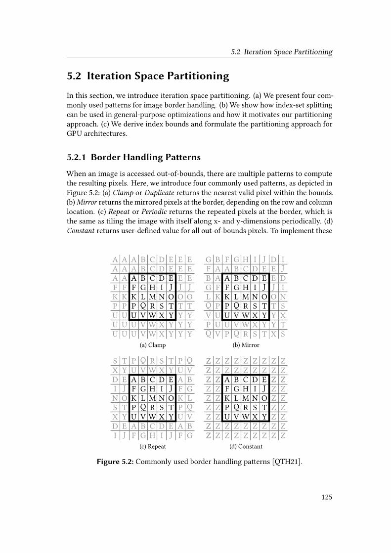
5.2 Iteration Space Partitioning
5.2 Iteration Space Partitioning
In this section, we introduce iteration space partitioning. (a) We present four com-monly used patterns for image border handling. (b) We show how index-set splittingcan be used in general-purpose optimizations and how it motivates our partitioningapproach. (c) We derive index bounds and formulate the partitioning approach forGPU architectures.
5.2.1 Border Handling Patterns
When an image is accessed out-of-bounds, there are multiple patterns to computethe resulting pixels. Here, we introduce four commonly used patterns, as depicted inFigure 5.2: (a) Clamp or Duplicate returns the nearest valid pixel within the bounds.(b)Mirror returns the mirrored pixels at the border, depending on the row and columnlocation. (c) Repeat or Periodic returns the repeated pixels at the border, which isthe same as tiling the image with itself along x- and y-dimensions periodically. (d)Constant returns user-defined value for all out-of-bounds pixels. To implement these
A A AA A AA A A
E E EE E EE E E
U U UU U UU U U
Y Y YY Y YY Y Y
FKP
FKP
JOT
JOT
B C DB C D
V W XV W X
A B C D EF G H I JK L M N OP Q R S TU V W X Y
(a) Clamp
G B F G H I J D IF A A B C D E E J
P U U V W X Y Y TQ V P Q R S T X S
BGLQV
AFKPU
EJOTY
DINSX
A B C D EF G H I JK L M N OP Q R S TU V W X Y
(b) Mirror
S T P Q R S T P QX Y U V W X Y U V
D E A B C D E A BI J F G H I J F G
DINSX
EJOTY
AFKPU
BGLQV
A B C D EF G H I JK L M N OP Q R S TU V W X Y
(c) Repeat
ZZ
ZZ
ZZ
ZZ
ZZ
ZZ
ZZ
ZZ
ZZ
ZZ
ZZ
ZZ
ZZ
ZZ
ZZ
ZZ
ZZ
ZZ
ZZ
ZZ
Z Z Z ZZ Z Z ZZ Z Z ZZ Z Z ZZ Z Z ZZ Z Z Z
A B C D EF G H I JK L M N OP Q R S TU V W X Y
(d) Constant
Figure 5.2: Commonly used border handling patterns [QTH21].
125

5 Efficient Computations for Local and Global Operators
patterns, conditional checks are inserted within the address calculation of each pixelaccess. Assume an image of size BG × B~; then, the iteration space can be definedas G ∈ [0, BG), ~ ∈ [0, B~) and G,~ ∈ ℤ. Listing 5.1 depicts a C++ implementationexample for these four patterns.
As can be observed in Listing 5.1, Clamp and Mirror implementations are similar incomputational cost. Repeat uses a while loop to iteratively check the index location,which is required in the pattern when small images are computed using a large filterwindow. Compared to these three patterns, Constant requires a different conditionalcheck. Unlike the other three, out-of-bounds pixels under the Constant pattern areindependent of their original location. Hence, the pixel’s value can be initializedwith the user-defined constant and only be updated when pixels are within bounds.
In real-world applications, which pattern to use depends on the filtering operationas well as the expected image content [BA18]. For example, medical imaging applica-tions such as multiresolution filters demand mirroring at the image border [KEF+03],while computer vision applications mostly use the clamp pattern to extend the edgesin an image [TT10]. Nevertheless, all these four patterns require costly conditional
Listing 5.1: Example border handling implementation in C++.
1 // current computing pixel
2 T in;
3
4 // (a) Clamp
5 if (x >= sx) x = sx - 1;
6 if (y >= sy) y = sy - 1;
7 if (x < 0) x = 0;
8 if (y < 0) y = 0;
9 in = input[x, y]; // Memory access
10
11 // (b) Mirror
12 if (x >= sx) x = sx - (x + 1 - sx);
13 if (y >= sy) y = sy - (y + 1 - sy);
14 if (x < 0) x = 0 - x - 1;
15 if (y < 0) y = 0 - y - 1;
16 in = input[x, y]; // Memory access
17
18 // (c) Repeat
19 while (x >= sx) x = x - sx;
20 while (y >= sy) y = y - sy;
21 while (x < 0) x = x + sx;
22 while (y < 0) y = y + sy;
23 in = input[x, y]; // Memory access
24
25 // (d) Constant
26 in = 0; // initialize with constant
27 if (y >= 0 && x >= 0 && y < sy && x < sx)
28 in = input[x, y]; // Memory access
126

5.2 Iteration Space Partitioning
checks before memory access, and minimizing the number of such conditional checksis the goal of iteration space partitioning. Before introducing our partitioningmethod,we first illustrate the concept of index-set splitting.
5.2.2 Index-Set Splitting
Index-Set Splitting (ISS) transforms a loop with conditional statements into multipleloops that iterate over disjoint portions of the original index range. An example isgiven in Listing 5.2. As can be seen in Listing 5.2, in the original loop, the conditionalstatements have to be executed # times for each iteration. Although the branchexecution might be accurately predicted on modern architectures, the existence ofsuch conditional statements still introduces a large overhead. Nevertheless, a closerlook into the loop unveils that the first conditional statement, namely the if-clause,does not affect the computation after" iterations. Similarly, the second statement,namely the else-clause, does not affect the computation of the first " iterations.Therefore, it is possible to split the original loop into two separate loops: The firstloop computes the first " iterations, and the second loop computes the remainingiterations, as can be seen in Listing 5.2. In this way, the conditional statements canbe eliminated. As a result, the total number of executed instructions is reduced.
The idea can be extended to the two-dimensional iteration space in image process-ing: Since the conditional checks, as shown in Listing 5.1, do not affect the wholeiteration space, we can partition the image into different regions, as depicted inFigure 5.1. For example, the left border check (if x < 0) only affects the left regions,namely L, TL, BL, and does not affect the other regions. Similarly, the top bordercheck (if y < 0) only affects top regions, namely T, TL, TR. In this way, we partition
Listing 5.2: Index-set splitting example in C++.
1 // Original loop
2 for (int i = 0; i < N; i++) {
3 if (i < M) { A[i] = A[i] * 2; }
4 else { A[i] = A[i] * 3; }
5 B[i] = A[i] * A[i];
6 }
7
8 // Splitted loops , assume M < N
9 for (int i = 0; i < M; i++) {
10 A[i] = A[i] * 2;
11 B[i] = A[i] * A[i];
12 }
13 for (int i = M; i < N; i++) {
14 A[i] = A[i] * 3;
15 B[i] = A[i] * A[i];
16 }
127

5 Efficient Computations for Local and Global Operators
the whole iteration space into multiple regions that iterate over disjoint portionsof the original image. As a result, the total number of executed conditional checkscan be reduced. In the following section, we derive the index bounds to perform thepartitioning of the iteration space.
5.2.3 Partitioning on GPUs
Partitioning an image iteration space requires different strategies for CPU and GPUarchitectures. For CPU implementations where the iteration space is executedsequentially, it is sufficient to partition the image into the body and border regionsbased on only the image and window size: Given an image size BG × B~ and a localoperator window size< × =. The body region that requires no conditional checkscan be defined as:
{(G,~) |⌊<2
⌋≤ G < BG −
⌊<2
⌋∧⌊=2
⌋≤ ~ < B~ −
⌊=2
⌋} (5.1)
The border of the image that requires conditional checks is the remaining part ofthe iteration space, which can be further partitioned into smaller regions. We omitthe remaining derivations here since we do not consider CPUs as target architecture.After obtaining the index bound of each region, the execution is straight forwardsince the computation of each region is sequential and is independent of the others.
The index bounds computed in Eq. (5.1) are not sufficient for parallel architecturessuch as GPUs. GPU architectures consist of an array of SMs that each can executethousands of concurrent threads. The input image is divided into threadblocks, basedon a user-defined block size. Each block is dispatched by the scheduler onto theSM for execution. Therefore, the user-defined block size should be considered topartition the iteration space. Assume a user-defined block size CG × C~. The indexbounds can then be computed as:
BH_L =
⌈ ⌊<2
⌋CG
⌉, BH_R =
⌊BG −
⌊<2
⌋CG
⌋BH_T =
⌈ ⌊=2
⌋C~
⌉, BH_B =
⌊B~ −
⌊=2
⌋C~
⌋ (5.2)
In Eq. (5.2), the four index bounds BH_L, BH_R, BH_T, BH_B collectively determine thepartitioning of the iteration space, as depicted in Figure 5.3. Any threadblock withan index between BH_L and BH_R in the x-dimension and between BH_T and BH_B inthe y-dimension requires no border handling. The region each threadblock needs toexecute can be identified by their block ID during runtime. A CUDA implementationof the routine is depicted in Listing 5.3.
128

5.2 Iteration Space Partitioning
BL B BR
R
TRTTL
L Body
BH_L BH_R
BH_T
BH_B
Figure 5.3: Index bounds for iteration space partitioning.
Instead of using the region switching statements as in Listing 5.3, we can alsoiterate over different regions in the iteration space by creating individual kernels foreach region. However, this approach has two disadvantages: First is the cost of kernellaunch from the host and the overhead from the additional PCIe communications.Second, programmers need to manually partition the host memory to match theoriginal iteration space. These costs may outweigh the benefits of applying thepartitioning approach. In contrast, iteration space partitioning employs one fatkernel and uses threadblock indices to control the fine-grained execution on eachregion during runtime. However, this approach still has two disadvantages: First, thegenerated fat kernel is lengthy and compromises the readability of the emitted code.Fortunately, the implementation can be largely hidden from programmers in our
Listing 5.3: Region switching for iteration space partitioning.
1 if (blockIdx.x < BH_L && blockIdx.y < BH_T)
2 goto TL;
3 if (blockIdx.x >= BH_R && blockIdx.y < BH_T)
4 goto TR;
5 if (blockIdx.y < BH_T)
6 goto T;
7 if (blockIdx.y >= BH_B && blockIdx.x < BH_L)
8 goto BL;
9 if (blockIdx.y >= BH_B && blockIdx.x >= BH_R)
10 goto BR;
11 if (blockIdx.y >= BH_B)
12 goto B;
13 if (blockIdx.x >= BH_R)
14 goto R;
15 if (blockIdx.x < BH_L)
16 goto L;
17 goto Body;
129

5 Efficient Computations for Local and Global Operators
compiler-based approach, and it should still be acceptable in most cases. Second, theadditional region switching statements, as shown in Listing 5.3, need to be executedfor all the threadblocks. This could potentially increase register usage on GPUscompared to a naive implementation. In the next section, we present an analyticmodel to encapsulate this trade-off.
5.3 Performance Modeling
In this section, we provide a systematic analysis of the potential benefits and costs ofiteration space partitioning. We use a real-world application to illustrate the benefitssuch as the reduction of arithmetic instructions, as well as the costs such as resourceusage increase on GPUs. Finally, we propose an analytic model to encapsulate thetrade-off and to suggest an optimized implementation.
5.3.1 Demystify the Benefits
By partitioning the iteration space into smaller regions, we expect the total numberof conditional checks to be reduced. To understand the impact on GPU architectures,two questions need to be answered: Which instructions are reduced and in whichregion? And how many instructions can be reduced given an application? To answerthese questions, we use a real-world application for illustration.
Motivation Example: Bilateral Filter
The bilateral filter is a widely used noise-removing filter that preserves edges in imageprocessing [TM98]. Each output pixel depends on the neighborhood pixels of thesame location. It basically performs two convolutions together, one for computing thespatial closeness component and the other one for computing the intensity similaritycomponent. In general, the computation of such local operators consists of twosteps: Address calculation and kernel computation. Address calculation needs to beperformed for each accessed pixel in the filter window, and it is generally computedusing integers. The conditional checks required for border handling are part of theaddress calculation, which is also where the iteration space partitioning approachtargets to optimize.
We performed two CUDA implementations for the bilateral filter: A naive versionwithout ISP, namely the conditional checks are performed for the whole iterationspace, and an optimized version with border handling using ISP. The compilation wasexecuted on a GTX680 using CUDA 10, under Ubuntu 18.04 LTS. The window sizeused in the filter is 13 × 13. The border handling pattern is Clamp. We compiled theCUDA kernel to PTX, and inventoried all executed instructions in the PTX code. Wechoose to measure at PTX level to obtain a more accurate estimation than at CUDA
130

5.3 Performance Modeling
Table 5.1: Bilateral filter PTX instruction comparison.
ISA Border Handling with ISP (partitioned into 9 regions) Naive
TL TR T BL BR B R L Body
add 703 704 366 704 705 367 704 703 377 705sub 169 169 169 169 169 169 169 169 169 169mul 1027 1027 1014 1027 1027 1014 1027 1027 1026 1027div 2 2 2 2 2 2 2 2 2 2
max 24 12 12 12 0 0 0 12 0 26min 0 1 0 1 2 1 1 0 0 2fma 507 507 507 507 507 507 507 507 507 507mad 4 4 17 4 4 17 4 4 4 4ex2 338 338 338 338 338 338 338 338 338 338cvt 512 512 356 512 512 356 512 512 354 512
cvta 2 2 2 2 2 2 2 2 2 2ld 170 170 170 170 170 170 170 170 169 170st 1 1 1 1 1 1 1 1 1 1
setp 342 355 342 355 367 355 357 345 344 363selp 340 351 339 351 362 350 350 339 338 362mov 10 10 10 10 9 9 9 10 9 10neg 169 169 169 169 169 169 169 169 169 169and 1 2 2 3 4 4 4 4 4 0
Total 4321 4336 3816 4337 4350 3831 4326 4314 3813 4369
source code. Further, it guarantees portability since PTX is a machine-independentISA across different architectures. Finally, we manually disassembled the PTX codeof the optimized version to obtain the statistics for each region. The instructionshave been categorized based on keywords for simplicity purposes. For example,add.s32 and add.f32 are both counted as an add instruction. Note that the countednumber of instructions includes both the kernel execution in the region as well asthe additional switching statements required to go to a region as shown in Listing 5.3.The results are depicted in Table 5.1.
We can make two important observations from Table 5.1: First, compared to thenaive implementation, not all the regions have a noticeable reduction in the totalnumber of executed instructions. It seems counter-intuitive that only three (T, B,Body) out of nine regions have a clear benefit over the naive approach. This can alsobe observed for other applications such as a Gaussian filter, which we will not showhere for simplicity. One reason is that the naive version may have many conditionalstatements in the source code, but many of them share common sub-expressions that
131

5 Efficient Computations for Local and Global Operators
can be optimized by the NVCC compiler. In addition, the region switching statementsalso account for extra instructions for the border regions. Second, compared to theregions with clear benefits (T, B, Body), the naive implementation is more costly onlyfor certain arithmetic instructions such as max, add, and cvt. Therefore, the benefitof iteration space partitioning mostly reduces the arithmetic pipeline utilization onthe GPU. Next, we construct an analytic model to capture the number of reductions.
Benefit Modeling
We assume the number of instructions2 to check one border (e.g., the left border) is=check, and the number of instructions to execute the actual kernel is =kernel. Then,the total number of instructions to execute a naive implementation #naive can beestimated as:
#naive = (=check · 4 + =kernel) ·< · = · BG · B~ (5.3)
Eq. (5.3) is straightforward to understand: The naive implementation requires fourborder checks for each accessed pixel, as shown in Listing 5.1, within each windowsize< · =, and the window slides along the whole iteration space of size BG · B~.
For the ISP implementation, the total number of instructions #ISP is the sum of allthe regions, namely
#ISP =∑
?∈{TL, TR, T, BL, BR, B, R, L, Body}=inst(?) (5.4)
In Eq. (5.4), =inst(?) is the number of instructions executed in region ? . For eachregion ? , =inst(?) can be further estimated as:
=inst(?) = (=switch(?) + =region(?)) ·< · = · =block(?) · CG · C~ (5.5)
Here, =switch(?) denotes the number of instructions needed to switch to region? , and =region(?) denotes the number of instructions needed to execute this region,including address calculation and kernel execution. Additionally, =block(?) denotesthe number of threadblocks executing this region. =switch can be estimated based onListing 5.3. =region can be estimated as follows:
=region(?) =
=check · 2 + =kernel if ? ∈ {TL, TR, BL, BR}=check + =kernel if ? ∈ {T, R, L, B}=kernel if ? = Body
(5.6)
2The type of instructions is not required in our model since both the ISP and the Naive approachuse the same checking statements.
132

5.3 Performance Modeling
Obviously, each region only needs to execute part of the conditional check de-pending on its location. For example, region TL requires two border checks, whileregion L requires only one border check. The Body region requires no border check.
Finally, we need to determine =block(?) in Eq. (5.5), namely the number of blocksexecuting each region. First, we derive the total number of blocks in the x-dimension,denoted as #blockx, the total number of blocks in the y-dimension, denoted as #blocky,and the total number of blocks in both dimensions, denoted as #block.
#blockx =⌈BGCG
⌉, #blocky =
⌈B~
C~
⌉, #block = #blockx · #blocky (5.7)
Then, based on the index bounds derived earlier in Eq. (5.2), the number of blocksexecuting each region can be computed as:
=block(?) =
(BH_R − BH_L) · BH_T if ? = T(BH_R − BH_L) · (#blocky − BH_B) if ? = BBH_T · BH_L if ? = TLBH_T · (#blockx − BH_R) if ? = TR(#blocky − BH_B) · BH_L if ? = BL(#blocky − BH_B) · (#blockx − BH_R) if ? = BRBH_L · (BH_B − BH_T) if ? = L(#blockx − BH_R) · (BH_B − BH_T) if ? = R
(5.8a)
=block(Body) = #block −∑
?∈{TL, TR, T, BL, BR, B, R, L}=block(?) (5.8b)
As can be seen in Eq. (5.8a), the number of blocks executing each region is deter-mined by the window size, block size, and image size. The partitioning is performedto minimize the number of blocks that execute border regions, hence maximizingthe number of blocks that execute the body region as shown in Eq. (5.8b). Finally,we can provide the estimated number of instructions for both implementations andthe ratio of the two as:
'reduced =#naive
#ISP(5.9)
Observations from the Model
Two observations can be made from our derived analytical model: First, if thekernel computation =kernel is relatively small compared to the address calculation=check, the iteration space partitioning is likely to contribute a larger reduction of
133

5 Efficient Computations for Local and Global Operators
512 768 1024 1280 1536 1792 2048 2304 2560 2816 3072 3328 3584 3840 40960%
20%
40%
60%
80%
100%
128 block size 256 block size
Figure 5.4: Percentage of blocks executed in region Body.
instructions. On the other hand, expensive kernels are likely to benefit less since theaddress calculation is insignificant. Second, as suggested by the model, the amountof instruction reduction depends on the image size as well as the user-defined blocksize, which in turn determines how many blocks execute which region. Based onEq. (5.8a) and Eq. (5.8b), large images are likely to benefit more from ISP due to thehigh percentage of blocks executed in the body region. To illustrate this relation,we computed the percentage of blocks that execute the body region for a 5 × 5 localoperator with two different block size configurations, as depicted in Figure 5.4. Thex-axis denotes the image size on one dimension, and all images have the same sizein both x- and y-dimension. As can be seen, given a block size, smaller images havea lower percentage of blocks executing the body region. When small images arecomputed using a large block size, there are not many blocks left to execute the bodyregion. In this case, the overall performance of ISP might be worse than a naiveimplementation. Next, we incorporate a cost parameter into the model.
5.3.2 Cost Model
Although iteration space partitioning can reduce the number of executed instructions,it comes with a certain cost such as resource usage increase. The region switchingstatements before partitioning may introduce additional register usage. To illustratethe effect of resource increase, we benchmarked the Bilateral filter using all fourborder handling patterns under the same environment as the previous PTX codegeneration. Then, we computed the speedups of the ISP implementation over thenaive implementation. The results are depicted in Figure 5.5. As can be seen in thefigure, ISP is not always beneficial. For small images, e.g., size of 512× 512, speedupsof Mirror, Clamp, and Constant implementations are less than 1.0, which implies thatthe naive approach with all conditional checks is the better implementation. This isdue to an increase in register usage that further reduces the achieved occupancy.
134

5.3 Performance Modeling
512 768 1024 1280 1536 1792 2048 2304 2560 2816 3072 3328 3584 3840 40960.5
1.0
1.5
2.0
2.5
3.0
3.5Sp
eedu
pover
Naive
Clamp Constant MirrorRepeat
Figure 5.5: Bilateral filter speedups over a naive implementation.
Reduced Occupancy
We logged the register usage for each implementation and computed the theoreticaloccupancy for the underlying architecture. The results are summarized in Table 5.2.As can be seen, compared to the naive implementation, ISP increases the registerusage under all four border handling patterns. Moreover, three of the four patternseventually result in a decrease in the computed theoretical occupancy. For GPUarchitectures, there exists a maximum number of threadblocks or warps that can beconcurrently active on an SM [Nvi20a]. In addition to this hardware limit, the numberof threadblocks that can be executed concurrently also depends on the hardwareresource usage, namely user-defined block size, register usage, etc. When a certainresource is heavily used in the kernel, fewer blocks will be executed concurrently.Since the total number of blocks is fixed for the given image and block size, thedevice will need more rounds/iterations to process all the blocks. This increase in thenumber of rounds/iterations can be modeled by an increase in the total number ofinstructions that need to be executed. In other words, a reduction in occupancy on
Table 5.2: Bilateral filter register usage and occupancy.
Implementation Clamp Mirror Repeat Constant
register usage naive 32 32 18 32ISP 40 40 32 63
occupancy (theor.) naive 100% 100% 100% 100%ISP 75% 75% 100% 50%
135

5 Efficient Computations for Local and Global Operators
the device can be modeled by an increase in the total number of instructions beingexecuted. Next, we put all these together to formulate a prediction model.
Prediction Model
Assume the obtained theoretical occupancy is $naive and $ISP for both implementa-tions. If the amount of occupancy decreases from$naive to$ISP, the number of roundsto execute all the blocks is increased by $naive/$ISP. Combined with the previousderived amount of instruction reduction in Eq. (5.9), we can derive a prediction modelas:
� =#naive
#ISP ·$naive/$ISP= 'reduced ·
$ISP
$naive(5.10)
Eq. (5.10) predicts the potential gains of a ISP implementation over the naiveimplementation. It captures the trade-off between instruction reduction and occu-pancy reduction. If� is larger than 1, it predicts the ISP implementation to be faster;otherwise, the naive implementation should be used.
Table 5.3: Measurement vs. model prediction.
Clamp Constant Mirror Repeat
Image size meas. pred. meas. pred. meas. pred. meas. pred.
512 Naive Naive Naive Naive Naive Naive ISP ISP768 Naive Naive Naive Naive Naive Naive ISP ISP1024 Naive Naive ISP Naive Naive Naive ISP ISP1280 Naive Naive ISP Naive Naive Naive ISP ISP1536 Naive ISP ISP Naive Naive ISP ISP ISP1792 ISP ISP ISP ISP Naive ISP ISP ISP2048 ISP ISP ISP ISP Naive ISP ISP ISP2304 ISP ISP ISP ISP Naive ISP ISP ISP2560 ISP ISP ISP ISP ISP ISP ISP ISP2816 ISP ISP ISP ISP ISP ISP ISP ISP3072 ISP ISP ISP ISP ISP ISP ISP ISP3328 ISP ISP ISP ISP ISP ISP ISP ISP3584 ISP ISP ISP ISP ISP ISP ISP ISP3840 ISP ISP ISP ISP ISP ISP ISP ISP4096 ISP ISP ISP ISP ISP ISP ISP ISP
Pears. 0.9791 0.9792 0.9798 0.9817
136

5.4 Hipacc Integration of Warp-grained Partitioning
Table 5.3 summarizes the measured best implementations as well as our model-predicted results for the Bilateral application. Green-colored results indicate a goodprediction by our model since it is the same as the measured ground truth. Red-colored results indicate a misprediction since it deviates from the measurement. Inaddition, we computed the Pearson correlation coefficient for each border handlingpattern to indicate the amount of correlation between the output value from themodel and the measurement. As can be seen in Table 5.3, the model has only afew mispredictions around the switching point, i.e., � ≈ 1.0, between the twoimplementations, where the performance difference is insignificant. For small andlarge images where the speedup or slowdown is significantly higher, our model candeliver an accurate prediction.
5.3.3 Intermediate Summary
We have presented a systematic analysis of the iteration space partitioning approach.This optimization can reduce the number of executed instructions in the addresscalculation, but at the cost of increasing register usage. We constructed an analyticmodel to encapsulate this trade-off with the help of domain knowledge such asmask size and architecture knowledge such as occupancy. In the end, the modeldelivers a good suggestion of which implementation is the best option. However,manual implementations of the ISP transformation are tedious, error-prone, and notportable. Therefore, we present an integration of the proposed approach into animage processing DSL to enable automatic code generation.
5.4 Hipacc Integration of Warp-grainedPartitioning
A kernel implementation of the Bilateral filter and the host code to launch the kernelin Hipacc are depicted in Listing 5.4. As can be seen in the kernel implementation, domindicates the sliding window of the filter, and iterate applies the filter computation.To launch the kernel from the host code, first, a mask is defined with pre-computedcoefficients. The domain can be automatically inferred from the mask. Then, theinput image can be read and assigned to the DSL image object. After that, a borderhandling pattern can be specified using the BoundaryCondition object. Afterward,the output image and its iteration space can be defined. Finally, the kernel can beinstantiated and executed. As can be seen in Listing 5.4, programmers can focuson the filter computation and do not have to worry about any index calculationsfor border handling. The source-to-source compiler is responsible for the loweringand optimizations, including iteration space partitioning. Next, we explain how tofurther optimize the ISP by implementing it using warp-grained partitioning.
137

5 Efficient Computations for Local and Global Operators
Listing 5.4: Bilateral filter in Hipacc.
1 // kernel implementation
2 class BilateralFilter : public Kernel <T> {
3 // ...
4 void kernel () {
5 float d = 0, p = 0;
6 iterate(dom , [&] () -> void {
7 float diff = in(dom) - in();
8 float c = mask(dom);
9 float s = expf(-c_r * diff*diff);
10 d += c*s;
11 p += c*s * in(dom);
12 });
13 output () = p/d;
14 }
15 };
16
17 // host kernel launch
18 // mask and domain with pre -computed coefficients
19 Mask <T> mask(coef);
20 Domain dom(mask);
21
22 // input image
23 T *image = read_image (...);
24 Image <T> in(width , height , image);
25 // clamping as boundary condition
26 BoundaryCondition <T> bound(in,dom ,Boundary :: CLAMP);27 Accessor <T> acc(bound);
28
29 // output image
30 Image <T> out(width , height);
31 IterationSpace <T> iter(out);
32
33 // instantiate and launch the Bilateral filter
34 BilateralFilter filter(iter ,acc ,mask ,dom ,sigma_r);
35 filter.execute ();
5.4.1 Warp-Grained Partitioning
On GPU architectures, a threadblock is the basic unit for kernel execution from aprogrammer’s perspective. Nevertheless, after each block is dispatched onto the SM,it is further divided into warps. A warp is a set of 32 threads that performs SIMTexecution in lock steps. Consider a block size of 128, and it consists of 4 warps, anda local operator with a small window size such as 3 × 3. Then, in the x-dimension,only the leftmost warps require the left border check. Similarly, only the rightmostwarps require the right border check. The analysis here is analogous to the blocklevel partitioning that has been described in the previous sections. Therefore, it ispossible to further improve the partitioning granularity by adding the warp location
138

5.5 Parallel Reduction on GPUs
Listing 5.5: Region switching with warp index.
1 if (blockIdx.x < BH_L && blockIdx.y < BH_T)
2 if (warpID.x > W_L) goto T;
3 goto TL;
4 if (blockIdx.x >= BH_R && blockIdx.y < BH_T)
5 if (warpID.x < W_R) goto T;
6 goto TR;
7 if (blockIdx.y < BH_T)
8 goto T;
9 if (blockIdx.y >= BH_B && blockIdx.x < BH_L)
10 if (warpID.x > W_L) goto B;
11 goto BL;
12 if (blockIdx.y >= BH_B && blockIdx.x >= BH_R)
13 if (warpID.x < W_R) goto B;
14 goto BR;
15 if (blockIdx.y >= BH_B)
16 goto B;
17 if (blockIdx.x >= BH_R)
18 if (warpID.x < W_R) goto Body;
19 goto R;
20 if (blockIdx.x < BH_L)
21 if (warpID.x > W_L) goto Body;
22 goto L;
23 goto Body;
into our region switching statement. Listing 5.5 depicts a refined region switchingmethod with the help of the additional warp location information. As can be seen inListing 5.5, similar to the previously computed block index bound BH_L and BH_R, thewarp index bound are denoted by W_L and W_R in the x-dimension. In this work, weonly consider the warp location in the x-dimension because the block layout in GPUapplications is mostly wide in x-dimension, which uses memory more efficiently.Recall our analysis based on Table 5.1, and we would like more blocks to executethe top (T), bottom (B), and body (Body) region due to their significant reductiongains. With the help of the warp index, we can further switch the redundant warpexecutions of all expensive regions (TL, TR, BL, BR, L, R) to the three cheaper regions(T, B, Body), as shown in lines 2, 5, 10, 13, 18, and 21 in Listing 5.5, respectively.
5.5 Parallel Reduction on GPUs
In this section, we present our contribution to optimizing global reduction on GPUs.The traditional GPU approach to compute a reduction in parallel can be summarizedin three steps: First, input data is loaded from the global memory. The operationsare executed in the granularity of threadblocks, and each block stages the datafrom global memory into its own shared memory for later use. Then, within each
139

5 Efficient Computations for Local and Global Operators
threadblock (intra-block), a tree-based approach is used to compute the partial resultfor this particular block. Finally, the partial results across all the blocks (inter-block)are collected, before the same approach is applied again to obtain the final resultas output. Figure 5.6 depicts an overview of the steps. In the remainder of thissection, we first present the provided abstraction in Hipacc. Then, we discuss theoptimizations that can be applied for each of the three steps. We present optimizationsdeveloped for old architecture generations as well as approaches that target recenthigh-end GPUs.
5.5.1 Global Reduction in Hipacc
Reductions in Hipacc can be specified by implementing a user-defined class. Thisclass should be derived from the Kernel class in the framework, which provides avirtual reduce() function to be implemented in the user class. An example is depictedin Listing 5.6. The reduce() method takes two pixels as inputs and describes theoperation applied to the entire input image. The final result can be retrieved usingthe reduce_data() method of the base class. In this work, we focus on the optimizationof simple use cases, where 2D images are linearized into 1D for global reduction.
5.5.2 Global Memory Load
Reductions are known to have low arithmetic intensity: Roughly one floating-pointoperation per load [Har07]. Therefore it is critical to improve the achieved band-
Global Memory Load
Block 0 Block 1
...
...
... Block N
Global Synchronization
Block 0
Load
Intra-block
Inter-block
Figure 5.6: Parallel reduction on GPUs [QRÖ+20].
140

5.5 Parallel Reduction on GPUs
Listing 5.6: Reduction max in Hipacc.
1 #include "hipacc.hpp"
2 class MaxReduction : public Kernel <int > {
3 // ...
4 int reduce(int left , int right) const {
5 return max(left ,right);
6 }
7 };
width during global memory access. Hipacc currently employs two methods foroptimization: (a) Grid-stride loops to optimize for coalesced memory access [Har13].By executing inside a for-loop with an incremental size of the entire grid, the memoryload achieves unit-stride within each warp and can handle arbitrary large input size.(b) Reduce during load is the second method that optimizes the number of blocksduring the memory load [Har07]. Because during reduction, half of the threads ineach iteration are wasted, minimizing the number of executed threadblocks improvesthe achieved bandwidth. In addition to the existing techniques, we incorporatedanother approach called vectorized load for bandwidth optimization.
Vectorized Load
We propose to use vectorized load [Lui13] for further optimization. Vector datatypes such as int2 and float4 are provided in the CUDA headers for use, whichleads to NVCC generating vectorized load instructions in the assembly code. Forexample, LD.E.64 for int2 instead of LD.E for int. The vectorized load instructioncan reduce the total number of load instructions being executed. For example, byutilizing LD.E.64 we can halve the executed instructions for int. In addition, avectorized load can be combined with the two existing methods grid-stride loops andreduce during load without extra cost. After loading each vector data, threads canunpack the pixels within their own register space and perform the first reduction.An example is illustrated in Figure 5.7.
Block 0 Block 1 Block 2 Block 3
Figure 5.7: Global memory load with a vector size 2 [QRÖ+20].
141

5 Efficient Computations for Local and Global Operators
5.5.3 Intra-block Reduce
After the global memory load step, each threadblock continues to perform reduc-tions within its own shared memory. Hipacc currently employs two methods tooptimize the usage of shared memory: (a) Sequential addressing is used to avoidbank conflict [Har07]. Instead of reading two consecutive addresses for reduction(default indexing), each thread in the block follows a rank-based indexing to avoidthe 2-way bank conflict3. (b) In addition, read and write to the shared memory mustbe synchronized within each block, which is a costly operation. Nevertheless, whenthe number of working threads is smaller than the warp size, synchronization isnot needed anymore due to the SIMT execution among warps. Therefore, warpunrolling [Har07] is used to unroll the rest of the loop in this situation. In this work,we explore the use of shuffle instruction from Nvidia to execute efficient intra-blockreduction.
Shuffle Instruction
The traditional approach to exchange data within a threadblock is via shared mem-ory. However, for Kepler and later architectures, Nvidia introduced new low-levelprimitives called shuffle instructions [Lui14]. The new instructions enable threads toexchange data within a warp without going through the shared memory, which avoidcostly operations such as synchronization and generate smaller memory footprint.We propose to execute the intra-block reductions using shuffle instructions. Theimplementation of a warp reduction is given in Listing 5.7.
Listing 5.7: Warp reduce with shuffle instructions.
1 // reduce within a warp
2 __device__ inline int reduce_warp_max(int val)
3 {
4 val = max(val , __shfl_down_sync(FULL_MASK , val , 16));
5 val = max(val , __shfl_down_sync(FULL_MASK , val , 8));
6 val = max(val , __shfl_down_sync(FULL_MASK , val , 4));
7 val = max(val , __shfl_down_sync(FULL_MASK , val , 2));
8 val = max(val , __shfl_down_sync(FULL_MASK , val , 1));
9 return val;
10 }
After the warp reduction, the partial results are written back to the shared memory.These partial results need to be further computed using the traditional approach.Nevertheless, the expensive part has already been done by the shuffle instructions.
3Shared memory is divided into equally sized banks. Memory accesses that span different banks canbe served simultaneously, while accessing the same bank must be serialized. 2-way bank conflicthappens when two threads access the same bank.
142

5.5 Parallel Reduction on GPUs
At this point, only a few elements need to be further reduced. The number of thepartial results depends on the user-defined block size. For example, a 128 block sizehas four elements after the shuffle instruction computation. For these four partialresults, the final reduction is performed by threads within the first warp, whichrequires no synchronization.
5.5.4 Inter-block Reduce
After the intra-block reduce step, the final step is to compute all the partial resultsfrom all the threadblocks. To make sure all threadblocks finish their executions, aglobal synchronization must be observed. The traditional solution for this problem isto use a second kernel, which waits for all blocks from the previous kernel to finishbefore execution starts. Currently, Hipacc employs a single-pass kernel approach thatuses the _threadfence() intrinsic and a global atomicInc() function to produce asingle value in a single kernel. This is achieved by using the first thread of each blockto update a global memory counter using the atomic function. Then, the last finishedblock is responsible for collecting the partial results and executes the final reduction.In this work, we explore the use of atomic functions to perform the inter-blockreduce on recent GPU architectures.
Atomic Function
We propose to exploit the performance of atomic functions on new Nvidia archi-tectures. CUDA offers arithmetic functions such as add, sub, and max, as well asbitwise functions such as and, xor. More generic operations can be implementedusing the compare-and-swap function atomicCAS(). In this work, we focus on simpleoperations such as max and sum. Utilizing atomic functions requires less memoryfootprint, and the performance is scalable for larger data sizes. However, implemen-tations running on old architectures are known to be inefficient. Hipacc addresses
Table 5.4: Baseline and proposed Hipacc implementationsOptimizations Baseline Implem. Proposed Implem. Requirement
Grid-stride loops 3 3 -Reduce during load 3 3 -Vectorized load 3 -Sequential addressing 3 3 -Warp unrolling 3 -Shuffle instruction 3 Kepler or higherSingle-pass kernel 3 CUDA 3 or higherAtomic function 3 Kepler or higher
143

5 Efficient Computations for Local and Global Operators
this issue with its architecture knowledge by automatically fall back to the single-pass kernel approach. We present the performance improvement in the followingresult section. In the end, we use Table 5.4 to depict a summary of all the discussedmethods.
5.6 Evaluation and Results
In this section, we present the results of benchmarking the proposed local and globaloperator optimizations. For the proposed local operator border handling approach,we benchmarked five commonly used filters in image processing: Gaussian, Laplace,Bilateral, Sobel, and Night filter [JPS+00]. Gaussian, Laplace, and Bilateral are singlekernel implementations with the window size of 3× 3, 5× 5, and 13× 13, respectively.The Sobel filter consists of 3 kernels to compute x-, y-derivatives, and the magnitude,among which the first two are local operators. The night filter consists of five kernelsthat first iteratively applying the Atrous (with holes) algorithm [She92] with differentsizes (3 × 3, 5 × 5, 9 × 9, 17 × 17), before performing the actual tone mapping. Foreach application, we benchmarked all four border handling patterns as introducedearlier, namely Clamp, Mirror, Repeat, and Constant, each using four image sizes512×512, 1024×1024, 2048×2048, and 4096×4096. We chose these implementationvariants to cover a mixture of different window sizes, number of kernels, and theexpensiveness of the filter kernel computation. Finally, for the global reductionoperators, we benchmarked three basic reduction operations: min, max, and sum.We applied the operations on different sized image data ranging from 1K (210) to16M (224) pixels.
5.6.1 Environment and Implementation Variant
For the local operator border handling comparisons, we employed twoGPUs: GTX680and RTX2080, whose specifications have been introduced previously in Section 4.7.3.The host OS is Ubuntu 18.04 LTS with CUDA version 11.0. The execution time isobtained from the output of NVProf. We computed the speedups of an isp implemen-tation (always apply ISP) over the naive implementation (always check all borders),as well as the isp+m implementation (apply ISP based on model prediction) over thenaive implementation. The results for the five applications are gathered in Figure 5.8,Figure 5.9, Figure 5.10, Figure 5.11, and Figure 5.12, respectively.
For the global reduction comparisons, we used two Nvidia GPUs: K20c with Keplerarchitecture and also the RTX2080. We compare among three implementations: Thebaseline (current Hipacc) implementation, the enhanced Hipacc implementation withthe proposed techniques, and an implementation using Thrust [BH12], the high-levelparallel algorithm library from Nvidia. Two speedups are computed and depicted inFigure 5.13: The speedup of the proposed approach over the baseline implementation,
144

5.6 Evaluation and Results
409620481024512
1
1.5
2Gaussian-Clamp-GTX680
nai. isp isp+m1
409620481024512
1
1.5
2Gaussian-Mirror-GTX680
nai. isp isp+m2
4096204810245121
2
3
4
Gaussian-Repeat-GTX680
nai. isp isp+m3
4096204810245120.8
1
1.2
1.4Gaussian-Constant-GTX680
nai. isp isp+m4
4096204810245120.60.81
1.21.41.6
Gaussian-Clamp-RTX2080
nai. isp isp+m5
409620481024512
1
1.5
2Gaussian-Mirror-RTX2080
nai. isp isp+m6
40962048102451212345
Gaussian-Repeat-RTX2080
nai. isp isp+m7
409620481024512
1
1.5
2Gaussian-Constant-RTX2080
nai. isp isp+m8
Figure 5.8: Gaussian filter normalized speedups: naive (nai.), always apply ISP (isp),apply ISP based on model prediction (isp+m).
145

5 Efficient Computations for Local and Global Operators
4096204810245120.81
1.21.41.6
Laplace-Clamp-GTX680
nai. isp isp+m9
4096204810245120.81
1.21.41.6
Laplace-Mirror-GTX680
nai. isp isp+m10
4096204810245121
2
3
4
Laplace-Repeat-GTX680
nai. isp isp+m11
4096204810245120.8
1
1.2
1.4Laplace-Constant-GTX680
nai. isp isp+m12
4096204810245120.8
1
1.2
1.4Laplace-Clamp-RTX2080
nai. isp isp+m13
4096204810245120.8
1
1.2
1.4Laplace-Mirror-RTX2080
nai. isp isp+m14
409620481024512
2
4
6
Laplace-Repeat-RTX2080
nai. isp isp+m15
4096204810245120.81
1.21.41.6
Laplace-Constant-RTX2080
nai. isp isp+m16
Figure 5.9: Laplace filter normalized speedups: naive (nai.), always apply ISP (isp),apply ISP based on model prediction (isp+m).
146

5.6 Evaluation and Results
4096204810245120.60.81
1.21.41.6
Bilateral-Clamp-GTX680
nai. isp isp+m17
4096204810245120.60.81
1.21.41.6
Bilateral-Mirror-GTX680nai. isp isp+m18
409620481024512
2
4
6
Bilateral-Repeat-GTX680
nai. isp isp+m19
4096204810245121
1.5
2
Bilateral-Constant-GTX680nai. isp isp+m20
4096204810245120.60.81
1.21.41.6
Bilateral-Clamp-RTX2080
nai. isp isp+m21
4096204810245120.60.81
1.21.41.6
Bilateral-Mirror-RTX2080nai. isp isp+m22
409620481024512
2
4
6
Bilateral-Repeat-RTX2080
nai. isp isp+m23
409620481024512
1
1.5
Bilateral-Constant-RTX2080nai. isp isp+m24
Figure 5.10: Bilateral filter normalized speedups: naive (nai.), always apply ISP (isp),apply ISP based on model prediction (isp+m).
147

5 Efficient Computations for Local and Global Operators
4096204810245120.81
1.21.41.6
Sobel-Clamp-GTX680
nai. isp isp+m25
4096204810245120.81
1.21.41.6
Sobel-Mirror-GTX680nai. isp isp+m26
4096204810245121
2
3
4Sobel-Repeat-GTX680
nai. isp isp+m27
4096204810245121
2
3
4Sobel-Constant-GTX680
nai. isp isp+m28
4096204810245120.8
1
1.2
1.4Sobel-Clamp-RTX2080
nai. isp isp+m29
4096204810245120.8
1
1.2
1.4Sobel-Mirror-RTX2080
nai. isp isp+m30
409620481024512
2
4
6
Sobel-Repeat-RTX2080
nai. isp isp+m31
409620481024512
2
4
6
Sobel-Constant-RTX2080nai. isp isp+m32
Figure 5.11: Sobel filter normalized speedups: naive (nai.), always apply ISP (isp),apply ISP based on model prediction (isp+m).
148

5.6 Evaluation and Results
4096204810245120.8
1
1.2
1.4Night-Clamp-GTX680
nai. isp isp+m33
4096204810245120.81
1.21.41.6
Night-Mirror-GTX680
nai. isp isp+m34
409620481024512
1
1.5
2Night-Repeat-GTX680
nai. isp isp+m35
4096204810245120.8
1
1.2
1.4Night-Constant-GTX680
nai. isp isp+m36
4096204810245120.8
1
1.2
1.4Night-Clamp-RTX2080
nai. isp isp+m37
4096204810245120.8
1
1.2
1.4Night-Mirror-RTX2080
nai. isp isp+m38
4096204810245120.81
1.21.41.6
Night-Repeat-RTX2080
nai. isp isp+m39
4096204810245120.8
1
1.2
1.4Night-Constant-RTX2080
nai. isp isp+m40
Figure 5.12: Night filter normalized speedups: naive (nai.), always apply ISP (isp),apply ISP based on model prediction (isp+m).
149

5 Efficient Computations for Local and Global Operators
and the speedup of the proposed approach over theThrust implementation. Executiontime is measured as the median of 20 executions each.
5.6.2 Discussions
Efficient Border Handling for Local Operators
Always Apply ISP over Naive Implementation As can be observed in Fig-ures 5.8 to 5.12, the isp approach contributes a speedup over the naive implementationin most cases, especially for large image sizes such as 2048 × 2048 and 4096 × 4096.In general, the amount of speedup also increases with the computed image size,which has been analyzed by our model, as discussed in Figure 5.4. Furthermore, theRepeat border handling pattern benefits more from the ISP approach than the otherthree patterns due to the more costly address calculation. For example, the Gaussiankernel achieves a speedup of up to 2.9 for the Repeat pattern and up to 1.3 for theothers, as can be seen in subplots 1© to 8© in Figure 5.8.
Apply ISP based on Model Prediction As analyzed in our prediction model, itis not always beneficial to apply the ISP optimization for certain applications such asthe Bilateral filter. This can be seen in subplot 17© (Bilateral-Clamp-GTX680) and 18©(Bilateral-Mirror-GTX680) in Figure 5.10, where the 512 × 512 image has a speedupof less than 1.0 for the ISP implementation. In these scenarios, our prediction modelsuggests falling back to the naive implementation. In these cases, applying ISP wouldslow down the execution by about 40%.
In only a few scenarios, our model did not predict the implementation performanceaccurately. For example, on the RTX2080, when executing the bilateral filter withsmall images, our model always suggested the ISP implementation, as can be seen insubplots 21© and 22© in Figure 5.10. The model did not see a reduction in occupancyin these scenarios due to the increased number of available registers on the Turingarchitecture. As a result, the implementation is up to 30% slower than the naiveversion. Nevertheless, by combining ISP with the prediction model, we can achievea performance-optimized implementation in almost all scenarios.
Geometric Mean Speedups For each application, we also computed the geomet-ric mean of the speedups of the isp+m implementation over the naive implementation
Table 5.5: Geometric mean across all implementations.
Applications Gaussian Laplace Bilateral Sobel Night
Geometric Mean 1.438 1.422 1.355 1.877 1.102
150

5.6 Evaluation and Results
across all benchmarks on both GPUs. The result is given in Table 5.5. Our finalimplementation can achieve a speedup range from 10% to 87%. In general, we canobserve that the less expensive the kernel computation is, the more speedup ourapproach contributes. As can be seen in the table, Gaussian and Laplace have ahigher geometric speedup (1.438, 1.422) than Bilateral and Night filter (1.355, 1.102).Our approach benefits most for applications such as the Sobel filter that consists ofmultiple less expensive kernels, where a speedup of more than 4.0 can be achievedon the RTX2080.
Efficient Global Reductions
Figure 5.13 and Figure 5.14 depict the two speedups computed on two GPUs: Thespeedup of the proposed approach over the baseline implementation, and the speedupof the proposed approach over the Thrust implementation, respectively.
Compared to the baseline implementation, our proposed approach achieves aconsistent speedup from 1.10 to 3.34 across two different architectures. One is Kepler,
210 211 212 213 214 215 216 217 218 219 220 221 222 223 2240.6
1.0
1.4
1.8
2.2
2.6
3.0
1.17
1.16
1.14
1.17
1.15
1.18
1.20 1.29 1.39 1.
61
1.56 1.63
1.90 2.08 2.21
1.18
1.16
1.17
1.17
1.15
1.17
1.18 1.31 1.37 1.
61
1.56 1.61
1.89 2.09 2.21
1.21
1.18
1.16
1.20
1.15
1.10 1.20 1.30 1.40 1.
65
1.57 1.63
1.90 2.09 2.21
Speedup over Baseline on RTX2080
Min Max Sum
210 211 212 213 214 215 216 217 218 219 220 221 222 223 2240.6
1.2
1.8
2.4
3.0
3.6
4.2
1.14
1.14
1.14
1.13
1.15 1.22 1.43 1.61 1.80 2.11 2.
53 2.84 3.06 3.17 3.27
1.15
1.14
1.13
1.13
1.15 1.21 1.43 1.61 1.78 2.11 2.
55 2.87 3.08 3.17 3.26
1.15
1.15
1.14
1.13
1.14 1.23 1.42 1.59 1.79 2.11
2.56 2.85 3.11 3.25 3.34
Speedup over Baseline on K20c
Min Max Sum
Figure 5.13: Speedups compared with the baseline implementation are plotted overthe number of pixels to be reduced.
151

5 Efficient Computations for Local and Global Operators
and the other is Turing. It can be observed in Figure 5.13 that when the reductionimages are above a certain size, the achieved speedups increase along with the imagesize. For small images, the achieved speedups show no increase due to the deviceresource availability. For example, the RTX2080 has sufficient resources to computeup to 8 threadblocks concurrently per SM for the min reduction kernel. This impliesimages smaller than 216 do not have enough data to occupy the GPU fully. Thespeedups observed for small images mainly come from the use of vectorized load andatomic functions. The improvement by using shuffle instructions can be observed onlarge images.
Compared to the Thrust implementation, our approach can achieve a consistentspeedup from 1.37 to 9.02, as depicted in Figure 5.14. After profiling, we observedthat the performance difference is mainly due to the generation of kernel launchconfigurations. Hipacc employs its default configuration (128 block size) for thebenchmarked architectures. In comparison, Thrust uses its internal tuner to decideon the launch configurations. For example, on the RTX2080, Thrust uses a constant
210 211 212 213 214 215 216 217 218 219 220 221 222 223 2240.0
2.0
4.0
6.0
8.0
10.0
12.0
1.41
1.40
1.44 1.68
1.70
1.80
1.77
1.82
1.86
9.02
5.22
4.28
3.13
2.25
1.62
1.39
1.42
1.43 1.66
1.66
1.77
1.79
1.78
1.83
8.75
5.32
4.25
2.96
2.25
1.63
1.37
1.39
1.40 1.65
1.61
1.76
1.77
1.81
1.85
8.71
5.23
4.31
3.15
2.24
1.63
Speedup over Thrust on RTX2080
Min Max Sum
210 211 212 213 214 215 216 217 218 219 220 221 222 223 2240.0
2.0
4.0
6.0
8.0
1.48
1.50
1.51 1.83
1.82
1.90
1.89
1.99
6.13
5.25
4.13
3.27
2.58
1.75
1.241.48
1.49
1.50 1.82
1.80
1.88
1.90
1.98
6.11
5.15
4.19
3.23
2.58
1.75
1.251.48
1.50
1.48 1.82
1.86
1.89
1.95
2.00
6.12
5.14
4.15
3.20
2.69
1.78
1.28
Speedup over Thrust on K20c
Min Max Sum
Figure 5.14: Speedups compared with the Thrust implementation are plotted overthe number of pixels to be reduced.
152

5.7 Related Work
block size of 256 for all the images with different grid sizes (up to 920). Moreover,Thrust executes two kernels for each reduction, while our approach employs one.
5.7 Related Work
Our employed ISP approach is similar to the general-purpose compiler optimizationtechnique called index-set splitting (ISS), or loop splitting [WSO95; Sak97], wherea single loop is transformed into multiple loops that iterate over disjoint portionsof the original index range. This technique has inspired several existing workstargeting different architectures for efficient image border management [Bai11;Ham15; Ham07]. For FPGA accelerators, Bailey [Bai11] proposed a filter design withborder management to minimize hardware costs. Özkan et al. [ÖRH+17] proposedan analytic model that determines efficient implementations with image borderhandling as well as loop coarsening for hardware synthesis. Beyond image processing,border communication has been studied in scientific computing for stencil kernels,where autotuning framework by Zhang and Mueller [ZM12] and DSLs such asStencilGen [RVS+18] and SDSL [RKH+15] provide boundary handling for the halomargins. However, these works mostly focus on reducing redundant inter-tilecommunications. Within the context of image processing DSLs, early efforts such asthe Apply DSL [Ham07] handles image borders by generating separate loops withdifferent bounds-check requirements. Later, the same author proposed a declarativeborder handling approach with domain inference using Halide [Ham15], a well-known image processing DSL [RBA+13]. It is highly beneficial to have an automatedborder handling approach within DSLs. Thus, programmers can be relieved fromthe burden of inferring the domain size manually. Nevertheless, both mentionedworks focus solely on the language constructs and do not consider GPU targets. ForGPU architectures, one popular DSL that addresses border handling is Lift [HSS+18].Like Halide, Lift is a DSL based on functional programming that offers high-orderprimitives such as pad to re-index out-of-bounds pixels. However, it does not furtheroptimize the branching overhead during device execution. Another DSL that supportsborder handling on GPUs is Hipacc [MHT+12b]. Compared to the existing techniquesin Hipacc, our approach proposes two major advancements: First, we show that itis not always beneficial to partition the iteration space during computation. Theperformance depends on kernel properties and inputs such as image size and blocksize. Based on a proposed analytic model, our approach can determine a performance-optimized implementation. Second, we illustrate that ISP can be applied at differentlevels of granularity. Instead of partitioning at the threadblock level, we propose topartition the iteration space at the warp level, which further improves the memoryaccess efficiency for GPU architectures.
153

5 Efficient Computations for Local and Global Operators
5.8 Conclusion
We presented our contributions on the single-kernel optimization. In particular,we improved the border handling computations for local operators and proposedan efficient reduction implementation in Hipacc. Local operators require borderhandling on GPUs, where conditional checks are needed for address calculations instencil kernels that introduce huge overhead. This can be optimized by partitioningthe iteration space into disjoint regions. Although partitioning can reduce the numberof executed conditional statements, it also comes with additional costs in registerincrease. We showed that it is possible to encapsulate this trade-off using an analyticmodel and make accurate predictions based on the combination of domain- andarchitecture-specific knowledge. We also integrated the proposed approach intoa source-to-source compiler called Hipacc, which enables a complete workflow togenerate efficient kernels for GPUs automatically. Additionally, we improved theperformance of the reduction implementation in Hipacc. Thanks to the enhancementof function support and the availability of new low-level intrinsics from Nvidia,high-level frameworks such as Hipacc can greatly benefit from the latest techniques.
154

6Conclusion and Future Directions
The emergence of domain-specific architectures such as GPUs provides massivecomputing performance that drives the development in an increasing number ofdomains. Nevertheless, the multi-layered compute and memory hierarchy in modernGPU architectures is challenging to program. Even for experts with deep archi-tecture knowledge, obtaining an efficient implementation incurs an iterative effortof performance profiling and tuning to exploit the trade-off space among locality,parallelism, and computations. Due to the lack of compiler support for high-leveloptimizations, GPU programming still requires explicit memory management toserve the computation at different granularities. Moreover, with the rapid evolutiontowards general-purpose computing architectures, it is not easy to achieve bothperformance portability and programmability at the same time. The hand-tunedimplementation by architecture experts is not performance portable, while library-based approaches are not programmable. Neither approach is able to achieve bothobjectives to enable high productivity. As a remedy, a DSL approach provides an al-ternative by limiting the language expressiveness within a single domain. Then, withthe combination of domain- and architecture-specific knowledge, a DSL approach canoffer domain-specific abstractions to programmers, and apply architecture-specificoptimizations to perform efficient code generation for various target back ends. Theabstractions enable programmability and flexibility for domain developers, and thecompiler-based automated optimizations facilitate performance portability. In a DSLapproach, optimizations should be applied at different levels, which is crucial toachieve high-performance implementations. The contributions in this thesis consistof system-level optimizations that explore inter-kernel transformations to improvelocality and parallelism, and techniques for optimizing single-kernel efficiency ofcommonly used abstractions. In the following, the contributions of our work aresummarized and possible future work is outlined.
6.1 Summary
Our first contribution targets system-level locality optimization. The peak perfor-mance scaling of compute and memory resources in contemporary GPU architectures
155

6 Conclusion and Future Directions
is developed at a different pace. It always seems easier for hardware vendors toincrease the SM’s computing power than the global memory bandwidth. As a result,data cannot be moved fast enough from memory to compute units. Even with theintroduction of HBM, the ratio between peak compute and memory performancein recent GPUs is still difficult to achieve. Consequently, locality is key to efficientimplementations, and data should be kept as close to the compute unit as possible.On the other hand, applications such as in image processing are increasing in com-plexity and generally consist of a sequence of kernels in a pipeline. The inter-kernelcommunications are intensive and exhibit an opportunity for locality optimization.Targeting this opportunity, we proposed kernel fusion: A multi-kernel transforma-tion technique for locality improvement at the system level. The proposed kernelfusion technique consists of two building blocks: a benefit estimation model and afusible kernel searching algorithm. Whether two kernels can be fused depends ona number of criteria including data dependence, resource usage, and header com-patibility. Kernel fusion transforms the redundant intermediate data access fromglobal memory into faster memories such as register or shared memory. If there is anexternal data dependence, fusion becomes illegal since the external consumer wouldlose access to the intermediate data. If the data dependence requirement is respected,kernels may still not be fused due to resource usage. During GPU execution, thenumber of blocks that can be executed in parallel can reduce when the kernel uses toomany resources. We consider a group of kernels legal to fuse when all the mentionedconstraints are met. Then, we proposed two approaches to search for fusible kernelsefficiently. A basic search strategy is fusion along edges, which has a restrictivedata dependence requirement that limits linearly dependent scenarios. Although thebasic approach can already optimize many applications, there are some scenarioswhere intermediate data is shared among multiple kernels (not linearly dependent),and it is also beneficial to apply kernel fusion. To cover these use cases, we devel-oped an advanced search strategy based on the graph min-cut algorithm. Insteadof expanding the fusion scope as in the basic search strategy, this approach shrinksthe fusion scope starting from the whole application. To assist the min-cut graphpartitioning, we also developed an analytic model to quantitatively estimate thefusion benefit depending on the compute patterns. This is only possible by combiningdomain-specific and architecture-specific knowledge. In the end, we integrated ourapproach into Hipacc to obtain an automated end-to-end optimization workflow.We evaluated our approach over commonly used image processing applications,and a geometric mean speedup of up to 2.52 can be observed in the experiment.Furthermore, all the present results in this work have been evaluated independentlyand archived for public use and reproducibility.
Our second contribution targets system-level parallelism optimization. As moreand more transistors are being crammed into the same chip, the number of CUDAcores and SMs for computation keeps increasing. With this performance improve-
156

6.1 Summary
ment, applications that were considered costly on the old GPUs, are not enough tooccupy the device fully on new architectures. Traditional GPU computing focuses ondata-level parallelism. Using the SIMD execution model, data is mapped to threads forparallel computation. Nevertheless, little attention has been paid to the threadblocklevel parallelism. Unlike threads that execute in SIMT mode, blocks can executedifferent kernels. This enables another level of parallelism based on the MPMD execu-tion model. Different blocks can be dispatched and executed on the same SM to haveconcurrent kernel executions. This is useful for many applications: One example isthe multiresolution filters widely used in medical imaging applications. We proposeda parallel, multi-stream implementation for multiresolution filter applications onGPUs. Our approach unveiled the concurrent kernel execution opportunities in thecoarse-grained level of the underlying image pyramid. In addition, we showed howto model the block level execution of both single- and multi-stream implementationswith high fidelity. Depending on the computation expensiveness of the level process-ing kernel, one implementation variant may be better than the other. Among fourreal-world image processing applications, we demenstrated that a geometric meanspeedup of up to 2.5 could be achieved using our proposed approach. The second partof this contribution is the combination of CUDA graph with Hipacc. CUDA graphas an asynchronous task-graph programming model. It captures data dependenceinformation in the graph and facilitates automatic multi-stream scheduling duringexecution. Nevertheless, it does not have other information, such as resource usagefor architecture-specific optimization. By combining CUDA graph with Hipacc, wecan join the benefits brought by these two approaches, i.e., workflow optimizationcombined with work launch overhead reduction. In addition, the multi-stream con-current kernel execution featured in CUDA graph can be improved by exploitingkernels with complementary resource usage. Compared to CUDA graph withoutHipacc, our approach can achieve a geometric mean speedup of 1.11 for selectedimage processing applications.
Our last contribution targets single-kernel optimizations. In particular, we opti-mized the border handling in local operators and the parallel reduction in globaloperators. Border handling is a critical step for local operators such as image filtering,where out-of-bound memory access may happen at the image border. We presented asystematic analysis of an efficient border handling approach based on iteration spacepartitioning, and illustrated the potential resource usage increase due to the regionswitching statement. We highlighted the scenarios in which applying the ISP-basedborder handling actually slows down the execution. For example, small imagescomputed with a large window size may not be beneficial from applying the ISPtransformation, where the occupancy reduction outweighs the benefit of ISP. Instead,it is faster to use a naive approach by checking all borders. This trade-off can becaptured using an analytic model, which is able to predict the better implementationvariant based on domain- and architecture-specific knowledge. By exploring this
157

6 Conclusion and Future Directions
performance trade-off, we can gain up to 40% speedup for commonly used imagefiltering operations. The second part of this contribution is optimizing global reduc-tions. We utilized the latest CUDA intrinsics and took advantage of the performanceimprovement of existing instructions. For example, the atomic instruction in CUDAhas been partially software implemented prior to the Pascal architecture, which isoften replaced by a demoted implementation such as in inter-block reduction forbetter performance. Nevertheless, Nvidia provided hardware acceleration for theatomic operations in recent architectures, which is now a better option for manyreduction kernels. We enhanced the Hipacc implementation to automatically selectthe better variant based on the architecture knowledge, while the input DSL coderemains untouched. The existing reduction implementation can achieve a speedupof up to 3.43.
6.2 Future Directions
The DSL and compiler framework presented in this work can be extended in threedirections for future research. First is the language abstraction and target domain.Hipacc was developed for 2D image processing applications, especially for medicalimaging and computer vision. It would be useful to extend the language abstractionsto support 3D images, or nD tensors even better. This would naturally extend ourtarget domain to machine learning, in which applications also consist of many kernelsthat share certain data dependencies. Moreover, existing optimizations can also beextended to support higher dimensions. For example, border handling can partitionthe iteration space into 28 regions for a 3D image. This potentially requires morecostly region switching statements, and the trade-off can be re-evaluated using anupdated model based on the techniques proposed in this work.
Another direction for future research is to utilize the latest GPU architecturefeatures for better performance support. For example, recent Nvidia architecturesfeature dedicated tensor cores for machine learning applications. It is beneficial toexploit the possibility of utilizing the tensor core hardware for image processingoperations, such as reductions and convolutions. For example, it is possible to usetensor cores for convolution by fitting the kernel operation within 16 by 16 sizeblock matrices. Although a tensor core implementation may be slower than theCUDA core version, it may still be beneficial to exploit concurrent computations,since both hardware components are separated computing resources on the device.Another interesting feature to investigate is the asynchronous data movement on thelatest Ampere architecture. Traditionally, data that is copied from global memoryto shared memory must travel a long journey through L2 cache, L1 cache, as wellas registers. With the new CUDA language construct and architecture support, it ispossible to bypass the register usage, which also reduces the resource usage in the
158

6.2 Future Directions
kernels. This new feature may contribute significantly to the performance of certainlocal operators in image processing that are already memory-bound.
Regarding the backend of Hipacc, one possible direction is to enable the CPU-GPUconcurrent execution. Currently, the host CPU acts as a GPU device controller, whichis responsible for initialization and task offloading. During GPU computation, itis possible to perform computations concurrently on the host. In this case, datadependence needs to be explored to take the CPU node into consideration. Anotherpossible direction is to explore the multi-GPU target. Instead of offloading compu-tations to one device, it is possible to have a cluster of GPU nodes locally or in thecloud. In this case, data transfer between host and device, as well as between deviceand device should be considered. It is also worth exploring the language abstractionsfor such architectures. Ideally, the target details should be hidden from the DSL user,which means the compiler is responsible for the design space exploration and taskmapping. Here, the design space consists not only the partitioning into differentcompute nodes, but also the order of transformations when multiple options areavailable. For example, kernel fusion is ideal when computing large image data, whileconcurrent kernel execution contributes more to kernels with smaller images. Inaddition to GPUs, Hipacc also supports other backends such as FPGAs. Our proposedsystem-level optimization can also be explored on these other targets. For example,kernel fusion can be researched for FPGAs to reduce the resource usage of localoperator implementations.
159


AAppendix
A.1 Kernel Fusion Artifact Evaluation
This artifact describes the steps to reproduce the results for the CUDA code generationwith kernel fusion in Hipacc (http://hipacc-lang.org) (an image processing DSL andsource-to-source compiler embedded in C++), as presented in the paper at the CGO2019 conference with the title ”From Loop Fusion to Kernel Fusion: A Domain-specific Approach to Locality Optimization”. We provide the original binaries as wellas the source code to regenerate the binaries, which can be executed on x86_64 Linuxsystem with CUDA-enabled GPUs. Furthermore, we include two Python scripts torun the application and compute the statistics as depicted in Figure 6 in the paper.
A.1.1 Artifact Check-list
• Algorithm: Min-cut based kernel fusion in an image processing DSL.
• Program: Hipacc, Clang AST, CUDA.
• Compilation: Please check subsection C3.
• Transformations: Kernel fusion is implemented as an optimization pass in theHipacc code generation.
• Binary: Included for x86_64 Linux (tested on Ubuntu 14.04 and 18.04).
• Run-time environment: Linux (Ubuntu 14.04 or later, 18.04 recommended),CUDA (9.0 or later, 10.0 recommended).
• Hardware: Please check subsection C2.
• Output: Execution time in milliseconds for each kernel.
• Experiments: Please check subsection E.
• Publicly available?: Yes.
161

A Appendix
A.1.2 Description
How Delivered
The pre-compiled binaries and the python scripts are available via:https://www12.cs.fau.de/downloads/qiao/kernel_fusion/The artifact source code is publicly available and hosted on GitHub at: https://github.com/hipacc/hipacc/tree/kernel_fusion
Hardware Dependencies
CUDA enabled GPUs are required. We used three Nvidia cards, as discussed inSection 5.1 in the paper:
• Geforce GTX 745 facilitates 384 CUDA cores with a base clock of 1,033 MHzand 900 MHz memory clock.
• Geforce GTX 680 has 1,536 CUDA cores with a base clock of 1,058 MHz and3,004 MHz memory clock.
• Tesla K20c has 2,496 CUDA cores with a base clock of 706 MHz and 2,600 MHzmemory clock.
For all three GPUs, the total amount of sharedmemory per block is 48 Kbytes, the totalnumber of registers available per block is 65,536. GPUs with similar configurationsare expected to generate comparable results.
Software Dependencies
To run the provided binaries, the prerequisites are the following:
• Clang/LLVM (5.0 or later), compiler_rt and libcxx for Linux (5.0 or later).
• CMake (3.4 or later), Git (2.7 or later).
• Nvidia CUDA Driver (9.0 or later).
To build Hipacc from source and re-generate the binaries, the prerequisites are thefollowing:
• Clang/LLVM (6.0), compiler_rt and libcxx for Linux (6.0).
• CMake (3.4 or later), Git (2.7 or later).
• Nvidia CUDA Driver (9.0 or later).
162

A.1 Kernel Fusion Artifact Evaluation
• OpenCV for producing visual output in the samples.
For Ubuntu 18.04, most of the software dependencies can be installed from therepository. CUDA driver is available on the Nvidia download website.
A.1.3 Datasets
The provided binaries generate random images of size 2,048 by 2,048 pixels, henceno additional data is required. Nevertheless, some real-world images are included inthe repository, which can be used for visualization. The location is: https://github.com/hipacc/hipacc/tree/siemens-dev/samples-public Images of the same size areexpected to have similar execution times. Throughout our experiment, we have usedan image size of 2,048 by 2,048 pixels. Note that an exception is the Night filter,which computes an image of size 1,920 by 1,200 pixels. The choice of image size wasmade randomly, and not relevant to the purpose of kernel fusion.
A.1.4 Installation
This subsection illustrates the installation steps to build Hipacc from source, theprevious software dependencies should be met prior to the following steps.
1. Clone the Hipacc repository:$ git clone https:// github.com/hipacc/hipacc.git
$ cd hipacc/
2. Switch to kernel fusion branch and update the submodule samples:$ git checkout kernel_fusion
$ git submodule init && git submodule update
3. Build Hipacc from source:$ mkdir build && cd build
$ cmake ../ -DCMAKE_INSTALL_PREFIX="pwd"/release
$ make && make install
Hipacc should be successfully installed in the release folder.
A.1.5 Experiment Workflow
After a successful installation, we can go to the release folder and generate binaries.
163

A Appendix
1. Disable/Enable kernel fusion:$ cd release/samples/common/config
disable fusion by (-fuse off) or enable by (-fuse on) in cuda.conf.
2. Generate binary and run the application, e.g. Harris corner:$ cd ../../3 _Preprocessing/Harris_Corner/
$ make cuda
The above step should produce a binary main_cuda, which should be comparableto the provided binary. The steps can be repeated for all six applications in thepaper, which are located within the preprocessing directory and the postprocessingdirectory, respectively.
After having the binaries, the provided python scripts can be used to collect thetotal execution time and the statistics as shown in Figure 6 in the paper. Note thatthe name of the executable binary might need to be adapted in the python script.
A.1.6 Evaluation and Expected Result
The above experiment workflow is expected to output the execution times comparableto Figure 6 in [QRH+19]. The values in the figure are also available in text format viathe provided download website.
The reproduced GPU execution results are expected to have small variationscompared with the original presented data. For example, the median value among50 runs of a baseline Harris corner implementation is expected to have a variationbetween 0.05 ms and 0.1 ms on a GTX680. In general, we expect a variation of +/-0.1 in the final speedup comparison. The gains in Table 1 and Table 2 in [QRH+19]can be derived from the median value of the obtained statistics.
A.1.7 Notes
• From experience, the first call to a GPU device takes a longer time. We didseveral dummy calls to the GPU at the beginning of our evaluation.
• The provided binaries were generated and documented at the beginning of thework, which might use an older version of Clang/LLVM, CUDA Driver/Run-time, and MVRTC version. Nevertheless, the results are expected to be compa-rable with executions with newer drivers.
164

A.2 Fusibility Exploration Algorithm Complexity
A.2 Fusibility Exploration Algorithm Complexity
In this section, we derive the algorithm complexity that is used in our fusibilitysearching approach based on the min-cut technique. We know that the complexityof the Stoer-Wagner algorithm is O(|�′| |+ ′| + |+ ′|2 log |+ ′|) for any graph �′ =(+ ′, �′) [SW97]. For simplicity, we denote the number of vertices in the graph as< = |� |, and the number of edges in the graph as= = |+ |. Assume the followingworst-case scenario: Every time the Stoer-Wagner algorithm is applied on the applicationgraph, only one vertex has been cut. This implies that no fusible kernel pair exists inthe graph, but we have to discover this by re-partitioning the whole graph. In thiscase, since each time the number of vertices in the graph is only reduced by 1, themin-cut algorithm is applied = − 1 times in total.
A.2.1 Worst-Case Running Time
Given the above scenario, the total running time can be calculated as the sum of therunning time of each step:
O(<(= − 1) + (= − 1)2 log((= − 1))) + O(<(= − 2) + (= − 2)2 log((= − 2))) + ...+O(< · 1 + 12 log(1)) + O(<)6 O(<= + =2 log(=)) + O(<(= − 1) + (= − 1)2 log((= − 1))) + ...+O(< · 1 + 12 log(1)) + O(<)
= O(<= +<(= − 1) + ... +< · 1) + O(=2 log(=) + (= − 1)2 log((= − 1)) + ...+12 log(1)) + O(<)
= O(< · (= + = − 1 + ... + 1) + O(=2 log(=) + (= − 1)2 log((= − 1)) + ...+12 log(1)) + O(<)
= O(< · (=(= + 1)2) + O(=2 log(=) + (= − 1)2 log((= − 1)) + ... + 12 log(1))+
O(<)6 O(< · =2) + O(=2 log(=) + =2 log((= − 1)) + ... + =2 log(1)) + O(<)= O(< · =2) + O(=2 · (log(=) + log(= − 1) + ... + log(1))) + O(<)= O(< · =2) + O(=2 · log(= · (= − 1) · ... · 1)) + O(<)= O(< · =2) + O(=2 · log(=!)) + O(<)= O(< · =2 + =2 · log(=!) +<)
Finally, we substitute the number for< and =. The complexity of the proposedfusibility exploration algorithm 2 can be given as: O(|� | · |+ |2 + |+ |2 · log( |+ |!) + |� |).
165


German Part
Optimierung auf System-Ebeneund Code-Generierung für
Grafikprozessoren mittels einerdomänenspezifischen Sprache
167


Zusammenfassung
Durch den steigenden Einsatz von Grafikprozessoren (GPUs) zur Durchführunggewöhnlicher Berechnungen gewinnen effiziente Programmierwerkzeuge für dieseimmer mehr an Bedeutung. Unabhängig von den andauernden Bestrebungen zumErreichen einer besseren Programmierbarkeit in CUDA und OpenCL, bleiben dieseSprachen dennoch relativ Hardware-nah und erfordern ein tiefgreifendes Architektur-verständnis, um gute Ergebnisse zu erzielen. Entwickler und Entwicklerinnenmüssenden Grafikspeicher manuell verwalten, um die vielschichtige Berechnungs- und Spei-cherhierarchie voll auszuschöpfen. Die Leistungsfähigkeit dieser händisch optimier-ten Implementierungen ist wenig portabel, d.h. es ist nicht garantiert, dass sich dieseauf neuen Architekturen effizient ausführen lassen. Stattdessenmüssen Entwickelndefür jede neue Architektur wiederholt aufwendige Optimierungen durchführen. Umdieses Problem zu umgehen, können Entwickelnde Hochleistungsbibliotheken ein-setzen, die von den Hardware-Herstellerfirmen oder der Open-Source-Gemeinschaftbereitgestellt werden. Durch den Einsatz solcher Bibliotheken wird die Portabilitäterhöht, da es die Aufgabe des Anbietenden der Bibliothek ist deren Effizienz aufverschiedenen Architekturen sicherzustellen. Allerdings ist der Einsatz solcher Biblio-theken mit eingeschränkten Freiheitsgraden bei der Programmierbarkeit verbunden.Bibliotheksfunktionen werden über ein vordefinierte Programmierschnittstelle (API)angeboten, dessen Abstraktionsebene für Entwickelnde einer bestimmten Domänenicht unbedingt ausreichend sein muss. Außerdem sind bibliotheksbasierte Ansätzehinderlich bei der Optimierung auf Systemebene über verschiedene Funktionenhinweg. In dieser Arbeit wird ein Ansatz mittels einer domänenspezifischen Sprache(DSL) vorgestellt, der sowohl einen hohen Grad an portabler Leistungsfähigkeit alsauch an Programmierbarkeit bietet. Dies wird ermöglicht durch die Kombinationvon domänenspezifischen Abstraktionen mit architekturspezifischen Optimierungen.Die Abstraktionen bieten ein hohes Maß an Programmierbarkeit und Flexibilität fürDomänenentwickelnde, während die Compiler-basierten Optimierungen die Portabi-lität der Leistungsfähigkeit über verschiedene Architekturen hinweg sicherstellen.Der Kern eines solchen DSL-Ansatzes sind Optimierungen, welche algorithmischesWissen mit Hardware-Wissen kombinieren, um Varianten effizient zu explorieren.
169

German Part
Die wissenschaftlichen Beiträge dieser Arbeit liegen im Bereich von Optimierungenauf Systemebene und der Quellcodegenerierung für GPUs.
Heutige Applikationen aus den Bereichen der Bildverarbeitung und dem ma-schinellen Lernen wachsen stetig in ihrer Komplexität und bestehen aus mehrerenBerechnungskernen (engl. Kernel) einer Berechnungskette. Jeden Kernel einzelnzu optimieren ist durch die schnelle Evolution moderner GPU-Architekturen nichtmehr zielführend. Mit jeder neuen Architekturgeneration steigt die Rechenleistungund die zur Verfügung stehende Speicherbandbreite. Dabei überwiegt der Anstiegzusätzlicher Leistung deutlich gegenüber dem Anstieg zusätzlicher Bandbreite. Da-her ist eine gute Datenlokalität essenziell, um Hochleistungsimplementierungen zuerhalten. So birgt beispielsweise die Inter-Kernel-Kommunikation innerhalb einerBildverarbeitungskette großes Potential für verbesserte Datenlokalität. Als ersterwissenschaftlicher Beitrag wird eine Technik namens Kernel-Fusion vorgestellt, mitderen Hilfe die Anzahl und Zugriffe auf den langsamen GPU-Hauptspeicher redu-ziert werden kann. Zusätzlich wird gezeigt, dass diese Transformation von einemQuelltext-zu-Quelltext-Übersetzer automatisiert durchgeführt werden kann, indemDomänenwissen aus der Bildverarbeitung mit dem Architekturwissen über GPUskombiniert wird.
Ein weiterer beobachtbarer Trend in der Architekturentwicklung ist die zuneh-mende Anzahl an CUDA-Rechenkernen und Streaming-Prozessoren (SMs) zur Be-rechnung. Herkömmliche GPU-Programmierung konzentriert sich auf die effizienteAusnutzung der vorhandenen Datenparallelität. Mit dem Single-Instruction, MultipleThreads (SIMT) Model können Daten einzelner Ausführungsfäden (engl. Threads)zugewiesen werden, um von der massiven Rechenleistung zu profitieren. Allerdingskann die GPU für kleinere Bilder, die auf älteren Architekturen noch als sehr be-rechnungsintensiv galten, nicht mehr voll belegt werden. Um dennoch die steigendeAnzahl an Rechenwerken einer GPU effizient auszunutzen, wird es immer wichtigerauch die Parallelität auf Kernel-Ebene zu betrachten. Als zweiter wissenschaftlicherBeitrag werden Techniken zur nebenläufigen Kernel-Ausführung vorgestellt, mitderen Hilfe Betriebsmittel innerhalb der Rechenwerke feingranular geteilt werdenkönnen. Zusätzlich werden verschiedene Implementierungsvarianten verglichenund analytische Modelle entwickelt, um geeignete Entwurfspunkte basierend aufalgorithmischem und architekturellem Wissen vorherzusagen.
Nachdem Datenlokalität und Parallelität betrachtet wurden, welche die zwei wich-tigsten Optimierungsziele moderner GPU-Architekturen darstellen, werden weitereOptimierungsmöglichkeiten der Berechnungen innerhalb eines Algorithmus erörtert.Als dritter wissenschaftlicher Beitrag dieser Arbeit werden Techniken zur Opti-mierung einzelner Kernels für lokale und globale Operatoren vorgestellt, die zuden am weitverbreitetsten Berechnungsschritten der Bildverarbeitung gehören. Fürlokale Operatoren wird eine systematische Analyse zur effizienten Randbehand-lung basierend auf Iterationsraumpartitionierung vorgestellt. Dazu wird Domänen-
170

und Architekturwissen verwendet, um einen geeigneten Arbeitspunkt zwischender Ressourcenbelegung und Reduzierung der Instruktionsauslastung zu finden.Das analytische Model unterstützt dabei die Quelltext-zu-Quelltext-Transformation,um zu entscheiden welches die bessere Implementierungsvariante ist und damitdie Ende-zu-Ende-Quellcodeerzeugung zu verbessern. Für globale Operatoren wirdein effizienter Ansatz zur Ausführung globaler Reduktionen auf GPUs vorgestellt.Der Ansatz profitiert von den kontinuierlichen Verbesserungen der Leistung undProgrammierbarkeit durch die Hardwarehersteller, wie beispielsweise die Nutzungneuer Hardware-naher Primitive bereitgestellt durch Nvidia.
Die vorgestellten Techniken beschränken sich nicht nur auf Optimierungen fürmehrere Kernels, sondern betrachten auch einzelne Kernels und lassen sich nahtlosin unsere DSL zur Bildverarbeitung und den dazugehörigen Quelltext-zu-Quelltext-Übersetzer namens Hipacc integrieren. Schließlich kann mit dem vorgestellten DSL-Framework die Produktivität der Entwicklerin bzw. Entwicklers, die nach hochleis-tungsfähigen GPU-Implementierungen streben, drastisch verbessert werden.
171


Bibliography
[ALS+06] Alfred V. Aho, Monica S. Lam, Ravi Sethi, and Jeffrey D. Ullman.Compilers: Principles, Techniques, and Tools (2nd Edition). Addison-Wesley Longman Publishing Co., Inc., Boston, MA, USA, 2006. ISBN:0321486811.
[ATB+15] Arash Ashari, Shirish Tatikonda, Matthias Boehm, Berthold Reinwald,Keith Campbell, John Keenleyside, and P. Sadayappan. On optimizingmachine learning workloads via kernel fusion. In Proceedings of the20th ACM SIGPLAN Symposium on Principles and Practice of ParallelProgramming, PPoPP 2015, pages 173–182, San Francisco, CA, USA.ACM, 2015. ISBN: 978-1-4503-3205-7. DOI: 10.1145/2688500.2688521.
[BA18] Donald G. Bailey and Anoop Suraj Ambikumar. Border handling for 2dtranspose filter structures on an FPGA. Journal of Imaging, 4(12):138–159, November 2018. DOI: 10.3390/jimaging4120138.
[BA83a] P. Burt and E. Adelson. The laplacian pyramid as a compact imagecode. IEEE Trans. on Communications, 31(4):532–540, April 1983. DOI:10.1109/TCOM.1983.1095851.
[BA83b] Peter J. Burt and Edward H. Adelson. A multiresolution spline withapplication to image mosaics. ACM Trans. on Graphics, 2(4):217–236,October 1983. DOI: 10.1145/245.247.
[Bai11] Donald G. Bailey. Image border management for FPGA based filters.In Proceedings of the 6th IEEE International Symposium on ElectronicDesign, Test and Application (DELTA) (Queenstown, New Zealand),pages 144–149, January 17–19, 2011. DOI: 10.1109/DELTA.2011.34.
[Ban08] Isaac N. Bankman. Handbook of Medical Image Processing and Analysis,volume 2. Academic Press, December 2008. ISBN: 978-0-123-73904-9.
[Ban09] I.N. Bankman. Handbook of Medical Image Processing and Analysis.January 2009.
173

Bibliography
[BCH+09] Jacob Benesty, Jingdong Chen, YitengHuang, and Israel Cohen. Pearsoncorrelation coefficient. In Noise Reduction in Speech Processing. SpringerBerlin Heidelberg, Berlin, Heidelberg, 2009, pages 1–4. ISBN: 978-3-642-00296-0. DOI: 10.1007/978-3-642-00296-0_5.
[BH12] Nathan Bell and Jared Hoberock. Thrust: a productivity-oriented li-brary for cuda. In GPU Computing Gems Jade Edition, Applications ofGPU Computing Series. Morgan Kaufmann, 2012. DOI: 10.1016/B978-0-12-385963-1.00026-5.
[BK13] Gary Bradski and Adrian Kaehler. Learning OpenCV: Computer Visionin C++ with the OpenCV Library. O’Reilly Media, Inc., 2nd edition, 2013.ISBN: 1449314651.
[Ble90] Guy E. Blelloch. Prefix Sums and Their Applications. Technical re-port CMU-CS-90-190, School of Computer Science, Carnegie MellonUniversity, November 1990.
[Bra00] Bradski, Gary. The OpenCV library. November 1, 2000. URL: http ://www.drdobbs.com/open-source/the-opencv-library/184404319(visited on 03/30/2021).
[Dem13] Julien Demouth. Shuffle: tips and tricks. 2013. URL: http://on-demand.gputechconf.com/gtc/2013/presentations/S3174-Kepler-Shuffle-Tips-Tricks.pdf.
[Dev20] AdvancedMicroDevices. Opencl programming guide. 2020.URL: https:/ / rocmdocs . amd . com / en / latest / Programming_Guides /Opencl -programming-guide.html.
[DGY+74] Robert H. Dennard, Fritz H. Gaensslen, Hwanien Yu, V. Leo Rideout,Ernest Bassous, and Andre R. LeBlanc. Design of ion-implanted mos-fet’s with very small physical dimensions. IEEE Journal of Solid-StateCircuits, 9(5):256–268, 1974. ISSN: 0018-9200. DOI: 10.1109/JSSC.1974.1050511.
[DH73] Richard O. Duda and Peter E. Hart. Pattern Classification and SceneAnalysis. Wiley, 1973. ISBN: 978-0471223610.
[DHG+19] Simon Garcia De Gonzalo, Sitao Huang, Juan Gómez-Luna, SimonHammond, Onur Mutlu, and Wen-mei Hwu. Automatic generation ofwarp-level primitives and atomic instructions for fast and portable par-allel reduction on GPUs. In Proceedings of the IEEE/ACM InternationalSymposium on Code Generation and Optimization (CGO) (Washington,DC, USA), pages 73–84. IEEE Press, 2019. DOI: 10.1109/CGO.2019.8661187.
174

Bibliography
[DLX+19] Abdul Dakkak, Cheng Li, Jinjun Xiong, Isaac Gelado, and Wen-meiHwu. Accelerating reduction and scan using tensor core units. InProceedings of the ACM International Conference on Supercomputing(ICS) (Phoenix, AZ, USA), pages 46–57. ACM, 2019. DOI: 10 .1145/3330345.3331057.
[EBA+11] Hadi Esmaeilzadeh, Emily Blem, Renee St Amant, Karthikeyan Sankar-alingam, and Doug Burger. Dark silicon and the end of multicorescaling. In Proceedings of the 38th annual international symposium onComputer architecture (ISCA) (San Jose, CA, USA), pages 365–376. In-stitute of Electrical and Electronics Engineers (IEEE), June 4–8, 2011.DOI: 10.1145/2000064.2000108.
[FMF+15] Jiří Filipovič, Matúš Madzin, Jan Fousek, and Luděk Matyska. Optimiz-ing CUDA code by kernel fusion: Application on BLAS. The Journalof Supercomputing, 71(10):3934–3957, October 2015. ISSN: 1573-0484.DOI: 10.1007/s11227-015-1483-z.
[Fow10] Martin Fowler. Domain Specific Languages. Addison-Wesley Profes-sional, 1st edition, 2010. ISBN: 0321712943.
[GH94] Olivier Goldschmidt and Dorit S. Hochbaum. A polynomial algorithmfor the k-cut problem for fixed k.Math. Oper. Res., 19(1):24–37, February1994. ISSN: 0364-765X. DOI: 10.1287/moor.19.1.24.
[GK10] Michael Garland andDavid B. Kirk. Understanding throughput-orientedarchitectures. Communications of the ACM, 53(11):58–66, November2010. ISSN: 0001-0782. DOI: 10.1145/1839676.1839694.
[GKK+18] PrasunGera, HyojongKim,HyesoonKim, SunpyoHong, VinodGeorge,and Chi-Keung Luk. Performance characterisation and simulation ofintel’s integrated GPU architecture. In Proceedings of the 2018 IEEEInternational Symposium on Performance Analysis of Systems and Soft-ware (ISPASS) (Belfast, UK), pages 139–148. Institute of Electrical andElectronics Engineers (IEEE), April 2–4, 2018. DOI: 10.1109/ISPASS.2018.00027.
[GOS+93] Guang R. Gao, R. Olsen, Vivek Sarkar, and Radhika Thekkath. Col-lective loop fusion for array contraction. In Proceedings of the 5thInternational Workshop on Languages and Compilers for Parallel Com-puting, pages 281–295, London, UK. Springer, 1993.
[Gra20] Alan Gray. Getting started with cuda graphs. 2020. URL: https : / /devblogs.nvidia.com/cuda-graphs/ (visited on 07/27/2021).
175

Bibliography
[GW14] Jeremy Gibbons and Nicolas Wu. Folding domain-specific languages:deep and shallow embeddings (functional pearl). In Proceedings of the19th ACM SIGPLAN International Conference on Functional Program-ming (ICFP) (Gothenburg, Sweden), pages 339–347. Association forComputing Machinery (ACM), September 1–6, 2014. DOI: 10.1145/2628136.2628138.
[Ham07] Leonard G. C. Hamey. Efficient image processing with the apply lan-guage. In Proceedings of the 9th Biennial Conference of the AustralianPattern Recognition Society on Digital Image Computing Techniques andApplications (DICTA) (Glenelg, SA, Australia), pages 533–540, Decem-ber 3–5, 2007. DOI: 10.1109/DICTA.2007.4426843.
[Ham15] Leonard G. C. Hamey. A functional approach to border handling inimage processing. In Proceedings of the International Conference onDigital Image Computing: Techniques and Applications (DICTA) (Ade-laide, SA, Australia), pages 1–8, November 23–25, 2015. DOI: 10.1109/DICTA.2015.7371214.
[Har07] Mark Harris. Optimizing parallel reduction in cuda. 2007. URL: https://developer.download.nvidia.com/assets/cuda/files/reduction.pdf.
[Har13] Mark Harris. Write flexible kernels with grid-stride loops. 2013. URL:https://devblogs.nvidia.com/cuda-pro-tip-write-flexible-kernels-grid-stride-loops/.
[HP19] John L. Hennessy and David A. Patterson. A new golden age for com-puter architecture. Communications of the ACM, 62(2):48–60, January2019. ISSN: 0001-0782. DOI: 10.1145/3282307.
[HS88] Chris Harris and Mike Stephens. A combined corner and edge detector.In In Proceedings of the Fourth Alvey Vision Conference (AVC) (Manch-ester, UK), pages 147–151, September 1988. DOI: 10.5244/C.2.23.
[HSS+18] Bastian Hagedorn, Larisa Stoltzfus, Michel Steuwer, Sergei Gorlatch,and Christophe Dubach. High performance stencil code generationwith lift. In Proceedings of the International Symposium on Code Gener-ation and Optimization (CGO) (Vienna, Austria), pages 100–112, Febru-ary 24–28, 2018. DOI: 10.1145/3168824.
[Int21a] Intel Corporation. Intel oneapi math kernel library. 2021. URL: https://software.intel.com/content/www/us/en/develop/tools/oneapi/components/onemkl.html (visited on 03/30/2021).
[Int21b] Intel Corporation. Intel® xeon® platinum 9282 processor. 2021. URL:https://ark.intel.com/content/www/us/en/ark/products/194146/intel-xeon-platinum-9282-processor-77m-cache-2-60-ghz.html (visited on04/17/2021).
176

Bibliography
[IT88] François Irigoin and Rémi Triolet. Supernode partitioning. In Proceed-ings of the 15th ACM SIGPLAN-SIGACT Symposium on Principles ofProgramming Languages (POPL) (San Diego, CA, USA), pages 319–329.ACM, January 1988. ISBN: 0-89791-252-7. DOI: 10.1145/73560.73588.
[Jer15] Jeremy Appleyard. GPU hardware and programming models. 2015.URL: https://confluence.ecmwf.int/download/attachments/51708254/ECMWF_GPU_overview.pdf (visited on 05/21/2021).
[JLY12] Hua Ji, Fue-Sang Lien, and Eugene Yee. Parallel adaptive mesh refine-ment combined with additive multigrid for the efficient solution of thepoisson equation. ISRN Applied Mathematics, 2012, March 2012. DOI:10.5402/2012/246491.
[Jon18] Stephen Jones. Cuda: new features and beyond. 2018. URL: http://on-demand.gputechconf.com/gtc/2018/presentation/s8278-cuda-new-features-and-beyond.pdf.
[JPS+00] HenrikWann Jensen, Simon Premoze, Peter Shirley, William B.Thomp-son, James A. Ferwerda, and Michael M. Stark. Night Rendering. Tech-nical report UUCS-00-016, Computer Science Department, Universityof Utah, August 2000.
[KEF+03] Dietmar Kunz, Kai Eck, Holger Fillbrandt, and Til Aach. Nonlinearmultiresolution gradient adaptive filter for medical images. Proc. SPIE,5032, February 2003. DOI: 10.1117/12.481323.
[Khr09] Khronos OpenCL Working Group. The OpenCL specification. Oc-tober 6, 2009. URL: http : / /www .khronos . org / opencl (visited on02/28/2018).
[KM94] Ken Kennedy and Kathryn S. McKinley. Maximizing loop parallelismand improving data locality via loop fusion and distribution. In Pro-ceedings of the 6th International Workshop on Languages and Compilersfor Parallel Computing, pages 301–320, London, UK. Springer, 1994.
[Lar13] Stephen Jones Lars Nyland. Understanding and using atomic memoryoperations. 2013. URL: http://on-demand.gputechconf.com/gtc/2013/presentations/S3101-Atomic-Memory-Operations.pdf.
[LDM+19] Zhen Lin, Hongwen Dai, Michael Mantor, and Huiyang Zhou. Coordi-nated cta combination and bandwidth partitioning for GPU concurrentkernel execution. ACM Trans. on Architecture and Code Optimization,16(3):23:1–23:27, June 2019. DOI: 10.1145/3326124.
[LHR+15] Y. Liang, H. P. Huynh, K. Rupnow, R. S. M. Goh, and D. Chen. EfficientGPU spatial-temporal multitasking. IEEE Trans. on Parallel and Dis-tributed Systems, 26(3):748–760, March 2015. DOI: 10.1109/TPDS.2014.2313342.
177

Bibliography
[LNO+08] Erik Lindholm, John Nickolls, Stuart Oberman, and John Montrym.Nvidia tesla: a unified graphics and computing architecture. IEEEMicro,28(2):39–55, 2008. DOI: 10.1109/MM.2008.31.
[Lui13] Justin Luitjens. Increase performance with vectorized memory access.2013. URL: https : / / devblogs .nvidia . com/cuda -pro - tip - increase -performance-with-vectorized-memory-access/.
[Lui14] Justin Luitjens. Faster parallel reductions on kepler. 2014. URL: https://devblogs.nvidia.com/faster-parallel-reductions-kepler/.
[LYK+14] H. Li, D. Yu, A. Kumar, and Y. Tu. Performance modeling in CUDAstreams – A means for high-throughput data processing. In Proc. ofthe IEEE Int’l Conference on Big Data, pages 301–310, October 2014.DOI: 10.1109/BigData.2014.7004245.
[MAS+16] Ravi Teja Mullapudi, Andrew Adams, Dillon Sharlet, Jonathan Ragan-Kelley, and Kayvon Fatahalian. Automatically scheduling Halide imageprocessing pipelines. ACM Transactions on Graphics, 35(4):83:1–83:11,July 2016. ISSN: 0730-0301. DOI: 10.1145/2897824.2925952.
[MAT+12] P. J. Martín, L. F. Ayuso, R. Torres, and A. Gavilanes. Algorithmicstrategies for optimizing the parallel reduction primitive in CUDA.In Proceedings of the International Conference on High PerformanceComputing Simulation (HPCS), pages 511–519, 2012. DOI: 10.1109/HPCSim.2012.6266966.
[MCT96] Kathryn S. McKinley, Steve Carr, and Chau-Wen Tseng. Improving datalocality with loop transformations. ACM Transactions on ProgrammingLanguages and Systems, 18(4):424–453, July 1996. DOI: 10.1145/233561.233564.
[Mem13] RichardMembarth.Code Generation for GPUAccelerators from aDomain-Specific Language for Medical Imaging. Dissertation, Hardware/Soft-ware Co-Design, Department of Computer Science, Friedrich-AlexanderUniversity Erlangen-Nürnberg, Germany, Munich, Germany, May 2,2013. ISBN: 978-3-8439-1074-3. Verlag Dr. Hut, Munich, Germany.
[MHS05] Marjan Mernik, Jan Heering, and Anthony M. Sloane. When andhow to develop domain-specific languages. ACM Computing Surveys,37(4):316–344, December 2005. ISSN: 0360-0300. DOI: 10.1145/1118890.1118892.
[MHT+12a] Richard Membarth, Frank Hannig, Jürgen Teich, Mario Körner, andWieland Eckert. Generating device-specific GPU code for local op-erators in medical imaging. In Proceedings of the 26th IEEE Interna-tional Parallel & Distributed Processing Symposium (IPDPS), pages 569–
178

Bibliography
581, Shanghai, China. Institute of Electrical and Electronics Engineers(IEEE), May 21–25, 2012. DOI: 10.1109/IPDPS.2012.59.
[MHT+12b] Richard Membarth, Frank Hannig, Jürgen Teich, Mario Körner, andWieland Eckert. Generating device-specific GPU code for local op-erators in medical imaging. In Proceedings of the 26th IEEE Interna-tional Parallel and Distributed Processing Symposium (IPDPS) (Shanghai,China), pages 569–581, May 21–25, 2012. DOI: 10.1109/IPDPS.2012.59.
[Mic12] Paulius Micikevicius. GPU performance analysis and optimization.May 2012. URL: http : / / on - demand . gputechconf . com/gtc / 2012 /presentations/S0514-GTC2012-GPU-Performance-Analysis.pdf.
[Mod09] JanModersitzki. Fair: Flexible Algorithms for Image Registration. Societyfor Industrial and Applied Mathematics, 2009. ISBN: 9780898716900.
[Moo65] Gordon E. Moore. Cramming more components onto integrated cir-cuits. Electronics, 38:144–148, 8, April 19, 1965. DOI: 10.1109/jproc.1998.658762.
[MRH+16a] Richard Membarth, Oliver Reiche, Frank Hannig, Jürgen Teich, MarioKörner, and Wieland Eckert. HIPAcc: A domain-specific languageand compiler for image processing. IEEE Transactions on Parallel andDistributed Systems, 27(1):210–224, January 1, 2016. ISSN: 1045-9219.DOI: 10.1109/TPDS.2015.2394802.
[MRH+16b] Richard Membarth, Oliver Reiche, Frank Hannig, Jürgen Teich, MarioKörner, and Wieland Eckert. HIPAcc: A domain-specific languageand compiler for image processing. IEEE Transactions on Parallel andDistributed Systems, 27(1):210–224, January 2016. DOI: 10.1109/TPDS.2015.2394802.
[MRS+14] Richard Membarth, Oliver Reiche, Christian Schmitt, Frank Hannig,Jürgen Teich,Markus Stürmer, andHarald Köstler. Towards a performance-portable description of geometric multigrid algorithms using a domain-specific language. J. of Parallel and Distributed Computing, 74(12):3191–3201, December 2014. DOI: 10.1016/j.jpdc.2014.08.008.
[MVB15a] Ravi Teja Mullapudi, Vinay Vasista, and Uday Bondhugula. Polymage:automatic optimization for image processing pipelines. In Proceedingsof the Twentieth International Conference on Architectural Support forProgramming Languages and Operating Systems (ASPLOS) (Istanbul,Turkey), pages 429–443. Association for Computing Machinery (ACM),March 14–18, 2015. DOI: 10.1145/2694344.2694364.
179

Bibliography
[MVB15b] Ravi Teja Mullapudi, Vinay Vasista, and Uday Bondhugula. Polymage:automatic optimization for image processing pipelines. In Proc. of the20th Int’l Conference on Architectural Support for Programming Lan-guages and Operating Systems (ASPLOS) (Istanbul, Turkey), pages 429–443. ACM, 2015. DOI: 10.1145/2694344.2694364.
[MVB15c] Ravi Teja Mullapudi, Vinay Vasista, and Uday Bondhugula. Polymage:Automatic optimization for image processing pipelines.ACM SIGARCHComputer Architecture News, 43(1):429–443, March 2015. ISSN: 0163-5964. DOI: 10.1145/2786763.2694364.
[Nvi07] Nvidia Corporation. NVIDIA Compute Unified Device Architectureprogramming guide. June 23, 2007. URL: http://developer.download.nvidia.com/compute/cuda/1.0/NVIDIA_CUDA_Programming_Guide_1.0.pdf (visited on 02/28/2018).
[Nvi15] Nvidia. Achieved occupancy. 2015. URL: https://docs.nvidia.com/gameworks/content/developertools/desktop/analysis/report/cudaexperiments/kernellevel/achievedoccupancy.htm.
[Nvi19] Nvidia. Cuda c programming guide. May 2019. URL: https : / /docs .nvidia.com/cuda/cuda-c-programming-guide/index.html.
[Nvi20a] Nvidia. Achieved occupancy. 2020. URL: https://docs.nvidia.com/gameworks/content/developertools/desktop/analysis/report/cudaexperiments/kernellevel/achievedoccupancy.htm.
[Nvi20b] Nvidia. Cuda c++ programming guide. 2020. URL: https://docs.nvidia.com/cuda/cuda-c-programming-guide/index.html#texture-fetching.
[Nvi21a] Nvidia Corporation. Cublas: the api reference guide. March 31, 2021.URL: https://docs.nvidia.com/cuda/cublas/index.html#using-the-cublas-api (visited on 03/31/2021).
[Nvi21b] Nvidia Corporation. Cuda c programming guide. 2021. URL: https://docs.nvidia.com/cuda/cuda-c-programming-guide/index.html#performance-guidelines (visited on 05/20/2021).
[Nvi21c] Nvidia Corporation. Cuda c++ best practices guide. 2021. URL: https://docs.nvidia.com/cuda/cuda-c-best-practices-guide/index.html(visited on 05/21/2021).
[Nvi21d] Nvidia Corporation. Nvidia a100 Tensor Core GPU. 2021. URL: https://www.nvidia.com/content/dam/en-zz/Solutions/Data-Center/a100/pdf/nvidia-a100-datasheet.pdf (visited on 05/04/2021).
[Nvi21e] Nvidia Corporation. Nvidia cuda-x. 2021. URL: https://www.nvidia.com/en-us/technologies/cuda-x/ (visited on 03/30/2021).
180

Bibliography
[Nvi21f] Nvidia Corporation. Nvidia turing GPU architecture. 2021. URL: https://www.nvidia.com/content/dam/en-zz/Solutions/design-visualization/technologies / turing - architecture /NVIDIA -Turing -Architecture -Whitepaper.pdf (visited on 04/23/2021).
[Nvi21g] Nvidia Corporation. Nvidia’s next generation cuda compute archi-tecture. Version v1.1. 2021. URL: https://www.nvidia.de/content/PDF/fermi_white_papers/NVIDIA_Fermi_Compute_Architecture_Whitepaper.pdf (visited on 04/23/2021).
[Nvi21h] Nvidia Corporation. Nvrtc user guide. 2021. URL: https://docs.nvidia.com/cuda/nvrtc/index.html (visited on 05/31/2021).
[OLG+05] John D. Owens, David Luebke, Naga Govindaraju, Mark Harris, JensKrüger, Aaron E. Lefohn, and Timothy J. Purcell. A Survey of General-Purpose Computation on Graphics Hardware. In Yiorgos ChrysanthouandMarcusMagnor, editors, Eurographics 2005 - State of the Art Reports,pages 21–51. The Eurographics Association, 2005. DOI: 10.2312/egst.20051043.
[Ope11] OpenACC Organization. The OpenACC Application ProgrammingInterface. November 2011. URL: https : / /www.openacc .org/sites /default/files/inline-files/OpenACC_1_0_specification.pdf (visited on02/27/2018).
[Ope18] OpenMP ARB. OpenMP C and C++ application program interface– version 1.0. October 2018. URL: http : / /www.openmp . org /wp -content/uploads/cspec10.pdf (visited on 02/26/2018).
[ÖRH+17] M. Akif Özkan, Oliver Reiche, Frank Hannig, and Jürgen Teich. Hard-ware design and analysis of efficient loop coarsening and border han-dling for image processing. In Proceedings of the 28th Annual IEEEInternational Conference on Application-specific Systems, Architecturesand Processors (ASAP) (Seattle, WA, USA), pages 155–163, July 10–12,2017. DOI: 10.1109/ASAP.2017.7995273.
[OYA+17] Nathan Otterness, Ming Yang, Tanya Amert, James Anderson, andF. Donelson Smith. Inferring the scheduling policies of an embeddedCUDA GPU. In Proc. of the 13th Annual Workshop on Operating SystemsPlatforms for Embedded Real-Time Applications (OSPERT) (Duprovnik,Croatia), pages 47–52, June 2017.
[Per21] Performanceportability.org. Performance portability definition. 2021.URL: https://performanceportability.org/perfport/definition/ (visitedon 03/31/2021).
181

Bibliography
[PHK15] Sylvain Paris, SamuelW. Hasinoff, and Jan Kautz. Local laplacian filters:edge-aware image processing with a laplacian pyramid. Commun.ACM, 58(3):81–91, February 2015. DOI: 10.1145/2723694.
[PPM17] Jason Jong Kyu Park, Yongjun Park, and Scott Mahlke. Dynamic re-source management for efficient utilization of multitasking GPUs.In Proc. of the 22nd Int’l Conference on Architectural Support for Pro-gramming Languages and Operating Systems (ASPLOS) (Xi’an, China),pages 527–540. ACM, 2017. DOI: 10.1145/3037697.3037707.
[PTG13] Sreepathi Pai, Matthew J. Thazhuthaveetil, and R. Govindarajan. Im-proving GPGPU concurrency with elastic kernels. In Proc. of the 18thInt’l Conference on Architectural Support for Programming Languagesand Operating Systems (ASPLOS) (Houston, TX, USA), pages 407–418.ACM, 2013. DOI: 10.1145/2451116.2451160.
[Ram18] Pramod Ramarao. Cuda 10 features revealed: turing, cuda graphs, andmore. September 2018. URL: https://devblogs.nvidia.com/cuda-10-features-revealed/.
[Ram98] Giovanni Ramponi. A cubic unsharp masking technique for contrastenhancement. Signal Process., 67(2):211–222, June 1998.
[RAP+12] Jonathan Ragan-Kelley, Andrew Adams, Sylvain Paris, Marc Levoy,Saman Amarasinghe, and Frédo Durand. Decoupling algorithms fromschedules for easy optimization of image processing pipelines. ACMTrans. on Graphics, 31(4):32:1–32:12, July 2012. DOI: 10.1145/2185520.2185528.
[RBA+13] Jonathan Ragan-Kelley, Connelly Barnes, Andrew Adams, SylvainParis, Frédo Durand, and Saman Amarasinghe. Halide: a language andcompiler for optimizing parallelism, locality, and recomputation in im-age processing pipelines. In Proceedings of the 34th ACM SIGPLAN Con-ference on Programming Language Design and Implementation (PLDI)(Seattle, WA, USA), pages 519–530. Association for Computing Ma-chinery (ACM), June 16–22, 2013. DOI: 10.1145/2491956.2462176.
[Rei18] Oliver Reiche. A Domain-Specific Language Approach for Designingand Programming Heterogeneous Image Systems. Dissertation, Hard-ware/Software Co-Design, Department of Computer Science, Friedrich-Alexander University Erlangen-Nürnberg, Germany, Munich, Ger-many, July 2018. ISBN: 978-3-8439-3726-9. Verlag Dr. Hut, Munich,Germany.
[RK82] Azriel Rosenfeld and Avinash C. Kak. Digital Picture Processing: Vol-ume 1. Morgan Kaufmann Publishers Inc., 2nd edition, 1982. ISBN:9780323139915.
182

Bibliography
[RKH+15] Prashant Rawat, Martin Kong, Tom Henretty, Justin Holewinski, KevinStock, Louis-Noël Pouchet, J. Ramanujam, Atanas Rountev, and P.Sadayappan. Sdslc: a multi-target domain-specific compiler for sten-cil computations. In Proceedings of the 5th International Workshopon Domain-Specific Languages and High-Level Frameworks for HighPerformance Computing (WOLFHPC) (Austin, TX, USA), pages 1–10,November 15, 2015. DOI: 10.1145/2830018.2830025.
[RKK+16] Samyam Rajbhandari, Jinsung Kim, Sriram Krishnamoorthy, Louis-Noel Pouchet, Fabrice Rastello, Robert J. Harrison, and P. Sadayappan.A domain-specific compiler for a parallel multiresolution adaptivenumerical simulation environment. In Proc. of the Int’l Conferencefor High Performance Computing, Networking, Storage and Analysis(SC) (Salt Lake City, UT, USA), 40:1–40:12. IEEE Press, 2016. DOI:10.1109/SC.2016.39.
[RÖM+17] Oliver Reiche, M. Akif Özkan, Richard Membarth, Jürgen Teich, andFrank Hannig. Generating FPGA-based image processing acceleratorswith Hipacc. In Proceedings of the International Conference On ComputerAided Design (ICCAD), pages 1026–1033, Irvine, CA, USA. Institute ofElectrical and Electronics Engineers (IEEE), November 13–16, 2017.ISBN: 978-1-5386-3093-8. DOI: 10.1109/ICCAD.2017.8203894. InvitedPaper.
[RSH+14] Oliver Reiche, Moritz Schmid, Frank Hannig, Richard Membarth, andJürgen Teich. Code generation from a domain-specific language forC-based HLS of hardware accelerators. In Proceedings of the Interna-tional Conference on Hardware/Software Codesign and System Synthesis(CODES+ISSS), 17:1–17:10, New Dehli, India. Association for Comput-ing Machinery (ACM), October 12–17, 2014. ISBN: 978-1-4503-3051-0.DOI: 10.1145/2656075.2656081.
[Rup20] Karl Rupp. 48 years of microprocessor trend data, version 2020.0, July2020. DOI: 10.5281/zenodo.3947824. URL: https://doi.org/10.5281/zenodo.3947824.
[RVS+18] P. S. Rawat, M. Vaidya, A. Sukumaran-Rajam, M. Ravishankar, V.Grover, A. Rountev, L. Pouchet, and P. Sadayappan. Domain-specificoptimization and generation of high-performance GPU code for stencilcomputations. Proceedings of the IEEE, 106(11):1902–1920, November2018. DOI: 10.1109/JPROC.2018.2862896.
[SAK17] Patricia Suriana, AndrewAdams, and Shoaib Kamil. Parallel associativereductions in halide. In Proceedings of the International Symposium onCode Generation and Optimization (CGO) (Austin, TX, USA), pages 281–291. IEEE Press, 2017. ISBN: 9781509049318.
183

Bibliography
[Sak97] R. Sakellariou. On the Quest for Perfect Load Balance in Loop-basedParallel Computations. Technical report UMCS-TR–98-2-1, Universityof Manchester. Department of Computer Science and University ofManchester. Faculty of Education, 1997.
[She92] Mark J. Shensa. The discrete wavelet transform: Wedding the à TrousandMallat algorithms. IEEE Transactions on Signal Processing, 40(10):2464–2482, 1992. DOI: 10.1109/78.157290.
[SHG08] Shubhabrata Sengupta, Mark Harris, and Michael Garland. Efficientparallel scan algorithms for GPUs. Technical report, 2008.
[SHM+14] Shipra Suman, Fawnizu Azmadi Hussin, Aamir Saeed Malik, Nico-las Walter, Khean Lee Goh, Ida Hilmi, and Shiaw hooi Ho. Imageenhancement using geometric mean filter and gamma correction forwce images. In Chu Kiong Loo, Keem Siah Yap, Kok Wai Wong, An-drew Teoh Beng Jin, and Kaizhu Huang, editors, Neural InformationProcessing, pages 276–283, Cham. Springer International Publishing,2014.
[SKH+18] Christian Schmitt, Stefan Kronawitter, FrankHannig, Jürgen Teich, andChristian Lengauer. Automating the development of high-performancemultigrid solvers. Proceedings of the IEEE, 106(11):1969–1984, Novem-ber 2018. ISSN: 0018-9219. DOI: 10.1109/JPROC.2018.2854229.
[SL05] Herb Sutter and James Larus. Software and the concurrency revolu-tion: leveraging the full power of multicore processors demands newtools and new thinking from the software industry. Queue, 3(7):54–62,September 2005. ISSN: 1542-7730. DOI: 10.1145/1095408.1095421.
[SM97] S. K. Singhai and K. S. McKinley. A parametrized loop fusion algorithmfor improving parallelism and cache locality. Computer, 40(6):340–355,1997. DOI: 10.1093/comjnl/40.6.340.
[SRD17a] Michel Steuwer, Toomas Remmelg, and Christophe Dubach. Lift: afunctional data-parallel ir for high-performance GPU code generation.In Proceedings of the 2017 IEEE/ACM International Symposium on CodeGeneration and Optimization (CGO) (Austin, TX, USA), pages 74–85.Institute of Electrical and Electronics Engineers (IEEE), February 4–8,2017. DOI: 10.1109/CGO.2017.7863730.
[SRD17b] Michel Steuwer, Toomas Remmelg, and Christophe Dubach. Lift: afunctional data-parallel ir for high-performance GPU code generation.In Proceedings of the International Symposium on Code Generation andOptimization (CGO) (Austin, TX, USA), pages 74–85. IEEE Press, 2017.ISBN: 9781509049318.
184

Bibliography
[ST94] Jianbo Shi and Carlo Tomasi. Good features to track. In Proceedings ofIEEE Conference on Computer Vision and Pattern Recognition (CVPR)(Seattle, WA, USA), pages 593–600. IEEE, June 21–23, 1994. DOI: 10.1109/CVPR.1994.323794.
[Ste21] Stephen Jones. How GPU computing works. 2021. URL: https://gtc21.event.nvidia.com/media/How%20GPU%20Computing%20Works%20%5BS31151%5D/1_8wfp83hd (visited on 05/04/2021).
[Str20] Strohmaier, Erich and Dongarra, Jack and Simon, Horst and Meuer,Martin. Top 500. 2020. URL: https : / /www.top500.org/ (visited on02/01/2021).
[SW97] Mechthild Stoer and Frank Wagner. A simple min-cut algorithm. J.ACM, 44(4):585–591, July 1997.
[TM98] C. Tomasi and R.Manduchi. Bilateral filtering for gray and color images.In Proc. of the 6th Int’l Conference on Computer Vision, pages 839–846,January 1998. DOI: 10.1109/ICCV.1998.710815.
[TT10] Xiapyang Tan and Bill Triggs. Enhanced local texture feature sets forface recognition under difficult lighting conditions. IEEE Transactionson Image Processing, 19(6):1635–1650, June 2010. DOI: 10.1109/TIP.2010.2042645.
[UAG93] Michael Unser, Akram Aldroubi, and Charles Gerfen. Multiresolutionimage registration procedure using spline pyramids. Proc. SPIE, 2034,November 1993. DOI: 10.1117/12.162061.
[Uja21] Manuel Ujaldón. GPGPU: challenges ahead. 2021. URL: http://hdl .handle.net/10630/10685 (visited on 04/17/2021).
[WD19] Stefan Wagner and Florian Deissenboeck. Defining productivity insoftware engineering. In Rethinking Productivity in Software Engineering.Caitlin Sadowski and Thomas Zimmermann, editors. Apress, Berkeley,CA, 2019, pages 29–38. ISBN: 978-1-4842-4221-6. DOI: 10.1007/978-1-4842-4221-6_4.
[WDW+12] H.Wu, G. Diamos, J.Wang, S. Cadambi, S. Yalamanchili, and S. Chakrad-har. Optimizing data warehousing applications for GPUs using kernelfusion/fission. In Proceedings of the IEEE 26th International Parallel andDistributed Processing Symposium Workshops & PhD Forum (IPDPSW),pages 2433–2442, May 2012. DOI: 10.1109/IPDPSW.2012.300.
185

Bibliography
[WLY10] Guibin Wang, YiSong Lin, and Wei Yi. Kernel fusion: An effectivemethod for better power efficiency on multithreaded GPU. In Pro-ceedings of the 2010 IEEE/ACM Int’L Conference on Green Computingand Communications & Int’L Conference on Cyber, Physical and SocialComputing, GREENCOM-CPSCOM ’10, pages 344–350, Washington,DC, USA. IEEE Computer Society, 2010. ISBN: 978-0-7695-4331-4. DOI:10.1109/GreenCom-CPSCom.2010.102.
[WSO95] Michael Joseph Wolfe, Carter Shanklin, and Leda Ortega. High Perfor-mance Compilers for Parallel Computing. Addison-Wesley LongmanPublishing Co., Inc., 1995. ISBN: 0805327304.
[WYM+16] Z. Wang, J. Yang, R. Melhem, B. Childers, Y. Zhang, and M. Guo. Si-multaneous multikernel GPU: multi-tasking throughput processorsvia fine-grained sharing. In Proc. of the IEEE Int’l Symposium on HighPerformance Computer Architecture (HPCA), pages 358–369, March2016. DOI: 10.1109/HPCA.2016.7446078.
[Xia21] Xianyi, Zhang and Kroeker Martin. Openblas: an optimized blas li-brary. March 31, 2021. URL: https://www.openblas.net/ (visited on03/31/2021).
[XJK+16] Qiumin Xu, Hyeran Jeon, Keunsoo Kim, Won Woo Ro, and MuraliAnnavaram. Warped-slicer: efficient intra-sm slicing through dynamicresource partitioning for GPU multiprogramming. In Proc. of the 43rdInt’l Symposium on Computer Architecture (ISCA) (Seoul, Republic ofKorea), pages 230–242. IEEE Press, 2016. DOI: 10.1109/ISCA.2016.29.
[ZG08] M. Zhang and B. K. Gunturk. Multiresolution bilateral filtering forimage denoising. IEEE Trans. on Image Processing, 17(12):2324–2333,December 2008. DOI: 10.1109/TIP.2008.2006658.
[ZM12] Yongpeng Zhang and Frank Mueller. Autogeneration and autotuningof 3d stencil codes on homogeneous and heterogeneous GPU clusters.IEEE Transactions on Parallel and Distributed Systems, 24(3):417–427,May 29, 2012. DOI: 10.1109/TPDS.2012.160.
186

Author’s Own Publications
[QRH+18] Bo Qiao, Oliver Reiche, Frank Hannig, and Jürgen Teich. Automatickernel fusion for image processing DSLs. In Proceedings of the 21thInternational Workshop on Software and Compilers for Embedded Sys-tems (SCOPES) (Sankt Goar, Germany), pages 76–85. Association forComputing Machinery (ACM), May 28–30, 2018. DOI: 10.1145/3207719.3207723.
[QRH+19] Bo Qiao, Oliver Reiche, Frank Hannig, and Jürgen Teich. From loopfusion to kernel fusion: a domain-specific approach to locality opti-mization. In Proceedings of the IEEE/ACM International Symposiumon Code Generation and Optimization (CGO) (Washington, DC, USA),pages 242–253. Institute of Electrical and Electronics Engineers (IEEE),February 16–20, 2019. DOI: 10.1109/CGO.2019.8661176.
[ÖRQ+19] M. Akif Özkan, Oliver Reiche, Bo Qiao, Richard Membarth, JürgenTeich, and Frank Hannig. Synthesizing high-performance image pro-cessing applications with Hipacc. Hardware and Software Demo at theUniversity Booth at Design, Automation and Test in Europe (DATE),Florence, Italy, March 25–29, 2019.
[QRT+20] Bo Qiao, Oliver Reiche, Jürgen Teich, and Frank Hannig. Unveilingkernel concurrency in multiresolution filters on GPUs with an imageprocessing dsl. In Proceedings of the 13th Annual Workshop on GeneralPurpose Processing Using Graphics Processing Unit (GPGPU) (San Diego,CA, USA), pages 11–20. Association for Computing Machinery (ACM),February 23, 2020. DOI: 10.1145/3366428.3380773.
[QRÖ+20] Bo Qiao, Oliver Reiche, M. Akif Özkan, Jürgen Teich, and Frank Hannig.Efficient parallel reduction on GPUs with hipacc. In Proceedings of the23th International Workshop on Software and Compilers for EmbeddedSystems (SCOPES) (St. Goar, Germany), pages 58–61. Association forComputing Machinery (ACM), May 25–26, 2020. DOI: 10.1145/3378678.3391885.
187

Author’s Own Publications
[QÖT+20] Bo Qiao, M. Akif Özkan, Jürgen Teich, and Frank Hannig. The bestof both worlds: Combining CUDA graph with an image processingDSL. In Proceedings of the 57th ACM/EDAC/IEEE Design AutomationConference (DAC) (San Francisco, CA, USA), pages 1–6. Institute ofElectrical and Electronics Engineers (IEEE), July 20–24, 2020. DOI:10.1109/DAC18072.2020.9218531.
[ÖOQ+20] M. Akif Özkan, Burak Ok, Bo Qiao, Jürgen Teich, and Frank Hannig.HipaccVX: Wedding of OpenVX and DSL-based code generation. Jour-nal of Real-Time Image Processing, September 22, 2020. ISSN: 1861-8200.DOI: 10.1007/s11554-020-01015-5.
[QTH21] Bo Qiao, Jürgen Teich, and Frank Hannig. An efficient approach forimage border handling on GPUs via iteration space partitioning. In Pro-ceedings of the 2021 IEEE International Parallel and Distributed Process-ing Symposium Workshops (IPDPSW) (Portland, OR, USA), pages 387–396. Institute of Electrical and Electronics Engineers (IEEE), May 17–21, 2021. DOI: 10.1109/IPDPSW52791.2021.00067.
188

Acronyms
ALU Arithmetic Logic Unit . . . . . . . . . . . . . . . . . . . . . . . . . . . . . . . . . . . . . . . 55
AOT Ahead-Of-Time . . . . . . . . . . . . . . . . . . . . . . . . . . . . . . . . . . . . . . . . . . . . . 43
API Application Programming Interface . . . . . . . . . . . . . . . . . . . . . . . . . . . . 6
ASIC Application-Specific Integrated Circuit . . . . . . . . . . . . . . . . . . . . . . . . . 2
AST Abstract Syntax Tree . . . . . . . . . . . . . . . . . . . . . . . . . . . . . . . . . . . . . . . . 34
BFS Breadth-First Search . . . . . . . . . . . . . . . . . . . . . . . . . . . . . . . . . . . . . . . . 103
CMOS Complementary Metal Oxide Semiconductor . . . . . . . . . . . . . . . . . . . 1
CNN Convolutional Neural Network . . . . . . . . . . . . . . . . . . . . . . . . . . . . . . . . 2
CPU Central Processing Unit . . . . . . . . . . . . . . . . . . . . . . . . . . . . . . . . . . . . . . . 2
CUDA Compute Unified Device Architecture . . . . . . . . . . . . . . . . . . . . . . . . . . 5
DAG Directed Acyclic Graph . . . . . . . . . . . . . . . . . . . . . . . . . . . . . . . . . . . . . . 11
DFS Depth-First Search . . . . . . . . . . . . . . . . . . . . . . . . . . . . . . . . . . . . . . . . . 104
DLP Data-Level Parallelism . . . . . . . . . . . . . . . . . . . . . . . . . . . . . . . . . . . . . . . . 4
DSA Domain-Specific Architecture . . . . . . . . . . . . . . . . . . . . . . . . . . . . . . . . . 1
DSL Domain-Specific Language . . . . . . . . . . . . . . . . . . . . . . . . . . . . . . . . . . . . 7
FPGA Field-Programmable Gate Array . . . . . . . . . . . . . . . . . . . . . . . . . . . . . . 10
GDDR Graphics Double Data Rate . . . . . . . . . . . . . . . . . . . . . . . . . . . . . . . . . . 18
GPGPU General-Purpose Computing on GPUs . . . . . . . . . . . . . . . . . . . . . . . . . 2
GPU Graphics Processing Unit . . . . . . . . . . . . . . . . . . . . . . . . . . . . . . . . . . . . . 2
HBM High-Bandwidth Memory . . . . . . . . . . . . . . . . . . . . . . . . . . . . . . . . . . . . 18
189

Acronyms
HIP Heterogeneous-computing Interface for Portability . . . . . . . . . . . . 24
HPC High Performance Computing . . . . . . . . . . . . . . . . . . . . . . . . . . . . . . . 22
ILP Instruction-Level Parallelism . . . . . . . . . . . . . . . . . . . . . . . . . . . . . . . . . . 4
IR Intermediate Representation . . . . . . . . . . . . . . . . . . . . . . . . . . . . . . . . . 34
LoC Lines of Code . . . . . . . . . . . . . . . . . . . . . . . . . . . . . . . . . . . . . . . . . . . . . . . . 4
MIMD Multiple Instructions, Multiple Data . . . . . . . . . . . . . . . . . . . . . . . . . . . 2
ML Machine Learning . . . . . . . . . . . . . . . . . . . . . . . . . . . . . . . . . . . . . . . . . . 100
MPMD Multiple Programs, Multiple Data . . . . . . . . . . . . . . . . . . . . . . . . . . . . 11
MRF Multiresolution Filter . . . . . . . . . . . . . . . . . . . . . . . . . . . . . . . . . . . . . . . . 79
OpenACC Open Accelerators . . . . . . . . . . . . . . . . . . . . . . . . . . . . . . . . . . . . . . . . . . 23
OpenCL Open Computing Language . . . . . . . . . . . . . . . . . . . . . . . . . . . . . . . . . . . 5
OpenMP Open Multi-Processing . . . . . . . . . . . . . . . . . . . . . . . . . . . . . . . . . . . . . . 23
SFU Special Functions Unit . . . . . . . . . . . . . . . . . . . . . . . . . . . . . . . . . . . . . . . 16
SIMD Single Instruction, Multiple Data . . . . . . . . . . . . . . . . . . . . . . . . . . . . . . 2
SIMT Single Instruction, Multiple Thread . . . . . . . . . . . . . . . . . . . . . . . . . . . . vi
SM Streaming Multiprocessor . . . . . . . . . . . . . . . . . . . . . . . . . . . . . . . . . . . . vi
SPMD Single Program, Multiple Data . . . . . . . . . . . . . . . . . . . . . . . . . . . . . . . . 9
SQL Structured Query Language . . . . . . . . . . . . . . . . . . . . . . . . . . . . . . . . . . 27
TDP Thermal Design Power . . . . . . . . . . . . . . . . . . . . . . . . . . . . . . . . . . . . . . . 1
TLP Thread-Level Parallelism . . . . . . . . . . . . . . . . . . . . . . . . . . . . . . . . . . . . . . 4
190

Curriculum Vitæ
Bo Qiao was born in 1991 in Heilongjiang, China. In 2009, he started to study Elec-trical Engineering at the Shanghai Maritime University in Shanghai. He graduatedin 2013 with a Bachelor’s degree in Electrical Engineering and minored in English.He then moved to the Netherlands and continued his master study at the EindhovenUniversity of Technology in Eindhoven. In 2015, he graduated with a Master’s degreein Embedded Systems. Between 2016 and 2017, he worked as a software engineerat Bosch Security Systems in Eindhoven, the Netherlands. Since 2017, he has beena Ph.D. student at the chair of Hardware/Software Co-Design at the department ofComputer Science at the Friedrich-Alexander University Erlangen-Nürnberg (FAU)under the supervision of PD Dr.-Ing. Frank Hannig. His research stay in Erlangenhas been funded by the German Academic Exchange Service (DAAD). Bo has been areviewer for several international conferences and workshops. His research interestsinclude GPU computing, domain-specific languages, image analysis and processing,and compiler optimizations.