Sustainable Treatment and Reuse of Municipal Wastewater

This title was made available Open Access through a partnership with Knowledge Unlatched.

IWA Publishing would like to thank all of the libraries for pledging to support the transition of this title to Open

Access through the KU Select 2018 program.

©2019 The Author(s)

This is an Open Access book distributed under the terms of the Creative Commons Attribution-NonCommercial-NoDerivatives Licence (CC BY-NC-ND 4.0), which permits copying and redistribution for non-commercial purposes, provided the

original work is properly cited (http://creativecommons.org/licenses/by-nc-nd/4.0/). This does not affect the rights

licensed or assigned from any third party in this book.

Downloaded from https://iwaponline.com/ebooks/book-pdf/613435/wio9781780400631.pdfby IWA Publishing useron 28 October 2019

Sustainable Treatment and Reuse of Municipal WastewaterFor Decision Makers and Practicing Engineers

Menahem Libhaber and Álvaro Orozco-Jaramillo

In many countries, especially in developing countries, many people are lacking access to water and sanitation services and this inadequate service is the main cause of diseases in these countries. Application of appropriate wastewater treatment technologies, which are effective, low cost (in investment and especially in Operation and Maintenance), simple to operate, proven technologies, is a key component in any strategy aimed at increasing the coverage of wastewater treatment.

Sustainable Treatment and Reuse of Municipal Wastewater presents the concepts of appropriate technology for wastewater treatment and the issues of strategy and policy for increasing wastewater treatment coverage. The book focuses on the resolution of wastewater treatment and disposal problems in developing countries, however the concepts presented are valid and applicable anywhere and plants based on combined unit processes of appropriate technology can also be used in developed countries and provide to them the benefits described.

Sustainable Treatment and Reuse of Municipal Wastewater presents the basic engineering design procedures to obtain high quality effluents by treatment plants based on simple, low cost and easy to operate processes. The main message of the book is the idea of the ability to combine unit processes to create a treatment plant based on a series of appropriate technology processes which jointly can generate any required effluent quality. A plant based on a combination of appropriate technology unit processes is still easy to operate and is usually of lower costs than conventional processes in terms of investment and certainly in operation and maintenance.

www.iwapublishing.comISBN 13: 9781780400167

Sustainable Treatment and Reuse of M

unicipal Wastew

aterM

enahem Libhaber and

Álvaro O

rozco-Jaramillo

Sustainable Treatment and Reuse of Municipal Wastewater_final.indd 1 24/05/2012 10:16


Sustainable Treatment and Reuseof Municipal Wastewater


Sustainable Treatment and Reuseof Municipal WastewaterFor Decision Makers and Practicing Engineers



Published by IWA PublishingAlliance House12 Caxton StreetLondon SW1H 0QS, UKTelephone: +44 (0)20 7654 5500Fax: +44 (0)20 7654 5555Email: [email protected]: www.iwapublishing.com

First published 2012© 2012 IWA Publishing

Apart from any fair dealing for the purposes of research or private study, or criticism or review, as permitted under the UKCopyright, Designs and Patents Act (1998), no part of this publication may be reproduced, stored or transmitted in anyform or by any means, without the prior permission in writing of the publisher, or, in the case of photographicreproduction, in accordance with the terms of licenses issued by the Copyright Licensing Agency in the UK, or inaccordance with the terms of licenses issued by the appropriate reproduction rights organization outside the UK.Enquiries concerning reproduction outside the terms stated here should be sent to IWA Publishing at the address printedabove.

The publisher makes no representation, express or implied, with regard to the accuracy of the information contained in thisbook and cannot accept any legal responsibility or liability for errors or omissions that may be made.

DisclaimerThe information provided and the opinions given in this publication are not necessarily those of IWA and should not be actedupon without independent consideration and professional advice. IWA and the Author will not accept responsibility for anyloss or damage suffered by any person acting or refraining from acting upon any material contained in this publication.

British Library Cataloguing in Publication DataA CIP catalogue record for this book is available from the British Library

ISBN 9781780400167 (Hardback)ISBN 9781780400631 (eBook)


Contents

About the Authors . . . . . . . . . . . . . . . . . . . . . . . . . . . . . . . . . . . . . . . . . . . . . . . . . . . . . . . . . xiii

Acknowledgements . . . . . . . . . . . . . . . . . . . . . . . . . . . . . . . . . . . . . . . . . . . . . . . . . . . . . . . . xv

Dedication . . . . . . . . . . . . . . . . . . . . . . . . . . . . . . . . . . . . . . . . . . . . . . . . . . . . . . . . . . . . . . . xvii

Preface . . . . . . . . . . . . . . . . . . . . . . . . . . . . . . . . . . . . . . . . . . . . . . . . . . . . . . . . . . . . . . . . . . . xix

Nomenclature . . . . . . . . . . . . . . . . . . . . . . . . . . . . . . . . . . . . . . . . . . . . . . . . . . . . . . . . . . . xxiii

Part 1: Concepts . . . . . . . . . . . . . . . . . . . . . . . . . . . . . . . . . . . . . . . . . . . . . . . . . . . . . . . 1

Chapter 1Appropriate technologies for treatment of municipal wastewater . . . . . . . . . . . . . 31.1 Introduction . . . . . . . . . . . . . . . . . . . . . . . . . . . . . . . . . . . . . . . . . . . . . . . . . . . . . . . . . . . . . . . . . 3

1.1.1 Wastewater treatment issues in developing countries . . . . . . . . . . . . . . . . . . . . . . . 31.1.2 Effluent quality standards . . . . . . . . . . . . . . . . . . . . . . . . . . . . . . . . . . . . . . . . . . . . . . . 5

1.2 Wastewater Treatment Principles . . . . . . . . . . . . . . . . . . . . . . . . . . . . . . . . . . . . . . . . . . . . . . 71.2.1 Introduction . . . . . . . . . . . . . . . . . . . . . . . . . . . . . . . . . . . . . . . . . . . . . . . . . . . . . . . . . . . 71.2.2 Key pollutants in municipal wastewater . . . . . . . . . . . . . . . . . . . . . . . . . . . . . . . . . . . 71.2.3 Treatment processes and sequencing of treatment units . . . . . . . . . . . . . . . . . . . . 7

1.3 The Appropriate Technology Concept . . . . . . . . . . . . . . . . . . . . . . . . . . . . . . . . . . . . . . . . . . 141.4 Sustainability Aspects of Appropriate Technology Processes . . . . . . . . . . . . . . . . . . . . . . 171.5 Proposed Strategy for Wastewater Management in Developing Countries . . . . . . . . . . . 19

1.5.1 The government’s perspective . . . . . . . . . . . . . . . . . . . . . . . . . . . . . . . . . . . . . . . . . . 191.5.2 The utility’s perspective . . . . . . . . . . . . . . . . . . . . . . . . . . . . . . . . . . . . . . . . . . . . . . . 201.5.3 The strategy pillars . . . . . . . . . . . . . . . . . . . . . . . . . . . . . . . . . . . . . . . . . . . . . . . . . . . 21

1.6 Anaerobic and Aerobic Processes of Decomposition of Organic Matter . . . . . . . . . . . . . 221.7 Unit Processes of Appropriate Technology for Treatment of Municipal Wastewater . . . 25

1.7.1 Introduction . . . . . . . . . . . . . . . . . . . . . . . . . . . . . . . . . . . . . . . . . . . . . . . . . . . . . . . . . . 25


1.7.2 Main unit processes of appropriate technology . . . . . . . . . . . . . . . . . . . . . . . . . . . 271.7.3 Additional unit processes of appropriate technology . . . . . . . . . . . . . . . . . . . . . . 71

1.8 Commonly Used Combined Unit Processes of Appropriate Technology . . . . . . . . . . . . 841.8.1 Introduction . . . . . . . . . . . . . . . . . . . . . . . . . . . . . . . . . . . . . . . . . . . . . . . . . . . . . . . . . 841.8.2 A series of conventional stabilization lagoons . . . . . . . . . . . . . . . . . . . . . . . . . . . . 861.8.3 A series of improved stabilization lagoons . . . . . . . . . . . . . . . . . . . . . . . . . . . . . . . 891.8.4 UASB followed by facultative lagoons . . . . . . . . . . . . . . . . . . . . . . . . . . . . . . . . . . 941.8.5 UASB followed by anaerobic filter . . . . . . . . . . . . . . . . . . . . . . . . . . . . . . . . . . . . . . 981.8.6 UASB followed by dissolved air flotation . . . . . . . . . . . . . . . . . . . . . . . . . . . . . . . 1031.8.7 Chemically Enhanced Primary Treatment (CEPT) followed by

Sand Filtration . . . . . . . . . . . . . . . . . . . . . . . . . . . . . . . . . . . . . . . . . . . . . . . . . . . . . 1051.8.8 Pre-treatment of various types followed by a stabilization reservoir

(Wastewater reuse for irrigation, the stabilization reservoirs concept) . . . . . . 1061.8.9 UASB followed by anaerobic filter followed by dissolved air flotation followed

by membrane filtration . . . . . . . . . . . . . . . . . . . . . . . . . . . . . . . . . . . . . . . . . . . . . . . 1111.9 Additional Potential Combined Processes of Appropriate Technology . . . . . . . . . . . . . 112

1.9.1 Introduction . . . . . . . . . . . . . . . . . . . . . . . . . . . . . . . . . . . . . . . . . . . . . . . . . . . . . . . . 1121.9.2 Additional potential combined processes . . . . . . . . . . . . . . . . . . . . . . . . . . . . . . . 116

1.10 The Effect of Temperature on Wastewater Treatment and Classification ofAppropriate Technology Processes According to their Adequacy for DifferentTemperature Zones . . . . . . . . . . . . . . . . . . . . . . . . . . . . . . . . . . . . . . . . . . . . . . . . . . . . . . . 1401.10.1 Introduction . . . . . . . . . . . . . . . . . . . . . . . . . . . . . . . . . . . . . . . . . . . . . . . . . . . . . . . 1401.10.2 Appropriate technology processes adequate for zones with seasons of

very low temperatures . . . . . . . . . . . . . . . . . . . . . . . . . . . . . . . . . . . . . . . . . . . . . . 1441.10.3 Appropriate technology processes adequate for zones with seasons of

medium low temperatures . . . . . . . . . . . . . . . . . . . . . . . . . . . . . . . . . . . . . . . . . . 1461.10.4 Appropriate technology processes adequate for zones with seasons of

mild low temperatures . . . . . . . . . . . . . . . . . . . . . . . . . . . . . . . . . . . . . . . . . . . . . . 1471.11 Processes Adequate for Projects in Which the Land Area Available for Wastewater

Treatment is Limited . . . . . . . . . . . . . . . . . . . . . . . . . . . . . . . . . . . . . . . . . . . . . . . . . . . . . . . 1531.11.1 The size of land area occupied by various appropriate technology based

wastewater treatment plants . . . . . . . . . . . . . . . . . . . . . . . . . . . . . . . . . . . . . . . . 1531.11.2 Processes which occupy small land areas and are adequate for cases in

which the land available for wastewater treatment is limited . . . . . . . . . . . . . 1561.12 Removal of Pathogens, Phosphorous and Nitrogen in Appropriate

Technology Processes . . . . . . . . . . . . . . . . . . . . . . . . . . . . . . . . . . . . . . . . . . . . . . . . . . . . . 1591.12.1 Removal of pathogenic organisms . . . . . . . . . . . . . . . . . . . . . . . . . . . . . . . . . . . 1591.12.2 Removal of phosphorous and nitrogen . . . . . . . . . . . . . . . . . . . . . . . . . . . . . . . 160

1.13 Recovery of Resources from Municipal Wastewater, the Potential tor Generation ofEnergy in Wastewater Treatment Plants and its Implications Regarding theSustainability of their Operation . . . . . . . . . . . . . . . . . . . . . . . . . . . . . . . . . . . . . . . . . . . . . 1641.13.1 Introduction . . . . . . . . . . . . . . . . . . . . . . . . . . . . . . . . . . . . . . . . . . . . . . . . . . . . . . . 1641.13.2 Effluents as a water source for irrigation . . . . . . . . . . . . . . . . . . . . . . . . . . . . . . 1651.13.3 Effluents as a source of fertilizers . . . . . . . . . . . . . . . . . . . . . . . . . . . . . . . . . . . . 1661.13.4 Wastewater as a source of energy . . . . . . . . . . . . . . . . . . . . . . . . . . . . . . . . . . . 1671.13.5 Wastewater treatment for reducing green house gases emission . . . . . . . . . 173

Sustainable Treatment and Reuse of Municipal Wastewatervi


1.13.6 Contribution of resources generation to sustainability and improvedmanagement of utilities . . . . . . . . . . . . . . . . . . . . . . . . . . . . . . . . . . . . . . . . . . . . . 173

1.13.7 Example of recovery of the resources contained in wastewater . . . . . . . . . . 1741.14 Appropriate Technology Treatment Processes Classified According to Their

Adequacy for Use in Various Categories of Size of Cities . . . . . . . . . . . . . . . . . . . . . . . 1751.15 Performance and Costs of Appropriate Technology Treatment Processes in

Relation to Activated Sludge . . . . . . . . . . . . . . . . . . . . . . . . . . . . . . . . . . . . . . . . . . . . . . . 1761.16 Selection of the Adequate Treatment Process . . . . . . . . . . . . . . . . . . . . . . . . . . . . . . . . 1781.17 Sewerage Networks, the Condominial Sewerage Concept . . . . . . . . . . . . . . . . . . . . . . 1821.18 Wastewater Treatment in the Context of Global Water Issues . . . . . . . . . . . . . . . . . . . 184

1.18.1 Introduction . . . . . . . . . . . . . . . . . . . . . . . . . . . . . . . . . . . . . . . . . . . . . . . . . . . . . . . 1841.18.2 The global water crisis . . . . . . . . . . . . . . . . . . . . . . . . . . . . . . . . . . . . . . . . . . . . . 1841.18.3 The main water consumers and the potential for water savings by

consumer category . . . . . . . . . . . . . . . . . . . . . . . . . . . . . . . . . . . . . . . . . . . . . . . . 1871.18.4 Reasons for the water crisis . . . . . . . . . . . . . . . . . . . . . . . . . . . . . . . . . . . . . . . . . 1871.18.5 Water and climate change . . . . . . . . . . . . . . . . . . . . . . . . . . . . . . . . . . . . . . . . . . 1881.18.6 The situation of the poor . . . . . . . . . . . . . . . . . . . . . . . . . . . . . . . . . . . . . . . . . . . . 1881.18.7 Water as a human right . . . . . . . . . . . . . . . . . . . . . . . . . . . . . . . . . . . . . . . . . . . . 1881.18.8 Proposed strategy options to alleviate the water crisis . . . . . . . . . . . . . . . . . . 1891.18.9 The water crises implications on wastewater treatment . . . . . . . . . . . . . . . . . 192

1.19 The Processes for Which Design Procedures are Presented in theFollowing Chapters . . . . . . . . . . . . . . . . . . . . . . . . . . . . . . . . . . . . . . . . . . . . . . . . . . . . . . . 193

Part 2: Design . . . . . . . . . . . . . . . . . . . . . . . . . . . . . . . . . . . . . . . . . . . . . . . . . . . . . . . . 195

Chapter 2Decomposition processes of organic matter . . . . . . . . . . . . . . . . . . . . . . . . . . . . . . . 1972.1 Introduction . . . . . . . . . . . . . . . . . . . . . . . . . . . . . . . . . . . . . . . . . . . . . . . . . . . . . . . . . . . . . . . 1972.2 The Bioconversion Equation . . . . . . . . . . . . . . . . . . . . . . . . . . . . . . . . . . . . . . . . . . . . . . . . . 203

2.2.1 Aerobic conversion . . . . . . . . . . . . . . . . . . . . . . . . . . . . . . . . . . . . . . . . . . . . . . . . . . 2032.2.2 Anaerobic conversion . . . . . . . . . . . . . . . . . . . . . . . . . . . . . . . . . . . . . . . . . . . . . . . . 204

2.3 Bacterial Metabolism . . . . . . . . . . . . . . . . . . . . . . . . . . . . . . . . . . . . . . . . . . . . . . . . . . . . . . . 2052.4 Aerobic Decomposition . . . . . . . . . . . . . . . . . . . . . . . . . . . . . . . . . . . . . . . . . . . . . . . . . . . . . 2092.5 Anaerobic Decomposition . . . . . . . . . . . . . . . . . . . . . . . . . . . . . . . . . . . . . . . . . . . . . . . . . . . 2112.6 Differences Between Aerobic and Anaerobic Treatment . . . . . . . . . . . . . . . . . . . . . . . . . 2132.7 Kinetics and Stoichiometry of Carbonaceous BOD Decomposition . . . . . . . . . . . . . . . 214

Chapter 3Calculation of the wastewater flow and BOD load . . . . . . . . . . . . . . . . . . . . . . . . . . 2233.1 Design Flow . . . . . . . . . . . . . . . . . . . . . . . . . . . . . . . . . . . . . . . . . . . . . . . . . . . . . . . . . . . . . . . 2233.2 BOD Design Load . . . . . . . . . . . . . . . . . . . . . . . . . . . . . . . . . . . . . . . . . . . . . . . . . . . . . . . . . 2263.3 Sample Calculation . . . . . . . . . . . . . . . . . . . . . . . . . . . . . . . . . . . . . . . . . . . . . . . . . . . . . . . . 228

3.3.1 Solution . . . . . . . . . . . . . . . . . . . . . . . . . . . . . . . . . . . . . . . . . . . . . . . . . . . . . . . . . . . . 228

Contents vii


Chapter 4Rotating Micro Screens (RMS) . . . . . . . . . . . . . . . . . . . . . . . . . . . . . . . . . . . . . . . . . . . . 2334.1 Process Description . . . . . . . . . . . . . . . . . . . . . . . . . . . . . . . . . . . . . . . . . . . . . . . . . . . . . . . . 233

4.1.1 Introduction . . . . . . . . . . . . . . . . . . . . . . . . . . . . . . . . . . . . . . . . . . . . . . . . . . . . . . . . . 2334.1.2 Process basics . . . . . . . . . . . . . . . . . . . . . . . . . . . . . . . . . . . . . . . . . . . . . . . . . . . . . . 2354.1.3 Performance . . . . . . . . . . . . . . . . . . . . . . . . . . . . . . . . . . . . . . . . . . . . . . . . . . . . . . . . 241

4.2 Basic Design Procedure . . . . . . . . . . . . . . . . . . . . . . . . . . . . . . . . . . . . . . . . . . . . . . . . . . . . 2434.2.1 General design considerations . . . . . . . . . . . . . . . . . . . . . . . . . . . . . . . . . . . . . . . . 2434.2.2 Orderly design method (ODM) . . . . . . . . . . . . . . . . . . . . . . . . . . . . . . . . . . . . . . . . . 243

4.3 Basic Design Example . . . . . . . . . . . . . . . . . . . . . . . . . . . . . . . . . . . . . . . . . . . . . . . . . . . . . . 245

Chapter 5Treatment in stabilization lagoons . . . . . . . . . . . . . . . . . . . . . . . . . . . . . . . . . . . . . . . . . 2575.1 Process Description . . . . . . . . . . . . . . . . . . . . . . . . . . . . . . . . . . . . . . . . . . . . . . . . . . . . . . . . 257

5.1.1 Introduction . . . . . . . . . . . . . . . . . . . . . . . . . . . . . . . . . . . . . . . . . . . . . . . . . . . . . . . . . 2575.1.2 Basics of the process . . . . . . . . . . . . . . . . . . . . . . . . . . . . . . . . . . . . . . . . . . . . . . . . 2615.1.3 Performance . . . . . . . . . . . . . . . . . . . . . . . . . . . . . . . . . . . . . . . . . . . . . . . . . . . . . . . . 270

5.2 Basic Design Procedures . . . . . . . . . . . . . . . . . . . . . . . . . . . . . . . . . . . . . . . . . . . . . . . . . . . 2735.2.1 General design considerations . . . . . . . . . . . . . . . . . . . . . . . . . . . . . . . . . . . . . . . . 2735.2.2 Orderly design method – ODM . . . . . . . . . . . . . . . . . . . . . . . . . . . . . . . . . . . . . . . . 275


Chapter 6Anaerobic treatment . . . . . . . . . . . . . . . . . . . . . . . . . . . . . . . . . . . . . . . . . . . . . . . . . . . . . . 3016.1 Process Description . . . . . . . . . . . . . . . . . . . . . . . . . . . . . . . . . . . . . . . . . . . . . . . . . . . . . . . . 301

6.1.1 Introduction . . . . . . . . . . . . . . . . . . . . . . . . . . . . . . . . . . . . . . . . . . . . . . . . . . . . . . . . . 3016.1.2 Basics of the processes . . . . . . . . . . . . . . . . . . . . . . . . . . . . . . . . . . . . . . . . . . . . . . 3026.1.3 Performance . . . . . . . . . . . . . . . . . . . . . . . . . . . . . . . . . . . . . . . . . . . . . . . . . . . . . . . . 310

6.2 Basic Design Procedure . . . . . . . . . . . . . . . . . . . . . . . . . . . . . . . . . . . . . . . . . . . . . . . . . . . . 3126.2.1 General design considerations . . . . . . . . . . . . . . . . . . . . . . . . . . . . . . . . . . . . . . . . 3126.2.2 Orderly design method, ODM . . . . . . . . . . . . . . . . . . . . . . . . . . . . . . . . . . . . . . . . . 313


Chapter 7Stabilization reservoirs, concepts and application for effluent reusein irrigation . . . . . . . . . . . . . . . . . . . . . . . . . . . . . . . . . . . . . . . . . . . . . . . . . . . . . . . . . . . . . . . 3397.1 Process Description . . . . . . . . . . . . . . . . . . . . . . . . . . . . . . . . . . . . . . . . . . . . . . . . . . . . . . . . 339


7.2 Basic Design Procedures . . . . . . . . . . . . . . . . . . . . . . . . . . . . . . . . . . . . . . . . . . . . . . . . . . . 353

Sustainable Treatment and Reuse of Municipal Wastewaterviii


7.2.1 General design considerations . . . . . . . . . . . . . . . . . . . . . . . . . . . . . . . . . . . . . . . . 3537.2.2 Orderly Design Method, ODM . . . . . . . . . . . . . . . . . . . . . . . . . . . . . . . . . . . . . . . . . 354


Chapter 8Sub-Surface Flow Constructed Wetlands (SSFCW) . . . . . . . . . . . . . . . . . . . . . . . . . 3838.1 Process Description . . . . . . . . . . . . . . . . . . . . . . . . . . . . . . . . . . . . . . . . . . . . . . . . . . . . . . . . 383


8.2 Basic Design Procedure . . . . . . . . . . . . . . . . . . . . . . . . . . . . . . . . . . . . . . . . . . . . . . . . . . . . 3908.2.1 General design considerations . . . . . . . . . . . . . . . . . . . . . . . . . . . . . . . . . . . . . . . . 3908.2.2 Orderly Design Method, ODM . . . . . . . . . . . . . . . . . . . . . . . . . . . . . . . . . . . . . . . . . 390

8.3 Design Example . . . . . . . . . . . . . . . . . . . . . . . . . . . . . . . . . . . . . . . . . . . . . . . . . . . . . . . . . . . 396

Chapter 9Chemically Enhanced Primary Treatment (CEPT) . . . . . . . . . . . . . . . . . . . . . . . . . . 4079.1 Process Description . . . . . . . . . . . . . . . . . . . . . . . . . . . . . . . . . . . . . . . . . . . . . . . . . . . . . . . . 407


9.2 Basic Design Procedures . . . . . . . . . . . . . . . . . . . . . . . . . . . . . . . . . . . . . . . . . . . . . . . . . . . 4219.2.1 General design considerations . . . . . . . . . . . . . . . . . . . . . . . . . . . . . . . . . . . . . . . . 4219.2.2 Orderly design method, ODM . . . . . . . . . . . . . . . . . . . . . . . . . . . . . . . . . . . . . . . . . 422


Chapter 10Complementary processes to combine with appropriatetechnology processes . . . . . . . . . . . . . . . . . . . . . . . . . . . . . . . . . . . . . . . . . . . . . . . . . . . . 43310.1 Introduction . . . . . . . . . . . . . . . . . . . . . . . . . . . . . . . . . . . . . . . . . . . . . . . . . . . . . . . . . . . . . . 43310.2 Sand Filtration . . . . . . . . . . . . . . . . . . . . . . . . . . . . . . . . . . . . . . . . . . . . . . . . . . . . . . . . . . . . 434

10.2.1 Introduction . . . . . . . . . . . . . . . . . . . . . . . . . . . . . . . . . . . . . . . . . . . . . . . . . . . . . . . 43410.2.2 Basics of the process . . . . . . . . . . . . . . . . . . . . . . . . . . . . . . . . . . . . . . . . . . . . . . 43710.2.3 Basic design . . . . . . . . . . . . . . . . . . . . . . . . . . . . . . . . . . . . . . . . . . . . . . . . . . . . . . 442

10.3 Dissolved Air Flotation (DAF) . . . . . . . . . . . . . . . . . . . . . . . . . . . . . . . . . . . . . . . . . . . . . . . 44510.3.1 Introduction . . . . . . . . . . . . . . . . . . . . . . . . . . . . . . . . . . . . . . . . . . . . . . . . . . . . . . . 44510.3.2 Basics of the process . . . . . . . . . . . . . . . . . . . . . . . . . . . . . . . . . . . . . . . . . . . . . . 44610.3.3 Basic design . . . . . . . . . . . . . . . . . . . . . . . . . . . . . . . . . . . . . . . . . . . . . . . . . . . . . . 447

10.4 UV Disinfection (By Ultraviolet Rays) . . . . . . . . . . . . . . . . . . . . . . . . . . . . . . . . . . . . . . . . 44910.4.1 Introduction . . . . . . . . . . . . . . . . . . . . . . . . . . . . . . . . . . . . . . . . . . . . . . . . . . . . . . . 449

Contents ix


10.4.2 Basics of the process . . . . . . . . . . . . . . . . . . . . . . . . . . . . . . . . . . . . . . . . . . . . . . 45110.4.3 Basic design . . . . . . . . . . . . . . . . . . . . . . . . . . . . . . . . . . . . . . . . . . . . . . . . . . . . . . 453

10.5 Membranes . . . . . . . . . . . . . . . . . . . . . . . . . . . . . . . . . . . . . . . . . . . . . . . . . . . . . . . . . . . . . . 45510.5.1 Introduction . . . . . . . . . . . . . . . . . . . . . . . . . . . . . . . . . . . . . . . . . . . . . . . . . . . . . . . 45510.5.2 Basics of the process . . . . . . . . . . . . . . . . . . . . . . . . . . . . . . . . . . . . . . . . . . . . . . 46010.5.3 Basic design . . . . . . . . . . . . . . . . . . . . . . . . . . . . . . . . . . . . . . . . . . . . . . . . . . . . . . 463

Chapter 11Combinations of unit processes of appropriate technology . . . . . . . . . . . . . . . . . 46511.1 Introduction . . . . . . . . . . . . . . . . . . . . . . . . . . . . . . . . . . . . . . . . . . . . . . . . . . . . . . . . . . . . . . 46511.2 Combination 1: Rotating Micro Screens Followed by UASB Followed by

Facultative Lagoons . . . . . . . . . . . . . . . . . . . . . . . . . . . . . . . . . . . . . . . . . . . . . . . . . . . . . . . 46711.2.1 Introduction . . . . . . . . . . . . . . . . . . . . . . . . . . . . . . . . . . . . . . . . . . . . . . . . . . . . . . . 46711.2.2 Performance . . . . . . . . . . . . . . . . . . . . . . . . . . . . . . . . . . . . . . . . . . . . . . . . . . . . . . 46911.2.3 Design . . . . . . . . . . . . . . . . . . . . . . . . . . . . . . . . . . . . . . . . . . . . . . . . . . . . . . . . . . . 469

11.3 Combination 2: Rotating Micro Screens Followed by UASB Followed byAnaerobic Filter . . . . . . . . . . . . . . . . . . . . . . . . . . . . . . . . . . . . . . . . . . . . . . . . . . . . . . . . . . . 47511.3.1 Introduction . . . . . . . . . . . . . . . . . . . . . . . . . . . . . . . . . . . . . . . . . . . . . . . . . . . . . . . 47511.3.2 Performance . . . . . . . . . . . . . . . . . . . . . . . . . . . . . . . . . . . . . . . . . . . . . . . . . . . . . . 47711.3.3 Design . . . . . . . . . . . . . . . . . . . . . . . . . . . . . . . . . . . . . . . . . . . . . . . . . . . . . . . . . . . 478

11.4 Combination 3: Rotating Micro Screens Followed by UASB Followed bySand Filtration Followed by UV Disinfection . . . . . . . . . . . . . . . . . . . . . . . . . . . . . . . . . . . 47811.4.1 Introduction . . . . . . . . . . . . . . . . . . . . . . . . . . . . . . . . . . . . . . . . . . . . . . . . . . . . . . . 47811.4.2 Performance . . . . . . . . . . . . . . . . . . . . . . . . . . . . . . . . . . . . . . . . . . . . . . . . . . . . . . 47911.4.3 Design . . . . . . . . . . . . . . . . . . . . . . . . . . . . . . . . . . . . . . . . . . . . . . . . . . . . . . . . . . . 479

11.5 Combination 4: Rotating Micro Screens Followed by CEPT Followed bySand Filtration Followed by UV Disinfection . . . . . . . . . . . . . . . . . . . . . . . . . . . . . . . . . . . 48211.5.1 Introduction . . . . . . . . . . . . . . . . . . . . . . . . . . . . . . . . . . . . . . . . . . . . . . . . . . . . . . . 48211.5.2 Performance . . . . . . . . . . . . . . . . . . . . . . . . . . . . . . . . . . . . . . . . . . . . . . . . . . . . . . 48311.5.3 Design . . . . . . . . . . . . . . . . . . . . . . . . . . . . . . . . . . . . . . . . . . . . . . . . . . . . . . . . . . . 484

11.6 Combination 5: Rotating Micro Screens Followed by UASB Followed by AnaerobicFilter Followed by DAF Followed by Membrane Filtration (Micro Filtration and ifNecessary Ultra Filtration) . . . . . . . . . . . . . . . . . . . . . . . . . . . . . . . . . . . . . . . . . . . . . . . . . . 48511.6.1 Introduction . . . . . . . . . . . . . . . . . . . . . . . . . . . . . . . . . . . . . . . . . . . . . . . . . . . . . . . 48511.6.2 Performance . . . . . . . . . . . . . . . . . . . . . . . . . . . . . . . . . . . . . . . . . . . . . . . . . . . . . . 48611.6.3 Design . . . . . . . . . . . . . . . . . . . . . . . . . . . . . . . . . . . . . . . . . . . . . . . . . . . . . . . . . . . 487

Chapter 12Global warming and wastewater treatment impact on climate . . . . . . . . . . . . . . . 49212.1 Global Warming . . . . . . . . . . . . . . . . . . . . . . . . . . . . . . . . . . . . . . . . . . . . . . . . . . . . . . . . . . 492

12.1.1 Introduction . . . . . . . . . . . . . . . . . . . . . . . . . . . . . . . . . . . . . . . . . . . . . . . . . . . . . . . 49212.1.2 Earth’s temperature and warming . . . . . . . . . . . . . . . . . . . . . . . . . . . . . . . . . . . . 49512.1.3 CO2 emission . . . . . . . . . . . . . . . . . . . . . . . . . . . . . . . . . . . . . . . . . . . . . . . . . . . . . 501

Sustainable Treatment and Reuse of Municipal Wastewaterx


12.1.4 GCM: global climate models . . . . . . . . . . . . . . . . . . . . . . . . . . . . . . . . . . . . . . . . 50212.1.5 The data of vostok and other analyses . . . . . . . . . . . . . . . . . . . . . . . . . . . . . . . 50512.1.6 The Kyoto Protocol . . . . . . . . . . . . . . . . . . . . . . . . . . . . . . . . . . . . . . . . . . . . . . . . 50712.1.7 IPPC proposals . . . . . . . . . . . . . . . . . . . . . . . . . . . . . . . . . . . . . . . . . . . . . . . . . . . 50812.1.8 Geoengineering proposals . . . . . . . . . . . . . . . . . . . . . . . . . . . . . . . . . . . . . . . . . . 51112.1.9 Final reflections . . . . . . . . . . . . . . . . . . . . . . . . . . . . . . . . . . . . . . . . . . . . . . . . . . . 515

12.2 Wastewater Treatment Impact on Climate . . . . . . . . . . . . . . . . . . . . . . . . . . . . . . . . . . . . 51612.2.1 Emission factors (EF) of green house gases in wastewater

treatment systems . . . . . . . . . . . . . . . . . . . . . . . . . . . . . . . . . . . . . . . . . . . . . . . . . 51612.2.2 Methodologies of quantification of green house gases in wastewater

treatment systems . . . . . . . . . . . . . . . . . . . . . . . . . . . . . . . . . . . . . . . . . . . . . . . . . 51912.2.3 The impact of wastewater on global warming . . . . . . . . . . . . . . . . . . . . . . . . . . 520

12.3 Clean Development Mechanisms (CDM) . . . . . . . . . . . . . . . . . . . . . . . . . . . . . . . . . . . . . 52312.3.1 The kyoto protocol and the CDM . . . . . . . . . . . . . . . . . . . . . . . . . . . . . . . . . . . . 52312.3.2 Requirements of the CDM . . . . . . . . . . . . . . . . . . . . . . . . . . . . . . . . . . . . . . . . . . 52412.3.3 A CDM case study: Santa Cruz, Bolivia . . . . . . . . . . . . . . . . . . . . . . . . . . . . . . . 527

References . . . . . . . . . . . . . . . . . . . . . . . . . . . . . . . . . . . . . . . . . . . . . . . . . . . . . . . . . . . . . . . 537

Index . . . . . . . . . . . . . . . . . . . . . . . . . . . . . . . . . . . . . . . . . . . . . . . . . . . . . . . . . . . . . . . . . . . . . 547

Contents xi


About the Authors

Menahem Libhaber, PhD, Consulting Engineer. Dr. Libhaber receivedan MSc in Chemical Engineering and a PhD in Water Resources andEnvironmental Engineering from the Technion, Israel Institute ofTechnology, Haifa, Israel. Prior to joining the World Bank in 1991, heworked for 18 years for the consulting firm Tahal Consulting Engineersas a water and sanitation engineer in Israel and many other countriesincluding Brazil, Costa Rica, Peru, El Salvador, Chile, Mexico,Honduras, Turkey, Spain, Yugoslavia, and Nigeria. He served for threeyears as a consultant to UNEP - United Nations Environmental Program,the Mediterranean Action Plan. He joined the World Bank in 1991 as aLead Water and Sanitation Engineer in the Latin America Region. Hehas served as task manager of water and sewerage projects in Colombia,

Bolivia, Argentina, Costa Rica, the Dominican Republic, Peru, and Trinidad and Tobago. He has alsoworked on other projects in Brazil, Paraguay, St. Lucia, Guyana, Venezuela, Jamaica, Honduras,Panama, Haiti, India, and China. Many of these projects involved design and construction of wastewatertreatment plants. Dr. Libhaber is Coauthor of the Book “Marine Wastewater Outfalls and TreatmentSystems” (2010). He also published numerous articles and reports and delivered numerous presentations

in international conferences and seminars. Dr. Libhaber retired from theWorld Bank in July 2009. He is presently a private consulting engineerto the World Bank and other institutions. E-mail: [email protected]

AlvaroOrozco-Jaramillo,MSc, ConsultingEngineer. Civil Engineerof the School of Mining, National University of Colombia (1971) and MScin Sanitary Engineering of the Pennsylvania State University (1976).Worked in the fields of environmental engineering, water treatment,solid wastes management and global warming. Winner of the AwardDiódoro Sánchez of the Colombian Society of Engineers in 1986 andMention of Honor of the same award in 1981. Was also granted theMerit Award “World Water Year” in 2003 from the Commission of


Sanitary Engineering of the Colombian Society of Engineers, Category Academic-Investigator. Works as anInternational Consultant for the World Bank, the Inter-American Development Bank, Biwater and otherinstitutions in various countries, including Brazil, Argentina, Uruguay, Bolivia, Central America, theCaribbean, Peru and Colombia. Was a professor in the Los Andes University in Bogota, Colombia, for20 years and in the University of Antioquia, Colombia, in various opportunities. Author of the Textooks“Bioingeniería de Aguas Residuales” (2005) (Wastewater Bioengineering), “Desechos Sólidos” (1980)(Solid Wastes) and Coauthor of the book “Tratamiento Biológico de las Aguas Residuales” (1985)(Biological Wastewater Treatment). Also published numerous articles and delivered internationalpresentations in conferences and seminars. E-mail: [email protected]

Sustainable Treatment and Reuse of Municipal Wastewaterxiv


Acknowledgements

Many people contributed to the writing of this book. The authors are particularly indebted to SAGUAPAC,the outstanding water and sanitation utility of the city of Santa Cruz, Bolivia, especially to its SeniorMangers, the General Manager Fernando Ibanez Cuellar and the Director of Projects and WorksFernando Yavari Mendez, as well as to the Engineers Tito Calvimonte and Fernando Trigo for involvingthe authors in selecting the processes of upgrading the wastewater treatment plants of the city, forauthorizing the publication of performance data of these treatment plants and for supplying andauthorizing the publication of photographs and illustrations of the treatment plants.

The authors are grateful to Klaus Dieter Neder, Adviser to the President of CAESB, the water andsanitation utility of the city of Brasilia, Brazil, for his support, important advice, hospitality in presentingthe wastewater treatment plants of Brasilia during the authors’ visit to the city and for authorizing thepublication of photographs of these treatment plants. Similarly, the authors are grateful to CleversonVitorio Andreoli, Research Engineer in SANEPAR, the water and sanitation utility of the State ofParana, Brazil, and Professor in the Federal University of Parana, for his hospitality in presenting thewastewater treatment plants of SANEPAR during the authors’ visit in the State of Parana.

Thanks are due to Yechiel Menuchin, CEO of Environmental Protection Technologies for his advice andideas, to Cicero Onofre de Andrade Neto, Professor at the Federal University of Rio Grande do Norte, Natal,Brazil, for his contribution on Anaerobic Filters and to Marcio Schittini and Luiz Pereira, of ACESABioengeneria in Rio de Janeiro, Brazil, for their advice and contribution on utilization of biogas forgeneration of energy. The authors are grateful to Albert Gordon, President of the National WaterCommission (NWC) of Jamaica, and to Vernon Barrett, Vice-president of NWC, for providinginformation on the Wastewater Treatment Plant of Kingston, Jamaica, and authorizing the publication ofthis information.

Several colleagues contributed, each in his own way, to the writing of this book. They include, amongothers: Haim Weinberg, Fernando Troyano, Miguel Vargas-Ramirez, Luz Maria Gonzalez, David Sislen,Franz Drees-Gross, Paula Dias Pini and Renan Alberto Poveda. Thanks are due to each of them.

The Authors are thankful toMarcelo Juanico, CEO of Environmental Consultants Ltd. for authorizing thepublication of illustrations from his articles and book. In addition, one of the Authors (Orozco) extends histhanks to the School of Mining’s former Professor Alvaro Pérez Arango, who was the first person to teach


him the importance of developing a design algorithm or Orderly Design Method based on processfundamentals, and not on trial and error methods so common in engineering design.

The Authors are thankful and acknowledge the contribution and authorization of Huber Technology and itsCEO,George Huber, to publish photographs and illustrations of its products, especially related to equipment ofRotating Micro Screens, and the contribution and authorization of Gurney Environmental and its CEO, JohnGillett, to publish photographs and illustrations of the products of this company, especially mixers for lagoons.

Sustainable Treatment and Reuse of Municipal Wastewaterxvi


Dedication

This book is dedicated to:– The memory of my beloved parents Shifra and Jacob Libhaber– My son Barak Libhaber– My sister Klara Glesinger, her husband David and her Children Ronen, Iris and Merav– Paula Dias Pini– And to the memory of my dear friend, mentor and teacher Dr. Emanuel Idelvitch, who was taken fromus before his time

Menahem Libhaber

– To my loving wife, Beatriz Munera, for a life of companionship and patience– My daughters Lina and Fernanda and her husband, Rainer Viertel– Last but not least, to my adored grandsons Friedrich and Martin Viertel-Orozco

Alvaro Orozco-Jaramillo


Preface

The uncontrolled disposal to the environment of municipal, industrial and agricultural liquid, solid andgaseous wastes constitutes one of the most serious threats to the sustainability of the human race bycontaminating water sources, land and air, and by its potential contribution to global warming. Withincreasing population and economic growth, treatment and safe disposal of wastewater is essential topreserve public health and reduce intolerable levels of environmental degradation. In addition, adequatewastewater management is also required for preventing contamination of water bodies for the purpose ofpreserving the sources of clean water.

Effective wastewater management is well established in developed countries, but is still limited indeveloping countries. In most developing countries many people are lacking access to water andsanitation services. Collection and conveyance of wastewater out of urban neighborhoods is not yet aservice provided to all the population and adequate treatment is provided only to a small portion of thecollected wastewater, in most cases covering less than 10% of the municipal wastewater generated. Inslums and peri-urban areas it is not rare to see raw wastewater flowing in the streets. The inadequatewater and sanitation service is the main cause of diseases in developing countries.

In 2011 the population of the planet was 7 billion. Population growth forecasts indicate a rapid globalpopulation growth which will reach 9 billion in 2030. The forecasts also indicate that: (i) most of thepopulation growth will occur in developing countries while the population of developed countries willremain constant at about 1 billion; and (ii) a strong migration from rural to urban areas will take place.Considering the expected population growth and the order of priorities in the development of the waterand sanitation sector in developing countries (water supply and sewerage first and only then wastewatertreatment), as well as the financial difficulties in these countries, it cannot be assumed that the currentlow percentage of the coverage of wastewater treatment in these countries will increase in the future,unless a new strategy is adopted and innovative, affordable wastewater treatment options are used.Application of appropriate wastewater treatment technologies, which are effective, low cost (ininvestment and especially in operation and maintenance), simple to operate, proven technologies, shouldbe a key component in any strategy aimed at increasing the coverage of wastewater treatment.Appropriate technology processes are also more environment-friendly since they consume less energyand have therefore a positive impact on mitigating climate change effects. Also, with modern design,


appropriate technology processes cause less environmental nuisance than conventional processes, forexample they produce lower amounts of excess sludge and their odor problems can be effectively controlled.

Unfortunately the need to adopt appropriate technology processes is in many cases not understood todecision makers in developing countries. There is a tendency to apply cutting edge technologiesconsisting of highly mechanized, complex treatment plants which are of high investment costs and ofhigh operation and maintenance costs. Investment financing for complex treatment plants can sometimesbe mobilized in developing countries in the form of grants and/or soft loans; however, it is almostimpossible to obtain grants or subsidies for operation and maintenance of such plants. Usually, theauthorities (municipalities or water and sanitation utilities) do not have the capacity to finance highoperation and maintenance costs of complex treatment plants from their internal cash generation, and sothis type of treatment plants tend to deteriorate rapidly due to insufficient budget for operation andmaintenance, and many of them are abandoned a short time after being commissioned. This indicatesthat complex plants are not sustainable in developing countries and points to the need for theemployment of plants based on alternative, simpler and low cost appropriate technology processes.

A variety of unit process of appropriate technology with a proven track record are known and in operationfor many years, each yielding a different effluent quality. Some provide low quality effluents and some,effluents of good quality. When an effluent quality higher than what a single unit process of appropriatetechnology can produce is required, a treatment plant consisting of a series of appropriate technologyunit processes can be used (2, 3 or more), in which the effluent of the first unit process is fed into thesecond process for polishing and the effluent of the second process is fed to the third and so on, ifnecessary. This approach can produce practically any final effluent quality required. The idea of theability to combine unit processes to create a treatment plant based on a series of appropriate technologyprocesses which jointly can generate any required effluent quality is the main message of this book. Aplant based on a combination in series of appropriate technology unit processes is still easy to operateand is usually of lower costs than conventional processes in terms of investments and certainly inoperation and maintenance. So in essence, this book present the concept of sustainable appropriatetechnology processes and the basic engineering design procedures to obtain high quality effluents bytreatment plants based on simple, low cost and easy to operate processes.

The concepts of appropriate technology for wastewater treatment and issues of strategy and policy forincreasing wastewater treatment coverage are presented in the first part of the book. In the second parteach chapter is dedicated to a selected unit process of appropriate technology and provides the scientificbasis, the equations and the parameters required to design the unit processes, with some design andprocess innovations developed by the authors. The book also presents some chapters on designprocedures for selected combined processes which are in use in developing countries. Once thefundamentals of each unit and combined process have been established, the book proposes in eachchapter an innovative Orderly Design Method (ODM), easy to be followed by practicing engineers,using the equations and formulas developed in the first section of each chapter. At the end of eachchapter, a numeric example for the basic design of each selected appropriate technology process issolved for a city with a population of 20,000 using the ODM and an Excel program which is providedto the readers for download from an online web site (http://www.iwawaterwiki.org/xwiki/bin/view/Articles/Software+Developed+for+Sustainable+Treatment+and+Reuse+of+Municipal+Wastewater). Thebook also presents ideas of many additional combinations of unit processes of appropriate technology,classified according to their adequacy for functioning in different temperature zones and in accordancewith the size of land area occupied by the wastewater treatment plant. Finally, the book contains achapter on climate change and the potential impact of wastewater treatment on climate change.

Sustainable Treatment and Reuse of Municipal Wastewaterxx


http://www.iwawaterwiki.org/xwiki/bin/view/Articles/Software+Developed+for+Sustainable+Treatment+and+Reuse+of+Municipal+Wastewater


The book title contains the concept of sustainability of wastewater treatment. It is intuitively clear thatthe use of appropriate technology wastewater treatment plants can significantly enhance their sustainability.They are simple to operate and their operation and maintenance costs are low so there are no financial andtechnical difficulties to keep them adequately operating over an extended period of many years and noreason to abandon them a short time after their commissioning. However the sustainability aspects ofappropriate technology treatment plants have a much wider scope. First they contribute to improvingthe overall environmental sustainability since the use of appropriate technology enables the expansionof the coverage of wastewater treatment in developing countries. In addition, appropriate technologyprocesses can contribute to enhancing the sustainability of utilities in several ways: (i) by enhancing thefinancial sustainability of the utilities due to reduced investment as well as operation and maintenancecosts; (ii) by enhancing the technical and operational sustainability of the treatment plants through theemployment of simple to operate and maintain processes based on simple, mostly locally manufacturedequipment; and (iii) by enhancing the institutional sustainability of the utilities since due to the limitedfinancial demand and technical efforts, they do not present meaningful problems to the utilities’managements, do not impose additional managerial efforts, reduce the institutional burden andchallenges of the water and sanitation utilities and thereby contribute to enhancing institutionalsustainability. In fact, the use of appropriate technologies in wastewater treatment helps to alleviate themain problems of the water and sanitation sector in developing countries, which are: financialweakness, low technical capacity and institutional weakness, thereby contributing to improving thesustainability of the sector as a whole.

The inclusion in the book title of the concept of reuse (which refers to reuse of effluents for irrigation)requires an explanation. Seemingly the book contains only one chapter on reuse, chapter 7, whichpresents the concept of stabilization reservoirs as an important component of any reuse system, andapplies an innovative algorithmic design approach. The proposed reuse concept provides that the generalscheme of a reuse system consists of preliminary treatment followed by a stabilization reservoir. Thepreliminary treatment system can be any installation able to reduce the organic matter content of thewastewater to a level which prevents development of anaerobic conditions in the reservoir. If thepretreatment system is based on any one of the appropriate technology processes presented in the otherchapters of the book, then the entire reuse system is an appropriate technology system. So in fact theentire book applies to wastewater reuse for irrigation. However, the focus of reuse in the book is on thetechnical aspects and design of reuse systems and practical implementation of reuse projects, and it doesnot analyze other aspects of reuse, which can be found in the professional literature.

Part 1 of the book (theory and concepts) is directed to policy and decision makers, utilities managers andstaff, as well as to practitioners and scholars interested in concepts but not in design. The objective of Part 1is to explain that there are alternatives to mechanized technologies which can be as effective in terms ofeffluent quality and advantageous from other perspectives. Part 2 of the book is directed to water andsanitation engineers, consulting firms, staff of water and sanitation utilities, project managers, water andsanitation practitioners, technicians and other professionals dealing with water and environmental issues,academic scholars, professors, teachers and students, providing them with an innovative tool whichemploys for each process an algorithmic Orderly Design Method applied through an Excel program toperform the calculations once the input information has been introduced.

Although the focus of the book is the resolution of wastewater treatment and disposal problems indeveloping countries, the concepts presented are valid and applicable anywhere and plants based oncombined unit processes of appropriate technology can be used also in developed countries and provideto them the benefits described in the book.

Preface xxi


The authors hope that the book provides information that will be of value to all who are involved in anyway with wastewater treatment and disposal, including those involved in the decision-making process, thoseinvolved in the design of treatment plants, and those concerned with their environmental impacts.We especially hope that the book will contribute to rational choices of wastewater treatment and disposalschemes and to sound wastewater management, especially in developing countries.

Contents: The first part of the book presents the concepts of appropriate technology and of combiningunit processes to achieve higher quality effluents, as well as issues of strategy and policy for expandingthe coverage of wastewater treatment. The second part deals with the fundamentals of wastewatertreatment, process design and design examples including: Decomposition Processes of Organic Matter,Calculation of Municipal Wastewater Flow and BOD Load, Rotating Micro Screens, Treatment inStabilization Lagoons, Anaerobic Treatment (Upflow Anaerobic Sludge Blanket Reactor-UASB,Anaerobic Filter, Piston Anaerobic Reactor), Stabilization Reservoirs, Horizontal Flow ConstructedWetland, Chemically Enhanced Primary Treatment (CEPT), Other complementary processes like SandFiltration, Dissolved Air Flotation (DAF) and UV Disinfection, as well as Combinations of appropriateTechnology Processes: (i) Rotating Micro Screens Followed by UASB followed by Anaerobic Filter, (ii)Rotating Micro Screens Followed by UASB followed by Facultative Lagoons, (iii) Rotating MicroScreens Followed by UASB followed by Sand Filtration, (iv) Rotating Micro Screens Followed byCEPT followed by Sand Filtration, and (v) Rotating Micro Screens Followed by UASB followed byAnaerobic Filter followed by DAF followed by Membrane Filtration, and Global Warming and theimpact of Wastewater Treatment on Climate Change.

Menahem LibhaberAlvaro Orozco-Jaramillo

Sustainable Treatment and Reuse of Municipal Wastewaterxxii


Nomenclature

a Net area, m2/m3

a Pipeline orifice areaap Passing area in the UASB separatorag Gas exit area of the UASB separatorAJ Surface area of process J (i.e des: grit channel, s: settling basing, M: maturation

lagoon, etc.)Ap Main pipeline areaAAL Aerated Aerobic LagoonsABR Anaerobic Baffle ReactorACF Altitude Correction Factor (masl)AD Anaerobic digestionAF Anaerobic FilterAMet Methanogenic ActivityAOR Actual Oxygen RequirementA/S Air to solids ratioA/V Area to volume ratioAa Afferent area of infiltration, haAc Crop area in SR, haAs Surface areaAT Transversal areaAUASB Surface area of the UASB, m2

α Earth Albedo, approximately 0,30α Transfer correction factor of O2, tap water/WWB Fecal Coliforms, MPN/100mLB Wetland widthBOD Biochemical Oxygen DemandBOD5 Biochemical Oxygen Demand at day fiveBODu Ultimate Biochemical Oxygen Demand


BODT Total BOD5

β Transfer correction factor of O2 for salinityc Concentration, mg/LC0 Concentration of O2 at operating conditionsCs Saturation concentration of O2 at Standard ConditionsCsT Saturation concentration of O2 at temperature TCAESB The water and sanitation utility of the Federal District of Brasilia, BrazilCal CaloriesCBOD Carbonaceous BODCEMS Chemically Enhanced Rotating MicroscreeningCDM Clean Development MechanismCEL Cost-Effective Level, kgBOD5r/USDi

CEL Cost-effective Level, USD$/kgCODr

CEPT Chemically Enhanced Primary TreatmentCER Carbon Emission ReductionCMAS Completely Mixed Activated SludgeCMI Mean Investment CostCMLP Mean Long-term CostCMO Mean Operating CostColi Fecal FC, NMP/100 mLCOD Chemical Oxygen DemandCOPASA The water and sanitation utility of the State of Minas Gerais, BrazilCO2 Carbon DioxideCRE The Power Utility of Santa Cruz, BoliviaCRT Cell retention time, θc (Sludge Age)CWW Combined waste watersd Particle effective sized Dispersion factorD Dose UV, W · s/m2 or J/m2.D Axial dispersion coefficient, m2/hDAF Dissolved air flotation (or diffused)DNA Deoxyribonucleic AcidDO Dissolved Oxygen, mg/LDOM Degradable Organic MatterDTC Developing and Transition CountriesDWW Domestic wastewaterDWWT Domestic Wastewater TreatmentD10 Sand effective sizeDT Drum diameter of a MS, mDw Total monthly demand for agriculture water in a SR, m3/ha · mesΔCH4 Methane produced, mg/L CH4

ΔG°′ Standard free energy, kJ/reactionΔG′ Real free energy, kJ/reactionΔh Hydraulic head lossΔO2 Oxygen uptake, mg/L of O2

Sustainable Treatment and Reuse of Municipal Wastewaterxxiv


ΔS Substrate Removal, mg/L BODu or CODΔX Biomass Production, mg/L SSVLMEF Emission FactorEHSA Extremely High Sludge AgesET Real evapotranspiration, mm/monthET0 Evapotranspiration Potential, mm/monthEU European UnionEW Equivalent Weight, eq/Lε0 Bed porosityf Factor of proportionality in photosynthetic lagoons, 0.5 m/dFC Fecal ColiformsFLC Food limiting conditionsFO2 Oxygenation factorFDS Fixed Dissolved SolidsFSS Fixed Suspended SolidsF/M Organic Load, kg COD/kg MLVSS · dw Granule form factor; 1 if sphericalG Hydraulic Gradient, s−1

GCM Global Climate ModelGHG Greenhouse GasesGSLS Gas-Solid-Liquid Separator, in a UASB and PARGSLS-SM Standard Model of the Gas-Solid-Liquid Separator, in a UASB and PARγ Water specific weight, N/m3

σ Boltzmann’s Constant, 5,6697× 10−8 W/m2K4

h Head loss, depth, mh Depthhf Head loss, mha HectareH DepthHJ Depth of process J (i.e UASB, lagoon, etc.)HG UASB’s GSLS DepthHL UASB’s Sludge depthHT UASB’s Total depthHCR Hydrograph Controlled ReleaseHDT Hydraulic detention time, tdHDPE High Density Poly EthyleneHP Horse powerI UV Ray intensity, W/m2

IAT Innovative Appropriate TechnologyIO Inverse OsmosisIPCC Intergovernmental Panel on Climate ChangeIWW Industrial wastewaterIWWT Industrial Wastewater Treatmentk Eckenfelder’s equation constantk Anaerobic metabolic change rate

Nomenclature xxv


k Bottle constant of the CBOD base eK Bottle constant of the CBOD base 10K Screens CoefficientKB FC removal constantKH Henry’s constantKHi Wetland constant of first order for i=BOD5, TKN, NO3 and FC, d−1

Kp First order area constant for P. Kp is 0,0273 m/d, in SSFCWKh Proportional constant of Percolator FilterKLa Aeration CoefficientKO Orozco’s constant (depends on θc)Kw Ion product constant, [H+][OH−]= 1× 10−14

k0 Net maximum rate of substrate removalkc Contois saturation constantkc Coefficient of each crop (ET real on ET0)ke Endogenous Coefficient, d−1

kL McKinney’s equation constantkm Monod’s saturation constantks Hydraulic Conductivity, m/dKWH Kilo Watt HourL Remnant CBOD, mg/LL Length, mL Literl LiterLAC Latin America and Caribbean RegionLAS Low Power Level mixersLps Liters per secondLBOD DBO load, kg/dLOD Dissolved Oxygen Load, kg/dLq Air load in the biofilterLs Surface Organic Load, kgBOD5/ha · dLv Volumetric Organic Load, kg /m3 · d BOD5 or sCODL/w Length to width ratioλ Substrate maximum biodegradability, %m −Kh/qan in percolating filterMBR Membrane Biological ReactorMCF Methane correction factorMF Micro FiltrationML Mixed LiquorMLC Mass limiting conditionsMLSS Mixed Liquor Suspended SolidsMLVSS Mixed Liquor Volatile Suspended SolidsMPN Most Probable Number, E-Coli per 100 mLMPS Method of Process SelectionMS Micro ScreensMW Molecular Weight, g/mole

Sustainable Treatment and Reuse of Municipal Wastewaterxxvi


masl Meters above sea levelmole Gram molecular weightn Potential constant of Percolating Filtern Manning’s rugosity coefficientn Filter media Porosity, %NF Nanofiltrationn Undefined numberη Methane Concentration in biogasNBOD Nitrogenous Biochemical Oxygen DemandNH3 AmmoniaNO3 NitrateN0 O2 Transfer of mixing aerator, kg/h · HPO2 Oxygen, mg/LODM Orderly Design MethodOECD High Income Countries (members of the Organization of Economic

Cooperation and Development)OM Organic MatterO&G Oil and Grease, mg/LO&M Operation and Maintenancep Barometric pressure, kPapsi Pounds per square inchP Population of design, habP Power, in HP or kWP Pressure, atmPAR Plug-flow anaerobic reactor or Piston anaerobic reactorPF Peak FactorPFEi Percentage of “fresh” effluent during the last “i” daysPL Power Level, kW/1000 m3 or HP/1000 ft3

PT Primary treatmentPx Sludge Production in the reactor, kg/dQ FlowQD Design Average Flow of a WWTPQDH Design Hydraulic Flow of a WWTPQdom Flow of domestic WWq Per capita flow, L/hab · dqa Hydraulic Load, Lps/m2

qBOD5Per capita BOD load, kg BOD5/capita · d

qdom Domestic per capita flow, L/hab · dqF Average Filtration Rate (m3/m2. d≡m/d)qH2O Hydraulic load in trickling filter, m3/m2 · hqI Infiltration, Lps/haQDWW Flow of domestic WWQI Infiltration Flow, LpsQmaxd Maximum daily flow, k1QD

Qmaxh Maximum hourly flow, k1k2QD

Nomenclature xxvii


Qr Return flowQs Solids Load, kgMLSS/m2 · dQS BOD5 Load, kg/dQw Excess sludge dischargera Removal rate of anaerobic substraters Net rate of substrate removal, dS/XdtR Recirculation Ratio, Q/QrR dO2/dtR Pressurized Recirculation at DAFR Hydraulic Radius, mRAFA Reactor Anaerobio de Flujo Ascendente (UASB in Spanish and Portuguese)RMS Rotating Micro ScreensRNA Ribonucleic AcidRNG Renewable Natural GasRO Reverse OsmosisRW Rain Waterρp Particle DensityS Solar Radiation (cal/cm2 · d)Sa MLSS at DAFs Hydraulic Slopesa Air Solubility, at DAFSa Influent suspended solids, mg/LS Substrate, mg/L BOD5 o CODSAGUAPAC The water and sanitation utility of the city of Santa Cruz, BoliviaSANEPAR The water and sanitation utility of the State of Parana, BrazilSAT Soil Aquifer TreatmentSBOD Sulfur Biochemical Oxygen DemandsBOD Soluble BODSBR Sequencing Batch ReactorsCOD Soluble CODSEPA Sidestream Elevated Pool AerationSF Sand FiltrationSFCW Surface Flow Constructed WetlandSL Stabilization LagoonSM-GSLS Standard model of GSLSSP Stabilization PondsSR Stabilization Reservoirs Slope, decimalSOR Surface Overflow Rate, Q/As

SOTR Standard Oxygen Transfer RateSS Suspended SolidsSSC Steady State ConditionsSSFCW Sub-Surface Flow Constructed WetlandSST Total Suspended SolidsST Septic Tank

Sustainable Treatment and Reuse of Municipal Wastewaterxxviii


SVI Sludge Volume IndexSW Solid WastesS/X Substrate to biomass ratio, Orozco’s equationTKN Total Kjehldahl NitrogenTSS Total Suspended Solidst Contact time, sT TemperatureTa Atmosphere Temperature, ºK, °CTg Temperature of earth’s surface, º KTi Temperature of influent DWW, °CTL Lagoon temperature, °CTaire Filter air draft, mm H2OTOC Total Organic Carbontd Detention time, V/Qtdmj Average detention time at SRθ Temperature correction coefficientθc Sludge Age or CRTθcmin Minimum Sludge AgeU dS/XdtUASB Upflow Anaerobic Sludge Blanket ReactorUC Uniformity Coefficient in Sand Filters (D60/D10)UF Ultra FiltrationUSA United States of AmericaUS$ United States DollarUSDi US $ investedUSEPA United States Environmental Protection AgencyUUFCCC United Nations Framework Convention on Climate ChangeUV Disinfection with ultraviolet raysμ Biomass net growth rateμ Dynamic viscosity, N · s/m2

μm Maximum biomass net growth rateμF Micro FiltrationμS Micro sievesV VolumeVJ Volume of process J (i.e. A: anaerobic lagoon, F: facultative lagoon, etc.)Va Settled Volume in ½ hour, mLVbiogas Volume of produced biogasVF Final volume (or definitive)Vg Gas exit load in a UASB, m3/m2 · hv Velocity, m/s, m/h, m/dvb Velocity of WW in the RAP’s bafflesvL Sludge accumulation rate, m3/hab · yearvr Ascent Velocity in the UASB, m/hvg Gas exit velocity in a UASB, m3/m2 · hvp Pass velocity through units of the GSLS, m/h

Nomenclature xxix


vs OFR in the Settling basinVFA Volatile Fatty AcidsVDS Volatile Dissolved SolidsVNG Vehicular Natural GasVSS Volatile Suspended Solidsυ Water kinematics viscosityW Parshall flume throat width, inchesW Width, mw Width, mWHO World Health OrganizationWSP Water and Sanitation Program of the World BankWW WastewaterWWT Wastewater TreatmentWWTP Wastewater Treatment PlantWWTS Wastewater Treatment Systemwb Width of tilted baffles of the GSLS at UASBX Biomass, mg/L MLVSSXe Effluent SS secondary settling basinXib Influents biodegradable SSXii Influents inorganic SSXinf Influents SSXT Total Mass of the ML, TMLSSY Yield Coefficient, g VSS/g COD removedYobs Observed Yield CoefficientYO2

Production of O2 (kg O2/ha · d)Ya Yield Coefficient of Acidogenic BacteriaYm Yield Coefficient of Methanogenic Bacteriaγa Viable Fraction, X/XT

Sustainable Treatment and Reuse of Municipal Wastewaterxxx


Part 1

Concepts


Chapter 1

Appropriate technologies for treatmentof municipal wastewater

1.1 INTRODUCTION1.1.1 Wastewater treatment issues in developing countriesThe uncontrolled disposal to the environment of municipal, industrial and agricultural liquid, solid andgaseous wastes constitutes one of the most serious threats to the sustainability of the human race bycontaminating water sources, land and air, and by its potential contribution to global warming.

It is commonly accepted that adequate collection, treatment and disposal of municipal wastewaters isrequired in order to prevent public health risks and environmental degradation. A lot of attention iscurrently being directed to the global water crisis and to water scarcity issues. Wastewater managementneeds also to be evaluated in the context of the global water crisis. A short discussion of this crisis ispresented in Section 1.18, from which it is concluded that in addition to protection of public health andof the environment, adequate wastewater management is also required for preventing contamination ofwater bodies for the purpose of maintaining additional sources of clean water. The water crisisdiscussion also indicates the importance of municipal effluents reuse to irrigate farmland as both meansfor generating an additional source of water for irrigation and as a method for totally eliminatingdischarge of effluents to clean surface water bodies. Similarly it highlights the need for adopting lowcost and simple to operate treatment processes in developing countries as means to alleviate economicproblems by lowering investments and O&M expenses, and especially as means to alleviate institutionalproblems by applying processes that are easily manageable.

On July 28, 2010 the UN General Assembly declared that “Safe drinking water and sanitation is a humanright essential to the full enjoyment of life and all other human rights”. Worth noting is the fact that not onlysafe drinking water but also sanitation services are considered by the UN as a human right. We profoundlyagree that water and sanitation services are a Human Right. These are basic rights essential for sustaininghuman life. Our interpretation regarding the UN declaration is that all governments have the obligationto supply potable water in sufficient quantities and sanitation services to all their citizens at an affordablecost. This is not being done by most governments in developing countries, in which part of thepopulation does not have access to water and sanitation services. Although water and sanitation arehuman rights, they are also economic goods. There is a cost for collection, conveyance, treatment,storage and distribution of water, and a cost for collection of the wastewater, its treatment and safedisposal. In principle, the beneficiaries of the services (known as service users) should pay the full cost


of these services. However, governments, national or locals, should provide subsidies to poor users whocannot pay for the full cost of the services.

The text of the UN General Assembly resolution of July 28, 2010 also expresses deep concern that anestimated 0.9 billion people lack access to safe drinking water and a total of more than 2.6 billion peopledo not have access to basic sanitation. The resolution does not specifically indicate that the water andsanitation problem is mainly located in developing countries, but the 192-memner assembly called on theUN member states and international organizations to offer funding, technology and other resources tohelp poorer countries scale up their efforts to provide clean, accessible and affordable drinking water andsanitation for everyone. The fact is that most of the people lacking access to water and sanitationservices reside in developing countries and the water crisis is, for the moment, mainly concentrated indeveloping countries and for the most part affects the poor population in those countries. Unfortunately,in developing countries collection and conveyance of wastewater out of urban neighbourhoods is not yeta service provided to all the population and adequate treatment is provided only to a small portion of thecollected wastewater, usually covering less than 10% of the municipal wastewater generated. In slumsand peri-urban areas, in which a large portion of the population of developing countries resides (anaverage of about 38% of the total urban population in 2005 with significant differences amonggeographical region), it is not rare to see raw wastewater flowing in the streets. The inadequate water andsanitation service is the main cause of diseases in developing countries. About 80% of the diseases inthese countries result from the effects of contaminated water or lack of water. Water Borne diseases areresponsible for more deaths than any other cause. About 3.3 million people die annually from waterborne diseases, 1.5 million of them children under the age of 5. In developed countries, water andsewerage coverage are higher than in developing countries, however, wastewater treatment coverage,although much higher than in developing countries, is still far from reaching universal coverage. In spiteof the low coverage of wastewater treatment in developing countries, given the prevailing water andsanitation sector problems, governments consider, and rightfully so, that provision of safe drinking waterand expanding sewerage coverage are of a higher priority than wastewater treatment.

In 2011 the population of the planet was approaching 7 billion. Forecasts indicated a rapid globalpopulation growth which will reach 9 billion in 2030. Given this rapid growth, the challenges in thewater sector are enormous. The ensuing global warming and the adaptation actions which need to beundertaken magnify the challenges. The world’s Population growth forecast (World Bank, 2003)indicates that: (i) most of the population growth will occur in developing countries while the populationof developed countries will remain constant at about 1 billion; and (ii) a strong migration from rural tourban areas will take place, mostly in developing countries. As a result of this urbanization process,about 60% of the population will live in urban areas in 2030 (up from 45% in 2010).

The implications of the trends of population growth and urbanization are: (i) increased urban waterdemand; (ii) increased generation of municipal wastewater; and (iii) increased demand of water foragriculture to increase irrigated farmland for the purpose of generating sufficient food for the growingpopulation. Future water resources management strategy will have to be based on: (i) efficient irrigation;(ii) water conservation (reduction of water losses, efficient use of water, water demand management);(iii) better use of all available resources including small scale solutions and use of marginal water suchas saline sources; (iv) reuse of municipal effluents for irrigation; (v) effluent recycling for industrial andnon potable municipal reuse; (vi) application of adequate tariff policies and regulation to reduceconsumption; (vii) desalination and (viii) additional measures. A more detailed discussion on the globalwater crisis and a strategy to mitigate it is presented in Section 1.18.

Considering the expected population growth and the order of priorities in the development of the waterand sanitation sector in developing countries (water supply and sewerage first and only then wastewater

Sustainable Treatment and Reuse of Municipal Wastewater4


treatment), as well as the financial difficulties in these countries, it is difficult to expect that the current lowpercentage of the coverage of wastewater treatment in developing countries will increase in the future,unless a new strategy is adopted and innovative, affordable wastewater treatment options are used.Application of appropriate wastewater treatment technologies, which are effective, low cost technologiesas detailed in the following sections, is a key component in any strategy aimed at increasing thecoverage of wastewater treatment in developing countries. Appropriate low cost solutions are moreadequate for such countries than highly mechanized and complex conventional solutions such asactivated sludge, which have high operation and maintenance cost due to their high energy consumptionand the production of large quantities of excess biomass which needs to be treated and properlydisposed, and which usually also constitutes an environmental nuisance. The modification of theapproach towards wastewater treatment and adoption of innovative, sustainable appropriate technologytreatment processes forms part of a more general strategy for facing the global water crisis, as discussedin Section 1.18.

There are several reasons to the sanitation problems in developing countries. Those include governanceweakness at the central and local governments’ levels, institutional capacity weakness at the utilities levelincluding low technical level, financial weakness and assigning low priority to sanitation problems. Themain problem and most difficult to resolve is the institutional weakness of the utilities. Institutionalweakness is a problem not only in the water and sanitation sector and is, in general, the main problem ofdeveloping countries. The concept outlined in this book mainly provides advice regarding means forrelief of the technical and financial wastewater treatment problems of water and sanitation utilities. Butin addition, it also provides advice on relief of the institutional problems of the utilities, since adoptionof simple, low cost treatment processes alleviates not only the financial problems, but also theinstitutional burden.

1.1.2 Effluent quality standardsDefining the level of wastewater treatment and selecting the treatment processes depends mainly on theeffluent quality standards prescribed by the Law, so these standards have an important impact on thedevelopment of the sector. Developed countries have usually stringent standards which are becomingmore stringent with time and do not take into account the assimilation capacity of the receiving waterbodies but rather require almost complete elimination of pollutants prior to the discharge of effluents tothe environment. There is a continuous endeavour in these countries to achieve higher and highereffluent quality levels, through the development of more sophisticated treatment technologies. Theproblem is that the investment costs and especially the operation and maintenance costs of processesbased on such technologies are high. This approach may be reasonable for developed countries, in whichusers have the capacity to pay for the high level of treatment and in which the governments usuallyprovide significant subsidies for environmental projects like grants for construction of wastewatertreatment plants. Even in developed countries standards have evolved during many years and were notvery stringent at the outset, since the principle of gradual development was well understood inthese countries.

In most developing countries, wastewater treatment and reuse standards are inspired by standards ofdeveloped countries, mainly the USA and the EU, without taking into account economic aspects andfinancing limitations related to such high standards. These standards usually require effluents of suchquality that secondary or higher treatment levels are required to produce it, irrespective of theassimilation capacity of the receiving water body (i.e., the capacity of the receiving body is not takeninto account in the standard setting process but rather the best available treatment technology). Since

Appropriate technologies for treatment of municipal wastewater 5


the costs of complying with these standards are high, sometimes beyond reach in developing countries,the overly stringent effluent standards induce a strategy of “No Action” with devastating public healthand environmental impacts. In most cities in developing countries raw wastewater is discharged toreceiving bodies, usually causing pollution problems. In many cases, raw wastewater is discharged tothe streets due to lack of sewerage systems. It is common to find that when local authorities take thefirst step in the sanitation program and request an environmental license to discharge to a receivingbody partially treated effluent, the environmental regulation agency denies the request, insisting onachievement of the stringent effluent quality standards right from the start. Since achieving higheffluent quality at the first stage of a sanitation program is usually not financially feasible, theplanned first stage of partial treatment cannot be implemented and raw wastewater keeps flowing intothe receiving body. This is an irrational behavior of regulation agencies; which accepts discharge ofraw wastewater to receiving bodies but do not accept discharge of partially treated effluents.Nevertheless, most of such agencies in developing countries consider that this is the correct courseof action.

As an example, there is no rationale in requiring secondary treatment prior to discharge of effluent to theocean through an effective submarine outfall. Partial treatment of the wastewater is sufficient in this case, asexplained by Roberts J.W.P. et al. (2010). However, standards of many developing countries requiresecondary treatment prior to ocean discharge. Similarly, stringent standards of effluent reuse forirrigation prevent in most cases implementation of adequate effluents reuse projects due to the high costsrequired for reaching these standards, thereby inducing reuse of raw wastewater for irrigation, which isan inadequate outcome.

It is important for authorities in developing countries to understand that not in all cases is the highesteffluent quality required. The assimilation capacity of receiving bodies needs to be taken into account, atleast at the first stage of project development. As an example, the wastewater of a small city located onthe bank of a large river does not need to undergo a high level of treatment. And even the wastewater ofa large city, if it is located on the bank of a very large river (like the Parana, De la Plata, Magdalena,Orinoco or the Amazon, to mention some such rivers in Latin America) does not need to undergo a highlevel of treatment. Also, wastewater contains different types of pollutants, whose relative impact indamaging the environment depends on the type of the receiving body into which the effluent isdischarged. Consequently, the type of treatment needs to be tailored to the type of the receiving body.For instance, if effluent is discharged to a river, organic matter is the main pollutant of importance due toits capacity to deplete the oxygen of the river water, if the effluent is discharged to a lake, nutrients arepollutants of importance due to their capacity for causing eutrophication, whereas if the effluent is usedfor irrigation of food crops or is discharged to the sea, pathogens are the pollutants of concern due to therisk they impose on the health of consumers of the irrigated crops or on the health to people bathing inthe sea water.

It is impractical to expect that cities in developing countries that never treated their wastewater canachieve in one stage the highest effluent quality level. Effluent standards in developing countries shouldtherefore take into account the need for staged development of treatment systems. Wastewatermanagement schemes should be developed in stages in accordance with availability of financialresources and capacity, while taking into account in the first stage the assimilation capacity of thereceiving bodies and the systems’ construction time, so that the stringent effluent standard are achievedafter time, at the ultimate project stage, while maintaining reasonable environmental standards at the firststages so that the systems are developed in such a manner that no environmental nuisance is caused bythem even at the first stage. This can usually be achieved by taking into account the assimilationcapacity of the receiving water bodies.



1.2 WASTEWATER TREATMENT PRINCIPLES1.2.1 IntroductionThe selection and design of an adequate wastewater treatment processes depends to a large extent on thefinal disposal option of the effluent. The selected treatment process must be tailored to fit the proposeddisposal method, which may include: discharge to an ocean or sea, to a river or stream, to a lake,infiltration to groundwater, reuse for irrigation, or recycling for other purposes. The size and design ofwastewater treatment plants is based on the forecasted raw wastewater flow rate (in m3/day) and on thecontaminants loads (in ton/day) contained in the raw wastewater.

Reliable forecasts of wastewater flows and contaminants loads are important since treatment plants aredesigned to handle conditions typically 10 to 20 years in the future. Plants are frequently constructed in amodular form, with new modules added as the raw wastewater flow increases. Forecasts of flows andcontaminants loads are based on forecasts of population growth, changes of water consumption,contribution of contaminants per capita, and evolution of the sewerage coverage area. Flow forecastsshould be prepared with care, since the flow may not always grow much with time, especially indeveloping countries. Changes of tariff policy may induce more efficient water use and moderate theevolution of water consumption and generation of wastewater. An example is Bogotá, Colombia, wherewater consumption has been constant over the past 15 years in spite of significant population growth.This resulted from: (i) periods of failures of the water supply infrastructure, with consequent severerationing that brought people to consume less water, and (ii) significant tariff increases which resulted inreduced consumption.

1.2.2 Key pollutants in municipal wastewaterTypical municipal wastewater consists of about 99.9% water and 0.1% pollutants. About 60 to 80% of thepollutants are dissolved and the rest are suspended matter. The pollutants include mineral and organicmatter, suspended solids, oil and grease, detergents, nitrogen (in various forms such as ammonia, nitrate,and organic nitrogen), phosphorous in various forms, sulphur, phenols, and heavy metals. The organicmatter consists of many compounds, and since it is practically impossible to identify and quantify all ofthem, it is usually represented by the Biochemical Oxygen Demand (BOD), which is the amount ofoxygen required to biologically decompose the organic matter, or by Chemical Oxygen Demand (COD),which is the amount of oxygen required to chemically decompose the organic matter. Municipalwastewaters also contain large amounts of bacteria and viruses, some of them pathogenic. Total bacteriacounts in raw wastewater are typically about 107–108 MPN/100 ml. As with organic matter, since it isdifficult to identify and quantify all the organisms present in a sample of wastewater, organisms areusually represented by an indicator organism. The most commonly used indicator for pathogenicorganisms is fecal coliforms (although others are now being used, such as intestinal enterococci). Fecalcoliform counts in raw municipal wastewater are typically in the range 106–107 MPN/100 ml.

1.2.3 Treatment processes and sequencing of treatment units1.2.3.1 Treatment units sequencing and processesThe principles of wastewater treatment are shown in Figure 1.1. Treatment is conventionally divided into asequence of preliminary, primary, secondary, and tertiary processes. Preliminary and primary treatments arebased on physical processes; secondary treatment is based on biological processes, and tertiary usually onphysicochemical processes, although it sometimes includes biological processes. For each of these fourtreatment units there are several alternative processes that can achieve similar results, so the total number



of combinations is large and that means that the total number of possible overall treatment process schemesis large. Many treatment processes also generate sludge as a by-product. There are also several alternativesfor sludge treatment and disposal so the number of combinations of treatment methods is myriad; one canfind treatment plants with completely different unit processes that achieve similar results with widelydiffering costs.

Following are some details on each treatment stage:

Preliminary treatment. All treatment processes, with the exception of septic tanks and household systems,require some sort of preliminary or screening process to remove large and floatable objects. Most widelyused are screening and grit removal, which also removes floatable material and rags.

Primary treatment. Primary treatment often precedes biological treatment in conventional secondarywastewater treatment facilities. Its main purpose is to reduce the portion of the suspended solids andBOD, which can be reduced by gravity settling. Sedimentation tanks are the most common form ofprimary treatment of domestic sewage. In sedimentation tanks the suspended solids settle on the bottom,are scraped to a central point and then removed by gravity or by a sludge pump. Scum, primarily oil andgrease, floats to the surface where it is collected by a mechanical arm and periodically drawn off. Adissolved air flotation (DAF) process can also be used as a primary treatment unit and can remove oiland grease in less space. In the DAF process the wastewater and air are pressurized and released into atank open to the atmosphere. Small bubbles are formed in the tank and float to the top. On their way thebubbles become enmeshed with the light solids and oil particles and bring them to the surface where askimmer collects them. The clarified liquid continues to downstream processes. DAF is more commonlyused for industrial wastewater. A conventional sedimentation tank removes 25–40% of BOD, 40–60% oftotal suspended solids, and about 50% of the bacterial load. The main residuals collected are settledsolids, scum, and oil. The cost of primary treatment is about half that of full secondary treatment.Although primary treatment processes are relatively simple mechanical processes, they require someroutine maintenance. This mostly consists of upkeep of pumps, sludge scrapers, scum collectors, andmotors. Most of the Operation and Maintenance (O&M) costs of primary treatment are due to the

Figure 1.1 The principles of wastewater treatment



treatment and disposal of the sludge. The capital cost of the sludge treatment unit is a significant part of thecost of primary treatment.

Secondary treatment. The main purpose of secondary treatment is removal of colloidal and dissolvedorganic matter (BOD). This is achieved through biological processes carried out by aerobic or anaerobicbacteria which feed on organic matter, transforming the BOD to bacterial mass and to by products ofBOD decomposed to generate the life maintenance energy of the bacteria. Aerobic processes are by farthe most common for large treatment facilities. Aerobic bacteria need sufficient oxygen to metabolize theorganic material. The two main types of biological reactors are suspended growth reactors and attachedgrowth reactors. In suspended-growth systems oxygen is provided by aeration through mechanicalaerators, a diffused air system, or some other process. The bacteria must be subsequently separated fromthe wastewater. Most secondary processes have a separate secondary sedimentation tank to settle theflocculated cell mass. The effluent, which is the overflow stream of the sedimentation tank, continues todownstream treatment processes or is discharged to a receiving water body for final disposal. The sludgeis returned from the sedimentation tank to the aeration tank, which maintains a viable concentration ofbacteria to metabolize the incoming organic material. This is called return activated sludge. A portion ofthe sludge must be removed and not returned to the aeration tank in order to prevent sludgeconcentrations from increasing to levels that would be too high to sustain sedimentation. The removedsludge is called excess activated sludge or waste activated sludge. Attached growth systems are similarin principle to suspended growth systems but the reactor is filled with a fixed media of stones or plasticmedia on which the bacteria grow. This type of reactor is not flooded, the primary effluent is sprayed onthe media and the bacteria extract the oxygen directly from the air. Sometimes assisted oxygen supply byaeration is required. There are many variants of the aerobic treatment processes. Lagoons are often usedin developing countries. They are natural systems that can provide secondary treatment. In aerobiclagoons the oxygen is provided by algae that develop in the lagoon and generate oxygen through thephotosynthesis process. In anaerobic lagoons oxygen is not required (nor is it present) since themetabolism of the organic matter is done by anaerobic bacteria that do not consume oxygen.

Tertiary treatment for nutrient removal. Conventional secondary treatment removes some nitrogen andphosphorus; however, specialized processes are needed to remove more. These include nitrification anddenitrification for nitrogen removal, partial phosphorus removal by biological processes, and chemicalprecipitation for complete phosphorus removal. Nutrient removal processes are more complex andexpensive than secondary treatment. They are rarely required in developing countries, except fordischarges into enclosed water bodies where eutrophication may occur such as lakes, estuaries, or bays.Sometimes nitrification is required also prior to discharge to rivers, to avoid nitrogenous oxygenconsumption in the river after the discharges of the effluent to it. Capital costs for nutrients removal arehigher and include construction of additional tanks, pipes, and recirculation pumps. O&M costsgenerally increase when nutrient removal is included, for maintaining the additional installations.Chemical costs for phosphorus precipitation also increase O&M expenses. The processes of nutrientsremoval are more complex and require skilled labour for efficient operation.

Disinfection removes pathogens and other bacteria from treated wastewater effluent. Common processesinclude chlorination, ultraviolet (UV) radiation, ozonation, and disinfection in lagoons (by natural UVradiation). Chlorine and ozone are strong oxidizing agents, which oxidize organic and inorganic matterand quickly kill all the pathogens they contact. Chlorine can be added to wastewater in gas, liquid, ortablet form; ozone is added as a gas only. UV radiation sterilizes pathogens and is applied throughlow-pressure mercury lamps. Disinfection in lagoons is a natural process that occurs in successive



stabilization ponds due to natural visible light and ultraviolet radiation from the sun, sedimentation, andnatural die-off. Wastewater effluent discharged into the ground by infiltration basins (not injection)generally undergoes significant pathogen and bacteria removal as it travels through the soil, so aproperly designed system of infiltration of effluent to groundwater can also achieve disinfection. Typicalmaintenance of disinfection installations includes maintaining the supply of chemicals, adjusting feedrates, and maintaining mechanical components. Most chlorine systems are designed for minimalmaintenance; UV radiation requires little maintenance other than regular cleaning and lamp replacement.Ozone needs to be generated on site since it is not a stable compound. The ozone generating and feederequipment uses large amounts of electricity and is complicated to operate. The USEPA estimates that 8to 10 KWH are used for each pound of ozone generated. Chlorination is the most widely useddisinfection process around the world. UV radiation performs less well with effluents that are high inturbidity or suspended solids so sand filtration prior to radiation is common. Ozonation disinfects morepowerfully than chlorine, with no harmful by-products. It is usually used to disinfect highly treatedsecondary or filtered effluents. Disinfection in lagoons is a simple technology and maintenance-free butrequires a large land area. Chlorination produces contain many undesirable organic compounds that aretoxic to humans and aquatic life. For this reason, it is desirable to remove as much of the organicmaterial as possible before adding chlorine. Dechlorination may be needed to lower the residual chlorineconcentration in the effluent so as to prevent damage in the receiving body. Chlorine gas is veryhazardous and robust safety features must be employed in its storage site. Because of these safetyconcerns, liquid sodium hypochlorite is commonly used instead of chlorine.

1.2.3.2 Conventional secondary treatment processesCommonly used secondary treatment processes

The most commonly used secondary wastewater treatment processes, especially in developed countries, areaerobic processes. Anaerobic processes are not commonly used in developed countries as secondarytreatment for treating liquid wastewater, especially not in large cities. They are mainly used for treatingexcess sludge generated as a by product in the aerobic processes. The activated sludge processes, basedon aerobic decomposition of the organic matter contained in the wastewater, is the most frequently usedprocess for secondary treatment. There are other secondary treatment processes which are commonlyused but most of them are variants of the activated sludge process. Since this type of conventionalprocesses is not the focus of this book, they are not discussed here in detail. Some typical processes arepresented briefly below. For more details, many specialized textbooks can be consulted, for exampleOrozco (2005) and Tchobanoglous et al. (2003). Most of the secondary treatment processes are not unitprocesses but rather a combination of several unit processes, so it is not just one unit that produces thefinal effluent. For example, the activated sludge process is composed of a primary sedimentation unit, abiological reactor, a secondary clarifier, sludge treatment installations and more. This is important tounderstand when discussing appropriate technology processes in the following chapters of this book.Some commonly used secondary conventional treatment processes are the following:

The activated sludge process (Figure 1.2), where wastewater is brought into an aeration tank usually afterprimary sedimentation, air is bubbled into the wastewater mixture (mixed liquor) or supplied by mechanicalaerators of various types, and aerobic bacteria which naturally develop in the reactor metabolize thedissolved and suspended organic material. From the aeration tank, the effluent flows into a secondarysedimentation tank, where the bacterial cells mass settles out and the treated effluent overflows from thetank. The activated sludge process consists of a combination of unit processes including preliminarytreatment units (bar screens and grit chambers), a primary sedimentation unit, a biological aerated



reactor, a secondary clarifier, sludge recirculation equipment from the secondary clarifier to the biologicalreactor, sludge treatment installations and more. If properly operated, an activated sludge plant yield a highquality effluent but it is quite a complex factory which is of high investment cost and requires highO&M costs.

The oxidation ditch process, which is an activated sludge consisting of a ring-shaped channel as thebiological reactor. Oxygen is supplied by horizontal surface aerators and is not evenly mixed throughoutthe ditch as in a conventional activated sludge process. This provides zones of varying reaction, allowingmore operational control. Cell mass is settled out in a secondary sedimentation tank and recycled back tothe oxidation ditch and the treated effluent overflows from the sedimentation tank.

The trickling filter, in which primary effluent is evenly distributed over an aerobic attached growthreactor composed of a circular bed of fist-sized stones or plastic filling 900 to 1800 mm deep. Bacteria,fungi, and algae grow on the rock surface. As wastewater flows between the rocks, aerobic bacteriametabolize the organic material in the wastewater. As the biomass grows, the influent wastewater flowsloughs off the excess, which settles out in a secondary sedimentation tank. Settled sludge is usuallyrecirculated to the trickling filter reactor to improve its performance. The trickling filter fixed bed reactoris not flooded with wastewater so the bacteria can absorb oxygen from the air that surrounds them.Sometimes, air is blown through the fixed media to provide more oxygen and thus improve theprocess performance.

The Sequencing Batch Reactor (SBR), which is variant of activated sludge in which all the treatment stepstake place in a single completely mixed tank to which influent is intermittently directed. The treatmentconsists of discrete, timed processes: fill, mix/aerate, settle, withdraw effluent, and withdraw sludge.Historically, SBRs have been used for only small treatment facilities but this is changing. There has beena recent resurgence of interest in the SBR process because it eliminates the need for secondarysedimentation and pumps.

The Membrane Biological Reactor (MBR), which is the most important development in water andwastewater treatment in recent years. In the wastewater treatment industry microfiltration, ultrafiltrationand nanofiltration membranes are used for replacing secondary sedimentation in activated sludgetreatment. The process is basically an activated sludge process in which the solids in the mixed liquorare separated not by sedimentation but rather by membrane filtration. This yields an extremely highquality effluent, basically void of suspended solids and of very low organic matter content andpathogenic organisms count.

Figure 1.2 The conventional activated sludge schematic process diagram



These processes can produce good quality effluent if operated and maintained properly, but very pooreffluent if operated improperly. They are of high cost and high skill levels are required for theiroperation and maintenance. Energy costs can be substantial and a standby generator must be provided,especially in developing countries, to provide a solution for oxygen supply in cases of power failureslasting longer than a few hours. In trickling filters flies can be a serious nuisance as they live and breedwithin the filter medium.

Sludge treatment and disposal

The mentioned aerobic secondary treatment processes generate large quantities of excess sludge whosetreatment and disposal is complicated and expensive. The sludge is generally high in volatile solids andcan become septic quickly, producing offensive odours and becoming a severe nuisance if not treated ordisposed immediately. Sludge treatment installations form part of the wastewater treatment plant andshould not be omitted at the design or construction stages (as sometimes happens). Sludge treatmentconsists of a succession of processes including thickening, stabilization, dewatering and drying. It canalso be treated by cold digestion/drying lagoons. These processes are briefly described below. There aremany variants of the mentioned processes and also other processes of sludge handling and disposal.Final disposal methods of sludge include conveyance and disposal in landfills, along with municipalsolid wastes, land application by spraying on agricultural farmlands as an organic fertilizer and soilconditioner, or in large scale projects also incineration. Recent land application regulations requiresterilization of the sludge before its application as a fertilizer. Sludge handling is one of the mainproblems of municipal wastewater treatment. A brief description of the main sludge treatment processesis described below. For more details, many specialized textbooks can be consulted, for example Andreoliet al. (2001).

Sludge thickening removes water from sludge to reduce the cost of subsequent treatment or sludgedisposal as a concentrated liquid. Typical processes include thickening by gravity, lagoon, gravity belt,and centrifuge. Gravity thickening feeds liquid sludge to a settling tank. The effluent is discharged over aweir and the thickened sludge is pumped from the tank bottom to be digested or disposed as liquidsludge. Lagoon thickening is gravity thickening in an earthen basin. Gravity belt thickening uses thegravity zone of a belt filter press for sludge thickening. Centrifuge thickening involves pumping thesludge to a solid bowl centrifuge rotating at up to 3,000 rpm. Lagoon thickening is appropriate for manyapplications in low to medium population density communities; it is simple and inexpensive but requiresa large land area. Gravity thickening uses less land area, but requires more operator attention andequipment maintenance. Gravity belt thickening and centrifuge thickening are used in high populationdensity communities and in industrial uses. Gravity belt thickening requires higher operator’s attentionand regular maintenance by qualified technicians. Centrifuge thickening has high power requirements.Maintenance can require highly skilled technicians and expensive shipment of spare parts from outsidethe country of use.

Sludge stabilization is performed on thickened sludge to reduce its volatile solids and pathogen contentso it can be safely disposed or used for land application. It also reduces the solids volume. Typical processesinclude: anaerobic digestion; aerobic digestion; composting; lime stabilization and air drying. Anaerobicdigestion is decomposition in the absence of free oxygen in closed tanks; aerobic digestion is oxidationin aerobic conditions. The stabilized sludge is drawn off the bottom or from the mixing tank.Composting is a process where aerobic organisms degrade and disinfect already thickened sludge. Thesludge is mixed with bulking material, such as wood chips, to provide porosity for aeration and then laidover a network of porous piping and aerated. The composted sludge can be used as a fertilizer. Limestabilization is the addition of alkaline compounds to raise the pH of the sludge mixture. Equipment and



O&M costs can be high in lime stabilization, and trained operators are needed for proper operation. Airdrying beds are shallow paved or earthen basins where thickened waste sludge is allowed to naturallydry in the sun. Composting and air drying require large land areas and large quantities of organicmaterials such as wood chips or waste plant material as a bulking agent. Air drying is easiest to operate,but may not be suited in rainy areas.

Sludge dewatering removes water from sludge to reduce the cost of subsequent treatment processes orprior to sludge disposal as concentrated solids. The processes are similar to thickening processes, buthigher solids concentrations are achieved. Typical processes include belt filter press dewatering,centrifuge dewatering, screw press dewatering, and plate and frame dewatering. In Belt filters press thesludge is dewatered by belts that apply pressure and squeeze out the liquid from the sludge. In centrifugedewatering, sludge is pumped to a solid rotating bowl. In screw press dewatering the sludge is pumpedinto a perforated cylinder surrounding a rotating screw. The screw forces the sludge toward the end ofthe container and progressively dewaters it by the pressure of the screw against the sludge. Plate andframe presses are an established, but high maintenance and high cost dewatering processes. Belt filterpress, centrifuge, and screw pump operations require close operator attention for control of the loadingrate. The equipment requires regular maintenance and may require periodic import of maintenance partsfrom outside the country of use.

Cold digestion/drying (CDD) lagoons are a low-technology alternative that incorporates thickening,stabilization, dewatering, and storage in a series of earthen basins. Digestion and stabilization takes placeat ambient temperatures. Two lagoons are needed, one for fill and one for maturation. At the end of theone year filling period the first lagoon is isolated and allowed to dry for up to one year and sludge fill isdirected to the second lagoon. Rooted aquatic plants grow on the surface during the maturation periodand assist in sludge drying by evapotranspiration. This sludge handling method is limited to hot climateswith a prolonged dry season. CDD lagoons require a large land area but little operation or maintenanceduring filling.

Advantages and disadvantages of the conventional processes

The conventional aerobic secondary treatment processes mentioned above, which are basically variants ofthe activated sludge process, are well known processes with a long trajectory of successful service, servingcities of all sizes. They are reliable processes which yield good quality effluents in terms of low organicmatter and suspended solids content. These effluents can be reliably disinfected and the processes can beadjusted to also remove nutrients when necessary. These processes can also be designed to perform wellat low temperatures and have a small footprint.

In spite of these advantages they also have some disadvantages: their investment costs are high. Theyconsume significant amounts of energy for the supply of oxygen and for operation of all the mechanicalequipment which forms part of this type of plants, and they generate large amounts of excess sludge.Consequently their O&M costs are high. They are complex processes which require highly skilledpersonnel for their operation, and that further increases their O&M costs. The excess sludge produced bythese processes generates an environmental problem. All these disadvantages constitute a specialproblem for the use of these processes in developing countries, where financial difficulties persist,especially for providing O&M costs, and where the complexity of the processes presents difficulties.

Investment financing for complex treatment plants can sometimes be mobilized in developing countriesin the form of grants and/or soft loans; however, it is almost impossible to obtain grants or subsidies foroperation and maintenance of such plants. Usually, the local or regional authorities (municipalities orwater and sanitation utilities) do not have the capacity to finance high operation and maintenance costsof complex treatment plants from their internal cash generation, and so this type of treatment plants tend



to deteriorate rapidly due to insufficient budget for O&M and many of them are abandoned a short time afterbeing commissioned. This indicates that complex plants are not sustainable in developing countries andpoints to the need for the employment of plants based on alternative, simpler and lower cost processes,that is, on appropriate technology.

1.3 THE APPROPRIATE TECHNOLOGY CONCEPTDeveloping countries cannot afford expensive and difficult to operate wastewater treatment installation.Experience shows that treatment plants based on complex aerobic mechanical biological processes areusually out of operation in developing countries a short time after their commissioning due to highoperation costs or lack of capacity to operate them adequately. It is therefore necessary to use indeveloping countries simple, low cost treatment processes, otherwise known as processes based onappropriate technologies.

Appropriate technologies for wastewater treatment means simple treatment processes of proventechnology, of low investment costs and especially of low Operation and Maintenance costs (much lesscostly than conventional processes), simple to operate and with the capacity of yielding any requiredeffluent quality. Such processes do exist and are especially fitted for countries of warm climates, as mostdeveloping countries are, since biological processes perform better at higher temperatures. Appropriatetechnology processes can also be fitted to perform in cold climates. Appropriate technology processesare often ignored, certainly in developed countries, and to a large extent also in developing countries,due to: (i) lack of understanding or interest of environmental authorities, professionals and politicians;(ii) fashion: the drive to install cutting edge technologies even when not necessary and not affordable; or(iii) combination of the above. Also, appropriate technology processes do not contain sophisticatedequipment and in most cases do not include equipment at all; just local construction materials, so thereare no equipment manufacturers to push these processes, while a lot of manufacturers and consultantspromote complex process based on complicated equipment and convince decision makers to stay awayfrom appropriate technologies.

Not all the appropriate technology processes achieve the same effluent quality, that is, each process yieldsan effluent of a different quality, and some do not achieve a high effluent quality, however, this does notpresent any impediment for the use of these processes since: (i) as explained, not always is a higheffluent quality required (cities located on the banks of large rivers or coastal cities may not need toproduce effluents of high quality); and (ii) high effluent quality can be achieved by combining variousappropriate technology processes into one treatment plant in which they function in series to yield higherquality effluents.

Appropriate technology processes can be divided into two types: (i) unit processes, each of which is onebasic process of a proven track record, usually the unit processes do not produce a very high quality effluent;and (ii) combined processes which are various combination of unit processes which can produce highquality effluents. Some of the combinations of appropriate unit processes are in use in various plants inthe world and others have not yet been used and have the potential to be used in the future. The fact thathigh effluent quality can be achieved by combining various appropriate technology unit processes intoone treatment plant is a very important and often a misunderstood point. In many cases, since a certainunit process does not achieve a required effluent quality, it is rejected without taking into account that itseffluent can be subjected to an additional treatment step of a different appropriate technology treatmentprocess. An analysis reveals that most of the conventional aerobic secondary treatment processesdiscussed above consist of a combination of unit processes. For example, the activated sludge process iscomposed of a combination of unit processes including preliminary treatment units (bar screens and grit



chambers), a primary sedimentation unit, a biological aerated reactor, a secondary clarifier, sludgerecirculation equipment from the secondary clarifier to the biological reactor, sludge treatmentinstallations and more. No one would expect to obtain a high quality effluent from an activated sludgeprocess that lacks a secondary clarifier. The same concept should be applied to appropriate technologyprocesses: high effluent quality can be achieved by combining unit processes. A combined treatmentplant composed of two or more processes is more costly than a unit process plant, however, it can stillbe simpler to operate and less costly than conventional processes.

Appropriate technology unit processes include (but are not limited to) the following: (i) PreliminaryTreatment by Rotating Micro Screens; (ii) Vortex Grit Chambers; (iii) Lagoons Treatment (Anaerobic,Facultative and Polishing), including recent developments in improving lagoons performance; (iv)Anaerobic Treatment processes of various types, mainly, Anaerobic Lagoons, Upflow Anaerobic SludgeBlanket (UASB) Reactors and Anaerobic Filters; (v) Physicochemical processes of various types likeChemically Enhanced Primary Treatment (CEPT); (vi) Constructed Wetlands; (vii) StabilizationReservoirs for wastewater reuse and other purposes; (viii) Overland Flow; (ix) Infiltration-Percolation;(x) Septic Tanks; (xi) Submarine and Large Rivers Outfalls and more. Of these processes variouscombinations can be set up. Combinations can also include some other simple processes like SandFiltration and Dissolved Air Floatation (DAF) which are not considered appropriate processes per se, butthey are in fact appropriate processes. One interesting combined process is the generation of effluentssuited for reuse in irrigation based on pretreatment by one of the mentioned unit processes followed by astabilization reservoir. Aerated lagoons is not strictly an appropriate technology process but can becombined with appropriate technology processes. It is a kind of hybrid processes since it is of lowinvestment cost and simple to operate, but when it serves as the main treatment step it is expensive inO&M because of the high energy consumption required to operate the aeration systems that suppliesoxygen for decomposing the bulk of the organic matter. However, when an aerated lagoon serves as apolishing step of the effluent of an upstream process which removes the main part of the organic matterfrom the wastewater, the oxygen demand (and energy consumption) of the aerated lagoons is not highand under such a configuration, the process as a whole can be considered an appropriate technology process.

Detailed explanations on the appropriate technology processes and the design procedures of part of thementioned appropriate technology unit processes are presented in the following chapters of this book.Detailed explanations and design procedures are also presented for some selected combinations of unitprocesses which can be used to achieve high quality effluents. Ideas regarding additional combination ofunit processes are presented as well, albeit without design procedures.

Treatment in lagoons is most common for small and medium size towns and not commonly used forlarge cities. However, in special cases lagoons can be used for large cities too, for instance, in case thatseveral smaller plants can be constructed in various parts of a large city, instead of one large plant. Themost widely used anaerobic process for wastewater is anaerobic lagoons. The UASB Reactor processbecame popular in Latin America in recent years. Originally it was used mainly for industrial wastestreatment applications and later for small cities, but now it is being used also for medium size and largecities. Reuse of effluents for irrigation using Stabilization Reservoirs can be applied for small and largecities; however, the concept requires a high level of inter-institutional coordination between themunicipalities and the farmers’ organizations. Physicochemical treatment requires a certain level ofoperating capacity. Constructed Wetlands and Overland Flow are mostly suitable for small cities becausethese processes require large extensions of land. Preliminary Treatment by Rotating Micro Screens canbe applied for cities of any size. It can be applied as the sole treatment when a preliminary level oftreatment is sufficient, or as the first step of any combination of processes used to achieve a highereffluent quality.



Since most plants based on appropriate technologies do not contain complex equipment and use onlylocal materials and labour, they can be readily implemented in developing countries and this is one oftheir great advantages.

A comparison of the performance of the appropriate technology processes (unit processes as well as somefrequently used combined processes) to that of conventional activated sludge process in terms of effluentquality, as well as in terms of investment costs and O&M costs shows that the investment costs in unitappropriate technology plants fall in the range of 20–50% of investments in activated sludge and O&Mcosts are mostly in the range of 5–25% of the O&M costs of activated sludge, except for CEPT which isin the range of 25–40%. Costs of combined appropriate technology processes need to be calculated foreach specific case and they are more costly than the unit processes, however, they are still of lowerinvestment cost than conventional processes and certainly have lower O&M costs, which is an importantfeature of these processes. This is an important fact which can be of benefit for the efforts to close thegap and increase the coverage of wastewater treatment in the world, especially when considering theforecasted population growth.

In terms of effluent quality, most of the processes (except the rotating Micros Screen process)achieve results that are not very different from those achieved by the activated sludge process. This isespecially true for the combined treatment processes, whose effluents are of similar quality to that of anactivated sludge effluent. If the dilution in the rivers to which the effluents are discharged is significant,than there is practically no difference between the effluents of the combined appropriate technologyprocesses and the effluent of an activated sludge process, in terms of their impact on the oxygen contentof the river.

The general conclusion that can be drawn is that by using appropriate technology treatment processes or acombination of such processes: (i) a significant amount can be saved in investment costs; (ii) a lot of O&Mexpenses can be saved; (iii) the operation and maintenance of the plants is much simpler than that of plantsbased on conventional process; and (iv) almost nothing is sacrificed in terms of effluent quality.

The appropriate technology processes are not new processes. All of them are known for many years andhave a good track record. The newest one is the UASB process. This process has been in use for decades inindustrial wastewater treatment plants. Its application to treatment of municipal wastewater is relativelynew, but even for that application it has been in use for about 20 years. The message of this book refersto the innovation of the use of combinations of appropriate technology unit processes. When an effluentquality higher than what a single unit process of appropriate technology can produce is required, atreatment plant consisting of a series of appropriate technology unit process functioning in series can beused (2, 3 or more), in which the effluent of the first unit process is fed into the second process, theeffluent of the second process is fed to the third and so on, or in other words, to improve the quality ofthe effluent of a certain unit process, this effluent can be subjected to one or more polishing steps, eachof which consists of an additional appropriate technology unit process. This approach can producepractically any final effluent quality required. The idea that it is possible to combine unit processes tocreate treatment plants each based on a series of appropriate technology processes and that it ispossible to combine unit process which jointly can generate any required effluent quality, is the mainmessage of this book. A plant based on a combination in series of appropriate technology unit processesis still easy to operate and is usually of lower costs than conventional processes in terms of investmentsand certainly in operation and maintenance.

The combinations of various unit processes yield interesting process diagrams for wastewater treatmentplants, some of them already being applied in existing treatment plants in many parts of the world and othersare only ideas and proposals, which have not yet been tested but there is no reason that they will not functionwell, and they might be advantageous for specific local condition in various parts of the world. So in essence,



this book shows the way to obtain high quality effluent by treatment plants based on simple, low cost andeasy to operate processes.

As mentioned, one of the main problems of using in development countries conventional technologybased on aerobic processes is the high cost of energy required for supply of oxygen to such processesand the difficulty in ensuring proper operation of the oxygen supply equipment (the aeration equipment)over a long time horizon. It is therefore good practice to avoid in developing countries the use of aerobicprocesses and base wastewater treatment, to the extent possible, on anaerobic processes. Aerobicprocesses which utilize mechanical air supply for decomposing the bulk of the organic matter containedin the wastewater cannot be considered appropriate technology processes.

The appropriate technology concept can contribute to satisfying the demand for increasing thewastewater treatment coverage by lowering investment and especially O&M costs. The simplicity ofoperation and maintenance of appropriate technology plants and the low O&M costs reduce theinstitutional burden and challenges of the water and sanitation utilities. In this way, the use ofappropriate technologies for wastewater treatment helps to confront the main problems of the water andsanitation sector in developing countries, which are financial weakness, low technical capacity andinstitutional weakness.

It is worth mentioning that the concept of appropriate technology for wastewater treatment is in wideapplication in Brazil, where treatment plants of this type are used for all sizes of cities and where theapplication of this concept is rapidly expanding. The utilities which are pioneers in this respect areSANEPAR, the water and sanitation utility of the State of Parana, CAESB, the water and sanitationutility of the Federal District of Brasilia and COPASA, the water and sanitation utility of the State ofMinas Gerais.

Finally, it is clarified that, although a lot of the discussion was dedicated to the situation in developingcountries, it was not meant to imply that appropriate technology treatment processes should be used onlyin this type of countries. Appropriate technology processes can be used anywhere, on condition thatthey are well designed and take into account the temperature conditions at the site of installation.Developed countries will be well advised to use more often wastewater treatment plants based onappropriate technology processes if they want to save money and provide more sustainable solutions.Appropriate technology processes are also more environment friendly, since these processes consume lessenergy and this fact has a positive impact on mitigating climate change effects. Also, with modern designappropriate technology processes cause less environmental nuisance than conventional processes, forexample they produce lower amounts of excess sludge and their odor problems can be effectively controlled.

1.4 SUSTAINABILITY ASPECTS OF APPROPRIATETECHNOLOGY PROCESSESOne of the main problems in developing country is ensuring the sustainability of the investments. In this casewe refer to sustainability of investments in wastewater treatment. Experience shows that in many cases, theexisting treatment plants in developing countries are based on non-sustainable processes and many of themare abandoned shortly after their commissioning. Investment financing for complex treatment plants cansometimes be mobilized in developing countries in the form of grants and soft loans; however, it isalmost impossible to obtain grants or subsidies for operation and maintenance of the treatment plantsafter their construction has been completed. Usually, the local or regional authorities (municipalities orwater and sanitation utilities) do not have the capacity to finance from their internal cash generation thehigh operation and maintenance costs of complex treatment plants, and so this type of treatment plantstend to deteriorate rapidly due to insufficient budget for O&M. This is the main reason that many of the



treatment plants are abandoned a short time after being commissioned and it indicates that complex plantsare not sustainable in developing countries.

The objective of achieving sustainability of wastewater treatment and of expanding the current lowcoverage of wastewater treatment in developing countries is an important and worthy objective. In orderto attain this objective, it is necessary to change the paradigm of constructing complex treatment plantsand move towards the employment of plants based on alternative, simpler and lower cost processes.Those are basically plants based on appropriate technology processes.

It is intuitively clear that the use of appropriate technology wastewater treatment plants will significantlyenhance their sustainability. They are simple to operate and their O&M costs are low so there will be noreason to abandon them a short time after their commissioning. However the sustainability aspects ofappropriate technology treatment plants have a much wider scope.

First there is the aspect of improving environmental sustainability through the expansion of the coverageof wastewater treatment in developing countries. With the current low coverage of wastewater treatment inthese countries and the forecasts of rapid population growth, the perspective of reaching a more sustainableenvironmental management by expanding wastewater treatment coverage through the use of conventionalprocesses is slim, because of the high investment and O&M costs of these processes. However, given thelower costs of the appropriate technology processes, especially their lower O&M cost, they can be thebasis of an innovative approach in supporting the efforts to close the gap in wastewater treatmentservices and in increasing the coverage of wastewater treatment in developing countries. Increase in thecoverage of wastewater treatment will contribute to the sustainability of water resource andenvironmental quality by eliminating or reducing the sources of contamination of water bodies.

In addition, appropriate technology processes can contribute to enhancing the sustainability of utilities inseveral ways:

– by enhancing the financial sustainability of the utilities: as mentioned, investment costs of unitappropriate technology treatment plants are in the range 20–50% of investments in conventionalprocesses, and more important, O&M costs are in the range 5–25% of the O&M costs ofconventional processes. These figures make a huge difference from the financial standpoint.Utilities which may collapse as a result of employing conventional processes can safely cope withthe use of appropriate technology processes.

– by enhancing the technical and operational sustainability of the treatment plants: the employment ofsimple to operate and maintain processes based on simple, mostly locally manufactured equipment,can ensure ease in overcoming technical difficulties and keeping the treatment plants functioningproperly as long as required without the risk of failing and being abandoned, ensuring thereby longterms sustainability in operating the plants.

– by enhancing the institutional sustainability of the utilities: given that the appropriate technologytreatment processes are reliable and keep functioning with limited financial and technical efforts,they do no present meaningful problems to the utilities’ managements, do not impose additionalmanagerial efforts, reduce the institutional burden and challenges of the water and sanitation utilitiesand thereby contribute to institutional sustainability. Appropriate technology treatment plants canalso generate income and further enhance institutional and financial sustainability as discussed below.

Municipal wastewater contains some resources which can be recovered and are of value. Those include thewater contained in the wastewater, nutrients (nitrogen, phosphorous and some potassium) which can be usedas fertilizers and organic matter which can generate some energy.

Properly treated municipal wastewater can generate effluents adequate for agricultural or industrial reuse.When effluent is used for irrigation, the nutrients contained in it function as fertilizers. Municipal and



industrial wastewaters contain organic matter measured as COD. This organic matter contains a certainamount of energy, which can be recovered in anaerobic processes. The end products of anaerobicdecomposition of wastewater are biogas, which contains about 65–85% methane, and small amounts ofexcess sludge. If the first treatment unit in a treatment plant is an anaerobic process unit like coveredanaerobic lagoons, UASB or anaerobic filters, the biogas can be captured, cleaned and used as an energysource. A more detailed discussion on options for energy generation is presented in Section 1.13.

The sale of effluent for irrigation or of the energy which can be produced in anaerobic processes cangenerate additional financial income to utilities which use appropriate technologies for wastewatertreatment. The reduction of emission of methane, a strong greenhouse gas, can in certain cases generateincome from the sale of Carbon Emission Reduction. All this additional income can further improve thefinancial sustainability of such utilities. In certain cases it can also improve the institutional sustainability.In many cities wastewater is not treated at all but rather discharged directly to receiving bodies, andutilities are institutionally weak to even manage appropriate technology treatment plants. If the dischargeof raw wastewater causes severe water contamination problems (which is the situation in many cases), anappropriate technology treatment plant can be constructed (usually with the support of government grants)to resolve the problem. Such plant can include installations for energy recovery or effluent reuse. Theincome generated from the recovery of the resources can be used to finance the hiring of a private operatorto operate the treatment plant. This can improve the overall institutional sustainability of the utility byensuring the sustainability of the operation of the treatment plant and by enhancing the sustainability of theenvironmental management through the reduction in the contamination of natural water bodies.

In summary, appropriate technology wastewater treatment processes are more sustainable since they areof low cost and simple to operate. Moreover, the use of appropriate technologies for wastewater treatmenthelps to alleviate the main problems of the water and sanitation sector in developing countries, which are:financial weakness, low technical capacity and institutional weakness, thereby contributing to improving thesustainability of the sector as a whole.

1.5 PROPOSED STRATEGY FOR WASTEWATER MANAGEMENT INDEVELOPING COUNTRIES1.5.1 The government’s perspectiveExpanding the coverage of wastewater treatment services is a common objective of the central government,local governments and water and sanitation utilities. Experience shows that a government support programis required to stimulate the expansion of sanitation services. Such programs were executed in developedcountries like USA, Japan, the EU countries and others, and should certainly be implemented in developingcountries because if cities in developed countries needed support, cities in developing countries need it evenmore. In essence such programs provide grants or soft loans to water and sanitation utilities to partiallyfinance the investment costs of the sanitation infrastructure. The programs should not provide financing ofO&M costs because financing O&M expenses is not a sustainable approach. O&M cost is a continuouseverlasting expense and while the government that starts the support program can ensure provision ofinvestment funds during its term in office, it cannot ensure provision of O&M by future governments. Toensure sustainability, O&M costs need to be financed by user tariffs. Government investment subsidies arewell justified as they provide support to improve the quality of life of the poor who have difficulties toparticipate in financing the sanitation infrastructure, and support environmental protection.

Governments need to ensure that reasonable effluent quality standards are adopted and realize that themost stringent standards cannot be achieved within a short period; right at the first stage of implementinga sanitation project, and that more time is required to reach them. The standards need to be flexible in



terms of quality and time so that they take into account the stages of project development and also theassimilation capacity of the receiving bodies. It is not an easy task for a government to convinceministries of environment to relax standards but if a reasonable approach is not adopted, costs will be toohigh and the goal of expansion of the sanitation services will not be achieved.

In most cases, governments in developing countries contract concessionary loans from multilateralfinancing institutions to finance the grants for investments in wastewater treatment infrastructure. Sincegovernments have limited funding for that purpose, they need to allocate the investment grants in such away that from the national perspective the method of allocation would maximize the benefits for theinvestments, or in other words, with a fixed amount of grants the maximum benefits needs to beachieved. To achieve that goal, the proposed eligibility criteria of a city to obtain access to sanitationinvestment grants are the following:

• Grants should be provided only to priority cities whose untreated wastewater discharge generates areal public health or environmental problem, such as contamination of critical water bodies orsevere contamination of water resources which are used downstream as a water supply source, forexample, a large city discharging its raw wastewater to a small river, or a coastal tourism citydischarging its raw wastewater on beaches used for bathing and recreation. Priority cities need tobe identified upfront. Cities whose raw wastewater discharge does not cause severe problems (forinstance cities which discharge to receiving bodies with high assimilation capacity) are ofsecondary priority. In this way, the government subsidies will support the implementation of thepriority wastewater management program of the country;

• Grants should be provided only to cities which agree to use one of the appropriate technology unitprocesses or combination of processes prescribed by the government. A list of acceptableappropriate technology treatment processes need to be identified upfront and the treatment processselected for each participating city needs to be one of the processes included in this list. In thisway the government ensures that the investment costs are kept reasonable while not sacrificing theeffluent quality;

• Grants should be provided only to cities which accept to undertake a strict institutional strengtheningprogram to ensure sustainability in operating the constructed wastewater treatment installations.Private sector participation should be considered as one of the institutional strengthening options.

The level of the grant for each city should be based on the financial analysis of the utility, with view ofminimizing the subsidy to each city so that the government will be able to support as many cities aspossible. Also, it is advisable to develop for each case financial models that would define a differentialset of tariffs to ensure that the government subsidies benefit only the poor (i.e., that the poor pay a lowertariffs), while users that have financial capacity pay the full cost of treatment.

1.5.2 The utility’s perspectiveFollowing are some guidelines for good practices of wastewater management in developing countries fromthe utility perspective:

• The order of priority of investments in the water and sanitation sector should be: (i) first water supply;(ii) then sewerage; and (iii) finally wastewater treatment;

• The highest health benefit to users stems from the evacuation of the wastewater from theirneighbourhood, not from treatment. Therefore wastewater should be first conveyed downstream ofthe city limits and treated there. Construction of multiple wastewater treatment plants within thecity limits, with discharge of effluents to water courses that cross the city, might be a lower cost



solution (depending on the specific conditions of each case) but it bears risks because it is difficult toensure in developing countries the production, on a continuous basis, of pathogens free effluents,especially in multiple plants. So adopting such decentralized solution will most probably render allthe water courses crossing the city contaminated with pathogens (although the water might have abetter appearance than that of raw sewage) and that poses risks to people that come in contact withthe water flowing in the water course.

• Wastewater contains many types of pollutants whose relative importance in generating public healthrisks and harm to the environment depends, to a large extent, on the type of the receiving body intowhich the treated effluent is discharged. The treatment process needs to be tailored in each specificcase to the type of the receiving body;

• Appropriate technology processes should be preferably used for treatment of wastewater. Suchprocesses are based on simple technologies which are less costly than conventional processes interms of investments and Operation and Maintenance, simple to operate and have the capacity ofyielding any required effluent quality;

• Wastewater management schemes should be developed in stages in accordance with financingavailability, while taking into account in the first stage the assimilation capacity of the receivingbody (using water quality simulation models) and the system’s construction time, so that thestringent effluent standards are achieved after time, at the ultimate stage, while maintainingreasonable environmental standards even during the first stages of the project. Projects can bedeveloped in such a manner that no environmental nuisance is caused by them even at the first stage.This can usually be achieved by taking into account the assimilation capacity of the receiving body;

• It is necessary to apply a comprehensive water quality monitoring program prior to and followingthe construction of the treatment installations. If the monitoring results demonstrate that noenvironmental problems are caused after the first stage, delaying or abolishing construction ofsubsequent stages should be considered, so as to prevent unnecessary investments. If themonitoring results demonstrate that environmental nuisance persists after the first stage,implementing the subsequent management stages needs to be continued;

• It is advisable to involve all the stakeholder through participatory processes right from the initiation ofproject planning, so as to ensure support and mitigate opposition;

• Tunnelling and trenchless technology can be used for trans-boundary transfers of raw sewage betweenbasins and for crossing municipal areas in which open cut trenches would cause severe environmentaland social interruptions. Tunnelling may be more expensive but would be more convenient from thesocial and environmental perspectives;

• Contrary to the position held by many, poor users in developing countries cannot pay the full cost ofwastewater treatment, so for achieving the goal of expanding wastewater treatment services, it isnecessary to secure subsidies for this type of users. Such subsidies are well justified as theyimprove the quality of life of the poor and support environmental protection.

1.5.3 The strategy pillarsIn summary, the proposed conceptual approach for wastewater management in developing countries is thefollowing:

– First and foremost, appropriate technology processes, unit or combined processes, should be used inthe wastewater treatment plants. Application of appropriate wastewater treatment technologies is thekey for success in any strategy aimed at increasing the coverage of wastewater treatment. Appropriatelow cost solutions are more adequate for developing countries than highly mechanized and complex



conventional solutions as activated sludge and its variants, which consume large amounts of energyand produce large quantities of excess biomass which needs to be treated and properly disposed.The appropriate technology approach provides the benefits of requiring low investment costs aswell as low O&M costs and providing simplicity of operation and thus allowing overcoming weakinstitutional capacity issues which are often a problem in these countries.

– When warranted, it is proposed to advance in stages, for instance, applying in the first stage the firstunit of a treatment processes composed of a combination of unit processes. Advancing in stagessimplifies the handling of the first stage and operation results may indicate that the first stage issufficient in producing the required results.

– the assimilation capacity of the water body into which the effluent is discharged should be taken intoaccount and, when justified, the stringent effluent quality standards should be relaxed, at leasttemporarily for the first years of the treatment plant’s operation.

– the government should provide investment subsidies for treatment plants in priority towns. Poor usersin small towns cannot pay the full cost of wastewater treatment, so for achieving the goal of treatment,it is necessary to secure subsidies for this type of users. Such subsidies are well justified both from thestandpoint of environmental protection and the standpoint of poverty alleviation.

1.6 ANAEROBIC AND AEROBIC PROCESSES OF DECOMPOSITIONOF ORGANIC MATTERIn view of the importance assigned within the appropriate technology concept to anaerobic processes ofdecomposition of organic matter and in view of the innovation in using anaerobic processes as the mainunit processes for removing the bulk of organic matter from the raw wastewater, it is important at thispoint to provide information on the difference between anaerobic and aerobic processes of wastewatertreatment.

The most commonly used method for decomposing the organic matter contained in wastewater is aerobicdecomposition, which is a biochemical pathway that requires supply of oxygen for the breakdown of organicmatter, usually by injection of air, and presence of aerobic bacteria. The final products of the decomposedorganic matter are CO2 and water, as well as sludge composed of new cells of aerobic bacteria, also knownas biosolids. About 50–60% of the organic matter contained in the raw wastewater is transformed under theaerobic pathway to sludge and that means that aerobic decomposition of wastewater generates largequantities of sludge and creates a new significant environmental problem which is the treatment,handling and disposal of the large quantities of sludge produced in this processes. Another biochemicalpathway of decomposition of the organic matter contained in wastewater is anaerobic decompositionwhich takes place in an oxygen void environment in presence of anaerobic bacteria. The anaerobicbiochemical pathway is different than the aerobic pathway and its final products are: (i) a biogas whichcontains a large portion of methane (65%–85%), in addition to lower quantities of CO2 (10–20%) aswell as nitrogen and some other impurities as water and hydrogen sulphide; and (ii) sludge composed ofnew cells of anaerobic bacteria. The sludge quantities produces in the anaerobic process are muchsmaller than the sludge quantity formed while decomposing the same amount of organic matter under anaerobic pathway. This is a result of the fact that only about 5–15% of the organic carbon is converted tobiomass during anaerobic decomposition of organic matter, while in aerobic decomposition; theequivalent number is about 50–60%.

Anaerobic decomposition is a two-stage process, each stage being carried out by a different group ofbacteria, with the second stage bacteria being more sensitive than the first to environmental conditionssuch as pH. In the first stage acid-forming or nonmethanogenic bacteria convert the organic matter present



in the sewage to organic acids, whereas in the second stage, methane forming-bacteria or methanogensconvert the organic acids to methane gas and carbon dioxide. For efficient performance, the methanogensrequire a pH in the range 6.5–7.5, and they cannot develop at all below a pH of 6.2. However, if too manyacids are produced by the acid-forming bacteria, which develop and multiply easily, the result is a low pHwhich may impede the production of methanogens. In the presence of high concentrations of sulphates,the methanogens also have to compete with sulphur-reducing bacteria. The main consequences of such asituation are the appearance of unpleasant odours and the reduction in the efficiency of the anaerobicprocess. Although the problem can be resolved by adding lime or other chemicals to raise the pH, it ispreferable to prevent it by controlling the pH and the volatile acids concentration.

The anaerobic process is sensitive to low temperatures and its rate declines strongly at temperatures lowerthan 12°C (in the liquid, not in the air), however, it is well functioning at higher temperatures and thereforeappropriate for developing countries which are usually located in hot climate zones. In spite of the commonperception that anaerobic processes do not function at temperatures lower than 12°C, there is evidence fromthe highlands of Bolivia and Peru that anaerobic lagoons function perfectly well in air temperatures wellbelow zero.

In developed countries, the anaerobic process is mainly used for digestion of excess sludge in activatedsludge plants. All over the world anaerobic decomposition is considered a slow rate process adequate mainlyfor digestion of sludge. Only in recent years the anaerobic process started to be considered a process suitablealso for municipal wastewater treatment, not only for sludge treatment. The capacity and rate ofdecomposition of organic matter in raw wastewater under anaerobic conditions at temperatures higherthan 12°C are similar to those of aerobic processes, as evidenced by the fact that the hydraulic detentiontimes in anaerobic reactors treating municipal wastewater are similar to the detention times in activatedsludge aerobic reactors. The sludge retention time in the anaerobic reactors is, however, much higherthan that of aerobic reactors since the portion of the raw wastewater organic matter that is transformed tosludge is much smaller in the anaerobic process. So an anaerobic process can perform well as the maintreatment process of wastewater, especially in hot climates.

An anaerobic treatment process has some advantages over an aerobic process: (i) it does not requireoxygen thus it does not consume energy; (ii) excess sludge quantities are much smaller than thosegenerated in aerobic process, thus expenses for sludge treatment and disposal are much smaller and soare negative environmental effects generated by the sludge; (iii) the gas it produces, mainly methane, canbe collected and used to generate energy or be burned, reducing the emission of greenhouse gases, andcarbon fund credit can be obtained for the emission reduction, increasing the financial benefits of theprocess; (iv) smaller amounts of nutrients are required in anaerobic processes because less biomass isproduced; (v) the occupied area of an anaerobic reactor is small, except in the case of anaerobic lagoons,which require a somewhat larger area; (vi) electromechanical equipment is not required for theseprocesses; (vii) construction is simple and uses mostly local materials; (viii) operation is quite simple;and (ix) both investment cost and operation and maintenance costs are way smaller than those of aerobicprocesses. Anaerobic treatment also has some disadvantages: (i) it needs longer start-up time to developthe necessary amount of anaerobic biomass in the reactor; (ii) it is more sensitive to lower temperatures;(iii) it is more sensitive to toxic substances; (iv) biological nitrogen and phosphorus removal cannot beachieved in an anaerobic process; (v) it may require alkalinity addition; (vi) it may produce odours andcorrosive gases, however those can be controlled; and (vii) the effluent quality of a one stage anaerobictreatment process may not meet discharge standards and, depending on the specific project conditions, asubsequent treatment stage might be necessary.

The fact that the rate of anaerobic decomposition of organic matter contained in raw wastewater is similarto the decomposition rate under aerobic conditions is still not known to many professionals, who consider



that because anaerobic decomposition of excess sludge is a slow rate process, then all anaerobic processesare slow rate processes. The fact is that excess sludge, which is basically excess bacterial cells, is a verydifficult matter to decompose due to the need to break the cell membranes, and even aerobic digestion ofexcess sludge is an equally slow process. So in anaerobic digestion of sludge the problem is the type ofsubstrate (which in this case is the excess bacterial cells) and not the anaerobic process itself.

Considering the advantages of anaerobic processes, it is surprising that their use is not more widespread.There are several reasons for that fact. First, they are not promoted by professionals due to lack of familiarityand experience. Second, they do not contain complex equipment and in fact contain minimal amounts ofequipment and are mainly based on local materials of construction. As such they are not attractive toequipment manufacturers, who usually discourage their use. Lack of marketing and advocating the useof anaerobic process by professionals and equipment manufacturers to politician and decision makers isprobably the main reason for the limited use of these processes. However, this is starting to change. Withthe increase of the microbiological and biochemical knowledge of anaerobic processes, an improvementhas occurred in the optimization and efficiency of anaerobic reactors and anaerobic processes arebecoming more frequently used.

Anaerobic processes achieve organic matter removal in the range 40%–85%, depending on the type ofreactor used, and as such they are most valuable for developing country since they have the potential toachieve such a meaningful removal at low cost and simple to operate installation. If a higher level oforganic matter removal is required, anaerobic processes can be the first stage of treatment followed by avariety of polishing processes, such as lagoons of various types, constructed wetlands, sand filtration,dissolved air floatation and others. It is also possible to use one anaerobic process as the first stagetreatment and another as a following polishing process, for instance, a UASB followed by an anaerobicfilter, or even anaerobic lagoons followed by UASB followed by an anaerobic filter. In South America,polishing of an effluent of an anaerobic first treatment stage is done in many cases by an activatedsludge treatment stage or another aerobic polishing process such as trickling filters or aerated lagoons.This combination of Anaerobic-Aerobic processes works well and produces a high quality effluent, butsuch a process as a whole cannot be considered an appropriate treatment process since it includes anaerobic stage that consumes energy, increases costs of investment and operation and complicatesoperation and maintenance. Aerated lagoons is an exception, since when used as a polishing step, it canbe considered an appropriate technology unit due to its simplicity of operation and relatively low cost.

There is a large variety of types of anaerobic reactors for treatment of wastewater including: anaerobicdigesters of excess sludge (of low loading, high loading and two stages), septic tanks, anaerobic lagoons,high loading reactors including fixed bed reactors also known as anaerobic filters (of ascending ordescending flows), piston anaerobic reactor, rotating bed reactor, expanded bed reactor, fluidized bedreactor, two stage anaerobic reactor, up-flow Anaerobic sludge blanket reactor (UASB), expanded bedgranular reactor, internal recirculation anaerobic reactor and various combinations of these reactors.Detailed information on all these types of reactor is presented by Chernicharo (2007) and Campos(2009). Most of these reactors are used to treat industrial wastewater. The three anaerobic reactors (oranaerobic unit processes) which are used most frequently for treatment of municipal wastewater are:Anaerobic Lagoons, UASB reactors and Anaerobic Filters. Anaerobic filters achieve the highest organicmatter removal, in the range 70–80% of BOD5 removal, followed by UASB with BOD5 removal levelsin the range 60–75%. Anaerobic lagoons achieve a lower BOD5 removal level, in the range 40–70%.The reason for the different removal level of organic matter in each of these reactors is that the mixingmechanisms and the intensity of the contact of the wastewater with the bacterial biomass are different ineach type of reactor. In anaerobic lagoons the mixing in the reactor is not effective and the contact of theorganic matter dissolved in the raw sewage flowing into the lagoon with the biomass which develops on



the bottom of the lagoon is not intense, so only partial removal of dissolved organic matter is achieved. Theremoval of the suspended solids contained in the raw sewage, which settle in the lagoon, is high, but as awhole, the organic matter removal in an anaerobic lagoon is low in comparison to other anaerobicprocesses. In a UASB reactor the granular biomass particles float in the liquid due to the flow patternand the action of the biogas released in the reactor. Consequently, the contact of the liquid with biomassis more intense than in anaerobic lagoons and as a result, the organic matter removal is higher. However,there is a limit to the capacity of the UASB reactor to remove organic matter since a higherconcentration of biomass is required for achieving higher removal efficiencies, but it is impossible toachieve higher sludge concentrations since when the concentration increases, more sludge is carriedaway with the effluent, so the organic matter removal in UASB is still not very high. In an anaerobicfilter, where the biomass is attached to the filter media and the reactor is flooded with the wastewater,the biomass concentration levels in this reactor are high and the contact of the liquid that flows into thereactor with the biomass is more effective, and as a result, the level of organic matter removal is higherthan in UASB and certainly higher than in anaerobic lagoons. Detailed discussion and design proceduresof the unit processes of Anaerobic Lagoons, UASB, Anaerobic Filters and Piston Anaerobic Reactors,are presented in the following chapters of the book.

In regard to selecting the anaerobic unit process to be used, some experts hold the position that UASBand anaerobic filters do not have an advantage over anaerobic lagoons, especially covered lagoons. Withdetention time in anaerobic lagoons of 24 hours or less and depth of more than 4 meters, the areaoccupied by lagoons is not much larger than that occupied by UASB or anaerobic filters, while theoperation of lagoons is easier. Analysing the attributes of each process, the following can be observed:(i) Anaerobic lagoons are the simplest to operate, are of lowest cost in terms of investment and O&Mand covered lagoons are free of nuisance, on the other hand lagoons achieve the lowest removal level oforganic matter and occupy more area than the other processes; (ii) UASB is of higher cost in terms ofinvestment and O&M and is more complicated to operate, but occupies less area and achieves a betterremoval of organic matter; and (iii) Anaerobic filter is of similar investment and O&M costs to those ofUASB, is comparable to UASB in terms of complexity of operation and occupied area, but achieves abetter removal of organic matter. The selection of the most adequate anaerobic unit is project specificand depends on the level of relative importance assigned to specific plant’s characteristics: ease ofoperation, effluent quality and minimum land occupation.

1.7 UNIT PROCESSES OF APPROPRIATE TECHNOLOGY FORTREATMENT OF MUNICIPALWASTEWATER1.7.1 IntroductionA series of commonly used unit process of appropriate technology for wastewater treatment is presented andbriefly discussed in the following paragraphs. Part of them is discussed in more detail in the followingchapters of the book and design procedures for some of them are also presented there. As mentioned,each of these unit processes alone does not produce a very high quality effluent, although there aredifferences between the processes presented and some produce quite good quality effluents. Asexplained, depending on the receiving bodies, even effluents of unit processes which do not produce avery high effluent quality might be sufficient for discharge without downstream polishing treatment. Forexample, if an effluent is discharged into a large river or to the sea, a high effluent quality is not requiredand a single unit process might be sufficient as the sole unit in the treatment plant. The discussion on theunit processes is divided into two sections: (i) main unit processes; and (ii) additional unit processes. Thedivision is somewhat arbitrary and is not based on the importance of the processes but rather on the level



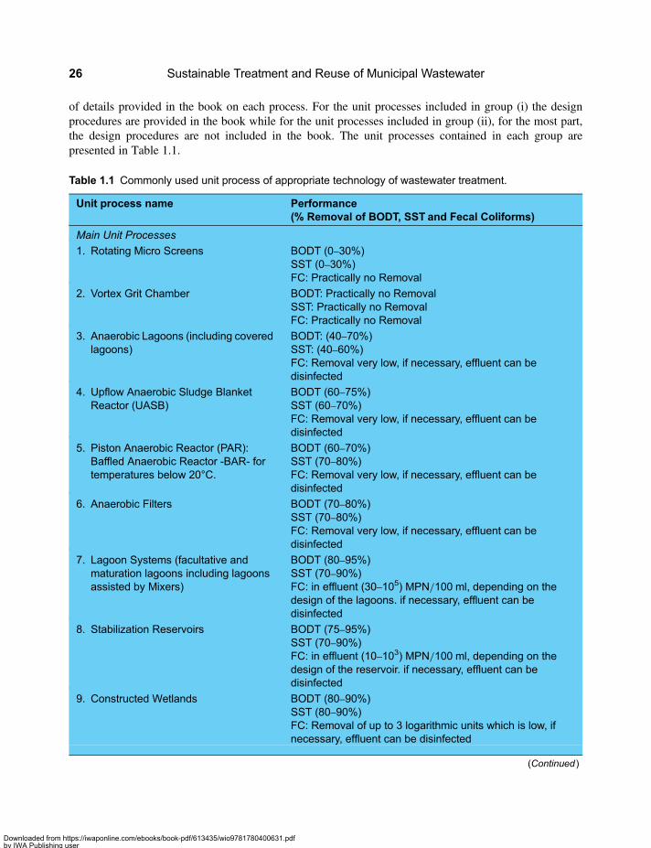
of details provided in the book on each process. For the unit processes included in group (i) the designprocedures are provided in the book while for the unit processes included in group (ii), for the most part,the design procedures are not included in the book. The unit processes contained in each group arepresented in Table 1.1.

Table 1.1 Commonly used unit process of appropriate technology of wastewater treatment.

Unit process name Performance(% Removal of BODT, SST and Fecal Coliforms)

Main Unit Processes

1. Rotating Micro Screens BODT (0–30%)SST (0–30%)FC: Practically no Removal

2. Vortex Grit Chamber BODT: Practically no RemovalSST: Practically no RemovalFC: Practically no Removal

3. Anaerobic Lagoons (including coveredlagoons)

BODT: (40–70%)SST: (40–60%)FC: Removal very low, if necessary, effluent can bedisinfected

4. Upflow Anaerobic Sludge BlanketReactor (UASB)

BODT (60–75%)SST (60–70%)FC: Removal very low, if necessary, effluent can bedisinfected

5. Piston Anaerobic Reactor (PAR):Baffled Anaerobic Reactor -BAR- fortemperatures below 20°C.

BODT (60–70%)SST (70–80%)FC: Removal very low, if necessary, effluent can bedisinfected

6. Anaerobic Filters BODT (70–80%)SST (70–80%)FC: Removal very low, if necessary, effluent can bedisinfected

7. Lagoon Systems (facultative andmaturation lagoons including lagoonsassisted by Mixers)

BODT (80–95%)SST (70–90%)FC: in effluent (30–105) MPN/100 ml, depending on thedesign of the lagoons. if necessary, effluent can bedisinfected

8. Stabilization Reservoirs BODT (75–95%)SST (70–90%)FC: in effluent (10–103) MPN/100 ml, depending on thedesign of the reservoir. if necessary, effluent can bedisinfected

9. Constructed Wetlands BODT (80–90%)SST (80–90%)FC: Removal of up to 3 logarithmic units which is low, ifnecessary, effluent can be disinfected

(Continued )



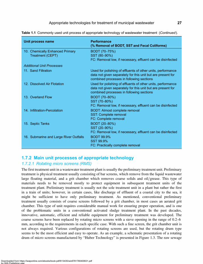
1.7.2 Main unit processes of appropriate technology1.7.2.1 Rotating micro screens (RMS)The first treatment unit in a wastewater treatment plant is usually the preliminary treatment unit. Preliminarytreatment is physical treatment usually consisting of bar screens, which remove from the liquid wastewaterlarge floating material, and a grit chamber which removes coarse solids and oil/grease. This type ofmaterials needs to be removed mostly to protect equipment in subsequent treatment units of thetreatment plant. Preliminary treatment is usually not the sole treatment unit in a plant but rather the firstin a train of units; however, in certain cases, like discharge of effluent of a coastal city to the sea, itmight be sufficient to have only preliminary treatment. As mentioned, conventional preliminarytreatment usually consists of coarse screens followed by a grit chamber, in most cases an aerated gritchamber. This type of unit requires considerable manual work for ensuring proper operation, and is oneof the problematic units in a conventional activated sludge treatment plant. In the past decades,innovative, automatic, efficient and reliable equipment for preliminary treatment was developed. Thecoarse screens have been replaced by rotating micro screens with a sieve opening in the range of 0.2–6mm, according to the requirements in each specific case. With such a fine screen, the grit chamber unit isnot always required. Various configurations of rotating screens are used, but the rotating drum typeseems to be the most efficient and easy to operate. As an example, a schematic presentation of a rotatingdrum of micro screens manufactured by “Huber Technology” is presented in Figure 1.3. The raw sewage

Table 1.1 Commonly used unit process of appropriate technology of wastewater treatment (Continued ).

Unit process name Performance(% Removal of BODT, SST and Fecal Coliforms)

10. Chemically Enhanced PrimaryTreatment (CEPT)

BODT (70–75%)SST (80–90%)FC: Removal low, if necessary, effluent can be disinfected

Additional Unit Processes

11. Sand Filtration Used for polishing of effluents of other units, performancedata not given separately for this unit but are present forcombined processes in following sections

12. Dissolved Air Flotation Used for polishing of effluents of other units, performancedata not given separately for this unit but are present forcombined processes in following sections

13. Overland Flow BODT (70–80%)SST (70–80%)FC: Removal low, if necessary, effluent can be disinfected

14. Infiltration-Percolation BODT: Almost complete removalSST: Complete removalFC: Complete removal

15. Septic Tanks BODT (20–80%)SST (20–90%)FC: Removal low, if necessary, effluent can be disinfected

16. Submarine and Large River Outfalls BODT 99.9%SST 99.9%FC: Practically complete removal



enters the rotating drum from the bottom to its inside and passes to the outside while floating and suspendedmaterial is retained on the internal side of the micro screen. The drum is cleaned with a water or effluent jetspray. The drum does not rotate continuously but rather starts rotating when the screen becomes clogged. Asthe drum rotates, a jet of high pressure water or effluent is sprayed on its upper part causing the materialclogging the screen to fall to the center of the drum, onto a screw conveyor which transports it upwards.The material retained on the conveyor is then dropped into a compactor that compresses it. Thecompressed solids are then transported out by a conveyer screw or belt conveyor into a central hopperand hauled for final disposal in a solid wastes disposal site such as a sanitary landfill. After rotatingseveral times the screen is cleaned and the drums stops rotating until new material clogs the internal sideof the screen. At that point the drum starts rotating again and so on. Drums are available in diametersranging from 600 to 2600 mm. The units are made completely of stainless steel. The wastewater flowwhich can be handled by one screening drum unit of a certain diameter depends on the screen openingand the drum’s diameter. For example, a 2600 mm diameter rotating screen with an opening of 0.5 mmcan handle a wastewater flow of about 0.5 m3/s, while the same diameter drum with a screen opening of6 mm can handle a wastewater flow of about 1.8 m3/s. Larger flows are accommodated by arrangingseveral drum units in parallel.

Removal levels of suspended solids and organic matter depends on the screen opening. According toinformation from the Huber Group, a manufacturer of this type of rotating screens, for a 1 mm screenopening, removal efficiencies of up to 20% of BOD, up to 90% of floatable solids, and up to 70% offloatable oil and grease can be achieved. Koppl and Frommann (2004) report removal of 20–30% BODand of 30–60% filterable solids (suspended solids) in rotating screens with screen opening of 0.2 to0.3 mm. These high removals of suspended solids result in large quantities of sludge, similar to that ofprimary treatment, and would require the provision of sludge treatment installations.

Figure 1.3 Diagram of a rotating micro screen for preliminary treatment (Courtesy Huber Technology)



Preliminary treatment by rotating micro screen is now awell-proven technologywith robust design. It hasreduced investment cost, is reliable and simple to operate and can be adjusted to particular hydraulic inflowconditions. Land and maintenance requirements are low, and package plants are available. It is a unit processof appropriate technology because it is less costly than conventional preliminary treatment that uses barscreens and aerated grit chambers, more reliable, requires less land and maintenance and removes moresolids. It includes only small electrical motors which operate intermittently and therefore has smallenergy consumption.

A preliminary treatment unit consisting of at least rotating micro screens should be the first unit in anytype of wastewater treatment plant. It removes coarse and floating materials from the raw wastewater in areliable and cost effective manner, and it is an exemplary appropriate technology treatment unit.

Investment costs of preliminary treatment based on a rotating micro screens unit are in the range 3–10 US$/Capita, depending on the unit size and level of plant finishing (outdoor plants are of lower cost than indoorplants with elaborated site development). Operation and maintenance costs are low, estimated at 0.1–0.15US$/Yr/Capita.

1.7.2.2 Vortex grit chambersIf a grit chamber is required as part of the preliminary treatment, a vortex type grit chamber is a better choiceas an appropriate technology unit, although a conventional aerated grit chamber is also quite a simple unit. Agrit chamber, including vortex grit chamber, is a physical treatment unit. In a vortex type unit of grit removal,a free vortex is generated by the flow that enters tangentially at the top of the cylindrical tank unit. Effluentexits the upper part of the unit cylinder. Grit settles by gravity at the bottom, where it is removed by a beltconveyor or lift station, and organic solids exit with the effluent. Another type of vortex grit chamber uses arotating turbine to maintain constant angular flow velocity and to promote separation of organic matter fromthe grit (see Figure 1.4). The grit settles by gravity into a hopper, from which it is removed by a grit pump orlift pump. Vortex grit chambers are more compact than conventional grit chambers, and are efficient andreliable. Because of their smaller size they are also less expensive.

Figure 1.4 Vortex grit chamber (Courtesy Huber Technology)



1.7.2.3 Anaerobic lagoons

Anaerobic lagoons technology is well known and widely spread all over the world. Organic matter isremoved in anaerobic lagoons through an anaerobic biological process; the anaerobic lagoon is in fact ananaerobic reactor. It is usually the first stage in lagoon treatment plants, followed by other types oflagoons. Anaerobic lagoons are designed to receive such a high organic loading that even if algae wouldhave developed in these lagoons they would not be able to produce sufficient oxygen to keep the lagoonaerobic, so this type of lagoons are completely devoid of oxygen and under such condition they favourthe development of anaerobic bacteria, which decompose the organic matter contained in the wastewaterflowing into the lagoons through the anaerobic biochemical pathway. A typical anaerobic lagoon isbasically a “hole in the ground”; usually with no equipment in it, except for inlet and outlet hydraulicstructures. Commonly, the depth of anaerobic lagoons is about 4 meters, but there is no specific limit tothe lagoons depth. An anaerobic lagoon is in fact a low rate anaerobic reactor. The concept “low rate”should not be interpreted to mean a second grade or low performing system, but rather that larger reactorvolumes, in relation to other higher rate anaerobic processes, are required to achieve high removal oforganic matter. Low rate systems can be designed to provide organic matter removals equal to thoseachieved in high rate systems. The volumetric loading rate of anaerobic lagoons is between 0.1 and 0.5kg BOD5/day/m

3. The low range loading is used for areas with a profound cold season of about 10°C,and the high range loading is used in areas where there are uniform annual warm temperatures in therange 25–30°C. These loading rates are equivalent to area BOD5 loading rates of between 4,000 and16,000 kg BOD/day/ha assuming an anaerobic lagoon depth of 4 meters. The depth of anaerobic lagoonsis usually in the range of 3–5 meters, 4 meters being a common figure. Detention times in anaerobiclagoon range from 2 to 6 days. There appears to be little treatment advantage in extending detention timeto more than 2 days and recently there is even a tendency to reduce the detention time in an anaerobiclagoon to 1 day. Mara (2004) provides data on experience with anaerobic lagoons from northeast Brazilwhich shows that at 25°C little variation in BOD removal was found at detention times in the range 0.8–6.8 days. To reduce the detention time and still have an efficient performance, the inflow to theanaerobic lagoon needs to be done in the bottom of the lagoon and distributed between several feedingpoints. This way, the contact between the biomass (which in an anaerobic lagoon develops on thebottom) and the substrate (the organic matter in the raw sewage) is more intensive and effective.

An anaerobic lagoon removes 40–70% of the organic matter contained in municipal wastewater.Considering that typical municipal raw wastewater contains a total BOD5 concentration in the range200–300 mg/l, an effluent of anaerobic lagoons usually contains 60–180 mg/l BOD5. The mixing in ananaerobic lagoon reactor is not effective and the contact of the organic matter dissolved in the raw sewageflowing into the lagoon with the biomass which develops in the bottom of the lagoon is not intense, soonly partial removal of dissolved organic matter is achieved. The removal of the suspended solidscontained in the raw sewage, which settle in the lagoon, is high, but as a whole, the organic matter removalin an anaerobic lagoon is lower than in other anaerobic processes. The mixing regime in anaerobic lagoonsis also the reason that the use of anaerobic lagoons in series is not effective when treating municipalwastewater. The first anaerobic lagoon will remove the organic matter it is capable of removing and thesecond one will not be able to remove a significant amount of additional dissolved organic matter. Theapproach of anaerobic lagoons in series might be a good solution for treating concentrated industrialwastewater. An anaerobic lagoon is a powerful unit, small in size, of low cost in investment and O&M,simple to operate and capable of removing a significant part of the organic matter contained in the rawwastewater. If additional removal of the remaining organic matter is necessary, the removal effort of theresidual organic matter is smaller since the major part was removed by the anaerobic lagoon.



The flow regime in an anaerobic lagoon is such that the mixing in the lagoon is not effective.Conventional anaerobic lagoons do not contain mechanical mixers. The solids contained in the rawsewage flowing into the lagoon settle to its bottom and new anaerobic biomass develops mainly in thebottom of the lagoon. Under the flow regime of the lagoon, the liquid does not come into effectivecontact with the bottom sediments, that is, with the anaerobic bacteria, so the removal of the dissolvedorganic matter is not very efficient. The mechanism by which the liquid phase comes in contact with thebottom sediments is through the assistance of gas bubbles, which develop at the bottom, grow and carrysludge particles upwards through the liquid column to the liquid surface, where they collapse and slowlysettle back to the sludge bed at the bottom. Sludge particles go through many up and down cycles duringtheir residence time in the lagoon. Settled solids stay a long time in the bottom of the lagoon and getwell digested, therefore, the excess sludge quantities generated in an anaerobic lagoon are much lowerthan in the other anaerobic process. However, due to the ineffective contact between the liquid and thesludge, a long detention time is required to remove even part of the dissolved organic matter in theliquid, and this is the reason that the detention time in anaerobic lagoons is much higher than that ofother anaerobic processes and even so the organic matter removal in an anaerobic lagoon is low incomparison to other anaerobic processes. Due to the flow regime in anaerobic lagoons they are mostadvantageously used to pre-treat wastewaters which have a high solid content. The solids settle to thebottom where they are digested anaerobically. The successful operation of anaerobic lagoons depends onthe delicate balance between the acid forming bacteria and the methanogenic bacteria, thus temperaturehigher than 10°C in the lagoon liquid is required and the pH in the lagoon must be higher than 6.2.Under such conditions, sludge accumulation is minimal, and desludging, which is required when thelagoon is half full of sludge, is necessary only once every 5–10 years. Although it is commonly acceptedthat anaerobic lagoons do not function at temperatures lower than 10°C, evidence from the highlands ofBolivia and Peru (with double the solar radiation than at sea level) show that anaerobic lagoons performwell even in zones with prolonged low air temperatures of up to −7°C. The temperature in the lagoonliquid is of course not that low, but it is certainly lower than 10°C. It seems that anaerobic bacteria canadjust to low temperatures if they are kept without severe fluctuations during prolonged periods ofseveral months.

Lagoons plants are, in general, suitable for serving small and medium size cities, of up to 400,000inhabitants in one plant. That applies also to anaerobic lagoons, which usually form part of variousconfigurations of lagoons systems. A lagoon plant serving larger populations requires a large land areawhich is usually not available in the vicinity of a large city or becomes prohibitively expensive.However, if several smaller plants can be constructed at different locations, lagoon systems can servecities with populations much larger than 400,000.

The advantages of anaerobic lagoons are low cost, simplicity of operation; effectiveness in handlinghighly concentrated sewage, the ability to cope with high concentrations of suspended solids (TSS), theability to handle shock loads and success in treating a variety of biodegradable industrial wastes. Themain disadvantage of anaerobic lagoons is the potential for generation of odours, caused by emission ofH2S when they are submitted to a too low or too high organic loading. A low loading may occur duringthe early years of operation and a high loading, during late years. Another disadvantage associated withthe odour problem is that once designed and constructed, there are no operational means of controllingthe process and resolving the odour problems when they appear. The odour problem associated withanaerobic lagoons is the reason for the resistance to use this process or when using it, locating the plantat a long distance from urban areas, which increases the cost of conveyance of the raw sewage. Therelationship between odour development and organic loading is now reasonably well understood so thatproblems can usually be overcome by proper design. Recently a method for completely eliminating the



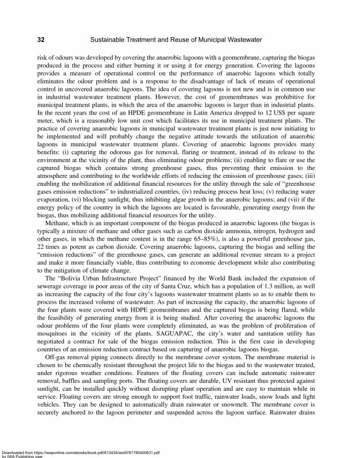
risk of odours was developed by covering the anaerobic lagoons with a geomembrane, capturing the biogasproduced in the process and either burning it or using it for energy generation. Covering the lagoonsprovides a measure of operational control on the performance of anaerobic lagoons which totallyeliminates the odour problem and is a response to the disadvantage of lack of means of operationalcontrol in uncovered anaerobic lagoons. The idea of covering lagoons is not new and is in common usein industrial wastewater treatment plants. However, the cost of geomembranes was prohibitive formunicipal treatment plants, in which the area of the anaerobic lagoons is larger than in industrial plants.In the recent years the cost of an HPDE geomembrane in Latin America dropped to 12 US$ per squaremeter, which is a reasonably low unit cost which facilitates its use in municipal treatment plants. Thepractice of covering anaerobic lagoons in municipal wastewater treatment plants is just now initiating tobe implemented and will probably change the negative attitude towards the utilization of anaerobiclagoons in municipal wastewater treatment plants. Covering of anaerobic lagoons provides manybenefits: (i) capturing the odorous gas for removal, flaring or treatment, instead of its release to theenvironment at the vicinity of the plant, thus eliminating odour problems; (ii) enabling to flare or use thecaptured biogas which contains strong greenhouse gases, thus preventing their emission to theatmosphere and contributing to the worldwide efforts of reducing the emission of greenhouse gases; (iii)enabling the mobilization of additional financial resources for the utility through the sale of “greenhousegases emission reductions” to industrialized countries, (iv) reducing process heat loss; (v) reducing waterevaporation, (vi) blocking sunlight, thus inhibiting algae growth in the anaerobic lagoons; and (vii) if theenergy policy of the country in which the lagoons are located is favourable, generating energy from thebiogas, thus mobilizing additional financial resources for the utility.

Methane, which is an important component of the biogas produced in anaerobic lagoons (the biogas istypically a mixture of methane and other gases such as carbon dioxide ammonia, nitrogen, hydrogen andother gases, in which the methane content is in the range 65–85%), is also a powerful greenhouse gas,22 times as potent as carbon dioxide. Covering anaerobic lagoons, capturing the biogas and selling the“emission reductions” of the greenhouse gases, can generate an additional revenue stream to a projectand make it more financially viable, thus contributing to economic development while also contributingto the mitigation of climate change.

The “Bolivia Urban Infrastructure Project” financed by the World Bank included the expansion ofsewerage coverage in poor areas of the city of Santa Cruz, which has a population of 1.3 million, as wellas increasing the capacity of the four city’s lagoons wastewater treatment plants so as to enable them toprocess the increased volume of wastewater. As part of increasing the capacity, the anaerobic lagoons ofthe four plants were covered with HDPE geomembranes and the captured biogas is being flared, whilethe feasibility of generating energy from it is being studied. After covering the anaerobic lagoons theodour problems of the four plants were completely eliminated, as was the problem of proliferation ofmosquitoes in the vicinity of the plants. SAGUAPAC, the city’s water and sanitation utility hasnegotiated a contract for sale of the biogas emission reduction. This is the first case in developingcountries of an emission reduction contract based on capturing of anaerobic lagoons biogas.

Off-gas removal piping connects directly to the membrane cover system. The membrane material ischosen to be chemically resistant throughout the project life to the biogas and to the wastewater treated,under rigorous weather conditions. Features of the floating covers can include automatic rainwaterremoval, baffles and sampling ports. The floating covers are durable, UV resistant thus protected againstsunlight, can be installed quickly without disrupting plant operation and are easy to maintain while inservice. Floating covers are strong enough to support foot traffic, rainwater loads, snow loads and lightvehicles. They can be designed to automatically drain rainwater or snowmelt. The membrane cover issecurely anchored to the lagoon perimeter and suspended across the lagoon surface. Rainwater drains



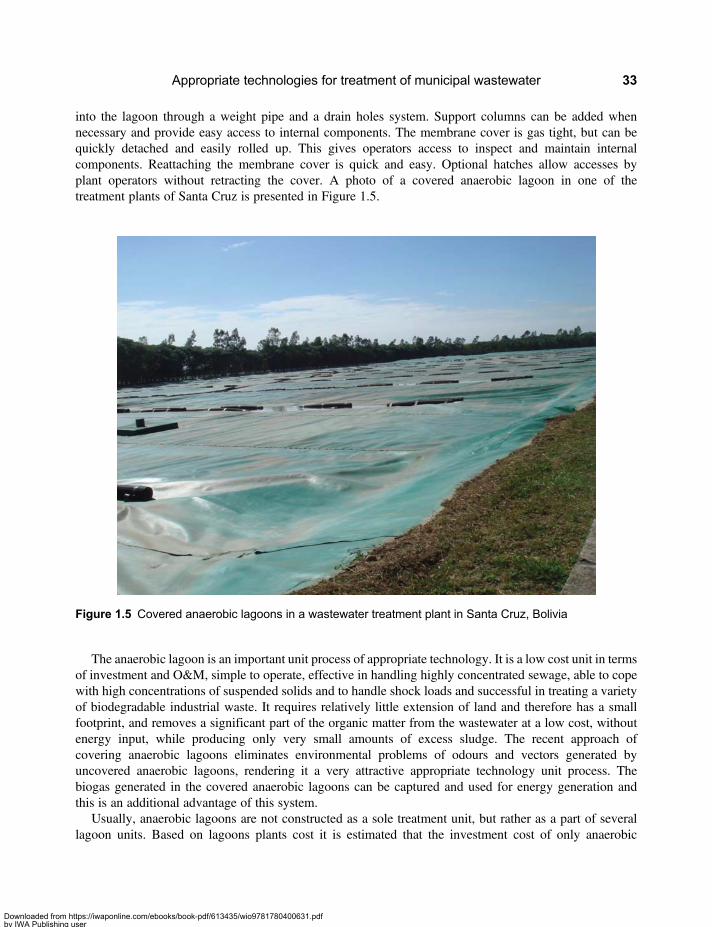
into the lagoon through a weight pipe and a drain holes system. Support columns can be added whennecessary and provide easy access to internal components. The membrane cover is gas tight, but can bequickly detached and easily rolled up. This gives operators access to inspect and maintain internalcomponents. Reattaching the membrane cover is quick and easy. Optional hatches allow accesses byplant operators without retracting the cover. A photo of a covered anaerobic lagoon in one of thetreatment plants of Santa Cruz is presented in Figure 1.5.

The anaerobic lagoon is an important unit process of appropriate technology. It is a low cost unit in termsof investment and O&M, simple to operate, effective in handling highly concentrated sewage, able to copewith high concentrations of suspended solids and to handle shock loads and successful in treating a varietyof biodegradable industrial waste. It requires relatively little extension of land and therefore has a smallfootprint, and removes a significant part of the organic matter from the wastewater at a low cost, withoutenergy input, while producing only very small amounts of excess sludge. The recent approach ofcovering anaerobic lagoons eliminates environmental problems of odours and vectors generated byuncovered anaerobic lagoons, rendering it a very attractive appropriate technology unit process. Thebiogas generated in the covered anaerobic lagoons can be captured and used for energy generation andthis is an additional advantage of this system.

Usually, anaerobic lagoons are not constructed as a sole treatment unit, but rather as a part of severallagoon units. Based on lagoons plants cost it is estimated that the investment cost of only anaerobic

Figure 1.5 Covered anaerobic lagoons in a wastewater treatment plant in Santa Cruz, Bolivia



lagoons would be about 5–10 US$/Capita. Operation and maintenance cost is extremely low. The cost ofcovering lagoons in Latin America amounts to 12 US$/m2. Additional information on AnaerobicLagoons can be found in the books byVon Sperling (2002), Campos (2009),Mara (2004) andArthur (1983).

1.7.2.4 Upflow anaerobic sludge blanket reactor (UASB)An Upflow Anaerobic Sludge Blanket Reactor is a high rate anaerobic biological reactor for treatment ofwastewater based on anaerobic granular sludge bed technology. UASB technology is being increasinglyconsidered for municipal wastewater treatment applications in warm-weather locations given its low costand simple operations. Although this technology can not by itself produce an effluent of the quality of aconventional secondary process like activated sludge, it can still achieve significant organic matterremoval rates in the range of 60–75% of BOD5 at a fraction of the construction and O&M costs ofactivated sludge. Experience to date in Latin America has shown that a UASB-based plant is simpler,less reliant on mechanical components and can easily achieve double the organic matter removal rates ofconventional primary treatment. In addition, the UASB process generates substantially lower quantitiesof sludge than aerobic processes, reducing therefore the associated sludge disposal costs. Given theanaerobic nature of the process, a potential for H2S generation (thus odour and corrosion problems)exists in municipal UASB applications when the sulphate concentration in the raw sewage is high.Appropriate selection of construction materials can reduce corrosion problems.

UASB reactors were developed in the 1970s for the treatment of highly concentrated industrialwastewater. Following the initial reactor designs for the treatment of sugar industry wastes, the benefitsof the system, such as low sludge production, small footprint, low energy requirements and valuablebiogas production, made the UASB reactors an attractive and hence widely applicable treatmentalternative for highly concentrated industrial wastewaters at mesophilic temperatures. These advantagesencouraged investigating the application of the UASB process to the treatment of domestic wastewaterfor municipal applications, where the low BOD concentrations coupled with high particulate BODfractions results in insufficient methane production for heating the reactor to mesophilic temperatures.However, since even moderate ambient temperatures favour satisfactory removal rates within areasonably sized reactor, the use of UASB reactors for domestic wastewater is becoming widespread intropical countries such as Brazil, Colombia and others. In applications requiring higher effluent qualitylevels than those which can be achieved by UASB, then UASB reactors are usually followed by anadditional treatment unit for polishing the UASB effluent. UASB technology followed by a polishingunit is a treatment option being increasingly implemented in warm-weather countries with minimumwastewater temperatures of over 10°C.

A schematic diagram of a UASB reactor is shown in Figure 1.6. From a hardware perspective, a UASBreactor appears to be nothing more than an empty tank with installations of three phases separation (liquid,solids and gas) on its upper part, thus extremely simple and inexpensive. UASB reactors are constructed astanks with a rectangular or circular cross section. Wastewater is fed into the tank in the bottom, throughappropriately spaced inlets. The wastewater passes upwards through an anaerobic sludge bed whereanaerobic bacteria in the sludge come into contact with the wastewater (the substrate). The sludge iscomposed of microorganisms that naturally form granules (pellets) of 0.5 to 2 mm in diameter, whichhave a high sedimentation velocity and thus resist washout from the system even at high hydraulic loads.The anaerobic decomposition process resulting from the contact between the granular sludge and thewastewater generates biogas as in other anaerobic processes. The upward motion of released gas bubblescauses hydraulic turbulence which provides effective reactor mixing without any mechanical equipment.At the top of the reactor, the liquid phase is separated from the sludge solids and gas in a three-phase



separator (also known as the gas-liquid-solids separator). This separator is usually a gas cap with a settlersituated above it. Baffles are used below the opening of the gas cap to deflect gas to the gas-cap opening.

The level of removal of organic matter in a UASB reactor is limited by the concentration of the sludge inthe reactor. Higher sludge concentrations would have resulted in higher organic matter removal, but wouldhave also result in higher escape of sludge in the effluent, which then controls the maximum achievablesludge concentration.

To achieve higher sludge concentrations and higher removal of organic matter, an Expanded GranularSludge Bed (EGSB) reactor, which is a variant of UASB, can be used. The distinguishing feature ofEGSB is that it includes effluent recycle, so sludge concentration can reach higher values and a fasterrate of upward flow velocity is designed for the wastewater passing through the bed. The increased fluxpermits partial expansion (fluidization) of the granular sludge bed, improving wastewater-sludge contact.The increased flow velocity is accomplished by a combination of utilizing tall reactors and effluentsrecycle. Organic matter removal of up to 90% and even higher can be achieved with the EGSB reactor.This type of reactor is used for treatment of industrial wastewaters but is not yet under widespread usefor treatment of municipal wastewater.

UASB reactors treating municipal wastes yields an effluent that usually contains 35–100 mg/l TotalBOD5, 30–40 mg/l Soluble BOD5 and 50–130 mg/l TSS (removal efficiencies are 60–75% for totalBOD and 65–80% for TSS).

Figure 1.6 Schematic diagram of a UASB reactor (Source: http://www.uasb.org/discover/agsb.htm)



http://www.germantoilet.org/en/projects/zambia/menu-sambia/progress.html






Typical hydraulic detention time values in a UASB reactor is in the range 4–5 hr and can be somewhatlarger. Maximum up-flow velocity is 1.0 m/hr and can be lower, water depth in the reactor is about 5 metersand the recommended maximum flow per reactor is 70 l/s. Additional information on USAB reactors can befound in the books by Orozco (2005), Campos (2009), Chernicharo (2007) and Mara (2004).

Several large UASB plants have been constructed in Brasilia and Belo Horizonte in Brazil, each serving apopulation of about 1 million. Many plants serving smaller population are in operation in Latin America.The UASB technology is therefore suitable for serving all range of cities size, including large cities.Most of the UASB tanks are constructed as over the ground level concrete tanks, as seen in Figure 1.7,which shows the Onca UASB treatment plant in the city Belo Horizonte, Brazil, serving a population of1 million. This type of tanks is relatively expensive. A less costly method of constructing UASB tanks isthe use of tanks buried in the ground. In this case concrete is used only for lining the tanks, not forstructural purposes. Concrete lined buried UASB tanks of the treatment plant of the city of Uberaba,Brazil, serving a population of about 300,000 are shown in Figures 1.8 and 1.9. Figure 1.8 shows one ofthe eight UASB tanks of the plant during the construction phase and Figure 1.9 shows the same tankafter the plant has been commissioned.

UASB plants treating industrial wastes are usually constructed of stainless steel or plastic materials andare designed to capture the biogas, and in most cases use it for generation of energy. The existing municipalUASB plants were not design to capture the biogas and its seems that with concrete tanks and without properdesign attention to biogas capture, the biogas escapes the system, so currently there are no municipal UASBplants that manage to capture and utilize the biogas. However, it is expected that with proper attention to thisissue and adequate design, the biogas in UASB plants can be captured and, if economically viable, utilizedfor energy generation.

Figure 1.7 The Onca UASB treatment plant in the City Belo Horizonte, Brazil



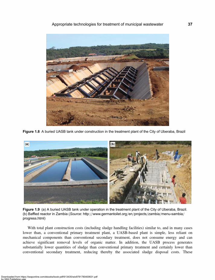
With total plant construction costs (including sludge handling facilities) similar to, and in many caseslower than, a conventional primary treatment plant, a UASB-based plant is simple, less reliant onmechanical components than conventional secondary treatment, does not consume energy and canachieve significant removal levels of organic matter. In addition, the UASB process generatessubstantially lower quantities of sludge than conventional primary treatment and certainly lower thanconventional secondary treatment, reducing thereby the associated sludge disposal costs. These

Figure 1.9 (a) A buried UASB tank under operation in the treatment plant of the City of Uberaba, Brazil.(b) Baffled reactor in Zambia (Source: http://www.germantoilet.org/en/projects/zambia/menu-sambia/progress.html)

Figure 1.8 A buried UASB tank under construction in the treatment plant of the City of Uberaba, Brazil













characteristics make it a member of the appropriate technology unit treatment processes. UASB is also a unitprocess with a small footprint, so it becomes an important process when the land available for the municipalwastewater treatment plant is scarce. The biogas generated in the UASB reactor may be captured and used todrive a downstream aerobic polishing processes (if such processes are included in the treatment plant),leading to energy-autonomous treatment plants. Alternatively, the energy produced from the biogas canbe used for other purposes.

Based on the recent construction of several medium to large size UASB facilities (serving equivalentpopulations of over 200.000) in Curitíba, Brazil, and some years ago in Bucaramanga, Colombia,construction costs in the range 20–40 US$/Capita have been documented for the UASB technology.Even including additional treatment steps for polishing the UASB effluent, these costs comparefavourably with the cost of over 100 US$/Capita considered typical for a conventional activated sludgetreatment plant. Operation and maintenance costs of UASB are in the range of 1.0–1.5 US$/Yr/Capita.

A different type of blanket reactor is the Baffled Anaerobic Reactor (BAR) initially proposed by PerryMcCarty in the early 1980s. The piston (or plug-flow) anaerobic reactor (PAR) is a variant of baffledreactors which uses a Gas-Solid-Liquid-Separator (GSLS) in the final chamber to improve theentrapment of solid particles so as to prevent their washout with the effluent and maintain thereby thesludge age at a level as high as possible. The PAR was developed at the Los Andes university in Bogota,Colombia, (Orozco, 1988, 1997) for temperatures below 20°C, taking advantage of the higher efficiencyof substrate removal obtained with the more perfect plug flow regime with baffles. Full scale plantsbased on RAP reactors were constructed and operated achieving COD removal efficiencies of 70% attemperatures between 13 and 17 °C (See Metcalf & Eddy, 2003, pp. 1005, 1018). These efficiencies canbe improved to the extent that the retention of solids becomes more effective, because the effluentcontains a high level of suspended solids which represent most of the COD in it. The PAR reactor in thecity of Tunja (Colombia) was the first baffled reactor constructed in the world in a full scale plant(Metcalf & Eddy, 2003, pp. 1005). Moreover, the use of PAR reactors for operation at sub-optimaltemperatures (lower than 15°C) has influenced the development of other baffled reactors that havebeen built at an accelerated pace in several countries, especially in China (Zonglian She et al. 2006),New Zealand (Foxon et al. 2003) and Bolivia (Medina et al. 1993). Figures 1.9b and 6.7 present photosof PAR reactors.

1.7.2.5 Anaerobic filterAnAnaerobic filter is a biological fixed bed anaerobic reactor which performs as an attached growth reactor,in which anaerobic bacteria grow on and are attached to a media of rocks or plastic filling of large surfacearea and the wastewater flows through the media. The reactor works under flooded conditions, which meansthat the media is flooded by the incoming wastewater so air, and consequently oxygen does not have contactwith the biomass attached to the media and the biomass which grows in this reactor is strictly anaerobic. Thebacteria are in continuous contact with the wastewater and consume the organic matter contained in it. Ananaerobic filter can be described as the anaerobic equivalent of a trickling filter. Both reactors are based onattached growth and look the same: a tank filled with a bacterial support media. However, the trickling filteris not flooded, the wastewater trickles through the media and the bacteria growing on the media have accessto oxygen so they are aerobic bacteria, while the anaerobic filter works when it is flooded, the bacteriagrowing on the media do not have access to oxygen and therefore they are anaerobic bacteria. Attachedgrowth bacterial reactors can be divided to fixed bed, rotating bed (rotating discs) and expanding bedreactors. They also have a variety of shapes and structures. This section deals with fixed bed anaerobicreactors, also known as anaerobic filters, which are the most commonly used anaerobic reactors. Twomain types of fixed bed reactors are ascending and descending flow reactors. The anaerobic fixed bed



attached growth reactors consist of a tank, which can be of circular or rectangular cross section, containingthe support media, rock particles or various types of plastic media. The bacteria develop in an attached formon the media and the consumption of substrate (i.e., the decomposition of the organic matter dissolved in thewastewater) as well as the growth of the anaerobic microorganism takes place on the external biofilm of eachmedia particle. Anaerobic microorganisms can also develop in the form of flakes or granules trappedbetween the media particles. With increased accumulation of the biomass, parts of it detach sporadicallyfrom the media particles to which it is attached and flow out with the liquid effluent. In spite of thisprocess, the average residence time of the biomass in the anaerobic filter is very long due to itsattachment to the support media. The average residence time of biomass in this type of reactor is morethan 20 days, resulting in an effective performance of the treatment process. Ascending flow filters aremore commonly used than descending flow filters. In descending flow filters, recirculation of effluent tothe filter inflow is commonly used. The elevated residence time of the biomass in the filter which resultsin high microorganisms concentration, associated with short hydraulic detention time of the liquid in thefilter and the effective contact between the liquid and the biomass result in high organic matter removal(higher than in anaerobic lagoons and UASB reactors) and provide the anaerobic filter with greatpotential for its use for treatment of non-concentrated wastewater.

To prevent clogging of the filter, effective removal of suspended solids from the raw sewage is requiredprior to its inflow to the filter. Such removal of suspended solids can be achieved by rotating micro screens.For small treatment plants, decanter-digesters (otherwise known as large septic tanks or Imhoff tanks) areused to remove suspended solids prior to an anaerobic filter. This is a common practice in Brazil. Inaddition to the use of anaerobic filters as the main treatment unit, they can be used as polishing unitesfor improvement of the quality of the effluent of a preceding unit. They are in fact more suitable toperform as polishing units since when fed with treated effluent of a preceding unit they are less bound toclog by suspended solids and have to treat a lower content dissolved organic matter. In Brazil anaerobicfilters are used as the main treatment unit mainly for small and medium size municipalities, while forpolishing application anaerobic filters are used in the entire range of cities size, including in treatmentplants of large cities.

With time, the anaerobic filter becomes clogged because of the growth of the biomass. When the pressuredrop on the filter becomes too high, it needs to be washed. Similarly to sand filters for water treatment, theanaerobic filter is washed by a stream of water or treated effluent which is passed through it in a counter wisedirection to its operation flow. The wash water, which contains the excess sludge, is directed to the sludgehandling facilities, which are usually just drying beds. Since the process is anaerobic, the excess sludgequantities are small and the washing, which is specific to each systems, is required infrequently, onceevery several days to once every few months.

Chernicharo (2000) reports Total BOD removal efficiencies of anaerobic filters in the range of 70–80%when the anaerobic filter is the main treatment unit and 75–95% when it used as a polishing units. AndradeNeto (1997, 2000) reports results of a research on an anaerobic filter system treating municipal wastewaterwhich was in operation for six years. This system, consisting of a septic tank followed by an up-flowanaerobic filter followed by a down-flow anaerobic filter, achieved a COD removal of up to 90%. Theeffluent of this anaerobic filter system contained less than 30 mg/l of BOD and less than 20 mg/l totalsuspended solids. Sludge withdrawal from the filter was undertaken once every six months.

A photo of a circular cross section ascending flow anaerobic filter in the treatment plant of the city ofTibagi in the state of Parana, Brazil, is presented in Figure 1.10. The filter is similar to a circularsedimentation tank. It is filled with a crushed rock media. The filter washing is done by a descendingwater stream. The wheels in the front of the filter operate the valves which change the flow direction toinitiate the filter washing cycle. Anaerobic filter media composed of plastic material shapes with a large



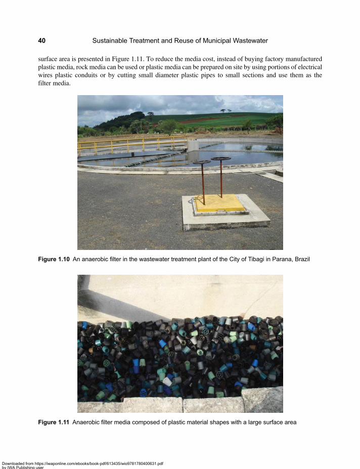
surface area is presented in Figure 1.11. To reduce the media cost, instead of buying factory manufacturedplastic media, rock media can be used or plastic media can be prepared on site by using portions of electricalwires plastic conduits or by cutting small diameter plastic pipes to small sections and use them as thefilter media.

Figure 1.10 An anaerobic filter in the wastewater treatment plant of the City of Tibagi in Parana, Brazil

Figure 1.11 Anaerobic filter media composed of plastic material shapes with a large surface area



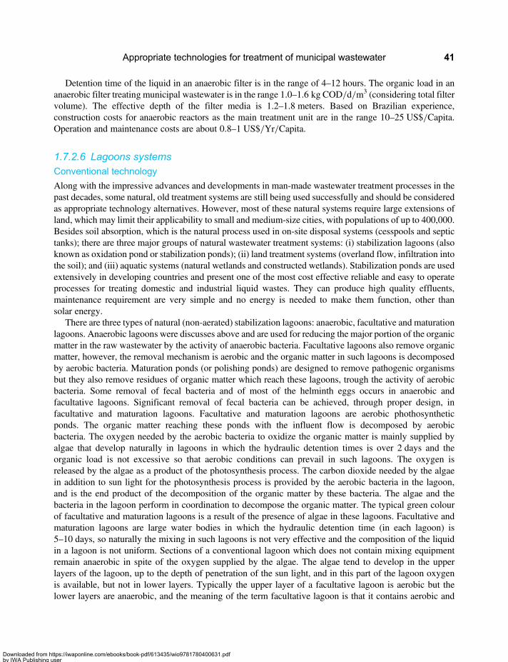
Detention time of the liquid in an anaerobic filter is in the range of 4–12 hours. The organic load in ananaerobic filter treating municipal wastewater is in the range 1.0–1.6 kg COD/d/m3 (considering total filtervolume). The effective depth of the filter media is 1.2–1.8 meters. Based on Brazilian experience,construction costs for anaerobic reactors as the main treatment unit are in the range 10–25 US$/Capita.Operation and maintenance costs are about 0.8–1 US$/Yr/Capita.

1.7.2.6 Lagoons systemsConventional technology

Along with the impressive advances and developments in man-made wastewater treatment processes in thepast decades, some natural, old treatment systems are still being used successfully and should be consideredas appropriate technology alternatives. However, most of these natural systems require large extensions ofland, which may limit their applicability to small and medium-size cities, with populations of up to 400,000.Besides soil absorption, which is the natural process used in on-site disposal systems (cesspools and septictanks); there are three major groups of natural wastewater treatment systems: (i) stabilization lagoons (alsoknown as oxidation pond or stabilization ponds); (ii) land treatment systems (overland flow, infiltration intothe soil); and (iii) aquatic systems (natural wetlands and constructed wetlands). Stabilization ponds are usedextensively in developing countries and present one of the most cost effective reliable and easy to operateprocesses for treating domestic and industrial liquid wastes. They can produce high quality effluents,maintenance requirement are very simple and no energy is needed to make them function, other thansolar energy.

There are three types of natural (non-aerated) stabilization lagoons: anaerobic, facultative and maturationlagoons. Anaerobic lagoons were discusses above and are used for reducing the major portion of the organicmatter in the raw wastewater by the activity of anaerobic bacteria. Facultative lagoons also remove organicmatter, however, the removal mechanism is aerobic and the organic matter in such lagoons is decomposedby aerobic bacteria. Maturation ponds (or polishing ponds) are designed to remove pathogenic organismsbut they also remove residues of organic matter which reach these lagoons, trough the activity of aerobicbacteria. Some removal of fecal bacteria and of most of the helminth eggs occurs in anaerobic andfacultative lagoons. Significant removal of fecal bacteria can be achieved, through proper design, infacultative and maturation lagoons. Facultative and maturation lagoons are aerobic phothosyntheticponds. The organic matter reaching these ponds with the influent flow is decomposed by aerobicbacteria. The oxygen needed by the aerobic bacteria to oxidize the organic matter is mainly supplied byalgae that develop naturally in lagoons in which the hydraulic detention times is over 2 days and theorganic load is not excessive so that aerobic conditions can prevail in such lagoons. The oxygen isreleased by the algae as a product of the photosynthesis process. The carbon dioxide needed by the algaein addition to sun light for the photosynthesis process is provided by the aerobic bacteria in the lagoon,and is the end product of the decomposition of the organic matter by these bacteria. The algae and thebacteria in the lagoon perform in coordination to decompose the organic matter. The typical green colourof facultative and maturation lagoons is a result of the presence of algae in these lagoons. Facultative andmaturation lagoons are large water bodies in which the hydraulic detention time (in each lagoon) is5–10 days, so naturally the mixing in such lagoons is not very effective and the composition of the liquidin a lagoon is not uniform. Sections of a conventional lagoon which does not contain mixing equipmentremain anaerobic in spite of the oxygen supplied by the algae. The algae tend to develop in the upperlayers of the lagoon, up to the depth of penetration of the sun light, and in this part of the lagoon oxygenis available, but not in lower layers. Typically the upper layer of a facultative lagoon is aerobic but thelower layers are anaerobic, and the meaning of the term facultative lagoon is that it contains aerobic and



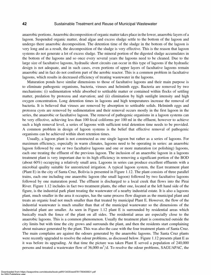
anaerobic portions. Anaerobic decomposition of organicmatter takes place in the lower, anaerobic layers of alagoon. Suspended organic matter, dead algae and excess sludge settle to the bottom of the lagoon andundergo there anaerobic decomposition. The detention time of the sludge in the bottom of the lagoon isvery long and as a result, the decomposition of the sludge is very effective. This is the reason that lagoonsystems do not generate a lot of excess sludge. The mineral portion of the digested sludge accumulates inthe bottom of the lagoons and so once every several years the lagoons need to be cleaned. Due to thelarge size of facultative lagoons, hydraulic short circuits can occur in this type of lagoons if the hydraulicdesign is not adequate, and in such cases, even portions of upper layers of facultative lagoons remainanaerobic and in fact do not conform part of the aerobic reactor. This is a common problem in facultativelagoons, which results in decreased efficiency of treating wastewater in the lagoons.

Maturation ponds have similar dimensions to those of facultative lagoons and their main purpose isto eliminate pathogenic organisms, bacteria, viruses and helminth eggs. Bacteria are removed by twomechanisms: (i) sedimentation while absorbed to settleable matter or contained within flocks of settlingmatter, predation by protozoa and starvation; and (ii) elimination by high sunlight intensity and highoxygen concentration. Long detention times in lagoons and high temperatures increase the removal ofbacteria. It is believed that viruses are removed by absorption to settleable solids. Helminth eggs andprotozoa cysts are removed by sedimentation and their removal occurs mostly in the first lagoon in theseries, the anaerobic or facultative lagoon. The removal of pathogenic organisms in a lagoon systems canbe very effective, achieving less than 100 fecal coliforms per 100 ml in the effluent, however to achievesuch a high removal level, a series of lagoons with sufficient total detention time needs to be provided.A common problem in design of lagoon systems is the belief that effective removal of pathogenicorganisms can be achieved within short retention times.

Usually, a lagoon plant is not constructed as one single lagoon but rather as a series of lagoons. Formaximum efficiency, especially in warm climates, lagoons need to be operating in series: an anaerobiclagoon followed by one or two facultative lagoons and one or more maturation (or polishing) lagoons,each one treating the effluent of the previous lagoon. The inclusion of an anaerobic lagoon in a lagoonstreatment plant is very important due to its high efficiency in removing a significant portion of the BOD(about 60%) occupying a relatively small area. Lagoons in series can produce excellent effluents with amicrobial quality suitable for unrestricted irrigation. A typical lagoon system, the East treatment plant(Plant E) in the city of Santa Cruz, Bolivia is presented in Figure 1.12. The plant consists of three paralleltrains, each one including one anaerobic lagoon (the small lagoon) followed by two facultative lagoonsfollowed by one maturation pond. The effluent is discharged to a local creek that flows into the PiraiRiver. Figure 1.12 includes in fact two treatment plants, the other one, located at the left hand side of thefigure, is the industrial park plant treating the wastewater of a nearby industrial estate. It is also a lagoonsplant, much smaller in the area it occupies, has the same process flow diagram as the municipal plant andtreats an organic load not much smaller than that treated by municipal Plant E. However, the flow of theindustrial wastewater is much smaller than that of the municipal wastewater so the dimensions of theindustrial plant are smaller. As seen in Figure 1.12 plant E is surrounded by residential areas whichbasically reach the fence of the plant on all sides. The residential areas are especially close to theanaerobic lagoons. This is a common phenomenon. Usually the treatment plant is constructed outside thecity limits but with time the city grows and surrounds the plant, and then the residents start complainingabout nuisance generated by the plant. This was also the case with the four treatment plants of Santa Cruz.The main complains are against the odours generated by the anaerobic lagoons. The Santa Cruz plantswere recently upgraded to resolve the odour problems, as discussed below. Figure 1.12 presents plant E asit was before its upgrading. At that time the picture was taken Plant E served a population of 240,000persons and treated a wastewater flow of 36,000 m3/d. To resolve the odour problems, SAGUAPAC, the



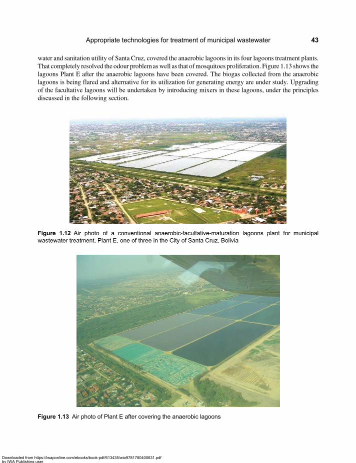
water and sanitation utility of Santa Cruz, covered the anaerobic lagoons in its four lagoons treatment plants.That completely resolved the odour problem aswell as that ofmosquitoes proliferation. Figure 1.13 shows thelagoons Plant E after the anaerobic lagoons have been covered. The biogas collected from the anaerobiclagoons is being flared and alternative for its utilization for generating energy are under study. Upgradingof the facultative lagoons will be undertaken by introducing mixers in these lagoons, under the principlesdiscussed in the following section.

Figure 1.12 Air photo of a conventional anaerobic-facultative-maturation lagoons plant for municipalwastewater treatment, Plant E, one of three in the City of Santa Cruz, Bolivia

Figure 1.13 Air photo of Plant E after covering the anaerobic lagoons



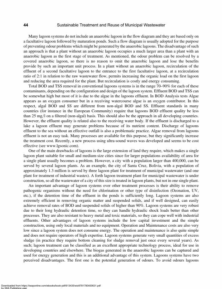
Many lagoon systems do not include an anaerobic lagoon in the flow diagram and they are based only ona facultative lagoon followed by maturation ponds. Such a flow diagram is usually adopted for the purposeof preventing odour problems which might be generated by the anaerobic lagoons. The disadvantage of suchan approach is that a plant without an anaerobic lagoon occupies a much larger area than a plant with ananaerobic lagoon as the first stage of treatment. As mentioned, the odour problem can be resolved by acovered anaerobic lagoon, so there is no reason to omit the anaerobic lagoon and lose the benefitsprovide by such an important unit process. In a plant without an anaerobic lagoon, recirculation of theeffluent of a second facultative lagoon to the entrance to the first facultative lagoon, at a recirculationratio of 2:1 in relation to the raw wastewater flow, permits increasing the organic load on the first lagoonand reducing the area required for the plant. But recirculation is costly and energy consuming.

Total BOD and TSS removal in conventional lagoons systems is in the range 70–90% for each of thesecontaminants, depending on the configuration and design of the lagoon system. Effluent BOD and TSS canbe somewhat high but most of it is due to the algae in the lagoons effluent. In BOD Analysis tests Algaeappears as an oxygen consumer but in a receiving watercourse algae is an oxygen contributor. In thisrespect, algal BOD and SS are different from non-algal BOD and SS. Effluent standards in manycountries (for instance in the European Community) require that lagoons BOD effluent quality be lessthan 25 mg/l on a filtered (non-algal) basis. This should also be the approach in all developing countries.However, the effluent quality is related also to the receiving water body. If the effluent is discharged to alake a lagoon effluent may generate problems because of its nutrient content. Discharge of lagoonseffluent to the sea without an effective outfall is also a problematic practice. Algae removal from lagoonseffluent is not an easy task. Many processes are available for this purpose, but they significantly increasethe treatment cost. Recently, a new process using ultra-sound waves was developed and seems to be costeffective (see www.lgsonic.com).

One of the main drawbacks of lagoons is the large extension of land they require, which makes a singlelagoon plant suitable for small and medium-size cities since for larger populations availability of area fora single plant usually becomes a problem. However, a city with a population larger than 400,000, can beserved by several lagoon plants. As an example, the city of Santa Cruz, Bolivia, with a population ofapproximately 1.3 million is served by three lagoon plant for treatment of municipal wastewater (and oneplant for treatment of industrial wastes). A forth lagoon treatment plant for municipal wastewater is underconstruction, so all the wastewater of a city of this size is treated in lagoon plants, but not in one single plant.

An important advantage of lagoon systems over other treatment processes is their ability to removepathogenic organisms without the need for chlorination or other type of disinfection (Ozonation, UV,etc.), if the detention time of the effluent in the ponds is sufficiently long. Lagoon systems are alsoextremely efficient in removing organic matter and suspended solids, and if well designed, can easilyachieve removal rates of BOD and suspended solids of higher than 90%. Lagoon systems are very robustdue to their long hydraulic detention time, so they can handle hydraulic shock loads better than otherprocesses. They are also resistant to heavy metal and toxic materials, so they can cope well with industrialeffluents. Other advantages of lagoon systems include the low capital investment and the simpleconstruction, using only local materials and no equipment. Operation and Maintenance costs are also verylow since a lagoon system does not consume energy. The operation and maintenance is also quite simpleand does not require operators of high expertise. Lagoon systems generate very small quantities of excesssludge (in practice they require bottom cleaning for sludge removal just once every several years). Assuch; lagoon treatment can be classified as an excellent appropriate technology process, ideal for use indeveloping countries and elsewhere. The biogas generated in the anaerobic lagoons can be captured andused for energy generation and this is an additional advantage of this system. Lagoons systems have twoperceived disadvantages. The first one is the potential generation of odours. To avoid odours lagoons



http://www.lgsonic.com

(both anaerobic and facultative)must be adequately designedwith correct loading rates andoverloading of thelagoons with time must be avoided since overloading is the main reason for odour generation. In addition, asexplained previously, anaerobic lagoons can be covered and this totally eliminates odours and vectors in suchlagoons. Regarding odours generation by facultative lagoons, as explained in the following section, windoperated mixers can be installed in facultative lagoons and this practically eliminates odours and vectorsin this type of lagoons. The second disadvantage is the large footprint of lagoons systems. The extensionof area of lagoons plants can be significantly decreased by inclusion of anaerobic lagoons in the flowdiagram. It can be further decreased by installing mixers in the facultative lagoons, as is explained in thefollowing section. However, even with all this measures, the area required for a lagoon plant is larger thanthat of other types of wastewater treatment plants. If land at the vicinity of the city is not available or isexpensive, the wastewater can be conveyed further downstream to rural areas where land is available andcheaper. The conveyance system will increase the investment cost, but even if the lagoons systeminvestment cost becomes comparable with the cost of a conventional treatment plant located closer to thecity, it would still be more reasonable to adopt the lagoon system solution because the O&M costs aremuch lower and a lagoon system is a more sustainable solution, especially in developing countries. Thechoice is between paying for conveyance and land on one hand and paying for complex equipment andhigh O&M costs, especially energy costs, on the other hand. Complex equipment and high O&M cost isnot a good solution for developing countries. In addition, investment in energy costs is lost forever whileinvestment in land is not lost.

The depth of facultative lagoons is usually in the range of 1.5–2 meters and that of maturation ponds issimilar or somewhat smaller. The organic load on facultative lagoons is generally in range of 100 to 250 kgBOD/day/ha, where the low value is applied during the low temperature season and the high value duringthe high temperature season. It is obvious that a treatment plant needs to be designed in such manner that it isable to cope also with the conditions of the low temperature season, which are the critical conditions. GTZreports that the uncovered anaerobic lagoons of Puchukollo, El Alto in the highlands of Bolivia, areoperating with efficiencies of more than 50% with detention times of 6 days and reactor temperatures aslow 8°C. However, the solar radiation at that altitude is about double than at sea level (Juanico &Weinberg, 1995) and that may be the reason that the anaerobic lagoons maintain higher temperaturesthan those with lower solar radiation, that is, at lower altitudes.

It is difficult to provide information on cots of stabilization lagoons system since the cost depends on theconfiguration on the lagoons, on the size of population served and on the cost of land, however,representative values can be mentioned. Information based on Arthur (1983), Yanez (1993), Rolim(2000), Mara (2004) and on experience of the authors indicates that construction costs of a lagoonssystem is in the range of 10–40 US$/Capita, depending on the size of population served (the lowerrange refers to larger size plants). Operation and Maintenance costs are in the range of 0.2–0.4 US$/Yr/Capita. The sources mentioned along with the book of Von Sperling (2002) are also good sourcesof information on design, performance, operation and maintenance of lagoon systems.

Aerated lagoons, a process developed to reduce the extension of land required by lagoons treatment isbased on installing aeration equipment in the lagoons so it is not a natural process of organic mattermetabolism in a lagoon but rather a process based on mechanical supply of oxygen to the lagoon forsupporting the decomposition of the organic matter. When aerated lagoons are the main process oftreating the raw wastewater they should not be considered an appropriate technology process. Althoughtheir construction costs may be lower than those of other lagoon types, with the aeration equipment theirinvestment cost becomes higher. But the main problem of aerated lagoons is that their energyconsumption is high since in this process the oxygen required for the treatment process is supplied byaeration equipment operated by electric energy. Usually in developing countries, and especially in small



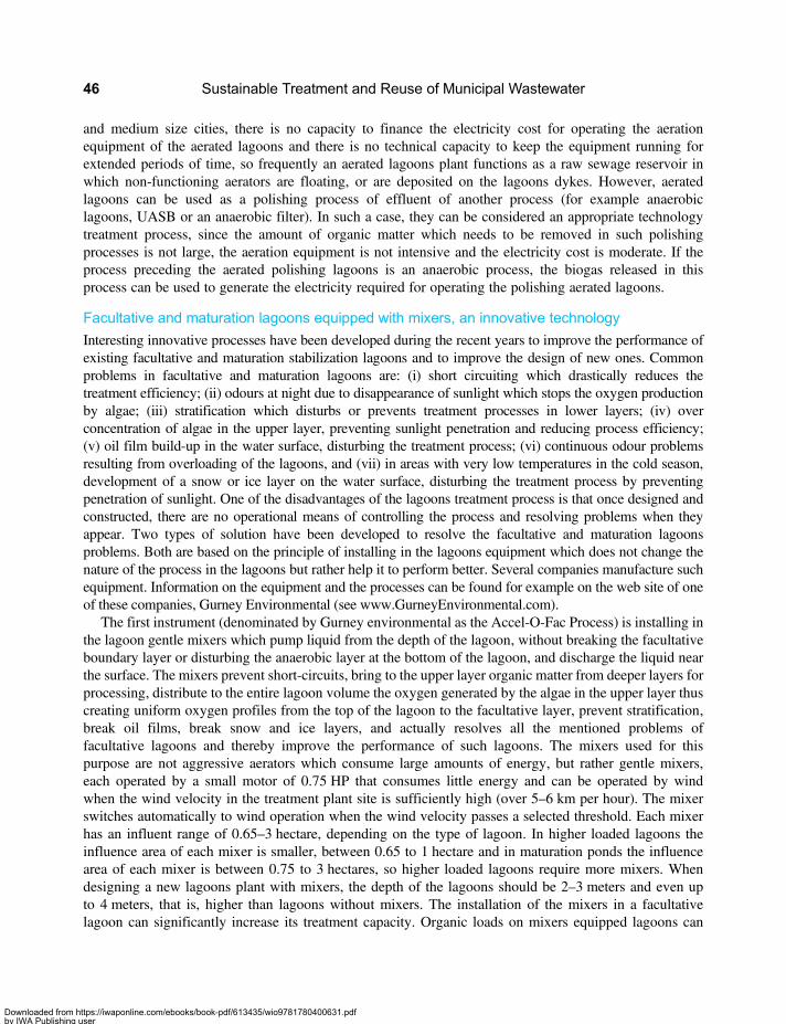
and medium size cities, there is no capacity to finance the electricity cost for operating the aerationequipment of the aerated lagoons and there is no technical capacity to keep the equipment running forextended periods of time, so frequently an aerated lagoons plant functions as a raw sewage reservoir inwhich non-functioning aerators are floating, or are deposited on the lagoons dykes. However, aeratedlagoons can be used as a polishing process of effluent of another process (for example anaerobiclagoons, UASB or an anaerobic filter). In such a case, they can be considered an appropriate technologytreatment process, since the amount of organic matter which needs to be removed in such polishingprocesses is not large, the aeration equipment is not intensive and the electricity cost is moderate. If theprocess preceding the aerated polishing lagoons is an anaerobic process, the biogas released in thisprocess can be used to generate the electricity required for operating the polishing aerated lagoons.

Facultative and maturation lagoons equipped with mixers, an innovative technology

Interesting innovative processes have been developed during the recent years to improve the performance ofexisting facultative and maturation stabilization lagoons and to improve the design of new ones. Commonproblems in facultative and maturation lagoons are: (i) short circuiting which drastically reduces thetreatment efficiency; (ii) odours at night due to disappearance of sunlight which stops the oxygen productionby algae; (iii) stratification which disturbs or prevents treatment processes in lower layers; (iv) overconcentration of algae in the upper layer, preventing sunlight penetration and reducing process efficiency;(v) oil film build-up in the water surface, disturbing the treatment process; (vi) continuous odour problemsresulting from overloading of the lagoons, and (vii) in areas with very low temperatures in the cold season,development of a snow or ice layer on the water surface, disturbing the treatment process by preventingpenetration of sunlight. One of the disadvantages of the lagoons treatment process is that once designed andconstructed, there are no operational means of controlling the process and resolving problems when theyappear. Two types of solution have been developed to resolve the facultative and maturation lagoonsproblems. Both are based on the principle of installing in the lagoons equipment which does not change thenature of the process in the lagoons but rather help it to perform better. Several companies manufacture suchequipment. Information on the equipment and the processes can be found for example on the web site of oneof these companies, Gurney Environmental (see www.GurneyEnvironmental.com).

The first instrument (denominated by Gurney environmental as the Accel-O-Fac Process) is installing inthe lagoon gentle mixers which pump liquid from the depth of the lagoon, without breaking the facultativeboundary layer or disturbing the anaerobic layer at the bottom of the lagoon, and discharge the liquid nearthe surface. The mixers prevent short-circuits, bring to the upper layer organic matter from deeper layers forprocessing, distribute to the entire lagoon volume the oxygen generated by the algae in the upper layer thuscreating uniform oxygen profiles from the top of the lagoon to the facultative layer, prevent stratification,break oil films, break snow and ice layers, and actually resolves all the mentioned problems offacultative lagoons and thereby improve the performance of such lagoons. The mixers used for thispurpose are not aggressive aerators which consume large amounts of energy, but rather gentle mixers,each operated by a small motor of 0.75 HP that consumes little energy and can be operated by windwhen the wind velocity in the treatment plant site is sufficiently high (over 5–6 km per hour). The mixerswitches automatically to wind operation when the wind velocity passes a selected threshold. Each mixerhas an influent range of 0.65–3 hectare, depending on the type of lagoon. In higher loaded lagoons theinfluence area of each mixer is smaller, between 0.65 to 1 hectare and in maturation ponds the influencearea of each mixer is between 0.75 to 3 hectares, so higher loaded lagoons require more mixers. Whendesigning a new lagoons plant with mixers, the depth of the lagoons should be 2–3 meters and even upto 4 meters, that is, higher than lagoons without mixers. The installation of the mixers in a facultativelagoon can significantly increase its treatment capacity. Organic loads on mixers equipped lagoons can



http://www.GurneyEnvironmental.com

reach values of 450 Kg BOD/d/ha in the high temperatures season of 25–30°C and even higher, with lowerloading values at lower temperatures.

The second instrument (denominated by Gurney environmental as the Aero-Fac Process) is injecting airinto the lagoon through blowers (not compressed air) to augment the oxygen quantity produced by the algaewithout changing the flow regime, that is, without transforming the lagoon to an aerated lagoon. For thatpurpose, a combination of blowers with air distributors and gentle mixers need to be installed in thelagoon. The addition of air to the lagoons increases its treatment capacity to a required level.

The use of mixers in lagoons provides some measure of operational control on the performance of thelagoon system and is a partial response to the disadvantage of lack of means of control in lagoons thatare not equipped with mixers.

Mixers can be used as part of a design of a new lagoon plant. In such case, the new plant will occupy asmaller area than a plant without mixers, since it can handle higher organic matter loads. Mixers can also beinstalled in existing lagoon plants to upgrade their capacity. In many cases lagoon plants become overloadedbut there is no area available to increase the capacity of the plant by adding lagoon units because the cityexpanded and occupied the land areas around the plant. Moving the plant to another site is expensiveand abandoning the lagoons process to replace it with a conventional mechanical treatment process isvery expensive. In this case mixers can be installed in the facultative lagoons without the employment ofblowers, and they will increase the capacity of the plant without increasing the lagoons area, and at avery small cost. If further capacity increase is required without increasing the lagoon area, then blowerscan be added. An excellent method to upgrade an existing conventional lagoons plant consisting ofanaerobic lagoons followed by facultative lagoons followed by polishing ponds is covering the anaerobiclagoon and installing mixers in the facultative lagoons. This was done in the municipal wastewatertreatment plants of Santa Cruz Bolivia and is discussed in a following chapter.

The mixing equipment principles of operation are presented in Figures 1.14 and 1.15. The mechanism bywhich the mixers improve the performance of facultative lagoons and resolves the above mentioned lagoonsproblems are presented in Figure 1.16. A photo of several mixers in a facultative lagoon (in Plant North 2 inSanta Cruz, Bolivia) is presented in Figure 1.17.

Figure 1.14 Mixers and air injectors in facultative lagoons (Courtesy Gurney Environmental)



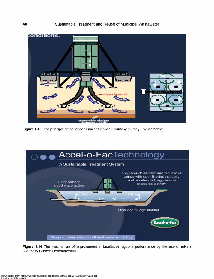
Figure 1.15 The principle of the lagoons mixer function (Courtesy Gurney Environmental)

Figure 1.16 The mechanism of improvement in facultative lagoons performance by the use of mixers(Courtesy Gurney Environmental)



Upgrading of existing plants can be done in stages, first mixers are installed in shallow lagoons, aftertime, lagoon depth is increased to 3–4 meters, since the mixers are more effective at such depths, andfinally, air blowers and injection equipment can be added. This is an effective method to increaselagoons plants capacity when additional area is not available. For design of new lagoons, it is proposedto provide a plant consisting of a basic unit of a covered anaerobic lagoon followed one or twofacultative lagoons in series, each one 3–4 meters deep, equipped with mixers, followed by a shallowermaturation pond which might also be equipped with mixers. An ultrasonic installation for reducing algaecontent in the effluent can be installed in the maturation pond. This yields effective treatment and goodquality effluent occupying less area. With mixing equipment aided lagoons it is possible to achieveeffluents of higher quality than those of conventional lagoons systems and reach Total BOD removals of90–95% and TSS removals of 80–90%.

A treatment plant of a small town in England, Sutton St. James, based on facultative lagoons (withoutanaerobic lagoons in the flow diagram) with mixers and air injection equipment is presented inFigure 1.18. The six box shaped structures in the right side lagoons are modules of plastic media onwhich nitrifying bacteria grow and convert the ammonia to nitrate by the nitrification process, so theeffluent of this plant does not contain nitrogenous BOD (in addition to the elimination of thecarbonaceous BOD).

Facultative lagoons, as any aerobic process, can function at low air temperatures, below zero, as long asthe wastewater and the liquid in the lagoons do not freeze, that is, the liquid temperature does not fall to lessthan 1°C. Such conditions require an adequate design, which leads to longer retention times but byconstructing deeper lagoons and adding mixers it is possible to retain cost effectiveness. A lagoonequipped with mixers functioning under severe winter conditions is presented in Figure 1.19.

Figure 1.17 Mixers in a facultative lagoon in the N2 plant in Santa Cruz, Bolivia



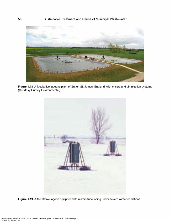
Figure 1.18 A facultative lagoons plant of Sutton St. James, England, with mixers and air injection systems(Courtesy Gurney Environmental)

Figure 1.19 A facultative lagoon equipped with mixers functioning under severe winter conditions



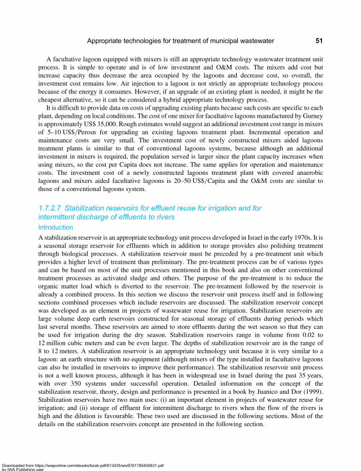
A facultative lagoon equipped with mixers is still an appropriate technology wastewater treatment unitprocess. It is simple to operate and is of low investment and O&M costs. The mixers add cost butincrease capacity thus decrease the area occupied by the lagoons and decrease cost, so overall, theinvestment cost remains low. Air injection to a lagoon is not strictly an appropriate technology processbecause of the energy it consumes. However, if an upgrade of an existing plant is needed, it might be thecheapest alternative, so it can be considered a hybrid appropriate technology process.

It is difficult to provide data on costs of upgrading existing plants because such costs are specific to eachplant, depending on local conditions. The cost of one mixer for facultative lagoons manufactured by Gurneyis approximately US$ 35,000. Rough estimates would suggest an additional investment cost range in mixersof 5–10 US$/Perosn for upgrading an existing lagoons treatment plant. Incremental operation andmaintenance costs are very small. The investment cost of newly constructed mixers aided lagoonstreatment plants is similar to that of conventional lagoons systems, because although an additionalinvestment in mixers is required, the population served is larger since the plant capacity increases whenusing mixers, so the cost per Capita does not increase. The same applies for operation and maintenancecosts. The investment cost of a newly constructed lagoons treatment plant with covered anaerobiclagoons and mixers aided facultative lagoons is 20–50 US$/Capita and the O&M costs are similar tothose of a conventional lagoons system.

1.7.2.7 Stabilization reservoirs for effluent reuse for irrigation and forintermittent discharge of effluents to riversIntroduction

A stabilization reservoir is an appropriate technology unit process developed in Israel in the early 1970s. It isa seasonal storage reservoir for effluents which in addition to storage provides also polishing treatmentthrough biological processes. A stabilization reservoir must be preceded by a pre-treatment unit whichprovides a higher level of treatment than preliminary. The pre-treatment process can be of various typesand can be based on most of the unit processes mentioned in this book and also on other conventionaltreatment processes as activated sludge and others. The purpose of the pre-treatment is to reduce theorganic matter load which is diverted to the reservoir. The pre-treatment followed by the reservoir isalready a combined process. In this section we discuss the reservoir unit process itself and in followingsections combined processes which include reservoirs are discussed. The stabilization reservoir conceptwas developed as an element in projects of wastewater reuse for irrigation. Stabilization reservoirs arelarge volume deep earth reservoirs constructed for seasonal storage of effluents during periods whichlast several months. These reservoirs are aimed to store effluents during the wet season so that they canbe used for irrigation during the dry season. Stabilization reservoirs range in volume from 0.02 to12 million cubic meters and can be even larger. The depths of stabilization reservoir are in the range of8 to 12 meters. A stabilization reservoir is an appropriate technology unit because it is very similar to alagoon: an earth structure with no equipment (although mixers of the type installed in facultative lagoonscan also be installed in reservoirs to improve their performance). The stabilization reservoir unit processis not a well known process, although it has been in widespread use in Israel during the past 35 years,with over 350 systems under successful operation. Detailed information on the concept of thestabilization reservoir, theory, design and performance is presented in a book by Juanico and Dor (1999).Stabilization reservoirs have two main uses: (i) an important element in projects of wastewater reuse forirrigation; and (ii) storage of effluent for intermittent discharge to rivers when the flow of the rivers ishigh and the dilution is favourable. These two used are discussed in the following sections. Most of thedetails on the stabilization reservoirs concept are presented in the following section.



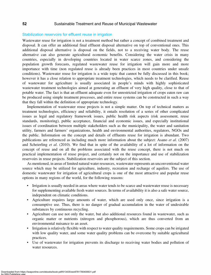
Stabilization reservoirs for effluent reuse in irrigation

Wastewater reuse for irrigation is not a treatment method but rather a concept of combined treatment anddisposal. It can offer an additional final effluent disposal alternative on top of conventional ones. Thisadditional disposal alternative is disposal on the fields, not to a receiving water body. The reusealternative can also generate agricultural economic benefits. Considering the water crisis in manycountries, especially in developing countries located in water scarce zones, and considering thepopulation growth forecasts, regulated wastewater reuse for irrigation will gain more and moreimportance with time (non regulated reuse is already been practices in most countries under unsafeconditions). Wastewater reuse for irrigation is a wide topic that cannot be fully discussed in this book;however it has a close relation to appropriate treatment technologies, which needs to be clarified. Reuseof wastewater for agriculture is usually associated in people’s minds with highly sophisticatedwastewater treatment technologies aimed at generating an effluent of very high quality, close to that ofpotable water. The fact is that an effluent adequate even for unrestricted irrigation of crops eaten raw canbe produced using simple treatment processes, and entire reuse systems can be constructed in such a waythat they fall within the definition of appropriate technology.

Implementation of wastewater reuse projects is not a simple matter. On top of technical matters astreatment technologies, efficiency and reliability, it entails resolution of a series of other complicatedissues as legal and regulatory framework issues, public health risk aspects (risk assessment, reusestandards, monitoring), public acceptance, financial and economic issues, and especially institutionalissues of coordination between multiple stakeholders such as the municipality, the water and sanitationutility, farmers and farmers’ organizations, health and environmental authorities, regulators, NGOs andthe public. Information on the concept and details of effluents reuse for irrigation is abundant. Twopublications are referenced as including much more information about the subject: Asano et al. (2007)and Scheierling et al. (2010). We find that in spite of the availability of a lot of information on theconcept of reuse and on all the problems associated with the reuse concept, there is not much onpractical implementation of reuse project, and certainly not on the importance and use of stabilizationreservoirs in reuse projects. Stabilization reservoirs are the subject of this section.

As mentioned, in areas of limited natural water resources, wastewater represents an unconventional watersource which may be utilized for agriculture, industry, recreation and recharge of aquifers. The use ofdomestic wastewater for irrigation of agricultural crops is one of the most attractive and popular reuseoptions in many regions of the world, for the following reasons:

• Irrigation is usually needed in areas where water tends to be scarce and wastewater reuse is necessaryfor supplementing available fresh water sources. In terms of availability it is also a safe water source,independent on climatic conditions.

• Agriculture requires large amounts of water, which are used only once, since irrigation is aconsumptive use. Thus, there is no danger of gradual accumulation in the water of undesirablesubstances by continuous recycling.

• Agriculture can use not only the water, but also additional resources found in wastewater, such asorganic matter or nutrients (nitrogen and phosphorous), which are thus converted from anenvironmental nuisance to an asset.

• Irrigation is relatively flexible with respect to water quality requirements. Some crops can be irrigatedwith low quality water, and some water quality problems can be overcome by suitable agriculturalpractices.

• Use of wastewater for irrigation prevents its discharge to receiving water bodies and pollution ofwater resources.



When considering irrigation with treated wastewater, several related factors and terms should bementioned, some of which are presented below:

• Restricted and unrestricted irrigation: “restricted irrigation1” refers to the use of low quality effluentin specific areas, where only certain crops should be cultivated. The restrictions imposed usually referto the type of crops to be cultivated, the irrigation methods, the harvesting method, fertilizerapplication rates, distance of irrigated fields from residential areas and paved roads and distancebetween non-potable and potable water supply mains. “Unrestricted Irrigation” refers to the useof high quality effluents for irrigation of all crops on any soil type, without any adverseenvironmental effect or the soil, crops, animals, persons involved in the production process orpersons consuming agricultural products.

• Effluent quality: the effluent quality is the main factor that dictates the type of reuse (i.e., restricted orunrestricted irrigation), types of crops and irrigation methods. The effluent quality should beconsidered regarding two aspects: public health and agronomics. Most existing standards forwastewater reuse deal only with public health aspects and prescribe the treatment processes orquality parameters that the effluent must meet before it can be used to irrigate a certain category ofcrops. These include mostly bacteria, viruses and other pathogens and sometimes also organicmatter (BOD, COD, TSS), dissolved oxygen, pH and residual chlorine. However, agronomicaspects related to crops and soils must also be taken into account. These include salinity, sodiumabsorption ratio of the water, nitrogen, phosphorus, chloride, bicarbonate, heavy metals, boron andother trace elements, pH and synthetic organics (including pesticides). Considering the agronomicaspect of effluent quality, water quality standards established for crop irrigation with fresh waterare, at present, also the best available criteria for effluent reuse. However, there are additionalconstituents in wastewater, usually absent from or unimportant in fresh water. For suchconstituents, specific reuse standards will have to be developed in the future. At present, onlypreliminary guidelines can be established based an available knowledge.

• Irrigation methods: the effluent quality has an effect on the irrigation method to be used. Surfaceirrigation methods can utilize low quality effluents, whereas sprinkler and mainly drip irrigationrequire higher-quality effluents, because of the danger of clogging the orifices of the irrigationequipment by suspended solids. This problem can be overcome by utilizing filters at the head ofthe irrigation system.

• Seasonal storage: while municipal wastewater is available at a relatively constant flow, irrigationwater is required mainly during the dry season. In order to compensate between the constantsupply and variable demand, seasonal storage is required.

• Economic aspects: From the point of view of overall economic evaluation, the wastewater treatmentsystem and the effluent reuse system are regarded as an integrated system for which a combinedcost-benefit analysis should be carried out in order to assess the feasibility of the project. Similarlyto other irrigation projects, the economy of a reuse projects depends on many factors, most ofwhich are specific to each project and include soil type climatic conditions and irrigation methods.

Several factors have to be taken into account when aiming at a feasible reuse project:

• Efficient water use:maximumefficiency ofwater usemust be attempted in order to attain themaximumpossible irrigated areas and thus maximize crop production. The efficiency of water use is interrelatedwith selection of the irrigation method, and high efficiency irrigation methods are preferable.

• Provision of seasonal storage: the inclusion of Seasonal Storage in a reuse scheme is a prerequisite.Provision of seasonal storage is basically part of the efficient water use. Without such storage, an



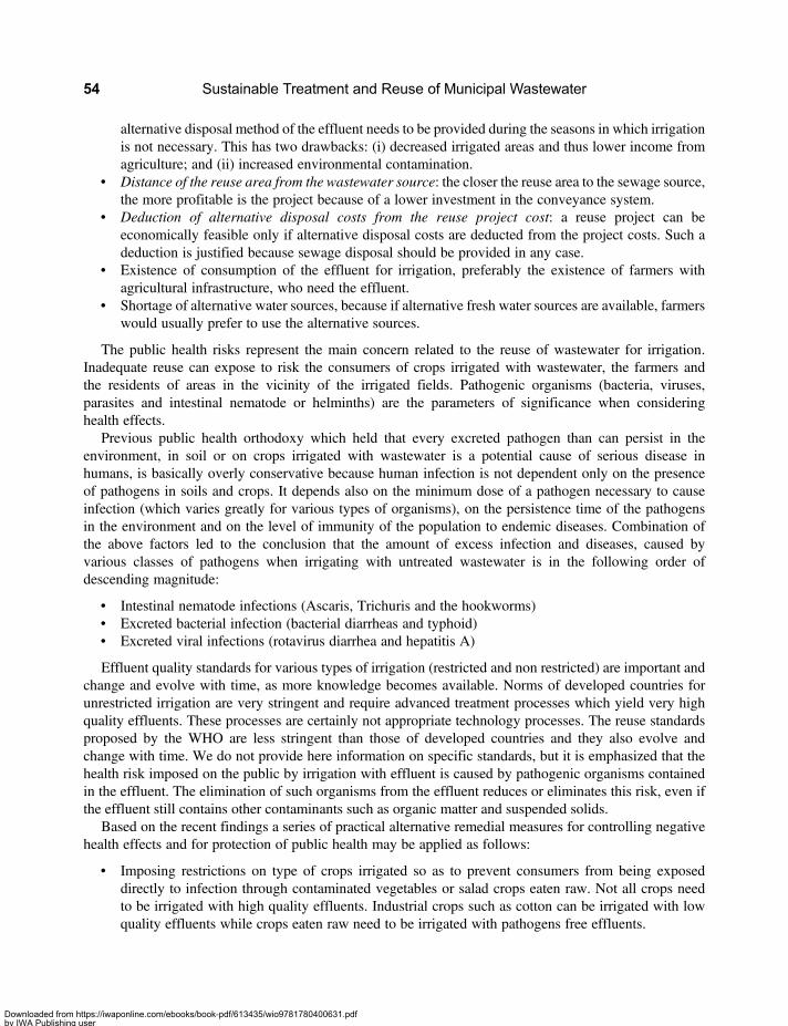
alternative disposal method of the effluent needs to be provided during the seasons in which irrigationis not necessary. This has two drawbacks: (i) decreased irrigated areas and thus lower income fromagriculture; and (ii) increased environmental contamination.

• Distance of the reuse area from the wastewater source: the closer the reuse area to the sewage source,the more profitable is the project because of a lower investment in the conveyance system.

• Deduction of alternative disposal costs from the reuse project cost: a reuse project can beeconomically feasible only if alternative disposal costs are deducted from the project costs. Such adeduction is justified because sewage disposal should be provided in any case.

• Existence of consumption of the effluent for irrigation, preferably the existence of farmers withagricultural infrastructure, who need the effluent.

• Shortage of alternative water sources, because if alternative fresh water sources are available, farmerswould usually prefer to use the alternative sources.

The public health risks represent the main concern related to the reuse of wastewater for irrigation.Inadequate reuse can expose to risk the consumers of crops irrigated with wastewater, the farmers andthe residents of areas in the vicinity of the irrigated fields. Pathogenic organisms (bacteria, viruses,parasites and intestinal nematode or helminths) are the parameters of significance when consideringhealth effects.

Previous public health orthodoxy which held that every excreted pathogen than can persist in theenvironment, in soil or on crops irrigated with wastewater is a potential cause of serious disease inhumans, is basically overly conservative because human infection is not dependent only on the presenceof pathogens in soils and crops. It depends also on the minimum dose of a pathogen necessary to causeinfection (which varies greatly for various types of organisms), on the persistence time of the pathogensin the environment and on the level of immunity of the population to endemic diseases. Combination ofthe above factors led to the conclusion that the amount of excess infection and diseases, caused byvarious classes of pathogens when irrigating with untreated wastewater is in the following order ofdescending magnitude:

• Intestinal nematode infections (Ascaris, Trichuris and the hookworms)• Excreted bacterial infection (bacterial diarrheas and typhoid)• Excreted viral infections (rotavirus diarrhea and hepatitis A)

Effluent quality standards for various types of irrigation (restricted and non restricted) are important andchange and evolve with time, as more knowledge becomes available. Norms of developed countries forunrestricted irrigation are very stringent and require advanced treatment processes which yield very highquality effluents. These processes are certainly not appropriate technology processes. The reuse standardsproposed by the WHO are less stringent than those of developed countries and they also evolve andchange with time. We do not provide here information on specific standards, but it is emphasized that thehealth risk imposed on the public by irrigation with effluent is caused by pathogenic organisms containedin the effluent. The elimination of such organisms from the effluent reduces or eliminates this risk, even ifthe effluent still contains other contaminants such as organic matter and suspended solids.

Based on the recent findings a series of practical alternative remedial measures for controlling negativehealth effects and for protection of public health may be applied as follows:

• Imposing restrictions on type of crops irrigated so as to prevent consumers from being exposeddirectly to infection through contaminated vegetables or salad crops eaten raw. Not all crops needto be irrigated with high quality effluents. Industrial crops such as cotton can be irrigated with lowquality effluents while crops eaten raw need to be irrigated with pathogens free effluents.



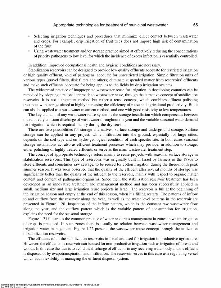
• Selecting irrigation techniques and procedures that minimize direct contact between wastewaterand crops. For example, drip irrigation of fruit trees does not impose high risk of contaminationof the fruit.

• Using wastewater treatment and/or storage practice aimed at effectively reducing the concentrationsof priority pathogens to low level for which the incidence of excess infection is essentially controlled.

In addition, improved occupational health and hygiene conditions are necessary.Stabilization reservoirs can be designed to provide low quality effluents adequate for restricted irrigation

or high quality effluent, void of pathogens, adequate for unrestricted irrigation. Simple filtration units ofvarious types (gravel filters, disk filters and others) eliminate suspended matter from reservoirs’ effluentsand make such effluents adequate for being applies to the fields by drip irrigation systems.

The widespread practice of inappropriate wastewater reuse for irrigation in developing countries can beremedied by adopting a rational approach to wastewater reuse, through the attractive concept of stabilizationreservoirs. It is not a treatment method but rather a reuse concept, which combines effluent polishingtreatment with storage aimed at highly increasing the efficiency of reuse and agricultural productivity. But itcan also be applied as a wastewater treatment method, and one with good resistivity to low temperatures.

The key element of any wastewater reuse system is the storage installation which compensates betweenthe relatively constant discharge of wastewater throughout the year and the variable seasonal water demandfor irrigation, which is required mainly during the dry season.

There are two possibilities for storage alternatives: surface storage and underground storage. Surfacestorage can be applied in any project, while infiltration into the ground, especially for large cities,depends on the soil type and on hydro-geological condition of each specific site. In both cases seasonalstorage installations act also as efficient treatment processes which may provide, in addition to storage,either polishing of highly treated effluents or serve as the main wastewater treatment step.

The concept of appropriate technology refers mainly to reuse projects with seasonal surface storage instabilization reservoirs. This type of reservoirs was originally built in Israel by farmers in the 1970s tostore effluents and sometimes raw sewage, to be reused for cotton irrigation during the three-month peaksummer season. It was soon observed that the quality of the effluent after several months of storage wassignificantly better than the quality of the influent to the reservoir, mainly with respect to organic mattercontent and content of pathogenic organisms. Since then, the stabilization reservoir treatment has beendeveloped as an innovative treatment and management method and has been successfully applied insmall, medium size and large irrigation reuse projects in Israel. The reservoir is full at the beginning ofthe irrigation season and empty at the end of this season, when it’s filling restarts. The patterns of inflowto and outflow from the reservoir along the year, as well as the water level patterns in the reservoir arepresented in Figure 1.20. Inspection of the inflow pattern, which is the constant raw wastewater flowalong the year, and the outflow pattern which is the variable pattern of consumption for irrigation,explains the need for the seasonal storage.

Figure 1.21 illustrates the common practice of water resources management in zones in which irrigationof crops is practiced. In such zones there is usually no relation between wastewater management andirrigation water management. Figure 1.22 presents the wastewater reuse concept through the utilizationof stabilization reservoirs.

The effluents of all the stabilization reservoirs in Israel are used for irrigation in productive agriculture.However, the effluent of a reservoir can be used for non-productive irrigation such as irrigation of forests andwoods. In this case the idea is to avoid the discharge of effluents to any receiving water body and the effluentis disposed of by evapotranspiration and infiltration. The reservoir serves in this case as a regulating vesselwhich adds flexibility in managing the effluent disposal system.



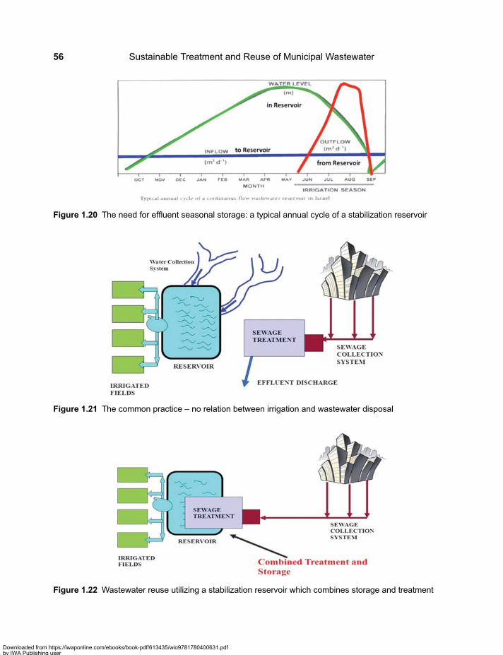
Figure 1.20 The need for effluent seasonal storage: a typical annual cycle of a stabilization reservoir

Figure 1.21 The common practice – no relation between irrigation and wastewater disposal

Figure 1.22 Wastewater reuse utilizing a stabilization reservoir which combines storage and treatment



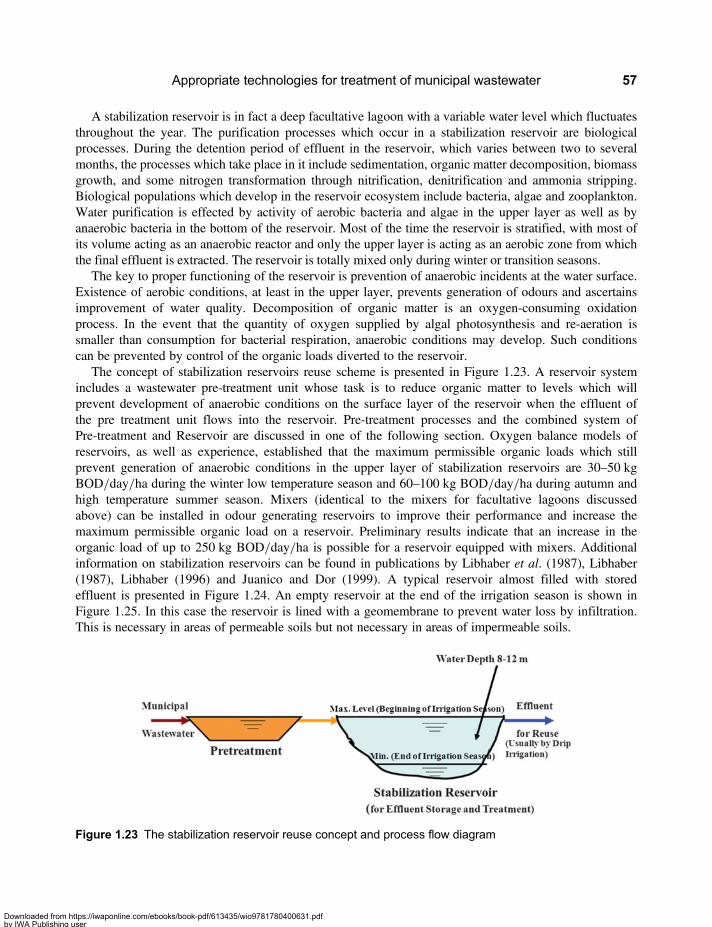
A stabilization reservoir is in fact a deep facultative lagoon with a variable water level which fluctuatesthroughout the year. The purification processes which occur in a stabilization reservoir are biologicalprocesses. During the detention period of effluent in the reservoir, which varies between two to severalmonths, the processes which take place in it include sedimentation, organic matter decomposition, biomassgrowth, and some nitrogen transformation through nitrification, denitrification and ammonia stripping.Biological populations which develop in the reservoir ecosystem include bacteria, algae and zooplankton.Water purification is effected by activity of aerobic bacteria and algae in the upper layer as well as byanaerobic bacteria in the bottom of the reservoir. Most of the time the reservoir is stratified, with most ofits volume acting as an anaerobic reactor and only the upper layer is acting as an aerobic zone from whichthe final effluent is extracted. The reservoir is totally mixed only during winter or transition seasons.

The key to proper functioning of the reservoir is prevention of anaerobic incidents at the water surface.Existence of aerobic conditions, at least in the upper layer, prevents generation of odours and ascertainsimprovement of water quality. Decomposition of organic matter is an oxygen-consuming oxidationprocess. In the event that the quantity of oxygen supplied by algal photosynthesis and re-aeration issmaller than consumption for bacterial respiration, anaerobic conditions may develop. Such conditionscan be prevented by control of the organic loads diverted to the reservoir.

The concept of stabilization reservoirs reuse scheme is presented in Figure 1.23. A reservoir systemincludes a wastewater pre-treatment unit whose task is to reduce organic matter to levels which willprevent development of anaerobic conditions on the surface layer of the reservoir when the effluent ofthe pre treatment unit flows into the reservoir. Pre-treatment processes and the combined system ofPre-treatment and Reservoir are discussed in one of the following section. Oxygen balance models ofreservoirs, as well as experience, established that the maximum permissible organic loads which stillprevent generation of anaerobic conditions in the upper layer of stabilization reservoirs are 30–50 kgBOD/day/ha during the winter low temperature season and 60–100 kg BOD/day/ha during autumn andhigh temperature summer season. Mixers (identical to the mixers for facultative lagoons discussedabove) can be installed in odour generating reservoirs to improve their performance and increase themaximum permissible organic load on a reservoir. Preliminary results indicate that an increase in theorganic load of up to 250 kg BOD/day/ha is possible for a reservoir equipped with mixers. Additionalinformation on stabilization reservoirs can be found in publications by Libhaber et al. (1987), Libhaber(1987), Libhaber (1996) and Juanico and Dor (1999). A typical reservoir almost filled with storedeffluent is presented in Figure 1.24. An empty reservoir at the end of the irrigation season is shown inFigure 1.25. In this case the reservoir is lined with a geomembrane to prevent water loss by infiltration.This is necessary in areas of permeable soils but not necessary in areas of impermeable soils.

Figure 1.23 The stabilization reservoir reuse concept and process flow diagram



Figure 1.24 A typical reservoir almost filled with effluent towards the beginning of the irrigation season

Figure 1.25 An empty lined reservoir at the end of the irrigation season



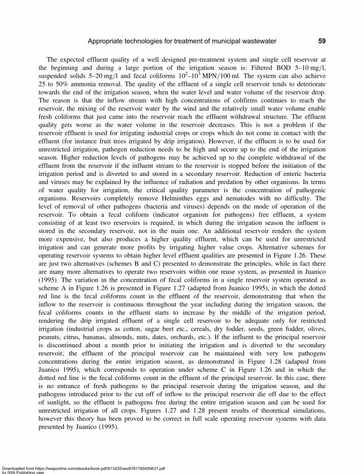
The expected effluent quality of a well designed pre-treatment system and single cell reservoir atthe beginning and during a large portion of the irrigation season is: Filtered BOD 5–10 mg/l,suspended solids 5–20 mg/l and fecal coliforms 102–103 MPN/100 ml. The system can also achieve25 to 50% ammonia removal. The quality of the effluent of a single cell reservoir tends to deterioratetowards the end of the irrigation season, when the water level and water volume of the reservoir drop.The reason is that the inflow stream with high concentrations of colifirms continues to reach thereservoir, the mixing of the reservoir water by the wind and the relatively small water volume enablefresh coliforms that just came into the reservoir reach the effluent withdrawal structure. The effluentquality gets worse as the water volume in the reservoir decreases. This is not a problem if thereservoir effluent is used for irrigating industrial crops or crops which do not come in contact with theeffluent (for instance fruit trees irrigated by drip irrigation). However, if the effluent is to be used forunrestricted irrigation, pathogen reduction needs to be high and secure up to the end of the irrigationseason. Higher reduction levels of pathogens may be achieved up to the complete withdrawal of theeffluent from the reservoir if the influent stream to the reservoir is stopped before the initiation of theirrigation period and is diverted to and stored in a secondary reservoir. Reduction of enteric bacteriaand viruses may be explained by the influence of radiation and predation by other organisms. In termsof water quality for irrigation, the critical quality parameter is the concentration of pathogenicorganisms. Reservoirs completely remove Helminthes eggs and nematodes with no difficulty. Thelevel of removal of other pathogens (bacteria and viruses) depends on the mode of operation of thereservoir. To obtain a fecal coliform (indicator organism for pathogens) free effluent, a systemconsisting of at least two reservoirs is required, in which during the irrigation season the influent isstored in the secondary reservoir, not in the main one. An additional reservoir renders the systemmore expensive, but also produces a higher quality effluent, which can be used for unrestrictedirrigation and can generate more profits by irrigating higher value crops. Alternative schemes foroperating reservoir systems to obtain higher level effluent qualities are presented in Figure 1.26. Theseare just two alternatives (schemes B and C) presented to demonstrate the principles, while in fact thereare many more alternatives to operate two reservoirs within one reuse system, as presented in Juanico(1995). The variation in the concentration of fecal coliforms in a single reservoir system operated asscheme A in Figure 1.26 is presented in Figure 1.27 (adapted from Juanico 1995), in which the dottedred line is the fecal coliforms count in the effluent of the reservoir, demonstrating that when theinflow to the reservoir is continuous throughout the year including during the irrigation season, thefecal coliforms counts in the effluent starts to increase by the middle of the irrigation period,rendering the drip irrigated effluent of a single cell reservoir to be adequate only for restrictedirrigation (industrial crops as cotton, sugar beet etc., cereals, dry fodder, seeds, green fodder, olives,peanuts, citrus, bananas, almonds, nuts, dates, orchards, etc.). If the influent to the principal reservoiris discontinued about a month prior to initiating the irrigation and is diverted to the secondaryreservoir, the effluent of the principal reservoir can be maintained with very low pathogensconcentrations during the entire irrigation season, as demonstrated in Figure 1.28 (adapted fromJuanico 1995), which corresponds to operation under scheme C in Figure 1.26 and in which thedotted red line is the fecal coliforms count in the effluent of the principal reservoir. In this case, thereis no entrance of fresh pathogens to the principal reservoir during the irrigation season, and thepathogens introduced prior to the cut off of inflow to the principal reservoir die off due to the effectof sunlight, so the effluent is pathogens free during the entire irrigation season and can be used forunrestricted irrigation of all crops. Figures 1.27 and 1.28 present results of theoretical simulations,however this theory has been proved to be correct in full scale operating reservoir systems with datapresented by Juanico (1995).



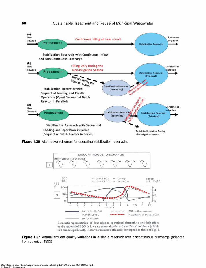
Figure 1.26 Alternative schemes for operating stabilization reservoirs

Figure 1.27 Annual effluent quality variations in a single reservoir with discontinuous discharge (adaptedfrom Juanico, 1995)



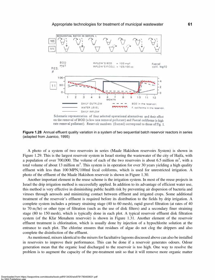
A photo of a system of two reservoirs in series (Maale Hakishon reservoirs System) is shown inFigure 1.29. This is the largest reservoir system in Israel storing the wastewater of the city of Haifa, witha population of over 700,000. The volume of each of the two reservoirs is about 6.5 million m3, with atotal volume of about 13 million m3. This system is in operation for over 30 years yielding a high qualityeffluent with less than 100 MPN/100ml fecal coliforms, which is used for unrestricted irrigation. Aphoto of the effluent of the Maale Hakishon reservoir is shown in Figure 1.30.

Another important element in the reuse scheme is the irrigation system. In most of the reuse projects inIsrael the drip irrigation method is successfully applied. In addition to its advantage of efficient water use,this method is very effective in diminishing public health risk by preventing air dispersion of bacteria andviruses through aerosols and minimizing contact between effluent and irrigated crops. Some additionaltreatment of the reservoir’s effluent is required before its distribution to the fields by drip irrigation. Acomplete system includes a primary straining stage (40 to 60 mesh), rapid gravel filtration (at rates of 40to 70 m/hr) or other type of filtration (such as the use of disk filters) and a secondary finer strainingstage (80 to 150 mesh), which is typically done in each plot. A typical reservoir effluent disk filtrationsystem (of the Kfar Menahem reservoir) is shown in Figure 1.31. Another element of the reservoireffluent treatment is chlorination, which is usually done by injection of a hypochlorite solution at theentrance to each plot. The chlorine ensures that residues of algae do not clog the drippers and alsocomplete the disinfection of the effluent.

As mentioned, mixers identical to the mixers for facultative lagoons discussed above can also be installedin reservoirs to improve their performance. This can be done if a reservoir generates odours. Odourgeneration mean that the organic load discharged to the reservoir is too high. One way to resolve theproblem is to augment the capacity of the pre-treatment unit so that it will remove more organic matter

Figure 1.28 Annual effluent quality variation in a system of two sequential batch reservoir reactors in series(adapted from Juanico, 1995)



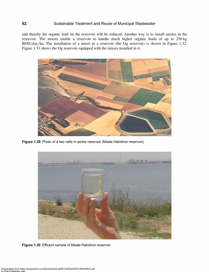
and thereby the organic load on the reservoir will be reduced. Another way is to install mixers in thereservoir. The mixers enable a reservoir to handle much higher organic loads of up to 250 kgBOD/day/ha. The installation of a mixer in a reservoir (the Og reservoir) is shown in Figure 1.32.Figure 1.33 shows the Og reservoir equipped with the mixers installed in it.

Figure 1.29 Photo of a two cells in series reservoir (Maale Hakishon reservoir)

Figure 1.30 Effluent sample of Maale Hakishon reservoir



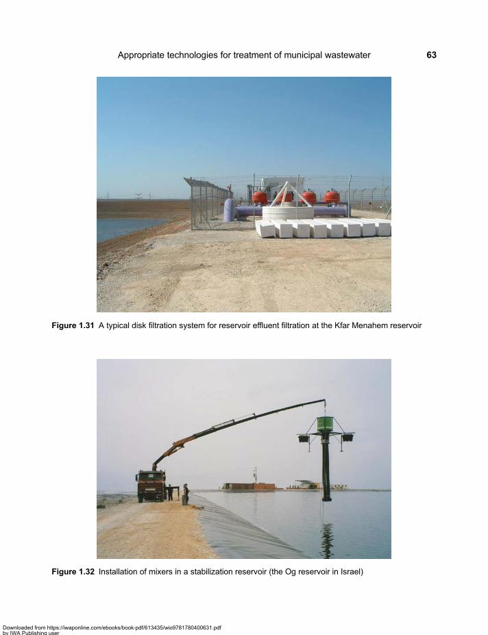
Figure 1.31 A typical disk filtration system for reservoir effluent filtration at the Kfar Menahem reservoir

Figure 1.32 Installation of mixers in a stabilization reservoir (the Og reservoir in Israel)



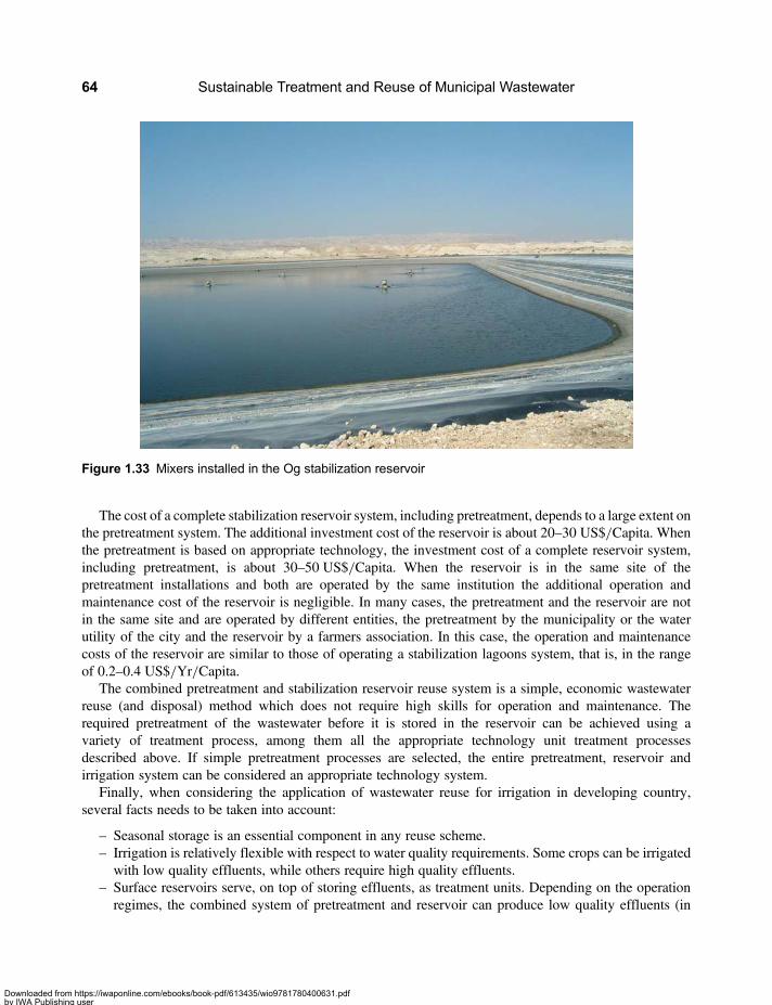
The cost of a complete stabilization reservoir system, including pretreatment, depends to a large extent onthe pretreatment system. The additional investment cost of the reservoir is about 20–30 US$/Capita. Whenthe pretreatment is based on appropriate technology, the investment cost of a complete reservoir system,including pretreatment, is about 30–50 US$/Capita. When the reservoir is in the same site of thepretreatment installations and both are operated by the same institution the additional operation andmaintenance cost of the reservoir is negligible. In many cases, the pretreatment and the reservoir are notin the same site and are operated by different entities, the pretreatment by the municipality or the waterutility of the city and the reservoir by a farmers association. In this case, the operation and maintenancecosts of the reservoir are similar to those of operating a stabilization lagoons system, that is, in the rangeof 0.2–0.4 US$/Yr/Capita.

The combined pretreatment and stabilization reservoir reuse system is a simple, economic wastewaterreuse (and disposal) method which does not require high skills for operation and maintenance. Therequired pretreatment of the wastewater before it is stored in the reservoir can be achieved using avariety of treatment process, among them all the appropriate technology unit treatment processesdescribed above. If simple pretreatment processes are selected, the entire pretreatment, reservoir andirrigation system can be considered an appropriate technology system.

Finally, when considering the application of wastewater reuse for irrigation in developing country,several facts needs to be taken into account:

– Seasonal storage is an essential component in any reuse scheme.– Irrigation is relatively flexible with respect to water quality requirements. Some crops can be irrigatedwith low quality effluents, while others require high quality effluents.

– Surface reservoirs serve, on top of storing effluents, as treatment units. Depending on the operationregimes, the combined system of pretreatment and reservoir can produce low quality effluents (in

Figure 1.33 Mixers installed in the Og stabilization reservoir



terms of pathogenic organism content) for restricted irrigation, or high quality effluents for unrestrictedirrigation.

– The basic condition for application of a wastewater reuse project is the existence of consumers of theeffluent and a commitment on their part for long term consumption of effluent, that is, the existence ofinfrastructure for agricultural activity based on consumption of the effluent for irrigation. Theagricultural activity can be based on farms owned by the wastewater producing municipality, suchas in the case of Melbourne, Australia and Muskegon County, USA, or by private farmers oragricultural communities as is the case in all wastewater reuse projects in Israel.

– Wastewater reuse projects are integrated projects which require a high level of inter-institutionalcooperation for their successful implementation and operation. The operation of the treatmentinstallation needs to be done in close cooperation with and participation of the farmers (in manysmall to medium size reuse schemes in Israel the farmers are in charge of operation of the treatmentinstallations). This is a sensitive point for developing countries, where institutions are weak andachieving cooperation between different institutions is difficult.

Stabilization reservoirs for intermittent discharge of effluents to rivers

Many of the municipal treated effluents are discharged to rivers. Wastewater treatment plants whichdischarge their effluent to a river are constructed to comply with the stringent discharge standards evenunder the most critical conditions, which usually occur during a short part of the year in the low flowseason in the river, when the dilution of the effluent in the river water is the smallest. At critically lowdilution of the effluent in the natural water of the river, the effluent quality needs to be very high andthat means that the treatment plant needs to be constructed based on a process which can produce a veryhigh quality effluent. But in fact its high capacity is utilized only during a short part of the year, whenthe river water flow is low, while during the rest of the year, the effluent quality could be lower.

A different strategy would be: (i) to construct a treatment plant that produces a lower effluent quality,which is still adequate for discharge to the river during most of the year; (b) to construct a deep storagereservoir (basically a stabilization reservoir) to store the effluent during the low flow season in the river,which might last up to several months; and (iii) the mode of operation would be the following: duringthe part of the year which is not low flow season, the plant effluent will be discharged directly into theriver whereas during the low flow season, the effluent will be stored in the stabilization reservoir and noriver discharge will take place during this season. At the end of the low flow season, the effluent of thetreatment plant will again be discharged to the river, and also the effluent stored in the reservoir will bedischarged to the river, at a flow adequate for the conditions of the specific river, so that the discharge ofthe treatment plant effluent plus the flow of effluent from the reservoir will still comply with the qualitystandards permitted for the river. Usually the low flow season coincides with the high temperatureseason so the treatment of the effluent in the reservoir during the storage period will be effective.

If quality consideration require, the effluent of the treatment plant can be discharged all year round to thereservoir and from there to the river. In that case the reservoir acts also as a polishing unit of the treatmentplant effluent. During the low flow season the treatment plant effluent fills the reservoir and effluent is notdischarged from the reservoir to the river. During the rest of the year the treatment plant effluent isdischarged to the reservoir and an effluent stream of a flow larger than the incoming flow is dischargedto the river. The reservoir is never totally emptied but rather remains with a minimum water depth ofabout 2 metres, so the reservoir act as a polishing lagoon (maturation pond) for the treatment plant effluent.

One of the key design aspects of such a system is the proper sizing of the reservoir relative to the flow andwater quality characteristics of the effluent-receiving river or stream. The design of the reservoir is based onpreparing a water balance, with the first stage being the determination of the amount of effluent which may



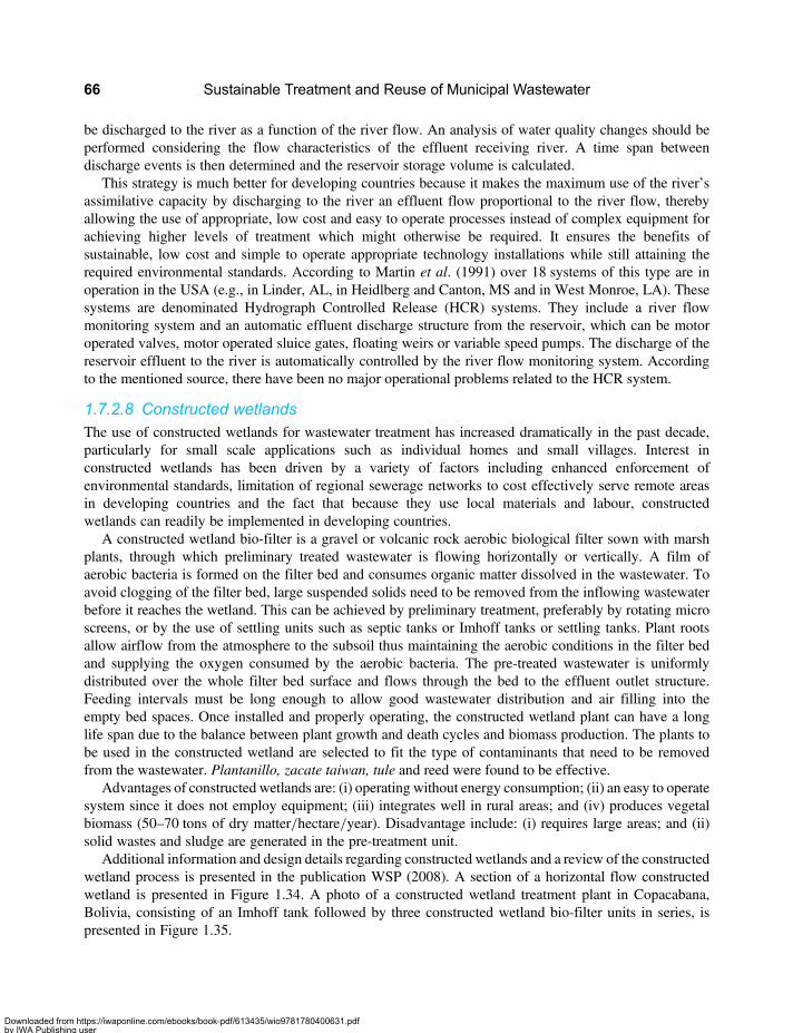
be discharged to the river as a function of the river flow. An analysis of water quality changes should beperformed considering the flow characteristics of the effluent receiving river. A time span betweendischarge events is then determined and the reservoir storage volume is calculated.

This strategy is much better for developing countries because it makes the maximum use of the river’sassimilative capacity by discharging to the river an effluent flow proportional to the river flow, therebyallowing the use of appropriate, low cost and easy to operate processes instead of complex equipment forachieving higher levels of treatment which might otherwise be required. It ensures the benefits ofsustainable, low cost and simple to operate appropriate technology installations while still attaining therequired environmental standards. According to Martin et al. (1991) over 18 systems of this type are inoperation in the USA (e.g., in Linder, AL, in Heidlberg and Canton, MS and in West Monroe, LA). Thesesystems are denominated Hydrograph Controlled Release (HCR) systems. They include a river flowmonitoring system and an automatic effluent discharge structure from the reservoir, which can be motoroperated valves, motor operated sluice gates, floating weirs or variable speed pumps. The discharge of thereservoir effluent to the river is automatically controlled by the river flow monitoring system. Accordingto the mentioned source, there have been no major operational problems related to the HCR system.

1.7.2.8 Constructed wetlandsThe use of constructed wetlands for wastewater treatment has increased dramatically in the past decade,particularly for small scale applications such as individual homes and small villages. Interest inconstructed wetlands has been driven by a variety of factors including enhanced enforcement ofenvironmental standards, limitation of regional sewerage networks to cost effectively serve remote areasin developing countries and the fact that because they use local materials and labour, constructedwetlands can readily be implemented in developing countries.

A constructed wetland bio-filter is a gravel or volcanic rock aerobic biological filter sown with marshplants, through which preliminary treated wastewater is flowing horizontally or vertically. A film ofaerobic bacteria is formed on the filter bed and consumes organic matter dissolved in the wastewater. Toavoid clogging of the filter bed, large suspended solids need to be removed from the inflowing wastewaterbefore it reaches the wetland. This can be achieved by preliminary treatment, preferably by rotating microscreens, or by the use of settling units such as septic tanks or Imhoff tanks or settling tanks. Plant rootsallow airflow from the atmosphere to the subsoil thus maintaining the aerobic conditions in the filter bedand supplying the oxygen consumed by the aerobic bacteria. The pre-treated wastewater is uniformlydistributed over the whole filter bed surface and flows through the bed to the effluent outlet structure.Feeding intervals must be long enough to allow good wastewater distribution and air filling into theempty bed spaces. Once installed and properly operating, the constructed wetland plant can have a longlife span due to the balance between plant growth and death cycles and biomass production. The plants tobe used in the constructed wetland are selected to fit the type of contaminants that need to be removedfrom the wastewater. Plantanillo, zacate taiwan, tule and reed were found to be effective.

Advantages of constructed wetlands are: (i) operating without energy consumption; (ii) an easy to operatesystem since it does not employ equipment; (iii) integrates well in rural areas; and (iv) produces vegetalbiomass (50–70 tons of dry matter/hectare/year). Disadvantage include: (i) requires large areas; and (ii)solid wastes and sludge are generated in the pre-treatment unit.

Additional information and design details regarding constructed wetlands and a review of the constructedwetland process is presented in the publication WSP (2008). A section of a horizontal flow constructedwetland is presented in Figure 1.34. A photo of a constructed wetland treatment plant in Copacabana,Bolivia, consisting of an Imhoff tank followed by three constructed wetland bio-filter units in series, ispresented in Figure 1.35.



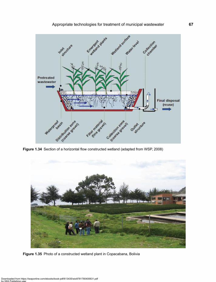
Figure 1.35 Photo of a constructed wetland plant in Copacabana, Bolivia

Figure 1.34 Section of a horizontal flow constructed wetland (adapted from WSP, 2008)



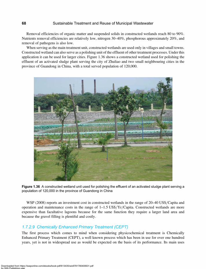
Removal efficiencies of organic matter and suspended solids in constructed wetlands reach 80 to 90%.Nutrients removal efficiencies are relatively low, nitrogen 30–40%, phosphorous approximately 20%, andremoval of pathogens is also low.

When serving as the main treatment unit, constructed wetlands are used only in villages and small towns.Constructed wetland can also serve as a polishing unit of the effluent of other treatment processes. Under thisapplication it can be used for larger cities. Figure 1.36 shows a constructed wetland used for polishing theeffluent of an activated sludge plant serving the city of Zhuliao and two small neighbouring cities in theprovince of Guandong in China, with a total served population of 120,000.

WSP (2008) reports an investment cost in constructed wetlands in the range of 20–40 US$/Capita andoperation and maintenance costs in the range of 1–1.5 US$/Yr/Capita. Constructed wetlands are moreexpensive than facultative lagoons because for the same function they require a larger land area andbecause the gravel filling is plentiful and costly.

1.7.2.9 Chemically Enhanced Primary Treatment (CEPT)The first process which comes to mind when considering physicochemical treatment is ChemicallyEnhanced Primary Treatment (CEPT), a well known process which has been in use for over one hundredyears, yet is not in widespread use as would be expected on the basis of its performance. Its main uses

Figure 1.36 A constructed wetland unit used for polishing the effluent of an activated sludge plant serving apopulation of 120,000 in the province of Guandong in China



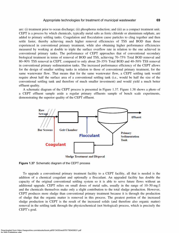
are: (i) treatment prior to ocean discharge; (ii) phosphorus reduction; and (iii) as a compact treatment unit.CEPT is a process by which chemicals, typically metal salts as ferric chloride or aluminium sulphate, areadded to primary settling tanks. Coagulation and flocculation cause particles to cling together and thensettle faster, thereby achieving much higher removal efficiencies of TSS and BOD than thoseexperienced in conventional primary treatment, while also obtaining higher performance efficienciesmeasured by working at double to triple the surface overflow rate in relation to the one achieved inconventional primary tanks. The performance of CEPT approaches that of conventional secondarybiological treatment in terms of removal of BOD and TSS, achieving 70–75% Total BOD removal and80–90% TSS removal in CEPT, compared to only about 20–35% Total BOD and 40–50% TSS removalin conventional primary sedimentation tanks. The increased performance efficiency of the CEPT allowsfor the design of smaller settling tanks in relation to those of conventional primary treatment, for thesame wastewater flow. That means that for the same wastewater flow, a CEPT settling tank wouldrequire about half the surface area of a conventional settling tank (i.e., would be half the size of theconventional settling tank and therefore of much smaller investment) and would yield a much bettereffluent quality.

A schematic diagram of the CEPT process is presented in Figure 1.37. Figure 1.38 shows a photo ofa CEPT effluent sample aside a regular primary effluents sample of bench scale experiments,demonstrating the superior quality of the CEPT effluent.

To upgrade a conventional primary treatment facility to a CEPT facility, all that is needed is theaddition of a chemical coagulant and optionally a flocculant. An upgraded facility has double thecapacity of the original conventional settling system so it is able to serve future flows without anadditional upgrade. CEPT relies on small doses of metal salts, usually in the range of 10–50 mg/land the chemicals themselves make only a slight contribution to the total sludge production. However,CEPT produces more sludge than conventional primary treatment because it is through the productionof sludge that the organic matter is removed in this process. The greatest portion of the increasedsludge production in CEPT is the result of the increased solids (and therefore also organic matter)removal in the settling tank through the physicochemical (not biological) process, which is precisely theCEPT’s goal.

Figure 1.37 Schematic diagram of the CEPT process



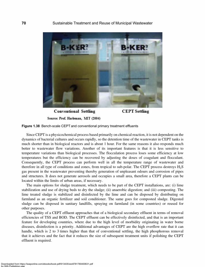
Since CEPT is a physicochemical process based primarily on chemical reaction, it is not dependent on thedynamics of bacterial cultures and occurs rapidly, so the detention time of the wastewater in CEPT tanks ismuch shorter than in biological reactors and is about 1 hour. For the same reasons it also responds muchbetter to wastewater flow variations. Another of its important features is that it is less sensitive totemperature variations than biological processes. The flocculation process loses some efficiency at lowtemperatures but the efficiency can be recovered by adjusting the doses of coagulant and flocculant.Consequently, the CEPT process can perform well in all the temperature range of wastewater andtherefore in all type of conditions and zones, from tropical to sub-polar. The CEPT process destroys H2Sgas present in the wastewater preventing thereby generation of unpleasant odours and corrosion of pipesand structures. It does not generate aerosols and occupies a small area, therefore a CEPT plants can belocated within the limits of urban areas, if necessary.

The main options for sludge treatment, which needs to be part of the CEPT installations, are: (i) limestabilization and use of drying beds to dry the sludge; (ii) anaerobic digestion; and (iii) composting. Thelime treated sludge is stabilized and disinfected by the lime and can be disposed by distributing onfarmland as an organic fertilizer and soil conditioner. The same goes for composted sludge. Digestedsludge can be disposed in sanitary landfills, spraying on farmland (in some countries) or reused forother purposes.

The quality of a CEPT effluent approaches that of a biological secondary effluent in terms of removalefficiencies of TSS and BOD. The CEPT effluent can be effectively disinfected, and that is an importantfeature for developing countries, where due to the high level of morbidity originating in water bornediseases, disinfection is a priority. Additional advantages of CEPT are the high overflow rate that it canhandle, which is 2 to 3 times higher than that of conventional settling, the high phosphorous removalthat it achieves and the fact that it reduces the size of subsequent treatment units if polishing the CEPTeffluent is required.

Figure 1.38 Bench-scale CEPT and conventional primary treatment effluents



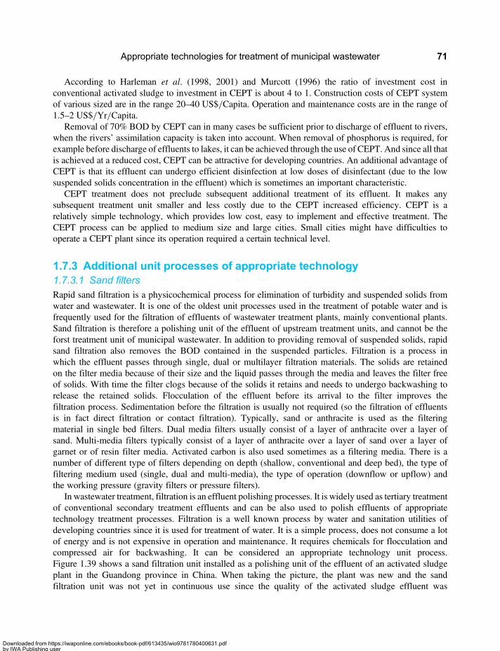
According to Harleman et al. (1998, 2001) and Murcott (1996) the ratio of investment cost inconventional activated sludge to investment in CEPT is about 4 to 1. Construction costs of CEPT systemof various sized are in the range 20–40 US$/Capita. Operation and maintenance costs are in the range of1.5–2 US$/Yr/Capita.

Removal of 70% BOD by CEPT can in many cases be sufficient prior to discharge of effluent to rivers,when the rivers’ assimilation capacity is taken into account. When removal of phosphorus is required, forexample before discharge of effluents to lakes, it can be achieved through the use of CEPT. And since all thatis achieved at a reduced cost, CEPT can be attractive for developing countries. An additional advantage ofCEPT is that its effluent can undergo efficient disinfection at low doses of disinfectant (due to the lowsuspended solids concentration in the effluent) which is sometimes an important characteristic.

CEPT treatment does not preclude subsequent additional treatment of its effluent. It makes anysubsequent treatment unit smaller and less costly due to the CEPT increased efficiency. CEPT is arelatively simple technology, which provides low cost, easy to implement and effective treatment. TheCEPT process can be applied to medium size and large cities. Small cities might have difficulties tooperate a CEPT plant since its operation required a certain technical level.

1.7.3 Additional unit processes of appropriate technology1.7.3.1 Sand filtersRapid sand filtration is a physicochemical process for elimination of turbidity and suspended solids fromwater and wastewater. It is one of the oldest unit processes used in the treatment of potable water and isfrequently used for the filtration of effluents of wastewater treatment plants, mainly conventional plants.Sand filtration is therefore a polishing unit of the effluent of upstream treatment units, and cannot be theforst treatment unit of municipal wastewater. In addition to providing removal of suspended solids, rapidsand filtration also removes the BOD contained in the suspended particles. Filtration is a process inwhich the effluent passes through single, dual or multilayer filtration materials. The solids are retainedon the filter media because of their size and the liquid passes through the media and leaves the filter freeof solids. With time the filter clogs because of the solids it retains and needs to undergo backwashing torelease the retained solids. Flocculation of the effluent before its arrival to the filter improves thefiltration process. Sedimentation before the filtration is usually not required (so the filtration of effluentsis in fact direct filtration or contact filtration). Typically, sand or anthracite is used as the filteringmaterial in single bed filters. Dual media filters usually consist of a layer of anthracite over a layer ofsand. Multi-media filters typically consist of a layer of anthracite over a layer of sand over a layer ofgarnet or of resin filter media. Activated carbon is also used sometimes as a filtering media. There is anumber of different type of filters depending on depth (shallow, conventional and deep bed), the type offiltering medium used (single, dual and multi-media), the type of operation (downflow or upflow) andthe working pressure (gravity filters or pressure filters).

In wastewater treatment, filtration is an effluent polishing processes. It is widely used as tertiary treatmentof conventional secondary treatment effluents and can be also used to polish effluents of appropriatetechnology treatment processes. Filtration is a well known process by water and sanitation utilities ofdeveloping countries since it is used for treatment of water. It is a simple process, does not consume a lotof energy and is not expensive in operation and maintenance. It requires chemicals for flocculation andcompressed air for backwashing. It can be considered an appropriate technology unit process.Figure 1.39 shows a sand filtration unit installed as a polishing unit of the effluent of an activated sludgeplant in the Guandong province in China. When taking the picture, the plant was new and the sandfiltration unit was not yet in continuous use since the quality of the activated sludge effluent was



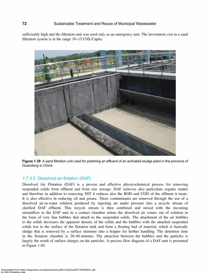
sufficiently high and the filtration unit was used only as an emergency unit. The investment cost in a sandfiltration system is in the range 10–15 US$/Capita.

1.7.3.2 Dissolved air flotation (DAF)Dissolved Air Flotation (DAF) is a proven and effective physicochemical process for removingsuspended solids from effluent and from raw sewage. DAF removes also particulate organic matterand therefore in addition to removing SST it reduces also the BOD and COD of the effluent it treats.It is also effective in reducing oil and grease. These contaminants are removed through the use of adissolved air-in-water solution produced by injecting air under pressure into a recycle stream ofclarified DAF effluent. This recycle stream is then combined and mixed with the incomingstreamflow to the DAF unit in a contact chamber where the dissolved air comes out of solution inthe form of very fine bubbles that attach to the suspended solids. The attachment of the air bubblesto the solids decreases the apparent density of the solids and the bubbles with the attached suspendedsolids rise to the surface of the flotation tank and form a floating bed of material, which is basicallysludge that is removed by a surface skimmer into a hopper for further handling. The detention timein the flotation chamber is 20–60 minutes. The attraction between the bubbles and the particles islargely the result of surface charges on the particles. A process flow diagram of a DAF unit is presentedin Figure 1.40.

Figure 1.39 A sand filtration unit used for polishing an effluent of an activated sludge plant in the province ofGuandong in China



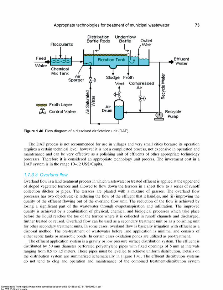
The DAF process is not recommended for use in villages and very small cities because its operationrequires a certain technical level, however it is not a complicated process, not expensive in operation andmaintenance and can be very effective as a polishing unit of effluents of other appropriate technologyprocesses. Therefore it is considered an appropriate technology unit process. The investment cost in aDAF system is in the range 10–12 US$/Capita.

1.7.3.3 Overland flowOverland flow is a land treatment process in which wastewater or treated effluent is applied at the upper endof sloped vegetated terraces and allowed to flow down the terraces in a sheet flow to a series of runoffcollection ditches or pipes. The terraces are planted with a mixture of grasses. The overland flowprocesses has two objectives: (i) reducing the flow of the effluent that it handles, and (ii) improving thequality of the effluent flowing out of the overland flow unit. The reduction of the flow is achieved bylosing a significant part of the wastewater through evapotanspiration and infiltration. The improvedquality is achieved by a combination of physical, chemical and biological processes which take placebefore the liquid reaches the toe of the terrace where it is collected in runoff channels and discharged,further treated or reused. Overland flow can be used as a secondary treatment unit or as a polishing unitfor other secondary treatment units. In some cases, overland flow is basically irrigation with effluent as adisposal method. The pre-treatment of wastewater before land application is minimal and consists ofeither septic tanks or anaerobic ponds. In certain cases oxidation ponds are utilized as pre-treatment.

The effluent application system is a gravity or low pressure surface distribution system. The effluent isdistributed by 50 mm diameter perforated polyethylene pipes with fixed openings of 5 mm at intervalsranging from 0.5 to 1.5 meters. These pipes must be levelled to achieve uniform distribution. Details onthe distribution system are summarized schematically in Figure 1.41. The effluent distribution systemsdo not tend to clog and operation and maintenance of the combined treatment-distribution system

Figure 1.40 Flow diagram of a dissolved air flotation unit (DAF)



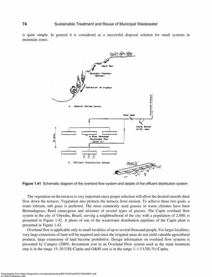
is quite simple. In general it is considered as a successful disposal solution for small systems inmountain zones.

The vegetation on the terraces is very important since proper selection will allow the desired smooth sheetflow down the terraces. Vegetation also protects the terraces from erosion. To achieve these two goals, awater tolerant, tuft grass is preferred. The most commonly used grasses in warm climates have beenBermudagrass, Reed canarygrass and mixtures of several types of grasses. The Capin overland flowsystem in the city of Uberaba, Brazil, serving a neighbourhood of the city with a population of 2,000, ispresented in Figure 1.42. A photo of one of the wastewater distribution pipelines of the Capin plant ispresented in Figure 1.43.

Overland flow is applicable only to small localities of up to several thousand people. For larger localities,very large extensions of land will be required and since the irrigated areas do not yield valuable agriculturalproduce, large extensions of land become prohibitive. Design information on overland flow systems ispresented by Campos (2009). Investment cost in an Overland Flow system used as the main treatmentstep is in the range 15–30 US$/Capita and O&M cost is in the range 1–1.5 US$/Yr/Capita.

Figure 1.41 Schematic diagram of the overland flow system and details of the effluent distribution system



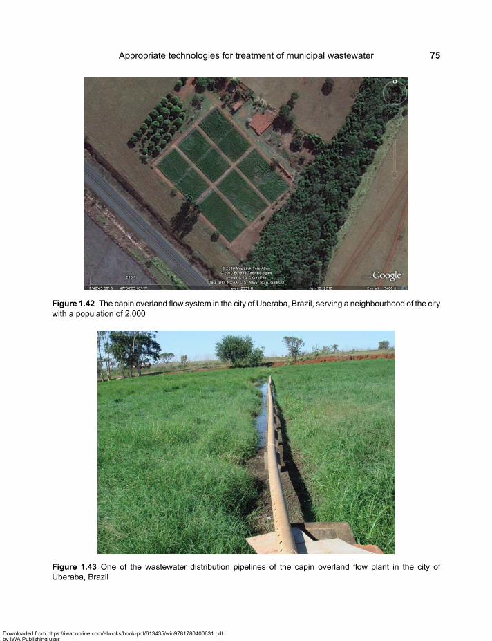
Figure 1.43 One of the wastewater distribution pipelines of the capin overland flow plant in the city ofUberaba, Brazil

Figure 1.42 The capin overland flow system in the city of Uberaba, Brazil, serving a neighbourhood of the citywith a population of 2,000



Overland flow is a low cost simple to operate unit process. It can be used as a secondary treatment unitor as a polishing unit for other secondary treatment units, including appropriate technology treatment units.As such it is an appropriate technology unit process.

1.7.3.4 Infiltration-percolationIn the infiltration-percolation process, the applied effluent percolates through the soil and eventually reachesgroundwater. So it is in fact an effluent disposal method. In many cases it is also a land treatment technologyfor indirect water reuse since the groundwater is pumped out for a variety of uses. The process requireshighly permeable soils such as sandy and loamy soils so that the effluent will be able to infiltrate throughthe use of infiltration basins (known also as spreading basins or recharge basins). On its way to the watertable, the effluent passes through the unsaturated layer of the soil and undergoes there a series oftreatment processes including biological, physical and chemical processes, as well as disinfectionthrough die off of microorganisms due to inadequate survival condition in the soil. The processes whichtake place during effluent infiltration and retention in the groundwater are known as soil aquifertreatment – SAT. Additional information on this process is given by Idelovitch et al. (1984) andLibhaber et al. (1987).

Infiltration may be a disposal solution in cases where there is no water receiving body in the vicinityof a city, or there is a strong opposition to discharge any type of effluent to a river. The infiltrationprocess can form part of projects of any size, even very large ones. The information presented byIdelovitch (1984) refers to the wastewater project of the Tel Aviv metropolitan area (the Dan Region)which to date serves a population of over 2 million and in which about 5 m3/s of effluent isinfiltrated (and then re-pumped for reuse in unrestricted irrigation). However, large projects requirelarge extensions of permeable soil for infiltration, which are not always available, and very goodknowledge and management capacity of the groundwater in the vicinity of the infiltration basins.Large Projects of this type are not exactly appropriate technology operations. But infiltration projectsof small towns do not have the complications of large projects, especially in zones wheregroundwater is not in use, and an infiltration project of a small town can be considered as based onan appropriate technology process.

The level of treatment of the wastewater prior to infiltration does not have to be very high. Effluents ofanaerobic reactors of various types and of CEPT can be infiltrated without additional polishing. Infiltrationof facultative lagoons effluents may be a problem because of clogging of the infiltration basins by algae. Thedesign of a SAT system depends to a large extent on the soil type and the infiltration rates that can beachieved in that type of soils.

Figure 1.44 shows one of the infiltration basins of the Dan Region project in Israel and from whichthe infiltration process can be appreciated. Each infiltration site contains four basins. The first basin onthe right is already recovered and ready to receive a new batch of effluent for infiltration. The secondbasin from the right is already inundated with a batch of effluent and has initiated the infiltrationprocess. The third basin from the right is already in the final stage of infiltrating the batch of effluentthat was diverted to it (see details in Figure 1.45) and the first basin on the left is already in the processof recovering after its batch of effluent has been infiltrated. From time to time the infiltration capacityof the basins needs to be recovered by a tractor or a similar type of mechanical equipment which turnup the soil, as shown in Figure 1.46. After over 30 years of operating the Dan region project it isknown that the average infiltration rate in this project is in the range of 0.7–1.0 cm/hr. The infiltrationrate is specific to each project and depends on the soil type in the project area. The soil at the DanRegion project is basically sand dunes which have a high infiltration rates. The infiltration rate in otherproject may be lower.



Figure 1.44 Satellite photo of one of the effluent infiltration basins of theDanRegionwastewater reuse projectin Israel, serving the metropolitan area of Tel Aviv

Figure 1.45 Photo of an infiltration basin after its inundation with effluent, initiating the infiltration process



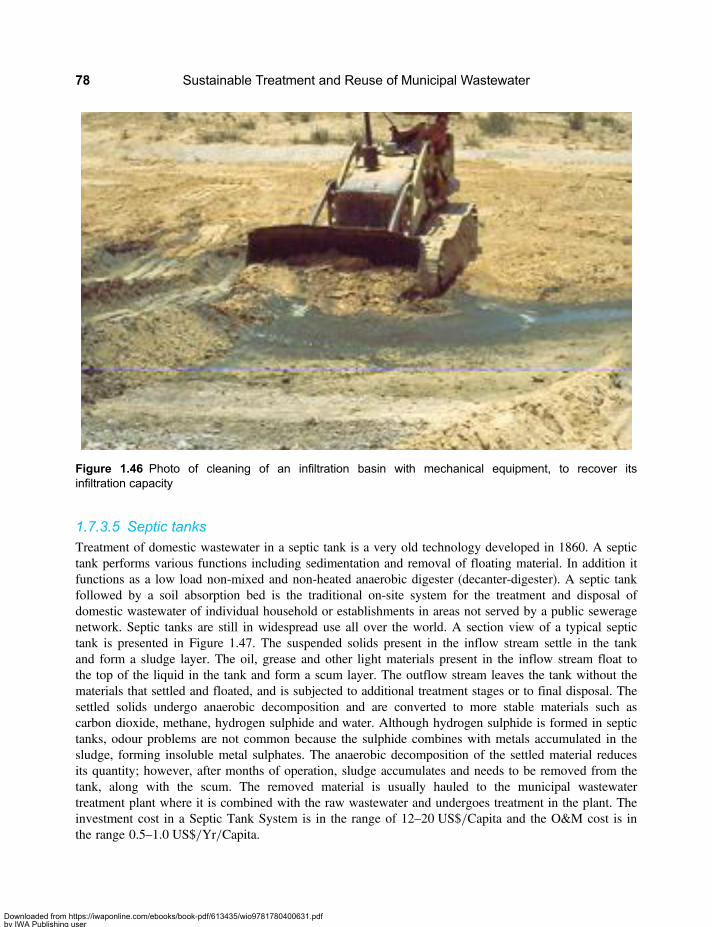
1.7.3.5 Septic tanksTreatment of domestic wastewater in a septic tank is a very old technology developed in 1860. A septictank performs various functions including sedimentation and removal of floating material. In addition itfunctions as a low load non-mixed and non-heated anaerobic digester (decanter-digester). A septic tankfollowed by a soil absorption bed is the traditional on-site system for the treatment and disposal ofdomestic wastewater of individual household or establishments in areas not served by a public seweragenetwork. Septic tanks are still in widespread use all over the world. A section view of a typical septictank is presented in Figure 1.47. The suspended solids present in the inflow stream settle in the tankand form a sludge layer. The oil, grease and other light materials present in the inflow stream float tothe top of the liquid in the tank and form a scum layer. The outflow stream leaves the tank without thematerials that settled and floated, and is subjected to additional treatment stages or to final disposal. Thesettled solids undergo anaerobic decomposition and are converted to more stable materials such ascarbon dioxide, methane, hydrogen sulphide and water. Although hydrogen sulphide is formed in septictanks, odour problems are not common because the sulphide combines with metals accumulated in thesludge, forming insoluble metal sulphates. The anaerobic decomposition of the settled material reducesits quantity; however, after months of operation, sludge accumulates and needs to be removed from thetank, along with the scum. The removed material is usually hauled to the municipal wastewatertreatment plant where it is combined with the raw wastewater and undergoes treatment in the plant. Theinvestment cost in a Septic Tank System is in the range of 12–20 US$/Capita and the O&M cost is inthe range 0.5–1.0 US$/Yr/Capita.

Figure 1.46 Photo of cleaning of an infiltration basin with mechanical equipment, to recover itsinfiltration capacity



Septic tanks can also be used as pre-treatment units in a treatment plant of small communities of up toseveral thousand inhabitants, as shown in Figure 1.35, where in the city of Copacabana, Bolivia, a septictank serves as a pre-treatment unit in a constructed wetlands plant. In performing such a function, theseptic tank can be an effective pre-treatment unit.

Septic tanks are easy to operate and simple to construct and a septic tank is certainly an appropriatetechnology unit process. The performance efficiency of a septic tank varies greatly with itsconfiguration, hydraulic loading and organic loading, and with temperature. The minimum recommendedhydraulic detention time in a septic tank is two days and the tank needs to have multiple compartmentsand baffles. The recommended organic loading is less than 0.1 kg BOD/day/m3. Such a loading enablesachieving a removal efficiency of more than 50% of BOD at the temperature range of 10–20°C, and80% at higher temperatures. The removal efficiency of SST is in the range 20–90% and of oil and greaseis in the range 70–90%. The tank’s volume should be sufficient keep the solids at a depth of 1 to3 meters. Such a configuration allows the tank to function two to three years without cleaning.

Septic tanks are used as a pre-treatment of anaerobic filters and constructed wetlands in small treatmentplants serving communities of up to several thousands of people.

1.7.3.6 Submarine and large rivers outfallsAbout 50% of the world’s population resides in or near coastal areas. The most probable receiving body ofsewage and treated effluents generated by this population are the oceans and seas. Ocean disposal of sewageand its treatment prior to discharge are therefore issues of major importance. Wastewater treatment is oftenseen as the only way to cope with water quality problems; although effective outfalls combined with lowerpre-treatment levels may substantially reduce costs while still reaching the same environmental objectives ashigher treatment levels. For developing countries, in which resources for wastewater treatment and disposalare scarce, low cost solutions are of major importance and a system of simple pre-treatment followed by aneffective submarine outfall is an appropriate technology unit process, since it is usually a low investment

Figure 1.47 A section view of a typical septic tank



cost system, simple to operate and of low operation and maintenance costs. The length of the sea outfall andtherefore its investment costs depend on the specific bathymetry and sea currents and the outfall site, butusually the investment is lower than that of other solutions. Detailed information on the design ofpretreatment systems and submarine outfall is an ample subject and is not treated in this book. Thereader is directed to the recently published book of Roberts and al (2010) which is dedicated to allaspects of submarine outfalls for treatment and disposal of wastewater of coastal cities. This chapter onlypresents general information on submarine outfalls and emphasises the fact that the combination ofpretreatment and a submarine outfall is an appropriate technology unit process. Similarly, a combinationof pretreatment and an outfall to a large river is an appropriate technology unit process for discharge ofeffluents of cities located on banks of large rivers. The pretreatment followed by an effective outfall aretreatment units which do not need to be combined with additional treatment units, provided that theoutfalls are adequately designed and constitute effective outfalls.

The World Health Organization (WHO) has published in October 2003 guidelines for recreational waterquality protection (WHO, 2003). Table 1.2 below presents the WHO findings on relative health risks tohuman health by exposure to effluent discharged from submarine outfalls, classified according to variousschemes of combination of sewage pretreatment and submarine outfall length.

The discharge methods of sewage or effluent into oceans can be classified into three principal types: (i)discharge directly onto the beach, which also includes discharge into rivers streams or canals, a shortdistance from the coastline; (ii) “short” outfalls, where sewage or effluent is likely to contaminaterecreational waters; and (iii) “effective” outfalls, designed so that the sewage or effluent is efficientlydiluted and dispersed so as to ensure that it does not pollute recreational water areas. While the terms“short” and “long” are often used, outfall length is generally less important than proper location andeffective dilution. An effective outfall is assumed to be properly designed, with sufficient length anddiffuser discharge depth to ensure that the sewage does not reach the recreational area.

According to the WHO, if an effective outfall is provided for discharge of effluent to the sea, the level ofpretreatment of domestic sewage practically does not have a bearing on the risk to human health of thedischarged effluent. The risk to human health of secondary effluent discharged through an effectiveoutfall is classified as low. The same low risk is assigned to primary effluent discharged through aneffective outfall, and even the risk of preliminary treated effluent discharged through an effective outfallis classified as low. The WHO findings lead to a conclusion that if an effective outfall is provided,

Table 1.2 Relative risk potential to human health by exposure to sewage through submarine outfalls (fromWHO, 2003).

Treatment Discharge type

Directly on beach Short outfall Effective outfall

None Very high High NA

Preliminary Very high High Low

Primary (including septic tanks) Very high High Low

Secondary High High Low

Secondary plus disinfection – – –

Tertiary Moderate Moderate Very low



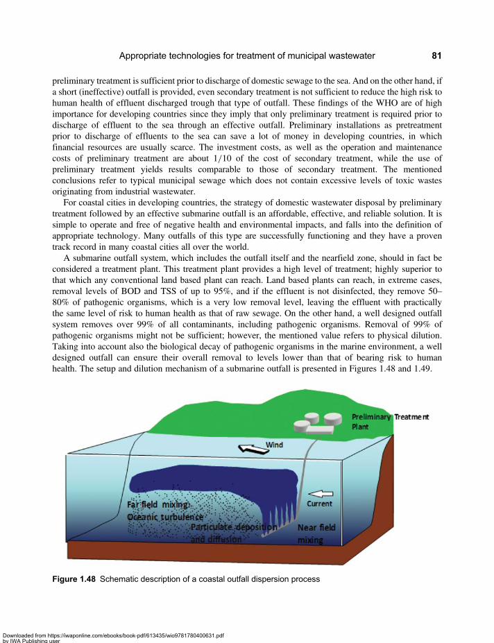
preliminary treatment is sufficient prior to discharge of domestic sewage to the sea. And on the other hand, ifa short (ineffective) outfall is provided, even secondary treatment is not sufficient to reduce the high risk tohuman health of effluent discharged trough that type of outfall. These findings of the WHO are of highimportance for developing countries since they imply that only preliminary treatment is required prior todischarge of effluent to the sea through an effective outfall. Preliminary installations as pretreatmentprior to discharge of effluents to the sea can save a lot of money in developing countries, in whichfinancial resources are usually scarce. The investment costs, as well as the operation and maintenancecosts of preliminary treatment are about 1/10 of the cost of secondary treatment, while the use ofpreliminary treatment yields results comparable to those of secondary treatment. The mentionedconclusions refer to typical municipal sewage which does not contain excessive levels of toxic wastesoriginating from industrial wastewater.

For coastal cities in developing countries, the strategy of domestic wastewater disposal by preliminarytreatment followed by an effective submarine outfall is an affordable, effective, and reliable solution. It issimple to operate and free of negative health and environmental impacts, and falls into the definition ofappropriate technology. Many outfalls of this type are successfully functioning and they have a proventrack record in many coastal cities all over the world.

A submarine outfall system, which includes the outfall itself and the nearfield zone, should in fact beconsidered a treatment plant. This treatment plant provides a high level of treatment; highly superior tothat which any conventional land based plant can reach. Land based plants can reach, in extreme cases,removal levels of BOD and TSS of up to 95%, and if the effluent is not disinfected, they remove 50–80% of pathogenic organisms, which is a very low removal level, leaving the effluent with practicallythe same level of risk to human health as that of raw sewage. On the other hand, a well designed outfallsystem removes over 99% of all contaminants, including pathogenic organisms. Removal of 99% ofpathogenic organisms might not be sufficient; however, the mentioned value refers to physical dilution.Taking into account also the biological decay of pathogenic organisms in the marine environment, a welldesigned outfall can ensure their overall removal to levels lower than that of bearing risk to humanhealth. The setup and dilution mechanism of a submarine outfall is presented in Figures 1.48 and 1.49.

Figure 1.48 Schematic description of a coastal outfall dispersion process



As an example, operating results of the submarine outfall of the city of Tome, in the Concepción region,Chile, consisting of preliminary treatment followed by an effective outfall, are presented in Table 1.3, basedon information provided by Leppe and Padilla (1999). The results are average results of five years ofmeasurements near the outfall discharge point.

Table 1.3 Marine water quality near the tome outfall, concepción, chile (average of 5 years monitoring).

Parameter Effluentdischargedinto outfall

Maximumaccordingto localstandards

Atdischargepoint

At 100mfrom thedischargepoint

Backgroundvalues

pH 7.3 5.5–9.0 7.6 7.7 7.8

Temperature, °C 17.8 – 13.1 14.1 14.2

Oil and Grease, mg/l 46.3 150 4.6 9.2 2.4

TSS (Total SuspendedSolid), mg/l

206 300 7.6 1.8 3.0

BOD5 (BiochemicalOxygenDemand),mg/l

348 – 2.3 2.2 2.4

TOC (Total OrganicCarbon), mg/l

203 – 2.1 3.4 2.0

O.D. (DissolvedOxygen), mg/l

0.5 – 4.8 7.5 7.2

Detergents, mg/l 9.2 15 0.07 0.06 0.05

Nitrogen Kjeldal, mg/l 72 – 0.52 0.41 0.57

Nitrites, mg/l 0.01 – 0.02 0.02 0.02

(Continued )

Figure 1.49 Setup and dilution mechanism of an effective submarine outfall



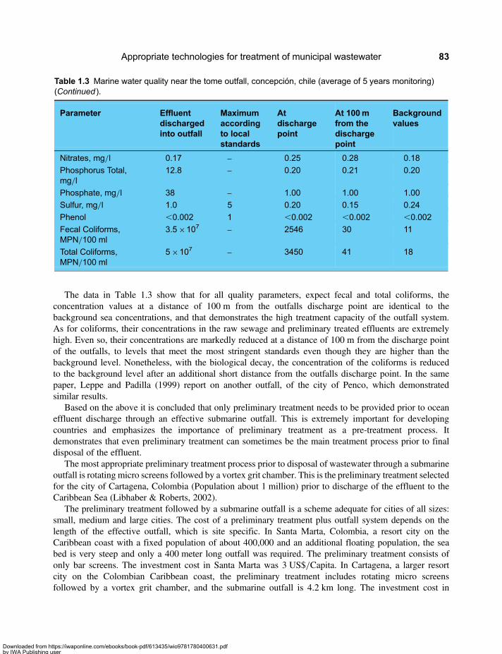
The data in Table 1.3 show that for all quality parameters, expect fecal and total coliforms, theconcentration values at a distance of 100 m from the outfalls discharge point are identical to thebackground sea concentrations, and that demonstrates the high treatment capacity of the outfall system.As for coliforms, their concentrations in the raw sewage and preliminary treated effluents are extremelyhigh. Even so, their concentrations are markedly reduced at a distance of 100 m from the discharge pointof the outfalls, to levels that meet the most stringent standards even though they are higher than thebackground level. Nonetheless, with the biological decay, the concentration of the coliforms is reducedto the background level after an additional short distance from the outfalls discharge point. In the samepaper, Leppe and Padilla (1999) report on another outfall, of the city of Penco, which demonstratedsimilar results.

Based on the above it is concluded that only preliminary treatment needs to be provided prior to oceaneffluent discharge through an effective submarine outfall. This is extremely important for developingcountries and emphasizes the importance of preliminary treatment as a pre-treatment process. Itdemonstrates that even preliminary treatment can sometimes be the main treatment process prior to finaldisposal of the effluent.

The most appropriate preliminary treatment process prior to disposal of wastewater through a submarineoutfall is rotating micro screens followed by a vortex grit chamber. This is the preliminary treatment selectedfor the city of Cartagena, Colombia (Population about 1 million) prior to discharge of the effluent to theCaribbean Sea (Libhaber & Roberts, 2002).

The preliminary treatment followed by a submarine outfall is a scheme adequate for cities of all sizes:small, medium and large cities. The cost of a preliminary treatment plus outfall system depends on thelength of the effective outfall, which is site specific. In Santa Marta, Colombia, a resort city on theCaribbean coast with a fixed population of about 400,000 and an additional floating population, the seabed is very steep and only a 400 meter long outfall was required. The preliminary treatment consists ofonly bar screens. The investment cost in Santa Marta was 3 US$/Capita. In Cartagena, a larger resortcity on the Colombian Caribbean coast, the preliminary treatment includes rotating micro screensfollowed by a vortex grit chamber, and the submarine outfall is 4.2 km long. The investment cost in

Table 1.3 Marine water quality near the tome outfall, concepción, chile (average of 5 years monitoring)(Continued ).

Parameter Effluentdischargedinto outfall

Maximumaccordingto localstandards

Atdischargepoint

At 100mfrom thedischargepoint

Backgroundvalues

Nitrates, mg/l 0.17 – 0.25 0.28 0.18

Phosphorus Total,mg/l

12.8 – 0.20 0.21 0.20

Phosphate, mg/l 38 – 1.00 1.00 1.00

Sulfur, mg/l 1.0 5 0.20 0.15 0.24

Phenol ,0.002 1 ,0.002 ,0.002 ,0.002

Fecal Coliforms,MPN/100 ml

3.5×107 – 2546 30 11

Total Coliforms,MPN/100 ml

5×107 – 3450 41 18



Cartagena amounted to about 28 US$/Capita. A range of 3–30 US$/Capita would be indicative of theinvestment cost of an outfall system, including preliminary treatment. Operation and maintenance costswould be similar to those of the preliminary treatment system itself.

1.8 COMMONLY USED COMBINED UNIT PROCESSES OFAPPROPRIATE TECHNOLOGY1.8.1 IntroductionA series of unit processes of appropriate technology for wastewater treatment was presented in the previoussections, each yielding a different effluent quality. The presented series of processes might not be thecomplete set of existing appropriate technology unit processes and perhaps there are others which can beconsidered as part of this group. When an effluent quality higher than what a single unit process ofappropriate technology can produce is required, a treatment plant consisting of a series of appropriatetechnology unit process can be used (2, 3 or more), in which the effluent of the first unit process is fedinto the second unit process, the effluent of the second is fed to the third and so on. Another way to lookat it is that to improve the quality of the effluent of a certain unit process, this effluent can be subjectedto one or more polishing steps, each of which consisting of an additional unit process. This approach canproduce practically any final effluent quality required. The main message of this book is the idea that itis possible to combine unit processes to create various treatment plants, each based on a series ofappropriate technology processes, and that it is possible to combine unit process in such a manner thatjointly they can generate any required effluent quality. A plant based on a combination in series ofappropriate technology unit processes is still easy to operate and is usually of lower costs thanconventional processes in terms of investments and certainly in operation and maintenance. However,the use of a complex process as a polishing step of an effluent of an appropriate technology processshould be avoided, because it transforms the entire treatment plant to a complex and costly treatmentplant. There are cases of plants consisting of a UASB unit followed by an activated sludge unit or atrickling filter unit. Such plants are not appropriate technology plants.

In this section we present several combined processes which are already in use in developing countries.Many other additional combinations of unit processes of appropriate technology can be formulated. Theyare not currently in common use but may be adequate for specific project conditions and can be used inthe future. Such combined processes are discussed in following sections of the book and it may well bethat treatment plants based on some of them already exist somewhere and are in operation. In all thecombined processes, Rotating Micros Screens (RMS) is proposed as the first unit of the preliminarytreatment section of any treatment plant, since we consider that RMS is the preferred, most reliable andmost effective screening process. If grit removal is required, a Vortex Grit Chamber is recommended asthe preferred unit process of the preliminary treatment, complementing the RMS. If the raw wastewatercontains large amounts of oil and grease which need to be removed, then an aerated grit chamber shouldbe used as part of the preliminary treatment installation, complementing the RMS. In the schematic flowdiagrams of the treatment processes which are presented in the book, the scheme of a Rotating MicroScreen is used to represent the entire preliminary treatment unit. Also, when discussing combinedtreatment processes, the mention of preliminary treatment is sometimes omitted, but it is clarified thatpreliminary treatment forms part of every treatment process.

The focus of the discussion in Chapter 1 of this book is the resolution of wastewater disposal problems indeveloping countries. However, the concepts presented are applicable anywhere and plants based on unitprocesses or on combined unit processes of appropriate technology can be used also in developedcountries and provide the same benefits described in this book also to such countries.



Several commonly used combined unit processes of appropriate technology for wastewater treatment arepresented in Table 1.4. Details on each process are presented in the following sections and design proceduresof these combined processes are presented in following chapters.

The suspended solids content in the effluents of all the combined processes mentioned in the table issufficiently low to allow for performing effective disinfection of these effluents by any existingdisinfection method. Since the final unit process in the combined processes 1, 2, 3 and 6 in the table

Table 1.4 Commonly used combined processes of appropriate technology for wastewater treatment.

Combined process structure Performance (% Removal of BODT, SST andfecal coliforms)

1. A series of Conventional StabilizationLagoons:Anaerobic Lagoons followed by FacultativeLagoons followed by Maturation Lagoons

BODT (70–95%)SST (70–90%)FC in effluent (30–105) MPN/100 ml, dependingon the design of the lagoons. If necessary, effluentcan be disinfected

2. A Series of Upgraded Stabilization Lagoons:Rotating Micro Screens (RMS) followed byCovered Anaerobic Lagoons followed byFacultative Lagoons with Mixersfollowed by Maturation Lagoons

BODT (80–95%)SST (70–90%)FC in effluent (30–105) MPN/100 ml, dependingon the design of the lagoons. If necessary, effluentcan be disinfected

3. UASB followed by Facultative Lagoons BODT (80–90%)SST (70–80%)FC in effluent (30–105) MPN/100 ml, dependingon the design of the lagoons. If necessary, effluentcan be disinfected

4. UASB followed by Anaerobic Filter BODT (80–90%)SST (80–90%)FC Removal very low, if necessary, effluent canbe disinfected

5. UASB followed by Dissolved Air Flotation(DAF)

BODT (70–90%)SST (70–80%)FC Removal very low, if necessary, effluent canbe disinfected

6. Chemically Enhance Primary Treatment(CEPT) followed by Sand Filtration

BODT (80–90%)SST (80–90%)FC Removal very low, if necessary, effluent canbe disinfected

7. Pre-Treatment of Various Types followed by aStabilization Reservoir

BODT (75–95%)SST (70–90%)FC in effluent (10–103) MPN/100 ml, dependingon the design of the reservoir. If necessary,effluent can be disinfected

8. UASB followed by Anaerobic Filter followed byDissolved Air Flotation followed by MembraneFiltration

BODT Practically 100%SST Practically 100%FC Practically 100%



above are lagoons or a stabilization reservoir, they can be designed to achieve an effluent of low pathogenscontent even without disinfection.

Some experts do not approve of using an anaerobic process for polishing the effluent of a precedinganaerobic process, arguing that the final effluent is strongly anaerobic. They promote the use of anaerobic process to polish the effluent of an anaerobic process. For example, in Brazil, the use ofactivated sludge or trickling filter is promoted for polishing of UASB reactors effluents. This is asomewhat overly cautious approach. Effluents of activated sludge and trickling filters are also anaerobicor close to anaerobic after an effluent detention time of 1–2 hours in secondary clarifiers. The level ofoxygen in the effluent needs to be considered taking into account the dilution of the effluent in thereceiving body. If the dilution is high, an oxygen void effluent does not present a problem. If the dilutionis low, the effluent can be hydraulically aerated before its discharge to the receiving body (treatmentplants are usually topographically located several meters higher than the receiving body and cascadeaeration can be provided before the effluent discharge to the receiving body). If the natural river flow isreally small and most of its flow downstream the discharge point is a result of the effluent discharge, formost types of treatment processes the oxygen in the river will be depleted a short distance after thedischarge point, irrespective of the oxygen level in the effluent. In such cases the river water needs to beaerated at several points along its trajectory. An efficient and environmentally friendly aeration methodis the SEPA (Sidestream Elevated Pool Aeration) method (Butts 1988).

As already mentioned, the concept of appropriate technology for wastewater treatment is in wideapplication in Brazil, where treatment plants of this type are used for all sizes of cities and where theapplication of this concept is rapidly expanding. Many of the examples of combined appropriatetechnology processes mentioned in Chapter 1 of the book are from Brazil, mainly from three utilitieswhich are pioneers in the use of this type of processes: (i) CAESB, the water and sanitation utility of theFederal District of Brasilia; (ii) SANEPAR, the water and sanitation utility of the State of Parana; and(iii) COPASA, the water and sanitation utility of the State of Minas Gerais. The information on treatmentplants located in Brasilia is based on personal communication with Klaus Dieter Neder, Chief, SpecialProjects, CAESB, on visit of the authors to Brasilia, and on the CAESB Report (2006). The informationon treatment plants located in the State of Parana is based on a visit of one of the authors to Parana andon the MSc dissertation by Prado (2010). The information on treatment plants located in Minas Gerais isbased on visits of one of the authors to the state of Minas Gerais and on papers related to specificprojects, as referenced with the description of the projects.

In Brasilia, out of 17 treatment plants, two large plants and one small plant are activated sludge plantswhile the rest are based on appropriate technology combined processes, twelve with a UASB reactor asthe first unit, one with a CEPT unit as the first unit and one with lagoons as the first unit. In Parana, outof 23 treatment plants in the Alto Iguacu river basin, which includes also the State Capital, Curitiba, onlyone old plant is an activated sludge plant. All the rest are based on appropriate technology combinedprocesses and in all of them, the first unit is an anaerobic unit. In 21 of the plants the first unit is aUASB reactor and in one plant the first unit is an anaerobic lagoon.

1.8.2 A series of conventional stabilization lagoonsThe most common and widespread combined appropriate technology process is a system of a series ofconventional lagoons composed of anaerobic lagoons followed by facultative lagoons followed bymaturation lagoons. A schematic flow diagram of such a system is presented in Figure 1.50. A photo ofsuch a typical lagoons system is presented in Figure 1.51, which depicts Plant N2 in the city Santa Cruz,Bolivia, composed of two parallel units each containing an anaerobic lagoon followed by two facultativelagoons followed by a maturation lagoon. The arrows show the flow pattern in the plant, red arrows in



one unit and blew arrows in the other. The N2 plant was recently upgraded. The figure presents Plant N2before its upgrade. The N2 plant produced a good effluent (30–40 mg/l BOD, 50–90 mg/l TSS and1.103–8.103 MPN/100 ml Fecal Coliforms) which complies with the local standard and is discharged tothe Pirai River. Downstream of the city this river flows through a very low density populated region andthe effluent discharged to the river causes no nuisance or problems.

This type of conventional stabilization lagoons plant is in widespread use all over the world, both indeveloping and developed countries. In many cases the system consists only of facultative lagoonsfollowed by maturation lagoons and the anaerobic lagoons are omitted for the purpose of avoidinggeneration of odours. Lagoon plants are usually constructed outside the limits of the city which generatesthe wastewater treated by them, but with time the city spreads and surrounds the plant. At that stage

Figure 1.50 Schematic flow diagram of a series of conventional stabilization lagoons

Figure 1.51 Air photo of a conventional anaerobic-facultative-maturation lagoons plant for municipalwastewater treatment, plant N2, one of three in the city of Santa Cruz, Bolivia



people start complaining about odours and mosquitoes. With time the plant becomes overloaded and if itincludes anaerobic lagoons, the odour problem becomes intensive.

Inclusion of an anaerobic lagoon as the first unit in a stabilization lagoons plant is of great importancesince this lagoon removes about 60% of BOD from the raw wastewater while occupying a small area,thus significantly reducing the total area of the plant in relation to an area of a lagoons plant composedof only facultative and maturation ponds. But it suffers from the drawback of generation of odours whenthe plant becomes overloaded. Fortunately, today there is a way to prevent odours generation byanaerobic lagoons, as explained in the following section.

A stabilization lagoons plant can produce a high quality effluent, provided that it is correctly designed.Mara (1987) and Mara (2004, PP 137) reports on a lagoons plant in Northeast Brazil consisting of fivelagoons in series: an anaerobic lagoon with 6.8 days detention time followed by a facultative pond andthree maturation ponds, each with a detention time of 5.5 days, providing a total detention time of28.8 days. The plant’s effluent contains 17 mg/l of BOD, 45 mg/l TSS, 8 mg/l N-NH3, 2.4 mg/l P,30 MPN/100 ml Fecal Coliforms and zero eggs/liter of intestinal nematodes. The plant achieved acumulative removal (from raw sewage to the effluent of the 5th lagoon) of 93% of BOD, 82% of COD,85% of SST, 82% of N-NH3, 64% of P, and 6 log units of Fecal Coliforms. As can be noted, this plantalso achieved a significant removal of nitrogen and phosphorous.

One important advantage of a stabilization lagoons plant is its ability to achieve natural disinfection,without the use of chemicals or energy, provided that the plant is correctly designed to achieve such atarget, as is the mentioned plant in Northeast Brazil. The term correctly designed means well designedmaturation ponds and a sufficiently long overall detention time of about 30 days or more. One commondisappointment of laymen with lagoons systems is that they are expected to reduce pathogens but areusually designed with a detention time too short to achieve an effective pathogens reduction, so theeffluent does not comply with the required quality standard and sometimes presents a public health risk.

Because of the large extension of land occupied by a stabilization lagoons plant, most of this type ofplants is designed to serve medium and small size cities but not large cities. However, if a large city hasseveral sewage drainage basins, each basin can be served by a lagoons plant treating the wastewater ofthe population residing in this basin. In this manner, even a large city can be completely served bylagoon plants. This is the case in Santa Cruz, Bolivia, a city with a population of 1.3 million served bythree lagoon plants for treatment of municipal wastewater, with an additional one under construction in2011. Several large stabilization lagoons plants do exist and are in operation, such as the Dandora Plantin Nairobi, Kenya, currently serving a population of about 1.2 million and is to be expanded to serveabout 2 million people.

In summary, conventional stabilization lagoons systems are used extensively for wastewater treatment inmoderate and tropical climates, and present one of the most cost-effective, easy to operate and reliableappropriate technology processes for treating domestic and industrial wastewater. The simplicity and lowcost of this system made it an attractive solution in both developing and developed countries, buteffective performance depends on correct design. Investment cost in a conventional lagoons system is inthe range 10 40 US$/Capita and the O&M cost is in the range 0.2–0.4 US$/Yr/Capita. Recent processdevelopments have improved the stabilization lagoons technology, as presented in the following section.

1.8.3 A series of improved stabilization lagoonsA most common and wide spread combined process is a lagoon system composed of anaerobic lagoonsfollowed by facultative lagoons followed by maturation lagoons, as presented in Figure 1.50. Asexplained, inclusion of an anaerobic lagoon as the first unit in this plant is of great importance since it



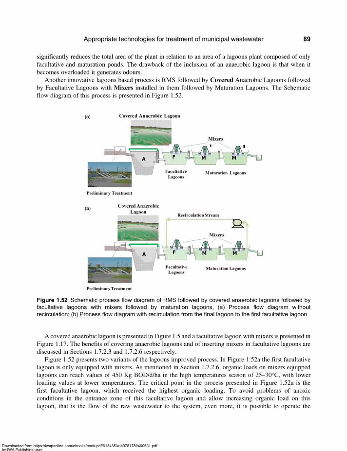
significantly reduces the total area of the plant in relation to an area of a lagoons plant composed of onlyfacultative and maturation ponds. The drawback of the inclusion of an anaerobic lagoon is that when itbecomes overloaded it generates odours.

Another innovative lagoons based process is RMS followed by Covered Anaerobic Lagoons followedby Facultative Lagoons with Mixers installed in them followed by Maturation Lagoons. The Schematicflow diagram of this process is presented in Figure 1.52.

A covered anaerobic lagoon is presented in Figure 1.5 and a facultative lagoon with mixers is presented inFigure 1.17. The benefits of covering anaerobic lagoons and of inserting mixers in facultative lagoons arediscussed in Sections 1.7.2.3 and 1.7.2.6 respectively.

Figure 1.52 presents two variants of the lagoons improved process. In Figure 1.52a the first facultativelagoon is only equipped with mixers. As mentioned in Section 1.7.2.6, organic loads on mixers equippedlagoons can reach values of 450 Kg BOD/d/ha in the high temperatures season of 25–30°C, with lowerloading values at lower temperatures. The critical point in the process presented in Figure 1.52a is thefirst facultative lagoon, which received the highest organic loading. To avoid problems of anoxicconditions in the entrance zone of this facultative lagoon and allow increasing organic load on thislagoon, that is the flow of the raw wastewater to the system, even more, it is possible to operate the

Figure 1.52 Schematic process flow diagram of RMS followed by covered anaerobic lagoons followed byfacultative lagoons with mixers followed by maturation lagoons, (a) Process flow diagram withoutrecirculation; (b) Process flow diagram with recirculation from the final lagoon to the first facultative lagoon



system using the process presented in Figure 1.52b. In this process, the effluent of the final lagoon isrecirculated to the inflow of the first facultative lagoon at a ratio of about 2:1 (recirculation stream to rawwastewater). The recirculated flow dilutes the inflow to the first facultative lagoon and brings in a streamrich in oxygen and in algae which immediately start to generate more oxygen. This preventsdevelopment of anoxic condition in the first facultative lagoon and enables increasing the organicloading on this lagoon, that is, increasing the flow to the plant. The recirculation requires energy andincreases the O&M cost of the process in Figure 1.52b but it also increases the capacity of the plant, sothe cost of reciculation is the cost of increasing the capacity, which is lower than the cost of increasingthe capacity using other methods.

Each process (of Figure 1.52a or 1.52b) can be designed from inception to function under its respectiveflow diagram or can be used to upgrade existing conventional lagoons plants to increase their treatmentcapacity without increasing their area. Most of the existing lagoons plants are conventional plants. Whenthey become overloaded, the option to upgrade them using the scheme proposed in Figure 1.52 is veryattractive since it is much cheaper than increasing the size of the plant, and usually there is no room toincrease the existing plant. The process has several important advantages in relation to conventionallagoons plants. First, it eliminates the odours which may be generated in the anaerobic lagoons bypreventing emission of gases from the lagoon to the external environment. This is achieved by collectingthe biogas generated in the lagoon and subjecting it to further processing. That is an importantenvironmental improvement of the lagoons plant. Second, it increases the treatment capacity of thelagoons units, without increasing their area. The anaerobic units can be subjected to increased loadsbecause the limiting factor of odour generation was eliminated. The facultative and maturation ponds canbe subjected to higher organic loads since by inserting in them the mixers they are turned into a moreefficient reactors, as explained in Section 1.7.2.6, and using the recirculation concept allows loadingthem even more. Overall, a lagoons plant based on this flow diagram requires less area than that of aconventional lagoons plant with the same treatment capacity, so this process saves area and this fact canbe an important factor in cases where availability of area is limited. Another important benefit of thisprocess is that the biogas collected in the anaerobic lagoon can be used to generate energy. There areseveral ways to generate energy from biogas, and all of them can generate income which can cover theentire O&M expenses of the plant and still leave significant revenue to the plant’s owner. The feasibilityfor generating energy depends on the size of the town served by the plant. In the case of very smallplants it might be unfeasible to generate energy. When not used for energy generation, the biogas mustbe flared. Flaring the biogas or generating energy has one more benefit (on top of preventing odours), itprevents the emission to the atmosphere of methane, a strong Green House Gas (GHG), thus supportingthe effort of Carbon Emission Reduction (CER) and contributing to the alleviation of global warming. Itis also possible to obtain CER credits for flaring the biogas or using it for generation of energy.

After years of operation lagoons plants, as any other plant, reach the stage of operating at full capacity andin many cases they are even being overloaded. Often there is no area available in the plant site to expand theircapacity under the principles of the conventional lagoons treatment process, that is, there is no room toconstruct additional lagoons. The process presented in Figure 1.52 can be used to extend the treatmentcapacity of such plants without extending their area. The city of Santa Cruz, Bolivia, has 4 conventionallagoons plants and all of them are being upgraded using the process of Figure 1.52a. The upgrade ofPlant N2 in Santa Cruz has already been completed and a satellite photo of the upgraded plant ispresented in Figure 1.53. As mentioned, this plant consists of 2 parallel lines, each composed of ananaerobic lagoon followed by 2 facultative lagoons followed by one maturation lagoon. The photo of theupgrade plant, Figure 1.53, can be compared to the photo of the plant before the upgrade, which ispresented in Figure 1.51. After the upgrade, the anaerobic lagoons are covered, as seen in Figures 1.53



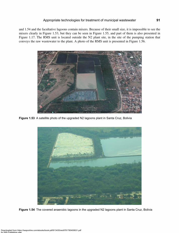
and 1.54 and the facultative lagoons contain mixers. Because of their small size, it is impossible to see themixers clearly in Figure 1.53, but they can be seen in Figure 1.55, and part of them is also presented inFigure 1.17. The RMS unit is located outside the N2 plant site, in the site of the pumping station thatconveys the raw wastewater to the plant. A photo of the RMS unit is presented in Figure 1.56.

Figure 1.53 A satellite photo of the upgraded N2 lagoons plant in Santa Cruz, Bolivia

Figure 1.54 The covered anaerobic lagoons in the upgraded N2 lagoons plant in Santa Cruz, Bolivia



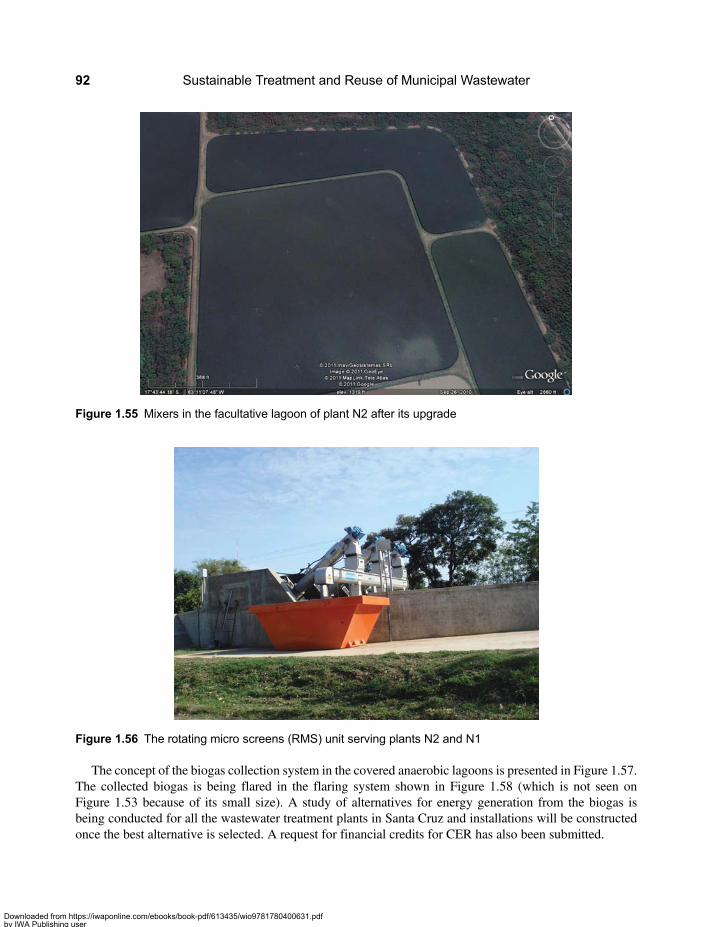
The concept of the biogas collection system in the covered anaerobic lagoons is presented in Figure 1.57.The collected biogas is being flared in the flaring system shown in Figure 1.58 (which is not seen onFigure 1.53 because of its small size). A study of alternatives for energy generation from the biogas isbeing conducted for all the wastewater treatment plants in Santa Cruz and installations will be constructedonce the best alternative is selected. A request for financial credits for CER has also been submitted.

Figure 1.55 Mixers in the facultative lagoon of plant N2 after its upgrade

Figure 1.56 The rotating micro screens (RMS) unit serving plants N2 and N1



As seen in Figure 1.53 residential areas are very close to the anaerobic lagoons of plant N2 and before theupgrade residents complained about odour problems. After the upgrade, the odour problems werecompletely eliminated. The upgrade method of a conventional existing lagoons system which wasexecuted in plant N2 in Santa Cruz can serve as an example to many other cases of lagoon plants whichbecome overloaded, need to be upgraded, but area for constructing additional lagoons is unavailable.The upgrade method selected in Santa Cruz is the lowest cost method of upgrade within the existingavailable area, The plant remained a simple to operate lagoons plant, odour problems were completelyeliminated, the emission of Green House Gases was stopped and an opportunity for generation energyfrom the captured biogas has been created.

Before the upgrade the N2 plant was serving a population of 170,000 and after the upgrade it is serving apopulation of 270,000, that is, the plant’s capacity was increased by about 60%, without an increase of theplant’s area, and at a very low investment cost.

Figure 1.58 The biogas flaring system serving plants N2 and N1

Figure 1.57 The biogas collection system in the covered anaerobic lagoons



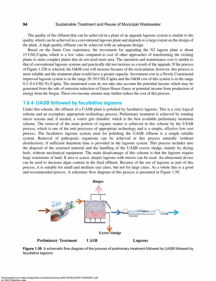
The quality of the effluent that can be achieved in a plant of an upgrade lagoons system is similar to thequality which can be achieved in a conventional lagoons plant and depends to a large extent on the design ofthe plant. A high quality effluent can be achieved with an adequate design.

Based on the Santa Cruz experience, the investment for upgrading the N2 lagoon plant is about15 US$/Capita, which is a low value compared to cost of other approaches of transforming the existingplants to more complex plants that do not need more area. The operation and maintenance cost is similar tothat of conventional lagoons systems and practically did not increase as a result of the upgrade. If the processof Figure 1.52b is selected, the O&M cost will increase because of the recirculation, however, this process ismore reliable and the treatment plant would have a greater capacity. Investment cost in a Newly Constructedimproved lagoons system is in the range 20–50 US$/Capita and the O&M cost of this system is in the range0.2–0.4 US$/Yr/Capita. The mentioned costs do not take into account the potential income which may begenerated from the sale of emission reduction of Green House Gases or potential income from production ofenergy from the biogas. These two income streams may further reduce the cost of this process.

1.8.4 UASB followed by facultative lagoonsUnder this scheme, the effluent of a UASB plant is polished by facultative lagoons. This is a very logicalscheme and an exemplary appropriate technology process. Preliminary treatment is achieved by rotatingmicro screens and, if needed, a vortex grit chamber, which is the best available preliminary treatmentscheme. The removal of the main portion of organic matter is achieved in this scheme by the USABprocess, which is one of the unit processes of appropriate technology and is a simple, effective low costprocess. The facultative lagoons system used for polishing the UASB effluent is a simple reliablesystem. Removal of pathogenic organisms can be achieved in this process naturally (withoutdisinfection), if sufficient detention time is provided in the lagoons system. This process includes alsothe disposal of the screened material and the handling of the UASB excess sludge, mainly by dryingbeds, without mechanical equipment. The main disadvantage of this scheme is that the lagoons requirelarge extensions of land. If area is scarce, deeper lagoons with mixers can be used. An ultrasound devicecan be used to decrease algae content in the final effluent. Because of the use of lagoons as part of thisprocess, it is suitable for small and medium size cities, but not for large cities. As a whole this is a goodand recommended process. A schematic flow diagram of this process is presented in Figure 1.59.

Figure 1.59 A schematic flow diagram of the process of preliminary treatment followed by UASB followed byfacultative lagoons



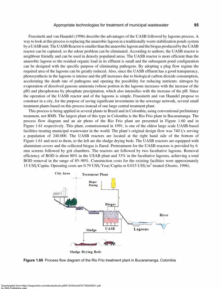
Frassinetti and van Haandel (1996) describe the advantages of the UASB followed by lagoons process. Away to look at this process is replacing the anaerobic lagoon in a traditionally waste stabilization ponds systembyaUASBunit.TheUASBReactor is smaller than theanaerobic lagoon and thebiogasproducedby theUASBreactor can be captured, so the odour problem can be eliminated. According to authors, the UASB reactor isneighbour friendly and can be used in densely populated areas. The UASB reactor is more efficient than theanaerobic lagoon so the residual organic load in its effluent is small and the subsequent pond configurationcan be designed with the specific purpose of eliminating pathogens. By adopting a plug flow regime therequired area of the lagoons can be greatly reduced. Also, since the UASB effluent has a good transparency,photosynthesis in the lagoons is intense and the pH increases due to biological carbon dioxide consumption,accelerating the death rate of pathogens and opening the possibility for reducing nutrients: nitrogen byevaporation of dissolved gaseous ammonia (whose portion in the lagoons increases with the increase of thepH) and phosphorous by phosphate precipitation, which also intensifies with the increase of the pH. Sincethe operation of the UASB reactor and of the lagoons is simple, Frassinetti and van Haandel propose toconstruct in a city, for the purpose of saving significant investments in the sewerage network, several smalltreatment plants based on this process instead of one large central treatment plant.

This process is being applied in several plants in Brazil and in Colombia, using conventional preliminarytreatment, not RMS. The largest plant of this type in Colombia is the Rio Frio plant in Bucaramanga. Theprocess flow diagram and an air photo of the Rio Frio plant are presented in Figure 1.60 and inFigure 1.61 respectively. This plant, commissioned in 1991, is one of the oldest large scale UASB-basedfacilities treating municipal wastewater in the world. The plant’s original design flow was 740 l/s servinga population of 240.000. The UASB reactors are located at the right hand side of the bottom ofFigure 1.61 and next to them, to the left are the sludge drying beds. The UASB reactors are equipped withaluminium covers and the collected biogas is flared. Pretreatment for the UASB reactors is provided by 6mm screens followed by grit chambers. The reactors are followed by two facultative lagoons. Removalefficiency of BOD is about 80% in the USAB plant and 33% in the facultative lagoons, achieving a totalBOD removal in the range of 85–90%. Construction costs for the existing facilities were approximately15 US$/Capita. Operating costs are 0.79 US$/Year/Capita or 0.015 US$/m3 treated (Osorio, 1996).

Figure 1.60 Process flow diagram of the Rio Frio treatment plant in Bucaramanga, Colombia



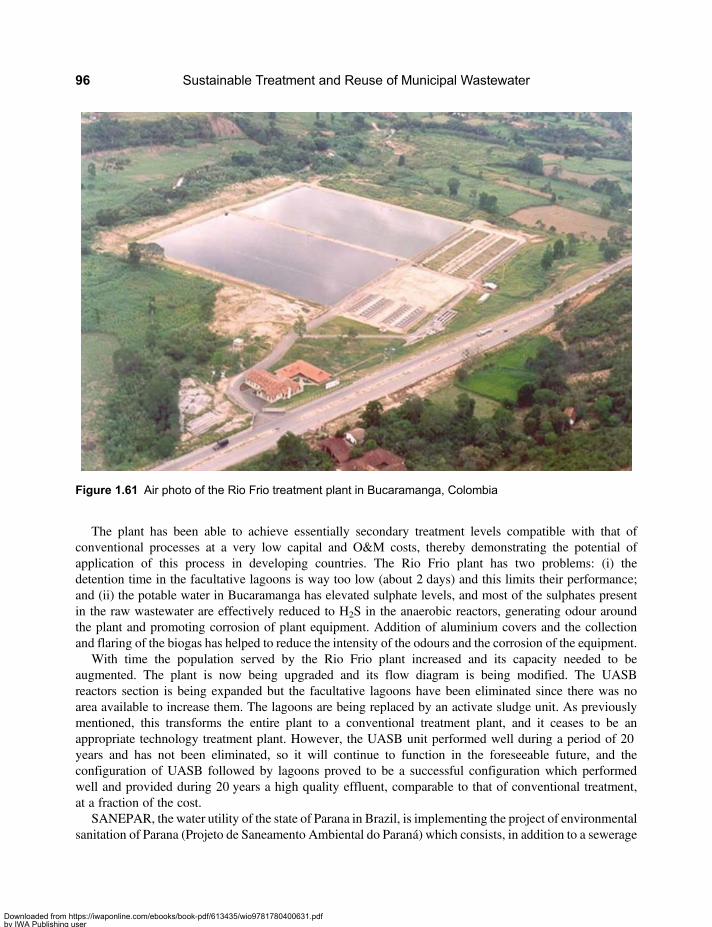
The plant has been able to achieve essentially secondary treatment levels compatible with that ofconventional processes at a very low capital and O&M costs, thereby demonstrating the potential ofapplication of this process in developing countries. The Rio Frio plant has two problems: (i) thedetention time in the facultative lagoons is way too low (about 2 days) and this limits their performance;and (ii) the potable water in Bucaramanga has elevated sulphate levels, and most of the sulphates presentin the raw wastewater are effectively reduced to H2S in the anaerobic reactors, generating odour aroundthe plant and promoting corrosion of plant equipment. Addition of aluminium covers and the collectionand flaring of the biogas has helped to reduce the intensity of the odours and the corrosion of the equipment.

With time the population served by the Rio Frio plant increased and its capacity needed to beaugmented. The plant is now being upgraded and its flow diagram is being modified. The UASBreactors section is being expanded but the facultative lagoons have been eliminated since there was noarea available to increase them. The lagoons are being replaced by an activate sludge unit. As previouslymentioned, this transforms the entire plant to a conventional treatment plant, and it ceases to be anappropriate technology treatment plant. However, the UASB unit performed well during a period of 20years and has not been eliminated, so it will continue to function in the foreseeable future, and theconfiguration of UASB followed by lagoons proved to be a successful configuration which performedwell and provided during 20 years a high quality effluent, comparable to that of conventional treatment,at a fraction of the cost.

SANEPAR, the water utility of the state of Parana in Brazil, is implementing the project of environmentalsanitation of Parana (Projeto de Saneamento Ambiental do Paraná) which consists, in addition to a sewerage

Figure 1.61 Air photo of the Rio Frio treatment plant in Bucaramanga, Colombia



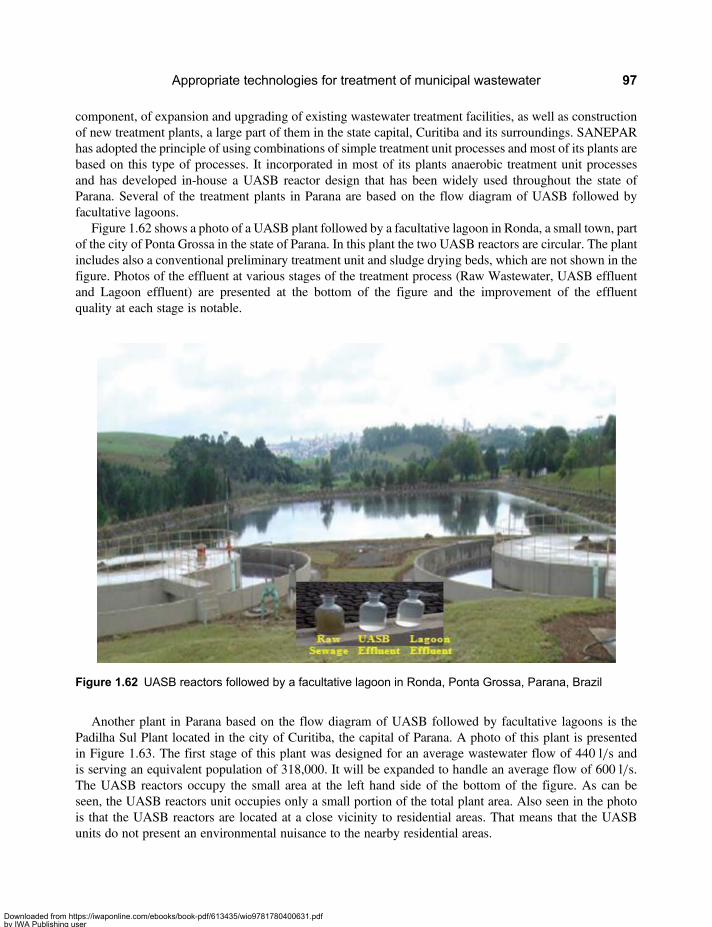
component, of expansion and upgrading of existing wastewater treatment facilities, as well as constructionof new treatment plants, a large part of them in the state capital, Curitiba and its surroundings. SANEPARhas adopted the principle of using combinations of simple treatment unit processes and most of its plants arebased on this type of processes. It incorporated in most of its plants anaerobic treatment unit processesand has developed in-house a UASB reactor design that has been widely used throughout the state ofParana. Several of the treatment plants in Parana are based on the flow diagram of UASB followed byfacultative lagoons.

Figure 1.62 shows a photo of a UASB plant followed by a facultative lagoon in Ronda, a small town, partof the city of Ponta Grossa in the state of Parana. In this plant the two UASB reactors are circular. The plantincludes also a conventional preliminary treatment unit and sludge drying beds, which are not shown in thefigure. Photos of the effluent at various stages of the treatment process (Raw Wastewater, UASB effluentand Lagoon effluent) are presented at the bottom of the figure and the improvement of the effluentquality at each stage is notable.

Another plant in Parana based on the flow diagram of UASB followed by facultative lagoons is thePadilha Sul Plant located in the city of Curitiba, the capital of Parana. A photo of this plant is presentedin Figure 1.63. The first stage of this plant was designed for an average wastewater flow of 440 l/s andis serving an equivalent population of 318,000. It will be expanded to handle an average flow of 600 l/s.The UASB reactors occupy the small area at the left hand side of the bottom of the figure. As can beseen, the UASB reactors unit occupies only a small portion of the total plant area. Also seen in the photois that the UASB reactors are located at a close vicinity to residential areas. That means that the UASBunits do not present an environmental nuisance to the nearby residential areas.

Figure 1.62 UASB reactors followed by a facultative lagoon in Ronda, Ponta Grossa, Parana, Brazil



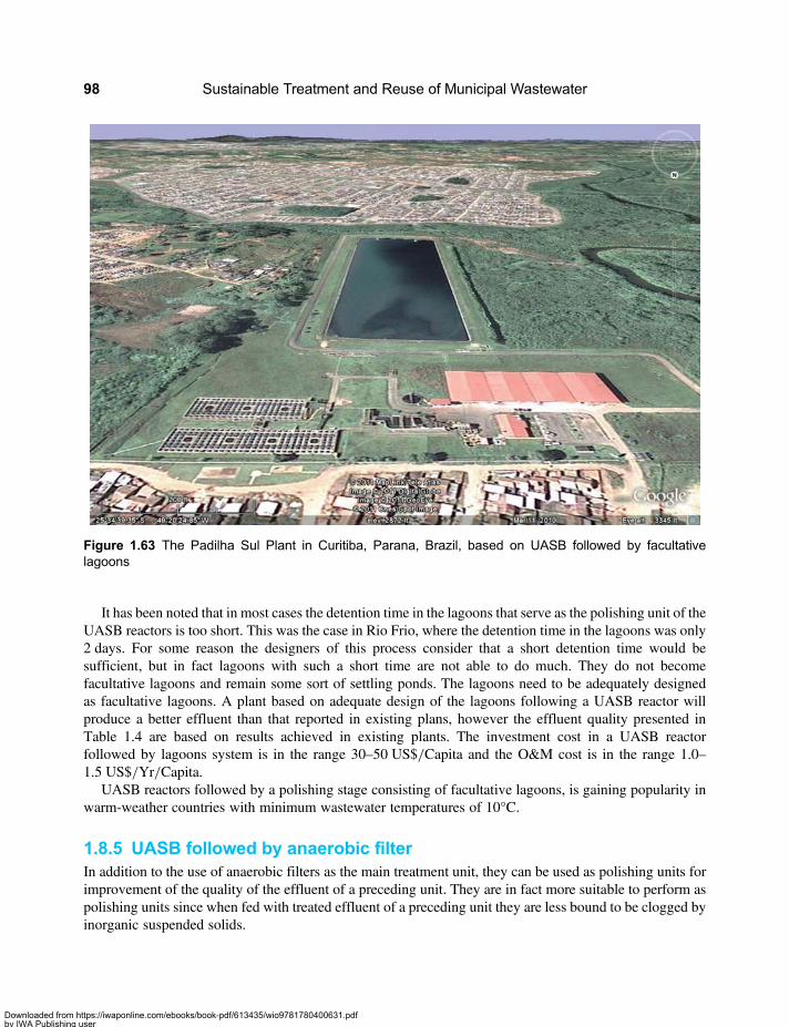
It has been noted that in most cases the detention time in the lagoons that serve as the polishing unit of theUASB reactors is too short. This was the case in Rio Frio, where the detention time in the lagoons was only2 days. For some reason the designers of this process consider that a short detention time would besufficient, but in fact lagoons with such a short time are not able to do much. They do not becomefacultative lagoons and remain some sort of settling ponds. The lagoons need to be adequately designedas facultative lagoons. A plant based on adequate design of the lagoons following a UASB reactor willproduce a better effluent than that reported in existing plans, however the effluent quality presented inTable 1.4 are based on results achieved in existing plants. The investment cost in a UASB reactorfollowed by lagoons system is in the range 30–50 US$/Capita and the O&M cost is in the range 1.0–1.5 US$/Yr/Capita.

UASB reactors followed by a polishing stage consisting of facultative lagoons, is gaining popularity inwarm-weather countries with minimum wastewater temperatures of 10°C.

1.8.5 UASB followed by anaerobic filterIn addition to the use of anaerobic filters as the main treatment unit, they can be used as polishing units forimprovement of the quality of the effluent of a preceding unit. They are in fact more suitable to perform aspolishing units since when fed with treated effluent of a preceding unit they are less bound to be clogged byinorganic suspended solids.

Figure 1.63 The Padilha Sul Plant in Curitiba, Parana, Brazil, based on UASB followed by facultativelagoons



A process composed of Rotating Micro Screens as preliminary treatment, followed by UASB as the unitfor removal of the main portion of organic matter, then followed by an anaerobic filter for polishing of theUASB effluent, and finally, if necessary, followed by a disinfection unit (chlorination or UV disinfection)for removal of pathogens is a reasonable schemes and an effective appropriate technology process. It is verysimilar to the process described in the previous section and is basically the replacement of the lagoons by ananaerobic filter followed by a disinfection unit. The advantages of this process are that it yields a high qualityeffluent and is compact, that is, does not occupy a large land area. This process can be applied in cases wherearea for locating a treatment plant is scarce and insufficient for installation of lagoons. The process includesalso the disposal of the screened material of the primary treatment and the handling of the UASB andanaerobic filter excess sludge, mainly by drying beds, without mechanical equipment. The process isadequate for application in small, medium and large cities.

This process has been applied in several pilot plants and full scale plants in Brazil, using conventionalpreliminary treatment or an Imhoff tank as the preliminary treatment stage. In pilot plant experimentsreported by Chernicharo (2000) a final effluent containing an average of 22 mg/l total BOD (soluble andsuspended) and 15 mg/l of TSS was achieved. Such an effluent quality is similar to that of an activatedsludge process effluent. Total BOD and total COD removal efficiencies achieved were 90%, solubleCOD removal achieved was 81% and TSS removal achieved was 95%. Additional investigationsreported by Chernicharo (2007) demonstrated that plants based on UASB followed by anaerobic filtersare capable to maintain in the final effluents concentrations of COD, BOD and SST lower than 120 mg/l,60 mg/l and 30 mg/l respectively.

Andrade Neto (2006) reports that several plants based on the UASB followed by an anaerobic filterprocess are under operation since 1996 in the state of Parana, Brazil, serving populations in the range of1,500 to 50,000 persons. Effluent quality achieved in these plants is total BOD lower than 60 mg/l andTSS lower than 20 mg/l. The same type of plants is under operation since 1997 in the state of MinasGerais, Brazil, serving populations in the range 2,000 to 15,000 persons. One plant in Minas Gerais, atIpatinga, serves a population of about 200,000.

Andrade Neto (2006) also reports that the investments costs of the UASB followed by anaerobic filtersystems in Parana were in the range of 5 to 30 US$/Capita. This process is of special importance since itis able to achieve essentially secondary treatment effluent levels at a low capital and O&M costs,occupying a small similar are and even a smaller area than that of activated sludge, therebydemonstrating the potential of applying this process in developing countries as a favourable alternative toactivated sludge.

A schematic flow diagram of the process of UAB followed by Anaerobic filter is presented inFigure 1.64 and a photo of such a plant in the small town of Tibagi, in the State of Parana, Brazil,serving a population of about 20,000 is presented in Figure 1.65. This plant, operated by SANEPAR,the water and sanitation utility of Parana, achieves an effluent quality of BOD 5–25 mg/l, COD 40–100 mg/l and TSS 4–10 mg/l. A photo of the Anaerobic Filter of the Tibagi plant is presented inFigure 1.66 and a photo of the effluent of this plant is presented in Figure 1.67. The anaerobic filter ispresented in a separate photo since in the general photo of the plant (Figure 1.65) the filter is not seenin detail because it is the last unit of the plant. The anaerobic filter in the Tibagi plant is a circular crosssection filter of an ascending flow. This filter is similar to a circular sedimentation tank. It is filled witha crushed rock media on which the anaerobic bacteria grow, attached to the media. The filter washing isdone by a descending stream of the incoming flow from the UASB reactor, which is basically abackwashing of the filter. The backwashing is done once every couple of days. The incoming flowdirection is changed and the stream used for washing of the rock media is directed, after the washingoperation, to the drying beds.



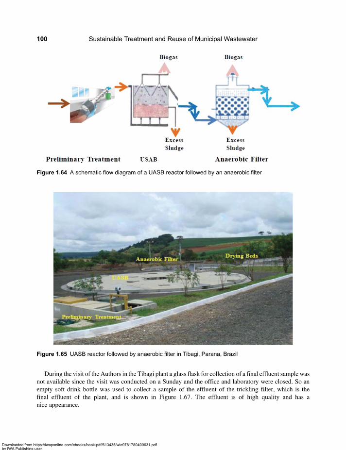
During the visit of the Authors in the Tibagi plant a glass flask for collection of a final effluent sample wasnot available since the visit was conducted on a Sunday and the office and laboratory were closed. So anempty soft drink bottle was used to collect a sample of the effluent of the trickling filter, which is thefinal effluent of the plant, and is shown in Figure 1.67. The effluent is of high quality and has anice appearance.

Figure 1.64 A schematic flow diagram of a UASB reactor followed by an anaerobic filter

Figure 1.65 UASB reactor followed by anaerobic filter in Tibagi, Parana, Brazil



Figure 1.66 The circular anaerobic filter at the Tibagi wastewater treatment plant

Figure1.67 The effluent of the Tibagi treatment plant, Parana, Brazil (Effluent Quality: BOD 5–25 mg/l, COD40–100 mg/l, TSS 4–10 mg/l)



COPASA, the water and sanitation utility of the State of Minas Gerais in Brazil operates several plantsbased on the process of UASB followed by anaerobic filters. The treatment plants of Arenal, Bela Vista,Horto, and Ipanema located in the municipality of Ipatinga are some of these plants. The performance ofthe Ipanema plant was evaluated during the period July 2005–September 2006 (Greco, 2007). Thewastewater flow to this plant was 180 l/s and it serves a population of about 200,000. The plantachieved an average BOD removal efficiency of 84%, an average COD removal efficiency of 87% andan average SST removal efficiency of 80%. A photo of the wastewater treatment plant in Ipatinga, MinasGerais, which is a UASB followed by anaerobic filters plant serving a population of about 200,000 ispresented in Figure 1.68. The UASB units and the Anaerobic Filters units in this plant are rectangularand that enables to achieve a compact configuration of the plants. As seen in the figure, the plant alsoincludes drying bed of the excess sludge, located in the upper part of the photo. The plant contains 10UASB units located in two rows (at the bottom of the photo) and two anaerobic reactors located in a rawbetween the UASB reactors and the drying beds.

The investment cost in the system UASB reactor followed by Anaerobic Filter is in the range 20–40US$/Capita and the O&M cost is in the range 1.0–1.5 US$/Yr/Capita.

Figure 1.68 The treatment plant of Ipatinga, State of Minas Gerais, Brazil, based on UASB reactors followedby anaerobic filters



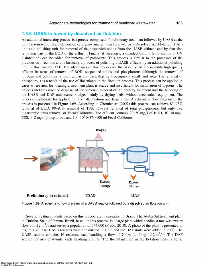
1.8.6 UASB followed by dissolved air flotationAn additional interesting process is a process composed of preliminary treatment followed by UASB as theunit for removal of the bulk portion of organic matter, then followed by a Dissolved Air Flotation (DAF)unit as a polishing unit for removal of the suspended solids from the UASB effluent and by that alsoremoving part of the BOD of the effluent. Finally, if necessary, a disinfection unit (chlorination or UVdisinfection) can be added for removal of pathogens. This process is similar to the processes of theprevious two sections and is basically a process of polishing a UASB effluent by an additional polishingunit, in this case by DAF. The advantages of this process are that it can yield a reasonably high qualityeffluent in terms of removal of BOD, suspended solids and phosphorous (although the removal ofnitrogen and coliforms is low), and is compact, that is, it occupies a small land area. The removal ofphosphorous is a result of the use of flocculants in the flotation process. This process can be applied incases where area for locating a treatment plant is scarce and insufficient for installation of lagoons. Theprocess includes also the disposal of the screened material of the primary treatment and the handling ofthe UASB and DAF unit excess sludge, mainly by drying beds, without mechanical equipment. Theprocess is adequate for application in small, medium and large cities. A schematic flow diagram of theprocess is presented in Figure 1.69. According to Chernicharo (2007) this process can achieve 83–93%removal of BOD, 90–97% removal of TSS, 75–88% removal of total phosphorous, but only 1–2logarithmic units removal of Fecal Coliforms. The effluent contains 20–50 mg/l of BOD, 10–30 mg/lTSS, 1–2 mg/l phosphorous and 106–107 MPN/100 ml Fecal Coliforms.

Several treatment plants based on this process are in operation in Brazil. The Atuba Sul treatment plantin Curitiba, State of Parana, Brazil, based on this process, is a large plant which handles a raw wastewaterflow of 1.12 m3/s and serves a population of 544,000 (Prado, 2010). A photo of the plant is presented inFigure 1.70. The UASB reactors were constructed in 1998 and the DAF units were added in 2008. TheUASB section contains 16 reactors, each handling a flow of 70 l/s (totalling 1.12 m3/s). The DAFsection consists of 4 units, each handling 280 l/s. The flocculant used in the flotation units is Ferric

Figure 1.69 A schematic flow diagram of a UASB reactor followed by a dissolved air flotation unit



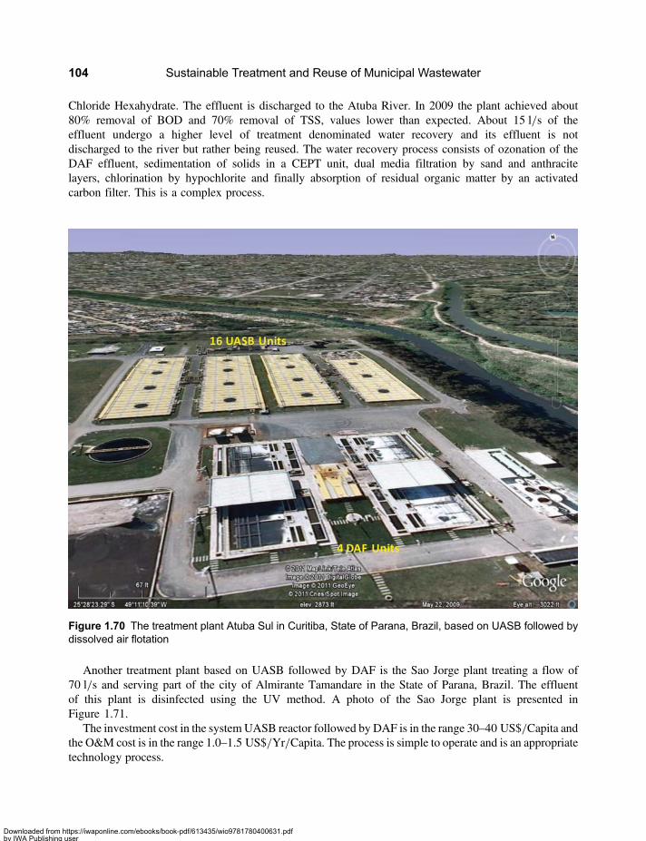
Chloride Hexahydrate. The effluent is discharged to the Atuba River. In 2009 the plant achieved about80% removal of BOD and 70% removal of TSS, values lower than expected. About 15 l/s of theeffluent undergo a higher level of treatment denominated water recovery and its effluent is notdischarged to the river but rather being reused. The water recovery process consists of ozonation of theDAF effluent, sedimentation of solids in a CEPT unit, dual media filtration by sand and anthracitelayers, chlorination by hypochlorite and finally absorption of residual organic matter by an activatedcarbon filter. This is a complex process.

Another treatment plant based on UASB followed by DAF is the Sao Jorge plant treating a flow of70 l/s and serving part of the city of Almirante Tamandare in the State of Parana, Brazil. The effluentof this plant is disinfected using the UV method. A photo of the Sao Jorge plant is presented inFigure 1.71.

The investment cost in the system UASB reactor followed by DAF is in the range 30–40 US$/Capita andthe O&M cost is in the range 1.0–1.5 US$/Yr/Capita. The process is simple to operate and is an appropriatetechnology process.

Figure 1.70 The treatment plant Atuba Sul in Curitiba, State of Parana, Brazil, based on UASB followed bydissolved air flotation



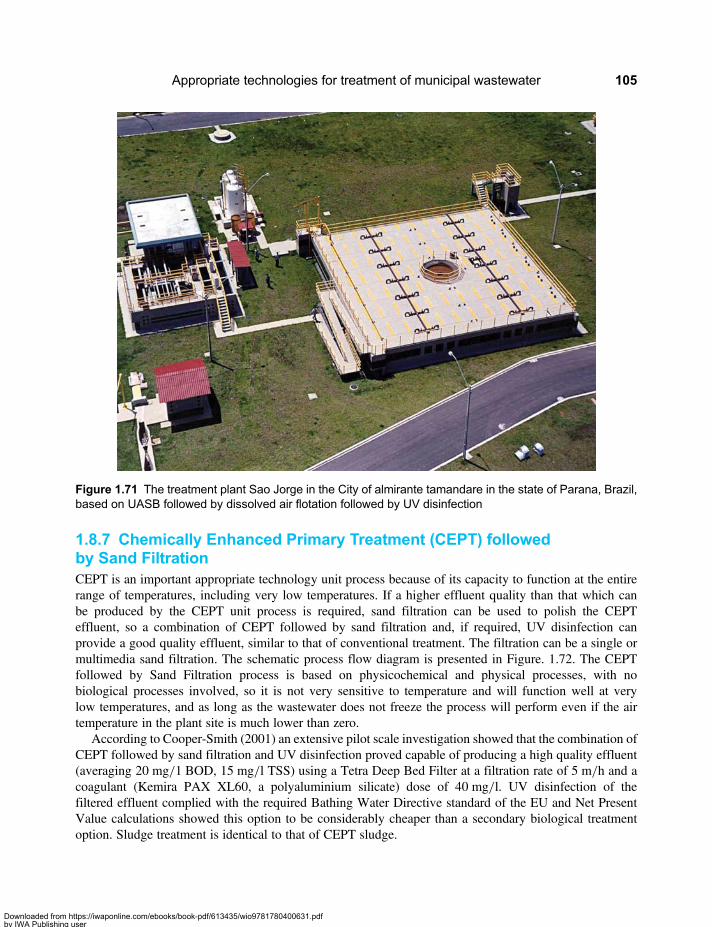
1.8.7 Chemically Enhanced Primary Treatment (CEPT) followedby Sand FiltrationCEPT is an important appropriate technology unit process because of its capacity to function at the entirerange of temperatures, including very low temperatures. If a higher effluent quality than that which canbe produced by the CEPT unit process is required, sand filtration can be used to polish the CEPTeffluent, so a combination of CEPT followed by sand filtration and, if required, UV disinfection canprovide a good quality effluent, similar to that of conventional treatment. The filtration can be a single ormultimedia sand filtration. The schematic process flow diagram is presented in Figure. 1.72. The CEPTfollowed by Sand Filtration process is based on physicochemical and physical processes, with nobiological processes involved, so it is not very sensitive to temperature and will function well at verylow temperatures, and as long as the wastewater does not freeze the process will perform even if the airtemperature in the plant site is much lower than zero.

According to Cooper-Smith (2001) an extensive pilot scale investigation showed that the combination ofCEPT followed by sand filtration and UV disinfection proved capable of producing a high quality effluent(averaging 20 mg/1 BOD, 15 mg/l TSS) using a Tetra Deep Bed Filter at a filtration rate of 5 m/h and acoagulant (Kemira PAX XL60, a polyaluminium silicate) dose of 40 mg/l. UV disinfection of thefiltered effluent complied with the required Bathing Water Directive standard of the EU and Net PresentValue calculations showed this option to be considerably cheaper than a secondary biological treatmentoption. Sludge treatment is identical to that of CEPT sludge.

Figure 1.71 The treatment plant Sao Jorge in the City of almirante tamandare in the state of Parana, Brazil,based on UASB followed by dissolved air flotation followed by UV disinfection



CEPT followed by filtration can be used to produce an almost secondary quality effluent which wouldrepresent a good option for developing countries, as its attributes include: (i) the ability to provide asecondary effluent quality at lower cost than conventional processes; (ii) reduced power needs; (iii) easyoperation; and (iv) occupies a small land area, smaller than that of conventional processes. This processis suitable for medium and large cities. Small cities may find it difficult to operate.

CEPT followed sand filtration is an appropriate technology process since it is a relatively simpletechnology, which provides low cost, easy to implement and effective treatment. The CEPT unit processis an easy to operate process since it is basically consisting of a settling unit and a sand filter. Sandfiltration is a process that most water utilities know how to operate since they operate filtration plants inthe water supply system, and it is basically an easy process to operate. The only complication might bethe handling of the sludge, but as a whole, it is an appropriate technology process.

It is estimated that the ratio of investment cost in conventional activated sludge to investment inCEPT followed by multimedia sand filtration is about 2 to 1. The investment cost of the system CEPTfollowed by a Sand Filter is in the range 40–50 US$/Capita and the O&M cost is in the range 1.5–2.0 US$/Yr/Capita.

1.8.8 Pre-treatment of various types followed by a stabilization reservoir(Wastewater reuse for irrigation, the stabilization reservoirs concept)The stabilization reservoir process was presented and discusses as one of the unit processes of appropriatetechnology. As part of this discussion, it was clarified that before discharging the wastewater to the reservoirfor storage, it needs to be treated to remove a part of the organic matter contained in it; so as to preventdevelopment of anaerobic conditions in the upper layer of the reservoir. Prevention of such conditions isimportant since anaerobic condition may generate odours. So in fact, the reservoir stores effluent and notraw wastewater. The required pre-treatment of the wastewater before it is stored in the reservoir is not aspecific treatment processes. It can be achieved using a variety of treatment process, among them; all theappropriate technology processes or combination of processes described in this book, as long as theyremove the required load of organic matter and ensure that the surface organic loading on the reservoirdoes not exceed the permitted limit. The combination of the pretreatment unit and the reservoir form as awhole an appropriate technology process, if the pretreatment unit is based on appropriate technology.

Figure 1.72 A schematic process flow diagram of CEPT followed by Sand Filtration



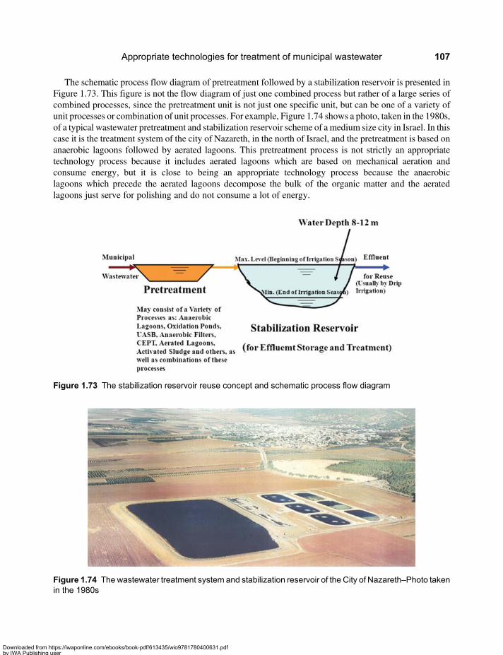
The schematic process flow diagram of pretreatment followed by a stabilization reservoir is presented inFigure 1.73. This figure is not the flow diagram of just one combined process but rather of a large series ofcombined processes, since the pretreatment unit is not just one specific unit, but can be one of a variety ofunit processes or combination of unit processes. For example, Figure 1.74 shows a photo, taken in the 1980s,of a typical wastewater pretreatment and stabilization reservoir scheme of a medium size city in Israel. In thiscase it is the treatment system of the city of Nazareth, in the north of Israel, and the pretreatment is based onanaerobic lagoons followed by aerated lagoons. This pretreatment process is not strictly an appropriatetechnology process because it includes aerated lagoons which are based on mechanical aeration andconsume energy, but it is close to being an appropriate technology process because the anaerobiclagoons which precede the aerated lagoons decompose the bulk of the organic matter and the aeratedlagoons just serve for polishing and do not consume a lot of energy.

Figure 1.73 The stabilization reservoir reuse concept and schematic process flow diagram

Figure 1.74 The wastewater treatment system and stabilization reservoir of the City of Nazareth–Photo takenin the 1980s



In the system of Nazareth, the anaerobic lagoons can be covered to prevent odours and capture the biogas,which can then be used for generating the energy to operate the aeration system in the aerated lagoons.Preliminary estimates indicate that the biogas would be more than sufficient to supply all the energyrequired for operating the aerated lagoons, however, the economic feasibility of such a system needs tobe analyzed.

In Israel, the pretreatment units preceding reservoirs are mostly of two types: (i) a unit based on variouscombinations of lagoons; and (ii) a unit based on activated sludge. When the pretreatment is based onlagoons, the entire scheme is an appropriate technology process, however, when the pretreatment isbased on activated sludge, it is not an appropriate technology process. There are about 350 reservoirssystems in Israel, each unique in its pretreatment process, in the volume of the reservoir designed to fitthe size of the town it serves, and in the shape of the reservoir, adjusted to the local topography in thereservoir site. The volumes of the reservoirs vary between the smallest of about 20,000 m3 serving avery small town, to 12 million m3 serving the city of Haifa with a population of about 700,000.

A recent satellite photo of the treatment system of Nazareth, with the city on the horizon, is shown inFigure 1.75, and a close-up satellite photo of the treatment plant is shown in Figure 1.76. In these twofigures it is possible to note that the number of lagoons in the pretreatment unit has grown since the1980s, because the population grew and the organic load received by the treatment plant grew, so thepretreatment had to be expanded to maintain the adequate organic loading on the reservoir.

Another combined reservoir treatment system, the Naan Reservoir, is shown in Figure 1.77. This is one ofthe first reservoir systems constructed in Israel and is in operation since the 1970s. The pretreatment unit inthis case is very simple and consists of only two anaerobic lagoons. The configuration of the pretreatment

Figure 1.75 The wastewater treatment system and stabilization reservoir of the city of Nazareth – recentsatellite photo



installations depends on the surface area of the reservoir, which in turn depends on its design, that is, therelation of volume to depth and the availability of land.

Figure 1.76 A close-up satellite photo of the treatment system of the city of Nazareth

Figure 1.77 The Naan wastewater treatment system and stabilization reservoir



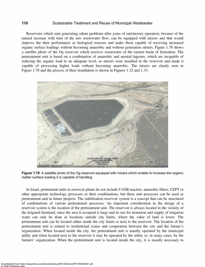
Reservoirs which start generating odour problems after years of satisfactory operation, because of thenatural increase with time of the raw wastewater flow, can be equipped with mixers and that wouldimprove the their performance as biological reactors and make them capable of receiving increasedorganic surface loadings without becoming anaerobic and without generation odours. Figure 1.78 showsa satellite photo of the Og reservoir which receives wastewater of the eastern basin of Jerusalem. Thepretreatment unit is based on a combination of anaerobic and aerated lagoons, which are incapable ofreducing the organic load to an adequate level, so mixers were installed in the reservoir and made itcapable of processing higher loads without becoming anaerobic. The mixers are clearly seen inFigure 1.78 and the process of their installation is shown in Figures 1.32 and 1.33.

In Israel, pretretment units in reservoir plants do not include UASB reactors, anaerobic filters, CEPT orother appropriate technology processes or their combinations, but these unit processes can be used aspretreatment unit in future projects. The stabilization reservoir system is a concept that can be structuredof combinations of various pretreatment processes. An important consideration in the design of areservoir system is the location of the pretreatment unit. The reservoir is always located in the vicinity ofthe irrigated farmland, since the area it occupied is large and its use for treatment and supply of irrigationwater can only be done in locations outside city limits, where the value of land is lower. Thepretreatment unit can be located either inside the city limits or next to the reservoir. The location of thepretreatment unit is related to institutional issues and cooperation between the city and the farmer’sorganization. When located inside the city, the pretreatment unit is usually operated by the municipalutility and when located next to the reservoir it may be operated by the utility or, in many cases, by thefarmers’ organization. When the pretreatment unit is located inside the city, it is usually necessary to

Figure 1.78 A satellite photo of the Og reservoir equipped with mixers which enable to increase the organicmatter surface loading it is capable of handling



base it on a process that occupies a small size of land. In this respect unit processes such as UASB, AnaerobicFilters and CEPT are advantageous since they occupy small land areas. In the reservoir systems of Nazareth,Naan and Og, the pretreatment units are located next to the reservoirs, where availability of land is notrestrictive and therefore all of them are lagoons based systems. But there are many reservoir systems inIsrael in which the pretreatment units are located inside the cities, at a large distance from the reservoirs.The systems of the city of Haifa and of the western basin of Jerusalem can be mentioned as suchexamples. In each of these cities the pretreatment is an activated sludge plant located inside therespective city limits and operated by the municipal water and sanitation utility. The effluents of thesepretreatment units are conveyed to the reservoirs located outside the cities, next to the farmlands.

The combination of CEPT as a pretreatment unit and a stabilization reservoir can be advantageous fromthe standpoint of resistance to low temperatures and can be used in regions with very low temperaturesduring the cold season. The CEPT unit performs well in low temperatures, and the CEPT effluent can bestored in a reservoir without causing nuisance until temperatures rise to the level that enables resumptionof bacterial activity.

The effluent of stabilization reservoirs is usually used for irrigation, and in Israel, the irrigation methodused is, for the most part, drip irrigation. But any other irrigation method can of course be used. Thecombined Pretreatment – Stabilization Reservoir – irrigation reuse system is a simple, economicwastewater reuse (and disposal) method which does not require high skills for operation andmaintenance. The required pretreatment of the wastewater before it is stored in the reservoir can beachieved using a variety of treatment process, among them, all the appropriate technology processes. Ifsimple pretreatment processes are selected, the entire pretreatment, reservoir and irrigation system can beconsidered an appropriate technology system.

The quality of the effluent of a reservoir system depends on the system’s design. If the effluent is used forrestricted irrigation, the effluent quality does not need to be very high and the system is designedaccordingly. Usually a single continuous flow reservoir is used to produce effluent for restrictedirrigation. The annual mean Total BOD removal percentage of such a system is 70–85% and the annualmean TSS removal is 40–80%. The total coliforms removal in continuous flow reservoirs is only oneorder of magnitude. If the effluent is used for unrestricted irrigation it needs to be of high quality and,most importantly, contain a low count of pathogenic organism. This can be achieved by the use of twoor more reservoirs system in which the reservoirs are operated under a sequential batch mode. Suchsystems can achieve effluents of a very high quality with BOD, COD and TSS removals of 85–95%each, continuously during the irrigation season. They produce an effluent with a BOD5 concentration of5–10 mg/l and a TSS concentration of 5–20 mg/l. Moreover, the faecal coliforms removals in suchsystems are very high, producing effluents with faecal coliforms levels of 0–100 MPN/100 ml. Thismeans that sequential batch reservoir systems perform disinfection without the use of chemicals. Inaddition, the stabilization reservoirs completely remove helminth eggs and nematodes without difficulty.The effluents of sequential batch reactors are adequate for unrestricted irrigation.

When appropriate technology processes are used for pretreatment, the investment cost in the system ofpretreatment followed by a Stabilization Resrevior is in the range of 30–50 US$/Capita and the O&M cost isin the range 0.2–0.4 US$/Yr/Capita.

1.8.9 UASB followed by anaerobic filter followed by dissolvedair flotation followed by membrane filtrationAll the combined processes which were presented above are processes used in full scale plants or processeswhich have been studies in pilot scale plants. The process discussed in this section, RMS followed by



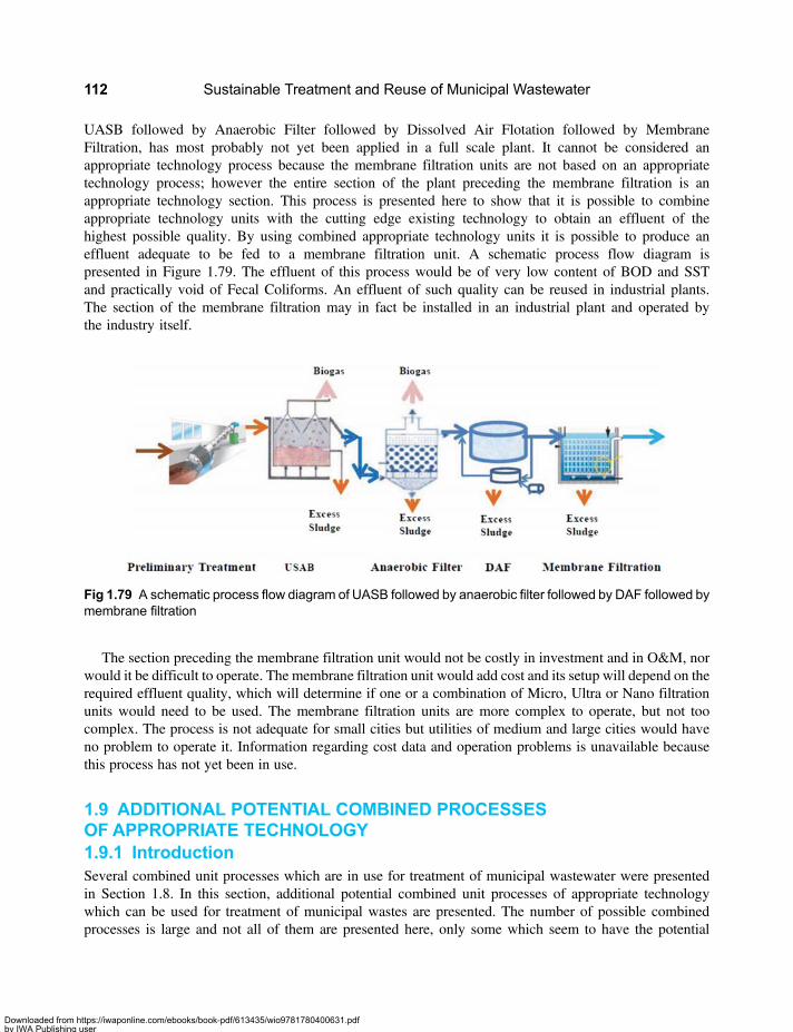
UASB followed by Anaerobic Filter followed by Dissolved Air Flotation followed by MembraneFiltration, has most probably not yet been applied in a full scale plant. It cannot be considered anappropriate technology process because the membrane filtration units are not based on an appropriatetechnology process; however the entire section of the plant preceding the membrane filtration is anappropriate technology section. This process is presented here to show that it is possible to combineappropriate technology units with the cutting edge existing technology to obtain an effluent of thehighest possible quality. By using combined appropriate technology units it is possible to produce aneffluent adequate to be fed to a membrane filtration unit. A schematic process flow diagram ispresented in Figure 1.79. The effluent of this process would be of very low content of BOD and SSTand practically void of Fecal Coliforms. An effluent of such quality can be reused in industrial plants.The section of the membrane filtration may in fact be installed in an industrial plant and operated bythe industry itself.

The section preceding the membrane filtration unit would not be costly in investment and in O&M, norwould it be difficult to operate. The membrane filtration unit would add cost and its setup will depend on therequired effluent quality, which will determine if one or a combination of Micro, Ultra or Nano filtrationunits would need to be used. The membrane filtration units are more complex to operate, but not toocomplex. The process is not adequate for small cities but utilities of medium and large cities would haveno problem to operate it. Information regarding cost data and operation problems is unavailable becausethis process has not yet been in use.

1.9 ADDITIONAL POTENTIAL COMBINED PROCESSESOF APPROPRIATE TECHNOLOGY1.9.1 IntroductionSeveral combined unit processes which are in use for treatment of municipal wastewater were presentedin Section 1.8. In this section, additional potential combined unit processes of appropriate technologywhich can be used for treatment of municipal wastes are presented. The number of possible combinedprocesses is large and not all of them are presented here, only some which seem to have the potential

Fig 1.79 A schematic process flow diagram of UASB followed by anaerobic filter followed by DAF followed bymembrane filtration



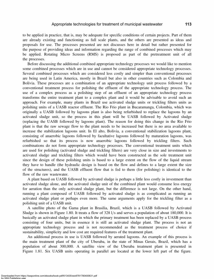
to be applied in practice, that is, may be adequate for specific conditions of certain projects. Part of themare already existing and functioning as full scale plants, and the others are presented as ideas andproposals for use. The processes presented are not discusses here in detail but rather presented forthe purpose of providing ideas and information regarding the range of combined processes which maybe applied. Rotating Micro Screens (RMS) is proposed as part of the pretreatment unit of allthe processes.

Before discussing the additional combined appropriate technology processes we would like to mentionsome combined processes which are in use and cannot be considered appropriate technology processes.Several combined processes which are considered less costly and simpler than conventional processesare being used in Latin America, mostly in Brazil but also in other countries such as Colombia andBolivia. These processes are a combination of an appropriate technology unit process followed by aconventional treatment process for polishing the effluent of the appropriate technology process. Theuse of a complex process as a polishing step of an effluent of an appropriate technology processtransforms the entire treatment plant to a complex plant and it would be advisable to avoid such anapproach. For example, many plants in Brazil use activated sludge units or trickling filters units aspolishing units of a UASB reactor effluent. The Rio Frio plant in Bucaramanga, Colombia, which wasoriginally a UASB followed by lagoons plant is also being refurbished to replace the lagoons by anactivated sludge unit, so the process in this plant will be UASB followed by Activated sludge(replacing the UASB followed by lagoons plant). The reason for doing this change in the Rio Frioplant is that the raw sewage flow to the plant needs to be increased but there is no area available toincrease the stabilization lagoons unit. In El alto, Bolivia, a conventional stabilization lagoons plant,consisting of anaerobic lagoons followed by facultative lagoons followed by maturation lagoons, wasrefurbished so that its process is now anaerobic lagoons followed by trickling filters. Suchcombinations do not form appropriate technology processes. The conventional treatment units whichare used for polishing (activated sludge and trickling filters) are very close in size and investments toactivated sludge and trickling filters which would have been constructed as the sole treatment unitsince the design of these polishing units is based to a large extent on the flow of the liquid streamthey have to handle (the hydraulic design is based on the flow and defines to a large extent the sizeof the structures), and the UASB effluent flow that is fed to them (for polishing) is identical to theflow of the raw wastewater.

A plant based on UASB followed by activated sludge is perhaps a little less costly in investment thanactivated sludge alone, and the activated sludge unit of the combined plant would consume less energyfor aeration than the only activated sludge plant, but the difference is not large. On the other hand,running a plant composed of UASB followed by activated sludge is as complicated as running anactivated sludge plant or perhaps even more. The same arguments apply for the trickling filter as apolishing unit of a UASB unit.

A satellite photo of the Gama plant in Brasilia, Brazil, which is a UASB followed by ActivatedSludge is shown in Figure 1.80. It treats a flow of 328 l/s and serves a population of about 180,000. It isbasically an activated sludge plant in which the primary treatment has been replaced by a UASB processconsisting of four units, but in essence it is still an activated sludge plant. The process is not anappropriate technology process and is not recommended as the treatment process of choice ifsustainability, simplicity and low cost are required features of the treatment plant.

An additional process in use is UASB followed by aerated lagoons. An example of this process isthe main treatment plant of the city of Uberaba, in the state of Minas Gerais, Brazil, which has apopulation of about 300,000. A satellite view of the Uberaba treatment plant is presented inFigure 1.81. Six UASB units operating in parallel are located at the lower left part of the figure.



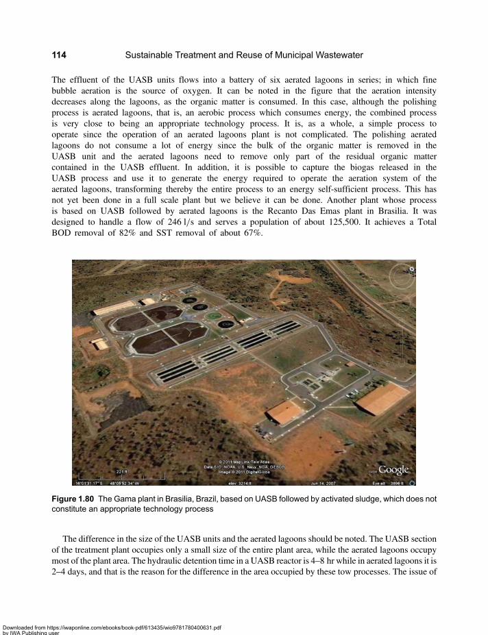
The effluent of the UASB units flows into a battery of six aerated lagoons in series; in which finebubble aeration is the source of oxygen. It can be noted in the figure that the aeration intensitydecreases along the lagoons, as the organic matter is consumed. In this case, although the polishingprocess is aerated lagoons, that is, an aerobic process which consumes energy, the combined processis very close to being an appropriate technology process. It is, as a whole, a simple process tooperate since the operation of an aerated lagoons plant is not complicated. The polishing aeratedlagoons do not consume a lot of energy since the bulk of the organic matter is removed in theUASB unit and the aerated lagoons need to remove only part of the residual organic mattercontained in the UASB effluent. In addition, it is possible to capture the biogas released in theUASB process and use it to generate the energy required to operate the aeration system of theaerated lagoons, transforming thereby the entire process to an energy self-sufficient process. This hasnot yet been done in a full scale plant but we believe it can be done. Another plant whose processis based on UASB followed by aerated lagoons is the Recanto Das Emas plant in Brasilia. It wasdesigned to handle a flow of 246 l/s and serves a population of about 125,500. It achieves a TotalBOD removal of 82% and SST removal of about 67%.

The difference in the size of the UASB units and the aerated lagoons should be noted. The UASB sectionof the treatment plant occupies only a small size of the entire plant area, while the aerated lagoons occupymost of the plant area. The hydraulic detention time in a UASB reactor is 4–8 hr while in aerated lagoons it is2–4 days, and that is the reason for the difference in the area occupied by these tow processes. The issue of

Figure 1.80 The Gama plant in Brasilia, Brazil, based on UASB followed by activated sludge, which does notconstitute an appropriate technology process



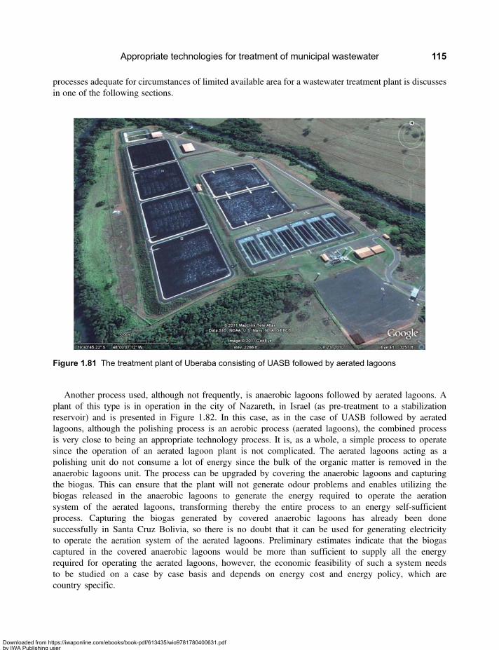
processes adequate for circumstances of limited available area for a wastewater treatment plant is discussesin one of the following sections.

Another process used, although not frequently, is anaerobic lagoons followed by aerated lagoons. Aplant of this type is in operation in the city of Nazareth, in Israel (as pre-treatment to a stabilizationreservoir) and is presented in Figure 1.82. In this case, as in the case of UASB followed by aeratedlagoons, although the polishing process is an aerobic process (aerated lagoons), the combined processis very close to being an appropriate technology process. It is, as a whole, a simple process to operatesince the operation of an aerated lagoon plant is not complicated. The aerated lagoons acting as apolishing unit do not consume a lot of energy since the bulk of the organic matter is removed in theanaerobic lagoons unit. The process can be upgraded by covering the anaerobic lagoons and capturingthe biogas. This can ensure that the plant will not generate odour problems and enables utilizing thebiogas released in the anaerobic lagoons to generate the energy required to operate the aerationsystem of the aerated lagoons, transforming thereby the entire process to an energy self-sufficientprocess. Capturing the biogas generated by covered anaerobic lagoons has already been donesuccessfully in Santa Cruz Bolivia, so there is no doubt that it can be used for generating electricityto operate the aeration system of the aerated lagoons. Preliminary estimates indicate that the biogascaptured in the covered anaerobic lagoons would be more than sufficient to supply all the energyrequired for operating the aerated lagoons, however, the economic feasibility of such a system needsto be studied on a case by case basis and depends on energy cost and energy policy, which arecountry specific.

Figure 1.81 The treatment plant of Uberaba consisting of UASB followed by aerated lagoons



The system of anaerobic lagoons followed by aerated lagoons is quite efficient in removing organicmatter. A full scale plant of this type serving a population of about 250,000 was operated in Santiago,Chile, and was used for investigation. This was the Santiago Poniente plant (which does not existanymore since the site was used to construct the La Farfana Activated sludge treatment plant whichserves most of Santiago). The Santiago poniente plant had a system of anaerobic lagoons followed byaerated lagoons whose effluent was discharged to a stabilization reservoir. The combined process ofanaerobic lagoon followed by aerated lagoons achieved 90% removal of soluble BOD and 60% removalof Total BOD. That means that most of the BOD was removed from the liquid phase. If the effluent ofsuch an aerated lagoon is deposited in a settling pond or a series of settling ponds (similar to what isdone in Uberaba) the suspended matter, which is basically the bacterial biomass developed in the firstaerated lagoon, would have settled out and undergo anaerobic decomposition. The system as a wholewould achieve a Total BOD removal of about 90% and the effluent of the final settling pond would be ahigh quality effluent.

1.9.2 Additional potential combined processesAdditional combined appropriate technology processes for treatment of municipal wastewater include:

– Preliminary Treatment followed by UASB followed by Sand Filtration and if required,Disinfection. The schematic flow diagram of this process is presented in Figure 1.83. This is asimple process which occupies a small area. The sand filter will capture and remove most ofthe solids contained in the UASB effluent, so the final effluent will be clear. The removal oftotal of BOD will be medium to high and the removal of total Suspended Solids will be high.Coagulants and/or Flocculants need to be injected to the UASB effluent to achieve an efficientfiltration. The biogas generated in the UASB reactor can be collected and put to use, ifeconomically feasible.

Figure 1.82 The pre-treatment unit of the wastewater treatment plant of Nazareth consisting of anaerobiclagoons followed by aerated lagoons



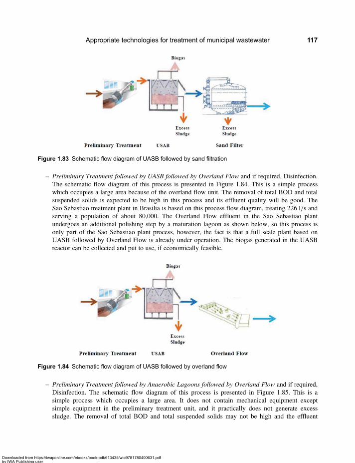
– Preliminary Treatment followed by UASB followed by Overland Flow and if required, Disinfection.The schematic flow diagram of this process is presented in Figure 1.84. This is a simple processwhich occupies a large area because of the overland flow unit. The removal of total BOD and totalsuspended solids is expected to be high in this process and its effluent quality will be good. TheSao Sebastiao treatment plant in Brasilia is based on this process flow diagram, treating 226 l/s andserving a population of about 80,000. The Overland Flow effluent in the Sao Sebastiao plantundergoes an additional polishing step by a maturation lagoon as shown below, so this process isonly part of the Sao Sebastiao plant process, however, the fact is that a full scale plant based onUASB followed by Overland Flow is already under operation. The biogas generated in the UASBreactor can be collected and put to use, if economically feasible.

– Preliminary Treatment followed by Anaerobic Lagoons followed by Overland Flow and if required,Disinfection. The schematic flow diagram of this process is presented in Figure 1.85. This is asimple process which occupies a large area. It does not contain mechanical equipment exceptsimple equipment in the preliminary treatment unit, and it practically does not generate excesssludge. The removal of total BOD and total suspended solids may not be high and the effluent

Figure 1.83 Schematic flow diagram of UASB followed by sand filtration

Figure 1.84 Schematic flow diagram of UASB followed by overland flow



quality may not be the highest, but the effluent will be of decent quality and if using a very simple, lowcost and easy to operate process is the objective, this process is a good candidate. The anaerobic lagooncan be a covered lagoon so the process will not cause nuisance, and the collected biogas can be put touse, if economically feasible.

– Preliminary Treatment followed by Anaerobic Filter followed by Overland Flow and if required,Disinfection. The schematic flow diagram of this process is presented in Figure 1.86. This is asimple process which occupies a large area. It does not contain mechanical equipment exceptsimple equipment in the preliminary treatment unit. The preliminary treatment often used prior toan anaerobic filter is a septic tank, and this can be a good solution for treatment plants of smallcommunities. The removal of total BOD and total suspended solids in this process will bereasonably high and the effluent quality will be high. The biogas generated in the anaerobic filtercan be collected and put to use, if economically feasible.

– Preliminary Treatment followed by UASB followed by Constructed Wetlands and if required,Disinfection. The schematic flow diagram of this process is presented in Figure 1.87. This is asimple process which occupies a large area due to the constructed wetlands unit. It does not containmechanical equipment except simple equipment in the preliminary treatment unit. According to

Figure 1.86 Schematic flow diagram of anaerobic filter followed by overland flow

Figure 1.85 Schematic flow diagram of covered anaerobic lagoons followed by overland flow



Chernicharo (2007) this process achieves medium level removals of total COD and total suspendedsolids and achieves good removal of phosphorous and partial removal of nitrogen. The biogasgenerated in the UASB reactor can be collected and put to use, if economically feasible.

– Preliminary Treatment followed by UASB followed by Lagoons followed by Overland Flow and ifrequired, Disinfection. The schematic flow diagram of this process is presented in Figure 1.88. Thisis a simple process which occupies a very large area because of the lagoons and the overland flowunits. It does not contain mechanical equipment except simple equipment in the preliminarytreatment unit. This process is used in two plants in Brasilia, Brazil: the Alagado plant and the SantaMaria plant. Each of them is designed to handle an average flow of 154 l/s and serve a populationof 85,000. These plants achieve a Total BOD removal of about 85% and a total suspended solidsremoval of about 80%. The biogas generated in the UASB reactor can be collected and put to use, ifeconomically feasible. Mixers can be installed in the lagoons to improve performance and reducetheir area. A satellite photo of the Alagado plant is presented in Figure 1.89. In addition to thepreliminary treatment installations the Alagado plant consists of 4 UASB reactors located at thebottom of the photo. The effluent of the UASB reactors flows into a series of 13 high rate lagoonslocated at the left hand side of the photo and the effluent of the lagoons flows into the overland flowarea at the right hand side of the photo. The SantaMaria plant is similar in its layout to theAlagado plant.

Figure 1.87 Schematic flow diagram of UASB followed by constructed wetlands

Figure 1.88 Schematic flow diagram of UASB followed by lagoons followed by overland flow



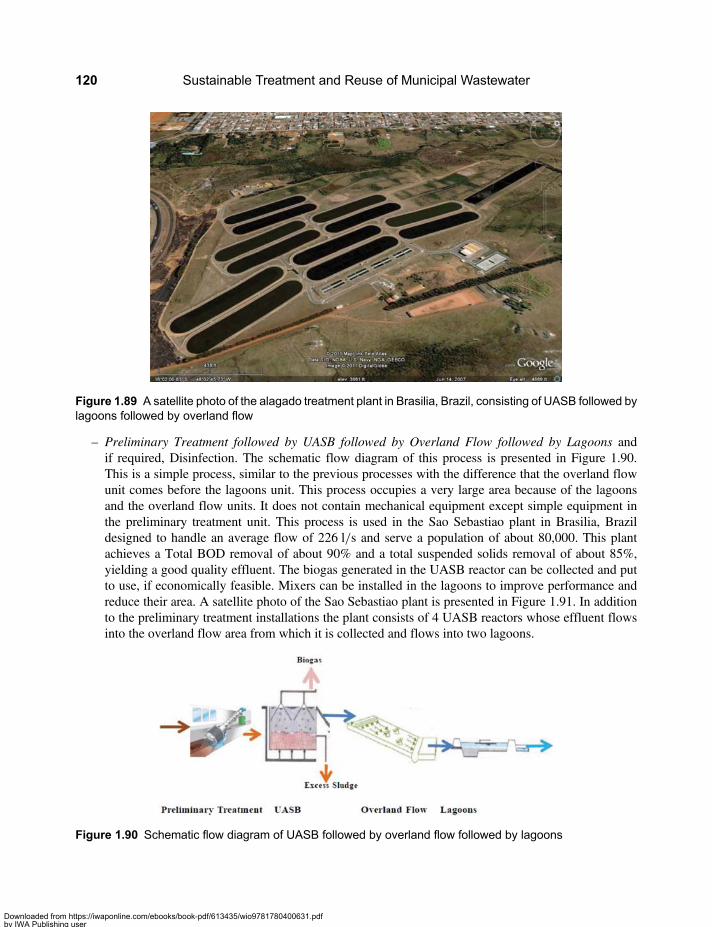
– Preliminary Treatment followed by UASB followed by Overland Flow followed by Lagoons andif required, Disinfection. The schematic flow diagram of this process is presented in Figure 1.90.This is a simple process, similar to the previous processes with the difference that the overland flowunit comes before the lagoons unit. This process occupies a very large area because of the lagoonsand the overland flow units. It does not contain mechanical equipment except simple equipment inthe preliminary treatment unit. This process is used in the Sao Sebastiao plant in Brasilia, Brazildesigned to handle an average flow of 226 l/s and serve a population of about 80,000. This plantachieves a Total BOD removal of about 90% and a total suspended solids removal of about 85%,yielding a good quality effluent. The biogas generated in the UASB reactor can be collected and putto use, if economically feasible. Mixers can be installed in the lagoons to improve performance andreduce their area. A satellite photo of the Sao Sebastiao plant is presented in Figure 1.91. In additionto the preliminary treatment installations the plant consists of 4 UASB reactors whose effluent flowsinto the overland flow area from which it is collected and flows into two lagoons.

Figure 1.89 A satellite photo of the alagado treatment plant in Brasilia, Brazil, consisting of UASB followed bylagoons followed by overland flow

Figure 1.90 Schematic flow diagram of UASB followed by overland flow followed by lagoons



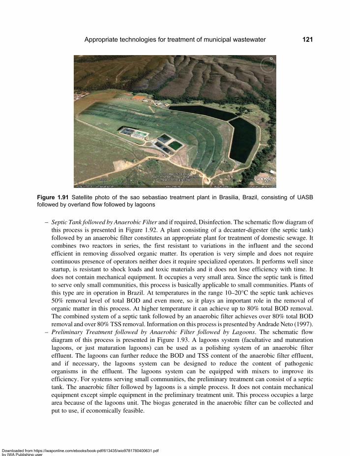
– Septic Tank followed by Anaerobic Filter and if required, Disinfection. The schematic flow diagram ofthis process is presented in Figure 1.92. A plant consisting of a decanter-digester (the septic tank)followed by an anaerobic filter constitutes an appropriate plant for treatment of domestic sewage. Itcombines two reactors in series, the first resistant to variations in the influent and the secondefficient in removing dissolved organic matter. Its operation is very simple and does not requirecontinuous presence of operators neither does it require specialized operators. It performs well sincestartup, is resistant to shock loads and toxic materials and it does not lose efficiency with time. Itdoes not contain mechanical equipment. It occupies a very small area. Since the septic tank is fittedto serve only small communities, this process is basically applicable to small communities. Plants ofthis type are in operation in Brazil. At temperatures in the range 10–20°C the septic tank achieves50% removal level of total BOD and even more, so it plays an important role in the removal oforganic matter in this process. At higher temperature it can achieve up to 80% total BOD removal.The combined system of a septic tank followed by an anaerobic filter achieves over 80% total BODremoval and over 80% TSS removal. Information on this process is presented by Andrade Neto (1997).

– Preliminary Treatment followed by Anaerobic Filter followed by Lagoons. The schematic flowdiagram of this process is presented in Figure 1.93. A lagoons system (facultative and maturationlagoons, or just maturation lagoons) can be used as a polishing system of an anaerobic filtereffluent. The lagoons can further reduce the BOD and TSS content of the anaerobic filter effluent,and if necessary, the lagoons system can be designed to reduce the content of pathogenicorganisms in the effluent. The lagoons system can be equipped with mixers to improve itsefficiency. For systems serving small communities, the preliminary treatment can consist of a septictank. The anaerobic filter followed by lagoons is a simple process. It does not contain mechanicalequipment except simple equipment in the preliminary treatment unit. This process occupies a largearea because of the lagoons unit. The biogas generated in the anaerobic filter can be collected andput to use, if economically feasible.

Figure 1.91 Satellite photo of the sao sebastiao treatment plant in Brasilia, Brazil, consisting of UASBfollowed by overland flow followed by lagoons



– Preliminary Treatment followed by Anaerobic Filter followed by Sand Filter and if required,Disinfection. The flow diagram of this process is presented in Figure 1.94. A Sand filter can beused to polish an anaerobic filter effluent, basically, to reduce suspended solids and with that toreduce also the BOD content of the effluent. This process occupies a very small area. For systemsserving small communities, the preliminary treatment can consist of a septic tank. It is a simpleprocess and it can produce a good quality effluent. The biogas generated in the anaerobic Filter canbe collected and put to use, if economically feasible.

– Preliminary Treatment followed by Anaerobic Filter followed by DAF and if required, Disinfection.The schematic flow diagram of this process is presented in Figure 1.95. A Dissolved Air Flotation(DAF) unit can be used to polish an anaerobic filter effluent, basically, to reduce suspended solidsand with that to reduce also the BOD content of the effluent. This process occupies a very smallarea. For systems serving small communities, the preliminary treatment can consist of a septic tank.It is a simple process and it can produce a good quality effluent. The biogas generated in theanaerobic filter can be collected and put to use, if economically feasible.

Figure 1.93 Schematic flow diagram of anaerobic filter followed by lagoons

Figure 1.92 Schematic flow diagram of septic tank followed by anaerobic filter



– Preliminary Treatment followed by Anaerobic Filter followed by Constructed Wetlands and ifrequired, Disinfection. The schematic flow diagram of this process is presented in Figure 1.96. Aconstructed wetlands unit can be used to polish an anaerobic filter effluent to reduce suspendedsolids and with that to reduce also the BOD content of the effluent. This process occupies a largearea because of the constructed wetlands. For systems serving small communities, the preliminarytreatment can consist of a septic tank. It is a simple process and it can produce a good qualityeffluent. The biogas generated in the anaerobic filter can be collected and put to use, ifeconomically feasible.

– Septic Tank followed by Constructed Wetlands and if required, Disinfection. This process can be usedonly in small communities because of the septic tank which is fitted to serve only such communities.This is the most frequently used process configuration involving constructed wetlands for smallcommunities. The septic tank is an anaerobic reactor which removes a significant part of theorganic matter from the raw sewage and the constructed wetlands remove an additional part. Theprocess is simple to operate. It does not contain mechanical equipment and yield a good quality

Figure 1.95 Schematic flow diagram of anaerobic filter followed by DAF

Figure 1.94 A schematic flow diagram of anaerobic filter followed by sand filter



effluent. A photo of a plant of this type is presented in Figure 1.35. The WSP (2008) publicationprovides ample information on this process.

– Preliminary Treatment followed by Anaerobic Lagoons followed by Anaerobic Filter and if required,Disinfection. The schematic flow diagram of this process is presented in Figure 1.97. An anaerobicfilter unit is used in this process to polish an anaerobic lagoons effluent to remove additionaldissolved and suspended organic matter as well as suspended solids. This process occupies arelatively small area. It is a simple process, does not contain mechanical equipment except for asmall amount in the preliminary treatment unit, and it can produce a good quality effluent. Theanaerobic lagoons can be covered to reduce environmental nuisance and collect the biogas. Thebiogas generated in the anaerobic lagoons and in the anaerobic filter can be collected and put touse, if economically feasible.

– Preliminary Treatment followed by Anaerobic Lagoons followed by Anaerobic Filter followed bySand Filter and if required, Disinfection. The schematic flow diagram of this process is presentedin Figure 1.98. This is a process similar to the previous one, with a sand filter unit added to

Figure 1.96 Schematic flow diagram of anaerobic filter followed by constructed wetlands

Figure 1.97 Schematic flow diagram of covered anaerobic lagoons followed by anaerobic filter



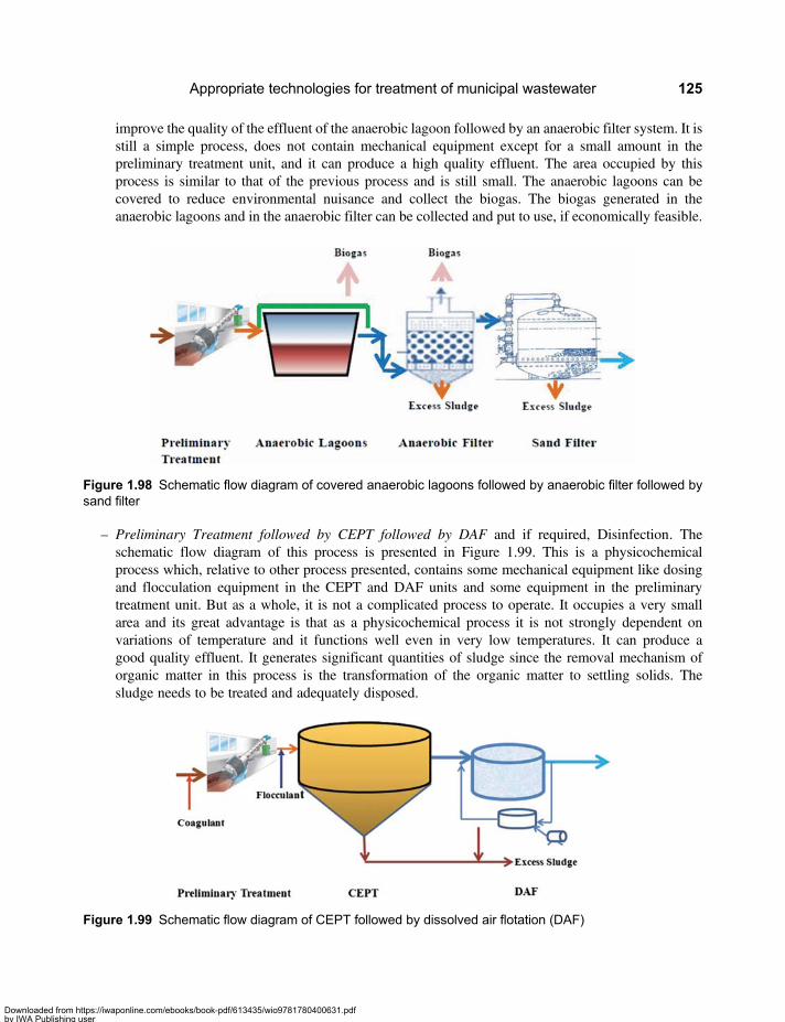
improve the quality of the effluent of the anaerobic lagoon followed by an anaerobic filter system. It isstill a simple process, does not contain mechanical equipment except for a small amount in thepreliminary treatment unit, and it can produce a high quality effluent. The area occupied by thisprocess is similar to that of the previous process and is still small. The anaerobic lagoons can becovered to reduce environmental nuisance and collect the biogas. The biogas generated in theanaerobic lagoons and in the anaerobic filter can be collected and put to use, if economically feasible.

– Preliminary Treatment followed by CEPT followed by DAF and if required, Disinfection. Theschematic flow diagram of this process is presented in Figure 1.99. This is a physicochemicalprocess which, relative to other process presented, contains some mechanical equipment like dosingand flocculation equipment in the CEPT and DAF units and some equipment in the preliminarytreatment unit. But as a whole, it is not a complicated process to operate. It occupies a very smallarea and its great advantage is that as a physicochemical process it is not strongly dependent onvariations of temperature and it functions well even in very low temperatures. It can produce agood quality effluent. It generates significant quantities of sludge since the removal mechanism oforganic matter in this process is the transformation of the organic matter to settling solids. Thesludge needs to be treated and adequately disposed.

Figure 1.98 Schematic flow diagram of covered anaerobic lagoons followed by anaerobic filter followed bysand filter

Figure 1.99 Schematic flow diagram of CEPT followed by dissolved air flotation (DAF)



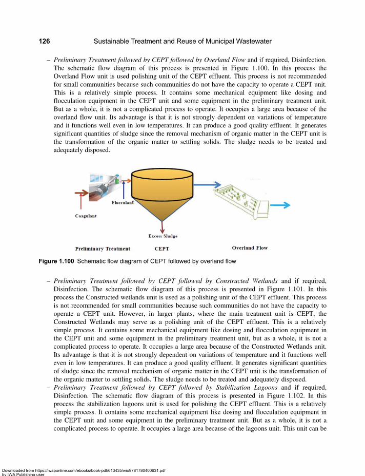
– Preliminary Treatment followed by CEPT followed by Overland Flow and if required, Disinfection.The schematic flow diagram of this process is presented in Figure 1.100. In this process theOverland Flow unit is used polishing unit of the CEPT effluent. This process is not recommendedfor small communities because such communities do not have the capacity to operate a CEPT unit.This is a relatively simple process. It contains some mechanical equipment like dosing andflocculation equipment in the CEPT unit and some equipment in the preliminary treatment unit.But as a whole, it is not a complicated process to operate. It occupies a large area because of theoverland flow unit. Its advantage is that it is not strongly dependent on variations of temperatureand it functions well even in low temperatures. It can produce a good quality effluent. It generatessignificant quantities of sludge since the removal mechanism of organic matter in the CEPT unit isthe transformation of the organic matter to settling solids. The sludge needs to be treated andadequately disposed.

– Preliminary Treatment followed by CEPT followed by Constructed Wetlands and if required,Disinfection. The schematic flow diagram of this process is presented in Figure 1.101. In thisprocess the Constructed wetlands unit is used as a polishing unit of the CEPT effluent. This processis not recommended for small communities because such communities do not have the capacity tooperate a CEPT unit. However, in larger plants, where the main treatment unit is CEPT, theConstructed Wetlands may serve as a polishing unit of the CEPT effluent. This is a relativelysimple process. It contains some mechanical equipment like dosing and flocculation equipment inthe CEPT unit and some equipment in the preliminary treatment unit, but as a whole, it is not acomplicated process to operate. It occupies a large area because of the Constructed Wetlands unit.Its advantage is that it is not strongly dependent on variations of temperature and it functions welleven in low temperatures. It can produce a good quality effluent. It generates significant quantitiesof sludge since the removal mechanism of organic matter in the CEPT unit is the transformation ofthe organic matter to settling solids. The sludge needs to be treated and adequately disposed.

– Preliminary Treatment followed by CEPT followed by Stabilization Lagoons and if required,Disinfection. The schematic flow diagram of this process is presented in Figure 1.102. In thisprocess the stabilization lagoons unit is used for polishing the CEPT effluent. This is a relativelysimple process. It contains some mechanical equipment like dosing and flocculation equipment inthe CEPT unit and some equipment in the preliminary treatment unit. But as a whole, it is not acomplicated process to operate. It occupies a large area because of the lagoons unit. This unit can be

Figure 1.100 Schematic flow diagram of CEPT followed by overland flow



a complete lagoons system consisting of anaerobic lagoons followed by facultative lagoons followed bymaturation lagoons, or a partial lagoons system consisting of facultative and maturation lagoons. Thefacultative lagoons may be equipped with mixers to improve their performance and reduce their size. Itcan produce a good quality effluent. It generates significant quantities of sludge since the removalmechanism of organic matter in the CEPT unit is the transformation of the organic matter to settlingsolids. The sludge needs to be treated and adequately disposed.

The CEPT followed by Lagoons process is used in the treatment plant of the city Riviera SaoLourenco (Tsukamoto, 2002) which is a vacation resort on the Atlantic coast of the state of SaoPaulo, Brazil, not far from the state’s capital Sao Paulo. Originally, the wastewater treatment systemof the city consisted of a conventional lagoon system with a capacity of handling the wastewater of32,000 persons. The system has a pretreatment unit, an anaerobic lagoon of 7,200 m2, three parallelfacultative lagoons (12,000 m2, 17,000 m2, and 18,000 m2) and an effluent chlorination system.During the summer season the population of Riviera Sao Lourenco increases significantly becauseof tourism. That results in increased wastewater flows and organic matter loads. All the lagoonsbecame strongly anaerobic and generated odours which reached the city, 3 km away. The problemswere resolved by adding two CEPT units between the preliminary treatment and the anaerobiclagoon. The sedimentation tank of each unit has an area of 180 m2 and a capacity for treating thewastewater of 40,000 persons, increasing thereby the treatment capacity by 250%. The upgradedplant functioned successfully when the population increased from 7,000 to 65,000 during a period of

Figure 1.101 Schematic flow diagram of CEPT followed by constructed wetlands

Figure 1.102 Schematic flow diagram of CEPT followed by stabilization lagoons



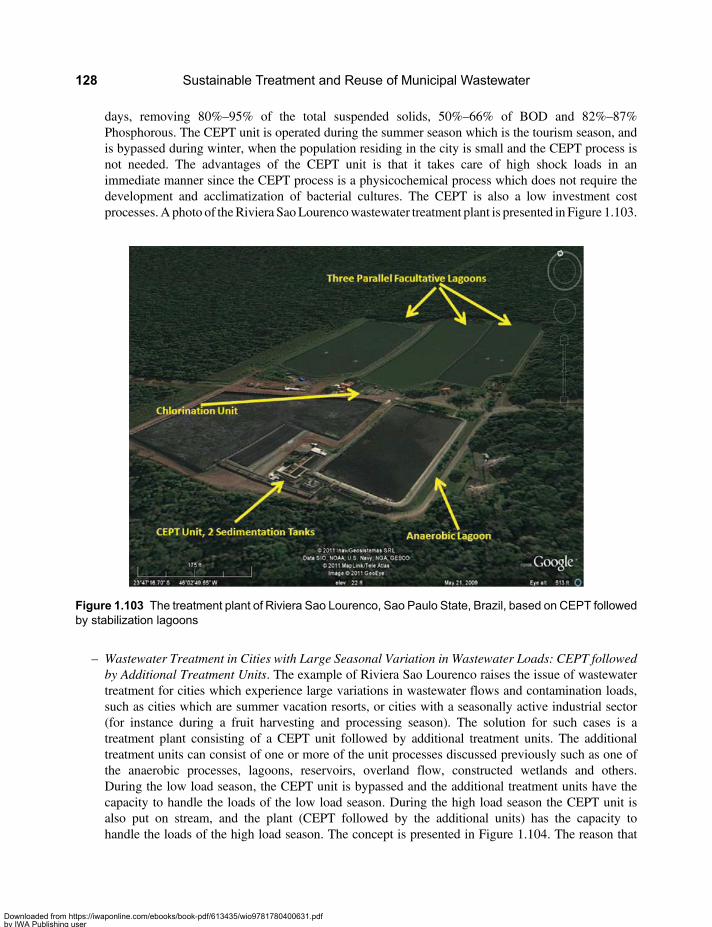
days, removing 80%–95% of the total suspended solids, 50%–66% of BOD and 82%–87%Phosphorous. The CEPT unit is operated during the summer season which is the tourism season, andis bypassed during winter, when the population residing in the city is small and the CEPT process isnot needed. The advantages of the CEPT unit is that it takes care of high shock loads in animmediate manner since the CEPT process is a physicochemical process which does not require thedevelopment and acclimatization of bacterial cultures. The CEPT is also a low investment costprocesses.A photo of theRiviera SaoLourencowastewater treatment plant is presented in Figure 1.103.

– Wastewater Treatment in Cities with Large Seasonal Variation in Wastewater Loads: CEPT followedby Additional Treatment Units. The example of Riviera Sao Lourenco raises the issue of wastewatertreatment for cities which experience large variations in wastewater flows and contamination loads,such as cities which are summer vacation resorts, or cities with a seasonally active industrial sector(for instance during a fruit harvesting and processing season). The solution for such cases is atreatment plant consisting of a CEPT unit followed by additional treatment units. The additionaltreatment units can consist of one or more of the unit processes discussed previously such as one ofthe anaerobic processes, lagoons, reservoirs, overland flow, constructed wetlands and others.During the low load season, the CEPT unit is bypassed and the additional treatment units have thecapacity to handle the loads of the low load season. During the high load season the CEPT unit isalso put on stream, and the plant (CEPT followed by the additional units) has the capacity tohandle the loads of the high load season. The concept is presented in Figure 1.104. The reason that

Figure 1.103 The treatment plant of Riviera Sao Lourenco, Sao Paulo State, Brazil, based on CEPT followedby stabilization lagoons



the CEPT followed by additional units is the adequate process is that in vacation resort cities, thepopulation can grow tenfold within a short period, during the vacation season and holydays. Theincrease in population can occur during a short time causing sharp peaks in wastewater flows.Biological treatment processes are incapable of handling sharp oscillations in wastewater loadsbecause they needs to develop the biomass capable of handling the peaks and that takes time. TheCEPT, which is a physicochemical process, has the capacity to handle the increased loads within ashort time. The application of the concept of Figure 1.104 to the case of Riviera Sao Lourencoyielded the flow diagram of the Treatment plant of this city presented in Figure 1.105.

The concept presented in Figure 1.104 can also be used in treatment plants located in zones with avery cold low temperature season (and in this case, without sharp seasonal variations of wastewaterloads). During the high and medium temperature seasons the CEPT unit is bypassed and theadditional treatment units, which are basically biological treatment units, have the capacity to treatthe wastewater. During the low temperature season the capacity of the biological treatment units

Figure 1.104 A treatment process concept adequate for cities with sharp seasonal variation of wastewaterflows or organic matter loads

Figure 1.105 The treatment process of Riviera Sao Lourenco (Source: Prof. Harleman, MIT, 2004)



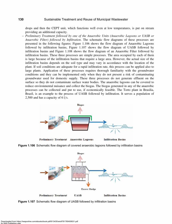
drops and then the CEPT unit, which functions well even at low temperatures, is put on streamproviding an additional capacity.

– Preliminary Treatment followed by one of the Anaerobic Units (Anaerobic Lagoons or UASB orAnaerobic Filter) followed by Infiltration. The schematic flow diagrams of these processes arepresented in the following figures: Figure 1.106 shows the flow diagram of Anaerobic Lagoonsfollowed by infiltration basins, Figure 1.107 shows the flow diagram of UASB followed byinfiltration basins and Figure 1.108 shows the flow diagram of an Anaerobic Filter followed byinfiltration basins. These three processes are simple processes. The area occupied by each of themis large because of the infiltration basins that require a large area. However, the actual size of theinfiltration basins depends on the soil type and may vary in accordance with the location of theplant. If soil conditions are adequate for a rapid infiltration rate, this process can be applied also tolarge plants. Application of these processes requires thorough familiarity with the groundwaterconditions and they can be implemented only when they do not present a risk of contaminatinggroundwater used for domestic supply. These three processes do not generate effluent on thesurface so they do not contaminate surface water bodies. The anaerobic lagoons can be covered toreduce environmental nuisance and collect the biogas. The biogas generated in any of the anaerobicprocesses can be collected and put to use, if economically feasible. The Torto plant in Brasilia,Brazil, is an example to the process of UASB followed by infiltration. It serves a population of2,500 and has a capacity of 6 l/s.

Figure 1.106 Schematic flow diagram of covered anaerobic lagoons followed by infiltration basins

Figure 1.107 Schematic flow diagram of UASB followed by infiltration basins



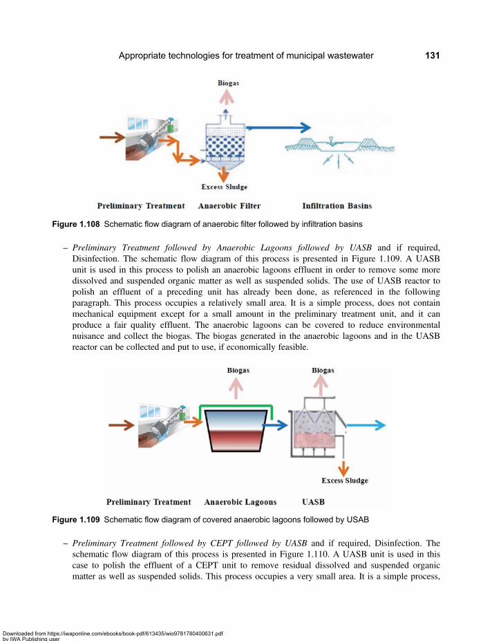
– Preliminary Treatment followed by Anaerobic Lagoons followed by UASB and if required,Disinfection. The schematic flow diagram of this process is presented in Figure 1.109. A UASBunit is used in this process to polish an anaerobic lagoons effluent in order to remove some moredissolved and suspended organic matter as well as suspended solids. The use of UASB reactor topolish an effluent of a preceding unit has already been done, as referenced in the followingparagraph. This process occupies a relatively small area. It is a simple process, does not containmechanical equipment except for a small amount in the preliminary treatment unit, and it canproduce a fair quality effluent. The anaerobic lagoons can be covered to reduce environmentalnuisance and collect the biogas. The biogas generated in the anaerobic lagoons and in the UASBreactor can be collected and put to use, if economically feasible.

– Preliminary Treatment followed by CEPT followed by UASB and if required, Disinfection. Theschematic flow diagram of this process is presented in Figure 1.110. A UASB unit is used in thiscase to polish the effluent of a CEPT unit to remove residual dissolved and suspended organicmatter as well as suspended solids. This process occupies a very small area. It is a simple process,

Figure 1.108 Schematic flow diagram of anaerobic filter followed by infiltration basins

Figure 1.109 Schematic flow diagram of covered anaerobic lagoons followed by USAB



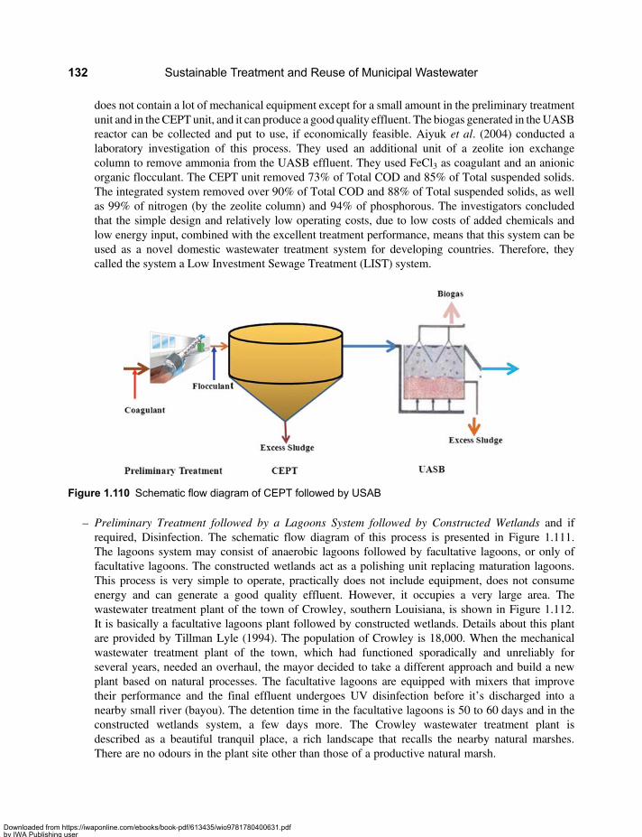
does not contain a lot of mechanical equipment except for a small amount in the preliminary treatmentunit and in the CEPT unit, and it can produce a good quality effluent. The biogas generated in theUASBreactor can be collected and put to use, if economically feasible. Aiyuk et al. (2004) conducted alaboratory investigation of this process. They used an additional unit of a zeolite ion exchangecolumn to remove ammonia from the UASB effluent. They used FeCl3 as coagulant and an anionicorganic flocculant. The CEPT unit removed 73% of Total COD and 85% of Total suspended solids.The integrated system removed over 90% of Total COD and 88% of Total suspended solids, as wellas 99% of nitrogen (by the zeolite column) and 94% of phosphorous. The investigators concludedthat the simple design and relatively low operating costs, due to low costs of added chemicals andlow energy input, combined with the excellent treatment performance, means that this system can beused as a novel domestic wastewater treatment system for developing countries. Therefore, theycalled the system a Low Investment Sewage Treatment (LIST) system.

– Preliminary Treatment followed by a Lagoons System followed by Constructed Wetlands and ifrequired, Disinfection. The schematic flow diagram of this process is presented in Figure 1.111.The lagoons system may consist of anaerobic lagoons followed by facultative lagoons, or only offacultative lagoons. The constructed wetlands act as a polishing unit replacing maturation lagoons.This process is very simple to operate, practically does not include equipment, does not consumeenergy and can generate a good quality effluent. However, it occupies a very large area. Thewastewater treatment plant of the town of Crowley, southern Louisiana, is shown in Figure 1.112.It is basically a facultative lagoons plant followed by constructed wetlands. Details about this plantare provided by Tillman Lyle (1994). The population of Crowley is 18,000. When the mechanicalwastewater treatment plant of the town, which had functioned sporadically and unreliably forseveral years, needed an overhaul, the mayor decided to take a different approach and build a newplant based on natural processes. The facultative lagoons are equipped with mixers that improvetheir performance and the final effluent undergoes UV disinfection before it’s discharged into anearby small river (bayou). The detention time in the facultative lagoons is 50 to 60 days and in theconstructed wetlands system, a few days more. The Crowley wastewater treatment plant isdescribed as a beautiful tranquil place, a rich landscape that recalls the nearby natural marshes.There are no odours in the plant site other than those of a productive natural marsh.

Figure 1.110 Schematic flow diagram of CEPT followed by USAB



– Preliminary Treatment followed by one of the Anaerobic Units (Anaerobic Lagoons or UASBor Anaerobic Filter) followed by Aerated Lagoons, and if required, by Disinfection. The schematicflow diagrams of these processes are presented in the following figures: Figure 1.113 shows the flowdiagram of Anaerobic Lagoons followed by Aerated Lagoons; Figure 1.114 shows the flow diagramof UASB followed by Aerated Lagoons and Figure 1.115 shows the flow diagram of an AnaerobicFilter followed by Aerated Lagoons. As explained in a previous section, when an aerated lagoon isused for polishing of the effluent of a preceding unit process, it can be considered as an appropriatetreatment technology unit process since it does not consume a lot of energy and its operation is

Figure 1.112 The treatment plant of Crowley, Louisiana, based on facultative lagoons followed byconstructed wetlands

Figure 1.111 Schematic flow diagram of lagoons system followed by constructed wetlands



simple. The three processes contain some equipment which is the aeration equipment in the aeratedlagoons, but this is simple equipment. The area occupied by each one of the three processes is ofmedium size. The anaerobic unit of each process occupied a small area, but the aerated lagoonsoccupy a larger area, since the detention time in these lagoons is 2–4 days. In the flow diagrams aseries of two aerated lagoons is presented, the first one with more intensive aeration and the secondone with partial aeration. The use of two aerated lagoons in series is a sound approach. In the firstone, the residual organic matter is decomposed and in the second one, which is a facultative lagoon,the biomass created in the aerated lagoons settles down to the bottom of the lagoon and undergoes ananaerobic decomposition process, so the aerated lagoons do not produce a lot of sludge and do notneed to be cleaned frequently. Each of the three processes can produce a good quality effluent.Although the use of two aerated lagoons in series is beneficial, the second lagoon can be omitted, butin such a case the effluent will be of lower quality. It is also recommended to install in the aeratedlagoons mixers since the combination of mixers and aerators produces better results. In each of theflow diagram figures of the three processes the aeration system is portrayed as consisting of floatingsurface aerators, but it can also be a fine bubble aeration system. Today there are very efficient finebubble aeration systems which can be employed in the aerated lagoons. In the process whichincludes anaerobic lagoons, these lagoons can be covered to reduce environmental nuisance andcollect the biogas. The biogas generated in each of the three anaerobic processes can be collected andput to use, if economically feasible. Preliminary estimates indicate that the biogas captured in each ofthe anaerobic processes would be more than sufficient to supply all the energy required for operatingthe aerated lagoons, however, the economic feasibility of such a system needs to be studied ona case by case basis and depends on local energy cost and energy policy, which are country specific.If the captured biogas can be used in an economically feasible fashion to generate the energyrequired to operate the aeration system of the aerated lagoons, the entire process becomes an energyself-sufficient process. This has not yet been done in a full scale plant but we believe it can be done.

Theprocess of anaerobic lagoons followedbyaerated lagoons is not a newprocess. Thephotoof sucha treatment plant is presented in Figure 1.82 which shows part of the treatment plant of the city ofNazareth. As seen in the figure, the system consists of two sets of aerated lagoons, the first one withhigh aeration intensity and the second with lower aeration intensity. The aeration method used isfloating surface aerators. Figure 1.116a presents a photo of the Carapongo treatment plant locatednear Lima, Peru, which consists of covered anaerobic lagoons followed by aerated lagoons. The

Figure 1.113 Schematic flow diagram of covered anaerobic lagoons followed by aerated lagoons



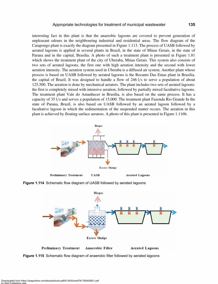
interesting fact in this plant is that the anaerobic lagoons are covered to prevent generation ofunpleasant odours in the neighbouring industrial and residential areas. The flow diagram of theCarapongo plant is exactly the diagram presented in Figure 1.113. The process of UASB followed byaerated lagoons is applied in several plants in Brazil, in the state of Minas Gerais, in the state ofParana and in the capital, Brasilia. A photo of such a treatment plant is presented in Figure 1.81which shows the treatment plant of the city of Uberaba, Minas Gerais. This system also consists oftwo sets of aerated lagoons, the first one with high aeration intensity and the second with loweraeration intensity. The aeration system used in Uberaba is a diffused air system. Another plant whoseprocess is based on UASB followed by aerated lagoons is the Recanto Das Emas plant in Brasilia,the capital of Brazil. It was designed to handle a flow of 246 l/s to serve a population of about125,500. The aeration is done by mechanical aerators. The plant includes two sets of aerated lagoons:the first is completely mixed with intensive aeration, followed by partially mixed facultative lagoons.The treatment plant Vale do Amanhecer in Brasilia, is also based on the same process. It has acapacity of 35 l/s and serves a population of 15,000. The treatment plant Fazenda Rio Grande In thestate of Parana, Brazil, is also based on UASB followed by an aerated lagoon followed by afacultative lagoon in which the sedimentation of the suspended matter occurs. The aeration in thisplant is achieved by floating surface aerators. A photo of this plant is presented in Figure 1.116b.

Figure 1.114 Schematic flow diagram of UASB followed by aerated lagoons

Figure 1.115 Schematic flow diagram of anaerobic filter followed by aerated lagoons



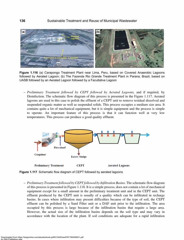
– Preliminary Treatment followed by CEPT followed by Aerated Lagoons, and if required, byDisinfection. The schematic flow diagram of this process is presented in the Figure 1.117. Aeratedlagoons are used in this case to polish the effluent of a CEPT unit to remove residual dissolved andsuspended organic matter as well as suspended solids. This process occupies a medium size area. Itcontains quite a lot of mechanical equipment, but it is simple equipment and the process is simpleto operate. An important feature of this process is that it can function well at very lowtemperatures. This process can produce a good quality effluent.

– Preliminary Treatment followed by CEPT followed by Infiltration Basins. The schematic flow diagramof this process is presented in Figure 1.118. It is a simple process, does not contain a lot of mechanicalequipment except for a small amount in the preliminary treatment unit and in the CEPT unit. Theeffluent produced by the CEPT unit is usually of a quality which can be infiltrated in rechargebasins. In cases where infiltration may present difficulties because of the type of soil, the CEPTeffluent can be polished by a Sand Filter unit or a DAF unit prior to the infiltration. The areaoccupied by this process is large because of the infiltration basins that require a large area.However, the actual size of the infiltration basins depends on the soil type and may vary inaccordance with the location of the plant. If soil conditions are adequate for a rapid infiltration

Figure 1.117 Schematic flow diagram of CEPT followed by aerated lagoons

Figure 1.116 (a) Carapongo Treatment Plant near Lima, Peru, based on Covered Anaerobic Lagoonsfollowed by Aerated Lagoon; (b) The Fazenda Rio Grande Treatment Plant in Parana, Brazil, based onUASB followed by an Aerated Lagoon followed by a Facultative Lagoon



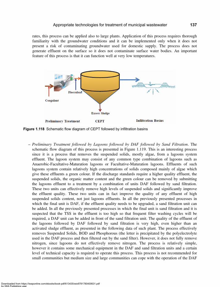
rates, this process can be applied also to large plants. Application of this process requires thoroughfamiliarity with the groundwater conditions and it can be implemented only when it does notpresent a risk of contaminating groundwater used for domestic supply. The process does notgenerate effluent on the surface so it does not contaminate surface water bodies. An importantfeature of this process is that it can function well at very low temperatures.

– Preliminary Treatment followed by Lagoons followed by DAF followed by Sand Filtration. Theschematic flow diagram of this process is presented in Figure 1.119. This is an interesting processsince it is a process that removes the suspended solids, mostly algae, from a lagoons systemeffluent. The lagoon system may consist of any common type combination of lagoons such asAnaerobic-Facultative-Maturation lagoons or Facultative-Maturation lagoons. Effluents of suchlagoons system contain relatively high concentrations of solids composed mainly of algae whichgive these effluents a green colour. If the discharge standards require a higher quality effluent, thesuspended solids, the organic matter content and the green colour can be removed by submittingthe lagoons effluent to a treatment by a combination of units DAF followed by sand filtration.These two units can effectively remove high levels of suspended solids and significantly improvethe effluent quality. These two units can in fact improve the quality of any effluent of highsuspended solids content, not just lagoons effluents. In all the previously presented processes inwhich the final unit is DAF, if the effluent quality needs to be upgraded, a sand filtration unit canbe added. In all the previously presented processes in which the final unit is sand filtration and it issuspected that the TSS in the effluent is too high so that frequent filter washing cycles will berequired, a DAF unit can be added in front of the sand filtration unit. The quality of the effluent ofthe lagoons followed by DAF followed by sand filtration is very high, even higher than anactivated sludge effluent, as presented in the following data of such plant. The process effectivelyremoves Suspended Solids, BOD and Phosphorous (the letter is precipitated by the polyelectrolyteused in the DAF process and then filtered out by the sand filter). However, it does not fully removenitrogen, since lagoons do not effectively remove nitrogen. The process is relatively simple,however it contains some mechanical equipment in the DAF and sand filtration units and a certainlevel of technical capacity is required to operate this process. This process is not recommended forsmall communities but medium size and large communities can cope with the operation of the DAF

Figure 1.118 Schematic flow diagram of CEPT followed by infiltration basins



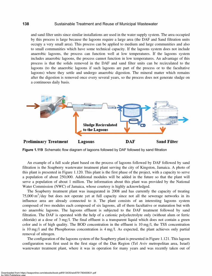
and sand filter units since similar installations are used in the water supply system. The area occupiedby this process is large because the lagoons require a large area (the DAF and Sand filtration unitsoccupy a very small area). This process can be applied to medium and large communities and alsoto small communities which have some technical capacity. If the lagoons system does not includeanaerobic lagoons, the process can function well at low temperatures. If the lagoons systemincludes anaerobic lagoons, the process cannot function in low temperatures. An advantage of thisprocess is that the solids removed in the DAF and sand filter units can be recirculated to thelagoons (to the anaerobic lagoons if such lagoons are part of the process or to the facultativelagoons) where they settle and undergo anaerobic digestion. The mineral matter which remainsafter the digestion is removed once every several years, so the process does not generate sludge ona continuous daily basis.

An example of a full scale plant based on the process of lagoons followed by DAF followed by sandfiltration is the Soapberry wastewater treatment plant serving the city of Kingston, Jamaica. A photo ofthis plant is presented in Figure 1.120. This plant is the first phase of the project, with a capacity to servea population of about 250,000. Additional modules will be added in the future so that the plant willserve a population of about 1 million. The information about this plant was provided by the NationalWater Commission (NWC) of Jamaica, whose courtesy is highly acknowledged.

The Soapberry treatment plant was inaugurated in 2008 and has currently the capacity of treating75,000 m3/day but does not operate yet at full capacity since not all the sewerage networks in itsinfluence area are already connected to it. The plant consists of an interesting lagoons systemcomposed of two modules each composed of six lagoons, all of them facultative or maturation but withno anaerobic lagoons. The lagoons effluent is subjected to the DAF treatment followed by sandfiltration. The DAF is operated with the help of a cationic polyelectrolyte only (without alum or ferricchloride) at a dose of 3 mg/l. The final effluent is a transparent liquid which does not contain a greencolor and is of high quality. The BOD concentration in the effluent is 10 mg/l, the TSS concentrationis 10 mg/l and the Phosphorous concentration is 4 mg/l. As expected, the plant achieves only partialremoval of nitrogen.

The configuration of the lagoons system of the Soapberry plant is presented in Figure 1.121. This lagoonconfiguration was first used in the first stage of the Dan Region (Tel Aviv metropolitan area, Israel)wastewater treatment plant, where it was in operation for many years and was recently taken out of

Figure 1.119 Schematic flow diagram of lagoons followed by DAF followed by sand filtration



stream. The idea in this plant is to keep all the lagoons with an aerobic top layer so as to prevent generation ofodours. The critical area in this respect is the first lagoon which receives the raw sewage, since in this lagoonthe organic load is the highest and the perspective of propagation of anaerobic conditions is high. To avoidthe generation of anaerobic conditions, the effluent of the final lagoon is recirculated to the raw sewage at arecirculation ratio of about 2:1 (effluent to raw sewage). The recirculated effluent contains highconcentration of oxygen and of algae and it also dilutes the raw sewage. So the liquid that enters thefirst lagoon is diluted, contains a high concentration of oxygen and high concentrations of algae whichimmediately start producing additional amounts of oxygen. All this prevents depletion of oxygen fromthe first lagoon (and from the following lagoons), maintains aerobic conditions and prevents propagationof odours. The solids removed in the DAF and sand filter units are recirculated to the lagoonswhere they settle and undergo anaerobic digestion at the bottom. The mineral matter which remains afterthe digestion is removed once every several years, so the process does not generate sludge on acontinuous daily basis. Sludge is only removed once every several years and this is also a great advantageof the process.

Figure 1.120 The Soapberry wastewater treatment plant in Kingston, Jamaica, based on a lagoons systemfollowed by DAF followed by sand filtration



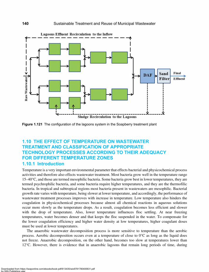
1.10 THE EFFECT OF TEMPERATURE ON WASTEWATERTREATMENT AND CLASSIFICATION OF APPROPRIATETECHNOLOGY PROCESSES ACCORDING TO THEIR ADEQUACYFOR DIFFERENT TEMPERATURE ZONES1.10.1 IntroductionTemperature is a very important environmental parameter that effects bacterial and physicochemical processactivities and therefore also effects wastewater treatment. Most bacteria grow well in the temperature range15–40°C, and those are termed mesophilic bacteria. Some bacteria grow best in lower temperatures, they aretermed psychrophilic bacteria, and some bacteria require higher temperatures, and they are the thermofilicbacteria. In tropical and subtropical regions most bacteria present in wastewaters are mesophilic. Bacterialgrowth rate varies with temperature, being slower at lower temperature, and accordingly, the performance ofwastewater treatment processes improves with increase in temperature. Low temperature also hinders thecoagulation in physicochemical processes because almost all chemical reactions in aqueous solutionsoccur more slowly as the temperature drops. As a result, coagulation becomes less efficient and slowerwith the drop of temperature. Also, lower temperature influences floc settling. At near freezingtemperatures, water becomes denser and that keeps the floc suspended in the water. To compensate forthe lower coagulation efficiency and higher water density at low temperatures, higher coagulant dosesmust be used at lower temperatures.

The anaerobic wastewater decomposition process is more sensitive to temperature than the aerobicprocess. Aerobic decomposition occurs even at a temperature of close to 0°C as long as the liquid doesnot freeze. Anaerobic decomposition, on the other hand, becomes too slow at temperatures lower than12°C. However, there is evidence that in anaerobic lagoons that remain long periods of time, during

Figure 1.121 The configuration of the lagoons system in the Soapberry treatment plant



months, under low temperatures (air temperature below zero), anaerobic activity does not seem to beadversely affected and the lagoons continue to function well, presumably because the anaerobic bacteriahave adjusted to long periods of low temperature. There is no such evidence in regards to the UASB andanaerobic filter processes but piston anaerobic reactors (PAR) are known to function well at lowtemperatures of about 12–13°C. The physicochemical processes also lose efficiency with the decline oftemperature, however, they still continue to function even at wastewater temperatures very close to zero,and their efficiency can be recovered by adjusting the doses and combination of coagulants andflocculants and, by adjusting the pH.

As to the performance of anaerobic lagoons under low temperature, there is evidence from the city of ElAlto in Bolivia, which is located at an altitude of about 4,000 meters above sea level in the Andean highlandsthat anaerobic lagoons function well at very low temperatures. During the low temperature season, airtemperatures in the El alto zone drop at night to −7°C. El alto has a large lagoons wastewater treatmentplant, the Puchukollo plant, consisting of anaerobic lagoons followed by facultative and maturationponds. The temperature in the anaerobic lagoons never drops below +7°C even when the air temperaturearound them is −7°C, and even at this temperature (+7°C) the anaerobic lagoons perform well andremove 60% of the BOD contained in the raw sewage. This happens presumably because the anaerobicbacteria have adjusted to long periods of low temperature, and perhaps it has to do with the higher solarradiation at high altitudes (which in El alto is double the radiation at sea level) which keeps the lagoonswarmer. This phenomenon has also been reported by Mara (2004) in reference to the highlands of Peru,but it cannot be considered a general phenomenon at all altitudes. Anaerobic lagoons are deep earthlagoons, usually of 4 meters depth or more. It seems that the heat loss from such lagoons is small, so thetemperature of the incoming raw sewage, which is much higher than the air temperature, tends to remainat the same level in the liquid inside the lagoon and not drop (probably because the temperature of thesoil around the lagoon is similar or even higher than the temperature of the raw wastewater). That helpsthe anaerobic decomposition process to continue functioning. It is estimated that covered anaerobiclagoons will maintain the heat even better than uncovered lagoons since the cover plastic sheets act asinsulators so the heat loss through the surface of the lagoons will be lower.

The effect of decreased efficiency of treatment processes at lower temperature must be taken into accountas part of the design of wastewater treatment plants and it is common practice to take into consideration theeffect of temperature when sizing the treatment units during the design process. Treatment plants aredesigned to achieve the required performance even during the low temperature season, that is, thevolumes of the biological reactors in treatment plants are designed for the critical conditions of thelowest temperatures in the locations of the treatment plants. Similarly, the physicochemical treatmentunits and the dosing systems of coagulants and flocculants are designed to cope with the lowtemperature conditions. In this section we expand the discussion on the effect of temperature to covertwo additional aspects: (i) the effect of temperature on appropriate technology processes; and (ii)tailoring the treatment process to the specific temperature conditions in the region in which the treatmentplant is located.

The general perception is that most of the developing countries are located in tropical and subtropicalregions in which the air temperatures are high and do not fall below 15–20°C even during the lowtemperature season. Such is the case of Central and South America, the Caribbean, Africa, the MiddleEast and large parts of Asia. However many developing countries are located in zones in which duringthe cold season air temperatures drop to low or very low values, way below zero, and consequently thetemperatures of the wastewater are also low and in some regions approach zero. Those include AndeanCountries in South America, countries in East Europe, Central Asia and in parts of China. In Some areasof China the air temperatures drop during wintertime to very low values of about −30°C. Given that



large populations reside in regions with seasonal low temperatures, we also need to present adequatewastewater treatment solution for such zones. In addition to regions with seasonal cold temperaturesthere are regions with perpetual cold temperatures, for example semi-polar zones or on high mountainszones like the Himalayas. However, the populations in such regions are not large so they are not of maininterest. Nevertheless, some of the treatment processes proposed for the regions with seasonal lowtemperature can be adjusted for perpetual low temperature regions. It is important to mention that thetemperature inertia of water makes it very difficult for the wastewater and the liquid in treatment plantsto vary by more than 4°C, even when great variation in air temperature occurs.

For any wastewater treatment process to keep functioning, the wastewater and the content of thebiological reactors and other treatment units in the treatment plant need to be liquid. If they freeze thetreatment processes stops functioning and the wastewater stops flowing. Mixers in the biological reactorsand other vessels in a treatment plant can prevent during periods of very low air temperatures thefreezing of liquids contained in them. There is a correlation between the air and wastewatertemperatures. In the high range temperatures (over 15°C), the air temperature is either higher than thewastewater temperatures or their temperatures are similar. But in the low range temperatures (below12°C), the wastewater temperature is higher than the air temperature. The relation between the airtemperature and the raw wastewater temperature (which is the temperature of the influent to thetreatment plant) is presented in Figure 1.122 which shows the variation of the air temperature, of thetemperature of the wastewater flowing into a constructed wetland plant and of the temperature ofthe effluent of this plant during a period of about two years in a constructed wetland treatment plant sitein Minnesota, USA (Wallace, 2007). During the cold season the air temperature in the site drops to−25°C (but the influent wastewater temperature keeps way above zero, in the range of +5°C to +10°C,most of the time closer to +10°C) and during the hot season the air temperature climbs to +30°C. Weuse here the mean air temperature of the coolest month of the year as the temperature indicator since airtemperature is a parameter meaningful to everybody, while wastewater temperature does not say much tomost people. But we bear in mind that there is a correlation between the two parameters (for instance,Wallace, 2007 seen in Figure 1.122) and this correlation is already taken into account when discussingthe adequate treatment processes for each temperature region.

For the purpose of discussing the effect of temperature on wastewater treatment we propose toconsider three types of temperature regions: (i) Regions type 1: are regions of very cold temperaturesin which the air temperatures drop during the cold season to below −3°C, (which would be roughlyequivalent to zones with low season wastewater temperatures in the range +1°C to +7°C); (ii)Region type 2: are regions of medium cold temperatures in which the air temperatures during thecold season remain above −3°C but below +7°C (which would be roughly equivalent to zones withlow season wastewater temperatures in the range +8°C to +12°C); and (iii) Region type 3: areregions of mild temperatures in which the air temperatures during the cold season remain alwaysabove +7°C (which would be roughly equivalent to zones with low season wastewater temperaturesabove +13°C).

For each region there is a group of adequate processes which functions well in this region. The processesadequate for each temperature region are presented in the following section. Processes which function inRegion type 1 (very cold low season temperatures) will obviously function well in Region type 2 and inRegion type 3 since the low temperatures in these two regions are higher than those of region type1. And because of the same reason, processes which function in Region type 2 (medium low seasontemperatures) will function well in Region type 3. But processes which function well in Region type 3(highest low season temperatures) will not necessarily function in Regions type 1 and 2 and processeswhich function in Region type 2 will not necessarily function in Region type 1.



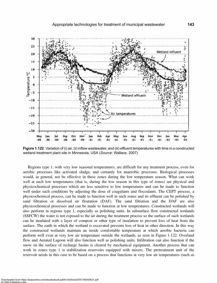
Regions type 1, with very low seasonal temperatures, are difficult for any treatment process, even foraerobic processes like activated sludge, and certainly for anaerobic processes. Biological processeswould, in general, not be effective in these zones during the low temperature season. What can workwell at such low temperatures (that is, during the low season in this type of zones) are physical andphysicochemical processes which are less sensitive to low temperatures and can be made to functionwell under such conditions by adjusting the dose of coagulants and flocculants. The CEPT process, aphysicochemical process, can be made to function well in such zones and its effluent can be polished bysand filtration or dissolved air floatation (DAF). The sand filtration and the DAF are alsophysicochemical processes and can be made to function at low temperatures. Constructed wetlands willalso perform in regions type 1, especially as polishing units. In subsurface flow constructed wetlands(SSFCW) the water is not exposed to the air during the treatment process so the surface of such wetlandscan be insulated with a layer of compost or other type of insulation to prevent loss of heat from thesurface. The earth in which the wetland is excavated prevents loss of heat in other direction. In this waythe constructed wetlands maintain an inside comfortable temperature at which aerobic bacteria canperform well even at very low air temperature outside the wetlands, as seen in Figure 1.122. Overlandflow and Aerated Lagoon will also function well as polishing units. Infiltration can also function if thesnow on the surface of recharge basins is cleared by mechanical equipment. Another process that canwork in zones type 1 is stabilization reservoirs equipped with mixers. The pretreatment unit of thereservoir needs in this case to be based on a process that functions at very low air temperatures (such as

Figure 1.122 Variation of (i) air, (ii) inflow wastewater, and (iii) effluent temperatures with time in a constructedwetland treatment plant site in Minnesota, USA (Source: Wallace, 2007)



CEPT, Aerated Lagoons or Constructed Wetlands). The effluent will be stored in the reservoir in which themixing will prevent ice formation. The aerobic biological processes will continue to function in the reservoireven at low water temperatures. When temperature will start increasing after the cold season, undigestedorganic matter will then be decomposed.

In regions type 2, Anaerobic Lagoons may function, especially covered lagoons, but its is notrecommended to use them. Facultative lagoons will perform well, but of course they have to be designedwith dimensions adjusted to the temperatures of the low season. Mixers can be added to the facultativelagoons to improve performance, and air supply can also be beneficial in low temperatures, as describedin the lagoons unit process section. Other aerobic unit processes (Aerated Lagoons, Overland Flow, andConstructed Wetlands) can be used as polishing units or in other process configurations. In addition, allthe unit processes mentioned as applicable in regions type 1 will function in regions type 2, as well ascombinations of all these unit processes. UASB, Anaerobic Filters and even PAR will not functionduring the low temperature season in regions type 2.

In regions type 3 all the appropriate technology processes, including all types of anaerobic processes(Anaerobic Lagoons, UASB and Anaerobic Filters, PAR), will function well. As a precautionarymeasure it is recommended to use UASB and Anaerobic Filters only in cases where the wastewatertemperature at the low temperature season is above 16°C. Anaerobic lagoons and PAR will perform wellduring all seasons, including during the low temperature season even if the wastewater temperatureduring this season is lower than 16°C.

The main implication of the effect of temperature on appropriate technology processes is the limitation onthe use of anaerobic processes in low temperatures. In regions where the air temperature does not fall below+7°C (which correspond to regions type 3), the four types of anaerobic reactors (Anaerobic Lagoons,UASB, Anaerobic Filter and PAR) can be used, but we recommend to restrict the use of UASB andAnaerobic Filter only to regions where the wastewater temperature during the low temperature season isabove +16°C. In regions where the air temperature does not fall much below zero (that is, not lowerthan −3°C, which correspond to regions type 2), Anaerobic Lagoons might function even in the lowtemperature season, especially covered anaerobic lagoons, but we do not recommend to use them. Otheranaerobic processes cannot be used during the low temperature season. In regions where the temperatureduring the cold season is lower than 7°C (which correspond to regions type 1), anaerobic reactors of anytype cannot not be used during the low temperature season.

1.10.2 Appropriate technology processes adequate for zones withseasons of very low temperaturesThe processes presented in this section are processes adequate for Regions type 1 that are regions of the verycold temperatures in which the air temperatures drop during the cold season to below−7°C. That would beroughly equivalent to zones with low season wastewater temperatures in the range+1°C to+7°C. The unitprocesses of appropriate technology which function in such temperatures during the low temperaturesseason are physical and physicochemical processes which are less sensitive to low temperatures and canbe made to function well under such conditions by adjusting the dose of coagulants and flocculants. TheCEPT process, a physicochemical process, can be made to function well in such zones and its effluentcan be polished by Sand Filtration or dissolved air floatation (DAF) which can also be made to functionat low temperatures. Constructed Wetland, Overland Flow, Infiltration and Aerated Lagoons will alsofunction in these temperature zones as polishing units. Treatment processes composed of combinationsof the mentioned units will also function in these temperature zones. The processes specified asfunctioning in this type of regions will also function in regions of higher temperatures. In the processes



presented, disinfection is not mention as a unit processes but it can of course be applied to the final effluent ofany of the processes, if required.

Processes which are adequate for zones in which air temperatures fall below −7°C include:

– Preliminary Treatment followed by CEPT. The CEPT process produces a fair quality effluent andsometimes this quality is sufficient, for example in case that the effluent is discharged to a largeflow river. The flow diagram of the CEPT process is presented in Figure 1.37.

– Preliminary Treatment followed by CEPT followed by Sand Filtration. The flow diagram of thisprocess is presented in Figure 1.72.

– Preliminary Treatment followed by CEPT followed by DAF. The flow diagram of this process ispresented in Figure 1.99.

– Preliminary Treatment followed by CEPT followed by Overland Flow. The flow diagram of thisprocess is presented in Figure 1.100.

– Preliminary Treatment followed by CEPT followed by ConstructedWetlands. The flow diagram of thisprocess is presented in Figure 1.101.

– Preliminary Treatment followed by CEPT followed by Infiltration Basins. The flow diagram of thisprocess is presented in Figure 1.118. If the CEPT effluent presents difficulties in infiltration, it canbe polished by a Sand Filter unit or a DAF unit prior to the infiltration.

– Preliminary Treatment followed by CEPT followed by Facultative Lagoons and MaturationLagoons. This is similar to the treatment plant of Riviera Sao Lourenco. The flow diagram ofthis process is presented in Figure 1.102 but omitting the anaerobic lagoon which appears in thisfigure.

– Preliminary Treatment followed by CEPT followed by Aerated Lagoons. The flow diagram of thisprocess is presented in Figure 1.117.

As seen, the main treatment unit process during the extreme cold season is the CEPT process. Thisprocess has relatively high O&M cost because of the consumption of chemicals for coagulation andflocculation. Such costs may be an overburden for part of the utilities in developing countries. Toovercome the problem, it is possible to construct two treatment units, each based on a different process,one for the very cold season and the other for all other seasons. The principle of this approach ispresented in Figure 1.123. During the very cold season the treatment process is preliminary treatmentfollowed by CEPT followed by a polishing unit resistant to cold temperatures. During all other seasons,in which the temperatures are higher, the treatment process is preliminary treatment followed by atreatment unit adequate for higher temperatures followed by the same polishing unit used during the coldtemperature season. The main treatment unit during the higher temperatures season can be one of themany processes mention above, for example any one of the anaerobic processes (Anaerobic Lagoons,UASB, Anaerobic Filter, PAR), lagoons system of various types and combinations of these unitprocesses. This concept is similar to the concept used in Riviera Sao Lourenco (see Figures 1.103, 1.104and 1.105) however, in Riviera Sao Lourenco the CEPT unit kicks in during high load seasons and inthis case it kicks in during the low temperature season.

As a more specific example of this concept, one of the parallel units can be a CEPT unit and the other ananaerobic unit (UASB or anaerobic lagoons). These two parallel units will be followed by a polishing unitwhich can be Sand Filtration or DAF. During the low temperature season the CEPT unit will be operated asthe first unit process (and the anaerobic unit will be bypassed), so the treatment process will be CEPTfollowed by Sand Filtration (or DAF). During the medium and high temperature seasons the CEPT willbe bypassed and the anaerobic unit will be put on stream (UASB or anaerobic lagoons) followed by thepolishing unit (Sand Filtration or DAF). Since the anaerobic unit will be working intermittently, part of



the year on and part of the year off, problems of sludge acclimatization during stat up periods might occur.This is not a serious problem in anaerobic filters or anaerobic lagoons. In the case of UASB the granularsludge might be kept active even during periods that the unit does not receive wastewater. Also, seedingfrom other plants can be helpful.

Under this concept the initial investment is higher since two main treatment unit need to be constructed.However, the investment is not very high and utilities can obtain grants or soft loans for investments. Thehigher investment is usually compensated by the reduced O&M costs. Since there are no subsidies forfinancing O&M costs and the utilities have to pay these costs from their own cash generation, a conceptwhich results in reducing O&M costs is very valuable.

1.10.3 Appropriate technology processes adequate for zoneswith seasons of medium low temperaturesThe processes presented in this section are processes adequate for Regions type 2 which are regions ofmedium cold temperatures in which the air temperatures during the cold season remain always above−3°C but below +7°C (which would be roughly equivalent to zones with low season wastewatertemperatures in the range +8°C to +12°C). Obviously, the unit processes of appropriate technologywhich function in zones of very low temperatures will also function in zones of medium lowtemperatures. Those include physical and physicochemical processes such as CEPT, as well as thefollowing polishing units: Sand Filtration, DAF, Constructed Wetland, Overland Flow, Infiltration andAerated Lagoons. Additional processes which can serve as the main treatment unit are AnaerobicLagoons, Facultative Lagoons and a complete lagoons system consisting of Anaerobic Lagoons followedby Facultative Lagoons followed by Maturation Lagoons. It is preferable to use in such low temperaturescovered Anaerobic Lagoons and Facultative Lagoons in which mixers are installed. Also, for these typeof zones the stabilization reservoir system can be used, with pretreatment consisting of processesadequate for these temperatures such as CEPT, or CEPT followed by one of the polishing unitsmentioned above, or a lagoons system. It is advisable to equip the reservoir with mixers to boost itsperformance during the cold season. Some of the cold temperatures regions are arid regions which can

Figure 1.123 Use of two parallel treatment processes, one for the low temperature season and another for allother seasons



use stores effluent to irrigate field crops during the high temperature season. Alternatively, it may bebeneficial to discharge the effluents stored in reservoirs to rivers during the high temperature seasonbecause of larger flows and higher dilution in the rivers during this season.

Processes which are adequate for zones in which air temperatures in the cold season are in the range−3°C to +7°C include:

– All the processes outlines in Section 1.10.2.– Preliminary Treatment followed by Facultative Lagoon with mixers (and if needed assisted aeration)followed by Maturation Lagoons. The flow diagram of this process is presented in Figure 1.52,omitting the Anaerobic Lagoon.

– Preliminary treatment followed by an Overland Flow System, for case under which the effluent qualityof a Overland Flow unit is sufficient. The flow diagram of this process is presented in Figure 1.41.

– Preliminary Treatment followed by Constructed Wetlands. A photo of this process is presented inFigure 1.36.

– Preliminary Treatment followed by any type of adequate Pretreatment (basically CEPT or CEPTfollowed by polishing with DAF or CEPT followed by polishing with Sand Filter or CEPT followedby polishing with Aerated Lagoons, or a full Lagoons System) followed by Stabilization Reservoirwith Mixers. The flow diagram of this process is presented in Figure 1.23. The reservoir effluentwill be either reused for irrigation during the high temperature season, or discharged to the riverduring the high temperature season.

The concept of using two parallel treatment processes, one for the low temperature season and another forall other seasons, as presented in Figure 1.123 can also be applied in zones with seasons of medium lowtemperatures. During the high temperature season in these zones, the treatment process will be based onanaerobic processes.

1.10.4 Appropriate technology processes adequate for zones withseasons of mild low temperaturesThe processes presented in this section are processes adequate for Region type 3 which are regions withseasons of mild low temperatures in which the air temperatures during the cold season remain alwaysabove +7°C (which would be roughly equivalent to zones with low season wastewater temperaturesabove +13°C). This basically refers to regions of high temperatures all year round, like tropical andsubtropical zones. Obviously, the unit processes of appropriate technology which function in zones ofvery low temperatures and in zones of medium low temperatures will also function well in zones of mildlow temperatures, so all the processes presented in sections 1.10.2 and 1.10.3 are adequate also for themild low temperatures zones.

Within this zone we make a distinction between regions with low season wastewater temperatures above+13°C and regions with low season wastewater temperatures above +16°C. We do not recommend usingUASB and anaerobic filters in regions with low season wastewater temperatures in the range+13°C to+16°C, but rather only in regions with low season wastewater temperatures of above +16°C.

Processes which are adequate for zones in which air temperatures in the cold season are above +7°Cinclude:

– All the processes outlines in Section 1.10.2.– All the processes outlines in Section 1.10.3.– Piston Anaerobic Reactor



– UASB Reactor, for cases under which the effluent quality of UASB reactor is sufficient.This process is to be preferably applied in regions with low season wastewater temperatures above+16°C.

– Anaerobic Filter, for cases under which the effluent quality of an Anaerobic Filter is sufficient.This process is to be preferably applied in regions with low season wastewater temperatures above+16°C.

– Anaerobic Lagoons, preferably covered, for cases under which the effluent quality of an anaerobiclagoon is sufficient.

– Preliminary Treatment followed by Anaerobic Lagoon followed by Facultative Lagoon with mixers(and if needed assisted aeration) followed by Maturation Lagoons. The flow diagram of thisprocess is presented in Figure 1.52.

– Preliminary Treatment followed by Anaerobic Lagoon followed by Constructed Wetlands. The flowdiagram of this process is presented in Figure 1.111, omitting the facultative lagoon.

– Preliminary Treatment followed by Anaerobic Lagoon followed by Overland Flow. The flow diagramof this process is presented in Figure 1.85.

– Preliminary Treatment followed by Anaerobic Lagoon followed by Infiltration Basins. The flowdiagram of this process is presented in Figure 1.106.

– Preliminary Treatment followed by a Lagoons System. The flow diagram of this process is presented inFigure 1.52.

– Preliminary Treatment followed by UASB followed by Facultative Lagoons. This process is to bepreferably applied in regions with low season wastewater temperatures above +16°C. The flowdiagram of this process is presented in Figure 1.59.

– Preliminary Treatment followed by UASB followed by Anaerobic Filter. This process is to bepreferably applied in regions with low season wastewater temperatures above +16°C. The flowdiagram of this process is presented in Figure 1.64.

– Preliminary Treatment followed by UASB followed by DAF. This process is to be preferably applied inregions with low season wastewater temperatures above +16°C. The flow diagram of this process ispresented in Figure 1.69.

– Preliminary Treatment followed by Pretreatment followed by a Stabilization Reservoir. The flowdiagram of this process is presented in Figure 1.73 and the pretreatment processes are also specifiedin this figure.

– Preliminary Treatment followed by UASB followed by Sand Filtration. This process is to be preferablyapplied in regions with low season wastewater temperatures above +16°C. The flow diagram of thisprocess is presented in Figure 1.83.

– Preliminary Treatment followed by UASB followed by Overland Flow. This process is to be preferablyapplied in regions with low season wastewater temperatures above +16°C. The flow diagram of thisprocess is presented in Figure 1.84.

– Preliminary Treatment followed by Anaerobic Filter followed by Overland Flow. This process is to bepreferably applied in regions with low season wastewater temperatures above +16°C. The flowdiagram of this process is presented in Figure 1.86.

– Preliminary Treatment followed by UASB followed by Constructed Wetlands. This process is to bepreferably applied in regions with low season wastewater temperatures above +16°C. The flowdiagram of this process is presented in Figure 1.87.

– Preliminary Treatment followed by UASB followed by Lagoons followed by Overland Flow. Thisprocess is to be preferably applied in regions with low season wastewater temperatures above+16°C. The flow diagram of this process is presented in Figure 1.88.



– Preliminary Treatment followed by UASB followed by Overland Flow followed by Lagoons. Thisprocess is to be preferably applied in regions with low season wastewater temperatures above+16°C. The flow diagram of this process is presented in Figure 1.90.

– Septic Tank followed by Anaerobic Filter. This process is to be preferably applied in regions with lowseason wastewater temperatures above +16°C. The flow diagram of this process is presented inFigure 1.92.

– Septic Tank followed by Constructed Wetlands. A photo of a plant of this type is presented inFigure 1.35.

– Preliminary Treatment followed by Anaerobic Filter followed by Lagoons. This process is to bepreferably applied in regions with low season wastewater temperatures above +16°C. The flowdiagram of this process is presented in Figure 1.93.

– Preliminary Treatment followed by Anaerobic Filter followed by Sand Filter. This process is to bepreferably applied in regions with low season wastewater temperatures above +16°C. The flowdiagram of this process is presented in Figure 1.94.

– Preliminary Treatment followed by Anaerobic Filter followed by DAF. This process is to be preferablyapplied in regions with low season wastewater temperatures above +16°C. The flow diagram of thisprocess is presented in Figure 1.95.

– Preliminary Treatment followed by Anaerobic Filter followed by Constructed Wetlands. This processis to be preferably applied in regions with low season wastewater temperatures above+16°C. The flowdiagram of this process is presented in Figure 1.96.

– Preliminary Treatment followed by Anaerobic Lagoons followed by Anaerobic Filter. This process isto be preferably applied in regions with low season wastewater temperatures above +16°C. The flowdiagram of this process is presented in Figure 1.97.

– Preliminary Treatment followed by Anaerobic Lagoons followed by Anaerobic Filter followed bySand Filter. This process is to be preferably applied in regions with low season wastewatertemperatures above +16°C. The flow diagram of this process is presented in Figure 1.98.

– Preliminary Treatment followed by one of the Anaerobic Units (Anaerobic Lagoons or UASB orAnaerobic Filter) followed by Infiltration. This process is to be preferably applied in regions withlow season wastewater temperatures above +16°C. The flow diagrams of these processes arepresented in Figures 1.106, 1.107 and 1.108.

– Preliminary Treatment followed by Anaerobic Lagoons followed by UASB. This process is to bepreferably applied in regions with low season wastewater temperatures above +16°C. The flowdiagram of this process is presented in Figure 1.109.

– Preliminary Treatment followed by CEPT followed by UASB. This process is to be preferably appliedin regions with low season wastewater temperatures above+16°C. The flow diagram of this process ispresented in Figure 1.110.

– Preliminary Treatment followed by a Lagoons System followed by Constructed Wetlands. The flowdiagram of this process is presented in Figure 1.111.

– Preliminary Treatment followed by one of the Anaerobic Units (Anaerobic Lagoons or UASB orAnaerobic Filter) followed by Aerated Lagoons. This process is to be preferably applied in regionswith low season wastewater temperatures above +16°C. The flow diagrams of these processes arepresented in Figures 1.113, 1.114 and 1.115.

– Preliminary Treatment followed by UASB followed by Anaerobic Filter followed by Dissolved AirFlotation followed by Membrane Filtration. This process is to be preferably applied in regions withlow season wastewater temperatures above +16°C. The flow diagram of this process is presentedin Figure 1.79.



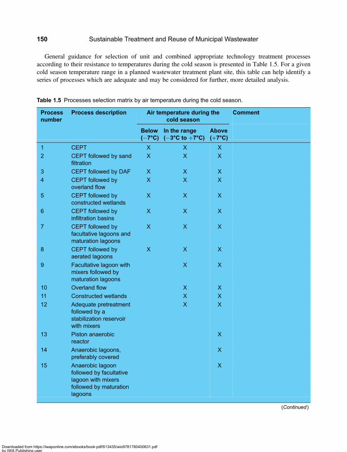
General guidance for selection of unit and combined appropriate technology treatment processesaccording to their resistance to temperatures during the cold season is presented in Table 1.5. For a givencold season temperature range in a planned wastewater treatment plant site, this table can help identify aseries of processes which are adequate and may be considered for further, more detailed analysis.

Table 1.5 Processes selection matrix by air temperature during the cold season.

Processnumber

Process description Air temperature during thecold season

Comment

Below(−7°C)

In the range(−3°C to +7°C)

Above(+7°C)

1 CEPT X X X

2 CEPT followed by sandfiltration

X X X

3 CEPT followed by DAF X X X

4 CEPT followed byoverland flow

X X X

5 CEPT followed byconstructed wetlands

X X X

6 CEPT followed byinfiltration basins

X X X

7 CEPT followed byfacultative lagoons andmaturation lagoons

X X X

8 CEPT followed byaerated lagoons

X X X

9 Facultative lagoon withmixers followed bymaturation lagoons

X X

10 Overland flow X X

11 Constructed wetlands X X

12 Adequate pretreatmentfollowed by astabilization reservoirwith mixers

X X

13 Piston anaerobicreactor

X

14 Anaerobic lagoons,preferably covered

X

15 Anaerobic lagoonfollowed by facultativelagoon with mixersfollowed by maturationlagoons

X

(Continued )



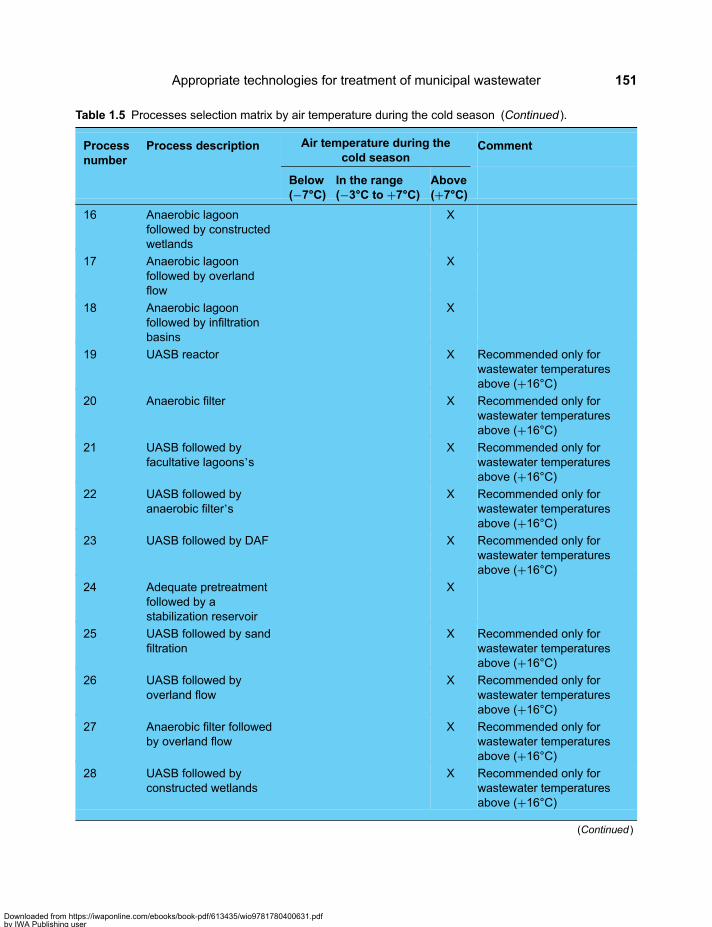
Table 1.5 Processes selection matrix by air temperature during the cold season (Continued ).

Processnumber


Comment

Below(−7°C)


Above(+7°C)

16 Anaerobic lagoonfollowed by constructedwetlands

X

17 Anaerobic lagoonfollowed by overlandflow

X

18 Anaerobic lagoonfollowed by infiltrationbasins

X

19 UASB reactor X Recommended only forwastewater temperaturesabove (+16°C)

20 Anaerobic filter X Recommended only forwastewater temperaturesabove (+16°C)

21 UASB followed byfacultative lagoons’s

X Recommended only forwastewater temperaturesabove (+16°C)

22 UASB followed byanaerobic filter’s


23 UASB followed by DAF X Recommended only forwastewater temperaturesabove (+16°C)

24 Adequate pretreatmentfollowed by astabilization reservoir

X

25 UASB followed by sandfiltration


26 UASB followed byoverland flow


27 Anaerobic filter followedby overland flow


28 UASB followed byconstructed wetlands


(Continued )




Processnumber


Comment

Below(−7°C)


Above(+7°C)

29 UASB followed bylagoons followed byoverland flow


30 UASB followed byoverland flow followedby lagoons


31 Septic tank followed byanaerobic filter


32 Septic tank followedby constructedwetlands

X

33 Anaerobic filter followedby lagoons


34 Anaerobic Filter followedby sand filter


35 CEPT followed byaerated lagoons

X

36 Anaerobic filter followedby DAF


37 Anaerobic filterfollowed by constructedwetlands


38 Anaerobic lagoonsfollowed by anaerobicfilter


39 Anaerobic lagoonsfollowed by anaerobicfilter followed by sandfilter


40 One of the anaerobicunits followed byinfiltration


41 Anaerobic lagoonsfollowed by UASB


(Continued )



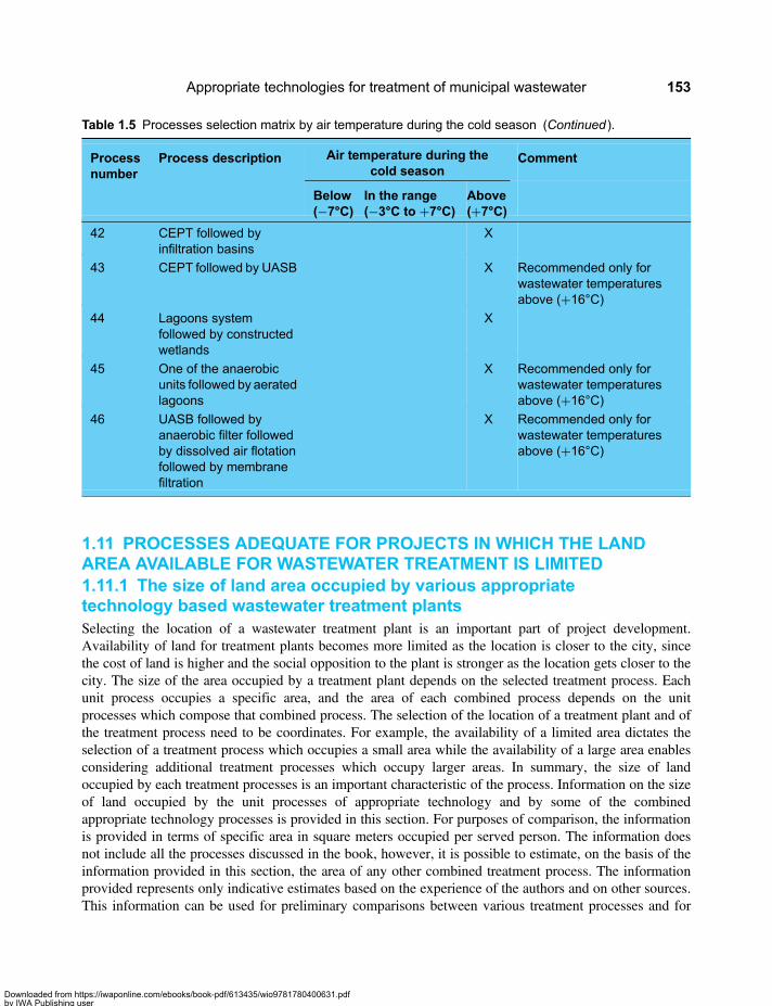
1.11 PROCESSES ADEQUATE FOR PROJECTS IN WHICH THE LANDAREA AVAILABLE FOR WASTEWATER TREATMENT IS LIMITED1.11.1 The size of land area occupied by various appropriatetechnology based wastewater treatment plantsSelecting the location of a wastewater treatment plant is an important part of project development.Availability of land for treatment plants becomes more limited as the location is closer to the city, sincethe cost of land is higher and the social opposition to the plant is stronger as the location gets closer to thecity. The size of the area occupied by a treatment plant depends on the selected treatment process. Eachunit process occupies a specific area, and the area of each combined process depends on the unitprocesses which compose that combined process. The selection of the location of a treatment plant and ofthe treatment process need to be coordinates. For example, the availability of a limited area dictates theselection of a treatment process which occupies a small area while the availability of a large area enablesconsidering additional treatment processes which occupy larger areas. In summary, the size of landoccupied by each treatment processes is an important characteristic of the process. Information on the sizeof land occupied by the unit processes of appropriate technology and by some of the combinedappropriate technology processes is provided in this section. For purposes of comparison, the informationis provided in terms of specific area in square meters occupied per served person. The information doesnot include all the processes discussed in the book, however, it is possible to estimate, on the basis of theinformation provided in this section, the area of any other combined treatment process. The informationprovided represents only indicative estimates based on the experience of the authors and on other sources.This information can be used for preliminary comparisons between various treatment processes and for


Processnumber


Comment

Below(−7°C)


Above(+7°C)

42 CEPT followed byinfiltration basins

X

43 CEPT followed by UASB X Recommended only forwastewater temperaturesabove (+16°C)

44 Lagoons systemfollowed by constructedwetlands

X

45 One of the anaerobicunits followed by aeratedlagoons


46 UASB followed byanaerobic filter followedby dissolved air flotationfollowed by membranefiltration




preliminary estimates of adaptability of certain processes to an available land size; however, accurateestimates need to be undertaken for each specific treatment plant as its design is progressing.

The specific land area in terms of square meters per served person occupied by the unit appropriatetechnology processes and by some combined processes is presented in Table 1.6. The values of sizes ofarea presented in this table refer to the actual land areas occupied by the treatment installations. The totalareas of the plants are somewhat larger in each case, usually by 20–50% to account for office space,maintenance shops, roads, parking area and gardens. Sometimes, the plant site includes large spare areasreserved for future expansion of the treatment installation. The table also includes data on the ratio of thearea of each process to the area of the Conventional Activated Sludge process. This information ispresented since the activated sludge processes is the conventional and most widely used process, so it isbeneficial to compare each process to the commonly used process.

Table 1.6 Land area per served person occupied by the unit processes of appropriate technology and bysome combined processes.

Process Specific areaoccupiedby the process(m2/////Capita)

Average ratio ofprocess area tothe area ofconventionalactivated sludge

Comments

Appropriate Technology Processes

Rotating micro screens (0.0005–0.001) 0.004 Very Small Area

Vortex grit chamber (0.0003–0.005) 0.014 Very Small Area

Anaerobic lagoons (0.15–0.2) 0.95 Small Area

Conventional lagoons system(anaerobic+ facultative+maturation)

(3.0–5.0)1 21.6 Large Area

Upgraded lagoons system(covered anaerobic+ facultativeand maturation with mixers)

(1.5–2.0) 9.5 Large area

UASB (0.03–0.1)2 0.35 Small Area

Anaerobic filter (0.03–0.1)3 0.35 Small Area

CEPT* (0.002–0.005)4 0.02 Very Small Area

Constructed wetlands (1.5–5.0)1 17.5 Large Area

Stabilization reservoir (withoutpretreatment area)

(0.5–4.0) 14.5 Large Area

Overland flow (2.0–3.5)1 14.9 Large Area

Infiltration (0.5–1.0) 4.0 Large Area

DAF (0.015–0.01) 0.07 Very Small Area

Sand filter (0.002–0.01) 0.03 Very Small Area

Septic tank (0.03–0.05)1 0.21 Very Small Area

Anaerobic lagoons followed byfacultative lagoons

(1.2–3.5)4 12.7 Large Area

(Continued )



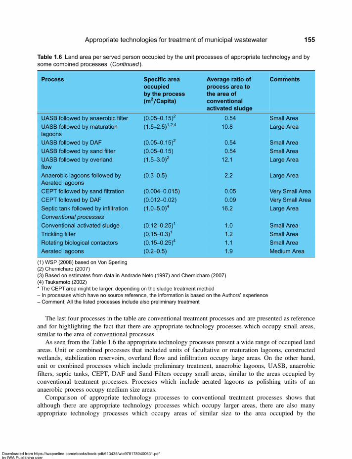
The last four processes in the table are conventional treatment processes and are presented as referenceand for highlighting the fact that there are appropriate technology processes which occupy small areas,similar to the area of conventional processes.

As seen from the Table 1.6 the appropriate technology processes present a wide range of occupied landareas. Unit or combined processes that included units of facultative or maturation lagoons, constructedwetlands, stabilization reservoirs, overland flow and infiltration occupy large areas. On the other hand,unit or combined processes which include preliminary treatment, anaerobic lagoons, UASB, anaerobicfilters, septic tanks, CEPT, DAF and Sand Filters occupy small areas, similar to the areas occupied byconventional treatment processes. Processes which include aerated lagoons as polishing units of ananaerobic process occupy medium size areas.

Comparison of appropriate technology processes to conventional treatment processes shows thatalthough there are appropriate technology processes which occupy larger areas, there are also manyappropriate technology processes which occupy areas of similar size to the area occupied by the

Table 1.6 Land area per served person occupied by the unit processes of appropriate technology and bysome combined processes (Continued ).

Process Specific areaoccupiedby the process(m2/////Capita)

Average ratio ofprocess area tothe area ofconventionalactivated sludge

Comments

UASB followed by anaerobic filter (0.05–0.15)2 0.54 Small Area

UASB followed by maturationlagoons

(1.5–2.5)1,2,4 10.8 Large Area

UASB followed by DAF (0.05–0.15)2 0.54 Small Area

UASB followed by sand filter (0.05–0.15) 0.54 Small Area

UASB followed by overlandflow

(1.5–3.0)2 12.1 Large Area

Anaerobic lagoons followed byAerated lagoons

(0.3–0.5) 2.2 Large Area

CEPT followed by sand filtration (0.004–0.015) 0.05 Very Small Area

CEPT followed by DAF (0.012–0.02) 0.09 Very Small Area

Septic tank followed by infiltration (1.0–5.0)4 16.2 Large Area

Conventional processes

Conventional activated sludge (0.12–0.25)1 1.0 Small Area

Trickling filter (0.15–0.3)1 1.2 Small Area

Rotating biological contactors (0.15–0.25)4 1.1 Small Area

Aerated lagoons (0.2–0.5) 1.9 Medium Area

(1) WSP (2008) based on Von Sperling(2) Chernicharo (2007)(3) Based on estimates from data in Andrade Neto (1997) and Chernicharo (2007)(4) Tsukamoto (2002)* The CEPTarea might be larger, depending on the sludge treatment method– In processes which have no source reference, the information is based on the Authors’ experience– Comment: All the listed processes include also preliminary treatment



conventional processes or even smaller areas. So limited availability of land does not disqualify the useappropriate technology processes. In other words, there are appropriate technology combined processesthat occupy small size areas, comparable to those of conventional processes and, as shown, which alsoyield effluent qualities comparable to those of conventional processes.

In many cases where processes that occupy a large area, mainly lagoons systems, were selected andlocated outside the city which they serve, after years the city grew and the plants became surrounded byresidential areas. As a result, social pressures mounted to move the plants to other site. At such time, thevalues of the lands on which the plants were located became higher than what was paid for them and theutilities could benefit from the change of site or from modifying the process at the same site to a processwhich occupies a smaller area.

1.11.2 Processes which occupy small land areas and are adequate forcases in which the land available for wastewater treatment is limitedLand availability for wastewater treatment in each specific project is an important consideration in selectingthe adequate treatment process or the scope of potential processes. If the area available for wastewatertreatment is limited, than the following appropriate technology processes may be considered since theydo not occupy large land extensions. The list of processes is not extensive and represents just a part ofsmall area processes, relatively simple ones. Additional combinations which contain more unit process,and still occupy small land areas are available.

– Preliminary Treatment followed by one of the Anaerobic Units (Anaerobic Lagoons or UASB orAnaerobic Filter). The effluent of an anaerobic lagoon is not of the highest quality, the effluents ofa UASB plant and of an anaerobic filter plant are of better quality, but still not the highest. Incertain cases the quality of the effluents of these anaerobic units is sufficiently high to bedischarges to large flow rivers. The specific area of an anaerobic lagoon is (0.15–0.2) m2/Capita(95% of the area of activated sludge), the specific area of an UASB is (0.03–0.1) m2/Capita (35%of the area of activated sludge) and the specific area of an Anaerobic Filter is (0.03–0.1) m2/Capita(35% of the area of activated sludge).

– Preliminary Treatment followed by CEPT. The effluent of a CEPT unit is not of the highest quality;however, it is quite good and in certain cases is sufficiently high to be discharged to large flow rivers.The process flow diagram of a CEPT unit is presented in Figure 1.37. The specific area of a CEPT unitis (0.002–0.005) m2/Capita (2% of the area of activated sludge). The numbers depend also on thetreatment method of the sludge produced by the CEPT unit. Certain sludge treatment installationmay require larger areas, but in any event, the area occupied by a CEPT unit is much smaller thanthe area occupied by an activated sludge unit treating the same flow.

– Septic Tank followed by Anaerobic Filter. The flow diagram of this process is presented in Figure 1.92.This is a processes usually used in small communities. The specific area of this process is (0.06–0.15)m2/Capita (57% of the area of activated sludge).

– Preliminary Treatment followed by Anaerobic Lagoon followed by Anaerobic Filter. The flowdiagram of this process is presented in Figure 1.97. The specific area of this process is (0.18–0.3)m2/Capita (130% of the area of activated sludge).

– Preliminary Treatment followed by one of the Anaerobic Units (UASB or Anaerobic Filter) followedby DAF. The process flow diagram of UASB followed by DAF is presented in Figure 1.69. Theprocess flow diagram of Anaerobic Filter followed by DAF is presented in Figure 1.95. Thespecific area of the process UASB followed by DAF is (0.05–0.15) m2/Capita (54% of the area of



activated sludge). The specific area of the process Anaerobic Filter followed by DAF is (0.04–0.12)m2/Capita (42% of the area of activated sludge).

– Preliminary Treatment followed by one of the Anaerobic Units (UASB or Anaerobic Filter) followedby Sand Filter. The process flow diagram of UASB followed by Sand Filter is presented in Figure 1.83.The process flow diagram of Anaerobic Filter followed by Sand Filter is presented in Figure 1.94. Thespecific area of the process UASB followed by Sand Filter is (0.05–0.15) m2/Capita (54% of the areaof activated sludge). The specific area of the process Anaerobic Filter followed by Sand Filter is (0.05–0.15) m2/Capita (54% of the area of activated sludge).

– Preliminary Treatment followed by UASB followed by Anaerobic Filter. The flow diagram of thisprocess is presented in Figure 1.64. The specific area of this process is (0.05–0.15) m2/Capita(54% of the area of activated sludge).

– Preliminary Treatment followed by CEPT followed by Sand Filter. The flow diagram of this process ispresented in Figure 1.72. The specific area of this process is (0.004–0.015) m2/Capita (5% of the areaof activated sludge).

– Preliminary Treatment followed by CEPT followed by DAF. The flow diagram of this process ispresented in Figure 1.99. The specific area of this process is (0.012–0.02) m2/Capita (9% of thearea of activated sludge).

– Preliminary Treatment followed by CEPT followed by UASB. The flow diagram of this process ispresented in Figure 1.110. The specific area of this process is (0.032–0.105) m2/Capita (37% of thearea of activated sludge).

– Preliminary Treatment followed by UASB followed by Aerated Lagoons. The flow diagram of thisprocess is presented in Figure 1.114. The specific area of this process is (0.23–0.6) m2/Capita(224% of the area of activated sludge).

– Preliminary Treatment followed by Anaerobic Filter followed by Aerated Lagoons. The flow diagramof this process is presented in Figure 1.115. The specific area of this process is (0.23–0.6) m2/Capita(224% of the area of activated sludge).

– Preliminary Treatment followed by UASB followed by Anaerobic Filter followed by DAF followed byMembrane Filtration. The flow diagram of this process is presented in Figure 1.79. The specific area ofthis process is (0.08–0.23) m2/Capita (84% of the area of activated sludge).

General guidance for selection of unit and combined appropriate technology treatment processesaccording to the land area they occupy is presented in Table 1.7. For a given available area size forlocating the treatment plant, this table can help identify a series of processes which are adequate and mayby considered for further, more detailed analysis.

Table 1.7 Processes selection matrix by occupied land area.

Processnumber

Process description Land area occupied by the process (m2/////Capita)

0.002–0.01 werysmall area

0.01–0.5small area

0.5–5.0large area

1 Rotating micro screens X

2 Vortex grit chamber X

(Continued )



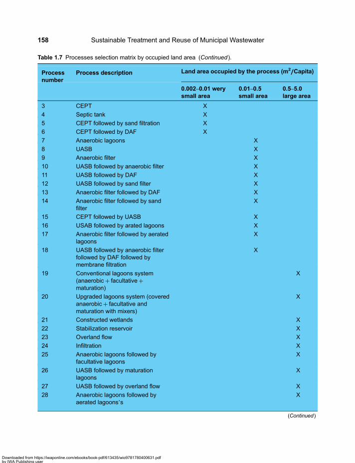
Table 1.7 Processes selection matrix by occupied land area (Continued ).

Processnumber




0.5–5.0large area

3 CEPT X

4 Septic tank X

5 CEPT followed by sand filtration X

6 CEPT followed by DAF X

7 Anaerobic lagoons X

8 UASB X

9 Anaerobic filter X

10 UASB followed by anaerobic filter X

11 UASB followed by DAF X

12 UASB followed by sand filter X

13 Anaerobic filter followed by DAF X

14 Anaerobic filter followed by sandfilter

X

15 CEPT followed by UASB X

16 USAB followed by arated lagoons X

17 Anaerobic filter followed by aeratedlagoons

X

18 UASB followed by anaerobic filterfollowed by DAF followed bymembrane filtration

X

19 Conventional lagoons system(anaerobic+ facultative+maturation)

X

20 Upgraded lagoons system (coveredanaerobic+ facultative andmaturation with mixers)

X

21 Constructed wetlands X

22 Stabilization reservoir X

23 Overland flow X

24 Infiltration X

25 Anaerobic lagoons followed byfacultative lagoons

X

26 UASB followed by maturationlagoons

X

27 UASB followed by overland flow X

28 Anaerobic lagoons followed byaerated lagoons’s

X

(Continued )



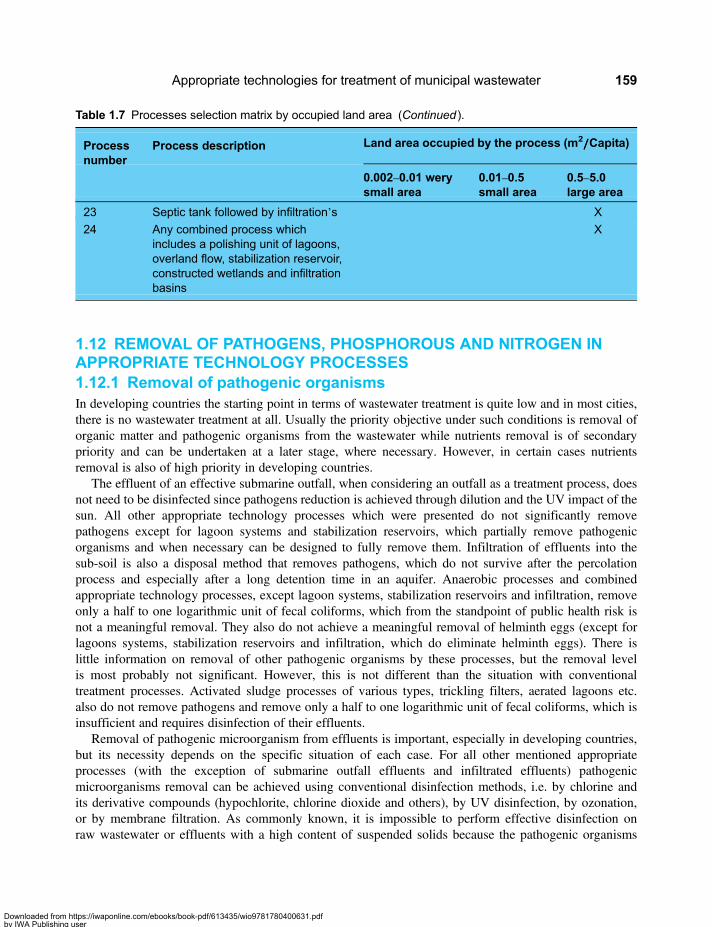
1.12 REMOVAL OF PATHOGENS, PHOSPHOROUS AND NITROGEN INAPPROPRIATE TECHNOLOGY PROCESSES1.12.1 Removal of pathogenic organismsIn developing countries the starting point in terms of wastewater treatment is quite low and in most cities,there is no wastewater treatment at all. Usually the priority objective under such conditions is removal oforganic matter and pathogenic organisms from the wastewater while nutrients removal is of secondarypriority and can be undertaken at a later stage, where necessary. However, in certain cases nutrientsremoval is also of high priority in developing countries.

The effluent of an effective submarine outfall, when considering an outfall as a treatment process, doesnot need to be disinfected since pathogens reduction is achieved through dilution and the UV impact of thesun. All other appropriate technology processes which were presented do not significantly removepathogens except for lagoon systems and stabilization reservoirs, which partially remove pathogenicorganisms and when necessary can be designed to fully remove them. Infiltration of effluents into thesub-soil is also a disposal method that removes pathogens, which do not survive after the percolationprocess and especially after a long detention time in an aquifer. Anaerobic processes and combinedappropriate technology processes, except lagoon systems, stabilization reservoirs and infiltration, removeonly a half to one logarithmic unit of fecal coliforms, which from the standpoint of public health risk isnot a meaningful removal. They also do not achieve a meaningful removal of helminth eggs (except forlagoons systems, stabilization reservoirs and infiltration, which do eliminate helminth eggs). There islittle information on removal of other pathogenic organisms by these processes, but the removal levelis most probably not significant. However, this is not different than the situation with conventionaltreatment processes. Activated sludge processes of various types, trickling filters, aerated lagoons etc.also do not remove pathogens and remove only a half to one logarithmic unit of fecal coliforms, which isinsufficient and requires disinfection of their effluents.

Removal of pathogenic microorganism from effluents is important, especially in developing countries,but its necessity depends on the specific situation of each case. For all other mentioned appropriateprocesses (with the exception of submarine outfall effluents and infiltrated effluents) pathogenicmicroorganisms removal can be achieved using conventional disinfection methods, i.e. by chlorine andits derivative compounds (hypochlorite, chlorine dioxide and others), by UV disinfection, by ozonation,or by membrane filtration. As commonly known, it is impossible to perform effective disinfection onraw wastewater or effluents with a high content of suspended solids because the pathogenic organisms

Table 1.7 Processes selection matrix by occupied land area (Continued ).

Processnumber




0.5–5.0large area

23 Septic tank followed by infiltration’s X

24 Any combined process whichincludes a polishing unit of lagoons,overland flow, stabilization reservoir,constructed wetlands and infiltrationbasins

X



hide within the pores of the suspended solids. The effluent qualities of all the appropriate technology unitprocesses (except for preliminary treatment) and combined processes presented above are such that each ofthem can undergo an effective disinfection, including lagoons and stabilization reservoirs effluents. This isan additional advantage of the appropriate treatment processes. Disinfection by chlorine gas, by liquidhypochlorite and by UV radiation can be considered appropriate technologies since they are notexpensive, relatively simple and well known to water and sanitation utilities since they are also used fordisinfection of water. Disinfection by ozone, chlorine dioxide and membrane filtration are not consideredappropriate technology processes. Ozone and chlorine dioxide need to be manufactured on spot sincethey are unstable materials. Their application as disinfectants is complicated and expensive. Membranefiltration (ultrafiltration, nanofiltration) is a good disinfection method since the membranes form a barrierto the passage of pathogenic organisms and they do not introduce chemical products into the water, butit is still and expensive method.

1.12.2 Removal of phosphorous and nitrogenUnder a wastewater reuse scheme for irrigation, removal of nutrients is not necessary since they are an assetfor irrigation, serving as fertilizers. Pathogens can be removed in the stabilization reservoir when theirrigated crops require a pathogen free effluent.

The effluent of an effective submarine outfall, when considering an outfall as a treatment process, doesnot need to undergo nutrients removal treatment because for the level of nutrients present in typical domesticwastewater, the dilution level of an effective outfall is sufficient to reduce the nutrients concentrationsaround the discharge point to safe levels, except in cases of discharge near a coral reef. But discharge ofeffluents in the vicinity of coral reefs is a practice that should be avoided in any case.

Wetlands and lagoons may provide reasonable nutrients removal efficiencies when designed forthat purpose.

All other appropriate technology processes which were presented do not remove nutrients with highefficiencies. When nutrients removal is required, additional installations need to be provided for thatpurpose, and this means added cost and complexity. This is not however different than in the caseof conventional treatment processes, to which specific nutrients removal installations need to be addedwhen nutrients removal is required. Such installations include providing conditions for nitrification,adding denitrification reactors with recirculation pumps and piping, adding anoxic tanks for phosphorousluxury uptake and more. However, it is easier to remove nutrients when the treatment process is basedon conventional technology than when it is based on appropriate technology.

If an effluent is discharged to a river, sometimes nitrogenous BOD needs to be removed from it on top ofcarbonaceous BOD, so that oxygen consumption for nitrification would not occur in the river. One way toremove nitrogenous BOD is to nitrify the effluent before discharging it to the river, but removal of nitrogenis not necessary and the effluent may contain nitrogen in the form of nitrate. In several countries, the qualitystandard for effluents discharged to a river requires a limit on ammonia, not on nitrate, and that is a goodapproach. If an effluent is discharged to a closed water body (lake, bay or estuary) phosphorous andnitrogen might need to be removed to prevent eutrophication, but in many cases the limiting factor is thephosphorous and it is this nutrient that needs to be removed, not nitrogen. The removal of phosphorousis easier than the removal of nitrogen, so eutrophication can be prevented by effective removal ofphosphorous even without removal of nitrogen. However, since in many cases effluent quality standardsalso require nitrogen removal, this matter is discussed here as well. The decision regarding the nutrientwhich needs to be removed has to be developed for the specific condition of each case, however, usuallythe effluent quality standards do not allow taking into account specific conditions and require complete



nutrients removal for all cases. Such an approach should be reconsidered in developing countries sincenutrients removal is costly and sometimes not necessary.

Removal of phosphorous by luxury uptake does not occur in appropriate technology processes.When removal of phosphorous is required, it can be achieved by precipitating the phosphorous with theaid of flocculants (iron salts, usually ferric chloride, or aluminium sulphate –Alum). In the CEPTprocesses phosphorous precipitation is an inherent part of the process. For lagoons processes or combinedprocesses whose last unit is lagoons based, only flocculants dosing equipment will be required. Mixingcan take place in line by installing static mixers in the pipelines and injecting the flocculants into theline before the mixers. Phosphorous salt precipitation is then taking place in one of the lagoons. For therest of the processes, installations for flocculants storage, dosing into the effluent stream, rapid and slowmixing of the flocculants and phosphorous sedimentation and clarification installations need to be added.

There is no nitrogen removal in anaerobic lagoons and in other types of anaerobic reactors (UASB,Anaerobic Filter etc.) only transformation of organic nitrogen to ammonia. The mechanisms of nitrogenremoval in facultative and polishing ponds are: (i) volatilization of ammonia; (ii) assimilation ofammonia by algae; (iii) assimilation of nitrate by algae; (iv) nitrification-denitrification; and (v)sedimentation of particulate organic nitrogen. Assimilation of ammonia and nitrate by algae removesonly a small portion of the nitrogen from the liquid. Similarly, sedimentation removes only a smallportion of the nitrogen. Natural nitrification does not seem to be common in facultative and polishinglagoons. Nitrifying populations are present in these lagoons but are small. Nitrification occurs in theWestern Treatment Plant in Melbourne, Australia, which is a lagoons plant with an overall detentiontime of 80 days. Perhaps a long detention time is required to achieve natural nitrification in lagoons, butin most lagoons systems the detention time is shorter and nitrification does not occur. The mostsignificant nitrogen removal mechanism in lagoons is volatilization of ammonia (NH3).

In an aqueous solution ammonia is present as dissolved ammonia gas (NH3) which is volatile and canleave the solution naturally or be stripped out of it, and as an ammonium ion (NH4

+) which cannot bestripped out. The relation between the NH3 and the NH4

+ in the solution depends on the pH and thetemperature of the solution. At low values of pH all the ammonia is present in the form of NH4

+ and withthe increase of the pH it is transformed to NH3. At a natural pH of 7 and at 20°C all the ammonia ispractically in the form of NH4

+. At a pH of about 9.5, 50% of the ammonia is in the form of NH4+ and

50% is NH3. At a pH of 11 and higher, all the ammonia is in the form of NH3. Natural volatilization canbe achieved in a lagoons system and its level depends on the pH, the temperature and the detention timein the lagoons. Von Sperling (2002) provides on page 145 a table and a graph of the theoreticalefficiency of nitrogen removal in lagoons as function of detention time and pH at 20°C. At pH 8 thepercentage of nitrogen removal varies from 43% at a detention time of 3 days to 55% at a detention timeof 40 days. At pH 9 the percentage of nitrogen removal varies from 61% at a detention time of 3 days to69% at a detention time of 40 days. The removal efficiencies increase with the increase of temperature.Rapid photosynthesis leads to increasing the lagoons pH, often up to values of 9–10. This induces thetransformation of the ammonia to dissolved gas and tends to increase nitrogen removal by volatilizationof ammonia. However, the dissolved ammonia gas, NH3, is toxic to algae. The ammonia toxicity increasewith the increase of pH since the pH increase induces the increase of the dissolved ammonia gas. So alagoon system is actually self-regulating the pH and ammonia levels. When the pH and dissolvedammonia gas increase the toxicity to algae increases, and therefore the photosynthesis decreases. As aresult, the pH falls and the toxicity decreases. This allows the photosynthesis to increase again resultingin pH increase and the cycle repeats itself. This cycle provides a limit to natural volatilization of ammonia.

When considering induced nitrogen removal from lagoons there are three options. Option 1 is actuallynot for nitrogen removal but rather for nitrogen transformation. It refers to induced nitrification. This



process transforms ammonia and organic nitrogen to nitrate and is sufficient to protect receiving waters fromnitrogenous Biochemical Oxygen Demand. As mentioned, in some countries the effluent quality standardsput an upper limit on the ammonia concentration (at about 5 mg/l N-NH3) but there is no restriction onnitrate concentration so nitrification can provide a solution to such a requirement. Nitrification isachieved in a lagoon by installing in it modules of aerated fixed film beds which provide optimalconditions for development of nitrifying bacteria. Each module is filled with thousands of pieces of bio-media where, during normal operation, a healthy biomass is formed by a supply of air produced by thefine bubble membrane diffusers located on the bottom of each module and by the contact with thewastewater. As with any fixed-film biological contactor, the units will tend to become overgrown withorganisms after a period of time. When this happens the module has a separate coarse-bubble system,controlled from the shore, to slough the media bed and clear it for renewed growth. Each module can bedeployed individually or in series to remove varying ammonia loads. The modules system can be sizedto eliminate as much ammonia as required to meet effluent requirements. The modules diffuse a highlevel of dissolved oxygen into the surrounding wastewater through the media bed. Induced nitrificationin lagoons is a proven technology and additional information on the method can be found at www.GurneyEnvironmental.com. The method has been successfully used to maintain nitrification in coldnorthern climates by creating the stable, oxygen-rich, and immobilised microenvironment favoured bythe nitrifying bacteria. Successful performance of this type of systems has been achieved throughout acomplete winter seasons at wastewater treatment plants in upstate New York and northern Pennsylvaniain the United States. A photo of such a fixed bed nitrifying modules installed in a lagoon is presented inFigure 1.18. They are the rectangular shaped objects seen in the right hand side lagoon of the photo. Thenitrifying modules add cost to the treatment plant, both in investment and in O&M cost for air supply,but as previously explained; nutrients removal adds cost in any process, even in conventional systems.However, the operation of the system is still simple and it can be considered an appropriate technologysystem.

The second option for nitrogen removal in a lagoons system is nitrification-denitrification. This option isproposed at a level of an idea, not known yet to be performing at a full scale plant, but theoretically it shouldwork. It is basically the same idea of nitrification-denitrification in activated sludge systems. The systemflow diagram is the following: Anaerobic lagoon followed by an anoxic reactor (retention tank or basin)in which the denitrification process takes place, followed by one or two facultative lagoons in which thenitrification process takes place, followed by polishing ponds. The nitrification process in the facultativelagoons is an induced process achieved by installing in the lagoons the modules of aerated fixed filmbeds as described above. A recirculation stream is installed from the last facultative lagoon to the anoxicreactor, at a rate of 1.5–2 in relation to the raw wastewater flow. This recirculation stream conveys to theanoxic reactor the nitrates and since the reactor is not aerated and is covered and contains mixers,photosynthesis will not take place in it so the nitrate will be used by the heterothrophic bacteria as theoxygen source and the denitrification process will take place in this reactor. It is necessary to provide avery short detention time in the anaerobic lagoon which precedes the anoxic reactor to restrict the BODremoval in it to no more than 50%, or perhaps even omit the anaerobic lagoon at all, so as to ensuresufficient substrate for the denitrification process. It might also be necessary to recirculate some sludgefrom the downstream facultative lagoons to increase the concentration of heterothrophic bacteria in theanoxic reactor. The anoxic reactor and the recirculation, which requires pumping, increase investmentsand O&M costs, but nitrogen removal is costly. The systems remains however simple to operate and isstill an appropriate technology system.

The third option for nitrogen removal in a lagoons system is natural or induced ammonia stripping. It hastwo variants. Variant 1 is ammonia stripping in a polishing lagoon. This variant is proposed at a level of an





idea, not known yet to be performing at a full scale plant, but theoretically it should work and it was tested ona pilot scale. As previously mentioned, it is recommended to add mixers in all the facultative and polishinglagoons. These mixers can increase the natural ammonia volatilization in the lagoons. On top of that, anadditional ammonia stripping lagoon can be added as a final lagoon, or the last polishing lagoon can beused for this purpose. Variant 1 has three options: (i) natural ammonia stripping in a long detention timeshallow lagoon; (ii) ammonia stripping by high lime treatment that raises pH to 11.0–11.5, and (iii)ammonia stripping by low lime treatment that raises pH to 9.0–9.5. As to natural ammonia stripping,there is evidence (Cavalcanti, 2009 and Mota and von Sperling, 2009) that Ammonia stripping can occurnaturally in a long detention time shallow (0.5–1.0 meter deep) polishing lagoon, even withoutincreasing the pH by lime. In long detention time polishing lagoons the photosynthesis rate is high,leading to high pH values of over 9.0 which stimulates ammonia stripping. Cavalcanti (2009) reports92% N-NH3 natural removal in an experimental lagoons system with a series of polishing lagoons with atotal detention time of about 30 days in the polishing lagoons. Von Sperling (2002) estimates that at pH9 and 20°C nitrogen removal can reach 69% at a detention time of 40 days. Mota and von Sperling,(2009) report that the specific area required to reduce N-NH3 to less than 5 mg/l in polishing lagoons is2–3 m2/Capita for lagoons 0.5 m deep and 3–4 m2/Capita for lagoons 1 m deep. This is equivalent toprolonged detention times in the polishing lagoons of 30–40 days. If land is available, ammoniastripping can then be achieved naturally in long detention time shallow polishing ponds. If landavailability is restricted, ammonia stripping can be induced in a shorter detention time by raising the pHin the polishing lagoon either by high lime treatment or by low lime treatment. In the case of option 2 ofVariant 1, the high lime treatment, the pH in the ammonia stripping lagoon is increased to 11.0 11.5 byusing either quick lime (CaO) or hydrated lime Ca(OH)2 to raise the pH. The lime cannot be addeddirectly to the lagoon because high-lime treatment results in precipitation of large quantities of calciumcarbonate which will fill the lagoon. Therefore, a reactor-clarifier must be installed prior to the lagoon.The addition of lime is done in the reactor-clarifier, in which the precipitation takes place and fromwhich the settling sludge is removed continuously. The reactor-clarifier’s effluent is then diverted to thelagoon in which the ammonia stripping takes place. Because of the large amount of lime required toraise the pH to 11.0 and above, high-lime treatment produces large quantities of sludge which need to bedewatered and disposed. The lagoon is to be equipped with mixers to obtain an intensive mixing, or ifnecessary it can be equipped with a combination of mixers and floating aerators. This would assist thestripping of ammonia. It is estimated that over 90% removal of ammonia can be achieved under thisvariant with high lime treatment and with detention times of about 10 days in the lagoon, depending onthe temperature and the mixing intensity in the lagoon. Higher ammonia removal efficiencies can beachieved with larger detention times. The pH in the lagoon effluent will drop naturally to about 9.5–10.0but discharge standards usually require a lower value so lowering the pH of the final effluent by addingto it an acid solution might be required. The high lime ammonia stripping process was tested on a pilotscale plant, the results of which are reported by Idelovitch et al. (1981), and it was also applied in a fullscale plant, the Dan Region wastewater treatment plant in Tel Aviv, Israel and functioned successfullyfor many years (Idelovitch et al (1981). The detention time in the lagoon of the high lime treatmentoption is much lower than that of the natural ammonia stripping lagoon so the area occupied by the highlime treatment installation is much smaller. In the case of low lime treatment the pH in the ammoniastripping lagoon is to be increased to 9.0–9.5 (again by using either quick lime or hydrated lime). In thiscase if the alkalinity of the wastewater is not high, the lime can be added directly to the inflow stream tothe lagoon. The lagoon is to be equipped with mixers to obtain an intensive mixing, or if necessary it canbe equipped with a combination of mixers and floating aerators. This would assist the stripping ofammonia. It is estimated that 70–80% removal of ammonia can be achieved under this variant with low



lime treatment. The required detention time in the lagoon needs to be established. It depends on the pH level,the temperature and the mixing intensity. It is estimated that it is not as long as in the case of natural ammoniastripping (Variant 1 option 1) because there is no fluctuation in the pH (which in this case does not depend onphotosynthesis) and because of the mixing assistance to the stripping process. As mentioned there is a risk ofcalcium carbonate precipitation in the lagoon, which will have to be cleaned periodically. If the alkalinity ofthe wastewater is high, the precipitated calcium carbonate quantity may be too high and in this case, areactor-clarifier must be installed prior to the lagoon. The addition of lime is done in the reactor-clarifier,in which the precipitation takes place and from which the sludge is removed continuously. The clarifier’seffluent is then diverted to the lagoon in which the ammonia stripping takes place.

Variant 2 of induced ammonia stripping is based on the use of a stripping tower instead of a lagoon.This is a more conventional method which can reach up to 90–95% of ammonia removal. Removalefficiency depends on temperature and on the efficiency of the air-water contact. As the temperaturedecreases, the amount of air required increases significantly for the same degree of removal. Lime orcaustic soda is added to the nitrogen rich effluent until the pH reaches 10.8 to 11.5 units, whichconverts ammonium hydroxide ions to dissolved ammonia gas. In a countercurrent stripping tower theeffluent rich ammonia is pumped to the top of a packed tower and effluent drops fall through thepacking. Air is drawn through openings in the bottom of the tower and flows up. Free ammonia isstripped from the falling effluent droplets into the air stream and then discharged to the atmosphere.There is another type of tower, cross flow tower, in which the air enters along the entire depth of thepacking, but the principle of its performance is similar to that of the countercurrent tower. Therequired airflow is about 1,000 times the water flow and can be higher depending on the temperature.Problems of calcium carbonate scaling and poor performance during cold weather have been reportedin regard to operation of ammonia stripping towers. Removal of ammonia in stripping towers is morecomplex than in lagoons.

In unit or combined appropriate technology processes which do not include lagoons, such as UASBfollowed by Anaerobic Filters and many others, there are two options for nitrogen removal. Option 1 isactually not for nitrogen removal but for nitrogen transformation. It refers to induced nitrification. Thisprocess transforms ammonia and organic nitrogen to nitrate and is sufficient to protect receiving watersfrom nitrogenous Biochemical Oxygen Demand. Nitrification can be achieved by subjecting the effluentto the same modules of aerated fixed film beds described above, which in this case can be installed notin a lagoon but rather in a retention tank or even in earth basins. Option 2 for nitrogen removal in unit orcombined appropriate technology processes which do not include lagoons is induced ammonia stripping.In this case there are two variants identical to the ones presented for the of lagoons systems. Variant 1 isammonia stripping in a lagoon or a basin, which needs to be added as the final unit of the treatmentplant. Variant 2 is ammonia removal in a stripping tower, which needs to be added as the final unit ofthe treatment plant.

1.13 RECOVERY OF RESOURCES FROM MUNICIPALWASTEWATER,THE POTENTIAL FOR GENERATION OF ENERGY IN WASTEWATERTREATMENT PLANTS AND ITS IMPLICATIONS REGARDING THESUSTAINABILITY OF THEIR OPERATION1.13.1 IntroductionMunicipal wastewaters contain several resources which can be recovered and reused. First, 99.9% of themunicipal wastewater is water. The rest 0.1% is partly dissolved and partly in form of suspended solids,



part of both is organic matter and part mineral matter. In water scarce zones, treated effluents can be used as asource of water for irrigation. Given the global water crisis, which will become more acute with time, thereclamation of water from municipal wastewater will gain importance and become more widespread.Municipal wastewaters also contain nutrients: nitrogen, phosphorous and some potassium. When effluentsare reused for irrigation, these nutrients become fertilizers. Depending on the irrigation method and typeof irrigated crops, the nutrients in the effluents may partially or completely satisfy the need for fertilizers.This is very important in developing countries, where poor farmers have financial difficulties to purchasefertilizers (and this is the reason that they prefer using effluents or even raw wastewater for irrigation).

Municipal and industrial wastewaters contain organic matter. This organic matter contains some energy,which can be recovered in anaerobic processes. The fact that municipal wastewater contains 99.9% watermay seem to contradict the fact that the wastewater contains energy. It is to be understood that municipalwastewater is not an oil well but it contains some energy which can be recovered and put to use and thismay result to be of significant financial importance, especially in developing countries.

Wastewater contains therefore three valuable resources which can be recovered: (i) water, (ii) fertilizers;and (iii) energy. They can become sources of income to utilities through the sale of effluent and thegeneration of energy for internal use or for sale, however in each case it is necessary to assess thefeasibility of energy recovery. Additional income flows on top of income from tariffs will have apositive financial effect on the utilities, and may result in positive institutional and sustainability impacts,as discussed below.

The successful use of these resources depends to a large extent on governments’ policies and regulations.An enabling environment is required both for effluents reuse in irrigation and for generation of energy. Inthe case of reuse for irrigation, reasonable effluent quality standards need to be in places as well as financialsupport and technical assistance. In the case of energy generation adequate policies and regulationare required to stimulate the generation of energy and render it financially feasible. If the enablingenvironment does not exist the result is utilization of raw wastewater for irrigation, because in areas ofscarcity, farmers in need of water ignore the laws and use raw wastewater. In the case of energy a lackof an enabling environment will prevent utilities from accessing this resource, losing thereby the benefitswhich it can provide.

Another issue related to wastewater disposal in general and to energy generation or methane flaring inparticular is the reduction of emission of Green House Gases. Such reduction is beneficial bycontributing to the effort of mitigating the global warming, and it can also generate an additional incometo the utilities through the Carbon emission Reduction (CER) credits.

Reuse of effluents for irrigation and utilization of the nutrients as fertilizers are more straightforwardresources, they are already in use and their utilization is increasing. In this chapter we expand thediscussion on energy generation, which is still in limited use, especially in developing countries.

1.13.2 Effluents as a water source for irrigationReuse of effluents for irrigation of crops is only one of the reuse options of effluents, but as explained inChapter 1 Section 1.7.2.7, it is an attractive option. The engineering design approach of effluent reusefor irrigation is explained also in Chapter 7. Reuse for irrigation has a significant economic value. It ispart of the measures to resolve water scarcity problems in arid zones. The economic value of effluents(value and not cost) may be different in different countries. The economic value of effluent irrigation isnot just the cost which can be charged for the effluent but also the economic value of generating a newwater source, because it liberates fresh water which was used for irrigation, to be used for purposes thatrequire only fresh water and that has a significant economic an environmental value. Irrigation with



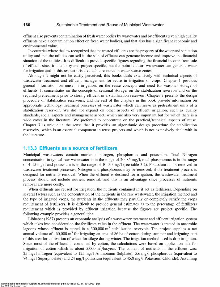
effluent also prevents contamination of fresh water bodies by wastewater and by effluents (even high qualityeffluents have a contamination effect on fresh water bodies), and that also has a significant economic andenvironmental value.

In countries where the law recognized that the treated effluents are the property of the water and sanitationutility and that the utilities can sell it, the sale of effluent can generate income and improve the financialsituation of the utilities. It is difficult to provide specific figures regarding the financial income from saleof effluent since it is country and project specific, but the point is clear: wastewater can generate waterfor irrigation and in this respect it is a valuable resource in water scarce zones.

Although it might not be easily perceived, this books deals extensively with technical aspects ofwastewater treatment and effluent management for reuse in irrigation of crops. Chapter 1 providesgeneral information on reuse in irrigation, on the reuse concepts and need for seasonal storage ofeffluents. It concentrates on the concepts of seasonal storage, on the stabilization reservoir and on therequired pretreatment prior to storing effluent in a stabilization reservoir. Chapter 7 presents the designprocedure of stabilization reservoirs, and the rest of the chapters in the book provide information onappropriate technology treatment processes of wastewater which can serve as pretreatment units of astabilization reservoir. We did not expand on other aspects of effluent irrigation, such as qualitystandards, social aspects and management aspect, which are also very important but for which there is awide cover in the literature. We preferred to concentrate on the practical/technical aspects of reuse.Chapter 7 is unique in the sense that it provides an algorithmic design procedure for stabilizationreservoirs, which is an essential component in reuse projects and which is not extensively dealt with inthe literature.

1.13.3 Effluents as a source of fertilizersMunicipal wastewaters contain nutrients: nitrogen, phosphorous and potassium. Total Nitrogenconcentration in typical raw wastewater is in the range of 20–85 mg/l, total phosphorous is in the rangeof 4–15 mg/l and potassium is in the range of 10–30 mg/l (see table 3.2). Potassium is not removed inwastewater treatment processes. Nitrogen and phosphorous may be removed, if the treatment process isdesigned for nutrients removal. When the effluent is destined for irrigation, the wastewater treatmentprocess should not include nutrient removal, and this is an advantage since processes of nutrientsremoval are more costly.

When effluents are reused for irrigation, the nutrients contained in it act as fertilizers. Depending onseveral factors such as the concentration of the nutrients in the raw wastewater, the irrigation method andthe type of irrigated crops, the nutrients in the effluents may partially or completely satisfy the cropsrequirement of fertilizers. It is difficult to provide general estimates as to the percentage of fertilizersrequirement which is provided by effluent irrigation because the figures are project specific. Thefollowing example provides a general idea.

Libhaber (1987) presents an economic analysis of a wastewater treatment and effluent irrigation systemwhich takes into consideration the fertilizers value in the effluent. The wastewater is treated in anaerobiclagoons whose effluent is stored in a 300,000 m3 stabilization reservoir. The project supplies a netannual volume of 460,000 m3 for irrigating an area of 86 ha of cotton during summer and irrigating partof this area for cultivation of wheat for silage during winter. The irrigation method used is drip irrigation.Since most of the effluent is consumed by cotton, the calculations were based on application rate forirrigation of cotton which is about 5,000 m3/ha.year. The content of nutrients in the effluent was:25 mg/l nitrogen (equivalent to 125 mg/l Ammonium Sulphate), 5.6 mg/l phosphorous (equivalent to74 mg/l Superphosfate) and 24 mg/l potassium (equivalent to 45.8 mg/l Potassium Chloride). Assuming



that 85% of the nutrients are available to the crops and an irrigation water use efficiency of 80% by dripirrigation, the resulting rates of nutrients application are the following:

Ammonium Sulphate: 5,000 ∗ 0.85 ∗ 0.8 ∗ 125 ∗ 0.001 = 425 kg/ha · yearSuperphosfate: 5,000 ∗ 0.85 ∗ 0.8 ∗ 74 ∗ 0.001 = 252 kg/ha · year

Potassium Chloride: 5,000 ∗ 0.85 ∗ 0.8 ∗ 45.8 ∗ 0.001 = 156 kg/ha · year

The required fertilizers application rates according to regular practice for cotton are 800 kg/ha.year ofAmmonium Sulphate, 500 kg/ha.year of Superphosfate and 500 kg/ha.year of Potassium Chloride. Thismeans that in this case the percentages of fertilizers applied by the effluent are:

Nitrogen: 53%

Phosphorous: 50%

Potassium: 31%

In this case we can assume that an average figure of 50% of saving on fertilizers can be considered. Thecost of fertilizers for cotton is 129 US$/ha.year, thus the saving is about 65 US$/ha.year or about 5,600 US$/year for the specific project described above. The price figures refer to the time that the analysis wasundertaken, which is years back, and which may be different to date.

The fertilizers value in the effluent is a very important economic factor for developing countries, wherepoor farmers have financial difficulties to purchase fertilizers. One of the reasons farmers prefer usingeffluents (or even raw wastewater) for irrigation in developing countries is the fertilizers content in theeffluents, which results in better crops and higher yields.

1.13.4 Wastewater as a source of energyMunicipal and industrial wastewaters contain organic matter measured as COD. This organic mattercontains some energy, which can be recovered in anaerobic processes. The end products of anaerobicdecomposition of wastewater are: (i) biogas, and (ii) small amounts of excess sludge (about 5–15% ofthe decomposed organic matter in the raw sewage). The biogas contains about 65–70% methane, about25–30% CO2 and the balance is mostly N2 and some impurities, one of which may be H2S, (if the rawwastewater contained high concentration of sulphur). If the first treatment unit in the treatment plant isan anaerobic process unit such as anaerobic lagoons, UASB or Anaerobic Filters, the biogas can becaptured, cleaned and used as an energy source. In the case of an anaerobic lagoons process, it isnecessary to cover the lagoons in order to be able to capture the biogas. The appropriate technologyprocesses described in this book have low energy consumption and in most cases it is not possible to usewithin the plants the entire amount of energy produced by the anaerobic process. Consumers for theenergy produced need therefore be found outside the wastewater treatment plants, either within oroutside the utility and the feasibility of energy production from biogas needs to be studied.

Utilization of biogas is a common practice in Sanitary landfills, in activated sludge plants treatingmunicipal wastewater, in which the sludge undergoes anaerobic digestion and the biogas produced iscaptured and utilized, and in industrial wastewater treatment plants where anaerobic processes are usedto treat highly concentrated organic wastes. In activated sludge plants the biogas is used to generateelectricity which is consumed within the plant itself (because such plants have high electricityconsumption in the aeration system of the biological rector). The fact that an activated sludge plant canbe the consumer of the energy it produces from the methane it generates facilitates the decision to utilize



the methane because there is no need to look for external consumers. Many industrial wastewaters are treatedin various types of anaerobic reactors and the biogas is captured and utilized. Usually the industry itself is theenergy consumer and the private sector which owns the industry is interested in financial efficiency and willnot lose the opportunity to generate additional income (or reduce expenses). However, in municipaltreatment plants which are based on anaerobic treatment processes (not of sludge treatment but oftreatment of the bulk of the wastewater), mainly anaerobic lagoons and UASB plants (existing anaerobicfilter plants are too small and do not generate attractive biogas quantities); the practice of utilization ofthe biogas is basically non-existent, although the concept is well known. To capture the biogas producedin anaerobic lagoons, those need to be covered and there are only dew covered lagoons plants (the caseof the city of Santa Cruz, Bolivia, is one of them). The number of UASB plant treating municipalwastewater is meaningful and increasing, but the concept of utilization of biogas still does not form partof the UASB concept. In most cases there is no need within the treatment plant for the energy which canbe produced, so there is no drive to generate the energy. The design practices of USAB reactors are notgeared to capture the biogas and a great part of it is lost to the atmosphere. And finally, public utilitiesdo not have the drive to be more efficient, reduce losses and generate income, and that is another reasonfor not utilizing the biogas in municipal treatment plants. Anaerobic reactors can be designed to capturethe biogas (as is done in industrial treatment plants) and the technology of biogas utilization is wellestablished. The main issue is achieving economic feasibility of the biogas utilization project. This inturn strongly depends on the energy policy, legislation and regulation and on the energy prices(electricity, gas, biofuel etc.) in the country where a project is to be executed. The same project can befeasible in one country and unfeasible in another. This point is further demonstrated in the exampleanalysis which follows.

There are several alternatives of the utilization of the biogas: (i) generation of electricity which can beused within the treatment plant if there is consumption for it, or in other installations of the utilityoutside the plant site, like water or wastewater pumping station, or be connected to the electricitydistribution grid; (ii) use of the biogas, after adequate treatment, as a biofuel to operate vehicles andmachinery; (iii) use of the biogas as an energy source for industry if there is industrial demand in thevicinity of the treatment plants. This could include generation of vapour in boilers, use of the biogas forheating and more; (iv) use of the bio gas for home cooking, and (v) use of the biogas for other purposes.Biogas can also be used in cogeneration. Cogeneration is defined as a system for generating electricityand producing another form of energy, usually steam or hot water. The biogas can be used to power anengine-generator to generate electricity, and the jacket water from the internal-combustion engine canthen be used as the other energy source, for heating buildings, or for use in industrial plants to generatesteam or in heat exchangers or for other purposes. In order to determine the best alternative for eachcase, it is necessary to undertake a specific feasibility study under the conditions of the project. This ismore applicable to industrial wastewater than to domestic wastewater because of its low CODconcentration. The analysis depends to a large extent on the energy policy in the country in which thetreatment plant is located and on the energy prices in the country. This point is demonstrated in thefollowing example.

The city of Santa Cruz in Bolivia has 4 wastewater treatment plants, two located in the East site (Plant Etreating municipal wastewater and plant PI treating industrial wastewater) and two located in the North site(Plants N1 and N2 both treating municipal wastewater). Another plant is under construction in the South site(Plant Sur which will treat municipal wastewater). The wastewater flows received by each of the existingplant are presented in Table 1.8. In the short term the flow will increase when the South plant comes onstream. In the longer term two additional plants will be built (totalling 7 treatment plants) and the flowwill increase accordingly.



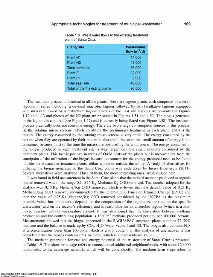
The treatment process is identical in all the plants. These are lagoon plants, each composed of a set oflagoons in series including: a covered anaerobic lagoon followed by two facultative lagoons equippedwith mixers followed by a maturation lagoon. Photos of the East site lagoons are presented in Figures1.12 and 1.13 and photos of the N2 plant are presented in Figures 1.51 and 1.53. The biogas generatedin the lagoons is captured (see Figure 1.57) and is currently being flared (see Figure 1.58). The treatmentprocess practically does not consume energy. There are two energy consumption sources in this process:(i) the rotating micro screens, which constitute the preliminary treatment in each plant; and (ii) themixers. The energy consumed by the rotating micro screens is very small. The energy consumed by themixers when they are operated by their motors is also small, but even this small amount of energy is notconsumed because most of the time the mixers are operated by the wind power. The energy contained inthe biogas produced in each treatment site is way larger than the small amounts consumed by thetreatment plants. This fact is positive in terms of O&M costs of the plants but is inconvenient from thestandpoint of the utilization of the biogas because consumers for the energy produced need to be foundoutside the wastewater treatment plants, either within or outside the utility. A study of alternatives forutilizing the biogas generated in the Santa Cruz plants was undertaken by Incisa Bioenergia (2011).Several alternatives were analyzed. Three of them, the more interesting ones, are discussed here.

It was found in field measurement in the Santa Cruz plants that the ratio of methane produced to organicmatter removed was in the range 0.1–0.15 Kg Methane/Kg COD removed. The number adopted for theanalysis was 0.15 Kg Methane/Kg COD removed, which is lower than the default value of 0.21 KgMethane/Kg COD removed recommended by the International Panel on Climate Change (IPCC) andthan the value of 0.25 Kg Methane/Kg COD removed considered by the USEPA as the maximumpossible value, but this number depends on the composition of the organic matter (i.e., on the specificwastewater) and on the reactor’s efficiency and is reasonable for an anaerobic lagoon (which is a non-mixed reactor) without temperature control. It was also found that the correlation between methaneproduction and the contributing population is 1380 m3 methane produced per day per 100,000 persons.Measurements showed that the biogas generated in the SAGUAPAC treatment plants contains 72–79%methane and the balance is made up by CO2, H2O (water vapour) and N2. The biogas also contains H2Sat a concentration lower than 100 ppm, which is a low content. In the analysis of alternatives it wasconsidered that the biogas contains 65% methane, which is a representative value.

The methane generation forecast and energy potential of the wastewater of Santa Cruz is presentedin Table 1.9. The short term stage refers to connection of additional neighbourhoods, with some 120,000inhabitants, to the sewerage network, which will be done shortly. The medium term stage refers to

Table 1.8 Wastewater flows to the existing treatmentplant of Santa Cruz.

Plant/////Site Wastewaterflow (m3/////d)

Plant N1 14,000

Plant N2 42,000

Total north site 56,000

Plant E 32,000

Plant PI 8,000

Total east site 40,000

Total of the 4 existing plants 96,000



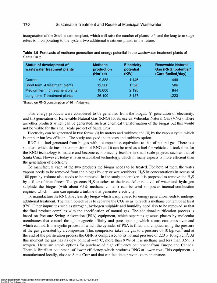
inauguration of the South treatment plant, which will raise the number of plants to 5, and the long term stagerefers to incorporating to the system two additional treatment plants in the future.

Two energy products were considered to be generated from the biogas: (i) generation of electricity,and (ii) generation of Renewable Natural Gas (RNG) for its use as Vehicular Natural Gas (VNG). Thereare other products which can be generated, such as chemical transformation of the biogas but this wouldnot be viable for the small scale project of Santa Cruz.

Electricity can be generated in two forms: (i) by motors and turbines; and (ii) by the vapour cycle, whichis simpler but less efficient. The study analyzed the motors and turbines option.

RNG is a fuel generated from biogas with a composition equivalent to that of natural gas. There is astandard which defines the composition of RNG and it can be used as a fuel for vehicles. It took time forthe RNG technology to mature and become economically feasible in small scale projects such as that ofSanta Cruz. However, today it is an established technology, which in many aspects is more efficient thanthe generation of electricity.

To manufacture each of the two products the biogas needs to be treated. For both of them the watervapour needs to be removed from the biogas by dry or wet scrubbers. H2S in concentrations in access of100 ppm by volume also needs to be removed. In the study undertaken it is proposed to remove the H2Sby a filter of iron fibres. The gaseous H2S attaches to the iron. After removal of water and hydrogensulphide the biogas (with about 65% methane content) can be used to power internal-combustionengines, which in turn can operate a turbine that generates electricity.

Tomanufacture theRNG, the clean dry biogaswhichwas prepared for energy generation needs to undergoadditional treatment. The main objective is to separate the CO2 so as to reach a methane content of at least97%. Other impurities such as nitrogen, hydrogen sulphide and humidity need also to be removed so thatthe final product complies with the specification of natural gas. The additional purification process isbased on Pressure Swing Adsorption (PSA) equipment, which separates gaseous phases by molecularmembranes that control through magnetic affinity and pore opening which atoms can cross over andwhich cannot. It is a cyclic process in which the cylinder of PSA is filled and emptied using the pressureof the gas generated by a compressor. This compressor takes the gas to a pressure of 10 kgf/cm2 and atthe end of the purification process the GNR is compressed to its normal pressure of 220×10 kgf/cm2. Atthis moment the gas has its dew point at −45°C, more than 97% of it is methane and less than 0.5% isoxygen. There are ample options for purchase of high efficiency equipment from Europe and Canada.There is Brazilian equipment of lower efficiency which produces RNG at lower cost. This equipment ismanufactured locally, close to Santa Cruz and that can facilitate preventive maintenance.

Table 1.9 Forecasts of methane generation and energy potential in the wastewater treatment plants ofSanta Cruz.

Status of development ofwastewater treatment plants

Methaneproduction(Nm3/////d)

Electricitypotential(KW)

Renewable NaturalGas (RNG) potential*(Cars fuelled/////day)

Current 9,388 1,146 440

Short term, 4 treatment plants 12,500 1,526 586

Medium term, 5 treatment plants 18,000 2,198 844

Long term, 7 treatment plants 26,100 3,187 1,223

*Based on RNG consumption of 16 m3/day/car



The potentials of electricity and RNG generation in the Santa Cruz project are specified in Table 1.9.To understand the potential RNG market in Santa Cruz it is important to understand its competitors. The

cost of fuels in Santa Cruz is presented in Table 1.10.

Several alternatives for biogas utilization were analyzed in the study. We discuss three of them which areconsidered the most interesting.

Alternative 1

This alternative consisted initially of generating electricity in each treatment plant site and connecting it tothe grid of the power utility, CRE, to sell the produced energy at a fair price. This is the simplest and moststraightforward solution. But it was soon found that due to the country’s energy policy it is impossible toimplement such alternative. First, the same entity cannot be a consumer and producer of electricity. Andeven if it could, CRE charges SAGUAPAC a price of 0.086 US$/KWh, but due to the existing policycan only pay to a producer 0.03 US$/KWh. The cost of generating electricity in this project underalternative 1 is 0.0294 US$/KWh so the existing policy basically eliminates the implementation ofAlternative 1 as described above. This is an example of the importance of the energy policy inestablishing the feasibility of a project and an example of the inexistence of an enabling environment tostimulate the utilization of biogas produced in wastewater treatment plants.

SAGUAPAC is trying to obtain a licence to generate electricity, connect it to the grid and sell it to CREfor a fair price. Another option related to this alternative is that SAGUAPAC obtains the status of a nonregulated producer. In this case it needs to generate more than 1 MW and it needs to identify a consumeror consumers who would buy its electricity at a price agreed between the parties. SAGUAPAC wouldthen connect to the grid of CRE and the identified consumers would withdraw the energy from this grid.This is an option under which the produced electricity can be sold at a fair price. The financial analysisof Alternative 1, assuming a sale price of 0.086 US$/KWh for the electricity produced, yielded thefollowing results:

Total investment: US$ 1.73 millionAnnual savings in electricity or annual income from sale of electricity: US$ 1.25 millionO&M cost: 245,600 US$/yearNet present value of savings during 10 years: US$ 5.56 millionIRR: 78%Cost of electricity generation: 0.0294 US$/KWh

Table 1.10 Fuel prices in Bolivia on March 2011.

Fuel type Price inBolivianos(Bs)

Price inamerican dollars(US$)

Unit of fuel

Special gasoline 3.74 0.53 Liter

Premium gasoline 4.28 0.61 Liter

Diesel 3.72 0.53 Liter

Butane (liquefied gas) 0.034 0.05 Kg

Natural gas 1.68 0.24 Nm3@250 Bar



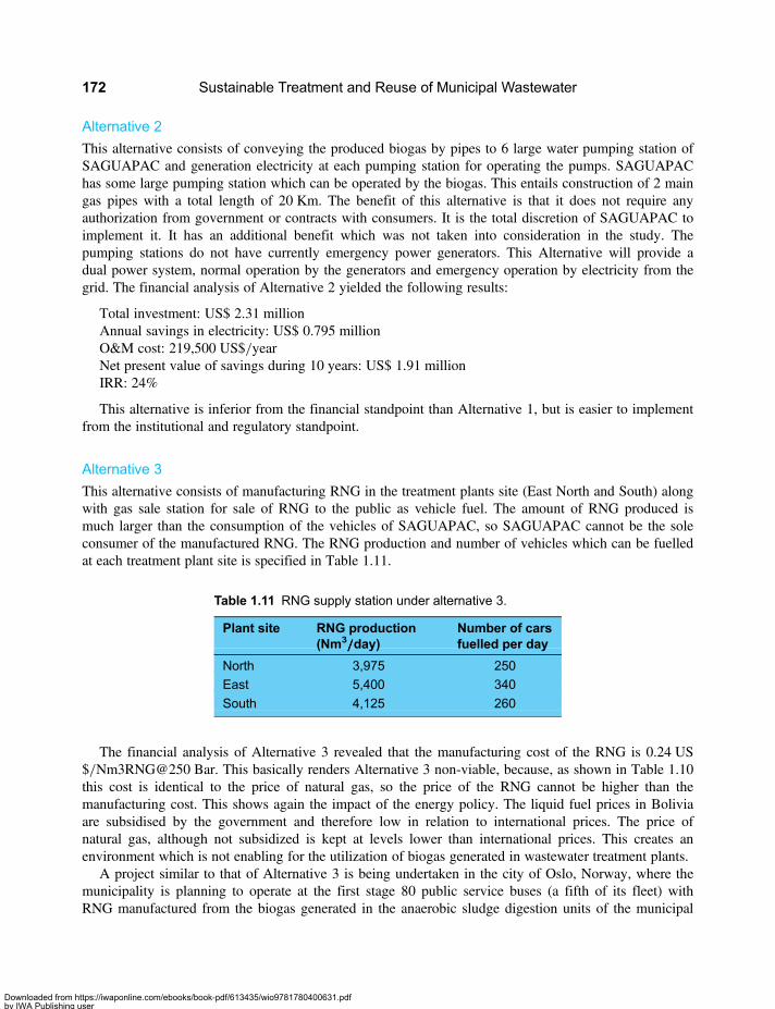
Alternative 2

This alternative consists of conveying the produced biogas by pipes to 6 large water pumping station ofSAGUAPAC and generation electricity at each pumping station for operating the pumps. SAGUAPAChas some large pumping station which can be operated by the biogas. This entails construction of 2 maingas pipes with a total length of 20 Km. The benefit of this alternative is that it does not require anyauthorization from government or contracts with consumers. It is the total discretion of SAGUAPAC toimplement it. It has an additional benefit which was not taken into consideration in the study. Thepumping stations do not have currently emergency power generators. This Alternative will provide adual power system, normal operation by the generators and emergency operation by electricity from thegrid. The financial analysis of Alternative 2 yielded the following results:

Total investment: US$ 2.31 millionAnnual savings in electricity: US$ 0.795 millionO&M cost: 219,500 US$/yearNet present value of savings during 10 years: US$ 1.91 millionIRR: 24%

This alternative is inferior from the financial standpoint than Alternative 1, but is easier to implementfrom the institutional and regulatory standpoint.

Alternative 3

This alternative consists of manufacturing RNG in the treatment plants site (East North and South) alongwith gas sale station for sale of RNG to the public as vehicle fuel. The amount of RNG produced ismuch larger than the consumption of the vehicles of SAGUAPAC, so SAGUAPAC cannot be the soleconsumer of the manufactured RNG. The RNG production and number of vehicles which can be fuelledat each treatment plant site is specified in Table 1.11.

The financial analysis of Alternative 3 revealed that the manufacturing cost of the RNG is 0.24 US$/Nm3RNG@250 Bar. This basically renders Alternative 3 non-viable, because, as shown in Table 1.10this cost is identical to the price of natural gas, so the price of the RNG cannot be higher than themanufacturing cost. This shows again the impact of the energy policy. The liquid fuel prices in Boliviaare subsidised by the government and therefore low in relation to international prices. The price ofnatural gas, although not subsidized is kept at levels lower than international prices. This creates anenvironment which is not enabling for the utilization of biogas generated in wastewater treatment plants.

A project similar to that of Alternative 3 is being undertaken in the city of Oslo, Norway, where themunicipality is planning to operate at the first stage 80 public service buses (a fifth of its fleet) withRNG manufactured from the biogas generated in the anaerobic sludge digestion units of the municipal

Table 1.11 RNG supply station under alternative 3.

Plant site RNG production(Nm3/////day)

Number of carsfuelled per day

North 3,975 250

East 5,400 340

South 4,125 260



wastewater treatment plants (Johansen, 2009). At a subsequent stage the entire fleet of 400 buses will beoperated with RNG. One of the drives to implement this project in Oslo is the reduced carbon emissionwhen using RNG in comparison to the emission from liquid fuel. In addition, in Oslo an enablingenvironment for this type of projects probably exists.

SAGUAPAC is still considering its options and trying to change the environment to somewhat moreenabling. We know that policies may change with time so there is still hope. The lesson learned fromthe example of SAGUAPAC is actually that the utilization of biogas can be feasible in other countries.A situation similar to that of SAGUAPAC in a country with international gas prices and with a policyof stimulation generation of energy by small producers and, in general, with an enabling environment,would render all the studied alternatives feasible.

1.13.5 Wastewater treatment for reducing green house gases emissionFlaring or use of biogas also eliminates the emission of methane which is a strong Green House Gases(GHG). The reduction of GHG emission can be sold as CER (Carbon Emission Reduction) and anadditional significant income can be obtained. As mentioned, SAGUAPAC operates four lagoonswastewater treatment plants. The anaerobic lagoons in each plant are covered and the biogas is beingflared. The utility is studying the options of generating energy from the biogas. SAGUAPAC has alreadysigned a contract for sale of the biogas emission reduction to the community development carbonfund, for an expected amount US$ 2,080,000 during the period 2007–2015 (the World Bank, 2007).This is the first case in developing countries of an emission reduction contract based on capturing ofanaerobic lagoons biogas. Additional information on this carbon emission reduction case is presentedin Chapter 12.

1.13.6 Contribution of resources generation to sustainabilityand improved management of utilitiesThe utilization of the resources contained in the effluent (reuse for irrigation) and in the by-product ofanaerobic treatment (utilization of the biogas) can generate an additional income stream for the utility,on top of the income generated by providing the water and sanitation services. The reduction of emissionof methane, a strong greenhouse gas, can in certain cases generate additional income from the sale ofCarbon Emission Reduction.

The appropriate technology processes described in this book have low energy consumption and in mostcases it is not possible to use within the plants the entire amount of energy produced by the anaerobic processbecause there is no demand for it. Consumers for the energy produced need therefore be found outside thewastewater treatment plants, either within or outside the utility. If the biogas is used within the utility it willsave expenses on energy purchase and if used outside the utility it will generate income from the sale ofenergy or biogas.

The additional income to the utilities from the resources contained in the wastewater can improve notonly the financial sustainability of such utilities but also their environmental and institutionalsustainability. In many cities wastewater is not treated at all but rather discharged directly to receivingbodies, and utilities are institutionally weak to even manage appropriate technology treatment plants. Ifthe discharge of raw wastewater causes severe water contamination problems (which is the situation inmany cases), an appropriate technology treatment plant can be constructed (usually with the support ofgovernment grants) to resolve the problem. Such plant can include installations for energy recoveryand/or effluent reuse. The income generated from the recovery of the resources can be sufficient tocover the O&M of the treatment plant and sometimes even part of the investment. This income stream



can be used to finance the hiring of a professional private operator to operate the treatment plant. This canimprove the overall institutional sustainability of the utility by ensuring the sustainability of the operation ofthe treatment plant and by enhancing the sustainability of the environmental management through thereduction in the contamination of natural water bodies. The hiring of private operators also reduces theinstitutional burden and challenges of the water and sanitation utilities managements and therebycontributes to enhancement of the institutional sustainability.

As an example consider a city the size of Santa Cruz, with about 1 million inhabitants, located in adeveloping country and with an institutionally weak utility. The city does not have any wastewatertreatment installations and discharges all its raw wastewater to receiving water bodies causing theirsevere contamination. Given its water supply problems, the perspective of managing the wastewaterdisposal problem by the utility is remote. Involving the private sector to support managing thewastewater disposal seems difficult because private operators require a guaranteed income and thefinancially weak utility cannot provide such reliable guarantee. Now imagine that a plan is developedregarding the construction of 5 wastewater treatment plants based on the treatment process applied inSanta Cruz and that the plan includes the utilization of the biogas to generate electricity according toAlternative 1 described in Section 1.13.4. The government will provide a grant for construction of thetreatment plants and the electricity generators installed in the treatment plants can be connected to thegrid. The power company will pay for the electricity produced by the treatment plants the price specifiedin Alternative 1. The financial analysis of alternative 1 shows that the O&M costs can be generated fromthe sale of the methane-produced electricity and on top of that, the energy production generates anamount of US$ 5.56 million at present value. A bidding process can be undertaken for construction andoperation of the treatment plants. The Constructor-Operator will specify in his proposal which portion ofthe investment he is willing to provide, and he will also be responsible for the O&M cost of theconstructed treatment plants, once they come on stream. The bidding variable can be the amount ofinvestment that the Constructor-Operator requests from the public sector (national government,municipally and utility). The bidder that requests the lowest public sector investment is the winningbidder. In this case, the sale of energy is the guaranteed income of the Constructor-Operator and this is areliable guarantee which does not depend on the financial performance of a weak utility but rather on thetechnical performance of the bidder, so a bidder that is self-confident will consider it as a safe guarantee.

1.13.7 Example of recovery of the resources containedin wastewaterFigure 1.77 presents the Naan wastewater treatment system and stabilization reservoir. It is a simple system,a typical system of a stabilization reservoir. The raw wastewater is pre-treated in a system of two parallelanaerobic lagoons. The effluents of the two lagoons are discharged to the Naan reservoir for seasonalstorage and treatment, and the effluent of the reservoir is used to irrigate the adjacent fields during theirrigation season. This is a system that already recovers two of the wastewater resources: the water andthe fertilizers. It is possible to recover in this system also the third resource: energy. The idea ispresented in Figure 1.124. It is possible to cover the anaerobic lagoons, capture the biogas and theneither use it for generation electricity, connecting to the power grid, or convey the biogas to an industrialpark located a few kilometres from the reservoir, if a consumer can be identified in this park. InFigure 1.124 one of the anaerobic lagoons was left uncovered, as it is in reality, and the other wascovered to show what needs to be done (cover the anaerobic lagoons with HDPE membranes). Also, thedimensions of the biogas storage tank and of the electricity generating system are not in scale andexaggerated in the figure. In reality they will be much smaller and will occupy a small land area.



1.14 APPROPRIATE TECHNOLOGY TREATMENT PROCESSESCLASSIFIED ACCORDING TO THEIR ADEQUACY FOR USE IN VARIOUSCATEGORIES OF SIZE OF CITIESThe appropriate technology unit processes and some of the combined appropriate technology processesdiscussed in this chapter are presented in Table 1.12 classified according to their adequacy of use incities of various sizes. The cities are classified into three categories: (i) small (with a population of up to20,000); (ii) medium (with a population between 20,000 and 300,000); and (iii) large (with a populationabove 300,000). For each category a recommended list of appropriate technology processes adequate forthis category is provided. This table is intended to support in taking a decision about processes whichshould be considered, or should be discarded for a city of a certain size. The table should be consideredas a guiding instrument but not as a strict rule.

According to the table, lagoon systems should not be considered for large cities, but this recommendationrefers to constructing one plant per city. If a large city needs to construct several treatment plants due totopographical considerations, each plant can be a lagoons plant if it does not serve a population largerthan 300,000–400,000, and even this range is just a reference range which can be somewhat exceeded ifit makes sense. Constructed wetlands are not a good solution for large cities because they consume largeland areas, and even for medium cities constructed wetlands are in most cases not adequate, for the same

Figure 1.124 Recovery of resource from wastewater in the naan wastewater treatment and stabilizationreservoir system



reason. CEPT is in most cases not adequate for small cities; however, small cities which have good waterutilities can use the CEPT process.

1.15 PERFORMANCE AND COSTS OF APPROPRIATE TECHNOLOGYTREATMENT PROCESSES IN RELATION TO ACTIVATED SLUDGEThe treatment capacities of the appropriate technology unit processes and of some of the combinedappropriate technology processes discussed in this chapter are presented in Table 1.13 in terms ofranges of removal percentages of total BOD and total suspended solids (TSS). Also presented in thistable are data on ranges of investment costs and operation and maintenance costs of each of thementioned process. Investment costs as well as O&M costs are also compared to those of secondarytreatment in a conventional activated sludge process. Activated sludge was selected to represent the

Table 1.12 Appropriate technology treatment process classified according to their adequacy for use invarious categories of size of cities.

Large cities*** Medium size cities** Small cities*

Rotating micro screens Rotating micro screens Rotating micro screens

Lagoon systems of varioustypes including mixers aidedsystems and coveredanaerobic lagoons

Lagoon systems of varioustypes including mixers aidedsystems and coveredanaerobic lagoons

UASB reactors UASB reactors UASB reactors

Anaerobic filters Anaerobic filters Anaerobic filters

CEPT CEPT

Constructed wetlands

Reuse for irrigation systems Reuse for irrigation systems Reuse for irrigation systems

Submarine outfalls Submarine outfalls Submarine outfalls

UASB-anaerobic filtercombination



UASB-lagoons combination UASB-lagoons combination

CEPT-sand filtrationcombination

CEPT-sand filtrationcombination

UASB-sand filtrationcombination



UASB-dissolved air flotationcombination



Other combinations need aspecific review to determineif they are adequate for largecities

Other combinations need aspecific review to determine ifthey are adequate for mediumsize cities

Other combinations need aspecific review to determineif they are adequate for smallcities

*Small cities: Cities with population up to 20,000**Medium size cities: Cities with populations in the range 20,000–300,000***Large cities: Cities with populations above 300,000



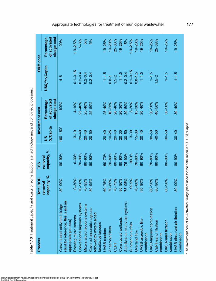
Table

1.13

Treatm

entca

pacity

andco

stsofs

omeappropria

tetech

nologyunitandco

mbinedproce

sses.

Proces

sTo

talB

OD

removal

capacity,

%

TSS

removal

capacity,

%

Investm

entcost

O&M

cost

US

$/////Capita

Percentage

ofactivated

sludgecost

US$/////Yr/////Capita

Percentage

ofactivated

sludgecost

Conve

ntionala

ctivatedsludge

(Just

forreference

,thisisnota

nappropria

teproce

ss)

80–

90%

80–

90%

100–150*

100%

4–8

100%

Rotatin

gmicro

screens

0–30%

0–30%

3–10

4–10%

0.1–0.15

1.9–2.5%

Conve

ntionallagoonssystems

70–

90%

70–

90%

20–40

25–40%

0.2–0.4

5–8%

Mixers

aidedlagoonssystems

70–

95%

80–

90%

20–40

25–40%

0.2–0.4

5%

Cove

redanaerobiclagoons

followedbymixers

aided

facu

ltativelagoons

80–

95%

80–

90%

20–50

25–50%

0.2–0.4

5%

UASBreactors

60–

75%

60–

70%

20–40

25–40%

1 –1.5

19–25%

Anaerobicfilters

70–

80%

70–

80%

10–25

10–25%

0.8–1

13–20%

CEPT

70–

75%

80–

90%

20–40

20–40%

1.5–2

25–38%

Constructedwetla

nds

80–

90%

80–

90%

20–30

20–30%

1–1.5

19–25%

Stabilizatio

nrese

rvoirs

systems

75–

95%

75–

90%

30–50

30–50%

0.2–0.4

5%

Submarin

eoutfa

lls99.9%

99.9%

3–30

3–30%

0.1–0.15

1.9–2.5%

Ove

rlandflo

w70–

80%

70–

80%

15–30

15–30%

0.8–1.5

19–20%

UASB-anaerobicfilter

combinatio

n80–

90%

80–

90%

20–40

20–40%

1–1.5

19–25%

UASB-la

goonsco

mbinatio

n80–

90%

70–

80%

30–50

30–50%

1–1.5

19–25%

CEPT-sandfiltratio

nco

mbinatio

n80–

90%

80–

90%

40–50

40–50%

1.5–2

25–38%

UASB-sandfiltratio

nco

mbinatio

n80–

90%

80–

90%

30–50

30–50%

1–1.5

19–25%

UASB-disso

lvedairflo

tatio

nco

mbinatio

n80–

90%

80–

90%

30–40

30–40%

1–1.5

19–25%

*Theinve

stmentc

ost

ofanActivatedSludgeplantu

sedfortheca

lculatio

nis100US$/

Capita



processes which are not based on appropriate technology. The investment cost in an activated sludge plantis in the range 100–150 US$/Capita. For the purpose of the comparison calculations, the figure 100 US$/Capita was used.

The cost of a combined appropriate technology process is not an arithmetic sum of the cost of the unitprocesses that constitute it, but is rather lower than the arithmetic sum due to economics of scale. Thecost data in the table, both investment costs and O&M costs, are only indicative costs, since the costs ofa wastewater treatment plant are site and country specific. However, these indicative costs allow us todraw some important conclusions.

In terms of effluent quality, most of the processes (except the Rotating Micros Screen process) achieveresults that are not very different from those achieved by the activated sludge process. This is especiallytrue for the combined treatment processes, whose effluents are of similar quality to that of an activatedsludge effluent. If the dilution in the river to which the effluents are discharged is significant, thanthere is practically no difference between the effluents of the combined appropriate technologyprocesses and the effluent of an activated sludge process, in terms of their impact on the oxygencontent of the river.

As shown in Table 1.13, the investment costs of the presented appropriate technology treatmentprocesses are in the range of 20–50% of investment in activated sludge. These estimates are based onthe investment figure of 100 US$/Capita. If a higher figure is taken (which might well be the case)than investment cost of the appropriate technology processes will be even lower in relation to that ofactivated sludge. Perhaps more important is that fact that in most cases, the operation and maintenancecosts of the appropriate technology processes are in the range 5–25% of the operation and maintenancecost of activated sludge.

The general conclusion that can be drawn is that by using appropriate technology treatment processes or acombination of such processes: (i) a significant amount can be saved in investment costs; (ii) a lot of O&Mexpenses can be saved; (iii) the operation and maintenance of the plants is much simpler than that of plantsbased on conventional process; and (iv) almost nothing is lost in terms of effluent quality.

All this has an outmost importance in terms of ensuring the sustainability of the utility by selecting anappropriate technology process. The much lower investment and especially operation and maintenancecosts ensure financial sustainability. The simplicity of operation and maintenance ensures ease inovercoming technical difficulties and long terms sustainability in operating the plant. And all the aboveensures institutional sustainability, since the wastewater management does not pose on the utilityfinancial and technical difficulties.

1.16 SLECTION OF THE ADEQUATE TREATMENT PROCESSA number of unit processes of appropriate technology were described in the book. Based on these processes,the idea of the use of combinations of appropriate technology unit processes was presented. Although unitprocesses by themselves cannot reach very high effluent qualities, specific combinations of unit processescan generate practically any required effluent quality. A plant based on a combination in series ofappropriate technology unit processes is still easy to operate and is usually of lower costs thanconventional processes in terms of investments and certainly in operation and maintenance. So inessence, this book shows the way to obtain high quality effluent by using treatment plants based onsimple, low cost and easy to operate processes.

A large number of simple, sustainable processes (including unit processes and combinations of unitprocesses) were presented and the design of part of them is discussed in the following chapters. Some ofthe presented processes are already used in full scale plants in many parts of the world. As to the rest, it



is not known if there are full scale plants based on these processes. Nevertheless, there is no reason that fullscale plants using these processes will not function well, and we believe that there is room for all theprocesses and that there are specific conditions that justify the use of each of the them, or at least justifythe consideration and analysis of each one of the processes. The processes presented constitute in fact adata base that should be considered for analysis when selecting a process for each new wastewatertreatment plant.

With the relatively large number of unit processes of appropriate technology and a larger number ofcombined processes, the question is how to select the most adequate process for each specific project.The basis for the decision is the local conditions specific to each case. Several parameters need to betaken into account, among them: the size of the city, climatic conditions, especially variation oftemperature during the day and especially during the seasons of the year, altitude above sea level,cloud cover, the flow and composition of the raw wastewater and their fluctuations (diurnal andseasonal), effluent quality required (based on local discharge standards or on the type and size of thereceiving water body), the alternative sites available for location the treatment plant or treatmentplants, the size of land area and topography of each site, preferences of the owner (utility ormunicipality) to have a very simple plant or a somewhat more complex plant, financial resourcesavailable and more.

Climate and temperature variation ranges define a series of processes that can be used. The size ofland available for the treatment plant defines another series of processes which can be fit into it. If itis a large area, then most of the processes can fit in. If the area is limited, then only part of theprocesses can be used. The required effluent quality defines another series of processes that can yieldsuch quality. The owner’s preferred level of simplicity of the plant also defines a series of processes,for example a municipality that opts for simplicity may favour a process of covered anaerobic lagoonsfollowed by overland flow, while a municipality that considers simplicity as a secondary objectivemay opt for UASB followed by DAF. Experience elsewhere with treatment plants of similar size canalso be a factor in selecting the treatment process. As a result of such an analysis, a limited number ofprocesses will be identified, and one of them will be selected. But at the end of the day, for each citya feasibility study has to be conducted by a consulting firm to select the most adequate alternative forthe treatment plant. The most adequate alternative refers to location of the plant and to the treatmentprocess. The preferences of the employer (utility or municipality) need to be defined in the Termsof Reference for the study. The large number of potential processes is reduced to a few after takinginto account the local conditions of each case, so the number of alternatives which needs to be studiesis not really large, and on the basis of the feasibility study the employer can select the alternativehe prefers.

Tables 1.12 and 1.13 provide preliminary guidance for selection of an adequate treatment process.Table 1.12 defines process according the size of the city and Table 1.13 provides information onperformance of various appropriate technology unit and combined processes in terms of BOD and TSSremoval percentages and information on investment costs per Capita and operation and maintenancecosts per Capita per year. General guidance for selection of several possible adequate treatmentprocesses for each case according to its specific characteristics is provided in Tables 1.5, 1.7, 1.14 and1.15. The possible alternatives need then to be considered in depth in a feasibility study. Table 1.14provides guidance on selection of adequate processes according the required BOD removal efficiency,Table 1.15 provides guidance on selection according to the number of people to be served by thetreatment plant, Table 1.5 provides guidance on selection according to the cold season air temperature inthe proposed treatment plant site and Table 1.7 provides guidance on selection according to the availableland size for location the treatment plant.



Table 1.14 Processes selection matrix by removal efficiency of DOD5.

Processnumber

Process description BOD5 removal (%)

10–40% 40–70% 70–85% 85–95% .95%

1 Rotating micro screens, RMS X

2 Anaerobic lagoons and/orfacultative and/or maturationlagoons

X X X

3 UASB X X

4 Anaerobic filter, AF X X

5 Plug flow anaerobic reactor,PAR

X

6 Stabilization reservoirs, SR,single, continuous flow

X

7 Stabilization reservoirs, SR, atleast two, sequential batchoperation

X

8 SSFCW X X

9 CEPT X X

10 Combination 1: MRS+UASB+ facultative lagoon

X

11 Combination 2: RMS+UASB+AF

X

12 Combination 3: MRS+UASB+ sand filtration+UV

X

13 Combination 4: MRS+CEPT+sand filtration+disinfection, UV

X

14 Combination 5: RMS+UASB+ FA+DAF+membrane filtration

X

Table 1.15 Processes selection matrix by population served.

Processnumber

Process description Population (× 1000)

10–20 20–50 50–100 100–300 .300

1 Rotating micro screens, RMS X X X X X

2 Anaerobic lagoons and/orfacultative and/or maturationlagoons

X X X X

3 UASB X X X X X

4 Anaerobic filter, AF X X

(Continued )



The method for a preliminary selection of the alternative unit and combined appropriate technologytreatment processes which may be adequate for a specific project (Method of Process Selection – MPS)is the following:

(1) Review the matrix Tables 1.5, 1.7, 1.14 and 1.15 to identify the processes that meet the desiredtargets of: (i) cold season temperature range, (ii) available land size, (iii) BOD removalefficiency and (iv) design population. The processes that jointly meet the four criteria arepre-selected.

(2) Analyze whether the land area available for construction of the treatment plant is sufficient to housethe pre-selected processes: for example, Lagoons, Stabilization Reservoirs and SSFCW requirelarge land extensions which might not be available and therefore these process might be rejectedeven if the comply with all other requirements.

(3) Analyze other external factors as cloud cover (for facultative lagoons a low cloudiness ispreferable), wind direction in the plant site (to avoid the odours transfer by the wind topopulation centers), altitude above the level sea, etc.

(4) Discarded from the pre-selected alternative processes the ones found inadequate and proceed tocarry out a more detailed feasibility study of the remaining processes.

Table 1.15 Processes selection matrix by population served (Continued ).

Processnumber

Process description Population (× 1000)

10–20 20–50 50–100 100–300 .300

5 Plug flow anaerobic reactor,PAR

X X

6 Stabilization reservoirs, SRsingle, continuous flow

X X X X X

7 Stabilization reservoirs, SR atleast two, sequential batchoperation

X X X X X

8 SSFCW X X

9 CEPT X X X X

10 Combination 1: MRS+UASB+facultative lagoon

X X X X

11 Combination 2: RMS+UASB+AF

X X X X

12 Combination 3: MRS+UASB+sand filtration+UV

X X X X X

13 Combination 4: MRS+CEPT+Sand filtration+ disinfection, UV

X X X X X

14 Combination 5: RMS+UASB+FA+DAF+membrane filtration

X X X

Comments:1. Anaerobic Filters are used for small towns when they are the main treatment process. When they are used as a polishingunit, they can serve larger populations.2. There is no experience with Combination 5. It might be adequate also for larger populations than specified in the Table.



It is clear that nothing can replace the sound criteria and the experience of a good designer and processengineer, but the MPS is a good start for a feasibility analysis, which should be complemented byappropriate calculations.

Design models prepared for part of the unit and combined appropriate technology processes presented inthe book may be used to carry out a first approximation of dimensioning the processes. A list of therespective Excel Programs is presented in Section 1.19. However, these model programs should be usedwith great caution. They do not replace the criteria of the design engineer who must ultimately beresponsible for the design results. These programs should not be used without a full understanding of theprocesses, as presented in the book.

1.17 SEWERAGE NETWORKS, THE CONDOMINIALSEWERAGE CONCEPTSewerage networks do not form part of wastewater treatment systems (although there are opinions that sometreatment takes place in the sewerage and conveyance systems); however, sewerage and treatment systemsare coupled in the sense that sewage treatment cannot take place without the existence of the seweragenetwork which collects the sewage and conveys it to the treatment plant. For a municipality, theinvestment in wastewater management includes investment in sewerage networks, wastewaterconveyance and wastewater treatment. Reducing the investment in sewerage networks and conveyance isas important as reducing treatment investments.

The analysis of sewerage networks and wastewater conveyance systems is not covered in this book.Detailed information on the theory and design of these systems is widely available in the professionalliterature. It can for example be found in Tscobanoglous (1981).

An innovative method for reducing the investment cost of sewerage networks and conveyance wasdeveloped in Brazil (Melo, 2008) and is denominated the Condominal system. The sewerage system ofthe city of Brasilia, the capital of Brazil is a condominial system. It is also used in other cities in Braziland in parts of the city of Lima, Peru and El Alto, Bolivia. The condominial sewerage technology, alsocalled “shallow sewerage”, is different from the denominated “small bore technology” or “simplifiedsewerage” because there is no retention of solids in the condominial systems. Consequently, there is noneed to construct household retention tanks and no need for periodic sludge removal. Detailedinformation on the condominial technology is provided by Melo (2008) and by Vargas-Ramirezand Lampoglia (2006) and can be found also in the report of The World Bank Water and SanitationProgram (2002).

From the technical standpoint, the condominial technology simplifies the design and characteristics ofpipelines, making it physically easier to connect households. Condominial sewerage considers that thenetwork is divided into a private part - the condominial lines) and a public part - the main sewers. Thecondominial lines are built in areas with no road traffic such as gardens, sidewalks, etc., and are laid at ashallow depth. The diameter of these lines is usually 100 mm and it uses much smaller inspectionchambers (manholes).

The condominial model also proposes the development of new relations of co-responsibility for servicesbetween the service provider and the user. From the social perspective, the model introduces a participatorycomponent in the implementation phase that is intended to motivate users to connect to the system and togenerate a commitment to keep good use practices. Consequently, one of the users’ responsibilities is themaintenance of the condominial lines, especially when pipes are laid on internal areas. In those cases, thebeneficiaries must receive the necessary training to perform that task. However, the utility remainsresponsible for the O&M of the overall system at the city level.



Condominial systems have been utilized in Brazil since the 80′s where theywere first employed in the cityof Natal. The conventional model of service provision has been shown to be inappropriate for the expansionof services to slums and peri-urban poor areas where chaotic occupation and complex topography constrainthe installation of regular sewerage layouts. The condominial system proved to be appropriate for such areas.In the capital of Brazil, the city of Brasilia, since 1995 the condominial technology was adopted by CAESB,the local water and sanitation utility, as the only option for sewage collection, with more than 120,000condominial connections built by the year 2000. The condominial technology had been used to expandsewerage connections to peri urban areas of cities like Salvador, Petronila, Recife and Rio de Janeiroamong other. By 2000, 13.6% of the sewerage connections in Brazil were condominial. In past years thetechnology has been expanded from Brazil to other Latin-American countries. In Bolivia it was employedto expand sewerage services to more than 50,000 households in the city of El Alto. In Peru, SEDAPAL,the utility of Lima, implemented a program to expand condominial sewerage to 25,000 families. The Cityof Durban, South Africa experimented with this technology in 2000 and is introducing adaptations forscaling it up. Experiences in various countries show that an increasing number of utilities and localservice providers are using this technology to reach the Millennium Development Goals, due to itssignificantly lower costs with identical level of service to that of conventional sewers.

Benefits of the condominial system include: (i) Financial Benefits – manifested by capital cost savings,which is one of its more appealing characteristics, since it allows the provision of services to significantlymore people with the same financial resources. Cost reductions stem mainly from (a) lower excavationvolumes due to more shallow location of the pipes; (b) use of simplified inspection chambers instead ofcostly manholes; (c) reduced pipe diameters and layout length; and (d) easiness of construction thatresult in reduced need for heavy machinery. The financial benefits are also manifested by reduction ofO&M costs since the accessibility of the system at depths varying from 60 to 150 cm allows for easieraccess for manual maintenance. In case of breakage, system components are much easier and cheaper toreplace; (ii) Adaptable layout - the flexible condominial layout allows working in irregular urban layoutsettlements, very steep slopes and rocky terrains. In fact, in many locations it may be the only feasibletechnical option; (iii) Better hydraulic functioning – the use of the shear stress boundary concept fordesign instead of the minimum velocity allows the use of lower minimum slopes. Similarly and counterintuitively, smaller diameters allow greater buoyancy and more efficient transportation of solids,especially in densely populated areas.

In addition, the condominial systems also provide social benefits such as: better and more appropriate useof services, increased rate of connections to the network, community development, and higher willingness topay as well as higher payment rates.

Challenges to scale up the condominial technology include issues of responsibility for operation andmaintenance of parts of the systems, legal constraints related to construction standards, and ownershipissues. Characteristically, the condominial approaches require intensive social work with thecommunities. These costs –along with the steep learning curve- can be quite onerous for small pilotprojects, even threatening to render system’s savings negligible. The larger the project scale the easier itis for service providers to administer the condominial system. The key challenge for scaling-up is tomaintain a social mobilization process on a large scale that brings about the benefits described above,while maintaining the per-capita social costs at a reasonable level.

The overall investment cost savings of implementing the condominial technology, when compared toconventional technology, are well documented, reaching 40–50%. Figure 1.125 demonstrates the reasonsfor cost saving. In the condominial system, most of the network consists of lower cost condominialsewers (the blue lines), while in the conventional system all the network consists of higher costconventional sewers (the red lines).



1.18 WASTEWATER TREATMENT IN THE CONTEXT OFGLOBALWATER ISSUES1.18.1 IntroductionIt is commonly accepted that adequate wastewater collection, treatment and disposal is required in order toprevent public health risks and environmental degradation. Unfortunately, in developing countries sewerageservices of collection and conveyance of wastewater out of urban neighborhoods is not yet a serviceprovided to all the population. Adequate treatment of wastewater is even less frequently practiced and isprovided only to a small portion of the collected wastewater, usually covering less than 10% of themunicipal wastewater generated. In slums and peri-urban areas, which constitute large portion of cities indeveloping countries (an average of about 38% of the total urban population in 2005 with significantdifferences among geographical region), it is not rare to see raw wastewater flowing in the streets. Inaddition to the obvious need to treat wastewater for the purposes of preventing public health risks andenvironmental degradation, there are also other aspects for the necessity of providing adequate treatmentand disposal of wastewater, especially in developing countries. To understand these aspects we need toexpand the discussion to the wider context of global water issues.

1.18.2 The global water crisisA lot of attention is being directed in the recent years to a potential global water crisis. The UN estimates thatabout 1 billion people in the world do not have access to safe drinking water and 2.5 do not have access tosanitation services. These data indicate that the water crisis is not a matter of the future, it is already here.

Figure 1.125 Comparison between condominial and conventional sewerage systems



Most of the people without access to drinking water and sanitation reside in developing countries, so for themost part; the water crisis is located in developing countries. Water is the main causes of diseases indeveloping countries. About 80% of the diseases in these countries result from the effects of contaminatedwater, lack of water and poor sanitation. About 3.3 million people die annually from water borne diseases,most of them children under the age of 5. Water Borne diseases are responsible for more deaths than anyother cause. More attention is being directed to the global water crisis as a result of the ensuing globalwarming, which is expected to exacerbate water scarcity in some zones and flooding in others.

Water is a resource of special nature, a global common resource. Water resources transcend nationalboundaries. Moreover, our global interdependencies are woven through water. Water is a cross cuttingnatural resource upon which most of the other sectors and human activities depend, including agricultureand food production, renewable energy, industry, health, forestry, land-use, disaster risk reduction andbasically most types of economic development activities. All these depend upon water for theirlong-term sustainability. Water as a resource is also affected by other sectors and activities, as energycosts, consumption by agriculture and industry, contamination, spread of diseases and epidemics andclimate change. Good water management is one that balances water across competing demands andprioritizes water for basic human needs and ecosystem functions; as well as responding effectively towater induced hazards such as droughts and floods.

Earth is known as the Blue Planet, the Water Planet. But actually it is the Salt Water Plant. About 97.5%of its water is salt water (in the Oceans). Only 2.5% of the plant’s water is fresh (sweet) and of that 69% istied in glaciers, 30% in groundwater, part of which is unavailable, and only 0.3% (of the 2.5 %) is in riversand lakes, so available sweet water is very limited in relation to the entire amount of water on the planet.Even so, on the average, the amount of rain water which comes down as part of the water cycle istheoretically sufficient for the needs of all the people on the plant. But this sensation of plentiful water isonly a myth. The distribution of location of the population across the planet is not uniform and this is aphenomenon beyond our control. As a result the demand for water is also not uniform. Neither is thedistribution of availability of fresh water uniform across the planet and along the seasons of the year.That is certainly a phenomenon beyond our control. Consequently, the relation between availability anddemand of water is not uniform, resulting in areas of physical abundance of water, and also wide areasof physical scarcity. In addition to the high spatial disparities there is also a high temporal disparity.

Forecasts indicate a rapid global population growth. In 2011 we are approaching 7 billion people andwithin 20 years the population will reach 9 billion or more. Several additional important facts related togrowth forecasts are: (i) most of the population growth is expected to take place in developing countries,while the population of developed countries will remain constant at about 1 billion, as shown inFigure 1.126; (ii) the urban population is growing and the rural population declining. As a result of thisurbanization process, about 60% of the population will be urban in 2030, up from about 45% in 2010(see Figure 1.124); and (iii) the size of cities is growing and in the future there will be much more largecities and especially mega cities (about 30 megacities with over 10 million each in 2030, up from 15 in2010), as shown in Figure 1.127. All this implies intensification of the water crisis in the future, unlessdrastic actions are taken to alleviate the problem.

For the most part, developed countries have managed to avoid the direct water crisis and will mostprobably succeed in avoiding it also in the future, but in developing countries the crisis may intensify.However, avoidance of direct crisis will not relieve developed countries from being impacted by thecrisis. The world is today a global village. Shortage of grains and rises in the prices of basic foodcommodities in the past few years caused social uprisings in developing countries with impacts on theentire world. Similarly will the water crisis in developing countries have an impact on developedcountries through the impact of social unrest, disruption of economic, commercial and trade activities,



disruption of flows of commodities, possible negative impacts on political interests of developed countries,spread of diseases, the need of emergency humanitarian support to countries in severe water crisis,stimulation of immigration out of such countries and more.

Figure 1.127 World population forecast and urbanization trends (Source: World Bank Development Report2003)

Figure 1.126 World population growth 1750–2100



According to forecasts of water availability and consumption in the Latin America Region (LAC), in theyear 2030 the region will experience a shortage of 40% of its demand. The global shortage forecast isprobably similar. The LAC forecast is based on certain assumptions. The scarcity trend can be mitigatedby actions that can be taken and by inducing behavior changes of the consumers, rendering theassumptions incorrect and reducing or eliminating the water deficit. Technological and institutionalmeasures are discussed below.

1.18.3 The main water consumers and the potential for water savingsby consumer categoryWho are the main water consumers (in terms of withdrawals of fresh water)? Forecast for 2030 generallyindicate the following water withdrawers and the percentage of consumption of each one: Agriculture –

about 75%, Municipal consumption – about 10%, Industrial consumption – about 10%, and Evaporationfrom reservoirs – about 5%. There are two additional water consumers which are sometimes omitted: (i)water serving as a receiving body of various types of pollutants, that is, water consumed for PollutionAbsorption; and (ii) water required for sustaining ecosystems and life of all other non human species thatshare with us this planet, also known as environmental water flows. It is difficult to estimate the level ofconsumption of these two. Worth noting is that the largest consumer is by far the use of water forirrigation and that the current irrigation efficiency worldwide is less than 40%.

The potential for water savings, that is, for reducing water consumption by each consumer is as follows:(i) Irrigation-50%, by moving from surface irrigation to more efficient methods of micro-sprinkling and dripirrigation; (ii) Municipal consumption-(20%–30%) by conservation, using water more efficiently, managingdemand and reducing losses in the piping systems; (iii) Industry-(50%–90%) by modifying productionprocesses, moving to clean development mechanisms (cleaner production processes), using water moreefficiently and recycling wastewater for use within the industries; (iv) pollution absorptionconsumption-100% by providing adequate treatment to all wastewaters; and (v) environmental flows-nopotential for reduction, probably increase is required. As can be seen there is significant room forsavings and therefore for alleviating the water crisis, all this with no sacrifice of economic output orquality of life. Achieving such savings involve application of a combination of technical measures andinstitutional improvements.

1.18.4 Reasons for the water crisisSeveral causes contribute to the water crisis: (i) Physical Water Scarcity in certain regions, which willintensify with time due to increase of the population, the urbanization trends and probable climatechange; (ii) Economic weakness which results in insufficient investments; (iii) Governance weakness atthe central and local governments’ levels; (iv) Institutional capacity weakness at the utilities level; and(v) various combinations of the above. The natural tendency of layman would be to consider thephysical scarcity as the main reason for the water crisis. However, the main problems, especially indeveloping countries, are weak governance and low institutional capacity. For the most part, the currentwater crisis is not a scarcity crisis but rather a management (or mismanagement) crisis. With time it willtransform to be also a scarcity crisis. It remains a grave moral shortcoming that about 1 billion peoplecannot drink water without risking disease or death and 2.5 billion do not have access to sanitationservices while the reason is not so much the scarcity of water as lack of social and political commitmentand capacity of governments to meet the basic needs of the poor.

The physical scarcity of water has technical solutions (which are discussed below). The economicshortcomings can also be alleviated with efforts of governments in developing countries, and with



support of developed countries and the private sector. The governance and institutional problems (in otherwords the management crisis) are the most difficult to resolve and are the reason for having the problemconcentrated in developing countries. Developed countries have managed to overcome the crisis, even inconditions of physical scarcity, through structural reforms and a combination of institutional andtechnical measures. Israel, Australia and Singapore can serve as examples of such countries, amongothers. These examples indicate that it is possible to overcome the water crisis also in many developingcountries, if the institutional and management problems are resolved. However, if the management crisisis not resolved before the scarcity crisis becomes more critical, the results can be devastating.

1.18.5 Water and climate changeClimate change and its implication on the water sector is a widely discussed topic. The relation of wastewatertreatment and climate changed is discussed in Chapter 12. So issues of climate change are not touched here, butit is clarified that adaptation to climate change is essentially about water management – building resiliencethough good water management. Global trade in food and other essential products for developmentdepends upon water availability in producing regions – climate-related interruptions to the water cycleupon which this production depends could have potentially devastating global consequences. Climatechange impacts on transboundary waters will demand a new paradigm of regional and internationalcooperation. Is that achievable? Given the limited international success in controlling the increase of GreenHouse Gases, the recent events of social unrest following food increase cost crisis are just an introductionto political and economic upsets which will occur in a warming world.

1.18.6 The situation of the poorA fewwords on the situation of the poor households not connected to themunicipal water distribution network.The poor usually live in slums and peri-urban areas, which in most cases are not connected to water supplynetwork. Poor households, as any other household, cannot live without water and they have to purchasesmall volumes of contaminated water from vendors supplying water in plastic containers or in tankers, atrates higher 2 to 10 times in relation to the tariffs charged by the water utility. The real meaning of theeffect of water scarcity on the poor is therefore paying a significant portion of the household income forsmall volumes of contaminated water. The population which lives in slums is large, totaling about 38% ofthe population of developing countries (about 2.1 billion). Connecting poor households to the water supplynetwork not only provides convenient access to adequate volumes of safe and clean water but also means arelief from an economic burden and a significant increase in the available income.

1.18.7 Water as a human rightOn July 28, 2010 the UN General Assembly declared that “Safe drinking water and sanitation is a humanright essential to the full enjoyment of life and all other human rights”. The declaration was not achieved inconsensus. It is noted that the declaration includes sanitation services and that it does not mentioneconomic aspects and provision of water at an affordable tariff. We profoundly agree that water is aHuman Right. This is a basic right essential for sustaining human life. The meaning of this human right isthat all governments have the obligation to supply potable water to all their citizens in sufficient quantitiesat an affordable cost (and this is not being done by most governments in developing countries). However,water is also an economic good. It is free when it falls from the sky, before it touches the ground. Once itreached the ground, there is a cost for its collection, conveyance, treatment, storage, distribution, collectionof the wastewater, its treatment and safe disposal. Who should pay for all this? Potential payers are: grants,users and taxpayers. Grants alone are by far insufficient. Payment by taxpayers only is not sustainable, as



shown from experience in countries that have adopted such a model. Logic provides that users pay for thewater service, with taxpayer support when necessary (which means government’s transfers). Those userswhich have the financial capacity should pay for the real cost of water. The poor that do not have thefinancial capacity should pay reduced, affordable tariffs and the utilities should be supported by subsidiesto compensate for the reduced tariffs of the poor. There are various forms for managing such subsidies.

1.18.8 Proposed strategy options to alleviate the water crisisDuring the quest for economic growth we ignore the limits of nature and over-exploit the water resources.We have to respect the limits of water resources and learn to live within these limits. Instead of continuouslysearching for new water sources we need to start looking inside. The efficient use of water is equivalentto creating new sources. The main additional water source is conservation, demand management(100 liter/capita/day not more), efficient water use, control of water losses, reuse and recycling.Investments in efficient water use, conservation and reuse are more beneficial than investing inconventional projects. Water cannot be used just once: it must be reused in agriculture and recycled forother purposes. Wastewater must be considered a resource containing water, fertilizers and energy.Reuse and recycling liberate more fresh water for potable use.

The strategy for alleviating the water crisis must include a combination of technical and institutionalmeasures. It must be based on integrated water resources management, correct and flexible allocation ofwater between sectors (municipal, agricultural and industrial), and sometimes on introducing measures ofwater markets for reasonable allocation. The largest water consumer is irrigation. The rapid populationgrowth requires increased food production, which in turn will require expansion of irrigated land. It isnecessary to plan ahead and change the type and quantities of produce, moving from industrial plants towheat, grains soy and alike, but this does not necessarily mean increase in water consumption forirrigation. A strategy approach of outmost importance for alleviating the water crisis is increasing theirrigation efficiency from the current less than 40% to the possible 90%, moving away from surfaceirrigation methods to micro-sprinkling, drip and subsurface drip irrigation methods.

Of great importance is incorporating in the strategy institutional strengthening measures, sinceinstitutional weakness is one of the main causes of the crisis and a prerequisite for success is to makeinstitution work. To resolve specific water crisis issues in each country and city, specific measures needto be tailored to respond to local conditions. A general manue of activities which can be included in acrisis alleviation strategy is presented below.

For each specific case, the corresponding portion of the manue needs to be identified and adopted. Thepresented manue is divided to three types of activities: (i) Technical measures; (ii) Institutional measures;and (iii) Extreme measures for cases of deep crisis. Some measures appear both as institutional andtechnical since they have aspects of both. It is obvious that each measure presented for crisis alleviationis a wide topic in itself and it is impossible to expand the discussion on all of them in this book. Also,the measures do not appear in an order of priority, since priority is also specific to each case and localconditions. Improvements will not materialize until policies, laws and institutions begin to foster therequired measures.

Technical Measures (Technical Options as part of the strategy to mitigate the water crisis)

• Integrated Water Resources Management• Application of Efficient Irrigation methods• Reduction of Unaccounted For Water• Water Conservation (Demand Management, flow limiting and efficient water use devices at the

household level)



• Undertaking only Rational Investments• Wastewater Treatment to prevent contamination of fresh water• Reuse of municipal effluents for irrigation, the stabilization reservoir concept• Effluent recycling for industrial reuse• Use of simple, low cost technologies for water treatment, wastewater treatment and water and sewage

networks• Small scale solutions: Microdams, Shallow wells, collection of dew for providing humidity to plants,

moisture conserving land techniques• Use of marginal water (springs, flood waters) by seasonal storage• Recharge of flood water to aquifers• Use of saline water (for direct irrigation, industrial uses, diluting with sweet water, desalination of

saline water)• Stimulating rainfall by cloud seeding with silver iodine• Increasing the irrigation efficiency by the use of efficient irrigation methods• Desalination of sea water• Effluent Recycling for potable municipal reuse, in certain cases

Institutional Measures (Institutional Options as part of the strategy to mitigate the water crisis)

• The key issue is to make institutions work• Adopting an adequate and strong legal and institutional framework (institutional reforms when

necessary)• Wise administration and management of water resources• Use of common sense, experience and innovations• Integrated Water Resources Management• Rational and intelligent water allocation between sectors and within sectors• Modification of allocations according to needs, more for the municipal sector and less for agriculture• Preparation of Master plans and conceptual plans with International Support• Undertaking only Rational Investments• Limiting increase of cities or even reducing population in accordance with water availability• Communication campaigns and education of the public to save water (not 600 liter/capita/day, 100

liter/capita/day is enough, and even less in critical cases)• Water conservation (Demand Management, flow limiting and efficient water use devices at the

household level)• Water Metering• Efficient Management of Water Utilities• Reduction of Unaccounted For Water• Use of water more than just one time: reuse for irrigation, industry and non-potable municipal

purposes• Use of simple, low cost technologies for water treatment, wastewater treatment and water and sewage

networks• Efficient Management of Irrigation systems and use of efficient irrigation methods• Application of adequate tariff policy (to stimulate saving and provide financing) and an effective

collection system• Application of adequate regulation• Small Scale Solutions• When applicable: Private sector participation in management of utilities and/or in financing



• In certain cases, creating frameworks and mechanisms for water markets• Public Participation• Obtaining support of the public sector through various Public Private Participation (PPP)

mechanisms• In developing countries, obtaining support from developed countries

Extreme Technical Measures for cases of deep crisis

• Limiting size of cities in accordance with availability of water• Displacement within the country, when necessary, to distribute the population in accordance with

availability of water• Reducing Birth Rate and providing Equal Economic opportunity to Women• Modification of water allocations according to needs, more for the municipal sector and less for

agriculture• Application of efficient irrigation methods (drip, subsurface drip, micro-sprinkles)• Collection and use of dew for providing humidity to plants• Use of Biogenetics to reduce plants consumption of water, resulting in allocation of less water for

irrigation• Desalination of seawater (50% of the world’s population lives within 50 km from coastlines and can

use desalinated sea water• Municipal wastewater must be reused (mainly in irrigation), using seasonal storage (the stabilization

reservoir concept)• In-house treatment and reuse of gray water (or even wastewater) for non potable purposes using

membrane techniques (Compact family size treatment plants are being developed, it is like havingan additional washing machine in the basement)

• When necessary, wastewater reclamation for potable use (as is being done in Singapore)

In summary, what is required is a paradigm shift from the old paradigm of: (i) Subdivided WaterManagement (Ag, Urban, Indus); (ii) Use of water just once; (iii) Inefficient use of water; and (iv)Polluting large quantities of water, to the emerging paradigm of: (i) Integrated Planning andManagement of Water; (ii) Use Water Efficiently and Multiple Times; (iii) Matching Needs with WaterSources; and (iv) Minimizing Pollution.

Involvement of developed countries is essential to support resolution of the crisis. Developed countriesneed to provide support to developing countries in their attempts to resolve the water crisis because of:(i) the status of water as a global common good, as mentioned previously; (ii) the difficult situation ofthe poor; and (iii) the incapacity of developing countries to resolve the problems on their own. Thesupport of developed countries should be provided especially in developing concepts and preparation ofconceptual plans (most important), in assistance for governance/institutional improvements andimplementation of reforms, and in financing.

The role of the private sector. The private sector can also play a role in alleviating the water crisis in twoways: (i) financing; and (ii) support in improving the performance of the water utilities. The private sectorhas to get involved in financing the water sector since the demand for funds is enormous and the publicsector alone cannot do provide the required funding. The private sector participates in financing othersectors (transport, energy, education, health) and there is no reason to forbid it from participating infinancing the water sector too, in spite of the ideological arguments used against such approach. The



private sector can also participate in various models of PPP and contribute to institutional improvement ofutilities in developing countries, which is the main problem of the sector and the major reason for the watercrisis. This type of activity is currently quite limited. The population in developing countries served byprivate water operators in 2007 was only 160 million. that is, about 3% of the total population in thesecountries, and is not expected to ever grow beyond 10%, so the provision of water will remain mostlythe responsibility of the public sector. Decision makers in developing countries need to have variousoptions to tackle the many challenges of water utilities. Private Public Participation (PPP) can be oneof them.

For many years the success in institutional improvement of water utilities in developing countries hasbeen modest, and with time it becomes more difficult to achieve because the challenges become greaterdue to the increase in population. The issue of adaptation to climate change has directed attention to thewater crisis and might help in identifying and implementing strategies for alleviating the problems,including addressing the institutional weakness problems, especially taking into account that theintensification of the problems caused social unrest which may push governments to take actions, ashappened in the case of the recent food crises.

Will the global water crisis intensify or diminish? That is a difficult question to answer. It depends on allof us, the inhabitants of the planet. Let’s hope that the human spirit will overcome the difficulties and that wewill manage to alleviate water scarcity and mitigate the water crisis which may cause a retreat and decay ofthe human race.

1.18.9 The water crises implications on wastewater treatmentIt is commonly accepted that adequate collection, treatment and disposal of municipal wastewaters isrequired in order to prevent public health risks and environmental degradation in general. However,wastewater management needs also to be evaluated in the context of the global water crisis. Consideringthe proposed strategy options to alleviate the water crisis which were discussed above, it is concludedthat in addition to protection of public health and of the environment, adequate wastewater managementalso plays an important role in the strategy to mitigate the effect of the water crisis. Wastewatertreatment is an important activity in preservation of the quality of exiting water sources by preventingcontamination of water bodies by raw wastewater thus maintaining additional sources of clean water.The water crisis discussion also indicates the importance of municipal effluents reuse to irrigate farmlandas both means for generating an additional source of water for irrigation (which liberates fresh water tobe used for urban supply) and as a method for totally eliminating discharge of effluents to clean surfacewater bodies for the purpose of maintaining their quality.

In developing countries, where the coverage of wastewater treatment is very low, increasing the treatmentcoverage is a necessary and important goal. The rapid increase of population and the urbanization tend willresult in generation of large quantities of wastewater which, if not treated, will increase the public healthrisks, especially in poor neighbourhoods, and will contaminate water sources. A common practice indeveloping countries is the uncontrolled reuse of raw wastewater to irrigate food crops, adding to thepublic health risks induced by untreated wastewater. Treatment of the wastewater will diminish the reuseof untreated wastewater. Untreated wastewater also contributes to the contamination of water bodieswhich serve as water supply sources. Consequently, increasing wastewater treatment coverage is apriority in developing countries. A key in the strategy to achieve this goal is adopting low cost andsimple to operate treatment processes as means of alleviating the economic burden by loweringinvestments and O&M expenses, and especially as means of alleviating institutional problems byapplying processes that are easily manageable.



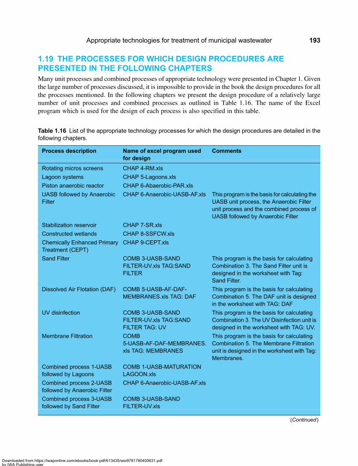
1.19 THE PROCESSES FOR WHICH DESIGN PROCEDURES AREPRESENTED IN THE FOLLOWING CHAPTERSMany unit processes and combined processes of appropriate technology were presented in Chapter 1. Giventhe large number of processes discussed, it is impossible to provide in the book the design procedures for allthe processes mentioned. In the following chapters we present the design procedure of a relatively largenumber of unit processes and combined processes as outlined in Table 1.16. The name of the Excelprogram which is used for the design of each process is also specified in this table.

Table 1.16 List of the appropriate technology processes for which the design procedures are detailed in thefollowing chapters.

Process description Name of excel program usedfor design

Comments

Rotating micros screens CHAP 4-RM.xls

Lagoon systems CHAP 5-Lagoons.xls

Piston anaerobic reactor CHAP 6-Abaerobic-PAR.xls

UASB followed by AnaerobicFilter

CHAP 6-Anaerobic-UASB-AF.xls This program is the basis for calculating theUASB unit process, the Anaerobic Filterunit process and the combined process ofUASB followed by Anaerobic Filter

Stabilization reservoir CHAP 7-SR.xls

Constructed wetlands CHAP 8-SSFCW.xls

Chemically Enhanced PrimaryTreatment (CEPT)

CHAP 9-CEPT.xls

Sand Filter COMB 3-UASB-SANDFILTER-UV.xls TAG:SANDFILTER

This program is the basis for calculatingCombination 3. The Sand Filter unit isdesigned in the worksheet with Tag:Sand Filter.

Dissolved Air Flotation (DAF) COMB 5-UASB-AF-DAF-MEMBRANES.xls TAG: DAF

This program is the basis for calculatingCombination 5. The DAF unit is designedin the worksheet with TAG: DAF

UV disinfection COMB 3-UASB-SANDFILTER-UV.xls TAG:SANDFILTER TAG: UV

This program is the basis for calculatingCombination 3. The UVDisinfection unit isdesigned in the worksheet with TAG: UV.

Membrane Filtration COMB5-UASB-AF-DAF-MEMBRANES.xls TAG: MEMBRANES

This program is the basis for calculatingCombination 5. The Membrane Filtrationunit is designed in the worksheet with Tag:Membranes.

Combined process 1-UASBfollowed by Lagoons

COMB 1-UASB-MATURATIONLAGOON.xls

Combined process 2-UASBfollowed by Anaerobic Filter

CHAP 6-Anaerobic-UASB-AF.xls

Combined process 3-UASBfollowed by Sand Filter

COMB 3-UASB-SANDFILTER-UV.xls

(Continued )



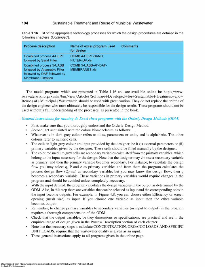
The model programs which are presented in Table 1.16 and are available online in: http://www.iwawaterwiki.org/xwiki/bin/view/Articles/Software+Developed+for+Sustainable+Treatment+and+Reuse+of+Municipal+Wastewater, should be used with great caution. They do not replace the criteria ofthe design engineer who must ultimately be responsible for the design results. These programs should not beused without a full understanding of the processes, as presented in the book.

General instructions for running de Excel sheet programs with the Orderly Design Methods (ODM)

• First, make sure that you thoroughly understand the Orderly Design Method.• Second, get acquainted with the colour Nomenclature as follows:• Whatever is in dark grey colour refers to titles, parameters or units, and is alphabetic. The other

colours refer to numeric cells.• The cells in light grey colour are input provided by the designer, be it (i) external parameters or (ii)

primary variables given by the designer. These cells should be filled manually by the designer.• The coloured medium grey cells are secondary variables calculated from the primary variables, which

belong to the input necessary for the design. Note that the designer may choose a secondary variableas primary, and then the primary variable becomes secondary. For instance, to calculate the designflow you may select q, P and c as primary variables and from them the program calculates theprocess design flow (QDWW) as secondary variable; but you may know the design flow, then qbecomes a secondary variable. These variations in primary variables would require changes in theprogram and should be avoided unless completely necessary.

• With the input defined, the program calculates the design variables in the output as determined by theODM. Also, in this step there are variables that can be selected as input and the corresponding ones inthe input become outputs. For example, in Figure 4.8, you can choose either Efficiency or screenopening (mesh size) as input. If you choose one variable as input then the other variablebecomes output.

• Remember, to change primary variables to secondary variables (or input to output) in the programrequires a thorough comprehension of the ODM.

• Check that the output variables, be they dimensions or specifications, are practical and are in theempirical range of design given in the Process Description section of each chapter.

• Note that the necessary steps to calculate CONCENTRATION, ORGANIC LOADS AND SPECIFCUNIT LOADS, require that the wastewater quality is given as an input.

• These general instructions apply to all programs given in the online page.

Table 1.16 List of the appropriate technology processes for which the design procedures are detailed in thefollowing chapters (Continued ).

Process description Name of excel program usedfor design

Comments

Combined process 4-CEPTfollowed by Sand Filter

COMB 4-CEPT-SANDFILTER-UV.xls

Combined process 5-UASBfollowed by Anaerobic Filterfollowed by DAF followed byMembrane Filtration

COMB 5-UASB-AF-DAF-MEMBRANES.xls




















Part 2

Design


Chapter 2

Decomposition processes of organic matter

2.1 INTRODUCTION1

Organic Matter (OM) is the most important pollutant of natural water bodies like rivers, lakes, bays, and soon, since it depletes dissolved oxygen (DO) from such water bodies. In domestic wastewater (DWW) oftypical composition, about 70% of suspended solids (SS) and 45–50% of dissolved solids is Organicmatter. Organic matter is made up of Carbon, Hydrogen, Oxygen, elements common to all organiccompounds, together with nitrogen in some cases. Other compounds such as phosphorus, sulphur, iron,and so on, are also often present in organic matter. For convenience organic matter is divided intodifferent groups as follows:

• Protein: up from 40 to 60% of the organic matter in domestic wastewater is composed of protein.Proteins are the main constituent of animal bodies. Plants also contain protein, to a lower extent.Proteins are complex and volatile substances, and their chemistry is associated with amino acids,which are made up by the acid group, −COOH, and the base group-NH2. Nitrogen is alwayspresent in Amino Acids at a relatively constant proportion of 16%. The molecular weight ofproteins is very high, from 20,000 to 20 million. Urea, CO(NH2)2, and Protein are the mainsources of nitrogen in wastewater. When Protein and Urea are present in wastewater in largequantities, the generation of odours from the wastewater is likely.

• Carbohydrates: constitute 25 to 50% of the domestic wastewater. Their source is mostly vegetablematter. They are widely present in nature and include sugars, starches, cellulose and wood fiber.The cellulose and wood fibers are known generically as fiber. The insoluble fibers are made up bycellulose, hemi-cellulose, lignin and certain starches. Carbohydrates are made up by Carbon, H2

and O2. Sugars soluble in water break down easily. Starches are more stable, but can be turnedinto sugars by microbial activity. Fibers are insoluble (mainly cellulose) and very resistant todecomposition in wastewater treatment plants. However in the soil they break down easily due tothe action of fungi in acidic conditions.

• Oil and Grease: This group is the third largest component in the organic matter present in domesticwastewater. Oil and Grease (O&G) are compounds of alcohol and glycerol. The glycerides of volatile

1This section was prepared based on the textbook “Bioingeniería de aguas residuales: teoría y diseño” (2005), by Álvaro OrozcoJaramillo, Published by ACODAL, Bogotá, Colombia.


fatty acids (VFA) are oils, which are liquid at ordinary temperatures. The volatile fatty acids react withbases (e.g. sodium hydroxide) to form soaps, which are also very stable materials. Among the sourcesof the Oil and Grease in domestic wastewater are butter and vegetable oils. These compounds are verystable and difficult to break down by the bacteria present in the wastewater therefore they must beremoved before treating the wastewater; otherwise they cause problems in the processes ofdecomposition of the organic matter.

• Surfactants: are large molecules slightly soluble in water, which cause foam. Known as detergents,they are used for cleaning. They can cause major problems in the aeration units of treatmentplants. In the past, detergents were made up by Alkyl-benzine-sulfonates (ABS), which arenon-biodegradable materials, but today they have been largely replaced by linear detergents suchas Linear-alkyl-sulfonates (LAS) that are biodegradable.

The main quality parameters of wastewater are:

Dissolved Oxygen (DO)Dissolved Oxygen is one of the important parameters in wastewater treatment since many of the organismsrely on it to maintain metabolic processes to obtain energy and carry out their reproduction. In addition,dissolved oxygen is the main indicator of contamination of a body of water, since its level has a directeffect in the dissolved oxygen uptake.

Oxygen gas is not very soluble in water, does not react with it and its solubility depends on its partialpressure in the air. The saturation concentration of oxygen in water varies from 7 mg/l at 35°C to14.7 mg/l at 0°C, at atmospheric pressure. The measurement of DO in water is made by means of anOxygen Meter probe or by titration using the Winkler method.

In waters over-saturated with oxygen to levels higher than 110% of the DO saturation concentration, fishcan suffer from the disease of “gas bubble”. This can occur in eutrophic waters containing an excessive algaepopulation and at certain times of the day when oxygen production by algae is the highest. However, morefrequent are circumstances of low DO concentrations resulting from the oxygen demand caused by theorganic matter present in the water. In DO concentrations of above 7 mg/l a diverse population of fish,snails, insects, and so on, is present in the water. To sustain the survival of salmon fish, the DOconcentration in the water must be above 5 mg/l. Most fish can however survive in water with DOconcentrations of 4 mg/l, and some, like tilapia and St. Peter’s fish, manage to resist DO concentrationsof 3 mg/l. Lower concentrations will cause the disappearance of higher aquatic life. At an average waterbody DO concentration of below 1 mg/l, anaerobic zones void of oxygen are certain to exist andtherefore such a water body generates some bad odours. When the DO concentration in a water bodyreaches zero, anaerobic conditions prevail throughout the water body causing anaerobic decompositionto takes place in the entire water body, resulting in persistent foul odours.

Biochemical Oxygen Demand (BOD)Biochemical Oxygen Demand is caused by organic matter discharged to rivers and other water bodies. Thisorganic matter becomes food (substrate) for bacteria that reproduce rapidly as a result of the availability ofthe organic matter. Under aerobic conditions these bacteria also consume oxygen, causing the decrease inthe DO concentration in the water body and consequently causing the effects that are explained in thepreceding paragraph. The BOD is defined as the amount of oxygen required to decompose the organicmatter present in the wastewater through the action of bacteria under aerobic conditions. The BOD iscaused by the respiration of the bacteria and completely ceases when the organic matter is totallyconsumed by the bacteria. BOD was proposed in 1912 as an indirect method to measure the content of



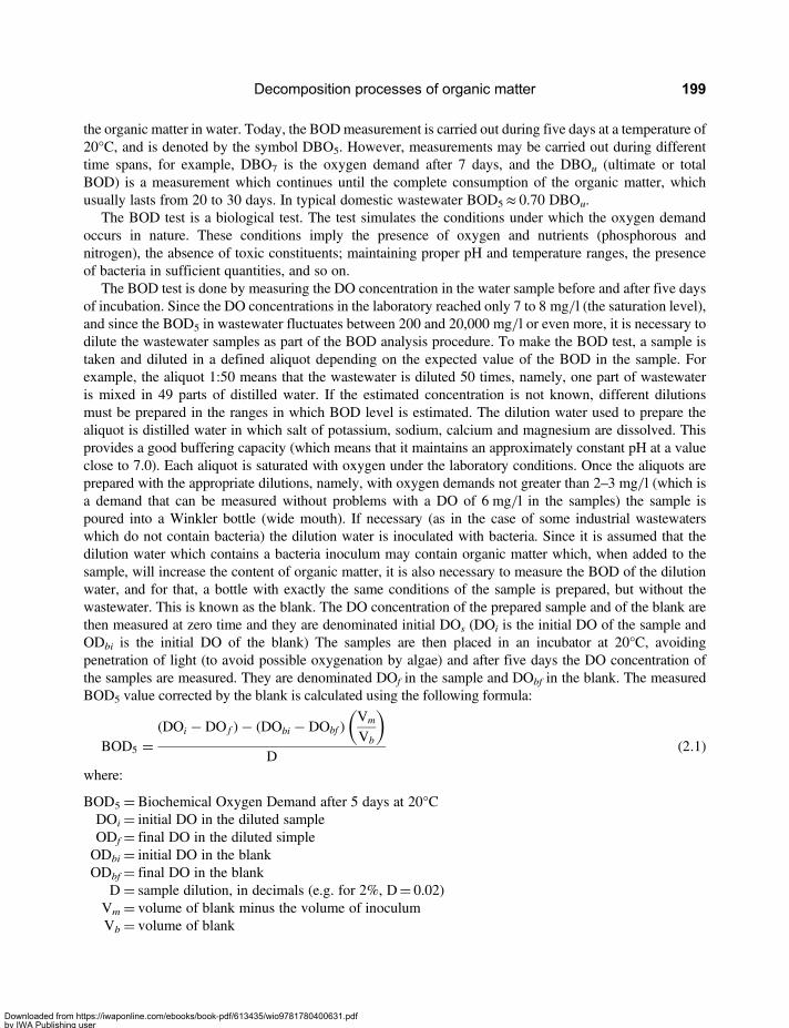
the organic matter in water. Today, the BODmeasurement is carried out during five days at a temperature of20°C, and is denoted by the symbol DBO5. However, measurements may be carried out during differenttime spans, for example, DBO7 is the oxygen demand after 7 days, and the DBOu (ultimate or totalBOD) is a measurement which continues until the complete consumption of the organic matter, whichusually lasts from 20 to 30 days. In typical domestic wastewater BOD5≈ 0.70 DBOu.

The BOD test is a biological test. The test simulates the conditions under which the oxygen demandoccurs in nature. These conditions imply the presence of oxygen and nutrients (phosphorous andnitrogen), the absence of toxic constituents; maintaining proper pH and temperature ranges, the presenceof bacteria in sufficient quantities, and so on.

The BOD test is done by measuring the DO concentration in the water sample before and after five daysof incubation. Since the DO concentrations in the laboratory reached only 7 to 8 mg/l (the saturation level),and since the BOD5 in wastewater fluctuates between 200 and 20,000 mg/l or even more, it is necessary todilute the wastewater samples as part of the BOD analysis procedure. To make the BOD test, a sample istaken and diluted in a defined aliquot depending on the expected value of the BOD in the sample. Forexample, the aliquot 1:50 means that the wastewater is diluted 50 times, namely, one part of wastewateris mixed in 49 parts of distilled water. If the estimated concentration is not known, different dilutionsmust be prepared in the ranges in which BOD level is estimated. The dilution water used to prepare thealiquot is distilled water in which salt of potassium, sodium, calcium and magnesium are dissolved. Thisprovides a good buffering capacity (which means that it maintains an approximately constant pH at a valueclose to 7.0). Each aliquot is saturated with oxygen under the laboratory conditions. Once the aliquots areprepared with the appropriate dilutions, namely, with oxygen demands not greater than 2–3 mg/l (which isa demand that can be measured without problems with a DO of 6 mg/l in the samples) the sample ispoured into a Winkler bottle (wide mouth). If necessary (as in the case of some industrial wastewaterswhich do not contain bacteria) the dilution water is inoculated with bacteria. Since it is assumed that thedilution water which contains a bacteria inoculum may contain organic matter which, when added to thesample, will increase the content of organic matter, it is also necessary to measure the BOD of the dilutionwater, and for that, a bottle with exactly the same conditions of the sample is prepared, but without thewastewater. This is known as the blank. The DO concentration of the prepared sample and of the blank arethen measured at zero time and they are denominated initial DOs (DOi is the initial DO of the sample andODbi is the initial DO of the blank) The samples are then placed in an incubator at 20°C, avoidingpenetration of light (to avoid possible oxygenation by algae) and after five days the DO concentration ofthe samples are measured. They are denominated DOf in the sample and DObf in the blank. The measuredBOD5 value corrected by the blank is calculated using the following formula:

BOD5 =(DOi − DO f )− (DObi − DObf )

Vm

Vb

( )D

(2.1)

where:

BOD5 =Biochemical Oxygen Demand after 5 days at 20°CDOi = initial DO in the diluted sampleODf = final DO in the diluted simpleODbi = initial DO in the blankODbf = final DO in the blank

D = sample dilution, in decimals (e.g. for 2%, D= 0.02)Vm = volume of blank minus the volume of inoculumVb = volume of blank

Decomposition processes of organic matter 199


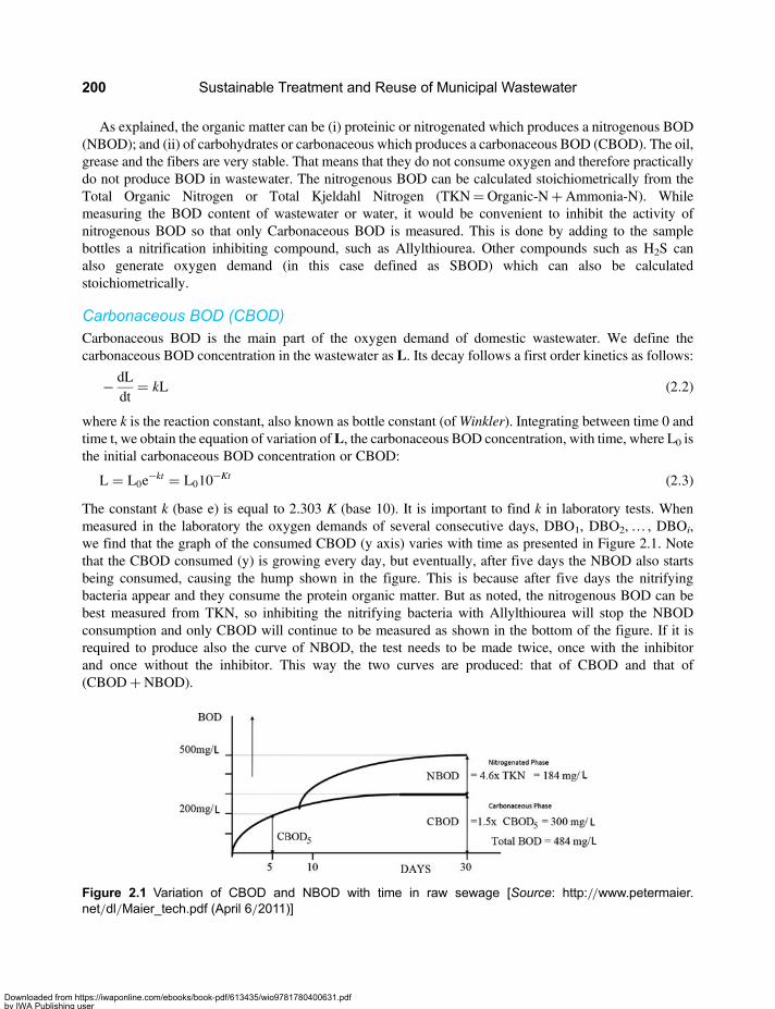
As explained, the organic matter can be (i) proteinic or nitrogenated which produces a nitrogenous BOD(NBOD); and (ii) of carbohydrates or carbonaceous which produces a carbonaceous BOD (CBOD). The oil,grease and the fibers are very stable. That means that they do not consume oxygen and therefore practicallydo not produce BOD in wastewater. The nitrogenous BOD can be calculated stoichiometrically from theTotal Organic Nitrogen or Total Kjeldahl Nitrogen (TKN=Organic-N+Ammonia-N). Whilemeasuring the BOD content of wastewater or water, it would be convenient to inhibit the activity ofnitrogenous BOD so that only Carbonaceous BOD is measured. This is done by adding to the samplebottles a nitrification inhibiting compound, such as Allylthiourea. Other compounds such as H2S canalso generate oxygen demand (in this case defined as SBOD) which can also be calculatedstoichiometrically.

Carbonaceous BOD (CBOD)Carbonaceous BOD is the main part of the oxygen demand of domestic wastewater. We define thecarbonaceous BOD concentration in the wastewater as L. Its decay follows a first order kinetics as follows:

− dLdt

= kL (2.2)

where k is the reaction constant, also known as bottle constant (ofWinkler). Integrating between time 0 andtime t, we obtain the equation of variation ofL, the carbonaceous BOD concentration, with time, where L0 isthe initial carbonaceous BOD concentration or CBOD:

L = L0e−kt = L010

−Kt (2.3)

The constant k (base e) is equal to 2.303 K (base 10). It is important to find k in laboratory tests. Whenmeasured in the laboratory the oxygen demands of several consecutive days, DBO1, DBO2,… , DBOi,we find that the graph of the consumed CBOD (y axis) varies with time as presented in Figure 2.1. Notethat the CBOD consumed (y) is growing every day, but eventually, after five days the NBOD also startsbeing consumed, causing the hump shown in the figure. This is because after five days the nitrifyingbacteria appear and they consume the protein organic matter. But as noted, the nitrogenous BOD can bebest measured from TKN, so inhibiting the nitrifying bacteria with Allylthiourea will stop the NBODconsumption and only CBOD will continue to be measured as shown in the bottom of the figure. If it isrequired to produce also the curve of NBOD, the test needs to be made twice, once with the inhibitorand once without the inhibitor. This way the two curves are produced: that of CBOD and that of(CBOD+NBOD).

Figure 2.1 Variation of CBOD and NBOD with time in raw sewage [Source: http://www.petermaier.net/dl/Maier_tech.pdf (April 6/2011)]



http://www.wtert.eu/default.asp?Menue=13&ShowDok=12







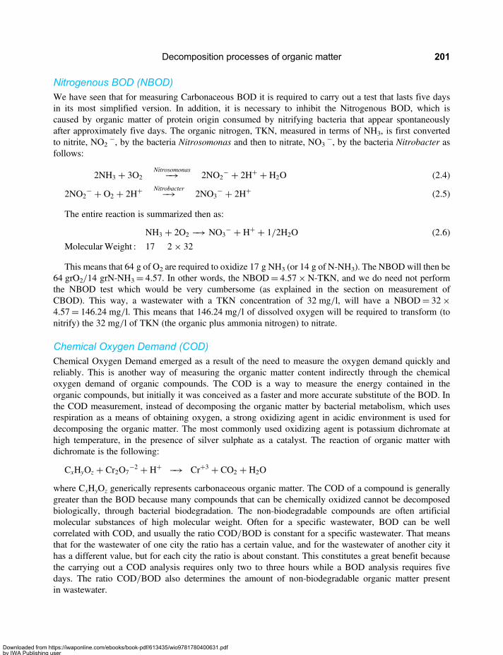
Nitrogenous BOD (NBOD)We have seen that for measuring Carbonaceous BOD it is required to carry out a test that lasts five daysin its most simplified version. In addition, it is necessary to inhibit the Nitrogenous BOD, which iscaused by organic matter of protein origin consumed by nitrifying bacteria that appear spontaneouslyafter approximately five days. The organic nitrogen, TKN, measured in terms of NH3, is first convertedto nitrite, NO2

−, by the bacteria Nitrosomonas and then to nitrate, NO3−, by the bacteria Nitrobacter as

follows:

2NH3 + 3O2 −�Nitrosomonas2NO2

− + 2H+ + H2O (2.4)

2NO2− + O2 + 2H+ −�Nitrobacter

2NO3− + 2H+ (2.5)

The entire reaction is summarized then as:

NH3 + 2O2 −� NO3− + H+ + 1/2H2O (2.6)

MolecularWeight : 17 2× 32

This means that 64 g of O2 are required to oxidize 17 g NH3 (or 14 g of N-NH3). The NBOD will then be64 grO2/14 grN-NH3= 4.57. In other words, the NBOD= 4.57×N-TKN, and we do need not performthe NBOD test which would be very cumbersome (as explained in the section on measurement ofCBOD). This way, a wastewater with a TKN concentration of 32 mg/l, will have a NBOD= 32×4.57= 146.24 mg/l. This means that 146.24 mg/l of dissolved oxygen will be required to transform (tonitrify) the 32 mg/l of TKN (the organic plus ammonia nitrogen) to nitrate.

Chemical Oxygen Demand (COD)Chemical Oxygen Demand emerged as a result of the need to measure the oxygen demand quickly andreliably. This is another way of measuring the organic matter content indirectly through the chemicaloxygen demand of organic compounds. The COD is a way to measure the energy contained in theorganic compounds, but initially it was conceived as a faster and more accurate substitute of the BOD. Inthe COD measurement, instead of decomposing the organic matter by bacterial metabolism, which usesrespiration as a means of obtaining oxygen, a strong oxidizing agent in acidic environment is used fordecomposing the organic matter. The most commonly used oxidizing agent is potassium dichromate athigh temperature, in the presence of silver sulphate as a catalyst. The reaction of organic matter withdichromate is the following:

CxHyOz + Cr2O7−2 + H+ −� Cr+3 + CO2 + H2O

where CxHyOz generically represents carbonaceous organic matter. The COD of a compound is generallygreater than the BOD because many compounds that can be chemically oxidized cannot be decomposedbiologically, through bacterial biodegradation. The non-biodegradable compounds are often artificialmolecular substances of high molecular weight. Often for a specific wastewater, BOD can be wellcorrelated with COD, and usually the ratio COD/BOD is constant for a specific wastewater. That meansthat for the wastewater of one city the ratio has a certain value, and for the wastewater of another city ithas a different value, but for each city the ratio is about constant. This constitutes a great benefit becausethe carrying out a COD analysis requires only two to three hours while a BOD analysis requires fivedays. The ratio COD/BOD also determines the amount of non-biodegradable organic matter presentin wastewater.



In addition, although not always necessary, it is possible to determine the COD of a specific organicmatter through stoichiometric calculations. This is achieved by calculating the weight of oxygen requiredper unit weight of the specific organic matter or per unit liquid volume of this organic matter for thecomplete oxidation of this organic matter. An example of stoichiometrically calculating the COD of aknown compound, in this case glucose, is the following:

C6H12O6 + 6O2 −� 6CO2 + 6H2O

Molecular weights: (180) 6× (32) 6× (44) 6× (18)

From this relationship we can conclude that (6× 32)/180= 1.066 g O2/g glucose are required todecompose the glucose. The COD of an aqueous solution containing 1 g/l of glucose would then be1066 mg/l.

SolidsSolids are another very important parameter in wastewater treatment. Organic matter is often present in theform of particles in suspension, so it is necessary to distinguish between suspended solids (SS) andDissolved Solids (DS). Also solids can be volatile (VS) indicating that they are of organic origin, orfixed which are considered inorganic solids. The general classification of solids in wastewater ispresented in Figure 2.2. Total Solids (TS) are made up by suspended solids plus dissolved solids. At thesame time those are sub-divided into volatile suspended solids (VSS) and fixed suspended solids (FSS),and these are sub-divided into in volatile dissolved solids (VDS) and fixed dissolved solids (FDS). Themost important in wastewater treatment are the suspended solids, especially the volatile suspended solidswhich are conformed of organic matter present in wastewater in the form of particles. The measurementof solids is made gravimetrically, namely, by measuring weight, and consists of filtering the sample witha dry filter of known weight. After drying the filtered sample in an oven at 105°C the filter along withthe dried filtered solids retained on it are weighted and by the subtracting the weight of the filter, welearn the weight of the filtered solids of a given volume of sample, and thus their concentration in thesample in units of mg/l. Volatile solids are determined by their evaporation in an oven at a temperatureof at least 550°C. Inorganic or fixed solids do not evaporate at this temperature (but rather at a muchhigher temperature) so the solids remaining on the filter paper after heating it to 550°C are the inorganicsolids and the balance are the volatile solids.

The total solids content (soluble and particulate) in typical municipal wastewater is usually lower than1000 mg/l. These solids basically contain all the contamination in the wastewater. This means thatmunicipal wastewater is composed of about 99.9% of water and only about 0.1% of contaminants.

Figure 2.2 Classification of solids in wastewater [Source: http://www.cee.ntu.edu.sg/AboutCEE/Facilities/EnvLab/Documents/EN2703%202C-4.pdf (April 2011)]














2.2 THE BIOCONVERSION EQUATION2.2.1 Aerobic conversionBOD and COD measure the state of “reduction” of organic matter. The BOD is used more as a criterionof water quality, while in order to interpret the kinetics of wastewater treatment, COD is a preferredindicator. Both tests estimate the amount of oxygen required for oxidizing organic matter, but the BODonly measures the biodegradable fraction, while the COD also takes into account the non-biodegradablefraction. On the other hand, the removal of substrate by bacteria is equivalent when presented in terms ofBOD and of COD since the O2 units removed are the same. In other words, if bacteria consumed 50mg/l BOD they also consumed 50 mg/l COD. Thus, for a substrate or wastewater with initialconcentrations BOD0 and COD0, subjected to treatment after which the final concentrations are BODe

and CODe, we have:

DS = S0 − S = BOD0 − BODe = COD0 − CODe

where ΔS=Removed oxygen demand. This means that ΔDBO= ΔCOD

Consequently, from the standpoint of substrate removal, BOD and COD are equivalent. COD is preferredbecause of the simplicity in the laboratory analysis for its measurement. As seen, COD indicates the amountof O2 required for total oxidation of the organic matter. The higher the COD in wastewater, the greater is thecontamination level in it and more O2 will be required for its oxidation.

For purposes of biological treatment, COD tells us howmuch food is provided to a reactor which containsa determined biological culture. Indeed, in a wastewater treatment system (WWTS) raw wastewater orinfluent substrate (S0) is the food that enters the reactor where which contains a highly concentratedculture of bacteria, measured as the Mixed Liquor Volatile Suspended Solids (MLVSS). After feeding onthe organic matter flowing into the reactor, the effluent which leaves the reactor is left with a residualsubstrate (S). The COD removed (ΔS) during the treatment is the amount of substrate consumed by thebacteria, namely:

DS = S0 − S = COD0 − CODe (2.7)

When consuming an organic compound with a determined COD, the bacteria use the energy available init for their metabolic reactions, turning it into another compound with less energy, that is, with less COD. Inthe transformation of an organic compound with a high energy level into another with a lower energy level, a“commission” is paid in terms of entropy, in accordance with the second law of thermodynamics. In otherwords, there cannot be a change from one energy state to another with 100% efficiency. The energy releasedin the reactions is used by the microorganisms (and in general by all living beings), for the maintenance oftheir life. This transformation allows the employment of the liberated energy in useful work necessary formotion and all other vital functions.

COD is in fact a measure of the energy content of a compound. Simplifying, we can say that the substrate(CxHyOz) “reacts”with O2 to producemicroorganisms, CO2 and H2O, but in fact, microorganisms consumesubstrate (food) respirate oxygen and transform the substrate partly to energy, used for sustaining their life,and partly for growth, producing additional microorganisms. The “chemical composition” or “formula” ofaerobic bacteria in the cultures of wastewater treatment plants is C5H7NO2 so we can express the reaction ofdecomposition of organic matter in the following summarized form:

CxHyOzN+ nO2 −� C5H7NO2 + CO2 + H2O

Substrate+ Oxygen −� Microorganisms



Microorganisms are measured in the laboratory gravimetrically as volatile suspended solids (mg/l), but,because they are organic matter, they have a stoichiometric oxygen demand that can be calculated asfollows:

C5H7NO2 + 5O2 −� 5CO2 + 2H2O+ NH3 (2.8)

(113)+ 5× (32)

Which lets us calculate the theoretical COD of microorganisms as follows:

COD (theoretical) = 5 × 32 gO2

113 g SSV= 1.42 gO2/gVSS

That is, the volatile organic matter formed by aerobic microorganisms with a composition of C5H7NO2

have a COD of 1.42 g O2/g VSS. The experimental measurement of the COD ofMLVSS in activated sludgeplants gives values in the range 1.40 to 1.46, which agrees with the calculation. Thus, one can express themicroorganisms present in a reactor in units of oxygen or equivalent COD, simply by multiplying thevolatile suspended solids concentration of aerobic sludge by 1.42, which also gives the total energycontent of the microorganisms. It is worth noting that the “formula” of the anaerobic microorganismsis C5H9NO3 so that for this type of microorganisms, the stoichiometric ratio of conversion to COD is1.22 g O2/g VSS.

It becomes clear from the information presented above that the substrate removed (ΔS) is converted intobiomass (ΔX) and in that conversion, microorganisms obtain the necessary energy for their metabolism andpay the “commission” of entropy for the change. These two factors ultimately are counted as energy loss andcan be measured, in terms of O2, as respiration. Thus we can say that, measured as units of oxygen, themacro-level phenomenon that occurs in an aerobic biological reactor can be expressed in the followingequation, also known as the Equation of the Bioconversion or Biotransformation:

DS = 1.42DX + DO2Substrate consumed = biomass produced + oxygen respired

(gO2) (gO2) (gO2)(2.9)

Respiration accounts for both the energy consumed in vital functions and those of entropy losses, whichclose the thermodynamic balance that must be accurate and which has been well demonstrated in practice.

Equation (2.9) not only gives a thermodynamic balance of what happens in a biological reactor, butallows realizing the stoichiometric balance, in units of O2, between the reactants and products.

Aerobic treatment can be summarized as follows: organic substrate is supplied continuously to a reactor,in which it is assimilated by a highly concentrated bacterial population. This bacterial population is providedwith oxygen, which, through respiration is used by the microorganisms for obtaining energy for their ownmetabolisms and for the conversion of substrate into newmicroorganisms. Some energy is lost in the processas heat.

2.2.2 Anaerobic conversionBioconversion of organic matter can also occur anaerobically, in which case the equation for thebioconversion is:

DS = 1.22DX + 4.00DCH4

Substratum consumed = Biomass produced + Methane produced(gO2) (gO2) (gO2)

(2.10)



In this case the removed substrate is converted to methane and biomass. The coefficients 1.22 and 4.00are coefficients required to convert anaerobic biomass (C5H9NO3) and methane into oxygen units.

In anaerobic treatment, bioconversion produces methane instead of consuming oxygen. The extraction ofenergy from organic matter is made by the delivery of an electron, which is received by an electron acceptor.The most common and efficient acceptor is O2.When no molecular O2 is present, other compounds functionas electron acceptors, but are less efficient thermodynamically. This is the case of anaerobic processes,which is the reason that the energy requirements of anaerobic bioconversion are minimal and notsufficiently high to be taken into account in Equations 2.10 and 2.12.

Now we can reduce the whole phenomenon of biological treatment of wastewater to three basic points:

(1) What is the substrate removal rate and what mechanisms govern it?(2) What is the rate of bacterial growth and what mechanisms define it?(3) How much oxygen is needed for the process to be done? or How much methane is produced?

The answer to these questions defines:

(1) The detention time needed in the biological reactor to ensure that the substrate is removed to thedesired level.

(2) The daily volume of biomass produced.(3) The weight of oxygen which needs to be supplied each day to carry out the aerobic process or the

amount of methane produced and which needs to be handled in the anaerobic process.

Considering these three points, Equation 2.9 for aerobic treatment can be transformed by dividing by Δtand taking Δt to the limit Δt → ∞, in the following equation:

− dSXdt

= − dO2

X dt+ 1.42

dXXdt

(2.11)

For anaerobic treatment, the Equation 2.10 turns into:

− dSXdt

= 4.00dCH4

X dt+ 1.22

dXXdt

(2.12)

In Equations 2.11 and 2.12 (−dS/dt) represents the removal rate of substrate or the rate at which thesupplied COD is removed, and (dS/X dt) is the removal of substrate per unit of biomass (X). The term(dX/X dt) is the rate of growth of the biomass (VSS) per unit of biomass. Finally (−dO2/X dt) is theoxygen consumed per unit of bacterial mass and (dCH4/X dt) is the methane produced, also per unit ofbiomass. The constant 1.42 converts aerobic VSS into units of O2 (COD), and for anaerobic processesthe constant 1.22 does the same for anaerobic biomass and the constant 4.00 converts the grams ofmethane into grams of COD.

The process of substrate removal used in wastewater treatment may be carried out in reactors ofsuspended media or in reactors of attached media (also known as fixed media reactors). However, themicrobiological process itself is identical in all types of reactors and can be explained by thesame phenomena.

2.3 BACTERIAL METABOLISMBacterial metabolism consists of two defined processes that are represented in Equation 2.11, and carry outthe process of bioconversion of assimilated food (−dS/dt), namely: (i) bioenergetics or catabolismwhich isexpressed by the term dO2/dt and refers to the decomposition processes through which energy stored in



organic matter is extracted to provide food for microorganisms. In the anaerobic process the energyextraction is minimal compared to the aerobic process, since it does not use oxygen as an electronacceptor; and (ii) biosynthesis or anabolism which is represented in Equations 2.11 and 2.12 by the termdX/dt, which corresponds to the processes by which the cellular architecture is built and the biomass isenhanced from compounds assimilated as food. The process of breakdown (catabolism) to obtain energyis done through several metabolic cycles, but it must be preceded by hydrolysis.

HydrolysisParticulate matter, biopolymers, and in general the complex organic compounds which are the mainconstituents of municipal wastewater, have to undergo initial dissolution or hydrolysis to turn them intosimple organic substrates. The products of hydrolysis are sugars, amino acids, low weight volatile fattyacids and alcohols. These substrates can then be assimilated by bacteria to undergo the process ofglucolysis. The hydrolysis takes place externally by the action of exoenzymes. The simple hydrolysis ofsome organic compounds is very fast, but that of the complex or particulate compounds can beextremely slow. A typical example is the hydrolysis of sucrose that by incorporating a water molecule isdecomposed into two isomeric sugar molecules, Glucose and Fructose:

C12H22O11 + H2O −� 2C6H12O6 (2.13)

The exoenzyme that fosters this reaction is Glucose Hydrolase. Immediately after crossing the bacterialcell membrane the sugar molecules are incorporated into the glucolysis process.

GlucolysisOnce hydrolysis occurs, soluble compounds can be assimilated by bacteria and initiate the processof Glucolysis, which is summarized in Figure 2.3. Once the decomposition process reaches pyruvic acid,it must make a thermodynamic decision that depends on the availability of external electron acceptors:(i) if oxygen is available then the Krebs cycle, which is the main aerobic metabolic cycle, is carried outin the bacteria; and (ii) if no oxygen (or other electron acceptor) is available, then a reaction thatproduces Acetic Acid (Acetate) and Hydrogen, as well as other volatile fatty acids (VFA) such aspropionic acid, butyric acid, and so on, occurs. This leads to anaerobic decomposition which requires thecoordinated participation of five different types of microorganisms. The reaction of glucolysis issummarized as follows:

C6H12O6 + 4H2O −� 2CH3COO− + 2HCO3− + 4H+ + 4H2

Glucose Acetate Alkalinity Hydrogen(2.14)

Bioenergetics and biosynthesisHydrolysis and the Glucolysis metabolic cycle need to occur prior the process of decomposition ofcarbohydrates by bacteria. The decomposition processes are carried out by acidogenic bacteria, whichusually are facultative, which means that they can operate in an aerobic pathway in the presence of O2,or in an anaerobic pathway in the absence of O2 or nitrates. The anaerobic decomposition pathway isdiscussed in the next section. If molecular O2 is available, it is then used as an electron acceptor, and thebacteria itself terminates the aerobic metabolism (i.e. the Krebs cycle). There are other metabolic cyclesfor different types of organic matter (lipids, proteins, and so on.).

The general plan of metabolism implies catalytic reactions and assimilation of nutrients. Small moleculeswhich are already dissolved are directly assimilated by the cells because they can pass through the cells



membrane wall without a problem. On the other hand, the polymer macromolecules once they are stoppedby physical and electric barriers of the cell wall, must undergo the hydrolysis process beforebeing assimilated.

Catabolic (bioenergetic) and anabolic (biosynthetic) processes are shown schematically in Figure 2.4.Catabolism initially produces energy through the Glucolysis, but then the decomposition continues withthe Krebs cycle which breaks down the organic matter in twelve key intermediaries, with a netproduction of energy of 266 KCal per molecule of glucose, energy that is stored mainly in molecules ofAdenosine tri-phosphate (ATP). The end product is CO2 and H2O. The key intermediates are used in

Figure 2.3 Simplified chart of glucolysis pathway [Source: http://dolly.biochem.arizona.edu/Bioc462b_Honors_Spring_2009/ksamsel/glycolysis%20thumb.html (April 2011)]











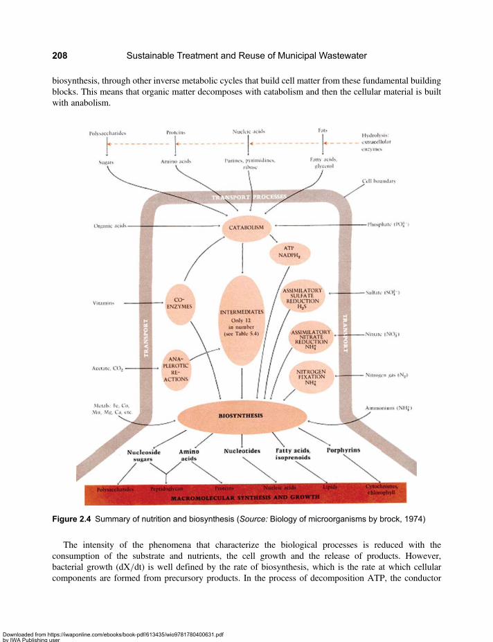
biosynthesis, through other inverse metabolic cycles that build cell matter from these fundamental buildingblocks. This means that organic matter decomposes with catabolism and then the cellular material is builtwith anabolism.

The intensity of the phenomena that characterize the biological processes is reduced with theconsumption of the substrate and nutrients, the cell growth and the release of products. However,bacterial growth (dX/dt) is well defined by the rate of biosynthesis, which is the rate at which cellularcomponents are formed from precursory products. In the process of decomposition ATP, the conductor

Figure 2.4 Summary of nutrition and biosynthesis (Source: Biology of microorganisms by brock, 1974)



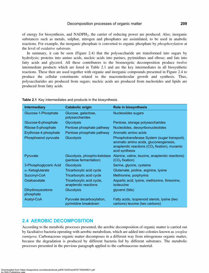
of energy for biosynthesis, and NADPH2, the carrier of reducing power are produced. Also, inorganicsubstances such as metals, sulphur, nitrogen and phosphates are assimilated, to be used in anabolicreactions. For example, the inorganic phosphate is converted to organic phosphate by phosphorylation atthe level of oxidative substrate.

In summary, it can be seen (Figure 2.4) that the polysaccharide are transformed into sugars byhydrolysis; proteins into amino acids, nucleic acids into purines, pyrimidines and ribose; and fats intofatty acids and glycerol. All these contributors to the bioenergetic decomposition produce twelveintermediate products which are listed in Table 2.1 and are the key intermediates in all biosyntheticreactions. These then are used together with organic and inorganic compounds presented in Figure 2.4 toproduce the cellular constituents related to the macromolecular growth and synthesis. Thus,polysaccharides are produced from sugars; nucleic acids are produced from nucleotides and lipids areproduced from fatty acids.

2.4 AEROBIC DECOMPOSITIONAccording to the metabolic processes presented, the aerobic decomposition of organic matter is carried outby facultative bacteria operating with aerobic metabolism, which are added into colonies known as zooglearamigera. Carbonaceous organic matter decomposes in a different way from nitrogenous organic matter,because the degradation is produced by different bacteria fed by different substrates. The metabolicprocesses presented in the previous paragraph applied to the carbonaceous material.

Table 2.1 Key intermediates and products in the biosynthesis.

Intermediary Catabolic origin Role in biosynthesis

Glucose-1-Phosphate Glucose, galactose,polysaccharides

Nucleosides sugars

Glucose-6-phosphate Glycolysis Pentose, storage polysaccharides

Ribose-5-phosphate Pentose phosphate pathway Nucleotides, deoxyribonucleotides

Erythrose-4-phosphate Pentose phosphate pathway Aromatic amino acids

Phosphoenol pyruvate Glucolysis Phosphotransferase System (sugar transport),aromatic amino acids, gluconeogenesis,anaplerotic reactions (CO2 fixation), muramicacid synthesis

Pyruvate Glucolysis, phospho-ketolase(pentose fermentation)

Alanine, valine, leucine, anaplerotic reactions)(CO2 fixation)

3-Phosphoglyceric Acid Glucolysis Serine, glycine, cysteine

α- Ketoglutarate Tricarboxylic acid cycle Glutamate, proline, arginine, lysine

Succinyl-CoA Tricarboxylic acid cycle Methionine, porphyrins

Oxaloacetate Tricarboxylic acid cycle,anaplerotic reactions

Aspartic acid, lysine, methionine, threonine,isoleucine

Dihydroxyacetonephosphate

Glucolysis glycerol (fats)

Acetyl-CoA Pyruvate decarboxylation,pyrimidine breakdown

Fatty acids, isoprenoid sterols, lysine (twocarbons) leucine (two carbons)



Aerobic decomposition of carbonaceous organic matterCarbonaceous organic matter comes from carbohydrates. The organic matter in the wastewater, whichconsists primarily of a mixture of carbonaceous material and protein material, has the generic “formula”H10C19O3N. The energy reaction for the decomposition of carbonaceous organic matter of in wastewateris as follows:

C10H19O3N+ 12.5O2 −�Microorganisms10CO2 + 8H2O+ NH3

Wastewater + Oxygen

Aerobic microorganisms are necessary for the reaction to be carried out and have, as seen above, theapproximate “formula” C5H7NO2. The equation that summarizes the bioenergetics and biosynthesis forthe carbonaceous BOD is the following:

2C10H19O3N+ 15O2 −�C5H7NO22C5H7NO2 + 10CO2 + 12H2O (2.15)

Aerobic decomposition of nitrogenous organic matterNitrogen is present in the wastewater in four main forms: organic nitrogen, ammonia nitrogen, nitritenitrogen and nitrate nitrogen. The organic nitrogen is usually transformed into NH3 and ammonium salts,by hydrolysis or bacterial action. Total Kjeldahl Nitrogen (TKN) which is the sum of organic nitrogenand ammonia nitrogen and when measured in the raw wastewater, it represents the original amount oforganic nitrogen. In the presence of nitrifying bacteria, the ammonia undergoes a process callednitrification, which involves its oxidation, first to nitrite and then to nitrate. The nitrification is the causeof the Nitrogenous Oxygen Demand (NBOD). The representative reactions for energy phase are:

NH4+ + 3

2O2 −�nitrosomas

NO2− + 2H+ + H2O

NO2− + 1

2O2 −�nitrobacter

NO3−

The overall nitrification process can be summarized by the following reaction:

NH4+ + 2O2 −� NO3

− + 2H+ + H2O (2.16)

At the same time that energy is produced, the synthesis of new bacteria occurs. Nitrification producesNBOD through the oxidation to nitrites by Nitrosomonas and the final nitrification to nitrates byNitrobacter as shown by the previous reactions. Once nitrification occurs, the denitrification process cantake place, if an energy source is added (organic matter) and anoxic conditions prevail (lack of O2 andpresence of nitrates). Methanol (CH3OH), acetic acid (CH3COOH) or the wastewater itself can be usedas a carbon source for the denitrification process. If methanol is used as the carbon source (i.e. theorganic matter), the overall reaction of synthesis and energy in denitrification and is the following:

NO3− + 1.08CH3OH

Methanol+H+ −� 0.065C5H7NO2

Bacteria+ 0.47N2 � + 0.76CO2 + 2.44H2O

Nitrification is required to prevent the presence of nitrogenous BOD in water bodies into which aneffluent is discharged, and denitrification might be necessary to prevent eutrophication of the water bodyby the presence of nitrogen.



2.5 ANAEROBIC DECOMPOSITIONIn anaerobic decomposition there is no free molecular O2, which means that there are no external electronacceptors. Under these conditions an aggregate of five different kinds of bacteria is formed, which operate ina coordinated manner in a flocculant aggregate (the floc) and, very often, in a granular form (see Figure 2.5).The general biochemistry of anaerobic decomposition is explained in Figure 2.6. The processes that occur inthe granules (Figure 2.5) are:

HydrolysisAs explained above, it is necessary to dissolve the particulate matter, the biopolymers, and in general thecomplex organic compounds, through hydrolysis. The products of hydrolysis are sugars, amino acids,volatile low weight fatty acids and alcohols. These substrates will be assimilated by the acidogenic

Figure 2.5 Grouping of the anaerobic bacteria in the granule (Source: Hulshoff et al. 2004)

Figure 2.6 Schematic diagram of the anaerobic decomposition process [Source: http://www.wtert.eu/default.asp?Menue=13&ShowDok=12 (April 2011)]









bacteria or fermentative2 bacteria (eubacteria) to undergo the process of glucolysis explained above (seeEquation 2.13).

Acidogenesis or fermentationOnce the hydrolysis occurred, the glucolysis process (which has already been described) starts. When theprocess arrives to the pyruvate stage, and since there are no external electron acceptors, the reactionwhich occurs produces Acetic Acid (Acetate), other volatile fatty acids, volatile fatty acids such aspropionic acid, and hydrogen. At this point the acidogenic bacteria (which are facultative) operate inanaerobic mode and deliver their metabolic products resultants of this mode (see Equation 2.14).

The accumulation of hydrogen hinders the decomposition of glucose. In fact there is a thermodynamiclimit, a maximum permissible concentration of hydrogen under which the anaerobic decomposition cancontinue, which is given in terms of partial pressure as follows: PH ,10−4 atm, where PH is the partialpressure of hydrogen. If this does not occur, that is, the partial pressure of hydrogen is above 10−4 atm,the reaction described in Equation 2.14 stops and only the reaction producing volatile fatty acids proceeds.

Acetoclastic acetogenesisFor the anaerobic decomposition to continue, it is necessary that the volatile fatty acids convert to aceticacid, because this is the only fatty acid that can be methanized (converted to methane). There are othercompounds that can be methanized, such as methanol and formic acid, but they are not common inanaerobic decomposition.

Hydrogenoclastic acetogenesisAlthough there may be Archaebacteria capable of methanizing Hydrogen, there are also bacteria, whichunder anaerobic decomposition conditions can produce acetic acid, and they are known as the acetogenichydrogenoclastics. The very essential function of these bacteria is to maintain the PH below thenecessary limits.

Hydrogenoclastic methanogenesisThis is a reaction carried out by a type of Archaebacteria that methanize approximately 30% of the originalsubstrate. It is a very fast reaction which competes with the previous one.

Acetoclastic methanogenesisThis is the most important reaction in the anaerobic decomposition process and is responsible for producing70% of methane gas. There are only two types of bacteria that produce this reaction: Methanothrix andMethanosarcina.

In order for anaerobic reactions to occur in a timely manner in wastewater treatment plants, the variousorganisms need to grouped as a floc or granule so that the bacteria producing intermediate products remainclose to the bacteria consuming the products and that all the reactions function in a sequence withoutaccumulation of intermediate products, all in accordance with Figure 2.5. Granules formed in ananaerobic reactor treating municipal wastewater are shown in Figure 2.7 (Orozco, 1988).

2They are actually facultative bacteria which in presence of O2 are aerobic and produce CO2 and H2O, and in absence of O2 areacidogenic or fermentative and produce volatile fatty acids and H2.



2.6 DIFFERENCES BETWEEN AEROBIC AND ANAEROBIC TREATMENTThe anaerobic process is sensitive to low temperatures and its rate is greatly reduced at temperatures below12°C (in the wastewater not in the air). However, it works well at higher temperatures and is thereforeappropriate for developing countries, many of which are located in warm climate zones. Anaerobicprocesses were traditionally used for treatment of excess sludge and not for treatment of wastewater.Only in recent years the anaerobic process being considered in some countries as a process also suitablefor treating municipal waste water, not only for treatment of sludge. The capacity and the rate ofdecomposition of organic matter in raw sewage under anaerobic conditions at temperatures above 12°Care similar to those of the aerobic process (as evidenced by the fact that the hydraulic detention times inanaerobic reactors for wastewater treatment are similar to the detention time in aerobic reactors ofactivated sludge), so an anaerobic process can perform well as the main treatment unit of wastewater inwarm climates.

The fact that the overall rate of anaerobic decomposition of organic matter in raw wastewater is similar tothe rate of decomposition under aerobic conditions seems to contradict the fact that anaerobic decompositionof sludge is a slow rate process. The slow rate of anaerobic stabilization of sludge made many professionalsto believe that because anaerobic decomposition of excess sludge is a slow rate process, then all anaerobicprocesses are slow rate processes for any type of substrate. The fact is that excess sludge, which is basicallyexcess bacterial cells, is a very difficult matter to decompose due to the need to break the cell membranes,and even aerobic digestion of excess sludge is an equally slow process. So in anaerobic digestion of sludgethe problem is the type of substrate (which in this case is the excess bacterial cells) and not the anaerobicprocess itself (Libhaber, 2007; Van Handel & Lettinga, 1994).

An anaerobic treatment process has some advantages over an aerobic process: (i) it does not requireoxygen thus it does not consume energy; (ii) excess sludge quantities are much smaller than thosegenerated in aerobic process, thus expenses for sludge treatment and disposal are much smaller and soare negative environmental effects generated by the sludge; (iii) the gas it produces, mainly methane, canbe collected and used to generate energy or be burned, reducing the emission of greenhouse gases, andcarbon fund credit can be obtained for the emission reduction, increasing the financial benefits of theprocess; (iv) smaller amounts of nutrients are required in anaerobic processes because less biomass is

Figure 2.7 Granulated sludge of domestic wastewater (Source: Orozco, 1988)



produced; (v) the occupied area of an anaerobic reactor is small, except in the case of anaerobic lagoons,which require a somewhat larger area; (vi) electromechanical equipment is not required for theseprocesses; (vii) construction is simple and uses mostly local materials; (viii) operation is quite simple;and (ix) both investment cost and operation and maintenance costs are way smaller than those of aerobicprocesses. Anaerobic treatment also has some disadvantages: (i) it needs longer start-up time to developthe necessary amount of anaerobic biomass in the reactor; (ii) it is more sensitive to lower temperatures;(iii) it is more sensitive to toxic substances; (iv) biological nitrogen and phosphorus removal cannot beachieved in an anaerobic process; (v) it may require alkalinity addition; (vi) it may produce odours andcorrosive gases, however those can be controlled; and (vii) the effluent quality of a one stage anaerobictreatment process may not meet discharge standards and, depending on the specific project conditions, asubsequent treatment stage might be necessary.

2.7 KINETICS AND STOICHIOMETRY OF CARBONACEOUS BODDECOMPOSITION3

To develop procedures for calculating the different wastewater treatment processes, it is necessary toprovide answers to the three questions raised in section 2.2, namely:

(1) What is the substrate removal rate (−dS/dt)?(2) What is the bacterial growth rate (dX/dt)?(3) How much oxygen (−dO2/dt) is necessary to supply for maintaining the process? Or How much

methane (dCH4/dt) is produced by the process?

To this end the kinetic and stoichiometric equations associated with the decomposition of carbonaceousorganic matter need to be consulted. Following are the differential equations that represent each of theprocesses:

Substrate removalWhen the concentration of biomass in a reactor is small compared to the substrate concentration andtherefore is the limiting factor, the familiar Monod equation is applied for estimating the bacterial growth(see Shuler & Kargi, 1992, pp 170). For such conditions, the removal of soluble substrate can be derivedfrom the following equation:

dSX dt

= kSKm + S

(2.17)

where:

X = biomass concentration in the reactor (mg VSS/l)S = substrate concentration in the reactor (mg COD/l)k= kinetic constant, maximum rate of unit removal (d −1).

Km =Monod’s kinetics saturation constant (mg COD/l).

On the other hand, if the concentration of biomass in a reactor is high compared to the substrateconcentration, the Contois equation is applied (see Shuler & Kargi, 1992, pp. 171). This equation can be

3Based on “Bioingeniería de aguas residuales: teoría y diseño”, Orozco (2005).



transformed into the following equation for the removal of substrate (see Orozco, 1976):

dSX dt

= kS/XKc + S/X

(2.18)

where:

k= constant kinetic, maximum rate of unit removal (d−1)Kc =Contois’ kinetics saturation constant (mg COD/mg SSV)

This situation (high biomass concentration per unit substrate concentration) is most common in thewastewater treatment plants, specifically in aerobic treatment with high sludge ages, and in anaerobictreatment. Therefore equation 2.18 should be applied for the design of wastewater treatment plants. Forfurther discussion on this equation see Orozco (1977). Table 2.2 presents typical values of k and Kc.

When the relation S/X is small compared with Kc (Kc≫ S/X) Equation 2.18 becomes the followingequation proposed by McKinney (1962):

dSdt

= kLS (2.19)

where:

kL= Synthesis Factor (d−1)kL≈ k/Kc

Biomass productionThe production of biomass or bacterial growth has been universally interpreted as follows:

dXXdt

= YdSXdt

− ke (2.20)

where:

dX/X dt= biomass net growth rate (d−1)Y = stoichiometric coefficient of production (mg VSS/mg COD),

typically 0.5 for aerobic decomposition.ke = endogenous respiration coefficient (d−1), typically 0.05

Table 2.2 Kinetic and stoichiometric constants.

Constant Units Aerobic Anaerobic

k mg COD/mg VSS · d 5.0 2.5

Kc mg COD/mg VSS 0.02 0.04

Y mg VSS/mg/COD 0.5 0.08

ke d−1 0.05 0.03

T °C 20 25

θ 1.04 1.04

Source: Orozco (2005), Metcalf & Eddy (2003), Pavlostathis & Giraldo-Gómez (1991)



For anaerobic treatment the same equation is applied, but the coefficient Y is replaced by the anaerobicproduction ratio, Yan, whose value is in the range 0.5–0.1, with a typical value presented in Table 2.2.

The value of the coefficient Y represents the portion of the energy contained in the incoming substratewhich is transformed to new bacterial cells, and therefore defined the excess sludge quantity of the process.In aerobic processes, about 50% of the energy of the incoming substrate is consumed by the aerobic bacteriafor their life maintenance and 50% is transformed to new bacterial cells. That means that about 50% of thesubstrate comes out of the aerobic process in the form of excess sludge, and this is a lot of sludge. Inanaerobic processes, 90–95% of the energy of the incoming substrate is consumed by the anaerobicbacteria for their life maintenance only 5–10% is transformed to new bacterial cells. This is the reasonthat anaerobic processes produce much less excess sludge.

The cell retention time of bacteria in the reactor (i.e. the average time in which bacterial biomass remainsin the reactor before being discharged from it as excess sludge, in days), also known as sludge age (θc) isdefined as:

uc = XdX/dt

(2.21)

So Equation 2.20 becomes,

1uc

= YdSXdt

− ke (2.22)

Oxygen uptake and methane productionThe oxygen uptake required for maintaining the aerobic biological treatment process is calculated from thebiotransformation Equation 2.11 as follows:

− dO2

X dt= dS

X dt− 1.42

dXXdt

(2.23)

where:

−dO2/dt=Oxygen uptake (mg O2/l)1.42 is the stoichiometric conversion factor of mg VSS/l to mg O2/l

In anaerobic treatment, methane gas (CH4) is produced instead of oxygen being consumed. The equationfor the production of methane derived from Equation 2.12 is as follows:

4.00dCH4

X dt= dS

Xdt− 1.22

dXXdt

(2.24)

where 4.00 is the stoichiometric conversion factor of CH4 to O2 and 1.22 is the stoichiometric of conversionof anaerobic biomass to oxygen units. For a broader discussion of these equations see Orozco (2005).

The kinetic constants k and ke must be corrected for variation of temperature according to the equation:

k(T) = k(T0)u(T0−T) (2.25a)

T0 being 20°C for aerobic treatment and 25°C for anaerobic treatment. However, in the anaerobictreatment the following equation is used more often:

k(T) = k(258C)e0.1(T−25) (2.25b)



Completely mixed and plug flow reactorsEquations 2.18, 2.22, 2.23 and 2.24 are always applied in environment of the bacterial reaction processes,but the end result of these processes depends on the hydraulic regime of the reactor in which they occur.Reactors with completely mixed hydraulic regime are the most common in wastewater treatment,especially in anaerobic treatment and in natural treatment processes (lagoons, wetlands and so on).Although the hydraulic regime of the reactor is important in any treatment system, its importance is mostobvious in the suspended media type treatment, where bacterial biomass is intimately mixed with thewastewater, resulting in a mixed liquid known as Mixed Liquor (ML). The mixed liquor has the samehydraulic properties as water (except for a slightly higher density because of the biomass concentrationranging between 1,000 and 10,000 mg/l Mixed Liquor Suspended Solids (MLSS), which ranges from0.1 to 1% concentration by weight).

The reactor in which the biological reactions take place is a basin where the mixed liquor biomass carriesout the biotransformation of organic substrate and has two extremes of fully differentiated hydraulicregimes: (i) the completely mixed regime; and (ii) the plug flow regime. In the completely mixed regimethere is a total and complete mixing of mixed liquor, so that there is no variation in the concentration ofany parameter at any point in the reactor. Mathematically this is defined by the concentration gradient,which is the spatial variation of the concentration of the parameters being measured (e.g. the substrate,S). If the spatial variable is ordinate z, then the variation of the substrate with the length (or depth, itdoes not matter which ordinate is chosen) must be zero, or:

dSdz

= 0

This means that S is constant throughout the reactor volume. Conversely, in a reactor under a plugflow regime there is a defined spatial gradient of all its constituents. As suggested by its name, theplug flow reactor resembles a piston that travels through a long tank undergoing in its way thebiotransformation in the z direction. As the wastewater travels in the tank at speed u, which dependson the wastewater flow which enters the reactor (according to the continuity equation Q=AT · u,where Q is the flow rate and AT the cross section area of the tank) it is clear that each position of thewater “piston” zi is associated with a transit time ti comparable to the detention time that the mixedliquor stayed in the reactor up to that point, and the biotransformation took place during this time. Wecan assume then that dS/dt= dS/dz, and if we also adopt, for example, the kinetics of McKinney(Equation 2.19), the resulting gradient in the plug flow reactor can then be represented by thefollowing equation:

− dSdz

= kLS

This equation means that at each point z there will be a definite concentration S different from the othersin other positions the z-axis, as shown in Figure 2.9.

Completely mixed reactors

For a completely mixed reactor the following equation holds:

− dSdt

= S0 − Std

(2.26)



Which when combined with Equation 2.22, allows presenting the equation of the concentration ofsubstrate (X) in the reactor as follows:

X = ucY(S0−S)td(1+ keuc)

= Y(S0 − S)

td ke + 1uc

( ) (2.27)

Likewise if we combine in Equation 2.22 with Equation 2.18 we receive:

SX= Kc(1+ keuc)uc(Yk− ke)− 1

=Kc ke + 1

uc

( )Yk− ke + 1

uc

( ) (2.28)

Now, if we combine Equation 2.27 with Equation 2.28, we obtain the equation for the substrate in theeffluent, as follows:

S = S0

1+ kY− ( 1uc + ke)KcY

[ ]td

(2.29)

And if we define:

KO =kY− 1

uc+ ke

( )KcY

(2.30)

Then we obtain:

S = S01+KOtd

(2.31)

where KO depends only on the sludge age θc, since Y, ke, k and Kc are constants. When the sludge age is

large enough (1/θc → 0), then KO is reduced tokY− keKcY

[ ]≈ k/Kc, which is the same kL of Equation 2.19

Extremely High Sludge Age (EHSA)

In conditions when the sludge age, θc, is very high, with a tendency to reach infinity, that is, (1/θc) → 0, thesludge age is denominatedExtremely High Sludge Age (EHSA)which is the case in a UASB reactor or in afacultative lagoon. Then we get:

S = S0

1+ kY− keKcY

[ ]td

(2.32)

and

X = Y(S0 − S)tdke

= YKOS0ke 1+ KOtd( ) (2.33)

This implies that for a given S0, S depends only on td. Under these conditions X also depends on td, whichmeans that the lower td, the greater X. Thus, we find that td can be as small as wanted provided that X is large



enough. It is noteworthy that in this case, the lesser the detention time, the higher the effluent substrate, asshown in Equation (2.32). Another finding of great importance under EHSA conditions is that, theoretically,the production of biomass can be zero. As 1/θc → 0, then we get that:

dXXdt

= 1uc

= 0 (2.34)

This happens because the biomass produced, Y · (dS/dt), is equal to that consumed in the endogenousrespiration phase, keX.

Reactors in series

Often the possibility of designing several completely mixed reactors in series occurs in practice. This case isinteresting from an analytical point of view, because it allows differentiating between the plug flow and thecompletely mixed reactors. Referring to Figure 2.8, let us study, for simplicity, only two completely mixedreactors in series without recycle from the second one to the first. We assume that both reactors have thesame volume, V/2, and that td= (V/2)/Q0. The total volume of the system is V and the total detentiontime is V/Q0.

Using Equation 2.31 we have for the reactor (1):

S1 = S0

1+ KOtd2

For the reactor (2), the influent is the reactor’s (1) effluent, namely, S1. Then:

S = S1

1+ KOtd2

= S0

1+ KOtd2

( )2 (2.35)

From this it follows that for n reactors in series of equal volume (V/n), where V is the total volumeof system and td=V/Q0 is the total detention time in the system, the substrate concentration in the finaleffluent is:

S = S0

1+ KOtdn

( )n (2.36)

It is clear that n reactors in series produce a much lower substrate concentration in the effluent than asingle completely mixed reactor, with all other circumstances maintained equal.

Plug flow reactor

Let us consider the plug flow reactor presented in Figure (2.9) and assume that the recirculation from thesecondary sedimentation tank is zero. This reactor can be considered as an infinite series of completelymixed reactors. Indeed, if we take Equation (2.35) and make in it n equal to infinity, we have:

S = limn�1

S0

(1+ KOtdn )

n

Figure 2.8 Two completely mixed reactors in series



But, as we know: limn�1 (1+ KO

tdn )

n = eKOtd , so we obtain:

S = S0e−KOtd (2.37)

In conclusion, from the analytical standpoint, there are two extremes in the hydraulics of treatmentsystems: completely mixed reactors and plug flow reactors. Between the two, there are all the systems inseries, improving its efficiency as the flow stops being completely mixed and becomes plug flow.

Efficiency in anaerobic treatment

It is clear from the previous analysis, summarized in Equation (2.37), that the plug flow gives the maximumpossible efficiency. In practice, the plug flow does not behave as efficiently because of microbiological andoperational reasons, since the environment is continuously changing during the passing of a fluid elementthrough the reactor. So the microbial population is forced to continuously readjust, losing efficiency in itsmetabolic function. The efficiency (E) can be calculated by the equation:

E = (S0 − S)/S0 (2.38)

For anaerobic treatment, which is in EHSA conditions (1/θc → 0), using the coefficients from Table 2.2we can calculated KO:

KO(258C) = kY− keKcY

[ ]

KO(258C) = 2.5× 0.08− 0.030.04× 0.08

[ ]= 53 d

−1(2.39)

This can be corrected for temperatures other than 25°C by the Equation 2.25b. Now, in anaerobictreatment the most widely used empirical design parameter is the volumetric loading (Lv):

Lv = S0/td (2.40)

It follows that td= S0/Lv= 0.5/Lv, because for municipal wastewater the COD is usually around 500mg/l (see Table 3.2), which is equivalent to 0.5 kg COD/m3.

For completely mixed reactors Equation 2.32 applies, in which case Equation 2.38 combined withEquations 2.32, 2.39 and 2.40 becomes:

E = Emax{(26.5/[26.5+ Lv])} (2.41)

Figure 2.9 Representation of a plug flow reactor



where Emax is the maximum possible efficiency in anaerobic treatment, namely 90% (0.9). See Figure 2.10to observe its behaviour. For plug flow reactors Equation 2.37 applies and Equations 2.38, 2.39 and 2.40become:

E = Emax(1− e−26.5/Lv) (2.42)

See Figure 2.11 to observe the behaviour, which is very common in UASB reactors. This suggests thatthe UASB reactor may behave sometimes as a plug flow reactor.

2 4 6 8 10kg COD/m3 · d

70

75

80

85

90

Eff

icie

ncy

Efficiency vs. Volumetric loading

Figure 2.11 Variation of efficiency with volumetric loading for a plug flow reactor

2 4 6 8 10kg COD/m3 · d

70

75

80

85

90E

ffic

ienc

y

Efficiency vs. Volumetric loading

Figure 2.10 Variation of efficiency with volumetric loading for a completely mixed reactor



Chapter 3

Calculation of the wastewater flowand BOD load

3.1 DESIGN FLOW1

The design flow is one of the essential basic data required for the preparation of the process design of awastewater treatment system (WWTS). There are two main flow values for design of a wastewatertreatment plant: (i) the average flow, and (ii) the peak flow or maximum flow. The average flow is usedfor the design of the treatment units such as the biological reactors and others. The peak flow is used forthe design of all the hydraulic structures of the treatment system.

The calculation of wastewater flow depends on two variables: the design population (P) and the per capitawater consumption (q) of this population in l/Capita · d. The design population is estimated by one of themethods of population projections during a given design period and per capita water consumption ismeasured directly, when possible.

There are two types of water consumption: (i) domestic consumption (qdom) that defines the consumptionper household (which is 20–30 m3/month, or about 150 to 250 l/Capita · d) and total consumption (qT)which is calculated by dividing the treated flow of the water purification plant by the number ofinhabitants supplied with potable water. This latter provision covers all uses, including commercial andindustrial, but it also includes non-revenue water, which comprises the physical losses of water in thepipe system and commercial losses resulting from fraud and erroneous connections. In general, qdom ispreferably measured separately from the other types of water consumption such as commercial, industrialand institutional, setting goals for the non-revenue water with an attempt to keep it low. The non-revenuewater is usually very high in cities of developing countries (40 to 50% and even more) while thedesirable goal should be between 15 and 25%.

The qdom value refers to the consumption of municipal drinking water and it includes the consumption ofcommercial and industrial activities. We are interested in determining the flow of wastewater (WW). Tocalculate it we use a constant c, the coefficient of return, which defines the fraction of the domestic waterconsumed which is discharged into the sewerage system. The value of c is usually between 0.8 and 0.9.So the wastewater flow generated by a population P is:

Qww = cqdomP86400

(3.1)

1This paragraph was prepared based on the textbook “Bioingeniaría de aguas residuales: teoría y diseño” (2005), Alvaro OrozcoJaramillo, published by ACODAL, Bogotá, Colombia.


where the coefficient 86,400 is the number of seconds in the day. Dividing by this coefficient is required inorder to present the result in liters per second. In addition to the domestic sewage that is discharged to thesewerage system, this system also continuously receives infiltration water which is always present in the soilmatrix, either from groundwater or from the physical loss of water supply piping network. The amount ofinfiltration water that penetrates the sewerage system depends not only on the water present in theunderground but also on the soil characteristic, mainly its transmissibility. The following formula appliedfor estimating the infiltration flow:

QI = qIAa (3.2)

where:

QI = infiltration flowqI = infiltration unit flow, usually in the range 0.1 to 0.2 lps/haAa = effective area of infiltration into the sewerage system, ha.

Consequently, the wastewater process design flow or the average flow of a domestic wastewater treatmentplant (QD) for the processes design is:

QD = cqdomP86400

+ qIAa = Qww + QI (3.3)

For design of the pre-treatments units and of the hydraulic of the plant the peak flow (QDH) is used. Thepeak flow is calculated as follows:

QDH = k1k2cqdomP86400

+ qIAa (3.4)

where k1 is the factor which defines the ratio of the flow of maximum day to the average flow (Qmaxd/QD),and its value is usually between 1.5 and 1.8, and k2 is the peak hourly flow during the day (Qmaxh/Qmaxd),usually between 1.3 and 1.7. A typical value of total peak facto is k1k2 is 2.7. The value of this peak factordepends on the population, the smaller the population the higher the peak factor. There are several equationsto calculate the total peak factor (PF= k1k2) depending on the population (P), in thousands, namely:

Babbit Equation:

PF = 5P0.2

(3.5)

Harmon Equation:

PF = 1+ 144+ ��

p√ (3.6)

“Ten States” Equation:

PF = 18+ ��P

√

4+ ��P

√ (3.7)

From these equations we can obtain the maximum peak flow if we know the population served.Figure 3.1 presents a comparison among the three: the equations, from which it is noted that Equations



3.6 and 3.7 overlap. If possible, the PF should be calculated from real data measured during two or threeyears (See Freni et al. 2003).

The maximum flow of wastewater in a town is a somewhat probabilistic value. At certain instances itcan be larger than the maximum flow value used for the hydraulic design of the treatment plant, for

20 40 60 80 1001000 P

0.5

1.0

1.5

2.0

2.5

3.0

3.5

PFPeaking Factor

Figure 3.1 Comparison of the maximum peak factor according to Babbit, Harmon and “Ten States”, thelast two equations are equivalent and overlap PF is maximum peak factor and P is the population inthousands

Table 3.1 Flows of municipal wastewater as recommended by RAS (2000), Colombia.

Range Popul.hab.

Complexitylevel

SpecifcComsumption(l/////person · d)

Peak factors Flow (lps)

k1 k2 k1 k2 Average Dailymaximum

Hourlymaximum

Range 1 Minimum 500 Low 100 1.3 1.6 2.08 0.58 0.75 1.21

Average 1500 Low 100 1.3 1.6 2.08 1.74 2.26 3.62

Maximum 2500 Medium 120 1.3 1.5 1.95 3.47 4.51 3.77

Range 2 Minimum 2500 Medium 120 1.3 1.5 1.95 3.47 4.51 6.77

Average 3750 Medium 120 1.3 1.5 1.95 5.21 6.77 10.16

Maximum 5000 Medium 120 1.3 1.5 1.95 6.94 9.02 13.53


Average 8750 Medium 120 1.3 1.5 1.95 12.15 15.80 23.69

Maximum 12500 Medium 120 1.3 1.5 1.95 17.36 22.57 33.85


Average 36250 Medium high 130 1.2 1.45 1.74 54.54 65.45 94.90

Maximum 60000 Medium high 130 1.2 1.45 1.74 90.28 108.34 157.09

Range 5 Minimum 60000 Medium high 130 1.2 1.45 1.74 90.28 108.34 157.09

Average 180000 High 150 1.2 1.45 1.74 312.50 375.00 543.75

Maximum 300000 High 150 1.2 1.45 1.74 520.83 625.00 906.24

Coefficient of return: 80%.

Calculation of the wastewater flow and BOD load 225


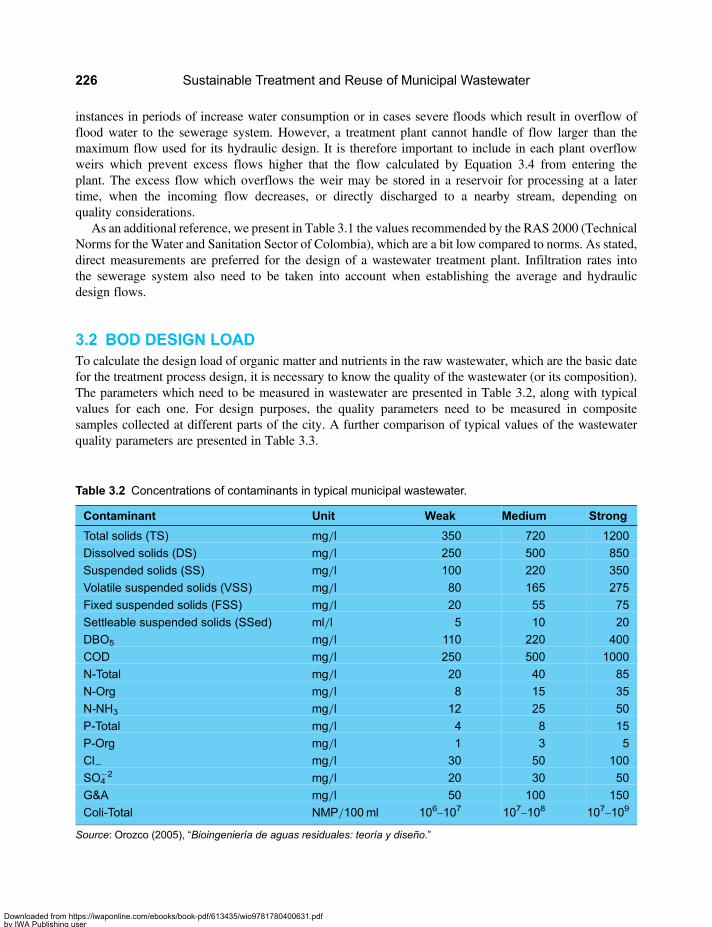
instances in periods of increase water consumption or in cases severe floods which result in overflow offlood water to the sewerage system. However, a treatment plant cannot handle of flow larger than themaximum flow used for its hydraulic design. It is therefore important to include in each plant overflowweirs which prevent excess flows higher that the flow calculated by Equation 3.4 from entering theplant. The excess flow which overflows the weir may be stored in a reservoir for processing at a latertime, when the incoming flow decreases, or directly discharged to a nearby stream, depending onquality considerations.

As an additional reference, we present in Table 3.1 the values recommended by the RAS 2000 (TechnicalNorms for the Water and Sanitation Sector of Colombia), which are a bit low compared to norms. As stated,direct measurements are preferred for the design of a wastewater treatment plant. Infiltration rates intothe sewerage system also need to be taken into account when establishing the average and hydraulicdesign flows.

3.2 BOD DESIGN LOADTo calculate the design load of organic matter and nutrients in the raw wastewater, which are the basic datefor the treatment process design, it is necessary to know the quality of the wastewater (or its composition).The parameters which need to be measured in wastewater are presented in Table 3.2, along with typicalvalues for each one. For design purposes, the quality parameters need to be measured in compositesamples collected at different parts of the city. A further comparison of typical values of the wastewaterquality parameters are presented in Table 3.3.

Table 3.2 Concentrations of contaminants in typical municipal wastewater.

Contaminant Unit Weak Medium Strong

Total solids (TS) mg/l 350 720 1200

Dissolved solids (DS) mg/l 250 500 850

Suspended solids (SS) mg/l 100 220 350

Volatile suspended solids (VSS) mg/l 80 165 275

Fixed suspended solids (FSS) mg/l 20 55 75

Settleable suspended solids (SSed) ml/l 5 10 20

DBO5 mg/l 110 220 400

COD mg/l 250 500 1000

N-Total mg/l 20 40 85

N-Org mg/l 8 15 35

N-NH3 mg/l 12 25 50

P-Total mg/l 4 8 15

P-Org mg/l 1 3 5

Cl− mg/l 30 50 100

SO4−2 mg/l 20 30 50

G&A mg/l 50 100 150

Coli-Total NMP/100ml 106–107 107–108 107–109

Source: Orozco (2005), “Bioingeniería de aguas residuales: teoría y diseño.”



In the design procedure, we need to calculate the Specific unit load of each contaminant, for example qDBO5

in kg DBO5/Capita · d since the quality of the effluent of the treatment plant depends on the total flow, whichin turn depends on the infiltration rate into the sewerage system, it is clear that the BOD5 measured in thedifferent sectors is not the same as the BOD5 which arrives to the plant. On the basis of the specific unitload, the calculation of the concentration of a parameter (C) in the raw wastewater is as follows:

C = P · qC/QD[Capita× (kg/Capita · d)/(m3/d)] (3.8)The result is the concentration in kg/m3, which is the same in g/l.This calculation is made for BOD5, COD, Nitrogen, Phosphorus, and so on. To design a wastewater

treatment plant it is necessary to have: (i) the flow rate of the raw wastewater, calculated as explained inParagraph 3.1, (ii) the quality of the raw wastewater, which is calculated by Equation 3.8; and (iii) the totalload of each parameter (e.g. LDBO5 : total load of BOD5, kg/d) estimated from the multiplication of thespecific unit load by the population:

LDBO5 = P× qDBO5(3.9)

The discussion presented above is best clarified by an example.

Table 3.3 Comparison of typical values of wastewater quality parameters proposed by different authors.

Parameter Unit Reference

a b c d

Total solids mg/L 720 403 600

Dissolved solids mg/L 500 243 308

Volatile dissolved solids mg/L 200 278

Suspended solids mg/L 220 160 291 416

Volatile suspended solids mg/L 165 129

Sedimentable solids mg/L 10 154

DBO mg/L 220 190 257 416

COT mg/L 160

COD mg/L 500 382 520

Coliform NMP/100 mL 107–108 8.23× 106 1.6× 108

Total Nitrogen mg/L-N 40 27

Organic Nitrogen mg/L-N 15

Ammoniacal Nitrogen mg/L-N 25

Nitrites mg/L-N 0

Nitrates mg/L-N 0

Total Phosphor mg/L-P 8

Organic Phosphor mg/L-P 3

Inorganic Phosphor mg/L-P 5

Chlorides mg/L-Cl 50

Alkalinity mg/L-CaCO3 100

Greases mg/L 100

Note: Table prepared on the basis of Sources Metcalf & Eddy (2003), Freni et al. (2003), Botiva (1997), Uribe (1981),RAS (200)



3.3 SAMPLE CALCULATIONNext, we will develop the calculation procedure for a town with a population of 20,000, which will be thebasis for all the examples presented in the following chapters of this book.

3.3.1 SolutionFlow CalculationThe flow for the design of a wastewater treatment plant for a population of 20,000 is obtained by addingflows from municipal inputs and infiltration. In these calculations, the flows of infiltration includecontributions by erroneous connections of drainage water. All the excess water contributions from stormwater drainage need to be prevented from reaching the treatment plant through the use of overflow weirs.The average design flow is calculated as:

QD = Qww + QI

The average flow is used for the design of biological processes, and the maximum flows used for thehydraulic design of the plant. If we have a known industrial wastewater flow QIWW, it should beincluded in the total flow. Since this is not the case of a small typical population, we will omit theseparate industrial flow and assume that in the example, the industrial and commercial wastewater flowsare includes in the domestic wastewater flow.

To calculate the maximum design flow, the domestic and industrial contributions need to be multipliedby their respective peak factors. When possible, it is recommended to undertake a consumption study inresidential sectors (not necessarily for the entire city) so that the per capita consumption, the peak factorand the net flow of infiltration can be calculated. For our example, we use the data shown in Table 3.4,which are date of a real-life case, obtained with direct measurements for a period of six months in thecity of Tunja, Colombia (Orozco, 1999).

Table 3.4 Calculation of the per capita contribution (q) the infiltration flow (qi) and the peaking factor k1× k2.

Calculation of the per capita consumption

Neighborhood Population(persons)

Area(ha)

Populationdensity(persons/////ha)

Mediumflow(m3/////d)

Maximumflow(m3/////d)

Minimumflow(m3/////d)

Peakfactor

Infiltrationflow(l · s · ha)

1 2699 6,89 391,79 243,50 393,49 144,23

2 185 1,69 109,17 100,68 148,20 59,96

3 734 3,40 215,74 260,01 483,06 110,28

4 230 0,74 310,14 34,86 90,46 8,73 2.59 0.136

5 257 0,80 320,63 21,38 62,90 9,46

6 1553 5,04 308,04 256,18 438,08 69,49 1.71 0.160

7 938 5,74 163,46 203,93 316,86 53,25 1.55 0.107

Total 6596 24,30 259,85 1120,55 Average, QD 1.95 0.13

Standard deviation 0.56 0.03

Unit flow,l/////capita · d

127,08 Infiltration, QI 3.27



It can be seen that, with the composite sampling in seven districts with a total of only 6,596 inhabitants,we can conclude that: (i) the wastewater per capita flow: qWW= c qdom= 1000 (QD-86 · 4QI)/P= 127≈130 l/Capita · d. This unit flow (per capita flow) excludes infiltration (which was subtracted), but it takesinto account the return factor (c); (ii) the net infiltration flow is qI= 0.13 l/s · ha; and (iii) the averagepeak factor for that population is PF= k1k2=Qmaxh/QD= 1.95, as an average over the districts 4, 6 and7, which had no leaks or special losses.

If we have had no measurements, we would use typical values with safety factors: qdom= 150–200 l/capita · d; qI= 0.2 l/s · ha; and the PF in accordance with Figure 3.1. Now, considering P= 20,000inhabitants, we receive from Equation 3.6:

PF = 1+ 14

14+ ��20

√ = 2.65

A value that is close to the maximum standard deviation: 1.95+ 0.56= 2.51. The value of Harmonis preferred so as to be on the side of safety. We adopted the parameters which are presented inTable 3.5.

Wastewater quality and contaminants loads calculationsData from the same real-life case are also be used for wastewater quality and contaminants loadscalculations. These are typical data. It is emphasized that nothing can replace direct measurement.

The specific unit loads are now used to calculate the load of each contaminant. For example, the unit loadof BOD (qDBO5

, kgDBO5/Capita · d) is used to calculate the total load of BOD. Table 3.6 presents the resultsof wastewater sampling and quality analyses in seven sectors. In the table, the measured concentration ofeach parameter is divided by the population and multiplied by the flow, to obtain the specific unit load inkg/person · d.

To calculate the quality of the wastewater at the treatment plant site, we calculate the concentrationof each parameter using Equation 3.8, and the total load using Equation 3.9. A summary of theresults for the example used is presented in Table 3.6. The flow data, population, wastewater qualityand contaminants loads presented in Table 3.7 are used for the examples of design calculations ofsome selected appropriate technology treatment processes presented in the following chapters ofthe book.

Table 3.5 Parameters and design flows.

• Population: P= 20,000 inhabitants (Example definition. This must calculate ineach case)

• Population density: d= 259.85≈ 260 hab/ha (measured)

• WW per capita flow: qWW= cqdom= 130 L/hab · d. (measured)

• Peak factor: PF= 2.65 (Harmon Equation)

• Infiltration flow: qI= 0.13 l/s · ha (measured)

• Area of influence (of infiltration): Aa=P/d= 20,000/260= 77 ha

• Process design flow: QD = cqdomP86400

+ qIAa = 40 I/s = 3456 m3/d

• Hydraulic design flow: QDH = 2,65cqdomP86400

+ qIAa = 90 I/s = 7776 m3/d



Table

3.6

Qualityparameters

ofthewastewaterandca

lculatio

nofthesp

ecific

unitloadforeach

qualityparameter.

Calculationoforganic

load

Calculationofphysico-chemical

parameters

Population

(hab)

AverageFlow

(m3/////d)

BOD5

Conce

n-

tration

(kg/////m

3)

BOD5Unit

load

(kg/////

capita·d

)

COD

Concen-

tration

(kg/////m

3)

CODUnit

load

(kg/////

capita·d

)

SS

Conce

n-

tration

(kg/////m

3)

SSUnit

load

(kg/////

capita·d

)

VSS

Concen-

tration

(kg/////m

3)

VSSUnit

load

(kg/////

capita·d

)

TKN

Conce

n-

tration

(kg/////m

3)

TKN

Unit

load

(kg/////

capita·d

)

PT

Concen-

tration

(kg/////m

3)

PTUnit

load

(kg/////

capita·d

)

12699

243.50

0.284

0.026

0.49

0.045

0.25

0.022

0.21

0.018

0.007

0.001

2185

100.68

0.075

0.041

0.19

0.104

0.04

0.019

0.03

0.015

0.002

0.001

3734

260.01

0.190

0.067

0.54

0.190

0.27

0.096

0.15

0.051

0.004

0.001

4230

34.86

0.217

0.033

0.51

0.078

0.11

0.017

0.36

0.054

0.05

0.007

0.003

0.000

5257

21.38

0.293

0.024

0.53

0.044

0.15

0.012

0.11

0.009

0.006

0.001

61553

256.18

0.449

0.074

0.67

0.111

0.21

0.035

0.16

0.026

0.10

0.016

0.010

0.002

7938

203.93

0.316

0.069

0.69

0.150

0.19

0.042

0.15

0.032

0.10

0.021

0.009

0.002

Ave

rage

6596

.00

1120.55

0.26

0.048

0.518

0.103

0.174

0.035

0.165

0.030

0.080

0.015

0.006

0.001

Stand

ard

deviatio

n0.12

0.022

0.163

0.054

0.082

0.029

0.101

0.018

0.029

0.007

0.003

0.001

Note:kg

/m

3=10−

3mg/

l



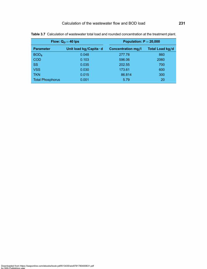
Table 3.7 Calculation of wastewater total load and rounded concentration at the treatment plant.

Flow: QD= 40 lps Population: P= 20,000

Parameter Unit load kg/////Capita · d Concentration mg/////l Total Load kg/////d

BOD5 0.048 277.78 860

COD 0.103 596.06 2060

SS 0.035 202.55 700

VSS 0.030 173.61 600

TKN 0.015 86.814 300

Total Phosphorus 0.001 5.79 20



Chapter 4

Rotating Micro Screens – RMS

4.1 PROCESS DESCRIPTION4.1.1 IntroductionWhen financial resources are limited it is advisable to use simple treatment processes that are highlycost-effective in terms of kgBOD removed per US$ invested. In many cases, for a given investment, ahigher environmental benefit is achieved at lower cost by removing organic matter by means ofmechanical microscreening processes which have a proven track record and are reliable. For example,rotating micro screen (RMS) with a screen opening of 0.2 mm can reduced the COD of municipalwastewater by almost 35%, and with the addition of coagulants before the micro screens treatment, atotal COD removal of 60% can be reached (Koehler & Rainer, 2003).

Fine screening is achieved in screen with openings in the range 0.2–2 mm while coarse screening isdone in screens with openings in the range 2–10 mm and even larger. Coarse screens remove floatingmaterials, paper and plastics. Rotating Micro Screens remove fine material, sand, and some suspendedorganic matter. A rotating micro screen with a screen opening of 0.2 and 1.5 mm can be compared witha primary treatment by sedimentation with BOD removal of around 15% (or 35% of COD) and SSremoval of about 50%. The efficiency can be significantly improved by the use of coagulants prior to thescreening operation (Orozco, 2005).

Treatment by a rotating micro screen is a mechanical process for removal of suspended matter fromwastewater. It is used to also to remove some organic load. Microscreening operates similarly to the roughscreening, but at a finer level. Screens can be static or rotational. The static screens are self-cleaning due tothe slope of water flow, while the rotating screens are cleaned by a scraper in the inner side of the screenwhich peals of the solids retained on it, or by backwashing, which is the more modern method.

A self explanatory diagram of a typical rotating micro screen is shown in Figure 4.1: raw wastewaterflows into the inner part of a drum which is covered by the screen and has to flow through the screen,coming out filtered downstream the channel. The system is backwashed by the jet stream located at theupper side of the drum. The removed material falls into a screw pump located inside the drum, whichcarried it up into a compactor which compresses the solid material and reduces its volume. Thecompacted material is then conveyed to a container located on top of the channel, from which it isremoved for its final disposal, usually to a sanitary landfill. The screen opening varies with itsapplication. If the rotating micro screen is the sole treatment unit prior to discharge of the effluent to awater body, for example to the sea, a fine screen is used so as to remove a significant portion of the


suspended matter from the raw sewage. If the rotating micro screen is part of a preliminary treatment unit inan activated sludge plant, there is no need to remove all the fine material because downstream units canhandle the fine suspended solids, so the screen does not need to be very fine.

A rotating micros screen with fine screen opening (0.2 to 1.5mm) can be used as part of a preliminarywastewater treatment unit often in conjunction with a preceding rough screening unit (which can also bea rotating screen with a wider opening of 6 to 10 mm) and a preceding grit chamber (sometimes the gritchamber is located following the micro screen). A typical scheme of such a preliminary treatment unit isshown in Figure 4.2. The rough screening unit is not shown in this figure because it is located in thepumping station which conveys the wastewater to the plant. The unit that follows the rotating finescreens is, in the Cartagena treatment plant, a Vortex grit chamber.

In Latin America, rotating fine screens have been installed in the four treatment plants of the city of SantaCruz, Bolivia, in the treatment plants of Cartagena, Colombia, La Plata and Bahia Blanca, Argentina and inseveral plants in Brazil, as well as in other cities. Information about the plants of Santa Cruz is given byLibhaber (2007), Annex 15 and by Blanco et al. (2007).

Figure 4.2 Typical rotating micro screen system, the wastewater treatment plant of Cartagena, Colombia(Courtesy Aguas de Cartagena)

Figure 4.1 Schematic presentation of the operation principle of a typical rotating micro screen (CourtesyHuber Technology)



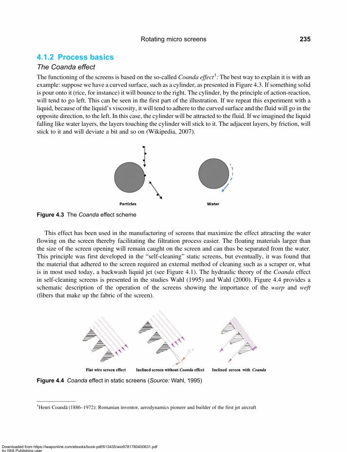
4.1.2 Process basicsThe Coanda effectThe functioning of the screens is based on the so-called Coanda effect1: The best way to explain it is with anexample: suppose we have a curved surface, such as a cylinder, as presented in Figure 4.3. If something solidis pour onto it (rice, for instance) it will bounce to the right. The cylinder, by the principle of action-reaction,will tend to go left. This can be seen in the first part of the illustration. If we repeat this experiment with aliquid, because of the liquid’s viscosity, it will tend to adhere to the curved surface and the fluid will go in theopposite direction, to the left. In this case, the cylinder will be attracted to the fluid. If we imagined the liquidfalling like water layers, the layers touching the cylinder will stick to it. The adjacent layers, by friction, willstick to it and will deviate a bit and so on (Wikipedia, 2007).

This effect has been used in the manufacturing of screens that maximize the effect attracting the waterflowing on the screen thereby facilitating the filtration process easier. The floating materials larger thanthe size of the screen opening will remain caught on the screen and can thus be separated from the water.This principle was first developed in the “self-cleaning” static screens, but eventually, it was found thatthe material that adhered to the screen required an external method of cleaning such as a scraper or, whatis in most used today, a backwash liquid jet (see Figure 4.1). The hydraulic theory of the Coanda effectin self-cleaning screens is presented in the studies Wahl (1995) and Wahl (2000). Figure 4.4 provides aschematic description of the operation of the screens showing the importance of the warp and weft(fibers that make up the fabric of the screen).

Figure 4.3 The Coanda effect scheme

Figure 4.4 Coanda effect in static screens (Source: Wahl, 1995)

1Henri Coanda (1886–1972): Romanian inventor, aerodynamics pioneer and builder of the first jet aircraft

Rotating micro screens 235


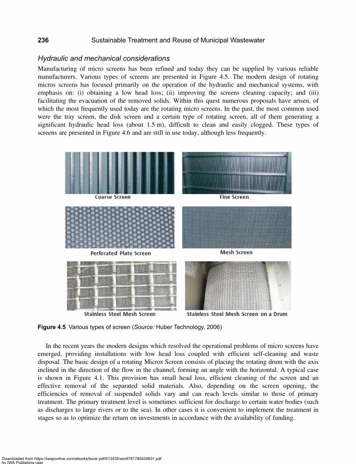
Hydraulic and mechanical considerationsManufacturing of micro screens has been refined and today they can be supplied by various reliablemanufacturers. Various types of screens are presented in Figure 4.5. The modern design of rotatingmicros screens has focused primarily on the operation of the hydraulic and mechanical systems, withemphasis on: (i) obtaining a low head loss; (ii) improving the screens cleaning capacity; and (iii)facilitating the evacuation of the removed solids. Within this quest numerous proposals have arisen, ofwhich the most frequently used today are the rotating micro screens. In the past, the most common usedwere the tray screen, the disk screen and a certain type of rotating screen, all of them generating asignificant hydraulic head loss (about 1.5 m), difficult to clean and easily clogged. These types ofscreens are presented in Figure 4.6 and are still in use today, although less frequently.

In the recent years the modern designs which resolved the operational problems of micro screens haveemerged, providing installations with low head loss coupled with efficient self-cleaning and wastedisposal. The basic design of a rotating Micros Screen consists of placing the rotating drum with the axisinclined in the direction of the flow in the channel, forming an angle with the horizontal. A typical caseis shown in Figure 4.1. This provision has small head loss, efficient cleaning of the screen and aneffective removal of the separated solid materials. Also, depending on the screen opening, theefficiencies of removal of suspended solids vary and can reach levels similar to those of primarytreatment. The primary treatment level is sometimes sufficient for discharge to certain water bodies (suchas discharges to large rivers or to the sea). In other cases it is convenient to implement the treatment instages so as to optimize the return on investments in accordance with the availability of funding.

Figure 4.5 Various types of screen (Source: Huber Technology, 2006)



Design considerationsOne of the main design parameters of a rotating micro screen is the hydraulic head loss which depends onthree factors: (i) the velocity of the wastewater; (ii) the screen opening; and (iii) the mechanical design of thescreen. The most commonly used equation for estimating the head loss (hf) is the following (Orozco, 2005):

h f = 1C(2g)

QA

( )2

(4.1)

where:

hf = head loss, mC = discharge coefficient of a clean screen. With large screen openings (.6 mm) the value of C is

approximately 0.6. But C must be obtained for each screen opening. Also, the load loss that reallymatters is that which occurs during operation, with the filtered material attached to the inner side ofthe screen. Such information is obtained from experiments during operation.

A = effective area of the screen, m2

Q = flow rate, m3/sg= gravity acceleration coefficient, 9.81 m/s2.

Figure 4.6 Other types of micro screens (Source: García Agudo & Rusell, 1992)



In Figure 4.7, which is used for the design of rotating micro screens, the variation of the drum diameterwith the wastewater flow for different screen openings can be observed.

The head loss of a clean screen is in fact very low so the true operating hydraulic head loss depends on thematerial which is collected in the screen, on the cleaning efficiency of the screen (which is usually achievedby backwash) and on the disposal of the material removed by the screen. For design purposes, the maximumoperating flow and the minimum cleaning cycle should be considered.

The design must take into account: (i) the nature of the suspended matter; (ii) the corrosiveness of thewastewater; (iii) the effect of chlorination when it is required as a pre-treatment; (iv) the duplication ofunits for continuous operation during equipment maintenance periods; and (v) the backwash operation.In addition, the following provisions should be installed: (i) a durable corrosion resistant screen; (ii) a

Figure 4.7 Dimensions of the screen drum diameter VS wastewater flow rate for different screen openings ofa Rotamat type rotating micro screen (Source: Catalog of Rotamat Micro Screens, Courtesy HuberTechnology)



by-pass; (iii) hydraulic seals when using potable water for backwashing; and (iv) proper disposal of solidsretained by the screen (Indian & Northern Affairs Canada, 2006). In addition, if increase of the processefficiency is required, application of coagulant agents should be considered to promote flocculation ofthe suspended solids before passing through the micro screens. This issue is further discussed in thechapter on chemically enhanced primary treatment (CEPT). Table 4.1 presents typical design parametersfor rotating micro screens.

Management and disposal of the solid wastes generated in preliminary treatmentThe appropriate technology treatment processes generate two types of solid wastes. Rotating screens withcoarse openings larger than 0.7 mm and grit chambers produce residual solids which are mainly mineral,consisting of sand, grit, coarse particles and large materials like plastics, bottles, cans and other floatablematerial. This material is defined as solid wastes from preliminary treatment. Rotating fine screens withopenings less than 0.7 mm and most other appropriate technology treatment processes (such as CEPT,UASB, Anaerobic Filter etc.) produce an additional stream of residual solids which consist of acombination of mineral and organic matter, defined as sludge. These two types of solids, solid wastesand sludge, are handled and disposed of differently. The management and disposal of the solid wastesgenerated in the preliminary treatment is discussed below. The management of the sludge is discussed inChapter 9.

Disposal of screenings (solid wastes collected in preliminary treatment plants) may include: (1) removalby hauling to disposal areas (sanitary landfill); (2) disposal by burial on the plant site (small installationsonly); (3) incineration alone or in combination with sludge and grit (large installations only); (4) disposalwith solid wastes; or (5) discharge to grinders or macerators where they are ground and returned tothe wastewater.

Removal to a sanitary landfill is the most common disposal method. In a rotating fine screen unit thesolids are compacted prior to disposal. A photograph of typical solid wastes of a preliminary treatmentunit is presented in Figure 4.8. The solid wastes container fills automatically without manualintervention. When the container is full it is put on a removal truck by a crane built onto the truck. Thesame truck leaves an empty container at the plant for filling and then travels to the landfill site to disposeof the solid wastes.

Table 4.1 Typical design parameters.

Item Unit Typical value

Screen opening mm 0.2–2 mm

Hydraulic load m3/m2 · min 3–6

Head loss mm 75–150

Submergence % area 60–70

Drum diameter m 0.6–5.0

Drum speed m/min 4.5

Backwash % of flow @ 350 and 500 kPa 2% and 5%

Waste removed l/1000 m3 100–250

Source: Prepared from Metcalf & Eddy (2003) and Catalog of HUBER Rotamat (2007)



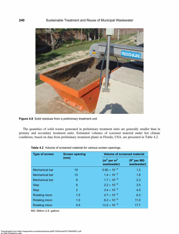
The quantities of solid wastes generated in preliminary treatment units are generally smaller than inprimary and secondary treatment units. Estimated volumes of screened material under hot climateconditions, based on data from preliminary treatment plants in Florida, USA, are presented in Table 4.2.

Table 4.2 Volume of screened material for various screen openings.

Type of screen Screen opening(mm)

Volume of screened material

(m3 per m3

wastewater)(ft3 per MGwastewater)

Mechanical bar 19 0.90× 10−5 1.2



Step 6 2.2× 10−5 3.0

Step 2 3.4× 10−5 4.5

Rotating micro 1.5 4.7× 10−5 6.3

Rotating micro 1.0 8.2× 10−5 11.0

Rotating micro 0.5 13.2× 10−5 17.7

MG: Million U.S. gallons

Figure 4.8 Solid residues from a preliminary treatment unit



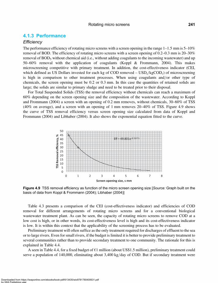
4.1.3 PerformanceEfficiencyThe performance efficiency of rotating micro screens with a screen opening in the range 1–1.5 mm is 5–10%removal of BOD. The efficiency of rotating micro screens with a screen opening of 0.2–0.3 mm is 20–30%removal of BOD5 without chemical aid (i.e., without adding coagulants to the incoming wastewater) and up50–60% removal with the application of coagulants (Koppl & Frommann, 2004). This makesmicroscreening competitive with primary treatment. In addition, the cost-effectiveness indicator (CEI,which defined as US Dollars invested for each kg of COD removed – USDi/kgCODr) of microscreeningis high in comparison to other treatment processes. When using coagulants and/or other type ofchemicals, the screen opening must be 0.2 or 0.3 mm. In this case the quantities of retained solids arelarge; the solids are similar to primary sludge and need to be treated prior to their disposal.

For Total Suspended Solids (TSS) the removal efficiency without chemicals can reach a maximum of60% depending on the screen opening size and the composition of the wastewater. According to Koppland Frommann (2004) a screen with an opening of 0.2 mm removes, without chemicals, 30–60% of TSS(40% on average), and a screen with an opening of 1 mm removes 20–40% of TSS. Figure 4.9 showsthe curve of TSS removal efficiency versus screen opening size calculated from data of Koppl andFrommann (2004) and Libhaber (2004). It also shows the exponential equation fitted to the curve.

Table 4.3 presents a comparison of the CEI (cost-effectiveness indicator) and efficiencies of CODremoval for different arrangements of rotating micro screens and for a conventional biologicalwastewater treatment plant. As can be seen, the capacity of rotating micro screens to remove COD at alow cost is high, or in other words, its cost-effectiveness level is high and its cost-effectiveness indicatoris low. It is within this context that the applicability of the screening process has to be evaluated.

Preliminary treatment will often suffice as the only treatment required for discharges of effluent to the seaor to large rivers. Even for small rivers, if the budget is limited it is better to provide preliminary treatment toseveral communities rather than to provide secondary treatment to one community. The rationale for this isexplained in Table 4.4.

A seen in Table 4.4, for a fixed budget of €1 million (about US$1.5 million), preliminary treatment couldserve a population of 140,000, eliminating about 3,400 kg/day of COD. But if secondary treatment were

05

101520253035404550

0 1 2 3 4

Screen opening size, s mm

5 6 7 8

TSS

Rem

oval

effi

cien

cy, % Eff = 49.801e-0.507 S

Figure 4.9 TSS removal efficiency as function of the micro screen opening size [Source: Graph built on thebasis of data from Koppl & Frommann (2004); Libhaber (2004)]



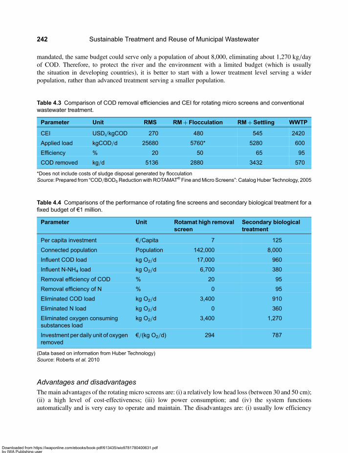
mandated, the same budget could serve only a population of about 8,000, eliminating about 1,270 kg/dayof COD. Therefore, to protect the river and the environment with a limited budget (which is usuallythe situation in developing countries), it is better to start with a lower treatment level serving a widerpopulation, rather than advanced treatment serving a smaller population.

Advantages and disadvantagesThemain advantages of the rotating micro screens are: (i) a relatively low head loss (between 30 and 50 cm);(ii) a high level of cost-effectiveness; (iii) low power consumption; and (iv) the system functionsautomatically and is very easy to operate and maintain. The disadvantages are: (i) usually low efficiency

Table 4.4 Comparisons of the performance of rotating fine screens and secondary biological treatment for afixed budget of €1 million.

Parameter Unit Rotamat high removalscreen

Secondary biologicaltreatment

Per capita investment €/Capita 7 125

Connected population Population 142,000 8,000

Influent COD load kg O2/d 17,000 960

Influent N-NH4 load kg O2/d 6,700 380

Removal efficiency of COD % 20 95

Removal efficiency of N % 0 95

Eliminated COD load kg O2/d 3,400 910

Eliminated N load kg O2/d 0 360

Eliminated oxygen consumingsubstances load

kg O2/d 3,400 1,270

Investment per daily unit of oxygenremoved

€/(kg O2/d) 294 787

(Data based on information from Huber Technology)Source: Roberts et al. 2010

Table 4.3 Comparison of COD removal efficiencies and CEI for rotating micro screens and conventionalwastewater treatment.

Parameter Unit RMS RM+ Flocculation RM+ Settling WWTP

CEI USDi/kgCOD 270 480 545 2420

Applied load kgCOD/d 25680 5760* 5280 600

Efficiency % 20 50 65 95

COD removed kg/d 5136 2880 3432 570

*Does not include costs of sludge disposal generated by flocculationSource: Prepared from “COD/BOD5Reductionwith ROTAMAT® Fine andMicro Screens”: CatalogHuber Technology, 2005



in removal of TSS (the efficiency of a rotating Micros Screen is determined by the hydraulic and solids loadsas well as by the characteristics of the influent stream); (ii) micro screens do not remove colloidal material (orsmall size algae); (iii) micro screens require an efficient self-cleaning system; and (iv) micro screens areaffected by fluctuations in the composition and quality of the influent.

The application of coagulants improves the operating efficiency of micro screens but also increases theproduction of solid residues (in this case sludge) which require disposal. The addition of chemicals modifiesthe type of solids retained on the screen, which in this case is practically sludge that is a material moredifficult to handle. The investment costs of rotating micro screens are in the range of and 3–10 US$ perCapita served and the operating costs are in the range 0.10 and 0.15 US$ per Capita per year (Libhaber, 2007).

4.2 BASIC DESIGN PROCEDURE4.2.1 General design considerationsPretreatment is the preparatory process necessary prior to subjecting municipal wastewater to secondarytreatment. Coarse screening is the first of the pretreatment units. Screens are classified as coarse whenthe screen opening is in the range of 2.0 to 6.0 mm (while in fine screens the opening is between 0.2 and2 mm). Screens are used to remove materials present in the wastewater, such as paper, plastics and otherfloating materials. The objective of screens is to protect the operation of valves, pumps, aerators andother equipment included in a wastewater treatment plant. The fine screens are used to remove finesuspended material, among which is the particulate organic matter. One type of very fine screen used isthe rotating micro screen (RMS) that can remove, under certain circumstances, up to 90% of TSS andabout 35% of the COD. The RMS are considered a sustainable Appropriate Technology process becauseof its ease of operation and cost-effectiveness (Koehler, 2003; Orozo, 2005).

To specify a RMS equipment it is most important to select the screen opening size. This is a designervariable (variable to be proposed by the designer, based on his experience and knowledge of theprocess). Some guidelines for making this selection are: (i) if the RMS is a pretreatment precedingbiological treatment, aerobic or anaerobic, the screen opening does not have to be very small and can bein the range of 2–10 mm since the organic matter will be removed in the biological process; (ii) if theRMS is used as the main treatment unit prior to direct discharge of the effluent to a water body through asubaquatic outfall, then, since it is the sole treatment unit, a smaller screen opening in the range 0.2–2.0mm should be used, however, the fine RMS should be protected by a preceding coarse screening, whichcan be a coarse rotating screen unit; (iii) when making the selection it is necessary to analyze the cost,taking into account that when the screen opening is smaller the cost is higher, so it is necessary to assessthe cost-effectiveness of screening unit. In practice, there is no procedure to determine the type of RMSto be used, except the designer’s experience (Indian & Northern Affairs Canada, 2006).

4.2.2 Orderly design method (ODM)In general, the design methodology of a RMS is the following:

(1) Determine the external variables (or independent variables), which, among others, are thefollowing:○ Flow rate: since this process is hydraulic, we must use as design flow the peak flow or the

hydraulic design flow (QHD) calculated by Equation 4.4 (below) using the appropriate units(lps, m3/h, etc):

QHD = k1k2cqdomP86400

+ qI Aa (4.4)



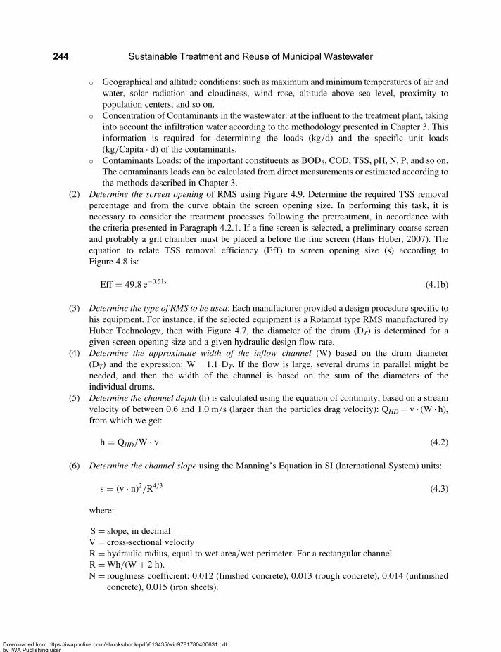
○ Geographical and altitude conditions: such as maximum and minimum temperatures of air andwater, solar radiation and cloudiness, wind rose, altitude above sea level, proximity topopulation centers, and so on.

○ Concentration of Contaminants in the wastewater: at the influent to the treatment plant, takinginto account the infiltration water according to the methodology presented in Chapter 3. Thisinformation is required for determining the loads (kg/d) and the specific unit loads(kg/Capita · d) of the contaminants.

○ Contaminants Loads: of the important constituents as BOD5, COD, TSS, pH, N, P, and so on.The contaminants loads can be calculated from direct measurements or estimated according tothe methods described in Chapter 3.

(2) Determine the screen opening of RMS using Figure 4.9. Determine the required TSS removalpercentage and from the curve obtain the screen opening size. In performing this task, it isnecessary to consider the treatment processes following the pretreatment, in accordance withthe criteria presented in Paragraph 4.2.1. If a fine screen is selected, a preliminary coarse screenand probably a grit chamber must be placed a before the fine screen (Hans Huber, 2007). Theequation to relate TSS removal efficiency (Eff) to screen opening size (s) according toFigure 4.8 is:

Eff = 49.8 e−0.51s (4.1b)

(3) Determine the type of RMS to be used: Each manufacturer provided a design procedure specific tohis equipment. For instance, if the selected equipment is a Rotamat type RMS manufactured byHuber Technology, then with Figure 4.7, the diameter of the drum (DT) is determined for agiven screen opening size and a given hydraulic design flow rate.

(4) Determine the approximate width of the inflow channel (W) based on the drum diameter(DT) and the expression: W= 1.1 DT. If the flow is large, several drums in parallel might beneeded, and then the width of the channel is based on the sum of the diameters of theindividual drums.

(5) Determine the channel depth (h) is calculated using the equation of continuity, based on a streamvelocity of between 0.6 and 1.0 m/s (larger than the particles drag velocity): QHD= v · (W · h),from which we get:

h = QHD/W · v (4.2)

(6) Determine the channel slope using the Manning’s Equation in SI (International System) units:

s = (v · n)2/R4/3 (4.3)

where:

S= slope, in decimalV = cross-sectional velocityR = hydraulic radius, equal to wet area/wet perimeter. For a rectangular channelR =Wh/(W+ 2 h).N = roughness coefficient: 0.012 (finished concrete), 0.013 (rough concrete), 0.014 (unfinished

concrete), 0.015 (iron sheets).



(7) Determine the head loss with Equation 4.1:

h f = 1C(2g)

QDH

A

( )2

C ≈ 0.6. The manufacturer curve can be used if C is not known(8) Determine the backwash volume and pressure from Table 4.1.(9) Determine the amount of solids to remove.

○ The amount of excess solids fromRMS is estimated in Table 4.1 (between 30 and 60 l/1000 m3).○ The study of Aguas de Cartagena (2007) proposes an excess solid generation rate of 4.7 m3 per

100,000 m3 of treated wastewater (equivalent to 47.5 l/1000 m3).○ If the screen opening is 0.7 mm and higher, the solids retained on it are mostly made of inert

mineral matter and can be directly transported to disposal in a sanitary landfill. If the screenopening is smaller than 0.7 mm, the retained solids contain a higher portion of organicmatter. In this case it is preferable to provide a stabilizing treatment prior to their finaldisposal. The stabilization is carried out in the containers which temporarily store thematerial, applying in the container a layer of saturated lime every time a layer 20 cm thick ofretained solids is deposited in the container. The high level of pH of the caused by the limeensures the destruction of bacteria and pathogenic microorganisms. The generation ofhydrogen sulphide (H2S), which causes odour problems, is also prevented this way,favouring the drying process of the solids and reducing the possibility of attracting vectors.

○ Should this measure be insufficient and offensive odours persist, the solids containers needs tobe stored in s closed structure equipped with odour control installations (such as air aspiratorsand treatment of the air for odour removal before its discharge to the atmosphere. The treatmentcan be based on passing the air through a biological filter or through an absorption tower, using achemical solution as an odour absorbent).

(10) Design a by-pass to divert the influent to the discharge of the RMS unit. The by-pass is used duringmaintenance operation and in cases of emergency. This can be avoided by using two parallelRMS units.

4.3 BASIC DESIGN EXAMPLE(The model program for this Example is available online at http://www.iwawaterwiki.org/xwiki/bin/view/Articles/Software+Developed+for+Sustainable+Treatment+and+Reuse+of+Municipal+Wastewater)

In continuation we present an example that follows the Orderly Design Method (ODM) of Paragraph4.2.2. The example is developed for a population of 20,000, as presented in Chapter 3. The ODM isdeveloped step by step and is calculated by a program developed in Excel, available online as explainedelsewhere. One way to solve the design example is presented by the ODM, but the reader should beaware that there might be several different methods to achieve a good design. If properly understood, themodel could be changed when the a priori (external) conditions demand a different approach, leaving aproper back up of the original program, called CHAP 4-RM.xls. Please note that the following Tablesidentified by alphabetic order contain computer calculated results.

General instructions for running de Excel sheet program with the ODM

• First, make sure that you thoroughly understand the Orderly Design Method.• Second, get acquainted with the colour Nomenclature as as shown in Table 4A.





















• Whatever is in dark grey colour refers to titles, parameters or units, and is alphabetic. The othercolours refer to numeric cells.

• The cells in light grey colour are input provided by the designer, be it (i) external parameters or (ii)primary variables given by the designer. These cells should be filled manually by the designer.

• The coloured medium grey cells are secondary variables calculated from the primary variables, whichbelong to the input necessary for the design. Note that the designer may choose a secondary variableas primary, and then the primary variable becomes secondary. For instance, to calculate the designflow you may select q, P and c as primary variables and from them the program calculates theprocess design flow (QDWW) as secondary variable; but you may know the design flow, then qbecomes a secondary variable. These variations in primary variables would require changes in theprogram and should be avoided unless completely necessary.

• With the input defined, the program calculates the design variables in the output as determined by theODM. Also, in this step there are variables that can be selected as input and the corresponding ones inthe input become outputs. For example, in Figure 4.8, you can choose either Efficiency or screenopening (mesh size) as input. If you choose one variable as input then the other variablebecomes output.

• Remember, to change primary variables to secondary variables (or input to output) in the programrequires a thoroughly comprehension of the ODM.

• Check that the output variables, be they dimensions or specifications, are practical and are in theempirical range of design given in the Process Description section of the chapter.

• Note that the necessary steps to calculate CONCENTRATION, ORGANIC LOADS AND SPECIFCUNIT LOADS, require that the wastewater quality is given as an input.

• These general instructions apply to all programs given in the attached CD.

(1) Calculation of external variables1.1 Design flows: The calculation related to the design flows are presented in Table 4B.

The final design flows are obtained from Equation 3.4, and are presented in different unitsas an output. The average flow QD is used for the design of the biological process and themaximum flow QHD for the hydraulic designs. The resulting design flows are presented inTable 4C.

In the case of RMs the design flow is QHD because the process is basically a physicalprocess depending on the hydraulics.

1.2 Determination of the external geographical and environmental variables: These variablesdepend solely on the geographic location. They values used in the example are presentedin Table 4D.

Table 4A

Nomenclature

Dark grey color Titles, parameters, units

Light grey color Input

Grey color Output

Medium grey color Calculated variables



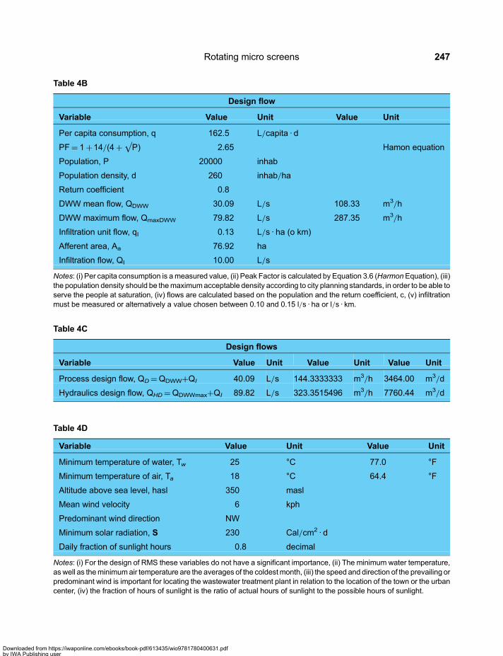
Table 4B

Design flow

Variable Value Unit Value Unit

Per capita consumption, q 162.5 L/capita · d

PF= 1+14/(4+√P) 2.65 Hamon equation

Population, P 20000 inhab

Population density, d 260 inhab/ha

Return coefficient 0.8

DWW mean flow, QDWW 30.09 L/s 108.33 m3/h

DWW maximum flow, QmaxDWW 79.82 L/s 287.35 m3/h

Infiltration unit flow, qI 0.13 L/s · ha (o km)

Afferent area, Aa 76.92 ha

Infiltration flow, QI 10.00 L/s

Notes: (i) Per capita consumption is ameasured value, (ii) Peak Factor is calculated by Equation 3.6 (HarmonEquation), (iii)the population density should be themaximumacceptable density according to city planning standards, in order to be able toserve the people at saturation, (iv) flows are calculated based on the population and the return coefficient, c, (v) infiltrationmust be measured or alternatively a value chosen between 0.10 and 0.15 l/s · ha or l/s · km.

Table 4D


Minimum temperature of water, Tw 25 °C 77.0 °F

Minimum temperature of air, Ta 18 °C 64.4 °F

Altitude above sea level, hasl 350 masl

Mean wind velocity 6 kph

Predominant wind direction NW

Minimum solar radiation, S 230 Cal/cm2 · d

Daily fraction of sunlight hours 0.8 decimal

Notes: (i) For the design of RMS these variables do not have a significant importance, (ii) The minimum water temperature,as well as theminimumair temperature are the averages of the coldestmonth, (iii) the speed and direction of the prevailing orpredominant wind is important for locating the wastewater treatment plant in relation to the location of the town or the urbancenter, (iv) the fraction of hours of sunlight is the ratio of actual hours of sunlight to the possible hours of sunlight.

Table 4C

Design flows

Variable Value Unit Value Unit Value Unit

Process design flow, QD=QDWW+QI 40.09 L/s 144.3333333 m3/h 3464.00 m3/d

Hydraulics design flow, QHD=QDWWmax+QI 89.82 L/s 323.3515496 m3/h 7760.44 m3/d



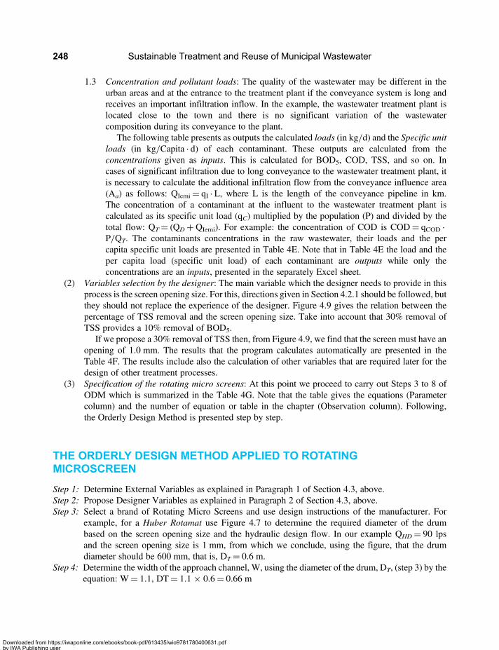
1.3 Concentration and pollutant loads: The quality of the wastewater may be different in theurban areas and at the entrance to the treatment plant if the conveyance system is long andreceives an important infiltration inflow. In the example, the wastewater treatment plant islocated close to the town and there is no significant variation of the wastewatercomposition during its conveyance to the plant.

The following table presents as outputs the calculated loads (in kg/d) and the Specific unitloads (in kg/Capita · d) of each contaminant. These outputs are calculated from theconcentrations given as inputs. This is calculated for BOD5, COD, TSS, and so on. Incases of significant infiltration due to long conveyance to the wastewater treatment plant, itis necessary to calculate the additional infiltration flow from the conveyance influence area(Aa) as follows: QIemi= qI · L, where L is the length of the conveyance pipeline in km.The concentration of a contaminant at the influent to the wastewater treatment plant iscalculated as its specific unit load (qC) multiplied by the population (P) and divided by thetotal flow: QT= (QD+QIemi). For example: the concentration of COD is COD= qCOD ·P/QT. The contaminants concentrations in the raw wastewater, their loads and the percapita specific unit loads are presented in Table 4E. Note that in Table 4E the load and theper capita load (specific unit load) of each contaminant are outputs while only theconcentrations are an inputs, presented in the separately Excel sheet.

(2) Variables selection by the designer: The main variable which the designer needs to provide in thisprocess is the screen opening size. For this, directions given in Section 4.2.1 should be followed, butthey should not replace the experience of the designer. Figure 4.9 gives the relation between thepercentage of TSS removal and the screen opening size. Take into account that 30% removal ofTSS provides a 10% removal of BOD5.

If we propose a 30% removal of TSS then, from Figure 4.9, we find that the screen must have anopening of 1.0 mm. The results that the program calculates automatically are presented in theTable 4F. The results include also the calculation of other variables that are required later for thedesign of other treatment processes.

(3) Specification of the rotating micro screens: At this point we proceed to carry out Steps 3 to 8 ofODM which is summarized in the Table 4G. Note that the table gives the equations (Parametercolumn) and the number of equation or table in the chapter (Observation column). Following,the Orderly Design Method is presented step by step.

THE ORDERLY DESIGN METHOD APPLIED TO ROTATINGMICROSCREEN

Step 1: Determine External Variables as explained in Paragraph 1 of Section 4.3, above.Step 2: Propose Designer Variables as explained in Paragraph 2 of Section 4.3, above.Step 3: Select a brand of Rotating Micro Screens and use design instructions of the manufacturer. For

example, for a Huber Rotamat use Figure 4.7 to determine the required diameter of the drumbased on the screen opening size and the hydraulic design flow. In our example QHD= 90 lpsand the screen opening size is 1 mm, from which we conclude, using the figure, that the drumdiameter should be 600 mm, that is, DT= 0.6 m.

Step 4: Determine the width of the approach channel, W, using the diameter of the drum, DT, (step 3) by theequation: W= 1.1, DT= 1.1 × 0.6= 0.66 m



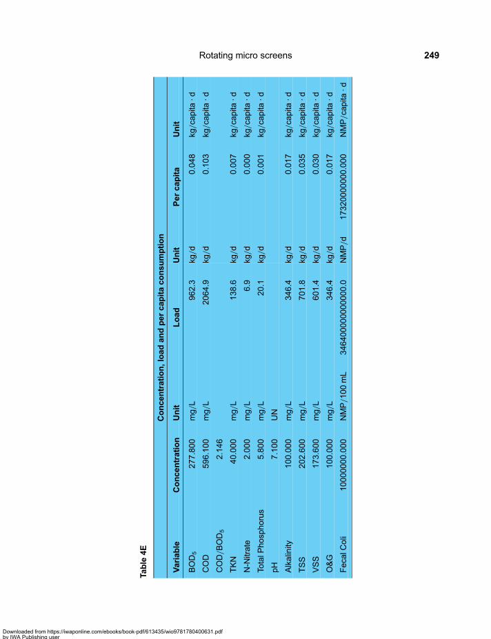
Table

4E

Concentration,loadandpercapitaconsumption

Variable

Concentration

Unit

Load

Unit

Percapita

Unit

BOD5

277.800

mg/

L962.3

kg/d

0.048

kg/ca

pita

·d

COD

596.100

mg/

L2064.9

kg/d

0.103

kg/ca

pita

·d

COD/BOD5

2.146

TKN

40.000

mg/

L138.6

kg/d

0.007

kg/ca

pita

·d

N-N

itrate

2.000

mg/

L6.9

kg/d

0.000

kg/ca

pita

·d

TotalP

hosp

horus

5.800

mg/

L20.1

kg/d

0.001

kg/ca

pita

·d

pH

7.100

UN

Alkalinity

100.000

mg/

L346.4

kg/d

0.017

kg/ca

pita

·d

TSS

202.600

mg/

L701.8

kg/d

0.035

kg/ca

pita

·d

VSS

173.600

mg/

L601.4

kg/d

0.030

kg/ca

pita

·d

O&G

100.000

mg/

L346.4

kg/d

0.017

kg/ca

pita

·d

Feca

lColi

100000

00.000

NMP/100mL

346400000000000.0

NMP/d

17320000000.000

NMP/ca

pita

·d



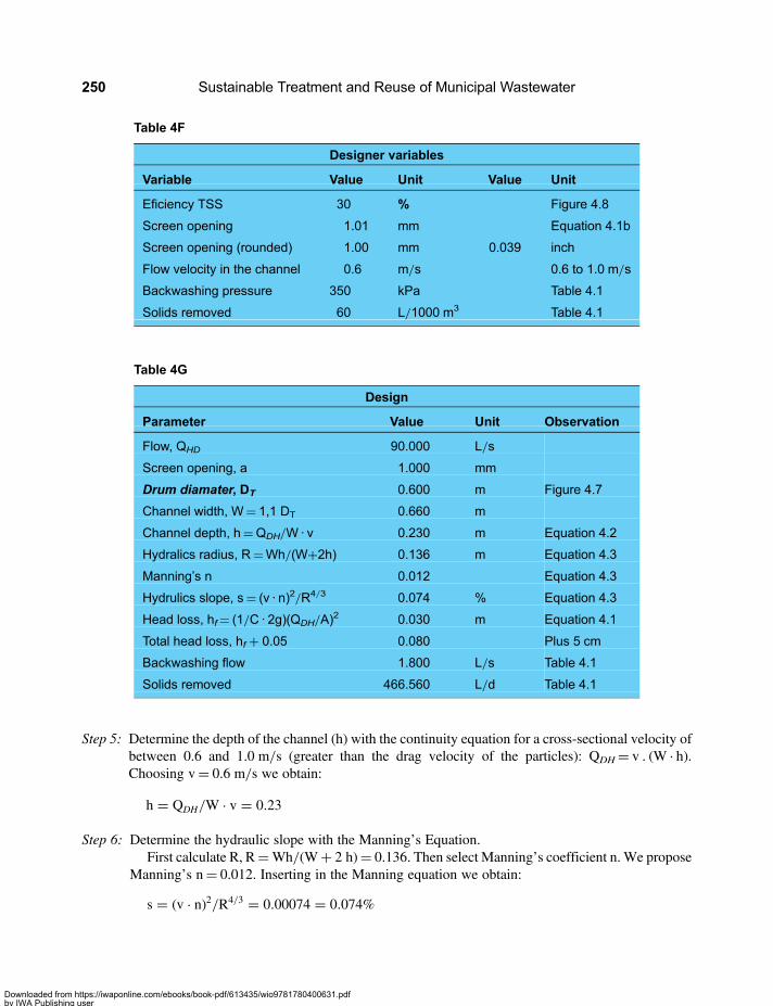
Step 5: Determine the depth of the channel (h) with the continuity equation for a cross-sectional velocity ofbetween 0.6 and 1.0 m/s (greater than the drag velocity of the particles): QDH= v . (W · h).Choosing v= 0.6 m/s we obtain:

h = QDH/W · v = 0.23

Step 6: Determine the hydraulic slope with the Manning’s Equation.First calculate R, R=Wh/(W+ 2 h)= 0.136. Then select Manning’s coefficient n. We propose

Manning’s n= 0.012. Inserting in the Manning equation we obtain:

s = (v · n)2/R4/3 = 0.00074 = 0.074%

Table 4G

Design

Parameter Value Unit Observation

Flow, QHD 90.000 L/s

Screen opening, a 1.000 mm

Drum diamater, DT 0.600 m Figure 4.7

Channel width, W= 1,1 DT 0.660 m

Channel depth, h=QDH/W · v 0.230 m Equation 4.2

Hydralics radius, R=Wh/(W+2h) 0.136 m Equation 4.3

Manning’s n 0.012 Equation 4.3

Hydrulics slope, s= (v · n)2/R4/3 0.074 % Equation 4.3

Head loss, hf= (1/C · 2g)(QDH/A)2 0.030 m Equation 4.1

Total head loss, hf + 0.05 0.080 Plus 5 cm

Backwashing flow 1.800 L/s Table 4.1

Solids removed 466.560 L/d Table 4.1

Table 4F

Designer variables


Eficiency TSS 30 % Figure 4.8

Screen opening 1.01 mm Equation 4.1b

Screen opening (rounded) 1.00 mm 0.039 inch

Flow velocity in the channel 0.6 m/s 0.6 to 1.0 m/s

Backwashing pressure 350 kPa Table 4.1

Solids removed 60 L/1000 m3 Table 4.1



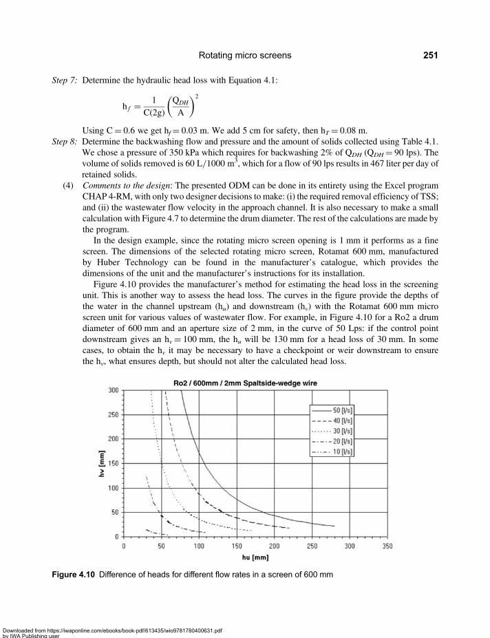
Step 7: Determine the hydraulic head loss with Equation 4.1:

h f = 1C(2g)

QDH

A

( )2

Using C= 0.6 we get hf= 0.03 m. We add 5 cm for safety, then hT= 0.08 m.Step 8: Determine the backwashing flow and pressure and the amount of solids collected using Table 4.1.

We chose a pressure of 350 kPa which requires for backwashing 2% of QDH (QDH= 90 lps). Thevolume of solids removed is 60 L/1000 m3, which for a flow of 90 lps results in 467 liter per day ofretained solids.

(4) Comments to the design: The presented ODM can be done in its entirety using the Excel programCHAP 4-RM, with only two designer decisions to make: (i) the required removal efficiency of TSS;and (ii) the wastewater flow velocity in the approach channel. It is also necessary to make a smallcalculation with Figure 4.7 to determine the drum diameter. The rest of the calculations are made bythe program.

In the design example, since the rotating micro screen opening is 1 mm it performs as a finescreen. The dimensions of the selected rotating micro screen, Rotamat 600 mm, manufacturedby Huber Technology can be found in the manufacturer’s catalogue, which provides thedimensions of the unit and the manufacturer’s instructions for its installation.

Figure 4.10 provides the manufacturer’s method for estimating the head loss in the screeningunit. This is another way to assess the head loss. The curves in the figure provide the depths ofthe water in the channel upstream (hu) and downstream (hv) with the Rotamat 600 mm microscreen unit for various values of wastewater flow. For example, in Figure 4.10 for a Ro2 a drumdiameter of 600 mm and an aperture size of 2 mm, in the curve of 50 Lps: if the control pointdownstream gives an hv= 100 mm, the hu will be 130 mm for a head loss of 30 mm. In somecases, to obtain the hv it may be necessary to have a checkpoint or weir downstream to ensurethe hv, what ensures depth, but should not alter the calculated head loss.

Figure 4.10 Difference of heads for different flow rates in a screen of 600 mm



This type of information should be requested from the manufacturer as a method to check the head losscalculations and to ensure the proper installation of the equipment.

For large flow treatment plant, a series of RMS drums in parallel is usually required. Figure 4.11 presentsa drawing of a rotating micro screens installation consisting of four drums in parallel.

Figure 4.12 shows a plan and a section of the preliminary treatment unit as that proposed in the designexample. It consists of first coarse rotating screen with an opening of 6 mm, followed by a unit of

Figure 4.11 Plan and sections of a typical rotating micro screen unit consisting of four drums in parallel



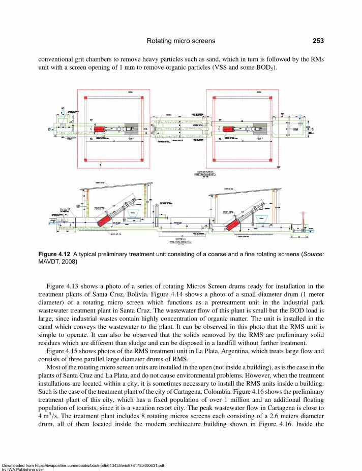
conventional grit chambers to remove heavy particles such as sand, which in turn is followed by the RMsunit with a screen opening of 1 mm to remove organic particles (VSS and some BOD5).

Figure 4.13 shows a photo of a series of rotating Micros Screen drums ready for installation in thetreatment plants of Santa Cruz, Bolivia. Figure 4.14 shows a photo of a small diameter drum (1 meterdiameter) of a rotating micro screen which functions as a pretreatment unit in the industrial parkwastewater treatment plant in Santa Cruz. The wastewater flow of this plant is small but the BOD load islarge, since industrial wastes contain highly concentration of organic matter. The unit is installed in thecanal which conveys the wastewater to the plant. It can be observed in this photo that the RMS unit issimple to operate. It can also be observed that the solids removed by the RMS are preliminary solidresidues which are different than sludge and can be disposed in a landfill without further treatment.

Figure 4.15 shows photos of the RMS treatment unit in La Plata, Argentina, which treats large flow andconsists of three parallel large diameter drums of RMS.

Most of the rotating micro screen units are installed in the open (not inside a building), as is the case in theplants of Santa Cruz and La Plata, and do not cause environmental problems. However, when the treatmentinstallations are located within a city, it is sometimes necessary to install the RMS units inside a building.Such is the case of the treatment plant of the city of Cartagena, Colombia. Figure 4.16 shows the preliminarytreatment plant of this city, which has a fixed population of over 1 million and an additional floatingpopulation of tourists, since it is a vacation resort city. The peak wastewater flow in Cartagena is close to4 m3/s. The treatment plant includes 8 rotating micros screens each consisting of a 2.6 meters diameterdrum, all of them located inside the modern architecture building shown in Figure 4.16. Inside the

Figure 4.12 A typical preliminary treatment unit consisting of a coarse and a fine rotating screens (Source:MAVDT, 2008)



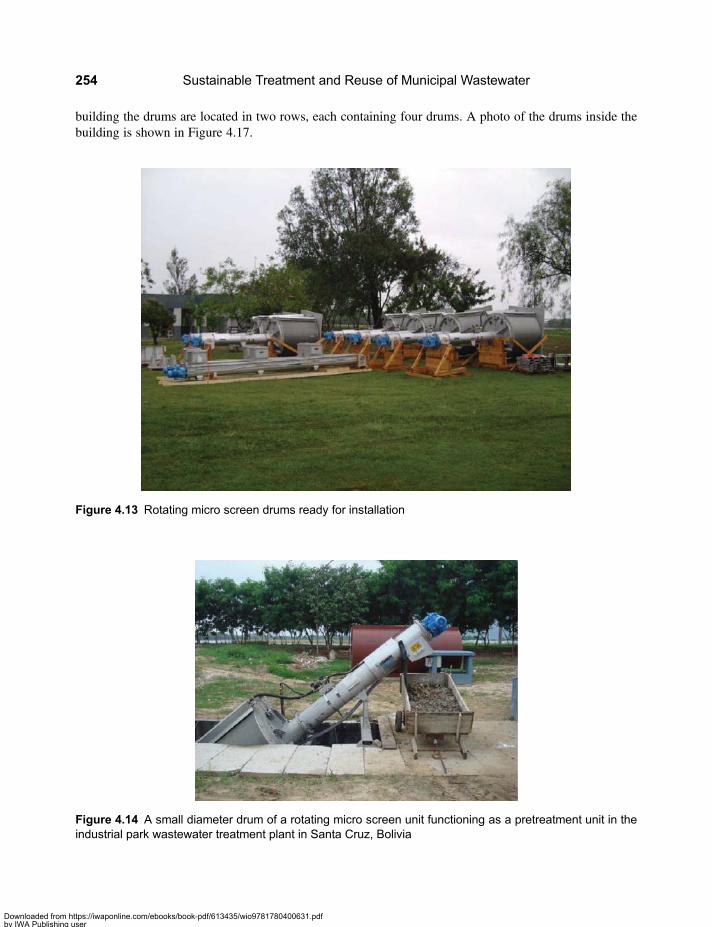
building the drums are located in two rows, each containing four drums. A photo of the drums inside thebuilding is shown in Figure 4.17.

Figure 4.14 A small diameter drum of a rotating micro screen unit functioning as a pretreatment unit in theindustrial park wastewater treatment plant in Santa Cruz, Bolivia

Figure 4.13 Rotating micro screen drums ready for installation



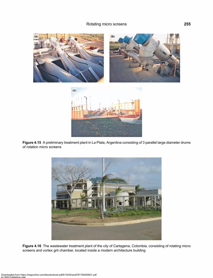
Figure 4.16 The wastewater treatment plant of the city of Cartagena, Colombia, consisting of rotating microscreens and vortex grit chamber, located inside a modern architecture building

Figure 4.15 A preliminary treatment plant in La Plata, Argentina consisting of 3 parallel large diameter drumsof rotation micro screens



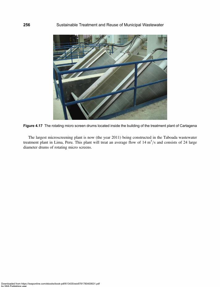
The largest microscreening plant is now (the year 2011) being constructed in the Taboada wastewatertreatment plant in Lima, Peru. This plant will treat an average flow of 14 m3/s and consists of 24 largediameter drums of rotating micro screens.

Figure 4.17 The rotating micro screen drums located inside the building of the treatment plant of Cartagena



Chapter 5

Treatment in stabilization lagoons

5.1 PROCESS DESCRIPTION5.1.1 IntroductionStabilization Lagoons (SL) consist of artificially constructed ponds, in which a microbial populationdevelops naturally, mainly composed of bacteria and algae that live in symbiotic union under which thealgae consume the CO2 generated by the bacteria and the bacteria consume the oxygen generated by thealgae. In addition, also by protozoa and fungi develop in the lagoons. Figure 5.1 presents the mainrelationships between algae and bacteria.

The microbial population develops gradually until it reaches the balance point of the various speciesaccording to the organic loads applied to the lagoon. The role of the algae in active photosyntheticlagoons is to produce the oxygen required by bacteria for respiration. The bacteria in turn are responsiblefor removing the organic substrate contained in the wastewater. Oxygen production is variable during theday, depending on solar illumination, and totally ceases in the absence of light. Aeration caused by windalso contributes somewhat to the oxygen supply to the lagoon, and occasionally additional oxygen isprovide by mechanical aeration equipment when photosynthesis is greatly reduced due to bad weather(Orozco, 2005). Stabilization lagoons have become very attractive with the appearance of low-cost mixersystems in the market (Gurney type and similar), and the application of ultrasound systems for theremoval of algae from the effluent, which is the main problem presented by the stabilization lagoons (LGSonic, 2003). In addition, CO2 production by bacteria and even by algal respiration causes variation inthe acidity of the lagoon when it is not consumed by algae in the photosynthesis. Thus, the pH tends tobe low during the afternoon and evening, giving the lagoon a green appearance. A declining pH isrecognized by the yellow colour of the lagoon.

Stabilization lagoons remove from the wastewater organic matter (BOD), Fecal Coliforms (FC) and otherorganisms such as helminth eggs (worms), protozoa of the strain Leishmania, and so on. Severalenvironmental factors are involved in the performance of a lagoon, among them dissolved oxygen (DO),pH, temperature, wind velocity, solar luminosity, and so on. Since the performance of the lagoon isdefined by the environmental conditions, these factors must be taken into account during stage of designof the lagoon. During the operation stage only the flow of wastewater from one lagoon to the next canbe controlled by the operator. In other words, once a lagoons is constructed, there are almost no meansto control its performance, so it needs to be designed in such a manner that it would perform well under


all the expected environmental conditions. One operating tool which helps to control a lagoons system isrecirculation of the effluent, through which it is possible to decrease or increase the detention time in thelagoons and to distribute organic shocks loads.

Lagoons are classified to several types as follows:

• Anaerobic Lagoons: These are lagoons subjected with a high volumetric organic load (LV)(g DBO5/m

3 · d) of approximately 100–500, in which anaerobic fermentation dominates.Anaerobic lagoons can be covered with plastic geomembrans to control odours and recover CH4.A photo of a covered anaerobic lagoon is presented in Figure 5.2.

• Facultative Lagoons: This type of lagoon is stratified into three zones: aerobic at the upper part,facultative beneath the aerobic zone and anaerobic at the bottom. The design parameter is thesurface organic load (LS) (kg DBO5/ha · d), because the functioning of the lagoon depends on thesunlight and so the area is the defining parameter. To maintain an aerobic upper layer this type oflagoon needs to be operated with a surface organic load in the range 100–350 kg DBO5/ha · d.

• Aerobic Lagoons: This type of lagoons is constructed as shallow lagoons to maintain dissolvedoxygen throughout the entire depth of the lagoon and the entire body of water of the lagoon. Theperformance of this lagoon also depends on the sunlight and consequently on the surface organicload (LS) which in this type of lagoon is usually in the range 20–200 kg DBO5/ha · d. Aerobic

Figure 5.1 Symbiotic union between algae and bacteria in stabilization lagoons (Source: Aktug, 2002)



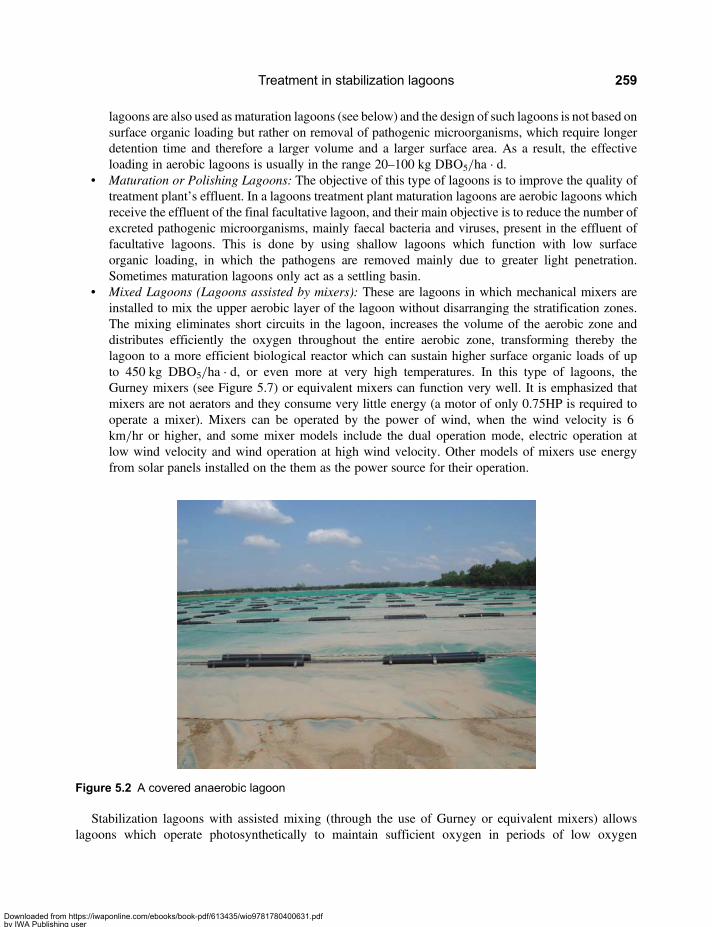
lagoons are also used as maturation lagoons (see below) and the design of such lagoons is not based onsurface organic loading but rather on removal of pathogenic microorganisms, which require longerdetention time and therefore a larger volume and a larger surface area. As a result, the effectiveloading in aerobic lagoons is usually in the range 20–100 kg DBO5/ha · d.

• Maturation or Polishing Lagoons: The objective of this type of lagoons is to improve the quality oftreatment plant’s effluent. In a lagoons treatment plant maturation lagoons are aerobic lagoons whichreceive the effluent of the final facultative lagoon, and their main objective is to reduce the number ofexcreted pathogenic microorganisms, mainly faecal bacteria and viruses, present in the effluent offacultative lagoons. This is done by using shallow lagoons which function with low surfaceorganic loading, in which the pathogens are removed mainly due to greater light penetration.Sometimes maturation lagoons only act as a settling basin.

• Mixed Lagoons (Lagoons assisted by mixers): These are lagoons in which mechanical mixers areinstalled to mix the upper aerobic layer of the lagoon without disarranging the stratification zones.The mixing eliminates short circuits in the lagoon, increases the volume of the aerobic zone anddistributes efficiently the oxygen throughout the entire aerobic zone, transforming thereby thelagoon to a more efficient biological reactor which can sustain higher surface organic loads of upto 450 kg DBO5/ha · d, or even more at very high temperatures. In this type of lagoons, theGurney mixers (see Figure 5.7) or equivalent mixers can function very well. It is emphasized thatmixers are not aerators and they consume very little energy (a motor of only 0.75HP is required tooperate a mixer). Mixers can be operated by the power of wind, when the wind velocity is 6km/hr or higher, and some mixer models include the dual operation mode, electric operation atlow wind velocity and wind operation at high wind velocity. Other models of mixers use energyfrom solar panels installed on the them as the power source for their operation.

Stabilization lagoons with assisted mixing (through the use of Gurney or equivalent mixers) allowslagoons which operate photosynthetically to maintain sufficient oxygen in periods of low oxygen

Figure 5.2 A covered anaerobic lagoon

Treatment in stabilization lagoons 259


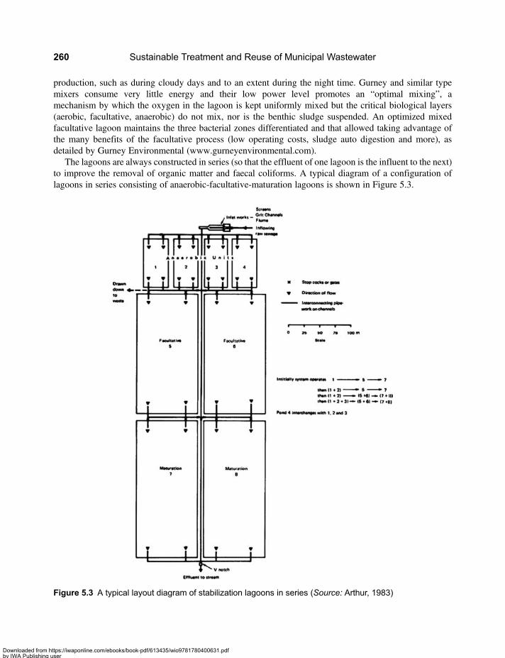
production, such as during cloudy days and to an extent during the night time. Gurney and similar typemixers consume very little energy and their low power level promotes an “optimal mixing”, amechanism by which the oxygen in the lagoon is kept uniformly mixed but the critical biological layers(aerobic, facultative, anaerobic) do not mix, nor is the benthic sludge suspended. An optimized mixedfacultative lagoon maintains the three bacterial zones differentiated and that allowed taking advantage ofthe many benefits of the facultative process (low operating costs, sludge auto digestion and more), asdetailed by Gurney Environmental (www.gurneyenvironmental.com).

The lagoons are always constructed in series (so that the effluent of one lagoon is the influent to the next)to improve the removal of organic matter and faecal coliforms. A typical diagram of a configuration oflagoons in series consisting of anaerobic-facultative-maturation lagoons is shown in Figure 5.3.

Figure 5.3 A typical layout diagram of stabilization lagoons in series (Source: Arthur, 1983)



http://www.gurneyenvironmental.com

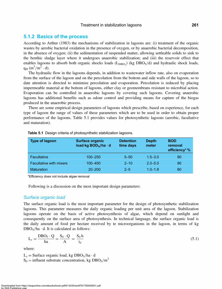
5.1.2 Basics of the processAccording to Arthur (1983) the mechanisms of stabilization in lagoons are: (i) treatment of the organicwastes by aerobic bacterial oxidation in the presence of oxygen, or by anaerobic bacterial decomposition,in the absence of oxygen; (ii) the sedimentation of suspended matter, allowing settleable solids to sink tothe benthic sludge layer where it undergoes anaerobic stabilization; and (iii) the reservoir effect thatenables lagoons to absorb both organic shocks loads (LDBO5

) (kg DBO5/d) and hydraulic shock loads,qH (m3/m2 · d).

The hydraulic flow in the lagoons depends, in addition to wastewater inflow rate, also on evaporationfrom the surface of the lagoon and on the percolation from the bottom and side walls of the lagoon, so todate attention is directed to minimize percolation and evaporation. Percolation is reduced by placingimpermeable material at the bottom of lagoons, either clay or geomembrans resistant to microbial action.Evaporation can be controlled in anaerobic lagoons by covering such lagoons. Covering anaerobiclagoons has additional benefits such as odour control and providing means for capture of the biogasproduced in the anaerobic process.

There are some empirical design parameters of lagoons which prescribe, based on experience, for eachtype of lagoon the range of values of these parameters which are to be used in order to obtain properperformance of the lagoons. Table 5.1 provides values for photosynthetic lagoons (aerobic, facultativeand maturation).

Following is a discussion on the most important design parameters:

Surface organic loadThe surface organic load is the most important parameter for the design of photosynthetic stabilizationlagoons. This parameter measures the daily organic loading per unit area of the lagoon. Stabilizationlagoons operate on the basis of active photosynthesis of algae, which depend on sunlight andconsequently on the surface area of photosynthesis. In technical language, the surface organic load isthe daily amount of food per hectare received by te microorganisms in the lagoon, in terms of kgDBO5/ha · d. It is calculated as follows:

Ls = DBO5 · Qha

= S0 · QA

= S0 htd

(5.1)

where:

Ls = Surface organic load, kg DBO5/ha · dS0 = influent substrate concentration, kg DBO5/m

3

Table 5.1 Design criteria of photosynthetic stabilization lagoons.

Type of lagoon Surface organicload kg BOD5/////ha · d

Detentiontime days

Depthmeter

BODremovalefficiency*%

Facultative 100–250 5–50 1.5–3.0 90

Facultative with mixers 100–450 2–10 2.0–5.0 90

Maturation 20–200 2–5 1.0–1.8 80

*Efficiency does not include algae removal



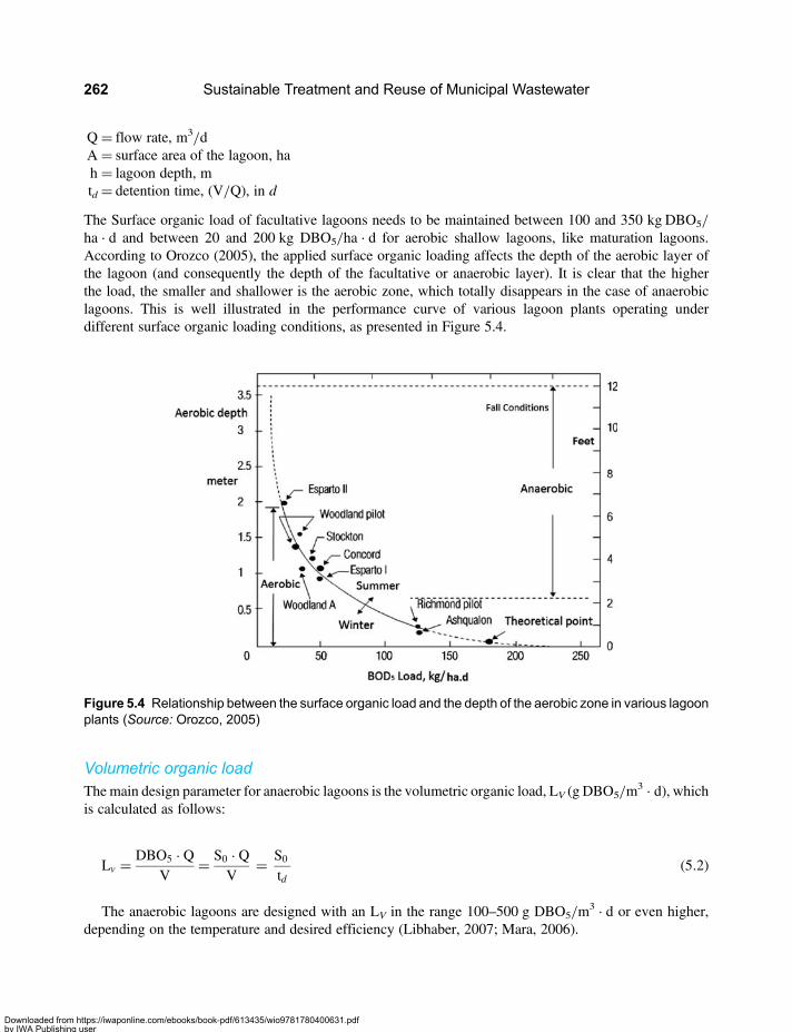
Q = flow rate, m3/dA = surface area of the lagoon, hah = lagoon depth, mtd = detention time, (V/Q), in d

The Surface organic load of facultative lagoons needs to be maintained between 100 and 350 kg DBO5/

ha · d and between 20 and 200 kg DBO5/ha · d for aerobic shallow lagoons, like maturation lagoons.According to Orozco (2005), the applied surface organic loading affects the depth of the aerobic layer ofthe lagoon (and consequently the depth of the facultative or anaerobic layer). It is clear that the higherthe load, the smaller and shallower is the aerobic zone, which totally disappears in the case of anaerobiclagoons. This is well illustrated in the performance curve of various lagoon plants operating underdifferent surface organic loading conditions, as presented in Figure 5.4.

Volumetric organic loadThemain design parameter for anaerobic lagoons is the volumetric organic load, LV (g DBO5/m

3 · d), whichis calculated as follows:

Lv = DBO5 · QV

= S0 · QV

= S0td

(5.2)

The anaerobic lagoons are designed with an LV in the range 100–500 g DBO5/m3 · d or even higher,

depending on the temperature and desired efficiency (Libhaber, 2007; Mara, 2006).

Figure 5.4 Relationship between the surface organic load and the depth of the aerobic zone in various lagoonplants (Source: Orozco, 2005)



MixingWhen the lagoons are mechanically mixed the Power Level (PL) becomes an important parameter. Themixed lagoons have to continue operating as facultative lagoons. Facultative lagoons have three layerszones: an aerobic layer on the top, a facultative layer in the center and an anaerobic layer at the bottom.The settleable solids should be left to sink to the bottom of the lagoon where they undergo anaerobicdecomposition. Therefore the mixer must sufficiently powerful to provide effective mixing which is ableto distribute the oxygen throughout the aerobic layer but should not be powerful enough to suspendthe bottom sediments but rather keep them at the bottom. The Gurney and equivalent mixers provide alow enough power level to maintain the lagoons in facultative conditions. The required power level is0.75 HP per 0.65–3 hectares, depending on the surface organic loading on the lagoon. Higher loadedlagoons require more mixing power. That translates to power per unit area in the range of 0.25–1.2 HP/ha.

The hydraulic power applied for mixing becomes then the design element. In addition, the temperatureand the pH in the lagoon must be taken into account during the design, as discussed below. The power levelunits are W/m3 (or kW/1000 m3) and for maintaining facultative conditions, the required power level isabout 0.5. At power levels above 1.0 W/m3 the lagoon becomes an aerated lagoon and particles willbecome suspended and discharged with the effluent.

Removal of algaeIt is important to note that often the amount of algae produced in a lagoon and discharged with the effluent isso large that if included in the effluent BODmeasurement, the effluent might contain more organic load thanthe influent. However, if the body receiving the discharge is an open water body (flowing river, open sea)algae produce more oxygen than they need for respiration and are incorporated into the food chain, areconsumed by higher life form and improve the productivity of ecosystems. Algal BOD and Suspendedsolids are therefore different from non-algal BOD and SS. This fact should be taken into account byregulators when setting effluent quality standards. The EU standard requires that lagoon systemseffluents achieve a Filtered BOD quality of 25 mg/l or less and a total suspended solids concentration of150 mg/l or less. This standard allows the algal SS to be discharged to receiving bodies. Such anapproach should also be adopted in developing countries.

If the effluent is discharged to closed water bodies such as lakes and bays, algae can sometimes contributeto eutrophication of the receiving body, in which case it might be necessary to remove the algae with the helpof a chemical coagulant followed by flotation followed by a filtration system (either sand filters or rotatingmicro screen with a very small screen opening). Filtration of a lagoons effluent by a rock filter can partiallyremove algae. Recently a different method of algae removal by ultrasonic sound waves was developed. Thismethod allows solving the algae problem effectively and economically (see LG Sonic, 2003). However, thefront part of the transducer (ultrasound emitting instrument) needs to be cleaned at least once a week, whichfor many operators seems inconvenient. An automatic cleaning system has been developed to solve thisproblem. If mixers are used to improve the performance of a lagoon plant, the lagoons, includingmaturation lagoons, can be deeper and then the effluent can be withdrawn from a deeper layer in whichthe algae content is low.

Design considerationsThe design of stabilization lagoons is one of the most studied subjects in the field domestic wastewatertreatment. It is therefore natural that different methodologies and conceptual approaches have emerged,all useful for the design of lagoon systems. The most representative and successful of thesemethodologies are presented in this chapter, as follows:



Kinetics approach

(i) Equations: For the design of completely mixed lagoons first-order kinetic equations can in generalbe used. The constant KL for the removal of BOD depends on the lagoon type. Thefollowing equation (similar to Equation 2.31) can be used for a single lagoon (aerobic, anaerobicor facultative):

S = S01+ KLtd

(5.3)

where:S= effluent substrate, mg/l (g/m3) of DBO5

S0= influent substrate, mg/l (g/m3) of BOD5

KL= kinetic constant of BOD5 removal, d−1

td=V/Q, hydraulic detention time, d

Equation 5.4 can be used for n lagoons in series (similar to Equation 2.36), where n is the number oflagoons:

S = S0

1+ KLtdn

( )n (5.4)

For a lagoon operating under a plug flow regime the equation that applies is the following (similarto Equation 2.37):

S = S0e−KLtd (5.5)

Note that the flow regime in a system of many lagoons in series approaches the plug flow regime(Orozco, 2005). In general, the fluid element (ΔV) in an elongated reactor tank is not transported in aperfect plug flow. A perfect completely mixed reactor neither exists in practice. This means that thereis always dispersion in a reactor, which can be measured by the dispersion factor (d). Wehner andWilhelm (1958) found that the expression for the substrate in the effluent of a tank with dispersiond is:

SS0

= 4a e1/2d

(1+ a)2ea/2d − (1− a)2e−a/2d(5.6)

where:

a = ��1+ 4KLtd

√d=D/u · L= dispersion factorD= axial dispersion coefficient, m2/hu= fluid velocity, m/hL= characteristic length, m

KL= reaction constant of 1st order, h−1

From this equation it is possible to draw a curve of the value KLtd versus S/S0. Figure 5.5 presentssuch a set of curves, in which variation parameter is the dispersion factor d. When d= 0 we havecompletely mixed conditions, and for d=∞ we have perfect plug flow conditions. As seen inthe figure these are the tow extreme cases.



The value of KL corresponds to the first-order substrate removal rate and td is the detention time inthe reactor. KL has reported values of between 0.01 and 1.50 d

−1, and typically 0.35 d−1 at 20°C. KL

fluctuates significantly with temperature, according to Equation (5.7)

KL = KL(208C) · u(T−20) (5.7)

where the value of θ (temperature correction coefficient) varies between 1.05 and 1.09 for the firstorder BOD5 reaction constant.

The kinetics of removal of faecal coliforms (B) has a different kinetics constant (KB), but stillfollows the first order kinetics as presented above. The typical value of KB (20°C) is 2.6 d−1, andof θ is 1.19.

(ii) Temperature: Due to the dependence of the design equation on the temperature of the liquid in thelagoon, it is of utmost importance to establish the heat balance of the lagoon, which defines theoperating temperature of the lagoon. According to Mancini and Barnhart, the heat balance isgiven by (see Yanez, 2003):

TL = Asf Ta + QTi

Asf + Q(5.8)

where:

TL= final temperature of the lagoon (°C)Ta= environmental air temperature (°C)Ti= temperature of influent wastewater (°C)As= surface area of the lagoon (m2)Q=wastewater flow rate (m3/d)f= proportionality factor, 0.5 m/d

Figure 5.5 KLtd vs BOD remaining values according to the Wehner andWilhelm equation (Source:Metcalf &Eddy, 2003)



As shown in Table 5.1 and Figures 5.4 and 5.5, the depth is important for the mode of operation of thelagoon since the penetration of light defines the depth of the layer in which the photosynthetic actionoccurs. Other important parameters are the detention time of the wastewater in the lagoon and surfaceorganic load. For the design of a lagoon Equations 5.1, 5.3 and 5.7 can be used, taking into accountthat the first order constant KL for this type of treatment varies between 0.01 and 1.50 d−1. Theimpact of temperature variation needs to be taken into account according to Equations 5.8 and 5.7.

Photosynthetic approach

For the design of photosynthetic lagoons we can use Oswald’s approach which found that the production ofoxygen by photosynthetic action is:

YO2 = 0.25 · FO2 · S (5.9)

where:

YO2= production of O2 (kg O2/ha · d)

FO2= oxygenation factor

S= solar radiation (cal/cm2 · d)

The oxygenation factor varies between 0 and 4 and is the ratio of the weight of O2 produced to the DBOu

that must be removed. McGauhey (1968) recommended a value of 1.6 for approximately 90% BODu

removal. The variation of FO2with the BOD removal percentage in relation to the oxygenation level is

shown in Figure 5.6 (Alley et al. 2007, Shammas et al. 2009).

The solar radiation, S, varies with months and latitude. Table 5.2 presents the maximum and minimumvalues of S as function of latitude and day of the year. The average value is calculated as:

S = Smin + P(Smax − Smin) (5.10)

where:

S: average value of solar radiation in cal/cm2/dP: actual hours of sunshine divided by the potential sunshine hours at the site

Figure 5.6 Relation FO2vs the percentage of BODu removed (Source: Orozco, 2005)



Equation 5.9 is used to determine the oxygen production (YO2, kg/ha · d). The surface organic load

(LS, in kg BOD5/ha · d) is obtained from Equation 5.1, using the appropriate units for design:

Ls = 10(h/td)DBO5 = 10(h/td)DBOu/1.5 (5.11)

where:

h = aerobic zone depth in the lagoon, mtd = detention time, d

DBOu = 1.5 DBO5

Equalizing the O2 production to the total oxygen demand, that is, YO2= LS (in terms BODu), we obtain:

10(h/td)(1.5DBO5) = 0.25 FO2S (5.12)

Which by rearranging becomes:

h/td = 0.017 FO2S/DBO5 (5.13)

Table 5.2 Probable values of visible solar energy based on month and latitude.

Latitude Monthb

Jan. Feb. Mar. Apr. May Jun. Jul. Aug. Sept. Oct. Nov. Dec.

0 max 255 266 271 266 249 236 238 252 269 265 256 253

min 210 219 206 188 182 103 137 167 207 203 202 195

10 max 223 244 264 271 270 262 265 266 266 248 228 225

min 179 184 193 183 192 129 158 176 196 181 176 162

20 max 183 213 246 271 284 284 282 272 252 224 190 182

min 134 140 168 170 194 148 172 177 176 150 138 120

30 max 136 176 218 261 290 296 289 271 231 192 148 126

min 76 96 134 151 184 163 178 166 147 113 90 70

40 max 80 130 181 181 286 298 288 258 203 152 95 66

min 30 53 95 125 162 173 172 147 112 72 42 24

50 max 28 70 141 210 271 297 280 236 166 100 40 26

min 10 19 58 97 144 176 155 125 73 40 15 7

60 max 7 32 107 176 249 294 268 205 126 43 10 5

min 2 4 33 79 132 174 144 100 38 26 3 1

aAfter Table II, W. J. Oswald and H. B. Gotaas, “Photosynthesis in Sewage Treatment” ASCEProceedings 81, Separate No.686 (May, 1955).bValues of S in Langleys, cal/(cm2)(d)Correction for cloudiness: Se = Smin + r (Smax − Smin)



The above relations are essentially valid for aerobic stabilization lagoons. To design a facultative lagoonmore depth needs to be added, since h is calculated in the above equations only for the aerobic zone.

Duncan Mara’s approximation method

A summary of the methodology proposed by DuncanMara based onMara (2006) and Pena-Varon andMara(2005) is presented below.

(i) Anaerobic lagoons: The volumetric load (LV) given by Equation 5.2 is used for design. Therecommended range of volumetric loads is 100 g/m3 · d for temperatures below 10°C,increasing linearly to 300 g/m3 · d at 20°C and then more slowly up to 350 g/m3 · d at 25°C.In this case, the lagoon is designed with the average environment temperature in the coldestmonth. The removal of BOD5 is 50% (,10°C) to 80% (at 25°C and above). The recommendeddepth of the anaerobic lagoon is between 3 and 5 m.

(ii) Facultative lagoons: The surface organic load (LS, on terms of BOD5) is used as the designparameter. It is given by Equations 5.1 and 5.11 (using the appropriate units). The followingequation can be employed using as the sole design parameter the average temperature of thecoldest month, T:

Ls = 350(1,107− 0,002T)(T−25) (5.14)

This equation assumes that LS= 350 kgDBO5/ha · d is the optimal surface organic loading at25°C.

(iii) Minimum detention time: The proposed minimum detention time, tdmin is 1d in anaerobic lagoons,4 d in facultative lagoons and 3 d in maturation lagoons.

(iv) Removal of helminth eggs: For the removal of helminth eggs (see Mara, 2006) the followingequation is used:

E(%) = 100(1− 0.41 exp [−0.49 td + 0.0085 t2d]) (5.15)

The concentration of helminth eggs in domestic wastewater of low income developing countries isbetween 300 and 800 Ova/l. For high and middle income developing countries the concentrationis between 1 and 300 Ova/l [see http://www.iwawaterwiki.org/xwiki/bin/view/Articles/Helmintheggs (May 12, 2011)].

(v) Removal of fecal coliforms: The removal of fecal coliforms (FC) in a series of maturation lagoonsof equal dimensions can be estimated using Equation 5.4, applied to FC:

B = B0

1+ KBtdn

( )n (5.25)

With B is the FC concentration. The constant KB is temperature dependent. According to Arthur(1983) the variation of KB with temperature is given by:

KB = 2.7× 1.19(T−20) (5.26)

Recent innovations in design of lagoons systems

(i) Use of mixers in facultative and maturation lagoons:Mechanical mixers which employ the conceptof “optimal mix” can be installed in facultative lagoons to improve their performance. The mixer












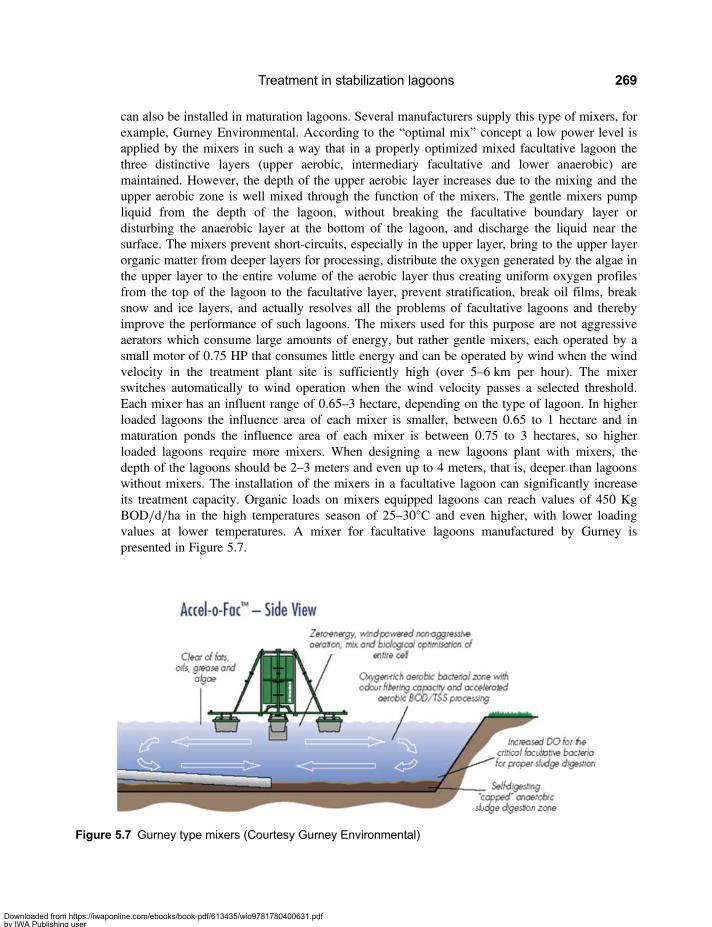
can also be installed in maturation lagoons. Several manufacturers supply this type of mixers, forexample, Gurney Environmental. According to the “optimal mix” concept a low power level isapplied by the mixers in such a way that in a properly optimized mixed facultative lagoon thethree distinctive layers (upper aerobic, intermediary facultative and lower anaerobic) aremaintained. However, the depth of the upper aerobic layer increases due to the mixing and theupper aerobic zone is well mixed through the function of the mixers. The gentle mixers pumpliquid from the depth of the lagoon, without breaking the facultative boundary layer ordisturbing the anaerobic layer at the bottom of the lagoon, and discharge the liquid near thesurface. The mixers prevent short-circuits, especially in the upper layer, bring to the upper layerorganic matter from deeper layers for processing, distribute the oxygen generated by the algae inthe upper layer to the entire volume of the aerobic layer thus creating uniform oxygen profilesfrom the top of the lagoon to the facultative layer, prevent stratification, break oil films, breaksnow and ice layers, and actually resolves all the problems of facultative lagoons and therebyimprove the performance of such lagoons. The mixers used for this purpose are not aggressiveaerators which consume large amounts of energy, but rather gentle mixers, each operated by asmall motor of 0.75 HP that consumes little energy and can be operated by wind when the windvelocity in the treatment plant site is sufficiently high (over 5–6 km per hour). The mixerswitches automatically to wind operation when the wind velocity passes a selected threshold.Each mixer has an influent range of 0.65–3 hectare, depending on the type of lagoon. In higherloaded lagoons the influence area of each mixer is smaller, between 0.65 to 1 hectare and inmaturation ponds the influence area of each mixer is between 0.75 to 3 hectares, so higherloaded lagoons require more mixers. When designing a new lagoons plant with mixers, thedepth of the lagoons should be 2–3 meters and even up to 4 meters, that is, deeper than lagoonswithout mixers. The installation of the mixers in a facultative lagoon can significantly increaseits treatment capacity. Organic loads on mixers equipped lagoons can reach values of 450 KgBOD/d/ha in the high temperatures season of 25–30°C and even higher, with lower loadingvalues at lower temperatures. A mixer for facultative lagoons manufactured by Gurney ispresented in Figure 5.7.

Figure 5.7 Gurney type mixers (Courtesy Gurney Environmental)



Another innovation in treatment by lagoons is injecting air into a facultative lagoon throughblowers (not compressed air) to augment the oxygen quantity produced by the algae withoutchanging the flow regime, that is without transforming the lagoon to an aerated lagoon. For thatpurpose, a combination of blowers with air distributors and gentle mixers can be installed in thelagoon. The addition of air to the lagoons increases its treatment capacity to a required level.Injection of air requires more energy so this process is not strictly an appropriate technologyprocess. However, it is still a simple process and is not very costly. It can be used to forincreasing the capacity of an existing lagoons plant if additional area is not available and therequired capacity increase cannot be reached by just adding mixers.

(ii) Control of odours in anaerobic lagoons: Using an anaerobic lagoon as the first of a series oflagoons in a lagoons treatment system is a cost-effective and practical approach to treatmunicipal wastewater. An anaerobic lagoon with a detention time of 1–2 days can removebetween 50 and 70% of the BOD contained in the raw wastewater. The main problem ofanaerobic lagoons, which is a problem difficult to control, is that under certain conditions theygenerate odours.

When the concentration of sulphate in the raw wastewater is low it is possible to designanaerobic lagoons which do not generate odours. However, when sulphate concentrations arehigh, emissions of odour producing gases (sulphide gases) and of greenhouse gases (methaneand carbon dioxide) can be significant. The emission of odours intensifies when high organicloads are applied on anaerobic lagoons. An effective way to prevent odours is to cover theanaerobic lagoons and collect the gases produced in the anaerobic process. The collected gasescan then be either flared or used to generate energy. Covering of the anaerobic lagoons totallyeliminates the odour problem. The lagoons can be covered by geomembrans as depicted inFigure 5.2. The cost of geomembrans has dropped in Latin America to levels which makecovering of anaerobic lagoons affordable. The geomembrane presented in Figure 5.3 is anHDPE geomembrane resistant to sun light.

According to Libhaber (2007), covering anaerobic lagoon has many benefits, namely: (i)capturing odorous gases to remove, flare or treat them, eliminating thereby odour problems; (ii)preventing emission of greenhouse gases into the atmosphere, contributing thereby to the effortof mitigating the global warming; (iii) generating additional funds for the water and sanitationutility from the sale of Carbon Emission Reductions (CER) to industrialized countries; (iv)reducing the loss of heat from the anaerobic reactor and improving thereby its performance; (v)reducing the evaporation and loss of water from the anaerobic lagoon; (vi) blocking sunlightfrom reaching the lagoon thus inhibiting the growth of algae in it; and (vii) generating energyfrom the collected methane gas, in case it is economically feasible under the energy policy ofthe country in which the lagoons are located.

5.1.3 PERFORMANCEEfficiencyThe removal efficiencies of some contaminants by lagoons compared to other treatment processes arepresented in Table 5.3. The lagoons can achieve a very high removal of pathogens while the otherprocess cannot achieve such removal levels without disinfection. For example, lagoons can achieve areduction of six orders of magnitude in fecal coliforms (equivalent to removal of 99.9999%, since onecycle of log10= 90%). Similarly, lagoons can achieve a reduction of four orders of magnitude of



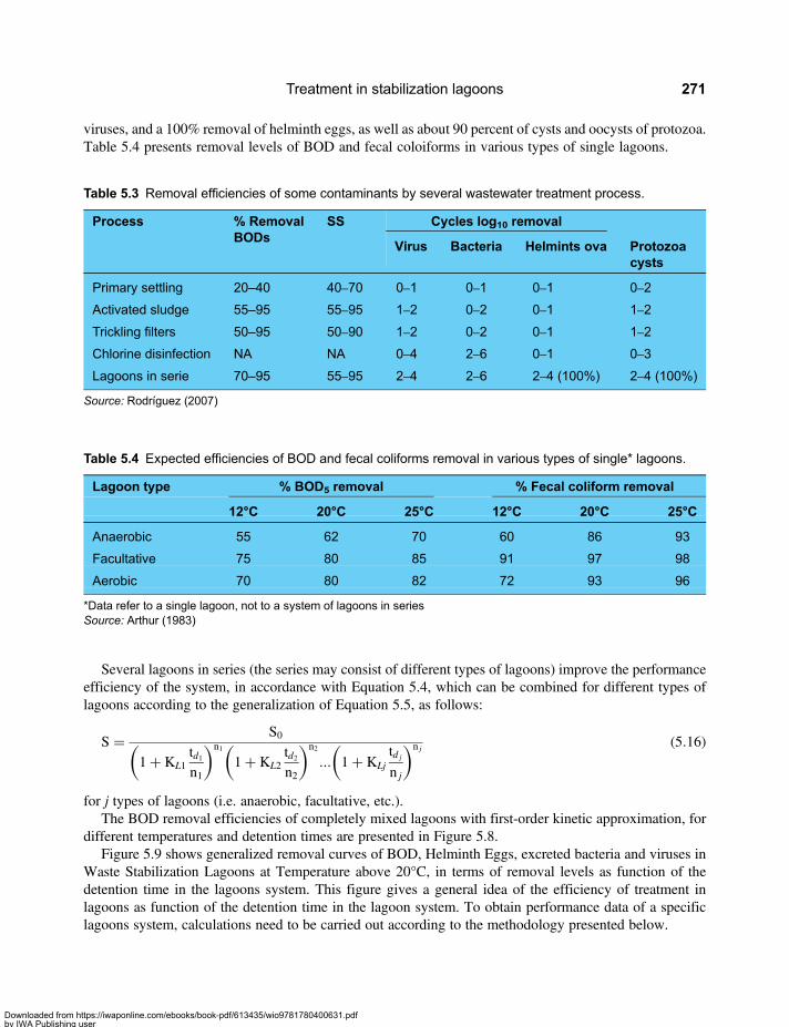
viruses, and a 100% removal of helminth eggs, as well as about 90 percent of cysts and oocysts of protozoa.Table 5.4 presents removal levels of BOD and fecal coloiforms in various types of single lagoons.

Several lagoons in series (the series may consist of different types of lagoons) improve the performanceefficiency of the system, in accordance with Equation 5.4, which can be combined for different types oflagoons according to the generalization of Equation 5.5, as follows:

S = S0

1+ KL1td1n1

( )n1

1+ KL2td2n2

( )n2

... 1+ KLjtd j

n j

( )n j(5.16)

for j types of lagoons (i.e. anaerobic, facultative, etc.).The BOD removal efficiencies of completely mixed lagoons with first-order kinetic approximation, for

different temperatures and detention times are presented in Figure 5.8.Figure 5.9 shows generalized removal curves of BOD, Helminth Eggs, excreted bacteria and viruses in

Waste Stabilization Lagoons at Temperature above 20°C, in terms of removal levels as function of thedetention time in the lagoons system. This figure gives a general idea of the efficiency of treatment inlagoons as function of the detention time in the lagoon system. To obtain performance data of a specificlagoons system, calculations need to be carried out according to the methodology presented below.

Table 5.4 Expected efficiencies of BOD and fecal coliforms removal in various types of single* lagoons.

Lagoon type % BOD5 removal % Fecal coliform removal

12°C 20°C 25°C 12°C 20°C 25°C

Anaerobic 55 62 70 60 86 93

Facultative 75 80 85 91 97 98

Aerobic 70 80 82 72 93 96

*Data refer to a single lagoon, not to a system of lagoons in seriesSource: Arthur (1983)

Table 5.3 Removal efficiencies of some contaminants by several wastewater treatment process.

Process % RemovalBODs

SS Cycles log10 removal

Virus Bacteria Helmints ova Protozoacysts

Primary settling 20–40 40–70 0–1 0–1 0–1 0–2

Activated sludge 55–95 55–95 1–2 0–2 0–1 1–2

Trickling filters 50–95 50–90 1–2 0–2 0–1 1–2

Chlorine disinfection NA NA 0–4 2–6 0–1 0–3

Lagoons in serie 70–95 55–95 2–4 2–6 2–4 (100%) 2–4 (100%)

Source: Rodríguez (2007)



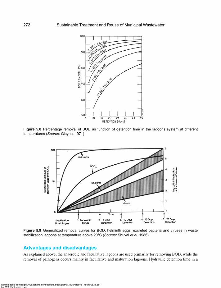
Advantages and disadvantagesAs explained above, the anaerobic and facultative lagoons are used primarily for removing BOD, while theremoval of pathogens occurs mainly in facultative and maturation lagoons. Hydraulic detention time in a

Figure 5.8 Percentage removal of BOD as function of detention time in the lagoons system at differenttemperatures (Source: Gloyna, 1971)

Figure 5.9 Generalized removal curves for BOD, helminth eggs, excreted bacteria and viruses in wastestabilization lagoons at temperature above 20°C (Source: Shuval et al. 1986)



lagoon system is between 5 and 50 days. This is much longer than the detention time in other process inwhich detention times are usually less than one day. In practical terms it means that the area occupied bylagoons plants is much larger than that occupied by plants based on other processes. Large areas are notavailable inside cities, so lagoon plants are usually located outside the limits of the city, so an additionalinvestment in conveyance of the wastewater is required. On the other hand, the operation andmaintenance costs are much smaller than those of conventional processes, so in the case of lagoons asignificant portion the money is invested in tangible assets and can be recovered after years, while in thecase of conventional processes the money is invested in paying electricity bills and maintenance ofequipment, and can never be recovered.

The advantages of stabilization lagoons are the followings (OPS, 2005):

• Because of the large volume of the lagoons they have the capacity to handle well organic andhydraulic shock lads.

• No additional mechanical facilities are required for the production of oxygen (except in the case ofaerated lagoons, which we do not consider as an appropriate technology process when they serveas the main treatment unit). The oxygen is produced naturally in the system by photosynthetic action.

• Utilization of mixers in facultative lagoons ensures the oxygen supply will be secured even duringunfavourable climate conditions.

• Due to the mechanisms of the processes occurring in the lagoons and the long detention times inlagoons systems they are (when properly designed) highly effective in removing pathogenicorganisms such as bacteria, viruses and parasites, compared to other treatment processes.Consequently there is no need to disinfect lagoons effluents.

• Lagoons require a low level of maintenance.• Lagoons do not require high level qualified personnel for operation.• Lagoons do not consume energy during their operation, and in certain cases can produce energy.• The O&M costs of lagoons are very low compared to other processes.

The disadvantages of the lagoons are:

• They occupy large land areas.• A lagoons system is sensitive to climatic conditions.• Once constructed, lagoons systems are difficult to control since only little can be done to change the

process operation. This problem is mitigated in a system with covered anaerobic lagoons and mixersin the facultative lagoons. Covering the anaerobic lagoons eliminated the odour problems, and theoperation of the mixers in facultative lagoons provides a measure of control on their performance.

• Lagoons may support the spread of disease vectors.• Lagoons may promote eutrophication of closed water bodies (lakes, bays) because of the continuous

supply of algae with the discharged effluent. However, this problem can be mitigated by the removalof algae from the effluent, for instance with ultrasonic waves.

Anaerobic lagoons may generate offensive odours. This problem can be resolved by covering the lagoons.

5.2 BASIC DESIGN PROCEDURES5.2.1 General design considerationsFor the design of stabilization lagoons, it is important to bear in mind that the main mechanisms ofstabilization, according to Section 5.1.2, are: (i) Removal of BOD by aerobic bacterial oxidation in thepresence of oxygen, or by anaerobic bacterial decomposition, in the absence of oxygen; (ii) the



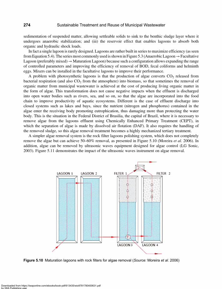
sedimentation of suspended matter, allowing settleable solids to sink to the benthic sludge layer where itundergoes anaerobic stabilization; and (iii) the reservoir effect that enables lagoons to absorb bothorganic and hydraulic shock loads.

In fact a single lagoon is rarely designed. Lagoons are rather built in series tomaximize efficiency (as seenfromEquation 5.4). The seriesmost commonly used is shown in Figure 5.3 (Anaerobic Lagoon→FacultativeLagoon (preferably mixed)→Maturation Lagoon) because such a configuration allows expanding the rangeof controlled parameters and improving the efficiency of removal of BOD, fecal coliforms and helmintheggs. Mixers can be installed in the facultative lagoons to improve their performance.

A problem with photosynthetic lagoons is that the production of algae converts CO2 released frombacterial respiration (and also CO2 from the atmosphere) into biomass, so that sometimes the removal oforganic matter from municipal wastewater is achieved at the cost of producing living organic matter inthe form of algae. This transformation does not cause negative impacts when the effluent is dischargedinto open water bodies such as rivers, sea, and so on, so that the algae are incorporated into the foodchain to improve productivity of aquatic ecosystems. Different is the case of effluent discharge intoclosed systems such as lakes and bays, since the nutrient (nitrogen and phosphorus) contained in thealgae enter the receiving body promoting eutrophication, thus damaging more than protecting the waterbody. This is the situation in the Federal District of Brasilia, the capital of Brazil, where it is necessary toremove algae from the lagoons effluent using Chemically Enhanced Primary Treatment (CEPT), inwhich the separation of algae is made by dissolved air flotation (DAF). It also requires the handling ofthe removed sludge, so this algae removal treatment becomes a highly mechanized tertiary treatment.

A simpler algae removal system is the rock filter lagoons polishing system, which does not completelyremove the algae but can achieve 50–60% removal, as presented in Figure 5.10 (Moreira et al. 2006). Inaddition, algae can be removed by ultrasonic waves equipment designed for algae control (LG Sonic,2003). Figure 5.11 demonstrates the impact of the ultrasonic waves instrument on algae removal.

Figure 5.10 Maturation lagoons with rock filters for algae removal (Source: Moreira et al. 2006)



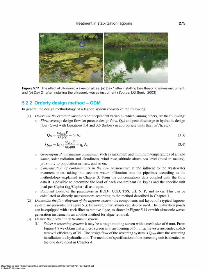
5.2.2 Orderly design method – ODMIn general the design methodology of a lagoon system consists of the following:

(1) Determine the external variables (or independent variable), which, among others, are the following:○ Flow: average design flow (or process design flow, QD) and peak discharge or hydraulic design

flow (QHD) with Equations 3.4 and 3.5 (below) in appropriate units (lps, m3/h, etc):

QD = cqdomP86400

+ qI Aa (3.3)

QHD = k1k2cqdomP86400

+ qI Aa (3.4)

○ Geographical and altitude conditions: such as maximum and minimum temperatures of air andwater, solar radiation and cloudiness, wind rose, altitude above sea level (masl in meters),proximity to population centers, and so on.

○ Concentration of contaminants in the raw wastewater: at the influent to the wastewatertreatment plant, taking into account water infiltration into the pipelines according to themethodology explained in Chapter 3. From the concentrations data coupled with the flowdata it is possible to determine the load of each contaminant (in kg/d) and the specific unitload per Capita (kg/Capita · d) as output.

○ Pollutant loads: of the parameters as BOD5, COD, TSS, pH, N, P, and so on. This can becalculated or directly measurement according to the method described in Chapter 3.

(2) Determine the flow diagram of the lagoons system: the components and layout of a typical lagoonssystem are presented in Figure 5.3. However, other layouts can also be used. The maturation pondscan be equipped with a rock filter to remove algae, as shown in Figure 5.11 or with ultrasonic wavesgeneration instruments an another method for algae removal.

(3) Design the preliminary treatment system3.1 Select a screening system: it may be a rough rotating screen with a mesh size of 6 mm. From

Figure 4.8 we obtain that a micro screen with an opening of 6 mm achieves a suspended solidsremoval efficiency of 3%. The design flow of the screening system is QHD since the screeninginstallation is a hydraulic unit. The method of specification of the screening unit is identical tothe one developed in Chapter 4.

Figure 5.11 The effect of ultrasonic waves on algae: (a) Day 1 after installing the ultrasonic waves instrument;and (b) Day 21 after installing the ultrasonic waves instrument (Source: LG Sonic, 2003)



3.2 Design the grit chamber: use a ratio length/width (L/W) of at least 4, with a surface overflowrate (SOR=QHD/Ades) in the range 600–1200 m/d and a water cross-sectional velocity inthe range 0.15–0.60 m/s. Large plants can contain several grit chamber units in parallel.Allow for one stand-by grit chamber unit to enable cleaning of one unit while the othersare in operation. The design flow of the grit chamber is also QDH since the grit chamber isalso an hydraulic unit.

To size the great chamber it is necessary to:• Calculate the surface area of the grit chamber: Ades=QDH/SOR.• Compute L and W (the length and width of the grit chamber): if L/W= 4; then Ades= L.

W= 4W2. Then find W=√(Ades/4) and L= 4w.• Calculate the depth (Hdes) of the grit chamber: If the cross-sectional velocity v=QHD/

W · Hdes, then the grit chamber depth is: Hdes=QHD/W · v. Add 0.20 m for freeboardand 0.30 for grit storage between cleaning cycles. Then the total depth is: H=Hdes+ 0.50.

3.3 Select a Parshall flume: The Parshall flume, used for measurement of the wastewater inflow,is thoroughly discussed in Chapter 9. The following equation is used to select the adequateparshall flume:

h0 = KQm (9.6)

• This equation allows obtaining the flow of the wastewater by measuring the depth of theflowing wastewater in the flume. The adequate flume throat width (w, in inches) isselected on the basis of with QHD using Table 5.5 shown below (which is identical toTable 9.2).

• With w known select the values of D, N, K and m defined in Figure 9.5 and whose valuesare given in Tables 9.1 and 9.3. These values define the partial flume. On the basis of thesefigures it is possible to obtain from manufacturers or suppliers the required parshall flume.It is also possible to obtain an adequate parshall flume just by the selecting w, theflume throat.

Table 5.5 Flow rate measured by a parshall flume as function of thethroat diameter.

Diameter throatinch

Minimum flowlps

Maximum flowlps

1 0.13 5.36

2 0.19 12.24

3 0.25 32.04

6 1.45 87.18

9 2.59 176.69

12 9.21 462.75

18 14.45 696.40

24 18.67 936.93

30 23.09 1180.92

(Continued )



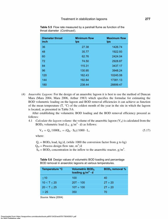
(4) Anaerobic Lagoon: For the design of an anaerobic lagoon it is best to use the method of DuncanMara (Mara 2004, Mara 2006, Arthur 1983) which specifies the formulae for estimating theBOD volumetric loading on the lagoon and BOD removal efficiencies it can achieve as functionof the mean temperature (T, °C) of the coldest month of the year in the site in which the lagoonis located, as presented in Table 5.6.

After establishing the volumetric BOD loading and the BOD removal efficiency proceed asfollows:4.1 Calculate the lagoon volume: the volume of the anaerobic lagoon (VA) is calculated from the

BOD5 volumetric load (LV, g/m3 · d) as follows:

VA = Qs/1000Lv = (QD · S0)/1000 · Lv (5.17)

where:

Qs=BOD5 load, kg/d, (while 1000 the conversion factor from g to kg)QD= Process design flow rate, m3/dS0= BOD5 concentration in the inflow to the anaerobic reactor, g/m3.

Table 5.5 Flow rate measured by a parshall flume as function of thethroat diameter (Continued ).

Diameter throatinch

Minimum flowlps

Maximum flowlps

36 27.38 1426.74

48 35.77 1922.93

60 62.76 2424.04

72 74.50 2928.87

84 115.31 3437.17

96 130.95 3948.24

120 162.43 10245.08

144 192.84 17381.13

180 238.44 28899.47

Table 5.6 Design values of volumetric BOD loading and percentageBOD removal in anaerobic lagoons at various temperatures.

Temperature °C Volumetric BOD5

loading g/////m3 · dBOD5 removal %

≤10 100 40

10, T≤ 20 20T− 100 2T+ 20

20, T≤ 25 10T+ 100 2T+ 20

. 25 350 70

Source: Mara (2004)



Theminimum detention time (tdmin) in an anaerobic lagoon is usually taken as one (1) day andthe final volume of the lagoon (VF) is established as the higher of the two values: (i) volumeVA calculated by applying Equation 5.17; and (ii) that calculated with detention time of oneday. In other words, if the calculation using Equation 5.17 yields a value lower than 1 day,than the volume is taken as 1 day (although a detention of somewhat lower than 1 daymight also be sufficient).

4.2 Calculate the filling time of the lagoon by excess sludge: This is the time required to fill half ofthe lagoon volume with the excess sludge generated by the anaerobic process. This time,denominated n years, is calculated as follows:

n = 12VF/vL · P (5.18)

where:

N= number of years to fill half of the lagoon with excess sludgeVF= final volume of the lagoon, m3

vL= sludge accumulation rate, m3/Capita · yr, between 0.05 in the tropics and 0.08 intemperate climate.

P= population4.3 Calculate the biogas production: The biogas produced in the anaerobic process is mainly

composed of methane and carbon dioxide (Usually about 70% CH4 and the balance isCO2, water and other impurities). According to Mara (2006) the volume of the biogas (Vg,m3/d) is approximately 30% of the influent BOD5, that is:

Vg = 0.30 S0 · QD/1000 (5.19)

Odours may become a problem if the BOD volumetric loading is too high, LV. 500 g/m3 · dor if there is excess of sulphate in the influent. To prevent odours and to control greenhousegases emission it is recommended to cover the anaerobic lagoon and provide a gas flaringsystem with a capacity to handle a flow two times larger than the flow calculated byEquation 5.19, so as to include a safety factor.

4.4 Calculate the inflow and outflow structures: for the dimensioning of the inflow and outflowstructures it is recommended to use an average cross-sectional velocity of 1m/s, and, andunder all circumstances remain in the range 0.6 and 2.2 m/s.

(5) Design the Cover of the anaerobic Lagoon for odour control1: to control odours produced byanaerobic lagoons and to be able to implement the Clean Development Mechanism (CDM) ofthe Kyoto Protocol, it is important to cover anaerobic lagoons, and to collect and flare the biogas.5.1 Cover: The cover of anaerobic lagoons must be a geomembrane of plastic material, smooth

texture and resistant to sunlight exposure, with a thickness of 1.5 mm (60 mil). High densitypolyethylene (HPDE) made of non-recycled polyethylene resins are an example of a materialused for manufacturing geomembrane for anaerobic lagoons covering. The polyethylenesheets are welded together by heat fusion or extrusion. The HDPE geomembrane musthave a density greater than or equal to 0.95 g/cm3, which is waterproof and applicable tostorage of liquids and solids. It must have high resistance to chemicals, ultraviolet

1Based on a report by SAGUAPAC (2007), “Project of capture and burning of biogas in the wastewater treatment plants – TechnicalStudies,” The Water and Sanitation Utility of Santa Cruz, Bolivia.



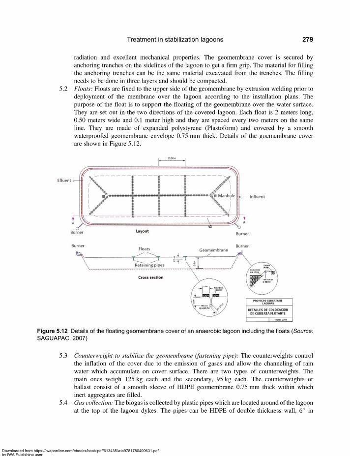
radiation and excellent mechanical properties. The geomembrane cover is secured byanchoring trenches on the sidelines of the lagoon to get a firm grip. The material for fillingthe anchoring trenches can be the same material excavated from the trenches. The fillingneeds to be done in three layers and should be compacted.

5.2 Floats: Floats are fixed to the upper side of the geomembrane by extrusion welding prior todeployment of the membrane over the lagoon according to the installation plans. Thepurpose of the float is to support the floating of the geomembrane over the water surface.They are set out in the two directions of the covered lagoon. Each float is 2 meters long,0.50 meters wide and 0.1 meter high and they are spaced every two meters on the sameline. They are made of expanded polystyrene (Plastoform) and covered by a smoothwaterproofed geomembrane envelope 0.75 mm thick. Details of the goemembrane coverare shown in Figure 5.12.

5.3 Counterweight to stabilize the geomembrane (fastening pipe): The counterweights controlthe inflation of the cover due to the emission of gases and allow the channeling of rainwater which accumulate on cover surface. There are two types of counterweights. Themain ones weigh 125 kg each and the secondary, 95 kg each. The counterweights orballast consist of a smooth sleeve of HDPE geomembrane 0.75 mm thick within whichinert aggregates are filled.

5.4 Gas collection:The biogas is collected by plastic pipes which are located around of the lagoonat the top of the lagoon dykes. The pipes can be HDPE of double thickness wall, 6′′ in

Figure 5.12 Details of the floating geomembrane cover of an anaerobic lagoon including the floats (Source:SAGUAPAC, 2007)



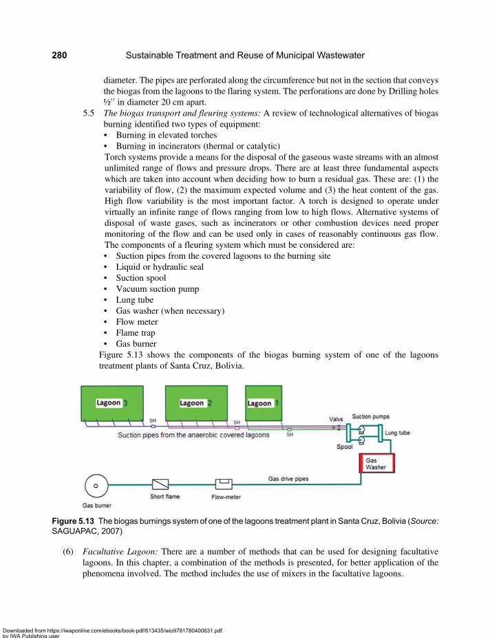
diameter. The pipes are perforated along the circumference but not in the section that conveysthe biogas from the lagoons to the flaring system. The perforations are done by Drilling holes½′′ in diameter 20 cm apart.

5.5 The biogas transport and fleuring systems: A review of technological alternatives of biogasburning identified two types of equipment:• Burning in elevated torches• Burning in incinerators (thermal or catalytic)Torch systems provide a means for the disposal of the gaseous waste streams with an almostunlimited range of flows and pressure drops. There are at least three fundamental aspectswhich are taken into account when deciding how to burn a residual gas. These are: (1) thevariability of flow, (2) the maximum expected volume and (3) the heat content of the gas.High flow variability is the most important factor. A torch is designed to operate undervirtually an infinite range of flows ranging from low to high flows. Alternative systems ofdisposal of waste gases, such as incinerators or other combustion devices need propermonitoring of the flow and can be used only in cases of reasonably continuous gas flow.The components of a fleuring system which must be considered are:• Suction pipes from the covered lagoons to the burning site• Liquid or hydraulic seal• Suction spool• Vacuum suction pump• Lung tube• Gas washer (when necessary)• Flow meter• Flame trap• Gas burner

Figure 5.13 shows the components of the biogas burning system of one of the lagoonstreatment plants of Santa Cruz, Bolivia.

(6) Facultative Lagoon: There are a number of methods that can be used for designing facultativelagoons. In this chapter, a combination of the methods is presented, for better application of thephenomena involved. The method includes the use of mixers in the facultative lagoons.

Figure 5.13 The biogas burnings system of one of the lagoons treatment plant in Santa Cruz, Bolivia (Source:SAGUAPAC, 2007)



6.1 Calculation of the detention time, td: The surface organic load can be calculated fromEquation 5.11:

Ls = 10(h/td)DBO5 = 10(h/td)DBOu/1.5

Another convenient way to calculate the surface organic load is by using Equation 5.14(the Mara’s approximation method):

Ls = 350(1.107− 0.002T)(T−25)

T is the average temperature of the coldest month of the year. Combining Equations 5.11and 5.14 yields a new form of obtaining the ratio h/td:

h/td = (35/DBO5)(1,107− 0.002T)(T−25) (5.20)

Note that Equation 5.20 allows calculating the detention time (td) from the value of Ls, for agiven temperature (based on Mara’s method).

The value h is proposed as a variable of the designer. Using Table 5.1 and Equations5.11 or 5.20 we calculate the td. If we install mixers in the facultative lagoon (forexample Gurney type mixers), we can adopt an organic surface load (Ls) of 400kgBOD5/ha · d at 20°C. The proposed minimum detention time (tdmin) for a facultativelagoon is 4 days. The larger of the two detention time values is selected as the designvalue. In other words, if the value calculated by Equation 5.20 is higher than 5 days, itbecomes the selected value. If the value calculated by Equation 5.20 is lower than 5 days,than 5 days is the selected value.

6.2 Calculation of the volume (VF) and the efficiency of the lagoon:With the td calculated as in theprevious section, we can calculate the volume of the lagoon (VF) and the surface area (As) asfollows:

VF = QD · td (5.21)

As = VF/h (5.22)

To calculate the efficiency we use Equation 5.4 from the kinetic method for a series oflagoons:

S = S0A

1+ KLtdn

( )nwhere S0A is the BOD concentration in the effluent of the Anaerobic Lagoon and n is thenumber of facultative lagoons in series. The final water temperature in the lagoon isobtained from Equation 5.8. If the value of KL is not known from pilot plant testing, wecan use the typical value of KL (20°C)= 0.35 d−1, corrected for temperature usingEquation 5.7. These values are also given in Figure 5.3.

To improve the performance of a facultative lagoon, mixers can be installed in it. Therequired power level is 0.75 HP per 0.65–3 hectares, depending on the surface organicloading on the lagoon. Higher loaded lagoons require more mixing power. It is proposedto use a value of 0.75 HP for every 1ha in facultative lagoons and 0.75 HP for every 3 ha



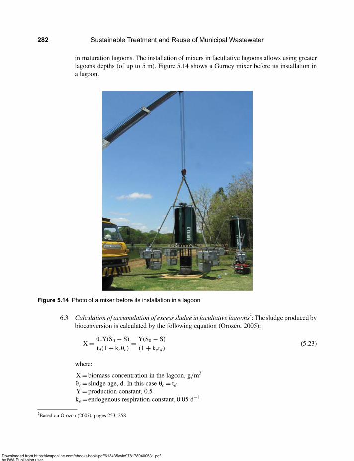
in maturation lagoons. The installation of mixers in facultative lagoons allows using greaterlagoons depths (of up to 5 m). Figure 5.14 shows a Gurney mixer before its installation ina lagoon.

6.3 Calculation of accumulation of excess sludge in facultative lagoons2

: The sludge produced bybioconversion is calculated by the following equation (Orozco, 2005):

X = ucY S0 − S( )td 1+ keuc( ) =

Y S0 − S( )1+ ketd( ) (5.23)

where:

X= biomass concentration in the lagoon, g/m3

θc= sludge age, d. In this case θc= tdY= production constant, 0.5ke= endogenous respiration constant, 0.05 d−1

Figure 5.14 Photo of a mixer before its installation in a lagoon

2Based on Orozco (2005), pages 253–258.



Taking into account the sludge accumulating in the lagoon is build-up of endogenous sludge(dXe/dt), it can be calculated as follows (Orozco, 2005):

dXe/dt = 0.1 ke X

And the rate of sludge accumulation (vF, kg/year) is:

vF = VF(dXe/dt) = VF(0,1Ke)Y S0 − S( )1+ ketd( )

365dyear

kg1000g

, or:

vF = 0.00091VFS0 − S( )

1+ 0.05 td( ) (5.24)

VF being the volume of the lagoon, Y= 0.5 and ke= 0.05.A facultative lagoon also removes Fecal Coliform and helminths ova. The removal levels of

these organisms can be calculated using Equations 5.25 (see below) and 5.15.(7) Maturation lagoons: The purpose of maturation lagoons is to remove pathogenic microorganism,

therefore they are constructed as a series of lagoons which is a configuration that achieves higherremoval efficiencies. The removal of fecal coliforms (FC) in a series of maturation lagoons can beestimated using Equation 5.4, applied to FC:

B = B0

1+ KBtdn

( )n (5.25)

With B is the FC concentration. The constant KB is temperature dependent. According to Arthur(1983) the variation of KB with temperature is given by:

KB = 2.7× 1.19(T−20) (5.26)

Also, the removal of helminth eggs is estimated by Equation 5.15:

E(%) = 100(1−0.41 exp [−0.49 td + 0.0085 t2d]).

The minimum detention time for maturation or polishing lagoons is three (3) days and the depthof such lagoons is between 1 and 1.5 m (See Peña-Baron, 2005). However, if mixers are installed inmaturation lagoons, they can be deeper.

The design method used is to target to a percentage removal of helminths and find the td requiredto achieve such removal using Equation 5.15. Then, this detention time is used to calculate theremoval of FC by Equations 5.25 and 5.26, and if resulting FC removal is satisfactory, thedesign is adopted. If the resulting FC removal is too low, the helminths removal efficiency isincreased and the calculations repeated successively until the two required removal criteria (ofhelminthes and FC) are met.

(8) Inlet, outlet and interconnection structures, and construction issues: Typical inlet structuresto lagoons, interconnection between lagoons and typical outflow structures fromlagoons proposed by Gloyna (1971) and others are presented in Figures 5.15, 5.16, 5.17, 5.18and 5.19.



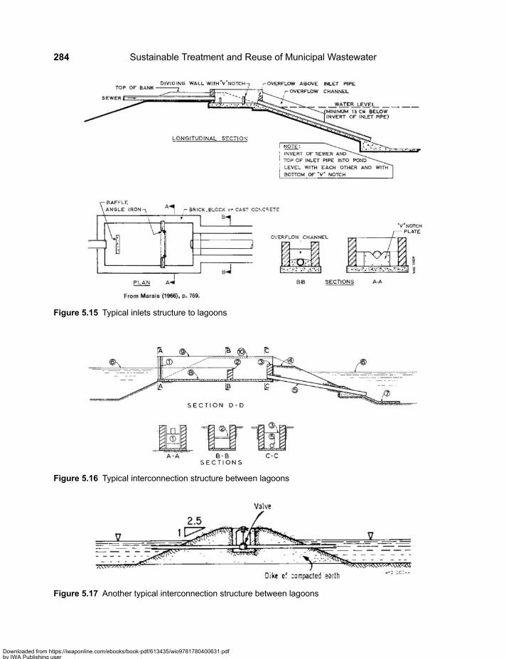
Figure 5.15 Typical inlets structure to lagoons

Figure 5.16 Typical interconnection structure between lagoons

Figure 5.17 Another typical interconnection structure between lagoons



A photo of a lagoon outlet structure of the type presented in Figure 5.18 is shown in Figure 5.20. Thisfigure also portrays the effluent of a lagoons system consisting of a series of anaerobic-facultative-maturation lagoons.

Figure 5.18 Typical outlet structure from lagoons

Figure 5.19 Another type of typical inlet and outlet structures of lagoons



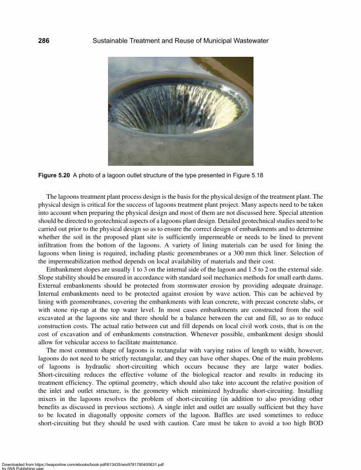
The lagoons treatment plant process design is the basis for the physical design of the treatment plant. Thephysical design is critical for the success of lagoons treatment plant project. Many aspects need to be takeninto account when preparing the physical design and most of them are not discussed here. Special attentionshould be directed to geotechnical aspects of a lagoons plant design. Detailed geotechnical studies need to becarried out prior to the physical design so as to ensure the correct design of embankments and to determinewhether the soil in the proposed plant site is sufficiently impermeable or needs to be lined to preventinfiltration from the bottom of the lagoons. A variety of lining materials can be used for lining thelagoons when lining is required, including plastic geomembranes or a 300 mm thick liner. Selection ofthe impermeabilization method depends on local availability of materials and their cost.

Embankment slopes are usually 1 to 3 on the internal side of the lagoon and 1.5 to 2 on the external side.Slope stability should be ensured in accordance with standard soil mechanics methods for small earth dams.External embankments should be protected from stormwater erosion by providing adequate drainage.Internal embankments need to be protected against erosion by wave action. This can be achieved bylining with geomembranes, covering the embankments with lean concrete, with precast concrete slabs, orwith stone rip-rap at the top water level. In most cases embankments are constructed from the soilexcavated at the lagoons site and there should be a balance between the cut and fill, so as to reduceconstruction costs. The actual ratio between cut and fill depends on local civil work costs, that is on thecost of excavation and of embankments construction. Whenever possible, embankment design shouldallow for vehicular access to facilitate maintenance.

The most common shape of lagoons is rectangular with varying ratios of length to width, however,lagoons do not need to be strictly rectangular, and they can have other shapes. One of the main problemsof lagoons is hydraulic short-circuiting which occurs because they are large water bodies.Short-circuiting reduces the effective volume of the biological reactor and results in reducing itstreatment efficiency. The optimal geometry, which should also take into account the relative position ofthe inlet and outlet structure, is the geometry which minimized hydraulic short-circuiting. Installingmixers in the lagoons resolves the problem of short-circuiting (in addition to also providing otherbenefits as discussed in previous sections). A single inlet and outlet are usually sufficient but they haveto be located in diagonally opposite corners of the lagoon. Baffles are used sometimes to reduceshort-circuiting but they should be used with caution. Care must be taken to avoid a too high BOD

Figure 5.20 A photo of a lagoon outlet structure of the type presented in Figure 5.18



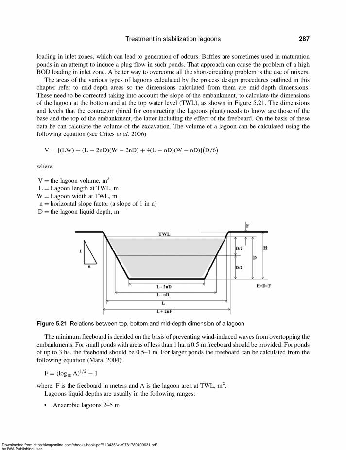
loading in inlet zones, which can lead to generation of odours. Baffles are sometimes used in maturationponds in an attempt to induce a plug flow in such ponds. That approach can cause the problem of a highBOD loading in inlet zone. A better way to overcome all the short-circuiting problem is the use of mixers.

The areas of the various types of lagoons calculated by the process design procedures outlined in thischapter refer to mid-depth areas so the dimensions calculated from them are mid-depth dimensions.These need to be corrected taking into account the slope of the embankment, to calculate the dimensionsof the lagoon at the bottom and at the top water level (TWL), as shown in Figure 5.21. The dimensionsand levels that the contractor (hired for constructing the lagoons plant) needs to know are those of thebase and the top of the embankment, the latter including the effect of the freeboard. On the basis of thesedata he can calculate the volume of the excavation. The volume of a lagoon can be calculated using thefollowing equation (see Crites et al. 2006)

V = LW( ) + L− 2nD( ) W− 2nD( ) + 4 L− nD( ) W− nD( )[ ] D/6( )where:

V= the lagoon volume, m3

L= Lagoon length at TWL, mW= Lagoon width at TWL, mn= horizontal slope factor (a slope of 1 in n)D= the lagoon liquid depth, m

The minimum freeboard is decided on the basis of preventing wind-induced waves from overtopping theembankments. For small ponds with areas of less than 1 ha, a 0.5 m freeboard should be provided. For pondsof up to 3 ha, the freeboard should be 0.5–1 m. For larger ponds the freeboard can be calculated from thefollowing equation (Mara, 2004):

F = (log10 A)1/2 − 1

where: F is the freeboard in meters and A is the lagoon area at TWL, m2.Lagoons liquid depths are usually in the following ranges:

• Anaerobic lagoons 2–5 m

Figure 5.21 Relations between top, bottom and mid-depth dimension of a lagoon



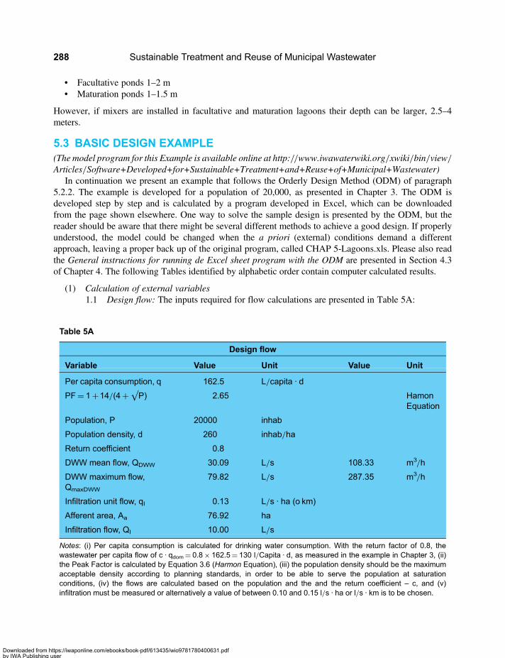
• Facultative ponds 1–2 m• Maturation ponds 1–1.5 m

However, if mixers are installed in facultative and maturation lagoons their depth can be larger, 2.5–4meters.


In continuation we present an example that follows the Orderly Design Method (ODM) of paragraph5.2.2. The example is developed for a population of 20,000, as presented in Chapter 3. The ODM isdeveloped step by step and is calculated by a program developed in Excel, which can be downloadedfrom the page shown elsewhere. One way to solve the sample design is presented by the ODM, but thereader should be aware that there might be several different methods to achieve a good design. If properlyunderstood, the model could be changed when the a priori (external) conditions demand a differentapproach, leaving a proper back up of the original program, called CHAP 5-Lagoons.xls. Please also readthe General instructions for running de Excel sheet program with the ODM are presented in Section 4.3of Chapter 4. The following Tables identified by alphabetic order contain computer calculated results.

(1) Calculation of external variables1.1 Design flow: The inputs required for flow calculations are presented in Table 5A:

Table 5A

Design flow



PF= 1+14/(4+√P) 2.65 HamonEquation





DWW maximum flow,QmaxDWW

79.82 L/s 287.35 m3/h




Notes: (i) Per capita consumption is calculated for drinking water consumption. With the return factor of 0.8, thewastewater per capita flow of c · qdom= 0.8× 162.5= 130 l/Capita · d, as measured in the example in Chapter 3, (ii)the Peak Factor is calculated by Equation 3.6 (Harmon Equation), (iii) the population density should be the maximumacceptable density according to planning standards, in order to be able to serve the population at saturationconditions, (iv) the flows are calculated based on the population and the and the return coefficient – c, and (v)infiltration must be measured or alternatively a value of between 0.10 and 0.15 l/s · ha or l/s · km is to be chosen.












The final design flows are obtained from Equations 3.3 and 3.4, and are presented inTable 5B in different units as an output. The average flow QD is used for the biologicalprocess design and the maximum flow QHD for hydraulic design.

In the case of preliminary treatment the design flows for the coarse screen, the gritchamber and the Parshall flume is the maximum flow QHD since they are hydraulicunits. On the other hand, the lagoons are designed on the basis of the average flow QD

since they are biological process with detention times of days, during which all variationsare averaged.

1.2 Determination of the geographical and external environmental variables: These variablesdepend solely on the geographic location. The values used in the example are presented inTable 5C.

1.3 Concentration and pollution loads: The quality of the wastewater may be different in theurban areas and at the entrance to the treatment plant if the conveyance system is long andreceives an important infiltration inflow. In the example, the wastewater treatment plant is

Table 5B

Design flow


Process design flow,QD=QDWW+QI

40.09 L/s 144.33 m3/h 3464.00 m3/d

Hydraulics design flow,QHD=QDWWmax+QI

89.82 L/s 323.35 m3/h 7760.44 m3/d

Table 5C


Minimum Temperature of water, Tw 25 °C 77.0 °F

Minimum Temperature of air, Ta 18 °C 64.4 °F

Altitude above sea level, hasl 350 masl





Notes: (i) for the design of the Preliminary Treatment process these variables do not have a significant importance, for thedesign of the biological processes they are important, (ii) the minimum water temperature as well as the minimum airtemperature are the average of the coldest month, (iii) the speed and direction of the predominant wind is important forlocating the wastewater treatment plant in relation to the location of the town or the urban center, (iv) the fraction of hoursof sunlight is the ratio of actual hours of sunlight to possible hours of sunlight.



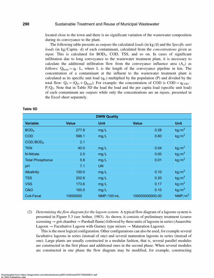
located close to the town and there is no significant variation of the wastewater compositionduring its conveyance to the plant.

The following table presents as outputs the calculated loads (in kg/d) and the Specific unitloads (in kg/Capita · d) of each contaminant, calculated from the concentrations given asinput. This is calculated for BOD5, COD, TSS, and so on. In cases of significantinfiltration due to long conveyance to the wastewater treatment plant, it is necessary tocalculate the additional infiltration flow from the conveyance influence area (Aa) asfollows: QIemi= qI · L, where L is the length of the conveyance pipeline in km. Theconcentration of a contaminant at the influent to the wastewater treatment plant iscalculated as its specific unit load (qC) multiplied by the population (P) and divided by thetotal flow: QT= (QD+QIemi). For example: the concentration of COD is COD= qCOD ·P/QT. Note that in Table 5D the load the load and the per capita load (specific unit load)of each contaminant are outputs while only the concentrations are an inputs, presented inthe Excel sheet separately.

(2) Determining the flow diagram for the lagoon system:A typical flow diagram of a lagoons system ispresented in Figure 5.3 (see Arthur, 1983). As shown, it consists of preliminary treatment (coarsescreening→ grit chamber→ Parshall flume) followed by three units of lagoons in series (AnaerobicLagoon → Facultative Lagoon with Gurney type mixers → Maturation Lagoon).

This is the most logical configuration. Other configurations can also be used, for example severalfacultative lagoons in series (instead of one) and several maturation lagoons in series (instead ofone). Large plants are usually constructed in a modular fashion, that is, several parallel modulesare constructed in the first phase and additional ones in the second phase. When several modulesare constructed in one phase the flow diagram may be modified, for example, constructing

Table 5D

DWW Quality


BOD5 277.8 mg/L 0.28 kg/m3

COD 596.1 mg/L 0.60 kg/m3

COD/BOD5 2.1

TKN 40.0 mg/L 0.04 kg/m3

N-Nitrate 2.0 mg/L 0.00 kg/m3

Total Phosphorus 5.8 mg/L 0.01 kg/m3

pH 7.1 UN

Alkalinity 100.0 mg/L 0.10 kg/m3

TSS 202.6 mg/L 0.20 kg/m3

VSS 173.6 mg/L 0.17 kg/m3

O&G 100.0 mg/L 0.10 kg/m3

Coli-Fecal 10000000 NMP/100mL 100000000000.00 NMP/m3



4 anaerobic lagoons which distribute their effluent to 2 trains of facultative followed by maturationlagoons. The only governing guideline is to set up a flow diagram which makes sense.

(3) Sizing the pretreatment system3.1 Coarse screening

Variables selection by the designer: The coarse screening system can be a rotating screen. If atarget of 3% solids removal efficiency (coarse screening has very low efficiency to removeTSS) is selected, than according to Figure 4.8 a rotating screen with an opening of 6 mmwill be adequate. The design flow is the maximum flow QHD since screening is a hydraulicunit. The results that the program calculates automatically are presented in Table 5E. Theyinclude in addition to the solids removal efficiency also the water velocity in the channeland the backwashing pressure. The module CHAP 4-RM.xls of the excel program is to beused for these calculations.

Design:A coarse rotating screen of 600 mm in diameter is obtained from the calculations. Thefinal output data are presented in the table below. The design of the coarse rotating screen issimilar to that of the rotating micro screen so the reader is referred to Chapter 4 in which thedesign procedure is explained in detail. Only course screening is used in the preliminarytreatment unit because further processing of the fine material that will be contained in theeffluent of this unit will be processed in the series of lagoons into which the preliminaryeffluent will be discharged. For the purpose of clarification, the preliminary treatment unitcalculations which are produced by the Excel program are presented in Table 5F. Thedesign support is presented in the column entitled OBSERVATION.

Table 5E

Designer variables




Screen opening (rounded) 6.00 mm 0.236 inch




Table 5F

Design




(Continued )



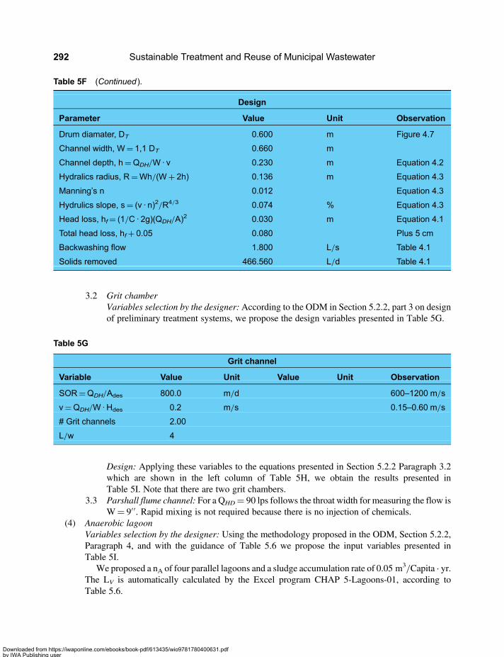
3.2 Grit chamberVariables selection by the designer:According to the ODM in Section 5.2.2, part 3 on designof preliminary treatment systems, we propose the design variables presented in Table 5G.

Design: Applying these variables to the equations presented in Section 5.2.2 Paragraph 3.2which are shown in the left column of Table 5H, we obtain the results presented inTable 5I. Note that there are two grit chambers.

3.3 Parshall flume channel: For a QHD= 90 lps follows the throat width for measuring the flow isW= 9′′. Rapid mixing is not required because there is no injection of chemicals.

(4) Anaerobic lagoonVariables selection by the designer: Using the methodology proposed in the ODM, Section 5.2.2,Paragraph 4, and with the guidance of Table 5.6 we propose the input variables presented inTable 5I.

We proposed a nA of four parallel lagoons and a sludge accumulation rate of 0.05 m3/Capita · yr.The LV is automatically calculated by the Excel program CHAP 5-Lagoons-01, according toTable 5.6.

Table 5F (Continued ).

Design





Hydralics radius, R=Wh/(W+ 2h) 0.136 m Equation 4.3




Total head loss, hf+ 0.05 0.080 Plus 5 cm



Table 5G

Grit channel

Variable Value Unit Value Unit Observation

SOR=QDH/Ades 800.0 m/d 600–1200 m/s

v=QDH/W ·Hdes 0.2 m/s 0.15–0.60 m/s

# Grit channels 2.00

L/w 4



Design: From the input date we obtain the results presented in Table 5J.Following are clarifications to the calculations of the figures in Table 5J:○ VA=QD · S0/1000 LV=Qs/LV= 3701.2 m3: preliminary volume of the lagoon calculated

using Equation 5.17.○ td=VA/QD= 1.1 d, which is larger than the minimum recommended detention time tdmin= 1d,

so we select the larger of the two numbers as final detention time, which in this case is td= 1.1d.○ VF= td · QD= 3701.2 m3: the final selected volume of the lagoon.○ As=VF/HA= 3701.2/4= 925.3 m2: total surface area of the lagoons at the surface level of

the lagoon.○ as=As/nA= 231,3 m2: area of each of the 4 (nA) anaerobic lagoons.○ The total width and length of the squared lagoons ate w=√(as)=√(231.3)= 15.2 m. There

are other possible geometric forms (for instance with a L/w= 2). Then the calculation of thedimensions would change.

Table 5I

Designer variables


Anaerobic lagoon (A)

Depth, HA 4.0 m 3–5 m

Tmin air 18.0 °C Coldest month

Sludge accumulation, vL 0.04 m3/capita · yr Range 0.04–0.08

# Lagoons A, nA 4 Parallel

L/w (ratio length to width) 1 Between 1 and 3

Velocity in inlet pipe, v 1 m/s Range 0.6–2.0 m/s

Volumetric load, LV 260 g/m3 · d Table 5.5

Table 5H

Grit channel


Area, Ades=QHD/SOR 9.7 m2 Section 5.2.2 Paragraph 3.1

Width, w=√(Ades/4) 1.6 m Section 5.2.2 Paragraph 3.1

Length, L= 4w 6.2 m Section 5.2.2 Paragraph 3.1

Depth, Hdes=QDH/v · W 0.3 m Section 5.2.2 Paragraph 3.1

Total Depth, H=Hdes+ 0.50 0.8 m Section 5.2.2 Paragraph 3.1

Parshall flume

Throat, W 9.0 inch See “PARSHALL” sheet



○ The time required to fill half of the lagoon with accumulated sludge is n= 2.3 years, calculatedaccording to Equation 5.18.

○ The volume of biogas produced is calculated by Equation 5.19 and is 288.7 m3/d.○ The BOD5 removal efficiency and effluent BOD5 concentration are automatically calculated by

the program CHAP 5-Lagoons-01, according to Table 5.6.○ For input and output structures use an average liquid velocity of 1m/s, (this value can be different

but preferably is in the range 0.6 and 2.0 m/s) which results in a diameter of w= 13′′ and 4′′ forinlet pipe conveying the totalwastewater flow and the inlet pipe to each lagoon respectively. Notethat the design of the inflow pipe is based on the maximum flow QHD since there are no flowequalization structures prior to entering the plant but the outlet flow is QD because the flow isequalized in the lagoon. Odours become a problem if LV. 400 g/m3 · d or if there is excesssulphate in the influent. To prevent odours and to control emission of greenhouse gases it isrecommended a cover the anaerobic lagoons, and burn the collected biogas in a gas burningsystem of a capacity that includes a safety factor of two (2) times the biogas flow calculatedby Equation 5.19: VgD= 2 Vg= 577.5 m3. See Paragraph 5 of Section 5.2.2 for details ofcover design.

Table 5J

Design

Parameter Value Unit Value Unit Observation

Anaerobic lagoon

Volume, VA= (QD · S0)/1000 · LV 3701.2 m3 Equation 5.17

Detention time, td=VA/QD 1.1 d

Final Volume, VF=QD · td 3701.2 m3 Larger of td and tdmin = 1d

Total Area, AS=VF/HA 925.3 m2

Area per lagoon as= (As/nA) 231.3 m2

Lagoon Width, w= [as/(L/w)]0,5 15.2 m

Lagoon Length, L= (L/w)w 15.2 m

Sludge filling time, n=½ VF/VL · P 2.3 years Equation 5.18 (half filled)

Gas production

Volume, Vg= 0.30 S0 · QD/1000 288.7 m3/d Equation 5.19

Efficiency of anaerobic lagoon

Efficiency, % BOD5 56 % Table 5.6

Effluent BODe, SA 122 mg/L

Inlet and outlet structures

Diameter of inlet pipew= (4 · PI · v · QDH/1000)

0.50.338 m 13 inch Calculated with QD

Diameter of pipe in LagoonwL= w= [4 · PI · v · (QD/4)/100]

0.113 m 4 inch Calculated with QD/4



(5) Facultative lagoonVariables selection by the designer: Use the methodology proposed in the ODM, Section 5.2.2,Paragraph 6, and with the guidance in Table 5.1, as shown below, propose the designer variables.

The issues that require consideration are: (i) are we choosing to install mixers in the facultativelagoons? If we do, the design needs to take that fact into account, (ii) selecting the number offacultative lagoons (nF) in series, (iii) adopting the value of KL (20°C)= 0.35 d−1, (iv) selectingthe ration of Length to width of the lagoon, and (v) taking into account that the influent of thefacultative lagoon is the effluent of the anaerobic lagoon. Other input data are based on externalconditions such as air and water temperatures, altitude, sun radiation, and so on.

In the design example we chose facultative lagoons with mixers, bearing in mind that under suchconditions we can choose a larger than usual lagoon depth. We propose to use the input variablespresented in Table 5K.

Design: From input data, the design values are obtained by following the ODM, the results obtainedare presented in Table 5L.○ The equation number used for each calculation is given in the right column, in accordance with

the procedures of Section 5.2.2, Paragraph 6. The equations are named in the right column.

Table 5K

Designer variables


Facultative lagoon

¿ Mixer installed? 1 YES:1; NOT:0

Depth, HF 3 m 2–5 m


Ti water 25.0

# Lagoons F, nF 2 Parallel


Velocity in inlet pipe, v 1 m/s Range 0.6–2.0 m/s

Ls= 350 (1.107–0.002T)(T-25)

or 400400.0 kgBOD5/ha · d Equation 5.14 or 400

KL (20°C) 0.35 d−1 Typical

θ (BOD5) 1.06 Range 1.04–1.09

Influent BOD5i, S0F=SA 122.2 mg/L

KB (20°C) 2.7 d−1 Typical for FC

θ (CF) 1.19 Typical for FC

Influent FC: B0 10000000 NMP/100mL

Influent Helminthes 500 Ova/L Between 300–800



Table 5L

Design


Facultative lagoon

Ls 400.0 kgBOD5/ha · d Selected in input

td= 10 · HFBOD5/LS 9.2 d Equation 5.11

Volume, V′F=Q · TD 31755.9 m3 Equation 5.21

Final Volume VF 31755.9 m3 Greater of td andtdmin= 4 d

Area, As=VF/h 10585.3 m2 Equation 5.20

Lagoon Area as= (As/nF) 5292.6 m2

Lagoon Width, w= [as/(L/w)]0.5 51.4 m

Lagoon Length, L= (L/w)w 102.9

# of mixers LAS=As/(3×10000) 2.0 0.75 hp/ha

TL= (AsfTa+QTi)/(Asf+Q) 18.0 °C Equation 5.8

KL=KL(20°C) θ(T-20) 0.31 d−1 Equation 5.7

Effluent BOD5 SF=S0/(1+KL · td):lagoons in parallel

31.70 mg/L Equation 5.4,parallel

Effluent BOD5 SF=S0/(1+KL · td/n)n:

lagoons in series20.74 mg/L Equation 5.5,

series

vF= 0.00091VF(S0 – S)/(1+ 0.05td) 1793.86 kg/yr 1793.86 m3/yr Equation 5.24

Filling years= 0.5 VF/vF 8.9 years ½ Volume

Facultative lagoon: Fecal coliform and helminthes removal and efficiencies

KB=KB(20°C) θ(T-20) 6.4 d−1 Equation 5.26

Effluent FC: B=B0/(1+KB · td) 166480.8 NMP/100mL Equation 5.25

Effluent helminthes 9.8 Ova/L

Efficiency FC= 100 · (B0–B)/B0 98.3 % From Equation5.25

Efficiency Helminthes= 100 (1− 0.41Exp [−0.49 td+ 0.0085 td

2])98.0 % Equation 5.15

Efficiency BOD5 removal facultative 74.1 %

Efficiency BOD5 removal (Anaerobic+Facultative)

88.6 %


Diameter in inlet pipe,w= (4 · PI · v · QD/1000)

0.50.226 m 9.00 in With QD

Diameter of pipes to lagoons,wL= w= [4 · PI · v · (QD/4)/1000]

0.50.160 m 6.00 in With QD/4



○ Note that the substrate concentration to the influent of the first facultative lagoon is that of theeffluent of the anaerobic lagoon and the substrate concentration in the influent to the secondfacultative lagoons is that of the effluent of the first facultative lagoon.

○ The organic surface load (LS, kg BOD5/ha · d) is calculated from Equation 5.14 and thedetention time td is calculated by solving Equation 5.11. Then td is chosen as the higher ofthe calculated detention time and the minimum acceptable of 4 days.

○ Then we calculate the final volume (VF), total surface area (AS), the area of each facultativelagoon (as) and the dimensions of each facultative lagoon.

○ Facultative lagoons can be operated in series or in parallel so the effluent BOD5 is calculated forboth cases: S (parallel) and S′ (in series).

○ Then the removal efficiencies of the BOD5 (of F and A+ F), Fecal Coliforms and Helmintheseggs are calculated and also the concentrations in the effluent.

○ The dimensions of the lagoon are calculated using in this case a ratio of L/w= 2.○ The diameters of the inflow pipelines to the facultative lagoons in series (calculated using QD) or

in parallel (calculated using QD/number of lagoons) are presented in the last rows of the table.

(6) Maturation lagoonsVariables selection by the designer: First, define the desired targets of removal of Fecal Coliforms(FC) AND helminthes eggs. According to procedure outlined in the ODM of Section 5.2.2,Paragraph 6, it is also necessary to choose de lagoon depth (HM) and the L/w ratio. The influentof the Maturation lagoon is the effluent of the Facultative lagoon. The design procedure issimilar to that of the facultative lagoon but the objectives are different and in this case are: (i)Remove Fecal Coliforms and additional BOD5, and (ii) remove helminth eggs, and in general,obtain the desired quality of the final effluent as expected from the complete lagoons system(and usually, as required by the prevailing effluent discharge standards). The variables selectedby the designer are presented in Table 5M.

Table 5M

Designer variables


Maturation lagoon

Depth, HM 1.5 m 2–5 m


Ti water 25.0

# Lagoons M, nM 2 Parallel or series


Water velocity in pipe, v 1 m/s 0.6–2.0 m/s

Ls= 350 (1.107–0.002T)(T-25)

or 400216.5 kgBOD5/ha · d Equation 5.14 or 400

KL (20°C) 0.35 d−1 Typical

θ (BOD5) 1.06 1.04–1.09

(Continued )



Design: The design outputs are calculated by the Excel program CHAP 5-Lagoons.xls and arepresented in the following Table 5N.

Table 5M (Continued).

Designer variables


Influent BOD5i, S0M=SF 31.7 mg/L

KB (20°C) 2.7 d−1 Typical FC

θ (CF) 1.19 Typical FC

Influent FC: B0M 166481 MPN/100mL

Influent helminthes 10 Ova/L Between 300–800

Target FC 10000 MPN/100mL Between 1000 and 10000

Target helminthes eggs 1 Ova/L ,1 Ova/L

Table 5N

Design


Maturation lagoon

Ls 216.5 kgBOD5/ha · d Selected in input

td= 10 · HFBOD5/Ls 2.2 d Equation 5.11;tdmin= 3 d

Volume, V′F=Q · td 7607.1 m3 Equation 5.21

Final Volume VF 10392.0 m3 Greater of td andtdmin = 3 d


Lagoon area as= (As/nF) 3464.0 m2

Lagoon width, w= [as/(L/w)]0.5 41.6 m

Lagoon length, L= (L/w) w 83.2

TL= (AsfTa+QTi)/(Asf+Q) 21.5 °C Equation 5,8

KL=KL(20°C) θ(T-20) 0.38 d−1 Equation 5.7

Effluent BOD5 SM= S0/(1+KL · td) 17.24 mg/L Equation 5.4,Parallel

Effluent BOD5 SM= S0/(1+KL · td/n)n 15.74 mg/L Equation 5.5, series

VF= 0.00091VF(S0 –S)/(1+ 0.05td) 123.23 kg/yr 123.23 m3/yr Equation 5.24

(Continued )



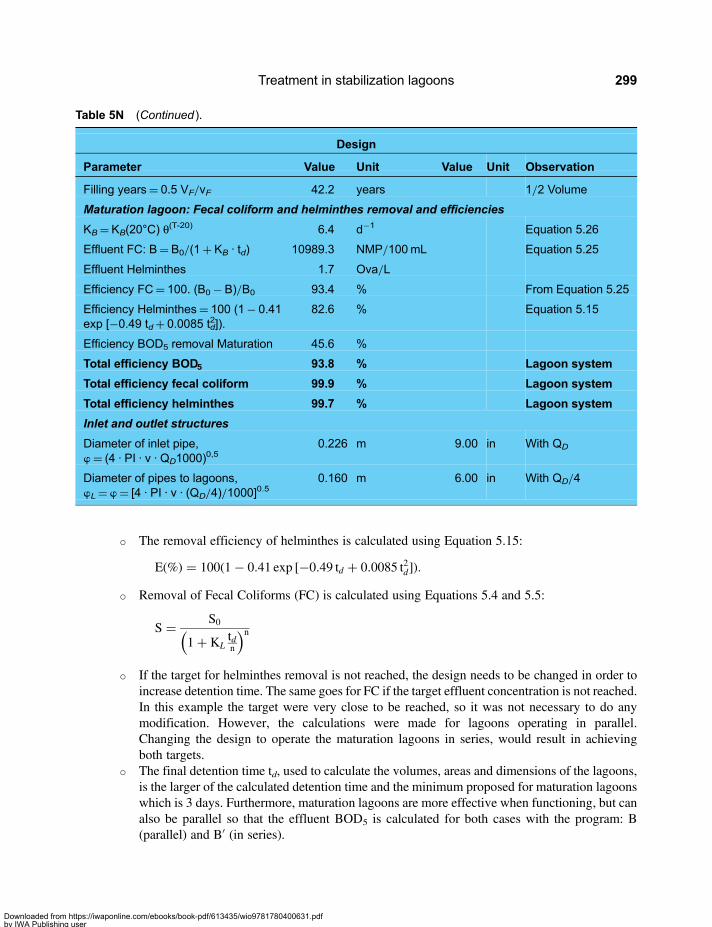
○ The removal efficiency of helminthes is calculated using Equation 5.15:

E(%) = 100(1− 0.41 exp [−0.49 td + 0.0085 t2d]).

○ Removal of Fecal Coliforms (FC) is calculated using Equations 5.4 and 5.5:

S = S0

1+ KLtdn

( )n○ If the target for helminthes removal is not reached, the design needs to be changed in order to

increase detention time. The same goes for FC if the target effluent concentration is not reached.In this example the target were very close to be reached, so it was not necessary to do anymodification. However, the calculations were made for lagoons operating in parallel.Changing the design to operate the maturation lagoons in series, would result in achievingboth targets.

○ The final detention time td, used to calculate the volumes, areas and dimensions of the lagoons,is the larger of the calculated detention time and the minimum proposed for maturation lagoonswhich is 3 days. Furthermore, maturation lagoons are more effective when functioning, but canalso be parallel so that the effluent BOD5 is calculated for both cases with the program: B(parallel) and B′ (in series).

Table 5N (Continued ).

Design


Filling years= 0.5 VF/vF 42.2 years 1/2 Volume

Maturation lagoon: Fecal coliform and helminthes removal and efficiencies


Effluent FC: B=B0/(1+ KB · td) 10989.3 NMP/100mL Equation 5.25

Effluent Helminthes 1.7 Ova/L

Efficiency FC= 100. (B0−B)/B0 93.4 % From Equation 5.25

Efficiency Helminthes= 100 (1− 0.41exp [−0.49 td+ 0.0085 td

2]).82.6 % Equation 5.15

Efficiency BOD5 removal Maturation 45.6 %

Total efficiency BOD5 93.8 % Lagoon system

Total efficiency fecal coliform 99.9 % Lagoon system

Total efficiency helminthes 99.7 % Lagoon system


Diameter of inlet pipe,w= (4 · PI · v · QD1000)

0,50.226 m 9.00 in With QD

Diameter of pipes to lagoons,wL= w= [4 · PI · v · (QD/4)/1000]

0.50.160 m 6.00 in With QD/4



○ Ultrasound waves generating instruments for removal of algae can be installed at the exit sectionof the maturation lagoons. LGSonic instruments are an example of such devices. According tothe manufacturer’s recommendation one instrument should be installed per acre of lagoon area.A photo of the instrument is presented in Figure 5.22.

○ The diameters of the inflow pipe for lagoons in series mode (calculated using QD) or in parallelmode (calculated using with QD/number of lagoons) are presented in the last rows of the table.The input and output structures are constructed in accordance with Paragraph 7 below.

(7) Inlet, outlet and interconnection structures: In the Orderly DesignMethod, Section 5.2.2 Paragraph8, different designs of inlet, outlet and interconnection structures are presented. Each tab of theCHAP 5-Lagoons-01program, “Anaerobic”, “Facultative” and “Maturation”, brings thediameters of the required inlet pipes. The slopes of the lagoons levee depend on soil andgeological conditions which needs to be established through corresponding studies, but as a firstapproximation a slope with a gradient of 2:1 can be proposed (see Figures 5.14–5.19 and 5.23).

Figure 5.23 Cross section of a typical lagoons system

Figure 5.22 Ultrasonic waves generating instrument (Manufactured by LGSONIC)



Chapter 6

Anaerobic treatment

6.1 PROCESS DESCRIPTION6.1.1 Introduction1

Anaerobic treatment emerged as an option for wastewater treatment in the 1960s. In the recent years anaerobicprocesses have proved to be cost-effective for the treatment of BOD removal in the range of 40 to 85%.Anaerobic treatment involves the bioconversion of substrate (in this case the municipal wastewater), whilepassing through a biomass medium (i.e. the anaerobic bacterial population) mainly to methane (CH4),CO2 and H2O and an additional small amount of more biomass. In this case the bioconversion does notrequire a high energy loss because most of the energy remains stored in methane. So the energy balancebetween the substrate and product only varies by less than 5% in terms of calories, and is equivalentin terms of COD. The energy balance in anaerobic bioconversion is presented by Equation 2.10 as follows:

DS = 4.00DCH4 + 1.22DX (2.10)

where:

ΔS= substrate removed, mg/l CODΔCH4 =methane produced, mg/l CH4

ΔX= anaerobic biomass produced, mg/l VSS.

The factors are 4.00 and 1.22 are converting the mass of CH4 and anaerobic biomass (X) to mass in terms ofCOD. The main treatment occurs by the conversion of COD into methane, which is then separated from thewater, and into the small amount of anaerobic biomass, which are the excess sludge removed from the process.

There is a large variety of types of anaerobic reactors for treatment of wastewater including: anaerobicdigesters of excess sludge (of low loading, high loading and two stages), septic tanks, anaerobic lagoons,high loading reactors including fixed bed reactors also known as anaerobic filters (of ascending ordescending flows, Andrade Neto, 1997), baffled reactor (BR), piston or plug-flow anaerobic reactor(PAR) described by Orozco (1997) and Metcalf and Eddy (2003), rotating bed reactor, expanded bed

1This paragraph is based on the textbook “Bioingeniería de aguas residuales: teoría y diseño” (2005), Alvaro by Orozco Jaramillo,published by ACODAL, Bogotá, Colombia and the article “Appropriate Technology for Wastewater Treatment and Reuse inDeveloping Countries” Menahem Libhaber (2007).


reactor, fluidized bed reactor, two stage anaerobic reactor, upflow Anaerobic sludge blanket reactor(UASB), expanded bed granular reactor, internal recirculation anaerobic reactor and variouscombinations of these reactors. Detailed information on all these types of reactor is presented byChernicharo (2007) and Campos (2009). Some of these reactors are used to treat industrial wastewater.The three anaerobic reactors (or anaerobic unit processes) which are used most frequently for treatmentof municipal wastewater are: Anaerobic Lagoons, UASB and Anaerobic Filters. The piston anaerobicreactor also has a potential for being used in municipal wastewater treatment plants. Wastewaterprocessing in the four anaerobic reactors used for treatment of municipal wastewater fall into thecategory of Appropriate Technology (AT) according to the classification of Libhaber (2007), which wasdiscussed in Chapter 1.

According to Libhaber (2007): “Anaerobic processes achieve organic matter removal in the range40%–80%, depending on the type of process, and as such they are most valuable for developing countrysince they have the potential to achieve such a meaningful removal at low cost and simple to operateinstallation. If a higher level of organic matter removal is required, anaerobic processes can be the firststage of treatment followed by a variety of polishing processes, such as lagoons of various types,activated sludge, constructed wetlands, filtration, dissolved air floatation and others. It is also possible touse one anaerobic process as the first stage treatment and another as a following polishing process, forinstance, a UASB followed by an anaerobic filter, or even anaerobic lagoons followed by UASBfollowed by an anaerobic filter.”

Treatment in Anaerobic Lagoons is discussed in Chapter 5. The current chapter deals with treatment in aUASB reactor, Anaerobic Filter and Piston Anaerobic Reactor.

6.1.2 Basics of the processesAnaerobic digestion fundamentsThe biochemistry of anaerobic decomposition is presented in paragraph 2.4, Chapter 2, and is summarizedin Figures 2.6 and 6.1 (which is a simplified diagram). Libhaber (2007) provides a summary of themicrobiology of the above processes, as follows: “Anaerobic decomposition is a two-stage process, eachstage being carried out by a different group of bacteria, with the second stage bacteria being moresensitive than the first to environmental conditions such as pH. In the first stage acid-forming ornonmethanogenic bacteria convert the organic matter present in the sewage to organic acids, whereas inthe second stage, methane forming-bacteria or methanogens convert the organic acids to methane gasand carbon dioxide. For efficient performance, the methanogens require a pH in the range 6.5–7.5, andthey cannot develop at all below a pH of 6.2. However, if too many acids are produced by theacid-forming bacteria, which develop and multiply easily, the result is a low pH which may impede theproduction of methanogens. In the presence of high concentrations of sulphates, the methanogens alsohave to compete with sulphur-reducing bacteria. The main consequences of such a situation are theappearance of unpleasant odours and the reduction in the efficiency of the anaerobic process.”

The reactions which take place in each stage of the anaerobic process are presented in a more detailedform in Table 6.1, along with the energy required for each reaction.

For these sequential reactions to be carried out under such defined and complex environmentalconditions, it is necessary that a consortium of different types of bacteria form into a floc or granule, soas to optimize the metabolic processes which dependent on one of another. In the granules, which formspontaneously in the UASB and the PAR reactors (see Figure 2.7), three concentric layers are formed:the acidogenic bacteria in the outside layer, the acetogenic in the middle layer and in the middle ofmethanogenic in the center of th granules (see Figure 2.5).



Figure 6.1 Schematic diagram of the anaerobic decomposition process [Source: http://water.me.vccs.edu/courses/ENV149/lesson4.htm (May 22, 2011)]

Table 6.1 Representative reactions of the anaerobic decomposition of organic matter.

Reaction Reactives Products Kj/////Reaction

ΔG°′ ΔG′

Completeconversion fromglucose to methaneand CO2

C6H12O6 ↔ 3CH4+ 3HCO3−+ 3H+ −403.6 −399.1

Acidogenesis ofcarbohydrates toacetic acid

C6H12O6+ 4H2O ↔ 2CH3COO−+2HCO3

−+ 4H++ 4H2

−206.3 −318.5

Acetogenesis ofpropionate

CH3CH2COO−+ 3H2O ↔ CH3COO−+H++ 3H2 76.1 −5.4

HydrogenoclasticAcetogenesis

4H2+ 2HCO3−+H+ ↔ CH3COO−+ 2H2O 104.6 −7.0

AcetoclasticMethanogenesis

CH3COO−+H2O ↔ CH4+HCO3−+H+ −31.0 −24.5

HydrogenoclasticMethanogenesis

4H2+HCO3−+H+ ↔ CH4+ 3H2O −135.6 −31.6

Notes: 1) Calculation of ΔG°′ (standard) is based in the following conditions: pH= 7; solutes conc. 1 molar; gasesat 1 atm., 25°C.2) Calculation of ΔG′(real) for an anaerobic decompostion; pH= 7; glucose= 10 micro-mole; acetate, propionate=1 mili-mole; HCO3

−= 20 mili-mole; CH4= 0.6 atm.; H2 = 10-4 atm., 37°C.Source: Orozco (2005)

Anaerobic treatment 303


http://wastewaterengineering.com/uasb_upflow_anaerobic_sludge_blanket.htm








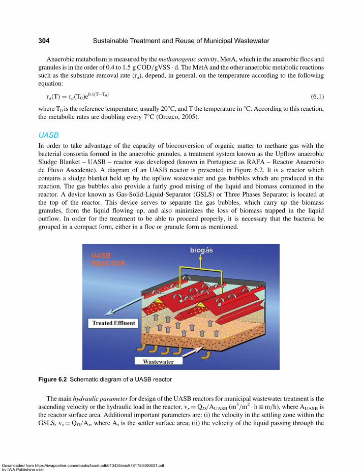
Anaerobic metabolism is measured by themethanogenic activity, MetA, which in the anaerobic flocs andgranules is in the order of 0.4 to 1.5 g COD/gVSS · d. TheMetA and the other anaerobic metabolic reactionssuch as the substrate removal rate (ra), depend, in general, on the temperature according to the followingequation:

ra(T) = ra(T0)e0.1(T−T0) (6.1)

where T0 is the reference temperature, usually 20°C, and T the temperature in °C. According to this reaction,the metabolic rates are doubling every 7°C (Orozco, 2005).

UASBIn order to take advantage of the capacity of bioconversion of organic matter to methane gas with thebacterial consortia formed in the anaerobic granules, a treatment system known as the Upflow anaerobicSludge Blanket – UASB – reactor was developed (known in Portuguese as RAFA – Reactor Anaerobiode Fluxo Ascedente). A diagram of an UASB reactor is presented in Figure 6.2. It is a reactor whichcontains a sludge blanket held up by the upflow wastewater and gas bubbles which are produced in thereaction. The gas bubbles also provide a fairly good mixing of the liquid and biomass contained in thereactor. A device known as Gas-Solid-Liquid-Separator (GSLS) or Three Phases Separator is located atthe top of the reactor. This device serves to separate the gas bubbles, which carry up the biomassgranules, from the liquid flowing up, and also minimizes the loss of biomass trapped in the liquidoutflow. In order for the treatment to be able to proceed properly, it is necessary that the bacteria begrouped in a compact form, either in a floc or granule form as mentioned.

The main hydraulic parameter for design of the UASB reactors for municipal wastewater treatment is theascending velocity or the hydraulic load in the reactor, vr=QD/AUASB (m

3/m2 · h≡m/h), where AUASB isthe reactor surface area. Additional important parameters are: (i) the velocity in the settling zone within theGSLS, vs=QD/As, where As is the settler surface area; (ii) the velocity of the liquid passing through the

Figure 6.2 Schematic diagram of a UASB reactor



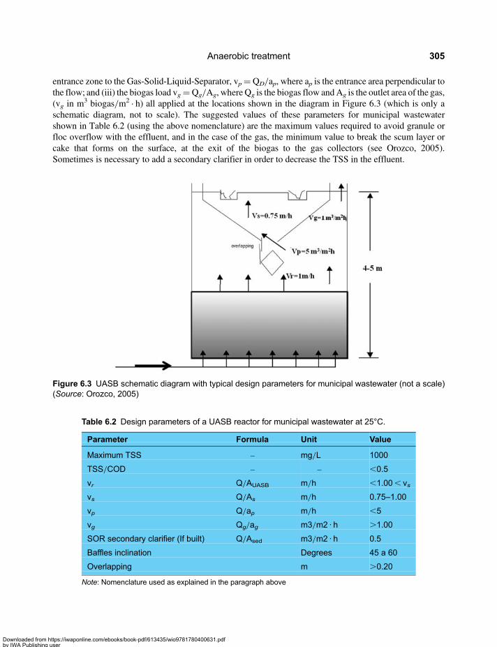
entrance zone to the Gas-Solid-Liquid-Separator, vp=QD/ap, where ap is the entrance area perpendicular tothe flow; and (iii) the biogas load vg=Qg/Ag, where Qg is the biogas flow andAg is the outlet area of the gas,(vg in m3 biogas/m2 · h) all applied at the locations shown in the diagram in Figure 6.3 (which is only aschematic diagram, not to scale). The suggested values of these parameters for municipal wastewatershown in Table 6.2 (using the above nomenclature) are the maximum values required to avoid granule orfloc overflow with the effluent, and in the case of the gas, the minimum value to break the scum layer orcake that forms on the surface, at the exit of the biogas to the gas collectors (see Orozco, 2005).Sometimes is necessary to add a secondary clarifier in order to decrease the TSS in the effluent.

Figure 6.3 UASB schematic diagram with typical design parameters for municipal wastewater (not a scale)(Source: Orozco, 2005)

Table 6.2 Design parameters of a UASB reactor for municipal wastewater at 25°C.

Parameter Formula Unit Value

Maximum TSS – mg/L 1000

TSS/COD – – ,0.5

vr Q/AUASB m/h ,1.00, vs

vs Q/As m/h 0.75–1.00

vp Q/ap m/h ,5

vg Qg/ag m3/m2 · h .1.00

SOR secondary clarifier (If built) Q/Ased m3/m2 · h 0.5

Baffles inclination Degrees 45 a 60

Overlapping m .0.20

Note: Nomenclature used as explained in the paragraph above



The main process parameter for design of the UASB reactors is the organic volumetric load,Lv= S0/td= S0 · Q/V (kg COD/m3 · d). This volumetric load should be maintained at values in therange 2–30, depending on the temperature, on the design of the reactor and on the concentration ofvolatile fatty acids in the wastewater. A value of Lv= 2 kg COD/m3 · d can be used for municipalwastewater at 15°C, adjusted for the temperature change using Equation 6.1.

The hydraulic load or Surface Overflow Rate (SOR), equivalent to the rising water velocity in thereactor (vr) (m

3/m2 · h=m/h) should be less than 1 m/h, so as to prevent trapping particles into theeffluent and their washout with the effluent stream leaving the reactor. Since the typical height of aUASB reactor is 4–5 m, for a vr of 1 m/h the detention time in the UASB reactor is td= 4–5 hours(0.17 to 0.21 d). So for municipal wastewater which received wastewater with a COD concentration of400 mg/l (0.4 kg/m3) or less, the Lv will be around (0.4 kg COD/m3)/(0.2 d)= 2 kg COD/m3 · d. It isclear that, for municipal wastewater, the hydraulic criterion vr≤ 1 m/h automatically implies that itmeets the criterion for volumetric load (which is the fundamental criterion), so the design of a UASBreactor for municipal wastewater becomes a purely hydraulic exercise. As a result the hydraulic criteriafor design of a UASB reactor for municipal wastewater which are summarized in Table 6.2 are theones to be applied. For instance, the settler in the GSLS could be wider than the reactor, if needed, inorder to meet the criteria vr, 1.00, vs. The overlapping is defined as the horizontal length (in thesettler entrance area) used to avoid the direct vertical flow of water from the reactor into the settler ofthe GSLS.

The UASB reactor is divided into two parts. The bottom part serves as the liquid volume storage andhas a height HL (1.5 to 2.0 m). This part is the site in which the sludge blanket material is stored. Anextra height of 0.5 to 1.0 m is left to take care of the peak flows so the total liquid height is HL≈ 2.5 m.The upper part, with a height HG of also about 2.5 m, comprises the GSLS, with an angle of plateinclination of 45 degrees. Thus, the typical total height of a UASB reactor is HT=HL+HG= 5.0 m(Metcalf & Eddy, 2003, pp. 1009). The UASB has proven to be a simple, cost-effective and reliable reactor.

Anaerobic filter (AF)2

The anaerobic filters (AF) are fixed medium (attached growth) reactors in which anaerobic bacteria growattached to a filter medium of rock or plastic material with a net area (a) of between 50 and 200 m2/m3

of media, and mostly in the porous zone of the media. Treatment occurs as the wastewater passesthrough the filter medium, where the bacteria come into close contact with the wastewater and consumethe BOD contained in it. Fixed bed reactors have a variety of geometrical forms such as circular andrectangular, and are of two kinds in terms of the direction of flow: (i) up-flow or ascending flow reactor;and (ii) down-flow or descending flow reactor. See Figures 6.4 and 6.5.

Anaerobic microorganisms are formed in flocs or granules and are trapped in the pores of the media. Withthe increasing accumulation of biomass, part of it is separated from the filter media and is carried outwith the effluent. Despite this process, the average residence time of the biomass in the reactor is overthan 20 days. Up-flow filters are more common than down-flow filters. Down-flow filters can work witha floating medium. In Down-flow filters, recirculation is commonly used. The need for a uniformdistribution along the bottom or surface, limit their size to a manageable hydraulic flow (LibhaberMenahem, 2007).

2This paragraph is mainly based on the Book “Sistemas Simples para Tratamento de Esgotos Sanitarios, Experiencia Brasileira” byCicero Onofre de Andrade Neto (1997) and on the article “Appropriate Technology for Wastewater Treatment and Reuse inDeveloping Countries” by Menahem Libhaber (2007).



To prevent clogging of the filter, effective removal of suspended solids from the raw sewage is requiredprior to its inflow to the filter. Such removal of suspended solids can be achieved by rotating micro screens.For small treatment plants, decanter-digesters (otherwise known as large septic tanks or Imhoff tanks) areused to remove suspended solids prior to an anaerobic filter. In addition to the use of anaerobic filters asthe main treatment unit, they can be used as polishing unites for improvement of the quality of theeffluent of a preceding unit. They are in fact more suitable to perform as polishing units since when fedwith treated effluent of a preceding unit they are less bound to clog by suspended solids and have to treata lower content dissolved organic matter. Anaerobic filters are used as the main treatment unit mainly forsmall and medium size municipalities, while for polishing application anaerobic filters are used in theentire range of cities size, including in treatment plants of large cities.

With time, the anaerobic filter becomes clogged because of the growth of the biomass. When the pressuredrop on the filter becomes too high, it needs to be washed. Similarly to sand filters for water treatment, theanaerobic filter is washed by a stream of water or treated effluent which is passed through it in a counter wisedirection to its operation flow. The wash water, which contains the excess sludge, is directed to the sludgehandling facilities, which are usually just drying beds. Since the process is anaerobic, the excess sludgequantities are small and the washing, which is specific to each systems, is required infrequently, onceevery several days to once every few months. Backwashing becomes more complicated as the anaerobicfilter system is larger. Therefore when they are the main treatment unit, anaerobic filters are morefrequently used for plants serving small populations (in which the backwashing is simpler). In larger

Figure 6.5 Down-flow anaerobic filter, with inflow and outflow by perforated tubes (Source: Andrade Neto etal. 2009)

Figure 6.4 Up-flow anaerobic filter (Source: Andrade Neto et al. 2009)



plants, anaerobic filters serve as a polishing unit, where they produce less sludge and need less frequent backwashing. All anaerobic filters must have efficient backwashing systems and convenient arrangements forreplacing the filtering media.

Design parameters are the detention time td (V/Q, h), volumetric organic load Lv (S0/td, kg COD/m3 · d)

and the hydraulic load, qa (m3/m2 · d). The up-flow filter should have a height between 1.2 and 3.0 m, and

the filter medium may be of rock or plastic with a net area (a) preferably larger than 100 m2/m3 of filtermaterial. Table 6.3 presents typical design criteria for a temperature of 25°C (Andrade Neto, 1997;Wikilibros 2007; Libhaber 2007).

Anaerobic Filters are often used as a Polishing treatment system for Septic Tanks (ST) with removalefficiencies of about 50% in the septic tank (and even higher at high temperatures), for a net efficiencyof the system (Septic Tank followed by Anaerobic Filter) of up to 85%. Another way of looking at sucha system is considering the septic tank as the pretreatment unit of the anaerobic filter. At any rate, such asystem is basically a system of two anaerobic reactors in series. This type of system is used in smalltowns of up to 10,000 inhabitants, because of the limitation of the septic tank in handling larger flows.The detention times in an anaerobic filter for a given population and temperature, in a system of a septictank followed by an anaerobic filter, are shown in Table 6.4 (based on Andrade Neto, 1997). Figure 6.6shows an innovative design of a septic tank combined with an up-flow anaerobic filter followed by adown-flow anaerobic filter (Andrade Neto, 1997).

Table 6.3 Design criteria of the up-flow anaerobic filter at 25°C*.

Detention time, td Volumetric load, LV Hydraulic load, qa Height, h

Units hours Kg COD/m3 · d m3/m2 · d m

Range 4–12 1.0–1.6 6–15 1.2–3.0

Typical value 6 1.2 10 2.5

*The temperature correction of LV is done using Equation 6.1Source: Prepared based on Andrade Neto, Cicero Onofre (1997), pp. 55–60

Table 6.4 Variation of detention time td in days, in an anaerobic filter with populationsize and with temperature in a system of a septic tank followed an anaerobic filter.

Population Temperature °C

inhabitants

, 15°C 15 to 25°C .25°C

1500 1.17 1.00 0.92

1501–3000 1.08 0.92 0.83

3001–4500 1.09 0.83 0.75

4501–6000 0.92 0.75 0.67

6001–7500 0.83 0.67 0.58

7501–9000 0.75 0.58 0.50

.9000 0.75 0.50 0.50

Source: Andrade Neto (1997) p. 56



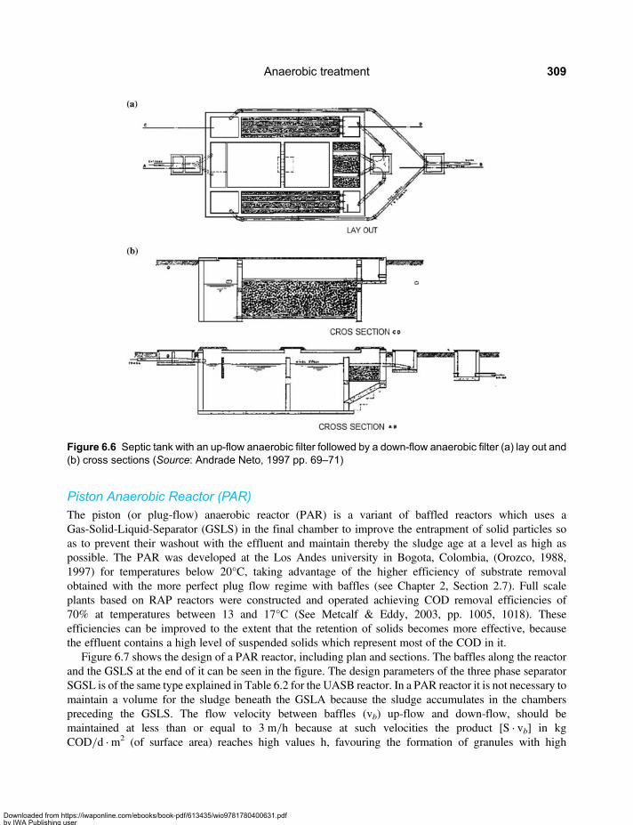
Piston Anaerobic Reactor (PAR)The piston (or plug-flow) anaerobic reactor (PAR) is a variant of baffled reactors which uses aGas-Solid-Liquid-Separator (GSLS) in the final chamber to improve the entrapment of solid particles soas to prevent their washout with the effluent and maintain thereby the sludge age at a level as high aspossible. The PAR was developed at the Los Andes university in Bogota, Colombia, (Orozco, 1988,1997) for temperatures below 20°C, taking advantage of the higher efficiency of substrate removalobtained with the more perfect plug flow regime with baffles (see Chapter 2, Section 2.7). Full scaleplants based on RAP reactors were constructed and operated achieving COD removal efficiencies of70% at temperatures between 13 and 17°C (See Metcalf & Eddy, 2003, pp. 1005, 1018). Theseefficiencies can be improved to the extent that the retention of solids becomes more effective, becausethe effluent contains a high level of suspended solids which represent most of the COD in it.

Figure 6.7 shows the design of a PAR reactor, including plan and sections. The baffles along the reactorand the GSLS at the end of it can be seen in the figure. The design parameters of the three phase separatorSGSL is of the same type explained in Table 6.2 for the UASB reactor. In a PAR reactor it is not necessary tomaintain a volume for the sludge beneath the GSLA because the sludge accumulates in the chamberspreceding the GSLS. The flow velocity between baffles (vb) up-flow and down-flow, should bemaintained at less than or equal to 3 m/h because at such velocities the product [S · vb] in kgCOD/d · m2 (of surface area) reaches high values h, favouring the formation of granules with high

Figure 6.6 Septic tank with an up-flow anaerobic filter followed by a down-flow anaerobic filter (a) lay out and(b) cross sections (Source: Andrade Neto, 1997 pp. 69–71)



sedimentation velocities (Orozco, 1988). Amedia of plastic material can be added at the top of each chamberto assist in the retention of solids in the chambers, because the ascending granules or flocs attached to gasbubbles find an obstacle (the plastic media) that forces the gas bubbles to release the flocs, which settle in thesame chambers. The recommended detention time in the RAP reactor is 10 h at 15°C. This value should becorrected for the temperature, in the range 15–20°C, using Equation (6.1).

The PAR reactor was the first baffled reactor constructed in the world in a full scale plant (Metcalf &Eddy, 2003, pp. 1005). Moreover, their use for operation at sub-optimal temperatures (lower than 15°C)has influenced the development of other baffled reactors that have been built at an accelerated pace inseveral countries, especially in China (Zonglian She et al. 2006), New Zealand (Foxon et al. 2003) andBolivia (Medina et al. 1993).

The quantity of the excess biomass is minimal and is slowly washed out with the effluent, but it couldbe trapped with a secondary clarifier. As the PAR is an open to air reactor, a possible improvement is tocover it with a geomembrane to capture the biogas for burning o use.

6.1.3 PerformanceEfficiencyUASB

UASB reactors treatingmunicipal wastewater produce an effluent that usually contains 35–100 mg/l of totalDBO5, 30–40 mg/l of soluble DBO5 and 50–130 mgmg/l TSS. The removal efficiencies are 60–75% of thetotal BOD5 and 65–80% for TSS. Construction costs of a UASB reactor are in the range 20–40 US$/Capita.Even after including additional treatment for effluent polishing, the investment cost still compares

Figure 6.7 Plan and sections of a PAR type baffled reactor (Source: Orozco, 2005)



favourably with the investment of 100–150 US$/Capita considered typical for a conventional secondarytreatment plant. The operation and maintenance costs (O&M) are in the range 1.0–1.5 US$/Capita · yr,which is much lower than those of conventional treatment plants. Several UASB plants under operationin Brazil are successfully serving populations of about 1 million each, making the UASB processadequate for cities of all sizes (Libhaber, 2004; Libhaber, 2007).

Anaerobic filter

Chernicharo (2000) reports Total BOD removal efficiencies of anaerobic filters in the range of 70–80%when the anaerobic filter is the main treatment unit and 75–95% when it used as a polishing units.Andrade Neto (1997, 2000) reports results of a research on an anaerobic filter system treating municipalwastewater which was in operation for six years. This system, consisting of a septic tank followed by anup-flow anaerobic filter followed by a down-flow anaerobic filter, achieved a COD removal of up to90%. The effluent of this anaerobic filter system contained less than 30 mg/l of BOD and less than20 mg/l total suspended solids. Sludge withdrawal from the filter was undertaken once every sixmonths. The investment cost in anaerobic filter systems is 10–25 US$/Capita and the O&M are in therange 0.8–1.0 US$/Capita · yr. (Libhaber, 2007).

Plug flow anaerobic reactor

The typical COD removal efficiency of a PAR reactor at 15°C is 60–70%, if an additional solids separationsystem after the GSLS system in last chamber is not used. An additional solids separator can improve theremoval efficiency (Orozco, 2005).

Reasons for the difference in performance of the various anaerobic reactors types

The three anaerobic reactors (or anaerobic unit processes) which are used most frequently for treatment ofmunicipal wastewater are: Anaerobic Lagoons, UASB reactors and Anaerobic Filters. Anaerobic filtersachieve the highest organic matter removal, in the range 70–80% of BOD5 removal, followed by UASBwith BOD5 removal levels in the range 60–75%. Anaerobic lagoons achieve a lower BOD5 removallevel, in the range 40–70%. The reason for the different removal level of organic matter in each of thesereactors is that the mixing mechanisms and the intensity of the contact of the wastewater with thebacterial biomass are different in each type of reactor. In anaerobic lagoons the mixing in the reactor isnot effective and the contact of the organic matter dissolved in the raw sewage flowing into the lagoonwith the biomass which develops on the bottom of the lagoon is not intense, so only partial removal ofdissolved organic matter is achieved. The removal of the suspended solids contained in the raw sewage,which settle in the lagoon, is high, but as a whole, the organic matter removal in an anaerobic lagoon islow in comparison to other anaerobic processes. In a UASB reactor the granular biomass particles floatin the liquid due to the flow pattern and the action of the biogas released in the reactor. Consequently,the contact of the liquid with biomass is more intense than in anaerobic lagoons and as a result, theorganic matter removal is higher. However, there is a limit to the capacity of the UASB reactor toremove organic matter since a higher concentration of biomass is required for achieving higher removalefficiencies, but it is impossible to achieve higher sludge concentrations since when the concentrationincreases, more sludge is carried away with the effluent, so the organic matter removal in UASB is stillnot very high. In an anaerobic filter, where the biomass is attached to the filter media and the reactor isflooded with the wastewater, the biomass concentration levels in this reactor are high and the contact ofthe liquid that flows into the reactor with the biomass is more effective, and as a result, the level oforganic matter removal is higher than in UASB and certainly higher than in anaerobic lagoons.



Advantages and disadvantagesBOD removal efficiencies in anaerobic systems are in the range 40–90% COD. The investment costs ofthese systems are in the range 20–40 US$/Capita and they employ a variety of flow patterns whichinclude completely mixed, plug flow, filters, and so on. These systems represent innovative technologieswith a high perspective to be used in developing countries. The various anaerobic systems have basicallythe same advantages and disadvantages, which are summarized below (Libhaber, 2007).

The main advantages are:

• They do not require oxygen, and thus has low power consumption.• The gas produced, primarily methane, can be collected and used to generate energy, or can be burned,

reducing greenhouse gas emissions. Carbon emission reduction credits can be obtained, increasingthe financial benefits of the project. The carbon credits may expire in 2012 with the end of theKyoto Protocol.

• The excess sludge quantities produced are much smaller than those generated by aerobic processes,thus the treatment and disposal costs of sludge are small and the negative environmental effects ofthe sludge are minor.

• The area occupied by an anaerobic reactor is small, except for anaerobic lagoons which require asomewhat larger area.

• The electromechanical equipment required for anaerobic processes is minimal.• Construction is simple and uses mostly local materials.• The operation is simpler than mechanized systems.• The investment and O&M costs of anaerobic processes, are much lower than those of aerobic

processes.

The main disadvantages are:

• Anaerobic processes need a longer start-up time to develop the necessary amount of anaerobicbiomass in the reactor.

• They are more sensitive to lower temperatures.• They are more sensitive to toxic substances.• Biological nitrogen and phosphorus removal cannot be achieved in an anaerobic process.• They have a potential of generating odours and corrosive gases, however those can be controlled.• They have a low removal efficiency of BOD compared to aerobic systems so the effluent quality of a

one stage anaerobic treatment process may not meet discharge standards and, depending on thespecific project conditions, a subsequent treatment stage might be necessary.

6.2 BASIC DESIGN PROCEDURE6.2.1 General design considerationsAs explained, the basic principle of anaerobic treatment is the concentration of a large amount of biomass,whether in a sludge blanket or attached to a fixed medium, which is a consortium of several types ofmicroorganisms cooperating metabolically to produce the bioconversion of BOD to biogas.

The main type of anaerobic treatment is the UASB, along with the baffled reactor (BR), one of whoseforms is the PAR. These types of treatment are known as “Suspended Growth Anaerobic Treatment”.Such treatment consists basically of a tank where biomass accumulates and reacts with the wastewater,and a three phase separation system, the gas-solid-liquid separator (GSLS). The other type of anaerobictreatment is the “Attached Growth Anaerobic Treatment” of which the main type is the Anaerobic Filter,



often used as a polishing treatment, consisting of tanks filled with crushed rocks or a plastic filter medium, towhich biomass is attached and grows, on the surface and within the pores of the medium. Attached growthanaerobic systems are mainly used in treatment plants of small towns and small communities, becausethey require filters backwashing and cleaning, which something are more difficult to perform in larger scaleplants. Also, the homogeneous hydraulic distribution system required for proper operation, limits the size ofanaerobic treatment plants. However, large plants can be built of smaller modules which enable overcomingthese problems. The anaerobic treatment system can be classified as Sustainable Innovative AppropriateTechnology processes as defined by Libhaber (2007) since they are low-priced treatments processes,simple to operate, and can be constructed using local materials, without major or equipment requirements.

The basic process design parameter of the UASB reactors is the volumetric load, Lv= S0/td= S0 · Q/V(kg COD/m3 · d) which must be maintained in the range 1–30, depending on the design of the reactor,temperature and concentration of volatile fatty acids. For municipal wastewater at 15°C it isrecommended to use Lv= 1 kg COD/m3 · d, corrected for the temperature using Equation 6.1.

The other parameter of importance for design of a UASB reactor is the hydraulic load or Surface overflowrate (SOR) which is the up-flow velocity in the reactor, vr (m

3/m2 · h=m/h). This parameter must be kept ata value lower than 1 m/h, to avoid dragging of suspended solid particles (the biomass granules) out of thereactor with the effluent. For municipal wastewater, the hydraulic criterion vr, 1 m/h automaticallyimplies that it meets the criteria for volumetric load so the design of a UASB for municipal wastewaterbecomes a hydraulic exercise. However, often, for certain geometric design of the UASB reactor andtypical GSLS, the detention time, td, can be used as the main design parameter3. In fact it has beenshown in practice that a reactor 5 m high with a GSLS with baffles at a 45° angle and 2.5 m high, workswell with municipal wastewater. The geometry of the reactor can vary. Here we analyze the standardmodule (denominated GSLS-SM) presented in Figure 6.9, but there are other typed of modules, withcircular reactor tank, triangular cross section, and so on.

For the anaerobic filter, the main design parameters are the td (V/Q), Lv (S0/td, kgCOD/m3 · d) and the

hydraulic load, qa (m3/m2 · d). The up-flow anaerobic filter should have a height of between 1.2 and 3.0 m,

and the filter medium may be rock or a plastic medium with a specific net area (a) greater than 100 m2/m3

of filter material.The PAR treatment presented above is usually designed for temperatures below 20°C, with chambers

(between baffles) water velocity of less than 3 m/h and a GSLS-SM located in the last chamber.In general, a main drawback of the anaerobic process is that the solids separation units are of low

efficiency, and so it is recommended whenever possible to design a final secondary clarifier to improvethe TSS (and BOD) removal efficiency in the effluent.

6.2.2 Orderly design method, ODMThe overall design methodology for anaerobic treatment consists of the following:

(1) Determine the external or independent variables: Same as in Chapter 5, Section 5.2.2, Paragraph 1.(2) Determine the Flow Diagram of the Anaerobic Treatment: The components of a typical UASB

system are shown in Figure 6.8.(3) Design the Preliminary Treatment System: This design is the same to the design of the preliminary

treatment in Chapter 5, Section 5.2.2, Paragraph 3.

3In effect the component that carries out the bioconversion is the sludge blanket, and hence its volume determines the td, what makes thismeasure a design parameter. The GSLS must meet the hydraulic relationships shown in Table 6.2.



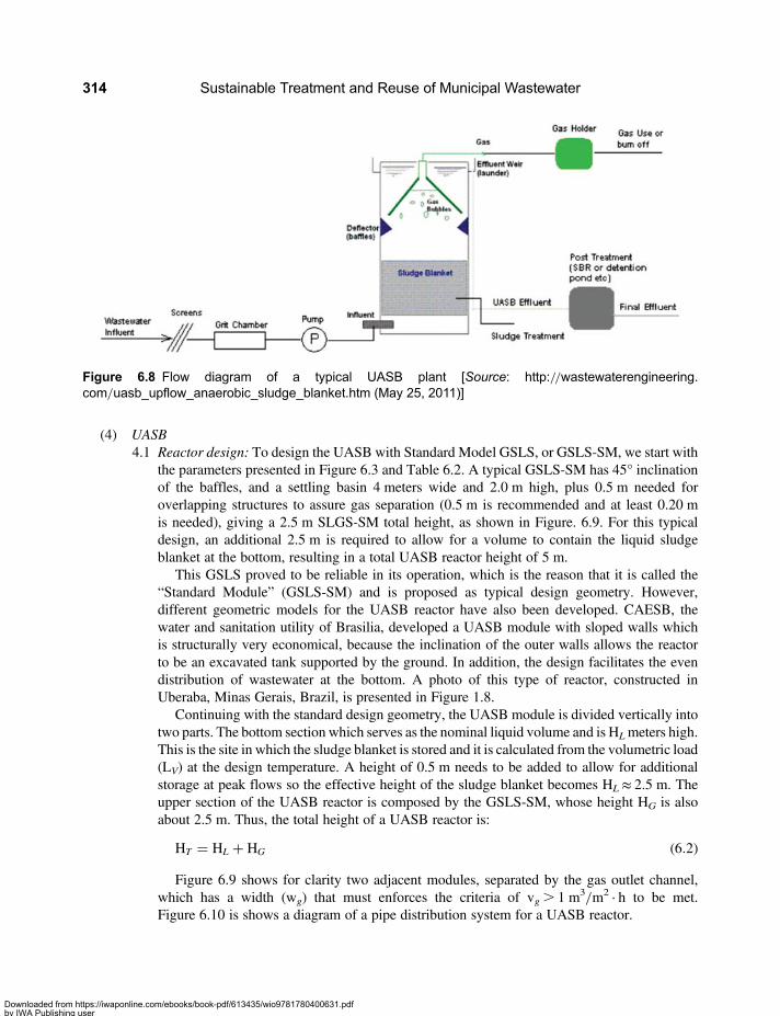
(4) UASB4.1 Reactor design: To design the UASB with Standard Model GSLS, or GSLS-SM, we start with

the parameters presented in Figure 6.3 and Table 6.2. A typical GSLS-SM has 45° inclinationof the baffles, and a settling basin 4 meters wide and 2.0 m high, plus 0.5 m needed foroverlapping structures to assure gas separation (0.5 m is recommended and at least 0.20 mis needed), giving a 2.5 m SLGS-SM total height, as shown in Figure. 6.9. For this typicaldesign, an additional 2.5 m is required to allow for a volume to contain the liquid sludgeblanket at the bottom, resulting in a total UASB reactor height of 5 m.

This GSLS proved to be reliable in its operation, which is the reason that it is called the“Standard Module” (GSLS-SM) and is proposed as typical design geometry. However,different geometric models for the UASB reactor have also been developed. CAESB, thewater and sanitation utility of Brasilia, developed a UASB module with sloped walls whichis structurally very economical, because the inclination of the outer walls allows the reactorto be an excavated tank supported by the ground. In addition, the design facilitates the evendistribution of wastewater at the bottom. A photo of this type of reactor, constructed inUberaba, Minas Gerais, Brazil, is presented in Figure 1.8.

Continuing with the standard design geometry, the UASB module is divided vertically intotwo parts. The bottom section which serves as the nominal liquid volume and is HLmeters high.This is the site in which the sludge blanket is stored and it is calculated from the volumetric load(LV) at the design temperature. A height of 0.5 m needs to be added to allow for additionalstorage at peak flows so the effective height of the sludge blanket becomes HL≈ 2.5 m. Theupper section of the UASB reactor is composed by the GSLS-SM, whose height HG is alsoabout 2.5 m. Thus, the total height of a UASB reactor is:

HT = HL + HG (6.2)

Figure 6.9 shows for clarity two adjacent modules, separated by the gas outlet channel,which has a width (wg) that must enforces the criteria of vg. 1 m3/m2 · h to be met.Figure 6.10 is shows a diagram of a pipe distribution system for a UASB reactor.

Figure 6.8 Flow diagram of a typical UASB plant [Source: http://wastewaterengineering.com/uasb_upflow_anaerobic_sludge_blanket.htm (May 25, 2011)]









Figure 6.9 Standardmoduleofagassolid liquidseparator (GSLS-SM)ofaUASBreactor (Source:Orozco,2005)

Figure 6.10 Plan and section of a manifold for inflow distribution at the bottom of the UASB reactor



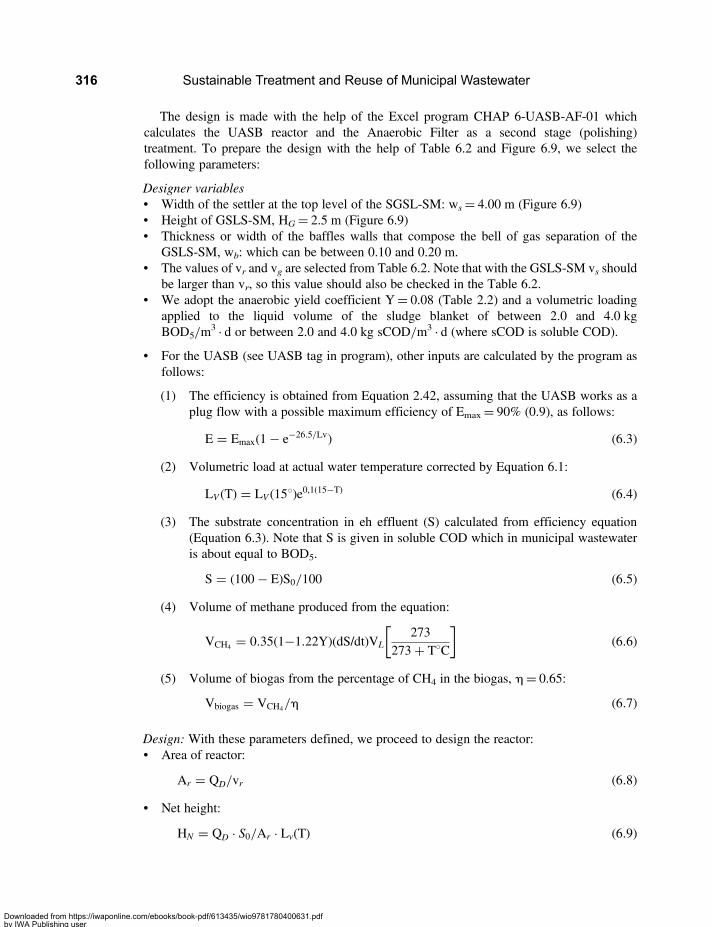
The design is made with the help of the Excel program CHAP 6-UASB-AF-01 whichcalculates the UASB reactor and the Anaerobic Filter as a second stage (polishing)treatment. To prepare the design with the help of Table 6.2 and Figure 6.9, we select thefollowing parameters:

Designer variables• Width of the settler at the top level of the SGSL-SM: ws= 4.00 m (Figure 6.9)• Height of GSLS-SM, HG= 2.5 m (Figure 6.9)• Thickness or width of the baffles walls that compose the bell of gas separation of the

GSLS-SM, wb: which can be between 0.10 and 0.20 m.• The values of vr and vg are selected from Table 6.2. Note that with the GSLS-SM vs should

be larger than vr, so this value should also be checked in the Table 6.2.• We adopt the anaerobic yield coefficient Y= 0.08 (Table 2.2) and a volumetric loading

applied to the liquid volume of the sludge blanket of between 2.0 and 4.0 kgBOD5/m

3 · d or between 2.0 and 4.0 kg sCOD/m3 · d (where sCOD is soluble COD).

• For the UASB (see UASB tag in program), other inputs are calculated by the program asfollows:

(1) The efficiency is obtained from Equation 2.42, assuming that the UASB works as aplug flow with a possible maximum efficiency of Emax= 90% (0.9), as follows:

E = Emax(1− e−26.5/Lv) (6.3)

(2) Volumetric load at actual water temperature corrected by Equation 6.1:

LV (T) = LV (158)e0,1(15−T) (6.4)

(3) The substrate concentration in eh effluent (S) calculated from efficiency equation(Equation 6.3). Note that S is given in soluble COD which in municipal wastewateris about equal to BOD5.

S = (100− E)S0/100 (6.5)

(4) Volume of methane produced from the equation:

VCH4 = 0.35(1−1.22Y)(dS/dt)VL273

273+ T8C

[ ](6.6)

(5) Volume of biogas from the percentage of CH4 in the biogas, h= 0.65:

Vbiogas = VCH4/h (6.7)

Design: With these parameters defined, we proceed to design the reactor:• Area of reactor:

Ar = QD/vr (6.8)

• Net height:

HN = QD · S0/Ar · Lv(T) (6.9)



• Effective liquid height (at least 2.5 m):

HL = HN + 0.5 (6.10)

• UASB height:

HT = HL + HG (6.11)

• Detention time:

td = HT/vr (6.12)

• UASB volume:

VUASB = QD · td = HT · Ar (6.13)

• Net volume of sludge blanket

VL = Ar · HL (6.14)

• Total gas extraction area:

Ag = Vbiogas/vg (6.15)

• UASB length in the direction perpendicular to Figure 6.9, so that the length to width ratiois 3/2:

LUASB/WUASB = 3/2 = 1.5: LUASB = √(1.5Ar) (6.16)

• UASB width:

WUASB = Ar/LUASB (6.17)

• Total width of the gas outlet throats (Wg= nMP · wg), wg being the throat width of each ofthe n modules:

Wg = Ag/LUASB (6.18)

• Preliminary number of modules (nMP):

nMP = WUASB/(wg + ws + 2wb)

From which:

nMP = (WUASB −Wg)/(ws + 2wb) (6.19)

It is noted from Figure 6.9 that the module width is (wg+ws+ 2wb). At this point, all thefigures necessary to compute the dimensions of the UASB reactor are calculated, but itshould be remembered that the number of modules (nM) must be an integer and thereforenMP must be rounded up. In this way all the hydraulic parameters are on the safe side.• Gas throat width:

wg = Wg/nM (6.20)



• Total UASB width:

WUASBD = nM(wg + ws + 2wb) (6.21)

• Total Area of settlers:

As = nM × 4,00× LUASB (6.22)

• Then, the settling velocity (or SOR): vs=QD/As, should be around 0.75 (or less). Note thatfor the geometric design proposed vr, vs. The subscript D is for design or definite values.The reactor final area is calculated as:

ArD = WUASBD × LUASBD (6.22a)

• Final reactor velocity:

vrD = QD/ArD (6.23)

• Net volume of sludge blanket:

VLD = ArD · HL (6.24)

• Design volume of UASB:

VUASBD = ArD · HT (6.24a)

• A system to remove the excess sludge should be provided. Sludge production (Qx):

Qx = VUASBD Y(S0 − S)/tdD (6.25)

4.2 Inlet and outlet structures: Inlet structures should ensure the proper effective flow thedistribution in the sludge blanket volume and this is achieved by placing outlets on thefloor, one at every 1 to 2 m2 of tank bottom. One way to do it is by using an externalmanifold that feeds a series of perforated pipes laid throughout the floor area, ensuring anapproximately uniform distribution as shown in Figure 6.10. To meet proper distributionobjectives, the design of the feed pipelines is the following:• Place two parallel branch pipes each driving a flow of Qm=QD/2 with a velocity that meets

following restriction: the area (ao) of each outlet orifice should have a diameter of at least 2′′

for the wastewater to flow freely. Then calculate the pipe diameter (wm) of each branchmanifold of area am for a given pipe velocity v:

am = QD/2v (6.26)

• Then calculate the preliminary number of outlet orifices (no) selecting either 1 or 2 for eachm2 of area. no is the orifices’ density (εo) or number of outlet orifices per square meter offloor area:

no = ArD/1o (6.27)

• Every manifold branch (there are two manifolds, one at each side of the reactor) feedsno/2 orifices, each orifice of an area ao (see Figure 6.10). The orifices are distributed ina number of distribution pipes nd, leaving the principal manifold branch and going



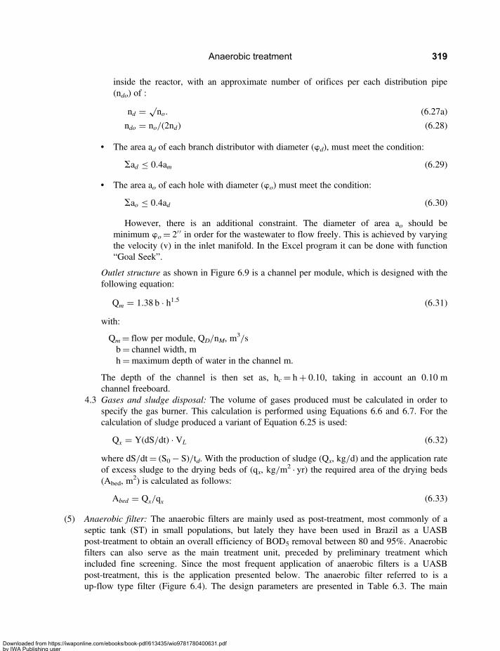
inside the reactor, with an approximate number of orifices per each distribution pipe(ndo) of :

nd = √no. (6.27a)

ndo = no/(2nd) (6.28)

• The area ad of each branch distributor with diameter (wd), must meet the condition:

Sad ≤ 0.4am (6.29)

• The area ao of each hole with diameter (wo) must meet the condition:

Sao ≤ 0.4ad (6.30)

However, there is an additional constraint. The diameter of area ao should beminimum wo= 2′′ in order for the wastewater to flow freely. This is achieved by varyingthe velocity (v) in the inlet manifold. In the Excel program it can be done with function“Goal Seek”.

Outlet structure as shown in Figure 6.9 is a channel per module, which is designed with thefollowing equation:

Qm = 1.38 b · h1.5 (6.31)

with:

Qm= flow per module, QD/nM, m3/s

b= channel width, mh=maximum depth of water in the channel m.

The depth of the channel is then set as, hc= h+ 0.10, taking in account an 0.10 mchannel freeboard.

4.3 Gases and sludge disposal: The volume of gases produced must be calculated in order tospecify the gas burner. This calculation is performed using Equations 6.6 and 6.7. For thecalculation of sludge produced a variant of Equation 6.25 is used:

Qx = Y(dS/dt) · VL (6.32)

where dS/dt= (S0− S)/td. With the production of sludge (Qx, kg/d) and the application rateof excess sludge to the drying beds of (qx, kg/m

2 · yr) the required area of the drying beds(Abed, m

2) is calculated as follows:

Abed = Qx/qx (6.33)

(5) Anaerobic filter: The anaerobic filters are mainly used as post-treatment, most commonly of aseptic tank (ST) in small populations, but lately they have been used in Brazil as a UASBpost-treatment to obtain an overall efficiency of BOD5 removal between 80 and 95%. Anaerobicfilters can also serve as the main treatment unit, preceded by preliminary treatment whichincluded fine screening. Since the most frequent application of anaerobic filters is a UASBpost-treatment, this is the application presented below. The anaerobic filter referred to is aup-flow type filter (Figure 6.4). The design parameters are presented in Table 6.3. The main



design parameter is the detention time, corrected for temperature by Equation 6.1, modified asfollows:

td(T) = td(258C)e−0.1(T−25) (6.34)

The design procedure, performed with the Excel program CHAP 6-Anaerobic-UASB-AF.xls(tag AF) is as follows:

Designer variables○ Select a detention time at 25°C based on Table 6.3.○ Choose the filter height (HF) from Table 6.3, depending on the selected filter medium material.

A freeboard of 0.50 m is added for to a final construction height (HT) (see Figures 6.4 and 6.5).○ Select a yield coefficient (Y) from Table 2.2.○ Propose the fraction of CH4 in the biogas (η), usually 0.65.○ Select the relation length/width (L/w) of the anaerobic filter, usually 2:1.○ Select the surface overflow rate (SOR) or vs for the design of the secondary settler, if there is one○ Propose porosity (n) for the support media. If the media is gravel the porosity should be between

35 and 40%. (See Table 8.3).○ Determine the water temperature.○ Calculate detention time for the determined temperature using Equation 6.34.○ Calculate the BOD concentration in the effluent (S) assuming a 50% BOD5 removal in the

Anaerobic Filter and taking into account that the effluent of the UASB is the influent to theAnaerobic Filter.

○ Calculate the production of CH4 using Equation 6.6.○ Calculate the biogas production using Equation 6.7.○ Calculate the input and output structures for a selected number of distribution manifolds (nM)

(See Figure 6.5). The flow per manifold is:

QD/nM (6.35)

○ Select a preliminary water velocity (1 m/s) for the inlet manifolds. This velocity will becorrected later with the “Goal Seek” function of Excel or by trial and error.

○ Propose an application rate (qx) for drying beds.

Design○ Calculate the nominal volume of the anaerobic filter:

VAF = QD · td (6.36)

○ Calculate the area of the reactor:

Ar = VAF/HF (6.37)

○ Calculate the total height of the reactor: HT=HF+ 0.50○ Calculate the actual LV using Equation 5.2 and then correct for the temperature using Equation

6.4. Compare with the limits defined in Table 6.3.○ Calculate the hydraulic load:

q = QD/Ar (6.38)



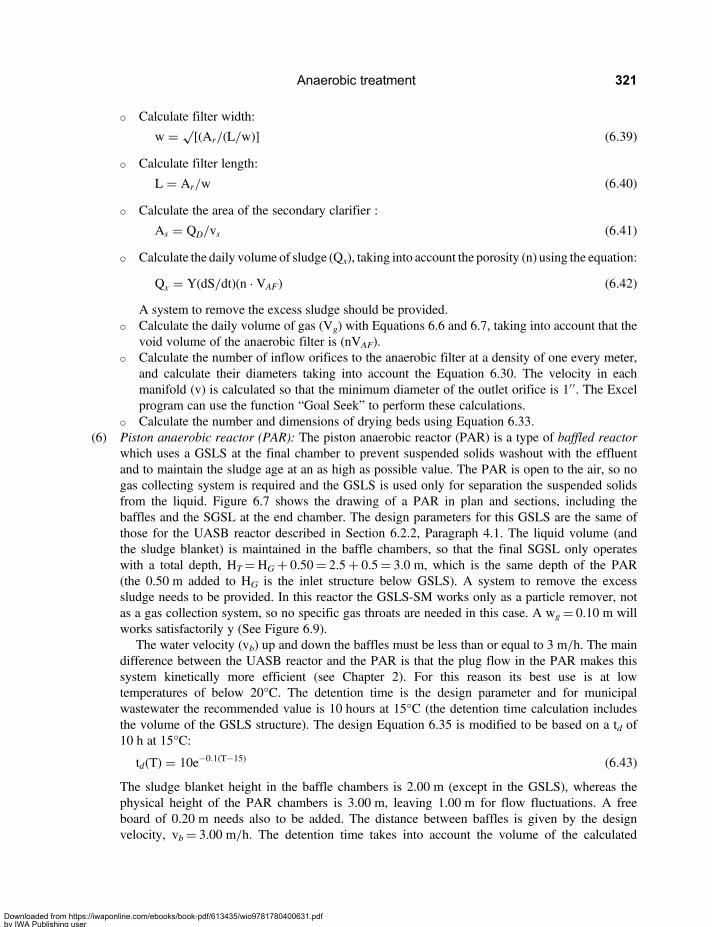
○ Calculate filter width:

w = √[(Ar/(L/w)] (6.39)

○ Calculate filter length:

L = Ar/w (6.40)

○ Calculate the area of the secondary clarifier :

As = QD/vs (6.41)

○ Calculate the daily volume of sludge (Qx), taking into account the porosity (n) using the equation:

Qx = Y(dS/dt)(n · VAF) (6.42)

A system to remove the excess sludge should be provided.○ Calculate the daily volume of gas (Vg) with Equations 6.6 and 6.7, taking into account that the

void volume of the anaerobic filter is (nVAF).○ Calculate the number of inflow orifices to the anaerobic filter at a density of one every meter,

and calculate their diameters taking into account the Equation 6.30. The velocity in eachmanifold (v) is calculated so that the minimum diameter of the outlet orifice is 1′′. The Excelprogram can use the function “Goal Seek” to perform these calculations.

○ Calculate the number and dimensions of drying beds using Equation 6.33.(6) Piston anaerobic reactor (PAR): The piston anaerobic reactor (PAR) is a type of baffled reactor

which uses a GSLS at the final chamber to prevent suspended solids washout with the effluentand to maintain the sludge age at an as high as possible value. The PAR is open to the air, so nogas collecting system is required and the GSLS is used only for separation the suspended solidsfrom the liquid. Figure 6.7 shows the drawing of a PAR in plan and sections, including thebaffles and the SGSL at the end chamber. The design parameters for this GSLS are the same ofthose for the UASB reactor described in Section 6.2.2, Paragraph 4.1. The liquid volume (andthe sludge blanket) is maintained in the baffle chambers, so that the final SGSL only operateswith a total depth, HT=HG+ 0.50= 2.5+ 0.5= 3.0 m, which is the same depth of the PAR(the 0.50 m added to HG is the inlet structure below GSLS). A system to remove the excesssludge needs to be provided. In this reactor the GSLS-SM works only as a particle remover, notas a gas collection system, so no specific gas throats are needed in this case. A wg= 0.10 m willworks satisfactorily y (See Figure 6.9).

The water velocity (vb) up and down the baffles must be less than or equal to 3 m/h. The maindifference between the UASB reactor and the PAR is that the plug flow in the PAR makes thissystem kinetically more efficient (see Chapter 2). For this reason its best use is at lowtemperatures of below 20°C. The detention time is the design parameter and for municipalwastewater the recommended value is 10 hours at 15°C (the detention time calculation includesthe volume of the GSLS structure). The design Equation 6.35 is modified to be based on a td of10 h at 15°C:

td(T) = 10e−0.1(T−15) (6.43)

The sludge blanket height in the baffle chambers is 2.00 m (except in the GSLS), whereas thephysical height of the PAR chambers is 3.00 m, leaving 1.00 m for flow fluctuations. A freeboard of 0.20 m needs also to be added. The distance between baffles is given by the designvelocity, vb= 3.00 m/h. The detention time takes into account the volume of the calculated



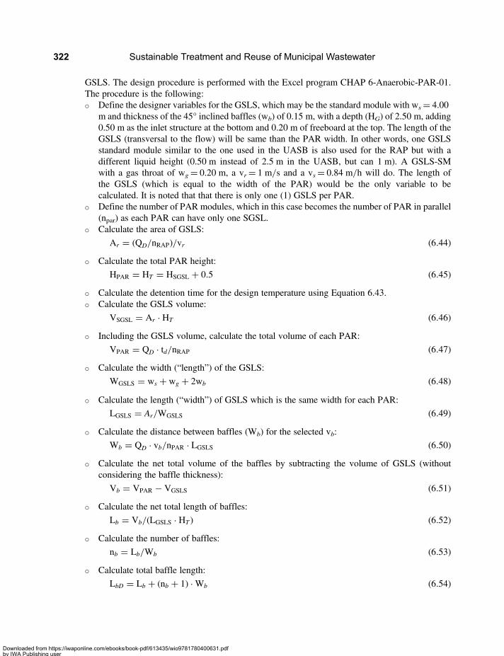
GSLS. The design procedure is performed with the Excel program CHAP 6-Anaerobic-PAR-01.The procedure is the following:○ Define the designer variables for the GSLS, which may be the standard module with ws= 4.00

m and thickness of the 45° inclined baffles (wb) of 0.15 m, with a depth (HG) of 2.50 m, adding0.50 m as the inlet structure at the bottom and 0.20 m of freeboard at the top. The length of theGSLS (transversal to the flow) will be same than the PAR width. In other words, one GSLSstandard module similar to the one used in the UASB is also used for the RAP but with adifferent liquid height (0.50 m instead of 2.5 m in the UASB, but can 1 m). A GSLS-SMwith a gas throat of wg= 0.20 m, a vr= 1 m/s and a vs= 0.84 m/h will do. The length ofthe GSLS (which is equal to the width of the PAR) would be the only variable to becalculated. It is noted that that there is only one (1) GSLS per PAR.

○ Define the number of PAR modules, which in this case becomes the number of PAR in parallel(npar) as each PAR can have only one SGSL.

○ Calculate the area of GSLS:

Ar = (QD/nRAP)/vr (6.44)

○ Calculate the total PAR height:

HPAR = HT = HSGSL + 0.5 (6.45)

○ Calculate the detention time for the design temperature using Equation 6.43.○ Calculate the GSLS volume:

VSGSL = Ar · HT (6.46)

○ Including the GSLS volume, calculate the total volume of each PAR:

VPAR = QD · td/nRAP (6.47)

○ Calculate the width (“length”) of the GSLS:

WGSLS = ws + wg + 2wb (6.48)

○ Calculate the length (“width”) of GSLS which is the same width for each PAR:

LGSLS = Ar/WGSLS (6.49)

○ Calculate the distance between baffles (Wb) for the selected vb:

Wb = QD · vb/nPAR · LGSLS (6.50)

○ Calculate the net total volume of the baffles by subtracting the volume of GSLS (withoutconsidering the baffle thickness):

Vb = VPAR − VGSLS (6.51)

○ Calculate the net total length of baffles:

Lb = Vb/(LGSLS · HT ) (6.52)

○ Calculate the number of baffles:

nb = Lb/Wb (6.53)

○ Calculate total baffle length:

LbD = Lb + (nb + 1) ·Wb (6.54)



○ Calculate total PAR length:LPARD = LbD +WGSLS (6.55)

○ Calculate sludge production using Equations 6.25 or 6.32.○ Calculate the outlet channel using Equation 6.31.○ Calculate production of sludge using Equation 6.32 and the drying beds dimensions using

Equation 6.33, as is done in the UASB example.

6.3 BASIC DESIGN EXAMPLE(The model program for this Example is available online at http://www.iwawaterwiki.org/xwiki/bin/view/Articles/Software+Developed+for+Sustainable+Treatment+and+Reuse+of+Municipal+Wastewater).

A Design example that follows the Orderly Design Method (ODM) of Paragraph 6.2.2 is presented incontinuation. The example is developed for a population of 20,000, with the calculation of flow aspresented in Chapter 3. The example refers to a UASB reactor followed by an Anaerobic Filter. TheODM is developed step by step in a program developed in Excel, CHAP 6-Anaerobic-UASB-AF.xls,which is posted online as presented elsewhere. The preliminary treatment preceding the UASB reactor isalso calculated by this and others programs. A PAR system is also calculated by a different program:CHAP 6-Anaerobic-PAR.xls, for temperatures below 20°C. Please note that the following Tablesidentified by alphabetic order contain computer calculated results.

(1) Calculation of external variables1.1 Design flow: The basis for calculation the design flow is presented in Table 6A.

Table 6A

Design flow



PF= 1+ 14/(4+√P) 2.65 Eq. Hamon






Infiltration unit flow, ql 0.13 L/s · ha (o km)


Infiltration flow, Ql 10.00 L/s

Notes: (i) Per capita consumption is calculated for domestic water consumption. With the return factor of 0.8, it has awastewater per capita flow of c · qdom= 0.8× 162.5= 130 L/hab · d, as measured in the example in Chapter 3; (ii) thepeak factor is calculated by Equation 3.6 (Harmon); (iii) the population density is selected to be the maximum acceptableaccording to planning regulations in order to serve the people at saturation; (iv) the flows are calculated based on thepopulation and the return factor (c); and (v) it is preferable that infiltration value be obtained from field measurements.Alternatively a value of between 0.10 and 0.15 l/s · ha or l/s · km can be used.



















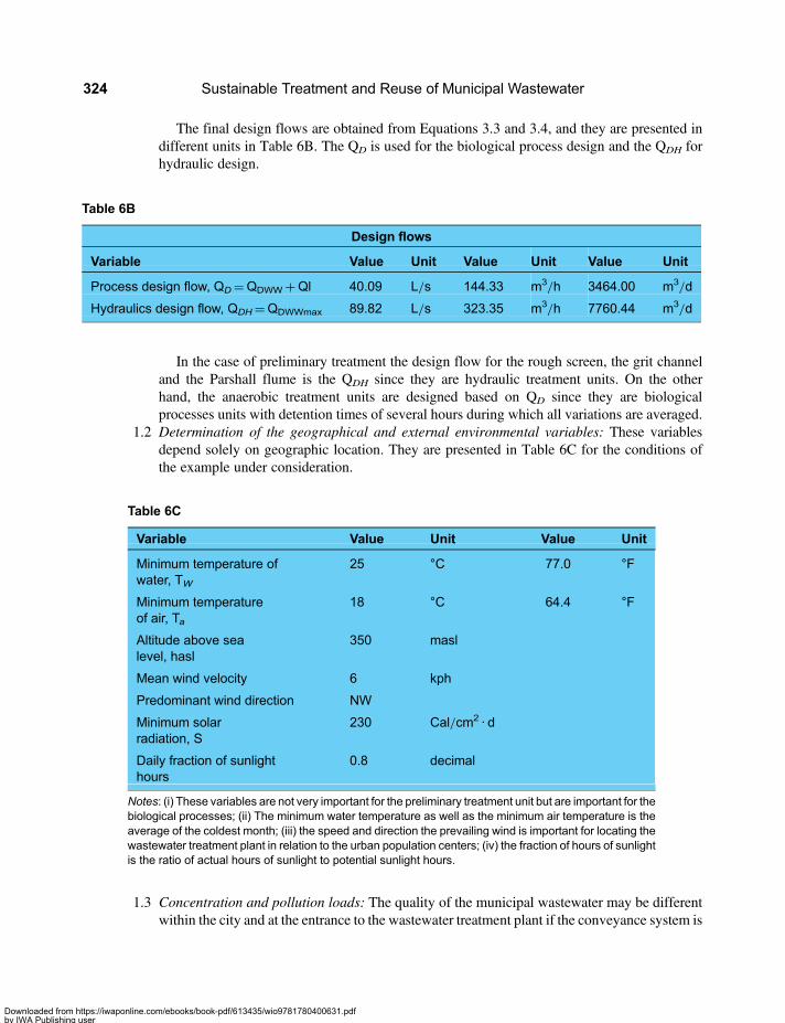
The final design flows are obtained from Equations 3.3 and 3.4, and they are presented indifferent units in Table 6B. The QD is used for the biological process design and the QDH forhydraulic design.

In the case of preliminary treatment the design flow for the rough screen, the grit channeland the Parshall flume is the QDH since they are hydraulic treatment units. On the otherhand, the anaerobic treatment units are designed based on QD since they are biologicalprocesses units with detention times of several hours during which all variations are averaged.

1.2 Determination of the geographical and external environmental variables: These variablesdepend solely on geographic location. They are presented in Table 6C for the conditions ofthe example under consideration.

1.3 Concentration and pollution loads: The quality of the municipal wastewater may be differentwithin the city and at the entrance to the wastewater treatment plant if the conveyance system is

Table 6B

Design flows


Process design flow, QD=QDWW+Ql 40.09 L/s 144.33 m3/h 3464.00 m3/d

Hydraulics design flow, QDH=QDWWmax 89.82 L/s 323.35 m3/h 7760.44 m3/d

Table 6C


Minimum temperature ofwater, TW

25 °C 77.0 °F

Minimum temperatureof air, Ta

18 °C 64.4 °F

Altitude above sealevel, hasl

350 masl



Minimum solarradiation, S

230 Cal/cm2 · d

Daily fraction of sunlighthours

0.8 decimal

Notes: (i) These variables are not very important for the preliminary treatment unit but are important for thebiological processes; (ii) The minimum water temperature as well as the minimum air temperature is theaverage of the coldest month; (iii) the speed and direction the prevailing wind is important for locating thewastewater treatment plant in relation to the urban population centers; (iv) the fraction of hours of sunlightis the ratio of actual hours of sunlight to potential sunlight hours.



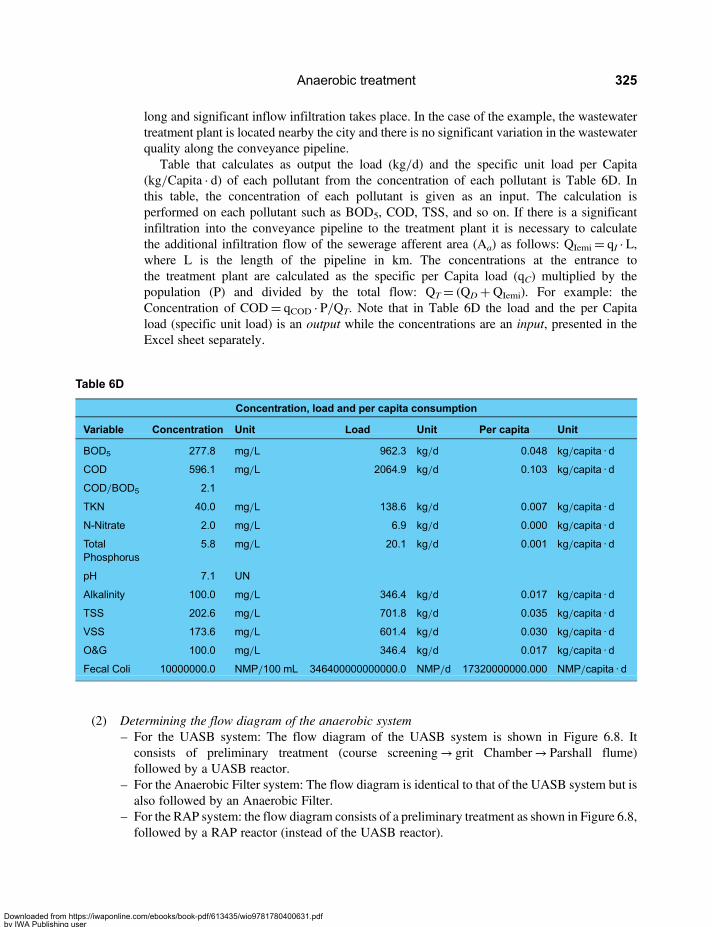
long and significant inflow infiltration takes place. In the case of the example, the wastewatertreatment plant is located nearby the city and there is no significant variation in the wastewaterquality along the conveyance pipeline.

Table that calculates as output the load (kg/d) and the specific unit load per Capita(kg/Capita · d) of each pollutant from the concentration of each pollutant is Table 6D. Inthis table, the concentration of each pollutant is given as an input. The calculation isperformed on each pollutant such as BOD5, COD, TSS, and so on. If there is a significantinfiltration into the conveyance pipeline to the treatment plant it is necessary to calculatethe additional infiltration flow of the sewerage afferent area (Aa) as follows: QIemi= qI · L,where L is the length of the pipeline in km. The concentrations at the entrance tothe treatment plant are calculated as the specific per Capita load (qC) multiplied by thepopulation (P) and divided by the total flow: QT= (QD+QIemi). For example: theConcentration of COD= qCOD · P/QT. Note that in Table 6D the load and the per Capitaload (specific unit load) is an output while the concentrations are an input, presented in theExcel sheet separately.

(2) Determining the flow diagram of the anaerobic system– For the UASB system: The flow diagram of the UASB system is shown in Figure 6.8. Itconsists of preliminary treatment (course screening→ grit Chamber→ Parshall flume)followed by a UASB reactor.

– For the Anaerobic Filter system: The flow diagram is identical to that of the UASB system but isalso followed by an Anaerobic Filter.

– For the RAP system: the flow diagram consists of a preliminary treatment as shown in Figure 6.8,followed by a RAP reactor (instead of the UASB reactor).

Table 6D

Concentration, load and per capita consumption

Variable Concentration Unit Load Unit Per capita Unit

BOD5 277.8 mg/L 962.3 kg/d 0.048 kg/capita · d

COD 596.1 mg/L 2064.9 kg/d 0.103 kg/capita · d

COD/BOD5 2.1

TKN 40.0 mg/L 138.6 kg/d 0.007 kg/capita · d

N-Nitrate 2.0 mg/L 6.9 kg/d 0.000 kg/capita · d

TotalPhosphorus

5.8 mg/L 20.1 kg/d 0.001 kg/capita · d

pH 7.1 UN

Alkalinity 100.0 mg/L 346.4 kg/d 0.017 kg/capita · d

TSS 202.6 mg/L 701.8 kg/d 0.035 kg/capita · d

VSS 173.6 mg/L 601.4 kg/d 0.030 kg/capita · d

O&G 100.0 mg/L 346.4 kg/d 0.017 kg/capita · d

Fecal Coli 10000000.0 NMP/100 mL 346400000000000.0 NMP/d 17320000000.000 NMP/capita · d



(3) Sizing the preliminary treatment system3.1 Course screening

Selection of designer variables: The course screening system can be a Rotating Screen. If thetarget efficiency for solids removal is 3%, we obtain from Figure 4.8, that a Rotating Screenwith 6 mm screen opening will be required. The design flow is the QDH since the screeningis a hydraulic unit. The designer variables are the water velocity in the inflow channel andthe screen backwashing pressure, in addition to the removal efficiency of TSS. The Excelprogram CHAP 4-RM.xls is used to perform these calculations. The values of the selecteddesigner variables are presented in the Table 6E.

Design: The diameter obtained for the course rotating screen is 600 mm. The final outputdata are presented in Table 6F. The course rotating screen design is similar to that of thefine rotating screen so the reader is referred to Chapter 4, in which the design process isexplained in detail. A coarse screening is sufficient in this case because further treatment isbe performed by the UASB-Anaerobic Filter system which follows the preliminarytreatment. For better clarity we show in Table 6F the calculations of the preliminarytreatment unit which is produced by the Excel program. The design support is presented inthe column entitled OBSERVATION.

Table 6E

Designer variables




Screen opening (rounded) 6.00 mm 0.236 Inch




Table 6F

Design







(Continued )



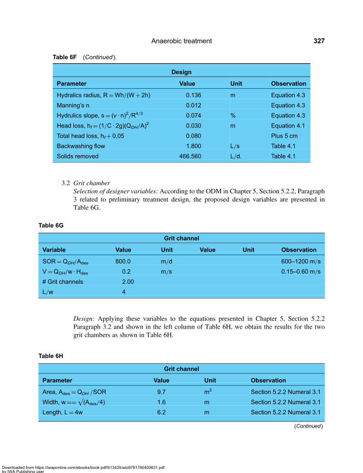
3.2 Grit chamberSelection of designer variables: According to the ODM in Chapter 5, Section 5.2.2, Paragraph3 related to preliminary treatment design, the proposed design variables are presented inTable 6G.

Design: Applying these variables to the equations presented in Chapter 5, Section 5.2.2Paragraph 3.2 and shown in the left column of Table 6H, we obtain the results for the twogrit chambers as shown in Table 6H.

Table 6F (Continued ).

Design






Total head loss, hf+ 0,05 0.080 Plus 5 cm


Solids removed 466.560 L/d. Table 4.1

Table 6G

Grit channel


SOR=QDH/Ades 800.0 m/d 600–1200 m/s

V=QDH/w · Hdes 0.2 m/s 0.15–0.60 m/s


L/w 4

Table 6H

Grit channel


Area, Ades=QDH /SOR 9.7 m2 Section 5.2.2 Numeral 3.1

Width, w==√(Ades/4) 1.6 m Section 5.2.2 Numeral 3.1

Length, L= 4w 6.2 m Section 5.2.2 Numeral 3.1

(Continued )



3.3 Parshall flume: For a QDH= 90 Lps the required throat width for flow measurement isW= 9′′. Rapid mixing is not required.

(4) UASB4.1 Reactor design

Designer variables: Using the methodology proposed in the ODM, Section 6.2.2, Paragraph4.1 and with the guidance of Table 6.2, Figure 6.9 and Equations 6.2 to 6.25 we proposethe input variables presented in Table 6I:

Table 6H (Continued ).

Grit channel


Depth, Hdes=QDH/v · w 0.3 m Section 5.2.2 Numeral 3.1

Total Depth, H=Hdes+ 0.50 0.8 m Section 5.2.2 Numeral 3.1

Parshall flume

Throat, W 9.0 inch See “PARSHALL” tag

Table 6I

Designer variables


UASB standard

Settling basin width, Ws 4.0 m Figure 6.10: UASB-SM

GSLS heigth, HG 2.5 m Figure 6.10: UASB-SM

Baffle width, wb 0.15 m Figure 6.10: Bafflewidth

Reactor velocity, vr 0.75 m/h ,1,00 m/h; Vr, vs;Table 6.2

Gas velocity, Vg 1.0 m3 /h · m2 .1,00 m/h; Tabla 6.3

Yield coefficient, Y 0.08 Table 3.2: 0.08

Fraction of CH4, h 0.65 Typical

Maximum Efficiency, Emax 90.00 % 80 to 90%

Volumetric load, Lv at 15°C 2.0 kg/m3 · d 2.0 to 4.0 kg/m3 · d at15°C,applied to liquidvolume

Efficiency, E 89.31 % DBO5

or sCODEquation 6.3

Actual volumetric load, Lv (T) 5.44 kg/m3 · d Equation 6.4

(Continued )



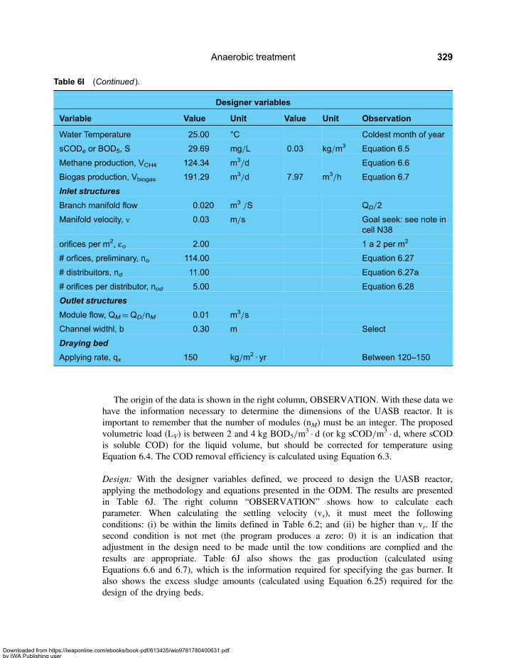
The origin of the data is shown in the right column, OBSERVATION. With these data wehave the information necessary to determine the dimensions of the UASB reactor. It isimportant to remember that the number of modules (nM) must be an integer. The proposedvolumetric load (LV) is between 2 and 4 kg BOD5/m

3 · d (or kg sCOD/m3 · d, where sCODis soluble COD) for the liquid volume, but should be corrected for temperature usingEquation 6.4. The COD removal efficiency is calculated using Equation 6.3.

Design: With the designer variables defined, we proceed to design the UASB reactor,applying the methodology and equations presented in the ODM. The results are presentedin Table 6J. The right column “OBSERVATION” shows how to calculate eachparameter. When calculating the settling velocity (vs), it must meet the followingconditions: (i) be within the limits defined in Table 6.2; and (ii) be higher than vr. If thesecond condition is not met (the program produces a zero: 0) it is an indication thatadjustment in the design need to be made until the tow conditions are complied and theresults are appropriate. Table 6J also shows the gas production (calculated usingEquations 6.6 and 6.7), which is the information required for specifying the gas burner. Italso shows the excess sludge amounts (calculated using Equation 6.25) required for thedesign of the drying beds.

Table 6I (Continued ).

Designer variables


Water Temperature 25.00 °C Coldest month of year

sCODe or BOD5, S 29.69 mg/L 0.03 kg/m3 Equation 6.5

Methane production, VCH4 124.34 m3/d Equation 6.6

Biogas production, Vbiogas 191.29 m3/d 7.97 m3/h Equation 6.7

Inlet structures

Branch manifold flow 0.020 m3 /S QD/2

Manifold velocity, ν 0.03 m/s Goal seek: see note incell N38

orifices per m2, εo 2.00 1 a 2 per m2

# orfices, preliminary, no 114.00 Equation 6.27

# distribuitors, nd 11.00 Equation 6.27a

# orifices per distributor, nod 5.00 Equation 6.28

Outlet structures

Module flow, QM=QD/nM 0.01 m3/s

Channel widthl, b 0.30 m Select

Draying bed

Applying rate, qx 150 kg/m2 · yr Between 120–150



Table 6J

Design


UASB Standard

Reactor Area, Ar 192.4 m2 Equation 6.8

Net height, HN 0.9 m Equation 6.9

Effective liquid height, HL 2.5 m Equation 6.10(minimum 2.5 m)

UASB heigth, HT 5.0 m Equation 6.11

Detention time, td 6.7 h Equation 6.12

UASB total volume, VUASB 962.2 m3 Equation 6.13

Sludge blanket volume VL 481.1 m Equation 6.14

Total gas extractionarea, Ag

8.0 m2 Equation 6.15

Design UASB length,LUASB

17.0 m Equation 6.16

Net UASB width, WWASB 11.3 m Equation 6.17

Total gas width, Wg=nMP · Wg


# preliminar modules, nMP 2.52 Equation 6.19

# modules, nM 3.00 Integer rounded up

Gas throat width, Wg 0.16 m Equation 6.20

Design UASB total width,WUASBD


Settling basisn totalarea, As

204.0 m2 Equation 6.22

Design SOR or vsD=QD/As

0.71 m/h ,1,00 and. vrD. Ifotherwise change vror/and vg

Design UASB area, ArD=WUASBD× LUASB

227.27 m2 For nM modules:Equation 6.22a

Design vr, vrD=QD ArD 0.64 m/h Equation 6.23

Design UASB volume,VUASBD=ArD · HT

1136.35 m3 6.24a

Design detention time,tdD= VUASBD/QD

7.87 H

Sludge production

Qx=VUASBD Y(S0−S)/tdD

68.76 kg/d Equation 6.25

(Continued )



A summary of the dimensions of the designed UASB reactor are presented in theTable 6K.

Table 6J (Continued ).

Design


Biogas production

Volume per day, Vg 191.3 m3/d Equations 6.6 and6.7

Inlet structure

Manifold area am 0.696 m2 Equation 6.26, withQD/2

Manifold diameter, wm=(4 am/π)∧(1/2)

0.942 m 37.0 Pulg

Distribuitor area, ad=0.4 am/nd

0.025 m2 From Equations6.29 and 6.27a

Distributor diameter, wd=(4 ac/π)∧(1/2)

0.180 m 7.0 Pulg

Orifice area, ao=0.4 ad/no

0.002 m2 From Equations6.30 and 6.28

Orifice diameter, wo=(4 ao/π)∧(l/2)

0.051 m 2.00 Pulg Goal seek: set cellL38 to 2 bychanging C14

Outlet structures

Channel water depth, h 0.102 m Equation 6.31

Total channel depth, hc 0.202 m h+ 0.10

Drying bed

Abed=Qx/qx 167.3 m2 Equation 6.33

Table 6K

Summary of the designed UASB reactor dimensions

Parameter Value Unit

Designed UASB area, ArD 227.27 m2

Designed UASB total width, WUASBD 13.4 m

Designed UASB length, LUASB 17.0 m

Designed UASB heigth, HT 5.0 m

(Continued )



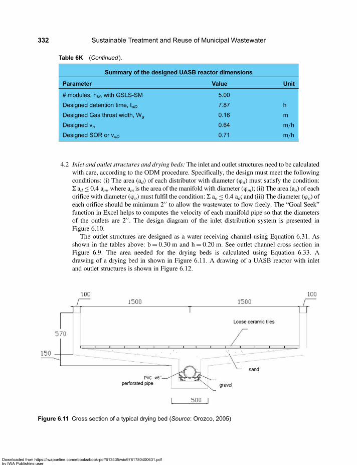
4.2 Inlet and outlet structures and drying beds: The inlet and outlet structures need to be calculatedwith care, according to the ODM procedure. Specifically, the design must meet the followingconditions: (i) The area (ad) of each distributor with diameter (wd) must satisfy the condition:Σ ad≤ 0.4 am, where am is the area of the manifold with diameter (wm); (ii) The area (ao) of eachorifice with diameter (wo) must fulfil the condition: Σ ao≤ 0.4 ad; and (iii) The diameter (wo) ofeach orifice should be minimum 2′′ to allow the wastewater to flow freely. The “Goal Seek”function in Excel helps to computes the velocity of each manifold pipe so that the diametersof the outlets are 2′′. The design diagram of the inlet distribution system is presented inFigure 6.10.

The outlet structures are designed as a water receiving channel using Equation 6.31. Asshown in the tables above: b= 0.30 m and h= 0.20 m. See outlet channel cross section inFigure 6.9. The area needed for the drying beds is calculated using Equation 6.33. Adrawing of a drying bed in shown in Figure 6.11. A drawing of a UASB reactor with inletand outlet structures is shown in Figure 6.12.

Table 6K (Continued ).

Summary of the designed UASB reactor dimensions


# modules, nM, with GSLS-SM 5.00

Designed detention time, tdD 7.87 h

Designed Gas throat width, Wg 0.16 m

Designed vr, 0.64 m/h

Designed SOR or vsD 0.71 m/h

Figure 6.11 Cross section of a typical drying bed (Source: Orozco, 2005)



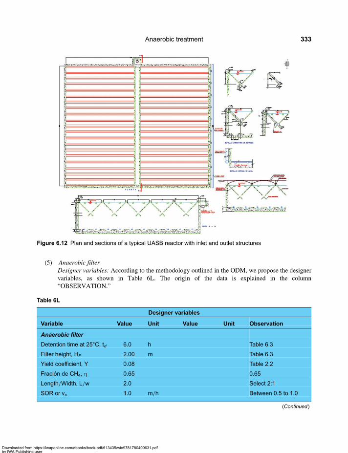
(5) Anaerobic filterDesigner variables: According to the methodology outlined in the ODM, we propose the designervariables, as shown in Table 6L. The origin of the data is explained in the column“OBSERVATION.”

Figure 6.12 Plan and sections of a typical UASB reactor with inlet and outlet structures

Table 6L

Designer variables


Anaerobic filter

Detention time at 25°C, td 6.0 h Table 6.3

Filter height, HF 2.00 m Table 6.3

Yield coefficient, Y 0.08 Table 2.2

Fración de CH4, η 0.65 0.65

Length/Width, L/w 2.0 Select 2:1

SOR or vs 1.0 m/h Between 0.5 to 1.0

(Continued )



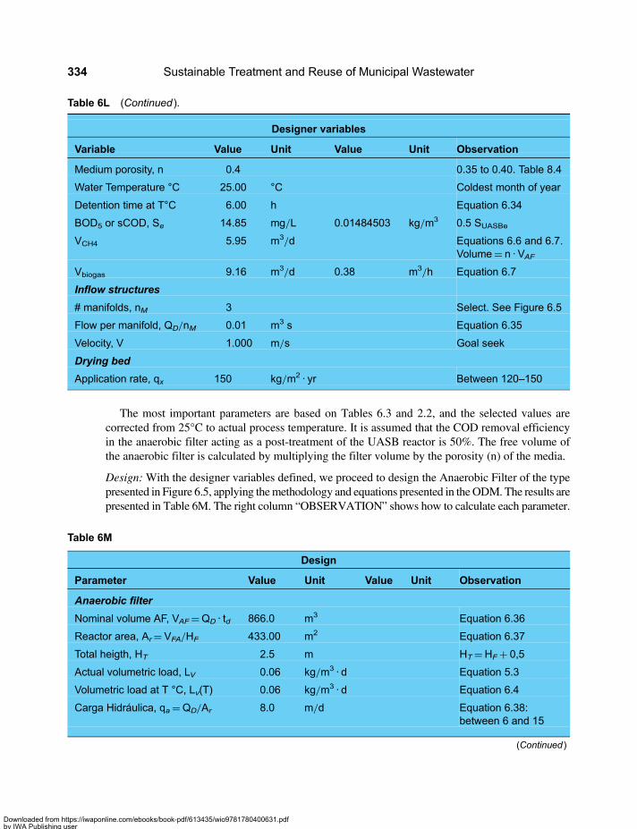
The most important parameters are based on Tables 6.3 and 2.2, and the selected values arecorrected from 25°C to actual process temperature. It is assumed that the COD removal efficiencyin the anaerobic filter acting as a post-treatment of the UASB reactor is 50%. The free volume ofthe anaerobic filter is calculated by multiplying the filter volume by the porosity (n) of the media.

Design:With the designer variables defined, we proceed to design the Anaerobic Filter of the typepresented in Figure 6.5, applying themethodology and equations presented in theODM. The results arepresented in Table 6M. The right column “OBSERVATION” shows how to calculate each parameter.

Table 6M

Design


Anaerobic filter

Nominal volume AF, VAF=QD · td 866.0 m3 Equation 6.36

Reactor area, Ar= VFA/HF 433.00 m2 Equation 6.37

Total heigth, HT 2.5 m HT=HF+ 0,5

Actual volumetric load, LV 0.06 kg/m3 · d Equation 5.3

Volumetric load at T °C, Lv(T) 0.06 kg/m3 · d Equation 6.4

Carga Hidráulica, qa=QD/Ar 8.0 m/d Equation 6.38:between 6 and 15

(Continued )

Table 6L (Continued ).

Designer variables


Medium porosity, n 0.4 0.35 to 0.40. Table 8.4

Water Temperature °C 25.00 °C Coldest month of year

Detention time at T°C 6.00 h Equation 6.34

BOD5 or sCOD, Se 14.85 mg/L 0.01484503 kg/m3 0.5 SUASBe

VCH4 5.95 m3/d Equations 6.6 and 6.7.Volume= n · VAF

Vbiogas 9.16 m3/d 0.38 m3/h Equation 6.7

Inflow structures

# manifolds, nM 3 Select. See Figure 6.5

Flow per manifold, QD/nM 0.01 m3 s Equation 6.35

Velocity, V 1.000 m/s Goal seek

Drying bed

Application rate, qx 150 kg/m2 · yr Between 120–150



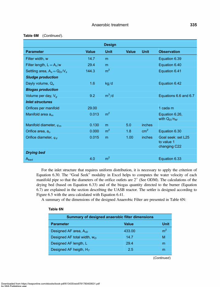
For the inlet structure that requires uniform distribution, it is necessary to apply the criterion ofEquation 6.30. The “Goal Seek” modality in Excel helps to computes the water velocity of eachmanifold pipe so that the diameters of the orifice outlets are 2′′ (See ODM). The calculations of thedrying bed (based on Equation 6.33) and of the biogas quantity directed to the burner (Equation6.7) are explained in the section describing the UASB reactor. The settler is designed according toFigure 6.5 with the area calculated with Equation 6.41.

A summary of the dimensions of the designed Anaerobic Filter are presented in Table 6N:

Table 6M (Continued).

Design


Filter width, w 14.7 m Equation 6.39

Filter length, L=Ar/w 29.4 m Equation 6.40

Settling area, As=QD/Vs 144.3 m2 Equation 6.41

Sludge production

Dayly volume, Qx 1.6 kg/d Equation 6.42

Biogas production

Volume per day, Vg 9.2 m3/d Equations 6.6 and 6.7

Inlet structures

Orifices per manifold 29.00 1 cada m

Manifold area am 0.013 m2 Equation 6.26,with QD/nM

Manifold diameter, wm 0.130 m 5.0 inches

Orifice area, ao 0.000 m2 1.8 cm2 Equation 6.30

Orifice diameter, wd 0.015 m 1.00 inches Goal seek: set L25to value 1changing C22

Drying bed

Abed 4.0 m2 Equation 6.33

Table 6N

Summary of designed anaerobic filter dimensions


Designed AF area, ArD 433.00 m2

Designed AF total width, wD 14.7 M

Designed AF length, L 29.4 m

Designed AF heigth, HT 2.5 m

(Continued)



(6) Piston anaerobic reactor, PARDesigner variables: Since the PAR is used in areas of low temperatures of between 15 and 20°C, inthis example we use for the RAP a wastewater temperature of 16°C, which is different than thetemperature used from the UASB example. For this to be consistent other external variables canchange but they are not of significant importance for the design. The geographical and externalenvironmental variables are presented in Table 6O. A PAR system is also calculated by adifferent program: CHAP 6-Anaerobic-PAR.xls, for temperatures below 20°C.

With this new temperature, and using the methodology proposed in the ODM, Section 6.2.2Paragraph 6, we obtain the input data presented in Table 6P (the selected designer variables),whose origin can be seen in the column denominated “OBSERVATION”.

Table 6N (Continued ).

Summary of designed anaerobic filter dimensions


# manifolds nM 3.00


Designed SOR or vsD 1.00 m/h

Table 6O


Minimum Temperature of water, Tw 16 °C 60.8 °F

Minimum Temperature of air, Ta 8 °C 46.4 °F

Altitude above sea level, masl 1850 masl





Table 6P

Designer variables


Piston anaerobic reactor, PAR

Settling basin width, Ws 4.0 m Figure 6.10: UASB-SM


Baffle thickness, wb 0.15 m Figure 6.10: Baffle width

Flow velocity in reactor vr 0.75 m/h ,1.00 m/h; Vr,Vs; Table 6.3

(Continued )



Design: Note that 3 PAR reactors were selected, so the design flow of each reactor is QD/nPAR=QD/3. Also note that there is one (1) GSLS-SM for each PAR reactor, and the “GSLS length” is thesame as the PAR reactor width. From the input data, we obtain the results shown in Table 6Qfollowing the ODM. The calculations were made with the equations presented in the ODM andidentified in the right column denominated “OBSERVATION”.

Table 6P (Continued ).

Designer variables


Settling velocity, SOR, vs 0.84 m/h Calculated for a gasthroat of Wg= 0.10 m

Gas throat, wg 0.10 m Given

Detention time at 15°C 10.0 h Typical



Efficiency, E 85.19 % DBO5

or sCODEquation 6.3

Water Temperature 16.00 °C Coldest month of year.Should be less than 20°C


Flow velocity in baffles, vb 3.0 m/h ≤3.0 m/h

PAR units, nPAR 3 Select

T agua 16.00 °C Below 20°C

Outlet structures

Flow per PAR 48.111 m3/h 0.0133642 m3/S QD/nRAP

Channel width, b 0.30 m Select

Drying bed

Application rate 150 kg/m2 · yr 120–150

Table 6Q

Design


Plug-flow anaerobic reactor, PAR

Area GSLS Ar 64.1 Equation 6.44

Total PAR height 3.0 Equation 6.44

Baffles height, HL=HT 3.0 Equation 6.45

(Continued )



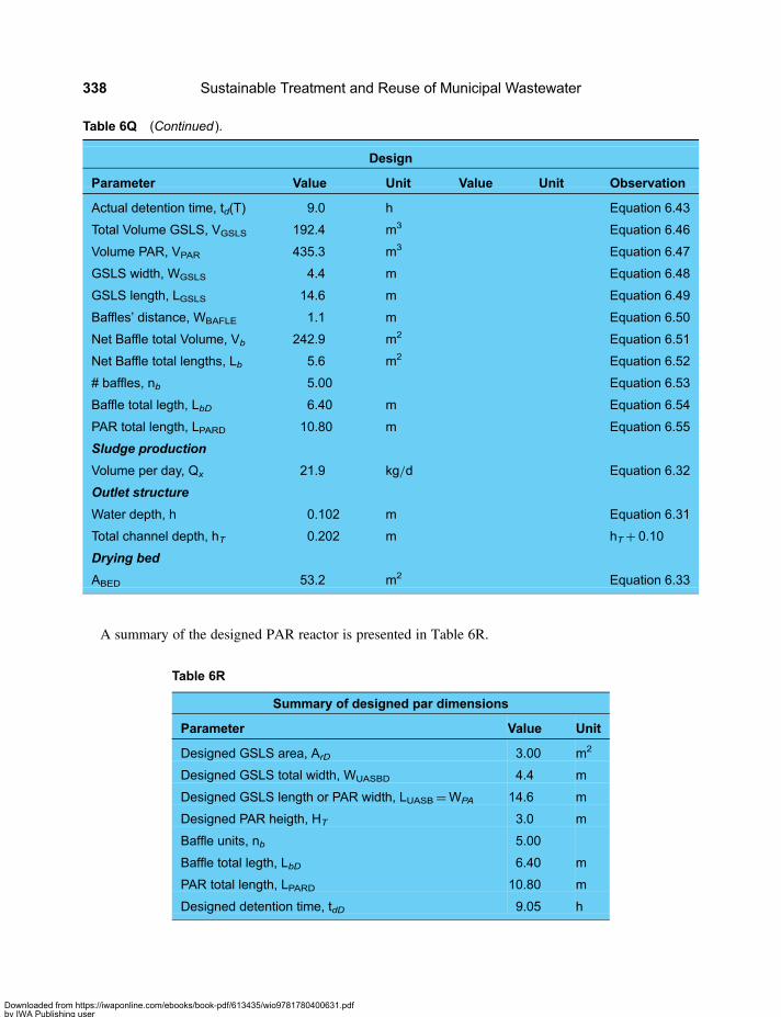
A summary of the designed PAR reactor is presented in Table 6R.

Table 6Q (Continued ).

Design


Actual detention time, td(T) 9.0 h Equation 6.43

Total Volume GSLS, VGSLS 192.4 m3 Equation 6.46

Volume PAR, VPAR 435.3 m3 Equation 6.47

GSLS width, WGSLS 4.4 m Equation 6.48

GSLS length, LGSLS 14.6 m Equation 6.49

Baffles’ distance, WBAFLE 1.1 m Equation 6.50

Net Baffle total Volume, Vb 242.9 m2 Equation 6.51

Net Baffle total lengths, Lb 5.6 m2 Equation 6.52

# baffles, nb 5.00 Equation 6.53

Baffle total legth, LbD 6.40 m Equation 6.54

PAR total length, LPARD 10.80 m Equation 6.55

Sludge production

Volume per day, Qx 21.9 kg/d Equation 6.32

Outlet structure

Water depth, h 0.102 m Equation 6.31

Total channel depth, hT 0.202 m hT+ 0.10

Drying bed

ABED 53.2 m2 Equation 6.33

Table 6R

Summary of designed par dimensions


Designed GSLS area, ArD 3.00 m2

Designed GSLS total width, WUASBD 4.4 m

Designed GSLS length or PAR width, LUASB=WPA 14.6 m

Designed PAR heigth, HT 3.0 m

Baffle units, nb 5.00

Baffle total legth, LbD 6.40 m

PAR total length, LPARD 10.80 m




Chapter 7

Stabilization reservoirs, concepts andapplication for effluent reuse in irrigation

7.1 PROCESS DESCRIPTION7.1.1 IntroductionAll municipal wastewater treatment processes depend on: (i) natural phenomena such as gravity whichinduces sedimentation, and (ii) of natural biological compounds such as organisms. However, in the caseof conventional wastewater treatment plants, these natural components are supported by a series (oftencomplex) of mechanical equipment intensive in energy consumption. In contrast, natural treatmentprocesses, many of which are discussed in this book, are processes that depend mostly on naturalcomponents to perform the treatment. A natural system may include pumps and pipes to transport thewastewater, but it does not depend solely on external energy sources to carry out the treatment process(Crites, Middlebrooks & Sherwood, 2006).

The land application of the municipal wastewater (also known as overland flow) was the first “natural”technology (recently re-discovered). In the nineteenth century it was the only method used for treatment ofsewage, but it was gradually replaced by other, more modern methods. Studies and research established thatland application treatment can obtain many desirable treatment goals, while at the same time, significantbenefits are obtained by the reuse of minerals and organic matter applied on land. Other “natural”concepts such as lagoon systems and the application of sewage sludge on land have never fallen intodisuse. The stabilization lagoons, including stabilization reservoirs, simulate physical and biochemicalinteractions that occur in natural lakes, while the application of sewage sludge on land mimicsconventional agricultural practices of utilization of manures. The concepts of surface and subsurfaceartificial wetlands are new developments related to reuse of wastewater and sludge.

Of these natural treatment processes, the Stabilization Reservoirs (SR) for wastewater treatment andreuse for irrigation, presented in this chapter, represents an interesting cost-effective option for municipalwastewater post-treatment and utilization. Other natural systems, such as stabilization lagoons andconstructed wetlands are discussed in other chapters of the book and other publications (such as Crites,Middlebrooks & Sherwood, 2006).

According to Libhaber (2007), reuse of wastewater for irrigation is a combined concept of treatment anddisposal. Stabilization Reservoirs offer an alternative disposal of municipal wastewater which is better thanconventional ones because it generates economic and agricultural benefits and eliminates the negativeimpacts of discharge of effluents to receiving water bodies. A stabilization reservoir system using simple


pretreatment processes can produce effluents with the required quality for both restricted irrigation(i.e. adequate for irrigation of industrial crops) and for unrestricted irrigation (i.e. for irrigation of foodcrops consumed uncooked).

The stabilization reservoirs concept was developed in Israel in the early 1970s and is in wide spread usein this country. Over 250 stabilization reservoirs are operated today in Israel and their number is increasingwith time. Therefore, the design methodology and most of the information on the process and relatedexamples come from Israel. The use of reservoirs to store and treat wastewater is an old practice, butthe development of deep reservoirs to reduce evaporation losses, the widespread use of reservoirs forlong term-storage of wastewater and the massive research undertaken to better understand the behaviourof this type of reservoirs and improve their design and operational criteria are relatively new. Asexplained by Libhaber (1996), stabilization reservoirs are deep lagoons (with depth of 4–12 meters, butusually in the range 8–12 meters) with a variable water level, that are used for a combination of twoobjectives: (i) storing partially treated sewage over a long period in order to use it for irrigation ordischarge it to a receiving water body during a specific period of the year, under strictly controlledoptimal conditions; and (ii) improve the quality of effluents stored during the long residence timewithin the reservoir. The controlled release is possible thanks to climates with “rains-dry” seasonswhich occurs in several regions of the world and generates a demand for large volumes of water forirrigation during the summer.

In some cases, wastewater can be stored in reservoirs during the summer in order to be discharge into thesea during the rainy season, which is not a bathing season. Also, in cases of effluent discharge into rivers thataffect their use, reservoirs can store the effluent during the season of minimum flow in the river (dry season),in order to discharge it to the river during the high flow season when the dilution capacity is high (usuallyduring the rainy season).

The stabilization reservoir process is presented and discusses as one of the unit processes of appropriatetechnology in Paragraph 1.7.2.7 of Chapter 1. As part of this discussion, it was clarified that beforedischarging the wastewater to the reservoir for storage, it needs to be treated to remove a part of theorganic matter contained in it; so as to prevent development of anaerobic conditions in the upper layer ofthe reservoir. Prevention of such conditions is important since anaerobic condition may generate odours.So in fact, the reservoir stores effluent and not raw wastewater. The reservoir system is therefore acombined system consisting of a pretreatment unit followed by the reservoir. The required pre-treatmentof the wastewater before it is stored in the reservoir is not a specific treatment processes. It can beachieved using a variety of treatment process, among them; all the appropriate technology processes orcombination of processes described in this book, as long as they remove the required load of organicmatter and ensure that the surface organic loading on the reservoir does not exceed the permitted limit.The reservoir itself, in addition to its function seasonal storage of effluent, is also a treatment unit. Itfunctions as a facultative lagoon with a varying water depth. The upper layer of the reservoir (whosedepth depends on the specific design of the reservoir and on the effectiveness of the pretreatment unit) isan aerobic layer in which algae and bacteria develop. The algae generate oxygen which is consumed bythe bacteria that decompose the organic matter present in the reservoir. An anaerobic layer is formedbeneath the upper layer and anaerobic bacteria develop in this layer and decompose the organic matterwhich arrives in it. Pathogenic organisms decay in the reservoir by similar mechanisms of decay inconventional lagoon. However, the detention time in a stabilization reservoir is much larger than inregular lagoons so the removal of pathogens can be much more effective. The actual removal ofpathogenic organisms depends on the mode of operation of the reservoir, as discussed below. Thecombination of the pretreatment unit and the reservoir form as a whole an appropriate technologyprocess, if the pretreatment unit is based on appropriate technology.



The schematic process flow diagram of pretreatment followed by a stabilization reservoir is presented inFigure 7.1. This figure is not the flow diagram of just one combined process but rather of a large series ofcombined processes, since the pretreatment unit is not just one specific unit, but can be one of a variety ofunit processes or combination of unit processes.

The aspects of wastewater reuse for irrigation, the characteristics of stabilization reservoirs andreservoirs as a combined appropriate technology systems are discussed in Chapter 1 (Paragraphs 1.7.2.7and 1.8.8). The current chapter deals with the design procedure of the stabilization reservoir. We believethat every wastewater reuse for irrigation project needs to include a stabilization reservoir in order to besuccessful. Inspection of the inflow pattern, which is the constant raw wastewater flow along the year,and the outflow pattern which is the variable pattern of consumption for irrigation, as shown inFigure 1.20, explains the need for the seasonal storage, that is, the need for a storage reservoir in areuse project.

7.1.2 Basics of the processFundamentalsThe design concepts of Stabilization Reservoirs (SR) are similar to those of stabilization lagoons, presentedin Chapter 5, namely on the following parameters: (i) the organic surface loading (LS) in (kg BOD5/ha · d);(ii) the detention time (td) days; and (iii) the temperature (T) °C. The hydraulic regime is very important anddue to the impact of the wind and the long fetch resulting from the large dimensions of reservoirs, theyusually act as completely mixed reactors. During periods of stratification the upper layer acts ascompletely mixed. The equations which apply for the design of a reservoir, as discussed below, aresimilar to those used in lagoons, but are modified for the hydraulic regime. In addition, there arelimnological components to be taken into account in the operation of reservoirs. For basic kineticequations refer to Chapter 2. The modified kinetic equations are presented below.

Figure 7.1 The stabilization reservoir reuse concept and schematic process flow diagram (Source: LibhaberMenahem, 1996)

Stabilization reservoirs, concepts and application for effluent reuse in irrigation 341


In terms of public health aspects of wastewater reuse, the guidelines of the World Health Organization1.(WHO) need to be addressed. It has been shown that the if these recommendations are applied, reuse oftreated municipal wastewater presents a public health risk of between 10 and 1000 times lower than thethan the risk posed by consumption of drinking water. WHO recognizes that the treatment of wastewater

Figure 7.2 Typical annual variations of inflow, outflow, effluent COD and effluent total coliforms in a typicalsingle continuous flow stabilization reservoir (the Getaot Reservoir) (Source: Adapted from Juanico &Shelef, 1994)

1Namely: (i) intestinal nematode eggs: ≤1 per liter; and (ii) for unrestricted irrigation: fecal coliforms ≤1000 per 100 mL. In 2006 theWHO issued new guidelines, but they are less stringent.



in stabilization lagoons is an effective and economical way of obtaining the microbiological quality limitsfor the reuse of wastewater. However, the effluents of the stabilization lagoons can be used to irrigate cropsonly during the dry season. In other seasons of the effluent must be discharged into surface streams or otherreceiving water bodies, unless it is stored in a Stabilization Reservoir to be used during the irrigation season.The use of stabilization reservoirs is also beneficial due to the fact that significant additional treatmentoccurs in them (Mara & Pearson, 1999, pp. 591).

According to Libhaber (1996), the priority criteria for treatment of wastewater for the specific objectiveof reuse of effluent for irrigation are: (i) maximum removal of helminths and protozoa, (ii) effective removalof bacterial and viral pathogens, and (iii) effective reduction of BOD to prevent unpleasant doors andunpleasant appearance of the effluent in the reservoir. This priority order differs from that used for thecontrol of BOD and COD pollution in surface water. The optimal treatment strategies for reuse aretherefore different from strategies for control of contamination of surface waters.

The operating regime used in a single continuous flow stabilization reservoirs is such that during theirrigation season when the withdrawal of effluent from the reservoir starts, the treated effluent from thelagoons or any other pretreatment system which feeds the reservoir keeps flowing, so that anincreasing proportion of pretreated effluent mixes with the initial content of the well treated liquidcontained in the stabilization reservoir. This causes that towards the end of the irrigation season theeffluent withdrawn from the reservoir for irrigation has an increasingly deteriorated quality, especiallyin terms of pathogenic organisms, as shown in Figure 7.2 (referring to the single continuous flowstabilization reservoir at Getaot, Israel). The lower quality of effluent has no negative impact when theeffluent is used for restricted irrigation. However, when it is used for restricted irrigation (i.e. irrigationof crops that require a high quality effluent all the time) the quality deterioration towards the end ofthe irrigation season presents a problem. A strategy to overcome the problem by the use of tworeservoirs is being practices in Israel for many years and is explained by Mara & Pearson (1999) asdiscussed below.

Operation regimesThere are many ways of operating a reservoir system which consists of a pretreatment unit followed by thestabilization the reservoir (a lagoon system as the pretreatment unit is a preferred solution, but there can beothers, practically all the appropriate technology unit processes and combinations of these processes) butthey can be reduced to three basic operation modes, as shown in Figure 7.3 (Mara & Pearson, 1999;Mara, 2004), which is based on lagoons as pretreatment:

(i) Operation mode of Figure 7.3(a): This is the conventional mode. In this case the pre-treatment is ananaerobic lagoon but can be different. Under this mode of operation there is one single stabilization reservoirwhich is continuously filled up with the pretreated effluent all the year round and discharges effluent onlyduring the irrigation season. The effluent quality deteriorates at the end of season, as seen in Figure 7.2,because the good water quality is used up at the beginning of the irrigation season and then. Finally, thelower quality of water from the bottom is mixed with the anaerobic pond effluent. In consequence theeffluent of this system can be use only for restricted irrigation, mainly of industrial crops. This system isefficient and is in widespread use, but is limited only to restricted irrigation. The main problem of thissystem is that the inflow stream to the reservoir continues to flow even during the irrigation season. Wesaw that the main requirement for unrestricted irrigation is to achieve a low content of coliforms in theeffluent. The inflow stream to the reservoir contains high concentrations of coliforms. Due to the windaction the content of the reservoir is well mixed and coliforms which enter with the inflow easily reachthe outflow and render the effluent to be of restricted quality.



(ii) Operation mode of Figure 7.3(b): Under this mode the pretreatment unit is followed by severalstabilization reservoirs, usually two, which are located in parallel. The reservoirs are filled one after theother. When the first reservoir becomes full, the second one starts to be filled. This mode of operation is asequential batch feeding mode. The principle of operation is that effluent is withdrawn for irrigation onlyfrom a reservoir which does not receive an inflow stream. That means that coliforms are not coming intothat reservoirs, coliforms which have previously entered have decayed with time and its effluent containsa low level of coliforms and is therefore fit for unrestricted irrigation. Even of food crops that are eatenraw. During the irrigation season, the pretreated effluent fills the second reservoir and will be used in thefollowing year’s irrigation season, so this system provides not only seasonal storage but actuallymultiannual storage. The storage volume in this system is larger than in the previous one so it is moreexpensive, but it also generates a higher quality of effluent which, allows producing higher value crops.

(iii)Operation mode of in 7.3(c): This is the hybrid system, in which the pretreatment is of higher level (inthe figure it consists of an anaerobic lagoon followed by a facultative lagoon, but it can also be of a differenttype, albeit of a level higher than just an anaerobic lagoon). Before the irrigation season, the pretreatedeffluent fills the reservoir. When the irrigation season starts, the inflow to the reservoir is stopped. Theeffluent of the reservoir is then used for unrestricted irrigation, while the effluent of the pretreatment unitis used for restricted irrigation. The difference between this operation mode and the previous mode isthat in this case the effluent of the pretreatment unit is not stored in a second reservoir for use ofunrestricted irrigation during the next season, but is rather used during the same season albeit only forrestricted irrigation. This system is of intermediate cost and its use is broad and serves for all types of crop.

Additional explanations on the various modes of operation and information on the effluent qualityyielded by each mode are presented in Chapter 1 and in Figures 1.26, 1.27 and 1.28. A photo of asystem type (a) of Figure 7.3 is presented in Figure 1.77, which is the system of the Naan reservoir in

Figure 7.3 Operation options of stabilization reservoirs (a) single SR for restricted irrigation; (b) sequentialbatch-fed for unrestricted irrigation; (c) hybrid system for both restricted and unrestricted irrigation A:anaerobic lagoon; F: facultative lagoon, WSTR: Waste Storage and Treatment Reservoir or StabilizationReservoir (Source: Mara & Pearson, 1999)



Israel and includes the anaerobic pretreatment unit and the reservoir. This system can also be operated assystem type (c) in Figure 7.3. In fact, systems (a) and (c) are similar in terms of infrastructure. Thedifference between them is in the mode of operation. A photo of a system type (b) of Figure 7.3 ispresented in Figure 1.29, which is the Maale Hakishon reservoir system consisting of two reservoirs. Thepretreatment system is not shown in Figure 1.29 because it is located in a different site, close to the citywhich is the source of the wastewater.

Design parameters of a stabilization reservoirThe design parameters of a stabilization reservoir are the same as those of a lagoon system, namely: volume(V), surface organic loading (Ls), detention time (td) and depth (H.) However, as there are differences in theflow regimes of a lagoon and a reservoir, the calculation of the parameters is done differently. In the case of astabilization reservoir it is also necessary to include other design parameters.

Percentage of Fresh Effluents, PFEi: This is a most important parameter, even more than the detentiontime. The PFEi (percentage of “fresh” pretreated effluent residing in the reservoir between 1 to i days),is expressed as the percentage of THE volume of pretreated effluent residing in the reservoir 1 to i days,in relation to the total volume of water in the reservoir (Juanicó & Dor, 1999). For example, PFE30 is thepercentage of pretreated effluent residing in the reservoir less and up to 30 days (expressed as a percentageof the total Reservoir content). The volume of effluent residing in the reservoir up to 30 days is the volumeof effluent which resides from 1 to 30 days. This means the volume of pretreated effluent residing 1 dayplus the volume residing 2 days plus the volume residing 3 days and so successively until plus the volumeresiding 30 days. The total fresh pretreated effluent is the portion that is still not well treated in thereservoir and since, because of the mixing characteristics in the reservoir (due to the wind effect), part of itis discharged with the reservoir effluent; it is the parameter that affects negatively the quality of thereservoir’s effluent. So the smaller the value of the fresh pretreated effluent in the reservoir, the better is thequality of the content of the reservoir and of its effluent. According to Juanico and Dor, 1999, it is the PFEthat governs the effluent quality of any reactor. In lagoon, which perform under steady state flowconditions (the inflow and outflow are continuous and equal), the ratio PFE/td (PFE to Detention Time) isconstant, so td can substitute for PFE in the analysis of reactor performance and hence the closerelationship between the performance of perfectly mixed steady state reactor (the lagoon) and the detentiontime. So for a lagoon, it can be said that it is the detention time that determines the quality of the lagooneffluent. In a reservoir, which is not a steady state reactor (the flow is not continuous and the inflow andoutflow are not equal), the performance is related to PFE and it is the PFE (the percentage offresh pretreated effluent in the reservoir) which determines the quality of the reservoir’s effluent.The content of each specific quality parameter in the effluent of the reservoir depends on the kinetics of theremoval of this parameter in the reservoir. It was found that the value of PFE30 has the highest correlationto the removal of BOD and that the values PFE1 and PFE5 have the highest correlation to the removal offaecal coliforms in a reservoir. Hence the importance of PFE30 and of PFE1−PFE5.

Mean Detention Time (or Mean Residence Time): themean time of detention (tdmj) is used in the designof a stabilization reservoir, but unlike the detention time in lagoons which function under stable conditionsof continuous flow (td=V/Q), the detention time of a stabilization reservoir that operate undernon-continuous conditions (the reservoir is filled throughout the year and discharged during only a fewmonths, more like a Sequential Batch Reactor, SBR) is calculated on a daily basis, day by day, with thefollowing equation:

tdmj =[(tdm( j−1) + 1) V( j−1)]+ 0.5 vj

V( j−1) + vj(7.1)



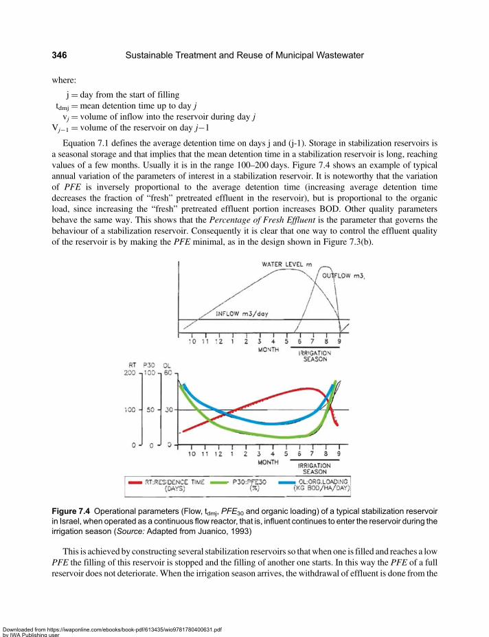
where:

j= day from the start of fillingtdmj =mean detention time up to day jvj = volume of inflow into the reservoir during day j

Vj−1 = volume of the reservoir on day j−1

Equation 7.1 defines the average detention time on days j and (j-1). Storage in stabilization reservoirs isa seasonal storage and that implies that the mean detention time in a stabilization reservoir is long, reachingvalues of a few months. Usually it is in the range 100–200 days. Figure 7.4 shows an example of typicalannual variation of the parameters of interest in a stabilization reservoir. It is noteworthy that the variationof PFE is inversely proportional to the average detention time (increasing average detention timedecreases the fraction of “fresh” pretreated effluent in the reservoir), but is proportional to the organicload, since increasing the “fresh” pretreated effluent portion increases BOD. Other quality parametersbehave the same way. This shows that the Percentage of Fresh Effluent is the parameter that governs thebehaviour of a stabilization reservoir. Consequently it is clear that one way to control the effluent qualityof the reservoir is by making the PFE minimal, as in the design shown in Figure 7.3(b).

This is achieved by constructing several stabilization reservoirs so thatwhen one is filled and reaches a lowPFE the filling of this reservoir is stopped and the filling of another one starts. In this way the PFE of a fullreservoir does not deteriorate.When the irrigation season arrives, the withdrawal of effluent is done from the

Figure 7.4 Operational parameters (Flow, tdmj, PFE30 and organic loading) of a typical stabilization reservoirin Israel, when operated as a continuous flow reactor, that is, influent continues to enter the reservoir during theirrigation season (Source: Adapted from Juanico, 1993)



reservoir with the oldest water in which the PFE is the smallest, the tdm is the highest and the water quality isthe best. A dual or multiple reservoir system, such as system (b) in Figure 7.3 is more expensive than a singlereservoir system, as systems (a) and (c), but the cost effectiveness analysis of each system needs to take intoaccount the income from agriculture. System (b) which is of higher investment might turn out to be morecost-effective because of its higher effluent quality (adequate for unrestricted irrigation) which maygenerate more income. In addition, the issue of regulation needs to be taken into account. In certaincountries reuse is permitted only when the effluent quality is adequate for unrestricted irrigation. In allcases, an economic analysis based on local conditions and regulations needs to be undertaken to decidewhich reservoir system is the optimal for each specific case,

Volume: The volume of a stabilization reservoir is specific to each case. It depends on the flow of thewastewater, on climate (the length of the irrigation season) and on the type of the irrigated crops (whichdefine the variation with time of consumption of effluent for irrigation). Stabilization reservoirs are usedfor seasonal storage so they are water bodies of large volume. In Israel, reservoirs volume range from20,000 m3 (the smallest) to 12 million m3 (the largest which are two reservoir in the Maale Hakishonproject receiving the treated effluent of the city of Haifa, each with a volume of 12 million m3 and arepresented in Figure 1.29). Most of the reservoirs have a volume in the range 200,000–6,000,000 m3. Thecalculation of the volume of the stabilization reservoir is a very important stage in the design. To designthe reservoir it is necessary to take into account the topography of the site, the geometry of the reservoir,the geology at the location of the reservoir and the depth of the reservoir, which is usually between 4 and12 m. Deeper reservoirs with an active depth of up to 20 meters are being considered. Dissolved oxygenin reservoirs comes from photosynthetic activity of algae and from diffusion of atmospheric oxygen.Thus deeper reservoirs with a small area/volume ratio have inferior oxygen supply conditions thanshallower reservoirs. Consequently, deeper reservoir need to be operated with lower surface organicloading (which means a higher level of pretreatment) or with mixers and even aerators, to maintain inthem aerobic conditions. Once the depth and embankments slopes are defined, the volume is calculatedbased on the incoming flow and the pattern of the outflow for irrigation, taking into account a deadvolume of 1 meter deep at the bottom for sediments storage, and a freeboard, which is around 1 m, butshould be calculated for each case on the basis of the intensity of local winds and the size of thereservoir (from which the fetch is calculated).

The volume of wastewater stored in the stabilization reservoir system is calculated on the basis of the flowof the incoming wastewater and the pattern of consumption of effluent for irrigation, which in turn dependson the type of crop to be irrigated. The monthly precipitation-evaporation balance must be taken into accountin the volume calculation procedure. Similarly, water loss by infiltration from the bottom of the reservoirmust be taken into account in permeable sites, if impermeabilization is not done. Due to the slope of theembankments the surface area of the water in the reservoir varies significantly with the water level, ascan be appreciated from Figure 1.25.

SurfaceOrganic Loading (Ls):The dimensions of the reservoir, including its surface area, are establishedon the basis of the raw wastewater flow and the consumption of water for irrigation, that is, on the basis ofhydraulic data without taking into account the quality of the wastewater. However, if the organic matterconcentration in the inflow stream entering the reservoir will be too high, the reservoir will becomeanaerobic up to the surface layer and may consequently generate offensive odours. To avoid suchconditions, the raw wastewater must be pretreated prior to its inflow to the reservoir so as to decrease theorganic loading on the reservoir to levels which will ensure the preservation of an aerobic top layer in thereservoir. Such aerobic layer prevents generation of odours. Oxygen balance models of reservoirs, as wellas experience, established that the maximum permissible organic loads which still prevent generation of



anaerobic conditions in the upper layer of stabilization reservoirs are 30–50 kg BOD/d · ha during the winterlow temperature season and 60–100 kg BOD/d · ha during autumn and high temperature summer season. InFigure 7.4 the variation of the organic loading on a continuous flow single reservoir is in the range 15–60 kgBOD/d · ha. The control of the organic loading on the reservoir is achieved by providing a pretreatment unitwhich reduces the organic matter content in the wastewater before it is discharged to the reservoir. Thepretreatment unit is designed in such a manner that it removes sufficient organic matter from the rawwastewater so that the organic loading on the reservoir will be maintained within the permissible limits.Another way to prevent odour generation in the reservoir is to install in it mixers (not aerators) identical tothe mixers for facultative lagoons discussed in Chapters 1 and 5. These mixers perform in the reservoir inthe same form they perform in lagoons, increasing the capacity of the reservoir as a biological reactor andallow for increasing the maximum permissible organic load on a reservoir. Preliminary results indicatethat an increase in the organic load of up to 250 kg BOD/d · ha is possible for a reservoir equipped withmixers. Most of the reservoirs in Israel are not equipped with mixers and their performance is controlledby the pretreatment unit. The practice is that if a reservoir starts to generate odours after years of odourlessperformance (usually due to increase of contributing population and therefore wastewater flow) mixersare used to resolve the problem. Figure 1.32 shows installation of mixers in a reservoir and Figure 1.33shows the reservoir operating with the mixers in it and Figure 1.78 shows a satellite photo of this reservoirwith the mixers operating in it.

In the design process, the area considered for calculating the average surface organic loading is taken asthe area at the mid-depth of the reservoir without taking into account the dead volume of 1 m depth. Tofacilitate the calculations curves of: (i) Area vs reservoir water level, and (ii) Volume vs reservoir waterlevel are prepared based on the topography and designed slopes.

In terms of pretreatment units, many systems in Israel are based on scheme (a) of Figure 7.3 under whichthe pretreatment is only anaerobic lagoons, as can be seen in Figure 1.77. Many others are based in scheme(b) of Figure 7.3, in which the pretreatment unit is a combination of anaerobic lagoons followed byfacultative lagoons. Another pretreatment systems used frequently in Israel is the system presented inFigure 7.5 (Juanico & Milstein, 2004), which consists of anaerobic ponds followed by aerated lagoons.Photos of such a system are shown in Figure 1.74 and Figure 1.82 (in both cases it is the system of thecity of Nazareth). As discussed in Chapter 1, aerated lagoons treatment is not an appropriate technologyprocess when it is the first and main treatment stage, however when aerated lagoons are used as apolishing process, it can be considered an appropriate technology process.

Figure 7.5 A pretreatment unit of a reservoir composed of an anaerobic lagoon followed by an aerated lagoon(Source: Juanico & Milstein, 2004)



During the past few years, many pretreatment units in Israel were replaced by activated sludge units dueto regulatory requirement. The activated sludge units achieve the required levels of organic matter removalbut are not appropriate technology units so their use turns the entire reservoir system to a complex processwhich is not based on appropriate technology. The use of activated sludge plants as pretreatment for astabilization reservoir is not recommended for developing countries.

We reiterate that the prtreatment units do not need to based only on lagoons treatment and can be basedon a variety of appropriate technology unit processes such as UASB, Anaerobic Filters, CEPT and ofcombined processes (and also on processes which are not appropriate technology processes). UASB,Anaerobic Filters and CEPT are not in use in Israel as pretreatment to stabilization reservoirs, but there isno reason that such systems would not successfully fulfil the pretreatment function. The combination ofCEPT as a pretreatment unit followed by a stabilization reservoir can be advantageous from thestandpoint of resistance to low temperatures and can be used in regions with very low temperaturesduring the cold season. The CEPT unit performs well in low temperatures, and the CEPT effluent can bestored in a reservoir without causing nuisance until temperatures rise to the level that enables resumptionof bacterial activity.

An important consideration in the design of a reservoir system is the location of the pretreatment unit.The reservoir is always located in the vicinity of the irrigated farmland, since the area it occupied is largeand its use for treatment and supply of irrigation water can only be done in locations outside city limits,where the value of land is lower. The pretreatment unit can be located either inside the city limits or nextto the reservoir. The location of the pretreatment unit is related to institutional issues and cooperationbetween the city and the farmer’s organization. When located inside the city, the pretreatment unit isusually operated by the municipal utility and when located next to the reservoir it may be operated bythe utility or, in many cases, by the farmers’ organization. When the pretreatment unit is locatedinside the city, it is usually necessary to base it on a process that occupies a small size of land. In thisrespect unit processes such as UASB, Anaerobic Filters and CEPT are advantageous since theyoccupy small land areas. In the reservoir systems of Nazareth, Naan and Og (Figures 1.75, 1.77 and1.78 respectively), the pretreatment units are located next to the reservoirs, where availability of landis not restrictive and therefore all of them are lagoons based systems. But there are many reservoirsystems in Israel in which the pretreatment units are located inside the cities, at a large distance fromthe reservoirs. The systems of the city of Haifa and of the western basin of Jerusalem can bementioned as such examples. In each of these cities the pretreatment is an activated sludge plantlocated inside the respective city limits and operated by the municipal water and sanitation utility. Theeffluents of these pretreatment units are conveyed to the reservoirs located outside the cities, next tothe farmlands. In the case of Haifa the reservoir is the Maale Hakishon reservoir, shown inFigure 1.29, located 36 km away from the city. The west Jerusalem Treatment plant feeds a series ofover 10 reservoirs located at distances of 20–40 km from the city. One of them is the Kfar MenahemResrevoir shown in Figure 1.31.

It would be beneficial to have on the same figure the variation of the operational parameters andthe quality parameters of a single continuous flow stabilization reservoir along the yea. For thatpurpose, Figures 7.2 and 7.4 were merged and are presented jointly in Figure 7.6. This figure showsthat as PFE30 and the organic surface loading decrease from September on, when the reservoir isjust filled with pretreated effluent, without withdrawal of effluent for irrigation, the water quality inthe reservoir significantly improves, the COD drops and the total coliforms count falls. With thestart of the irrigation season on May, as effluent is withdrawn from the reservoir for irrigation, thePFE and the surface loading change direction and start to increase at a rate which accelerates withtime. This causes deterioration of the water quality in the reservoir, which also accelerates with the



progress of the irrigation season. The quality of the effluent withdrawn from a single continuous flowstabilization reservoir is not constant throughout the irrigation season. It is of good quality at thebeginning of the season and deteriorates along the season. To obtain a good and stable effluent qualityduring the entire irrigation season, the reservoir needs to be operated under a sequential batch modewhich means that the inflow to the reservoir needs to be stopped a short time before initiating thewithdrawal of effluent for irrigation. Under such an operation mode the effluent quality remainsconstant, at the level it had before the initiation of effluent withdrawal. This has been measured in fullscale systems operating under a sequential batch mode, for example, a reservoir named Reservoir IIIwhich produced an effluent containing a BOD concentration of less than 10 mg/l and practically voidof Fecal coliforms (Juanico & Dor, 1999, pp. 75–76). A photo of a Stabilization reservoirs systemconsisting of a pretreatment unit of anaerobic lagoons followed by aerated lagoons (as presented inFigure 7.5) and of two stabilization reservoirs, is presented in Figure 7.7. This system can be operatedas a sequential batch system under an operation mode presented in Figure 7.3 (b) or in Figure 1.26(B) or 1,26 (C).

Figure 7.6 Typical annual variations of some operational parameters and main effluent quality parameters ina single continuous flow stabilization reservoir in Israel (Source: Adapted from Juanico, 1993; Juanico &Shelef, 1994)



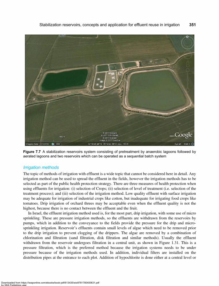
Irrigation methodsThe topic of methods of irrigation with effluent is a wide topic that cannot be considered here in detail. Anyirrigation method can be used to spread the effluent in the fields, however the irrigation methods has to beselected as part of the public health protection strategy. There are three measures of health protection whenusing effluents for irrigation: (i) selection of Crops; (ii) selection of level of treatment (i.e. selection of thetreatment process); and (iii) selection of the irrigation method. Low quality effluent with surface irrigationmay be adequate for irrigation of industrial crops like cotton, but inadequate for irrigating food crops liketomatoes. Drip irrigation of orchard threes may be acceptable even when the effluent quality is not thehighest, because there is no contact between the effluent and the fruit.

In Israel, the effluent irrigation method used is, for the most part, drip irrigation, with some use of microsprinkling. These are pressure irrigation methods, so the effluents are withdrawn from the reservoirs bypumps, which in addition to the conveyance to the fields provide the pressure for the drip and micro-sprinkling irrigation. Reservoir’s effluents contain small levels of algae which need to be removed priorto the drip irrigation to prevent clogging of the drippers. The algae are removed by a combination ofchlorination and filtration (sand filtration, disk filtration and similar methods). Usually the effluentwithdrawn from the reservoir undergoes filtration in a central unit, as shown in Figure 1.31. This is apressure filtration, which is the preferred method because the irrigation systems needs to be underpressure because of the irrigation methods used. In addition, individual filters are installed on thedistribution pipes at the entrance to each plot. Addition of hypochlorite is done either at a central level or

Figure 7.7 A stabilization reservoirs system consisting of pretreatment by anaerobic lagoons followed byaerated lagoons and two reservoirs which can be operated as a sequential batch system



individually by each farmer. The chlorination is done mainly to facilitate the filtration and removal of algaefor preventing clogging of the drippers; however it also helps to complement the disinfection ofthe effluents.

7.1.3 PerformanceEfficiencyThe performance of a reservoir system and the quality of effluent it produces is highly dependent on themode of operation of the system and on the operational parameters. As explained above, a singlecontinuous flow reservoir does not produce a high quality effluent. The effluent quality is notconstant and it deteriorates along the irrigation season. In regions with an irrigation season of 4–5months like Israel, the annual mean detention time in a reservoir is 80–130 days. The annual meantotal BOD removal percentage is 70–85%, total COD removal 50–85% and TSS removal is 40–80%.The system also achieves 25 to 50% removal of N and P. Higher nutrient removal percentages areachieved in system with a longer detention time (the Maale Hakishon reservoirs, with a joint meandetention time of 180 days achieve 70% removal of N and 60% removal of P). The total coliformsremoval in continuous flow reservoirs is only one order of magnitude, a low value for reactors withsuch a long mean detention time. However, as explained, the effluent quality is not constant duringthe irrigation season and the maximum effluent quality, which is the quality at the beginning of theirrigation season, is much higher, with removal values of BOD, COD in the range 85–95% and TSSin the range 90–98%. Effluents of single continuous flow reservoir systems are usually used forrestricted irrigation.

A very high effluent quality is achieved in reservoir systems operated under a sequential batch mode.Such systems can achieve BOD, COD and TSS removals of 85–95% each, continuously during theirrigation season. They produce an effluent with a BOD5 concentration of 5–10 mg/l and a TSSconcentration of 5–20 mg/l. Moreover, the faecal coliforms removals in such systems are very high,producing effluents with faecal coliforms levels of 0–100 MPN/100 ml. This means that sequentialbatch reservoir systems perform disinfection without the use of chemicals. In addition, the stabilizationreservoirs completely remove helminth eggs and nematodes without difficulty. The effluents ofsequential batch reactors are adequate for unrestricted irrigation.

An important characteristic of the stabilization reservoir is the fact that they do not produce excess sludge.The only unit that may generate excess sludge in a reservoir system is the pretreatment unit. If this unit is astabilization lagoons unit, it produces very small quantities of excess sludge so the entire system ispractically a sludge free system. If the pretreatment unit is based on other anaerobic processes, itgenerates small quantities of excess sludge. However, if the pretreatment is based on aerobic treatmentprocesses, it generates larger amounts of excess sludge.

A comparison of some basic performance parameters of a Stabilization Reservoir system and a facultativelagoons system is presented in Table 7.1.

Advantages and disadvantages of a reservoir systemThemain purpose of using stabilization reservoir is to recover wastewater for its efficient reuse for irrigation.According to Libhaber, 1996, this brings the following benefits

• Irrigation is usually needed in areas where water tends to be scarce and wastewater reuse is necessaryfor supplementing available fresh water sources. In terms of availability it is also a safe water source,independent on climatic conditions.



• Agriculture requires large amounts of water, which are used only once, since irrigation is aconsumptive use. Thus, there is no danger of gradual accumulation in the water of undesirablesubstances by continuous recycling.

• Agriculture can use not only the water, but also additional resources found in wastewater, such asorganic matter or nutrients (nitrogen and phosphorous), which are thus converted from anenvironmental nuisance to an asset.

• Irrigation is relatively flexible with respect to water quality requirements. Some crops can be irrigatedwith low quality water, and some water quality problems can be overcome by suitable agriculturalpractices.

• Use of wastewater for irrigation prevents its discharge to receiving water bodies and pollution of waterresources.

The disadvantages associated with the reuse of treated wastewater for irrigation can be divided into twocategories:

• Public health is the issue of greatest concern, and it is related to wastewater reuse that can endangerconsumers of crops irrigated with effluents, to farmers, and to residents in the neighbourhood of theirrigated fields.

• The agro-technical problems that may be caused by inappropriate reuse of effluent, relate primarily todamage to crops and soils.

These two problems can be managed through the proper design of reuse systems (conveyance, treatment andirrigation) and through the adoption of adequate agro-technical practices during the cultivation of crops.

7.2 BASIC DESIGN PROCEDURES7.2.1 General design considerationsTwo basic factors need to be considered prior to the design of a stabilization reservoir: (i) the type of cropwhich will be irrigated with the reservoir’s effluent and the quality of effluent they require, that is, is it a

Table 7.1 Basic parameters of facultative lagoons and reservoir systems.

Process Treatmentgoal

Requiredclimate

Meandetentiontime (days)

Depth(m)

Surfaceorganicloading(kg/////ha · d)

Effluent quality(mg/////l)

Facultativelagoons

Secondary toadvanced

any 10–50 1.5 a 2.5 50–250 DBO: 30–40

SST: 40–100

Stabilizationreservoirs


any 80–200 4 a 12 ,50 Continuous flow:Varying qualityBOD: 15–30TSS: 20–60

Sequential batch:BOD: 5–10TSS: 5–20

Sources: Crites, Middlebrooks & Sherwood (2006); Juanicó & Dor (1999); Orozco (2005)



quality for restricted or for unrestricted irrigation; and (ii) the required volume of the reservoir, whichdepends on the irrigation needs of crops. Stabilization reservoirs are deep lagoons that are used for twopurposes: (i) storing partially treated wastewater over a long period of time in order to use it during aspecific period of the year, under optimal and controlled conditions; and (ii) improving the quality ofstored effluents during their long residence time in the reservoir. The stabilization reservoir receiveseffluents of primary or secondary treatment units, stores them and improves their quality exercising thefollowing priorities of treatment: (i) maximum removal of helminths and protozoa, (ii) effective removalof bacterial and viral pathogens and (iii) Effective reduction of BOD to avoid unpleasant smellunpleasant appearance of the effluent (Libhaber, 2007).

There are basically three modes of operating stabilization reservoirs system, as shown in Figure 7.3. Theselection of the mode of operation is determined on the basis of the planned objective of use of the effluent:either for restricted irrigation, unrestricted irrigation, or a combined of the two. Each use objective prescribesa different mode of operation.

7.2.2 Orderly Design Method, ODMIn general the design methodology of a Stabilization Reservoir consists of the following:

(1) Determine the external or independent variables, which among others, include the following:○ Wastewater flows, geographical conditions pollutants concentrations and loads are handles

using the methodology described in Chapter 5, Section 5.2.2, Paragraph 1. In the case ofreservoirs is necessary to calculate the municipal wastewater flows available forirrigation, as well as the amounts and patterns of water required by the crops. Twospecific issues are important for these calculations: (i) the estimates of availability ofmunicipal wastewater for irrigation, both in terms of quantity and quality, using themethodology presented in Chapter 2 and the efficiencies of the treatment processemployed in pretreatment of the wastewater prior to its discharge into the reservoir; and(ii) the estimated water requirements for irrigation and for, and its distribution along theyear, for which it is necessary to have the curves of monthly precipitation and evapotranspiration for the type of crop in the specific project area (which needs to bedetermined by a specialist in agronomy). The monthly distributions of precipitation andevapo-transpiration and consumption of water for irrigation depends on the climate onthe type of soil, on the type of crops to be cultivated, and so on. These data properlyprocessed provide the irrigation requirements and the net balance needed to meet thedemand. The net demand is calculated in Paragraph 4 below. Figure 7.8 shows anexample a summary of the results of such calculations.

○ Geographical conditions, such as maximum and minimum temperatures of air and water, solarradiation and cloud cover, wind rose, altitude above sea level, proximity to population centers,and so on. These data are very important from the agricultural standpoint, as well as from thewastewater treatment standpoint.

○ In addition, the data regarding potential evapo-transpiration (ET0) and monthly precipitationmust be obtained. Usually they are provided by the regional hydrological authority. Anexample of this type of data is presented in the Table 7.2 below and in Figure 7.9.

(2) Determine the flow diagram of the stabilization reservoir system: The components of a typicalstabilization reservoir system are shown in Figure 7.5, but obviously, the pretreatment unit canbe different than the one presented in Figure 7.5.



Table 7.2 An example of data of monthly distribution of evapo-transpiration and precipitation.

Month Jan Feb Mar April May June July August Sept Oct Nov Dec

ET0, mm/month 145.08 156.52 190.03 177.00 163.68 173.70 193.50 197.78 155.10 139.81 125.40 139.19

Precipitation,mm/month

5.80 8.80 4.10 24.00 89.60 27.00 4.60 29.00 102.00 167.00 115.00 26.00

Figure 7.8 Example of the distribution of availability and demand of treated wastewater for irrigation along themonths of the year (Availability-▴, Demand-▪)

0.00

50.00

100.00

150.00

200.00

250.00

Jan

Feb

Mar

Apr

il

May

June July

Aug

ust

Sept Oct

Nov Dec

Prec

ipit

a�on

and

f ET0

, mm

/mon

th

month

ET0, mm/month

Precipita�on,mm/month

Figure 7.9 Example of the variation of potential evapo-transpiration (ET0) and precipitation along the monthsof the year



(3) Identify the pretreatment system. The stabilization reservoir design depends on the pretreatmentunit. Usually both systems (the pretreatment unit and the reservoir) are designed andconstructed jointly. The design of the pretreatment unit is performed in accordance with themethodologies of design of the appropriate technology processes presented in other chapters ofthe book. The level of pretreatment and the design of the pretreatment unit are adjusted to thedesign of the reservoir, taking into account its dimensions of the reservoir and the surfaceorganic loading which will be applied to it. The objective of the pretreatment is to reduce theorganic matter content in the wastewater so that the effluent discharged to the reservoir wouldnot cause the entire reservoir to become anaerobic, but will rather leave an aerobic upper layerin the reservoir. It is again emphasized that the pretreatment process is not just one specificprocess, but can be one of a variety of unit processes or combination of unit processes, whichcan be based appropriate technology processes and also on processes which are not appropriatetechnology processes. The purpose of the pretreatment unit is to reduce the organic mattercontent in the wastewater to a desired level and this objective can be achieved through the useof a variety of processes. We obviously recommend employing appropriate technologyprocesses as pretreatment units, especially in developing countries.

Hydraulic design

(4) Determine the net demand of water for irrigation. The participation of an expert agronomist isessential for the estimation of the demand of water for irrigation. This expert has to determinethe type of crops that can be cultivated, depending on the availability and quality of thewastewater. In particular, once the crops have been defined, the monthly demand of water forirrigation needs to be calculated. The formula for estimation the monthly water demand is thefollowing (Gurovich & Ramos, 1990).

Dw = 10 ET0SkcAc/ETa (7.2)

where:

Dw = total monthly demand of water for agriculture, m3/ha · month. The value 10 is a conversionfactor from mm/month to m3/ha · month.

ET0 = potential evapo-transpiration, mm/month. In general, the hydrological control authorityprovides these data2.

Ac = area of each crop, ha.kc = coefficient of each crop (ratio of ET0 to actual ET), that is, actual evapo-transpiration (ET)

is a fraction of the potential (ET0). For example, for corn it is 0.55. If there are multiplecrops there are different kc (per crop), and they can vary month to month, depending onthe harvest season. Therefore, the expression Σ kcAc is used.

ETa = overall efficiency of water use in the conveyance system, in the application method ofirrigation (the irrigation method), and so on. It does not necessarily include infiltrationlosses (which can be treated as a sensitivity parameter, for example, for 1 mminfiltration, 5 mm, and so on).

2This is a climate parameter and it can also be calculated by the Penmanmethod, by the Radiationmethod or by Tank Class AMethod.The results are similar, and for their calculation the following data are required: (i) temperature, (ii) wind velocity, (iii) relative humidity,(iv) cloudiness, (v) radiation, and (vi) effective number of hours of sunshine.



With these data, for the crops that are to be developed using the reservoir’s effluent, the monthlywater demand for agriculture is determined by the use of Equation 7.2.

To calculate the net demand (Vw) it is necessary to take into account the monthly precipitation(P) that sometimes may be sufficient to meet the irrigation demand, and the infiltration (I) which is awater loss.

Vw = Dw − 10 · P− I( ) · Ac (7.3)

The factor 10 is again a conversion factor used to convert “mm/month” to “m3/ha · month”. Duringthe rainy months, the rainfall may be sufficient to meet the water demand of the crops and evenexcessive (negative demand), but since the rainwater is not stored, for calculation purposes Vw isconsidered zero in the rainy season months.

When the demand is positive, the domestic wastewater flow (QWW) has to provide this demand.A properly designed stabilization reservoir provides the necessary irrigation water in the mostefficient manner, and it is the available storage volume which determines the area Ac. that canbe irrigated.

(5) Determine the volume of the stabilization reservoir. Taking into consideration the available supplyof wastewater and the distribution of net monthly demand of effluent for irrigation (i.e., the requiredwater volume every month), and considering a single continuous flow reservoir (operation mode ofFigure 7.3a), which means restricted irrigation, the volume of the reservoir required to cover theirrigation water deficit is calculated using the mass curve method.

The mass curve is calculated using the following methodology: (i) build the consumption line forirrigation or aggregate demand (ΣVw) adding demands every month, taking care to sum zero whenthe demand generated by the formula is negative (i.e. there is sufficient rainwater and no additionaldemand from the reservoir, and the excess rainwater is not stored), (ii) connect the string joining thefirst and last point of the series, (iii) draw the tangents parallel to the string of the curve through thepoints of maximum (maximum deficit) and minimum (minimum deficit), and (iv) calculate thevertical distance between the two parallel tangent lines and this distance gives the net operativevolume of the reservoir (VSR) required to provide effluent for irrigation when required.

If it is decide to provide effluent for unrestricted irrigation, it is necessary to construct one, two ormore reservoirs which will function in parallel. This is done using the calculated volume VSR anddividing it by the number of reservoirs to be built. After one reservoir is filled, the pretreated effluentis diverted to another reservoir. If irrigation water is needed before the first reservoir (SR1) has beenfilled up then its filling is stopped and only then is his effluent conveyed to irrigation, while thepretreated effluent is diverted to the second reservoir (SR2). This ensures that the PFE of thefirst reservoir is not increased during the irrigation period, because irrigation is applied on cropswhich require unrestricted effluent quality.

(6) Calculate the irrigated area (Ac). Since the crop area (which is the same irrigate area) depends onthe available water for irrigation, it is calculated by trial and error from the following equation:

S QWW − 10 E− P( ) · ASR[ ] = SVw (7.4)

with:

ΣQww = the amount of wastewater produced during the year, Σm3/month=m3/year.ASR =Area of the stabilization reservoir, ha. Initially this number needs to be estimated.E= evaporation from the reservoir, mm/monthP= the precipitation over the SR, mm/month



ΣVw = The annual net water demand for irrigation, which depends on crop area, Ac (m3), as shown

in Equation 7.3.

Again 10 is the conversion factor from mm/month to m3/ha · month. Note that the evaporation (E)is from the reservoir surface and is different from the ET for the crop area. If E is not known, theVisentini’s Equation can be applied:

E = CT+M (7.5)

where T is the mean annual temperature, in degree centigrade, and C and M are constants thatdepend on the altitude (meters above sea level, masl) as follows:

Altitude, masl C M

,200 75 0

200 to 500 90 0

.500 90 300

Kinetics design

(7) Calculate of the quality of the reservoir’s effluent: according to Juanico (2005), the efficienciesobtained by stabilization reservoirs (additional to pretreatment) with continuous flow-singlereservoir and with a sequential batch flow reservoir system (two or more stabilization reservoirs)are presented in Table 7.3. This table can be use as a first approximation; however, a directkinetics design will provide more accurate results.

Instead of using Equation 7.1 to calculate the mean residence time, which would be impracticalfor design, it is better to use, as an approximation, the average detention time (td) of the reservoircalculated with the half (or approximate “average”) reservoir volume (V1/2). The same goes for the“average” surface area (As). Note that the net volume VN= 2 · V1/2:

V1/2 = Q · td (7.6)

As = V1/2/h (7.7)

Table 7.3 Efficiencies in continuous flow and sequential batch fed stabilization reservoirs.

Parameter Continuous flowreservoir

Sequential batch flow reservoirswith batch from 30 to 50 Days

BOD5 70% 90%

COD 50% 80–90%

Detergents 50% 90%

Nitrogen – 70–80%

Phosphorus ,30% 10–60%

Fecal Coliforms 90–99% 99.99%

Streptococcus – 90%

Giardia – 80–90%

Source: Juanico (2005)



To calculate the efficiency by the kinetics method, Equation 7.8 is used:

S = S0A

1+ KLtdn

( )n (7.8)

where S0A is the pretreatment effluent BOD, and “n” the number of reservoirs in series. Note that thedetention time is the cycle’s “average” detention time.

The final water temperature in the reservoir is calculated as follows:

TL = AEEf Ta + QwwTi

AEEf + Qww(7.9)

where

TL = Final reservoir temperature (°C)Ta =Air temperature (°C)Ti = Influent wastewater temperature (°C)

AEE = Surface area (m2)Qww =Mean wastewater flow (m3/d)

f= Proportionality factor, 0.5 m/d

If KL is unknown the typical KL (20°C)= 0.35 d−1, can be used corrected for temperature withEquation 7.10:

KL = KL(208C) u(T−20) (7.10)

where θ is a constant and its value is between 1.05 and 1.09.The above approximation of the average detention time (td) was used as the kinetic approach in the

Excel program CHAP 7-SR for calculating the reservoir. However the following additionalinformation is presented in regard to the dynamic solution analysis.

If it is desired to calculate the Stabilization Reservoir (SR) effluent quality on a dynamic basis (i.e.day by day) instead of the approximated (or “averaged”) calculation proposed in Equation 7.6 usingthe “average” detention time (td=QD/V1/2), it is necessary to apply a dynamicmass balance in orderto obtain the exact solution to be used in the kinetics equations governing the water quality.

For instance if we assume for simplicity a Sequential Batch (SB) regime (i.e. the StabilizationReservoir is filling during the rainy season without outflow, and the wastewater inflow is cut offjust prior to starting the use of treated water outflow for irrigation during the dry season) thedynamic mass balance is (Vi.dS/dt)=QD.S0− Vi.r(S), where S is the BOD5 (or any otherparameter) concentration in the reservoir, S0 is the influent concentration, r(S) is the reaction rate ofthe BOD5 inside the reservoir, and Vi is the instantaneous volume at time t. For simplicity let’sassume that QD is constant, and Vi=QD.t, where t is the elapsed time. Note that r(S) acts as a sink,while the inflow BOD5 (QD.S0) acts as a source in the mass balance. Now, the reaction rate forBOD in its most common form can be expressed as r(S)=KLS. Then the mass balance becomes:

dSdt

Vi = QDS0 − KLSV

or

dSdt

t = S0 − KLSt



The solution of this differential equation according to Wolfram’sMathematica 8.0 is:

S[t] = u−KLtC[1]+ u−KLtS0ExpIntegralEi[KLt]

Where:

ExpIntegralEi[KL.t] =∫1−KLt

u−KLt

KLtdt

and C is the integration constant,which at t= 0 becomes (−∞). Then, themathematical exact solution even for the simplest case

becomes intractable.On the other hand, it is possible to reach another “exact” approach with the mean detention time

(tdmj) as calculated on a daily base from Equation 7.1:

tdmj = [(tdm(j−1) + 1)V(j−1)]+ 0.5vjV(j−1) + vj

For simplicity let’s assume that QD is constant and is given in m3/d, then replacing V(j−1)=QD ·( j− 1), v( j−1)=QD and “j” by “t” (remember: t is the elapsed time and tdmj is themean detention timeat t= j), Equation 7.1 becomes:

tdmt = [(tdm(t−1) + 1)(t − 1)]+ 0.5t

Using this approach we can simulate day by the detention time as presented in the table below:

t, days tdmt, days

1 0.5

2 1.0

3 1.5

4 2.0

5 2.5

6 3.0

7 3.5

8 4.0

9 4.5

10 5.0

11 5.5

12 6.0

13 6.5

14 7.0

15 7.5

(Continued )



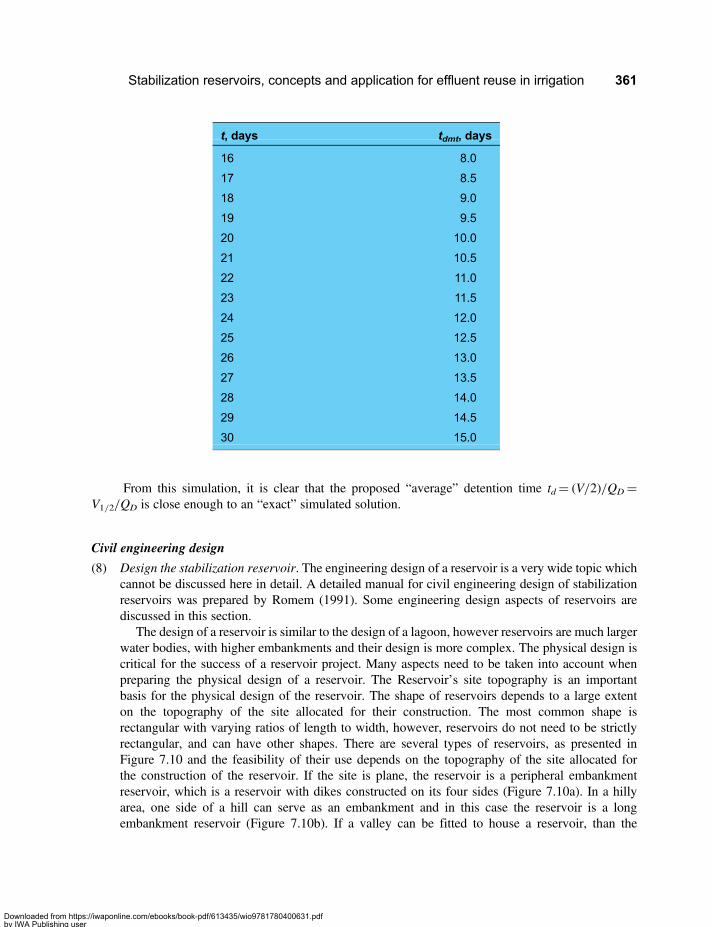
t, days tdmt, days

16 8.0

17 8.5

18 9.0

19 9.5

20 10.0

21 10.5

22 11.0

23 11.5

24 12.0

25 12.5

26 13.0

27 13.5

28 14.0

29 14.5

30 15.0

From this simulation, it is clear that the proposed “average” detention time td= (V/2)/QD=V1/2/QD is close enough to an “exact” simulated solution.

Civil engineering design

(8) Design the stabilization reservoir. The engineering design of a reservoir is a very wide topic whichcannot be discussed here in detail. A detailed manual for civil engineering design of stabilizationreservoirs was prepared by Romem (1991). Some engineering design aspects of reservoirs arediscussed in this section.

The design of a reservoir is similar to the design of a lagoon, however reservoirs are much largerwater bodies, with higher embankments and their design is more complex. The physical design iscritical for the success of a reservoir project. Many aspects need to be taken into account whenpreparing the physical design of a reservoir. The Reservoir’s site topography is an importantbasis for the physical design of the reservoir. The shape of reservoirs depends to a large extenton the topography of the site allocated for their construction. The most common shape isrectangular with varying ratios of length to width, however, reservoirs do not need to be strictlyrectangular, and can have other shapes. There are several types of reservoirs, as presented inFigure 7.10 and the feasibility of their use depends on the topography of the site allocated forthe construction of the reservoir. If the site is plane, the reservoir is a peripheral embankmentreservoir, which is a reservoir with dikes constructed on its four sides (Figure 7.10a). In a hillyarea, one side of a hill can serve as an embankment and in this case the reservoir is a longembankment reservoir (Figure 7.10b). If a valley can be fitted to house a reservoir, than the



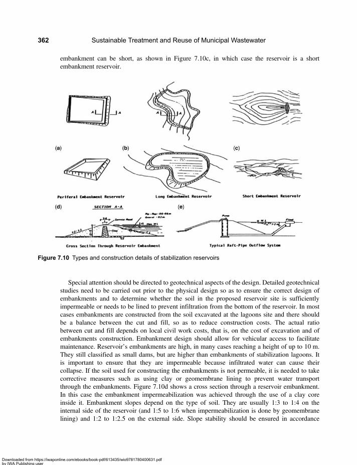
embankment can be short, as shown in Figure 7.10c, in which case the reservoir is a shortembankment reservoir.

Special attention should be directed to geotechnical aspects of the design. Detailed geotechnicalstudies need to be carried out prior to the physical design so as to ensure the correct design ofembankments and to determine whether the soil in the proposed reservoir site is sufficientlyimpermeable or needs to be lined to prevent infiltration from the bottom of the reservoir. In mostcases embankments are constructed from the soil excavated at the lagoons site and there shouldbe a balance between the cut and fill, so as to reduce construction costs. The actual ratiobetween cut and fill depends on local civil work costs, that is, on the cost of excavation and ofembankments construction. Embankment design should allow for vehicular access to facilitatemaintenance. Reservoir’s embankments are high, in many cases reaching a height of up to 10 m.They still classified as small dams, but are higher than embankments of stabilization lagoons. Itis important to ensure that they are impermeable because infiltrated water can cause theircollapse. If the soil used for constructing the embankments is not permeable, it is needed to takecorrective measures such as using clay or geomembrane lining to prevent water transportthrough the embankments. Figure 7.10d shows a cross section through a reservoir embankment.In this case the embankment impermeabilization was achieved through the use of a clay coreinside it. Embankment slopes depend on the type of soil. They are usually 1:3 to 1:4 on theinternal side of the reservoir (and 1:5 to 1:6 when impermeabilization is done by geomembranelining) and 1:2 to 1:2.5 on the external side. Slope stability should be ensured in accordance

Figure 7.10 Types and construction details of stabilization reservoirs



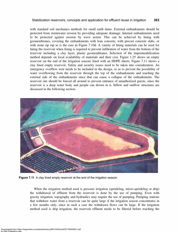
with standard soil mechanics methods for small earth dams. External embankments should beprotected from stormwater erosion by providing adequate drainage. Internal embankments needto be protected against erosion by wave action. This can be achieved by lining withgeomembranes, covering the embankments with lean concrete, with precast concrete slabs, orwith stone rip rap as is the case in Figure 7.10d. A variety of lining materials can be used forlining the reservoir when lining is required to prevent infiltration of water from the bottom of thereservoir including a clay layer, plastic geomembranes. Selection of the impermeabilizationmethod depends on local availability of materials and their cost. Figure 1.25 shows an emptyreservoir (at the end of the irrigation season) lined with an HDPE sheets. Figure 7.11 shows aclay lined empty reservoir. Safety and security issues need to be taken into consideration. Anemergency overflow weir needs to be included in the design, so as to prevent the possibility ofwater overflowing from the reservoir through the top of the embankments and reaching theexternal side of the embankments since that can cause a collapse of the embankments. Thereservoir site should be fenced all around to prevent entrance of unauthorized guests, since thereservoir is a deep water body and people can drown in it. Inflow and outflow structures arediscussed in the following section.

When the irrigation method used is pressure irrigation (sprinkling, micro-sprinkling or drip)the withdrawal of effluent from the reservoir is done by the use of pumping. Even withgravity irrigation, topography and hydraulics may require the use of pumping. Pumping stationsthat withdraw water from a reservoir can be quite large if the irrigation season concentrates ina few months only, since in such a case the withdrawn flows can be large. If the irrigationmethod used is drip irrigation, the reservoir effluent needs to be filtered before reaching the

Figure 7.11 A clay lined empty reservoir at the end of the irrigation season



drippers, to prevent their clogging bay algae residues that are contained in the reservoir. A sample ofa reservoir effluent is presented in Figure 1.30 and the green colour can be noted. This effluent isvoid of coliforms but still has algae and therefore needs to be filtered. In Israel, the main irrigationmethod is drip irrigation so pressure the filtration method mostly used is pressure filtration since theeffluent system is a pressure system. A typical reservoir effluent filtration system is shown inFigure 7.12 (Lehavim Reservoir) and also in Figure 1.31 (Kfar Menahem Reservoir).

Stabilization reservoirs are always located outsides cities, close to the irrigated fields. Thepretreatment units are located wither within the cities and operated by the utilities, or near thereservoir, in which case they might be operated the utilities or the farmers’ association. Thereservoirs are mostly operated by the farmers’ association. Operation and maintenance of areservoir system includes mainly the operation and maintenance of the pumping station and thefiltration system and periodical preventive maintenance of the embankments. Operation andmaintenance is similar to that of a lagoons system, with an additional aspect of operation andmaintenance of the system of effluent supply for irrigation.

(9) Inflow and outflow structures. A single inlet and outlet in a reservoir are usually sufficient but theyhave to be located in diagonally opposite corners of the reservoir to prevent short circuiting (as canbe seen in Figure 1.25 and in Figure 7.11). Hydraulic short-circuiting is a series problem and shouldbe avoided. An effective way to avoid this problem is to properly locate the inflow and outflow

Figure 7.12 A typical sand filtration system for reservoir effluent filtration at the lehavim reservoir



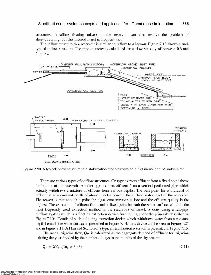
structures. Installing floating mixers in the reservoir can also resolve the problem ofshort-circuiting, but this method is not in frequent use.

The inflow structure to a reservoir is similar an inflow to a lagoon. Figure 7.13 shows a suchtypical inflow structure. The pipe diameter is calculated for a flow velocity of between 0.6 and5.0 m/s.

There are various types of outflow structures. On type extracts effluent from a fixed point abovethe bottom of the reservoir. Another type extracts effluent from a vertical perforated pipe whichactually withdraws a mixture of effluent from various depths. The best point for withdrawal ofeffluent is at a constant depth of about 1 meter beneath the surface water level of the reservoir.The reason is that at such a point the algae concentration is low and the effluent quality is thehighest. The extraction of effluent from such a fixed point beneath the water surface, which is themost frequently used extraction method in the reservoirs of Israel, is done using a raft-pipeoutflow system which is a floating extraction device functioning under the principle described inFigure 7.10e. Details of such a floating extraction device which withdraws water from a constantdepth beneath the water surface is presented in Figure 7.14. This device can be seen in Figure 1.25and in Figure 7.11. A Plan and Section of a typical stabilization reservoir is presented in Figure 7.15.

The mean irrigation flow, QR, is calculated as the aggregate demand of effluent for irrigationduring the year divided by the number of days in the months of the dry season:

QR = SVww/ nd × 30.3( ) (7.11)

Figure 7.13 A typical inflow structure to a stabilization reservoir with an outlet measuring “V” notch plate



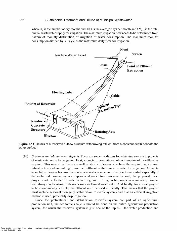
where nd is the number of dry months and 30.3 is the average days per month and ΣVww is the totalannual wastewater supply for irrigation. Themaximum irrigation flow needs to be determined frompattern of monthly distribution of irrigation of water consumption. The maximum month’sconsumption divided by 30.3 yields the maximum daily flow for irrigation.

(10) Economic and Management Aspects. There are some conditions for achieving success in projectsof wastewater reuse for irrigation. First, a long term commitment of consumption of the effluent isrequired. This means that there are well established farmers who have the required agriculturalinfrastructure and are willing to use their effluent as the source of water for irrigation. Attemptsto mobilize farmers because there is a new water source are usually not successful, especially ifthe mobilized farmers are not experienced agricultural workers. Second, the proposed reuseproject must be located in water scarce regions. If a region has water in abundance, farmerswill always prefer using fresh water over reclaimed wastewater. And finally, for a reuse projectto be economically feasible, the effluent must be used efficiently. This means that the projectmust include seasonal storage (a stabilization reservoir system) and that an efficient irrigationmethod is used, preferably drip irrigation.

Since the pretreatment and stabilization reservoir system are part of an agriculturalproduction unit, the economic analysis should be done on the entire agricultural productionsystem, for which the reservoir system is just one of the inputs – the water production and

Figure 7.14 Details of a reservoir outflow structure withdrawing effluent from a constant depth beneath thewater surface



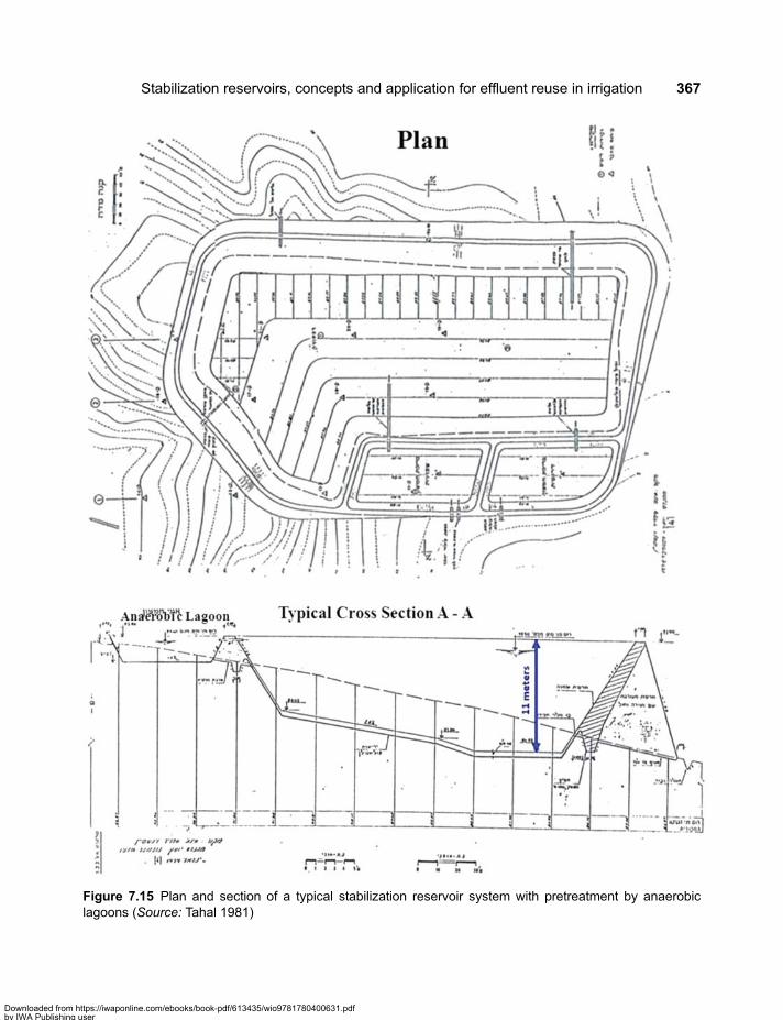
Figure 7.15 Plan and section of a typical stabilization reservoir system with pretreatment by anaerobiclagoons (Source: Tahal 1981)



supply input. The investment and O&M costs of the water production system should not be theentire costs of the pretreatment and stabilization reservoir system. The cost of the alternativewastewater treatment which the wastewater contribution city has to provide under theprevailing regulations should be deducted from the cost of the reservoir system since it isthe obligation of the city to provide such investments and O&M costs. Sometimes thealternative cost which the city should have invested is larger than the entire costs of thepretreatment and reservoir system because discharge of effluents to water streams (whichwould have had to be done if the wastewater would not have been used for irrigation)requires a higher quality effluent and a higher and more costly level of treatment. Such typeof analysis was undertaken on a pretreatment and single continuous flow reservoirproducing effluent for restricted irrigation under the conditions of Israel at the period whichde analysis was undertaken (Libhaber, 1987). The effluent was used to irrigate cotton andwheat and the outcome of the analysis depends on the market price of cotton and wheat.The results (valid for the agricultural inputs and produce prices used in the calculations)show that if the city does not contribute anything to the investment costs (which means thatthe farmers provide the entire funds for the pretreatment and for the reservoir), the IRR(Internal Rate of Return of the project) would be 16%. If the city provides 50% of theinvestment costs of the water production system (pretreatment and reservoir, includingO&M costs) the IRR would be 28%, and if the city provides 100% of the investment costsof the water production system (pretreatment and reservoir, including O&M costs), the IRRwould reach a value of 57%.

This type of economic analysis is usually not undertaken prior to taking decisions on reuseprojects. Wastewater reuse is usually practiced in scarce water zones, where the demand forirrigation water is high and the driving force for investments is the generation of anadditional water source. The city provides the investment and O&M costs of thepretreatment installations and the farmers’ organization provides the investment and O&Mcosts of the reservoir. Governments usually provide grants to render reuse projects feasible.Such grants may be directed to the farmers, to the city or to both.

In Israel, the cities finance the wastewater treatment installations and the farmersassociations (the group of users in each case) finance the stabilization reservoir investmentand O&M. The government provides a grant to the farmers association to partially financethe investment of the reservoir system (including pumping stations and filtration systems) sothat the resulting cost of water for the farmers is reasonable and somewhat lower than thecost of fresh water supplied by the national water company. Government grants reachsometimes 70% of the investment in the reservoir system. The government’s interest indoing that is the generation of an additional water source. The use of effluent for irrigationliberates the fresh water which was previously used by the farmers to be directed formunicipal water supply. It is a win-win situation for all. The government generates anadditional water source; the national water company increases its fresh water reserves andthe farmers maintain their occupation as farmers (without effluent they would have lost theirwaster source because fresh water are no more available for irrigation).

The way all this works id the following. The farmers to whom the wastewater of a certaincity was allocated constitute an effluent use management unit. This is an independent entity incharge of constructing and managing the reservoir system. This unit retains the consultingengineer to design the reservoir and the construction of the reservoir. It uses the



government fund and bank loans to finance the investment. Then it sells the water to thefarmers, each farmer pays monthly for the measured water he consumed, at a tariff set bythe management unit. The monthly income of the unit is used to repay the bank loans andto cover O&M costs (mainly electricity costs). The level of the government grant is set onsuch a level that the tariff for the farmers would be about 0.2–0.3 US$/m3, which issomewhat lower than the tariff of fresh water for irrigation.

The tasks of the management unit after the reservoirs construction has been completed is tooperate the reservoir system (mainly the pumping station, filtration unit and embankmentsperiodical maintenance) and sometimes also to operate the pretreatment installations, and toconduct the financial management (collection of payments from the farmers, repayment of loansand payment of O&M costs). A management unit can be in charge of one reservoir system andof several reservoirs, depending on the size of the wastewater contributing city. If the number ofreservoirs handled by a management unit is small (one or two) the management is apart timejob. For larger systems, management can be a full time job. As an example, in one of the largestsystems in Israel, which consists of about 10 reservoirs (the number increases with time becauseof the increase of wastewater flow), the management unit consists of two full time employees:the manager, who is mainly in charge of the financial management, and the technician, who isin charge of operation and maintenance.

When appropriate technology processes are used for pretreatment, the investment cost inthe system of pretreatment followed by a Stabilization Reservoir is in the range of 30–50 US$/Capita and the O&M cost is in the range 0.2–0.4 US$/Year/Capita.

The cost of a complete stabilization reservoir system, including pretreatment, depends to a largeextent on the pretreatment system. The additional investment cost of the reservoir system is about20–30 US$/Capita. When the pretreatment is based on appropriate technology, the investmentcost of a complete reservoir system, including pretreatment, is about 30–50 US$/Capita. Whenthe reservoir is in the same site of the pretreatment installations and both are operated by thesame operator (usually the farmers’ organization) the additional operation and maintenance costof the reservoir is small. In many cases, the pretreatment and the reservoir are not in the samesite and are operated by different entities, the pretreatment by the municipality or the waterutility of the city and the reservoir by a farmers association. In this case, the operation andmaintenance costs of the reservoir are similar to those of operating a stabilization lagoonssystem, that is, in the range of 0.2–0.4 US$/Year/Capita. The cost of construction of reservoirsin Israel is 1–2 US$/m3 of reservoir volume.


Following is a design example based on the Orderly Design Method (ODM) presented in Section 7.2.2.The example is developed for a population of 20,000, with a raw wastewater flow and quality as presented inChapter 3. The ODM is applied step by step and is specified in the Excel program CHAP 7-SR. Thecalculations presented below are the outputs of this program. An anaerobic lagoon (A) is selected as thetreatment prior to the reservoir (for details of design, see Chapter Five). The crop area has the Evapo-transpiration (ET0) and Precipitation given, and E is the Evaporation in the Stabilization Reservoir area(without vegetation). The data are given in Table 7A.



















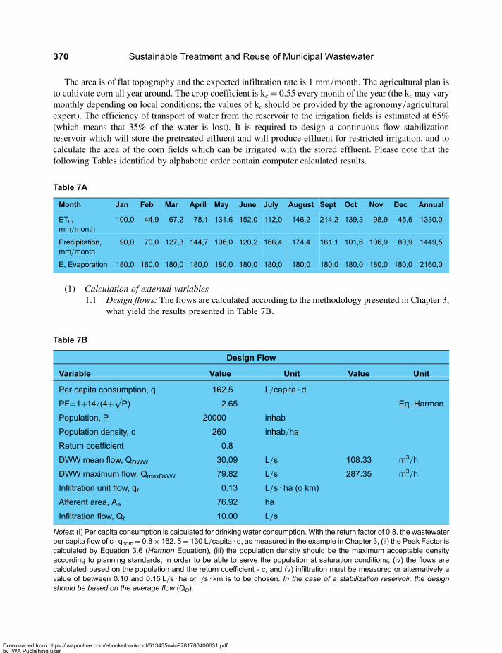
The area is of flat topography and the expected infiltration rate is 1 mm/month. The agricultural plan isto cultivate corn all year around. The crop coefficient is kc= 0.55 every month of the year (the kc may varymonthly depending on local conditions; the values of kc should be provided by the agronomy/agriculturalexpert). The efficiency of transport of water from the reservoir to the irrigation fields is estimated at 65%(which means that 35% of the water is lost). It is required to design a continuous flow stabilizationreservoir which will store the pretreated effluent and will produce effluent for restricted irrigation, and tocalculate the area of the corn fields which can be irrigated with the stored effluent. Please note that thefollowing Tables identified by alphabetic order contain computer calculated results.

(1) Calculation of external variables1.1 Design flows: The flows are calculated according to the methodology presented in Chapter 3,

what yield the results presented in Table 7B.

Table 7A

Month Jan Feb Mar April May June July August Sept Oct Nov Dec Annual

ET0,mm/month

100,0 44,9 67,2 78,1 131,6 152,0 112,0 146,2 214,2 139,3 98,9 45,6 1330,0

Precipitation,mm/month

90,0 70,0 127,3 144,7 106,0 120,2 166,4 174,4 161,1 101,6 106,9 80,9 1449,5

E, Evaporation 180,0 180,0 180,0 180,0 180,0 180,0 180,0 180,0 180,0 180,0 180,0 180,0 2160,0

Table 7B

Design Flow



PF=1+14/(4+√P) 2.65 Eq. Harmon









Notes: (i) Per capita consumption is calculated for drinking water consumption. With the return factor of 0.8, the wastewaterper capita flow of c · qdom= 0.8× 162. 5= 130 L/capita · d, as measured in the example in Chapter 3, (ii) the Peak Factor iscalculated by Equation 3.6 (Harmon Equation), (iii) the population density should be the maximum acceptable densityaccording to planning standards, in order to be able to serve the population at saturation conditions, (iv) the flows arecalculated based on the population and the return coefficient - c, and (v) infiltration must be measured or alternatively avalue of between 0.10 and 0.15 L/s · ha or l/s · km is to be chosen. In the case of a stabilization reservoir, the designshould be based on the average flow (QD).



The design flow data are presented in Table 7C.

1.2 Determination of the geographical and external environmental variables: These variablesdepend solely on geographic location. They are presented in Table 7D for the example.

1.3 Pollutants concentrations and loads: The calculation of the contaminants loads (in kg/d) andof the specific unit loads (kg/per capita · d) as outputs base on the concentrations given asinputs is presented in Table 7E. This is calculated for each contaminant, such as BOD5,COD, TSS, and so on. If there is significant infiltration of groundwater into the sewerageand conveyance system it is required to calculate the additional infiltration flow from theinfluence area of the conveyance system (Aa) as follows: QIemi= qI · L, where L is thelength of the sewerage pipes in km. The concentrations at the entrance to the wastewatertreatment plant are calculated as the net load (qC) multiplied by the population (P) anddivided by the total flow: QT= (QD+QIemi). For example: COD= qCOD · P/ QT. Notethat in Table 7E the load and the specific per capita unit load is an outputs while only theconcentrations are an inputs, presented in the Excel sheet separately.

Table 7C

Design Flows


Process design flow, QD=QDWW+QI 40,09 L/s 144,33 m3/h 3464,00 m3/d

Hydraulics design flow, QDH=QDWWmax+QI 89,82 L/s 323,35 m3/h 7760,44 m3/d

Table 7D


Minimum temperature of water, Tw 25 °C 77.0 °F


Mean annual air temperature, T 24 °C 75.2 °F






Notes: (i) For the design of the anaerobic lagoon process these variables are important; (ii) the minimum watertemperature as well as the minimum air temperature are the averages of the coldest month; (iii) the mean annual airtemperature is needed in order to calculate the Evaporation over the water surface of the reservoir; (iv) the velocityand direction of the predominant wind is important for correctly locating the reservoir system in relation to the locationof the town or the urban center; and (v) the fraction of hours of sunlight is the ratio of actual hours of sunlight topossible hours of sunlight.



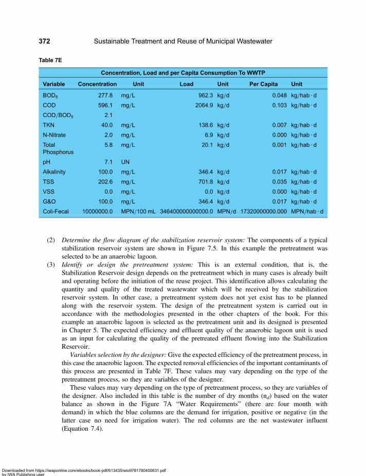
(2) Determine the flow diagram of the stabilization reservoir system: The components of a typicalstabilization reservoir system are shown in Figure 7.5. In this example the pretreatment wasselected to be an anaerobic lagoon.

(3) Identify or design the pretreatment system: This is an external condition, that is, theStabilization Reservoir design depends on the pretreatment which in many cases is already builtand operating before the initiation of the reuse project. This identification allows calculating thequantity and quality of the treated wastewater which will be received by the stabilizationreservoir system. In other case, a pretreatment system does not yet exist has to be plannedalong with the reservoir system. The design of the pretreatment system is carried out inaccordance with the methodologies presented in the other chapters of the book. For thisexample an anaerobic lagoon is selected as the pretreatment unit and its designed is presentedin Chapter 5. The expected efficiency and effluent quality of the anaerobic lagoon unit is usedas an input for calculating the quality of the pretreated effluent flowing into the StabilizationReservoir.

Variables selection by the designer: Give the expected efficiency of the pretreatment process, inthis case the anaerobic lagoon. The expected removal efficiencies of the important contaminants ofthis process are presented in Table 7F. These values may vary depending on the type of thepretreatment process, so they are variables of the designer.

These values may vary depending on the type of pretreatment process, so they are variables ofthe designer. Also included in this table is the number of dry months (nd) based on the waterbalance as shown in the Figure 7A “Water Requirements” (there are four month withdemand) in which the blue columns are the demand for irrigation, positive or negative (in thelatter case no need for irrigation water). The red columns are the net wastewater influent(Equation 7.4).

Table 7E

Concentration, Load and per Capita Consumption To WWTP

Variable Concentration Unit Load Unit Per Capita Unit

BOD5 277.8 mg/L 962.3 kg/d 0.048 kg/hab · d

COD 596.1 mg/L 2064.9 kg/d 0.103 kg/hab · d

COD/BOD5 2.1

TKN 40.0 mg/L 138.6 kg/d 0.007 kg/hab · d

N-Nitrate 2.0 mg/L 6.9 kg/d 0.000 kg/hab · d

TotalPhosphorus

5.8 mg/L 20.1 kg/d 0.001 kg/hab · d

pH 7.1 UN

Alkalinity 100.0 mg/L 346.4 kg/d 0.017 kg/hab · d

TSS 202.6 mg/L 701.8 kg/d 0.035 kg/hab · d

VSS 0.0 mg/L 0.0 kg/d 0.000 kg/hab · d

G&O 100.0 mg/L 346.4 kg/d 0.017 kg/hab · d

Coli-Fecal 10000000.0 MPN/100 mL 346400000000000.0 MPN/d 17320000000.000 MPN/hab · d



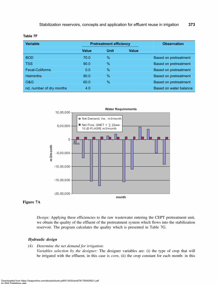
-20,00,000

-15,00,000

-10,00,000

-5,00,000

0

5,00,000

10,00,000

mes

m3/

mo

nth

month

Water Requirements

Net Demand, Vw, m3/month

10.(E-P).ASR] m3/month

Figure 7A

Design: Applying these efficiencies to the raw wastewater entering the CEPT pretreatment unit,we obtain the quality of the effluent of the pretreatment system which flows into the stabilizationreservoir. The program calculates the quality which is presented in Table 7G.

Hydraulic design

(4) Determine the net demand for irrigation:Variables selection by the designer: The designer variables are: (i) the type of crop that willbe irrigated with the effluent, in this case is corn, (ii) the crop constant for each month: in this

Table 7F

Variable Pretreatment efficiency Observation

Value Unit Value

BOD 70.0 % Based on pretreatment

TSS 90.0 % Based on pretreatment

Fecal-Coliforms 0.0 % Based on pretreatment

Helminths 80.0 % Based on pretreatment

O&G 60.0 % Based on pretreatment

nd, number of dry months 4.0 Based on water balance



case kc= 0.55 throughout the year (these are data supplied by the agronomy/agricultural expert,this constant may vary monthly), (iii) the total water use efficiency: ETa= 0.65 (65%); thismeans that the water losses in the conveyance system from the stabilization reservoir toirrigation area is (1−ETa) or 35%, (iv) precipitation (P) and potential evapotranspiration (ET0).The data for this example are given at the beginning of section 7.3 above, in the statementdefining the example. This type of data is obtained from the regional hydrological institution.For design purposes, these date are by the agricultural expert of the design team; (v) infiltrationrate at the reservoir site. This information is an outcome of the soil and geotechnical study at thereservoir site. It can also be handles as a sensitivity parameter, that is, a range of probableinfiltration rate values is used and the impact of their variation on the design is analyzed.

Design:With the data mentioned in the previous paragraph and applying Equation 7.2 for the dataof each month, the total monthly demand of water for irrigation, Dw is calculated Then the netmonthly demand (Vw) is calculated using Equation 7.3 with the data for each month. Themeaning of a negative value of a calculated monthly value of Vw is that the precipitation on thatmonth is sufficient to provide the water needed by the plants, so the requirements of effluentduring such a month is zero. The results of the net monthly water demand after determining thepossible cultivation areas for irrigation with the effluent under the example case, as explainedbelow, are presented in Table 7H.

The Table also shows the availability of effluent for irrigation (corrected by evaporation, E,and precipitation, P, in the reservoir) on a monthly and total basis [Σ(QWW− 10 (E− P) · ASR)],and the aggregate irrigation water demand (ΣVw) that results from adding the demand of each

Table 7G

Concentrations and Loads Flowing into the Stabilization Reservoir

Variable Concentration Unit Load Unit

BOD5 83 mg/L 289 kg/d

COD 179 mg/L – kg/d

COD/BOD5 2 –

TKN – mg/L – kg/d

N–Nitrate – mg/L – kg/d

Total phosphorus – mg/L – kg/d

pH 7 UN –

Alkalinity – mg/L kg/d

TSS 20 mg/L 70 kg/d

VSS – mg/L – kg/d

O&G 40 mg/L 0 kg/d

Helminths 100 Ova/L

Fecal coliforms 10000000 MPN/100 mL 0 MPN/d



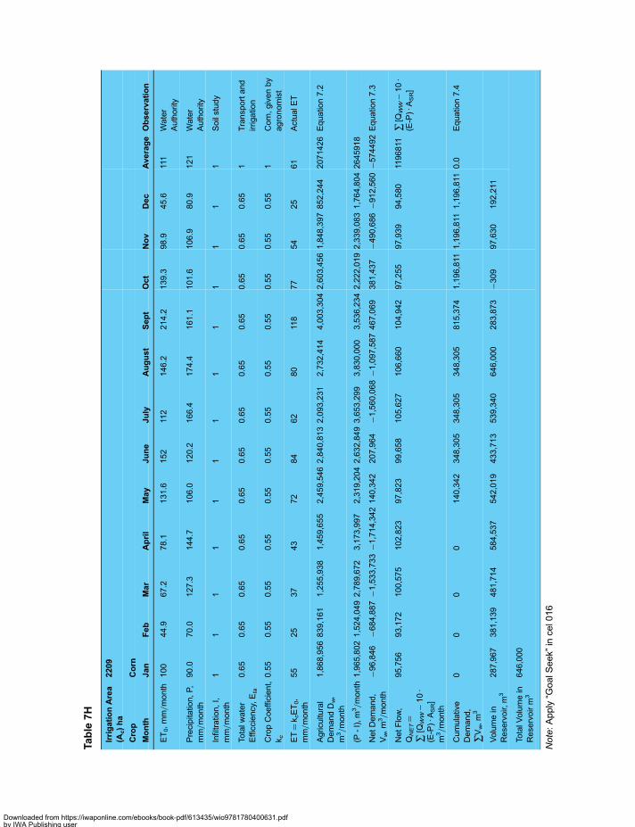
Table

7H

IrrigationArea

(Ac)ha

2209

Crop

Corn

Month

Jan

Feb

Mar

April

May

June

July

August

Sept

Oct

Nov

Dec

Average

Observation

ET0,m

m/month

100

44.9

67.2

78.1

131.6

152

112

146.2

214.2

139.3

98.9

45.6

111

Water

Authority

Precipita

tion,P,

mm/month

90.0

70.0

127.3

144.7

106.0

120.2

166.4

174.4

161.1

101.6

106.9

80.9

121

Water

Authority

Infiltratio

n,I,

mm/month

11

11

11

11

11

11

1Soilstudy

Totalw

ater

Efficciency,E

ta

0.65

0.65

0.65

0.65

0.65

0.65

0.65

0.65

0.65

0.65

0.65

0.65

1Transp

ortand

irrigatio

n

CropCoefficient,

k c

0.55

0.55

0.55

0.55

0.55

0.55

0.55

0.55

0.55

0.55

0.55

0.55

1Corn,givenby

agronomist

ET=k cET0,

mm/month

55

25

37

43

72

84

62

80

118

77

54

25

61

ActualE

T

Agric

ultu

ral

DemandDw,

m3/month

1,868,956839,161

1,255,938

1,459,655

2,459,5462,840,8132,093,231

2,732,414

4,003,3042,603,4561,848,397852,244

2071426

Equatio

n7.2

(P-I),m

3/month

1,965,8021,524,0492,789,672

3,173,997

2,319,2042,632,8493,653,299

3,830,000

3,536,2342,222,0192,339,0831,764,8042645918

NetDemand,

Vw,m

3/month

−96,846

−684,887

−1,533,733−1

,714,342140,342

207,964

−1,560,068−1

,097,587467,069

381,437

−490,686

−912,560

−574492Equatio

n7.3

NetFlow,

QNET=

∑[Q

WW−10·

(E-P)·ASR]

m3/month

95,756

93,172

100,575

102,823

97,823

99,658

105,627

106,660

104,942

97,255

97,939

94,580

1196811

∑[Q

WW−10·

(E-P)·ASR]

Cumulative

Demand,

∑Vw,m

3

00

00

140,342

348,305

348,305

348,305

815,374

1,196,811

1,196,811

1,196,811

0.0

Equatio

n7.4

Volumein

Rese

rvoir,

m3

287,967

381,139

481,714

584,537

542,019

433,713

539,340

646,000

283,873

−309

97,630

192,211

TotalV

olumein

Rese

rvoirm

3646,000

Note:Apply“G

oalS

eek”

ince

l016


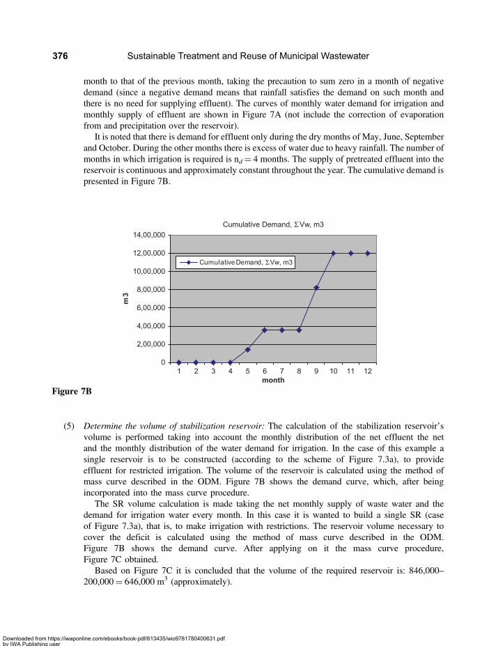
month to that of the previous month, taking the precaution to sum zero in a month of negativedemand (since a negative demand means that rainfall satisfies the demand on such month andthere is no need for supplying effluent). The curves of monthly water demand for irrigation andmonthly supply of effluent are shown in Figure 7A (not include the correction of evaporationfrom and precipitation over the reservoir).

It is noted that there is demand for effluent only during the dry months of May, June, Septemberand October. During the other months there is excess of water due to heavy rainfall. The number ofmonths in which irrigation is required is nd= 4 months. The supply of pretreated effluent into thereservoir is continuous and approximately constant throughout the year. The cumulative demand ispresented in Figure 7B.

0

2,00,000

4,00,000

6,00,000

8,00,000

10,00,000

12,00,000

14,00,000

1 2 3 4 5 6 7 8 9 10 11 12

m3

month

Figure 7B

(5) Determine the volume of stabilization reservoir: The calculation of the stabilization reservoir’svolume is performed taking into account the monthly distribution of the net effluent the netand the monthly distribution of the water demand for irrigation. In the case of this example asingle reservoir is to be constructed (according to the scheme of Figure 7.3a), to provideeffluent for restricted irrigation. The volume of the reservoir is calculated using the method ofmass curve described in the ODM. Figure 7B shows the demand curve, which, after beingincorporated into the mass curve procedure.

The SR volume calculation is made taking the net monthly supply of waste water and thedemand for irrigation water every month. In this case it is wanted to build a single SR (caseof Figure 7.3a), that is, to make irrigation with restrictions. The reservoir volume necessary tocover the deficit is calculated using the method of mass curve described in the ODM.Figure 7B shows the demand curve. After applying on it the mass curve procedure,Figure 7C obtained.

Based on Figure 7C it is concluded that the volume of the required reservoir is: 846,000–200,000= 646,000 m3 (approximately).



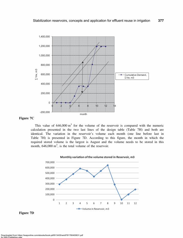
-200,000

0

200,000

400,000

600,000

800,000

1,000,000

1,200,000

1,400,000

0 2 4 6 8 10 12 14

month

Cumulative Demand,

Figure 7C

This value of 646,000 m3 for the volume of the reservoir is compared with the numericcalculation presented in the two last lines of the design table (Table 7H) and both areidentical. The variation in the reservoir’s volume each month (one line before last inTable 7H) is presented in Figure 7D. According to this figure, the month in which therequired stored volume is the largest is August and the volume needs to be stored in thismonth, 646,000 m3, is the total volume of the reservoir.

0

100,000

200,000

300,000

400,000

500,000

600,000

700,000

1 2 3 4 5 6 7 8 9 10 11 12

Monthly varia�on of the volume stored in Reservoir, m3

Volume in Reservoir, m3

Figure 7D



Note that the month in which the reservoir is completely empty (October) coincides with thestart of the heavy rainy season (November, December, January, February, March and April). InMay, with the start of the dry season, the reservoir is almost filled, and in August it is completelyfilled ready for the heaviest demand of effluent for irrigation in September and October.

If it is required to produce effluent for unrestricted irrigation, three (3) stabilization reservoirscan be constructed to function under a sequential batch mode, each with a volume of 323,000 m3.This ensures that a full reservoir of 323,000 m3 filled and well treated effluent (void of coliforms)will be ready when needed. The storage volume of 646,000 cubic meters ensures the requiredsupply of effluent during the irrigation season but the quality of this effluent is only adequatefor restricted irrigation. A storage volume of 969,000 m3 guarantees the continuous supplyduring the irrigation season of high quality effluent, adequate for unrestricted irrigation.

The procedure of calculating the reservoir volume using the method of mass curve isperformed manually on the drawing board, or using a computer as shown in Figure 7.D,based on the explanation in Section 7.22 regarding the ODM. The reservoir volume is alsocalculated by the Excel program CHAP 7-SR.

(6) Calculate the irrigated area, Ac

Variables selection by the designer: From the ODMSection 7.22 Paragraph 5 it is clear that the totalannual water demand for irrigation (ΣVw) must be equal to the supply of wastewater corrected forthe losses for evaporation and the gains of precipitation over the reservoir [Σ(QWW –10 (E – P) ·ASR)]. Since ΣVw depends on the area to be irrigated (Ac), Equation 7.4 is applied to calculateAc. In the Table 7H this area is already determined (Ac= 2209 ha). However, to start we mustuse an approximate value, and then proceed as indicated in the design section below. Also, toinitiate the calculations a starting value of the area of the reservoir (ASR) is required, and anapproximate value is used, to be corrected once the design is performed. Some trial and erroriterations for Ac and ASR may be necessary to obtain the right design. These calculations arefacilitated through the use of the Excel program CHAP 7-SR.xls.Design:After calculating all the designer variables we proceed to calculate the exact area of irrigatedcrops applying a varyingAc values in Equation 7.3 until theEquation 7.4 ismet (which is the trial anderror procedure). In the example it is possible to irrigate 2,199 ha with the wastewater of thepopulation of the contributing town and with the given values of evaporation and precipitationover the reservoir. In the Excel spreadsheet the exact value is calculated using the “goal seek”function in Data’s “What if analisys” (go to Data, then open What if Analisys and select thefunction “goal seek”, at the cell “Evap-T’ O16”. All graphs can be generated automatically by theExcel program except the mass curve to calculate VSR, which must be prepared manually. Everyassumption on Ac produces a different ASR, and some trial and error is required to close thedifferences (note that Ac define the reservoir volume, which affects ASR, which in turn affects Ac:the circle in the operations is cut because the total volume is defined, but in any case it isnecessary to observe how changes in ASR causes changes in Ac. It is considered that the trial anderror ends when the minimum volume of water in reservoir is close to zero).

Civil engineering design

(7) Design the stabilization reservoirVariables selection by the designer: Topographical maps of the site allocated for constructing thereservoir are required for the design. In the example it is assumed that the reservoir site is flat. Weselect an effective depth of 5 m (the range is 4 to 12 m. It is necessary to leave a dead reservoir



volume of about 1 m high and a freeboard of about 1 m so the total depth of the reservoir is 7 m.Assuming an internal embankment slope of 1:1, the angle of the embankment is 45 degrees.Also, a geometric shape of an inverted truncated cone is proposed for the reservoir in theexample. When the topography is complex, it is necessary to do volume calculations based onthe topographic surveys.Design: The net volume of the truncated cone is VSR=⅓ h (A1+A2+√ [A1A2])= 646,000 m3,with Ai the areas of the bases, ri their radii and h the net depth (selected as 5 m). Calculating for a1∶1 slope and solving for the height of 5m as the useful volume of the reservoir we find r1= 200.3m and r2 = 205.3 m. Taking into account a dead reservoir volume of 1 m depth and a freeboard of1 m (which gives a total depth of hT= 7 m): then R1 (at the bottom of dead volume) is 199.3 m(A1= 124,786 m2) and R2 (at the top of freeboard) is 206.3 m2 (A2= 133,705 m2) for a totalvolume of 904,539 m3. The variation of reservoir’s water volume with depth, taking intoaccount the first dead meter (water depth of 6 m), is as presented in Figure 7E and the variationof the reservoir’s surface area with the depth is presented in Figure 7F.

0 1 2 3 4 5 6 7hm

0

200000

400000

600000

800000

m3 V

Figure 7E

0 1 2 3 4 5 6 7hm

126000

128000

130000

132000

Am

2

Figure 7F

The depth of the average volume of the reservoir (taking into account the first meter that is adead volume) is 4 m. The corresponding surface area at that depth is 129845 m2 or 13 hectares.



The BOD5 of the pretreated effluent that reaches the reservoir is 83.3 mg/l and the organic load is288.7 kg DBO5/d. This implies that the average surface organic loading on the stabilization reservoiris Ls= 288.7 (kg DBO5/d)/12.9 ha= 22.4 kg BOD5/ha · d, which is within the acceptable rangeof loading. The pretreated effluent that enters the reservoir is of a very good quality andtherefore the surface organic loading is low and this reservoir will not generate odour problems.

Kinetics design(8) Calculation of the quality of the effluent used for irrigation

Variables selection by the designer: For the calculation of quality of the effluent used for irrigation,we use the geometric and kinetics values presented in Table 7I. It is noted that the reservoir volumesand areas for different depths have already been calculated in the previous paragraph on “CivilEngineering Design” (see Figures 7E and 7F) and the kinetic coefficients proposed are similar tothose of facultative lagoons.

Design: The kinetics constants need to be corrected according to the actual temperature, and onceapplied to the stabilization reservoir conditions the results presented in Table 7J are obtained:

Table 7I

Stabilization reservoir net dimensions and coefficients

VSR, net volume 646000 m3

SR net depth, H 5.0 m

ASR at total depht h= 6 m 129200.0 m2 12.92 ha

V1/2, net 323000 m3

A1/2 at h= 4 m (1 m death reservoir) 129845.0 m2 12.98 ha

KL(20°C) 0.35 d−1 Typical

θ (BOD5) 1.06 1,04–1,09

KB (20°C) 2.7 d−1 FC typical

θ (FC) 1.19 Typical

Table 7J

Stabilization reservoir kinetics

Variable Value Unit Value Observation

td=V1/2/QD 93 d Equation 7.6

TL= (ASfTa+QDTi)/(Asf+QD) 18 °C Equation 7.9

KL=KL(20°C) θ(T−20) 0.32 d−1 Equation 7.10

S=S0/(1+KL*td/n)n 2.72 mg/L Equation 7.8

KB=KB(20°C) θ(T−20) 2.03 d−1 Equation 7.10

B=B0/(1+KB*td) 52590 MPN/100mL Equation 7.8

LS=QD*DBO5/A1/2 22.23 kg DBO5/d · ha ,50



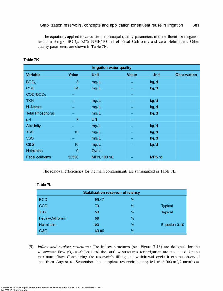
The equations applied to calculate the principal quality parameters in the effluent for irrigationresult in 3 mg/l BOD5, 5275 NMP/100 ml of Fecal Coliforms and zero Helminthes. Otherquality parameters are shown in Table 7K.

The removal efficiencies for the main contaminants are summarized in Table 7L.

(9) Inflow and outflow structures: The inflow structures (see Figure 7.13) are designed for thewastewater flow (QD= 40 Lps) and the outflow structures for irrigation are calculated for themaximum flow. Considering the reservoir’s filling and withdrawal cycle it can be observedthat from August to September the complete reservoir is emptied (646,000 m3/2 months=

Table 7K

Irrigation water quality


BOD5 3 mg/L – kg/d

COD 54 mg/L – kg/d

COD/BOD5 – –

TKN – mg/L – kg/d

N–Nitrate – mg/L – kg/d

Total Phosphorus – mg/L – kg/d

pH 7 UN –

Alkalinity – mg/L – kg/d

TSS 10 mg/L – kg/d

VSS – mg/L – kg/d

O&G 16 mg/L – kg/d

Helminths 0 Ova/L

Fecal coliforms 52590 MPN/100mL – MPN/d

Table 7L

Stabilization reservoir efficiency

BOD 99.47 %

COD 70 % Typical

TSS 50 % Typical

Fecal–Coliforms 99 %

Helminths 100 % Equation 3.10

G&O 60.00 %



343,000 m3/month= 11,320 m3/d= 131 Lps, which is the maximum flow for irrigation). Thecalculated diameters of the inflow and outflow pipes are presented in Table 7M.

The design inlet flow for is QD= 40 lps, which for a flow velocity of 1 m/s results in a 9′′ pipediameter. The maximum design outflow for irrigation is QR= 131 Lps (as calculated above) and theresulting outlet pipe diameter for a flow velocity of 1 m/s is 16′′.

Table 7M

Maximum irrigation flow


Irrigation flow, QR 131 L/s 472 m3/h 11320.00 m3/d

Inlet and oulet pipes

ve, water velocity 1 m/s 0,6–5,0 m/s

Ae, pipe area 0.040 m2

De, inlet pipe diameter 0.226 m 9.000 inch

vs, water velocity 1 m/s 0,6–5,0 m/s

As, irrigation pipe are 0.131 m2

Ds, irrigation pipe diameter 0.408 m 16.000 inch



Chapter 8

Sub-Surface Flow ConstructedWetlands (SSFCW)

8.1 PROCESS DESCRIPTION8.1.1 IntroductionThe concepts of artificial wetlands, aquatic and subsurface, are essentially new advances in wastewaterreuse. Subsurface Flow Constructed Wetland (SSFCW) represents a cost-effective option for post-treatment of municipal wastewater of small populations (Crites, Middlebrooks & Sherwood, 2006). TheSSFCW is discussed in this chapter.

A wetland is defined as an area where the water table is at or above the soil surface for a long enoughperiod to maintain saturation conditions and allow the growth of related vegetation. The capacity of theimprovement of the quality of wastewater in wetlands has been verified in studies in a variety ofgeographical locations. Wetlands used for wastewater treatment include swamps, mangroves, and so on.Ultimately wetlands systems are built especially for the treatment of wastewater (artificial wetlands).

Amajor constraint in the use of many natural wetlands for treatment of wastewater is the fact that they areconsidered by most regulatory authorities as part of the receiving water bodies. Consequently, thewastewater discharged to them must comply with the standards of use of the wetland. In these cases, thepotential capacity of the wetland for improving the quality of wastewater is not utilized completely.Constructed wetlands avoid these special requirements of influent quality and can also ensure a bettercontrol on the hydraulic regime in the system; therefore, they are more reliable than natural wetlands.

The mostly used two types of constructed wetlands are: (i) surface flow constructed wetland, which is asystem similar to a natural swamp because the water surface is exposed to the atmosphere; and (ii)subsurface flow constructed wetland, which uses a permeable medium in which the wastewater flowsand the water level remains below the level of the bed. Table 8.1 presents the basic parameters of themain types of wetlands, natural and constructed (Reed et al. 1995; Crites et al. 2006).

This chapter focuses on the Subsurface Flow Constructed Wetlands (SSFCW) which are those that canbetter handle higher organic loads and generate fewer environmental problems common in surface wetlands,such as the proliferation of mosquitoes and the generation of unpleasant odours. A schematic cross section ofa SSFCW unit which shows its internal structure is presented in Figure 8.1. During its transport through thematrix of saturated soil or rock filter, the inflow stream undergoes treatment processes and in addition, theplant roots are the media of adherence to multiple microorganisms that support the bioconversion of theorganic matter contained in the inflow. The effluent out flowing from a constructed wetland has thewater quality shown in Table 8.1.


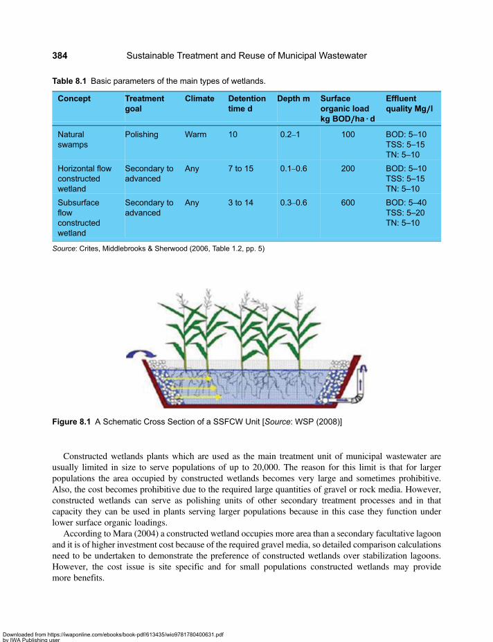
Constructed wetlands plants which are used as the main treatment unit of municipal wastewater areusually limited in size to serve populations of up to 20,000. The reason for this limit is that for largerpopulations the area occupied by constructed wetlands becomes very large and sometimes prohibitive.Also, the cost becomes prohibitive due to the required large quantities of gravel or rock media. However,constructed wetlands can serve as polishing units of other secondary treatment processes and in thatcapacity they can be used in plants serving larger populations because in this case they function underlower surface organic loadings.

According to Mara (2004) a constructed wetland occupies more area than a secondary facultative lagoonand it is of higher investment cost because of the required gravel media, so detailed comparison calculationsneed to be undertaken to demonstrate the preference of constructed wetlands over stabilization lagoons.However, the cost issue is site specific and for small populations constructed wetlands may providemore benefits.

Table 8.1 Basic parameters of the main types of wetlands.

Concept Treatmentgoal

Climate Detentiontime d

Depth m Surfaceorganic loadkg BOD/////ha · d

Effluentquality Mg/////l

Naturalswamps

Polishing Warm 10 0.2–1 100 BOD: 5–10TSS: 5–15TN: 5–10

Horizontal flowconstructedwetland


Any 7 to 15 0.1–0.6 200 BOD: 5–10TSS: 5–15TN: 5–10

Subsurfaceflowconstructedwetland


Any 3 to 14 0.3–0.6 600 BOD: 5–40TSS: 5–20TN: 5–10

Source: Crites, Middlebrooks & Sherwood (2006, Table 1.2, pp. 5)

Figure 8.1 A Schematic Cross Section of a SSFCW Unit [Source: WSP (2008)]



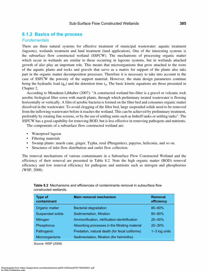
8.1.2 Basics of the processFundamentalsThere are three natural systems for effective treatment of municipal wastewater: aquatic treatment(lagoons), wetlands treatment and land treatment (land application). One of the interesting systems isthe subsurface flow constructed wetland (SSFCW). The mechanisms of processing organic matterwhich occur in wetlands are similar to those occurring in lagoons systems, but in wetlands attachedgrowth of also play an important role. This means that microorganisms that grow attached to the rootsof the aquatic plants and rocks and gravels that serve as a matrix for support of the plants also takepart in the organic matter decomposition processes. Therefore it is necessary to take into account in thecase of SSFCW the porosity of the support material. However, the main design parameters continuebeing the hydraulic load (qa) and the detention time td. The basic kinetic equations are those presented inChapter 2.

According to Menahem Libhaber (2007): “A constructed wetland bio-filter is a gravel or volcanic rockaerobic biological filter sown with marsh plants, through which preliminary treated wastewater is flowinghorizontally or vertically. A film of aerobic bacteria is formed on the filter bed and consumes organic matterdissolved in the wastewater. To avoid clogging of the filter bed, large suspended solids need to be removedfrom the inflowing wastewater before it reaches the wetland. This can be achieved by preliminary treatment,preferably by rotating fine screens, or by the use of settling units such as Imhoff tanks or settling tanks”. TheSSFCW has a good capability for removing BOD, but is less effective in removing pathogens and nutrients.

The components of a subsurface flow constructed wetland are:

• Waterproof lagoon• Filtering materials• Swamp plants: marsh cane, ginger, Typha, reed (Phragmites), papyrus, heliconia, and so on.• Structures of inlet flow distribution and outlet flow collection.

The removal mechanisms of various contaminants in a Subsurface Flow Constructed Wetland and theefficiency of their removal are presented in Table 8.2. Note the high organic matter (BOD) removalefficiency and low removal efficiency for pathogens and nutrients such as nitrogen and phosphorous(WSP, 2008).

Table 8.2 Mechanisms and efficiencies of contaminants removal in subsurface flowconstructed wetlands.

Type ofcontaminant

Main removal mechanism Removalefficiency

Organic matter Bacterial degradation 80–90%

Suspended solids Sedimentation, filtration 80–90%

Nitrogen Ammonification, nitrification-denitrification 20–40%

Phosphorus Absorbing processes in the filtrating material 20–30%

Pathogenic Predation, natural death (for fecal coliforms) 1–3 log units

Microorganisms Sedimentation, filtration (for helminths)

Source: WSP (2008)

Sub-Surface Flow Constructed Wetlands 385


Figure 8.2 shows a flow diagram of a complete SSFCW system, including preliminary and primarytreatment. Figure 1.35 shows a photo of a constructed wetland plant in Copacabana, Bolivia, consistingof pretreatment in a septic tank and three constructed wetlands lagoon in series.

The specific unit area of SSFCW is 1.5 to 5.0 m2 per Capita. Construction of SSFCW requires access togood building material (fine gravel), and stable land with adequate drainage so that rainwater is be deviatedaway from the wetland. The level of the water table at the plant’s site should be below the wetland and, if thesoil is not impermeable, impermeabilization is required.

It is important to take into consideration possible negative impacts of the pretreatment unit, especially thegeneration of excess solid and sometimes unpleasant odours. The generation of odours from the wetland unititself, as well as proliferation of insects in this unit are moderate, but precautions must taken.

Design considerationsHydraulics

The main hydraulic design parameters are Darcy’s law for calculating the flow through the filter bed andporosity (n) for correctly calculating the of hydraulic detention time in the wetland. The recommendedhydraulic slope of the wetland is between 0.5 and 1%. To avoid going deepening too much at the endpart of the wetland because the bottom slope, it is recommended to limit its length (50 m is an

Figure 8.2 Flow Diagram of a Complete Subsurface Flow Constructed Wetlands System [Source: WSP(2008)]



appropriate value) and divide the system into parallel treatment units. The hydraulic design is based onDarcy’s law:

v = kss ; QD/B · H (8.1)

where:

v=Darcy’s velocity, m/ds= terrain slope, m/mks = hydraulic conductivity, m3/m2 · dQD = average flow, m3/dB =width of the wetland, mH = average depth of the wetland, 0.3 to 0.6 m

The hydraulic load is defined by the following equation:

qa = QD/As (8.2)

where:

qa =Hydraulic load, between 0.04 and 0.75 m/dQD =Design flow, m3/dAs = Surface area of the wetland, m2 (width× length)

The SSFCW’s length is obtained from the hydraulic load. The length (L) obtained from Equation 8.2 istherefore:

L = QD/B · qa (8.3)

The ratio length/width (L/B) is usually between 3/1 and 0.5/1.The hydraulic load (q) correlates with total suspended solids (TSS) according to the following equation

(Crites et al. 2006):

TSSe = TSS0(0.1058+ 0.000011qa) (8.4)

where:

TSSe = Total Suspended Solids in the Effluent, mg/lTSS0 = Inffluent TSS, mg/l

qa = hydraulic load, m/d

The calculation of the detention time in the wetland is done using the equation:

td = L · B · H · n/QD ; VN/QD (8.5)

where:

L = filter length, mB = filter width, mH = effective depth, mN = porosity of the filter bed as a decimal fraction, see Table 8.3VN = net volume, m3

QD = flow rate, m3/d

Characteristics of the filter medium of a SSFCW is given in Table 8.3.



Kinetic equations

The kinetic equations of a SSFCW give another approach to the design of the wetland. The BOD removalkinetics is similar to that of a stabilization lagoon under a plug flow regime (see Equation 2.37), but thekinetic of removal of other contaminants are different. It is also necessary to consider the hydraulicequations that have been explained in the previous section. The kinetic equations proposed for othercontaminants are those used by Reed et al. (1995) as quoted by Merz (2000) in his article “Guidelinesfor Using Free Water Surface Constructed Wetlands to Treat Municipal Sewage”, complemented by thebook of Crites, Middlesbrooks and Sherwood (2006. The equations are written using the following notpreviously defined nomenclature:

Nomenclature:

Sub-indexes “0” and “e” (S0, Se): influent, effluentKHi: first order wetland constant for parameter i=DBO5, NTK, NO3 and CF, d−1

Kp: first order area constant for P: Kp= 0.0273 m/dQD: wetland average flow, m3/dtmed: average detention time, VN/Qmed, dN: Fecal coliforms, MPN/100 ml, for the influent (0) and the effluent (e)Nc: number of wetland units in seriesPj: Phosphorus, mg/l, for the influent (0) and effluent (e).

EquationsFor removal of DBO5, NTK and NO3:

Se = S0 exp− KHi · n · As · H( )/QD

[ ](8.6)

From where we conclude:

As = QDL · n S0/Se( )

/KHi · n · H (8.7)

Also, the average hydraulic load is:

qa = QD/As (8.8)

For removal of SST: use Equation 8.4.

Table 8.3 Characteristics of the filter media of the SFCW.

Filtrating bed Effective size D10, mm Porosity n, % Hydraulic conductivity ks, m/////d

Thick Sand 2 28–32 100–1000

Gravel Sand 8 30–35 500–5000

Fine Gravel 16 35–38 1000–10000

Gravel 32 36–40 10000–50000

Thick Gravel 128 40–45 50000–250000



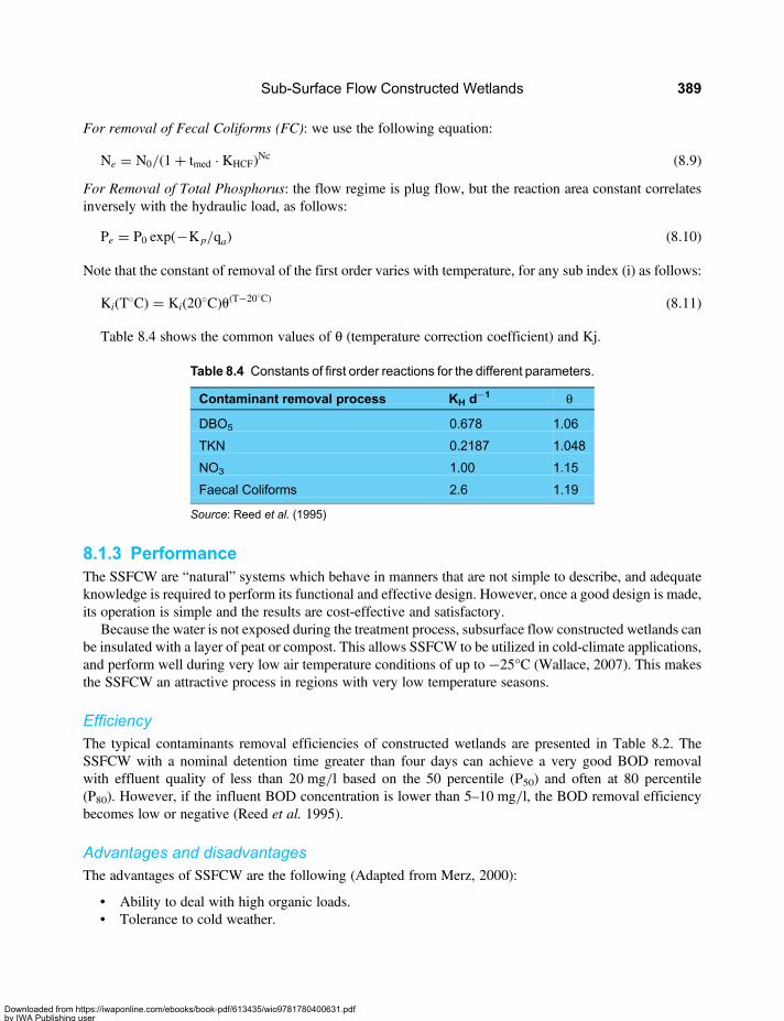
For removal of Fecal Coliforms (FC): we use the following equation:

Ne = N0/ 1+ tmed · KHCF( )Nc (8.9)

For Removal of Total Phosphorus: the flow regime is plug flow, but the reaction area constant correlatesinversely with the hydraulic load, as follows:

Pe = P0 exp(−K p/qa) (8.10)

Note that the constant of removal of the first order varies with temperature, for any sub index (i) as follows:

Ki T8C( ) = Ki(208C)u(T−208C) (8.11)

Table 8.4 shows the common values of θ (temperature correction coefficient) and Kj.

8.1.3 PerformanceThe SSFCW are “natural” systems which behave in manners that are not simple to describe, and adequateknowledge is required to perform its functional and effective design. However, once a good design is made,its operation is simple and the results are cost-effective and satisfactory.

Because the water is not exposed during the treatment process, subsurface flow constructed wetlands canbe insulated with a layer of peat or compost. This allows SSFCW to be utilized in cold-climate applications,and perform well during very low air temperature conditions of up to −25°C (Wallace, 2007). This makesthe SSFCW an attractive process in regions with very low temperature seasons.

EfficiencyThe typical contaminants removal efficiencies of constructed wetlands are presented in Table 8.2. TheSSFCW with a nominal detention time greater than four days can achieve a very good BOD removalwith effluent quality of less than 20 mg/l based on the 50 percentile (P50) and often at 80 percentile(P80). However, if the influent BOD concentration is lower than 5–10 mg/l, the BOD removal efficiencybecomes low or negative (Reed et al. 1995).

Advantages and disadvantagesThe advantages of SSFCW are the following (Adapted from Merz, 2000):

• Ability to deal with high organic loads.• Tolerance to cold weather.

Table 8.4 Constants of first order reactions for the different parameters.

Contaminant removal process KH d−1 θ

DBO5 0.678 1.06

TKN 0.2187 1.048

NO3 1.00 1.15

Faecal Coliforms 2.6 1.19

Source: Reed et al. (1995)



• More treatment per unit land area compared the Surface Flow Constructed Wetlands.• Proliferation of mosquitoes and generation of odours are not usually a problem.• SSFCW do not pose a public health problem because they are not open surface water.• There is less need for weed control compared to Surface Flow Constructed Wetlands.• Insulated SSFCW can be utilized in cold-climate applications and perform well during very low air

temperature conditions. This makes the SSFCW an attractive process in regions with very lowtemperature seasons.

The main disadvantages are:

• High capital cost due to the value of the filter media.• It has a tendency to clogging, especially in the entrance area.• It is a treatment method limited to small communities. Most of the existing constructed wetland plants

are designed for a flow of up to 2,000 m3/d, serving populations of up to 20,000.

8.2 BASIC DESIGN PROCEDURE8.2.1 General design considerationsA flow diagram of a SSFCW is shown in Figure 8.2 and a section of a plant in Figure 8.1. The inflow to thewetland unit undergoes treatment during its transport through the matrix of saturated soil or rock filterartificially constructed, where in addition the plant roots are a basis for adherence of microorganisms thataid in the bioconversion of organic matter. The removal mechanisms of various contaminants and theirremoval efficiencies in a SSFCW are presented in Table 8.2. The SSFCW occupies a specific unit areaof 1.5 to 5.0 m2 per Capita and requires the availability of good building material (fine gravel), as wellas a stable soil with adequate drainage.

The design of a SSFCW needs to take into account the combination of hydraulic and kinetic aspects,because the goals of treatment may be incorporated in the hydraulic variables of the system. Theproposed design procedure is based on both aspects.

The SSFCW unit must be preceded by a pre-treatment unit, preferably primary treatment, to avoid rapidclogging of the filter.

8.2.2 Orderly Design Method, ODMIn general the design methodology of a SSFCW plant consists of the following:

(1) Determine the external or independent variables: which is the same as is presented in Chapter 5,Section 5.2.2, Paragraph 1.

(2) Determine the SSFCW flow diagram: A typical Flow Diagram is presented in Figure 8.2. Thecomponents of a subsurface flow constructed wetland according to WSP (2008) are:○ Pretreatment: Usually Primary Treatment but may also be a septic tank or a Imhoff tank or

anaerobic lagoon.○ Impermeable Lagoon:One or more parallel impermeable lagoon are required. Impermeability is

required in order to prevent groundwater contamination by infiltration from the wetland lagoon.The impermeabilization can be achieved by lining with layers of compacted clay (less than 0.30m in 2 layers with a hydraulic permeability equal to or less than 10−7 m/d). Alternatively, liningwith plastic membranes of HDPE (high density polyethylene) can be used forimpermeabilization of the lagoon.



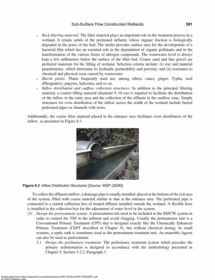
○ Rock filtering material: The filter material plays an important role in the treatment process in awetland. It retains solids of the pretreated influent, whose organic fraction is biologicallydegraded in the pores of the bed. The media provides surface area for the development of abacterial film which has an essential role in the degradation of organic pollutants and in thetransformation of the various forms of nitrogen compounds. The wastewater level is alwayskept a few millimeters below the surface of the filter bed. Coarse sand and fine gravel arepreferred materials for the filling of wetland. Selection criteria include: (i) size and materialgranulometry, which determine its hydraulic permeability and porosity; and (ii) resistance tochemical and physical wear caused by wastewater.

○ Marsh plants: Plants frequently used are, among others, canes, ginger, Typha, reed(Phragmites), papyrus, heliconia, and so on.

○ Inflow distribution and outflow collection structures: In addition to the principal filteringmaterial, a coarser filling material (diameter 5–10 cm) is required to facilitate the distributionof the inflow in the entry area and the collection of the effluent in the outflow zone. Simplestructures for even distribution of the inflow across the width of the wetland include buriedperforated pipes or channels with weirs.

Additionally, the coarse filter material placed in the entrance area facilitates even distribution of theinflow, as presented in Figure 8.3.

To collect the effluent outflow, a drainage pipe is usually installed, placed at the bottom of the exit areaof the system, filled with coarse material similar to that at the entrance area. The perforated pipe isconnected to a central collection box of treated effluent installed outside the wetland. A flexible hoseis installed in the collection box for the adjustment of water level in the system.(3) Design the pretreatment system: A pretreatment init need to be included in the SSFCW system in

order to control the TSS in the influent and avoid clogging. Usually the pretreatment unit is aConventional Primary Treatment (CPT) that is designed exactly like the Chemically EnhancedPrimary Treatment (CEPT described in Chapter 9), but without chemical dosing. In smallsystems, a septic tank is sometimes used as the pretreatment treatment unit. An anaerobic lagooncan also be used as pretreatment.3.1 Design the preliminary treatment: The preliminary treatment system which precedes the

primary sedimentation is designed in accordance with the methodology presented inChapter 5, Section 5.2.2, Paragraph 3.

Figure 8.3 Inflow Distribution Structures [Source: WSP (2008)]



3.2 Design primary clarifier: The main design parameter is the Surface Overflow Rate (SOR)measured m3/d · m2 of m/d. The average SOR (i.e. SOR based on the average flow) is inthe range 24–48 m/d and the peak SOR is in the range 48–120 m/d. The weir load shouldbe in the range 125–500 m3/d · m(linear), and the detention time in the range 1.5 to 4.0 h,as shown in Table 9.4. Consequently:• Ased=QD/SOR, Asedmax=QDH/SORmax. Select the largest area of the two, and define it

as As.• Calculate the net diameter (DN) of the clarifier (between the ends of weirs) by using the

following equation:

DN =��4As

p

√(8.12)

• Calculate the clarifier’s perimeter, C= πDN, and estimate the weir load, qv=QD/C. Thenumber must be between 125–250 m3/d · m (linear weir length), or less.

• Calculate the sludge produced, Qx (kg/d), using Figure 8.4 and Table 9.4. Defining E asthe TSS removal efficiency then Qx= E · TSS · QD. The removal efficiency of BOD5 andTSS is calculated, respectively with:

E DBO( ) = −0.29 SOR+ 42.48 (8.13)

E SST( ) = −0.4 SOR+ 73.78 (8.14)

• Define the sludge concentration at the bottom in the settler, for example, 5%.• Calculate the volume of sludge produced at 5% (0.05): V5%=QX/0.05 (m3/d).• Determine the mean depth (HSed) of the settler, usually between 3.5 and 4.5 m. Then

calculate the settler volume, V=HSed · As. Calculate the settling detention time, td=V/QD.

(4) Define the type of filter bed to be used: Table 8.3 is used for this purpose, and the selection dependson the designer’s experience, the availability of materials in the project zone and type of marsh plantto be planted. The parameters specifying the filter bed are the effective size (D10, mm), which in turn

y = -0.4006x + 73.782

y = -0.2911x + 42.486

0

10

20

30

40

50

60

70

0 50 100 150

Effici

ency

, %

Surface Overflow Rate, m/d

REMOVAL EFFICIENCY vs. SOR

REMOVAL EFFICIENCY, % SS

REMOVAL EFFICIENCY, % DBO5

Figure 8.4 Efficiencies of BOD and TSS Removal in a Primary Settling Basin [Source: based on Harleman(2004)]



determines the porosity (n,%), and the hydraulic conductivity (ks, m/d). The values of theseparameters are very important to design.

(5) Calculate the size of the wetland5.1 First define the designer variables: There are several possibilities for selecting the variables

since some variables depend on others. We present a methodology to calculate the surfacearea of the wetland, As (m2), from the desired efficiency of BOD5 removal. The othervariables to be selected are geometric variables and their selection is based on theexperience of the designer. Following are some guidelines:• Hydraulic gradient: s, m/m, should be between 0.3 and 1.0%.• Required effluent BOD5 concentration: Table 8.1 can be used as a guide to select the

BOD5 concentration.• Surface Area: An initial surface area is first proposed, and then using Equations 8.6 and

8.7 it is possible to perform the exact calculation of As.• The Kinetics Constant of BOD5: KHDBO= 0.678 at 20° C, according to Table 8.4.• Depth of the wetland: H, should be between 0.3 and 0.6 m.• Length/width ratio of each wetland lagoon unit: (L/b), where L is the length and b the

width of each wetland unit. The ratio should be between 0.5 and 4.0. L should notexceed 100 m.

5.2 Calculate the dimensions of the wetland: With the proposed designer variables proceed tocalculate all the dimensions of the wetland lagoon as follows:• Darcy Velocity: is calculated using Equation 8.1:

v = kss (8.1)

where:

v=Darcy velocity, m/ds= bottom wetland slope, m/mks = hydraulic conductivity, m3/m2 · d

• Water temperature in thewetland: thereare severalmethodsof calculation. In tropical regionsEquation 5.8 can be used (the same equation used in the design of stabilization lagoons):

TL = As f Ta + QDTi

As f + QD(5.8)

where:

TL = Final temperature of the wetland water (°C)Ta =Ambient air temperature (°C)Ti = Influent wastewater temperature (°C)As = Surface area of the wetland (m2)QD =Wastewater Flow (m3/d)f= Proportionality factor, 0.5 m/d

• Correction of Kinetics the Constant of BOD5 and the temperature: calculate KHDBO at thewetland temperature (TL), using Equation 8.11:

KHi T8C( ) = KHi(208C)u(T−208C) (8.11)

The value of θ is obtained from Table 8.4.



• Transversal Area: AT (m2), using the equation:

AT = QD/v (8.15)

• Hydraulic load: qa (m/d o m3/d · m2) using equation:

qa = QD/As (8.2)

The hydraulic load should be between 0.04 and 0.75 m/d (based on the definitive surfacearea is once it has been calculated).

• Minimum width of the wetland unit: Bmin (m) using the equation:

Bmin = AT/H (8.16)

For the purpose of providing a safety factor to the infiltration capacity to absorb the peaksin inflow, the total final width of the wetland unit (B) must be at least twice Bmin, (WSP,2008). In addition, since the system is designed with at least two parallel SSFCW units tofacilitate their maintenance, a single wetland unit will receive all the flow during theduration of the maintenance, and even the maintenance period is short, the unit musthave the capacity to handle the entire flow. Therefore:

B = 2Bmin (8.17)

One strategy is to design each wetland unit for width Bmin and build two identical parallelunits of SFFCWs

• Wetland length: The length L (m) of the wetland unit is calculated using the equation:

L = As/Bmin (8.18)

• Number of wetland units: The number of units N, is calculated using the equation:

N = Bmin · L/b( )

/L (8.19)

It is clear that the length (L) calculated using Equation 8.18 does not have to adjust to theselected length to width ratio (L/b), so to achieve required (L/b), the SSFCW is dividedinto several parallel channels, each fulfilling the required (L/b). It is important to maintainthe length (L) not larger than 100 m in order to avoid excessive depth at the end of thewetland, which might be caused by the bottom slope.

• Width of the wetland unit: each parallel channel will then have a width (b) which iscalculated using the equation:

b = Bmin/N (8.20)

• Detention time: The detention time is calculated using Equation 8.5.• TSS concentration in the effluents: TSSe is calculated using equation 8.4:

TSSe = TSS0(0.1058+ 0.000011 qa)

where:

TSSe = total suspended solids concentration in the effluent, mg/lTSS0 = total suspended solids concentration in the inflow, mg/l

qa = hydraulic load, m/d



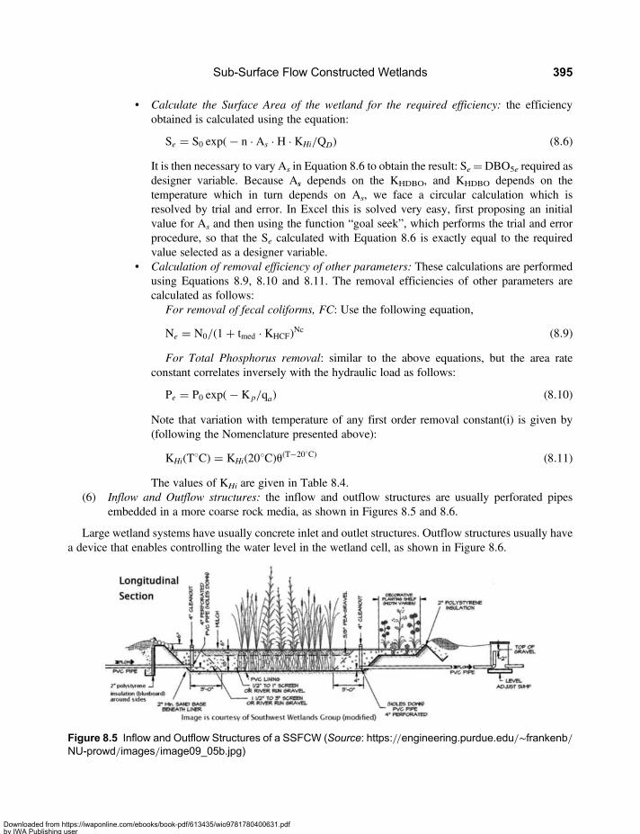
• Calculate the Surface Area of the wetland for the required efficiency: the efficiencyobtained is calculated using the equation:

Se = S0 exp(− n · As · H · KHi/QD) (8.6)

It is then necessary to vary As in Equation 8.6 to obtain the result: Se=DBO5e required asdesigner variable. Because As depends on the KHDBO, and KHDBO depends on thetemperature which in turn depends on As, we face a circular calculation which isresolved by trial and error. In Excel this is solved very easy, first proposing an initialvalue for As and then using the function “goal seek”, which performs the trial and errorprocedure, so that the Se calculated with Equation 8.6 is exactly equal to the requiredvalue selected as a designer variable.

• Calculation of removal efficiency of other parameters: These calculations are performedusing Equations 8.9, 8.10 and 8.11. The removal efficiencies of other parameters arecalculated as follows:

For removal of fecal coliforms, FC: Use the following equation,

Ne = N0/(1+ tmed · KHCF)Nc (8.9)

For Total Phosphorus removal: similar to the above equations, but the area rateconstant correlates inversely with the hydraulic load as follows:

Pe = P0 exp(− K p/qa) (8.10)

Note that variation with temperature of any first order removal constant(i) is given by(following the Nomenclature presented above):

KHi T8C( ) = KHi(208C)u(T−208C) (8.11)

The values of KHi are given in Table 8.4.(6) Inflow and Outflow structures: the inflow and outflow structures are usually perforated pipes

embedded in a more coarse rock media, as shown in Figures 8.5 and 8.6.

Large wetland systems have usually concrete inlet and outlet structures. Outflow structures usually havea device that enables controlling the water level in the wetland cell, as shown in Figure 8.6.

Figure 8.5 Inflow and Outflow Structures of a SSFCW (Source: https://engineering.purdue.edu/∼frankenb/NU-prowd/images/image09_05b.jpg)



https://engineering.purdue.edu/~frankenb/NU-prowd/images/image09_05b.jpg








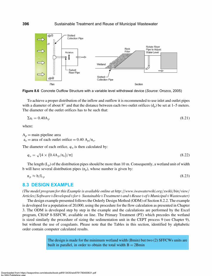
To achieve a proper distribution of the inflow and outflow it is recommended to use inlet and outlet pipeswith a diameter of about 8′′ and that the distance between each two outlet orifices (dp) be set at 1–5 meters.The diameter of the outlet orifices has to be such that:

Sai = 0.40A p (8.21)

where:

Ap =main pipeline areaao = area of each outlet orifice= 0.40 Ap/no.

The diameter of each orifice, wo is then calculated by:

wo =√[4× 0.4A p/no

( )/p] (8.22)

The length (Lp) of the distribution pipes should be more than 10 m. Consequently, a wetland unit of widthb will have several distribution pipes (np), whose number is given by:

n p ≈ b/L p (8.23)

8.3 DESIGN EXAMPLE(The model program for this Example is available online at http://www.iwawaterwiki.org/xwiki/bin/view/Articles/Software+Developed+for+ Sustainable+Treatment+and+Reuse+of+Municipal+Wastewater)

The design example presented follows the Orderly DesignMethod (ODM) of Section 8.2.2. The exampleis developed for a population of 20,000, using the procedure for the flow calculation as presented in Chapter3. The ODM is developed step by step in the example and the calculations are performed by the Excelprogram, CHAP 8-SSFCW, available on line. The Primary Treatment (PT) which precedes the wetlandis sized similarly the procedure of sizing the sedimentation unit in the CEPT process 9 (see Chapter 9),but without the use of coagulants. Please note that the Tables in this section, identified by alphabeticorder contain computer calculated results.

The design is made for the minimum wetland width (Bmin) but two (2) SFFCWs units arebuilt in parallel, in order to obtain the total width B= 2Bmin

Figure 8.6 Concrete Outflow Structure with a variable level withdrawal device (Source: Orozco, 2005)





















(1) Calculation of external variables1.1 Design flows: The input required for flow calculations are presented in Table 8A and are

identical to those presented in the examples in previous chapters.

The final design flows are obtained from Equations 3.3 and 3.4, and are presented inTable 8B in various units. The QD is used for the biological process design and the QDH

for hydraulic design.

In the case of a Primary Treatment the design flow for screening, grit channel, the Parshallflume is the QDH because they are hydraulic units. The primary settler, the thickener and thedrying beds are designed with QD.

1.2 Determination of the external geographical and environmental variables: These variablesdepend solely on geographic location. The values used in the example are presented inTable 8C.

Table 8A

Design flow



PF = 1+14/(4 + √P) 2.65 Eq·Harmon









Notes: (i) Per capita consumption is calculated for drinking water consumption. With the return factor of 0.8, the wastewaterper capita flow of c · qdom= 0.8× 162. 5 = 130 L/capita · d, as measured in the example in Chapter 3, (ii) the Peak Factor iscalculated by Equation 3.6 (Harmon Equation), (iii) the population density should be the maximum acceptable densityaccording to planning standards, in order to be able to serve the population at saturation conditions, (iv) the flows arecalculated based on the population and the return coefficient – c, and (v) infiltration must be measured or alternatively avalue of between 0.10 and 0.15 L/s · ha or l/s · km is to be chosen.

Table 8B

Design flows


Process design flow, QD = QDWW + QI 40.09 L/s 144.33 m3/h 3464.00 m3/d

Hydraulics design flow, QDH = QDWWmax + QI 89.82 L/s 323.35 m3/h 7760.44 m3/d



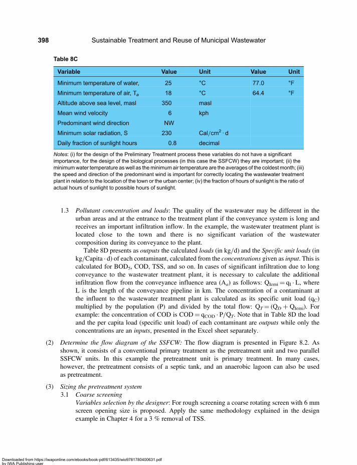
1.3 Pollutant concentration and loads: The quality of the wastewater may be different in theurban areas and at the entrance to the treatment plant if the conveyance system is long andreceives an important infiltration inflow. In the example, the wastewater treatment plant islocated close to the town and there is no significant variation of the wastewatercomposition during its conveyance to the plant.

Table 8D presents as outputs the calculated loads (in kg/d) and the Specific unit loads (inkg/Capita · d) of each contaminant, calculated from the concentrations given as input. This iscalculated for BOD5, COD, TSS, and so on. In cases of significant infiltration due to longconveyance to the wastewater treatment plant, it is necessary to calculate the additionalinfiltration flow from the conveyance influence area (Aa) as follows: QIemi= qI · L, whereL is the length of the conveyance pipeline in km. The concentration of a contaminant atthe influent to the wastewater treatment plant is calculated as its specific unit load (qC)multiplied by the population (P) and divided by the total flow: QT= (QD + QIemi). Forexample: the concentration of COD is COD= qCOD · P/QT. Note that in Table 8D the loadand the per capita load (specific unit load) of each contaminant are outputs while only theconcentrations are an inputs, presented in the Excel sheet separately.

(2) Determine the flow diagram of the SSFCW: The flow diagram is presented in Figure 8.2. Asshown, it consists of a conventional primary treatment as the pretreatment unit and two parallelSSFCW units. In this example the pretreatment unit is primary treatment. In many cases,however, the pretreatment consists of a septic tank, and an anaerobic lagoon can also be usedas pretreatment.

(3) Sizing the pretreatment system3.1 Coarse screening

Variables selection by the designer: For rough screening a coarse rotating screen with 6 mmscreen opening size is proposed. Apply the same methodology explained in the designexample in Chapter 4 for a 3 % removal of TSS.

Table 8C


Minimum temperature of water, 25 °C 77.0 °F







Notes: (i) for the design of the Preliminary Treatment process these variables do not have a significantimportance, for the design of the biological processes (in this case the SSFCW) they are important; (ii) theminimumwater temperature aswell as theminimumair temperature are the averages of the coldestmonth; (iii)the speed and direction of the predominant wind is important for correctly locating the wastewater treatmentplant in relation to the location of the town or the urban center; (iv) the fraction of hours of sunlight is the ratio ofactual hours of sunlight to possible hours of sunlight.



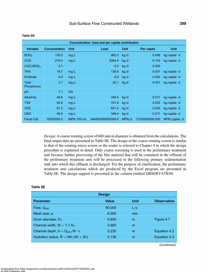
Design: A coarse rotating screen of 600 mm in diameter is obtained from the calculations. Thefinal output data are presented in Table 8E. The design of the coarse rotating screen is similarto that of the rotating micro screen so the reader is referred to Chapter 4 in which the designprocedure is explained in detail. Only coarse screening is used in the preliminary treatmentunit because further processing of the fine material that will be contained in the effluent ofthe preliminary treatment unit will be processed in the following primary sedimentationtank into which this effluent is discharged. For the purpose of clarification, the preliminarytreatment unit calculations which are produced by the Excel program are presented inTable 8E. The design support is presented in the column entitled OBSERVATION.

Table 8E

Design



Mesh size, a 6.000 mm


Channel width, W = 1,1 DT 0.660 m

Channel depth, h = QDH/W · v 0.230 m Equation 4.2

Hydralics radius, R =Wh/(W + 2h) 0.136 m Equation 4.3

(Continued )

Table 8D

Concentration, load and per capita contribution

Variable Concentration Unit Load Unit Per capita Unit

BOD5 130.0 mg/L 962.3 kg/d 0.048 kg/capita · d

COD 279.0 mg/L 2064.9 kg/d 0.103 kg/capita · d

COD/BOD5 2.1 0.0 kg/d 0.000

TKN 18.7 mg/L 138.6 kg/d 0.007 kg/capita · d

N-Nitrate 0.9 mg/L 6.9 kg/d 0.000 kg/capita · d

TotalPhosphorus

2.7 mg/L 20.1 kg/d 0.001 kg/capita · d

pH 7.1 UN

Alkalinity 46.8 mg/L 346.4 kg/d 0.017 kg/capita · d

TSS 94.8 mg/L 701.8 kg/d 0.035 kg/capita · d

VSS 81.2 mg/L 601.4 kg/d 0.030 kg/capita · d

O&G 46.8 mg/L 346.4 kg/d 0.017 kg/capita · d

Fecal Coli 10000000.0 MPN/100 mL 346400000000000.0 MPN/d 17320000000.000 MPN/capita · d



3.2 Grit chamberVariables selection by the designer: According to the ODM numeral 3, propose the followingdesign variables:According to the ODM in Section 8.2.2, Part 3 on design of preliminary treatment systems, wepropose the design variables presented in Table 8F.

Design: Applying these variables to the equations presented in the ODM Section 5.2.2Paragraph 3.2 which are shown in the left column of Table 8G, we obtain the resultspresented in Table 8G. Note that there are two grit chambers.

3.3 Parshall flume channel: For a QHD= 90 lps the throat width for measuring the flow isW= 9′′

(see Table 9.2). Rapid mixing is not required because there is no injection of chemicals.3.4 Primary clarification

Variables selection by the designer: According to the ODM, it is necessary to propose fordetailed design the average and peak Surface Overflow Rate (SOR) and a weir loadingrate, qv. It is also necessary to select the sludge concentration required at the bottom of theclarifier and to select the depth of the clarifier. The selected variables are shown in Table 8H:

Table 8E (Continued ).

Design



Hydrulics slope, s = (v · n)2/R4/3 0.074 % Equation 4.3

Head loss, hf = (1/C · 2g)(QDH/A)2 0.030 m Equation 4.1

Total head loss, hf + 0,05 0.080 Plus 5 cm


Waste solids excess 466.560 L/d Table 4.1

Table 8F

Designer variables

Variable Value Unit Observation

Grit channel

Sor 800 m/d 600–1200

v 0.20 m/s 0,15–0,60

# Grit Channels 2.00

L/w 4 3 a 6



The SOR values for conventional clarification are selected from Figure 8.4 and Table 9.4.Design: By applying the methodology proposed in the ODMwe obtain the dimensions of theprimary clarifier, as well as the sludge production and the sludge volume. For a 4 m clarifierdepth (Hsed) the average detention time, a td, is 3.0 hours. The sludge production is 8.6 m3/d ata 5% TSS concentration (XR= 50.000mg/l= 0.05%). The net clarifier diameter (DN) is 12.8m. The weir hydraulic load (qv) is well in the required range (less than 125 m3/d · m). TheBOD and TSS removal efficiencies are calculated using Equation 8.13 and 8.14, obtainedfrom Figure 8.4. The resulting design figures for the primary clarifier are presented inTable 8I. The right column indicates how the calculations are performed. A more detailedexplanation of primary treatment is given in Chapter 9.

Table 8H

Primary clarifier

SOR 32.00 m/d Table 9.4

SORmax 60.00 m/d Table 9.4

XR 5 % typical

Hsed 4 m ≥3.5 m

Table 8I

Primary clarifier

Ased 108.3 m2 QD/SOR

Asedmax 129.3 m2 QDH/SORmax

As 129.3 m2 Larger Ased and Asedmax

DN 12.8 m Equation 8.12

C 40.3 m C=ΠDN

qv = QD/C 85.9 m3/d · m 125–250 or less

(Continued )

Table 8G

Grit channel

Parámetro Valor Unit Observation

Area, Ades = QDH /SOR 9.7 m2 Section 5.2.2 Numeral 3.1

Width, w == √(Ades/4) 1.6 m Section 5.2.2 Numeral 3.1

Length, L = 4w 6.2 m Section 5.2.2 Numeral 3.1

Depth, Hdes = QDH/V ·W 0.3 m Section 5.2.2 Numeral 3.1

Total depth, H = Hdes + 0,50 0.8 m Section 5.2.2 Numeral 3.1

Parshall flume

Throat, W 9.0 inch See “Parshall” tag



3.5 Excess sludge thickener and drying bedsVariables selection by the designer: The most important parameter for calculating thedimensions of the excess sludge thickener is the solids load on the thickener, Qs (kgTSS/m2·d) from which the area and the diameter of the thickener are obtained. Thedesigner variable for Drying Beds is the rate of the sludge application, which should be inthe range 120–150 kg/yr·m2. The proposed designer variables and their sources arepresented in Table 8J:

Design: Application of The ODM methodology presented in Chapter 9, Section 9.2.2,Paragraph 6 and Paragraph 7, yields the design values presented in Table 8K.

Table 8I (Continued ).

Primary clarifier

E (BOD) 29.7 %BOD5 Equation 8.13

E (TSS) 61.0 % TSS Equation 8.14

Qx = E×SST×QD 428.0 kg/d

Vx = Qx/Xr 8.6 m3/d at 5%

V = Hsed×As 517.4 m3

td = V/QD 3.6 h Between 1.5–4.0 h

Table 8J

Thickener

Qs 100 kg/m2 · d Table 9.5

He 3.5 m Table 9.5

Xe 10 % 5–10%

Drying beds


Table 8K

Thickener

Ae 4.3 m2 Qs=QXT · QD/Ae

De 2.3 m D==(4As/π)(1/2)

Vxe 4.3 m3/d Vxe=QxT/0.10

Drying beds

Alecho 1041.4 m2 Equation 6.33



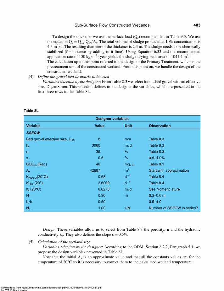
To design the thickener we use the surface load (Qs) recommended in Table 9.5. We usethe equation Qs=QXT·QD/Ae. The total volume of sludge produced at 10% concentration is4.3 m3/d. The resulting diameter of the thickener is 2.3 m. The sludge needs to be chemicallystabilized (for instance by adding to it lime). Using Equation 6.33 and the recommendedapplication rate of 150 kg/m2 · year yields the sludge drying beds area of 1041.4 m2.The calculation up to this point referred to the design of the Primary Treatment, which is thepretreatment unit of the constructed wetland. From this point on, we handle the design of theconstructed wetland.

(4) Define the gravel bed or matrix to be usedVariables selection by the designer: From Table 8.3 we select for the bed gravel with an effective

size, D10= 8 mm. This selection defines to the designer the variables, which are presented in thefirst three rows in the Table 8L.

Design: These variables allow us to select from Table 8.3 the porosity, n and the hydraulicconductivity ks. They also defines the slope s= 0.5%.

(5) Calculation of the wetland sizeVariables selection by the designer: According to the ODM, Section 8.2.2, Paragraph 5.1, we

propose the design variables presented in Table 8L.Note that the initial As is an approximate value and that all the constants values are for the

temperature of 20°C so it is necessary to correct them to the calculated wetland temperature.

Table 8L

Designer variables


SSFCW

Bed gravel effective size, D10 8 mm Table 8.3

ks 3000 m/d Table 8.3

n 35 % Table 8.3

s 0.5 % 0.5–1.0%

BOD5e(Req) 40 mg/L Table 8.1

As 42687 m2 Start with approximation

KHDBO(20°C) 0.68 d−1 Table 8.4

KHCF(20°) 2.6000 d−1 Table 8.4

Kp(20°C) 0.0273 m/d See Nomenclature

H 0.30 m 0.3–0.6 m

L/b 0.50 0.5–4.0

Nc 1.00 UN Number of SSFCW in series?



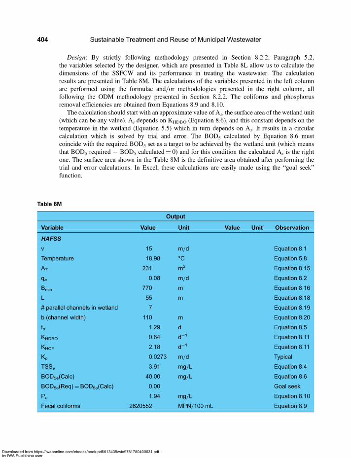
Design: By strictly following methodology presented in Section 8.2.2, Paragraph 5.2,the variables selected by the designer, which are presented in Table 8L allow us to calculate thedimensions of the SSFCW and its performance in treating the wastewater. The calculationresults are presented in Table 8M. The calculations of the variables presented in the left columnare performed using the formulae and/or methodologies presented in the right column, allfollowing the ODM methodology presented in Section 8.2.2. The coliforms and phosphorusremoval efficiencies are obtained from Equations 8.9 and 8.10.

The calculation should start with an approximate value of As, the surface area of the wetland unit(which can be any value). As depends on KHDBO (Equation 8.6), and this constant depends on thetemperature in the wetland (Equation 5.5) which in turn depends on As. It results in a circularcalculation which is solved by trial and error. The BOD5 calculated by Equation 8.6 mustcoincide with the required BOD5 set as a target to be achieved by the wetland unit (which meansthat BOD5 required − BOD5 calculated= 0) and for this condition the calculated As is the rightone. The surface area shown in the Table 8M is the definitive area obtained after performing thetrial and error calculations. In Excel, these calculations are easily made using the “goal seek”function.

Table 8M

Output


HAFSS

v 15 m/d Equation 8.1

Temperature 18.98 °C Equation 5.8

AT 231 m2 Equation 8.15

qa 0.08 m/d Equation 8.2

Bmin 770 m Equation 8.16

L 55 m Equation 8.18

# parallel channels in wetland 7 Equation 8.19

b (channel width) 110 m Equation 8.20

td 1.29 d Equation 8.5

KHDBO 0.64 d−1 Equation 8.11

KHCF 2.18 d−1 Equation 8.11

Kp 0.0273 m/d Typical

TSSe 3.91 mg/L Equation 8.4

BOD5e(Calc) 40.00 mg/L Equation 8.6

BOD5e(Req)=BOD5e(Calc) 0.00 Goal seek

Pe 1.94 mg/L Equation 8.10

Fecal coliforms 2620552 MPN/100 mL Equation 8.9



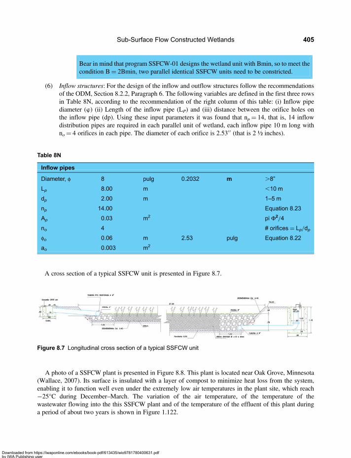
Bear in mind that program SSFCW-01 designs the wetland unit with Bmin, so to meet thecondition B= 2Bmin, two parallel identical SSFCW units need to be constricted.

(6) Inflow structures: For the design of the inflow and outflow structures follow the recommendationsof the ODM, Section 8.2.2, Paragraph 6. The following variables are defined in the first three rowsin Table 8N, according to the recommendation of the right column of this table: (i) Inflow pipediameter (w) (ii) Length of the inflow pipe (LP) and (iii) distance between the orifice holes onthe inflow pipe (dp). Using these input parameters it was found that np= 14, that is, 14 inflowdistribution pipes are required in each parallel unit of wetland, each inflow pipe 10 m long withno= 4 orifices in each pipe. The diameter of each orifice is 2.53′′ (that is 2 ½ inches).

A cross section of a typical SSFCW unit is presented in Figure 8.7.

A photo of a SSFCW plant is presented in Figure 8.8. This plant is located near Oak Grove, Minnesota(Wallace, 2007). Its surface is insulated with a layer of compost to minimize heat loss from the system,enabling it to function well even under the extremely low air temperatures in the plant site, which reach−25°C during December–March. The variation of the air temperature, of the temperature of thewastewater flowing into the this SSFCW plant and of the temperature of the effluent of this plant duringa period of about two years is shown in Figure 1.122.

Table 8N

Inflow pipes

Diameter, φ 8 pulg 0.2032 m .8”

Lp 8.00 m ,10 m

dp 2.00 m 1–5 m

np 14.00 Equation 8.23

Ap 0.03 m2 pi Φ2/4

no 4 # orifices = Lp/dp

φo 0.06 m 2.53 pulg Equation 8.22

ao 0.003 m2

Figure 8.7 Longitudinal cross section of a typical SSFCW unit



Figure 8.8 Insulated subsurface flow constructed wetland near Oak Grove, Minnesota (Source: Wallace,2007)



Chapter 9

Chemically Enhanced PrimaryTreatment (CEPT)

9.1 PROCESS DESCRIPTION9.1.1 Introduction1

Chemically Enhanced Primary Treatment (CEPT) is a process known over one hundred years. However, itsapplication to municipal wastewater was consolidated only in the past two decades, based on technologicaldevelopment of coagulation, flocculation and sedimentation stages for wastewater. It’s most commonapplications are: (i) treatment prior to discharge into oceans, seas or large rivers, (ii) removal ofphosphorus, and (iii) as a component in compact treatment units. The CEPT is a process by whichwastewater is treated with chemical coagulants as ferrous chloride or aluminium sulphate (alum), to whicha flocculating agent (polymer) is added after coagulation, before the primary sedimentation tanks. Thecoagulation and flocculation cause particles to cling together to larger flocs which are heavier and settlemore rapidly. In this way higher removal rates than in conventional primary treatments are reached forboth TSS (about 80–85% in CEPT compared to about 40–50% in conventional primary sedimentation)and for BOD (BOD 50–70% in CEPT compared to 20–35% in conventional primary sedimentation).CEPT is operated at twice the Surface Overflow Rate (SOR) used in conventional primary tanks, reducingthereby the area of the sedimentation tanks by half. Figure 9.1 shows a typical flow diagram of the CEPTprocess (Libhaber, 2007).

Figure 9.1 A typical flow diagram of the CEPT process [Source: Libhaber (2007)]

1Section adapted mainly from Menahem Libhaber (2007, 2004).


To convert a conventional primary treatment plant into a CEPT plant, all that is needed is the addition of achemical coagulant and optionally addition of flocculants. The chemical dosing systems are inexpensive andsimple to install. CEPT effluent quality approaches that of an effluent of a secondary biological treatmentplant in terms of removal efficiency of TSS and BOD. In addition, the CEPT process removes phosphorus.Because of the high TSS removal in the CEPT process, its effluent is clear can be effectively disinfected, andthis is an important feature for developing countries, in which high levels of morbidity result fromwaterborne diseases. A primary treatment facility upgraded to CEPT has double the capacity of theoriginal conventional settling system so it is able to serve future flows without an additional upgrade. Ifa CEPT unit is designed from scratch, the sedimentation tanks will be smaller and cheaper than primarysedimentation tanks for the same wastewater flow without chemicals addition. In this case, the additionalinvestment required for treating the increased sludge generated is offset by the lower cost of thesedimentation tanks. When a primary treatment unit is upgraded to CEPT, however, this offset does notexist and additional investment for sludge treatment is required, but an upgraded system is able to servefuture flows without an additional expansion.

The chemistry of coagulation and flocculation is widely known, so that incorporation of the CEPT toengineering practice is relatively easy. However, CEPT produces more sludge than conventional primarytreatment because it is through the production of sludge that the organic matter is removed in thisprocess. The greatest portion of the increased sludge production in CEPT is the result of the increasedsolids (and therefore also organic matter) removal in the settling tank through the physicochemical (notbiological) process, which is precisely the CEPT’s goal. The chemicals themselves add only a slightcontribution to the sludge quantities. An adequate treatment and disposal of sludge needs to be part ofthe CEPT system. The main options for sludge treatment, which must be part of the installation, are limestabilization and use of drying beds for drying the sludge, anaerobic digestion, and composting, asdiscussed below.

CEPT treatment does not preclude additional polishing treatment such as secondary or tertiary. It reducesthe size and cost of these subsequent treatment units due to increased removal of suspended solids andorganic matter. CEPT is a relatively simple technology, which provides low cost, easy to implement andeffective treatment.

9.1.2 Basics of the processFundamentals2

Tsukamoto (2002) classifies into six classes contaminants which need to be removed from municipalwastewater before their discharge to receiving waters:

• Pathogenic Organisms: These are the most important pollutants from the standpoint of risk to humanhealth since they generate water-borne diseases (which are transmitted through water). Among thecauses of these diseases are the worms (earthworm, tapeworm, schistosoma and others), protozoa(amoebas, Giardia, Cryptosporidium, and so on.), Bacteria (cholera, Salmonella, E. coli, and soon.), and viruses (hepatitis, enterovirus, and so on.).

• Organic Matter (BOD): is the aggregate of organic substances present in wastewater whosebiodegradable part produces Biochemical Oxygen Demand. The BOD in the municipal wastewater

2This paragraph is based on the article by Tsukamoto (2002), “Tratamiento físico-químico de aguas residuales municipales: estrategiaeficiente, rápida y de bajo costo para Latinoamérica” (Physicochemical Treatment of MunicipalWastewater: Efficient, Rapid and LowCost Strategy for Latin America).



is only about half of the organic matter contained in this type of wastewater. The rest isnon-biodegradable organic matter. The sum of biodegradable and non-biodegradable organicmatter is measured by the COD test.

• Suspended Solids (SS): is the aggregate of all particles in the wastewater. It is one of the parameters ofmajor environmental and health impacts since it encompasses all organic and inorganic matterin suspension. The SS include 100% of pathogenic organisms present in the wastewater, 50% to70% of the organic matter present in the wastewater and 100% of the colloidal matter inthe wastewater.

• Nutrients (P and N):Organic and inorganic compounds of phosphorus (P) and nitrogen (N) containedin wastewater stimulate the uncontrolled reproduction of micro algae in aquatic environments.Phosphorus is the major contaminant responsible for the effects of eutrophication and waterpoisoning. Its elimination is an important goal of wastewater treatment. In fresh water, blue-greenalgae (cyanophyte) and some diatoms produce carcinogenic toxins and generate in the waterunpleasant taste and odour.

• Fetid Odour (H2S): The smell of “rotten egg” that characterizes wastewater is caused by hydrogensulphide gas produced by anaerobic bacteria from the sulphur present in the wastewater. This gasis toxic to plants, animals and humans. It is also corrosive to metal and concrete pipes and toconstruction materials. The human smell sense perceives H2S in concentrations in the order of afew ppt (parts per trillion= 10−12).

• Heavy metals: These toxic chemicals released into municipal wastewater by industries withinadequate effluents treatment (mercury, chromium, nickel, lead, arsenic, silver and others) have,in general, a cumulative and often carcinogenic effect, being toxic to all living beings.Contamination of sediment in the bottom of receiving water bodies is prolonged, since heavymetals do not degrade in the environment, and therefore have a cumulative effect.

According to Tsukamoto (2002) the conventional classification of municipal wastewater treatment is: (i)primary treatment: which is the separation of the SS by settling or flotation, which can be chemicallyenhanced, (ii) secondary treatment: which is the removal of soluble and insoluble organic matter bybiological treatment, and (iii) tertiary treatment: which is the removal of N and P, (P is present mainlyin colloidal form). The suspended solids contain 100% of the pathogens, 50% to 70% of the organicmatter and 100% of the colloidal matter present in wastewater. Accordingly, the CEPT removes veryeffectively, SS, phosphorus, heavy metals and H2S. It also removes a large amount of BOD (it does notreach the efficiency of BOD removal in secondary treatment, but it is close) and part of the pathogens.To obtain the same degree of removal of these parameters by conventional treatment primary treatment,secondary treatment and advanced treatment (to remove nutrients heavy metals) is required. This is muchmore complex and costly than CEPT. However, if a high efficiency of BOD removal (over 80%) isrequired, biological treatment is inevitable. In this case, a good alternative is biological treatment aspost-treatment (polishing) of a CEPT effluent. In terms of cost-effectiveness, CEPT emerges as a newparadigm because it achieves a lot more treatment goals for less cost, as shown in Figure 9.2. It isimportant to emphasize that the CEPT system must include installation for management of the sludgegenerated in this process.

Coagulation by addition of metallic electrolytesThe processes by which the coagulation of colloidal suspensions and particulate matter is facilitated for theirsubsequent removal by sedimentation are known as coagulation and flocculation.

Chemically enhanced primary treatment 409


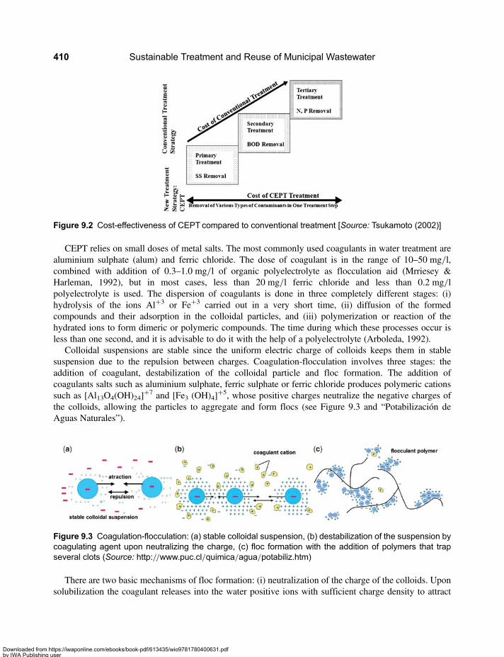
CEPT relies on small doses of metal salts. The most commonly used coagulants in water treatment arealuminium sulphate (alum) and ferric chloride. The dose of coagulant is in the range of 10–50 mg/l,combined with addition of 0.3–1.0 mg/l of organic polyelectrolyte as flocculation aid (Mrriesey &Harleman, 1992), but in most cases, less than 20 mg/l ferric chloride and less than 0.2 mg/lpolyelectrolyte is used. The dispersion of coagulants is done in three completely different stages: (i)hydrolysis of the ions Al+3 or Fe+3 carried out in a very short time, (ii) diffusion of the formedcompounds and their adsorption in the colloidal particles, and (iii) polymerization or reaction of thehydrated ions to form dimeric or polymeric compounds. The time during which these processes occur isless than one second, and it is advisable to do it with the help of a polyelectrolyte (Arboleda, 1992).

Colloidal suspensions are stable since the uniform electric charge of colloids keeps them in stablesuspension due to the repulsion between charges. Coagulation-flocculation involves three stages: theaddition of coagulant, destabilization of the colloidal particle and floc formation. The addition ofcoagulants salts such as aluminium sulphate, ferric sulphate or ferric chloride produces polymeric cationssuch as [Al13O4(OH)24]

+7 and [Fe3 (OH)4]+5, whose positive charges neutralize the negative charges of

the colloids, allowing the particles to aggregate and form flocs (see Figure 9.3 and “Potabilización deAguas Naturales”).

There are two basic mechanisms of floc formation: (i) neutralization of the charge of the colloids. Uponsolubilization the coagulant releases into the water positive ions with sufficient charge density to attract

Figure 9.3 Coagulation-flocculation: (a) stable colloidal suspension, (b) destabilization of the suspension bycoagulating agent upon neutralizing the charge, (c) floc formation with the addition of polymers that trapseveral clots (Source: http://www.puc.cl/quimica/agua/potabiliz.htm)

Figure 9.2 Cost-effectiveness of CEPT compared to conventional treatment [Source: Tsukamoto (2002)]



http://www.unep.or.jp/ietc/publications/techpublications/techpub-15/2-5/5-5.asp







colloidal particles and neutralize their charge. It has been observed that the effect increases sharply with thenumber of charges of the coagulant ions3, and (ii) coalescence of the neutralized colloids into a floc.The coagulants form in water certain low solubility products which precipitate. The colloidal particlesserve as the nucleus of precipitation and remain immersed within the precipitate.

The pH is a critical factor in the coagulation process. There is always a pH range in which a specificcoagulant works best, which coincides with the range of the minimum solubility of the metal ions of thecoagulant used. Whenever possible, the coagulation should be made within this optimum pH range sinceotherwise chemicals are wasted and a decrease in plant performance can be experienced. If the pH of thewater is not adequate, it can be modified through the use of coagulant aids, among which are lime, quicklime, sodium carbonate, caustic soda and mineral acids. Other factors which also influent coagulation arethe alkalinity of the water, the quantity of coagulant and the mixing intensity.

CoagulantsAlum

The alum, a hydrated aluminium sulphate with n molecules of H2O (n is between 13 and 18), reacts withalkalinity in the water according to the following equation:

Al2(SO4)3Alum

nH2O + 3Ca(HCO3)2Alkalinity

−� 2Al(OH)3 Al Hydroxide

+ 6CO2 + 3CaSO4 + xH2O

The formation of aluminium hydroxide leads to floc precipitation. If the water does not have enoughalkalinity, then it should be increased by adding calcium carbonate. The range of pH for optimumcoagulation is between 5 and 7.5. The Alum dose for wastewater treatment is from 100 to 300 g/m3,depending on the type of wastewater and the effluent quality requirement. The pH regulation can be done with:

• Lime: it takes about 30% of the dose of commercial aluminium sulphate, according to the followingreaction:

Al2(SO4)3 + Ca(OH)2 = 2Al(OH)3 + 3CaSO4

• Sodium carbonate: it takes between 50 and 100% of the dose of commercial aluminium sulphate:

Al2(SO4)3 + 3H2O+ 3Na2CO3 = 2Al(OH)3 + 3Na2SO4 + 3CO2

Ferric chloride

Ferric chloride, FeCl3, is the most widely used coagulant in wastewater treatment. It reacts with naturalalkalinity as follows:

2FeCl3Fe Chloride

+ 3Ca(HCO3)2Alkalinity

= 3CaCl2 + 2Fe(OH)3Fe Hydroxide

+6CO2

The range of pH for optimum coagulation is between 4 and 6, and above 8. The dose of FerricChloride when using lime (to provide alkalinity when needed) is from 5 to 160 g/m3 of commercialreagent FeCl3 · 6H2O, and it reacts with the lime as follows:

2FeCl3 + 3Ca(OH)2 = 2Fe(OH)+ 3CaCl2

3For negatively charged colloids, divalent ions (Ba and Mg) are 30 times more effective than monovalent Na, and, in turn, trivalent Feand Al, are about 30 times more effective than divalent ions. For positively charged colloids, the same approximate ratios exist betweenthe monovalent chloride ion, Cl−, the divalent sulfate (SO4)

−2, and the trivalent phosphate (PO4)−3 (Wikibooks, 2007).



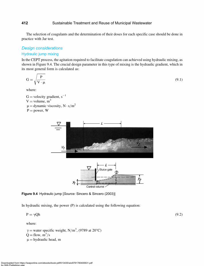
The selection of coagulants and the determination of their doses for each specific case should be done inpractice with Jar test.

Design considerationsHydraulic jump mixing

In the CEPT process, the agitation required to facilitate coagulation can achieved using hydraulic mixing, asshown in Figure 9.4. The crucial design parameter in this type of mixing is the hydraulic gradient, which inits most general form is calculated as:

G =��P

V · m

√(9.1)

where:

G= velocity gradient, s−1

V= volume, m3

µ= dynamic viscosity, N · s/m2

P= power, W

In hydraulic mixing, the power (P) is calculated using the following equation:

P = gQh (9.2)

where:

γ=water specific weight, N/m3, (9789 at 20°C)Q= flow, m3/sμ= hydraulic head, m

Figure 9.4 Hydraulic jump [Source: Sincero & Sincero (2003)]



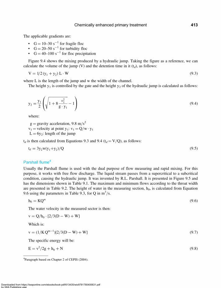
The applicable gradients are:

• G= 10–30 s−1 for fragile floc• G= 20–50 s−1 for turbidity floc• G= 40–100 s−1 for floc precipitation

Figure 9.4 shows the mixing produced by a hydraulic jump. Taking the figure as a reference, we cancalculate the volume of the jump (V) and the detention time in it (td), as follows:

V = 1/2 (y1 + y2) L ·W (9.3)

where L is the length of the jump and w the width of the channel.The height y1 is controlled by the gate and the height y2 of the hydraulic jump is calculated as follows:

y2 =y12

��1+ 8

v21g · y1

√− 1

⎛⎝

⎞⎠ (9.4)

where:

g= gravity acceleration, 9.8 m/s2

v1= velocity at point y1: v1=Q/w · y1L= 6y2: length of the jump

td is then calculated from Equations 9.3 and 9.4 (td=V/Q), as follows:

td = 3y2w(y1+y2)/Q (9.5)

Parshall flume4

Usually the Parshall flume is used with the dual purpose of flow measuring and rapid mixing. For thispurpose, it works with free flow discharge. The liquid stream passes from a supercritical to a subcriticalcondition, causing the hydraulic jump. It was invented by R.L. Parshall. It is presented in Figure 9.5 andhas the dimensions shown in Table 9.1. The maximum and minimum flows according to the throat widthare presented in Table 9.2. The height of water in the measuring section, h0, is calculated from Equation9.6 using the parameters in Table 9.3, for Q in m3/s.

h0 = KQm (9.6)

The water velocity in the measured sector is then:

v = Q/h0 · [2/3(D−W)+W]

Which is:

v = (1/KQm−1)[2/3(D−W)+W] (9.7)

The specific energy will be:

E = v2/2g+ h0 + N (9.8)

4Paragraph based on Chapter 2 of CEPIS (2004).



Figure 9.5 Basic dimensions of Parshall flumes (Source: http://www.usbr.gov/pmts/hydraulics_lab/pubs/wmm/chap08_10.html)

Table 9.1 Dimensions of the parshall flumes (see Figure 9.5).

W A B C D E F G K N

inches (cm) (cm) (cm) (cm) (cm) (cm) (cm) (cm) (cm) (cm)

1′′ 2,5 36,3 35,6 9,3 16,8 22,9 7,6 20,3 1,9 2,9

3′′ 7,6 46,6 45,7 17,8 25,9 45,7 15,2 30,5 2,5 5,7

6′′ 15,2 61,0 61,0 39,4 40,3 61,0 30,5 61,0 7,6 11,4

9′′ 22,9 88,0 86,4 38,0 57,5 76,3 30,5 45,7 7,6 11,4

1′ 30,5 137,2 134,4 61,0 84,5 91,5 61,0 91,5 7,6 22,9

1 1/2′ 45,7 144,9 142,0 76,2 102,6 91,5 61,0 91,5 7,6 22,9

2′ 61,0 152,5 149,6 91,5 120,7 91,5 61,0 91,5 7,6 22,9

3′ 91,5 167,7 164,5 122,0 157,2 91,5 61,0 91,5 7,6 22,9

4′ 122,0 183,0 179,5 152,5 193,8 91,5 61,0 91,5 7,6 22,9

5′ 152,5 198,3 194,1 183,0 230,3 91,5 61,0 91,5 7,6 22,9

6′ 183,0 213,5 209,0 213,5 266,7 91,5 61,0 91,5 7,6 22,9

7′ 213,5 228,8 224,0 244,0 303,0 91,5 61,0 91,5 7,6 22,9

8′ 244,0 244,0 239,2 274,5 274,5 91,5 61,0 91,5 7,6 22,9

10′ 305,0 274,5 427,0 366,0 475,9 122,0 91,5 183,0 15,3 34,3












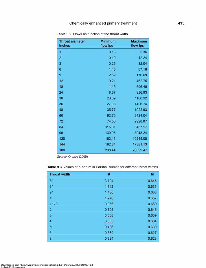
Table 9.2 Flows as function of the throat width.

Throat aiameterinches

Minimumflow lps

Maximumflow lps

1 0.13 5.36

2 0.19 12.24

3 0.25 32.04

6 1.45 87.18

9 2.59 176.69

12 9.21 462.75

18 1.45 696.40

24 18.67 936.93

30 23.09 1180.92

36 27.38 1426.74

48 35.77 1922.93

60 62.76 2424.04

72 74.50 2928.87

84 115.31 3437.17

96 130.95 3948.24

120 162.43 10245.08

144 192.84 17381.13

180 238.44 28899.47

Source: Orozco (2005)

Table 9.3 Values of K and m in Parshall flumes for different throat widths.

Throat width K M

3′′ 3.704 0.646

6′′ 1.842 0.636

9′′ 1.486 0.633

1′ 1.276 0.657

11/2′ 0.966 0.650

2′ 0.795 0.645

3′ 0.608 0.639

4′ 0.505 0.634

5′ 0.436 0.630

6′ 0.389 0.627

8′ 0.324 0.623



For N see Table 9.1. The velocity before the jump, according to Arboleda (1992), is obtained by solvingEquation 9.9:

v31 − 2gv1E+ 2Qg/W = 0 (9.9)

In order for the Parshall flume to produce good mixing, it is required that the velocity at the throat bemaintained between 2 and 7 m/s (Orozco, 2005).

Sedimentation5

Sedimentation is a fundamental process in CEPT. According to Orozco (2005) Sedimentation is generallyclassified into four types, namely:

(1) Discrete Sedimentation: or Sedimentation Type I. This refers to sedimentation of discrete particlesin low concentrations, where sedimentation occurs individually by each particle, withoutinterference of one particle to others. The theory of discrete sedimentation is explained by theStokes equation; however when it refers to wastewater treatment, the approximation through theSurface Overflow Rate (SOR), which is defined as the flow divided by the sedimentation area(Q/As), is more frequently used.

(2) Flocculent Sedimentation: or sedimentation Type II. This refers to the sedimentation of particleswhich are not highly concentrated but which tend to flocculate, so that the settling velocity ofthe particle increases with the sedimentation process. This is what happens in primary clarifiersand in the CEPT process. The design parameter of this type of sedimentation is SOR.

(3) Hindered or Zone Sedimentation: also known as Sedimentation Type III, occurs with in caseswhere the particles concentrations is of intermediate levels. In this case at the end of thesedimentation the particles form a defined solid-liquid interface. The forces between particles aresufficient to hinder each other, remaining in fixed positions one in relation to the others. Thisoccurs in secondary clarifiers in biological wastewater treatment plant, and the parametersgoverning the design are SOR and the solids loading, Qs (Q · X/As), where X is the TSSconcentration in the mixed liquor (also known as MLSS – Mixed Liquor Suspended Solids), andAs is the surface area of the clarifier.

(4) Thickening: also known as Sedimentation Type IV, is what happens when the particles alreadyunderwent a sedimentation process and have reached a structure of formed particles. Thishappens when the particles concentration is very large, and additional “sedimentation” can occuronly by compression. This is what happens in thickeners and at the bottom of secondaryclarifiers. The design parameter of this type of sedimentation is the solids loading, Qs.

Sedimentation tanks can be designed as tanks of horizontal flow, of vertical up flow, with inclinedparallel plates, or as circular sedimentation tanks with variable horizontal flow. The latter is preferred inthe wastewater treatment industry because it allows continuous removal of solids by mechanical rotatingscrapers for sludge removal, as shown in Figure 9.6.

The CEPT process is used in the flocculent or type II sedimentation and the parameter of design is theSurface Overflow Rate (SOR). Table 9.4 shows the SOR design values used for conventional primarysedimentation without chemical enhancement. When coagulants are used, the sedimentation efficiencysubstantially improves, as shown in Figure 9.7 prepared based on Harleman (2004). Because of its much

5Paragraph based on Chapter 7 of Orozco (2005).



higher sedimentation efficiency, SOR values used in CEPT are double of those used in conventional primarysedimentation, that is, in the range 60–100 m3/d · m2. This implies that for treatment of the same flow ofwastewater a much smaller CEPT settler can be used in relation to a settler required for conventionalsedimentation, while obtaining a much higher TSS and BOD removal efficiencies than those which canbe obtained in conventional sedimentation without chemical enhancement (Libhaber, 2007).

Figure 9.6 Circular sedimentation tank with continuous sludge removal [Source: http://www.ecomacchine.it/documentazione/4-sedimentazione-eng.html (2001)]

Table 9.4 Surface Overflow Rate (SOR) for conventional primary treatment.

Parameter Units Range Typical

td hour 1.5–2.5 2

SOR mean m3/d · m2 24–48 32

SOR peak m3/d · m2 48–120 60

Weir Hydraulic Load m3/d · m 125–500 250













Chemically Enhanced Rotating Microscreens (CERM)

Multiple-stage screening and the addition to flocculants can significantly increase contaminant removallevels. The rotating fine screen devices discussed in Chapter 4 can remove up to 50% of particulate CODand up to 30% of total COD with screen openings of around 0.2 mm. Investigations by HuberTechnology (2003) indicate that addition of organic coagulant to the raw sewage entering a fine rotatingscreen of 0.2 to 0.3 mm opening achieves up to 60% reduction of total COD and BOD, and TSSreduction from 50% to 95%. This process is still under development and seems to be based on two-stagescreening where the first screen has an opening of about 6 mm and the second is a fine screen with anopening of 0.2 mm, as shown in Figure 9.8. This process is named Chemically Enhanced RotatingMicroscreens (CERM). The coagulant is added to the wastewater before the second unit Libhaber (2007).

The CERM process is achieved by a simple machine that removes a significant amount of solids andorganic matter. It might not reach the level of solids and BOD removed by CEPT, however, it is lesscostly and simpler to operate. It is certainly more affordable for developing countries. The level oforganic matter removal achieved in CERM might be sufficient to prevent environmental problems if theeffluent is discharged to a high flow river or to other receiving bodies with high assimilation capacity.The chemically enhanced rotating fine screens might be a better first stage goal than CEPT, especially inlow income developing countries.

Raw wastewater

Pre-screening 6 mm

Finescreening 0.2 mm

Anaerobic sludge treatment

Sludge production: 300 – 500 l per 1000 m³ wastewater

Treated effluent50 - 60% COD reduction

Flocculants

Figure 9.8 Chemically enhanced solids separation in rotating micro screens (CERM)

E = -0.4006SOR + 73.782

E = -0.114SOR + 96.553

E = -0.2911SOR + 42.486

E = -0.0966SOR + 77.307

0

10

20

30

40

50

60

70

80

90

100

0 20 40 60 80 100 120

EFFI

CIEN

CY, %

SOR, m/d

REMOVAL EFFICIENCY vs. Surface Overflow Rate (SOR)

SS CONV.

SS CEPT

BOD CONV

BOD CEPT

Figure 9.7 Comparison of BOD and TSS removal efficiencies of conventional primary treatment and CEPT[Source: Harleman (2004)]



The high removal of solids in CERM generates larger quantities of sludge those generated in preliminarytreatment without chemicals addition, so sludge treatment facilities need to be included as part of the CERMconcept. Sludge treatment options are similar to that of CEPT sludge, as described below.

Since the CERM is still a new concept, more research is required to establish its performance and its cost.A comparison among the different options of screening, with and without addition of coagulants, accordingto Köppl & Frommann (2004), is shown in Figure 9.9.

Sludge management

As mentioned, CEPT produces more sludge than conventional primary treatment because it is through theproduction of sludge that the organic matter is removed in this process. Therefore, adequate treatment anddisposal of sludge needs to be part of the CEPT system. In most cases the doses of chemicals in the CEPTprocess are less than 20 mg/l of metal salt and less than 0.2 mg/l of polyelectrolyte. Most of the sludgeconsists of the solids settled from the raw wastewater. The chemicals used for coagulation add only aslight contribution to the sludge quantities.

The CEPT process, as well as most of the appropriate technology processes described in the book,generates two types of solid wastes. Rotating screens with coarse openings larger than 0.7 mm, orpreliminary treatment in general, produce residual solids which are mainly mineral, consisting of sand,grit, coarse particles and large materials like plastics, bottles, cans and other floatable material. Thismaterial is defined as solid wastes from preliminary treatment. Rotating micro screens with openings lessthan 0.7 mm, CEPT, CERM, UASB, Anaerobic Filters and some of the other appropriate technologyprocesses produce residual solids which consist of a combination of mineral and organic matter, definedas sludge. These two types of solids, that is, solid wastes and sludge, are handled and disposed ofdifferently. The management and disposal of the solid wastes generated in the preliminary treatment is

Figure 9.9 Various innovative chemically enhanced screening options [Source: Köppl & Frommann (2004)]



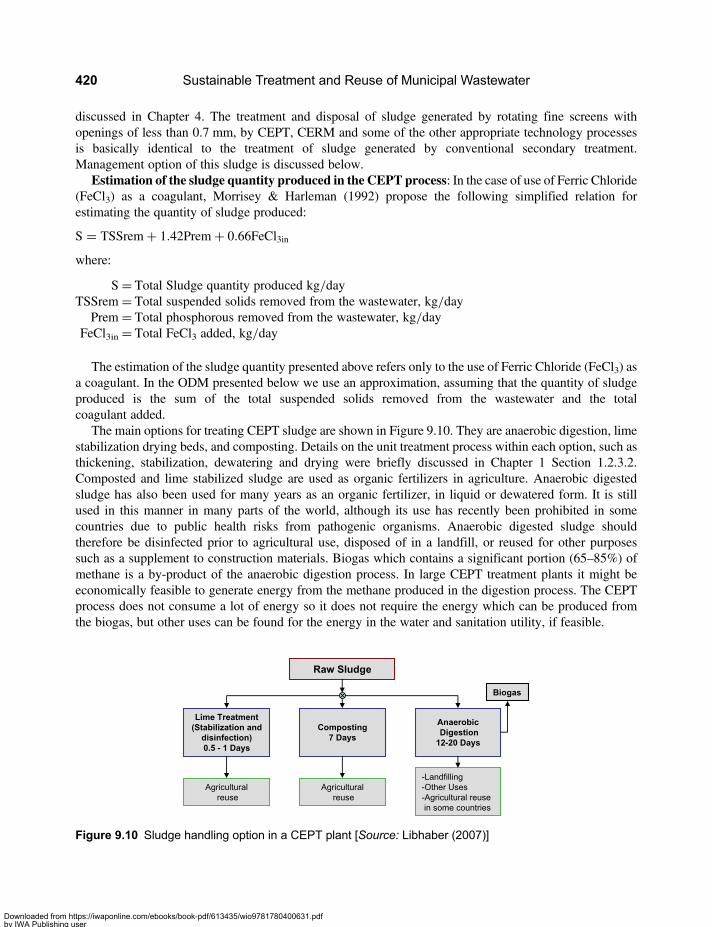
discussed in Chapter 4. The treatment and disposal of sludge generated by rotating fine screens withopenings of less than 0.7 mm, by CEPT, CERM and some of the other appropriate technology processesis basically identical to the treatment of sludge generated by conventional secondary treatment.Management option of this sludge is discussed below.

Estimation of the sludge quantity produced in the CEPT process: In the case of use of Ferric Chloride(FeCl3) as a coagulant, Morrisey & Harleman (1992) propose the following simplified relation forestimating the quantity of sludge produced:

S = TSSrem+ 1.42Prem+ 0.66FeCl3in

where:

S= Total Sludge quantity produced kg/dayTSSrem = Total suspended solids removed from the wastewater, kg/day

Prem = Total phosphorous removed from the wastewater, kg/dayFeCl3in = Total FeCl3 added, kg/day

The estimation of the sludge quantity presented above refers only to the use of Ferric Chloride (FeCl3) asa coagulant. In the ODM presented below we use an approximation, assuming that the quantity of sludgeproduced is the sum of the total suspended solids removed from the wastewater and the totalcoagulant added.

The main options for treating CEPT sludge are shown in Figure 9.10. They are anaerobic digestion, limestabilization drying beds, and composting. Details on the unit treatment process within each option, such asthickening, stabilization, dewatering and drying were briefly discussed in Chapter 1 Section 1.2.3.2.Composted and lime stabilized sludge are used as organic fertilizers in agriculture. Anaerobic digestedsludge has also been used for many years as an organic fertilizer, in liquid or dewatered form. It is stillused in this manner in many parts of the world, although its use has recently been prohibited in somecountries due to public health risks from pathogenic organisms. Anaerobic digested sludge shouldtherefore be disinfected prior to agricultural use, disposed of in a landfill, or reused for other purposessuch as a supplement to construction materials. Biogas which contains a significant portion (65–85%) ofmethane is a by-product of the anaerobic digestion process. In large CEPT treatment plants it might beeconomically feasible to generate energy from the methane produced in the digestion process. The CEPTprocess does not consume a lot of energy so it does not require the energy which can be produced fromthe biogas, but other uses can be found for the energy in the water and sanitation utility, if feasible.

Raw Sludge

Agriculturalreuse

-Landfilling-Other Uses-Agricultural reusein some countries

Biogas

Lime Treatment(Stabilization and

disinfection)0.5 - 1 Days

Composting7 Days

AnaerobicDigestion

12-20 Days

Agriculturalreuse

Figure 9.10 Sludge handling option in a CEPT plant [Source: Libhaber (2007)]



9.1.3 PerformanceEfficiency

The BOD removal efficiency in the CEPT process is 70–75% and the TSS removal efficiency is 80–95%,depending on the SOR employed (see Figure 9.7). The removal CERM efficiency is in the range of 50–60%for COD and 70–80% for TSS.

Construction costs of the CEPT system are in the range of 20–40 USD/Capita. Operating andmaintenance costs are in the range of 1.5–2 USD/Capita · yr. The construction costs of CERM areestimated to be in the range of 15–25 USD/capita and O & M costs in the range of 1.5–2 USD/Capita · yr.

Advantages and disadvantages

The advantages of CEPT are:

• Achieves removal of all important contaminants present in wastewater (SS, BOD, phosphorus, H2S,heavy metals and partial removal of pathogens) in a single treatment stage.

• Because it uses installations of primary treatment, it is of low investment cost. Existing primarytreatment installations can easily be converted to CEPT.

• The wastewater treatment is quick (detention time of about an hour) and yields a transparent anddeodorized treated effluent.

• Since it is not a biological treatment process, the CEPT process is less sensitive to temperaturevariations. The flocculation process loses some efficiency at low temperatures but the efficiencycan be recovered by adjusting the doses of coagulant and flocculant. Consequently, the CEPTprocess can perform well in all the temperature range of wastewater and therefore in all types ofconditions and zones, from tropical to sub-polar.

• Because of its low SS content, the CEPT effluent can be effectively disinfected, and that is animportant feature for developing countries, where due to the high level of morbidity originating inwater borne diseases, disinfection is a priority.

• It achieves high phosphorous removal.• It is a very compact treatment process which occupies a very small land area, so it is advantageous for

projects with restricted land availability.• It reduces the size of subsequent treatment units if polishing of the CEPT effluent is required.

The main disadvantages of the CEPT are:

• It produces more sludge than conventional primary treatment and even more sludge than thatproduced by the conventional activated sludge process.

• The sludge produced is more difficult to handle than biological sludge.

9.2 BASIC DESIGN PROCEDURES9.2.1 General design considerationsThe CEPT can be presented as the original design choice or as a conversion of a conventional primarytreatment plant. The latter modification is easy, since it only requires incorporation of installations foradding a coagulant and a polymeric flocculant. The injection of the chemicals must be made atappropriate points to meet the design variables corresponding to the coagulation/flocculation in a waythat promotes a good mixing for these processes, namely: (i) the adequate velocity gradient, and (ii) therequired detention time. The CERM process is presented as an additional design option because



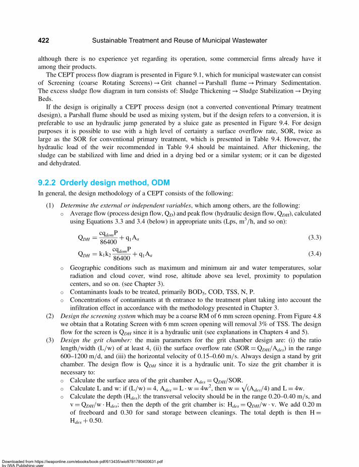
although there is no experience yet regarding its operation, some commercial firms already have itamong their products.

The CEPT process flow diagram is presented in Figure 9.1, which for municipal wastewater can consistof Screening (coarse Rotating Screens)→Grit channel→ Parshall flume→ Primary Sedimentation.The excess sludge flow diagram in turn consists of: Sludge Thickening→ Sludge Stabilization→DryingBeds.

If the design is originally a CEPT process design (not a converted conventional Primary treatmentdsesign), a Parshall flume should be used as mixing system, but if the design refers to a conversion, it ispreferable to use an hydraulic jump generated by a sluice gate as presented in Figure 9.4. For designpurposes it is possible to use with a high level of certainty a surface overflow rate, SOR, twice aslarge as the SOR for conventional primary treatment, which is presented in Table 9.4. However, thehydraulic load of the weir recommended in Table 9.4 should be maintained. After thickening, thesludge can be stabilized with lime and dried in a drying bed or a similar system; or it can be digestedand dehydrated.

9.2.2 Orderly design method, ODMIn general, the design methodology of a CEPT consists of the following:

(1) Determine the external or independent variables, which among others, are the following:○ Average flow (process design flow, QD) and peak flow (hydraulic design flow, QDH), calculated

using Equations 3.3 and 3.4 (below) in appropriate units (Lps, m3/h, and so on):

QDH = cqdomP86400

+ q1Aa (3.3)

QDH = k1k2cqdomP86400

+ q1Aa (3.4)

○ Geographic conditions such as maximum and minimum air and water temperatures, solarradiation and cloud cover, wind rose, altitude above sea level, proximity to populationcenters, and so on. (see Chapter 3).

○ Contaminants loads to be treated, primarily BOD5, COD, TSS, N, P.○ Concentrations of contaminants at th entrance to the treatment plant taking into account the

infiltration effect in accordance with the methodology presented in Chapter 3.(2) Design the screening system which may be a coarse RM of 6 mm screen opening. From Figure 4.8

we obtain that a Rotating Screen with 6 mm screen opening will removal 3% of TSS. The designflow for the screen is QDH since it is a hydraulic unit (see explanations in Chapters 4 and 5).

(3) Design the grit chamber: the main parameters for the grit chamber design are: (i) the ratiolength/width (L/w) of at least 4, (ii) the surface overflow rate (SOR=QDH/Ades) in the range600–1200 m/d, and (iii) the horizontal velocity of 0.15–0.60 m/s. Always design a stand by gritchamber. The design flow is QDH since it is a hydraulic unit. To size the grit chamber it isnecessary to:○ Calculate the surface area of the grit chamber Ades=QDH/SOR.○ Calculate L and w: if (L/w)= 4, Ades= L · w= 4w2, then w=√(Ades/4) and L= 4w.○ Calculate the depth (Hdes): the transversal velocity should be in the range 0.20–0.40 m/s, and

v=QDH/w · Hdes; then the depth of the grit chamber is: Hdes=QDH/w · v. We add 0.20 mof freeboard and 0.30 for sand storage between cleanings. The total depth is then H=Hdes+ 0.50.



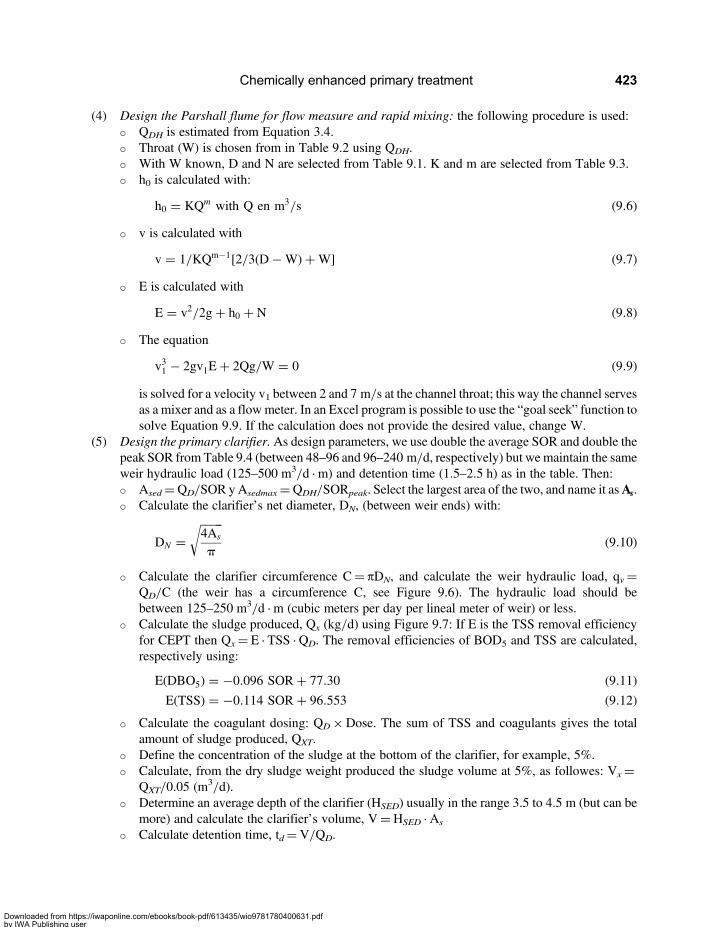
(4) Design the Parshall flume for flow measure and rapid mixing: the following procedure is used:○ QDH is estimated from Equation 3.4.○ Throat (W) is chosen from in Table 9.2 using QDH.○ With W known, D and N are selected from Table 9.1. K and m are selected from Table 9.3.○ h0 is calculated with:

h0 = KQm with Q en m3/s (9.6)

○ v is calculated with

v = 1/KQm−1[2/3(D−W)+W] (9.7)

○ E is calculated with

E = v2/2g+ h0 + N (9.8)

○ The equation

v31 − 2gv1E+ 2Qg/W = 0 (9.9)

is solved for a velocity v1 between 2 and 7 m/s at the channel throat; this way the channel servesas a mixer and as a flowmeter. In an Excel program is possible to use the “goal seek” function tosolve Equation 9.9. If the calculation does not provide the desired value, change W.

(5) Design the primary clarifier. As design parameters, we use double the average SOR and double thepeak SOR from Table 9.4 (between 48–96 and 96–240 m/d, respectively) but wemaintain the sameweir hydraulic load (125–500 m3/d · m) and detention time (1.5–2.5 h) as in the table. Then:○ Ased=QD/SOR yAsedmax=QDH/SORpeak. Select the largest area of the two, and name it asAs.○ Calculate the clarifier’s net diameter, DN, (between weir ends) with:

DN =��4As

p

√(9.10)

○ Calculate the clarifier circumference C= πDN, and calculate the weir hydraulic load, qv=QD/C (the weir has a circumference C, see Figure 9.6). The hydraulic load should bebetween 125–250 m3/d · m (cubic meters per day per lineal meter of weir) or less.

○ Calculate the sludge produced, Qx (kg/d) using Figure 9.7: If E is the TSS removal efficiencyfor CEPT then Qx= E · TSS · QD. The removal efficiencies of BOD5 and TSS are calculated,respectively using:

E(DBO5) = −0.096 SOR+ 77.30 (9.11)

E(TSS) = −0.114 SOR+ 96.553 (9.12)

○ Calculate the coagulant dosing: QD×Dose. The sum of TSS and coagulants gives the totalamount of sludge produced, QXT.

○ Define the concentration of the sludge at the bottom of the clarifier, for example, 5%.○ Calculate, from the dry sludge weight produced the sludge volume at 5%, as followes: Vx=

QXT/0.05 (m3/d).○ Determine an average depth of the clarifier (HSED) usually in the range 3.5 to 4.5 m (but can be

more) and calculate the clarifier’s volume, V=HSED · As

○ Calculate detention time, td=V/QD.



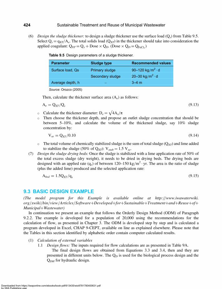
(6) Design the sludge thickener: to design a sludge thickener use the surface load (Qs) from Table 9.5.Select Qs= qXT/Ae. The total solids load (QXT) in the thickener should take into consideration theapplied coagulant: QXT=Qx+Dose×QD. (Dose×QD=QFeCl3 )

Then, calculate the thickener surface area (Ae) as follows:

Ae = QXT/Qs (9.13)

○ Calculate the thickener diameter: De=√4As/π○ Then choose the thickener depth, and propose an outlet sludge concentration that should be

between 5–10%, and calculate the volume of the thickened sludge, say 10% sludgeconcentration by:

Vxe = QXT/0.10 (9.14)

○ The total volume of chemically stabilized sludge is the sum of total sludge (QXT) and lime addedto stabilize the sludge (50% of QXT): Vstab= 1.5 Vxe.

(7) Design the sludge drying beds: Once the sludge is stabilized with a lime application rate of 50% ofthe total excess sludge (dry weight), it needs to be dried in drying beds. The drying beds aredesigned with an applied rate (qx) of between 120–150 kg/m2 · yr. The area is the ratio of sludge(plus the added lime) produced and the selected application rate:

Abed = 1.5QXT/qx (9.15)


In continuation we present an example that follows the Orderly Design Method (ODM) of Paragraph9.2.2. The example is developed for a population of 20,000 using the recommendations for thecalculation of flow, as presented in Chapter 3. The ODM is developed step by step and is calculated aprogram developed in Excel, CHAP 9-CEPT, available on line as explained elsewhere. Please note thatthe Tables in this section identified by alphabetic order contain computer calculated results.

(1) Calculation of external variables1.1 Design flows: The inputs required for flow calculations are as presented in Table 9A.

The final design flows are obtained from Equations 3.3 and 3.4, then and they arepresented in different units below. The QD is used for the biological process design and theQDH for hydraulic design.

Table 9.5 Design parameters of a sludge thickener.

Parameter Sludge type Recommended values

Surface load, Qs Primary sludge 90–120 kg/m2 · d

Secondary sludge 20–30 kg/m2 · d

Average depth, h – 3–4 m























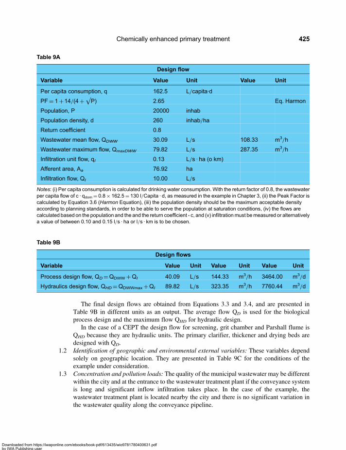
The final design flows are obtained from Equations 3.3 and 3.4, and are presented inTable 9B in different units as an output. The average flow QD is used for the biologicalprocess design and the maximum flow QHD for hydraulic design.

In the case of a CEPT the design flow for screening, grit chamber and Parshall flume isQHD because they are hydraulic units. The primary clarifier, thickener and drying beds aredesigned with QD.

1.2 Identification of geographic and environmental external variables: These variables dependsolely on geographic location. They are presented in Table 9C for the conditions of theexample under consideration.

1.3 Concentration and pollution loads: The quality of the municipal wastewater may be differentwithin the city and at the entrance to the wastewater treatment plant if the conveyance systemis long and significant inflow infiltration takes place. In the case of the example, thewastewater treatment plant is located nearby the city and there is no significant variation inthe wastewater quality along the conveyance pipeline.

Table 9B

Design flows


Process design flow, QD=QDWW+QI 40.09 L/s 144.33 m3/h 3464.00 m3/d

Hydraulics design flow, QHD=QDWWmax+QI 89.82 L/s 323.35 m3/h 7760.44 m3/d

Table 9A

Design flow


Per capita consumption, q 162.5 L/capita·d

PF= 1+14/(4+√P) 2.65 Eq. Harmon




Wastewater mean flow, QDWW 30.09 L/s 108.33 m3/h

Wastewater maximum flow, QmaxDWW 79.82 L/s 287.35 m3/h




Notes: (i) Per capita consumption is calculated for drinking water consumption. With the return factor of 0.8, the wastewaterper capita flow of c · qdom= 0.8× 162.5= 130 l/Capita · d, as measured in the example in Chapter 3, (ii) the Peak Factor iscalculated by Equation 3.6 (Harmon Equation), (iii) the population density should be the maximum acceptable densityaccording to planning standards, in order to be able to serve the population at saturation conditions, (iv) the flows arecalculated based on the population and the and the return coefficient - c, and (v) infiltrationmust bemeasured or alternativelya value of between 0.10 and 0.15 l/s · ha or l/s · km is to be chosen.



The table that calculates as output the load (kg/d) and the specific unit load perCapita (kg/Capita · d) of each pollutant from the concentration of each pollutant isTable 9D. In this table, the concentration of each pollutant is given as an input. Thecalculation is performed on each pollutant such as BOD5, COD, TSS, and so on. If thereis a significant infiltration into the conveyance pipeline to the treatment plant it isnecessary to calculate the additional infiltration flow of the sewerage afferent area (Aa) asfollows: QIemi= qI · L, where L is the length of the pipeline in km. The concentrations atthe entrance to the treatment plant are calculated as the specific per Capita load (qC)multiplied by the population (P) and divided by the total flow: QT= (QD+QIemi). Forexample: the Concentration of COD= qCOD · P/QT. Note that in Table 9D the load andthe per Capita load (specific unit load) is an output while the concentrations are an input,presented in the Excel sheet separately.

(2) ScreeningVariables selection by the designer: For coarse screening a coarse rotating screen is proposed withan opening of 6 mm.We apply the same methodology explained in the design example in Chapter 4for a 3% removal of TSS.Design: The diameter obtained for the course rotating screen is 600 mm. The final output data arepresented in Table 9E. The course rotating screen design is similar to that of the fine rotating screenso the reader is referred to Chapter 4, in which the design process is explained in detail. A coarsescreening is sufficient in this case because further treatment is be performed by the CEPT systemwhich follows the preliminary treatment. For better clarity we show in Table 9E the calculations ofthe preliminary treatment unit which is produced by the Excel program. The design support ispresented in the column entitled OBSERVATION.

(3) Grit chamberVariables selection by the designer: According to the ODM Section 9.2.2, Paragraph 3 related topreliminary treatment design, the proposed design variables are presented in Table 9F.

Table 9C


Minimum temperatureof water, Tw

25 °C 77.0 °F

Minimum temperatureof air, Ta

18 °C 64.4 °F

Altitude above sealevel, hasl

350 masl





Notes: (i) These variables are not very important for the CEPT process because it is not a biological processes and thereforeit is less sensitive to external environmental conditions; (ii) The minimum water temperature as well as the minimum airtemperature is the average of the coldestmonth; (iii) the velocity and direction the prevailing wind is important for locating thewastewater treatment plant in relation to the urban population centers; (iv) the fraction of hours of sunlight is the ratio of actualhours of sunlight to potential sunlight hours.



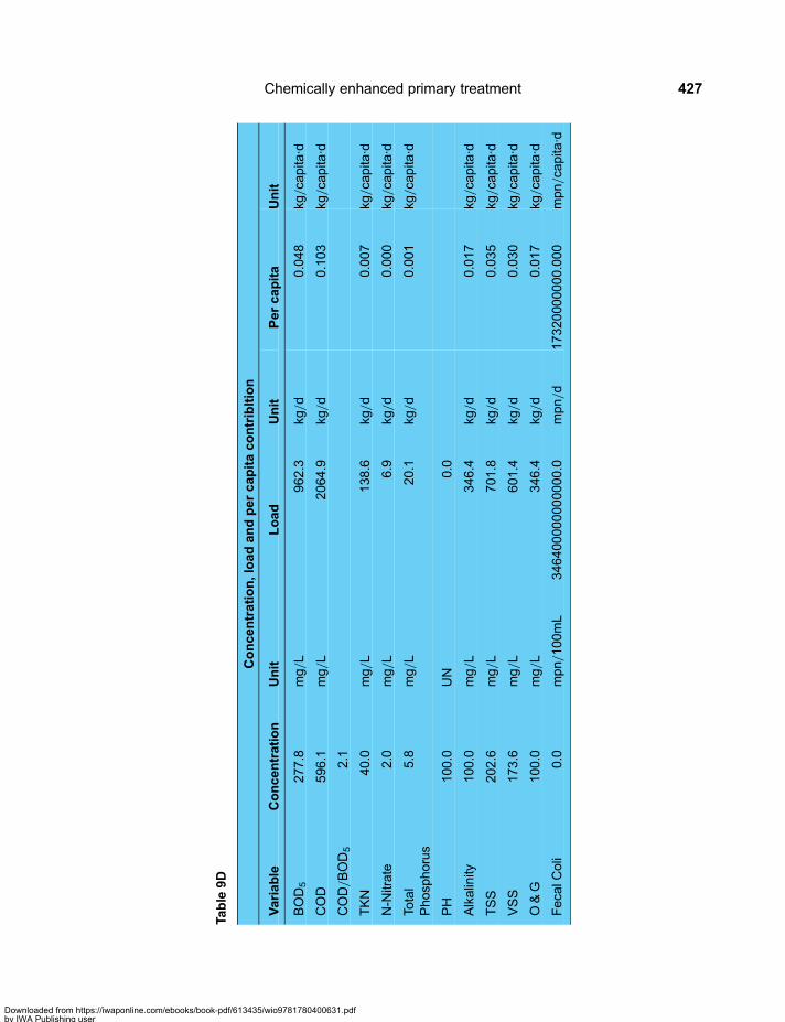
Table

9D

Concentration,loadandpercapitacontribltion

Variable

Concentration

Unit

Load

Unit

Percapita

Unit

BOD5

277.8

mg/

L962.3

kg/d

0.048

kg/ca

pita

·d

COD

596.1

mg/

L2064.9

kg/d

0.103

kg/ca

pita

·d

COD/BOD5

2.1

TKN

40.0

mg/

L138.6

kg/d

0.007

kg/ca

pita

·d

N-N

itrate

2.0

mg/

L6.9

kg/d

0.000

kg/ca

pita

·d

Total

Phosp

horus

5.8

mg/

L20.1

kg/d

0.001

kg/ca

pita

·d

PH

100.0

UN

0.0

Alkalinity

100.0

mg/

L346.4

kg/d

0.017

kg/ca

pita

·d

TSS

202.6

mg/

L701.8

kg/d

0.035

kg/ca

pita

·d

VSS

173.6

mg/

L601.4

kg/d

0.030

kg/ca

pita

·d

O&G

100.0

mg/

L346.4

kg/d

0.017

kg/ca

pita

·d

Feca

lColi

0.0

mpn/100mL

346400000000

000.0

mpn/d

17320000000.000

mpn/ca

pita

·d



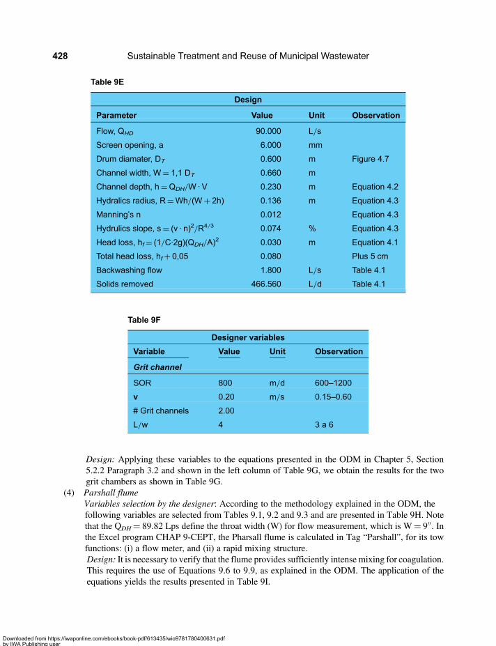
Design: Applying these variables to the equations presented in the ODM in Chapter 5, Section5.2.2 Paragraph 3.2 and shown in the left column of Table 9G, we obtain the results for the twogrit chambers as shown in Table 9G.

(4) Parshall flumeVariables selection by the designer: According to the methodology explained in the ODM, thefollowing variables are selected from Tables 9.1, 9.2 and 9.3 and are presented in Table 9H. Notethat the QDH= 89.82 Lps define the throat width (W) for flow measurement, which is W= 9′′. Inthe Excel program CHAP 9-CEPT, the Pharsall flume is calculated in Tag “Parshall”, for its towfunctions: (i) a flow meter, and (ii) a rapid mixing structure.Design: It is necessary to verify that the flume provides sufficiently intense mixing for coagulation.This requires the use of Equations 9.6 to 9.9, as explained in the ODM. The application of theequations yields the results presented in Table 9I.

Table 9E

Design






Channel depth, h=QDH/W · V 0.230 m Equation 4.2




Head loss, hf= (1/C·2g)(QDH/A)2 0.030 m Equation 4.1

Total head loss, hf+ 0,05 0.080 Plus 5 cm



Table 9F

Designer variables


Grit channel

SOR 800 m/d 600–1200

v 0.20 m/s 0.15–0.60


L/w 4 3 a 6



Note that the throat velocity (v1) of 3.2 m/s is within the required range for good rapid mixing(which is between 2 and 7 m/s) and this ensures a sufficiently high mixing intensity. To calculatethe throat velocity through Equation 9.9 it is necessary to use the Excel function “goal seek” toobtain the value “0” for the sum in Equation 9.9. Note that the function approached to −0.001at end of calculation (close enough to zero). If the calculation does not yield a value of v1within the required range which ensures good mixing, W needs to be changed and thecalculation repeated.

The coagulant is applied first before the flume and the flocculant polymer is then applied after ashort coagulation time (see Figure 9.1).

Table 9H Parshall flume deimensions.

Variable Value Unit Value Unit Source Hint

Caudal 89.82 Lps 7760.44 Lps Equation 2.4

W 9.00 inch 0.2286 m Table 9.2

K 1.84 Table 9.3

m 0.64 Table 9.3

D 57.50 cm 0.575 m Table 9.1

N 11.40 cm 0.114 m Table 9.1

Table 9G

Parameter Valor Unit Observation

Grit channel

Area, Ades=QDH/SOR 9.7 M2 Section 5.2.2 Numeral 3.1

Width, w== √(Ades/4) 1.6 m Section 5.2.2 Numeral 3.1

Length, L= 4w 6.2 m Section 5.2.2 Numeral 3.1

Depth, Hdes=QDH/v · w 0.3 m Section 5.2.2 Numeral 3.1

Total Depth, H=Hdes+ 0,50 0.8 m Section 5.2.2 Numeral 3.1

Parshall flume

Throat, W 9.0 inch See “Parshall” tag

Table 9I Parshall flume design as rapid mixer.

h0 0.40 m Equation 9.6

v 0.49 m/s Equation 9.7

E 0.52 m Equation 9.8

Vi 3.20 m/s −0.001 Equation 9.9 Goal seek: “0”



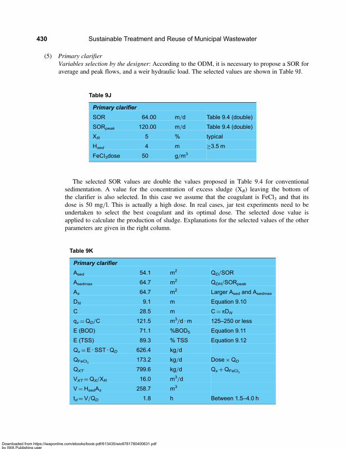
(5) Primary clarifierVariables selection by the designer: According to the ODM, it is necessary to propose a SOR foraverage and peak flows, and a weir hydraulic load. The selected values are shown in Table 9J.

The selected SOR values are double the values proposed in Table 9.4 for conventionalsedimentation. A value for the concentration of excess sludge (XR) leaving the bottom ofthe clarifier is also selected. In this case we assume that the coagulant is FeCl3 and that itsdose is 50 mg/l. This is actually a high dose. In real cases, jar test experiments need to beundertaken to select the best coagulant and its optimal dose. The selected dose value isapplied to calculate the production of sludge. Explanations for the selected values of the otherparameters are given in the right column.

Table 9J

Primary clarifier

SOR 64.00 m/d Table 9.4 (double)

SORpeak 120.00 m/d Table 9.4 (double)

XR 5 % typical

Hsed 4 m ≥3.5 m

FeCI3dose 50 g/m3

Table 9K

Primary clarifier

Ased 54.1 m2 QD/SOR

Asedmax 64.7 m2 QDH/SORpeak

As 64.7 m2 Larger Ased and Asedmax

DN 9.1 m Equation 9.10

C 28.5 m C= πDN

qv=QD/C 121.5 m3/d · m 125–250 or less

E (BOD) 71.1 %BOD5 Equation 9.11

E (TSS) 89.3 % TSS Equation 9.12

Qx=E · SST · QD 626.4 kg/d

QFeCl3 173.2 kg/d Dose×QD

QXT 799.6 kg/d Qx+QFeCl3

VXT=QX/XR 16.0 m3/d

V=HsedAs 258.7 m3

td=V/QD 1.8 h Between 1.5–4.0 h



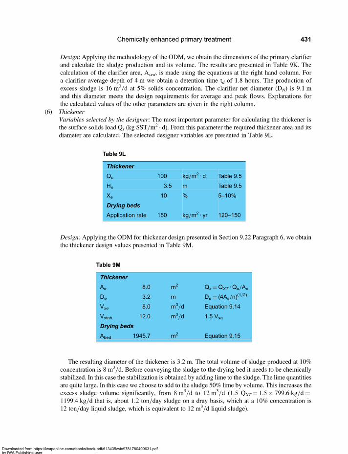
Design: Applying the methodology of the ODM, we obtain the dimensions of the primary clarifierand calculate the sludge production and its volume. The results are presented in Table 9K. Thecalculation of the clarifier area, Ased, is made using the equations at the right hand column. Fora clarifier average depth of 4 m we obtain a detention time td of 1.8 hours. The production ofexcess sludge is 16 m3/d at 5% solids concentration. The clarifier net diameter (DN) is 9.1 mand this diameter meets the design requirements for average and peak flows. Explanations forthe calculated values of the other parameters are given in the right column.

(6) ThickenerVariables selected by the designer: The most important parameter for calculating the thickener isthe surface solids load Qs (kg SST/m

2 · d). From this parameter the required thickener area and itsdiameter are calculated. The selected designer variables are presented in Table 9L.

Design: Applying the ODM for thickener design presented in Section 9.22 Paragraph 6, we obtainthe thickener design values presented in Table 9M.

The resulting diameter of the thickener is 3.2 m. The total volume of sludge produced at 10%concentration is 8 m3/d. Before conveying the sludge to the drying bed it needs to be chemicallystabilized. In this case the stabilization is obtained by adding lime to the sludge. The lime quantitiesare quite large. In this case we choose to add to the sludge 50% lime by volume. This increases theexcess sludge volume significantly, from 8 m3/d to 12 m3/d (1.5 QXT= 1.5× 799.6 kg/d=1199.4 kg/d that is, about 1.2 ton/day sludge on a dray basis, which at a 10% concentration is12 ton/day liquid sludge, which is equivalent to 12 m3/d liquid sludge).

Table 9L

Thickener

Qs 100 kg/m2 · d Table 9.5

He 3.5 m Table 9.5

Xe 10 % 5–10%

Drying beds


Table 9M

Thickener

Ae 8.0 m2 Qs=QXT · Qo/Ae

De 3.2 m De= (4As/n)(1/2)

Vxe 8.0 m3/d Equation 9.14

Vstab 12.0 m3/d 1.5 Vxe

Drying beds

Abed 1945.7 m2 Equation 9.15



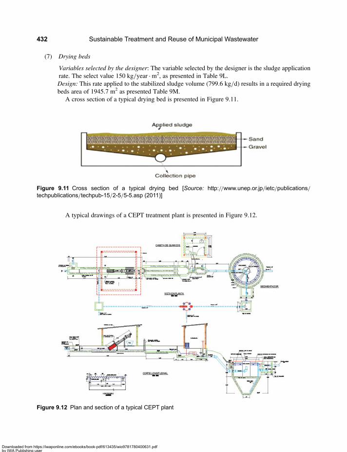
(7) Drying beds

Variables selected by the designer: The variable selected by the designer is the sludge applicationrate. The select value 150 kg/year · m2, as presented in Table 9L.Design: This rate applied to the stabilized sludge volume (799.6 kg/d) results in a required dryingbeds area of 1945.7 m2 as presented Table 9M.

A cross section of a typical drying bed is presented in Figure 9.11.

A typical drawings of a CEPT treatment plant is presented in Figure 9.12.

Figure 9.11 Cross section of a typical drying bed [Source: http://www.unep.or.jp/ietc/publications/techpublications/techpub-15/2-5/5-5.asp (2011)]

Figure 9.12 Plan and section of a typical CEPT plant
















Chapter 10

Complementary processes to combine withappropriate technology processes

10.1 INTRODUCTIONIn cases that require higher quality of effluent than those possible with unit processes of appropriatetechnology it is possible to subject the effluent of a unit process to one or more polishing stages. In thisway, combination of processes can yield higher quality effluents. The polishing units can be otherappropriate technology unit processes such as those which have already been discussed in the secondpart of the book, and also additional processes which have not yet been discussed and which arenominated as complementary processes. However, the use of a complex process as a polishing step ofeffluent of a unit appropriate technology process should be avoided, since it transforms the entiretreatment plant into a complex plant (Libhaber, 2007). There are certain treatment technologies whichperhaps are not appropriate technologies when they are used as the main treatment unit, but they meetthe requirements of being simple to operate and easy to maintain, and when they are used as polishingunits of a preceding main treatment step they can be considered appropriate technology processes.

Complementary treatment unit which can be mentioned include Sand Filtration (SF), Dissolved AirFlotation (DAF), Disinfection with ultraviolet rays (UV disinfection), Overland Flow, Infiltration‐Percolation, Septic Tanks, Submarine and Large River Outfalls, and under certain circumstances,Aerated Lagoons. Among those Sand Filtration, Dissolved Air Flotation, UV disinfection, andInfiltration‐Percolation can only be used as polishing units since they require a pretreatment stage andare not able to perform as a main treatment unit. Septic tanks usually perform as a pretreatment unit andsometimes as the main treatment unit, but are not used as a polishing unit. Aerated lagoons can performboth as a main treatment unit and as a polishing unit. As discussed in Chapter 1, they can be consideredappropriate technology units when they are employed as polishing units.

It was not possible to present in this book the design procedures of all the mentioned complementaryprocesses. We chose to present the following: Sand Filtration, Dissolved Air Flotation and UVdisinfection. This does not mean that the others are of a lower level of importance. All of thecomplementary processes are worthy processes and are discussed in Chapter 1.

The Membrane Filtration Technology [Micro Filtration (MF), Ultra Filtration (UF ), Nanofiltration (NF)and Reverse Osmosis (RO)] is not an appropriate treatment technology. However, in certain cases, a veryhigh effluent quality is required even in developing countries. In such cases the use of Membrane Filtrationis advantageous because it is not too complex to operate and it yields effluent qualities which are higher than


those that can be achieved by any other known technology. Membrane Filtration can be combined withappropriate technology processes which can serve as its pretreatment units. For these reasons it wasdecided to present in this chapter also the Membrane Filtration Technology.

These complementary processes are introduced only briefly in this chapter, but there is an extensivebibliography which can be used by readers interested to deepen their knowledge, for example Metcalf &Eddy (2003).

10.2 SAND FILTRATION10.2.1 IntroductionSand filtration is one of the oldest and most wildly used water treatments processes. It is used primarily forpotable water treatment but is recently enployed as a polishing process for wastewater treatment. Filtration isthe removal of suspended and colloidal particles present in an aqueous suspension by passing the suspensionthrough a porous medium (Arboleda, 1992; Metcalf & Eddy, 2003).

Filtration is the result of two distinct but complementary mechanisms: transport and adhesion. Initially,particles which are to be removed are carried from the aqueous suspension to the surface of filter mediumgrains. The particles remain attached to the grains, provided that they resist the action of shear forces due tothe hydrodynamic flow conditions. The particle transport is a hydraulic phenomenon, governed by theparameters that define the mass transfer. The adhesion between particles and grains is a phenomenon ofsurface action, which is influenced by physical and chemical parameters.

Themechanisms that can carry out the transport are: (i) straining, (ii) sedimentation, (iii) interception, (iv)diffusion, (v) inertial impact, (vi) hydrodynamic action, and (vii) combined transport mechanisms. Theadhesion mechanisms are: (i) Van der Waals forces, (ii) electrochemical forces, and (iii) chemicalbridges (Maldonado-Yactayo, 2007).

Filtration through granular media can be simple filtration (with sand as the sole filtration medium) ormixed filtration (with two or more filter media usually sand and anthracite). Design elements of a sandfilter are:

• Hydraulic loading rate or filtration rate (qF), L/min · m2, (the filtration rate can be slow, rapid andhigh)

• Type of flow (continuous, driven, intermittent)• Flow direction (up flow, down flow).

Mixed filters consist of two or more filter media. A multi-media filter works with finer and denser mediain the top and middle part and thicker and less dense media at the lower part. This is achieved when gravel isused at the bottom of the bed as support, sand in the middle and anthracite coal on top as filter media. Themost common flow of multi-media filters is gravity down flow. However, other filter types with up flow,horizontal flow and double flow directions are also in use. The granular media filters require a periodicbackwash cleaning to maintain their efficiency. In rapid filters this is done by reversing the direction offlow, injecting water and air through a false bottom to expand the filter medium, with upper collection ofwater washout.

When hydraulic losses caused by trapped particles reduce the wastewater rate of filtration through thefilter bed, it reaches the end of the “filter cycle” and it requires backwashing to remove the suspendedsolids trapped in the filter bed. Also, the bed may be shaken mechanically or with air to help removesolids. The wash water is recycled back to the inflow wastewater stream. Filtration through granularmedia is most often used for tertiary treatment of sewage and for additional suspended solids removalfrom effluents of chemical treatment processes such as CEPT. Figure 10.1 shows a typical diagram of a



gravity sand filter, used in large towns. The use of pressure filters it is becoming more widespread in smallcommunities (Maldonado-Yactayo, 2007).

The filteration parameters for the three most common types of filters (slow, rapid and pressure filters) arepresented in Table 10.1. Rapid gravity filters can be of constant or declining rate. Declining rate filter usesmall amounts of equipment such as valves and automatic controls, which are replaced by hydraulic-type

Table 10.1 Classification of filters.

Slow sand filter Fast sand filter Pressure filter

Filtration rate, L/min · m2 0.006–0.024 80–200 80–160

Filtrating media Sand Sand Sand + Anthracite Sand Sand + Anthracite

¿Gravity or pressure? Gravity Gravity Pressure

Washing Top layer removal (5 cm) Backwash Backwash

Advantages Reliable, little operation Reliable, compact Cheap for small plants

Disadvantages Requires large area,Manual cleaning

Requires chemicaltreatment

Mechanized

Application Small populations Surface water of allkinds

Industry and smallcommunities

Source: Prepared from http://water.me.vccs.edu/concepts/filters.html

Figure 10.1 A Diagram of a rapid sand filter [Source: http://water.me.vccs.edu/concepts/filters.html (2011)]

Complementary processes to combine with appropriate technology processes 435


http://water.me.vccs.edu/concepts/filters.html






http://konchewater.com/product/device/disinfection_system/ultraviolet_dis/2011/0714/77.html






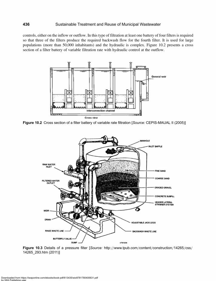
controls, either on the inflow or outflow. In this type of filtration at least one battery of four filters is requiredso that three of the filters produce the required backwash flow for the fourth filter. It is used for largepopulations (more than 50,000 inhabitants) and the hydraulic is complex. Figure 10.2 presents a crosssection of a filter battery of variable filtration rate with hydraulic control at the outflow.

Figure 10.2 Cross section of a filter battery of variable rate filtration [Source: CEPIS-MAUAL II (2005)]

Figure 10.3 Details of a pressure filter [Source: http://www.tpub.com/content/construction/14265/css/14265_293.htm (2011)]













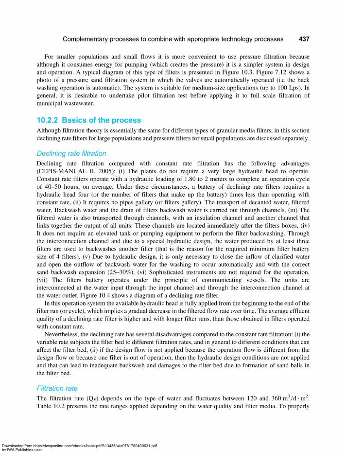
For smaller populations and small flows it is more convenient to use pressure filtration becausealthough it consumes energy for pumping (which creates the pressure) it is a simpler system in designand operation. A typical diagram of this type of filters is presented in Figure 10.3. Figure 7.12 shows aphoto of a pressure sand filtration system in which the valves are automatically operated (i.e the backwashing operation is automatic). The system is suitable for medium-size applications (up to 100 Lps). Ingeneral, it is desirable to undertake pilot filtration test before applying it to full scale filtration ofmunicipal wastewater.

10.2.2 Basics of the processAlthough filtration theory is essentially the same for different types of granular media filters, in this sectiondeclining rate filters for large populations and pressure filters for small populations are discussed separately.

Declining rate filtrationDeclining rate filtration compared with constant rate filtration has the following advantages(CEPIS-MANUAL II, 2005): (i) The plants do not require a very large hydraulic head to operate.Constant rate filters operate with a hydraulic loading of 1.80 to 2 meters to complete an operation cycleof 40–50 hours, on average. Under these circumstances, a battery of declining rate filters requires ahydraulic head four (or the number of filters that make up the battery) times less than operating withconstant rate, (ii) It requires no pipes gallery (or filters gallery). The transport of decanted water, filteredwater, Backwash water and the drain of filters backwash water is carried out through channels, (iii) Thefiltered water is also transported through channels, with an insulation channel and another channel thatlinks together the output of all units. These channels are located immediately after the filters boxes, (iv)It does not require an elevated tank or pumping equipment to perform the filter backwashing. Throughthe interconnection channel and due to a special hydraulic design, the water produced by at least threefilters are used to backwashes another filter (that is the reason for the required minimum filter batterysize of 4 filters), (v) Due to hydraulic design, it is only necessary to close the inflow of clarified waterand open the outflow of backwash water for the washing to occur automatically and with the correctsand backwash expansion (25–30%), (vi) Sophisticated instruments are not required for the operation,(vii) The filters battery operates under the principle of communicating vessels. The units areinterconnected at the water input through the input channel and through the interconnection channel atthe water outlet. Figure 10.4 shows a diagram of a declining rate filter.

In this operation system the available hydraulic head is fully applied from the beginning to the end of thefilter run (or cycle), which implies a gradual decrease in the filtered flow rate over time. The average effluentquality of a declining rate filter is higher and with longer filter runs, than those obtained in filters operatedwith constant rate.

Nevertheless, the declining rate has several disadvantages compared to the constant rate filtration: (i) thevariable rate subjects the filter bed to different filtration rates, and in general to different conditions that canaffect the filter bed, (ii) if the design flow is not applied because the operation flow is different from thedesign flow or because one filter is out of operation, then the hydraulic design conditions are not appliedand that can lead to inadequate backwash and damages to the filter bed due to formation of sand balls inthe filter bed.

Filtration rateThe filtration rate (QF) depends on the type of water and fluctuates between 120 and 360 m3/d · m2.Table 10.2 presents the rate ranges applied depending on the water quality and filter media. To properly



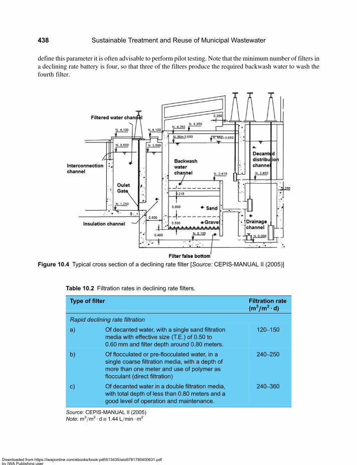
define this parameter it is often advisable to perform pilot testing. Note that the minimum number of filters ina declining rate battery is four, so that three of the filters produce the required backwash water to wash thefourth filter.

Figure 10.4 Typical cross section of a declining rate filter [Source: CEPIS-MANUAL II (2005)]

Table 10.2 Filtration rates in declining rate filters.

Type of filter Filtration rate(m3/////m2 · d)

Rapid declining rate filtration

a) Of decanted water, with a single sand filtrationmedia with effective size (T.E.) of 0.50 to0.60mm and filter depth around 0.80 meters.

120–150

b) Of flocculated or pre-flocculated water, in asingle coarse filtration media, with a depth ofmore than one meter and use of polymer asflocculant (direct filtration)

240–250

c) Of decanted water in a double filtration media,with total depth of less than 0.80 meters and agood level of operation and maintenance.

240–360

Source: CEPIS-MANUAL II (2005)Note: m3/m2 · d≡ 1.44 L/min · m2



Filtration mediaThe selection of the filter bed material is of great importance for the operation and durability of the filter. Thefilter material determines the characteristics of the bed. Usually the filter bed materials are: (i) Sand bed, and(ii) Combined beds of sand and anthracite. To select the filter material it is necessary to apply the followingparameters (Maldonado-Yactayo, 2007):

Effective size (D10) is defined as the size of the sieve in mm through which ten percent of the sample ofsand by weight will pass.

Uniformity coefficient (UC): is defined as the ratio of the sieve size in mm through which 60 percent of thesample of sand will pass, to the effective size of the sand.

Form: the shape of the grains is usually evaluated based on sphericity coefficient (Ce). The sphericitycoefficient of a particle is defined as the result of dividing the surface area of the sphere of equal volumeto the grain by the surface area of the particle considered.

Minimum size: size below which no grain is to be found in the filter medium.Maximum size: size above which no grain is to be found in the filter medium.Table 10.3 presents the desirable characteristics for the two types of beds used in declining rate filtration.

Filtration hydraulicsThe hydraulic head available in the system is calculated so that the relationship between the highest filtrationrate (qFmax) occurring at the start of the filtration cycle (filter recently washed) and the average filtration rate(qF), does not exceed 1.5. A careful calculation of the head loss in the filter needs to be undertaken to definethis head (H) because: (i) if it is insufficient, the filter runs between washings will be very short, and (ii) if it is

Table 10.3 Recommended beds for (a) sand bed and (b) combined sand andanthracite beds.

Characteristics Symbol Criteria

(a)

Depth (cm) L1 60–80

Effective size (mm) D30 0.50–0.80

Uniformity coefficient CU ≤1.5Minimum size (mm) 0.42

Maximum size (mm) D90 2.0

Characteristics Symbol Sand Anthracite

(b)

Depth (cm) L1 15–30 45–60

Effective size (mm) D30 0.50–0.60 0.80–1.10

Uniformity coefficient CU ≤1.5 ≤1.5Minimum size (mm) 0.42 0.59

Maximum size (mm) D90 1.41 2.0

Source: CEPIS-MANUAL II (2005)



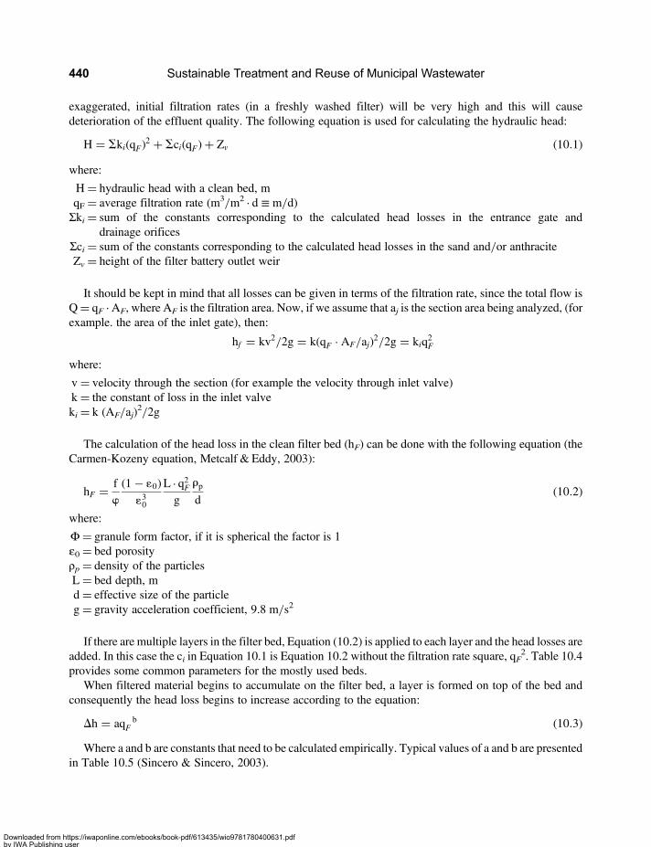
exaggerated, initial filtration rates (in a freshly washed filter) will be very high and this will causedeterioration of the effluent quality. The following equation is used for calculating the hydraulic head:

H = Ski(qF)2 + Sci(qF)+ Zv (10.1)

where:

H = hydraulic head with a clean bed, mqF = average filtration rate (m3/m2 · d ≡ m/d)Σki = sum of the constants corresponding to the calculated head losses in the entrance gate and

drainage orificesΣci = sum of the constants corresponding to the calculated head losses in the sand and/or anthraciteZv = height of the filter battery outlet weir

It should be kept in mind that all losses can be given in terms of the filtration rate, since the total flow isQ= qF · AF, where AF is the filtration area. Now, if we assume that aj is the section area being analyzed, (forexample. the area of the inlet gate), then:

hf = kv2/2g = k(qF · AF/aj)2/2g = kiq

2F

where:

v= velocity through the section (for example the velocity through inlet valve)k= the constant of loss in the inlet valveki = k (AF/aj)

2/2g

The calculation of the head loss in the clean filter bed (hF) can be done with the following equation (theCarmen-Kozeny equation, Metcalf & Eddy, 2003):

hF = fw

(1− 10)

130

L · q2Fg

rp

d(10.2)

where:

Φ= granule form factor, if it is spherical the factor is 1ε0 = bed porosityρp = density of the particlesL= bed depth, md= effective size of the particleg= gravity acceleration coefficient, 9.8 m/s2

If there are multiple layers in the filter bed, Equation (10.2) is applied to each layer and the head losses areadded. In this case the ci in Equation 10.1 is Equation 10.2 without the filtration rate square, qF

2. Table 10.4provides some common parameters for the mostly used beds.

When filtered material begins to accumulate on the filter bed, a layer is formed on top of the bed andconsequently the head loss begins to increase according to the equation:

Dh = aq bF (10.3)

Where a and b are constants that need to be calculated empirically. Typical values of a and b are presentedin Table 10.5 (Sincero & Sincero, 2003).



Thus, the total hydraulic head (HT) is calculated using the following equation:

HT = H+Dh (10.4)

Backwashing hydraulicsFor a filter battery to provide sufficient water for backwashing a filter, it is necessary that two conditions aremet: (i) The flow should be sufficient to produce a washing velocity necessary to expand the filter bed tobetween 25 and 30%, and (ii) The level of the outflow weir should provide the required hydraulic headto overcome the head losses that occur during the operation.

The length (Le) of the bed expanded by the backwash is calculated by the following equation using theexpanded porosity (εe):

L(1− 10)(1− 1e)

(10.5)

The expanded porosity is obtained by the empirical formula:

10 = (qRL/vs)0.22 (10.6)

where:

qRL = backwash rate, equal at least to 3qF.vs = settling velocity of sand particle (Stokes’ law)

Table 10.5 Typical values of constants in the formula of head loss in the filter bed.

Δh Bed material Diameter

0.051 qF2.22 uniform sand 0.5 mm



0.00114 qF2.10 uniform anthracite 1.0 mm



Table 10.4 Typical properties of commonly used filtering granular beds.

Characteristic Silicasand

Anthracitecoal

Granularactivated coal

Granateidaho

Material density (ρs) (g/cm3) 2.65 1.45–1.73 1.3–1.5 4.0–4.2

Bed porosity (ε0) 0.42–0.47 0.56–0.60 0.50 0.45–0.65

Sphericity (Ce) 0.7–0.8 0.46–0.60 0.75 0.60

Source: CEPIS-MANUAL II (2005)



Stokes’s law in laminar flow is as follows:

vs =d2pg(g− 1)

18y(10.7)

where:

vs = sedimentation velocitydp = particle diameterγ= specific gravity of the particleυ= kinematics viscosity of water

Finally, the head loss in the backwash, HRL can be calculated as follows (Sincero & Sincero, 2003):

hRL = Le(1− 1e)(gp − gw)/gw (10.8)

γp, γw are the specific weights of particle and water respectively.

Pressure filtersRapid pressure filters are generally used for small and medium flows. They are easy to install and operateand usually present little maintenance problems. They are the preferred solution for industrial applicationsand for small and medium towns. Pressure filters are contained in steel or fiberglass tanks. There are twobasic structure types: of pressure filters: vertical and horizontal.

They have the following characteristics:

• The water flows into and out of the filter under pressure. The filter bed rests on a bed supportcomposed of several layers of decreasing particle size (coarse material at the bottom and becomingfiner towards the top).

• Normally the filter bed is one single material, sand or anthracite. The filtered water collector is a gridof perforated pipes, embedded within the gravel support bed, or alternatively, a false bottom ofperforated metal with plastic or metal nozzles. Details of the internal structure of a pressure filterare shown in Figure 10.5.

The same principles of rapid sand filtration apply to pressure filtration but the operation of pressure filtersis simpler. Some types of internal structure of pressure filters are manufacturers’ property, but a simplesystem as shown in Figure 10.5 is available in the market supplied by numerous workshops atcompetitive prices. The construction of this filter is very similar to the gravity filter. The sand rests onthe gravel that serves as a bed support. Raw water enters the unit through the inlet of raw water, using apump or other means to increase its pressure. It passes through the filter bed and then reaches the outletpipe. The unit operates under pressure, so the filter medium is encapsulated. When the filter bed isclogged by particles entering with the water, it is necessary to clean it by backwashing. The operation ofthe filter needs to be guaranteed by the manufacturer and can be manual or automatic.

10.2.3 Basic designThe following procedure is used to calculate the dimensions of a filter, applied to the case of a population of20,000.



Variables selected by the designerThe main variables selected by the designer are: (i) the flow, which is calculated using Equation 3.4, (ii) Thefiltration rate (qF) which is determined from Tables 10.1 and 10.2, (iii) the backwash flow rate (QBW), whichis selected as at least 3qF, (iv) the number of filters (nF) which should be at least two. The design variablesapplied to a population of 20,000 are presented in Table 10A. (Please note that Tables identified byalphabetic order contain computer calculated results).

Basic designHaving defined the design variables the sizing of the filter units is as follows:

• Calculate the flow per filter,

QF = QD/nF (10.9)

Table 10A

Designer variable


Filtro de arena

QD 89.8 L/s Equation 3.4

Pressure filter? Yes Yes for P, 100,000 inhab

QF 120.00 L/min · m2 2.94 gpm/ft2 Tables 10.1 and 10.2

qBW (select) 480.00 L/min · m2 11.76 gpm/ft2 Minimum 3qF

nF 3.00 .2

Figure 10.5 Internal structure of a pressure filter [Source: Nalco (1988)]



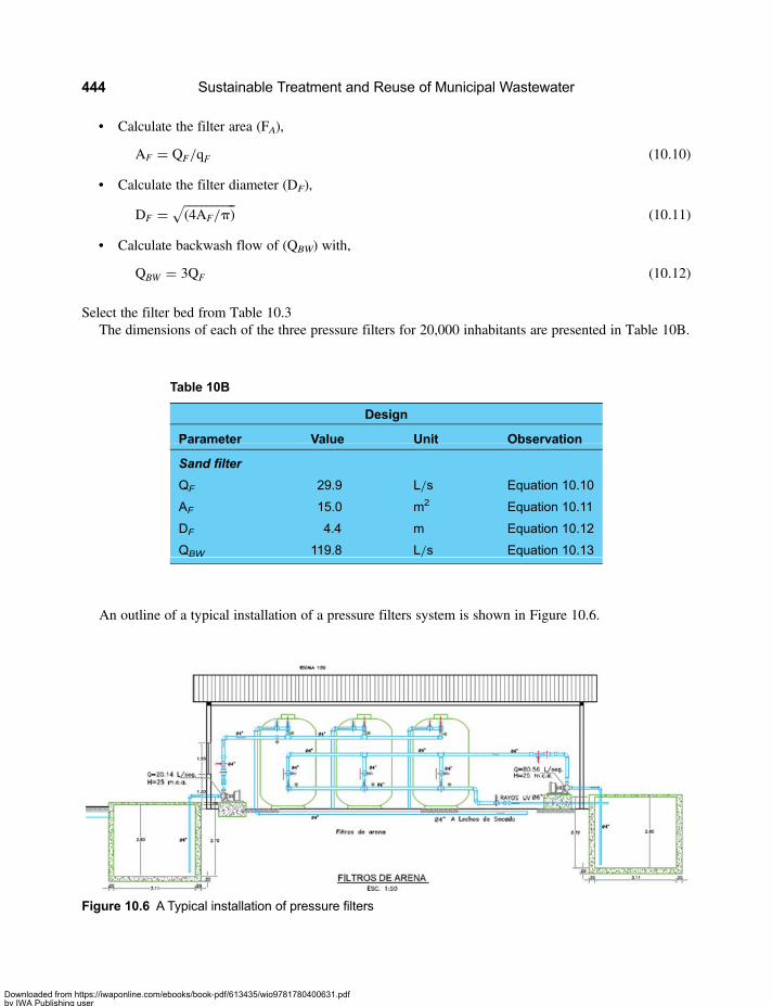
• Calculate the filter area (FA),

AF = QF/qF (10.10)

• Calculate the filter diameter (DF),

DF =��(4AF/p)

√(10.11)

• Calculate backwash flow of (QBW) with,

QBW = 3QF (10.12)

Select the filter bed from Table 10.3The dimensions of each of the three pressure filters for 20,000 inhabitants are presented in Table 10B.

An outline of a typical installation of a pressure filters system is shown in Figure 10.6.

Table 10B

Design


Sand filter

QF 29.9 L/s Equation 10.10

AF 15.0 m2 Equation 10.11

DF 4.4 m Equation 10.12

QBW 119.8 L/s Equation 10.13

Figure 10.6 A Typical installation of pressure filters



10.3 DISSOLVED AIR FLOTATION (DAF)1

10.3.1 IntroductionDAF (Dissolved Air Flotation) is used to remove particles and oil and grease (O&G) by flotation. Flotationis a primary clarification process, which is also used as post treatment in wastewater treatment plants. Toseparate suspended solids from wastewater the wastewater needs to first be coagulated with aluminiumor iron salts, and flocculated with a polyelectrolyte. When air bubbles are applied to acoagulated-flocculated solution they clog to the flocs and create a net flotation action which carries thefloc-particles upwards. The same procedure applies to oil and grease, but in this case less time isrequired for flotation since oils are lighter than water and therefore float easily. The following activitiesare necessary to produce the flotation process: (i) produce bubbles of suitable size for the particles whichneed to be removed, (ii) produce an effective adhesion between the air bubbles and suspended particles,which is achieved by coagulation-flocculation, and (iii) ensure an adequate separation of floating material.

There are basically two types ofDAFprocesses: (i) dispersed air flotationwhich usually employs air nozzlesthat produce dispersion, aeration and agitation of the suspension, producing air bubbles that are about 1 mmin diameter, and (ii) dissolved air flotation which has been one of the most studied processes inwastewater treatment and this is the process discussed below. There are three basic types of dissolved airflotation systems: with partial influent pressurization, with total influent pressurization and with recirculation.

TheDAFprocess is used in several applications: (i)DAF is applied as pretreatmentwhen the rawwastewatercontains high concentrations of oil and greases that needs to be removed prior to the biological treatment of thewastewater since they can interfere with the performance of the biological reactor, (ii) DAF is also used aspretreatment when the raw wastewater contains large amounts of SS and there is not enough space toremove them by conventional primary treatment, and (ii) DAF is used as post treatment when it is necessaryto polish an effluent of a main treatment process by removing suspended solids from its effluent.

A diagram of a DAF process with partial air pressurization of the effluent is shown in Figure 10.7.

Figure 10.7 A Diagram of the dissolved air floating system with partial pressurization of the effluent (Source:http://www.esi.info/detail.cfm//stetfield-separators-ltd/stetfloat-dissolved-air-flotation-DAF-unit/_/R-26789_TR109EP#)

1Based on Orozco (2005), Chapter 7






















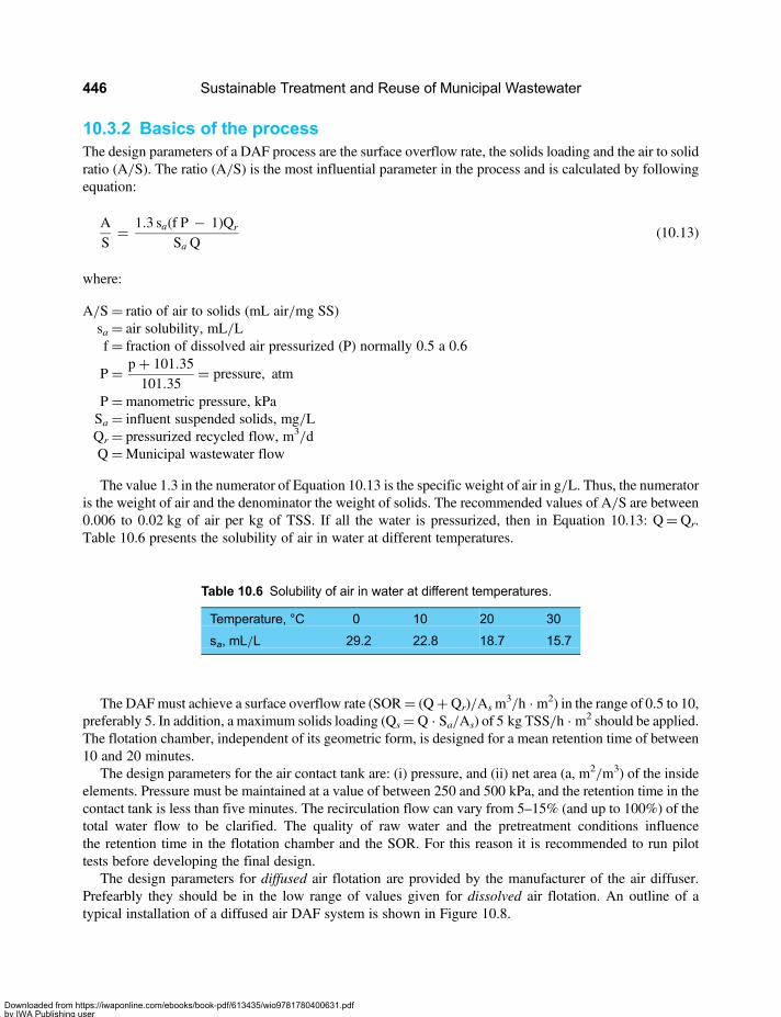
10.3.2 Basics of the processThe design parameters of a DAF process are the surface overflow rate, the solids loading and the air to solidratio (A/S). The ratio (A/S) is the most influential parameter in the process and is calculated by followingequation:

AS

= 1.3 sa(f P − 1)Qr

Sa Q(10.13)

where:

A/S= ratio of air to solids (mL air/mg SS)sa = air solubility, mL/Lf= fraction of dissolved air pressurized (P) normally 0.5 a 0.6

P= p+ 101.35101.35

= pressure, atm

P=manometric pressure, kPaSa = influent suspended solids, mg/LQr = pressurized recycled flow, m3/dQ =Municipal wastewater flow

The value 1.3 in the numerator of Equation 10.13 is the specific weight of air in g/L. Thus, the numeratoris the weight of air and the denominator the weight of solids. The recommended values of A/S are between0.006 to 0.02 kg of air per kg of TSS. If all the water is pressurized, then in Equation 10.13: Q=Qr.Table 10.6 presents the solubility of air in water at different temperatures.

The DAFmust achieve a surface overflow rate (SOR= (Q+Qr)/Asm3/h · m2) in the range of 0.5 to 10,

preferably 5. In addition, a maximum solids loading (Qs=Q · Sa/As) of 5 kg TSS/h · m2 should be applied.The flotation chamber, independent of its geometric form, is designed for a mean retention time of between10 and 20 minutes.

The design parameters for the air contact tank are: (i) pressure, and (ii) net area (a, m2/m3) of the insideelements. Pressure must be maintained at a value of between 250 and 500 kPa, and the retention time in thecontact tank is less than five minutes. The recirculation flow can vary from 5–15% (and up to 100%) of thetotal water flow to be clarified. The quality of raw water and the pretreatment conditions influencethe retention time in the flotation chamber and the SOR. For this reason it is recommended to run pilottests before developing the final design.

The design parameters for diffused air flotation are provided by the manufacturer of the air diffuser.Prefearbly they should be in the low range of values given for dissolved air flotation. An outline of atypical installation of a diffused air DAF system is shown in Figure 10.8.

Table 10.6 Solubility of air in water at different temperatures.

Temperature, °C 0 10 20 30

sa, mL/L 29.2 22.8 18.7 15.7



10.3.3 Basic designThe following procedure is used to calculate the dimensions of a DAF system, applied to the case of apopulation of 20,000.

The main variables selected by the designer are: (i) the flow, which is calculated using Equation 3.4, (ii)The filtration rate (qF) which is determined from Tables 10.1 and 10.2, (iii) the backwash flow rate (QBW),which is selected as at least 3qF, (iv) the number of filters (nF) which should be at least two. The designvariables applied to a population of 20,000 are presented in Table 10A.

Variables selected by the designerThe main variables selected by the designer are: (i) the flow rate (QHD), which is calculated using Equation3.4, (ii) Sa which is determined from the SST concentration in the outflow of preceding process, (iii) TheSOR which should be between 0.5 and 10 m3/m2 · h, (iv) the solids load which should be between 0.5and 10.0 kg/m2 · h, (v) the ratio (A/S) which should be in the range 0.006 to 0.2, (vi) the recirculationratio (R) which should be between 0.05 and 1.0; (vii) the fraction of dissolved air pressure (P),preferably from pilot test with a TSS removal of 95% or more; and (viii) the air solubility (sa) which iscalculated by the following equation constructed from data in Table 10.6:

sa = 28.638e−0,021T (10.14)

The design variables applied to a population of 20,000 are presented in Table 10C.

Basic designHaving defined the design variables, the sizing of the DAF unit is done as follows:

• From the design variables, the pressure is calculated using Equation 10.13.

Figure 10.8 Plan and cross section of a typical diffused air flotation installation



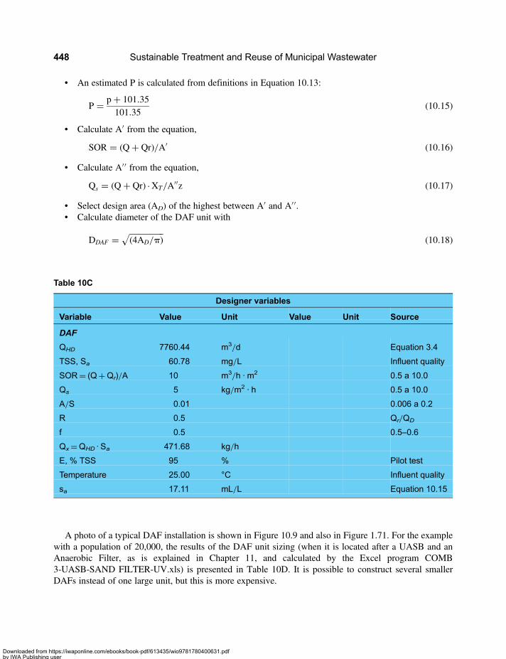
• An estimated P is calculated from definitions in Equation 10.13:

P = p+ 101.35101.35

(10.15)

• Calculate A′ from the equation,

SOR = (Q+ Qr)/A′ (10.16)

• Calculate A′′ from the equation,

Qs = (Q+ Qr) ·XT/A′′z (10.17)

• Select design area (AD) of the highest between A′ and A′′.• Calculate diameter of the DAF unit with

DDAF =��(4AD/p)

√(10.18)

A photo of a typical DAF installation is shown in Figure 10.9 and also in Figure 1.71. For the examplewith a population of 20,000, the results of the DAF unit sizing (when it is located after a UASB and anAnaerobic Filter, as is explained in Chapter 11, and calculated by the Excel program COMB3-UASB-SAND FILTER-UV.xls) is presented in Table 10D. It is possible to construct several smallerDAFs instead of one large unit, but this is more expensive.

Table 10C

Designer variables

Variable Value Unit Value Unit Source

DAF

QHD 7760.44 m3/d Equation 3.4

TSS, Sa 60.78 mg/L Influent quality

SOR= (Q+Qr)/A 10 m3/h · m2 0.5 a 10.0

Qs 5 kg/m2 · h 0.5 a 10.0

A/S 0.01 0.006 a 0.2

R 0.5 Qr/QD

f 0.5 0.5–0.6

Qx=QHD · Sa 471.68 kg/h

E, % TSS 95 % Pilot test

Temperature 25.00 °C Influent quality

sa 17.11 mL/L Equation 10.15



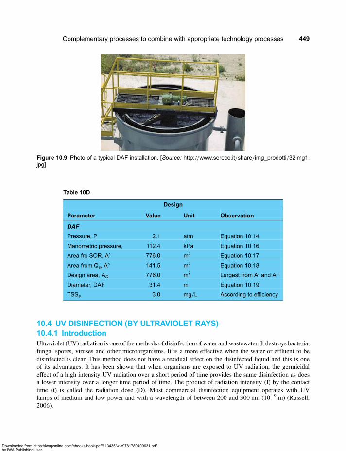
10.4 UV DISINFECTION (BY ULTRAVIOLET RAYS)10.4.1 IntroductionUltraviolet (UV) radiation is one of the methods of disinfection of water and wastewater. It destroys bacteria,fungal spores, viruses and other microorganisms. It is a more effective when the water or effluent to bedisinfected is clear. This method does not have a residual effect on the disinfected liquid and this is oneof its advantages. It has been shown that when organisms are exposed to UV radiation, the germicidaleffect of a high intensity UV radiation over a short period of time provides the same disinfection as doesa lower intensity over a longer time period of time. The product of radiation intensity (I) by the contacttime (t) is called the radiation dose (D). Most commercial disinfection equipment operates with UVlamps of medium and low power and with a wavelength of between 200 and 300 nm (10−9 m) (Russell,2006).

Figure 10.9 Photo of a typical DAF installation. [Source: http://www.sereco.it/share/img_prodotti/32img1.jpg]

Table 10D

Design


DAF

Pressure, P 2.1 atm Equation 10.14

Manometric pressure, 112.4 kPa Equation 10.16

Area fro SOR, A′ 776.0 m2 Equation 10.17

Area from Qs, A′′ 141.5 m2 Equation 10.18

Design area, AD 776.0 m2 Largest from A′ and A′ ′

Diameter, DAF 31.4 m Equation 10.19

TSSe 3.0 mg/L According to efficiency











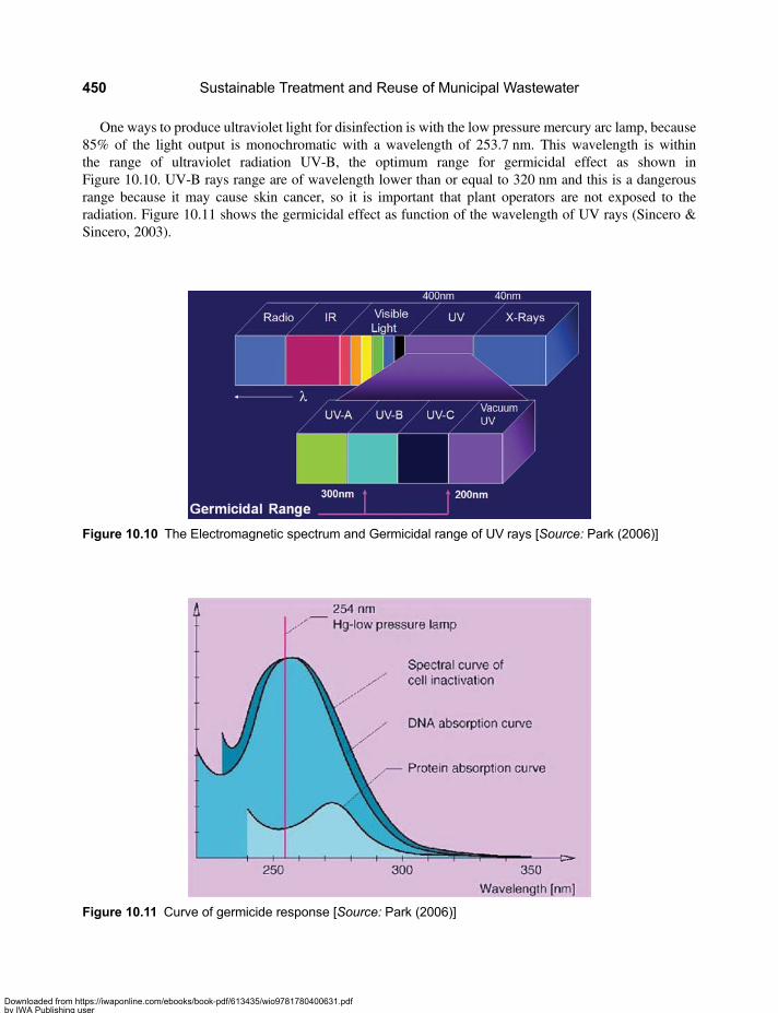
One ways to produce ultraviolet light for disinfection is with the low pressure mercury arc lamp, because85% of the light output is monochromatic with a wavelength of 253.7 nm. This wavelength is withinthe range of ultraviolet radiation UV-B, the optimum range for germicidal effect as shown inFigure 10.10. UV‐B rays range are of wavelength lower than or equal to 320 nm and this is a dangerousrange because it may cause skin cancer, so it is important that plant operators are not exposed to theradiation. Figure 10.11 shows the germicidal effect as function of the wavelength of UV rays (Sincero &Sincero, 2003).

Figure 10.10 The Electromagnetic spectrum and Germicidal range of UV rays [Source: Park (2006)]

Figure 10.11 Curve of germicide response [Source: Park (2006)]



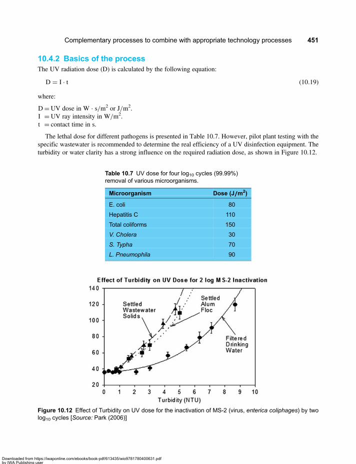
10.4.2 Basics of the processThe UV radiation dose (D) is calculated by the following equation:

D = I · t (10.19)

where:

D=UV dose in W · s/m2 or J/m2.I =UV ray intensity in W/m2.t = contact time in s.

The lethal dose for different pathogens is presented in Table 10.7. However, pilot plant testing with thespecific wastewater is recommended to determine the real efficiency of a UV disinfection equipment. Theturbidity or water clarity has a strong influence on the required radiation dose, as shown in Figure 10.12.

Table 10.7 UV dose for four log10 cycles (99.99%)removal of various microorganisms.

Microorganism Dose (J/////m2)

E. coli 80

Hepatitis C 110

Total coliforms 150

V. Cholera 30

S. Typha 70

L. Pneumophila 90

Figure 10.12 Effect of Turbidity on UV dose for the inactivation of MS-2 (virus, enterica coliphages) by twolog10 cycles [Source: Park (2006)]



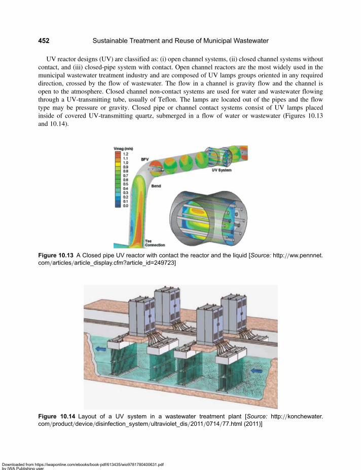
UV reactor designs (UV) are classified as: (i) open channel systems, (ii) closed channel systems withoutcontact, and (iii) closed-pipe system with contact. Open channel reactors are the most widely used in themunicipal wastewater treatment industry and are composed of UV lamps groups oriented in any requireddirection, crossed by the flow of wastewater. The flow in a channel is gravity flow and the channel isopen to the atmosphere. Closed channel non-contact systems are used for water and wastewater flowingthrough a UV-transmitting tube, usually of Teflon. The lamps are located out of the pipes and the flowtype may be pressure or gravity. Closed pipe or channel contact systems consist of UV lamps placedinside of covered UV-transmitting quartz, submerged in a flow of water or wastewater (Figures 10.13and 10.14).

Figure 10.13 A Closed pipe UV reactor with contact the reactor and the liquid [Source: http://ww.pennnet.com/articles/article_display.cfm?article_id=249723]

Figure 10.14 Layout of a UV system in a wastewater treatment plant [Source: http://konchewater.com/product/device/disinfection_system/ultraviolet_dis/2011/0714/77.html (2011)]






















The hydraulics for ideal UV disinfection is designed as a longitudinal plug flow with completetransversal mixing. The reactor inlet conditions can be designed with baffles to minimize dead spots andshort circuits. High flows can be maintained through the reactor to promote turbulence and transversalmixing. The relationship between the length and hydraulic radius of the reactor must be high tominimize longitudinal dispersion. The UV dose generated by the reactor at a flow rate Q can becalculated using Equation 10.19:

D = I · t = I · V/QWhere t is the contact time in a reactor with an effective volume (V) and a water flow (Q). The effective

volume of a UV reactor is the volume of water exposed to UV light, and the average radiation intensity iscalculated for the effective volume. The UV dose calculated using the average intensity is often higher thanthe dose calculated using the intensity measured at the reactor wall. The UV intensity inside the reactordepends on the energy at the UV lamp output, reflectance, refraction and absorption of UV light as itpasses through the quartz cover, and the UV light absorption by organic and inorganic chemicals. TheUV intensity at a point in the water is the sum of the contributions of light from each point along the arcof each UV lamp immersed in water. The death rate of microorganisms is calculated by the equation:

N = N0ekIt = N0e

kD (10.20)

Where N0 is the initial microorganism concentration in MPN2100 ml and N the survivors concentrationafter a time t. From equation 10.20 it is clear that Log(N/N0)= kD. The layout of a UV system in awastewater treatment plant and the lamps placement arrangement in the treatment plant is shown inFigure 10.14.

10.4.3 Basic designThe following procedure is used to design the UV disinfection system, applied to the case of a populationof 20,000.

Variables selected by the designerAfter choosing the reactor type, the following designer variables are selected: (i) the flow rate (QHD) whichis calculated using Equation 3.4, (ii) the dose of UV (D) is determined, and it must be between 16 and38 mW · s/m2, (iii) the velocity (v) in the channel or pipe is determined, and it must be between 0.6 and2.0 m/s, (iv) the channel depth (hc) is selected and it should be between 0 3 and 1.0 m, and (v) the ration(Lc/wc) is selected and it should be between 1 to 4. The variables selected by the designer for theexample of 20,000 inhabitants are shown in Table 10E.

Basic designOnce the design variables are defined, the sizing is as follows:

• Calculate the channel width (wc) by:

wc = QHD/v · hc (10.21)

2MPN: most probable number of microorganisms.



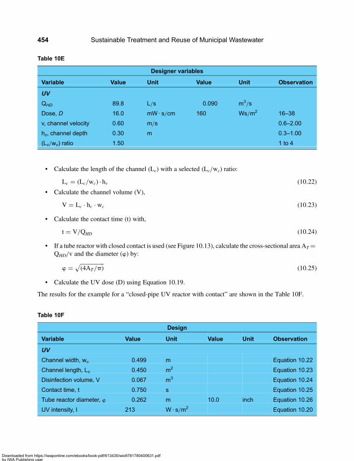
• Calculate the length of the channel (Lc) with a selected (Lc/wc) ratio:

Lc = (Lc/wc) · hv (10.22)

• Calculate the channel volume (V),

V = Lc · hc · wc (10.23)

• Calculate the contact time (t) with,

t = V/QHD (10.24)

• If a tube reactor with closed contact is used (see Figure 10.13), calculate the cross-sectional area AT=QHD/v and the diameter (w) by:

w =��(4AT/p)

√(10.25)

• Calculate the UV dose (D) using Equation 10.19.

The results for the example for a “closed-pipe UV reactor with contact” are shown in the Table 10F.

Table 10E

Designer variables


UV

QHD 89.8 L/s 0.090 m3/s

Dose, D 16.0 mW · s/cm 160 Ws/m2 16–38

v, channel velocity 0.60 m/s 0.6–2.00

hc, channel depth 0.30 m 0.3–1.00

(Lc/wc) ratio 1.50 1 to 4

Table 10F

Design


UV

Channel width, wc 0.499 m Equation 10.22

Channel length, Lc 0.450 m2 Equation 10.23

Disinfection volume, V 0.067 m3 Equation 10.24

Contact time, t 0.750 s Equation 10.25

Tube reactor diameter, w 0.262 m 10.0 inch Equation 10.26

UV intensity, I 213 W · s/m2 Equation 10.20



In this case it is necessary to apply UV rays with an intensity I= 213 W · s/m2 and a contact time t= 1 s(0.750 s), in an installation similar to that shown in Figure 10.13.

10.5 MEMBRANES10.5.1 IntroductionThe membrane separation technologies are used both for treatment of potable water and of wastewater. Themost commonly used are Micro Filtration (MF), Ultra Filtration (UF), Nano Filtration (NF) and ReverseOsmosis (RO). Figure 10.15 shows the types of membranes, their pore size openings in microns andtypes of particles and dissolved matter removed by the different types of membranes.

In membrane processes the stream of water (solvent) that crosses the membrane is defined as permeate(or filtrate), while the stream that does not flow through the membrane is the reject (or concentrate) andit contains concentrated solutes. In the membrane filtration process one pump feeds tangentially themembranes, while a valve in the concentrate (reject) pipe controls the necessary pressure so that thepermeated water exits without pressure. See Figure 10.16.

The type of material that is removed depends on the membrane pore size and applied pressure, as shownin Table 10.8. The membranes come in different shapes, as shown by Figures 10.17 and 10.18.

A facility with membranes as one of its processes consists of:

• Pre-treatment, which eliminate or reduce substances that could impair the proper functioning ofthe membrane.

• Membrane modules, which is where the membrane is housed.

Figure 10.15 Types of membranes, pore size openings and classification of particles and dissolved matterremoved by each membrane type [Source: Gravel (2002)]



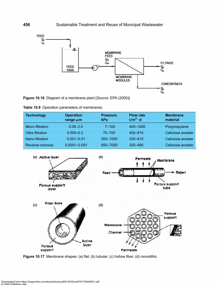
Table 10.8 Operation parameters of membranes.

Technology Operationrange mm

PressurekPa

Flow ratel/////m2 · d

Membranematerial

Micro filtration 0.08–2.0 7–100 400–1600 Polypropylene

Ultra filtration 0.005–0.2 70–700 400–815 Cellulose acetate

Nano filtration 0.001–0.01 500–1000 200–815 Cellulose acetate

Reverse osmosis 0.0001–0.001 850–7000 320–490 Cellulose acetate

Figure 10.16 Diagram of a membrane plant [Source: EPA (2005)]

Figure 10.17 Membrane shapes: (a) flat; (b) tubular; (c) hollow fiber; (d) monolithic



• Circuit cleaning as necessary to periodically remove the membrane substances that cause reduction ofthe permeate flux and/or quality of the permeate stream. Usually an acid wash and another alkalinewash are done for cleaning.

The principle of functioning of a package of pressurized hollow fiber membranes is presented inFigure 10.19. In this figure the feed solution is pressurized. Another way of operating such a system iswith an external vaccum, but this can be done only with microfiltration membranes and to some extentwith ultrafiltration membranes, where the required pressure is less than 1 atmosphere. A module ofhollow fiber membranes is presented in Figure 10.20.

Membrane filtration is usually combined with conventional activated sludge to a process denominatedMembrane BioReactor (MBR). There are three options for locating the membrane modules in an

Figure 10.18 Details of a module or package of hollow fiber membrane [Source: Wagner, Jorgen (2001)]

Figure 10.19 The principle of functioning of a package of hollow fiber membranes



activated sludge treatment plant: (i) leave the activated sludge process as it is and pass the effluent through amembrane treatment as a tertiary treatment process in a separate membrane tank; (ii) immerse the membranemodules in the aeration tank, and (iii) immerse the membrane modules in a separate membrane tank whichreplaces the secondary sedimentation tank. All three options work well; however, the third option is in mostwidespread use. The first option is the most expensive and therefore scarcely used. In the case of usingmembrane filtration as polishing of the effluent of another appropriate technology processes, themembrane filtration would be done by immersing the membrane modules in a separate membrane tank.A section of a membrane tank with several membrane modules immersed in it is presented inFigure 10.21. It illustrates the form of operation of the membrane tank.

Figure 10.22 shows a general view of a membranes plant which consists of several membrane tanks inwhich the membrane modules are immersed.

Membranes need to be cleaned periodically to maintain their solids separation capacity. The cleaning isbeing done automatically by the control system through backflushing with chemical solutions, usually CitricAcid and Sodium Hypochlorite. Cleaning cycles vary by application and raw water quality and there arevarious types of cleaning. Typical cleaning cycles are the following: Backpulse of Permeate every15 minutes for 30 seconds, maintenance cleaning occurs about once every 40 hours and recoverycleaning about once every 20 days minimum. The membranes also need to be replaced periodically,once every 5 to 9 years, depending on the composition of the raw sewage. For typical municipalwastewater, replacement is required about once every 8 years. Membrane replacement increases O&M

Figure 10.20 A hollow fiber membrane module



costs, however, membrane systems cost has been steadily declining over the past 10 years, and if this trendcontinues, replacement will become less of a burden.

Figure 10.21 A Section of a membrane tank with several membrane modules immersed in it

Figure 10.22 General view of a typical membrane plant



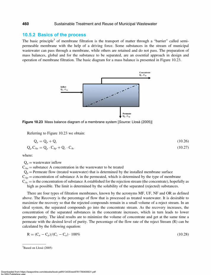
10.5.2 Basics of the processThe basic principle3 of membrane filtration is the transport of matter through a “barrier” called semi‐permeable membrane with the help of a driving force. Some substances in the stream of municipalwastewater can pass through a membrane, while others are retained and do not pass. The preparation ofmass balances, global and for the substance to be separated, are an essential approach in design andoperation of membrane filtration. The basic diagram for a mass balance is presented in Figure 10.23.

Referring to Figure 10.23 we obtain:

Qa = Qp + Qc (10.26)

Qa.CAa = Qp · CAp + Qc · CAc (10.27)

where:

Qa=wastewater inflowCAa= substance A concentration in the wastewater to be treatedQp= Permeate flow (treated wastewater) that is determined by the installed membrane surfaceCAp= concentration of substance A in the permeated, which is determined by the type of membraneCAc= is the concentration of substance A established for the rejection stream (the concentrate), hopefully as

high as possible. The limit is determined by the solubility of the separated (rejected) substances.

There are four types of filtration membranes, known by the acronyms MF, UF, NF and OR as definedabove. The Recovery is the percentage of flow that is processed as treated wastewater. It is desirable tomaximize the recovery so that the rejected compounds remain in a small volume of a reject stream. In anideal system, the separated compounds go into the concentrate stream. As the recovery increases, theconcentration of the separated substances in the concentrate increases, which in turn leads to lowerpermeate purity. The ideal results are to minimize the volume of concentrate and get at the same time apermeate with the desired level of purity. The percentage of the flow rate of the reject Stream (R) can becalculated by the following equation:

R = (Ca − Cp)/(Cc − Ca) · 100% (10.28)

Figure 10.23 Mass balance diagram of a membrane system [Source: Llosá (2005)]

3Based on Llosá (2005)



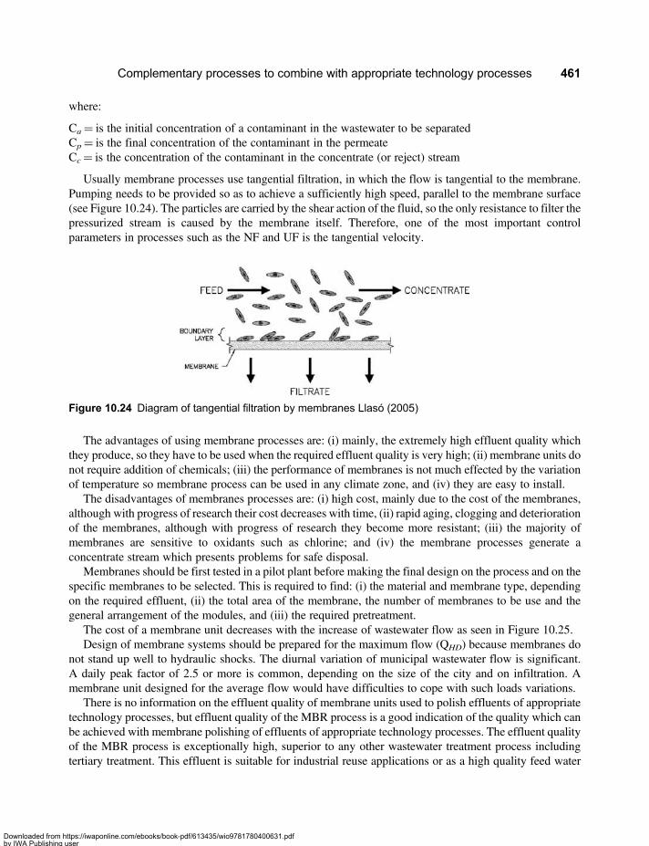
where:

Ca= is the initial concentration of a contaminant in the wastewater to be separatedCp= is the final concentration of the contaminant in the permeateCc= is the concentration of the contaminant in the concentrate (or reject) stream

Usually membrane processes use tangential filtration, in which the flow is tangential to the membrane.Pumping needs to be provided so as to achieve a sufficiently high speed, parallel to the membrane surface(see Figure 10.24). The particles are carried by the shear action of the fluid, so the only resistance to filter thepressurized stream is caused by the membrane itself. Therefore, one of the most important controlparameters in processes such as the NF and UF is the tangential velocity.

The advantages of using membrane processes are: (i) mainly, the extremely high effluent quality whichthey produce, so they have to be used when the required effluent quality is very high; (ii) membrane units donot require addition of chemicals; (iii) the performance of membranes is not much effected by the variationof temperature so membrane process can be used in any climate zone, and (iv) they are easy to install.

The disadvantages of membranes processes are: (i) high cost, mainly due to the cost of the membranes,although with progress of research their cost decreases with time, (ii) rapid aging, clogging and deteriorationof the membranes, although with progress of research they become more resistant; (iii) the majority ofmembranes are sensitive to oxidants such as chlorine; and (iv) the membrane processes generate aconcentrate stream which presents problems for safe disposal.

Membranes should be first tested in a pilot plant before making the final design on the process and on thespecific membranes to be selected. This is required to find: (i) the material and membrane type, dependingon the required effluent, (ii) the total area of the membrane, the number of membranes to be use and thegeneral arrangement of the modules, and (iii) the required pretreatment.

The cost of a membrane unit decreases with the increase of wastewater flow as seen in Figure 10.25.Design of membrane systems should be prepared for the maximum flow (QHD) because membranes do

not stand up well to hydraulic shocks. The diurnal variation of municipal wastewater flow is significant.A daily peak factor of 2.5 or more is common, depending on the size of the city and on infiltration. Amembrane unit designed for the average flow would have difficulties to cope with such loads variations.

There is no information on the effluent quality of membrane units used to polish effluents of appropriatetechnology processes, but effluent quality of the MBR process is a good indication of the quality which canbe achieved with membrane polishing of effluents of appropriate technology processes. The effluent qualityof the MBR process is exceptionally high, superior to any other wastewater treatment process includingtertiary treatment. This effluent is suitable for industrial reuse applications or as a high quality feed water

Figure 10.24 Diagram of tangential filtration by membranes Llasó (2005)



source for reverse osmosis treatment. Indicative effluent quality of an MBR system is BOD, 2 mg/l, SS,1 mg/l, Turbidity,1 NTU, practically complete void of bacteria and with up to 4 log removal of virus(depending on the membrane nominal pore size). In addition, it provides a barrier to certain chlorineresistant pathogens such as Cryptosporidium and Giardia. As to Nitrogen and Phosphorous removal, themembrane itself does not remove these elements and if their elimination is needed, specific removalprocess can be incorporated into the MBR process.

The effluent quality of MBR is stable, while that of other treatment processes fluctuates with time inresponse to fluctuations of sewage flow rate and variations in climatic conditions. The high and stablequality of the MBR effluent enables it to be reused in industrial plants, which require a stable quality.Industrial plants need sometimes desalinated water, and the MBR effluent can be a good feed to thereverse osmosis process, because the ultra filtration prevents fouling of RO membranes.

The MBR effluent can certainly be reused in agriculture and also in landscape irrigation within urbanareas. This is very important in water scarce regions. The MBR effluent is less offensive to theenvironment when discharged to receiving water bodies. It is practically free of pathogens since membranesare effective means of bacteria and virus removal, and therefore presents a lower public health risk.

A photo of a sample of effluent of an MBR treatment plant at the Ben Gurion International Airport inIsrael aside a sample of the raw sewage is presented in Figure 10.25. The effluent looks as pure water,and indeed in terms of turbidity it is better than natural surface water and even treated water, as itsturbidity is 0.075 NTU according to the reading of the continuous monitoring effluent tubidimeter. Inspite of the low turbidity content of the effluent, it of course does not reach the quality of potable watersince it contains dissolved organic compounds whose origin is the wastewater, which are not present innatural fresh water. The Ben Gurion MBR plant effluent is reused for irrigating all the green areas in theairport, for feeding cooling towers in the airport area, and for cleaning the runways, when necessary.

Figure 10.25 Samples of effluent and raw sewage of the ben gurion MBR treatment plant



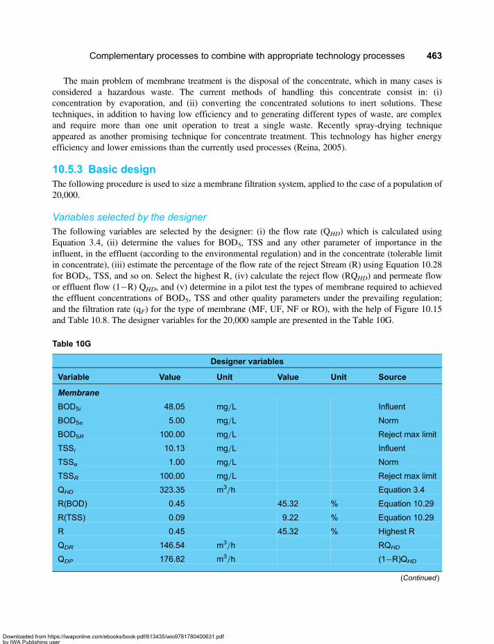
The main problem of membrane treatment is the disposal of the concentrate, which in many cases isconsidered a hazardous waste. The current methods of handling this concentrate consist in: (i)concentration by evaporation, and (ii) converting the concentrated solutions to inert solutions. Thesetechniques, in addition to having low efficiency and to generating different types of waste, are complexand require more than one unit operation to treat a single waste. Recently spray-drying techniqueappeared as another promising technique for concentrate treatment. This technology has higher energyefficiency and lower emissions than the currently used processes (Reina, 2005).

10.5.3 Basic designThe following procedure is used to size a membrane filtration system, applied to the case of a population of20,000.

Variables selected by the designerThe following variables are selected by the designer: (i) the flow rate (QHD) which is calculated usingEquation 3.4, (ii) determine the values for BOD5, TSS and any other parameter of importance in theinfluent, in the effluent (according to the environmental regulation) and in the concentrate (tolerable limitin concentrate), (iii) estimate the percentage of the flow rate of the reject Stream (R) using Equation 10.28for BOD5, TSS, and so on. Select the highest R, (iv) calculate the reject flow (RQHD) and permeate flowor effluent flow (1−R) QHD, and (v) determine in a pilot test the types of membrane required to achievedthe effluent concentrations of BOD5, TSS and other quality parameters under the prevailing regulation;and the filtration rate (qF) for the type of membrane (MF, UF, NF or RO), with the help of Figure 10.15and Table 10.8. The designer variables for the 20,000 sample are presented in the Table 10G.

Table 10G

Designer variables


Membrane

BOD5i 48.05 mg/L Influent

BOD5e 5.00 mg/L Norm

BOD5R 100.00 mg/L Reject max limit

TSSi 10.13 mg/L Influent

TSSe 1.00 mg/L Norm

TSSR 100.00 mg/L Reject max limit

QHD 323.35 m3/h Equation 3.4

R(BOD) 0.45 45.32 % Equation 10.29

R(TSS) 0.09 9.22 % Equation 10.29

R 0.45 45.32 % Highest R

QDR 146.54 m3/h RQHD

QDP 176.82 m3/h (1−R)QHD

(Continued )



Note that the BOD concentration in the inflow is 48 mg/l and the TSS is 10 mg/l. These values are quitelow, because the inflow to the membrane tank is an effluent of preceding appropriate technology unitprocesses. The required effluent quality is 5 mg/l BOD and 1 mg/l TSS, which are values that amembrane process can achieve.

Basic designHaving defined the design variables, the dimensioning of the membranes is as follows:

• Calculate the filtration area for each type of filtration required using:

AF = qF · QDP (10.29)

For the example chose MF and NF. The filtration areas and the working pressure for MF and NF areshown in Table 10H.

Table 10H

Design


Membrane

AMF 176815.8 m2 Equation 10.30

AUF 0.0 m2 Equation 10.30

ANF 88407.9 m2 Equation 10.30

AOR 0.0 m2 Equation 10.30

Pressure MF 50.0 kPa Table 10.7

Pressure UF 0.0 kPa Table 10.7

Pressure NF 750.0 kPa Table 10.7

Pressure OR 0.0 kPa Table 10.7

Table 10G Samples of effluent and raw sewage of the ben gurion MBR treatment plant (Continued ).

Designer variables


Define Membrane MF Figure 10.16

qMF 1000.00 L/m2 · d Table 10.7

Define Membrane UF Figure 10.16

qUF 0.00 Table 10.7

Define Membrane NF L/m2 · d Figure 10.16

qNF 500.00 Table 10.7

Define Membrane RO Figure 10.16

qOR 0.00 Table 10.7



Chapter 11

Combinations of unit processesof appropriate technology

11.1 INTRODUCTIONA series of unit processes of appropriate technology for wastewater treatment was presented in the previouschapters, each yielding a different effluent quality. The presented series of processes might not be thecomplete set of existing appropriate technology unit processes and perhaps there are others which can beconsidered as part of this group. Sometimes an effluent quality higher than what a single unit process ofappropriate technology can produce is required. In such cases a treatment plant consisting of a series ofappropriate technology unit process can be used (2, 3 or more), in which the effluent of the first unitprocess is fed into the second unit process, the effluent of the second is fed to the third and so on.Another way to look at it is that to improve the quality of the effluent of a certain unit process, thiseffluent can be subjected to one or more polishing steps, each of which consisting of an additional unitprocess. This approach can produce practically any final effluent quality required. As presented inChapter 1, the main message of this book is the idea that it is possible to combine unit processes tocreate various treatment plants, each based on a series of appropriate technology processes, and that itis possible to combine unit process in such a manner that jointly they can generate any required effluentquality. A plant based on a combination in series of appropriate technology unit processes is still easy tooperate and is usually of lower costs than conventional processes in terms of investments and certainly inoperation and maintenance. However, the use of a complex process as a polishing step of an effluent ofan appropriate technology process should be avoided, because it transforms the entire treatment plant toa complex and costly treatment plant. There are cases of plants consisting of a UASB unit followed byan activated sludge unit or a trickling filter unit. Such plants are not appropriate technology plants.

A large number of combined processes are presented and discussed in Chapter 1, part of them already inuse in full scale plants and others may be used in the future. It is impossible to provide design proceduresfor all the combined processes mentioned in the book. In this chapter we present the design procedures offive combined processes. We consider that a sample of five combined processes which consist of a total ofnine appropriate technology unit processes constitute a sufficiently large sample. This sample can serve forthe readers as the basis for developing the design of other combined processes in which they might beinterested. The processes dealt with in this chapter are defined in Table 11.1. The unit processes thatcompose each of the five combined processes have been described in previous chapters, so for anytechnical considerations on fundamentals, design equations and design procedures the reader is referredto the corresponding chapters.


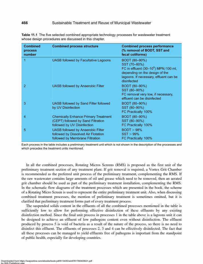
In all the combined processes, Rotating Micros Screens (RMS) is proposed as the first unit of thepreliminary treatment section of any treatment plant. If grit removal is required, a Vortex Grit Chamberis recommended as the preferred unit process of the preliminary treatment, complementing the RMS. Ifthe raw wastewater contains large amounts of oil and grease which need to be removed, then an aeratedgrit chamber should be used as part of the preliminary treatment installation, complementing the RMS.In the schematic flow diagrams of the treatment processes which are presented in the book, the schemeof a Rotating Micro Screen is used to represent the entire preliminary treatment unit. Also, when discussingcombined treatment processes, the mention of preliminary treatment is sometimes omitted, but it isclarified that preliminary treatment forms part of every treatment process.

The suspended solids content in the effluents of all the combined processes mentioned in the table issufficiently low to allow for performing effective disinfection of these effluents by any existingdisinfection method. Since the final unit process in processes 1 in the table above is a lagoons unit it canbe designed to achieve an effluent of low pathogens content even without disinfection. The effluentproduced by process 5 is void of bacteria as a result of the nature of the process, so there is no need todisinfect this effluent. The effluents of processes 2, 3 and 4 can be effectively disinfected. The fact thatall these processes can be managed to yield effluents free of pathogens is important from the standpointof public health, especially for developing countries.

Table 11.1 The five selected combined appropriate technology processes for wastewater treatmentwhose design procedures are discussed in this chapter.

Combinedprocessnumber

Combined process structure Combined process performance(% removal of BODT, SST andfecal coliforms)

1 UASB followed by Facultative Lagoons BODT (80–90%)SST (70–80%)FC in effluent (30–105) MPN/100 ml,depending on the design of thelagoons. If necessary, effluent can bedisinfected

2 UASB followed by Anaerobic Filter BODT (80–90%)SST (80–90%)FC removal very low, if necessary,effluent can be disinfected

3 UASB followed by Sand Filter followedby UV Disinfection

BODT (80–90%)SST (80–90%)FC Practically 100%

4 Chemically Enhance Primary Treatment(CEPT) followed by Sand Filtrationfollowed by UV Disinfection

BODT (80–90%)SST (80–90%)FC Practically 100%

5 UASB followed by Anaerobic Filterfollowed by Dissolved Air Flotationfollowed by Membrane Filtration

BODT. 98%SST. 99%FC Practically 100%

Each process in the table includes a preliminary treatment unit which is not shown in the description of the processes andwhich precedes the treatment units mentioned.



11.2 COMBINATION 1: ROTATING MICRO SCREENS FOLLOWED BYUASB FOLLOWED BY FACULTATIVE LAGOONS11.2.1 IntroductionIn this combined processes the effluent of a UASB plant is polished by facultative lagoons. This is a verylogical scheme and an exemplary appropriate technology process. Preliminary treatment is achieved byrotating screens and, if needed, a vortex grit chamber, which is the best available preliminary treatmentscheme. The screen opening should not be less than of 6 mm in order to avoid removing organic matterwhich is necessary for the proper functioning of the UASB reactor. The removal of the main portion oforganic matter is achieved in this combination by the USAB process, which is one of the main unitprocesses of appropriate technology and is discussed in detail in Chapter 6. It is a simple, effective lowcost process. The facultative or maturation lagoons system used for polishing the UASB effluent is asimple reliable system discussed in Chapter 5. Removal of pathogenic organisms can be achieved in thisprocess naturally (without disinfection), if sufficient detention time is provided in the lagoons system.The emphasis of the design of the lagoon must be on the removal of pathogens, since the bulk of organicmatter is removed in the UASB Reactor. In several plants visited the lagoon are designed with a veryshort detention time, practically operating as clarifier where settled sludge is decomposed in the bottom.Such an approach should be avoided and the lagoons need to be designed for the removal of pathogens.The design basis for disinfection in lagoons is discussed by Arthur (1983).

This combined process generates solid waste material in the rotating screen and excess sludge in theUASB reactor. This process includes therefore the disposal of the screened material, usually in a sanitarylandfill, and the handling of the UASB excess sludge, mainly by drying beds, without mechanicalequipment. The main disadvantage of this combined process is that the lagoons occupy large extensionsof land. If area is scarce, deeper lagoons with mixers can be used. An ultrasound device can be used todecrease algae content in the final effluent. Because of the use of lagoons as part of this process, it issuitable for small and medium size cities, but not for large cities (Libhaber, 2007). The biogas generatedin the UASB reactor can be collected and put to use, if economically feasible. As a whole this is a goodand recommended process. A schematic flow diagram of this process is presented in Figure 11.1.

This process is being applied in several plants in Brazil and in Colombia, using conventional preliminarytreatment, not RMS. The largest plant of this type in Colombia is the Rio Frio plant in Bucaramanga. A photoof the plant is presented in Figure 11.2. This plant, commissioned in 1991, is one of the oldest in the worldlarge scale UASB-based facilities treating municipal wastewater. The plant’s original design flow was740 l/s serving a population of 240.000. The UASB reactors are located at the bottom of Figure 1.2 andnext to them are the sludge drying beds (not seen in the figure). The UASB reactors are equipped withaluminium covers and the collected biogas is flared. Pretreatment for the UASB reactors is provided by6 mm screens followed by grit chambers. The reactors are followed by two facultative lagoons. Removalefficiency of BOD is about 80% in the USAB plant and 33% in the facultative lagoons, achieving a totalBOD removal in the range of 85–90%.

Paragraph 1.19 of Chapter 1 present Table 1.11 with all the programs used in the book, including theCombinations, and a short explanation of how to use them. Note that that combination 2 is calculatedwith program CHAP 6-ANAEROBIC-UASB-AF.xls, and each of the other combinations has its ownprogram working analogous to the process programs. Also note that in combination programs theeffluent of a preceding unit is the influent to the following unit. For all other details the programs workexactly as presented in each process program, of course with the specific influent for each case.

Combinations of unit processes of appropriate technology 467


The plant has been able to achieve essentially secondary treatment levels compatible with that ofconventional processes at a very low capital and O&M costs, thereby demonstrating the potential ofapplication of this process in developing countries. The Rio Frio plant has two problems: (i) thedetention time in the facultative lagoons is way too low (about 2 days) and this limits their performance;and (ii) the potable water in Bucaramanga has elevated sulphate levels, and most of the sulphates presentin the raw wastewater are effectively reduced to H2S in the anaerobic reactors, generating odour aroundthe plant and promoting corrosion of plant equipment. Addition of aluminium covers and the collectionand flaring of the biogas has helped to reduce the intensity of the odours and the corrosion of the equipment.

With time the population served by the Rio Frio plant increased and its capacity needed to be augmented.The plant is now being upgraded and its flow diagram is being modified. The UASB reactors section isbeing expanded but the facultative lagoons have been eliminated since there was no area available toincrease them. The lagoons are being replaced by an activate sludge unit. As previously mentioned, thistransforms the entire plant to a conventional treatment plant, and it ceases to be an appropriatetechnology treatment plant. However, the UASB unit performed well during a period of 20 years and hasnot been eliminated, so it will continue to function in the foreseeable future, and the configuration ofUASB followed by lagoons proved to be a successful configuration which performed well and providedduring 20 years a high quality effluent, comparable to that of conventional treatment, at a fraction of the cost.

Figure 11.2 A photo of the Rio Frio Plant, Bucaramanga, Colombia

Figure 11.1 A schematic flow diagram of the combined process of preliminary treatment followed by UASBfollowed by facultative lagoons



Several plants of UASB followed by lagoons are in operation in Brazil. SANEPAR, the water utility ofthe state of Parana in Brazil operates several plants of this type. Figure 1.62 shows a photo of a UASB plantfollowed by a facultative lagoon in Ronda, a small town, part of the city of Ponta Grossa in the state ofParana. Another plant in Parana based on this process is the Padilha Sul Plant located in the city ofCuritiba, the capital of Parana. A photo of this plant is presented in Figure 1.63. The first stage of thisplant was designed for an average wastewater flow of 440 l/s and is serving an equivalent population of318,000. It will be expanded to handle an average flow of 600 l/s. The UASB reactors occupy the smallarea at the left hand side of the bottom of the figure. As can be seen, the UASB reactors unit occupiesonly a small portion of the total plant area. Also seen in the photo is that the UASB reactors are locatedat a close vicinity to residential areas. That means that the UASB units do not present an environmentalnuisance to the nearby residential areas.

11.2.2 PerformanceThe advantages of combined process of UASB followed by lagoons are: (i) low capital and operation cost,(ii) easy maintenance, it does not use mechanical equipment, (iii) small quantities of sludge, and (iv) goodeffluent quality. The main disadvantage of this process is that the lagoons occupy a large land area. Theapproach of deeper lagoons equipped with mixer can reduce the area of the lagoons).

The plant of Rio Frio, Colombia, obtained BOD removal of about 80% in the UASB reactor and 33% inthe maturation ponds, for a total removal of BOD of 85–90%. In general, this process achieves 80–90%BOD removal and 70–80% SST removal. The removal of FC depends on the design of the lagoons. If ashort detention time is provided, the FC removal is low. However, properly designed lagoons canachieve a high FC removal.

Construction costs for the existing facilities of the Rio Frio treatment plant in Bucaramanga wereapproximately 15 US$/Capita. Operating costs are 0.79 US$/Yr/Capita or 0.015 US$/m3 treated(Osorio, 1996). However, this plant was constructed in the early 1990s. It is estimated that today Theinvestment cost in a UASB reactor followed by a lagoons system is in the range 30–50 US$/Capita,depending on the design of the lagoons, and the O&M cost is in the range 1.0–1.5 US$/Yr/Capita.

11.2.3 Design(The model program for this Example is available online at http://www.iwawaterwiki.org/xwiki/bin/view/Articles/Software+Developed+for+Sustainable+Treatment+and+Reuse+of+Municipal+Wastewater)

The design procedures and a detailed example of the design of a UASB reactor and a lagoons systemwhich make up this combination are presented in Chapter 6 and 5 respectively. The reader is referred tothe design examples in these chapters. The results of application in series of a UASB reactor and alagoons system for the example of 20,000 people, with an influent Fecal Coliform of 5 × 106 MPN/100ml are presented below. The Excel program COMB 1-USAB-MATURATION LAGOON-01.xls is theprogram used to calculate example of this combined process.

Variables selected by the designerThe quality parameters of the raw wastewater are the same of all other examples and presented inTable 11A. The specifics of each process design are explained in the corresponding chapter (in this case,Chapters 5 and 6). Please note that the following Tables identified by alphabetic order contain computercalculated results.



















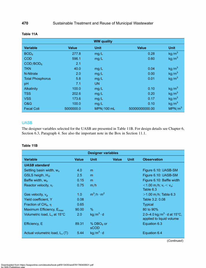
UASB

The designer variables selected for the UASB are presented in Table 11B. For design details see Chapter 6,Section 6.3, Paragraph 4. See also the important note in the Box in Section 11.1.

Table 11A

WW quality


BOD5 277.8 mg/L 0.28 kg/m3

COD 596.1 mg/L 0.60 kg/m3

COD/BOD5 2.1

TKN 40.0 mg/L 0.04 kg/m3

N-Nitrate 2.0 mg/L 0.00 kg/m3

Total Phosphorus 5.8 mg/L 0.01 kg/m3

pH 7.1 UN

Alkalinity 100.0 mg/L 0.10 kg/m3

TSS 202.6 mg/L 0.20 kg/m3

VSS 173.6 mg/L 0.17 kg/m3

O&G 100.0 mg/L 0.10 kg/m3

Fecal Coli 5000000.0 MPN/100mL 50000000000.00 MPN/m3

Table 11B

Designer variables


UASB standard

Settling basin width, ws 4.0 m Figure 6.10: UASB-SM


Baffle width, wb 0.15 m Figure 6.10: Baffle width

Reactor velocity, vr 0.75 m/h ,1.00 m/h; vr , vs;Table 6.3

Gas velocity, vg 1.0 m3/h · m2 .1.00 m/h; Tabla 6.3


Fraction of CH4, η 0.65 Typical


Volumetric load, Lv at 15°C 2.0 kg/m3 · d 2.0–4.0 kg/m3 · d at 15°C,applied to liquid volume

Efficiency, E 89.31 % DBO5 orsCOD

Equation 6.3

Actual volumetric load, Lv (T) 5.44 kg/m3 · d Equation 6.4

(Continued )



Maturation lagoonThe designer variables selected for the maturation lagoons are presented in Table 11C. For design details seeChapter 5, Section 5.3, Paragraph 6.

Table 11C

Designer variables


Maturation lagoon

Depth, HM 1.5 m 2–5 m


Ti water 25.0

# Lagoons M, nM 2 Parallel

L/w (ratio length towidth)

2 Between 1 and 3

Pipe velocity, v 1 m/s 0.6–2.0 m/s

LS= 350 (1.107−0.002T)(T–25) or 400

216.5 kg BOD5/ha · d Equation 5.14 or 400

(Continued )

Table 11B (Continued ).

Designer variables


Water temperature 25.00 °C Coldest month of year


Methane production, VCH4124.34 m3/d Equation 6.6

Biogas production, Vbiogas 191.29 m3/d 7.97 m3/h Ecuación 6.7

Inlet structures

Branch manifold flow 0.020 m3/s QD/2

Manifold velocity, v 0.03 m/s Goal seek: see notein cell N38

orifices per m2, ε0 2.00 1 a 2 per m2

# orfices, preliminary, n0 114.00 Equation 6.27

# distribuitors, nd 11.00 Equation 6.27a

# orifices per distributor, nod 5.00 Equation 6.28

Outlet structures

Module flow, QM =QD/nM 0.01 m3/s

Channel widthl b 0.30 m Select

Draying bed

Applying rate, qx 150 kg/m2 · yr Between 120–150



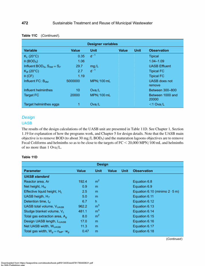
DesignUASB

The results of the design calculations of the UASB unit are presented in Table 11D. See Chapter 1, Section1.19 for explanation of how the programs work, and Chapter 5 for design details. Note that the UASB mainobjective is to remove BOD (to about 30 mg/L BOD5) and the maturation lagoons objectives are to removeFecal Coliforms and helminths so as to be close to the targets of FC, 20,000 MPN/100 mL and helminthsof no more than 1 Ova/L.

Table 11D

Design


UASB standard

Reactor area, Ar 192.4 m2 Equation 6.8

Net height, HN 0.9 m Equation 6.9

Effective liquid height, HL 2.5 m Equation 6.10 (minimo 2 · 5 m)

UASB heigth, HT 5.0 m Equation 6.11

Detention time, td 6.7 h Equation 6.12

UASB total volume, VUASB 962.2 m3 Equation 6.13

Sludge blanket volume, VL 481.1 m3 Equation 6.14

Total gas extraction area, Ag 8.0 m2 Equation 6.15

Design UASB length, LUASB 17.0 m Equation 6.16

Net UASB width, WUASB 11.3 m Equation 6.17

Total gas width, Wg= nMP · wg 0.47 m Equation 6.18

(Continued )

Table 11C (Continued ).

Designer variables


KL (20°C) 0.35 d−1 Tipical

θ (BOD5) 1.06 1.04–1.09

Influent BOD5i, S0M=SF 29.7 mg/L UASB Effluent

KB (20°C) 2.7 d−1 Tipical FC

θ (CF) 1.19 Tipical FC

Influent FC: B0M 5000000 MPN/100mL UASB does notremove

Influent helminthes 10 Ova/L Between 300–800

Target FC 20000 MPN/100mL Between 1000 and20000

Target helminthes eggs 1 Ova/L ,1 Ova/L



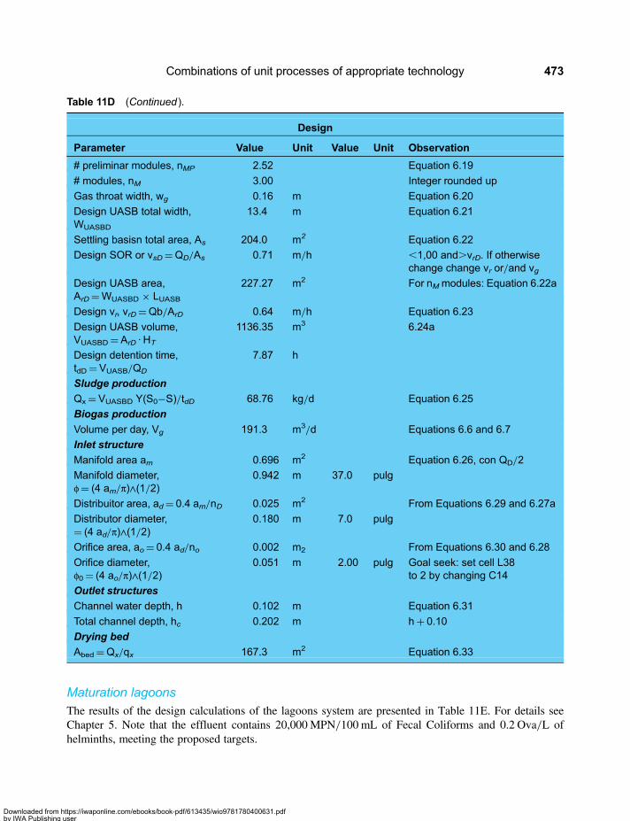
Maturation lagoonsThe results of the design calculations of the lagoons system are presented in Table 11E. For details seeChapter 5. Note that the effluent contains 20,000MPN/100 mL of Fecal Coliforms and 0.2 Ova/L ofhelminths, meeting the proposed targets.

Table 11D (Continued ).

Design


# preliminar modules, nMP 2.52 Equation 6.19

# modules, nM 3.00 Integer rounded up

Gas throat width, wg 0.16 m Equation 6.20

Design UASB total width,WUASBD


Settling basisn total area, As 204.0 m2 Equation 6.22

Design SOR or vsD=QD/As 0.71 m/h ,1,00 and.vrD. If otherwisechange change vr or/and vg

Design UASB area,ArD=WUASBD × LUASB

227.27 m2 For nM modules: Equation 6.22a

Design vr, vrD=Qb/ArD 0.64 m/h Equation 6.23

Design UASB volume,VUASBD=ArD · HT

1136.35 m3 6.24a

Design detention time,tdD=VUASB/QD

7.87 h

Sludge production

Qx=VUASBD Y(S0−S)/tdD 68.76 kg/d Equation 6.25

Biogas production

Volume per day, Vg 191.3 m3/d Equations 6.6 and 6.7

Inlet structure

Manifold area am 0.696 m2 Equation 6.26, con QD/2

Manifold diameter,φ= (4 am/π)∧(1/2)

0.942 m 37.0 pulg

Distribuitor area, ad= 0.4 am/nD 0.025 m2 From Equations 6.29 and 6.27a

Distributor diameter,= (4 ad/π)∧(1/2)

0.180 m 7.0 pulg

Orifice area, ao= 0.4 ad/no 0.002 m2 From Equations 6.30 and 6.28

Orifice diameter,φ0= (4 ao/π)∧(1/2)

0.051 m 2.00 pulg Goal seek: set cell L38to 2 by changing C14

Outlet structures

Channel water depth, h 0.102 m Equation 6.31

Total channel depth, hc 0.202 m h+ 0.10

Drying bed

Abed=Qx/qx 167.3 m2 Equation 6.33



Table 11E


Maturation Lagoon

LS 216.5 kg BOD5/ha · d Selected in input

td 38.6 d Equation 5.11; tdmin= 3 d

Volume, V′F=Q · td 133868.6 m3 Equation 5.21

Final Volume, VF 133868.6 m3 Greater of td and tdmin= 3 d


Lagoon area, as= (As/nF) 44622.9 m2

Lagoon width, w= [as/(L/w)]0,5 149.4 m

Lagoon length, L= (L/w) w 298.7

TL= (AsfTa+QTi)/(Asf+Q) 18.5 °C Equation 5.8

KL= KL(20°C) θ(T-20) 0.32 d−1 Equation 5.7

Effluent BOD5 SM=S0/(1+ KL · td) 2.22 mg/L Equation 5.4, parallel

Effluent BOD5 SM=S0/(1+ KL · td/n)n 0.57 mg/L Equation 5.5, series

vF= 0,00091VF(S0−S)/(1+ 0.05td) 1141.39 kg/yr 1141.39 m3/yr Equation 5.24

Filling years= 0.5 VF/vF 58.6 years 1/2 volume

Maturation lagoon: fecal coliform and helminthes removal and efficiencies


Effluent FC: B=B0/(1+KB · td) 20000.0 MPN/100mL Equation 5.25; Goal seekTarget effluent FC

Effluent Helminthes 0.2 Ova/L

Efficiency FC= 100 · (B0−B)/B0 99.6 % From Equation 5.25

Efficiency Helminthes= 100 [1− 0.41exp (−0.49 td+ 0.0085td

2)]98.2 % Equation 5.15

Efficiency BOD5 removal maturation 92.5 %

Total efficiency BOD5 99.2 % Combination system

Total efficiency fecal coliform 99.6 % Combination system

Total efficiency helminthes 98.2 % Combination system


Total diameter, φ=(4 · PI · v · QD/1000)0,5 0.226 m 9.00 In With QD

Lagoon diameter, φL=φ=[4 · PI · v · (QD/4)/1000]0.5 0.160 m 6.00 in With QD/4

Susta

inable

Treatm

entandReuse

ofM

unicip

alW

aste

water

474


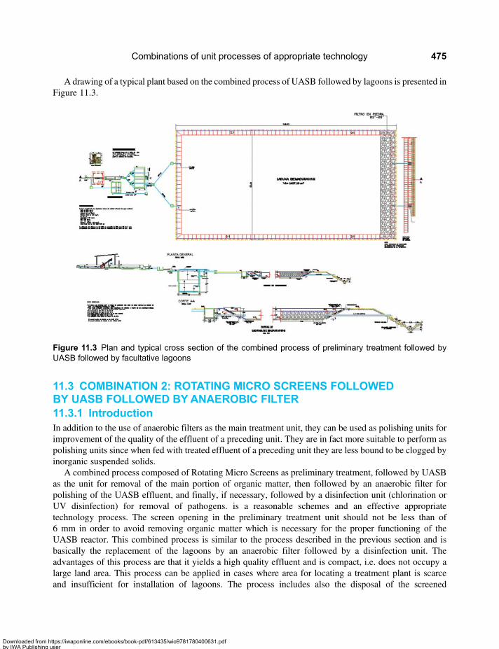
A drawing of a typical plant based on the combined process of UASB followed by lagoons is presented inFigure 11.3.

11.3 COMBINATION 2: ROTATING MICRO SCREENS FOLLOWEDBY UASB FOLLOWED BYANAEROBIC FILTER11.3.1 IntroductionIn addition to the use of anaerobic filters as the main treatment unit, they can be used as polishing units forimprovement of the quality of the effluent of a preceding unit. They are in fact more suitable to perform aspolishing units since when fed with treated effluent of a preceding unit they are less bound to be clogged byinorganic suspended solids.

A combined process composed of Rotating Micro Screens as preliminary treatment, followed by UASBas the unit for removal of the main portion of organic matter, then followed by an anaerobic filter forpolishing of the UASB effluent, and finally, if necessary, followed by a disinfection unit (chlorination orUV disinfection) for removal of pathogens. is a reasonable schemes and an effective appropriatetechnology process. The screen opening in the preliminary treatment unit should not be less than of6 mm in order to avoid removing organic matter which is necessary for the proper functioning of theUASB reactor. This combined process is similar to the process described in the previous section and isbasically the replacement of the lagoons by an anaerobic filter followed by a disinfection unit. Theadvantages of this process are that it yields a high quality effluent and is compact, i.e. does not occupy alarge land area. This process can be applied in cases where area for locating a treatment plant is scarceand insufficient for installation of lagoons. The process includes also the disposal of the screened

Figure 11.3 Plan and typical cross section of the combined process of preliminary treatment followed byUASB followed by facultative lagoons



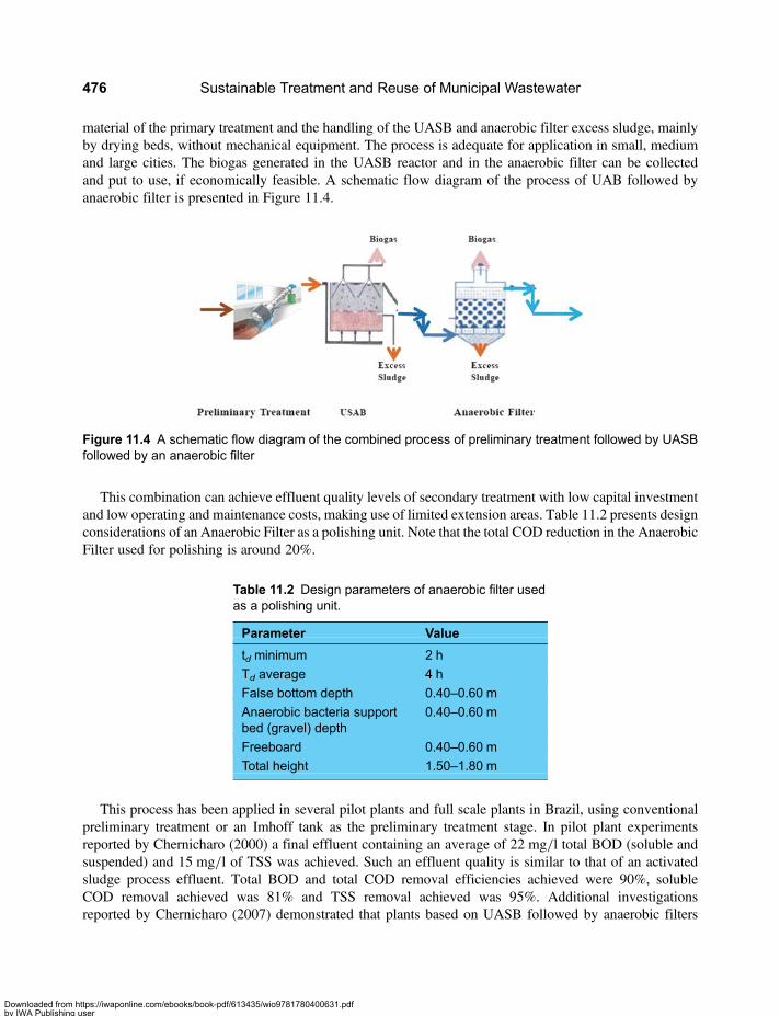
material of the primary treatment and the handling of the UASB and anaerobic filter excess sludge, mainlyby drying beds, without mechanical equipment. The process is adequate for application in small, mediumand large cities. The biogas generated in the UASB reactor and in the anaerobic filter can be collectedand put to use, if economically feasible. A schematic flow diagram of the process of UAB followed byanaerobic filter is presented in Figure 11.4.

This combination can achieve effluent quality levels of secondary treatment with low capital investmentand low operating and maintenance costs, making use of limited extension areas. Table 11.2 presents designconsiderations of an Anaerobic Filter as a polishing unit. Note that the total COD reduction in the AnaerobicFilter used for polishing is around 20%.

This process has been applied in several pilot plants and full scale plants in Brazil, using conventionalpreliminary treatment or an Imhoff tank as the preliminary treatment stage. In pilot plant experimentsreported by Chernicharo (2000) a final effluent containing an average of 22 mg/l total BOD (soluble andsuspended) and 15 mg/l of TSS was achieved. Such an effluent quality is similar to that of an activatedsludge process effluent. Total BOD and total COD removal efficiencies achieved were 90%, solubleCOD removal achieved was 81% and TSS removal achieved was 95%. Additional investigationsreported by Chernicharo (2007) demonstrated that plants based on UASB followed by anaerobic filters

Figure 11.4 A schematic flow diagram of the combined process of preliminary treatment followed by UASBfollowed by an anaerobic filter

Table 11.2 Design parameters of anaerobic filter usedas a polishing unit.

Parameter Value

td minimum 2 h

Td average 4 h

False bottom depth 0.40–0.60 m

Anaerobic bacteria supportbed (gravel) depth

0.40–0.60 m

Freeboard 0.40–0.60 m

Total height 1.50–1.80 m



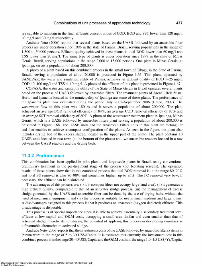
are capable to maintain in the final effluents concentrations of COD, BOD and SST lower than 120 mg/l,60 mg/l and 30 mg/l respectively.

Andrade Neto (2006) reports that several plants based on the UASB followed by an anaerobic filterprocess are under operation since 1996 in the state of Parana, Brazil, serving populations in the range of1,500 to 50,000 persons. Effluent quality achieved in these plants is total BOD lower than 60 mg/l andTSS lower than 20 mg/l. The same type of plants is under operation since 1997 in the state of MinasGerais, Brazil, serving populations in the range 2,000 to 15,000 persons. One plant in Minas Gerais, atIpatinga, serves a population of about 200,000.

A photo of a plant based on this combined process in the small town of Tibagi, in the State of Parana,Brazil, serving a population of about 20,000 is presented in Figure 1.65. This plant, operated bySANEPAR, the water and sanitation utility of Parana, achieves an effluent quality of BOD 5–25 mg/l,COD 40–100 mg/l and TSS 4–10 mg/l. A photo of the effluent of this plant is presented in Figure 1.67.

COPASA, the water and sanitation utility of the State of Minas Gerais in Brazil operates several plantsbased on the process of UASB followed by anaerobic filters. The treatment plants of Arenal, Bela Vista,Horto, and Ipanema located in the municipality of Ipatinga are some of these plants. The performance ofthe Ipanema plant was evaluated during the period July 2005–September 2006 (Greco, 2007). Thewastewater flow to this plant was 180 l/s and it serves a population of about 200,000. The plantachieved an average BOD removal efficiency of 84%, an average COD removal efficiency of 87% andan average SST removal efficiency of 80%. A photo of the wastewater treatment plant in Ipatinga, MinasGerais, which is a UASB followed by anaerobic filters plant serving a population of about 200,000 ispresented in Figure 1.68. The UASB units and the Anaerobic Filters units in this plant are rectangularand that enables to achieve a compact configuration of the plants. As seen in the figure, the plant alsoincludes drying bed of the excess sludge, located in the upper part of the photo. The plant contains 10UASB units located in two rows (at the bottom of the photo) and two anaerobic reactors located in a rawbetween the UASB reactors and the drying beds.

11.3.2 PerformanceThis combination has been applied in pilot plants and large-scale plants in Brazil, using conventionalpreliminary treatment as the pre-treatment stage of the process (not Rotating screens). The operationresults of these plants show that in this combined process the total BOD removal is in the range 80–90%and total SS removal is also 80–90% and sometimes higher, up to 95%. The FC removal very low, ifnecessary, the effluent can be disinfected.

The advantages of this process are: (i) it is compact (does not occupy large land area), (ii) it generates ahigh effluent quality, comparable to that of an activates sludge process, (iii) the management of excesssludge generated by the UASB and anaerobic filter can be done by the use of drying beds, without theneed of mechanical equipment, and (iv) the process is suitable for use in small medium and large towns.A disadvantages assigned to this process is that it produces an anaerobic (oxygen depleted) effluent. Thisdisadvantage is disputable.

This process is of special importance since it is able to achieve essentially a secondary treatment leveleffluent at low capital and O&M costs, occupying a small area similar and even smaller than that ofactivated sludge, thereby demonstrating the potential of applying this process in developing countries asa favourable alternative to activated sludge.

AndradeNeto (2006) reports that the investments costs of theUASB followedby anaerobic filter systems inParana were in the range of 5 to 30 US$/Capita. It is estimates that currently the investment cost in thiscombinedprocess is in the range20–40US$/Capita and theO&Mcost is in the range 1.0–1.5US$/Yr/Capita.



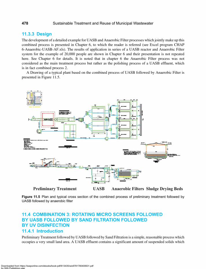
11.3.3 DesignThe development of a detailed example for UASB and Anaerobic Filter processes which jointly make up thiscombined process is presented in Chapter 6, to which the reader is referred (see Excel program CHAP6-Anaerobic-UASB-AF.xls). The results of application in series of a UASB reactor and Anaerobic Filtersystem for the example of 20,000 people are shown in Chapter 6 and their presentation is not repeatedhere. See Chapter 6 for details. It is noted that in chapter 6 the Anaerobic Filter process was notconsidered as the main treatment process but rather as the polishing process of a UASB effluent, whichis in fact combined process 2.

A Drawing of a typical plant based on the combined process of UASB followed by Anaerobic Filter ispresented in Figure 11.5.

11.4 COMBINATION 3: ROTATING MICRO SCREENS FOLLOWEDBY UASB FOLLOWED BY SAND FILTRATION FOLLOWEDBY UV DISINFECTION11.4.1 IntroductionPreliminary Treatment followed byUASB followed by Sand Filtration is a simple, reasonable process whichoccupies a very small land area. A UASB effluent contains a significant amount of suspended solids which

Figure 11.5 Plan and typical cross section of the combined process of preliminary treatment followed byUASB followed by anaerobic filter



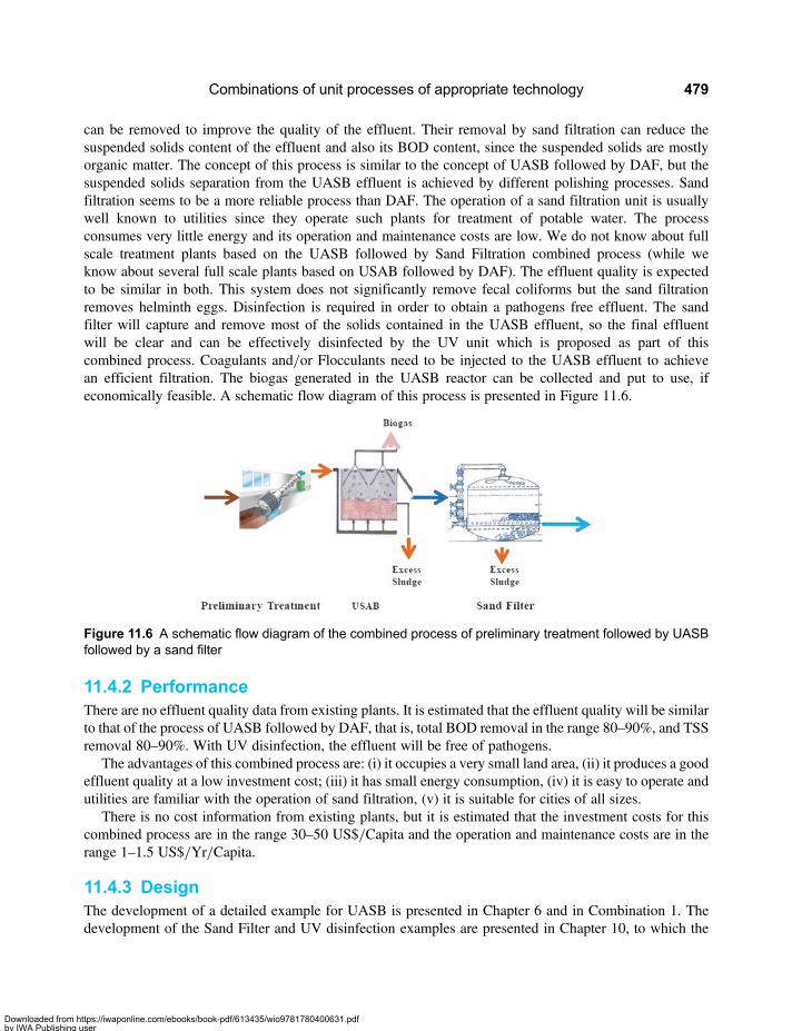
can be removed to improve the quality of the effluent. Their removal by sand filtration can reduce thesuspended solids content of the effluent and also its BOD content, since the suspended solids are mostlyorganic matter. The concept of this process is similar to the concept of UASB followed by DAF, but thesuspended solids separation from the UASB effluent is achieved by different polishing processes. Sandfiltration seems to be a more reliable process than DAF. The operation of a sand filtration unit is usuallywell known to utilities since they operate such plants for treatment of potable water. The processconsumes very little energy and its operation and maintenance costs are low. We do not know about fullscale treatment plants based on the UASB followed by Sand Filtration combined process (while weknow about several full scale plants based on USAB followed by DAF). The effluent quality is expectedto be similar in both. This system does not significantly remove fecal coliforms but the sand filtrationremoves helminth eggs. Disinfection is required in order to obtain a pathogens free effluent. The sandfilter will capture and remove most of the solids contained in the UASB effluent, so the final effluentwill be clear and can be effectively disinfected by the UV unit which is proposed as part of thiscombined process. Coagulants and/or Flocculants need to be injected to the UASB effluent to achievean efficient filtration. The biogas generated in the UASB reactor can be collected and put to use, ifeconomically feasible. A schematic flow diagram of this process is presented in Figure 11.6.

11.4.2 PerformanceThere are no effluent quality data from existing plants. It is estimated that the effluent quality will be similarto that of the process of UASB followed by DAF, that is, total BOD removal in the range 80–90%, and TSSremoval 80–90%. With UV disinfection, the effluent will be free of pathogens.

The advantages of this combined process are: (i) it occupies a very small land area, (ii) it produces a goodeffluent quality at a low investment cost; (iii) it has small energy consumption, (iv) it is easy to operate andutilities are familiar with the operation of sand filtration, (v) it is suitable for cities of all sizes.

There is no cost information from existing plants, but it is estimated that the investment costs for thiscombined process are in the range 30–50 US$/Capita and the operation and maintenance costs are in therange 1–1.5 US$/Yr/Capita.

11.4.3 DesignThe development of a detailed example for UASB is presented in Chapter 6 and in Combination 1. Thedevelopment of the Sand Filter and UV disinfection examples are presented in Chapter 10, to which the

Figure 11.6 A schematic flow diagram of the combined process of preliminary treatment followed by UASBfollowed by a sand filter



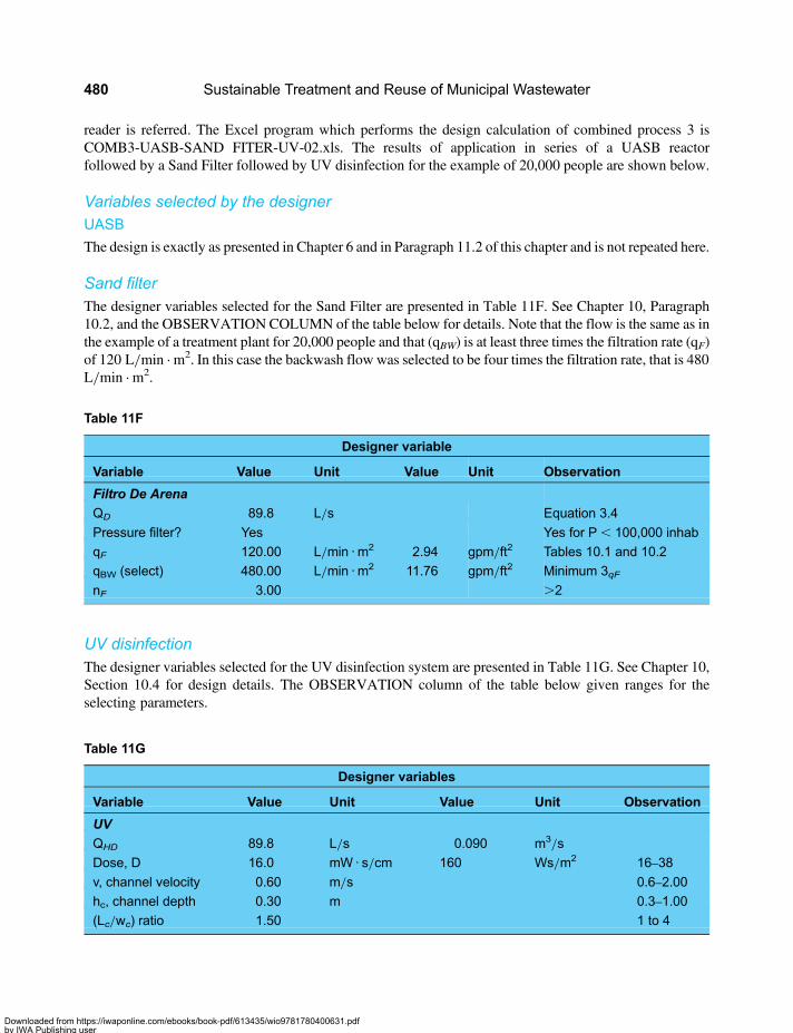
reader is referred. The Excel program which performs the design calculation of combined process 3 isCOMB3-UASB-SAND FITER-UV-02.xls. The results of application in series of a UASB reactorfollowed by a Sand Filter followed by UV disinfection for the example of 20,000 people are shown below.

Variables selected by the designerUASB

The design is exactly as presented in Chapter 6 and in Paragraph 11.2 of this chapter and is not repeated here.

Sand filterThe designer variables selected for the Sand Filter are presented in Table 11F. See Chapter 10, Paragraph10.2, and the OBSERVATION COLUMN of the table below for details. Note that the flow is the same as inthe example of a treatment plant for 20,000 people and that (qBW) is at least three times the filtration rate (qF)of 120 L/min · m2. In this case the backwash flow was selected to be four times the filtration rate, that is 480L/min · m2.

UV disinfectionThe designer variables selected for the UV disinfection system are presented in Table 11G. See Chapter 10,Section 10.4 for design details. The OBSERVATION column of the table below given ranges for theselecting parameters.

Table 11F

Designer variable


Filtro De Arena

QD 89.8 L/s Equation 3.4

Pressure filter? Yes Yes for P , 100,000 inhab

qF 120.00 L/min · m2 2.94 gpm/ft2 Tables 10.1 and 10.2

qBW (select) 480.00 L/min · m2 11.76 gpm/ft2 Minimum 3qFnF 3.00 .2

Table 11G

Designer variables


UV

QHD 89.8 L/s 0.090 m3/s

Dose, D 16.0 mW · s/cm 160 Ws/m2 16–38

v, channel velocity 0.60 m/s 0.6–2.00

hc, channel depth 0.30 m 0.3–1.00

(Lc/wc) ratio 1.50 1 to 4



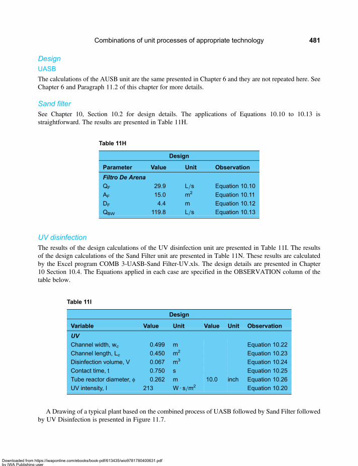
DesignUASB

The calculations of the AUSB unit are the same presented in Chapter 6 and they are not repeated here. SeeChapter 6 and Paragraph 11.2 of this chapter for more details.

Sand filterSee Chapter 10, Section 10.2 for design details. The applications of Equations 10.10 to 10.13 isstraightforward. The results are presented in Table 11H.

UV disinfectionThe results of the design calculations of the UV disinfection unit are presented in Table 11I. The resultsof the design calculations of the Sand Filter unit are presented in Table 11N. These results are calculatedby the Excel program COMB 3-UASB-Sand Filter-UV.xls. The design details are presented in Chapter10 Section 10.4. The Equations applied in each case are specified in the OBSERVATION column of thetable below.

A Drawing of a typical plant based on the combined process of UASB followed by Sand Filter followedby UV Disinfection is presented in Figure 11.7.

Table 11H

Design


Filtro De Arena

QF 29.9 L/s Equation 10.10

AF 15.0 m2 Equation 10.11

DF 4.4 m Equation 10.12

QBW 119.8 L/s Equation 10.13

Table 11I

Design


UV

Channel width, wc 0.499 m Equation 10.22

Channel length, Lc 0.450 m2 Equation 10.23

Disinfection volume, V 0.067 m3 Equation 10.24

Contact time, t 0.750 s Equation 10.25

Tube reactor diameter, φ 0.262 m 10.0 inch Equation 10.26

UV intensity, I 213 W · s/m2 Equation 10.20



11.5 COMBINATION 4: ROTATING MICRO SCREENS FOLLOWEDBY CEPT FOLLOWED BY SAND FILTRATION FOLLOWEDBY UV DISINFECTION11.5.1 IntroductionCEPT is an important appropriate technology unit process because of its capacity to function at the entirerange of temperatures, including very low temperatures. If a effluent quality higher than that which canbe produced by the CEPT unit process is required, sand filtration can be used to polish the CEPTeffluent, so a combination of CEPT followed by sand filtration and, if required, UV disinfection canprovide a good quality effluent, similar to that of conventional treatment. The filtration can be a single ormultimedia sand filtration. The schematic process flow diagram of this combined process is presented inFigure 11.8. The CEPT followed by Sand Filtration process is based on physicochemical and physicalprocesses, with no biological processes involved, so it is not very sensitive to temperature and willfunction well at very low temperatures, and as long as the wastewater does not freeze the process willperform even if the air temperature in the plant site is much lower than zero. The sand filtration producesa clear effluent which can be effectively disinfected. It is recommended to perform pilot plant test to

Figure 11.7 Plan and typical cross section of the combined process of preliminary treatment followed byUASB followed by sand filter followed by UV disinfection



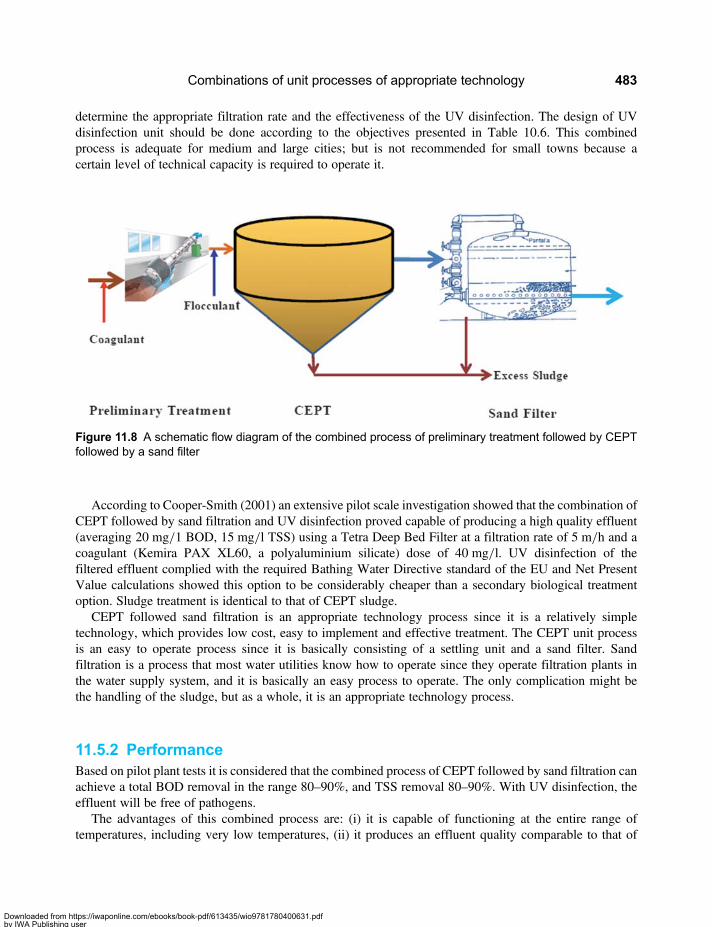
determine the appropriate filtration rate and the effectiveness of the UV disinfection. The design of UVdisinfection unit should be done according to the objectives presented in Table 10.6. This combinedprocess is adequate for medium and large cities; but is not recommended for small towns because acertain level of technical capacity is required to operate it.

According to Cooper-Smith (2001) an extensive pilot scale investigation showed that the combination ofCEPT followed by sand filtration and UV disinfection proved capable of producing a high quality effluent(averaging 20 mg/1 BOD, 15 mg/l TSS) using a Tetra Deep Bed Filter at a filtration rate of 5 m/h and acoagulant (Kemira PAX XL60, a polyaluminium silicate) dose of 40 mg/l. UV disinfection of thefiltered effluent complied with the required Bathing Water Directive standard of the EU and Net PresentValue calculations showed this option to be considerably cheaper than a secondary biological treatmentoption. Sludge treatment is identical to that of CEPT sludge.

CEPT followed sand filtration is an appropriate technology process since it is a relatively simpletechnology, which provides low cost, easy to implement and effective treatment. The CEPT unit processis an easy to operate process since it is basically consisting of a settling unit and a sand filter. Sandfiltration is a process that most water utilities know how to operate since they operate filtration plants inthe water supply system, and it is basically an easy process to operate. The only complication might bethe handling of the sludge, but as a whole, it is an appropriate technology process.

11.5.2 PerformanceBased on pilot plant tests it is considered that the combined process of CEPT followed by sand filtration canachieve a total BOD removal in the range 80–90%, and TSS removal 80–90%. With UV disinfection, theeffluent will be free of pathogens.

The advantages of this combined process are: (i) it is capable of functioning at the entire range oftemperatures, including very low temperatures, (ii) it produces an effluent quality comparable to that of

Figure 11.8 A schematic flow diagram of the combined process of preliminary treatment followed by CEPTfollowed by a sand filter



secondary treatment at lower costs, (iii) It occupies a very low land area, smaller than that of conventionalprocesses, (iv) it has a low energy consumption, and (v) it is easy to operate.

The disadvantages of the combined process are: (i) it produces large quantities of sludge which needs tobe properly managed, and (ii) it is not adequate for small towns.

The estimated investment cost of the combined system CEPT followed by a Sand Filter is in the range40–50 US$/Capita and the O&M cost is in the range 1.5–2.0 US$/Yr/Capita.

11.5.3 DesignThe development of a detailed example for each of the unit process which constitute this combined processare presented in previous chapters. The CEPT process was handled in Chapter 9 while the Sand Filter andUV disinfection are presented in Chapter 10. The reader is referred to these chapters for detailed information.The Excel program which performs the design calculation of combined process 4 is COMB 4-CEPT-SANDFITER-UV.xls. The results of application in series of a CEPT reactor followed by a Sand Filter followed byUV disinfection for the example of 20,000 people are shown below.

Variables selected by the designerCEPT

The designer variables selection and the design procedure in this case is exactly the same as presented inChapter 9, Section 9.3, which can be consulted for details.

Sand filterThe designer variables selection and the design of the sand filter is same as the one presented in paragraph11.4 of this chapter, which can be consulted for details.

UV disinfectionThe designer variables selection is the same as in Paragraph 11.4 of this chapter, which can be consultedfor details.

DesignCEPT

The design procedure in this case is exactly the same as presented in Chapter 9, Section 9.3, which can beconsulted for details.

Sand filterThe design of the sand filter is same as the one presented in Paragraph 11.4 of this chapter, which can beconsulted for details.

UV disinfectionThe procedure in this case is the same as in Paragraph 11.4 of this chapter, which can be consulted for details.

A Drawing of a typical plant based on the combined process of CEPT followed by Sand Filter followedby UV Disinfection is presented in Figure 11.9.



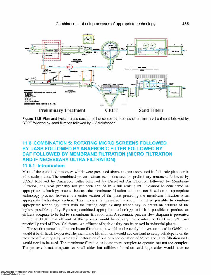
11.6 COMBINATION 5: ROTATING MICRO SCREENS FOLLOWEDBY UASB FOLLOWED BYANAEROBIC FILTER FOLLOWED BYDAF FOLLOWED BY MEMBRANE FILTRATION (MICRO FILTRATIONAND IF NECESSARY ULTRA FILTRATION)11.6.1 IntroductionMost of the combined processes which were presented above are processes used in full scale plants or inpilot scale plants. The combined process discussed in this section, preliminary treatment followed byUASB followed by Anaerobic Filter followed by Dissolved Air Flotation followed by MembraneFiltration, has most probably not yet been applied in a full scale plant. It cannot be considered anappropriate technology process because the membrane filtration units are not based on an appropriatetechnology process; however the entire section of the plant preceding the membrane filtration is anappropriate technology section. This process is presented to show that it is possible to combineappropriate technology units with the cutting edge existing technology to obtain an effluent of thehighest possible quality. By using combined appropriate technology units it is possible to produce aneffluent adequate to be fed to a membrane filtration unit. A schematic process flow diagram is presentedin Figure 11.10. The effluent of this process would be of very low content of BOD and SST andpractically void of Fecal Coliforms. An effluent of such quality can be reused in industrial plants.

The section preceding the membrane filtration unit would not be costly in investment and in O&M, norwould it be difficult to operate. The membrane filtration unit would add cost and its setup will depend on therequired effluent quality, which will determine if one or a combination of Micro and Ultra filtration unitswould need to be used. The membrane filtration units are more complex to operate, but not too complex.The process is not adequate for small cities but utilities of medium and large cities would have no

Figure 11.9 Plan and typical cross section of the combined process of preliminary treatment followed byCEPT followed by sand filtration followed by UV disinfection



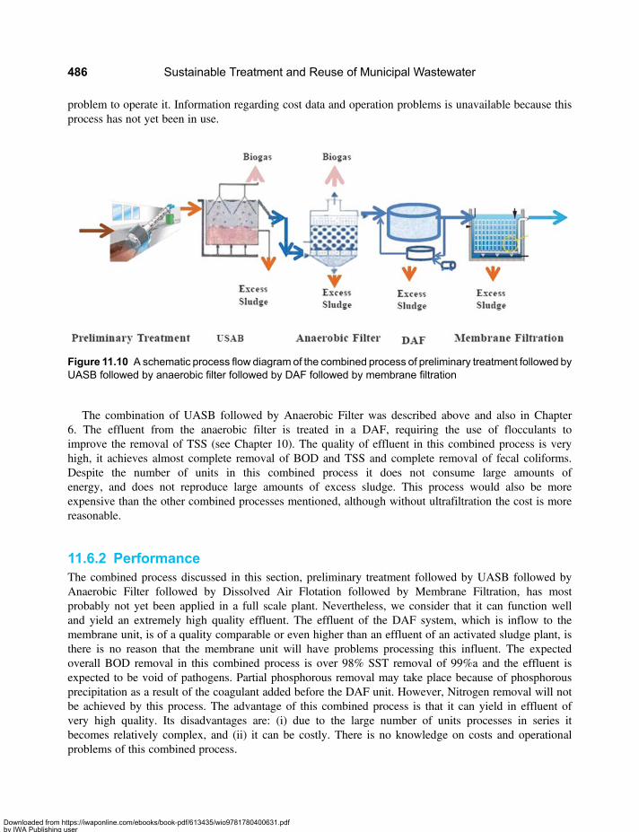
problem to operate it. Information regarding cost data and operation problems is unavailable because thisprocess has not yet been in use.

The combination of UASB followed by Anaerobic Filter was described above and also in Chapter6. The effluent from the anaerobic filter is treated in a DAF, requiring the use of flocculants toimprove the removal of TSS (see Chapter 10). The quality of effluent in this combined process is veryhigh, it achieves almost complete removal of BOD and TSS and complete removal of fecal coliforms.Despite the number of units in this combined process it does not consume large amounts ofenergy, and does not reproduce large amounts of excess sludge. This process would also be moreexpensive than the other combined processes mentioned, although without ultrafiltration the cost is morereasonable.

11.6.2 PerformanceThe combined process discussed in this section, preliminary treatment followed by UASB followed byAnaerobic Filter followed by Dissolved Air Flotation followed by Membrane Filtration, has mostprobably not yet been applied in a full scale plant. Nevertheless, we consider that it can function welland yield an extremely high quality effluent. The effluent of the DAF system, which is inflow to themembrane unit, is of a quality comparable or even higher than an effluent of an activated sludge plant, isthere is no reason that the membrane unit will have problems processing this influent. The expectedoverall BOD removal in this combined process is over 98% SST removal of 99%a and the effluent isexpected to be void of pathogens. Partial phosphorous removal may take place because of phosphorousprecipitation as a result of the coagulant added before the DAF unit. However, Nitrogen removal will notbe achieved by this process. The advantage of this combined process is that it can yield in effluent ofvery high quality. Its disadvantages are: (i) due to the large number of units processes in series itbecomes relatively complex, and (ii) it can be costly. There is no knowledge on costs and operationalproblems of this combined process.

Figure 11.10 A schematic process flow diagram of the combined process of preliminary treatment followed byUASB followed by anaerobic filter followed by DAF followed by membrane filtration



11.6.3 DesignThe development of a detailed example for each of the unit process which constitute this combined processare presented in previous chapters. The UASB and Anaerobic Filter processes are handled in Chapter 6. TheDAF andmembrane processes are handled in Chapter 10. The reader is referred to these chapters for detailedinformation. The Excel program which performs the design calculation of combined process 5 is COMB5-UASB-AF-DAF-MEMBRANES-02.xls. The results of application in series of a UASB reactorfollowed by a Sand Filter followed by a DAF unit followed by a Membrane Filtration unit for theexample of 20,000 people are shown below.

Variables selected by the designerUASB

The calculations are the same as in Chapter 6 and in Section 11.2 of this chapter, and are not repeated here.Consult there for details.

Anaerobic filterThe calculations are the same as in Chapter 6 and in Section 11.2 of this chapter, and are not repeated here.Consult there for details.

DAF

The designer variables selected for the DAF are presented in Table 11J. For design details see Chapter 10,Section 10.3.

Membrane filtrationThe designer variables selected for the Membrane Filtration unit are presented in Table 11K. For designdetails see Chapter 10, Section 10.5.

Table 11J

Designer variables


DAF

QHD 7760.44 m3/d Equation 3.4

TSS, Sa 60.78 mg/L Influent quality

SOR= (Q+Qr)/A 10 m3/h · m2 0.5 a 10.0

Qs 5 Kg/m2 · h 0.5 a 10.0

A/S 0.01 0.006 a 0.2

R 0.5 Qr/QD

f 0.5 0.5–0.6

Qx=QHD · Sa 471.68 kg/h

E, % TSS 95 % Pilot test

Temperature 25.00 °C Influent quality

Sa 17.11 mL/L Equation 10.15



DesignUASB

The calculations are the same as in Chapter 6 and in Section 11.2 of this chapter, and are not repeated here.Consult there for details.

Table 11K

Designer variables


Membrane

BOD5i 48.05 mg/L Influent

BOD5e 5.00 mg/L Norm

BOD5R 100.00 mg/L Reject max limit

TSSi 10.13 mg/L Influent

TSSe 1.00 mg/L Norm

TSSR 100.00 mg/L Reject max limit

QHD 323.35 m3/h Equation 3.4

R(BOD) 0.45 45.32 % Equation 10.29

R(TSS) 0.09 m3/h 9.22 % Equation 10.29

R 0.45 45.32 % Highest R

QDR 146.54 m3/h RQHD

QDP 176.82 m3/h (1−R)QHD

Define Membrane MF Figure 10.16

qMF 1000.00 L/m2 · d Table 10.7

Define Membrane UF Figure 10.16

qUF 0.00 Table 10.7

Define Membrane NF Figure 10.16

qNF 500.00 L/m2 · d Table 10.7

Define Membrane RO Figure 10.16

qOR 0.00 Table 10.7

Table 11L

Design


DAF

Pressure, P 2.1 atm Equation 10.14

Manometric pressure, p 112.4 kPa Equation 10.16

Area fro SOR, A′ 776.0 m2 Equation 10.17

Area from Qs, A′ ′ 141.5 m2 Equation 10.18

Design area, AD 776.0 m2 Largest from A′ and A′ ′

Diameter, DAF 31.4 m Equation 10.19

TSSe 3.0 mg/L According to efficiency



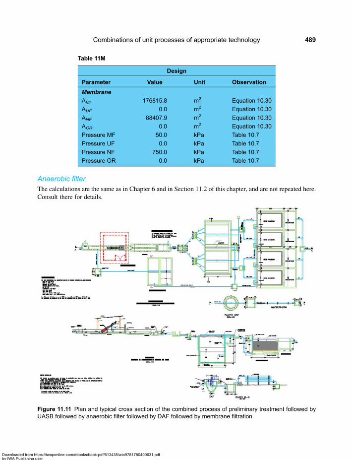
Anaerobic filterThe calculations are the same as in Chapter 6 and in Section 11.2 of this chapter, and are not repeated here.Consult there for details.

Table 11M

Design


Membrane

AMF 176815.8 m2 Equation 10.30

AUF 0.0 m2 Equation 10.30

ANF 88407.9 m2 Equation 10.30

AOR 0.0 m2 Equation 10.30

Pressure MF 50.0 kPa Table 10.7

Pressure UF 0.0 kPa Table 10.7

Pressure NF 750.0 kPa Table 10.7

Pressure OR 0.0 kPa Table 10.7

Figure 11.11 Plan and typical cross section of the combined process of preliminary treatment followed byUASB followed by anaerobic filter followed by DAF followed by membrane filtration



DAF

The results of the design calculations of the DAF unit are presented in Table 11L. For design details seeChapter 10, Section 10.3.

Membrane filtrationThe results of the design calculations of theMembrane Filtration unit are presented in Table 11M. For designdetails see Chapter 10, Section 10.5.

A Drawing of a typical plant based on the combined process of UASB followed by Anaerobic Filterfollowed by DAF followed by Membrane Filtration is presented in Figure 11.11.



Chapter 12

Global warming and wastewater treatmentimpact on climate

12.1 GLOBALWARMING1

12.1.1 IntroductionGlobal warming is the increase in average temperature of the earth’s surface and oceans, which is occurringsince the mid-twentieth century, and the projection of its continuation. Global warming is probably a resultof the observed increase in the concentration of Greenhouse Gases (GHG) emissions of anthropogenicorigin (mainly CO2), which are largely generated by the burning of fossil fuels (coal, oil, natural gas,etc.). Other GHG emissions also contribute to global warming (CH4, N2O, SF6). Water vapour is also agreenhouse gas but its concentration depends on the temperature of the Earth, and is considered in globalclimate models (GCM)2 as the feedback of water vapour. The main non-greenhouse gas contributors togreenhouse effect are the clouds which also absorb and emit infrared radiation and have a similar effectto that of the radiative properties of greenhouse gases. The most abundant greenhouse gases are: (i)water vapour, which contributes about 36–70%, (ii) carbon dioxide, which contributes 9–26%, (iii)methane, which contributes 4–9%; and (iv) ozone, which contributes about 3–7%.

The Kyoto Protocol on climate change is an international agreement that aims to reduce emissions of sixgreenhouse gases that contribute to global warming: carbon dioxide (CO2), methane (CH4) and nitrousoxide (N2O), plus three fluorinated industrial gases: hydro fluorocarbons (HFC), perfluorocarbons (PFC)and sulphur hexafluoride (SF6). This instrument is within the United Nations Framework on ClimateChange Convention (UNFCCC), signed in 1992 during what is known as the Earth Summit in Rio deJaneiro.

On 11 December 1997, industrialized countries agreed in the city of Kyoto to execute a set of measures toreduce greenhouse gases. Signatory governments agreed to reduce during 2008–2012 the averagecontaminating emissions by 5%. with reference to 1990 levels, known as the base year. The agreementcame into force on February 16, 2005, after ratification by Russia on November 18, 2004. The protocolcame to give binding force to what the UNFCCC could not do at the time.

1This section is based on presentations of A. Orozco: (i) “La lucha contra el calentamiento global: una visión diferente”,CORPORACIÓN OTRAPARTE, Medellín-Colombia, 2007” and (ii) “The impact of global warming on wastewater treatment,Water Week 2009, The World Bank, Washington DC, USA, 2009.2Global Climate Models include theGeneral Circulation Models are also known as GCM. Both meanings are valid and relate basicallyto models for the projection of global climate.


On the other hand, other signatories to the Kyoto Protocol which are large producers of CO2, such asChina and India (see Table 12.1 and Figure 12.1), did not acquire reduction commitments because theyare classified as developing countries, whose treatment is different from that of developed countries.However, if we analyze the ranking from the standpoint of per capita emissions, the order is quitedifferent as China and India rank among the lower CO2 emitters as shown in Figure 12.2.

Themain objective of the Kyoto Protocol is to lower anthropogenic greenhouse gas concentrations whichcause greenhouse effect. According to UN Global Climate Model (GCM) projections, it is expected that theaverage temperature of the planet’s surface will rise by between 1.4 and 5.8°C by the year 2100.

The Intergovernmental Panel on Climate Change, known by the acronym IPCC, was established in 1988by the World Meteorological Organization (WMO) and the United Nations Environmental Programme(UNEP). The objective of the IPCC is to assess the risk of climate change caused by human activitiesand its reports are based on publications in scientific and peer-reviewed journals. In 2007 it was awardedthe Nobel Peace Prize, shared with Al Gore. The IPCC is a multinational body charged with conductingnegotiations on global climate change and lead the scientific debate on global warming, the emission ofcarbon particles, the greenhouse effect, and others. Different scenarios of global climate change are

Table 12.1 World ranking producer of CO2 (2005).

Rank Country CO2 MTM

1 United States of America 1576537

2 China (Mainland) 1514126

3 Russian Federation 410290

4 India 382740

5 Japan 335706

6 Germany 213969

7 United Kingdom 149131

8 Canada 146704

9 Republic of Korea 123422

10 Italy (Including San Marino) 123392

11 Islamic Republic of Iran 123246

12 Mexico 115043

13 Indonesia 114518

14 South Africa 111570

15 Saudi Arabia 104015

16 France (Including Monaco) 103082

17 Australia 100671

18 Spain 93805

19 Ukraine 89282

20 Brazil 88834



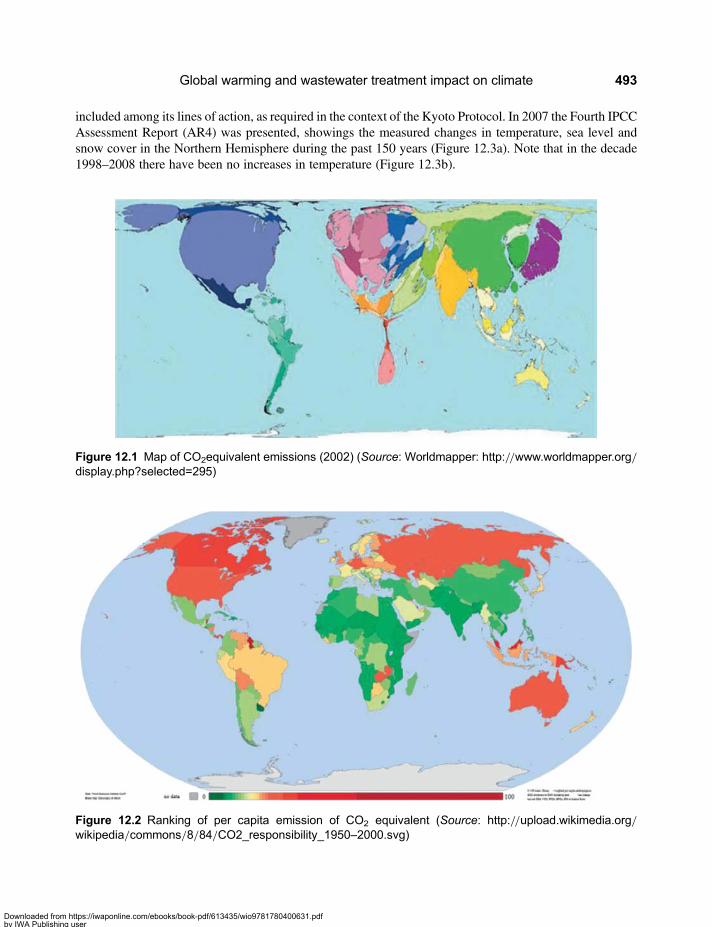
included among its lines of action, as required in the context of the Kyoto Protocol. In 2007 the Fourth IPCCAssessment Report (AR4) was presented, showings the measured changes in temperature, sea level andsnow cover in the Northern Hemisphere during the past 150 years (Figure 12.3a). Note that in the decade1998–2008 there have been no increases in temperature (Figure 12.3b).

Figure 12.2 Ranking of per capita emission of CO2 equivalent (Source: http://upload.wikimedia.org/wikipedia/commons/8/84/CO2_responsibility_1950–2000.svg)

Figure 12.1 Map of CO2equivalent emissions (2002) (Source: Worldmapper: http://www.worldmapper.org/display.php?selected=295)

Global warming and wastewater treatment impact on climate 493


http://www.undp.org/energy/docs/cdmchapter2.pdf














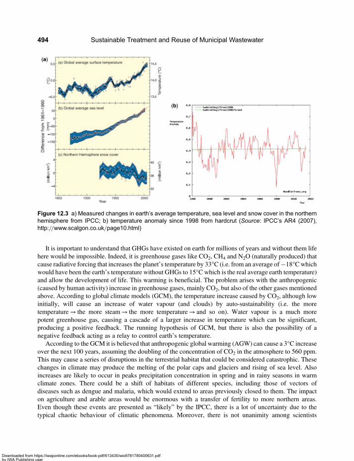
It is important to understand that GHGs have existed on earth for millions of years and without them lifehere would be impossible. Indeed, it is greenhouse gases like CO2, CH4 and N2O (naturally produced) thatcause radiative forcing that increases the planet’s temperature by 33°C (i.e. from an average of−18°Cwhichwould have been the earth’s temperature without GHGs to 15°C which is the real average earth temperature)and allow the development of life. This warming is beneficial. The problem arises with the anthropogenic(caused by human activity) increase in greenhouse gases, mainly CO2, but also of the other gases mentionedabove. According to global climate models (GCM), the temperature increase caused by CO2, although lowinitially, will cause an increase of water vapour (and clouds) by auto-sustainability (i.e. the moretemperature→ the more steam→ the more temperature→ and so on). Water vapour is a much morepotent greenhouse gas, causing a cascade of a larger increase in temperature which can be significant,producing a positive feedback. The running hypothesis of GCM, but there is also the possibility of anegative feedback acting as a relay to control earth’s temperature.

According to the GCM it is believed that anthropogenic global warming (AGW) can cause a 3°C increaseover the next 100 years, assuming the doubling of the concentration of CO2 in the atmosphere to 560 ppm.This may cause a series of disruptions in the terrestrial habitat that could be considered catastrophic. Thesechanges in climate may produce the melting of the polar caps and glaciers and rising of sea level. Alsoincreases are likely to occur in peaks precipitation concentration in spring and in rainy seasons in warmclimate zones. There could be a shift of habitats of different species, including those of vectors ofdiseases such as dengue and malaria, which would extend to areas previously closed to them. The impacton agriculture and arable areas would be enormous with a transfer of fertility to more northern areas.Even though these events are presented as “likely” by the IPCC, there is a lot of uncertainty due to thetypical chaotic behaviour of climatic phenomena. Moreover, there is not unanimity among scientists

Figure 12.3 a) Measured changes in earth’s average temperature, sea level and snow cover in the northernhemisphere from IPCC; b) temperature anomaly since 1998 from hardcrut (Source: IPCC’s AR4 (2007),http://www.scalgon.co.uk/page10.html)








regarding the assumption that anthropogenic CO2 can cause such a temperature change, and some suggestthat the GCM are inaccurate. But invoking the precautionary principle over the magnitude of the globalconsequences that this phenomenon may cause, serious actions are immediately required by the IPCC.

Moreover, it is important to note that in this case enormous economic and political interests areinvolved. Supporters of the Kyoto Protocol, which promotes the reduction of CO2 emissions, benefit inseveral ways. The Kyoto Protocol is very favourable for developing countries that can make big dividendsfrom their forests, as CO2 sequestration agents. So the Kyoto Protocol becomes a source of greateconomic value, without the obligation to comply with limits on greenhouse gas emissions produced bytheir industries. They are also direct beneficiaries of the Clean Development Mechanism (CDM). On theother hand, those who are sceptics that CO2 is responsible for global warming are opposed to the KyotoProtocol because they do not want to spend money on controlling emissions from industries, arguing thatit is going to be wasted money. Each side takes positions on the subject according to its interests.

There is a group of scientists as important as Gregory Benford (professor at the University of California atIrvine, an advisor to NASA and also a science fiction novelist), Paul Crutzen (Nobel Prize laurite inChemistry shared with Molina and Rowland for his research on the ozone hole) and Edward Teller(inventor of the Hydrogen Bomb, now deceased) who while accepting the possibility of CO2 as an agentof global warming, argue that it is not economically feasible to sufficiently control its emissions to stopthe warming. Rather, they proposed global environmental management solutions, which are known asgeoengineering solutions. For example, under one solution it is proposed to place a mylar lens 1000 kmin diameter in a geosynchronous orbit to reduce solar radiation by 1%, which would control the effectsof global CO2 emission in the next 50 years. A most viable solution proposed by Crutzen is to reflect the1% of solar radiation with aerosols artificially injected into the atmosphere in sufficient quantity. Lately,a proposed geoengineering solution known as Budyko’s blanket would cost only US$ 250 million peryear in contraposition to the US$ 1.2 trillion per year required by the IPCC’s proposed solution of fossilfuels substitution by clean energy sources. However, the negative global effects of these solutions areunknown (Orozco, 2011).

12.1.2 Earth’s temperature and warmingIn this section the main factors involved in calculating the earth’s temperature and the greenhouse effect areexplained in a simple form. To begin, it is confirmed that the main energy source of the planet is the sun.Although there are other sources of geological origin, they are so insignificant compared to solarradiation that the latter can be considered for all practical purposes the sole energy source.

Theplanet’s temperature is the result of: (i) theheat coming fromsolar radiation (which radiatesmainly in theelectromagnetic spectrumofvisible light) less the radiation that bounces by reflection (like amirror) of the polarice caps and clouds, and (ii) the heat emitted by the earth as a black body, which itself depends on temperature.The GHG influence warming because they are transparent to solar radiation (visible light), but opaque toinfrared radiation, which is the wavelength at which the planet gives off heat, given its low temperature.

How much radiation comes from the sun?

With reference to the Figure 12.4, it is clear that radiation from the Sun that is intercepted by Earthcorresponds to the shaded area projected onto a plane placed behind the planet. On average the radiationis 1,370 W/m2. However, this radiation is distributed to the entire area of the globe which is four timesgreater, that is, 1,370/4= 342 W/m2 reaches theearth’s surface. Moreover, from the solar radiation thatreaches the earth about 30% is reflected by the polar ice caps, clouds, etc. The percentage reflected,written in decimal form, is called albedo, α.



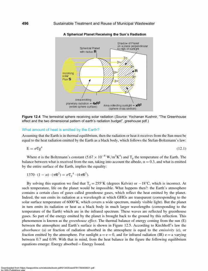
What amount of heat is emitted by the Earth?

Assuming that the Earth is in thermal equilibrium, then the radiation or heat it receives from the Sun must beequal to the heat radiation emitted by the Earth as a black body, which follows the Stefan-Boltzmann’s law:

E = sTg4 (12.1)

Where σ is the Boltzmann’s constant (5.67× 10−8 W/m2K4) and Tg the temperature of the Earth. Thebalance between what is received from the sun, taking into account the albedo, α= 0.3, and what is emittedby the entire surface of the Earth, implies the equality:

1370 · (1− a) · (pR2) = sTg4 · (4pR2).

By solving this equation we find that Tg= 255°K (degrees Kelvin) or −18°C, which is incorrect. Atsuch temperature, life on the planet would be impossible. What happens then?: the Earth’s atmospherecontains a certain class of gases called greenhouse gases, which reflect the heat emitted by the planet.Indeed, the sun emits its radiation at a wavelength at which GHGs are transparent (corresponding to thesolar surface temperature of 6000°K, which covers a wide spectrum, mainly visible light). But the planetin turn emits its radiation or heat as a black body in much larger wavelengths (corresponding to thetemperature of the Earth) which are in the infrared spectrum. These waves are reflected by greenhousegases. So part of the energy emitted by the planet is brought back to the ground by this reflection. Thisphenomenon is known as the greenhouse effect. The thermal balance of energy coming from the sun (E)between the atmosphere and Earth’s surface is shown in Figure 12.5. According to Kirchhoff’s law theabsorbance (a) or fraction of radiation absorbed in the atmosphere is equal to the emissivity (e), orfraction emitted by the atmosphere. For sunlight a= e= 0, and for infrared radiation (IR) e= a varyingbetween 0.7 and 0.99. With that in mind, from the heat balance in the figure the following equilibriumequations emerge: Energy absorbed= Energy Issued.

Figure 12.4 The terrestrial sphere receiving solar radiation (Source: Yochanan Kushnir, “The Greenhouseeffect and the two dimensional pattern of earth’s radiation budget”, greehouse pdf.)



Figure 12.6 The greenhouse effect (Source: Yochanan Kushnir, “The Greenhouse effect and the twodimensional pattern of earth’s radiation budget, pdf Greehouse.)

Figure 12.5 Thermal balance between solar radiation (E) and radiation emission of the atmosphere andsurface. The fraction of E which absorbs the atmosphere is a= 0, and the fraction of IR light it emits is e=aa. Tg is the ground temperature (°K) and Ta is atmosphere temperature



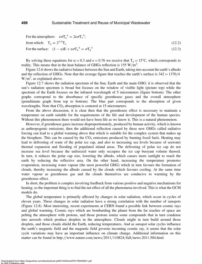
For the atmosphere: esTg4 = 2esTa

4;

fromwhich: Tg = 21/4Ta (12.2)

For the surface: (1− a)E+ esTa4 = sTg

4 (12.3)

By solving these equations for α= 0.3 and e= 0.76 we receive that Tg= 15°C, which corresponds toreality. This means that in the heat balance of GHGs reflection is 155 W/m2.

Figure 12.6 shows the radiative balance between the Sun and Earth, taking into account the earth’s albedoand the reflection of GHGs. Note that the average figure that reaches the earth’s surface is 342= 1370/4W/m2, as explained above.

Figure 12.7 shows the radiation spectrum of the Sun, Earth and the main GHG: it is observed that thesun’s radiation spectrum is broad but focuses on the window of visible light (picture top) while thespectrum of the Earth focuses on the infrared wavelength of 5 micrometers (figure bottom). The othergraphs correspond to the absorbance of specific greenhouse gases and the overall atmosphere(penultimate graph from top to bottom). The blue part corresponds to the absorption of givenwavelengths. Note that CO2 absorption is centered at 15 micrometers.

From the above discussion, it is clear then that the greenhouse effect is necessary to maintain atemperature on earth suitable for the requirements of the life and development of the human species.Without this phenomenon there would not have been life as we know it. This is a natural phenomenon.

However, if greenhouse gases increase disproportionately, produced by human activity, which is knownas anthropogenic emissions, then the additional reflection caused by these new GHGs called radiativeforcing can lead to a global warming above that which is suitable for the complex system that makes upthe biosphere. This can be caused by the CO2 emissions produced by burning fossil fuels. Heating maylead to defrosting of some of the polar ice cap, and also to increasing sea levels because of seawaterthermal expansion and flooding of populated inland areas. The defrosting of polar ice cap do notincrease sea level because the unfreezed water only occupies the ice cap buoyant volume thawed.In turn, it reduces the polar cap size, lowering the albedo, which causes more sunlight to reach theearth by reducing the reflective area. On the other hand, increasing the temperature promotesevaporation, increasing water vapour (the most powerful GHG) which in turn favours the formation ofclouds, thereby increasing the albedo caused by the clouds which favours cooling. At the same timewater vapour as greenhouse gas and the clouds themselves are conducive to warming by thegreenhouse effect.

In short, the problem is complex involving feedback from various positive and negative mechanisms forheating, so the important thing is to find the net effect of all the phenomena involved. This is what the GCMmodels do.

The global temperature is primarily affected by changes in solar radiation, which occur in cycles ofeleven years. These changes in solar radiation have a strong correlation with the number of sunspots(Figure 12.8). Most interesting, recent experiments at CERN found a possible link between cosmic raysand global warming. Cosmic rays which are bombarding the planet from the far reaches of space arepelting the atmosphere with protons, and those protons ionize some compounds that in turn condenseinto aerosols which produce droplets in the atmosphere. Clouds might in turn build around thosedroplets, and those clouds shield the Earth, reducing temperatures. And as sunspot solar cycles influencethe earth’s magnetic field and the magnetic field governs incoming cosmic ray, it seems that the solarcycle variations may have an important influence on climate change. Additional information on thismatter can be found in http://www.nature.com/news/2011/110824/full/news.2011.504.html



http://www.nature.com/news/2011/110824/full/news.2011.504.html









In addition, solar radiation is affected by Milankovitch cycles3, which are related to changes in theposition of the planet, caused by the eccentricity, inclination and precession of the orbit of the Earth,

Figure 12.7 (i) Intensity of solar radiation (top) and terrestrial (bottom) according to wavelength, (ii)wavelengths at which main GHG and the atmospheric reflect radiation (note that CO2 absorbs atwavelengths of 15 micrometers) (Source: http://www.abelard.org/briefings/global_warming_atmospheric_chemistry_physics.php)

3Milutin Milankovitch: Serbian civil engineer and mathematician (1879–1958).



with a period 100,000 years. When all these changes occur simultaneously they cause a significant warmingor cooling, that is, changes in the temperature of the Earth, as shown in Figure 12.9.

Figure 12.9 Milankovicht cycles (Source: http://en.wikipedia.org/wiki/Milankovitch_cycles)

Figure 12.8 Cycle of sunspots (Source: http://es.wikipedia.org/wiki/Variaci%C3%B3n_solar)















Another important point is that the radiative forcings caused by carbon dioxide are not the mostimportant. The most important greenhouse gas is in fact the water vapour, but in the GCM it isconsidered as a feedback that depends on temperature and is not of anthropogenic origin. Indeed, thebasic proposed mechanism of global warming in the GCM is that by increasing (slightly) the temperaturebecause of the CO2, the increase caused by water vapour and clouds will generate a positive feedbackincreasing temperature in an uncontrolled manner (up to 3°C over the next 100 years)4. Warming mayalso be caused by other GHGs, but aerosols cause cooling. The most important sources of aerosols arethe particles emitted by volcanic eruptions and, surprisingly, the fall of meteorites. Indeed, it was ameteorite that caused the cooling of the Earth that led to the extinction of dinosaurs. To project futurewarming trends, it is necessary to model all these effects in the Global Climate Models, and additionally,to incorporate the changes in CO2 and other greenhouse gases caused by anthropogenic emissions.

12.1.3 CO2 emissionThe first alarm about the possibility of global warming caused by anthropogenic emission was given byatmospheric CO2 measurements on the island of Mauna Loa, made by Keeling. These measurementsshowed that regardless of variations caused by the change of seasons, there was a significant trend ofincreasing CO2. Over the years, the trend continued to increase until shaping the hockey stick curvewhich shows CO2 levels above the natural variations of the gas in the pre-industrial era (before 1840), asshown in Figures 12.10 and 12.11. The hockey stick curve somehow overlooked the Medieval WarmPeriod between 1000 and 1200 and the Little Ice Age which occurred around 1600. For these reasonsthere is a controversy about its exactitude.

Figure 12.11 shows that this increase in CO2 (top graph) is correlated with the increase in emissions fromburning fossil fuels which occurred during the industrial era (bottom graph), from the year 1840 on. It seemsthat all the pieces fit in perfectly and that if the atmospheric discharge of CO2 and other greenhouse gases

Figure 12.10 CO2 increase of CO2 in the industrial age (blue) correlated with the increase in the earth’stemperature in respect to the average temperature during 1960–1990 (red) (Source: http://imageshack.us/photo/my-images/244/1000yearsco2smallej4.jpg/sr=1)

4However, it is not fully demonstrated that there is positive feedback. Some authors claim that water vapor decreases with temperaturecausing a negative feedback, that is, rather tends to reduce the temperature to the original temperature of the planet (see Bill Gray, 2009).














(which show similar increasing trends) continues, it is apparent that the fate of the planet is in question,unless necessary precautionary measures are taken. These measures include decrease in the currenttrends of fuel use, by application of new technologies that promote energy saving and substitution offossil fuels with other energy sources such as solar, wind, and in spite of the 2011 explosion atFukuyama’s (Japan) atomic plant, the nuclear energy. At present (2011) global emissions of CO2 amountto more than 9 billion tons, and the tendency is that this figure will double in the next 50 years. Howeverit is important to note that the each KWh of energy produced by solar panel or wind is four and twotimes, respectively, more expensive than conventional energy produced from fossil fuels. Furtherdevelopments in the clean energy field are necessary to lower prices before they can obtain a generalizeduse in times of economic crisis.

12.1.4 GCM: global climate modelsThe GCMhave became the widespread tools to determine howmuch CO2 can be tolerated in the atmospherewithout causing catastrophic global warming and how much fossil fuel emissions may be allowed to obtainthe desired level of CO2. The final temperature of the earth depends on solar radiation, albedo, theconcentration of greenhouse gases, the CO2 sequestered in biomass and dissolved in the ocean, and soon. These variables in turn depend on temperature, thus constituting a feedback phenomenon. In additionGHG concentrations also depend on the anthropogenic emissions and aerosols depend on volcanicevents. And if we consider that each of these variables has a particular value for each of the differentgeographical locations in the planet’s surface since the temperature, humidity, cloudiness and other

Figure 12.11 Growth in CO2 in the industrial era correlated with fossil fuels emissions (Source: http://en.wikipedia.org/wiki/Greenhouse_gas)










variables vary from the Poles to the Equator and from east to west, one can imagine the complexity of theclimate models. Predicting the climate differs from the predicting the weather. The latter applies to theknowledge of weather in one day and given place, while climate predictions refer to monthly averages atfairly large geographic areas. Climate is less exigent than weather forecasting which requires a degree ofprecision that GMC do not posses.

To achieve its goal, in this type of program the entire volume of the atmosphere is divided in cubiccells whose bases are on the surface of the Earth divided like a chessboard, and whose heights are thedepth of the atmosphere divided into several layers from the surface to the stratosphere. In each cell,starting from given initial conditions, the fundamental equations of physics and thermodynamics areapplied. The interrelationships between each cell and its neighbouring cells are applied every hour,simulating the evolution of Earth’s climate. Figures 12.12 and 12.13 show the distribution of cells onthe surface of the Earth taken in one of the most important models, and the formation of the cubiccells with unit volumes. It is possible to build models with smaller cells and estimates of shorter timeintervals (e.g. one minute intervals) but these computations are increasingly complicated, demanding agreater number of operations, that is, greater computing power. But the chaotic nature of theNavier-Stoke’s Equation at the core of the program model will always shown growing uncertainties.Until recently the implementation of the GCM were undertaken in powerful supercomputers located ina selected number of institutions which could afford it. But with the increase in computing capacity ofpersonal computers (PC) model versions such as EdGMC of NASA have been produced, which canrun on a PC to generate acceptable results as research tools. Many scientists prefer in fact usingsimpler versions for their research.

Figure 12.12 Distribution of the grid that forms the cells on the surface of the earth. the third dimension of thecubic cells is given by the height of the atmosphere (Source: Hansen et al. (1983) “efficient three-dimensionalglobal models for climate studies: Models I and II”, Monthly Weather Review, New York, USA)



There are different types of models which apply to different scenarios of behaviour (i.e. businessas usual-. nothing is done; or CO2 doubling, etc.) and then the results can be compared with eachother. Figure 12.14 shown the results of the predicted global average temperature by eight differentGCMs for the IPCC SRES A2 scenario which refers to a “very heterogeneous world, with increasedpopulation.”

Figure 12.14 Temperature increase after 2000 predicted by eight different GCMs for the IPCC SRES A2scenario (Source: http://www.theoildrum.com/story/2006/1/27/44052/9337)

Figure 12.13 Determination of unit volumes (cubic cells) and other elements necessary for theGMC (Source:Gail Box (2000), “The physics of climate and climate change”, ppt)













As seen in Figure 12.14, all the models predict that by the year 2100, the temperature will increase. Therange of the predicted temperature increase is between 2.3 and 4.8°C, concentrating around 3.5°C. Thedifference between the models is not big, but not small either. The IPCC offers various scenarios ofaction to anticipate probable warming for different cases5 simulated by different models, which yield aprobable value and range. The GCM is the tool available to anticipate the effects of the conduct ofhuman society on the climate and on this tool scientists base their proposals to remedy the impact of theforecasted trends.

On the other hand, a new theory has recently been proposed6 with a constraint in the initialconditions of the modelling that, if correct, could convert the GCM results obtained until now intoirrelevant data. According to this theory, the planet has a regulatory system that maintains a constanttemperature, regardless of internal phenomena, and it can only change with incidence of changes insolar radiation.

12.1.5 The data of vostok and other analysesOne of the most surprising modern science accomplishments has been undertaken by a group of Russian,French and North-American scientists in 1998 to measure the earth’s climate in the past, includingtemperature and concentrations of GHGs, from analysis of the contents of air bubbles trapped in ice inthe Russian station at Vostok, Antarctica. For this research 3623 meters were drilled in order to obtainice cores. The conclusions of the analysis of data obtained in this study are surprising and have beenconfirmed by additional ice drilling in different locations. Given the importance of these data to validatethe results obtained by the IPCC, it is important to give a brief discussion to understand their meaning.In the drilling of ice cores, age can be inferred from seasonal layers that are clearly visible, GHGs can bemeasured directly from the bubbles, and temperature can be estimated quite accurately from the variationin the bubble’s frozen oxygen 18 isotope (δ18O).

Analysis of data from Vostok produced the results shown in Figure 12.15. At a first glance the resultsare surprising and at a time of their generation they were considered as the definite proof of theimportance of the impact of CO2 on global warming. A version of these curves is presented by Al Gorein his famous documentary.

However, these same data analyzed in detail showed phenomena that have become a Gordian knot for thecommunity of the IPCC. Indeed, a careful analysis of the curves shows two things: (i) increase of thetemperature always occurs before the increase of CO2 concentration, about 800 years earlier, and (ii) theglaciations (variation of the glacial-interglacial temperature change of approximately 6°C) occur every100,000 years, the same period of one of Milankovitch’s cycles which are related to changes in solarradiation or sunlight that reaches Earth. This means that the temperature triggers climate changes and theCO2 concentration increases in response to this change, and is not the reason for the change.Interestingly, it also triggered changes in CH4 and N2O, which follow the same patterns of temperaturechange. And temperature changes coincide with the extreme heat, as shown in Figure 12.16, which alsoshows the correlation of the glaciations to the Milankovitch’s cycles. Although there are explanations ofthese graphs in the IPCC scenarios, they have not generated consensus within the scientific communityitself.

5See the IPCC report “Climate Change 2007: The Physical Science Basis-Summary for Policymakers”, for a clarification of scenariosand outcomes. The article can be downloaded from http://www.ipcc.ch/SPM2feb07.pdf.6See F. Miskolczi (2007), “Greenhouse Effect in Semi-Transparent Planetary Atmospheres”, Idojaras, 111, No. 1, Hungary.



http://www.ipcc.ch/SPM2feb07.pdf





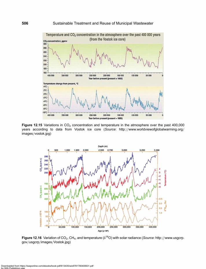
Figure 12.15 Variations in CO2 concentration and temperature in the atmosphere over the past 400,000years according to data from Vostok ice core (Source: http://www.worldviewofglobalwarming.org/images/vostok.jpg)

Figure 12.16 Variation of CO2, CH4, and temperature (δ18O) with solar radiance (Source: http://www.usgcrp.gov/usgcrp/images/Vostok.jpg)

















Themost common explanation is that: (i) radiation triggers temperature change but then, by feedback, theCO2 takes command of climate change; and (ii) δ18O (the proxy by which temperature id calculated) doesnot correspond to the same period of the gases, because of diffusion within the ice. This is not a satisfactoryexplanation to the community of climate scientists.

12.1.6 The Kyoto ProtocolThe Kyoto Protocol is an agreement made within the framework of the United Nations Convention onClimate Change. This international instrument aimed at reducing within the period from 2008 to 2012approximately 5% emissions, compared to 1990 emissions, of six greenhouse gases which are probablepromoters of warming Global: (i) carbon dioxide (CO2), (ii) methane (CH4), and (iii) nitrous oxide(N2O), plus three fluorinated industrial gases: (iv) hydrofluorocarbons (HFCs), (v) perfluorocarbons(PFCs), and (vi) sulphur hexafluoride (SF6). The protocol required that it be ratified by countries with acombined CO2 production greater than 55% of global emissions. Currently 160 countries have ratifiedthe Kyoto protocol. The protocol follows, in general terms, the following principles7:

(a) Governments are separated into different categories: developed countries, referred to as Annex Icountries (which have the obligation of reducing GHG emissions and must undergo an annualinventory of greenhouse gas) and developing countries, designated as non-Annexed (which haveno obligation to reduce GHG emissions, but rather, can participate in the Clean DevelopmentMechanism). There is a special category within the annexed countries, which is that of“transition countries” (towards a market economy), typically the countries of the former “ironcurtain” that can benefit through the mechanisms of Joint Investment (JI).

(b) Any Annex I country which cannot meet its Kyoto obligation will be penalized 1.3 times its GHGemission permits and still have to meet them in the second quarter of the commission for each ton ofGHG emissions that exceed their top in the first period of commission (i.e. 2008–2012).

(c) By 2008–2012, Annex I countries must reduce their GHG emissions by an average 5% belowtheir 1990 levels. For many countries, such as the European Union (EU) Member States, thispercentage corresponds in some cases to 15% below their expected GHG emissions in 2008.While the average emissions reduction is 5%, national limitations range from 8% reductions forthe EU to a 10% emissions increase for Iceland, but since the EU intends to meet its target bydistributing different rates among its member states, much larger increases (up to 27%) areallowed for some of the least developed countries of the EU. The limitations of the reductionwill expire in 2013.

(d) The Kyoto Protocol includes “flexible mechanisms” that do not prevent economies of Annex I toobtain the limits by purchasing GHG emission reductions elsewhere. These can be purchased orobtained in financial exchanges (such as the new emissions trading system in the EU, which hasno relation to Kyoto) or projects that reduce emissions in non-Annexed countries under theClean Development Mechanism (CDM), or in other Annex I countries in transition, under themechanism of JI (Joint Implementation).

(e) Only the certified emission reduction (CER) accredited by the board of the CDM can be bought andsold in this way. Under the aegis of the UN, Kyoto established the board of the clean developmentmechanism to determine and approve “CDM projects” in economies that are not annexed beforegranting CER. A similar scheme called “Joint Implementation (JI) is applied in transitionaleconomies mainly covering the former Soviet Union and Eastern Europe before.

7http://en.wikipedia.org/wiki/Kyoto_Protocol.



http://en.wikipedia.org/wiki/Kyoto_Protocol






This means that non-Annexed countries do not need to comply the GHG emission limits, but if they developa GHG reduction project, it can provide them carbon credits to be sold to Annex I countries. This also createsa global system of carbon trade credits through the CER. In this way, it helps to highly developed countriesto meet targets with cheaper projects in developing countries, and at the same time stimulates the reductionof greenhouse gases in these countries. This protocol favours developing countries. It also favours thedeveloped nations that have no indigenous sources of fossil fuels, since these restrictions aretremendously expensive thus forcing the search for less expensive systems in energy use and researchand development of alternative fuels. However, Germany made an exception with its coal industry,which does not need to comply with the protocol.

An interesting case is that of Russia. President Putin ratified Kyoto in November 2004 against the opinionof the Russian Academy of Sciences, the Ministry of Industry and Energy and the president’s economicadviser, Andrey Illaroniov, in return for the EU support for Russia’s admission to WTO (World TradeOrganization). With this ratification, the Kyoto Protocol could enter into force after completing morethan 55% of global CO2 emissions. It is noteworthy that in the base year for emissions of 1990 Russiahad a terrible environmental control system, so it is relatively easy for Russia to meet its goals.

The Kyoto Protocol allows the possibility of obtaining carbon credits through sequestration of CO2

permanently in the jungles and forests, with sustained techniques of forestation and reforestation. Theyare being implemented gradually while obtaining agreements on verification methods. There are othermethods of carbon sequestration in oceans, soil, and so on, not eligible for CER. The CO2 can also bestored geologically (in the subsoil)8.

The main countries that initially opposed the Kyoto Protocol were USA (most recently demandingthat China and India be included among countries requested to provide legally binding commitments oncurbing greenhouse gas emissions) and Australia (which signed in 2009 and now is one of the firstcountries to tax oil).

As of today (November 2011) Russia, Japan and Canada told the G8 that they would not join a secondround of carbon cuts under the Kyoto Protocol at United Nations talks this year, and the US reiterated itwould remain outside the treaty. The future of the Kyoto Protocol has become central to the efforts tonegotiate reductions of carbon emissions under the UN’s Framework Convention on Climate Change,whose annual meeting will take place in Durban, South Africa, from November 28 to December 9, 2011.

12.1.7 IPPC proposalsThe IPCC is a multinational body in charge of conducting negotiations on global climate change and directthe scientific debate on global warming, the emission of carbon particles, the greenhouse effect, and others.The different scenarios of global climate change (those arising in the context of the Kyoto Protocol) areincluded among its lines of action.

There is a range of proposals to meet the proposed limits of GHGs. A summary of those proposals ispresented in the September 2006 issue of Scientific American, “Energy’s Future-Beyond Carbon”.Basically, these proposals aim at the following goals: (i) avoiding the use of fossil fuels, (ii)implementation of nuclear energy, (iii) use of hydrogen as a fuel, (iv) use of biofuels and renewableenergy (solar, wind, biomass, etc.), and (v) development of new methods of energy generation such asnuclear fusion, the capture of wind at high altitude, the use of solar panels in space to obtain energyfrom the sun, the production solar cells by nanotechnology, the implementation of a global electric

8http://en.wikipedia.org/wiki/Carbon_sequestration



http://en.wikipedia.org/wiki/Carbon_sequestration






interconnection by superconductors, utilization of the energy of waves and tides, the genetic creation ofmicrobes to produce energy. All these methods are still far from immediate implementation and may bein use in the future. Curiously, one of the most promising clean energy sources, Low Energy NuclearReactions (LENR)9 is not mentioned in this description. On the other hand, big hopes are assigned tonuclear energy, now banned in several countries because of the Fukuyama atomic plant explosion duringthe aftermath of 2011 earthquake in Japan of 8.9 degrees on Richter scale. Biofuels are still considered apromising path to meet the limits, in spite of the fact the breakthroughs are still needed to be able toreplace oil with plant-based fuels, since efforts are proving that this is difficult to achieve10.

In any case, the intended effect is to reduce atmospheric CO2 emissions, for which action have beenproposed in different fields, namely: (i) generation of energy, (ii) efficiency and energy conservation bythe end-user, (iii) carbon sequestration, (iv) use of alternative energies, and (v) best practices inagriculture and reforestation. Each measure has several proposals to cut a wedge on the CO2 productionequivalent to the reduction of 25 Giga-tons of carbon in 50 years. Figure 12.17 shows the trend ofgrowth of CO2 emissions in the “business as usual” scenario – nothing is done-, and how, with sevenwedges it can be maintained constant at 7 billion tons of emissions per year.

The proposal of the wedges was made by Socolow and Pacala in the article “A Plan to Keep Carbon inCheck” in the September 2006 issue of Scientific American (pp 28–35). According to the authors, thereduction of each wedge starts at zero and ends at 1 GtC/yr in 50 years (2055 in Figure 12.17). In thearticle the authors propose fifteen feasible methods of lowering a wedge, each method defined withinone of the five fields mentioned above. For example, increasing the fuel economy from 30 to 60 milesper gallon in two billion cars produce a wedge of savings (25 GtC) in the field: “(ii) energy efficiencyand conservation by the end user”; raising the efficiency of 1600 coal-based power plants from 40 to

Figure 12.17 With the reduction of seven wedges it is possible to maintain the CO2 emission levels of 2005(Source: http://climatechangeaction.blogspot.com/2007/01/guest-post-by-almuth-ernsting-global.html)

9http://landshape.org/enm/rossis-e-cat-a-black-swan-event/10Biello (2011).















http://landshape.org/enm/rossis-e-cat-a-black-swan-event/












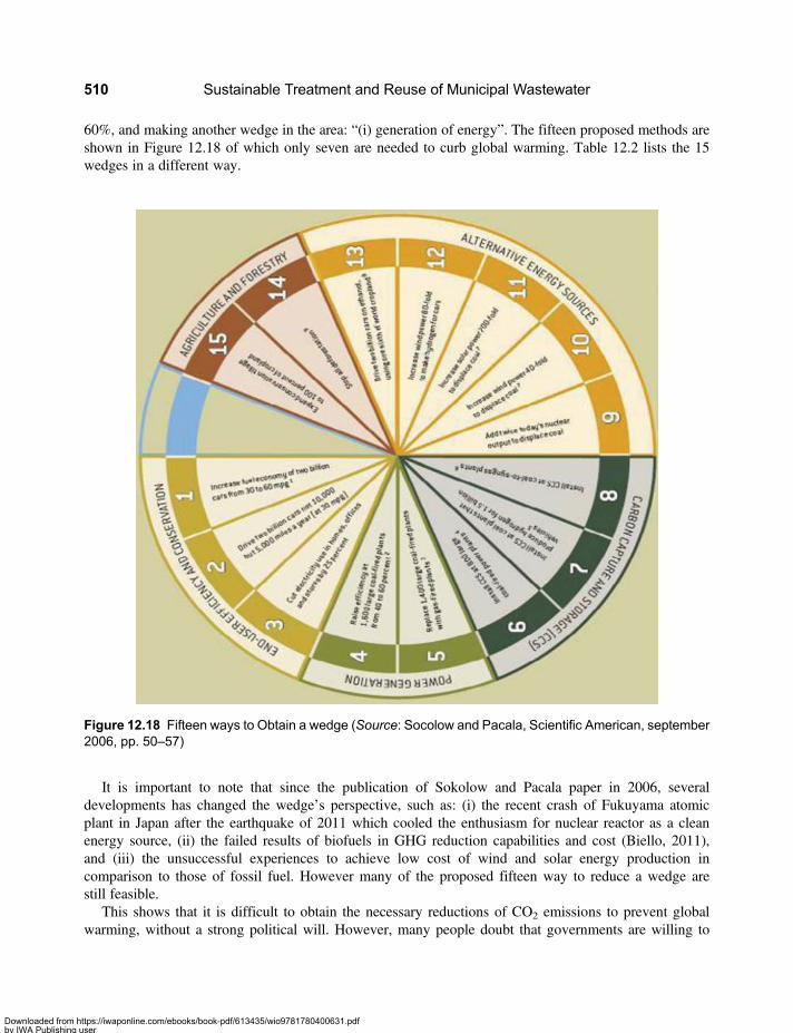
60%, and making another wedge in the area: “(i) generation of energy”. The fifteen proposed methods areshown in Figure 12.18 of which only seven are needed to curb global warming. Table 12.2 lists the 15wedges in a different way.

It is important to note that since the publication of Sokolow and Pacala paper in 2006, severaldevelopments has changed the wedge’s perspective, such as: (i) the recent crash of Fukuyama atomicplant in Japan after the earthquake of 2011 which cooled the enthusiasm for nuclear reactor as a cleanenergy source, (ii) the failed results of biofuels in GHG reduction capabilities and cost (Biello, 2011),and (iii) the unsuccessful experiences to achieve low cost of wind and solar energy production incomparison to those of fossil fuel. However many of the proposed fifteen way to reduce a wedge arestill feasible.

This shows that it is difficult to obtain the necessary reductions of CO2 emissions to prevent globalwarming, without a strong political will. However, many people doubt that governments are willing to

Figure 12.18 Fifteen ways to Obtain a wedge (Source: Socolow and Pacala, Scientific American, september2006, pp. 50–57)



take actions that go against their interests in the short term, and it is therefore necessary to evaluate otheralternatives to control the phenomenon of global warming, by cutting CO2 global emissions.

12.1.8 Geoengineering proposalsGeoengineering is defined as “options that would involve large-scale engineering of our environment inorder to combat or counteract the effects of changes in atmospheric chemistry”. Many believegeoengineering is a politically more realistic method of controlling climate change. In fact, whenanalyzing the complexity of actions required meeting the objectives of the Kyoto Protocol and themultiplicity of political interests of different states, one can conclude that it is required to seekmechanisms to achieve more direct control of global climate. When one of the authors of this book(Orozco) became interested in the details of global warming, it seemed to him that the obvious thing wasto control solar radiation, the main source of energy that heats the Earth. In fact the relevant calculationswere made with the help of 1D (one dimension) programs written with symbolic algebra softwareMathematica 5.2 and concluded that the a deviation of 1% of solar radiation would control globalwarming the next 100 years. The result is presented in Figure 12.19, which shows that with a 1%deviation of solar radiation global average temperatures will vary by less than 1°C in the next century.

As the average temperature of the planet is composed of extreme temperatures that vary from the poles tothe equator, and has multiple causes that the GCM can assess more accurately, then the EdGMC programfrom NASA was ran with 1% reduction in solar radiation during the next 20 years and it was found that thevariation of the average surface temperature is minimal (see Figure 12.20), and the average temperature

Table 12.2 Fifteen ways to reduce a wedge of 25 GtC in 50 years.

1. Fuel Economy: increase mileage from 30 to 60 mpg in 2 billion cars.

2. Reduce annual mileage of 2 billion cars from 10,000 to 5000 miles (30 mpg).

3. Efficient use of electricity in homes, offices, warehouses with cuts of 25% (a 50% cut would yield twowedges)

4. Efficient use of oil and gas in space heating and industrial processes.

5. Biofuels: drive two billion cars on ethanol (shown ineffective and unfeasible, see Biello, 2011)

6. Increase wind power 80 times to make hydrogen for cars (wind power twice as costly as coal power)

7. Increase 700-fold solar energy to displace coal (solar power four times as costly as coal power)

8. Increase wind power 40-fold to displace coal (wind power twice as costly as coal power)

9. Increase twice today’s nuclear output to displace coal (banned in many countries today)

10. Install CCS (Carbon Capture and Storage) in 800 large coal-fired power plants.

11. Install CCS at coal plants to produce hydrogen for 1.5 billion vehicles

12. Install CCS at coal plants-syngas

13. Raise efficiency at 1,600 large coal-fired power plants from 40 to 60%

14. Stop logging

15. Expand conservation tillage methods to the entire arable area.

Source: https://www.commentmgr.com/projects/1148/docs/IAF_5Feb07_Part_One_B.ppt



http://cd4cdm.org/Publications/cdm%20guideline%202nd%20edition.pdf








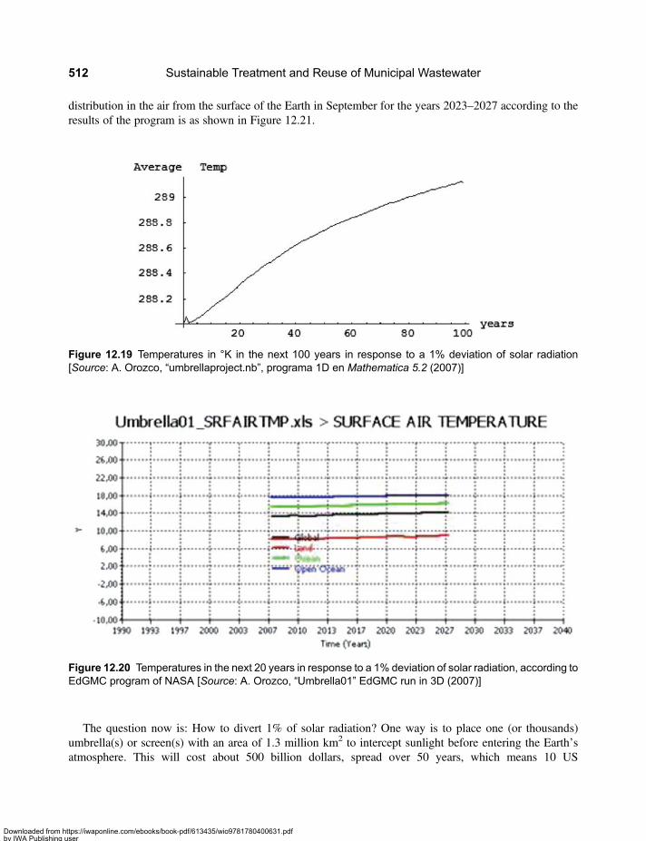
distribution in the air from the surface of the Earth in September for the years 2023–2027 according to theresults of the program is as shown in Figure 12.21.

The question now is: How to divert 1% of solar radiation? One way is to place one (or thousands)umbrella(s) or screen(s) with an area of 1.3 million km2 to intercept sunlight before entering the Earth’satmosphere. This will cost about 500 billion dollars, spread over 50 years, which means 10 US

Figure 12.19 Temperatures in °K in the next 100 years in response to a 1% deviation of solar radiation[Source: A. Orozco, “umbrellaproject.nb”, programa 1D en Mathematica 5.2 (2007)]

Figure 12.20 Temperatures in the next 20 years in response to a 1% deviation of solar radiation, according toEdGMC program of NASA [Source: A. Orozco, “Umbrella01” EdGMC run in 3D (2007)]



$billion/year11, not really much compared with the costs of Kyoto (USD1.2 trillion per year during50 year).

However, there have been several proposals in this regard since years ago. In fact in 1991 the patent5’003.186 was granted in the U.S. to Chang and collaborators, to control global warming with thelaunch into the stratosphere of Welsbach particles (metal oxides, e.g. aluminium) which reflect sunlightof certain wavelengths12. In 1998 Edward Teller, father of the hydrogen bomb, proposed the reduction of1% of solar radiation reaching the Earth at an estimated cost of US$ one billion per year13. In 2006 theNobel laureate Paul Crutzen proposed altering Earth’s albedo deliberately adding sulphate aerosols tomimic the volcanic eruptions that have cooled the planet in the past, obviously making it in a controlledmanner14.

Figure 12.21 Average surface air temperatures in september during 2023–2027 in response to a 1%deviation of solar radiation, according to EdGMC program of NASA [Source: A. Orozco, “Umbrella01”EdGMC run in 3D (2007)]

11A. Orozco, “EconomicsUmbrella.nb” (2007) en Mathematica 5.2.12See http://www.airapparent.ca/library/abstract/welsbach_seeding.htm13See http://www.hoover.org/publications/digest/3522851.html14See http://www.realclimate.org/index.php/archives/2006/06/geo-engineering-in-vogue/



http://www.airapparent.ca/library/abstract/welsbach_seeding.htm







http://www.hoover.org/publications/digest/3522851.html







http://www.realclimate.org/index.php/archives/2006/06/geo-engineering-in-vogue/












And even before that, Gregory Benford science fiction novelist and professor at the Universityof California at Irvine, had proposed to launch a Fresnel lens made of Mylar of 1,000 km indiameter to a geosynchronous orbit at the Lagrangian point L-1 (located at a distance of 1.5 millionkilometres from earth, where the gravity of the Sun and of the Earth cancel each other). In factothers had proposed similar ideas before. But in June 2006 in a presentation at the Skeptics Society15

Benford improved the idea proposing to locate a curtain of particles of diatomaceous earth ofspecific size in the stratosphere (of 25 km height) to reflect the income of 1% of solar radiation.Interestingly, we can select the wavelength that is rejected and the first option is very seductively,ultraviolet rays.

The estimated cost of one billion dollars per year of this solution is hundreds of times less thanthe proposed by Kyoto Protocol. Benford proposed the idea along with colleagues fromStanford University and the Lawrence Livermore National Laboratory. He projected to conduct asmall scale test in the Arctic, where the released particles can be controlled by circulation patternspresent in the area. NASA has shown interest in the project and there are private investors willing tofund the research.

In fact since 1992 the U.S. Congress had funded a study that was published in 2000 by the NationalAcademy Press, with the participation of a member of the National Academies of Science, Engineeringand Medicine, which concluded that the more effective mitigation solution to global warming is thelaunch in the atmosphere of reflective spray aerosol compounds via commercial military andprivate aircrafts.

It is clear then that the U.S., as the main opponent of Kyoto, has in its sleeve studied options for the casethat global warming is a reality and not, as some think, an implausible idea. According to the apologists ofgeoengineering, the implementation of the Kyoto protocol is not feasible because trying to regulate theclimate by policy actions is simply impossible, given the diversity of interests of states and due tohuman nature.

Projects to control solar radiation have the advantage of the speed of implementation. Other techniquesthat fall into the geoengineering category include:

• Cool Roof: using light-coloured materials to cover floors and ceilings to increase the albedo ofthe earth.

• Increasing the reflectivity of clouds, using fine aerosols of sea water to whiten the clouds with saltcrystals. A very interesting proposal in this regard is the Roto-Nave Buckau. Stephen Salterproposed robots versions of these ships that could spray seawater into the air to create clouds,shielding the earth from the sun (see Figure 12.22).

There are other proposals for geoengineering in radically different directions. The main other, perhaps, isto add iron into the ocean to promote the growth of phytoplankton, which in turn sequester CO2 from theatmosphere, known as the Geritol16 solution. In a trial in which 500 kg of iron were added into a 100km2 area of the Pacific Ocean the stimulation to the formation of plankton served to sequester about350,000 kg of CO2. Performing this procedure on a global scale could capture billions of tons. However,many fear the side effects of such a planktonic soup spreading through all the oceans of the world, whichwould certainly be unpredictable.

15See http://www.heartland.org/Article.cfm?artId=1948416See http://www.airapparent.ca/library/full_text/iron_vs_greenhouse.htm



http://www.heartland.org/Article.cfm?artId=19484






http://www.airapparent.ca/library/full_text/iron_vs_greenhouse.htm







12.1.9 Final reflectionsThanks to the documentary “An Inconvenient Truth” by Al Gore, the IPCC reports (with the support of theUN) and the Virgin Earth Challenge Prize of US$ 25 million for finding a technically and economicallyfeasible solution to the problem of global warming, it was possible to convey to the public the notionthat anthropogenic global warming is a reality and that the effects of this phenomenon has implicationswhich may be disastrous for mankind if not prevented in a timely manner.

Consequently, strategies have been adopted as the Kyoto protocol, with the support of the IPCC, leadingto controling the emissions of CO2 and other greenhouse gases. The protocol is supported almost by allnon-Annex countries, including two of the largest global contributors of GHG: China and India.

On the other hand, the geoengineering community has made proposals, some a little dangerous asthe Geritol solution, others to be implemented somewhat in the future as a Mylar lens to be placed1,500,000 km away from the Earth and other plausible as the inflation of aerosol of Diatomaceousearth of 1 micron in diameter to reject 1% of solar radiation and with it a great deal of ultravioletradiation. The most practical up to day is the solution known as the Budyko’ Blanket which proposes topump to the stratosphere SO2 with a cost of USD 250 million per year estimated by Intellectual Ventures(Orozco, 2011). The world needs to keep working on these type of solutions which do not requiremonumental political effort as that required for implementing Kyoto Protocol.

What then needs to be done? the solution probably is in the middle, a combination of several initiatives.To resolve this impasse it will be necessary to reduce some emissions wedges of 25,000 million tons ofcarbon, reflect away from the earth part of the solar radiations at a level of some digits per thousandspraying aerosols in the stratosphere, and replace some fossil fuels with alternative forms of energy. Onerecently emerging alternative form of energy is the known as Low Energy Nuclear Reactions (LENR),which is in an experimental stages in Bologna, Italy17 and other places (including at NASA), which ifsuccessful would represent a completely new avenue to confront global warming.

Figure 12.22 The ship roto-nave buckau that can spray sea water into the air

17http://landshape.org/enm/academics-eat-rossis-dust/



http://landshape.org/enm/academics-eat-rossis-dust/









Global warming will probably not be the predicted warming, so it will be necessary to refine thetechnical tools, especially the GMC, and above all to improve the knowledge of the laws that govern theplanet’s climate. With these and other actions, the human species will manage to reign on Earth foranother thousand years. However, major environmental organizations such as Friends of the Earth andGreenpeace are reluctant to endorse geoengineering. Some have argued that any public support for thistype of solution could undermine the fragile political consensus to reduce GHG emissions.

12.2 WASTEWATER TREATMENT IMPACT ON CLIMATE12.2.1 Emission factors (EF) of green house gases in wastewatertreatment systems18

The wastewater originating from a variety of domestic, commercial and industrial sources can be treatedin situ, or can be conveyed by sewerage systems to a centralized plant, or be discharged throughsub-aquatic outfalls. Domestic wastewater is generated by household activity, while industrial wastewateris the waste of industrial processes. The treatment and discharge systems can be differentiated for ruraland urban users and for high income and low income users. The wastewater treated in a wastewatertreatment system (WWTS) includes both domestic and industrial wastewater, as well as some rainwater,all of which jointly are known as municipal wastewater.

Most WWTS consist of several combined processes including mechanical treatment, biological andchemical processes. In the mechanical treatment suspended particles, sand and oil are separated from thewastewater and dehydrated sludge is generated and further stabilized by different processes. In general,the stabilization of organic sludge can be divided into biological and chemical processes. Biologicalprocesses include anaerobic stabilization where sludge is stabilized in anaerobic digesters, and aerobicstabilization is effected by extended aeration of the sludge.

The wastewater and sludge produced can be a source of methane (CH4) when treated anaerobically ordisposed of without treatment. They can also be a source of nitrous oxide (N2O) if they are nitrificationand then denitrification. Emissions of carbon dioxide (CO2) from wastewater are not considered in theIPCC guidelines because they are of biogenic origin and should not be included in the counting nationaltotal emissions. “Biogenic origin” means that the carbonaceous organic matter of the wastewater comesfrom the atmospheric CO2: which is used by CO2-fixing vegetation to form organic biomass, which inturn serves as food for animals, and so on. This organic matter is consumed by man, and part of it, dueto its metabolic transformation, is discharged into the wastewater. When the organic matter isdecomposed in the wastewater treatment plants, the CO2 originally captured in food is recycled again(liberated to the athmosphere), so there is no new addition of carbon dioxide to the atmosphere. Thecarbon dioxide came from the atmosphere and is returned to the atmosphere in the same amount.

This is the reason that GHGs considered in wastewater treatment plants are CH4 (generated by anaerobictreatment processes) and N2O (generated by nitrification and denitrification). The methane gas produced inanaerobic treatment has an equivalence of 1ton CH4= 23 ton-equivalent CO2 (CO2e) from the standpoint ofthe Global Warming Potential (GWP) of 100 years. This locates the methane as the most important GHG inwastewater treatment industry. Nitrous oxide, produced in the process of nitrification-denitrification, has anequivalence of 1ton N2O= 320 ton CO2e, that is, it is a stronger GHG than methane, but it is produced only

18Based On “2006 IPCC guidelines for national greenhouse gas inventories, Volume 5: WASTE-Chapter 6: wastewater treatment anddischarge”, IPCC, WMO, UNEP (2006); In “Guidelines for College-Level Greenhouse Gas Emissions Inventories” by JulianDautremont-Smith (2002); “Approved baseline and monitoring methodology AM0039: Methane emissions reduction from organicwastewater and bioorganic solid waste using composting” de UNFCCC/CCNUCC (1996).



in small quantities so its impact is not large and it is less important than the methane. If nitrification-denitrification does not occur in the WWTS it might occur in the effluent receiving water body and thegeneration of N2O may occur there.

Emission factor of N2OAccording to FAO, the consumption of protein in the USA in 1999 was 114.9 g protein/capita · d, whilein Colombia it was 60 g (0.060 kg) in 200019. The default fraction of nitrogen in the proteins providedby the IPCC is 0.16 kg-N/kg-protein. Default Emission Factor (EF) in sewage given by the IPCC is0.005 kg N2O-N/kg-N (range 0.0005 to 0.25). Using the default values as described above and takinginto account that the fraction of N in N2O is (28/44) the equation for the production of N2O based onthe nitrogen discharged in the wastewater directly into a water body, is thus:

kgN2O/yr = NAREFAR(44/28) (12.4)

where:

N2O = nitrous oxide, kg N2O /yearNAR = nitrogen discharged to the aquatic environment, kg N/yearEFAR = emission factor of N2O discharged in wastewater, N2O-N kg/kg NThe (44/28) is the conversion factor from kg N2O-N to kg N2O

On the other hand, the N2O produced during nitrification and denitrification in wastewater treatment, asmeasured in the USA plants, is 3.2 g N2O/capita · yr

20 and if we have industrial and commercialdischarges, it is necessary to apply a default factor (Find-com) of 1.25, so another equation for N2Oproduction in WWTS is:

(kgN2O/yr)WTSP = P× 3.2 kgN2O/capita · year × Find−com = P× 4 kgN2O/capita · yr (12.5)

where P is the population.

Emission factors of CH4

The IPCC provides the following equation to calculate CH4 emissions from treated wastewater:

kgCH4 = P · (DOM) · [1− (%DOM) eliminated as sludge](CH4)maxMCF− kg(CH4)burned (12.6)

where DOM is the per capita degradable organic matter andMCF is the methane correction factor. Similarly,to calculate the emissions from sludge treatment, the IPCC suggests the following equation:

kgCH4 = P · (DOM) · [(%DOM)eliminated as sludge] · (CH4)max ·MCF− kg(CH4)burned (12.7)

The per capita degradable organic matter can be measured as BOD. The IPCC suggests a default value(DOM)= 0.05 kg DBO5/capita · d, unless we know the real value for the country. The latest IPCCguidelines on best practices suggest a maximum output of 0.6 kg CH4/kg DBO5. The methanecorrection factor (MCF) depends on the type of treatment (see Table 12.3 below) and the proposed

19Food Security Statistics – Colombia, FAO (2006)20“2006 IPCC guidelines for national greenhouse gas inventories, Volume 5: WASTE-Chapter 6:wastewater treatment and discharge”,

IPCC, WMO, UNEP (2006)



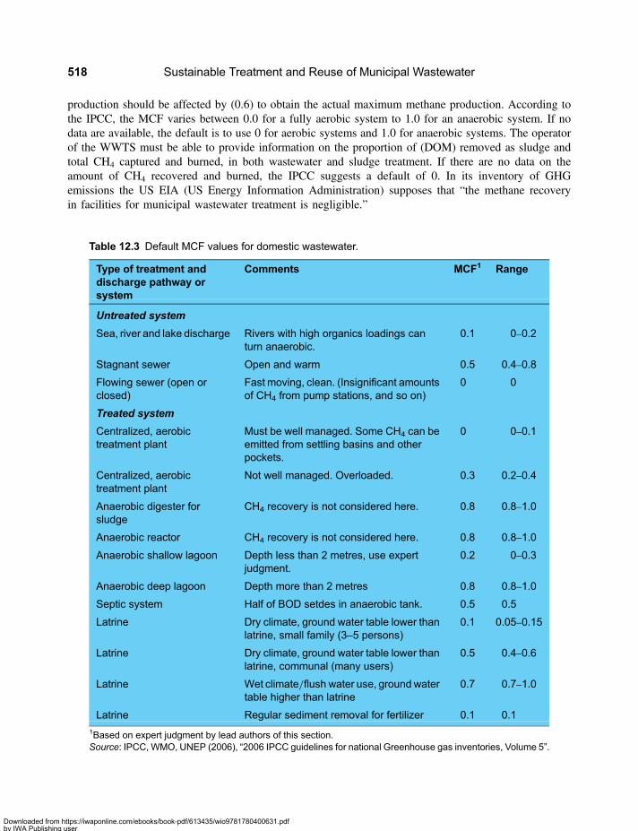
production should be affected by (0.6) to obtain the actual maximum methane production. According tothe IPCC, the MCF varies between 0.0 for a fully aerobic system to 1.0 for an anaerobic system. If nodata are available, the default is to use 0 for aerobic systems and 1.0 for anaerobic systems. The operatorof the WWTS must be able to provide information on the proportion of (DOM) removed as sludge andtotal CH4 captured and burned, in both wastewater and sludge treatment. If there are no data on theamount of CH4 recovered and burned, the IPCC suggests a default of 0. In its inventory of GHGemissions the US EIA (US Energy Information Administration) supposes that “the methane recoveryin facilities for municipal wastewater treatment is negligible.”

Table 12.3 Default MCF values for domestic wastewater.

Type of treatment anddischarge pathway orsystem

Comments MCF1 Range

Untreated system

Sea, river and lake discharge Rivers with high organics loadings canturn anaerobic.

0.1 0–0.2

Stagnant sewer Open and warm 0.5 0.4–0.8

Flowing sewer (open orclosed)

Fast moving, clean. (Insignificant amountsof CH4 from pump stations, and so on)

0 0

Treated system

Centralized, aerobictreatment plant

Must be well managed. Some CH4 can beemitted from settling basins and otherpockets.

0 0–0.1

Centralized, aerobictreatment plant

Not well managed. Overloaded. 0.3 0.2–0.4

Anaerobic digester forsludge

CH4 recovery is not considered here. 0.8 0.8–1.0

Anaerobic reactor CH4 recovery is not considered here. 0.8 0.8–1.0

Anaerobic shallow lagoon Depth less than 2 metres, use expertjudgment.

0.2 0–0.3

Anaerobic deep lagoon Depth more than 2 metres 0.8 0.8–1.0

Septic system Half of BOD setdes in anaerobic tank. 0.5 0.5

Latrine Dry climate, ground water table lower thanlatrine, small family (3–5 persons)

0.1 0.05–0.15

Latrine Dry climate, ground water table lower thanlatrine, communal (many users)

0.5 0.4–0.6

Latrine Wet climate/flush water use, ground watertable higher than latrine

0.7 0.7–1.0

Latrine Regular sediment removal for fertilizer 0.1 0.1

1Based on expert judgment by lead authors of this section.Source: IPCC, WMO, UNEP (2006), “2006 IPCC guidelines for national Greenhouse gas inventories, Volume 5”.



Indirect emissionsFor fully aerobic WWTP, up to 1.4 kilograms of CO2/kg COD (removed) originate from the production ofenergy for aeration. This means that more CO2 is produced in generating energy for the aeration than in theactual treatment process of the wastewater, and this energy generation is typically from fossil fuels, while thecarbon of wastewater comes mostly from sources of renewable energy (i.e. food, which is of biogenicorigin).

With this consideration, a change from anaerobic to aerobic processes for sludge treatment or for theliquid wastewater treatment has a massive impact on the production of fossil fuel: 0.8 kg extra of CO2

produced per kg COD removed because of the shift to aerobic sludge digestion. In terms of GHGproduction, the total output (in CO2 equivalent) may be reduced from 2.4 kg of CO2/kg COD (removed)in fully aerobic treatment to 1.0 kg CO2/kg COD (removed) in anaerobic processes.

In this respect, significant advantages are associated with the use of anaerobic processes because it ispossible to largely eliminate the net energy input to the aerobic processes when using anaerobicprocesses, and therefore reduce the production of greenhouse gases from fossil fuels.

12.2.2 Methodologies of quantification of green house gases inwastewater treatment systemsBased on the foregoing discussion we suggest the following methodology for calculating GHG in theWWTP:

Quantification of N2OEmissions of nitrous oxide (N2O) can take place as direct emissions at treatment plants, or indirectly asemissions after the disposal of wastewater or effluents into watercourses, lakes or the sea. Directemissions from nitrification and denitrification processes in wastewater treatment plants can beconsidered small sources. Typically, these emissions are much lower than those of the effluent. and canonly be of interest to advanced countries whose wastewater treatment plants predominantly includenitrification and denitrification. The calculation of N2O emission from a WWTS is as follows:

(1) Determine the contributing population (P) to the WWTP(2) Determine if there are industrial and commercial contributions. If there are, assume Find-com= 1.25.(3) Apply Equation 12.5:

(kgN2O/yr)STAP = P× 3.2 kgN2O/capita · yr × Find-com

(4) Determine equivalent CO2 (CO2e) with:

CO2e = 320 (kg N2O/yr)STAP/1000 ton

Quantification of CH4

Methane production of a WWTP depends on the watewater treatment process and on the sludgeproduction and treatment. If treatment is aerobic in both cases (wastewater and sludge), then there is noproduction of CH4 and the CO2 produced is not taken into account because it is biogenic, that is, CO2

eventually will be trapped again in the wastewater through the biological mechanisms of organic matterformation.

If the wastewater treatment is aerobic but there is anaerobic sludge treatment, then, for the calculation ofCH4 produced, use the equation:

(kg CH4)WWTP = P× DOM× (%DOM) eliminated as sludge× (CH4)max ×MCF



If part or all of the CH4 is recovered or burned, subtract it from the total amount produced, and iteventually may be subject to obtain Carbon certificates in the case of a non-annexed countries under theKyoto protocol. The calculation is as follows:

(1) Determine the contributing population (P) to the WWTP (use the concept of equivalent populationif there are industrial wastewaters).

(2) Determine country’s DOM or set a DOM= 0.05 kg DBO5/capita · d.(3) Determine the fraction of the DOM trapped as primary or secondary sludge. If the exact figure is not

known for the WWTP, use 0.30.(4) Define (CH4)max= 0.05 kg DBO5/capita · d(5) From Table 12.3 determine the MCF= 0.8.(6) For aerobic wastewater treatment apply the equation:

(kg CH4)WWTP = P× DOM× (%DOM) eliminated as sludge× (CH4)max ×MCF

(7) Determine the CO2e with:

CO2e = 23 (kgCH4/yr)WWTP/1000 ton

(8) If the wastewater treatment is anaerobic, then use the equation:

(kg CH4)WWTP = P× DOM× (1−%DOM) eliminated as sludge× (CH4)max ×MCF

and follow the previous steps.

12.2.3 The impact of wastewater on global warmingTo have some measure of the participation of wastewater in the production of GHG, it is important to obtainthe proportions by sector from the country’s GHG inventories (see the different sectors in Figure 12.23) andthe GHG for different countries (see Figures 12.24 and 12.25). From these figures it is observed that theproportions for different countries are reasonably constant, so if you get data from a country that hasgood inventories of GHGs which were estimated with sufficient resources, it is possible to extend thefindings to the rest of the world. As a basis of inventory for these proportions the inventories of the USAsince its GHGs inventories were carefully estimated.

Figure 12.23 Structure of GHG-producing sectors [Source: IPCC, WMO, UNEP (2006)]



Table 12.4 taken from the EPA (2008) - “Inventory of U.S. Greenhouse Gas Emissions and Sinks: 1990–2006”, USA, shows that in terms of CO2e, the waste sector contributes 2.3% of the total GHG. In addition,Table 12.5 shows the different proportions of contributions within the waste sector and indicates that interms of CO2e the percentage of GHG contribution by the wastewater’s sector to the waste sector is 20%.Figure 12.26 summarizes the above conclusions and provides that wastewater contributes 0.46% of thetotal GHG emissions. Consequently, it is concluded that the wastewater sector is not a significant sectorin terms of generating GHGs, but it still has an influence on the final results of GHG emissions, so itshould not be overlooked.

Figure 12.24 Share of GHG by sector and country [Source: EPA (2008), “Inventory of U.S. Greenhouse gasemissions and sinks: 1990–2006”]

Figure 12.25 Share of GHG by GHG and country [Source: EPA (2008), “Inventory of U.S. Greenhouse gasemissions and sinks: 1990–2006”]



Table 12.4 Recent trends in US Greenhouse gas emissions and sinks by chapter/IPCC sector.

Chapter/////IPCCsector

1990 1995 2000 2001 2002 2003 2004 2005 2006

Energy 5,203.9 5,529.6 6,067.8 5,982.8 6,036.3 6,078.3 6,150.9 6,174.4 6,076.9

Industrialprocesses

299.9 315.7 326.5 297.9 308.6 301.2 315.9 315.5 320.9

Solvent and otherProduct use

4.4 4.6 4.9 4.9 4.4 4.4 4.4 4.4 4.4

Agriculture 447.5 453.8 447.9 463.7 449.0 434.3 432.1 453.6 454.1

Land use,land-use change,and forestry(Emissions)

13.1 13.6 30.0 20.0 28.4 19.7 17.1 23.2 36.9

Waste 179.6 176.8 155.6 152.1 154.5 160.3 157.7 158.7 161.0

Total Emissions 6,148.3 6,494.0 7,032.6 6,921.3 6,981.2 6,998.2 7,078.0 7,129.9 7,054.2

Net CO2 Flux fromland use, land-usechange, andforestry (Sinks)*

(737.7) (775.3) (673.6) (750.2) (826.8) (860.9) (873.7) (878.6) (883.7)

Net emissions(sources andsinks)

5,410.6 5,718.7 6,359.0 6,171.1 6,154.4 6,137.3 6,204.3 6,251.3 6,170.5

* The net CO2 flux total includes both emissions and sequestration, and constitutes a sink in theUnited States. Sinks are onlyincluded in net emissions total.Note: Totals may not sum due to independent rounding. Parentheses indicate negative values or sequestration.Source: EPA (2008), “Inventory of U.S. Greenhouse Gas Emissions and Sinks: 1990–2006”.Note that Waste Sector Emissions are 2.3% of Total Emissions.

Table 12.5 Emissions from wastes.

Gas/////Source 1990 1995 2000 2001 2002 2003 2004 2005 2006

CH4 172.9 169.1 146.7 143.0 145.5 151.0 148.1 149.0 151.1

Landfills 149.6 144.0 120.8 117.6 120.1 125.6 122.6 123.7 125.7

Wastewater Treatment 23.0 24.3 24.6 24.2 24.1 23.9 24.0 23.8 23.9

Composting 0.3 0.7 1.3 1.3 1.3 1.5 1.6 1.6 1.6

N2O 6.6 7.7 8.9 9.2 9.0 9.3 9.6 9.7 9.9

Domestic WastewaterTreatment

6.3 6.9 7.6 7.8 7.6 7.7 7.8 8.0 8.1

Composting 0.4 0.8 1.4 1.4 1.4 1.6 1.7 1.7 1.8

Total 179.6 176.8 155.6 152.1 154.5 160.3 157.7 158.7 161.0

Note: Totals may not sum due to independent rounding.Note that Emissions of Domestic Wastewater Treatment are 20% of the Emissions of the Waste Sector.



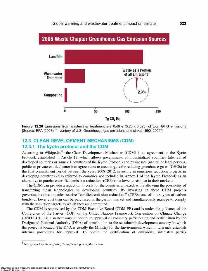
12.3 CLEAN DEVELOPMENT MECHANISMS (CDM)12.3.1 The kyoto protocol and the CDMAccording to Wikipedia21, the Clean Development Mechanism (CDM) is an agreement on the KyotoProtocol, established in Article 12, which allows governments of industrialized countries (also calleddeveloped countries or Annex 1 countries of the Kyoto Protocol) and businesses (natural or legal persons,public or private entities) enter into agreements to meet targets for reducing greenhouse gases (GHGs) inthe first commitment period between the years 2008–2012, investing in emissions reduction projects indeveloping countries (also referred to countries not included in Annex 1 of the Kyoto Protocol) as analternative to purchase certified emission reductions (CERs) at a lower costs than in their markets.

The CDM can provide a reduction in costs for the countries annexed, while allowing the possibility oftransferring clean technologies to developing countries. By investing in these CDM projectsgovernments or companies receive “certified emission reductions” (CERs, one of three types of carbonbonds) at lower cost than can be purchased in the carbon market and simultaneously manage to complywith the reduction targets to which they are committed.

The CDM is supervised by the CDM Executive Board (CDM-EB) and is under the guidance of theConference of the Parties (COP) of the United Nations Framework Convention on Climate Change(UNFCCC). It is also necessary to obtain an approval of voluntary participation and certification by theDesignated National Authority (DNA) of contribution to the sustainable development country in whichthe project is located. The DNA is usually the Ministry for the Environment, which in turn may establishinternal procedures for approval. To obtain the certification of emissions, interested parties

Figure 12.26 Emissions from wastewater treatment are 0.46% (0.20× 0.023) of total GHG emissions[Source: EPA (2008), “Inventory of U.S. Greenhouse gas emissions and sinks: 1990–2006”]

21http://en.wikipedia.org/wiki/Clean_Development_Mechanism



http://en.wikipedia.org/wiki/Clean_Development_Mechanism






(industrialized country and developing country recipient of the project) should demonstrate a long-term andmeasurable real emission reduction.

CDM projects can be carried out in various sectors and activities such as energy; industry; transportation;agriculture; solids waste and wastewater; and reduce some of the greenhouse gases or capture CO2 inforestry projects (reforestation). They can be small or large scale project. Projects that are classified assmall-scale are:

• Renewable energy projects (i.e. hydroelectric plants) with a maximum capacity equivalent to 15 MW,• Energy efficiency projects to reduce energy consumption by the supply and/or demand side, up to 60

GWh per year;• Other projects that reduce anthropogenic emissions and directly emit less than 60 kt CO2e;• Reforestation activities with a capture capacity of less than 16 kton of CO2e annually.

Some useful definitions are:

COP: The Conference of the Parties, the supreme body of the Kyoto Protocol which is responsible for theimplementation of the protocol.

Executive Board (EB): is responsible for overseeing the operation of the CDM, to review and prepare thedetailed decisions of the mechanism and ensure satisfactory performance. It is also the entity thatapproves the list of projects and issues CERs.

Designated Operational Entity (DOE): Institutions responsible for validating CDM projects and verifyand certify the CERs.

Designated National Authority (DNA): In the host countries, is responsible for evaluating the sustainabledevelopment criteria country on a CDM project. After assessing the project, the DNA issuesd a letterapproving the project. For example, in the case of Colombia the DNA is the Ministry of Environment,Housing and Territorial Development.

CER: Certified Emission Reductions.PDD: Project Design Document.

The format and guidelines for preparing a PDD is available on the website of the UNFCCC http://cdm.unfccc.int/Reference/Documents. The CDM project cycle is presented in Figure 12.27. Table 12.6presents some applicable projects to CDM by sector.

12.3.2 Requirements of the CDMTo develop a practical methodology for preparation of a CDM project, use the PDD form which is availablein pdf format on the web:

http://cd4cdm.org/Publications/cdm%20guideline%202nd%20edition.pdf (as of 2011). This brochureshows the guidelines and procedures, step by step, to fill in the paperwork.

In order to be eligible for CDM, take into account the following:

• Projects should be developed on a voluntary basis.• GHG emissions reductions must be real and measurable.• GHG emissions reductions must be additional. Some definitions:

Additionality: A project activity is additional if GHG emissions of anthropogenic origin are reducedbelow those that occurred in the absence of the proposed project activity.Baseline or reference scenario for a CDM project activity is the scenario that reasonably representsthe GHG emissions of anthropogenic origin that occurred in the absence of the proposed projectactivity.



http://cdm.unfccc.int/Reference/Documents













Figure 12.27 Cycle of a proposed clean development mechanism (CDM) project [Source: http://www.undp.org/energy/docs/cdmchapter2.pdf]











Methodologies for baselines are the methodologies used to establish the baseline and monitoring plan.They are of two types: (i) methodologies approved by the UNFCCC and (ii) new developmentmethodology.

• The project should have contributions to Sustainable Development of the host country, according to:Social criteria.Economic criteria.Environmental criteria.

• The project should have a limited crediting period. There are two types:Renewable: 3 periods of 7 years.Mixed: 10 years, not renewable.

The format for the PDD contains the following sections:

A. General description of project activity

B. Baseline methodology

C. Duration of the project activity/crediting period

D. Monitoring methodology and plan

E. Calculation of GHG emission by sources

F. Environmental impacts

G. Stakeholder comments

(Continued )

Table 12.6 Projects applicable to CDM.

Project types Small-scale CDM project activity categories

Type 1: Renewableenergy projects

A. Electricity generation by the userB. Mechanicaf energy for the userC. Thermal energy for the userD. Renewable electricity generation for a grid

Type II: Energyefficiencyimprovementprojects

A. Supply side energy efficiency improvements – transmissionand distribution

B. Supply side energy efficiency improvements – generationC. Demand-side energy efficiency programmes for specific

technologiesD. Energy efficiency and fuel switching measures for industrial

facilitiesE. Energy efficiency and fuel switching measures for buildings

Type III: Otherproject activities

A. AgricultureB. Switching fossil fuelsC. Emission reductions by low-greenhouse gas emission

vehiclesD. Methane recoveryE. Methane avoidance

Types 1 – III: Other small-scale project

Source: http://cd4cdm.org/Publications/cdm%20guideline%202nd%20edition.pdf (2011)









Annex 1. Contact information on project participants

Annex 2. Information regarding public funding

Annex 3. New baseline methodology

Annex 4. New monitoring methodology

Annex 5. Table of baseline data

Table 12.7 defines the conditions which the investing country and the host country have to comply(Rozado, 2006).

The methodology for calculating emissions follows the procedures presented in paragraph 12.2.2.The nomenclature of the PDD is different from the one presented in this chapter, However, the examplepresented in the following section will follow the official PDD nomenclature so as to avoid confusion.

12.3.3 A CDM case study: Santa Cruz, Bolivia22

The total population of Santa Cruz, Bolivia, in 2007 (see city’s location in Figure 12.28) was about 1.3million and it keeps growing at a high annual rate of about 6%. Forecasts indicate that by 2025 the city’spopulation will be about 2.76 million and in 2039 it will reach about 3.7 million. In Santa Cruz,sanitation services are provided by 10 cooperatives of which SAGUAPAC is the largest, serving 65% ofthe city’s area. Sewerage coverage in SAGUAPAC’s service area is about 50%, giving Santa Cruz anoverall level of sewerage coverage of 32% that represents approximately 450,000 inhabitants. Thecollected wastewater is conveyed to three existing municipal wastewater treatment plants: Plant North 1(denominated plant N1), Plant North 2 (denominated N2) and Plant East (denominated Plant E). The

Table 12.7 Conditions for investing and host countries for CDM.

Investing country Host country

• Ratification of Kyoto Protocol.• To be the country in Annex I.• Voluntary participation.• Designate a national authority.• Establish national working guides and

procedures to approve CDM projects.• Establish a National Registration.• Allocate and control the rights of emission

in the country.• Submit the yearly national inventory most

recently required.

• Ratification of Kyoto Protocol.• To be country not Annex I.• Designate a national authority for the

activity of the CDM project.• Participation in an activity of CDM

projects must be voluntary.

22Based on SAGUAPAC (2006), “Project design document form-Clean Development Mechanisms”. Santa Cruz de la Sierra, Bolivia;and Libhaber, Menahem (2006), “Annex 15: Wastewater Treatment Technical Aspects: Increasing the Treatment Capacity of theExisting Wastewater Treatment Plants of Santa Cruz”, in The World Bank (2006) Project Appraisal Document on the BoliviaUrban Infrastructure Project, Report No. 36796-BO, October 13, 2006, Washington D.C, USA.



Figure 12.28 The location of the city of Santa Cruz

Figure 12.29 Locations of the lagoon systems in Santa Cruz [Source: SAGUAPAC (2007), personalcommunication]



location of these plants is presented in Figure 12.29. When the three plants were constructed they werelocated outside the city limits. As a result of the city’s growth, they are currently located within the cityand are surrounded by residential neighbourhoods.

Treatment plants have proved to be very efficient for the removal of organic matter and fecal coliforms;however, by including in each plant anaerobic lagoons, biogas is being generated by them as a by-productand the main component in the biogas is methane. Figure 12.30 shows the layout of Plants N1 and N2,indicating the location of the anaerobic lagoon.

SAGUAPAC, fulfilling its quality policy of continuous improvement, conducted a study to define theworks of upgrading its treatment plants, seeking to increase their capacity and to reduce the emission ofgreenhouse gases that contribute to global warming. As a result of the study the treatment process wasmodified. The new treatment process flow diagram is presented in Figure 12.31. The treatment plantswere upgraded in accordance with the new flow diagram. The project involved the capture of the biogasgenerated in the anaerobic lagoons, washing and flaring it. The main facilities included in the project ofcapturing and flaring the biogas are:

Figure 12.30 Wastewater treatment plants N1 and N2 in Santa Cruz [Source: SAGUAPAC (2007)]



• Floating cover on the anaerobic lagoons, including a system of biogas collection.• Gas extraction and conveyance system.• Gas flaring unit.

One of the objectives of the project was to reduce biogas emissions from the treatment plants ofSAGUAPAC by installing a system to capture, transport and flare it, framed within the guidelines of theClean Development Mechanism (CDM). The methodology for the capture and transport of the biogas ispresented in the Chapter 5.

To apply for the CDM, SAGUAPAC considered the following aspects:

• Type III: Other project activities;• Category III.H: Methane recovery in wastewater treatment.• Technology/measure (iv): Introduction of methane recovery and combustion to an existing anaerobic

wastewater treatment system such as anaerobic reactor, lagoon, septic tank or an onsite industrialplant.

• The technology employed includes the following stages: 1) capturing of biogas generated at theanaerobic lagoons, 2) transportation of the biogas from the anaerobic lagoons to the biogastreatment plants, 3) washing of the biogas in a packed tower, and 4) combustion of the biogas in aclosed flare.

The main components of the biogas system and their main technical specifications are:

(a) geomembrane to cover the lagoons: HDPE, 1.5 mm, UV resistant, 0.94 g/cm3

(b) floaters, counterweights and inspection openings(c) collection pipes: HDPE, 6′′ diameter, ½′′ holes every 0.20 m(d) transportation pipes: HDPE, 4′′ diameter, 3.5 m/s, 3.5 kg/cm2

(e) suction pool: 18′′ diameter, 6 m long(f) regenerative turbines: multistage, 2 bars(g) scrubbing tower (for the industrial wastewater treatment plant only): absorption of H2S, 24′′

diameter tower, 3 m long, relief valve, manometer, safety valve

Figure 12.31 The upgraded process flow diagram of the wastewater treatment in Santa Cruz [Source:SAGUAPAC (2007)]



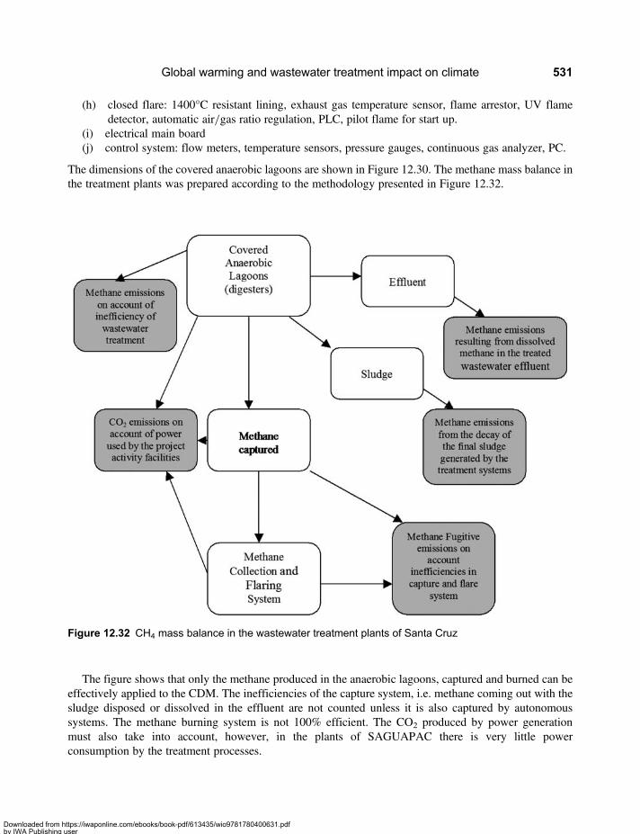
(h) closed flare: 1400°C resistant lining, exhaust gas temperature sensor, flame arrestor, UV flamedetector, automatic air/gas ratio regulation, PLC, pilot flame for start up.

(i) electrical main board(j) control system: flow meters, temperature sensors, pressure gauges, continuous gas analyzer, PC.

The dimensions of the covered anaerobic lagoons are shown in Figure 12.30. The methane mass balance inthe treatment plants was prepared according to the methodology presented in Figure 12.32.

The figure shows that only the methane produced in the anaerobic lagoons, captured and burned can beeffectively applied to the CDM. The inefficiencies of the capture system, i.e. methane coming out with thesludge disposed or dissolved in the effluent are not counted unless it is also captured by autonomoussystems. The methane burning system is not 100% efficient. The CO2 produced by power generationmust also take into account, however, in the plants of SAGUAPAC there is very little powerconsumption by the treatment processes.

Figure 12.32 CH4 mass balance in the wastewater treatment plants of Santa Cruz



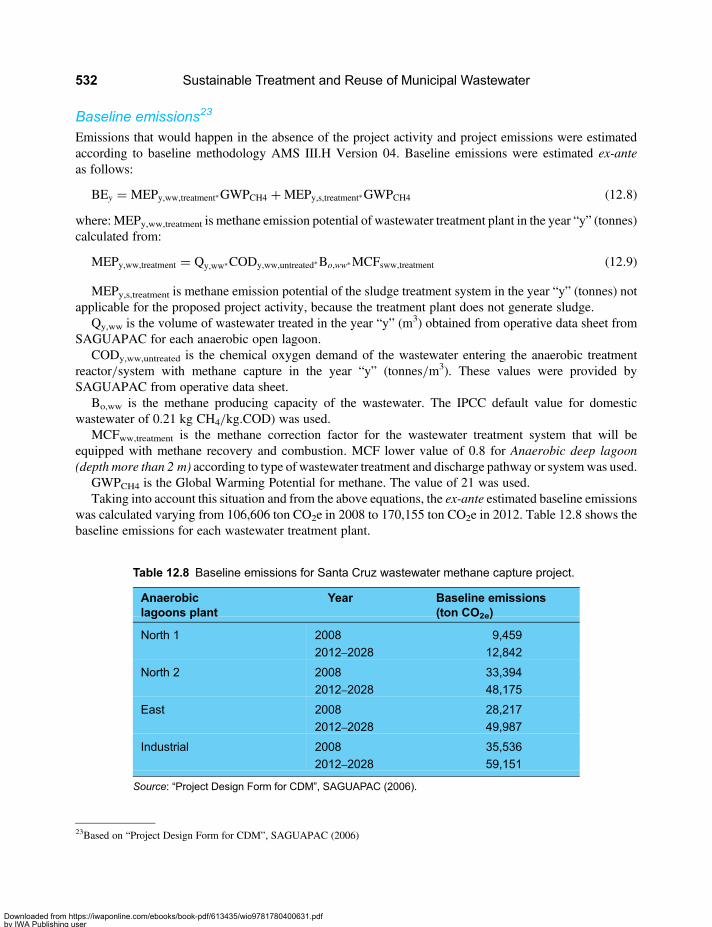
Baseline emissions23

Emissions that would happen in the absence of the project activity and project emissions were estimatedaccording to baseline methodology AMS III.H Version 04. Baseline emissions were estimated ex-anteas follows:

BEy = MEPy,ww,treatment∗GWPCH4 +MEPy,s,treatment∗GWPCH4 (12.8)

where: MEPy,ww,treatment is methane emission potential of wastewater treatment plant in the year “y” (tonnes)calculated from:

MEPy,ww,treatment = Qy,ww∗CODy,ww,untreated∗Bo,ww∗MCFsww,treatment (12.9)

MEPy,s,treatment is methane emission potential of the sludge treatment system in the year “y” (tonnes) notapplicable for the proposed project activity, because the treatment plant does not generate sludge.

Qy,ww is the volume of wastewater treated in the year “y” (m3) obtained from operative data sheet fromSAGUAPAC for each anaerobic open lagoon.

CODy,ww,untreated is the chemical oxygen demand of the wastewater entering the anaerobic treatmentreactor/system with methane capture in the year “y” (tonnes/m3). These values were provided bySAGUAPAC from operative data sheet.

Bo,ww is the methane producing capacity of the wastewater. The IPCC default value for domesticwastewater of 0.21 kg CH4/kg.COD) was used.

MCFww,treatment is the methane correction factor for the wastewater treatment system that will beequipped with methane recovery and combustion. MCF lower value of 0.8 for Anaerobic deep lagoon(depth more than 2 m) according to type of wastewater treatment and discharge pathway or systemwas used.

GWPCH4 is the Global Warming Potential for methane. The value of 21 was used.Taking into account this situation and from the above equations, the ex-ante estimated baseline emissions

was calculated varying from 106,606 ton CO2e in 2008 to 170,155 ton CO2e in 2012. Table 12.8 shows thebaseline emissions for each wastewater treatment plant.

Table 12.8 Baseline emissions for Santa Cruz wastewater methane capture project.

Anaerobiclagoons plant

Year Baseline emissions(ton CO2e)

North 1 2008 9,459

2012–2028 12,842

North 2 2008 33,394

2012–2028 48,175

East 2008 28,217

2012–2028 49,987

Industrial 2008 35,536

2012–2028 59,151

Source: “Project Design Form for CDM”, SAGUAPAC (2006).

23Based on “Project Design Form for CDM”, SAGUAPAC (2006)



The emission reductionThe emission reduction achieved by the project activity was estimated as the difference between the baselineemission BEy and the sum of the project emission PEy and leakage. Leakage of the project activity isassumed zero due to that the technology employed.

ERy = BEy − (PEy + Leakagey) (12.10)

The Project emissions PEy consist of:

(i) CO2 emissions on account of power used by the project activity facilities PEy,power. Emissionfactors for grid electricity or diesel fuel use was calculated as described in category AMS I.D,yielding a emission factor of 0.436 tonCO2e/MWh;

(ii) Methane emissions on account of inefficiency of the wastewater treatment and presenceof degradable organic carbon (Degradable Organic Matter, DOM) in the treated wastewater,PEy,ww, treated calculated from:

PEy,ww,treated = Qy,ww∗CODy,ww,treated∗Bo,ww∗MCFww,final∗GWPCH4 (12.11)

where: CODy,ww,treated is the chemical oxygen demand of the treated wastewater in the year “y”(tonnes/m3) obtained from operative data sheets of SAGUAPAC.

MCFww,final is the methane correction factor based on the type of treatment and dischargepathway of the wastewater. MCF higher value of 0.1 was used for Aerobic treatment wellmanaged.

(iii) Methane emissions from the decay of the final sludge generated by the treatment systemsPEs,y,final calculated as:

PEy,s,final = Sy,final∗DOCy,s,final∗MCFs,final∗DOCF∗F∗16/12∗GWPCH4 (12.12)

where: Sy,final is the amount of final sludge generated by the wastewater treatment in the year y(tonnes). These values were obtained from operational data sheet from SAGUAPAC.

DOCy,s,final is the degradable organic content of the final sludge generated by the wastewatertreatment in the year y. For ex-ante estimates using the IPCC default values of 0.05 fordomestic sludge and 0.09 for industrial sludge were used.

MCFs,final is the methane correction factor of the landfill that receives the final sludge, estimatedas described in category AMS III.G. The value of 0.4 was used according to the IPCC 2006Guidelines for National Greenhouse Gases Inventories for unmanaged shallow landfill (deepbelow 5 m). DOCF is the fraction of DOC dissimilated to biogas. The IPCC default value of0.5 was used.

F is the fraction of CH4 in landfill gas. The IPCC default of 0.5 was used.(iv) Methane fugitive emissions on account of inefficiencies in capture and flare systems PEy,fugitive

calculated from:

PEy,fugitive = PEy,fugitive,ww + PEy,fugitive,s (12.13)



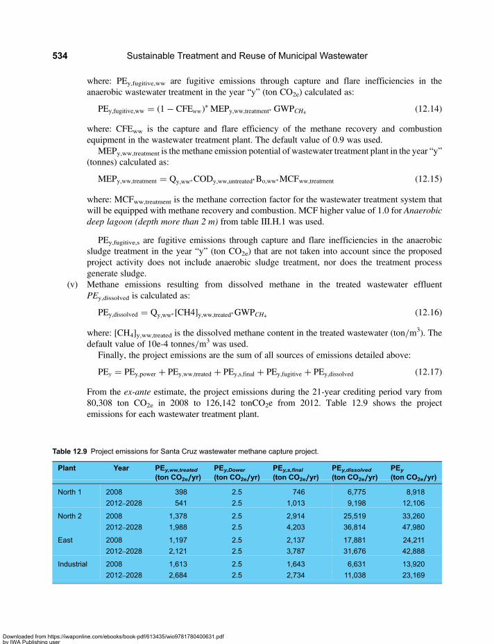
where: PEy,fugitive,ww are fugitive emissions through capture and flare inefficiencies in theanaerobic wastewater treatment in the year “y” (ton CO2e) calculated as:

PEy,fugitive,ww = (1− CFEww)∗ MEPy,ww,treatment∗ GWPCH4 (12.14)

where: CFEww is the capture and flare efficiency of the methane recovery and combustionequipment in the wastewater treatment plant. The default value of 0.9 was used.

MEPy,ww,treatment is the methane emission potential of wastewater treatment plant in the year “y”(tonnes) calculated as:

MEPy,ww,treatment = Qy,ww∗CODy,ww,untreated∗Bo,ww∗MCFww,treatment (12.15)

where: MCFww,treatment is the methane correction factor for the wastewater treatment system thatwill be equipped with methane recovery and combustion. MCF higher value of 1.0 for Anaerobicdeep lagoon (depth more than 2 m) from table III.H.1 was used.

PEy,fugitive,s are fugitive emissions through capture and flare inefficiencies in the anaerobicsludge treatment in the year “y” (ton CO2e) that are not taken into account since the proposedproject activity does not include anaerobic sludge treatment, nor does the treatment processgenerate sludge.

(v) Methane emissions resulting from dissolved methane in the treated wastewater effluentPEy,dissolved is calculated as:

PEy,dissolved = Qy,ww∗ [CH4]y,ww,treated∗GWPCH4 (12.16)

where: [CH4]y,ww,treated is the dissolved methane content in the treated wastewater (ton/m3). Thedefault value of 10e-4 tonnes/m3 was used.

Finally, the project emissions are the sum of all sources of emissions detailed above:

PEy = PEy,power + PEy,ww,treated + PEy,s,final + PEy,fugitive + PEy,dissolved (12.17)

From the ex-ante estimate, the project emissions during the 21-year crediting period vary from80,308 ton CO2e in 2008 to 126,142 tonCO2e from 2012. Table 12.9 shows the projectemissions for each wastewater treatment plant.

Table 12.9 Project emissions for Santa Cruz wastewater methane capture project.

Plant Year PEy,ww,treated

(ton CO2e/////yr)PEy,Dower

(ton CO2e/////yr)PEy,s,final

(ton CO2e/////yr)PEy,dissolved

(ton CO2e/////yr)PEy

(ton CO2e/////yr)

North 1 2008 398 2.5 746 6,775 8,918

2012–2028 541 2.5 1,013 9,198 12,106

North 2 2008 1,378 2.5 2,914 25,519 33,260

2012–2028 1,988 2.5 4,203 36,814 47,980

East 2008 1,197 2.5 2,137 17,881 24,211

2012–2028 2,121 2.5 3,787 31,676 42,888

Industrial 2008 1,613 2.5 1,643 6,631 13,920

2012–2028 2,684 2.5 2,734 11,038 23,169



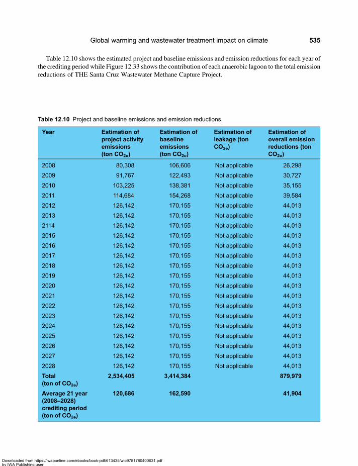
Table 12.10 shows the estimated project and baseline emissions and emission reductions for each year ofthe crediting period while Figure 12.33 shows the contribution of each anaerobic lagoon to the total emissionreductions of THE Santa Cruz Wastewater Methane Capture Project.

Table 12.10 Project and baseline emissions and emission reductions.

Year Estimation ofproject activityemissions(ton CO2e)

Estimation ofbaselineemissions(ton CO2e)

Estimation ofleakage (tonCO2e)

Estimation ofoverall emissionreductions (tonCO2e)

2008 80,308 106,606 Not applicable 26,298

2009 91,767 122,493 Not applicable 30,727

2010 103,225 138,381 Not applicable 35,155

2011 114,684 154,268 Not applicable 39,584

2012 126,142 170,155 Not applicable 44,013

2013 126,142 170,155 Not applicable 44,013

2114 126,142 170,155 Not applicable 44,013

2015 126,142 170,155 Not applicable 44,013

2016 126,142 170,155 Not applicable 44,013

2017 126,142 170,155 Not applicable 44,013

2018 126,142 170,155 Not applicable 44,013

2019 126,142 170,155 Not applicable 44,013

2020 126,142 170,155 Not applicable 44,013

2021 126,142 170,155 Not applicable 44,013

2022 126,142 170,155 Not applicable 44,013

2023 126,142 170,155 Not applicable 44,013

2024 126,142 170,155 Not applicable 44,013

2025 126,142 170,155 Not applicable 44,013

2026 126,142 170,155 Not applicable 44,013

2027 126,142 170,155 Not applicable 44,013

2028 126,142 170,155 Not applicable 44,013

Total(ton of CO2e)

2,534,405 3,414,384 879,979

Average 21 year(2008–2028)crediting period(ton of CO2e)

120,686 162,590 41,904



0

10,000

20,000

30,000

40,000

1 3 5 7 9 11 13 15 17 19 21Year

Em

issi

ons

Red

ucti

onto

n C

O2e

/yr

North 1 Covered Lagoon

North 2 Covered Lagoon

East Covered Lagoon

Industrial Covered Lagoon

Figure 12.33 Contribution of each anaerobic lagoon to the emission reductions of the Santa Cruz wastewatermethane capture project



References

Aguas de Cartagena. (2007). Environmental Management Plan for Handling, Transportation and Final Disposal of SolidWastes of the Wastewater Treatment in of Punta Canoas, Cartagena, Colombia (Internal Document, In Spansih).

Aiyuk S., Amoako J., Raskin L., van Haandel A. and Verstraete W. (2004). Removal of carbon and nutrients fromdomestic wastewater using a low investment, integrated treatment concept. Water Research, 38, 3031–3042.

Aktug S. (2002). Dynamic Modelling of Facultative Stabilization Ponds. Izmir, Turkey. In (http://www.veribaz.com/viewdoc.html?dynamic-modelling-of-facultative-stabilization-ponds-355648.html)

Alley E. R. (2007). Water Quality Control-Handbook. Mc Graw-Hill, New York, USA.Andoh R. Y. G., Smith B. P. and Saul A. J. (1999). The screen efficiency of a novel self-cleansing cso, 8th International

Conference on Urban Storm Drainage, Sydney, Australia.Andrade Neto C. O. (1997). Sistemas Simples para Tratamento de Esgotos Sanitarios, Experiencia Brasilera (Simple

Systems for Treatment of Sanitary Wastewater, Brazilian Experience), ABES, Rio de Janeiro, Brazil (inPortuguese), pp. 35–74.

Andrade Neto C. O., Guimarães P., Pereira M. G. and de Souza Melo H. N. (2000). Decanto-Digestor e FiltrosAnaeróbios (Decantor-Digester and Anaerobic Filters), Centro de Tecnologia, Campus Universitário, 59072–970, Natal, RN, Brasil (in Portuguese).

Andrade Neto C. O. (2006). O uso do Filtro Anaerobio para Tratamento de Esgoto Sanitario (The use of Anaerobic Filterfor Treatment of Sanitary Wastewater).Medio Filtrante Journal, Marco/Abril, Brazil (in Portuguese). pp. 12–16.

Andrade Neto C. O., Campos J. R., Sobrinho P. A., Chernicharo C. A. d. L., Nour E. A. (2009). Filtros Anaerobios,Chapter 6 in: Campos J. R. (2009). Tratamento de Esgotos Sanitarios por Procerso Anaerobio e DisposicaoContolada no Solo (Treatment of Sanitary Wastewater by Anaerobic Process and Controlled Disposal on Soil)PROSAB. ABES, Brazil, (in Portuguese), pp. 139–154.

Andreoli V. C., Von SperlingM. and Fernandes F. (2001). Lodos de Esgotos: Tratamento e Dispsicao Final (WastewaterSludge: Treatment and Final Disposal). DESA-UFMG, SANEPAR, Capa Editoracao, Brazil, (in Portuguese).

Arboleda J. (1992). Teoría y Práctica de la Purificación del Agua (Theory and Practice inWater Purification). ACODAL,Bogotá, Colombia (in Spanish).

Arthur J. P. (1983). Notes on the design and development of waste stabilization ponds. In:WarmClimates of DevelopingCountries, World Bank Technical Paper Number 7, The World Bank, Washington DC, USA, 18, pp. 50–53.

Asano T., Burton F., Leverenz H., Ryvjiro T. and Tchobanoglous G. (2007). Water Reuse, Issues, Technologies andApplication. Metcalf & Eddy Inc.

Biello D. (2011). The false promise of biofuels, Scientific American, August 2011, USA, 302 N2, pp. 38–45.Blanco G. and Wagner Santallana E. L. (2007). Environmental Impact Study: Expanding the Plant Capacity of

Wastewater Treatment of Saguapac-Santa Cruz de la Sierra. The World Bank, Bolivia.


Botiva S. C. (1977). Evaluación de parámetros de calidad de aguas residuales domésticas para cálculo de poblaciónequivalente (Evaluation of Domestic Wastewater Quality Parameters for Calculating Equivalent Population),College of Engineering National University (in Spanish).

Brock T. (1974). Biology of Microorganisms. Prentice-Hall, New Jersey, USA.Butts A. T. (1988). Development of Design Criteria for Sidestream Elevated Pool aeration Stations, Illinois State Water

Survey Division, Water Quality Section.CAESB (2006). Estacoes de Tratamento de Esgotos (Wastewater Treatment Plants). The Water Utility of Brasilia,

Brasil, October 2006 (in Portuguese).Campos J. R. (2009). Tratamento de Esgotos Sanitarios por Procerso Anaerobio e Disposicao Contolada no Solo

(Treatment of Sanitary Wastewater by Anaerobic Process and Controlled Disposal on Soil) PROSAB. ABES,Brazil, (in Portuguese), pp. 73–99, 101–115, 144–145, 155–198, 321–407.

Catalog HUBER Rotamat (2007). High Performance Screen for Efficient and Economical Purification of Waste Water,Germany.

Cavalcanti P. F. F. (2009). Aplicacao de Reatores UASB e Lagoas de Polimento no Tratamento de Esgoto Domestico(Application of UASB Reactores and Polishing Lagoons in Domestic Wastewater Treatment), Federal Universityof Campina Grande – UFCG, Brazil (in Portuguese), pp. 48–50.

CEPIS (2004). Diseño de plantas de tecnología apropiada – Capítulo cinco: Batería de filtros de tasa declinante y lavadomutuo (Design of appropriate Technology Plants), Chapter 5, A battery of Filters of Declining Rate and MutualWashing, CEPIS-MANUAL II: in http://www.cepis.ops-oms.org/bvsatr/fulltext/tratamiento/manualII/cinco.pdf (in Spanish).

Chernicharo C. A. d. L. (2000). Reatores Anaerobios (Anaerobic Reactors). DESA-UFMG, Brazil, (in Portuguese), 150,pp. 218–224.

Chernicharo C. A. d. L. (2007). Reatores Anaerobios (Anaerobic Reactors). DESA-UFMG, Capa Editoracao, Brazil (inPortuguese), pp. 127–152, 360–361, 363–364, 365.

Chernicharo C. and Augusto de Lemos (2007). Reatores Anaerobios (Anaerobic Reactors). DESA-UFMG, CapaEditoracao, Brazil (in Portuguese).

COD/BOD5 (2005). COD/BOD5 Reduction with ROTAMAT® Fine and Micro Screens: Huber Technology, Catalogof Huber Technology, Germany.

Colorado Department of Public Health and Environment (2007). Design Criteria Considered in the Review ofWastewater Treatment Facilities-Policy 96-1, Colorado, USA.

Cooper-Smith G. (2001). Chemically Enhanced Primary Treatment: The UK Experience, Water 21, p. 10, August 2001.Crites R. W., Middlebrooks E. J. and Reed S. C. (2006). Natural Wastewater Treatment Systems. Taylor & Francis

Group, LLC, FL, USA.Crutzen P. J., Mosier A. R., Smith K. A. and Winiwarter W. (2008). N2O release from agro-biofuel production negates

global warming reduction by replacing fossil fuels, Atmos. Chem. Phys., 8, pp. 389–395.Daiger G., Peterson R., Whiterspoon J. and Allen E. (2000). Impact of Global Warming Concerns on Wastewater

Treatment Plant Design and Operation. ASCE, USA.Dautremont-Smith J. (2002). Guidelines for College-Level Greenhouse Gas Emissions Inventories.de Vargas L. (2007). Flotación (Filtration), CEPIS, MANUAL I, http://www.cepis.ops-oms.org/bvsatr/fulltext/

tratamiento/manualI/tomoII/ocho.pdf (in Spanish).DeGarie C. J., Crapper T., Howe B. M., Burke B. F. and McCarthy P. J. (2005). Floating geomembrane covers for

odour control and biogas collection and utilization in municipal lagoons. Water Science & Technology, 52(10),pp. 291–298, © IWA Publishing 2000.

EPA (1999). Wastewater Technology Fact Sheet: Screening and Grit Removal, USA.EPA (2005). Membrane Filtration Guidance Manual. Cincinnati, USA.EPA (2008). Inventory of U.S. Greenhouse Gas Emissions and Sinks: 1990–2006, USA.FAO (2006). Food Security Statistics – Colombia.Fernades C. (2007).DigestàoAnaeróbia (AnaerobicDigestion). http://www.dec.ufcg.edu.br/saneamento/DigeAnae.htmlFernandez C. (2006). “El Protocolo de Kioto y los mecanismos flexibles: MDL”, PPT, España, The Kyoto Protocol and

the Flexible Mechanisms: CMD, PPT, PPT, Spain (in Spanish).



http://www.cepis.ops-oms.org/bvsatr/fulltext/tratamiento/manualII/cinco.pdf











http://www.cepis.ops-oms.org/bvsatr/fulltext/tratamiento/manualI/tomoII/ocho.pdf











http://www.dec.ufcg.edu.br/saneamento/DigeAnae.html






FORET (2007). http://www.fmcforet.com/productes/OHP.htmFoxon K. M., Pillay S., Lalbahadur T., Rodda N., Holder F. and Buckley C. A. (2003). The Anaerobic Baffled Reactor

(ABR): An Appropriate Technology for On-Site Sanitation, Available on website http://www.wrc.org.zaFrassinetti P. C. and van Haandel A. C. (1996). Improved performance and increased applicability of waste stabilization

ponds by pretreatment in a UASB reactor. Water Science and Technology, 33(7), 147–156.Freni G., Maglionico M. and Di Federico V. (2003). State of the Art Urban Drainage Modeling. University of Bologna,

University of Palermo, SINTEF, NTNU and Wrc, Italy.Garcia Agudo E. and Russell G. L. (1992). Militamices como sistema de pretratamiento, (Micro Screens as Pretraetment

Systems), CEPIS, OPE, WHO (in Spanish).Gloyna E. F. (1971). Waste Stabilization Ponds. WHO, Monograph Series Nº 60, Geneva.Gravel M. (2002). Membrane Filtration-Application from the Inside to the Outside. Newfoundland Design Associates

Ltd, Canada.Gray B. (2009). Appendix of the paper: On the Hijacking of the American Meteorological Society (AMS).Greco N. H. C. (2007). Desempenho de um Sistema Reator UASB – Filtro Anaerobio en Escala Real: ETE Ipanema

(Performance of a System of UASB Reactor – Anaerobic Filter in a Full Scale Plant: The Ipanema WastewaterTreatment Plant), 24a Congresso Brasileiro de Engenharia Sanitaria e Ambiental, 2–7 de Setembro de 2007,Belo Horizonte, Minas Gerias, Brazil (in Portuguese).

Gurney Environmental, www.gurneyenvironmental.comGurovich L. and Ramos R. (1990). Tasa de Riego Mensual para una Hectárea Tipo en la Zona de Maipú (Monthly

Irrigation Rate of a Typical Hectar in the Maipu Zone, Santiago, Chile), Unpublished Internal Report byIfarle-Tahal Consulting Engineers prepared for the Santiago Poniente Project, Chile (in Spanish).

Hackman B. (2000). Membrane Filtration. Strand Ass, USA.Hans Huber AG Catalogue (2007). Innovative Equipment and Processes for Water and Wastewater Treatment.Harleman D. R. F. (2004). Personal Communication.Harleman D. R. F. and Chagnon F. (2004). Personal Communication.Harleman D. R. F. and Murcott S. (1998). Low Cost Nutrient Removal Demonstration Study, Tech. Rep., World

Bank/UNDP, BRA/90/010.Harleman D. R. F. and Murcott S. (2001). An Innovative Approach to Urban Wastewater Treatment in the Developing

World, Water 21, June 2001, pp. 44–48.Hermann L. F. and Schittini M. (2011). Estudio de las Opciones de Aprovechamiento del Biogas de las PTARs de

SAGUAPAC y Analisis Finnaciero en el Mercado de Santa Cruz (Study of the Options for Utilizing the BiogasGenerated in the Wastewater Treatment Plants of SAGUAPAC and Financial Analysis in the Santa CruzMarket), SAGUAPAC Unpublished Internal Report Prepared by the Consulting Firm Incisa Bioenregia (inSpanish).

http://en.wikipedia.org/wiki/Milankovich_Effecthttp://icecap.us/images/uploads/On_The_Hijacking_of_the_American_Meteorological_Society.pdfhttp://themes.eea.europa.eu/Sectors_and_activities/energy/indicators/EN01, 2007.04/Fig1.gif/viewhttp://unfccc.int/files/meetings/cop_13/application/pdf/cp_bali_action.pdfhttp://www.abelard.org/briefings/global_warming_atmospheric_chemistry_physics.phphttp://www.iwawaterwiki.org/xwiki/bin/view/Articles/Helmintheggs (May 12, 2011).Huber Technology Group (2003). Personal Communication.Huber-Bombas y Riegos (2007). Personal Comunication. Medellin, Colombia.Hulshoff Pol L. W., de Castro Lopes S. I., Lettinga G. and Lens P. N. L. (2004). Anaerobic Sludge Granulation,Water

Research 38, UK.Idelovitch E. and Michail M. (1981). Nitrogen removal by free Ammonia stripping from high pH ponds. Journal

of Water Pollution Control Federation, 53(9), September 1981, pp. 1391–1401.Idelovitch E. and Michael M. (1984). Soil aquifer treatment: a new approach to an old method of wastewater reuse.

Journal of Water Pollution Control Federation, 56(8), pp. 963–943.Indian & Northern Affairs Canada Gatineau, Quebec, K1A 0H4 (2006). Design Guidelines for First Nations Water

Works, Canada.

References 539


http://www.fmcforet.com/productes/OHP.htm






http://www.wrc.org.za




http://www.gurneyenvironmental.com

http://en.wikipedia.org/wiki/Milankovich_Effect






http://icecap.us/images/uploads/On_The_Hijacking_of_the_American_Meteorological_Society.pdf







http://themes.eea.europa.eu/Sectors_and_activities/energy/indicators/EN01








http://unfccc.int/files/meetings/cop_13/application/pdf/cp_bali_action.pdf










http://www.abelard.org/briefings/global_warming_atmospheric_chemistry_physics.php






http://www.iwawaterwiki.org/xwiki/bin/view/Articles/Helmintheggs









Instituto de Investigación e Información Geocientífica, Minero Ambiental y Nuclear Ingeominas (2000). Estudio Básicopara la Conformación de un ParqueMinero Industrial para el Ordenamiento y Desarrollo de la Actividad Extractivay Transformadora de Minerales Arcillosos con Fines a Desmarginalización de Barrios en el Distrito Capital.Informe Final. Proyecto PNUD/DAMA/COL/96-023. Bogotá, Colombia, p. 202.

IPAC (2007). http://www.llnl.gov/ipac/technology/profile/environment/UV-H2O2TreatmentOfAqueousMixedWastes/index.php

IPCC (2008). Climate Change 2007: Synthesis Report-Summary for Policymakers, Switzerland.IPCC, WMO, UNEP (2006). 2006 IPCC Guidelines for National Greenhouse Gas Inventories, Vol. 5.Johansen J. O. (2009). Sewage biogas fuels public transport buses in Oslo. World Water and Environmental

Engineering, March/April, 47–48.Juanico M. (1993). Alternative schemes for municipal sewage treatment and disposal in industrialized countries: Israel

as a case study. Ecological Engineering, 2, 101–118.Juanico M. (1995). The Effect of the Operational Regime on the Performance of Wastewater Storage Reservoirs, IAWQ

Waste Stabilization Ponds Conference, Joao Pessoa, Brazil, March 1995.Juanico M. (2005). Wastewater reservoirs. In: Pond Treatment Technology, A. Shilton (ed.). IWA Publishers,

pp. 357–380.Juanico M. and Dor I. (1999a). Reservoirs for Wastewater Storage and Reuse, Ecology, Performance and Engineering

Design. Springer.Juanicó M. and Dor I. (eds.) (1999b). Hypertrophic Reservoirs for Wastewater Storage and Reus. Springer, Germany,

pp. 87–90.JuanicóM. andMilsten A. (2004). Semi-intensive treatment plants for wastewater reuse in irrigation.Water Science and

Technology, 50(2), 62–103.JuanicoM. and Shelef G. (1994). Design, operation and performance of stabilization reservoirs for wastewater irrigation

in Israel, Water Research, 28(1), 175–186.Juanico M. and Weinberg H. (1995). Diseno de Procesos de Lagunas de Estabilizacion a Diferentes Altitudes para las

Condiciones de Bolivia (Design of Stabilization Lagoons Process at Different Altitudes for the Conditions ofBolivia), PRORPAL (in Spanish).

Keller J. and Hartley K. (2002). “Greenhouse Gas Production in Wastewater Treatment: Process Selection is the MajorFactor”, Water Science and Technology, ISSN 0273-1223 CODEN WSTED4, London, UK.

Kemmer and Frank M. (ed.) (1988). Nalco, “The Nalco Water Handbook”, McGraw-Hill Co., New York, USA.Koehler R. (2003). Innovative and Economic Processes for Water and Wastewater Treatment, Presentation of Huber

Technology in the World Bank.Koppl S. and Formmann C. (2004). Eco-efficient Wastewater Treatment of River and Sea Outfalls, MWWD 3rd

International Conference on Marine Wastewater Disposal and Marine Environment, Catania, Italy, September27–October 2.

Lara J. A. (1999). Depuración de Aguas Residuales Municipales con Humedales Artificiales, (Municipal WastewaterPurification by Constructede Wetlamds), Trabajo Final de Maestria, Universidad Politécnica de Catalumña,España (MSc thesis, Politechnic University of Catalumña, Spain), in Spanish.

Leppe A. Z. and Padilla L. B. (1999). Emisarios Submarinos de Penco y Tome, 5 Años de Vigilancia y una EvaluacionGlobal de sus Efectos Ambientales (The Submarine Outfalls of Penco and Tome, 5 Years of Monitoring and aGlobal Evaluation of their Environmental Impact), XIII Congreso Chileno de Ingenieria Sanitaria y Ambiental,AIDIS Chile, Antofagasta, October 1999 (in Spanish).

LG Sonic (2003). AMicrocosm Trial of Novel Controls for Phytoplankton – The Effects of Ultrasound on Algae, http://www.lgsonic.com/pond-algae-control-detail/

Libhaber M. (1987). Integrated Planning and On-Farm Economics of Reclaimed Wastewater Irrigation, Workshop onTreatment and Use of Sewage Effluents for Irrigation and other Purposes, UNEP,Mediterranean Action Plan, Split,Yugoslavia, November 25–27.

LibhaberM. (1996). Reuso de Aguas Servidas Tratadas y Almacenadas en Embalses de Estabilizacion (Reuse of TreatedWastewater Stored in Stabilization Reservoirs), International Seminar on Management of Urban Wastewater,Organized by the World Bank in Medellin, Colombia, December 2–4 (in Spanish).



http://www.llnl.gov/ipac/technology/profile/environment/UV-H2O2TreatmentOfAqueousMixedWastes/index.php











http://www.lgsonic.com/pond-algae-control-detail/








Libhaber M. (2003). Wastewater Reuse for Irrigation, the Stabilization Reservoirs Concept, Presentation in the WorldBank Water Week, Washington DC, USA.

Libhaber M. (2004). Wastewater Treatment in Developing Countries: the Use of Physico-Chemical Processes forAchieving Affordable Disposal Schemes, Paper presented in the Seminar “Wastewater Treatment withoutBiology – May Advanced Physico-Chemical Treatment Methods Replace Biological Treatment or SupplementIt?”, Technical University of Munich, Munich, July 15, 2004.

Libhaber M. (2006). Annex 15: Wastewater Treatment Technical Aspects: Increasing the Treatment Capacity of theExisting Wastewater Treatment Plants of Santa Cruz, in The World Bank (2006) Project Appraisal Documenton the Bolivia Urban Infrastructure Project, Report No. 36796-BO, October 13, 2006, Washington D.C, USA.

Libhaber M. (2007). Appropriate Technology for Wastewater Treatment and Reuse in Developing Countries, Paperpresented in the Conference “Water Supply and Sanitation for All” Huber Technology, Berching, Germany,September 27–28, 2007.

Libhaber M. and Michail M. (1987). Innovative Methods in Wastewater Treatment for Agricultural Reuse in Israel,Water Reuse Symposium IV, AWWA Research Foundation, Denver, Colorado, August 2–7.

Libhaber M. and Roberts J. W. P. (2002). Social Aspects of Wastewater Submarine Outfalls in Developing Countries,the Case of Cartagena, Colombia, MWWD Conference, Istanbul.

Llosá O. M. (2005). Generalidades de las tecnologías de membranas (Generality of Membrane Technology), SeminarioInternacional de Aguas Residuales, Valencia, España.

Lyle J. T. (1994). Regenerative Design for Sustainable Development. John Wiley & Sons, Inc, New York, USA,pp. 245–246.

Maldonado-Yactayo V. (2007). Fitración (Filtration), http://www.cepis.ops-oms.org/bvsatr/fulltext/tratamiento/manualI/tomoII/nueve.pdf

Mara D. (1987). Waste stabilization ponds: problems and controversies. Water Quality International, 1, 20–22.Mara D. (2004). DomesticWastewater Treatment in Developing Countries. Earthscan, UK, USA, pp. 91, 105–113, 165,

189–191, 194–199.Mara D. (2006). “Waste Stabilization Ponds, WSP”, http://www.personal.leeds.ac.uk/~cen6ddm/WSP.htmlMara D. and Pearson H. W. (1999). A hybrid waste stabilization pond and wastewater storage and treatment reservoir

system for wastewater reuse for both restricted and unrestricted crop irrigation. Water Research, 33(2), 591–594,Great Britain.

Martin J. E. and Martin T. E. (1991). Technologies for Small Water and Wastewater Systems, Van Nostrand Reinhold,pp. 320–322.

McGauhey P. H. (1968). Engineering Management of Water Quality. McGraw-Hill, NY.McKinney R. T. (1962). Microbiology for Sanitary Engineers. McGraw-Hill Book Co, New York.Medina Hoyos I. R. (1993). Process Pilot Plant Anaerobic Wastewater Treatment. Fondo Nacional Para el Medio

Ambiente, Bolivia.Melo J. C. (2008). Sistema Condominial: Uma Resposta ao Desafio de Universializaco do Saneamento (Condominial

System: A Response to the Challenge of Universal Sanitation), Program of Modernization of the Sanitation Sector,Ministry of Cities, Government of Brazil (in Portuguese).

Merz S. K. (2000). Guidelines for Using Free Water Surface Constructed Wetlands to Treat Municipal Sewage.Queensland Department of Natural Resources, Queensland State Government, Brisbane, Queensland, Australia.

Metcalf and Eddy (2003). Wastewater Engineering: Treatment and Reuse. 4th, and 5th edn, McGraw-Hill Book Co,New York, p. 280.

Ministry of Environment, Housing and Regional Development of Colombia (MAVDT) (2008). Studies Leading to theDetermination of Technologies for Municipal Wastewater Treatment Applicable to Populations of Less than300,000 inhabitants (unpublished Report).

Moreira-Oliveira C., Martins Godinho V. and Von Sperling M. (2006). Influência de diferentes Granulometrias deFiltros de Pedra na Composição e Concentração de Algas em Efluentes de Lagoas de Polimento (Influence ofDifferent Granulometries of Rock Filters on the Composition and Concentration of Algae in Polishing LagoonsEffluents), 25° Congresso Brasileiro de Engenharia Sanitária e Ambiental, Brasil (25th Brazilian Congress ofSanitary Engineering), in Portuguese.

References 541


http://www.cepis.ops-oms.org/bvsatr/fulltext/tratamiento/manualI/tomoII/nueve.pdf











http://www.personal.leeds.ac.uk/~cen6ddm/WSP.html






Morrisey S. P. and Harleman D. R. F. (1992). Retrofitting Conventional Primary Treatment for Chemically EnhancedPrimary Treatment in the USA, in Chenical Water and Wastewater Treatment II, Proceedings of the FifthGothenburg Simposium, Nice, France, Springer-Verlag, 1992.

Mota F. S. B. and von SperlingM. (2009). Nutrientes de Esgotos Sanitarios: Utilizacao e Remocao (Nutrients in SanitaryWastewater: Utilization and Removal), PROSAB, Editora ABES (in Portuguese), pp. 317.

Murcott S., Dunn A. and Harleman D. R. F. (1996). Chemically EnhancedWastewater Treatment for Agricultural Reusein Mexico, International Association of Water Quality, Biennal Conference, Singapore.

OPS (2005).Guías para elDiseño deTanques Sépticos, Tanques Imhoff yLagunas deEstabilización (Guidelines forDesignof Septic Tanks, Inhoff Tanks and Stabilization Lagoons) OPS-CEPIS, Lima, Peru (in Spanish).

Orozco Á. (1976). Comparison of Complete Mixing Activated Sludge Models Using a Glicerol Feed. The PennsylvaniaState University, State College.

Orozco Á. (1977). Teoría de la Remoción de Sustrato Soluble en Plantas de Lodos Activados (Theory of SolubleSubtsrate Removal in Activated Sludge Plants). Revista ACODAL, Bogotá, Colombia (in Spanish).

Orozco Á. (1988). Anaerobic wastewater treatment using an open flow baffled reactor at low temperature, FifthInternational Symposium on Anaerobic Digestion, Poster paper book, Bologna, Italy.

Orozco Á. (1997). Pilot and full-scale anaerobic treatment of low-strength wastewater at sub-optimal temperature(15 °C). with a hybrid plug flow reactor, Proceedings of the 8th International Conference on AnaerobicDigestion, Vol. 2, Oral presentation, Sendai, Japan, May 25–29.

Orozco Á. (1999). Prediseño de Alternativas de Tratamiento de Agua Residual (Pre-design of Alternatives forWastewater Treatment), Final Report for SERAQA, Tunja, Colombia (in Spanish).

Orozco A. (2005). Bioingeniería de aguas residuales: teoría y diseño, (Biengineering of Wastewater: Theory andDesign). ACODAL, Bogotá, Colombia (in Spanish).

Orozco Á. (2007). La lucha contra el calentamiento global: una visión diferente, (The against Global Warming:A Different Vison) Corporación Otraparte, Medellín, Colombia (in Spanish).

Orozco Á. (2008). Los gases de efecto invernadero (GEI) y su relación con los sistemas de tratamiento de aguasresiduales (STAR), Manejo de Vertimientos Líquidos para contribuir a la Mitigación del Cambio Climático,Seminario Internacional, ACODAL-Seccional occidente, Cali, Colombia.

Orozco Á. (2009). The Impact of Wastewater Treatment on Global Warming, Presentation in Water Week 2009, TheWorld Bank, Washington DC-USA.

Orozco Á and Salazar A. (1988). Tratamiento Biológico de Aguas Residuales (Biological Treatment of Wastewater).CESET, U de A, Medellín, Colombia.

Orozco-Jaramillo Á. (2005). Bioingenieria de Aguas Residuales (Wastewater Bioengineering). ACODAL, Colombia,(in Spanish).

Osorio E. S. (1996). Sistema de Tratamiento de Aguas Residuales Tipo UASB y Lagunas Facultativas, en Bucaramanga,Colombia (Wastewater Treatment System by UASB followed by Facultative Lagoons), International Seminar onManagement of Urban Wastewater, Organized by the World Bank in Medellin, Colombia, December 2–4 (inSpanish).

Paradowska M. (2004). Tailored Chemical Oxidation Techniques for the Abatement of Bio-Toxic Organic WastewaterPollutants. Doctoral thesis, Universitat Rovira I Virgili, España.

Park J. (2006). Application of UV Light for Drinking Water Disinfection – Is It The Magic Bullet?, PPT presentation,University of Wisconsin-Madison, USA.

Pavlostathis G. and Giraldo-Gómez E. (1991). Kinetics of anaerobic treatment. Water Science and Technology, 24(8),IAWPRC, Oxford, UK, pp. 35–59.

Peña-Varón M. and Mara D. (2005). Waste Stabilization Ponds, Universidad del Valle, Instituto Cinara. Cali, Colombiaand School of Civil Engineering, University of Leeds, Leeds, UK.

Potabilización de Aguas Naturales (Potabilization of Natural Water). http://www.puc.cl/quimica/agua/potabiliz.htmPrado P. L. F. (2010). Analise da Potencialidade do Reuso Indireto Potavel: Estudo de Caso da ETE Atuba Sul, Regiao

Metropolitana de Curitiba (Analysis of the Potential Indirect Potable Reuse: Case Study of the Atuba Sul TreatmentPlant, Metropolitan Region of Curitiba), MSc dissertation, Federal University of Parana in Cooperation with theUniversity of Stuttgart (in Portuguese), p. 36.



http://www.puc.cl/quimica/agua/potabiliz.htm







RAS (2000). Reglamento Técnico del Sector de Agua Potable y Saneamiento Básico, (Technical Regulation forthe Water and Sanitation Sector) MINDESARROLLO (Ministry of Economic Development), Colombia(in Spanish).

Rebhum M., Ronen D. and Eren J. (1987). Monitoring and study program of an interregional wastewater reclamationsystem for agriculture. Journal Water Pollution Control Federation, Washington DC, USA, 59(5), pp. 242–248.

Reina J. (2005). El secado por Aspersión. Una Alternativa para el Tratamiento de los Concentrados Procedentes dePlanta de Osmosis Inversa (Drying by Spraying. An Alternative for Treatment of Concentrates of ReverseOsmosis Plants). Barcelona, España (in Spanish).

Roberts J. W. P., Salas J. H., Reiff M. F., Libhaber M., Labbe A. and Thomson C. J. (2010). Marine Wastewater Outfalland Treatment Systems. IWA Publishing, London, New York, pp. 1–13, 188–190.

Rodríguez J. P. (2007). Tratamiento de aguas residuales con lagunas de oxidación (Treatment of Wastewater inOxidation Ponds). ACODAL Diplome in Wastewater and Industrial Wastes Treatment, Barranquilla, Colombia(in Spanish).

Rolim S. M. (2000). Sistemas de Lagunas de Estabilizacion (Stabilization Lagoons Systems). McGraw-Hill Publishing,(in Spanish), pp. 341–347.

Romem M. (1991). Manual for Design of Stabilization Reservoirs. Israeli Association of Engineers and Architects (inHebrew).

Russell D. L. (2006). Practical Wastewater Treatment. John Wiley & Sons, USA.SAGUAPAC (2006). Project Design Document form-Clean Development Mechanisms”, Santa Cruz, Bolivia.SAGUAPAC (2007a). “Proyecto de captura y quemado de biogas en PTAR” (The Project of Capture and Flaring of the

Biogas of the Wastewater Treatment Plants), PPT in ACODAL Conference, Santa Marta, Colombia.SAGUAPAC (2007b). Proyecto de captura y quemado de biogás en las plantas de tratamiento de aguas

residuales-Estudios Técnicos (Collection and Burning of the Biogas Produced in the wastewater TreatmentPlants – Technical studies), Cooperativa de Servicios Públicos, Santa Cruz Ltda., Bolivia (in Spanish).

Scheierling M. S., Bartone C., Mara D. D. and Drechsel P. (2010). Improving Wastewater Use in Agriculture: AnEmerging Priority, World Bank Policy Research Paper 5412, Available at http://siteresources.worldbank.org/INTWAT/Resources/ESWWastewaterAg.pdf

Schirg P. G. (2001). Introducción a la Teoría y Práctica de la Técnica de Membranas (Introduction to the Theory andPractice of Membrane Techniques). PS Prozesstechnik, Switzerland.

Shammas N. K., Wang L. K. and Wu Z. (2009). Waste stabilization ponds and lagoons. In: Biological TreatmentProcesses, L. K. Wang, N. C. Pereira and Y. T. Hung (eds.), Humana Press, New York, USA.

Shuler L. and Kargi F. (1992). Bioprocess Engineering. Prentice Hall International Series, New Jersey.Shuval H., Adin A., Fattal B., Rawitz E. and Yekutiel P. (1986). Wastewater Irrigation in Developing Countries, Health

effects and Technical Solutions, World Bank Technical Paper 51, UNDP Project Management Report Number 6,The World Bank, Washington DC, p. 276.

Silva Martínez A. E., Vega González E. and Martínez Pereda P. (2000). Criterios de Selección de Procesos deSeparación por Membranas, (Criteria for Selection of Separation Processes by Memebranes). Univ. Nal.,Autónoma, Mexico (in Spanish).

Sincero A. P. and Sincero G. (2003). Physical-Chemical Treatment of Water and Wastewater. IWA Publishing, USA.Soler A., Moreno M. D., Saez J. and Moreno J. (2000). Kinetic model for deep waste stabilization ponds operating in

batch mode. Water Science and Technology, 42(10), pp. 315–325. © IWA Publishing 2000.Tahal Consulting Engineers and The HebrewUniversity (1981) Storage of Effluents in the Naan Reservoir, Tahal Report

04/81/87 (in Hebrew), PP 6, 9.Tchobanoglous G. (1981). Wastewater Engineering: Collection and Pumping of Wastewater. Metcalf Eddy Inc.,

McGraw-Hill Publishing.Tchobanoglous G., Burton L. F. and Stensel H. D. (2003). Wastewater Engineering: Treatment and Reuse. 4th edn,

Metcalf Eddy Inc., McGraw-Hill Publishing.The World Bank (2003). World Development Report (WDR), p. xiii.The World Bank (2007). Project Appraisal Document on a Proposed Purchase of Emission Reduction by the

Community Development Carbon Fund in the Amount of US$ 2.080,000 from the Water Supply and Sanitation

References 543


http://siteresources.worldbank.org/INTWAT/Resources/ESWWastewaterAg.pdf








Cooperative of Santa Cruz for the Urban Wastewater Methane Gas Capture Project, Report No. 39377-BO, May17, 2007, Washington DC, USA.

Thomsen M. and Lyck E. (2005). Emission of CH4 and N2O from Wastewater Treatment Plants (6B). NationalEnvironmental Research Institute, Denmark.

Tsukamoto R. (2005). “Tratamiento Físico-Químico de Aguas Residuales Municipales: Estrategia Eficiente, Rápida yde Bajo Costo para Latinoamérica” (Physico-Chemical Treatment of Municipal Wastewater: An Efficient, Rapidand Low Cost Strategy for Latin America). Seminario Internacional de Aguas Residuales, Armenia, Colombia.

Tsukamoto R. Y. (2002). Tratamento Primário Avançado: O Paradigma Moderno do Tratamento de Esgotos, Paper 1 of3, (Chemically Enhanced Primary Treatment: The Modern Paradigm of Wastewater Treatment), Agua LatinoAmérica, São Paulo, Vol. March–April 2002 (in Portuguese and Spanish) http://www.agualatinoamerica.com/docs/PDF/3-4-02basico.pdf (Acessado em 20/03/2008).

Types of filters (2011). http://water.me.vccs.edu/concepts/filters.htmlUNFCCC/CCNUCC (1996). Approved Baseline and Monitoring Methodology AM0039: Methane Emissions

Reduction from Organic Waste Water and Bioorganic Solid Waste Using Composting.United Nations (2008a). National greenhouse gas inventory data for the period 1990–2006, FCCC/SBI/2008/12.United Nations (2008b). Synthesis and Assessment Report on the Greenhouse Gas Inventories submitted in 2008,

FCCC/WEB/SAI/2008 21 July 2008.Uribe J. H. Caracterización de los residuos líquidos domésticos de la ciudad de Medellín (Characterization of the liquid

domestic wastewater of the city of Medellin). Empresas Publicas de Medellin, Medellin, Colombia.USEPA (1993). Constructed Wetlands for Wastewater Treatment and Wildlife Habitat: 17 Case Studies,

EPA832-R-93-005.Vall P., Michel T. and Rituerto J. M. (2007). “A Radical Approach to Industrial Wastewater”, Water 21.Van Handel A. C. and Lettinga G. (1994). Anaerobic Treatment of Wastewater. Campina Grande, Brazil.Vargas-Ramirez M. and Lampoglia T. C. (2006). Scaling-up access to sewerage services using condominial technology.

Waterlines, 25(2), 11–13.Von Sperling M. (2002). Lagoas de Estabilizacao (Stabilization Lagoons). DESA-UFMG, Capa Editora UFMG, Brazil,

(in Portuguese), pp. 61–69, 145.Von Sperling M. and Oliveira S. C. (2007). Challenges in the Implementation and Operation of Secondary Wastewater

Treatment. A comparison between actual and expected performance in Brazil, Department of Sanitary andEnvironmental Engineering – Federal University of Minas Gerais; Belo Horizonte, Brazil.

Wagner J. (2001). Membrane Filtration Handbook – Practical Tips and Hints. Osmonics Inc. p. 16.Wahl T. (1995). Hydraulic Testing of Static Self-Cleaning Inclined Screens, The First International Conference on

Water Resources Engineering, ASCE, USA.Wahl T. and Einhellig R. F. (2000). Laboratory testing and numerical modeling of coanda effect screens. Joint

Conference on Water Resources Engineering and Water Resources Planning & Management, July 30–August 2,2000—Minneapolis, Minnesota, USA: http://www.usbr.gov/pmts/hydraulics_lab/pubs/PAP/PAP-0841.pdf.

Wallace S. (2007). The Wetland Wastewater Alternative, Water 21 February 2007, pp. 38–40.Wehner J. F. and Wilhelm R. H. (1958). Boundary Conditions of Flow Reactor. Chemical Engineering Science,

New York, Volume 6, p. 89.WHO (2003). Guidelines for Safe Recreational Water Environments, Vol. 12, Coastal and Fresh Waters, World Health

Organization, Geneva, Switzerland, p. 80 (http://www.who.int/water_sanitation_health/bathing/srwe1/en/).Wikibooks (2007). “Ingeniería de Aguas Residuales/Tratamiento Físico-químico” (Wastewater Engineering/

Physico-Chemical Treatment). http://es.wikibooks.org/wiki/IngenierC3ADa_de_aguas_residuales/ Tratamiento_fC3ADsico-quC3ADmico

Wikilibros (2007). Wastewater Engineering/Design of anaerobic digestion processes. http://es.wikibooks.org/wiki/Ingenier%C3%ADa_de_aguas_residuales/Dise%C3%B1o_de_procesos_en_digesti%C3%B3n_anaerobia#6._REACTOR_DE_FLUJO_SUSPENDIDO_.28UASB.29

Wikipedia (2007). http://es.wikipedia.org/wiki/Efecto_CoandaWright H. B. and Caims W. L. (2006). Rayos ultravioleta (Ultraviolet Rays). Trojan Technologies Inc., London,

Ontario, Canada.



http://www.agualatinoamerica.com/docs/PDF/3-4-02basico.pdf
















http://www.who.int/water_sanitation_health/bathing/srwe1/en/








http://es.wikibooks.org/wiki/IngenierC3ADa_de_aguas_residuales/Tratamiento_fC3ADsico-quC3ADmico









http://es.wikibooks.org/wiki/Ingenier%C3%ADa_de_aguas_residuales/Dise%C3%B1o_de_procesos_en_digesti%C3%B3n_anaerobia#6._REACTOR_DE_FLUJO_SUSPENDIDO_.28UASB.29








http://es.wikipedia.org/wiki/Efecto_Coanda






WSP –Water and Sanitation Program of the World Bank (2002). Condominial Water and Sewerage Systems – Costs ofImplementing of the Model – Economic and Financial Evaluation, Washington DC, USA.

WSP – Water and Sanitation Program of the World Bank (2008). Constructed Wetlands: A Promising WastewaterTreatment System for Small Localities, Prepared by Martin Gauss, April 2008.

Yanez F. C. (1993). Lagunas de Estabilización (Stabilization Lagoons). ETAPA, Cuenca, Ecuador, (in Spanish), pp.252–276.

Yochanan K., The Green House Effect and the Two Dimensional Pattern of Earth’s Radiation Budget, Greehouse, pdf.Columbia University, Palisades, NY, USA.

Zonglian S., Xilai Z., Bairen Y., Chunji J. and Mengchun G. (2006). Granule development and performance in sucrosefed anaerobic baffled reactors. Journal of Biotechnology, 122, 198–208.

References 545


Index

Note: t= Table, f= Figure

AAccel-O-Fac Process, 46Acetoclastic Acetogenesis, 213Acetoclastic Methanogenesis, 213Acid Forming Bacteria, 31Acidogenesis, 213, 305Acidogenic Bacteria, 207, 213, 304Activated Sludge, 5, 9–11, 13–16, 22–24, 27, 34, 38, 51,

68, 71–72, 84, 86, 99, 106, 108, 111, 113–114,116, 137, 143, 154–157, 159, 162, 166, 175–177,205, 214, 235, 272, 302, 349, 421, 457, 458, 468,476, 477, 479–480, 486, 489

Activated Sludge Treatment Process, 10–16, 99, 154, 159,175, 177, 421, 458, 476

Adenosine Tri Phosphate (ATP), 208–209Aerated Lagoons, 15, 24, 45–46, 107–108, 110, 113–116,

133–136, 144–147, 149–150, 152, 155, 157–159,274, 351, 353–354, 436

Aero-Fac Process, 47Aerobic Bacteria, 9–11, 22, 38, 41, 57, 66, 143, 204,

217, 388Aerobic Conversion, 203Aerobic Decomposition, 10, 22, 140, 210–211, 216Aerobic Lagoons, 9, 259–260Aerobic Processes, 9–10, 17, 22–24, 34, 143, 215, 217,

314, 522Alagado Treatment Plant, Brasilia, 120fAlbedo, 498–499, 501, 505, 516–517

Alcohol, 198Algae, 9, 11, 30, 32, 41–42, 44, 46–47, 49, 57, 61, 76, 90,

94, 137, 139, 161, 199–200, 244, 258–259, 262,264, 270–271, 274–276, 301, 343, 350, 354–355,367–368, 412, 470

Alkalinity, 23, 207, 215, 228, 250, 291, 327, 375, 377,384, 402, 414, 430, 473

Alkyl Benzine Sulfonates (ABS), 199Almirante Tamandare, Parana, Brazil, 104, 105fAluminium Sulphate (Alum), 69, 138, 161, 410, 413–414Ammonia (N-NH3), 7, 32, 49, 57, 59, 88, 95, 132,

160–163, 201–202, 211, 227Ammonia Stripping, 57, 162–163Ammonia Stripping by High Lime Treatment, 57,

162–163Ammonia Stripping by Low Lime Treatment, 57,

162–163Ammonia Stripping Tower, 163Ammonia Volatilization, 163Ammonium Ion (NH4), 161, 243Anaerobic Bacteria, 9, 22, 30–31, 34, 38, 41, 57, 99, 141,

212, 217, 308, 343, 412, 479Anaerobic Conversion, 204Anaerobic Decomposition, 19, 22–24, 34, 42, 78, 116,

134, 140–141, 166, 199, 207, 212–214, 264,304–305

Anaerobic Filter, 24–25, 38–41, 46, 85, 98–102, 111–112,118, 121–125, 130–131, 133, 135, 141, 144–145,


148–149, 151–158, 161, 167, 175–176, 179,192–193, 240, 304, 308–311, 313–315, 318,321–323, 325, 327–328, 335–337, 451, 469,478–481, 488–490, 492–493

Anaerobic Filter followed by Constructed Wetlands,123–124, 149

Anaerobic Filter followed by DAF, 112, 122, 149,156–158, 489, 492–493

Anaerobic Filter followed by Lagoons, 121–122, 149Anaerobic Filter followed by Overland Flow, 118, 148Anaerobic Filter followed by Sand Filter, 122–125,

149, 157Anaerobic Filter Media, 39–40Anaerobic Lagoons, 9, 15, 19, 23–26, 30–34, 39, 41–47,

49, 51, 85–93, 107–108, 113, 115–118, 124–125,127, 130–134, 136, 138, 140–141, 144–146,148–150, 152, 154–156, 158, 161, 165–167,172–173, 175–176, 178–179, 215, 259, 262–263,269, 271, 274, 278–279, 288, 292, 294–295,303–304, 313–314, 351, 353–354, 532–534

Anaerobic Lagoons followed by Anaerobic Filter,124–125, 149

Anaerobic Lagoons followed by Anaerobic Filterfollowed by Sand Filter, 124–125, 149

Anaerobic Lagoons followed by Overland Flow,117–118, 178

Anaerobic Lagoons followed by UASB, 24, 131,149, 304

Anaerobic Processes, 10, 17, 19, 22–25, 30–31, 34, 128,130, 134, 143–145, 147, 159, 164, 166, 206, 214,217, 303–304, 313–314, 355, 522

Anaerobic Units (Anaerobic Lagoons or UASB orAnaerobic Filter) followed by Aerated Lagoons,133, 149

Anaerobic Units (Anaerobic Lagoons or UASB orAnaerobic Filter) followed by Infiltration,130, 149

Anoxic Tanks, 160Anthracite, 71, 104, 437–438, 442–445Anthropogenic Global Warming (AGW), 497, 518Appropriate Technology, 5, 10, 14–22, 24–27, 29, 33, 38,

41, 44–46, 51–52, 54–55, 64, 66, 71, 73, 76,79–81, 84–86, 88, 94, 96, 99, 104–108, 110–116,140–141, 144, 146–147, 150, 153–157, 159–163,165–166, 172, 174–178, 180–181, 192–193, 230,240, 244, 271, 274, 303–304, 308, 315, 343–344,346, 351–352, 359, 372, 422–423, 436–438, 440,442, 444, 446, 448, 450, 452, 454, 456, 458,460–462, 464, 466–472, 474, 476, 478, 480, 482,484–486, 488, 490, 492

Appropriate Technology Concept, 14, 17, 22Appropriate Technology Processes, 10, 14–18, 21, 54, 73,

84, 86, 88, 106, 110–111, 113, 116, 140–141, 144,146–147, 153–156, 159–161, 163, 166, 172,174–175, 177, 181, 192–193, 315, 343, 352, 359,372, 422–423, 436–438, 440, 442, 444, 446, 448,450, 452, 454, 456, 458, 460–462, 464, 466,468–469

Appropriate Wastewater Treatment, 5, 21Aquifer, 76, 159Ascaris, 54Assimilation Capacity, 5–6, 20–22, 71, 421Atuba Sul Treatment Plant, Curitiba, Brazil, 103, 104f

BBabbit Equation, 225Backwashing, 71, 99, 234, 240, 251–252, 292–293,

309–310, 315, 328–329, 403, 431, 437, 440,444–445

Bacteria, 7, 9–11, 22–23, 30–31, 34, 38–39, 41–42, 49,53–54, 57, 59, 61, 66, 99, 140–141, 143, 162,199–202, 204, 207, 210–213, 217, 246, 258–260,272–274, 304, 306, 308, 343, 388, 411–412, 452,465, 469, 479

Bacterial Infection, 54Bacterial Metabolism, 202, 206Belo HoriZonte, 36Ben Gurion MBR Treatment Plant, 462f, 462, 464tBiosolids, 22Biochemical Oxygen Demand (BOD), 7–9, 28, 30, 34–35,

39, 42, 44–45, 47, 49, 53, 57, 59, 62, 69–72, 79,81, 87–89, 95, 99, 101–105, 111–112, 114,116–123, 128, 137–138, 141, 160, 162, 164,175–176, 178, 180, 199–202, 204, 211, 215, 224,226–228, 230, 232, 234, 242, 254, 258, 262,264–267, 270–275, 278–279, 282, 287–288, 303,308, 313–315, 322, 346, 348–349, 351, 353,355–357, 362, 376, 384, 387–388, 391–392, 395,404–405, 410–412, 420–421, 424, 433, 465–467,470, 472, 475, 479–480, 482, 486, 488–489, 491,520–521

Bioconversion, 204–206, 283, 303, 306, 314–315,386, 393

Bioenergetics, 206–207, 211Biogas, 19, 22, 25, 32–34, 36, 38, 43–44, 46, 90, 92–96,

108, 114–125, 130–132, 134, 166–173, 262,279–281, 295, 307, 312–314, 318, 322, 331,333, 336, 423, 470–471, 474, 476, 479, 482,532–533, 536

Biogas Flaring System, 93f



Biomass, 5, 11, 22–25, 30–31, 38–39, 57, 66, 116,129, 134, 162, 205–207, 214–218, 220, 275,283, 303, 306, 308–309, 312–315, 505, 511, 519

Biosynthesis, 207, 209–211Biotransformation, 205, 217–218BOD and TSS Removal efficiency in CEPT, 401, 418fBOD and TSS Removal in Primary settling Basins, 392fBOD Load, 224, 226, 228, 230, 232, 254, 262BOD Test, 200Brasilia, Brazil, 113–114, 119–121, 130Bucaramanga, Colombia, 38, 95–96, 113, 471

CCalculation of Wastewater Flow, 224Capin Plant, Uberaba, 74, 75fCarapongo Treatment Plant, Peru, 136fCarbohydrates, 198, 201, 207, 211, 305Carbon Dioxide (CO2), 22, 23, 32, 41, 78, 95, 166,

168–169, 202, 204, 208, 210, 213, 258, 271, 275,279, 303–305, 494–498, 501–502, 504–505,507–514, 517–519, 522, 525, 527, 534, 536

Carbon Emission Reduction, 19, 90, 164, 172, 314Carbonaceous BOD (CBOD), 49, 160, 201–202, 211, 215Cartagena, Colombia, 83, 235, 254, 256CEPT followed by Aerated Lagoons, 136, 145CEPT followed by Constructed Wetlands, 126–127CEPT followed by DAF, 125, 145, 150, 155,

157–158CEPT followed by Infiltration Basins, 136–137, 145CEPT followed by Overland Flow, 126, 145CEPT followed by Sand Filtration, 105–106, 145, 155,

158, 485–486, 488CEPT followed by Stabilization Lagoons, 126–128CEPT followed by UASB, 131, 149, 153, 157–158CEPT Settling, 69Certified Emission Reduction (CER), 90, 92, 164, 270,

507–508, 524CH4, 217, 259, 279, 303, 305, 318, 322, 330, 335, 473,

494, 497, 508–510, 519–523, 525, 534Chemical Oxygen Demand (COD), 7, 19, 38–39, 41, 53,

72, 88, 99, 101–102, 111, 119, 132, 166–168,202–206, 215–216, 221–222, 227–228, 231–232,234, 242–245, 249–250, 276, 291, 303, 306–308,310–311, 313–315, 318, 327, 331, 335, 345–346,352, 355, 361, 374–375, 377, 384, 401–402, 412,421, 424–425, 429–430, 473, 479–480, 522, 535

Chemically Enhanced Primary Treatment (CEPT), 15,27t, 68–71, 105–106, 239, 374, 391, 406–431

Chemically Enhanced Rotating Microscreens (CERM),418, 421–424

Chlorination, 9–10, 44, 61, 99, 103–104, 127, 239,354–355, 478

Chlorine Dioxide, 159–160Chlorine Gas, 10, 160Classification of Filters, 438Clean Development Mechanisms (CDM), 186, 279, 498,

510, 526–530, 533–535CO2 Emission, 498, 504, 512Coagulants, 116, 141, 143–144, 234, 242, 244, 399, 410,

413–415, 419, 422, 426, 482Coagulation, 69, 140, 145, 410–415, 422, 424,

431–432, 448Coanda Effect, 236Coefficient of Return, 224, 226Cold Digestion Drying (CDD), 13Combined Processes, 14, 16, 21, 27, 51, 84–86, 107,

111–113, 116, 154–156, 160–161, 176–178, 192,344, 352, 468–470, 488–489, 519

Completely Mixed Reactor, 217, 219–220, 219f, 221f,264, 341

Condominial Sewerage, 181–182ConstructedWetlands, 15, 24, 26, 41, 66, 68, 79, 118–119,

123–124, 126–128, 132–133, 143–144, 147–155,158–159, 174–176, 192, 304, 342, 386–394, 396,398, 400, 402, 404, 406, 408

Contaminants, 7, 44, 54, 66, 72, 81, 203, 227, 230, 245,249, 271–272, 276, 374–375, 384, 388, 391–393,411, 424–425

BOD, See Biochemical Oxygen DemandCOD, See Chemical Oxygen DemandTSS, See Suspended SolidsNitrogen, 7, 9, 18, 22–23, 32, 52–53, 57, 68, 82, 88, 95,

103, 119, 132, 137–138, 159–167, 170, 198,200–202, 210–211, 215, 228, 275, 314, 356, 361,388, 394, 412, 465, 489, 520

Phosphorous, 7, 18, 52, 68, 70, 88, 95, 103, 119, 128,132, 138, 159–161, 164–166, 200, 356, 388,423–424, 465, 489

Fecal Coliforms, 7, 26–27, 42, 59, 61, 83, 85, 87–88,103, 112, 159, 258, 269, 271–272, 275, 284, 298,300, 345, 353, 361, 377, 384, 388, 391–392, 398,407, 469, 475–476, 482, 488–489, 532

Toxic Substances, 23, 215, 314Conventional Activated Sludge, 11, 16, 27, 38, 71, 106,

154–155, 175–176, 424, 460Conventional Secondary Treatment, 9–10, 37, 71,

313, 423Conventional Settling, 69–70, 411Conventional Stabilization Lagoons, 86–88, 113Copacabana, Bolivia, 66–67, 79, 389

Index 549


Cost Effectiveness Indicator, 241Covered Anaerobic Lagoons, 19, 33, 51, 85, 89,

91–93, 115, 136, 141, 144, 146, 175–176, 178,274, 534

Crowley, Louisiana, 133Cryptosporidium, 411, 465Curitiba, Parana, Brazil, 98

DDan Region Project, 76Dandora Lagoons Plant, Nairobi, Kenya, 88Decentralized Solution, 21Dechlorination, 10Declining Rate Filtration, 440–442Denitrification, 9, 57, 160, 162, 210, 516–517, 519Design, 7, 12, 15, 17, 25–26, 29, 31, 36, 41–42, 44–47, 49

51, 65–66, 69, 74, 76, 80, 85, 88, 94–95, 97–98,109–111, 113, 132, 141, 154, 164–165, 167, 178,180–182, 192–194, 196, 216, 221, 224–230,237–240, 244–249, 251–253, 258–260, 262–269,271, 274, 276–279, 282, 284, 287–290, 292–300,306–308, 310–311, 314–316, 318, 320–326,328–340, 343–344, 348–352, 356–357, 359, 361,364–366, 371–377, 380–383, 385, 388–397,399–408, 415, 419, 424–429, 431–432, 434–437,440, 445–447, 449–452, 456–457, 463–464,466–470, 472–476, 479, 481–484, 486–487,490–493, 527, 530, 535

Designated National Authority (DNA), 526–527Disinfection, 9–10, 44, 61, 70–71, 76, 80, 85–86, 88,

94, 99, 103, 105, 111, 116–126, 131–133, 136,145, 159–160, 179–180, 192, 271–272, 355,423–424, 436, 452–454, 456–457, 469–470, 478,481–488

Dissolved Air Flotation (DAF), 8, 15, 27, 72–73, 85,103–105, 111–112, 122, 125, 137–139, 143–153,175–176, 178–180, 192–193, 275, 436, 448–449,469, 482, 488–493

Dissolved Oxygen (DO), 4–6, 9, 13–14, 16–18, 23–25,31, 38, 42, 44, 49, 53, 54, 59, 61, 73–74, 76, 80,86, 88, 94, 96–98, 107, 110, 113–115, 126, 130,134–135, 138, 141, 144, 147, 156, 159–160, 162,163, 167, 171, 181, 183, 186, 188, 190, 193,198–203, 244, 248, 254, 258–259, 261, 271, 274,287, 290, 296, 300, 314, 320, 324, 350, 352, 355,364, 382, 393, 401, 412–413, 440, 463–464, 472,482, 494, 498, 501, 506, 510–511, 518

Downflow Filter, 71Drip Irrigation, 53, 55, 59, 61, 111, 165–166, 186, 188,

354, 366–367, 369

EEarth Summit, 494Effect of Temperature onWastewater Treatment, 140, 142Efficient Water Use, 7, 53, 61, 188–189Effluent, 4–7, 9–12, 14–30, 34–35, 38–39, 42, 44, 46, 49,

51–63, 65–66, 68–74, 76–77, 80–88, 90, 94–101,103–106, 111–114, 116–127, 130–134, 136–139,142–145, 147–148, 156, 159–166, 172–173,177–178, 189, 204, 211, 215, 219–220, 228, 234,242, 244, 258–261, 264–265, 274–275, 282, 286,292, 295–300, 307–309, 311–315, 318, 322–323,342–350, 352–362, 364, 366–377, 379–384,386–387, 390–392, 394, 396–397, 402, 408,411–412, 414, 421, 424, 436, 440, 443, 448, 452,461, 464–472, 475–482, 485–486, 488–489, 520,522, 534

Effluent Quality, 5–6, 14–16, 19–23, 25, 34, 44, 53–54,59–61, 65, 69, 84, 97–99, 101, 105–106, 111–112,117–118, 137, 147–148, 160, 162, 164, 177–178,215, 264, 314, 346–350, 353–356, 360, 362, 368,375, 392, 411, 414, 436, 440, 443, 464–465,467–468, 472, 479–480, 482, 485–486, 488

Effluent Quality Standards, 5–6, 19, 22, 54, 160, 162,164, 264

Effluent Reuse for Irrigation, 6, 51, 164EGSB Reactor, 35El Alto, Bolivia, 113, 181Energy from Wastewater, 164, 166–172Energy Generation from Biogas, 32, 90, 93–94, 172Energy Generation in Anaerobic Processes, 164, 166–172Eutrophic, 198Eutrophication, 6, 9, 160, 211, 264, 274–275, 412Evapo-Transpiration, 357–359Extremely High Sludge Age (EHSA), 219–221

FFacultative Bacteria, 210, 213Facultative Lagoons, 41–43, 45–51, 57, 61, 68, 76, 85–91,

94–98, 113, 127, 132–133, 135, 138, 144–146,148, 150–151, 154, 158, 162, 168, 176, 180,259–260, 263–264, 269–270, 273–275, 281–283,291, 296, 298, 351, 355–356, 383, 469–471, 478

Fazenda Rio Grande Plant. Parana, Brazil, 135Fecal Coliforms, 7, 26–27, 42, 59, 61, 83, 85, 87–88, 103,

112, 159, 258, 269, 271–272, 275, 284, 298, 300,345, 353, 361, 377, 384, 388, 391–392, 398, 407,469, 475–476, 482, 488–489, 532

Fecal Coliforms Removal, 272Fermentation, 210, 213, 259Ferric Chloride, 69, 138, 161, 413–414, 423



Fertilizers, 18, 160, 164–166, 173, 188, 423Fibers, 198, 201, 236Filtration, 10–11, 15, 24, 27, 55, 61, 63, 71–72, 85,

104–106, 111–112, 116–117, 137–139, 143–146,148–151, 153, 155, 157–160, 175–176, 179–180,193, 236, 264, 304, 354–355, 367, 371–372, 388,436–443, 445–446, 450, 458–461, 463–467, 469,481–483, 485–486, 488–490, 492–493

Filtration Media, 441–442Financial Sustainability, 18–19, 172, 177Fixed Film Reactor, 162–163Flocculants, 103, 116, 141, 143–144, 161, 411, 421,

482, 489Flocculation, 69–71, 125–126, 145, 240, 243, 410–413,

424, 448Flocculent Sedimentation, 419Flotation Tank, 72Freeboard, 277, 288, 321–322, 324, 350, 382, 425, 479

GGama Plant, Brasilia, 113, 114fGas Solid Liquid Separator (GSLs), 38, 306, 308, 311,

313–318, 323–324, 330, 334, 337–339, 473Global Climate Models (GCM), 494–495, 497–498, 501,

504–506, 508, 514Geoengineering, 498, 514, 517–519Getaot Reservoir, 345Green House Gases (GHGs), 93–94, 164, 172, 187, 497,

499, 501, 504, 508, 511, 519, 522, 523–524, 526Giardia, 361, 411, 465Global Warming, 3–4, 90, 164, 184, 271, 494–498,

500–502, 504–506, 508, 510–514, 516–520,522–524, 526, 528, 530, 532, 534–536

Global Water Crisis, 3–5, 164, 183–184, 191Glucolysis, 207–208, 210, 213Glycerol, 198, 210Grants, 5, 13, 17, 19–20, 146, 172, 188, 371Granular sludge, 34–35, 146Green House Effect, 90, 93–94, 164, 172, 187, 516, 519Grit Chamber, 26–27, 29, 83–84, 94, 154, 157, 235, 245,

256, 277, 290–291, 293, 327, 329, 403, 425,428–429, 469–470

Grit Removal, 8, 29, 84, 469Guandong, China, 68, 68f, 71–72Gurney Mixers, 260

HHaifa, Israel, 61, 108, 111, 347, 349Harmon Equation, 225, 230, 289, 373, 400, 428HDPE Geomembranes, 32

Heavy Metals, 7, 53, 412, 424Helminth Eggs, 41–42, 111, 159, 258, 269, 272–273, 275,

284, 298, 355, 482Helminths, 54, 284, 346, 357, 376–377, 384, 388,

475–476Hepatitis A, 54Heterothrophic Bacteria, 162High Density Polyethylene (HDPE), 32, 173, 270,

278–279, 363, 390, 530High pH Ammonia Stripping, 161, 163Hindered Sedimentation, 416Hollow Fiber Membrane, 460–461Hookworm, 54Huber Rotating Micro Screens, 28f, 234f, 236f, 238f, 242tHuber Technology, 27–29, 235, 237, 239, 243, 245,

252, 421Hydraulic Jump Mixing, 415Hydraulic Loading, 79, 437, 440Hydrogenoclastic Methanogenesis, 212, 303tHydrogen Sulphide (H2S), 22, 31, 34, 70, 78, 96, 166,

168–169, 201, 246, 412, 424, 471, 533Hydrogenoclastic Acetogenesis, 213Hydrograph Controlled Release (HCR), 66Hydrolysis, 206–207, 209–212, 410Hypochlorite, 10, 61, 104, 159–160, 354, 461

IImpact of Wastewater on Global Warming, 523Indicator Organisms, 7Industrial Wastewater, 8, 16, 24, 30, 32, 34, 42, 81, 88,

166–167, 229, 304, 519, 533Infiltration, 7, 10, 15, 27, 41, 55, 57, 73, 76–78, 130–131,

136–137, 143–146, 148–155, 158–159, 225,227–230, 245, 248–249, 276, 287, 289–291, 325,327, 350, 359–360, 365–366, 373–374, 377–378,393, 397, 400–401, 425, 428–429, 436, 464

Infiltration Basins, 10, 76–77, 130–131, 136–137, 145,148, 150–151, 153, 159

Infiltration Flow, 225, 229–230, 248–249, 289, 291, 325,327, 373–374, 400–401, 428–429

Infiltration-Percolation, 15, 27, 76Inflow Structures, 335, 384, 408Inlet Structures, 284, 320, 331, 336, 474Institutional Sustainability, 18–19, 172–173, 177Inter-Institutional Cooperation, 65Intergovernmental Panel on Climate Change (IPCC), 492Intermittent Discharge of Effluent to Rivers, 51, 65Intestinal Nematodes, 88Ipatinga, Minas Gerais, Brazil, 99, 102, 102f, 477Irrigation Methods, 53, 188–190, 354

Index 551


JJerusalem, Israel, 110, 111, 349

KKfar Menahem Reservoir, 61, 63, 367Kingston, Jamaica, 138–139Kjeldahl Nitrogen, 201, 211Krebs Cycle, 207–208Kyoto Protocol, 279, 314, 494–496, 498, 510–511, 514,

517–518, 523, 526–527, 530

LLagoons, 9–10, 12–13, 15, 19, 23–26, 30–34, 39, 41–51,

48f, 57, 61, 64, 68, 76, 85–99, 94, 95, 98, 99, 103,107–108, 110–111, 113–122, 119–122f, 124–128,130–141, 144–163, 165–168, 172–176, 178–180,192–193, 215, 218, 258–276, 278–301, 303–304,313–314, 342–344, 346, 348, 351–357, 365, 367,370, 372, 383, 387–388, 396, 436, 468, 469–472,474–476, 478, 532–535

Lagoons Design Methods, 257–300Kinetic Approach, 264Photosynthetic Approach, 266–268Duncan Mara Method, 268–277

Lagoons followed by DAF followed by Sand Filtration,137–138, 150t, 180t

Lagoons System, 41–46, 45, 51, 64, 86, 88, 93–94, 98,121, 127, 132–133, 133f, 137–140, 145–149,153–154, 158, 161–163, 259, 268, 273–274, 276,286, 291, 298, 300f, 301, 355, 367, 372, 470,472, 476

Lagoons System followed by Constructed Wetlands,132–133, 149

Lagoons Treatment, 15, 42–43, 45–46, 51, 90, 259,260, 270, 271, 281, 286, 287, 348, 349, 351–352

Land Application, 12, 73, 342, 388Large River Outfalls, 27, 27t, 433, 436LG Sonic, 258, 264, 275–276Linear Alkyl Sulfonates, 198Low energy Nuclear Reaction (LENR), 509, 515Low pH Ammonia Stripping, 161, 163Luxury Phosphorous Uptake, 160

MMaale Hakishon Reservoir, 61–62, 348, 352Maturation Lagoons, 26, 41, 43, 46, 85–89, 113, 117, 121,

127, 132, 137, 145–148, 150, 155, 168, 179,260–261, 263–264, 269–270, 273, 274, 275,283–284, 289, 290, 291–292, 297, 297t, 298, 298t,300–301, 470, 471, 471t, 474t, 474–476

Membrane Biological Reactor (MBR), 11Membrane Filtration, 11, 111–112, 149, 153, 157–160,

179–180, 193, 436–437, 458, 460–461, 463, 466,469, 488–490, 492–493

Mesophilic, 34, 140Mesophilic bacteria, 140Methane(CH4), 19, 22–23, 32, 34, 78, 90, 164, 166–169,

172–173, 205–206, 213–215, 217, 271, 279,303–306, 314, 318, 331, 423, 474, 494, 510,519–522, 529, 532–535

Methane Forming Bacteria, 23, 302Methanogenic Activity, 304Methanogens, 23, 304Micro-Sprinkling Irrigation, 186, 188, 363Microfiltration, 11, 457, 460Microorganisms, 34, 39, 76, 159, 204–205, 207, 209, 211,

246, 260, 262, 308, 314, 386, 388, 393, 452,454, 456

Mixed Lagoons (Lagoons with Mixers), 259,263–264, 271

Mixers, 26, 31, 43, 45–51, 57, 61–64, 85, 89–92, 94, 110,119–121, 127, 132, 134, 142–144, 146–148, 150,154, 158, 161–163, 168, 175–176, 260–262, 264,269–271, 274–275, 281–284, 287–289, 291,296–297, 350–351, 368, 470

Mixers in Lagoons, 47Multimedia Filter, 105–106, 482

NN2O, 494, 497, 508, 510, 519–520, 522, 525Naan Reservoir, 108, 109f, 173, 174f, 344, 349Nairobi, Kenya, 88Nanofiltration, 11, 160, 433, 436NASA, 498, 506, 514–518National Water Commission (NWC) of Jamaica, 138Nazareth, Israel, 107f, 108f, 109f, 111, 115, 116f, 134,

348, 349Nitrate (N-NO3), 7, 49, 160–163, 201, 202, 211, 227t,

250, 291, 327, 375, 377, 384, 402, 430, 473Nitrification, 9, 49, 57, 160–163, 201, 211, 388,

519–520, 522Nitrification-Denitrification, 161–162, 388, 519Nitrifying Bacteria, 49, 162, 201–202, 211Nitrifying Modules, 162Nitrobacter, 202, 211Nitrogen, 7, 9, 18, 22–23, 32, 52–53, 57, 68, 82, 88, 95,

103, 119, 132, 137–138, 159–167, 170, 198,200–202, 210–211, 215, 228, 275, 314, 356,361, 388, 394, 412, 465, 489, 520

Nitrogen removal, 9, 161–163, 489



Nitrogenous BOD (NBOD), 49, 160, 201–202, 211Nitrosomonas, 202, 211Non-Revenue Water, 224NonMethanogenic Bacteria, 22, 304Nutrients, 6, 9, 13, 18, 23, 52, 68, 95, 159–162, 164–166,

199, 200, 206, 208, 207, 209, 214, 227, 353, 356,385, 388, 409, 412

Nutrients Removal, 9, 68, 159–162, 165

OOdour, 31–32, 34, 42–46, 57, 61, 78, 88, 90, 93, 95–96,

110, 115, 246, 262, 271, 274, 279, 351, 383,412, 471

Og Reservoir, 62–63, 110Oil and Grease(O&G), 7–8, 28, 72, 79, 82, 84,

198–199, 250, 291, 327, 376–377, 384, 402,448, 469, 473

Olso, Norway, 171Onca Treatment Plant, Belo Horizonte, 36, 36fOperation and Maintenance (O&M), 3, 5, 8–9, 11, 12–19,

21, 22, 23–24, 25, 29, 30, 33–34, 38, 41, 44–45,51, 64, 68, 71, 73, 74, 78, 80–81, 84, 88, 90, 94,96, 98–99, 102, 104, 106, 111–112, 145–146, 162,168, 170–173, 175–178, 181–182, 192, 215, 274,313–314, 367, 371–372, 441, 461, 468, 471–472,480, 482, 487–488

Orderly Design Method (ODM), 193–194, 244, 246–247,249, 252, 276, 289, 293, 296, 298, 315, 325,329–331, 334–337, 357, 372, 379, 381, 393,399, 403–408, 423, 425, 427, 429, 431,433–434

Organic Loading, 30–31, 79, 89–90, 106, 108, 260,262–264, 269, 282, 343, 348–351, 359, 383

Organic Matter (OM), 6–7, 9–11, 13, 15, 17–19, 22–25,28–31, 33–35, 37–39, 41–42, 44–47, 51–55, 57,61, 66, 68–69, 72, 94, 99, 103–104, 106–107, 110,114–116, 121, 123–127, 129, 131, 134, 136–137,144, 159, 165, 167, 169, 198-212, 214–216, 218,220, 222, 227, 234, 240, 244, 246, 254, 258, 261,270, 275, 304–306, 309, 313, 342–343, 350–352,356, 359, 386, 388, 393, 411–412, 421–422, 470,478, 482, 519–520, 522, 532

Organic Matter Removal, 24–25, 30–31, 34–35, 39, 304,313, 352, 421

Organic Nitrogen, 7, 161–163, 201–202, 211, 228Outflow Structures, 279, 284, 366–368, 384, 398, 408Outlet Structures, 286, 295, 297, 300, 320, 331, 333–334,

338, 340, 398, 474, 476–477Overland Flow, 15, 27, 41, 73–76, 117–121, 126, 128,

143–152, 154–155, 158–159, 176, 178, 342, 436

Oxidation Ditch, 11Oxidation Lagoons, 257–300Oxidation Ponds, 73Ozonation, 9–10, 44, 104, 159Ozone, 9–10, 160, 491, 494, 495, 498

PPadilha Sul Plant, Parana, Brazil, 97, 98f, 469Pan American Center of Sanitary Engineering (CEPIS),

413, 436f, 437, 438f, 438t–439t, 441fParasites, 54, 274Parshall Flume, 277–278, 290–291, 293–294, 326–327,

330, 400, 403–404, 416, 419, 425–426, 428,431–432

Pathogenic Organisms, 11, 41–42, 44, 54–55, 59, 81,94, 121, 159–160, 274, 343, 346, 411–412,423, 470

Pathogens, 6, 9, 21, 53–55, 59, 68, 86, 88, 95, 99,103, 159–160, 260, 271, 273, 343, 346, 357,388, 412, 424, 454, 465, 469–470, 478, 482,486, 489

Pathogens Removal, 10Peak Factor, 225–226, 229–230, 248, 289, 325, 373, 400,

428, 464Peak Wastewater Flow, 254Penco, Chile, 83Percentage of Fresh Effluent (in a Reservoir) (PFE),

345–347, 349, 357Phosphorous, 7, 18, 52, 68, 70, 88, 95, 103, 119, 128, 132,

138, 159–161, 164–166, 200, 356, 388, 423–424,465, 489

Phosphorous Luxury Uptake, 160Phosphorous Removal, 70, 159–160, 424, 465, 489Photosynthesis, 9, 41, 57, 95, 161–162, 257, 258, 261,

262, 268Photosynthetic, 257, 258, 261, 261t, 262, 266, 267,

273–275, 350Piston Anaerobic Reactor, 24, 26, 26t, 147, 150t, 192,

192t, 302, 304, 309–310, 311, 321, 323, 335, 336t,337–338

Plug Flow Reactor, 218, 220–222Polishing Lagoons, 46, 161–162, 260, 284Pollutants, 5–7, 21, 186, 357, 374, 394, 411

BOD, See Biochemical Oxygen DemandCOD, See Chemical Oxygen DemandTSS, See Suspended SolidsNitrogen, 7, 9, 18, 22–23, 32, 52–53, 57, 68, 82, 88, 95,

103, 119, 132, 137–138, 159–167, 170, 198,200–202, 210–211, 215, 228, 275, 314, 356, 361,388, 394, 412, 465, 489, 520

Index 553


Pollutants (continued)Phosphorous, 7, 18, 52, 68, 70, 88, 95, 103, 119, 128,

132, 138, 159–161, 164–166, 200, 356, 388,423–424, 465, 489

Fecal Coliforms, 7, 26–27, 42, 59, 61, 83, 85,87–88, 103, 112, 159, 258, 269, 271–272, 275,284, 298, 300, 345, 353, 361, 377, 384, 388,391–392, 398, 407, 469, 475–476, 482,488–489, 532

Toxic Substances, 23, 215, 314Polyelectrolyte, 138, 410, 413, 419, 422, 445, 448Ponds, 10, 41–42, 44–47, 73, 88–90, 95, 98, 116, 141,

161–162, 258, 270, 276, 288–289, 351, 472Ponta Grosa, Parana, Brazil, 97, 97f, 469Potential Water Saving by Consumer Category, 186Public Private Participation (PPP), 190–191Pre-Treatment of Various Types followed by a

Stabilization Reservoir, 106Preliminary Treatment, 8, 10, 14–15, 27–29, 66, 81–84,

94–95, 97, 99, 103, 116–127, 130–133, 136–137,145, 147–149, 155–157, 160, 168, 235, 240–242,253–254, 256, 276, 290–293, 315, 321, 325–329,388, 394, 401–403, 422, 429, 469–471, 478–482,485–486, 488–489, 492

Pressure Filters, 71, 438, 440, 445, 447Pretreatment, 15, 64, 80–81, 95, 106–108, 110–111,

113, 127, 143, 146–148, 150–151, 154, 165,244–245, 254–255, 292, 310, 343–344, 346–348,350–355, 357, 359, 361–362, 367, 369–372,375–376, 389, 393–394, 401, 406, 436–437,448–449, 464, 470

Primary Treatment, 8–9, 15, 28, 34, 37, 68–70, 85, 99,103, 105, 113, 234, 237, 240, 242, 275, 389,393–394, 399–401, 404, 406, 410–412, 414, 416,418, 420–422, 424–426, 428, 430, 432, 434, 448,469, 479

Private Sector, 20, 167, 173, 187, 190–191Private Sector Participation, 20, 190Process Selection Matrix by Air Temperature during the

Cold Season, 150–153Process Selection Matrix by Occupied Land area,

157–159Process Selection Matrix by Population served, 180Process Selection Matrix by Removal Efficiency

of BOD, 179–180Processes which Occupy Small Land Areas, 156Protein, 198, 201–202, 211, 520Protozoa, 42, 258, 272, 346, 357, 411Public Health Risks, 3, 21, 54, 183, 191, 423Puchukollo, Bolivia, 45, 141

RRaw Wastewater, 4, 6–7, 19–20, 22–23, 29–30, 41,

44–45, 55, 78, 84, 88–91, 96–97, 103, 106, 110,113, 141–142, 159, 162, 164–166, 172–173, 178,183, 191, 204, 211, 214, 227–228, 234, 249, 271,276, 343–344, 350–351, 372, 376, 422, 448, 469,471–472

Raw Wastewater Quality, 227Reactors in Series, 61, 121, 220, 310Recanto das Emas Plant, Brasilia, 114, 135Recharge Basins, 76, 137, 143Recovery of Resources from Municipal Wastewater,

163–174Removal of Pathogens, 68, 99, 103, 159, 271, 273, 343,

424, 470, 478Renewable Natural Gas (RNG), 166–172Reservoir with Discontinuous Discharge, 60Resources in Wastewater, 18, 52, 79, 163–164,

172–173, 353Water, 164–165Fetilizers, 165–166Energy, 164–166

Respiration, 57, 199, 202, 205, 216, 220, 258, 264,275, 283

Restricted Irrigation, 55, 59, 65, 111, 343, 346–347, 355,357, 360, 371, 373, 379, 381

Reuse, 3–8, 10, 12, 14–16, 18–20, 22, 24, 26, 28, 30,32, 34, 36, 38, 40, 42, 44, 46, 48, 50–62, 64–66,68, 70, 72, 74, 76–78, 80, 82, 84, 86, 88, 90,92, 94, 96, 98, 100, 102, 104, 106–108,110–112, 114, 116, 118, 120, 122, 124, 126,128, 130, 132, 134, 136, 138, 140, 142, 144,146, 148, 150, 152, 154, 156, 158, 160, 162,164–166, 168, 170, 172, 174–176, 178, 180,182, 184, 186, 188–195, 199, 201, 203, 205,207, 209, 211, 213, 215, 217, 219, 221, 225,227, 229, 231, 235, 237, 239, 241, 243,245–247, 249, 251, 253, 255, 257, 259, 261, 263,265, 267, 269, 271, 273, 275, 277, 279, 281, 283,285, 287, 289, 291, 293, 295, 297, 299, 301–304,306, 308, 310, 312, 314, 316, 318, 320, 322,324–326, 328, 330, 332, 334, 336, 338, 340–377,379–387, 389, 391, 393, 395, 397, 399, 401, 403,405, 407, 409, 411, 413, 415, 417, 419, 421, 423,425, 427, 429, 431, 433, 435, 437, 439, 441, 443,445, 447, 449, 451, 453, 455, 457, 459, 461,463–465, 467, 469, 471–473, 475, 477, 479,481, 483, 485, 487, 489, 491, 493, 495, 497, 499,501, 503, 505, 507, 509, 511, 513, 515, 517, 519,521, 523, 525, 527, 529, 531, 533, 535



Reuse for irrigation, 6–7, 51–52, 55, 64, 106, 164, 172,175, 175t, 189, 339, 341, 342, 344, 355, 366, 369

Reuse Standards, 5, 52–54Reverse Osmosis (RO), 436, 458–459, 465–467, 491Rio Frio Treatment Plant, Bucaramanga,

95f, 96f, 469Riviera Sao Lourenco, Sao Paulo, Brazil, 128fRonda, Parana, Brazil, 97fRotamat Type Rotating Screen, 238fRotating Micro Screens (RMS), 27–29, 84, 85, 89, 91, 92,

95, 111, 113, 179, 233–256, 466, 467Rotavirus, 54

SSand Filter, 106, 116, 122–125, 137–139, 145, 147, 149,

152, 154–155, 157–158, 192–193, 437–438, 447,451, 469, 482–487, 490

Sand Filtration, 10, 15, 24, 27, 27t, 71–72, 72f, 85,105–106, 116–117, 137–139, 143–146, 148, 155,158, 175–176, 179–180, 351, 354, 364f, 367,434–444, 445, 469, 479, 481–482, 484,485–486, 488

Santa Cruz, Bolivia, 33, 33f, 42–44, 43f, 47, 49, 49f,86–88, 90–91, 91f, 167, 234, 235, 253, 254–255,254f, 279, 280, 281, 527, 530

Sao Sebastiao Treatment plant, Brasilia, 117, 121Soil Aquifer Treatment (SAT), 76Seasonal Storage, 51, 53, 55–56, 64, 165, 173, 189–190,

343–344, 347, 349–350, 369Secondary Treatment, 6–10, 12–14, 37, 71, 73, 76, 81, 96,

99, 175, 241–242, 244, 313, 357, 387, 412, 423,471, 479–480, 487

Selection of the Adequate Treatment Process, 177–181Septic Tank, 39, 78–79, 79f, 118, 121–123, 149, 152,

154–156, 158–159, 308, 310–311, 313, 321, 386,389, 390–391, 393–394, 398, 401, 530, 533

Septic Tank followed by Anaerobic Filter, 39, 118,121–123, 149, 152t, 155t, 156, 159t, 308, 309f,310, 311

Septic Tank followed by Constructed Wetlands, 123,152t, 149

Sequencing Batch Reactor (SBR), 11, 348Sequential Batch Reservoir, 61, 111, 355SF6, 494, 510Side stream Elevated Pool Aeration (SEPA), 86Single Cell Reservoir, 59Sludge Age, 38, 217, 219, 283, 311, 323Sludge Dewatering, 13Sludge Drying Beds, 95, 97, 406, 427, 470Sludge handling Option in a CEPT Plant, 420f

Sludge Treatment and Disposal, 8, 12, 23, 214Soapberry Treatment Plant, Kingston, Jamaica, 139fSpreading basins, 76Sprinkler Irrigation, 53, 186, 188, 190Stabilization Lagoons, 41, 42, 45–46, 64, 85–88, 85t, 113,

126–128, 128f, 257–299, 300, 339, 342, 343, 344,346, 355, 365, 372, 384, 387, 396

Stabilization Reservoirs, 15, 26, 51–52, 55, 57, 60, 65,106, 111, 143, 155, 159–160, 165, 176, 179–180,339–384

Standard Module GSLS (GSLS-SM), 315–318, 323–324,334, 337

Starch, 197Stoichiometric Balance, 205Strategy for Wastewater Management, 19–22

Government’s Perspective, 19–20Utility’s Perspective, 20–21The strategy Pillars, 21–22

Stripping Tower, 163Sub-Soil, 159Sub-Surface flow Constructed Wetlands (SSFCW),

381–406Submarine Outfalls, 80, 80t, 175–176tSubsidies, 4–5, 13, 17, 19–22, 146, 159, 188Substrate, 24, 30, 34, 38–39, 162, 199, 204–206,

209–210, 213–220, 258, 262, 265–266, 298, 303,306, 311, 318

Subsurface flow Constructed Wetlands (SSFCW),383–405

Sugar, 34, 59, 207, 210Surface Irrigation, 53, 186, 188, 354Surface Storage, 55Surfactants, 199Suspended Solids (SS), 7–8, 10–11, 13, 25, 28, 30–31, 33,

38–39, 44, 53–54, 59, 66, 68, 71–72, 78, 85, 98,103, 116–120, 122–124, 128, 131–132, 136–137,159, 163, 175, 198, 203–205, 218, 227–228, 235,237, 240, 242, 264, 276, 309, 311, 313, 323, 388,390, 397, 411–412, 419, 423, 437, 448–449, 469,478, 481–482

Sustainability, 3, 17–20, 113, 163, 164–174, 177, 184, 497

TTaboada Wastewater Treatment Plant, Lima, Peru, 256Technical and Operational Sustainability, 18–19Temperature, 17, 31, 45, 49, 57, 65, 70, 79, 82, 105, 121,

125–126, 129, 140–147, 150–153, 161, 163, 168,178, 180, 200, 202–203, 217, 248, 258, 263–264,266–267, 269, 272–273, 278, 282, 284, 290, 306,308, 310, 312, 315–316, 318, 322, 324, 326, 331,

Index 555


335, 337–338, 344, 351, 359, 361–362, 374, 383,392–393, 396, 398, 401, 406–408, 424, 429, 449,451, 464, 474, 485, 490, 494–501, 503–505,507–510, 514, 534

Ten States Equation, 224Tertiary Treatment, 9, 71, 275, 412, 437, 461, 464the Electricity Utility of the city of Santa Cruz, Bolivia,

(CRE), 170the water utility of the city of Santa Cruz Bolivia

(SAGUAPAC), 32, 42, 168, 170–172, 279–281,527, 529–536

the water utility of Brasilia, Brazil (CAESB), 17,86–182, 316

the water utility of the State of Minas Gerias, Brazil(COPASA), 17, 86, 100, 480

the water utility of the state of Parana Brazil (SANEPAR),17, 86, 96–97, 99, 472, 480, 496, 477

Thickening, 12–13, 419, 423, 425Tibagi, Parana, Brazil, 100Tome, Chile, 82, 82tTotal BOD, 35, 39, 44, 49, 69, 95, 99, 111, 114,

116–121, 175–176, 200, 313, 355, 470,479–480, 482, 486

Total Solids, 203, 227–228, 427Total Suspended Solids (TSS), 8, 116–120, 128, 132, 175,

241, 263, 387, 420Toxic Substances, 23, 215, 314Trenchless Technology, 21Trickling Filter, 11, 38, 84, 86, 100, 113, 155t, 465, 468Two Cell Reservoir, 59, 60f, 61f, 62f, 344f, 350, 351f

UUASB, 15–16, 19, 24–26, 34–39, 46, 84–86, 94–100,

102–105, 110–121, 130–133, 135, 141, 144–149,151–158, 161, 163, 166–167, 175–176, 178–180,192–193, 219, 222, 240, 304, 306–308, 311–325,327–328, 330–338, 340, 352, 422, 451, 468–473,475–476, 478–485, 488–493

UASB Followed by Activated Sludge, 113–114UASB followed by Aerated Lagoons, 113–115, 133,

135, 157UASB followed by Anaerobic Filter, 85, 98–99, 111–112,

148–149, 155, 157–158, 192, 469, 481, 488–489,492–493

UASB followed by Anaerobic Filter followed byDissolved Air Flotation followed by MembraneFiltration, 85t, 111–112, 149, 153t, 157, 466t,488–489, 492–493

UASB followed by Constructed Wetlands,118–119, 148

UASB followed by Dissolved Air Flotation, 85t, 103,103f–105f, 149, 175t–176t

UASB followed by Facultative Lagoons, 85, 94, 97–98,148, 469–471, 478

UASB followed by Lagoons followed by Overland Flow,119–120, 148

UASB followed by Overland Flow, 117, 120–121,148–149, 158

UASB followed by Overland Flow followed by Lagoons,120–121, 149

UASB followed by Sand Filtration, 116–117, 117f, 148,151t, 175t, 179t, 180t, 478–480, 481–482

Uberaba, Brazil, 36–37, 74–75Ultimate BOD, 199Ultrafiltration, 11, 160, 457, 460, 486, 489Ultrasonic Waves Algae Removal, 44, 49, 257, 263, 273,

275, 300Ultraviolet Radiation, 9–10, 278, 449–450, 453, 515, 518Underground Storage, 55Unit Processes, 8, 10, 14–16, 20, 22, 24–27, 27t, 27–34,

51, 71–85, 94, 97, 106–107, 110–112, 128,144–147, 153–155, 160, 174–175, 177–178, 192,304, 313, 343–344, 346, 352, 359, 433, 436,465–490, 492

United Nation Environmental Program (UNEP), 492United Nations Framework on Climate Change

Convention (UNFCCC), 494, 519, 526–527, 529United States Environmental Protection Agency

(USEPA), 10Unrestricted Irrigation, 42, 52–55, 59, 61, 65, 76, 111,

343, 345–347, 350, 355, 357, 360, 381Upflow Anaerobic Sludge Blanket (USAB), 15, 26t,

34–38, 302, 304, 306Upflow Filter, 71Upgraded Stabilization Lagoons, 85UV Disinfection, 99, 103, 105, 105f, 132, 159, 192t,

433, 436, 449–451, 452–454, 456, 466t, 469,478–488

UV-Ultraviolet, 9–10, 450

VVehicular Natural Gas (VNG), 169Viruses, 7, 42, 53–54, 59, 61, 260, 272–274, 411, 452Volatil Suspended Solids (VSS), 203, 205–206, 215–217,

227, 231–232, 250, 254, 291, 303, 327, 375, 377,384, 402, 430, 473

Volatile Dissolved Solids (VDS), 203, 228Volatile Fatty Acids (VFA), 199, 207, 213, 308, 315Vortex Grit Chamber, 26t, 29, 29f, 83–84, 94, 154t, 157t,

234, 235, 255f, 256, 466–467, 469–470



WWastewater, 3–195, 198–207, 209, 211, 213–219, 221,

224–232, 234–235, 237–249, 251–259, 261–267,269, 271–277, 279, 281, 283, 285, 287, 289–291,293, 295, 297, 299, 301–304, 306–308, 310,312–316, 318, 320–328, 330, 332, 334, 336–338,340–351, 353, 355–363, 365, 367, 369, 371–377,379, 381, 383–389, 391, 393–397, 399–401, 403,405, 407–415, 417, 419–425, 427–429, 431, 433,435, 437, 439–441, 443, 445, 447–449, 451–459,461, 463–465, 467–473, 475, 479–481, 483, 485,487, 489, 491, 493–535

Wastewater Bacteria, 7, 9–11, 22–23, 30–31, 34, 38–39,41–42, 49, 53–54, 57, 59, 61, 66, 99, 140–141,143, 162, 199–202, 204, 207, 210–213, 217, 246,258–260, 272–274, 304, 306, 308, 343, 388,411–412, 452, 465, 469, 479

Wastewater Flow, 223–226Wastewater Loads, 226–231Wastewater Pollutants, 5–7, 21, 186, 357, 374, 394, 411Wastewater Quality Parameters, 226–227Wastewater Discharge, 20Wastewater Disposal, 56, 81, 84, 164, 173Wastewater Reuse, 15, 51–53, 55–56, 64–65, 106, 111,

160, 344–345, 355–356, 369, 371, 386Wastewater Treatment, 3–5, 7–8, 10–12, 14, 16–23,

25–27, 29, 32–34, 38, 40–41, 43, 45, 47, 51–53,55, 65–66, 71, 78–79, 84–88, 92, 97, 101–102,107–109, 115–116, 127–128, 132, 138–142, 150,

153, 156, 159, 162–163, 165–174, 177–178, 181,183, 187, 189, 191, 198–199, 203–204, 206,213–216, 218, 224–225, 227–229, 235, 242–244,248–249, 254–257, 264, 272, 276, 279, 290–291,303–304, 306, 308, 326–327, 342, 357, 371, 374,386, 401, 412, 414, 419, 421, 424, 428–429, 437,448, 455–456, 464, 468–469, 480, 494, 496, 498,500, 502, 504, 506, 508, 510, 512, 514, 516,518–526, 528, 530, 532–535

Preliminary, 7, 8f, 27–29, 233–256Primary, 7, 8fSecondary, 7, 8f, 9, 10–12Tertiary, 7, 8f, 9Sludge, 12–13

Water as a Human Right, 187Water Crisis Implication on Wastewater Treatment,

191–192Water Utilities, 106, 175, 189–191, 486Wetlands, 15, 24, 26, 41, 66, 68, 79, 118–119, 123–124,

126–128, 132–133, 143–144, 147–155, 158–160,174–176, 192, 218, 304, 342, 386–394, 396, 398,400, 402, 404, 406, 408

World Health Organization (WHO), 4, 19, 23–24, 54,80–81, 170, 181, 186, 188, 193, 345, 369,372, 498

World Population Growth Forecasts, 184–185, 186f, 187f

ZZone Sedimentation, 419

Index 557


Sustainable Treatment and Reuse of Municipal WastewaterFor Decision Makers and Practicing Engineers


In many countries, especially in developing countries, many people are lacking access to water and sanitation services and this inadequate service is the main cause of diseases in these countries. Application of appropriate wastewater treatment technologies, which are effective, low cost (in investment and especially in Operation and Maintenance), simple to operate, proven technologies, is a key component in any strategy aimed at increasing the coverage of wastewater treatment.

Sustainable Treatment and Reuse of Municipal Wastewater presents the concepts of appropriate technology for wastewater treatment and the issues of strategy and policy for increasing wastewater treatment coverage. The book focuses on the resolution of wastewater treatment and disposal problems in developing countries, however the concepts presented are valid and applicable anywhere and plants based on combined unit processes of appropriate technology can also be used in developed countries and provide to them the benefits described.

Sustainable Treatment and Reuse of Municipal Wastewater presents the basic engineering design procedures to obtain high quality effluents by treatment plants based on simple, low cost and easy to operate processes. The main message of the book is the idea of the ability to combine unit processes to create a treatment plant based on a series of appropriate technology processes which jointly can generate any required effluent quality. A plant based on a combination of appropriate technology unit processes is still easy to operate and is usually of lower costs than conventional processes in terms of investment and certainly in operation and maintenance.

www.iwapublishing.comISBN 13: 9781780400167

Sustainable Treatment and Reuse of M

unicipal Wastew

aterM

enahem Libhaber and

Álvaro O

rozco-Jaramillo

Sustainable Treatment and Reuse of Municipal Wastewater_final.indd 1 24/05/2012 10:16


Sustainable Treatment and Reuse of Municipal Wastewater

Documents

Transcript of Sustainable Treatment and Reuse of Municipal Wastewater