
Sustainable energy systems : A process system engineering ...
79
[email protected] © Industrial Process and Energy Systems Engineering- IPESE-IGM-STI-EPFL 2013 IPESE Sustainable energy systems : A process system engineering perspective • Prof. François Marechal • http://ipese.epfl.ch Industrial Process and Energy Systems Engineering Institute of Mechanical Engineering Sciences et Techniques de l’Ingénieur Ecole Polytechnique fédérale de Lausanne ASME meeting 2013 mardi, 16 juillet 13
-
Upload
khangminh22 -
Category
Documents
-
view
0 -
download
0
Transcript of Sustainable energy systems : A process system engineering ...
fran
cois
.mar
echa
l@ep
fl.c
h ©In
dust
rial
Pro
cess
and
Ene
rgy
Syst
ems
Engi
neer
ing-
IPES
E-IG
M-S
TI-E
PFL
2013
IPESE
Sustainable energy systems :A process system engineering perspective
• Prof. François Marechal• http://ipese.epfl.ch
Industrial Process and Energy Systems EngineeringInstitute of Mechanical EngineeringSciences et Techniques de l’IngénieurEcole Polytechnique fédérale de Lausanne
ASMEmeeting
2013
mardi, 16 juillet 13

fran
cois
.mar
echa
l@ep
fl.c
h ©In
dust
rial
Pro
cess
and
Ene
rgy
Syst
ems
Engi
neer
ing-
IPES
E-IG
M-S
TI-E
PFL
2013
IPESE
Socio - ecologic - economic environment
The energy system
Conversion systems
Raw materials
Resources
Price
Availability
t
t
Waste Emissions
Products &Energy services products
products
Demand
Price
t
t
mardi, 16 juillet 13
fran
cois
.mar
echa
l@ep
fl.c
h ©In
dust
rial
Pro
cess
and
Ene
rgy
Syst
ems
Engi
neer
ing-
IPES
E-IG
M-S
TI-E
PFL
2013
IPESE
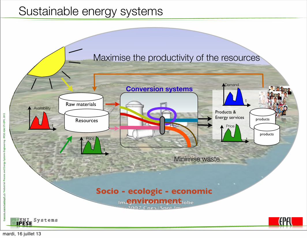
Socio - ecologic - economic environment
Sustainable energy systems
Conversion systems
Raw materials
Resources
Price
Availability
t
t
Minimise waste
Maximise the productivity of the resources
Products &Energy services products
products
Demand
Price
t
t
mardi, 16 juillet 13

fran
cois
.mar
echa
l@ep
fl.c
h ©In
dust
rial
Pro
cess
and
Ene
rgy
Syst
ems
Engi
neer
ing-
IPES
E-IG
M-S
TI-E
PFL
2013
IPESE
Perspectives for Process & Energy Systems Engineering
3 EXECUTIVE SUMMARY
step change in the rate of progress and broader engagement of the full range of countries, sectors and stakeholders.
ETP scenarios present options rather than forecasts
ETP 2010 analyses and compares various scenarios. This approach does not aim to forecast what will happen, but rather to demonstrate the many opportunities to create a more secure and sustainable energy future.
The ETP 2010 Baseline scenario follows the Reference scenario to 2030 outlined in the World Energy Outlook 2009, and then extends it to 2050. It assumes governments introduce no new energy and climate policies. In contrast, the BLUE Map scenario (with several variants) is target-oriented: it sets the goal of halving global energy-related CO2 emissions by 2050 (compared to 2005 levels) and examines the least-cost means of achieving that goal through the deployment of existing and new low-carbon technologies (Figure ES.1). The BLUE scenarios also enhance energy security (e.g. by reducing dependence on fossil fuels) and bring other benefits that contribute to economic development (e.g. improved health due to lower air pollution). A quick comparison of ETP 2010 scenario results demonstrates that low-carbon technologies can deliver a dramatically different future (Table ES.1).
Figure ES.1 � Key technologies for reducing CO2 emissions under the BLUE Map scenario
2010 2015 2020 2025 2030 2035 2040 2045 2050
Gt C
O2
05
1015202530354045505560
WEO 2009 450 ppm case ETP 2010 analysis
CCS 19%Renewables 17%Nuclear 6%
Power generation efficiencyand fuel switching 5%
End-use fuel switching 15%End-use fuel and electricityefficiency 38%
Baseline emissions 57 Gt
BLUE Map emissions 14 Gt
Key point
A wide range of technologies will be necessary to reduce energy-related CO2 emissions substantially.
Energy Technology Perspective 2010, International Energy Agency , 2010
The challenges for the engineers1. Efficient energy use and reuse2. Efficient energy conversion with CO2 capture3. Integration of renewable energy resources4. Large Scale Energy System integration & Operation
mardi, 16 juillet 13

fran
cois
.mar
echa
l@ep
fl.c
h ©In
dust
rial
Pro
cess
and
Ene
rgy
Syst
ems
Engi
neer
ing-
IPES
E-IG
M-S
TI-E
PFL
2013
IPESE
Sustainability issue• Environmental impact
– Minimise the emissions– Minimise the impact– Preserve resources
• Energy Efficiency– Minimize energy usage– Maximize energy recovery– Maximise energy conversion efficiency– Integrate renewable energy sources– Minimize GREY energy
• Economy– Engineer solutions for profits &/or competitive advantage
• Social– Integration of endogenous (human) resources– Human Development (Happiness ?) Index
mardi, 16 juillet 13
fran
cois
.mar
echa
l@ep
fl.c
h ©In
dust
rial
Pro
cess
and
Ene
rgy
Syst
ems
Engi
neer
ing-
IPES
E-IG
M-S
TI-E
PFL
2013
IPESE
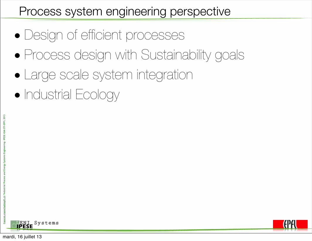
Process system engineering perspective
• Design of efficient processes• Process design with Sustainability goals• Large scale system integration• Industrial Ecology
mardi, 16 juillet 13
fran
cois
.mar
echa
l@ep
fl.c
h ©In
dust
rial
Pro
cess
and
Ene
rgy
Syst
ems
Engi
neer
ing-
IPES
E-IG
M-S
TI-E
PFL
2013
IPESE
Process efficiency & sustainability
example in a brewing process
mardi, 16 juillet 13

fran
cois
.mar
echa
l@ep
fl.c
h ©In
dust
rial
Pro
cess
and
Ene
rgy
Syst
ems
Engi
neer
ing-
IPES
E-IG
M-S
TI-E
PFL
2013
IPESE
Analysing the brewing process requirement
Malt Water
Mashing
MascheFiltration
Water
WortCooking
Hop
Cooling
Fermentation
Chilling Pasteurization et Packaging
Beer
Wort
WortYeast
Steam
Cleaning in Place
Water
Husk
Water
System boundaries? Bio methane ?
? Recover ?
mardi, 16 juillet 13

fran
cois
.mar
echa
l@ep
fl.c
h ©In
dust
rial
Pro
cess
and
Ene
rgy
Syst
ems
Engi
neer
ing-
IPES
E-IG
M-S
TI-E
PFL
2013
IPESE
Maximum heat recovery by process integration
• Heat recovery but magic heat input/output– 2700 kW out of 4000 kW
!"#$%&'()*+,-&.%/+0%
Utility MER
[kW]
Current
[kW]
Hot utility 1386 2220
Cold utility - 16
Refrigeration utility 837 1200
Heat recovery leads to 37 % energy savings
Pinch analysis based on ∆Tmin assumption
mardi, 16 juillet 13
fran
cois
.mar
echa
l@ep
fl.c
h ©In
dust
rial
Pro
cess
and
Ene
rgy
Syst
ems
Engi
neer
ing-
IPES
E-IG
M-S
TI-E
PFL
2013
IPESE
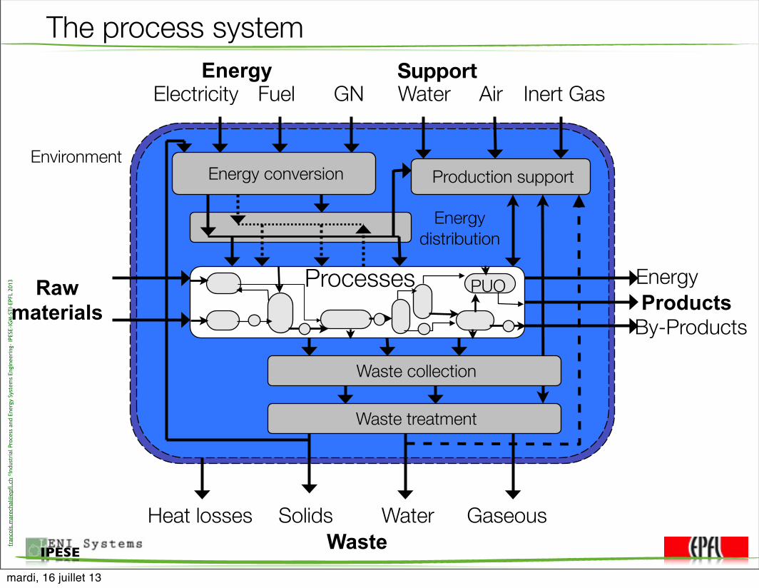
Energy conversion Production support
Waste treatment
Environment
EnergyWater
Rawmaterials Products
By-Products
Heat losses WaterSolids
Energy
Air
Waste collection
Gaseous
Inert GasFuelElectricity GN
Energydistribution
Waste
Processes PUO
Support
The process system
mardi, 16 juillet 13
fran
cois
.mar
echa
l@ep
fl.c
h ©In
dust
rial
Pro
cess
and
Ene
rgy
Syst
ems
Engi
neer
ing-
IPES
E-IG
M-S
TI-E
PFL
2013
IPESE
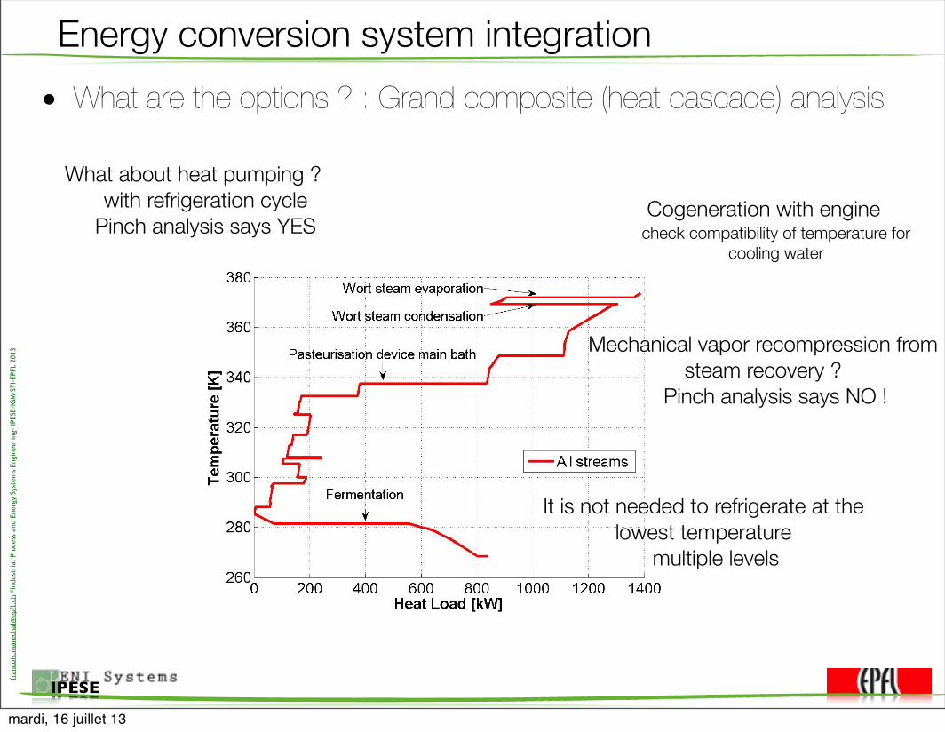
Energy conversion system integration• What are the options ? : Grand composite (heat cascade) analysis
2nd European Conference on Polygeneration - 30th March-1st April, 2011 - Tarragona, Spain
In the following example, we are discussing the integration of a trigeneration energy con-version system in a brewing process.
2 Process integration and trigeneration
The first step of the methodology is the definition of the energy requirement. In an industrialprocess, the energy requirement is defined by the set of streams to be heated up and cooled down.The definition of the requirement is obtained from a process model in which the process unitsare calculated in order to define the hot and cold streams enthalpy-temperature profiles. Thedetails of the analysis are presented in [13], the focuss being here to comment on the integrationof the trigeneration system. This analysis results in the definition of the hot and cold compositecurve of the process (Figure 1) that allows one to calculate the possible heat recovery by heatexchange between process streams. Resulting from the heat balance of the process requirement,the hot and cold composite define also the heating and cooling requirement of the process. Thecalculation of the Grand composite curve (Figure 2) defines the enthalpy-temperature profileof the heating, cooling and refrigeration requirement. Resulting from the pinch analysis, theheat recovery potential corresponds to 1143 kW i.e. 45 % of the actual consumption. This alsocorresponds to more or less doubling the present heat exchange recovery.
!"#$%&'()*+,-&.%/+0%
Figure 1: Hot and cold composite curves of the process
Figure 2: Grand composite curve of the process
The analysis of the energy requirement leads to the following conclusion
2
Cogeneration with enginecheck compatibility of temperature for
cooling water
Mechanical vapor recompression from steam recovery ?
Pinch analysis says NO !
It is not needed to refrigerate at the lowest temperature
multiple levels
What about heat pumping ?with refrigeration cycle
Pinch analysis says YES
mardi, 16 juillet 13
fran
cois
.mar
echa
l@ep
fl.c
h ©In
dust
rial
Pro
cess
and
Ene
rgy
Syst
ems
Engi
neer
ing-
IPES
E-IG
M-S
TI-E
PFL
2013
IPESE
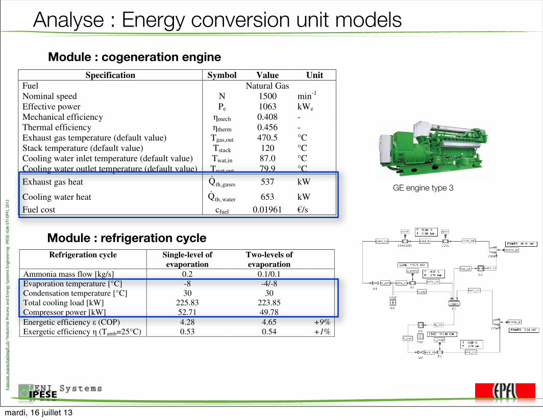
Analyse : Energy conversion unit models
Ecole Nationale des Ponts et Chaussées – Projet de fin d’Etudes
Monika Dumbliauskaite – Département Génie Civil et Construction 62
273 10 273 10 273 10 273 101118 550 160
373.5 432 337.5 373.5tL kW kW kW+ + + +
! " # + " # !
The use of steam at 123°C to supply heat to the process generates therefore around
170kW of exergetic losses. This corresponds to 160kW of mechanical work which could be
generated through the use of reversible Rankine cycles operating between T*steam and T*
process.
Therefore, it is necessary to reduce as much as possible the temperature difference between
the process and the utilities in order to lessen the exergy losses resulting from the heat transfer
between the utility streams and the corresponding process streams.
Solutions allowing the improvement of the present configuration of the utilities are
studied in the following paragraphs.
3.1.4 Integration of a Cogeneration Engine
The integration of a cogeneration engine is a sustainable solution known to reduce the
operating costs, as the combined heat and power system produces both mechanical power and
heat by taking advantage of fuel combustion.
A reciprocating engine fed with natural gas is considered in this study (see Figure 38).
It appears to be the most relevant technology, as it is possible to recover heat from both
exhaust gases and cooling water, which can be used in low temperature processes like
breweries.
Figure 38: Cogeneration Installation (Internal Combustion Engine) Source: Model GE-Jenbacher type 3, www.gejenbacher.com
Ecole Nationale des Ponts et Chaussées – Projet de fin d’Etudes
Monika Dumbliauskaite – Département Génie Civil et Construction 65
Specification Symbol Value Unit Fuel Natural Gas Nominal speed N 1500 min-1 Effective power Pe 1063 kWe Mechanical efficiency mech 0.408 - Thermal efficiency therm 0.456 - Exhaust gas temperature (default value) Tgas,out 470.5 °C Stack temperature (default value) Tstack 120 °C Cooling water inlet temperature (default value) Twat,in 87.0 °C Cooling water outlet temperature (default value) Twat,out 79.9 °C Exhaust gas heat gases,thQ 537 kW
Cooling water heat water,thQ 653 kW Fuel cost cfuel 0.01961 !/s
Table 28: Implemented Specifications of the Cogeneration Engine
For engine sizes close to 1000kW, a linear approximation of the heat loads and
mechanical power delivered by the engine can be accepted, based on the product described in
Table 26.
The computation was performed using the same hypotheses as in the previous case for
the estimation of costs and emissions (see Table 17 and Table 19). The maintenance fees are
not taken into account in the expression of the operating costs resulting from the purchase of a
new utility. This is due to the fact that the increase in maintenance fees compared with the
current setup can not be evaluated, as it would imply the complete characterisation of the
current installation and the associated maintenance costs. This criterion will not be taken into
account, since it would unfairly penalise the purchase of new installations.
As no information was provided concerning the electrical consumption of the different
production units, the electricity produced can either be sold or directly used on site. It is
assumed that in both cases, the production of 1kWhe corresponds to a saving of 0.0541 ! (see
Table 17).
The integration of the cogeneration engine described previously leads to the results
presented in Figure 40.
Ecole Nationale des Ponts et Chaussées – Projet de fin d’Etudes
Monika Dumbliauskaite – Département Génie Civil et Construction 57
Figure 32: NH3 Refrigeration Cycle with Two Evaporation Levels (Belsim-Vali® model)
Figure 33: Example of a (h,log(P)) Diagram for a Two-Level Evaporation Refrigeration Cycle Where e1 and e2 [kJ/kg] are the specific compressor works
The advantage of this installation over single-stage refrigeration cycle is the saving in
mechanical consumption. A comparison between both solutions is shown in Table 22.
Ecole Nationale des Ponts et Chaussées – Projet de fin d’Etudes
Monika Dumbliauskaite – Département Génie Civil et Construction 58
Refrigeration cycle Single-level of evaporation
Two-levels of evaporation
Ammonia mass flow [kg/s] 0.2 0.1/0.1 Evaporation temperature [°C] -8 -4/-8 Condensation temperature [°C] 30 30 Total cooling load [kW] 225.83 223.85 Compressor power [kW] 52.71 49.78 Energetic efficiency (COP) 4.28 4.65 +9% Exergetic efficiency (Tamb=25°C) 0.53 0.54 +1%
Table 22: Comparison between Single and Two-Levels of Evaporation NH3 Refrigeration Cycles
3.1.3.2 Unit Costs
The evaluation of the operating costs by Easy2 requires the determination of the unit
cost of the utilities [!/s].
Utility Reference flow [kg/s] Heat load [kW] Cost [!/s] Steam 1 2297.2 0.02034
Cooling water 1 4.19 0.00000657 Table 23: Unit Costs of Steam and Cooling Water
The detailed calculation of the values presented in Table 23 can be found in Appendix I.
3.1.3.3 Results for the Current Utility Setup
Using the assumptions formulated previously, the integration of the existing utilities
was performed so as to fulfil the MER.
The streams of the energy conversion technologies are added to the process hot and
cold streams. The resulting composite curves are called “integrated composite curves”, as
they take into account the utility streams. When the utilities are well integrated, there is no
additional energy requirement.
In Figure 34 and Figure 35 are shown the integrated composite curves of the steam
cycle and the refrigeration unit defined previously.
GE engine type 3
Module : cogeneration engine
Module : refrigeration cycle
mardi, 16 juillet 13

fran
cois
.mar
echa
l@ep
fl.c
h ©In
dust
rial
Pro
cess
and
Ene
rgy
Syst
ems
Engi
neer
ing-
IPES
E-IG
M-S
TI-E
PFL
2013
IPESE
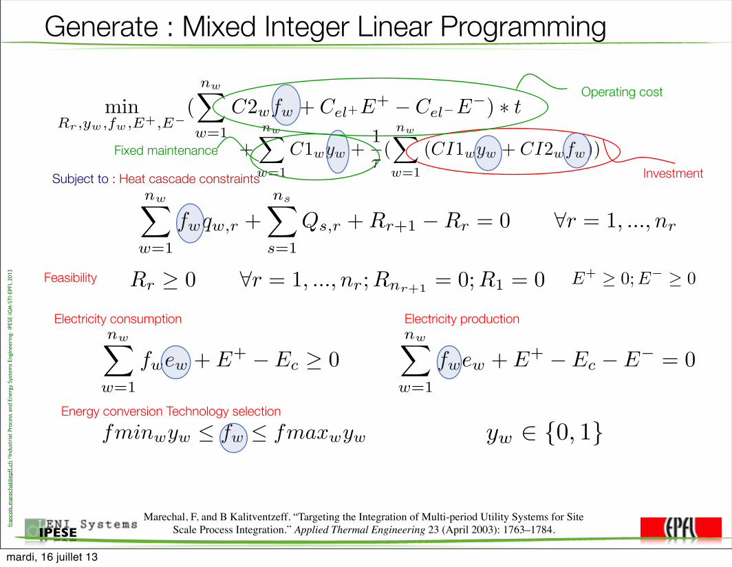
Generate : Energy conversion system integration• Utility system made of a list of optional sub-systems “w”
– Mechanical vapor recompression– Steam boiler– Cogeneration engine– Refrigeration cycle (multi levels)– Cooling water
• For each sub-system “w”– Calculate hot and cold streams
• qw,r : contribution of a stream to the heat cascade interval r if the stream is used– Calculate power consumption/production
• ew : electricity – Calculate fuel consumption => operating cost C2w
– Investment cost : piecewize linearized function : CI1w,CI2w
• Unknowns are :– is the sub-system “w” used ? : integer variable yw ={0,1}– flow in utility sub-system w : continuous variable fw : fminw ≤ fw ≤ fmaxw
mardi, 16 juillet 13
fran
cois
.mar
echa
l@ep
fl.c
h ©In
dust
rial
Pro
cess
and
Ene
rgy
Syst
ems
Engi
neer
ing-
IPES
E-IG
M-S
TI-E
PFL
2013
IPESE
Generate : Mixed Integer Linear Programming
minRr,yw,fw,E+,E!
(nw!
w=1
C2wfw + Cel+E+! Cel!E!) " t
+nw!
w=1
C1wyw +1
!(
nw!
w=1
(CI1wyw + CI2wfw))
nw!
w=1
fwqw,r +
ns!
s=1
Qs,r + Rr+1 ! Rr = 0 "r = 1, ..., nr
Rr ! 0 "r = 1, ..., nr; Rnr+1= 0; R1 = 0
nw!
w=1
fwew + E+! Ec " 0
nw!
w=1
fwew + E+! Ec ! E!
= 0
fminwyw ! fw ! fmaxwyw yw ! {0, 1}
E+ ! 0; E
! ! 0
Subject to : Heat cascade constraints
Electricity consumption Electricity production
Feasibility
Energy conversion Technology selection
Operating cost
Fixed maintenanceInvestment
Marechal, F, and B Kalitventzeff. “Targeting the Integration of Multi-period Utility Systems for Site Scale Process Integration.” Applied Thermal Engineering 23 (April 2003): 1763–1784.
mardi, 16 juillet 13
fran
cois
.mar
echa
l@ep
fl.c
h ©In
dust
rial
Pro
cess
and
Ene
rgy
Syst
ems
Engi
neer
ing-
IPES
E-IG
M-S
TI-E
PFL
2013
IPESE
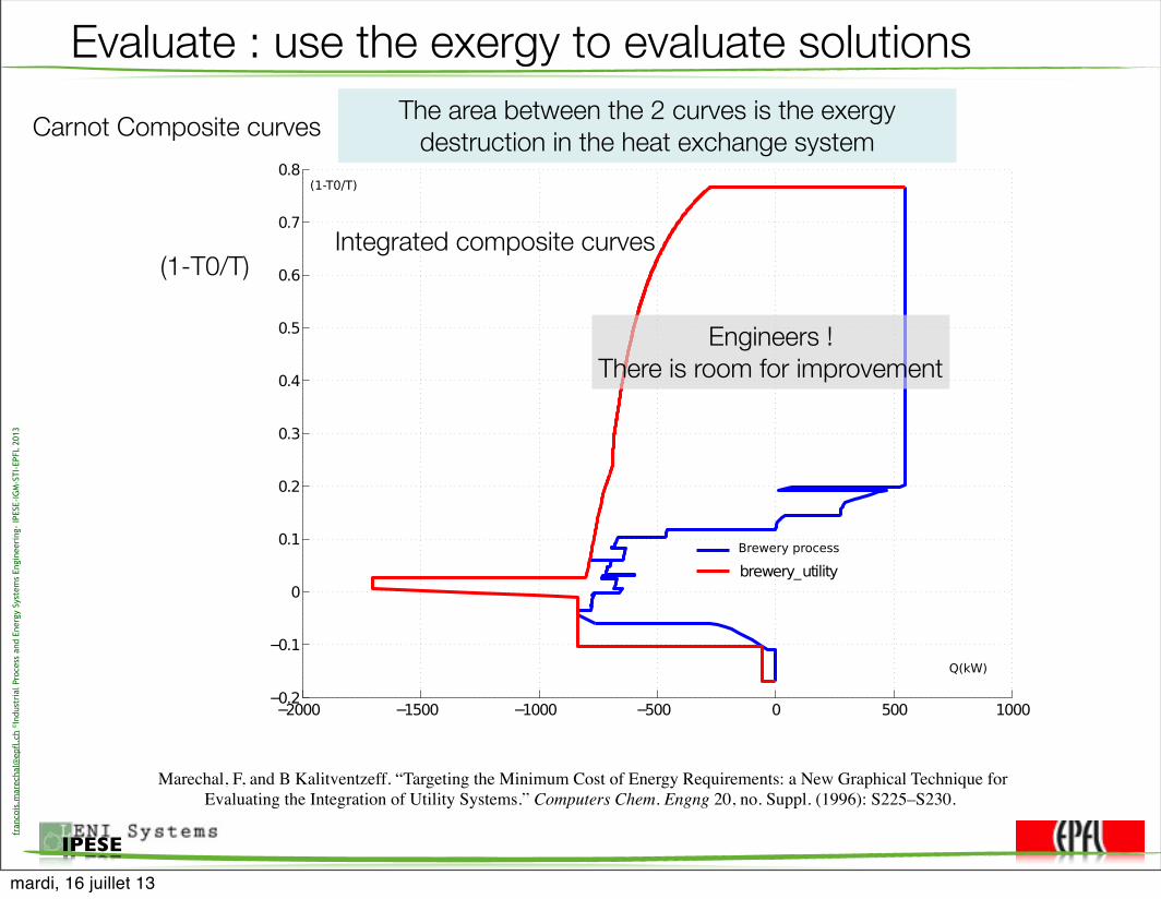
Evaluate : use the exergy to evaluate solutions
The area between the 2 curves is the exergy destruction in the heat exchange system
(1-T0/T)
Engineers ! There is room for improvement
Carnot Composite curves
Marechal, F, and B Kalitventzeff. “Targeting the Minimum Cost of Energy Requirements : a New Graphical Technique for Evaluating the Integration of Utility Systems.” Computers Chem. Engng 20, no. Suppl. (1996): S225–S230.
Integrated composite curves
mardi, 16 juillet 13

fran
cois
.mar
echa
l@ep
fl.c
h ©In
dust
rial
Pro
cess
and
Ene
rgy
Syst
ems
Engi
neer
ing-
IPES
E-IG
M-S
TI-E
PFL
2013
IPESE
Energy conversion system integration
• 2 heat pumps + 1 cogeneration engine
Fuel 1677 kW
CHP -‐374 kWe
« Heat Pumps » 295 kWe
Cooling Water 3.0 kg/s
Fuel 1140 kW
CHP -‐166 kWe
« Heat Pumps » 379 kWe
Cooling Water 0.2 kg/s
11
Engine
HP 2 set up (Tcond=351K)• HP1 set up 1 (Tcond=340K)
Becker H., Spinato G. and Marechal F., 2011b, A multi objective optimization method to integrate heat pumps in industrial processes, Computer Aided Chemical Engineering 29, 1673–1677.
mardi, 16 juillet 13
fran
cois
.mar
echa
l@ep
fl.c
h ©In
dust
rial
Pro
cess
and
Ene
rgy
Syst
ems
Engi
neer
ing-
IPES
E-IG
M-S
TI-E
PFL
2013
IPESE
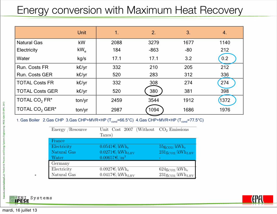
Energy conversion with Maximum Heat Recovery
1. Gas Boiler 2.Gas CHP 3.Gas CHP+MVR+HP (Tcond=66.5°C) 4.Gas CHP+MVR+HP (Tcond=77.5°C)
•
Unit 1. 2. 3. 4.
Natural Gas kW 2088 3279 1677 1140
Electricity kWe 184 -863 -80 212
Water kg/s 17.1 17.1 3.2 0.2
Run. Costs FR k€/yr 332 210 205 212
Run. Costs GER k€/yr 520 283 312 336
TOTAL Costs FR k€/yr 332 308 274 274
TOTAL Costs GER k€/yr 520 380 381 398
TOTAL CO2 FR* ton/yr 2459 3544 1912 1372
TOTAL CO2 GER* ton/yr 2987 1094 1686 1976
12
2nd European Conference on Polygeneration - 30th March-1st April, 2011 - Tarragona, Spain
Energy /Resource Unit Cost 2007 (WithoutTaxes)
CO2 Emissions
FranceElectricity 0.0541�/kWhe 55gCO2/kWhe
Natural Gas 0.0271�/kWhLHV 231gCO2/kWhLHV
Water 0.00657�/m3 -GermanyElectricity 0.0927�/kWhe 624gCO2/kWhe
Natural Gas 0.0417�/kWhLHV 231gCO2/kWhLHV
Table 2: Cost data and CO2 emissions for the electricity mix
0 1 2 3 4Natural Gas [kW] 3133 2088 3279 1677 1140Electricity [kWe] 465 184 -863 -80 212Water [kg/s] 32.0 17.1 17.1 3.2 0.2Run. Costs FR [k⇡/yr] 580 332 210 205 212Run. Costs GER [k⇡/yr] 910 520 283 312 336TOTAL Costs FR [k⇡/yr] 580 332 308 274 274TOTAL Costs GER [k⇡/yr] 910 520 380 381 398TOTAL CO2 FR* [ton/yr] 3767 2459 3544 1912 1372TOTAL CO2 GER* [ton/yr] 5277 2987 1094 1686 1976
Table 3: Summary of the results0 : reference1 : Heat recovery and boiler2 : Heat recovery and cogeneration engine3 : Heat recovery, cogeneration, mechanical vapor recompression and heat pump at Tcond=66.5°C4 : Heat recovery , , cogeneration, mechanical vapor recompression and heat pump at Tcond=77.5°CTotal Yearly Costs = Operating Costs+Annualised Investment (interest rate=5%, payback time=15years)
7
mardi, 16 juillet 13
fran
cois
.mar
echa
l@ep
fl.c
h ©In
dust
rial
Pro
cess
and
Ene
rgy
Syst
ems
Engi
neer
ing-
IPES
E-IG
M-S
TI-E
PFL
2013
IPESE
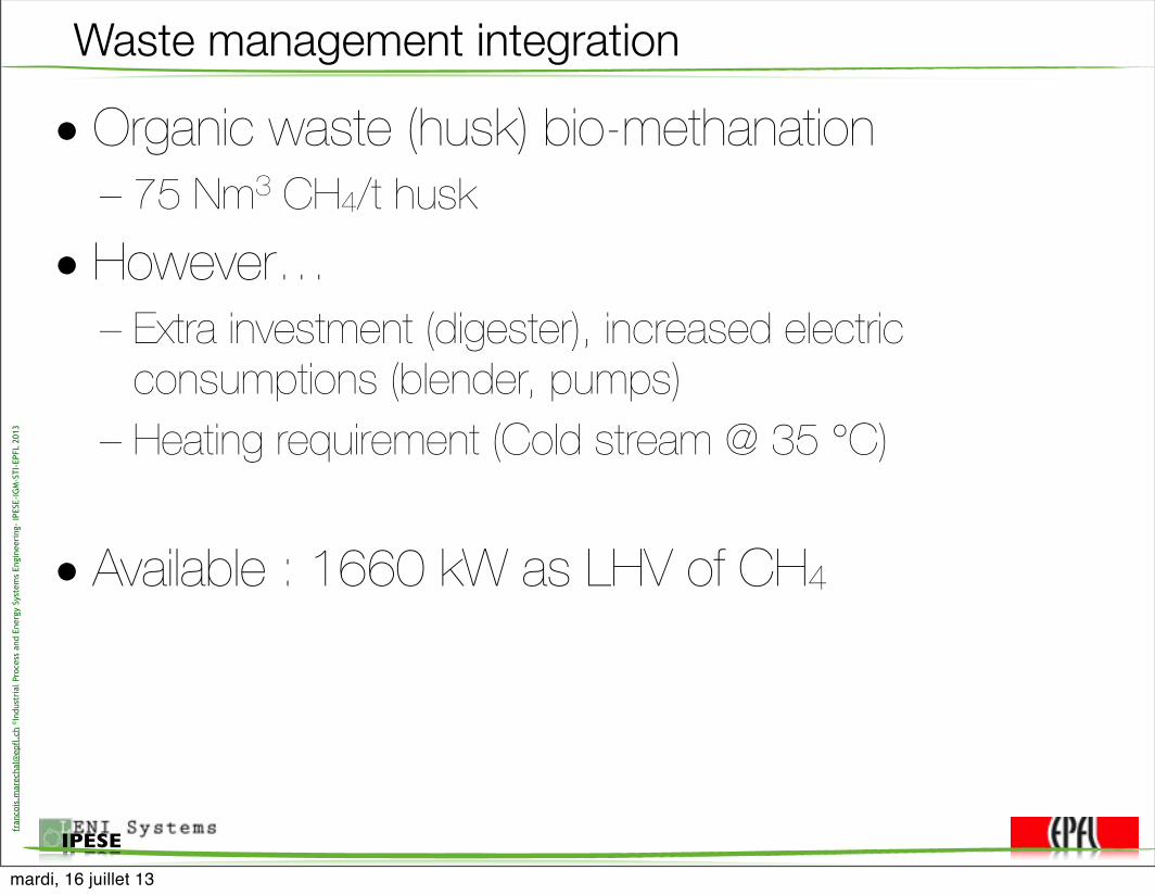
Waste management integration
• Organic waste (husk) bio-methanation– 75 Nm3 CH4/t husk
• However…– Extra investment (digester), increased electric
consumptions (blender, pumps)– Heating requirement (Cold stream @ 35 °C)
• Available : 1660 kW as LHV of CH4
mardi, 16 juillet 13
fran
cois
.mar
echa
l@ep
fl.c
h ©In
dust
rial
Pro
cess
and
Ene
rgy
Syst
ems
Engi
neer
ing-
IPES
E-IG
M-S
TI-E
PFL
2013
IPESE
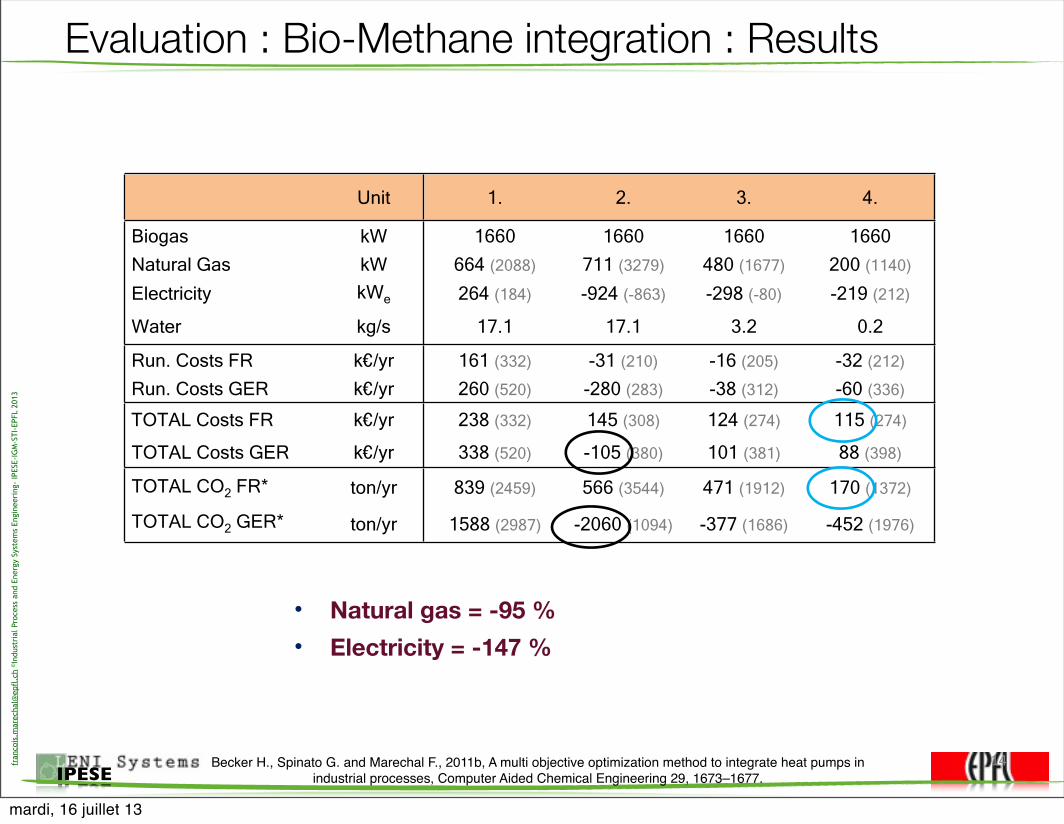
Evaluation : Bio-Methane integration : Results
• Natural gas = -95 %• Electricity = -147 %
Unit 1. 2. 3. 4.
Biogas kW 1660 1660 1660 1660
Natural Gas kW 664 (2088) 711 (3279) 480 (1677) 200 (1140)
Electricity kWe 264 (184) -924 (-863) -298 (-80) -219 (212)
Water kg/s 17.1 17.1 3.2 0.2
Run. Costs FR k€/yr 161 (332) -31 (210) -16 (205) -32 (212)
Run. Costs GER k€/yr 260 (520) -280 (283) -38 (312) -60 (336)
TOTAL Costs FR k€/yr 238 (332) 145 (308) 124 (274) 115 (274)
TOTAL Costs GER k€/yr 338 (520) -105 (380) 101 (381) 88 (398)
TOTAL CO2 FR* ton/yr 839 (2459) 566 (3544) 471 (1912) 170 (1372)
TOTAL CO2 GER* ton/yr 1588 (2987) -2060 (1094) -377 (1686) -452 (1976)
14Becker H., Spinato G. and Marechal F., 2011b, A multi objective optimization method to integrate heat pumps in industrial processes, Computer Aided Chemical Engineering 29, 1673–1677.
mardi, 16 juillet 13

fran
cois
.mar
echa
l@ep
fl.c
h ©In
dust
rial
Pro
cess
and
Ene
rgy
Syst
ems
Engi
neer
ing-
IPES
E-IG
M-S
TI-E
PFL
2013
IPESE
Conclusions : Before the analysis
Raw materialsProducts& by-products
Heat losses
Food or agro process
WasteFossil resources
ABC
ABC
CO2 Exergy
Key performance indicators
Conversion
CIPPackaging
ConditioningProcessing
Coo
ling
& r
efri
gera
tion
Hea
ting
Heat
Electricity
ABC
Costs
Biomass
100
mardi, 16 juillet 13

Products and by-products
Heat losses
Waste
Raw materials
ElectricityHeat recovery
Heat pumps and refrigeration
CogenerationConversion
Waste management
Waste
Fossil resources
Biomass
ABC
ABC
CO2 Exergy
ABC
Costs
Industrial food and agro symbiosis system
Key performance indicators
CIPPackaging
ConditioningProcessing
Coo
ling
& r
efri
gera
tion
Hea
ting
fran
cois
.mar
echa
l@ep
fl.c
h ©In
dust
rial
Pro
cess
and
Ene
rgy
Syst
ems
Engi
neer
ing-
IPES
E-IG
M-S
TI-E
PFL
2013
IPESE
More sustainable solution for Beer production
5
5
mardi, 16 juillet 13
fran
cois
.mar
echa
l@ep
fl.c
h ©In
dust
rial
Pro
cess
and
Ene
rgy
Syst
ems
Engi
neer
ing-
IPES
E-IG
M-S
TI-E
PFL
2013
IPESE
Process design with sustainability goals
• Fuel cell systems design• Biomass conversion systems• Power plant with CO2 mitigation• but also
– biorefineries– waste water treatment
mardi, 16 juillet 13

fran
cois
.mar
echa
l@ep
fl.c
h ©In
dust
rial
Pro
cess
and
Ene
rgy
Syst
ems
Engi
neer
ing-
IPES
E-IG
M-S
TI-E
PFL
2013
IPESE
Process System Engineeringre
sour
ces
Prod
ucts
/ser
vices
Waste heat/emissions
“System Engineering : Treatment of Engineering Design as a decision making process”
Hazelrigg, 2012
EquipmentType & size
Connexions
Operatingconditions
mardi, 16 juillet 13

fran
cois
.mar
echa
l@ep
fl.c
h ©In
dust
rial
Pro
cess
and
Ene
rgy
Syst
ems
Engi
neer
ing-
IPES
E-IG
M-S
TI-E
PFL
2013
IPESE
The system engineering methodology
Solutions
Energy servicesResources
Context & Constraints
Process Superstructure
System Boundaries
Technologies Thermodynamics
Economics Environmental impact
System performances indicators•Economic•Thermodynamic• Life cycle environmental impact
Results analysis•Exergy analysis•Composite curves•Sensitivity analysis•Multi-criteria
Technology options
Models
250
300
350
400
450
500
550
600
0 5000 10000 15000 20000 25000 30000
T(K
)
Q(kW)
Cold composite curve
Hot composite curve
DTmin/2
DTmin/2Heat & Mass integration
Decision variables
Solving method
Thermo-economic Pareto
Multi-objectiveOptimization
mardi, 16 juillet 13

fran
cois
.mar
echa
l@ep
fl.c
h ©In
dust
rial
Pro
cess
and
Ene
rgy
Syst
ems
Engi
neer
ing-
IPES
E-IG
M-S
TI-E
PFL
2013
IPESE
ApproachA systematic approach to problem solving
EG
A
mardi, 16 juillet 13
fran
cois
.mar
echa
l@ep
fl.c
h ©In
dust
rial
Pro
cess
and
Ene
rgy
Syst
ems
Engi
neer
ing-
IPES
E-IG
M-S
TI-E
PFL
2013
IPESE
AGE methodology
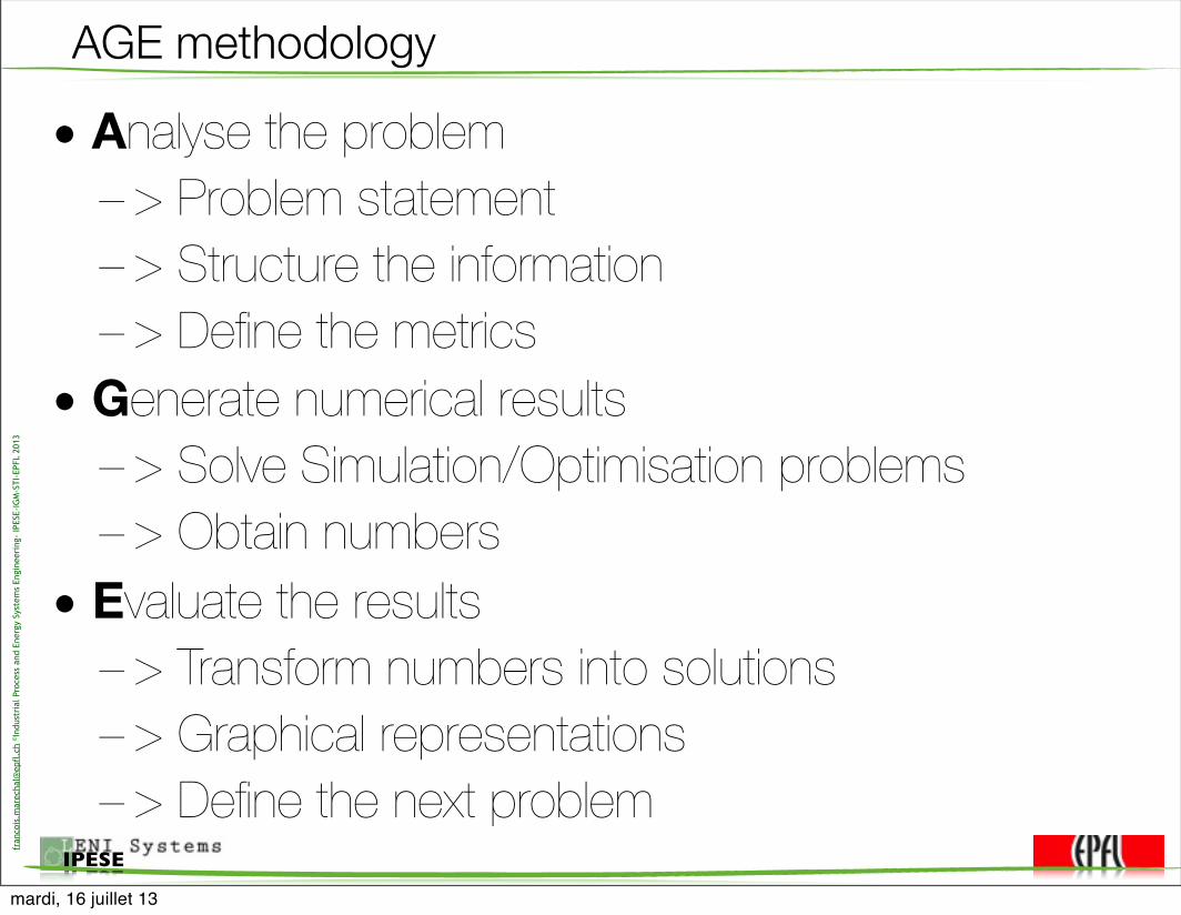
• Analyse the problem– > Problem statement– > Structure the information– > Define the metrics
• Generate numerical results– > Solve Simulation/Optimisation problems– > Obtain numbers
• Evaluate the results– > Transform numbers into solutions– > Graphical representations– > Define the next problem
mardi, 16 juillet 13
fran
cois
.mar
echa
l@ep
fl.c
h ©In
dust
rial
Pro
cess
and
Ene
rgy
Syst
ems
Engi
neer
ing-
IPES
E-IG
M-S
TI-E
PFL
2013
IPESE
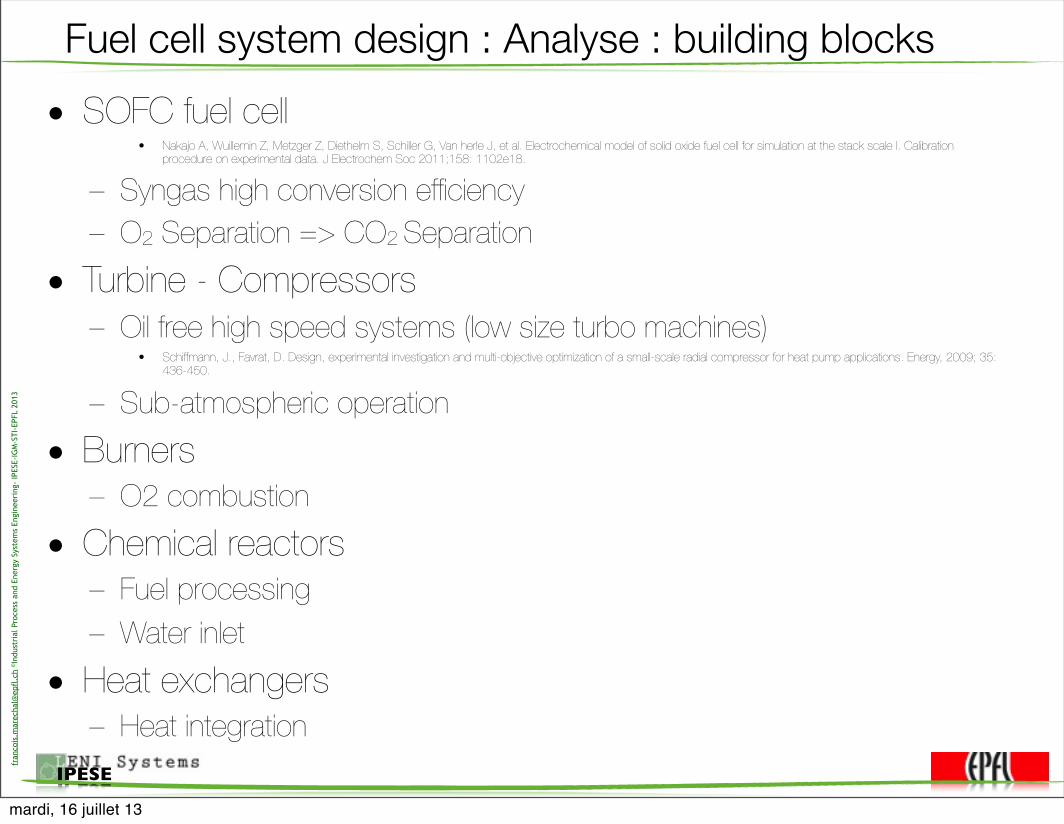
Fuel cell system design : Analyse : building blocks• SOFC fuel cell
• Nakajo A, Wuillemin Z, Metzger Z, Diethelm S, Schiller G, Van herle J, et al. Electrochemical model of solid oxide fuel cell for simulation at the stack scale I. Calibration procedure on experimental data. J Electrochem Soc 2011;158: 1102e18.
– Syngas high conversion efficiency– O2 Separation => CO2 Separation
• Turbine - Compressors– Oil free high speed systems (low size turbo machines)
• Schiffmann, J., Favrat, D. Design, experimental investigation and multi-objective optimization of a small-scale radial compressor for heat pump applications. Energy, 2009; 35: 436-450.
– Sub-atmospheric operation• Burners
– O2 combustion• Chemical reactors
– Fuel processing– Water inlet
• Heat exchangers– Heat integration
mardi, 16 juillet 13

fran
cois
.mar
echa
l@ep
fl.c
h ©In
dust
rial
Pro
cess
and
Ene
rgy
Syst
ems
Engi
neer
ing-
IPES
E-IG
M-S
TI-E
PFL
2013
IPESE
Process synthesis of a fuel cell hybrid system
Facchinetti, Emanuele, Daniel Favrat, and François Marechal. Fuel Cells, no. 0 (2011): 1-8.
⌘d =E�
CH4+LHV
= 80%
80 - 82%
18- 16%100%
Facchinetti, M, Daniel Favrat, and Francois Marechal. “Sub-atmospheric Hybrid Cycle SOFC-Gas Turbine with CO2 Separation.” PCT/IB2010/052558, 2011.
Facchinetti et al.: Innovative Hybrid Cycle Solid Oxide Fuel Cell-Inverted Gas Turbine with CO2 Separation
fuel cell and thus reduced fuel cell cooling requirement.Indeed, the optimal HCP fuel cell air excess decreases withthe pressure ratio (Figure 4). HCox and HCair are character-ized by a nearly constant steam to carbon ratio and fuel cellair excess.
The cathodic turbine pressure ratio remains nearly con-stant for HCox while decreases slightly for HCair withrespect to the anodic pressure ratio (Figure 5).
Figure 6 displays the relation between the pressure ratioand the anodic and cathodic compressor inlet temperatures.Anodic and cathodic compressor inlet temperatures of HCair
are minimized in order to reduce the compression work.The compressor inlet temperatures of HCox are slightlyhigher than the lower limit of the range. This is due to thelow temperature heat load required by the system energyintegration.
Corrected composite curves of optimal solutions, charac-terized by the same pressure ratio, are compared inFigures 7–9. The decision variables describing those solutionsare presented in Table 2. The corrected composite curvesrepresent the relation between corrected temperature!T±!DT min!2"" and the heat load specific to the power output.
/ -/ -
Fig. 3 Pressure ratio vs. steam to carbon ratio with max TIT = 1,573 K.
/ -
/ -
Fig. 4 Pressure ratio vs. fuel cell air excess with max TIT = 1,573 K.
/ -
/ -
Fig. 5 Pressure ratio vs. cathodic turbine pressure ratio with maxTIT = 1,573 K.
/ K
Fig. 6 Pressure ratio vs. compressor inlet temperature with maxTIT = 1,573 K.
/ K
Fig. 7 HCox composite curves of optimal solution with p = 3 and maxTIT = 1,573 K.
Table 2 Decision variables for optimal solutions p = 3 and maxTIT = 1,573 K.
Variables HCox HCair HCP
nsc 1.35 1.30 1.65Tsr [K] 1,065 1,073 1,071Tfc [K] 1,072 1,073 1,073k 3.3 2.6 2.6l 0.8 0.8 0.8p 3 3 3pcathode 2.9 3.0 –Tic cathode [K] 299 298 –Tic anode [K] 304 298 –
ORIG
INAL
RES
EARCH
PAPER
6 © 2011 WILEY-VCH Verlag GmbH & Co. KGaA, Weinheim FUEL CELLS 00, 0000, No. 0, 1–8www.fuelcells.wiley-vch.de
2 kWth/kWel
15 kWe
Fuel cell Gas turbine
6 kWe
21 kWe
26.3 kWLHV
5.3 kWth
Process integration
to recycling ?
mardi, 16 juillet 13
fran
cois
.mar
echa
l@ep
fl.c
h ©In
dust
rial
Pro
cess
and
Ene
rgy
Syst
ems
Engi
neer
ing-
IPES
E-IG
M-S
TI-E
PFL
2013
IPESE
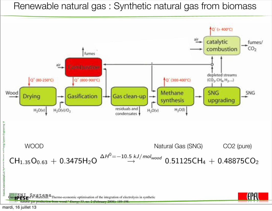
Renewable natural gas : Synthetic natural gas from biomass
Gassner, M., and F. Maréchal. “Thermo-economic optimisation of the integration of electrolysis in synthetic natural gas production from wood.” Energy 33, no. 2 (February 2008): 189-198.
WOOD Natural Gas (SNG) CO2 (pure)
mardi, 16 juillet 13

fran
cois
.mar
echa
l@ep
fl.c
h ©In
dust
rial
Pro
cess
and
Ene
rgy
Syst
ems
Engi
neer
ing-
IPES
E-IG
M-S
TI-E
PFL
2013
IPESE
LENI Systems
Flowsheet generation (2)Energy-integration model
Integrating heat recovery technologies in the superstructure
43 / 87
Closing the energy balance
mardi, 16 juillet 13
fran
cois
.mar
echa
l@ep
fl.c
h ©In
dust
rial
Ene
rgy
Syst
ems
Labo
rato
ry-
LEN
I-IG
M-S
TI-E
PFL
2012
LENI Systems
Flowsheet generation (2)Energy-integration model
MILP resolution: ... to an integrated solution
49 / 87
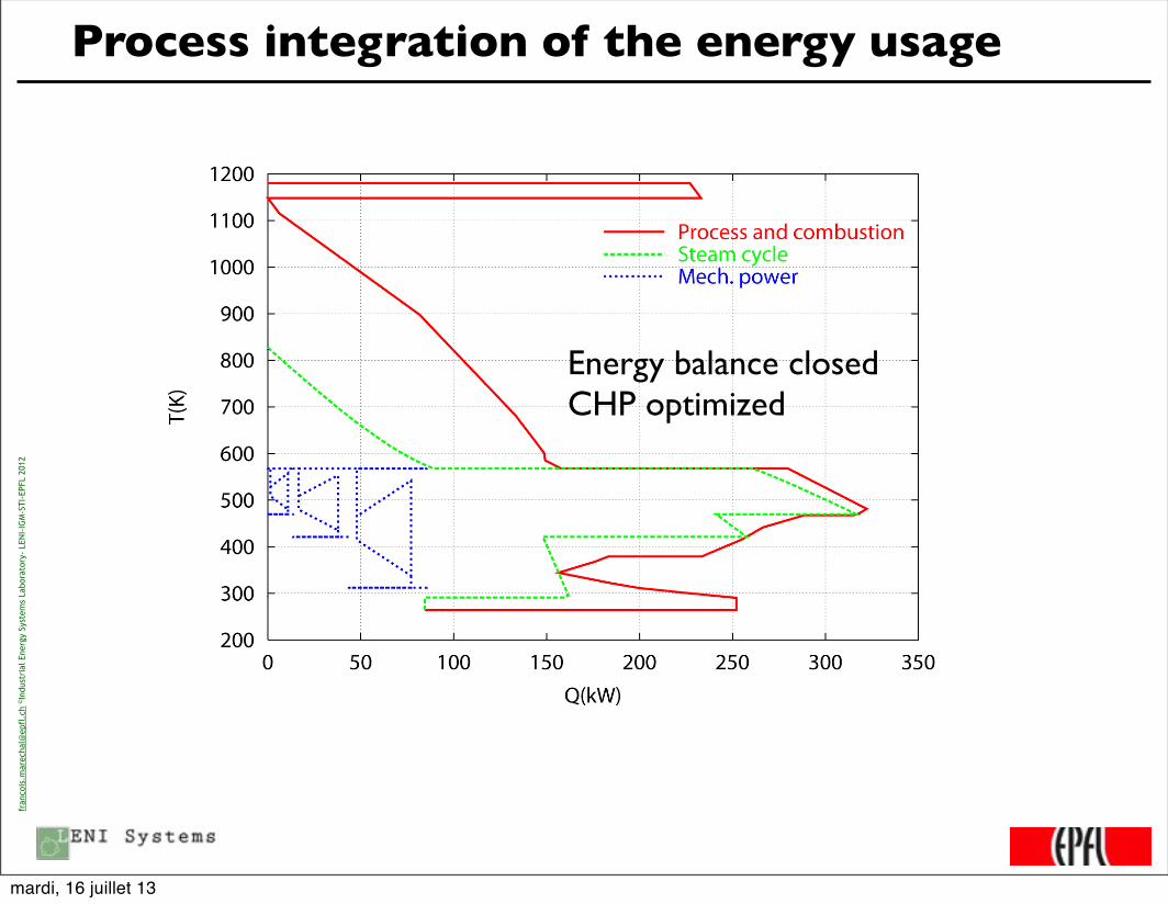
Energy balance closedCHP optimized
Process integration of the energy usage
mardi, 16 juillet 13

fran
cois
.mar
echa
l@ep
fl.c
h ©In
dust
rial
Pro
cess
and
Ene
rgy
Syst
ems
Engi
neer
ing-
IPES
E-IG
M-S
TI-E
PFL
2013
IPESE
LENI Systems
Thermo-economic optimisationTrade-o�s: e⇥ciency and scale vs. investment
E⇥ciency vs. investment and optimal scale-up:
62 63 64 65 66 67 68900
1000
1100
1200
1300
1400
1500
1600
energy e!ciency [%]
spec
i"c
inve
stm
ent
cost
[#/k
W]
trade-o$: e!ciency vs.investment (& complexity)
TECHNOLOGY: drying: air, T & humidity optimisedgasi"cation: indirectly heated dual %uid. bed (1 bar, 850°C)methanation: once through %uid. bed, T, p optimised (p = [1 15] bar)SNG-upgrade: TSA drying (act. alumina) 3-stage membrane: p, cuts optimised quality: 96% CH4, 50 barheat recovery: steam Rankine cycle T, p & utilisation levels optimised
input: 20 MW wood at 50% humidity (~4t/h dry)
0 20 40 60 80 100 120 140 160 180800
1000
1200
1400
1600
1800
2000
2200
2400
input capacity [MW]
spec
i!c
inve
stm
ent
cost
["/k
W]
scale-up objective: minimisation of production costs(incl. investment by depreciation)! ~ 62%
! ~ 66%
! ~ 64%
! ~ 68%
optimal con!gurations:increasing e#ciency
discontinuities due tocapacity limitations of
equipment (diameter < 4 m)
1nb. ofgasi!ers: 2 3 4 5 ...
61 / 87Gassner, Martin, and François Maréchal. Energy & Environmental Science 5, no. 2 (2012): 5768 – 5789.
Thermo-economic multi-objective optimisation
• Thermo-economic Pareto Front
mardi, 16 juillet 13

fran
cois
.mar
echa
l@ep
fl.c
h ©In
dust
rial
Pro
cess
and
Ene
rgy
Syst
ems
Engi
neer
ing-
IPES
E-IG
M-S
TI-E
PFL
2013
IPESE
LENI Systems
Some resultsCmparing technologies and processes
Thermo-economic Pareto front(cost vs e�ciency):
LENI Systems
Quelques resultatsComparaison des technologies
Optimisation de toutes les combinaisions technologiques(cout et e�cacite):
� gaz. pressurise a chau�age direct est la meilleure option� The best solution is the pressurised directly heated gasifier
69 / 87
Comparing options
• Each point of the Pareto is a process design
Gassner, Martin, and François Maréchal. Energy & Environmental Science 5, no. 2 (2012): 5768 – 5789.
Note : 1.5 years of calculation time !
mardi, 16 juillet 13

fran
cois
.mar
echa
l@ep
fl.c
h ©In
dust
rial
Pro
cess
and
Ene
rgy
Syst
ems
Engi
neer
ing-
IPES
E-IG
M-S
TI-E
PFL
2013
IPESE
LENI Systems
Process performanceconventional SNG
Some (non-optimised) scenarios for conventional SNGproduction:
MaintenanceLabour
OxygenBiodieselWoodElectricity
Depreciation
0
5
10
15
20
25
30
35Heat echangernetwork Steam cycle CO2-removalMethanationGas conditioning GasificationPretreatment
(base) (torr) (pM) (pM,SA) (pGM) (pGM,hot)
Inv
estm
en
t c
ost
[Mio
. EU
R]
32.6 33.1
23.324.1
17.0 17.6
FICFB CFB
0
20
40
60
80
100
Pro
du
cti
on
co
sts
[E
UR
/MW
hS
NG
]
102.9 105.4
(base) (torr) (pM) (pM,SA) (pGM) (pGM,hot)
FICFB CFB
90.3 89.3
80.675.7
pressurised methanation & gasification
Investment cost Total production costs
59 / 87
Thermo-economic comparison of process options
Gassner, Martin, and François Maréchal. Energy & Environmental Science 5, no. 2 (2012): 5768 – 5789.
mardi, 16 juillet 13

fran
cois
.mar
echa
l@ep
fl.c
h ©In
dust
rial
Pro
cess
and
Ene
rgy
Syst
ems
Engi
neer
ing-
IPES
E-IG
M-S
TI-E
PFL
2013
IPESE
BIOSNG process
• Resource productivity : + 33% per forest m2
From conventional (58%) to optimised (> 75% eff.)
mardi, 16 juillet 13
fran
cois
.mar
echa
l@ep
fl.c
h ©In
dust
rial
Pro
cess
and
Ene
rgy
Syst
ems
Engi
neer
ing-
IPES
E-IG
M-S
TI-E
PFL
2013
IPESE
• Process design with sustainability factors– Life cycle approach– Sustainability metrics
mardi, 16 juillet 13

/29
Em
FUj,i = emi · V
FUj (xd)
Guidelines for Life Cycle Analysis model
37
LCA model completed,linked with
process designand scale
Goal and scope de!nition Identi!cation of LCI "ows- material and energy !ows - process equipment
Quanti!cation of LCI "ows- link with process design and scale
Impact assessment (LCIA)- selection of appropriate environmental indicators
De!ne objectives
De!ne functional unit
De!ne system limits
Do literature review
Find equivalences of unit processes in ecoinvent
Write LCA function with necessary data to calculate LCI
Write impact functions for types of process equipment
Extend model with necessary parameters, if required
Identify driving parameters of design & scale for each "ow
Select impact assessment methods from ecoinvent
Thermo-environomic
model
Identify at which step LCI "ows occur and their function
Life Cycle Inventory Impact assessmentGoal and scope
Interpretation
FU
tot
= ˙FU(x
d
) · t
yr
· r
o
8i = 1...ni : EmFUi =
njX
j=1
EmFUj,i
[F1,1 ... F1,ni
... ... ...Fnl,1 ... Fnl,ni
] · [EmFU
1
...EmFU
ni
] = [IFU1
...IFUnl
]
Total functional unitquantity
Scaled emission i of LCI
Quantity ofelement j
of LCI
Specific emission from LCI database
Decision variables of optim. problem
mardi, 16 juillet 13

fran
cois
.mar
echa
l@ep
fl.c
h ©In
dust
rial
Pro
cess
and
Ene
rgy
Syst
ems
Engi
neer
ing-
IPES
E-IG
M-S
TI-E
PFL
2013
IPESE
Environmental Process performance indicators
• Process superstructure, extended with LCI
➡ use of ecoinvent emission database (1) for each LCI element, to take into account off-site emissions
(1) http://www.ecoinvent.org
wastewater
cradle-to-gate LCA system limits
hard wood chips
soft wood chips
transport to SNG plant
empty transport
wood chips production wood chips
thermo-economic model flowsLCA model flows, addedLCA model flows, value directly taken from t-e model
NOx PM CO2 (biogenic + fossil)
gypsum ZnO CO2 (fossil)
polymeric membranes
SNGFunctional Unit: 1MJout
FNG (substituted)
purificationCO2 (biogenic)
compression
compression
flue gas drying
indirectly heated, steam blown gasification
directly heated, oxygen blown gasification
H2O (v)
Q
H2O (v)
air
airO2
olivinecharcoal
combustion
Q
cold gas clean-up (filter, scrubber, guard
beds)
internally cooled, fluidised
bed reactor
waterCaCO3
CaCO3ZnO
oil (starting)
drying
gasification gas clean-up
methane synthesis
heat recovery system
QH2O (v)
Ni, Al2O3 (catalyst)
Ni, Al2O3
electricity (mix substituted if produced)
air separation
Q
ion transfer membranes
boiler, steam network and turbines
Identification of Life Cycle Inventory elements
Gerber, L. et al., 2010 Comp & Chem Eng., 1405-1410
mardi, 16 juillet 13
fran
cois
.mar
echa
l@ep
fl.c
h ©In
dust
rial
Pro
cess
and
Ene
rgy
Syst
ems
Engi
neer
ing-
IPES
E-IG
M-S
TI-E
PFL
2013
IPESE
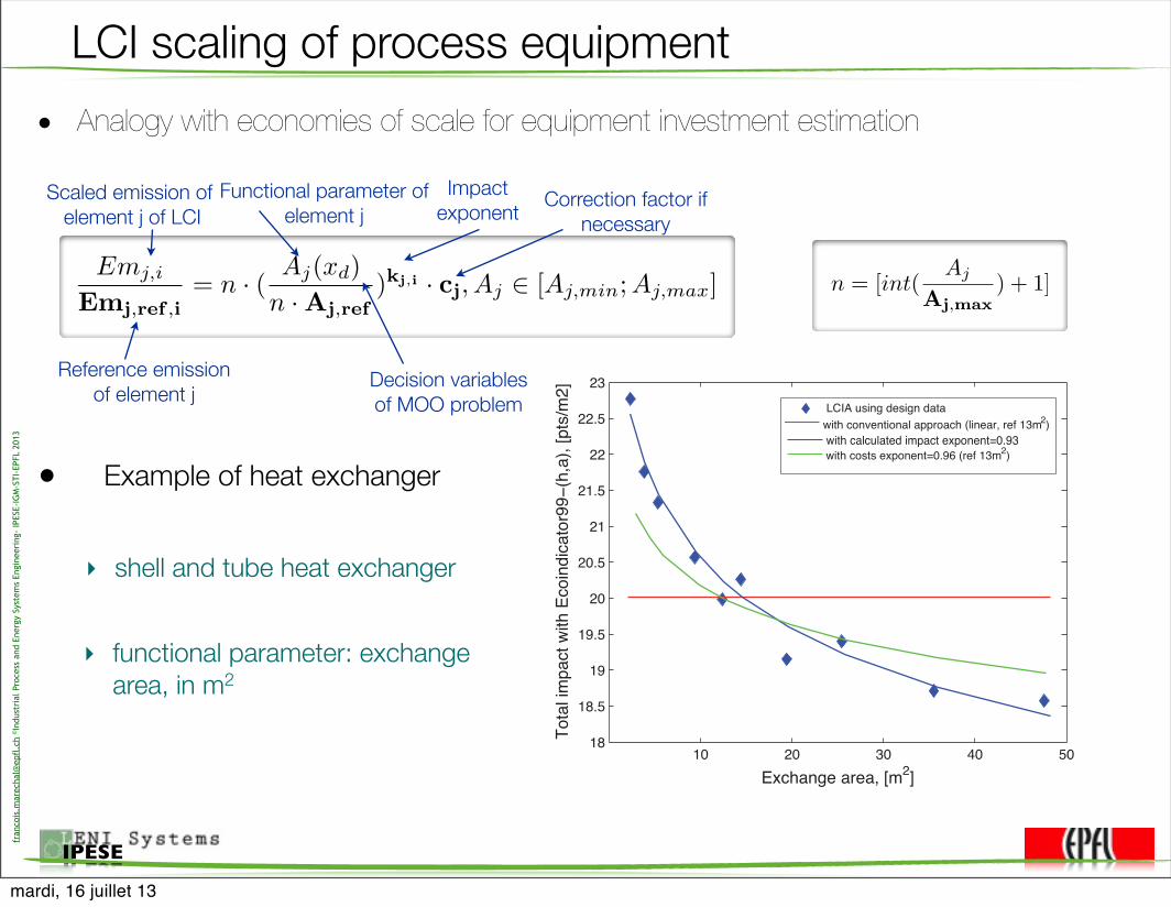
LCI scaling of process equipment• Analogy with economies of scale for equipment investment estimation
Em
j,i
Emj,ref ,i= n · (
A
j
(xd
)n · Aj,ref
)kj,i · cj, Aj
2 [Aj,min
;Aj,max
] n = [int(Aj
Aj,max
) + 1]
• Example of heat exchanger
Scaled emission of element j of LCI
Reference emission of element j
Functional parameter ofelement j
Decision variablesof MOO problem
‣ shell and tube heat exchanger
Correction factor ifnecessary
10 20 30 40 5018
18.5
19
19.5
20
20.5
21
21.5
22
22.5
23
Exchange area, [m2]
Tota
l im
pact
with
Eco
indi
cato
r99−
(h,a
), [p
ts/m
2]
LCIA using design datawith conventional approach (linear, ref 13m2)with calculated impact exponent=0.93with costs exponent=0.96 (ref 13m2)
‣ functional parameter: exchange area, in m2
Impactexponent
mardi, 16 juillet 13

fran
cois
.mar
echa
l@ep
fl.c
h ©In
dust
rial
Pro
cess
and
Ene
rgy
Syst
ems
Engi
neer
ing-
IPES
E-IG
M-S
TI-E
PFL
2013
IPESE
Results interpretation : comparing options
• pilot-scale vs integrated process for wood conversion to SNG & electricity (Ecoscarcity06)
0
5
10
15
20
25
Remaining processes
Rape methyl ester
NOx emissions
Solid waste
Charcoal
Olivine
Infrastructure
Wood chips production
Electricity cons./prod.
Avoided NG extraction
Avoided CO2 emissions
UB
P/M
Jw
oo
d
scale-independent,
conventional LCIA
(average lab/pilot tech.)
harm
ful
bene
!cia
l
harm
ful
bene
!cia
l
without cogenerationIntegrated industrial base case scenario (8 MWth)
harm
ful
bene
!cia
lwith cogeneration
Impa
ct p
er M
J of
SNG
mardi, 16 juillet 13
fran
cois
.mar
echa
l@ep
fl.c
h ©In
dust
rial
Pro
cess
and
Ene
rgy
Syst
ems
Engi
neer
ing-
IPES
E-IG
M-S
TI-E
PFL
2013
IPESE
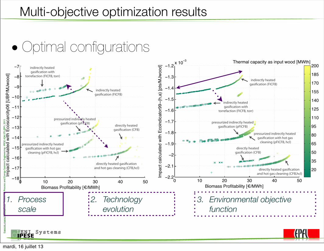
Multi-objective optimization results
• Optimal configurations
Biomass Profitability [¤/MWh]
Impa
ct c
alcu
late
d w
ith E
cosc
arci
ty06
[UBP
/MJw
ood]
0 10 20 30 40 50−18
−17
−16
−15
−14
−13
−12
−11
−10
−9
−8
−7
Biomass Profitability [¤/MWh]
Impa
ct c
alcu
late
d w
ith E
coin
dica
tor9
9−(h
,a) [
pts/
MJw
ood]
0 10 20 30 40 50−2.2
−2.1
−2
−1.9
−1.8
−1.7
−1.6
−1.5
−1.4
−1.3
−1.2x 10⁻³
20
35
50
65
80
95
110
125
140
155
170
185
200Thermal capacity as input wood [MWth]
indirectly heated gasi!cation (FICFB)
indirectly heated gasi!cation (FICFB)
indirectly heated gasi!cation with
torrefaction (FICFB, torr)
indirectly heated gasi!cation with
torrefaction (FICFB, torr)
pressurized indirectly heated gasi!cation (pFICFB)
pressurized indirectly heated gasi!cation (pFICFB)
pressurized indirectly heated gasi!cation with hot gas
cleaning (pFICFB, hcl)
pressurized indirectly heated gasi!cation with hot gas
cleaning (pFICFB, hcl)
directly heated gasi!cation (CFB)
directly heated gasi!cation (CFB)
directly heated gasi!cation and hot gas cleaning (CFB,hcl)
directly heated gasi!cation and hot gas cleaning (CFB,hcl)
1. Process scale
2. Technology evolution
3. Environmental objective function
mardi, 16 juillet 13

fran
cois
.mar
echa
l@ep
fl.c
h ©In
dust
rial
Pro
cess
and
Ene
rgy
Syst
ems
Engi
neer
ing-
IPES
E-IG
M-S
TI-E
PFL
2013
IPESE
Extending the system boundaries
• Large scale integration of industrial sites• Process and power plants• Integration in cities
mardi, 16 juillet 13
LENI Systems
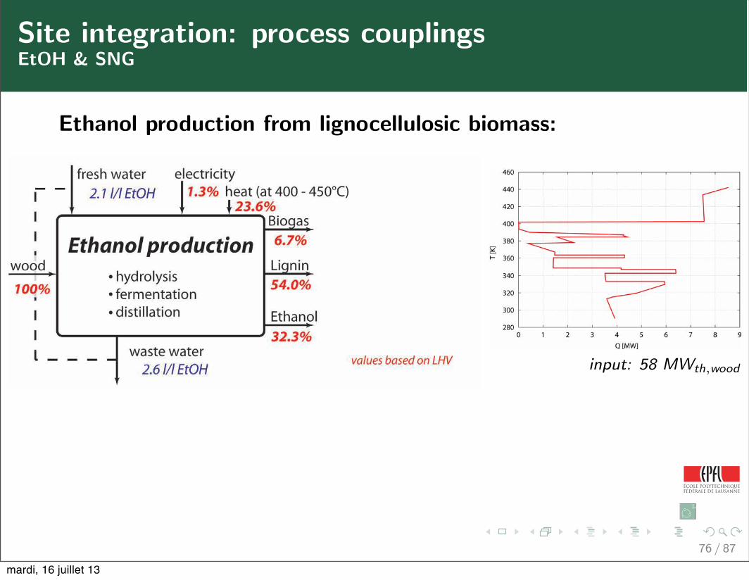
Site integration: process couplingsEtOH & SNG
Ethanol production from lignocellulosic biomass:
input: 58 MWth,wood
steam cycleInput wood 100 %
ethanol 32.3 %Output SNG -
electricity 17.1 %chem. e⇤ciency (��NGCC =55%) 62.3 %total e⇤ciency 49.4 %Energy balance for di⇥erent process integration options (without seed train, non-optimised).
76 / 87
mardi, 16 juillet 13

LENI Systems
Site integration: process couplingsEtOH & SNG
Ethanol production from lignocellulosic biomass:
input: 58 MWth,wood
steam cycleInput wood 100 %
ethanol 32.3 %Output SNG -
electricity 17.1 %chem. e⇤ciency (��NGCC =55%) 62.3 %total e⇤ciency 49.4 %Energy balance for di⇥erent process integration options (without seed train, non-optimised).
77 / 87
mardi, 16 juillet 13
LENI Systems
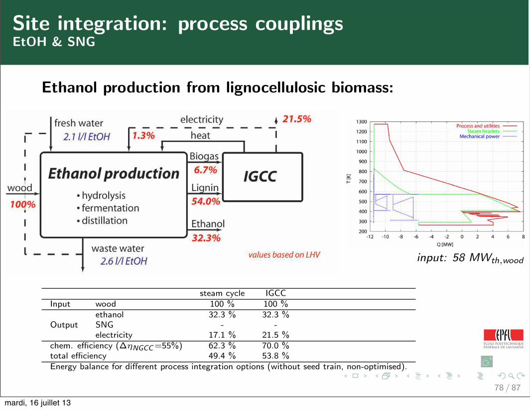
Site integration: process couplingsEtOH & SNG
Ethanol production from lignocellulosic biomass:
input: 58 MWth,wood
steam cycle IGCCInput wood 100 % 100 %
ethanol 32.3 % 32.3 %Output SNG - -
electricity 17.1 % 21.5 %chem. e⇤ciency (��NGCC =55%) 62.3 % 70.0 %total e⇤ciency 49.4 % 53.8 %Energy balance for di⇥erent process integration options (without seed train, non-optimised).
78 / 87
mardi, 16 juillet 13
LENI Systems
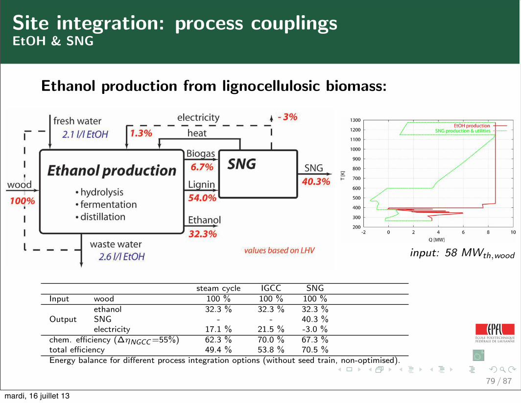
Site integration: process couplingsEtOH & SNG
Ethanol production from lignocellulosic biomass:
input: 58 MWth,wood
steam cycle IGCC SNGInput wood 100 % 100 % 100 %
ethanol 32.3 % 32.3 % 32.3 %Output SNG - - 40.3 %
electricity 17.1 % 21.5 % -3.0 %chem. e⇤ciency (��NGCC =55%) 62.3 % 70.0 % 67.3 %total e⇤ciency 49.4 % 53.8 % 70.5 %Energy balance for di⇥erent process integration options (without seed train, non-optimised).
79 / 87
mardi, 16 juillet 13

LENI Systems
Site integration: process couplingsEtOH & SNG
Ethanol production from lignocellulosic biomass:
input: 58 MWth,wood
steam cycle IGCC SNG + steamInput wood 100 % 100 % 100 % 100 %
ethanol 32.3 % 32.3 % 32.3 % 32.2 %Output SNG - - 40.3 % 30.5 %
electricity 17.1 % 21.5 % -3.0 % 1.5 %chem. e⇤ciency (��NGCC =55%) 62.3 % 70.0 % 67.3 % 65.3 %total e⇤ciency 49.4 % 53.8 % 70.5 % 64.2 %Energy balance for di⇥erent process integration options (without seed train, non-optimised).
81 / 87
mardi, 16 juillet 13
LENI Systems
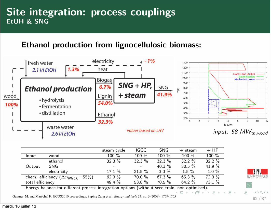
Site integration: process couplingsEtOH & SNG
Ethanol production from lignocellulosic biomass:
input: 58 MWth,wood
steam cycle IGCC SNG + steam + HPInput wood 100 % 100 % 100 % 100 % 100 %
ethanol 32.3 % 32.3 % 32.3 % 32.2 % 32.2 %Output SNG - - 40.3 % 30.5 % 41.9 %
electricity 17.1 % 21.5 % -3.0 % 1.5 % -1.0 %chem. e⇤ciency (��NGCC =55%) 62.3 % 70.0 % 67.3 % 65.3 % 72.3 %total e⇤ciency 49.4 % 53.8 % 70.5 % 64.2 % 73.1 %Energy balance for di⇥erent process integration options (without seed train, non-optimised).
82 / 87Gassner, M. and Maréchal F. ECOS2010 proceedings, Suping Zang et al. Energy and fuels 23, no. 3 (2009): 1759-1765
mardi, 16 juillet 13

fran
cois
.mar
echa
l@ep
fl.c
h ©In
dust
rial
Ene
rgy
Syst
ems
Labo
rato
ry-
LEN
I-IG
M-S
TI-E
PFL
2012
IPESE
INPUT:10 MWdry BM
15 % solid content
Depleted gas are not sufficient to close the energy balance;
Considering a 94%vol methane rich crude product, about 8 % of the total massflow has to be burned in order to satisfy the energy demand of the process ;
8
SNG 6.2 MW
ELEC 0.25 MWe
15% solids content in feedstock – 94% CH4 in crude SNG Sludge treatment
New technology Hydrothermal gasification
Salts
Water
Gassner, Martin, and François Maréchal. “Thermo-economic Optimisation of the Polygeneration of Synthetic Natural Gas (SNG), Power and Heat from Lignocellulosic Biomass by Gasification and Methanation.” Energy and Environmental Science 5, no. 2 (2012): 5768 – 5789.
mardi, 16 juillet 13

fran
cois
.mar
echa
l@ep
fl.c
h ©In
dust
rial
Ene
rgy
Syst
ems
Labo
rato
ry-
LEN
I-IG
M-S
TI-E
PFL
2012
IPESE
Results for different wet biomass substrates
not considered20
25
30
35
40
45
50
55
60
65
70
75
80
SNG
e!
cien
cy e
quiv
alen
t [%
]
Power rec. considerednot consideredconsideredconsideredCat. cost not considered
economic optimum
Gassner, Martin, and François Maréchal. “Thermo-economic Optimisation of the Polygeneration of Synthetic Natural Gas (SNG), Power and Heat from Lignocellulosic Biomass by Gasification and Methanation.” Energy and Environmental Science 5, no. 2 (2012): 5768 – 5789.
mardi, 16 juillet 13
fran
cois
.mar
echa
l@ep
fl.c
h ©In
dust
rial
Ene
rgy
Syst
ems
Labo
rato
ry-
LEN
I-IG
M-S
TI-E
PFL
2012
IPESE
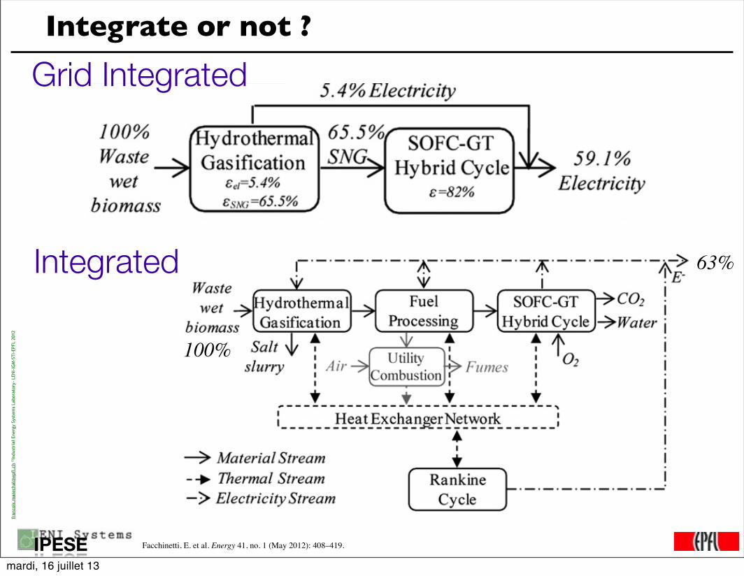
Integrate or not ?
The First Law efficiency (Eq. (1)) is defined as the ratio betweenthe electrical power output and the transformation energy receivedby the system as input. The electrical power output is the sum ofthe net power production of all process sections. The trans-formation energy received by the system, consisting in biomass andin pure oxygen used as oxidant in the SOFC-GT hybrid cycle unit, iscalculated on the basis of the lower heating value of the drybiomass [22] and considering an electricity consumption of1080 kJ/kg for cryogenic oxygen production, as estimated byHamelinck et al. [23].
3!
P
i
_E"i
_M#dry Biomass$Dh0idry Biomass #
_M#O2$ecryO2
i ! 1;.;n Process sections
(1)
The second-law performance is based on a theoretical exergyefficiency definition that represents a coherent thermodynamicindicator of the upper bound system performance. According tothe general definition and following the formalism proposed byFavrat [24,25], the exergy efficiency is defined as the ratiobetween the exergy rate delivered by the system and the exergyrate received by the system. In our case (Eq. (2)), the exergy ratedelivered by the system consists in the electrical power outputand in the diffusion exergy of the separated carbon dioxide, whichis equivalent to the ideal work needed to separate the carbondioxide from the atmosphere if it was not separated by thesystem. The exergy rate received by the system is reduced tothe transformation exergy received from the biomass [26] and thediffusion exergy of the pure oxygen, which is equivalent to theideal work needed to separate the oxygen from the atmosphere.Compared to the First Law efficiency (1), this exergy efficiencydefinition provides a consistent indication that also includes theadditional value provided by the system of separating the carbondioxide.
h !
P
i
_E"i # _M
#CO2
$esCO2
_M#dryBiomass$Dk0dryBiomass #
_M#O2$esO2
i ! 1;.;n Process sections
(2)
3. Process description
The integrated system is divided into four units: the hydro-thermal gasification unit, the fuel processing unit, the SOFC-GThybrid cycle unit and the steam Rankine cycle unit. A conceptualflowsheet of the system is presented in Fig. 1. The principles andmodeling of these units are described in the following paragraphs.
Default operating conditions, general assumptions and the decisionvariables that have been identified for the optimization are detailedin Table 1.
3.1. Hydrothermal gasification
3.1.1. Principles and issuesAs discussed in detail in the process model development [8],
hydrothermal gasification of wet waste biomass in supercriticalwater takes advantage of the thermophysical properties of theaqueous environment at high pressure. Conventional gasificationtypically decomposes the carbonaceous matter above 1073 K intosynthesis gas and requires a dry feedstock to limit the considerableheat demand at high temperature [27]. Since waste biomass isusually very wet, an energy-intense drying step would thus bemandatory prior to gasification. At supercritical pressure, thespecific and latent heat of water is sharply decreasing [28] andlimits the energy requirement for its heat-up to the gasificationtemperature. Wet feedstock can thus be processed directly withouta significant penalty on the conversion efficiency.
Depending on the temperature, two principal strategies forsupercritical water gasification can be distinguished [29]. Ifhydrogen is targeted as the principal product [30], high gasificationtemperatures of 773e1023 K are applied and low-grade, non-metalcatalysts like activated carbon or no catalysts at all are used. Thishas the advantage that its deactivation is not an issue, and theinorganics do not need to be removed prior to gasification. At thelower bound, the temperature range is thereby limited by theconversion kinetics, while mechanical stress limitations of theconstruction materials prevent higher operating temperature andpressure to be feasible.
If methane is targeted as the principal product [28,31], thegasification is carried out at lower temperatures of 623e873 K andcatalyzed by noble metal (typically nickel- or ruthenium-based)catalysts. The lower gasification temperature has the advantage todecrease the enthalpy of reaction and the heat requirement of theprocess, but also requires to prevent an excessive degradation of thehigh-grade catalyst by a prior removal of the dissolved catalystspoisons such as sulfur. Since the solubility of the inorganiccompounds that are present in the feedstock decreases drasticallywhen reaching supercritical conditions, they precipitate as a saltbrine that needs to be removed and fromwhich the nutrients mightbe recovered. As investigated by Peterson et al. [32] and Schubertet al. [33,34], this may be done in a heated separator device that actssimilar to a cyclone. In addition, the use of guards or catalyst recy-cling may be economically advantageous to allow for low temper-atures and thus decrease the heat demand for the separation [9].
In addition to these technological issues, the successful devel-opment of an efficient process design strongly depends on theprocess integration and, in particular, the heat supply andpower recovery from the hot gasification product at supercriticalpressure [8,9].
3.1.2. ModelingBased on the experimental results of the process development
conducted by Vogel and coworkers [28,32e35], we have developeda detailed process model including several configurations for thepolygeneration of SNG, power and heat fromwet waste biomass bycatalytic hydrothermal gasification, in which the inorganiccompounds are precipitated and removed in a salt separator priorto gasification (Fig. 2) [8].
In this model, the biomass decomposition during hydrolysisbetween 473 and 623 K is phenomenologically representedconsidering the breakdown of the macromolecules (cellulose,hemicellulose and lignin) into the principal substances (methanol,Fig. 1. Conceptual flowsheet of the system.
E. Facchinetti et al. / Energy xxx (2012) 1e12 3
Please cite this article in press as: Facchinetti E, et al., Process integration and optimization of a solid oxide fuel cell e Gas turbine hybrid cyclefueled with hydrothermally gasified waste biomass, Energy (2012), doi:10.1016/j.energy.2012.02.059
100%
63%Integrated
below the pinch that is provoked by the salt separator. If thisconstraint is released, only marginally better results are obtainedwith the increased power output from the GT expansion in thefuel processing.
The capability of the system to adapt to different processrequirements has been experienced also in additional analyses thathave been performed for gasification temperatures between 673 Kand 973 K.
5. Conclusions
This paper presents a systematic process integration and opti-mization of a SOFC-GT hybrid cycle fueled with hydrothermallygasified waste biomass. For this purpose, a general processsuperstructure based on detailed process models has been devel-oped. Special attention has thereby been paid to completelyrecover the thermal and physical exergy potential from the processstreams. The crucial role of fuel processing (i.e. the expansion,separation and reforming of the crude gasification product) hasbeen highlighted by analyzing different flowsheet options for flashseparation both at high and low pressure. All these design alter-natives have been compared through a thermodynamic optimi-zation approach with respect to First Law and exergy performanceindicators.
The analysis has demonstrated that the systemmay convert wetwaste biomass to electricity at a First Law efficiency of up to 63%. Atthe same time, the biogenic carbon dioxide is separated and thusallows for negative net emissions of carbon dioxide if it would besequestrated. Despite more conservative assumptions that lead tolower conversion efficiencies in the gasification and fuel cellsubsystems, 1 the overall electric efficiency thus is improved byroughly 10% with respect to the only comparable flowsheetingapproach available in the scientific literature [17]. This resulthighlights the potential of a systematic process design approachthat combines the development of a general process superstructurewith methods for systematical energy recovery, process integrationand optimization.
The optimal design solution consists in maximizing the flowrate of fuel that is converted in the SOFC and in adjusting the otherprocess subsystems in order to supply the process heat require-ments andminimize the exergy losses. The analysis has shown thatflowsheets based on liquidevapor separation at gasification pres-sure are more efficient than reheating and expanding the entirecrude product to the pressure of the fuel cell since not enoughexcess heat is available in the system. Furthermore, upgrading the
fuel quality by separating the carbon dioxide before reformingslightly increases the performance of the SOFC itself, but is notworthwhile from an overall system perspective.
The relation between system efficiency and its complexity hasalso been investigated by limiting the number of subsystems thatare considered for recovering the available exergy. It has beenshown that although the system efficiency always increases withthe number of available conversion technologies, these alternativesare both complementary and competing in different temperatureranges. The maximum efficiency, which is 13.5% higher than for thesimplest case, is thereby only achievable when all options areconsidered.
A sensitivityanalysiswith respect to the gasification temperaturehas shown that the conversion efficiency remains constant forgasificationbetween673and973 Ksince it is limitedby theavailableheat. For this reason, the system is flexible to adapt to designconstraints imposed by issues such as catalyst deactivation bysulfurous compounds or limited material strength at hightemperature.
Compared to a non-integrated, decentralized system in whichwaste biomass is hydrothermally gasified, purified and injected asSNG into the gas grid [8,9] that is afterward locally converted toelectricity in an SOFC-GT hybrid cycle [7], this work demonstratesthat process integration allows for a considerable increase of theoverall conversion system performance. As shown in Fig. 13, thenon-integrated combination allows for an overall electric effi-ciency of only 59.1%, which is 3.9%-points lower than the one ofthe optimally integrated system that has been proposed in thiswork.
References
[1] Zhang X, Chan SH, Li G, Ho HK, Li J, Feng Z. A review of integration strategiesfor solid oxide fuel cells. J Power Sources 2010;195:685e702.
[2] Palsson J, Selimovic A, Sjunnesson L. Combined solid oxide fuel cell and gasturbine systems for efficient power and heat generation. J Power Sources2000;86:442e8.
[3] Massardo AF, Lubelli F. Internal reforming solid oxide fuel cellegas turbinecombined cycles (IRSOFCeGT): part a e cell model and cycle thermodynamicanalysis. J Eng Gas Turbines Power 2000;122:27e35.
[4] Park SK, Kim TS. Comparison between pressurised design and ambient pres-sure design of hybrid solid oxide fuel cell-gas turbine systems. J PowerSources 2006;163:490e9.
[5] Franzoni A, Magistri L, Traverso A, Massardo AF. Thermoeeconomic analysisof pressurised hybrid SOFC systems with CO2 separation. Energy 2008;33:311e20.
[6] Park SK, Kim TS, Sohn JL, Lee YD. An integrated power generation systemcombining solid oxide fuel cell and oxy-fuel combustion for high performanceand CO2 capture. Appl Energy 2011;88:1187e96.
[7] Facchinetti E, Favrat D, Marechal F. Innovative hybrid cycle solid oxide fuelcell e inverted gas turbine with CO2 separation. Fuel Cells 2011;11:565e72.
[8] Gassner M, Vogel F, Heyen G, Maréchal F. Optimal process design for thepolygeneration of SNG, power and heat by hydrothermal gasification of wastebiomass: thermo-economic process modelling and integration. EnergyEnviron Sci 2011;4:1726e41.
[9] Gassner M, Vogel F, Heyen G, Maréchal F. Optimal process design for thepolygeneration of SNG, power and heat by hydrothermal gasification of wastebiomass: process optimisation for selected substrates. Energy Environ Sci2011;4:1742e58.
[10] Panopoulos K, Fryda L, Karl J, Poulou S, Kakaras E. High temperature solidoxide fuel cell integrated with novel allothermal biomass gasification. J PowerSources 2006;159:570e85.
[11] Athanasiou C, Coutelieris F, Vakouftsi E, Skoulou V, Antonakou E, Marnellos G,et al. From biomass to electricity through integrated gasification/SOFCsystem-optimisation and energy balance. Int J Hydrogen Energy 2007;32:337e42.
[12] Aravind P, Woudstra T, Woudstra N, Spliethoff H. Thermodynamic evaluationof small-scale systems with biomass gasifiers, solid oxide fuel cells with Ni/GDC anodes and gas turbines. J Power Sources 2008;190:461e75.
[13] Nagel F, Schildhauer T, Biollaz S. Biomass-integrated gasification fuel cellsystems e part 1: definition of systems and technical analysis. Int J HydrogenEnergy 2009;34:6809e25.
[14] Sadhukhan J, Zhao Y, Shah N, Brandon N. Performance analysis of integratedbiomass gasification fuel cell (BGFC) and biomass gasification combined cycle(BGCC) systems. Chem Eng Sci 2010;65:1942e54.
Fig. 13. Integrated system versus non-integrated system.
E. Facchinetti et al. / Energy xxx (2012) 1e12 11
Please cite this article in press as: Facchinetti E, et al., Process integration and optimization of a solid oxide fuel cell e Gas turbine hybrid cyclefueled with hydrothermally gasified waste biomass, Energy (2012), doi:10.1016/j.energy.2012.02.059
Grid Integrated
Facchinetti, E. et al. Energy 41, no. 1 (May 2012): 408–419.
mardi, 16 juillet 13
fran
cois
.mar
echa
l@ep
fl.c
h ©In
dust
rial
Pro
cess
and
Ene
rgy
Syst
ems
Engi
neer
ing-
IPES
E-IG
M-S
TI-E
PFL
2013
IPESE
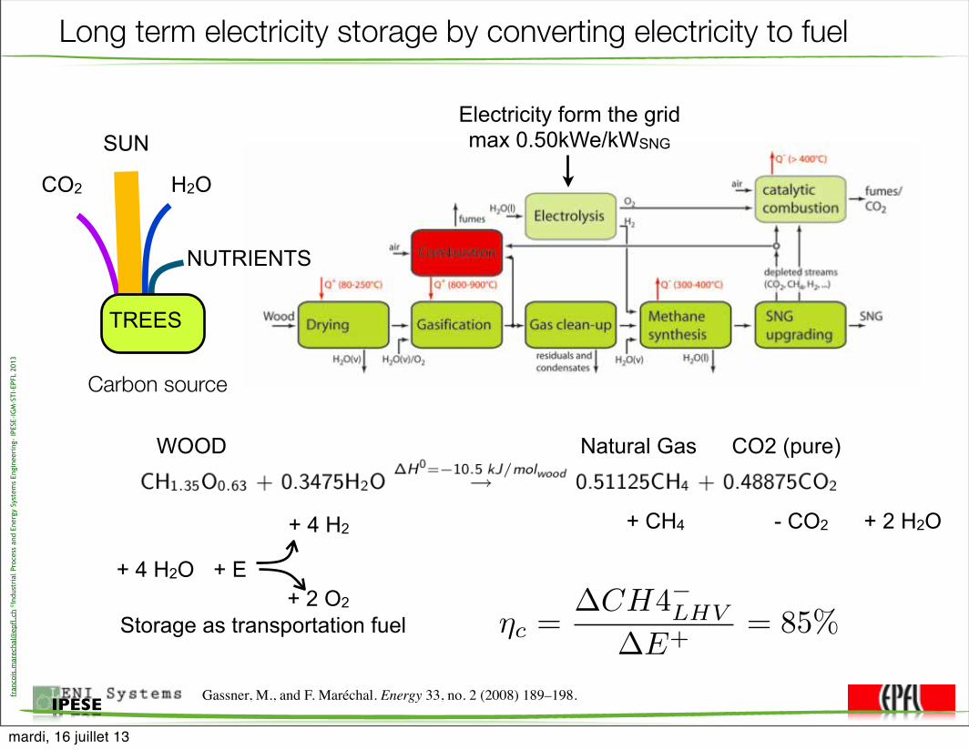
Long term electricity storage by converting electricity to fuel
⌘c =�CH4�LHV
�E+= 85%
WOOD Natural Gas CO2 (pure)
+ 4 H2 + CH4 - CO2
Electricity form the gridmax 0.50kWe/kWSNG
Storage as transportation fuel
+ E
Gassner, M., and F. Maréchal. Energy 33, no. 2 (2008) 189–198.
+ 2 H2O
+ 2 O2
+ 4 H2O
CO2 H2O
SUN
NUTRIENTS
TREES
Carbon source
mardi, 16 juillet 13
fran
cois
.mar
echa
l@ep
fl.c
h ©In
dust
rial
Pro
cess
and
Ene
rgy
Syst
ems
Engi
neer
ing-
IPES
E-IG
M-S
TI-E
PFL
2013
IPESE
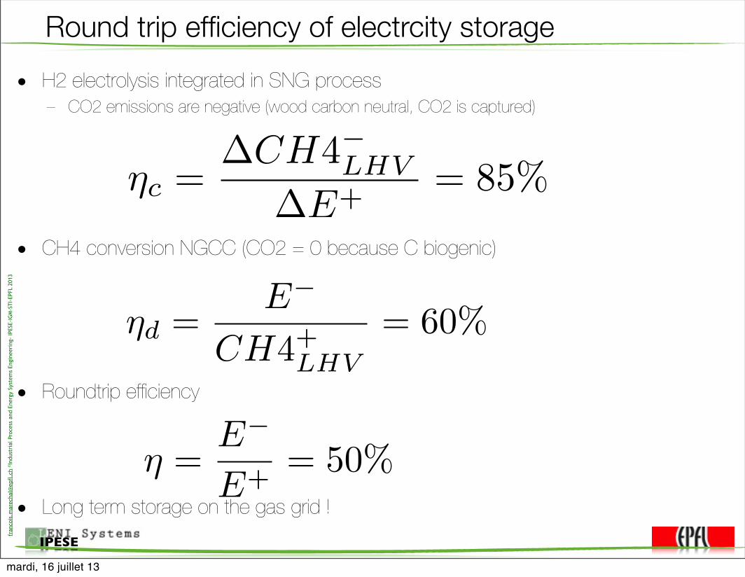
Round trip efficiency of electrcity storage• H2 electrolysis integrated in SNG process
– CO2 emissions are negative (wood carbon neutral, CO2 is captured)
• CH4 conversion NGCC (CO2 = 0 because C biogenic)
• Roundtrip efficiency
• Long term storage on the gas grid !
⌘d =E�
CH4+LHV
= 60%
⌘ =E�
E+= 50%
⌘c =�CH4�LHV
�E+= 85%
mardi, 16 juillet 13

fran
cois
.mar
echa
l@ep
fl.c
h ©In
dust
rial
Pro
cess
and
Ene
rgy
Syst
ems
Engi
neer
ing-
IPES
E-IG
M-S
TI-E
PFL
2013
IPESE
If Electricity production efficiency increases
• Hybrid gas turbine SOFC combined cycle
• Round trip with long term storage on gas grid and decentralised production
Facchinetti, Emanuele, Daniel Favrat, and François Marechal. “Innovative Hybrid Cycle Solid Oxide Fuel Cell-Inverted Gas Turbine with $CO_2$ Separation.” Fuel Cells, no. 0 (2011): 1-8.
⌘d =E�
CH4+LHV
= 80%
⌘ =E�
E+= 68%
80%
12%100%
mardi, 16 juillet 13
fran
cois
.mar
echa
l@ep
fl.c
h ©In
dust
rial
Pro
cess
and
Ene
rgy
Syst
ems
Engi
neer
ing-
IPES
E-IG
M-S
TI-E
PFL
2013
IPESE
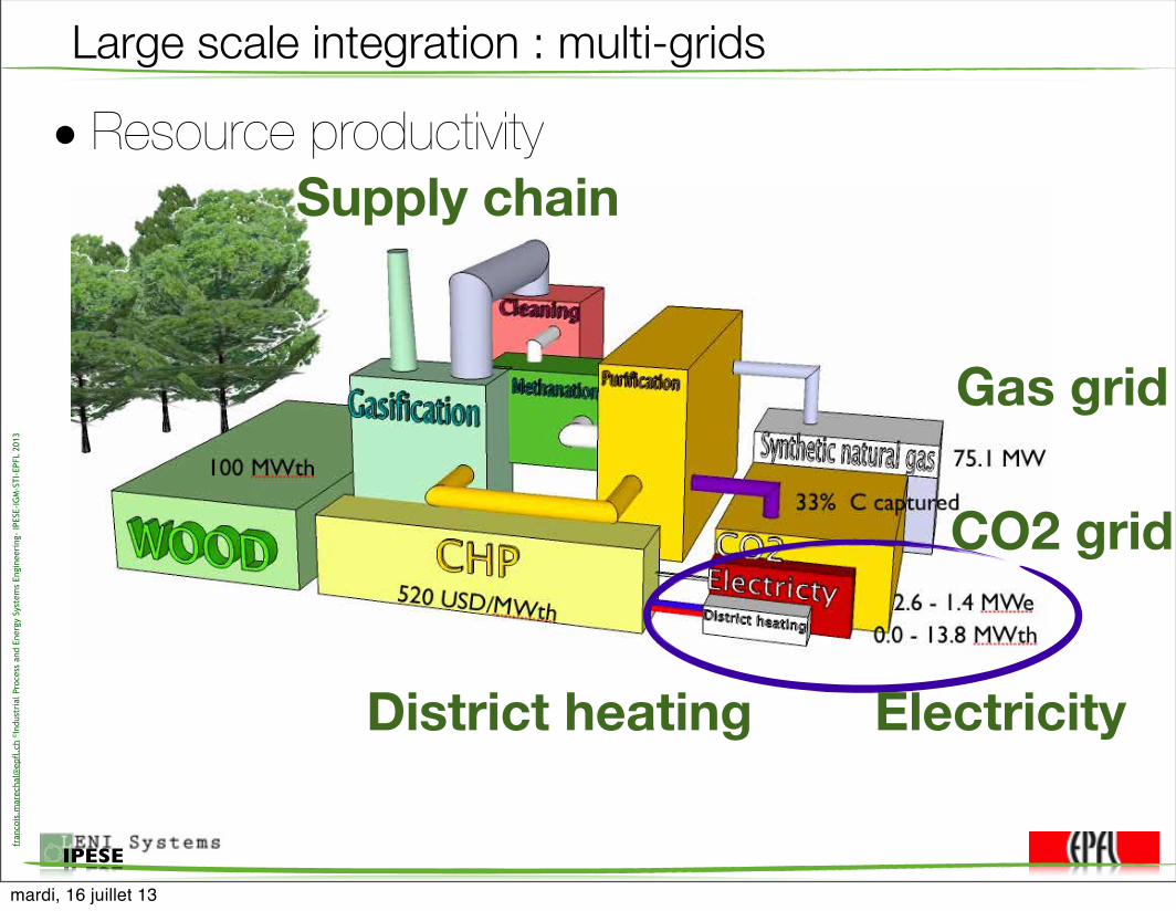
Large scale integration : multi-grids
• Resource productivity
Gas grid
CO2 grid
District heating Electricity
Supply chain
mardi, 16 juillet 13

• Canton of Geneva integration
fran
cois
.mar
echa
l@ep
fl.c
h ©In
dust
rial
Pro
cess
and
Ene
rgy
Syst
ems
Engi
neer
ing-
IPES
E-IG
M-S
TI-E
PFL
2013
IPESE
LENI Systems
ÉCOLE POLYTECHNIQUEFÉDÉRALE DE LAUSANNE
INTRODUCTION METHODOLOGY REQUIREMENTS RESSOURCES DISTRICT HEATING CONVERSION CONCLUSION
Context
IntroductionContext
I State of Geneva strategic energy planning 2007-2030I EU Concerto pilot project : TetraenerI Urban Energy GIS platform concept
Figure: Geneva District Map
I 475 zones (282 km2),445’000 inhabitant
I 22’189 buildings
I 9’200 annual bill monitoring
I 200 detailed monitoring
Industrial Energy Systems LaboratoryEcole Polytechnique Federale de Lausanne
Urban system integration
Where to place the heating network ?Which fluid ?@ which temperature ?
mardi, 16 juillet 13

fran
cois
.mar
echa
l@ep
fl.c
h ©In
dust
rial
Pro
cess
and
Ene
rgy
Syst
ems
Engi
neer
ing-
IPES
E-IG
M-S
TI-E
PFL
2013
IPESE
Process integration in buildings
• Definition of the energy needs– Heating– Air renewal– Hot water– Waste Water– Air renewal Text
Tw Twmin
TrTs
mardi, 16 juillet 13

fran
cois
.mar
echa
l@ep
fl.c
h ©In
dust
rial
Pro
cess
and
Ene
rgy
Syst
ems
Engi
neer
ing-
IPES
E-IG
M-S
TI-E
PFL
2013
IPESE
Local heat recovery
-20
0
20
40
60
80
0 50 100 150 200 250 300 350 400
T(C
)
Q(kW)
AirWaste Water
Heating Hot water
recoveryRecoverable
Heat requirement
mardi, 16 juillet 13
fran
cois
.mar
echa
l@ep
fl.c
h ©In
dust
rial
Pro
cess
and
Ene
rgy
Syst
ems
Engi
neer
ing-
IPES
E-IG
M-S
TI-E
PFL
2013
IPESE
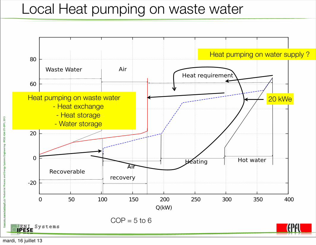
Local Heat pumping on waste water
-20
0
20
40
60
80
0 50 100 150 200 250 300 350 400
T(C
)
Q(kW)
AirWaste Water
Heating Hot water
recoveryRecoverable
Heat requirement
20 kWe
Heat pumping on water supply ?
COP = 5 to 6
Heat pumping on waste water- Heat exchange- Heat storage- Water storage
mardi, 16 juillet 13

Heating & Hot water production, Power [MW] at -6°C
5.36 - 11.11 [MW]
2.87 - 5.35
1.08 - 2.86
0.00 - 1.07
fran
cois
.mar
echa
l@ep
fl.c
h ©In
dust
rial
Pro
cess
and
Ene
rgy
Syst
ems
Engi
neer
ing-
IPES
E-IG
M-S
TI-E
PFL
2013
IPESE
Waste water reuse perspective
Girardin et al., ENERGIS, A geographical information based system for the evaluation of integrated energy conversion systems in urban areas, Energy, 2010
15 °C
13°C-16°C3°C
18 °C
5 l/s/1000 hab
60 kWth
Biogas 9 kW
Boues 6 kWth
200 kWth
<1 kWe
70 kWth 250 kWth
COP =4.850 kWe
COP =6.210 kWe
3 kWth
3 kWe
9 kWth
Potential = 330 kWth/1000 hab
1000 hab
329 kWth
40°C
Network
mardi, 16 juillet 13

fran
cois
.mar
echa
l@ep
fl.c
h ©In
dust
rial
Pro
cess
and
Ene
rgy
Syst
ems
Engi
neer
ing-
IPES
E-IG
M-S
TI-E
PFL
2013
IPESE
Define the demands of a district
• Characterizing the services
For one building
for all the building in the city
Seasonal temperature variation
Heating signature Heating temperature
mardi, 16 juillet 13
fran
cois
.mar
echa
l@ep
fl.c
h ©In
dust
rial
Pro
cess
and
Ene
rgy
Syst
ems
Engi
neer
ing-
IPES
E-IG
M-S
TI-E
PFL
2013
IPESE
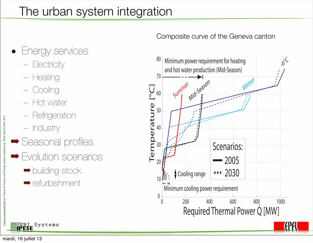
The urban system integration
• Energy services– Electricity– Heating– Cooling– Hot water– Refrigeration– Industry
➡ Seasonal profiles➡ Evolution scenarios
➡ building stock➡ refurbishment
0 200 400 600 800 1000 12000
10
20
30
40
50
60
70
80
Required Thermal Power Q [MW]
Te
mp
era
ture
[°C
]
2030
Summer
Mid-Season Winter
-6°C Minimum power requirement for heating and hot water production (Mid-Season)
Minimum cooling power requirement
2005Scenarios:
Cooling range
Composite curve of the Geneva canton
mardi, 16 juillet 13
fran
cois
.mar
echa
l@ep
fl.c
h ©In
dust
rial
Pro
cess
and
Ene
rgy
Syst
ems
Engi
neer
ing-
IPES
E-IG
M-S
TI-E
PFL
2013
IPESE
Heat/power requirement of a cityTypical days: Cergy
34
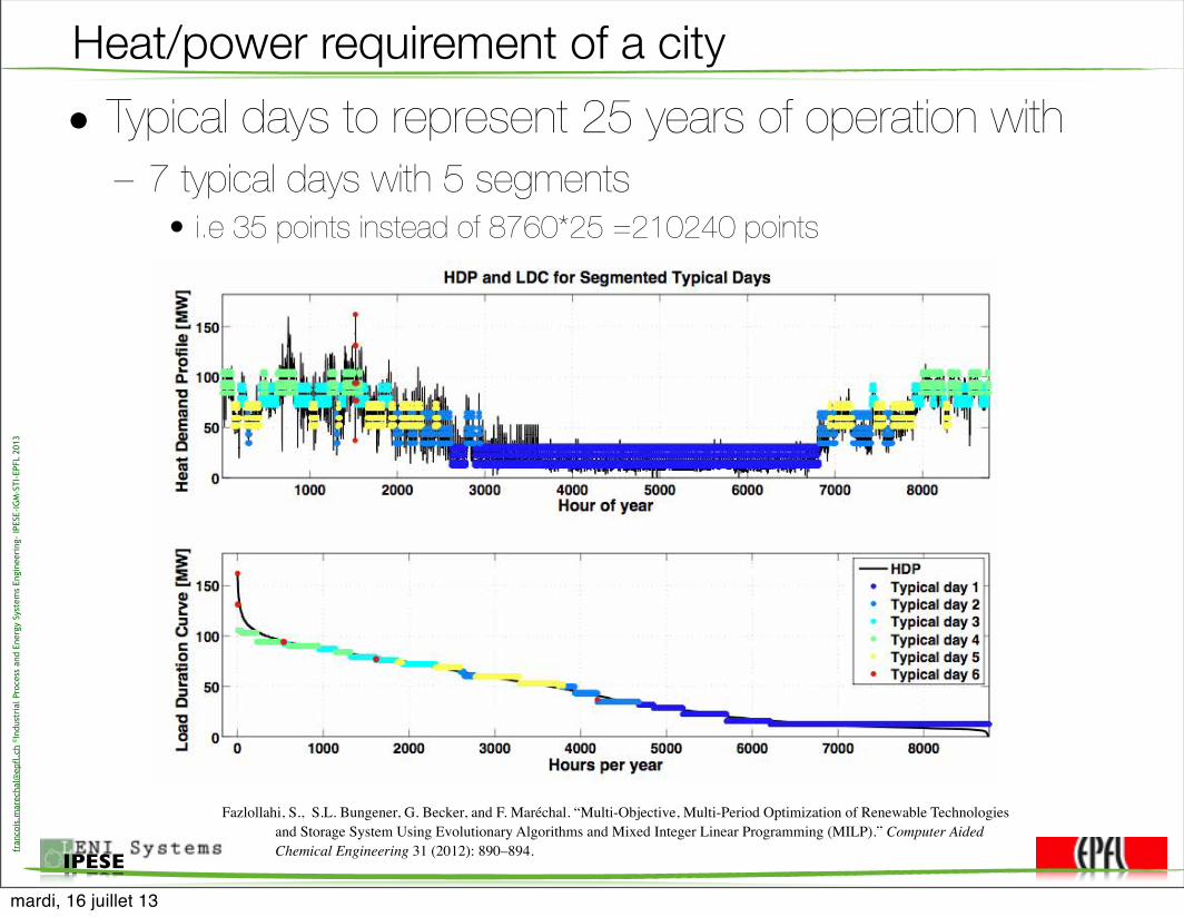
• In order to reduce the number of time steps and the optimization size, the heating demand series of 8760 values are compressed to the limited number of typical days.
• Typical days to represent 25 years of operation with– 7 typical days with 5 segments
• i.e 35 points instead of 8760*25 =210240 points
Fazlollahi, S., S.L. Bungener, G. Becker, and F. Maréchal. “Multi-Objective, Multi-Period Optimization of Renewable Technologies and Storage System Using Evolutionary Algorithms and Mixed Integer Linear Programming (MILP).” Computer Aided Chemical Engineering 31 (2012): 890–894.
mardi, 16 juillet 13

fran
cois
.mar
echa
l@ep
fl.c
h ©In
dust
rial
Pro
cess
and
Ene
rgy
Syst
ems
Engi
neer
ing-
IPES
E-IG
M-S
TI-E
PFL
2013
IPESE
District heating cost : cts CHF/annual kWh
Indice de coût des réseaux [cts/kW]Température aller : 90°C.
0.65 - 1.08
1.09 - 1.45
1.46 - 1.94
1.95 - 2.56
2.57 - 3.29
3.30 - 4.72
4.73 - 6.38
6.39 - 7.96
cts/kWh
• Building density– nb + m2
• Power density• Annual energy
LENI Systems
ÉCOLE POLYTECHNIQUEFÉDÉRALE DE LAUSANNE
INTRODUCTION METHODOLOGY REQUIREMENTS RESSOURCES DISTRICT HEATING CONVERSION CONCLUSION
Investment costs estimation
DISTRICT HEAT DISTRIBUTION SYSTEMInvestment costs estimation
Annualised network cost
(90°C, prediction 2030)
[CHF/MWh]
0.6 - 10
10 - 20
20 - 60
> 60
� LDHN = 2(Nb � 1)K
sAh
Nb
� T⇥supply = Treturn + (Tsupply � Treturn) · (1 +
floss,refTsupply�Tground
Tref �Tground)
� QDHN = mDHNcpfluid (T⇥supply � Treturn)
� dDHN =
vuut4mDHN
�vs⇥(T⇥supply )
� CDHN =(c1dDHN + c2)LDHN
1
⇤QDHN
[CHF/kWh]
Industrial Energy Systems LaboratoryEcole Polytechnique Federale de Lausanne
Girardin, Luc, François Marechal, Matthias Dubuis, Nicole Calame-Darbellay, and Daniel Favrat. “EnerGis: A Geographical Information Based System for the Evaluation of Integrated Energy Conversion Systems in Urban Areas.” Energy 35, no. 2 (February 2010): 830–840.
mardi, 16 juillet 13

fran
cois
.mar
echa
l@ep
fl.c
h ©La
bora
tory
for
Indu
stri
al E
nerg
y Sy
stem
s -
LEN
I ISE
-STI
-EPF
L –
Mar
sh 2
006
IPESE
Given a set of energy conversion technologies :Where to locate the energy conversion technologies ?How to connect the buildings ?How to operate the energy conversion technologies ?
Energy system design : problem definition
1 Symbols
Roman lettersAn Annuities of a given investment [-]Ai,j,p Surface of the pipe of network p between nodes i and j [m2]B Arbitrarily big valueCaw Investment costs for air/water heat pump(s) [CHF]Cboiler Annual investment costs of the boiler(s) [CHF/year]Cfix Fix part of investment costs for a given device [CHF]Cgas Total gas costs [CHF]cgas Gas costs [CHF/kWh]Cgrid Total grid costs [CHF]cgrid Grid costs [CHF/kWh]C inv Investment costs of a given device [CHF]C inv
an Annual investment costs of a given device [CHF]Cpipes Total costs for the piping [CHF]Cprop Fix part of investment costs for a given device [CHF/kW]Cref Investment costs of a device chosen as reference [CHF]Cww Investment costs for water/water heat pump(s) [CHF]CO2
gas Total CO2 emissions for one year due to the combustion of gas [kg]co2
gas CO2 emissions due to the combustion of gas per kWh [kg/kWh]CO2
grid Total CO2 emissions for one year due to the consumption of electricity from the grid [kg]co2
grid CO2 emissions due to the consumption of electricity from the grid [kg/kWh]COP aw
t,k Coe⇤cient of performance for the air/water heat pump during period t at node k [-]COPww
t,k Coe⇤cient of performance for a water/water heat pump during period t at node k [-]cp Isobaric specific heat [kJ/(K· kg)]Disti,j Distance between nodes i and j [m]Ht Number of hours in period t [hour]Econs
t,k Electricity consumption during period t at node k [kW]Eexp
t,k Eletricity exported to the grid during period t by device e [kW]Egrid
t,k Electricity bought from the grid during period t [kW]Eaw
t,k Electricity consumed by the air/water heat pump during period t at node k [kW]Eww
t,k Electricity consumed by the water/water heat pump during period t at node k [kW]Eloss
t,k Electricity losses during period t [kW]Epump
t Pumping power for the network during period t [kW]Etech
t,k,e Electricity produced or consumed during period t at node k by device e [kW]Fm Maintenance factor [-]Gast Overall gas consumption during period t [kg]Lmin
e Minimum allowable part-load of device e [-]
Mbuildt,k
Mass flow of water from the network, circulating during period t through thebuilding at node k to heat up the building [kg/s]
Mpipet,i,j,p
Mass flow of water flowing during period t, in network p, from node i to nodej [kg/s]
Mmaxt,p,i,j
Maximum mass flow of water flowing in network p, from node i to node j, overall periods of time [kg/s]
M techt,k
Mass flow from the network being heated up by the device(s) at node k duringperiod t [kW]
MT buildt,k
Mass flow from the network flowing through a device at node k during periodt, to be re-heated, times its temperature [(kg/s)K]
2
MT pipet,i,j,p
Mass flow flowing during period t from node i to node j in the network p, timesits temperature [(kg/s)K]
N Expected lifetime for a given investment [year]Ploss Pressure losses in the pipes [Pa/m]Qaw
t,k Heat delivered by the air/water heat pump to the consumer at node k during period t [kW]Qboiler
t,k Heat delivered by the boiler at node k during period t [kW]Qcons
t,k Heat consumption at node k during period t [kW]Qnet
t,k Heat delivered by the network to the consumer at node k during period t [kW]Qnet ww
t,k Heat delivered by the network to the water/water heat pump at node k during period t [kW]Qtech
t,k,e Heat produced by device e located at node k during period k [kW]Qww
t,k Heat delivered by an water/water heat pump to the consumer at node k during period t [kW]r Interest rate [-]S Size of a given device [kW]Saw
k Nominal size of the air/water heat pump located at node k [kW]Sboiler
k Nominal size of the boiler at node k [kW]Snom
e Nominal power of a device [kW]Sref Size of a device chosen as reference [kW]Sww
k Nominal power of the water/water heat pump located at node k [kW]T atm Atmospheric temperature [K]T cold Temperature of the heat source for heat pumps [K]T cons
t,k Temperature at which the heat is required by the consumer at node k during period t [K]T hot Temperature of the heat sink for heat pumps [K]T net Design temperature of the network [K]v Velocity of the water through the pipes [m/s]X = 1 if a device exists, 0 otherwiseXaw
k = 1 if there is an air/water heat pump at node k, 0 otherwiseXboiler
k = 1 if there is a boiler at node k, 0 otherwiseXgas
e = 1 if device e needs gas to operate, 0 otherwiseXnode
k = 1 if a device e is implemented at node k, 0 otherwiseXtech
k,e = 1 if a device can be implemented at node k, 0 otherwiseXww
k = 1 if there is an water/water heat pump at node k, 0 otherwiseY i,j,p = 1 if a connection exists between i and j for network p , 0 otherwise
Greek letters�Theat Pinch at the heat-exchangers [K]�Tnet ww Temperature di⇥erence of the water in the network when it serves as heat source for water/water heat pump(s) [K]�boiler Thermal e⌅ciency of the boiler(s) [-]�ele Electric e⌅ciency of device e [-]�grid E⌅ciency of the grid [-]�the Thermal e⌅ciency of device e [-]⇥ Exergetic e⌅ciency [-]⇤ Density [kg/m3]
Indicesk nodesi, j connection from node i to node jt timee technologies
3
Network superstructure
1 Symbols
Roman lettersAn Annuities for a given investment [-]Ai,j,p Area of the pipe between nodes i and j of network p [m2]B Arbitrarily big valueCaw Investment costs for air/water heat pump(s) [CHF]Cboiler Annual investment costs for the boiler(s) [CHF/year]Cfix Fix part of the investment costs for a given device [CHF]Cgas Total annual natural gas costs [CHF/year]cgas Natural gas costs [CHF/kWh]Cgrid Total annual grid costs [CHF/year]cgrid Grid costs [CHF/kWh]C inv Investment costs of a given device [CHF]C inv
an Annual investment costs of a given device [CHF/year]Cpipes Total annual costs for the piping [CHF/year]Cprop Fix part of the investment costs for a given device [CHF/kW]Cref Investment costs of a device chosen as reference [CHF]Cww Investment costs for water/water heat pump(s) [CHF]CO2
gas Total annual CO2 emissions due to the combustion of natural gas [kg/year]co2
gas CO2 emissions due to the combustion of natural gas [kg/kWh]CO2
grid Total annual CO2 emissions due to the consumption of electricity from the grid [kg/year]co2
grid CO2 emissions due to the consumption of electricity from the grid [kg/kWh]COPhp Coe⇤cient of performance of the central heat pumpCOP aw
t,k Coe⇤cient of performance for the air/water heat pump during period t at node k [-]COPww
t,k Coe⇤cient of performance for a water/water heat pump during period t at node k [-]cp Isobaric specific heat [kJ/(K· kg)]Disti,j Distance between nodes i and j [m]Ht Number of hours in period t [hour]Econs
t,k Electricity consumption during period t at node k [kW]Eexp
t,e Eletricity exported to the grid during period t by device e [kW]Egrid
t,k Electricity bought from the grid during period t by node k [kW]Eaw
t,k Electricity consumed by the air/water heat pump during period t at node k [kW]Eww
t,k Electricity consumed by the water/water heat pump during period t at node k [kW]Eloss
t Electricity losses during period t [kW]Epump
t Pumping power for the network during period t [kW]Etech
t,k,e Electricity produced or consumed during period t at node k by device e [kW]Fs Scaling factor [-]Fm Maintenance factor [-]Gast Natural gas consumption during period t [kg]Lmin
e Minimum allowable part-load of device e [-]Mbuild
t,k Water circulating during period t through the building at node k, to heat it up [kg/s]Mpipe
t,i,j,p Water flowing during period t, from node i to node j, in network p [kg/s]Mmax
i,j,p Maximum flow of water between nodes i and j, in network p, over all periods [kg/s]M tech
t,k Water being heated up by the device(s) during period t, at node k [kg/s]MT tech
t,k Water flowing through a device during period t at node k to be re-heated, times its temperature [(kg/s)K]
2
Q1..T
E1..T
Q1..T
E1..T
Q1..T
E1..T
Q1..T
E1..T
Q1..T
E1..TQ1..T
E1..T
Q1..T
E1..T
Q1..T
E1..T
Cinv =ne�
e=1
nk�
k=1
ae + ae � Se,k
Investment
Operating cost
Cgas =ne�
e=1
nk�
k=1
np�
t=1
HtQe,k,t
�the
1 Symbols
Roman lettersAn Annuities for a given investment [-]Ai,j,p Area of the pipe between nodes i and j of network p [m2]B Arbitrarily big valueCaw Investment costs for air/water heat pump(s) [CHF]Cboiler Annual investment costs for the boiler(s) [CHF/year]Cfix Fix part of the investment costs for a given device [CHF]Cgas Total annual natural gas costs [CHF/year]cgas Natural gas costs [CHF/kWh]Cgrid Total annual grid costs [CHF/year]cgrid Grid costs [CHF/kWh]C inv Investment costs of a given device [CHF]C inv
an Annual investment costs of a given device [CHF/year]Cpipes Total annual costs for the piping [CHF/year]Cprop Fix part of the investment costs for a given device [CHF/kW]Cref Investment costs of a device chosen as reference [CHF]Cww Investment costs for water/water heat pump(s) [CHF]CO2
gas Total annual CO2 emissions due to the combustion of natural gas [kg/year]co2
gas CO2 emissions due to the combustion of natural gas [kg/kWh]CO2
grid Total annual CO2 emissions due to the consumption of electricity from the grid [kg/year]co2
grid CO2 emissions due to the consumption of electricity from the grid [kg/kWh]COPhp Coe⇤cient of performance of the central heat pumpCOP aw
t,k Coe⇤cient of performance for the air/water heat pump during period t at node k [-]COPww
t,k Coe⇤cient of performance for a water/water heat pump during period t at node k [-]cp Isobaric specific heat [kJ/(K· kg)]Disti,j Distance between nodes i and j [m]Ht Number of hours in period t [hour]Econs
t,k Electricity consumption during period t at node k [kW]Eexp
t,e Eletricity exported to the grid during period t by device e [kW]Egrid
t,k Electricity bought from the grid during period t by node k [kW]Eaw
t,k Electricity consumed by the air/water heat pump during period t at node k [kW]Eww
t,k Electricity consumed by the water/water heat pump during period t at node k [kW]Eloss
t Electricity losses during period t [kW]Epump
t Pumping power for the network during period t [kW]Etech
t,k,e Electricity produced or consumed during period t at node k by device e [kW]Fs Scaling factor [-]Fm Maintenance factor [-]Gast Natural gas consumption during period t [kg]Lmin
e Minimum allowable part-load of device e [-]Mbuild
t,k Water circulating during period t through the building at node k, to heat it up [kg/s]Mpipe
t,i,j,p Water flowing during period t, from node i to node j, in network p [kg/s]Mmax
i,j,p Maximum flow of water between nodes i and j, in network p, over all periods [kg/s]M tech
t,k Water being heated up by the device(s) during period t, at node k [kg/s]MT tech
t,k Water flowing through a device during period t at node k to be re-heated, times its temperature [(kg/s)K]
2
Maintenance
Gas
Electricity
Electricity
Emissions
1 Symbols
Roman lettersAn Annuities for a given investment [-]Ai,j,p Area of the pipe between nodes i and j of network p [m2]B Arbitrarily big valueCaw Investment costs for air/water heat pump(s) [CHF]Cboiler Annual investment costs for the boiler(s) [CHF/year]Cfix Fix part of the investment costs for a given device [CHF]Cgas Total annual natural gas costs [CHF/year]cgas Natural gas costs [CHF/kWh]Cgrid Total annual grid costs [CHF/year]cgrid Grid costs [CHF/kWh]C inv Investment costs of a given device [CHF]C inv
an Annual investment costs of a given device [CHF/year]Cpipes Total annual costs for the piping [CHF/year]Cprop Fix part of the investment costs for a given device [CHF/kW]Cref Investment costs of a device chosen as reference [CHF]Cww Investment costs for water/water heat pump(s) [CHF]CO2
gas Total annual CO2 emissions due to the combustion of natural gas [kg/year]co2
gas CO2 emissions due to the combustion of natural gas [kg/kWh]CO2
grid Total annual CO2 emissions due to the consumption of electricity from the grid [kg/year]co2
grid CO2 emissions due to the consumption of electricity from the grid [kg/kWh]COPhp Coe⇤cient of performance of the central heat pumpCOP aw
t,k Coe⇤cient of performance for the air/water heat pump during period t at node k [-]COPww
t,k Coe⇤cient of performance for a water/water heat pump during period t at node k [-]cp Isobaric specific heat [kJ/(K· kg)]Disti,j Distance between nodes i and j [m]Ht Number of hours in period t [hour]Econs
t,k Electricity consumption during period t at node k [kW]Eexp
t,e Eletricity exported to the grid during period t by device e [kW]Egrid
t,k Electricity bought from the grid during period t by node k [kW]Eaw
t,k Electricity consumed by the air/water heat pump during period t at node k [kW]Eww
t,k Electricity consumed by the water/water heat pump during period t at node k [kW]Eloss
t Electricity losses during period t [kW]Epump
t Pumping power for the network during period t [kW]Etech
t,k,e Electricity produced or consumed during period t at node k by device e [kW]Fs Scaling factor [-]Fm Maintenance factor [-]Gast Natural gas consumption during period t [kg]Lmin
e Minimum allowable part-load of device e [-]Mbuild
t,k Water circulating during period t through the building at node k, to heat it up [kg/s]Mpipe
t,i,j,p Water flowing during period t, from node i to node j, in network p [kg/s]Mmax
i,j,p Maximum flow of water between nodes i and j, in network p, over all periods [kg/s]M tech
t,k Water being heated up by the device(s) during period t, at node k [kg/s]MT tech
t,k Water flowing through a device during period t at node k to be re-heated, times its temperature [(kg/s)K]
2
Weber, Celine, Francois Marechal, and Daniel Favrat. 10th International Symposium on District Heating and Cooling, 3-5 September, 2006,
mardi, 16 juillet 13
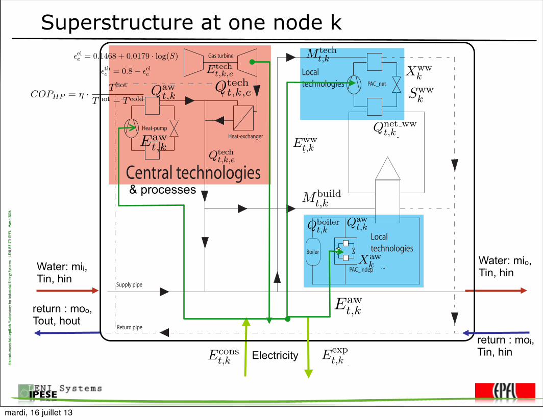
fran
cois
.mar
echa
l@ep
fl.c
h ©La
bora
tory
for
Indu
stri
al E
nerg
y Sy
stem
s -
LEN
I ISE
-STI
-EPF
L –
Mar
sh 2
006
IPESE
Superstructure at one node k
Water: mii, Tin, hin
return : moo, Tout, hout
Electricity
Water: mio, Tin, hin
return : moi, Tin, hin
1 Symbols
Roman lettersAn Annuities of a given investment [-]Ai,j,p Surface of the pipe of network p between nodes i and j [m2]B Arbitrarily big valueCaw Investment costs for air/water heat pump(s) [CHF]Cboiler Annual investment costs of the boiler(s) [CHF/year]Cfix Fix part of investment costs for a given device [CHF]Cgas Total gas costs [CHF]cgas Gas costs [CHF/kWh]Cgrid Total grid costs [CHF]cgrid Grid costs [CHF/kWh]C inv Investment costs of a given device [CHF]C inv
an Annual investment costs of a given device [CHF]Cpipes Total costs for the piping [CHF]Cprop Fix part of investment costs for a given device [CHF/kW]Cref Investment costs of a device chosen as reference [CHF]Cww Investment costs for water/water heat pump(s) [CHF]CO2
gas Total CO2 emissions for one year due to the combustion of gas [kg]co2
gas CO2 emissions due to the combustion of gas per kWh [kg/kWh]CO2
grid Total CO2 emissions for one year due to the consumption of electricity from the grid [kg]co2
grid CO2 emissions due to the consumption of electricity from the grid [kg/kWh]COP aw
t,k Coe⇤cient of performance for the air/water heat pump during period t at node k [-]COPww
t,k Coe⇤cient of performance for a water/water heat pump during period t at node k [-]cp Isobaric specific heat [kJ/(K· kg)]Disti,j Distance between nodes i and j [m]Ht Number of hours in period t [hour]Econs
t,k Electricity consumption during period t at node k [kW]Eexp
t,k Eletricity exported to the grid during period t by device e [kW]Egrid
t,k Electricity bought from the grid during period t [kW]Eaw
t,k Electricity consumed by the air/water heat pump during period t at node k [kW]Eww
t,k Electricity consumed by the water/water heat pump during period t at node k [kW]Eloss
t,k Electricity losses during period t [kW]Epump
t Pumping power for the network during period t [kW]Etech
t,k,e Electricity produced or consumed during period t at node k by device e [kW]Fm Maintenance factor [-]Gast Overall gas consumption during period t [kg]Lmin
e Minimum allowable part-load of device e [-]
Mbuildt,k
Mass flow of water from the network, circulating during period t through thebuilding at node k to heat up the building [kg/s]
Mpipet,i,j,p
Mass flow of water flowing during period t, in network p, from node i to nodej [kg/s]
Mmaxt,p,i,j
Maximum mass flow of water flowing in network p, from node i to node j, overall periods of time [kg/s]
M techt,k
Mass flow from the network being heated up by the device(s) at node k duringperiod t [kW]
MT buildt,k
Mass flow from the network flowing through a device at node k during periodt, to be re-heated, times its temperature [(kg/s)K]
2
MT pipet,i,j,p
Mass flow flowing during period t from node i to node j in the network p, timesits temperature [(kg/s)K]
N Expected lifetime for a given investment [year]Ploss Pressure losses in the pipes [Pa/m]Qaw
t,k Heat delivered by the air/water heat pump to the consumer at node k during period t [kW]Qboiler
t,k Heat delivered by the boiler at node k during period t [kW]Qcons
t,k Heat consumption at node k during period t [kW]Qnet
t,k Heat delivered by the network to the consumer at node k during period t [kW]Qnet ww
t,k Heat delivered by the network to the water/water heat pump at node k during period t [kW]Qtech
t,k,e Heat produced by device e located at node k during period k [kW]Qww
t,k Heat delivered by an water/water heat pump to the consumer at node k during period t [kW]r Interest rate [-]S Size of a given device [kW]Saw
k Nominal size of the air/water heat pump located at node k [kW]Sboiler
k Nominal size of the boiler at node k [kW]Snom
e Nominal power of a device [kW]Sref Size of a device chosen as reference [kW]Sww
k Nominal power of the water/water heat pump located at node k [kW]T atm Atmospheric temperature [K]T cold Temperature of the heat source for heat pumps [K]T cons
t,k Temperature at which the heat is required by the consumer at node k during period t [K]T hot Temperature of the heat sink for heat pumps [K]T net Design temperature of the network [K]v Velocity of the water through the pipes [m/s]X = 1 if a device exists, 0 otherwiseXaw
k = 1 if there is an air/water heat pump at node k, 0 otherwiseXboiler
k = 1 if there is a boiler at node k, 0 otherwiseXgas
e = 1 if device e needs gas to operate, 0 otherwiseXnode
k = 1 if a device e is implemented at node k, 0 otherwiseXtech
k,e = 1 if a device can be implemented at node k, 0 otherwiseXww
k = 1 if there is an water/water heat pump at node k, 0 otherwiseY i,j,p = 1 if a connection exists between i and j for network p , 0 otherwise
Greek letters�Theat Pinch at the heat-exchangers [K]�Tnet ww Temperature di⇥erence of the water in the network when it serves as heat source for water/water heat pump(s) [K]�boiler Thermal e⌅ciency of the boiler(s) [-]�ele Electric e⌅ciency of device e [-]�grid E⌅ciency of the grid [-]�the Thermal e⌅ciency of device e [-]⇥ Exergetic e⌅ciency [-]⇤ Density [kg/m3]
Indicesk nodesi, j connection from node i to node jt timee technologies
3
ture of the network (seen from the decentralized water/water heat pump, this temperaturecorresponds to the temperature di�erence of the heat source in the evaporator).
5. the thickness of the insulation around the pipes.
The multi-objective evolutionary optimizer used for this study was developed at the IndustrialEnergy Systems Laboratory of the Ecole Polytechnique Federale de Lausanne [11]. This optimizeruses the technique of the evolutionary algorithms to compute the trade-o�s between multiple objec-tives. In our case, two objectives have to be minimized: the CO2 emissions and the costs (includingoperation and investment). In order to find the optimal configurations (energy systems) with thebest performances in terms of CO2 emissions and costs, the evolutionary algorithm starts creatinga population of individuals by choosing randomly, for each individual, a set of values (genome,individual). These are the initial master sets of decision variables. The performance of each masterset is computed. New master sets (genome, individuals) are then selected based on the performanceof the existing ones, using a set of combination operators such as mutation and crossover. Afterthe evolution process is continued su⇤ciently, keeping the best master sets (according to CO2 emis-sions and costs), the optimal solutions can be found. This multi-objective strategy results in anestimation of the Pareto optimal frontier (hereafter Pareto curve) that represents the set of optimalconfigurations (optimal in terms of one or both of the two objectives). Each point of this curvecorresponds to a configuration of the energy system, in other words to a master set of decisionvariables and its associated slave set, that define one configuration of the energy system and theoptimal way of operating it on a yearly basis.
5.2 Thermodynamic models of the technologies
The method presented allows the use of thermodynamic models with various degrees of details.However, when designing and optimizing the entire energy network, there is no need in spendingmuch time using very detailed models. For the current study, the following simple relations wereimplemented:
1. Heat pump:
COPHP = ⇥ · T hot
T hot � T cold
2. Gas turbine [12]:�ele = 0.1468 + 0.0179 · log(S)
�the = 0.8� �ele
S being the size of the gas turbine [kWel], �the and �ele the thermal respectively electricale⇤ciency.
3. Solid Oxide Fuel Cell:�ele = 0.45
�the = 0.45
10
MT pipet,i,j,p Water flowing during period t from node i to node j in the network p, times its temperature [(kg/s)K]
N Expected lifetime for a given investment [year]Ploss Pressure losses in the pipes [Pa/m]Qaw
t,k Heat delivered by the air/water heat pump during period t, at node k [kW]Qboiler
t,k Heat delivered by the boiler during period t, at node k [kW]Qcons
t,k Heat consumption during period t, at node k [kW]Qnet
t,k Heat delivered by the network during period t, at node k [kW]Qnet ww
t,k Heat delivered by the network to the water/water heat pump during period t, at node k [kW]Qtech
t,k,e Heat produced during period t, at node k, by device e [kW]Qww
t,k Heat delivered by an water/water heat pump to the consumer at node k during period t [kW]r Interest rate [-]S Design size of a given device [kW]Saw
k Design size of the air/water heat pump located at node k [kW]Sboiler
k Design size of the boiler at node k [kW]Snom
e Design size of a device [kW]Sref Size of a device chosen as reference [kW]Sww
k Design size of the water/water heat pump located at node k [kW]T atm Atmospheric temperature [K]T cold Temperature of the heat source for heat pumps [K]T cond Temperature at the condenser of a heat pump [K]T cons
t,k Temperature at which the heat is required by the consumer during period t, at node k [K]T hot Temperature of the heat sink for heat pumps [K]T net Design supply temperature of the network [K]v Velocity of the water through the pipes [m/s]X = 1 if a device exists, 0 otherwiseXaw
k = 1 if there is an air/water heat pump at node k, 0 otherwiseXboiler
k = 1 if there is a boiler at node k, 0 otherwiseXgas
e = 1 if device e needs natural gas to operate, 0 otherwiseXtech
k = 1 if a device can be implemented at node k, 0 otherwiseXnode
k,e = 1 if device e is implemented at node k, 0 otherwiseXww
k = 1 if there is an water/water heat pump at node k, 0 otherwiseY i,j,p = 1 if a connection exists between i and j for network p , 0 otherwise
Greek letters�T heat Pinch at the heat-exchangers [K]�T net ww Temperature di⇥erence of the water in the network if used as heat source in water/water heat pumps [K]�boiler Thermal e⌅ciency of the boiler(s) [-]�ele Electric e⌅ciency of device e [-]�grid E⌅ciency of the grid [-]�the Thermal e⌅ciency of device e [-]⇥ Exergetic e⌅ciency [-]⇤ Density [kg/m3]
Indicesk nodesi, j connection from node i to node jt timee devicep network (to: from the plant to the building(s), ret: from the buildings back to the plant)
3
1 Symbols
Roman lettersAn Annuities for a given investment [-]Ai,j,p Area of the pipe between nodes i and j of network p [m2]B Arbitrarily big valueCaw Investment costs for air/water heat pump(s) [CHF]Cboiler Annual investment costs for the boiler(s) [CHF/year]Cfix Fix part of the investment costs for a given device [CHF]Cgas Total annual natural gas costs [CHF/year]cgas Natural gas costs [CHF/kWh]Cgrid Total annual grid costs [CHF/year]cgrid Grid costs [CHF/kWh]C inv Investment costs of a given device [CHF]C inv
an Annual investment costs of a given device [CHF/year]Cpipes Total annual costs for the piping [CHF/year]Cprop Fix part of the investment costs for a given device [CHF/kW]Cref Investment costs of a device chosen as reference [CHF]Cww Investment costs for water/water heat pump(s) [CHF]CO2
gas Total annual CO2 emissions due to the combustion of natural gas [kg/year]co2
gas CO2 emissions due to the combustion of natural gas [kg/kWh]CO2
grid Total annual CO2 emissions due to the consumption of electricity from the grid [kg/year]co2
grid CO2 emissions due to the consumption of electricity from the grid [kg/kWh]COPhp Coe⇤cient of performance of the central heat pumpCOP aw
t,k Coe⇤cient of performance for the air/water heat pump during period t at node k [-]COPww
t,k Coe⇤cient of performance for a water/water heat pump during period t at node k [-]cp Isobaric specific heat [kJ/(K· kg)]Disti,j Distance between nodes i and j [m]Ht Number of hours in period t [hour]Econs
t,k Electricity consumption during period t at node k [kW]Eexp
t,e Eletricity exported to the grid during period t by device e [kW]Egrid
t,k Electricity bought from the grid during period t by node k [kW]Eaw
t,k Electricity consumed by the air/water heat pump during period t at node k [kW]Eww
t,k Electricity consumed by the water/water heat pump during period t at node k [kW]Eloss
t Electricity losses during period t [kW]Epump
t Pumping power for the network during period t [kW]Etech
t,k,e Electricity produced or consumed during period t at node k by device e [kW]Fs Scaling factor [-]Fm Maintenance factor [-]Gast Natural gas consumption during period t [kg]Lmin
e Minimum allowable part-load of device e [-]Mbuild
t,k Water circulating during period t through the building at node k, to heat it up [kg/s]Mpipe
t,i,j,p Water flowing during period t, from node i to node j, in network p [kg/s]Mmax
i,j,p Maximum flow of water between nodes i and j, in network p, over all periods [kg/s]M tech
t,k Water being heated up by the device(s) during period t, at node k [kg/s]MT tech
t,k Water flowing through a device during period t at node k to be re-heated, times its temperature [(kg/s)K]
2
MT pipet,i,j,p Water flowing during period t from node i to node j in the network p, times its temperature [(kg/s)K]
N Expected lifetime for a given investment [year]Ploss Pressure losses in the pipes [Pa/m]Qaw
t,k Heat delivered by the air/water heat pump during period t, at node k [kW]Qboiler
t,k Heat delivered by the boiler during period t, at node k [kW]Qcons
t,k Heat consumption during period t, at node k [kW]Qnet
t,k Heat delivered by the network during period t, at node k [kW]Qnet ww
t,k Heat delivered by the network to the water/water heat pump during period t, at node k [kW]Qtech
t,k,e Heat produced during period t, at node k, by device e [kW]Qww
t,k Heat delivered by an water/water heat pump to the consumer at node k during period t [kW]r Interest rate [-]S Design size of a given device [kW]Saw
k Design size of the air/water heat pump located at node k [kW]Sboiler
k Design size of the boiler at node k [kW]Snom
e Design size of a device [kW]Sref Size of a device chosen as reference [kW]Sww
k Design size of the water/water heat pump located at node k [kW]T atm Atmospheric temperature [K]T cold Temperature of the heat source for heat pumps [K]T cond Temperature at the condenser of a heat pump [K]T cons
t,k Temperature at which the heat is required by the consumer during period t, at node k [K]T hot Temperature of the heat sink for heat pumps [K]T net Design supply temperature of the network [K]v Velocity of the water through the pipes [m/s]X = 1 if a device exists, 0 otherwiseXaw
k = 1 if there is an air/water heat pump at node k, 0 otherwiseXboiler
k = 1 if there is a boiler at node k, 0 otherwiseXgas
e = 1 if device e needs natural gas to operate, 0 otherwiseXtech
k = 1 if a device can be implemented at node k, 0 otherwiseXnode
k,e = 1 if device e is implemented at node k, 0 otherwiseXww
k = 1 if there is an water/water heat pump at node k, 0 otherwiseY i,j,p = 1 if a connection exists between i and j for network p , 0 otherwise
Greek letters�T heat Pinch at the heat-exchangers [K]�T net ww Temperature di⇥erence of the water in the network if used as heat source in water/water heat pumps [K]�boiler Thermal e⌅ciency of the boiler(s) [-]�ele Electric e⌅ciency of device e [-]�grid E⌅ciency of the grid [-]�the Thermal e⌅ciency of device e [-]⇥ Exergetic e⌅ciency [-]⇤ Density [kg/m3]
Indicesk nodesi, j connection from node i to node jt timee devicep network (to: from the plant to the building(s), ret: from the buildings back to the plant)
3
& processes
mardi, 16 juillet 13
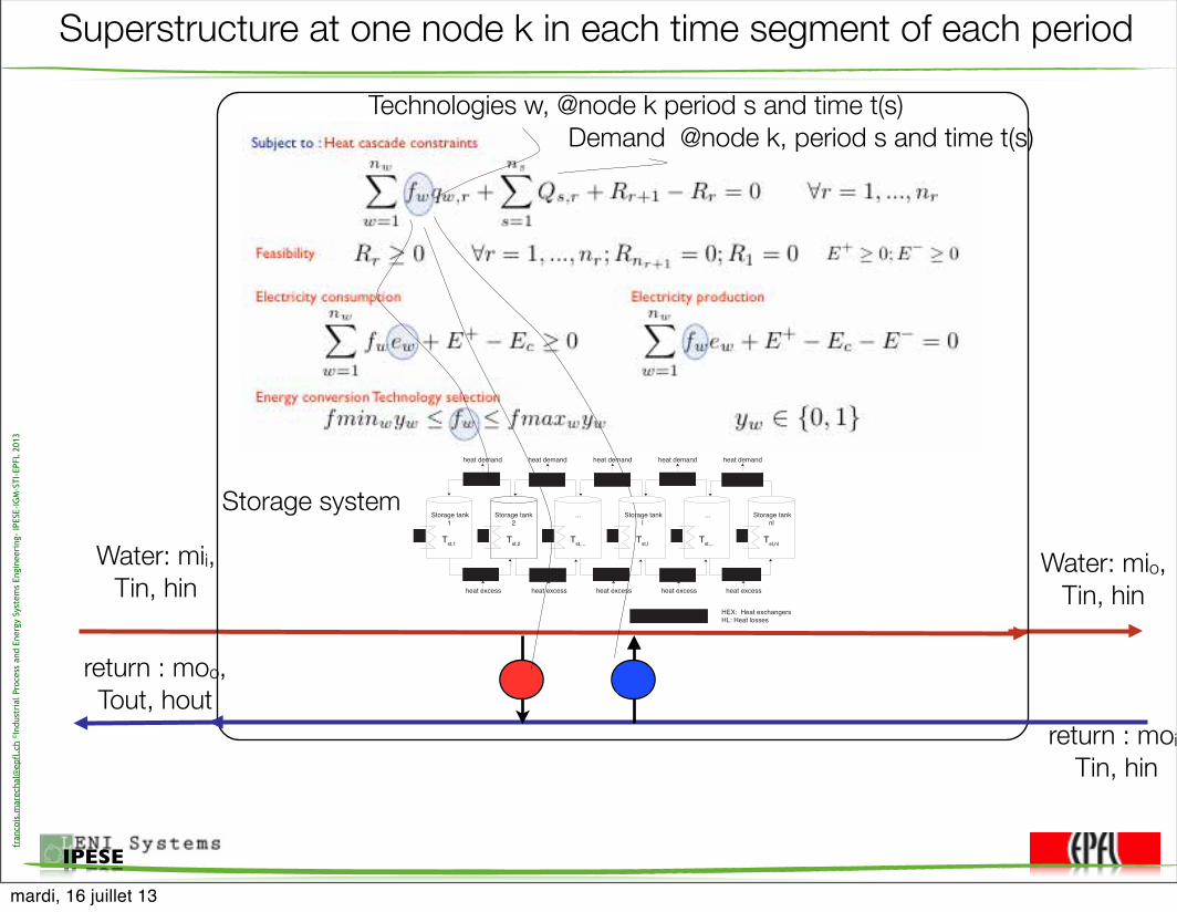
fran
cois
.mar
echa
l@ep
fl.c
h ©In
dust
rial
Pro
cess
and
Ene
rgy
Syst
ems
Engi
neer
ing-
IPES
E-IG
M-S
TI-E
PFL
2013
IPESE
Superstructure at one node k in each time segment of each period
Water: mii, Tin, hin
return : moo, Tout, hout
Water: mio, Tin, hin
return : moi, Tin, hin
Technologies w, @node k period s and time t(s)Demand @node k, period s and time t(s)
Storage tank2
Tst,2
HEX h1(t)
heat demand
Storage tank1
Tst,1
...
Tst,...
Storage tankl
Tst,l
...
Tst,...
Storage tanknl
Tst,nl
HEX h2(t) HEX h..(t) HEX hl(t) HEX hnl-1(t)
heat demand heat demand heat demand heat demand
heat excess
HEX c1(t)
heat excess
HEX c2(t)
heat excess
HEX c..(t)
heat excess
HEX cl(t)
heat excess
HEX cnl-1(t)
Units for heat integration
HL HL HL HL HL HL
HEX: Heat exchangersHL: Heat losses
Storage system
mardi, 16 juillet 13

fran
cois
.mar
echa
l@ep
fl.c
h ©In
dust
rial
Pro
cess
and
Ene
rgy
Syst
ems
Engi
neer
ing-
IPES
E-IG
M-S
TI-E
PFL
2013
IPESE
Engine
Hot water
HeatingWater
Heat pumpElectricity grid
Natural gas grid
Buildings
Electricity storage and “smart” electrical grids
Optimal predictive control management boxPrice
T ambient
T confort
T storage
Polygeneration system : Heat pump & CogenerationInstead of storing electricity : manage the electricity demand to supply services, dephasing heat production & consumption
mardi, 16 juillet 13

IPESE
High electrcity cost during the afternoonStorage tank = 200 m3
Low cost cost during the afternoonStorage tank = 200 m3
Heating : 72315 kWhElectricity : 77897 kWhe
Electricity in : 99596 kWheElectricity out : 8710 kWhe
Low price periodElectricity in : 19345 kWhe
Electricity out : 5650 kWheElectricity bought : 62894 kWhe
Low price periodElectricity out : 4407 kWheElectricity in : 1269 kWheBalance : -3138 kWhe
Storage : 22480 kWhe
Demonstration of the “storage” capacityby changing the operation strategy
Engine : 2000 kWeHeat pump : 2000 kWeStorage 200 m3
Demand mean heating power = 3000 kW
Storage filling at night
Empty storage tanks before cheap elec price
Fill storage tanks during cheap elec price
mardi, 16 juillet 13
fran
cois
.mar
echa
l@ep
fl.c
h ©In
dust
rial
Pro
cess
and
Ene
rgy
Syst
ems
Engi
neer
ing-
IPES
E-IG
M-S
TI-E
PFL
2013
IPESE
Urban system design solution
• Size of each of the elements in the system– conversion– storage
• District heating interconnections– locations– size
• Operating strategy for each of the element• Operating cost• CO2 emissions
mardi, 16 juillet 13
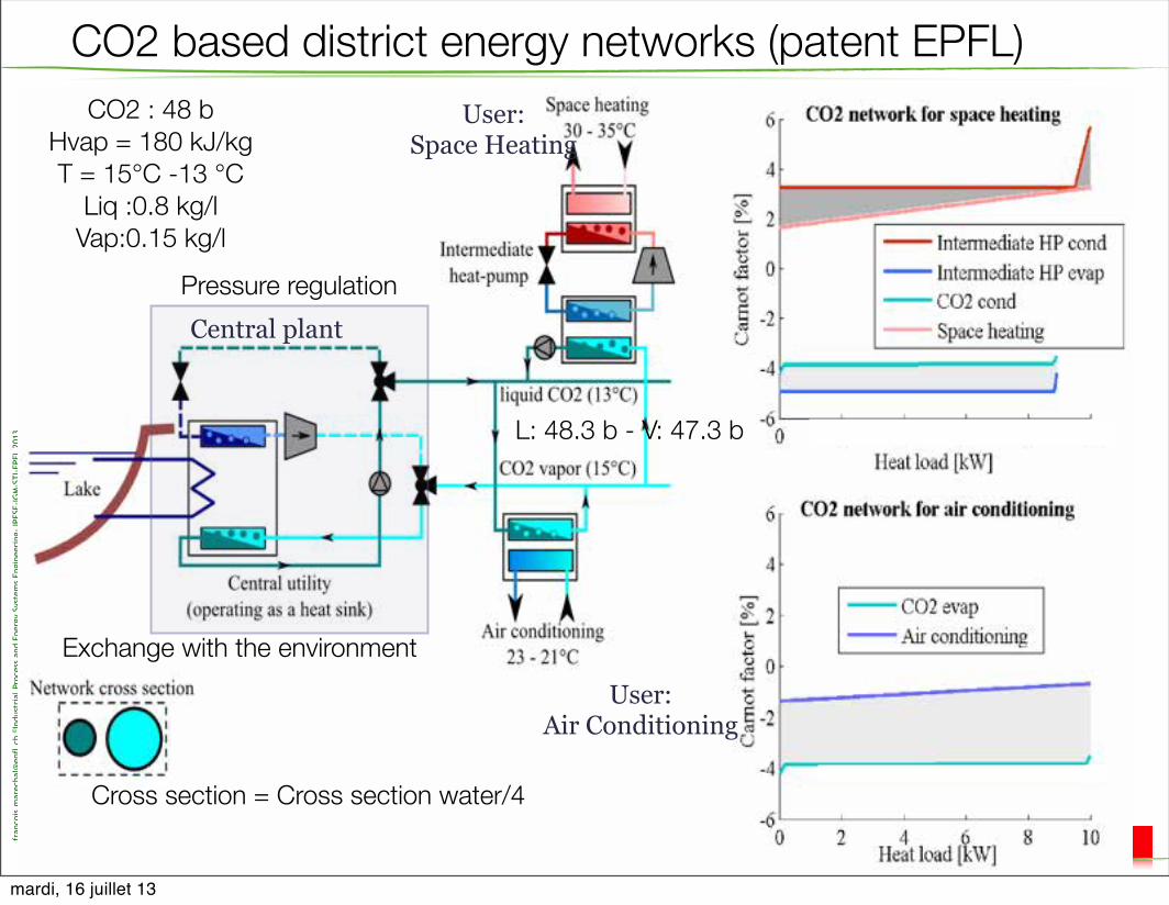
fran
cois
.mar
echa
l@ep
fl.c
h ©In
dust
rial
Pro
cess
and
Ene
rgy
Syst
ems
Engi
neer
ing-
IPES
E-IG
M-S
TI-E
PFL
2013
IPESE
L: 48.3 b - V: 47.3 b
CO2 : 48 bHvap = 180 kJ/kgT = 15°C -13 °C
Liq :0.8 kg/lVap:0.15 kg/l
Central plantPressure regulation
Exchange with the environmentUser:
Air Conditioning
User:Space Heating
CO2 based district energy networks (patent EPFL)
Cross section = Cross section water/4
mardi, 16 juillet 13
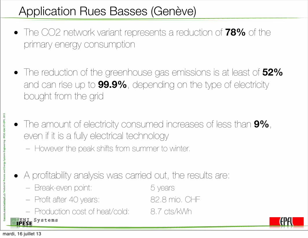
fran
cois
.mar
echa
l@ep
fl.c
h ©In
dust
rial
Pro
cess
and
Ene
rgy
Syst
ems
Engi
neer
ing-
IPES
E-IG
M-S
TI-E
PFL
2013
IPESE
Application Rues Basses (Genève) 62
• The CO2 network variant represents a reduction of 78% of the primary energy consumption
• The reduction of the greenhouse gas emissions is at least of 52% and can rise up to 99.9%, depending on the type of electricity bought from the grid
• The amount of electricity consumed increases of less than 9%, even if it is a fully electrical technology– However the peak shifts from summer to winter.
• A profitability analysis was carried out, the results are:– Break-even point: 5 years– Profit after 40 years: 82.8 mio. CHF– Production cost of heat/cold: 8.7 cts/kWh
mardi, 16 juillet 13

IPESE
Energy services (process)fu = 1
Space heating
Domestic hot water
Electricity Transport
Waste to be treated (process)fu = 1
Municipal solid waste
Municipal organic waste
Waste-water
Limits of the action system
DieselBiogas
HeatElectricity
WaterWastewater
Woody biomassUnit U
fu, COu, CIu, Iu
Alternative S1Alternative S2
Required S3
Produced S4
Produced S5
LegendPetrolSolid waste
Organic waste
Natural gas (fossil)Oil
Natural gas (biogenic)Mobility
Average technology (LCI database) Detailed technology
Indigeneous resources (utilities)fmax = limited
BiomassHydro
Deepaquifers
Geothermal heat
Hot DryRock
Imported resources (utilities)fmax = unlimited
Natural gas Oil
PetrolDiesel
Electricity import
Conversion technologies (utilities)fmax = unlimited
Boilers
Cars
Engines
Turbines
Heat pumps
Biometh-anation
Dryers
Gasi!ers
Biogas puri!cation
Synthetic naturalgas production
Cycles for CHP from geo. heat
Incineration
Wastewater treatment
Dams
Energy transfer networks (utilities)fmax = unlimited
District heating network
Supply the energy services of a region
• min. investment
• min. operating costs
• min. CO2-eq. emissions
Ecodesign of a urban system
Gerber, Léda, Samira Fazlollahi, and François Marechal. “Environomic Optimal Design and Synthesis of Energy Conversion Systems in Urban Areas.” Accepted in Computers and Chemical Engineering (2013).
Application : City La chaux de fonds (CH)
mardi, 16 juillet 13

fran
cois
.mar
echa
l@ep
fl.c
h ©In
dust
rial
Pro
cess
and
Ene
rgy
Syst
ems
Engi
neer
ing-
IPES
E-IG
M-S
TI-E
PFL
2013
IPESE
0 50 100 150 20030
40
50
60
70
80
90
100
Additional investment costs [mio¤]
Opera
ting C
osts
[m
io¤
/yr]
2.2
2.4
2.6
2.8
3.0
3.2
3.4
3.6
3.8
4.0
2.0
Optimal configurations
Current situation (ref.)x
Multi-objective optimization : City La chaux de fonds (CH)
A: no EGS
B: 6000m EGS,Kalina for CHP
C: 6500m EGS,ORC for elec.
D: 9500m EGS,ORC for CHP
E: 9500m EGS,1F & ORC for elec
Trade-off between 3 objectives
‣ In each cluster, panel of “environomic“ solutions
• not considered if pure economic optimization
• Biomass & biowaste conversion
‣ economic: 39.5% max impact reduction
‣ environomic: 44.8% max impact reduction
1. Seasonal operation 2. Optimal pathways 3. Selection of technologies 4. Competitions & synergies
CO2
mardi, 16 juillet 13

fran
cois
.mar
echa
l@ep
fl.c
h ©In
dust
rial
Pro
cess
and
Ene
rgy
Syst
ems
Engi
neer
ing-
IPES
E-IG
M-S
TI-E
PFL
2013
IPESE
Seasonal operation (multi-period problem)
• Example of summer and winter system operation
1.020 kWe/cap
Seasonal variation in service requirement• Quantity (heat load)• Quality (temperature)
Seasonal adaptation• Selection of utilities• Operating conditions
Summer
Winter
mardi, 16 juillet 13

fran
cois
.mar
echa
l@ep
fl.c
h ©In
dust
rial
Pro
cess
and
Ene
rgy
Syst
ems
Engi
neer
ing-
IPES
E-IG
M-S
TI-E
PFL
2013
IPESE
Heat losses
Waste
Raw materials
ElectricityHeat recovery
Heat pump
Conversion
Waste management
Waste emissionsFossilresources
Biomass
SunIndustrial urban site
ABC
ABC
CO2 Exergy
ABC
Costs
Key Performance Indicators
CO2 Valorisation
Biofuel
CO2 sequestration
ProductsHe
ating
Cool
ing
Side Processes
CO2
The Vision : energy transition by system integrationProcess system engineering : selection, integration, sizing and optimal operation in industrial system
CO2/H2
Processes
Heating
mardi, 16 juillet 13
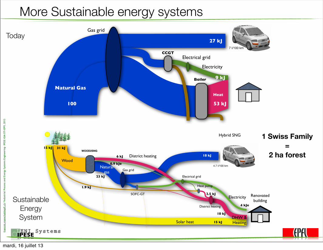
fran
cois
.mar
echa
l@ep
fl.c
h ©In
dust
rial
Pro
cess
and
Ene
rgy
Syst
ems
Engi
neer
ing-
IPES
E-IG
M-S
TI-E
PFL
2013
IPESE
More Sustainable energy systems
ElectricitySOFC-GT
4.7 l/100 km
WOOD2SNG
Wood
Naturalgas
District heating
Solar heat
Gas grid
Heat pump
Electrical grid
DHW & Heating
Hybrid SNG
1.9 kJ
15 kJ
10 kJ
4 kJe
31 kJ
2.5 kJ
6 kJ
23 kJ
0.9 kJe
District heating
18 kJ
15 kJ
Renovated building
Gas grid
CCGT
Electricity
Heat
Boiler
Natural Gas
7 l/100 km
27 kJ
9 kJ
53 kJ100
Electrical grid
Today
Sustainable Energy System
1 Swiss Family=
2 ha forest
mardi, 16 juillet 13

fran
cois
.mar
echa
l@ep
fl.c
h ©In
dust
rial
Pro
cess
and
Ene
rgy
Syst
ems
Engi
neer
ing-
IPES
E-IG
M-S
TI-E
PFL
2013
IPESE
The impact of the hidden fuel
ElectricitySOFC-GT
4.7 l/100 km
WOOD2SNG
Wood
Naturalgas
District heating
Solar heat
Gas grid
Heat pump
Electrical grid
DHW & Heating
Hybrid SNG
1.9 kJ
15 kJ
10 kJ
4 kJe
31 kJ
2.5 kJ
6 kJ
23 kJ
0.9 kJe
District heating
18 kJ
15 kJ
Renovated building
Gas grid
CCGT
Electricity
Heat
Boiler
Natural Gas
7 l/100 km
27 kJ
9 kJ
53 kJ100
Electrical grid
Today
• 45 kJ of renewable energy replaces 100 kJ of fossil fuel•Overall negative CO2 balance–Trees sucks CO2 from the atmosphere–CO2 sequestration or recycling !
mardi, 16 juillet 13
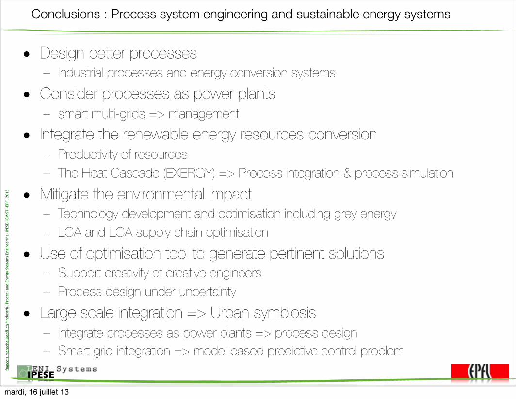
fran
cois
.mar
echa
l@ep
fl.c
h ©In
dust
rial
Pro
cess
and
Ene
rgy
Syst
ems
Engi
neer
ing-
IPES
E-IG
M-S
TI-E
PFL
2013
IPESE
Conclusions : Process system engineering and sustainable energy systems
• Design better processes– Industrial processes and energy conversion systems
• Consider processes as power plants– smart multi-grids => management
• Integrate the renewable energy resources conversion– Productivity of resources– The Heat Cascade (EXERGY) => Process integration & process simulation
• Mitigate the environmental impact– Technology development and optimisation including grey energy– LCA and LCA supply chain optimisation
• Use of optimisation tool to generate pertinent solutions– Support creativity of creative engineers– Process design under uncertainty
• Large scale integration => Urban symbiosis– Integrate processes as power plants => process design– Smart grid integration => model based predictive control problem
mardi, 16 juillet 13