Survival attributable to an exposure
19
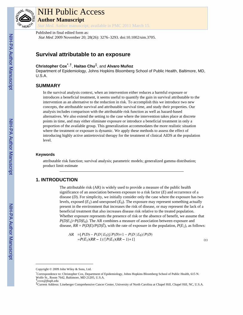
Survival attributable to an exposure Christopher Cox *,† , Haitao Chu ‡ , and Alvaro Muñoz Department of Epidemiology, Johns Hopkins Bloomberg School of Public Health, Baltimore, MD, U.S.A. SUMMARY In the survival analysis context, when an intervention either reduces a harmful exposure or introduces a beneficial treatment, it seems useful to quantify the gain in survival attributable to the intervention as an alternative to the reduction in risk. To accomplish this we introduce two new concepts, the attributable survival and attributable survival time, and study their properties. Our analysis includes comparison with the attributable risk function as well as hazard-based alternatives. We also extend the setting to the case where the intervention takes place at discrete points in time, and may either eliminate exposure or introduce a beneficial treatment in only a proportion of the available group. This generalization accommodates the more realistic situation where the treatment or exposure is dynamic. We apply these methods to assess the effect of introducing highly active antiretroviral therapy for the treatment of clinical AIDS at the population level. Keywords attributable risk function; survival analysis; parametric models; generalized gamma distribution; product limit estimate 1. INTRODUCTION The attributable risk (AR) is widely used to provide a measure of the public health significance of an association between exposure to a risk factor (E) and occurrence of a disease (D). For simplicity, we initially consider only the case where the exposure has two levels, exposed (E 1 ) and unexposed (E 0 ). The exposure may represent something actually present in the environment that increases the risk of disease, or may represent the lack of a beneficial treatment that also increases disease risk relative to the treated population. Whether exposure represents the presence of risk or the absence of benefit, we assume that P(D|E 1 )>P(D|E 0 ). The AR combines a measure of association between exposure and disease, RR = P(D|E)/P(D|Ē), with the rate of exposure in the population, P(E 1 ), as follows: (1) Copyright © 2009 John Wiley & Sons, Ltd. * Correspondence to: Christopher Cox, Department of Epidemiology, Johns Hopkins Bloomberg School of Public Health, 615 N. Wolfe St., Room 7642, Baltimore, MD 21205, U.S.A. † [email protected] ‡ Current Address: Lineberger Comprehensive Cancer Center, University of North Carolina at Chapel Hill, Chapel Hill, NC, U.S.A. NIH Public Access Author Manuscript Stat Med. Author manuscript; available in PMC 2011 March 15. Published in final edited form as: Stat Med. 2009 November 20; 28(26): 3276–3293. doi:10.1002/sim.3705. NIH-PA Author Manuscript NIH-PA Author Manuscript NIH-PA Author Manuscript
-
Upload
independent -
Category
Documents
-
view
3 -
download
0
Transcript of Survival attributable to an exposure
Survival attributable to an exposure
Christopher Cox*,†, Haitao Chu‡, and Alvaro MuñozDepartment of Epidemiology, Johns Hopkins Bloomberg School of Public Health, Baltimore, MD,U.S.A.
SUMMARYIn the survival analysis context, when an intervention either reduces a harmful exposure orintroduces a beneficial treatment, it seems useful to quantify the gain in survival attributable to theintervention as an alternative to the reduction in risk. To accomplish this we introduce two newconcepts, the attributable survival and attributable survival time, and study their properties. Ouranalysis includes comparison with the attributable risk function as well as hazard-basedalternatives. We also extend the setting to the case where the intervention takes place at discretepoints in time, and may either eliminate exposure or introduce a beneficial treatment in only aproportion of the available group. This generalization accommodates the more realistic situationwhere the treatment or exposure is dynamic. We apply these methods to assess the effect ofintroducing highly active antiretroviral therapy for the treatment of clinical AIDS at the populationlevel.
Keywordsattributable risk function; survival analysis; parametric models; generalized gamma distribution;product limit estimate
1. INTRODUCTIONThe attributable risk (AR) is widely used to provide a measure of the public healthsignificance of an association between exposure to a risk factor (E) and occurrence of adisease (D). For simplicity, we initially consider only the case where the exposure has twolevels, exposed (E1) and unexposed (E0). The exposure may represent something actuallypresent in the environment that increases the risk of disease, or may represent the lack of abeneficial treatment that also increases disease risk relative to the treated population.Whether exposure represents the presence of risk or the absence of benefit, we assume thatP(D|E1)>P(D|E0). The AR combines a measure of association between exposure anddisease, RR = P(D|E)/P(D|Ē), with the rate of exposure in the population, P(E1), as follows:
(1)
Copyright © 2009 John Wiley & Sons, Ltd.*Correspondence to: Christopher Cox, Department of Epidemiology, Johns Hopkins Bloomberg School of Public Health, 615 N.Wolfe St., Room 7642, Baltimore, MD 21205, U.S.A.†[email protected]‡Current Address: Lineberger Comprehensive Cancer Center, University of North Carolina at Chapel Hill, Chapel Hill, NC, U.S.A.
NIH Public AccessAuthor ManuscriptStat Med. Author manuscript; available in PMC 2011 March 15.
Published in final edited form as:Stat Med. 2009 November 20; 28(26): 3276–3293. doi:10.1002/sim.3705.
NIH
-PA Author Manuscript
NIH
-PA Author Manuscript
NIH
-PA Author Manuscript

The AR is typically interpreted as the proportion of disease that could be prevented byelimination of exposure to the risk factor. Note that this is distinct from what is sometimescalled the preventable fraction [1], which is defined by PF = [P(D|E1) − P(D)]/P(D|E1); seeSection 4.2. For additional discussion and references see Rothman and Greenland [1],Gefeller [2] and Uter and Pfahlberg [3].
If the measure of disease occurrence is FD(t) = P(T≤t), the cumulative event rate at time tmeasured from a well-defined origin (e.g. infection with a virus), then the attributable riskbecomes dynamic, and its behavior over time may provide information about effects of thetiming of interventions, or may suggest approaches that are more appropriate in the contextof survival. In Section 2, we consider the natural extension of the AR in the survival context,the attributable risk function, as well as alternatives based on the hazard function. We showthat the behavior of the attributable risk function is unsatisfactory in some respects. Wetherefore introduce two new definitions in Section 3, the attributable survival, andattributable survival time, which are based on the attribution of survival rather than failure,and characterize their properties. We conclude that the proposed measures are useful in thecontext of survival analysis.
As a generalization, in Section 4 we allow the distribution of exposure to change at discretepoints in time and extend the various definitions to this case, giving additional insight intothe different approaches to attribution. Section 5 first considers the simple example of twoexponential distributions; the new approach is then applied at the population level to studythe beneficial effects of highly active antiretroviral therapy on survival after a diagnosis ofclinical AIDS, using both parametric models and nonparametric methods.
2. THE ATTRIBUTABLE RISK FUNCTION AND HAZARD-BASEDALTERNATIVES2.1. The attributable risk function
We begin with the simple case of a population composed of individuals who are eitheralways exposed (E1) or never exposed (E0). The proportion of exposed individuals is 0<π =P(E1)<1, with failure distribution P(T≤t|E1) = F1(t), while the proportion unexposed is 1 −π, with distribution P(T≤t|E0) = F0(t). Time to event in the overall population then has amixture distribution, F(t) = πF1(t) + (1 − π)F0(t), representing the proportion of disease attime t in the entire population. In survival analysis it is more natural to work with thecorresponding survival functions, S1(t), S0(t) and S(t) = πS1(t) + (1 − π)S0(t). In the setting ofa deleterious exposure, which could be the absence of a beneficial treatment, we must haveF0(t)≤F1(t) or equivalently, S0(t)≥S1(t).
For the case of a fully effective intervention that completely eliminates the exposure at timezero among all those exposed, the obvious extension of the attributable risk in the survivalcontext is the attributable risk function
(2)
If we fix a particular time point, t = t*, then we obtain equation (1) with P(D) = F(t*). Theattributable risk function is interpreted as the proportion of disease that would be preventedat time t by a fully effective intervention, relative to the cumulative incidence proportion attime t with no intervention. Panel (Ia) of Figure 1 depicts the three survival distributions, aswell as the numerator and denominator of equation (2).
Cox et al. Page 2
Stat Med. Author manuscript; available in PMC 2011 March 15.
NIH
-PA Author Manuscript
NIH
-PA Author Manuscript
NIH
-PA Author Manuscript
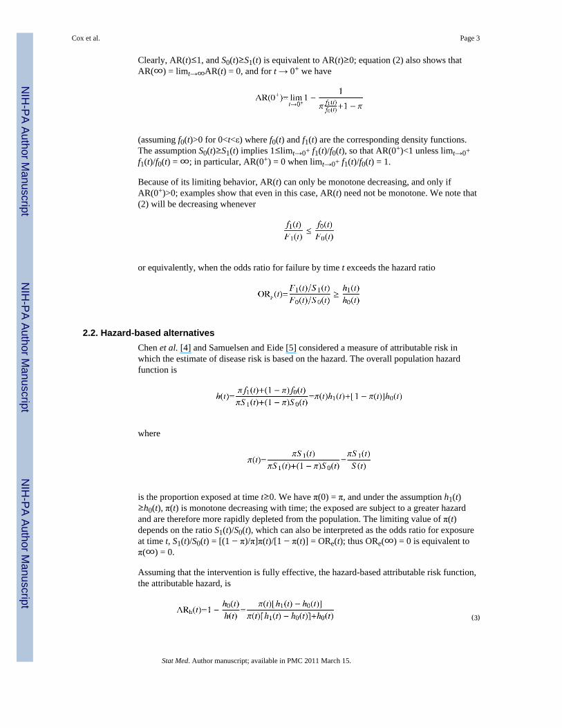
Clearly, AR(t)≤1, and S0(t)≥S1(t) is equivalent to AR(t)≥0; equation (2) also shows thatAR(∞) = limt→∞AR(t) = 0, and for t → 0+ we have
(assuming f0(t)>0 for 0<t<ε) where f0(t) and f1(t) are the corresponding density functions.The assumption S0(t)≥S1(t) implies 1≤limt→0+ f1(t)/f0(t), so that AR(0+)<1 unless limt→0+f1(t)/f0(t) = ∞; in particular, AR(0+) = 0 when limt→0+ f1(t)/f0(t) = 1.
Because of its limiting behavior, AR(t) can only be monotone decreasing, and only ifAR(0+)>0; examples show that even in this case, AR(t) need not be monotone. We note that(2) will be decreasing whenever
or equivalently, when the odds ratio for failure by time t exceeds the hazard ratio
2.2. Hazard-based alternativesChen et al. [4] and Samuelsen and Eide [5] considered a measure of attributable risk inwhich the estimate of disease risk is based on the hazard. The overall population hazardfunction is
where
is the proportion exposed at time t≥0. We have π(0) = π, and under the assumption h1(t)≥h0(t), π(t) is monotone decreasing with time; the exposed are subject to a greater hazardand are therefore more rapidly depleted from the population. The limiting value of π(t)depends on the ratio S1(t)/S0(t), which can also be interpreted as the odds ratio for exposureat time t, S1(t)/S0(t) = [(1 − π)/π]π(t)/[1 − π(t)] = ORe(t); thus ORe(∞) = 0 is equivalent toπ(∞) = 0.
Assuming that the intervention is fully effective, the hazard-based attributable risk function,the attributable hazard, is
(3)
Cox et al. Page 3
Stat Med. Author manuscript; available in PMC 2011 March 15.
NIH
-PA Author Manuscript
NIH
-PA Author Manuscript
NIH
-PA Author Manuscript

This measure can be interpreted as the approximate proportion of events that are preventedin a small interval of time [t, t + Δ). It follows from (3) that h1(t)≥h0(t) is required in order tohave ARh(t)≥0. The limiting behavior of (3) is governed by the ratio of the correspondinghazard functions rather than the ratio of the densities. Under the assumption h1(t)≥h0(t), itcan easily be shown that 0≤ARh(0+) = AR(0+)≤1 and ARh(∞) = 0 = AR(∞). Chen et al. [4]provided estimation procedures for (3) and (2) based on the Cox proportional hazardsmodel.
Alternatively, Silverberg et al. [6] and Samuelsen and Eide [5] used the original proportionexposed, π = π(0) to weight the difference between the two hazard functions in (3). That is,analogous to the overall survival function, define the combined hazard as hπ(t) = πh1(t) + (1− π)h0(t); the alternative hazard-based measure uses the combined, mixture hazard insteadof the population hazard
However, the survival function corresponding to hπ(t) is , whichunder-estimates the overall survival function in the actual population; thus, we believe thatthis approach does not provide a useful measure of public health risk.
3. ATTRIBUTION IN THE SURVIVAL CONTEXT3.1. Attributable survival
If the measure of disease is the cumulative failure rate, then the obvious extension ofattributable risk is the attributable risk function. In the survival context, however, analternative measure of the public health significance of an intervention is the proportion ofthe resulting survival, after the intervention is carried out, that is due to the intervention. Inparticular, if prior to the intervention the population survival function is S(t), and after theintervention the population survival function becomes S0(t) = S(t) + [S0(t) − S(t)], then thepart of S0(t) resulting from the intervention [S0(t) − S(t)] is the attributable portion. In otherwords, the attributable survival is the proportion of survivors with the intervention whowould have experienced the event had the intervention not been administered. Specifically,we define the attributable survival function as
(4)
Panel (Ib) of Figure 1 provides a graphical depiction of (4), showing that the numerator isless than the denominator, resulting in a measure between zero and one. The attributablesurvival is related to but distinct from the preventable fraction, which corresponds to PF(t) =[S(t) − S1(t)]/[1 − S1(t)] = (1 − π)[S0(t) − S1(t)]/[1 − S1(t)]. It is also in contrast to analternative measure using S(t) as the denominator (i.e. AS(t)/[1 − AS(t)]), which has theproperties of an odds instead of a proportion, making its interpretation as an attributablefraction difficult. The attributable survival does bear a functional if not an exact conceptualrelationship to the susceptible fraction discussed by Khoury et al. [7], whose definition,under certain independence assumptions about the relationship between exposure and theunderlying disease process, corresponds to AS(t)/π, so that the definition is independent ofthe proportion exposed.
Cox et al. Page 4
Stat Med. Author manuscript; available in PMC 2011 March 15.
NIH
-PA Author Manuscript
NIH
-PA Author Manuscript
NIH
-PA Author Manuscript

Clearly, AS(0) = 0 and 0≤AS(∞)≤π, depending on 1≥ORe(∞) = limt→∞S1(t)/S0(t) =limt→∞ f1(t)/f0(t)≥0, or equivalently on the limiting odds of exposure π (t)/[1 − π(t)] =πS1(t)/[(1 − π)S0(t)], so that AS(∞) = π[1 − ORe(∞)] = π − (1 − π)π(∞)/[1 − π(∞)]. Weexpect that the effect of exposure would typically be such that π(∞) = 0, in which caseAS(∞) = π; the limiting attributable survival is the original proportion exposed. That is, ifthe intervention entirely eliminates the exposure of the π per cent of the population that wasoriginally exposed, then π per cent of the resulting survival in the population over the entiretime span is due to such an intervention. Under the additional assumption h1(t)≥h0(t), (4) ismonotone increasing since ∂AS(t)/∂t = π[h1(t) − h0(t)]S1(t)/S0(t).
The attributable risk function (2) is the product of the survival odds and the attributablesurvival odds
Thus, initially AR(t)>AS(t), except possibly for AR(0+) = 0 = AS(0), until the unique t*>0when S0(t*) = 1 − S(t*), after which AR(t)<AS(t).
3.2. Attributable survival timeThe attributable survival represents the additional proportion of individuals in the populationwho survive to a given time if the exposure is eliminated, but it does not account for theactual survival time. To provide a measure of the gain in survival time resulting from an
intervention, we can use the area under the survival curve, . Changing theorder of integration (or integrating by parts) shows that Ei(t) can be interpreted as theexpected survival time at time t. Specifically, letting T1 and T0 denote the random eventtimes in the exposed and unexposed populations,
Thus, Ei(t) is a weighted average, according to the probability of having the event before t,[Fi(t)] of the expected value before t [E(Ti|Ti≤t)] and t itself. The expected survival to time tin the entire population is E(t) = πE1(t) + (1 − π)E0(t).
The attributable survival time is defined as the ratio of the change in expected survival timeresulting from the intervention to that achieved by the intervention,
(5)
As with the attributable survival we have AST(0+) = 0, and
Thus, for a fully effective intervention, AST(∞) represents the average gain in survival timerelative to that in the unexposed population (the distribution resulting from the intervention),
Cox et al. Page 5
Stat Med. Author manuscript; available in PMC 2011 March 15.
NIH
-PA Author Manuscript
NIH
-PA Author Manuscript
NIH
-PA Author Manuscript
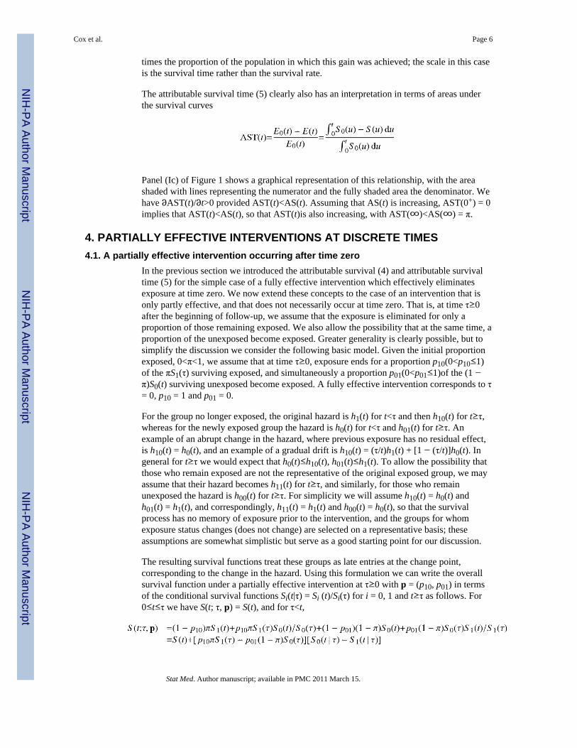
times the proportion of the population in which this gain was achieved; the scale in this caseis the survival time rather than the survival rate.
The attributable survival time (5) clearly also has an interpretation in terms of areas underthe survival curves
Panel (Ic) of Figure 1 shows a graphical representation of this relationship, with the areashaded with lines representing the numerator and the fully shaded area the denominator. Wehave ∂AST(t)/∂t>0 provided AST(t)<AS(t). Assuming that AS(t) is increasing, AST(0+) = 0implies that AST(t)<AS(t), so that AST(t)is also increasing, with AST(∞)<AS(∞) = π.
4. PARTIALLY EFFECTIVE INTERVENTIONS AT DISCRETE TIMES4.1. A partially effective intervention occurring after time zero
In the previous section we introduced the attributable survival (4) and attributable survivaltime (5) for the simple case of a fully effective intervention which effectively eliminatesexposure at time zero. We now extend these concepts to the case of an intervention that isonly partly effective, and that does not necessarily occur at time zero. That is, at time τ≥0after the beginning of follow-up, we assume that the exposure is eliminated for only aproportion of those remaining exposed. We also allow the possibility that at the same time, aproportion of the unexposed become exposed. Greater generality is clearly possible, but tosimplify the discussion we consider the following basic model. Given the initial proportionexposed, 0<π<1, we assume that at time τ≥0, exposure ends for a proportion p10(0<p10≤1)of the πS1(τ) surviving exposed, and simultaneously a proportion p01(0<p01≤1)of the (1 −π)S0(t) surviving unexposed become exposed. A fully effective intervention corresponds to τ= 0, p10 = 1 and p01 = 0.
For the group no longer exposed, the original hazard is h1(t) for t<τ and then h10(t) for t≥τ,whereas for the newly exposed group the hazard is h0(t) for t<τ and h01(t) for t≥τ. Anexample of an abrupt change in the hazard, where previous exposure has no residual effect,is h10(t) = h0(t), and an example of a gradual drift is h10(t) = (τ/t)h1(t) + [1 − (τ/t)]h0(t). Ingeneral for t≥τ we would expect that h0(t)≤h10(t), h01(t)≤h1(t). To allow the possibility thatthose who remain exposed are not the representative of the original exposed group, we mayassume that their hazard becomes h11(t) for t≥τ, and similarly, for those who remainunexposed the hazard is h00(t) for t≥τ. For simplicity we will assume h10(t) = h0(t) andh01(t) = h1(t), and correspondingly, h11(t) = h1(t) and h00(t) = h0(t), so that the survivalprocess has no memory of exposure prior to the intervention, and the groups for whomexposure status changes (does not change) are selected on a representative basis; theseassumptions are somewhat simplistic but serve as a good starting point for our discussion.
The resulting survival functions treat these groups as late entries at the change point,corresponding to the change in the hazard. Using this formulation we can write the overallsurvival function under a partially effective intervention at τ≥0 with p = (p10, p01) in termsof the conditional survival functions Si(t|τ) = Si (t)/Si(τ) for i = 0, 1 and t≥τ as follows. For0≤t≤τ we have S(t; τ, p) = S(t), and for τ<t,
Cox et al. Page 6
Stat Med. Author manuscript; available in PMC 2011 March 15.
NIH
-PA Author Manuscript
NIH
-PA Author Manuscript
NIH
-PA Author Manuscript
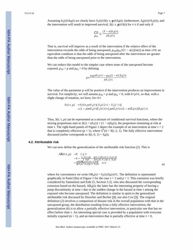
Assuming h1(t)≥h0(t) we clearly have S1(t)≤S(t; τ, p)≤S0(t); furthermore, S0(t|τ)≥S1(t|τ), andthe intervention will result in improved survival, S(t; τ, p)≥S(t) for τ<t if and only if
That is, survival will improve as a result of the intervention if the relative effect of theintervention exceeds the odds of being unexposed, p10/p01≥[1 − π(τ)]/π(τ) at time τ≥0; anequivalent condition is that the odds of being unexposed after the intervention are greaterthan the odds of being unexposed prior to the intervention.
We can reduce this model to the simpler case where none of the unexposed becomeexposed, p10 = p and p01 = 0 by defining
The value of the parameter p will be positive if the intervention produces an improvement insurvival. For simplicity, we will assume p10 = p and p01 = 0, with 0<p≤1, so that, with aslight change of notation, we have, for t≥τ
Thus, S(t; τ, p) can be represented as a mixture of conditional survival functions, where themixing proportions sum to S(τ) = πS1(τ) + (1 − π)S0(τ), the proportion remaining at risk attime τ. The right-hand panels of Figure 1 depict the example of an intervention at time τ = 2that is completely effective (p = 1), where S*(t) = S(t; 2, 1). The fully effective interventiondiscussed earlier corresponds to S(t; 0, 1) = S0(t).
4.2. Attributable riskWe can now define the generalization of the attributable risk function (2). This is
(6)
where for convenience we write ORe(τ) = S1(τ)/S0(τ)≤1. The definition is representedgraphically in Panel (IIa) of Figure 1 for the case τ = 2 and p = 1. This extension was brieflyconsidered by Samuelsen and Eide [5, Section 3.2], who also discussed the correspondingextension based on the hazard, ARh(t); the latter has the interesting property of having ajump discontinuity at time τ due to the sudden change in the hazard at time τ among theexposed who become unexposed. The definition is similar in spirit to the generalizedattributable risk discussed by Drescher and Becher [8]; see also Cox [9]. The originaldefinition (2) involves a comparison of disease risk in the overall population with that in theunexposed group, the distribution resulting from a fully effective intervention; thegeneralization (6) is to allow a partially effective intervention, in particular one that has noeffect before time τ. An interesting special case is provided by a population with everyoneinitially exposed (π = 1), and an intervention that is partially effective at time τ = 0,
Cox et al. Page 7
Stat Med. Author manuscript; available in PMC 2011 March 15.
NIH
-PA Author Manuscript
NIH
-PA Author Manuscript
NIH
-PA Author Manuscript

removing a proportion 1 − p of the exposure. The attributable risk in this case correspondsto the preventable fraction discussed above, with a proportion p exposed, AR(t; 0, 1 − p) =(1 − p)[S0(t) − S1(t)]/[1 − S1(t)].
We again have AR(∞; τ, p) = 0, so that AR(t; τ, p) cannot be monotone, except in the caseof a fully effective intervention, AR(t; 0, 1) = AR(t). Clearly, for each t>τ, AR(t; τ, p)increases as p approaches one. The limit is the special case that exposure is eliminated (p =1), where we obtain a simpler expression for τ≤t.
In this case, as τ ↘ 0(ORe(τ) ↗ 1), we have AR(t; τ, 1) ↗ AR(t).
4.3. Attributable survivalThe attributable survival (4) is the ratio of the change in survival resulting from theintervention to the survival achieved by the intervention, which for the case of a partiallyeffective intervention at time τ is S(t, τ, p) instead of S0(t). The attributable survival istherefore AS(t; τ, p) = 0 for t≤τ, and for t>τ,
(7)
As above, the denominator of (7) is a mixture of conditional survival functions, with weightssumming to S(τ). For the case τ = 2 and p = 1, the numerator and denominator of (7) areshown in Panel (IIb) of Figure 1. As a special case we have AS(t; 0, 1) = AS(t) in (4).
The limit AS(∞; τ, p) is again determined by π(t), the proportion exposed; in particular,under the assumption π(∞) = 0,
This represents the survival at time τ for the group whose exposure is eliminated by theintervention (at time τ), divided by the total unexposed at time τ. For the case p = 1, this totalis simply S(τ), and the limit is AS(∞; τ, 1) = π(τ), the proportion exposed at time τ. For τ =0, we have AS(∞; 0, p) = pπ/(pπ + 1 − π), and AS(∞; 0, 1) = π. These limiting resultsactually suggest an alternative definition of the attributable survival, in which we divide byS(t; τ, 1) instead of S(t; τ, p) in (7). This alternative definition would have the property thatAS(∞; 0, p) = pπ. However, for a number of reasons, including both simplicity andinterpretability, we prefer our original approach.
As with the attributable survival (4), it is not difficult to show that under the assumptionh1(t)≥h0(t), we have AS(t; τ, p) ↗ AS(∞; τ, p). For fixed t, AS(t; τ, p) is increasing as p ↗1; in the limiting case (p = 1), we again have a simplification for t > τ.
Cox et al. Page 8
Stat Med. Author manuscript; available in PMC 2011 March 15.
NIH
-PA Author Manuscript
NIH
-PA Author Manuscript
NIH
-PA Author Manuscript
In this case we have for fixed t that AS(t; τ, 1) ↗ AS(t) as τ ↘ 0 (ORe(τ) ↗ 1). Thus themore the exposure that is eliminated by the intervention and the earlier it occurs, the largerthe attributable survival.
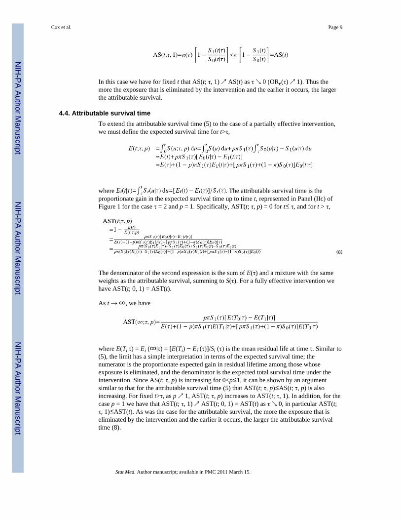
4.4. Attributable survival timeTo extend the attributable survival time (5) to the case of a partially effective intervention,we must define the expected survival time for t>τ,
where . The attributable survival time is theproportionate gain in the expected survival time up to time t, represented in Panel (IIc) ofFigure 1 for the case τ = 2 and p = 1. Specifically, AST(t; τ, p) = 0 for t≤ τ, and for t > τ,
(8)
The denominator of the second expression is the sum of E(τ) and a mixture with the sameweights as the attributable survival, summing to S(τ). For a fully effective intervention wehave AST(t; 0, 1) = AST(t).
As t → ∞, we have
where E(Ti|τ) = Ei (∞|τ) = [E(Ti) − Ei (τ)]/Si (τ) is the mean residual life at time τ. Similar to(5), the limit has a simple interpretation in terms of the expected survival time; thenumerator is the proportionate expected gain in residual lifetime among those whoseexposure is eliminated, and the denominator is the expected total survival time under theintervention. Since AS(t; τ, p) is increasing for 0<p≤1, it can be shown by an argumentsimilar to that for the attributable survival time (5) that AST(t; τ, p)≤AS(t; τ, p) is alsoincreasing. For fixed t>τ, as p ↗ 1, AST(t; τ, p) increases to AST(t; τ, 1). In addition, for thecase p = 1 we have that AST(t; τ, 1) ↗ AST(t; 0, 1) = AST(t) as τ ↘ 0, in particular AST(t;τ, 1)≤AST(t). As was the case for the attributable survival, the more the exposure that iseliminated by the intervention and the earlier it occurs, the larger the attributable survivaltime (8).
Cox et al. Page 9
Stat Med. Author manuscript; available in PMC 2011 March 15.
NIH
-PA Author Manuscript
NIH
-PA Author Manuscript
NIH
-PA Author Manuscript

5. AN EXAMPLE AND AN APPLICATION5.1. An exponential example
A simple example is provided by the case of two exponential distributions. Suppose S0(t) =e−λ0t and S1(t) = e−λ1t, with λ1 > λ0. In this case S(t) = πe−λ1t + (1 − π)e−λ0t, Ei(t) = (1 −e−λit)/λi, and for t>τ, S(t; τ, p) = S(t) + pπ[e−(λ1−λ0)τe−λ0t −e−λ1t], Ei (t|τ) = (1−e−λi(t−τ))/λi,and of course E(Ti|τ) = 1/λi. We also have π(∞) = 0 for this example. Table I summarizesthe four different measures of attribution. Graphs of these functions for (λ1, λ0, π) = (1.5,0.5, 0.6), and both a fully effective (τ, p) = (0, 1) and partially effective (τ, p) = (1, 0.8)intervention, are shown in Figure 2. Both AR(t) and ARh(t) are strictly decreasing from theircommon left-hand limit AR(0+) = 0.545. In this case, ARh(t) is a reasonable approximationto AR(t); see also Figure 2 of Chen et al. [4]. Both AS(t; τ, p) and AST(t; τ, p) areincreasing, and AST(t; τ, p)<AS(t; τ, p). We have AS(∞) = π = 0.6, and AST(∞) = 0.6(1.5–0.5)/1.5 = 0.4. Similarly, AS(∞; 1, 0.8) = 0.306, and AST(∞; 1, 0.8) = 0.106.
5.2. An application: Study design and methodsIn the absence of treatment, individuals who become infected with HIV are at risk of AIDSand subsequent death. Treatments for HIV have evolved from a period of no availabletherapy (prior to 1987) to combinations of three or more drugs (after 1995), collectivelyknown as HAART (DHHS/Henry J. Kaiser Family Foundation Panel, 2006). Since theevolution of HIV therapy followed a definite pattern over time, it is possible to definesequential calendar periods corresponding to distinct therapeutic eras. Cox et al. [10],distinguished four such periods, the first an initial period of no or only monotherapy (July1984–December 1989), followed by two intermediate periods, and the final period the (shortto moderate-term stable) era of HAART (July 1998 – December 2003). To illustrate theattributable survival and compare it with the conventional attributable risk function, wechose the first and last of the four periods, corresponding to essentially no effectivetreatment (exposed) vs highly effective HAART therapy (unexposed), the intervention thatwe wish to study. Thus, the survival function for the first period corresponds to S1(t), andthat for the HAART era is S0(t). The outcome of interest in this analysis was the time from adiagnosis of clinical AIDS to death.
We based our analysis on data from the Multicenter AIDS Cohort Study (MACS), alongitudinal study of HIV-1 infection in a cohort of homosexual and bisexual men, whichbegan in 1983 [11]. The MACS conducts semi-annual interviews, which include detailedquestions about the use of antiretroviral therapy. Deaths are ascertained using both activeand passive methods, including abstraction of death certificates and searches of nationaldeath registries. Schneider et al. [12] showed that a high percentage of participants withclinical AIDS used HAART between early 1995 and December 2003.
The analysis included a total of 786 men with follow-up after an incident diagnosis ofclinical AIDS. In this study, AIDS was defined using the 1993 CDC surveillance criteria[13] based on clinical conditions (i.e. excluding the laboratory criterion of low CD4 count).For simplicity, individuals with an AIDS diagnosis in the first period who were still alive atthe end of the period were treated as censored observations, and did not contribute time tothe subsequent calendar periods. Individuals with a diagnosis after January 1995, whenHAART therapy became widely available, were eligible for inclusion in the last (fourth)period. Those with a diagnosis before the beginning of the last period who survived until thebeginning of the period were treated as late entries. For purposes of comparison we chosetwo values for the proportion untreated, π = 0.7 and 0.3. To study the effects of delayedtreatment for a proportion of the untreated population, we chose τ = 1 year and, forcomparison, p = 1.0 and 0.5.
Cox et al. Page 10
Stat Med. Author manuscript; available in PMC 2011 March 15.
NIH
-PA Author Manuscript
NIH
-PA Author Manuscript
NIH
-PA Author Manuscript

The free, downloadable R software (http://www.r-project.org/) was used for both parametricand nonparametric estimation of the attributable risk, attributable survival, and theattributable survival time. The three-parameter generalized gamma (GG) distribution wasused for parametric estimation [10]. The analysis included likelihood ratio tests to determinewhether the two-parameter Weibull and log normal models provided an adequate fit. For theattributable survival time, a numerical integration method was implemented through thecumulative summation function cumsum(). The programs are available upon request.
5.3. An application: resultsFor the first period, a GG model provided an adequate fit, with parameter estimates (SE) β =0.6737(0.0716), σ = 0.7731(0.0679) and λ = 1.369(0.189), while for the last period aWeibull (λ = 1) fit was reasonable, with parameters β = 3.053(0.298) and σ = 1.617(0.299).Figure 3 shows the survival curves for the two periods. Included are parametric (GG forS1(t) and Weibull for S0(t)) and product limit estimates, indicating that the parametricmodels in this case provided a good fit to the data. The two sets of survival curves show thedramatic improvement in survival after a diagnosis of AIDS, resulting from the introductionof HAART therapy. In addition, we have included S(t) for π = 0.7, and the correspondingS*(t) = S(t; τ, p) for τ = 1 and p = 0.5.
In Figure 4 we present parametric and in Figure 5 nonparametric examples of theattributable risk, attributable survival, and attributable survival time curves for the differentcombinations of the parameters. In addition, Figure 4 includes ARh(t) as an alternative toAR(t). By definition data are only available for 4 years in period one, while follow up inperiod two extends for 8 years. For purposes of comparison the time scale in Figures 4 and 5has been set at 6 years, and the parametric curves projected beyond the actual data. Theattributable risk function starts at zero, increases to a maximum, and then begins to declinetoward zero. The attributable hazard behaves similarly, but in this case does not follow theattributable risk very closely. This example indicates that the attributable hazard can be quitedifferent from the attributable risk. The attributable survival function increases from zero,and by 5 years most of the attributable survival has been realized. Initially AR(t)>AS(t) fort>0, and the two curves cross exactly once. We also show AS(t; τ, p) curves for τ = 1 and p= 1.0 and 0.5. The first of these curves looks similar to the original attributable survivalfunction. The curves for the attributable survival time have a similar shape, but reflect theeffect of averaging. As the fit of the parametric models is quite good, it is no surprise thatthe curves on Figures 4 and 5 are similar, although of course this will not always be the case.
6. DISCUSSIONWe have considered the extension of the attributable risk to the attributable risk function inthe context of survival analysis, and have proposed two new measures, the attributablesurvival and attributable survival time. The attributable survival function tracks the gain insurvival rather than the decrease in risk, and the attributable survival time provides acumulative measure, leading to an interpretation based on the relative gain in survival timerather than survival rate. We believe that these new measures are appropriate and useful inthe survival context; of the two, the attributable survival is easier to compute and perhapsmore likely to be useful in practice.
Under the assumption h1(t)≥h0(t), both AS(t) and AST(t) are increasing, so that the benefitof a treatment or intervention accumulates over time. In contrast, AR(t) can initially take anyvalue between zero and one depending on the limiting properties of the two densityfunctions, and its subsequent behavior is then strongly influenced by this initial value.Another undesirable property of the attributable risk function is that the risk attributable to
Cox et al. Page 11
Stat Med. Author manuscript; available in PMC 2011 March 15.
NIH
-PA Author Manuscript
NIH
-PA Author Manuscript
NIH
-PA Author Manuscript

any intervention is eventually zero, a property that reflects the behavior of the two survivalfunctions more than the intervention.
All of these measures can be computed with standard statistical software using either aparametric or nonparametric approach, as illustrated by the application. Whennonparametric methods are used and the longest observed time is censored, both attributablesurvival [AS(t) and AST(t)] and attributable risk [AR(t)] can only be computed up to thattime. An advantage of parametric methods is the ability to obtain all of these measures forarbitrary t≥0. Caution should be used, however, since it is generally not recommended toextrapolate results beyond the range of the data.
As part of the inference it is frequently useful to also calculate a standard error. Forparametric models, approximate standard errors for the individual survival functions can beobtained using the delta method, and for the nonparametric approach Greenwood’s formulacan be used. In either case an approximate standard error for the attributable survival (or itslogarithm) can then be computed using the delta method. Similar computations are discussedand illustrated by Cox et al. [10]. An alternative approach is to use the bootstrap; additionalsmoothing of bootstrap confidence intervals at individual values of time may be desired toproduce smooth looking bands. Simultaneous confidence bands can also be produced usingeither parametric [14] or nonparametric approaches [15]. A similar approach can in theoryalso be used for the attributable survival time, although to use the delta method one mustintegrate the derivatives of the survival functions with respect to the parameters.
In addition to considering attributable survival for the case of populations that are eitheralways exposed or unexposed (a completely effective intervention), we have discussed thegeneralization to the situation where exposure changes with time. Our discussion waslimited to the case of a single time point, and to interventions for which those who remainexposed are representative of the originally exposed, while those who become unexposedabruptly change to the same hazard as the originally unexposed, and similarly for theunexposed. These conditions may not hold in observational studies where the intervention isnot randomized, or in situations where previous exposure has a lasting effect. As we haveindicated, the measures can be extended by allowing the hazard functions for those who donot change their exposure status to be different from the original hazards. In addition theycan also be extended to the case of more than one time point at which the intervention isadministered. The details are increasingly cumbersome, but there are no methodologicallimitations.
A related generalization is to allow several levels of exposure as well as adjustment forcovariates [5,9]. The simplest framework is to partition the population into K strata, definedby ZK. The conditional survival function is Sk(t) = S(t|ZK = k), and we let πk = P(ZK = k). Theoverall survival function is then S(t) = Σk πk Sk(t). We now assume that the interventionresults in an alternative distribution ; the resulting survival function is then
, and the adjusted attributable survival function is
The generalizations of the attributable survival time and attributable risk are alsostraightforward.
Cox et al. Page 12
Stat Med. Author manuscript; available in PMC 2011 March 15.
NIH
-PA Author Manuscript
NIH
-PA Author Manuscript
NIH
-PA Author Manuscript

AcknowledgmentsData in this manuscript were collected by the Multicenter AIDS Cohort Study (MACS) with centers (PrincipalInvestigators) at The Johns Hopkins University Bloomberg School of Public Health (Joseph B. Margolick, LisaJacobson), Howard Brown Health Center and Northwestern University Medical School (John Phair), University ofCalifornia, Los Angeles (Roger Detels), and University of Pittsburgh (Charles Rinaldo).
Studies were approved by the Committees of Human Research of participating institutions. The MACS web site islocated at http://statepi.jhsph.edu.
Contract/grant sponsor: National Institute of Allergy and Infectious Diseases; contract/grant numbers: UO1-AI-35042, UO1-AI-35043, UO1-AI-35039, UO1-AI-35040, UO1-AI-35041
Contract/grant sponsor: National Center for Research Resources; contract/grant number: MO1-RR-00052
REFERENCES1. Rothman, KJ.; Greenland, S. Modern Epidemiology. Philadelphia: Lippincott-Raven Publishers;
1998. p. 53-58.2. Gefeller O. An annotated bibliography on attributable risk. Biometrical Journal 1992;34:1007–1012.3. Uter W, Pfahlberg A. The application of methods to quantify attributable risk in medical practice.
Statistical Methods in Medical Research 2001;10:231–237. [PubMed: 11446150]4. Chen YQ, Hu C, Wang Y. Attributable risk function in the proportional hazards model for censored
time-to-event. Biostatistics 2006;7:515–529. [PubMed: 16478758]5. Samuelsen SO, Eide GE. Attributable fractions with survival data. Statistics in Medicine
2007;27:1447–1467. [PubMed: 17694507]6. Silverberg MJ, Smith MW, Chmiel JS, Detels R, Margolick JB, Rinaldo CR, O’Brien SJ, Muñoz A.
Fraction of cases of acquired immunodeficiency syndrome prevented by the interactions ofidentified restriction gene variants. American Journal of Epidemiology 2004;159:232–241.[PubMed: 14742283]
7. Khoury MJ, Flanders WD, Greenland S, Adams MJ. On the measurement of susceptibility inepidemiologic studies. American Journal of Epidemiology 1989;129:183–190. [PubMed: 2910059]
8. Drescher K, Becher H. Estimating the generalized impact fraction from case-control data.Biometrics 1997;53:1170–1176. [PubMed: 9290235]
9. Cox C. Model-based estimation of the attributable risk in case-control and cohort studies. StatisticalMethods in Medical Research 2006;15:611–625. [PubMed: 17260927]
10. Cox C, Chu H, Schneider MF, Muñoz A. Parametric survival analysis and taxonomy of hazardfunctions for the generalized gamma distribution. Statistics in Medicine 2007;26:4352–4374.[PubMed: 17342754]
11. Kaslow RA, Ostrow DG, Detels R, Phair JP, Polk BF, Rinaldo CR. The multicenter AIDS cohortstudy: rationale, organization, and selected characteristics of the participants. American Journal ofEpidemiology 1987;126:310–318. [PubMed: 3300281]
12. Schneider MF, Gange SJ, Williams CM, Anastos K, Greenblatt RM, Kingsley LA, Detels R,Muñoz A. Patterns of the hazard of death after AIDS through the evolution of antiretroviraltherapy: 1984–2004. AIDS 2005;19:2009–2018. [PubMed: 16260908]
13. Centers for Disease Control and Prevention. MMWR. 1992. 1993 Revised classification system forHIV infection and expanded surveillance case definition for AIDS among adolescents and adults;p. 1-19.
14. Cox C, Ma G. Asymptotic confidence bands for generalized nonlinear regression models.Biometrics 1995;51:142–150. [PubMed: 7766770]
15. Hall WJ, Wellner JA. Confidence bands for a survival curve from censored data. Biometrika1980;67:133–143.
Cox et al. Page 13
Stat Med. Author manuscript; available in PMC 2011 March 15.
NIH
-PA Author Manuscript
NIH
-PA Author Manuscript
NIH
-PA Author Manuscript
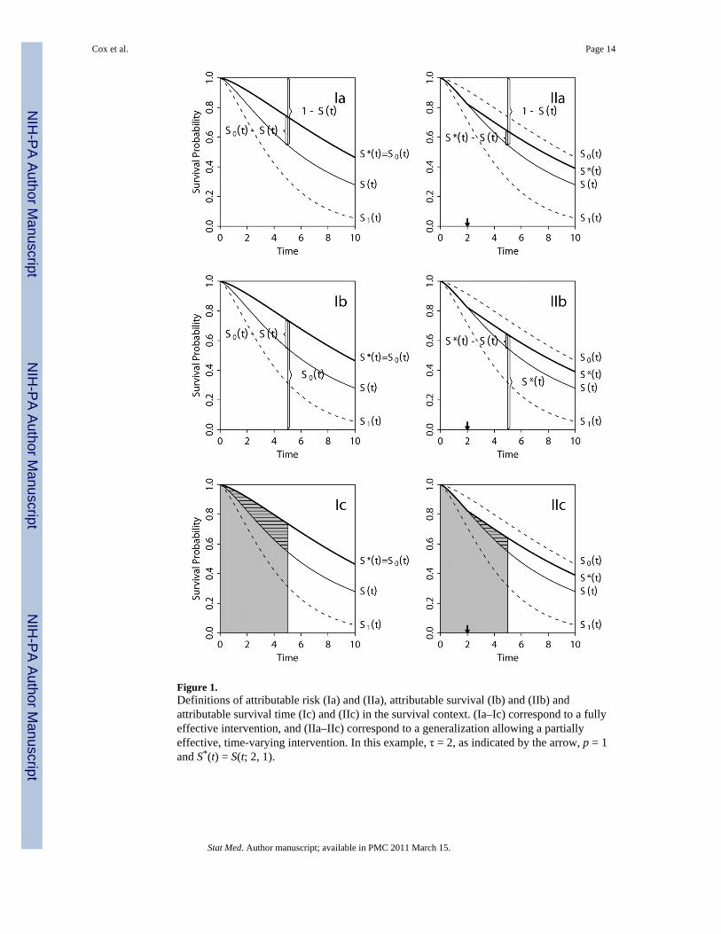
Figure 1.Definitions of attributable risk (Ia) and (IIa), attributable survival (Ib) and (IIb) andattributable survival time (Ic) and (IIc) in the survival context. (Ia–Ic) correspond to a fullyeffective intervention, and (IIa–IIc) correspond to a generalization allowing a partiallyeffective, time-varying intervention. In this example, τ = 2, as indicated by the arrow, p = 1and S*(t) = S(t; 2, 1).
Cox et al. Page 14
Stat Med. Author manuscript; available in PMC 2011 March 15.
NIH
-PA Author Manuscript
NIH
-PA Author Manuscript
NIH
-PA Author Manuscript

Figure 2.Graphs of AR(t, τ, p), ARh(t, τ, p), AS(t, τ, p) and AST(t, τ, p) for exponential distributionswith (λ1, λ0, π) = (1.5, 0.5, 0.6) and both a fully effective (τ, p) = (0, 1) and partiallyeffective (τ, p) = (1, 0.8) intervention.
Cox et al. Page 15
Stat Med. Author manuscript; available in PMC 2011 March 15.
NIH
-PA Author Manuscript
NIH
-PA Author Manuscript
NIH
-PA Author Manuscript
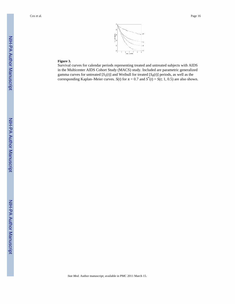
Figure 3.Survival curves for calendar periods representing treated and untreated subjects with AIDSin the Multicenter AIDS Cohort Study (MACS) study. Included are parametric generalizedgamma curves for untreated [S1(t)] and Weibull for treated [S0(t)] periods, as well as thecorresponding Kaplan–Meier curves. S(t) for π = 0.7 and S*(t) = S(t; 1, 0.5) are also shown.
Cox et al. Page 16
Stat Med. Author manuscript; available in PMC 2011 March 15.
NIH
-PA Author Manuscript
NIH
-PA Author Manuscript
NIH
-PA Author Manuscript

Figure 4.Illustrations of the attributable risk, the attributable hazard, attributable survival andattributable survival time curves for different combinations of τ and p for the MACS datausing generalized gamma and Weibull distributions for untreated and treated periods,respectively.
Cox et al. Page 17
Stat Med. Author manuscript; available in PMC 2011 March 15.
NIH
-PA Author Manuscript
NIH
-PA Author Manuscript
NIH
-PA Author Manuscript

Figure 5.Illustrations of the attributable risk, attributable survival and attributable survival timecurves for different combinations of τ and p for the MACS data using the Kaplan–Meierestimates.
Cox et al. Page 18
Stat Med. Author manuscript; available in PMC 2011 March 15.
NIH
-PA Author Manuscript
NIH
-PA Author Manuscript
NIH
-PA Author Manuscript

NIH
-PA Author Manuscript
NIH
-PA Author Manuscript
NIH
-PA Author Manuscript
Cox et al. Page 19
Table I
Attributable risk, survival and survival time functions for the case of two exponential distributions withparameters λ1>λ0.
Attribution Function (t≥τ≥0) t = 0+ (0, ∞) t→∞
AR(t) Decreasing 0
ARh(t) AR(0+) Decreasing 0
AS(t) π[1−e(λ0−λ1t] 0 Increasing π
AST(t) 0 Increasing
AR(t; τ, p) AR(t; τ, p) = 0 (t≤τ) Arc-shaped 0
AS(t; τ, p) AS(t; τ, p) = 0 (t≤τ) Increasing
AST(t; τ, 1) AST(t; τ, p) = 0 (t≤τ) Increasing
Stat Med. Author manuscript; available in PMC 2011 March 15.