Supporting Complex Thematic, Spatial and Temporal

Queries over Semantic Web Data*

Matthew Perry1, Amit P. Sheth1, Farshad Hakimpour2, Prateek Jain1

1 Kno.e.sis Center, Department of Computer Science and Engineering, Wright State

University, Dayton, OH, USA 2 LSDIS Lab, Department of Computer Science, University of Georgia, Athens, GA, USA

{perry.66, amit.sheth, jain.18}@wright.edu, {fhakimpour}@uga.edu

Abstract. Spatial and temporal data are critical components in many

applications. This is especially true in analytical domains such as national

security and criminal investigation. Often, the analytical process requires

uncovering and analyzing complex thematic relationships between disparate

people, places and events. Fundamentally new query operators based on the

graph structure of Semantic Web data models, such as semantic associations,

are proving useful for this purpose. However, these analysis mechanisms are

primarily intended for thematic relationships. In this paper, we describe a

framework built around the RDF metadata model for analysis of thematic,

spatial and temporal relationships between named entities. We discuss

modeling issues and present a set of semantic query operators. We also describe

an efficient implementation in Oracle DBMS and demonstrate the scalability of

our approach with a performance study using a large synthetic dataset from the

national security domain.

Keywords: Ontology, Semantic Analytics, RDF Querying, Spatial RDF,

Temporal RDF

1 Introduction

Analytical applications are increasingly exploiting complex thematic relationships

between named entities as a powerful tool in the analysis process. Such “connecting

the dots” applications are common in many domains, for example national security,

drug discovery and medical informatics. Semantic Web data models, such as

Resource Description Framework (RDF) [1], fit nicely with this analysis paradigm

because relationships are modeled as first class objects. Fundamentally new analytical

operators based on the graph structure of RDF have emerged (e.g., semantic

associations [2] and subgraph discovery [3]) which allow querying for complex

relationships between named entities where an ontology provides the context or

domain semantics. We use the term semantic analytics to refer to this process of

searching, analyzing and visualizing semantically meaningful connections between

named entities. Many successful applications of semantic analytics can be seen in the

* This work is partially funded by NSF-ITRIDM Award #0325464 & #0714441 entitled

“SemDIS: Discovering Complex Relationships in the Semantic Web.”

literature (e.g., identifying conflict of interest [4], detecting patent infringement [5]

and metabolic pathway discovery [6]).

While spatial and temporal data often play a crucial role in many analytical

domains, research in semantic analytics has focused on thematic relationships.

Current approaches do not adequately handle spatial and temporal data. Furthermore,

traditional spatial and spatiotemporal data models used for GIS [7] excel at modeling

and analyzing spatial and temporal relationships between geographic entities but tend

to model the thematic aspects of a given domain as directly attached attributes of

geospatial entities.

In a recent work [8], we have tried to overcome this limitation by modeling spatial,

temporal and thematic data using ontologies and temporal RDF graphs [9]. An upper-

level ontology is used to define the basic classes and relationships of the thematic and

spatial domains. With this approach, thematic entities and relationships are

represented as first class objects and are modeled separately from their spatial

properties (basic spatial features, such as points and lines, termed spatial entities).

Thematic entities and events are connected to spatial entities through located_at and

occurred_at relationships modeled in the upper-level ontology. Deeper domain

ontologies are integrated with this upper-level ontology through rdfs:subClassOf and

rdfs:subPropertyOf statements. A unique aspect of this approach is that a 1-to-1

mapping between thematic and spatial entities is not enforced. Rather, a many-to-

many mapping is achieved by utilizing indirect thematic connections (specified with

domain ontologies) between entities. For example, using a military ontology, a soldier

could be associated with the spatial properties of his residence through one set of

relationships (Soldier – lives_at – Residence – located_at – Spatial_Entity) or with

the locations of his training facilities using a different set of relationships (Soldier –

member_of – Military_Unit – trains_at – Base – located_at – Spatial_Entity).

A variety of query operators are possible over this model which combine thematic

relationships with spatial and temporal relationships, thus adding more expressive

domain semantics to spatial and temporal queries. We argue that by incorporating

more complex models and operators for thematic data, a GIS can be significantly

more useful in applications which require complex thematic analysis in addition to

spatial and temporal analysis.

Spatial and temporal data bring many unique challenges to semantic analytics

applications. Thematic relationships can be explicitly stated in the RDF graph, but

some spatial and temporal relationships (e.g., quantitative relationships like distance)

are implicit and only evident after additional computation. RDF and RDF Schema

(RDFS) inferencing rules [10, 11] are also affected as the temporal properties of

asserted statements will have implications on the temporal properties of the

corresponding inferred statements.

Example (biochemical threat detection): Suppose an intelligence analyst is

assigned the task of monitoring the health of soldiers in order to detect possible

exposure to a chemical or biological agent which may imply a biochemical attack. In

this case, the analyst may search for relationships connecting a sick soldier to

potential chemical or biological agents by matching the soldier's symptoms with

known reactions to these agents. In addition, the analyst could further determine the

likelihood of a particular chemical substance by querying for associations between the

substance and enemy groups in the knowledgebase. For example, a member of the

group may have worked at a facility which was reported to have produced the

chemical. It is doubtful that such an analysis could produce definitive evidence of a

biochemical attack, but incorporating spatial and temporal relationships could help in

this regard. For instance, the analyst may want to limit the results to soldiers and

enemies in close spatial proximity (e.g., find all soldiers with symptoms indicative of

exposure to chemical X which fought in battles within 2 miles of sightings of any

members of enemy group Y). We may pose the following SQL query involving the

spatial_eval table function for such a search:

select a from table (spatial_eval (‘(?a has_symptom ?b) (Chemical_X induces ?b)(?a fought_in ?c)’, ?c, ‘(?d member_of Enemy_Group_Y)(?d spotted_at ?e)’, ?e, ‘geo_distance(distance=2 units=mile)’));

With this query, we are using the spatial_eval operator to specify (1) a relationship

between a soldier, a chemical agent and a battle location and (2) a relationship

between members of an enemy organization and their known locations. We are then

limiting the results based on the spatial proximity of the battles and enemy sightings.

Additionally, we provide a spatial_extent operator which allows retrieving the spatial

geometry associated with the spatial entities composing a thematic relationship and

optionally filtering the results using a spatial predicate. For example, find all soldiers

participating in military events that take place within an input bounding box. For

temporal aspects, we provide an analogous temporal_extent operator which returns

the temporal properties of a given relationship and allows optional filtering. For

example, return all soldiers exhibiting a given symptom during a specific time period.

We also provide a temporal_eval operator which can answer queries such as find

soldiers who exhibited symptoms after participating in a given military event.

This paper focuses on providing a framework to support spatial and temporal

analysis of RDF data. RDF is a World Wide Web Consortium (W3C) standard for

representing ontologies and corresponding instance data. We address problems of

both data storage and operator design and implementation. Specifically, the

contributions of this paper are:

− A storage and indexing scheme for spatial and temporal RDF data

− An efficient treatment of temporal RDFS inferencing

− The definition and implementation of four spatial and temporal query operators

− A performance study using a large RDF dataset

The remainder of the paper is organized as follows. Section 2 discusses

background information and related work regarding data modeling and querying.

Section 3 further describes the set of spatial and temporal query operators. Section 4

describes the implementation of this framework in Oracle DBMS. An experimental

evaluation of this implementation follows in Section 5, and Section 6 gives

conclusions.

2 Background and Related Work

In this section, we discuss background information and related work with regards to

data modeling and querying Semantic Web data.

RDF and Ontologies. RDF [1] has been adopted by the W3C as a standard for

representing metadata on the Web. Resources in RDF are identified by Uniform

Resource Identifiers (URIs) that provide globally-unique and resolvable identifiers for

entities on the Web. These resources are described through participation in

relationships. Relationships in RDF are called Properties and are binary relationships

connecting resources to other resources or resources to Literals, i.e., literal values

such as Strings or Numbers. These binary relationships are encoded as triples of the

form (Subject, Property, Object), which denotes that a resource – the Subject – has a

Property whose value is the Object. These triples are referred to as Statements. RDF

also allows for anonymous nodes called Blank Nodes which can be used as the

Subject or Object of a statement. We call a set of triples an RDF graph, as RDF data

can be represented as a directed, labeled graph with typed edges and nodes. In this

model, a directed edge labeled with the Property name connects the Subject to the

Object.

RDF Schema (RDFS) [10] provides a standard vocabulary for describing the

classes and relationships used in RDF statements and consequently provides the

capability to define ontologies. Ontologies serve to formally specify the semantics of

RDF data so that a common interpretation of the data can be shared across multiple

applications. RDFS allows us to define hierarchies of class and property types, and it

allows us to define the domain and range of property types.

Additionally, a set of entailment rules are defined for RDF and RDFS [11]. These

rules essentially specify that an additional triple can be added to the RDF graph if the

graph contains triples of a specific pattern. Such rules describe, for example, the

transitivity of the rdfs:subClassOf property.

Temporal RDF Graphs. In order to analyze the temporal properties of relationships

in RDF graphs, we need a way to record the temporal properties of the statements in

those graphs, and we must account for the effects of those temporal properties on

RDFS inferencing rules. For this purpose, we adopt temporal RDF graphs defined in

[9]. Temporal RDF graphs model absolute time and are defined as follows. Given a

set of discrete, linearly ordered time points T, a temporal triple is an RDF triple with a

temporal label t∈T. A statement's temporal label represents its valid time. The

notation (s, p, o) : [t] is used to denote a temporal triple. The expression (s, p, o) : [t1,

t2] is a notation for {(s, p, o) : [t] | t1 ≤ t ≤ t2}. A temporal RDF graph is a set of

temporal triples. For example, consider a soldier s1 assigned to the 1st Armored

Division (1stAD) from April 3, 1942, until June 14, 1943, and then assigned to the 3rd

Armored Division (3rdAD) from June 15, 1943, until October 18, 1943. This would

yield the following triples: (s1, assigned_to, 1stAD) : [04:03:1942, 06:14:1943], (s1,

assigned_to, 3rdAD) : [06:15:1943, 10:18:1943]. Any temporal ontology that defines a

vocabulary of time units can be used to precisely specify the start and end points of

time intervals.

As discussed in [9], we must account for the effects of temporal labels on RDFS

inferencing rules. To incorporate inferencing into temporal RDF graphs, we must use

a basic arithmetic of intervals to derive the temporal label for the inferred statements.

For example, interval intersection would be needed for rdfs:subClassOf (e.g., (x,

rdfs:subClassOf, y) : [1, 4] ∧ (y, rdfs:subClassOf, z) : [3, 5] � (x, rdfs:subClassOf,

z) : [3, 4]).

Related Work. We will first discuss our modeling approach using temporal RDF as it

compares with other spatiotemporal models in the literature. For a recent survey, see

[7]. Of the models discussed in the literature, the object-oriented and event-based

models and the three domain model are most similar to our RDF-based approach. The

three domain model, introduced by Yuan, is described in [12, 13]. This model

represents semantics, space and time separately. To represent spatiotemporal

information in this model, semantic objects are linked via temporal objects to spatial

objects. This provides temporal information about the semantic (thematic) properties

of a given spatial region. This is analogous to temporal located_at and occurred_at

relationships in our model. The three domain model is quite similar to our approach in

that it represents thematic entities as first class objects rather than attributes of

geospatial objects. The key difference is that the three domain model relies on direct

connections from thematic entities to spatial regions whereas our model allows

indirect connections composed of sequences of thematic relationships, which is made

possible by a richer modeling of the thematic domain. Additionally, relaxing the

direct connection requirement better tolerates incompleteness of information – a

necessity when handling Web data. In [14], the authors discuss a combination of the

object-oriented and event-based modeling approaches for dynamic geospatial

domains. They define an upper-level ontology similar to the one we present in [8].

They model the concept of a setting and a situate function which maps entities and

events to settings. Settings can be spatial, temporal, or spatiotemporal. In contrast to

our work, the authors focus on geospatial objects and events and model what we

would consider a thematic entity (e.g., an airplane) as a geospatial entity. That is, the

separation between the thematic and spatial domains is not as strongly emphasized.

Our RDF-based modeling approach provides a means to assign spatial properties to

those entities not directly connected to a spatial setting and allows deeper analysis of

purely thematic relationships.

Many RDF query languages have been proposed in the literature. These include

SQL-like languages (e.g., SPARQL [15]), functional languages (e.g., RQL [16]), rule-

based languages (e.g., TRIPLE [17]) and graph traversal languages (e.g., RxPath

[18]). Efficient implementations of these languages for persistent RDF data usually

involve translation into a SQL query against an underlying RDBMS representation of

the RDF data (e.g., Jena2 [19], RDFSuite [20]). As an alternative to defining a new

query language, an approach for querying RDF data directly in SQL has been

proposed [21]. This facilitates easy integration with other SQL queries against

traditional relational data and saves the overhead of translating data from SQL to the

RDF query language data format. Our implementation follows this approach and

introduces new SQL functions for spatial and temporal querying of RDF data.

Work is somewhat limited with regards to incorporating spatial and temporal

relationships into queries over Semantic Web data. Examples of querying geospatial

RDF data are mostly seen in web applications and semantic geospatial web services

[22, 23] in the spirit of the Geospatial Semantic Web [24]. In general, query

processing proceeds by translating RDF representations of spatial features into

geometric representations on the fly and then performing spatial calculations, and the

focus is more on interoperability than efficient query processing. The SPIRIT spatial

search engine [25] combines an ontology describing the geospatial domain with the

searching and indexing capability of Oracle Spatial for the purposes of searching

documents based on the spatial features associated with named places mentioned in

the document. In contrast, our searching operators are intended for general purpose

querying of ontological and spatial relationships. Querying for temporal data in RDF

graphs is less complicated as RDF supports typed literals such as xsd:date, and

corresponding query languages support filtering results based on literal values.

However, this is far from supporting full temporal RDF as graphs discussed in this

paper. In addition to formally defining temporal RDF graphs, Gutierrez et al. briefly

discussed aspects of a query language for these graphs, but no implementation issues

were mentioned [9]. Also, to the best of our knowledge, this paper is the first to

investigate implementation of RDFS inferencing which incorporates the concept of

valid time for RDF statements.

3 Query Operators

In this section, we introduce a set of spatial and temporal query operators for

searching and analyzing spatial and temporal relationships between named entities in

temporal RDF graphs. These operators are an adequate functional set in that they (1)

allow precise specification of a thematic portion of the RDF graph (subgraph), (2)

provide facilities to compute spatial and temporal properties of these subgraphs and

(3) allow filtering and joins based on the computed spatial and temporal properties.

The operators are implemented as SQL table functions. Table functions produce a set

of rows as output which can be queried. They are used in SQL queries in the same

manner as a database table name. For example, we may have the query select x,

y from table (table_func (...)) order by x.

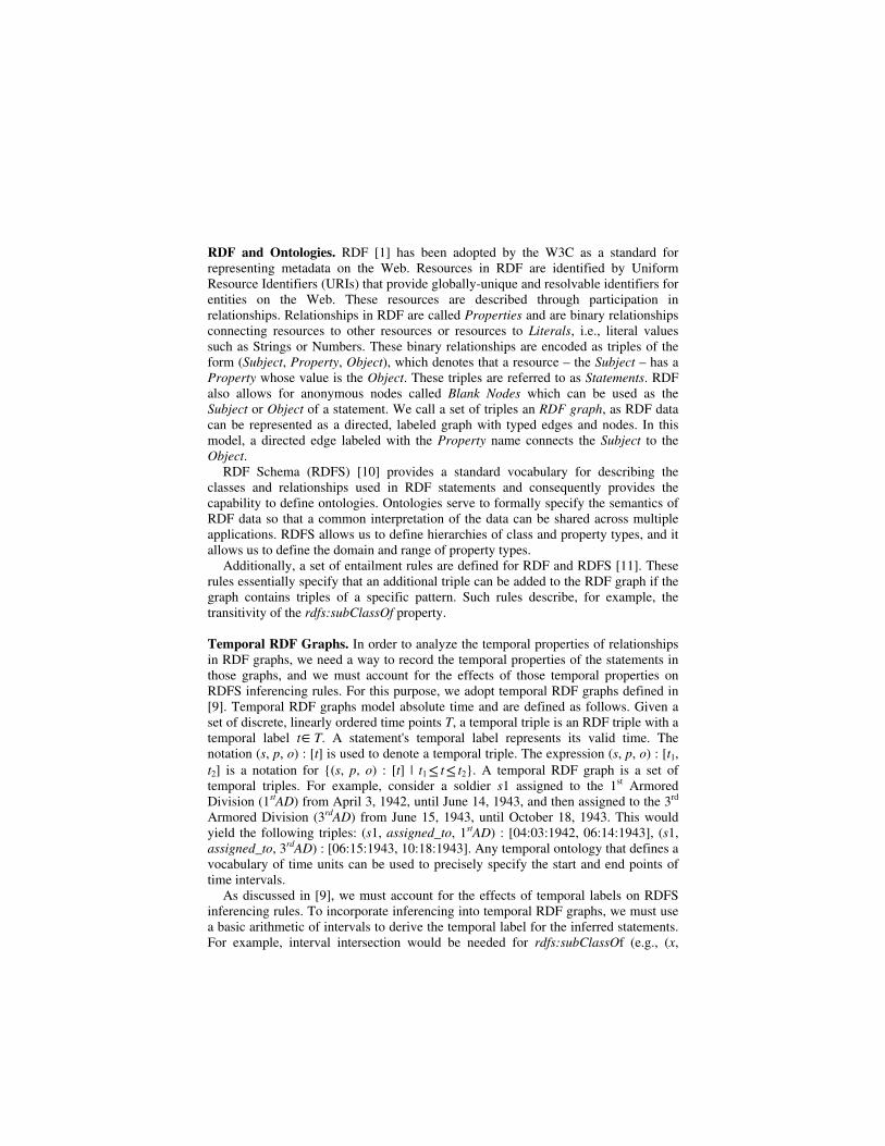
Graph Patterns. SPARQL-like graph patterns are the basic building block of these

operators. Intuitively, a graph pattern is a set of RDF triples where the subjects,

properties and/or objects may be replaced with variables. In general, a graph pattern

query against an RDF graph G returns a set of mappings between the variables in the

graph pattern and terms (URIs, Blank Nodes and Literals) in G such that substituting

the mapped terms into the graph pattern results in a set of triples actually present in G.

We refer to the set of triples resulting from a substitution as a graph pattern instance,

and the result of a graph pattern query on a given RDF graph G is the set of variable

bindings for all matching graph pattern instances in G. Fig. 1 illustrates these

concepts for an example graph pattern query.

Spatial Query Operators. We define two spatial query operators for RDF graphs

containing geospatial data: spatial_extent and spatial_eval. The following

descriptions assume the existence of a class Geometry in the ontology which models

spatial objects, and we use the term spatial feature to refer to an SDO_GEOMETRY

object that would be stored in Oracle Spatial (i.e., the implementation of Geometry).

The first spatial operator, spatial_extent, is intended to retrieve the spatial feature

of the Geometry connected to a thematic entity and optionally filter the results based

on the properties of the spatial feature. The signature for the corresponding table

function is shown below: spatial_extent (graphPattern VARCHAR, spatialVar VARCHAR, ontology RDFModels, <geom SDO_GEOMETRY>, <spatialRelation VARCHAR>) returns AnyDataSet;

The graphPattern parameter specifies the relationship between a thematic entity and a

Geometry, for example (Soldier, fought_in, Battle) (Battle, located_at, Geometry).

The spatialVar parameter identifies the variable in the graph pattern that corresponds

to a Geometry, and ontology determines the ontology to search against. This function

returns a table with rows containing columns for each variable in the graph pattern

and one column for the spatial features. Each row contains the URI bound to each

variable and the spatial feature corresponding to the Geometry bound to spatialVar

(displayed as well known text format in Oracle). Two optional parameters, a spatial

feature and a spatial relationship, can be used to filter the graph pattern instances. In

this case, the table would only contain those graph pattern instances whose associated

spatial features satisfy the specified spatial relation with the input spatial feature. We

support the following spatial relationships: touch, overlap, equal, inside, covered by,

contains, covers, any interact and within distance.

The second spatial operator, spatial_eval, acts as a spatial join between graph

pattern instances. It is intended to allow for searching thematic entities based on their

spatial relationships. The signature for the corresponding table function is shown

below: spatial_eval (graphPattern VARCHAR, spatialVar VARCHAR, graphPattern2 VARCHAR, spatialVar2 VARCHAR, spatialRelation VARCHAR, ontology RDFModels) return AnyDataSet;

graphPattern and spatialVar specify the left hand side of the join operation, while

graphPattern2 and spatialVar2 specify the right hand side. spatialRelation identifies

the spatial join condition. This function returns a table containing a column for each

variable in graphPattern and graphPattern2 and a column for each associated spatial

feature (sf1 and sf2). For each row in the resulting table, sf1 spatialRelation sf2

evaluates to true.

Temporal Query Operators. We define two temporal query operators for temporal

RDF graphs: temporal_extent and temporal_eval. The basic idea behind the operators

Fig. 1. Example graph pattern with resulting variable bindings.

is that we compute a temporal interval for a graph pattern instance based on the

temporal properties of the triples making up the graph pattern instance.

The first temporal operator, temporal_extent, is used to compute the temporal

interval for a graph pattern instance and optionally filter the results based on the

computed temporal interval. We support two basic intervals for a graph pattern

instance: the interval during which the entire graph pattern instance is valid

(INTERSECT) and the interval during which any part of the graph pattern is valid

(RANGE). The signature for the corresponding table function is shown below. temporal_extent (graphPattern VARCHAR, intervalType VARCHAR, ontology RDFModels, <start DATE>, <end DATE>, <temporalRel VARCHAR>) return AnyDataSet;

This function takes three parameters as input, specifically a graph pattern, a String

value specifying the interval type (INTERSECT or RANGE), and a parameter

specifying the ontology to search against. The table returned contains a column for

each variable in the graph pattern and two DATE columns which specify the start and

end of the time interval computed for the graph pattern instance. Three optional

parameters, two DATE values to identify the boundaries of a time interval and a

temporal relationship, can be used to filter the found graph pattern instances. In this

case, assuming the DATE columns in the returned table are named stDate and

endDate, each row in the result satisfies the condition [stDate, endDate] temporalRel

[start, end]. We currently support seven temporal relationships: before, after, during,

overlap, during_inv, overlap_inv and any interact.

The second temporal operator, temporal_eval, acts as a temporal join operator for

graph pattern instances. The corresponding table function has the following signature: temporal_eval (graphPattern VARCHAR, intervalType VARCHAR, graphPattern2 VARCHAR, intervalType2 VARCHAR, temporalRel VARCHAR, ontology RDFModels) return AnyDataSet;

graphPattern and intervalType specify the left hand side of the join operation, while

graphPattern2 and intervalType2 specify the right hand side. temporalRel identifies

the join condition. This function returns a table containing a column for each variable

in graphPattern and graphPattern2 and four DATE columns (start1, end1, start2,

end2) to indicate the time interval for each found graph pattern instance. For each row

in the resulting table, [start1, end1] temporalRel [start2, end2] evaluates to true.

4 Implementation in Oracle

In this section, we describe the implementation of our spatial and temporal RDF

query operators in Oracle DBMS. The implementation builds upon Oracle's existing

support for RDF storage and inferencing and support for spatial object types and

indexes. We create SQL table functions for each of the previously discussed query

operators. Additional structures are created to allow for spatial and temporal indexing

of the RDF data for efficient query evaluation. We should note that in general this

approach is not limited to Oracle and could be implemented using any extensible

DBMS that supports user-defined object types and functions.

Existing Oracle Technologies. Oracle's Semantic Data Store [26] provides the

capabilities to store, infer, and query semantic data, which can be plain RDF

descriptions and RDFS based ontologies. To store RDF data, users create a model

(ontology) to hold RDF triples. The triples are stored after normalization in two

tables: an RDFValues table which stores RDF terms and a numeric id and an

RDFTriples table which stores the ids of the subject, predicate and object of each

statement. Users can optionally derive a set of inferred triples based on user-defined

rules and/or RDFS semantics. These triples are materialized by creating a rules index

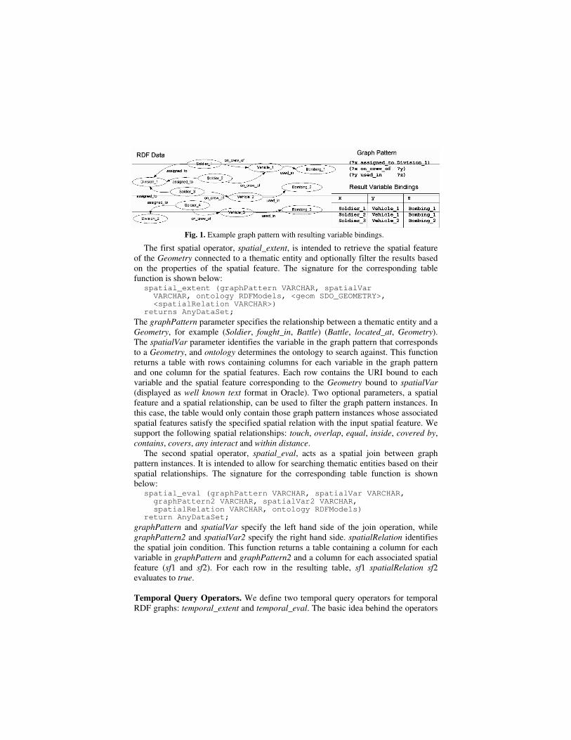
and stored in a separate InferredTriples table. These storage structures are illustrated

in Fig. 2. A SQL table function is provided that allows issuing graph pattern queries

against both asserted and inferred RDF statements.

Oracle Spatial [27] provides facilities to store, query and index spatial features. It

supports the object-relational model for representing spatial geometries. A native

spatial data type, SDO_GEOMETRY, is defined for storing vector data. Database

tables can contain one or more SDO_GEOMETRY columns. Oracle Spatial supports

spatial indexing on SDO_GEOMETRY columns, and provides a variety of procedures,

functions and operators for performing spatial analysis operations.

Data Representation. Our Framework supports spatial and temporal data serialized in

RDF using an RDFS ontology discussed in [28]. This ontology models the concept of

a Geometry Class and allows for recording coordinate system information and

representing points, lines, and polygons. This model complies with the OGC simple

feature specification [29]. Using this representation, spatial features are stored as

instances of Geometry and are uniquely identified by their URI. Temporal labels are

associated with statements using RDF reification, as suggested in [9]. Reification

allows us to assert statements about RDF statements. Our framework supports time

interval values serialized as instances of the Class Interval from this ontology. A

property type, temporal, is defined to assert that a statement has a valid time which is

represented as an Interval instance.

Indexing Approach. In order to ensure efficient execution of graph pattern queries

involving spatial and temporal predicates, we must provide a means to index portions

of the RDF graph based on spatial and temporal values. Basically, this is done by

building a table mapping Geometry instance URIs to their SDO_GEOMETRY

representation and by building a modified RDFTriples table which also stores the

Fig. 2. Storage structures for RDF data. Existing tables of Oracle Semantic Data Store are

shown on the right, and our additional tables for efficiently searching spatial and temporal data

are shown on the left.

temporal intervals associated with the triple. In order to build these indexes, users first

load the set of asserted RDF statements into Oracle Semantic Data Store and build an

RDFS rules index.

Spatial Indexing Scheme. We provide the procedure build_geo_index() to construct a

spatial index for a given ontology. This procedure first creates the table SpatialData

(value_id NUMBER, shape SDO_GEOMETRY) for storing spatial features

corresponding to instances of the class Geometry in the ontology. value_id is the id

given to the URI of the Geometry instance in Oracle's RDFValues table, and shape

stores the SDO_GEOMETRY representation of the Geometry instance (see Fig. 2).

This table is filled by querying the ontology for each Geometry instance, iterating

through the results and creating and inserting SDO_GEOMETRY objects into the

spatial indexing table. Finally, to enable efficient searching with spatial predicates on

this table, a spatial (R-Tree) index is created on the shape column.

Temporal Indexing Scheme. Our temporal indexing scheme is a bit more complicated,

as it must account for temporal labels on statements inferred through RDFS

semantics. However, we only need to handle a subset of the RDFS inference rules.

This is the case because we are not interested in handling temporal evolution of the

ontology schema. What we need to handle are temporal properties of instance data.

Specifically, we need to account for temporal labels of inferred rdf:type statements

and statements resulting from rdfs:subPropertyOf statements. rdf:type statements

result from the following rules: (1) (x, rdf:type, y) ∧ (y, rdfs:subClassOf, z) � (x,

rdf:type, z), and (2) (x, p, y) ∧ (p, rdfs:domain, a) ∧ (p, rdfs:range, b) � (x,

rdf:type, a), (y, rdf:type, b). We infer instance statements from rdfs:subPropertyOf

using the following rule: (1) (x, p, y) ∧ (p, rdfs:subPropertyOf, q) � (x, q, y). In

each case, if we assume that schema level statements in the ontology are eternally

true, the temporal label of an inferred instance statement s is the union of the time

intervals of all statements which can be used to infer s.

We provide the procedure build_temporal_index() to create a temporal index for a

given ontology. This procedure executes in three phases.

The first phase creates the temporary table asserted_temporal_triples (subj_id

NUMBER, prop_id NUMBER, obj_id NUMBER, start DATE, end DATE). The

ontology is then queried to retrieve all asserted temporal reifications. The subject,

property, and object ids of each temporally reified statement and the start time and

end time are inserted into this temporary table. The final step of this phase inserts

statements without asserted temporal reifications into the asserted_temporal_triples

table using min_start_time and max_end_time as the default start and end times.

These values are specified during index creation. Additionally, all schema-level

statements also receive these start and end values to denote that the ontology schema

is always valid.

At this point, we have recorded the temporal values for each asserted statement,

and the second and third phases perform the temporal inferencing process and create

the final temporal triples table (see Fig. 2). In the procedure TemporalInference

(shown below), we first create a second temporary table redundant_triples (subj_id

NUMBER, prop_id NUMBER, obj_id NUMBER, start DATE, end DATE). Then, we

iterate through the asserted_temporal_triples table and add any inferred statements to

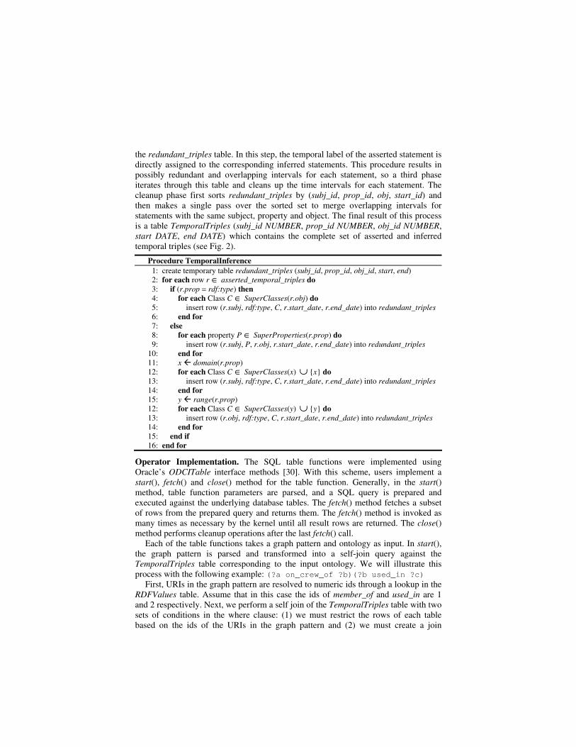
the redundant_triples table. In this step, the temporal label of the asserted statement is

directly assigned to the corresponding inferred statements. This procedure results in

possibly redundant and overlapping intervals for each statement, so a third phase

iterates through this table and cleans up the time intervals for each statement. The

cleanup phase first sorts redundant_triples by (subj_id, prop_id, obj, start_id) and

then makes a single pass over the sorted set to merge overlapping intervals for

statements with the same subject, property and object. The final result of this process

is a table TemporalTriples (subj_id NUMBER, prop_id NUMBER, obj_id NUMBER,

start DATE, end DATE) which contains the complete set of asserted and inferred

temporal triples (see Fig. 2).

Procedure TemporalInference

1: create temporary table redundant_triples (subj_id, prop_id, obj_id, start, end)

2: for each row r ∈ asserted_temporal_triples do

3: if (r.prop = rdf:type) then

4: for each Class C ∈ SuperClasses(r.obj) do

5: insert row (r.subj, rdf:type, C, r.start_date, r.end_date) into redundant_triples

6: end for

7: else

8: for each property P ∈ SuperProperties(r.prop) do

9: insert row (r.subj, P, r.obj, r.start_date, r.end_date) into redundant_triples

10: end for

11: x domain(r.prop)

12: for each Class C ∈ SuperClasses(x) ∪ {x} do

13: insert row (r.subj, rdf:type, C, r.start_date, r.end_date) into redundant_triples

14: end for

15: y range(r.prop)

12: for each Class C ∈ SuperClasses(y) ∪ {y} do

13: insert row (r.obj, rdf:type, C, r.start_date, r.end_date) into redundant_triples

14: end for

15: end if

16: end for

Operator Implementation. The SQL table functions were implemented using

Oracle’s ODCITable interface methods [30]. With this scheme, users implement a

start(), fetch() and close() method for the table function. Generally, in the start()

method, table function parameters are parsed, and a SQL query is prepared and

executed against the underlying database tables. The fetch() method fetches a subset

of rows from the prepared query and returns them. The fetch() method is invoked as

many times as necessary by the kernel until all result rows are returned. The close()

method performs cleanup operations after the last fetch() call.

Each of the table functions takes a graph pattern and ontology as input. In start(),

the graph pattern is parsed and transformed into a self-join query against the

TemporalTriples table corresponding to the input ontology. We will illustrate this

process with the following example: (?a on_crew_of ?b)(?b used_in ?c)

First, URIs in the graph pattern are resolved to numeric ids through a lookup in the

RDFValues table. Assume that in this case the ids of member_of and used_in are 1

and 2 respectively. Next, we perform a self join of the TemporalTriples table with two

sets of conditions in the where clause: (1) we must restrict the rows of each table

based on the ids of the URIs in the graph pattern and (2) we must create a join

condition based on variable correspondences between different parts of the graph

pattern. We must also join with the RDFValues table to resolve the ids of URIs bound

to variables to actual URI Strings for return from the function. The graph pattern

above results in the following query: select rv1.uri, rv2.uri, rv3.uri from TemporalTriples t1, TemporalTriples t2, RDFValues rv1, RDFValues rv2, RDFValues rv3 where t1.prop_id = 1 and t2.prop_id = 2 and t1.obj_id = t2.subj_id and rv1.id = t1.subj_id and rv2.id = t1.obj_id and rv3.id = t2.obj_id;

Spatial operators are implemented by augmenting the base graph pattern query in

start(). For the spatial_extent operator, we add an additional join with the SpatialData

table to retrieve the SDO_GEOMETRY object corresponding to the spatial_variable

parameter. In the case of optional result filtering, we need to modify the where clause

so that we filter the spatial features from SpatialData according to the input spatial

feature and spatial relation. This is done by adding the appropriate sdo_relate or

sdo_within_distance predicate available in Oracle Spatial. For example, given the

query spatial_extent (..., sdo_geometry (...), 'geo_relate

(inside)'), we would modify the query as follows: where ... and

sdo_relate (SpatialData.shape, sdo_geometry (...), 'mask=inside') = 'true';

For the spatial_eval operator, we implement what is essentially a nested loop join

(NLJ) using the basic spatial_extent and filtered spatial_extent operators. We first

construct and execute a basic spatial_extent query in the start() routine. Next, in the

fetch() routine, we consume a row from the spatial_extent query and then construct

and execute the appropriate filtered spatial_extent query using the second pair of

graph pattern and spatial variable parameters and the spatial relation parameter. This

is repeated until all rows in the outer spatial_extent query are consumed. This NLJ

strategy is needed to avoid an awkward query plan on what would be a very large

single base query.

The implementation of the temporal operators does not translate directly to a SQL

query. We must do some extra processing of the base query results in fetch() to form a

single time interval for each found graph pattern instance.

For the temporal_extent operator, we first augment the basic graph pattern query in

start() to also select the start and end values for each temporal triple in the graph

pattern instance. In the fetch() routine, to compute the final temporal interval for each

graph pattern instance, we examine the start and end times for each triple and select

the earliest start and latest end (RANGE) or the latest start and earliest end

(INTERSECT). In each case, we ensure that the resulting time interval is valid (i.e.,

start time less than end time) before including it in the result. When the optional

filtering parameters are specified, we must perform additional checking of the found

graph patterns to ensure they satisfy the filter condition. In addition to these extra

computations in fetch(), as an optimization, we augment the base query in start() with

a series of predicates involving the start and end times of each statement in the graph

pattern. This is done to filter the results as much as possible in the base query to

reduce subsequent overhead in fetch(). To illustrate these additional predicates,

consider the following temporal_extent query and corresponding base query: select ... from table(temporal_extent('(?x on_crew_of ?y)(?y

used_in ?z)', 'range', 1942, 1944, 'during'));

select ... from ..., TemporalTriples t1, TemporalTriples t2 where ... and t1.start > 1942 and t1.end < 1944 and t2.start > 1942 and t2.end < 1944;

The implementation of the temporal_eval operator is similar to the implementation

of spatial_eval. We first build a basic temporal_extent query involving the first pair

of graph pattern and interval type parameters which is executed in the start() routine.

Next, in fetch(), we consume a row from the basic temporal_extent query and execute

an appropriate filtered temporal_extent query using the second pair of graph pattern

and interval type parameters. This query uses the time interval from the current outer

temporal_extent result and the inverse of the temporal relation parameter from the

original temporal_eval query.

5 Experimental Evaluation

In this section, we describe the experimental evaluation of our spatial and temporal

query operators. All experiments were conducted using Oracle 10g Release 2 running

on a Red Hat Enterprise Linux machine with dual Xenon 3.0 GHz processors and 2

GB of main memory. The database used an 8 KB block size and was configured with

an sga_target size of 512 MB and a pga_aggregate_target size of 512 MB. The times

reported for each query are an average of 15 trials using a warm cache. Times were

obtained by querying for systimestamp before and after query execution and

computing the difference. Datasets and queries can be downloaded from

http://knoesis.wright.edu/students/mperry/STData.html.

Dataset. Three synthetically generated datasets were used in our experiments. The

datasets correspond to an ontology schema from the military domain that we created

with the overall idea being to analyze historical entities and events of WWII. The

ontology schema defined 15 class types and 9 property types. Each dataset was

created in three phases. First we populated the thematic portion of the ontology.

Second we added spatial information, and in the final step we generated temporal

labels for the statements in the populated ontology.

To populate the thematic portion of the military ontology, we used the ontology

population tool described in [31]. This tool inputs an ontology schema and relative

probabilities for generating instances of each class and property type. Based on these

probabilities, it generates instance data, which, in effect, simulates the population of

the ontology. We generated three RDF datasets this way. The first contained 95,000

triples, the second contained 1.6 million triples and the third contained over 15

million triples (asserted and inferred statements). We integrated these military RDF

graphs with the upper-level ontology described in [8] by adding a handful of

rdfs:subClassOf statements to each RDF dataset.

To add spatial aspects to this dataset, we randomly assigned spatial features to each

instance of Geometry in the ontology with uniform probability. We used year 2000

census block group boundary polygons from the US Census Bureau for the spatial

features [32]. Differently-sized sets of contiguous US States were chosen in

proportion with the ontology size. The total numbers of features for each dataset were

873; 9,352 and 83,236 for the small, medium and large ontology, respectively.

The final phase of dataset generation assigned temporal labels to statements in the

ontology. Temporal intervals were randomly assigned to each asserted instance

statement. Start times and end times for each interval were randomly selected with

uniform probability from two overlapping date ranges. We ensured that each interval

was valid (i.e., start time earlier than end time) before adding it to the dataset.

Experiments. Our experiments are designed to characterize the overall performance

of our approach with respect to (1) ontology size and (2) graph pattern complexity.

For testing, B-Tree indexes were created on each column of the TemporalTriples table

and on the value_id column of the SpatialData table, and an R-Tree index was created

on the shape column of SpatialData. We also created two additional B-Tree indexes

(prop_id, subj_id, obj_id, start, end) and (prop_id, obj_id, subj_id, start, end) on the

TemporalTriples table. For the 15 million triple dataset, the physical size of the

TemporalTriples table was 642 MB, and the inferencing procedure took 1 hour and 31

min. to execute, which compared with 1 hour and 11 min. for Oracle RDFS rules

index creation. The SpatialData table was 47 MB in size.

Query Execution Time. Table 1 summarizes the results of our experimentation with

respect to ontology size.

Table 1. Experimental results for query execution time with respect to ontology size

Graph Pattern Type Avg. Execution Time for

each ontology (ms) Operator

(Exp. #) # Vars # Triples Queries

Avg.

Result

Size Small Medium Large

T-Ext (1) 4 3 4 N/A 394 390 385

(2) 3 3 5 221 22 32 48

S-Ext (3) 4 3 3 N/A 360 350 365

(4) 3 3 3 100 22 30 67

T-Filter(5) 4 3 4 312 157 345 714

S-Filter (6) 4 3 3 331 173 192 374

2/2 2/2 3 129 414 411 437 T-Eval(7)

2/3 3/3 3 220 306 195 268

2/2 2/1 3 244 343 467 485 S-Eval (8) 2/2 2/3 3 209 251 385 457

Experiments 1 through 4 were designed to test the general scalability of basic

temporal_extent and spatial_extent queries. Experiments 1 and 3 measured the

response time (i.e., time to return the first 1000 rows of results) for a very unselective

query. Our unselective graph patterns consisted of 3 triples and 4 variables. For each

triple in the pattern a constant URI was given for the property, and the subject and

object were left as variables. We used 4 different graph patterns for temporal_extent

with an INTERSECT type query in each case. For spatial_extent, 3 different graph

patterns were used. In each case, the DBMS uses a nested loop joion (NLJ) strategy

for evaluating the base query which results in response times which are essentially

constant across each dataset as the execution time of a NLJ usually grows in

proportion with the result set size. Experiments 2 and 4 are designed to measure

scalability for a very selective graph pattern. For experiment 2, we used 5 different

graph patterns consisting of 3 triples and 3 variables. For experiment 4, we used 3

different graph patterns with 3 triples and 3 variables. The graph patterns are of the

same basic form as the previous experiment except we replace one of the variables in

the subject or object position with a constant URI. This restricts the nodes in the

resulting graph pattern instance instead of just the edges, providing a much more

selective query. In each case, query execution time increases slightly as the ontology

size increases, which is a consequence of scanning larger indexes during query

evaluation and querying a larger SpatialData table.

In experiment 5, we measured the scalability of the temporal_extent operator using

optional filtering with respect to dataset size. For these tests, we used very unselective

graph patterns in combination with very selective temporal conditions. Note that this

represents a worst case scenario for temporal_extent. Because we only store the

temporal labels for single triples in the DB, we can only index these single triples.

The temporal labels for graph pattern instances are constructed during query

evaluation and therefore cannot be indexed. We must apply the temporal filter to each

graph pattern instance as it is being constructed, which can potentially lead to very

large intermediate result sets because in many cases we cannot exclude a graph

pattern from the results until its time interval has been fully constructed. Our

experiments show an increase in execution time which is roughly linear with respect

to ontology size which reflects the growth of intermediate results processed during the

query. Each query used the INTERSECT option and either a before, after or during

temporal relation.

In experiment 6, we measured the performance of spatial_extent using the optional

filtering capability as dataset size increases. As with experiment 5, we combined a

low selectivity graph pattern with a highly-selective spatial predicate. We used three

different queries. The first retrieved results which were within a short distance of a

point; another retrieved results which were covered by an input polygon, and the final

query retrieved results which intersected with an input polygon. The results show that

spatial_extent with filter scales better than its temporal counterpart because we can

effectively index the spatial features and quickly reduce the search space using the

spatial index. The execution time increases because larger indexes must be scanned

when evaluating the graph pattern.

Experiment 7 illustrates the scalability of selective temporal_eval queries. For this

test, we used selective graph patterns for both the LHS and RHS input patterns. We

varied the constant URIs in the graph pattern and the temporal condition so that the

result set sizes were constant across each dataset. The results show that execution

time is roughly constant across each dataset with variations resulting from slight

differences in the number of query restarts required in fetch() and the selectivity of the

graph patterns used. Each query used the INTERSECT option and either a before,

after, during or any interact temporal relation.

Experiment 8 characterizes the performance of selective spatial_eval queries as the

dataset size increases. Again, we used selective graph patterns for both the LHS and

RHS pattern and varied the constant URIs and spatial predicates so that result set size

was consistent across each dataset. The results show that execution time grows

slightly as ontology size increases, which is a result of scanning larger indexes and

querying a larger spatial dataset.

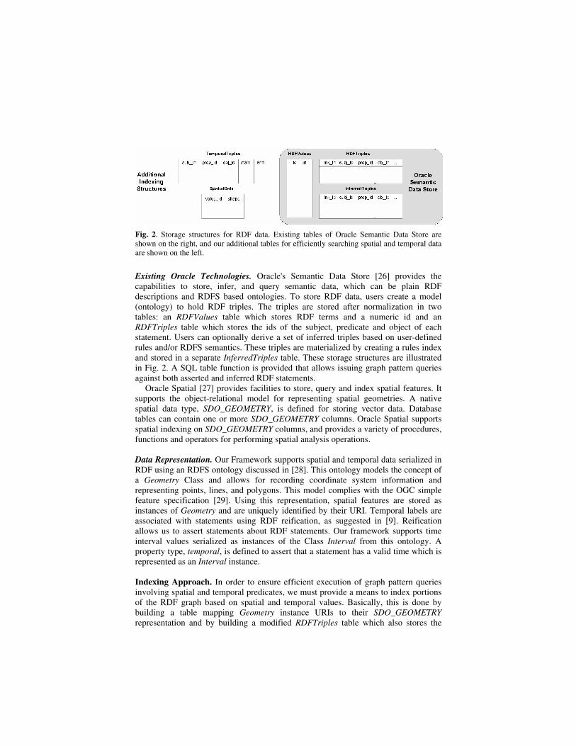
Our next experiments were designed to test the scalability of the temporal_extent

operator as the graph pattern size increased. We elected to present experimental

results for only temporal queries due to space limitations, and, because temporal

processing is less efficient than spatial processing in our scheme, these numbers

should represent an upper bound. All queries in these tests were run against the 15

million triple dataset. The graph on the left side of Fig. 3 shows the response time

(first 1000 rows) of basic temporal extent queries (INTERSECT vs. RANGE) for low

selectivity graph patterns of increasing length. The times are the mean of 4 different

queries for a given length. Each graph pattern has a constant URI in each predicate

position and variables in each subject and object position. The results show that

response time scales roughly linearly with graph pattern size. More processing time is

required for INTERSECT because of extra join conditions needed to ensure valid time

intervals. The graph on the right side of Fig. 3 shows the execution time for filtered

temporal_extent queries using unselective graph patterns and selective temporal

predicates. The idea behind this experiment was to bound the execution time for

filtered temporal_extent queries. In some circumstances, our filtering optimization in

the base query can only place weak conditions on the temporal properties of each

triple in the result. For example, using INTERSECT and during [x, y], we can only

enforce that each triple does not end before x or start after y. In contrast, using

RANGE and during [x, y] we can enforce that each triple both starts after x and ends

before y, which completely filters any unmatching graph patterns. The graph in Fig. 3

(right) shows the execution times for each scenario. Each value is the average of four

different queries of that type. We can see that performance using the worst-case

scenario scales much worse than the best case, but the growth is still roughly linear.

The temporal predicates were increasingly selective as the pattern length increased to

keep result set size constant for each query. We should note that we needed to pass a

FIRST_ROWS hint to the query optimizer to avoid a query plan containing a full table

scan in the case of the RANGE query (we provide an option to communicate this hint

with our implementation).

Fig. 3. Scalability of temporal operators with respect to graph pattern size

6 Conclusions

This paper discussed an approach for realizing spatial and temporal query operators

for Semantic Web data. Our work was motivated by a lack of support for spatial and

temporal relationship analysis in current semantic analytics tools. Spatial and

temporal data is critical in many analytical applications and must be effectively

utilized for semantic analytics to reach its full potential. Our approach built upon

existing support for storage and querying of RDF data and spatial data in Oracle

DBMS. A set of experiments using a synthetic RDF dataset of over 15 million triples

showed that our implementation exhibited good scalability for a fairly large populated

ontology. Basic temporal_extent and spatial_extent queries were quite fast in all

circumstances. The worst performance was seen with filtered temporal_extent queries

using low selectivity graph patterns with highly selective temporal predicates.

However, the resulting execution times were quite manageable.

A possible limitation of this work is that Oracle Semantic Data Store does not

support incremental maintenance of RDFS rules indexes. Consequently, our indexing

scheme inherits this limitation. However, incremental maintenance of a materialized

set of inferred triples upon updates of asserted triples is possible (e.g., [33]), and

existing algorithms could be extended to incorporate temporal information.

In the future, we plan investigate this incremental maintenance issue and to

perform further testing using other ontologies populated with both real and synthetic

data. We also plan to investigate extensions of the SPARQL query language which

support the types of operations discussed in this paper.

References

1. RDF. http://www.w3.org/RDF/

2. Anyanwu, K., Sheth, A.P.: ρ-Queries: Enabling Querying for Semantic Associations on the

Semantic Web. In: 12th Int’l World Wide Web Conf., Budapest, Hungary (2003)

3. Ramakrishnan, C., et al.: Discovering Informative Connection Subgraphs in Multi-relational

Graphs. SIGKDD Explorations. 7(2), 56-63 (2005)

4. Aleman-Meza, B., et al.: Semantic Analytics on Social Networks: Experiences in

Addressing the Problem of Conflict of Interest Detection. In: 15th Int’l World Wide Web

Conf., Edinburgh, Scotland (2006)

5. Mukherjea, S., Bamba, B.: BioPatentMiner: An Information Retrieval System for

BioMedical Patents. In: 30th Int’l Conf. on Very Large Data Bases, Toronto, Canada (2004)

6. Kochut, K., Janik, M.: SPARQLeR: Extended Sparql for Semantic Association Discovery.

In: 4th European Semantic Web Conf., Innsbruck, Austria (2007)

7. Pelekis, N., et al.: Literature Review of Spatio-Temporal Database Models. The Knowledge

Engineering Review. 19(3), 235-274 (2004)

8. Perry, M., Hakimpour, F., Sheth, A.P.: Analyzing Theme, Space and Time: an Ontology-

based Approach. In: 14th ACM Int’l Symposium on Geographic Information Systems,

Arlington, VA (2006)

9. Gutierrez, C., Hurtado, C., Vaisman, A.: Temporal RDF. In: European Conf. on the

Semantic Web, Heraklion, Crete, Greece (2005)

10. Brickley, D., Guha, R.V.: RDF Vocabulary Description Language 1.0: RDF Schema, W3C

Recommendation. 2004: http://www.w3.org/TR/rdf-schema/

11. Hayes, P.: RDF Semantics. http://www.w3.org/TR/rdf-mt/

12. Yuan, M.: Wildfire Conceptual Modeling for Building GIS Space-Time Models. In:

GIS/LIS, Pheonix, AZ (1994)

13. Yuan, M.: Modeling Semantical, Temporal and Spatial Information in Geographic

Information Systems. In: Craglia, M., Couclelis, H. (eds.) Geographic Information

Research: Bridging the Atlantic. pp. 334-347. Taylor & Francis (2006)

14. Worboys, M., Hornsby, K.: From Objects to Events: GEM, the Geospatial Event Model. In:

Geographic Information Science: 3rd Int’l Conf., Adelphi, MD (2004)

15. Prud'hommeaux, E., Seaborne, A.: SPARQL Query Language for RDF.

http://www.w3.org/TR/rdf-sparql-query/

16. Karvounarakis, G., et al.: RQL: A Declarative Query Language for RDF. In: 11th Int’l

World Wide Web Conf., Honolulu, HI (2002)

17. Sintek, M., Decker, S.: TRIPLE - A Query, Inference, and Transformation Language for the

Semantic Web. In: 1st Int’l Semantic Web Conf., Sardinia, Italy (2002)

18. Souzis, A.: RxPath Specification Proposal. 2004: http://rx4rdf.liminalzone.org/RxPathSpec

19. Wilkinson, K., et al.: Efficient RDF storage and retrieval in Jena2. In: VLDB Workshop on

Semantic Web and Databases, Berlin, Germany (2003)

20. Alexaki, S., et al.: On Storing Voluminous RDF Descriptions: The Case of Web Portal

Catalogs. In: 4th Int’l Workshop on the Web and Databases, Santabarbara, CA (2001)

21. Chong, E.I., et al.: An Efficient SQL-based RDF Querying Scheme. In: 31st Int’l Conf. on

Very Large Data Bases, Trondheim, Norway (2005)

22. Kammersell, W., Dean, M.: Conceptual Search: Incorporating Geospatial Data into

Semantic Queries. In: Terra Cognita - Directions to the Geospatial Semantic Web, Athens,

GA (2006)

23. Tanasescu, V., et al.: A Semantic Web GIS based Emergency Management System. In: Int’l

Workshop on Semantic Web for eGovernment, Budva, Montenegro (2006)

24. Egenhofer, M.J.: Toward the Semantic Geospatial Web. In: 10th ACM Int’l Symposium on

Advances in Geographic Information Systems, McLean, VA (2002)

25. Jones, C.B., et al.: The SPIRIT Spatial Search Engine: Architecture, Ontologies, and Spatial

Indexing. In: 3rd Int’l Conf. on Geographic Information Science, Adelphi, MD (2004)

26. Oracle Spatial Resource Description Framework (RDF) 10g Release 2. http://download-

east.oracle.com/docs/cd/B19306_01/appdev.102/b19307/toc.htm

27. Oracle Spatial User's Guide and Reference 10g Release 2. http://download-

east.oracle.com/docs/cd/B19306_01/appdev.102/b14255/toc.htm

28. Hakimpour, F., et al.: Data Processing in Space, Time and Semantics Dimension. In: Terra

Congita - Directions to the Geospatial Semantic Web, Athens, GA (2006)

29. Open GIS Consortium: Open GIS Simple Feature Specification for SQL. 1999:

http://portal.opengeospatial.org/files/?artifact_id=829

30. Oracle Database Data Cartridge Developer's Guide, 10g Release 2. http://download-

east.oracle.com/docs/cd/B19306_01/appdev.102/b14289/toc.htm

31. Perry, M.: TOntoGen: A Synthetic Data Set Generator for Semantic Web Applications. AIS

SIGSEMIS Bulletin. 2(2), 46-48 (2005)

32. U.S. Census 2000 Cartographic Boundary Files.

http://www.census.gov/geo/www/cob/bg2000.html

33. Volz, R., Staab, S., Motik, B.: Incrementally maintaining materializations of ontologies

stored in logic databases. Journal on Data Semantics. 2, 1-34 (2005)