sumario - Sociedad Española de Matemática Aplicada
230
S eMA BOLET ´ IN N ´ UMERO 43 Junio 2008 sumario Editorial .................................................... 5 Art´ ıculos ................................................... 7 Neumann boundary conditions for the infinity Laplacian and the Monge-Kantorovich mass transport problem, por J. Garcia-Azorero, J. J. Manfredi, I. Peral y J.D. Rossi ......................... 7 Hyperbolic models in gas-solid chromatography, por C. Bourdarias, M. Gisclon y S. Junca .................................... 29 Actas del Workshop Iberoamericano de Matem´ aticas Aplicadas ......... 59 Primer y segundo corrector en homogeneizaci´ on por ondas de Bloch, por C. Conca, R. Orive y M. Vanninathan .................... 61 Several questions concerning the control of parabolic systems, por E. Fern´andez-Cara ......................................... 71 Fractional time-derivative of some evolution partial differential equations, por E. Ortega-Torres, M. Poblete-Cantellano and M. Rojas-Medar ........................................... 83 Numerical methods for a coupled nonlinear Schr¨ odinger system, por M. Sep´ ulveda and O. Vera ................................. 97 Premio S eMA a la Divulgaci´on de la Matem´ atica Aplicada 2008 ........ 105 The Navier-Stokes equations. A challenge to Newtonian determi- nism, por X. Mora ....................................... 105 Escuelas Hispano-Francesas Jacques-Louis Lions .................... 171 Res´ umenes de tesis doctorales ................................... 211 Res´ umenes de libros ........................................... 215 Anuncios ................................................... 217
-
Upload
khangminh22 -
Category
Documents
-
view
1 -
download
0
Transcript of sumario - Sociedad Española de Matemática Aplicada
S~eMA
BOLETIN NUMERO 43
Junio 2008
sumario
Editorial . . . . . . . . . . . . . . . . . . . . . . . . . . . . . . . . . . . . . . . . . . . . . . . . . . . . 5
Artıculos . . . . . . . . . . . . . . . . . . . . . . . . . . . . . . . . . . . . . . . . . . . . . . . . . . . 7
Neumann boundary conditions for the infinity Laplacian and theMonge-Kantorovich mass transport problem, por J. Garcia-Azorero,J. J. Manfredi, I. Peral y J.D. Rossi . . . . . . . . . . . . . . . . . . . . . . . . . 7
Hyperbolic models in gas-solid chromatography, por C. Bourdarias,M. Gisclon y S. Junca . . . . . . . . . . . . . . . . . . . . . . . . . . . . . . . . . . . . 29
Actas del Workshop Iberoamericano de Matematicas Aplicadas . . . . . . . . . 59
Primer y segundo corrector en homogeneizacion por ondas de Bloch,por C. Conca, R. Orive y M. Vanninathan . . . . . . . . . . . . . . . . . . . . 61
Several questions concerning the control of parabolic systems, por E.Fernandez-Cara . . . . . . . . . . . . . . . . . . . . . . . . . . . . . . . . . . . . . . . . . 71
Fractional time-derivative of some evolution partial differentialequations, por E. Ortega-Torres, M. Poblete-Cantellano and M.Rojas-Medar . . . . . . . . . . . . . . . . . . . . . . . . . . . . . . . . . . . . . . . . . . . 83
Numerical methods for a coupled nonlinear Schrodinger system, porM. Sepulveda and O. Vera . . . . . . . . . . . . . . . . . . . . . . . . . . . . . . . . . 97
Premio S~eMA a la Divulgacion de la Matematica Aplicada 2008 . . . . . . . . 105
The Navier-Stokes equations. A challenge to Newtonian determi-nism, por X. Mora . . . . . . . . . . . . . . . . . . . . . . . . . . . . . . . . . . . . . . . 105
Escuelas Hispano-Francesas Jacques-Louis Lions . . . . . . . . . . . . . . . . . . . . 171
Resumenes de tesis doctorales . . . . . . . . . . . . . . . . . . . . . . . . . . . . . . . . . . . 211
Resumenes de libros . . . . . . . . . . . . . . . . . . . . . . . . . . . . . . . . . . . . . . . . . . . 215
Anuncios . . . . . . . . . . . . . . . . . . . . . . . . . . . . . . . . . . . . . . . . . . . . . . . . . . . 217
Boletın de la Sociedad Espanola de Matematica Aplicada S~eMA
Grupo Editor
P. Pedregal Tercero (U. Cast.-La Mancha) E. Fernandez Cara (U. de Sevilla)E. Aranda Ortega (U. Cast.-La Mancha) A. Donoso Bellon (U. Cast.-La Mancha)J.C. Bellido Guerrero (U. Cast.-La Mancha)
Comite Cientıfico
E. Fernandez Cara (U. de Sevilla) A. Bermudez de Castro (U. de Santiago)C. Conca Resende (U. de Chile) A. Delshams Valdes (U. Pol. de Cataluna)Martin J. Gander (U. de Ginebra) Vivette Girault (U. de Parıs VI)Arieh Iserles (U. de Cambridge) J.M. Mazon Ruiz (U. de Valencia)P. Pedregal Tercero (U. Cast.-La Mancha) I. Peral Alonso (U. Aut. de Madrid)Benoıt Perthame (U. de Parıs VI) O. Pironneau (U. de Parıs VI)Alfio Quarteroni (EPF Lausanne) J.L. Vazquez Suarez (U. Aut. de Madrid)L. Vega Gonzalez (U. del Paıs Vasco) C. Wang Shu (Brown U.)E. Zuazua Iriondo (U. Aut. de Madrid)
Responsables de secciones
Artıculos: E. Fernandez Cara (U. de Sevilla)Matematicas e Industria: M. Lezaun Iturralde (U. del Paıs Vasco)Educacion Matematica: R. Rodrıguez del Rıo (U. Comp. de Madrid)
Historia Matematica: J.M. Vegas Montaner (U. Comp. de Madrid)Resumenes: F.J. Sayas Gonzalez (U. de Zaragoza)
Noticias de S~eMA: C.M. Castro Barbero (Secretario de S~eMA)
Anuncios: O. Lopez Pouso (U. de Santiago de Compostela)
Pagina web de S~eMAhttp://www.sema.org.es/
Direccion Editorial: Dpto. de Matematicas. E.T.S.I. Industriales. Univ. de Castilla - LaMancha. Avda. de Camilo Jose Cela s/n. 13071. Ciudad Real. [email protected]
ISSN 1575-9822.Deposito Legal: AS-1442-2002.
Imprime: Graficas Lope. C/ Laguna Grande, parc. 79, Polıg. El Montalvo II 37008. Salamanca.
Diseno de portada: Ernesto Aranda
Ilustracion de portada: Esculturas de Keizo Ushio

Consejo Ejecutivo de la Sociedad Espanola de Matematica AplicadaS~eMA
PresidenteCarlos Vazquez Cendon
VicepresidenteRosa Marıa Donat Beneito
SecretarioCarlos Manuel Castro Barbero
VocalesSergio Amat PlataRafael Bru Garcıa
Jose Antonio Carrillo de la PlataInmaculada Higueras Sanz
Carlos Pares MadronalPablo Pedregal Tercero
Luis Vega Gonzalez


EDITORIAL
Estimados socios,
Aquı teneis un nuevo numero del Boletın el en que incluimos dos interesantesartıculos de J. Garcia-Azorero, J. J. Manfredi, I. Peral y J.D. Rossi, y deC. Bourdarias, M. Gisclon y S. Junca, ademas de la segunda parte de lasActas del Workshop Iberoamericano de Matematicas Aplicadas celebrado enChillan (Chile), cuya primera parte publicamos en el volumen 41. Junto a estopresentamos el trabajo galardonado con el Premio S~eMA a la Divulgacion dela Matematica Aplicada 2008, que recayo en X. Mora y una revision de MichelBernadou de las Escuelas Hispano-Francesas de Simulacion Numerica en Fısicae Ingenierıa celebradas hasta la fecha.
Os recordamos que la Sociedad tiene un importante encuentro en el marcode la XIII Escuela Hispano-Francesa sobre Simulacion Numerica en Fısica eIngenierıa que se celebrara en el proximo mes de septiembre en Valladolid.
Recibid un cordial saludo,
Grupo [email protected]
5

Bol. Soc. Esp. Mat. Apl.no43(2008), 7–28
ARTICULOS
NEUMANN BOUNDARY CONDITIONS FOR THE INFINITYLAPLACIAN AND THE MONGE-KANTOROVICH MASS
TRANSPORT PROBLEM
J. GARCIA-AZORERO∗, J. J. MANFREDI†, I. PERAL∗ AND J. D. ROSSI‡
∗Departamento de Matematicas, U. Autonoma de Madrid, 28049 Madrid, Spain.†Department of Mathematics, University of Pittsburgh. Pittsburgh, Pennsylvania
15260 U.S.A.‡IMDEA Matematicas, C-IX, Campus UAM, Madrid, Spain
[email protected] [email protected] [email protected]
Abstract
In this note we review some recent results concerning the naturalNeumann boundary condition for the ∞-Laplacian and its relation withthe Monge-Kantorovich mass transport problem.
1. We study the limit as p → ∞ of solutions of −∆pup = 0 in adomain Ω with |Dup|
p−2∂up/∂ν = g on ∂Ω. We obtain a naturalminimization problem that is verified by a limit point of up and alimit problem that is satisfied in the viscosity sense. It turns out thatthe limit variational problem is related to the Monge-Kantorovichmass transport problems when the measures are supported on ∂Ω.
2. Next, we study the limit of Monge-Kantorovich mass transportproblems when the involved measures are supported in a small stripnear the boundary of a bounded smooth domain, Ω. Given anabsolutely continuous measure (with respect to the surface measure)supported on the boundary ∂Ω with zero mean value, by performinga suitable extension of the measures to a strip of width ε near theboundary of the domain Ω we consider the mass transfer problemfor the extensions. Then we study the limit as ε goes to zero ofthe Kantorovich potentials for the extensions and obtain that itcoincides with a solution of the original mass transfer problem.
3. Also we present a Steklov like eigenvalue problem that appears as thelimit of the usual Steklov eigenvalue problem for the p−Laplacianas p → ∞.
Key words: Quasilinear elliptic equations, Neumann boundary condi-tions, Monge-Kantorovich mass transport problem.
AMS subject classifications: 35J65 35J50 35J55
7
8 J. Garcia-Azorero, J. J. Manfredi, I. Peral y J.D. Rossi
1 Introduction. The Monge-Kantorovich mass transportationproblem and the ∞−Laplacian
In this note we review some recent results obtained by the authors in [8], [13],[14] and [15]. We study the Monge-Kantorovich mass transport problem whenthe involved measures are supported on the boundary of the domain. Thisproblem is related to the natural Neumann boundary conditions that appearwhen one considers the ∞-Laplacian in a smooth bounded domain as limit ofthe Neumann problem for the p-Laplacian as p→ ∞.
To formalize the mass transportation problem, let g be a measure with zerototal mass and let Ω be a domain with supp(g) ⊂ Ω. We want to determine themost efficient way of transport the measures g+ to g−, that is, we want to finda function T : supp(g+) → supp(g−) in such a way that T minimizes the totaltransport cost
L(T ) =
∫
Ω
|x− T (x)|dg+(x).
We refer to [24] and [10] for references and details.On the other hand, let ∆pu = div
(|Du|p−2Du
)be the p-Laplacian. The
∞-Laplacian is the limit operator ∆∞ = limp→∞ ∆p given by
∆∞u =
N∑
i,j=1
∂u
∂xj
∂2u
∂xj∂xi
∂u
∂xi
in the viscosity sense (to be more precise, in the sense that a uniform limit ofp−harmonic functions (solutions to ∆pu = 0) is ∞−harmonic (a solution to∆∞u = 0)). This operator appears naturally when one considers absolutelyminimizing Lipschitz extensions of a boundary function f ; see [2], [3], and [17].A fundamental result of Jensen [17] establishes that the Dirichlet problem for∆∞ is well posed in the viscosity sense.
The close relation between the Monge-Kantorovich problem and the limitas p → ∞ for solutions to ∆pu = f was first noticed by Evans and Gangbo in[11]. They considered mass transfer optimization problems between absolutelycontinuous measures (with respect to the Lebesgue measure) that appear aslimits of p-Laplacian problems. A very general approach is discussed in [7],where a problem related to but different from ours is discussed (see Remark 4.3in [7]).
Here we study the Neumann problem for the ∞-Laplacian obtained as thelimit as p→ ∞ of the problems
−∆pu = 0 in Ω,|Du|p−2 ∂u
∂ν = g on ∂Ω,(1)
∗Supported by project MTM2007-65018, M.E.C. Spain and project CCG06-UAM/ESP-0340, Comunidad de Madrid
†Supported in part by NSF award DMS-0100107‡Supported by UBA X066, CONICET and ANPCyT PICT 05009.

Neumann problem and mass transport problem 9
where Ω is a bounded domain in RN with smooth boundary and ∂
∂ν is theouter normal derivative. The boundary data g is a continuous function thatnecessarily verifies the compatibility condition
∫∂Ωg = 0, otherwise there is no
solution to (1). Imposing the normalization∫Ωu = 0 there exists a unique
solution to problem (1) that we denote by up.
We will find a variational problem that is verified by a limit point of up anda limit partial differential equation that is satisfied in the viscosity sense. Next,we will study the limit of Monge-Kantorovich mass transfer problems when theinvolved measures are supported in a small strip near the boundary. Given anabsolutely continuos measure (with respect to the surface measure) supportedon the boundary ∂Ω with zero mean value, by performing a suitable extensionof the measures to a strip of width ε near the boundary of the domain Ω weconsider the mass transfer problem for the extensions. Then we study the limitas ε goes to zero of the Kantorovich potentials for the extensions and obtainthat it coincides with a solution of the original mass transfer problem. Moreover,recent results from game theory allow to give a probabilistic interpretation ofthe infinity Laplacian (see Section 5 for details). Here, we use these resultsand show that the PDE that is solved by the continuous value of the game isactually a mixed boundary value problem for the infinity Laplacian. In addition,this game theory interpretation provides a proof of the uniqueness of viscositysolutions to this mixed problem. Also, at the end of this paper, we will indicatea Steklov like eigenvalue problem that appears as the limit of the usual Stekloveigenvalue problem for the p−Laplacian as p→ ∞.
When considering the Neumann problem, boundary conditions that involvethe outer normal derivative, ∂u/∂ν have been addressed from the point ofview of viscosity solutions for fully nonlinear equations in [4] and [16]. Inthese references it is proved that there exist viscosity solutions and comparisonprinciples between them when appropriate hypothesis are satisfied. In particulara suitable strict monotonicity is needed and such property does not hold in ourcase of interest.
The rest of the paper is organized as follows: in Section 2 we deal with avariational setting, in Section 3 we perform a viscosity analysis of the limit asp → ∞ in (1), in Section 4 we approximate these problems (both variationallyand in the viscosity sense) by problems with measures supported in small stripsnear the boundary, in Section 5 we present some results using a game theoryapproach and finally in Section 6 we present a related eigenvalue problem.
2 A variational approach
A solution to (1) can be obtained by a variational principle. In fact, up to aLagrange multiplier, λp → 1 as p→ ∞, we can write
∫
∂Ω
up g = max
∫
∂Ω
wg : w ∈W 1,p(Ω),
∫
Ω
w = 0 ,
∫
Ω
|Dw|p ≤ 1
. (2)

10 J. Garcia-Azorero, J. J. Manfredi, I. Peral y J.D. Rossi
Our first result states that there exist accumulation points of the familyupp>1 as p → ∞ which are maximizers of a variational problem that is thenatural limit of variational problems (2). Observe that for q > N the setupp>q is bounded in C1−p/q(Ω).
Theorem 1 Let v∞ be a uniform limit of a subsequence upi, pi → ∞, then
v∞ is a solution to the maximization problem∫
∂Ω
v∞g = max
∫
∂Ω
wg : w ∈W 1,∞(Ω),
∫
Ω
w = 0, ‖Dw‖∞ ≤ 1
. (3)
An equivalent dual statement is the minimization problem
‖Dv∞‖∞ = min
‖Dw‖∞ : w ∈W 1,∞(Ω),
∫
Ω
w = 0,
∫
∂Ω
wg ≥ 1
. (4)
The maximization problem (3) is also obtained by applying the Kantorovichoptimality principle to a mass transfer problem for the measures µ+ =g+HN−1
x ∂Ω and µ− = g−HN−1x ∂Ω that are concentrated on ∂Ω. The
mass transfer compatibility condition µ+(∂Ω) = µ−(∂Ω) holds since g haszero average on ∂Ω. The maximizers of (3) are called maximal Kantorovichpotentials [1].
To prove Theorem 1 we follow [13]. We review some previous estimates.Suppose that we have a sequence up of solutions to (1). Since we are
interested in large values of p we may assume that p > N and hence up ∈ Cα(Ω).Multiplying the equation by up and integrating we obtain,
∫
Ω
|Dup|p =
∫
∂Ω
up g ≤(∫
∂Ω
|up|p)1/p(∫
∂Ω
|g|p′
)1/p′
(5)
where p′ is the exponent conjugate to p, that is 1/p′ + 1/p = 1. Recall thefollowing trace inequality, see for example [9],
∫
∂Ω
|φ|pdσ ≤ Cp
(∫
Ω
|φ|p + |Dφ|pdx),
where C is a constant that does not depend on p. Going back to (5), we get,
∫
Ω
|Dup|p ≤(∫
∂Ω
|g|p′
)1/p′
C1/pp1/p
(∫
Ω
|up|p + |Dup|pdx)1/p
.
On the other hand, for large p we have
|up(x) − up(y)| ≤ Cp|x− y|1−Np
(∫
Ω
|Dup|pdx)1/p
.
Since we are assuming that∫Ωup = 0, we may choose a point y such that
up(y) = 0, and hence
|up(x)| ≤ C(p,Ω)
(∫
Ω
|Dup|pdx)1/p
.

Neumann problem and mass transport problem 11
The arguments in [9], pag. 266-267, show that the constant C(p,Ω) can bechosen uniformly in p. Hence, we obtain
∫
Ω
|Dup|p ≤(∫
∂Ω
|g|p′
)1/p′
C1/pp1/p(Cp2 + 1)1/p
(∫
Ω
|Dup|pdx)1/p
.
Taking into account that p′ = p/(p− 1), for large values of p we get
(∫
Ω
|Dup|p)1/p
≤ αp
(∫
∂Ω
|g|p′
)1/p
where αp → 1 as p→ ∞. Next, fix m, and take p > m. We have,
(∫
Ω
|Dup|m)1/m
≤ |Ω| 1m
− 1p
(∫
Ω
|Dup|p)1/p
≤ |Ω| 1m
− 1pαp
(∫
∂Ω
|g|p′
)1/p
,
where |Ω| 1m
− 1p → |Ω| 1
m as p→ ∞. Hence, there exists a weak limit in W 1,m(Ω)that we will denote by v∞. This weak limit has to verify
(∫
Ω
|Dv∞|m)1/m
≤ |Ω| 1m .
As the above inequality holds for every m, we get that v∞ ∈ W 1,∞(Ω) andmoreover, taking the limit m→ ∞,
|Dv∞| ≤ 1, a.e. x ∈ Ω.
Lemma 1 The subsequence upiconverges to v∞ uniformly in Ω.
Proof . From our previous estimates we know that
(∫
Ω
|Dup|pdx)1/p
≤ C,
uniformly in p. Therefore we conclude that up is bounded (independently of p)and has a uniform modulus of continuity. Hence up converges uniformly to v∞.
Proof Proof of Theorem 1. Multiplying by up, passing to the limit, and usingLemma 1, we obtain,
limp→∞
∫
Ω
|Dup|p = limp→∞
∫
∂Ω
upg =
∫
∂Ω
v∞g.
If we multiply (1) by a test function w, we have, for large enough p,
∫
∂Ω
wg ≤(∫
Ω
|Dup|p)(p−1)/p(∫
Ω
|Dw|p)1/p
≤(∫
∂Ω
v∞gdσ + δ
)(p−1)/p(∫
Ω
|Dw|p)1/p
.
12 J. Garcia-Azorero, J. J. Manfredi, I. Peral y J.D. Rossi
As the previous inequality holds for every δ > 0, passing to the limit as p→ ∞we conclude, ∫
∂Ω
wg ≤(∫
∂Ω
v∞g
)‖Dw‖∞.
Hence, the function v∞ verifies,∫
∂Ω
v∞g = max
∫
∂Ω
wg : w ∈W 1,∞(Ω),
∫
Ω
w = 0, ‖Dw‖∞ ≤ 1
,
or equivalently,
‖Dv∞‖∞ = min
‖Dw‖∞ : w ∈W 1,∞(Ω),
∫
Ω
w = 0,
∫
∂Ω
wg ≤ 1
.
This ends the proof.
On the other hand, taking as a test function in the maximization problemv∞ itself we obtain the following corollary.
Corollary 1 If g 6≡ 0, then ‖Dv∞‖L∞(Ω) = 1.
3 Viscosity setting
In this section we discuss the equation that v∞, a uniform limit of up as p→ ∞,satisfies in the viscosity sense.
Following [4] let us recall the definition of viscosity solution taking intoaccount general boundary conditions. Assume
F : Ω × RN × S
N×N → R
a continuous function. The associated equation
F (x,Du,D2u) = 0
is called (degenerate) elliptic if
F (x, ξ,X) ≤ F (x, ξ, Y ) if X ≥ Y.
Definition 1 Consider the boundary value problemF (x,∇u,D2u) = 0 in Ω,B(x, u,∇u) = 0 on ∂Ω.
(6)
1. A lower semi-continuous function u is a viscosity supersolution if for everyφ ∈ C2(Ω) such that u−φ has a strict minimum at the point x0 ∈ Ω withu(x0) = φ(x0) we have: If x0 ∈ ∂Ω the inequality
maxB(x0, φ(x0),∇φ(x0)), F (x0,∇φ(x0),D2φ(x0)) ≥ 0
holds and if x0 ∈ Ω then we require
F (x0,∇φ(x0),D2φ(x0)) ≥ 0.

Neumann problem and mass transport problem 13
2. An upper semi-continuous function u is a subsolution if for every ψ ∈C2(Ω) such that u − ψ has a strict maximum at the point x0 ∈ Ω withu(x0) = ψ(x0) we have: If x0 ∈ ∂Ω the inequality
minB(x0, ψ(x0),∇ψ(x0)), F (x0,∇ψ(x0),D2ψ(x0)) ≤ 0
holds, and if x0 ∈ Ω then we require
F (x0,∇ψ(x0),D2ψ(x0)) ≤ 0.
3. Finally, u is a viscosity solution if it is a super and a subsolution.
The main result in this section is the following theorem.
Theorem 2 A limit v∞ is a solution of
∆∞u = 0 in Ω,B(x, u,Du) = 0, on ∂Ω,
(7)
in the viscosity sense. Here
B(x, u,Du) ≡
min|Du| − 1 , ∂u
∂ν
if g(x) > 0,
max1 − |Du| , ∂u∂ν if g(x) < 0,
H(|Du|)∂u∂ν if g(x) = 0,
∂u∂ν = 0 if x ∈ g(x) = 0o,
where g(x) = 0o is the interior of the zero level set of g and H(a) is given by
H(a) =
1 if a ≥ 1,0 if 0 ≤ a < 1.
Proof Proof of Theorem 2. Again we follow [13]. First, let us check that−∆∞v∞ = 0 in the viscosity sense in Ω. Let us recall the standard proof. Letφ be a smooth test function such that v∞ − φ has a strict maximum at x0 ∈ Ω.Since upi
converges uniformly to v∞ we get that upi− φ has a maximum at
some point xi ∈ Ω with xi → x0. Next we use the fact that upiis a viscosity
solution (see [13] for a proof of this fact) of
−∆piupi
= 0
and we obtain
−(pi − 2)|Dφ|pi−4∆∞φ(xi) − |Dφ|pi−2∆φ(xi) ≤ 0. (8)
If Dφ(x0) = 0 we get −∆∞φ(x0) ≤ 0. If this is not the case, we have thatDφ(xi) 6= 0 for large i and then
−∆∞φ(xi) ≤1
pi − 2|Dφ|2∆φ(xi) → 0, as i→ ∞.
14 J. Garcia-Azorero, J. J. Manfredi, I. Peral y J.D. Rossi
We conclude that−∆∞φ(x0) ≤ 0.
That is v∞ is a viscosity subsolution of −∆∞u = 0.
A similar argument shows that v∞ is also a supersolution and therefore asolution of −∆∞v∞ = 0 in Ω.
Let us check the boundary condition. There are six cases to be considered.Here we deal only with one and refer to [13] for the rest of the cases.
Assume that v∞−φ has a strict minimum at x0 ∈ ∂Ω with g(x0) > 0. Usingthe uniform convergence of upi
to v∞ we obtain that upi−φ has a minimum at
some point xi ∈ Ω with xi → x0. If xi ∈ Ω for infinitely many i, we can argueas before and obtain
−∆∞φ(x0) ≥ 0.
On the other hand if xi ∈ ∂Ω we have
|Dφ|pi−2(xi)∂φ
∂ν(xi) ≥ g(xi).
Since g(x0) > 0, we have Dφ(x0) 6= 0, and we obtain
|Dφ|(x0) ≥ 1.
Moreover, we also have∂φ
∂ν(x0) ≥ 0.
Hence, if v∞ − φ has a strict minimum at x0 ∈ ∂Ω with g(x0) > 0, we have
max
min−1 + |Dφ|(x0),
∂φ
∂ν(x0) ,−∆∞φ(x0)
≥ 0. (9)
This ends the proof.
Remark 1 The function v∞ is a viscosity solution of ∆∞v∞ = 0 in Ω andtherefore it is an absolutely minimizing function, [3]. It is a minimizer of theLipschitz constant of u among functions that coincide with v∞ on ∂Ω′ in everysubdomain Ω′ of Ω. Therefore we can rewrite the maximization problem (3) asa maximization problem on ∂Ω: v∞|∂Ω is a function that has Lipschitz constantless or equal than one on ∂Ω and maximizes
∫∂Ωug.
Concerning the limit PDE, note that there is no uniqueness of viscositysolutions of (7), see [13]. Nevertheless we can say something about uniquenessunder some favorable geometric assumptions on g and Ω. The proof ofuniqueness is based on some tools from [11]. To state our uniqueness resultlet us describe the required geometrical hypothesis on the boundary data. Let∂Ω+ = suppg+ and ∂Ω− = suppg−. For a given v∞ a maximizer in (3) following[11] we define the transport set as
T (v∞) =
z ∈ Ω : ∃x ∈ ∂Ω+, y ∈ ∂Ω−, v∞(z) = v∞(x) − |x− z|
and v∞(z) = v∞(y) + |y − z|
.
Observe that this set T is closed. We have the following property (see [11])
Neumann problem and mass transport problem 15
Proposition 1 Suppose that Ω is a convex domain. Let v∞ be a maximizer of(3) with ∆∞v∞ = 0, then |Dv∞(x)| = 1, for a.e. x ∈ T (v∞).
Define a transport ray by Rx = z | |v∞(x) − v∞(z)| = |x − z|. Noticethat two transport rays cannot intersect in Ω unless they are identical. Indeed,assume z ∈ T then there exist x, y ∈ Ω such that v∞(x) − v∞(z) = |x− z| andv∞(z)− v∞(y) = |z− y|, then |x− y| ≤ |x− z|+ |z− y| = v∞(x)− v∞(y). If x,y and z are not colinear we contradict the Lipschitz condition verified by v∞.
Our first geometric hypothesis for uniqueness is then
∂Ω ⊂ T (v∞).
Note that with similar ideas but using the uniqueness of viscosity solutionsto a mixed problem for the infinity Laplacian, this hypothesis can be relaxed(see the last remark of Section 3).
We have:
Theorem 3 Assume that we have a convex domain Ω and a boundary datumg on ∂Ω such that every maximizer v∞ with ∆∞v∞ = 0 verifies ∂Ω ⊂ T (v∞),then there exists a unique infinite harmonic solution, u∞ to (3). Hence, thelimit limp→∞ up = u∞, uniformly in Ω exists.
Remark 2 Observe that if g = 0 has empty interior on the boundary thenthe uniqueness of the limit holds since for every v∞ we get ∂Ω ⊂ T (v∞).
Examples. To illustrate our results we present some examples. In aninterval Ω = (−L,L) with g(L) = −g(−L) > 0 the limit of the solutions of (1),up, turns out to be u∞(x) = x. It is easy to check that this function is indeedthe unique solution of the maximization problem (3) and of the problem (7).
This example can be easily generalized to the case where Ω is an annulus,Ω = r1 < |x| < r2, and the function g is a positive constant g1 on|x| = r1 and a negative constant g2 on |x| = r2 with the constraint
∫∂Ωg =∫
|x|=r1g +
∫|x|=r2
g = 0. The solutions up of (1) in the annulus converge
uniformly as p → ∞ to a cone u∞(x) = C − |x|. However one can modifythe function g on |x| = r2 in such a way it does not change its sign and thatthe cone does not maximize (3). Hence, there is no uniqueness for (7) even fornon-vanishing boundary data.
An example of a domain and boundary data such that uniqueness of thelimit holds is a disk in R
2, D = |(x, y)| < 1 with g(x, y) > 0 for x > 0 andg(x, y) < 0 for x < 0 with
∫∂D
g = 0.
4 Approximations by measures supported in small strips near theboundary
In this section we will show that these variational problems can be achieved as asingular limit of mass transport problems where the measures are supported insmall strips near the boundary. In this sense we get a natural Neumann problem
16 J. Garcia-Azorero, J. J. Manfredi, I. Peral y J.D. Rossi
for the p−Laplacian while in the paper [11] it appears a Dirichlet condition ina large ball.
Precisely, let us consider the subset of Ω,
ωδ = x ∈ Ω : dist(x, ∂Ω) < δ .Note that this set has measure |ωδ| ∼ δHN−1(∂Ω) for small values of δ.Then for sufficiently small s > 0 we can define the parallel interior boundaryΓs = z − sν(z), z ∈ ∂Ω where ν(z) denotes the outwards normal unit atz ∈ ∂Ω. Note that Γ0 = ∂Ω. Then we can also look at the set ωδ as theneighborhood of Γ0 defined by
ωδ = y = z − sν(z), z ∈ ∂Ω, s ∈ (0, δ) =⋃
0<s<δ
Γs
for sufficiently small δ, say 0 < δ < δ0. We also denote Ωs = x ∈ Ω :dist(x, ∂Ω) > s and for s small we have that ∂Ωs = Γs.
Let us consider the transport problem for a suitable extension of g. To definethis extension, as we have mentioned, let us denote by dσ and dσs the surfacemeasures on the sets ∂Ω and Γs respectively. Given a function φ defined on Ω,and given y ∈ Γs (with s small) , there exists z ∈ ∂Ω such that y = z − sν(z).Hence, we can change variables:
∫
Γs
φ(y)dσs =
∫
∂Ω
φ(z − sν(z))G(s, z) dσ
where G(s, z) depends on Ω (more precisely, it depends on the surface measuresdσ and dσs), and by the regularity of ∂Ω, G(s, z) → 1 as s → 0 uniformly forz ∈ ∂Ω.
Using these ideas, we define the following extension of g in Ω. Considerη : [0,∞) → [0,∞) a C∞ such that η(s) = 1 if 0 ≤ s ≤ 1
2 , η(s) = 0 if
s > 1, 0 ≤ η(s) ≤ 1 and∫∞
0η(s) ds = A. Defining ηε (s) = 1
Aε η(
sε
), we get∫∞
0ηε (s) ds = 1. For δ < ε consider Γs and
gε (y) = ηε (s)g(z)
G(s, z), y = z − sν(z).
We have gε ≡ 0 in Ω − ωε and gε ∈ C(Ω). Moreover,∫
Ω
gε (x) dx =
∫ ε
0
∫
Γs
gε (y) dσs ds
=
∫ ε
0
∫
∂Ω
gε (z − sν(z))G(s, z) dσ ds
=
∫ ε
0
ηε (s)
∫
∂Ω
g(z) dσ ds = 0.
Associated to this extension we could consider the following two variationalproblems. First, the maximization problem in W 1,p(Ω),
max
∫
ωε
wgε : w ∈W 1,p(Ω),
∫
Ω
w = 0, ‖Dw‖Lp(Ω) ≤ 1
, (10)

Neumann problem and mass transport problem 17
and the maximization problem in W 1,∞(Ω),
max
∫
ωε
wgε : w ∈W 1,∞(Ω),
∫
Ω
w = 0, ‖Dw‖L∞(Ω) ≤ 1
. (11)
We call up,ε a solution to (10) and u∞,ε a solution to (11).Our first result says that we can take the limits as ε → 0 and p → ∞ in
these variational problems. With the above notations we have the followingcommutative diagram
u∞,ε → u∞,0
p→ ∞ ↑ ↑
up,ε → up,0
ε → 0
(12)
This diagram can be understood in two senses, either taking into accountthe variational properties satisfied by the functions, or considering thecorresponding PDEs that the functions satisfy.
From the variational viewpoint, first we can state the following result:
Theorem 4 Diagram (12) is commutative in the following sense:
1. Maximizers of (10), up,ε , converge along subsequences uniformly in Ω toup,0 a maximizer of (2) as ε → 0.
2. Maximizers of (10), up,ε , converge along subsequences uniformly in Ω tou∞,ε a maximizer of (11) as p→ ∞.
3. Maximizers of (11), u∞,ε , converge along subsequences uniformly in Ω tou∞,0 a maximizer of (3) as ε → 0.
4. Maximizers of (2), up,0, converge along subsequences uniformly in Ω tou∞,0 a maximizer of (3) as p→ ∞.
Proof Proof of Theorem 4. The proof of the uniform convergence (alongsubsequences) of up,0 to u∞,0 is contained in [13].
Let us prove that up,ε converges to up,0 as ε → 0. We have
‖Dup,ε ‖Lp(Ω) ≤ 1.
Therefore we can extract a subsequence (that we still call up,ε ) such that
up,ε v, as ε → 0,
weakly in W 1,p(Ω) and, since p > N ,
up,ε → v, as ε → 0,
18 J. Garcia-Azorero, J. J. Manfredi, I. Peral y J.D. Rossi
uniformly in Ω (in fact, convergence holds in Cβ). This limit v verifies thenormalization constraint ∫
Ω
v = 0
and moreover‖Dv‖Lp(Ω) ≤ 1.
On the other hand, thanks to the uniform convergence and to the definitionof the extension gε we obtain,
limε→0
∫
ωε
gε up,ε = limε→0
∫ ε
0
∫
Γs
gε (y)up,ε (y) dσs ds
= limε→0
∫ ε
0
∫
∂Ω
gε (z − sν(z))up,ε (z − sν(z))G(s, z) dσ ds
= limε→0
∫ ε
0
ηε (s)
∫
∂Ω
g(z)up,ε (z − sν(z)) dσ ds
=
∫
∂Ω
gv dσ
and hence∫
Ω
|Dv|p −∫
∂Ω
gv dσ ≤ lim infε→0
(∫
Ω
|Dup,ε |p −∫
ωε
gε up,ε
). (13)
On the other hand for every w ∈ C1(Ω) we have∫
Ω
|Dw|p −∫
∂Ω
gw dσ = limε→0
∫
Ω
|Dw|p −∫
ωε
gε w.
Hence, the extremal characterization of up,ε implies
infu∈W 1,p(Ω),
R
Ωu=0
∫
Ω
|Du|p −∫
∂Ω
gudσ
≥ lim inf
ε→0
∫
Ω
|Dup,ε |p −∫
ωε
gε up,ε .
And by (13) we obtain
infu∈W 1,p(Ω),
R
Ωu=0
∫
Ω
|Du|p −∫
∂Ω
gu dσ
=
∫
Ω
|Dv|p −∫
∂Ω
gv dσ,
and therefore all possible limits v = up,0 satisfy the extremal property (2).Now, let us prove that u∞,ε converges to u∞,0, a maximizer of (3). Recall
that u∞,ε is a solution to the problem
Mε = max
∫
ωε
wgε : w ∈W 1,∞(Ω),
∫
Ω
w = 0, ‖Dw‖L∞(Ω) ≤ 1
.
That is,
Mε =
∫
ωε
u∞,ε gε .

Neumann problem and mass transport problem 19
Therefore u∞,ε is bounded in W 1,∞(Ω) and then there exists a subsequence(that we still denote by u∞,ε ) such that,
u∞,ε∗ v weakly-* in W 1,∞(Ω) and
u∞,ε → v uniformly in Ω,(14)
as ε → 0. Hence
limε→0
∫
ωε
u∞,ε gε =
∫
∂Ω
vg dσ.
On the other hand, for every z ∈ C1(Ω) it holds that
limε→0
∫
ωε
gε z =
∫
∂Ω
gz dσ.
Hence, if we call
M = max
∫
∂Ω
wg dσ : w ∈W 1,∞(Ω),
∫
Ω
w = 0, ‖Dw‖L∞(Ω) ≤ 1
, (15)
we obtain, from (14),
M ≤ lim infε→0
Mε =
∫
∂Ω
vg dσ.
Therefore v = u∞,0 is a maximizer of (15), as we wanted to prove.Finally, let us prove that up,ε → u∞,ε . Recall that
∫
ωε
up,ε gε = max
∫
ωε
wgε : w ∈W 1,p(Ω),
∫
Ω
w = 0, ‖Dw‖Lp(Ω) ≤ 1
.
Therefore, for any q < p
‖Dup,ε ‖Lq(Ω) ≤(‖Dup,ε ‖Lp(Ω)|Ω| p−q
p
)1/q
≤ |Ω| p−qpq .
Hence, we can extract a subsequence (still denoted by up,ε ) such that,
up,ε → u, uniformly in Ω,
as p→ ∞ with‖Du‖L∞(Ω) ≤ 1.
Then ∫
ωε
up,ε gε →∫
ωε
ugε , as p→ ∞.
This limit u verifies that∫
ωε
ugε ≤ max
∫
ωε
wgε : w ∈W 1,∞(Ω),
∫
Ω
w = 0, ‖Dw‖L∞(Ω) ≤ 1
.
20 J. Garcia-Azorero, J. J. Manfredi, I. Peral y J.D. Rossi
Let us prove that we have an equality here. If not, there exists a function vsuch that v ∈W 1,∞(Ω),
∫Ωv = 0, ‖Dv‖L∞(Ω) ≤ 1 with
∫
ωε
ugε <
∫
ωε
vgε .
If we normalize, taking ϕ = v/|Ω|1/p, we obtain a function in W 1,p(Ω) with∫Ωϕ = 0, ‖Dϕ‖Lp(Ω) ≤ 1 and such that
limp→∞
∫
ωε
up,ε gε =
∫
ωε
ugε <
∫
ωε
vgε = limp→∞
|Ω|1/p
∫
ωε
ϕgε .
This contradiction proves that∫
ωε
ugε = max
∫
ωε
wgε : w ∈W 1,∞(Ω),
∫
Ω
w = 0, ‖Dw‖L∞(Ω) ≤ 1
.
This ends the proof.
Now, we turn our attention to the PDE verified by the limits in the viscositysense (see Section 3 for the precise definition) or in the weak sense.
Up to a Lagrange multiplier λp the functions up,0 are viscosity (and weak)solutions to the problem,
−∆pu = 0 in Ω,
|Du|p−2 ∂u∂ν = λp g on ∂Ω.
(16)
Let us to point out that it is easily seen that λp → 1 as p → ∞. Hence, tosimplify the notation, we will drop this Lagrange multiplier in the sequel.
In the previous section, see [13] and also [14], the limit as p → ∞ of thefamily up,0 is studied in the viscosity setting. It is proved that the problem thatis satisfied by a uniform limit u∞,0 in the viscosity sense is (7) that we recallbelow,
−∆∞u = 0 in Ω,
B(x, u,Du) = 0, on ∂Ω,(17)
where
B(x, u,Du) ≡
min|Du| − 1 , ∂u
∂ν
if g > 0,
max1 − |Du| , ∂u∂ν if g < 0,
H(|Du|)∂u∂ν if g = 0,
and H(a) is given by
H(a) =
1 if a ≥ 1,
0 if 0 ≤ a < 1.
Moreover, u∞,0 satisfies in the sense of viscosity the estimates:
|Du∞,0| ≤ 1 and − |Du∞,0| ≥ −1,

Neumann problem and mass transport problem 21
see [6].On the other hand, when we deal with the problems in the strips, again up
to a Lagrange multiplier that converges to one, the functions up,ε are weak (andhence viscosity) solutions to the problem,
−∆pu = gε in Ω,
|Du|p−2 ∂u∂ν = 0 on ∂Ω.
(18)
Passing to the limit as p → ∞ in these problems we get that the functionu∞,ε satisfy the following properties in the viscosity sense (see again [6]):
|Du| ≤ 1 in Ω,
−|Du| ≥ −1 in Ω,(19)
and, in the different regions determined by gε :
−∆∞u = 0 in Ω \ ωǫ,
min|Du| − 1, −∆∞u = 0 in gǫ > 0,max1 − |Du|, −∆∞u = 0 in gǫ < 0,−∆∞u ≥ 0 in Ω ∩ ∂gǫ > 0 ∩ (∂gǫ < 0)c,
−∆∞u ≤ 0 in Ω ∩ ∂gǫ < 0 ∩ (∂gǫ > 0)c.
∂u
∂ν= 0 on ∂Ω.
(20)
Notice that the equations in gǫ > 0 and gǫ < 0 can be simplified by theestimate (19), however to understand the boundary condition in viscosity senseit is necessary to consider such equations in its full generality.
We split our following results in two theorems.First, we have,
Theorem 5
1. The limit up,0 of a uniformly converging sequence up,ε of weak solutions to(18) as ε → 0 is a weak solution to (16) (and hence a viscosity solution).
2. The limit u∞,0 of a uniformly converging sequence up,0 of viscositysolutions to (16) as p→ ∞ is a viscosity solution to (17).
Let us to point out that when ε → 0, gε concentrates on the boundary,and therefore the sequence gε is not uniformly bounded. This makes difficultto give a sense to pass to the limit in the viscosity framework when ε → 0.Hence in this case we consider the variational characterization of the sequenceup,ε (that is equivalent to the fact of being a weak solution). To the best ofour knowledge, it is not known that the notions of viscosity and weak solutions

22 J. Garcia-Azorero, J. J. Manfredi, I. Peral y J.D. Rossi
coincide for solutions to (18), cf. [19] where such equivalence is only proved forDirichlet boundary conditions.
Now, we deal with the rest of the commutative diagram. To pass to the limitin the sequence u∞,ε we need the variational characterization, and we also needa uniqueness result for the limit problem, which has been proved in [13]. Thisuniqueness result says that:
If Ω is convex and g = 0o = ∅, then there is a unique function whichsatisfies the extremal property (3).
Let us to point out that the hypothesis g = 0o = ∅ implies also theuniqueness of the extremals to (11). Therefore, under this hypothesis thereexists a unique u∞,ε reached as a limit of the solutions up,ε as p→ ∞.
Now, we can state our second theorem, see [15] for the proof.
Theorem 6
1. The limit u∞,ε of a uniformly converging sequence up,ε of viscositysolutions to (18) as p→ ∞ is a viscosity solution to (19)-(20).
2. Assume that Ω is convex and g = 0o = ∅. Consider the viscositysolutions u∞,ε to (19)-(20), obtained as a uniform limit as p → ∞ ofthe solutions up,ε . Then, the sequence u∞,ε converges uniformly to aviscosity solution to (17), u∞,0.
5 Connections with game theory. Tug-of-War games
In this section we deal with an approach to these type of problems based ongame theory.
A Tug-of-War is a two-person, zero-sum game, that is, two players are incontest and the total earnings of one are the losses of the other. Hence, one ofthem, say Player I, plays trying to maximize his expected outcome, while theother, say Player II is trying to minimize Player I’s outcome (or, since the gameis zero-sum, to maximize his own outcome). Recently, these type of games havebeen used in connection with some PDE problems, see [5], [20], [22], [23].
For the reader’s convenience, let us first describe briefly the game introducedin [23] by Y. Peres, O. Schramm, S. Sheffield and D. Wilson. Consider a boundeddomain Ω ⊂ R
n, and take ΓD ⊂ ∂Ω and ΓN ≡ ∂Ω \ ΓD. Let F : ΓD → R be aLipschitz continuous function. At an initial time, a token is placed at a pointx0 ∈ Ω \ ΓD. Then, a (fair) coin is tossed and the winner of the toss is allowedto move the game position to any x1 ∈ Bε(x0) ∩ Ω. At each turn, the coin istossed again, and the winner chooses a new game state xk ∈ Bε(xk−1)∩Ω. Oncethe token has reached some xτ ∈ ΓD, the game ends and Player I earns F (xτ )(while Player II earns −F (xτ )). This is the reason why we will refer to F as thefinal payoff function. In more general models, it is considered also a runningpayoff f(x) defined on Ω, which represents the reward (respectively, the cost) ateach intermediate state x, and gives rise to nonhomogeneous problems. We will
Neumann problem and mass transport problem 23
assume throughout this paper that f ≡ 0. This procedure gives a sequence ofgame states x0, x1, x2, . . . , xτ , where every xk except x0 are random variables,depending on the coin tosses and the strategies adopted by the players.
Now we want to give a definition of the value of the game. To this endwe introduce some notation and the normal or strategic form of the game (see[22] and [21]). The initial state x0 ∈ Ω \ ΓD is known to both players (publicknowledge). Each player i chooses an action ai
0 ∈ Bε(0); this defines an actionprofile a0 = a1
0, a20 ∈ Bε(0) × Bε(0) which is announced to the other player.
Then, the new state x1 ∈ Bε(x0) (namely, the current state plus the action) isselected according to the distribution p(·|x0, a0) in Ω. At stage k, knowing thehistory hk = (x0, a0, x1, a1, . . . , ak−1, xk), (the sequence of states and actionsup to that stage), each player i chooses an action ai
k. If the game terminatedat time j < k, we set xm = xj and am = 0 for j ≤ m ≤ k. The current state xk
and the profile ak = a1k, a
2k determine the distribution p(·|xk, ak) of the new
state xk+1.
Denote Hk = (Ω\ΓD)×(Bε(0)×Bε(0)×Ω
)k, the set of histories up to stage
k, and by H =⋃
k≥1Hk the set of all histories. Notice that Hk, as a productspace, has a measurable structure. The complete history space H∞ is the set ofplays defined as infinite sequences (x0, a0, . . . , ak−1, xk, . . .) endowed with theproduct topology. Then, the final payoff for Player I, i.e. F , induces a Borel-measurable function on H∞. A pure strategy Si for Player i, is a mappingfrom histories to actions, namely, a mapping from H to Bε(0) such that Sk
i
is a Borel-measurable mapping from Hk to Bε(0) that maps histories endingwith xk to elements of Bε(0) (roughly speaking, at every stage the strategygives the next movement for the player, provided he win the coin toss, as afunction of the current state and the past history). The initial state x0 anda profile of strategies SI , SII define (by Kolmogorov’s extension theorem) aunique probability P
x0
SI ,SIIon the space of plays H∞. We denote by E
x0
SI ,SIIthe
corresponding expectation. Then, if SI and SII denote the strategies adoptedby Player I and II respectively, we define the expected payoff for player I as
Vx0,I(SI , SII) =
E
x0
SI ,SII[F (xτ )], if the game terminates a.s.
−∞, otherwise.
Analogously, we define the expected payoff for player II as
Vx0,II(SI , SII) =
E
x0
SI ,SII[F (xτ )], if the game terminates a.s.
+∞, otherwise.
The ε-value of the game for Player I is given by
uεI(x0) = sup
SI
infSII
Ex0
SI ,SII[F (xτ )],
while the ε-value of the game for Player II is defined as
uεII(x0) = inf
SII
supSI
Ex0
SI ,SII[F (xτ )].
24 J. Garcia-Azorero, J. J. Manfredi, I. Peral y J.D. Rossi
In some sense, uεI(x0), u
εII(x0) are the least possible outcomes that each player
expects to get when the ε-game starts at x0. As in [23], we penalize severely thegames that never end. If the game does not stop then we define uε
I(x0) = −∞and uε
II(x0) = +∞.If uε
I = uεII := uε, we say that the game has a value. In [23] it is shown
that, under very general hypotheses, that are fulfilled in the present setting, theε-Tug-of-War game has a value.
All these ε−values are Lipschitz functions which converge uniformly whenε→ 0. The uniform limit as ε→ 0 of the game values uε is called the continuousvalue of the game that we will denote by u. Indeed, see [23], it turns out thatu is a viscosity solution to the problem
−∆∞u(x) = 0 in Ω,
u(x) = F (x) on ΓD,(21)
where ∆∞u = |∇u|−2∑
ij uxiuxixj
uxjis the 1−homogeneous infinity Laplacian.
When ΓD ≡ ∂Ω, it is known that problem (21) has a unique viscositysolution, (as proved in [17], and in a more general framework, in [23]). Moreover,it is the unique AMLE (absolutely minimal Lipschitz extension) of F : ΓD → R
in the sense that LipU (u) = Lip∂U∩Ω(u) for every open set U ⊂ Ω\ΓD. AMLEextensions were introduced by Aronsson, see the survey [3] for more referencesand applications of this subject.
When ΓD 6= ∂Ω the PDE problem (21) is incomplete, since there is amissing boundary condition on ΓN = ∂Ω \ ΓD. Our main concern is to findthe boundary condition that completes the problem. We have that it is in factthe homogeneous Neumann boundary condition
∂u
∂n(x) = 0.
On the other hand, we give an alternative proof of the property −∆∞u(x) = 0by using direct viscosity arguments. We have the following result:
Theorem 7 Let u(x) be the continuous value of the Tug-of-War gameintroduced in [23]. Then,
i) u(x) is a viscosity solution to the mixed boundary value problem
−∆∞u(x) = 0 in Ω,
∂u
∂n(x) = 0 on ΓN ,
u(x) = F (x) on ΓD.
(22)
ii) Reciprocally, assume that Ω verifies for every z ∈ Ω and every x∗ ∈ ΓN
z 6= x∗ that ⟨ x∗ − z
|x∗ − z| ;n(x∗)⟩> 0.
Neumann problem and mass transport problem 25
Then, if u(x) is a viscosity solution to (22), it coincides with the uniquecontinuous value of the game.
The hypothesis imposed on Ω in part ii) holds for the case which ΓN isstrictly convex. The first part of the theorem comes as a consequence of theDynamic Programming Principle read in the viscosity sense. To prove thesecond part we use that the continuous value of the game enjoys comparisonwith quadratic functions, and this property uniquely determine the value of thegame.
We have found a PDE problem, (22), which allows to find both thecontinuous value of the game and the AMLE of the Dirichlet data F (whichis given only on a subset of the boundary) to Ω. To summarize, we point outthat a complete equivalence holds, in the following sense:
Theorem 8 It holds
u is AMLE of F ⇔ u is the value of the game ⇔ u solves (22).
The first equivalence was proved in [23] and the second one is just Theorem 7.Another consequence of Theorem 7 is the following:
Corollary 2 There exists a unique viscosity solution to (22).
The existence of a solution is a consequence of the existence of a continuousvalue for the game together with part i) in the previous theorem, while theuniqueness follows by uniqueness of the value of the game and part ii).
Note that to obtain uniqueness we have to invoke the uniqueness of thegame value. It should be interesting to obtain a direct proof (using only PDEmethods) of existence and uniqueness for (22) but we have not been able to findthe appropriate perturbations near ΓN to obtain uniqueness (existence followseasily by taking the limit as p → ∞ in the mixed boundary value problemproblem for the p−laplacian).
Remark 3 Corollary 2 allows to improve the convergence result given in [13]for solutions to the Neumann problem for the p−laplacian as p → ∞. Theuniqueness of the limit holds under weaker assumptions on the data (forexample, Ω strictly convex).
6 Eigenvalue problems
We end this note by briefly describe a similar limit in an eigenvalue problem.Eigenvalues of −∆pu = λ|u|p−2u with Dirichlet boundary conditions, u = 0
on ∂Ω, have been extensively studied since [12]. The limit as p→ ∞ was studiedin [18].
Our last aim here is to state a result concerning the limit as p→ ∞ for theSteklov eigenvalue problem
−∆pu = 0 in Ω,
|∇u|p−2 ∂u
∂ν= λ|u|p−2u on ∂Ω.
(23)

26 J. Garcia-Azorero, J. J. Manfredi, I. Peral y J.D. Rossi
Theorem 9 For the first eigenvalue of (23) we have,
limp→∞
λ1/p1,p = λ1,∞ = 0,
with eigenfunction given by u1,∞ = 1.For the second eigenvalue, it holds
limp→∞
λ1/p2,p = λ2,∞ =
2
diam(Ω).
Moreover, given u2,p eigenfunctions of (23) of λ2,p normalized by‖u2,p‖L∞(∂Ω) = 1, there exits a sequence pi → ∞ such that u2,pi
→ u2,∞,
in Cα(Ω). The limit u2,∞ is a solution of
∆∞u = 0 in Ω,Λ(x, u,∇u) = 0, on ∂Ω,
(24)
in the viscosity sense, where
Λ(x, u,∇u) ≡
min|∇u| − λ2,∞|u| , ∂u
∂ν
if u > 0,
maxλ2,∞|u| − |∇u| , ∂u∂ν if u < 0,
∂u∂ν if u = 0.
For the k-th eigenvalue we have that if λk,p is the k-th variational eigenvalueof (23) with eigenfunction uk,p normalized by ‖uk,p‖L∞(∂Ω) = 1, then for everysequence pi → ∞ there exists a subsequence such that
limpi→∞
λ1/pk,p = λ∗,∞
and uk,pi→ u∗,∞ in Cα(Ω), where u∗,∞ and λ∗,∞ is a solution of (24).
References
[1] L. Ambrosio, Lecture Notes on Optimal Transport Problems, CVGMTpreprint server.
[2] G. Aronsson, Extensions of functions satisfiying Lipschitz conditions.Ark. Math., 6 (1967), 551-561.
[3] G. Aronsson, M.G. Crandall and P. Juutinen, A tour of the theory ofabsolutely minimizing functions. Bull. Amer. Math. Soc., 41 (2004), 439-505.
[4] G. Barles, Fully nonlinear Neumann type conditions for second-orderelliptic and parabolic equations. J. Differential Equations, 106 (1993),90-106.
Neumann problem and mass transport problem 27
[5] E.N. Barron, L.C. Evans and R. Jensen, The infinity laplacian,Aronsson’s equation and their generalizations. Trans. Amer. Math. Soc.360 (2008), 77-101.
[6] T. Bhattacharya, E. Di Benedetto and J. Manfredi. Limits as p → ∞of ∆pup = f and related extremal problems. Rend. Sem. Mat. Univ.Politec. Torino, (1991), 15–68.
[7] G. Bouchitte, G. Buttazzo and L. De Pasquale. A p-Laplacianapproximation for some mass optimization problems. J. Opt TheoryAppl., 118(1) (2003), 1–25.
[8] F. Charro, J. Garcıa-Azorero and J. D. Rossi, A mixed problem for theinfinity laplacian via Tug-of-War games. To appear in Calc Var PDE.
[9] L.C. Evans. Partial Differential Equations. Grad. Stud. Math. 19, Amer.Math. Soc., 1998.
[10] L. C. Evans. Partial differential equations and Monge-Kantorovich masstransfer. Current developments in mathematics, 1997 (Cambridge, MA),65–126, Int. Press, Boston, MA, 1999.
[11] L.C. Evans and W. Gangbo, Differential equations methods for theMonge-Kantorovich mass transfer problem. Mem. Amer. Math. Soc.,137 (1999), no. 653.
[12] J. Garcıa-Azorero and I. Peral, Existence and non-uniqueness forthe p−Laplacian: nonlinear eigenvalues. Comm. Partial DifferentialEquations, 12 (1987), 1389-1430.
[13] J. Garcıa-Azorero, J. J. Manfredi, I. Peral and J. D. Rossi, The Neumannproblem for the ∞-Laplacian and the Monge-Kantorovich mass transferproblem. Nonlinear Analysis TM&A. Vol. 66(2), (2007) 349-366.
[14] J. Garcıa-Azorero, J. J. Manfredi, I. Peral and J. D. Rossi, Stekloveigenvalues for the ∞-Laplacian. Rendiconti Lincei Matematica eApplicazioni. Vol. 17(3), (2006) 199-210, .
[15] J. Garcıa-Azorero, J. J. Manfredi, I. Peral and J. D. Rossi, Limits forMonge-Kantorovich mass transport problems. Comm. Pure Appl Anal.7(4) (2008), 853-865.
[16] H. Ishii and P. L. Lions, Viscosity solutions of fully nonlinear second-order elliptic partial differential euqations. J. Differential Equations, 83(1990), 26-78.
[17] R. Jensen, Uniqueness of Lipschitz extensions: minimizing the sup normof the gradient. Arch. Rational Mech. Anal. 123 (1993), 51-74.
[18] P. Juutinen, P. Lindqvist and J. J. Manfredi, The ∞−eigenvalueproblem. Arch. Rational Mech. Anal., 148 (1999), 89-105.
28 J. Garcia-Azorero, J. J. Manfredi, I. Peral y J.D. Rossi
[19] P. Juutinen, P. Lindqvist and J. J. Manfredi, On the equivalence ofviscosity solutions and weak solutions for a quasilinear equation. SIAMJ. Math. Anal., 33(3) (2001), 699–717.
[20] R.V. Kohn and S. Serfaty, A deterministic-control-based approach tomotion by curvature, Comm. Pure Appl. Math. 59(3) (2006), 344–407.
[21] A. Neymann and S. Sorin (eds.), Sthocastic games & applications, pp.27–36, NATO Science Series (2003).
[22] Y. Peres, S. Sheffield; Tug-of-war with noise: agame theoretic view of the p-Laplacian (preprint).http://arxiv.org/PS cache/math/pdf/0607/0607761v3.pdf
[23] Y. Peres, O. Schramm, S. Sheffield and D. Wil-son; Tug-of-war and the infinity Laplacian (preprint).http://arxiv.org/PS cache/math/pdf/0605/0605002v1.pdf
[24] C. Villani. Topics in Optimal Transportation. Graduate Studies inMathematics. Vol 58. 2003.
Bol. Soc. Esp. Mat. Apl.no43(2008), 29–57
HYPERBOLIC MODELS IN GAS-SOLID CHROMATOGRAPHY
CHRISTIAN BOURDARIAS∗, MARGUERITE GISCLON∗ AND STEPHANE JUNCA†
∗Laboratoire de Mathematiques, UMR CNRS 5127Universite de Savoie. 73376 Le Bourget-du-Lac Cedex, France
†Laboratoire JAD, UMR CNRS 6621
IUFM et Universite de Nice. Parc Valrose, 06108 Nice
[email protected] [email protected]
Abstract
We present different models arising in chemical engineering andessentially related to isothermal gas chromatography. These modelsdescribe a fixed bed adsorption process of separation of a gaseous mixture:each compound can exist either in a mobile phase or a solid and staticone, with a finite or infinite mass-exchange kinetics. Many authors, in thefields of chemical engineering and mathematics, have investigated thesemodels under various assumptions, from a theoretical or numerical pointof view. We explain first the relations between some of these approaches.Next, we present some results related to these models, some of thembeing new, particularly in the case of a monovariant system with one ortwo active compounds for the Cauchy problem. Lastly, we mention someopen problems.
Key words: gas chromatography, nonlinear chromatography, mass transferkinetics, adsorption, systems of conservation laws
1 Introduction
Chromatography is the collective term for a family of laboratory techniquesfor the separation of mixtures. It involves passing a mixture dissolved in a“mobile phase” (liquid or gaseous) through a stationary phase, which separatesthe analyte to be measured from other molecules in the mixture and allows itto be isolated (source: Wikipedia).The principal methods are
Frontal Chromatography: a procedure in which the sample (liquid or gas) is fedcontinuously into the chromatographic bed. In frontal chromatography noadditional mobile phase is used.
29

30 C. Bourdarias, M. Gisclon y S. Junca
Displacement Chromatography: a procedure in which the mobile phasecontains a compound (the Displacer) more strongly retained than thecompounds of the sample under examination. The sample is fed into thesystem as a finite slug.
Elution Chromatography: a procedure in which the mobile phase iscontinuously passed through or along the chromatographic bed and thesample is fed into the system as a finite slug.
Chromatography may be preparative or analytical. Preparative chromatogra-phy seeks to separate the compounds of a mixture for further use (and is thusa form of purification). It is a process that has lately become of considerableinterest in the pharmaceutical industry: only chromatography is sufficientlyflexible and powerfull to satisfy the practical requirements encountered in mostdifficult separations of pharmaceutical intermediates. Analytical chromatogra-phy normally operates with smaller amounts of material and seeks to measurethe relative proportions of analytes in a mixture. The two are not mutuallyexclusive.
Another method of separating chemical substances is distillation, based ondifferences in their volatilities in a boiling liquid mixture. It is a process usedfor instance in petroleum industry. A common feature both to chromatographyand distillation is that the separation follows from the interaction between twophases in motion one with respect to the other. A distillation column is heatedat the bottom, thus separating the mixture in a gaseous phase moving upwards,and a liquid one moving downwards by gravity. In standard chromatographythe mixture, in gaseous or liquid form, is injected in a column filled with someporous medium. The chemical compounds are partially retained by the pores,thus generating stationary phase in the column (fixed bed adsorption). In themodelling of such process, two types of phenomena are to be considered. Onthe one hand, the propagation of the mobile phase is ruled by the laws of fluiddynamics, gas dynamics, porous media,... On the other hand, the repartitionof matter between the two phases relies on thermodynamics and the notion ofdiphasic equilibrium is involved.
There are many reference works in the field of Chromatography. G.Guiochon and B. Lin [17], for instance, describe the different mathematicalmodels of chromatography, examine the assumptions on which they are based,consider their properties and discuss their solutions. In [18], one can findthe fundamentals of thermodynamics, mass-transfer kinetics and flow throughporous media that are relevant to chromatography. The authors presentthe models used in chromatography, the applications, describe the differentprocesses used and the methods of optimization of the experimental conditions.
In this article we mainly consider the case of isothermal gas-solidchromatography, a procedure in which the temperature of the column is keptconstant during the process. The mixture analyzed is vaporized at the entranceof a column that contains a solid substance (the adsorber) called the stationaryphase and then is transported across it by a carrier gas. The carrier gas, orvector gas (usually nitrogen, sometimes hydrogen or helium), is the mobile
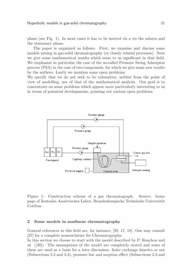
Hyperbolic models in gas-solid chromatography 31
phase (see Fig. 1). In most cases it has to be inerted vis a vis the solutes andthe stationary phase.
The paper is organized as follows. First, we examine and discuss somemodels arising in gas-solid chromatography (or closely related processes). Nextwe give some mathematical results which seem to us significant in that field.We emphasize in particular the case of the so-called Pressure Swing Adsorpionprocess (PSA) in the case of two compounds, for which we give some new resultsby the authors. Lastly we mention some open problems.We specify that we do not seek to be exhaustive, neither from the point ofview of modelling, nor of that of the mathematical analysis. Our goal is toconcentrate on some problems which appear more particularly interesting to usin terms of potential developments, pointing out various open problems.
Figure 1: Construction scheme of a gas chromatograph. Source: homepage of Zentrales Analytisches Labor, Brandenburgische Technische UniversitatCottbus.
2 Some models in nonlinear chromatography
General references in this field are, for instance, [29, 17, 18]. One may consult[27] for a complete nomenclature for Chromatography.In this section we choose to start with the model described by P. Rouchon andal. ([30]). The assumptions of the model are completely stated and some ofthem are used as a basis for a later discussion: finite exchange kinetics or not(Subsections 2.2 and 2.4), pressure law and sorption effect (Subsections 2.3 and
32 C. Bourdarias, M. Gisclon y S. Junca
2.4). The mathematical results given in Section 3 are related to the modelspresented here. Some of them are new.
2.1 The model of Rouchon-Schonauer-Valentin-Guiochon
We recall the model described by P. Rouchon and al. ([30]) which accountsfor the migration and transformation of the large concentration band of asingle pure gaseous compound along a chromatography column. The mainassumptions of this model are the following:
1. The column is supposed to be radially homogeneous and so is the inputprofile. Therefore the problem is monodimensional. The only variablesare the abscissa x along the column and the time t.
2. Gases follow ideal gas laws for compressibility and mixing.
3. Darcy’s law is valid in the range of flow velocity u investigated. Thecolumn permeability is constant independent of the abscissa.
4. The local pressure p is constant during an experiment, depends on theabscissa not on the time even during the passage of a large concentrationband.
5. The carrier gas is not sorbed by the stationary phase.
6. Temperature T is constant during an experiment, independent of theposition or the time.
7. Mass and heat energy exchanges between the mobile and the stationaryphases are infinitely fast. The two phases are constantly at thermal andcomposition equilibrium.
8. Axial diffusion proceeds at negligible speed.
Notice that the assumption of isothermality 6 is easily justified providedthat adequate time is allowed for exchange of energy with the surroundings andalso for systems with little adsorption. Assumption 7 may be relaxed: it willbe investigated in the next subsection. As pointed out in [30], combinationof Assumptions 7 and 8 results in an infinite efficiency of the column. For athorough discussion of the hypothesis, we refer to the book by Guiochon et al.[18] where a large amount of bibliography can also be found.
Let N iM and N i
S , 1 ≤ i ≤ d, be the number of moles of compound i perunit length of column at equilibrium, where the subscripts S and M stand forstationary and mobile phase respectively. We assume that the index d standsfor the carrier gas, if present, thus Nd
S = 0. The equations for the conservationof mass are:
∂t(NiM +N i
S) + ∂x(uN iM ) = 0, 1 ≤ i ≤ d. (1)
The quantities N iM and N i
S are not independent, they are related by the so-called equilibrium isotherm ki: RT N i
S = ki(N1M , · · · , Nd
M ) where T is the
Hyperbolic models in gas-solid chromatography 33
temperature, R a positive constant. In particular we have kd = 0 because thecarrier gas is not sorbed.
Notice that the precise form of the isotherms is usually unknown butcan be experimentally obtained. Simple examples of such a function arethe linear isotherm ki = KiN
iM , with Ki ≥ 0, the Langmuir isotherm
ki =QiKiN
iM
1 +
d∑
j=1
KjNjM
, with Ki ≥ 0, Qi > 0 (see for instance [31]) and the
BET isotherm defined by
k1 =QKN1
M
(1 +KN1M − (N1
M/NsM ))(1 − (N1
M/NsM ))
, Q > 0,K > 0, NsM > 0, k2 = 0
for one adsorbable compound in an inert gas.The unknowns are therefore the local mobile phase velocity u and the values
of N iM for each compound i.
Introducing the local pressure p and the mole fraction Xi =N i
M
d∑
k=1
NkM
of each
compound i, Rouchon and al. [30] write the equations (1) under the form:
∂x(upXi) + ∂t(pXi + ki(pX1, ..., pXd)) = 0, 1 ≤ i ≤ d. (2)
Becaused∑
i=1
Xi = 1 and kd = 0, the equation for the carrier gas may be
replaced by the sum of all equations (1). This gives the total mass balanceequation of the column:
∂x(u p) + ∂t(p+d−1∑
i=1
ki(pX1, ..., pXd)) = 0. (3)
The law of ideal gas writes:
pXiε1 = N i
MRT
where ε1, the porosity, and the temperature T are assumed here to be constant.Setting
Fi =up
RTXi =
uN iM
ε1, 1 ≤ i ≤ d, F0 =
up
RT, ε2 =
d∑
i=1
N iS ,
James ([19]) write these equations under the form:
∂xFi + ∂t(p
RT
Fi
F0+ε2
ε1hi(F1, · · · , Fd, F0)) = 0, 1 ≤ i ≤ d,
34 C. Bourdarias, M. Gisclon y S. Junca
∂xF0 + ∂t(p
RT+ε2
ε1
d−1∑
i=1
hi(F1, · · · , Fd, F0)) = 0,
thus keeping track of the temperature: this may be useful in case of experimentswith prescribed temperature as a function of the time.
The functions hi(F1, · · · , Fd, , F0) =ε1ki
ε2RT=
ε1
ε2N i
S are the isotherms,
written in the F -variables.In the sequel we will make use of the concentrations ci (moles/m3) of the
ith compound in the mobile phase as main unknowns (joined to u). Thecorresponding concentrations in the stationnary phase are denoted qi. Atequilibrium they are given by qi = q∗i (c1, ..., cd)) where q∗i , 1 ≤ i ≤ d arethe equilibrium isotherms corresponding to this new set of variables. Setting
ρ =d∑
i=1
ci, equations (2) and (3) read
∂x(u ci) + ∂t(ci + q∗i (c1, ..., cd)) = 0, 1 ≤ i ≤ d, (4)
∂x(u ρ) + ∂t(ρ+
d∑
i=1
q∗i (c1, ..., cd)) = 0. (5)
This is our reference model in the sequel.
2.2 A model with finite exchange kinetics
A question is that, given a certain amount of mixture, there exists aprivileged repartition of the matter between the two phases (the so calledstable equilibrium state): the equilibrium state can be reached in a shorttime with respect to the relative velocities of the phases (infinite mass-transferkinetics: Assumption 7 above) or not. When the time needed to reach theequilibrium is not negligible with respect to the characteristic times inducedby the velocity, we must give up Assumption 7 and take the deviation fromequilibrium into account: the actual concentration qi in the solid phase differsfrom q∗i (c1, · · · , cd). This phenomenon is known as a finite exchange kinetics.Finite exchange kinetics can be modelled by the following system of equations(with a suitable pressure law) for a column of length L:
∂tci + ∂x(u ci) = Ai (qi − q∗i (c1, · · · , cd)), (6)
∂tqi = −Ai (qi − q∗i (c1, · · · , cd)), t ≥ 0, x ∈ (0, 1). (7)
The right hand sides of the equations quantify the attraction of the systemto the equilibrium state: it is a pulling back force proportional to the deviationfrom equilibrium. A compound with concentration ci is said to be inert if Ai = 0and q∗i = 0.When the coefficients Ai in (6)-(7) tend to infinity (instantaneous equilibrium),

Hyperbolic models in gas-solid chromatography 35
say Ai = 1/ε with ε → 0 for instance, we get formally qi − q∗i = − 1
Ai∂tqi → 0
and Eqs. (6)-(7) reduce to (4).In Section 2.4 we present some theoretical results for a particular pressure lawarising in the so-called “Pressure Swing Adsorption” process, dealing with anon constant velocity u.
In [21], James studied a system of semi linear transport equations, closely relatedto (6)-(7), modelling diphasic propagation arising in chemical engineering inwhich two phases are in motion with distinct constant speeds u > 0 and v ≤ 0,covering the cases of liquid-solid chromatography and distillation. The modelis the following:
∂tcε + ∂x(ucε) =1
ε(qε − h(cε)), (8)
∂tqε + ∂x(vqε) = −1
ε(qε − h(cε)), (9)
where ε > 0. The unknowns are the concentrations vectors cε, qε ∈ Rd.
The right hand side, which has the same interpretation as in Eqs. (6)-(7), iswritten in an academic form, of course not standard in the chemical engineeringliterature. Note that this set of equations can be used at two levels: on the onehand, specific phenomena due to slow exchange kinetics are related to largevalues of ε, on the other hand, we can let ε go to zero as above.
2.3 Velocity and pressure law
In gas chromatography, velocity variations accompany changes in gascomposition, especially in the case of high concentration solute: it is knownas the sorption effect. To neglect this effect or not leads of course to modelswith very different mathematical properties. The sorption effect is of majorimportance in gas chromatography but often close to being insignificant inliquid-solid chromatography or distillation, which is the context of the model(8)-(9), for instance, where the velocities are kept constant.
2.3.1 Neglecting the sorption effect
According to Assumption 3 we write u = −C ∂xp where C is a constantdepending on the porosity. Next, Assumption 4 gives ∂tp = 0. Neglectingthe sorption effect in first approximation, we assume that the total flow rate isconstant i.e. u p = cste. Thus p ∂xp is a constant and we obtain immediately
p(x) =
√P 2
in − x
L(P 2
in − P 2out).
In this expression Pin is the inlet pressure ratio, Pout is the outlet pressure ratioand L is the column length. For very small variations of pressure between inletand outlet, we can therefore assume a constant velocity.

36 C. Bourdarias, M. Gisclon y S. Junca
As pointed out by James ([21]), the assumption of constant total flow rateis not really physically relevant but the derivation of the pressure law may beviewed as an independent reasoning and others models are of course admissible.
2.3.2 Taking the sorption effect into account
Assume that the pressure is given by p = kργ , k > 0, γ > 0 (pressure law fora polytropic ideal gas) and that the speed follows Darcy’s law: we have then
u = −K ∂xργ , with K > 0. (10)
To our knowledge the problem (6)-(7)-(10) has never been investigated froma mathematical point of view. As a first approach we propose an existenceresult for two simplified models: see Theorem 5 and Remark 2 in Subsection3.2.
Notice that setting K =1
εin (10) we get formally, when ε tends to zero,
∂xργ = 0, that is ρ = ρ(t). This means, in the isothermal case, that the total
pressure is only time dependant (which dramatically differs from Assumption4): the velocity u(t, x) of the mixture has to be found in order to achieve agiven pressure. This is exactly the context of the model developed in the nextsection.
2.4 Pressure Swing Adsorption (PSA)
2.4.1 Introduction
“Pressure Swing Adsorption (PSA) is a technology that is used to separatesome species from a gas under pressure according to these species’ molecularcharacteristics and affinity for an adsorbent material. It operates at near-ambient temperatures and so differs from cryogenic distillation techniques of gasseparation. Special adsorptive materials (e.g., zeolites) are used as a molecularsieve, preferentially adsorbing the undesired gases at high pressure. The processthen swings to low pressure to desorb the adsorbent material. Using twoadsorbent vessels allows near-continuous production of the target gas. It alsopermits so-called pressure equalization, where the gas leaving the vessel beingdepressurized is used to partially pressurize the second vessel. This results insignificant energy savings, and is common industrial practice.” (Wikipedia)PSA is used extensively in the production and purification of oxygen, nitrogenand hydrogen for industrial uses. PSA can be used to separate a single gasfrom a mixture of gases. A typical PSA system involves a cyclic process wherea number of connected vessels containing adsorbent material undergo successivepressurization and depressurization steps in order to produce a continuousstream of purified product gas (see Fig. 2).
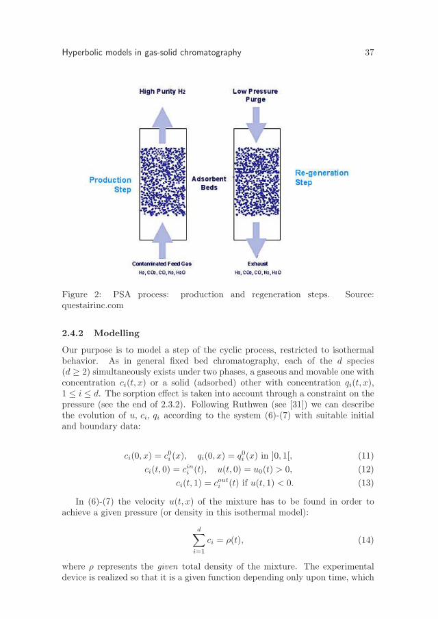
Hyperbolic models in gas-solid chromatography 37
Figure 2: PSA process: production and regeneration steps. Source:questairinc.com
2.4.2 Modelling
Our purpose is to model a step of the cyclic process, restricted to isothermalbehavior. As in general fixed bed chromatography, each of the d species(d ≥ 2) simultaneously exists under two phases, a gaseous and movable one withconcentration ci(t, x) or a solid (adsorbed) other with concentration qi(t, x),1 ≤ i ≤ d. The sorption effect is taken into account through a constraint on thepressure (see the end of 2.3.2). Following Ruthwen (see [31]) we can describethe evolution of u, ci, qi according to the system (6)-(7) with suitable initialand boundary data:
ci(0, x) = c0i (x), qi(0, x) = q0i (x) in ]0, 1[, (11)
ci(t, 0) = cini (t), u(t, 0) = u0(t) > 0, (12)
ci(t, 1) = couti (t) if u(t, 1) < 0. (13)
In (6)-(7) the velocity u(t, x) of the mixture has to be found in order toachieve a given pressure (or density in this isothermal model):
d∑
i=1
ci = ρ(t), (14)
where ρ represents the given total density of the mixture. The experimentaldevice is realized so that it is a given function depending only upon time, which
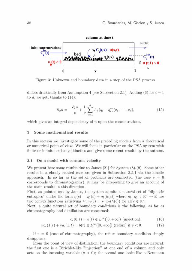
38 C. Bourdarias, M. Gisclon y S. Junca
C (t)iin
C (t)iout
q (t,x)i
0 1
column at time toutlet
x
if
C (t,x)
u (t) > 00 u (t,1) < 0
u(x,t)inlet concentrationsi
bed
Figure 3: Unknown and boundary data in a step of the PSA process.
differs drastically from Assumption 4 (see Subsection 2.1). Adding (6) for i = 1to d, we get, thanks to (14):
∂xu = −∂tρ
ρ+
1
ρ
d∑
i=1
Ai (qi − q∗i )(c1, · · · , cd), (15)
which gives an integral dependency of u upon the concentrations.
3 Some mathematical results
In this section we investigate some of the preceding models from a theoreticalor numerical point of view. We will focus in particular on the PSA system withfinite or infinite exchange kinetics and give some recent results by the authors.
3.1 On a model with constant velocity
We present here some results due to James [21] for System (8)-(9). Some otherresults in a closely related case are given in Subsection 3.5.1 via the kineticapproach. In so far as the set of problems are connected (the case v = 0corresponds to chromatography), it may be interesting to give an account ofthe main results in this direction.First, as pointed out by James, the system admits a natural set of “diphasicentropies” under the form η(c) = η1(c) + η2(h(c)) where η1, η2 : R
d → R aretwo convex functions satisfying ∇cη1(c) = ∇cη2(h(c)) for all c ∈ R
d.Next, a quite natural set of boundary conditions is the following, as far aschromatography and distillation are concerned:
cε(0, t) = a(t) ∈ L∞(]0,+∞[) (injection), (16)
ucε(1, t) + vqε(1, t) = b(t) ∈ L∞(]0,+∞[) (reflux) if v < 0. (17)
If v = 0 (case of chromatography), the reflux boundary condition simplydisappears.
From the point of view of distillation, the boundary conditions are natural:the first one is a Dirichlet-like ”injection” at one end of a column and onlyacts on the incoming variable (u > 0); the second one looks like a Neumann
Hyperbolic models in gas-solid chromatography 39
condition on the other hand and imposes v < 0 (it is a simplified model of”reflux” in a distillation column).
It turns out that System (8)-(9) with (16)-(17) is well posed. Applying thefixed point theorem, there is an existence and uniqueness result for (8)-(9) inL∞(]0, T [;L1(]0, 1[)2d):
Theorem 1For a given T > 0, assume that a and b are in L∞(]0, T [), c0 ∈ L∞ ∩ L1(]0, 1[)and that the function h is of class C1. Then there exists an unique solution to(8)-(9) which lies in L∞(]0, T [;L1(]0, 1[)).
When ε tends to zero we get formally a set of equations which express theconservation of matter:
∂t(c+ h(c)) + ∂x(u c+ v h(c)) = 0. (18)
However a difficulty arises if one lets ε go to 0 because the boundaryconditions are not at equilibrium for ε > 0 so that boundary layers may appear.
James imposes the condition
f(c) = u c+ v h(c) ≤ mint>0
b(t).
This condition implies some restrictions on the initial and boundary data, whichlead to uniform L∞ estimates for the solution to (8)-(9) for a broader class offluxes.
In the scalar case and using compensated compactness, James proves thatthe solution of this system converges, as ε → 0, to a solution of the precedingequation satisfying a set of entropy inequalities:
Theorem 2Let be T > 0, a, b ∈ L∞(]0, T [), a ≥ 0, b ≤ 0, c0 ∈ L1(]0, 1[)∩L∞(]0, 1[), c0 ≥ 0and
c∗ = supc ≥ 0,∃c′ ≤ c, f(c′) ≤ min b(t) ≥ max[|| a ||∞, || c0 ||∞].
Let cε, qε be a solution of (8)-(9) with initial data at equilibrium:
cε(x, 0) = c0(x) ∈ L1(]0, 1[) ∩ L∞(]0, 1[), qε(x, 0) = h(c0(x)).
Then there exists a subsequence of solutions which converges a.e. and stronglyin ]0, 1[×]0,+∞[ to c ∈ L∞(]0, T [;L1(]0, 1[) satisfying for any φ ∈ D′
+([0, 1] ×R+), k ∈ R:
∫ ∞
0
∫ 1
0
[(|c− k| + |h(c) − h(k)|) ∂tφ+ (u|c− k| + v|h(c) − h(k)|) ∂xφ] dx dt
≤∫ ∞
0
(u | a(t) − k | φ(0, t)+ | b(t) − f(k) | φ(1, t)) dt−∫ 1
0
(| c0(x) − k | + | h(c0(x)) − h(k) |
)φ(x, 0) dx.
40 C. Bourdarias, M. Gisclon y S. Junca
This result is meaningful for c∗ > 0, which occurs only if f(c) becomes nonpositive for some c: notice that this excludes the case of the chromatography(v = 0).
In [23], James and al. study numerically the same model to take in accountthe finite exchange kinetics. The resulting hyperbolic system with a nonlinear relaxation term is then formally treated with a Chapman-Enskog typeexpansion. A first order correction to the classical quasilinear hyperbolic modelis derived which consists in a nonlinear diffusion term. Numerical schemes forboth models, relaxed and parabolic, are then tested and compared for differentinitial and boundary values.Lastly, in [22], the authors describe and validate a numerical solution of theinverse problem of nonlinear chromatography using the model given by Eq.(18). The method allows the determination of best numerical estimates ofthe coefficients of an isotherm model from the individual elution profiles ofthe two compounds of a binary mixture. In two cases, when the isothermmodel is satisfactory, the authors observed a very good agreement betweenthe equilibrium isotherm equations obtained by this new method and thosedetermined by the classical combination of elution by characteristic points andbinary frontal analysis. Practically, this method would significantly reducethe amounts of products required to determine a set of competitive binaryisotherms.
3.2 On a model with Darcy’s velocity
As a first approach to a study of the complete model (6)-(7)-(10) we proposean existence result for the following simplified one:
∂tci + ∂x(u ci) = 0, in (0, T ) × R, (19)
u = −∂xργ , γ > 0, ρ =
d∑
i=1
ci, (20)
ci(0, x) = c0i (x), x ∈ R. (21)
Notice that we work on R in order to focus on the main difficulties, butwe assume that the initial data c0i are compactly supported. Furthermore weassume Ai = 0 to avoid some problems related to the nonlinearities q∗i . Adding(19) for i = 1 to d we get, thanks to (10), ∂tρ − ∂x(ρ ∂xρ
γ) = 0, that we writeunder the form:
∂tρ−γ
γ + 1∆ργ+1 = 0
which is a porum medium equation. There exists a large amount of works onthis subject. The first results are due to Oleinik, Kalashnikov and Chzhou[28]. For regularity results on ρ consult for instance Aronson [1, 2, 3], Aronson-Benilan [4], Caffarelli-Friedmann [5], Dibenedetto [14]. Concerning the domainof dependency P[ρ] = ρ > 0 in one dimension we know, under suitable
Hyperbolic models in gas-solid chromatography 41
assumptions, that if the initial data ρ0 is supported in a bounded interval,then ρ is compactly supported for all time and P[ρ] is enclosed between twomonotonic and lipschitz continuous curves x = ξi(t) (see [24, 34] for instance).More precisely we will use explicitly the following results:
consider the problem
∂tρ = ∆ρm in S = (0, T ] × R, ρ(0, x) = ρ0(x), x ∈ R (22)
where m > 1. Following [1] we say that a function ρ(t, x) is a weak solution of(22) if
• ρ0 is non negative, continuous, bounded in S,
• ∂xρm ∈ L∞,
• ρ satisfies:
∀φ ∈ D([0, T ) × R)
∫
S
(∂xρm ∂xφ− ρ ∂tφ) dx dt =
∫
R
ρ0(x)φ(0, x) dx.
Proposition 3 If (ρ0)m is lipschitz continuous, the problem (22) has a uniqueweak solution ρ. Moreover ρ is a classical solution on P[ρ] = ρ > 0.
Remark 1 The L∞ bound for ∂xρm depends only upon the lipschitz constant
of (ρ0)m.
Proposition 4 Assume that (ρ0)m is lipschitz continuous and let ρ be theweak solution of (22). For all τ > 0 there exists a positive constant C =C(m, τ, ‖ρ0‖∞) such that
∀(t, x), (t, x′) ∈ [τ, T ] × R,∣∣ρm−1(t, x) − ρm−1(t, x′)
∣∣ ≤ C |x− x′| .
If (ρ0)m−1 is lipschitz continuous the same conclusion holds for all(t, x), (t, x′) ∈ [0, T ] × R and C depends on the lipschitz constant of (ρ0)m−1
instead of τ .
We are looking a priori for a weak solution with ci ∈ L∞ and we willget, depending on the assumption on ρ0, u ∈ L∞((τ, T ) × R) for all τ > 0 oru ∈ L∞((0, T ) × R) which does not allow to pass to the limit in a sequenceof smooth approximate solutions in the weak formulation of (19). However, if
ρ is smooth, we have u ci = − γ
γ + 1
ciρ∂xρ
γ+1 withciρ
∈ L∞ and we will get
∂xργ+1 ∈ L∞ and a BV estimate for
ciρ
. Thus we choose to formulate the
problem as follows:
∂tci −γ
γ + 1∂x(
ciρ∂xρ
γ+1) = 0 in (0, T ) × R, 1 ≤ i ≤ d, (23)
with γ > 0, ρ =
d∑
i=1
ci. (24)

42 C. Bourdarias, M. Gisclon y S. Junca
For mere technical reasons, the initial data c0i (x) are written under the formc0i (x) = ρ0(x) ai(x) where the functions ai are defined on R, non negative, and
satisfy
d∑
i=1
ai = 1. We make the following assumptions:
∀i ∈ 1, · · · , d ai has bounded variation on R, (25)
ρ0 is lipschitz continuous, non negative and compactly supported, (26)
∃C > 0, ∀η > 0
∫
R
∣∣∣∂x
(1
ρ0 + η
) ∣∣∣ ≤ C/η. (27)
The technical assumption (27) is related to the the behavior of ρ0 near thepoint where this function vanishes. It is satisfied for instance if ρ0 is lipschitzcontinuous, supported in some interval [a, b], positive in ]a, b[, monotone in theneighborhood of a and b.We state now our main result:
Theorem 5 Under the assumptions (25)-(26)-(27), Problem (23)-(24) has at
least a solution (c1, ..., cd) with ci ∈ L∞, ci ≥ 0, ρ =
d∑
i=1
ci continuous on
R+ × R and such that:
∀T > 0, ∂xργ+1 ∈ L∞((0, T ) × R),
ciρ
∈ L∞((0, T );BV (R)),
∀T > 0,∀τ > 0, u = −∂xργ ∈ L∞((τ, T ) × R).
Moreover, if (ρ0)γ is lipschitz continuous then u ∈ L∞((0, T ) × R).
Outlines of the proof- The estimates on u are straightforwardconsequences of the general properties of the solution of the porous mediumequation: consult for instance Aronson [1].Assume the initial data in C2(R) (thanks to a regularization step that we skip),
let be η > 0, c0i,η = c0i + η/d, 1 ≤ i ≤ d and ρ0η = ρ0 + η =
∑
1≤i≤d
c0i,η. Let ρη be
the unique solution of the following problem (Pη):
∂tρη − γ
γ + 1∆ργ+1
η = 0, (28)
ρη(0, x) = ρ0η. (29)
Notice that ρη satisfies:
∂tρη + ∂x(uη ρη) = 0, (30)
with uη = −∂x(ργη) which is Lipschitz continuous on R, uniformly with
respect to t ∈ [0, T ]. Let ci,η, 1 ≤ i ≤ d, be the solution of the advectionequation
Hyperbolic models in gas-solid chromatography 43
∂tci,η + ∂x(uη ci,η) = 0 (31)
ci,η(0, x) = c0i,η, (32)
then we have clearly ρη =∑
1≤i≤d
ci,η.
Notice that by comparison principle we have
η ≤ ρη ≤‖ ρ0 ‖∞ +η in [0, T ] × R
and also0 < η1 ≤ η2 =⇒ ρη1
≤ ρη2in [0, T ] × R.
Thanks to standard arguments we can then assume that (up to asubsequence):
ρη → ρ in Lploc ∀p ≥ 1, uη u = −∂xρ
γ in D′, ci,η ci in L∞ weak∗
(33)but it is not enough to pass to the limit in the weak formulation of (Pη).
More precisely, according to (23), we have to show that for all φ ∈ D′([0, T ]×R):
∫ T
0
∫
R
uη ci,η ∂xφ −−−→η→0
∫ T
0
∫
R
− γ
γ + 1
ciρ∂xρ
γ+1 ∂xφ. (34)
Let be α > 0 fixed. The left hand side of (34) is written as:
∫ T
0
∫
R
uη ci,η ∂xφ = Iη + Jη
with Iη =
∫ T
0
∫
ρ<α
uη ci,η ∂xφ and Jη =
∫ T
0
∫
ρ≥α
uη ci,η ∂xφ.
The integral Iη: we have uη ci,η = −(∂xργ+1η ) ci,η = − γ
γ + 12
ρ12η ∂x (ρη)
γ+ 12ci,ηρη
and thus ∣∣∣uη ci,η
∣∣∣ ≤ ρ12η
∣∣∣∂x (ρη)γ+ 1
2
∣∣∣. (35)
Using Assumption (26) and Eq. (28) multiplied by ργη , we get the following
lemma:
Lemma 6
∃C > 0, ∀η > 0, ∀(a, b) ∈ R2, a ≥ b, ∀T > 0
∫ T
0
∫ b
a
∣∣∣∂x (ρη)γ+ 1
2
∣∣∣2
dx dt ≤ C.
Notice that we use here that there exists a uniform L∞ bound for ∂x (ρη)γ+1
as a solution of (28): see the remark following Prop. 3. Using (35), this lastlemma and the Holder inequality, we finally get
∃C > 0, lim sup Iη ≤ C√α (36)

44 C. Bourdarias, M. Gisclon y S. Junca
The integral Jη: we write uη ci,η = − γ
γ + 1∂x (ρη)
γ+1 ci,ηρη
. Thanks to the
uniform L∞ bound for ∂x (ρη)γ+1
and (33) we can assume that
∂x (ρη)γ+1
∂xργ+1 weak∗
and it remains to study the sequence
(ci,ηρη
)
η>0
. From (30)-(31) we deduce
that
∂t
(ci,ηρη
)+ uη ∂x
(ci,ηρη
)= 0 (37)
and we get classically (recall that ci,η/ρη is compactly supported):
∂t
∫
R
∣∣∣∂x
(ci,ηρη
) ∣∣∣ dx = 0.
Next, we have:
∂x
(c0i + η/d
ρ0 + η
)= (∂xai)
(ρ0
ρ0 + η
)2
+ηρ0
(ρ0 + η)2∂xai + (ai −
1
d)
η
(ρ0 + η)2∂xρ
0
and thus, thanks to Assumptions (25)-(26)-(27), we get the uniform bound:∫ T
0
∫
R
∣∣∣∂x
(ci,ηρη
) ∣∣∣ dx ≤ C (38)
for some positive constant C. Recall that uη is uniformly bounded inL∞((τ, T ) × R) for all τ > 0. Thus, from (37) and (38) we deduce
∫
ρ≥α∩τ≤t≤T
∣∣∣∂t
(ci,ηρη
) ∣∣∣ ≤ C(τ, α). (39)
From (38) and (39) we deduce that the sequence
(ci,ηρη
)
η>0
is uniformly
bounded with respect to η in BV (ρ ≥ α ∩ τ ≤ t ≤ T), and the followinglemma holds:
Lemma 7 The sequence
(ci,ηρη
)
η>0
is relatively compact in Lploc(ρ ≥ α ×
t ≥ β) for all p ≥ 1, α > 0 and β ∈]0, T [.
Then, using lemma 7 and a diagonal extraction process we deduce that thereexists a sequence (αn, τn) ∈ R+ × R+ such that αn, τn → 0 and
lim supJη = − γ
γ + 1
∫
ρ≥αn∩t>τn
ciρ∂xρ
γ+1 ∂xφ+Rn (40)
with |Rn| ≤ C τn.Thanks to (36) and (40) we get easily (34), and thus Theorem 5 holds.
Notice that the method used for the proof of Lemma 7 is no longer valid inmore than one dimension.
Hyperbolic models in gas-solid chromatography 45
Remark 2 Dealing with a single compound and working in Rn, the problem
(6)-(7) with u given by (10) writes :
∂tρ−γ
γ + 1∆ργ+1 = A (q − q∗(ρ)),
∂tq = −A (q − q∗(ρ)),
with initial data ρ0, q0. For this problem, Bourdarias ([7]) obtained an existenceresult with continuous bounded solutions. The solution is easily obtained via amonotonicity argument. The method cannot be extended to the case of manycompounds, which is an open problem.
3.3 PSA with finite exchange kinetics
In [6], both BV and L∞ theory are developed for the isothermal model (6)-(7)-(14) and the main results are summarized below. Let us point out thatone of the mathematical interests of the model is its analogies and differencescompared to various other classical equations of physics or chemistry. First,this model shares a similar structure with conservation laws under the form
∂tρ+ ∂x(ρ u(ρ)) = 0, ∂xu(ρ) = F (ρ)
where u(ρ) has an integral dependency upon ρ , while in scalar conservation lawsu depends upon ρ. It is underlined that, due to this particular dependency,oscillations can propagate thus differing from Burger’s example (see Lions-Perthame-Tadmor[25]), but we will not insist on this aspect.
3.3.1 Theoretical results in BV or L∞ framework
As a first result, we give an existence result for a solution with concentrationshaving bounded variation and a lipschitz continuous velocity.
Theorem 8 Assume that the initial and boundary data are at equilibrium, thatthe initial data have bounded variation in (0, 1) and that the boundary data,the isotherms and the total density are lipschitz continuous. Then the problem(6)-(7)-(14) has an unique solution ((ci), (qi), u) such that ci ≥ 0, qi ≥ 0 and
∀T > 0, ci, qi ∈ L∞((0, T ) × (0, 1)) ∩ L∞(0, T ;BV (0, 1)),
∂xu ∈ L∞((0, T ) × (0, 1)) ∩ L1(0, T ;BV (0, 1)).
Outlines of the proof- the proof is performed in two steps. First, fora fixed velocity u uniformly Lipschitz continuous in (0, 1) we get a solution((ci), (qi)) of (6)-(7) via a fixed point procedure in L1((0, T ) × (0, 1))2d. Thissolution satisfies some L∞ estimates. Moreover, the fundamental BV estimateholds:
∀T > 0, ∃C > 0, ∀t ≤ T, ∀i, TV (ci(t, ·))+TV (qi(t, ·)) ≤ C (1+
∫ t
0
∫ 1
0
∣∣∂2xxu∣∣),
(41)
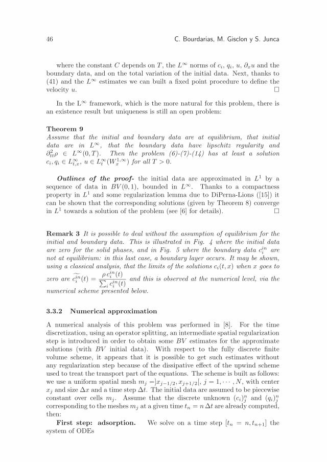
46 C. Bourdarias, M. Gisclon y S. Junca
where the constant C depends on T , the L∞ norms of ci, qi, u, ∂xu and theboundary data, and on the total variation of the initial data. Next, thanks to(41) and the L∞ estimates we can built a fixed point procedure to define thevelocity u.
In the L∞ framework, which is the more natural for this problem, there isan existence result but uniqueness is still an open problem:
Theorem 9Assume that the initial and boundary data are at equilibrium, that initialdata are in L∞, that the boundary data have lipschitz regularity and∂2
ttρ ∈ L∞(0, T ). Then the problem (6)-(7)-(14) has at least a solutionci, qi ∈ L∞
t,x, u ∈ L∞t (W 1,∞
x ) for all T > 0.
Outlines of the proof- the initial data are approximated in L1 by asequence of data in BV (0, 1), bounded in L∞. Thanks to a compactnessproperty in L1 and some regularization lemma due to DiPerna-Lions ([15]) itcan be shown that the corresponding solutions (given by Theorem 8) convergein L1 towards a solution of the problem (see [6] for details).
Remark 3 It is possible to deal without the assumption of equilibrium for theinitial and boundary data. This is illustrated in Fig. 4 where the initial dataare zero for the solid phases, and in Fig. 5 where the boundary data cini arenot at equilibrium: in this last case, a boundary layer occurs. It may be shown,using a classical analysis, that the limits of the solutions ci(t, x) when x goes to
zero are cini (t) =ρ cini (t)∑
i cini (t)
and this is observed at the numerical level, via the
numerical scheme presented below.
3.3.2 Numerical approximation
A numerical analysis of this problem was performed in [8]. For the timediscretization, using an operator splitting, an intermediate spatial regularizationstep is introduced in order to obtain some BV estimates for the approximatesolutions (with BV initial data). With respect to the fully discrete finitevolume scheme, it appears that it is possible to get such estimates withoutany regularization step because of the dissipative effect of the upwind schemeused to treat the transport part of the equations. The scheme is built as follows:we use a uniform spatial mesh mj =]xj−1/2, xj+1/2[, j = 1, · · · , N , with centerxj and size ∆x and a time step ∆t. The initial data are assumed to be piecewiseconstant over cells mj . Assume that the discrete unknown (ci)
nj and (qi)
nj
corresponding to the meshesmj at a given time tn = n∆t are already computed,then:
First step: adsorption. We solve on a time step [tn = n, tn+1] thesystem of ODEs
Hyperbolic models in gas-solid chromatography 47
∂tci = Ai (qi − q∗i (c1, · · · , cd)), (42)
∂tqi = −Ai (qi − q∗i (c1, · · · , cd)), tn ≤ t ≤ tn+1, (43)
for x = xj , j = 1, · · · , N , with (ci)nj and (qi)
nj as initial data. We get
the updated values (qi)n+1j , intermediate values (ci)
n+1/2j and we set ρn+1
j =∑
j
(ci)n+1/2j . We assume that we proceed with an arbitrary accuracy, in such
a way that (ci)n+1/2j , (qi)
n+1/2j ≥ 0 and 0 < α ≤ ρn+1
j ≤ β where α andβ depend only upon the data of the problem (following the properties of theexact solution).
Second step: transport. The transport part is discretized with a classicalupwind finite volume scheme as
(ci)n+1j = (ci)
n+1/2j − λ
(un
j+1/2(ci)n+1/2j+1/2 − un
j−1/2(ci)n+1/2j−1/2
)(44)
with λ = ∆t/∆x and
(ci)n+1/2j+1/2 =
(ci)
n+1/2j if un
j+1/2 ≥ 0,
unj+1/2 if un
j+1/2 < 0,
where unj+1/2 has to be defined in such a way that the constraint (14) holds. It
is easy to show that this is realized through the formula
unj+1/2 =
ρn+1j − ρ(tn) + λun
j−1/2
∑j(ci)
n+1/2j−1/2
λ∑
j(ci)n+1/2j+1/2
which allows to compute all the discrete velocities used in (44), starting fromthe given velocity un
−1/2 = u0(tn). The positivity of the updated concentrations
(ci)n+1j is ensured thanks to the CFL condition ∆t ≤ ∆x/ ‖ u ‖∞.
This scheme is convergent and an O(∆t)1/2 convergent rate is obtained.Notice that it may be extended to second order, adapting Van-Leer’s method.As a conclusion we present two numerical experiments illustrating Remark 3.The results have been obtained with Langmuir isotherms. We do not precise thevalues of all the parameters involved, because we just emphasize the qualitativeaspect.
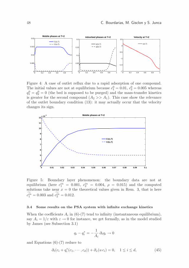
48 C. Bourdarias, M. Gisclon y S. Junca
0 0.2 0.4 0.6 0.8 10
0.005
0.01
0.015
0.02Mobile phases at T=2
C1(x,T)
C2(x,T)
0 0.2 0.4 0.6 0.8 10
0.05
0.1
0.15
0.2Adsorbed phases at T=2
q1(x,T)
q2(x,T)
0 0.2 0.4 0.6 0.8 1−2
−1.5
−1
−0.5
0
0.5Velocity at T=2
u(x,T)
Figure 4: A case of outlet reflux due to a rapid adsorption of one compound.The initial values are not at equilibrium because c01 = 0.01, c02 = 0.005 whereasq01 = q02 = 0 (the bed is supposed to be purged) and the mass-transfer kineticsis greater for the second compound (A2 >> A1). This case show the relevanceof the outlet boundary condition (13): it may actually occur that the velocitychanges its sign.
0 0.01 0.02 0.03 0.04 0.05 0.06 0.07 0.08 0.09 0.13
4
5
6
7
8
9
10
11
12x 10
−3 Mobile phases at T=2
C1(x,T)
C2(x,T)
Figure 5: Boundary layer phenomenon: the boundary data are not atequilibrium (here cin1 = 0.001, cin2 = 0.004, ρ = 0.015) and the computedsolutions take near x = 0 the theoretical values given in Rem. 3, that is here
cin1 = 0.003 and cin2 = 0.012.
3.4 Some results on the PSA system with infinite exchange kinetics
When the coefficients Ai in (6)-(7) tend to infinity (instantaneous equilibrium),say Ai = 1/ε with ε→ 0 for instance, we get formally, as in the model studiedby James (see Subsection 3.1)
qi − q∗i = − 1
Ai∂tqi → 0
and Equations (6)-(7) reduce to
∂t(ci + q∗i (c1, · · · , cd)) + ∂x(u ci) = 0, 1 ≤ i ≤ d, (45)
Hyperbolic models in gas-solid chromatography 49
with the constraint (14), thus dealing with a non constant speed. Thisequation is similar to (18) but here v = 0 and u is not constant.
Recently ([9]) the authors focused on the problem (45)-(14) with twocompounds and a constant total density ρ ≡ 1, assuming an isobaric behavior(which is not really restrictive from a theoretical point of view). The system is:
∂t(c1 + q∗1(c1, c2)) + ∂x(u c1) = 0, (46)
∂t(c2 + q∗2(c1, c2)) + ∂x(u c2) = 0, (47)
c1 + c2 = ρ = 1. (48)
Douglas and al. ([16]) developed a general criterion for determining thetransitions type for this monovariant system and gave several examples (seealso [33]). A first attempt, in the simpler case where one of the compounds isinert, led the authors to an existence and uniqueness result (see [9]) summarizedin the next subsection. Rouchon and al. ([30]) discussed this model andperformed a numerical simulation in the case of one inert compound. Thegeneral case, presented in Subsection 3.4.2, is now better understood ([10])from a mathematical point of view.
3.4.1 Case of an inert carrier gas
In this subsection, we assume that one of the compounds is inert withconcentration c2 and that the spatial domain is R+ for the sake of simplicity.We set c = c2 and h(c) = −q∗1(c1, c2) = −q∗1(1 − c, c), thus, using (15), thesystem (46)-(47)-(48) may be written under the form:
∂tc+ ∂x(uc) = 0,∂th(c) − ∂xu = 0,
(49)
supplemented by initial and boundary data:
c(0, x) = c0(x) ∈ [0, 1], x > 0,c(t, 0) = cb(t) ∈ [0, 1], t > 0,u(t, 0) = ub(t), t > 0.
(50)
We assume in (50) an influx boundary condition, i.e. ∀t > 0, ub(t) > 0 and, inthis first simplified approach
H ′(c) ≥ 0, h′(c) > 0, (51)
where H(c) = 1 + ch′(c). The reference for the results described in thissubsection is [9].
First we obtain an existence result for smooth solutions using a classicalcharacteristic method. The interest of this result is mainly to suggest us anentropy condition for shockwaves:
(EC) “c increases through a shock”.

50 C. Bourdarias, M. Gisclon y S. Junca
For smooth solutions, the active gas desorbs and u increases to evacuategases. Next, we obtain a global existence theorem for a weak solution of System(49)-(50):
Theorem 10 (Global large weak solution)Let be X > 0, T > 0. Assume (51) and that c0 ∈ BV (0,X), cb ∈ BV (0, T ),ub ∈ L∞(0, T ), satisfying 0 ≤ c0, cb ≤ 1 and inf
0<t<Tub(t) > 0. Then the
system (49)-(50) admits a weak solution given by an adapted Godunov scheme.Furthermore, c and u satisfy:
c ∈ L∞((0, T ) × (0,X)) ∩ L∞((0, T );BV (0,X)),
c ∈ Lip(0, T ; L1(0,X)), c ∈ BV ((0, T ) × (0,X)),
u ∈ L∞((0, T ) × (0,X)) ∩ L∞((0, T );BV (0,X)),
with bounds on c and u and these functions satisfy initial boundary conditions(50) strongly.
The proof relies on a precise study of the solutions to the Riemann problemsatisfying the entropy condition (EC). We use a Godunov scheme to constructan approximate weak solution of Problem (49)-(50) and we give some L∞ andBV bounds. Lastly, we show that a sequence of approximate solutions convergesin some sense towards a global weak entropy solution.
The uniqueness problem for weak entropy solutions was solved in someclass of piecewise smooth functions. Nevertheless, this case is relevant inmost practical cases and involve global solutions with shock waves and contactdiscontinuities. Notice that the assumptions in (51) are not really physicallyrelevant because they hold for particular isotherm only. This restriction isavoided in the general approach below (but we no longer have an uniquenessresult).
As an illustration for this particular problem we consider the case of anincreasing smooth initial concentration of inert gas: a shock develops and thenpropagates (Fig. 6). Dealing with a finite exchange kinetics, the same case isinvestigated using the numerical method described in Section 3.3.2 with someincreasing values of the coefficient A governing the kinetics for the active gas.The numerical experiments suggest that the model (6)-(7)-(14) could convergein some sense towards the model (45)-(14), but this is still an open problem.
3.4.2 General case
In [10], the authors deal with the case of two compounds which may be active ornot, with physically relevant assumptions. Following Rouchon and al. ([30]) theproblem is analyzed as an hyperbolic system with respect to the (x, t) variables,that is with x as the evolution variable. It appears to be really the key for themathematical analysis of the problem.
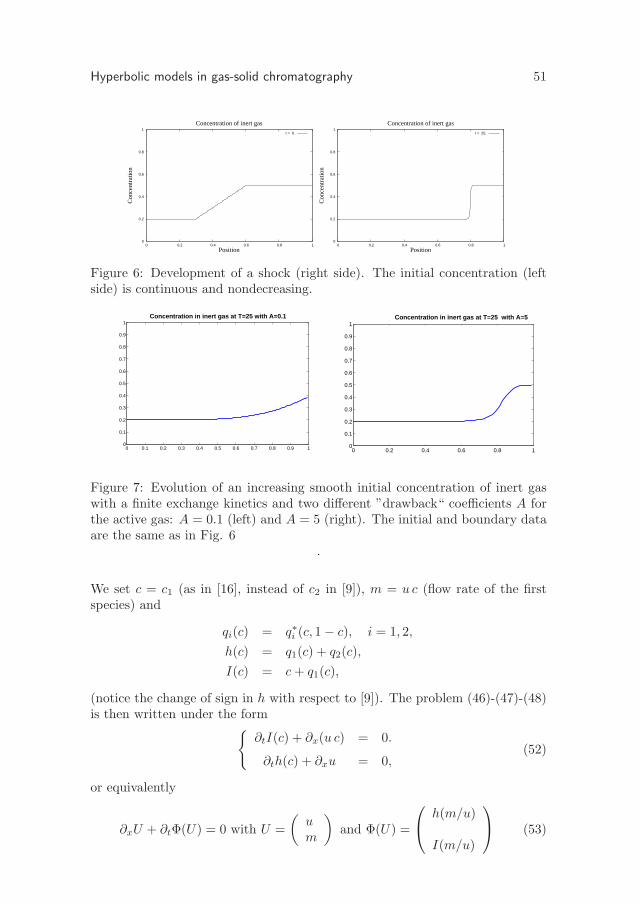
Hyperbolic models in gas-solid chromatography 51
0
0.2
0.4
0.6
0.8
1
0 0.2 0.4 0.6 0.8 1
Con
cent
ratio
n
Position
Concentration of inert gas
t = 0.
0
0.2
0.4
0.6
0.8
1
0 0.2 0.4 0.6 0.8 1
Con
cent
ratio
n
Position
Concentration of inert gas
t = 25.
Figure 6: Development of a shock (right side). The initial concentration (leftside) is continuous and nondecreasing.
0 0.1 0.2 0.3 0.4 0.5 0.6 0.7 0.8 0.9 10
0.1
0.2
0.3
0.4
0.5
0.6
0.7
0.8
0.9
1Concentration in inert gas at T=25 with A=0.1
0 0.2 0.4 0.6 0.8 10
0.1
0.2
0.3
0.4
0.5
0.6
0.7
0.8
0.9
1Concentration in inert gas at T=25 with A=5
Figure 7: Evolution of an increasing smooth initial concentration of inert gaswith a finite exchange kinetics and two different ”drawback“ coefficients A forthe active gas: A = 0.1 (left) and A = 5 (right). The initial and boundary dataare the same as in Fig. 6
.
We set c = c1 (as in [16], instead of c2 in [9]), m = u c (flow rate of the firstspecies) and
qi(c) = q∗i (c, 1 − c), i = 1, 2,
h(c) = q1(c) + q2(c),
I(c) = c+ q1(c),
(notice the change of sign in h with respect to [9]). The problem (46)-(47)-(48)is then written under the form
∂tI(c) + ∂x(u c) = 0.
∂th(c) + ∂xu = 0,(52)
or equivalently
∂xU + ∂tΦ(U) = 0 with U =
(um
)and Φ(U) =
h(m/u)
I(m/u)
(53)

52 C. Bourdarias, M. Gisclon y S. Junca
supplemented by initial and boundary data.We assume that q′1 ≥ 0 and q′2 ≤ 0 (general property of all isotherms, see [16]).
This system (53) is hyperbolic, with eigenvalues 0 and λ =H(c)
u.
Introducing the function f = q1 c2 − q2 c1 defined by Douglas and al. in [16],written here under the form f(c) = q1(c)− c h(c), it appears that λ is genuinelynonlinear in each domain where f” 6= 0.Next, the system admits the two Riemann invariants: c and w = lnu + g(c),
where g satisfies g′(c) =−h′(c)H(c)
and the smooth entropy families
S(c, u) = φ(w) + uψ(c) (54)
where φ and ψ are any smooth real functions.Let be G = eg: if the sign of G′′ changes then the system does not admitany convex smooth entropy but for each convex or degenerate convex smoothfunction ψ (i.e. ψ′′ ≥ 0) the corresponding entropy S = uψ(c) is degenerateconvex. Introducing a suitable notion of entropy solution, the authors in [10]show the existence of at least such a solution.
The mathematical definition of weak entropy solution is the following: letbe T > 0, X > 0, u ∈ L∞((0, T ) × (0,X),R+), 0 ≤ c(t, x) ≤ 1 for almost(t, x) ∈ (0, T ) × (0,X). Then (c, u) is a weak entropy solution if for all convex(or degenerate convex) ψ
∂
∂x(uψ(c)) +
∂
∂tQ(c) ≤ 0,
in the distribution sense, where Q′ = Hψ′ + h′ψ.
In addition, if G′′ ≥ 0 on [0, 1], (c, u) has to satisfy∂
∂x(uG(c)) ≤ 0.
The main result, relying on the resolution of the Riemann problem and onthe Godunov scheme, is the following:
Theorem 11Let be T > 0, X > 0, c0 ∈ BV (0,X), cb ∈ BV (0, T ), satisfying 0 ≤ c0, cb ≤ 1and inf0<t<T ub(t) > 0. Then the system admits a weak entropy solution.
A natural framework for this problem, as in the case of the PSA systemwith finite exchange kinetics, would be the L∞ one. Some tracks are presentlyexplored but it is still an open problem.
3.5 Kinetic approaches
The theory of kinetic formulation of hyperbolic systems, introduced by P.-L.Lions, B. Perthame and E. Tadmor [25], consists in representing a whole familyof entropy inequalities by a single equation, using a supplementary variable, forthe fundamental solution of the wave equation for entropies. It often leads tonumerical schemes enjoying interesting properties and easy to implement.We give first a result due to James, Peng and Perthame ([20]) concerning the
Hyperbolic models in gas-solid chromatography 53
system of electrophoresis. Next, using the results stated in 3.4.2, we present asimilar approach for the PSA system, currently developed by the authors.
3.5.1 Kinetic formulation for Electrophoresis
Electrophoresis is a process of separation for compounds in a aqueous solutionwith an electric field. The corresponding model is close to the chromatographysystem with Langmuir isotherm ([13, 32]). F. James, Y.-J. Peng and B.Perthame ([20]) have complemented on the system of electrophoresis the theoryof kinetic formulation of hyperbolic systems. They gave several applicationsof this kinetic formulation: a maximum principle and a stability result in L∞
using compensated compactness. Even though this system is rather related toliquid-solid chromatography (the sorption effect is neglected) we mention theseresults because the method is powerful and may be extended in other contexts.
The system of electrophoresis is
∂tci + ∂xαiciD
= 0, t ≥ 0, 1 ≤ i ≤ d, (55)
where c1, · · · , cd are the positive unknowns, D = 1+ c1 + ...+ cd and the αi aregiven numbers satisfying 0 < α1 < ... < αd.This system admits d eigenvalues 0 < λ1(c) ≤ ... ≤ λd(c) and wi = λiD is ai−Riemann invariant.
The first step consists in building d+ 1 families of nonlinear entropies: it issummarized in the following proposition.
Proposition 12For 0 ≤ i ≤ d, the function
χi(ξ;w1, · · · , wd) =
d∏
j=1
∣∣∣1 − ξ
wj
∣∣∣ 1I]wi,wi+1[(ξ)
is an entropy of System (55), convex in c, with the entropy flux
φi(ξ;w1, · · · , wd) =ξ
Dχi(ξ;w1, · · · , wd).
An entropy solution of (55) is a solution satisfying in the distribution sensethe inequality
∂tE + ∂xF ≤ 0
for any convex entropy of the form
E(c) =
∫
R+
g(ξ)χi(ξ;w1, · · · , wd) dξ
for some i, 1 ≤ i ≤ d, g ∈ L1(R+). Then the authors in [20] derive the followingkinetic formulation of (55): there are d + 1 non-positive measures mi(x, ξ, t)such that
∂tχi(ξ, c(x, t)) + ∂x
(ξ
Dχi(ξ, c(x, t))
)= mi in D
′(Rx × R+ξ × R+t).
54 C. Bourdarias, M. Gisclon y S. Junca
Two applications are given in [20]: the maximum and minimum principleon the Riemann invariants and a compactness result. They are recalled in thefollowing two theorems.
Theorem 13Let c be an entropy solution satisfying c ∈ L∞(0, T ;L1
loc(R)), ci ≥ 0, 1 ≤ i ≤ d.Then
αi−1 ≤ infy∈R
wi(y, 0) ≤ wi(x, t) ≤ supy∈R
wi(y, 0) ≤ αi
and for some constant L > 0
L infy∈R
c0i (y) ≤ ci(x, t) ≤1
Lsupy∈R
c0i (y), 1 ≤ i ≤ d.
Theorem 14Consider an uniformly bounded family (ci,n(x, t))n≥0 of entropy solutions to theelectrophoresis who satisfy that the initial data are uniformly bounded and
ci,n(x, t) ci(x, t) ∈ L∞((0, T ) × R), 1 ≤ i ≤ d
weak* for all T ∈ (0,∞) as n tends to +∞. Then (ci,n)n converges pointwiseto ci an entropy solution.
3.5.2 A kinetic approach for the PSA system
A kinetic formulation built on the entropies (54) given in Section 3.4.2 as wellas several applications were investigated and will be presented in a forthcomingpaper ([11]). More precisely, using the entropy family uψ(c) where ψ′′ ≥ 0 wefirst state:
Theorem 15If (u, c) is a weak entropy solution of System (52), then there exists a nonnega-tive measure m(t, x, ξ) such that:
∂x(uχ(c, .)) + (H(ξ) − a(ξ)) ∂tχ(c, .) + ∂t (h(c)χ(c, .)) = ∂ξm.
where
χ(c, ξ) =
1 if 0 < ξ < c0 else
and a(ξ) = 1 + f ′(ξ) = H(ξ) − h(ξ).
Conversely, if there exists a positive function u such that lnu ∈ L∞, afunction f ∈ L1
ξ such that 0 ≤ f ≤ 1 and a nonnegative measure m such that
∂x(u f(t, x, ξ)) + a(ξ) ∂tf(t, x, ξ) + ∂t (h(c) f(t, x, ξ)) = ∂ξm
then (u, c) is an entropy solution of (52) with c(t, x) =
∫ 1
0
f(t, x, ξ) dξ.

Hyperbolic models in gas-solid chromatography 55
Notice that this formulation is not purely kinetic, as in the case of the isentropicgas dynamics system (see [26]).
With this kinetic formulation, the authors in [11] derive a kinetic numericalscheme. This first order explicit scheme satisfies in-cell entropy inequalities, themaximum principle on the concentrations, some BV bounds and is much moresimple to implement than Godunov’s scheme.
4 Open problems
There are a lot of open problems related to the system (46)-(47)-(48). First, therigorous derivation of this system from (6)-(7)-(14) considered as a relaxationproblem, as in James ([21]), with a small parameter ε = 1/Ai is a priori quitemore difficult than for the system (8)-(9). In particular, all the BV estimatesstated in [7] blow up. Notice however that numerical experiments, as in Section3.4.1, show a good behavior in physically relevant context.The study of oscillating solutions is currently performed by the authors ([12]).A rigorous and general link between the problem with the velocity given byDarcy’s law and the constraint (14) has still to be carried out.There exists some variants of the model taking the axial diffusion or thetemperature into account. In particular, the temperature plays a role whichmay be non negligible. Up to our knowledge, the corresponding problems havenever been mathematically studied.
References
[1] D. G. Aronson. Regularity properties of flows through porous media. SIAMJ. Appl. Math., 17:461–467, 1969.
[2] D. G. Aronson. Regularity properties of flows through porous media: Theinterface. Arch. for Rational Mech. Anal., 37:1–10, 1970.
[3] D. G. Aronson. The porous medium equation. In Nonlinear DiffusionProblems. Lectures Notes in Mathematics, edited by A.Fasano andM.Primicerio, 1224, Springer, Berlin, 1986.
[4] D. G. Aronson and P. Benilan. Regularite des solutions de l’equation desmilieux poreux. C.R. Acad. Sci. Paris, 288:103–105, 1979.
[5] L. A. Caffarelli and A. Friedman. Continuity of the density of a gas flowin a porous medium Trans. Am. Math. Soc., 252:99–113, 1979.
[6] C. Bourdarias. Sur un systeme d’edp modelisant un processus d’adsorptionisotherme d’un melange gazeux. (french) [on a system of p.d.e. modellingheatless adsorption of a gaseous mixture]. M2AN, 26(7):867–892,1992.
[7] C. Bourdarias. Etude mathematique et numerique de certaines equationsde transport. Phd thesis, University of Orleans, 1993.
56 C. Bourdarias, M. Gisclon y S. Junca
[8] C. Bourdarias. Approximation of the solution to a system modeling heatlessadsorption of gases. SIAM J. Num. Anal., 35(1):13–30, 1998.
[9] C. Bourdarias, M. Gisclon and S. Junca. Some mathematical results on asystem of transport equations with an algebraic constraint describing fixed-bed adsorption of gases. J. Math. Anal. Appl., 313:551–571, 2006.
[10] C. Bourdarias, M. Gisclon and S. Junca. Existence of weak entropysolutions for gas chromatography with one or two active species and nonconvex isotherms. Commun. in Math. Sci., 5(1):67–84, 2007.
[11] C. Bourdarias, M. Gisclon and S. Junca. A kinetic formulation for a 2x2hyperbolic system arising in gas chromatography. In preparation.
[12] C. Bourdarias, M. Gisclon and S. Junca. Stability with respect to weaklimit on the boundary velocity and wave front tracking for a 2x2 hyperbolicsystem arising in gas chromatography with convex isotherm. Submitted.
[13] E. Canon and F. James. Resolution of the Cauchy problem for severalhyperbolic systems arising in chemical engineering. Ann. I.H.P. Analysenon lineaire, 9(2):219–238, 1992.
[14] E. Dibenedetto. A Boundary Modulus of Continuity for a Class of SingularParabolic Equations. Journal of Differential Equations, 3(63):418–447,1986.
[15] R.-J. Di Perna and P.-L. Lions. Ordinary differential equations transporttheory and Sobolev spaces. Invent. Math., 98:511–547, 1989.
[16] M. Douglas Le Van, C.-A. Costa, A.E. Rodrigues, A. Bossy andD. Tondeur. Fixed-bed adsorption of gases: Effect of velocity variationson transition types. AIChE Journal, 34(6):996–1005, 1988.
[17] G. Guiochon and B. Lin. Modeling for Preparative Chromatography.Elsevier, Amsterdam, The Netherlands, 345 pages, 2003.
[18] G. Guiochon, Dean-G. Shirazi, A. Felinger and A. M. Katti. Fundamentalsof Preparative and Nonlinear Chromatography. Elsevier, 975 pages, 2006.
[19] F. James. Sur la modelisation mathematique des equilibres diphasiques etdes colonnes de chromatographie. PhD thesis, Ecole Polytechnique, 1990.
[20] F. James, Y.-J. Peng and B. Perthame. Kinetic formulation forchromatography and some other hyperbolic systems. Jour. Maths. Puresand Appl., 74, no 4, 367–385, 1995.
[21] F. James. Convergence results for some conservation laws with a refluxboundary condition and a relaxation term arising in chemical engineering.SIAM Jour. Math. Num. Anal., 29, no 5, 1200–1223, 1998.
Hyperbolic models in gas-solid chromatography 57
[22] F. James, M. Sepulveda, F. Charton, I. Quinones and G. Guiochon.Determination of binary competitive equilibrium isotherms from theindividual chromatographic band profiles. Chem. Eng. Sci., 54, no 11,1676–1696, 1999.
[23] F. James, M. Postel and M Sepulveda. Numerical comparison betweenrelaxation and nonlinear equilibrium models. Application to chemicalengineering. PhysicalD 138, no 3-4, 316–333, 2000.
[24] B. F. Knerr. The porous medium equation in one dimension. Trans. Am.math. Soc. 234:381–415, 1977.
[25] P.-L. Lions, B. Perthame and E. Tadmor. A kinetic formulation ofmultidimensional scalar conservation laws and related questions. J. Amer.Math. Soc., 7:169–191, 1994.
[26] P.-L. Lions, B. Perthame and E. Tadmor. Kinetic formulation of theisentropic gas dynamics and p-systems. Commun. in Math. Phys., 163:no 2, 415–431, 1994.
[27] NOMENCLATURE FOR CHROMATOGRAPHY. Pure & Appl, Chem.,65(4):819–872, 1993.
[28] O. A. Oleinik, A. S. Kalashnikov and Y. L. Chzhou. The Cauchy problemand boundary problems for equations of the type of nonstationary filtrationIsv. Akad. Nauk. SSSR, Ser. Mat, 22:667–704, 1958
[29] H. Rhee, R. Aris and N.-R. Amundson. On the theory of multicomponentchromatography. Philos. Trans. Roy. Soc., A(267):419–455, 1970.
[30] P. Rouchon, M. Schonauer, P. Valentin and G. Guiochon. NumericalSimulation of Band Propagation in Nonlinear Chromatography. J. Phys.Chem., 88, 89, 2076, 1985.
[31] P.M. Ruthwen. Principles of adsorption and adsorption processes. WileyInterscience, 1984.
[32] D. Serre. Systemes de lois de conservation I. Hyperbolicite, entropies, ondesde choc. Diderot, 1996.
[33] P. Valentin and G. Guiochon. Propagation of Signals of FiniteConcentration in Gas Chromatography. II. Study of the Discontinuitiesand Their Conditions of Stability Separation Science and Technology, 10(3):271–288, 1975.
[34] J. L. Vazquez. The interface of one-dimensional flows in porous media.Trans. Amer. Math. Soc., 285:717–737, 1984.

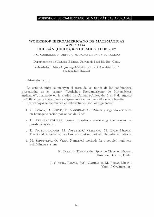
WORKSHOP IBEROAMERICANO DE MATEMATICAS APLICADAS
WORKSHOP IBEROAMERICANO DE MATEMATICASAPLICADAS
CHILLAN (CHILE), 6–8 DE AGOSTO DE 2007
R.C. CABRALES, J. ORTEGA, M. ROJAS-MEDAR Y F. TOLEDO
Departamento de Ciencias Basicas, Universidad del Bıo-Bıo, Chile.
[email protected] [email protected] [email protected]
Estimado lector:
En este volumen se incluyen el resto de los textos de las conferenciaspresentadas en el primer “Workshop Iberoamericano de MatematicasAplicadas”, realizado en la ciudad de Chillan (Chile), del 6 al 8 de Agostode 2007, cuya primera parte ya aparecio en el volumen 41 de este boletın.
Los trabajos seleccionados en este volumen son los siguientes:
1. C. Conca, R. Orive, M. Vanninathan, Primer y segundo correctoren homogeneizacion por ondas de Bloch.
2. E. Fernandez-Cara, Several questions concerning the control ofparabolic systems.
3. E. Ortega-Torres, M. Poblete-Cantellano, M. Rojas-Medar,Fractional time-derivative of some evolution partial differential equations.
4. M. Sepulveda, O. Vera, Numerical methods for a coupled nonlinearSchrodinger system.
F. Toledo (Director del Dpto. de Ciencias Basicas,Univ. del Bıo-Bıo, Chile)
J. Ortega Palma, R.C. Cabrales, M. Rojas-Medar(Comite Organizador)
59

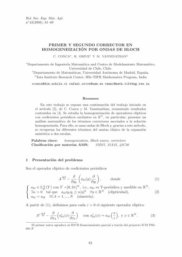
Bol. Soc. Esp. Mat. Apl.no43(2008), 61–69
PRIMER Y SEGUNDO CORRECTOR ENHOMOGENEIZACION POR ONDAS DE BLOCH
C. CONCA∗, R. ORIVE† Y M. VANNINATHAN‡
∗Departamento de Ingenierıa Matematica and Centro de Modelamiento Matematico,Universidad de Chile, Chile.
†Departamento de Matematicas, Universidad Autonoma de Madrid, Espana.‡Tata Institute Research Center, IISc-TIFR Mathematics Program, India
[email protected] [email protected] [email protected]
Resumen
En este trabajo se expone una continuacion del trabajo iniciado enel artıculo [5], de C. Conca y M. Vanninathan, resumiendo resultadoscontenidos en [4]. Se estudia la homogeneizacion de operadores elıpticoscon coeficientes periodicos oscilantes en R
N , en particular, presenta unanalisis matematico de los terminos correctores asociados a la solucionhomogeneizada. Para ello, se usan ondas de Bloch y, gracias a este metodo,se recuperan los diferentes terminos del anstaz clasico de la expansionasintotica a dos escalas.
Palabras clave: homogenization, Bloch waves, correctors
Clasificacion por materias AMS: 35B27, 35A25, 42C30
1 Presentacion del problema
Sea el operador elıptico de coeficientes periodicos
Adef= − ∂
∂yk
(akl(y)
∂
∂yl
), donde (1)
akl ∈ L∞# (Y ) con Y =]0, 2π[N , i.e., akl es Y-periodica y medible en R
N ,
∃α > 0 tal que aklηkηl ≥ α|η|2 ∀η ∈ RN (elipticidad),
akl = alk ∀l, k = 1, ..., N (simetrıa).(2)
A partir de (1), definimos para cada ε > 0 el siguiente operador elıptico
Aε def= − ∂
∂xk
(aε
kℓ(x)∂
∂xℓ
)con aε
kℓ(x) = akℓ
(xε
), y x ∈ R
N . (3)
El primer autor agradece al IDCB financiamiento parcial a traves del proyecto ICM P05-001-F.
61
62 C. Conca, R. Orive y M. Vanninathan
Pedimos como hipotesis que exista una sucesion uε de H1(RN ) tal que paraf ∈ L2(RN ) satisfaga
Aεuε = f en RN , (4)
Ademas, cuando ε→ 0 uε u∗ debilmente en H1(RN ),
uε → u∗ fuerte en L2(RN ).
Es clasico en homogeneizacion, que u∗ se denomine solucion homogeneizada; sesabe que satisface
A∗u∗ = f en RN , donde A∗ def
= − ∂
∂xk
(qkℓ
∂
∂xℓ
)(5)
es el operador homogeneizado, con coeficientes qkℓ constantes y simetricos (vease[1]).
Nuestro objetivo es recuperar el primer y segundo corrector de la solucionhomogeneizada u∗, de una forma distinta a la clasica de [1]. Se llama primercorrector a una funcion θε
1 ∈ H1(RN ), que sea facilmente construible, nodependa de uε y satisfaga:
‖uε − u∗ − εθε1‖H1(RN ) → 0 cuando ε→ 0. (6)
Por definicion, un segundo corrector θε2 ∈ H1(RN ) posee la propiedad
‖uε − u∗ − εθε1 − ε2θε
2‖H1(RN )≤ cε. (7)
El artıculo ha sido redactado en el orden siguiente. Primero, se repasa elmetodo de Bloch y se obtiene el desarrollo de Taylor del primer autovalory autofuncion de Bloch. En la seccion “Coeficientes de Bloch”, se estudiala convergencia de la primera autofuncion a la transformada de Fourier,y se observa que solamente el primer autovalor de Bloch es relevante enla homogeneizacion del operador Aε. En la ultima seccion, enunciamos losresultados de correctores y se bosquejan sus demostraciones; para otros detallesel lector podra consultar [4].
2 Autovalores y autofunciones de Bloch
El metodo de Bloch, vease [3] o [5], introduce una familia de problemasespectrales, parametrizados por η ∈ R
N : Encontrar λm = λm(η) y φm =φm(y; η) tales que
A(η)φm(·, η) = λm(η)φm(·, η) en RN , φ(·, η) Y -periodica,
donde A(η)φdef=A(eiy·ηφ). Gracias a la η-periocidad de φm, podemos confinar η
a la celda Y ′ =] − 12 ,
12 [N . Ademas, sabemos de [5] que
i) 0 ≤ λ1(η) ≤ ... ≤ λm(η) ≤ ... → +∞, λ2(η) ≥ λ(2)N >
0, ∀η ∈ Y ′,ii) φm(·; η)m es base ortonormal de L2
#(Y ).
Primer y segundo corrector en homogeneizacion por ondas de Bloch 63
Sean g, h ∈ L2(RN ). El m-esimo coeficiente de Bloch de g se define por
(Bmg)(η) =
∫
RN
g(y)e−iy·ηφm(y; η)dy ∀m ≥ 1, η ∈ Y ′. (8)
g(y) =
∫
Y ′
∞∑
m=1
(Bmg)(η)eiy·ηφm(y; η)dη, (9)
∫
RN
|g(y)|2dy =
∫
Y ′
∞∑
m=1
|(Bmg)(η)|2dη (Parseval), (10)
∫
RN
g(y)h(y)dy =
∫
Y ′
∞∑
m=1
(Bmg)(η)(Bmh)(η)dη (Plancherel). (11)
Ası, la familia φm(y; η) : m ≥ 1, η ∈ Y ′ forma una base de L2(RN ), en unsentido generalizado, y L2(RN ) se identifica con L2(Y ′, l2 (N )) por la identidadde Parseval.
En [5] se prueban los siguientes resultados de regularidad: Para cada m ≥ 1,λm(η) es una funcion Lipschitziana de η y existe una bola Bδ, de centro η = 0y radio δ > 0, tal que, en ella, el primer autovalor de Bloch, λ1(η), es simple ydefine una funcion analıtica de η.
La aplicacion η → λ1(η), definida de Y ′ en RN , posee un mınimo estricto
global en η = 0 y, existe una constante c > 0 tal que λ1(η) ≥ c|η|2, paratodo η ∈ Y ′. Mas aun, es posible escoger la primera autofuncion de modo quesea analıtica en Bδ y satisfaga: Im(
∫Yφ1(y; η)dy) = 0 para todo η ∈ Bδ y
φ1(y; 0) = (2π)−N/2, que denotamos p(0).
Consideremos las funciones auxiliares χk, χkℓ, χkℓm, χkℓmn ∈ H1#(Y ),
soluciones de:
Aχk =∂akℓ
∂yℓen R
N , mY (χk)def=
1
|Y |
∫
Y
χk(y)dy = 0. (12)
Aχkℓ = (akℓ − qkℓ) −1
2
(Ckχ
ℓ + Cℓχk)
en RN , mY (χkℓ) = 0. (13)
Aχkℓm =1
3
[(akℓ − qkℓ)χ
m + (aℓm − qℓm)χk + (ank − qnk)χℓ−
Ckχℓm − Cℓχ
mk − Cmχkℓ
]en R
N , mY (χkℓm) = 0.(14)
Aχkℓmn =1
4!D4
kℓmnλ1(0) − 1
4
(Cnχ
kℓm + Ckχℓmn + Cℓχ
mnk + Cmχnkℓ)+
1
3!
[(akℓ − qkℓ)χ
mn + (aℓm − qℓm)χkn + (akm − qkm)χℓn + (aℓn − qℓn)χkm
+(amn − qmn)χkℓ + (akn − qkn)χℓm]
en RN , mY (χkℓmn) = 0,
(15)

64 C. Conca, R. Orive y M. Vanninathan
donde Ckdef= −akℓ(y)
∂(.)∂yℓ
− ∂∂yℓ
(akℓ(y)(·)). Los problemas (12), (13), (14) y (15)
admiten solucion unica. En efecto, para f ∈ L2#(Y ), el problema
Aϕ = f en RN , ϕ ∈ H1
#(Y ), m(ϕ) = 0,
por la alternativa de Fredholm (ver [2]), tiene solucion unica, si y solo si∫Yf(y)dy = 0.
Proposicion 1 Las derivadas de λ1 en η = 0 de orden menor o igual que 4son
Dβλ1(0) = 0 ∀β ∈ ZN+ : |β| = β1 + ...+ βN impar.
1
2D2
kℓλ1(0) =1
|Y |
∫
Y
akℓ(y)dy −1
2|Y |
∫
Y
(Ckχℓ(y) + Cℓχ
k(y))dy = qkℓ
1
4!D4
kℓmnλ1(0) =1
4
1
|Y |
∫
Y
Cnχ
kℓm + Ckχℓmn + Cℓχ
mnk + Cmχnkℓdy −
− 1
3!
1
|Y |
∫
Y
akℓχ
mn + aℓmχnk + amnχ
kℓ + ankχℓm + akmχ
ℓn + aℓnχkmdy,
para todo k, ℓ,m, n = 1, ..., N . Ademas, Daλ1(0) con a ∈ N par, es real.
Proposicion 2 Las derivadas de φ1 en η = 0 de orden menor o igual que 4son
Dkφ1(y; 0) = ip(0)χk(y),
1
2!D2
kℓφ1(y; 0) = −p(0)χkℓ(y) + β(2)kℓ p
(0),
1
3!D3
kℓmφ1(y; 0) = −ip(0)χkℓm(y) +i
3
(β
(2)kℓ χ
m(y) + β(2)ℓmχ
k(y) + β(2)mkχ
ℓ(y))p(0),
1
4!D4
kℓmnφ1(y; 0) = p(0)χkℓmn(y) − 1
3!
(β
(2)kℓ χ
mn(y) + β(2)ℓmχ
nk(y) + β(2)mnχ
kℓ+
+β(2)nk χ
ℓm(y) + β(2)kmχ
nℓ(y) + β(2)ℓn χ
km(y))p(0) + β
(4)kℓmnp
(0),
donde β(2)kℓ y β
(4)kℓmn son constantes. Ademas, Daφ1(y, 0) con a ∈ N par, es real,
y con a ∈ N impar, es imaginaria.
Para obtener estos resultados, consideremos la ecuacion del primer autovalor
(A(η) − λ1(η))φ1(·; η) = 0. (16)
Derivando con respecto a ηk y evaluando en η = 0 se obtienen las distintasecuaciones que han de verificar las derivadas de φ1. Tomamos producto escalarde (16) con φ1(·; η), y evaluando en η = 0 se tienen las derivadas de λ1. Paraconocer el valor de las constantes β utilizamos que ‖φ1(·; η)‖L2(Y ) = 1 para todoη.
Primer y segundo corrector en homogeneizacion por ondas de Bloch 65
3 Analisis de los coeficientes de Bloch
Asociado al operador (3), consideremos las autofunciones φεm(x; ξ) = φm(y; η)
y los autovalores λεm(ξ) = ε−2λm(η), cuyas variables verifican: y = x/ε, η = εξ.
Como en (8), definimos los coeficientes Bεmu
ε asociados a φεm. Para estos
coeficientes seran tambien validas las igualdades (9), (10), (11). Notemos queuε(x) = P ε
1 (x) + vε(x), x ∈ RN ,donde
P ε1 (x) =
∫
ε−1Y ′
Bε1u
ε(ξ)eix·ξφε1(x; ξ)dξ
vε(x) =
∫
ε−1Y ′
∞∑
m=2
Bεmu
ε(ξ)eix·ξφεm(x; ξ)dξ.
Proposicion 3 Tenemos que
(i) ‖vε‖L2(RN ) ≤ cε‖f‖H−1(RN ) para f ∈ H−1(RN ).
(ii) ‖vε‖L2(RN ) ≤ cε2‖f‖L2(RN ) para f ∈ L2(RN ).
(iii) ‖∇vε‖L2(RN )N ≤ cε‖f‖L2(RN ) para f ∈ L2(RN ).
(iv) ‖∇vε‖L2(RN )N ≤ cε2‖∇f‖L2(RN ) para f ∈ H1(RN ).
Sabemos que λεm(ξ)Bε
mu(ξ) = Bεmf(ξ) para todo m ≥ 2, y que
‖vε‖2L2 =
∫
ε−1Y ′
∞∑
m=2
|Bεmu
ε(ξ)|2dξ, ‖∇vε|2L2 ≤ c
∫
ε−1Y ′
∞∑
m=2
λεm(ξ)|Bε
muε(ξ)|2dξ,
‖f‖2H−1 =
∫
ε−1Y ′
∞∑
m=1
|Bεmf(ξ)|2
1 + λεm(ξ)
dξ.
Como sup[λεm(ξ)]−1 | m ≥ 2, ξ ∈ ε−1Y ′ ≤ (λ
(N)2 )−1ε2, esto prueba la
Proposicion 3. Ası los coeficientes de Bloch mayores que 1 son irrelevantes paranuestro estudio.
En [5], se demuestra que dada una sucesion en L2(RN ), digamos gε, se tieneque(1) Si gε g debilmente en L2(RN ), entonces χ
ε−1Y ′Bε
1gε g debilmente en
L2loc(R
N ) cuando supp (gε) ⊂ K, compacto.(2) Si gε → g en L2(RN ), entonces χ
ε−1Y ′Bε
1g → g en L2loc(R
N ),
donde χ es la funcion caracterıstica de ε−1Y ′. Otro resultado en este mismosentido es:
Proposicion 4
(i) Para g ∈ L2(RN ), con soporte compacto, se tiene que χε−1Y ′
(ξ)Bε1g(ξ) →
g(ξ) en L∞loc(R
Nξ ).

66 C. Conca, R. Orive y M. Vanninathan
(ii) Si g ∈ L2(RN ), entonces χε−1Y ′
(ξ)Bε1g(ξ) → g(ξ) en L2(RN
ξ ).
(iii) Si g ∈ H1(RN ), entonces ‖χε−1Y ′
(ξ)Bε1g(ξ) − g(ξ)‖L2 ≤ cε.
Para demostrarla, se usa una aproximacion en celdas de la transformadade Fourier, denominada transformada de Fourier aproximada. ConsideremosY ε
ℓ ℓ∈ZN el reticulado de RN generado por la celda εY , Y ε
ℓ = xεℓ + εY donde
xεℓ = 2πεℓ es el origen de la celda Y ε
ℓ . Dado p > N , para g ∈ W 1,p(RN ) consoporte compacto, definimos
F εg(ξ) =∑
ℓ∈ZN
g(xεℓ)e
−ixεℓ ·ξ ∀ξ ∈ ε−1Y ′, ası (17)
(a) εNχε−1Y ′
F εg(ξ) → (2π)−N/2g(ξ) puntualmente para ξ ∈ RN .
(b) ‖εNF εg‖L2(ε−1Y ′) ≤ c|K| p−22p
‖g‖Lp(RN ) + ε‖∇g‖Lp(RN )N
1.
(c) εNχε−1Y ′
F εg → (2π)−N/2g en L2(RN ).
En efecto, (a) se prueba usando que g tiene soporte compacto. Utilizando ladesigualdad de Morrey (ver [2]) se demuestra (b), y por el Teorema de Egorovse prueba (c).
Demostracion Proposicion 4. Consideremos el ε-reticulado Y εℓ ℓ∈ZN .
Escribimos
Bε1g(ξ) =
∑
ℓ∈ZN
∫
Y εℓ
g(x)e−ix·ξφε1(x; ξ)dx =
∑
ℓ∈ZN
g(xεℓ)
∫
Y εℓ
e−ix·ξφε1(x; ξ)dx+ rε
1(ξ), (18)
rε1(ξ) =
∑
ℓ∈ZN
∫
Y εℓ
(g(x) − g(xεℓ))e
−ix·ξφε1(x; ξ)dx. (error de aproximacion) (19)
Utilizando la desigualdad de Morrey, se prueba que
‖rε1‖L2(ε−1Y ′) ≤ C(K)ε‖∇g‖Lp ,
y dado que ‖φ1(·, εξ) − φ(·, 0)‖L2(Y ) ≤ cε, de (18) se demuestra (i). Utilizandoargumentos de densidad y el Teorema de Convergencia Dominada, se tiene (ii).
Para probar (iii), se considera el espacio W 2,p(RN ), y se escriben lasidentidades
Bε1g(ξ) =
∑
ℓ∈ZN
∫
Y εℓ
[g(xεℓ) + ∇g(xε
ℓ) · (x− xεℓ)] e
−ix·ξφε1(x; ξ)dx+ rε
2(ξ),
rε2(ξ) =
∑
ℓ∈ZN
∫
Y εℓ
g(x) − g(xεℓ) −∇g(xε
ℓ) · (x− xεℓ) e−ix·ξφε
1(x; ξ)dx.
Luego, se utilizan las mismas tecnicas que en (i) y en (ii).
1|K| es la medida de Lebesgue de K.
Primer y segundo corrector en homogeneizacion por ondas de Bloch 67
4 Resultados de correctores
Definimos la siguiente funcion, que llamaremos Aproximacion de Bloch
θε def=
∫
ε−1Y ′
u∗(ξ)eix·ξφε1(x; ξ)dξ, (20)
donde u∗ es la transformada de Fourier de la solucion homogeneizada y φε1 es
la primera onda de Bloch asociada al operador (3).
Teorema 5 Los coeficientes akℓ verifican (2), y pertenecen a W 1,∞(Y ).Entonces
(i) Si f ∈ L2(RN ), se tiene que (uε − θε) → 0 en H1(RN ).
(ii) Si f ∈ H1(RN ), se tiene que ‖∇(uε − θε)‖L2(RN )N ≤ cε12 .
Demostracion. Utilizando la Proposicion 3 nos basta probar, respectivamen-te
∥∥∥P ε1u
ε(x) − θε∥∥∥
H1(RN )→ 0, (21)
∣∣∣P ε1u
ε(x) − θε∣∣∣2
H1(RN )≤ cε (22)
Tomamos las antitransformadas de Bloch y consideramos los integrandos
(θε)δ(x) =
∫
ξ∈ε−1Y ′
|ξ|>δε−1
u∗(ξ)eix·ξφε1(x; ξ)dξ, (P ε
1uε)δ(x) =
∫
ξ∈ε−1Y ′
|ξ|>δε−1
Bε1u
ε(ξ)eix·ξφε1(x; ξ)dξ.
Utilizando la regularidad de uε, u∗ y que λ1(η) ≥ c|η|2 para todo η ∈ Y ′, sigueque
|(P ε1u
ε)δ|2H1(RN ) ≤ cδ−2ε2‖f‖2L2(RN ), ‖(θε)δ‖2
H1(RN ) ≤ cε2‖u∗‖2H2(RN ).
Para demostrar (21), (22), basta probar, respectivamente, que∫
|ξ|≤δε−1
[1 + λε1(ξ)]|Bε
1uε(ξ) − u∗(ξ)|2dξ → 0, (23)
∫
|ξ|≤δε−1
λε1(ξ)|Bε
1uε(ξ) − u∗(ξ)|2dξ ≤ cε (24)
Utilizando las siguientes relaciones, ya conocidas (ver [5]),
λε1(ξ)B
ε1u
ε(ξ) = Bε1f(ξ), qkℓξkξℓu
∗(ξ) = f(ξ) ∀ξ ∈ RN ,
|λε1 − ξtλ′′(0)ξ| ≤ cε|ξ|4 ∀|εξ| = |η| ≤ δ,
y gracias a la Proposicion 4, como Bε1u
ε → u∗ en L2loc(R
N ), se concluye lademostracion.
68 C. Conca, R. Orive y M. Vanninathan
Teorema 6 Bajo las hipotesis del Teorema 5, se tiene que
(i) Si f ∈ H−1(RN ), entonces ‖θε − u∗‖L2(RN ) ≤ cε.
(ii) Si f ∈ L2(RN ), entonces∥∥∥θε − u∗ − εχk ∂u∗
∂xk
∥∥∥H1(RN )
≤ cε.
(iii) Si f ∈ H1(RN ),∥∥∥θε − u∗ − εχk ∂u∗
∂xk− ε2
(χkℓ − β
(2)kℓ
)∂2u∗
∂xk∂xℓ
∥∥∥H1(RN )
≤cε2.
En definitiva, hemos obtenido los primeros tres terminos en el anstazo expansion asintotica de la ası llamada Aproximacion de Bloch. Estosproporcionan, respectivamente, la solucion homogeneizada, y el primer ysegundo corrector a esta solucion.
Demostracion . En (i), como f ∈ H−1(RN ), entonces u∗ ∈ H1(RN ). Comose tiene que ‖φ1(y; εξ) − φ1(y; 0)‖L2(Y ) ≤ c|εξ|, entonces por Parseval
‖θε − u∗‖L2(RN ) ≤ cε2∫
ε−1Y ′
|ξ|2|u∗|2dξ +
∫
RN−ε−1Y ′
|u∗|2. (25)
Es claro que
∫
RN−ε−1Y ′
|u∗|2dξ ≤ cε2∫
RN−ε−1Y ′
|ξ|2|u∗|))dξ ≤ cε2|u∗|H1(RN ),
por integrar fuera de un entorno de 0. Entonces volviendo a (25), sigue (i).A partir de los resultados de la Proposicion 2, ya que escribimos el desarrollo
de Taylor de φ1 con respecto de η, en η = 0,
φ1(·; η) = p(0) + ip(0)χk(·)ηk − p(0)(χkℓ(·) − β
(2)kℓ
)ηkηℓ + 0(|η|3),
entonces, gracias a la regularidad que se tiene para cada caso, se demuestra (ii)y (iii).
Nota 1 Por (i) del Teorema 5 y (ii) del Teorema 6, tenemos
∥∥∥∥uε(x) − u∗ − εχk ∂u
∗
∂xk
∥∥∥∥H1(RN )
≤ cε.
Por lo tanto, se tiene que εχk(xε )∂u∗
∂xk(x) es el primer corrector. Ası, θε equivale
al primer corrector, pero ademas por el apartado (ii) del Teorema 5 lo mejora.
5 Conclusiones
El problema (4) se reduce a la ecuacion algebraica
λε1(ξ)B
ε1u
ε(ξ) = Bε1f(ξ) ∀ξ ∈ ε−1Y ′,
Primer y segundo corrector en homogeneizacion por ondas de Bloch 69
ya que todos los coeficientes de Bloch mayores que 1 se pueden despreciar, veasela Proposicion 3. Entonces, si queremos encontrar los terminos correctores, solotenemos que expandir asintoticamente el primer coeficiente de Bloch de uε enfuncion de f y del primer autovalor λε
1. Ademas, en las demostraciones de losTeoremas 5 y 6, se utilizo y probo que fuera de un entorno de 0, los coeficientesde Bloch son irrelevantes para nuestro estudio. Ası, por la analiticidad delprimer autovalor y autofuncion de Bloch, la expansion asintotica de uε seencuentra utilizando los desarrollos de Taylor de λ1 y φ1, que conocemos porlas Proposiciones 1 y 2.
Referencias
[1] A. Bensoussan, J. L. Lions and G. Papanicolaou. Asymptotic analysis forperiodic structures. North-Holland, Amsterdam, 1978.
[2] H. Brezis. Analyse fonctionnelle, theorie et applications, CollectionMathematiques Appliquees pour la Maitrise. Masson, 1983.
[3] C. Conca, J. Planchard and M. Vanninathan. Fluids and periodic structures.Research Notes in Applied Mathematics 38, J. Wiley/Masson, NewYork/Paris, 1995.
[4] C. Conca, R. Orive and M. Vanninathan. Bloch approximation inhomogenization and applications. SIAM J. Math. Anal. 33:1166–1198, 2002.
[5] C. Conca and M. Vanninathan. Homogenization of periodic structures viaBloch decomposition. SIAM J. Appl. Math. 57:1639–1659, 1997.
[6] L. Tartar. Problemes d’homogeneisation dans les equations aux deriveespartielles. Cours Peccot, College de France, 1977.

Bol. Soc. Esp. Mat. Apl.no43(2008), 71–82
SEVERAL QUESTIONS CONCERNING THE CONTROL OFPARABOLIC SYSTEMS
E. FERNANDEZ-CARA
Departamento de Ecuaciones Diferenciales y Analisis Numerico, Universidad de
Sevilla, Espana.
Abstract
This paper is devoted to recall several recent results concerning the nullcontrollability of some parabolic systems. Among others, we will considerthe classical heat equation, the Burgers, Navier-Stokes and Ginzburg-Landau equations, etc.
Key words: Controllability, linear and nonlinear partial differentialequations, parabolic systems.
AMS subject classifications: 93B05, 35K15
1 Introduction
Let us first recall some general ideas that can be applied to a large family of(linear and nonlinear) evolution problems.
Suppose that we are considering an abstract state equation of the formyt −A(y) = Bv, t ∈ (0, T ),y(0) = y0,
(1)
which governs the behavior of a physical system. It is assumed that
• A : D(A) ⊂ H 7→ H is a (generally nonlinear) operator,
• y : [0, T ] 7→ H is the state, i.e. the variable that can be used to identifythe properties of the system,
• v : [0, T ] 7→ U is the control, i.e. the variable we can choose in order to getgood properties,
• B ∈ L(U ;H) and
• y0 ∈ H (for simplicity, we assume that U and H are Hilbert spaces).
Suppose that the state equation is well-posed in the sense that, for eachy0 ∈ H and each v ∈ L2(0, T ;U), it possesses exactly one solution. Then thenull controllability problem for (1) can be stated as follows:
71
72 E. Fernandez-Cara
For each y0 ∈ H, find v ∈ L2(0, T ;U) such that the correspondingsolution of (1) satisfies y(T ) = 0.
For each system of the form (1), the null controllability problem leads toseveral interesting questions. Among them, let us mention the following:
• First, are there controls v such that y(T ) = 0?
• Then, if this is the case, which is the cost we have to pay to drive y to zero?In other words, which is the minimal norm of a control v ∈ L2(0, T ;U)satisfying this property?
• How can these controls be computed?
The controllability of differential systems is a very relevant area of researchand has been the subject of many papers the last years. In particular, in thecontext of partial differential equations, the null controllability problem wasfirst analyzed in [31, 32, 28, 29, 24, 27]. For semilinear systems of this kind, thefirst contributions have been given in [33, 9, 17].
In this contribution, I will recall some recent results concerning the nullcontrollability of some relevant parabolic systems. More precisely, we willconsider the classical heat equation, the Burgers equation and the Navier-Stokesand Ginzburg-Landau systems.
2 The heat equation. Controllability, observability and Carlemanestimates
We will first consider the controlled heat equation, complemented with initialand Dirichlet boundary conditions:
yt − ∆y = v1ω, (x, t) ∈ Ω × (0, T ),y(x, t) = 0, (x, t) ∈ ∂Ω × (0, T ),y(x, 0) = y0(x), x ∈ Ω.
(2)
Here (and also in the following Sections), Ω ⊂ RN is a nonempty bounded
domain, ω ⊂⊂ Ω is a (small) nonempty open subset (1ω is the characteristicfunction of ω) and y0 ∈ L2(Ω).
It is well known that, for every y0 ∈ L2(Ω) and every v ∈ L2(ω × (0, T )),there exists a unique solution y to (2), with
y ∈ L2(0, T ;H10 (Ω)) ∩ C0([0, T ];L2(Ω)).
In this context, the null controllability problem reads:
For each y0 ∈ L2(Ω), find v ∈ L2(ω × (0, T )) such that the correspondingsolution of (2) satisfies
y(x, T ) = 0 in Ω. (3)
Several questions concerning the control of parabolic systems 73
Together with (2), for each ϕ1 ∈ L2(Ω), we can introduce the associatedadjoint system
−ϕt − ∆ϕ = 0, (x, t) ∈ Ω × (0, T ),ϕ(x, t) = 0, (x, t) ∈ ∂Ω × (0, T ),ϕ(x, T ) = ϕ1(x), x ∈ Ω.
(4)
Then, it is well known that the null controllability of (2) is in practice equivalentto the following property:
There exists C > 0 such that
‖ϕ(·, 0)‖2L2 ≤ C
∫∫
ω×(0,T )
|ϕ|2 dx dt ∀ϕ1 ∈ L2(Ω). (5)
This is called an observability estimate for the solutions of (4). We thusfind that, in order to solve the null controllability problem for (2), it suffices toprove (5).
The estimate (5) is implied by the so called global Carleman inequalities.These have been introduced in the context of the controllability of PDEs byFursikov and Imanuvilov, see [24, 17]. When they are applied to the solutionsof the adjoint systems (4), they take the form
∫∫
Ω×(0,T )
ρ2 |ϕ|2 dx dt ≤ K
∫∫
ω×(0,T )
ρ2 |ϕ|2 dx dt ∀ϕ1 ∈ L2(Ω), (6)
where ρ = ρ(x, t) is an appropriate weight, depending on Ω, ω and T and theconstant K only depends on Ω and ω.1
Combining (6) and the dissipativity of the backwards heat equation (4), itis not difficult to deduce (5) for some C only depending on Ω, ω and T .
As a consequence, we have:
Theorem 1 The linear system (2) is null controllable. In other words, for eachy0 ∈ L2(Ω), there exists v ∈ L2(ω× (0, T )) such that the corresponding solutionof (2) satisfies (3).
There are many generalizations and variants of this result that provide thenull controllability of other similar linear state equations:
• Time-space dependent (and sufficiently regular) coefficients can appear inthe equation, other boundary conditions can be used, boundary control(instead of distributed control) can be imposed, etc. For a review of recentapplications of Carleman inequalities to the controllability of parabolicsystems, see [12].
1In order to prove (6), we have to use a weight ρ decreasing to zero, as t → 0 and also ast → T , for instance exponentially.

74 E. Fernandez-Cara
• The controllability of Stokes-like systems can also be analyzed with thesetechniques. This includes systems of the form
yt − ∆y + (a · ∇)y + (y · ∇)b+ ∇p = v1ω, ∇ · y = 0, (7)
where a and b are regular enough; see for instance [13].
• Other linear parabolic (non-scalar) systems can also be considered, etc.
As mentioned above, an interesting question related to theorem 1 concernsthe cost of null controllability. One has the following result from [15]:
Theorem 2 For each y0 ∈ L2(Ω), let us set
C(y0) = inf ‖v‖L2(ω×(0,T )) : the solution of (2) satisfies y(x, T ) = 0 in Ω .
Then we have the following estimate
C(y0) ≤ exp
(C
(1 +
1
T
))‖y0‖L2 , (8)
where the constant C only depends on Ω and ω.
Remark 1 Notice that theorem 1 ensures the null controllability of (2) forany ω and T . This is a consequence of the fact that, in a parabolic equation,the information is transmitted at infinite speed. This is not the case for thewave equation. Indeed, null controllability does not always hold, for hyperbolicequations. Contrarily, the couple (ω, T ) has to satisfy appropriate geometricalassumptions; see [29] and [4] for more details.
3 Positive and negative controllability results for the one-dimensional Burgers equation
In this Section, we will be concerned with the null controllability of the followingsystem for the viscous Burgers equation:
yt − yxx + yyx = v1ω, (x, t) ∈ (0, 1) × (0, T ),
y(0, t) = y(1, t) = 0, t ∈ (0, T ),
y(x, 0) = y0(x), x ∈ (0, 1).
(9)
Some controllability properties of (9) have been studied in [17] (seeChapter 1, theorems 6.3 and 6.4). It is shown there that, in general, a stationarysolution of (9) with large L2-norm cannot be reached (not even approximately)at any time T . In other words, with the help of one control, the solutions of theBurgers equation cannot go anywhere at any time.
For each y0 ∈ L2(0, 1), let us introduce
T (y0) = inf T > 0 : (9) is null controllable at time T .
Several questions concerning the control of parabolic systems 75
Then, for each r > 0, let us define the quantity
T ∗(r) = sup T (y0) : ‖y0‖L2 ≤ r .
Our main purpose is to show that T ∗(r) > 0, with explicit sharp estimatesfrom above and from below. In particular, this will imply that (global) nullcontrollability at any positive time does not hold for (9).
More precisely, let us set φ(r) = (log 1r )−1. We have the following result
from [10]:
Theorem 3 One has
C0φ(r) ≤ T ∗(r) ≤ C1φ(r) as r → 0, (10)
for some positive constants C0 and C1 not depending of r.
Remark 2 The same estimates hold when the control v acts on system (9)through the boundary only at x = 1 (or only at x = 0). Indeed, it is easy totransform the boundary controlled system
yt − yxx + yyx = 0, (x, t) ∈ (0, 1) × (0, T ),
y(0, t) = 0, y(1, t) = w(t), t ∈ (0, T ),
y(x, 0) = y0(x), x ∈ (0, 1)
(11)
into a system of the kind (9). The boundary controllability of the Burgersequation with two controls (at x = 0 and x = 1) has been analyzed in [21]. There,it is shown that even in this more favorable situation null controllability doesnot hold for small time. It is also proved in that paper that exact controllabilitydoes not hold for large time.2
The proof of the estimate from above in (10) can be obtained by solvingthe null controllability problem for (9) via a (more or less) standard fixed pointargument, using global Carleman inequalities to estimate the control and energyinequalities to estimate the state and being very careful with the role of T inthese inequalities.
Let us recall the proof of the estimate from below, that is inspired by thearguments in [1].
Let us show that there exist positive constants C0 and C ′0 such that, for any
sufficiently small r > 0, we can find initial data y0 satisfying ‖y0‖L2 ≤ r withthe following property: for any state y associated to y0, one has
|y(x, t)| ≥ C ′0r for some x ∈ (0, 1) and any t : 0 < t < C0φ(r).
Thus, let us set T = φ(r) and let ρ0 ∈ (0, 1) be such that (0, ρ0) ∩ ω = ∅.Notice that this is not restrictive, since it is always possible to work in a suitableopen subset ω ⊂ ω.
2Let us remark that the results in [21] do not allow to estimate T (r); in fact, the proofsare based in contradiction arguments.

76 E. Fernandez-Cara
We can suppose that 0 < r < ρ0. Let us choose y0 ∈ L2(0, 1) such thaty0(x) = −r for all x ∈ (0, ρ0) and let us denote by y an associated solution of(9).
Let us introduce the function Z = Z(x, t), with
Z(x, t) = exp
−2
t
(1 − e−ρ2
0(ρ0−x)3/(ρ0/2−x)2)
+1
ρ0 − x
. (12)
Then one has Zt − Zxx + ZZx ≥ 0.Let us now set w(x, t) = Z(x, t) − y(x, t). It is immediate that
wt − wxx + ZZx − yyx ≥ 0, (x, t) ∈ (0, ρ0) × (0, T ),
w(0, t) ≥ 0, w(ρ0, t) = +∞, t ∈ (0, T ),
w(x, 0) = r, x ∈ (0, ρ0).
(13)
Consequently, w−(x, t) ≡ 0. Indeed, let us multiply the differential equationin (13) by −w− and let us integrate in (0, ρ0). Since w− vanishes at x = 0 andx = ρ0, after some manipulation we find that
1
2
d
dt
∫ ρ0
0
|w−|2 dx+
∫ ρ0
0
|w−x |2 dx
=
∫ ρ0
0
w−(ZZx − yyx) dx ≤ C
∫ ρ0
0
|w−|2 dx.(14)
Hence,y ≤ Z in (0, ρ0) × (0, T ). (15)
Let us set ρ1 = ρ0/2 and let r be a regular function satisfying the following:r(0) = r(ρ1) = 0; r(x) = r for all x ∈ (δρ1, (1 − δ)ρ1) and some δ ∈ (0, 1/4);−r ≤ −r(x) ≤ 0;
|rx| ≤ Cr and |rxx| ≤ C in (0, ρ1), (16)
where C = C(ρ1) is independent of r.Let us introduce the solution u of the auxiliary system
ut − uxx + uux = 0, (x, t) ∈ (0, ρ1) × (0, T ),
u(0, t) = Z(ρ1, t), u(ρ1, t) = Z(ρ1, t), t ∈ (0, T ),
u(x, 0) = −r(x), x ∈ (0, ρ1).
(17)
We need the following lemma, whose proof can be found in [10]:
Lemma 4 One has
|u| ≤ Cr and |ux| ≤ Cr1/2 in (0, ρ1) × (0, φ(r)), (18)
where C is independent of r.
Several questions concerning the control of parabolic systems 77
Taking into account (15) and that ux, y ∈ L∞((0, ρ1)× (0, T )) (see lemma 4below), a standard application of Gronwall’s lemma shows that
y ≤ u in (0, ρ1) × (0, T ). (19)
On the other hand, we see from (18) that ut − uxx ≤ C∗r3/2 in (0, ρ1) ×(0, φ(r)) for some C∗ > 0. Let us consider the functions p and q, given by
p(t) = C∗r3/2t−r and q(x, t) = c(e−(x−(ρ1/4))2/4t +e−(x−3(ρ1/4))2/4t). It is thenclear that b = u− p− q satisfies
bt − bxx ≤ 0 in (ρ1/4, 3ρ1/4) × (0, φ(r)),
b(ρ1/4, t) ≤ Z(ρ1, t) − C∗r3/2t+ r − c(1 + e−ρ21/(16t)) for t ∈ (0, φ(r)),
b(3ρ1/4, t) ≤ Z(ρ1, t) − C∗r3/2t+ r − c(1 + e−ρ21/(16t)) for t ∈ (0, φ(r)),
b(x, 0) = 0 for x ∈ (ρ1/4, 3ρ1/4).
Obviously, in the definition of q the constant c can be chosen large enoughto have Z(ρ1, t) − C∗r3/2t + r − c(1 + e−ρ2
1/(16t)) < 0 for any t ∈ (0, φ(r)). Ifthis is the case, we get u ≤ p+ q and, in particular,
u(ρ1/2, t) ≤ (p+ q)(ρ1/2, t) = 2ce−ρ21/(64t) + C∗r3/2t− r.
Therefore, we see that there exist C0 and C ′0 such that u(ρ1/2, t) < −C ′
0r forany t ∈ (0, C0φ(r)).
This proves the first inequality in (10) and, consequently, ends the proof oftheorem 3.
4 Other more realistic nonlinear equations and systems
There are a lot of more realistic nonlinear equations and systems from mechanicsthat can also be considered. First, we have the well known Navier-Stokesequations:
yt + (y · ∇)y − ∆y + ∇p = v1ω, ∇ · y = 0, (x, t) ∈ Q,
y = 0, (x, t) ∈ Σ,
y(x, 0) = y0(x), x ∈ Ω.
(20)
Here and below, Q and Σ respectively stand for the sets
Q = Ω × (0, T ) and Σ = ∂Ω × (0, T ),
where Ω ⊂ RN is a nonempty bounded domain, N = 2 or N = 3 and (again)
ω ⊂⊂ Ω is a nonempty open set.The controllability of this system has been analyzed in [13] and [14].3
Essentially, these results establish the local exact controllability of the solutions
3The main ideas come from [18, 25]; some additional results will appear soon in [22]and [19]; for other control results concerning the Navier-Stokes equations, see [6, 7].
78 E. Fernandez-Cara
of (20) to uncontrolled trajectories (this is, more or less, the analog of thepositive controllability result in theorem 3).
Similar results have been given in [20] for the Boussinesq equations
yt + (y · ∇)y − ∆y + ∇p = θk + v1ω, ∇ · y = 0,
θt + y · ∇θ − ∆θ = u1ω,(21)
complemented with initial and Dirichlet boundary conditions for y and θ(see [14] for a controllability result with a reduced number of scalar controls).
Let us also mention [3, 23], where the controllability of the MHD and otherrelated equations has been analyzed.
Another system is considered in [11]:
yt + (y · ∇)y − ∆y + ∇p = ∇× w + v1ω, ∇ · y = 0,
wt + (y · ∇)w − ∆w −∇(∇ · w) = ∇× y + u1ω.(22)
Here, N = 3. These equations govern the behavior of a micropolar fluid,see [30]. As usual, y and p stand for the velocity field and pressure and w isthe microscopic velocity of rotation of the fluid particles. Again, the local exactcontrollability of the solutions to the trajectories is established.
Notice that this case involves a nontrivial difficulty. The main reason is thatw is a nonscalar variable and the equations satisfied by its components wi arecoupled through the second-order terms ∂i(∇·w). This is a serious inconvenientand an appropriate strategy has to be applied in order to deduce the requiredCarleman estimates.
For these systems, the proof of the controllability can be achieved arguingas in the first part of the proof of theorem 3. This is the general structure ofthe argument:
• First, consider a linearized similar problem and the associated adjointsystem and rewrite the original controllability problem in terms of a fixedpoint equation.
• Then, prove a global Carleman inequality and an observability estimate forthe adjoint system. This provides a controllability result for the linearizedproblem.
• Prove appropriate estimates for the control and the state (this needs somekind of smallness of the data); prove an appropriate compactness propertyof the state and deduce that there exists at least one fixed point.
There is an alternative method that relies on the implicit function theorem.It corresponds to another strategy introduced in [17]:
• First, rewrite the original controllability problem as a nonlinear equationin a space of admissible “state-control” pairs.
Several questions concerning the control of parabolic systems 79
• Then, prove an appropriate global Carleman inequality and a regularityresult and deduce that the linearized equation possesses at least onesolution. Again, this provides a controllability result for a related linearproblem.
• Check that the hypotheses of a suitable implicit function theorem aresatisfied and deduce a local result.
At present, no negative result is known to hold for these nonlinear systems(apart from the one-dimensional Burgers equation).
5 Some remarks on the Ginzburg-Landau equation
This Section is concerned with the controllability of the Ginzburg-Landauequation. The system under consideration is the following:
mt − αm×mt − ∆m+|m|2 − 1
εm = v1ω, (x, t) ∈ Q,
∂m
∂n= 0, (x, t) ∈ Σ,
m(x, 0) = m0, x ∈ Ω.
(23)
Here, Ω ⊂ R3 is a regular bounded open set, m = (m1,m2,m3) is the
magnetization field, ε > 0 is a parameter, α ≥ 0 is a physical constant and itis assumed that m0 is a measurable initial field satisfying |m0(x)| ≡ 1. For themotivation of the system satisfied by m, see for instance [5].
In this framework, an interesting controllability problem is the following:
Given a stationary solution m∗ = m∗(x) and an initial field m0 =m0(x) with |m∗(x)| ≡ |m0(x)| ≡ 1, find a control v ∈ L2(ω×(0, T ))3
such that the associated solution of (23) satisfies
m(x, T ) = m∗ in Ω.
By introducing the new variable y, with m = m∗ + y, this can be rewrittenin terms of a null controllability problem. Indeed, let us consider the system
yt − α(y +m∗) × yt − ∆y +Gε(x, y)y = v1ω, (x, t) ∈ Q,
∂y
∂n= 0, (x, t) ∈ Σ,
y(x, 0) = m0(x) −m∗(x), x ∈ Ω,
(24)
where
Gε(x, y)y ≡ |m∗(x) + y|2 − 1
ε(m∗(x) + y) − |m∗(x)|2 − 1
εm∗(x).
Then the problem is:

80 E. Fernandez-Cara
Given a stationary solution m∗ = m∗(x) and an initial field m0 =m0(x) with |m∗(x)| ≡ |m0(x)| ≡ 1, find a control v ∈ L2(ω×(0, T ))3
such that the associated solution of (24) satisfies
y(x, T ) = 0 in Ω.
A partial (positive) answer to this problem is given in [8].4
More precisely, it is shown there that there exists κ = κ(Ω, ω, T, α, ε) suchthat, whenever ‖m∗−m0‖L2 ≤ κ, the existence of such controls can be ensured.
Remark 3 For any fixed v, the solutions of (23) converge in some sense asε→ 0 to a solution of the so called Landau-Lifshitz equation:
αmt = m× (∆m−mt + v1ω) , |m| = 1. (25)
Consequently, it would be very interesting to be able to solve the previous problemwith controls v uniformly bounded with respect to ε. However, this is apparentlya difficult question.
Acknowledgements: The author has been partially supported by D.G.I.(Spain), Grant MTM2006–07932.
References
[1] S. Anita and D. Tataru. Null controllability for the dissipative semilinearheat equation. Appl. Math. Optim. 46: 97–105, 2002.
[2] J.P. Aubin. L’Analyse non Lineaire et ses Motivations Economiques.Masson, Paris 1984.
[3] V. Barbu, T. Havarneanu, C. Popa and S. S. Sritharan. Exactcontrollability for the magnetohydrodynamic equations. Comm. Pure Appl.Math.56: 732–783, 2003.
[4] C. Bardos, G. Lebeau and J. Rauch. Sharp sufficient conditions for theobservation, control and stabilization of waves from the boundary. SIAMJ. Cont. Optim. 30:1024–1065, 1992.
[5] M. Bertsch, P. Podio-Guidugli and V. Valente. On the dynamics ofdeformable ferromagnets. I. Global weak solutions for soft ferromagnetsat rest. Ann. Mat. Pura Appl. 179:331–360, 2001.
[6] J.-M. Coron. On the controllability of the 2-D incompressible Navier-Stokes equations with the Navier slip boundary conditions. ESAIM ControlOptim. Calc. Var. 1: 35–75, 1995/96.
4A similar result has been obtained independently by L. Rosier and B.-Y. Zhang.

Several questions concerning the control of parabolic systems 81
[7] J.-M. Coron and A.V. Fursikov. Global exact controllability of the 2DNavier-Stokes equations on a manifold without boundary. Russian J. Math.Phys. 4(4): 429–448, 1995/96.
[8] J. L. Boldrini, E. Fernandez-Cara and S. Guerrero. Some controllabilityresults for the Ginzburg-Landau equation. In preparation.
[9] C. Fabre, J.-P. Puel and E. Zuazua. Approximate controllability of thesemilinear heat equation. Proc. Royal Soc. Edinburgh. 125 A: 31–61, 1995.
[10] E. Fernandez-Cara and S. Guerrero. Null controllability of the Burgerssystem with distributed controls. Systems & Control Letters. 56: 366–372,2007.
[11] E. Fernandez-Cara and S. Guerrero. Local exact controllability ofmicropolar fluids. J. Math. Fluid Mech. 8:1–35, 2006.
[12] E. Fernandez-Cara and S. Guerrero. Global Carleman inequalities forparabolic systems and applications to controllability. SIAM J. ControlOptim. 45(4):1395–1446, 2006.
[13] E. Fernandez-Cara, S. Guerrero, O. Yu. Imanuvilov and J.-P. Puel. Localexact controllability to the trajectories of the Navier-Stokes equations. J.Math. Pures Appl. 83(12): 1501–1542, 2004.
[14] E. Fernandez-Cara, S. Guerrero, O. Yu. Imanuvilov and J.-P. Puel. Somecontrollability results for the N -dimensional Navier-Stokes and Boussinesqsystems with N−1 scalar controls. SIAM J. Control and Optim. 45(1):146–173, 2006.
[15] E. Fernandez-Cara and E. Zuazua. The cost of approximate controllabilityfor heat equations: The linear case. Advances Diff. Eqs. 5(4–6): 465–514,2000.
[16] E. Fernandez-Cara and E. Zuazua. Null and approximate controllabilityfor weakly blowing up semilinear heat equations. Ann. Inst. H. PoincareAnal. Non Lineaire. 17(5): 583–616, 2000.
[17] A. V. Fursikov and O. Yu. Imanuvilov. Controllability of EvolutionEquations. Lecture Notes #34, Seoul National University, Korea, 1996.
[18] A. V. Fursikov and O. Yu. Imanuvilov. Exact controllability of theNavier-Stokes and Boussinesq equations (Russian). Uspekhi Mat. Nauk.54(3)(327):93–146; translation in Russian Math. Surveys. 54(3):565–618,1999.
[19] M. Gonzalez-Burgos, S. Guerrero and J.-P. Puel. On the exactcontrollability of the Navier-Stokes and Boussinesq equations. To appear.
[20] S. Guerrero. Local exact controllability to the trajectories of the Boussinesqsystem. Annales IHP, Anal. non lineaire. 23:29–61, 2006.
82 E. Fernandez-Cara
[21] S. Guerrero and O. Yu. Imanuvilov. Remarks on global controllability forthe Burgers equation with two control forces. to appear in Annal. de l’Inst.Henri Poincare, Analyse Non Lineaire.
[22] S. Guerrero, O. Yu. Imanuvilov and J.-P. Puel. Remarks on globalapproximate controllability for the 2-D Navier-Stokes system with Dirichletboundary conditions. C. R. Math. Acad. Sci. Paris. 343(9):573–577, 2006.
[23] T. Havarneanu, C. Popa and S. S. Sritharan. Exact internal controllabilityfor the magnetohydrodynamic equations in multi-connected domains Toappear.
[24] O. Yu. Imanuvilov. Boundary controllability of parabolic equations.Russian Acad. Sci. Sb. Math. 186:109–132, 1995. (in Russian).
[25] O. Yu. Imanuvilov. Remarks on exact controllability for the Navier-Stokesequations. ESAIM Control Optim. Calc. Var. 6: 39–72, 2001.
[26] O. A. Ladyzenskaya, V. A. Solonnikov and N. N. Uraltzeva. Linear andQuasilinear Equations of Parabolic Type. Trans. Math. Monograph:Moscow, 1967; Vol. 23.
[27] G. Lebeau and L. Robbiano. Controle exact de l’equation de la chaleur.Comm. P.D.E. 20:335–356, 1995.
[28] J.-L. Lions. Exact controllability, stabilizability and perturbations fordistributed systems. SIAM Review 30: 1–68, 1988.
[29] J.-L. Lions. Controlabilite Exacte, Stabilisation et Perturbations deSystemes Distribues. Tomes 1 & 2, Masson, RMA 8 & 9, Paris 1988.
[30] G. Lukaszewicz. Micropolar fluids. Theory and applications. Modeling andSimulation in Science, Engineering and Technology, Birkhauser, Boston,Inc., Boston, MA, 1999.
[31] D.L. Russell. A unified boundary controllability theory for hyperbolic andparabolic partial differential equations. Studies in Appl. Math. 52:189–221,1973.
[32] D. L. Russell. Controllability and stabilizability theory for linear partialdifferential equations. Recent progress and open questions. SIAM Review.20:639–739, 1978.
[33] E. Zuazua. Exact boundary controllability for the semilinear wave equation.Nonlinear Partial Differential Equations and their Applications. Vol. X:357–391. H. Brezis and J.L. Lions eds., Pitman, New York 1991.
Bol. Soc. Esp. Mat. Apl.no43(2008), 83–95
FRACTIONAL TIME-DERIVATIVE OF SOME EVOLUTIONPARTIAL DIFFERENTIAL EQUATIONS
E. ORTEGA-TORRES∗, M. POBLETE-CANTELLANO† AND M. ROJAS-MEDAR‡
∗Departamento de Matematicas, Universidad de Antofagasta, Chile.†Departamento de Matematicas, Universidad de Atacama, Chile.
‡ Departamento de Ciencias Basicas, Universidad del Bıo-Bıo, Chile.
[email protected] [email protected] [email protected]
Abstract
We study the problem of the existence of fractional time-derivativeof some nonlinear partial differential equations of fluid mechanics. Weuse a result due to J. Simon on Nikolskii spaces and the classical Hardy-Littlewood maximal Theorem to obtain results similar to those given byJ.-L Lions using the Fourier transform.
Key words: fractional time-derivative, Nikolskii spaces, evolution partialdifferential equations.
AMS subject classifications: 35B65, 35Q10, 76D05.
1 Introduction
The first work that recognized the importance of the existence of fractionaltime-derivative in partial differential equations was carried out by Lions [7].
One of the main techniques to show the existence of solutions in evolutionpartial differential equations is the Galerkin method. This method requiresuniform a priori estimates of the approximate solutions and to take the limitin the nonlinear terms, the strong convergence of the approximate solutions isneeded.
To obtain this convergence, the so called “compactness theorems”are usual.One of the well known “compactness theorems”is Aubin-Lions’ Lemma [[8], p.58]. To apply this lemma, some information on the time-derivatives of theapproximate solutions is needed. Usually this requires, among other things, toconsider the special basis for Galerkin approximation. When one takes other
∗Partially supported by Fondecyt-Chile, Grant 1040205†Partially supported by Direccion de Investigacion y Post-Grado, Universidad de
Atacama, grant No 221145.‡Partially supported by DGI-MEC (Spain), Grant BFM2003-06446 and CGCI MECD-
DGU Brazil/Spain Grant 2137-05-4 and by Fondecyt-Chile, grant No 7060025
83
84 E. Ortega-Torres, M. Poblete-Cantellano and M. Rojas-Medar
basis, it is not possible to obtain the information on the time-derivative of theapproximate solutions, which from computational view point is very important.There exist also problems where even by using the special basis it is not possibleto obtain such information, for example for nonhomogeneous fluids (see [1], [14])or for diffusion fluids (see [2]). Consequently, generalizations of the Aubin-LionsLemma are desirable.
By using the Fourier transform, Lions proved in [7] a compactness theoremof the Aubin-Lions kind, where the required information is not on the usualtime-derivative, but on a fractional time-derivative. However, the result is onlyvalid in the L2-context. Later, Simon [[14], p. 1097] extended these results usingNikolskii spaces and Lions [[8], p. 77] proved that the approximate solutions ofthe Navier-Stokes equations constructed with an arbitrary basis have uniformlybounded fractional time-derivatives Dγ
t uk for all 0 ≤ γ < 1/4 (this result being
true for n-dimensional bounded domains, n = 2, 3, 4). Later, for the Shinbrot’sconjecture that the weak solution of the Navier-Stokes equations has a fractionaltime-derivative Dγ
t u for 0 ≤ γ < 1/2, in [11] Shinbrot provided an incorrectprove (he pointed out this fact in [[12], p. 179]).
In Zhang [16], by using the classical maximality Theorem due to Hardy-Littlewood together with results of Simon [14], it was proved that this conjectureis true in the two-dimensional case and partially in the three and fourthdimensional cases (see Section 3).
The main purpose of this work is to provide an abstract result (seeProposition 2.6) that can be used to obtain and estimate the fractional time-derivatives and to show how to use this result in some evolution partialdifferential equations from fluids mechanics. The ideas developed in this workcan be adapted to study other evolution partial differential equations.
The paper is organized as follows. In Section 2, we give some preliminaryresults and we prove our abstract result. Section 3 is devoted to apply thisresult to the classical Navier-Stokes equations and the generalized Boussinesqsystem.
2 Preliminaries and results
Let Ω ⊂ Rn be a bounded domain with smooth boundary ∂Ω. we denote by
Lp(Ω) the usual Lebesque spaces and by ‖ · ‖Lp the Lp-norm on Ω; in the casep = 2, we simply denote the L2-norm by |.| and the corresponding inner productby (·, ·). When B is a Banach spaces, we denote by Lq(0, T ;B) the Banach spaceof the B-valued functions defined in the interval (0, T ) that are Lq-integrable inthe sense of Bochner. We will denote the usual Sobolev spaces
Wm,q(D) = f ∈ Lq(D) / ‖∂αf‖Lq <∞, |α| ≤ m,m = 0, 1, 2, . . . , 1 ≤ q ≤ ∞, D = Ω or D = (0, T ) × Ω, 0 < T <∞
with the usual norm. We denote by Hm(D) = Wm,2(D) and Hm0 (D)=closure
of C∞0 (D) in Hm(D). Also, we consider Hs(Ω), with s ∈ R, as defined in Lions
[8].
Fractional time-derivative of some evolution partial differential equations 85
Let I be an interval of R and let B be a Banach space. The fractionalSobolev spaces are defined for 0 < s < 1, 1 ≤ p <∞ by
W s,p(I;B) = f ∈ Lp(I;B) / ‖f‖pW s,p =
∫
I×I
(‖f(y) − f(x)‖B
|y − x|s)p
dydx
|y − x| <∞,
when p = 2, we observe that W s,2 coincides with Hs as defined in Lions [8].For any h ≥ 0 we set Ih = t ∈ I / t + h ∈ I a decreasing sequence of
subintervals of I and denote by uh(·) the function uh(t) = u(t + h) − u(t).Given f ∈ Lp(I;B)(1 ≤ p <∞), then f, fh and fh + f are all defined in Ih.
The Nikolskii spaces are defined for 0 < s < 1, 1 ≤ p <∞ by
Ns,p(I;B) = f ∈ Lp(I;B) / ρ(f) = suph>0
1
hs
(∫
Ih
‖fh(t)‖pBdt
)1/p
<∞.
We observe that the condition ρ(f) <∞ is equivalent to
‖f‖Lp(0,T ;B) ≤ c hs, ∀h ∈ I,
where c > 0 is a positive constant.The Nikolskii space Ns,p(I;B) together with the following norm
‖f‖Ns,p(I;B) = ‖f‖Lp(I;B) + ρ(f)
is a Banach space. An important result that relates the Sobolev and Nikolskiispaces is the following due to Simon [[13], p. 141, Corollary 24].
Proposition 1 We assume s > r (0 < r < s < 1, 1 ≤ p <∞). Then
W s,p(I;B) → Ns,p(I;B) →W r,p(I;B).
Remark 1 In the case p = 2, we have
W s,2(I;B) = Hs(I;B) → Ns,2(I;B) →W r,2(I;B) = Hs(I;B),
consequently, if f ∈ Ns,2(I;B), 0 < s < 1, then Drt f ∈ L2(I;B), ∀ r < s, i.e.,
f has “fractional derivative”of order r in L2(I;B).
The following compactness theorem is given in Simon [13].
Theorem 2 Let X → E → Y Banach spaces, we assume that the imbeddingX → E is compact. Then the following imbedding are compact:(i) Lq(0, T ;X) ∩ ϕ/ϕt ∈ L1(0, T ;Y ) → Lq(0, T ;E) if 1 ≤ q ≤ ∞,(ii) L∞(0, T ;X) ∩ ϕ/ϕt ∈ Lr(0, T ;Y ) → C([0, T ];E) if 1 < r ≤ ∞,(iii) For every function given k ∈ L1(0, T ), k ≥ 0 and 1 < r ≤ ∞,
L∞(0, T ;X) ∩ ϕ/ ‖ϕt‖Y − k ∈ Lr(0, T ) → C([0, T ];E),
iv) Lq(0, T ;X) ∩Ns,q(0, T ;Y ) → Lq(0, T ;E) if s > 0, 1 ≤ q ≤ ∞.

86 E. Ortega-Torres, M. Poblete-Cantellano and M. Rojas-Medar
Remark 2 The Aubin-Lions compactness theorem [[8], p. 58] is a particularcase of (i). Moreover, the Theorem 5.2 in Lions [8] is a particular case of (iv).
The following result is classic and is fundamental in our next arguments.
Lemma 3 (Hardy-Littlewood Lemma) Suppose that f is integrable over(0, a). For every t, 0 < t ≤ a, we set
θ(t) = supζ
1
t− ζ
∫ t
ζ
f(s)ds, where 0 ≤ ζ < t,
θ(t) = supζ
1
ζ − t
∫ ζ
t
f(s)ds, where t < ζ ≤ a and G(t) = maxθ(t), θ(t).
Then, if f ∈ Lr(0, a), r > 1, we have G ∈ Lr(0, a) and
∫ a
0
Gr(t)dt ≤ 2
(r
r − 1
)r ∫ a
0
fr(t)dt.
Subsequently, we give our following results
Proposition 4 Let X and Y Banach spaces . We assume that X → Y ,w ∈ L2(0, T ;X) and
∫ T−h
0
‖wh(t)‖2Y dt ≤
∫ T−h
0
‖wh(t)‖X
∫ t+h
t
g(τ) dτ dt. (1)
Then,a) If g ∈ L1(0, T ) has that w ∈ N1/4,2(0, T ;Y ) and ‖w‖
N14
,2(0,T ;Y )≤
C‖w‖1/2L2(0,T ;X)
where C is a constant positive that only depend on ‖g‖L1(0,T ).
b) If g ∈ L2(0, T ) has that w ∈ N1/2,2(0, T ;Y ) and ‖w‖N
12
,2(0,T ;Y )≤
C‖w‖1/2L2(0,T ;X)
where C is a constant positive that only depend on ‖g‖L2(0,T ).
Proof .a) By using the Fubini’s Theorem in the right-hand side of (1), we get
∫ T−h
0
∫ t+h
t
g(τ)‖wh(t)‖Xdτ dt =
∫ T
0
g(τ)
∫ τ
τ−h
‖wh(t)‖Xdt dτ, (2)
where τ = 0 if τ ≤ 0, τ = τ if 0 ≤ τ ≤ T − h, τ = T − h if τ > T − h. Byother hand,
∫ τ
τ−h
‖wh(t)‖Xdt ≤(∫ τ
τ−h
12dt
)1/2(∫ τ
τ−h
‖wh(t)‖2Xdt
)1/2
≤ 2h1/2‖w‖L2(0,T ;X).
(3)

Fractional time-derivative of some evolution partial differential equations 87
Consequently, setting (3) in (2), we get
∫ T−h
0
∫ t+h
t
g(τ)‖wh(t)‖Xdτ dt ≤ 2h1/2 ‖w‖L2(0,T ;X)
∫ T
0
g(τ) dτ
≤ c1 h1/2‖w‖L2(0,T ;X)
(4)
where c1 = 2 ‖g‖L1(0,T ). Then, from (4) and (1), we obtain
1
h1/2
∫ T−h
0
‖wh(t)‖2Y dt ≤ c1 ‖w‖L2(0,T ;X),
which implies (a) with C =√c1.
b) In this case, we will estimate better the right-hand side of (1).We observe that∫ T−h
0
∫ t+h
t
g(τ)‖wh(t)‖Xdτ dt = h
∫ T−h
0
[ ‖wh(t)‖X1
h
∫ t+h
t
g(τ) dτ ] dt
≤ h
∫ T−h
0
‖wh(t)‖Xθ(t) dt (5)
where θ(t) = suph>0
1
h
∫ t+h
t
g(τ) dτ .
By using the Cauchy-Schwarz inequality in the right-hand side of (5), weobtain
∫ T−h
0
∫ t+h
t
g(τ)‖wh(t)‖Xdτ dt ≤ h
(∫ T−h
0
‖wh(t)‖2Xdt
)1/2(∫ T−h
0
θ2(t) dt
)1/2
≤ h ‖w‖L2(0,T ;X)
(∫ T−h
0
θ2(t) dt
)1/2
. (6)
Applying the Hardy-Littlewood’s Lemma to the second integral of (6), withr = 2, a = T − h e f = g, we have
∫ T−h
0
θ2(t) dt ≤ 8
∫ T−h
0
g2(t) dt ≤ 8‖g‖2L2(0,T ). (7)
Consequently, from (1) together (6) and (7), we get
1
h
∫ T−h
0
‖wh(t)‖2Y dt ≤
√8 ‖g‖L2(0,T )‖w‖L2(0,T ;X) ≡ c2 ‖w‖L2(0,T ;X)
where c2 =√
8 ‖g‖L2(0,T ) and this implies (b) with C =√c2.
Taking into account Remark 1, we have the following result.
Corollary 5 Under the hypotheses of the Proposition 4, we have
Dαt w ∈ L2(0, T ;Y )
with 0 ≤ α < 1/4 if (a) is true and 0 ≤ α < 1/2 if (b) is true.
88 E. Ortega-Torres, M. Poblete-Cantellano and M. Rojas-Medar
The following result is an extension of the Proposition 4 and the proof isanalogous.
Proposition 6 Let X and Y Banach spaces, assume X → Y, w ∈Lp(0, T ;X)(1 < p <∞), 1 ≤ r < p and
∫ T−h
0
‖wh(t)‖pY dt ≤
∫ T−h
0
‖wh(t)‖rX
∫ t+h
t
g(τ) dτ dt.
Then,
a) If g ∈ L1(0, T ), we have w ∈ Np−r
p2 ,p(0, T ;Y ) and ‖w‖
Np−r
p2 ,p(0,T ;Y )
≤
C‖w‖rp
Lp(0,T ;X) where C is a constant positive that only depend on ‖g‖L1(0,T ).
b) If g ∈ Lp
p−r (0, T ), we have w ∈ N1p
,p(0, T ;Y ) and ‖w‖N
1p
,p(0,T ;Y )
≤
C‖w‖rp
Lp(0,T ;X) where C is a constant positive that only depend on ‖g‖L
pp−r (0,T )
.
3 Applications
3.1 The Navier-Stokes Equations
Our first application is in the classical Navier-Stokes equations. We refer toLadyzhenskaya [6], Lions [8] or Temam [15] to more information.
In the domain Q = (0, T )×Ω, we consider the following system of equationsthat describes the motion of a viscous incompressible fluid:
∂u
∂t− ∆u + (u · ∇)u + ∇p = f in Q,
div u = 0 in Q, (8)
u(t, x) = 0 on (0, T ) × ∂Ω and u(0, x) = u0(x) on Ω.
Here, u(t, x) ∈ Rn denotes the velocity of the fluid at a point x ∈ Ω and time
t ∈ [0, T ], p(t, x) ∈ R the hydrostatic pressure and f(t, x) ∈ Rn, is a given
external field.For reference, let
C∞0,σ(Ω) = v ∈ (C∞
0 (Ω))n ; div v = 0 in Ω,H = closure of C∞
0,σ(Ω) in L2(Ω) − norm,
Vs = closure of C∞0,σ(Ω) in Hs(Ω) − norm.
By simplicity, we denote V = V1, L2 = L2(Ω) and Hm = Hm(Ω). Let P bethe orthogonal projection from L2 on H, then
H⊥ = φ ∈ L2 ; exist p ∈ H1 with φ = ∇p.The Stokes Operator A = −P∆ is defined on D(A) = V∩H2. It is well knownthat A is a positive definite, self-adjoint operator and is characterized by therelation
(Aw,v) = (∇w,∇v), ∀w ∈ D(A), ∀v ∈ V.
Fractional time-derivative of some evolution partial differential equations 89
The weak formulation of problem (8) is
d
dt(u,v) + a (u,v) + b (u,u,v) = 〈f ,v〉, ∀v ∈ V ∩ Ln (9)
u(0) = u0,
where a (u,v) =n∑
i,j=1
∫
Ω
∂vj
∂xi
∂wj
∂xidx and b (u,v,w) =
n∑
i,j=1
∫
Ω
uj∂vi
∂xjwidx.
Definition 1 Let u0 ∈ H and f ∈ L2(0, T ;V∗). We will say that u is a weaksolution of the (8) if and only if u ∈ L2(0, T ;V)∩L∞(0, T ;H) and satisfies (9).
The following result on existence of weak solutions is well known (see Lions[8], p. 74-79).
Theorem 7 If f ∈ L2(0, T ;V∗), u0 ∈ H, then there exist a weak solution u of(8). Furthermore,
u ∈ C([0, T ];V∗(n−2)/4) ∩ Cw([0, T ];H). (10)
If n = 2, the weak solution u is unique and
u ∈ C([0, T ];H). (11)
Remark 3 It should be noted that the precise meaning of u ∈ C([0, T ];B) in(3.3) (with B = V∗
(n−2)/4(Ω)) or in (3.4) (with B = H) is that u is almost
everywhere equal to a continuous function from [0, T ] → B.
Lions [8] proved the above theorem in two ways. One of them was by usingthe special basis for Galerkin approximations valid for any n ≥ 2. The secondmethod was using any arbitrary basis of the separable Hilbert space V ∩Ln. Butthis proof is valid only for n ≤ 4. The second proof is clearly more interestingfrom the computational view point, in this proof he prove the existence offractional time-derivative for the approximations, Dγ
t uk for 0 ≤ γ < 1/4 andconsequently for u.
In fact, we have.
Proposition 8 For the weak solution u obtained in Theorem 7, Dγt u ∈
L2(0, T ;H) for 0 ≤ γ < 1/4 if n = 3, 4 and 0 ≤ γ < 1/2 if n = 2.
Proof . We observe that the following estimates should be proved firstfor the approximations uk and then carried to u in the limit, Since that isa standard procedure and all the computations with the approximate solutionsare exactly the same as those to be done formally with the solution, tosimplify the notation, we will work directly with u in the rest of paper. Sinceu ∈ L2(0, T ;V) ∩ L∞(0, T ;H), integrating the weak formulation (9) from t tot+ h, we obtain
(uh(t),v) =
∫ t+h
t
( 〈f(τ),v〉 − a(u(τ),v) + b(u(τ),v,u(τ)) ) dτ
≤ ‖v‖V∫ t+h
t
( g1(τ) + g2(τ) ) dτ (12)
90 E. Ortega-Torres, M. Poblete-Cantellano and M. Rojas-Medar
where g1(τ) = ‖f(τ)‖V∗ + ‖u(τ)‖V and g2(τ) = ‖u(τ)‖Lp‖u(τ)‖Lq with1/p+ 1/q = 1/2.
Setting v = uh(t) in (12) and integrating from 0 to T − h, we get
∫ T−h
0
‖uh(t)‖2dt ≤∫ T−h
0
‖uh(t)‖V∫ t+h
t
( g1(τ) + g2(τ) ) dτ dt. (13)
We observe that g1 ∈ L2(0, T ) for any n ≥ 2, g2 ∈ L2(0, T ) only if n = 2, andg2 ∈ L1(0, T ) if n = 3, 4. Consequently, g(t) = g1(t) + g2(t) belong to L2(0, T )if n = 2 and to L1(0, T ) if n ≥ 3. Then, applying Proposition 4 in (13), weobtain the desired result.
Remark 4 If we assume that u ∈ L4(0, T ;L4), then g ∈ L2(0, T ) for n = 3, 4and consequently we obtain the result of Zhang [16]. But, this is not known forthe weak solutions.
The Proposition 4 is also useful for strong solution. First, we recall thefollowing theorem, see for instance Ladyzhenskaya [6], Heywood [5], Temam[15].
Theorem 9 If u0 ∈ D(A) and f , ft ∈ L2(0, T ;L2), then the problem (8) hasan unique strong solution. Moreover, this solution satisfies
u ∈ L∞(0, T ∗;D(A)), ut ∈ L∞(0, T ∗;H)∩L2(0, T ∗;V), utt ∈ L2(0, T ∗;V∗),
where T ∗ = T if n = 2 and 0 < T ∗ ≤ T if n = 3.
By using the Proposition 4, we can prove the following result.
Proposition 10 The strong solution given by the Theorem 9, satisfies
Dγt ut ∈ L2(0, T ∗;H), ∀ 0 ≤ γ < 1/2. (14)
Proof . In fact, differentiating the weak formulation (9) with respect to t, wehave
(utt,v) = (ft,v) − (ut · ∇u,v) − (u · ∇ut,v) − (∇ut,∇v), ∀v ∈ V. (15)
Integrating (15) from t to t+ h ≤ T ∗, we get
((ut)h(t),v) ≤ ‖v‖V∫ t+h
t
g(τ) dτ (16)
where g(τ) = ‖ft(τ)‖V∗ + c ‖ut(τ)‖ ‖Au(τ)‖+ c ‖Au(τ)‖ ‖ut(τ)‖V + ‖ut(τ)‖V.Setting v = (ut)h(t) in (16) and integrating the result from 0 to T ∗ − h, we
obtain∫ T∗−h
0
‖(ut)h(t)‖2 dt ≤∫ T∗−h
0
‖(ut)h(t)‖V∫ t+h
t
g(τ) dτ dt. (17)
We observe that Theorem 9 implies g ∈ L2(0, T ∗), consequently the Proposition4 and (17) implies (14).
Fractional time-derivative of some evolution partial differential equations 91
Remark 5 Analogous results are proved for the micropolar, magnetohydrody-namic equations, see [3], [10].
Remark 6 In the case of strong solution the dimension of Rn (n = 2 or 3) is
not important as in the case of weak solutions.
An open question important in the theory of Navier-Stokes equations is theuniqueness of weak solutions for n ≥ 3. We believe that this problem isequivalent to existence of the fractional time-derivative Dγ
t u of weak solutionfor 0 ≤ γ < 1/2.
3.2 The Generalized Boussinesq Equations
Our second application is in the Generalized Boussinesq equations. Thesesystem of equations describe the motion of a viscous, incompressible heatconducting fluids with viscosity and thermal conductivity depending on thetemperature.
Let u(t, x) ∈ Rn, θ(t, x) ∈ R, p(t, x) ∈ R be the velocity, the temperature
and the pressure of the fluid respectively. The motion of the fluid is describedby the initial boundary-valued problem:
∂u
∂t+ u · ∇u −∇ · (µ(θ)∇u) + grad p = α θ g,
div u = 0 on (0, T ) × Ω, (18)
u(t, x) = 0 on (0, T ) × ∂Ω and u(0, x) = u0(x) on Ω,
where g(t, x) ∈ Rn denotes the gravitational field, µ(θ) is the Kinematic
viscosity and Ω is a bounded open subset of Rn, n = 2, 3.
The conservation of internal energy is described by the initial boundary-value problem:
∂θ
∂t+ u · ∇θ −∇ · (χ(θ)∇θ) = f on (0, T ) × Ω
θ(t, x) = 0 on (0, T ) × ∂Ω (19)
θ(0, x) = θ0(x) on Ω,
Where f(t, x) ∈ R is an external force and χ(θ) is the thermal conductivity.In the system (19) we have used a standard argument to reduce the case of
a non-homogeneous boundary condition to one homogeneous. Also, we observethat the usual Boussinesq equations correspond to the case where µ(θ) and χ(θ)are positive constants.
For the derivation and physical discussion of equations (18)-(19) see Drazinand Reid [4].
The weak formulation of problem (18)-(19) is
d
dt(u,v) + b (u,u,v) + (µ(θ)∇u,∇v) = 〈α θ g,v〉 ∀v ∈ V, (20)
d
dt(θ, ϕ) + b (u, θ, ϕ) + (χ(θ)∇θ,∇ϕ) = 〈f, ϕ〉 ∀ϕ ∈ H1
0 , (21)
92 E. Ortega-Torres, M. Poblete-Cantellano and M. Rojas-Medar
where we used the notation given in subsection 3.1 and
b (u, θ, ϕ) =
n∑
j=1
∫
Ω
uj∂θ
∂xjϕdx.
Definition 2 Let u0 ∈ L2, θ0 ∈ L2, f ∈ L2(0, T ;L2), g ∈ L∞(0, T ;Lp) (p >3/2 if n = 3 and p > 1 if n = 2). We will say that (u, θ) is a weak solutionof (18)-(19) if and only if u ∈ L2(0, T ;V) ∩ L∞(0, T ;H), θ ∈ L2(0, T ;H1
0 ) ∩L∞(0, T ;L2) and (20), (21) is verified.
We assume that µ(·) and χ(·) are continuous functions, and
0 < µ0 ≤ µ(σ) ≤ µ1 <∞; 0 < χ0 ≤ χ(σ) ≤ χ1 <∞ for all σ ∈ R. (22)
The following result on existence of weak solutions was proved by Lorca andBoldrini [9] using the special basis for Galerkin approximations as in Lions [8].
Theorem 11 Under the hypothesis (22) and the conditions of Definition 2, theproblem (18)-(19) has a weak solution.
We can proved the above theorem using the Theorem 2. In first time, weprove the following lemma.
Lemma 12 Let wk and ϕk arbitrary basis of the Hilbert spaces Vand H1
0 , respectively. We consider the Galerkin approximations uk(t, x) =k∑
i=1
αi(t)wi(x) and θk(t, x) =
k∑
i=1
βi(t)ϕi(x) of u and θ respectively, solutions
of
d
dt(uk,v) + b (uk,uk,v) + (µ(θk)∇uk,∇v) = 〈α θk g,v〉 ∀v ∈ Vk,(23)
d
dt(θk, ϕ) + b (uk, θk, ϕ) + (χ(θk)∇θk,∇ϕ) = 〈f, ϕ〉 ∀ϕ ∈ Hk, (24)
where Vk = spanw1, . . . ,wk and Hk = spanϕ1, . . . , ϕk. Then, uk ∈L∞(0, T ;H) ∩ L2(0, T ;V), θk ∈ L∞(0, T ;L2) ∩ L2(0, T ;H1
0 ) uniformly in k.
Proof. The same observations done in the proof of the Proposition 8 is valid.Setting v = u in (23) and ϕ = θ in (24), we get
1
2
d
dt‖u‖2 + ‖µ(θ)1/2∇u‖2 = (α θ g,u),
1
2
d
dt‖θ‖2 + ‖χ(θ)1/2∇θ‖2 = (f, θ).
By using (22) and the Holder inequality, we obtain
1
2
d
dt‖u‖2 + µ0‖∇u‖2 ≤ α ‖g‖Lp‖θ‖
L2p
p−1‖u‖
L
2pp−1
,
1
2
d
dt‖θ‖2 + χ0‖∇θ‖2 ≤ ‖f‖ ‖θ‖.

Fractional time-derivative of some evolution partial differential equations 93
The Sobolev imbedding together with Young’s inequality imply
1
2
d
dt‖u‖2 +
µ0
2‖∇u‖2 ≤ α2 c ‖g‖2
Lp‖∇θ‖2, (25)
1
2
d
dt‖θ‖2 +
χ0
2‖∇θ‖2 ≤ c ‖f‖2. (26)
Integrating (25) and (26) with respect to t, we get
‖u(t)‖2 + µ0
∫ t
0
‖∇u(s)‖2ds ≤ c‖g‖2L∞(0,T ;Lp)
∫ t
0
‖∇θ(s)‖2ds+ ‖u0‖2, (27)
‖θ(t)‖2 + χ0
∫ t
0
‖∇θ(s)‖2ds ≤ c‖f‖2L2(0,T ;L2) + ‖θ0‖2. (28)
By using (28) in (27), we get
‖u(t)‖2 + χ0
∫ t
0
‖∇θ(s)‖2ds ≤ c1 c2 + c3
where c1 = c ‖g‖2L∞(0,T ;Lp), c2 = c ‖f‖2
L2(0,T ;L2) + ‖θ0‖2, c3 = ‖u0‖2.
Consequently, uk ∈ L∞(0, T ;H) ∩ L2(0, T ;V), and θk ∈ L∞(0, T ;L2) ∩L2(0, T ;H1
0 ) uniformly in k.
Proposition 13 Dγt uk ∈ L2(0, T ;H), Dγ
t θk ∈ L2(0, T ;L2) for 0 ≤ γ < 1/4 if
n = 3 and 0 ≤ γ < 1/2 if n = 2.
Proof . Integrating (20) from t to t+ h, we get
(uh(t),v) =
∫ t+h
t
[(αθ(τ)g(τ),v) − (µ(θ(τ))∇u(τ),∇v) + b(u(τ),v,u(τ))] dτ
≤ ‖v‖V
∫ t+h
t
[f1(τ) + f2(τ)] dτ
where f1(τ) = α ‖g‖L∞(0,T ;Lp)‖θ(τ)‖H10+µ1‖u(τ)‖V, f2(τ) = ‖u(τ)‖Lp‖u(τ)‖Lq
with1
p+
1
q= 1. The rest of analysis is exactly equals to (8). For temperature
we work in the same manner.
Proof of Theorem 11
From Lemma 12 and Theorem 2-(iv), we have that there exist subsequences ofuk, θk and u, θ such that
uk → u strongly in L2(0, T ;H) and θk → θ strongly in L2(0, T ;L2), (29)
uk → u weakly in L2(0, T ;V) and θk → θ weakly in L2(0, T ;H10 ). (30)

94 E. Ortega-Torres, M. Poblete-Cantellano and M. Rojas-Medar
Then the convergence in (29) imply
uk → u a.e. on [0, T ] × Ω and θk → θ a.e. on [0, T ] × Ω.
Now, let φ ∈ C1([0, T ]) with φ(T ) = 0. Multiplying (23) by φ(t) and integratingthe result, we obtain
−∫ T
0
(uk,wj)φ′(t)dt+
∫ T
0
(µ(θk)∇uk,∇wj)φ(t)dt−∫ T
0
b (uk,uk,wj)φ(t)dt
= α
∫ T
0
(θkg,wj)φ(t)dt+ (Pku0,wj)φ(0), (31)
for all wj ∈ Vk and where Pk : L2 → Vk.Taking the limit in (31) as k → ∞, we get
−∫ T
0
(u,wj)φ′(t)dt+
∫ T
0
(µ(θ)∇u,∇wj)φ(t)dt−∫ T
0
b (u,u,wj)φ(t)dt
= α
∫ T
0
(θg,wj)φ(t)dt+ (u0,wj)φ(0). (32)
In fact, the convergence of the trilinear form b (·, ·, ·) is well known and for theother nonlinear term, we have that
∫ T
0
(µ(θk)∇uk, φ(t)∇wj)dt =
∫ T
0
(∇uk, µ(θk)φ(t)∇wj)dt
−→∫ T
0
(∇u, µ(θ)φ(t)∇wj)dt,
since ∇uk → ∇u weakly in L2(0, T ;H) and µ(θk)φ(t)wj → µ(θ)φ(t)wj stronglyin L2(0, T ;L2).
Finally, applying arguments of density and continuity, we have that (32) istrue for all v ∈ V and consequently u satisfies (20). Analogously, we can toprove that θ satisfies (21).
Remark 7 When we use the Proposition 4 in the case of nonhomogeneousfluids in the two-dimensional domain, we obtain better results than the given bySimon [14].
References
[1] S.N. Antontsev, A.V. Kazhikhov and V.N Monakhov. Boundaryvalue problems in mechanics of nonhomogeneous fluids. North-Holland,Amsterdam, 1990.
[2] H. Beirao da Veiga. Diffusion on viscous fluids: existence and asymptoticproperties of solutions. Ann. Scuola Norm. Sup. Pisa 10:341–355, 1983.
Fractional time-derivative of some evolution partial differential equations 95
[3] P.D. Damazio and M.A. Rojas-Medar. On some questions of theweak solutions of evolution equations for magnetohydrodynamic type.Proyecciones. 16(2):83–97, 1997.
[4] P.G. Drazin and W.H. Reid. Hidrodynamic stability. Cambridge UniversityPress, 1981.
[5] J.G. Heywood. The Navier-Stokes equations: on the existence, regularityand decay of solutions. Indiana Univ. Math. J. 29:639-681, 1980.
[6] O.A. Ladyzhenskaya. The mathematical theory of viscous incompressibleflow. New York, Gordon and Breach, 1969.
[7] J.L. Lions. Quelques resultats d’existence dans les equations aux deriveespartielles non lineaires. Bull Soc. Math. Fr. 87:245–273, 1959.
[8] Lions, J.L. Quelques methodes de resolution des problemes aux limites nonlineaires. Paris-Dunod, 1969.
[9] S.A. Lorca and J.L. Boldrini. The initial value problem for a generalizedBoussinesq model. Nonlinear Analysis. 36(4):457–480, 1999.
[10] E.E. Ortega-Torres and M.A. Rojas-Medar. On the Uniqueness andRegularity of the Weak Solution for Magneto-Micropolar Fluid Equations.Rev. de Mat. Apl. 17:75–90, 1996.
[11] M. Shinbrot. Fractional derivatives of solutions of the Navier-Stokesequations. Arch. Ration. Mech. Anal. 40:139–154, 1971.
[12] M. Shinbrot. Lectures on Fluid Mechanics. New York, Gordon and Breach,1973.
[13] J. Simon Sobolev, Besov and Nikolskii fractional spaces: imbeddings andcomparisons for vector valued spaces on an interval. Annali Mat. PuraAppl. 157:117–148, 1990.
[14] J. Simon. Nonhomogeneous viscous incompressible fluids: existence ofvelocity, density and pressure. SIAM J., Math. Anal. 21:1093–1117, 1990.
[15] R. Temam. Navier-Stokes equations:Theory and numerical analysis. reviseded., Amsterdam, North-Holland, 1979.
[16] K. Zhang. On Shinbrot’s conjecture for the Navier-Stokes equations. Proc.R. Soc. Lond. A. 440:537–540, 1993.

Bol. Soc. Esp. Mat. Apl.no43(2008), 97–104
NUMERICAL METHODS FOR A COUPLED NONLINEARSCHRODINGER SYSTEM
M. SEPULVEDA∗ AND O. VERA†
∗Departamento de Ingenierıa Matematica, Universidad de Concepcion, Chile.†Departamento de Matematica, Universidad del Bıo-Bıo, Chile.
[email protected] [email protected]
Abstract
We study a numerical method based on a Crank-Nicolson schemefor a coupled nonlinear Schrodinger system that describes some physicalphenomena such as the propagation in birefringent optical fibers, Kerr-like photo refractive media in optics and Bose-Einstein condensates. Thisnumerical scheme preserves the densities and the energy of the solution,and it is proved the convergence of its sequence of solutions.
Key words: Schrodinger equations, asymptotically free solution, Crank-Nicolson scheme.
AMS subject classifications: 35Q55, 35B40, 65N06
1 Introduction
In this paper we consider the initial value problem for the coupled nonlinearSchrodinger system
i ut + uxx + |u|2 u+ β |v|2 u = 0 (1)
i vt + vxx + |v|2 v + β |u|2 v = 0 (2)
u(x, 0) = u0(x) (3)
v(x, 0) = v0(x) (4)
where x ∈ R, t ∈ R. u = u(x, t) and v = v(x, t) are complex unknown functionsand β is a real positive constant which depends on the anisotropy of the fiber.If β = 0 the equations (1)-(4) are two copies of a single nonlinear Schrodingerequation which is integrable; when β = 1, (1)-(4) is known as the Manakovsystem [16] which is also integrable. In all the other cases the situation is muchmore complicated from different points of view. The study of the propagationof pulses in nonlinear optical fiber has been of great interest in the last years. In1981, I. P. Kaminow [13] showed that single-mode optical fibers are not really”single-mode” but actually bimodal due to the presence of birefringence whichcan deeply influence the way in which an optical evolves during the propagation
97
98 M. Sepulveda and O. Vera
along the fiber. In a single mode optical fiber, when third order nonlineareffects are included, pulse propagation is described by the nonlinear Schrodingerequation. However, a single-mode optical fiber is not exactly single mode, itis actually bimodal due to the presence of birefringence tends to split a pulseinto two pulses in the two polarization directions, but nonlinear effects cantrap then together against splitting. Menyuk [17, 18] showed that the twopolarization components in a birefringent optical fiber are governed by the twocoupled nonlinear Schrodinger equations (1)-(4). The Cauchy problem for thesystem (1)-(4) was firstly studied by E. S. P. Siqueira [19, 20] for initial datau0 ∈ H1(R) and v0 ∈ H1(R), then it was proved that using the techniquesdeveloped in [4, 5] the solution u ∈ C(R : H1(R)) ∩ C1(R : H−1(R)) andv ∈ C(R : H1(R)) ∩ C1(R : H−1(R)). This Schrodinger system has beenextensively studied by many authors [13, 15, 16, 17, 18] and references therein.Recently, J. C. Ceballos et al. [6] proved following the idea of N. Hayashi etal. [11, 12] the gain in regularity for the coupled system using the operatorJ = x + 2 i t∂x that commutes with the Schrodinger operator. Indeed theyproved that all solutions of finite energy to (1)-(4) are smooth for t 6= 0 providedthat the initial functions (u0, v0) ∈ H1(R) × H1(R) decay rapidly enough as|x| → ∞. For the Nonlinear Schrodinger equation
i ut = u− λ |u|p−1 u (5)
where x ∈ R, t ∈ R, p > 1, and the constant λ is positive, W. Strauss [21]showed that if p is large enough, then a substantial class of solutions of (5) areasymptotically free(definition 2.1). Indeed, W. Strauss proved that the onlyasymptotically free solution to (5) is identically zero when 1 < p ≤ 1 + 1/n forn ≥ 2, and when 1 < p ≤ 2 for n = 1. In 1984, J. Barab [1] using the ideaof R. Glassey [10] extended the theorem of W. Strauss and proof that the onlysmooth asymptotically free solution of (5) is identically zero when n ≥ 1 and1 < p ≤ 1+2/n. In this work, we will show numerically that there does not existany finite energy asymptotically free solution of the coupled system (1)-(4). Itis well-known that the one-dimensional system (1)-(4) is integrable by inversescattering if β = 0 or β = 1. For instance, if we take β = 0, then we recallthat the long-time dynamics of the solutions of the scalar nonlinear Schrodingerequation (1) is defined in terms of the scattering data of the associated Laxoperator [14] which is the Zakharov-Shabat operator [22]. If the initial data islarge enough in L1(R)-norm, e. g. for u0 = Asech(x) for A > 1/
√2, there
are isolated eigenvalues of the Lax operator, which contribute to the nonlinearSchrodinger equation solitons in the limit as t → ∞. However, if the initialdata is small enough in L1(R)-norm, e. g. for small values of A, no isolatedeigenvalues occur and the solution u disperses away as t → ∞, similar to thesolutions of the linear Schrodinger equation.
2 Numerical scheme. Semi-discretization in time
Let T be the computation time and N the points for the time discretization,thus we define a time step δt = T/N . Equations (1)-(4) are discretized at time
Numerical methods for a coupled nonlinear Schrodinger system 99
tn = nδt and tn+ 12
= (n + 12 )δt using the Crank-Nicolson scheme proposed by
Delfour-Fortin-Payre [9]. It takes the semi-discretized form
iun+1 − un
δt+ ∂xx
(un+1 + un
2
)
+
(|un+1|2 + |un|2 + β
(|vn+1|2 + |vn|2
)
2
)un+1 + un
2= 0, (6)
ivn+1 − vn
δt+ ∂xx
(vn+1 + vn
2
)
+
(|vn+1|2 + |vn|2 + β
(|un+1|2 + |un|2
)
2
)vn+1 + vn
2= 0, (7)
with the initial data u0(x) = u0(x) and v0(x) = v0(x). This scheme is studiedfor the scalar case (a single Schrodinger equation) with different discretizationsof the operator ∆ = ∂xx in [7, 8, 9]. In [2] the author propose a relaxationscheme which is a different version of the discretization of the nonlinear part.
The scheme (6)-(7) has the property to conserve the energy like in thecontinuous case (see Lemma 3.1). Indeed, multiplying (6) by un+1 + un and (7)by vn+1 + vn, integrating with respect to the space and taking the imaginarypart, we get
∫
R
|un+1|dx =
∫
R
|un|dx, and
∫
R
|vn+1|dx =
∫
R
|vn|dx. (8)
Moreover, we have
Proposition 1 Let (un, vn)n∈N be a numerical solution of (6)-(7). Let(0, 0) 6= (u0, v0) ∈ H1(R) ×H1(R), then for all n ∈ N
||un+1x ||2L2(R) + ||vn+1
x ||2L2(R) −1
2||un+1||4L4(R) −
1
2||vn+1||4L4(R)
−β∫
R
|un+1|2 |vn+1|2 dx = ||unx ||2L2(R) + ||vn
x ||2L2(R) −1
2||un||4L4(R)
−1
2||vn||4L4(R) − β
∫
R
|un|2 |vn|2 dx (9)
and
||unx ||2L2(R) + ||vn
x ||2L2(R) ≤ c (10)
with c = c(||u0||H1(R), ||v0||H1(R)
)independent of n ∈ N.
Proof . The arguments are very similar to the proof of [3, Lemma 3.2].Differentiating (6) and (7) with respect to x and multiplying by un+1 + un and

100 M. Sepulveda and O. Vera
vn+1 + vn respectively, integrating in space and taking the imaginary part, weobtain (9). Thus, the rest is a copy of the proof of [3, Lemma 3.2].
From the conservation law (8) and Proposition 1 we deduce the estimate ofthe numerical solution of (6)-(7) in L∞(0, T,H1(R)). On the other hand, fromthe existence and uniqueness of the solution of (1)-(2) (see Ceballos et al. [6]),we can pass to the limit obtaining:
Corollary 2 Let (un, vn)n∈N be the numerical solution of (6)-(7) and (u, v)be the smooth solution of (1)-(2). Let (u0, v0) = (u0, v0) ∈ H1(R) × H1(R),then
(un, vn) → (u, v) in L∞(0, T, L2loc(R)),
as n→ ∞.
3 Full discretization
For the spatial approximation, we restrict the infinite domain R to a largeenough bounded interval (L1, L2) and take a homogeneous Dirichlet conditionon the boundary. We consider that the approximated domain is large enoughwhen the value of the solution at the boundary is less than 10−6. The numericaltests show that this is enough to avoid a damage of the qualitative behavior ofthe solution.
We mesh the bounded domain in K intervals, we denote δx = K/(L2−L1)the space step, and un
j the value of the approximation of the solution at thepoint jδx. For the approximation of ∆ = ∂xx we consider the centered finite
difference ∂xxu ≈ uj+1 − 2uj + uj−1
δx2. Thus, the full discrete scheme can be
read asi Id+A
(|un+1|2 + |un|2 + β
(|vn+1|2 + |vn|2
)) un+1
= − δt
2δx2
(un
j+1 − 2unj + un
j−1
)(11)
+
i− δt
4
[|un+1|2 + |un|2 + β
(|vn+1|2 + |vn|2
)]un
i Id+A
(|vn+1|2 + |vn|2 + β
(|un+1|2 + |un|2
)) vn+1 =
− δt
2δx2
(vn
j+1 − 2vnj + vn
j−1
)(12)
+
i− δt
4
[|vn+1|2 + |vn|2 + β
(|un+1|2 + |un|2
)]vn
where A(ξ) =δt
2δx2
2 + ξ1/2 −1 0 · · ·−1 2 + ξ2/2 −1 0
0. . .
. . . 00 · · · −1 2 + ξJ/2
, with ξ ∈ R
K .
The scheme (11)-(12) is defined by a nonlinear system of K × K equations.
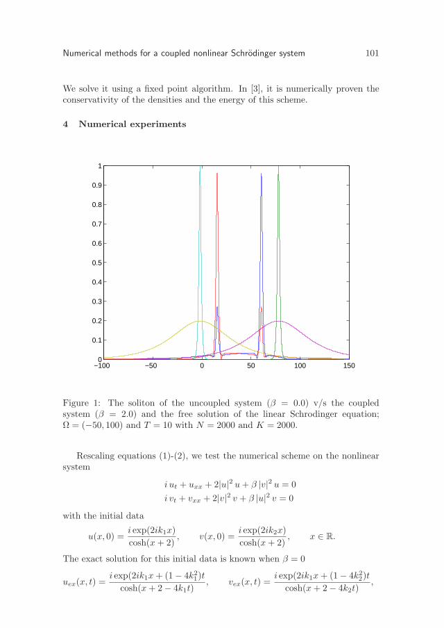
Numerical methods for a coupled nonlinear Schrodinger system 101
We solve it using a fixed point algorithm. In [3], it is numerically proven theconservativity of the densities and the energy of this scheme.
4 Numerical experiments
−100 −50 0 50 100 1500
0.1
0.2
0.3
0.4
0.5
0.6
0.7
0.8
0.9
1
Figure 1: The soliton of the uncoupled system (β = 0.0) v/s the coupledsystem (β = 2.0) and the free solution of the linear Schrodinger equation;Ω = (−50, 100) and T = 10 with N = 2000 and K = 2000.
Rescaling equations (1)-(2), we test the numerical scheme on the nonlinearsystem
i ut + uxx + 2|u|2 u+ β |v|2 u = 0
i vt + vxx + 2|v|2 v + β |u|2 v = 0
with the initial data
u(x, 0) =i exp(2ik1x)
cosh(x+ 2), v(x, 0) =
i exp(2ik2x)
cosh(x+ 2), x ∈ R.
The exact solution for this initial data is known when β = 0
uex(x, t) =i exp(2ik1x+ (1 − 4k2
1)t
cosh(x+ 2 − 4k1t), vex(x, t) =
i exp(2ik1x+ (1 − 4k22)t
cosh(x+ 2 − 4k2t),

102 M. Sepulveda and O. Vera
where x ∈ R and t > 0.
We choose k1 = 1.0 and k2 = 0.0, and the final time T = 10. We takeΩ = (−50, 100) to avoid any numerical reflections due to the boundaries.
Figure 1 shows the behavior of the solutions of the uncoupled system (whenβ = 0.0) comparing them with the free solutions and the behavior of solutionsof the coupled system (β = 2.0). These simulation were done for Ω = (−20, 50),T = 10.0, N = 2000 and K = 2000. We remark, as least for this two numericalexamples, that the solutions of the nonlinear system, coupled or uncoupled, cannot decay as the free solutions, that is on O(t−1/2), which is in agreement withthe statement of the Main Theorem and its proof.
0 5 10 15 20 25 30 35 40 45 500.1
0.2
0.3
0.4
0.5
0.6
0.7
0.8
0.9
1
1.1Norm L∞ of the coupled, uncoupled and free solutions
t
||⋅ ||
L∞
Figure 2: The L∞−norm of the solution for the free system (’−·’), the nonlinearuncoupled system with β = 0.0 (’−−’) and the nonlinear coupled system withβ = 2.0 (’continuous line’).
In Figure 2 we can see the behavior of the L∞−norm for the differentsolutions. We compare the L∞−norm of the solution for the nonlinearuncoupled system, that is for β = 0.0, which is constant in time (‖u‖L∞ =‖v‖L∞ = 1.0), with the coupled system, that is for β = 2.0, which oscillatein time, and with the solutions of the free linear Schrodinger equation, whichdecays as t−1/2. In this case, Ω = (−50, 250) and T = 50 with N = 50000 andK = 50000.
Numerical methods for a coupled nonlinear Schrodinger system 103
Acknowledgments
MS has been supported by Fondecyt project # 1070694 and Fondap in AppliedMathematics (Project # 15000001). OV and MS acknowledge support byCNPq/CONICYT Project, # 490987/2005-2 (Brazil) and # 2005-075 (Chile).
References
[1] J.E. Barab. Nonexistence of asymptotic free solutions for a nonlinearequation. J. Math. Phys. 25:3270–3273, 1984.
[2] C. Besse. A relaxation scheme for the nonlinear Schrodinger equation.SIAM J. Numer. Anal. 42:934–952, 2004.
[3] V. Bisognin, M. Sepulveda and O. Vera. On the nonexistence ofasymptotically free solutions for a coupled nonlinear Schrodinger system.Technical Report,DIM, U. de Concepcion, 14, 2007. Submitted.
[4] T. Cazenave. An introduction to nonlinear Schrodinger equations. Institutode Matematica. U.F.R.J. 22, 1989.
[5] T. Cazenave and F.B. Weissler. The Cauchy problem for the criticalnonlinear Schrodinger equation in Hs. Nonlinear Anal. T.M.A. 100:807–836, 1990.
[6] J.C. Ceballos, M. Sepulveda and O. Vera. Gain in regularity for a couplednonlinear Schrodinger system. Bol. Soc. Paran. Mat. 24(3):41–68, 2006.
[7] H. Ceniceros. A semi-implicit moving mesh method for the focusingnonlinear Schrodinger equation. Comm. in Pure and Appl. Anal. 1:1–18,2002.
[8] T. Colin and P. Fabrie. Semidiscretization in time for nonlinearSchrodinger-waves equations. Discrete Contin. Dynam. Systems. 4 :277–288, 1981.
[9] M. Delfour, M. Fortin and G. Payre. Finite-difference solutions of anonlinear Schrodinger equation. J. Comput. Phys. 44:227–288, 1981.
[10] R. Glassey. On the assymptotic behavior of nonlinear wave equations.Trans. AMS. 182(187): 187–200, 1973.
[11] N. Hayashi, K. Nakamitsu and M. Tsutsumi. On solutions on the initialvalue problem for the nonlinear Schrodinger equations in One SpaceDimension. Math. Z. 192:637–650, 1986.
[12] N. Hayashi, K. Nakamitsu and M. Tsutsumi. On solutions of the initialvalue problem for nonlinear Schrodinger equations. J. of Funct. Anal.71:218–245, 1987.
104 M. Sepulveda and O. Vera
[13] I.P. Kaminow. Polarization in optical fibers. IEEE J. Quantum Electron17:15–22, 1981.
[14] C. Lanczos. Linear Differential Operators. Van Nostrand-Reinhold London,1961.
[15] L.A. Maia, E. Montefusco and B. Pellacci. Positive solutions for a weaklycoupled nonlinear Schrodinger systems. J. Diff. Eqns. 229: 743–767, 2006.
[16] S.V. Manakov. On the theory of two-dimensional stationary self-focusingof electromagnetic waves. Sov. Phys. JET 38:248–253, 1974.
[17] C.R. Menyuk. Nonlinear pulse propagation in birefringence optical fiber.IEEE J. Quantum Electron. 23:174–176, 1987.
[18] C.R. Menyuk. Pulse Propagation in an elliptically birefringent Kerrmedium. IEEE J. Quantum Electron. 25:2674–2682, 1989.
[19] E.S.P. Siqueira. Comportamento assintotico das solucoes de um sistemanao linear de equacoes de Schrodinger. Tese de doutorado. U.F.R.J., 1990.
[20] E.S.P. Siqueira. Asymptotic behavior of the solutions of a nonlinearsystem of Schrodinger equations. Nonlinear analysis, Theory Meth. & Appl.20(10):1231–1243, 1993.
[21] W. Strauss. Nonlinear scattering theory. Scattering Theory in MathematicalPhysics. 53–78, 1974.
[22] V.E. Zakharov and A.B. Shabat. Exact theory of two-dimensional self-focusing and one dimensional self-modulation of waves in nonlinear media.Soviet Physics, JETP 3(1):62–69, 1972.
Bol. Soc. Esp. Mat. Apl.no 43(2008), 105–169
PREMIO S~eMA DIVULGACION
THE NAVIER-STOKES EQUATIONS. A CHALLENGE TONEWTONIAN DETERMINISM
XAVIER MORA
Departament de Matematiques,
Universitat Autonoma de Barcelona
Abstract
The question of global existence and uniqueness of solutions of thetime-dependent Navier-Stokes equations is reviewed. Special emphasisis put on its philosophical implications and the historical perspective.An attempt is made to approach the core of the problem while keepingtechnicalities to a minimum.
Key words: Navier-Stokes equations, global existence, uniqueness, regularity.
AMS subject classifications: 35Q30, 76D03, 76D05.
One of the most valued features of science is its ability to predict the future.For instance, celestial mechanics is able to predict eclipses with great precisionand well in advance of their taking place. More related to the subject of thisarticle is the case of meteorology; in this case, predictions are not as precise andlong-lasting as one would like, but they are still quite remarkable.
In these examples, and many others of the same kind, the possibility ofpredicting the future evolution of a system is based upon knowing in detail thelaws that govern that evolution, as well as its present state. Mathematically,the state of a system is described by means of a more or less large collectionof numeric variables, and the laws that govern the temporal evolution of thesevariables take usually the form of differential equations. These equations specifya condition that must be satisfied at every moment in time and that determinesthe rate of variation of the different variables as a function of their value atthat very moment. In the case of celestial mechanics the state variables are thepositions and velocities of the different bodies, and the differential equationsare provided by Newton’s laws, namely that the mass of a body times itsacceleration is equal to the force that acts on it, and that this force can be
This article originates from a talk given in the Trobada en honor de Carles Perello :
Matematica i Pensament (Sant Cugat del Valles, 16th Novembre 2002) and another one givenin the IV Cicle de Matematiques Ferran Sunyer i Balaguer (Sabadell, 24th February 2005).
105

106 X. Mora
calculated from the positions of the different bodies by means of the formulathat we know as the law of universal gravitation.
The Navier-Stokes equations are simply the differential equations thatgovern another form of motion, namely the motion of a fluid, for instance air orwater. In fact, these equations are still expressing Newton’s law —mass timesacceleration is equal to force—, although here one is not considering a finiteset of particles but a continuum of matter. Another difference from celestialmechanics is that the Navier-Stokes equations take into account the frictionforces, which act so as to slow the motion down. In this article we restrictourselves to the special case of an incompressible fluid, i. e. a fluid of constantdensity, which is approximately the case of liquids.
It goes without saying that a quantitative knowledge about fluid motions isimportant in many fields of science and technology, from physiology to airplaneindustry.
As we have suggested, one expects that the Navier-Stokes equations willshare with the equations of celestial mechanics the property of determining thefuture evolution from the present state. However, certain difficulties arise whenone faces the task of providing a proper mathematical proof of such a statement.In the case of celestial mechanics, and many other differential equations, such aproof can indeed be given. But the Navier-Stokes equations resist tenaciouslyto it. In spite of the earnest efforts that have been made about it, until now onehas not been able to prove mathematically neither the supposed determinismof these equations nor the absence of it.
The difficulties that arise in this mathematical problem are not deprived ofphysical meaning. Already at the end of the nineteenth century, some accurateexperimenters had pointed out that in certain situations the motions of fluidsexhibited an apparent lack of determinism. This experimental phenomenon wasgiven the name of turbulence, since what is observed is not so different fromthe ordinary meaning of this term. On the other hand, such an apparent lackof determinism could be simply a consequence of an insufficient precision in thespecification of the initial state. In fact, today it is well known that the exactsolutions of a differential equation can be perfectly deterministic at the sametime that they exhibit a highly sensitive dependence on the initial state, so thatin practice one observes an apparently non-deterministic behaviour. Towards1960 the meteorologists became well aware of such a possibility, thanks to thecomputing power provided by electronic machines, and some years later theychristened it as the “butterfly effect”.
In this regard, it must be remarked that the problem about the determinismof the Navier-Stokes equations could be more severe than a simple butterflyeffect: According to the present state of affairs, it could be that theexact solutions of the Navier-Stokes equations were genuinely indetermined!Distinguishing between one thing and the other is probably not important forpractical purposes, but it is certainly important for science as an instrument forunderstanding the world.
The Navier-Stokes equations 107
The importance of the problem has been recognized by several people andinstitutions that have engaged in giving a list of mathematical challenges for thetwenty-first century [72–81]. In particular, it is one of the seven “MillenniumProblems” for which the Clay Mathematics Institute (CMI) has established aprize of one million dollars. Let us remark, however, that the specific problemstated by the CMI (see [78]) is not concerned exactly with the question ofdeterminism. In fact, the notion of determinism is about the existence anduniqueness of solutions, whereas the CMI statement is about their existenceand regularity. As we will see, a positive answer to the latter question impliesa positive answer to the former, i. e. the question of determinism, but theconverse implication is not true. In this connection we fully agree with Ol’gaLadyzhenskaya [31] and other authors in that the really important question isthat of determinism, and this point of view will prevail in the present exposition.
1 Differential equations and determinism: the case of celestialmechanics
In order to help understand the meaning of the Navier-Stokes equations and thedifficulties with the question of determinism, it will be good to keep in mindthe case of celestial mechanics.
In that case one wants to describe the motion of celestial bodies. Naturally,such a description must start by giving a list of the bodies under consideration;symbolically, this can be done by means of an index α that takes integer valuesfrom 1 to N , the number of bodies. Of course, one must pay attention to theposition of each body α . In the following we will denote it by xα and wewill assume that it is specified by cartesian coordinates x = (x, y, z). Anotheressential component of the description is the variable time t .
The motion of the bodies is certainly described by the functions t 7→ xα(t),one for every α . However, in order to attain a deterministic descriptionone needs to go into more details. To begin with, it is essential to considerthe velocity u , that is, the derivative of the position with respect to time,u = dx/dt . Like position, we assume that the velocity is specified by thecorresponding cartesian coordinates u = (u, v, w), and the velocity of eachbody α will be denoted by uα . If at time t we know not only the position ofa body but also its velocity, then we can figure out an estimate of the positionof that body after a short interval of time. Similarly, the fact that velocity canchange with time leads to considering its own derivative du/dt , that is, theacceleration : if at time t we know the velocity and the acceleration, then wecan figure out an estimate of the velocity after a short interval of time. But theacceleration can also change with time, so that in principle one should consideralso its own derivative, and so on towards derivatives of progressively higherorders.
At first sight it looks like we have gone into an endless spiral. But it is not so:as Robert Hooke and Isaac Newton discovered towards 1679–80, it turns outthat nature has certain laws that determine the accelerations of celestial bodies
108 X. Mora
out of their positions! This changes things in a crucial way: if at time t we knowthe positions and velocities of the different bodies, then these laws determinealso their accelerations, and therefore we can get an estimate of the positionsand velocities after a short interval of time; but from here we can now repeatthe same process over and over towards progressively larger times.
The laws in question are known today as Newton’s second law of motion andthe law of universal gravitation. Newton’s second law has a very wide scope andit can be viewed as saying that the product of the mass times the accelerationof a body is equal to the sum of the forces acting on that body, and thatthese forces are determined by some function of the positions of all bodies, andpossibly also of their velocities. The law of universal gravitation is simply aspecification of this function in the case of celestial mechanics.
So, the deterministic description of the motion of celestial bodies can besummarized in a set of equations of the following form:
dxα/dt = uα,
duα/dt = fα(x1,x2, . . . ,xN ) /mα,(1)
where mα denotes the mass of the body α , and fα gives the gravitational forceon the body α as a function of the relative positions of all bodies. Specifically,this function is given by the following formula:
fα(x1,x2, . . . ,xN ) =∑
β 6=α
Gmαmβ |xβ − xα|−3 (xβ − xα), (2)
where G is a universal constant and |v| denotes the length of a vector v .
Conceptually, the system of equations (1) has the form
dZ/dt = F (Z). (3)
In the case under consideration Z represents the collection of all positions xα
and velocities uα , i. e. a collection of 6N numbers, and F represents thecollection of functions that, starting from these numbers, determine the right-hand sides of (1). Using a more general terminology, Z represents the state ofthe system under consideration, which can change with time. Equation (3) saysthat at every moment t this state is varying in a specific way dZ/dt which isdetermined by the own value of Z at that very moment.
But what we are interested in is the possibility of determining the futureout of the present, that is seeing whether Z(0) determines Z(t) for t > 0.If the derivative is interpreted as a quotient of infinitesimal quantities, one cansay that equation (3) embodies that determinism for infinitesimal values of t .A fundamental task of the theory of differential equations deals with goingover from here to finite values of t , and seeing whether this can be achievedfor arbitrarily large values of t . Traditionally, one distinguishes three aspectsof the problem, namely the existence, the uniqueness, and the globality of thedesired solution of (3). When Z is specified by a finite collection of numbers, likein celestial mechanics, we are in the field of the so-called ordinary differential

The Navier-Stokes equations 109
equations, for which there are fairly complete results about these questions.Applied to the equations of celestial mechanics, these results guarantee thedeterminism of the motion as long as the bodies do not collide with each other(notice that the right-hand side of (2) is not well defined when some xβ coincideswith xα ).
2 The equations of motion of an incompressible fluid
2.1. In accordance with the molecular constitution of matter, one can viewa fluid as a multitude of small bodies interacting with each other. From thatpoint of view, the case of a fluid would not be so different from that of celestialmechanics. However, there is a circumstance which changes things quite a lot:now the number of bodies in play is extremely large, of the order of 1023 (thisquantity corresponds to about 3 grams of water). Obviously, with such figures itis totally out of the question to think about putting into practice the approachof the preceding section. For instance, even if we had at our disposal all thecomputer storage presently existing on our planet, this would only allow tospecify the initial state of a few micrograms of water.
In front of this, one cannot but resort to a less detailed point of view. We willdo this by looking at the fluid not as a discrete collection of molecules, but as acontinuous distribution of matter over space. In contrast to the case of celestialmechanics, now the variable α that indexes the “particles” in interaction willnot be restricted to a finite set, but we will allow it to take values in a continuousset. Contrary to what it may seem, the resulting model will be much easier todeal with than one concerned with a finite but very large number of interactingparticles.
Like in the case of celestial mechanics, in principle the motion of the fluidis specified by a function of α and t , namely the position of each particle αat time t . Because of the continuous character of the variable α , now wewill prefer to write x(α, t) instead of xα(t), but this is just a question ofnotation. A quite natural hypothesis that we will adopt is that two differentparticles cannot be in the same position at the same time; in other words,the mapping α 7→ x(α, t) is one-to-one at every time t . We will also assumethat the fluid permanently fills a certain region (i. e. an open and connectedsubset) of space; this region and its boundary will be denoted respectively by Ωand ∂Ω. In such conditions, the function x(α, t) defines a change of variables(α, t) ↔ (x, t) that leads to an alternative description where the independentvariables are not the particle α and the time t , but the position x ∈ Ωand the time t . Among the variables that depend on x and t it is especiallyrelevant the velocity u ; by definition, u(x, t) means the velocity at time t ofthe particle that is occupying the position x at that very moment t .
Since we are interested in the question of whether the future of the fluid isdetermined from its present, the independent variables x and t play differentroles. So, when dealing with functions of x and t we will tend to look atthem not as such but rather as functions of x that change with time t , which

110 X. Mora
is essentially the same, but more in the spirit of our interests. Symbolically,instead of functions (x, t) 7→ f(x, t), we will tend to think in terms of functionst 7→ f(t) where each value f(t) is itself a function of x (namely the functionx 7→ f(x, t)). In particular, the velocity will be looked at as a vector field thatchanges with time (here we use the classical terminology where the functions ofposition are called “fields”).
2.2. As it will be seen shortly, the character of the problem calls for anextensive usage of the tools of infinitesimal calculus, especially those that dealwith functions of several variables, like partial derivatives, volume integrals andsurface integrals. Typically, these tools presume certain regularity hypotheseson the functions involved, as well as on the regions and surfaces of integration.In this connection, it is important to distinguish between the regularityhypotheses that refer to the data of the problem, like the region Ω and itsboundary ∂Ω, and those that refer to the unknowns, especially the velocityfield u . In the latter case, we must consider them as working hypotheses thatawait confirmation.
To a great extent, the difficulty of the problem lies precisely in the fact thatsome of these working hypotheses do not get such a confirmation.
In some cases this is not so bad, since it is solved by means of a suitablegeneralization of the notions involved (in complete analogy to how the equationx2 =2 leads to extending the notion of number, passing from rational numbers to“real” ones). Among the generalized notions that suit our problem are especiallyrelevant the Lebesgue integral and the weak derivatives. In fact, the Navier-Stokes equations have played an important historical role as a motivation for thedevelopment of these now standard techniques, especially the weak derivatives.
In other cases the problem is more serious: neither a generalization is foundthat eliminates the need for the hypothesis in question, nor a proof is found ofits fulfilment.
In this connection, this exposition has the spirit of not entering into suchtechnicalities unless it becomes absolutely necessary; let us say that “everyfunction is as regular as needed unless there is a reasonable evidence to thecontrary”. In particular, we will not be especially precise about the regularityhypotheses to be imposed on the data of the problem, since the existing resultsshow no substantial improvement no matter how much regular the data areassumed to be. On the other hand, concerning the unknowns, for the momentwe will adopt the working hypothesis that they are as regular as needed, andlater on we will make the amendments that turn out necessary.
2.3. As we have already mentioned, we will restrict our attention to the caseof a homogeneous incompressible fluid. By definition, this means that thedensity ρ remains constant, that is, independent of x and t . Combined withthe principle of mass conservation, this hypothesis entails a crucial constrainton the velocity field. In the following we will enter into some details to see how
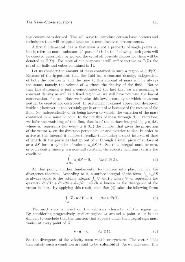
The Navier-Stokes equations 111
this constraint is derived. This will serve to introduce certain basic notions andtechniques that will reappear later on in more involved circumstances.
A first fundamental idea is that mass is not a property of single points x ,but it refers to more “substantial” parts of Ω. In the following, such parts willbe denoted generically by ω , and the set of all possible choices for them will bedenoted as P(Ω). For most of our purposes it will suffice to take as P(Ω) theset of all balls and cubes contained in Ω.
Let us consider the amount of mass contained in such a region ω ∈ P(Ω).Because of the hypothesis that the fluid has a constant density, independentof both the position x and the time t , this amount of mass will be alwaysthe same, namely the volume of ω times the density of the fluid. Noticethat this statement is just a consequence of the fact that we are assuming aconstant density as well as a fixed region ω ; we still have not used the law ofconservation of mass. Now we invoke this law, according to which mass canneither be created nor destroyed. In particular, it cannot appear nor disappearinside ω ; however, it can certainly get in or out of ω because of the motion of thefluid. So, independently of its being known to vanish, the variation of the masscontained in ω must be equal to the net flux of mass through ∂ω . Therefore,we infer the vanishing of this flux, that is of the surface integral
∫∂ωρ u⊥dS ,
where u⊥ represents (for every x ∈ ∂ω ) the number that gives the projectionof the vector u on the direction perpendicular and exterior to ∂ω . In order toarrive at this integral it suffices to realize that during a short interval of timeof length dt the particles that go out of ω through a small piece of surface ofarea dS form a cylinder of volume u⊥dS dt . So, that integral must be zero,or equivalently, since ρ is a non-null constant, the velocity field must satisfy thecondition ∫
∂ωu⊥dS = 0, ∀ω ∈ P(Ω). (4)
At this point, another fundamental tool enters into play, namely thedivergence theorem. According to it, a surface integral of the form
∫∂ωu⊥dS
is always equal to the volume integral∫
ω∇·udV , where ∇·u represents the
quantity ∂u/∂x + ∂v/∂y + ∂w/∂z , which is known as the divergence of thevector field u . By applying this result, condition (4) takes the following form:
∫
ω∇·u dV = 0, ∀ω ∈ P(Ω). (5)
The next step is based on the arbitrary character of the region ω .By considering progressively smaller regions ω around a point x , it is notdifficult to conclude that the function that appears under the integral sign mustvanish at every point of Ω:
∇·u = 0, ∀x ∈ Ω. (6)
So, the divergence of the velocity must vanish everywhere. The vector fieldsthat satisfy such a condition are said to be solenoidal . As we have seen, this
112 X. Mora
condition is a local version of the integral condition (4), which expresses the lawof conservation of mass in the particular case of an incompressible fluid.
2.4. Another fundamental equation for describing the motion of a fluid derivesfrom similar considerations in connection with momentum instead of mass.The details are here more involved, but the argumentation follows essentially thesame lines. In the same way as the amount of mass contained in ω is given by thescalar
∫ωρdV , the amount of momentum is given by the vector
∫ωρudV . Like
in the case of mass, the motion of the fluid entails also a transport of momentumthrough ∂ω . However, the momentum need not remain constant, neither in afixed region of space, like ω , nor in a material part of the fluid (a fixed set ofparticles α , whose positions change with time). Even so, Newton’s second lawensures that the time-variation of the momentum of a material part of the fluidis determined by the forces that act on it. These forces divide into two kinds:those that act over a distance, like gravity, and those that act by contact, whichare associated with the notions of pressure and friction. If we are not dealingwith a material part of the fluid but with a fixed region of space, then we musttake into account also the flux of momentum through the boundary.
Altogether one arrives at the following equation:
d
dt
(∫
ωρudV
)+
∫
∂ωρuu⊥ dS =
∫
ωf dV +
∫
∂ωTe⊥ dS, ∀ω ∈ P(Ω). (7)
The first term of this equation is the derivative of the momentum contained in ω ,whereas the other three terms correspond respectively, from left to right, to thetransport through ∂ω , the distance forces and the contact ones. The distanceforces are represented simply by a vector field f with dimensions of force perunit of volume, whereas the contact forces require a more elaborate description:e⊥ represents the unit vector in the direction perpendicular and exterior to ∂ω ,and Te⊥ represents a vector, with dimensions of force per unit of area, whichis obtained from e⊥ by means of a linear map T that generally depends on theposition x (and the time t); this linear map is called the stress tensor and incartesian coordinates it is given by a symmetric matrix.
Equation (7) expresses Newton’s second law. Analogously to the role of thelaw of universal gravitation in celestial mechanics, here one must also providesome supplementary information for determining f and T at every point x .Concerning f , we will assume simply that we directly know its dependence on xand t . Concerning T , the question is more involved, not only on account ofthe tensorial character of this variable, but rather because its dependence on xand t is, partially, through the velocity field u . In fact, the forces of frictionbetween two bodies in contact depend on their relative velocities. For standardfluids, the law that relates the stress tensor T with the velocity field u hasthe following form (for brevity, we directly write a formula specialized for theincompressible case):
T = −p I + µ (∇u+ (∇u)t). (8)

The Navier-Stokes equations 113
The two terms of this formula correspond respectively to the notions of pressureand friction. The pressure p is a scalar variable that depends directly on xand t ; this variable appears as a coefficient of I , which represents the identitymatrix. The friction forces are given by the second term, where ∇u representsthe matrix that contains the derivatives of (u, v, w) with respect to (x, y, z),(∇u)t represents the matrix obtained by transposing the preceding one, and µ isa positive coefficient, known as (the dynamic coefficient of) viscosity, whosevalue depends on the material of the fluid. For more details about the meaningof equations (7) and (8) and their different terms the reader is referred to [67].
Now we will pass from the integral equation (7), valid for an arbitraryregion ω , to a differential equation valid at every point x . This is done incomplete analogy with the preceding section, that is, by making use of thedivergence theorem and the arbitrary character of the region ω . Besidesthat, here we will perform some additional minor operations, like puttingd(∫
ωρudV )/dt =
∫ωρ (∂u/∂t) dV (which holds if u is regular enough),
dividing by the constant ρ , and using equations (8) and (6). Altogether itresults in a vector equation that can be written in the following way:
∂u/∂t+ (u ·∇)u = f −∇p+ ν∆u, ∀x ∈ Ω. (9)
Here, ∇p represents the gradient of p , i. e. the vector of coordinates( ∂p
∂x ,∂p∂y ,
∂p∂z ), ∆ represents the Laplace operator ∂2
∂x2 + ∂2
∂y2 + ∂2
∂z2 , and u · ∇represents the differential operator u∂
∂x +v ∂∂y +w ∂
∂z . The two last operatorsare applied separately to each component of u . Finally, ν denotes thequotient µ/ρ , which is known as (the kinematic coefficient of) viscosity, andf and p are the same as before but divided by the constant ρ (alternatively,we can imagine that the units have been chosen in such a way that the valueof ρ is equal to one). Notice that the left-hand side of (9) is nothing elsethan the acceleration of the particle which is passing through the point x ,i. e. the derivative of u with respect to t when one fixes α (not x); in fact,the chain rule applied to the composition (α, t) 7→ (x, t) 7→ u ensures that thisderivative is equal to ∂u/∂t + ∇u · ∂x/∂t = ∂u/∂t + u · ∇u , and similarlywith the other components of u . Notice also that the pressure appearsin the equation only through its gradient, so that two pressure fields witha constant difference between them can be considered equivalent to each other.
Equation (9) was obtained in the first half of the nineteenth centuryby several authors: Claude Navier (1822), Augustin Cauchy (1822), Si-meon Poisson (1829), Adhemar Barre de Saint-Venant (1843), and GeorgeStokes (1845) [2–6]. Nowadays we know it by the name of the first andlast of these authors, but the other three also arrived at it more or lessindependently of each other. The reader interested in the historical detailsis referred to [68]. The principal merit of these authors was finding the wayto describe friction, by means of the stress tensor T , since in the absence offriction the corresponding equations (ν=0) had been obtained already in 1755by Leonhard Euler [1].
114 X. Mora
2.5. With a view towards determining the future of the fluid from its present,equations (9) and (6) must be supplemented with some additional conditionson u that specify what happens at the limits of the region Ω.
In this connection, one often considers the case where Ω represents acontainer whose walls are at rest. In this case, a viscous fluid is bound tosatisfy the following non-slip condition :
u = 0, ∀x ∈ ∂Ω. (10)
This condition can be decomposed into two parts which are concernedrespectively with the normal and tangential components of u at ∂Ω, whichwe will denote respectively by u⊥ and u// (u = u⊥e⊥ + u// ):
u⊥ = 0, ∀x ∈ ∂Ω, (10)⊥
u// = 0, ∀x ∈ ∂Ω. (10)//
Conditions (10)⊥ and (10)// lie on different grounds: the first one obeys topurely kinematical reasons, whereas the second is a consequence of viscosity.As it will be seen below, they play different roles in the mathematics of theproblem. The vector fields that satisfy condition (10)⊥ are said to be “parallelto the boundary”.
In the case of an unbounded region Ω, which arises in a natural way whenstudying small-scale phenomena ocurring away from any boundary, one needsalso some condition at infinity, i. e. a specification of the behaviour of thevelocity u when x goes away towards infinity. In this connection, it often suitsa condition of the form
u→ 0, as |x| → ∞. (11)
On the other hand, some mathematical aspects of the problem call for conditionsmore restrictive than (11), like some condition of the following sort:
In the limit |x| → ∞ the vector field u tends to zero at leastas fast |x|−α , and its spatial derivatives of order k≤m satisfysimilar conditions with the exponent α+k instead of α .
(12)
However, such conditions can be considered as conditions of regularity atinfinity, so, in the spirit of § 2.2, we will not enter into details about them. Let usremark only that they can be related to the convergence of certain integrals, inparticular the one that gives the kinetic energy, namely ρ 1
2
∫Ω|u|2 dV .
Although the preceding paragraphs did not refer explicitly to time, of courseall of these equations and conditions are required to hold at every moment t .Let us recall also here that our main interest lies in determining the solutionfor t > 0 from an initial condition of the form
u | t=0 = u0, (13)
where the vector field u0 is suposed to be given.
The Navier-Stokes equations 115
2.6. The region Ω occupied by the fluid will be supposed to be either three-dimensional or two-dimensional. The latter case is not just an academic exer-cise, but it corresponds to the case of a three-dimensional region of the form(x, y, z) | (x, y) ∈ Ω, z ∈ R where every particle of the fluid is moving on aplane perpendicular to the direction z , and this motion is independent of z .Such motions are called plane motions.
In particular, one can single out the following three cases, with n = 2 or 3:
(i) Ω is a bounded region of Rn and u is required to satisfy
condition (10).
(ii) Ω is the whole space Rn and u is required to satisfy condition (11).
(iii) Ω is the torus Rn/Zn ; or equivalently: Ω is the whole space R
n
and u is required to satisfy a condition of periodicity in n orthogonaldirections.
The cases (ii) and (iii) are less realistic than (i), but they retain theessential difficulties of the problem while simplifying some technical aspects; thissimplification is due to the fact that some aspects of the problem lend themselvesto explicit computation, mainly because ∂Ω = ∅ . This relative simplicity is thereason why the “millennium problem” posed by the Clay Mathematics Institute
is restricted to the cases (ii) and (iii) (with n=3).
On the other hand, we will also specialize to the case where distance forcesare not present: f = 0 . Instead, we could consider the general case where thefield of distance forces is the gradient of a “potential”, f = ∇φ , which is thecase of gravity. But this apparently more general case reduces to f = 0 bytaking q = p − φ as a new variable instead of p . So, we are concerned withthe problem of solving the Navier-Stokes equations (9) (with f = 0) and (6)together with conditions (10), (11) and (13). The complete system of equationsis thus the following:
∂u/∂t = ν∆u− (u ·∇)u−∇p, ∇·u = 0,
u |∂Ω = 0, u |∞ = 0, u |t=0 = u0,(14)
where the expression u |∞ = 0 must be understood as a symbolic representationof the condition at infinity (11). From now on we will refer to these equationsalso as (14.1)–(14.5), and instead of (10)⊥ and (10)// we will also write (14.3)⊥and (14.3)// . Notice that in the case (i) there is no way for x ∈ Ω to goaway to infinity, so that condition (14.4) is then empty. On the other hand,condition (14.3) is empty in the case (ii), because then ∂Ω = ∅ . Finally, in thecase (iii) Ω is a torus, without any boundary nor the possibility of going awayto infinity, so that both (14.3) and (14.4) are then empty.
3 Perspectives of determinism
3.1. Let us begin by noticing that we have somehow so many equations asunknowns. In fact, only two of the equations listed in (14) are required to hold

116 X. Mora
on the whole of Ω, namely equations (14.1) and (14.2), of which the first one hasa vector character whereas the second has a scalar character. Correspondingly,there are also two unknown functions to be determined on the whole of Ω,namely the vector field u and the scalar field p .
As we have already suggested in § 1, we intend to look at system (14) asan “abstract” equation of the form (3), namely dZ/dt = F (Z), where Z is anobject that represents the varying state of the system. According to what wehave just said, it looks like Z amounts to specifying the fields of velocity andpressure, u and p . This is true to a certain extent, but there is somethingwhich looks awkward: If we know the fields u and p at a certain moment oftime, then we know the right-hand side of (14.1), which determines ∂u/∂t .However, equation (14.2), which corresponds somehow to pressure, does notinvolve ∂p/∂t . The solution to this puzzle is that conditions (14.2), (14.3)⊥and (14.4) determine p directly from u : at every moment in time there is onlyone pressure field (except for an additive constant) that keeps the evolution of uwithin those conditions.
This is due to a result that can be traced back to Stokes (1849) [7] andHermann von Helmholtz (1858) [9] and that can be stated in the followingterms: Every vector field on a bounded region decomposes in a unique way as
a sum of a gradient field plus a solenoidal field parallel to the boundary; the
same holds for an unbounded region if one restricts oneself to fields vanishing
at infinity. So, for every vector field g on Ω that satisfies g |∞ = 0 there isa unique gradient field ∇q for which v = g − ∇q satisfies ∇ · v = 0 in Ω,v⊥ = 0 in ∂Ω, and v |∞ = 0 . By applying this result to the vector field thatappears in equation (14.1), namely g = ν∆u − (u ·∇)u , we see that ∇p isindeed determined by the restriction that ∂u/∂t keeps conditions (14.2), (14.3)⊥and (14.4).
According to these remarks, the problem that we are dealing with fits intoan abstract equation of the form dZ/dt = F (Z), where Z reduces to specifyingthe velocity field u .
3.2 Like many other differential equations, the equations of Navier-Stokesdo not lend themselves to an explicit resolution. At least, this can be doneonly in just a few particular cases. However, one can always try to solve themnumerically; in other words, one can look for an approximate solution by meansof numerical methods.
In this connection it is worth mentioning that the development of numericalmethods for partial differential equations was motivated to a certain extent by afield quite related to the one that we are dealing with, and quite relevant to dailylife, namely meteorology. Certainly, the weather is a matter of certain physicalprocesses, among which it is especially relevant the motion of the atmosphereas a fluid; so one can look at its evolution in time as governed by a system ofpartial differential equations that contains certain variants of the equations offluid dynamics [69]. Already in 1904, the norwegian mathematician Vilhelm
The Navier-Stokes equations 117
Bjerknes was looking at weather forecast as a question of numerically solvingthe relevant differential equations from a given initial state [11]. Of course,he lacked the computing tools of today, instead of which he made use of certaingraphical techniques. A few years later, in 1920, the british mathematicianLewis Fry Richardson was attacking the same problem by means of the finite-difference method, that is, by resorting to a close net of discrete values of thecoordinates of space and time and replacing the partial derivatives by quotientsof finite differences. Nevertheless, he still lacked the present day computingtechnology: in order to work out a six-hours forecast he needed six weeksof intensive calculation! Such figures started to change at the middle of thetwentieth century with the arrival of the first computers: in 1953, as a finalresult of a project promoted by John von Neumann, the computer MANIAC I(Mathematical Analyzer, Numerical Integrator And Computer) of Princeton’sInstitute for Advanced Study was already able to produce reasonable weatherforecasts of 24 hours with a computing time of the order of 10 minutes. Sincethen, the power of computers has not ceased to increase, and the numericalmethods have also been made more efficient, with the result that the numericalsolution of the equations of meteorology or the Navier-Stokes equations isnowadays within reach of a personal computer. The reader interested in thestate of the art of the numerical solution of the Navier-Stokes equations isreferred to [70], which reviews the so-called method of finite elements.
Anyway, the computational meteorologists did not take long to realize thatthe predictions produced by the computers were very sensitive to small changesin the initial data: slightly different initial states led often to quickly divergingevolutions, so that after a relatively short period of time these evolutions seemedquite unrelated to each other. This sensitivity with respect to the initial datawas put forward in a crucial symposium held in Tokyo in 1960, where EdwardLorenz reported several “experimental” instances of it. Shortly afterwards,in 1963, Lorenz himself showed that the phenomenon can already be present inthe exact solutions of quite simple systems of ordinary differential equations.Nowadays we know it as “butterfly effect”, by the title of a talk given by Lorenzin 1972: “Predictability: Does the flap of a butterfly’s wings in Brazil set off atornado in Texas?”
3.3 These numerical and theoretical remarks made by Lorenz bear someresemblance to certain experimental observations on real fluids that had beenmade already in the nineteenth century, mainly by Osborne Reynolds in1883 [10].
Reynolds’ experiment dealed with the flow of water through a long horizontalpipe. The entrance to the pipe was submerged in a large reservoir where thewater was practically at rest. At the other end there was a valve that allowedto control the rate of flow, i. e. the amount of water passing through the pipeper unit of time. The entrance was a well-rounded funnel and near to it therewas a capillary that let aniline-dyed water out towards the entrance of the pipe.The whole apparatus was made of glass, which allowed to observe the motion of
118 X. Mora
the dyed water. When the flow rate was small, the dyed water formed a threadwhich remained clear-cut and rectilinear along the whole length of the pipe.In contrast, for larger flow rates this clear-cut and rectilinear character lastedonly up to a certain distance of the entrance, after which the thread startedundulating and wiggling until the dye was eventually dispersed over the wholesection of the pipe.
This phenomenon is called turbulence , since what is observed is notso different from the ordinary meaning of this term. Generally speaking,turbulence occurs for sufficiently large values of a dimensionless parameter todayknown as the Reynolds number, namely Re = Ud/ν , where U represents theaverage velocity of the fluid through the pipe (that is, the rate of flow dividedby the area of the section), d is the diameter of the pipe, and ν is the kinematicviscosity of the fluid.
Reynolds’ experiment is especially remarkable in that the turbulent motiondevelops out of a flow that starts being quite straight and apparently shouldremain in the same way, but it does not. This is highly reminiscent of alack of determinism or a high sensitivity with respect to the initial conditions.Somehow, the variable time t is here replaced by the distance x from thebeginning of the pipe, but these two variables are related to each other throughthe average velocity U , which is fixed by the experimental settings.
3.4 So, both the experiments with real fluids and the numerical simulationsshow signs of an apparent lack of determinism, or at least a high sensitivitywith respect to the initial conditions.
Concerning the numerical simulations, one must keep in mind that theyare not giving the exact solutions of the equations of motion of the fluid.In principle, one expects that the numerical solution will approach the exactone as the mesh of the net becomes smaller. However, in the same way assolutions can show a high sensitivity to small changes in the initial conditions,they could also show a similar phenomenon with respect to small changes inthe equations. Therefore, even if we get numerical solutions defined for alltimes t ≥ 0, in general it is not clear that they stay near to an exact solution.
Altogether the following question therefore stands:
Question 1 Is it true that the Navier-Stokes equations determine all the futuremotion of the fluid out of its initial state?
In other words: Is it true that for every initial state there is only one solutionof the Navier-Stokes equations, and that this solution is determined for alltime t ≥ 0? Or still: Is it true that the “evolution problem” for the Navier-Stokes equations has the properties of existence, uniqueness and globality ofsolutions?
The Navier-Stokes equations 119
4 The functional point of view
4.1. We have seen that in order to specify the state of motion of anincompressible fluid it suffices to give the velocity field u . As we have alreadymentioned, we think of the dependence of u on the position x as an “internal”component of a certain object, and it is this object as a whole what we viewas varying with the time t . This point of view is characteristic of functionalanalysis, where functions defined on some region Ω are viewed as points ofcertain abstract spaces.
In fact, one can say that the study of the Navier-Stokes equations has playedan important role in the development of several parts of functional analysis.For instance, later on we will see that some crucial ideas of the celebratedtheory of distributions, which Laurent Schwartz formulated in detail in 1950–51,appear already in the works of Carl Oseen (1910) and Jean Leray (1933–34)about the Navier-Stokes equations (significantly, in 1934–35 the latter wasexposing them in some lectures at the College de France where the youngSchwartz was one of the attendees). Other subjects of functional analysis thathave received a definite impulse from the study of the Navier-Stokes equationsare, for instance, semigroup theory, differential equations in Banach spaces, andfractional powers of operators.
4.2. In the following we briefly introduce the basic notions that we need fromfunctional analysis as well as their associated notations. Let us remember thatthe objects of our interest are functions on Ω, especially those with valuesin R
n , like the velocity field u . Such functions form certainly a linear space,but in contrast to R
n this space does not have a finite basis. Even so, one canstill apply several tools of great utility.
To begin with, we will make use of the notion of norm , which can be viewedas extending the notion of length of a vector from R
n . A norm is just a suitableway to measure the magnitude of a “vector”. In the case that interests us, onecan choose from multiple options, among which we will single out the sup norm‖u‖∞ = sup
x∈Ω |u(x)| and the quadratic norm ‖u‖2 = (∫Ω|u(x)|2 dV )1/2 ,
where |w| denotes the length of a vector w from Rn . The quadratic norm is
especially significant in our problem, since its square is essentially the kineticenergy (it differs from it by the factor ρ/2).
Matching up with the quadratic norm, it is interesting to consider alsothe operation that combines two vector fields u,v into the number 〈u ,v〉 =∫Ωu(x) ·v(x) dV , where w ·w′ denotes the scalar product of two vectors w
and w′ from Rn . In particular, 〈u ,u〉 = ‖u‖2
2 . This operation is referredto as scalar product (or inner product) of the vector fields u and v , sinceits properties are analogous to those of the scalar product of vectors from R
n .By analogy with the latter case, the functional scalar product that we have justdefined gives rise to a notion of orthogonality, which is especially useful in theproblem that we are dealing with. By definition, two vector fields u and v are
120 X. Mora
orthogonal to each other when 〈u ,v〉 = 0. On the other hand, sometimes thequestion is not so much whether 〈u ,v〉 is zero, but whether it is positive ornegative, that is, whether the angle formed by u and v is acute or obtuse.
Every norm gives rise to a notion of distance , which determines a topology.By definition, the distance between u and v is the magnitude of their difference,that is ‖u− v‖ . Contrary to what happens in finite-dimensional vector spaces,a sequence of functions can converge in one norm but diverge in another.Similarly, if we have a vector field that varies with time, this variation canbe continuous in one norm but not in another. Therefore, the choice of thenorm can be crucial when analyzing the different aspects of the problem thatwe are dealing with.
On the other hand, in order to ensure the existence of solutions for certainequations, it is essential to place oneself in a complete space (that is, a spacewhere all Cauchy sequences are convergent). In other words, one must placeoneself in some Banach space (i. e. a complete normed space) or a Hilbertone (the case where the norm derives from a scalar product). Unfortunately,completeness conflicts with the regularity that we have adopted as a workinghypothesis in § 2.2 : regular functions do not form complete spaces in the normsthat interest us (like ‖u‖∞ or ‖u‖2 ). So, one must rely on certain constructionsof completion, or equivalently, of closure in certain complete spaces defined inadvance.
Among the latter one has the spaces C(Ω) and L2(Ω). The space C(Ω),which uses the sup norm ‖u‖∞ , is made up simply by all functions that arecontinuous and bounded on Ω. The space L2(Ω), which uses the quadraticnorm ‖u‖2 and the scalar product 〈u ,v〉 , is made up by all functions on Ωwhose square is integrable in the sense of Lebesgue (here one identifies twofunctions whenever they differ only in a set of zero measure). In general, it willbe clear from the context whether we are dealing with functions with values in R
or Rn ; otherwise, we will make it explicit by means of notations like L2(Ω,R
n).
Besides being a natural starting point for the completion constructions thatgive the spaces where solutions are looked for, regular functions play anotherfundamental role —somehow dual to the preceding one— in the definition ofa weak solution, which will be given later on. In this connection, it will beuseful to fix some particular sets of regular functions. Somehow, it amounts todefining what do we mean by a regular function and distinguishing those thatsatisfy certain conditions that interest us, like vanishing at ∂Ω and at infinity.On the other hand, the results that are obtained through the use of these sets arerelatively independent of the exact way that they are defined. For our purposes,it will suffice to consider the following sets of functions of x∈Ω:
D(Ω) : the set formed by the functions on Ω that are infinitelydifferentiable, with bounded derivatives of all orders, and vanishwhen |x| exceeds a certain value (which may depend on thefunction; the latter condition is empty when Ω is bounded);
D(Ω) : the subset of D(Ω) formed by the functions that vanish in
The Navier-Stokes equations 121
a whole neighbourhood of ∂Ω (which may depend on the function);such functions are said to have compact support in Ω.
Dσ(Ω) : the subset of D(Ω,Rn)≃D(Ω)n formed by solenoidal vector fields(i. e. those with zero divergence).
On the other hand, it will be necessary to consider also regular functions of x∈Ωand t∈ [0, T ). In this connection, we will make use of the following sets, whereX(Ω) stands for either D(Ω) or D(Ω) or Dσ(Ω), and the value of T will beclear from the context:
X(Ω) : the set formed by the functions of x ∈ Ω and t ∈ [0, T ) thatare infinitely differentiable with respect to these two variablesand belong to X(Ω) for every t ∈ [0, T ).
5 Successive approximations and classical solutions
5.1. The first results about the existence and uniqueness of (exact) solutionsof the Navier-Stokes were obtained by the swedish mathematician Carl Oseenin a series of articles that started off in 1907. In one of them, publishedin 1910 [12: § II.3], Oseen obtained solutions for Ω = R
3 by means of a methodthat Joseph Liouville (1830), Emile Picard (1890) and other authors had success-fully applied to other differential equations and that is today quite standard,especially in the case of ordinary differential equations. It is traditionally knownas the method of successive approximations, although in principle this namewould be applicable to any other method where the solution u is obtained as thelimit of some sequence um (m=1, 2, ...). What is characteristic of the methodof successive approximations is that this sequence results from an iteration,i. e. each approximation um (m>1) is determined from the preceding one um−1
(the first one u1 will be completely arbitrary). More specifically, each step isbased upon solving a (non-homogeneous) linear problem which is related to thenon-linear one that interests us. Such a plan still admits of several variants;in fact, the one described below is different from the one used by Oseen.
Let us recall that we would like to solve problem (14), which we rewrite herewith a little change in the order of the terms of (14.1):
∂u/∂t− ν∆u+ ∇p = −(u ·∇)u, ∇·u = 0,
u |∂Ω = 0, u |∞ = 0, u |t=0 = u0.(14)
In order to approach the solution of this system, we will base ourselves uponknowing how to solve the following non-homogeneous linear one:
∂u/∂t− ν∆u+ ∇p = f , ∇·u = 0,
u |∂Ω = 0, u |∞ = 0, u |t=0 = u0,(15)
where f is a given function of x and t .
5.2. Problem (15) is akin to the heat equation ∂u/∂t − ν∆u = f with sup-plementary conditions analogous to those of (15) (except (15.2), since in the

122 X. Mora
heat equation u is a scalar). In fact, solving (15) amounts to combining thesolution of the heat equation with the Stokes-Helmholtz decomposition thatwas mentioned in § 3.1. Altogether it turns out that the solution of (15) can beexpressed by means of a formula of the kind
u(t) = Γ(t) ∗ u0 +
∫ t
0
Γ(t−s) ∗ f(s) ds, (16)
where Γ(t) represents a n× n matrix that depends on t and two spatialvariables x,y ∈ Ω, and, for a general vector field v , Γ(t)∗v represents theintegral operator with kernel Γ(t), that is
(Γ(t) ∗ v)(x) =
∫
Ω
Γ(x,y, t)v(y) dV(y). (17)
For Ω = Rn , the dependence of Γ on the spatial variables x,y is through
their diference x−y (so the integral Γ(t) ∗ v corresponds then to the notionof convolution, which is the usual meaning of the symbol “∗”). However, wewill keep the general form Γ(x,y, t) so as to keep including the case Ω 6= R
n
whenever possible.
5.3. Certainly, system (14) can be seen as a particular case of (15) wheref = −(u ·∇)u . By applying formula (16), it follows that u is a solution of (14)if and only if it satisfies the following integral equation:
u(t) = Γ(t) ∗ u0 −∫ t
0
Γ(t−s) ∗ ((u(s)·∇)u(s)) ds. (18)
Notice that this equation does not involve the derivative of u with respect to t ,nor any second derivative of u with respect to x . So, equation (18) is lessdemanding than (14) about the regularity to be assumed a priori on u . On theother hand, as soon as u has a certain minimum of regularity, for instance, if ithas bounded and continuous spatial derivatives, then being a solution of (18)automatically implies the regularity required by (14) and being a solution of it.This is due to a regularizing effect produced by Γ .
5.4. In the following we will transform equation (18) into another one that isstill less demanding about the regularity to be assumed a priori on u . This stepis not strictly necessary, but it simplifies the ensuing treatment (in particular,it allows to treat at the same time the cases n=2 and n=3).
More specifically, we will transform the expression Γ(t−s) ∗ ((u(s)·∇)u(s))of (18) into another one that is equivalent to it whenever u is a solution. In fact,in this case one has ∇·u = 0, so that the expression (u ·∇)u can be rewrittenin the following way (where the different components of a vector are indicatedby means of subscript indices):
∑k uk∇kuj =
∑k ∇k(uk uj). This leaves things
ready for an integration by parts inside the integral indicated by the symbol “∗”,which transfers the differential operator ∇k to Γ(t− s).
The Navier-Stokes equations 123
As a result of these operations, one arrives at a new integral equation thatcan be written as follows:
u(t) = Γ(t) ∗ u0 +
∫ t
0
∇yΓ(t−s) ∗ u(2)(s) ds, (19)
where u(2) represents the energy tensor, i. e. the symmetric matrix formedby the products uiuj , and ∇yΓ operates on u(2) in the following way:∑
jk(∂Γij/∂yk)ukuj .
As one can see, equation (19) does not contain any derivative of thefunction u . Even so, and similarly to what we said about equation (18),Γ and ∇yΓ have a regularizing effect which guarantees that, if u has a minimumof regularity, for instance it is simply bounded and continuous, then being asolution of (19) automatically implies the regularity which is required for goingback to equations (18) and (14). Furthermore, one can prove that in theseconditions the functions u and p are in fact infinitely differentiable.
5.5. In order to look for the solution of (19), and therefore of (14), it is quitenatural to proceed by iteration according to the following formula (the firstapproximation u1 can be taken simply as u1 = 0):
um(t) = Γ(t) ∗ u0 +
∫ t
0
∇yΓ(t−s) ∗ u(2)m−1(s) ds. (20)
If everything goes as expected, the sequence um will converge towards somelimit u and this limit will satisfy (19).
In order to obtain the desired convergence to some limit, it suffices to ensurethat um is a Cauchy sequence in a suitable complete space. In this connection,the preceding formulation, based upon equation (19), allows to work in a spaceof the form C([0, τ ], C(Ω)) with the norm sup0≤t≤τ ‖u(t)‖∞ (this space is
certainly equivalent to C(Ω×[0, τ ]) with the norm sup0≤t≤τ, x∈Ω |u(x, t)|).Unfortunately, in order to achieve the convergence it turns out necessary
to restrict τ to be small enough. So, in general this method does not give aglobal solution (applying the same procedure with u0 replaced by u(τ) andso on is not ensured to work because the subsequent values of τ could becomeprogressively smaller and their sum could be finite).
What does not present any problem is the uniqueness of the solutionobtained. In fact, this property is essentially a consequence of the samemechanism that ensures that um is a Cauchy sequence.
5.6. In order to convert the preceding arguments into a proper proof it isessential to have suitable bounds on the entries of the matrix Γ and theirderivatives. In this connection, the case Ω = R
n has the great advantagethat there are explicit formulae for Γ(x,y, t), which were obtained by Oseenin 1907. These formulae allow to arrive at the following result, which is due

124 X. Mora
to Leray (1934) [20: § III] (part (b) requires some additional arguments relatedto § 6.2):
Theorem 1 Let Ω = Rn (n= 2, 3) . If the initial state u0 is regular enough,
then the solution u(t) of (14) is determined, that is, it exists and is unique,in a time interval of the form 0 ≤ t < T (u0) , where T (u0) can be infinite.Furthermore, there exist two constants C1 and C2 such that:
(a) If T (u0) <∞ then ‖u(t)‖∞ >C1 ν
(ν(T (u0) − t))1/2as t→ T (u0) .
(b) If1
ν3‖u0‖∞ ‖u0‖2
2 < C2 then T (u0) = ∞ .
5.7. As one can see in the works of Leray from 1933–34, the method thatwe have just described allows for certain variations that lead to analogousresults in several other norms [18: § IV ; 19: § III ; 20: § III]. On the other hand,we already mentioned that the first result of this kind was obtained by Oseenin 1910 [12: § II.3].
Remarkably, Leray dealed not only with the case Ω = Rn , but he was able
to apply the preceding method also to the case where Ω is a convex boundedregion of R
2 [19: § III]. In general, the main difficulty of the case Ω 6= Rn
lies in obtaining suitable information about Γ(x,y, t). A crucial step in thisconnection is being able to deal with the case where Ω is a half-space (a half-plane when n = 2). By analogy with other partial differential equations, onewould expect that ΓΩ could be constructed from the derivatives of ΓRn —thematrix function that Oseen had given in 1907—, but in the present case thisparallelism does not work. Even so, Leray still recognized the solution of thehalf-plane problem in another of Oseen’s articles, published in 1919 [15]. Fromhere, he was able to construct the kernel Γ in the case of a convex boundedregion of R
2 —using complex variable methods—, and he obtained the boundsthat allow to arrive at a result similar to theorem 1.
Since 1960 this method has been extended in several directions, especiallyby Kirill K. Golovkin and Vsevolod A. Solonnikov, who among other thingseliminated the condition of convexity on Ω and extended the treatment to thethree-dimensional case [32].
On the other hand, towards 1960 two methods appeared that made it easierto obtain results of the type of theorem 1 for Ω 6= R
n . One of them, which wewill consider in more detail in § 10.2, had been introduced in 1957 by AndreıA. Kiselev and Ol’ga A. Ladyzhenskaya. The other, which was introduced atabout the same time, is the method based on “semigroup theory”, which wewill consider in § 10.3. Here we remark only that the latter is not so differentfrom the procedure that we have been describing in this section.
5.8. Theorem 1 and the analogous results that we have just said to apply inthe case Ω 6=R
n can be summarized as follows:
The Navier-Stokes equations 125
Answer 1 The Navier-Stokes equations determine the short-term future of thefluid, but in general it is not clear that they determine the long-term future.On the other hand, the latter does get determined when either the initial stateis near enough to rest or the viscosity is large enough.
6 The direction of the quadratic term · Dissipation of energy ·Globality for plane motions
6.1. The reason why the preceding methods are not able to extend thesolutions to arbitrarily long times is the quadratic character of the non-linearterm (u ·∇)u .
In fact, the problem is already present in the following simple ordinarydifferential equation:
du/dt+ ν u = u2, u(0) = u0, (21)
where u represents a number that depends on t , u0 is its initial value, and ν isa positive parameter that will play a role analogous to the viscosity of a fluid.By making use of the elementary tools of infinitesimal calculus, the solution iseasily found to be given by the following formula:
u(t) =ν
1 − eνt (u0 − ν)/u0.
By examining this expression, one immediately sees that in the case u0 > νthe denominator vanishes for a certain positive value of t , which we will denoteas T (u0). For this value of t there is not a well-defined value of u , and stillless a well-defined value of du/dt , so the preceding function is a solution of (21)only during the interval [0, T (u0)). In contrast, for u0 ≤ ν the denominatorremains positive for all positive values of t , so the existence time T (u0) is theninfinite. These facts are summarized in the following statements, which show aclear parallelism with the results of theorem 1:
(a) If u0 > ν then T (u0) =1
νlog
u0
u0 − ν,
and u(t) =ν
1 − e−ν(T (u0)−t)>
1
T (u0) − t→ ∞ as t→ T (u0).
(b) If u0 ≤ ν then T (u0) = ∞(and if u0 < ν then u(t) → 0 as t→ ∞).
If equation (21) is changed by inverting the sign of the quadratic term,i. e. u2 is replaced by −u2 , the problem is still there, with the only differencethat now the problematic initial states are u0 < −ν . However, the problemdisappears when u2 is replaced by −u|u| : in this case the existence time isinfinite for any u0 . So, quadratic terms are not always at odds with globalexistence. In this example of a single ordinary equation, what matters is thesign of the term in question in comparison with the sign of u . In a higher-dimensional space one cannot talk about the sign of a vector, but one can
126 X. Mora
talk about its direction, so it will not be a matter of comparing signs but ofcomparing directions. To this effect it is quite suitable to use a scalar product.
As it will be seen next, the Navier-Stokes equations do not look bad at allfrom that point of view.
6.2. In fact, let us take equation (14.1), i. e. ∂u/∂t−ν∆u+∇p = −(u ·∇)u ,and see what happens when we multiply it by u in the sense of the functionalscalar product 〈u ,v〉 . Let us recall that this means taking the scalar productby u at every point of Ω followed by an integration over Ω. In order to simplifymatters we will assume that Ω is bounded; however, in the unbounded case thecondition at infinity (14.4) allows to arrive at the same conclusions.
To begin with, one immediately sees that the term ∂u/∂t gives rise to thederivative of the total kinetic energy of the fluid:
∫
Ω
u · ∂u/∂t dV =d
dt
(12
∫
Ω
|u|2 dV
)=
d
dt
(12 ‖u‖2
2
). (22)
On the other hand, the viscosity term ν∆u can be transformed by meansof Green’s formula (which is nothing else than a particular application of thedivergence theorem). This formula gives rise to an integral over ∂Ω, but thisintegral vanishes since u satisfies the non-slip condition (14.3):
∫
Ω
u · ∆u dV =
∫
∂Ω
u · ∇⊥u dS −∫
Ω
|∇u|2 dV = −∫
Ω
|∇u|2 dV. (23)
( |∇u|2 means the sum of the squares of all derivatives of the form ∇iuj ).
Concerning the pressure term, the condition of incompressibility ∇·u = 0leads to another application of the divergence theorem, with a final result equalto zero because the velocity field is parallel to the boundary, i. e. u⊥ = 0 on ∂Ω:
∫
Ω
u ·∇p dV =
∫
Ω
∇· (pu) dV =
∫
∂Ω
p u⊥ dS = 0 (24)
By the way, this shows that the vector fields which are solenoidal and parallel to
the boundary are orthogonal to gradient vector fields. So, the Stokes-Helmholtzdecomposition that was introduced in § 3.1 is quite analogous to the orthogonaldecompositions often used by elementary geometry in R
n .
Finally, let us see what happens with the quadratic term. The expressionthat must be integrated over Ω is the scalar product of (u ·∇)u by u , that isthe quantity
∑i,k uk (∇kui)ui , which from now on will be denoted as u·∇u·u .
This expression can be rewritten in a way that makes things much simpler.In fact, because of the form taken by the derivative of a square, we see that
u·∇u·u =∑
i,k
uk (∇kui)ui =∑
k
uk∇k( 12
∑
i
u2i ) = u · ∇( 1
2 |u|2).
The Navier-Stokes equations 127
So, at the end we are taking the scalar product of u by a gradient, whichaccording to the preceding paragraph is always zero:
∫
Ω
u·∇u·u dV =
∫
Ω
u·∇( 12 |u|2) dV = 0. (25)
Altogether one arrives at the conclusion that
d
dt
(12 ‖u‖2
2
)= −
∫
Ω
ν |∇u|2 dV ≤ 0. (26)
So, the kinetic energy of the fluid decreases at a rate which involves the viscositycoefficient ν . As a limiting case, the energy can remain constant, but thishappens only in the state of rest (in order for (26) to hold with an equality sign,∇u must vanish all over Ω, which implies that u is a constant, from which thenon-slip condition allows to conclude that u=0). By integrating the precedingrelation in time one obtains the so-called energy equality:
12 ‖u(t)‖2
2 +
∫ t
t0
∫
Ω
ν |∇u|2 dV ds = 12 ‖u(t0)‖2
2, whenever 0 ≤ t0 ≤ t. (27)
Here we have introduced a convention that we will use from now on: unlesswe explicitly express the contrary, in any integral of the form
∫ t
.....ds it will be
understood that the expression under the integral sign is evaluated at time s .
The preceding arguments appeared for the first time in a memoir of Stokesread in 1850 [8: part I, sec. V].
6.3. In particular, the preceding result entails that the quadratic norm ‖u(t)‖2
is bounded by a number independent of t≥0, namely ‖u0‖2 . More precisely,
If u is a solution defined in an interval of the form 0≤ t<T ,then ‖u(t)‖2 is bounded by a quantity independent of t .
(28)
If an analogous result were true for the sup norm, then the globality of solutionswould follow. In fact, according to part (a) of theorem 1, if the existence time isfinite then the sup norm must increase without limit as we approach that time,which contradicts the bound under consideration. But for the moment we onlyhave a bound on the quadratic norm, which is perfectly compatible with anunbounded sup norm.
On the other hand, equality (27) imposes a bound not only on ‖u(t)‖2 , but
also on the integral∫ t
0
∫Ω|∇u|2 dV ds . Most remarkably, in the two-dimensional
case this fact turns out to be sufficient for deriving the boundedness of the supnorm and therefore the globality of the solution:
Theorem 2 In the two-dimensional case the solution of problem (14) isdetermined for all t ≥ 0 .
128 X. Mora
This result was proved by Leray in 1933 for Ω = R2 [18: § IV], and by
Ladyzhenskaya in 1958 for Ω ⊆ R2 [26]. In both cases, the proof is
crucially based upon certain integral inequalities quite related to the celebratedimmersion theorems of Sergeı L. Sobolev, which the latter stated in 1936–50.More specifically, Leray based his proof on the following inequality [18: p. 74],where ω stands for an arbitrary disc in Ω=R
2 :
(∫
∂ω|f |2 dS
)2
≤ 8
∫
Ω
|f |2 dV
∫
Ω
|∇f |2 dV. (29)
On the other hand, Ladyzhenskaya based herself in the followingone [26c: p. 428], where Ω represents a bounded but otherwise arbitrary regionof R
2 , and f is restricted to vanish on ∂Ω:∫
Ω
|f |4 dV ≤ 1
2
∫
Ω
|f |2 dV
∫
Ω
|∇f |2 dV. (30)
([26c] gives a less adjusted constant). In both cases, especially the former, theseinequalities were derived earlier that the similar results of other authors.
7 Singularities and turbulence · Weak solutions
7.1. The preceding theorem gives a positive answer to question 1 in the two-dimensional case, but not in the three-dimensional one. In the latter case, theonly thing that we know by now is what is stated in theorem 1.
According to part (a) of that theorem, the properties of existence anduniqueness of a solution are guaranteed until a certain time T which can befinite, in which case there must be some point X ∈Ω such that |u(x, t)| takesarbitrarily large values as (x, t) approaches (X, T ). Such a situation is referredto by saying that the solution develops a singularity in the point (X, T )(let us remark that Oseen already talked about singularities in 1910 [13], but hisdefinition was concerned with the local behaviour of ∇u rather than that of u ;this is due to the fact that he used an integral equation related to (18) insteadof (19)).
Instead of question 1, we can therefore raise the following more specific one:
Question 2 Is it possible for the solutions of the three-dimensional Navier-Stokes equations to develop singularities?
On the other hand, part (b) of theorem 1 guarantees the absence ofsingularities whenever the initial state is near enough to rest or the viscosityis large enough. In this connection, it is interesting to notice that the latterconditions are quite analogous to the condition of smallness of the Reynoldsnumber that guarantees the absence of turbulence in the experiments (§ 3.3).
The Navier-Stokes equations 129
In fact, since the dimensions of ‖u0‖22 are the square of a velocity times a
volume, the expression that appears at the left-hand side of the inequality ofpart (a) of theorem 1 is analogous to the cube of a Reynolds number. In thesame connection, it is quite interesting also the analogy between the time Tat which the solution ceases to be determined and the distance required forturbulence to develop in Reynolds’ experiment.
These analogies lead to answering question 2 by means of a conjecture:
Answer 2 (conjecture) It looks like the solutions of the three-dimensionalNavier-Stokes equations might develop singularities. Such singularities wouldbe related to turbulence.
This was at least the opinion shared by Oseen, Leray and Ladyzhenskaya.In fact, already in 1910 Oseen was expressing himself in the followingterms [12: § II.3]:
“According to our theory, therefore, it seems likely that irregularities may ariseat the interior of an incompressible viscous fluid, even when both the externalforces and the initial motion are completely regular”.
Later on, in 1927, he explicitly conjectured a relation between singularities andturbulence [16: §78 , p. 82]:
“A detailed study of the singularities which can occur in the motion of aviscous fluid is also interesting from another point of view. If singularitiescan arise, then we must obviously distinguish between two kinds of motion:the regular motions, i. e. motions without singularities, and the irregularmotions, i. e. motions with singularities. On the other hand, hydraulics isalready distinguishing between two kinds of motions: the laminar motions andthe turbulent ones. This leads to conjecturing that the ‘laminar’ motions ofthe experiments correspond to the ‘regular’ motions of the theory, and the‘turbulent’ motions of the experiments correspond to the ‘irregular’ motionsof the theory. Only further researches can decide whether this conjecture istrue”.
Concerning Leray, it suffices to say that he chose the term “turbulent solution”for referring to a generalized notion of solution which, as it will seen in awhile, can go past some singularities. In fact, Leray explicitly conjectured thatsolutions might develop singularities (the “reason” which he alludes to will beseen shortly, in § 7.2) [20: p. 193]:
“However, it does not seem possible to deduce from this fact that the motionitself remains regular; I even pointed out a reason which makes me believe in theexistence of motions that become irregular after a finite time; unfortunately,I have failed to construct an example of such a singularity”.
Finally, concerning Ladyzhenskaya we can quote the following passage[30: § 8, p. 273]:

130 X. Mora
“But one can not exclude the possibility that at some moment this smoothnesswill be destroyed (...) At such catastrophic moments the solution may branch(...) We think that such a branching of the solution is possible in the Navier-Stokes equations”.
7.2. In an attempt to produce a specific example of a solution which developeda singularity, Leray [18: § III.9, p. 60–61] considered the so-called self-similarsolutions . This name refers to solutions of the form
u(x, t) = φ(t)U(φ(t)x), p(x, t) = φ(t)2 P (φ(t)x). (31)
By introducing these expressions into equations (14.1), (14.2) and (14.4), oneeasily sees, by separation of variables, that the function φ should be of the form
φ(t) =1
(2λ (T − t))1/2, (32)
with λ constant, and that the functions U(X) and P (X) should satisfy thefollowing equations, which involve the same constant λ :
ν∆U − λ ((X ·∇)U +U)−∇P = (U ·∇)U , ∇·U = 0, U |∞ = 0. (33)
If these equations had a solution different from zero for some λ > 0, thenformulae (31) and (32) would give a solution of (14) defined for t < T whichwould satisfy ‖u(t)‖∞ = (2λ(T − t))−1/2 ‖U‖∞ and would have a singularityat the point (0, T ). In this connection Leray remarked that, by means of somecomputations similar to those of § 6.2 (and suitable hypotheses on the behaviourof U and P at infinity), the scalar product of equation (33.1) by U results inthe following equality:
ν
∫
Ω
|∇U |2 dV =1
2λ (n− 2)
∫
Ω
|U |2 dV. (34)
In the case n = 2 this implies U = 0 , which shows the impossibility of suchsingularities, in agreement with theorem 2.
In the case n = 3 the possibility of such singularities has remained openuntil 1996, when Jindrich Necas, Michael Ruzicka and Vladimır Sverak showedtheir impossibility under quite pertinent assumptions on U , for instance thatU is bounded and its square is integrable [47]. A crucial point of the proof liesin seeing that if U , P , λ satisfy (33) then Π = P + 1
2 |U |2 + λX ·U satisfiesa certain differential inequality which entails a maximum principle: for anybounded region ω , the maximum of Π on ω is always attained at ∂ω .
7.3. In front of the possibility that the solutions of the Navier-Stokes equationsdevelop singularities, it is natural to insist upon the following question:

The Navier-Stokes equations 131
Question 3 Can one give a meaning to the Navier-Stokes equations for vectorfields that contain singularities?
In fact, the presence of a singularity at a point (x, t) means that the velocity uis not well defined in this point (or maybe it is defined but it is not continuous)and still less are defined its derivatives ∇u , ∆u and ∂u/∂t . Therefore,the differential equations that were supposed to determine the future motion ofthe fluid cease to make sense at singular points.
In this connection, it must be remembered that in section 5 we alreadyreplaced the differential equations by certain integral equations that makesense for a wider class of functions u , namely equation (19) or alternativelyequation (18). In fact, the integrals which appear in these equations canmake sense even in the presence of some kinds of singularities. However, theintegral equations (18) and (19) have been derived from the same differentialequations which we say that cease to make sense in the presence of singularities.On the other hand, these differential equations come from another kind ofintegral equations that, again, make sense for a wider class of functions u ,namely equations (7) and (4) of section 2, which keep account of the amount ofmomentum and mass contained in an arbitrary part ω ∈ P(Ω). In front of this,it is quite natural to ask oneself whether the integral equations (18) and (19)can be obtained from the original integral equations (7) and (4) in a direct way,without going through their differential counterparts. This question was dealtwith by Oseen himself in one of his articles of 1910 [14], where he showed howto go from one kind of integral equations to the other and vice versa.
Notably, one of the intermediate steps of this derivation [14: eq. (10), p. 10]corresponds essentially to a generalized notion of solution which was lateradopted by Leray and which is today a standard tool for the study of partialdifferential equations of any kind. This generalization of the notion of solutionadmits of several variants, and the associated terminology is also quite varied:depending on the authors and the variant under consideration, one talks aboutweak solutions, generalized solutions, variational solutions or distributionalsolutions. Anyway, the essential idea is always the same.
7.4. In order to explain this idea we will start with a simple example thatforms part of our problem, namely the differential equations which expressesthe incompressibility of the fluid:
∇·u = 0, ∀x ∈ Ω.(6)
The classical notion of solution needs that certain partial derivatives —in thiscase ∂u/∂x , ∂v/∂y and ∂w/∂z— be well defined at each point of Ω.In order to pass to the weak notion of solution, the equation in question ismultiplied by a “test function” φ and the result is integrated over the region Ω.The crucial step is the next one, which uses integration by parts so as to transferthe derivatives to the test function. In the case of equation (6), this operation
132 X. Mora
takes the following form:∫
Ω
(∇·u)φdV =
∫
∂Ω
u⊥φdS −∫
Ω
u · ∇φdV.
The test functions are required to be regular enough for the arising integralsto make sense; in fact, one often imposes them to be infinitely differentiable.On the other hand, they are often required also to have compact support in Ω;this ensures that the arising integrals on ∂Ω are always zero, and in the case ofan unbounded region it avoids having to worry about what happens at infinity.So, the test functions are often taken from the set D(Ω) that we introducedin § 4.2. In the case of equation (6) the preceding operations lead to the followingresult: ∫
Ω
u · ∇φ dV = 0, ∀φ ∈ D(Ω), (35)
Now, a weak solution of the differential equation (6) means simply afunction u that satisfies equation (35). As one can see, this equation does notrequire any differentiability on u , but only that it be integrable on compactsubsets of Ω, i. e. on every bounded part of Ω that keeps away from theboundary ∂Ω. The procedure that we have followed immediately implies thatany classical solution is also a weak solution. On the other hand, if u is a weaksolution, i. e. it satisfies (35), and it has the differentiability that is required bythe classical notion, then the preceding sequence of operations can be reversedso as to derive that u is also a classical solution. To this effect, it is crucial thatthe integral equation (35) be satisfied for an arbitrary test function (and thatthe set of test functions be rich enough). In fact, the fulfilment of the differentialequation (6) at each point x of Ω is obtained by a limit process where the testfunction φ is concentrated at the point x .
Following Oseen, it is interesting also to compare the integral equation (35)with that from which we derived the differential equation (6), namely theintegral equation (4):
∫
∂ωu⊥dS = 0, ∀ω ∈ P(Ω)(4)
This equation would correspond to the case where the test function φ is thecharacteristic function of the subregion ω . This function does not belongto D(Ω), but it can be suitably approximated by functions from D(Ω), whichallows to go from (4) to (35). Conversely, one can go also from (35) to (4).As it was shown by Oseen, this can be achieved by means of a a close net ofdiscrete values of the spatial coordinates; starting from (35), the central idea isapproximating the partial derivatives of φ by finite differences and rearrangingthe terms so as to get what would be a finite-difference approximation of thedivergence of u ; however, this approximation is not compared with the valueof ∇·u at any point, but it is directly related to the flux integral through theboundary of the corresponding cell of the net; finally, the sum of these integralsleads to (4).

The Navier-Stokes equations 133
7.5. Let us consider now the differential equation that corresponds toNewton’s second law. As we have been doing since § 2.6, we assume f = 0 :
∂u/∂t = ν∆u− (u ·∇)u−∇p, ∀x ∈ Ω.(9)
This case is more involved than the preceding one. On the one hand,equation (9) has a vector character. This leads to considering vector testfunctions which operate on the different terms of the equation by means ofthe scalar product of R
n (followed by an integration). In the following theywill be denoted by ψ . Furthermore, it is interesting to restrict these vectortest functions to be solenoidal. In this way, the process that leads to theintegral equation which defines a weak solution has the virtue of automaticallyeliminating the pressure.
On the other hand, equation (9) combines spatial and temporal derivatives,which calls for test functions depending on both x and t . In this connection,we will opt for a variant where the test functions will not vanish in the limitsof integration of the time variable. This will have the effect of including theinitial condition (14.5) in the same integral equation that defines a weak solutionof (9).
As a matter of fact, the calculations that lead from (9) to the weakformulation are quite analogous to those of § 6.2. The main difference is thatthere the equation was multiplied by the same function u , whereas here wemultiply it by the test function ψ . These calculations lead to the followingresult:∫
Ω
u(t)·ψ(t) dV =
∫
Ω
u0 ·ψ(0) dV
+
∫ t
0
∫
Ω
(u·(∂ψ/∂t) − ν∇u:∇ψ − u·∇u·ψ
)dV ds,
∀ψ ∈ Dσ(Ω), ∀t ∈ [0, T ), (36)
where we use the notations ∇u : ∇v =∑
i,k ∇kui ∇kvi and v · ∇u ·w =∑i,k vk ∇kui wi , as well as the convention adopted at the end of § 6.2 in
connection with∫ t
.....ds . From here one can still perform a second integration
by parts so as to complete the transferring of derivatives to the test function(in the last term one uses the equation ∇· u = 0). The result of this secondintegration by parts is the following:
∫
Ω
u(t)·ψ(t) dV =
∫
Ω
u0 ·ψ(0) dV
+
∫ t
0
∫
Ω
(u·(∂ψ/∂t) − ν u·∆ψ − u·∇ψ ·u
)dV ds,
∀ψ ∈ Dσ(Ω), ∀t ∈ [0, T ), (37)
If u is regular enough (and satisfies the equation ∇ · u = 0), then onecan follow the reverse path from (37) to (9). In this connection we will
134 X. Mora
remark only that the pressure appears as a consequence of the Stokes-Helmholtzdecomposition (§ 3.1) and its orthogonal character. Concerning the equivalencebetween (9) and (36) or (37), it is interesting to remark also that the latterequations can be considered as an expression of the so-called principle of virtualworks, which classical mechanics has been using since the eighteenth century inconnection with Newton’s second law.
The main difference between equations (36) and (37) is that the latterdoes not involve any derivative of u . This is useful for certain purposes,but for other ones (for example, to give a proper meaning to the non-slipcondition) it is advisable to assume a little more regularity in what concernsthe dependence of u with respect to x . On the other hand, we do notwant to require it to be differentiable in a classical sense, since this wouldnot allow to include singularities. In front of such a situation, it turns outto be very suitable the notion of weak derivative (which Leray called“quasi-derivative”): the weak derivative of a function f with respect to xk
can be defined simply as a function g such that f is a weak solution ofthe equation ∇kf = g . By applying this idea, we will assume that thereexist some functions ∇kui which possibly cannot be identified exactly with theclassical derivatives of ui with respect to xk , but at any rate they are relatedto u in the following way:
∫ t
0
∫
Ω
ui (∇kφ) dV ds = −∫ t
0
∫
Ω
(∇kui)φ dV ds,
∀φ ∈ D(Ω), ∀t ∈ [0, T ). (38)
Here we have allowed the test function to vary in D(Ω), and not only in D(Ω).In this way, equation (38) is saying not only that ∇kui is the weak derivativeof ui with respect to xk , but it also incorporates the non-slip condition (14.3).
7.6. Putting together the different pieces that we have introduced throughout§ 7.4–7.5, we will define a weak solution of (14) on the interval [0, T ) as avector field u together with a tensor field ∇u (with components ∇kui ) whichdepend on t∈ [0, T ) and satisfy the following conditions for every value of t inthe interval [0, T ):
(a) |u|2 is integrable on Ω,and the norm ‖u(s)‖2 is bounded independently of s ∈ [0, t] .
(b) |∇u|2 =∑
i,k |∇kui|2 is integrable on Ω×[0, t] .
(c) Equation (38) is satisfied.
(d) Equation (35) is satisfied.
(e) Either equation (36) or alternatively equation (37) are satisfied.
Although equation (37) is in principle more general than (36), one can showthat in the presence of (a)–(d) these two equations are equivalent to each other.On the other hand, each of them is also equivalent to an apparently weaker
The Navier-Stokes equations 135
variant where the test function ψ does not depend on t (see for instance[23: Lemma 4.1]).
As we have been seeing, the equations (38), (35), (36) and (37) translatein some sense the equations (14.1) and (14.2) together with the non-slipcondition (14.3) and the initial condition (14.5). On the other hand, theintegrability conditions (a) and (b) are slightly stronger than what is needed forgiving a proper meaning to equations (35)–(38). In fact, since the test functionsvanish outside of a bounded set, it would suffice to restrict the requirementof integrability to bounded sets. However, in requiring the global integrability,conditions (a) and (b) can be understood as incorporating also a generalizedversion of the condition at infinity (14.4).
Anyway, by making use of the notion of regularity at infinity that wasintroduced in § 2.5, one sees that if the function u is regular enough then thefact of its being a solution of (14) in the weak sense implies that it is also asolution of (14) in the classical sense.
Altogether we get an affirmative answer to question 3:
Answer 3 The notion of weak solution gives a meaning to the Navier-Stokesequations for vector fields that may contain singularities.
As we have already mentioned, the integral equations (18) and (19),especially the latter, can also be applied to velocity fields with some kindsof singularities. However, those integral equations take it for granted theprevious construction of the kernel Γ that solves the linear problem. As itwas mentioned in § 5.7, in general terms this construction may present certaindifficulties (see however § 10.3). In contrast, the notion of weak solution doesnot depend on such a construction.
7.7. Independently of its being a motivation behind the notion of weaksolution, the possibility of solutions leading to singularities raises doubtsabout the validity of the equations, that is their being in agreement with thephysical reality. In fact, let us remember that, besides Newton’s second law,the differential equation (9) embodies another less fundamental physical lawwhich is expressed by equation (8). This law postulates a linear relationshipbetween the stress tensor T and the gradient tensor ∇u . The fluids that satisfysuch a law are said to be Newtonian. Indeed, Newton was the first one to modelthe friction of fluids by means of a linear relationship of this kind. However,this linear relationship might be valid only as an approximation suitable forsmall gradients ∇u , whereas large gradients —which are unavoidable neara singularity— might involve deviations with respect to linearity.
Now, if such deviations go in a suitable direction then one can show that thesolutions cannot develop any singularities; in particular, this is the case if onesupposes a law of the same form as (8) where µ is not a constant but it grows
136 X. Mora
fast enough when |∇u| increases. Once again, this remark is present alreadyon the work of Leray [19: § III.10, p. 61–62]. Afterwards, several authors haveconsidered a dependence of the form µ = µ0 + ε |∇u|α (µ0, ε > 0) and theyhave studied how large must α be so as to guarantee the existence, uniquenessand globality of the solutions. This line of research was initiated in 1966 byLadyzhenskaya, who needed α ≥ 1/2 (for n = 3) [28]. Later on, in 1993,Hamid Bellout, Frederick Bloom and Jindrich Necas were able to weaken thiscondition to α ≥ 1/5 [46].
This non-Newtonian model is not interesting as a realistic one: in practicemost fluids agree quite well with the Newtonian model, and those that deviatefrom it require other more involved models. However, the results that wehave just mentioned suggest a new strategy for dealing with the Newtoniancase, i. e. the Navier-Stokes equations that we have been considering untilnow. The idea is to consider a modification which, like the preceding one,gives existence, uniqueness and globality of solutions, and try to approachthe Newtonian case while keeping these properties. For instance, in thepreceding case it would be a matter of considering the limit ε→ 0.
On the other hand, with the purpose of looking at the Newtonian case,the above modification of the equations can be replaced by other possibilitieswhich can be even less realistic but easier to deal with from a mathematical pointof view. By means of such a strategy, Leray was able to prove that the evolutionproblem for the Navier-Stokes equations has always a weak solution defined forarbitrarily long times; what he was not able to prove is the uniqueness of sucha global weak solution. These weak solutions, global but not necessarily unique,are the ones that Leray called “turbulent” solutions. In fact, Leray developedtwo different methods of this kind; one of them was used in the case whereΩ is a convex bounded region of R
2 [19: § IV] —where by now we already havea result of existence, uniqueness and globality (§ 6.3)—, and the other was usedin the case Ω = R
3 [20: §V]. In the following section we will describe the secondof these two methods.
8 Global solutions exist, but they might be not unique
8.1 As we have said, the idea is replacing problem (14) by a slightly modifiedone where one can prove the existence, uniqueness and globality of a solution;this modified problem must depend on a parameter that allows to progressivelyapproach problem (14). Specifically, Leray considered a problem of the followingform, where the parameter is ε and the approach to problem (14) correspondsto the limit ε→ 0:
∂u/∂t− ν∆u+ ∇p = −((Rε ∗ u)·∇)u, ∇·u = 0,
u |∂Ω = 0, u |∞ = 0, u |t=0 = Rε ∗ u0,(39)ε
As one can see, this problem differs from (14) only in that an integral operatorof kernel Rε has been introduced in a couple of places. This operator hasa regularizing effect: Rε ∗ f is defined for functions f with little regularity (it
The Navier-Stokes equations 137
suffices that f be integrable in a neighbourhood of every point) but the result isalways an infinitely differentiable function. Furthermore, the resulting functionapproaches f as ε → 0, this convergence being true in many different norms.Instead of a scalar function, the operator Rε∗ can be applied also to a vectorfield, in which case it is understood that it acts separately on each component.As it is remarked by Leray, for Ω = R
n the preceding properties can be easilyachieved by taking
Rε(x,y) =cnεn
( |x− y|ε
), (40)
where (r) is an infinitely differentiable function [0,∞) → R that vanishesfor r ≥ 1 and is positive for 0 ≤ r < 1 (for instance, (r) = exp(−(1−r2)−1)for r < 1), and cn is the constant that results in
∫Rn Rε(x,y) dV (y) = 1.
From this construction one easily derives the following specific properties of Rε ,where f represents in each case an arbitrary function (as long as if givesa meaning to the objects under consideration) and Cε is a constant thatdepends on ε :
‖Rε ∗ f‖∞ ≤ Cε ‖f‖2, (41)
‖Rε ∗ f − f‖2 → 0 as ε→ 0, (42)
‖Rε ∗ f‖2 ≤ ‖f‖2, (43)
‖Rε ∗ f‖∞ ≤ ‖f‖∞, (44)
∇k(Rε ∗ f) = Rε ∗ (∇kf). (45)
In particular, property (41) will be crucial for our purposes. In fact, let us recall—see for instance § 6.3— that our problem lies somehow in that a finite valueof the quadratic norm ‖f‖2 is quite compatible with an infinite value of the supnorm ‖f‖∞ (which corresponds to the notion of singularity as defined in § 7.1).However, property (41) ensures that ‖Rε∗f‖∞ is finite whenever ‖f‖2 is finite.
The present considerations refer especially to the case Ω = R3 . However,
the extension to the case Ω ⊂ R3 is only a matter of suitably defining the
operator Rε (see for instance [42]), and having suitable bounds on the solutionsof the linear problem (15), the same that were considered in § 5.7. In fact,problem (39)ε will be solved by a method analogous to that used in section 5.
8.2 By making use of properties (43)–(45), one easily checks thatproblem (39)ε admits the same treatment that in sections 5 and 6 was appliedto problem (14). This leads to results completely analogous to theorem 1 andthe energy inequality (27). The solution of (39)ε obtained in this way will bedenoted as uε. With this notation, the corresponding energy inequality readsas follows:
12 ‖uε(t)‖2
2 +
∫ t
t0
∫
Ω
ν |∇uε|2 dV ds = 12 ‖uε(t0)‖2
2, whenever 0≤ t0≤ t. (46)
138 X. Mora
While in the case of problem (14) these results where not sufficient toderive the globality of the solution, now this conclusion does follow. In fact,owing to property (41), inequality (46) with t0 = 0 allows to deduce thefollowing bound independent of t ≥ 0: ‖Rε ∗ uε(t)‖∞ ≤ Cε ‖uε(0)‖2 , andintroducing this bound in the integral equation homologous to (19) shows that‖uε(t)‖∞ remains bounded for all t ≥ 0. According to part (a) of theorem 1(applied to problem (39)ε ), this allows to conclude that the solution uε isdefined for all time t≥0. So, in contrast to (14), problem (39)ε has existence,uniqueness and globality of solutions.
8.3. Having seen that, now it is a question of considering the limit ε→0 andseeing: (a) whether uε converges to some limit, and (b) whether we can saythat this limit satisfies in some sense the Navier-Stokes equations.
Concerning part (a), we advance that we will not get a limit of uε asε approaches zero in an arbitrary way, but only when it does so through certainsequences εn (n→ ∞); unfortunately, the limit of uεn cannot be ensured tobe independent of the sequence εn . So, this method will be far from giving auniqueness result.
Concerning part (b), in principle it is a matter of considering the equationsolved by uεn and taking limits as n → ∞ , that is, as εn → 0. However,when dealing with a differential equation this is a delicate matter: in fact,generally speaking it is quite possible that uεn has a limit but its derivatives,for instance ∂uεn/∂t , do not have any limit. This difficulty is solved, at leastpartially, by making use of the notion of weak solution.
8.4. The functions uε that were obtained above solve equation (39)ε in theclassical sense and therefore they solve it also in the weak sense. Accordingto the definition given in § 7.6, this means that the following conditions aresatisfied for every t ∈ [0,∞): |uε|2 is integrable on Ω and ‖uε(s)‖2 is boundedindependently of s ∈ [0, t] ; |∇uε|2 is integrable on Ω×[0, t] ;∫
Ω
uε(t)·ψ(t) dV =
∫
Ω
(Rε ∗ u0)·ψ(0) dV
+
∫ t
0
∫
Ω
(uε·(∂ψ/∂t) + ν uε·∆ψ + (Rε ∗ uε)·∇ψ ·uε
)dV ds,
∀ψ ∈ Dσ(Ω), ∀t ≥ 0; (47)∫
Ω
uε(t) · ∇φ dV = 0, ∀φ ∈ D(Ω), ∀t ≥ 0; (48)
and finally∫ t
0
∫
Ω
uεi (∇kφ) dV ds = −
∫ t
0
∫
Ω
(∇kuεi )φ dV ds,
∀φ ∈ D(Ω), ∀t ≥ 0. (49)
The Navier-Stokes equations 139
8.5. In order to establish the existence of sequences εn which give a limitto uεn one uses certain results similar to that which ensures that any boundedsequence of real numbers has a convergent subsequence (Bolzano-Weierstrasstheorem). In functional spaces one has not exactly the same result, but there aresome generalizations. Among those that interest us, the most classical one is dueto David Hilbert (1906) and it is based upon the notion of weak convergence(of square-integrable functions). We will define this notion in the following way:a sequence of functions fn defined on a region Ω is weakly convergent towards fwhen it satisfies
∫
Ω
fn φdV →∫
Ω
f φdV, ∀φ ∈ D(Ω). (50)
Instead of the preceding definition, one often asks for an equivalent analogouscondition where the test function φ varies over the whole space L2(Ω). We havepreferred version (50) because it emphasizes the connection with the notion ofweak solution. Besides the notion of weak convergence, one has also the notionof strong convergence : a sequence fn is said to be strongly convergenttowards f when ‖fn−f‖ → 0; as it is suggested by the terminology, the strongconvergence implies the weak one, but the converse is not true. Anyway, theso-called Hilbert’s selection principle ensures the following: if fn is a sequenceof functions whose quadratic norm is bounded independently of n , then one canextract a subsequence f ′n which has the property of being weakly convergent.
In order to apply this principle and other similar ones to our problem, it iscrucial to have bounds on uε that do not depend on ε . Such bounds areprovided by the energy equality (46). In fact, by putting t0 = 0 and takinginto account that uε(0) = Rε ∗ u0 , property (43) allows to derive the followingbounds independent of ε :
‖uε(t)‖2 ≤ ‖u0‖2, (51)
2 ν
∫ t
0
∫
Ω
|∇uε|2 dV ds ≤ ‖u0‖22. (52)
From (51), Hilbert’s selection principle immediately implies the existenceof a sequence εn → 0 such that uεn(t) is weakly convergent. However,by proceeding in this way the sequence εn could depend on t , which obviouslydoes not interest us, since we want the limit to depend on t not in an arbitraryway but according to a certain differential equation. On the other hand, it isnot so difficult to make the sequence εn independent of t . This can beachieved as a consequence of the fact that the values of uε(t) for differenttimes t are related to each other through equation (47) (which is the weakformulation of the corresponding differential equation). In fact, by means ofa selection principle not so different from Hilbert’s one —which was alreadyknown to Stefan Banach (1923)— one can see that (51) entails the existenceof a sequence εn which gives a limit to the right-hand side of (47) for everyψ ∈ Dσ(Ω) and t ∈ [0,∞). Obviously, this implies an analogous convergence
140 X. Mora
of the left-hand side of (47). From that, together with (48), one obtains theexistence of a function t 7→ u(t) defined for 0≤ t<∞ such that uεn(t) convergesweakly towards u(t) at every time t∈ [0,∞).
On the other hand, the decreasing character of the function t 7→ ‖uε(t)‖2 ,which follows from (46), allows to achieve the convergence of the quadraticnorm ‖uεn(t)‖2 to a certain limit U(t) which is also a decreasing functionof t . This is achieved by extracting a subsequence, which we will still denoteas εn , and it involves another selection principle due to Eduard Helly (1921).The quantities U(t) and ‖u(t)‖2 , namely the limit of the norm and the norm ofthe weak limit of uεn(t), are forced to satisfy the inequality ‖u(t)‖2 ≤ U(t), butthe equality is satisfied only when the convergence of uεn(t) to u(t) is strong.
Finally, from (52) Hilbert’s selection principle allows to achieve also thatthe different entries of the matrix ∇uεn converge weakly to some limit asfunctions of position and time (more specifically, as functions on Ω × [0, t]for every t∈ [0,∞)). By taking limits on equation (49), one easily checks thatthe limiting functions satisfy the condition of being the weak derivatives of u .More sharply, Leray proves also the existence of a set S⊂ (0,∞) of zero length inthe sense of Lebesgue such that for t /∈ S∪0 one can extract a subsequence ε′nthat makes ∇uε′
n(t) weakly convergent (as a sequence of functions on Ω); thisimplies that the convergence of uεn(t) to u(t) is strong (for the sequence εn ,which does not depend on t). This part is related to another selection principlewhich is due to Franz Rellich (1930); however, the result of the latter referred tothe case where Ω is a bounded region, so Leray had to provide certain additionalarguments so as to take care of the unboundedness of Ω = R
3 . On the otherhand, one immediately checks the strong convergence of uεn(0) towards u(0).
Summarizing the contents of this paragraph, there exists a sequence εn→0and a set S ⊂ (0,∞) of zero length such that, for every time t ∈ [0,∞):
(a) uεn(t) converges weakly to a certain limit u(t);this convergence is strong when t /∈ S .
(b) ‖uεn(t)‖2 converges to a certain limit U(t) ≥ ‖u(t)‖2 ;the last inequality becomes an equality when t /∈ S .
(c) ∇uεn converges weakly, as a function on Ω×[0, t] ,to a certain limit which can be identified with ∇u .
8.6. It turns out that these convergences are sufficient to take limits on theequations (49), (48) and (47) satisfied by uεn and deduce that the limitingfunction u satisfies equations (38), (35) and (37) with T =∞ . In other words,u is indeed a weak solution of problem (14) in the interval 0 ≤ t <∞ .
On the other hand, it is also interesting to take limits on the energyequality (46). In this case, the weak convergence of ∇uεn is not enoughto ensure that the space-time integral of |∇uεn|2 converges towards theanalogous integral of |∇u|2 . However, one can still derive the following energy
The Navier-Stokes equations 141
inequality :
12 ‖u(t)‖2
2 +
∫ t
t0
∫
Ω
ν |∇u|2 dV ds ≤ 12 ‖u(t0)‖2
2, if 0≤ t0≤ t and t0 /∈S. (53)
Notice that this inequality has not been derived from the notion of weaksolution, but from the energy equality satisfied by the approximate solutions uε.As it will be seen more clearly in the following section, the notion of weaksolution does not itself imply the energy inequality, let alone the correspondingequality. In front of this, and on account of the importance of the energyinequality, it makes sense to introduce a new concept of solution whichexplicitly requires the fulfilment of that inequality. At this point we willdepart from Leray’s terminology: instead of “turbulent solutions”, we will talkabout “globally dissipative solutions”. By definition, a globally dissipativesolution of problem (14) in the interval [0, T ) means a weak solution in thesense of § 7.6 which satisfies also the inequality (53), where S is some subsetof (0, T ) that has zero length in the sense of Lebesgue.
With this definition, the result of this section can be stated in the followingway [20: §V.31]:
Theorem 3 Let Ω=R3 . For every initial state u0 whose square is integrable
and whose divergence is zero in the weak sense, problem (14) has at least oneglobally dissipative solution u(t) which is defined for all t ≥ 0 .
9 Semi-regular solutions · Partial regularity of globally dissipativesolutions
The preceding section has left open the possibility of having several globallydissipative solutions with the same initial state. On the other hand, we havealso raised the question of whether the notion of weak solution implies or notthe energy inequality (53), or maybe even the corresponding equality. In thepresent section we will continue looking at Leray’s work on these and otherrelated questions.
9.1. The contrast between the energy inequality obtained in the precedingsection and the energy equality obtained in § 6.2 calls for re-examining thearguments of § 6.2 and their applicability to weak solutions. In doing so,one immediately sees that those arguments correspond essentially to applyingequation (36) with ψ = u . The problem is that this operation is not allowedunless u is regular enough. In this connection, condition (36) explicitly asks ψ
to belong to Dσ(Ω). This condition can be relaxed to a certain extent, butnot to the point of allowing to take ψ = u when u is just a weak solution.The main difficulty lies in ensuring that the integral
∫ t
0
∫Ωu·∇u·udV ds is well
defined (paradoxically enough, we expect this integral to vanish as soon as itmakes sense!).
142 X. Mora
To this effect, the conditions of integrability of u and ∇u that we includedin the definition of a weak solution (conditions (a) and (b) of § 7.6 ) are sufficientin dimension 2 (owing to inequality (30) ) but not in dimension 3, where someadditional condition on u is needed. For example, it would suffice to know thatthe sup norm ‖u(s)‖∞ is bounded independently of s in the interval [0, t] .More generally, it suffices that the following integral be well defined:
‖u‖2∞,2,t :=
∫ t
0
‖u‖2∞ ds. (54)
Following Leray [20: § IV.23] (see also [19: § III] ), we define a semi-regularsolution of problem (14) in the interval [0, T ) as a weak solution in this intervalwhich is a classical solution in the open interval (0, T ) and has the propertythat the integral (54) converges for every t∈ (0, T ).
With this definition, the preceding arguments allow to state that semi-regular solutions satisfy the energy equality (which by the way implies thatu(t) converges strongly to u0 as t ↓ 0).
9.2. Let us assume that u is a weak solution of (14) in the interval [0, T ) andthat it is also a classical solution in the open interval (0, T ). Certainly, the latterimplies the convergence of the integral
∫ t
t0‖u‖2
∞ ds whenever 0 < t0 < t < T .So, if any, the convergence problems of the integral (54) lie in the limit s ↓ 0.If the initial state u0 is regular enough, then there is no problem at all: in fact,the solutions that were obtained in section 5 are clearly semi-regular since theyhave the property that ‖u(s)‖∞ is bounded independently of s∈ [0, t] (§ 5.5).On the other hand, the convergence of the integral (54) does not exclude thepossibility that ‖u(s)‖∞ → ∞ as s ↓ 0, as one expects to happen in the caseof initial states that contain singularities (in the sense of § 7.1).
Now, let us assume that, besides having an integrable square (i. e. finiteenergy) and zero divergence, u0 is required to satisfy the following additionalcondition:
|∇u0|2 is integrable (55)
(where the derivatives ∇u0 are understood in the weak sense). In dimension 3this condition allows u0 to contain singularities. Even so, Leray showedthat under condition (55) the problem (14) has one and only one semi-regular solution. More generally, he arrived at the same conclusion under avariety of hypotheses alternative to (55) —for instance that |u0|p be integrablefor some p > 3—, but later on it will be especially relevant the case ofcondition (55).
In order to obtain solutions of problem (14) for initial states u0 of lowregularity, Leray considered the classical solutions with initial state Rε ∗ u0 ,where Rε is the regularizing kernel that was introduced in § 8.1, and he thenpassed to the limit ε → 0. The semi-regular character of the solution, i. e. theconvergence of the integral (54), derives from condition (55) through a bound
The Navier-Stokes equations 143
of the form ‖u(t)‖∞ ≤ C (νt)−1/4 ‖∇u0‖2 , which is obtained from the integralequations of section 5 by making use of certain general inequalities.
Altogether it gives the following existence result (the uniqueness will be dealtwith in the next paragraph) [20: § III.21, IV.24]:
Theorem 4 Let Ω = R3 . If the initial state u0 satisfies condition (55) then
problem (14) has a semi-regular solution which is defined in a time interval ofthe form 0 ≤ t < T (u0) , where T (u0) can be infinite. Furthermore, there existtwo constants C3 and C4 such that:
(a) If T (u0) <∞ then ‖∇u(t)‖2 >C3 ν
(ν(T (u0) − t))1/4as t→ T (u0) .
(b) If1
ν4‖∇u0‖2
2 ‖u0‖22 < C4 then T (u0) = ∞ .
9.3. In § 9.1 we saw that semi-regular solutions satisfy the energy equality.Besides that, they are also especially interesting in connection with the questionof uniqueness. In fact, this question can be analysed by means of a method quitesimilar to the calculations that lead to the energy equality. So, if u and v aretwo classical solutions of (14) corresponding respectively to the initial states u0
and v0 , their difference w = u− v is a solution of the problem
∂w/∂t− ν∆w + ∇r = − (w ·∇)u− (v ·∇)w, ∇·w = 0,
w |∂Ω = 0, w |∞ = 0, w |t=0 = w0,(56)
where w0 = u0 − v0 . By proceeding as in § 6.2, that is, by taking the scalarproduct by w and integrating, one arrives at the following equality:
12 ‖w(t)‖2
2 +
∫ t
0
∫
Ω
ν |∇w|2 dV ds = 12 ‖w0‖2
2 +
∫ t
0
∫
Ω
w ·∇w ·u dV ds. (57)
Notice that the term that contained v has disappeared since∫Ωv·∇w·w dV = 0
(by the same reason as in equation (25)). From equation (57) one can deducethat
‖w(t)‖22 ≤ ‖w0‖2
2 exp
(1
2 ν
∫ t
0
‖u‖2∞ ds
). (58)
In particular, if u and v have the same initial state, that is, u0 = v0 ,we have w0 = 0 , from which (58) ensures that w = 0 , that is u = v .
As one can see, (58) requires the convergence of the integral (54) thatmotivated the definition of semi-regular solutions. As a matter of fact,the preceding argument can be reformulated in such a way that it becomesapplicable to semi-regular solutions instead of classical ones. Furthermore,in connection with the fact that equation (57) contains u but not v , it turnsout that the hypothesis of semi-regularity can be circumscribed to u only,whereas v can be any globally dissipative solution [20: §VI.32]. The proof isbased upon the identity ‖w‖2
2 = ‖u − v‖22 = ‖u‖2
2 + ‖v‖22 − 2 〈v ,u〉 , and
144 X. Mora
it proceeds by dealing with the three terms of the right-hand side by usingrespectively: (a) the energy equality applied to the semi-regular solution u ;(b) the energy inequality applied to the globally dissipative solution v ; and(c) a particular case of the condition which expresses that v is a weaksolution of (14), namely the case where the test function is taken to be theregular function u (that is, equation (36) with u and ψ replaced respectivelyby v and u); at this point one uses also the fact that u is a classicalsolution for t > 0. All of this results in a relation that differs from (57)only in that the equality sign is replaced by an inequality one. Anyway,this still allows to derive inequality (58) and to conclude that u0 = v0
implies u = v .
So, one can state the following result, where part (a) was obtained in § 9.1:
Theorem 5 Let Ω = R3 . A semi-regular solution u of problem (14) in the
interval [0, T ) has the following properties: (a) it satisfies the energy equality;(b) it is unique; and (c) more generally, it coincides in the whole interval [0, T )with any globally dissipative solution that begins at the same initial state and isdefined on [0, T ′) with T ′ ≥ T .
9.4 Most remarkably, theorems 4 and 5 allow to derive quite interesting resultsof partial regularity for the globally dissipative solutions.
By definition, a globally dissipative solution u is a weak solution, so it hasthe property that |∇u|2 is integrable on Ω × [0, t] for any t > 0. Now, thisimplies that |∇u(t0)|2 is integrable on Ω for any t0 ∈ [0,∞) \ S , whereS represents a set of zero length. Therefore, by virtue of the two precedingtheorems, u(t0) is the initial state of a unique semi-regular solution which isdefined on an interval of the form [t0, T ), and in this interval the globallydissipative solution u must necessarily coincide with this semi-regular solution.From this, one can deduce that u is a classical solution in a collection of disjointopen intervals Jk (k = 0, 1, 2, . . .) whose union differs from [0,∞) only in a setof zero length. On the other hand, the fact that a globally dissipative solutionsatisfies the energy inequality (53) can be combined with the upper bound (b)of theorem 4 so as to obtain some consequences about the intervals of regularityand the behaviour of the solution in the limit t→ ∞ .
Specifically, the following result is obtained [20: § IV.33–34]:
Theorem 6 Let Ω = R3 . Let u be a globally dissipative solution of
problem (14) in the interval [0,∞) . Then u is a classical solution in acollection of disjoint open intervals Jk (k = 0, 1, 2, . . .) whose union differsfrom [0,∞) only in a set of zero length in the sense of Lebesgue. Furthermore,the intervals Jk have the following properties, where C3 is the constant of

The Navier-Stokes equations 145
theorem 4 and |J | represents the length of a subset of R :
J0 = (ϑ0,∞) with ϑ0 ≥ (2C3)−4 ‖u0‖4
2 / ν5, (59)
∑
k>0
|Jk|1/2 < (2C3)−2 ‖u0‖2
2 / ν5/2. (60)
Finally, as t → ∞ the state of motion u(t) approaches the state of rest in thefollowing way: for every T >ϑ0 there exist two constants M and M ′ such that
‖∇u(t)‖2 ≤M ‖u0‖2 (νt)−1/2, ‖u(t)‖∞ ≤M ′ ‖u0‖2 (νt)−3/4, ∀t > T. (61)
Notice that according to (59) and (61) any globally dissipative solutionends up being a classical solution and tending to zero, at least in the sensesof (61). In this connection, Leray left open the question of whether the quadraticnorm, that is the energy, converged also to zero. This question was answeredaffirmatively in 1984, first in the two-dimensional case (where the question isnot trivial either) by Tosio Kato [43], and shortly afterwards in the three-dimensional case by Kyuya Masuda [44].
On the other hand, theorem 6 allows the possibility that the set of singulartimes be something like the celebrated ternary set of Georg Cantor (1883).In this connection, the bound (60) can be interpreted as a restriction on theway that singular times can get near each other: as it was pointed out byVladimir Scheffer in 1975 [39b], (60) entails that the complement of
⋃k Jk has
fractional dimension lower than or equal to 1/2 in the sense of Haussdorff,which is stronger than saying that it has zero length.
So, in general one cannot discard the possibility that, after a while,the globally dissipative solutions that start from a given initial statebranch off into a sort of tree. Even so, we are ensured that in the long term allof the branches end up approaching the null solution.
10 Other techniques
10.1. Theorem 3 about the global existence of globally dissipative solutionswas extended to the case Ω ⊂ R
3 by Eberhard Hopf (1950) [23]. This authorbased his result upon an idea that had previously been applied to otherdifferential equations, especially in order to obtain approximate solutions.The version that interests us is due mainly to Boris G. Galerkin (1915) andAlessandro Faedo (1949). Applied to our problem, it is a matter of takingthe weak formulation (37) and restricting both the unknown u and the testfunction ψ to certain spaces of finite but progressively larger dimension, so thatin the limit one recovers the original problem.
This strategy works because of certain results analogous to those providedby Fourier series. They can be viewed as saying that the functional spaces thatwe are concerned with admit denumerable bases formed by regular functions.In particular, one can select from Dσ(Ω) an infinite but denumerable collection
146 X. Mora
of vector fields ψk (k = 1, 2, ...) whose finite linear combinations allow toapproach any other element of Dσ(Ω) within any desired degree of accuracyand in a variety of norms; more generally, one can approach in this wayany element of the corresponding completion of Dσ(Ω). In the case of thequadratic norm, this completion is formed by all vector fields whose squareis integrable in the sense of Lebesgue and which satisfy the two followingconditions: their divergence is zero in the weak sense; their normal componentto the boundary is zero in a certain generalized sense. By means of a standardprocedure, one can achieve that the vector fields ψk be also orthogonal toeach other and have quadratic norm equal to one, i. e. that the scalar products〈ψk ,ψl〉 =
∫Ωψk · ψl dV be equal to zero when k 6= l and equal to one
when k= l . In complete analogy with Fourier series, it follows that any vectorfield v from that completion in the quadratic norm can be represented bymeans of a convergent series of the form v =
∑∞k=1 ξk ψk , where ξk denotes
a numerical coefficient which is given by ξk = 〈v ,ψk〉=∫Ωv ·ψk dV . In terms
of these coefficients, which can be interpreted as the coordinates of v in the basisformed by the vector fields ψk (k= 1, 2, ...), the quadratic norm of v is givenby the following convergent numerical series: ‖v‖2
2 =∑∞
k=1 ξ2k . In what follows,
En denotes the space formed by the linear combinations of ψ1,ψ2, ...,ψn , andPn denotes the operator of orthogonal projection on En (Pnv=
∑nk=1 ξk ψk ).
So, a natural way to approach the Navier-Stokes equations from finitedimension is the following: one introduces an integer parameter n , which lateron will be let to grow towards infinity, and one considers for every value of na problem completely analogous to (37) where both u and ψ are restricted totake values in the space En :
u(t) ∈ En, ∀t ∈ [0, T ); (62.1)n
∫
Ω
u(t)·ψ(t) dV =
∫
Ω
u0 ·ψ(0) dV
+
∫ t
0
∫
Ω
(u·(∂ψ/∂t) − ν u·∆ψ − u·∇ψ ·u
)dV ds,
∀ψ ∈ En, ∀t ∈ [0, T ), (62.2)n
Here En represents the subset of Dσ(Ω) described by the condition thatψ(t)∈En, ∀t∈ [0, T ). As it was already mentioned in the infinite-dimensionalcase (see § 7.6), one can restrict ψ to be independent of t . Furthermore, sinceequation (62.2)n is linear in ψ , it suffices to consider the n cases ψ(t) =ψk
(k=1, 2, ..., n). On the other hand, by introducing the representations
u(t) =
n∑
k=1
ζk(t)ψk, u0 =
∞∑
k=1
ζk0ψk, (63)
one easily sees that the problem reduces to a system of ordinary differential
The Navier-Stokes equations 147
equations of the form
dζk/dt = −νn∑
l=1
akl ζl +n∑
l,m=1
bklm ζl ζm, ζk(0) = ζk0, (k=1, 2, ..., n) (64)
for the numerical functions ζ1, ζ2, ..., ζn . More specifically, akl and bklm arethe following constants: akl =
∫Ω∇ψk :∇ψl dV and bklm =
∫Ωψl ·∇ψk ·ψm dV .
In the following, the solution of (64) will be denoted by ζk(n) and the
corresponding solution of (62)n will be denoted by u(n) (notice that u(n)(0) =Pnu0 ).
As one can see, system (64) inherits from the Navier-Stokes equations certainquadratic terms that in principle could limit its solutions to a finite existencetime. On the other hand, it turns out that the solutions of this finite-dimensionalproblem satisfy also the energy equality:
12 ‖u(n)(t)‖2
2 +
∫ t
t0
∫
Ω
ν |∇u(n)|2 dV ds = 12 ‖u(n)(t0)‖2
2, for 0≤ t0≤ t. (65)
This equality follows immediately from equation (62.2)n by taking ψ = u(n).In this case this is allowed because the solutions of (64) are infinitelydifferentiable —as one can see by successive differentiation of (64.1)—,which entails, by (63.1), that u(n) satisfies the conditions that are imposedupon ψ . As in Leray’s method (see § 8.2), the preceding equality allows toinfer that u(n) remains defined for all t ≥ 0. The difference with respectto § 6.3, where we had apparently the same ingredients, is that here everythinghappens in a space of finite dimension, where two norms are always equivalentto each other, whereas there we had to distinguish between the quadratic norm,whose boundedness is ensured by the energy equality, and the sup norm, whoseboundedness would entail the globality of the solution.
Therefore, we are in a situation completely analogous to that of section 8:problem (14) appears as a limit of a sequence (62)n (n→ ∞) where each ofthe problems (62)n has existence, uniqueness and globality of solution andfurthermore the solution satisfies the energy equality. Form here one can followessentially the same process as in section 8, which results in an extension oftheorem 3 to the case of a region Ω ⊂ R
3 .
10.2 The case Ω ⊂ R3 was also considered in 1955–57 by Andreı A. Kiselev
and Ol’ga A. Ladyzhenskaya [25], who gave essentially a result of existence anduniqueness of semi-regular solutions similar to theorems 4 and 5 of section 9.
Concerning the result itself, apart from the hypothesis on Ω, the maindifference with respect to the results of section 9 is that the solutions of Kiselevand Ladyzhenskaya do not require the boundedness of the quantity (54), but ofsome other one, for instance ‖u‖4,∞,t := sup0≤s≤t (
∫Ω|u(s)|4 dV )1/4 (or two
other alternatives). Anyway, the fundamental idea is essentially the same:on the one hand, the boundedness of this integral has the virtue of entailing the

148 X. Mora
uniqueness of such solutions, and on the other hand, one can prove the existenceof such a solution, possibly extended to a finite interval only, if the initial stateis regular enough. In view of this, we will refer to the solutions of [25] as“semi-regular solutions of Kiselev and Ladyzhenskaya”.
Concerning the methods used by these authors, the uniqueness is provedin essentially the same way as in § 9.3. However, the existence is obtainedby methods quite different from those of § 9.2. On the one hand, thesemi-regular solutions are not obtained as limits of the classical solutions ofsection 5, but they use Galerkin’s method, like in the preceding paragraph.On the other hand, and more fundamentally, the bounds on the solutionsare neither derived from the integral equations of section 5, but they areobtained by means of calculations similar to those that lead to the energyequality. More specifically, besides the bound implied by this equality, Kiselevand Ladyzhenskaya use another one which is obtained by differentiatingequation (14.1) with respect to time, taking its scalar product by ∂u/∂t , andintegrating over Ω. The subsequent calculations are crucially based upon beingable to bound the integral
∫Ω|u|4 dV in terms of
∫Ω|u|2 dV and
∫Ω|∇u|2 dV
(and similarly for ∂u/∂t instead of u). In this connection, in the three-dimensional case one can use an inequality similar to (30) but with differentexponents, namely:
∫
Ω
|f |4 dV ≤ 1
3√
3
(∫
Ω
|f |2 dV
)1/4 (∫
Ω
|∇f |2 dV
)3/4
, (66)
where f is restricted to vanish outside a bounded subset of R3 (to be precise,
the original article [25c] does not use inequality (66) but a slightly weakervariant). Altogether it shows that the numerical function t 7→ ‖∂u(t)/∂t‖2
satisfies a certain differential inequality from which one can derive the boundsin question for a certain time interval, possibly finite.
Subsequent to [25], in 1958 it was published the work [26] which we alreadymentioned in § 6.3, where Ladyzhenskaya brought this method to the two-dimensional case and she noticed that the fact of having inequality (30) insteadof (66) allowed to extend the solutions to arbitrarily long times. Shortlyafterwards, in 1958–62, these works of Kiselev and Ladyzhenskaya were refinedby several authors, especially Jacques L. Lions, Giovanni Prodi, Ciprian Foiasand James Serrin.
A remarkable feature of this method is its independence from the integralequations of section 5. In particular, it obviates any calculations about thekernel Γ(t) (which we already said in § 5.7 that they become especially difficultin the case Ω ⊂ R
n ). In this sense, and also in a more intrinsic one, thepreceding method is comparable to the so-called “functional”, “direct”, or“energy” methods that several authors had developed previously in the caseof partial differential equations of elliptic type.
Having said that, it is also true that in order to prove the regularity ofthe obtained solutions, for instance, to ensure that they are classical solutions
The Navier-Stokes equations 149
for t > 0, then one can hardly avoid an accurate study of the kernel Γ(t)in the lines that were mentioned in § 5.7 and that we resume in the followingparagraph.
10.3. As we have mentioned in § 5.7, in the case Ω ⊂ Rn it is not easy to obtain
detailed information about the kernel Γ(t), which limits to a certain extentthe possibilities of the successive approximation method described in section 5.However, this statement must be revised in a more optimistic direction. To beprecise, what is quite difficult if not impossible in the case Ω ⊂ R
n is obtainingan explicit expression for the function Γ(x,y, t). Certainly, without such anexpression the method of successive approximations cannot be considered asa method of effective calculation (of approximate solutions). However, forobtaining results of existence and uniqueness (of exact solutions) there is no needto know an explicit expression of the kernel Γ , but it suffices to be able to boundthe magnitude of Γ(t) ∗ v , measured in a certain norm, in terms of the valueof t and of the magnitude of v , measured in a norm possibly different from thepreceding one. Now, there are certain constructions that appreciably facilitatethis task and provide a functional-analytic framework where the method ofsuccessive approximations becomes quite manageable, even in the case Ω ⊂ R
n .These constructions have quite a general character and they are dealt with in theso-called semigroup theory.
10.3.1. Semigroup theory can be viewed as the general study of theevolution problem associated with a linear differential equation in a Banachspace. More specifically, one studies a problem of the form
dZ/dt + AZ = 0, Z(0) = Z0, (67)
where the unknown Z is a function of t≥ 0 with values in a Banach space E ,and A is a linear operator which is defined on a certain subset X of the space E .The resulting theory allows to study also the non-homogeneous case
dZ/dt + AZ = f , Z(0) = Z0, (68)
where f represents a given function of t . In its turn, this case provides the basefor applying the method of successive approximations to non-linear problems ofthe form
dZ/dt + AZ = B(Z), Z(0) = Z0. (69)
In the following we will use the following notations: ‖ · ‖ represents thenorm of the space E ; ‖ · ‖(1) represents another norm, defined by the formula‖X‖(1) =‖AX‖+‖X‖ , which will be applied to the elements of X . In connectionwith the operator A and its domain of definition, we will ask as a startinghypothesis that X be dense in E , and that the operator A be closed; the latteris equivalent to say that X is a complete space in the norm ‖ · ‖(1) .
In § 3.1 we already looked at the Navier-Stokes equations as a differentialequation of the form dZ/dt= F (Z) where Z represented the velocity field u .
150 X. Mora
In this connection, a fundamental role was played by the Stokes-Helmholtzdecomposition, which allows to associate every vector field v on Ω with thepart of it which is solenoidal and parallel to the boundary, which we will denoteas P v . With this notation, we can be more explicit and write the Navier-Stokesequations in the form (69) with
Z = u, AZ = −ν P ∆u, B(Z) = −P (u ·∇)u. (70)
In a natural way, the supplementary conditions (14.2)–(14.4) come into playat the time of specifying both the space E and the subset X where oneconsiders the operator A to be defined. In the spirit of § 4.2, one can startfrom the set Dσ(Ω), whose elements satisfy all those conditions, and passfrom there to E and X by means of certain constructions of completion.Concerning E , it is simply a matter of completing that set in some specificnorm ‖ · ‖ . According to what has been seen in the preceding sections, it isquite natural to opt for the quadratic norm, but one can also work in othernorms. Concerning the operator A and its domain of definition X , one usesa certain closure operation which is equivalent to completing Dσ(Ω) in thenorm ‖ · ‖(1) . In particular, this leaves us under the above starting hypotheseson A and X . In the following we will refer to A as the Stokes operator.
In equations (67)–(69) the derivative dZ/dt is understood as a functionallimit in the norm ‖ · ‖ of E . This is not the same as the partial derivative ∂u/∂t ,which properly means a numerical limit for every point x ∈ Ω. So, in principlethe concept of solution of (67)–(69) is also an extension of the classical conceptof solution of the corresponding partial differential equations.
Coming back to the general problem of semigroup theory, when X coincideswith E then the linear operator A is bounded (i. e. continuous) from E to E .In such a case (which is the only one that can happen in finite dimension)the solution of problem (67) can be expressed in the form
Z(t) = e−AtZ0, (71)
where e−At represents a bounded linear operator from E to E that depends on tand can be constructed from A by means of the power series of the exponentialfunction. To a large extent, semigroup theory deals with constructing suchoperators e−At in other situations where A is not a bounded linear operatorfrom E to E (but only from X to E). These operators must be definedat least for t ≥ 0 and formula (71) must provide the solution of (67) at leastfor Z0 ∈ X ; moreover, one asks that for every t ≥ 0 the operator e−At extends toa bounded linear operator from E to E , and that for every Z0 ∈ E formula (71)defines a continuous function from t ∈ [0,∞) to E . For every t ≥ 0, theoperator e−At goes from the initial state to the state after time t , so that onehas e−A(t+s) = e−At e−As (t, s ≥ 0). Because of this property, the family ofoperators e−At (t≥ 0) is said to form a semigroup. Notice that in the casewhere A is the Stokes operator the operators e−At are nothing else than theintegral operators of kernel Γ(t) introduced in section 5, that is e−At
Z0 =

The Navier-Stokes equations 151
Γ(t) ∗ u0 . As it will be seen below, the methods of semigroup theory allow toconstruct and analyse these operators not only in the case Ω = R
n but alsowhen Ω ⊂ R
n . Notice also that as soon as the solution of (67) is availablein the form (71), then the solution of the non-homogeneous problem (68)is expected to be given by the formula
Z(t) = e−AtZ0 +
∫ t
0
e−A(t−s) f (s) ds. (72)
10.3.2. A situation where it is relatively easy to construct theoperators e−At (t≥0) is that where E is a Hilbert space and the operator A isself-adjoint and positive. Under the starting hypotheses stated above, these twoconditions are equivalent to saying that 〈AX ,Y 〉 = 〈X ,AY 〉 and 〈AX ,X〉 ≥ 0,where X, Y are arbitrary elements of X and 〈 · , · 〉 represents the scalarproduct of E . For the Stokes operator in the quadratic norm setting, theseproperties follow easily from the orthogonal character of the Stokes-Helmholtzdecomposition and the validity of the formula
∫Ωu·∆v dV = −
∫Ω∇u:∇v dV
for u,v ∈ Dσ(Ω). In such a situation the operators e−At (t ≥ 0) can bedefined by means of the so-called spectral decomposition of the operator A .This is specially simple when one has a basis of E formed by eigenfunctionsof A (in the sense of a denumerable basis in the style of Fourier series,like the one that we have already considered in § 10.1). As it was provedby David Hilbert and Erhard Schmidt (1904–07), such a basis exists wheneverA has a certain property (compact resolvent) which in the case of the Stokesoperator is satisfied as soon as the region Ω is bounded. Form now on wewill assume this hypothesis. In such a situation, the eigenfunctions and thecorresponding eigenvalues ψk and λk (k=1, 2, ...) have the following properties:(a) by definition
Aψk = λk ψk; (73)
(b) the eigenvalues are positive real numbers and they form a non-decreasingsequence that tends to ∞ ; (c) suitably adjusted, the eigenfunctions areorthogonal to each other and their norm is equal to one; and (d) the followingformulae establish a one-to-one correspondence between the elements X of E
and the numerical sequences ξk (k=1, 2, ...) with a convergent quadratic sum∑∞k=1 ξ
2k :
X =∞∑
k=1
ξk ψk, ξk = 〈X ,ψk〉, ‖X‖2 =∞∑
k=1
ξ2k. (74)
By operating term-wise on (74.1), equality (73) entails that AX should begiven by the series
AX =∞∑
k=1
λk ξk ψk. (75)
This can be viewed as saying that in the basis under consideration thecoefficients of X and those of AX are related to each other through an (infinite)
152 X. Mora
diagonal matrix. However, one cannot expect the preceding series to convergefor any X ∈ E (because λk →∞ as k→∞). Even so, the closed character ofoperator A ensures that the convergence of this series is exactly equivalent toX being a member of X , and that equality (75) holds as soon as these conditionsare satisfied (in other words, as soon as one of the two sides of (75) is definedthe other one is defined too and the equality holds).
On the other hand, equality (73) entails that the function Z(t) =e−λktψk solves equation (67) with Z0 = ψk , which leads to defining theoperators e−At (t≥0) in the following way:
e−AtX =
∞∑
k=1
e−λkt ξk ψk. (76)
In contrast to (75), here the property λk > 0 ensures that the precedingseries converges for every X ∈ E (with the bound ‖e−At
X‖ ≤ ‖X‖).The operators e−At (t ≥ 0) defined in this way are easily checked to satisfythe desired properties. In particular, the two following equalities are easilyjustified for X ∈ X :
d
dt(e−At
X) = −∞∑
k=1
λk e−λkt ξk ψk, A e−AtX =
∞∑
k=1
λk e−λkt ξk ψk, (77)
which ensures that in this case (X ∈ X) the function Z(t)=e−AtX is indeed a
solution of (67.1).
The idea of using the preceding spectral method for solving the linearproblem (67) associated with the Stokes operator was proposed already in 1931by Folke Odqvist [17]. Since 1950, several authors developed this idea in afunctional setting like the one above (see for instance [35a, 24a, 37]). It isinteresting to notice that in that article of 1931 Odqvist suggested also anothermethod, based upon the Laplace transform, which later on has been usedsystematically in semigroup theory. Here we will remark only that the methodbased upon the Laplace transform has a wider application than the precedingone. In particular, it allows to work in other norms instead of the quadraticone.
10.3.3 Semigroups like the one that we have just constructed have certainspecial properties which become crucial when looking at non-linear equationsof the form (69). For instance, using the fact that the numerical function λe−λ
is bounded independently of λ≥0, one immediately sees that for t>0 the seriesin (77) is convergent for any X ∈ E . Therefore, the equalities in (77) can bejustified not only for X ∈ X and t ≥ 0, but also for any X ∈ E and t > 0.This fact allows to say that the function Z(t)=e−At
Z0 gives the solution of theevolution problem (67) not only for Z0 ∈ X , but also for every Z0 ∈ E : in fact,by an argument like the ones used in § 6.2 and § 9.3, one can ensure that Z(t) isthe only function continuous in the closed interval 0 ≤ t <∞ and derivable in

The Navier-Stokes equations 153
the open interval 0 < t < ∞ which satisfies the initial condition (67.2) andlater on evolves according to the differential equation (67.1).
In the terminology of semigroup theory, we are in front of a differentiablesemigroup. By definition, this means that, for any X ∈ E , the functiont 7→ e−At
X is differentiable in the open interval 0 < t < ∞ . As it is proved insemigroup theory, this automatically implies that, for t > 0, the values of e−At
X
belong to X , the domain of the operator A . Not only that, in fact the semigroupproperty allows to derive that, for any X ∈ E , the function t 7→ e−At
X
is infinitely differentiable in the open interval 0 < t < ∞ , and in this intervalthe values of e−At
X belong to⋂∞
n=1 Xn , where X
n represents the domainof the operator An . In the case that interests us —and generally wheneverX represents a function of some variable x , and A involves derivatives withrespect to this variable— X = X
1 is a strict subset of E = X0 , and this entails
that Xn is a strict subset of X
n−1 for every positive integer n . More specifically,the sets X
n (n = 0, 1, 2, ...) are formed by functions which are progressivelymore differentiable with respect to x (in some generalized sense). So, thedifferentiability of the semigroup corresponds to the regularizing properties thatwe were meeting already in section 5.
In the case of § 10.3.2, this regularizing character is quantified by thefollowing bound, which follows from (77) by taking into account that λe−λ ≤e−1 (∀λ≥0): For every X ∈ E and every t > 0 one has
‖Ae−AtX‖ ≤ C1 t
−1 ‖X‖, (78)
where C1 = e−1 . A bound of this form, possibly with a different value ofthe constant C1 , characterizes the so-called analytic semigroups. As it issuggested by this name, from (78) one can deduce that the function t 7→ e−At
X
is not only differentiable but also analytic (in the open interval 0 < t < ∞ ,from which one can then extend it to complex values of t).
Together with the preceding bound, analytic semigroups satisfy the followinggeneralization in terms of a parameter α > 0:
‖Aα e−AtX‖ ≤ Cα t
−α ‖X‖. (79)
As we will see in a while, for studying the non-linear equation (69) it is especiallyinteresting the case where α is a fractional number between 0 and 1. In thecase of § 10.3.2, the above fractional powers of A can be defined by thefollowing formula analogous to (75) and (76):
AαX =
∞∑
k=1
λαk ξk ψk, (80)
and their domain of definition Xα is simply characterized by the convergence
of the series of the right-hand side of the preceding formula. Combinedwith (76), this definition immediately gives the bound (79) with Cα = (α/e)α .Analogously to the case α = 1, the domain X
α is a complete space in thenorm ‖ · ‖(α) defined by the formula ‖X‖(α) =‖Aα
X‖ + ‖X‖ .
154 X. Mora
10.3.4. The preceding tools allow to study equation (69) by a method ofsuccessive approximations in the style of section 5. Analogously to what we didthere, the idea is using formula (72) with f (t) = B(Z(t)), that is
Z(t) = e−AtZ0 +
∫ t
0
e−A(t−s)B(Z(s)) ds, (81)
and following a process of successive approximations that corresponds to puttingZ = Zm−1 in the right-hand side of this integral equation and Z = Zm in itsleft-hand side.
In connection with all this, the problem arises that the non-linear operator Bhas also, like A , a domain of definition smaller than E , let us call it Y . So, inorder to give a meaning to (81) and the corresponding process of successiveapproximations, it must be ensured that Z takes values in Y . Now, this is not sodifficult if one can take Y = X
α for some α < 1: in fact, the bound (79) together
with the convergence of the integral∫ t
0(t− s)−αds ensure that the integral in
the right-hand side of (81) gives an element of Xα . More specifically, in order
to get a result analogous to theorem 1, it suffices to assume that B maps Xα
to E and satisfies a bound of the form ‖B(X)−B(Y )‖ ≤ L ‖X−Y ‖(α) wheneverthe norms ‖X‖(α) and ‖Y ‖(α) are bounded.
In order to check the validity of the latter condition in specific applications,one must rely on less abstract characterizations of the spaces X
α and theirnorms ‖ · ‖(α) for 0 ≤ α ≤ 1. Obtaining them for the Stokes operator isrelatively easy for α = 1/2, but the case α = 1 is more technical. Once thiscase is solved, which was done in 1960–61 by Vsevolod A. Solonnikov [33] andLamberto Cattabriga [34], then it is not so difficult to deal with the remainingvalues of α .
The application of these ideas to the Navier-Stokes equations was carriedout around 1960 with the contributions of Selim G. Kreın [35], Pavel E.Sobolevskiı [36], and of Hiroshi Fujita together with Tosio Kato [38]. Accordingto the final results of these works, the Navier-Stokes equations for n = 2 or 3can be put into the preceding scheme (in the quadratic norm setting) bytaking α > n/4.
In general terms, the techniques described in this section allow to extendthe results of the preceding sections to the case of a region Ω ⊂ R
n . However,the core of the problem is still essentially the same.
11 Uniqueness versus regularity · Local dissipation · Partialregularity of locally dissipative solutions
11.1. Let us recall the fundamental questions which are awaiting an answer.They are concerned with the evolution problem for the Navier-Stokes equations,i. e. the problem of finding a solution, or solutions, of (14) for a given initialstate. In order to simplify the wording, from now on it will be understood

The Navier-Stokes equations 155
that we are considering global solutions, i. e. solutions defined for all t ≥ 0.With this convention, together with a certain loosening of the terminology in adirection which will be explained shortly, questions 1 and 2, posed respectivelyin § 3.4 and § 7.1, can be reformulated in the following way (question 2′ goes ina direction opposite to that of question 2):
Question 1. Existence and uniqueness: Is it true that the problem hasone solution only?
Question 2 ′ . Existence and regularity: Is it true that the problem has(at least) one regular solution?
Let us explain what do we mean in each case. We will start with question 2 ′
and the term regular solution . This term can be viewed as embracing a widerange of meanings which generally speaking are different from each other but inthe present case turn out to be equivalent.
One possible meaning is a “solution without singularities”. More precisely,the absence of singularities should be understood as saying that the function uis bounded and continuous on every set of the form Ω× [0, t] . In such a context,the condition of being a solution can be understood in the weak sense or in thesense of equation (19) of section 5.
Another possible meaning is a “solution with a maximal regularity”,say infinitely differentiable in the open set Ω × (0,∞) and “as differentiableas possible” in the closed set Ω × [0,∞). What one can hope for in the latterset depends on the regularity of the data u0 and Ω. In this context, thecondition of being a solution can be understood in the classical sense, at leastwhen the data are regular enough. A low regularity of u0 can prevent thesolution u from being continuous in the closed set Ω× [0,∞), in which case theinitial condition (14.5) must be understood in some weaker sense (in particular,this is the case of the semi-regular solutions considered in section 9, whereu(t) approaches u0 in the quadratic norm as t ↓ 0).
In principle, the “classical solutions” are located between the “solutionswithout singularities” and those with a “maximal regularity”. In fact, theclassical interpretation of equations (14) assumes only a limited regularity.
As we have seen in section 5 and in § 10.3.3, the Navier-Stokes equationshave a regularizing character that entails the equivalence between these differentmeanings. In other words, if u is a solution of (14) without singularitiesthen it is “maximally regular”. More generally, there are many results of thefollowing type: if u is a solution of (14) and it is “minimally regular” in somesense, then it is “maximally regular” (the problem is that this minimal regularityis never low enough to include the weak solutions, at least in the results of thiskind obtained so far).
In particular, the term “regular solution” can therefore be considered asa synonym of “classical solution”. So, question 2 ′ is the same that we were

156 X. Mora
considering in sections 5–7, namely whether classical solutions can be extendedto all t≥ 0. However, now we can also look at it from another point of view:among the weak solutions, which are already known to exist for all t≥0, is thereone of them (at least) which contains no singularities?
Let us consider now question 1: Is it true that the problem has one solutiononly? In contrast to question 2 ′ , here we are not specifying which kind ofsolution. The idea is that we are now open to any generalized meanings of theterm “solution”. On the other hand, it is obvious that not any thing can beadmitted as a solution. In this connection, for a generalized notion of solutionto be admissible it is natural to require it to satisfy the following condition:when u is regular enough, then it is a generalized solution if and only if it isa classical one. Anyway, an affirmative answer to question 1 must specify inwhich sense it understands the term “solution”.
As we have seen in the preceding sections, the weak notion of solutionsatisfies the property of (global) existence, but the solution is not ensured to beunique. On the other hand, the property of (global) existence holds in classes ofsolutions more restrictive than the weak ones. In fact, we have seen it to holdin the class of globally dissipative solutions, which is contained in the class ofweak solutions. In front of this, it is natural to ask whether uniqueness holds insuch more restrictive classes of solutions. This line of thought will be exploreda little further in a while. Before that, however, we will make a remark aboutthe relationship between questions 1 and 2 ′ .
11.2. Questions 1 and 2 ′ are not independent from each other. In fact, by theuniqueness part of theorem 1, it is clear that an affirmative answer to question 2 ′
automatically entails an affirmative answer to question 1 in the class of regularsolutions.
On the other hand, the converse of this statement is also true: if we haveone and only one regular solution, we obviously have at least one such solution.However, an affirmative answer to question 1 in a class of generalized solutionsdoes not necessarily entail an affirmative answer to question 2 ′ . In general,it might happen that every initial state determined a unique solution definedfor all t≥ 0, but this solution were not regular. As Michael Struwe points outin [64], in fact such a situation occurs in certain partial differential equationswhich are not so different from the Navier-Stokes equations (like the equation∂u/∂t = ∆u + |∇u|2 u , where x varies over a disc and u takes values in asphere).
Therefore, the two questions posed above are not equivalent to each other.From a philosophical point of view, the most important one is certainlyquestion 1, that is, the question of determinism. However, the “millenniumproblem” as specified by the Clay Mathematics Institute is not question 1but question 2 ′ [78].
The Navier-Stokes equations 157
11.3. In connection with question 1, in 1969 Ladyzhenskaya exploredthe possible non-uniqueness of weak solutions by means of an examplewhich contains some undesirable features but is still quite interesting [29].The example in question is based upon an idea of Golovkin (1964) and certainconstructions akin to Leray’s self-similar solutions (§ 7.2). The main differencefrom the latter is that here the singularities do not arise as t ↑ T but as t ↓ 0.In other words, the example is not about the formation of a singularity,but about its future evolution. On the other hand, the singularity is associatedwith an infinite value of the energy, which makes it less interesting. Nevertheless,Ladyzhenskaya adapts her construction to a time-varying domain of the form (x, t) | t > 0, x/
√t ∈ Ω1 —where the spatial region becomes contracted
to a point as t ↓ 0— and she argues that the two functions constructed can beconsidered as two weak solutions of the same boundary value problem on thistime-varying domain.
11.4. As we have seen in § 8.6 and § 10.1, the weak solutions obtained by Lerayand Hopf satisfy the so-called energy inequality instead of the correspondingequality satisfied by the regular solutions. However, while the latter equality isa consequence of the very fact of being a regular solution, the energy inequalityis not automatically ensured to hold for any weak solution. In front if this, Lerayopted for explicitly including that inequality in his definition of a “turbulent”solution. Let us recall that we refer to such solutions as “globally dissipative”,which emphasizes that they satisfy that inequality.
According to the energy equality, when the time increases from t0 to t ,the kinetic energy of a regular solution decreases exactly in the amount∫ t
t0
∫Ων |∇u|2 dV ds . In contrast, the energy inequality allows the kinetic energy
to decrease by a larger amount. Therefore, requiring a weak solution to satisfythe energy inequality can be put in the following way: if the singularities resultin a deviation from the energy equality, this deviation should be in the directionof having an additional decrease of energy.
Such a restriction is quite in line with the second principle ofthermodynamics, which in the present context can be interpreted in terms ofthe “dissipation” of “macroscopic” kinetic energy into “microscopic” energy.Now, the second principle is not just a matter of what happens on the wholeof Ω, but it places restrictions on what happens in every part of the fluid.This strongly suggests to consider a local version of the energy inequality.
Symbolically, this local condition of additional dissipation corresponds toscalarly multiplying the differential equation (14.1) by u and then replacingthe equality sign by an inequality one, whithout any integration with respectto x nor t :
∂(
12 |u|2
)/∂t − ν u·∆u + (u ·∇)
(p+ 1
2 |u|2)
≤ 0. (82)
Somehow, this relation should be satisfied with an equality sign at every pointwhere u is regular and with a strict inequality at any singular point.
158 X. Mora
In an attempt to be more accurate, we could look at such a condition fromthe point of view of the integral equation that keeps account of the amountof energy contained in a part ω . This corresponds to integrating the precedingrelation on a space-time region of the form ω× [t0, t] , which gives the followingresult:∫
ω
12 |u(t)|2 dV +
∫ t
t0
∫
ων |∇u|2 dV ds ≤
∫
ω
12 |u(t0)|2 dV +
∫ t
t0
∫
∂ω
(ν u·∇⊥u+
(p+ 1
2 |u|2)u⊥
)dS ds.
∀t0 ≥ 0, ∀t ≥ t0, ∀ω ∈ P(Ω). (83)
For ω = Ω, the last integral vanishes because of the non-slip condition and soone recovers the global energy inequality that has been considered until now.In the general case, it must be noticed that the integral of (p+ 1
2 |u|2)u⊥ whichappears in the last term might be not well defined for an arbitrary weak solution.
Alternatively, we can look at the question from a point of view akin to theintegral equations which appear in the definition of a weak solution (section 7).Since the relation that we want to translate into a weak form is not an equalitybut an inequality, it is natural to restrict ourselves to positive test functionson the space-time region Ω× (0,∞). In the following, the set of such testfunctions will be denoted by D+(Ω×(0,∞)) . As in section 7, we will multiplyrelation (82) by an arbitrary element of this set, after which we will integrateon Ω×(0, t), and finally we will apply the formula of integration by parts so asto transfer the derivatives to the test function. By so doing, one arrives at thefollowing formulation:
∫
Ω
12 |u(t)|2 φ(t) dV +
∫ t
0
∫
Ω
ν |∇u|2 φdV ds ≤∫ t
0
∫
Ω
(12 |u|2 (∂φ/∂t+ ν∆φ) +
(p+ 1
2 |u|2)u · ∇φ
)dV ds.
∀t > 0, ∀φ ∈ D+(Ω×(0,∞)). (84)
Although it is not obvious at all, it turns out that the definition of a weaksolution entails certain bounds on the space-time integrals of |u|3 and |pu|which give a proper meaning to the different terms of (84). In consonance withour previous terminology, the weak solutions which satisfy this condition willbe called locally dissipative solutions.
Let us mention also that there exists an additional and quite interestingreformulation of the preceding condition which is due to Jean Duchon andRaoul Robert [50].
11.5. In fact, condition (84) was introduced in 1977 by Vladimir Scheffer [40],who remarked that its being fulfilled implied certain properties of partial

The Navier-Stokes equations 159
regularity for u . These properties say essentially that u is regular excepton a set of low dimension. Besides, Scheffer checked that Leray’s proof of theexistence of weak solutions (section 8) can be adapted so that the solutionsobtained satisfy the local dissipation condition (84). In 1982 these resultswere improved by Luis Caffarelli, Robert Kohn and Louis Nirenberg [42] (whorefer to such solutions as “suitable weak solutions”), and afterwards theyhave been refined by Fang-Hua Lin [48] and by Ol’ga A. Ladyzhenskaya andGrigoriı A. Seregin [49]. Altogether these works allow to state the two followingtheorems:
Theorem 7 Let Ω ⊆ R3 . For any initial state u0 whose square is integrable
and whose divergence is zero in the weak sense, problem (14) has at least onelocally dissipative solution u(t) which is defined for all t ≥ 0 .
Theorem 8 Let Ω ⊆ R3 . Let u be a locally dissipative solution of (14) in the
interval [0,∞) . Then u is regular in an open subset of Ω× (0,∞) whosecomplement is a set of dimension less than or equal to 1 in the sense ofHaussdorff.
11.6. As a matter of fact, the proof of this last theorem does not make use ofthe hypothesis that u solves (14) in the weak sense, but it is based only on theinequality (84) and the boundedness of certain integrals associated to it. In thisconnection, towards 1985 Scheffer showed that one can construct functions uthat satisfy all of these premises but have a singular set of fractional dimensionarbitrarily near to 1 [45]. This means that if a result stronger than theorem 8is ever obtained, its proof will have to rely on the full hypothesis that u doessolve (14) in the weak sense.
In fact, the funtion u constructed by Scheffer in [45] is not a solution ofproblem (14), but it solves a more general one where an external force f isadded to equation (14.1), like it was considered in equation (9). On the otherhand, u and f are constructed in such a way that the inequality f ·u ≤ 0 holds(everywhere), i. e. f contributes to an additional dissipation of energy. At firstsight, this should act against the formation of singularities. However, it mustbe remarked that in the presence of the external force f the condition of localdissipation in the spirit of the second principle of thermodynamics is not givenby (82)–(84), but the right-hand side of (82) must be changed into f ·u , whichresults in a more restrictive condition (because of the sign of that product).However, Scheffer’s construction satisfies only (82). It would seem that thismargin plays an essential role in order to make it possible that u developssingularities.
Let us remark also that Scheffer’s example uses certain ideas of self-similaritythat remind of Leray’s attempt in the same direction (§ 7.2). In the case ofScheffer, this self-similarity gives rise to a “fractal” character that plays anessential role in order to obtain a positive fractional dimension of the singularset.

160 X. Mora
According to Scheffer, one could make f infinitely differentiable in Ω×[0, T ),where T represents the first singular time. However, it seems unavoidable thatf has some kind of singularity at time T . So, the singularities of u are somehowa consequence of those of f .
11.7. Especially after the preceding example, theorem 8 can be seen as afrustated attempt to give a positive answer to question 2 ′ (existence andregularity). On the other hand, independently of their possible regularity,the locally dissipative solutions are also quite interesting in connection withquestion 1 (existence and uniqueness). Since the existence part is alreadyestablished by theorem 7, the question reduces to the following one:
Question 4 Is it true that the evolution problem for the Navier-Stokesequations has no more than one locally dissipative solution?
In support of an affirmative answer to this question, one can adduce that,for non-viscous compressible fluids, there are some cases where an “entropycondition” imposed at the singularities has indeed the virtue of determining aunique solution of the evolution problem.
12 Epilogue: After all, celestial mechanics is not perfect either
Because of space limitations, the present account has left out many otherinteresting contributions about the question of determinism of the Navier-Stokesequations. For more information, the reader is directed to other monographs,like [51–54]. From a more historical and human point of view, we stronglyrecommend also the scientific biographies of Carl Oseen, Jean Leray and Ol’gaLayzhenskaya [55–66].
In spite of the earnest efforts of other authors, one can still say that thestate of the question has not changed in an essential way since the works ofJean Leray in 1933–34. According to him, in that time Henri Lebesgue alreadyrecognized that the problem was really a difficult one: “Do not devote too muchtime to such a refractory question. Do something else!”. This quotation comesfrom [22], a brief retrospective vision of Jean Leray published in 1994 (whichis also his last article). As it is pointed out in there, in the last decades of thetwentieth century one has arrived at a similar state of affairs in two other cases offluid mechanics, namely, the Navier-Stokes equations for a viscous compressiblefluid in isentropic regime, and the Botzmann equation of kinetic gas theory.Similarly to the case of a viscous incompressible fluid, in those two other casesone has also been able to prove, on the one hand, the local existence anduniqueness of a classical solution, and on the other hand, the global existenceof some kind of generalized solutions; however, as yet one has not been able toensure both the global existence and uniqueness at the same time.
The Navier-Stokes equations 161
So, in its present state fluid mechanics is quite far from being able tosubstantiate the possibility of making long-term predictions. As we have saidin the introduction, the problem could be more severe than the “butterfly effect”invoked by the meteorologists: if future researches confirmed that a single initialstate can give rise to a multiplicity of solutions, then we would be in front ofa sort of “butterfly effect with no butterfly”.
Certainly, the picture is quite different from the one offered by celestialmechanics, where eclipses can be predicted thousands of years in advance.However, the truth is that even celestial mechanics is not completelydeterministic in the sense that we are asking of Navier-Stokes equations: Evenin the ideal case of point bodies one cannot completely discard the possibilityof collisions. When a collision involves only two bodies, one can show thatthere is just one “reasonable” way to extend the solution past the collision.In the terminology of celestial mechanics, one says that such singularities are“regularizable”; in the terminology that we have been using in this article,we would say that there is a generalized solution that goes across the singularitywithout any branching. However, one has shown also that this statement is nolonger true for most triple collisions (see for instance [71]). In this case thereare often several different ways to continue the motion.
So, perhaps fluid mechanics is not so different from celestial mechanics in thequestion of determinism. Anyway, the difference between them is that celestialmechanics knows quite well its limitations in that connection, whereas fluidmechanics still lacks such a knowledge.
References
We use the following symbols: ≡ means a subsequent publication of the samework; ≫ means a translation; finally, > introduces the translation of the title orother bibliographical data. In some references, especially the oldest ones, we havedistinguished between the year of publication and that when the memoir was readbefore a scholar society or when the manuscript was received by the publisher; in thatcase, the year that appears next to the author’s name is the year of reading or receipt,whereas the year of publication is indicated after the title of the corresponding bookor series.
[1] L. Euler, 1755. Principes generaux du mouvement des fluides. Memoires del’Academie des Sciences de Berlin, 11 : 274–315. / ≡ Opera Omnia, Ser. 2, 12(1954) : 59–91.
[2] C. L. Navier, 1822. Memoire sur les lois du mouvement dels fluides. Memoiresde l’Academie des Sciences de l’Institut de France, 6 (1823, pub. 1827) : 389–440.
[3] A. L. Cauchy, 1822.[a] Recherches sur l’equilibre et le mouvement des corps solides ou fluides, elastiques
ou non elastiques. Bulletin de la Societe Philomatique, 1823 : 9–13.[b] Sur les equations qui expriment les conditions d’equilibre ou les lois de
mouvement d’un corps solide, elastique ou non elastique. Exercices deMathematiques, 3 (1828) : 160–187.
162 X. Mora
[4] S. D. Poisson, 1829. Memoire sur les equations generales de l’equilibre etdu mouvement des corps solides elastiques et des fluides. Journal de EcolePolytechnique, 13 (cahier 20) (1831) : 1–174.
[5] A. Barre de Saint-Venant, 1843. Note a joindre au memoire sur la dynamique desfluides, presente le 14 avril 1834. Comptes-Rendus Hebdomadaires des Seancesde l’Academie des Sciences, 17 : 1240–1243.
[6] G. G. Stokes, 1845. On the theories of the internal friction of fluids inmotion, and of the equilibrium and motion of elastic solids. Transactions ofthe Cambridge Philosophical Society, 8 (1849), part 3, n. 22 : 287–319. / ≡Mathematical and Physical Papers (Cambridge Univ. Press), 1 (1880) : 75–129.
[7] G. G. Stokes, 1849. On the dynamical theory of diffraction. Transactions of theCambridge Philosophical Society, 9 (1856), part 1, n. 1 : 1–62. / ≡ Mathematicaland Physical Papers (Cambridge Univ. Press), 2 (1883) : 243–328.
[8] G. G. Stokes, 1850. On the effect of the internal friction of fluids on the motionof pendulums. Transactions of the Cambridge Philosophical Society, 9 (1856)part 2, n. 10 : 8–106. / ≡ Mathematical and Physical Papers (Cambridge Univ.Press), 3 (1901) : 1–141.
[9] H. von Helmholtz, 1858. Ueber Integrale der hydrodynamischen Gleichungen,welche den Wirbelbewegungen entsprechen. J. reine angew. Math., 55: 25–55./ ≡ Wissenschaftliche Abhandlungen (Leipzig: Johann Ambrosius Barth), 1(1882) : 101–134.
[10] O. Reynolds, 1883. An experimental investigation of the ciscumstances whichdetermine whether the motion of water will be direct or sinuous, and of the law ofresistance in parallel channels. Philosophical Transactions of the Royal Societyof London, 174: 935–982. / ≡ Papers on Mechanical and Physical Subjects(Cambridge Univ. Press), 2 (1899): 51.
[11] V. Bjerknes, 1904. Das Problem der Wettervorhersage, betrachtet vomStandpunkte der Mechanik und der Physik. Meteorologische Zeitschrift, 21 : 1–7.
[12] C. W. Oseen, 1910. Sur les formules de Green generalisees qui se presententdans l’hydrodynamique et sur quelques-unes de leurs applications. Acta Math.,34 : 205–284.
[13] C. W. Oseen, 1910. Ein Satz uber die Singularitaten, welche in der Bewegungeiner reibenden und unzusammendruckbaren Flussigkeit auftreten konnen.Arkiv for Matematik, Astronomi och Fysik, 6 : n. 16, 17 pp.
[14] C. W. Oseen, 1910. Uber die Bedeutung der Integralgleichungen in der Theorieder Bewegung einer reibenden, unzusammendruckbaren Flussigkeit. Arkiv forMatematik, Astronomi och Fysik, 6 : n. 23, 19 pp.
[15] C. W. Oseen, 1919. Losung eines hydrodynamischen Problems. Arkiv forMatematik, Astronomi och Fysik, 14 : n. 8, 26 pp.
[16] C. W. Oseen, 1927. Neuere Methoden und Ergebnisse in der Hydrodynamik.Leipzig: Akademische Verlagsgesellschaft.
[17] F. K. G. Odqvist, 1931. Beitrage zur Theorie der nichtstationaren zahenFlussigkeitsbewegungen. Arkiv for Matematik, Astronomi och Fysik, 22A : n. 28,22 pp.
The Navier-Stokes equations 163
[18] J. Leray, 1933. Etude de diverses equations integrales non lineaires et dequelques problemes que pose l’hydrodynamique. J. Math. Pures Appl. (Ser. 9),12 : 1–82. / ≡ Selected Papers - Œuvres Scientifiques (Springer & SocieteMathematique de France), 2 (1997) : 18–99.
[19] J. Leray, 1934. Essai sur les mouvements plans d’un liquide visqueux que limitentdes parois. J. Math. Pures Appl. (Ser. 9), 13 : 331–418. / ≡ Selected Papers -Œuvres Scientifiques (Springer & Societe Mathematique de France), 2 (1997) :159–246.
[20] J. Leray, 1934. Sur le mouvement d’un liquide visqueux emplissant l’espace.Acta Math., 63 : 193–248. / ≡ Selected Papers - Œuvres Scientifiques (Springer& Societe Mathematique de France), 2 (1997) : 100–155.
[21] J. Leray, L. Robin, 1937. Complement a l’etude des mouvements d’un liquidevisqueux illimite. C. R. Acad. Sci. Paris, 205 : 18–20. / ≡ Selected Papers -Œuvres Scientifiques (Springer & Societe Mathematique de France), 2 (1997) :156–158.
[22] J. Leray, 1994. Aspects de la mecanique theorique des fluides. C. R. Acad. Sci.Paris Ser. Gen. Vie Sci., 11 : 287–290.
[23] E. Hopf, 1950. Uber die Anfangswertaufgabe fur die hydrodynamischenGleichungen. Math. Nachr., 4 (1951) : 213–231. / ≡ Selected Works (Amer.Math. Soc. & Oxford Univ. Press, 2003) : 193–212, followed by a commentaryby J. B. Serrin (p. 213–220).
[24] A. A. Kiselev (K), O. A. Ladyzhenskaya (L), 1954–55 [A.A. Kisel ev, O.A.Ladyenska ].
[a] (K, L) O rexenii linearizovannyh uravneni$i ploskogo nesta ionarnogoteqeni vzko$i nesimaemo$i idkosti. Dokl. Akad. Nauk SSSR, 95 (1954) :1161–1164. / > On the solution of the linearized equations of a plane unsteadyflow of a viscous incompressible fluid.
[b] (K) O rexenii uravneni$i opisyvawih dvienie nesimaemo$i idkos-ti. Uspehi Mat. Nauk, 9 (1954), n. 4 : 251–254. / > On the solution of theequations describing the motion of an incompressible fluid.
[c] (K) O nesta ionarnom teqenii vzko$i idkosti pri naliqii vnexnih sil.Dokl. Akad. Nauk SSSR, 100 (1955) : 871–874. / > On unsteady flow of aviscous fluid in the presence of external forces.
[25] A. A. Kiselev (K), O. A. Ladyzhenskaya (L), 1955–57 [A.A. Kisel ev, O.A.Ladyenska ].
[a] (K) Rexenie linearizirovannyh uravneni$i nesta ionarnogo teqeni vz-ko$i nesimaemo$i idkosti v ograniqenno$i oblasti. Dokl. Akad. NaukSSSR, 101 (1955) : 43–46. / > Solution of the linearized equations of unsteadyflow of a viscous incompressible fluid in a bounded region.
[b] (K) Nesta ionarnoe teqenie vzko$i nesimaemo$i idkosti v ograniqenno$itrehmerno$i oblasti. Dokl. Akad. Nauk SSSR, 106 (1956) : 27–30. / >Unsteady flow of a viscous incompressible fluid in a bounded three-dimensio-nal domain.
[c] (K, L) O suwestvovanii i edinstvennosti rexeni nesta ionarno$i zadaqidl vzko$i nesimaemo$i idkosti. Izv. Akad. Nauk SSSR, Ser. Mat.,21 (1957) : 655–680. / ≫ On the existence and uniqueness of solutions of thenon-stationary problems for flows of non-compressible fluids. Amer. Math. Soc.Transl. (Ser. 2), 24 (1963) : 79–106.

164 X. Mora
[26] O. A. Ladyzhenskaya, 1958–59 [O.A. Ladyenska ].[a] Rexenie \v elom" kraevo$i zadaqi dl uravneni$i Nav~e-Stoksa v sluqae
dvuh prostranstvennyh peremennyh. Dokl. Akad. Nauk SSSR, 123 (1958) :427–429. / ≫ Solution “in the large” of boundary value problems for the Navier-Stokes equations in two space variables. Soviet Phys. Dokl., 3 : 1128–1131.
[b] Rexenie v elom zadaqi Koxi dl nesta ionarnogo ploskogo teqenivzko$i nesimaemo$i idkosti. Trudy Moskov. Mat. Obw., 8 (1959) : 71–81. / ≫ Solution in the large of the Cauchy problem for a nonstationary planeflow of a viscous, incompressible fluid. Amer. Math. Soc. Transl. (Ser. 2), 25(1963) : 161–172.
[c] Solution “in the large” of the nonstationary boundary value problem for theNavier-Stokes equations in two space variables. Comm. Pure Appl. Math., 12(1959) : 427–433.
[27] O. A. Ladyzhenskaya, 1961–70 [O.A. Ladyenska ]. MatematiqeskieVoprosy Dinamiki Vzko$i Nesimaemo$i idkosti. Fitmatgiz, 1961./ ≫ The Mathematical Theory of Viscous Incompressible Flow. New York:Gordon and Breach, 1963. / Second english edition: Gordon and Breach, 1969./ Second russian edition: Nauka, 1970.
[28] O. A. Ladyzhenskaya, 1966–67 [O.A. Ladyenska ].[a] O nekotoryh neline$inyh zadaqah teorii sploxnyh sred. Trudy Medu-
narodnogo Kongressa Matematikov (Moskva - 1966) (Mir, 1968), p. 560–573./ ≫ On some nonlinear problems in the theory of continuous media. Amer.Math. Soc. Transl. (Ser. 2), 70 (1968) : 73–88.
[b] O novyh uravnenih dl opisani dvieni vzkih nesimaemyh idkos-te$i i razreximosti v elom dl nih kraevyh zadaq. Trudy Mat. Inst.Steklov., 102 (1967) : 85–104. / ≫ New equations for the description of motionof viscous incompressible fluids and solvability in the large of boundary valueproblems for them. Proc. Steklov Math. Inst., 102 (pub. 1970) : 95–118.
[29] O. A. Ladyzhenskaya, 1969 [O.A. Ladyenska ]. Primer needinstvennostiv klasse slabyh rexeni$i Hopfa dl uravneni$i Nav~e-Stoksa. Izv. Akad.Nauk SSSR, Ser. Mat., 33 : 240–247. / ≫ Example of nonuniqueness inthe Hopf class of weak solutions for the Navier-Stokes equations. Math. USSRIzvestija, 3 : 229–236.
[30] O. A. Ladyzhenskaya, 1975. Mathematical analysis of Navier-Stokes equationsfor incompressible liquids. Annual Review of Fluid Mechanics, 7 : 249–272.
[31] O. A. Ladyzhenskaya, 2003 [O.A. Ladyenska ]. Xesta problematysqeleti: uravneni$i Nav~e-Stoksa, suwestvovanie i gladkost~. UspehiMat. Nauk, 58, n. 2 : 45–78. / ≫ Sixth problem of the millennium: Navier-Stokes equations, existence and smoothness. Russian Math. Surveys, 58, n. 2 :251–286.
[32] K. K. Golovkin, 1960 [K.K. Golovkin ].[a] O ploskom dvienii vzko$i nesimaemo$i idkosti. Trudy Mat. Inst.
Steklov., 59 : 37–86. / ≫ The plane motion of a viscous incompressible fluid.Amer. Math. Soc. Transl. (Ser. 2), 35 (1964) : 297–350.
[b] Teori poten ialov dl nesta ionarnyh line$inyh uravneni$i Nav~e-Stoksa v sluqae treh prostranstvennyh peremennyh. Trudy Mat. Inst.Steklov., 59 : 87–99. / > Potential theory for the non-stationary linear Navier-Stokes equations in the case of three space variables.
The Navier-Stokes equations 165
[33] V. A. Solonnikov, 1960 [V.A. Solonnikov ]. Ob o enkah tenzorov Grina dlnekotoryh kraevyh zadaq. Dokl. Akad. Nauk SSSR, 130 : 988–991. / ≫ Onestimates of Green’s tensors for certain boundary problems. Soviet Math. Dokl.,1 : 128–131.
[34] L. Cattabriga, 1961. Su un problema al contorno relativo al sistema di equazionidi Stokes. Rend. Sem. Mat. Univ. Padova, 31 : 308–340.
[35] S. G. Kreın, 1953–57 [S.G. Kre$in ].[a] O funk ional~nyh svo$istvah operatorov vektornogo analiza i gidrodi-
namiki. Dokl. Akad. Nauk SSSR, 93 (1953) : 969–972. / > On functionalproperties of operators of vector analysis and hydrodynamics.
[b] Matematiqeskie voprosy teorii dvieni tverdogo tela s polostmi,napolnennymi idkost~. Trudy Tret~ego Vsesoznogo Matematiq-eskogo Sezda (1956) (Izd. Akad. Nauk SSSR, 1958), 1 : 205. / > Mathe-matical problems of the theory of motion of a vessel filled with a fluid.
[c] Differen ial~nye uravneni v Banaxovom prostranstve i ih priloeniev gidromehanike. Uspehi Mat. Nauk, 12 (1957), n. 1 : 208–211. / ≫ Differen-tial equations in a Banach space and their application in hydromechanics. Amer.Math. Soc. Transl. (Ser. 2), 16 (1960) : 423–426.
[36] P. E. Sobolevskiı, 1959–64. [P.E. Sobolevski$i ].[a] O nesta ionarnyh uravnenih gidrodinamiki vzko$i idkosti. Dokl.
Akad. Nauk SSSR, 128 (1959) : 45–48. / > On the non-stationary equations ofthe hydrodynamics of viscous fluids.
[b] O gladkosti obobwennyh rexeni$i uravneni$i Nav~e-Stoksa. Dokl. Akad.Nauk SSSR, 131 (1960) : 758–760. / ≫ On the smoothness of generalizedsolutions of the Navier-Stokes equations. Soviet Math. Dokl., 1 : 341–343.
[c] O primenenii metoda drobnyh stepene$i operatorov k issledovaniuravneni$i Nav~e-Stoksa. Dokl. Akad. Nauk SSSR, 155 (1964) : 50–53. / ≫The use of fractional powers of operators in studying the Navier-Stokes equations.Soviet Math. Dokl., 5 : 356–360.
[d] Issledovanie uravneni$i Nav~e-Stoksa metodami teorii paraboliqeskihuravneni$i v Banaxovyh prostranstve. Dokl. Akad. Nauk SSSR, 156 (1964) :745–748. / ≫ Study of the Navier-Stokes equations by the methods of the theoryof parabolic equations in Banach spaces. Soviet Math. Dokl., 5 : 720–723.
[37] S. Ito, 1961. [伊藤清三 ][a] The existence and the uniqueness of regular solution of non-stationary Navier-
Stokes equations. J. Fac. Sci. Univ. Tokyo I, 9 (1961) : 103–140.[b] Navier-Stokes 方程式の解の存在. 科学 (岩波), 32 (1962): 82. / > Existence of
solutions of Navier-Stokes equations. Kagaku (Iwanami).[c] Navier-Stokes 方程式の正則解の存在と一意性. 数学, 14 (1962/63): 13–27. / >
The existence and the uniqueness of regular solutions of Navier-Stokes equations.Sugaku.
[38] H. Fujita (F), T. Kato (K), 1962–64. [藤田宏, 加藤敏夫 ][a] (K, F) On the non-stationary Navier-Stokes system. Rend. Sem. Mat. Univ.
Padova, 32 (1962) : 243–260.[b] (F) Navier-Stokes 方程式の初期値問題の解の一意存在 —作用素の分数巾の応用—. 数学, 14 (1962/63): 65–81. / > The unique existence of solutions forthe initial-value problem of Navier-Stokes equations (an application of fractionalpowers of operators). Sugaku.
166 X. Mora
[c] (F, K) On the Navier-Stokes initial value problem. Arch. Rat. Mech. Anal., 16(1964) : 269–315.
[39] V. Scheffer, 1976.[a] Geometrie fractale de la turbulence. Equations de Navier-Stokes et dimension de
Haussdorff. C. R. Acad. Sci. Paris A, 282 : 121–122.[b] Turbulence and Haussdorff dimension. Turbulence and Navier Stokes Equations
(ed. R. Temam; Springer) : Lecture Notes in Math., 565 : 174–183.[c] Partial regularity of solutions to the Navier-Stokes equations. Pacific J. Math.,
66 : 535–552.
[40] V. Scheffer, 1977. Haussdorff measures and Navier-Stokes equations. Comm.Math. Phys., 55 : 97–112.
[41] V. Scheffer, 1980. The Navier-Stokes equations on a bounded domain. Comm.Math. Phys., 73 : 1–42.
[42] L. Caffarelli (C), R. Kohn (K), L. Nirenberg (N), 1982.[a] (C, K,N) Partial regularity of suitable weak solutions of the Navier-Stokes
equations. Comm. Pure Appl. Math., 35 (1982) : 771–831.[b] (K) Partial regularity and the Navier-Stokes equations. Nonlinear Partial
Differential Equations in Applied Science (ed. H. Fujita, P. Lax and G. Strang;North-Holland, 1983), p. 101–118.
[c] (K) The method of partial regularity as applied to the Navier-Stokes equations.Seminar on Nonlinear Partial Differential Equations (ed. S. S. Chern; Springer,1984), p. 117–128.
[43] T. Kato, 1984. Strong Lp -solutions of the Navier-Stokes equations in Rm .
Math. Z., 187 : 471–480.
[44] K. Masuda, 1984.[a] L2 -decay of solutions of the Navier-Stokes equations in the exterior domain.
Nonlinear Functional Analysis and its Applications (ed. F. E. Browder; Amer.Math. Soc., 1986) : Proc. Sympos. Pure Math., 45, part 2 : 179–182.
[b] Weak solutions of the Navier-Stokes equations. Tohoku Math. J., 36 (1984) :623–646.
[45] V. Scheffer, 1985–87.[a] A solution to the Navier-Stokes inequality with an internal singularity. Comm.
Math. Phys., 101 (1985) : 47–85.[b] Solutions to the Navier-Stokes inequality with singularities on a Cantor set.
Geometric Measure Theory and the Calculus of Variations (ed. W. K. Allard,F. J. Almgren; Amer. Math. Soc., 1986) : Proc. Sympos. Pure Math., 44 : 359–367.
[c] Nearly one-dimensional singularities of solutions to the Navier-Stokes inequality.Comm. Math. Phys., 110 (1987) : 525–551.
[d] A self-focusing solution to the Navier-Stokes equations with a speed-reducingexternal force. Proceedings of the International Congress of Mathematicians1986 (ed. A. M. Gleason; Amer. Math. Soc., 1987), 2 : 1110–1112.
[46] H. Bellout, F. Bloom, J. Necas, 1993–94.[a] Solutions for incompressible non-Newtonian fluids. C. R. Acad. Sci. Paris I, 317
(1993) : 795–800.[b] Young measure-valued solutions for non-Newtonian incompressible fluids.
Comm. Partial Differential Equations, 19 (1994) : 1763–1803.
The Navier-Stokes equations 167
[47] J. Necas, M. Ruzicka, V. Sverak, 1996.[a] Sur une remarque de Leray concernant la construction de solutions singulieres
des equations de Navier-Stokes. C. R. Acad. Sci. Paris I, 323 : 245–249.[b] On Leray’s self-similar solutions of the Navier-Stokes equations. Acta Math.,
176 : 283–294.
[48] F. H. Lin, 1998. A new proof of the Caffarelli-Kohn-Nirenberg theorem. Comm.Pure Appl. Math., 51 : 241–257.
[49] O. A. Ladyzhenskaya, G. A. Seregin, 1999. On partial regularity of suitableweak solutions to the three-dimensional Navier-Stokes equations. J. Math. FluidMech., 1 : 356–387.
[50] J. Duchon, R. Robert, 1999–2000.[a] Dissipation d’energie pour des solutions faibles des equations d’Euler et Navier-
Stokes incompressibles. C. R. Acad. Sci. Paris I, 329 (1999) : 243–248.[b] Inertial energy dissipation for weak solutions of incompressible Euler and Navier-
Stokes equations. Nonlinearity, 13 (2000) : 249–255.
[51] G. P. Galdi, 2000. An introduction to the Navier-Stokes initial-boundary valueproblem. Fundamental Directions in Mathematical Fluid Dynamics (ed. G. P.Galdi, J. G. Heywood, R. Rannacher; Birkhauser), p. 1–70.
[52] C. Foias, O. Manley, R. Rosa, R. Temam, 2001. Navier-Stokes Equations andTurbulence. Cambridge Univ. Press.
[53] H. Sohr, 2001. The Navier-Stokes equations. An Elementary Functional AnalyticApproach. Birkhauser.
[54] D. Cordoba, M. A. Fontelos, J. L. Rodrigo, 2005. Las matematicas de los fluidos:torbellinos, gotas y olas. La Gaceta de la Real Sociedad Matematica Espanola,8 : 565–595.
[55] I. Waller, 1948. Carl Wilhelm Oseen: 17/4 1879, 7/11 1944 · Minnesteckning.Kungliga Svenska Vetenskapsakademiens Arsbok, 46 : 357–379. / ≡ Levnads-teckningar over Kungliga Svenska Vetenskapsakademiens Ledamoter, 133(Stockholm: Almqvist & Wiksell, 1950). / > Carl Wilhelm Oseen: 17/4/1879,7/11/1944 · In memoriam.
[56] K. Grandin, 1999. Ett slags modernism i vetenskapen: Teoretisk fysik iSverige under 1920-talet. Uppsala Universitet, Institutionen for Ide- ochLardomshistoria (Skrifter, 22). / > A kind of modernism in science : Theoreticalphysics in Sweden during the 1920s.
[57] J. Mawhin, 1999. Jean Leray (1906–1998). Bulletin de la Classe des Sciences(Ser. 6) (Academie Royale de Belgique), 10 : 89–98.
[58] J. M. Kantor (ed.), 2000. Jean Leray (1906–1998) : Gazette des Mathematiciens,84, supplement.
[59] J. Y. Chemin, 2000–2004.[a] Jean Leray et Navier-Stokes. [58], p. 71–82.[b] Le systeme de Navier-Stokes incompressible soixante dix ans apres Jean Leray.
[62], p. 99–123.
[60] M. Andler, 2000. Jean Leray. Proceedings of the American PhilosophicalSociety, 144 : 470–150.
168 X. Mora
[61] A. Borel, G. M. Henkin, P. D. Lax, 2000. Jean Leray (1906–1998). NoticesAmer. Math. Soc., 47 : 350–359.
[62] L. Guillope, D. Robert (ed.), 2004. Actes des Journees Mathematiques ala memoire de Jean Leray (Nantes, 2002) : Seminaires et Congres (SocieteMathematique de France), 9.
[63] Y. Meyer, 2004. Jean Leray et la recherche de la verite. [62], p. 1–12.
[64] M. Struwe, 2002. Olga Ladyzhenskaya · A life-long devotion to mathematics.Geometric Analysis and Nonlinear Partial Differential Equations (ed.S. Hildebrandt, H. Kracher; Springer, 2003), p. 1–10.
[65] G. A. Seregin, N. N. Ural’tseva, 2003 [G.A. Ser egin, N.N. Ural~ eva ]. Ol~gaAleksandrovna Ladyenska (k vos~midesttileti so dl rodeni).Uspehi Mat. Nauk, 58, n. 2 : 181–206. / ≫ Ol’ga Aleksandrovna Lady-zhenskaya (on her 80th birthday). Russian Math. Surveys, 58, n. 2 : 395–425.
[66] S. Friedlander, P. Lax, C. Morawetz, L. Nirenberg, G. Seregin, N. Ural’tseva, M.Vishik, 2004. Olga Aleksandrovna Ladyzhenskaya (1922–2004). Notices Amer.Math. Soc., 51 : 1320–1331.
[67] G. K. Batchelor, 1967. An Introduction to Fluid Dynamics. Cambridge Univ.Press.
[68] O. Darrigol, 2002. Between hydrodynamics and elasticity theory: The first fivebirths of the Navier-Stokes equation. Arch. Hist. Exact Sci., 56 : 95–150.
[69] A. D. Dalmedico, 2001. History and epistemology of models: Meteorology (1946–1963) as a case study. Arch. Hist. Exact Sci., 55 : 395–422.
[70] R. Glowinski, T.W. Pan, L. H. Juarez V., E. Dean, 2006–2007. Finite elementmethods for the numerical simulation of incompressible viscous fluid flowmodeled by the Navier-Stokes equations. Bol. Soc. Esp. Mat. Appl., 36 : 7–62,37 : 11–46, 38 : 11–37.
[71] R. Mc Gehee, 1975. Triple collision in Newtonian gravitational systems.Dynamical Systems, Theory and Applications (ed. J. Moser; Springer) : Lect.Notes in Phys., 38 : 550–572.
[72] S. Smale, 1998. Mathematical problems for the next century. MathematicalIntelligencer, 20, n. 2 : 7–15. / ≡ Collected Papers (ed. F. Cucker, R. Wong;Singapore Univ. Press & World Scientific, 2000), 1 : 480–488. / ≡ [73], p. 271–294. / ≫ Problemas matematicos para el proximo siglo. Gaceta de la RealSociedad Matematica Espanola, 3 (2000) : 413–434.
[73] V. I. Arnold, M. Atiyah, P. Lax, B. Mazur (eds.), 2000. Mathematics : Frontiersand Perspectives. International Mathematical Union & American MathematicalSociety.
[74] P. L. Lions, 2000. On some challenging problems in nonlinear partial differentialequations. [73], p. 121–135.
[75] N. Alon, J. Bourgain, A. Connes, M. Gromov and V. Milman (eds.), 2000.Visions in Mathematics : Towards 2000 (Proceedings of a meeting held in TelAviv, 25th August – 3rd September 1999). Birkhauser, 2000 (Geom. Funct.Anal. 2000, Special Volume, Part I).

The Navier-Stokes equations 169
[76] S. Klainerman, 2000.[a] PDE as a unified subject. [75], p. 279–315.[b] Great problems in nonlinear evolution equations · On the analysis
of geometric evolution equations. Lecture given at the meeting [79].http://www.math.princeton.edu/~seri/homepage/losangeles/index.htm.
[77] M. Atiyah, 2000. The Millennium Prize Problems (video). Lecture read atthe Clay Mathematics Institute Millennium Meeting (Paris, 24–25 May 2000).Springer & Clay Mathematics Institute.
[78] C. Fefferman, 2000. Existence and smoothness of the Navier-Stokes equa-tion. Official statement of the prize problem set by the Clay Mathematics In-stitute. http://www.claymath.org/millennium/Navier-Stokes-Equations/Official
-Problem-Description.pdf.
[79] F. Browder (org.), 2000. Mathematical Challenges of the 21st Century. Meetingorganized by the American Mathematical Society (Los Angeles, 7–12 August2000). / Announcement: Notices Amer. Math. Soc., 47 : 324. / Report: NoticesAmer. Math. Soc., 47 : 1271–1273.
[80] B. Engquist, W. Schmid, 2001. Mathematics Unlimited : 2001 and Beyond.Springer.
[81] P. Constantin, 2001. Some open problems and research directions in themathematical study of fluid dynamics. [80], p. 353–360.

ESCUELAS HISPANO-FRANCESAS JACQUES-LOUIS LIONS
LAS ESCUELAS HISPANO-FRANCESAS JACQUES-LOUISLIONS DE SIMULACION NUMERICA EN FıSICA E
INGENIERıA (1984-2006)
MICHEL BERNADOU∗
Pole Universitaire Leonard de Vinci, 92916 Paris La Defense - Cedex (France)
e INRIA, 78153 Le Chesnay, Cedex (France)
Resumen
El objetivo de esta memoria es sintetizar las orientaciones yrealizaciones de las doce primeras Escuelas Hispano-Francesas celebradasen Espana, con frecuencia bianual, entre 1984 y 2006. Estas escuelas sehan denominado “Escuelas Jacques-Louis Lions” por iniciativa de SeMAdesde 2004 para honrar la memoria de Jacques-Louis Lions quien, con susexcepcionales cualidades cientıficas y humanas, se implico enormementeen la puesta en marcha de numerosas colaboraciones fructıferas entre lamayor parte de los grupos de analisis y simulacion numerica de nuestrosdos paıses. Tras una breve sinopsis de los principales aspectos del Analisisy de la Simulacion Numerica en Fısica e Ingenierıa, daremos una resenadetallada de las doce primeras Escuelas.
1 Principales aspectos del Analisis y la Simulacion Numerica enFısica e Ingenierıa
Los procesos de diseno, de produccion, de analisis de comportamientos, definanciacion, ligados a problemas concretos de ingenierıa de origen mecanico,fısico, quımico, medico... se realizan hoy dıa esencialmente por vıa numerica, enel marco de lo que se denomina “Ingenierıa Virtual”. Esta se ha desarrolladoconsiderablemente en estrecho paralelismo con el auge de los utiles informaticos(materiales y logicos). A la modelizacion de los problemas unidisciplinares debase siguio la de los problemas multidisciplinares acoplados y el estudio delos problemas inversos. Indicamos en las Figuras 1, 2 y 3 los esqueletos delas diferentes etapas, remitiendo a las publicaciones generales y especializadassobre los diferentes temas para mas detalles. El objeto de estas Escuelas esesencialmente enfocar el proyector sobre las diversas tecnicas subyacentes a finde ayudar y motivar a los investigadores que se enfrentan a ellas.
∗con la colaboracion de Carlos Pares Madronal y Carlos Vazquez Cendon para latraduccion al castellano y la presentacion.
171

172 Escuelas Hispano-Francesas Jacques-Louis Lions
Figura 1: Problemas unidisciplinares directos
2 El contexto general de las colaboraciones hispano-francesas
La creacion y la continuidad de las Escuelas de Otono Hispano-Francesasdesde hace mas de 20 anos se inscriben de lleno en el contexto de la muy

Escuelas Hispano-Francesas Jacques-Louis Lions 173
Figura 2: Problemas acoplados
Figura 3: Problemas inversos
importante colaboracion desarrollada desde hara pronto 40 anos entre nuestrosdos paıses en el dominio del Analisis Numerico y, mas precisamente como loindica el tıtulo de las Escuelas, en la Simulacion Numerica en Fısica e Ingenierıa.Por tanto, antes de abordar el contenido de las doce primeras Escuelas,recordaremos los principales aspectos de esta larga y muy rica colaboracionque ha asociado cientıfica y amistosamente a la mayor parte de los mejoresespecialistas del Analisis y de la Simulacion Numerica de nuestros dos paıses.
La genesis de esta colaboracion se remonta a 1963, cuando Alberto Dou deMadrid sugiere a uno de sus discıpulos, Antonio Valle, que realice el doctoradobajo la direccion de Jacques-Louis Lions, que acababa de incorporarse a laFacultad de Ciencias de Parıs. Las cualidades cientıficas y humanas de J.L.Lions y el incondicional apoyo brindado a A. Valle sellaron una amistad y unaestima mutua que se amplificaron en el transcurso del tiempo y de las sucesivas
174 Escuelas Hispano-Francesas Jacques-Louis Lions
colaboraciones cada vez mas fructıferas.Inspirandose en su propia experiencia y con el objetivo de formar un nucleo
duro de cientıficos espanoles especialistas en Analisis y Metodos Numericos, A.Valle propicio a su vez estancias en Francia de algunos de sus mejores alumnosde las Universidades de Santiago de Compostela, de Sevilla a continuacion y,finalmente, de Malaga. La mayor parte de ellos obtuvieron el DEA de AnalisisNumerico de la Universidad Pierre y Marie Curie (Parıs VI) y prolongaronposteriormente su estancia a fin de realizar la tesis doctoral en el INRIA (InstitutNacional de Recherche en Informatique et Automatique) o tambien, en algunoscasos, en el propio Laboratorio de Analisis Numerico de la citada Universidad oen la Escuela Politecnica. Estos intercambios, inicialmente informales, recibieronrapidamente el precioso apoyo de las universidades espanolas involucradas,ası como el de los Servicios Cientıficos de las Embajadas de Espana en Parıs yde Francia en Madrid, a traves de la puesta en marcha de Acciones Integradasbilaterales (financiacion de viajes y estancias de los responsables francesesy espanoles de los intercambios, financiacion de becas de estudios de tercerciclo), que asociaban universidades espanolas (Santiago de Compostela, Sevilla,Universidad Politecnica de Madrid, Malaga...) y, del lado frances, el INRIA,piedra angular de la colaboracion, ası como el Laboratorio de Analisis Numericode la Universidad Parıs VI, la Escuela Politecnica...
Anadamos que estas numerosas y fructructıferas colaboraciones en losdominios del Analisis y de la Simulacion Numerica se extendieron enseguidaa otros sectores, particularmente en lo que se refiere al INRIA, a la informatica,a la vision por ordenador y al tratamiento de imagenes, tanto en el marco de losproyectos bilaterales PICASSO como en el de la participacion comun en Redeso Proyectos de Investigacion europeos multilaterales.
3 Puesta en marcha de las Escuelas de Otono
Volvamos al principio de los anos 80. Las Acciones Integradas bilateraleshabıan permitido institucionalizar los intercambios que aumentaban sin cesarespecialmente entre (la lista no es exhaustiva):
• las Universidades de Santiago de Compostela, Sevilla, Politecnica deMadrid, Malaga
• el IRIA (convertido en el INRIA a finales de 1979), la Universidad ParısVI, la Escuela Politecnica
Estas colaboraciones comportaban la acogida de doctorandos espanoles en losequipos franceses y estancias de trabajo de corta duracion de los responsablesespanoles y franceses.
Mientras tanto, J.L. Lions fue nombrado Presidente Director General delINRIA y se propuso dar un fuerte impulso complementario a esta colaboraciona la que A. Valle y el mismo se sentıan muy vinculados. En este contexto y enmi calidad de responsable en el INRIA de las actividades de Formacion parala Investigacion, J.L. Lions y R. Glowinski me pidieron que viajara a Madrid
Escuelas Hispano-Francesas Jacques-Louis Lions 175
los dıas 6 y 7 de Junio de 1983 para asistir a una reunion cientıfica en la queparticiparıan un gran numero de cientıficos espanoles especialistas en Analisis yMetodos Numericos. En paralelo a esta reunion, se abordarıa una iniciativa parareforzar los intercambios franco-espanoles: “ya veras sobre el terreno como estanlas cosas”, me dijeron. Siguiendo estas instrucciones generales, viaje a Madriddonde fui acogido calurosamente en el aeropuerto por F. Michavila, Directordel Departamento de Analisis Numerico de la Escuela de Minas de Madrid(Universidad Politecnica de Madrid) y por H. Carsalade, Consejero Cientıfico dela Embajada de Francia en Madrid. De allı, nos dirigimos inmediatamente haciaAlcala de Henares, donde la reunion acababa de comenzar. Y, efectivamente,tras una jornada y media de intercambios cientıficos y algunas consumicionesnocturnas en la muy bella plaza de Alcala de Henares, empezaron a dibujarse loscontornos de una primera Escuela de Otono Hispano-Francesa sobre SimulacionNumerica en Mecanica y Fısica. Fue A. Bermudez de Castro, Profesor en laUniversidad de Santiago de Compostela y primer doctorando espanol del INRIA,el encargado de organizar este primer encuentro.
4 Objetivos de las Escuelas
Los objetivos generales de las Escuelas se pueden resumir en los siguiente cuatropuntos:
• Proporcionar informacion a los interesados en las Matematicas Aplicadas,y, mas precisamente, en las nuevas posibilidades ofrecidas por laSimulacion Numerica que son objeto de investigacion y desarrollo tantoen Espana y Francia.
• Servir de punto de encuentro entre investigadores, profesores, ingenierosindustriales y jovenes titulados de los dos paıses
• Presentar aplicaciones efectivas de la Simulacion Numerica en empresasindustriales espanolas y francesas
• Analizar las contribuciones futuras que la Simulacion Numerica puedeaportar en los diversos sectores industriales de nuestros dos paıses.
5 Las Escuelas sucesivas
Una vez fijados el contexto de la creacion de esta serie de Escuelas y susobjetivos, recordamos sucintamente los principales hitos y las evolucionesque se han ido sucediendo. Para cada una de las ediciones, indicaremossistematicamente:
• el contexto,
• los profesores, los conferenciantes y los programas,
• los participantes,

176 Escuelas Hispano-Francesas Jacques-Louis Lions
• los trıpticos.
Conviene senalar que todas estas Escuelas se han beneficiado de un apoyoconstante y decisivo de las universidades espanolas organizadoras, del INRIA yde los Servicios Cientıficos de la Embajada de Francia en Madrid.
5.1 I Escuela: Santiago de Compostela, del 22-10 al 28-10 de 1984
La eleccion de Santiago de Compostela no fue fruto del azar. Tras habersedoctorado en Parıs, A. Valle organizo allı un primer grupo de Analisis Numericoantes de trasladarse a Sevilla, donde impulsarıa la creacion de un segundoequipo. El grupo de Santiago de Compostela quedarıa en adelante bajo laresponsabilidad de A. Bermudez de Castro.
Esta Escuela, que no es aun calificada de primera (nada aseguraba entoncesque fuera haber otras...) es ya titulada “de Otono”, ya que tuvo lugar a finales deOctubre. Habra algunas distorsiones en el calendario mas adelante: el resto delas Escuelas tendra lugar los anos pares hacia el final del verano, por la generalen la tercera semana de Septiembre. La ultima semana del verano ofrece laventaja de situarse en Espana entre la segunda sesion de examenes y la vueltaa clase de los estudiantes universitarios.
La Escuela se celebro en los modernos locales de la Universidad deSantiago de Compostela, situados no demasiado lejos del notable centro de laciudad, que fue declarado por la UNESCO poco despues, y con toda justicia,Patrimonio Cultural de la Humanidad. Es inutil precisar que sus riquezashistoricas, religiosas y monumentales ocuparon completamente la tarde libredel miercoles... ¡ con mayor razon (al menos para la parte francesa) si se tieneen cuenta que, en Espana, la tarde empieza hacia las 15h30-16h, y no tras elmediodıa como en Francia!
5.1.1 Programa
En esta primera Escuela, los cinco cursos trataron sobre temas “clasicos” demetodos numericos.
• Propagacion del calor, A. Bermudez de Castro y J. Durany (Univ. Santiagode Compostela): Modelizacion. Marco funcional. Aproximacion numerica
• Mecanica del solido, M. Bernadou (INRIA) y J.M. Viano (Univ. Santiagode Compostela): Placas y laminas delgadas. Biomecanica osea
• Mecanica de fluidos, T. Chacon (Univ. de Sevilla), R. Glowinski (Univ.Parıs VI e INRIA) y O. Pironneau (Univ. Parıs XIII e INRIA): Ecuacionesde Navier-Stokes para fluidos viscosos incompresibles. Ecuaciones deNavier-Stokes para fluidos viscosos compresibles. Ecuaciones de Euler
• Metodos numericos para la difusion de impurezas en un semiconductor,E. Fernandez Cara (Univ. de Sevilla) y A. Marrocco (INRIA)

Escuelas Hispano-Francesas Jacques-Louis Lions 177
Figura 4: Cartel de la EHF1984

178 Escuelas Hispano-Francesas Jacques-Louis Lions
• Software de investigacion Modulef, P.L. George (INRIA): Presentaciongeneral. Algunos ejemplos de problemas resueltos con Modulef.Demostraciones de uso
5.1.2 Participantes
Esta Escuela reunio a 93 participantes (incluyendo a los conferenciantes) queprocedıan esencialmente de universidades y centros de investigacion espanolesmuy repartidos en el territorio del paıs. Mas precisamente:
• Espana: Universidades Autonoma de Barcelona (1); de Cadiz (2, delos cuales 1 de Algeciras); Cantabria (4); Cordoba (2); Autonoma (2)y Politecnica (8) de Madrid; Oviedo (15); Paıs Vasco (2); Politecnicade Cataluna (1); Politecnica de Valencia (3); UNED (1); Santiago deCompostela (32, de los cuales 6 de Vigo, 5 de La Coruna, 1 de Orense, 1del Ferrol); Sevilla (2); Valladolid (4, de los cuales 2 de Burgos); Pontificia(1); San Sebastian (2); Zaragoza (2); Telefonica (1), INT Aerospacial (1),ENIEPSA (1) de Madrid.
• Francia: INRIA Rocquencourt (4); Univ. Parıs VI (1)
• Portugal: IST de Lisboa (1)
5.1.3 Conclusion
El objetivo de reunir durante una semana a los principales investigadoresy utilizadores espanoles en metodos numericos, jovenes y consagrados, fueplenamente alcanzado. La demanda de colaboracion entre los dos paıses fuefuertemente percibida, ası como la de formacion complementaria en Francia.Evidentemente, esta demanda estaba relacionada en primer lugar con losmetodos de simulacion numerica, aunque tambien, en un sentido mas amplio,con la formacion de informaticos de alto nivel y de futuros responsablesuniversitarios, por lo que el INRIA fue especialmente solicitado.
5.2 II Escuela: Castillo de Bil-Bil, Benalmadena-Costa, Malaga, del 22-9al 4-10 de 1986
Tras el exito cosechado por la primera Escuela tan bien organizada por A.Bermudez de Castro, J. Durany y J.M. Viano en la ciudad historica de Santiagode Compostela, se confirmo la celebracion de una segunda Escuela, esta vez enel sur de Espana. A. Valle acababa de dejar Sevilla para volver a su ciudadnatal, Malaga, donde impulso la creacion, tras Santiago de Compostela ySevilla, de un tercer grupo de Analisis Numerico. En la celebracion de estaEscuela vio la ocasion de dar a conocer a su joven equipo de especialistas enNumerico, tanto a la comunidad espanola como a algunos responsables franceses.Esta forma de proceder, que reitero bastantes veces y bajo distintas formas,contribuyo fuertemente a dar a conocer al grupo de Malaga, poco numerosopero de gran calidad.
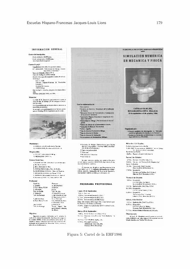
Escuelas Hispano-Francesas Jacques-Louis Lions 179
Figura 5: Cartel de la EHF1986
180 Escuelas Hispano-Francesas Jacques-Louis Lions
En lo que se refiere a la ubicacion de la Escuela, A. Valle reservo el seductorCastillo de Bil-Bil que se alza en la playa como un castillo de arena. Fue sudeseo ademas asociar a sus antiguos colegas de Sevilla en la celebracion de estaEscuela: ası, el conjunto de los participantes se desplazo a Sevilla para asistir auna presentacion de Modulef seguida de un almuerzo y una excursion al centrode la ciudad, incluida la ascension de la Giralda.
5.2.1 Programa
El programa fue muy rico, ya que se establecieron sesiones en paralelo y laEscuela se prolongo hasta el sabado por la manana. En total, casi 35 horas deintervenciones cientıficas, un record absoluto aun imbatido:
• Las herramientas de base de los metodos numericos, C. Conde (Escuelade Minas de Madrid) y J. Durany (Univ. de Santiago de Compostela)
• Elasto-visco-plasticidad, P. Le Tallec (LCPC Parıs) y J.M. Viano (Univ.de Santiago de Compostela)
• Turbulencia, T. Chacon (Univ. de Sevilla)
• Fractura, P. Destuynder (Escuela Central de Parıs) y F. Michavila(Escuela de Minas de Madrid)
• Modulef, E. Fernandez Cara y R. Echevarrıa (Univ. de Sevilla)
• Optimizacion, J. Cea (Univ. de Niza)
• Mecanica de Fluidos, J. Periaux (Avions Marcel Dassault BreguetAviation, Parıs) y O. Pironneau (Univ. Parıs VI)
• Laminas, M. Bernadou (INRIA).
5.2.2 Participantes
La Escuela conto con 80 participantes, incluyendo los conferenciantes,procedentes en su mayorıa de universidades y centros de investigacion espanolescon un excelente reparto geografico y un buen equilibrio entre matematicos,fısicos/quımicos e ingenieros. Los conferenciantes franceses se expresaron enfrances, salvo J. Cea, cuyo bilinguismo frances/espanol fue muy apreciado, y yomismo, que intente hablar en espanol: ¡el sonoro “somos partidos” con el quearranco mi curso no dejo ninguna duda sobre mi dominio del espanol!
5.3 III Escuela: Madrid, del 26-9 al 30-9 de 1988
Esta Escuela fue organizada por F. Michavila que era entonces Director de laEscuela de Minas de la Universidad Politecnica de Madrid, en colaboracion conlos profesores C. Conde, M. Lopez y A. Ruiz. Tuvo lugar en el anfiteatro de laFundacion Gomez-Pardo situado en las proximidades inmediatas de la Escuela

Escuelas Hispano-Francesas Jacques-Louis Lions 181
de Minas y, por consiguiente, muy cerca del centro historico de Madrid. Estaproximidad fue evidentemente aprovechada durante la media jornada libre paravisitar dicho centro historico (Plaza Mayor, Palacio Real) y sobre todo el Prado,que figura entre los principales Museos del Mundo, con los pintores del Siglo deOro (s. XVII): el Greco, Velazquez, Zurbaran, Murillo ası como Ribera y el masimportante pintor espanol del siglo XVIII, Goya.
5.3.1 Programa
Esta Escuela permitio analizar la situacion de algunos de los temas objeto decolaboracion hispano-francesa:
• Nociones generales de control, F.J. Elorza (Escuela de Minas de Madrid)
• Uniones de placas, confluencias de laminas, M. Bernadou (INRIA)
• Optimizacion de forma de laminas, F. Palma (Univ. de Malaga)
• Aproximacion de laminas mediante metodos DKT, P. Mato Eiroa (Univ.Santiago de Compostela)
ası como de algunos temas mas recientes que debıan constituir vıas deinvestigacion prometedoras para el futuro:
• Controlabilidad exacta, J.L. Lions (College de France y CNES)
• Problemas hiperbolicos no lineales, P.A. Raviart (Escuela Politecnica deParıs)
• Combustion, B. Larrouturou (INRIA) y A. Linan (ETSI Aeronauticos deMadrid).
Mas alla de los cursos, ya clasicos en la forma, los organizadores desearonacentuar la presentacion de metodos de simulacion numerica para el diseno,la puesta a punto y la optimizacion de nuevos productos industriales.Algunas colaboraciones entre analistas numericos e industriales comenzabana establecerse en Espana y era importante llamar la atencion de los nuevostitulados y de los ingenieros de los gabinetes de estudio espanoles sobreestas nuevas posibilidades que experimentaban ya un auge considerable enlos paıses anglosajones, en Alemania y en Francia. Para cubrir este objetivo,complementando los cursos tradicionales, se organizaron cursos en el marco deesta apertura industrial:
• Seminarios “industriales”: Estos seminarios, presentados por losresponsables de cuatro polos industriales diferentes, permitieron definire ilustrar algunos problemas resueltos (o susceptibles de serlo) gracias alas nuevas contribuciones de la simulacion numerica:
– Seminario Nuclear, C. del Olmo (ENRESA)
– Seminario Aerospacial, J.L. Lions (CNES)
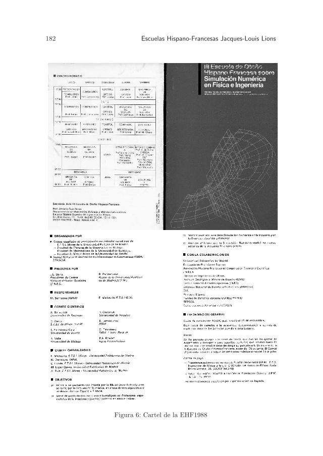
182 Escuelas Hispano-Francesas Jacques-Louis Lions
Figura 6: Cartel de la EHF1988

Escuelas Hispano-Francesas Jacques-Louis Lions 183
– Seminario Materiales, J. Martı (PRINCIPIA)
– Seminario Petroleo, P. Samier (ELF-SNEA(P))
• Mesas redondas: Dos mesas redondas fueron destinadas a aportar otrosenfoques sobre estos temas industriales de actualidad y a abrir la discusioncon los participantes:
– Mesa redonda sobre Nuevos Materiales en Aerospacial, con laparticipacion de G. Duvaut (ONERA), J.L. Lions (CNES), J.Martı (PRINCIPIA), M. Simon (CASA), M. Bernadou (Moderador) ;
– Mesa redonda sobre Energıa, con la participacion de P. Oustriere(CEA-ANDRA), L. Perez (REPSOL Exploracion), P. Samier (ELF),A. Uliberri (ENRESA), F. Michavila (Moderador).
Ası, esta Escuela puso especialmente el acento en las repercusionesindustriales efectivas de la Simulacion Numerica. Introdujo tambien la novedadde Seminarios/Conferencias de una hora acompanando a los cursos, a fin deilustrar algunas aplicaciones importantes.
5.3.2 Participantes
La presencia de J.L. Lions, las aperturas, la posicion central de Madrid y laexcelente organizacion explican sin ninguna duda el numero de participantes:145 incluyendo profesores y conferenciantes. Mas precisamente, los centros deorigen de los participantes fueron:
• Espana : Universidades de Cantabria (2); Castilla-La Mancha (4, de loscuales 1 de Albacete y 3 de Almaden); Cordoba (3); Granada (2); LasPalmas (1); Malaga (6); Murcia (2); Oviedo (8); Paıs Vasco (6); Politecnicade Cataluna (1); Politecnica de Valencia (2); Salamanca (1); Santiagode Compostela (16, de los cuales 1 del Ferrol, 2 de La Coruna y 2 deVigo); Sevilla (8); Valencia (6); Valladolid (2); Zaragoza (3); Instituto deMijas (Malaga) (1); INCAPSA (1); Murcia (1), y finalmente de Madrid,procedentes de Univ. Politecnica (38) ; UNED (5) ; CASA (3) ; CIEMAT(2) ; ENRESA (5) ; ICAI (1) ; EGME (1) ; INYPSA (1) ; REPSOL (4) ;SITECSA (2) ; 1 otros.
• Francia: CEA-Andra (1) ; CNES Parıs (1) ; ELF Pau (1) ; INRIARocquencourt (1) y Niza (1) ; Escuela Politecnica, Palaiseau (2) ; ONERA,Chatillon (1)
5.4 IV Escuela: Santiago de Compostela, del 24-9 al 28-09 de 1990
Despues de las tres primeras Escuelas organizadas por los tres principales polosespanoles de colaboracion con Francia, esto es, las Universidades de Santiagode Compostela, de Malaga y Sevilla, y la Escuela de Minas de la UniversidadPolitecnica de Madrid, la experiencia fue juzgada como muy satisfactoria yse decidio efectuar un nuevo ciclo de tres Escuelas que serıan nuevamente
184 Escuelas Hispano-Francesas Jacques-Louis Lions
organizadas por cada uno de los tres polos sucesivamente. Esta cuarta Escuelafue ası organizada en Santiago de Compostela por A. Bermudez de Castro, P.Quintela y J.M. Viano. Se retomo la formula mixta de cursos acompanados deconferencias, de seminarios de aplicaciones y de una mesa redonda y fueron casiuna centena los participantes que asistieron a esta nueva edicion.
5.4.1 Programa
En los cursos se abordaron dos temas en plena expansion:
• Metodos numericos en electromagnetismo, A. Bermudez de Castro(Santiago de Compostela) y A. Bossavit (Electricite de France)
• Algunos metodos numericos para los diferentes problemas de la mecanicade fluido, J.A. Desideri (Univ. de Niza), L. Fezoui (INRIA) y E. FernandezCara (Univ. de Sevilla).
Junto a las 16 horas de curso, nueve seminarios, de hora y media cada uno,permitieron presentar de forma sintetizada o bien algunos resultados recientesen otros ejes de investigacion, o bien algunas aplicaciones de estos metodosnumericos en el medio industrial:
• Conferencias: Las conferencias permitieron analizar la situacion de
– Las metodologıas utilizadas para realizar mallados, P.L. George(INRIA)
– Los modelos asintoticos de barras elasticas, J.M. Viano (Univ.Santiago de Compostela)
– Los metodos numericos para el diseno de dispositivos optoelectricos,F.J. Mustieles (Telefonica I+D)
– Algunos avances recientes en la modelizacion de singularidadesmediante el metodo de elementos finitos, F. Michavila (Escuela deMinas de Madrid)
– La evolucion de superordenadores para la simulacion numerica, Ch.Eisenbeis (INRIA)
• Seminarios industriales: El objetivo de estos seminarios era presentaralgunos ejemplos de uso en el medio industrial de resultados recientesde investigacion en metodos numericos.
– Simulacion numerica de problemas de laminas delgadas y algunasaplicaciones a la optimizacion de forma, F. Palma (Univ. de Malaga)
– Problematicas numericas en la industria nuclear, C. del Olmo(ENRESA)
– Simulacion de flujos en diseno aerospacial, B. Stoufflet (AvionsMarcel Dassault Breguet Aviation)
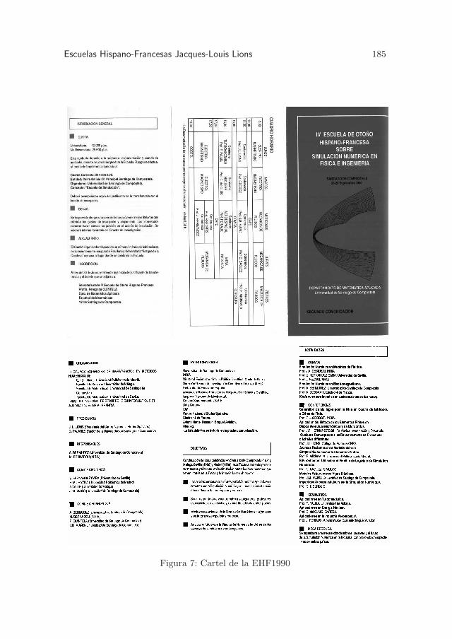
Escuelas Hispano-Francesas Jacques-Louis Lions 185
Figura 7: Cartel de la EHF1990

186 Escuelas Hispano-Francesas Jacques-Louis Lions
– Entorno de utilizador y fiabilidad de software de simulacionnumerica, C. Saguez (SIMULOG).
Dos volumenes que reunıan la casi totalidad de los textos de lasintervenciones fueron entregados a los participantes en el momento de laapertura de la Escuela. En estos volumenes figura el soporte escrito de laintervencion que J.L. Lions, que se encontraba en Moscu por cuestionesrelacionadas con asuntos espaciales, no pudo efectuar: Algunos comentariossobre el ensamblado de problemas de escalas diferentes.
5.4.2 Participantes
A pesar de la situacion geografica excentrica de Santiago de Compostela,esta Escuela reunio 81 participantes procedente en casi su totalidad delsector universitario: Universidades de Cordoba (3), Las Palmas (2), Malaga(3), Murcia (1), Oviedo (3), Paıs Vasco (1), Politecnica de Madrid (13),Politecnica de Valencia (5), Santiago de Compostela (25, de los cuales 1 deLa Coruna y 4 de Vigo), Salamanca (2), Sevilla (12), Valladolid (7). Laaudiencia estaba compuesta esencialmente por jovenes investigadores ası comopor algunos profesores en ejercicio. A estos 81 participantes hay que anadir los16 conferenciantes, lo que da un total de 97 asistentes.
5.4.3 Perspectivas
Esta colaboracion franco-espanola en Analisis Numerico y Calculo Cientıfico esya muy importante. Entre los desarrollos recientes, conviene destacar:
• la estancia de Matthieu Hallard en Santiago de Compostela: modelizacionde la combustion de carbon (abril a junio de 1990)
• la obtencion de un programa SCIENCE de la Comunidad Europea queasociaba al INRIA con la Universidad de Santiago de Compostela y laUniversidad Tecnica de Lisboa, en el tema de Modelizacion de uniones deestructuras
• la obtencion de un contrato ERASMUS entre las Universidades ParısVI (con la implicacion del INRIA), de Sevilla, Malaga, Santiago deCompostela y la Universidad Politecnica de Madrid
• la ida a Parıs VI de tres estudiantes espanoles (1 de Santiago deCompostela, 1 de Sevilla y 1 de Malaga) para la preparacion del DEAde Analisis Numerico. Tras la obtencion de este DEA, dichos estudiantescontinuarıan su estancia en Francia a fin de preparar sus tesis de doctoradoen los Laboratorios asociados a la citada formacion doctoral (entre ellosel INRIA)
Estos cuatro ejemplos no solo ponen de manifiesto la vitalidad de lacolaboracion, sino que muestran la evolucion de la misma hacia un regimende intercambios a partes iguales.
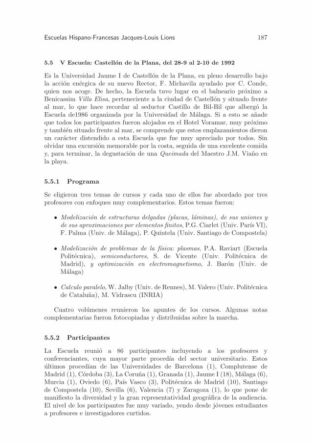
Escuelas Hispano-Francesas Jacques-Louis Lions 187
5.5 V Escuela: Castellon de la Plana, del 28-9 al 2-10 de 1992
Es la Universidad Jaume I de Castellon de la Plana, en pleno desarrollo bajola accion energica de su nuevo Rector, F. Michavila ayudado por C. Conde,quien nos acoge. De hecho, la Escuela tuvo lugar en el balneario proximo aBenicassim Villa Elisa, perteneciente a la ciudad de Castellon y situado frenteal mar, lo que hace recordar al seductor Castillo de Bil-Bil que albergo laEscuela de1986 organizada por la Universidad de Malaga. Si a esto se anadeque todos los participantes fueron alojados en el Hotel Voramar, muy proximoy tambien situado frente al mar, se comprende que estos emplazamientos dieronun caracter distendido a esta Escuela que fue muy apreciado por todos. Sinolvidar una excursion memorable por la costa, seguida de una excelente comiday, para terminar, la degustacion de una Queimada del Maestro J.M. Viano enla playa.
5.5.1 Programa
Se eligieron tres temas de cursos y cada uno de ellos fue abordado por tresprofesores con enfoques muy complementarios. Estos temas fueron:
• Modelizacion de estructuras delgadas (placas, laminas), de sus uniones yde sus aproximaciones por elementos finitos, P.G. Ciarlet (Univ. Parıs VI),F. Palma (Univ. de Malaga), P. Quintela (Univ. Santiago de Compostela)
• Modelizacion de problemas de la fısica: plasmas, P.A. Raviart (EscuelaPolitecnica), semiconductores, S. de Vicente (Univ. Politecnica deMadrid), y optimizacion en electromagnetismo, J. Baron (Univ. deMalaga)
• Calculo paralelo, W. Jalby (Univ. de Rennes), M. Valero (Univ. Politecnicade Cataluna), M. Vidrascu (INRIA)
Cuatro volumenes reunieron los apuntes de los cursos. Algunas notascomplementarias fueron fotocopiadas y distribuidas sobre la marcha.
5.5.2 Participantes
La Escuela reunio a 86 participantes incluyendo a los profesores yconferenciantes, cuya mayor parte procedıa del sector universitario. Estosultimos procedıan de las Universidades de Barcelona (1), Complutense deMadrid (1), Cordoba (3), La Coruna (1), Granada (1), Jaume I (18), Malaga (6),Murcia (1), Oviedo (6), Paıs Vasco (3), Politecnica de Madrid (10), Santiagode Compostela (10), Sevilla (6), Valencia (7) y Zaragoza (1), lo que pone demanifiesto la diversidad y la gran representatividad geografica de la audiencia.El nivel de los participantes fue muy variado, yendo desde jovenes estudiantesa profesores e investigadores curtidos.

188 Escuelas Hispano-Francesas Jacques-Louis Lions
Figura 8: Cartel de la EHF1992

Escuelas Hispano-Francesas Jacques-Louis Lions 189
5.5.3 Otras colaboraciones en curso
Esta colaboracion franco-espanola en analisis numerico y calculo cientıficoes cada vez mas importante. Sus desarrollos recientes se orientan en dosdirecciones:
• Acogida en Parıs de un flujo regular de estudiantes espanoles que vienena prepara el DEA de Analisis Numerico y, posteriormente, la tesis (2 a 3estudiantes por ano).
• Colaboraciones bilaterales cada vez mas equilibradas que se traducen enparticular en:
– visitas de corta duracion (2 a 4 semanas) de espanoles a Franciay de franceses a Espana. Estas visitas permiten finalizar trabajosefectuados en comun y publicados como artıculos conjuntos
– obtencion de un programa SCIENCE que reune a la UniversidadParıs VI (Responsable y director cientıfico: P.G. Ciarlet), INRIA(coordinador: M. Bernadou), Universidad de Santiago de Compostela(coordinador: J.M. Viano) y la Universidad Tecnica de Lisboa(coordinador: L. Trabucho). El tema de este programa es laModelizacion de uniones de estructuras y su duracion es de 3 anos(1991 a 1993).
5.6 VI Escuela: Sevilla, del 19-9 al 23-9 de 1994
La Escuela vuelve a Andalucıa, esta vez a Sevilla, donde tuvo lugar dos anosantes la emblematica y muy conseguida Exposicion Universal. Los organizadoresson T. Chacon, E. Fernandez Cara, D. Franco, F. Guillen y F. Ortegon. Juntoa un programa cientıfico de primer plano, consiguieron restituir el ambientefestivo de la Expo: visita al Ayuntamiento de Sevilla, conferencia general de J.L.Lions en la magnıfica Sala de Fiestas del Ayuntamiento, visita de la Catedral ydel Alcazar, declaradas por la UNESCO patrimonio mundial de la humanidad,seguida de una cena y de una muy calurosa velada de Sevillanas. Ademas, elalojamiento de los participantes en la residencia Hernando Colon, proxima alas salas de curso, dieron un caracter residencial a esta Escuela, que fue muyapreciado.
5.6.1 Programa
Se impartieron cuatro cursos de cinco horas:
• Control optimo de sistemas distribuidos, E. Casas (Univ. de Cantabria)
• Introduccion al metodo de elementos finitos en mecanica de fluidos, C.Pares (Univ. de Malaga)
• Controlabilidad exacta y aproximada para sistemas con parametrosdistribuidos, J.L. Lions (College de France)

190 Escuelas Hispano-Francesas Jacques-Louis Lions
Figura 9: Cartel de la EHF1994

Escuelas Hispano-Francesas Jacques-Louis Lions 191
• Resultados fundamentales sobre metodos espectrales, Y. Maday (Univ.Parıs VI)
Los dos primeros cursos tenıan el caracter de introduccion a metodos muyutilizados en calculo cientıfico desde hacıa muchos anos y que aun hoy sonobjeto de numerosas investigaciones. Estos cursos estaban destinados a jovenesinvestigadores. Los dos ultimos cursos presentaban teorıas recientes que sontambien objeto de numerosas investigaciones actualmente y que, en aquelmomento, empezaban a suscitar numerosas aplicaciones. El contenido y la formade los cuatro cursos fueron extremadamente apreciados. El formato de 5 horasy la presentacion de pizarra parece optima... ¡las excelentes pedagogicas de loscuatro profesores tuvieron ciertamente mucho que ver con esta apreciacion!
Siete conferencias completaron este ciclo de cursos y permitieron ilustraralgunas otras facetas del calculo cientıfico:
• Matematicas y medio ambiente (conferencia general en el Ayuntamientode Sevilla), J.L. Lions (College de France)
• Estimacion de error a posteriori para problemas elıpticos mediante unmetodo de dualidad, L. Ferragut (Univ. Politecnica de Madrid)
• Algunas cuestiones relativas a la controlabilidad aproximada de lasecuaciones de Navier-Stokes, J. Real (Univ. de Sevilla)
• Guıas de ondas electromagneticas, D. Gomez (Univ. Santiago deCompostela)
• Teorıa matematica de la plasticidad, C. Moreno (Univ. Politecnica deMadrid)
• Observaciones sobre la modelizacion numerica de la turbulencia, O.Pironneau (Univ. Parıs VI)
• Analisis de la evolucion de MODULEF, seguido de algunas observacionessobre las laminas piezoelectricas, M. Bernadou (INRIA)
En el conjunto de los cursos y conferencias, los idiomas de trabajo fueron elespanol y el frances. Dos volumenes agrupaban la totalidad de los apuntes delos cursos y conferencias (casi 350 paginas cada uno).
5.6.2 Participantes
Esta Escuela reunio a 135 participantes, incluyendo profesores y conferenciantes,procedentes en su mayor parte del sector universitario. Estos ultimos procedıande las Universidades de Barcelona (1), Cadiz (5), Cantabria (2), Cordoba (3), LaCoruna (1), Granada (2), la Laguna (1), Las Palmas (4), Madrid Autonoma (2),Madrid Complutense (7), Malaga (6), Oviedo (8), Paıs Vasco (1), Politecnicade Madrid (10), Salamanca (3), Santiago de Compostela (13), Sevilla (21), Vigo(5), junto a una treintena de participantes de los que no nos consta la afiliacion,
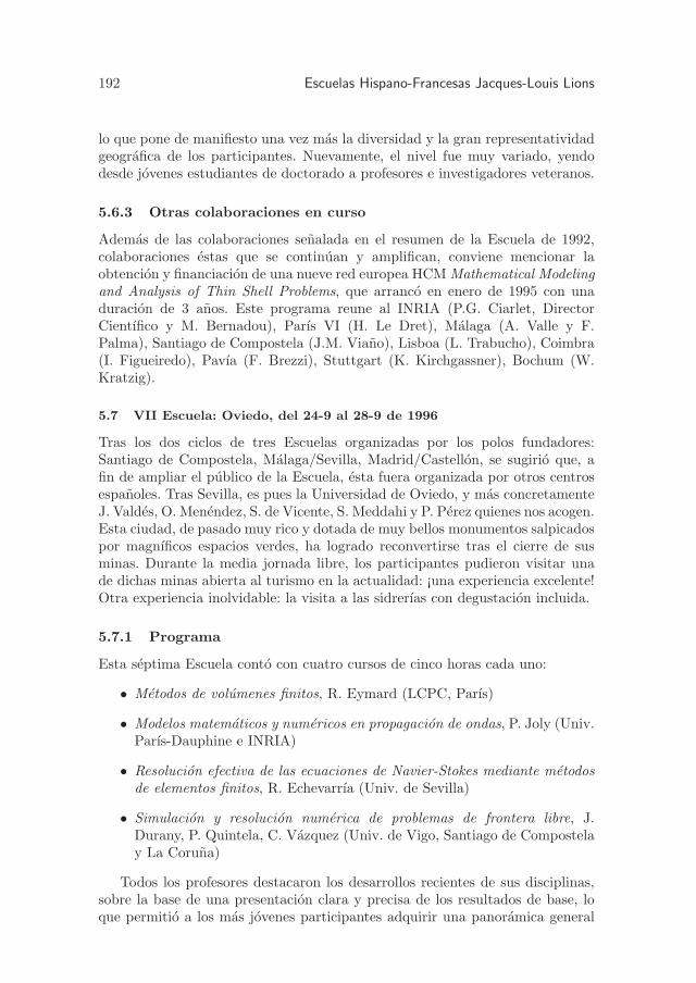
192 Escuelas Hispano-Francesas Jacques-Louis Lions
lo que pone de manifiesto una vez mas la diversidad y la gran representatividadgeografica de los participantes. Nuevamente, el nivel fue muy variado, yendodesde jovenes estudiantes de doctorado a profesores e investigadores veteranos.
5.6.3 Otras colaboraciones en curso
Ademas de las colaboraciones senalada en el resumen de la Escuela de 1992,colaboraciones estas que se continuan y amplifican, conviene mencionar laobtencion y financiacion de una nueve red europea HCM Mathematical Modelingand Analysis of Thin Shell Problems, que arranco en enero de 1995 con unaduracion de 3 anos. Este programa reune al INRIA (P.G. Ciarlet, DirectorCientıfico y M. Bernadou), Parıs VI (H. Le Dret), Malaga (A. Valle y F.Palma), Santiago de Compostela (J.M. Viano), Lisboa (L. Trabucho), Coimbra(I. Figueiredo), Pavıa (F. Brezzi), Stuttgart (K. Kirchgassner), Bochum (W.Kratzig).
5.7 VII Escuela: Oviedo, del 24-9 al 28-9 de 1996
Tras los dos ciclos de tres Escuelas organizadas por los polos fundadores:Santiago de Compostela, Malaga/Sevilla, Madrid/Castellon, se sugirio que, afin de ampliar el publico de la Escuela, esta fuera organizada por otros centrosespanoles. Tras Sevilla, es pues la Universidad de Oviedo, y mas concretamenteJ. Valdes, O. Menendez, S. de Vicente, S. Meddahi y P. Perez quienes nos acogen.Esta ciudad, de pasado muy rico y dotada de muy bellos monumentos salpicadospor magnıficos espacios verdes, ha logrado reconvertirse tras el cierre de susminas. Durante la media jornada libre, los participantes pudieron visitar unade dichas minas abierta al turismo en la actualidad: ¡una experiencia excelente!Otra experiencia inolvidable: la visita a las sidrerıas con degustacion incluida.
5.7.1 Programa
Esta septima Escuela conto con cuatro cursos de cinco horas cada uno:
• Metodos de volumenes finitos, R. Eymard (LCPC, Parıs)
• Modelos matematicos y numericos en propagacion de ondas, P. Joly (Univ.Parıs-Dauphine e INRIA)
• Resolucion efectiva de las ecuaciones de Navier-Stokes mediante metodosde elementos finitos, R. Echevarrıa (Univ. de Sevilla)
• Simulacion y resolucion numerica de problemas de frontera libre, J.Durany, P. Quintela, C. Vazquez (Univ. de Vigo, Santiago de Compostelay La Coruna)
Todos los profesores destacaron los desarrollos recientes de sus disciplinas,sobre la base de una presentacion clara y precisa de los resultados de base, loque permitio a los mas jovenes participantes adquirir una panoramica general
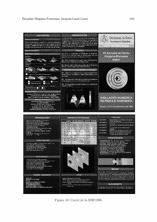
Escuelas Hispano-Francesas Jacques-Louis Lions 193
Figura 10: Cartel de la EHF1996

194 Escuelas Hispano-Francesas Jacques-Louis Lions
de cada uno de los temas. En los dos primeros cursos, los profesores insistieronademas en la puesta en practica numerica efectiva de los metodos.
Seis conferencias completaron este ciclo de conferencias y permitieronilustrar otras tantas facetas del calculo cientıfico, que se pueden clasificar enacademicas:
• Introduccion a la teorıa del control optimo H∞, P. Bernhard (INRIASophia-Antıpolis)
• Resultados recientes y problemas abiertos sobre los fluidos visco-elasticos,J.C. Saut (Univ. Parıs-Sur)
• Acoplamientos entre elementos finitos y elementos de contorno, S.Meddahi (Univ. de Oviedo)
• Ecuaciones diferenciales y tratamiento de imagenes, L. Alvarez (Univ. deLas Palmas)
e industriales:
• Aplicacion de la tecnica de descomposicion de dominio al calculo deplataformas petrolıferas, M. Bernadou (Univ. Leonardo da Vinci e INRIA)
• Simulacion de problemas estructurales en la industria mediante metodosnumericos, A. Santos (TGI SA).
Tres volumenes agruparon la totalidad de las notas de los cursos yconferencias (casi 920 paginas), lo que fue muy apreciado por los participantes.
5.7.2 Participantes
Esta escuela reunio a 113 participantes, incluyendo profesorado. Nuevamente,la mayor parte procedıan del sector universitario: Cadiz (3), Cantabria (1),Castilla-La Mancha (1), Complutense de Madrid (1), Cordoba (3), La Coruna(2), Granada (1), Las Palmas (1), Leon (1), Malaga (4), Oviedo (26), Politecnicade Madrid (11), Salamanca (8), Santiago de Compostela (8), Sevilla (18), UNED(1), Valladolid (6), Vigo (7) y Zaragoza (4), ademas de 5 franceses y unaportuguesa. De nuevo, se puso de manifiesto la diversidad y representatividadgeografica de la audiencia cuyo nivel, tambien en este caso, iba desde jovenesestudiantes de doctorado a investigadores curtidos.
5.8 VIII Escuela: Cordoba, del 21-9 al 25-9 de 1998
Vuelta al sur para descubrir otra faceta de Andalucıa: Cordoba, cuyo centrohistorico, encrucijada de varias culturas, fue declarado por la UNESCOPatrimonio Mundial de la Humanidad. Como era de esperar, los organizadoresJ.L. Cruz, M. Marın, M.C. Calzada, J.R. Galo y J.A. Herencia incluyeron visitasal centro en el programa « social » de la Escuela; incluso anadieron un conciertode cuerdas, un Perol en la sierra de Cordoba y la cena de gala. Todo ello sindescuidar el programa cientıfico, que fue del mejor nivel y muy completo.
Escuelas Hispano-Francesas Jacques-Louis Lions 195
Esta Escuela tuvo lugar en el Colegios Mayor Ntra. Sra. De la Asuncionde Cordoba, lo que garantizo la unidad del emplazamiento (alojamiento,restauracion y sala de conferencias) en un entorno confortable muy apreciadopor los participantes.
5.8.1 Programa
Esta octava Escuela conto con cuatro cursos de cuatro horas cada uno:
• Problemas de vibraciones en sistemas acoplados fluido-estructura, A. Ber-mudez de Castro (Univ. de Santiago de Compostela)
• Metodos de dominios ficticios con multiplicadores en la frontera ymultiplicadores distribuidos; aplicaciones, V. Girault y R. Glowinski(Univ. de Parıs VI y Houston)
• Equilibrio, transporte y estabilidad de un plasma, J. Blum (Univ. deGrenoble)
• Fluidos no newtonianos, F. Guillen (Univ. de Sevilla)
En cada uno de los cursos, los profesores se propusieron presentar elorigen fısico o mecanico de los problemas considerados, su modelizacion enterminos de ecuaciones en derivadas parciales, su formulacion matematica, suaproximacion numerica y algunas aplicaciones concretas. Ademas, el segundocurso presento las bases teoricas y los ultimos avances del metodo de losdominios ficticios que permite, para problemas formulados en dominios degeometrıa compleja, aproximar las soluciones utilizando una malla estructuradade un dominio regular de mayor tamano (rectangulo, paralelepıpedo...)combinada con una malla grosera de la frontera del dominio inicial.
Diez conferencias completaron este ciclo de cursos e ilustraron otrasaplicaciones recientes de la simulacion numerica:
• Aplicacion del metodo de los dominios ficticios a la resolucion deproblemas de Stokes, V. Girault (Univ. Parıs VI)
• Estudio del fenomeno de corrientes oceanicas « El Nino » mediante unmodelo acoplado hıbrido oceano/atmosfera, J. Macıas (Univ. de Malaga)
• Modelizacion asintotica de lagos, J. Simon (Univ. de Clermont-Ferrand)
• Aplicacion de los filtros de Kalman a la estimacion de parametros en unAlto Horno, O. Menendez (Univ. de Oviedo)
• Resolucion numerica de las ecuaciones de Navier-Stokes mediante metodosmixtos aumentados, T. Chacon (Univ. de Sevilla)
• Controlabilidad de ecuaciones de ondas y de ecuaciones parabolicas y susversiones discretas, E. Zuazua (Univ. Complutense de Madrid)
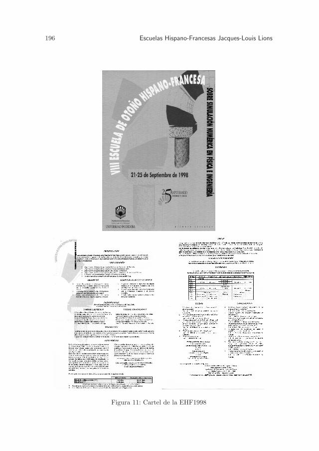
196 Escuelas Hispano-Francesas Jacques-Louis Lions
Figura 11: Cartel de la EHF1998
Escuelas Hispano-Francesas Jacques-Louis Lions 197
• Aplicacion del metodo de los dominios ficticios a problemas desedimentacion, R. Glowinski (Univ. de Parıs VI y Houston)
• Optimizacion no convexa mediante algoritmos geneticos: teorıa yaplicaciones problemas de optimizacion de forma y de controlmultidisciplinar/multicriterios en CFD (Computational Fluids Dynamics)y CEM (Computational ElectroMagnetism), J. Periaux (Avions MarcelDassault)
• Metodos de volumenes finitos para la simulacion de procesos de transporteen la geosfera, A. Lopez (Univ. Politecnica de Madrid)
• El problema 16 de Hilbert: estado de la cuestion, J. Chavarriga (Univ. deLerida)
Dos volumenes agruparon la totalidad de los apuntes de cursos y conferencias(casi 550 paginas) lo que fue muy apreciado por los asistentes y muy util paraaquellos que no dominaban completamente los dos idiomas: frances y espanol.
5.8.2 Participantes
Esta Escuela reunio 128 participantes, incluyendo profesores y conferenciantes,la mayor parte procedente del sector universitario. Estos ultimos procedıan delas Universidades de Burgos (2), Cadiz (9), Cantabria (2), Castilla-La Mancha(2), Cordoba (14), La Coruna (4), Lerida (1), Madrid (1 de la Autonoma,5 de la Complutense, 6 de la Politecnica), Malaga (8), Murcia (1), Oviedo(11), Santiago de Compostela (12), Sevilla (28), Valencia (1), Valladolid (2),Vigo (5), Zaragoza (3) del lado espanol, y del lado frances: Clermont-Ferrand(1), Grenoble (1), Parıs (4), Pau (2), Perpinan (1), y de Lisboa (2) del ladoportugues. Esta distribucion ha confirmado la ampliacion del publico de lasEscuelas en Espana y tambien, en menor medida, a Francia y Portugal.
El nivel cientıfico del auditorio iba desde jovenes estudiantes de doctorado ainvestigadores muy experimentados de estatura internacional en el caso de unaveintena de entre ellos.
5.9 IX Escuela: Laredo, Cantabria, del 18-9 al 22-9 de 2000
Rumbo al norte a la ciudad de Laredo, que combina una inmensa playa de finaarena con un centro historico reputado. Los organizadores de la Escuela, E.Casas, L.A. Fernandez, E. Moyano, C. Pola y J. Puig-Pey de la Universidad deCantabria nos acogen en la sede de los Cursos de Verano de la Universidad deCantabria a unos 50 km al este de Santander. Ademas del completo programacientıfico que recordamos a continuacion, visita al Parque Natural de Cabarceno,demostracion de vuelo libre de aves de presa (muy impresionante) y cena de galaen el Centro Nautico de Laredo.
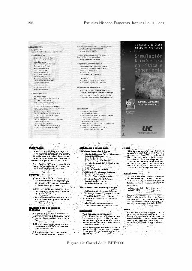
198 Escuelas Hispano-Francesas Jacques-Louis Lions
Figura 12: Cartel de la EHF2000

Escuelas Hispano-Francesas Jacques-Louis Lions 199
5.9.1 Programa
Se impartieron cuatro cursos de cinco horas cada uno:
• Metodos de elementos finitos para problemas de mecanica de fluidos, R.Codina (Univ. Politecnica de Cataluna), curso panoramico sobre uno delos temas « clasicos » pero siempre de gran actualidad de la SimulacionNumerica
• Metodos wavelets: del analisis a la simulacion, A. Cohen (Univ. ParısVI), curso prospectivo sobre una de las nuevas disciplinas que haexperimentado un mayor desarrollo en el transcurso de la ultima decada.Este disciplina presenta importantes aplicaciones tanto en simulacionnumerica como en tratamiento de la senal y de la imagen
• Modelizacion numerica de estructuras en grandes deformaciones, P.Le Tallec (Escuela Politecnica e INRIA), curso panoramico sobre lamodelizacion y la aproximacion numerica de los principales problemasno lineales que aparecen en mecanica del solido: elasticidad no lineal,postflameado, termoviscoelasticidad, contacto, comportamiento no linealde polımeros y de caucho sintetico, aplicaciones en biomecanica. Enla parte numerica, se discutieron las contribuciones de los metodos deelementos finitos mixtos, estimaciones de error a posteriori y tecnicas dedescomposicion de dominio
• Metodos de elementos de contorno, F.J. Sayas (Univ. de Zaragoza),curso introductorio a la tecnica consistente en reformular un problemade contorno en la forma de una ecuacion integral que, posteriormente,es aproximada numericamente. Se presentaron algunas aplicaciones aproblemas de potencial interior/exterior, a las ecuaciones de Helmholtz, ala elasticidad y a otros problemas menos clasicos
Cinco conferencias completaron este ciclo de cursos y permitieron abordaralgunos resultados recientes de Calculo Cientıfico:
• Simulacion numerica y visualizacion de los datos y resultados para lapropagacion de un incendio forestal en la cuenca del Ebro, L. Ferragut(Univ. de Salamanca)
• Modelizacion numerica en quımica cuantica, C. Le Bris (CERMICS,ENPC Parıs)
• Calculo paralelo para la resolucion de ecuaciones en derivadas parciales,J.L. Cruz (Univ. de Cordoba)
• Acoplamientos elementos finitos/elementos de contorno para la resolucionde problemas de Stokes en el plano, S. Meddahi (Univ. de Oviedo)
• Modelizacion numerica de problemas medioambientales en el Estrecho deGibraltar, C. Pares (Univ. de Malaga)
200 Escuelas Hispano-Francesas Jacques-Louis Lions
Es conveniente destacar, tanto en lo que se refiere a los cursos como a lasconferencias, la excelente cualidades cientıficas y pedagogicas del conjunto deconferenciantes.
Un volumen que reunıa los apuntes de los cursos y las conferencias (deaproximadamente 400 paginas) facilito el trabajo de los asistentes.
5.9.2 Participantes
Esta Escuela reunio a 81 participantes, incluyendo profesores y conferenciantes,procedentes en su mayor parte del medio universitario (Universidades deCantabria (8), Cordoba (3), Malaga (5), Oviedo (10), Salamanca (7), Santiagode Compostela (11), Sevilla (6), Valencia (2), Valladolid (2) Vigo (4), Zaragoza(3), 5 de las universidades de Madrid, 5 de las universidades catalanasy 9 de otras universidades) y de nivel cientıfico doctoral, postdoctoral oinvestigador experimentado. La representatividad geografica en Espana se pusouna vez mas de manifiesto; es de destacar que una buena proporcion delos investigadores experimentados que participaron mantienen colaboracionesregulares con Francia.
La participacion en esta Escuela experimento un ligero retroceso comparadacon las precedentes, lo que se debio esencialmente al gran numero de Coloquiosy Congresos de Matematicas Aplicadas celebrados en Espana durante este ano2000 declarado Ano Mundial de las Matematicas.
5.10 X Escuela: Jaca, del 23-9 al 27-9 de 2002
La organizacion de esta decima Escuela, a cargo de nuestros colegas de ZaragozaF. Lisbona , F.J. Sayas, R. Celorrio, C. Clavero y F. Gaspar en la ciudad deJaca, nos conduce por primera vez al corazon de los Pirineos espanoles. Lacandidatura de esta villa turıstica a la organizacion de los Juegos Olımpicos deinvierno de 2010 atestigua la calidad de su entorno montanoso, que pudimosapreciar durante la media jornada de excursion. Ademas, la propia ciudadcuenta con una gran riqueza arquitectonica, especialmente la Catedral de estiloromanico, el Castillo de San Pedro y el Ayuntamiento. La Escuela tuvo lugaren la Residencia Universitaria de Jaca, con alojamiento y comida en el mismolugar, lo que favorecio las conversaciones y discusiones cientıficas.
5.10.1 Programa
Se impartieron cuatro cursos de cinco horas cada uno:
• Modelos numericos para los fluidos hidrodinamicos, T. Chacon (Univ. deSevilla), presentacion de la problematica de distintos tipos de modelosmatematicos, de su analisis matematico y de la aproximacion de sussoluciones, ası como de algunos ejemplos de aplicaciones concretas
• Problemas de evolucion parabolicos, M. Crouzeix (Univ. de Rennes I),presentacion de una sıntesis de los metodos de analisis matematicos y de

Escuelas Hispano-Francesas Jacques-Louis Lions 201
Figura 13: Cartel de la EHF2002

202 Escuelas Hispano-Francesas Jacques-Louis Lions
aproximacion numerica actualmente disponibles para abordar de formaoptima la simulacion numerica de los problemas
• Esquemas numericos de alto orden para leyes de conservacion hiperbolicacon buenas propiedades de captura de ondas de choque, R. Donat (Univ.de Valencia), presentacion de una amplia sıntesis de metodos matematicosy numericos recientes para modelizar fenomenos de tipo propagacion deondas, discontinuidades de contacto, choques, rarefacciones...
• Algunos nuevos resultados y desafıos actuales en el analisis medianteelementos finitos de problemas de laminas, D. Chapelle (INRIA,Rocquencourt), sıntesis de los resultados matematicos y numericos,enfatizando la combinacion de la calidad de los modelos matematicos conla eficacia y la fiabilidad de la aproximacion numerica
Cinco conferencias de una hora cada una permitieron abordar cinco temasmas especıficos:
• Avances recientes en el modelado numerico de la propagacion del oleaje ysu interaccion con estructuras costeras, I. Losada (Univ. de Cantabria)
• Metodos iterativos para la resolucion de grandes sistemas lineales conmatrices vacıas, G. Meurant (CEA Bruyeres-le-Chatel)
• Metodos numericos para problemas de valorizacion de opciones, C. Moreno(Univ. Politecnica de Madrid)
• Aplicacion del metodo de volumenes finitos y de esquemas de tipo Godunova las ecuaciones de aguas someras, E. Vazquez (Univ. Santiago deCompostela)
• Aproximacion mediante elementos finitos de problemas coercivos noelıpticos, J.M. Thomas (Univ. de Pau)
Ademas se celebro una sesion especial sobre algunas aplicaciones deherramientas matematicas y metodos numericos en la bioingenierıa. En efecto,la extension de los metodos de simulacion numerica a los seres vivos hatropezado durante mucho tiempo con la complejidad de los modelos (losmedios concernidos son muy inhomogeneos, anisotropos y requieren modelosfuertemente acoplados) y con el hecho de conducir a problemas numericosde una dimension demasiado grande. Los enormes progresos realizados tantoen modelizacion de fenomenos acoplados como en la combinacion algoritmianumerica/prestaciones informaticas y calculo paralelo permite abordar en laactualidad de manera fiable algunos dominios importantes de la bioingenierıa.Esta sesion permitio abordar tres de ellos:
• Tratamiento de la senal biomedica en el diagnostico y monitorizacion depatologıas, P. Carminal (Univ. Politecnica de Cataluna)
• Adaptacion en mecanica osea, S. Ramtani (Univ. Parıs Val de Marne)

Escuelas Hispano-Francesas Jacques-Louis Lions 203
• Algunas aplicaciones del metodo de elementos finitos a la modelizacion detejidos vivos y al diseno de implantes, M. Doblare (Univ. de Zaragoza).
Un volumen recopilo los apuntes de los cursos, a los que se anadieron dostiradas aparte (las transparencias de la conferencia de J.M. Thomas y losresumenes de la sesion especial de bioingenierıa).
5.10.2 Participantes
Esta Escuela reunio 78 participantes, incluyendo profesores y conferenciantes,procedentes en su mayor parte del sector universitario espanol. Masprecisamente, estos ultimos procedıan de las Universidades de Alicante (1),Barcelona (1), Cantabria (3), Cartagena (1), Cordoba (3), La Coruna (6),Navarra (2), Oviedo (2), Salamanca (4), Santiago de Compostela (8, de los cuales1 de Lugo), Sevilla (7), Valencia (8), Valladolid (1), Vigo (1 de Pontevedra),Zaragoza (13, 1 de Huesca), 5 de las Universidades de Madrid y, del lado frances,del CEA (1), del INRIA (1), de las Universidades de Pau (2), Rennes (1) y delPolo Universitario Leonardo da Vinci (1). Este reparto atestigua la diversidad yla gran representatividad geografica de la audiencia. El numero de participantessigue siendo elevado, a pesar de las dificultades de acceso de la localizaciony de las fechas algo tardıas de la Escuela, muy proximas al inicio del cursouniversitario.
El nivel de los participantes fue muy variado, yendo de doctorandos aprofesores e investigadores con muy distinto nivel de experiencia. Un terciode entre ellos aproximadamente participa personalmente en colaboracionescon equipos franceses (Parıs VI, INRIA, Escuela Politecnica, Escuela Central,Universidades de Pau y de Rennes...).
5.10.3 Otras colaboraciones en curso
Numerosas colaboraciones estan en marcha, especialmente codirecciones detesis, participacion en proyectos y contratos conjuntos o en Redes Europeas: elproyecto Smart Systems acaba de ser aprobado por la Comunidad Europea y sedesarrollara en el periodo 2003/2006. El INRIA, el ESIEE, el Polo UniversitarioLeonardo da Vinci son miembros del lado frances y la Universidad de Santiagode Compostela del lado espanol.
5.11 XI Escuela: Cadiz, del 20-9 al 24-9 de 2004
A propuesta de A. Valle de la Universidad de Malaga y por iniciativa de SeMA,la Escuela paso a denominarse « Escuela Jacques-Louis Lions Hispano-Francesasobre Simulacion Numerica en Fısica e ingenierıa ». De esta manera, SeMAdeseaba honrar la memoria de Jacques-Louis Lions, fallecido en 2001, quien,con sus excepcionales cualidades cientıfica y humana, se implico en gran medidaen el establecimiento de numerosas y fructıferas colaboraciones entre la mayorparte de los grupos de simulacion numerica espanoles y franceses.
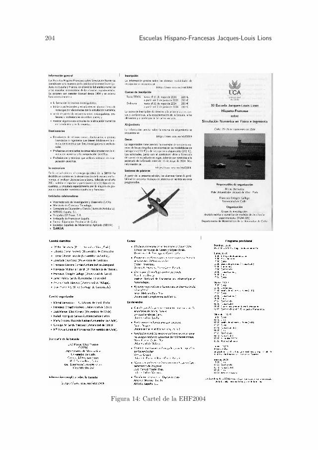
204 Escuelas Hispano-Francesas Jacques-Louis Lions
Figura 14: Cartel de la EHF2004

Escuelas Hispano-Francesas Jacques-Louis Lions 205
Esta undecima Escuela fue organizada en Cadiz por F. Ortegon y suscolaboradores J.M. Dıaz, R. Rodrıguez, M.V. Redondo, C. Garcıa y M.T.Gonzalez.
Junto a la parte cientıfica de la Escuela, una excursion a Jerez de la Fronteranos permitio visitar una bodega, asistir al espectaculo de la celebre Real EscuelaEcuestre y visitar el Museo Taurino; ademas, la cena de gala en el ParadorAtlantico nos permitio degustar las especialidades locales.
El formato general de esta Escuela fue analogo a la de las cuatro o cincoprecedentes: cuatro cursos de unas cuatro horas cada uno permitieron presentarde forma detallada los retos y los resultados mas significativos de cuatrodisciplinas de actualidad en simulacion numerica y seis conferencias permitieronanalizar sucintamente el progreso de otros tantos temas de actualidad.
5.11.1 Programa
Se impartieron los cuatro cursos siguientes:
• Modelos matematicos en los procesos industriales, A. Bermudez de Castro(Univ. de Santiago de Compostela), el curso se apoyo en dos ejemplosconcretos: el primero, la combustion en una central termica y el segundo,la reduccion del ruido en recintos cerrados mediante tecnicas anti-ruido
• Generacion de mallados tridimensionales, P.L. George (INRIA Rocquen-court), presentacion de los principales metodos de generacion de malladostridimensionales que permiten responder de manera fiable y eficaz a lasnecesidades industriales, particularmente en terminos de rapidez y de ta-mano de los mallados tridimensionales generados
• Actuar a favor del medio ambiente: reflexiones generales y analisis mate-matico de dos problemas concretos, J.I. Dıaz (Univ. Complutense deMadrid y Real Academia de Ciencias), consecuencias de la revolucionindustrial en la evolucion del clima e ilustracion mediante algunos ejemplosque conducen a estudios de controlabilidad
• Problemas matematicos y numericos planteados por la seguridad delos residuos nucleares, O. Pironneau (Univ. Parıs VI y Academiedes Sciences), presentacion de herramientas matematicas apropiadas:desarrollos multi-escala, los metodos de descomposicion de dominios yde homogeneizacion, ası como los metodos numericos correspondientes
Los cursos se completaron con las conferencias:
• Esquemas numericos con dos mallas para las ecuaciones de Navier-Stokes,V. Girault (Univ. Parıs VI)
• Calculo paralelo para la resolucion numerica de las ecuaciones de Navier-Stokes, E. Fernandez Cara (Univ. de Sevilla)
• Resolucion numerica de las ecuaciones de aguas someras bicapa medianteesquemas de volumenes finitos, M.J. Castro (Univ. de Malaga)

206 Escuelas Hispano-Francesas Jacques-Louis Lions
• Esquemas de volumenes finitos y teorema de Lax, B. Despres (Univ. ParısVI)
• Simulacion de procesos: « digital factory », A. Montosa (Airbus Espana)
• Modelos matematicos para el tratamiento de imagenes, J.M. Mazon (Univ.de Valencia)
Ademas, tres sesiones de posteres permitieron a los mas jovenes presentarsus primeros resultados.
El conjunto de las notas de los cursos y las conferencias fue recopiladoen un volumen de excelente factura. Este volumen y su contenido fueronobjeto de recension « Mathematical Reviews » bajo la referencia MR2117095(2005h :00013) 00B15.
5.11.2 Participantes
Esta Escuela reunio a 84 participantes, incluyendo profesores y conferenciantes,procedentes en su mayor parte del sector universitario espanol, doctorandos,profesores-investigadores jovenes o experimentados. Estos asistentes procedıande las Universidades de Cadiz (13), Cantabria (1), Cordoba (4), La Coruna (5),Madrid (3, 1 de la Autonoma, 1 de Carlos III y 1 de Complutense), Malaga (10),Navarra (3), Oviedo (2), Santiago de Compostela (10), Sevilla (17), Valencia (1),Valladolid (1), Vigo (3) y Zaragoza (1); de AIRBUS Espana (1); del INRIA (2)y de la Universidad Parıs VI (3); de la Universidad de Campinas de Brasil (1),de la Universidad Autonoma de Mexico (1) y de la Universidad de Tetuan (2).
5.12 XII Escuela: Castro Urdiales, del 18-9 al 22-9 de 2006
Este ano 2006 fue excepcional para la comunidad matematica espanola, yaque Espana organizo en agosto el Congreso general de la Union MatematicaInternacional. Se trata del Congreso mayor de los matematicos, que tiene lugarcada cuatro anos, en el transcurso del cual se entregan las Medallas Fields. Juntoal Congreso general, se organizaron un gran numero de encuentros, reunionesde trabajo, seminarios, etc. centrados sobre temas concretos que reunıan a losespecialistas de una misma disciplina. El conjunto de estos eventos, empezandopor el Congreso general, tuvieron un gran exito, tanto por la calidad de lasintervenciones como por una organizacion muy notable.
La organizacion de la duodecima Escuela en Castro Urdiales menos de unmes despues del Congreso de la UMI y de los eventos asociados era un autenticodesafıo. Debido a este hecho, la Escuela experimento una sensible disminuciondel numero de participantes, pero la calidad de la organizacion y el calor de laacogida hicieron de ella un evento muy logrado y muy apreciado.
Recordemos que esta Escuela fue organizada por la Universidad del PaısVasco, bajo la responsabilidad de L. Vega, M. Escobedo y M. Lezaun asistidospor L. A. Fernandez de la Universidad de Cantabria. La Escuela tuvo lugaren la ciudad balneario de Castro Urdiales a unos 40 km al oeste de Bilbao,
Escuelas Hispano-Francesas Jacques-Louis Lions 207
Figura 15: Cartel de la EHF2006

208 Escuelas Hispano-Francesas Jacques-Louis Lions
mas precisamente en el recien estrenado Centro Internacional de EstudiosMatematicos, instalado en una soberbia residencia perfectamente restauraday muy funcional.
Ademas de las actividades cientıficas, los organizadores reservaron mediajornada para hacernos descubrir el Puente Colgante de Portugalete que, desdehace mas de cien ano, asegura el traslado de vehıculos y peatones de unaorilla a otra de la rıa. Despues nos condujeron al celebre e ineludible MuseoGuggenheim de Bilbao, cuya audaz arquitectura ha contribuido fuertementeal renacimiento de una ciudad marcada por delicadas reestructuracionesindustriales.
5.12.1 Programa
Esta Escuela conto con cuatro cursos de tres horas cada uno:
• Integracion geometrica, J. Sanz Serna (Univ. de Valladolid)
• Optimizacion de forma y de topologıa, G. Allaire (Escuela Politecnica,Parıs)
• Modelos y algoritmos para problemas de localizacion y rutas, E. FernandezAreizaga (Univ. Politecnica de Cataluna)
• Una introduccion a la modelizacion matematica de flujos bifasicosdispersos, P. Villedieu (ONERA, Univ. Paul Sabatier, Toulouse)
Las siguientes ocho conferencias de una hora cada una complementaron loscursos:
• Estimaciones del error para la aproximacion numerica de problemas decontrol gobernados por EDPs, M. Mateos (Univ. de Oviedo)
• Analisis matematico y simulacion numerica del ensayo de flexion entres puntos para materiales ceramicos, P. Quintela (Univ. Santiago deCompostela)
• De la Mecanica a la Biologıa mediante procesos de fragmentacion: estadode la cuestion y problemas abiertos, J. Soler (Univ. de Granada)
• Blow-up y problemas parabolicos mal puestos, A. Rodrıguez Bernal (Univ.Complutense de Madrid)
• Ecuaciones con solitones: sinergia entre estudio analıtico y simulacion, A.Sanchez (Univ. Carlos III de Madrid)
• Preservacion de invariantes mediante metodos Runge-Kutta, L. Randez(Univ. de Zaragoza)
• Metodos de bases reducidas para la aproximacion fiable de la solucion deproblemas no lineales, Y. Maday (Univ. Parıs VI)

Escuelas Hispano-Francesas Jacques-Louis Lions 209
• Simulacion numerica de la interaccion sangre-venas en arterias largas, M.Fernandez (INRIA Rocquencourt)
Todos los profesores y conferenciantes pusieron a disposicion de losparticipantes soportes (en papel y electronico) directamente relacionados conel contenido de su presentacion e incluyendo una bibliografıa muy completa yactualizada sobre los temas abordados.
5.12.2 Participantes
Los participantes procedıan de las Universidades de Cantabria (1), Castilla-La Mancha (1), Cordoba (2), La Coruna (3), Granada (1), Madrid (3, 2 deCarlos III y 1 de la Complutense), Oviedo (2), Paıs Vasco (14), Politecnicade Cataluna (1), Santiago de Compostela (4), Sevilla (4), Valladolid (1), Vigo(1), Zaragoza (2); del Consejo Superior de Investigaciones Cientıficas (1) ; dela Escuela Politecnica de Palaiseau (1), de la Universidad Parıs VI (1), delINRIA Rocquencourt (1), del ONERA y la Universidad Paul Sabatier (1) y dela Escuela Superior de Ingenieros Leonardo da Vinci (1).
El nivel de los participantes fue muy variando, yendo desde doctorandosa profesores-investigadores con muy distinto nivel de experiencia. Un terciode entre ellos al menos participa personalmente en colaboraciones regularescon equipos franceses (Parıs VI, INRIA, Escuela Politecnica, Universidad PaulSabatier...).
5.12.3 Conclusiones
La participacion en esta Escuela, por una parte, de los profesores J.I. Montijanoy C. Vazquez, presidentes saliente y entrante de SeMA respectivamente,y por otra parte de los profesores Y. Maday y G. Allaire, presidentesde la SMAI (Societe de Mathematiques Appliquees et Industrielles) y delGamni/SMAI (Groupe pour l’Avancement des Methodes Numeriques del’Ingenieur) respectivamente, permitieron discutir sobre el futuro de estoseventos.
A partir de 2008, las Escuelas seran organizadas por SeMA del lado espanoly por la SMAI del lado frances, lo que introducira una mayor simetrıa yaumentara la visibilidad. La Escuela de 2008 sera organizada localmente porla Universidad de Valladolid (www.uva.es/ehf2008).

RESUMENES DE TESIS DOCTORALES
Tıtulo: Influencia del Potencial de Hardy enecuaciones Elıpticas y Parabolicas.
Doctorando: Ana Primo Ramos.Director/es: Ireneo Peral Alonso.
Defensa: 19 de mayo de 2008, Universidad Autonoma deMadrid.
Calificacion: Sobresaliente cum laude por unanimidad.
Resumen:Los protagonistas de la Tesis son el clasico potencial de Hardy y los terminos
de orden cero y uno que son potencias de la incognita o del modulo de sugradiente respectivamente. Todos estos terminos actuan en la Ecuacion delCalor y la Ecuacion de Laplace. Los problemas que se tratan estudian comocooperan o compiten el potencial de Hardy con dichas potencias. Es un perfectolaboratorio para estudiar algunos casos lımite y descubrir fenomenos nuevos.Muchos de los resultados se pueden extender a otros operadores.
Debido a su gran interes fısico se considera con preferencia el siguienteproblema
(P )
ut − ∆u = |∇u|p + λu
|x|2 + f(x, t) en ΩT ≡ Ω × (0, T ),
u(x, t) > 0 en ΩT ,
u(x, t) = 0 en ∂Ω × (0, T ),
u(x, 0) = u0(x) si x ∈ Ω,
que representa una aproximacion viscosa a la ecuacion de Hamilton-Jacobi. Seconsidera λ > 0, f(x, t) > 0, u0(x) ≥ 0 funciones en clases convenientes y Ω undominio acotado de R
N con N ≥ 3 y 0 ∈ Ω.En el caso l = 0 y p = 2, este modelo aparece en la teorıa fısica
del crecimiento de rugosidades en superficies por deposicion de partıculaspor gravedad, donde es conocido como modelo de Kardar-Parisi-Zhang. Unamodificacion de este problema ha sido considerado por H. Berestycki, S. Kamin,G. Sivashinsky, como un modelo para la propagacion de llamas. El caso1 < p < 2 es conocido como modelo generalizado de Kardar-Parisi-Zhang.Tanto en el caso estacionario como en el de evolucion, si l = 0 y p = 2, B.Abdellaoui, A. Dall’Aglio e I. Peral, demuestran un resultado de no unicidad desoluciones positivas, dando la caracterizacion de todas las soluciones en relaciona medidas concentradas en conjuntos de capacidad cero. Este fenomeno de nounicidad salvaje es producido por el termino |∇u|2.
211
212 Resumenes de tesis doctorales
Con estos resultados como motivacion, se estudia en primer lugar el casoestacionario del problema (P ), analizando la influencia conjunta del potencial deHardy en problemas que tienen un termino |∇u|2. Si el cuadrado del gradienteaparece en el lado derecho de la ecuacion (compitiendo con el operador deLaplace), se demuestra un resultado de no existencia de solucion positiva en elsentido mas debil posible, es decir, exigiendo las condiciones mınimas necesariaspara que la ecuacion tenga significado en el sentido de las distribuciones.Como consecuencia de este resultado tan fuerte de no existencia, se produceun fenomeno de explosion de las soluciones de los problemas aproximados(truncando el potencial de Hardy) en todo punto del dominio (el caso de noexistencia para 1 < q < 2 es analizado por B.Abdellaoui e I. Peral en Ann.Scuola Norm. Sup. Pisa Cl. Sci. (5) Vol. VI (2007), 159-183).
Si el cuadrado del gradiente aparece en el lado izquierdo de la ecuacion(cooperando con el operador de Laplace), el resultado es completamentediferente. Se prueba la existencia de solucion positiva para todo parametro λ,sin necesidad de restringir su tamano y para toda funcion positiva f en L1(Ω),sin imponer condiciones extras de integrabilidad.
El fenomeno de rotura de resonancia y efecto regularizante se analiza enpesos mas generales y con una potencia |∇u|q, 1 < q < 2, llamados en lamemoria pesos admisibles, entre los que, en particular, se encuentra el potencialde Hardy. Un dato importante: se prueba la optimalidad de la condicionimpuesta a estos pesos admisibles, utilizando de nuevo el potencial de Hardycomo laboratorio de pruebas. Extendemos estos resultados a operadores enforma divergencia, con funciones mas generales que dependen de la incognita yde su gradiente y con datos en los que no imponemos condiciones de signo.
Para analizar la influencia del potencial de Hardy en el caso de evolucion, separte del estudio de la sumabilidad de las soluciones de la Ecuacion del Calor conrespecto a la sumabilidad del termino fuente, completando algunos resultadosclasicos.
Al perturbar con el potencial de Hardy, se prueba que las supersolucionesen general no estan acotadas y por tanto, el estudio se sale de marcos clasicos.Se estudia en primer lugar el problema semilineal tomando la potencia crıticaoptimal para el problema elıptico asociado obtenida por Brezis-Dupaigne-Tesei.Se comprueba que esta misma potencia es la crıtica para determinar la existenciao la no existencia de solucion positiva en la ecuacion del calor semilinearperturbada con el potencial de Hardy. El analisis del problema de Cauchyasociado, permite obtener el exponente de Fujita que depende del parametroλ.
El problema (P ) es particularmente interesante. Por un lado, plantea seriasdificultades tecnicas, apareciendo de forma natural la necesidad de demostrar unprincipio de comparacion que en particular extiende un resultado de Alaa-Pierrepara el caso elıptico asociado. Por otro lado, se hallan profundas diferencias conrespecto a la ecuacion del calor. Si λ > 0, el exponente crıtico obtenido por B.Abdellaoui e I. Peral es tambien el exponente crıtico para el problema parabolicocasi-lineal, en el sentido que a partir de el no hay solucion positiva para ningundato inicial no trivial. Sin embargo, para λ = 0, bajo ciertas hipotesis en el
Resumenes de tesis doctorales 213
dato incial, B. Gilding, M. Guedda, R. Kersner demuestran un resultado deexistencia global de solucion para todo p > 1.
Si λ > 0, en el problema de Cauchy (Ω = RN ) existe un exponente de tipo
Fujita tal que por debajo de el todas las soluciones no negativas explotan entiempo finito. Sin embargo, para λ = 0, existe solucion para dato no trivial.Los resultados son bastante sorprendentes, ademas hay una discontinuidad decomportamiento cuando λ→ 0+, a diferencia del caso semilineal.

RESUMENES DE LIBROS
Un Curso de Calculo Numerico: Interpolacion, Aproximacion,Integracion y Resolucion de Ecuaciones Diferenciales.Anna Doubova y Francisco Guillen GonzalezSecretariado de Publicaciones, Universidad de Sevilla.ISBN: 978-84-472-0941-5 – 2007
Por Enrique Fernandez Cara
Un Curso de Cálculo Numérico:
Interpolación, Aproximación, Integración
y Resolución de Ecuaciones Diferenciales
A. Doubova
F. Guillén González
Este texto de Calculo Numerico esta orien-tado a la docencia universitaria en Cienciase Ingenierıa. Los autores dedican una par-te importante al Analisis Numerico (plan-teamiento riguroso de los problemas, conver-gencia, estimaciones del error, etc.) y presen-tan tambien algoritmos eficientes de calcu-lo, numerosos ejemplos y ejercicios resueltos,ası como una relacion de ejercicios propues-tos al final de cada materia.
La obra consta de cinco capıtulos. En losCapıtulos 1 y 2 se desarrollan tecnicas deinterpolacion polinomica (global, a trozos ycon splines) y de aproximacion de funciones(en el sentido de la convergencia uniformey en el sentido de los mınimos cuadrados,incluyendo el caso discreto de aproximacionde un conjunto de puntos en el plano).
En el Capıtulo 3 se estudia la integracionnumerica en una variable (de nuevo con metodos globales y a trozos), masconcretamente las formulas de cuadratura de tipo interpolatorio, el casoparticular de las formulas de Newton-Cotes y las formulas de cuadratura deGauss con soporte optimo.
Finalmente, los Capıtulos 4 y 5 estan dedicados al estudio de esquemasnumericos para aproximar soluciones de problemas diferenciales ordinarios:problemas de Cauchy en el Capıtulo 4 y problemas de contorno en elCapıtulo 5. En el caso de los problemas de Cauchy, estan recogidos los
215

216 Resumenes de libros
resultados analıticos mas importantes de los esquemas de un paso (consistenciay orden, estimaciones del esquema, convergencia y estimaciones del error dediscretizacion y estabilidad). En el caso de problemas de contorno, tan solo serealiza una introduccion, desde el punto de vista de la implementacion numerica,a algoritmos de dos tipos: los metodos de disparo y los metodos de diferenciasfinitas.
En conjunto, el libro pretende proporcionar una vision unificada yequilibrada de resultados propios del Analisis Numerico, complementados conel estudio detallado de un buen numero de algoritmos.

ANUNCIOS
Tipo de evento: CongresoNombre: International Workshop on Dynamical Sys-
tems and Multidisciplinary Applications(IWDSMA)
Lugar: Universidad Miguel Hernandez de ElcheFecha: September 16–19, 2008Organiza:Informacion:E-mail: [email protected]
WWW: http://hefesto.umh.es/IWDSMA
Tipo de evento: CongresoNombre: 13th GAMM-IMACS International Sympo-
sium on Scientific Computing, ComputerArithmetic, and Verified Numerical Compu-tations (SCAN’2008)
Lugar: El Paso, TEXAS, USAFecha: September 29–October 3, 2008Organiza:Informacion:E-mail: [email protected], [email protected]
WWW: http://www.cs.utep.edu/interval-comp/scan08.html
Tipo de evento: CongresoNombre: II Encuentro Iberico de MatematicasLugar: Badajoz. Facultad de Ciencias de la Universidad de
ExtremaduraFecha: Del 3 al 5 de octubre de 2008Organiza: Sociedad Matematica Portuguesa (SPM), Real So-
ciedad Matematica Espanola (RSME), Departamen-to de Matematicas de la Universidad de Extremadu-ra
Informacion:E-mail: [email protected]
WWW: http://imm2.unex.es/indexes.html
217
218 Anuncios
Tipo de evento: CongresoNombre: 10th International Conference on In-
formation and Communications Security(ICICS’08)
Lugar: Birmingham, United KingdomFecha: October 20–22, 2008Organiza: School of Computer Science, University of Bir-
mingham, in co-operation with HP Laboratories(Bristol, UK), the UK Engineering and PhysicalSciences Research Council (EPSRC), and the Inter-national Communications and Information SecurityAssociation (ICISA).
Informacion:E-mail: [email protected]
WWW: http://events.cs.bham.ac.uk/icics08
Tipo de evento: CongresoNombre: International Conference in Modeling
Health Advances 2008Lugar: San Francisco, California, USAFecha: October 22–24, 2008Organiza:Informacion:E-mail: [email protected]
WWW: http://www.iaeng.org/WCECS2008/ICMHA2008.html
Tipo de evento: CongresoNombre: International Conference on Modeling,
Simulation and Control (ICMSC’08)Lugar: San Francisco, USAFecha: October 22–24, 2008Organiza: International Association of EngineersInformacion:E-mail: [email protected]
WWW: http://www.iaeng.org/WCECS2008/ICMSC2008.html

Anuncios 219
Tipo de evento: CongresoNombre: Second Workshop on Mathematical Crypto-
logy (WMC 2008)Lugar: Universidad de Cantabria, SantanderFecha: October 23–25, 2008Organiza:Informacion:E-mail: [email protected]
WWW: http://grupos.unican.es/amac/wmc-2008
Tipo de evento: CongresoNombre: Elliptic and Hyperbolic Equations on Singu-
lar SpacesLugar: Mathematical Sciences Research Institute, Berkeley,
California, USAFecha: October 27–31, 2008Organiza:Informacion:E-mail: [email protected]
WWW: http://www.msri.org/calendar/workshops/
WorkshopInfo/444/show workshop
Tipo de evento: CongresoNombre: Second SIAM Conference on Financial
Mathematics and EngineeringLugar: Campus of Rutgers, The State University of New
Jersey, at the Heldrich Hotel, New Brunswick, NEWJERSEY, USA
Fecha: November 21–22, 2008Organiza:Informacion:E-mail: [email protected];
WWW: http://www.siam.org/meetings/fm08/index.php;
http://www.finmath.rutgers.edu/conferences/
220 Anuncios
Tipo de evento: CongresoNombre: International Conference on Partial Diffe-
rential Equations and Applications in ho-nour of Professor Philippe G. Ciarlet’s70th birthday
Lugar: City University of Hong Kong, Kowloon, Hong KongFecha: December 5–8, 2008Organiza:Informacion:E-mail: [email protected]
WWW: http://www6.cityu.edu.hk/rcms/ICPDEA2008
Tipo de evento: CongresoNombre: FEMTEC 2008 (Finite Element Methods in
Engineering and Science)Lugar: University of Texas at El Paso, USAFecha: December 8–12, 2008Organiza:Informacion:E-mail: [email protected]; [email protected]
WWW: http://servac.math.utep.edu/femtec 2008/home
Tipo de evento: CongresoNombre: 2008 International Conference on Compu-
ter Science and Software Engineering (CS-SE 2008)
Lugar: Wuhan, ChinaFecha: December, 12-14th, 2008Organiza: Y. Wang, University of Calgary, Canada; P. Shen,
University of California at Irvine, USA; H. B. Zhou,Wuhan University, China
Informacion:E-mail: [email protected]
WWW: http://www.highsci.org/csse2008submission/
website/csse/index.aspx
RELACION ALFABETICA DE NUEVOS SOCIOS
Cid Araujo, Jose AngelContratado Doctor. Lıneas de investigacion: Ecuaciones diferenciales ordinarias,problemas de frontera – Univ. de Jaen – Depto. de Matematicas – EdificioB3, Campus de Las Lagunillas. 23071 Jaen.Tlf.: 953.212.944.e-mail: [email protected]://www4.ujaen.es/~angelcid
Martınez Fernandez, RebecaEstudiante. – Univ. de Santiago de Compostela – Fac. de Matematicas– Depto. de Matematica Aplicada – Avda. Lope Gomez de Marzoa, CampusSur. 15782 Santiago de Compostela.Tlf.: 981.563.100, Ext. 13130. Fax: 981.597.054.e-mail: [email protected].
Perez Sinusıa, EsterProf. Ayudante Doctor. Lıneas de investigacion: Asintotica de integrales,perturbacion singular, aproximacion de funciones especiales y polinomiosortogonales, ecuaciones diferenciales ordinarias – Univ. Publica de Navarra– Edif. de las Encinas – Dpto. de Ingenierıa Matematica e Informatica –Campus de Arrosadıa, s/n. 31006 Pamplona.Tlf.: 948.168.414. Fax: 948.169.521.e-mail: [email protected].
Rosado Linares, JesusEstudiante (Becario). Lıneas de investigacion: Ecuaciones de difusion,transporte optimo – Univ. Autonoma de Barcelona – Fac. de Ciencias– Dpto. de Matematicas – Campus Universitario. 08193 Bellaterra.Tlf.: 935.813.742. Fax: 935.812.790.e-mail: [email protected].
Soler Vizcaıno, JuanCatedratico de Universidad. Lıneas de investigacion: EDP’s en teorıa cinetica,cinetico-cuantica, mecanica de fluidos y biomatematica – Univ. de Granada– Fac. de Ciencias – Dpto. de Matematica Aplicada – Severo Ochoa, s/n.18071 Granada.Tlf.: 958.243.287. Fax: 958.248.596.e-mail: [email protected]://www.ugr.es/~kinetic
221

DIRECCIONES UTILES
Direcciones utiles
Consejo Ejecutivo de S~eMA
Presidente:Carlos Vazquez Cendon. ([email protected]).Dpto. de Matematicas. Facultad de Informatica. Univ. de A Coruna. Campus deElvina, s/n. 15071 A Coruna. Tel: 981 16 7000-1335.
Vicepresidente:Rosa Marıa Donat Beneito. ([email protected])Dpto. de Matematica Aplicada. Fac. de Matematiques. Univ. de Valencia. Dr.Moliner, 50. 46100 Burjassot (Valencia) Tel: 963 544 727.
Secretario:Carlos Castro Barbero. ([email protected]).Dpto. de Matematica e Informatica. E.T.S.I. Caminos, Canales y Puertos.Univ. Politecnica de Madrid. Av. Aranguren s/n. 28040 Madrid. Tel: 91 336 6664.
Vocales:Sergio Amat Plata. ([email protected])Dpto. de Matematica Aplicada y Estadıstica. Univ. Politecnica de Cartagena.Paseo de Alfonso XIII, 52. 30203 Cartagena (Murcia). Tel: 968 325 694.
Rafael Bru Garcıa. ([email protected])Dpto. de Matematica Aplicada. E.T.S.I. Agronomos. Univ. Politecnica deValencia. Camı de Vera, s/n. 46022 Valencia. Tel: 963 879 669.
Jose Antonio Carrillo de la Plata. ([email protected])Dpto. de Matematicas. Univ. Autonoma de Barcelona. Edifici C. 08193 Bellaterra(Barcelona). Tel: 935 812 413.
Inmaculada Higueras Sanz. ([email protected]).Dpto de Matematica e Informatica Univ. Publica de Navarra. Campus deArrosadıa, s/n. Tel: 948 169 526. 31006 Pamplona.
Carlos Pares Madronal. ([email protected]).Dpto. de Analisis Matematico. Fac. de Ciencias. Univ. de Malaga. Campus deTeatinos, s/n. 29080 Malaga. Tel: 952 132 017.
Pablo Pedregal Tercero. ([email protected]).Dpto. de Matematicas. E.T.S.I. Industriales. Univ. de Castilla-La Mancha. Avda.de Camilo Jose Cela, s/n. 13071 Ciudad Real. Tel: 926 295 436
Luis Vega Gonzalez. ([email protected]).Dpto. de Matematicas. Fac. de Ciencias. Univ. del Paıs Vasco. Aptdo. 644. 48080Bilbao (Vizcaya). Tel: 944 647 700.
Tesorero:Inigo Arregui Alvarez. ([email protected]).Dpto. de Matematicas. Fac. de Informatica. Univ. de A Coruna. Campus deElvina, s/n. 15071 A Coruna. Tel: 981 16 7000-1327.
223

224 Direcciones utiles
Comite Cientıfico del Boletın de S~eMA
Enrique Fernandez Cara. ([email protected]).Dpto. de Ecuaciones Diferenciales y An. Numerico. Fac. de Matematicas. Univ. deSevilla. Tarfia, s/n. 41012 Sevilla. Tel: 954 557 992.
Alfredo Bermudez de Castro. ([email protected]).Dpto. de Matematica Aplicada. Fac. de Matematicas. Univ. de Santiago deCompostela. Campus Univ.. 15706 Santiago (A Coruna) Tel: 981 563 100.
Carlos Conca Rosende. ([email protected]).Dpto. de Ingenierıa Matematica. Univ. de Chile. Blanco Encalada 2120. Santiago(Chile) Tel: (+56) 0 978 4459.
Amadeus Delshams Valdes. ([email protected]).Dpto. de Matematica Aplicada I. Univ. Politecnica de Cataluna. Diagonal 647.08028 Barcelona. Tel: 934 016 052.
Martin J. Gander ([email protected]).Section de Mathematiques. Universite de Geneve. 2-4 rue du Lievre, CP 64. CH-1211 Geneve (Suiza). Fax: (+41) 22 379 11 76.
Vivette Girault ([email protected]). Laboratoire Jacques-Louis Lions.Universite Paris VI. Boite Courrier 187, 4 Place Jussieu 75252 Paris Cedex 05(Francia).
Arieh Iserles ([email protected]).Department of Applied Mathematics and Theoretical Physics. University ofCambridge. Wilberforce Rd Cambridge (Reino Unido). Tel: (+44) 1223 337891.
Jose Manuel Mazon Ruiz. ([email protected]).Dpto. de Analisis Matematico. Fac. de Matematicas. Univ. de Valencia. Dr.Moliner, 50. 46100 Burjassot (Valencia) Tel: 963 664 721.
Pablo Pedregal Tercero. ([email protected]).Dpto. de Matematicas. E.T.S.I. Industriales. Univ. de Castilla-La Mancha. Avda.Camilo Jose Cela s/n. 13071 Ciudad Real. Tel: 926 295 436 .
Ireneo Peral Alonso. ([email protected]).Dpto. de Matematicas, C-XV. Fac. de Ciencias. Univ. Aut. de Madrid.Cantoblanco, Ctra. de Colmenar, km. 14. 28049 Madrid. Tel: 913 974 204.
Benoıt Perthame. ([email protected]).Laboratoire Jacques-Louis Lions. Universite Paris VI. 175, rue du Chevaleret.75013 Paris, (Francia). Tel: (+33) 1 44 32 20 36.
Olivier Pironneau ([email protected]).Laboratoire Jacques-Louis Lions. Universite Paris VI. 35 rue de Bellefond. 75009Paris (Francia). Tel: (+33) 1 42 80 12 97.
Alfio Quarteroni. ([email protected]).Institute of Analysis and Scientific Computing. Ecole Polytechnique Federale deLausanne. Piccard Station 8. CH-1015 Lausanne (Suiza) Tel: (+41) 21 69 35546.
Juan Luis Vazquez Suarez. ([email protected]).Dpto. de Matematicas, C-XV. Fac. de Ciencias. Univ. Aut. de Madrid.Cantoblanco, Crta. de Colmenar, km. 14. 28049 Madrid. Tel: 913 974 935.
Direcciones utiles 225
Luis Vega Gonzalez. ([email protected]).Dpto. de Matematicas. Fac. de Ciencias. Univ. del Paıs Vasco. Aptdo. 644. 48080Bilbao (Vizcaya). Tel: 944 647 700.
Chi-Wang Shu. ([email protected]).Division of Applied Mathematics Box F. 182 George Street Brown UniversityProvidence RI 02912 Tel: (401) 863-2549
Enrique Zuazua Iriondo. ([email protected]).Dpto. de Matematicas. Fac. de Ciencias. Univ. Aut. de Madrid. Cantoblanco,Ctra. de Colmenar, km. 14. 28049 Madrid. Tel: 913 974 368.
Grupo Editor del Boletın de S~eMA
Pablo Pedregal Tercero. ([email protected]).Dpto. de Matematicas. E.T.S.I. Industriales. Univ. de Castilla-La Mancha. Avda.Camilo Jose Cela, s/n. 13071 Ciudad Real. Tel: 926 295 300 ext. 3809
Enrique Fernandez Cara. ([email protected]).Dpto. de Ecuaciones Diferenciales y An. Numerico. Fac. de Matematicas. Univ. deSevilla. Tarfia, s/n. 41012 Sevilla. Tel: 954 557 992.
Ernesto Aranda Ortega. ([email protected]).Dpto. de Matematicas. E.T.S.I. Industriales. Univ. de Castilla-La Mancha. Avda.Camilo Jose Cela, s/n. 13071 Ciudad Real. Tel: 926 295 300 ext. 3813
Jose Carlos Bellido Guerrero. ([email protected]).Dpto. de Matematicas. E.T.S.I. Industriales. Univ. de Castilla-La Mancha. Avda.Camilo Jose Cela, s/n. 13071 Ciudad Real. Tel: 926 295 300 ext. 3859
Alberto Donoso Bellon. ([email protected]).Dpto. de Matematicas. E.T.S.I. Industriales. Univ. de Castilla-La Mancha. Avda.Camilo Jose Cela, s/n. 13071 Ciudad Real. Tel: 926 295 300 ext. 3859
Responsables de secciones del Boletın de S~eMA
Artıculos:
Enrique Fernandez Cara. ([email protected]).Dpto. de Ecuaciones Diferenciales y An. Numerico. Fac. de Matematicas.Univ. de Sevilla. Tarfia, s/n. 41012 Sevilla. Tel: 954 557 992.
Matematicas e Industria:
Mikel Lezaun Iturralde. ([email protected]).Dpto. de Matematica Aplicada, Estadıstica e I. O. Fac. de Ciencias. Univ. delPaıs Vasco. Aptdo. 644. 48080 Bilbao (Vizcaya). Tel: 944 647 700.
Educacion Matematica:
Roberto Rodrıguez del Rıo. ([email protected]).Dpto. de Matematica Aplicada. Fac. de Quımicas. Univ. Compl. de Madrid.Ciudad Universitaria. 28040 Madrid. Tel: 913 944 102.
Resumenes de libros:
Fco. Javier Sayas Gonzalez. ([email protected]).Dpto. de Matematica Aplicada. Centro Politecnico Superior . Universidad deZaragoza. C/Marıa de Luna, 3. 50015 Zaragoza. Tel: 976 762 148.
226 Direcciones utiles
Noticias de S~eMA:
Carlos Castro Barbero. ([email protected]).Dpto. de Matematica e Informatica. E.T.S.I. Caminos, Canales y Puertos.Univ. Politecnica de Madrid. Av. Aranguren s/n. 28040 Madrid. Tel:91 336 6664.
Anuncios:
Oscar Lopez Pouso. ([email protected]).Dpto. de Matematica Aplicada. Fac. de Matematicas. Univ. de Santiago deCompostela. Campus sur, s/n. 15782 Santiago de Compostela Tel:981 563 100, ext. 13228.
Responsables de otras secciones de S~eMA
Gestion de Socios:
Inigo Arregui Alvarez. ([email protected]).Dpto. de Matematicas. Fac. de Informatica. Univ. de A Coruna. Campus deElvina, s/n. 15071 A Coruna. Tel: 981 16 7000-1327.
Pagina web: www.sema.org.es/:
Carlos Castro Barbero. ([email protected]).Dpto. de Matematica e Informatica. E.T.S.I. Caminos, Canales y Puertos.Univ. Politecnica de Madrid. Av. Aranguren s/n. 28040 Madrid. Tel:91 336 6664.
INFORMACION PARA LOS AUTORES
1. Los artıculos publicados en este Boletın podran ser escritos en espanol oingles y deberan ser enviados por correo certificado a
Prof. E. FERNANDEZ CARA
Presidente del Comite Cientıfico, Boletın S~eMA
Dpto. E.D.A.N., Facultad de Matematicas
Aptdo. 1160, 41080 SEVILLA
Tambien podran ser enviados por correo electronico a la direccion
En ambos casos, el/los autor/es deberan enviar por correo certificadouna carta a la direccion precedente mencionando explıcitamente que elartıculo es sometido a publicacion e indicando el nombre y direccion delautor corresponsal. En esta carta, podran sugerirse nombres de miembrosdel Comite Cientıfico que, a juicio de los autores, sean especialmenteadecuados para juzgar el trabajo.
La decision final sobre aceptacion del trabajo sera precedida de unprocedimiento de revision anonima.
2. Las contribuciones seran preferiblemente de una longitud inferior a 24paginas y se deberan ajustar al formato indicado en los ficheros a tal efectodisponibles en la pagina web de la Sociedad (http://www.sema.org.es/).
3. El contenido de los artıculos publicados correspondera a un area de trabajopreferiblemente conectada a los objetivos propios de la MatematicaAplicada. En los trabajos podra incluirse informacion sobre resultadosconocidos y/o previamente publicados. Se anima especialmente a losautores a presentar sus propios resultados (y en su caso los de otrosinvestigadores) con estilo y objetivos divulgativos.
227
Ficha de Inscripcion Individual
Sociedad Espanola de Matematica Aplicada S~eMA
Remitir a: Inigo Arregui, Dpto de Matematicas, Fac. de Informatica,Universidad de A Coruna. Campus de Elvina, s/n. 15071 A Coruna.
CIF: G-80581911
Datos Personales
• Apellidos: . . . . . . . . . . . . . . . . . . . . . . . . . . . . . . . . . . . . . . . . . . . . . . . . . . . . . . . . . . . . .
• Nombre: . . . . . . . . . . . . . . . . . . . . . . . . . . . . . . . . . . . . . . . . . . . . . . . . . . . . . . . . . . . . . . .
• Domicilio: . . . . . . . . . . . . . . . . . . . . . . . . . . . . . . . . . . . . . . . . . . . . . . . . . . . . . . . . . . . . .
• C.P.: . . . . . . . . . . . . Poblacion: . . . . . . . . . . . . . . . . . . . . . . . . . . . . . . . . . . . . . . . . . .
• Telefono: . . . . . . . . . . . . . . . . . . . . . . . . . DNI/CIF: . . . . . . . . . . . . . . . . . . . . . . . . .
• Fecha de inscripcion: . . . . . . . . . . . . . . . . . . . . . . . . . . . . . . . . . . . . . . . . . . . . . . . . . . .
Datos Profesionales
• Departamento: . . . . . . . . . . . . . . . . . . . . . . . . . . . . . . . . . . . . . . . . . . . . . . . . . . . . . . . .
• Facultad o Escuela: . . . . . . . . . . . . . . . . . . . . . . . . . . . . . . . . . . . . . . . . . . . . . . . . . . . .
• Universidad o Institucion: . . . . . . . . . . . . . . . . . . . . . . . . . . . . . . . . . . . . . . . . . . . . . .
• Domicilio: . . . . . . . . . . . . . . . . . . . . . . . . . . . . . . . . . . . . . . . . . . . . . . . . . . . . . . . . . . . . .
• C.P.: . . . . . . . . . . . . Poblacion: . . . . . . . . . . . . . . . . . . . . . . . . . . . . . . . . . . . . . . . . . .
• Telefono: . . . . . . . . . . . . . . . . . . . . . . . . . Fax: . . . . . . . . . . . . . . . . . . . . . . . . . . . . . . .
• Correo electronico: . . . . . . . . . . . . . . . . . . . . . . . . . . . . . . . . . . . . . . . . . . . . . . . . . . . . .
• Pagina web: http:// . . . . . . . . . . . . . . . . . . . . . . . . . . . . . . . . . . . . . . . . . . . . . . . . . .
• Categorıa Profesional: . . . . . . . . . . . . . . . . . . . . . . . . . . . . . . . . . . . . . . . . . . . . . . . . .
• Lıneas de Investigacion: . . . . . . . . . . . . . . . . . . . . . . . . . . . . . . . . . . . . . . . . . . . . . . . .
. . . . . . . . . . . . . . . . . . . . . . . . . . . . . . . . . . . . . . . . . . . . . . . . . . . . . . . . . . . . . . . . . . . . . . .
Direccion para la correspondencia: Profesional Personal
Cuota anual para el ano 2008
Socio ordinario: 30e Socio de reciprocidad con la RSME: 12e Socio estudiante: 15e Socio extranjero: 25e

Datos bancarios
. . . de . . . . . . . . . . . . . . . . . . . . . . de 200. .
Muy Sres. Mıos:Ruego a Uds. que los recibos que emitan a mi cargo en concepto de cuotas
de inscripcion y posteriores cuotas anuales de S~eMA (Sociedad Espanola deMatematica Aplicada) sean pasados al cobro en la cuenta cuyos datos figurana continuacion
Entidad Oficina D.C. Numero de cuenta
(4 dıgitos) (4 dıgitos) (2 dıgitos) (10 dıgitos)
• Entidad bancaria: . . . . . . . . . . . . . . . . . . . . . . . . . . . . . . . . . . . . . . . . . . . . . . . . . . . . . .
• Domicilio: . . . . . . . . . . . . . . . . . . . . . . . . . . . . . . . . . . . . . . . . . . . . . . . . . . . . . . . . . . . . .
• C.P.: . . . . . . . . . . . . Poblacion: . . . . . . . . . . . . . . . . . . . . . . . . . . . . . . . . . . . . . . . . . .
Con esta fecha, doy instrucciones a dicha entidad bancaria para que obrenen consecuencia.
Atentamente,
Fdo. . . . . . . . . . . . . . . . . . . . . . . . . . . . . . . . .
Para remitir a la entidad bancaria
. . . de . . . . . . . . . . . . . . . . . . . . . . de 200. .
Muy Sres. Mıos:Ruego a Uds. que los recibos que emitan a mi cargo en concepto
de cuotas de inscripcion y posteriores cuotas anuales de S~eMA (SociedadEspanola de Matematica Aplicada) sean cargados a mi cuenta corriente/libreta. . . . . . . . . . . . . . . . . . . . . . . . . . . . . . . . en esa Agencia Urbana y transferidas a
SEMA: 0128 - 0380 - 03 - 0100034244BankinterC/ Hernan Cortes, 6339003 Santander
Atentamente,
Fdo. . . . . . . . . . . . . . . . . . . . . . . . . . . . . . . . .

Ficha de Inscripcion Institucional
Sociedad Espanola de Matematica Aplicada S~eMA
Remitir a: Inigo Arregui, Dpto de Matematicas, Fac. de Informatica,Universidad de A Coruna. Campus de Elvina, s/n. 15071 A Coruna.
CIF: G-80581911
Datos de la Institucion
• Departamento: . . . . . . . . . . . . . . . . . . . . . . . . . . . . . . . . . . . . . . . . . . . . . . . . . . . . . . . .
• Facultad o Escuela: . . . . . . . . . . . . . . . . . . . . . . . . . . . . . . . . . . . . . . . . . . . . . . . . . . . .
• Universidad o Institucion: . . . . . . . . . . . . . . . . . . . . . . . . . . . . . . . . . . . . . . . . . . . . . .
• Domicilio: . . . . . . . . . . . . . . . . . . . . . . . . . . . . . . . . . . . . . . . . . . . . . . . . . . . . . . . . . . . . .
• C.P.: . . . . . . . . . . . . Poblacion: . . . . . . . . . . . . . . . . . . . . . . . . . . . . . . . . . . . . . . . . . .
• Telefono: . . . . . . . . . . . . . . . . . . . . . . . . . DNI/CIF: . . . . . . . . . . . . . . . . . . . . . . . . .
• Correo electronico: . . . . . . . . . . . . . . . . . . . . . . . . . . . . . . . . . . . . . . . . . . . . . . . . . . . . .
• Pagina web: http:// . . . . . . . . . . . . . . . . . . . . . . . . . . . . . . . . . . . . . . . . . . . . . . . . . .
• Fecha de inscripcion: . . . . . . . . . . . . . . . . . . . . . . . . . . . . . . . . . . . . . . . . . . . . . . . . . . .
Forma de pago
La cuota anual para el ano 2008 como Socio Institucional es de 150e.El pago se realiza mediante transferencia bancaria a
SEMA: 0128 - 0380 - 03 - 0100034244BankinterC/ Hernan Cortes, 6339003 Santander