Subsurface stress field of a dry line contact

Wear 249 (2001) 546–556

Subsurface stress field of a dry line contact

A. Mihailidis a,∗, V. Bakolas b, N. Drivakos a

a Laboratory of Machine Elements and Machine Design, Department of Mechanical Engineering,Aristotle University of Thessaloniki, 54006 Thessaloniki, Greece

b INA Wälzlager Schaeffler, CAE Development — Analysis and Simulation, Industriestr. 1-3, D91074 Herzogenaurach, Germany

Received 15 September 2000; received in revised form 8 February 2001; accepted 22 February 2001

Abstract

The calculation of the pressure distribution and the subsurface stress field developed at the dry line contact of two cylinders, can becarried out with sufficient accuracy, using the Hertzian theory assuming that both cylinders are smooth. However, for the investigation ofsurface failures, such as micro-pitting, Hertz’s solution cannot be applied, because the effect of roughness is significant. This paper presentsa model for the determination of the asperity pressure distribution at the contact of two rough cylinders, assuming elastic–perfectly plasticdeformation. Having determined the surface load, the subsurface stress field is then calculated. The effect of roughness on the stress fieldis investigated. For this investigation, numerically generated rough surfaces are used. The results show that the maximum shear stressesdeveloped in small depths are significantly higher than those predicted by the Hertzian solution. This conclusion is in good agreement withthe small depth of cracks observed on the flanks of gears that have suffered from micro-pitting. © 2001 Elsevier Science B.V. All rightsreserved.

Keywords: Micro-pitting; Real pressure distribution; Subsurface stress field; Surface roughness

1. Introduction

Surface roughness has been recognised as an importantfactor for the operational behaviour of dry or lubricated,heavily loaded contacts, because it influences the wear, fric-tion and surface failures, such as pitting and micro-pitting.Schönnenbeck [1] has identified the roughness and the sub-sequent subsurface stress field as a key factor for the cre-ation of micro-pitting. The major role of surface roughnessin these phenomena has lead, in recent years, to the develop-ment of many models for the determination of the real con-tact area, the actual pressure distribution and the subsequentsubsurface stress field in rough contacts [2]. These modelscan be divided into two major categories, depending on themanner they describe the rough surfaces.

The first category includes the models that assume the realrough surface is equivalent to a smooth one covered withasperities of known geometry. Greenwood and Williamson(GW) [3], Grennwood and Tripp [4] and Onions and Ar-chard [5] were among the first who made the assumptionthat the asperity tips are spherical and deform elasticallywhen in contact. Chang et al. [6] suggested an elastic–plasticmicro-contact model. Bush et al. [7] assumed that the asper-

∗ Corresponding author. Tel.: +30-31-996073; fax: +30-31-996039.E-mail address: [email protected] (A. Mihailidis).

ity tips are elliptical paraboloids with uniform curvatures,which behave elastically when they are in contact. Horng[8] assumed that the contact area is elliptical and also tookinto consideration the plastic asperity deformation. Gelinkand Schipper [9] extended the GW model and applied it forline contacts. In order to simplify the GW model, Polycar-pou and Etsion [10] suggested approximating relationshipsfor the calculation of the real area of contact, the pressureand the multitude of contacting tips. Moreover, Liu et al.[11] provided analytical solutions for the models presentedin [3,6,8] by substituting the Gaussian distribution with anexponential one.

A key issue in this approach is the validity of the ap-proximation of a real surface produced by a standardmachining process such as grinding with a plane coveredwith semi-spheres or paraboloids of given geometry. Thestatistical representation used, describes the asperity heightdistribution of the surface but it does not provide any kindof information about its frequency characteristics. The prob-lem was approached indirectly by McCool [12]. He wasable to correlate the roughness spectral moments with thedensity of asperity tips and the number of them crossingthe mean line and from then on with the real contact areaand the load carried by the asperities.

In order to improve the modelling of a rough surface anddescribe its repeating micro-structure, fractal functions were

0043-1648/01/$ – see front matter © 2001 Elsevier Science B.V. All rights reserved.PII: S0 0 4 3 -1 6 48 (01 )00542 -7

A. Mihailidis et al. / Wear 249 (2001) 546–556 547

Nomenclature

a bandwidth parameterbH semi-width of Hertzian contact (m)d(x) deformation of roughness profile (m)dY deformation at onset of yielding (m)dP deformation when full plasticity is

reached (m)D(X) dimensionless form of d(x)

D(X) = d(x)/Rq

E1, 2 Young’s modulus of cylinder 1, 2 (N/m2)E′ equivalent Young’s modulus (2/E′)

= (1 − ν21/E1) + (1 − ν2

2/E2) (N/m2)g(x) distance of the equivalent cylinder from the

reference plane in the absence of load (m)G(X) dimensionless form of g(x), G(X) = g(x)/Rq

H hardness (N/m2)h(x) distance of the deformed surface measured

from the rigid plane (m)H(X) dimensionless form of h(x), H(X) = h(x)/Rqh0(x) composite roughness height measured

from the mean line (m)h0 1, 2(x) roughness height of the contacting cylinders

1, 2 measured from the mean line (m)hap approach (m)Hap dimensionless approach Hap = (hap/Rq)

L control width (m)m0 roughness profile variance, m0 = R2

q (m2)m2 slope variancem4 curvature variance (1/m2)p(ξ ) asperity pressure (N/m2)P(X) dimensionless asperity pressure

P (X) = (4L/πE′Rq)(p(x))

pm mean pressure (N/m2)p0 maximum pressure (N/m2)pH0 maximum Hertzian pressure (N/m2)pH0Y maximum Hertzian pressure at onset of

yielding (N/m2)pHm mean Hertzian pressure (N/m2)pHmY mean Hertzian pressure at onset of

yielding (N/m2)R equivalent radius of curvature (m)R1, 2 radius of curvature of the contacting

cylinders 1, 2 (m)Rq standard deviation of composite

roughness height (m)x Cartesian co-ordinatexr abscissa of a reference point on the

equivalent cylinder (m)X dimensionless abscissa, X = x/L

Xr dimensionless abscissa of the referencepoint, Xr = xr/L

Y uniaxial yield strength (N/m2)Y dimensionless form of Y, Y = (4L/πE′Rq)Y

Greek symbolsλx autocorrelation length (m)ν1, 2 Poisson’s ratio of cylinder 1, 2ωC width of real contact (m)ΩC dimensionless form of ωC, ΩC = ωC/L

σ x normal stress (N/m2)τxz shear stress (N/m2)τ max maximum shear stress (N/m2)ξ dummy variable for x (m)ξ ′ dimensionless form of ξ , ξ ′ = ξ/L

used. Majumdar and Bushan [13], Bushan and Majumdar[14] and Warren and Krajcinovic [15] used this approach,among others.

The development of most of the aforementioned modelsrelies on the Hertzian solution, which is used for each indi-vidual asperity contact. The statistical approximation of therough surfaces prohibits the determination of the real asper-ity pressure and, consequently, the subsurface stress field.The severity of the contact is characterised by the plasticityindex, whose calculation demands the knowledge of the as-perity geometry. Only the individual asperity deformation istaken into account and the bulk deformation of the contact-ing bodies is neglected. This means that each asperity tipis assumed to deform independently of its neighbouring as-perities. This assumption implies that this kind of approachis restricted to lightly loaded contacts where neighbouringasperity interaction is not significant. As load increases, thisassumption can no longer be valid. This is the reason for theinconsistency of the results of these models with more exactcalculations [16] as well as the experimental observationsof Lee-Prudhoe et al. [17].

The second category of models includes those that useroughness profiles for the determination of the pressure dis-tribution, the contact area and the subsurface stress field.These profiles can be either acquired by measurements orgenerated numerically. Patir [18], Hu and Tonder [19], aswell as Mihailidis and Bakolas [20] have presented methodsfor the numerical generation of roughness profiles with givencharacteristics that are equivalent to profiles of machine el-ements. Even though the “finite element method” has beenused for the determination of the pressures and deformationsin rough contacts [21], the most commonly used approachinvolves the solution of the Flamant pressure-deformationequation for the 2-D and the corresponding Boussinesq equa-tion for the 3-D models [22]. The contacting asperities arenot known a priori and an iterative procedure is used fortheir determination. After the discretisation of the surfacesinto nodes and an initial assumption regarding which nodesare in contact, a linear set of equations, which correlates thepressures with the deformations for all contacting nodes, isset up and solved. The pressures are determined by invertingthe influence (or correlation) matrix and multiplying it bythe deformation matrix. The contact area is then modified by

548 A. Mihailidis et al. / Wear 249 (2001) 546–556

excluding nodes with zero or negative pressure values andthe calculation is repeated. This procedure, known as “ma-trix inversion method”, was used by Lai and Cheng [23] forthe determination of the pressures developed at the contactbetween a square elastic punch or an elastic semi-infinitebody with a smooth rigid plane assuming that the deforma-tion remains elastic independently of the imposed pressure.Webster and Sayles [24] used this method to calculate thepressures at the contact of a smooth rigid cylinder and arough plane, also assuming only elastic deformations. Leeand Cheng [25] improved the model of Lai and Cheng by as-suming elastic–perfectly plastic deformation, meaning thatthe pressure can be increased only up to the hardness of thesofter material. Ren and Lee [26] also extended the modelof Lai and Cheng for the contact of a sphere or cylinder with2-D roughness with a rigid plane by introducing the “mov-ing grid method” in order to facilitate the convergence of thesolution, but they neglected the plasticity of the materials.Later, Ren and Lee [27] used the same model for the con-tact of surfaces with 3-D roughness but they assumed againpurely elastic deformation. They dropped this assumption intheir later model [28] when they assumed elastic–perfectlyplastic material behaviour. Poon and Sayles [29] calculatedthe pressure distribution, which develops at the contact of asmooth rigid sphere and a rough plane with 2-D roughness,assuming also elastic–perfectly plastic deformation.

In order to increase the speed and minimise the storagecapacity required for the solution of the rough contact prob-lem, several numerical methods have been presented [30].Ju and Farris [31] introduced a spectral method, which, byrecognising that the pressure–deformation equation is actu-ally a convolution of two functions, solves the contact modelby means of a Fast Fourier Transform (FFT). The assump-tion about the elastic behaviour of the asperities is also madein this model. Tian and Bushan [32] used the minimum to-tal complementary potential energy principle and they con-verted the pressure–deformation calculation to a problem ofminimisation of the total complementary potential energyof the two contacting surfaces. For the solution they usedquadratic programming. They applied their model to the con-tact between a sphere and a plane and between two planes,assuming that each asperity deforms plastically when thepressure exceeds the hardness of the softer material. Stanleyand Kato [33] combined FFT with the variational formula-tion for modelling the contact of planes having 2-D or 3-Dsinusoidal roughness. The contact was assumed purely elas-tic. Hu et al. [34] used in their model the conjugate gradientmethod (CGM) in order to facilitate convergence. They usedactual roughness profiles of surfaces produced by grindingand they assumed that the deformations were purely elastic.Ai and Sawamiphakdi [35] presented an improved modelthat uses both FFT and CGM based on the minimisationof the deformation energy, for point and line contacts withreal roughness profiles. However, by using FFT techniques,a periodicity error is introduced in all the aforementionedmodels, especially when they are applied to concentrated

contacts, and therefore, it is necessary to use special tech-niques in order to minimise this error.

In this paper, a solution to the dry contact problem oftwo rough cylinders is presented. The deformation and pres-sure distribution are calculated using the matrix inversionmethod. The model simulates a cylinder with given 2-Droughness pressing down on a rigid plane. The asperities areassumed to follow the elastic–perfectly plastic deformationmodel. The influence of roughness on the pressure distribu-tion and the subsurface stress field is investigated.

2. Pressure–deformation model

Since asperity tips are random in size, it is proper toassume that at the contact of two rough surfaces, certaintips, no matter how few, will experience great pressures andtherefore, deform plastically. Thus, it is necessary to usea pressure–deformation model that covers the entire defor-mation range, i.e. the purely elastic, elastoplastic and fullyplastic deformation regimes.

As an example, the pressure–deformation relationship, i.e.the function pm/Y = f (d/dY), will be examined for thecontact of a smooth sphere of radius r and a smooth plane.Up to a certain deformation dY, at which the plastic deforma-tion starts, the material deforms elastically and the Hertziantheory applies, according to which

pHm = 2

3πE′√

d

r(1a)

and

pH0 = 1

πE′√

d

r(1b)

The elastic behaviour is maintained until the maximum pres-sure pH0 reaches a critical value pH0Y which is calculatedby the plasticity coefficient K and the yield limit Y of thematerial

pH0 = pH0Y = KY (2)

According to Chang [36], the coefficient K depends only onthe material’s Poisson ratio ν and can be calculated by

K = 1.282 + 1.158ν (3)

For common steels ν = 0.28, and therefore, K = 1.606.From Eqs. (1a) and (1b), it can be deduced that the mate-rial behaves purely elastically until the pressure pHm or pH0reaches its critical value pHmY or pH0Y, respectively

pHmY = 23 (pH0Y) = 1.07Y (4a)

or

pH0Y = 1.606Y (4b)


The corresponding upper limit of the elastic deformation dYcan then be calculated by Eqs. (1a), (1b), (4a) and (4b)

dY = r

(3π

2E′ × 1.07Y

)2

(5)

Therefore, the requested function has, up to d/dY = 1,where the upper limit of elastic deformation is, the followingform that is derived from Eqs. (1a), (1b) and (5)

pHm

Y= 1.07 ×

√d

dY(6a)

or

pH0

Y= 1.606 ×

√d

dY(6b)

When the deformation is between dY and another largervalue dP, the material behaviour is elastoplastic, meaningthat a part is elastic and the rest is plastic. The Hertziantheory cannot be applied and the pressure distribution is nolonger semi-elliptical but begins to form a steep pressurebuild-up at the contact area boundaries approximating a uni-form pressure distribution [21]. Consequently, the mean tomaximum pressure ratio pm:p0 shifts from 2:3 as predictedby Hertz towards 1. When the deformation exceeds dP thematerial behaves as a perfectly plastic one, which meansthat it deforms without supporting any additional pressure.In this perfectly plastic regime, the pressure is almost con-stant throughout the contact area and is equal to the hardnessH of the material

pm ≈ p0 = H (7)

Using the empirical equation of Tabor [37]

Y = κH (8a)

κ = 0.354 (8b)

Eq. (7) results to

pm

Y= 2.825 ≈ 3 (9)

This relationship has also been verified by using the FiniteElement Method [38].

Several models have been proposed describing the mate-rial behaviour in the intermediate, elastoplastic regime be-tween dY and dP.

Chang [39] suggested the following relationship:

F =[

3 +(

2

3K − 3

d

dY

)]YA (10)

where F is the normal load and A the contact area.From Eq. (10), it can be calculated that

pm

Y= 3 − 1.929

1

d/dY(11)

Zhao et al. [40], based on the experimental observation ofJohnson [22], that the fully plastic deformation begins at a

load 400 times larger than the load necessary for the onsetof yielding, calculated the corresponding deformation dP

dP = 54dY (12)

They suggested the following pressure–deformation rela-tionship for the elastoplastic regime

pm = H − H(1 − κ)ln dP − ln d

ln dP − ln dY(13)

By substituting Eqs. (8a), (9) and (12) into Eq. (13), the fol-lowing mean pressure–deformation function can be derived

pm

Y= 1 + 0.459 ln

(d

dY

)(14)

Fig. 1 shows the behaviour of a material that follows inthe elastic regime Eq. (6a) and in the elastoplastic regime ei-ther Eq. (11) (curve a) or Eq. (14) (curve b). Chang’s model,as opposed to that of Zhao et al. does not confirm the abovementioned observation which results in an extensive elasto-plastic regime. In the same figure, the elastic–perfectly plas-tic deformation model is shown (curve c). It is obvious thatthe error of assuming this deformation behaviour is smallwhen compared to the model proposed by Chang, but it de-viates significantly from the Zhao et al. model, which cor-relates better with the experimental data, as was mentionedearlier.

It should be noted that the aforementioned analysis isstrictly valid for the contact between a sphere and a plane.Therefore, it can be used only in a model that is based onthe assumption that the asperity tips are spherical. However,the analysis of Sackfield and Hills [41] shows that the elasticlimit is only weakly dependent on contact geometry.

In the present paper, the material is assumed to followthe elastic–perfectly plastic deformation model. As it wasshown in the above example, this assumption leads to anoverestimation of the stiffness of the asperities in the elasto-plastic regime. On the other hand, it simplifies the numericalformulation of the problem and minimises the time neededfor the solution since it allows for better convergence. Thisis the reason why, even though the assumption of such a ma-terial behaviour is somewhat far from the experimental ob-servations, it is adopted by many researchers [25,28,29,32].

Fig. 1. Pressure–deformation models: (a) Chang [39]; (b) Zhao et al. [40]and (c) elastic–perfectly plastic.


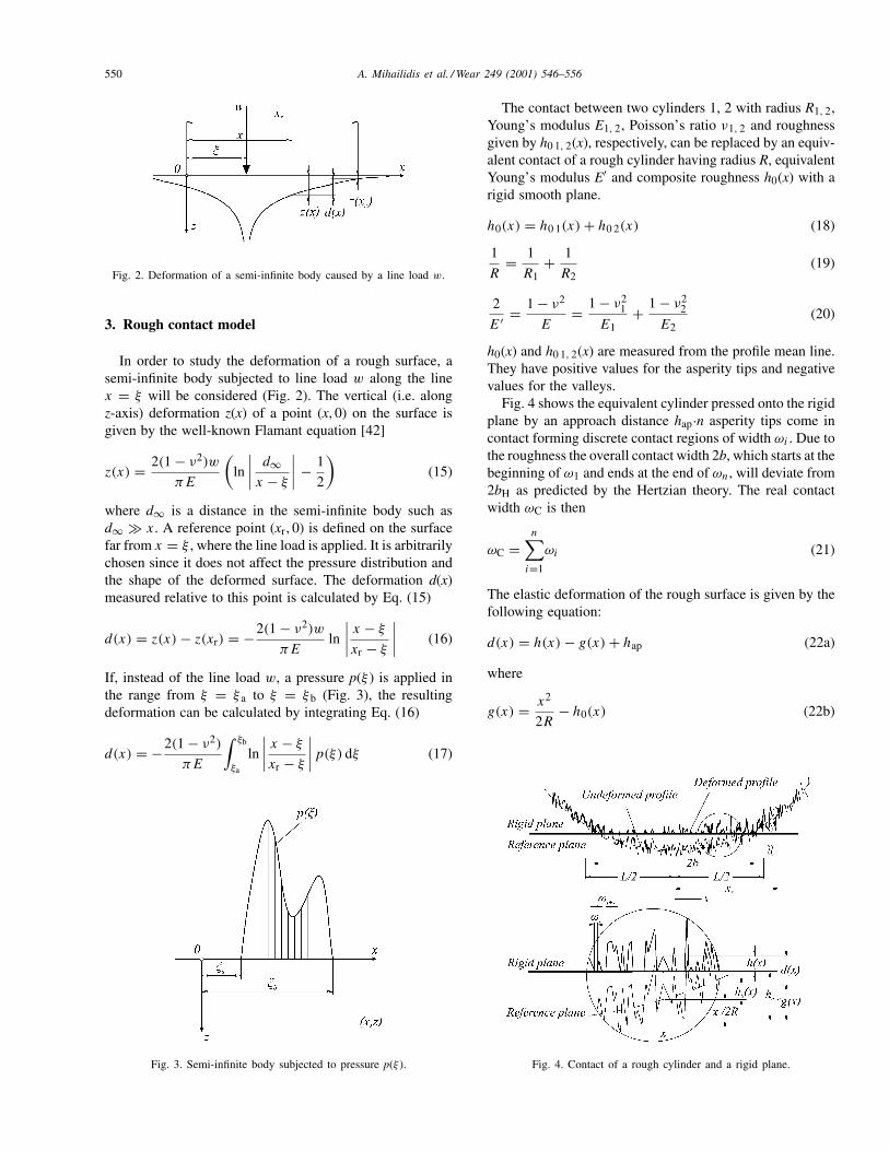
Fig. 2. Deformation of a semi-infinite body caused by a line load w.

3. Rough contact model

In order to study the deformation of a rough surface, asemi-infinite body subjected to line load w along the linex = ξ will be considered (Fig. 2). The vertical (i.e. alongz-axis) deformation z(x) of a point (x, 0) on the surface isgiven by the well-known Flamant equation [42]

z(x) = 2(1 − ν2)w

πE

(ln

∣∣∣∣ d∞x − ξ

∣∣∣∣ − 1

2

)(15)

where d∞ is a distance in the semi-infinite body such asd∞ x. A reference point (xr, 0) is defined on the surfacefar from x = ξ , where the line load is applied. It is arbitrarilychosen since it does not affect the pressure distribution andthe shape of the deformed surface. The deformation d(x)measured relative to this point is calculated by Eq. (15)

d(x) = z(x) − z(xr) = −2(1 − ν2)w

πEln

∣∣∣∣ x − ξ

xr − ξ

∣∣∣∣ (16)

If, instead of the line load w, a pressure p(ξ ) is applied inthe range from ξ = ξ a to ξ = ξb (Fig. 3), the resultingdeformation can be calculated by integrating Eq. (16)

d(x) = −2(1 − ν2)

πE

∫ ξb

ξa

ln

∣∣∣∣ x − ξ

xr − ξ

∣∣∣∣p(ξ) dξ (17)

Fig. 3. Semi-infinite body subjected to pressure p(ξ ).

The contact between two cylinders 1, 2 with radius R1, 2,Young’s modulus E1, 2, Poisson’s ratio ν1, 2 and roughnessgiven by h0 1, 2(x), respectively, can be replaced by an equiv-alent contact of a rough cylinder having radius R, equivalentYoung’s modulus E′ and composite roughness h0(x) with arigid smooth plane.

h0(x) = h0 1(x) + h0 2(x) (18)

1

R= 1

R1+ 1

R2(19)

2

E′ = 1 − ν2

E= 1 − ν2

1

E1+ 1 − ν2

2

E2(20)

h0(x) and h0 1, 2(x) are measured from the profile mean line.They have positive values for the asperity tips and negativevalues for the valleys.

Fig. 4 shows the equivalent cylinder pressed onto the rigidplane by an approach distance hap·n asperity tips come incontact forming discrete contact regions of width ωi . Due tothe roughness the overall contact width 2b, which starts at thebeginning of ω1 and ends at the end of ωn, will deviate from2bH as predicted by the Hertzian theory. The real contactwidth ωC is then

ωC =n∑

i=1

ωi (21)

The elastic deformation of the rough surface is given by thefollowing equation:

d(x) = h(x) − g(x) + hap (22a)

where

g(x) = x2

2R− h0(x) (22b)

Fig. 4. Contact of a rough cylinder and a rigid plane.


The developed pressure can then be calculated using theaforementioned form of the Flamant equation

d(x) = − 4

πE′

∫ ξ=+L/2

ξ=−L/2ln

∣∣∣∣ ξ − x

ξ − xr

∣∣∣∣p(ξ) dξ (23)

where L is a control width chosen such as L > 2bH, because2b = 2bH.

Eqs. (22a) and (23) allow for the determination of thepressure distribution for a known roughness profile if anapproach hap is given. There is no need to make assump-tions regarding the surface topography such as asperity tipradius, or height distribution. According to the assumedelastic–perfectly plastic deformation model, the asperity tipsdeform purely elastically up to a pressure of about 3Y, whereY is the yield strength of the softer material of the two bod-ies. If the local pressure exceeds this limit the asperity tipsdeform perfectly plastically without supporting any addi-tional pressure. The boundary conditions of Eqs. (22a) and(23) are

p(ξ) > 0, ξ ∈ ωC; p(ξ) > 0, ξ /∈ ωC (24)

h(x) = 0, ξ ∈ ωC; h(x) > 0, ξ /∈ ωC (25)

p(ξ) = p(ξ), if p(ξ) ≤ 3Y ;p(ξ) = 3Y, if p(ξ) > 3Y (26)

d(x) = −g(x) + hap, x ∈ ωC (27)

Once p(ξ ) is known, the resulting stress components at apoint (x, z) (Fig. 3), can be determined [43].

σx = −2z

π

∫ ξb

ξa

p(ξ)(x − ξ)2

[(x − ξ)2 + z2]2dξ (28)

σz = −2z3

π

∫ ξb

ξa

p(ξ)

[(x − ξ)2 + z2]2dξ (29)

τxz = −2z2

π

∫ ξb

ξa

p(ξ)(x − ξ)

[(x − ξ)2 + z2]2dξ (30)

In the present analysis, the maximum subsurface shearstress τ max is considered. For plane strain conditions it iscalculated as follows:

τmax =√(

σx − σz

2

)2

+ τ 2xz (31)

Eqs. (22a) and (23), along with their boundary conditions ofEqs. (28)–(31), can be solved numerically. At first, a controlwidth L of sufficient magnitude is chosen and divided intoM −1 intervals by M equally distributed nodes. The spacingbetween them is taken equal to the sampling interval. In thisway, each node matches an actual point of the measuredor generated roughness profile. Thus, the aforementioned

Fig. 5. Pressure distribution over contacting asperities: (a) second-degreepolynomial and (b) Sayles [44].

equations can be written in discrete dimensionless form asfollows:

Di = −M∑

j=1

CijPj (32)

Hi = Gi + Di + Hap (33)

Pj = 0, j /∈ ΩC (34a)

Pj > 0, j ∈ ΩC (34b)

Hi > 0, j /∈ ΩC (35a)

Hi = 0, j ∈ ΩC (35b)

Pj = Pj , if Pj ≤ 3Y (36a)

Pj = 3Y , if Pj > 3Y (36b)

Di = −Gi + Hap, j ∈ ΩC (37)

The influence coefficients Cij relate the pressure to the de-formation and depend only on the material’s elastic proper-ties, the grid geometry and the approximation of the pressuredistribution that develops at every asperity contact. Sayles[44] assumed that at every node in contact a uniform pressureis imposed over a total width equal to the sampling interval.In this paper, the assumption is made that when a node isin contact, the pressure that is built up in the region aroundit, extends over two intervals. Due to its large curvature thepressure distribution is approximated by a second-degreepolynomial. Fig. 5 illustrates a deformed profile with thesubsequent pressure distribution according to [44] and theproposed approximation. Following this assumption the in-fluence coefficients Cij are calculated as outlined in Ap-pendix A.

The solution scheme of the system of Eqs. (32)–(37) ispresented in Fig. 6. At first, a value for the approach Hap,


Fig. 6. Flow-chart for rough, dry line contact simulation.

must is given. Then, the nodes that are in contact can beidentified using Eq. (33). Every node that does not satisfy theboundary condition of Eq. (35a) is assumed to be in contactand the corresponding deformations are calculated using Eq.(37). Thus, Eq. (32) results to a N ×N system of equations.The solution of this system determines the pressures of thesenodes. Contact nodes that have zero or negative pressures areremoved from ΩC and the calculations are repeated until theboundary conditions of Eqs. (34a), (34b), (35a) and (35b)are met. When the iteration procedure has converged, theobtained pressures may exceed the pressure’s upper limit3Y . Therefore, in order to satisfy the boundary conditionsof Eqs. (36a) and (36b), these pressures are set equal to 3Y

and the calculation begins again, by determining the newdeformed shape using Eq. (32). At this stage, the resultingN × N system of equations has only N − Np unknowns,where Np is the number of nodes that deform plastically.This iteration is continued until all the boundary conditionsare met. Finally, the subsurface stress field is computed.

The mean contact pressure pm supported by the contactfor the given approach hap are calculated at the end of thesolution. If, instead of the approach distance, the pressurepm is given, then the whole procedure is repeated until anappropriate hap is found, so that the calculated pressure dis-tribution p(x) has a mean value pm equal to the given one.

4. Results and discussion

A series of simulations were conducted in order to de-termine both the validity of the numerical method and the

Table 1Roughness parameters of the profiles used in the simulations

No. Rq × 106 λx × 106 m2 m4 × 10−12 a

1 0.000130 70 1.20E−09 1.28E−09 15.012 0.0013 86 1.20E−07 1.40E−07 17.163 0.0142 84 1.33E−05 1.42E−05 16.244 0.0707 86 3.47E−04 3.92E−04 16.275 0.1320 106 1.26E−03 1.42E−03 15.596 0.4325 66 1.13E−02 1.22E−02 17.877 0.7478 58 3.16E−02 3.43E−02 19.218 0.9664 102 5.94E−02 6.20E−02 16.419 0.000145 50 4.15E−09 4.62E−09 5.62

10 0.0014 30 4.36E−07 4.82E−07 5.3211 0.0147 38 4.35E−05 4.89E−05 5.5912 0.0744 26 1.04E−03 1.15E−03 5.8813 0.1444 32 4.04E−03 4.43E−03 5.6614 0.4331 36 3.78E−02 4.22E−02 5.5415 0.7229 28 1.06E−01 1.23E−01 5.7216 1.0287 44 2.14E−01 2.51E−01 5.80

effect that roughness has on the subsurface stress field. Theroughness profiles used were generated with given compos-ite roughness Rq and autocorrelation length λx using a nu-merical procedure presented by Mihailidis and Bakolas [20].Sixteen different pairs of Rq and λx were chosen as shownin Table 1. In order to exclude statistical errors, five pro-files were generated for each one of the above-mentionedpairs. Consequently, the simulations were run for 80 differ-ent composite profiles. Table 1 also lists their slope vari-ance m2, curvature variance m4 and bandwidth parameter a.The variances m2 and m4 were calculated using a numericalmethod, based on FFT, proposed by Moalic et al. [45]. Thebandwidth parameter a is defined as

a = m0m4

m22

(38)

where m0 is the profile variance.The sampling interval was set equal to 2 m, a value

commonly used by most profilometers. The sample lengthwas chosen 1.2 mm. The equivalent radius of curvature was

Fig. 7. Deformation, pressure distribution and subsurface stress field atthe contact of a practically smooth cylinder and a rigid plane.


Fig. 8. Deformation, pressure distribution and subsurface stress field at the contact of a rigid plane and a cylinder with roughness profile (a) no. 1(Table 1), (b) no. 5 (Table 1) and (c) no. 7 (Table 1).

R = 15 mm. The yield strength of the cylinder materialwas assumed Y = 1350 N/mm2 and the equivalent Young’smodulus E′ = 2.26 × 1011 Pa. The applied line load was4094 N/mm resulting in 1250 N/mm2 maximum Hertzianpressure and 0.684 mm contact width.

Fig. 7 shows the deformed shape, the pressure distribu-tion and the resulting subsurface stress field as calculated bythe proposed model for an almost smooth cylinder (Rq =0.00013 m). These results are practically identical withthose predicted by the Hertzian theory.

Fig. 8a–c show some typical results. Even for very smallroughness, such as Rq = 0.014 m, the subsurface stressfield deviates from the Hertzian one, showing local peaksunder the asperity tips in contact. The real contact area isequal to its nominal value. All contacting asperities are de-formed elastically. For Rq = 0.75 m, the subsurface stressfield bears no resemblance to the Hertzian one. The loca-tion of the maximum shear stress shifts from z = 0.78bH,as predicted by the Hertzian theory, very close to the sur-face. About 23% of the nominal contact area is deformed


plastically and only 9% elastically. Consequently, the valueof the maximum shear stress is independent of the imposedload.

In spite of the fact that by using the elastic–perfectly plas-tic deformation model, the asperity stiffness is overestimatedas compared to the Zhao et al. model, the simulations showedthat the plastically deformed contact area is considerable andcannot be neglected when subjected to high Hertzian pres-sure, even for surfaces having composite roughness as low asRq = 0.75 m. It is evident that in these cases, the maximumshear stress appears very close to the surface and is mainlyaffected more by the surface hardness 3Y than the imposedload.

5. Conclusions

A 2-D model for the determination of the pressuredistribution at the dry contact of two rough cylinders ispresented and the resulting subsurface stress field is calcu-lated. This model can use either a numerically generatedroughness profile or an actual one, as it can be obtainedfrom a stylus type profilometer. Therefore, no assump-tions regarding the surface topography, such as roughnessheight distribution or asperity tip radius, need to be made.Digitised profiles can be used directly without any addi-tional processing such as filtering. Apart from this realisticsurface description, this model accounts for both the asper-ity interactions and the bulk deformation of the material.Deformation is assumed to follow the elastic–perfectlyplastic model. Results obtained for practically smooth sur-faces showed excellent agreement with those predictedby the Hertzian theory, verifying, thus the validity of themodel.

From the examples shown, it was concluded that rough-ness significantly alters the subsurface stress field. At mod-erate roughness or load, local maximum shear stress peaksare developed just under the contacting asperities follow-ing the de Saint–Venant principle. They coexist with themaximum that occurs in the bulk material as expected fromthe Hertzian theory. However, as the roughness or load in-creases, the stress peaks under the contacting asperities gethigher significantly exceeding the values predicted by Hertz.As the plastically deformed area of contact increases, themaximum shear stress becomes dependent only on the sur-face hardness.

The depth, at which these local maximum shear stresspeaks develop, coincides well with the depth of cracks ob-served on surfaces that failed due to micro-pitting. This ob-servation can open the way to an approach for the predictionof micro-pitting failure based on the developed subsurfacestress field.

The proposed model can be expanded to include the effectof asperity friction. It can also be incorporated in a mixedlubrication model similar to one presented earlier by theauthors [46].

Appendix A. Determination of the influencecoefficients Cij

In order to integrate Eq. (23), a method presented byWernick [47] for the integration of functions with irregular-ities was applied as follows.

The dimensionless form of Eq. (23) can be written as

D(x) = −∫ 0.5

−0.5P (ξ ′) ln

∣∣∣∣ ξ ′ − X

ξ ′ − Xr

∣∣∣∣ dξ ′

= −∫ 0.5

−0.5P (ξ ′) ln|ξ ′ − X| dξ ′

+∫ 0.5

−0.5P (ξ ′) ln|ξ ′ − Xr| dξ ′ = O1(X) + O2(Xr)

(A.1)

The control width L is divided by M equally spaced nodesinto M − 1 intervals. The values of P(ξ ′) have to be knownat the ends of these intervals. An arbitrary assumption asregards the degree of the polynomial that approximates thepressure distribution must be made. As stated earlier, theassumption is made that when a node (i.e. an asperity tip) isin contact, the pressure that is built up in the area around itextends to a width of two intervals. In this case, the integralO1(X) is

O1(X) = −I (X) = −M−1∑

j=2,4,...

Ij (X) (A.2)

where

Ij (x) =∫ ξ ′

j+1

ξ ′j−1

P (ξ ′) ln|ξ ′ − X| dξ ′ (A.3)

In this interval [ξ ′j−1, ξ ′

j+1], the pressure distribution P(ξ ′)can be sufficiently approximated by a second-degree poly-nomial, since it has a large curvature

P (ξ ′) = 1

2 · ∆2j

· [(ξ ′ − ξ ′j ) · (ξ ′ − ξ ′

j+1) · Pj−1

−2 · (ξ ′ − ξ ′j−1) · (ξ ′ − ξ ′

j+1) · Pj

+(ξ ′ − ξ ′j−1) · (ξ ′ − ξ ′

j ) · Pj+1] (A.4)

where

Pj = P (ξ ′j ) (A.5)

and

∆j = 12 (ξ ′

j+1 − ξ ′j−1) (A.6)

Integrating Eq. (A.3) one yields

Ij (X) = −uj−1(ln|uj−1| − 1)Pj−1

+(P ′j−1kj−1 − P ′

j+1kj+1)

−P ′′Aj + uj+1(ln|uj+1| − 1)Pj+1 (A.7)


where

uj = ξ ′j − X (A.8)

kj = 12 [u2

j (ln|uj | − 1.5)] (A.9)

Aj = uj−1(kj−1 − 16 (u2

j−1)) − uj+1(kj+1 − 16 (u2

j+1))

(A.10)

P ′j−1 = P ′(ξ ′

j−1) = −3Pj−1 + 4Pj − Pj+1

2∆j

(A.11)

P ′j+1 = P ′(ξ ′

j+1) = Pj−1 − 4Pj + 3Pj+1

2∆j

(A.12)

P ′′j−1 = P ′′

j+1 = Pj−1 − 2Pj + Pj+1

∆2j

(A.13)

The integral described in Eq. (A.7) can be calculated at everypoint. The only irregularity is presented at uj = 0. In thiscase, we have

limuj →0

uj ln|uj | = lim1/uj →∞

−ln(1/uj )

1/uj

= 0 (A.14)

and

limuj →0

u2j ln|uj | = lim

1/uj →∞−ln(1/uj )

(1/uj )2= 0 (A.15)

When calculating the integral I(X), it is evident fromEq. (A.7) that the contribution of P(ξ ′) at the end of the in-tervals is cancelled except for the cases, where j − 1 = 1and j +1 = M . Therefore, the integral I(X) can be written as

I (X) = −u1(ln|u1| − 1)P1

+M−1∑

j=2,4,...

I ′j (X) + uM(ln|uM | − 1)PM (A.16)

where

I ′j (X) = Pj−1

(−3kj−1 − kj+1

2∆j

− Aj

3∆2j

)

+Pj

(4kj−1 + 4kj+1

2∆j

− 2Aj

3∆2j

)

+Pj+1

(−kj−1 − 3kj+1

2∆j

− Aj

3∆2j

)(A.17)

Finally, Eq. (A.16) can also be written in the following dis-crete form:

I (X) = Qj−1Pj−1 + Qj Pj + Qj+1Pj+1 (A.18)

The following apply to the coefficients Qj of Eq. (A.18). Ifsubscript j is an even number, then Qj = Q′

j . If subscript jis odd, then the value of Qj is the sum of the values that arecalculated at the ends of the two consecutive intervals, i.e. if

j = 5, the value of Qj will be determined by the sum of thevalues Q′

4+1 from interval [ξ ′3, ξ ′

5] and Q′6−1 from interval

[ξ ′5, ξ ′

7]. Finally, at the endpoints j = 1 and j = M , we have

Q1 = −u1(ln|u1| − 1) + Q′1 (A.19)

and

QM = uM(ln|uM | − 1) + Q′M (A.20)

where

Q′j−1 = −3kj−1 − kj+1

2∆j

− Aj

3∆2j

(A.21)

Q′j = 4kj−1 + 4kj+1

2∆j

− 2Aj

3∆2j

(A.22)

Q′j+1 = −kj−1 − 3kj+1

2∆j

− Aj

3∆2j

(A.23)

Therefore, Eq. (A.2) reduces to

O1i = −M∑

j=1

Qi,j Pj (A.24)

Accordingly, the integral O2(Xr) can be written as

O2(Xr) =M∑

j=1

QXr,j Pj (A.25)

Thus, the discrete form of Eq. (A.1) and the influence coef-ficients Cij are given by

Di = O1i + O2(Xr) = −M∑

j=1

CijPj (A.26)

and

Cij = Qij − QXr,j (A.27)

References

[1] G. Schönnenbeck, Einfluß der Schmierstoffe auf die Zahnflankenermüdung (Graufleckigkeit und Grübchenbildung) hauptsä-chlich im Umfangsgeschwindigkeitbereich 1. . . 9 m/s, Diss. TUMünchen, 1984.

[2] G. Liu, Q. Wang, C. Lin, A survey of current models for simulatingthe contact between rough surfaces, Tribol. Trans. 42 (1999)581–591.

[3] J.A. Greenwood, J.B.P. Williamson, Contact of nominally flatsurfaces, Proc. R. Soc. London Ser. A 295 (1966) 300–319.

[4] J.A. Greenwood, J.H. Tripp, The contact of two nominally flat roughsurfaces, Proc. Inst. Mech. Eng. 185 (1970) 625–633.

[5] R.A. Onions, J.F. Archard, The contact of surfaces having a randomsurface structure, J. Phys. D Appl. Phys. 6 (1973) 289–304.

[6] W.R. Chang, I. Etsion, D.B. Bogy, An elastic–plastic model for thecontact of rough surfaces, ASME J. Tribol. 110 (1987) 50–56.

[7] A.W. Bush, R.D. Gibson, T.R. Thomas, The elastic contact of arough surface, Wear 35 (1975) 87–111.


[8] J.H. Horng, An elliptic elastic–plastic asperity micro-contact modelfor rough surfaces, ASME J. Tribol. 120 (1998) 82–88.

[9] E.R.M. Gelink, D.J. Schipper, Deformation of rough line contacts,ASME J. Tribol. 121 (1999) 449–454.

[10] A.A. Polycarpou, I. Etsion, Analytical approximations in modellingcontacting rough surfaces, ASME J. Tribol. 121 (1999) 234–239.

[11] Z. Liu, A. Neville, R.L. Reuben, An analytical solution for elasticand elastic–plastic contact models, Tribol. Trans. 43 (2000) 627–634.

[12] J.I. McCool, Comparison of models for the contact of rough surfaces,Wear 107 (1986) 37–60.

[13] A. Majumdar, B. Bushan, Fractal model of elastic–plastic contactbetween rough surfaces, ASME J. Tribol. 113 (1991) 1–11.

[14] B. Bushan, A. Majumdar, Elastic–plastic contact model of bi-fractalsurfaces, Wear 153 (1992) 53–64.

[15] T.L. Warren, D. Krajcinovic, Random cantor set models for theelastic–perfectly plastic contact of rough surfaces, Wear 196 (1996)1–15.

[16] L. Yongsheng, Y. Guiping, H. Yan, Z. Linqing, The characteristicsof elastically contacting ideal rough surfaces, ASME J. Tribol. 118(1996) 90–97.

[17] I. Lee-Prudhoe, R.S. Sayles, A. Kaderic, Investigations into asperitypersistence in heavily loaded contacts, ASME J. Tribol. 121 (1999)441–448.

[18] N. Patir, A numerical procedure for random generation of roughsurfaces, Wear 47 (1978) 263–277.

[19] Y.Z. Hu, K. Tonder, Simulation of 3-D random surface by 2-D digitalFilter and Fourier analysis, Int. J. Mach. Tools Manufact. 32 (1992)83–90.

[20] A. Mihailidis, V. Bakolas, Numerical simulation of real 3-D roughsurfaces, J. Balkan Tribol. Assoc. 5 (1999) 247–255.

[21] E.R. Kral, K. Komvopoulos, D.B. Bogy, Elastic–plastic finite elementanalysis of repeated indentation of a half-space by a rigid sphere, J.Appl. Mech. 60 (1963) 829–841.

[22] K.L. Johnson, Contact Mechanics, Cambridge University Press,Cambridge, MA, 1987.

[23] W.T. Lai, H.S. Cheng, Computer simulation of elastic rough contacts,ASLE Trans. 28 (1985) 172–180.

[24] M.N. Webster, R.S. Sayles, A numerical model for the elasticfrictionless contact of real rough surfaces, ASME J. Tribol. 108(1986) 314–320.

[25] S.C. Lee, H.S. Cheng, On the relation of load to average gap in thecontact between surfaces with longitudinal roughness, Tribol. Trans.35 (1992) 523–529.

[26] N. Ren, S.C. Lee, Contact simulation of three-dimensional roughsurfaces using moving grid method, ASME J. Tribol. 115 (1993)597–601.

[27] N. Ren, S.C. Lee, The effect of surface roughness and topographyon the contact behaviour of elastic bodies, ASME J. Tribol. 116(1994) 804–811.

[28] S.C. Lee, N. Ren, Behaviour of elastic–plastic surface contacts asaffected by surface topography, load and material Hardness, Tribol.Trans. 39 (1996) 67–74.

[29] C.Y. Poon, R.S. Sayles, Numerical contact model of a smooth ball onan anisotropic rough surface, ASME J. Tribol. 116 (1994) 194–201.

[30] I.A. Polonsky, I.M. Keer, Fast methods for solving rough contactproblems: a comparative study, ASME J. Tribol. 122 (2000) 36–41.

[31] Y. Ju, T.N. Farris, Spectral analysis of two-dimensional contactproblems, ASME J. Tribol. 118 (1996) 320–328.

[32] X. Tian, B. Bushan, A numerical three-dimensional model for thecontact of rough surfaces by variational principle, ASME J. Tribol.118 (1996) 33–42.

[33] H.M. Stanley, T. Kato, An FFT-based method for rough surfacecontact, ASME J. Tribol. 119 (1997) 481–485.

[34] Y.Z. Hu, G.C. Barber, D. Zhu, Numerical analysis of the elasticcontact of real rough surfaces, Tribol. Trans. 42 (1999) 443–452.

[35] X. Ai, K. Sawamiphakdi, Solving elastic contact between roughsurfaces as an unconstrained strain energy minimisation by usingCGM and FFT techniques, ASME J. Tribol. 121 (1999) 639–647.

[36] W.R. Chang, Contact, Adhesion and Static Friction of Metallic RoughSurfaces, Ph.D. Thesis, University of California, Berkeley, CA, 1986.

[37] D. Tabor, The Hardness of Metals, Oxford University Press, Oxford,1951.

[38] C. Hardy, C.N. Baronet, G.V. Tordion, Elasto-plastic indentation ofa half-space by a rigid sphere, Int. J. Numer. Mech. Eng. 3 (1971)451–462.

[39] W.R. Chang, An elastic–plastic contact model for a rough surfacewith an ion plated soft metallic coating, Wear 212 (1997)229–237.

[40] Y. Zhao, D.M. Maietta, L. Chang, An asperity micro-contact modelincorporating the transition from elastic deformation to fully plasticflow, ASME J. Tribol. 122 (2000) 86–93.

[41] A. Sackfield, D.A. Hills, Some useful results in the tangential loadHertz problem, J. Strain Anal. 18 (1983) 108–110.

[42] I. Szabó, Höhere Technische Mechanik, 5. Auflage, Springer, Berlin,Heidelberg, New York, 1972.

[43] S. Timoshenko, J.N. Goodier, Theory of Elasticity, 3rd Edition,McGraw-Hill, New York, 1970.

[44] R.S. Sayles, Basic principles of rough surface contact analysis usingnumerical methods, Tribol. Int. 29 (1996) 639–650.

[45] H. Moalic, J.A. Fitzpatrick, A.A. Torrance, The correlation of thecharacteristics of rough surfaces with their friction coefficients, Proc.Inst. Mech. Eng. 201 (1987) 321–329.

[46] A. Mihailidis, V. Bakolas, Subsurface stresses of gear contactsunder Partial–EHD lubrication, Balkantrib ’96, 5–7 June 1996,Thessaloniki, Greece.

[47] R.J. Wernick, Some Computer Results in the Direct Iteration Solutionof the Elastohydrodynamic Equations, MTI-62TR38, MechanicalTechnologies Inc., Latham, New York, 1963.

Subsurface stress field of a dry line contact

Documents

Transcript of Subsurface stress field of a dry line contact