Studying Irreversible Transitions in a Model of Cell Cycle Regulation

Studying Irreversible Transitions in a Modelof Cell Cycle Regulation

Paolo Ballarini a,1,2, Tommaso Mazza a,1,2,Alida Palmisano a,1,2 and Attila Csikasz-Nagy a,1,2

a The Microsoft Research - University of TrentoCentre for Computational and Systems Biology

Piazza Manci 17, 38100 Trento, Italy

Abstract

Cells life follows a cycling behaviour which starts at cell birth and leads to cell division through a number ofdistinct phases. The transitions through the various cell cycle phases are controlled by a complex networkof signalling pathways. Many cell cycle transitions are irreversible: once they are started they must reachcompletion. In this study we investigate the existence of conditions which lead to cases when irreversibilitymay be broken. Specifically, we characterise the elements of the cell cycle signalling network that areresponsible for the irreversibility and we determine conditions for which the irreversible transitions maybecome reversible. We illustrate our results through a formal approach in which stochastic simulationanalysis and model checking verification are combined. Through probabilistic model checking we provide aquantitative measure for the probability of irreversibility in the “Start” transition of the cell cycle.

Keywords: Budding Yeast, Cell Cycle, Probabilistic Model Checking, BlenX, Stochastic Simulation.

1 Introduction

The cell division cycle is a coordinated set of processes by which a cell replicatesall its components and divides into two nearly identical daughter cells. The eukary-otic cell cycle is driven by an underlying molecular network which centers aroundcomplexes of cyclin dependent kinases (Cdk’s) and their regulatory cyclin partners.Active Cdk/cyclin (CycB) complexes can induce critical cell cycle processes by phos-phorylating target molecules [16]. The activity of this complex can be regulated inseveral ways, one of which is the controlled degradation of the cyclin subunit. TheAnaphase Promoting Complex (APC) with help from the regulatory protein Cdh1labels cyclins for degradation at the end of the cell cycle. Interestingly, Cdk/CycB

1 The authors would like to thank Ivan Mura for comments and discussions about stochastic modeling.2 Email: {ballarini,mazza,palmisano,csikasz}@cosbi.eu

Electronic Notes in Theoretical Computer Science 232 (2009) 39–53

1571-0661/$ – see front matter © 2009 Elsevier B.V. All rights reserved.

www.elsevier.com/locate/entcs

doi:10.1016/j.entcs.2009.02.049

http://www.elsevier.com/locate/entcs

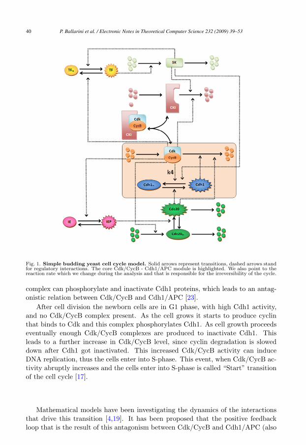
Fig. 1. Simple budding yeast cell cycle model. Solid arrows represent transitions, dashed arrows standfor regulatory interactions. The core Cdk/CycB - Cdh1/APC module is highlighted. We also point to thereaction rate which we change during the analysis and that is responsible for the irreversibility of the cycle.

complex can phosphorylate and inactivate Cdh1 proteins, which leads to an antag-onistic relation between Cdk/CycB and Cdh1/APC [23].

After cell division the newborn cells are in G1 phase, with high Cdh1 activity,and no Cdk/CycB complex present. As the cell grows it starts to produce cyclinthat binds to Cdk and this complex phosphorylates Cdh1. As cell growth proceedseventually enough Cdk/CycB complexes are produced to inactivate Cdh1. Thisleads to a further increase in Cdk/CycB level, since cyclin degradation is sloweddown after Cdh1 got inactivated. This increased Cdk/CycB activity can induceDNA replication, thus the cells enter into S-phase. This event, when Cdk/CycB ac-tivity abruptly increases and the cells enter into S-phase is called “Start” transitionof the cell cycle [17].

Mathematical models have been investigating the dynamics of the interactionsthat drive this transition [4,19]. It has been proposed that the positive feedbackloop that is the result of this antagonism between Cdk/CycB and Cdh1/APC (also

P. Ballarini et al. / Electronic Notes in Theoretical Computer Science 232 (2009) 39–5340

called double negative feedback, since the two negative effects bring together apositive loop) can create bistability and hysteresis in the system [4]. Furthermore ithas been proposed that this simple module can be responsible for the irreversibilityof the Start transition of the cell cycle [20]. Experiments proved the existence ofbistability in the cell cycle of budding yeast cells [6], but the irreversibility of thistransition was never tested yet.

In this paper we present an analysis of this module by application of both prob-abilistic model checking and stochastic simulations on a simple budding yeast cellcycle model. More specifically we show that irreversibility can be removed fromthe system by weakening the positive feedback loop. The remainder of the paperis organised as follows: we first briefly describe a model of the budding yeast cellcycle (Sec. 2) concentrating, in Sec 2.1, on one of its basic mechanism, namely theCdk/CycB-Cdh1/APC interaction, which is what we focus our irreversibility studyon. In Section 3 we present probabilistic model checking and describe a quantitativeanalysis of the stochastic model obtained through verification of probabilistic logicalqueries. In Section 4 we discuss results obtained through stochastic simulation ofthe detailed model of the cell cycle that is containing the core mechanism analysedin the previous sections. We summarise our contribution in the conclusive section.

2 A model of budding yeast cell cycle regulation

During normal cell cycles of the budding yeast the two stable states of the presentedbistable switch (G1 with low Cdk/CycB and high Cdh1/APC activity; S/G2/M,with high Cdk/CycB and low Cdh1/APC activity) are alternating. There are sev-eral assisting molecules that help the switch to turn back and forth between thesestable states [3]. A starter kinase (SK) helps Cdk/CycB to turn off Cdh1/APC andto remove CKI (another inhibitor of Cdk/CycB) at the G1/S transition. On theother hand Cdc20 helps to reactivate Cdh1/APC and remove Cdk/CycB activityat the end of the cell cycle (see Figure 1). In addition there are further regulators(transcription factors (TF), intermediary enzymes (IE), etc . . . ) that play roles inrobust cell cycle regulation.

2.1 Cdk/CycB - Cdh1/APC interactions in the core of cell cycle regulation

At the core of the cell cycle regulation stands the antagonistic interaction betweenCdk/CycB and Cdh1/APC (Fig 2). This switch makes the decisions on commit-ment to start the cell cycle [3]. The wiring diagram of Figure 2 was turned to ODE’sby Novak and Tyson [12]. The dynamic of the real valued variables X and Y (rep-resenting the concentration of Cdk/CycB and Cdh1/APC complexes respectively)are described by the following linear ordinary differential equations, taken from [12]:

P. Ballarini et al. / Electronic Notes in Theoretical Computer Science 232 (2009) 39–53 41

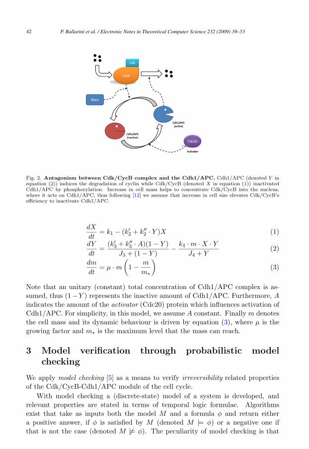
Fig. 2. Antagonism between Cdk/CycB complex and the Cdh1/APC. Cdh1/APC (denoted Y inequation (2)) induces the degradation of cyclin while Cdk/CycB (denoted X in equation (1)) inactivatedCdh1/APC by phosphorylation. Increase in cell mass helps to concentrate Cdk/CycB into the nucleus,where it acts on Cdh1/APC, thus following [12] we assume that increase in cell size elevates Cdk/CycB’sefficiency to inactivate Cdh1/APC.

dX

dt= k1 − (k′

2 + k′′2 · Y )X (1)

dY

dt=

(k′3 + k′′

3 · A)(1 − Y )J3 + (1 − Y )

− k4 · m · X · YJ4 + Y

(2)

dm

dt= μ · m

(1 − m

m∗

)(3)

Note that an unitary (constant) total concentration of Cdh1/APC complex is as-sumed, thus (1−Y ) represents the inactive amount of Cdh1/APC. Furthermore, A

indicates the amount of the activator (Cdc20) protein which influences activation ofCdh1/APC. For simplicity, in this model, we assume A constant. Finally m denotesthe cell mass and its dynamic behaviour is driven by equation (3), where μ is thegrowing factor and m∗ is the maximum level that the mass can reach.

3 Model verification through probabilistic modelchecking

We apply model checking [5] as a means to verify irreversibility related propertiesof the Cdk/CycB-Cdh1/APC module of the cell cycle.

With model checking a (discrete-state) model of a system is developed, andrelevant properties are stated in terms of temporal logic formulae. Algorithmsexist that take as inputs both the model M and a formula φ and return eithera positive answer, if φ is satisfied by M (denoted M |= φ) or a negative one ifthat is not the case (denoted M �|= φ). The peculiarity of model checking is that


// Budding yeast CELL-CYCLE

ctmc // stocastic modelconst double k4=35;const int n=4; // power in rate of Cdc20 reactionconst double alpha=0.00302023; //conversion factor from continuous concentrations to discreteconst double mu=0.01; // rate of Mass growthconst int noise d=2;

// initial populationconst int Y init=42;const int X init=1;const int m init=50;const int A=42; //424;

// maximum populationconst int Y max=42;const int X max=42;const int m max=50;

Table 1PRISM model’s constants. Discretized quantities translate to integer constants: noise d represents the

desired level of noise and is set to 2, which is roughly 5% of maximum signal level

verification of φ against M is achieved through an exhaustive exploration of themodel state space, hence the outcome of model verification is exact, as opposed tothe approximated results obtained through model simulation. The obvious downsideof model checking, is that, due to the complexity of many real systems, the resultingmodel dimension blows up to the point that model checking becomes untreatable.

Model checking techniques can be classified according to the type of model theyrefer to and to the query language they adopt. A broad taxonomy may distinguishbetween non-probabilistic model checking, such as LTL and CTL model checking,and probabilistic model checking, such as PCTL [14] and CSL [1,2] model checking.Since the nature of the models we develop in this work is inherently stochastic,we focus on probabilistic/stochastic model checking, which we briefly introduce inthe following sections. We first shortly describe the class of stochastic processes wehave considered in our modelling effort, namely Continuous Time Markov Chains(CTMCs), pointing out some relevant steps for the derivation of a stochastic modelof the cell-cycle regulatory network described in Figure 2.

3.1 On the Markovian model of the Cdk/CycB-Cdh1/APC module of the cell cycle

CTMCs are a well established form of discrete-state stochastic processes largelyused for modelling and analysis of many different types of systems. Praticallyspeaking a CTMC model can be thought of as a graph whose states correspond tovariables’ value and whose transitions indicate the dynamic of the modeled system.In a CTMC, transitions are labelled with real valued numbers, representing therate of an exponentially distributed delay (the time consumed by the transition totake place). Once a CTMC model is developed then it can be analysed in severalmanners. Classical steady-state and transient analysis, provides information aboutthe system evolution, respectively, in the long run (steady-state), or with respect toa specific instant of time (transient analysis). If the model is too large, stochasticsimulation can be applied to derive relevant statistics. For a detailed descriptionof CMTC models the reader is referred to one the many books, such as, for


module cyclinBX : [0.. X max ] init X init ;X inc count : [0.. noise d ] init 0;X dec count : [0.. noise d ] init 0;increasing macro X : bool init true;decreasing macro X : bool init true;

[synth X ] true & X inc count<noise d − 1 → (k1/alpha) : X ′=(min( X + 1,X max))& ( X inc count ′=min( X inc count + 1,noise d))& ( X dec count ′=max( X dec count − 1, 0));

[synth X ] true & X inc count{≥}noise d − 1 → (k1/alpha) : X ′=(min( X + 1,X max))& (increasing macro X ′=true)& (decreasing macro X ′=false)& ( X inc count ′=0) & ( X dec count ′=0);

[selfdeg X ] ( X>0) & X dec count<noise d − 1 → k2 1 ∗ X : X ′=(max( X − 1, 0))& ( X dec count ′=min( X dec count + 1,noise d))& ( X inc count ′=max( X inc count − 1, 0));

[selfdeg X ] ( X>0) & X dec count{≥}noise d − 1 → k2 1 ∗ X : X ′=(max( X − 1, 0))& ( X dec count ′=0) & ( X inc count ′=0)& (decreasing macro X ′=true) & (increasing macro X ′=false);

[deg X ] ( X>0) & X dec count<noise d − 1 → k2 2 ∗ alpha ∗ X : X ′=(max( X − 1, 0))& ( X dec count ′=min( X dec count + 1,noise d))& ( X inc count ′=max( X inc count − 1, 0));

[deg X ] ( X>0) & X dec count{≥}noise d − 1 → k2 2 ∗ alpha ∗ X : X ′=(max( X − 1, 0))& ( X dec count ′=0) & ( X inc count ′=0)& (decreasing macro X ′=true) & (increasing macro X ′=false);

[deactivation Y ] ( X>0) → X : true;endmodule

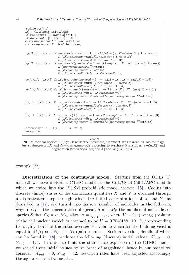
Table 2PRISM code for species X (CycB): noise-free increment/decrement are recorded on boolean flagsincreasing macro X and decreasing macro X according to synthesis (transitions [synth X]) and

degradation (transitions [selfdeg X] and [deg X]) of X.

example [22].

Discretization of the continuous model. Starting from the ODEs (1)and (2) we have derived a CTMC model of the Cdk/CycB-Cdh1/APC modulewhich we coded into the PRISM probabilistic model checker [15]. Coding intodiscrete (finite) states of the continuous quantities X and Y is obtained througha discretization step through which the initial concentrations of X and Y , asdescribed in [12], are turned into discrete number of molecules in the followingway: if CS is the concentration of species S and MS the number of molecules ofspecies S then CS = α ·MS , where α = 1

NA·V ·10−6 , where V is the (average) volumeof the cell nucleus (which is assumed to be V = 0.7043188 · 10−15, correspondingto roughly 1.67% of the initial average cell volume which for the budding yeast isequal to 42fl) and NA the Avogadro number. Such conversion, details of whichcan be found in [18], produces the following (discrete) initial values: Xinit = 0,Yinit = 424. In order to limit the state-space explosion of the CTMC model,we scaled those initial values by an order of magnitude, hence in our model weconsider: Xinit = 0, Yinit = 42. Reaction rates have been adjusted accordinglythrough a re-scaled value of α.


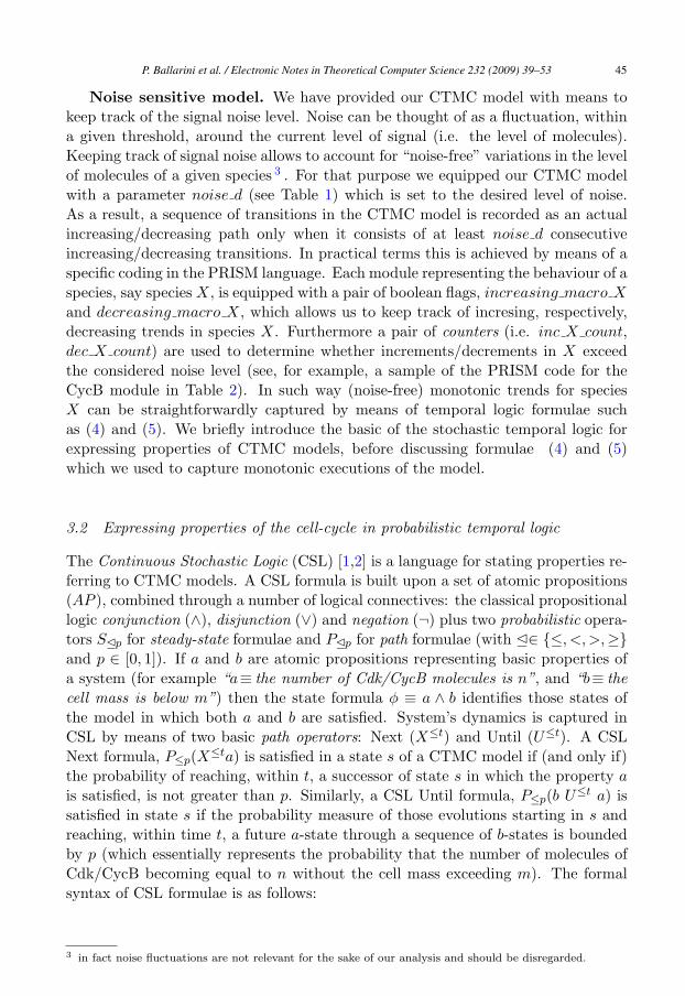
Noise sensitive model. We have provided our CTMC model with means tokeep track of the signal noise level. Noise can be thought of as a fluctuation, withina given threshold, around the current level of signal (i.e. the level of molecules).Keeping track of signal noise allows to account for “noise-free” variations in the levelof molecules of a given species 3 . For that purpose we equipped our CTMC modelwith a parameter noise d (see Table 1) which is set to the desired level of noise.As a result, a sequence of transitions in the CTMC model is recorded as an actualincreasing/decreasing path only when it consists of at least noise d consecutiveincreasing/decreasing transitions. In practical terms this is achieved by means of aspecific coding in the PRISM language. Each module representing the behaviour of aspecies, say species X, is equipped with a pair of boolean flags, increasing macro X

and decreasing macro X, which allows us to keep track of incresing, respectively,decreasing trends in species X. Furthermore a pair of counters (i.e. inc X count,dec X count) are used to determine whether increments/decrements in X exceedthe considered noise level (see, for example, a sample of the PRISM code for theCycB module in Table 2). In such way (noise-free) monotonic trends for speciesX can be straightforwardly captured by means of temporal logic formulae suchas (4) and (5). We briefly introduce the basic of the stochastic temporal logic forexpressing properties of CTMC models, before discussing formulae (4) and (5)which we used to capture monotonic executions of the model.

3.2 Expressing properties of the cell-cycle in probabilistic temporal logic

The Continuous Stochastic Logic (CSL) [1,2] is a language for stating properties re-ferring to CTMC models. A CSL formula is built upon a set of atomic propositions(AP ), combined through a number of logical connectives: the classical propositionallogic conjunction (∧), disjunction (∨) and negation (¬) plus two probabilistic opera-tors S�p for steady-state formulae and P�p for path formulae (with �∈ {≤, <, >,≥}and p ∈ [0, 1]). If a and b are atomic propositions representing basic properties ofa system (for example “a≡ the number of Cdk/CycB molecules is n”, and “b≡ thecell mass is below m”) then the state formula φ ≡ a ∧ b identifies those states ofthe model in which both a and b are satisfied. System’s dynamics is captured inCSL by means of two basic path operators: Next (X≤t) and Until (U≤t). A CSLNext formula, P≤p(X≤ta) is satisfied in a state s of a CTMC model if (and only if)the probability of reaching, within t, a successor of state s in which the property a

is satisfied, is not greater than p. Similarly, a CSL Until formula, P≤p(b U≤t a) issatisfied in state s if the probability measure of those evolutions starting in s andreaching, within time t, a future a-state through a sequence of b-states is boundedby p (which essentially represents the probability that the number of molecules ofCdk/CycB becoming equal to n without the cell mass exceeding m). The formalsyntax of CSL formulae is as follows:

3 in fact noise fluctuations are not relevant for the sake of our analysis and should be disregarded.


φ := a | | ¬φ | φ ∧ φ | S�p(φ) | P�p(ϕ)

ϕ := XI φ | φ U Iφ

where a ∈ AP is an atomic proposition, is the truth value true, �∈ {<,≤, >,≥},I ⊆ R≥0 is a non empty (time) interval, S denotes the steady-state operator (i.e. itrefers to the steady-state measure of probability) and P denotes paths’ measure ofprobability.

Relaying on the expressiveness of the CSL language we formulate a numberof properties which capture relevant features of the cell-cycle CTMC model.Irreversibility in the Cdk/CycB-Cdh1/APC module of the cell-cycle correspondsto the monotonic trend of both X (Cdk/CycB) and Y (Cdh1/APC). In the initialstate X is low (X = 0) whereas Y is high (Y = 42) , when the cell’s mass reachesa certain threshold then Y gets inactivated thus X starts growing. We formallycharacterise monotonicity of Y and X with the following CSL path formulae:

Probability of Monotonic decrease of Cdh1/APC. “What is the proba-bility that the number of molecules of Cdh1/APC decreases monotonically until thevalue k is reached?”

P=?[(decreasing Y U (Y = k)] (4)

Probability of Monotonic increase of Cdk/CycB. ‘What is the probabilitythat the number of molecules of Cdk/CycB increases monotonically until the valuek is reached?”

P=?[(increase X U (X = k)] (5)

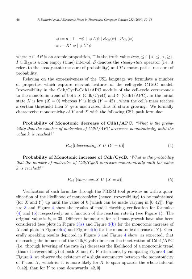
Verification of such formulae through the PRISM tool provides us with a quan-tification of the likelihood of monotonicity (hence irreversibility) to be maintained(for X and Y ) up until the value of k (which can be made varying in [0, 42]). Fig-ure 3 and Figure 4 show the results of model checking verification for formulae(4) and (5), respectively, as a function of the reaction rate k4 (see Figure 1). Theoriginal value is k4 = 35. Different boundaries for cell mass growth have also beenconsidered (see plots in Figure 3(a) and Figure 3(b) for the monotonic increase ofX and plots in Figure 4(a) and Figure 4(b) for the monotonic decrease of Y ). Gen-erally speaking results depicted in Figure 3 and Figure 4 show, as expected, thatdecreasing the influence of the Cdk/CycB dimer on the inactivation of Cdh1/APC(i.e. through lowering of the rate k4) decreases the likelihood of a monotonic trend(thus of irreversibility) of both X and Y . Furthermore, by comparing Figure 4 andFigure 3, we observe the existence of a slight asymmetry between the monotonicityof Y and X, which is: it is more likely for X to span upwards the whole interval[0, 42], than for Y to span downwards [42, 0].


0.001

0.01

0.1

1

0 5 10 15 20 25 30 35

Probability

k

Cdk/CycB monotonic increase from 1 to k

k4=5k4=15k4=25k4=35

(a) variable cell mass:Minit = 50,Mmax = 150

0.001

0.01

0.1

1

0 5 10 15 20 25 30 35

Probability

k

Cdk/CycB monotonic increase from 1 to k

k4=5k4=15k4=25k4=35

(b) variable cell mass:Minit = 100,Mmax = 200

Fig. 3. Monotonic increase of Cdk/CycB with cell mass growth.

1e-07

1e-06

1e-05

0.0001

0.001

0.01

0.1

1

0 5 10 15 20 25 30 35

Probability

k

Cdh1/APC monotonic decrease from k to 1

k4=5k4=15k4=25k4=35

(a) variable cell mass: Minit = 50, Mmax = 150

1e-07

1e-06

1e-05

0.0001

0.001

0.01

0.1

1

0 5 10 15 20 25 30 35

Probability

k

Cdh1/APC monotonic decrease from k to 1

k4=5k4=15k4=25k4=35

(b) variable cell mass: Minit = 100, Mmax = 200

Fig. 4. Monotonic decrease of Cdh1/APC with with cell mass growth.

4 Stochastic simulation of the detailed model

In order to “validate” the results obtained through probabilistic model checking weuse a more detailed version of the cell cycle regulatory network which we consideredin Sec. 3. By means of the Beta Workbench [8], a computational tool based onthe BlenX modelling language for biological systems, we developed a model of thewild-type network [12] as depicted in Figure 1.

The resulting BlenX code obtained through the translation of the ODEs in [12]is contained in Appendix A. A detailed description of the BlenX language and of themodel building procedure is out of the scope of this paper; here we just summarizethe sub-set of the BlenX language needed for the understanding of the code of thepresented model. We refer the reader to [8,9] for a detailed description of thelanguage and its modeling approach.

The basic metaphor that BlenX relies on is that a biological entity (i.e. a compo-nent that is able to interact with other components to accomplish some biological


functions) is represented by a box in BlenX. A box has an interface (its set of binders)and an internal structure that drives its behaviour (see Fig. 5).

Fig. 5. Boxes as abstractions of biological entities.

For example, in a box modeling a protein, binders may represent sensing andeffecting domains. Sensing domains are the places where the protein receives signals,effecting domains are the places that a protein uses for propagating signals, and theinternal structure codifies for mechanism that transforms an input signal into aprotein conformational change, which can result in the activation or deactivation ofanother domain.

The exchanging of signals can happen between boxes whose binders have acertain degree of affinity, which codes the strength of their interaction.

The basic primitives of the language that are used to build the model in Ap-pendix A are summarized in graphical form in Fig. 6. Besides the action in thefigure, we can specify events of the form: “when(conditions) verb”, where the actionverb is triggered when conditions are satisfied. The verb can be one among split,new or delete, modeling respectively the substitution, creation, and deletion ofboxes in the system (see Fig. 6). Conditions, in the models presented here, are inthe form of “entity name : : rate function”, whose meaning is that with the raterate function the action after the condition is triggered on the entity entity name.

Fig. 6. Intuitive behaviour of some BlenX primitives. Each row represents one of the primitives used inour translation. The first primitive code the interaction between two boxes, through the exchange of aninput/output signal (input is in the form of b?() and the output is in the form a!()). The meaning of thelast three events is explained in the text.

Rate functions can be declared using real numbers that will be used as baserate for the elementary mass action law, or arbitrary functions (e.g. a sigmoidalresponse) that are useful when a box represents an aggregated process or when theprecise mechanism of interaction between entities is not known.

Using this sub-set of the BlenX language, we were able to built the executablemodel in Appendix A of the wild-type cell-cycle in Figure 1. On that model weperformed Multiple stochastic simulative Replications in Parallel (MRIP).

MRIP approaches are frequently used to speed up simulations by working outindependent replications of the same stochastic trajectory on multiple computers.Each run is calculated starting from a seed chosen among a stream of pseudorandom


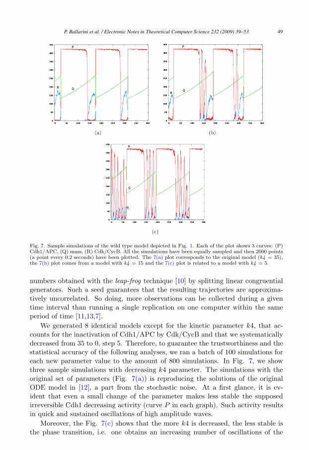
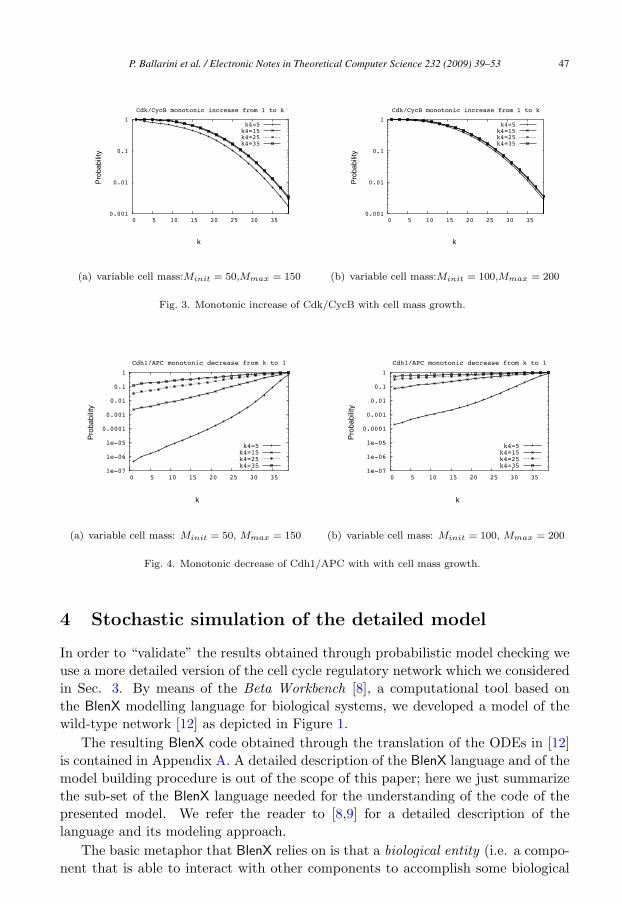
Fig. 7. Sample simulations of the wild type model depicted in Fig. 1. Each of the plot shows 3 curves: (P)Cdh1/APC, (Q) mass, (R) Cdk/CycB. All the simulations have been equally sampled and then 2000 points(a point every 0.2 seconds) have been plotted. The 7(a) plot corresponds to the original model (k4 = 35),the 7(b) plot comes from a model with k4 = 15 and the 7(c) plot is related to a model with k4 = 5.

numbers obtained with the leap-frog technique [10] by splitting linear congruentialgenerators. Such a seed guarantees that the resulting trajectories are approxima-tively uncorrelated. So doing, more observations can be collected during a giventime interval than running a single replication on one computer within the sameperiod of time [11,13,7].

We generated 8 identical models except for the kinetic parameter k4, that ac-counts for the inactivation of Cdh1/APC by Cdk/CycB and that we systematicallydecreased from 35 to 0, step 5. Therefore, to guarantee the trustworthiness and thestatistical accuracy of the following analyses, we ran a batch of 100 simulations foreach new parameter value to the amount of 800 simulations. In Fig. 7, we showthree sample simulations with decreasing k4 parameter. The simulations with theoriginal set of parameters (Fig. 7(a)) is reproducing the solutions of the originalODE model in [12], a part from the stochastic noise. At a first glance, it is ev-ident that even a small change of the parameter makes less stable the supposedirreversible Cdh1 decreasing activity (curve P in each graph). Such activity resultsin quick and sustained oscillations of high amplitude waves.

Moreover, the Fig. 7(c) shows that the more k4 is decreased, the less stable isthe phase transition, i.e. one obtains an increasing number of oscillations of the


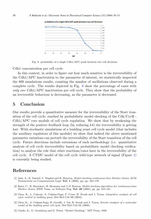
Fig. 8. probability of a single Cdh1/APC peak between two cell divisions

Cdh1 concentration per cell cycle.In this context, in order to figure out how much sensitive is the irreversibility of

the Cdh1/APC inactivation to the parameter of interest, we statistically inspectedthe 800 simulations results, counting the number of oscillations observed during acomplete cycle. The results depicted in Fig. 8 show the percentage of cases withonly one Cdh1/APC inactivation per cell cycle. They show that the probability ofan irreversible behaviour is decreasing, as the parameter is decreased.

5 Conclusion

Our results provide a quantitative measure for the irreversibility of the Start tran-sition of the cell cycle, reached by probabilistic model checking of the Cdk/CycB -Cdh1/APC core module of cell cycle regulation. We show that by weakening thestrength of the positive feedback loop (by reducing k4) the irreversibility is gettinglost. With stochastic simulations of a budding yeast cell cycle model (that includesthe auxiliary regulators of this module) we show that indeed the above mentionedparameter variations can perturb the irreversibility of the Start transition of the cellcycle. Future directions include extensions of such methodology (i.e. quantitativeanalysis of cell cycle irreversibility based on probabilistic model checking verifica-tion) to analyze the role that other reactions/rates have in the irreversibility of thecell cycle. A CTMC model of the cell cycle wild-type network of signal (Figure 1)is currently being studied.

References

[1] Aziz, A., K. Sanwal, V. Singhal and R. Brayton, Model-checking continuous-time Markov chains, ACMTransactions on Computational Logic Vol. 1 (2000), pp. pp. 162–170.

[2] Baier, C., B. Haverkort, H. Hermann and J.-P. Katoen, Model-checking algorithms for continuous-timeMarkov chains, IEEE Trans. on Software Eng. Vol. 29 (2003), pp. pp. 524–541.

[3] Chen, K., L. Calzone, A. Csikasz-Nagy, F. Cross, B. Novak and J. Tyson, Integrative analysis of cellcycle control in budding yeast, Mol Biol Cell 15 (2004).

[4] Chen, K., A. Csikasz-Nagy, B. Gyorffy, J. Val, B. Novak and J. Tyson, Kinetic analysis of a molecularmodel of the budding yeast cell cycle, Mol Biol Cell 11 (2000).

[5] Clarke, E., O. Grumberg and D. Peled, “Model Checking,” MIT Press, 1999.


[6] Cross, F., V. Archambault, M. Miller and M. Klovstad, Testing a mathematical model for the yeast cellcycle, Mol Biol Cell 13 (2002), pp. 52–70.

[7] Dematte, L. and T. Mazza, On Parallel Stochastic Simulation of Diffusive Systems, Proceedings ofthe sixth International Conference on Computational Methods in Systems Biology (CMSB2008) LNBI5307 (2008), pp. 191 – 210.

[8] Dematte, L., C. Priami and A. Romanel, The Beta Workbench: a computational tool to study thedynamics of biological systems, Briefings in Bioinformatics (2008).

[9] Dematte, L., C. Priami and A. Romanel, “The BlenX Language: a tutorial,” Number 5016 in LNCS,Springer-Verlag, 2008 pp. 313–365.

[10] Entacher, K., A. Uhl and S. Wegenkittl, Linear congruential generators for parallel monte-carlo: theleap-frog case, Monte Carlo Methods and Applications 4 (1998), pp. 1–16.

[11] Ewing, G., D. McNickle and L. Pawlikowski, Multiple replications in parallel: Distributed generationof data for speeding up quantitative stochastic simulation, Proceedings of the 15th Congress of Int.Association for Matemathics and Computer in Simulation (1997).

[12] Fall, P., E. Marland, J. Wagner and J. Tyson, “Computational Cell Biology,” Interdisciplinary AppliedMathematics, 1999.

[13] Glynn, P. and P. Heidelberger, Analysis of parallel replicated simulations under a completion timeconstraint, ACM TOMACS 1(1) (1991), pp. 3–23.

[14] Hansson, H. A. and B. Jonsson, A framework for reasoning about time and reliability, in: Proc. 10thIEEE Real -Time Systems Symposium (1989), pp. 102–111.

[15] Kwiatkowska, M. Z., G. Norman and D. Parker, Probabilistic symbolic model checking with prism:A hybrid approach, in: TACAS ’02: Proceedings of the 8th International Conference on Tools andAlgorithms for the Construction and Analysis of Systems (2002), pp. 52–66.

[16] Morgan, D., Principles of cdk regulation, Nature (1995), pp. 131–134.

[17] Morgan, D., The cell cycle: Principles of control, New Science Press (2006).

[18] Mura, I. and A. Csikasz-Nagy, Stochastic Petri Net Extension of a Yeast Cell Cycle Model, Journal ofTheoretical Biology (2008 (in press)), doi:10.1016/j.jtbi.2008.07.019.

[19] Novak, B., A. C.-N. B. Gyorffy, K. Nasmyth and J. Tyson, Model scenarios for evolution of theeukaryotic cell cycle, Phil Trans R Soc Lond B Vol. 353 (1998), pp. 2063–2076.

[20] Novak, B., J. Tyson, B. Gyorffy and A. Csikasz-Nagy, Irreversible cell-cycle transitions are due tosystems-level feedback, Nat Cell Biol 9 (2007), pp. 724–728.

[21] Palmisano, A., I. Mura and C. Priami, From Odes to Language-based, executable models of BiologicalSystems, Proceedings of Pacific Symposium on Biocomputing 2009 (PSB 2009) (To appear, 2009).

[22] Stewart, W. J., “Introduction to numerical solution of Markov Chains,” Princeton, 1994.

[23] Zachariae, W. and K. Nasmyth, Whose end is destruction: cell division and the anaphase-promotingcomplex, Genes Dev 13 (1999), pp. 2039–2058.

A Appendix: BlenX code for the cell cycle model

BlenX code for the [12] cell cycle model. The model is composed by three files:the first defines the model, the second declares the functions and the third definesthe types definitions. Each element is defined through the let constructor. In themodel file, each protein is represented by a bproc and its dynamic behaviour iscoded by a series of events (coded with the when constructor). The rates of thedifferent reactions are recorded in the function definition file, as constants (const),variables (var) or more complex mathematical functions (function). For a moredetailed description of the translation from ODE to BlenX, we refer the reader to[21].


//------------------------------------------------------------------------------------------//MODEL DEFINITION FILE

[steps = 5000, delta = 0.2]

let CYCBT: bproc = #(x,CYCBT)[ nil ];when(CYCBT:: d_dtCYCBT_1) new(1); when(CYCBT:: d_dtCYCBT_2) delete(1);when(CYCBT:: d_dtCYCBT_3) delete(1); when(CYCBT:: d_dtCYCBT_4) delete(1);

let CDH1: bproc = #(y,CDH1)[ nil ]; let CDH1_IN : bproc = #(y_in,CDH1_IN) [ nil ];when(CDH1_IN :: d_dtCDH1_1 ) split(Nil, CDH1); when(CDH1_IN :: d_dtCDH1_2 ) split(Nil, CDH1);when(CDH1 :: d_dtCDH1_3 ) split(Nil, CDH1_IN); when(CDH1 :: d_dtCDH1_4 ) split(Nil, CDH1_IN);

let CDC20_IN : bproc = #(a,CDC20_IN)[ nil ]; let CDC20_A : bproc = #(a,CDC20_A)[ nil ];when(CDC20_IN :: d_dtCDC20_IN_1 ) new(1); when(CDC20_IN :: d_dtCDC20_IN_2 ) new(1);when(CDC20_IN :: d_dtCDC20_IN_5 ) delete(1);when(CDC20_IN :: d_dtCDC20_IN_4 ) split(Nil, CDC20_A);when(CDC20_A :: d_dtCDC20_A_2) split(Nil,CDC20_IN);when(CDC20_A :: d_dtCDC20_A_3) delete(1);

let IEP : bproc = #(y,IEP)[ nil ]; let IEP_IN : bproc = #(y_in,IEP_IN) [ nil ];when(IEP_IN :: d_dtIEP_1 ) split(Nil, IEP); when(IEP :: d_dtIEP_2 ) split(Nil, IEP_IN);

let CKIT : bproc = #(x,CKIT )[ nil ];when(CKIT :: d_dtCKIT_1 ) new(1); when(CKIT :: d_dtCKIT_2 ) delete(1);when(CKIT :: d_dtCKIT_3 ) delete(1); when(CKIT :: d_dtCKIT_4 ) delete(1);

let SK : bproc = #(x,SK)[ nil ];when(SK :: d_dtSK_2) new(1); when(SK :: d_dtSK_3) delete(1);

let TF : bproc = #(y,TF)[ nil ]; let TF_IN : bproc = #(y_in,TF_IN) [ nil ];when(TF_IN :: d_dtTF_1) split(Nil, TF); when(TF_IN :: d_dtTF_2) split(Nil, TF);when(TF :: d_dtTF_3) split(Nil, TF_IN); when(TF :: d_dtTF_4) split(Nil, TF_IN);

when ( : mCycB -> 0.2, mCycB <- 0.1 : ) update (m, mass_div);

run 25 CKIT || 97 CYCBT || 39 SK || 5 CDH1 || 419 CDH1_IN || 0 CDC20_A ||24 CDC20_IN || 40 IEP || 384 IEP_IN || 15 TF || 409 TF_IN

//------------------------------------------------------------------------------------------

//------------------------------------------------------------------------------------------//FUNCTION DEFINITION FILE

let J15 : const = 0.01; let J16 : const = 0.01;let J3 : const = 0.04; let J4 : const = 0.04;let J5 : const = 0.3; let J7 : const = 0.0010;let J8 : const = 0.0010; let alpha : const = 0.00236012;let k1 : const = 0.04; let k10 : const = 0.02;let k11 : const = 1.0; let k12p : const = 0.2;let k12s : const = 50.0; let k12t : const = 100.0;let k13s : const = 1.0; let k14 : const = 1.0;let k15p : const = 1.5; let k15s : const = 0.05;let k16p : const = 1.0; let k16s : const = 3.0;let k2p : const = 0.04; let k2s : const = 1.0;let k2t : const = 1.0; let k3p : const = 1.0;let k3s : const = 10.0; let k4 : const = 35.0;let k4p : const = 2.0; let k5p : const = 0.005;let k5s : const = 0.2; let k6 : const = 0.1;let k7 : const = 1.0; let k8 : const = 0.5;let k9 : const = 0.1; let keq : const = 1000.0;let mstar : const = 10.0; let mu : const = 0.005;let n : const = 4.0;

let SIGMA : function = alpha*|CYCBT| + alpha*|CKIT|+1/keq;

let alphaDimer : function = alpha * |CYCBT| -( (2*alpha*|CYCBT|*alpha*|CKIT|)/(SIGMA + sqrt(SIGMA*SIGMA- 4*alpha*|CYCBT|*alpha*|CKIT|)) );

let d_dtCDC20_A_1 : function = (k7*alpha*|IEP|*|CDC20_IN|)/(J7+alpha*|CDC20_IN|);let d_dtCDC20_A_2 : function = (k8*|CDC20_A|)/(J8+alpha*|CDC20_A|);let d_dtCDC20_A_3 : function = k6*|CDC20_A|;

let d_dtCDC20_IN_1 : function = k5p/alpha;let d_dtCDC20_IN_2 : function = (k5s)/(alpha*(1+pow((J5/(m*alphaDimer)),n)));let d_dtCDC20_IN_3 : function = (k8*|CDC20_A|)/(J8+alpha*|CDC20_A|);let d_dtCDC20_IN_4 : function = (k7*alpha*|IEP|*|CDC20_IN|)/(J7+alpha*|CDC20_IN|);let d_dtCDC20_IN_5 : function = k6*|CDC20_IN|;

let d_dtCDH1_1 : function = (k3p*(|CDH1_IN|))/(J3+alpha*|CDH1_IN|);


let d_dtCDH1_2 : function = (k3s*alpha*|CDC20_A|*|CDH1_IN|)/(J3+alpha*|CDH1_IN|);let d_dtCDH1_3 : function = (k4*m*alphaDimer*|CDH1|)/(J4+alpha*|CDH1|);let d_dtCDH1_4 : function = (k4p*alpha*|SK|*|CDH1|)/(J4+alpha*|CDH1|);

let d_dtCKIT_1 : function = k11/alpha;let d_dtCKIT_2 : function = k12p*|CKIT|;let d_dtCKIT_3 : function = k12s*|SK|*alpha*|CKIT|;let d_dtCKIT_4 : function = k12t*m*alphaDimer*|CKIT|;

let d_dtCYCBT_1 : function = k1/alpha;let d_dtCYCBT_2 : function = k2p*|CYCBT|;let d_dtCYCBT_3 : function = k2s*alpha*|CDH1|*|CYCBT|;let d_dtCYCBT_4 : function = k2t*alpha*|CYCBT|*|CDC20_A|;

let d_dtIEP_1 : function = k9*m*alphaDimer*|IEP_IN|;let d_dtIEP_2 : function = k10*|IEP|;

let m(0.1): var = mu * m * (1 - m/mstar) init 0.7040450659379;let mass_div : function = m / 2;let mCycB : var = m * alphaDimer ;

let d_dtSK_2 : function = k13s*|TF|;let d_dtSK_3 : function = k14*|SK|;

let d_dtTF_1 : function = (k15p*m*|TF_IN|)/(J15+alpha*|TF_IN|);let d_dtTF_2 : function = (k15s*alpha*|SK|*|TF_IN|)/(J15+alpha*|TF_IN|);let d_dtTF_3 : function = (k16p*|TF|)/(J16+alpha*|TF|);let d_dtTF_4 : function = (k16s*m*alphaDimer*|TF|)/(J16+alpha*|TF|);//------------------------------------------------------------------------------------------

//------------------------------------------------------------------------------------------//TYPE DEFINITION FILE{ CDH1, CDH1_IN, CYCBT, CDC20_A, IEP_IN, CDC20_IN, IEP, SK, TF, TF_IN, CKIT }//------------------------------------------------------------------------------------------


Studying Irreversible Transitions in a Model of Cell Cycle Regulation

Documents

Transcript of Studying Irreversible Transitions in a Model of Cell Cycle Regulation