Study on optimal dwell time at Jakarta International Container ...

World Maritime University World Maritime University

The Maritime Commons: Digital Repository of the World Maritime The Maritime Commons: Digital Repository of the World Maritime

University University

World Maritime University Dissertations Dissertations

8-31-2012

Study on optimal dwell time at Jakarta International Container Study on optimal dwell time at Jakarta International Container

Terminal Terminal

Siti Nurrochmah Badrudin

Follow this and additional works at: https://commons.wmu.se/all_dissertations

Part of the Analysis Commons, Models and Methods Commons, Operational Research Commons, and

the Transportation Commons

Recommended Citation Recommended Citation Badrudin, Siti Nurrochmah, "Study on optimal dwell time at Jakarta International Container Terminal" (2012). World Maritime University Dissertations. 1769. https://commons.wmu.se/all_dissertations/1769

This Dissertation is brought to you courtesy of Maritime Commons. Open Access items may be downloaded for non-commercial, fair use academic purposes. No items may be hosted on another server or web site without express written permission from the World Maritime University. For more information, please contact [email protected].

https://commons.wmu.se/

https://commons.wmu.se/

https://commons.wmu.se/all_dissertations

https://commons.wmu.se/dissertations

https://commons.wmu.se/all_dissertations?utm_source=commons.wmu.se%2Fall_dissertations%2F1769&utm_medium=PDF&utm_campaign=PDFCoverPages

http://network.bepress.com/hgg/discipline/177?utm_source=commons.wmu.se%2Fall_dissertations%2F1769&utm_medium=PDF&utm_campaign=PDFCoverPages




https://commons.wmu.se/all_dissertations/1769?utm_source=commons.wmu.se%2Fall_dissertations%2F1769&utm_medium=PDF&utm_campaign=PDFCoverPages

mailto:[email protected]

WORLD MARITIME UNIVERSITY Shanghai, China

STUDY ON OPTIMAL DWELL TIME

AT JAKARTA INTERNATIONAL CONTAINER

TERMINAL

By

SITI NURROCHMAH BADRUDIN Indonesia

A research paper submitted to the World Maritime University in partial

Fulfillments of the requirements for the award the degree of

MASTER OF SCIENCE

INTERNATIONAL TRANSPORT AND LOGISTICS

2012

© Copyright Siti Nurrochmah Badrudin, 2012

WORLD MARITIME UNIVERSITY Shanghai, China

STUDY ON OPTIMAL DWELL TIME

AT JAKARTA INTERNATIONAL CONTAINER

TERMINAL

By

SITI NURROCHMAH BADRUDIN Indonesia

A research paper submitted to the World Maritime University in partial

Fulfillments of the requirements for the award the degree of

MASTER OF SCIENCE

INTERNATIONAL TRANSPORT AND LOGISTICS

2012

© Copyright Siti Nurrochmah Badrudin, 2012

ii

DECLARATION

I certify that all the material in this research paper that is not my own work has been

identified, and that no material is included for which a degree has previously been

conferred on me.

The contents of this dissertation reflect my own personal views, and are not

necessarily endorsed by the University.

…………………….

Siti Nurrochmah Badrudin

…………………….

Supervised by

Associate Professor Gu Weihong

Shanghai Maritime University

Assessor

World Maritime University

Co-Assessor

Shanghai Maritime University

iii

ACKNOWLEDGEMENT

I am thankful to the World Maritime University, Shanghai Maritime University, and

Indonesia Port Corporation II for giving me this opportunity to study.

I am profoundly grateful to Associate Prof. Gu Weihong for all the times and

guidance that she has given to me, from the beginning of this study, during the work,

until the completion of this thesis.

I would like to thank Joint Educational Program Department staff and all my

classmates for their continue help and support during the year I studied.

I am deeply thankful to Jakarta International Container Terminal for providing me the

access to the data and information that is valuable for this study.

Last but not least, I am very grateful to my parents for their continue support and

prayer. I am very grateful to all my sisters and brothers for their support and also my

beloved best friends for always supporting me despite the distance apart.

iv

ABSTRACT

Title of Dissertation : Study on Optimal Dwell Time at Jakarta International

Container Terminal

Degree : Master of Science in International Transport and

Logistics

Along with the rapid growth of containerization, ports are required to have an

adequate terminal yard capacity in order to anticipate continued growth and

compete in the business. Expansion of container terminal capacity is often costly to

acquire and takes a long time. Effective policies will be a simple and inexpensive

solution that may be used to improve terminal yard capacity by port operators. Since

container dwell time is a principal factor that determines yard capacity, port

operators must be able to describe the factors that may affect container dwell time

and when they can influence the elements under their control. Good understanding

of these factors might help port operators estimate optimal container dwell time;

then it can help them manage yard capacity better and establish appropriate

policies.

The research paper will study the optimal dwelling time in the terminal by

considering the factors influencing container dwell time. Using SPSS software, a

dummy regression model will be utilized to predict the container dwell time in

practical scenarios based on factors influencing it. Furthermore, the yard capacity

and the terminal’s revenue earned from the demurrage fee will be calculated using

the predicted container dwell time. The result from the calculation may assist

terminal operators to better manage yard capacity and apply policies which are

appropriate for existing needs.

KEYWORDS: container terminal yard, container dwell time, influencing factors,

optimal model, dummy regression.

v

Table of Contents

Declaration ................................................................................................................ii

Acknowledgement .................................................................................................... iii

Abstract .................................................................................................................... iv

Table of contents ...................................................................................................... v

List of Tables ........................................................................................................ vii

List of Figures ...................................................................................................... viii

List of Abbreviations ................................................................................................. ix

Chapter 1 Introduction ........................................................................................... 1

1.1 Background ...................................................................................................... 1

1.2 The Research Problems ................................................................................... 3

1.3 Methodology ................................................................................................... 3

1.4 Problem Limitation .......................................................................................... 4

1.5 The Expected Contribution .............................................................................. 5

1.6 Structure of Thesis .......................................................................................... 5

Chapter 2 Literature Review .................................................................................. 7

2.1 Container Terminal ......................................................................................... 7

2.1.1 Container Terminal Operation ..................................................................... 7

2.1.2 Container Terminal Capacity ....................................................................... 9

2.1.3 Container Terminal Performance .............................................................. 10

2.2 Dwell Time Concept ....................................................................................... 11

2.2.1 The Capacity Constraints of Container Terminal to Optimize Dwell Time .. 12

2.2.2 Factors Influencing Container Dwell Time ................................................. 14

2.3 Data Mining Techniques................................................................................. 15

Chapter 3 Container Dwell Time at Jakarta International Container Terminal

(JICT) ..................................................................................................................... 17

3.1 Terminal Facilities and Equipment ................................................................. 17

3.2 Terminal Traffic Flow and Operation Time ..................................................... 19

3.2.1 Container Traffic Flow ............................................................................... 19

vi

3.2.2 Terminal Operational Time ........................................................................ 21

3.3 Container Dwell Time and Container Yard Capacity at JICT .......................... 22

3.3.1 Container Dwell Time at JICT ................................................................... 22

3.3.2 Container Yard Capacity at JICT ............................................................... 26

Chapter 4 Analysis of Dwell Time at JICT........................................................... 28

4.1 Sensitivity Analysis of Dwell Time on Container Yard Capacity ...................... 28

4.2 Analysis of Factors Influencing Container Dwell Time .................................... 31

4.2.1 The Factor of Container’s Status ............................................................... 31

4.2.2 The Factor of Container’s Type and Size .................................................. 34

4.2.3 The Factor of Port Policy and Daily Terminal Operation Time ................... 38

Chapter 5 Modeling and Application ................................................................... 42

5.1 Assessment of the Fitness of a Model ............................................................ 42

5.2 Dummy Regression ........................................................................................ 43

5.2.1 Hypothesis Testing ................................................................................... 46

5.3 Container Dwell Time Estimation ................................................................... 49

5.4 Yard Capacity and Terminal Revenue Optimization ....................................... 52

Chapter 6 Conclusions and Recommendation................................................... 57

6.1 Conclusion ..................................................................................................... 57

6.2 Recommendation ........................................................................................... 58

References ............................................................................................................ 59

Appendices ........................................................................................................... 62

vii

LIST OF TABLES

Table 2.1 Common productivity measures in container terminal 10

Table 2.2 DM problems with corresponding proposed DM algorithms 16

Table 3.1 Equipment & Facility of JICT in 2011 18

Table 3.2 Container Throughput at JICT 20

Table 3.3 Operational Time and Storage Policy in Terminal 1 JICT 22

Table 3.4 Container Dwell Time at JICT from 2009 to 2011 23

Table 3.5 Import Container Dwell Time 24

Table 3.6 Export Container Dwell Time 25

Table 3.7 Data Assumption 26

Table 3.8 Calculation of Container Yard Area Required 26

Table 4.1 Various Scenarios of Average Dwell Time 29

Table 4.2 Calculation of TGS and Area Required 29

Table 4.3 Distribution of Import & Export Container in Different Class of Dwell Time 32

Table 4.4 Distribution of CDT based on Container's Type and Size 36

Table 4.5 Percentage of Containers Population 40

Table 4.6 Distribution of Container Flow in Daily Operation Time 40

Table 4.7 Distribution of Daily Terminal Operation in Each Class of Dwell Time 41

Table 5.1 Goodness-of-Fit of Models 42

Table 5.2 Result of Multiple Regression Analysis 45

Table 5.3 Result of F Testing 47

Table 5.4 Partial Hypothesis Testing Results 48

Table 5.5 Area Required on Different Average CDT 50

Table 5.6 Estimated CDT based on Container's Status 50

Table 5.7 Estimated CDT Based on Operational Day 51

Table 5.8 Basic Tariff of Container Storage Services in JICT 53

Table 5.9 Summary of Base Case & Different Scenario 54

viii

LIST OF FIGURES

Figure 1.1 Best and median lead times for import/export transactions 1

Figure 1.2 Research methodology 4

Figure 2.1 Operation areas of a seaport container terminal and flow of

transports 8

Figure 2.2 Transportation and handling chain of a container 8

Figure 2.3 Optimal dwell time given a constraint in quay capacity 13

Figure 2.4 Optimal dwell time given an additional constraint in gate capacity 13

Figure 2.5 Hierarchy of data mining strategies 16

Figure 3.1 Terminal layout of JICT 18

Figure 3.2 Container traffic in JICT from 2006 to 2011 20

Figure 3.3 Ship calls in JICT from 2006 to 2011 21

Figure 3.4 CDT at JICT from 2009 to 2011 23

Figure 3.5 Import container dwell time 2009 – 2011 24

Figure 3.6 Export container dwell time 2009 – 2011 25

Figure 4.1 TGS and area required based on difference dwell time 30

Figure 4.2 Distribution of export containers in each class of dwell time 33

Figure 4.3 Distribution of import containers in each class of dwell time 33

Figure 4.4 Distribution of type & size export containers in different

class of dwell time 35

Figure 4.5 Distribution of type & size import containers in different

class of dwell time 36

Figure 4.6 Distribution of weekend terminal operation in each class of

dwell time 38

Figure 4.7 Distribution of weekday terminal operation in each class of

dwell time 39

ix

LIST OF ABBREVIATIONS

ADT Average Dwell Time

AVG Average

CDT Container Dwell Time

DM Data Mining

ECDT Export Container Dwell Time

HA Hectare

ICDT Import Container Dwell Time

JICT Jakarta International Container Terminal

SPSS Statistical Packages for the Social Sciences

TEUs Twenty Equivalent Units

TGS TEU Ground Slot

1

Chapter 1 INTRODUCTION

1.1 Background

Indonesia is an archipelago country which consists of many islands. Maritime

transport has an important role in transporting goods for domestic as well as

international trade. As a logistic base of ASEAN countries, Indonesia currently has a

logistics cost reaching 17 percent, compared to South Korea’s 12.5 percent, the

Philippines’ 7 percent, Singapore’s 6 percent, Malaysia’s 8 percent, Japan’s 5.9

percent, and the United States’ 9.4 percent. This high cost of logistics has

weakened the competitiveness of national logistics companies in the global market.

Figure 1.1 Best and median lead times* for import/export transactions.

Source : The World’s Bank LPI (2010)

Moreover, based on The World’s Bank Logistics Performance Index (LPI) 2010,

Indonesia ranked 75th in 2010 as measured by the International LPI. Indonesia’s

overall performance is in line with its per capita income level, while regarding time

and cost for Domestic LPI exports, Indonesia’s performance is slightly better than

the ASEAN+6 countries’ average and noticeably better than the G-20 and lower

middle income group averages. While import costs and lead times are significantly

2

higher than the ASEAN+6 averages, the best import lead time is still worse than the

G-20 and lower middle income averages.

Port of Tanjung Priok is a major gateway port that has great potential. It not only

plays a fundamental role in the Indonesia logistics chain but also in facilitating

Indonesia’s integration to international trade, where 75 percent of the in and out flow

of goods in Indonesia is through this port. In fact, Indonesia’s main international sea-

freight gateway is inefficient because Tanjung Priok is close to full capacity.

Tanjung Priok Port has several dedicated container terminals, such as Koja and

Jakarta International Container Terminal (JICT), which are operated by joint venture.

JICT is one of the largest container terminals in Indonesia, is strategically located at

the industrial heartland of Western Java, and serves as the nation’s gateway with

major deep-sea and short-sea shipping lanes. With this important role, JICT is

required to perform an effective and efficient operation by minimizing the waiting

time of cargo and ship. In order to minimize the ship and cargo waiting time, an

adequate capacity of facilities and equipment in the terminal is an essential factor to

achieve it.

There are several factors that affect the capacity of a container terminal. One of

these factors is the dwelling time of containers on the stacking yard. Therefore,

reduction of container dwelling time becomes an important priority for a container

terminal to increase their capacity. Moreover, dwelling time has an important impact

on growth, competitiveness and urban traffic. It can affect productivity (especially on

exports and re-exports); affect terminal capacity, performance and cost; and also

cause congestion, which is disruptive for the trade and port city environment,

especially due to Tanjung Priok Port’s location in a dense urban area, now operating

close to full capacity.

The shorter the dwell time, the higher the storage yard capacity. Therefore, a

thorough analysis should be performed to determine the optimal dwell time, by

considering the factors influencing container dwell time, to help terminal operators

manage yard capacity better and apply appropriate policies.

3

1.2 The Research Problem

There are two common ways to improve terminal capacity, namely terminal

expansion and reduction on container dwell time. In this scenario, applying a

terminal expansion seems impossible because of JICT’s location in a dense urban

area with limited expandable space within the existing port area. Therefore,

reduction of dwell time could be the best way to increase the capacity of this

particular container terminal.

The aim of this study is to determine the optimal dwelling time in the container

terminal by considering the factors influencing container dwell time. We use the

container dwell time modeling that will be utilized in practical scenarios to estimate

the yard capacity and terminal revenue earned from the demurrage fee.

1.3 Methodology

The purpose of the study is to assess the optimal dwelling time by analyzing factors

that influence container dwell time. First, we make a sensitivity analysis of container

dwell time on storage yard capacity. Second, we analyze the terminal’s existing

capacity. Third is to list out and analyze the factors influencing container dwell time

based on available data. Last, we estimate the capacity of the yard and the terminal

revenue earned from the demurrage fee using estimated CDT, which is obtained by

utilizing the container dwell time model in the practical scenario.

4

Figure 1.2 Research Methodology

1.4 Problem Limitation

To sharpen the scope of the study, some limitation is required in this research

problem, as follows:

Sensitivity Analysis

of Dwell Time on

Yard Capacity

Container’s

Status

Container’s

Content

Terminal

Operation Policy

Dwell Time Average

Value of Import &

Export Container

Existing Assumption

of Container

Terminal

Assumptions

Distribution of

Containers dwell

Time

Data Collection

Model Measurement

& Application

Dwell Time

Estimation

Optimum Capacity and

Revenue of Container

Terminal

Analysis of factors

influencing Container

Dwell Time

5

a. Object of the study is Terminal I Jakarta International Container Terminal

(JICT), which is assumed to only handle import and export containers, due to

the small proportion of the transshipment container.

b. Terminal facility to be analyzed is the container yard.

c. The analysis is based on primary data in the year of 2011, which was collected

by a related institution.

d. Analysis of factors influencing dwell time is based on available data in JICT and

only covered factors that resided in and were limited to terminal boundaries.

1.5 The Expected Contribution

The purpose of the study is to determine the optimal dwelling time at Jakarta

International Container Terminal by analyzing factors that influence container dwell

time. It is important because this information might assist terminal operators to

achieve an expected balance between container dwell time and adequate yard

capacity. Therefore, a better managed yard capacity and appropriate policies could

be applied to anticipate the growth of containerization and to be able to compete in

the business.

1.6 Structure of Thesis

Aiming to explain the study in a systematic order, the thesis will be presented in the

five chapters as follows:

In Chapter 1, the background of the study, research problem, methodology, problem

limitation of the study, and the expected contribution will be explained.

Chapter 2 will discuss relevant literature, such as research papers and findings

related to container dwell time as a research topic, such as container terminal

operation, container terminal capacity, the concept of dwell time divided into

capacity constraints on dwell time, factors influencing dwell time, and also data

mining techniques.

6

Chapter 3 presents the existing conditions and data collection about JICT, such as

terminal facilities and equipment, terminal traffic flow and operation time, container

dwell time and container yard capacity.

Chapter 4 will analyze the data and do a case study related to the existing problems

at JICT, especially regarding container dwell time. This study will present a

sensitivity analysis of container dwell time on yard capacity and an analysis of

factors influencing container dwell time.

The measurement and application of the model will be presented in Chapter 5.

Since the dummy regression model is the most suitable model, this chapter will

utilize this model to estimate container dwell time based on the various scenarios,

which is then used to calculate container yard capacity and terminal revenue.

The last is Chapter 6, which will present the conclusions that can be drawn from this

research and suggest some recommended studies for the future.

7

Chapter 2 LITERATURE REVIEW

To support this research, some literature and theoretical framework related to

container terminal operation and dwelling time will be presented in this section.

2.1. Container Terminal

2.1.1 Container Terminal Operation

An overview of container terminal operation can be found in four main literatures,

namely Vis and de Koster (2003), Steenken et al. (2004), Murty et al. (2005), and

Kim (2005), as well as Günther and Kim (2005). Vis and de Koster (2003) explain

the main logistics processes in container terminals, while Steenken et al. (2004)

presents an overview of optimization methods in container terminal operations.

According to Dirk Steenken, Stefan Voß, and Robert Stahlbock (2004), seaport

container terminals differ in size, function, and geometrical layout but consist of the

same sub-system (see figure 2.1). The container terminal is divided into four main

areas. They are the ship operation or berthing area; quayside operation area, which

is equipped with quay cranes for the loading and unloading of vessels; yard

operation area, which consist of yards for stacking import and export containers,

divided into a number of blocks; and also special areas for special needs containers,

such as reefer container or hazardous goods. Separate areas are also reserved for

empty containers. In some terminals, there are sheds for stuffing and stripping

containers or additional logistic services. The truck and train operation area links the

terminal to outside transportation systems.

8

Figure 2.1 Operation areas of a seaport container terminal and flow of transports

Source: Steenken et al. (2004), p. 6

Figure 2.2 Transportation and handling chain of a container

Source: Steenken et al. (2004), p. 13

Steenken et al. (2004) explain that operations in a container terminal can be divided

into two sides, quayside and landside. The quayside manages the loading and

unloading of ships, and the landside is where containers are loaded and unloaded

on/off trucks and trains. Containers are stored in stacks, thus facilitating the

decoupling of quayside and landside operation.

On the quayside, there is ship-to-shore operation, which is associated with a

process of discharging or loading containers from a ship to the quay or in the

9

reverse order by using Quay Cranes (QCs). After arrival at the port, a container

vessel is assigned to a berth equipped with cranes to load and unload containers.

Unloaded import containers are transported to yard positions near to the place

where they will be transshipped next. Containers arriving at the terminal by road or

railway are handled within the truck and train operation areas. They are picked up

by internal equipment and distributed to the respective stocks in the yard. Additional

moves are performed if sheds and/or empty depots exist within a terminal; these

moves encompass the transports between empty stock, packing center, and import

and export container stocks. On the landside, there are three subsystems, namely

transfer operation, storage and receiving/delivery. For import or inbound containers,

after being discharged from the ship, the containers are then transferred from the

apron to the stacking yard by internal transportation equipment. Trucks or trains that

arrive at the terminal and have been identified and registered with container major

data—such as content, destination, inbound vessel, shipping line, etc—pick up the

containers. The operations to handle an export container are performed in the

reverse order.

2.1.2 Container Terminal Capacity

NPC Bulletin (1980), Manalytics (1979), De Monie (1981 and 1985), and Lester et

al. (1986) present the general framework of how to calculate terminal capacity. Ding

(2010) defines container terminal capacity as the maximum theoretical throughput,

which is limited by the capacities of the berths, equipment, stacks and

transportation. Meanwhile, Huang et al. (2008) define container terminal capacity as

the throughput level beyond which the terminal cannot sustain operations because

either the overflow of containers at the yard exceeds certain acceptable levels or the

Berth-On-Arrival (BOA) rate drops below the target percentage.

Ding (2010) calculates container terminal throughput capacity by using a formula

focusing on berth capacity,

(2.1)

Where,

CC = α₁ .α₂ .α₃ .N .Vɋ .Eɋ .t

10

CC = Throughput capacity of a container terminal in a year (TEUs/year);

α₁ = Conversion coefficient of TEU per move;

α₂ = Quay cranes rates in good condition;

α₃ = Ratio of terminal operation time per day (hours/day);

N = Total number of the quay cranes at a container terminal;

Vɋ = Quay cranes utilization rates;

Eɋ = Average operation efficiency of quay cranes (moves/hour);

t = Total terminal operation hours in a year.

Dally (1983) proposes a formula related to yard capacity. He calculates the

throughput capacity of a container yard as follows,

(2.2)

Where,

CC = Yard throughput in a year;

Tgs = Total ground slot;

H = Average stacking height;

U = Land utilization ratio;

K = Service days of the yard (usually 265 days);

DT = Dwell time of containers;

PF = Peaking factor.

2.1.3 Container Terminal Performance

Related to the container terminal performance, Theofanis et al. (2008) and Le-Griffin

et al. (2006) define the key factors in measuring marine terminal performance as

productivity, utilization, and service rate.

Table 2.1 Common productivity measures in container terminal

Productivity Utilization Service Rate

Crane Moves per crane-

hour

TEUs/year per crane

PFDT

KUHTgsCC

11

Berth Vessels/year per

berth

Vessel service

time (hours)

Yard TEUs/Storage-

Acre

TEUs/year per gross

acre

Gate

Gate throughput

(containers/hour/lan

e)

Truck turn time

Source: Le-Griffin et al., 2006

The quay crane and berth productivity are major factors of seaside operation.

Vessel turn time is the time between arrival and departure of a vessel, which

includes waiting time, the vessel movement time from anchorage to a berth, service

time, the vessel movement time from anchorage to a berth, service time, the time

between vessel berthing and leaving the berth, sailing delay, and the delay between

a vessel leaving the berth and leaving the port. Therefore, this time becomes one of

the factors to measure berth productivity.

Related to the yard side, container dwell time is a major factor impacting yard

performance because yard performance or utilization is defined as the average

number of containers per area unit per time unit. From the operational side, gantry

crane utilization is also necessary.

The key factors on the landside are gate and truck interchange area performance,

which is measured by truck turn time. Truck turn time is the time between a truck’s

arrival and departure at the gates, which includes the truck’s arrival at the gate, a

driver’s service at the reception counter, the truck’s arrival at the interchange area,

the truck’s leaving the interchange area, the truck’s arrival at the exit gate, and the

truck’s leaving the gate.

2.2 Dwell Time Concept

In general terms, container dwell time is the average time a container remains

stacked on the terminal waiting for some activity to occur (Manalytics, 1979:31).

Merckx (2005) defines the same concept of dwell time as the average time a

container remains stacked on the terminal. The capacity of a container terminal

12

depends on several factors, but dwell time becomes one of the major factors

because it has a direct impact on terminal productivity and overall terminal

operations, whereby the reduction of dwell time could improve yard efficiency.

According to Vickerman (2000), reducing the mean dwell time by one half doubles

the storage yard capacity of a container terminal.

Chu et al. (2005) explains that there are two approaches that can be drawn on in the

container yard calculations using container dwell time, namely demand and supply

approach. Hoffman (1985) concluded that the land area needed for a container yard

can be measured for a specific demand. He developed an equation to estimate the

required storage yard area as a function of container dwell time, number of

containers handled per year, height of the containers stacked, and the peak-hour.

UNCTAD (1985) developed approaches from the demand side. He developed some

container terminal planning charts accompanied with an algorithm designed to

estimate the container park area needed for port planners.

Meanwhile, Dally (1983) developed another equation to estimate annual yard

capacity using container dwell time, number of container ground slots, mean

stacking height, and working slots in the container yard from supply approach sides.

The estimation of terminal yard capacity based on container dwell time variations is

present in this study by utilizing this developed formula. Dharmalingam (1987)

modified Dally’s equation by introducing a slot utilization factor. He calculated the

annual yard capacity using the total number of available slots, slot utilization factor,

and the result of the division of a number of days per year by the mean of container

dwell time.

2.2.1 The Capacity Constraints of Container Terminal to Optimize Dwell Time

Watanabe (2001) analyzed capacity constraints, productivity, selectivity and

flexibility of different container handling systems in function of the type and size of

the terminal. Merckx (2005) discussed the impact of dwell times on container

terminal capacity and provides a theoretical framework of capacity constraints that a

terminal operator has to take into consideration to determine the optimal dwell time,

namely the quay capacity and the gate capacity or level of gate utilization. He

13

describes that the unremitting pressures to reduce dwell time will result in capacity

problems in other segments of the container terminal system. He also explains the

impact of dwell time charges and the different schemes of dwell time charges, and

he summarizes a number of pricing mechanisms available in order to optimize

terminal capacity. In conclusion, he defined that implementation of a terminal charge

will affect the dwell time by optimizing the available quay and gate capacities.

Figure 2.3 Optimal Dwell Time Given a Constraint in Quay Capacity

Source: Merckx (2005), p. 12.

Figure 2.4 Optimal Dwell Time given an Additional Constraint in Gate Capacity

Source: Merckx (2005), p. 13.

14

Moreover, Merckx (2006) introduced parameters in his other literature that influence

storage yard capacity, namely yard area, container dwell time, stacking height, and

the handling system. He observed the effect of dwell time changes on storage yard

capacity and resultantly performed a sensitivity analysis to determine the impact of

the reduction of container dwell time on yard capacity.

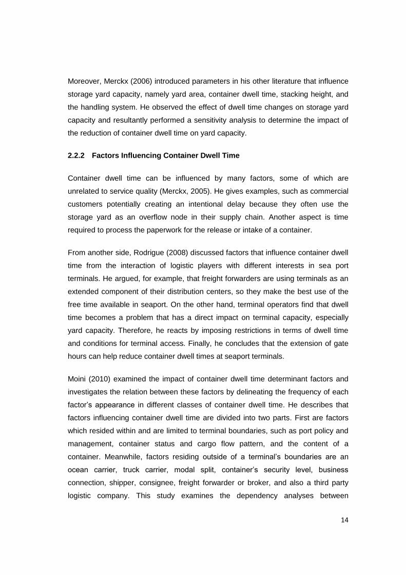
2.2.2 Factors Influencing Container Dwell Time

Container dwell time can be influenced by many factors, some of which are

unrelated to service quality (Merckx, 2005). He gives examples, such as commercial

customers potentially creating an intentional delay because they often use the

storage yard as an overflow node in their supply chain. Another aspect is time

required to process the paperwork for the release or intake of a container.

From another side, Rodrigue (2008) discussed factors that influence container dwell

time from the interaction of logistic players with different interests in sea port

terminals. He argued, for example, that freight forwarders are using terminals as an

extended component of their distribution centers, so they make the best use of the

free time available in seaport. On the other hand, terminal operators find that dwell

time becomes a problem that has a direct impact on terminal capacity, especially

yard capacity. Therefore, he reacts by imposing restrictions in terms of dwell time

and conditions for terminal access. Finally, he concludes that the extension of gate

hours can help reduce container dwell times at seaport terminals.

Moini (2010) examined the impact of container dwell time determinant factors and

investigates the relation between these factors by delineating the frequency of each

factor’s appearance in different classes of container dwell time. He describes that

factors influencing container dwell time are divided into two parts. First are factors

which resided within and are limited to terminal boundaries, such as port policy and

management, container status and cargo flow pattern, and the content of a

container. Meanwhile, factors residing outside of a terminal’s boundaries are an

ocean carrier, truck carrier, modal split, container’s security level, business

connection, shipper, consignee, freight forwarder or broker, and also a third party

logistic company. This study examines the dependency analyses between

15

containers’ dwell time determinant factors limited to within a terminal’s boundaries,

helping us predict container dwell time at Jakarta International Container Terminal.

Huynh (2008) considered that there are two import storage strategies. First is non-

mixed: no stacking of new import containers on top of old ones, where the increase

in container dwell time lowered throughput while it increased re-handling

productivity. The second strategy is mixed: stacking where the increase in container

dwell time raised throughput but decreased re-handling productivity. He uses a

different approach to introduce a method to evaluate the effect of the CDT and

storage policies on import container throughput, storage density, and re-handling

productivity.

2.3 Data Mining Techniques

Data mining techniques are techniques utilized to establish a relationship between

container dwell time and its determinants, which is employed in a mining database.

Moini (2010) describes that data mining refers to the process of analyzing data in

order to determine patterns and their relationships, where technically, data mining

requires either exploring an immense amount of material or intelligently probing it to

find where the value resides. In his literature, he examines how the objectives will be

addressed by Data Mining algorithm capabilities and how the algorithm manipulates

categorical, discrete and non-numeric data, as the most determinant data on

container dwell time has these characteristics.

Three common approaches can be traced in mining data: first is market basket

analysis, second is unsupervised learning, and third is supervised learning.

16

Figure 2.5 Hierarchy of data mining strategies

Source: Roiger, et al., 2003

Data mining problem types are related to appropriate modeling techniques, followed

by a description of the most common modeling techniques (Rudjer Boskovic

Institute, 2001).

Table 2.2 DM problems with corresponding proposed DM algorithms

Segmentation or clustering K-Mean Clustering, Neural networks,

Visualization methods

Dependency analysis Correlation analysis, Naïve Bayesian,

Association rules, Bayesian networks

Classification Decision trees, Neural networks, K-

nearest neighbors

Prediction Regression analysis, Logistic regression,

Neural networks, K-nearest neighbors

Source: Rudjer Boskovic Institute (2001)

17

Chapter 3 CONTAINER DWELL TIME AT JAKARTA INTERNATIONAL

CONTAINER TERMINAL (JICT)

This chapter will present an overview and evaluation of the existing condition of

JICT based on the terminal facilities and equipment, container traffic, and container

dwell time, which is expected to give an existing picture of JICT related to the dwell

time problem. The evaluation will be limited to cover only Terminal 1 of JICT.

3.1 Terminal Facilities and Equipment

Jakarta International Container Terminal (JICT) is strategically located at the

industrial heartland of West Java. JICT is a joint venture between Hutchison Port

Holdings and PT Pelabuhan Indonesia II and was formed to operate Container

Terminal 1 and 2 at Tanjung Priok Seaport. JICT covers a total of 100 hectares,

which is the largest container terminal in Indonesia and serves as a national hub

port and as the gateway to Jakarta and the industrial heartland of West Java.

As container volume grew, JICT committed to providing excellent, efficient and

reliable service for 24 hours a day, all year round to more than 30 shipping lines with

direct services to 25 countries.

JICT has accredited to ISO 9001:2008, which aims to promote excellence in

container handling services through the dedication of the workforce and the

application of proven and reliable technology to its operation.

With 85 hectares of area currently in use, JICT consist of two terminals, namely T1

and T2, as shown in a figure 3.1. They have a total quay length of 2.150 meters with

alongside depth of 8.5 - 14 meters, equipped with 19 quay cranes, four of which are

Super Post Panamax size. The yard operation is serviced by 74 Rubber Tyred

Gantry Cranes (RTGCs) and backed by more than 150 trucks and chassis, as listed

on table 3.1.

18

Figure 3.1 Terminal Layout of JICT

Source: http://www.jict.co.id/en/content/terminal-layout

Table 3.1 Equipment & Facility of JICT in 2011

Description Terminal I Terminal II Total

I. Berth

Length

Width

Draught

1640 M 26.5 – 34.9 M 11 – 14 M

510 M 16 M 8.6 M

2150

II. Container Yard

Area

Capacity

Ground Slot 1. Import 2. Export 3. Reefer

- 220 V - 380 V

40.00 Ha 4,614 Teus 4,317 Teus - 260 Plug

9.24 Ha 960 Teus 984 Teus - 68 Plug

49.24 Ha 5,574 Teus 5,301 Teus - 328 Plug

III. Equipment

http://www.jict.co.id/en/content/terminal-layout

19

Quay Crane Container

Rubber Tyred Gantry Crane

Head Truck

Chassis/Trailer

Forklift Diesel

Reach Stacker

Side Loader

16 Unit 63 Unit 129 Unit 112 Unit 8 Unit 4 Unit 6 Unit

3 Unit

11 Unit 13 Unit 21 Unit 6 Unit 1 Unit -

19 Unit 74 Unit 142 Unit 133 Unit 14 Unit 5 Unit 6 Unit

Source: http://www.jict.co.id/en/content/terminal-facilities

3.2 Container Traffic Flow and Operation Time

Operational data comprises container traffic flow and ship call, container dwell time,

terminal operational time, and other supporting data.

3.2.1 Container Traffic Flow

As presented in table 3.2 and figure 3.2, container traffic flow at JICT from 2006 until

2011 has continuously increased. Even though the throughput volume was

decreased from 1,995 million TEUs to 1,675 million TEUs in 2009 because of the

economic crisis, 2010 saw a slight increase to 2,095 million TEUs. Import

containers’ volume occupied the biggest proportion of JICT traffic flow. The average

proportion of import volume was 52%, while export containers’ volume is 43%, and

transshipment is around 5%.

http://www.jict.co.id/en/content/terminal-facilities

20

Table 3.2 Container Throughput at JICT

YEAR SHIP

CALLS

IMPORT EXPORT TRANSHIPMENT TOTAL

TEUS TEUS TEUS TEUS

2006 1,900 839,313 688,649 91,533 1,619,495

2007 2,030 950,065 778,585 92,642 1,821,292

2008 1,852 1,010,628 908,386 76,767 1,995,781

2009 1,680 884,330 727,969 63,096 1,675,395

2010 1,879 1,049,882 946,658 98,468 2,095,008

2011 1,984 1,180,387 1,011,181 103,697 2,295,264

Source: JICT

Figure 3.2 Container Traffic in JICT from 2006 to 2011

Source: JICT

Based on figure 3.2, there was not much fluctuation in ship calls. Year 2007 was

recorded as the year with the biggest number of ship calls in JICT. The growth was

smaller than container traffic growth, where the average growth is 2% per year for

ship calls and 6% for container traffic growth. In line with the decrease in container

volume in 2009 as presented in figure 9, the number of ship calls also dropped

21

significantly from 1,852 ship calls in 2008 to 1,680 ship calls in 2009, but then it

slightly increased in 2010 into 1,879 ship calls and 1,984 ship calls in 2011.

Figure 3.3 Ship Calls in JICT from 2006 to 2011

Source: JICT

3.2.2 Terminal Operational Time

This section provides information about the work hours of Terminal 1 JICT,

operational time of the gate, and the policy on storage services, including free time

for container stacking on yard.

Based on table 3.3, the operational time and gate in Terminal 1 JICT is 24/7,

meaning the terminal and gate are operated 24 hours, 7 days per week. The policy

in the stacking yard is divided into three periods, and import and export containers

are treated differently regarding the free time policy.

22

Table 3.3 Operational Time and Storage Policy in Terminal 1 JICT

Description Data

Terminal Work Hours · Shift 1: 07.00 – 15.30

· Shift 2: 15.30 – 23.00

· Shift 3: 23.00 – 07.00

Gate Operation Hours · Shift 1: 07.00 – 15.30

· Shift 2: 15.30 – 23.00

· Shift 3: 23.00 – 07.00

Free time for stacking on yard · Empty and full imported container will be counted as follow:

- 1st day to 3rd day is free time;

- 4th day to 10th day will be counted 200% per day from basic tariff per day;

- 11th day up to the next is counted 300% per day from basic tariff.

· Empty and full export container will be counted as follow:

- 1st day to 5th day is counted as 1 day

basic tariff;

- 6th day to 10th day will be counted

200% per day from basic tariff per day;

- 11th day up to next is counted 300%

per day from basic tariff.

Source: JICT

3.3 Container Dwell Time and Container Yard Capacity at JICT

3.3.1 Container Dwell Time at JICT

The average container dwell time for an import container in 2009 was 5.3 days,

which then decreased in 2010 to 5.2 days, but then increased to 5.6 days in 2011.

The international definition of import container dwell time includes the total container

time from vessel to gate, out of the port area, while the container dwell time

mentioned on the table below is the time from unloading the container until the

container leaves the port through the main gate. In this case, the gate is located at

the exit point of the JICT Container Yard (JICT, 2011). Therefore, the average dwell

23

time in JICT might increase due to time added at overbrengen and inspection yards

to around 9 days for 2011.

For export containers, the average dwell time in 2009 was 2.3 days and remained

the same in 2010, but then it increased in 2011 to become 4.3 days, as presented in

table 5. This shows that dwell time for import containers is longer than export

containers. This is because import container operations deal with uncertainty,

dependent on many factors, such as the trucks’ arrival time at the terminal to pick up

the container.

Figure 3.4 CDT at JICT from 2009 to 2011

Source: Author

Table 3.4 Container Dwell Time at JICT from 2009 to 2011

CDT 2009 2010 2011

Import 5.3 5.2 5.6

Export 2.3 2.3 4.3

Source: JICT

Table 3.5 and 3.6 presents container dwell time at JICT in detail. Based on table 3.5

and figure 3.5 in import containers, full container dwell time occupies the longest

time of any container. Average stay at port for a full import container was 5.4 days in

2009 and remains the same in 2010, then increases the next year to 5.7 days. For

24

an imported empty container, the dwell time is almost half compared to full

container, where the empty container occupied the yard for 2.1 days in 2009,

increased the next year to 2.7 days in 2010, and became 3.1 days in 2011.

Table 3.5 Import Container Dwell Time

ICDT Jan Feb Mar Apr May Jun Jul Aug Sep Oct Nov Dec Avg

2009

Full 5.5 5.0 5.7 5.4

Empty 1.9 1.7 2.7 2.1

Overall 5.3 4.9 5.6 5.3

2010

Full 6.0 4.9 5.3 5.3 5.3 5.3 5.5 5.3 5.6 5.3 5.3 5.4 5.4

Empty 2.6 2.3 2.4 2.6 3.0 2.7 2.3 2.7 3.0 2.6 3.1 2.9 2.7

Overall 5.8 4.8 5.1 5.2 5.3 5.3 5.4 5.2 5.4 5.0 5.1 5.3 5.2

2011

Full 5.3 5.5 4.8 5.0 5.5 6.1 5.9 5.4 6.8 6.2 5.8 5.9 5.7

Empty 2.4 2.8 2.6 3.1 2.6 3.0 3.1 4.1 2.7 3.6 3.6 3.7 3.1

Overall 5.2 5.4 4.7 5.0 5.4 6.0 5.8 5.4 6.7 6.1 5.8 5.8 5.6

Source: JICT

Figure 3.5 Import Container Dwell Time 2009 – 2011

Source: Author

The dwell time of export containers experience the opposite of import containers,

where empty containers have a longer dwell time than full containers. As described

on table 7, the average dwell time of a full export container in 2009 was 2.3 days,

while an empty container was 2.4 days. When the dwell time of a full export

container remains the same in 2010, the dwell time of an empty container is

25

increased slightly to 2.5 days, and then it increases more in 2011 to become 2.7

days, while the dwell time of a full container averages 2.5 days (table 3.6 and figure

3.6).

Table 3.6 Export Container Dwell Time

ECDT Jan Feb Mar Apr May Jun Jul Aug Sep Oct Nov Dec Avg

2009

Full 2.3 2.3 2.3 2.3

Empty 2.5 2.1 2.5 2.4

Overall 2.3 2.2 2.3 2.3

2010

Full 2.2 2.4 2.2 2.3 2.3 2.3 2.3 2.4 2.3 2.1 2.2 2.3 2.3

Empty 2.3 3.3 2.2 2.1 2.4 2.4 2.5 2.9 3.1 2.2 2.4 2.2 2.5

Overall 2.2 2.6 2.2 2.2 2.3 2.4 2.4 2.5 2.5 2.1 2.2 2.2 2.3

2011

Full 2.6 2.3 2.5 2.4 2.6 2.5 2.4 2.6 2.3 2.6 2.3 2.3 2.5

Empty 2.4 2.3 2.6 2.9 2.9 2.9 3.0 2.8 2.9 2.9 2.3 2.8 2.7

Overall 2.5 2.3 2.6 2.6 2.7 2.6 2.6 2.6 2.5 2.6 2.3 2.5 2.5

Source: JICT

Figure 3.6 Export Container Dwell Time 2009 – 2011

Source: Author

3.3.2 Container Yard Capacity at JICT

The analysis situation of the container terminal on JICT is based on the previous

data and information about the condition of JICT. This section presents an analysis

of container yard capacity based on throughput.

26

Based on what has been mentioned previously in table 3, JICT Terminal 1 area is

40 Ha or 400,000 m2. To analyze whether container yard capacity in Terminal 1

JICT is sufficient for the existing throughput, calculating the area required for

stacking is an important step. To calculate the area required for the stacking yard,

there are several assumptions and steps, as explained in table 3.8:

Table 3.7 Data Assumption

No. Assumption Data

1 Capability of stacking and spanning using RTG as equipment at the stacking yard

One over four with spanning 7 rows

2 Distance between containers in a block 0.25 meter

3 Dimension of a TEU container 6.1 m x 2.4 m

4 Number and width of roadways for trailer in a block

3 roadways with 3.75 meter for the width of each

5 Number and width of side roadways for RTG in a block

2 sides with a width of 1.5 m each

6 Width of roadway between blocks 25 meter

7 Number of slots and rows (in each slot) in a block 66 slots with 7 rows in each slot

8 The proportion of export and import containers 54% for import and 46% for export

9 Average Dwelling Time (DT) for import and export

4.3 days (import is 5.6 days and export 2.5 days)

10 Peaking factor (PF) 1.30

11 Average Stacking height (H) for export and import

3.2 containers high (3.5 for export and 3 for import)

12 Land utilization (U) ratio 80%

13 Number of working days in a year (K) 365 days

Source: JICT

Table 3.8 Calculation of Container Yard Area Required

Year Throughput TGS

No of

Slot

Required

Block

requir

ed

Total

area of

overall

slot

Area for

distance

between

container

Effective

Area

Total

Area for

trailer

roadway

s

RTG

Roadway

between

block

Total Area

Required

m2 Ha

2011 2,295,264 13,731 1,962 30 205,969 8,114 214,083 140,049 49,795 23,013 426,941 43

Source: Author’s Calculation

27

According to table 3.8, the area required to fulfill the needed space of the container

yard based on throughput in 2011 is exceeding the available area. This means there

is a shortage of container yard space at JICT, where the need of space for the

import and export container yard is around 43 Hectare, but the available area is

around 40 Hectare.

Expansion of a new container terminal is the best solution to capitalize on

opportunities anticipated from the rapid growth of containerization. In this case, the

expansion of a new container terminal is a long-term development program of

Tanjung Priok Port, where the first phase is to be operational in 2015.

To cope with container yard space shortages that have occurred since 2011, JICT

must find solutions to solve the problem while waiting for the expansion of the new

container terminal. There are several factors that can influence the container yard

capacity in the terminal. Since the longer time of a container stay in the JICT

terminal yard is one of the major problems in JICT, this study will focus on finding

the optimal dwell time from the factors influencing it to find a solution for the area

shortage problem in JICT.

28

Chapter 4 ANALYSIS OF CONTAINER DWELL TIME

This chapter will further analyze data that was presented in the previous chapter.

The analysis that will be presented in this chapter consists of the following subjects:

a. Sensitivity analysis of dwell time on container yard capacity is the first

methodology that will be used in this study. Recall the fact that JICT’s storage

yard forms the bottleneck in throughput capacity, causing the necessity to limit

container dwell times. By using this analysis, the impact of mean container

dwell time on storage yard capacity will indicate the importance of dwell time

on container terminal capacity.

b. We analyze factors influencing container dwell time. Since the reduction of

container dwell time will improve yard capacity at a container terminal,

measurement of the factors influencing container dwell time is important in

order to develop a proper strategy of container dwell time reduction.

4.1 Sensitivity Analysis of Container Dwell Time on Yard Capacity

The first step in this study is to analyze the average container dwell time based on

the cargo flow of import and export containers. The analysis will give a hint how

sensitive the effects of dwell time changes are on container yard capacity at

Terminal 1 JICT. Therefore, this analysis will present the effect of varying average

container dwell times on the TGS required and on the area required for stacking

containers with the existing throughput in 2011. The analysis will be conducted

using Dally’s (1983) formula with several assumptions based on the situation in

Terminal 1 JICT.

Dally (1983) proposed a formula related to yard capacity. He calculated the

throughput capacity of a container yard as follows,

PFDT

KUHTgsCC

29

(4.1)

Where,

CC = Yard throughput in a year;

Tgs = Total ground slot;

H = Average stacking height;

U = Land utilization ratio;

K = Service days of the yard (usually 265 days);

DT = Dwell time of containers;

PF = Peaking factor.

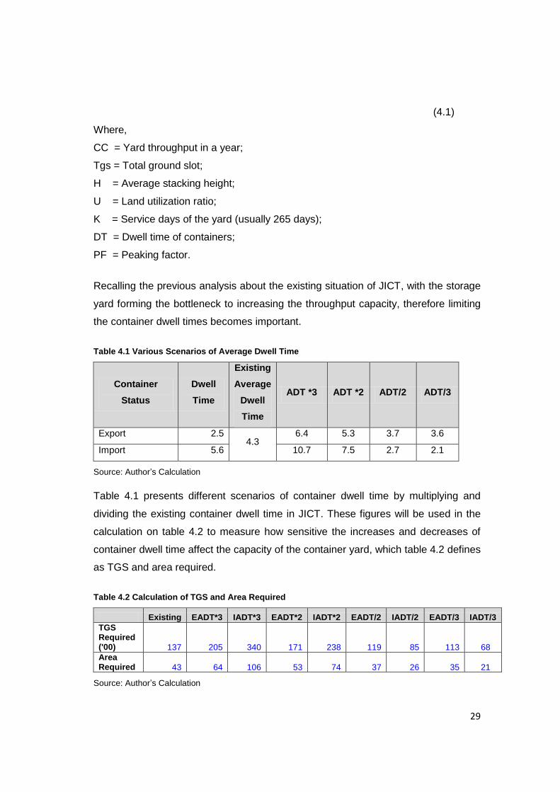
Recalling the previous analysis about the existing situation of JICT, with the storage

yard forming the bottleneck to increasing the throughput capacity, therefore limiting

the container dwell times becomes important.

Table 4.1 Various Scenarios of Average Dwell Time

Container

Status

Dwell

Time

Existing

Average

Dwell

Time

ADT *3 ADT *2 ADT/2 ADT/3

Export 2.5 4.3

6.4 5.3 3.7 3.6

Import 5.6 10.7 7.5 2.7 2.1


Table 4.1 presents different scenarios of container dwell time by multiplying and

dividing the existing container dwell time in JICT. These figures will be used in the

calculation on table 4.2 to measure how sensitive the increases and decreases of

container dwell time affect the capacity of the container yard, which table 4.2 defines

as TGS and area required.

Table 4.2 Calculation of TGS and Area Required

Existing EADT*3 IADT*3 EADT*2 IADT*2 EADT/2 IADT/2 EADT/3 IADT/3

TGS Required ('00) 137 205 340 171 238 119 85 113 68

Area Required 43 64 106 53 74 37 26 35 21


30

Figure 4.1 TGS and Area Required Based on Difference Dwell Time

Source: Author’s

Table 4.2 shows the effect of varying average container dwell times on the TGS

required and area required for stacking containers with the existing throughput.

Table 4.2 and figure 4.1 describe that when import container dwell time is doubled,

the TGS required is increased by almost one half, which means a reduction in

storage yard capacity. And when the import container dwell time is reduced by one

half, it reduces the TGS required by one half and doubles the storage yard capacity.

Meanwhile, the effect for export containers is not as dramatic as import containers.

This is because in JICT, the proportion of import container volume is much higher,

and import containers have a longer dwell time than export containers.

From the analysis above, it can be concluded that the longer the dwell time, the less

space there is available for additional throughput. So, a reduction in dwell times

would increase the capacity of the container yard. Therefore, it is essential that

containers be moved through the terminal as quickly as possible.

Moreover, analyzing the obtained information on average container dwell times for

the different container statuses, import containers have the highest dwell times.

Import container operations deal with uncertainty, depending on many factors, such

as a truck’s arrival time at the terminal to pick up a container, current habits of the

consignee using the container terminal as cheap storage of their goods, etc.

31

4.2 Analysis of Factors Influencing Container Dwell Time

Sensitivity analysis on the previous section shows that container dwell time has a

direct impact on terminal productivity, and the yard efficiency can be improved by

reducing the time. Container dwell time, which refers to the length of container stay

in the terminal, is influenced by several factors.

This section provides a dependency examination of factors influencing container

dwell time. It therefore investigates the correlation between factors that influence

container dwell time and container dwell time as the next step in this study. The

investigation will be limited to the factors influencing the dwell time of containers that

resided within and were limited to terminal boundaries. The analysis in this study is

also only cover export and import containers, due to the small proportion of

transshipment containers. This way, the analysis examines whether a container’s

status, content of the unit container, and operation day policy for export and import

containers have an impact on container dwell time in JICT.

The first step of this investigation is to make an observation on the proposed factors

that can influence container dwell time based on the available data by providing the

significant percentage values of the factors in each class of container dwell time on

the specific period. In this observation, the data were provided by JICT about

containers that were handled by Terminal 1 during May, June and July, which is

considered the three-month peak period, and September, October and December

as a low period. This analysis will classify the dwell time into classes of one to nine

days of dwell time, since the average import container dwell time in JICT in 2011

was around 8 days.

4.2.1 The Factor of Container’s Status

Container status in this analysis refers to a full or empty container. As described on

the previous chapter, the average proportion of transshipment container volume is

only around 5% of the whole container’s volume, so this analysis was confined to

import and export containers.

32

Table 4.3 Distribution of Import & Export Container in Different Class of Dwell Time

Peak Period Dwell Time

1,2,3 4,5,6 7,8,9

Export Empty 59% 38% 3%

Full 66% 30% 4%

Import Empty 73% 24% 3%

Full 40% 36% 24%

Low Period Dwell Time

1,2,3 4,5,6 7,8,9

Export Empty 78% 21% 1%

Full 69% 28% 4%

Import Empty 63% 28% 9%

Full 45% 35% 19%


Table 4.3 describes a different pattern of container dwell time distribution between

import and export containers during the peak period and low period. As shown in the

table, export containers for both empty and full containers are more often distributed

in the class of shorter dwell time (three or less class) for about 59% in the peak

period and 78% in the low period for empty containers and 66% in the peak period

and 69% in the low period for full containers. For import containers, containers with

a status of empty have distributed more in the class of three days or less dwell time,

for about 73% on peak period and 63% on low period.

In the longer class of dwell time (four or more days), full import containers are

distributed highest, with the peak period around 60% while empty imports are about

27%, full export is around 34%, and 41% for empty export containers. The same

pattern occurred in the low period, where full import containers have the greatest

value of about 55% on the dwell time class of four while empty import is about 37%,

full export is around 32%, and 22% for empty export containers.

33

Figure 4.2 Distribution of Export Containers in Each Class of Dwell Time

Source: Author’s

Figure 4.3 Distribution of Import Containers in Each Class of Dwell Time

Source: Author’s

Figure 4.2 and 4.3 illustrate that export full, export empty and empty import

containers are expected to leave the container yard in three days or less.

34

Conversely, full import containers can be expected to stay in the container yard

longer, for about four or more days.

The volume proportion between full and empty containers, policy of storage service

tariff, and the existence of an inland container depot at or near the terminal could be

interpreted as the cause of different patterns of dwell time between import and

export containers. The proportion between full and empty container flow in JICT is

as follows for export containers: full container is about 73% while empty is 27%. For

import containers, full containers are around 97%, and empty is 3%. From the policy

side, for import containers in this terminal, the first to third days count as free time or

free of charge for storage services, and demurrage fees are calculated after that.

But for export containers, the basic tariff is already counted from the first day.

Hence, export full containers left the terminal yard in three days or less while import

full containers stayed longer, for four or more days after demurrages fees are

calculated.

The existence of an empty container depot and the lack of an inland container depot

for importers to stack their goods near the terminal could be interpreted as a cause

of lower value for empty container dwell time and higher value for full import

containers on the longer class of container dwell time. Therefore, from the

observation above, we can conclude that a container’s status plays a role in the

length of time the container remains in the terminal yard.

4.2.2 The Factor of Container’s Type and Size

In this section, container’s type and size are observed to determine whether they

have an influence on container dwell time by comparing data of dry and reefer

containers in each class of container dwell time.

Figure 4.4 shows that the distribution of each class of container dwell time in export

containers for dry and reefer in the container size of 20 feet and 40 feet have similar

patterns, where each type and size of export container has distributed more in the

dwell time class of shorter dwell time (three or less days), then the value decreases

for the longer dwell time. The graph also shows that reefer containers have the

35

greatest value on the container dwell time class of three or less days in both the

peak and low period for more than 89% for full reefer and 57% for empty reefer. This

means most of export reefer containers leave the terminal yard during the first three

days.

Figure 4.4 Distribution of Type & Size Export Containers in Different Class of Dwell Time

Source: Author’s

36

Figure 4.5 Distribution of Type & Size Import Containers in Different Class of Dwell Time

Source: Author’s

While figure 4.5 shows that for import containers, container dwell time for the

different types and sizes of containers have different patterns. Based on the graph,

full reefer containers have a greater value on the shorter class of container dwell

time, while 40-foot full reefer containers have accounted for more than 90% on both

periods, which is the greatest value on the container dwell time of three or less days.

This is followed by the 20-foot full reefer containers with about 65% on the low

period and 72% on the peak period.

Table 4.4 Distribution of Container Dwell Time based on Container's Type and Size

Export Container

Type & Size

Status CDT (days)

Full Empty Full Empty

1,2,3 4,5,6 7,8,9 1,2,3 4,5,6 7,8,9

Peak 20' Dry 69% 31% 64% 31% 5% 62% 36% 2%

40' Dry 82% 18% 67% 30% 2% 52% 43% 5%

20' Reefer 46% 54% 89% 10% 1% 73% 27% 0%

40' Reefer 25% 75% 94% 5% 1% 59% 38% 3%

Low 20' Dry 71% 29% 66% 29% 5% 71% 28% 1%

40' Dry 79% 21% 70% 28% 2% 71% 28% 1%

37

20' Reefer 49% 51% 90% 9% 1% 94% 6% 0%

40' Reefer 33% 67% 94% 6% 0% 57% 40% 3%

Import Container

Type & Size

Status CDT (days)

Full Empty Full Empty

1,2,3 4,5,6 7,8,9 1,2,3 4,5,6 7,8,9

Peak 20' Dry 99% 1% 38% 37% 25% 73% 26% 0%

40' Dry 98% 2% 37% 38% 25% 73% 24% 3%

20' Reefer 97% 3% 72% 19% 9% 35% 47% 18%

40' Reefer 99% 1% 93% 5% 2% 21% 74% 5%

Low 20' Dry 98% 2% 43% 36% 21% 46% 40% 15%

40' Dry 99% 1% 43% 37% 20% 65% 28% 8%

20' Reefer 97% 3% 65% 24% 11% 17% 33% 50%

40' Reefer 99% 1% 90% 7% 2% 41% 57% 2%


Table 4.4 performs more investigation to examine whether container types and sizes

influence container dwell time in JICT. As illustrated in this table, there are different

proportions between import and export containers. For export containers, full

containers have a greater value than dry containers and reefer containers, of which

more than 69% of dry containers are full and more than 18% are empty. For empty

containers, reefer containers occupied more value than dry containers for around

51% and above for empty reefer and 25% for full reefer. That means most reefer

export containers were empty, while most dry export containers were full. From the

distribution of container dwell time, the percentage of containers shipped within the

first day is more than 52%, which means both of full and empty dry and full and

empty reefer export containers were shipped within the first three days. In contrast,

for import containers, 97% and above of the reefer and dry containers are full.

For these containers, dry and reefer containers have a different pattern on the

distribution of container dwell time. Table 4.4 also shows that in both periods, most

of the full 20-foot and 40-foot reefer containers stayed at the terminal yard for three

or less days, while for empty 20-foot and 40-foot reefer containers stayed longer at

the yard, for four or more days. On the other hand, empty 20-foot and 40-foot dry

import containers mostly moved in three or less days, and full 20-foot and 40-foot

38

dry import containers are more common in the class of four or more days. That

means both sizes of empty dry import containers stayed in the terminal yard for

three or less days, while the consignee of full dry import containers will stack their

containers for four or more days in the terminal yard.

From the observation above, it can be concluded that different types and sizes of

containers perform differently on container dwell time.

4.2.3 The Factor of Port Policy on Daily Terminal Operation Time

This analysis will examine whether daily operation time has an impact on container

dwell time. The operation time in this analysis is divided into 2 categories: first is

Weekday time, which contains the operation days of Monday, Tuesday,

Wednesday, and Thursday; and second is Weekend time, which covers the

operation days of Friday, Saturday, and Sunday.

Figures 4.6 and 4.7 provide the distribution of daily terminal operation in each

container dwell time class in JICT. Based on these figures, export containers have

the greater percentage value in the shorter dwell time class during weekend terminal

operation for about 65% on Friday, 72% on Saturday, and 80% on Sunday. On

weekdays, the percentage of export containers in the three or less day class is not

more than 49%.

Figure 4.6 Distribution of Weekend Terminal Operation in each Class of Dwell Time

Source: Author’s

39

Figure 4.7 Distribution of Weekday Terminal Operation in each Class of Dwell Time

Source: Author’s

Table 4.5 presents the percentage proportion of each type and status of containers

in 2011, while table 4.6 describes the distribution of container dwell time daily

operation time.

Table 4.7 presents more observation about the distribution of container dwell time

classes in daily container terminal activities by considering the container status. The

table illustrates that in export containers, the three or less days class of container

dwell time contributed to a greater percentage value for full and empty containers in

dry and reefer containers. This happened in both a peak period and a low period,

which means export containers had a shorter dwell time. The percentage of

containers that arrived at the terminal on a weekday was higher than on weekend

terminal operation. That means there are more containers arriving on weekdays.

For import containers, dry full import containers accounted for around 44% of the

whole container volume and had a greater percentage of longer container dwell time

40

(four or more days) for about 62% during the peak period and 56% in the low period.

These containers were transported into the terminal mostly on weekdays. In line

with dry full containers, empty reefer containers also had a higher value of the four

or more day class of container dwell time for about 61% in the peak period and

100% in the low period, but it was mostly transported on weekends.

Meanwhile, dry empty containers and full reefer containers have a greater value of

the three or less day container dwell time. The percentage of dry empty containers

on the shorter class of dwell time is 62% and above, while it is more than 86% for

full reefer containers. These containers are transported into the terminal mostly on

weekends.

Table 4.5 Percentage of Containers Population

Period

Export Import

Dry Reefer Dry Reefer

Full Empty Full Empty Full Empty Full Empty

Peak 37.43% 12.14% 0.62% 1.62% 44.31% 1.38% 2.47% 0.02%

Low 37.90% 12.59% 0.88% 1.64% 43.13% 1.46% 2.37% 0.03%


Table 4.6 Distribution of Container Flow in Daily Operation Time

Export Friday Saturday Sunday Monday Tuesday Wednesday Thursday

Dry Empty 16% 15% 13% 18% 15% 9% 13%

Full 9% 13% 28% 14% 10% 13% 14%

Reefer Empty 7% 13% 15% 16% 15% 19% 15%

Full 8% 7% 41% 8% 6% 15% 15%

Import Friday Saturday Sunday Monday Tuesday Wednesday Thursday

Dry Empty 18% 13% 28% 7% 8% 7% 18%

Full 16% 15% 6% 11% 18% 17% 17%

Reefer Empty 19% 29% 1% 23% 25% 3% 0%

Full 12% 19% 11% 15% 13% 14% 16%


41

Table 4.7 Distribution of Daily Terminal Operation in Each Class of Dwell Time

Export Dwell

Time

Weekday Weekend



Peak

1,2,3 55% 55% 92% 53% 77% 62% 82% 73%

4,5,6 39% 39% 8% 42% 21% 37% 13% 27%

7,8,9 6% 5% 1% 4% 2% 1% 5% 0%

Low

1,2,3 60% 72% 89% 59% 77% 68% 98% 65%

4,5,6 35% 26% 11% 40% 20% 31% 2% 32%

7,8,9 5% 2% 0% 2% 3% 1% 0% 4%

Import Dwell

Time

Weekday Weekend



Peak

1,2,3 37% 72% 89% 15% 37% 75% 93% 39%

4,5,6 38% 27% 8% 68% 37% 20% 5% 59%

7,8,9 25% 1% 3% 17% 26% 5% 2% 2%

Low

1,2,3 44% 52% 85% 31% 42% 75% 89% 0%

4,5,6 36% 39% 11% 41% 38% 17% 7% 63%

7,8,9 20% 9% 3% 28% 20% 8% 4% 38%


Based on the results from figures 4.6 and 4.7, as well as table 4.6, the hint that

could be drawn is export full dry containers and export full reefer containers arrive at

the terminal most often on Sunday, at the same time as most of the import empty

dry containers also arrived, and all of those containers will be shipped out and

transported in the next two days. Therefore, it is possible that there will be a high

number of containers flowing into the terminal on the same day. So, a new policy in

the terminal would be necessary to handle the surges of container flow more

efficiently.

42

CHAPTER 5 MODELLING AND APPLICATION

Two prediction techniques, namely logistic regression and dummy regression, are

assessed in this chapter by using SPSS software to find the most suitable model for

CDT prediction. Then the model will be utilized to estimate container dwell time

based on the influencing factors to calculate the terminal yard capacity and revenue.

5.1 Assessment of the Fitness of a Model

To evaluate the performance of the models for predicting the container dwell time,

the value of R2 is used as a determination coefficient, whether or not a model is fit to

the data sample. Where the larger value of R2 is the better, means model with larger

value of R2 is much fit with the data than model with lower value. The determination

coefficient has a maximum value of 1.0, which means the model exactly matches

the data.

Table 5.1 Goodness-of-Fit of Models

Model R Square

Logistic Regression 0.173

Dummy Regression 0.338

Linear regression 0.094

Source: SPSS Software Calculation

The result from an SPSS Software calculation on table 5.1 shows that every model

performs different values of R2, where logistic regression is about 0.173, dummy

regression is 0.338, and linear regression is about 0.094. Since the dummy

regression model has a higher R2 value than the other models, it means the dummy

regression model is the most suitable model to predict container dwell time based

on the available data.

43

5.2 Dummy Regression

Dummy regression was utilized in the regression equation, where the independence

variable is a qualitative variable, such as nominal data or ordinal. This model is an

extension of the range of regression analysis application. The aim of using dummy

regression is to predict the value of dependent variable or dependent on the basis of

one or more independent variable where one or more independent variables used

are dummies. A dummy variable is a variable that is used to create a category of

data that are qualitative (qualitative data does not have a unit of measurement).

Therefore, the qualitative data that will be used in the regression analysis must be

transformed first into a quantitative form by using binary code.

In this study, the variables of operational day, type of container and container’s size

each have two categories, such as operational day being either a weekday or

weekend, which is qualitative data. Therefore, it will be transformed into the form of

Weekday is 0; Weekend is 1. The type of container categories are dry and reefer, so

the transformation is 0 for Reefer and 1 for Dry. For container size, it will be

transformed into 0 for 20 feet and 1 for 40 feet.

There are four categories for container status, such as import empty, import full,

export empty, and export full. Thus, the transformation follows: for the import empty

category, it will be transformed into the form of import empty is 1, import full is 0, and

export empty is 0. When the category is import full, the form is 0 for import empty, 1

for import full, and 0 for export empty. And when the category is export empty, the

form is 0 for import empty, 0 for import full, and 1 for export empty. Moreover, when

the category is export full, the form of import empty is 0, import full is 0, and export

empty is 0.

To analyze this, multiple regression or hierarchical regression can be utilized in

dummy regression. Multiple regression finds a direct prediction of all the

independent variables, but to see the prediction of each independent variable in

sequence, a hierarchical regression is utilized. This study will be using multiple

regression.

44

In multiple regression analysis with dummy variables, not all categories of dummy

variables were included in the regression analysis. If the category is more than 2,

then the number of categories that are involved is k-1 (k = number of categories).

The category that was not included in the analysis will be the basis for future

interpretations of the variable. For example, in this study the category of status of

container is 4, then the number of categories that we are involved is 4-1 = 3

category. Therefore, the variables that will be analyzed are container dwell time (Y);

operational day (X1); three categories in the status of container, namely import

empty (X2), import full (X3), and export empty (X4); type of container (X5); and size of

container (X6). The export full category will be the basis for future interpretation of

the variable status of a container.

The equation of dummy regression is formulated as follows:

Y = a + b1X1 + b2X2 + b3X3 + b4X4+ b5X5 + b6X6 (5.1)

Where,

Y = Container Dwell Time

X1 = Operational Days (Weekday or weekday)

X2 = Status 1 (Import Empty)

X3 = Status 2 (Import Full)

X4 = Status 3 (Export Empty)

X5 = Type of Container (Reefer or Dry)

X6 = Size of Container (Feet: 20’ or 40’)

a = Constanta

b1, b2,….b6 = Regression Coefficient

The equation is the same as the linear regression equation, but the resulting

interpretation changed it because one of the variables in dummy regression is a

qualitative variable.

To calculate the yard capacity and revenue of the terminal in the various scenarios,

the container dwell time is estimated from different scenarios, based on the factors

that influence it (variable X1, X2, X3, X4, X5, X6), which are define as qualitative

45

variables. Therefore, the dummy regression model incorporates qualitative

explanatory variables into a linear model.

The result of the processing software SPSS 13 for multiple regression analysis are

presented in table 5.2.

Table 5.2 Result of Multiple Regression Analysis

Variables Regression

Coefficient Std. Error t Sig.

(Constant) 4.360 0.038 116.255 0.000

X1 -0.073 0.031 -2.337 0.019

X2 -1.463 0.039 -37.184 0.000

X3 0.836 0.033 -25.168 0.000

X4 -0.380 0.052 -7.314 0.000

X5 -0.122 0.085 -1.435 0.151

X6 -0.039 0.030 -1.308 0.191


Based on the calculation in table 5.2, the dummy regression equation is:

Y = 4.360 –– 0.073 X1 – 1.463 X2 + 0.836 X3 – 0.380 X4 – 0.122 X5 – 0.039 X6 (5.2)

Regression coefficient values of the independent variables show that if the

independent variable is estimated to rise by one unit and other independent

variables are estimated as constant or equal to zero, then the value of the

dependent variable can be expected to go up or down according to the sign of the

regression coefficients of independent variables.

From equation 5.2, constant values were obtained at 4.360. This means if the CDT

variable (Y) is not affected by the six independent variables, namely operational

days (X1), status 1 as import empty (X2), status 2 as import full (X3), status 3 as

export empty (X4), reefer or dry type of container (X5), and 20-foot or 40-foot size of

container (X6), then the average value of the CDT will be worth 4.360 or 4.36 days.

46

The sign of regression coefficients of independent variables indicate the direction of

the relationship of the variables concerned with CDT. The regression coefficient for

the independent variable X is negative, indicating the existence of trade-offs

between the factors influencing CDT with CDT, means each increment of one unit

of variable X would lead to a decrease of CDT (Y). Meanwhile, if the regression

coefficient of the independent variable X is positive, it indicates a direct relationship

between factors influencing CDT with CDT, which means each increment of one unit

of variable X would lead to an increased of CDT (Y).

5.2.1 Hypothesis Testing

In this section, an F Test and T Test of variables are utilized to find out whether the

independent variables have a significant influence or not on the dependent variable.

F Test is overall hypothesis testing to find out the significance of the independent

variables’ collective influence on the dependent variable.

The first step to do an F test is formulating a statistical hypothesis, where:

Ho or Null Hypothesis means there is no significant effect from the independent

variables, namely Operational Days (X1), Status 1 (X2), Status 2 (X3), Status 3

(X4), Container Type (X5), and Container Size (X6) against CDT (Y) as the

dependent variable.

Ha means there is a significant effect from Operational Days (X1), Status 1 (X2),

Status 2 (X3), Status 3 (X4), Container Type (X5), and Container Size (X6) against

CDT (Y).

Statistic Test formula: 2

2

1

1

Rk

knRF

(5.3)

F Table formula = F α ; (df1, df2) ; df1 = k , df2 = n-k-1

Where,

n = number of sample

k = number of regression coefficient

47

α = 5% (significance level)

df = degree of freedom

Testing Criteria:

1. If the value of ‘F Count’ < ‘F Table’, then null hypothesis is accepted.

2. If the value of ‘F Count’ ≥ ‘F Table’, then null hypothesis is rejected.

Table 5.3 Result of F Testing

F Count Degree of

freedom (df) F Table Sig

372.022 df1 = 8

2.099 0.000 df2 = 23100

Source: Author’s Calculations

Table 5.3 presents results of F Testing by SPSS 13 software. Based on the table,

the value of F Calculate is 372.022, which is higher than F Table’s value (2.099).

This means the result meets the second criteria which the null hypothesis is

rejected. Thus, it can be concluded that there is simultaneously a significant effect of

Operational Time (X1), Status 1 (X2), Status 2 (X3), Status 3 (X4), Container Type

(X5), and Container Size (X6) against CDT (Y).

Partial Hypothesis Testing is a test to find out the significance of the independent

variables’ effect on the dependent variable. In this hypothesis testing, each of the

independent variables will be tested to find out whether they have a significant effect

or not on the CDT as the dependent variable. Therefore, the statistical hypothesis in

this testing will be divided, based on the independent variables as follows:

H01 : β 1 = 0 means Operational Days(X1) has no significant effect on CDT (Y).

Ha1 : β 1 ≠ 0 means Operational Days(X1) has significant effect on CDT (Y).

H02 : β 2 = 0 means Status 1 (X2) has no significant effect on CDT (Y).

Ha2 : β 2 ≠ 0 means Status 1 (X2) has significant effect on CDT (Y).

H03 : β 3 = 0 means Status (X3) has no significant effect on CDT (Y).

Ha3 : β 3 ≠ 0 means Status (X3) has significant effect on CDT (Y).

H04 : β 4 = 0 means Status (X4) has no significant effect on CDT (Y).

Ha4 : β 4 ≠ 0 means Status (X4) has significant effect on CDT (Y).

48

H05 : β 5 = 0 means Container Type (X5) has no significant effect on CDT (Y).

Ha5 : β 5 ≠ 0 means Container Type (X5) has significant effect on CDT (Y).

H06 : β 6 = 0 means Container Size (X6) has no significant effect on CDT (Y).

Ha6 : β 6 ≠ 0 means Container Size (X6) has significant effect on CDT (Y).

With Testing Criteria:

1. If the value of ‘-T Table’ ≤ ‘T Count’ ≤ ’T Table’, then null hypothesis is accepted.

2. If the value of ‘T Count’ < ‘-T Table’ or ‘T Count’ > ‘T Table’, then null hypothesis

is rejected.

By utilizing the Statistic Test formula :

Ttest = ( )

b

Se b , df = n-k-1 (5.4)

Where,

n = number of sample

k = number of regression coefficient

α = 5% (significance level)

df = degree of freedom

The results of T test based on SPSS processing is present on the table 5.4:

Table 5.4 Partial Hypothesis Testing Results

Variables T Count df T Table Sig

X1 -2.337

23100 ±1.960

0.019

X2 -37.184 0.000

X3 -25.168 0.000

X4 -7.314 0.000

X5 -1.435 0.151

X6 -1.308 0.191


Based on table 5.3, variables such as Operational Days (X1), Status 1(X2) or import

empty container, Status 2 (X3) or import full container, and Status 3 (X4) or export

empty all have a T count value lower than –T table value, which means Null

Hypothesis is rejected. Therefore, it can be concluded that operational days has a

partially significant effect on CDT (Y).

49

The Container Type (X5) and Container Size (X6) variables obtained a T count equal

to -1.435 and -1.308. Since T count (-1.435 and -1.308) is bigger than T table (-

1.960), the Ho is accepted, which means the Status 1 variable does not have a

significant effect on CDT (Y).

Based on the results on table 5.3, the scenario that will be drawn in the next section

is a scenario on container status and operational days in JICT.

5.3 Container Dwell Time Estimation

Moini (2010) states that container dwell time modeling based on the factors

influencing it may assist in achieving an expected balance between optimal or

suitable container dwell time and an adequate yard capacity. There are two different

scenarios that will be presented in this section. The first scenario is to assess

whether a change in the characteristics of a terminal has an impact on container

dwell time, while the second scenario is the scenario to assess the impact of

changing terminal policy on container dwell time.

The container dwell time to be predicted in the two different scenarios will be

estimated using dummy regression technique.

Base scenario for export and import containers

Based on the calculations of table 3.9 in chapter 3, the average container dwell time

is about 4.3 days, with composition 2.53 days for export containers and 5.61 days

for import containers. The area required to fulfill the needed container yard space

based on throughput in 2011 is 43 Ha, which exceeds the available area of only

about 40 Ha. To make the available area sufficient with the existing throughput, the

average container dwell time must be reduced to 4 days with composition 2.51 days

for export and 5.12 days for import, which will be used as the base scenario for this

study.

50

Table 5.5 Area Required on Different Average CDT

Average CDT Throughput in

2011

Total Area Required

m2 Ha

4.3

2,295,264

426,941 43

4.2 416,993 42

4.1 407,046 41

4.0 397,098 40


Scenario 1: Changing on the container’s status

Table 5.5 shows that by changing the container’s status, the dummy regression

model results present that the average container dwell time is changed. When

empty export containers become full export containers, the value of average dwell

time decreases to 2.52 days, but when the container’s status of full changes to

export empty, the average container dwell time increases slightly to 2.90 days.

When the status of import containers changes from empty into import full containers,

the average container dwell time is increased to 5.20 days, and the average

container dwell time decreases to 2.78 days when the status of container is changed

from full containers to import empty containers.

Table 5.6 Estimated CDT based on Container's Status

Container's Status CDT

Export Empty into Full 2.52

Full into Empty 2.90

Import Empty into Full 5.20

Full into Empty 2.78


From the dummy regression outcomes above, for import containers, the changing of

the status from empty to full containers obtained a higher value of average container

dwell time than other container status changes, but the value change is not very

much from the base case CDT scenario. But when the status changes from full into

empty containers, the CDT value changes dramatically, reduced by almost half from

51

the base case scenario (from 5.12 days to 2.78 days). It indicates that nearly 99% of

import containers were full containers, and almost 60% of the full containers stay in

the yard for four or more days, while 63% and up of empty containers are stacking

for three days or less.

Scenario 2: Changing on the Operational Day

The operational time and gate in Terminal 1 JICT is 24/7, which means the terminal

and the gate are operated 24 hours a day, 7 days a week for all containers.

According to table 4.6, which shows the distribution of container flow in daily

operation time at JICT in chapter 4, export containers have low volume on Tuesday,

which is defined as a weekday operational day in this study. Meanwhile, import

containers have low volume on Sunday, which is defined as a weekend operational

day. Based on that result, this study will draw the scenario on the operational day by

dedicating import or export containers on the one of truck gates operational day.

Table 5.7 Estimated CDT Based on Operational Day

Operational Days CDT

Export Dedicated on Weekend 2.90

Dedicated on Weekday 2.82

Import Dedicated on Weekend 5.12

Dedicated on Weekday 5.20


The results in table 5.7 show that when the gates’ operational day is dedicated for

export or import containers, the average value of CDT increases. In export

containers, dedication of the gates’ operational day on weekends will obtain a higher

CDT average value for about 2.90 days than when dedicated on a weekday, which

results in around 2.82 days. On the other hand, when on the weekend the gates are

dedicated to handle import containers, the average CDT value obtained is lower

than when it is dedicated on a weekday.

52

5.4 Yard Capacity and Terminal Revenue Optimization

Optimal container dwell time is defined as a suitable number of days a container

remains in the terminal yard, in balance with an adequate yard capacity. Moini

(2010) described that increasing container dwell time would reduce the yard

capacity, but it may serve as a revenue stream for terminal operators who charge

demurrage fees.

In this section, the study will evaluate the impact of the new container dwell time

predicted by dummy regression on the terminal yard capacity and terminal earnings

based on the demurrage fees policy. Therefore, the tradeoff between storage yard

capacity and earnings from demurrage fees will be assessed.

The results from the analysis could assist terminal operators in managing the

terminal better by determining the optimal dwell time, so the desired balance

between container dwell time and yard capacity can be achieved.

In the previous section, some practical scenarios were drawn to calculate the yard

capacity and the revenue earned from the demurrage fee in this section. Revenue

from demurrage fees on table 5.8 below is calculated based on the estimated CDT

by dummy regression technique in each scenario and according to the basic tariff

structure presented on table 5.7 and the storage policy at JICT in table 3.4. In JICT

terminal, there are different policies between import and export containers, where

import containers have three days free time for empty and full container, then after

these three days, a demurrage fee is charge for about 200% per day of the basic

tariff per day. For export containers, there is no free time, but the first day until the

fifth day are counted as 1 day basic tariff, then after five days the demurrage fee will

be counted 200% per day from basic tariff. In this calculation the demand is

assumed fixed (using demand in 2011), and all containers are 20 feet in size.

53

Table 5.8 Basic Tariff of Container Storage Services in JICT

Container Storage

Tariff Tariff (USD) Remarks

Empty 62.25 Per Box/ day

Full 83 Per Box/ day

Source: JICT

The formula to be used to calculate the annual capacity yard is developed by Dally

(1983) as equation 5.5.

(5.5)

Where,

Cs = Number of container ground slots (TEU),

H = Mean profile height,

W = Working slots (TEUs) in the container storage expressed as a proportion

(0.8),

K’ = Number of days per year (365),

T = Mean CDT in the CY, and

F = Peaking factor (about 1.3 based on the existing assumption in JICT). It’s

ensuring the storage space sufficiency.

The static capacity in JICT for export is about 4,317 TEU, and import is 4,614 TEU

as mentioned in the previous chapter on the table 4.1.

Table 5.9 presents the results of the annual container yard capacity and annual

demurrage fee earning calculation. The table shows that by changing the container’s

status and operational days of export and import containers, the dummy regression

outcomes show that the average CDT is changing, resulting in a change of the

annual yard capacity and also the annual earnings from demurrage fees.

C = (Cs*H*W*K’) (T*F)

54

Table 5.9 Summary of Base Case & Different Scenario

Scenarios

Average

CDT

(Day)

Annual Yard

Capacity

(TEU per

annum)

Change in

capacity

(TEU per

annum)

Demurrage

fee ($ per

annum in

'000)

Change in

Revenue ($

per annum)

Base Scenario

Export 2.51 3,386.92 0 158,755.76 -

Import 5.12 1,774.62 0 336,562.21 -

Scenario 1

Export

Empty into Full 2.52 3,377.50 (9.42) 158,755.76 -

Full into Empty 2.90 2,934.47 (452.45) 119,066.82 (39,688.94)

Import

Empty into Full 5.20 1,748.93 (25.69) 348,500.64 11,938.43

Full into Empty 2.78 3,273.66 1,499.04 119,066.82 (217,495.39)

Scenario 2

Export

Dedicated on

Weekend 2.90 2,934.47 (452.45) 158,755.76 -

Dedicated on

Weekday 2.82 3,010.33 (376.59) 158,755.76 -

Import

Dedicated on

Weekend 5.12 1,773.92 (0.69) 336,879.72 317.51

Dedicated on

Weekday 5.20 1,748.93 (25.69) 348,500.64 11,938.43


Scenario 1 : The changing of the status of export containers from empty to full and

from full to empty resulted in an increase of average CDT, but the increase from the

full to empty scenario is much higher than the empty to full scenario. As the effect of

CDT increases, the annual yard capacity is reduced by about 9.42 TEU per annum

due to changing from empty to full and about 452.45 TEU per annum for changing

from full to empty. This indicates that the volume of full export containers is much

higher than empty containers, but the time an empty container stays in the terminal

yard is longer than a full container. On the demurrage fee earning, there is no

changing in earning from the empty to full scenario, though the full to empty

55

scenario reduces the demurrage fee earnings by about $39,688.94. This is because

the basic tariff for an empty container is much cheaper than a full container.

In import containers, the changing of the empty into full containers result in an

increase in average CDT from 5.12 days (base case CDT) to 5.20 days and reduces

the annual yard capacity for about 25.69 TEU, but the demurrage fees earned

increases slightly for about $11,938.43. Also, by changing import containers’ status

from full to empty, the average CDT is reduced by almost half, from 5.12 days

(import CDT on base scenario) to 2.78 days. Reducing average CDT by half

doubled the annual yard capacity from 1,774.62 TEU to 3,273.66 TEU. On the other

hand, earnings from demurrage fees are reduced to about $217,495.39.

The results above may help JICT terminal operators to establish a new policy in the

container terminal, where they could prefer to earn more from the demurrage fees

when yard capacity is not a significant constraint or when the volume of containers

is not high or low season. Increasing the demurrage fees or shortening the policy on

free storage time could be an alternative choice to gain more storage capacity

during the peak season.

Scenario 2: The specialization of the truck gates scenario for export containers

results in the increasing of the average CDT in weekday scenarios for about 2.90

days and 2.82 days for weekend scenarios. It reduces the annual yard capacity, but

the demurrage fee earnings remain the same.

For import containers, the increasing of average CDT only occurs when weekday

gates are dedicated to handle these containers, where 5.12 days becomes 5.20

days. But when the gates’ dedication changes to the weekend, the average CDT is

the ideal time or same with average CDT on base scenario (5.12 days). From the

annual yard capacity perspective, the gates’ dedication both on weekdays and

weekends reduces the capacity, but the reduction of the weekend scenario is only

about 0.69 TEU, which is far less than the capacity reduction in the weekday

scenario. Since the average CDT increases, the earnings from demurrage fees also

increases. In the weekend scenario, the demurrage fees revenue is about $317.51

and $11,938.43 in a weekday scenario.

56

The results from the changing of the policy of the gates’ operational day scenario

could give a little hint for the terminal operator that dedicating the truck gates for

import containers on weekends may result in the optimal dwell time, where the

reduction in yard capacity is not much, but the terminal operator still gets the

revenue from the demurrage fee.

Generally, as the average CDT and revenue from the demurrage fees increases, it

will reduce the capacity. But it does not apply to both scenarios above, especially for

export containers, because even the average CDT is increasing, and yard capacity

is reducing, but the revenue from the demurrage fee is not increasing. This is

because of the policy on storage charge structure at JICT stipulating that for export

containers, the first day until fifth day will be counted as 1 day basic tariff. In export

containers, the base average CDT is about 2.52 days, and estimated average CDT

is around 2.52 to 2.90 days. This is why there is no changing of the demurrage fee

earnings for empty to full and operational day scenarios in export containers.

57

Chapter 6 CONCLUSION AND RECOMMENDATION

6.1 Conclusion

Expansion of a new terminal container is the best solution to improve container

terminal capacity in order to capitalize on opportunities, anticipating the rapid growth

of containerization, but it is costly to acquire and takes a long time. Another simple

and inexpensive solution may be used to improve terminal capacity by establishing

an effective policy to the factors that determine yard capacity. Container dwell time

is a principal factor that has direct impact on the container yard capacity in a

terminal. Therefore, JICT as port operator as well as decision maker should be able

to understand the factors that can affect container dwell time, which is under their

control. Better understanding of these factors might assist port operators to optimize

container dwell time, manage the yard capacity efficiently, and establish policies

appropriately.

This study analyzes the factors that influence container dwell time, varying from

physical location and operational policy of JICT terminal to the characteristics of the

containers in JICT, namely status of containers, type and size of containers, and

operational day of containers. Henceforth, these factors are estimated by utilizing

dummy regression techniques. The estimation CDT is used to measure how

changes in the factors that influence CDT effects container dwell time, yard

capacity, and terminal revenue.

Generally, it can be concluded that any changes in the factors that influence CDT in

Terminal 1 JICT could affect the CDT, yard capacity, and revenue earning from

demurrage fees. The analysis shows that based on the sample dataset, type of

container and container size does not have a significant effect on CDT in JICT.

Meanwhile, container status and container operational day have significant effect on

CDT in JICT. From the container status scenario results, JICT terminal operators

may help establish a new seasonal policy in the container terminal, where they

58

could prefer to earn more from the demurrage fees when yard capacity is not a

significant constraint or when the volume of the containers is not in high or low

season. Increasing the demurrage fees or changing the policy on free time storage

by shortening it could be an alternative choice during the peak season in order to

gain more storage capacity.

The analysis from the operational day policy scenario could assist JICT to establish

a new policy on operational day by dedicating truck gates on the weekend for import

containers and weekday for export containers, since the gates being dedicated for

import containers on weekends seem result in a balance between CDT and an

adequate yard capacity.

6.2 Recommendation

Based on this study, we recommend to JICT as a terminal operator to not only

establish new policies based on the analysis of influencing factors, such as

container dwell time and operational status of the day, but also to review the policies

that are likely to affect the length of the container in container yard, such as free

time, storage charges, and structure policies. Therefore, for future study, the free

time, storage charge, and structure evaluation should be considered to measure the

most suitable free time period and storage charge and structure in order to achieve

optimal dwell time. Moreover, in calculating revenue earned from the demurrage

fees using CDT, a more elaborate economic analysis should be provided to perform

further evaluation on the effectiveness of this policy.

59

REFERENCES

Chu, C. Y., & Huang, W. C. (2005). Determining Container Terminal Capacity on the

Basis of an Adopted Yard Handling System. Transport Reviews: Vol. 25, 2, Taylor & Francis Ltd., 181-199.

Data Mining Server, DM methodology. Retrieved February, 2012 from the World

Wide Web: http://dms.irb.hr/tutorial/tut_modelling.php, Rudjer Boskovic Institute. Dally, H. K. (1983). Container Handling and Transport: A Manual of Current

Practice, London, Cargo Systems IIR Publications Ltd. De Monie, G. (1981). The determination of port capacity. Proceedings of Port

Management Training Course (17 November – 12 December 1980). UNCTAD/Nigerian Ports Authority, Lagos (Nigeria).

De Monie, G. (1985). Container Terminal Pricing. Proceedings of the Seminar on

Container terminal capacity (August 1985, 573-638). UNCTAD/APEC,Antwerp (Belgium).

Dharmalingam, K. (1987). Design of storage facilities for containers: A case study of

Port Louis Harbour, Mauritius (September 27–31). Ports and Harbors. Ding, Y. Z. (2010). Throughput capacity of a container terminal considering the

combination patterns of the types of arriving vessels, Journal of Shanghai Jiaotong Univ, 15(1), 124-128, doi: 10.1007/s12204-010-8174-y.

Hardy, M. A. (1993). Regression with dummy variables (Sage University Paper

series on Quantitative Applications in the Social Sciences, series no. 07-093). Newbury Park, CA: Sage.

Huang, S. Y., Hsu, W. J., Chen, C., Ye, R. & Nautiyal, S. (2008). Capacity Analysis

of Container Terminals Using Simulation Techniques. International Journal of Computer Applications in Technology, doi: 10.1504/IJCAT.2008.021379.

Hoffman, P. (1985). Container facility planning: A case description. Port

management textbook containerization. Institute of shipping economics and logistics, (pp 353-364).

Huynh, N. (2008). Analysis of Container Dwell Time on Marine Terminal Throughput

and Rehandling Productivity. In Proceeding TRB.

60

Kozan, E. (1997). Increasing the operational efficiency of container terminals in Australia. The Journal of the Operational Research Society, 48 (2), 151-161.

Kozan, E. (2000). Optimizing container transfers at multimodal terminals,

Mathematical and Computer Modeling, 31, 235–243. Kozan, E., & Preston, P. (2006). Mathematical modeling of container transfers and

storage locations at seaport terminals. OR Spectrum, 28, 519–537. Le-Griffin, H., Murphy, M. (2006). Container terminal productivity: Experiences at the

ports of Los Angeles and Long Beach, NUF Conference. Lloyd, S. P. (1982). Least squares quantization in PCM. IEEE Transactions on

Information Theory (IT-28, 129–137). Manalytics, Inc. (1976). Methodology for estimating capacity of Marine Terminals:

Vol. I: Standardized Methodology, February 1976. Merckx, F. (2005). The issue of dwell time charges to optimize container terminal

capacity, IAME Annual Conference, Cyprus. Merckx, F. (2006). The impact of dwell times on container terminal capacity. Ports

are more than piers, Prof. Willy Winkelmans. Mitchell T. (1997). Machine learning, McGraw-Hill. Moon, S. H. (2011). Port Logistics (Queuing Theory). Unpublished lecture handout,

WMU, Malmo, Sweden. Moon, S. H. (2011). Port Logistics (Why ‘Proper Container Throughput Capacity’?),

Unpublished lecture handout, WMU, Malmo, Sweden. Moini, N. (2010). Modeling the interrelationship between vessel and truck traffic at

marine container terminals: The Graduate School-New Brunswick Rutgers, The State University of New Jersey Journal.

Murty, K. G., Liu, J., & Wan, Y. W. (2005). A decision support system for operations

in a container terminal, Journal of Decision Support Systems, 39(3), 309-332. Rodrigue, J.P. (2008). The terminalization of supply chains: Reassessing

port/hinterland logistical relationships. In proceeding of IAME. Stahlbock, R., & Voß, S. (2007). Operations research at container terminals: A

literature update, OR Spectrum 2008, 30, 1–52, doi: 10.1007/s00291-007-0100-9.

Steenken, D., Voss, S., & Stahlbock, R. (2004). Container terminal operation and

operations research: A classification and literature review, OR Spectrum, 26, 3–49.

61

Theofanis, S., Boile, M. (2008). Empty Marine Container Logistics: Facts, Issues

and Management Strategies. Accepted for Publication in GeoJournal. UNCTAD (1985). Port Development: A hand book for planners in developing

countries, United nations, New York. Vickerman, J. (2000). Panel of Transcomp 2000 seminar. National Industrial

Transportation League - Transcomp 2000 seminar, 11-12 November 2000. Vis, I. F. A., & de Koster, R. (2003). Transshipment of containers at a container

terminal: An overview, European Journal of Operational Research, 147, 1–16. Watanabe, I. (2001). Container Terminal Planning: A Theoretical Approach. World

Cargo News Publishing, Leatherhead, UK.

62

APPENDICES

Appendix I- Sensitivity Changes of Yard Capacity on Different Level of CDT

Scenario Throughpu

t 2011

Average

TGS No of Slot

Required

Block

required

Total

area of

overall

slot

area for

distance

between

container

Effective

Area

Total Area

for trailer

roadways

RTG

Roadway

between

block

Total Area

Required

Dwell

Time m2 Ha

Existing

2,295,264

4.3 13,731 1,962 30 205,969 8,114 214,083 140,049 49,795 23,013 426,941 43

EADT *3 8.6 27,619 3,946 60 414,286 16,320 430,606 281,694

100,15

8 47,099 859,557 86

IADT * 3 6.7 21,341 3,049 46 320,115 12,611 332,725 217,663 77,391 36,211 663,990 66

EADT *2 6.2 19,930 2,847 43 298,943 11,777 310,720 203,267 72,273 33,763 620,022 62

IADT *2 5.3 16,791 2,399 36 251,858 9,922 261,779 171,251 60,889 28,319 522,238 52

EADT / 2 2.6 8,395 1,199 18 125,929 4,961 130,890 85,625 30,445 13,759 260,718 26

IADT / 2 3.1 9,965 1,424 22 149,472 5,888 155,360 101,633 36,136 16,481 309,610 31

EADT / 3 2.2 7,114 1,016 15 106,705 4,204 110,908 72,554 25,797 11,536 220,796 22

IADT / 3 2.9 9,206 1,315 20 138,095 5,440 143,535 93,898 33,386 15,165 285,985 29

Appendix II- CDT Distribution based on Container’s Status

Peak Period

CDT 1 2 3 4 5 6 7 8 9

Export Empty 8.5% 22.2% 27.9% 20.6% 11.4% 6.1% 1.6% 1.4% 0.3%

Full 13.0% 27.1% 26.3% 18.4% 8.0% 3.6% 1.9% 1.3% 0.5%

Import Empty 9.5% 41.4% 22.2% 12.5% 7.9% 3.2% 2.1% 1.0% 0.2%

Full 10.0% 14.7% 15.4% 13.3% 11.7% 10.9% 9.5% 8.3% 6.3%

63

Low Period

CDT 1 2 3 4 5 6 7 8 9

Export Empty 33.8% 21.7% 22.5% 15.7% 3.9% 1.3% 0.7% 0.2% 0.1%

Full 14.1% 27.0% 27.6% 17.7% 6.7% 3.1% 2.0% 1.1% 0.6%

Import Empty 9.9% 35.0% 18.1% 14.1% 7.7% 6.4% 5.3% 2.7% 0.9%

Full 10.5% 17.4% 17.6% 14.1% 11.6% 9.3% 7.3% 6.1% 6.2%

Appendix III- CDT Distribution based on Type and Size of Container

Peak Period

Export CDT Size 1 2 3 4 5 6 7 8 9

Empty Dry 20' 8.6% 25.4% 27.6% 19.0% 11.6% 5.5% 1.1% 0.9% 0.4%

40' 7.7% 16.7% 27.8% 22.9% 12.4% 7.3% 2.7% 2.4% 0.2%

Reefer 20' 26.0% 19.8% 27.3% 23.3% 2.1% 1.5% 0.0% 0.0% 0.0%

40' 9.2% 20.2% 29.4% 22.9% 8.8% 6.2% 1.4% 1.7% 0.1%

Full Dry 20' 11.9% 26.3% 25.8% 18.6% 7.9% 4.2% 2.6% 2.0% 0.8%

40' 12.4% 27.5% 27.4% 18.8% 8.5% 3.2% 1.4% 0.6% 0.2%

Reefer 20' 29.2% 41.5% 17.9% 6.1% 3.4% 0.7% 0.5% 0.5% 0.0%

40' 49.8% 33.6% 10.2% 3.6% 1.2% 0.9% 0.6% 0.1% 0.0%

64

Low Period

Export CDT Size 1 2 3 4 5 6 7 8 9

Empty Dry 20' 10.3% 30.9% 29.5% 20.9% 5.5% 1.5% 1.2% 0.2% 0.1%

40' 6.7% 30.8% 33.8% 21.8% 4.4% 1.3% 0.5% 0.2% 0.3%

Reefer 20' 5.9% 43.6% 44.0% 5.9% 0.6% 0.0% 0.0% 0.0% 0.0%

40' 6.1% 21.9% 29.2% 26.5% 8.8% 4.9% 1.1% 1.1% 0.3%

Full Dry 20' 13.0% 25.6% 27.2% 17.3% 7.2% 4.2% 2.8% 1.6% 1.1%

40' 13.1% 27.9% 28.9% 18.9% 6.6% 2.3% 1.4% 0.7% 0.3%

Reefer 20' 31.4% 41.2% 17.5% 6.2% 1.5% 1.3% 0.2% 0.7% 0.0%

40' 54.9% 30.4% 8.6% 3.8% 2.0% 0.2% 0.0% 0.0% 0.0%

Peak Period

Import CDT Size 1 2 3 4 5 6 7 8 9

Empty Dry 20' 15.0% 32.8% 25.2% 12.7% 9.1% 4.6% 0.5% 0.0% 0.0%

40' 11.1% 33.5% 28.3% 15.7% 7.1% 1.3% 1.2% 1.5% 0.3%

Reefer 20' 8.8% 0.0% 26.5% 11.8% 26.5% 8.8% 8.8% 0.0% 8.8%

40' 15.8% 1.8% 3.5% 36.8% 17.5% 19.3% 5.3% 0.0% 0.0%

Full Dry 20' 7.2% 15.2% 15.4% 13.6% 11.9% 11.2% 10.0% 8.7% 6.7%

40' 6.0% 14.3% 16.2% 14.1% 12.7% 11.6% 9.9% 8.7% 6.4%

Reefer 20' 22.7% 26.9% 22.5% 8.3% 5.7% 4.7% 4.5% 2.1% 2.6%

40' 75.6% 11.8% 5.6% 2.7% 1.5% 1.3% 0.7% 0.2% 0.7%

65

Low Period

Import CDT Size 1 2 3 4 5 6 7 8 9

Empty Dry 20' 14.1% 18.1% 13.3% 19.6% 11.2% 9.1% 7.5% 5.0% 2.0%

40' 10.8% 31.9% 22.1% 14.2% 7.2% 6.2% 5.1% 2.3% 0.2%

Reefer 20' 8.3% 0.0% 8.3% 0.0% 0.0% 33.3% 36.1% 8.3% 5.6%

40' 30.4% 8.7% 2.2% 21.7% 8.7% 26.1% 2.2% 0.0% 0.0%

Full Dry 20' 8.1% 17.7% 17.6% 14.7% 11.8% 9.0% 7.4% 6.5% 7.0%

40' 7.3% 17.0% 18.5% 14.5% 12.4% 10.5% 7.7% 6.1% 5.9%

Reefer 20' 20.5% 24.8% 20.1% 10.1% 8.9% 4.7% 5.1% 3.2% 2.7%

40' 67.6% 15.1% 7.7% 3.9% 2.2% 1.2% 1.1% 0.6% 0.5%

Appendix IV-CDT Distribution based on Operational Day

Peak Period

Friday CDT 1 2 3 4 5 6 7 8 9

Export

Dry Empty 7% 28% 29% 11% 15% 10% 0% 1% 0%

Full 5% 28% 34% 22% 4% 3% 2% 2% 0%

Reefer Empty 9% 26% 29% 3% 14% 17% 1% 0% 0%

Full 17% 64% 16% 3% 1% 0% 0% 0% 0%

Import

Dry Empty 7% 39% 32% 4% 8% 7% 4% 0% 0%

Full 6% 17% 15% 11% 13% 13% 11% 7% 6%

Reefer Empty 18% 0% 0% 47% 29% 0% 0% 0% 6%

Full 59% 17% 11% 2% 3% 4% 1% 0% 2%

66

Monday CDT 1 2 3 4 5 6 7 8 9

Export

Dry Empty 7% 19% 21% 17% 18% 13% 4% 3% 0%

Full 1% 19% 31% 26% 14% 5% 2% 1% 0%

Reefer Empty 8% 15% 24% 17% 13% 16% 5% 2% 0%

Full 6% 58% 31% 5% 1% 0% 0% 0% 0%

Import

Dry Empty 1% 52% 43% 2% 2% 0% 0% 0% 0%

Full 6% 11% 18% 12% 14% 11% 9% 11% 8%

Reefer Empty 33% 0% 0% 0% 43% 14% 10% 0% 0%

Full 66% 15% 11% 2% 2% 2% 1% 0% 1%

Saturday CDT 1 2 3 4 5 6 7 8 9

Export

Dry Empty 9% 20% 31% 26% 9% 5% 0% 1% 0%

Full 16% 27% 30% 15% 7% 2% 1% 1% 1%

Reefer Empty 16% 21% 36% 17% 3% 7% 0% 0% 0%

Full 41% 41% 14% 3% 1% 0% 0% 0% 0%

Import

Dry Empty 2% 21% 32% 28% 2% 5% 6% 2% 0%

Full 7% 14% 16% 13% 11% 15% 11% 10% 4%

Reefer Empty 8% 4% 42% 46% 0% 0% 0% 0% 0%

Full 79% 9% 6% 3% 1% 1% 1% 0% 0%

67

Sunday CDT 1 2 3 4 5 6 7 8 9

Export

Dry Empty 18% 27% 19% 19% 12% 5% 0% 0% 0%

Full 25% 33% 24% 13% 3% 1% 0% 0% 0%

Reefer Empty 13% 36% 27% 23% 2% 0% 0% 0% 0%

Full 62% 25% 6% 3% 1% 2% 1% 0% 0%

Import

Dry Empty 8% 70% 5% 8% 6% 0% 1% 2% 0%

Full 8% 17% 13% 13% 10% 9% 11% 11% 8%

Reefer Empty 0% 0% 0% 0% 0% 100% 0% 0% 0%

Full 85% 11% 1% 2% 1% 0% 0% 0% 0%

Thursday CDT 1 2 3 4 5 6 7 8 9

Export

Dry Empty 9% 26% 28% 20% 14% 1% 0% 1% 1%

Full 9% 31% 34% 10% 8% 3% 2% 1% 0%

Reefer Empty 7% 23% 25% 30% 15% 0% 0% 0% 0%

Full 47% 38% 9% 2% 2% 0% 1% 0% 0%

Import

Dry Empty 24% 41% 9% 9% 12% 4% 0% 0% 0%

Full 8% 16% 13% 15% 15% 12% 8% 7% 5%

Reefer Empty 0% 0% 0% 0% 0% 0% 0% 0% 0%

Full 67% 17% 4% 4% 3% 2% 1% 0% 1%

68

Tuesday CDT 1 2 3 4 5 6 7 8 9

Export

Dry Empty 1% 15% 41% 25% 9% 3% 4% 3% 0%

Full 6% 7% 24% 31% 14% 7% 6% 4% 1%

Reefer Empty 1% 15% 39% 16% 13% 6% 3% 8% 0%

Full 32% 23% 24% 14% 5% 0% 0% 1% 0%

Import

Dry Empty 1% 5% 52% 28% 7% 3% 2% 0% 0%

Full 6% 15% 16% 15% 8% 10% 10% 10% 9%

Reefer Empty 0% 0% 0% 22% 22% 39% 9% 0% 9%

Full 58% 18% 13% 5% 1% 2% 2% 0% 1%

Wednesday CDT 1 2 3 4 5 6 7 8 9

Export

Dry Empty 9% 26% 25% 30% 2% 3% 2% 1% 2%

Full 7% 33% 12% 23% 12% 7% 2% 2% 1%

Reefer Empty 19% 11% 27% 39% 3% 1% 0% 0% 0%

Full 47% 34% 11% 5% 2% 1% 0% 0% 0%

Import

Dry Empty 16% 13% 27% 23% 20% 0% 1% 1% 0%

Full 7% 14% 18% 16% 13% 8% 9% 7% 6%

Reefer Empty 0% 0% 0% 0% 0% 33% 67% 0% 0%

Full 69% 10% 7% 6% 3% 2% 2% 1% 1%

69

Low Period

Monday CDT 1 2 3 4 5 6 7 8 9

Export

Dry Empty 8% 42% 29% 18% 2% 1% 0% 0% 0%

Full 1% 21% 38% 26% 8% 2% 1% 1% 1%

Reefer Empty 6% 34% 40% 13% 6% 0% 0% 0% 0%

Full 17% 49% 28% 6% 0% 0% 0% 1% 0%

Import

Dry Empty 2% 28% 35% 17% 14% 3% 0% 1% 0%

Full 6% 11% 19% 11% 15% 10% 9% 10% 9%

Reefer Empty 100% 0% 0% 0% 0% 0% 0% 0% 0%

Full 50% 24% 15% 4% 1% 3% 1% 1% 1%

Tuesday CDT 1 2 3 4 5 6 7 8 9

Export

Dry Empty 8% 36% 39% 13% 3% 0% 0% 0% 0%

Full 6% 12% 30% 26% 13% 7% 4% 2% 1%

Reefer Empty 4% 24% 22% 32% 9% 3% 5% 0% 1%

Full 40% 31% 11% 6% 11% 1% 0% 0% 0%

Import

Dry Empty 8% 12% 35% 30% 5% 5% 4% 0% 0%

Full 8% 18% 19% 15% 9% 9% 8% 7% 8%

Reefer Empty 0% 8% 12% 0% 0% 60% 20% 0% 0%

Full 56% 17% 13% 6% 3% 2% 1% 1% 1%

70

Wednesday CDT 1 2 3 4 5 6 7 8 9

Export

Dry Empty 5% 22% 35% 27% 5% 1% 3% 1% 0%

Full 12% 30% 13% 20% 13% 5% 4% 1% 1%

Reefer Empty 3% 10% 42% 39% 6% 0% 1% 0% 0%

Full 56% 31% 6% 6% 1% 0% 0% 0% 0%

Import

Dry Empty 13% 14% 17% 15% 21% 9% 11% 0% 1%

Full 9% 19% 20% 17% 11% 6% 7% 6% 6%

Reefer Empty 13% 9% 4% 0% 0% 17% 22% 4% 30%

Full 61% 15% 9% 7% 4% 1% 2% 1% 0%

Thursday CDT 1 2 3 4 5 6 7 8 9

Export

Dry Empty 11% 28% 26% 24% 7% 3% 2% 0% 0%

Full 14% 33% 28% 7% 7% 6% 4% 1% 1%

Reefer Empty 2% 30% 22% 32% 11% 2% 1% 0% 0%

Full 52% 28% 6% 9% 4% 1% 0% 0% 0%

Import

Dry Empty 13% 33% 4% 7% 13% 17% 8% 6% 0%

Full 9% 18% 15% 16% 15% 9% 5% 5% 7%

Reefer Empty 0% 0% 0% 53% 21% 0% 21% 5% 0%

Full 56% 18% 10% 5% 6% 2% 1% 1% 2%

71

Friday CDT 1 2 3 4 5 6 7 8 9

Export

Dry Empty 6% 29% 28% 28% 6% 1% 1% 0% 1%

Full 5% 28% 32% 20% 4% 4% 3% 2% 2%

Reefer Empty 3% 21% 34% 11% 11% 18% 0% 0% 1%

Full 46% 36% 16% 3% 0% 0% 0% 0% 0%

Import

Dry Empty 11% 47% 21% 6% 1% 4% 8% 1% 0%

Full 6% 19% 18% 13% 14% 12% 8% 4% 6%

Reefer Empty 0% 0% 0% 0% 0% 67% 0% 33% 0%

Full 51% 20% 13% 4% 3% 3% 4% 1% 1%

Saturday CDT 1 2 3 4 5 6 7 8 9

Export

Dry Empty 5% 26% 34% 23% 10% 1% 0% 0% 0%

Full 21% 29% 29% 13% 5% 1% 1% 1% 0%

Reefer Empty 14% 18% 51% 18% 0% 0% 0% 0% 0%

Full 47% 37% 11% 4% 1% 0% 0% 0% 0%

Import

Dry Empty 10% 16% 44% 14% 4% 1% 3% 8% 0%

Full 7% 16% 18% 14% 10% 13% 10% 7% 5%

Reefer Empty 0% 0% 0% 0% 0% 60% 0% 0% 40%

Full 80% 7% 3% 3% 3% 0% 2% 1% 0%

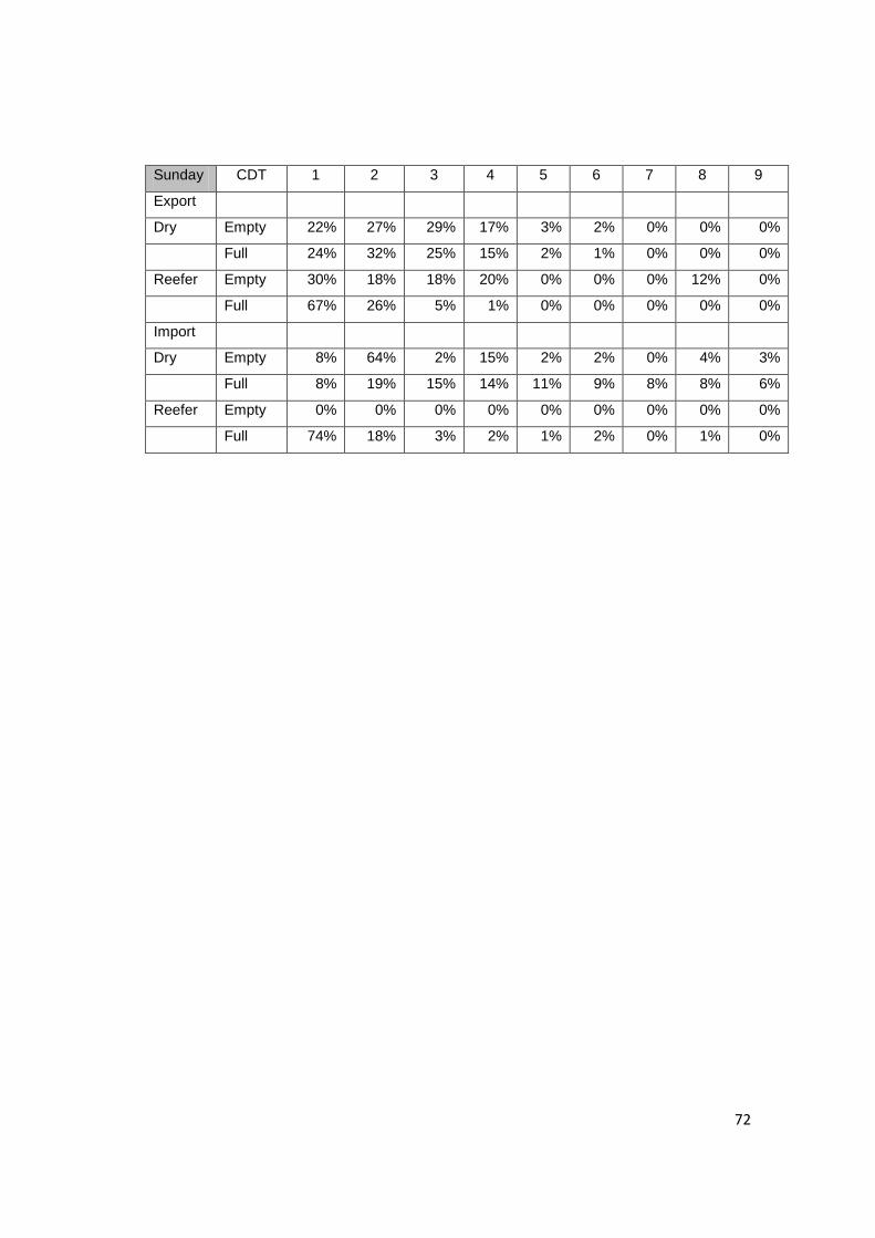
72

Sunday CDT 1 2 3 4 5 6 7 8 9

Export

Dry Empty 22% 27% 29% 17% 3% 2% 0% 0% 0%

Full 24% 32% 25% 15% 2% 1% 0% 0% 0%

Reefer Empty 30% 18% 18% 20% 0% 0% 0% 12% 0%

Full 67% 26% 5% 1% 0% 0% 0% 0% 0%

Import

Dry Empty 8% 64% 2% 15% 2% 2% 0% 4% 3%

Full 8% 19% 15% 14% 11% 9% 8% 8% 6%

Reefer Empty 0% 0% 0% 0% 0% 0% 0% 0% 0%

Full 74% 18% 3% 2% 1% 2% 0% 1% 0%

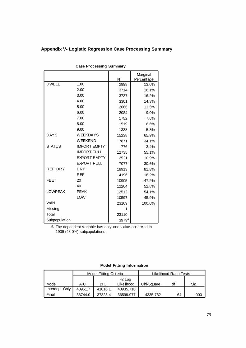
73

Appendix V- Logistic Regression Case Processing Summary

Case Processing Summary

2998 13.0%

3714 16.1%

3737 16.2%

3301 14.3%

2666 11.5%

2084 9.0%

1752 7.6%

1519 6.6%

1338 5.8%

15238 65.9%

7871 34.1%

776 3.4%

12735 55.1%

2521 10.9%

7077 30.6%

18913 81.8%

4196 18.2%

10905 47.2%

12204 52.8%

12512 54.1%

10597 45.9%

23109 100.0%

1

23110

3979a

1.00

2.00

3.00

4.00

5.00

6.00

7.00

8.00

9.00

DWELL

WEEKDAYS

WEEKEND

DAYS

IMPORT EMPTY

IMPORT FULL

EXPORT EMPTY

EXPORT FULL

STATUS

DRY

REF

REF_DRY

20

40

FEET

PEAK

LOW

LOWPEAK

Valid

Missing

Total

Subpopulation

N

Marginal

Percentage

The dependent variable has only one v alue observed in

1909 (48.0%) subpopulations.

a.

Model Fitting Information

40951.7 41016.1 40935.710

36744.0 37323.4 36599.977 4335.732 64 .000

Model

Intercept Only

Final

AIC BIC

-2 Log

Likelihood

Model Fitting Criteria

Chi-Square df Sig.

Likelihood Ratio Tests

74

Goodness-of-Fit

33558.987 31760 .000

22376.286 31760 1.000

Pearson

Deviance

Chi-Square df Sig.

Pseudo R-Square

.171

.173

.044

Cox and Snell

Nagelkerke

McFadden

75

Appendix VI- Dummy Regression Case Processing Summary

Variables Entered/Removedb

LOWPEAK,

STATUS2,

FEET,

BOX,

DAYS,

STATUS1,

REF_DRY,

STATUS3a

. Enter

Model

1

Variables

Entered

Variables

Removed Method

All requested v ariables entered.a.

Dependent Variable: DWELLb.

Model Summary

.581a .338 .338 2.22544

Model

1

R R Square

Adjusted

R Square

Std. Error of

the Estimate

Predictors: (Constant), LOWPEAK, STATUS2, FEET,

BOX, DAYS, STATUS1, REF_DRY, STATUS3

a.

76

Appendix VII- Linear Regression Case Processing Summary

Variables Entered/Removedb

LOWPEAK,

STATUS2,

FEET,

BOX,

DAYS,

STATUS1,

REF_DRY,

STATUS3a

. Enter

Model

1

Variables

Entered

Variables

Removed Method

All requested v ariables entered.a.

Dependent Variable: DWELLb.

Model Summary

.338a .114 .114 2.22544

Model

1

R R Square

Adjusted

R Square

Std. Error of

the Estimate

Predictors: (Constant), LOWPEAK, STATUS2, FEET,

BOX, DAYS, STATUS1, REF_DRY, STATUS3

a.

77

Appendix VIII- Partial Hypothesis Testing Results

Study on optimal dwell time at Jakarta International Container ...

Documents

Transcript of Study on optimal dwell time at Jakarta International Container ...