Study of the March 31, 2001 magnetic storm effects on the ionosphere using GPS data
23
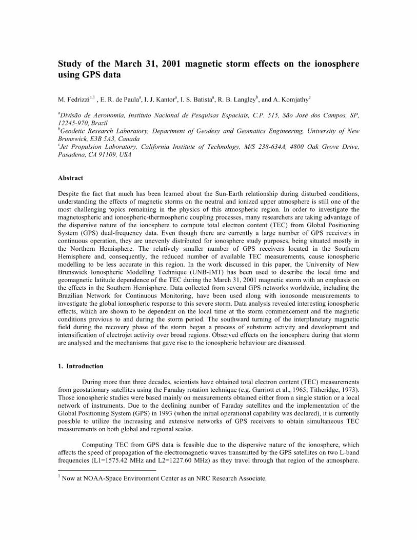
Study of the March 31, 2001 magnetic storm effects on the ionosphere using GPS data M. Fedrizzi a,1 , E. R. de Paula a , I. J. Kantor a , I. S. Batista a , R. B. Langley b , and A. Komjathy c a Divisão de Aeronomia, Instituto Nacional de Pesquisas Espaciais, C.P. 515, São José dos Campos, SP, 12245-970, Brazil b Geodetic Research Laboratory, Department of Geodesy and Geomatics Engineering, University of New Brunswick, E3B 5A3, Canada c Jet Propulsion Laboratory, California Institute of Technology, M/S 238-634A, 4800 Oak Grove Drive, Pasadena, CA 91109, USA Abstract Despite the fact that much has been learned about the Sun-Earth relationship during disturbed conditions, understanding the effects of magnetic storms on the neutral and ionized upper atmosphere is still one of the most challenging topics remaining in the physics of this atmospheric region. In order to investigate the magnetospheric and ionospheric-thermospheric coupling processes, many researchers are taking advantage of the dispersive nature of the ionosphere to compute total electron content (TEC) from Global Positioning System (GPS) dual-frequency data. Even though there are currently a large number of GPS receivers in continuous operation, they are unevenly distributed for ionosphere study purposes, being situated mostly in the Northern Hemisphere. The relatively smaller number of GPS receivers located in the Southern Hemisphere and, consequently, the reduced number of available TEC measurements, cause ionospheric modelling to be less accurate in this region. In the work discussed in this paper, the University of New Brunswick Ionospheric Modelling Technique (UNB-IMT) has been used to describe the local time and geomagnetic latitude dependence of the TEC during the March 31, 2001 magnetic storm with an emphasis on the effects in the Southern Hemisphere. Data collected from several GPS networks worldwide, including the Brazilian Network for Continuous Monitoring, have been used along with ionosonde measurements to investigate the global ionospheric response to this severe storm. Data analysis revealed interesting ionospheric effects, which are shown to be dependent on the local time at the storm commencement and the magnetic conditions previous to and during the storm period. The southward turning of the interplanetary magnetic field during the recovery phase of the storm began a process of substorm activity and development and intensification of electrojet activity over broad regions. Observed effects on the ionosphere during that storm are analysed and the mechanisms that gave rise to the ionospheric behaviour are discussed. 1. Introduction During more than three decades, scientists have obtained total electron content (TEC) measurements from geostationary satellites using the Faraday rotation technique (e.g. Garriott et al., 1965; Titheridge, 1973). Those ionospheric studies were based mainly on measurements obtained either from a single station or a local network of instruments. Due to the declining number of Faraday satellites and the implementation of the Global Positioning System (GPS) in 1993 (when the initial operational capability was declared), it is currently possible to utilize the increasing and extensive networks of GPS receivers to obtain simultaneous TEC measurements on both global and regional scales. Computing TEC from GPS data is feasible due to the dispersive nature of the ionosphere, which affects the speed of propagation of the electromagnetic waves transmitted by the GPS satellites on two L-band frequencies (L1=1575.42 MHz and L2=1227.60 MHz) as they travel through that region of the atmosphere. 1 Now at NOAA-Space Environment Center as an NRC Research Associate.
Transcript of Study of the March 31, 2001 magnetic storm effects on the ionosphere using GPS data
Study of the March 31, 2001 magnetic storm effects on the ionosphere using GPS data M. Fedrizzia,1 , E. R. de Paulaa, I. J. Kantora, I. S. Batistaa, R. B. Langleyb, and A. Komjathyc
aDivisão de Aeronomia, Instituto Nacional de Pesquisas Espaciais, C.P. 515, São José dos Campos, SP, 12245-970, Brazil bGeodetic Research Laboratory, Department of Geodesy and Geomatics Engineering, University of New Brunswick, E3B 5A3, Canada cJet Propulsion Laboratory, California Institute of Technology, M/S 238-634A, 4800 Oak Grove Drive, Pasadena, CA 91109, USA Abstract Despite the fact that much has been learned about the Sun-Earth relationship during disturbed conditions, understanding the effects of magnetic storms on the neutral and ionized upper atmosphere is still one of the most challenging topics remaining in the physics of this atmospheric region. In order to investigate the magnetospheric and ionospheric-thermospheric coupling processes, many researchers are taking advantage of the dispersive nature of the ionosphere to compute total electron content (TEC) from Global Positioning System (GPS) dual-frequency data. Even though there are currently a large number of GPS receivers in continuous operation, they are unevenly distributed for ionosphere study purposes, being situated mostly in the Northern Hemisphere. The relatively smaller number of GPS receivers located in the Southern Hemisphere and, consequently, the reduced number of available TEC measurements, cause ionospheric modelling to be less accurate in this region. In the work discussed in this paper, the University of New Brunswick Ionospheric Modelling Technique (UNB-IMT) has been used to describe the local time and geomagnetic latitude dependence of the TEC during the March 31, 2001 magnetic storm with an emphasis on the effects in the Southern Hemisphere. Data collected from several GPS networks worldwide, including the Brazilian Network for Continuous Monitoring, have been used along with ionosonde measurements to investigate the global ionospheric response to this severe storm. Data analysis revealed interesting ionospheric effects, which are shown to be dependent on the local time at the storm commencement and the magnetic conditions previous to and during the storm period. The southward turning of the interplanetary magnetic field during the recovery phase of the storm began a process of substorm activity and development and intensification of electrojet activity over broad regions. Observed effects on the ionosphere during that storm are analysed and the mechanisms that gave rise to the ionospheric behaviour are discussed. 1. Introduction
During more than three decades, scientists have obtained total electron content (TEC) measurements from geostationary satellites using the Faraday rotation technique (e.g. Garriott et al., 1965; Titheridge, 1973). Those ionospheric studies were based mainly on measurements obtained either from a single station or a local network of instruments. Due to the declining number of Faraday satellites and the implementation of the Global Positioning System (GPS) in 1993 (when the initial operational capability was declared), it is currently possible to utilize the increasing and extensive networks of GPS receivers to obtain simultaneous TEC measurements on both global and regional scales.
Computing TEC from GPS data is feasible due to the dispersive nature of the ionosphere, which affects the speed of propagation of the electromagnetic waves transmitted by the GPS satellites on two L-band frequencies (L1=1575.42 MHz and L2=1227.60 MHz) as they travel through that region of the atmosphere. 1 Now at NOAA-Space Environment Center as an NRC Research Associate.
The change in satellite-to-receiver signal propagation time due to the ionosphere is directly proportional to the integrated free-electron density along the signal path. GPS pseudorange measurements are increased (the signal is delayed) and the carrier-phase measurements are reduced (the phase is advanced) by the presence of the ionosphere. After forming the linear combination of these measurements on the L1 and L2 frequencies, the carrier phase and the pseudorange TEC are obtained.
Owing to its continuous operation and the large number of worldwide receivers, GPS is a powerful tool to investigate ionospheric structures, mainly during magnetically disturbed periods when dynamics and energy dissipation processes in the magnetosphere-thermosphere-ionosphere system become extremely complex (e.g., Prölss, 1995; Fuller-Rowell et al., 1997). Various researchers have shown that ionospheric spatial and temporal structures associated with magnetic storms can be investigated and monitored by TEC measurements provided by GPS observables (e.g., Ho et al., 1996; Basu et al., 2001; Saito et al., 2001; Jakowski et al., 2002, Coster et al., 2003; Shiokawa et al., 2003; Vlasov et al., 2003; Tsurutani et al., 2004). In this paper, we used data from about 250 GPS stations distributed worldwide, including stations from the Brazilian Network for Continuous Monitoring of GPS (RBMC), which is maintained and operated by the Brazilian Institute of Geography and Statistics (IBGE), to investigate the TEC response to the March 31, 2001 magnetic storm. Ionosonde data from stations located in the Australian and South American regions were used to help explain TEC variations observed during that storm. TEC measurements are provided by the University of New Brunswick Ionospheric Modelling Technique (UNB-IMT), which applies a spatial linear approximation of the vertical TEC above each station using stochastic parameters in a Kalman filter estimation, to describe the local time and geomagnetic latitude dependence of the TEC. 2. UNB Ionospheric Modelling Technique
The UNB Ionospheric Modelling Technique (UNB-IMT) was developed in 1997, in the Department of Geodesy and Geomatics Engineering at University of New Brunswick (UNB), to compute the total electron content (TEC) from GPS observables at both L1 and L2 frequencies in order to provide ionospheric corrections to communication, surveillance and navigation systems operating at one frequency. The software is based on a modified version of UNB’s DIfferential POsitioning Program (DIPOP) and applies a spatial linear approximation of the vertical TEC above each GPS ground station using stochastic parameters in a Kalman filter estimation to describe TEC dependence with local time and geomagnetic latitude (Komjathy, 1997).
Initially, UNB-IMT computes the ionospheric delay of the leveled carrier phase along the satellite-receiver line-of-sight. During this first step, the PhasEdit version 2.2 automatic data editing program (Freymueller, 2001) is used to detect bad points and cycle slips, as well as repair the cycle slips and adjust phase ambiguities using the undifferenced GPS data. The program takes advantage of the high precision dual-frequency pseudorange measurements to adjust L1 and L2 phases by an integer number of cycles to agree with the pseudorange measurements. The elevation cutoff angle was set to 10°.
In a second step, the software estimates the coefficients of the linear spatial approximation of TEC over each station plus the satellite and receiver differential biases, modeling the ionospheric measurements from a dual frequency GPS receiver with the single-layer ionospheric model, according to the following observation equation (Komjathy, 1997):
i
j
i
jj
i
jjj
i
j
i
j
s
r
s
rkr
s
rkrkr
s
rk
s
r bbdtadtataeMtI ++++= ])()()([)()( ,2,1,0 !" (1)
where
)( ks
r tI i
j represents the line-of-sight L1-L2 phase-levelled measurement (in TEC units) obtained by the
receiver jr observing the satellite
is at epoch
kt ; )( i
j
s
reM is the mapping function projecting the line-of-
sight measurement to the vertical of the sub-ionospheric point, where )( i
j
s
re represents the satellite elevation
angle; jr
a,0 ,
jra,1 and
jra,2 are the stochastic parameters for spatial linear approximation of TEC to be
estimated for each station assuming a first-order Gauss-Markov stochastic process; 0
!!! "= i
j
i
j
s
r
s
rd is the
difference between the longitude of the sub-ionospheric point and the mean longitude of the Sun;
0!!! "= i
j
i
j
s
r
s
rd is the difference between the geomagnetic latitude of the sub-ionospheric point and the
geomagnetic latitude of the station; and jrb and isb represent, respectively, the receiver and the satellite
differential delay biases.
The single layer ionospheric model assumes that the vertical TEC can be approximated by a thin spherical shell, which is typically located at the height of maximum electron density. In the UNB-IMT approrach, the ionospheric shell height can be a value either fixed or computed by the IRI-95 (International Reference Ionosphere-1995) model (Bilitza, 1997). In the first case, it is usually assumed that the ionospheric shell height has no temporal or geographical variation and therefore it is set to a constant value regardless of the time or location of interest. IRI output, on the other hand, depends on local time and location. Ionospheric shell height values computed by IRI correspond to the barycentre of the ionosphere, i.e., the height at which 50% of TEC lies below and 50% lies above (Komjathy, 1997). Since IRI TEC values were obtained through electron density integration from 100 to 1000 km of altitude, they do not include the plasmaspheric electron content.
The combined satellite-receiver differential delays for a reference station are estimated using the Kalman filter algorithm and, in a network solution, additional biases for the other stations are estimated based on the fact that the other receivers have different instrumental delays. Therefore, for each station other than the reference station, an additional differential delay parameter is estimated, which is the difference between the receiver differential delay of a station in the network and the reference station. This technique is described by Sardon et al. (1994). The mapping function we used in our work is the standard geometric mapping function, which computes the secant of the zenith angle of the signal geometric ray path at the ionospheric pierce point at a shell height computed by IRI-95. The standard geometric mapping function is given by (e.g., Komjathy, 1997):
[ ] 21
222 )(cos1)(!
+!= hrereMEE
(2) where e is the satellite elevation angle, Er is the mean radius of the Earth and, h is the mean value for the height of the ionosphere (assumed shell height).
Because of the dependence of the ionosphere on the solar radiation and the geomagnetic field, a solar-geomagnetic reference frame is used to compute the TEC at each station. Since the ionosphere changes more slowly in the Sun-fixed reference frame than in the Earth-fixed one, using such a reference frame results in more accurate ionospheric delay estimates when the Kalman filter is applied (Komjathy, 1997). The ionospheric model was evaluated for the four closest stations to a grid node at which a TEC value is computed. Subsequently, the inverse distance squared weighted average of the individual TEC data values for the four GPS stations were computed. The closer a particular grid node is to a GPS station, the more weight was put on the TEC values computed by evaluating the ionospheric model describing the temporal and spatial variation of the ionosphere above the particular station.
3. Observations and Discussion
Apart from station coordinates and satellite ephemerides, GPS observations are the only data input that UNB-IMT requires to provide TEC for either a specific station, a region or the entire globe. In this work, we have used data obtained from the Brazilian Network for Continuous Monitoring (RBMC) and Scripps Orbits and Permanent Array Center (SOPAC) data archive networks to investigate the global ionospheric response to a magnetic storm that occurred on March 31, 2001. In order to have the best possible global TEC representation during the storm period, we have processed data from about 250 GPS receivers distributed worldwide (Figure 1). The quality of the GPS data was checked for all stations using the Translate/Edit/Quality Check (TEQC) software (UNAVCO, 2004). Based on the QC results, we have chosen Albert Head (geographic coordinates: 48.4°N, 123.5°W) as the reference station since, amongst the stations located in a geomagnetic mid-latitude region where the ionosphere is fairly well behaved, it had the best results in terms of data quality during the period analysed (March 15, 16, 31 and April 1, 2001). TEC maps were produced using a 5-degree grid spacing, so that each 15-minute map contains the observations obtained from 7.5 minutes before to 7.5 minutes after the respective quarter hour. The maps were generated using the Generic Mapping Tools (Wessel and Smith, 1998). Ionosonde measurements (such as F region minimum virtual height (h’F), height of peak electron density (hmF2) and F2 layer maximum electron density (NmF2)) from Australian and South American stations (Table 1) were also analyzed to help explain the observed ionospheric variations. The local time at the storm commencement, as well as the storm development and recovery duration are some of the most the important factors that influence the ionospheric behaviour during magnetically disturbed periods (e.g., Prölss, 1995; Basu et al., 2001). Therefore, this storm was particularly interesting because it lasted more than 15 hours, causing distinct effects on the ionosphere during daytime over approximately opposite longitude sectors. In the following sections, a discussion about the storm effects on both Australian/Asian and American sectors is presented.
3. 1 Storm Effects in the Australian/Asian Sector
A summary of the magnetic conditions for the period March 30 to April 3 is presented in Figure 2. On March 31, the north-south component of the interplanetary magnetic field (Bz) (top panel) exhibited two significant incursions to the south: the first one lasted about 4 hours and the second one approximately 8 hours. In the middle panel, the auroral electrojet (AE) index shows the significant amount of energy that was injected at high latitudes during the storm period. In the bottom panel, the longitudinally symmetric (SYM-H) disturbance index initiated its negative incursion around 04:30 UT, reaching –437 nT at 08:07 UT. We have used the SYM-H index instead of the disturbance storm time (Dst) index, since its one-minute resolution is more appropriate for studies of phenomena occurring on a short time scale. The SYM-H index follows essentially the same variations as the Dst index, however it is obtained from a different set of stations and a slightly different coordinate system (Iyemori et al., 2003). Also, in the bottom panel, the Kp index shows the intense activity occurred on March 31, reaching values of 9¯ that lasted for about 6 hours.
Figure 3a shows a TEC map during the first hours after the storm commencement, when the largest
values occurred on March 31 (daytime in the Australian/Asian sector). For comparison purposes, the TEC map for a quiet day (March 16) is shown in Figure 3b. On March 31, the equatorial anomaly crests were significantly increased and displaced towards higher latitudes in the Australian/Asian longitude sector. However, we should mention that TEC values could be overestimated in remote and oceanic areas due to station/data absence. In general, TEC uncertainties in regions with good station coverage are normally less than 10%; over oceanic areas without GPS stations where the TEC gradients are large, the uncertainties can reach up to 50%. This can occur since UNB-IMT does not use an ionospheric climatological model to adjust the data in regions where GPS data coverage is poor, unless the IRI injector technique (Komjathy et al., 1998) is used.
Amongst the possible causes for TEC enhancements over the Australian/Asian sector are the fountain effect intensification due to an eastward magnetospheric electric field penetrating to the equatorial ionosphere, the thermal expansion caused by the transport of Joule and particle heating from high latitudes,
and the storm-time thermospheric disturbance winds flowing towards lower latitude regions transporting the ionization upwards along the geomagnetic field lines to regions where recombination rates are lower. The effectiveness of thermospheric winds in modifying the ionospheric height is maximum at middle latitudes and minimum at the geomagnetic equator due to the dip angle, while in equatorial latitudes the ionospheric height modifications are mainly associated with electric field influences (e.g. Rishbeth, 1998).
Ionosonde stations located in the Australian region (Figure 4) showed an uplift of the F2 layer over
all stations (Figure 5). At Vanimo, the closest ionosonde to the geomagnetic equator, hmF2 uplift from approximately 04:00 UT (13:25 LT) to 08:00 UT (17:25 LT) is most likely caused by a magnetospheric eastward electric field penetration into the equatorial ionosphere. At higher latitudes, equatorward storm-time thermospheric winds and thermal expansion are most likely the dominant mechanisms that uplift the ionosphere, but the relative contribution of each mechanism in raising the F2 layer is uncertain. During the main phase of the storm, Vanimo showed a data gap in NmF2 from 05:00 UT (14:25 LT) to 08:00 UT (17:25 LT), according to Figure 6. Its geomagnetic location lies somewhere between the south crest of the equatorial anomaly and its trough, so that no conspicuous differences between NmF2 measurements at quiet and disturbed periods are observed. However, Darwin station showed an increase in NmF2 around that period, corresponding to plasma deposited at the south crest of the equatorial anomaly due to the fountain effect intensification already mentioned.
In the period between 09:00 UT (~ 18:00 LT) and 16:00 UT (~ 01:00 LT), both stations Vanimo and
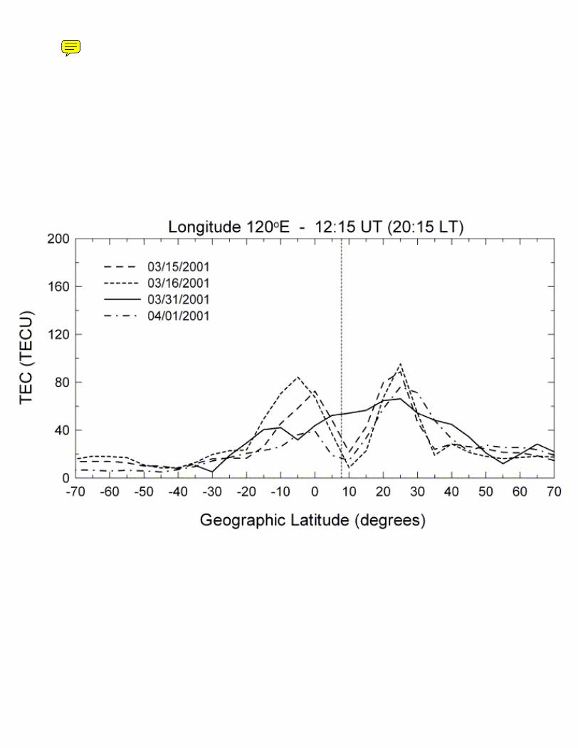
Darwin registered decreases in NmF2 (Figure 6). Those decreases seem to be associated with the presence of disturbance dynamo electric fields, which are westward during daytime and post sunset hours (Abdu, 1997). The dynamo action of winds driven by storm heating at high latitudes tends to reduce the daytime eastward electric field characteristic of quiet periods (Blanc and Richmond, 1980; Scherliess and Fejer, 1997), weakening the upward plasma drift at the geomagnetic equator and inhibiting the equatorial anomaly development. The consequences are that more plasma is retained at equatorial latitudes and less plasma is transported away from the geomagnetic equator. This feature can be observed in a meridional cross section of TEC along the Australian/Asian sector (Figure 7), showing that the equatorial anomaly development was inhibited on the storm day (March 31). Disturbance dynamo electric field signatures are also observed in Figure 5 at Vanimo, where h’F showed a decrease from about 09:00 UT (18:25 LT) to 12:00 UT (21:25 LT), followed by an uplift of h’F and hmF2 from 12:00 UT (21:25 LT) to 21:00 UT (06:25 LT) due to the electric field polarization reversal from westward to eastward around 12:00 UT. 3. 2 Storm Effects in the American Sector
On March 31, around 08:30 UT, Bz turned northward and remained predominantly north until approximately 14:30 UT, then it turned again southward for about 8 hours, beginning a process of substorm activity and development and intensification of electrojet activity over broad regions. During that period, the largest increases in TEC were observed around 19:30 UT over the American sector (Figure 8a). For comparison purposes, a TEC map representing a quiet day (March 16) is shown in Figure 8b. However, the anomaly crests did not show a significant displacement towards higher latitudes as in the early stages of the storm in the Australian/Asian sector (see Figure 3a), and the ionization depletion over the geomagnetic equator was not so conspicuous. Once more, it is worth mentioning that due to station/data absence in the Pacific/Atlantic oceans, TEC values over those regions might be uncertain.
Ionosonde data for three stations located in South America (Figure 9) are shown in Figure 10 to help identify possible causes for the TEC enhancements observed in Figure 8a. On March 31, hmF2 above São Luís station showed an uplift between 15:00 UT (12:03 LT) and 19:00 UT (16:03 LT), which may be associated with a plasma uplift due to the penetration of an eastward magnetospheric electric field into the equatorial ionosphere. The other two stations (Cachoeira Paulista and Port Stanley) showed longer lasting hmF2 uplifts, which are probably due to the presence of disturbed thermospheric winds flowing equatorwards and thermal expansion. However, possibly due to the geomagnetic pole offset from the geographic ones and/or the spatial distribution of the energy input over the poles (Fuller-Rowell et al., 1997), hmF2 uplift was not so large in the South American sector in comparison to the uplifts registered by the Australian ionosondes.
During that period, NmF2 measurements at São Luís and Cachoeira Paulista (Figure 11) did not show deviations from the quiet time, possibly due to a competition between the eastward prompt penetration electric field and the westward disturbance dynamo electric field. The former can intensify the fountain effect while the later weakens it.
Due to the large energy injection that occurred during this magnetic storm, we should also expect to
observe disturbance dynamo electric field effects in the American sector. Their signatures can be seen in ionosonde measurements at São Luís station (Figure 10), when h’F and hmF2 measurements shows an increase of both h’F and hmF2 from approximately 07:30 UT (04:33 LT) to 10:30 UT (07:33 LT), corresponding to an eastward electric field playing a role during the nightime. The spike-like feature occurring around 08:30 UT (~ 05:33 LT) coincides with the Bz inversion to north. According to Kelley et al. (1979), sudden IMF northward turnings from a steady southward direction causes a temporary imbalance between the convection related charge density and the charge in the inner edge of ring current, producing a dusk to dawn electric field perturbation that can penetrate to the equatorial ionosphere. This magnetospheric electric field is westward during the day and eastward at night. Therefore, it is possible that a superposition of both magnetospheric and disturbance dynamo electric fields has occurred during that time. A few hours later, h’F and hmF2 at São Luís station showed a decrease from about 22:00 UT (19:03 LT) to 03:00 UT (00:03 LT), followed by an uplift lasting until 06:00 UT (03:03 LT), which is a signature of a westward disturbance dynamo electric field.
The NmF2 response to the eastward disturbance dynamo electric field during the early morning
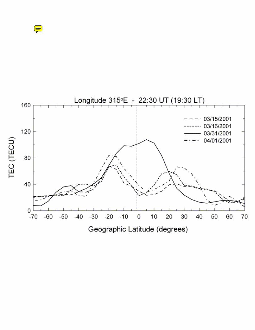
hours (between 07:30 UT (~ 04:30 LT) and 10:30 UT (~ 07:30LT), on March 31) at São Luís and Cachoeira Paulista stations (Figure 11) was not clear (despite the NmF2 increase from about 10:00 UT to 11:00 UT in Cachoeira Paulista), possibly because of the low ambient plasma densities (e.g., Abdu, 1997). However, evidences of a westward electric field was observed at those stations from 22:00 UT (~ 19:00 LT) to 03:00 UT (~ 24:00 LT) on March 31-April 1, when more plasma was retained in the geomagnetic equator region and less plasma was transported towards the southern equatorial anomaly crest. This observation is in agreement with the inhibition of the post-sunset uplift of the F layer over São Luís station shown in Figure 10, and also with TEC observations presented in Figure 12.
4. Summary and Future Considerations We have used GPS data to investigate the global ionospheric response to the March 31, 2001 magnetic storm using TEC measurements computed using the UNB-IMT data assimilation model. This technique is currently being improved through the investigation of different approaches for modelling the ionosphere with sparse networks and experimenting with different algorithms, such as the quadratic interpolation technique (Rho et al., 2004). Ionosonde data for a few stations located in the Australian and South American sectors were also used to help elucidate the possible mechanisms responsible for TEC enhancements and depletions. Magnetospheric and disturbance dynamo electric field, as well as thermal expansion and equatorward storm-time thermospheric wind effects were found. TEC response to this storm was distinct over the Australian/Asian and American sectors, showing its dependence on local time at the storm commencement, and storm development and recovery duration. We are currently comparing these results with physical models (Maruyama et al., 2004) to investigate the importance of each mechanism during the various phases of the storm occurrence. Acknowledgements We thank the following institutes for providing data: Scripps Orbit and Permanent Array Center (SOPAC), Brazilian Institute of Geography and Statistics (IBGE), National Institute for Space Research (INPE), IPS Radio and Space Services, National Geophysical Data Center (NGDC) at NOAA, Coordinated Data Analysis Web at NASA/GSFC and the World Data Center for Geomagnetism. We are grateful to Bela G. Fejer, Timothy J. Fuller-Rowell, Mihail Codrescu and David Anderson for their valuable discussions. E. R. de Paula thanks CNPq for the partial support under Process 502223/91-0. This research was supported by the CAPES Foundation (Brazil) and performed while the author was enrolled in a Ph.D. programme at INPE.
References Abdu, M. A. Major phenomena of the equatorial ionosphere-thermosphere system under disturbed conditions. J. Atmos. Sol. Terr. Phys., 59, 1505-1519, 1997. Basu, Su, Basu, S, Valladares, C. E., Yeh, H.-C., Su, S.-Y., MacKenzie, E., Sultan, P.J., Aarons, J., Rich, F. J., Doherty, P., Groves, K. M., Bullet, T. W. Ionospheric effects of major magnetic storms during the International Space Weather period of September and October 1999: GPS observations, VHF/UHF scintillations, and in situ density structures at middle and equatorial latitudes. J. Geophys. Res., 106 (A12), 30389-30413, 2001. Bilitza, D. International Reference Ionosphere - Status 1995/96. Adv. Space Res., 20 (9), 1751-1754, 1997. Blanc, M, Richmond, A. D. The ionospheric disturbance dynamo. J. Geophys. Res., 85 (A4), 1669-1686, 1980. Coster, A, Foster, J., Erickson, P., Sandel, B. Monitoring space weather with GPS mapping techniques. Institute of Navigation, Proceedings of the National Technical Meeting 2003. Anaheim, CA, 26-28 January 2003. Freymueller, J. T. Personal communication. Geophysical Institute, University of Alaska, Fairbanks. June, 2001. Fuller-Rowell, T. J., Codrescu, M. V., Roble, R. G., Richmond, A. D. How does the thermosphere and ionosphere react to a geomagnetic storm?, in: Tsurutani, B. T., Gonzalez, W. D., Kamide, Y., Arballo, J. L. (Eds.), Magnetic Storms. Washington: American Geophysical Union, 203-225, 1997. Garriott, O. K., Smith, III F. L., Yuen, P. C. Observations of ionospheric electron content using a geostationary satellite. Planet. Space Sci., 13, 829-838, 1965. Ho, C. M., Mannucci, A. J., Lindqwister, U. J., Pi, X., Tsurutani, B. T. Global ionosphere perturbations monitored by the worldwide GPS network. Geophys. Res. Lett., 23 (22), 3219-3222, 1996. Iyemori, T., Araki, T., Kamei, T., Takeda, M. Mid-latitude Geomagnetic Indices “ASY” and “SYM” for 1999 (Provisional). http://swdcwww.kugi.kyoto-u.ac.jp/aeasy/asy.pdf. Accessed 16 November 2003. Jakowski, N., Heise, S., Wehrenpfennig, A., Schlüter, S., Reimer, R. GPS/GLONASS-based TEC measurements as a contributor for space weather forecast. J. Atmos. Sol. Terr. Phys., 64, 729-735, 2002. Kelley, M. C., Fejer, B. G. Gonzales, C. A. Explanation for anomalous ionospheric electric fields associated with a northward turning of the interplanetary magnetic field. Geophys. Res. Lett., 6, 301-304, 1979. Komjathy, A. Global Ionospheric Total Electron Content Mapping Using the Global Positioning System. 248 pp. (Dept. of Geodesy and Geomatics Engineering, Technical Report No. 188). Ph. D. dissertation. University of New Brunswick, 1997. Komjathy, A., Langley, R. B., Bilitza, D. Ingesting GPS-derived TEC data into the International Reference Ionosphere for single frequency radar altimeter ionospheric delay corrections. Adv. Space Res., 22 (6), 793-801, 1998. Maruyama, N., Fuller-Rowell, T. J., Codrescu, M., Richmond, A. D., Millward, G., Spiro, R. W., Sazykin, S., Toffoletto, F., Lin, C. Relative importance of direct penetration and disturbance dynamo electric fields on the
storm-time equatorial ionosphere and thermosphere. Eos Trans. AGU, 85 (17), Jt. Assem. Suppl., Abstract SA42A-06, 2004. Prölss, G. W. Ionospheric F-region storms, in: Volland, H. (Ed.), Handbook of Atmospheric Electrodynamics. Boca Raton: CRC Press, 2, 195-248, 1995. Rho, H., Langley, R. B., Komjathy, A. An enhanced UNB Ionospheric Modeling Technique for SBAS: the quadratic approach. Proceedings of ION GNSS 2004. Long Beach, Sept. 21-24, 2004. Rishbeth, H. How the thermospheric circulation affects the ionospheric F2-layer. J. Atmos. Sol. Terr. Phys., 60, 1385-1402, 1998. Saito, A., Nishimura, M., Yamamoto, M., Fukao, S., Kubota, M., Shiokawa, K., Otsuka, Y., Tsugawa, T., Ogawa, T., Ishii, M., Sakanoi, T., Miyazaki, S. Traveling ionospheric disturbances detected in the FRONT campaign. Geophys. Res. Lett, 28 (4), 689-692, 2001. Sardón, E., Rius, A., Zarraoa, N. Estimation of the transmitter and receiver differential biases and the ionospheric total electron content from Global Positioning System observations. Radio Sci., 29, 577-586, 1994. Scherliess, L., Fejer, B. G. Storm time dependence of equatorial disturbance dynamo zonal electric fields. J. Geophys. Res., 102 (A11), 24037-24046, 1997. Shiokawa, K., Otsuka, Y., Ogawa, T., Kawamura, S., Yamamoto, M., Fukao, S., Nakamura, T., Tsuda, T., Balan, N., Igarashi, K., Lu, G., Saito, A., Yumoto, K. Thermospheric wind during a storm-time large-scale traveling ionospheric disturbance. J. Geophys. Res., 108 (A12), 1423, doi: 10.1029/2003JA010001, 2003. Titherdidge, J. E. The electron content of the southern mid-latitude ionosphere, 1965-1971. J. Atmos. Terr. Phys., 35, 981-1001, 1973. Tsurutani, B., Mannucci, A., Iijima, B., Abdu, M. A., Sobral, J. H. A., Gonzalez, W., Guarnieri, F., Tsuda, T., Saito, A., Yumoto, K., Fejer, B., Fuller-Rowell, T. J., Kozyra, J., Foster, J. C., Coster, A., Vasyliunas, V. M. Global dayside ionospheric uplift and enhancement associated with interplanetary electric fields. J. Geophys. Res., 109, A08302, doi: 10.1029/2003JA010342, 2004. University NAVSTAR Consortium (UNAVCO). TEQC: The Toolkit for GPS/GLONASS Data. http://www.unavco.org/facility/software/teqc/teqc.html. Accessed 14 February 2004. Vlasov, M.; Kelley, M. C.; Kil, H. Analysis of ground-based and satellite observations of F-region behavior during the great magnetic storm of July 15, 2000. J. Atmos. Sol. Terr. Phys., 65, 1223-1234, 2003. Wessel, P., Smith, W. H. F. New, improved version of Generic Mapping Tools released, EOS Trans. Amer. Geophys. U., 79, 579, 1998. Tables: Table 1. Ionosonde stations. Figures:
Figure 1. Map showing GPS stations used in this study. Figure 2. Bz component of the interplanetary magnetic field in geocentric-solar-magnetospheric (GSM) coordinates provided by the Advanced Composition Explorer (ACE) spacecraft for the period March 30 to April 03, 2001 (top); AE index (middle); and SYM-H and Kp indices for the same period (bottom). In the top panel, the time delay of the magnetic field convection from ACE to the magnetopause was taken into account. Figure 3. TEC maps comparing values between days (a) March 31, 2001 (day 090) and (b) March 16, 2001 (day 075), at 07:15 UT. Figure 4. Ionosonde stations located in the Australian region and used in this study. They are operated by IPS Radio and Space Services ionosonde network. Figure 5. F layer minimum virtual height (h’F) and F2 peak height (hmF2) for the period March 30, 2001 to April 1, 2001. Bz, AE, SYM-H and Kp index values for the same period are shown in the top panels. Midnight local time is indicated by the “star” symbol and geomagnetic latitude of each station is provided. Figure 6. F2 layer maximum electron density (NmF2) for the period March 30, 2001 to April 1, 2001. Bz, AE, SYM-H and Kp index values for the same period are shown in the top panels. Midnight local time is indicated by the “star” symbol and geomagnetic latitude of each station is provided. Figure 7. TEC meridional cross section along the geographic longitude of 120°E for two quiet days (March 15, 2001 and March 16, 2001), the storm day (March 31, 2001) and the day following the storm (April 1, 2001). The vertical dashed line indicates the latitude of the geomagnetic equator on March 31, 2001. Figure 8. TEC maps comparing values between days (a) March 31, 2001 (day 090) and (b) March 16, 2001 (day 075), at 19:30 UT. Figure 9. Ionosondes stations located in the South American region and used in this study. São Luís and Cachoeira Paulista are operated by INPE, while Port Stanley is operated by Rutherford Appleton Laboratory. Figure 10. F layer minimum virtual height (h’F) and F2 peak height (hmF2) for the period March 30, 2001 to April 1, 2001. Bz, AE, SYM-H and Kp index values for the same period are shown at the top panels. Midnight local time is indicated by the “star” symbol and geomagnetic latitude of each station is provided. Figure 11. F2 layer maximum electron density (NmF2) for the period March 30, 2001 to April 1, 2001. Bz, AE, SYM-H and Kp index values for the same period are shown at the top panels. Midnight local time is indicated by the “star” symbol and geomagnetic latitude of each station is provided. Figure 12. TEC meridional cross section along the geographic longitude of 315°E, approximately at the same longitude as the Brazilian ionosonde stations of São Luís and Cachoeira Paulista, for two quiet days (March 15, 2001 and March 16, 2001), the storm day (March 31, 2001) and the day following the storm (April 1, 2001). The vertical dashed line indicates the latitude of the geomagnetic equator on March 31, 2001.
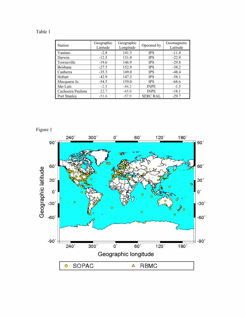
Table 1
StationGeographic
LatitudeGeographicLongitude Operated by
GeomagneticLatitude
Vanimo -2.8 141.3 IPS -11.4Darwin -12.5 131.0 IPS -22.9Townsville -19.6 146.9 IPS -29.8Brisbane -27.5 152.9 IPS -38.2Canberra -35.3 149.0 IPS -48.4Hobart -42.9 147.3 IPS -58.1Macquarie Is. -54.5 159.0 IPS -68.6São Luís -2.5 -44.2 INPE -1.5Cachoeira Paulista -22.7 -45.0 INPE -18.1Port Stanley -51.6 -57.9 SERC RAL -29.7
Figure 1
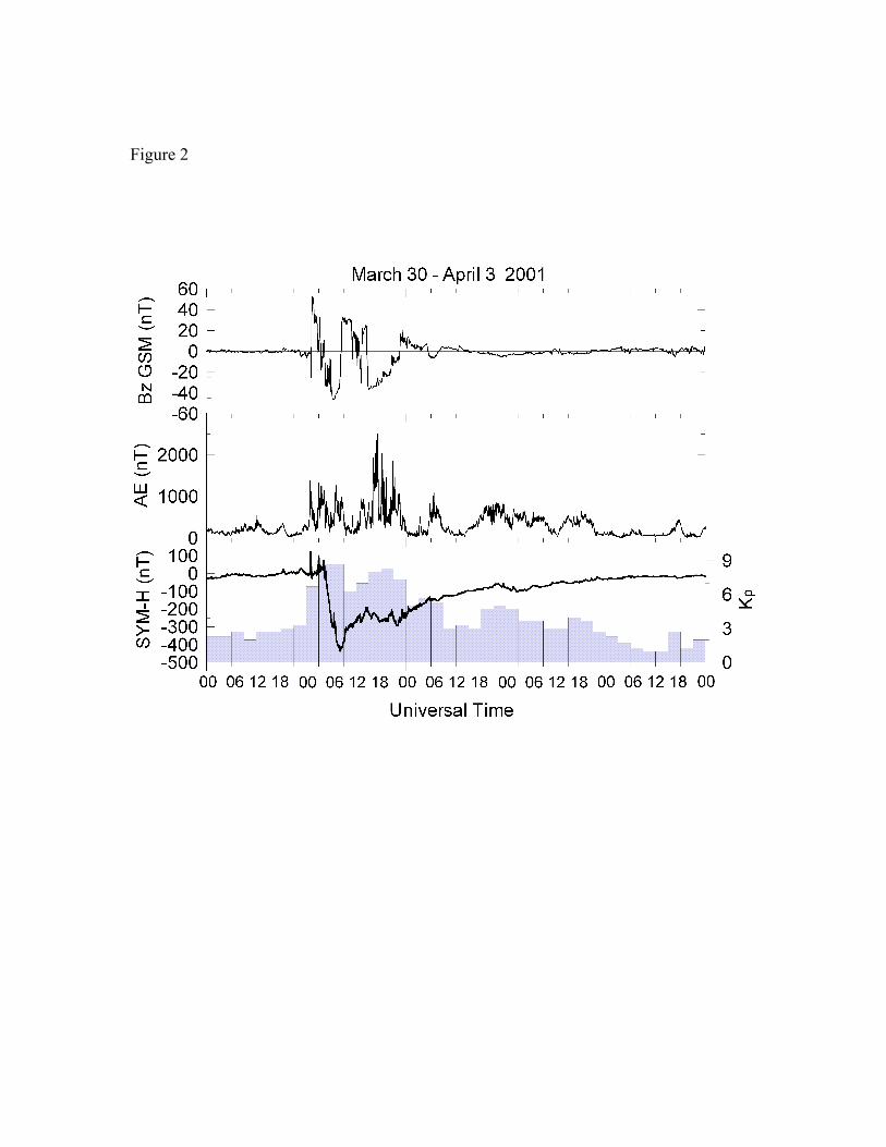
Figure 2
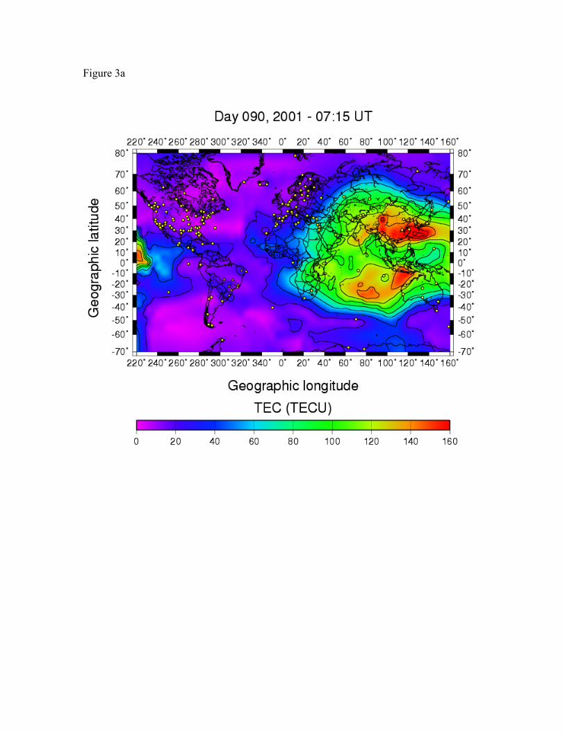
Figure 3a
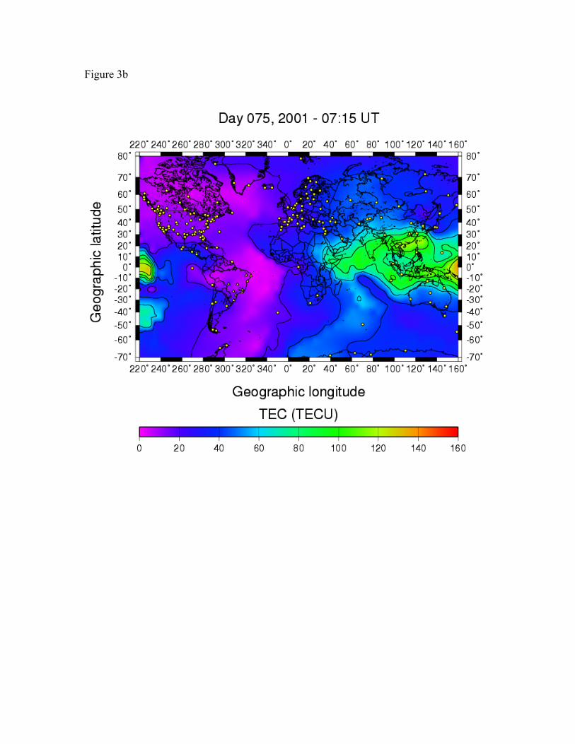
Figure 3b
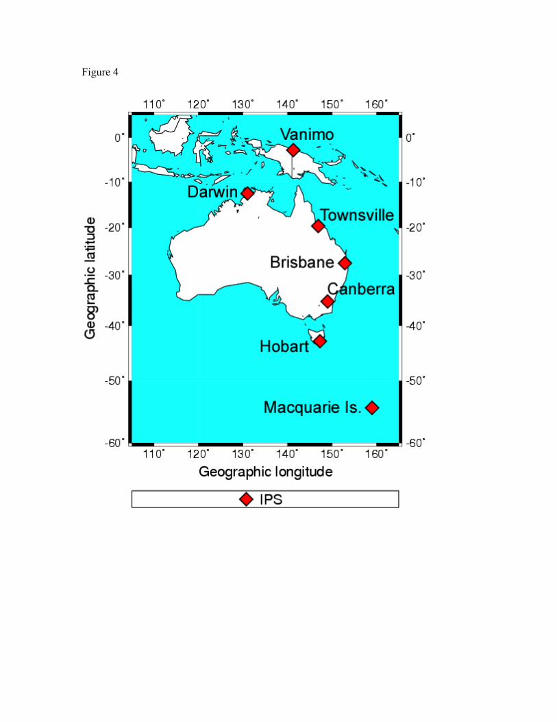
Figure 4
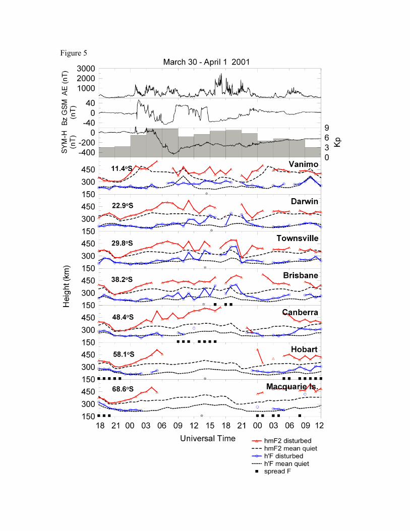
Figure 5
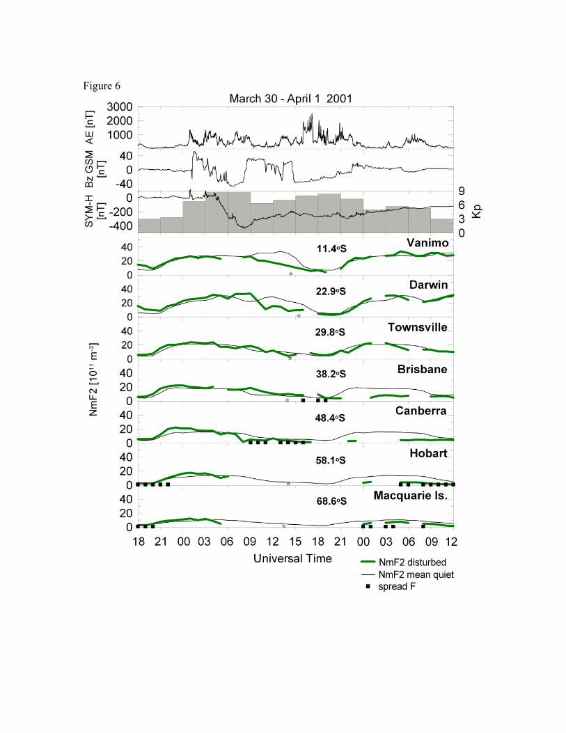
Figure 6
richardlangley
Note
Figure 7
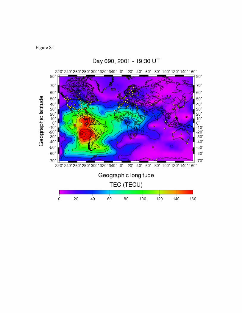
Figure 8a
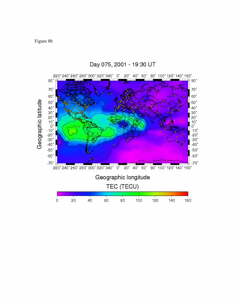
Figure 8b
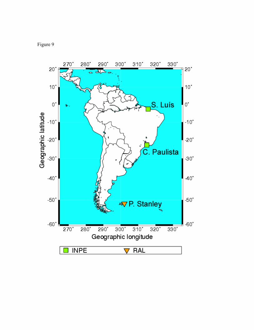
Figure 9
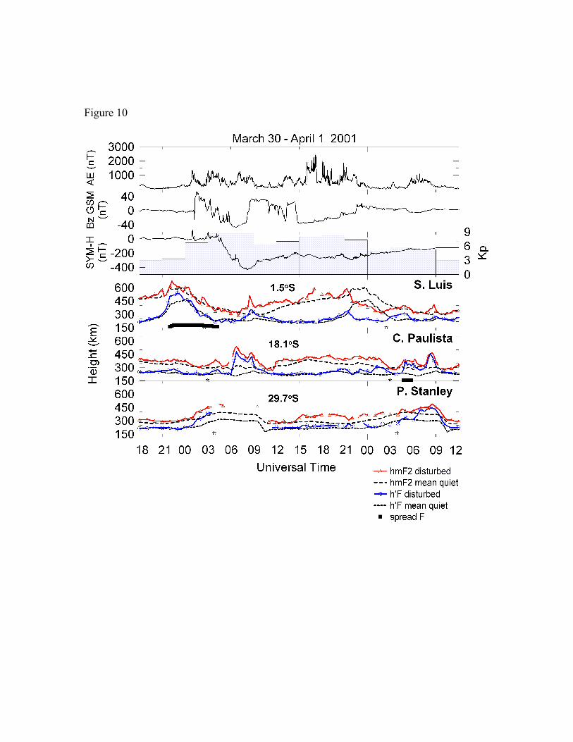
Figure 10
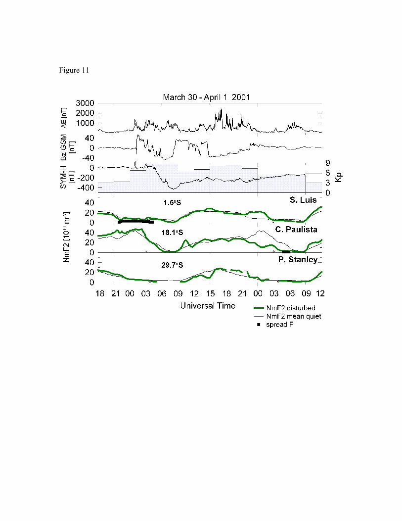
Figure 11
richardlangley
Note
Figure 12