arX

iv:c

ond-

mat

/991

2114

v1 7

Dec

199

9

Study of Pairing Correlations in the Attractive Hubbard Model

on Chains, Ladders, and Squares

M. Guerrero, G. Ortiz, and J. E. Gubernatis

Theoretical Division, Los Alamos National Laboratory, Los Alamos, NM 87444

(February 1, 2008)

Abstract

We report the results of zero temperature quantum Monte Carlo simulations

and zero temperature mean-field calculations of the attractive Hubbard model

on chains, ladders, and square lattices. We investigated the predictability of

the BCS approximation, the dimensional cross-over of the pairing correla-

tion function from one to two dimensions as a function of the ladder width,

and the scaling of these correlations to the thermodynamic limit of the two-

dimensional model. We found that the BCS wave function is quantitatively

correct only for small values of U/t. For the system sizes, electron fillings,

and interaction strengths studied, we never saw the dimensional cross-over. In

general our ability to achieve the dimensional cross-over and accurate scaling

to the thermodynamic limit was limited by the size of the systems we could

simulate. For these sizes, although we saw the necessary signature of ODLRO,

the properties of the model did not vary monotonically with increasing system

size because of shell effects. We contrast this situation with the dimensional

cross-over and scaling to the thermodynamic limit of the Ising model.

Typeset using REVTEX

1

I. INTRODUCTION

We report the results of zero temperature quantum Monte Carlo (QMC) simulations

and zero temperature mean-field calculations of the attractive Hubbard model on chains,

ladders, and square lattices. We investigated the predictability of the BCS approximation,

the dimensional cross-over of pairing correlations from one to two dimensions as a function of

the ladder width, and the scaling of these correlations to the thermodynamic limit of the two-

dimensional model. We found that the BCS wave function is quantitatively correct only for

weak attractive interactions. For the system sizes, electron fillings, and interaction strengths

studied, we never saw the dimensional cross-over, and we were unable to scale the pairing

correlations on finite-size square lattices to those on infinitely-sized ones. In general our

ability to achieve the dimensional cross-over and the proper scaling to the thermodynamic

limit was limited by the size of the systems we could simulate. For these sizes, although we

saw the necessary signature of off-diagonal long-range order (ODLRO), the properties of the

model did not vary monotonically with increasing system size because of shell effects.

The BCS wave function occupies a deservedly prominent place in the theory of super-

conductivity. For traditional superconductors, the electron-phonon interaction induces an

attractive interaction between pairs of electrons that is well described by the reduced BCS

Hamiltonian [1]

H =∑

kσ

ǫknk,σ −∑

k,k′

Vk,k′c†k,↑c

†−k,↓c−k′,↓ck′,↑ , (1)

and the BCS wave function

|BCS〉 =∏

k

(uk + vkc†k,↑c

†−k,↓)|0〉 (2)

provides an excellent approximation to the eigenstates of this Hamiltonian. In fact, under

a number of circumstances, it is the exact solution in the thermodynamic limit [2].

Characteristic of BCS-like superconductors is the large number of Cooper pairs inside

the volume defined by the coherence length a0 of a pair. In high temperature (cuprate)

2

superconductors, as well as several other classes of much lower temperature superconductors,

including doped cuprate ladders [4], the coherence length is comparatively small. For these

materials, one often proposes the attractive Hubbard model

H = −t∑

〈ij〉,σ

(c†i,σcj,σ + c†j,σci,σ) − U∑

i

ni,↑ni,↓ , (3)

where U > 0, as a counterpart to the BCS reduced Hamiltonian. Indeed, for any allowable

electron filling, two electrons are energetically favored to pair onto a lattice site, thus giving

them a seemingly very short coherence length. For dimensions of two and higher, the ground-

state possesses s-wave ODLRO in the thermodynamic limit over certain ranges of electron

fillings if the lattice is bipartite and the number of A sites does not equal the number of B

sites, a condition not satisfied, for example, by a square lattice [3].

In this work we studied the attractive Hubbard model on chains, ladders and squares,

using an exact QMC method. The attractive Hubbard model has no fermion sign problem so

it is relatively easy to study by QMC simulations. One goal was to observe the dimensional

cross-over of the superconducting pairing correlation functions from the well-known power-

law behavior in one dimension to ODLRO in two dimensions. We studied mostly the quarter-

filled system and compared our results with the predictions of the BCS approximation. We

tried to establish the range of validity of this approximation, and for the square lattices we

tried to investigate both the weak and strong coupling regimes to assess the validity of the

argument of Nozieres and Schmitt-Rink [5] regarding the smooth cross-over from one regime

to the other.

Nozieres and Schmitt-Rink [5] studied the transition from weak to strong coupling su-

perconductivity in an attractive continuum fermion model

H =∑

k,σ

k2

2mnk,σ −

∑

k,k′,q

Vk,k′c†k+q/2,↑c

†−k+q/2,↓c−k′+q/2,↓ck′+q/2,↑ , (4)

and the attractive lattice Hamiltonian (3). For both models, they argued that the BCS wave

function is a good approximation in the weak and strong coupling limits. In the continuum

model, weak coupling corresponds to carrier densitites 〈n〉 satisfying 〈n〉a0 ≫ 1, and strong

3

coupling satisfying the opposite limit. For the lattice model, coupling strength corresponds

to the relative size of the interaction strength U and the non-interacting bandwidth W :

Strong coupling is U ≫ W and weak coupling is U ≪ W . Further they argued that

this approximation interpolates smoothly and accurately between these limits, a remarkable

fact because of the distinctly different physics occurring at these limits: For weak coupling,

Cooper pairs form according to the usual BCS picture; for strong coupling, (Schafroth) pairs

are hard-core bosons which may Bose condense.

We found the weak coupling regime for a quarter-filled system, i.e. 〈n〉 = 1/2, on a

square lattice is limited to values of U/t satisfying 0 ≤ U/t <∼ 1. For larger values of

U/t, significant disagreements in the values of on-site s-wave pairing correlations existed

between the results of the simulations and the predictions of the BCS approximation. These

disagreements remained for values of U/t as large as 8, which is as large as we could push

our simulations, and suggest the strong coupling regime, if the arguments of Nozieres and

Schmitt-Rink are correct, lies well beyond U/t = 8. (With our numerical technique we can

only accurately simulate values of U comparable to the size of W .)

We comment that in the strong coupling limit (U/t≫ 1 and with any band filling of an

even number of fermions), the attractive Hubbard model, up to second order in degenerate

perturbation theory, maps to an interacting hard-core boson system in the subspace of

doubly occupied and empty sites [6]. These bosons hop to nearest neighbors with an effective

amplitude −2t2/U and interact with a nearest neighbor repulsion 2t2/U . However, the BCS

wave function is the exact eigenstate of this effective problem only in the completely empty

and completely filled lattice cases (see Appendix A). From our analysis we are unable to

say whether away from the extreme cases the BCS fixed point is the correct strong coupling

limit. The BCS fixed point can still be the correct one and large quantitative differences

can exist.

Our main object of study was pairing correlation functions. We found that the distance

dependent pairing properties of the model on a square lattice did not vary monotonically as

we systematically expanded its size, and we were unable to obtain a very accurate estimate of

4

the order parameter in the thermodynamic limit, even though it is clear from the calculations

that the system has ODLRO in that limit. This shortcoming contrasts a much earlier zero

temperature QMC study [7] that claimed to do such an extrapolation on the integrated

pairing correlation function and obtained a value for the order parameter consistent with

our results. Our computed results for the long-range spatial dependence of the s-wave pairing

correlations for a long chain compared very favorably with the Bethe ansatz predictions for a

chain in the thermodynamic limit. Systematically coupling these long chains did not produce

a monotonic variation in these correlations, and computational costs forced us to limit our

study to a L× 4 systems with L ∼ 50. We believe the irregular variations in the properties

of the rectangular and square structures are consequences of shell effects characteristic of

finite-sized systems of fermions. We remark that increasing the value of U/t reduces the

shell effects as one would expect. These finite-size shell effects prevented us from observing

the cross-over to the two dimensional behavior in the correlation functions. Wider systems

or larger values of the interactions are needed to observe such cross-over.

In the next section we summarize several useful exact properties of the attractive Hub-

bard model in two-dimensions, and then in Section III, we summarize our numerical ap-

proach. In Section IV we present our main results, and in the final section, Section V, we

will discuss the implications of our results and the effects of finite-size on other simulations

of interacting electron systems.

II. ATTRACTIVE HUBBARD MODEL

A number of exact statements can be made about the properties of the attractive Hub-

bard model at zero temperature. In one dimension the most important statements for

present purposes are the absence of any LRO [8] and the inverse power-law form for the

pairing correlation function at large distances between pairs [9]. In this Section we will fo-

cus on those statements that are at least true for ground state properties in two dimensions.

Most are in fact true for any dimension. Most assume a bipartite lattice. Unfortunately,

5

we are unaware of any exact results assuring the model on a square lattice has ODLRO.

The Mermin-Wagner theorem [10] only assures that LRO cannot exist in two-dimensions at

finite temperature. We are also unaware of any pertinent theorems regarding the attractive

Hubbard model on ladder structures.

Perhaps the most fundamental theorem says the ground state for an even number of

electrons is a non-degenerate singlet for every electron filling [11]. On the other hand, the

most useful property of the model is its mapping for any electron filling onto a half-filled

repulsive Hubbard model in a magnetic field [12]. Charge and pairing operators map into

pseudo-spin operators and vice versa. A specific version of this mapping maps staggered

components of the pseudo-spin operators in the half-filled repulsive model into charge and

pairing operators in the attractive half-filled model [13].

At half-filling, on-site s-wave ODLRO exists in the attractive Hubbard model if and

only if a charge-density wave (CDW) LRO exists [14]. It is generally accepted that the

ground state of the half-filled, two-dimensional, repulsive model is one of anti-ferromagnetic

(AF) LRO. Because longitudinal pseudo-spin maps to charge, and transverse pseudo-spin,

to pairing, the acceptance of AF LRO for the half-filled repulsive model seems sufficient to

establish on-site s-wave ODLRO and CDW LRO as ground states of the half-filled attractive

model. Indeed numerical studies support this conclusion [7] .

Another theorem states if the charge spectrum is gapped in either the repulsive or attrac-

tive models, then there can be no on-site s-wave ODLRO [15]. It is generally accepted that

the ground state of the half-filled, two-dimensional, repulsive model has a charge gap. This

presence implies a spin gap for the ground state of the half-filled, two-dimensional, attractive

model. Thus the theorem does not violate the inference of ODLRO in the attractive model

at half-filling.

In this paper we are exclusively interested in the properties of the attractive model away

from half-filling. Here a theorem states that on-site s-wave ODLRO exists if and only if

extended s-wave ODLRO exists [16]. Noteworthy is that this theorem also states that the

magnitude of the order parameter for the extended s-wave state vanishes as half-filling is

6

approached, making the doped case essentially different in character from the half-filled

case. In particular, if 〈∆s〉 is the expectation value of the on-site s-wave order parameter

and 〈∆s∗〉 is that of extended s-wave, then

〈∆s∗〉 =−U − 2µ

t〈∆s〉 (5)

where µ is the chemical potential. At half-filling, because of particle-hole symmetry, 2µ =

−U . Accordingly, at half-filling 〈∆s∗〉 = 0. We comment that this relation between the

extended s-wave order parameter and the on-site (isotropic) s-wave order parameters depends

on the hopping integral being isotropic. If one were to set, for example, tx = t and ty = −t,

the dx2−y2-wave order parameter would appear on the left hand side of (5). In the isotropic

hopping case we did not see any significant signal of d-wave pairing. In Appendix A, we

prove the equivalent theorem for the BCS approximation.

Ground-state numerical studies away from half-filling see a necessary signature of on-site

s-wave ODLRO order [7]. The pair-pair correlation function clearly does not vanish when the

pairs are well separated. To establish ODLRO one also needs to show that this correlation

also does not vanish in the thermodynamic limit. Establishing this for the two-dimensional

attractive model was one of our goals. To achieve this objective we used an exact QMC

method, that is, a method with no sign problem. We now summarize this method.

III. NUMERICAL APPROACH

The details of our numerical approach are the same as those for the constrained-path

Monte Carlo (CPMC) method [17] except we have no constraint because the simulations

have no sign problem. Because of this, apart from statistical error, the method is exact.

Briefly the strategy of our approach is as follows:

Starting with some trial state |ψT 〉, we project out the ground state by iterating

|ψ′〉 = e−∆τ(H−ET )|ψ〉 , (6)

7

where ET is some guess of the ground-state energy. Purposely ∆τ is a small parameter so

for H = T + V we can write

e−∆τH ≈ e−∆τT/2e−∆τV e−∆τT/2 , (7)

where T and V are the kinetic and potential energies. We used values of ∆τ ranging from

0.03 to 0.05.

For the study at hand, the initial state |ψT 〉 is the direct product of two spin Slater

determinants, i.e.,

|ψT 〉 =∏

σ

|φσT 〉 . (8)

Because the kinetic energy is a quadratic form in the creation and destruction operators

for each spin, the action of its exponential on the trial state is simply to transform one

direct product of Slater determinants into another. While the potential energy is not a

quadratic form in the creation and destruction operators, its exponential is replaced by sum

of exponentials of such forms via the discrete Hubbard-Stratonovich transformation

e∆τUni,σni,−σ =1

2e−

1

2∆τU

∑

x=±1

e−x∆τJ(ni,σ+ni,−σ−1)e1

2∆τU(ni,σ+ni,−σ) (9)

provided U ≥ 0 and cosh ∆τJ = e∆τU/2. Accordingly we re-express the iteration step as

∏

σ

|φ′σ〉 =

∫

d~xP (~x)∏

σ

Bσ(~x)|φσ〉 , (10)

where ~x = (x1, x2, . . . , xN ) is the set of Hubbard-Stratonovich fields (one for each lattice

site), N is the number of lattice sites, P (~x) = (12)N is the probability distribution for these

fields, and Bσ(~x) is an operator function of these fields formed from the product of the

exponentials of the kinetic and potential energies.

Upon examination, one sees that Bσ(~x) = B−σ(~x) ≡ B(~x). This equivalence means the

equivalence of the propagators for the separate spin components of the initial state. If these

components are identical, i.e., if |φσT 〉 = |φ−σ

T 〉 ≡ |φT 〉, then only one component needs to be

propagated

8

|φ′〉 =∫

d~xP (~x)B(~x)|φ〉 (11)

but more importantly, the overlap of the initial state with the current state 〈ψ′|ψT 〉 =

〈φ′|φT 〉2 and thus is always positive. This positivity is sufficient to eliminate the sign prob-

lem.

The Monte Carlo method is used to perform the multi-dimensional integration over the

Hubbard-Stratonovich fields. It does so by generating a set of random walkers initialized by

replicating |ψT 〉 many times. Each walker is then propagated independently by sampling a

~x from P (~x) and propagating it with B(~x). After the propagation has “equilibrated,” the

sum over the walkers provides an estimate of the ground-state wave function |ψ0〉.

In practice we performed an importance-sampled random walk, obtained by defining for

each Slater determinant |φ〉 another one |φ〉 via

|φ〉 = 〈φT |φ〉|φ〉 , (12)

and using the transformed iterative equation

|φ′〉 =∫

d~x P (~x)B(~x)|φ〉 . (13)

In this equation

P (~x) = P (~x)〈φT |φ′〉〈φT |φ〉

. (14)

Thus importance sampling changes the probability distribution of the Hubbard-Stratonovich

fields, biasing it towards the generation of states with large overlap with the initial state.

The branching nature of the random walk is the same as described for the CPMC method

and will not be discussed here. It is a necessary procedure for controlling the variance of

the computed results.

We used two different estimators for the expectation values of some observable O. One

is the mixed estimator

〈O〉mixed =〈ψT |O|ψ0〉〈ψT |ψ0〉

, (15)

9

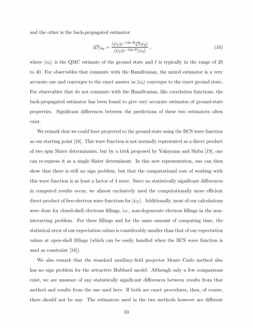
and the other is the back-propagated estimator

〈O〉bp =〈ψT |e−ℓ∆τHO|ψ0〉〈ψT |e−ℓ∆τH |ψ0〉

, (16)

where |ψ0〉 is the QMC estimate of the ground state and ℓ is typically in the range of 20

to 40. For observables that commute with the Hamiltonian, the mixed estimator is a very

accurate one and converges to the exact answer as |ψ0〉 converges to the exact ground state.

For observables that do not commute with the Hamiltonian, like correlation functions, the

back-propagated estimator has been found to give very accurate estimates of ground-state

properties. Significant differences between the predictions of these two estimators often

exist.

We remark that we could have projected to the ground state using the BCS wave function

as our starting point [18]. This wave function is not normally represented as a direct product

of two spin Slater determinants, but by a trick proposed by Yokayama and Shiba [19], one

can re-express it as a single Slater determinant. In this new representation, one can then

show that there is still no sign problem, but that the computational cost of working with

this wave function is at least a factor of 4 more. Since no statistically significant differences

in computed results occur, we almost exclusively used the computationally more efficient

direct product of free-electron wave functions for |ψT 〉. Additionally, most of our calculations

were done for closed-shell electrons fillings, i.e., non-degenerate electron fillings in the non-

interacting problem. For these fillings and for the same amount of computing time, the

statistical error of our expectation values is considerably smaller than that of our expectation

values at open-shell fillings (which can be easily handled when the BCS wave function is

used as constraint [18]).

We also remark that the standard auxiliary-field projector Monte Carlo method also

has no sign problem for the attractive Hubbard model. Although only a few comparisons

exist, we are unaware of any statistically significant differences between results from that

method and results from the one used here. If both are exact procedures, then, of course,

there should not be any. The estimators used in the two methods however are different

10

as the auxiliary-field projector method uses a different back-propagation estimator for all

observables.

IV. RESULTS

In sequence we will now report and discuss results for the attractive Hubbard model on

chains, squares, and ladders. In each case we will comment on the predictions of the BCS

approximation relative to the predictions of the QMC simulations. For chains we will also

comment on supportive calculations we performed using the density matrix renormalization

group (DMRG) method [20]. Included in a separate subsection is a discussion on the specific

issue of dimensional cross-over.

Because the variances of our computed results are smaller for closed-shell fillings, we

only considered such fillings, and because the shell structure changes with lattice size, as we

changed lattice sizes, we could not maintain the electron densities 〈n〉 at a fixed value. For

the results reported here, we fixed the electron density as close as possible to the quarter-

filled value, that is, to a value of 1 electron per 2 lattice sites. The actual fillings for many of

the lattices studied are given in Table 1. In all cases we had equal numbers of up and down

spin electrons. In one-dimension we used 〈n〉 = 1/2+1/L which converges to quarter filling

as L is increased. We remark that the accuracy of our QMC calculations were benchmarked

against those of exact diagonalizations calculations of 4 × 4 lattices. The QMC results,

and in particular those computed by the back-propagation estimators, agreed well within

statistical error with those of the more precise method.

A. Chains

For both finite and infinite chain lengths one can obtain the energies of the attractive

Hubbard model from its Bethe ansatz solution [8]. Marsiglio and Tanaka [21,22], for ex-

ample, have made extensive comparisons of these energies with the predictions of the BCS

approximation. Additionally, by computing the Bethe ansatz energies for systems of Ne,

11

Ne − 1 and Ne + 1 electrons, they also calculated the pair binding energy by evaluating

∆Ne= (ENe−1 − 2ENe

+ ENe+1)/2, which in the BCS approximation is the gap ∆ [23].

The energy is the least accurate at intermediate coupling strengths at half-filling, where the

disagreement however is only a few per cent, and becomes exact in the weak and strong

coupling limits at low electron density. In general, the pair binding energy is poorly repro-

duced, with the disagreement being the least in the dilute electron density limit. Typically,

the BCS wave function overestimates the binding energy. For finite-size systems they also

found significant shell effects in the energy as a function of electron density or as a function of

chain length in the weak coupling regime. They did not investigate the pairing correlations.

Exact analysis of the Bethe ansatz solution by Kawakami and Yang [9] showed that in

the thermodynamic limit the on-site s-wave pairing correlation function Ps(R) behaves like

Ps(R) = 〈∆†s(R)∆s(0)〉 ∼ 1

Rβ(17)

at large separations R between the pairs. The non-universal exponent β is a function of

both U/t and the electron filling. (Kawakami and Yang provide a graph giving β for a

selection of values of U/t for all fillings between 0 and 1.) Because the BCS approximation

always predicts ODLRO, its predictions for the behavior of pairing correlation functions is

qualitatively incorrect.

We computed the on-site s-wave pairing function in several different ways. In the QMC

simulations, we used periodic boundary conditions, took

∆s(i) = ci,↓ci,↑ , (18)

and then calculated

Ps(R) =1

L

∑

i

〈∆†s(i+R)∆s(i)〉 (19)

for each possible value of R by using the back-propagation estimator. In the DMRG cal-

culation, we used open boundary conditions and computed Ps(R) in two different ways. In

the first way we computed

12

Ps(R) = 〈∆†s(iR +R)∆s(iR)〉 (20)

for each value of R relative to some site iR, which depends on R, chosen to place the pairs as

close to the center of the chain as possible. In other words, to avoid edge effects, for a given

value of R, we used the sites closest to the center. At the large values of R, the resulting

estimate displayed rapid fluctuations that made comparisons with the QMC and Bethe

ansatz predictions difficult. We found we could smooth out the fluctuations by computing

Ps(R) from [24]

Ps(R) =1

Np(R)

Np(R)∑

i=1

〈∆†s(R)∆s(0)〉i . (21)

Here we sum over all possible pairs of lattice sites separated by the same displacement R

and divide this sum by the number Np(R) of such pairs of sites, which is a function of R.

At large values of R, this function was much smoother. More importantly, it compared very

well with the QMC results.

In Figs. 1 and 2 we show samples of our results for U/t = 2. In Fig. 1, we superimpose

several calculations of Ps(R) for different chain lengths L to illustrate that increasing the

chain length did not change the pairing correlations at short and intermediate distances. It

simply increased the range in distance over which we correctly captured these correlations.

We fitted the large distance behavior of the correlation functions to the inverse power-

law function (17) and found exponents β consistent with the Bethe ansatz prediction. For

example, from Kawakami and Yang’s graph, we estimated β = 0.80(2). Our fit for the chain

of L = 66, shown in the inset to Fig. 1, predicted β = 0.79(3). Exponents for other fits are

given in Table 1. For long enough chains we obtained close agreement between the value of β

obtained by fitting and the value obtained from Kawakami and Yang’s graph. In performing

the fit we eliminated the short-range behavior and the up-turn in the correlations at large

distances. This up-turn is a finite-size effect caused by periodic boundary conditions.

A comparison of our QMC results with those from BCS and DMRG calculations are

shown in Fig. 2a. Clearly the predictions from the two quite different numerical methods

13

agree, provided we average the DMRG results as discussed above. For purposes of compari-

son, we also show the prediction of the BCS approximation. It is qualitatively different from

what is required from the exact solution. Fig. 2b shows the difference in the DMRG results

when computed for the two different ways of averaging, that is, when computed from (20)

and (21).

In short, both the DMRG and QMC predictions agree well with each other and with

the exact prediction of the Bethe ansatz solution for the asymptotic form of the pairing

correlation function at large distances. As expected, the BCS approximation is qualitatively

incorrect for this same function.

B. Squares

In two dimensions, an exact analytic solution for the Hubbard model does not exist.

Within statistical error, the QMC approach however provides an exact numerical solution.

In this subsection we are principally concerned with comparing predictions of the BCS

approximation with those of the exact QMC simulations.

In Fig. 3, we show the QMC and BCS Ps(R) as a function of the distance R for an 8× 8

lattice with U/t = 1, 2, and 4. The curves show the same behavior: The correlations rapidly

drop in magnitude over a distance of a few lattice spacings and then stay constant over the

remainder of the distances. The constant behavior at these larger distances is a signature of

ODLRO, if the distances extended to infinity. As the results go from U/t = 1 to U/t = 4,

the agreement between the QMC simulations and the BCS approximation for lattices of

the same size progressively worsens. Beyond U/t = 1, the quantitative agreement is poor.

One also sees that as U/t increases, the magnitude of the pairing correlations increases. At

large distances, if there is ODLRO, the pairing correlation function becomes asymptotically

equal to 〈∆s〉2. In the BCS approximation, U times 〈∆s〉 equals the energy gap, and this

gap becomes exponentially small when decreasing U/t to 0 and proportional to U/t when

increasing U/t to infinity. However, as noted before, the attractive Hubbard model is gapless

14

if it has on-site s-wave ODLRO [15].

While we computed several cases for U/t = 8, the statistical error was considerably

larger and hence we do not show these results. However in all cases computed, as we

increased the magnitude of U/t, we never saw the QMC and BCS results approach each

other. In fact, as we increased U/t beyond 1, their difference continuously increased. In

Fig. 4, we show both the on-site and extended s-wave pairing correlation functions as a

function of distance for U/t = 4 and a 14 × 14 lattice. In the inset we eliminated the short

distance part to emphasize the flat large distance behavior for both correlation functions.

By averaging over this flat behavior we estimated both 〈∆s∗〉2 and 〈∆s〉2 and attempted to

verify that the ratio is proportional to (−U − 2µ/t)2 as stated by Eq. (5). Because most of

our simulations were done for fixed particle numbers and closed-shell fillings, the estimation

of µ was difficult. Using a variation of the present method [18] that allows an estimation

of µ, we found µ = −2.77 for a 8 × 8 system with U/t = 4. Using this same value of µ

for the 14 × 14 system with U/t = 4 yields (−U − 2µ/t)2 = 2.37 which compares very well

to the value of 2.40(3) estimated from the figures. We also observed that the ratio of the

expectation values for the on-site and extended s-wave order parameters was exactly obeyed

in the BCS approximation, provided the BCS value of µ was used. In Appendix A we present

the analysis leading to this result. We also observed that the long range values of both the

on-site and extended s-wave pairing correlation functions do not vary monotonically with

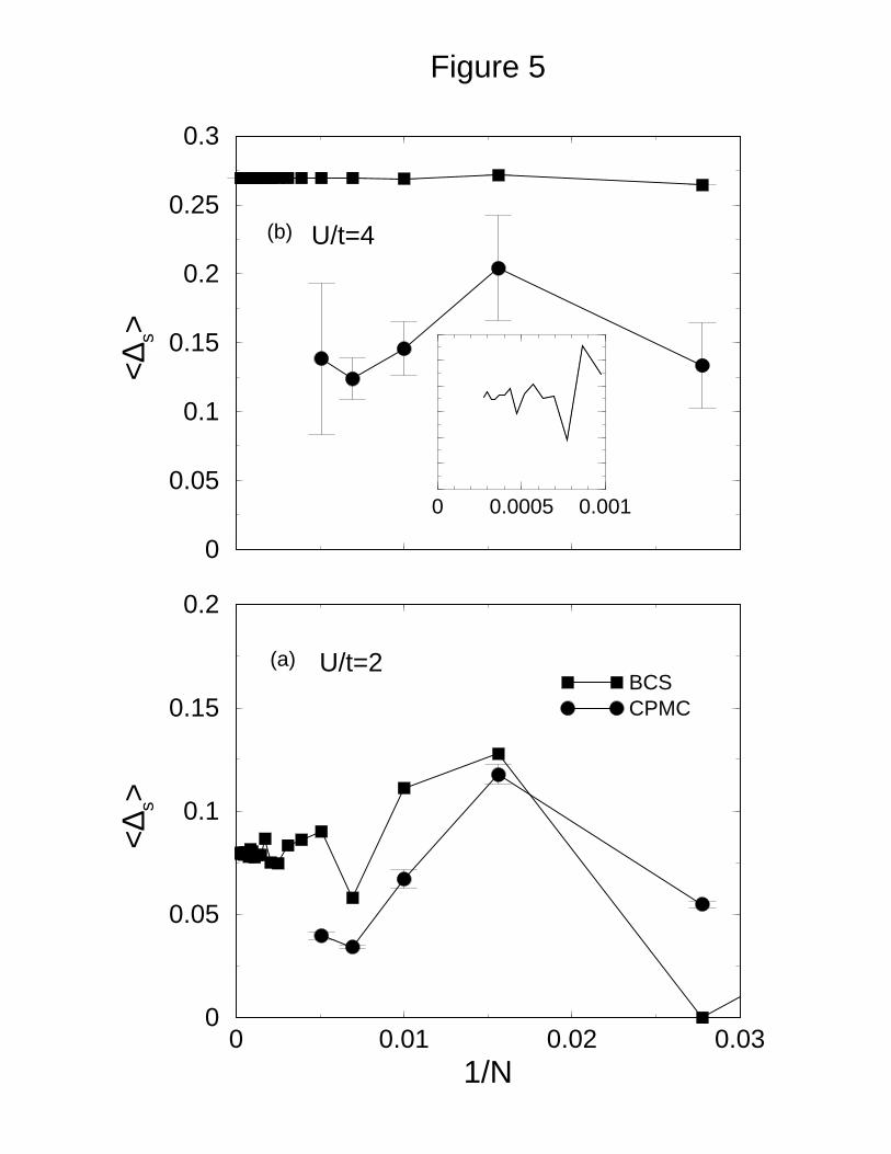
lattice size. We illustrate this in Fig. 5 by plotting both the QMC and BCS results for 〈∆s〉

as a function of the reciprocal of the number N of lattice sites for both U/t = 2 and U/t = 4.

Within the BCS approximation one can compute 〈∆s〉 directly for any lattice size.

In Fig. 5a, the BCS result for U/t = 2 clearly does not converge to the thermodynamic

limit monotonically. The same lack of monotonicity is apparent in the variation of the QMC

results. Because the BCS and QMC results are quantitatively different, we see no reason why

the QMC results might extrapolate to the BCS result, but more importantly we do not see

how to extract an accurate value of 〈∆s〉 in the thermodynamic limit, although it is clear from

our results that it is a finite value and therefore there will be ODLRO in the thermodynamic

15

limit. In Fig. 5b, we show similar curves for U/t = 4. The apparent monotonicity of the

BCS result is deceptive, as illustrated in the inset to this figure. The more important point

is that the BCS results approach the thermodynamic limit for U/t = 4 case more rapidly

than they did for the U/t = 2 case. This trend is very general and suggests that the QMC

results for larger values of U/t will also converge more rapidly to the thermodynamic limit.

Large interactions reduces fermion shell effects. Unfortunately both the necessarily large

values of U/t and lattice sizes appear inaccessible with our simulation method. For U/t = 1

we estimate that the BCS approximation has approached the thermodynamic limit within

a per cent for lattices of the order of 60 × 60; for U/t = 8 our estimate is for lattices of the

order of 10 × 10. As mentioned before, at U/t = 8 the QMC results have large statistical

errors in the back-propagation estimate of the pairing correlation functions.

In summary, for on-site s-wave pairing correlations, we find that the QMC and BCS

results agree in the weak coupling limit. While the QMC results show a necessary signature

of ODLRO, we were unable to extrapolate accurately our results for the order parameter to

the thermodynamic limit.

C. Ladders

An alternate way to reach the two-dimensional thermodynamic limit is extrapolating

from a ladder structure of fixed, but long, length L by letting the number of legs M become

large. Here we report our results from the use of this strategy.

We built up the ladder structures by coupling 1, 2, and 3 additional chains to the one-

dimensional chain and making the interchain and intrachain hopping amplitudes equal. We

used periodic boundary conditions in the x (long) direction and open boundary conditions

in the y (short) direction. We call this a cylindrical boundary condition. For the on-site

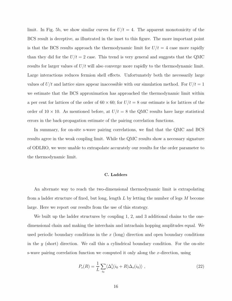
s-wave pairing correlation function we computed it only along the x-direction, using

Ps(R) =1

L

∑

i0

〈∆†s(i0 +R)∆s(i0)〉 , (22)

16

where the i0 are lattice sites along one of the central legs of the ladder. For a 3-legged ladder,

the sites in the x-direction are on the central leg. For a 2-legged ladder, we used just one

of the legs. By symmetry, the chain-directed pairing correlations are the same on each leg.

For a 4-legged ladder, we just used one of the two central legs.

To provide some perspective, we first present in Fig. 6 plots of the energy as a function of

system size. In particular, in Fig. 6a is the energy per site for a U/t = 2 chain as a function of

the reciprocal of chain length. The variation with length is smooth and monotonic. Linearly

extrapolating this data to infinite length, we find an energy per site of −1.079(1) which is

within statistical error of the Bethe ansatz value of -1.079 [?]. In Fig. 6b is the energy per

site as a function of the reciprocal of the number of legs M for a ladder of length L = 50.

The variation is smooth and monotonic and extrapolates to a value of -1.49(1), a value

similar to the one we found from the QMC simulations for the two-dimensional lattice. This

is not surprising since, although the extrapolating function can be shape-dependent, the

energy is a bulk quantity, i.e., independent of the way one performs the thermodynamic

limit. These two-dimensional QMC results are shown in Fig. 6c for the non-interacting

case and for the interacting case computed by both the BCS approximation and the QMC

method. The variation is neither smooth or monotonic. Additionally it tracks the non-

interacting problem. This tracking supports a claim that the non-monotonic variations are

caused by shell effects that are obvious and inherent to non-interacting fermion problems.

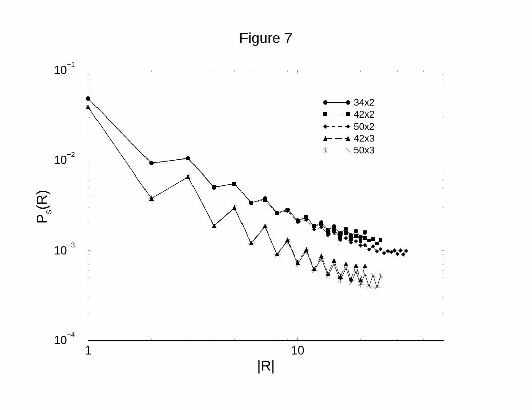
For the s-wave pairing correlation function, a typical result is shown in Fig. 7. Similar to the

one-dimensional case (Fig. 1), the curves for increasing ladder length lie on top of those for

shorter lengths. In contrast to the one-dimensional case, however, distinct oscillations exist

but the overall trend is a decrease in magnitude with increasing distance. For the 2 and

3-legged cases we fitted the top and bottom envelopes of the oscillations to the power law

decay (17) and found the two decays rates to be close but not the same. These exponents

were also close to the one-dimensional value (Table 1). An important observation is the

overall magnitude of the pairing correlations at first decreasing below the one-dimensional

value and then, as we built-up the ladder structure to 4-legs, increasing above the 3-leg

17

value. For a ladder of length L = 50, the variation of the s-wave pairing correlation function

with the number of legs is shown in Fig. 8a. A typical fit to determine the exponents of

decay is shown in the inset. Other fitted values are given in Table 1. We note that while the

exponent does not change much from the one-dimensional case to the 2 and 3 legged ladder

cases, it does decrease significantly when the 4th leg is added.

We remark that using the BCS approximation, we computed the pairing correlations for

the same system sizes but with periodic boundary conditions in both directions. While this

approximation always showed ODLRO, its order parameter 〈∆s〉 showed the same trend as

we obtained from the QMC simulations: In going from 1 to 3-legs, the value of the order

parameter at first monotonically decreased but then increased relative to the value of the

3-legged ladder when the fourth leg was added.

D. Dimensional Cross-Over

What type of variation with ladder width should one expect? Recently finite temperature

QMC studies of quantum spin ladders found non-monotonic variations with the number of

legs [26–28]. More specifically, the dynamic susceptibilities of even-legged ladders had spin

gaps while those of odd-legged ones did not. The size of the spin gap rapidly decreased

with increasing number of legs and is a result of topological considerations similar to those

associated with Haldane gaps in one-dimensional chains. For fixed, but large, ladder lengths

the uniform susceptibility vanished as the temperature was lowered and then the number of

legs extrapolated to infinity. This susceptibility however extrapolated to a non-zero value if

at low temperatures the two-dimensional results were extrapolated to the thermodynamic

limit. Proper extrapolation of this system to the thermodynamic limit appears to be an

unsolved problem. The theoretical and experimental situation has received several recent

reviews [29,30].

Turning from quantum critical phenomena to the finite temperature critical behavior and

using the two-dimensional Ising model as an example, we can easily study the dimensional

18

cross-over from one to two dimensions and the extrapolation of two-dimensional results to

the thermodynamic limit. We in fact were able to derive exact results, given in Appendix B,

for the spin-spin correlations for such finite systems. Using these exact results we computed

the spin-spin correlation function as a function of distance along the central leg for several

illustrative cases. For the calculations presented in Fig. 9, we fixed the reciprocal of the

critical temperature at its bulk value of 12ln(

√2 + 1) ≈ 0.44, chose a long ladder length of

200 lattice sites, and computed the correlation function for various number of legs. What

is seen is a smooth but gradual transition from the expected exponential decay in one

dimension to the expected power-law decay in two dimensions. Proper extrapolation of this

system to the thermodynamic limit is an exactly solvable problem [31].

What is the relevance of the studies on these spins systems to our QMC simulations?

From studies in finite-temperature critical phenomena, one suggestion on the controlling

physics of a dimensional cross-over is the type of behavior depending on the relative size of

the dominant correlation length to the width of the system [32]. This insight was developed

in part from analytic studies of D-dimensional ladders sized ∞ × ∞ × · · · × ∞ ×M and

scaling its behavior to a (D + 1)-dimensional systems by letting M → ∞. In going from

one to two dimensions, as long as one is on the critical surface, one expects the long range

behavior to be one-dimensional-like if the correlation length is larger than the width and

two-dimensional-like if it is smaller. The various correlation functions we computed for

the Hubbard model, such as charge-charge, spin-spin, and pair-pair, rapidly decayed over

a distance of several lattice spacings from their on-site value, suggesting our system sizes

were large enough so that if we were on the quantum critical surface, our physics would be

more two-dimensional-like than one-dimensional. We find that it appears to be the other

way around.

The picture so appropriate for finite-temperature critical phenomena established for clas-

sical systems might not be appropriate to our fermion simulations because the systems sizes

are too small and are dominated by shell effects, a phenomenon intrinsic to quantum fermion

systems. In Fig. 10, we plot the band-structure of the free-electron case for 1, 2, 3, and 4

19

legged ladders of infinite length with cylindrical boundary conditions. The horizontal line

represents the Fermi energy for an electron density of 1/2. For 1 leg, the one-dimensional

case, there is one-band. For 2-legs there are two bands but only the lower band is filled.

While the entire system is quarter-filled, the one-dimensional-like lower band is half-filled.

Not surprisingly then is the one-dimensional-like decay rate of the pairing correlations. For 3

and 4 legs there are 3 and 4 bands. More than one band is participating but the situation is

not yet two-dimensional-like. This simple band picture therefore provides some qualitative

basis for understanding our data. This understanding suggests, at least for the sizes of the

systems we were able to study, that the length scale interpretation of dimensional cross-over

is not yet applicable.

As still another way of looking at the finite-size effects we present Fig. 11 which displays

the allowable k-values for non-interacting 2 × 8, 4 × 8, and 8 × 8 lattices with periodic

boundary conditions. For quarter-filling the black dots are occupied by an up and down

spin electron, the gray dots are the degenerate states in the open shell, and the open dots

are unoccupied. Clearly for 2×8 the occupied k-states are those of a one-dimensional lattice.

This situation changes little in the 4 × 8 case, but has significantly changed for the 8 × 8

case. Obviously in the non-interacting case the dimensional cross-over requires more than

just a few legs.

While finite-size shell effects may explain the non-monotonic variations we observed, we

emphasize that the nature of the variation of the pairing correlation to cross-over from one

to two dimensions was not revealed in our simulations. We note than even in the apparently

simpler classical Ising model the cross-over was slow.

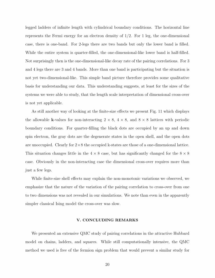
V. CONCLUDING REMARKS

We presented an extensive QMC study of pairing correlations in the attractive Hubbard

model on chains, ladders, and squares. While still computationally intensive, the QMC

method we used is free of the fermion sign problem that would prevent a similar study for

20

the repulsive Hubbard model. By using a method free of the sign problem, we obtained

results that apart from statistical errors are exact. In several instances we re-enforced this

exactness by reproducing behavior predicted by exact analysis. For example, for chains

we got the correct asymptotic behavior of the on-site s-wave pairing correlation function.

For squares, we verified Zhang’s relation between the on-site and extended s-wave order

parameters. Several of our ambitious computational objectives were, however, limited by

the size of the systems and interactions strengths we could afford to simulate. Still, we

demonstrated the validity of the BCS approximation in the weak coupling limit for a short-

ranged interaction and highlighted several important unresolved issues about finite-scaling

of fermion systems.

To a degree, the finite-size and shell effects exhibited by our results are expected. Such

effects have been reported before [33,17,34]. The difficulty we had in trying to extrapolate

beyond them to the thermodynamic limit was unexpected. Part of the surprise follows from

QMC simulations of the attractive Hubbard model always having an easier time revealing a

signature of ODLRO than simulations of the repulsive model. Years ago, in fact, ODLRO

was reported for the attractive model via a QMC simulation [7]. How we attempted to

establish ODLRO in this paper however differs from how it was attempted in that previous

work. There, the uniform susceptibility

χs =1

N

∑

R

Ps(R) (23)

was extrapolated to the thermodynamic limit. While this is an appropriate quantity for very

large system sizes, it is now appreciated that for small systems, it is often dominated by the

values of Ps(R) near R = 0. These values merely measure local spin and charge fluctuations.

Directly examining the long-distance behavior of Ps(R), as done here, is a more appropriate

procedure.

Re-examining Fig. 3 of Ref. [7], we notice the following: The values of χs for small lattices

were excluded from the extrapolation. The values for the larger lattice sizes fluctuated

about the fit by amounts larger than the statistical error. We do not doubt that a proper

21

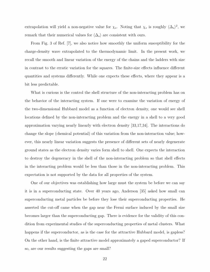
extrapolation will yield a non-negative value for χs. Noting that χs is roughly 〈∆s〉2, we

remark that their numerical values for 〈∆s〉 are consistent with ours.

From Fig. 3 of Ref. [7], we also notice how smoothly the uniform susceptibility for the

charge-density wave extrapolated to the thermodynamic limit. In the present work, we

recall the smooth and linear variation of the energy of the chains and the ladders with size

in contrast to the erratic variation for the squares. The finite-size effects influence different

quantities and systems differently. While one expects these effects, where they appear is a

bit less predictable.

What is curious is the control the shell structure of the non-interacting problem has on

the behavior of the interacting system. If one were to examine the variation of energy of

the two-dimensional Hubbard model as a function of electron density, one would see shell

locations defined by the non-interacting problem and the energy in a shell to a very good

approximation varying nearly linearly with electron density [33,17,34]. The interactions do

change the slope (chemical potential) of this variation from the non-interaction value; how-

ever, this nearly linear variation suggests the presence of different sets of nearly degenerate

ground states as the electron density varies form shell to shell. One expects the interaction

to destroy the degeneracy in the shell of the non-interacting problem so that shell effects

in the interacting problem would be less than those in the non-interacting problem. This

expectation is not supported by the data for all properties of the system.

One of our objectives was establishing how large must the system be before we can say

it is in a superconducting state. Over 40 years ago, Anderson [35] asked how small can

superconducting metal particles be before they lose their superconducting properties. He

asserted the cut-off came when the gap near the Fermi surface induced by the small size

becomes larger than the superconducting gap. There is evidence for the validity of this con-

dition from experimental studies of the superconducting properties of metal clusters. What

happens if the superconductor, as is the case for the attractive Hubbard model, is gapless?

On the other hand, is the finite attractive model approximately a gaped superconductor? If

so, are our results suggesting the gaps are small?

22

What are the implications of our results for establishing ODLRO in the repulsive Hub-

bard model? The behavior of the repulsive model is quite different than the behavior of

the attractive model. For any size of the repulsive model studied so far, the difficulty is

finding pairing correlations larger than those of the non-interacting problem [36]. In the

thermodynamic limit the non-interacting problem is not superconducting so whatever long-

range correlations seen for small systems must suppressed in larger systems. In the repulsive

model, d-wave pairing correlations are stronger than the s-wave pairing correlations, and as

the system size was increased, the magnitude of the d-wave pairing correlations systemat-

ically vanished [36,18]. What our results underscore is the care needed to establish that

any observed enhancement of the d-wave pairing correlations is an intrinsic effect and not a

finite-size effect.

We comment that all results reported here are for a single electron filling. All the

properties studied are a function of filling so at some other fillings, it might be easier to

extrapolate to the thermodynamic limit and it might be possible that the BCS approximation

remains in quantitative agreement with the QMC simulations for larger values of U/t. In

fact, a few simulations for 〈n〉 = 0.875 for 4×4, 6×6, and 8×8 lattices showed only a weak

variation in the results for the pairing correlation function.

While we simulated systems at other fillings, these simulations were neither extensive or

systematic enough to establish conclusions other than those now being reported. Also in

building up the ladder to a square, we took quite long ladders which restricted the number

of legs we could afford to simulate. We made the ladder long so the pairing properties

of the chain clearly matched the predications of the Bethe ansatz solution of the infinite

chain. It might be possible to see the dimensional cross-over and extrapolate to the bulk

two-dimensional properties from shorter but wider ladders. For example, in Fig. 12 we show

Ps(R) for a 16×8 ladder at U/t = 2. The flatness suggests possible ODLRO consistent with

the results for the square geometry.

What are possible ways of handling the finite-size effects? One way, suggested by Bor-

mann et al. [37], is adjusting U/t for different system sizes so the BCS approximation for

23

Ps(R) closely approximates the one from the QMC simulations, subtracting this approxima-

tion from the QMC results, and then extrapolating the differences to the thermodynamic

limit. After this, then one would add to this result the BCS results for an infinite system.

(Actually, Bormann et al. did this for χs.) We did not try this procedure because it is related

to another one, scaling the vertex correction. Here, one replaces averages like 〈c†c†cc〉 with

〈c†c†cc〉 − 〈c†c〉〈c†c〉 and studies the size dependence of the remainder which is called the

vertex contribution [38]. In spot checks, we found no significantly different scaling behavior.

Another way to remove finite-size effects is the phase averaging method suggested for

exact diagonalization studies by Loh et al. [39] and recently adopted for QMC simulations

by Ceperley [40]. In this procedure, one replaces the hopping amplitude t at the boundary

by teiφ and obtains various physical quantities as a function of φ. Then one averages these

quantities over φ. Loh et al. give a justification and demonstration of the method. In exact

diagonalization studies, one just does a sequence of diagonalizations for different values of φ.

In a Monte Carlo method for computational efficiency it is necessary to treat φ as another

stochastic parameter and then let the random walk do the averaging. To do this one needs

to change the QMC method. In the applications contemplated by Ceperley, this means

changing form the fixed-node to the fixed-phase method [41]. In our case we are developing

an analog of the the fixed-phase method, called the constrained phase [42]. Hopefully we

will be able to report results from this method soon.

Finally, we would like to emphasize that this paper has been dealing exclusively with

systems having a homogeneous long-range phase coherence. There is a rapidly growing body

of experimental evidence suggesting that inhomogeneously textured (intrinsically nanoscale)

phases characterize the quantum state of high temperature superconductors. It is possible

that the superfluid density characterizing that state is inhomogeneous. We believe that

an extension of the attractive Hubbard model including inhomogeneous terms (mimicking

stripes) could be the starting point to understand the fundamental problem of inhomoge-

neous superfluids.

24

ACKNOWLEDGMENTS

We thank D. Abrahams, G. A. Baker, Jr., E. Dagotto, E. Domany, J. Eroles, J. L.

Lebowitz, D. Pines, D. J. Scalapino, and S. A. Trugman for helpful discussions and sug-

gestions. We also thank N. Kawakami, A. Moreo, and F. Marsiglio for providing us with

some data, and T. Momoi for some comments and for sending us copies of his works. This

work was supported by the U. S. Department of Energy which also provided computational

support at NERSC.

25

APPENDIX A: BCS EQUATIONS

In this Appendix we present the key equations used in our BCS calculations. Some are

well documented while others are not. For completeness and convenience we give them here.

First to establish notation, we take (3) as the Hamiltonian for a lattice of N sites and

rewrite it in k-space

H =∑

k,σ

ǫknk,σ − U

2N

∑

k,k′,q

σ=↑,↓

c†k,σc†k′,−σck′+q,−σck−q,σ , (A1)

using ǫk = −2t(cos kx + cos ky) and assuming periodic boundary conditions in all spatial

directions. We used the BCS wave function (2) with k-independent relative phase ϕ

|BCS(ϕ)〉 =∏

k

(uk + vkeiϕc†k,↑c

†−k,↓)|0〉 . (A2)

The effective mean-field Hamiltonian, resulting from the neglect of pairing fluctuation, is

HBCS =∑

k,σ

ξknk,σ − ∆∑

k

(c†k,↑c†−k,↓ + c−k,↓ck,↑) +

UN2e

4N, (A3)

where Ne = 〈Ne〉 = 2∑

k v2k is the average number of electrons and ∆ = U

N

∑

k〈c†k,↑c†−k,↓〉 =

UN

∑

k ukvk is the BCS gap, and ξk = ǫk − µ − UNe/2N . The value of the energy was

calculated from

〈HBCS〉 = 〈H − µNe〉 = 2∑

k

(ǫk − µ)v2k −

U

N

[

(

Ne

2

)2

+(

N∆

U

)2]

(A4)

and µ and ∆ were determined by self-consistently solving

∑

k

[

1 − ξkEk

]

= Ne , (A5)

U

2N

∑

k

E−1k = 1 , (A6)

where Ek =√

ξ2k + ∆2. With these values of µ and ∆ we determined uk, vk from

2ukvk =∆

Ek

, (A7)

u2k − v2

k =ξkEk

. (A8)

26

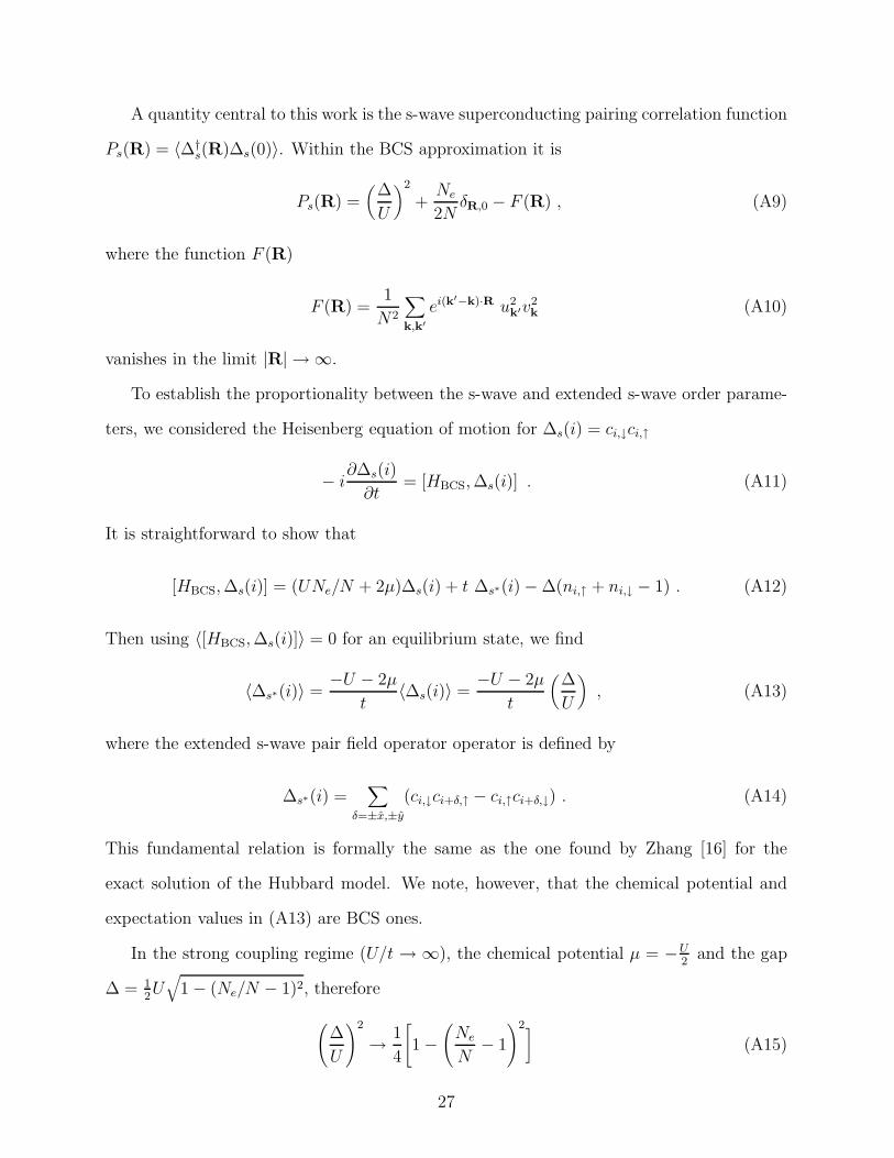
A quantity central to this work is the s-wave superconducting pairing correlation function

Ps(R) = 〈∆†s(R)∆s(0)〉. Within the BCS approximation it is

Ps(R) =(

∆

U

)2

+Ne

2NδR,0 − F (R) , (A9)

where the function F (R)

F (R) =1

N2

∑

k,k′

ei(k′−k)·R u2k′v2

k (A10)

vanishes in the limit |R| → ∞.

To establish the proportionality between the s-wave and extended s-wave order parame-

ters, we considered the Heisenberg equation of motion for ∆s(i) = ci,↓ci,↑

− i∂∆s(i)

∂t= [HBCS,∆s(i)] . (A11)

It is straightforward to show that

[HBCS,∆s(i)] = (UNe/N + 2µ)∆s(i) + t ∆s∗(i) − ∆(ni,↑ + ni,↓ − 1) . (A12)

Then using 〈[HBCS,∆s(i)]〉 = 0 for an equilibrium state, we find

〈∆s∗(i)〉 =−U − 2µ

t〈∆s(i)〉 =

−U − 2µ

t

(

∆

U

)

, (A13)

where the extended s-wave pair field operator operator is defined by

∆s∗(i) =∑

δ=±x,±y

(ci,↓ci+δ,↑ − ci,↑ci+δ,↓) . (A14)

This fundamental relation is formally the same as the one found by Zhang [16] for the

exact solution of the Hubbard model. We note, however, that the chemical potential and

expectation values in (A13) are BCS ones.

In the strong coupling regime (U/t → ∞), the chemical potential µ = −U2

and the gap

∆ = 12U√

1 − (Ne/N − 1)2, therefore

(

∆

U

)2

→ 1

4

[

1 −(

Ne

N− 1

)2]

(A15)

27

and in that limit 〈∆s∗〉 = 0 and

|BCS(0)〉 =∏

i

[

√

1 − Ne

2N+

√

Ne

2Nc†i↑c

†i↓

]

|0〉 . (A16)

While not used in any of the results reported here, another relation we derived and

found useful in other contexts is a simple way to project from the BCS wave function the

component corresponding to a fixed number of particles. Although in the thermodynamic

limit one can ignore exact particle number conservation, for a finite system, one often cannot

because the particle number fluctuations 〈N2e 〉 − 〈Ne〉2 = 4

∑

k u2kv

2k, inherent in the BCS

wave function, can be large. To project out the Ne-particle component, one uses

|ΨNe〉 =

1

2π

∫ 2π

0dϕ e−iϕNe/2 |BCS(ϕ)〉 . (A17)

By directly doing the implied integration over the phase, one can show that the amplitude

〈BCS(0)|ΨNe〉 = 〈ΨNe

|ΨNe〉 = ωNe

where∑

NeωNe

= 1. To find ωNeone can use the recursion

relation

Np ωNp= ωNp−1

∑

k

(

vkuk

)2

+Np−1∑

j=1

(−1)j ωNp−(j+1)

∑

k

(

vkuk

)2(j+1)

, (A18)

where Np = Ne/2 is the number of pairs. We also note that |BCS(0)〉 =∑

Ne|ΨNe

〉.

28

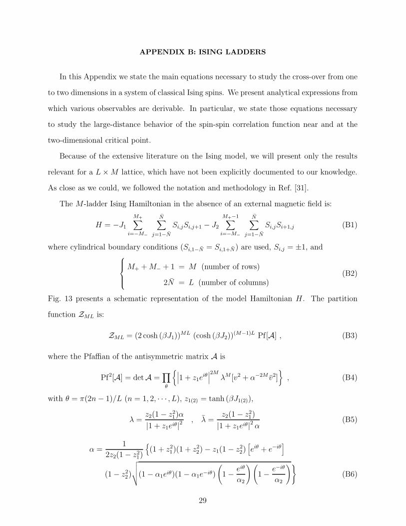
APPENDIX B: ISING LADDERS

In this Appendix we state the main equations necessary to study the cross-over from one

to two dimensions in a system of classical Ising spins. We present analytical expressions from

which various observables are derivable. In particular, we state those equations necessary

to study the large-distance behavior of the spin-spin correlation function near and at the

two-dimensional critical point.

Because of the extensive literature on the Ising model, we will present only the results

relevant for a L×M lattice, which have not been explicitly documented to our knowledge.

As close as we could, we followed the notation and methodology in Ref. [31].

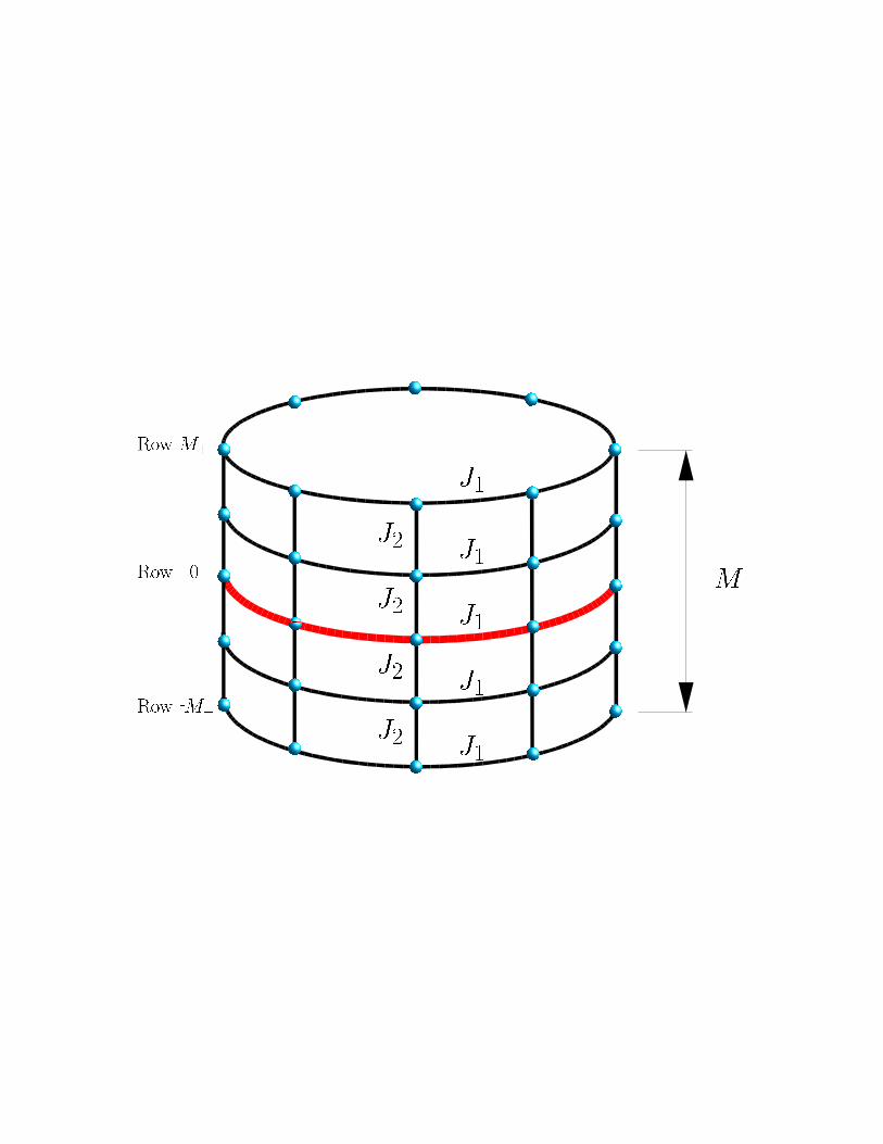
The M-ladder Ising Hamiltonian in the absence of an external magnetic field is:

H = −J1

M+∑

i=−M−

N∑

j=1−N

Si,jSi,j+1 − J2

M+−1∑

i=−M−

N∑

j=1−N

Si,jSi+1,j (B1)

where cylindrical boundary conditions (Si,1−N = Si,1+N) are used, Si,j = ±1, and

M+ +M− + 1 = M (number of rows)

2N = L (number of columns)(B2)

Fig. 13 presents a schematic representation of the model Hamiltonian H . The partition

function ZML is:

ZML = (2 cosh (βJ1))ML (cosh (βJ2))

(M−1)L Pf[A] , (B3)

where the Pfaffian of the antisymmetric matrix A is

Pf2[A] = detA =∏

θ

{

∣

∣

∣1 + z1eiθ∣

∣

∣

2MλM [v2 + α−2M v2]

}

, (B4)

with θ = π(2n− 1)/L (n = 1, 2, · · · , L), z1(2) = tanh (βJ1(2)),

λ =z2(1 − z2

1)α

|1 + z1eiθ|2, λ =

z2(1 − z21)

|1 + z1eiθ|2 α(B5)

α =1

2z2(1 − z21)

{

(1 + z21)(1 + z2

2) − z1(1 − z22)[

eiθ + e−iθ]

(1 − z22)

√

√

√

√(1 − α1eiθ)(1 − α1e−iθ)

(

1 − eiθ

α2

)(

1 − e−iθ

α2

)}

(B6)

29

α1 =z1(1 − |z2|)

1 + |z2|, α2 =

z−11 (1 − |z2|)

1 + |z2|(B7)

v2 =1

2

1 +z22 − (4z2

1 sin2 (θ) + (1 − z21)

2)/∣

∣

∣1 + z1eiθ∣

∣

∣

4

λ− λ

, v2 = 1 − v2 (B8)

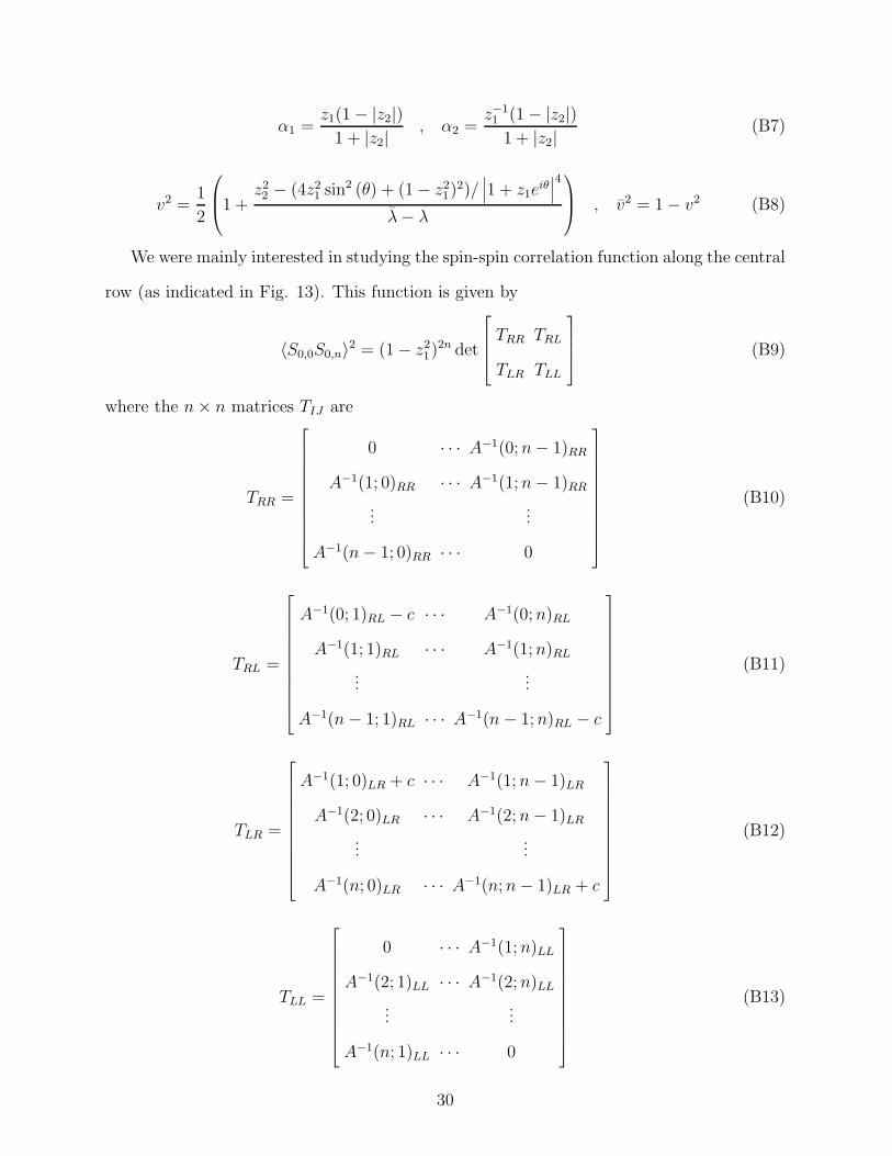
We were mainly interested in studying the spin-spin correlation function along the central

row (as indicated in Fig. 13). This function is given by

〈S0,0S0,n〉2 = (1 − z21)

2n det

TRR TRL

TLR TLL

(B9)

where the n× n matrices TIJ are

TRR =

0 · · · A−1(0;n− 1)RR

A−1(1; 0)RR · · · A−1(1;n− 1)RR

......

A−1(n− 1; 0)RR · · · 0

(B10)

TRL =

A−1(0; 1)RL − c · · · A−1(0;n)RL

A−1(1; 1)RL · · · A−1(1;n)RL

......

A−1(n− 1; 1)RL · · · A−1(n− 1;n)RL − c

(B11)

TLR =

A−1(1; 0)LR + c · · · A−1(1;n− 1)LR

A−1(2; 0)LR · · · A−1(2;n− 1)LR

......

A−1(n; 0)LR · · · A−1(n;n− 1)LR + c

(B12)

TLL =

0 · · · A−1(1;n)LL

A−1(2; 1)LL · · · A−1(2;n)LL

......

A−1(n; 1)LL · · · 0

(B13)

30

with c = (z−11 − z1)

−1, A−1(k; k′)IJ = 1L

∑

θ eiθ(k−k′) [B−1(θ)]IJ and

[

B−1(θ)]

RR= −

[

B−1(θ)]

LL=

1

|1 + z1eiθ|2{[

b−122

]

UU+[

b−122

]

DD

}

[

B−1(θ)]

RL= −

[

B−1(θ)]∗

LR=

−1

(1 + z1e−iθ)

{

1 − 1

(1 + z1e−iθ)

([

b−122

]

UU−[

b−122

]

DD−[

b−122

]

DU+[

b−122

]

UD

)

}

[

b−122

]

UU= i

vv

z2

(

1 − α−2(M−+1)) v2 + v2α−2M+

v2 + v2α−2M(B16)

[

b−122

]

DD= −ivv

z2

(

1 − α−2(M++1)) v2 + v2α−2M−

v2 + v2α−2M(B17)

[

b−122

]

UD=

(

v2 + v2α−2M+

) (

v2 + v2α−2M−

)

z2α (v2 + v2α−2M−)(B18)

[

b−122

]

DU= −

[

b−122

]

UD(B19)

If one were interested in the strip geometry (L→ ∞), then TRR = TLL = 0 and 〈S0,0S0,n〉

could be written in terms of an n× n Toeplitz determinant.

31

REFERENCES

[1] J. R. Schrieffer, Theory of Superconductivity (Addison-Wesley, New York, 1988).

[2] R.J. Bursill and C. J. Thompson, J. Phys. A: Math. Gen. 26, 769 (1991).

[3] S.-Q. Shen and Z.-M. Qiu, Phys. Rev. Lett. 71, 4238 (1993).

[4] M. Uehara, T. Nagata, J. Akimitsu, U. Takahashi, N. Mori, and K. Kinoshita, J. Phys.

Soc. Jpn. 65, 2764 (1996).

[5] P. Nozieres and S. Schmitt-Rink, J. Low Temp. Phys. 59, 195 (1985).

[6] See, for example, R. Micnas, J. Ranninger, and S. Robaszkiewicz, Rev. Mod. Phys. 62,

113 (1990).

[7] R.T. Scalettar, E. Y. Loh, J. E. Gubernatis, A. Moreo, S. R. White, D. J. Scalapino,

R. L. Sugar, and E. Dagotto. Phys. Rev. Lett. 62, 1407 (1989).

[8] E. H. Lieb and F. Y. Wu, Phys. Rev. Lett. 20, 1445 (1968).

[9] N. Kawakami and S.-K. Yang, Phys. Rev. B 44, 7844 (1991); J. Phys.: Condens. Matter

3, 5983 (1991).

[10] N. D. Mermin and H. Wagner, Phys. Rev. Lett. 17, 1133 (1966).

[11] E. H. Lieb, Phys. Rev. Lett. 62, 1202 (1989).

[12] A. Auerbach, Interacting Electrons and Quantum Magnetism (Springer-Verlag, Heidel-

berg, 1994).

[13] See, for example, R. R. P. Singh and R. T. Scalettar, Phys. Rev. Lett. 24, 3203 (1991).

[14] S.-Q. Shen and X. C. Xie, J. Phys.: Condens. Matter 8, 4805 (1996).

[15] T. Momoi, Phys. Lett. A 201, 261 (1995).

[16] S. Zhang, Phys. Rev. B 42, 1012 (1990); G.-S. Tian, J. Phys. A: Math. Gen. 30, 841

32

(1997).

[17] S. Zhang, J. Carlson, and J. E. Gubernatis, Phys. Rev. Lett. 74, 3652 (1995); Phys.

Rev. B 55, 7464 (1997); J. Carlson, J. E. Gubernatis, G. Ortiz, and Shiwei Zhang, Phys.

Rev. B 59, 12788 (1999).

[18] M. Guerrero, G. Ortiz, and J. E. Gubernatis, Phys. Rev. B 59, 1706 (1999).

[19] H. Yokoyama and H. Shiba, J. Phys. Soc. Jpn. 57, 2482 (1988).

[20] S. White, Phys. Rev. Lett. 69, 2863 (1992).

[21] F. Marsiglio, Phys. Rev. 55, 575 (1997); cond-mat/9902173.

[22] K. Tanaka and F. Marsiglio, cond-mat/9907183.

[23] In the ground state all the electrons are in spin-paired (singlet) bound states which

resemble Cooper pairs. These singlet pairs do not form bound states of pairs, that is,

these pairs move freely throughout the chain. See K.-J.-B. Lee and P. Schlottmann,

Phys. Rev. B 38, 11566 (1988).

[24] R. M. Noack, S. R. White, and D. J. Scalapino, Phys. Rev. Lett. 73, 882 (1994).

[25] F. Marsiglio, private communication.

[26] B. Frischmuth, B. Ammon, and M. Troyer, Phys. Rev. B 54, R3714 (1996).

[27] M. Greven, R. J. Birgeneau, and U.-J. Wiese, cond-mat/9605068.

[28] B. Ammon, M. Troyer, T. M. Rice, and N. Shibata, Phys. Rev. Lett. 82, 3855 (1999).

[29] E. Dagotto and T. M. Rice, Science 271, 618 (1996).

[30] T. M. Rice, Physica B 241-243, 5 (1998).

[31] B. M. McCoy and T. T. Wu, The two-dimensional Ising model (Harvard, Boston, 1973).

[32] J. G. Brankov, Introduction to finite-size scaling (Leuven Univ. Press, Leuven, 1996).

33

[33] N. Furukawa and M. Imada, J. Phys. Soc. Jpn. 61, 3331 (1992).

[34] M. Guerrero, J. E. Gubernatis, S. Zhang, Phys. Rev. B 57, 11980 (1998).

[35] P. A. Anderson, Phys. Rev. 112, 1900 (1958).

[36] S. Zhang, J. Carlson, and J. E. Gubernatis, Phys. Rev. Lett. 78, 4486 (1997).

[37] D. Bormann, T. Schneider, and M. Frick, Europhys. Lett. 14, 101 (1991); Z. Phys. B -

Condens. Matter 87, 1 (1992).

[38] S.R. White, D. J. Scalapino, R. L. Sugar, N. E. Bickers, and R. T. Scalettar, Phys. Rev.

B 39, 839 (1989).

[39] E. Y. Loh, Jr. and D. K. Campbell, Syn. Met. 27, A499-A508 (1988); E. Y. Loh, Jr.,

J. T. Gammel, and D. K. Campbell, Syn. Met. 57/2-3, 4437 (1993).

[40] D. M. Ceperley, private communication.

[41] G. Ortiz, D. M. Ceperley, and R. M. Martin, Phys. Rev. Lett. 71, 2777 (1993).

[42] G. Ortiz, J. Carlson, and J. E. Gubernatis, unpublished.

34

FIGURES

FIG. 1. The QMC on-site s-wave pairing correlation function Ps(R) as a function of the distance

|R| between pairs for a U/t = 2 chain of different lengths L. The inset shows the fit of results for

the L = 66 chain to the inverse power law form (17) using a value of β = 0.79.

FIG. 2. The on-site s-wave pairing correlation function Ps(|R|) as a function of the distance

|R| between pairs for a U/t = 2 chain of length L = 50. (a) Comparison of the results of the BCS

approximation with a QMC calculation that used (19) and a DMRG calculation that used (21).

(b) Comparison of the DMRG results for the two different ways, (20) and (21), of estimating the

correlation function.

FIG. 3. The QMC and BCS on-site s-wave pairing correlation function Ps(R) as a function of

the distance |R| between pairs for a 8 × 8 lattice and U/t = 1, U/t = 2, and U/t = 4.

FIG. 4. The QMC and BCS on-site and extended s-wave pairing correlation functions Ps(R)

as a function of the distance |R| between pairs for U/t = 2 and a 14 × 14 lattice. The inset shows

the large distance behavior of these same functions.

FIG. 5. The expectation value of the on-site s-wave order parameter 〈∆s〉 as a function of the

reciprocal of the size N of a square lattice. In both (a) and (b) the QMC results are compared to

those of the BCS approximation. In (a), U/t = 2. In (b), U/t = 4 and the inset shows the behavior

of the BCS predictions for small values of the reciprocal of the lattice size.

FIG. 6. The QMC energy per site E/N as a function of the reciprocal of the number N of

lattice sites for U/t = 2 systems. (a) Chains (N = L), (b) ladders (N = L × M), and (c) squares

(N = L × L). For squares the free-electron and BCS results are also shown. For chains and

ladders, the QMC curves smoothly and linearly extrapolate to the thermodynamic limit indicated

by star-burst symbol at 1/N = 0.

FIG. 7. The QMC on-site s-wave pairing correlation function Ps(R) as a function of the distance

|R| between pairs for U/t = 2, and 2 and 3-legged ladders of different lengths.

35

FIG. 8. The QMC on-site s-wave pairing correlation function Ps(R) as a function of the distance

|R| between pairs for a U/t = 2 ladder of length 50 as a function of the number of legs M . The

inset shows the long-range behavior of these correlations fitted to the inverse-power law function

(17)

FIG. 9. The spin-spin correlation function for an Ising ladder of length L =200 as a function

of the distance |R| between spins and of the number of legs M . The temperature is at the bulk

critical value, and the distance |R| is along a central leg in the x-direction. Cylindrical boundary

conditions were used.

FIG. 10. Band structure of the non-interacting problem on 1, 2, 3, and 4 legged ladders.

Cylindrical boundary conditions are applied. The long length L is infinite, and the horizontal line

represents the Fermi energy for a quarter-filled systems.

FIG. 11. The allowed k-states for a 2 × 8, 4 × 8, and 8 × 8 non-interacting problem with

periodic boundary conditions. Illustrated are which k-states are occupied for quarter-filling of an

equal number of up and down spin electrons. A black dot denotes double occupancy, an open circle

represents no occupancy, and a grey dot represents the degenerate state comprising the open shell.

FIG. 12. The QMC on-site s-wave pairing correlation function Ps(R) as a function of the

distance |R| between pairs for a rectangular quarter-filled U/t = 2 lattice of size 16 × 8.

FIG. 13. The cylindrical geometry used for the Ising model ladder with M legs.

36

TABLES

TABLE I. Summary of relevant parameters of the QMC simulations. Shown are the systems

sizes, the electron fillings 〈n〉, and the exponent β of the power law decay for U/t = 2. For 2 and

3-legged ladders, where there is a double entry, for example, 50 × 2, the top entry gives the value

of β for the top envelope, while the bottom entry is for the bottom envelope. In one dimension the

fillings are always 〈n〉 = 1/2 + 1/L

System Size 〈n〉 β

34 × 1 0.53 0.88(9)

42 × 1 0.52 0.82(6)

50 × 1 0.52 0.86(4)

66 × 1 0.52 0.79(3)

50 × 1 0.52 0.86(4)

50 × 2 0.50 1.07(3)

0.87(2)

50 × 3 0.51 1.32(4)

0.95(3)

50 × 4 0.51 0.68(5)

6 × 6 0.5

8 × 8 0.5

10 × 10 0.5

12 × 12 0.51

14 × 14 0.5

16 × 8 0.45

37

1 10|R|

10−2

10−1

100

Ps(

R)

Figure 1

L=66L=50L=42L=34

1 10 10010

−3

10−2

10−1

1 10 100|R|

10−4

10−3

10−2

10−1

Ps(

R)

Figure 2a

QMCBCSDMRG(average)

1 10 100|R|

10−4

10−3

10−2

10−1

Ps(

R)

Figure 2b

DMRG(center)DMRG(average)

(b)

0 2 4 6|R|

0

0.05

0.1

0.15

Ps(

R)

Figure 3

BCS, U/t=1QMC, U/t=1BCS, U/t=2QMC, U/t=2BCS, U/t=4QMC, U/t=4

0 2 4 6 8 10|R|

0

0.5

1

1.5

2

Pai

ring

Cor

rela

tions

Figure 4

QMC on−site s−waveQMC extended s−waveBCS on−site s−waveBCS extended s−wave

3 5 7 90

0.05

0.1

0.15

0 0.01 0.02 0.031/N

0

0.05

0.1

0.15

0.2

<∆ s>

BCSCPMC

0

0.05

0.1

0.15

0.2

0.25

0.3<

∆ s>

Figure 5

0 0.0005 0.001

(a)

(b) U/t=4

U/t=2

0 0.005 0.01 0.015 0.02 0.025 0.031/N

−1.2

−1.1

−1

−1.5

−1.4

−1.3

−1.2

−1.1

E/N

−1.5

−1.4

−1.3

Figure 6

BCSQMCFree Electron

(c)

(b)

(a)

1 10|R|

10−4

10−3

10−2

10−1

Ps(

R)

Figure 7

34x242x250x242x350x3

10|R|

10−4

10−3

10−2

10−1

Ps(

R)

Figure 8

M=1M=2 M=3 M=4

10

0 20 40 60 80 100|R|

0

0.2

0.4

0.6

0.8

1M=1 (chain)M=10M=50M=100M=200 (square)

0 10 20 30 4010

−15

10−10

10−5

100

<S

0,0S

0,R>

2 10 600.2

0.3

0.4

0.5

Figure 9

(a)

(b)

(c)

Figure 10

Figure 11

(a)

(b)

(c)

0 2 4 6 8 10|R|

0

0.05

0.1

0.15

Ps(

R)

Figure 12

J1J1J1J1J1

J2J2J2J2 M

Row M�-Row 0Row M+