Structure of urban movements: polycentric activity and entangled hierarchical flows

Camille Roth,1, 2 Soong Moon Kang,3 Michael Batty,4 and Marc Barthelemy1, 5

1CAMS (CNRS/EHESS) 54, boulevard RaspailF-75006 Paris, France

2Institut des Systemes Complexes de Paris-Ile de France (ISC-PIF), 57-59 rue Lhomond , F-75005 Paris, Franceroth@ehess.fr

3Department of Management Science and InnovationUniversity College London (UCL), Gower Street, London WC1E 6BT, UK

smkang@ucl.ac.uk4Centre for Advanced Spatial Analysis (CASA)

University College London (UCL), 1-19 Torrington Place, London WC1E 7HB, UKm.batty@ucl.ac.uk

5Institut de Physique TheoriqueCEA, IPhT, CNRS-URA 2306, F-91191 Gif-sur-Yvette, France

marc.barthelemy@cea.fr

(Dated: November 22, 2010)

The spatial arrangement of urban hubs and centers and how individuals interact with thesecenters is a crucial problem with many applications ranging from urban planning to epidemiology.We utilize here in an unprecedented manner the large scale, real-time ’Oyster’ card database ofindividual person movements in the London subway to reveal the structure and organization ofthe city. We show that patterns of intraurban movement are strongly heterogeneous in terms ofvolume, but not in terms of distance travelled, and that there is a polycentric structure composed oflarge flows organized around a limited number of activity centers. For smaller flows, the pattern ofconnections becomes richer and more complex and is not strictly hierarchical since it mixes differentlevels consisting of different orders of magnitude. This new understanding can shed light on theimpact of new urban projects on the evolution of the polycentric configuration of a city and thedense structure of its centers and it provides an initial approach to modeling flows in an urbansystem.

I. INTRODUCTION

The structure of a large city is probably one of themost complex spatial system that we can encounter. It ismade of a large number of diverse components connectedby different transportation and distribution networks. Inthis respect, the popular conception of a city with onecenter and pendular movements going in and out of thebusiness center is likely to be an audacious simplifica-tion of what actually happens. The most prominent andvisible effects of such spatial organization of economicactivity in large and densely populated urban areas arecharacterized by severe traffic congestion, uncontrolledurban sprawl of such cities and the strong possibilitiesof rapidly spreading viruses biologial and social throughthe dense underlying networks [1–3]. The mitigation ofthese undesirable effects depends intrinsically on our un-derstanding of urban structure [4], the spatial arrange-ment of urban hubs and centers, and how the individ-uals interact with these centers. The dominant modelof the industrial city is based on a monocentric struc-ture [6, 7], but contemporary cities are more complex,displaying patterns of polycentricity that require a cleartypology for their understanding [8]. One of the mostimportant features of an urban landscape is the cluster-ing of economic activity in many centers [5]: the ideaof the polycentric city in such terms can be traced backover one hundred years [9, 10], but so far no clear quan-titative definition has been proposed, apart from various

methods of density thresholding based, for example, onemployment [11]. In order to characterize polycentricity,we must investigate movement data such as person flowand mobile-phone usage [12] which offers the possibilityof analyzing quantitatively various features of the spa-tial organization associated with individual traffic move-ments. More precisely, in this study, we analyze data forthe London underground rail (‘tube’) system collectedfrom the Oyster card (an electronic ticketing system usedto record public transport passenger movements and faretariffs within Greater London) which enables us to inferthe statistical properties of individual movement patternsin a large urban setting.

II. RESULTS

World cities [13] are among those with the most com-plex spatial structure. The number, the diversity of com-ponents and their localization warns us intuitively thatthese megapoles are far from their original historical formwhich is invariably represented by a simple, monocentricstructure. In particular, the level of commercial and in-dustrial activity varies strongly from one area to another.Thus flows of individuals can be thought as good prox-ies for the activity of an area and to this end we firstchecked that the flows at different stations correlate pos-itively with other activity indicators such as counts ofemployees and the employee density. This shows that in-

arX

iv:1

001.

4915

v3 [

phys

ics.

soc-

ph]

19

Nov

201

0

2

dicators of a different nature and on different time scales,which are also widely regarded as measures of polycen-tricity in large cities, are also consistent with movementdata recorded over much shorter time scales.

The main results that we will discuss in this sectionare that (i) flows are generally of a local nature (ii) theyare also organized/aggregated around polycenters and(iii) the examination and decomposition of these flowslead to the description of entangled hierarchies, and (iv)hence one likely structure describing this large metropoli-tan area is based on polycentrism. This perspective thusdraws new insights from data that has become availablefrom electronic sources that have so far not been utilisedin analyzing the urban spatial structure and in this sense,are unprecedented in the field.

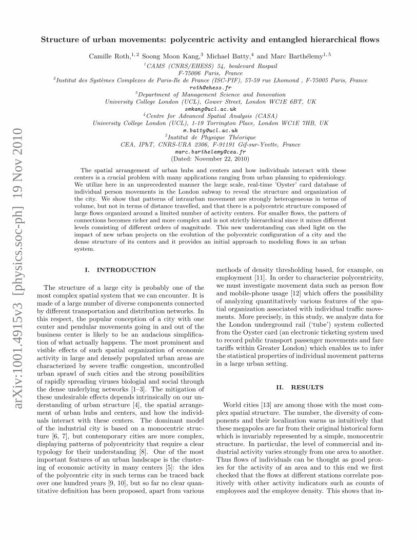
To get a preliminary grasp on the data, we observethat the flow distribution (normalized histogram of flowsof individuals) is fitted by a power law with exponent≈ 1.3 which indicates that there is strong heterogene-ity of individuals’ movements in this city (for this distri-bution, the ratio of the two first moments has a largevalue 〈w2〉/〈w〉2 ' 15.0, which confirms this strongheterogeneity)— see Figure 1. Broad distribution of flows

FIG. 1: Flow distribution. Loglog plot of the histogram ofthe number of trips between two stations of the tube system.The line is a power law fit with exponent ≈ 1.3.

have already been observed at the inter-urban level [14],but it is the first time that we observe this empiricallyat an intra-urban level showing that, in agreement withother studies (for Madrid [15] and for Portland, Oregon[1]), the movement patterns in large cities exhibit an het-erogeneous organization of flows.

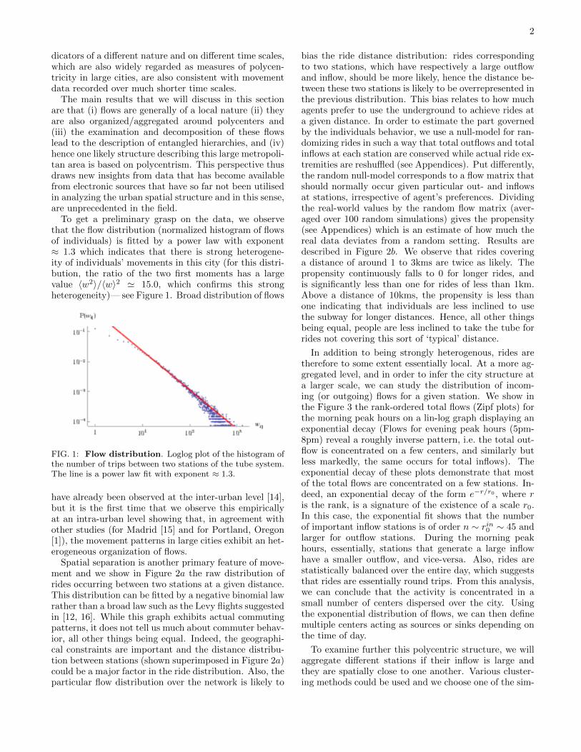
Spatial separation is another primary feature of move-ment and we show in Figure 2a the raw distribution ofrides occurring between two stations at a given distance.This distribution can be fitted by a negative binomial lawrather than a broad law such as the Levy flights suggestedin [12, 16]. While this graph exhibits actual commutingpatterns, it does not tell us much about commuter behav-ior, all other things being equal. Indeed, the geographi-cal constraints are important and the distance distribu-tion between stations (shown superimposed in Figure 2a)could be a major factor in the ride distribution. Also, theparticular flow distribution over the network is likely to

bias the ride distance distribution: rides correspondingto two stations, which have respectively a large outflowand inflow, should be more likely, hence the distance be-tween these two stations is likely to be overrepresented inthe previous distribution. This bias relates to how muchagents prefer to use the underground to achieve rides ata given distance. In order to estimate the part governedby the individuals behavior, we use a null-model for ran-domizing rides in such a way that total outflows and totalinflows at each station are conserved while actual ride ex-tremities are reshuffled (see Appendices). Put differently,the random null-model corresponds to a flow matrix thatshould normally occur given particular out- and inflowsat stations, irrespective of agent’s preferences. Dividingthe real-world values by the random flow matrix (aver-aged over 100 random simulations) gives the propensity(see Appendices) which is an estimate of how much thereal data deviates from a random setting. Results aredescribed in Figure 2b. We observe that rides coveringa distance of around 1 to 3kms are twice as likely. Thepropensity continuously falls to 0 for longer rides, andis significantly less than one for rides of less than 1km.Above a distance of 10kms, the propensity is less thanone indicating that individuals are less inclined to usethe subway for longer distances. Hence, all other thingsbeing equal, people are less inclined to take the tube forrides not covering this sort of ‘typical’ distance.

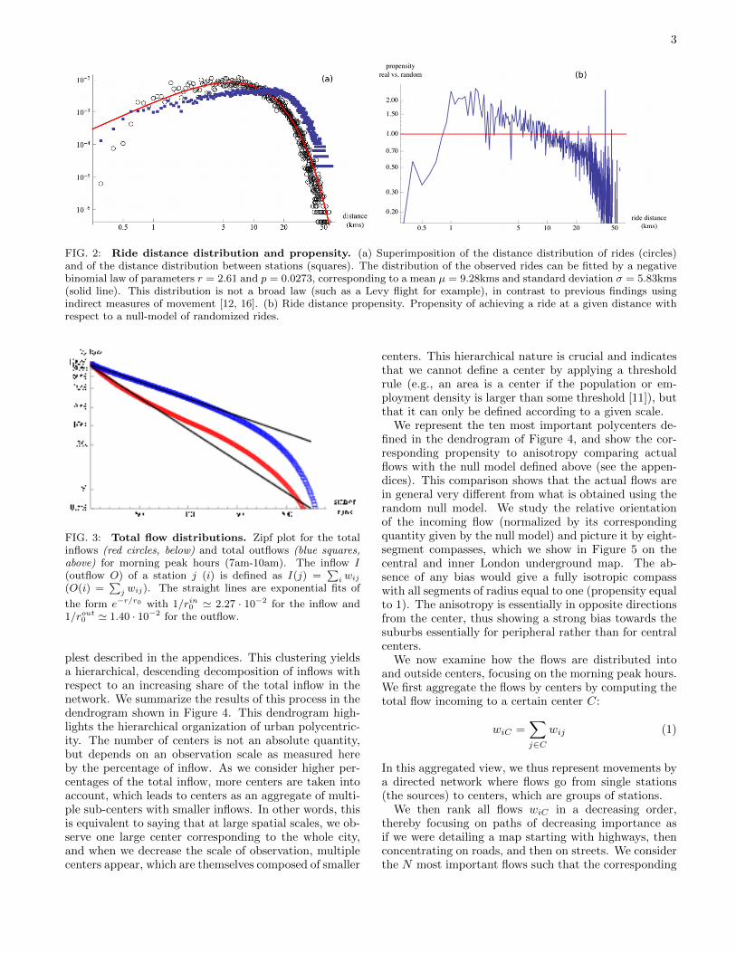
In addition to being strongly heterogenous, rides aretherefore to some extent essentially local. At a more ag-gregated level, and in order to infer the city structure ata larger scale, we can study the distribution of incom-ing (or outgoing) flows for a given station. We show inthe Figure 3 the rank-ordered total flows (Zipf plots) forthe morning peak hours on a lin-log graph displaying anexponential decay (Flows for evening peak hours (5pm-8pm) reveal a roughly inverse pattern, i.e. the total out-flow is concentrated on a few centers, and similarly butless markedly, the same occurs for total inflows). Theexponential decay of these plots demonstrate that mostof the total flows are concentrated on a few stations. In-deed, an exponential decay of the form e−r/r0 , where ris the rank, is a signature of the existence of a scale r0.In this case, the exponential fit shows that the numberof important inflow stations is of order n ∼ rin0 ∼ 45 andlarger for outflow stations. During the morning peakhours, essentially, stations that generate a large inflowhave a smaller outflow, and vice-versa. Also, rides arestatistically balanced over the entire day, which suggeststhat rides are essentially round trips. From this analysis,we can conclude that the activity is concentrated in asmall number of centers dispersed over the city. Usingthe exponential distribution of flows, we can then definemultiple centers acting as sources or sinks depending onthe time of day.

To examine further this polycentric structure, we willaggregate different stations if their inflow is large andthey are spatially close to one another. Various cluster-ing methods could be used and we choose one of the sim-

3

FIG. 2: Ride distance distribution and propensity. (a) Superimposition of the distance distribution of rides (circles)and of the distance distribution between stations (squares). The distribution of the observed rides can be fitted by a negativebinomial law of parameters r = 2.61 and p = 0.0273, corresponding to a mean µ = 9.28kms and standard deviation σ = 5.83kms(solid line). This distribution is not a broad law (such as a Levy flight for example), in contrast to previous findings usingindirect measures of movement [12, 16]. (b) Ride distance propensity. Propensity of achieving a ride at a given distance withrespect to a null-model of randomized rides.

FIG. 3: Total flow distributions. Zipf plot for the totalinflows (red circles, below) and total outflows (blue squares,above) for morning peak hours (7am-10am). The inflow I(outflow O) of a station j (i) is defined as I(j) =

∑i wij

(O(i) =∑

j wij). The straight lines are exponential fits of

the form e−r/r0 with 1/rin0 ' 2.27 · 10−2 for the inflow and1/rout0 ' 1.40 · 10−2 for the outflow.

plest described in the appendices. This clustering yieldsa hierarchical, descending decomposition of inflows withrespect to an increasing share of the total inflow in thenetwork. We summarize the results of this process in thedendrogram shown in Figure 4. This dendrogram high-lights the hierarchical organization of urban polycentric-ity. The number of centers is not an absolute quantity,but depends on an observation scale as measured hereby the percentage of inflow. As we consider higher per-centages of the total inflow, more centers are taken intoaccount, which leads to centers as an aggregate of multi-ple sub-centers with smaller inflows. In other words, thisis equivalent to saying that at large spatial scales, we ob-serve one large center corresponding to the whole city,and when we decrease the scale of observation, multiplecenters appear, which are themselves composed of smaller

centers. This hierarchical nature is crucial and indicatesthat we cannot define a center by applying a thresholdrule (e.g., an area is a center if the population or em-ployment density is larger than some threshold [11]), butthat it can only be defined according to a given scale.

We represent the ten most important polycenters de-fined in the dendrogram of Figure 4, and show the cor-responding propensity to anisotropy comparing actualflows with the null model defined above (see the appen-dices). This comparison shows that the actual flows arein general very different from what is obtained using therandom null model. We study the relative orientationof the incoming flow (normalized by its correspondingquantity given by the null model) and picture it by eight-segment compasses, which we show in Figure 5 on thecentral and inner London underground map. The ab-sence of any bias would give a fully isotropic compasswith all segments of radius equal to one (propensity equalto 1). The anisotropy is essentially in opposite directionsfrom the center, thus showing a strong bias towards thesuburbs essentially for peripheral rather than for centralcenters.

We now examine how the flows are distributed intoand outside centers, focusing on the morning peak hours.We first aggregate the flows by centers by computing thetotal flow incoming to a certain center C:

wiC =∑j∈C

wij (1)

In this aggregated view, we thus represent movements bya directed network where flows go from single stations(the sources) to centers, which are groups of stations.

We then rank all flows wiC in a decreasing order,thereby focusing on paths of decreasing importance asif we were detailing a map starting with highways, thenconcentrating on roads, and then on streets. We considerthe N most important flows such that the corresponding

4

FIG. 4: Hierarchical organization of the activity: Polycenters. Breakdown of centers in terms of underlying stationsand inflows. We gather stations by descending order of total inflow and we aggregate the stations to centers when taking intoaccount more and more stations. In this process, all stations within 1, 500 meters of an already-defined center are aggregated tothis main center. This yields the dendrogram shown here which highlights the hierarchical nature of the polycentric organizationof this urban system. The bold names to the left of the aggregates — such as “West End” for the group of stations aroundOxford Circus — are used throughout the paper as convenient labels to denote the polycenters.

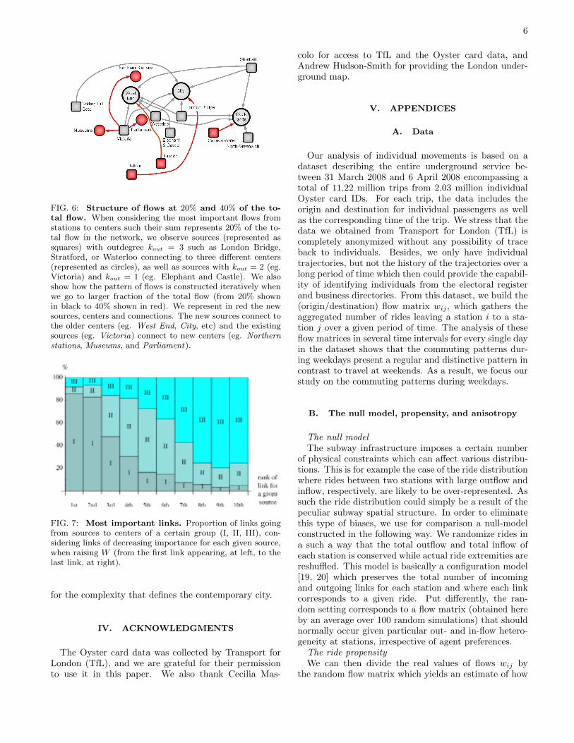
sum of flows is a given percentage W of the total flow inthe network. For example, if we consider the flows up toW = 20% of the total flow, we obtain the structure thatwe show in Figure 6 (it should be noted that we kept the‘station-to-center’ flows such that they represent 20% ofthe total flow, which is different from keeping the mostimportant station-to-station flows such as it is done forthe Figure 4 precisely in order to define those ‘centers’.We thus cannot directly compare these Figures 4 and 6).

At this scale, it is clear that we have three main cen-ters and sources (with various outdegree values), whichmostly correspond to intermodal rail-subway connec-tions. Adding more links, we reach a fraction W = 40%of the total flow and we then investigate smaller flows ata finer scale. We see that we have new sources appearingat this level and new connections from sources that werepresent at W = 20%.

We can summarize this result with the graph shown inFigure 7 where we divide the centers into three groupsaccording to their inflow (decreasing from first Group I tothe last Group III). In other words (see Figure 4), GroupI gathers centers with the most important total inflownamely the West End, City and Mid-town. Group IIgathers the next three centers Parliament, Governmentand Docklands while Group III gathers the other centerssuch as the Northern stations, West London, Museumsand the Western stations. This figure shows that formore than 80% of the sources, the most important link(ie. the 1st link) connects to a center of Group I. Con-

versely for more than 80% of the sources, the least impor-tant link (ie. 10th link) goes to a center of Group III. Theflow structure thus follows an original yet simple patternwhen we explore smaller and smaller weights.

We can quantify in a more precise way how the struc-ture of flows evolves when we investigate smaller flowsby exploring the list of flows wiC in decreasing order andby introducing the transition matrix T , which describeshow the outdegree of a source varies with increasing W(see Appendices). When we explore smaller flows, theanalysis of the T-matrix shows that the pattern of con-nections from sources to centers becomes richer and morecomplex, but can nonetheless be described by the simpleiterative process described above: the most importantlink of a source goes to the most important centers, thesecond most important link connects to the second mostimportant centers, and so on. It is interesting to note thateven if the organization of flows follows a simple iterativescheme, it leads to a complex and rich structure, whichis not strictly hierarchical since it mixes different levelsof flows consisting of different orders of magnitude. Inaddition, the fact that the most important flows alwaysconnect to the same center naturally leads to the ques-tion of efficiency and congestion in such a system. In thisrespect, London appears as a ‘natural’ city as opposed toan ‘artificial’ city for which flows would be constructedaccording to an optimized, hierarchical schema [17, 18].

5

FIG. 5: The London subway (tube) system: polycenters and basins of attraction. In the inset, we show theentire tube network while in the main figure, we zoom in on the central part of London. We represent the ten most importantpolycenters defined in the dendrogram of Figure 3, and show the corresponding propensity to anisotropy comparing actual flowswith the null model defined in the text. A propensity of 1 means that there is no deviation in a given direction with respect tothe null model. Circles correspond to various levels of identical propensity values: the thicker circle in the middle correspondsto 1, inner circles correspond to propensities of 0.2 and 0.5, and outer circles to 2 and 5. The anisotropy is essentially inopposite directions from the center, thus showing a strong bias towards the suburbs for peripheral centers essentially, ratherthan for central centers. Moreover, most stations control their own regions and seem to have their own distinctive basins ofattraction.

III. DISCUSSION

World cities such as London have tended to defy under-standing hitherto because simple hierarchical subdivisionhas ignored the fact that their polycentricity subsumesa pattern of nested urban movements. Using the Oysterdata we can identify multiple centers in London, thendescribe the traffic flowing into these centers as a sim-ple hierarchic decomposition of multiple flows at variousscales. In other words, these movements define a seriesof subcenters at different levels where the complex pat-tern of flows can be unpacked using our simple iterativescheme based on the representation of ever finer scales

defined by smaller weights. Casual observation suggeststhat this kind of complexity might apply to other worldcities such as Paris, New York or Tokyo where spatialstructure tends to reveal patterns of polycentricity con-siderably more intricate than cities lower down the citysize hierarchy. Our approach needs to be extended ofcourse to other modes of travel, which will complementand enrich the analysis of polycentricity. The Oyster cardis already used on buses and has just expanded beyondthe tube system to cover other modes of travel such assurface rail in Greater London. With GPS traffic sys-tems monitoring, in time, all such movements will becaptured, extending our ability to understand and plan

6

FIG. 6: Structure of flows at 20% and 40% of the to-tal flow. When considering the most important flows fromstations to centers such their sum represents 20% of the to-tal flow in the network, we observe sources (represented assquares) with outdegree kout = 3 such as London Bridge,Stratford, or Waterloo connecting to three different centers(represented as circles), as well as sources with kout = 2 (eg.Victoria) and kout = 1 (eg. Elephant and Castle). We alsoshow how the pattern of flows is constructed iteratively whenwe go to larger fraction of the total flow (from 20% shownin black to 40% shown in red). We represent in red the newsources, centers and connections. The new sources connect tothe older centers (eg. West End, City, etc) and the existingsources (eg. Victoria) connect to new centers (eg. Northernstations, Museums, and Parliament).

FIG. 7: Most important links. Proportion of links goingfrom sources to centers of a certain group (I, II, III), con-sidering links of decreasing importance for each given source,when raising W (from the first link appearing, at left, to thelast link, at right).

for the complexity that defines the contemporary city.

IV. ACKNOWLEDGMENTS

The Oyster card data was collected by Transport forLondon (TfL), and we are grateful for their permissionto use it in this paper. We also thank Cecilia Mas-

colo for access to TfL and the Oyster card data, andAndrew Hudson-Smith for providing the London under-ground map.

V. APPENDICES

A. Data

Our analysis of individual movements is based on adataset describing the entire underground service be-tween 31 March 2008 and 6 April 2008 encompassing atotal of 11.22 million trips from 2.03 million individualOyster card IDs. For each trip, the data includes theorigin and destination for individual passengers as wellas the corresponding time of the trip. We stress that thedata we obtained from Transport for London (TfL) iscompletely anonymized without any possibility of traceback to individuals. Besides, we only have individualtrajectories, but not the history of the trajectories over along period of time which then could provide the capabil-ity of identifying individuals from the electoral registerand business directories. From this dataset, we build the(origin/destination) flow matrix wij , which gathers theaggregated number of rides leaving a station i to a sta-tion j over a given period of time. The analysis of theseflow matrices in several time intervals for every single dayin the dataset shows that the commuting patterns dur-ing weekdays present a regular and distinctive pattern incontrast to travel at weekends. As a result, we focus ourstudy on the commuting patterns during weekdays.

B. The null model, propensity, and anisotropy

The null modelThe subway infrastructure imposes a certain number

of physical constraints which can affect various distribu-tions. This is for example the case of the ride distributionwhere rides between two stations with large outflow andinflow, respectively, are likely to be over-represented. Assuch the ride distribution could simply be a result of thepeculiar subway spatial structure. In order to eliminatethis type of biases, we use for comparison a null-modelconstructed in the following way. We randomize rides ina such a way that the total outflow and total inflow ofeach station is conserved while actual ride extremities arereshuffled. This model is basically a configuration model[19, 20] which preserves the total number of incomingand outgoing links for each station and where each linkcorresponds to a given ride. Put differently, the ran-dom setting corresponds to a flow matrix (obtained hereby an average over 100 random simulations) that shouldnormally occur given particular out- and in-flow hetero-geneity at stations, irrespective of agent preferences.The ride propensityWe can then divide the real values of flows wij by

the random flow matrix which yields an estimate of how

7

much the real data deviates from a random setting (atfixed inflow-outflow constraints). For the ride distribu-tion we then obtain the ride propensity R shown in Fig-ure 1b

R(d) =1

N(d)

∑ij/d(i,j)=d

wijwnmij

(2)

where wnmij is the number of individuals going from i toj in the null model, d(i, j) represents the distance on thenetwork between i and j, and where N(d) is the numberof pairs of nodes at distance d. This propensity givesan estimate of how much the real data deviates from arandom flow assignment with the same geographical andflow constraints. In other words, when the propensity isequal to one the observed flows are entirely due to the ge-ographical and flow structure of the network. Converselywhen the propensity is smaller or larger than 1, the flowsreflect non-uniform preferences for rides of certain dis-tance.

The anisotropy propensityWe used the null model in order to extract the part

due to the behavior of the commuters in their ride distri-bution. We can also study the relative orientation of theincoming flow normalized by its corresponding quantitygiven by the null model which gives the anisotropy A dueto the commuters behavior

A(θ) =1

N(θ)

∑ij/iOj=θ

wijwnmij

(3)

where θ is a particular direction (we binned the anglein eight equal intervals so to represent an eight-segmentcompass) and where the sum is over the N(θ) nodes i andj such that the angle of i− j is given by θ. The absenceof any bias would give a fully isotropic compass with allsegments of radius equal to one (anisotropy propensityequal to 1).

C. Identifying the polycenters

Clustering methods for point in spaces has been thesubject of many studies and are used in many differ-ent fields. In particular, in computational biology andbioinformatics, clustering is used to build group of geneswith related expression patterns. Many different meth-ods were developped and the most common ones are hi-erarchical clustering methods (such as those based on K-means and their derivatives, see for example [21]). Here,we are in a slightly different position. The stations areclearly located in space and thus Euclidean distance ap-pears as the natural distance measure (a necessary ingre-dient for clustering methods). Yet these stations are alsocharacterized by their inflow. For this reason, the usualmethods are not directly applicable and we thus adoptedthe simplest clustering method which we describe as fol-lows. We first gather stations by descending order of total

inflow, thereby defining centers of decreasing importance.In order to account for geographical proximity of groupsof stations, indicating subsets of distinct stations belong-ing to a single geographical center, we aggregate all sta-tions within a distance rc of an already-defined center.In this way we systematically increase the total flow as-sociated with these centers and we continue this processuntil we capture a large percentage of the total flow. Wethus chose to stop at 60 percent of the total flow in orderto avoid to include too many details and too much noise.

We varied the value of rc from 1 to 2 kms and ob-served that our results were stable. This stability prob-ably comes from the fact that the inter-distance stationis of order 1.2kms for London in 2008 and correspondsto some psychological threshold above which individualsprefer to take the subway if they can choose. The resultsdiscussed above are obtained with rc = 1500 meters.

D. The T matrix

We face here a difficult problem: we have a completeweighted directed network featuring flows from stationsto centers, and the goal is to extract some meaningful in-formation. We started with the analysis of the dominantflows and we would like to understand how the flows arestructured when we explore smaller values. In order todo this, we introduce a ‘transition ’matrix T which char-acterizes quantitatively the changes in the flow structurewhen we explore the list of flows wiC going from a sta-tion i to a center C in decreasing order of importance. Inwhat follows, when we talk of ‘total flow at W ’, we meanthat we consider only the most important flows wiC sothat we reach a total fraction W of the total flow on thewhole network of station-to-center flows. When the totalflow goes from W to W + δW , the elements tij of T rep-resent the number of sources with outdegree i at W andwith outdegree j at W + δW . Note that i starts at i = 0while j starts at j = 1 (i.e. T only denotes sources thathave a strictly positive outdegree at W + δW ).

As an example, when we go from W = 20% to W +∆W = 40%, the T matrix is

T =

37 12 1 0 04 9 4 1 00 4 2 1 20 0 0 2 10 0 0 0 00 0 0 0 0

(4)

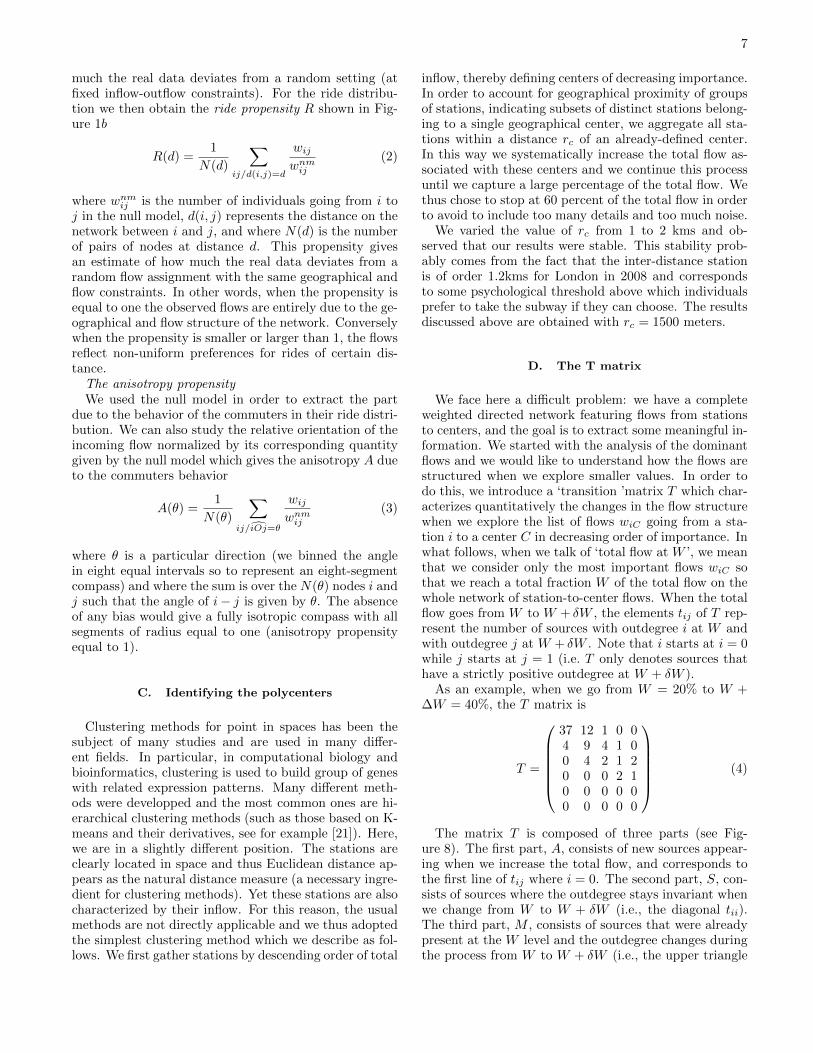
The matrix T is composed of three parts (see Fig-ure 8). The first part, A, consists of new sources appear-ing when we increase the total flow, and corresponds tothe first line of tij where i = 0. The second part, S, con-sists of sources where the outdegree stays invariant whenwe change from W to W + δW (i.e., the diagonal tii).The third part, M , consists of sources that were alreadypresent at the W level and the outdegree changes duringthe process from W to W + δW (i.e., the upper triangle

8

FIG. 8: Transition matrix. Typical form of the outdegreetransition matrix tij , consisting essentially of a row vector(A, inexistent sources before the transition) and an uppertriangular matrix (made of a diagonal S of sources havingthe same out-degree after the transition, and a submatrix Mof sources whose out-degree increases after the transition).

tij where j > i). We can compute the number of sourcesin each of these types and plot them. A proper T matrixis a (N + 1)×N matrix (in Eq. 4, N = 5), as the T ma-trix is made of a row vector (A) and an upper triangularmatrix (S, M and the zeros) because a source that feedsn centers cannot become a source feeding n′ < n centerswhen transitioning to a larger inflow-cut W + dW . Therow vector A indicates sources that were not feeding cen-ters before, and now feed some centers, i.e., sources thatwere non-existent for a lower inflow-cut, hence the extrainitial row represented by vector A. Thus, ‘37’ meansthat after the transition (at the new inflow-cut), thereare 37 new sources feeding one center, 12 new sourcesfeeding two, 1 new source feeding three. The ‘9’ on thesecond row means that 9 sources that used to feed onecenter, now feed two, and so on. The row A is thus givenby

A =(

37 12 1 0 0)

(5)

and the diagonal is

S =(

4 4 0 0 0)

(6)

The upper triangular matrix M is given by

M =

9 4 1 00 2 1 20 0 2 10 0 0 0

(7)

In the case of the transition 20% → 40%, the majorphenomenon is the appearance of new sources (37 in thiscase) followed by sources feeding new centers.

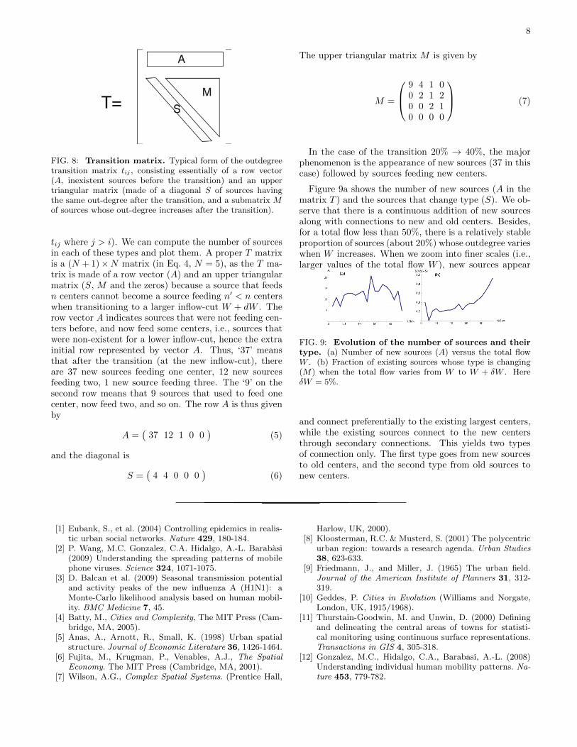
Figure 9a shows the number of new sources (A in thematrix T ) and the sources that change type (S). We ob-serve that there is a continuous addition of new sourcesalong with connections to new and old centers. Besides,for a total flow less than 50%, there is a relatively stableproportion of sources (about 20%) whose outdegree varieswhen W increases. When we zoom into finer scales (i.e.,larger values of the total flow W ), new sources appear

FIG. 9: Evolution of the number of sources and theirtype. (a) Number of new sources (A) versus the total flowW . (b) Fraction of existing sources whose type is changing(M) when the total flow varies from W to W + δW . HereδW = 5%.

and connect preferentially to the existing largest centers,while the existing sources connect to the new centersthrough secondary connections. This yields two typesof connection only. The first type goes from new sourcesto old centers, and the second type from old sources tonew centers.

[1] Eubank, S., et al. (2004) Controlling epidemics in realis-tic urban social networks. Nature 429, 180-184.

[2] P. Wang, M.C. Gonzalez, C.A. Hidalgo, A.-L. Barabasi(2009) Understanding the spreading patterns of mobilephone viruses. Science 324, 1071-1075.

[3] D. Balcan et al. (2009) Seasonal transmission potentialand activity peaks of the new influenza A (H1N1): aMonte-Carlo likelihood analysis based on human mobil-ity. BMC Medicine 7, 45.

[4] Batty, M., Cities and Complexity, The MIT Press (Cam-bridge, MA, 2005).

[5] Anas, A., Arnott, R., Small, K. (1998) Urban spatialstructure. Journal of Economic Literature 36, 1426-1464.

[6] Fujita, M., Krugman, P., Venables, A.J., The SpatialEconomy. The MIT Press (Cambridge, MA, 2001).

[7] Wilson, A.G., Complex Spatial Systems. (Prentice Hall,

Harlow, UK, 2000).[8] Kloosterman, R.C. & Musterd, S. (2001) The polycentric

urban region: towards a research agenda. Urban Studies38, 623-633.

[9] Friedmann, J., and Miller, J. (1965) The urban field.Journal of the American Institute of Planners 31, 312-319.

[10] Geddes, P. Cities in Evolution (Williams and Norgate,London, UK, 1915/1968).

[11] Thurstain-Goodwin, M. and Unwin, D. (2000) Definingand delineating the central areas of towns for statisti-cal monitoring using continuous surface representations.Transactions in GIS 4, 305-318.

[12] Gonzalez, M.C., Hidalgo, C.A., Barabasi, A.-L. (2008)Understanding individual human mobility patterns. Na-ture 453, 779-782.

9

[13] Hall, P., The World Cities (Weidenfeld and Nicolson,London, UK, 1984).

[14] De Montis, A., Barthelemy, M., Chessa, A., Vespignani,A. (2007) The structure of inter-urban traffic: A weightednetwork analysis. Environment and Planning: B 34, 905-924.

[15] Guttierez, J., Garcia-Palomares, J.C. (2006) New spa-tial patterns of mobility with the metropolitan area ofMadrid: Towards more complex and dispersed flow net-work. Journal of Transport Geography 15, 18-30.

[16] Brockmann, D., Hufnagel, L., Geisel, T. (2006) The scal-ing laws of human travel. Nature 439, 462-465.

[17] Alexander, C. (1965) A city is not a tree, Architectural

Forum 122 (1) ,58-61 and (2), 58-62.[18] Batty, M. (2006) Hierarchy in Natural and Social Sci-

ences, D. Pumain (Ed.) 143-168, Springer (Berlin, DE,2006).

[19] Molloy, M., and Reed, B. (1995) A critical point for ran-dom graphs with a given degree sequence. Random Struc-tures and Algorithms, 6:161-179.

[20] Newman, M.E.J., Strogatz, S.H., Watts, D.J. (2001)Random graphs with arbitrary degree distributions andtheir applications. Physical Review E, 64:026118.

[21] T. Hastie, R. Tibshirani, J.H. Friedman, The Elementsof Statistical Learning, Springer (Berlin, DE, 2001).