On VR SpatialQuery for Dual Entangled Worlds∗

Shao-Heng Ko1, Ying-Chun Lin

2, Hsu-Chao Lai

13, Wang-Chien Lee

4, De-Nian Yang

15

1Institute of Information Science, Academia Sinica, Taipei, Taiwan

2Department of Computer Science, Purdue University, West Lafayette, USA

3Department of Computer Science, National Chiao Tung University, Hsinchu, Taiwan

4Department of Computer Science and Engineering, The Pennsylvania State University, State College, USA

5Research Center for Information Technology Innovation, Academia Sinica, Taipei, Taiwan

1{arsenefrog, hclai0806, dnyang}@iis.sinica.edu.tw

2lin915@purdue.edu

4wlee@cse.psu.edu

ABSTRACTWith the rapid advent of Virtual Reality (VR) technology and vir-

tual tour applications, there is a research need on spatial queries

tailored for simultaneous movements in both the physical and vir-

tual worlds. Traditional spatial queries, designed mainly for one

world, do not consider the entangled dual worlds in VR. In this

paper, we first investigate the fundamental shortest-path query in

VR as the building block for spatial queries, aiming to avoid hitting

boundaries and obstacles in the physical environment by leveraging

Redirected Walking (RW) in Computer Graphics. Specifically, we

first formulate Dual-world Redirected-walking Obstacle-free Path(DROP) to find the minimum-distance path in the virtual world,

which is constrained by the RW cost in the physical world to ensure

immersive experience in VR. We prove DROP is NP-hard and de-

sign a fully polynomial-time approximation scheme,Dual EntangledWorld Navigation (DEWN), by finding Minimum Immersion Loss

Range (MIL Range). Afterward, we show that the existing spatial

query algorithms and index structures can leverage DEWN as a

building block to support kNN and range queries in the dual worlds

of VR. Experimental results and a user study with implementation

in HTC VIVE manifest that DEWN outperforms the baselines with

smoother RW operations in various VR scenarios.

1 INTRODUCTIONWith the growing availability of Virtual Reality (VR) devices, in-

novative VR applications in virtual social, travel, and shopping

domains have emerged. This technological trend of VR not only

attracts business interests from prominent vendors such as Face-

book and Alibaba1but also brings a new wave of research in the

academia. While current research on VR mostly originated from

Computer Graphics, Multimedia, and HCI, focusing on constructing

vivid VR worlds [21, 22, 41], the needs for research and support

from the database community are also imminent.

Traditional research on spatial data management has contributed

significantly to various applications in the physical world. For ex-

ample, for mobile users on a journey, the information about the

closest gas stations along a routing path can be found by spatial

queries [29]. These queries are also needed in the virtual worlds in

VR applications where moving between point-of-interests (POIs)

is a basic operation. For example, in VR campus touring2and VR

∗A shorter version of this paper has been accepted for publication in the 28thACM International Conference on Information and KnowledgeManagement(CIKM 2019).1Facebook: https://youtu.be/YuIgyKLPt3s; Alibaba:https://cnn.it/2GkXUDX.

2CampusTours: https://campustours.com/; UNSW 360: https://ocul.us/2VBzGlC.

architecture/indoor navigation3applications, spatial queries can

be issued to find POIs and guide users to move to them. However,

in many VR applications where users move in both the virtual

and physical worlds, the simple one-world setting may no longer

sustain, rendering the aforementioned queries useless. To study

this problem, we revisit a number of spatial queries widely used in

many VR applications to develop new algorithms by considering

factors in the dual entangled virtual and physical worlds.

Traditional VR applications adopt simple stand-and-play ap-

proaches, e.g., teleportation [6], which have users to stand still in

the physical world and rely on handheld devices, e.g., joysticks, to

move to the destination. However, unlike previous generation of VR

Head Mound Displays (HMDs), which are tied to computers with

cable wires, the new VR devices are either wireless4 or standalone5

devices. As this new wave of technology unties VR devices from a

fixed computer,mobile VR [30, 54, 55] and room-scale VR [25, 27, 61]

recently attract massive attention in HCI and Computer Graphics

research communities, as they allow untethered walking6in VR

to improve user experience. Indeed, research [10, 36, 49] finds that

stand-and-play approaches do not facilitate immersive experience

intended in VR. On the contrary, walking is able to bring benefits

to the users’ cognition in virtual environments (VEs) [46], because

users can experience correct stimulations [36] in order to reduce the

side-effect of motion sickness. To avoid hitting physical obstacles,

various hardware and HCI solutions leveraging saccadic movement

[53], space partition [32] and Galvanic vestibular stimulation [50]

are proposed recently.

Usually, users in VR applications are severely constrained [25, 27,

59] by the small size and setting of physical space, e.g., living room,

during exploration of massive VEs. As a result, if the movement

in the virtual world is simply realized by a directly matched walk

in the real world, users may easily get hindered by boundaries of

the small physical space.7To address this issue, Redirected Walking

(RW) [24, 36, 43, 59] has been proposed to steer users away from

physical boundaries and obstacles by slightly tailoring the walking

direction and speed displayed in HMDs.8For example, when a user

intends to walk straightly in the virtual world, RW continuously

adjusts the walking direction displayed in the HMD to guide the

user walking along a curve in the physical world in a small room.

3IrisVR: https://irisvr.com/; VR for Architects: https://bit.ly/2JlwiVq.

4HTC Vive Pro: https://bit.ly/2AM0vUM; DisplayLink XR: https://bit.ly/2HdI2FJ.

5HTC Vive Focus: https://bit.ly/2US4DwI; Oculus Go: https://www.oculus.com/go/.

6A number of demo videos on walking with wireless VR can be found at https://bit.ly/

2vWP9gG, https://bit.ly/2LIlgeT, and https://bit.ly/2HojNX3.

7See also https://bit.ly/2YuKSgU and https://bit.ly/2Ebcfox on this issue.

8A series of demo videos elaborating Redirected Walking can be found at https://bit.

ly/2JGv8D8 and https://bit.ly/2H6UCb4.

arX

iv:1

908.

0869

1v1

[cs

.DS]

23

Aug

201

9

Sv (2,8, 270°) (6,8)

(12,6)

(12,5)

(3,6)(5,5)

(6,3)

(3,1) (5,1)

𝑇 (10,2)

(a) A virtual world.

Door

𝑆p(2,4, 270°)

(6,6) (10,6)

(11,5)

(10,2)

(b) A physical world.

Figure 1: An illustrative example for DROP.

It has been successfully demonstrated that the human visual-

vestibular system does not conceive those minor differences if the

RW operations (detailed later) are carefully controlled [36, 37, 48],

and RW provides the most immersive user experiences compared

to joystick and teleportation-based locomotion techniques [27, 36].

However, when a path in the virtual world (called v-path) is iden-tified by directly employing the shortest-path query, the walking

path in the physical world (called p-path) may involve many RW

operations that may incur motion sickness [37, 48, 51], thereby

deteriorating the user experience.

In this paper, therefore, we first formulate a new query, namely

Dual-world Redirected walking Obstacle-free Path (DROP), to find

the minimum-distance v-path from the current user location to the

destination that is RW-realizable by a corresponding obstacle-free

p-path, bounded by a preset total cost on Redirected Walking (RW

cost) to restrict the loss of immersive experience in VR. Specifically,

given the current positions of the user, the layouts of both the

virtual and physical worlds, and a destination in the virtual world,

DROP finds a v-path and an RW-realized obstacle-free p-path such

that (i) the length of v-path is minimized, and (ii) the total cost

incurred by RW operations does not exceed a preset threshold. We

introduce the notion ofMinimum Immersion Loss (MIL) to represent

the RW cost for realizing a short walk in dual worlds.

Example 1. (Motivating Example). Figure 1 lays out an example

of virtual and physical worlds to illustrate the notions of v-path

and p-path. As shown, Sv and Sp denote the current locations of

the user in both worlds, while the thick black arrows indicate the

corresponding orientations, i.e., the user faces south in both worlds.

The coordinates of some POIs are shown right beside them. The

face direction is given (in degrees) for the starting state. LetT be the

destination in the virtual world and the preset RW cost threshold is

small. In the virtual world, the shortest obstacle-free path, bypassing

corners of the obstacles as indicated by the red solid line segments,

has a total length of 10.83. However, this path is actually infeasible

because the starting location in the physical world is too close to

the wall and door area (see the corresponding infeasible p-path

shown in red). Similarly, the brown path (which features a length

of 14.17 in the virtual world) is not feasible. In contrast, the optimal

path of DROP is the blue one with a total length of 14.93. This

path, bypassing the upper part of virtual obstacles, incurs only

minimal RW operations including a rotation at the beginning to

avoid obstacles and prohibited areas in the physical world. □

DROP, which actually returns not only the paths in the dual

worlds but also the corresponding RW operations, is much more

challenging than finding the shortest obstacle-free path in a single

world. Some heuristics useful in geographic space, e.g., the triangu-

lar inequality, are not applicable here due to the obstacles appearing

in both worlds. Moreover, traditional spatial index structures, e.g.,

R-Tree [15], M-Tree [8], and O-Tree [62] are designed for only one

world instead of the entangled dual worlds, and thus do not handle

the cost of RW operations. Finally, in a multi-user VR environment,

the same path in the virtual world may be walked differently by

users in their individual physical worlds. The RW operations car-

ried out for the same virtual path are unlikely to be the same for

different users and thus are not precomputable. Indeed, we prove

DROP is NP-hard.

To solve DROP, we first present a dynamic programming algo-

rithm, namely Basic DP, as a baseline to find the optimal solution

which unfortunately requires exponential time. Basic DP is compu-

tationally intensive due to the need of maintaining an exponentially

large number of intermediate states to ensure the optimal solution.

To address the efficiency issue while still ensuring the solution qual-

ity, we propose a Fully Polynomial-Time Approximation Scheme,

namely Dual Entangled World Navigation (DEWN), to approach the

optimal solution in polynomial time. The main idea of DEWN is to

quickly obtain a promising feasible solution (called reference path)in an early stage. Via the reference path, we explore novel pruning

strategies to avoid redundant examinations of states that lead to

excessive RW costs or long path lengths.

However, finding a promising reference path directly from the

entangled dual worlds is actually computationally intensive. To

address this issue, we precompute the range of RW cost, termed as

Minimum Immersion Loss Range (MIL Range), which consists of an

MIL lower bound and anMIL upper bound, for a possible straight-linewalk between two POIs in the virtual world. With MIL Ranges for

potential path segments in the virtual world, we jointly minimize

the weighted sum of v-path length and RW cost by Lagrangianrelaxation (LR). Accordingly, we derive the optimal weight (i.e., the

Lagrange multiplier) to ensure both the feasibility and quality of the

reference path. Equipped with DEWN as a building block, we then

show that existing spatial query algorithms and index structures

can support the counterparts of kNN and range queries in VR. The

contributions of this work are summarized as follows:

• We redefine a new shortest path query, namely Dual-worldRedirected-walking Obstacle-free Path (DROP), tailored for

the dual entangled obstructed spaces in VR applications.

We introduce a novel notion of MIL Range that captures the

possible range of RedirectedWalking cost in state transitions

of movements and prove DROP is NP-hard.

• We first tackle DROP by dynamic programming and then

design an online query algorithm, DEWN, which exploits

efficient ordering and pruning strategies to improve compu-

tational efficiency significantly. We prove that DEWN is a

Fully Polynomial-Time Approximation Scheme for DROP.

• We show that existing spatial query algorithms and index

structures can leverage DEWN as a building block to support

kNN and range queries in VR.

• We perform experiments on real datasets and conduct a user

study to evaluate the proposed algorithms with various base-

lines. Experimental results show that DEWN outperforms

the baselines in both solution quality and efficiency.

This paper is organized as follows. Section 2 reviews the related

work. Section 3 introduces the preliminaries and formulates DROP.

Section 5 details DEWN and provides a theoretical analysis. Section

6 proposes an enhancement for DROP and extends our ideas for

spatial queries. Section 7 reports the experimental results, and

Section 8 concludes this paper.

2 RELATEDWORK

Shortest Path Query. Exact [3], top-k [2], approximate [40, 42],

constrained [38, 57], and adaptive [14, 16] shortest path queries

have been studied extensively in the database community. Akiba etal. [3] precompute shortest path distances by breadth-first search

and store the distances on the vertices. To improve efficiency, a

query-dependent local landmark scheme [42] is proposed to provide

a more accurate solution than the global landmark approach [40]

by identifying a landmark close to both query nodes and leveraging

the triangular inequality. In continental road networks with length

and cost metrics, COLA [57] utilizes graph partition to minimize

the path length within a cost constraint. Hassan et al. [16] find the

adaptive type-specific shortest paths in dynamic graphs with edge

types. Nevertheless, the above research is designed for one network(i.e., one world). None of the existing works incorporates the cost,e.g., Redirected Walking, in dual worlds of different layouts.

Spatial Query. Spatial database is a major research area in the

database research community [45]. Queries on spatial network

databases, including range search, nearest neighbors, e-distance

joins, and closest pairs [39], have attracted extensive research in-

terests. In recent years, considering the presence of obstacles, the

obstructed version of various spatial queries are revisited [60]. Sul-

tana et al. [52] study the obstructed group nearest neighbor (OGNN)query to find a rally point with the minimum aggregated distance.

Range-based obstructed nearest neighbor search [62] extracts the

nearest neighbors within a range for obstructed sequenced routes,

where the route distance is minimized [4]. However, the above

algorithms are designed for one world, instead of the entangled

dual worlds, where the physical worlds of users are different from

each other. As a result, these existing works are not applicable to

the dual world spatial queries tackled in this paper.

Walking in Virtual Reality. To move in the virtual space, Point-

and-Teleport [6] allows a user to point at and then transport to

a target location, but the experience is not immersive due to the

abrupt scene change and loss of sense in time [10]. Research shows

that real walking is more immersive than Point-and-Teleport [56].

Redirected Walking (RW) [36] exploits the inability of the human

vestibular system to detect a subtle difference (in the walking speed

and direction) between movements in the dual worlds. It has been

demonstrated that RW can support free walking in a large virtual

space for a relatively small physical space [35, 36], and the degra-

dation in user immersion can be quantitatively measured from the

acoustic and visual perspectives [37, 48, 51]. Detailed implemen-

tation and performance evaluation of RW have been studied in

(2,8)(6,8)

(12,6)

(12,5)

(3,6)

(5,5)(6,3)

(3,1)(5,1)

(10,2)

(6,6)

46.3

1

7.1

2 5.1

3.6

22.2

3

4 4.15

63

2.2

2.2

2.2

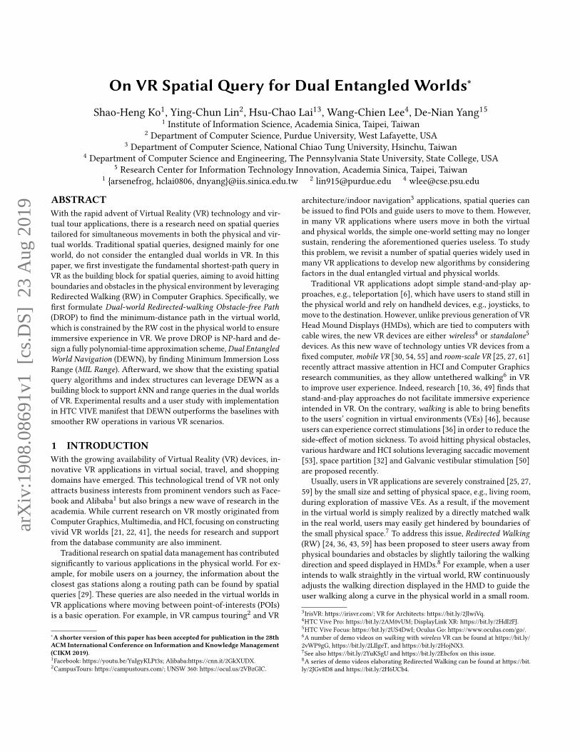
Figure 2: VG of the virtual world in Example 1.

[17] and [36]. Recent evaluation [27] demonstrates that RW pro-

vides the most preferable user experience than joystick-based and

teleportation-based systems. However, most existing works on RW

focus on creating immersive experience but do not provide system-

atic approaches for query processing in dual worlds, which inspires

our study in this work.

3 PROBLEM FORMULATIONIn this section, we first provide background on the Visibility Graph

and Redirected Walking operations. Then we formulate the DROP

problem and prove that DROP is NP-hard.

3.1 Preliminaries

Visibility Graph. The notion of Visibility Graph (VG), widely

used in computational geometries and obstructed spatial query

processing [4, 34, 62], models obstacles as polygons and regards

their corners as VG nodes. Those corners are important as they

are usually the turning points for shortest paths in an obstructed

space. In VG, two nodes are connected by a weighted edge if and

only if there exists a straight line segment between them without

crossing any obstacle [52, 62]. In this paper, we exploit VG to define

the DROP problem on dual worlds for the following reasons: 1) VG

preserves the unobstructed shortest paths in the obstructed spatial

space [52, 60], simplifying the distance computation and reduc-

ing the computational complexity in processing obstructed spatial

queries. 2) Representing the virtual world in VG ensures natural

movements of users since the obtained v-paths avoid zigzagging

patterns. 3) Whereas DROP depends on both worlds due to the

RW operations, VG for both worlds can be constructed separately

[18, 33]. While existing works on obstructed spatial queries most

consider only corners of obstacles in VG, we also extend VG to

include all POIs in the virtual world. We refer the interested readers

to [11] for more background on VGs.

Example 2. Figure 2 illustrates the VG constructed from the virtual

world in Example 1, where the nodes represent virtual locations

of interests (POIs and obstacle corners) in the application, and the

edges (called v-edges) denote straight-line moving paths between

two virtual locations9. For example, the virtual location (2, 8) is

a POI (the start location), while (6, 8) represents the upper rightcorner of the white gameboard in Example 1. The v-edge between

them represents a move along the upper side of the gameboard

which has a length of 4 (shown in red). □

9We omit a few of VG nodes for brevity and handiness to continue using it as the

running example.

RedirectedWalking Operations. RedirectedWalking (RW) [43]

introducesminor differences in thewalking speed and turning angle

to adapt the perception of walking in the dual worlds. Basic RW

operations include Translation (TO) [59], Rotation (RO) [24, 37],

and Curvature (CO) [26, 35]. TO introduces a slight scaling factor

between the walking speed in the virtual world and the actual

walking speed in the physical world. Thus, the distances in the dual

worlds are different after a user walks for a period of time. Similarly,

RO tailors the mapping between the rotation angular velocity in

the virtual world to that in the physical world. When a user intends

to move straightly in the virtual world, CO lets the user traverse a

slightly bending curve10

to avoid obstacles in the physical world.

However, when a user is very close to obstacles and not able to

escape from them with the above operations, a Reset operation [58]

may be issued to specifically ask the user to rotate her body to

face a different direction in the physical world, whereas the virtual

world is suspended (remaining the same).11

Note that Reset incurs

significantly higher disturbance for users [36] and thus introduces

a much larger RW cost. An RW cost model of different operations

can be constructed based on the usage count or other measures of

user experience, e.g., detection thresholds in [37, 48] or immersion

thresholds in [47]. For example, according to [48], a TO that down-

scales the walking distance by 40% has a roughly 90% chance to

be detected by the users. Thus, applying a TO of such magnitude

may incur an RW cost of 0.9 in a detection threshold-based cost

model. In Appendix A, we provide some definitions of the basic RW

operations, as well as briefly discuss some possible RW cost models.

For a complete survey on RW, we refer the interested readers to

[36].

Given a user’s current location and orientation in both worlds

(formally introduced later as the loco-state), the possible combina-

tions of RW operations to pilot the user to a target loco-state is

bounded due to the finite operations.12

It is also more efficient for

the user to move along straight line segments in the VG. Therefore,

in this paper, a near-shortest path between two locations with the

smallest RW cost (i.e., minimum degradation of user experience) can

be precomputed by exploring different RW operation sequences.

This RW cost is coined as the Minimum Immersion Loss (MIL) be-

tween the two loco-states. Note that MIL represents the RW costs

on small segments of movements. It is independent of the start and

destination locations in DROP and thus can be precomputed offline.

3.2 Problem FormulationIn the following, we introduce the notations used to formulate

DROP. We use VG graphs for both virtual and physical worlds to

abstract unobstructed movements of users. We also summarize the

notations in Tables 1 and 2.

10https://youtu.be/THk92rev1VA.

11https://youtu.be/gD1qa0edVA8.

12For instance, in Example 1, to guide the user from the start locations (Sv and Sp , in

the virtual and physical world, respectively) to the next locations on the blue paths,

i.e., (6,8) in the virtual world and (6,6) in the physical world, one possible configuration

of RW operations is to first perform an RO that down-scales the rotation angular

velocity by 25.0% to re-orient the user to face the targeted locations, then followed by

a TO, which down-scales the walking speed by 10.6% in the virtual world, to align the

walking distances in the dual worlds. Another feasible configuration is a Reset and

then a TO, which incurs a larger RW cost since Reset severely downgrades the user

experience.

Definition 1. Location Sets (Γv, Γp). The virtual location set Γv

contains all virtual locations γ v ∈ Γv corresponding to a VG node

in the virtual world. Similarly, the physical location set Γp includes

all locations in the physical world, where each physical locationγ p ∈ Γp represents either an unoccupied location or an obstacle in

a coarse-grained coordinate of the physical world.13

Definition 2. Virtual Graph (Gv) and Physical Graph (Gp

). The vir-

tual graph (v-graph)Gvconsists of the vertex set Γv and undirected

edge set Ev : Γv → Γv, where a virtual edge (v-edge) ev connectsunobstructed virtual locations with a cut-off distance threshold

ℓmax [18, 33]. Each v-edge ev is associated with a positive length

l(ev) that denotes the Euclidean distance between the two endpoints

in the virtual world. The physical graph (p-graph)Gpand the edge

set Ep are defined analogously.

To determine the appropriate v-path and the corresponding se-

quence of RW operations, the user’s face orientation needs to be

considered. In the following, we formally introduce the notion of

loco-state, which describes the user status in both worlds.

Definition 3. Virtual State (stv) and Physical State (stp). A v-statestv is a tuple (γ v,θv) while γ v is the current user location in the

virtual world, and θv is her face orientation. The p-state stp =(γ p,θp) is defined similarly in the physical world, and θv,θp ∈ Θ,which is the Orientation Set consisting of all legal face directions.

Definition 4. Locomotion State (st) and Loco-state Space (ST ). Aloco-state st = (stv, stp) describes the current user status. The Eu-clidean distance dist(st1, st2) between two loco-states is the straight-

line distance between their virtual locations. Two loco-states st1and st2 are neighboring if there exists a v-edge ev between their vir-

tual locations γ v1and γ v

2with the v-edge length l(ev) = dist(st1, st2).

The loco-state space ST contains all possible loco-states.

Example 3. In Example 1, the starting v-state for the user, denoted

as stvs, is ((2, 8), 270◦), and the starting p-state is st

p

s= ((2, 4), 270◦).

The starting loco-state is then sts = (((2, 8), 270◦), ((2, 4), 270◦)). □

Equipped with the notion of loco-state, user movements in the

dual worlds can be regarded as sequences of state transitions be-

tween neighboring loco-states. The possible combinations of RW

operations to pilot the user to a target loco-state is bounded due to

the finite operations. Therefore, a configuration with the smallest

RW cost (i.e., minimum degradation of user experience) can be pre-

computed by exploring different RW operation sequences. This RW

cost is coined as the Minimum Immersion Loss (MIL) between the

two loco-states. Note that MIL represents the RW costs on small

segments of movements. It is independent of the start and destina-

tion locations in DROP and thus can be precomputed offline. It is

also generic, i.e., supporting any cost model of RW operations.

Definition 5. Minimum Immersion Loss (MIL).MIL(st1, st2) represents the smallest RW cost achievable (i.e., real-

izable by a set of RW operations) for a VR user to move from a

loco-state st1 to a neighboring loco-state st2 with a sequence of RW

operations.

13As the position tracking accuracy in mainstream VR devices varies [23], representing

a physical world by a coarse-grid or mesh-based [20] graph structure leaves room for

errors and may be more suitable than a fine-grained coordinate system.

Next, we introduce RW path to describe the RW-realizable v-path

and the corresponding RW-realized p-path.

Definition 6. Redirected Walking Path (RW path). An RW path

p = ⟨st1, st2, · · · , stn⟩ is a sequence of loco-states, including a v-

path pv = ⟨stv1, stv

2, · · · , stvn⟩ with v-path length l(p) = l(pv) =∑n−1

i=1 l

((γ vi ,γ

v

i+1)), and a p-pathpp = ⟨stp

1, st

p

2, · · · , stpn⟩ with the in-

curred RW cost to realize pv with pp as c(p) = ∑n−1i=1 MIL(sti , sti+1).

Example 4. In Example 1, the two blue paths in the dual worlds

combine for an RWpathp = ⟨st1 = sts = (((2, 8), 270◦), ((2, 4), 270◦)),st2 = (((6, 8), 0◦), ((6, 6), 30◦)), st3 = (((12, 6), 330◦), ((10, 6), 0◦)),st4 = (((12, 5), 270◦), ((11, 5), 315◦)), st5 = (((10, 2), 225◦), ((10, 2),240◦)) ⟩. The lengths of the corresponding v-edges are respectively

l

(((2, 8), (6, 8))

)= 4, l

(((6, 8), (12, 6))

)= 6.32, l

(((12, 6), (12, 5))

)= 1,

and l

(((12, 5), (10, 2))

)= 3.61. Thus, the total v-path length is

4+6.32+1+3.61 = 14.93. Assume the MIL values between the loco-

states are MIL(st1, st2) = 0.17, MIL(st2, st3) = 1, MIL(st3, st4) =1.18, and MIL(st4, st5) = 1 (these values are derived via a detection

threshold-based cost model). The total RW cost along p is then

0.17 + 1 + 1.18 + 1 = 3.35. □

Note that dist(st1, st2) is the straight-line distance between their

virtual locations. However, the v-path length l(p) of some RW path

p from st1 to st2 may not be the same as the Euclidean distancedist(st1, st2) or the obstructed distance [52] between st1 and st2 inthe virtual world. For instance, in the above example, the v-path

length pv is 14.93, while the Euclidean distance between (2, 8) and(10, 2) is 10.0, and the obstructed shortest distance is 10.83. We

formulate DROP as follows.

Problem: Dual-world RW Obstacle-free Path (DROP).Given: Loco-state space ST , MIL costMIL(·, ·) between neighboringloco-states, start loco-state sts, destination location γ v

t∈ Γv, and

RW cost constraint C .Find: An RW path p∗ from sts to γ

v

twith c(p∗) ≤ C such that l(p∗)

is minimized.

Note that ST depends onGv,Gpand the orientation setΘ. Moreover,

p∗ may end at any feasible loco-state associated with γ vt. In the

following, we prove that DROP is NP-hard.

Theorem 3.1. DROP is NP-hard.

Proof. We prove this theorem with a reduction from the NP-

hard 0-1 Knapsack problem (KP) [31]. Given a set of n items with

weights w1,w2, ...wn , values v1,v2, ...vn , and a capacity limitW ,

KPmaximizes the total value of the selected items such that the total

weight does not exceedW . Given a KP instance with V = maxi vias the maximum value, we first create a source a0 and then add two

virtual locations ai and bi in DROP corresponding to each item iin KP, whereas the destination is an . For each element i ≤ n − 1in KP, we construct three edges in DROP: 1) e1i = (ai ,ai+1) withlength V + 2, 2) e2i = (ai ,bi+1) with length V − vi+1 + 1, and 3)

e3i = (bi+1,ai+1) with length 1. The p-graph is identical to the

v-graph in DROP, and MIL(st1, st2) are set as follows.• wi+1, if the transition corresponds to e2i for some i , i.e., st1and st2 are ai and bi+1, respectively;• 0, if the transition corresponds to e1i or e

3

i for some i;• 2W , otherwise.

The RW constraint C in DROP is identical to W in KP, and

ℓw = ∞. Any feasible solution of DROP includes a v-path and a

p-path with every ai and ai+1 either 1) connected by a direct edge

e1i or 2) connected via bi+1, i.e., via e2

i and e3i , with an RW cost

wi+1. The above two cases correspond to dropping and selecting

item i + 1 in KP, respectively. The former contributes V + 2 to the

total v-path length, while the latter contributes V − vi+1 + 2, or

vi+1 less than the former. Therefore, any feasible solution in the

KP instance with a total value of v∗ and a total weight of w∗ isone-to-one correspondent to one feasible solution in DROP with a

v-path of length (V + 2) · (n − 1) −v∗ and a total RW cost ofw∗ inthe DROP instance. The theorem follows. □

4 BASIC DYNAMIC PROGRAMMINGALGORITHM

A simple approach for DROP is to first find the shortest v-path in

the virtual world via state-of-the-art approaches [3, 42], then try

to follow the v-path until approaching an obstacle in the physical

world, and then adapt by Reset. As this approach does not carefully

examine the entangled dual worlds, the solutions are not always

feasible, as illustrated in Example 1.

In this section, therefore, we propose a basic dynamic program-

ming algorithm, Basic DP, as a baseline to find the optimal solution

of DROP. Basic DP cautiously derives the feasible solutions with

short lengths by examining the space of Dynamic ProgrammingStates (DP States) which is defined as follows. For every valid loco-

state st ∈ ST and every possible v-path length l , Basic DP creates a

DP state (st , l) where l represents the v-path length from source ststo st . Let DP cost c(st , l) represent the minimum RW path cost for

(st , l). We construct a transition edge from a DP state (st1, l) to an-

other DP state (st2, l + l(st1, st2))with a transition cost MIL(st1, st2).Let N(st) be the set of loco-states neighboring to st . We derive

c(st , l) as follows.

c(st , l) = min

st ′∈N(st )c(st ′, l − l(st ′, st)) +MIL(st ′, st) (1)

Equation (1) captures the fact that any RW path should arrive at

st via a transition edge from some other neighboring loco-state st ′.Equipped with Equation (1), the DP costs for all DP states can be

iteratively derived from DP states with smaller l values to larger

ones. Therefore, any DP state (st , l)with c(st , l) ≤ C corresponds to

a feasible RW path from sts to st . Let D denote the set of all destina-

tion DP states, i.e., D = {(st , l) : γ v = γ vt }. The objective of DROPis equivalent to finding min

c(st,l )≤C,(st,l )∈Dl , and the RW path can be

generated by backtracking from the destination toward sts. Differ-ent from single-world algorithms, Basic DP carefully examines the

entangled dual worlds and MIL values to find the optimal solution

of DROP inO(N 2 · 2 |Ev |)-time. Below, we prove the optimality and

analyze the time complexity of Basic DP. The pseudocode of Basic

DP is given in Algorithm 1.

Optimality. For the correctness of Equation (1), if Equation (1)

does not hold for some DP state (st , l), i.e., there exists an RW path

p∗ from sts to st with total RW cost c(st , l) < min

st ′∈N(st )c(st ′, l −

l(st , st ′)) +MIL(st , st ′). Let st ′′ ∈ N(st) be the previous one of the

Algorithm 1 Basic Dynamic Programming Algorithm

Input: ST , sts,γ vt,MIL(·),C

Output: p∗: optimal solution for DROP

1: Construct the set of possible v-path lengths L

2: Construct the DP space XDPwith ST ,L

3: for (st , l) ∈ XDP do4: c(st , l) ← ∞5: c(sts, 0) ← 0

6: for l ∈ L do7: for st ∈ ST do8: for st ′ ∈ N(st) do9: if c(st ′, l − l(st , st ′)) +MIL(st , st ′) < c(st , l) then10: c(st , l) ← c(st ′, l − l(st , st ′)) +MIL(st , st ′)11: pred(st) ← st ′

12: if γ v = γ vtand c(st , l) ≤ C then

13: p∗ ← Backtrack(st)14: return p∗

15: return Infeasible

Algorithm 2 Backtrack(st )

Input: stOutput: RW path p1: p ← ∅2: ThisState← st3: while ThisState , sts do4: Add ThisState to p5: ThisState← Predecessor(ThisState)

6: return p

last loco-state on p∗. By definition, the RW cost along the RW path

p∗ from sts to st′′is at least c(st ′′, l − l(st , st ′′)). Therefore, we have

c(st ′′, l − l(st , st ′′)) +MIL(st , st ′′)≤c(st , l)< min

st ′∈N(st )c(st ′, l − l(st , st ′)) +MIL(st , st ′)

≤c(st ′′, l − l(st , st ′′)) +MIL(st , st ′′),leading to a contradiction.

Time Complexity. The number of possible v-path lengths is

O(2 |Ev |). Basic DP generatesO(N · 2 |Ev |) DP states, and finding the

total RW cost for one DP state involves O(N )-time. Therefore, the

total complexity is O(N 2 · 2 |Ev |).

5 DUAL ENTANGLEDWORLD NAVIGATIONALGORITHM

In investigation of Basic DP, we observe three types of loco-states

that can be avoided: 1) those with v-states far away from the source

and destination in the v-graph (unlikely to create short v-paths);

2) those with p-states near the physical boundaries and obstacles

(hard to generate feasible RW paths); 3) intermediate loco-states

with insufficient RW budget to find a v-path shorter than the best

intermediate feasible solution obtained during processing. There-

fore, we propose the Dual Entangled World Navigation (DEWN)

Table 1: Notations used in Section 5.1 and 5.2.

Symbol Description

Γv, Γp virtual and physical location sets

γ vs

start virtual location

γ vt

destination virtual location

Gv,Gpvirtual and physical graphs

ev, ep virtual and physical edges

l(ev) virtual edge length

stv = (γ v,θv) virtual state (v-state)

stp = (γ p,θp) physical state (p-state)

Θ orientation set

st locomotion state (loco-state)

ST loco-state space

sts start loco-state in DROP

dist(st1, st2)Euclidean distance

between loco-states

MIL(st1, st2) MIL between neighboring loco-states

p Redirected Walking path (RW path)

pv, pp virtual and physical path (v/p-path)

l(p), c(p) RW path length and cost

C RW cost constraint

r Lagrange multiplier in LR-DROP

r∗ optimal r in LR-DROP

⟨α(l), β(l)⟩ MIL Range for v-edge length l

α(l) MIL lower bound for v-edge length l

β(l) MIL upper bound for v-edge length l

α(pv) aggregated MIL lower bound for pv

β(pv) aggregated MIL upper bound for pv

rα Lagrange multiplier in COS-LR-DROP

rβ Lagrange multiplier in CPS-LR-DROP

r∗α optimal rα in COS-LR-DROP

r∗β optimal rβ in CPS-LR-DROP

pα ,pβ current shortest feasible paths

qα ,qβ current min-cost infeasible paths

ptemp

α ,ptemp

β temporary paths in CSMS

Q priority queue

stt a loco-state with virtual location γ vt

f(sts, st ,γ vt) ordering function in TECO

g(sts, st) AEC of st

h(st ,γ vt) REC of st

MRL(st ,γ vt) MRL of γ v

t

MRC(st ,γ vt) MRC of γ v

t

premain remaining v-path

ds(stp) distance to physical obstacles

da(stv) total distance to γ vsand γ v

t

Q′ tie-breaking loco-states

algorithm, which 1) quickly generates a reference path (i.e., a fea-

sible solution) by problem transformation techniques and a novel

ordering strategy; 2) leverages the reference path to filter redun-

dant loco-states via several pruning strategies; 3) adopts dynamic

Table 2: Notations used in Section 5.3 and 5.4.

Symbol Description

ll(sts, st) path length in shortest RW path

cl(sts, st) path cost in shortest RW path

predl(st) predecessor state in shortest RW path

lc(sts, st) path length in min-cost RW path

cc(sts, st) path cost in min-cost RW path

predc(st) predecessor state in min-cost RW path

cαmin(γ v1,γ v

2) minimum path cost in COS-DROP

cβmin(γ v1,γ v

2) minimum path cost in CPS-DROP

lmin(γ v1,γ v

2) lower bound of feasible path length

L̃ current best reference path length

S scaling parameter

DROPX post-rounding DROP problem

X post-rounding loco-state space

L lower bound of optimal path length

p∗ optimal RW path

lX(p) v-path length of p in DROPX

ϵ approximation parameter

Dual-World Simplification

Revised v-graph(COS-DROP)

Loco-state Space (DROP)

Revised v-graph(CPS-DROP)

MILlower bound

Reference Path Searching (Ordering heuristics: TECO/VWNO/PWSO)

multiplier r*α multiplier r*β

Pruning and Path Navigation(ILSP, SLSP, ULSL)

Reference RW Path

(1+ϵ)-approximate solution for DROP

Dual-WorldSimplificationPhase

ReferencePathGeneratingPhase

Pruning andPathNavigationPhase

MILupper bound

Sec. 5.1

Sec. 5.2

Sec. 5.3-5.4

Figure 3: System model of DEWN.

programming on the dramatically trimmed solution space to ensure

the approximation guarantee.

DEWN consists of three phases as illustrated in Figure 3. As it is

computationally expensive to find a reference path directly from the

loco-state space, in Dual World Simplification Phase (Section 5.1),

we exploit the precomputedMIL Range to transform the dual-world

DROP problem into two single-world problems, COS-DROP and

CPS-DROP, respectively, by incorporating the MIL lower and upper

bounds as new edge weights of the v-graph to find corresponding

v-paths. These problems are then further reduced into Lagrangian

relaxed problems where the weighted sum of the v-path length

and MIL upper/lower bounds are jointly minimized with Lagrange

multipliers rα and rβ as their weights, respectively. We present an

efficient algorithm to find the best multipliers r∗α and r∗β .

Table 3: Abbreviations used in algorithms.

Abbreviation Full

DROP

Dual-world Redirected-walking

Obstacle-free Path

LR-DROP Lagrange relaxation of DROP

COS-DROP Cost-Optimistic Simplified DROP

CPS-DROP Cost-Pessimistic Simplified DROP

COS-LR-DROP Lagrange relaxation of COS-DROP

CPS-LR-DROP Lagrange relaxation of CPS-DROP

CSMS Cost Simplified Multiplier Searching

IDWS Informed Dual-World Search

AEC Accumulated Estimated Cost

REC Remaining Estimated Cost

TECO Total Estimated Cost Ordering

VWNO Virtual World Naturalness Ordering

PWSO Physical World Safety Ordering

ILSP Infeasible Loco-State Pruning

SLSP Suboptimal Loco-State Pruning

ULSL Unpromising Loco-State Locking

Next, Reference Path Generation Phase (Section 5.2) exploits r∗αand r∗β to find a reference RW path quickly with a new ordering

strategy tailored for dual-world path finding that balances the re-

maining RW cost and v-path distance to the destination. Equipped

with the reference RW path, Pruning and Path Navigation Phase(Section 5.3) effectively trims off redundant candidate loco-states

that incur excessive RW costs and large path distances. DEWN

then further applies dynamic programming with the rounding-and-

scaling technique on the remaining loco-state space to retrieve an

(1 + ϵ)-approximate RW path with significantly reduced computa-

tional cost. The notations used in this section are summarized in

Table 1 and 2, and the abbreviations are summarized in Table 3.

5.1 Dual-World Simplification PhaseTo strike a good balance between minimizing the v-path length and

the RW cost of the reference RW path, the Lagrangian relaxation

(LR) problem of DROP, called LR-DROP, is defined as follows.

Problem: LR-DROP.Given: A DROP instance and a Lagrange multiplier r > 0.

Find: An RW path p∗ from sts to γv

tto minimize l(p∗) + r · c(p∗).

This new problem incorporates the constraint on RW cost into

the objective via the Lagrange multiplier r . Intuitively, with a small

r , the optimal solution in LR-DROP tends to favor shorter v-paths

instead of lower RW costs. In contrast, a feasible solution (in the

original problem) is easier to be found by solving LR-DROP with

large values of r , as manifested in the following property:

Property 1. Let p∗1and p∗

2be the optimal RW paths of LR-DROP

with multipliers 0 ≤ r1 < r2. Then l(p∗1) ≤ l(p∗

2) and c(p∗

1) ≥ c(p∗

2).

Proof. Since p∗1and p∗

2are optimal, we have

l(p∗1) + r1 · c(p∗1) ≤ l(p∗

2) + r1 · c(p∗2), (2)

l(p∗2) + r2 · c(p∗2) ≤ l(p∗

1) + r2 · c(p∗1). (3)

By summing up the two inequalities,

r1 · c(p∗1) + r2 · c(p∗2) ≤ r2 · c(p∗1) + r1 · c(p

∗2),

(r2 − r1) · c(p∗2) ≤ (r2 − r1) · c(p∗1).

Since r1 < r2, c(p∗1) ≥ c(p∗

2), and l(p∗

1) ≤ l(p∗

2) from Equation (2). □

An excellent reference path would be one generated with a

small r while complying with the RW cost constraint. Although

the LARAC algorithm [19] is effective in approaching the optimal

LR-based solution for the constrained shortest path problem, it is

too computationally expensive for the dual-world DROP.14

Inspired

by the fact that traditional LR-based algorithms are only practical in

single-world problems, our idea is to first simplify the problem via

MIL Range, and then estimate the multiplier through investigating

the simplified problems on the much smaller v-graph.

Dual-World Simplification. We aim to search r in the trans-

formed v-graph, instead of in the loco-state space. For each possible

v-edge length l , we derive its MIL Range (α(l), β(l)) as follows.

α(l) = min

st1,st2∈STdist(st1,st2)=l

MIL(st1, st2)

β(l) = max

st1∈STmin

st2∈STdist(st1,st2)=l

MIL(st1, st2)

The MIL lower bound α(l) is the smallest possible RW cost to

realize a v-edge of length l in the physical world, as it takes the min-

imum RW cost among all loco-state pairs (st1, st2). In contrast, the

MIL upper bound β(l) is the maximum required RW cost to realize

such a v-edge starting from any fixed loco-state.More specifically,

given st1, the smallest possible RW cost to realize a v-edge of length

l would be minst2∈ST ,dist(st1,st2)=l MIL(st1, st2), and β(l) takes themaximum value among all st1. For each v-pathp

v = ⟨e1, e2, · · · , en⟩,MIL Range helps finding the range of the total RW cost along pv inthe following theorem.

Theorem 5.1. There exists a p-pathpp realizingpv with a total RW

cost bounded by α(pv) =n∑i=1

α(l(ei )) ≤ c(p) ≤n∑i=1

β(l(ei )) = β(pv).

Proof. Wefirst prove the lower bound. Since every edge ei in thev-pathpv incurs at least an RW cost α(l(ei )), the total RW cost along

pp is at least

∑ni=1 α(l(ei )). Thus, pv is not feasible when α(pv) > C .

For the upper bound, to build an RW-realized p-path from pv, asimple approach iteratively selects the next loco-state by choosing

the next p-state with the smallest RW cost. Since the cost of ei doesnot exceed β(l(ei )), the total RW cost is at most

∑ni=1 β(l(ei )). If it

does not exceedC , there exists at least one feasible pp. The theoremfollows. □

Note that α(l) for a v-edge length l refers to the MIL lower bound

value of l , while α(pv) for a v-path pv is the aggregate of MIL lower

bound values for the v-edges along pv. A v-path pv is feasible ifβ(pv) ≤ C and is able to act as a reference path in the later phases.

In contrast, a v-path pv is infeasible if α(pv) > C . Accordingly, weformulate DROP for the transformed v-graph as Cost-Optimistic

14Solving LR-DROP for each r requiresO (N ·logN ) time, and there areO (N ·log3 N )

iterations to find the optimal r , where N = |ST |.

(a) COS-DROP. (b) CPS-DROP.

(c) COS-LR-DROP, rα = 1. (d) CPS-LR-DROP, rβ = 4.2.

(e) CSMS on CPS-DROP. (f) Example of pruning.

Figure 4: Running example.

Table 4: Precomputed MIL Range values.

l 1 1.4 2 2.2 3 3.6 4 4.1 5 5.1 6 6.3 8.1

α(l) 0 0 0 1 2 2 2 2 2 2 3 3 4

β(l) 1 2 3 3 3 3 3 3 4 4 4 4 7

and Cost-Pessimistic versions, corresponding to the MIL lower and

upper bounds, respectively.

Problem: Cost-Optimistic Simplified DROP (COS-DROP).Given: A DROP instance.

Find: A v-path pv from γ vs(the virtual location of sts) to γ

v

t, so that

l(pv) is minimized, and

∑e ∈pv α(l(e)) ≤ C .

Analogous to LR-DROP, the LR problem of COS-DROP (called COS-

LR-DROP) incorporates a multiplier rα > 0.

Problem: COS-LR-DROP.Given: A DROP instance, and a multiplier rα > 0.

Find: A v-path pv from γ vsto γ v

twhere l(pv) + rα ·

∑e ∈pv α(l(e)) is

minimized.

Similarly, Cost-Pessimistic Simplification of DROP (CPS-DROP),

corresponding to the MIL upper bound, is formulated by replacing

α(l(e))with β(l(e)), and its LR problem, CPS-LR-DROP, is associated

with multiplier rβ .

Example 5. Figures 4(a) and 4(b) present the COS/CPS-DROP

instances of Example 1 with MIL Ranges (computed from the MIL

between loco-states) listed in Table 4. The tuple beside each v-edge

Algorithm 3 Cost Simplified Multiplier Searching (CSMS)

Input: Gv, s, t ∈ Γv,C,α(·), β(·)Output: r∗α , r∗β : Lagrange parameters

1: p ← Dijkstra(s, t , l)2: if β(p) ≤ C then3: return Optimal

4: pα ← Dijkstra(s, t ,α(l)), pβ ← Dijkstra(s, t , β(l))5: qα ← p,qβ ← p6: if α(pα ) > C then7: return Infeasible

8: for i ∈ {α , β} do9: while True do10: ri ← l(qi )−l(pi )

i(pi )−i(qi )11: xi ← Dijkstra(s, t , l + ri · i(l))12: if xi = pi or xi = qi then13: r∗i ← ri14: break15: if i(xi ) ≤ C then16: pi ← xi17: else18: qi ← xi

19: return r∗α , r∗β

describes the edge length (in red) and the MIL lower/upper bound

values (in blue). The v-edge lengths are identical in Figures 4(a)

and 4(b), but the estimated RW cost, i.e., MIL upper/lower bound

values, is larger in Figure 4(b). Figure 4(c) illustrates the COS-LR-

DROP instance obtained from COS-DROP with rα = 1. For the

top-left v-edge, the weighted sum of the edge length and RW cost

in COS-LR-DROP is 4 + 1 · 2 = 6. Similarly, Figure 4(d) shows a

CPS-LR-DROP instance with rβ = 4.2. □

We then present Cost Simplified Multiplier Searching (CSMS)(Algorithm 3), which can be viewed as generalizing the LARAC

algorithm on simplified dual worlds, to find the optimal r∗α for COS-

DROP and the optimal r∗β for CPS-DROP. CSMS maintains two

v-paths pα and qα . pα is initialized as the v-path from γ vsto γ v

twith

the minimum RW cost, i.e., the optimal v-path in COS-LR-DROP

with r = ∞. qα is initialized as the shortest v-path from γ vsto γ v

t,

i.e., the optimal v-path in COS-LR-DROP with r = 0 (usually not

feasible). The above two paths can be found by Dijkstra’s algorithm

on v-graph (instead of from the large loco-state space ST ). Theinitial (and trivial) knowledge is that the optimal multiplier lies in

[0,∞), which is the possible region for the best multiplier ˜rα .

CSMS iteratively 1) updates rα =l(qα )−l(pα )α (pα )−α (qα ) , where α(p) =∑

e ∈p α(l(e)), 2) finds the optimal v-path ptemp

α in COS-LR-DROP

with r = rα , and 3) examines if ptemp

α is feasible to COS-DROP. If it

is feasible, the optimal multiplier leading to the shortest feasible RW

path is greater than 0 but smaller than rα . CSMS thereby replaces

pα with ptemp

α to decrease rα in the next iteration to search for a

shorter v-path. Otherwise, qα is substituted by ptemp

α to increase the

multiplier in the next iteration. The above process stops whenptemp

αequals one of pα or qα , and it returns rα as the optimal multiplier

r∗α for COS-DROP. r∗β for CPS-DROP is optimized analogously, as

illustrated below.15

As mentioned earlier, DWSP repeats CSMS for COS-LR-DROP

and CPS-LR-DROP. Therefore it passes two candidates of multi-

plier, r∗α and r∗β , to the next phase RPGP. Note that here |Gv | istiny compared with the number of loco-states. Hence, finding nice

multipliers with CSMS is significantly more efficient than directly

applying the existing LARAC algorithm.

Example 6. Figure 4(e) finds r∗β for the CPS-DROP instance in

Figure 4(b). In the first iteration, v-path pβ is the blue one with

length 14.9 and estimated RW cost 11. V-path qβ is the red path

with length 10.7 and estimated RW cost 12. CSMS then updates

rβ =10.7−14.911−12 = 4.2. Afterwards, since the shortest path is exactly

pβ and qβ (both with aggregated cost 61.1) in Figure 4(d), ptemp

β is

either pβ or qβ . Thus CSMS terminates with the optimal multiplier

r∗β = 4.2. □

5.2 Reference Path Generation PhaseSince CSMS only finds v-paths, we leverage r∗α and r∗β to find the

reference path p∗ in the corresponding LR-DROP instances. Specifi-

cally, because CPS-DROP considers the worst-case RW cost for each

v-edge, any v-path feasible to CPS-DROP is also feasible to DROP.

Consequently, the optimal RW path for LR-DROP with r = r∗βis feasible. On the other hand, as r∗α is obtained by an optimisticestimate of the RW costs, the the optimal RW-path for LR-DROP

with r∗α tends to be shorter but may not be feasible. Thus, we solve

LR-DROP for both r = r∗α and r = r∗β and return the better (shorter)

feasible RW path as the reference path.

To solve LR-DROP with any multiplier r , a simple approach is

to associate each edge (st1, st2) with an LR cost l((st1, st2)) + r ·MIL(st1, st2) and apply Dijkstra’s algorithm in O(N · logN ) time.

However, it is again computationally expensive for a large N =|ST |. In contrast, we propose Informed Dual-World Search (IDWS),

which maintains a priority queue Q to store the loco-states on

the boundaries of the visited area. Initially, Q contains only the

start loco-state sts. The algorithm pops one loco-state st from Qaccording to the ordering strategies (detailed later) and expands stby pushing all unvisited neighboring loco-states of st to Q.

Moreover, IDWS derives the Accumulated Estimated Cost (AEC)g(sts, st) and Remaining Estimated Cost (REC) h(st ,γ v

t) upon reach-

ing each loco-state st .16 g(sts, st) is the current aggregated LR

cost from sts to st in LR-DROP. Therefore, if a loco-state st2 is

reached from expanding st1, g(sts, st2) = g(sts, st1) + l(st1, st2) + r ·MIL(st1, st2). h(st ,γ v

t) is the estimated total LR cost from st to the

destination virtual location γ vt(detailed later). The above process

repeats until the destination is reached, where IDWS then finds

the corresponding RW path by backtracking from stt to sts. IDWS

leverages the idea of informed search [12] such that if IDWS is ad-missible, i.e., h(st ,γ v

t) does not exceed the real total LR cost from st

15To accelerate the process, an alternative is to adopt an early termination rule: simply

terminate when the current value of rα cannot be increased or decreased by a small

ratio δ .16Note that sts is the start loco-state, and γ v

tis the destination virtual location, i.e.,

they are fixed variables for comprehensive representations.

to γ vt, then 1) the returned RW path is optimal to LR-DROP, and 2)

the search process visits the fewest states among all algorithms.

Total Estimated Cost Ordering (TECO). Specifically, let Mini-mum Remaining Length MRL(st ,γ v

t) and Minimum Remaining Cost

MRC(st ,γ vt) represent the lower bounds on the v-path length and

RW cost from st to γ vt, respectively. They are initialized as the ex-

act v-path length and RW cost obtained from Dijkstra’s algorithm

on the transformed v-graph (instead of loco-states),17

MRL(st) isinitiated as the shortest v-path length from st to the destination,

and MRC(st) is initiated as the least RW cost from st to the des-

tination. Both values can be computed by Dijkstra’s algorithm.18

where MRL(st ,γ vt) is derived by setting the edge cost between γ v

1

and γ v2as l(γ v

1,γ v

2), and MRC(st ,γ v

t) is obtained by setting the edge

cost as the MIL lower bound α(l(γ v1,γ v

2)). Equipped with MRL and

MRC, h(st ,γ vt) and the ordering function f(sts, st ,γ v

t) in TECO are

defined as follows.

h(st ,γ vt) = MRL(st ,γ v

t) + r ·MRC(st ,γ v

t) (4)

f(sts, st ,γ vt ) = g(sts, st) + h(st ,γ vt ) (5)

TECO is guided by AEC g(sts, st) and REC h(st ,γ vt) to extract the

next loco-state in Q with the minimum f(sts, st ,γ vt). Therefore,

IDWS features the admissible property h(st ,γ vt) ≤ l(premain) +

r · c(premain) for any premain from st to γ vt, such that it generates an

optimal solution to LR-DROP by exploring the fewest loco-states

[12].

Ordering Strategies to improve user experience. A feasible

solution could be found in various orders of visiting candidate

loco-states. In the following, we propose Physical World Safety

Ordering (PWSO) and VirtualWorld Naturalness Ordering (VWNO)

to generate good reference paths that enhance the user experience.

PWSO prioritizes a p-state stp with the largest distance ds(stp) toany physical obstacle in p-graph, and VWNO prefers a v-state stv

with the minimum total straight-line distance da(stv) to the source

and destination in v-space. When there are multiple loco-states

Q′ = {argmin

st ′∈Qf(sts, st ′,γ v

t)}, IDWS extracts st = argmin

st ∈Q′(da(stv)−

ds(stp)) fromQ′ based on PWSO and VWNO, in favor of loco-states

with lower da and higher ds.

Since two relaxation parameters ˜rα , ˜rβ were obtained in DWSP,

RPGP repeats IDWS twice with r = ˜rα and r = ˜rβ , and return the

shorter feasible RW path. From the previous result, at least one

RW path would be feasible; in fact, since the ˜rα and ˜rβ are good

estimations from DWS, most of the time RPGP returns a close-to-optimal RW path p̃, and the subsequent pruning strategies in PPNP

are guided by l(p̃). The detailed steps of IDWS is given in Algorithm

4.

Example 7. Recall the state after Example 6 where Q = {sts}= {(((2, 8), 270◦), ((2, 4), 270◦))}. IDWS first expands sts and adds

all neighboring loco-states toQ. Figure 5 presents three neighboringloco-states: st1 = (((2, 8), 270◦), ((2, 4), 180◦)), which is the result of

17Traditional index frameworks [3] can be incorporated to retrieve the v-path lengths

but cannot be directly used for RW cost, since the users’ physical worlds vary.

18Note here the Dijkstra’s algorithm is not computationally intensive since it only

runs on the v-graph instead of the whole loco-state space. The MRL and MRC values

are also stored, or offline indexed, to avoid repeated calculation. They are reused in

the subsequent PPNP phase.

Algorithm 4 Informed Dual-World Search (IDWS)

Input: LR-DROP instance, multiplier r , ds(·), da(·)Output: v-path length l(p) and RW path p1: Q← {sts}2: Visited← ∅3: while Q , ∅ do4: Q′ = {argmin

st ′∈Qf(sts, st ′,γ v

t)} (TECO)

5: st = argmin

st ∈Q′(da(stv) − ds(stp)) (PWSO and VWNO)

6: if st contains γ vtthen

7: return g(sts, st) and Backtrack(st)8: for st ′ ∈ N (st) do9: if st ′ < Visited then10: pred(st ′) ← st11: MRL(st ′,γ v

t) ← Dijkstra(st ′v,γ v

t, l(·))

12: MRC(st ′,γ vt) ← Dijkstra(st ′v,γ v

t,α(l(·)))

13: h(st ′,γ vt) ← MRL(st ′,γ v

t) + r ·MRC(st ′,γ v

t)

14: g(sts, st ′) ← g(sts, st ) + (l(st, st ′) + r ·MIL(st, st ′))15: f(sts, st ′,γ v

t) ← g(sts, st ′) + h(st ′,γ v

t)

16: Add st ′ to Q17: return Infeasible

𝑠𝑡sv = 𝑠𝑡1

v (2,8)

𝛾tv (10,2)

𝑠𝑡3v(3,1)

𝑠𝑡2v(3,6)

(a) A virtual world.

Exhibited Door Area

𝑠𝑡1p

(2,4)

𝑠𝑡2p

(3,2)

𝑠𝑡3p

(3,1)

1

(b) A physical world.

Figure 5: Three neighboring loco-states in IDWS.

Table 5: An example of TECO in IDWS.

g(sts, st)(AEC)

MRL MRC

h(st ,γ vt)

(REC)

f(sts, st ,γ vt)

(TECO)

st1 4.5 10.7 5 31.7 36.2

st2 2.2 8.5 4 25.3 27.5

st3 20.7 7.1 2 15.5 36.2

Table 6: An example of PWSO and VWNO in IDWS.

ds

(PWSO)

da

(VWNO)

Total

(da − ds)st1 1 10 9

st3 1 14.14 13.14

a Reset operation right at the start loco-state; st2 = (((3, 6), 315◦),((3, 2), 315◦)), which represents a simple straight south-east step

without RW operations; and st3 = (((3, 1), 270◦), ((3, 1), 270◦)).From sts to st3, the user walks a long step from (2, 8) to (3, 1) inthe virtual world, while a set of acute RW operations are used to

realize the physical transition from (2, 4) to (3, 1) so that the userdoes not bump into the boundary.

Table 5 shows the heuristic values of st1, st2 and st3, whereg(sts, st) is the aggregated LR cost from sts to st in LR-DROP with

r = 4.2. For st2, moving from sts to st2 does not incur any RW cost,

and the aggregated LR cost is 2.2 (the v-edge length). MRL(st2,γ vt)

is the shortest v-path length 8.5 from (3, 6) to the destination (10, 2),following the red v-path in Figure 5(a). Note that the v-path, while

containing γ vs= γ v

1= (2, 8), is obtained on the v-graph instead of

from the loco-states. Thus, it is not an RW path and does not passes

through the unexplored st1. MRC(st2,γ vt) is the lowest estimated

cost 4 from (3, 6) to (10, 2) in COS-DROP (also following the red

path).

Therefore, h(st2,γ vt) = 8.5 + 4 · 4.2 = 25.3, and f(sts, st2,γ v

t) for

TECO is 2.2 + 25.3 = 27.5. Since st2 has the minimum heuristic

value, IDWS explores st2 earlier than st1 and st3. For st1 and st3 withthe same heuristic value 36.2, Table 6 shows the PWSO and VWNO

values of st1 and st3. For PWSO, their physical locations (2, 4) and(3, 1) are identically proximal to the nearest obstacle (shown in blue

in Figure 5(b)). In the virtual world, stv1is right to the source with

the combined straight-line distance 10 (also shown in blue in Figure

5(a)). However, stv3deviates a lot from the straight line and incurs a

combined distance 7.07 + 7.07 = 14.14. Thus, VWNO favors st1. □

5.3 Pruning and Path Navigation PhaseThe main idea behind PPNP is to leverage the reference RW path

to remove redundant loco-states. It starts from the source state

sts and iteratively updates the labels of loco-states according to

MRL and MRC values. More specifically, for each loco-state st , letll(sts, st) and c

l(sts, st) respectively denote the length and RW cost

for an RW path from sts to st with the minimal length. Similarly, let

lc(sts, st) and cc(sts, st) denote the length and RW cost for an RW

path from sts to st with the minimal RW cost. Finally, let predl(st)

and predc(st) represent the predecessor loco-states of st on the

above paths. At the beginning, all four label values of sts itself isinitiated to zero, and pred

l(sts) = pred

c(sts) = sts. The label values

and predecessors for all other loco-states are initiated upon first

visiting (detailed later).

Moreover, for any location pair (γ v1,γ v

2) in the v-graph, let

cαmin(γ v1,γ v

2) and c

βmin(γ v1,γ v

2) denote the minimum RW costs for a

v-path from γ v1to γ v

2in COS-DROP and CPS-DROP, respectively.

19

Meanwhile, let lmin(γ v1,γ v

2) denote the lower bound of the length

for a feasible v-path from γ v1to γ v

2, i.e., the lower bound of DROP.

Note that exactly computing the tightest (largest) lmin is exactly

a DROP query. However, here we only require lmin to be a lower

bound. Therefore, lmin is given the shortest v-path length between

(γ v1,γ v

2), which can be found with Dijkstra’s algorithm again with

the edge weight set between (γ v1,γ v

2) set to their original distnace

l(γ v1,γ v

2). According to CSMS, if c

βmin(γ v1,γ v

2) ≤ C , the shortest v-

path between (γ v1,γ v

2) is feasible, and lmin is tight. Also, let γ v

sand

19cαmin(γ v

1, γ v

2) is acquired by finding the shortest-path on the v-graph with the edge

weight between (γ v

1, γ v

2) as α (l(γ v

1, γ v

2)). Similarly, c

βmin(γ v

1, γ v

2) is found by replacing

α (l(γ v

1, γ v

2)) with β (l(γ v

1, γ v

2)). According to Theorem 5.1, there is a p-path incurring

an RW cost between cαmin(γ v

1, γ v

2) and c

βmin(γ v

1, γ v

2).

γ vst respectively represent the virtual locations of the source loco-

state sts and the current loco-state st . Let L̃ denote the length of

the current best feasible reference path.

The search process of PPNP resembles that in IDWS; PPNP here

also maintains a priority queue Q, and the search process also con-

tains iterative rounds of loco-state examination. However, PPNP is

subtly different from IDWS in RPGP. IDWS explores a tiny fraction

of the loco-state space and finds a reference RW path, while PPNP

investigates the loco-state space comprehensively and trims off

redundant loco-states. While the search order in IDWS follows

TECO, PWSO and VWNO, PPNP does not employ them. Instead,

the order in PPNP is controlled by pruning strategies, and loco-

states may re-enter the priority queue in PPNP. Throughout the

search process, To skip redundant loco-states, PPNP explores the

following pruning strategies. 1) Infeasible Loco-State Pruning (ILSP).

If cαmin(γ vs,γ vst ) + cαmin

(γ vst ,γ vt ) > C , every RW path from sts to the

destination via st is infeasible. Thus, st is removed. 2) SuboptimalLoco-State Pruning (SLSP). If lmin(γ vs ,γ vst ) + lmin(γ vst ,γ vt ) > L̃, anyRW path from sts to the destination via st is longer than the ref-

erence RW path. st is thereby removed. 3) Unpromising Loco-StateLocking (ULSL). If cc(sts, st) + cα

min(γ vst ,γ vt ) > C , currently it is not

likely to find any feasible RW path via st . Therefore, PPNP pauses

the search expanded from st . Note that st cannot be removed yet

because when the RW path from sts to st improves later, cc(sts, st)decreases. Hence, st may be expanded accordingly. However, if

PPNP now expands st , the subsequently visited loco-states always

satisfy ULSL and create no feasible solution. Thus, when a loco-

state satisfies ULSL, its examination is postponed (i.e., not revisited)

until all other loco-states in Q are examined. Similarly, a loco-state

st is shelved when ll(sts, st) + lmin(γ vst ,γ vt ) > L̃. If all remaining

loco-states are postponed, the reference path cannot be improved,

and those states are removed accordingly.

If the current loco-state st passes the above pruning crite-

ria, for each unvisited st ′ ∈ N(st), PPNP assigns ll(sts, st ′) =

ll(sts, st)+l(st , st ′), cl(sts, st ′) = c

l(sts, st)+MIL(st , st ′), lc(sts, st ′) =

lc(sts, st) + l(st , st ′), cc(sts, st ′) = cc(sts, st) +MIL(st , st ′), and also

predl(st ′) = pred

c(st ′) = st . On the other hand, for each visited st ′,

PPNP updates ll(sts, st ′), cl(sts, st ′), and pred

l(st ′) when the new

ll(sts, st ′) is lower. lc(sts, st ′), cc(sts, st ′) and pred

c(st ′) are also up-

dated when cc(sts, st ′) is better. If the values are updated for a

previously locked st ′, PPNP unlocks st ′ by increasing the prior-

ity value from −∞ to 0. An improved reference path with length

l′l(sts, st ′) appears when l

′l(sts, st ′) = l

l(sts, st ′) + lmin(γ vst ′ ,γ

v

t) < L̃

and cl(sts, st ′) + c

βmin(γ vst ′ ,γ

v

t) ≤ C . Similarly, an improved ref-

erence path with length l′c(sts, st ′) appears when l

′c(sts, st ′) =

lc(sts, st)+ lmin(γ vst ,γ vt ) < L̃ and cc(sts, st)+ cβmin(γ vst ,γ vt ) ≤ C . The

above two cases correspond to the minimum-length and minimum-

RW-cost paths to st , respectively.When all remaining loco-states inQ are locked, i.e., postponed by

ULSL before, PPNP computes the exact values of ll(sts, st), cl(sts, st),

lc(sts, st), and cc(sts, st) by Dijkstra’s algorithm on ST with edge

weight assigned to dist(st1, st2) for ll(sts, st) and c

l(sts, st), and

MIL(st1, st2) for lc(sts, st), and cc(sts, st).20 PPNP then re-checks

20Note that the exact values are not computed for all loco-states to reduce the compu-

tational cost of PPNP. Also, for ll(sts, st ) and cl(sts, st ), it suffices to apply Dijkstra’s

Algorithm 5 Search Process in PPNP

Input: DROP instance, reference RW path p̃Output: Trimmed loco-state space X1: Q← {sts }2: Visited← ∅3: L̃ ← l(p̃)4: Compute or query c

αmin(·), cβ

min(·), l

min(·)

5: while Q , ∅ do6: if top(Q) is locked then7: for st ∈ Q do8: Compute exact labels and check ULSL

9: if Some labels of st are updated then10: Add st to Q with priority 0 and break11: return X = Visited

12: else13: st ← top(Q)14: if cα

min(γ v

s, γ v

st ) + cαmin(γ v

st , γv

t) > C (ILSP) then

15: Discard st and break16: if l

min(γ v

s, γ v

st ) + lmin(γ v

st , γv

t) > L̃ (SLSP) then

17: Discard st and break18: if cc(sts, st )+ cα

min(γ v

st , γv

t) > C or l

l(sts, st )+ lmin

(γ v

st , γv

t) > L̃ (ULSL) then

19: Add st back to Q with priority −∞ and break20: for st ′ ∈ N (st ) do21: Compute l

l(sts, st ′), cl(sts, st ′), lc(sts, st ′), cc(sts, st ′)

22: Update L̃23: if st < Q or Visited then24: Add st to Q with priority 0

25: predl(st ′), pred

c(st ′) ← st

26: else27: Update the labels and predecessor tag

28: return X = Visited

the ULSL criteria. If all loco-states still satisfy at least one of the

criteria in ULSL, the search process is terminated.

Example 8. Figure 4(f) illustrates the pruning strategies in Exam-

ple 1 in the same DROP query from sts = ((2, 8), 270◦, (2, 4), 270◦) toγ vt= (10, 2) but with the RW with C = 5.5. The reference RW path

has the v-path (in red) length as 14.3 and RW cost as 5. For virtual lo-

cation (6, 6), cαmin((2, 8), (6, 6))+cα

min((6, 6), (10, 2)) = 2+4 = 6 > 5.5.

Therefore, any loco-state at (6, 6) is pruned by ILSP. For virtual

location (12, 6), since lmin((2, 8), (12, 6)) + lmin((12, 6), (10, 2)) =10.3+4.6 = 14.9 > 14.3, any loco-state at (12, 6) is removed by SLSP.

After PPNP expands st1 = ((5, 1), 0◦, (5, 2), 0◦), for st1, ll(sts, st1) =9.1, c

l(sts, st1) = 4, lc(sts, st1) = 9.2, cc(sts, st1) = 4. PPNP then

visits the neighboring loco-states st2 = ((6, 3), 53◦, (6, 4), 53◦).The transition from st1 to st2 has a step length of 2.2 with the

RW cost as 1. When st2 is examined, PPNP updates ll(sts, st2) =

9.1 + 2.2 = 11.3, cl(sts, st2) = 4 + 1 = 5, lc(sts, st2) = 9.2 + 2.2 =

11.4, cc(sts, st2) = 4+1 = 5. Since cc(sts, st2)+ cαmin((6, 3), (10, 2)) =

5 + 2 = 7 > 5.5, st2 is postponed by ULSL. However, after the

optimal RW path with the v-path in blue is explored, cc(sts, st2) islowered to 3, and PPNP then finds a better RW path corresponding

to the blue v-path with length 10.7. □

5.4 Approximate SolutionWith substantial loco-states removed, DP states are then generated

from the remaining loco-states, where each DP state is a combi-

nation of a loco-state and a rounded v-path length (detailed later).

Note that the number of DP states is much smaller compared with

Basic DP because 1) the pruning process effectively trims off the

loco-states, and 2) the number of possible v-path lengths is reduced

algorithm on the v-graph instead of ST since the path length only depends on the

v-edge lengths.

Algorithm 6 Round-and-Scaled DEWN DP

Input: X : the remaining loco-state space, ϵ : the desired approxi-

mation ratio, L,L: a lower bound and an upper bound of the

optimal objective

Output: p̃: a (1 + ϵ)-approximation solution

1: S ← ϵ ·L|X |

2: for (st1, st2) ∈ X × X do3: l

′(st1, st2) ← S · ⌈ l(γv

1,γ v

2)

S ⌉4: for l

S = 1 to ⌈ LS ⌉ + |X | do5: for st ∈ X do6: c(st , l) ← ∞7: for st ′ ∈ N (st) do8: if c(st ′, l − l(st, st ′)) +MIL(st, st ′) < c(st, l ) then9: c(st , l) ← c(st ′, l − l(st , st ′)) +MIL(st , st ′)10: Predecessor(st) ← st ′

11: if γ v = γ vtand c(st , l) ≤ C then

12: p̃ ← Backtrack(st)13: return p̃

14: return “Infeasible”

Algorithm 7 Dual Entangled World Navigation (DEWN)

Input: ST , sts,γ vt,MIL(·),C

Output: RW path p1: Construct or query α(·) and β(·) (MIL Range)

2: (r∗α , r∗β ) ← CSMS(Gv,γ vs,γ v

t,C,α(·), β(·))

3: if Infeasible then4: return Infeasible

5: if Optimal (the shortest v-path pv is feasible) then6: pp ← IMCA(pv)7: return p

8: p̃α ← IDWS(ST , sts,γ vt, r∗α )

9: p̃β ← IDWS(ST , sts,γ vt, r∗β )

10: p̃ ← the shorter feasible RW path between p̃α and p̃β11: X ← Search and Pruning in PPNP(ST ,C, p̃)12: p ← Rounded-and-Scaled DEWN DP(X , ϵ,L,L)13: return p

by a rounding strategy that discretizes the length of v-edges with

a scale parameter S . The length l(e) of each edge e is rounded to

S · ⌈ l(e)S ⌉. The degradation of solution quality is limited because

the rounding error in each edge is at most S (correlated to the ap-

proximation ratio). Let DROPX denote the post-rounding problem

instance of DROP with (i) the edge length in v-graph rounded by Sand (ii) redundant loco-states removed, and let X be the loco-state

space in DROPX. We set S to

ϵ ·L|X | , where L is a lower bound of l(p∗),

the length of the optimal RW path.21

The detailed procedure is

shown in Algorithm 6, and Algorithm 7 presents the framework of

DEWN.

21One approach here is to leverage the length of the v-path obtained by CSMS in

CPS-LR-DROP; one can prove that it is indeed a lower bound of l(p∗) via Property 1.

We revisit this issue in the time complexity discussions.

Lemma 1. There exists an RW path p∗ such that p∗ is optimal inDROP and feasible in DROPX.

Proof. If the lemma does not hold, every optimal path p∗ inDROP is infeasible in DROPX. Since the MIL values are identical in

DROP and DROPX, the only possibility that some feasible path pin DROP is infeasible in DROPX is that p consists of non-existing

loco-states, i.e., loco-states not inX . For every p∗, the above implies

there exists at least one loco-state in p∗ that is not in X . Given an

arbitrary p∗, let st represent the first loco-state st ∈ p∗ such that

st < X , i.e., st precedes all other loco-states in p∗ that are not inX . Let predst represent the predecessor of st in p

∗. Thus, we have

predst ∈ X . Furthermore, let γ vpredst

denote the virtual location of

predst .

Since st < X , st is either 1) removed by ILSP, 2) removed

by SLSP, or 3) never visited in PPNP. Suppose st is removed

by ILSP. It follows from the definition of ILSP that c(p∗) ≥cαmin(γ vs,γ vst ) + c

αmin(γ vst ,γ vt ) > C , which contradicts with the fact

that p∗ is feasible in DROP. Next, if st is removed by SLSP, it

implies lmin(γ vs ,γ vst ) + lmin(γ vst ,γ vt ) > L̃ for some reference path

length L̃ during PPNP. However, lmin(γ vs ,γ vst ) is a lower bound of

any v-path length between γ vsand γ vst , and lmin(γ vst ,γ vt ) is a lower

bound of any v-path length between γ vst and γ vt. Thus, we have

l(p∗) > lmin(γ vs ,γ vst ) + lmin(γ vst ,γ vt ) > L̃ > l(p∗), which is a contra-

diction, where the last inequality comes from the optimality of p∗

in DROP.

Finally, suppose st is never visited in PPNP. For this to happen,

predst satisfies ULSL, and also remains satisfying ULSL in the final

round of checking in PPNP, since otherwise PPNP either discards

predst later (not consistent with the definition of st ) or visits theneighborhood of predst (which will visit st ). In the final checking,

PPNP either finds that cc(sts, predst ) + cαmin(γ vpredst

,γ vt) > C or

ll(sts, predst ) + lmin(γ v

predst,γ v

t) > L̃. For the former case, since

cc(sts, predst ) was given the exact minimum RW cost from ststo predst , the total RW cost incurred by the subpath from sts topredst in p∗ is at least cc(sts, predst ), which implies that c(p∗) ≥cc(sts, predst ) + cαmin

(γ vpredst

,γ vt) > C , which contradicts with the

fact that p∗ is feasible. For the latter case, since ll(sts, predst ) was

given the exact shortest RW path length from sts to predst , the path

length of p∗ is l(p∗) ≥ ll(sts, predst ) + lmin(γ v

predst,γ v

t) > L̃ ≥ l(p∗),

which is a contradiction, where the last inequality again comes from

the optimality of p∗ in DROP. Since all cases lead to contradictions,

it implies st does not exist, which completes the proof.

□

Theorem 5.2. DEWN returns a (1 + ϵ)-approximation for DROP.

Proof. Let the solution returned by DEWN be p. By Lemma

1, let p∗ denote an optimal solution in DROP which is a feasible

solution (not necessarily optimal) for DROPX. The MIL values are

identical in DROP and DROPX. Let l(p∗) and l(p) denote the v-pathlengths ofp∗ andp in DROP, respectively. Similarly, lX(p∗) and lX(p)are their v-path lengths in DROPX. Due to the possible rounding

error, we have lX(p) ≤ lX(p∗), where p∗ may not be the optimal

solution in DROPX.

Since p∗ is optimal and it does not pass through more than |X |loco-states, l(p∗) is the sum of at most |X | v-edge lengths, and

the rounding error of each edge is at most S . The total roundingerror along p∗ thereby does not surpass S · |X |. Thus, we have

lX(p) ≤ lX(p∗) ≤ l(p∗) + S · |X | = l(p∗) + ϵ · L ≤ (1 + ϵ)l(p∗). Thefinal inequality holds because L is a lower bound of l(p∗). □

Time Complexity. First, the MIL range can be obtained offline in

O(N 2)-time since every pair of loco-states needs to be examined

once. First, CSMS involves at mostO(|Ev | · log3 |Ev |) iterations [19].On the other hand, if CSMS chooses to binary partition the re-

maining possible region for r , and early termination is applied with

parameter δ , then the number of iterations isO(log( 1δ )). Specifically,each iteration of CSMS needsO(|Ev |+ |Γv | · log |Γv |) time. The total

complexity of CSMS is O(|Ev |2 · log3 |Ev | + |Γv |3 · log4 |Γv |). More-

over, for RPGP, all MRL and MRC values can be derived in O(|Γv |)iterations, whereas each iteration invokes one Dijkstra’s algorithm

in the v-graph. The total complexity to find MRL and MRC is there-

fore O(|Γv |) · O(|Ev | + |Γv | · log |Γv |) = O(|Γv |3 + |Γv |2 · log |Γv |),and the complexity of IDWS is O(N 2 + N · logN ) = O(N 2). Notethat the first two phases collaborate to generate a promising ref-

erence RW path in O(N 2) time, while the actual computing effort

is effectively reduced by TECO. In contrast, directly finding the

optimal r in LR-DROP needs O(N 2 · log4 N ).For PPNP, three times of Dijkstra’s algorithm on the v-graph is

involved to find cαmin(γ v1,γ v

2), cβ

min(γ v1,γ v

2), and lmin(γ v

1,γ v

2) for each

pair (γ v1,γ v

2), and the time complexity is O(|Γv |2) · O(|Ev | + |Γv | ·

log |Γv |) = O(|Γv |4 + |Γv |3 · log |Γv |). The complexity of the main

search process in PPNP is O(N 2) time because each loco-state has

at most N neighboring loco-states, and PPNP updates all labels in

O(1) time. After the pruning, there are |X | remaining loco-states.

Let L be the length of the reference RW path. For each loco-state,

PPNP creates up to ⌈ LS ⌉ + |X | = O( LL ·|X |ϵ ) DP states. Each DP

state is examined at most once inO(|X |)-time to determine the best

predecessor DP state. Thus the total time complexity of the last

step isO(|X |2 · ( LL ·|X |ϵ )) = O(

|X |3ϵ ·

LL ) time to traverse those states

to find the approximate solution.22

To sum up, the time complexity of DEWN is O(N 2 + N 3

ϵ ) since|Γv |, |Ev |, and |X | are all smaller than N . Therefore, DEWN is an

FPTAS of DROP. In contrast, the time complexity of Basic DP is

O(N 2 ·2 |Ev |). The running time of DEWN is significantly lower than

Basic DP due to the following reasons: 1) DEWN processes mainly

on v-graphs (of size |Γv | and |Ev |), whereas Basic DP examines

the whole DP space. 2) ILSP and SLSP effectively reduce loco-state

space toX ; 3) The rounding strategy scales the total possible v-path

lengths from O(2 |Ev |) to O( |X |ϵ ).

22Here we point out that the ratio

LL is not guaranteed to be in O (1). To lower this

ratio to O (1), from a theoretical view, it may be necessary to invoke polynomial-time

parameter testing techniques [13]; practically, L is usually already very close to L, asmost of the time the ratio is less than 2 in our experiments.

6 ENHANCEMENTS AND EXTENSIONSIn this section, we propose an enhancement for DROP, then show

that DEWN can serve as a building block to support other spatial

queries.

6.1 Critical Orientation SimplificationWhile DEWN is efficient and effective in solving DROP, the practical

efficiency is still a concern in some applications. In Simp-DEWN

(see also Section 7) as a simplified implementation, we introduce the

COS strategy to efficiently simplify the loco-states by ignoring the

orientations for the computationally intensive parts of DEWN. The

idea of COS is as follows. On solving DROP, DEWN always examine

the user orientations in the dual worlds carefully to leverage RO

to steer users away from obstacles, incurring the side-effect of

a large time complexity, since a single pair of locations (γ v,γ p)corresponds to |Θ|2 valid loco-states. The final time complexity is

then dependent on O(Θ4). However, through careful investigation

of the RW paths, we found that the complexity can be significantly

reduced by allowing an additional RW operation at each loco-state

along the RW path. More specifically, if an additional RO (or Reset,

but more costly) is allowed at each loco-state along the RW path,

then the orientations of the user need not to be considered inDEWN,

which trades solution quality for computational efficiency.

Concretely, this is achieved by setting Θ = {0◦}, or equivalentlyspeaking, merging all the loco-states with identically locations

(γ v,γ p). The additional RW cost incurred can be bounded since this

incurs at most the largest cost of an RO or Reset at each loco-state.

Denote Cθ as the maximum RW cost incurred, depending on the

cost model, to correct the user orientation. The following theorem

shows that this simplification gives an error-bounded FPTAS.

Theorem 6.1. DEWN with COS finds an RW path p̃ that (i) l(p̃) ≤(1 + ϵ) · l(p∗), and (ii) c(p̃) ≤ C + Cθ · D(Gv), where D(Gv) is thediameter of the v-graph.

Proof. The first part of the theorem is trivial since the simplifi-

cation does not affect the path length. Let psim be the returned path

by DEWN with the simplification, and pvsim

be its v-path. Note that

pvsim

may not necessarily be a simple path, since the optimal RW

path may traverse the same location in the virtual world multiple

times while realizing at different physical locations. Nevertheless,

consider the following steps: 1) at each v-state (a turning point on

the v-path), apply an additional Reset operation to find the opti-

mal face orientation for the next edge (so that the real RW cost

for the next step is the lowest). 2) if the v-path goes through the

same v-state multiple times, remove all the intermediate part of the

RW path between the first and last times, and apply an additional

Reset operation to connect the loco-states (to relocate the user in

the physical world). 3) merge the Reset operations if there exists

multiple ones at a turning point due to the above. Denote pfin

to

be the resulted RW path. From the definitions, it is clear that the

above modifications invoke at most D(Gv) seperated Reset opera-

tions that cannot be merged, each incurring an RW cost at most

Cθ . Therefore, it must hold that c(p̃) ≤ C +Cθ ·D(Gv), which is the

second part of the theorem. □

6.2 Extension to Spatial Queries in Dual WorldsHerewe show that existing spatial query algorithms and index struc-

tures can exploit DEWN as a building block to support Dual-worldk-Nearest Neighbors (DkNN) and Dual-world Range (DR) queries.Similar to DROP, DkNN and DR incorporate the RW cost constraint

for dual-world VR applications (e.g., virtual touring and naviga-

tion). Given a start loco-state sts, DkNN finds the POIs in the virtual

world so that the v-paths from sts to them are the top-k shortest

ones, and and they comply with the RW cost constraint. Similarly,

DR query returns all virtual POIs within a specified range with the

RW paths from sts following the RW cost constraint.

For DkNN, a computationally intensive approach is to find the

RW path for every POI with DEWN and then extract the top-k so-

lution. In contrast, the resurging Incremental Euclidean Restriction

(IER) algorithm [1] for kNN can solve DkNN more efficiently, by

exploiting DEWN to find promising RW paths. More specifically,

upon retrieval of the next Euclidean NN γ v in the virtual world,

instead of using Dijkstra’s algorithm to evaluate the path distance

from γ vs(the v-state of sts) to γ v in the v-graph, DEWN can be

invoked to find the v-path length of the RW path from sts to γv

following the RW constraint C . Moreover, the results for previous

DEWN queries can be reused as pruning criteria in determining

v-path lengths for subsequent candidate NN’s, similar to the idea

of Pruned Landmark Labeling [2].

Moreover, ROAD [28] for kNN and range queries can incorpo-

rate MIL Range in DEWN to support DR. After ROAD partitions

the network into multiple Regional Subnetworks (Rnets), in addition

to precomputing the path distances between each pair of border

nodes of an Rnet, potential RW costs between pairs of border nodes

can also be obtained by aggregating MIL Ranges on the v-edges.

Furthermore, DEWN queries with different RW cost constraints can

be issued to find multiple v-path lengths and the corresponding RW

costs between border nodes for constructing multiple shortcut RW

subpaths to bypass the Rnets. These shortcuts enable the traver-

sal algorithm to bypass sparse areas containing few POIs without

examining the detailed paths inside the Rnets, thereby achieving

significant speedups in DkNN and DR queries.

7 EXPERIMENTSIn this section, we evaluate DEWN against several state-of-the-art

algorithms on real datasets for various VR application scenarios.

7.1 Experiment Setup and Evaluation PlanWe collect virtual maps for VR traveling and gaming scenarios, and

physical maps from real indoor spatial layouts. For VR traveling, real

spatial datasets (POIs and their spatial information) are extracted

from OpenStreetMap23

where convex-hull corners of objects (e.g.,

buildings, lakes) are added to the location sets according to [33] to

build the visibility graphs. The numbers of virtual locations are 40kin Seattle, 79k in Boston, 110k in Taipei, and 564k in Yellow Stone.For VR gaming, maze-puzzle layouts are collected from a maze

generator project24

in which all turning corners are regarded as the

locations in visibility graphs, and the number of locations ranges

23https://www.openstreetmap.org/.

24https://github.com/boppreh/maze.

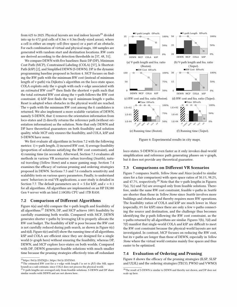
from 625 to 2025. Physical layouts are real indoor layouts25

divided

into up to 672 grid cells of 0.3m × 0.3m (body-sized areas), where

a cell is either an empty cell (free space) or a part of an obstacle.

For each combination of virtual and physical maps, 100 samples are

generated with random start and destination locations. RW costs

are derived according to the detection thresholds in [37, 48, 51].

We compare DEWNwith five baselines: Basic DP (DP), Minimum

Cost Path (MCP), Constrained Labeling (COLA) [57], k-Shortest-

Path (kSP) [2], and Simplified DEWN (S-DEWN). DP is the dynamic

programming baseline proposed in Section 4. MCP focuses on find-

ing the RW path with the minimum RW cost (instead of minimum

length of v-path) via Dijkstra’s algorithm on the loco-state space.

COLA exploits only the v-graph with each v-edge associated with

an estimated RW cost26

then finds the shortest v-path such that

the total estimated RW cost along the v-path follows the RW cost

constraint. 4) kSP first finds the top-k minimum-length v-paths.

Reset is adopted when obstacles in the physical world are reached.

The v-path with the minimum RW cost among the k candidates is

returned. We also implement a more scalable variation of DEWN,

namely S-DEWN, that 1) removes the orientation information from

loco-states and 2) directly returns the reference path (without ori-

entation information) as the solution. Note that only DEWN and

DP have theoretical guarantees on both feasibility and solution

quality, while MCP only ensures the feasibility, and COLA, kSP and

S-DEWN have none.

We first evaluate all algorithms in Section 7.2 with the following

metrics: 1) v-path length, 2) incurred RW cost, 3) average feasibility

(proportion of solutions satisfying the RW cost constraint), and

4) running time (in seconds). Afterward, Section 7.3 evaluates all

methods in various VR scenarios: urban traveling (Seattle), natu-ral traveling (Yellow Stone) and a maze gaming map. Section 7.4

examines the efficacy of various pruning and ordering strategies

proposed in DEWN. Sections 7.5 and 7.6 conducts sensitivity and

scalability tests on various query parameters. Finally, to understand

users’ behaviors in real VR applications, a user study is detailed in

Section 7.7. The default parameters are k = 5 for kSP, and ϵ = 0.1

for all algorithms. All algorithms are implemented on an HP DL580

Gen 9 server with an Intel 2.10GHz CPU and 1TB RAM.

7.2 Comparison of Different AlgorithmsFigure 6(a) and 6(b) compare the v-path length and feasibility of

all algorithms.27

DEWN, DP, and MCP achieve 100% feasibility by

carefully examining both worlds. Compared with MCP, DEWN

generates shorter v-paths by leveraging LR to properly allocate the

RW cost budget. The feasibility of kSP is poor because the RW cost

is not carefully reduced during path search, as shown in Figure 6(c)

and 6(d). Figure 6(e) and 6(f) show the running time of all algorithms.

kSP and COLA are efficient since they are designed for a single

world (v-graph here) without ensuring the feasibility, whereas DP,

DEWN, and MCP explore loco-states on both worlds. Compared

with DP, DEWN generates feasible solutions with much smaller

time because the pruning strategies effectively trim off redundant

25https://bit.ly/2DZXQLv, https://bit.ly/2DZXS65.

26The estimated RW cost for a v-edge with length l is set to β (l ) (the MIL upper

bound) as a safe estimate, since COLA does not process the physical world.

27V-path lengths are averaged only from feasible solutions. S-DEWN and DP share

similar results with DEWN and are not shown here.

(a) V-path length and fea. ratio

(Boston).(b) V-path length and fea. ratio

(Taipei).

(c) RW cost and fea. ratio (Boston). (d) RW cost and fea. ratio (Taipei).

(e) Running time (Boston). (f) Running time (Taipei).

Figure 6: Experimental results in city maps.

loco-states. S-DEWN is even faster as it only invokes dual-world

simplification and reference path generating phases on v-graph,

but it does not provide any theoretical guarantee.

7.3 Comparisons on Different VR ScenariosFigure 7 compares Seattle, Yellow Stone and Maze (scaled to similar

sizes for a fair comparison) with open space ratios of 50.1%, 98.2%,

and 47.7%, respectively.28

Note that the v-path lengths in Figures

7(a), 7(c) and 7(e) are averaged only from feasible solutions. There-

fore, under the same RW cost constraint, feasible v-paths in Seattleare shorter than those in Yellow Stone since Seattle involves more

buildings and obstacles and thereby requires more RW operations.

The feasibility ratios of COLA and kSP are much lower in Maze(especially, 0% for kSP) since there are only a few v-paths connect-

ing the source and destination, and the challenge thus becomes

identifying the p-path following the RW cost constraint, as the

v-paths returned by all algorithms are similar. Figures 7(b), 7(d) and

7(f) manifest that single-world COLA and kSP are difficult to meet

the RW cost constraint because the physical-world layouts are not

investigated. In contrast, MCP focuses on reducing the RW cost,

but its v-paths are longer than those of DEWN, especially in YellowStone where the virtual world contains mainly free spaces and thus

easier to be optimized.

7.4 Evaluation of Ordering and PruningFigure 8 shows the efficacy of the pruning strategies (ILSP, SLSP

and ULSL) and the ordering strategies (TECO, PWSO and VWNO)

28The result of S-DEWN is similar to DEWN and thereby not shown, and DP does not

scale up here.

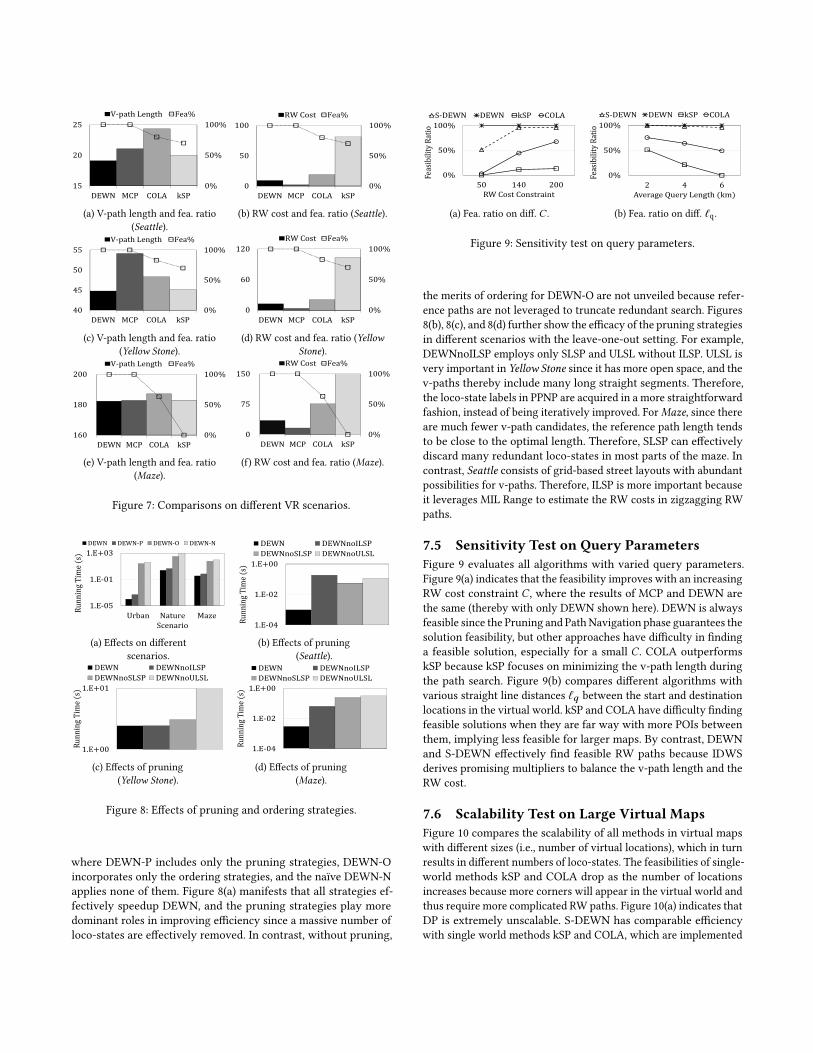
(a) V-path length and fea. ratio

(Seattle).(b) RW cost and fea. ratio (Seattle).

(c) V-path length and fea. ratio

(Yellow Stone).(d) RW cost and fea. ratio (Yellow

Stone).

(e) V-path length and fea. ratio

(Maze).(f) RW cost and fea. ratio (Maze).

Figure 7: Comparisons on different VR scenarios.

(a) Effects on different

scenarios.

(b) Effects of pruning

(Seattle).

(c) Effects of pruning

(Yellow Stone).(d) Effects of pruning

(Maze).

Figure 8: Effects of pruning and ordering strategies.

where DEWN-P includes only the pruning strategies, DEWN-O

incorporates only the ordering strategies, and the naïve DEWN-N

applies none of them. Figure 8(a) manifests that all strategies ef-

fectively speedup DEWN, and the pruning strategies play more

dominant roles in improving efficiency since a massive number of

loco-states are effectively removed. In contrast, without pruning,

0%

50%

100%

50 140 200

Feas

ibili

ty R

atio

RW Cost Constraint

S-DEWN DEWN kSP COLA

(a) Fea. ratio on diff. C .

0%

50%

100%

2 4 6

Feas

ibili

ty R

atio

Average Query Length (km)

S-DEWN DEWN kSP COLA

(b) Fea. ratio on diff. ℓq.

Figure 9: Sensitivity test on query parameters.

the merits of ordering for DEWN-O are not unveiled because refer-

ence paths are not leveraged to truncate redundant search. Figures

8(b), 8(c), and 8(d) further show the efficacy of the pruning strategies

in different scenarios with the leave-one-out setting. For example,

DEWNnoILSP employs only SLSP and ULSL without ILSP. ULSL is

very important in Yellow Stone since it has more open space, and the

v-paths thereby include many long straight segments. Therefore,

the loco-state labels in PPNP are acquired in a more straightforward

fashion, instead of being iteratively improved. ForMaze, since thereare much fewer v-path candidates, the reference path length tends

to be close to the optimal length. Therefore, SLSP can effectively

discard many redundant loco-states in most parts of the maze. In

contrast, Seattle consists of grid-based street layouts with abundant

possibilities for v-paths. Therefore, ILSP is more important because

it leverages MIL Range to estimate the RW costs in zigzagging RW

paths.

7.5 Sensitivity Test on Query ParametersFigure 9 evaluates all algorithms with varied query parameters.

Figure 9(a) indicates that the feasibility improves with an increasing

RW cost constraint C , where the results of MCP and DEWN are

the same (thereby with only DEWN shown here). DEWN is always

feasible since the Pruning and Path Navigation phase guarantees the

solution feasibility, but other approaches have difficulty in finding

a feasible solution, especially for a small C . COLA outperforms

kSP because kSP focuses on minimizing the v-path length during

the path search. Figure 9(b) compares different algorithms with

various straight line distances ℓq between the start and destination

locations in the virtual world. kSP and COLA have difficulty finding

feasible solutions when they are far way with more POIs between

them, implying less feasible for larger maps. By contrast, DEWN

and S-DEWN effectively find feasible RW paths because IDWS

derives promising multipliers to balance the v-path length and the

RW cost.

7.6 Scalability Test on Large Virtual MapsFigure 10 compares the scalability of all methods in virtual maps

with different sizes (i.e., number of virtual locations), which in turn

results in different numbers of loco-states. The feasibilities of single-

world methods kSP and COLA drop as the number of locations

increases because more corners will appear in the virtual world and

thus require more complicated RW paths. Figure 10(a) indicates that

DP is extremely unscalable. S-DEWN has comparable efficiency

with single world methods kSP and COLA, which are implemented

1.E-03

1.E+00

1.E+03

7.1E+03 8.1E+05 1.4E+08Com

pu

tati

on T

ime

(s)

# of loco-states

S-DEWN DEWN Basic DP

MCP kSP COLA

(a) Efficiency on diff. maps.

0%

50%

100%

7.1E+03 8.1E+05 1.4E+08Feas

ibili

ty r

atio

# of loco-states

S-DEWN DEWN kSP COLA

(b) Fea. ratio on diff. maps.

Figure 10: Scalability test on large virtual maps.

with specialized index structures. In regards to feasibility, S-DEWN

and DEWN consistently outperforms single world methods.

7.7 User StudyWe conduct a user study to understand users’ behaviors while

they walk along paths returned by different algorithms in a VR

maze, built by Unity 2017.3.1f1 and SteamVR Plugin 1.2.2, for users

wearing hTC VIVE HMD. The VE is a 3D Pac-man arcade game im-

plemented like [9] but incorporated with real walking experience,

where users are navigated along precomputed RW paths. Following

the user-study setting of VR in Computer Graphics and HCI re-

search [5, 7, 17], we recruited 30 users to test our developed system

and provide feedback on immersion according to Presence Ques-

tionnaire [5], including important questions such as “How much

are your experiences in the virtual environment consistent with

your real-world experiences?” We also measure the dizziness ac-

cording to Simulator Sickness Questionnaire (SSQ), which evaluates

symptoms such as headaches, vertigo, and nausea, and is widely

used in measuring motion sickness in VR applications [17, 35].

The experiment is described to the users as a single-user VR

arcade game similar to the classical Pac-Man. Users are asked to

actually walk along predefined paths in the virtual world and touch

red reward pellets along the path in order to collect game points.

The specified path is shown as a sequence of blue guide wires. The

reward pellets actually play the role of anchor points; we update

the user’s location information when the device detects the user

“touching” the cube, and apply different RW operation gains accord-

ingly. Every user experiences multiple paths that vary in both total

length, total RW cost, kinds of used RW operations, and also the

virtual environment. We ask the users to provide feedback after

finishing each path.

An example of the virtual and physical worlds is shown in Figure

11(a) and 11(b), respectively. The virtual world is a maze environ-

ment while the physical world is an office equipped with two VIVE

Lighthouse tracking base stations in the corners. The numbers rep-

resent the sequence of states in v-path and p-path of the example,

where S and T are the start and destination locations, respectively.

The Rotation, Reset, and Translation operations are labeled as yel-

low stars, green triangles, and red lines, respectively. No RW opera-

tion is involved for the white circles and blue lines in this example.

Figure 11(c) compares the average immersion scores of DEWN,

COLA, and kSP. DEWN outperforms kSP and COLA because it

allows the users to follow the path with fewer and smoother RW

operations. Figure 11(d) presents the average immersion scores of

(a) A v-path in the maze environment.

S

1 2

34 56

7

9T

8

(b) A p-path.

(c) Effects on diff. methods.

2

4

6

1x 1.5x 2x

Aver

age S

core

Cost Constraint

Immersion Dizziness

(d) Effects on C .

Figure 11: Results of user study.

DEWN with different RW cost constraints. As C grows, the immer-

sion slightly decreases with dizziness growing. However, according

to user feedback, 93.5% of the users are upset with kSP because

it involves many Reset operations, and users almost bump into

physical obstacles before RW operations are performed because the

physical layout is not processed during the path search. All user

recognizes that the RW operations in DEWN are much smoother

for them.

8 CONCLUSIONTo the best of our knowledge, there exists no prior research that fully

supports simultaneous movements in dual worlds for immersive

user experience in VR. In this paper, we leverage RedirectedWalking

(RW) to formulate DROP, aiming to find the shortest-distance path

in the virtual world, while constraining the RW cost to ensure

immersive experience. Based on the idea of MIL Range, we design

DEWN and propose various ordering and pruning strategies for

efficient processing of DROP. Afterward, we show that the existing

spatial query algorithms and index structures can leverage DEWN

as a building block to support kNN and range queries in the dual

worlds of VR. Experimental results and a user study manifest that

DEWN can effectively find shorter v-paths with smoother RW

operations compared with the baselines in various VR scenarios.

ACKNOWLEDGMENTSThis work is supported in part by MOST in Taiwan through grant

107-2221-E-001-011-MY3.

REFERENCES[1] Tenindra Abeywickrama, Muhammad Aamir Cheema, and David Taniar. k-

nearest neighbors on road networks: A journey in experimentation and in-

memory implementation. PVLDB, 9(6):492–503, 2016.[2] Takuya Akiba, Takanori Hayashi, Nozomi Nori, Yoichi Iwata, and Yuichi Yoshida.

Efficient top-k shortest-path distance queries on large networks by pruned land-

mark labeling. In AAAI, pages 2–8, 2015.[3] Takuya Akiba, Yoichi Iwata, and Yuichi Yoshida. Fast exact shortest-path distance

queries on large networks by pruned landmark labeling. In ACM SIGMOD, pages349–360, 2013.

[4] Anika Anwar and Tanzima Hashem. Optimal obstructed sequenced route queries

in spatial databases. In EDBT, pages 522–525. OpenProceedings.org, 2017.[5] Mahdi Azmandian, Mark Hancock, Hrvoje Benko, Eyal Ofek, and Andrew D.

Wilson. Haptic retargeting: Dynamic repurposing of passive haptics for enhanced

virtual reality experiences. In CHI, pages 1968–1979. ACM, 2016.

[6] Evren Bozgeyikli, Andrew Raij, Srinivas Katkoori, and Rajiv V. Dubey. Point &

teleport locomotion technique for virtual reality. In CHI PLAY, pages 205–216.ACM, 2016.

[7] Haiwei Chen and Henry Fuchs. Supporting free walking in a large virtual

environment: imperceptible redirected walking with an immersive distractor. In

CGI, pages 22:1–22:6. ACM, 2017.

[8] Paolo Ciaccia, Marco Patella, and Pavel Zezula. M-tree: An efficient access

method for similarity search in metric spaces. In VLDB, pages 426–435. Morgan

Kaufmann, 1997.

[9] Daniel Clarke, Graham McGregor, Brianna Rubin, Jonathan Stanford, and

T. C. Nicholas Graham. Arcaid: Addressing situation awareness and simula-

tor sickness in a virtual reality pac-man game. In CHI PLAY (Companion), pages39–45. ACM, 2016.

[10] Daniel C. Cliburn, Stacy Rilea, David Parsons, Prakash Surya, and Jessica Semler.

The effects of teleportation on recollection of the structure of a virtual world. In

EGVE/ICAT/EuroVR, pages 117–120. Eurographics Association, 2009.[11] Mark de Berg, Otfried Cheong, Marc J. van Kreveld, and Mark H. Overmars.

Computational geometry: algorithms and applications, 3rd Edition. Springer, 2008.[12] Rina Dechter and Judea Pearl. Generalized best-first search strategies and the

optimality of A*. J. ACM, 32(3):505–536, 1985.

[13] Funda Ergün, Rakesh K. Sinha, and Lisa Zhang. An improved FPTAS for restricted

shortest path. Inf. Process. Lett., 83(5):287–291, 2002.[14] Marcus Goetz and Alexander Zipf. Formal definition of a user-adaptive and

length-optimal routing graph for complex indoor environments. Geo-spatialInformation Science, pages 119–128, 2011.

[15] Antonin Guttman. R-trees: A dynamic index structure for spatial searching. In

SIGMOD Conference, pages 47–57. ACM Press, 1984.

[16] Mohamed S. Hassan, Walid G. Aref, and Ahmed M. Aly. Graph indexing for

shortest-path finding over dynamic sub-graphs. In SIGMOD Conference, pages1183–1197. ACM, 2016.

[17] Eric Hodgson, Eric R. Bachmann, and Tyler Thrash. Performance of redirected

walking algorithms in a constrained virtual world. IEEE Trans. Vis. Comput.Graph., 20(4):579–587, 2014.

[18] Han-PangHuang and Shu YunChung. Dynamic visibility graph for path planning.

In IROS, pages 2813–2818. IEEE, 2004.[19] Alpár Jüttner, Balázs Szviatovszki, Ildikó Mécs, and Zsolt Rajkó. Lagrange relax-

ation based method for the QoS routing problem. In INFOCOM, pages 859–868.

IEEE, 2001.

[20] Marcelo Kallmann. Shortest paths with arbitrary clearance from navigation

meshes. In Symposium on Computer Animation, pages 159–168. EurographicsAssociation, 2010.

[21] Sanket Khanwalkar, Shonali Balakrishna, and Ramesh Jain. Exploration of large

image corpuses in virtual reality. In ACM Multimedia, pages 596–600. ACM, 2016.

[22] Sujeong Kim, Aniket Bera, Andrew Best, Rohan Chabra, and Dinesh Manocha.

Interactive and adaptive data-driven crowd simulation. In VR, pages 29–38. IEEEComputer Society, 2016.

[23] Manikanta Kotaru and Sachin Katti. Position tracking for virtual reality using

commodity wifi. In CVPR, pages 2671–2681. IEEE Computer Society, 2017.

[24] Andreas Kunz, Markus Zank, Morten Fjeld, and Thomas Nescher. Real walking

in virtual environments for factory planning and evaluation. Procedia Cirp,44:257–262, 2016.

[25] Eike Langbehn, Paul Lubos, Gerd Bruder, and Frank Steinicke. Application of

redirected walking in room-scale VR. In VR, pages 449–450. IEEE Computer

Society, 2017.

[26] Eike Langbehn, Paul Lubos, Gerd Bruder, and Frank Steinicke. Bending the curve:

Sensitivity to bending of curved paths and application in room-scale VR. IEEETrans. Vis. Comput. Graph., 23(4):1389–1398, 2017.

[27] Eike Langbehn, Paul Lubos, and Frank Steinicke. Evaluation of locomotion

techniques for room-scale VR: joystick, teleportation, and redirected walking. In

VRIC, pages 4:1–4:9. ACM, 2018.

[28] Ken C. K. Lee, Wang-Chien Lee, Baihua Zheng, and Yuan Tian. ROAD: A new

spatial object search framework for road networks. IEEE Trans. Knowl. Data Eng.,24(3):547–560, 2012.

[29] Ying Lu, Jiaheng Lu, Gao Cong, Wei Wu, and Cyrus Shahabi. Efficient algorithms

and cost models for reverse spatial-keyword k-nearest neighbor search. ACMTrans. Database Syst., 39(2):13:1–13:46, 2014.

[30] Pietro Lungaro, Rickard Sjöberg, Alfredo Fanghella Valero, Ashutosh Mittal, and

Konrad Tollmar. Gaze-aware streaming solutions for the next generation of

mobile VR experiences. IEEE Trans. Vis. Comput. Graph., 24(4):1535–1544, 2018.[31] Silvano Martello. Knapsack problems: algorithms and computer implementations.

John Wiley & Sons Ltd., 1990.

[32] Sebastian Marwecki, Maximilian Brehm, Lukas Wagner, Lung-Pan Cheng, Flo-

rian ’Floyd’ Mueller, and Patrick Baudisch. Virtualspace - overloading physical

space with multiple virtual reality users. In CHI, page 241. ACM, 2018.

[33] Ellips Masehian and M. R. Amin-Naseri. A voronoi diagram-visibility graph-

potential field compound algorithm for robot path planning. J. Field Robotics,21(6):275–300, 2004.

[34] Marcell Missura, Daniel D. Lee, and Maren Bennewitz. Minimal construct: Effi-

cient shortest path finding for mobile robots in polygonal maps. In IROS, pages7918–7923. IEEE, 2018.

[35] Christian T. Neth, Jan L. Souman, David Engel, Uwe Kloos, Heinrich H. Bülthoff,

and Betty J. Mohler. Velocity-dependent dynamic curvature gain for redirected

walking. IEEE Trans. Vis. Comput. Graph., 18(7):1041–1052, 2012.[36] Niels Christian Nilsson, Tabitha C. Peck, Gerd Bruder, Eri Hodgson, Stefania

Serafin, Mary C. Whitton, Frank Steinicke, and Evan Suma Rosenberg. 15 years

of research on redirected walking in immersive virtual environments. IEEEComputer Graphics and Applications, 38(2):44–56, 2018.

[37] Niels Christian Nilsson, Evan A. Suma, Rolf Nordahl, Mark T. Bolas, and Stefania

Serafin. Estimation of detection thresholds for audiovisual rotation gains. In VR,pages 241–242. IEEE Computer Society, 2016.

[38] Masaaki Nishino, Norihito Yasuda, Shin-ichi Minato, and Masaaki Nagata. Bdd-

constrained search: A unified approach to constrained shortest path problems.

In AAAI, pages 1219–1225. AAAI Press, 2015.[39] Dimitris Papadias, Jun Zhang, Nikos Mamoulis, and Yufei Tao. Query processing

in spatial network databases. In VLDB, pages 802–813. Morgan Kaufmann, 2003.

[40] Michalis Potamias, Francesco Bonchi, Carlos Castillo, and Aristides Gionis. Fast

shortest path distance estimation in large networks. In CIKM, pages 867–876.

ACM, 2009.

[41] Mores Prachyabrued and Christoph W. Borst. Design and evaluation of vi-

sual interpenetration cues in virtual grasping. IEEE Trans. Vis. Comput. Graph.,22(6):1718–1731, 2016.

[42] Miao Qiao, Hong Cheng, Lijun Chang, and Jeffrey Xu Yu. Approximate shortest

distance computing: A query-dependent local landmark scheme. IEEE Trans.Knowl. Data Eng., 26(1):55–68, 2014.

[43] Sharif Razzaque, David Swapp, Mel Slater, Mary C. Whitton, and Anthony Steed.

Redirected walking in place. In EGVE, pages 123–130. Eurographics Association,2002.

[44] Michael Rietzler, Jan Gugenheimer, Teresa Hirzle, Martin Deubzer, Eike Langbehn,

and Enrico Rukzio. Rethinking redirected walking: On the use of curvature gains

beyond perceptual limitations and revisiting bending gains. In ISMAR, pages115–122. IEEE, 2018.

[45] Philippe Rigaux, Michel Scholl, and Agnes Voisard. Spatial databases: withapplication to GIS. Elsevier, 2001.

[46] Roy A. Ruddle, Ekaterina P. Volkova, and Heinrich H. Bülthoff. Walking improves

your cognitive map in environments that are large-scale and large in extent. ACMTrans. Comput.-Hum. Interact., 18(2):10:1–10:20, 2011.

[47] Patric Schmitz, Julian Hildebrandt, André Calero Valdez, Leif Kobbelt, and Mar-

tina Ziefle. You spin my head right round: Threshold of limited immersion for

rotation gains in redirected walking. IEEE Trans. Vis. Comput. Graph., 24(4):1623–1632, 2018.

[48] Stefania Serafin, Niels C. Nilsson, Erik Sikström, Amalia de Götzen, and Rolf

Nordahl. Estimation of detection thresholds for acoustic based redirected walking

techniques. In VR, pages 161–162. IEEE Computer Society, 2013.

[49] Jongkyu Shin, Gwangseok An, Joon-Sang Park, Seung Jun Baek, and Kyogu Lee.

Application of precise indoor position tracking to immersive virtual reality with

translational movement support. Multimedia Tools Appl., 75(20):12331–12350,2016.

[50] Misha Sra. Asymmetric design approach and collision avoidance techniques for

room-scale multiplayer virtual reality. In UIST (Adjunct Volume), pages 29–32.ACM, 2016.

[51] Frank Steinicke, Gerd Bruder, Jason Jerald, Harald Frenz, and Markus Lappe.

Estimation of detection thresholds for redirected walking techniques. IEEE Trans.Vis. Comput. Graph., 16(1):17–27, 2010.

[52] Nusrat Sultana, TanzimaHashem, and Lars Kulik. Group nearest neighbor queries

in the presence of obstacles. In SIGSPATIAL/GIS, pages 481–484. ACM, 2014.

[53] Qi Sun, Anjul Patney, Li-Yi Wei, Omer Shapira, Jingwan Lu, Paul Asente, Suwen

Zhu, Morgan McGuire, David Luebke, and Arie E. Kaufman. Towards virtual real-

ity infinite walking: dynamic saccadic redirection. ACM Trans. Graph., 37(4):67:1–67:13, 2018.

[54] Yaping Sun, Zhiyong Chen, Meixia Tao, and Hui Liu. Communication, computing

and caching for mobile VR delivery: Modeling and trade-off. In ICC, pages 1–6.IEEE, 2018.

[55] Sam Tregillus, Majed Al Zayer, and Eelke Folmer. Handsfree omnidirectional VR

navigation using head tilt. In CHI, pages 4063–4068. ACM, 2017.

[56] Martin Usoh, Kevin Arthur, Mary C. Whitton, Rui Bastos, Anthony Steed, Mel

Slater, and Frederick P. Brooks Jr. Walking > walking-in-place > flying, in virtual

environments. In SIGGRAPH, pages 359–364. ACM, 1999.

[57] Sibo Wang, Xiaokui Xiao, Yin Yang, and Wenqing Lin. Effective indexing for

approximate constrained shortest path queries on large road networks. PVLDB,10(2):61–72, 2016.

[58] Betsy Williams, Gayathri Narasimham, Björn Rump, Timothy P. McNamara,

Thomas H. Carr, John J. Rieser, and Bobby Bodenheimer. Exploring large virtual

environments with an HMD when physical space is limited. In APGV, volume

253 of ACM International Conference Proceeding Series, pages 41–48. ACM, 2007.

[59] Graham A. Wilson, Mark McGill, Matthew Jamieson, Julie R. Williamson, and

Stephen A. Brewster. Object manipulation in virtual reality under increasing

levels of translational gain. In CHI, page 99. ACM, 2018.

[60] Jun Zhang, Dimitris Papadias, Kyriakos Mouratidis, and Manli Zhu. Spatial

queries in the presence of obstacles. In EDBT, volume 2992 of Lecture Notes inComputer Science, pages 366–384. Springer, 2004.

[61] Yang Zhang, Chouchang (Jack) Yang, Scott E. Hudson, Chris Harrison, and

Alanson P. Sample. Wall++: Room-scale interactive and context-aware sensing.

In CHI, page 273. ACM, 2018.

[62] Huaijie Zhu, Xiaochun Yang, Bin Wang, and Wang-Chien Lee. Range-based

obstructed nearest neighbor queries. In SIGMOD Conference, pages 2053–2068.ACM, 2016.

A DEFINITIONS OF RW OPERATIONSWithout loss of generality, when a user moves in the virtual

world, it is assumed that the user first changes her orientation

and then walks a straight step afterward. Given the walking length

ℓ of a user, the transition function from the previous loco-state

stn−1 = ((γ vn−1,θv

n−1), (γp

n−1,θp

n−1)) to the next loco-state stn =

((γ vn ,θvn ), (γp

n ,θp

n )) after walking a step is calculated as follows:

θp

n = θp

n−1 + △θ

θvn = θv

n−1 + △θ

γp

n = γp

n−1 + ℓ × [cos(θp

n ), sin(θp

n )]T

γ vn = γv

n−1 + ℓ × [cos(θv

n ), sin(θvn )]T

where △θ is the orientation difference between two loco-states.

Definition 7. Translation Gain (mT). When a Translation Opera-

tion (Translation) is applied into an HMD, the change in the transi-

tion function is

γ vn = γv

n−1 + ℓ ×mT × [cos(θvn ), sin(θvn )]⊺.

In otherwords, when a userwalks an ℓ-length step in the physical

world, she walks an (ℓ ×mT)-length step in the virtual world, and

mT is the translation gain.

Definition 8. Rotation Gain (mR). The Rotation Operation (RO)

manipulates the rotation speed in a VE when a user is turning into

another direction, so that the rotation speeds in two worlds can be

slightly different. The virtual orientation of the transition function

becomes

θvn = θv

n−1 +mR × △θwheremR is the rotation gain applied to an HMD.

Definition 9. Curvature Gain (mC). When a user walks straight

in the virtual world, the Curvature Operation (CO) allows her to

walk along a curve in the physical world. The physical orientation

and position of the transition function are changed as follows.

θp

n = θp

n−1 +mC × ℓ

γp

n = γp

n−1 +1

mC

×[sin(θpn +mC × ℓ) − sin(θ

p

n )cos(θpn ) − cos(θ

p

n +mC × ℓ),

]wheremC is the curvature gain applied to an HMD.

Definition 10. Reset turning angle (θReset.) Sometimes the Resetoperation (Reset) is required to explicitly ask the user to turn in a

different direction in the physical world (but remains in the same

direction in the VR world) in order to avoid the physical walls

or obstacles. It is expected that Reset usually incurs a higher cost

since it interrupts the user experience in the VR world. Given the

Reset turning angle θReset, a user is asked to turn θReset in her cur-

rent physical position, but the image display in the VR world is

suspended during the turning. Therefore,

θp

n = θp

n−1 + θReset.

While the above sets of transition functions represent the ba-

sic RW operations, one can define other transition functions to

abstract other implementations of VR locomotion techniques, e.g.,

teleportation, where the user determines the next v-state, and the

p-state remains unchanged. Thus, the notion of transition functions

is general.

B COST MODEL APPROACHESHere we briefly discuss several possible approaches to setup the cost

model for RW operations. This cost model can be viewed as a cost

function CRW(op, z) that takes both the type of the RW operation

op and the usage magnitude z and maps to a positive RW cost

CRW(op, z), where z ismT for Translation,mR for RO,mC for CO,

and θReset for Reset.

• Usage Count. Using any RW operation op incurs an RW

cost of 1 unit, regardless of the magnitude z and type of op.Thus, CRW(op, z) = 1 for all op and z.• Detection Likelihood. When an RW operation op is ap-

plied with a specific magnitude z, it incurs an RW cost pro-

portional to the likelihood that it is detected by an aver-

age user. For example, according to [48], a Translation with

mT = 0.6, i.e., down-scaling the walking distance by 40%,

has a roughly 90% chance to be detected by the users. Thus,

CRW(Translation, 0.6) = 0.9.

• Detection Threshold.When an RW operation op is appliedwith a specific magnitude z, if z is in the non-detectable re-

gion, e.g., z = mR ∈ (0.77, 1.10) for no-audio RO in [37],

CRW(op, z) = 0, indicating the user does not feel the modifi-

cation, and CRW(op, z) = 1 for all other values of z.• Other Threshold. The detection thresholds used above can

be changed to any other variations of threshold of RW oper-

ations, e.g., perception, applicability, or immersion thresholds

in [44].

• Reset Cost. Since Reset directly interrupts the user ex-

perience, it is not meaningful to quantify the detection-

based cost for it. Instead, a possible approach is to set

CRW(Reset, z) = cReset for some constant cost cReset for allz , 0 to represent the inconvenience and degradation of

immersion experienced by the user. Another possibility is to

consider the angle that the user is asked to rotate in Reset,

e.g., CRW(Reset, z) = cReset · |z |180, where z ∈ (−180, 180] is

the reset turning angle.

Note that in any cost model, CRW(op, z) = 0 for z = mT = 1

for Translation, z = mR = 1 for RO, z = mC = 0 for CO, and

(a) Feasibility ratio.

0

25

50

0 3 6 9

V-p

ath

Leng

th

Reset Cost unit

DEWN MCP kSP COLA

(b) V-path length.

Figure 12: Experimental results on diff. cReset.

z = θReset = 0 for Reset, since these values corresponds to no RW

operations, i.e., the movements in the dual worlds are aligned.

For walking operations, i.e., Translation and CO, it is also applica-ble to further weight the RW cost by the total walking distance that

the user is under the given RW operation. In other words, given opand z, the total RW cost of the user walks under op for a distance of

ℓ isCRW(op, z) · ℓ. RO and Reset only affects the turning movement

and do not need to be weighted.

C EXPERIMENTAL RESULTS ON COSTMODEL

Figure 12 reports the experimental results for the detection thresh-

old cost model with different values of cReset, where the query

distances (distance between start and destination locations) are

randomly distributed from 0 to 100, and the cost constraint is set

to 10. The feasibility ratios are shown in Figure 12(a). MCP and DP

share similar results (i.e., 100% feasibility) with DEWN and thus

are not shown here. All methods are 100% feasible when cReset = 0,

i.e., Reset is free, as it becomes feasible to abuse Reset to steer the

user away from obstacles and boundaries in the physical world. As

cReset increases, the feasibility ratio of kSP is significantly affected

as it relies on Reset as its only way to align the dual worlds. The

feasibility ratio of COLA also significantly decreases as cReset be-comes nonzero. However, as cReset grows large, Reset is less likelyto be used in the RW operation configuration corresponding to the

MIL values. Thus, the MIL Ranges are narrower, and the MIL upper

bound values become more accurate in reflecting the total MIL

values. Therefore, the feasibility ratio of COLA slightly improves

as cReset grows.Figure 12(b) reports the average feasible v-path lengths. All

queries are feasible when cReset = 0. As cReset grows, DROP queries

with longer query distances become infeasible as Reset becomes

costly. However, the feasibility of query instances becomes stable

after cReset becomes sufficiently large (around cReset = 6). Since

the feasible solutions do not rely on Reset when cReset is large,continuing to increase cReset does not affect the instance feasibility.