Structural Analaysis: A Tool for Testing 3D Computer Reconstructions of Thule Whalebone Houses
Upload
khangminh22Category
view
4download
0


We barely rememberWho or what came before
This precious momentChoosing to be here
Right nowHold on, stay inside
This bodyHolding me
Reminding me that I am not alone inThis body
Makes me feel eternalAll this pain is an illusion
- Maynard James Keenan


To my family– old and new


Acknowledgements
I didn’t plan to become a PhD student. As a matter of fact, for the better part ofmy youth, my main interest in computers was enjoying a couple of hours withgood friends in front of a compelling adventure game, like The Bard’s Tale orThe Last Ninja. As we threw a smoke grenade, conjured a mighty lightningbolt or slained a few Hydras, I never pondered on the amount of skill anddedication that it must have taken to design, develop, and test a commerciallysuccessful computer game. However, as life goes, a random set of events (Iactually did not realize that my taking a masters in Information Technologyat Uppsala University would require me to learn how to write a program), adeep fascination for mathematics, and a heart-felt respect for the competence,dedication and independence of great scientists somehow landed me a PhDcandidate position at Malardalen University.
One of the best things of writing a thesis is that you are allowed to fill anentire section (probably the most read one, too) with nice words about peoplewhose support you highly value and appreciate, without you actually feelingawkward about it. So, here it goes. First, I owe a major thank you to mysupervisors Henrik Thane, Andreas Ermedahl, and Hans Hansson. Henrik, youare a brilliant visionary, and unfortunately also eloquent to the the degree that itoften takes me several hours to realize that I don’t understand what you mean.Andreas, you are supportive, devoted and enthusiastic, and I truly believe thatthis thesis wouldn’t have been finished if it was not for your efforts. Hans,you are pragmatic, outspoken, and amazingly easy-going. Had it not been foryou being so polite, I would have thought of you as the Gordon Ramsay ofreal-time system research, clearly competent within your field, but even morecompetent in facilitating activites in your field for others. You all make up asplendid mix!
Also, although not given formal credit for this, I feel that Jukka Maki-Turja,Mikael Nolin, and Sasikumar Punnekkat deserve a recognition for the de facto
v

vi
co-supervision they have provided during strategic stages through my studies.Sometimes, a pat on the back or an encouraging word is worth much more thantwenty pages of detailed comments on the latest article.
Next, I don’t think there are many department colleagues I haven’t both-ered with various questions regarding countless topics, ranging from weddingtable seating, publication strategy and very formal takes on program analysis.Thanks for being friendly and supportive all along! I however feel that some ofyou deserve a special mention. Anders Pettersson, my roommate, PhD studentcolleague, and primary recepient for general everyday whining. If it wasn’t foryou, I probably wouldn’t have finished in a year from now. I would like tothank Thomas Nolte for being a true inspiration and a good friend at best, andan annoying wiseacre at worst, constantly quering me of which decade i plan topresent my thesis in. Well, Thomas, the moment is here! Furthermore, MarkusLindgren, thanks a lot for providing that unique atmosphere of support, an un-compromised professionalism, and an infinite series of totally pointless MSNwinks. Also, I would like to thank Anders Moller for being a great travelingcompanion and for teaching me about the boredom of long-distance flight clearair turbulence.
In addition to the above, there are many department colleagues whose pathof everyday work periodically seem to cross my own, and whose companion-ship I highly appreciate. These include (but are not restricted to) Lars Asplund,Mats Bjorkman, Per Branger, Stefan Bygde, Jan Carlson, Ivica Crnkovic, RaduDobrin, Gordana Dodig-Crnkovic, Harriet Ekwall, Sigrid Eldh, Cecilia Fern-strom, Johan Fredriksson, Joakim Froberg, Jan Gustafsson, Ewa Hansen, An-dreas Hjertstrom, Joel Huselius, Damir Isovic, Helena Jerregard, Johan Kraft,Rikard Land, Stig Larsson, Jorgen Lidholm, Maria Linden, Bjorn Lisper, AsaLundqvist, Jonas Neander, Christer Norstrom, Dag Nystrom, Hongyu Pei-Breivold, Paul Pettersson, Ingemar Reyier, Larisa Rizvanovic, Christer Sand-berg, Anders Wall, Peter Wallin, Monica Wasell, and Gunnar Widforss.
Not surprisingly, I was not able to keep my nose out of the inner workingsof the University organisation. In this context, I would like to thank my fellowPhD student council members, and my colleagues from the three years I spenton the Faculty Board of Natural Sciences and Technology (naturally includingthe members of the UFO staff, who are doing a massive work “backstage”).
I still owe a major thank you to my main lab-partner during my years asan undergraduate in Uppsala – Mattias Sjogren. Besides from being a goodcomrade, you gave me the first impression of what it means to be a skilledprogrammer.
It also seems impossible to thank anyone without thanking the notoriusly

vii
supportive team of Grabbarna Grus – the foie gras or white truffle version ofchildhood friends: Anders, David, Kristoffer, Magnus, and Robert. I actuallytotalled over 7000 mails from you during the course of my PhD studies, av-eraging nearly 3.5 mails per day (including weekends and vacations). Thankyou also to Ammi, Helena, Malin and Petra for all amazing parties and travels.We’ve had great fun – I accept nothing less than to keep it up!
To my mother, father and sister – I can not enough stress how importantyour support has been to me. It means the world to have a number of peoplewhose appreciation of you is utterly uncorrelated with the acceptance of yourlatest article. This naturally also goes for Niclas, Malin, Janne, Gittan, Micke,Farmor, Barbro, Sigurd, Helene, Calle, Victoria, and Lovisa. Thank you!
Finally, Kristina, my beautiful wife. Thank you for being there, for beingyou, and for getting the daily routines working when I was so busy I didn’teven notice you did. I love you. You make me proud!
This work has been supported by the KK Foundation (KKS) and Malar-dalen University.
Tack ska ni alla ha!
Vasteras, September 2007Karl Daniel Sundmark


Contents
Contents ix
List of Publications xii
1 Introduction 11.1 Background . . . . . . . . . . . . . . . . . . . . . . . . . . . 3
1.1.1 Software Testing . . . . . . . . . . . . . . . . . . . . 31.1.2 Concurrent Real-Time System Testing . . . . . . . . . 9
1.2 System Model . . . . . . . . . . . . . . . . . . . . . . . . . . 141.3 Problem Formulation and Hypothesis . . . . . . . . . . . . . 151.4 Contributions . . . . . . . . . . . . . . . . . . . . . . . . . . 161.5 Thesis Outline . . . . . . . . . . . . . . . . . . . . . . . . . . 17
2 Structural Test Criteria for System-Level RTS Testing 192.1 Structural Test Criteria . . . . . . . . . . . . . . . . . . . . . 19
2.1.1 Control Flow Criteria . . . . . . . . . . . . . . . . . . 222.1.2 Data Flow Criteria . . . . . . . . . . . . . . . . . . . 252.1.3 Useful and Non-Useful Criteria . . . . . . . . . . . . 272.1.4 Structural Coverage Criteria Summary . . . . . . . . . 292.1.5 A Note on Feasibility . . . . . . . . . . . . . . . . . . 29
2.2 Structural Test Items . . . . . . . . . . . . . . . . . . . . . . 302.2.1 Sets of Test Items . . . . . . . . . . . . . . . . . . . . 30
2.3 Summary . . . . . . . . . . . . . . . . . . . . . . . . . . . . 34
3 Deriving DU-paths for RTS System-Level Testing 373.1 Introduction . . . . . . . . . . . . . . . . . . . . . . . . . . . 37
3.1.1 General Analysis Properties . . . . . . . . . . . . . . 383.2 Approach 1: Deriving DU-paths using UPPAAL and COXER . 41
ix

x Contents
3.2.1 Preliminaries . . . . . . . . . . . . . . . . . . . . . . 413.2.2 RTS Control Flow Modeling in UPPAAL . . . . . . . 433.2.3 Automatic System Model Generation using SWEET . 453.2.4 Deriving ModelDU (MS) using COXER . . . . . . . 46
3.3 Approach 2: DU-path derivation using EOGs . . . . . . . . . 473.3.1 Preliminaries . . . . . . . . . . . . . . . . . . . . . . 473.3.2 Shared Variable DU Analysis . . . . . . . . . . . . . 493.3.3 Deriving ModelDU (MS) using EOGs . . . . . . . . . 53
3.4 Discussion . . . . . . . . . . . . . . . . . . . . . . . . . . . . 53
4 Test Item Monitoring Using Deterministic Replay 614.1 Introduction . . . . . . . . . . . . . . . . . . . . . . . . . . . 63
4.1.1 The Probe Effect . . . . . . . . . . . . . . . . . . . . 644.1.2 Deterministic Replay . . . . . . . . . . . . . . . . . . 65
4.2 Deterministic Replay DU-path Monitoring . . . . . . . . . . . 664.3 Reproducibility . . . . . . . . . . . . . . . . . . . . . . . . . 68
4.3.1 Context Issues . . . . . . . . . . . . . . . . . . . . . 684.3.2 Ordering Issues and Concurrency . . . . . . . . . . . 694.3.3 Timing Issues . . . . . . . . . . . . . . . . . . . . . . 704.3.4 Reproducibility - Summary and Problem Statement . . 72
4.4 The Time Machine . . . . . . . . . . . . . . . . . . . . . . . 744.4.1 System Model Refinements . . . . . . . . . . . . . . 744.4.2 The Mechanisms of the Time Machine . . . . . . . . . 744.4.3 Deterministic Replay Summary . . . . . . . . . . . . 80
4.5 Discussion . . . . . . . . . . . . . . . . . . . . . . . . . . . . 81
5 System-Level DU-path Coverage – An Example 835.1 The Process . . . . . . . . . . . . . . . . . . . . . . . . . . . 835.2 The Example System . . . . . . . . . . . . . . . . . . . . . . 84
5.2.1 Example System Structure . . . . . . . . . . . . . . . 855.2.2 System Replay Instrumentation . . . . . . . . . . . . 86
5.3 DU-path Analysis . . . . . . . . . . . . . . . . . . . . . . . . 875.3.1 Task-Level Analysis . . . . . . . . . . . . . . . . . . 885.3.2 Deriving DU-paths using UPPAAL and COXER . . . 895.3.3 Deriving DU-paths using EOGs . . . . . . . . . . . . 90
5.4 System Testing . . . . . . . . . . . . . . . . . . . . . . . . . 905.4.1 Initial Testing . . . . . . . . . . . . . . . . . . . . . . 925.4.2 Replaying Test Cases . . . . . . . . . . . . . . . . . . 92
5.5 Summary . . . . . . . . . . . . . . . . . . . . . . . . . . . . 93

Contents xi
6 Evaluation 956.1 Test Item Derivation Methods . . . . . . . . . . . . . . . . . 95
6.1.1 Experimental Systems . . . . . . . . . . . . . . . . . 966.1.2 UPPAAL-based Test Item Derivation . . . . . . . . . . 976.1.3 EOG-Based Test Item Derivation . . . . . . . . . . . 986.1.4 Test Item Derivation Evaluation Discussion . . . . . . 1006.1.5 Evaluation Extension: The Impacts of Varying Execu-
tion Time Jitter . . . . . . . . . . . . . . . . . . . . . 1016.2 Time Machine Case Studies . . . . . . . . . . . . . . . . . . 104
6.2.1 Introduction . . . . . . . . . . . . . . . . . . . . . . . 1056.2.2 Implementing The Recorder . . . . . . . . . . . . . . 1066.2.3 Implementing The Historian . . . . . . . . . . . . . . 1086.2.4 Implementing The Time Traveler . . . . . . . . . . . 1136.2.5 IDE Integration . . . . . . . . . . . . . . . . . . . . . 1146.2.6 Instrumentation Load . . . . . . . . . . . . . . . . . . 1166.2.7 Time Machine Case Studies Discussion . . . . . . . . 117
6.3 Checksums . . . . . . . . . . . . . . . . . . . . . . . . . . . 1196.3.1 Approximation Accuracy . . . . . . . . . . . . . . . . 1206.3.2 Perturbation . . . . . . . . . . . . . . . . . . . . . . . 1226.3.3 Checksum Evaluation Discussion . . . . . . . . . . . 123
6.4 Summary . . . . . . . . . . . . . . . . . . . . . . . . . . . . 124
7 Related Work 1257.1 Structural Testing . . . . . . . . . . . . . . . . . . . . . . . . 125
7.1.1 Concurrent Systems Structural Testing . . . . . . . . . 1267.1.2 Preemptive RTS Structural Testing . . . . . . . . . . . 1267.1.3 Program Analysis for Concurrent System Testing . . . 1277.1.4 Race Detection . . . . . . . . . . . . . . . . . . . . . 1277.1.5 Model-Based Testing . . . . . . . . . . . . . . . . . . 1287.1.6 Relation to Our Work . . . . . . . . . . . . . . . . . . 129
7.2 Monitoring for Testing . . . . . . . . . . . . . . . . . . . . . 1307.2.1 Monitoring using Execution Replay . . . . . . . . . . 1317.2.2 Hybrid and Hardware-Based Monitoring . . . . . . . 1347.2.3 Relation to Our Work . . . . . . . . . . . . . . . . . . 135
8 Discussion, Conclusion and Future Work 1378.1 Summary . . . . . . . . . . . . . . . . . . . . . . . . . . . . 1378.2 Discussion . . . . . . . . . . . . . . . . . . . . . . . . . . . . 138
8.2.1 Research Hypotheses Revisited . . . . . . . . . . . . 139

xii Contents
8.2.2 System model . . . . . . . . . . . . . . . . . . . . . . 1398.2.3 Test Item Derivation Method Applicability . . . . . . 1408.2.4 Handling Infeasible Test Items . . . . . . . . . . . . . 1408.2.5 Approximative Checksums . . . . . . . . . . . . . . . 141
8.3 Future Work . . . . . . . . . . . . . . . . . . . . . . . . . . . 1418.3.1 Structural System-Level Test Case Generation . . . . . 1428.3.2 Checksum Unique Marker Precision . . . . . . . . . . 1428.3.3 Facilitating Sporadic Tasks through Servers . . . . . . 1428.3.4 Expressing Flow Facts in UPPAAL . . . . . . . . . . 1438.3.5 Regression Testing . . . . . . . . . . . . . . . . . . . 143
A Timed Automata Test Item Derivation 147A.1 Timed Control Flow Modeling using UPPAAL . . . . . . . . . 147
A.1.1 Clocks . . . . . . . . . . . . . . . . . . . . . . . . . 148A.1.2 Task CFG modeling . . . . . . . . . . . . . . . . . . 149A.1.3 Modeling of Task Execution Control . . . . . . . . . . 153A.1.4 FPS Scheduler and Task Switch Modeling . . . . . . . 154
B The DUANALYSIS Algorithm 159
C Reproduction of Asynchronous Events 165C.1 Context Checksums . . . . . . . . . . . . . . . . . . . . . . . 165
C.1.1 Execution Context . . . . . . . . . . . . . . . . . . . 166C.1.2 Register Checksum . . . . . . . . . . . . . . . . . . . 166C.1.3 Stack Checksum . . . . . . . . . . . . . . . . . . . . 167
C.2 Adaptations . . . . . . . . . . . . . . . . . . . . . . . . . . . 168C.2.1 Instrumentation Jitter . . . . . . . . . . . . . . . . . . 168C.2.2 Partial Stack Checksum . . . . . . . . . . . . . . . . 169C.2.3 System call markers . . . . . . . . . . . . . . . . . . 170
Bibliography 171

List of Publications
These publications have been (co-)authored by the author of this thesis:
Publications Related to This ThesisA. Debugging the Asterix Framework by Deterministic Replay and Simula-
tion, Daniel Sundmark, Master Thesis, Uppsala University, May 2002.My contribution: I am the sole author of this thesis.
B. Replay Debugging of Real-Time Systems Using Time Machines, Hen-rik Thane, Daniel Sundmark, Joel Huselius, and Anders Pettersson, InProceedings of the 1st Workshop on Parallel and Distributed Systems:Testing and Debugging (PADTAD), April 2003.My contribution: This paper was a joint effort. I wrote the sectiondiscussing the Time Machine.
C. Starting Conditions for Post-Mortem Debugging using Deterministic Re-play of Real-Time Systems, Joel Huselius, Daniel Sundmark and HenrikThane, In Proceedings of the 15th Euromicro Conference on Real-TimeSystems (ECRTS), July 2003.My contribution: This paper was a joint effort. I wrote the sectiondiscussing the Implementation, and parts of the Introduction.
D. Replay Debugging of Complex Real-Time Systems: Experiences fromTwo Industrial Case Studies, Daniel Sundmark, Henrik Thane, Joel Huse-lius, Anders Pettersson, Roger Mellander, Ingemar Reiyer, and MattiasKallvi, In Proceedings of the 5th International Workshop Automated andAlgorithmic Debugging (AADEBUG), September 2003.My contribution: I am the main author of this paper, even though thecase studies described were joint efforts between all authors.
xiii

xiv Contents
E. Replay Debugging of Embedded Real-Time Systems: A State of the ArtReport, Daniel Sundmark, MRTC report ISSN 1404-3041 ISRN MDH-MRTC-156/2004-1-SE, Malardalen Real-Time Research Centre, Malar-dalen University, February, 2004.My contribution: I am the sole author of this report.
F. Deterministic Replay Debugging of Embedded Real-Time Systems usingStandard Components, Licentiate thesis no. 24, ISSN 1651-9256, ISBN91-88834-35-2, Malardalen University, March 2004.My contribution: I am the sole author of this thesis.
G. Regression Testing of Multi-Tasking Real-Time Systems: A Problem State-ment, Daniel Sundmark, Anders Pettersson, Henrik Thane, In SIGBEDReview, vol 2, nr 2, ACM Press, March 2005.My contribution: This paper was written by me and Anders Pettersson,under supervision of Henrik Thane.
H. Shared Data Analysis for Multi-Tasking Real-Time Systems Testing, An-ders Pettersson, Daniel Sundmark, Henrik Thane, and Dag Nystrom, InProceedings of the 2nd IEEE International Symposium on Industrial Em-bedded Software (SIES), July 2007.My contribution: I took part in the discussions and wrote parts of thepaper, but Anders Pettersson was the main author.
I. Finding DU-Paths for Testing of Multi-Tasking Real-Time Systems usingWCET Analysis, Daniel Sundmark, Anders Pettersson, Christer Sand-berg, Andreas Ermedahl, and Henrik Thane, In Proceedings the of 7th In-ternational Workshop on Worst-Case Execution Time Analysis (WCET),July 2007.My contribution: I am the main author of this paper, and responsible forall parts of the paper except for the task-level shared variable analysis.
Other Publications1. Efficient System-Level Testing of Embedded Real-Time Software, Daniel
Sundmark, Anders Pettersson, Sigrid Eldh, Mathias Ekman, and HenrikThane, In Proceedings of the Work-in-Progress Session of the 17th Euro-micro Conference on Real-Time Systems (ECRTS), July 2005.My contribution: This paper was a joint effort, but I was the main au-thor.

Contents xv
2. Monitored Software Components - A Novel Software Engineering Ap-proach, Daniel Sundmark, Anders Moller, and Mikael Nolin, In Pro-ceedings of the 11th IEEE Asia-Pacific Software Engineering Conference(APSEC), Workshop on Software Architectures and Component Tech-nologies (SACT), November 2004.My contribution: This paper was written by me and Anders Moller,under supervision of Mikael Nolin.
3. Availability Guarantee for Deterministic Replay Starting Points, JoelHuselius, Henrik Thane and Daniel Sundmark, In Proceedings of the5th International Workshop Automated and Algorithmic Debugging (AA-DEBUG), September 2003.My contribution: This paper was a joint effort. I was not the mainauthor, but took part in the discussions preceding the paper.
4. The Asterix Real-Time Kernel, Henrik Thane, Anders Pettersson andDaniel Sundmark, In Proceedings of the 13th Euromicro Conference onReal-Time Systems (ECRTS), Industrial Session, June 2001.My contribution: This paper was a joint effort. I implemented the re-play mechanism and wrote the sections regarding the support for replay,but I was not the main author.
5. A Framework for Comparing Efficiency, Effectiveness, and Applicabilityof Software Testing Techniques, Sigrid Eldh, Hans Hansson, SasikumarPunnekkat, Anders Pettersson, and Daniel Sundmark, In Proceedings ofthe 1st IEEE Testing Academic and Industrial Conference (TAIC-PART),August 2006.My contribution: This paper was mainly written by Sigrid Eldh in co-operation with Hans Hansson and Sasikumar Punnekkat. I contributedin some discussions and in the finalization of the paper.
6. Using a WCET Analysis Tool in Real-Time Systems Education, SamuelPettersson, Andreas Ermedahl, Anders Pettersson, Daniel Sundmark,and Niklas Holsti, In Proceedings of 5th International Workshop on Worst-Case Execution Time Analysis (WCET), July 2005.My contribution: This paper was a joint effort. I was not the main au-thor, but took part in the discussions preceding the paper. Me and AndersPettersson wrote the parts on the Asterix kernel.


Chapter 1
Introduction
Software engineering is hard. In fact, it is so hard that the annual cost of soft-ware errors is estimated to range from $22.2 to $59.5 billion per year in the USalone [71]. One possible explanation for these high costs could be that softwaredoes not follow the laws of physics, as the subjects of traditional engineeringdisciplines do. Instead, software is discrete in its nature, and discontinuousin its behaviour, making it impossible to interpolate between software test re-sults. For example, in solid mechanics, it is possible to test the strength of, e.g.,a metallic cylinder under a specific load, and from the result of this test esti-mate the cylinder’s capability of withstanding a heavier or lighter load. Hence,a bridge that withstands a load of 20 tons could be assumed to withstand a loadof 14, 15 or 17 tons. However, if you bear with us and assume a bridge builtof software, a test showing that it withstands 20 tons would not guarantee thatit could handle 14, 15 or 17 tons. In fact, theoretically we could construct asoftware bridge that holds for all other loads than exactly 20.47 pounds - and itwill only break for that load if it is applied between 14:00 and 14:15 on a tues-day afternoon. In addition, if a software bridge would fail to withstand a load,it is very hard to foresee in what fashion it would fail. Sure, it could collapse,but it could also implode, move left or fall up in the sky.
Another explanation to the high expenses related to software engineeringcould be that they are inherent in its young age as an engineering discipline.Methods and tools for aiding developers in their task of delivering bug-freesoftware are still in an early phase of their development. Traditionally, oneof the main countermeasures against poor software quality is testing, i.e., theprocess of dynamically investigating the software behaviour in order to reveal
1

2 Chapter 1. Introduction
the existence of bugs. A fundament of software testing is the impracticabilityof exhaustive testing. In other words, testing of the entire behavioural spaceof the software is generally impossible. This is often illustrated by means of asimple example: Consider a small software function taking two 16-bit integersas arguments. Further assume that the function is deterministic (i.e., given thesame input, it will always exhibit the same behaviour), and that each executionof the function will last 10 milliseconds (ms). An exhaustive testing, where allpossible input combinations of this function are tested, will require at least
216 ∗ 216 ∗ 10 ms ≈ 497 days
In addition, this example is overly simplified. The behaviour of most softwareprograms depend on more aspects than input alone, e.g., time or other programsexecuted on the same computer. More generally, the following statements canbe considered fundaments of software testing:
1. Testing cannot be used to prove absence of bugs, but only to show theirpresence [24].
2. We face a delicate problem of how to perform testing in order to get themost out of our testing efforts [33, 49, 73, 76].
Statement 1 sets the scene of software testing. In today’s software industry,an effective testing method is not a method that proves the software correct,but one that reveals as many (serious) flaws as possible in the least amount oftesting time [109]. It is however Statement 2 that states the core problem of thisthesis. As, generally, only a fraction of the overall function behaviour can betested during the assigned time, there is a need to determine how to perform thetesting in such an effective (in this case, failure-detecting) manner as possible.
For this purpose, in this thesis, we present a set of methods for enabling theuse of a more structured way of testing software systems. Specifically, given acertian type of software system, and an hypothesis on what types of errors wemay encounter, we describe how to:
1. Derive information on what parts of the system should be covered bytesting using models of the system under test.
2. Extract run-time information on which of these parts have been tested bya certain set of test cases.
3. Establish measurements on how well-tested the system is.
A more detailed description of the contributions of this thesis is given inthe end of this chapter.

1.1 Background 3
1.1 BackgroundOur research rests on three software engineering assumptions:
1. In practice, no industrially relevant software is free from bugs [98].
2. Bugs have a detrimental effect on the quality of the software in whichthey reside [71, 110].
3. Low software quality is costly and troublesome [71, 74, 82].
Based on these assumptions, it can be concluded that each method or tech-nique that reduces the number of bugs in software (e.g., testing or formal ver-ification) also increases the quality of the software, and saves resources andtrouble for the industry (given that the effort for using the methods and tech-niques is less than the ordeal of coping with the bugs).
1.1.1 Software TestingOver the years, numerous testing techniques have been proposed, applied andadopted in industry practices [22, 107]. There is no general way of placingthese techniques in any strict order of precedence with respect to adequacyor efficiency, since all techniques are specialized in revealing some types offailures and adapted for some types of systems, but fail when it comes to oth-ers (even though studies are being undertaken regarding this problem [27, 42,108]). All these techniques are, however, similar in the sense that they seeksuitable abstractions of the software (e.g., flow graphs) in order to focus onaspects that are critical for the software correctness. Other aspects are disre-garded, thereby reducing the behavioral complexity of the abstraction.
Functional and Structural Testing
When investigating the underlying properties used to evaluate the adequacyand thoroughness of testing (i.e., the test criteria), two fundamentally differentapproaches to testing emerge:
• Structural, or white-box, test criteria are expressed in terms of the struc-ture of the software implementation.
• Functional, or black-box, test criteria are expressed in terms of the spec-ification of the software.

4 Chapter 1. Introduction
int empty_program (int argc, char* argv[]) { }
Figure 1.1: An empty program.
As structural test criteria are strictly based on the actual software imple-mentation and different inherent aspects of its structure, these are possible toformulate formally. Examples of structural test criteria include exercising ofall instructions, all execution paths, or all variable definition-use paths in thesoftware. However, while structural techniques are highly aware of the actualimplementation of the software, they are ignorant in the sense that they haveno concept of functionality or semantics. In the extreme case, an empty pro-gram (like the one in Figure 1.1) could be considered structurally correct; if aprogram contains no code, its code could contain no faults.
Test case selection based on functional test criteria is, in the general case,ad-hoc in the sense that it depends on the quality, expressiveness, and the levelof abstraction of the specification. Basically, a more detailed and thoroughspecification will result in a more ambitious and thorough functional test suite.Examples of functional test criteria might be exercising of all use cases, orboundary value testing. Functional techniques, that excel in investigating theintended behaviour of the software, would easily detect the missing functional-ity in Figure 1.1. However, a functional technique does not consider the innerstructure of the software, and is weak in detecting the existence of bugs hiddenin code or paths that are not explicitly coupled with a certain functionality ofthe software.
Structural and functional testing techniques complement each other, sincethey focus on different aspects of the same software. One might say that thestrategy of structural testing techniques is to try to cover aspects of what thesoftware could do, whereas the strategy of functional testing techniques is totry to cover aspects of what the software should do. For example, considerFigure 1.2. Each area (A,B, andC) in the figure represents different subsets ofthe behaviour of an example program. Let the left circle (made up of setsA andB) represent the intended behaviour of the program. Further, let the right circle(made up of sets B and C) represent the actual implemented behaviour of theprogram. Hence,B represents a correct partial implementation of the program,A represents what should be implemented, but is not, andC represents programbehaviour that was not intended, but is included in the implementation. Thebehaviours in the latter set could be unnecessary at best, and failure-prone atworst.

1.1 Background 5
A B C
Figure 1.2: The intended and actual behaviour of a program.
Simplified, functional testing will focus on detecting anomalies belongingin set A, and structural testing will focus on detecting anomalies belongingin C. If only functional or structural testing could be used, one of these setswould be disregarded.
Levels of Testing
In the traditional view of the software engineering process, testing is performedat different levels. Throughout the literature, many such levels are discussed,but the most commonly reappearing levels of testing are unit, integration, sys-tem and acceptance testing [12, 21, 22, 107].
• Unit testing is performed at the “lowest” level of software development,where the smallest units of software are tested in isolation. Such unitsmay be functions, classes or components1. Unit-level testing typicallyuses both functional and structural techniques [107].
• Integration testing can be performed whenever two or more units areintegrated into a system or a subsystem. Specifically, integration testingfocuses on finding failures that are caused by interaction between thedifferent units in the (sub)system. Integration-level testing typically usesboth functional and structural techniques [107].
• System testing focuses on the failures that arise at the highest level ofintegration [21], where all parts of the system are incorporated and ex-ecuted on the intended target hardware(s). A system testing test case
1Note that both unit and integration testing sometimes are referred to as component testing,depending on the definition of a component.

6 Chapter 1. Introduction
is considered correct if its output and behaviour complies with what isstated in the system specification. System-level testing typically usesfunctional techniques [107].
• Acceptance testing, like system testing, is performed on the highestlevel of integration, where all parts of the system are incorporated andexecuted on the intended target hardware(s). But, unlike system test-ing, acceptance testing output and behaviour are not checked against thesystem specification, but rather against what is actually intended by thecustomer, or required by the end user. Hence, while system testing aimsat providing support that the system has been built correctly according tothe system specifications, acceptance testing aims at providing supportthat the system specifications correctly represent the customer intentionsor user needs [107].
In this thesis, we will focus on structural testing on system-level, since weargue that this is a neglected area of software testing, and that the possibilitiesfor discovering certain types of failures on system-level would increase fromthe addition of a structural perspective. A more detailed motivation for ourselection of this focus is given in Section 1.1.2.
Test Criteria
A test criterion is a specification for evaluating the test adequacy given by a cer-tain set of test cases. A test criterion determines (1) when to stop testing (whenthe test criterion is fulfilled), and (2) what to monitor during the execution oftest cases (to know when the test criterion is fulfilled) [118].
As stated earlier, this thesis focuses on structural testing rather than onfunctional testing. Structural test criteria are based on the actual software im-plementation, or on control flow graphs, i.e., abstract representations of thesoftware implementation describing the possible flow of control when execut-ing the software. In general, a control flow graph (CFG) of a function is de-rived in two basic steps: First, the function is partitioned into basic blocks (i.e.,a “sequence of consecutive statements in which flow of control enters at thebeginning and leaves at the end without halt or possibility of branching exceptat the end” [2]). Second, the basic blocks are interconnected by directed edgesrepresenting conditional or unconditional jumps from one block to another.An example function and its corresponding control flow graph is depticted inFigure 1.3.

1.1 Background 7
A
B C
D
E F
X
true false
true false
foo(fun_params) {do {
if Athen { B }else { C }
if Dthen { E }else { F }
} while X}
true
false
Figure 1.3: The structure and CFG of a small program.
Control flow criteria [116, 117] are structural test criteria that are basedon, or expressed in terms of, the control flow graph of the system under test.Examples of control flow criteria are:
• The Statement coverage criterion, which is fulfilled when each state-ment in the software code are exercised at least once during testing [116].This test criterion is equivalent to the criteria of visiting all basic blocks.In Figure 1.3, this would correspond to exercising A,B,C,D,E, F andX at least once during testing.
• The Branch coverage criterion, which is fulfilled when all edges (bran-ches) in the CFG of the software are taken at least once [116]. Thistest criterion is stronger than the statement coverage criterion (i.e., a testcase set fulfilling the branch coverage criterion also fulfills the statementcoverage criterion, while the opposite is not true). In Figure 1.3, a fullbranch coverage would correspond to taking branches A → B,A →C,B → D,C → D,D → E,D → F,E → X,F → X and X → A atleast once during testing.
• The Path coverage criterion, which is fulfilled when all feasible pathsthrough the code are taken during testing [116]. In Figure 1.3, the num-ber of potential paths is infinite, since the X → A branch could be takenan arbitrary number of times. In cases where a full coverage is infeasible,approximations are often done in order to make the criterion applicable.Examples of paths in the figure are A → B → D → F → X andA→ C → D → E → X → A→ C → D → E → X .

8 Chapter 1. Introduction
A control flow graph can also be extended to encompass information of ac-cesses to variables (e.g., at which points in the control flow graph assignmentsand accesses to variables can be made). Test criteria based on such graphs arecommonly referred to as data flow criteria [34, 116]. An example of a dataflow criterion is:
• The All-DU-paths coverage criterion, which is fulfilled when all pathsp from the definition of a variable (i.e., an assignment of a value to thevariable) to a use of the same variable, such that p contains no other def-initions of that variable, are exercised during testing [116]. For example,given the program in Figure 1.3, and that basic blocks C, E, and F con-tain the statements x = 2, y = x, and z = x respectively, exercisingsubpaths C → D → E and C → D → F would correspond to testingtwo DU-paths.
Test Items
Test items are the “atoms” of test criteria. A test criterion is generally formu-lated such that test adequacy (with respect to that criterion) is attained when alltest items are exercised during testing. For example, for the statement cover-age criterion, statements are the test items. Test items are also called coverageitems.
Coverage
Coverage is a generic term for a set of metrics used for expressing test ad-equacy (i.e., the thoroughness of testing or determining when to stop testingwith respect to a specific test criterion [118]). A coverage measure is gener-ally expressed as a real number between 0 and 1, describing the ratio betweenthe number of test items exercised during testing and the overall number oftest items. Hence, a statement coverage of 1 implies that all statements in thesoftware under test are exercised. Stopping rules (e.g., rules for when to stoptesting) can be formulated in terms of coverage. For example, a statement cov-erage of 0.5 (indicating that half of the statements in the software are exercised)may be a valid, if not very practical, stopping rule.
Generic coverage metrics (i.e., coverage metrics that can be applied to alltypes of software, or a subset of software types) can be formalized for moststructural test criteria, and for some formal functional test criteria.

1.1 Background 9
Monitoring for Software Testing
A necessity for establishing coverage measures (i.e., the ratio between what hasbeen tested and what theoretically or practically could be tested) is the abilityof instrumenting and monitoring the test process. For example, in order toestablish a statement coverage, there is a need to know (1) the total number ofstatements in the code, and (2) which of these statements have been exercisedduring testing. Instrumentation for coverage is most often performed usingsoftware probes, automatically inserted by testing tools.
1.1.2 Concurrent Real-Time System TestingTraditionally, a real-time system (RTS) is a system whose correctness not onlydepends on its ability to produce correct results, but also on the ability of pro-ducing these results within a well-defined interval of time [90]. In the scope ofthis thesis, we focus on the system-level testing performed after combining aset of sequential program units or components (i.e., tasks in a RTS) to a multi-tasking RTS. Note that we by the term system-level testing refer to any typeof testing performed on the system as a whole, where the interaction betweenintegrated subsystems come fully into play – not only the traditional functionalacceptance-test type of testing usually performed at this level.
Up until this point, the discussion has implicitly assumed sequential non-preemptive, non-real-time software. However, when looking at system-leveltesting of RTSs, structural testing is, partly due to complexity, overlooked infavour of functional specification-based testing. This is problematic, not onlybecause the structural aspects of testing are lost at this stage, but also becausefailures caused by structural bugs in a complex system are often extremelyhard to find and correct [71, 103]. A bug that is hard to find is also a bugthat consumes much resources in terms of time and money (and also companygoodwill). There are two main problems that need to be solved for facilitatingstructural system-level testing of real-time systems: derivation of test items andovercoming the probe effect.
Deriving Structural Test Items in Multi-Tasking RTSs
To illustrate the problem of structural test item derivation, consider the follow-ing example: Given two small programs (in this example, represented by thefoo and bar functions in Figure 1.3 on Page 7 and Figure 1.4), assume thatthese two programs are assembled into a small software system on a singleprocessor, where they are allowed to execute in a pseudoparallel, preemptive

10 Chapter 1. Introduction
G
H
I
J K
Y
true
false
true false
bar(fun_params) {if G
then { H }do {
if Ithen { J }else { K }
} while Y}
true
false
Figure 1.4: The structure and CFG of another small program.
fashion. Further assume that this system is to be tested using the path coveragetest criterion. Now, although both programs may produce an infinite number ofpaths, this could be handled using restrictions or approximations (e.g., boundson the number of times iterative constructs may be visited during the executionof the program). Still, the combinatory execution of foo and bar might pro-duce an intractable number of paths depending on how the programs executeand preempt each other. Possible paths include
p1 : A→ G→ H → B → I → K → Y → D → E → X
p2 : A→ B → D → F → X → G→ H → I → K → Y
p3 : A→ C → G→ I → J → Y → D → E → X
In addition, these are just examples of paths where the programs preempt eachother in between basic blocks. For example, foo could just as well preempt barin the start, the middle or the end of the execution of basic block G. Note alsothat we disregard the actual execution of the kernel context switch routine atthis stage.
The need for considering system-level execution paths becomes evidentwhen there are dependencies between the programs in the system. For exam-ple, assume that foo and bar share a variable x, which is assigned a value inblocks I and F , and is read in blocks K and X . Further assume that the pro-grammer of bar assumes that the assignment in block I and the use in blockK always will execute in strict sequence, without any interference from anyother assignments to x, but fails to design or implement the necessary synchro-nization for this to be ensured. Regardless of the missing or faulty synchro-nization, from a program-level perspective, the assumption will always hold.

1.1 Background 11
In a preemptive system, however, there is a possibility that foo preempts barin between the assignment in I and the use in K, just to re-assign x in F andinfect the state of the system (i.e., put the system in an erronous state, possiblyleading to a failure).
This kind of infection (and its potential propagation to output) could neverbe discovered using only testing of isolated sequential units, such as functions,single-tasking programs or tasks. However, using system-level testing with acorrect representation of the data flow, a test criterion like the all DU-pathscriterion would easily detect such failures. Note here that at system-level, adefinition of a variable may reside in one task, and a use of the same variablemay reside in another.
As the above examples however show, multi-tasking systems, when com-pared to sequential software, exhibit an additional level of control flow. Inaddition to the path described by traversed and executed basic blocks on task-level, a system-level sequence of task interleavings, preemptions and interruptswill also affect the behavior of the system. Naturally, these sequences are prod-ucts of the run-time model, the operating system (if any), and the schedulerused. In order for structural coverage to work on system-level, there is a needto be able to represent the possible flow of control through the system. For anyconcurrent system, the combination of task-level control flow and system-levelexecution orderings constitute the system-level control flow.
Definition 1. We define an Execution Ordering of a system S to be an orderedfinite sequence of task switches E = e1, e2, ..., ek, such that each task switchei, i = 1..k switches between two tasks tA, tB ∈ WS , where WS is the taskset of S, and the sequence E is achievable by the run-time scheduler of S.
Definition 2. We define a System-Level Control Flow Path of a system S to bean ordered finite sequence of statements s1, s2, ..., sn, such that each statementsk, k = 1..n belongs to a task tA ∈ WS , where WS is the task set of S, andany pair of statements (sk, sk+1) in the sequence either is part of the feasiblecontrol flow of a task tB ∈ WS , or is a consequence of a task switch in afeasible execution ordering of S (i.e., sk belongs to the preempted task andsk+1 belongs to the preempting task or vice versa).
Hence, the system-level control flow of a system S is given by the feasibleexecution orderings of S, and the control flow of each task t in the task set of S.Note that we, in the definition of a System-Level Control Flow Path, disregardthe kernel statements executed during the task-switch routine.
Using these definitions, and the fact that each traditional task-level con-trol flow path also can be seen as a sequence of statements, we are able to

12 Chapter 1. Introduction
apply task-level definitions of coverage criteria on structural system-level test-ing. Here, it should be noted that not all structural coverage criteria suffer fromconcurrency and interleavings. In a multi-tasking system, there is, e.g., no dif-ference between a full system-level statement coverage and a full task-levelstatement coverage of all tasks in the system. Testing based on such coveragecriteria should preferably be performed on task-level and not on system level,since this is less time-consuming. Testing efficiency is also about detecting theright kinds of bugs at the right level of integration. The discussion on whichcoverage criteria are suitable for system-level testing will be elaborated andformalized in Section 2.1.
The Probe Effect in Structural RTS Testing Monitoring
As previously described, testing requires some type of instrumentation in orderto measure test progress. Such monitoring is often performed by instrumentingstatements inserted in the code of the system. However, these software-basedprobes are intrusive with respect to the resources of the system being instru-mented. Hence, in a multi-tasking or concurrent system, the very act of ob-serving may alter the behavior of the observed system. Such effects on systembehavior are known as probe effects and their presence in concurrent softwarewere first described by Gait [31].
P R
I O
R I
T Y
T I M E
A
By=x
x++
Figure 1.5: An execution leading to a system failure.
The cause of probe effects is best described by an example. Consider thetwo-task system in Figure 1.5. The two tasks (A and B) share a resource, x,accessed within critical sections. In our figure, accesses to these sections aredisplayed as black sections within the execution of each task. Now, assume

1.1 Background 13
that the intended order of the accesses to x is first an access by B, then anaccess by A. Further assume that the synchronization mechanisms ensuringthis ordering are incorrectly implemented, or even neglected. As we can seefrom Figure 1.5, the intended ordering is not met and this leads to a systemfailure.
Since the programmers are confused over the faulty system behavior, aprobe, represented by the white section in Figure 1.6, is inserted in the pro-gram before it is restarted. This time, however, the execution time of the probewill prolong the execution of task A such that it is preempted by task B beforeit enters the critical section accessing x and the failure is not repeated. Thus,simply by probing the system, the programmers have altered the outcome ofthe execution they wish to observe such that the observed behavior is no longervalid with respect to the erroneous reference execution. Conversely, the addi-tion of a probe may lead to a system failure that would otherwise not occur.
In concurrent systems, the effects of setting debugging breakpoints, thatmay stop one thread of execution from executing while allowing all others tocontinue their execution, thereby invalidating system execution orderings, arealso probe effects. The same goes for instrumentation for facilitating measure-ment of coverage. If the system probing code is altered or removed in betweenthe testing and the software deployment, this may manifest in the form of probeeffects. Hence, some level of probing code is often left resident in deployedcode.
P R
I O
R I
T Y
T I M E
A
B x++
y=xy=xy=x
Figure 1.6: The same execution, now with an inserted software probe, “invali-dating” the failure.

14 Chapter 1. Introduction
1.2 System Model
The execution platform we consider for this thesis is a small resource-con-strained single-processor processing unit running an application with real-timerequirements, e.g., an embedded processor in an industrial control system, ora vehicular electronic control unit. The following assumptions should be readwith this in mind. Furthermore, this is a basic system model description, whichwill be refined or relaxed in subsequent chapters of this thesis.
We assume that the functionality of the system (S) is implemented in a setof tasks, denoted WS . We assume strictly periodic tasks that conform to thesingle-shot task model [8]. In other words, the tasks terminate within their ownperiod time. We further assume the use of the immediate inheritance protocolfor task synchronization. In the section on future work in Chapter 8, we discusshow to generalise the model to also encompass non-periodic tasks by usingserver-based scheduling [61, 85, 88].
The tasks of the system are periodically scheduled using the fixed prior-ity scheduling policy [7, 63]. As for restrictions on the system, we assumethat no recursive calls or function pointers (i.e., calls to variable addresses) areused. Further, we assume that all iterative constructs (e.g., loops) in the codeare (explicitly or implicitly) bounded with an upper bound on the number ofiterations.
In this thesis, we represent a task as a tuple:
〈T,O, P,D,ET 〉
where T is the periodicity of the task. Consequently, the release time of thetask for the nth period is calculated by adding the task offset O to (n − 1) ∗T . For all released tasks the scheduling mechanism determines which taskthat will execute based on the task’s unique priority, P . The latest allowedtask completion time, relative to the release of the task, is given by the task’sdeadline D. In this work, we asssume that D ≤ T . Further, ET describesthe execution time properties of the task (i.e., the task’s best- and worst-caseexecution time).
For each least common multiple (LCM) of the period times of the tasks inthe system, the system schedule performs a recurring pattern of task instancereleases (jobs). In each LCM, each task is activated at least once (resulting inat least one job per task and LCM). For each release, a job inherits the P andET properties of its native task, and its release time and deadline are calculatedusing the task T , O, and D properties respectively. For example, a task with

1.3 Problem Formulation and Hypothesis 15
T = 5, O = 1, and D = 3 will release jobs at times 1, 6, 11, ... with deadlines4, 9, 14, ...
1.3 Problem Formulation and Hypothesis
In structural system-level RTS testing, some of the basics of traditional cov-erage-based testing are not applicable. Specifically, we conclude that perform-ing coverage-based structural testing on multi-tasking RTSs currently lacks (as-suming a system under test S):
Nec–1 The ability to, by traditional static analysis, derive the actual set ofexisting test items in S.
To meet the above necessity, we state the following research hypothesis(again assuming a system under test S):
Hyp–1 By analysing timing, control, and data flow properties for each taskin S, while also considering all possible task interleaving patterns, it ispossible to determine a safe over-approximation of which test items thatare exercisable by executing S.
In addition, when performing test progress monitoring on system-level, welose the following necessity:
Nec–2 The ability to, in a resource-efficient manner, instrument and monitorS without perturbing its correct temporal and functional operation.
In order to meet this second necessity, we state the following research hy-pothesis:
Hyp–2 By recording events and data causing non-determinism during test caseexecutions with a latent low-perturbing instrumentation, it is possible touse the recorded information to enforce the system behaviour in sucha way that each test execution can be deterministically re-executed andmonitored for test progress without perturbing the temporal correctnessof the initial execution.

16 Chapter 1. Introduction
1.4 ContributionsThe contributions of the thesis are directly aimed at providing evidence forhypotheses Hyp-1 and Hyp-2, thereby meeting necessities Nec-1 (test itemderivation) and Nec-2 (probe effect-free monitoring) for structural testing. Inthis thesis, we present:
In order to meet structural testing necessity Nec-1:
• A method for deriving test items from a multi-tasking RTS based ontimed automata UPPAAL models [10, 59] and the COXER test case gen-eration tool [41].
• A method for deriving test items from a multi-tasking RTS based onexecution order graph theory [77, 103].
• An evaluation of the two methods with respect to accuracy, analysis time,and sensitivity to system size and complexity.
In order to meet structural testing necessity Nec-2:
• A replay-based method for probe effect-free monitoring of multi-taskingRTSs by recording non-deterministic events during run-time, and usingthis recording for replaying a fully monitorable deterministic replica ofthe first execution.
• A description of how to use the replay method for monitoring test prog-ress (in terms of exercised test items) in structural system-level RTS test-ing.
• An evaluation of the replay method with respect to run-time recordingintrusiveness, and replication accuracy.
• Results and experiences from a number of industrial- and academic casestudies of the above method.
The setting in which these contributions are considered is a structural sys-tem-level test process for RTSs. The process in its entirety is depicted in Fig-ure 1.7, and works as follows:
1. A set of sequential subunits (tasks) are instrumented to facilitate execu-tion replay, and assembled into a multi-tasking RTS.
2. A timed abstract representation (model) of the system control- or dataflow structure is derived by means of static analysis.

1.5 Thesis Outline 17
G
H
I
J K
L
M
true
true
true
false
false
false
M
K
L
M
true
false
M
K
L
M
true
false
M
J
G
H
I
J K
L
M
true
true
true
false
false
false
M
K
L
M
true
false
M
K
L
M
true
false
M
J
G
H
I
J K
L
M
true
true
true
false
false
false
M
K
L
M
true
false
M
K
L
M
true
false
M
J
A
B C
D
E F
true false
true false
E
X
E
XE
X
E
XE
X
E
X
F
X
F
XF
X
F
XF
X
F
XD
E F
X
truefalse
B
X
D
E F
X
truefalse
B
X
D
E F
X
truefalse
B
X
D
E F
X
truefalse
B
X
D
E F
X
truefalse
B
X
D
E F
X
truefalse
B
X
G
H
I
J K
L
M
true
true
true
false
false
false
M
K
L
M
true
false
M
K
L
M
true
false
M
J
G
H
I
J K
L
M
true
true
true
false
false
false
M
K
L
M
true
false
M
K
L
M
true
false
M
J
G
H
I
J K
L
M
true
true
true
false
false
false
M
K
L
M
true
false
M
K
L
M
true
false
M
J
G
H
I
J K
L
M
true
true
true
false
false
false
M
K
L
M
true
false
M
K
L
M
true
false
M
J
G
H
I
J K
L
M
true
true
true
false
false
false
M
K
L
M
true
false
M
K
L
M
true
false
M
J
A
B C
D
E F
true false
true false
E
X
E
XE
X
E
XE
X
E
X
F
X
F
XF
X
F
XF
X
F
XD
E F
X
truefalse
B
X
D
E F
X
truefalse
B
XD
E F
X
truefalse
B
X
D
E F
X
truefalse
B
X
D
E F
X
truefalse
B
X
D
E F
X
truefalse
B
XD
E F
X
truefalse
B
X
D
E F
X
truefalse
B
X
D
E F
X
truefalse
B
X
D
E F
X
truefalse
B
XD
E F
X
truefalse
B
X
D
E F
X
truefalse
B
X
1
2
3
4
7
Structuralcoverage
5
6
R
Figure 1.7: The structural system-level testing process.
3. The system schedule is added to the representation.
4. A suite of test cases is selected and executed. During test execution, thenon-deterministic events and data of the execution are recorded.
5. The recordings are used to deterministically replay the test suite execu-tions with an enforced timing behaviour, and an added instrumentation,allowing test item derivation without probe effects.
6. After the testing phase, the monitored run-time information is extracted.
7. Using analysis of the model derived in Step 2 with respect to the se-lected coverage criterion, the theoretical maximum coverage is derived,and compared with the results from Step 6, allowing the system-levelcoverage to be determined.
1.5 Thesis OutlineThe remainder of this thesis is organized as follows:
Chapter 2 identifies a number of test criteria that are suitable for structuralsystem-level RTS testing. Further, based on these test criteria, this chap-ter more formally defines the goals of this thesis.
Chapter 3 describes how to, based on a selected test criterion, derive testitems using different system-level flow abstractions of the RTS undertest.

18 Chapter 1. Introduction
Chapter 4 shows how to monitor test items for system-level testing withoutprobe-effects, by recording non-deterministic events during run-time,and using these events in order to create a fully monitorable deterministicreplica of the initial execution.
Chapter 5 presents a simple system example illustrating how the contribu-tions in this thesis interact for establishing structural coverage in a sys-tem-level test process.
Chapter 6 presents experimental evaluations of the methods proposed in thisthesis, including numbers on accuracy and performance of the test itemderivation methods, industrial and academic case study results, run-timeperturbation of the replay recording, and replay reproduction accuracy.
Chapter 7 presents and discusses previous work relevant to this thesis.
Chapter 8 concludes this thesis by presenting a summary and a discussion ofthe contributions, and by presenting some thoughts on future work.

Chapter 2
Structural Test Criteria forSystem-Level RTS Testing
When software units (e.g., functions, components, or tasks) are tested in iso-lation, the focus of the testing is to reveal the existence of bugs in the isolatedunit behaviour. As the units are composed into a software system, intended andnon-intended interaction between these units will give rise to a new source ofpotential failures. In a multi-tasking RTS, examples of such interactions couldbe inter-task memory corruption, race conditions, and use of unitialized sharedvariables. As these interactions are undetectable in unit-level testing, they needto be addressed in system-level testing. The purpose of this chapter is to:
• Identify structural test criteria that are effective in finding failures causedby the effects of task interactions, and hence are suitable for usage instructural system-level testing.
• Define the desired sets of test items required in order to calculate cover-age with respect to a test suite, a real-time system, and the chosen testcriterion.
2.1 Structural Test CriteriaSo, which of the structural test criteria defined for unit-level testing can be ap-plied to system-level testing? In their 1997 survey on Software Unit Test Cov-erage and Adequacy, Zhu et al. list and discuss the most commonly used test
19

20 Chapter 2. Structural Test Criteria for System-Level RTS Testing
criteria for unit testing [118]. In this section, we make use of the definitions inZhu’s survey to discuss how control- and data flow-based test criteria intendedfor unit-level testing apply to system-level testing. In doing this, we focus on(1) usefulness for detecting the existence of bugs related to concurrency, and(2) redundancy with respect to unit testing with the same test criterion.
Usefulness will be discussed and shown using examples for each (non-redundant) test criterion. Redundancy for a test criterion in system-level test-ing is expressed in terms of the globally scalable-property, defined in Defini-tion 3 below. Generally, a test criterion is globally scalable if it can be satisfiedequally well by unit-level testing and system-level testing. We will howeverbegin by giving a more informal description of this property.
Traditionally, structural test criteria are defined in terms of a set of exe-cution paths P and a flow graph of a sequential program (in our case, a taskt) [118]. The definition of a test criterion is formulated such that the test cri-terion is satisfied if the execution of the paths in P causes all test items of t(with respect to the test criterion) to be exercised. Now, consider that we havea set of tasks t1..tN that are intended to be assembled into a multi-tasking RTS.Furthermore, assume that we for each task tk, k = 1..N have derived a set ofexecution paths Pk, such that Pk satisfies a specific test criterion TC for tk (see(1) in Figure 2.1). Next, these tasks are assembled into a multi-tasking RTSS (step (2) in Figure 2.1). In the same step, we merge all execution paths ofPk, k = 1..N into a large set of execution paths P . The main question is asfollows: Does the new set of execution paths P satisfy TC for S? If so, the testcriterion is globally scalable. Otherwise, it is not. Note here that all executionpaths p ∈ P can be classified as system-level execution paths according toDefinition 2.
Hence, a test criterion that fulfils the property can be tested fully ade-quately, and with less effort, on unit-level. If a criterion is globally scalable,system-level testing with respect to that criterion is redundant. Formally, wedefine the property as follows:
Definition 3. A test criterion TC is globally scalable if and only if, for all pre-emptive multi-tasking real time systems S with task set WS = {t1, t2, ..., tn},and a set of sets of execution paths PWS
= {P1, P2, ..., Pn},
Pk satisfies TC for tk, k ∈ {1..n} ⇒
⋃Pk∈PWS
Pk
satisfies TC for S
As an example of the use of the property, consider a system S with atask set WS consisting of three tasks {A,B,C}. Further assume that a set

2.1 Structural Test Criteria 21
P1T1 P2 P3
P4 PN
T2 T3
T4 TN
S P
1
2
3
satisfies TC
satisfies TC?
mergeassemble
Figure 2.1: An informal view on the globally scalable property.
of sets of execution paths PWS: {{pA1, pA2, pA3}, {pB1, pB2}, {pC1, pC2}}
satisfies a certain test criterion TC (i.e., {pA1, pA2, pA2} satisfies TC for A,etc.). Now, if we assume TC to be the statement coverage criterion, the setPS : {pA1, pA2, pA3, pB1, pB2, pC1, pC2} will also satisfy TC for S (since Swill contain no statement that does not belong to any of the tasks in WS , andall statements that belong to a task in WS will, by definition, be covered bysome path in a set in PWS
).
However, if we assume TC to be the all DU-paths coverage criterion, thesystem may include a path pD 6∈ PS in which a definition of a variable x in,e.g., task A is followed by a subsequent use of x in task B. Thus, on system-level new test items that are not covered in unit testing may emerge. Hence,the statement coverage criterion is globally scalable, while the all DU-pathscriterion is not.
In the following sections, we will list the most commonly used coverage-based test criteria, and categorize them with respect to redundancy (i.e., if theyare globally scalable) and usefulness. These sections will show that manytraditional criteria, developed for structural unit-level testing, do not scale tosystem-level testing of concurrent systems.

22 Chapter 2. Structural Test Criteria for System-Level RTS Testing
2.1.1 Control Flow CriteriaControl flow criteria are test criteria that are based on, or expressed in terms of,the control flow graph of the software. For sequential programs:
• Statement coverage criterion
“A set P of execution paths satifies the statement coverage criterion ifand only if for all nodes n in the flow graph, there is at least one pathp ∈ P such that node n is on the path p” [118].
Since the reasoning in the statement coverage example on Page 21 holdsfor arbitrary tasks and path sets, the statement coverage criterion is glob-ally scalable, and hence redundant and not useful in system-level testing.
• Branch coverage criterion
“A set P of execution paths satifies the branch coverage criterion if andonly if for all edges e in the flow graph, there is at least one path p ∈ Psuch that p contains the edge e” [118].
In general, the branch coverage criterion is analogous to the statementcoverage criterion with respect to redundancy and usefulness. However,if the transitions from one basic block or statement in one task (via thetask switch routine) to another basic block or statement in another task isalso considered a control flow edge, such an edge would not be coveredin unit-level testing, and the criterion is not globally scalable.
• Path coverage criterion
“A set P of execution paths satisfies the path coverage criterion if andonly if P contains all execution paths from the begin node to the endnode in the flow graph” [118].
In order to show that the path coverage criterion is not globally scalable,we will make use of a trivial example: Consider two very small tasksA and B. Assume that task A consists of two machine code statementssA1 and sA2 executed in sequence, whereas task B consists of a singlestatement sB1. In order to satisfy the path coverage criterion for the tasksin isolation, we need the following PWS
: {{pA}, {pB}}, where pAtraverses sA1 followed by sA2, and pB traverses sB1. On system-level,however, there might, e.g., exist an additional path pS , that traverses sA1,switches task to B, traverses sB1, switches task back to A, and traversessA2. Hence, the path coverage criterion is not globally scalable.
2.1 Structural Test Criteria 23
a
b c
d
e
gf
h i
j
A B
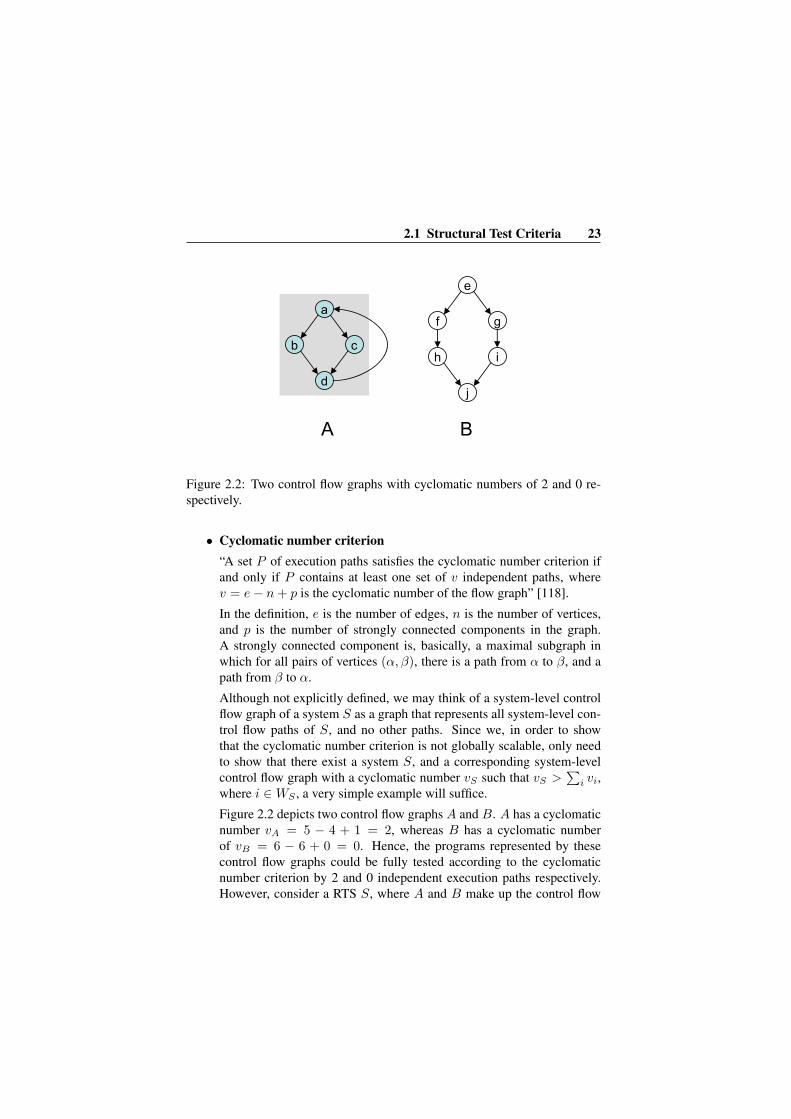
Figure 2.2: Two control flow graphs with cyclomatic numbers of 2 and 0 re-spectively.
• Cyclomatic number criterion“A set P of execution paths satisfies the cyclomatic number criterion ifand only if P contains at least one set of v independent paths, wherev = e− n+ p is the cyclomatic number of the flow graph” [118].
In the definition, e is the number of edges, n is the number of vertices,and p is the number of strongly connected components in the graph.A strongly connected component is, basically, a maximal subgraph inwhich for all pairs of vertices (α, β), there is a path from α to β, and apath from β to α.
Although not explicitly defined, we may think of a system-level controlflow graph of a system S as a graph that represents all system-level con-trol flow paths of S, and no other paths. Since we, in order to showthat the cyclomatic number criterion is not globally scalable, only needto show that there exist a system S, and a corresponding system-levelcontrol flow graph with a cyclomatic number vS such that vS >
∑i vi,
where i ∈WS , a very simple example will suffice.
Figure 2.2 depicts two control flow graphs A and B. A has a cyclomaticnumber vA = 5 − 4 + 1 = 2, whereas B has a cyclomatic numberof vB = 6 − 6 + 0 = 0. Hence, the programs represented by thesecontrol flow graphs could be fully tested according to the cyclomaticnumber criterion by 2 and 0 independent execution paths respectively.However, consider a RTS S, where A and B make up the control flow

24 Chapter 2. Structural Test Criteria for System-Level RTS Testing
a
b c
d
e
gf
h i
j
a
b c
d
Figure 2.3: A system level control flow graph with a cyclomatic number of 6.
graphs of the system tasks, each statement a..j has an execution time ofone time unit, task A has a higher priority than task B, and the releasetime of A and B is 2 and 0 respectively. The system-level control flowgraph of S is shown in Figure 2.3. This graph contains two stronglyconnected components (shaded in the figure), has a cyclomatic numberof vS = 18 − 14 + 2 = 6, and would require at least 6 independentexecution paths in order to fulfil the cyclomatic number criterion. Hence,the cyclomatic number criterion is not globally scalable.1
• Multiple condition coverage criterion
“A test set T is said to be adequate according to the multiple-conditioncoverage criterion if, for every condition C, which consists of atomicpredicates (p1, p2, ..., pn), and all possible combinations (b1, b2, ..., bn)of their truth values, there is at least one test case in T such that the valueof pi equals bi, i = 1, 2, ..., n” [118].
Even though this criterion is defined in terms of a test set (or test suite)rather than in terms of a set of execution paths, it is informally intuitiveto recognize that no new conditions will be introduced in the system byassembling the individual tasks together. Since no new test items will beintroduced if no new conditions are introduced, the multiple conditioncoverage criterion is, even if not formally proven so, globally scalable.
1Note that there exist alternate definitions of cyclomatic complexity [21, 107], none of whichare globally scalable.

2.1 Structural Test Criteria 25
2.1.2 Data Flow Criteria
Data flow criteria are based on, or expressed in terms of, control flow graphsextended with information of accesses to data (i.e., data flow graphs). Weconsider the following data flow criteria:
• All definition-use (DU) paths criterion
“A set P of execution paths satisfies the all DU-paths criterion if andonly if for all definitions of a variable x and all paths q through which thatdefinition reaches a use of x, there is at least one path p in P such that q isa subpath of p, and q is cycle-free or contains only simple cycles” [118].
As shown in the exemple on Page 21, the integration of tasks into amulti-tasking system may introduce new test items in the form of newDU-paths. Since these test items do not exist at unit level, this criterionis not globally scalable.
• All definitions criterion
“A set P of execution paths satisfies the all-definitions criterion if andonly if for all definition occurrences of a variable x such that there isa use of x which is feasibly reachable from the definition, there is atleast one path p in P such that p includes a subpath through which thedefinition of x reaches some use occurrence of x” [118].
In terms of redundancy and usefulness, this criterion is analogous to theall DU-paths criterion. The assembly of tasks may cause definitions, thatin isoloation did not reach any use, to reach a use of the same variable inanother task. Hence, this criterion is not globally scalable.
• All uses criterion
“A set P of execution paths satisfies the all-uses criterion if and only iffor all definition occurrences of a variable x and all use occurrences ofx that the definition feasibly reaches, there is at least one path p in Psuch that p includes a subpath through which that definition reaches theuse” [118].
As above, in terms of redundancy and usefulness, this criterion is anal-ogous to the all DU-paths criterion. Task integration may cause defini-tions, that in isoloation did not reach any use, to reach a use of the samevariable in another task. Hence, this criterion is not globally scalable.

26 Chapter 2. Structural Test Criteria for System-Level RTS Testing
• Required k-tuples criterionThe definition of this criterion requires the definitions of k-dr interactionand interaction path:
“For k > 1, a k-dr interaction is a sequence K = [d1(x1), u1(x1),d2(x2), u2(x2), ..., dk(xk), uk(xk)] where
(i) di(xi), 1 ≤ i < k, is a definition occurrence of the variable xi;
(ii) ui(xi), 1 ≤ i < k, is a use occurrence of the variable xi;
(iii) the use ui(xi) and the definition di+1(xi) are associated with thesame node ni+1;
(iv) for all i, 1 ≤ i < k, the ith definition di(xi) reaches the ith useui(xi)” [118].
“An interaction path for a k-dr interaction is a path p = (n1)∗p1 ∗ (n2)∗... ∗ (nk−1) ∗ pk−1 ∗ (nk) such that for all i = 1, 2, ..., k − 1, di(xi)reaches ui(xi) through pi” [118].
Using these definitions,
“a set P of execution paths satisfies the required k-tuples criterion, k >1, if and only if for all j-dr interactions L, 1 < j ≤ k, there is at leastone path p in P such that P includes a subpath which is an interactionpath for L” [118].
Since the required k-tuples criterion essentially is an extension of theall DU-paths criterion, the same argumentation can be made regardingglobal scalability. E.g., a use in a preempting task may interfere with anexisting interaction path, causing a new interaction path not testable onunit-level. The required k-tuples criterion is thus not globally scalable.
• Ordered-context and context coverage criterionFor the last two data flow criteria (The ordered-context coverage crite-rion and the context coverage criterion), we require the definitions ofordered context and ordered context path:
“Let n be a node in the flow graph. Suppose that there are uses of thevariables x1, x2, ..., xm at the node n. Let [n1, n2, ..., nm] be a sequenceof nodes such that for all i = 1, 2, ...,m, there is a definition of xi onnode ni, and the definition of xi reaches the node n with respect to xi. Apath p = (n1)∗p1∗(n2)∗...∗pm∗(nm)∗pm+1∗(n) is called an orderedcontext path for the node n with respect to the sequence [n1, n2, ..., nm]

2.1 Structural Test Criteria 27
if and only if for all i = 2, 3, ...m, the subpath pi ∗(ni)∗pi+1 ∗ ...∗pm+1
is definition clear with respect to xi−1. In this case, we say that thesequence [n1, n2, ..., nm] of nodes is an ordered context for n” [118].
Further, the ordered-context coverage criterion is defined as:
“a set P of execution paths satisfies the ordered-context coverage crite-rion if and only if for all nodes n and all ordered contexts c for n, thereis at least one path p in P such that p contains a subpath which is anordered context path for n with respect to c” [118].
If the order, in which the definitions in the sequence [n1, n2, ..., nm] areperformed, is ignored, the ordered context is transformed to a definitioncontext. Using definition contexts and corresponding definition contextpaths, a weaker condition, the context coverage criterion, can be defined:
“a set P of execution paths satisfies the context coverage criterion if andonly if for all nodes n and all contexts for n, there is at least one path pin P such that p contains a subpath which is a definition context path forn with respect to the context” [118].
The fact that the context criteria are not globally scalable can easily beshown by a simple example. Consider a system S with two tasks A andB, and two sets PA and PB of execution paths, such that PA satisfiesthe ordered-context criterion for A and PB satisfies the ordered-contextcoverage criterion for B (hence, PA and PB also satisfy the context cov-erage criterion for A and B respectively). Further assume that thereexists a system-level path pS = (n1)∗p1 ∗(n2)∗ ...∗pm ∗(nm)∗pm+1 ∗(n), such that pS is an ordered context path, with the ordered context[n1, n2, ..., nm] for the node n in S, and ∃i, j ∈ [1,m] : ni ∈ A ∧ nj ∈B ∧ i 6= j. Hence, in order for the ordered context coverage criterion tobe globally scalable, the proposition pS ∈ PA∪PB must hold. However,pS cannot be a path in PA since it contains at least one node from B’sflow graph. Furthermore, pS cannot be a path in PB since it contains atleast one node from A’s flow graph. Thus, the ordered context coveragecriterion, and the context coverage criterion, are not globally scalable.
2.1.3 Useful and Non-Useful Criteria
A useful test criterion is efficient (the effort of selecting test cases, and derivingtest items is less than the effort of a corresponding exhaustive testing [83])and applicable (the test criterion does not generally call for intractably large

28 Chapter 2. Structural Test Criteria for System-Level RTS Testing
test suites in order to be satisfied). When discussing usefulness of test criteriafor structural system-level testing, we can start by establishing the followingfact: No globally scalable test criteria are useful for system-level testing, sincethey can be met equally well and more efficiently in unit-level testing. Forexample, if we aim at acheiving full statement coverage in a certain task A, itis easier to test the task in isolation, than to try to reach that goal once A hasbeen integrated into a large multi-tasking system. For efficiency purposes, it isimportant to perform the right type of testing on the right level of integration.Hence, we will henceforth only discuss the usefulness of non-globally scalablecriteria.
As one might expect, some test criteria are not useful even though theyare non-globally scalable. E.g., although the path coverage criterion is non-globally scalable, its usefulness is very low due to its severe complexity prob-lems. Attempting to perform test case selection, or even test case generation,based on all possible sequences of statements that can be executed in a pre-emptive RTS, would inevitably result in infeasibly large test suites. In mostsystems, the same would apply to the cyclomatic number criterion. Similarly,considering the branch coverage criterion, and assuming that this criterion isnot globally scalable, the remaining test cases to execute on system-level wouldhave us covering each possible task switch branch in the system. This is an in-triguing thought, but it does not correspond to any known fault hypothesis. Inaddition, it would likely crave its fair share of test cases in order to be satisfied.
Hence, in the remainder of this thesis, we will focus on test criteria basedon definitions and uses of variables, and specifically on definitions and uses ofvariables shared globally between tasks. From an analysis perspective, thereis no significant difference between the all definitions-, all uses-, and the allDU-paths coverage criterion. A full all DU-path coverage subsumes a fullall definitions, and all uses coverage [116]. Furthermore, the all-DU-pathscriterion is considered highly useful in traditional sequential testing [11]. Inaddition, we have shown in several examples (see sections 1.1.2 and 1.1.2) thesignificance of being able to test unsynchronized accesses to shared variables.Note that the required k-tuples, context, and ordered context criteria all sub-sume and/or extend the all DU-path coverage criterion, and can hence be usefulfor detecting more complex task inter-dependencies. Even though we focus onall DU-path testing in this thesis, we see no reason why system-level testingusing these criteria could not be facilitated using the same approach.
Using our methods for facilitating all DU-path coverage in system-leveltesting, we will be able to detect failures caused by, e.g., race conditions, unini-tialized shared variables, and interleaving failures.

2.1 Structural Test Criteria 29
Test Criterion CF/DF Useful Globally scalableStatement Control Flow No YesBranch Control Flow No Yes/NoPath Control Flow No NoCyclomatic-number Control Flow No NoMultiple condition Control Flow No YesAll definitions Data Flow Yes NoAll uses Data Flow Yes NoAll DU-paths Data Flow Yes NoRequired k-tuples Data Flow Yes NoOrdered Context Data Flow Yes NoContext Data Flow Yes No
Table 2.1: A summary of structural test criteria and their respective properties.
2.1.4 Structural Coverage Criteria Summary
In Table 2.1, the results of our reasoning is summarized. In the remainder ofthis thesis, we will make use of the all-DU-paths criterion for exemplification.In any of these examples, however, this criterion could with a minor effort bereplaced by most other non-globally scalable test criteria.
In this thesis, we focus on existing test criteria instead of formulating new,specialized criteria for structural system-level testing. The main reason fordoing this is that we believe that some of the traditional criteria (specificallythe DU criteria) address problems overlooked by current system-level testingpractices. It should be noted that other efforts have been made in order toadapt old, and formulate new structural test criteria for system-level testing ofconcurrent systems [47, 86, 97]. These contributions however disregard theaspect of time and mostly focus on synchronous task communication. Hence,they are not suitable in multi-tasking RTS testing.
2.1.5 A Note on Feasibility
Note that some test items that are feasible when testing a task in isolation mightbe made infeasible by system integration and vice versa. For example, a def-inition of a shared variable in one task may influence the flow of control andmake control flow paths considered infeasible [32, 35, 37] in other tasks feasi-

30 Chapter 2. Structural Test Criteria for System-Level RTS Testing
ble. This should be considered when performing testing of multi-tasking (andparallel) systems.
2.2 Structural Test ItemsA representation of the control- or data flow is a basic requirement for derivingthe test items necessary for performing testing based on any structural test cri-terion. In this section, we provide a more in-depth description of the flow rep-resentation problem in structural system-level testing based on test item sets.Further, in the same manner, we describe the desired outcome of the methodswe propose.
2.2.1 Sets of Test ItemsOnce the test criterion to be used for testing is selected, we stumble upon theproblem of finding all possible test items with respect the criterion and thesystem under test. For example, if we plan to measure test thoroughness in asystem S by means of visited DU-paths during testing, we need to be aware ofthe total number of DU-paths in S. The set of existing test items in the sys-tem under test can be used as a reference when measuring test adequacy, andas a rule for when to stop testing. For this purpose, rTC is a real number inthe interval [0, 1] describing the adequacy of a test set with respect to the testcriteron TC . Ideally, rTC is the ratio between the number of tested elementsdivided by the total number of possible (feasible) test items. In order to fullysatisfy a test criterion, all existing test items must be exercised during testing(i.e., rTC = 1), but a stopping rule may state that the system is adequatelytested when rTC = 0.8. In addition, since the exact contents of the set ofexisting (or feasible) test items is undecidable in the general case, an approxi-mate set has to be used in order for the metric to be applicable. Note that thisover-approximation is not unique for our method, since the exact determina-tion of feasible test cases in the general case is undecidable even for unit-leveltesting [116].
Example-I As an explanatory example throughout this section, we willconsider all-DU-path coverage of shared variables in the concur-rent example system in Figure 2.4. The system contains two sharedvariables (x and y) and two local variables (z and w). In the fig-ure, each statement corresponding to a CFG node in the code ofthe system is labeled with a superscript letter for node reference

2.2 Structural Test Items 31
h
i
j
k l
m
true
false
true falsetrue
false
a
b c
d
e f
g
true false
true falsetrue
false
h
i
j
k l
m
true
false
true falsetrue
false
a
b c
d
e f
g
true false
true falsetrue
false
a
b c
d
e f
g
true false
true falsetrue
false
int x,y;
functionC(funC_params){int z:=0;do{
if [x<10]a
then [z:=x-3]b
else [y:=z+4]c
if [x>5]d
then [z:=y+3]e
else [y:=z-1]f
} while [z<10 && y>3]g
}
functionD(funD_params){int w:=0;if [y>10]h
then [x:=w]i
do{if [y<5]j
then [w:=y+x+w]k
else [x:=w+x+3]l
} while [w<6 && x<10]m
}
Figure 2.4: Example system.
(e.g., “c” refers to the statement y := z in functionC). Conse-quently, in the example program, x is defined in statements {i, l},and used in statements {a, b, d, k, l,m}, while y is defined in state-ments {c, f}, and used in statements {e, g, h, j, k}.
In this example, a DU-path coverage item is defined by an orderedpair (dv, uv), where dv is a statement with a definition of a variablev, and uv is a statement with a use of a variable v. In the exampleprogram, e.g., (b, i) is a DU-path test item of variable y.

32 Chapter 2. Structural Test Criteria for System-Level RTS Testing
We will formalize our problem, and the desired outcome, in terms of dif-ferent sets of test items. Given a generic structural test criterion TC , a multi-tasking RTS S, a test suite Q, and a system model MS we will define fourdifferent sets of test items: StructuralTC (S), TestTC (S,Q), FeasibleTC (S),and ModelTC (MS). Note that in our explanatory examples, where the testcriterion is all-DU-path coverage, TC = DU .
Now, we know that our systems of interest are preemptive, pseudo-parallelmulti-tasking RTSs. Considering arbitrary preemption (assuming that any taskmay preempt any other task in the system at any point in time), there is a num-ber of structurally feasible coverage items StructuralTC (S) such that each testitem t ∈ StructuralTC (S) may or may not be feasible, depending on the taskinteractions allowed by the run-time system. Basically, the structurally feasibletest items in a system S are the test items that can be derived by each task inisolation, plus the test items that can be derived by unrestricted task interactionin S. As such, StructuralTC (S) is a rough over-approximation of the feasibletest items in the system.
Example-II In the case of the all-DU-path criterion, the naive overesti-mation of all system test items (StructuralDU (S)) would be givenby the set of all possible define-use combinations (dv, uv), suchthat dv is a statement with a definition of a shared variable v, anduv is a use of the same variable v. In our example system, thiswould correspond to:
StructuralDU (S) = {(i, a), (i, b), (i, d), (i, k), (i, l), (i,m),(l, a), (l, b), (l, d), (l, k), (l, l), (l,m),(c, e), (c, g), (c, h), (c, j), (c, k),(f, e), (f, g), (f, h), (f, j), (f, k)}
Further, the set TestTC (S,Q) is defined to be the set of all exercised cov-erage items during the execution of test suiteQ on the system S. By definition,this set will always be a subset of StructuralTC (S) (since TestTC (S,Q) cancontain no coverage items based on definitions and uses not in S, regardlessformulation of Q). Hence:
TestTC(S,Q) ⊆ StructuralTC (S)
Example-III In order to exemplify TestDU (S,Q) on our example sys-tem, assume we test the system using a test suite QS of three dif-ferent initial settings to the shared variables x and y, such that

2.2 Structural Test Items 33
(x, y) ∈ {(4, 10), (10, 3), (5, 6)} (since these are the only fac-tors affecting the flow in the system). Further, assume (1) thatthe priority of the task executing functionD (taskD) is higher thanthe priority of the task executing functionC (taskC), (2) that eachstatement has an execution time of 1 time unit, and (3) that taskCis released at time 0, and that taskD is released at time 8.
The first parameter setting (4, 10) will result in path p1, parametersetting (10, 3) will result in path p2, and parameter setting (5, 6)will result in path p3, as described below:
p1 : 〈a, b, d, f, g, h, j, k,m, j, k,m〉p2 : 〈a, c, d, e, g, a, c, d, h, i, j, l,m, j, l,m, j, l,m, j, l,m, e, g〉p3 : 〈a, b, d, f, g, h, j, k,m〉
From these execution paths, the following set of tested DU-pathscan be derived:
TestDU (S,QS) = {(i, l), (l, l), (l,m), (c, e),(c, g), (c, h), (c, j), (f, g),(f, h), (f, j), (f, k)}
FeasibleTC (S) is the set of all feasible coverage items in a system S withregards to the test criterion TC . A test item t ∈ StructuralTC (S) can beexcluded from FeasibleTC (S) if the timing of the system does not allow theexecution of the test item, regardless of the input parameter settings, or if theexecution of t requires the execution of an infeasible system-level path. Formost structural test criteria, the calculation of the set of feasible test items isundecidable in the general case, even in sequential unit testing [118].
The set of feasible test items is always a subset of StructuralTC (S), sincethe latter always is a safe over-approximation of the set of test items containedin S. Still, FeasibleTC (S) by definition safely contains all test items that canbe executed during testing. Hence:
TestTC (S,Q) ⊆ FeasibleTC(S) ⊆ StructuralTC (S)
Example-IV Since FeasibleDU (S) is undecidable in the general case,we will not explicitly derive it for our example system (even thoughit probably could be calculated in this particular case). However,

34 Chapter 2. Structural Test Criteria for System-Level RTS Testing
considering the structure of the system, and assuming the timingand priority properties described in the previous example, sometest items in StructuralTC (S) are intuitively infeasible. For ex-ample, the DU-path (l, k) will not be included in any valid execu-tion path, since the statements are mutually exclusive with respectto a certain value of variable y which will remain unchanged whilein functionD. The DU-path (i, k) is also infeasible with the samemotivation.
Basing test coverage and adequacy metrics on a set that is undecidableis naturally a major problem. In order for the metric to be applicable, weneed some alternative approximate reference of which test items actually arecontained in S. The fourth test item set, ModelTC (MS), is the set derivedusing an abstract model MS of the system control and data flow. Basically, themore accurate the model, the smaller the set ModelTC (MS) \FeasibleTC (S).
Any model MS useful for our method will model the behaviour of S suchthat each behaviour in S yielding a test item will be represented in MS . Assuch, it will yield a set ModelTC (MS) that is a safe over-approximation ofFeasibleTC (S):
TestTC (S,Q) ⊆ FeasibleTC (S) ⊆ModelTC(MS) ⊆ StructuralTC (S)
Although bounded by the above constraints, the contents of ModelTC (MS)will be highly dependent on the model used of system representation. Forexample, bounding the system behaviour to a specific execution order (deter-mined by a run-time or offline schedule) enables us to discard some of the testitems in StructuralTC (S). Naturally, a more thourogh modeling may furtherreduce the set.
2.3 SummaryThis chapter identified structural test criteria that are suitable for use in system-level RTS testing based on a classification of existing criteria for non-RTS unit-level testing. Furthermore, in the chapter, we chose one of these criteria, the allDU-path coverage criterion, to be the example test criterion for the remainderof this thesis. In addition, this chapter defined four different sets of test items:StructuralTC (S), TestTC (S,Q), FeasibleTC (S), and ModelTC (MS), whereFeasibleTC (S) describes the the set of test items we wish to derive given asystem S, ModelTC (MS) describes its practically derivable approximation,

2.3 Summary 35
and StructuralTC (S) describes its worst-case over-approximation. Further,TestTC (S,Q) describes the set of test items exercised by executing a certaintest suite Q. In Chapter 3 we will describe how to derive ModelDU (MS) giventwo different system models. Chapter 4 describes how to extract TestDU (S,Q)during testing, and Chapter 5 provides a system example, where the abovesets are derived and an approximate DU-path coverage is derived by dividingthe number of test items in TestDU (S,Q) with the number of test items inModelDU (MS) (i.e., rDU = |TestDU (S,Q)|
|ModelDU (MS)| ).


Chapter 3
Deriving DU-paths for RTSSystem-Level Testing
In order to calculate coverage for system-level DU-path testing, we need toknow (1) the number of unique DU-paths exercised by testing, and (2) the num-ber of exercisable DU-paths in the system under test. As previously described,the former divided by the latter gives us the DU-path coverage achieved bya certain set of test cases. However, the derivation of potentially exercisableDU-paths requires a correct representation of control and data flow on system-level. In this chapter, we seek model representations of the system under testin order to derive the set of potentially exercisable DU-paths (ModelDU (MS)).Specifically, we present two different methods for deriving this set. In doingthis, we bring together state-of-the-art methods in worst-case execution time(WCET) analysis, model-based testing, and real-time scheduling analysis.
3.1 IntroductionThe two methods presented in this chapter make it possible to determine testadequacy in a multi-tasking RTS using the all DU-path coverage criterion withrespect to shared variables. Generally, by analyzing the temporal attributes ofeach access to globally shared data within each task, while at the same timeconsidering the progress of the run-time schedule of the RTS, our methods areable to model and analyze task interaction. Further, the task interaction patterntogether with the shared variable access information allow us to derive which
37

38 Chapter 3. Deriving DU-paths for RTS System-Level Testing
DU-paths are potentially feasible in the execution of the RTS, and which arenot. In detail, our contributions in this field are:
• A test item derivation method based on the timed automata modeling andverification tool UPPAAL [10, 59, 78], and UPPAAL’s test case genera-tion extension COXER [41] (Section 3.2).
• A modeling and test item derivation method based on Execution OrderGraph (EOG) theory [101] (Section 3.3).
• Theoretical and empirical evaluations and comparisons of the two meth-ods and their respective usefulness (sections 3.4 and 6.1).
The EOG representation was chosen since it, to our knowledge, is the onlyabstract representation of a preemptive RTS that describes the full executiontime complexity, considering the best case-, and worst case execution timeof the system. UPPAAL, on the other hand, has some alternatives in, e.g.,KRONOS [23] and HYTECH [38]. For this thesis, we chose UPPAAL due tothe usefulness of its COXER extension (i.e., the ability to derive test itemsfrom an UPPAAL model), and for the benefit given by geographical proximityto its originators. The latter also applies for the SWEET tool discussed below.
3.1.1 General Analysis PropertiesBefore delving into the details of our both approaches, we will discuss theproperties, assumptions, and methods that are common for both approaches.These include the structure of the analysis process, the need for run-time sys-tem representation, and the use of static program analysis.
Process Overview
Formally, our ambition in this chapter is to, given a generic RTS S, and a testsuite Q, generate a model MS , and to analyse this model for DU-paths, suchthat the resulting set of test items ModelDU (MS) is as close to FeasibleDU (S)as possible (i.e., such that ModelDU (MS) \ FeasibleDU (S) contains the leastnumber of elements possible). In sections 3.2 and 3.3, we describe two ap-proaches for performing the modeling and analysis for deriving ModelDU (MS).However, both approaches follow the same basic structure:
1. Given a multi-tasking RTS S with a set of tasks WS , each task in WS
is individually analysed with respect to a certain selected test criterion

3.1 Introduction 39
TC (in this chapter represented by all DU-paths, DU ). In this step, thenecessary input to the system-level analysis (e.g., best-, and worst-caseexecution time, variable definitions and uses, etc.) is derived.
2. A model of the system (MS) is created based on the information col-lected in Step 1 combined with information of the run-time system andthe system scheduling parameters (e.g., task periodicity, offset, etc.).
3. UsingMS , the set of test items in the model (ModelDU (MS)) is derived.
4. The results from system testing (TestDU (S,Q)) are compared with theresults from Step 3. Using these, a coverage thoroughness measure isderived by calculating rDU = |TestDU (S,Q)|
|ModelDU (MS)| .
Run-Time System Modeling
As shown by several examples in earlier chapters, the system-level control flowhas major impact on the execution behaviour of a RTS. Consequently, it alsoinfluences the system-level testing of such systems. The system-level controlflow, in turn, is dictated by the execution times of the tasks in the system, andthe underlying real-time kernel and scheduler. Hence, in order to correctlyderive test items for structural testing of a RTS, we also need to consider theimpacts of timing as well as the underlying scheduler on the system. In thetwo approaches presented in this chapter, this is done by explicitly or implicitlymodeling or simulating the behaviour of a FPS-scheduler on timed abstractionsof tasks.
Static Analysis
Both our DU-path derivation approaches require static task-level informationregarding the control flow structure of the tasks in the system, the temporalbehaviour of the tasks, and shared variable definitions and uses. For this pur-pose, we use the SWEET (SWEdish Execution time Tool) tool [28], a researchprototype tool for worst-case execution time analysis developed at MalardalenUniversity1. However, any WCET analysis tool that is modified to provide thedata we require could be used for this purpose.
The static analysis we perform consists of three distinguished phases: aflow analysis where bounds on the number of times different entities in the
1www.mrtc.mdh.se/projects/wcet

40 Chapter 3. Deriving DU-paths for RTS System-Level Testing
C-file
COMPILERInter-
mediatecode
Basic blockinfo
FLOWANALYSIS
Flow info
Flow info
Flow info LOW-LEVELANALYSIS
EOG fmt.ET info
UppAal fmt.ET info
MERGE 2
MERGE 1
schedule
UppAalconfig file
EOGconfig file
ModelDU(M1,S)
ModelDU(M2,S)
1
2 3
4
5
67
EOG-basedanalysis
(approach 2)
UppAal-basedanalysis
(approach 1)
INPUT
ANALYSIS OUTPUT
Figure 3.1: The use of static analysis in the process.
code can be executed are derived, a low-level analysis where bounds of the ex-ecution times for instructions are derived, and a final calculation phase wherethe flow and timing information are combined to yield a WCET estimate. Ba-sically, the static analysis answers to Step 1 and parts of Step 2 in the processoverview described above. Figure 3.1 depicts the schematic process of howthe static analysis is used in the analysis. In (1), the source code is compiledusing a compiler that supports the formats required by the analysis tool (inour case, the NIC compiler2). Using the intermediate code from the compiler,the analysis tool performs a high-level flow analysis (2), producing a programflow representation (in our case, a scope graph [28]), and corresponding flowinformation for both our analysis approaches. Next, a low-level analysis (3)produces execution time information for the entities in the scope graph, us-ing information of the assembly code. The flow information and the executiontime information is merged with the run-time schedule information to form
2See user.it.uu.se/svenolof/wpo. This step in the process assumes an application written in C,but all other steps in the analysis are language-independent.

3.2 Approach 1: Deriving DU-paths using UPPAAL and COXER 41
two configuration files (4,6). Last, the system-level analyses are performed(5,7), taking the two configuration files as input. The result of each system-level analysis is a set ModelDU (MS). In Approach 1 (5), the model is given inUPPAAL XML format, and in Approach 2 (7), it is given as an implicit EOGrepresentation annotated with shared variable access information. A more de-tailed description of the specific use of SWEET is given in the description ofeach approach, respectively.
3.2 Approach 1: Deriving DU-paths using UPPAALand COXER
In our first approach, we present a method for modeling system-level controlflow of multi-tasking RTSs using timed automata. In contrast to traditionalcontrol flow models or graphs used for testing, our model also expresses: (1)subroutine interaction, (2) timing, such as basic block execution times andtime-triggered preemption, (3) certain flow information, such as loop boundsand infeasible paths, and (4) system-level properties, such as concurrency, task-interleaving and race conditions. Consequently, the model may serve as a rep-resentation of all possible system-level control flow paths that can be traversedduring the execution of a multi-tasking RTS.
3.2.1 PreliminariesIn order to fully describe the contribution of this approach, there is a need toaccount for the refined system model assumptions, and to give a brief summaryof UPPAAL [10, 59], the tool used for modeling.
Refined System Model
To make way for our line of reasoning, we extend the system model defined inSection 1.2. Hence, for the scope of this approach, we define a task using the6-tuple:
〈T,O, P,D,ET , G〉
The first five items are identical to those in the original definition, where Tis the period time of the task, O is the activation offset relative to the taskperiod (i.e., a task t with period time Tt and offset Ot is activated at timeOt, Tt +Ot, 2Tt +Ot, 3Tt +Ot, ...), P is the unique priority of the task, D isthe deadline of the task, and ET describes the best- and worst case execution
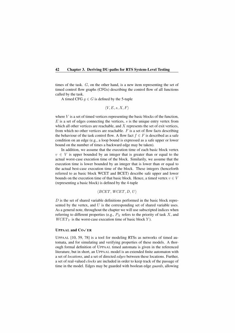
42 Chapter 3. Deriving DU-paths for RTS System-Level Testing
times of the task. G, on the other hand, is a new item representing the set oftimed control flow graphs (CFGs) describing the control flow of all functionscalled by the task.
A timed CFG g ∈ G is defined by the 5-tuple
〈V,E, s,X, F 〉
where V is a set of timed vertices representing the basic blocks of the function,E is a set of edges connecting the vertices, s is the unique entry vertex fromwhich all other vertices are reachable, and X represents the set of exit vertices,from which no other vertices are reachable. F is a set of flow facts describingthe behaviour of the task control flow. A flow fact f ∈ F is described as a safecondition on an edge (e.g., a loop bound is expressed as a safe upper or lowerbound on the number of times a backward edge may be taken).
In addition, we assume that the execution time of each basic block vertexv ∈ V is upper bounded by an integer that is greater than or equal to theactual worst-case execution time of the block. Similarily, we assume that theexecution time is lower bounded by an integer that is lower than or equal tothe actual best-case execution time of the block. These integers (henceforthreferred to as basic block WCET and BCET) describe safe upper and lowerbounds on the execution time of that basic block. Hence, a timed vertex v ∈ V(representing a basic block) is defined by the 4-tuple
〈BCET ,WCET ,D ,U 〉
D is the set of shared variable definitions performed in the basic block repre-sented by the vertex, and U is the corresponding set of shared variable uses.As a general note, throughout the chapter we will use subscripted indices whenreferring to different properties (e.g., PX refers to the priority of task X , andWCETY is the worst-case execution time of basic block Y ).
UPPAAL and COXER
UPPAAL [10, 59, 78] is a tool for modeling RTSs as networks of timed au-tomata, and for simulating and verifying properties of these models. A thor-ough formal definition of UPPAAL timed automata is given in the referencedliterature, but in short, an UPPAAL model is an extended finite automaton witha set of locations, and a set of directed edges between these locations. Further,a set of real-valued clocks are included in order to keep track of the passage oftime in the model. Edges may be guarded with boolean edge guards, allowing

3.2 Approach 1: Deriving DU-paths using UPPAAL and COXER 43
the edge to be taken only if the guard condition is satisfied. Similarily, locationsmay be restricted by boolean invariants, allowing the location to be visited onlyif the invariant condition is fulfilled. Different automata may synchronouslyinter-communicate by means of synchronization channels, expressed as labelson edges, such that a synchronization edge can only performed if both au-tomata involved in the synchronization are ready to communicate. In addition,UPPAAL locations may be labeled urgent or committed, where an urgent lo-cation is a location where no time may pass, and a committed location is anurgent location in which no edges from non-committed location may occur.
UPPAAL supports declaration of global variables (i.e., variables that are ac-cessible by all automata in the model within which they are declared). Hence,a global variable in the UPPAAL model translates directly to a global variablein the system under test. For the method of modeling described in this paper,the 3.4.11 version of UPPAAL3 is used.
COXER [41] is an UPPAAL-based test case generation tool that generatessuites of test cases based on UPPAAL timed automata system specificationmodels, and observer automata.
3.2.2 RTS Control Flow Modeling in UPPAAL
In order to use the analysis engine of UPPAAL to derive shared variable DU-paths, we need to correctly model the structural and temporal behaviour ofthe system under test. In this section, we describe a RTS control flow modelmade up as a network of three categories of timed automata for this purpose.First, each task is modeled as a set of timed automata (the task main function,and the set of subroutines directly or indirectly called by the main function).Second, the run-time state (ready, running, waiting, etc.) of each task in thesystem is modeled as an Execution Control Automaton (ECA). Third, the run-time kernel (i.e., the schedule, task switch, and the system clock) is modeledas a set of timed automata. In the following subsections, we will show howthese automata form the timed system-level control flow model of the RTS.Using the COXER tool, a search of all possible DU-paths in the model can beperformed. These together form ModelDU (MS).
Figure 3.2 displays the overall structure of the system-level control flowmodel. In the figure, the white parts are specific for each system, the grey partsare semi-generic in that they have a generic structure, but need to be param-eterized for each specific system, and the black parts are completely generic.
3www.uppaal.com

44 Chapter 3. Deriving DU-paths for RTS System-Level Testing
This section will focus on this structure and the purpose of our model. For anin-depth description of the model, we refer to Appendix A.
ECA 1
ECA 2
ECA 3
ECA N-1
ECA NTaskSwitch
Task 1
System
clock
cfg1a
cfg1c
cfg1b
…
Task 2
cfg2a
cfg2c
cfg2b Task 3
cfg3a
cfg3c
cfg3b
…
…
Task N-1
cfg
N-1a
cfg
N-1c
cfg
N-1b
…
Task N
cfgNa
cfgNc
cfgNb
…
Schedule
Figure 3.2: The structure of the UPPAAL control flow model.
Task CFG modeling
From a standard CFG perspective, a task is made up of a set of function-levelgraphs (i.e., a graph for the task main function, and a graph for each functionthat is explicitly or implicitly called by the main function). In our model, eachfunction CFG translates to a timed automaton in the UPPAAL format. The basiccontrol flow structure of a function is intuitively modeled in UPPAAL using aone-to-one mapping between basic blocks and UPPAAL locations, and betweenCFG edges and UPPAAL edges. Each location where a shared variable is ac-cessed (defined or used) is explicitly marked in the model. By using UPPAALclock guards and invariants, the correct temporal behaviour of each node in thegraph can be expressed. Further, subroutine invocation is solved by means ofUPPAAL synchronization channels.
Hence, this part of the system-level control flow model ensures that thecorrect task-level control flow, and shared variable accesses are expressed.

3.2 Approach 1: Deriving DU-paths using UPPAAL and COXER 45
Modeling of Task Execution Control
Even though there are a number of CFG models describing the timing and theinternal structure of each task, no task can be allowed to execute unless it isscheduled and released by the run-time scheduler. For each task in the model,a separate task ECA is used in order to keep track of the run-time state of thetask. An ECA is generic in the sense that it has an identical structure regardlessof the task it controls.
An ECA has five basic locations: waiting, ready, scheduled, executing, andterminated. Basically, a task model is only allowed to consume any time if itsECA is in the executing location. If a task model has not yet been releasedby the scheduler, its ECA is in the waiting location. If a task model has beenreleased, but there are other released task models with higher priorities, itsECA will be in the ready location. The scheduled and terminated locations areintermediate locations, described further in Appendix A. In summary, the ECAautomata restricts the behaviour of the system model, such that no task modelsmake transitions when they are not executing.
FPS Scheduler and Task Switch Modeling
The third part of the system model is the FPS scheduler and the task switch au-tomaton. These models ensure that the run-time schedule of the modeled RTSis correctly represented in the model. The FPS schedule model determinesthe ordering and timing of task releases (i.e., when certain task ECAs shouldchange location from waiting to ready). Furthermore, the task switch automa-ton facilitates task model preemption in the system model. When a task modelwith a higher priority than the currently executing task model is released, theexecuting task model should be preempted in favour of the newly released taskmodel and only the latter should be able to consume any execution time.
3.2.3 Automatic System Model Generation using SWEETUsing SWEET, the automata for the task models can be automatically gener-ated from the RTS application source code. Basically, in our extension of theSWEET tool for this purpose, timed SWEET scope graph files for each taskfunction are translated into xml-file UPPAAL automata. These automata canthereafter be imported into the main RTS UPPAAL project, initially comprisingtask switch, schedule, system clock and ECA automata. When all generatedtask automata are incorporated in the overall model, the test item analysis canbe performed.

46 Chapter 3. Deriving DU-paths for RTS System-Level Testing
CovItems=2Traces=2TotCost=0TotLength=4du<x offset=0, edgeid ctl.a_to_b, edgeid ctl.b_to_c>du<y offset=0, edgeid ctl.a_to_b, edgeid ctl.b_to_d>
Figure 3.3: Example partial COXER output.
3.2.4 Deriving ModelDU (MS) using COXER
COXER [41] is an UPPAAL-based tool that generates suites of test cases basedon UPPAAL timed automata system specification models, and observer au-tomata. Hence, COXER is initially intended for functional testing. In thissection, we have described how to express the control flow structure of a FPS-scheduled RTS S as an UPPAAL model MS , hence allowing COXER to per-form a structural test case generation. By defining different kinds of observerautomata, COXER will generate different kinds of test suites, each of whichcorresponds to the test criteria represented by the observer automaton4. For thepurpose of this thesis, we use a pre-defined DU-observer5. Using this observerautomaton, and a model MS of a system S, COXER will generate a suite oftest cases that, when exercised, satisfies the all DU-path coverage criterion.
As COXER is primarily directed towards usage with functional and tempo-ral models of event-triggered reactive systems, it will generate a test case suiteconsisting of traces through the model that satisfies the test criterion definedby the observer. In a functional and temporal model of a reactive system, suchtraces will tell us exactly which inputs to give the system, and when to givethem, in order to execute the tests. Using our system model (time-triggeredFPS), we will not be able to fully control the execution of the system just byrudimentary user interaction, but we will still be able to derive the set of testitems in the system (i.e., ModelDU (MS)), as this is part of the COXER testcase generation output (see Figure 3.36.). In this case, the output tells us thatCOXER has found two separate DU-paths; one of variable x and one of vari-able y, reachable through two different traces through the model. The discus-sion of test case generation versus test item derivation is further elaborated in
4In the referenced literature on COXER, test criteria are called coverage criteria.5Given at www.uppaal.com/cover.6This output is also in essence taken from the example at www.uppaal.com/cover

3.3 Approach 2: DU-path derivation using EOGs 47
Job Rel Prio BCET WCETA0 0 4 7 8A1 90 4 7 8B0 100 2 7 37C0 135 1 13 47D0 170 3 5 41A2 180 4 7 8
Table 3.1: An example 270 ms schedule with job identity, release time, priority,and best- and worst-case execution time.
Section 8.3.1. For a full example of the process of deriving DU-paths usingCOXER from a small multi-tasking RTS, see Chapter 5.
3.3 Approach 2: DU-path derivation using EOGsIn our second approach, we present a method for modeling system-level con-trol flow of multi-tasking RTSs using Execution Order Graphs. In contrast tothe previous approach, this approach does not explicitly model control flowon task-level, but relies on more abstract representations, such as timing in-tervals for task execution, preemption, and shared variable access. Hence,the modeling and analysis require less effort than those in the previous ap-proach, but it is also likely to give a slightly less precise result. In other words,ModelDU (MS)\FeasibleDU (S) for Approach 1 will generally be smaller thanModelDU (MS) \ FeasibleDU (S) for Approach 2.
3.3.1 PreliminariesAs stated in Definition 1 on Page 11, an execution ordering is defined as anordered list of task switches and interrupts. This list includes all transfers ofcontrol from one task to another task, or from a task to an interrupt serviceroutine and back during the execution in question.
The Execution Order Graph
In 1999, Thane and Hansson [101] defined an algorithm for deriving a di-rected reachability graph of all possible execution orderings from a periodicallyscheduled set of task instances during a LCM (the Least Common Multiple of

48 Chapter 3. Deriving DU-paths for RTS System-Level Testing
root
[0,8)A:4
[90,98)A:4
[100,137)B:2
[135,184)C:1
[170,211)D:3
[170,211)D:3
[180,188)A:4
[187,219)D:3
II
[180,188)A:4
I
[180,188)A:4
[175,194)C:1
[180,188)A:4
[180,188)A:4
[180,188)A:4
[187,202)C:1
[187,219)D:3
III [187,202)C:1
V [187,233)C:1
IV VI
[0,0]
[7,8)
[97,98)
[107,137)
[148,170)
[175,180)
[187,188)
[180,180]
[187,188)
[187,219)
[170,170]
[175,180)
[180,180][180,180)
[180,180][175,180)
[187,188) [187,188)
[187,188) [187,188)
[187,219)[187,202)
[187,202) [187,233)
Figure 3.4: An Execution Order Graph (EOG) based on the schedule in Ta-ble 3.1.
the period times of the tasks; the shortest time before the schedule periodicallyrepeats itself). This graph is called an Execution Order Graph (EOG). Basi-cally, knowing the offset and period time for each task (or release time for eachtask instance), the task priority, the WCET, and the BCET for each task, allpossible execution orderings can be derived and visualized. An example of anEOG (based on the fixed-priority schedule in Table 3.1) is shown in Figure 3.4.
Subsequent work by Thane and Hansson described how to handle sporadicinterrupts in the EOG (in fact, the same technique could be used by our methodin order to model functionally non-interactive tasks as temporal interferences,but this is considered future work) [100]. Furthermore, Thane and Petters-son addressed testing of preemptive multi-tasking RTSs [103] where input and

3.3 Approach 2: DU-path derivation using EOGs 49
output from a task can be given and produced at the beginning of a task’sexecution and at the end of the task’s execution respectively (using a singleshot task model [8]). Later, the model was relaxed to cover testing of taskswhere input and output could also be given within critical sections guarded withsemaphores [77]. In this approach, we extend the EOG-based method to alsohandle all-DU-path coverage in preemptive multi-tasking RTSs. Hence, we arefurther relaxing the model, allowing inter-task communication anywhere in theexecution of the tasks, however bounded to reads and writes of globally sharedvariables.
Refined System Model
As with the first approach, we need to make some extensions to the systemmodel for this approach. Assuming a system S with a set of tasks WS asdescribed in Section 1.2, each task in WS is extended with a set of globalvariable definitionsD and a set of global variable uses U (hence, in this section,a task is defined as 〈T,O, P,D,ET ,D,U〉). A definition d ∈ D is defined asa five-tuple:
〈id, v,min,max , rdMax 〉
where id is the unique address of the definition, v is the name of the sharedvariable, min is the shortest-, and max is the longest execution time fromthe start of the task within which the statement id can be reached (with notemporal or functional interference from other tasks considered), and rdMaxis the longest time d can be live (before it is overwritten by another definition).These temporal properties will be described more in-depth in Section 3.3.2.
A use u ∈ U is defined as a four-tuple:
〈id, v,min,max 〉
where id is the unique address of the use, v is the name of the shared variable,min is the shortest, and max is the longest execution time from the start ofthe task within which the statement id can be reached (with no temporal orfunctional interference from other tasks considered).
As an example, consider the code in Figure 3.5, where uses are enclosed ina selection statement. Figure 3.6 shows an example execution of two concur-rently executing tasks, A and B, where B consists of the code from Figure 3.5,and A has a higher priority than B, and contains a definition of variable a.Hence, at task level, A only has a definition and no DU-paths. In B there isa definition (a:=b+4) and two uses (result:=a+1 and result:=a*2)

50 Chapter 3. Deriving DU-paths for RTS System-Level Testing
1. a:=b+42. if expression is true then3. result:=a+14. else then5. result:=a*2
Figure 3.5: Example of defs and uses.
of the same variable a. In two example executions of the systems (shown inFigure 3.6), B is allowed to finish before A starts (Figure 3.6a), alternativelyis preempted by A (Figure 3.6b). Consequently, the result differs betweenthe executions. This is another example of a situation where task executionorderings influence the functional system behaviour, but that is not the primecontribution of this example.
a:=b+4…P
R I
O R
I T
Y
T I M E
B
a:=0
…result:=a+1
A
a:=b+4result:=a+1P
R I
O R
I T
Y
T I M E
B
a:=0A
b)
result:=1
a)
result:=b+5
Figure 3.6: Shared variable communication (assuming that the conditional ex-pression is true in task B).
Instead, consider Figure 3.7, where the scenarios from Figure 3.6 are revis-ited, but here, the focus is on the exact times when the accesses are executed.For example, in Figure 3.7a definition a:=b+4 is executed at def 1 and over-written at rd1. In Figure 3.7b, a:=b+4 is executed at def 4 and overwrittenat rd4. Generally, for each access x, there is an interval with extremal valuesx.min and x.max within which x can be executed. Furthermore, for each def-

3.3 Approach 2: DU-path derivation using EOGs 51
P R
I O
R I
T Y
T I M E
B
A
a)
result:=b+5
result:=a+1
a:=0
a:=b+4def1 rd1
def3 rd3
use2
P R
I O
R I
T Y
T I M E
B
A
b)
result:=1
result:=a+1
a:=0
a:=b+4def4 rd4
def6 rd6
use5
Figure 3.7: Shared variable access attributes.
inition d, there is a point in time d.rdMax , where d is safely overwritten. Notehere that a definition, that may live after the termination of the task in whichit is performed (as is the case with def 1, def 4 and def 6 in our example), willhave a rdMax equal to the WCET of that task.
3.3.2 Shared Variable DU Analysis
In this section, we will present, in abstract terms, the analysis performed forderiving ModelDU (MS) using EOG models. In Appendix B, the details of thecorresponding algorithm is presented. Basically, the analysis consists of twosteps:
1. A task-level analysis, deriving ET , D, and U for each task w ∈WS bymeans of static program analysis.

52 Chapter 3. Deriving DU-paths for RTS System-Level Testing
...1. i := 1;2. p := INIT;3. do {4. i := i + 1;5. if(i <= MIN)6. g := g + INCR;7. p := p * g;8. } while(i < MAX)9. return;
Figure 3.8: Example code for timing analysis.
2. A system-level analysis, based on EOG analysis combined with the re-sults from step 1, deriving shared variable DU-paths. In fact, the DU-paths are derived using the same algorithm that builds the EOG. Hence,strictly speaking, the EOG model of the system is not actually used, as itis derived along with the DU-paths.
Task-Level Analysis
The task-level analysis derives the temporal properties for each shared variableaccess (definition or use) in each task w ∈ WS . Three properties (min , max ,and rdMax ) are derived for each definition, and two properties (min and max )are derived for each use. As min and max are analogous for definitions anduses, we will focus on the definition properties.
Assuming a definition d that defines a variable x:
• The d .min property is a safe lower bound on the shortest possible exe-cution time from the start of the task to the statement containing d.
• The d .max property is a safe upper bound on the longest possible exe-cution time from the start of the task to the statement containing d.
• The d .rdMax property is a safe upper bound on the longest possibleexecution time for any path p, starting at task start s and ending at astatement e, such that d is on p, e contains a statement that redefines x,and no other redefinitions of x are made between d and e. Intuitively,this property describes the time (relative to the start of a task) where d

3.3 Approach 2: DU-path derivation using EOGs 53
i:=1A
p:=INITB
i:=i+1C
if(i<=MIN)D
g:=g+INCRE
p:=p*gF
while(i<MAX)G
returnH
tA=1
tB=1
tC=2
tD=3
tE=2
tF=5
tG=2
tH=8
exit
#C<=10
i:=1A
p:=INITB
i:=i+1C
if(i<=MIN)D
g:=g+INCRE
p:=p*gF
while(i<MAX)G
returnH
exit
#C<=10
#H=0
i:=1A
p:=INITB
i:=i+1C
if(i<=MIN)D
g:=g+INCRE
p:=p*gF
while(i<MAX)G
returnH
exit
#C<=10
#H=0
(a) CFG with flow and (b) CFG for g use (c) CFG for p rdMaxtiming info timing analysis timing analysis
Figure 3.9: Example of timing analysis for defs and uses.
is safely overwritten. Note that, if d is not safely overwritten during theexecution of the task, d .rdMax is equal to the worst-case execution timeof the task.
Timing analysis for defs and uses
For the purpose of DU-path derivation, we have extended SWEET to, exceptthe “normal” program WCET and BCET estimates, also produce estimatesupon the above mentioned min , max , and rdMax values. We use SWEETto perform program flow- and low-level analysis, but not the calculation. Theresult can be seen as a CFG containing both flow- and timing bounds and withtwo extra start and exit nodes. Derived flow constraints are expressed as(lower or upper) bounds on the number of times a certain entitity in the graph,(node or edge), can be taken, valid for all possible executions of the program.Derived timing bounds are expressed as a (lower or upper) bounds on the costfor executing a certain entity, valid each time the entity is executed. Figure 3.8depicts an example code with two globals g and p. Figure 3.9a illustrates theCFG for the code. The flow analysis has derived a loop bound of 10, expressedas an upper bound on the number of times node C could be executed. Each nodei has also been given an timing bound ti valid each time the node is executed.

54 Chapter 3. Deriving DU-paths for RTS System-Level Testing
Secondly, we perform a reaching definition (RD) analysis for global vari-ables [69]. The analysis derives, for each global variable, where in the programit may be used and defined as well as how far each definition may reach. Sincepointers could be used to update globals, SWEET’s RD analysis takes the inputof a pointer analysis.
We derive the different estimates using an Implicit Path Enumeration Tech-nique (IPET) calculation [28]. In IPET each node and/or edge in the CFG isgiven a time (tentity), and a count variable (xentity), the latter denoting the num-ber of times that block or edge is executed. The WCET is found by maximisingthe sum
∑i∈entities xi ∗ ti, subject to constraints reflecting the structure of the
program and possible flows. For example, there are constraints specifying thatthe start and exit nodes each must be taken exactly once, and constraints spec-ifying that each node must be entered the same number of times as it is exited.The WCET estimate is derived using integer linear programming (ILP). TheBCET is found by minimizing the same sum (or, if the statements do not haveconstant execution times, the corresponding statement BCET sum), subject tothe same constraints (using ILP).
Our min, max and rdMax analyses start from the above mentioned CFG.Depending on what timing values to derive, we modify the graph by addingextra edges and flow contraints. E.g., the graph for deriving min , max for ause u is constructed by adding en extra edge from the node holding u to the exitnode. Additionally, for all other edges going to the exit node we add a flowconstraint specifying that its source node cannot be taken. Thus, we force theIPET calculation to exit through our newly created exit-edge, thereby derivingthe best-case and worst-case estimates for u, instead of the “normal” BCETand WCET. Figure 3.9b shows the CFG for calculating min and max for theuse of g in node F. For each global use and def derived in the RD analysis, weconstruct a corresponding graph. The resulting modified graphs are given asinput to SWEET to derive the corresponding min and max values.
To derive rdMax for a definition d we first use the RD analysis to derivethe set of nodes which d may reach. From each of these nodes we add anextra edge to the exit node. Additionally, for all other edges going to the exitnode from a node which d cannot reach, we add a flow constraint specifyingthat its source node cannot be taken. Thus, we force the IPET calculation toexit through one of the nodes d may reach. The rdMax value is derived by aWCET calculation upon the resulting graph. Figure 3.9c shows the graph forcalculating the rdMax value of the p:=INIT definition in node B.

3.3 Approach 2: DU-path derivation using EOGs 55
System-Level Analysis
The algorithm for deriving system-level DU-paths is based on the algorithmfor deriving EOGs [101]. Consequently, the analysis exhaustively simulatesthe execution of the system during the time interval of one LCM on an execu-tion ordering level. In this simulation, performed by the recursive algorithmdescribed in Appendix B, all possible task interleaving sequences of the sys-tem are traversed. After the time interval of one LCM, the system behaviouris periodically repeated, and no new shared variable definitions and uses willbe found. During the analysis, information on the possible orderings of sharedvariable definitions and uses is collected.
Specifically, given our extended task model (including the set of sharedvariable definitions, D, and the set of shared variable uses, U), the analysisderives an overestimation of all DU-paths in the system. In order to derive,this, the algorithm needs to keep track of which shared variable accesses havebeen, will be, or might have been performed at any time in the simulation.For this purpose, throughout the analysis, each definition and each use holds acertain variable state (dead, active or live, see Figure 3.10). An active accesshas been executed, or can be executed at any time until it has become live ordead. A live access has safely been executed, and not been safely overwrittenby another access. A dead access is neither active nor live (i.e., the access hassafely not yet been executed, is safely overwritten, or has safely passed thetime where it can affect the result of the analysis). As the analysis progressesthrough the LCM time interval, the state of each access may change accordingto a set of rules. These rules for making the transitions between these accessstates constitute the foundation of the algorithm for deriving all system-levelDU-paths7:Definition rules:
1. At d.min , d makes a transition from dead → active .
2. At d.max , d makes a transition from active → live .
3. At d.rdMax , d makes a transition from live → dead .
Use rules:
1. At u.min , u makes a transition from dead → active .
2. At u.max , u makes a transition from active → dead .7The rules assume that ModelDU (MS) = ∅ initially.

56 Chapter 3. Deriving DU-paths for RTS System-Level Testing
dead
live
active
dead
active
Def: dead, active, or liveUse: dead or active
d.min
d.max
d.rdMax
u.maxu.min
DEF USE
Figure 3.10: Access states and transition rules.
DU-path rules:
1. At d.min , all DU-paths (d, u), such that u.var = d.var and u is cur-rently active, are added to ModelDU (MS).
2. At u.min , all DU-paths (d, u), such that u.var = d.var and d is cur-rently live or currently active, are added to ModelDU (MS).
3.3.3 Deriving ModelDU (MS) using EOGsThe above seven rules (partially depicted in Figure 3.10) are implemented inthe DUANALYSIS algorithm, deriving all system-level DU-paths. The detailsof the DUANALYSIS algorithm are described in Appendix B.
3.4 DiscussionIn this chapter, we have presented two different methods for deriving test itemsfor structural system-level testing. Specifically, we have described how thesemethods derive the set of DU-paths (ModelDU (MS)) from a time-triggeredmulti-tasking RTS. Theoretically, there are some basic differences between thetwo approaches described in this chapter. For example:
• The COXER method has the ability to prune live definitions at resump-tion [40]. In the EOG-based approach, the set of live definitions propa-gates through the analysis. If a definition d in a task instance t1 is notsafely overwritten by the end of t1’s execution, d is considered live at

3.4 Discussion 57
[x:=3]1
[x:=4]2
[y:=x]3
[x:=0]1 [x:=4]2
[x>0]3
t f
[y:=x+1]4 [y:=x-1]5
a) b)
Figure 3.11: Example CFGs.
the start of the next scheduled task instance t2. To prevent d from be-ing live indefinitely, t2 “inherits” d as a live definition and assigns it anew rdMax value, describing how long into t2’s execution d can be livebefore it is safely overwritten. This value is derived for each global vari-able by the task level analysis, by calculating the rdMax property for a“virtual definition” of the variable at the task CFG entry point.
However, should the task switch from t1 to t2 be a resumption of a pre-viously preempted, partially executed task, d cannot be assigned a newrdMax value, since there is no way of knowing how long d will livein t2 from the arbitrary resumption point. In this case, the EOG-basedapproach will let d live throughout the execution of t2 and make a newdecision based on the next scheduled task instance t3.
Using the COXER based approach, each system-level control flow pathis considered (even if not always individually searched), and in the abovedescribed scenario of a resumption of a previously preempted task t2, allpaths from the resumption point to the end of t2 will be traversed. Ifall these paths contain at least one statement where d is overwritten, dwill not be considered live when scheduling task instance t3. This willresult in a tighter over-approximation of ModelDU (MS), and hence amore detailed analysis result.
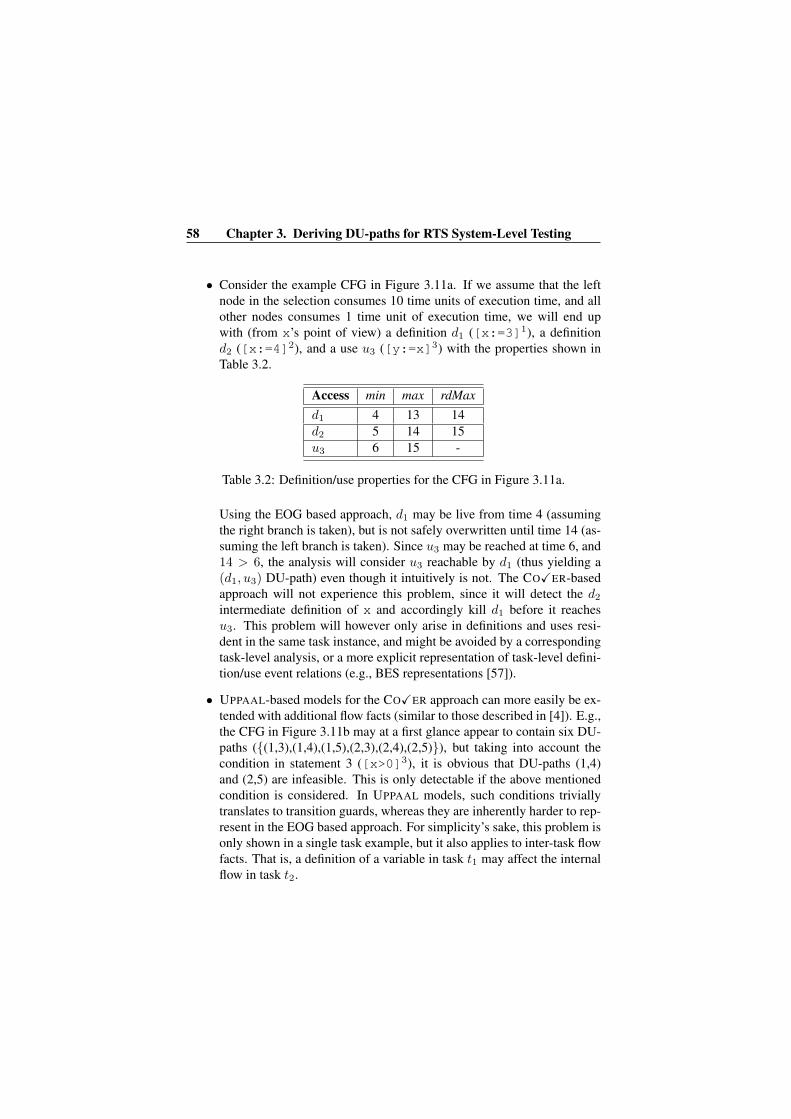
58 Chapter 3. Deriving DU-paths for RTS System-Level Testing
• Consider the example CFG in Figure 3.11a. If we assume that the leftnode in the selection consumes 10 time units of execution time, and allother nodes consumes 1 time unit of execution time, we will end upwith (from x’s point of view) a definition d1 ([x:=3]1), a definitiond2 ([x:=4]2), and a use u3 ([y:=x]3) with the properties shown inTable 3.2.
Access min max rdMaxd1 4 13 14d2 5 14 15u3 6 15 -
Table 3.2: Definition/use properties for the CFG in Figure 3.11a.
Using the EOG based approach, d1 may be live from time 4 (assumingthe right branch is taken), but is not safely overwritten until time 14 (as-suming the left branch is taken). Since u3 may be reached at time 6, and14 > 6, the analysis will consider u3 reachable by d1 (thus yielding a(d1, u3) DU-path) even though it intuitively is not. The COXER-basedapproach will not experience this problem, since it will detect the d2
intermediate definition of x and accordingly kill d1 before it reachesu3. This problem will however only arise in definitions and uses resi-dent in the same task instance, and might be avoided by a correspondingtask-level analysis, or a more explicit representation of task-level defini-tion/use event relations (e.g., BES representations [57]).
• UPPAAL-based models for the COXER approach can more easily be ex-tended with additional flow facts (similar to those described in [4]). E.g.,the CFG in Figure 3.11b may at a first glance appear to contain six DU-paths ({(1,3),(1,4),(1,5),(2,3),(2,4),(2,5)}), but taking into account thecondition in statement 3 ([x>0]3), it is obvious that DU-paths (1,4)and (2,5) are infeasible. This is only detectable if the above mentionedcondition is considered. In UPPAAL models, such conditions triviallytranslates to transition guards, whereas they are inherently harder to rep-resent in the EOG based approach. For simplicity’s sake, this problem isonly shown in a single task example, but it also applies to inter-task flowfacts. That is, a definition of a variable in task t1 may affect the internalflow in task t2.

Chapter 4
Test Item Monitoring UsingDeterministic Replay
Monitoring embedded RTSs using software probes may perturb the correcttemporal operation of the software. Still, monitoring is essential for extractingthe information required for determining test adequacy, e.g., coverage, duringtesting. Execution replay is an established method for overcoming the probeeffect problem [5, 6, 9, 16, 19, 25, 60, 95, 102, 106]. In this chapter, we de-scribe our RTS-oriented replay method, called Deterministic Replay [94, 105].We also present the Time Machine, a Deterministic Replay tool implementa-tion, and its three sub-components; the Recorder, the Historian, and the TimeTraveler. Further, we describe the use of this replay method to extract the setof exercised test items, i.e., TestDU (S,Q), from a RTS without introducingprobe effects. Our method of replay-based DU-path monitoring consists of thefollowing steps (also shown in Figure 4.1):
1. As the system S is designed and built, it is equipped with instrumentationfor Deterministic Replay1, i.e., probes, that extract the system events anddata causing non-determinism, are introduced. Due to the low perturba-tion levels for this instrumentation [94, 105], the probes can be placedpermanently in the source code of S, thereby eliminating probe effects.With the replay-probes embedded, S is tested using some test suite Q(4.1-A and 4.1-B). This yields a set of test reference execution record-ings (4.1-A), each of which may span over several system LCMs.
1Naturally, also legacy code systems may be instrumented for replay [94].
59

60 Chapter 4. Test Item Monitoring Using Deterministic Replay
T I M ELCM1 LCM2 LCMN
Analysis
Reference execution Replay executionin=q in=q
out=yout=y
Extraction of non-deterministicevents and data
Enforcement of non-deterministicevents and data
Extraction of run-time definition
and use information
Reference execution recordingA
B D E
C
Figure 4.1: Replay-based DU-path monitoring - an overview.

4.1 Introduction 61
2. The replay logs from Step 1 are gathered and analysed (4.1-C). Addi-tional probes are added to S in order to be able to extract accesses toshared variables. For each test execution, its temporal behaviour is en-forced based on the recorded execution, rather than by external eventsor the passage of time (4.1-D). This creates a monitorable determinis-tic replica of the test execution. Thus, the execution of added probes inthe replay execution will not consume any execution time relevant to thedeterminism of the execution reproduction. The test suite Q is then re-executed by replay execution and information of exercised shared vari-able accesses are recorded (4.1-E). In this two-phase scheme, the amountof information extracted is of no significance to the determinism of thetemporal behaviour of the system. Based on the outcome of this step, wederive TestDU (S,Q), and are able to determine DU-path coverage bycalculating rDU = |TestDU (S,Q)|
|ModelDU (MS)| .
4.1 IntroductionRun-time monitoring, e.g., for the purpose of test progress monitoring, is tra-ditionally performed using hardware or software probes, where the hardwareprobe category includes in-circuit emulators, logic analysers, and custom mon-itoring devices [26]. Software probes, on the other hand, are implemented us-ing instrumenting statements included in the source code of the system. Asfor hardware probes, they have the benefit of being able to extract run-timeinformation without temporally or functionally perturbing the execution of theinstrumented system. However, hardware probes suffer from other types ofdrawbacks:
• The support for hardware instrumentation is dependent on the target em-bedded system target hardware. Small volume, new, and high-end pro-cessors may lack state-of-the-art support for hardware instrumentation.
• Hardware instrumentation does in many cases require resources that, dueto spatial reasons, may not be shipped with deployed systems [93]. Thismight not be a problem for testing, but post-deployment support for in-strumentation is attractive for other reasons (e.g., debugging [94, 105]).
• Some hardware-based solutions, e.g., some In-Circuit Emulators, are ex-pensive, making them unsuitable for usage in small projects, and a po-tential bottleneck resource in the development for big projects.

62 Chapter 4. Test Item Monitoring Using Deterministic Replay
Software probes are more flexible than hardware probes, since they areadded, altered and removed with less effort. There are two main problems withsoftware probes:
• Software probes are intrusive in the sense that they consume both execu-tion and memory resources, thereby affecting, and potentially affectingthe temporal behaviour of the system. This phenomenon is called theprobe effect [31].
• In resource-constrained embedded RTSs, memory and execution timeare critical issues, limiting the amount of invasive monitoring allowed atrun-time.
Due to the drawbacks of hardware probes, and the hypothesis that we areable to overcome the problems of software probes, we focus on the latter ratherthan the hardware-based solutions in this thesis. Further, we will show how toovercome the above software probe drawbacks.
4.1.1 The Probe EffectThe probe effect [31] describes the fact that it is not always possible to ob-serve without interfering. If probes are added, removed, or altered over time,such that the level of perturbation that they cause varies, the system behaviourmay be affected. On function or unit-level in a non-RTS, where execution isperformed sequentially and without races or strict deadlines, this intrusivenessmay be acceptable. However, in RTSs, software probes may lead to severediscrepancies in execution behaviour when comparing probed and non-probedexecutions. As an illustrative example, consider the following scenario: Twotasks (A and B) share a resource, x, accessed within critical sections. In Fig-ure 4.2, accesses to these sections are displayed as black sections within theexecution of each task. Now, assume that the intended ordering of the accessesto x is first access by B, then access by A. As we can see from Figure 4.2,the intended ordering is not met and this leads to a system failure. When in-strumenting the system for testing (e.g., all-du-path based testing), the insertedprobes (the white sections in Figure 4.3) will alter the temporal behaviour ofthe system in which case, no system failure will occur.
Thus, when testing, the execution time of the probes will prolong the exe-cution of taskA such that it is pre-empted by taskB before it enters the criticalsection accessing x and the failure is not repeated. Hence, simply by probingthe system, the instrumentation has altered the outcome of the execution we

4.1 Introduction 63
P R
I O
R I
T Y
T I M E
A
By=x
x++
Figure 4.2: An execution of two tasks leading to a system failure.
wish to observe and the observed behaviour is no longer valid with respect tothe original execution in Figure 4.2.
P R
I O
R I
T Y
T I M E
A
By=x
x++
Figure 4.3: Execution of the same tasks as in Figure 4.2, now with insertedsoftware probes for coverage instrumentation, “invalidating” the failure.
4.1.2 Deterministic ReplayIn our work on debugging of embedded RTSs, we have proposed a replaymethod for recording events and data causing non-determinism during a ref-erence execution and to reproduce the execution in a subsequent replay execu-tion [105]. Similar to other replay debugging methods (described in Chapter 7),the replay execution can be used to reproduce a failure in a debugger environ-

64 Chapter 4. Test Item Monitoring Using Deterministic Replay
ment if the reference execution fails. Our method allows replay of real-time ap-plications running on top of standard commercial real-time operating systems(RTOS) and uses standard cyclic debuggers for sequential software [16]. Thereis no need for specialized hardware or specialized compilers for the method towork and the software based instrumentation overhead has so far proven indus-trially acceptable (in the area of 3% of the total system load [94]). This allowsour probes to be left permanently in the system, making post-mortem debug-ging of a deployed system possible while at the same time eliminating the riskof experiencing probe effects during debugging. We refer to our method asDeterministic Replay.
Considering the full potential of the ability of forcing concurrent executionsinto a deterministic run-time behaviour, other possibilities than system-leveldebugging arise. In this chapter, we describe the Deterministic Replay method,the Time Machine tool implementation, and the use of these in order to performreplay-based monitoring of DU-paths (i.e., extracting TestDU (S,Q)).
4.2 Deterministic Replay DU-path Monitoring
The method for replay-based monitoring that we propose is a two-phase sche-me, where phase (1) performs a limited instrumentation of a reference exe-cution in order to facilitate replay, and phase (2) extracts definition and useinformation during the enforced behaviour of the replay execution. From thisinformation, visited DU-paths in the reference execution can be derived. Dur-ing phase (1), the software probes may be acceptably intrusive (i.e., they shouldnot consume more resources than affordable in a deployed system, since theyshould be left permanently in the system). If this requirement is fulfilled, probeeffects are eliminated and the technique is also applicable post-deployment [94].
In this section, we describe the process of using Deterministic Replay inorder to derive the set of DU-paths exercised by testing the system S with thetest suite Q (TestDU (S,Q)). The process requires a monitorable determinis-tic replica of a multi-tasking RTS execution. For now, this replica is assumedto be provided by the Deterministic Replay method. In the later sections ofthis chapter, we will describe the process of creating this deterministic replicafully. In order to derive exercised DU-paths during the deterministic replicaexecution, we monitor definitions (assignments of values to shared variables)and uses (read accesses to shared variables) by placing debugger breakpointson the statements containing the definitions and uses. Using the breakpoint

4.2 Deterministic Replay DU-path Monitoring 65
commands facilitated, e.g., by a scripting language [89], or by a plug-in API2,we are able to extract a sequence of definitions and uses from each test caseexecution. From these, and the definition of a DU-path, it is trivial to de-rive the DU-paths. Alternatively, the definition/use access monitoring could beperformed by placing debugger watchpoints on the shared variables, but thiswould have a significant detrimental effect on the performance of the replayexecution.
In detail, in order to derive TestDU (S,Q) given a system S and a test suiteQ, the following steps are undertaken:
1. Ensure that S is instrumented to facilitate Deterministic Replay.
2. Execute all test cases inQ on S. As an outcome of the replay instrumen-tation, this will yield a set of execution traces E, where each executiontrace ek ∈ E can be used to deterministically replay the execution of testcase qk ∈ Q.
3. For each task w ∈ WS , statically identify the set G of all statementscontaining shared variable accesses (actually, this information is a by-product of the task level analysis described in Section 3.3.2).
4. For each statement g ∈ G, place a breakpoint on that statement. Insteadof halting the execution, set the breakpoint to issue a set of commands(an example of breakpoint commands is shown in Section 6.2.3). Thecommands are set to log the time of occurrence, the variable accessed,the type of access (def or use), and the address of the PC (i.e., the state-ment itself) before resuming the execution.
5. For each trace ek ∈ E, perform a replay execution of S in a debuggerwith all shared variable access breakpoints set. This will yield a new setof traces E′, where each e′k ∈ E′ contains ordered information of theshared variable accesses performed by test case qk ∈ Q.
6. For each trace e′k ∈ E′ , derive the set of tested DU-paths Γk in that traceusing the following rule: For each shared variable x and each subtrace γof e′k, such that γ starts with a definition of x, ends with a use of x, andcontains no other definitions of x, γ describes a tested DU-path.
Consequently, TestDU (S,Q) =⋃e′
k∈E′ Γk.
2See, e.g., www.iar.com

66 Chapter 4. Test Item Monitoring Using Deterministic Replay
However, in order for the above scheme to work, and to correctly deriveTestDU (S,Q) from a system S, it is imperative that we are able to determin-istically reproduce the execution of each test case in Q. Therefore, in the nextsection, we will focus on the concept of reproducibility.
4.3 Reproducibility
For sequential programs with no external interaction, reproducibility is not aproblem. If such a program is started an arbitrary number of times with identi-cal inputs, all invocations of the program will exhibit identical behaviours andproduce identical outputs. A program with this property is said to be determin-istic [99]. For example, consider the program in Figure 4.4. If the program isexecuted with an input value of 0, it will eventually come across a division byzero. If the execution is repeated with the same input, we will again end up atthe division by zero. Naturally, there is no limit on the number of times thisfailure will occur. Each time this program is executed with the input 0, we willreach the division by zero.
int avg (int x){
int y, ret;y = getTotal();ret = y / x;return ret;
}
Figure 4.4: A sequential deterministic program.
In order to be able to monitor DU-paths exercised in an execution by meansof execution replay, the system or program needs to be not only deterministic,but also reproducible (i.e., deterministic and controllable with respect to execu-tion parameters [99]). Unfortunately, not many applications or systems todayare even deterministic due to factors such as asynchronous I/O, concurrency,and timing.
Starting with the next section, we will try to give a clear picture of theproblems involved in deterministic reproduction of non-deterministic systemexecutions.

4.3 Reproducibility 67
4.3.1 Context Issues
Any useful computer system interacts with its environment. In its most ba-sic form, an example of such interaction could be that of a program taking acommand line input, sequentially calculating something based on that inputand finishing by returning a command line output. This example system is de-picted in Figure 4.5. If the command line input given to this program is theonly parameter that can affect the output of this program and we know of thisinput (after all, we gave it on the command line in the first place), to us, thisis a deterministic system. In addition, since we gave the input, we can simplygive it again and receive the same behaviour and the same output. Thus, thisprogram is also reproducible.
CalculationInput Output
Figure 4.5: A basic interaction with a known and controllable external context.
This might seem somewhat trivial, but as we continue our line of reasoningand consider the system shown in Figure 4.6, we come across a slightly morecomplex situation. Suppose that the system is part of a mechatronic controlsystem. It can be initialized and terminated by a user, but in between theseevents it leads a life of its own within a loop. This loop structure is usedto periodically sample some external process, calculate a response to thesesamples and to produce actuating values based on the result of the calculation.As the observed system behaviour is uniquely defined by the inputs read atsampling time, this is a deterministic system. However, without the help ofsome kind of recording mechanism, it is nearly impossible to reproduce theseinputs. Hence, the system in its basic form is not reproducible.
In short: A system, whose behaviour depends on parameters provided by anoutside environment, is not reproducible if we cannot control this environment.To make the system reproducible, our only options are to gain control of theseparameters or the environment providing them. In this thesis, we concentrateon the former.

68 Chapter 4. Test Item Monitoring Using Deterministic Replay
Get input
TerminationInitialization
Produce outputE N V I R O N M E N T
S Y S T E M
Figure 4.6: An interaction with a known, but uncontrollable external context.
4.3.2 Ordering Issues and Concurrency
So far in this chapter, we have only focused on reproducibility of sequentialprograms, i.e., programs running in a single thread of execution on a singleprocessor. Looking at current state-of-the-practice commercial software, theapplications that fulfill these restrictions are easily accounted for. In orderto meet requirements regarding efficiency, interactivity and hardware utiliza-tion, most applications are pseudoparallel (several threads of executions on thesame processor) or parallel (several threads of executions on several differentor identical processors). If the interaction with an external context described inthe above section seemed troublesome with regard to deterministic reproduc-tion, it is merely a minor problem compared to the problems introduced by theconcept of concurrency. Although deterministic reproduction of truly parallelsystem executions introduces additional complexity compared to deterministicreproduction of pseudoparallel system executions, the main focus of this chap-ter will be on the latter. In such systems, we face the additional challenge ofreproducing the system-level control flow caused by the execution ordering oftasks.
4.3.3 Timing Issues
When discussing the concept of execution orderings, there is an importantdistinction to be made. Execution ordering events (in essence, events thatcause task switches) can be either synchronous or asynchronous. In our view,synchronous events are manifestations of the internal inter-task synchroniza-

4.3 Reproducibility 69
tion mechanisms of a system (e.g., message receipts or semaphore releases),whereas those events we categorize as asynchronous occur due to correspond-ing events in the system’s external temporal- or functional context (such astimer- or peripheral interrupts). As a consequence, synchronous events alwaysoccur at pre-determined statements in the code of the system (e.g., a semaphorewill always be released at a semaphore_release operation). In contrast,asynchronous interrupts can occur anywhere outside interrupt_disable-protected sections. This temporally and logically unrestricted access of asyn-chronous events makes the location of occurrence of these events inherentlyharder to pinpoint than that of synchronous events. Previous methods for han-dling this problem have been proposed and are discussed in Section 7.2.1.
In 1978, Lamport presented a method for achieving a total ordering ofevents in a distributed system execution [56]. This paper addressed the prob-lem of lack of a mutual timebase in multiprocessor systems. As an example,consider a two-processor system (processor A and B) with local per-processorclocks. As it is practically impossible to achieve a perfect synchronization ofthese clocks, they will differ with a precision of, say, 2δ. Given this, orderingan event e1 occurring at local time x in processor A and an event e2 occurringat local time x+ δ in processor B will be very difficult. In Lamport’s proposal,this problem is solved using a distributed algorithm based on per-node logicalclocks rather than physical clocks. In addition, Lamport’s solution allows forevents on different nodes to have indistinguishable logical timestamps. Suchevents are said to be concurrent.
Even if we do not focus on distributed multiprocessor systems, Lamport’spaper makes an important point: A correct reproduction of the temporal be-haviour of an execution implies a correct reproduction of the ordering of eventsin the execution. However, a correct reproduction of the ordering of eventsdoes not necessarily imply a correct reproduction of the temporal behaviour.In a more formal notation:
Timing ⇒ Ordering, whereas Ordering 6⇒ Timing
In many systems, a correct reproduction of the ordering of synchronous eventsis sufficient for acheiving a correct reproduction of the entire system behaviour.However, in systems with real-time requirements, alterations in the temporalbehaviour of an execution that do not explicitly alter the ordering of eventsmight nevertheless affect the correctness of the system. An example of a sys-tem with this type of behaviour is a multi-tasking RTS with hard deadlines.
In addition, relying solely on the synchronization ordering for reproducingnon-deterministic executions will only work if the system is properly synchro-

70 Chapter 4. Test Item Monitoring Using Deterministic Replay
nized. If data races exist in an execution, these will go undetected if we focusexclusively on the correct reproduction of the synchronization sequence.
4.3.4 Reproducibility - Summary and Problem Statement
To summarize this section, there are a few issues that have to be resolved whentrying to deterministically reproduce multi-tasking real-time programs. At thestart of this section, we started with a sequential, non-real-time program with abehaviour depending solely on its command-line inputs.
As systems are incorporated in different temporal and environmental con-texts, the assumption of a completely deterministic and reproducible systembehaviour will no longer hold. Interactions with external contexts and multi-tasking will lower the probability of traditional execution reproducibility to anegligible level. As depicted in Figure 4.7, events occurring in the temporal ex-ternal context will actively or passively have an impact on the RTS execution.In this section, we discussed issues related to context, ordering, timing and theembedded nature of embedded systems. Now, let us see if we can derive a lessabstract problem formulation from these sections.
TIME
PR
IOR
ITY
Temporal context
External context
Figure 4.7: Execution of a multi-tasking RTS, dependent on the temporal- andthe external context within which it is executing. Grey areas in the tasks rep-resent temporal interaction (e.g., interrupts), and external context interaction(e.g., sampling) respectively.
In order to correctly monitor and derive test items during testing withoutprobe effects using Deteriministic Replay, we need to achieve the same levelof reproducibility in multi-tasking RTSs as the one we have in non-real-timesequential software. Considering this, there are a number of clarifying steps we

4.3 Reproducibility 71
can take. First, even though they served a logical- and (hopefully) pedagogicalpurpose, all issues related to ordering can be ignored. This might seem odd,but consider the conclusion in Section 4.3.3. As timing implies ordering andwe need to be able to reproduce timing in order to meet our requirements,the reproduction of system timing will have correct reproduction of executionordering as a consequence.
Second, from the point of view of the temporal and external contexts, theinteraction with the system manifests in two different ways: The context (orrather a peripheral device) can actively interact with the system by means of anasynchronous interrupt. This interrupt most often has its origin in a correspond-ing event in the context itself (e.g., a reset of a clock register or a completionof an I/O transaction). The other means of interaction is when the context ispassively being read by the system (e.g., synchronous reads of sensor values orclock registers). Hence, there are exactly three things required for deterministicreproduction of executions for monitoring on a single-node concurrent system:
• Starting StateWe need to be able to provide the exact initial state of the execution weseek to reproduce.
• InputAny input, initial or intermediate, to the execution must be reproduced,such that it exactly simulates the temporal, external or random contextof the execution we desire to reproduce.
• Asynchronous EventsAll asynchronous events that occurred within the execution must be re-produced in such a way that their temporal and causal interference withthe execution is not altered.
The first item of this list of requirements is no different to that of repro-duction of non-real-time sequential software (i.e., command-line input), albeitslightly more difficult to achieve in real-time multi-tasking software. This re-quirement is equivalent to that of being able to pinpoint the current location ona map in order to use the map correctly. If you do not know where you are,there is no use reading the map in order to get where you want to be.
The second and the third requirement simply reflect the influence of tem-poral and external means of passive (input) or active (asynchronous events)interaction. However, note that these requirements are based on theoretical as-sumptions. As we shall see in Section 7.2.1, due to practical reasons, some of

72 Chapter 4. Test Item Monitoring Using Deterministic Replay
these requirements have been ignored, under-elaborated or over-elaborated inprevious work.
4.4 The Time MachineThe contribution of this chapter is a monitoring technique based on Determinis-tic Replay [105, 94], and we hence need to describe the details of this techniqueas well as its prototype implementation (the Time Machine). This is the purposeof this section. In our method, information is recorded during runtime with re-spect to interrupts, task-switches, timing, and data. The system behaviour canthen be deterministically reproduced off-line using the recorded history, andinspected to a level of detail, which vastly surpasses what has been recordedsince the system is deterministically re-executed such that all calculated datais restored. We will show how entire test executions including interrupts, task-switches and data can be reproduced off-line in order to facilitate the probeeffect-free DU-path instrumentation process described in Section 4.2.
4.4.1 System Model RefinementsIn addition to the assumptions posed in Section 1.2, we assume access to adebugger with an interface or scripting language such that macros or programscan be invoked conditionally at specified breakpoints, as well as target mem-ory access. As we shall see, the availability of a proper debugger environmentis imperative for the extraction of DU-paths from a replay execution. We fur-ther assume that the RTOSs have kernel instrumentation support such that taskswitches can be recorded during runtime. Several commercial RTOSs, e.g.,VxWorks3 and QNX Neutrino4, do.
4.4.2 The Mechanisms of the Time MachineWe will now in further detail discuss and describe our method for achievingexecution replay by describing its Time Machine implementation. The basicelements of the Time Machine are:
1. The Recorder, which is an in-target mechanism that collects all neces-sary information regarding the task-switches, interrupts, and data caus-
3www.windriver.com4www.qnx.com

4.4 The Time Machine 73
ing non-determinism in the system. The function of the Recorder basi-cally answers to Step B in Figure 4.1 on Page 62.
2. The Historian, which is the off-target system that automatically ana-lyzes, and correlates events and data in the recording, and composesthese into a chronological timeline of breakpoints and break conditions.The Historian analysis corresponds to Step C in Figure 4.1.
3. The Time Traveler, which interacts with the debugger and, given theinformation provided by the historian, allows the recreation of the pro-gram state (i.e., state variables, global variables, program counter, etc.)for any given time in the scope of the memory of the Historian. Thefunction of the Time Traveler is shown as Step D in Figure 4.1.
This process is performed without ever changing the target executable code.The same code (including RTOS) that is run in the target, during runtime, isrun during the replayed execution in the debugger. DU-path instrumentation isfacilitated using watch- or breakpoints with associated commands.
The Recorder
To achieve Deterministic Replay of an execution, a sufficient amount of infor-mation of the execution must be gathered. The basic idea of replay recordingis that we need only record external inputs and internal state variables sincewe later during replay re-execute the system and consequently recalculate allintermediate variable values and outputs. If we use system start-up replay (i.e.,if we do not allow old entries to be overwritten during the recording), all staticand global variables are also recalculated, and can be omitted from recording.
The first part of the Time Machine, the Recorder, is basically a collectionof kernel and application software probes and buffers for replay recording. Inthe Recorder, the storage space for monitored data is divided into two parts:the execution ordering buffer and a set of data flow buffers.
The execution ordering buffer is used to store all kernel events causingnon-determinism, such as task switches, interrupts and missed deadlines. Itconsists of a cyclic buffer of a user-defined number of entries and an indexpointing at the next entry available to write. Each entry in the buffer consists ofa 7-tuple and is defined as 〈Tk ,STk ,PC ,SP ,C ,Ev ,EvT 〉 where Tk and STkdefine the time of the event. Tk is the value of a software-based tick counter,incremented by a timer interrupt. STk, on the other hand can be viewed upon asfractions of a tick and is the value of a free-running counter in the underlying

74 Chapter 4. Test Item Monitoring Using Deterministic Replay
hardware, reset at each tick. This means that an event that occurred at Tk=43,STk=256 predates an event occurring at Tk=43 and STk=398. Moving on, wehave PC, which is the value of the program counter register at the time of theevent. SP is the value of the stack pointer and C is the unique marker used todifferentiate between PC values in iterative constructs (see, e.g., Figure 4.8).
for (i=0; i<10; i++){
a = a + i;----------------------PC=0x2340b = q * 2 + i;
}
Figure 4.8: The PC is not sufficient as a unique marker.
In general, to correctly pinpoint asynchronous events, we need to recordwhere and when they occur by using timestamps and the PC value. How-ever, since PC values can be revisited in loops, subroutines and in recursivecalls, additional mechanisms are required in order to define a unique markerfor asynchronous events. We make use of a generic marker consisting of theSP value, register-bank checksums, and/or checksums of part of the user-stack.This approach is described in-depth in Appendix C.
Finally, we have Ev and EvT. EvT tells us what type of event that occurredand Ev is an identifier of the event. For example, if a hardware interrupt occurs,EvT tells us that an interrupt occurred and Ev tells us which interrupt serviceroutine that was run. Another example can be made from a task switch. If atask switch occurred, EvT tells us that a task switch occurred (and what type oftask switch that occurred) and Ev tells us which task that gained control afterthe task switch. The structure of an event in the execution ordering buffer isshown in Figure 4.9.
The other part of the memory storage space for monitor data is the data flowbuffers. This is a set of user-defined buffers, used to record task data insteadof kernel events. The data recorded here could be data external to the task,such as inputs to the task, system state, readings of sensors and messages fromother tasks or nodes. In other words, data, that cannot be reproduced just byproviding the same internal state as in the first run, should be recorded. A thingto keep in mind is that in contrast to the execution ordering buffer, each dataflow buffer is tied to a specific task. The execution ordering buffer is globaland is used only by the kernel.

4.4 The Time Machine 75
Tk STk PC SP C Ev EvT
Execution ordering buffer
Event
Figure 4.9: A magnified event in the execution ordering buffer.
An entry in a data flow buffer is defined as a 3-tuple: 〈Tk ,STk ,Dt〉 wherethe meanings of Tk and STk are analogous to those in the control flow buffer.Dt, however, is a set of user-defined data recording entries, that can be usedto record data during a run-time execution of the task. The data flow buffersare cyclic and their recording mechanism works in the exact same way as theexecution ordering buffer. Note that no full checkpoints of data contents aremade (in order to potentially restore a starting state for replay), but individualdata are incrementally stored when accessed. This approach requires moreeffort for instrumenting the system, but has the benefits of storing only thedata that needs to be stored, and allowing replay start-up not only from pre-determined checkpoints.
In our basic approach we make use of a separate basic FIFO cyclic bufferfor each task data flow, and one for the execution ordering. In these buffers, theoldest entry is always discarded when a new entry has to be recorded. Conse-quently, the system can only be replayed for the length of the recording in thetemporally shortest buffer. Huselius [45] proposed the use of a single bufferand an eviction scheduler for Deterministic Replay recording purposes. Themonitoring of this approach is more intrusive than that of cyclic buffers, butgenerally it provides a longer available replay.
In either case, it is important that the developer in an early state of thedesign allocates sufficient space to achieve a replay long enough to be ableto fulfill the purpose of the replay. Note that for some purposes, e.g., for testitem derivation, it is often desirable to replay the entire execution from systemstart-up.

76 Chapter 4. Test Item Monitoring Using Deterministic Replay
The Historian
The Historian is an off-line analysis tool with the objective of providing a com-plete basis for the Time Traveler mechanism. The input to the off-line analy-sis is the raw data of the execution ordering buffer and the data flow buffersrecorded on the target system. The idea is to use the information from systemevents to create breakpoints in the replay execution where the events occurredin the recorded execution. When halted at a breakpoint, different parts of thesystem state can be automatically altered in order to simulate an interrupt or atask switch. When the system state variables are set, the execution resumes. Inthis way, all external system events can be simulated.
Once the execution ordering and the data-flow of the application is recorded,the first job for the historian is to sort the execution ordering entries in order ofoccurrence and to construct a timeline. An execution ordering entry is eitherasynchronous (e.g. task preemption or interrupt) or synchronous (e.g. block-ing system call). For each asynchronous execution ordering entry, the historiangenerates a conditional breakpoint, such that for each PC value where asyn-chronous events occurred, a breakpoint is set. These breakpoints are guardedby the condition of the recorded unique marker, e.g.,
break at PC(event) if(SP == SP(event) &&CHKSUMS_REGS(event) ==
(R0+R1+R2+...+Rn) &&CHKSUMS_STACK(event) ==
(*(SP)+*(SP+1)+*(SP+2)+...+*(SP+m)))
Synchronous events, on the other hand, are not represented by unique indi-vidual breakpoints. Instead, the entry point of each blocking system call, thatmight give rise to a synchronous event, is breakpointed. The control and matchof the synchronous unique marker is here managed by the Time Traveler tool,as is the transfer of control from the executing task to the subsequent task. Atimeline, similar to that of the execution ordering, is also assembled for thedata-flow. To allow a smooth correlation between data and execution ordering,both monitoring activities are closely integrated.
Should the recordings contain the entire execution history from systemstart-up, the timelines are replayable as-is. Making use of a set of cyclic buffersfor recording, where old values can be overwritten, might however raise theproblem of having to start the replay from a non-startup state. In this case itis crucial to find a mutually consistent starting point for the replay. In other

4.4 The Time Machine 77
words, we need to figure out at what execution ordering log entry and at whichdata instance to start the replay execution from.
Data flow
Data flow
Execution ordering
t1 t2 tendLog
Figure 4.10: Insufficient data-flow between t1 and t2.
Since the basic idea of Deterministic Replay is to re-execute the applicationin exactly the same temporal and environmental context as the recorded exe-cution, thus creating a fully monitorable sequential deterministic replica of thereference execution, a basic requirement is that both the execution ordering andthe data flow information that constitute the replay context need to be availableat the start of the replay. Consider, for instance, the scenario in Figure 4.10.Due to the dimensioning of the buffers, the execution ordering timeline spansfrom t1 to tendLog, while the shortest data flow timeline spans from t2 to tendLog.In this case, replay starting points between t1 and t2 will not be valid since notall data flow information is available. Similarly, Figure 4.11 shows a scenariowith an interval where no execution ordering information is available.
Data flow
Data flow
Execution ordering
t1 t2 tendLog
Figure 4.11: Insufficient execution ordering between t1 and t2.
The requirement of available data flow at the replay starting point has tobe considered when choosing how to record data. However, how to handlestarting point issues are highly dependent on the underlying run-time model,and will be discussed in detail in Section 6.2.3.

78 Chapter 4. Test Item Monitoring Using Deterministic Replay
The Time Traveler
The Time Traveler is the “engine” driving the replay forward by automaticallyacting upon breakpoint events and issuing commands to the debugger. Initially,by setting breakpoints at all blocking system calls, we can initialise the replayof the recorded execution. First, the system is reset in the debugger and thetimeline index, an index pointing at the current execution ordering entry tobe matched, is set to point at the first suitable starting point in the executionordering timeline. Then, each task is initialised such that its run-time statematches a suitable starting point in the historian-generated timeline. At thispoint, the recorded data flow of the suspended task is written back into theapplication. The timeline index is incremented and the next task is set up forexecution. Once the data flow of all instrumented tasks has been rewritten intothe application, the replay session initialisation phase is complete.
When the initialisation is ready, the replay will step forward as the timelineindex is incremented at each execution ordering entry successfully matched. Inaddition, in the event of a subsequent asynchronous event for the current taskin the historian timeline, its corresponding conditional breakpoint is set, mak-ing it possible to replay this event as that breakpoint is hit. Once breakpointsrepresenting asynchronous events are hit and successfully matched, they areremoved in order to enhance the performance of the replay session. This De-terministic Replay session will behave exactly like a (fully monitorable) regularsequential program mimicking the exact execution of the recorded multitaskingreal-time application.
4.4.3 Deterministic Replay Summary
In conclusion, we have described how to record and reproduce interrupts andasynchronous task-switches in a multi-tasking RTS. Assuming that significantvariables, like state variables, and peripheral inputs like readings of sensor val-ues or events like accesses to the local clock, are identified and recorded, itis possible to reproduce the interference from all sources of non-determinismoff-line. Hence, decoupling of the external system (the real-world) and theprogression of the system is accomplished, and Deterministic Replay of RTSsis facilitated. During the replay execution, the software behaviour of the sys-tem can be investigated to any level of detail. In this thesis, we use this newlyachieved observability in order to derive exercised DU-paths during system-level testing.

4.5 Discussion 79
4.5 DiscussionIn this chapter, we have presented our RTS-oriented replay method, called De-terministic Replay [94, 105], and how to use this method in order to extractthe set of exercised test items (i.e., TestDU (S,Q)) from an embedded RTSwithout introducing probe effects. We conclude the chapter with a discussionregarding the lessons learned during the development and application of theDeterministic Replay method.
• System ModelThe Deterministic Replay method is not as sensitive to changes in theassumed system model as the other contributions in this thesis. For theDU-analyses proposed in Chapter 3, a periodically repeated system be-haviour is an absolute necessity (for the EOG-based approach), or highlydesirable (for the UPPAAL-based approach). Even though some aspectsare somewhat complicated (e.g., dimensioning of recording buffers, andthe process of finding a consistent starting point), Deterministic Replayis applicable in time-triggered, as well as sporadic and event-triggeredreal-time systems with terminating or non-terminating tasks.
• Data Flow AnalysisWe have successfully applied the time machine approach proposed inthis paper in a number of applications running on different operatingsystems, different hardware, different compilers, and different debug-gers (a thorough description of our case studies is given in Section 6.2).What we have learned however from these studies, is that it is necessaryto carefully analyze the target system’s data flow with respect to whatdata is re-executed, re-transmitted and what data has external (process)origin in order not to forego something that may inhibit deterministicre-execution or that we do not record too much.


Chapter 5
System-Level DU-pathCoverage – An Example
In the previous chapters, we presented the main technical contributions of thisthesis. Specifically, Chapter 3 described how to derive a the set of DU-pathsfrom an abstract model of a RTS S (ModelDU (MS)), and Chapter 4 describedhow to derive the set of DU-paths exercised by testing S by the test suite Q(TestDU (S,Q)).
In this chapter, we show how these contributions are combined in order todetermine structural DU-path coverage for system-level testing. For this pur-pose, we will follow an example system as it propagates through our proposedsystem-level testing process.
5.1 The ProcessFirst of all, we review the abstract description of our system-level test process.At this stage in the thesis, we are able to introduce our notion of DU-pathsets in the process description. Hence, the process, in its entirety depicted inFigure 5.1, works as follows (assuming an all DU-path coverage test criterion):
1. A set of sequential subunits (tasks) are instrumented to facilitate replay,and assembled into a multi-tasking RTS S.
2. A timed abstract representation (model) MS of the system data flowstructure is derived by means of static analysis.
81

82 Chapter 5. System-Level DU-path Coverage – An Example
G
H
I
J K
L
M
true
true
true
false
false
false
M
K
L
M
true
false
M
K
L
M
true
false
M
J
G
H
I
J K
L
M
true
true
true
false
false
false
M
K
L
M
true
false
M
K
L
M
true
false
M
J
G
H
I
J K
L
M
true
true
true
false
false
false
M
K
L
M
true
false
M
K
L
M
true
false
M
J
A
B C
D
E F
true false
true false
E
X
E
XE
X
E
XE
X
E
X
F
X
F
XF
X
F
XF
X
F
XD
E F
X
truefalse
B
X
D
E F
X
truefalse
B
X
D
E F
X
truefalse
B
X
D
E F
X
truefalse
B
X
D
E F
X
truefalse
B
X
D
E F
X
truefalse
B
X
G
H
I
J K
L
M
true
true
true
false
false
false
M
K
L
M
true
false
M
K
L
M
true
false
M
J
G
H
I
J K
L
M
true
true
true
false
false
false
M
K
L
M
true
false
M
K
L
M
true
false
M
J
G
H
I
J K
L
M
true
true
true
false
false
false
M
K
L
M
true
false
M
K
L
M
true
false
M
J
G
H
I
J K
L
M
true
true
true
false
false
false
M
K
L
M
true
false
M
K
L
M
true
false
M
J
G
H
I
J K
L
M
true
true
true
false
false
false
M
K
L
M
true
false
M
K
L
M
true
false
M
J
A
B C
D
E F
true false
true false
E
X
E
XE
X
E
XE
X
E
X
F
X
F
XF
X
F
XF
X
F
XD
E F
X
truefalse
B
X
D
E F
X
truefalse
B
XD
E F
X
truefalse
B
X
D
E F
X
truefalse
B
X
D
E F
X
truefalse
B
X
D
E F
X
truefalse
B
XD
E F
X
truefalse
B
X
D
E F
X
truefalse
B
X
D
E F
X
truefalse
B
X
D
E F
X
truefalse
B
XD
E F
X
truefalse
B
X
D
E F
X
truefalse
B
X
1
2
3
4
7
DU-pathcoverage
5
6
R
Figure 5.1: The structural system-level testing process.
3. The system schedule is added to the representation.
4. A suite of test cases Q are selected and executed. During test execution,the non-deterministic events and data of the execution are recorded.
5. The recordings are used to deterministically replay the test suite execu-tions with an enforced timing behaviour, and an added instrumentation,allowing DU-path derivation without probe effects.
6. After the testing phase, the monitored run-time information is extracted,yielding TestDU (S,Q).
7. Using analysis of the model derived in step 2, the theoretical maximumDU-path coverage (i.e., ModelDU (MS)) is derived and compared withthe results from step 6, allowing an estimate of the system-level coverageto be determined by calculating rDU = |TestDU (S,Q)|
|ModelDU (MS)|
5.2 The Example System
We will use a periodic 3-task RTS Sex with 3 shared variables in order toexemplify the test process. The system makes no claim of being functionallysound, reasonably scheduled, or of performing any useful task. Its purpose issolely to exemplify the above test process.

5.2 The Example System 83
void modeChange(){
if (mode == 0)mode = 1;
if (mode == 1)mode = 2;
if (mode == 2)mode = 0;
}
void calculate(){
if (mode == 0){
if (x < 0)x = -x;
x = x * y;}if (mode == 1){
if (y < 0)y = -y;
y = y - x;}if (mode == 2){
y = x + y;x = y - x;
}}
void shift(){
x = -y;y = -x;
}
(a) modeChange task (b) calculate task (c) shift task
Figure 5.2: Tasks of example system.
5.2.1 Example System Structure
The source code of the tasks of Sex are shown in Figure 5.2. Specifically,5.2a displays the code of the modeChange task, 5.2b shows the code of thecalculate task, and 5.2c displays the shift task code. Shared variablesused are integers x, y, and mode.
We assume that the system requirements call for a period time of 800 timeunits for all tasks, but with modeChange being offset by 100, and shiftbeing offset by 200 time units. In other words, this means that calculatetask instances (jobs) will be released at time 0, 800, 1600, ..., modeChangejobs will be released at time 100, 900, 1700, ..., and shift jobs will be re-leased at time 200, 1000, 1800, .... Furthermore, this implies a repeated systembehaviour, and a LCM, of 800 time units. In addition, we assume that theshift task is given the highest priority, the modeChange task the mediumpriority, and the calculate task the lowest priority. We further assume thatthe system is schedulable using these task parameters.

84 Chapter 5. System-Level DU-path Coverage – An Example
shift_BB31
bbet<=1
shift_BB28
bbet<=9
shift_BB26
bbet<=1
shift_BB27
bbet<=9
shift_BB32
bbet<=4
shift_BB29
bbet<=21
shift_BB30
bbet<=21
go__shift?
bbet>=1
ready__shift!
bbet>=1
ready__shift!
bbet>=9
ready__shift!
bbet>=9
ready__shift!
bbet>=21
ready__shift!
x:=1, local_var:=y
bbet>=21
ready__shift!
y:=1, local_var:=x
go__shift?
go__shift?
go__shift?
go__shift?
go__shift?
go__shift?
ready__shift!
terminate__shift!
Figure 5.3: shift UPPAAL task model automaton.
5.2.2 System Replay Instrumentation
The next step in the process is to ensure that any execution of Sex can be de-terministically reproduced by means of Deterministic Replay. Specifically, weneed to make sure that the execution ordering and the data flow of the systemcan be reproduced. As the execution ordering instrumentation (e.g., monitor-ing of interrupts and task switches) is part of the underlying run-time systemrather than the application itself, there is no need for inserting any executionordering probes in any task code. For the purpose of this example, we simplyassume that such instrumentation is included in the RTS kernel. The data flowrecording, on the other hand, is performed on the application level. The dataflow recording consists of (1) recording of intermittent input (e.g., readings ofsensor values or the real-time clock), and (2) recording of accesses to sharedor static variables (i.e., system state-preserving data). For (1), the applicationcode of Sex does not include any statements that consume external or temporalcontext input. Hence, no such instrumentation need to be inserted. For (2),

5.3 DU-path Analysis 85
bbet<=12
bbet<=12
bbet<=1
bbet<=12
bbet<=1
bbet<=20
bbet<=1
bbet<=1
bbet<=1
bbet<=20
bbet<=20
bbet<=1
bbet>=1
bbet>=20 bbet>=20
bbet>=1
bbet>=12
bbet>=1
bbet>=1
bbet>=20bbet>=20
bbet>=12
bbet>=12
bbet>=1
bbet>=20 bbet>=20
Figure 5.4: modeChange UPPAAL task model automaton.
this type of instrumentation is only required if it is required to start a replayexecution from any other point in the recording than system start-up, which isnecessary, e.g., if the entire recording is not available. In this example we as-sume that the full recording is available, and no instrumentation of this type isnecessary. If we, however, were forced to facilitate replay with a partial replayrecording, each use access of a shared variable would have to be preceded byan instrumenting statement, recording the value of the variable at that point1.
5.3 DU-path AnalysisAfter the system has been instrumented for replay, we are able to staticallyderive the models required to find ModelDU (MSex
). Note that, if the modelderivation is done before the system instrumentation, the timing of the resulting
1Note that any schedulability analysis must also consider the execution time of instrumentationinserted in the system to facilitate execution replay.

86 Chapter 5. System-Level DU-path Coverage – An Example
local_var:=mode local_var:=mode
x:=1, local_var:=x
local_var:=mode
local_var:=mode
local_var:=mode local_var:=mode
local_var:=x
y:=1, local_var:=y
y:=1, local_var:=y
y:=1,
local_var:=x,
local_var:=y
x:=1, local_var:=x,
local_var:=y
local_var:=y
local_var:=ylocal_var:=xlocal_var:=x
Figure 5.5: calculate UPPAAL task model automaton.
model will not consider the temporal effects of the software probes. Since thisthesis proposes two different modeling paradigms, we will consider both andderive model M ′
Sexusing the UPPAAL-based method, and model M ′′
Sexusing
the EOG-based method. Both model representations are generated using aSWEET-based task-level analysis.
5.3.1 Task-Level Analysis
The first step of the task-level analysis is the compilation of the system sourcecode (in our case, by the NIC C compiler). Basically, we require this compi-lation to produce the format that the static analysis tool (in our case, SWEET)operates on. Next, given the intemediate code format files, the static analy-sis tool generates the configuration files for both approaches (as described inSections 3.2.3 and 3.3.2).

5.3 DU-path Analysis 87
relCalculate !relCalculate
cCalculate>=OCalculate
moveToReady__calculate!
relCalculate:=0
cCalculate<OCalculate
cCalculate<TCalculate
cCalculate>=TCalculate
cCalculate:=0, relCalculate:=1
!relModeChangerelModeChange
cModeChange>=OModeChange
moveToReady__modeChange!
relModeChange:=0
cModeChange>=TModeChange
cModeChange:=0, relModeChange:=1
cModeChange<OModeChange
cModeChange<TModeChange
relShift !relShift
cShift<TShift
cShift<OShift
cShift>=OShift
moveToReady__shift!
relShift:=0
cShift>=TShift
cShift:=0, relShift:=1
scheduled!
schedule?
Figure 5.6: Sex schedule automaton.
5.3.2 Deriving DU-paths using UPPAAL and COXER
In the UPPAAL-based method, the configuration files generated by the staticanalysis are made up of native UPPAAL XML-based descriptions of UPPAALtimed automata. For the tasks of the example Sex system, the generated au-tomata are depicted in Figures 5.3 through 5.5. Note that the detailed explana-tion of our method for task modeling in UPPAAL is given in Appendix A. Fur-ther note that the figure displaying the shift task automaton (Figure 5.3) isthe only figure that shows complete model annotation as required by COXER,including synchronization labels for task termination (i.e., terminate shift),statement labels (e.g., shift BB26), execution control synchronization (go/readylabels), timing guards and invariants (e.g., bbet<=9), and shared variable ac-cesses (e.g., x:=1 and local var:=y). For presentation purposes, the mode-Change (5.4) and calculate (5.5) figures show solely timing and sharedvariable access annotation, respectively.

88 Chapter 5. System-Level DU-path Coverage – An Example
Once generated, the Sex task model automata are imported into the genericUPPAAL run-time system model, comprised of the task switch, system clock,and execution control automata. Model M ′
Sexis completed by the addition of a
tailored schedule automaton (depicted in Figure 5.6), and the definition of taskproperties, e.g., task period, offset, and priority, in the model.
Using the above M ′Sex
model, the UPPAAL test case generation extensionCOXER is capable of deriving ModelDU (M ′Sex
). To do this, we simply config-ure COXER to focus on DU-path coverage, using a standard DU-path observeras described in [41]. Further, we limit the variables of interest in the model tothe three shared variables in Sex (x, y, and mode) by the configuration line:
cover duVar ({x,y,mode})
Running COXER under these configurations, the analysis will yield the com-plete set of DU-paths feasible in M ′
Sex(i.e., ModelDU (M ′Sex
)). In our examplesystem, ModelDU (M ′Sex
) is a set of 81 DU-paths. As described, this set is anover-approximation of the actual number of feasible DU-paths in Sex.
5.3.3 Deriving DU-paths using EOGsFor the EOG-based approach, the static task-level analysis will generate a moreabstract task representation than in the UPPAAL case. In our case, given the in-termediate system code produced by the NIC compiler, SWEET will derive andgenerate a representation including the BCET and WCET for each task in Sex,the min and max times for each shared variable use in Sex, and the min, max,and rdMax times for each shared variable definition in Sex. Adding schedulinginformation, like task priority, offset, and periodicity, the M ′′
Sexrepresentation
is completed (see Figure 5.7).Once generated, the M ′′
Sexsystem representation is analysed for DU-paths
using the EOG-based DUANALYSIS algorithm, as described in Section 3.3 andAppendix B. The resulting set, ModelDU (M ′′Sex
) includes 83 different DU-paths, i.e., two more than considered potentially feasible by the UPPAAL-basedapproach.
5.4 System TestingNow that the sets of potentially feasible DU-paths have been derived, we areable to test Sex using an arbitrary test suite Qex, monitor the test progress (i.e.,extract TestDU (Sex, Qex)), and calculate an approximate DU-path coverage

5.4 System Testing 89
Job Rel 0 Prio 1 WCET 348 BCET 77Def BB0 Var mode min 0 max 0 rdMax 348Def BB0 Var x min 0 max 0 rdMax 348Def BB0 Var y min 0 max 0 rdMax 348Def BB22 Var x min 151 max 338 rdMax 348Def BB4 Var x min 78 max 78 rdMax 120Def BB7 Var x min 87 max 120 rdMax 348Def BB12 Var y min 99 max 194 rdMax 233Def BB15 Var y min 105 max 233 rdMax 348Def BB21 Var y min 123 max 310 rdMax 348Use BB1 Var mode min 25 max 25Use BB17 Var mode min 67 max 254Use BB9 Var mode min 46 max 141Use BB15 Var x min 105 max 233Use BB2 Var x min 45 max 45Use BB20 Var x min 98 max 285Use BB4 Var x min 78 max 78Use BB7 Var x min 87 max 120Use BB10 Var y min 66 max 161Use BB12 Var y min 99 max 194Use BB15 Var y min 105 max 233Use BB21 Var y min 123 max 310Use BB22 Var y min 151 max 338Use BB7 Var y min 87 max 120
Job Rel 100 Prio 2 WCET 102 BCET 66Def BB33 Var mode min 0 max 0 rdMax 102Def BB33 Var x min 0 max 0 rdMax 102Def BB33 Var y min 0 max 0 rdMax 102Def BB35 Var mode min 33 max 33 rdMax 102Def BB38 Var mode min 54 max 66 rdMax 102Def BB41 Var mode min 75 max 99 rdMax 102Use BB34 Var mode min 21 max 21Use BB37 Var mode min 42 max 54Use BB40 Var mode min 63 max 87
Job Rel 200 Prio 3 WCET 66 BCET 66Def BB26 Var mode min 0 max 0 rdMax 66Def BB26 Var x min 0 max 0 rdMax 40Def BB26 Var y min 0 max 0 rdMax 61Def BB29 Var x min 40 max 40 rdMax 66Def BB30 Var y min 61 max 61 rdMax 66Use BB30 Var x min 61 max 61Use BB29 Var y min 40 max 40
Figure 5.7: M ′′Sex
configuration file.
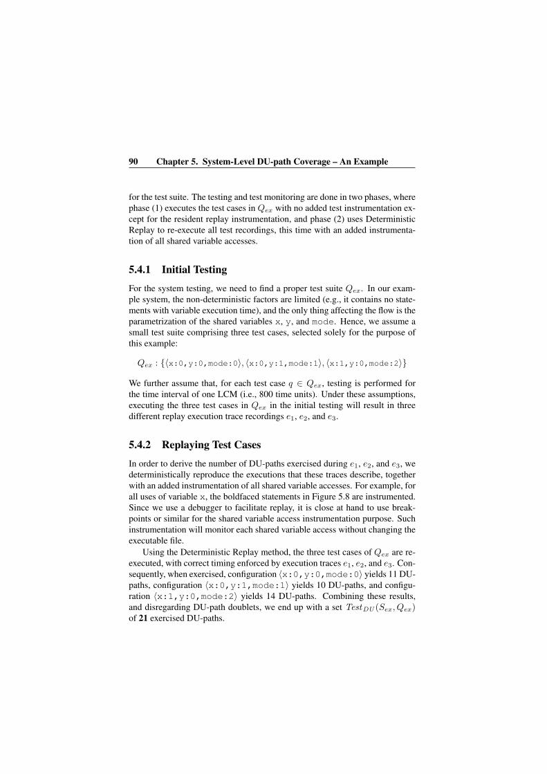
90 Chapter 5. System-Level DU-path Coverage – An Example
for the test suite. The testing and test monitoring are done in two phases, wherephase (1) executes the test cases in Qex with no added test instrumentation ex-cept for the resident replay instrumentation, and phase (2) uses DeterministicReplay to re-execute all test recordings, this time with an added instrumenta-tion of all shared variable accesses.
5.4.1 Initial Testing
For the system testing, we need to find a proper test suite Qex. In our exam-ple system, the non-deterministic factors are limited (e.g., it contains no state-ments with variable execution time), and the only thing affecting the flow is theparametrization of the shared variables x, y, and mode. Hence, we assume asmall test suite comprising three test cases, selected solely for the purpose ofthis example:
Qex : {〈x:0,y:0,mode:0〉, 〈x:0,y:1,mode:1〉, 〈x:1,y:0,mode:2〉}
We further assume that, for each test case q ∈ Qex, testing is performed forthe time interval of one LCM (i.e., 800 time units). Under these assumptions,executing the three test cases in Qex in the initial testing will result in threedifferent replay execution trace recordings e1, e2, and e3.
5.4.2 Replaying Test Cases
In order to derive the number of DU-paths exercised during e1, e2, and e3, wedeterministically reproduce the executions that these traces describe, togetherwith an added instrumentation of all shared variable accesses. For example, forall uses of variable x, the boldfaced statements in Figure 5.8 are instrumented.Since we use a debugger to facilitate replay, it is close at hand to use break-points or similar for the shared variable access instrumentation purpose. Suchinstrumentation will monitor each shared variable access without changing theexecutable file.
Using the Deterministic Replay method, the three test cases of Qex are re-executed, with correct timing enforced by execution traces e1, e2, and e3. Con-sequently, when exercised, configuration 〈x:0,y:0,mode:0〉 yields 11 DU-paths, configuration 〈x:0,y:1,mode:1〉 yields 10 DU-paths, and configu-ration 〈x:1,y:0,mode:2〉 yields 14 DU-paths. Combining these results,and disregarding DU-path doublets, we end up with a set TestDU (Sex, Qex)of 21 exercised DU-paths.

5.5 Summary 91
void modeChange(){
if (mode == 0)mode = 1;
if (mode == 1)mode = 2;
if (mode == 2)mode = 0;
}
void calculate(){
if (mode == 0){
if (x < 0)x = -x;
x = x * y;}if (mode == 1){
if (y < 0)y = -y;
y = y - x;}if (mode == 2){
y = x + y;x = y - x;
}}
void shift(){
x = -y;y = -x;
}
(a) modeChange task (b) calculate task (c) shift task
Figure 5.8: Example instrumentation of system tasks, with use accesses of theshared variable x highlighted.
5.5 SummaryOnce the ModelDU (MS) and TestDU (S,Q) sets are found, the DU-path cov-erage can be calculated as rDU = |TestDU (S,Q)|
|ModelDU (MS)| . For the M ′Sex
UPPAAL-based model, the coverage is r′DU = 21
81 ≈ 0.259. For the M ′′Sex
EOG-basedmodel, the coverage is r′′DU = 21
83 ≈ 0.253. We let this example calculation ofsystem-level DU-path coverage conclude our example chapter.
In summary, this chapter described how the contributions of this thesis canbe combined to determine structural DU-path coverage in system-level testing.Specifically, we have followed an example 3-task system Sex through replayinstrumentation, static DU-path analysis, initial testing, replay testing, and cal-culation of DU-path coverage.


Chapter 6
Evaluation
This chapter collects the results from the experimental evaluations performedon the techniques and methods proposed in this thesis, and is structured as fol-lows: The first part of this chapter (Section 6.1) will focus on experimentalevaluation of the DU-path derivation methods. The second part (Section 6.2)will focus on the case studies and implementations of the Time Machine, andthe third part (Section 6.3) will focus on the evaluations of the checksum-basedtechnique for pinpointing asynchronous events, for the purpose of determinis-tically reproducing them. Our intention is that the evaluations presented in thischapter shall serve as an initial investigation of the feasibility and applicabilityof the techniques presented in this thesis. Considering this intention, in sum-mary, some of our methods show very promising results, while others needadditional future work in order to be fully applicable in real contexts.
6.1 Test Item Derivation Methods
This section presents the experimental evaluation of the EOG-based and theUPPAAL-based DU-path derivation methods presented in Chapter 3. Bothmethods are evaluated with respect to precision of the analysis result, and anal-ysis run-time for a number of different systems with different properties, size,and run-time complexity. In addition, for the second approach (deriving DU-paths using EOGs), we glance upon the run-time, and analysis result, conse-quences of varying the execution time jitter (the difference between task BCETand task WCET), since a large execution time jitter is generally said to signifi-
93

94 Chapter 6. Evaluation
System Tasks Gvar SDU Avg WCET−BCETWCET
Size Loops SelectionsS1 4 18 216 42.4% 292 0 18S2 4 27 183 50.4% 484 1 53S3 4 22 34 48.0% 99 1 7S4 3 7 41 67.3% 257 11 17S5 2 4 228 89.0% 137 7 14S6 3 4 223 55.1% 76 2 2S7 3 7 132 23.7% 74 0 3S8 4 2 40 18.3% 45 0 2
Table 6.1: Properties of systems used in evaluation.
cantly impair system testability [99]. The purpose of the evaluations presentedin this section is:
• To show that both the EOG-based analysis and the UPPAAL-based analy-sis are executable, and able to derive the set of DU-paths given a numberof multi-tasking RTSs.
• To compare the precision of the result of both methods with the worst-case over-approximation, and to compare the run-time complexity of theboth methods.
• To get a first notion of the limits of both methods in terms of manageablesystem size and structural system complexity (e.g., number of sharedvariable accesses, or number of unique task interleaving patterns).
6.1.1 Experimental SystemsIdeally, our methods should be evaluated using an established benchmark suitefor concurrent system-level testing. Some such benchmarks are available [36,29], but are unfortunately highly focused on specific run-time environments(e.g., testing of Java synchronization mechanisms).
Instead, as an experimental evaluation of our method, we provide analysisresults from eight different control-oriented systems (S1-S8). All systems com-prise control-oriented code (e.g., calculation of planet orbits (S1) and a controlsystem for a forklift able to solve the Towers Of Hanoi problem (S2)). Sys-tems S3 and S4 are taken from WCET analysis benchmarks1, and S5 through
1www.mrtc.mdh.se/projects/wcet

6.1 Test Item Derivation Methods 95
Sys Config 1 Config 2 Config 3(MDU , MDU
SDU) (MDU , MDU
SDU) (MDU , MDU
SDU)
S1 (-, -) (-, -) (-, -)S2 (-, -) (-, -) (-, -)S3 (-, -) (-, -) (21, 61.8%)S4 (-, -) (-, -) (-, -)S5 (-, -) (-, -) (-, -)S6 (28, 12.6%) (25, 11.2%) (19, 8.5%)S7 (-, -) (117, 88.6%) (127, 96.2%)S8 (23, 57.5%) (27, 67.5%) (16, 40.0%)
Table 6.2: UPPAAL-based test item derviation evaluation results.
S8 are slightly smaller systems that were written by us for the purpose ofthis evaluation. In Table 6.1, Tasks and Gvar refer to the number of tasksand global variables respectively. SDU refers to the number of DU-paths inStructuralDU (S), considering that each definition d and use u of the sameshared variable may naively form a DU-path (d, u). Generally, throughout thischapter, we will use the abbreviations SDU for denoting the number of DU-paths in StructuralDU (S), i.e., |StructuralDU (S)|, and MDU for denotingthe number of DU-paths in ModelDU (MS), i.e., |ModelDU (MS)|. Further,Avg WCET−BCET
WCET describes the average ratio between the task jitter and itsworst case execution time for all tasks in the system and, as such, is a measureof the relative system jitter. Thus, a high ratio (as the case in system S5) impliesa large difference between task BCET and WCET compared to the task WCETin the system and hence a large execution time jitter. Size is the size of thesystem in terms of number of machine code statements. Loops and Selectionsis the number of loops and selections in the system respectively.
For our evaluations, each system is scheduled in three different ways (Con-fig 1-3). As for the configurations, in Config 3, the tasks are completely sepa-rated in time and suffer no preemptions. In contrast, Config 1 is scheduled in aneffort to maximize the number of task preemptions. Config 2 is an in-betweenconfiguration of Config 1 and Config 3. All evaluations were carried out on a512 MB RAM Dell Precision M70 laptop computer running Windows XP ontop of a 1.6 GHz Pentium M processor.
6.1.2 UPPAAL-based Test Item DerivationWe first present the evaluation of the method presented as Approach 1 in Chap-ter 3. In Table 6.2, MDU refers to the number of DU-paths found feasible by

96 Chapter 6. Evaluation
Sys Config 1 Config 2 Config 3S1 - - -S2 - - -S3 - - 7.62 ∗ 106
S4 - - -S5 - - -S6 8.08 ∗ 104 2.47 ∗ 104 1880S7 - 5.98 ∗ 105 1.99 ∗ 104
S8 2930 8920 1907
Table 6.3: UPPAAL-based evaluation analysis run-times (in ms).
COXER using the UPPAAL-based system model (i.e., the number of items inModelDU (MS), where the model of the system is the UPPAAL representa-tion). Hence, MDU
SDUdescribes the ratio between the number of DU-paths found
feasible by this approach, and the combinatorially feasible DU-paths (i.e., thenumber of test items in StructuralDU (S)).
The analysis results vary significantly depending on the modelled systembeing analysed. At most, the analysis discards 91.5% of all structurally possi-ble DU-paths as being infeasible (system S6, Config 3). On the other end of thescale, for system S7, Config 3, only 3.8% of the DU-paths are discarded. Here,a DU-path being discarded should be interpreted as it is not found potentiallyfeasible by the analysis of this approach, as the analysis does not in practicesearch for safely infeasible DU-paths, but for potentially feasible DU-paths.
For the systems and configurations that are analysable, the run-times of theanalysis are shown in Table 6.3. As can be seen, the run-times range frombetween just under 2 seconds (S8, Config 3) to well over 2 hours (S3, Config3). However, the UPPAAL-based test item derivation method is the more de-tailed of our two approaches, and as such results in a more complex analysis.As a consequence, merely roughly a third of the systems or system config-urations can be analysed by the approach. In Figure 6.2 and Table 6.3, thenon-analysable configurations are marked “(-, -)” and “-” respectively. Theanalysis of such a configuration suffers from a state space explosion problem,causing the simulation to run out of virtual memory when executed.
6.1.3 EOG-Based Test Item DerivationThe EOG-based approach (the DUANALYSIS algorithm) was evaluated withthe exact same set of systems and configurations. Compared to the UPPAAL-based approach, the DUANALYSIS algorithm shows more consistent results

6.1 Test Item Derivation Methods 97
Sys Config 1 Config 2 Config 3(MDU , MDU
SDU) (MDU , MDU
SDU) (MDU , MDU
SDU)
S1 (157, 72.7%) (148, 68.5%) (140, 64.0%)S2 (-, -) (177, 96.7%) (164, 89.6%)S3 (28, 82.4%) (21, 61.8%) (24, 70.6%)S4 (35, 85.4%) (35, 85.4%) (25, 60.1%)S5 (204, 89.5%) (196, 86.0%) (180, 78.9%)S6 (122, 54.7%) (119, 53.4%) (27, 12.1%)S7 (132, 100%) (132, 100%) (132, 100%)S8 (26, 65.0%) (33, 82.5%) (19, 47.5%)
Table 6.4: EOG-based test item derivation evaluation results.
Sys Config 1 Config 2 Config 3S1 4423 690 13S2 - 4229 16S3 145 78 3S4 125 14 1S5 416 265 8S6 33 28 3S7 488 5932 6S8 8 5 1
Table 6.5: EOG-based evaluation analysis run-times (in ms).
(see Table 6.4). As previously stated, MDU in the table refers to the numberof DU-paths in ModelDU (MS) (in this case, the model MS being the implicitEOG system representation), and MDU
SDUdescribes the ratio between the number
of DU-paths found feasible by our algorithm, and the combinatorially feasibleDU-paths. Generally, a less complex scheduling results in more DU-pathsbeing found infeasible (except for Config 1 and Config 2 of S8 and Config2 and Config 3 of S3). Similarily, as shown in Table 6.5, a more complexscheduling renders a longer analysis run-time (the only exceptions here beingConfig 1 and Config 2 of S7).
As with the previous approach, the main analysis result difference stemsfrom the analysed systems. At most (for system S6, Config 3), 87.9% of theDU-paths are discarded as being infeasible, but for some configurations (i.e.,all system S7 configurations), none of the structurally possible DU-paths arediscarded. The analysis run-times (see Table 6.5) are significantly lower thanin the previous approach, ranging from less than a millisecond in some config-urations (Config 3, S8 and Config 3, S4) to nearly 6 seconds (Config 2, S7).

98 Chapter 6. Evaluation
0
20
40
60
80
100
120
S3, c
fg3
S6, c
fg1
S6, c
fg2
S6, c
fg3
S7, c
fg2
S7, c
fg3
S8, c
fg1
S8, c
fg2
S8, c
fg3
Configuration
Pe
rce
nta
ge o
f fe
as
ible
te
st
ite
ms
CoVer-based analysis
EOG-based analysis
Figure 6.1: The difference in analysis precision in the configurationsanalysable with both methods.
Note also that the system-level analysis of Config 1 of S2 proved too com-plex to execute, rendering a state-space explosion similar to those experiencedin the UPPAAL-based approach evaluation.
6.1.4 Test Item Derivation Evaluation DiscussionThe evaluations presented in this section suggest that our DU-path derivationmethods are applicable for small multi-tasking RTSs. As for the precision ofthe analysis result, Figure 6.1 displays the MDU
SDUpercentage for all configura-
tions analysable with both test item derivation methods. For all cases, moreDU-paths are discarded by the UPPAAL-based approach. Hence, in our eval-uations, the UPPAAL-based approach invariably produces a more exact resultthan the EOG-based approach. In the cases where the COXER analysis couldbe performed, it improved over the EOG results by 28.8% in the average case,and 15.8% in the median case.
The obvious drawback of the UPPAAL-based approach is the high complex-ity of its analysis. Out of our 24 different configurations, the UPPAAL-basedapproach was merely able to derive a result from 9. For fairness sake, theCOXER tool was not initially intended for test item derivation for structuraltesting, but for specification model-based functional testing. We however be-lieve that with a more detailed modeling it will be possible to reduce the state

6.1 Test Item Derivation Methods 99
WCETX = WCET
BCETX = BCET + (1−X
100)(WCET − BCET )
u.maxX = u.max
u.minX = u.min + (1−X
100)(u.max − u.min)
d .maxX = d .max
d .minX = d .min + (1−X
100)(d .max − d .min)
d .rdMaxX = d .rdMax
Figure 6.2: Rules for jitter reduction by X%.
space during the analysis. Some thoughts on this are described in the sectionon future work (Section 8.3). Furthermore, there is ongoing research on how tosave memory during model-based test case generation by dynamically buildingpartitions along the search traces [62].
6.1.5 Evaluation Extension: The Impacts of Varying Execu-tion Time Jitter
As a high level of execution time jitter is generally considered to impair systemtestability [99], we were interested to see what would happen with the numberof feasible DU-paths and the analysis run-time as the jitter in the system wasdecreased. Specifically, in preemptive RTSs, an increased level of jitter in-creases the number of task interleaving sequences in the system (i.e., increasesthe number of paths in the system EOG) [77, 99]. We focused on the EOG-based approach when investigating the implications of varying the level of ex-ecution time jitter, as a jitter reduction in the UPPAAL-based approach needsto be represented in the internal control flow of the system’s tasks, somethingwhich is disregarded in the EOG-based approach. Further, at this stage, wefocused on the larger systems in terms of number of statements and analysisrun-time (S1, S2, and S7), as well as the system with the highest level of execu-tion time jitter (S5). For the purpose of this evaluation, the jitter in the systemwas reduced according to the rules given in Figure 6.2. Intuitively, as X ap-proaches 100, BCET approaches WCET, u.min approaches u.max, and d.minapproaches d.max.

100 Chapter 6. Evaluation
0
50
100
150
200
250
0 10 20 30 40 50 60 70 80 90 100
Jitter reduction (%)
DU
-path
s S1, cfg1
S2, cfg2
S5, cfg1
S7, cfg2
Figure 6.3: The effect of jitter reduction on the number of DU-paths.
The results of the reduced jitter analysis in terms of DU-paths are shownin Figure 6.3. As suspected, a reduced jitter results in a reduced, or, in onecase, unchanged, number of potentially feasible DU-paths in the system. Thisreduction was most significant in the system with the highest level of executiontime jitter. At a full execution time jitter, the analysis of Config 1 of system S5
rendered 204 potentially feasible DU-paths. Without jitter (resulting in a deter-ministic scheduling of tasks), the same configuration rendered 135 potentiallyfeasible DU-paths, a reduction of 34%. The other configurations, however,showed less significant reductions, ranging from 0% to 22%.
The analysis run-time, on the other hand, was more significantly reduced(see Figure 6.4). All configurations showed a reduction of analysis time of over75%, with the three largest systems showing an analysis run-time reductionof over 90%. Surprisingly, the system configuration with the highest levelof execution time jitter shows the smallest analysis run-time reduction wheneliminating the jitter. On the other hand, this could be explained by the numberof DU-paths found feasible in this configuration, which at a full jitter reduction

6.1 Test Item Derivation Methods 101
0
1000
2000
3000
4000
5000
6000
7000
0 10 20 30 40 50 60 70 80 90 100
Jitter reduction (%)
An
aly
sis
ru
nti
me (
ms)
S1, cfg1
S2, cfg2
S5, cfg1
S7, cfg2
Figure 6.4: The effect of jitter reduction on the run-time of the DUANALYSISalgorithm.

102 Chapter 6. Evaluation
still is the second largest of all configurations. In addition, the run-time of thisconfiguration at a full execution time jitter is more than ten times smaller thanthe run-time of the next fastest configuration.
Considering the results in Figure 6.3 and 6.4, it should be noted that, givenour specific test criterion (the all-DU-path coverage criterion), and these twospecific system configurations, the number of test items to test do not dramati-cally decrease when significantly reducing (or even eliminating) the executiontime jitter. On the other hand, the analysis performed for finding these testitems is made less complex. In addition, the scheduling determinism causedby zero jitter is highly benefitial for system behaviour predictability and repro-ducibility of bugs.
6.2 Time Machine Case Studies
The Time Machine is the tool implementation of the Deterministic Replaymethod proposed in this thesis for test item monitoring, and for extracting theset of exercised test items during the execution of a test suiteQ, TestDU (S,Q).Throughout the course of our work, we have successfully implemented theTime Machine for replay-based monitoring and debugging on a number of dif-ferent platforms, including:
1. Processors, among them the 8/16 bit CISC Hitatchi H8, the 32 bit RISCNEC V850, and the 32bit CISC Intel Pentium.
2. Compilers, among them GNU GCC (Hitatchi H8, Intel x86), IAR Sys-tems (Hitatchi H8, NEC V850).
3. Real-time operating systems, among them VxWorks, and Asterix [104].
In this section, we describe aspects of the implementation of the Time Ma-chine and its three subcomponents (1) The Recorder, (2) The Historian, and(3) The Time Traveler learnt from three case studies. Specifically, we presentthe adaptions required for using the Time Machine with a small experimentalopen-source real-time kernel, as well as with full-scale commercial industrialapplications. For a more detailed description of these case studies, see [94]and [92].

6.2 Time Machine Case Studies 103
6.2.1 IntroductionFor our Time Machine case studies, we had the opportunity to work with threedifferent types of systems, all of which operate under hard real-time require-ments:
1. A small real-time application running on top of the Asterix open sourceRTOS [104].
2. A state-of-the-art robotics system for industrial automation running ontop of the commercial VxWorks RTOS.
3. A state-of-the-art military aircraft radar warning system, also running ontop of VxWorks.
The systems were chosen as subjects based on their high level of software-and overall technical complexity. In addition, the systems operate (or, in theAsterix case, are intended to operate) in safety-critical and high availabilityenvironments, where failures might be very costly, making system validationand verification even more important.
The Asterix RTOS
The Asterix real-time kernel [104] is a small RTOS developed at the Depart-ment of Computer Science and Electronics at Malardalens University. The As-terix RTOS comes together with a highly configurable compiling distributedreal-time kernel, a single-shot task model supporting state-of-the-art schedul-ing theory [8], wait- and lock-free interprocess communication and supportfor monitoring and replay. All these features are collected in an open-sourceframework, called the Asterix framework. For the purpose of this thesis, theAsterix real-time kernel is configured according to the system model describedin Section 1.2.
In short, the Asterix replay system is an implementation of the Time Ma-chine, consisting of a set of generic software probes, analysis tools and systemadd-ons. In our work, we have implemented replay functionality in the 16-bitNEC V850 and the 8-bit Renesas H8/300 microcontroller ports of Asterix.
The VxWorks RTOS and Applications
To validate our ideas in an industrial setting, we had the opportunity to workwith a robotics system that is state-of-the-art in industrial manufacturing au-tomation built by ABB Robotics, a world leading manufacturer of industrial

104 Chapter 6. Evaluation
robots for industrial automation, especially for car manufacturing. Further, wewere able to work with a military aircraft radar system built by SAAB Avionics,a major supplier of electronic warfare technology on the international market.SAAB Avionics products can for example be found in the Swedish fighter air-craft Gripen, the American F-15 and the NH-90 helicopter. Similar for bothsystems is that they run on top of the commercial VxWorks real-time operatingsystem2 [55].
6.2.2 Implementing The RecorderThe Recorder is basically a collection of kernel and application software probesfor recording execution ordering- and data flow information, in order to facili-tate replay of the system. In the Recorder, the storage space for monitored datais divided into two parts: the execution ordering buffer and a set of data flowbuffers.
In our case study implementations, we have made use of cyclic buffers forboth execution ordering and data flow.
The Asterix Recorder
In the Asterix kernel there are four different entries into the kernel, causing atask switch: timertick, return, irq and yield. The first one, timertick is calledwhen a timer interrupt is generated. The second, return, is called each time atask terminates and wants to hand over the control to the kernel. The third, irq,is a task switch generated by an external interrupt and the forth, yield, is a taskswitch generated by a semaphore race. In addition to these event types, EvTcan also indicate a missed deadline. Furthermore, the unique marker, C, is a8-bit or 16-bit register checksum (depending on the hardware platform).
The VxWorks Recorder
In order to avoid the somewhat impossible mission of analyzing and instru-menting an approximate of 2.5 million lines of code in an academic project,we focused on instrumenting five central parts in the Robotics system:
• The operating system.
• The application’s operating system abstraction layer.
2www.windriver.com

6.2 Time Machine Case Studies 105
• The inter-process communication abstraction layer.
• The peripheral I/O abstraction layer.
• The state preserving structures of each individual task.
A common denominator for the Robotics system and the Avionics systemsis that they both run on top of the Wind River VxWorks RTOS. Therefore,we instrumented the VxWorks kernel entries, including semaphore semTakeand semGive operations, message queue blocking operations msgQSendand msgQReceive, task sleep function taskDelay as well as preemptivescheduling decisions. In the VxWorks Recorder, these correspond to the EvTevent types.
To instrument the blocking task delay-, semaphore- and message queueprimitives, we added an instrumentation layer on top of the VxWorks systemcall API. This layer replaces the ordinary primitives with wrappers includingthe added functionality of instrumentation. However, in order to see which ofthe invoked calls actually lead to task interleavings, we need to be able to probethe scheduling mechanisms of the kernel. Fortunately, VxWorks provides aTaskSwitchHook, implemented as an empty callback function included in ker-nel mechanisms. This hook can be used for instrumentation purposes, makingit possible to monitor and log sufficient information of each task switch in orderto be able to reproduce it. Similarly, asynchronous events can be monitored.
In contrast to the execution ordering instrumentation, which is handled onthe VxWorks RTOS level, some of the data flow instrumentation needs to behandled on the application level. Such data include static and global variablesand structures holding information that can be altered during the process of sys-tem execution. To be able to reproduce interaction with an external context andinter-task communication, the peripheral I/O and the inter-task communicationmessage queues are instrumented in two operating system abstraction layers.This solution gives the instrumentation a quality of transparency, making it lesssensitive to changes in the application code.
A summarizing overview of system instrumentation can be viewed in Fig-ure 6.5. In the figure, the gray area represents the instrumentation layer, whichis slightly integrated into different parts of the RTOS and some applicationabstraction layers.
Since both the Robotics and the Avionics system run on top of VxWorksand the RTOS-level instrumentation is application independent, the instrumen-tation of the Avionics execution ordering was implemented in a very similarfashion. However, one aspect had to be taken into account. In contrast to the

106 Chapter 6. Evaluation
Application
VxWorks
RTOS abstraction
layer
Inter-process
abstraction
I/O abstraction
layer
Instrumentation
Figure 6.5: Instrumentation layer in the system model.
Robotics system, the Avionics system was implemented in Ada. As the Adaruntime environment is added as a layer on top of VxWorks, this layer had tobe altered in order to be able to monitor rendezvous and other Ada synchro-nization mechanisms.
6.2.3 Implementing The HistorianThe Historian is the off-line tool that analyses the recordings from the recorder,and prepares the Time Machine for replay. This is basically done by sortingthe execution ordering- and data flow buffers, creating breakpoints, and, if nec-essary, finding a consistent starting point for replay.
The Asterix Historian
The debugger used in the Asterix replay system is the GNU source-level C-debugger, gdb [89]. The current version of the Asterix replay system uses gdb-4.17 configured with a h8300-renesas-hms microcontroller software simulator(which is included in the standard gdb distribution). Gdb supports script com-mand files, which means that the breakpoints and settings of system variablescan be defined as macros in script files, automatically generated by the Asterixoff-line analysis tool. A gdb macro breakpoint can have different commandsattached to it and will follow the syntax seen in Figure 6.6.
As previously stated, an execution ordering buffer entry is made up of a7-tuple and represents an event in the history of the recorded execution. Toreproduce these events, each preemptive (asynchronous) entry in the bufferhas to be transformed into a conditional breakpoint macro. This is done in

6.2 Time Machine Case Studies 107
break [BREAKPOINT] if [BREAK_CONDITION]commands[COMMAND_1][COMMAND_2]..[COMMAND_N]end
Figure 6.6: Generic structure of a conditional breakpoint with commands ingdb.
break *0x8845 if (sp==0x91ae &®ister_checksum==0xc2)
Figure 6.7: Specific conditional breakpoint example.
a number of steps. When the control flow buffer and the data flow buffersare uploaded from the recorded execution, they are represented as a bunch ofunsorted raw data. Therefore, the first step is to separate the execution orderingbuffer and the different data flow buffers from each other. Next, they are sortedin a chronological order. After that, each entry in the execution ordering bufferis translated into a gdb conditional breakpoint macro.
This conditional breakpoint will be slightly different for different types ofevents, but the principle is the same. For a fictional event e1:
〈12 (Tk), 235 (STk), 0x8845 (PC ), 0x91ae(SP), 0xc2 (C ), 3 (Ev), tt(EvT )〉
the corresponding breakpoint is depicted in Figure 6.7.The break condition is there to make sure that the execution is not halted at
the wrong iteration of a loop or at the wrong instance of a recursive call, wherethe same program counter value is visited a number of times, but almost neverwith the same stack pointer or register checksum values.
To make sure that the system behaves in exactly the same way as in therecorded run, we must see to it that tasks are invoked at the right clock ticks.This is done by setting the task’s length-to-next-period (LDP)-variable [2] atthe different breakpoints. In the conditional breakpoint macro, this is shown inin Figure 6.8. Here, N is the number of tasks - 1 and Lx is the LDP calculated

108 Chapter 6. Evaluation
break *0x8845 if (sp==0x91ae &®ister_checksum==0xc2)
commandsset tasklist[0].LDP = L0set tasklist[1].LDP = L1..set tasklist[3].LDP = 0..set tasklist[N].LDP = LNjump timertickend
Figure 6.8: Conditional breakpoint macro
for task x. At each breakpoint, the LDP for all tasks is calculated and set.Creating a replay basis of the data flow buffers is a lot easier than creating
the conditional breakpoints from the execution ordering buffer. The data flowbuffers are just a set of sorted data arrays, which are written back in the systemby gdb command files. In order to facilitate replay, the Historian writes backthe data to the same storage in memory where it once was recorded. Thenthe index is set to the initial value and when the replay execution starts, thesame kernel mechanisms that once stored the data can be used to retrieve datainstead. In other words, this time the data is read from the recording area intouser tasks variables instead of the other way round.
The last step of the off-line analysis that has to be performed before wecan start reproducing the execution by deterministic replay is the task of set-ting a valid replay starting point. Consider the recorded execution ordering inFigure 6.9, representing an execution history.
The first task executing at starting point s in our execution history is task B.After task B has terminated, task A is scheduled. However, we know nothing ofthis invocation of task A. Is it a resumed preempted execution, or is it an initialtask start? We don’t know. The easiest way around this problem is to find thefirst point in the execution history where no user-tasks are in the ready-queue.We could call this an idle point. At such a point, no task will be in a preemptedstate and therefor all task executions will be reproducible. In Figure 6.10, thefirst idle point in the recorded execution is identified and set to starting point s.

6.2 Time Machine Case Studies 109
P R
I O
R I T
Y
T I M E
A
B
s
Figure 6.9: A non-valid replay starting point.
P R
I O
R I T
Y
T I M E
A
B
s
Figure 6.10: A valid replay starting point.
The VxWorks Historian
In the VxWorks case, we differ between local starting points, which are suit-able task-level starting points, and global starting points, which are suitablesystem-level starting points [46]. To be able to perform a replay of the refer-ence execution, the data flow and the execution ordering logs need to be corre-lated. For example, a local starting point p is made up of a log point where theexecution ordering and data flow entries for that task coincide.
Consider, for instance, the example code in Figure 6.11. The potentiallyblocking system call msgQReceive is followed by a software probe, storing(or retrieving) the contents of the received message. In addition, the value of

110 Chapter 6. Evaluation
TaskA(){
int gvar = 0;while(FOREVER){
msgQReceive(msgQId, &msg);probe(MSG_PROBE);...subr(gvar);gvar++;...semTake(sem);...
}}
Figure 6.11: Probed Code Example.
the global variable gvar should be stored due to the fact that it helps define thestate of the task in each iteration of the loop. If the global variable is not stored,the replay execution will always start with a gvar-value of zero, corrupting thecorrelation between data- and execution ordering of the replay.
In the case of an empty message queue, the task will make a transition to awaiting state and thus cause a task switch, which will be logged as an entry inthe execution ordering log. When a message arrives to the queue, the task willbe awaken and the software probe will execute, storing the received message inthe data flow log. This is an example of a situation where control- and data flowlog entries coincide, producing a potential local starting point for this task. Onthe other hand, consider the next potentially blocking system call, semTake.When executed, if the semaphore is taken, this call will cause a running- towaiting- state transition for this task as well. This transition will be stored in theexecution ordering log and will be essential for the deterministic reproductionof the execution. However, since no data flow is stored in conjunction with this,the task state will not be restored during the replay execution at this locationand the execution ordering log entry is not part of the set of potential localstarting points.
By viewing each task in the replay execution as a fairly autonomous andisolated entity, we ensure that the state consistency of the global starting point

6.2 Time Machine Case Studies 111
does not depend on any irreproducible communication. In our implementation,a message sent by a task A to a subsequent task B is logged using a data flowprobe in the execution of task B. Using this approach, tasks A and B operatein isolated environments during the replay execution and task B needs not relyon the correct deliverance of messages from task A in order to be reproduceddeterministically.
6.2.4 Implementing The Time Traveler
As the replay execution is started, the Time Traveler interacts with the debug-ger and, given the information provided by the Historian and the breakpointsvisited in the program, allows recreation of the system state for any given timein the scope of the replay execution [105].
The Asterix Time Traveler
For Asterix, once all gdb command files are created by the Asterix off-lineanalysis tool, gdb can be started. A static initiation file is read into gdb, whichin turn reads all dynamic command files created by the Historian. This sets allconditional breakpoints in the system. The breakpoints causing the simulatedevents are stepped through and the replay execution will run exactly the samepath as the recorded run did.
The VxWorks Time Traveler
Even though the Tornado 2 Integrated Development Environment (IDE) fea-tures a VxWorks-level simulator, both recording and replay execution are per-formed on the actual target system. The VxWorks replay execution is initiatedby breakpoints being set at all potential local starting points in the code of thesystem. In VxWorks, this is done by issuing breakpoint commands to the on-target debug task. Once these breakpoints are set, the system application canbe started and executed up until all tasks have hit their first breakpoint. Thiswill leave the entire application in a suspended state, from which we are able tochose, from local starting points in the log, which task to release for executionfirst. The chosen task is released and deterministically executed up until its nextbreakpointed location of task interleaving (blocking system call, preemption orinterrupt) in the log. An asynchronous event occurrence is always checked forcorrectness with respect to its logged unique marker (e.g., to minimize the riskthat a task is preempted during the wrong iteration of a loop during replay). At

112 Chapter 6. Evaluation
each new event breakpoint a new selection is made, based on the log sequence,regarding which task to release for execution next.
6.2.5 IDE Integration
Depending on the purpose of replay, the integration of the technology in anIDE may face different requirements. We have currently implemented threedifferent IDE integrations: gdb, Embedded Workbench, and Tornado 2.
Asterix IDE Integration
The original gdb-based version of the Asterix Time Machine was based on acommand-line interface and was not the most user-friendly application. In or-der to improve applicability, we integrated the Asterix Time Machine in theIAR Embedded Workbench (EW) IDE3, both for H8/300 and NEC V850 ports(see Figure 6.12). EW is an IDE for small, embedded applications, and in-cludes a text editor, a compiler, a debugger, and a cycle accurate instruction-level simulator. The Time Machine was made into an interactive EW plugin,with an execution timeline as primary user interface (see bottom left windowof Figure 6.12). Regardless of how the replay log was collected, the replayexecution is performed on the instruction-level simulator on the host machine.Conditional breakpoints, hidden from the user, make sure of the progress ofthe replay. As the replay execution progresses, this is shown on the execu-tion timeline. Furthermore, a double-click on any job instance on the in thetimeline will cause the replay to execute (or start over and re-execute) up un-til that point. This interactive solution is primarily developed for concurrentdebugging purposes, but could naturally also be used for test instrumentation.
VxWorks IDE Integration
WindRiver Tornado 24 is an IDE for VxWorks applications, including a texteditor, a project/workspace handler, a gcc compiler, a target simulator and agdb-based debugger, capable of performing multi-threaded debugging with norequirements on deterministic reproduction of execution orderings. We use theTornado 2 IDE as this is the standard IDE for developing VxWorks real-timeapplications.
3www.iar.com4www.windriver.com

6.2 Time Machine Case Studies 113
Figure 6.12: The IAR Embedded Workbench version of the Time Machine.
Debugging in the Tornado 2 environment is performed by means of remotedebugging. That is, the debugging session is executed on-target and controlledfrom the development environment via communication with an on-target task.
To provide tool vendors with a possibility to create their own add-ons tothe Tornado 2 IDE, a programming interface is provided. The Wind River ToolExchange (WTX) API enables developers to create tools that communicate andinteract directly with the VxWorks target server. For the implementation of ourTime Machine system, the Historian and the Time Traveler were integrated andimplemented as a WTX tool, able to connect with a running target server and toforce a replay execution upon the system running on that target. The structureof the Tornado 2 IDE, the Time Machine and the target system interactions isdepicted in Figure 6.13.
To handle the on-target debugging operation, VxWorks provides a dedi-cated task, the Wdb task. This task handles requests of breakpoints, watches,single-stepping and other debugging functions from the IDE. These functions

114 Chapter 6. Evaluation
Time
Traveler
Target
SystemW
T
X Wdb task
Target server
Tornado 2 IDE and tools
HOST
REPLAY TOOL TARGET
Figure 6.13: Target system, IDE and Time Machine integration.
are used by the Time Traveler via the WTX interface and the target server inorder to control the replay execution.
Breakpoints play a central role in the interaction between the time machineand the target system. Breakpoints are set at each point of possible task inter-leaving and as they are encountered in the target system, their occurrence isechoed from the Wdb task through the WTX and into the event handler of theTime Traveler. Based on the individual features of each breakpoint, the state ofthe replay execution can be deduced and the Time Traveler replay engine willforce the desired behavior on the target system.
6.2.6 Instrumentation Load
One of the main reasons for the industrial Time Machine case studies wasto investigate whether the overhead incorporated by system-level executionordering- and data flow instrumentation was acceptable in a full-scale com-plex industrial real-time application (in our case, a robotic control system fromABB Robotics and an avionic radar warning system from SAAB Avionics). Inorder to resolve this issue, we performed benchmarks measuring instrumen-tation mechanism CPU load and memory usage in both systems. Since theinstrumentation is yet to be optimized and the benchmark tests are performed

6.2 Time Machine Case Studies 115
ABB Robotics system SAAB Avionics systemExecution Ordering Data Flow Execution Ordering Data FlowCPU Mem CPU Mem CPU Mem CPU Mem
0.05% 72.0 kBps 3.5% 2.18 MBps 0.03% 43.2 kBps 1.9% 11.1 kBpsTotal instrumentation load Total instrumentation load
CPU Mem CPU Mem3.55% 2.19 MBps 1.93% 54.3 kBps
Table 6.6: Replay instrumentation processor and memory bandwith utilizationin the ABB Robotics and the SAAB Avionics case study systems.
under worst-case scenario conditions, many results might be rather pessimistic.In the ABB Robotics system case, we timestamped the entry and the exit
of all instrumentation and recording mechanisms. This gave us a possibilityof extracting the execution time of the software probes. In addition, we in-strumented the frequency and recording size of the data flow instrumentationmechanisms. The system was then executed in a simulated environment underheavy user interaction. The results of the ABB Robotics system evaluationsare shown in the left column of Table 6.6.
As the data instrumentation in the Avionics system is performed solely onmessage queues, the data flow benchmark was made in a per-queue fashion. Aswith the robotics system, the evaluations were performed on the instrumentedsystem in a simulated environment. The results of the SAAB Avionics systemevaluations are shown in the right column of Table 6.6.
6.2.7 Time Machine Case Studies Discussion
In this chapter, we presented the experiences from the implementation of theTime Machine on three different platforms. We will end this chapter with adiscussion of lessons learned from numerous hours spent designing and imple-menting the Time Machine replay technology on several hardware platformsand real-time operating systems.
• Full Kernel Source Code AccessAsterix is an open-source compiling real-time kernel, whereas VxWorksis a pre-compiled library linked together with the application tasks in or-der to form a target executable. From a replay point of view, full sourcecode access is an obvious advantage when probing the kernel code, es-pecially significant for execution ordering instrumentation. On kernels

116 Chapter 6. Evaluation
like VxWorks, we rely on kernel hooks (i.e., pre-declared instrumenta-tion functions, defined by the user and called from within the kernel) forinstrumentation.
An even more disabling disadvantage of is the lack of knowledge ofthe inner structure of the kernel. E.g., investigating the ready queue,or which semaphores are taken at a certain point, calls for advanced andtime consuming reverse engineering. Hence, introducing replay in a real-time kernel should preferably be done in cooperation with the real-timekernel developers.
• Task ModelAsterix uses a single-shot task model [8], in which tasks are terminatedafter each task instance. Hence, each task instance is started with anentirely new scope and the system state is solely dependent on static orglobal variables. VxWorks, on the other hand, uses a more traditionaltask model, where tasks are implemented using infinite loops and eachiteration in the loop is guarded by a blocking system call (see, e.g., Fig-ure 6.11). Hence, data flow instrumentation in the VxWorks case has toconsider local state-preserving variables as well. Another aspect of thisis that in order for the register checksums to operate properly on non-terminating tasks, it is required that tasks periodically reset their regis-ters each iteration. Concerning stack checksums, the compiler-generatedcode will always initialise the stack space to zero.
In addition, the Asterix tasks have only one distinct entry point and onedistinct exit point. When no tasks are active, the system is completelyidle. This significantly decreases the effort of finding consistent startingpoints for replay.
• Replay-Based Debugging versus Test Item InstrumentationThe Time Machine case studies were initially aimed towards concurrentreal-time system debugging [94]. In the scope of this thesis, we use re-play for avoiding probe effects in test item instrumentation. Regardlessof the objective, the underlying technology is identical in both cases.The usage of the techniques are however different. Replay Debuggingposes high demands on interactivity, since debugging is a highly inter-active process. Details of an execution is investigated in a repetitivefashion until the causes of a failure are revealed. Replay-based test iteminstrumentation is more of a batch job and calls for a higher level ofautomatisation. All implemented versions of the Time Machine could

6.3 Checksums 117
do automated test item instrumentation at some level, but a well-definedplug-in API (e.g., that of IAR EW) would significantly help the automa-tisation process.
Concerning the instrumentation load, the main thing one notices whencomparing the industrial studies is the difference between the data flow mem-ory instrumentation load in the robotics and the avionics system. The roboticssystem, with its memory load of 2.18 MBps, is nearly 200 times more heavilyloaded by the data flow instrumentation than the avionics system. The mainreason for this is that, in the data flow instrumentation, the ABB Robotics sys-tem state preserving structures for each task are also probed. With the downsideof causing a significantly heavier load, this facilitates an execution replay thatneed not be started from system start-up (see The VxWorks Historian, Sec-tion 6.2.3). In the SAAB Avionics case, only the queue input to the tasks areprobed, and each replay execution has to start from system start-up.
Naturally, the applicability of the approach in a general system dependson how heavily loaded the system is prior to the replay instrumentation. Veryhigh utilization systems might struggle to fit in another 4% of CPU utiliza-tion. Vendors of both systems in our case study, however, conceded that theinstrumentation perturbation was well within an acceptable range [94].
6.3 Checksums
Our method for pinpointing asynchronous interrutps is briefly mentioned inChapter 4 and thoroughly described in Appendix C. As an approximation ofthe execution context is used, and the method is not exact, we performed anumber of tests where we evaluated the approximation accuracy and the levelof perturbation of our method. For the accuracy tests, a tailor-made programP was written, executed and preempted by an interrupt I . Our test platformwas the IAR EW commercial IDE for embedded systems5. We used the NECV850 (a RISC architecture processor) version of EW and our tests were per-formed using the Deterministic Replay implementation on the EW V850 targetsimulator. Using the cycle counter of the simulator, we were able to simulateinterrupts after a fixed number of clock cycles. In our experiments, both P andI were implemented as real-time tasks running on top of the Asterix real-timeoperating system [104]. By varying the time t (or rather the number of clock
5www.iar.com

118 Chapter 6. Evaluation
P R
I O
R I T
Y
T I M E
P
t
I
Figure 6.14: Execution of program P preempted at time t by interrupt I
cycles during t), we can cause I to preempt P at different states of its execution(see Figure 6.14).
The perturbation tests were performed on the ABB Robotics system de-scribed in Section 6.2. In a way, it would be desirable to use the full-scaleindustrial application for the checksum accuracy tests as well. However, us-ing a tailor-made program instead, it is possible to force execution scenariosupon the method in such a way that it is tested more thoroughly. In addition,due to the current implementations, applications running on top of Asterix aresignificantly more manageable with respect to interactive debugging. This isan invaluable property when examining and comparing program states duringrun-time.
6.3.1 Approximation Accuracy
To be able to test the accuracy of the context checksum methods under differentcircumstances, the program P was written such that its properties could be eas-ily changed. Over all tests, however, P preserved its basic structure (depictedin Figure 6.15). In short, P consists of a main function and four subroutinessr1..sr4. In a loop with 100 iterations, P main calls sr1, which in turn per-forms some calculations and calls sr2. The sr2 subroutine, in turn, calls sr3in two loop iterations. From sr3, sr4 is called four times. In its structure, sr4has a loop that iterates eight times.
On the lowest subroutine level, this yields 6400 iterations (100 ∗ 1 ∗ 2 ∗4 ∗ 8) in the sr4 loop for each execution of P , meaning that each instructionin this loop is visited 6400 times. As a consequence, in an execution of P ,every instruction of the sr4 loop will result in 6400 states in EP . All of these

6.3 Checksums 119
sr1 sr2 sr3 sr4P main
100
1
2
4
8
Figure 6.15: The structure of test program P .
states will have identical program counter values, but different environments.Hence, P is well suited for examination of how well our method will performregarding differentiation between states with identical program counter values.In our tests, we used four different allocation schemes in order to investigatethe performance of our method. These schemes were modeled such that theallocation of variables were placed in different parts of the execution context:
1. In the Stack Allocation 1 scheme, all variables (loop counters and cal-culation variables) were allocated on the stack of each subroutine. Noparameters were passed.
2. The Stack Allocation 2 scheme is allocated like Stack Allocation 1, butalso passed parameters explicitly between subroutines.
3. In the Heap Allocation 1 scheme, all variables were allocated globally.No parameters were passed.
4. In Heap Allocation 2, all variables were allocated globally and parame-ters were passed between subroutines.
Each of these schemes were tested using the register checksum, the stackchecksum and the partial stack checksum. In our test, we used the scope ofthe current subroutine as a delimiter of the partial stack interval (correspond-ing to the [SP,BP ] interval in Figure C.1). All in all, this yielded 12 differenttest scenarios. These scenarios were tested by executing P during t time units.At time t, P is preempted by an interrupt and the unique marker and the pro-gram counter are sampled. Then, P is deterministically re-executed until theprogram counter and the unique marker matches those that were sampled. Atthis point, we compare the current state of execution with the original interruptstate by comparing the values of a set of globally defined loop counters. If thestates match, we consider the test successful. By varying t, we can cause the

120 Chapter 6. Evaluation
Stack Stack Heap Heapallocation 1 allocation 2 allocation 1 allocation 2
Register checksum 42% 45%? 54% 46%Stack checksum 100% 100% 68%? 73%Partial stack checksum 100% 93% 59%? 49%
Table 6.7: Success rates for different unique marker techniques. Those figuresmarked with a star are based on 82 test cases rather than 41.
interrupt to preempt the program at different states each time. In our tests, westarted at a t value of 10000 clock cycles and in increments of 200, we raisedit to 18000 cycles. This produced 41 test cases in each of the 12 test scenarios.The reason for the sparse number of tests is that they had to be performed byhand. Each test case yields a binary outcome (either the interrupt is success-fully pinpointed, or it is not).
In Table 6.7, the results of the accuracy simulations are shown. Naturally,since the partial stack checksum and the stack checksum are complementarytechniques to the register checksum, these always exhibit a better accuracy.If all variables are allocated on the stack, the stack checksum techniques willoutperform the register checksum techniques by far. However, if all variablesare allocated on the heap, the difference is not that significant. It should alsobe noted that a checksum of parts of the stack in many cases performs nearlyas well as a full stack checksum.
6.3.2 Perturbation
As the unique marker checksums need to be sampled during run-time at theoccurrence of an interrupt, this imposes a perturbation to the execution of thecontext switch. However, contrary to the perturbation of the software instruc-tion counter (SIC) [65], further discussed in Chapter 7, the size of this per-turbation is not proportional to the number of branches in the code, but to thenumber of interrupts in an execution.
The perturbation tests were performed on the ABB Robotics system de-scribed in Section 6.2. While letting the system perform some robot arm move-ments, we sampled the unique markers at interrupt occurrences as well as theexecution time of the unique marker code. The upper and lower boundariesof the instrumentation execution time is presented in Table 6.8. The instru-mentation jitter of the stack checksum execution is several magnitudes largerthan that of the register checksum. The alterations in stack checksum execu-

6.3 Checksums 121
Register checksum Stack checksumWCET 1.75 µs 0.11 msBCET 0.37 µs 0.40 µsOverall perturbation 0.002 – 0.007 % 0.003 – 0.37%
Table 6.8: Perturbation levels for stack- and register checksum.
tion time are mostly due to differences in the size of the stack at the time ofthe interrupt, whereas the register checksum execution time alterations are dueto cache effects (since the registers are sampled from the task control blocksrather than the actual hardware registers).
Regarding the level of perturbation, this could be compared with that of theSIC [65], which requires approximately 10 % of the overall CPU utilization.
6.3.3 Checksum Evaluation Discussion
When considering the results of this evaluation, we would again like to stressthat the program P used for this evaluation was designed to be malignant toour method. For example, both heap allocations assume that all variables af-fecting the program flow of control are allocated globally, a practice neitherrecommended nor common in real systems.
However, as the checksum markers proposed in this chapter for reproduc-ing asynchronous events are approximate, and not always truly unique, we facea problem of handling the situations when the markers ambiguously pinpointprogram locations. This basically occurs when the execution context of thelocation li of an interrupt i generates the same checksum as another locationl2, such that li and l2 are on the same PC address and l2 predates li in theexecution. Luckily, this problem can be handled in a number of ways:
First, we believe that the precision of the checksum markers can be signif-icantly improved by combining them with the system call markers describedin Section C.2.3, and with debugger cycle counters6, by mapping the recordedevent timestamps to small cycle counter intervals in which the event is feasible.As for now, this is listed as future work. Second, if the ambiguity is discovered(by detecting dissimilarities between the reference and the replay execution),the replay execution can be reset and restarted with an added skip count onl2. Third, in the worst case, the Determinstic Replay method can be facilitatedusing hardware- or software instruction counters [6, 15, 48, 52, 65], however
6See, e.g., www.iar.com

122 Chapter 6. Evaluation
inheriting the drawbacks inherent to these methods.
6.4 SummaryThis chapter presented a collection of experimental evaluation results from thetechniques proposed in this thesis. These experiments included an evaluationof the test item derivation methods with respect to analysis precision, run-timeand sensitivity to jitter variation, which showed that the UPPAAL-based methodproduces a less pessimistic result than the EOG-based method at the cost of asignificantly higher run-time complexity. Further, a set of case study reports,and an evaluation of the Time Machine with respect to instrumentation mecha-nism CPU load and memory usage was presented. The case studies showed thatthe Time Machine is applicable in an industrial setting, but also that the hands-on effort of instrumenting the application can be quite significant. In addition,the chapter presented an evaluation of the approximate checksum method forpinpointing asynchronous events. This evaluation showed that the method insome cases is unsuccessful in pinpointing these events correctly. Hence, someideas on improving the technique was also presented.

Chapter 7
Related Work
Naturally, the problems considered in this thesis have not gone by undetectedor uninvestigated. This section describes related work performed and pub-lished within structural RTS testing (Section 7.1), and monitoring for testing(Section 7.2). Furthermore, we relate and compare previous efforts to our ownwork with respect to similarities and differences.
7.1 Structural Testing
Testing based on structural test criteria focuses on the actual software imple-mentation and different inherent aspects of its structure. Classic structural testcriteria (e.g., statement coverage, edge coverage, and all-DU-path coverage)are based on graph representations of the software implementations, such ascontrol flow graphs or data flow graphs and are thoroughly examined and ap-plied [21, 22, 107]. Related to our work, Hong et al. [43] showed how toperform data flow-based test case generation using model checking temporallogic properties of program flow graphs.
As for structural testing on system-level, most effort has been put intotesting of non-preemptive systems (or testing of preemptive systems withoutconsidering the preemptive aspects of the system). However, a few methodshave also considered the effects of asynchronous preemption when performingstructural system-level testing. In the following two subsections, previouslyproposed non-preemptive system testing, and preemptive system testing tech-niques will be discussed, respectively.
123

124 Chapter 7. Related Work
7.1.1 Concurrent Systems Structural Testing
For structural testing of concurrent systems, many approaches combine theinternal control flow structure of concurrent threads with the possible synchro-nizations between the threads. By doing this, a system-level control flow rep-resentation for structural testing can be achieved.
Wong et al. proposed a method for derivning test sequences from a concur-rent program’s reachability graph (including synchronization selections) [111].Similarily, Katayama et al. proposed a method for automatically deriving unit-level control flow graphs from a concurrent program, and their interactionsequences [51]. In their article, they also present an algorithm for derivingtest cases in order to cover all possible interaction sequences. Furthermore,C. D. Yang et al. describe how to combine thread-level control flow graphsat synchronization points in order to build a concurrent program-level graph[112, 114, 113]. This graph is then used to automatically extract test items forall-uses and all-du-paths coverage testing, and to exercise them using “tem-poral testing” (a testing method where execution time is added to programsegments in order to enforce certain paths).
R. D. Yang et al. use knowledge of the synchronization constructs of theAda language and runtime environment in order to derive SYN-sequences ofconcurrent Ada programs [115]. These sequences are used for concurrentprogram-level path coverage, by (1) running tests on the program, (2) look-ing for the SYN-sequence, (3) examining coverage on SYN-sequence level,and (4) enforcing remaining paths by controlled execution.
7.1.2 Preemptive RTS Structural Testing
Although the major portion of preemptive RTS testing research has focusedon testing of system timeliness [13, 18, 70], where the aim is to detect, en-force, and test the worst case response times of the system tasks, some effortshave been made in control- and data-flow-based testing of RTSs. Specifically,Thane [103] and Pettersson [77] defined and elaborated an algorithm for de-riving a directed graph of all possible system-level control flow paths froma preemptive, FPS-scheduled set of task instances during a LCM (the LeastCommon Multiple of the period times of the tasks; the shortest time beforethe schedule periodically reappears). This graph is called the Execution Or-der Graph (EOG). The EOG has been proposed for usage in integration- andsystem-level testing by treating and testing each of the EOG paths in a systemas a regular sequential program. However, the EOG paths do not provide suffi-

7.1 Structural Testing 125
cient information in order to establish control flow coverage on a more detailedlevel than that of execution orderings.
7.1.3 Program Analysis for Concurrent System Testing
There are several concurrent program analysis methods not aimed directly to-wards testing that are of interest to our work. Chen et al. [17] survey methodsfor dependence analysis of concurrent programs, specifically different tech-niques for representing inter-task communciation.
Masticola and Ryder [64], on the other hand, focus on the determinationof non-concurrent sets of statements (i.e., statements that can never happentogether). This type of analysis is helpful in concurrent system analysis ingeneral, since it may be used to isolate parts of the concurrent program that arenot actually concurrent.
Ranganath and Hatcliff [80] describe how to perform data flow analysis inconcurrent Java programs using program slicing, and Knoop et al. [53] proposethe use of bitvector analysis for performing data flow analysis of truly parallelprograms.
7.1.4 Race Detection
Race Conditions are data flow-based software errors caused by synchronizationdefects in shared data accesses. In a journal article from 1992 [68], Netzer andMiller formalize and cathegorize race conditions into two different types ofraces:
• General Races General races occur in improperly synchronized pro-grams intended to be completely deterministic. Such a program couldfor instance be a parallelization of a sequential program, where the par-allel program is forced into the same semantics as the sequential pro-gram by means of explicit synchronization. If this syncronization fails,the program will exhibit general races.
• Data Races Data races describe the situation where critical-section ac-cesses, intended to be atomic, are non-atomic due to erroneous use- orlack of mutual exclusion mechanisms in the program. In other words, adata race requires a possibility for a process or a task to execute a criticalsection access during the same time interval that another process or taskaccesses that very critical section.

126 Chapter 7. Related Work
Races in concurrent systems can be detected by either dynamic or staticanalysis. Dynamic methods generally focus on detecting actual or potentialrace conditions in specific system executions during or after the execution [20,67, 72, 81], whereas static methods focus on detecting race conditions by in-vestigating the source code of the system [66, 79, 84]. Since we focus on pre-deployment testing of non-deterministic systems, static detection of data racesis the the type of race detection most related to our work. Using these tech-niques, an over-approximation of all data races in the system can be derivedand analysed based on the output of the race detection algorithm.
7.1.5 Model-Based Testing
Model-based testing is a growing area within the field of software verification.Basically, the main idea of model-based testing is to derive a model MS of asystem S, where MS is an abstraction of S. I.e., MS only thoroughly repre-sents the aspects of S that are needed for testing purposes (given a certain testcriterion). Once MS is (manually or automatically) derived, this model canbe used for test case selection and generation with less effort than if the entiresystem was used.
Model-Based Testing of Concurrent and RTSs
Using modeling for RTS testing is established within the testing community,but most contributions to this field describe methods for performing functionaltesting [30, 39, 50, 58, 87, 96]. Most often, the system specification is mod-eled using some formal modeling tool or method. The model is then analysedwith respect to different test criteria, and through searches of the possible statespace, test suites (i.e., sets of test cases aimed at fulfilling a specific test crite-rion) are generated.
One inherent drawback of functional model-based testing is that the qualityand thoroughness of the generated test suite are highly dependent of the qualityand thoroughness of the system specification model. If the models are manu-ally generated, the skills of the person modeling the system will have seriousimpact on the quality assuring abilities of the test suite generated by the model.
There are also model-based system-level testing techniques that are struc-tural in nature, e.g., [54], but none to our knowledge that take the timing aspectsof RTSs into account.

7.1 Structural Testing 127
semaphore LIST;llist t* list;
void bar(){
wait(LIST);list=removeItem(list);signal(LIST);
}
void foo(){
bool newlist;
wait(LIST);if(list==NULL);{
newlist=TRUE;list=createNewListHead();
} else {newlist=FALSE;
}signal(LIST);...if(newlist){
wait(LIST);setNodeName(list,‘‘1ST’’);signal(LIST);
}}
(a) bar task (b) foo task
Figure 7.1: Stale-value error.
7.1.6 Relation to Our Work
While the above methods for synchronous concurrent program testing ([51,111, 112, 113, 114, 115]) excel in revealing ordering failures related to erro-neous synchronizations, they fail in capturing the behaviour of asynchronoustask interleaving in preemptive systems. Hence, they are not sufficient forstructural system-level testing of preemptive RTSs. This is also the case forthe model-based techniques with similar restrictions [54]
The contribution described in Section 3.3 is a direct extension of the workof Thane [103] and Pettersson [77], where the strict limitations on inter-taskcommunication in the original work are loosened. Further, although no otherapproaches for concurrent system analysis consider time as a factor [17, 53, 64,80], aspects of these could possibly be used in order to perform more efficienttest item derivation.
It could be argued that static race detection could be used instead of ourDU-path based testing, as both types of methods focus on, and find, the sametypes of concurrency-related bugs. There are, however, some problems with

128 Chapter 7. Related Work
static data race detection: First, since race detection generally produces falsepositives, a zero tolerance towards statically reported race conditions might behard to enforce. Second, there are benign races that do not cause system failure,and opinons vary whether allowing such races are good software engineeringpractice. Regardless of the opinion, the truth of the matter is that many in-dustrial control systems are built without eliminating races. Particularly, sometypes of systems, e.g., multirate control systems, are intuitively implementedsuch that data races exist in the system. Furthermore, very small RTSs mightnot afford the execution time cost of explicit synchronization to protect sharedvariables. We consider this a solid ground for not only focusing on race detec-tion and elimination, but also on testing the actual consequences of differentshared variable access patterns. In addition, considering an example system(given in Figure 7.1), where two concurrently executing processes foo andbar perform protected accesses of a linked list list, one might imagine thefollowing execution scenario: foo initially executes the first critical section,finding the list empty, thus creating a new list head and setting the local newlistboolean to FALSE. Next, foo is pre-empted by bar, which removes the newlist head and terminates. The scenario is concluded by the resumption of foo,which tries to name the newly created (and removed) list head. This type ofconcurrency-bug is not actually a race condition, but a stale-value error [14],and can accordingly not be found by traditional race detection methods.
Since models used for concurrent system testing ([30, 39, 50, 58, 87, 96])generally focus on the functional aspects of the system, these approaches havea specific advantage over our methods. Not only can these models perform avalid test case selection with respect to a selected test criterion, many are alsoable to derive entire test suites that are guaranteed to fulfil the test criterionselected once executed on the system under test. Most often, such test suitesare sets of test cases consisting of (timed) sequences of inputs that, when fedto the system, enforce a desired behaviour. Although functional and structuraltesting aim at finding fundamentally different types of errors, this is a currentdrawback of our approach. We further address this issue, and propose an ideafor a solution, in Section 8.3.1.
7.2 Monitoring for Testing
Instrumentation and monitoring are absolute necessities for determining testprogress and accuracy. In sequential software without real-time requirementson execution time, monitoring for testing can be performed by introducing

7.2 Monitoring for Testing 129
software probes at suitable locations in the source- or assembly code withoutperturbing the functional operation of the software. As described in this thesis,this is not the case for concurrent or RTSs.
7.2.1 Monitoring using Execution Replay
Monitoring (and also debugging) by means of execution replay was first pro-posed in 1987 by LeBlanc and Mellor-Crummey [60]. Their method was calledInstant Replay and focused on logging the sequence of occurrence of signifi-cant events in parallel programs. This log sequence could then be used toreproduce the program behavior with respect to the correct ordering of events.The method was simple in that it did not include any support for reproductionof, e.g., interrupts or auxilliary input.
Many subsequent proposals have been extenisions to the work of LeBlancand Mellor-Crummey. Audenaert and Levrouw have proposed methods forminimizing recordings [5] and replaying interrupts [6] and Chassin de Ker-gommeaux and Fagot included support for threads [16] in Instant Replay.
In addition, some methods have been proposed that use constructs in therun-time environment of specific programming languages, such as Ada [95]and Java [19], for execution recording and monitorable reproduction.
Replay Monitoring of RTSs
As for RTS replay-based monitoring, results have been very scarce and allcontributions known to us are at least ten years old. In 1989, Banda and Volzproposed a method for reproducing the execution behavior of RTSs using anon-intrusive hardware-based recording and replay mechanism [9]. In addi-tion to the dedicated monitoring hardware required, this method also called forspecialized compiler support. Similarily, Tsai et al. proposed a non-intrusivehardware-based monitoring- and replay mechanism [106], craving a highlyspecialized hardware platform.
In contrast, Dodd and Ravishankar [25] proposed a software-based replaymethod for the distributed multiprocessor-node RTS HARTS. The logging issoftware-based in that it is performed by intrusive software probes. However,in order for the method to work, a dedicated processor needs to handle themonitor processing on each node.
In 2000, Thane and Hansson proposed the use of a method called Deter-ministic Replay for replay-based monitoring and debugging of distributed RTSs

130 Chapter 7. Related Work
[102]. The method was similar to previous replay methods in that it used a two-pass scheme (recording execution and replay execution). However, the methodmade use of software probes and required no specialized hardware to collectexecution information. In addition, the method included a novel approach forusing breakpoints to reproduce asynchronous events as well as a possibility ofreproducing only parts of long-running executions. The contributions on mon-itoring described in this thesis are primarily implementations, extensions andgeneralizations of the original Deterministic Replay method.
Recently, execution replay tools have also made their debut on the commer-cial scene. ZealCore Embedded Solutions1 offer an execution replication tool(the BlackBox Replicator) that basically is a commercialization of the abovework by Thane and Hansson [102]. After the proposal of our Time Machinetool, Green Hill Software Inc.2 released a commercial execution replay tool forembedded RTSs with the same name. Furthermore, the Silicon Valley-basedReplay Solutions3 offer the ReplayDIRECTOR tool, primarily aimed at facili-tating replay in entertainment software and computer game platforms.
Reproduction of Asynchronous Events
A correct reproduction of the ocurrence of asynchronous events is an absolutenecessity for reproducing executions in preemptive systems. The main prob-lem of monitoring asynchronous events is the difficulty of pin-pointing theirexact location of ocurrence (i.e., the correct machine code instruction with thecorrect data state). As we describe in this thesis, the program counter aloneis not sufficient for marking the location of ocurrence of the event. Machinecode instructions can be revisited in loops or recursive calls, with different datastates. For the purpose of pinpointing events, instruction counter techniqueshave been proposed.
The simplest unique marker technique is the instruction counter. In itsbasic form, this is a mechanism that counts machine code instructions as theyare executed. When an asynchronous event occurs, the instruction counter issampled along with the program counter in order to pinpoint the exact locationof ocurrence. In order to be able to count each instruction as it is executed, thereis an obvious need for some kind of specialized hardware [15, 48]. Doing thisin software would call for an instrumentation of the assembly code, adding anincrementing instruction to each instruction. Not only would this significantly
1www.zealcore.com2www.ghs.com3www.replaysolutions.com

7.2 Monitoring for Testing 131
slow down overall system performance, it would also double the size of thecode part of the program (assuming all instructions are of the same size).
The hardware required to count instructions is not a complicated mecha-nism, but a simple counter incremented on each instruction execution cycle.Even though this technique solves the problem of uniquely pinpointing inter-rupts, the method has drawbacks. One of the more significant problems islack of the hardware needed in modern state-of-the-practice embedded micro-processors. Even though some of the larger processors available today haveregisters capable of performing instruction counting [1], this is no standardcomponent in smaller or embedded processors. In addition, for many exist-ing hardware platforms, there is reason to doubt the accuracy of the providedinstruction counters [75]. Another problem is the sampling of the instructioncounter. For applications using an Operating System (OS) or a Real-Time Op-erating System (RTOS), this may call for OS- or RTOS support. For example,consider an interrupt occurring at time tevt. At time tevt + δ, the hardware in-struction counter is sampled. Obviously, we will receive the instruction countervalue of the latter, giving us a sampling error equal to the number of instruc-tions executed during δ. This might be problematic, especially if δ varies fromtime to time, due to interrupt service routine- or kernel jitter.
In 1989, Mellor-Crummey and LeBlanc proposed the use of a software in-struction counter (SIC) [65], suitable for applications and systems running ontop of platforms not equipped with the instruction counter hardware. As statedin the previous section, a software-based instruction counter performing thesame task as a traditional hardware instruction counter would incur an intoler-able overhead on the system. Thus, the software counterpart had to be muchmore restrictive when selecting upon which instructions to increment.
The SIC idea is based on the fact that only backward branches in a programcan cause program counter values to be revisited. For instance, in a sequen-tial program without backward branches, no instruction will be executed morethan once. In such a system, the program counter is a unique marker, defin-ing unique states in the execution. However, using structures such as loops,subroutines and recursive calls will require backward branches. Due to perfor-mance reasons, the implementation of the SIC not only increments on back-ward branches, but also on forward branches. In short, the SIC is implementedas a register-bound counter, requiring special compiler support. In addition, aplatform-specific tool is used to instrument the machine code with increment-ing instructions before each branch. According to the authors, the SIC incursan execution overhead of approximately 10 % in the instrumented programs.
The problem of getting the correct instruction counter value at sampling

132 Chapter 7. Related Work
time tevt + δ is not solved using software instruction counters, although we areonly interested in the number of backward branches rather than the number ofinstructions during δ.
In 2002, Kim et. al. proposed an “enhanced software instruction counter”[52], which operated similarily to the original instruction counter. The en-hanced software instruction counter managed to achieve an approximate 4 –22% overhead reduction rate (i.e., a resulting CPU utilization overhead of about9%) by analysing the machine code and separating deterministic scopes fromnon-deterministic scopes, and only instrumenting the non-deterministic scopes.
In 1994, Audenaert and Levrouw proposed the use of an approximate soft-ware instruction counter [6]. Their method was called Interrupt Replay. In In-terrupt Replay, the run-time logging of system interrupts is done by recordinginterrupt ID and an approximate SIC value. This version of SIC is incrementedat entry- and exit points of interrupt service routines and can therefore not beused to pinpoint exact locations (program states) of occurrence of interrupts.As a consequence, Interrupt Replay is able to reproduce orderings of interruptscorrectly, but the interrupts will not be reproduced at the correct instruction.
7.2.2 Hybrid and Hardware-Based Monitoring
Monitoring for testing does not have to be performed using software probes.Instrumentation can be performed in different ways, ranging from intrusive-free hardware and usually immobile techniques, to intrusive but mobile soft-ware techniques. We describe two alternative monitoring approaches, wherethe appropriateness depends on the resources available, the architecture of thetarget system, and whether or not black-box functionality is required (i.e., ifleaving the probes in the deployed system serves a purpose).
Non-Intrusive Hardware Recorders use in-circuit emulators (ICE) with dualport RAM. An ICE replaces the ordinary CPU; it is plugged-in into the CPUtarget socket, and works together with the rest of the system. The differencefrom an ordinary CPU is the amount of auxiliary output available. If the ICE(like those from e.g., Lauterbach, and AMC) has RTOS awareness, this typeof history recorder needs no instrumentation of the target system. The onlyinput needed is the location of the data to monitor. The hardware monitor cat-egory also includes hardware probes using specialized microcontroller debugand trace ports, such as JTAG [91] and BDM [44] ports4. Certain microcon-trollers also provide trace ports that allow each machine code instruction to
4See, e.g., www.ghs.com

7.2 Monitoring for Testing 133
be recorded. While hardware-based recorders in general have the potential benon-intrusive, since they do not steal any CPU-cycles or target memory, dueto price and space limitations these cannot usually be delivered with the prod-uct. The application of this type of recorder is consequently best suited forpre-deployment lab testing and debugging.
Hybrid Recorders have hardware support and a minimum of target softwareinstrumentation. Software probes write history data to specific addresses, anda hardware component snoops the bus at these addresses, typically in the formof a modern logic analyzer (example manufacturers are Agilent, HP, Lauter-bach, VisionICE, and Microtek.) This type of recording system could also beintrusive free if all data manipulations and states were reflected in the system’sexternal memory, and we had RTOS and data awareness (knowledge of the ker-nels data structures, and variable locations). However, many micro-controllersand CPUs have on-chip memory and caches, wherefore changes in state or dataof the system are not necessarily reflected in the external memory. As a con-sequence it is necessary to perform instrumentation such that events and datamonitored are recorded and stored in external memory, temporarily bypassingthe cache and on-chip memory. Data-flow monitoring is similar to softwarerecorders, with the additional penalty of a computing slowdown due to cachewrite-throughs and access to slower external memory. This type of historyrecorder is cheaper than ICE:s, but the same argumentation for not leavingthe monitoring hardware in the target system still applies. There are howeverSystem on Chip (SoC) solutions [26] which can be permanently resident.
7.2.3 Relation to Our WorkMost replay techniques require properly synchronized systems and are not ableto reproduce erroneous unsynchronized accesses to shared variables [5, 6, 16,19, 60, 95]. Others are able to correctly reproduce a preemptive execution,but require specialized hardware solutions for this purpose [9, 25, 106]. Thetechnique upon which the replay method in this thesis is based ([102]) requires,in its original form, support from a specially tailored real-time kernel and is notable to perform replay if not a full log (from system start-up) is available.
The recent commercial replay tools mentioned above are more generallyapplicable. In fact, the BlackBox tool is an extension and commercializationof the work presented in [102] and Chapter 4 of this thesis.
Compared to hardware probing techniques, our method leaves an option ofleaving software probes in the deployed system, with the equivalent benefit ofa black-box functionality, similar to what is employed in airplanes.


Chapter 8
Discussion, Conclusion andFuture Work
This chapter concludes this thesis by reviewing and discussing its contribu-tions, and by providing directions for future work. Specifically, Section 8.1summarizes the contributions of this thesis, Section 8.2 provides a concludingdiscussion, and Section 8.3 lists ideas for future work.
8.1 SummaryIn this thesis, we have described how to apply traditional structural unit-leveltesting techniques to system-level testing of real-time systems. Particularly,we have focused on how to perform test item derivation and probe effect-freemonitoring for structural testing in this setting.
In Chapter 3, the test item derivation problem was solved, partly by amethod for deriving test items from a multi-tasking RTS based on timed au-tomata UPPAAL [10, 59] models and the COXER test case generation tool [41],and partly by a method for deriving test items from a multi-tasking RTS basedon EOG theory [77, 103]. In our case, both approaches use the SWEET worst-case execution time static analysis tool1 in order to create the system analysisconfiguration files. We also provided an evaluation of the above methods withrespect to accuracy, analysis time, and sensitivity to system size and complex-ity. This evaluation showed that, in all applicable cases, the UPPAAL-based
1www.mrtc.mdh.se/projects/wcet
135

136 Chapter 8. Discussion, Conclusion and Future Work
method provided a more detailed analysis result at the cost of a more complexanalysis. Furthermore, the evaluations suggest that an increased system jitterwill significantly decrease the analysability, and, to a lesser extent, also thenumber of test items found in the system.
In Chapter 4, the probe effect problem was solved by a method for probeeffect-free monitoring of multi-tasking real-time systems by recording non-deterministic events and data during test case execution run-time, and usingthis recording for replaying a fully monitorable deterministic replica of theoriginal reference execution. We call this method Deterministic Replay and itsprototype implementation the Time Machine. With this method, we providedresults and experiences from two industrial and one academic case study. Thecase studies not only showed that our method is applicable, but also that itis applicable in a more general system model than the one assumed for thegeneral scope of this thesis, and that the perturbation caused by the latent in-system instrumentation can be held within an acceptable range for a full-scaleindustrial real-time control system.
In Chapter 6, we also provided an evaluation of the replay method withrespect to execution replication accuracy. This evaluation showed that in theworst-case scenario, additional mechanisms are required in order for the methodto work. We have also suggested several examples of such additional mecha-nisms, e.g., taking timestamps, debugger cycle counters and system call mark-ers into consideration when pinpointing asynchronous events, e.g., hardwareinterrupts.
8.2 Discussion
In the starting chapter, we began this thesis with an ambitious statement ofthe problem of software quality assurance in a complex multi-tasking real-timesystem setting. By the contributions of this thesis, have we solved the problem?Truthfully, no, not in the general case, but hopefully we have provided results,insights, and angles of approach that takes us one step closer to the elusivegoal of bug-free RTS software. This part of the concluding chapter provides aself-reflecting discussion on the contributions of this thesis and their generality,starting by revisiting the research hypotheses of this thesis.

8.2 Discussion 137
8.2.1 Research Hypotheses RevisitedIn Chapter 1, two hypotheses were posed regarding the research presented inthis thesis:
Hyp–1 By analysing timing, control, and data flow properties for each taskin S, while also considering all possible task interleaving patterns, it ispossible to determine which test items are exercisable by executing S.
Hyp–2 By recording events and data causing non-determinism during test caseexecutions with a latent low-perturbing instrumentation, it is possible touse the recorded information to enforce the system behaviour in sucha way that each test execution can be deterministically re-executed andmonitored for test progress without perturbing the temporal correctnessof the initial execution.
Evidence for Hyp–1 is given in the form of the two test item derviationmethods presented in Chapter 3, and the evaluations in Section 6.1. Evidencefor Hyp–2 is given by the Deterministic Replay method presented in Chap-ter 4, and the evaluations and the case studies presented in sections 6.2 and 6.3.As stated, however, the solutions are not generally applicable. The followingsections discuss specific aspects of the generality and the limitations of ourapproach.
8.2.2 System modelIn this thesis, we assume a FPS-scheduled system with periodic tasks. Also, inSection 8.3.3, we give an indication on how this system model can be extendedto a model with a server-based scheduling, also allowing sporadic tasks with adeferred preemption without violating the basic requirements of our methods.For the test item derivation analyses proposed in Chapter 3, those requirementsencompass a periodically repeated system behaviour. A purely event-triggeredsystem, without bounds on event inter-arrival times can thus not be handled byour approach.
The Deterministic Replay method is not as sensitive to changes in the as-sumed system model as the test item derivation methods. Even though someaspects are somewhat complicated (e.g., dimensioning of recording buffers,and the process of finding a consistent starting point), Deterministic Replay isapplicable in time-triggered, as well as sporadic and event-triggered real-timesystems with terminating or non-terminating tasks. This is shown by our casestudies, where Asterix uses a single-shot task model [8], in which tasks are

138 Chapter 8. Discussion, Conclusion and Future Work
terminated after each task instance, and VxWorks uses a more traditional taskmodel, where tasks are implemented using infinite loops and each iteration inthe loop is guarded by a blocking system call (see, e.g., Figure 6.11).
8.2.3 Test Item Derivation Method ApplicabilityThe applicability of the test item derivation methods primarily depend on twodifferent aspects. First, since both methods rely on SWEET for deriving staticsystem properties, and SWEET requires full application and library sourcecode access for this analysis, this is a requirement for our the current imple-mentation of our methods as well. Naturally, for the time being, this is a majorproblem for analysing systems where source code is not fully available. Sec-ond, the inherent complexity of the system being modeled is crucial. As shownby the evaluations, the EOG-based approach is able to handle larger and morecomplex systems than the UPPAAL-based approach. However, even the EOG-based method is in its current state only able to handle relatively small systems.
The applicability of the Deterministic Replay test item monitoring methodis technically not as dependent of system or schedule complexity as it is ofsheer system size. Since the method requires a selective monitoring of thedata flow, and this process for the time being is not automated, large systemsare currently a problem simply for the effort of analysing and inserting thedata flow probes by hand. For example, the ABB Robotics case study systemconsisted of 2.5 million lines of code, a matter that probably caused a massiveover-pessimistic instrumentation. Static analysis could be a potential solutionto this problem, and something which we intend to investigate further.
8.2.4 Handling Infeasible Test ItemsAs both our test item derivation methods potentially report false positives (i.e.,test items considered feasible by the analysis, but actually being infeasible inthe system execution), a test strategy including our test item derivation methodsrequires some way of dealing with infeasible test items that have been found(potentially) feasible.
Ideally, our method for test item derivation should, given a certain test cri-terion, and a multi-tasking real-time system, generate a set of test cases that,when executed, would satisfy the test criterion. For the time being, this isnot the case (although an idea for solving this problem is sketched in Sec-tion 8.3.1), and hence, a different approach must be taken to test case genera-tion. However, once the test case set (Q) is generated, executed and monitored

8.3 Future Work 139
(yielding TestTC (S,Q)), we are able to determine the coverage as the ratiorTC = |TestT C(S,Q)|
|ModelT C(MS)| . If rTC < 1, there are some items in ModelTC thathave not been exercised during testing. Does this mean that these test itemsdo not actually exist in the system (i.e., are they infeasible?), or that the testsuite simply has not been able to enforce them? Just as absence of bugs ispractically impossible to prove by testing, it is impossible to show that a testitem is infeasible by exhaustive testing. However, it could be considered that amore detailed analysis, with respect to these non-exercised test items, could beperformed, in cases where a more general analysis fails.
8.2.5 Approximative Checksums
The fact that the checksums we use for asynchronous event reproduction duringreplay are approximative might result in ambiguous replay executions. Specif-ically, we face a problem of handling the situations when the execution contextof the location li of an interrupt i generates the same checksum as another lo-cation l2, such that li and l2 are on the same PC address and l2 predates li inthe execution. Luckily, in these cases, this problem can be handled in a numberof ways:
First, we believe that the precision of the checksum markers can be signif-icantly improved by combining them with the system call markers describedin Section C.2.3, and with debugger cycle counters2, by mapping the recordedevent timestamps to small cycle counter intervals in which the event is feasible.As for now, this is listed as future work. Second, if the ambiguity is discovered(by detecting dissimilarities between the reference and the replay execution),the replay execution can be reset and restarted with an added skip count onl2. Third, in the worst case, the Determinstic Replay method can be facilitatedusing hardware- or software instruction counters [6, 15, 48, 52, 65], howeverinheriting the drawbacks inherent to these methods.
8.3 Future Work
Based on the conclusions and discussions in this chapter, this section providesdirections for future work in the area of structural system-level testing of multi-tasking real-time systems.
2See, e.g., www.iar.com

140 Chapter 8. Discussion, Conclusion and Future Work
8.3.1 Structural System-Level Test Case GenerationFunctional model-based testing can not only perform a valid test case selectionwith respect to a selected test criterion. Many such methods are also able toderive entire test suites that are guaranteed to satisfy the test criterion selectedonce executed on the system under test [30, 39, 50, 58, 87, 96]. For example,a functional test case (of, say, a coffee vending machine) could be a sequenceof system interactions: (1) insert a coin, (2) wait 3,5 seconds, (3) press button’A’, (4) insert another coin, whereas a structural test case would be a sequenceof internal selections: (1) execute task C along control flow path pC for 14 ms,(2) switch to task D and execute along path pD until interrupt i preempts theexecution 22 ms later. Intuitively, the latter is a test case less easily enforced.Although functional and structural testing aim at finding fundamentally differ-ent types of errors, this is a current drawback of our approach.
However, given that we are able to synthetically create system-level exe-cution traces, and enforce these traces on the system under test by means ofthe replay method proposed in this thesis, this would facilitate work on testcase generation techniques for the structural test criteria described here. Thiswould be truly novel work, and strongly enhance the ease of use of the methodsproposed in this thesis.
8.3.2 Checksum Unique Marker PrecisionThe precision of the checksum markers used for pinpointing of asynchronousevents can be significantly improved by combining them with (1) the systemcall markers described as a part of the implementation of the Time Machine inVxWorks (see Section C.2.3), and (2) debugger cycle counters3, by mappingthe recorded event timestamps to small cycle counter intervals in which theevent is feasible. We predict that this method will significantly reduce theproblem of the Time Traveler invoking interrupts prematurely in the replayexecution (since that state has the same program counter value and its executioncontext produces the same checksum).
8.3.3 Facilitating Sporadic Tasks through ServersTask periodicity is an important property for the termination of our DU-pathanalyses, as it is required for the behaviour space of the analysis to be finitelybounded. As a consequence, DU-path analysis of systems with aperiodic tasks
3See, e.g., www.iar.com

8.3 Future Work 141
are not facilitated by our methods. However, through the use of a periodicserver task [85, 61, 88], even aperiodic tasks can be facilitated. The basicidea of server-based scheduling is that all aperiodic tasks are executed by aperiodically invoked server task. Note that not all types of periodic serverswould work for facilitating DU-path analysis of aperiodic tasks. For example,high-utilization servers, like the Deferrable Server or the Priority ExchangeServer [61], are not well-suited for our methods, as they allow restricted butarbitrary preemption by asynchronous tasks. However, simpler server-basedmethods, like the Polling Server [88] suit our method well, as they give anyaperiodic tasks of the system the periodic qualities required for bounding theanalysis behaviour space. We aim at extending the EOG- and the UPPAAL-based DU-path derivation methods, such that they support the use of aperiodictasks executed by a polling server.
8.3.4 Expressing Flow Facts in UPPAAL
The original UPPAAL control flow models described in this thesis do not in-clude information on boolean selections, exact conditions for loop termina-tion, etc. In SWEET, the worst case analysis time analysis tool used to au-tomatically generate these models from system source code, such informationis represented as flow facts [4]. SWEET includes a fairly detailed languagefor describing quite complex flow fact relations in a single control flow graph.In our work of automatically generating UPPAAL models from SWEET rep-resentations, we have translated a small subset of the SWEET flow facts intoUPPAAL semantics (essentially the facts needed for expressing loop bounds).However, if the entire set of flow facts is translated from the SWEET repre-sentation, this would aid in producing a more detailed analysis result in theUPPAAL-based approach, since inter-task infeasible paths will be considered.In addition, the analysis runtime and complexity would be reduced, since anumber of infeasible paths would not have to be searched for test items.
8.3.5 Regression TestingAs a piece of software evolves during its life cycle, the set of test cases used toverify the software cannot remain static. Each change to the software requiresa corresponding change in the test set. An initial set of test cases T0 shouldevolve to a modified test set T1 following software changes. Hence, after nchanges, the software is verified by the test cases in Tn (see Figure 8.1). Weassume that Ek is an exhaustive set of test cases, including all possible test

142 Chapter 8. Discussion, Conclusion and Future Work
Tk
tk
Ck+1
tk+1
Tk
CHANGES
Ek Ek+1Tk
tk
Ck+1
tk+1
Tk
CHANGES
Ek Ek+1Figure 8.1: Test case sets Ek and Ek+1.
cases of our system. The smaller set Tk ⊂ Ek contains all test cases selectedby the test selection method of our choice. Furthermore, tk ∈ Tk is a specifictest case, which results in an error. To correct this error, the source code ofthe software is changed. This change yields a new system, and hence a newexhaustive test set Ek+1. Finally, the set Ck+1 defines all test cases that areaffected by program changes. From the above sets, we can derive four subsetsof particular importance for test set maintenance (see Figure 8.2):
1. Tk\(Ek+1∩Tk) contains test cases that no longer are part of the behaviorof the software. Note the possibility of tk+1 /∈ Ek+1. By changing thesystem, we may have prohibited execution of tk.
2. (Ek+1∩Tk)\Ck+1 is is the set of unaffected, still valid test cases. Theserequire no re-testing at this stage.
3. Ck+1 \ (Tk ∩ Ck+1) holds untested test cases that should be tested dueto the software changes.
4. Tk ∩ Ck+1 contains still valid test cases, possibly affected by softwarechanges. These need to be re-tested.
In short, set 1 needs to be identified, such that no effort is spent trying toexercise test cases that cannot be exercised. Similarly, a tight identification of

8.3 Future Work 143
CHANGES
1
2
3 4
Figure 8.2: Derived test case subsets.
set 2 saves us the effort of testing test cases that need not be tested. Identi-fication of set 3 is also required in order to keep the test set up to date withthe changed system. For the purpose of regression testing, however, set 4 is ofhighest importance. This set contains all test cases that are possibly affected bysoftware changes, and must be re-verified by means of regression testing. Inthe next iteration of software and test set evolution, (Ek+1 ∩ Tk) ∪ Ck+1 willserve as Tk+1.
To our knowledge, no work has been done on investigating the impact ofchanges on the system-level control-flow. We intend to tackle the test selectionproblem for system-level regression testing by performing static analysis of thesystem prior to, and after system changes. By comparing the analysis results,we hope to be able to determine which parts of the system need to be re-tested.Further, we aim at enforcing these tests using synthesized replay traces.


Appendix A
Timed Automata Test ItemDerivation
In order to use the analysis engine of UPPAAL to derive shared variable DU-paths, we need to correctly model the behaviour of the system under test. In thisappendix, we describe the UPPAAL-based real-time system control flow modelfor this purpose. In the model, each task is modeled as a set of timed automata(the task main function, and the set of subroutines directly or indirectly calledby the main function). Further, the run-time state (ready, running, waiting,etc.) of each task in the system is modeled as an Execution Control Automaton(ECA). In addition, the run-time kernel (i.e., the schedule, task switch, and thesystem clock) is modeled as a set of timed automata. Together, these automataform the system-level control flow model of the real-time system. Figure A.1describes the overall structure of the system-level control flow model.
A.1 Timed Control Flow Modeling using UPPAAL
This section will in depth describe the three different categories of timed au-tomata included in the model. First, however, the clocks of the model aredescribed.
145
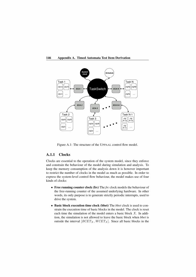
146 Appendix A. Timed Automata Test Item Derivation
ECA 1
ECA 2
ECA 3
ECA N-1
ECA NTaskSwitch
Task 1
System
clock
cfg1a
cfg1c
cfg1b
…
Task 2
cfg2a
cfg2c
cfg2b Task 3
cfg3a
cfg3c
cfg3b
…
…
Task N-1
cfg
N-1a
cfg
N-1c
cfg
N-1b
…
Task N
cfgNa
cfgNc
cfgNb
…
Schedule
Figure A.1: The structure of the UPPAAL control flow model.
A.1.1 ClocksClocks are essential to the operation of the system model, since they enforceand constrain the behaviour of the model during simulation and analysis. Tokeep the memory consumption of the analysis down it is however importantto restrict the number of clocks in the model as much as possible. In order toexpress the system-level control flow behaviour, the model makes use of fourkinds of clocks:
• Free running counter clock (frc) The frc clock models the behaviour ofthe free-running counter of the assumed underlying hardware. In otherwords, its only purpose is to generate strictly periodic interrupts, used todrive the system.
• Basic block execution time clock (bbet) The bbet clock is used to con-strain the execution time of basic blocks in the model. The clock is reseteach time the simulation of the model enters a basic block X . In addi-tion, the simulation is not allowed to leave the basic block when bbet isoutside the interval [BCETX ,WCETX ]. Since all basic blocks in the

A.1 Timed Control Flow Modeling using UPPAAL 147
entire model are mutually exclusive (i.e., if a basic block X in a task isvisited during simulation, no other basic blocks can be visited until thesimulation leavesX), there is no need for individual clocks for each task,but a single clock can be used for all tasks.
• Kernel execution time clock (ket) This clock keeps track of the timespent in the kernel during task switches.
• Task scheduling clocks (cT) Each task T in the system keeps a clockcT for keeping track of the release time of the task.
Note that the first three clocks are one-per-system clocks, whereas the num-ber of cT clocks are given by the number of tasks in the system. E.g., a systemwith four tasks will be modeled using a total of seven clocks.
A.1.2 Task CFG modelingFrom a standard CFG perspective, a task is made up of a set of function-levelgraphs (i.e., a graph for the task main function, and a graph for each func-tion that is explicitly or implicitly called by the main function). In our model,each function translates to a timed automaton. The basic control flow structureof a function is intuitively modeled in UPPAAL using a one-to-one mappingbetween basic blocks and UPPAAL locations, and between CFG edges and UP-PAAL edges. An UPPAAL model of a very small example task is shown inFigure A.2. The details of UPPAAL task modeling are described below.
Definitions and Uses belonging to a vertex v are modeled using assign-ments on all outgoing edges from v. This should be interpreted as once thebasic block is visited, the definition or use is executed. Definitions are mod-eled using the update functionality in UPPAAL (e.g., a definition of a sharedvariable x to 5 is modeled as an update with x on the left hand side: “x := 5”).Similarily, a use of a shared variable y is modeled either using the same func-tionality (e.g., a use of a shared variable y in an assignment to another variablez is modeled as an update with y on the right hand side: “z := y”). Notethat, if the left hand side variable in such a statement is not a shared variable,we will use updates to local dummy variables in order to express the sharedvariable usage. An example of a definition of y and a use of x can be found inFigure A.2.
Best case execution time (BCET) of a basic block is modeled using aclock guard on each transition from the node representing the basic block. Theguard makes sure that no transitions are made before the requirement of the

148 Appendix A. Timed Automata Test Item Derivation
bbet<=2
bbet<=2
bbet<=4
bbet<=1
terminateB!
bbet>=2 && lbB>270
readyB!
goB?
goB?
bbet>=2 && lbB<300
readyB!
lbB++
goB?
bbet>=2
readyB!
goB?
readyB!
bbet>=1
goB?
bbet>=2
readyB!
y:=x
goB?
bbet>=1
readyB!
Figure A.2: An example task automaton.
guards is fulfilled. For example, the BCET guards of basic block j are for-mulated as bbet ≥ BCETj . The semantics of the guard could be expressedas “it is not possible to leave this basic block before BCETj time units havepassed”.
Worst case execution time (WCET) of a basic block is modeled using aninvariant in the node representing the basic block. For example, the WCETinvariant of a basic block i is formulated as bbet ≤WCETi . The semantics ofthe invariant could be expressed as “it is not possible to stay in this basic blocklonger than WCETi”. It should be noted that WCET could be expressed asguards on transitions (as BCET is), but this would result in a semantics thatdoes not enforce transitions within the WCET, but only restricts transitions tobe made within the WCET.
Upper loop bounds are essential to our method of modeling (and to timeanalysis in RTSs in general [35]). An unbounded loop may iterate e.g., 2, 5,127, or infinitely many times, causing an unbounded WCET of the functionincluding the loop. In the model, upper loop bounds are expressed in the formof guard/assignment pairs on backward branches. Each transition representing

A.1 Timed Control Flow Modeling using UPPAAL 149
MAIN FUNCTION
B
Abbet<=A.WCET
FOO SUBROUTINE
FOO BODY
foo?
bbet>=A.BCET
foo!
foo!
foo?
Figure A.3: A subroutine call to subroutine foo from the task main function.
a backward branch (i.e., a prerequisite for an iterative construct) will have avariable associated with it. The variable is initialized to the value of the upperloop bound. The transition may be taken if the value of the variable is above 0.Each time the branch is taken, the variable is decremented. When the variablereaches 0, the guard will prevent the backward branch from being taken.
Lower loop bounds are not essential to the operation of the model, but ifthey can be derived, they help reducing the complexity of the model by re-stricting the number of derivable test items. In addition, existing lower loopbounds that are not explicitly expressed in the system may result in infeasibletest items being added to the result. Both upper and lower loop bounds arestated per entry to the loop. Hence, a loop bound is reset each time the loop isentered.
Since the control flow of a task is represented by the main function graphand a set of subroutine CFGs, there is a need for expressing the mechanismsof subroutine invocation and subroutine return. For this purpose, we useUPPAAL synchronization channels. As a subroutine is called by another func-tion automata, this is modeled using a synchronization channel by the nameof the called subroutine. While the called subroutine automaton executes, thecallee is suspended in an intermediate location (see Figure A.3), waiting for thecalled function to terminate and synchronize back on the same channel. Notethat this way of working with subroutine automata imposes two restrictions on

150 Appendix A. Timed Automata Test Item Derivation
B B
SCENARIO I SCENARIO II
Abbet<=A.WCET
Abbet<=A.WCET
bbet>=A.BCET
go?
ready!
bbet>=A.BCET
Figure A.4: The construct for facilitating in-between-basic block preemption.
our model. First, if several tasks use a common function, each task needs tohave a unique automaton instance of that function. Second, no recursive callsare allowed (since this assumes that a subroutine is allowed to call itself).
In order to enable a preemptive behaviour in the model, there is a need forthe model to be able to suspend and preempt an executing task. Since a trulypreemptive behaviour is troublesome to model and analyse using timed au-tomata, we approximate a preemption such that it always occurs in between ba-sic blocks. Note that the negative effects of this approximation can be avoidedif each statement is modeled as a separate basic block (as is done in the eval-uation in Section 6.1). As the system is strictly time-triggered, all task pre-emption will be caused by clock interrupts. If a clock interrupt is signaled bythe system clock automaton (described in Section A.1.1) during the executionof a basic block, the interrupt is deferred to preempt the task instantaneouslyafter the execution of the basic block. In the model, this is expressed by addingextra locations in between all basic block locations. When a basic block hasfinished executing, the task synchronizes on the ready channel with the task’sECA. The ECA checks whether an interrupt has occurred during the executionof the basic block. If so, the task is preempted. If not, the task may continueexecuting the next basic block (modeled using the go synchronization chan-nel). In other words, the task model “asks” the ECA if it is allowed to executethe next basic block. As an example of this, consider the transitions in Fig-ure A.4. Scenario I describes a transition from a basic block A (with best-caseexecution time BCETA and worst-case execution time WCETA) to a basic

A.1 Timed Control Flow Modeling using UPPAAL 151
WAITING
TERMINATED
EXECUTING READY
SCHEDULED
terminated!
prio:=prio-PrA
moveToReadyA?
prio:=prio+PrA
terminate?
!ticked
ready?
resume?
prio<2*PrA,
prio>=PrA
preempt?
go!
bbet:=0
!ticked
Figure A.5: An example Execution Control Automaton for a task “A”. A “C”denotes a commited state, where no time may pass and no transitions fromnon-committed states may occur.
block B. Scenario II describes the same scenario with the added in-betweenlocation and synchronizations of our model. If a clock interrupt would occursomewhere during the execution of basic blockA, the task would be suspendedin the intermediate state between A and B until it is resumed by the scheduler.
A.1.3 Modeling of Task Execution Control
For each task in the model, a separate task ECA (depicted in Figure A.5) isused in order to keep track of the state of the task. An ECA is generic in thesense that it has identical structure regardless of the task it controls. The initialstate of the automaton (WAITING) represents a waiting state of the task (i.e.,the task has not yet been put in the ready-queue).
The ECA needs to be able to handle task activation. From the initial state,the task can be made ready by an synchronization on the moveToReady chan-nel. The new state (the top rightmost in the figure) represents the task beingin the ready-queue, where it might be selected for execution. The transitionfrom WAITING to READY also adds the unique task priority to the currentglobal system priority. Since each task in the underlying system model has aunique priority P enumerated from 0 (idle task) and up, task priorities in the

152 Appendix A. Timed Automata Test Item Derivation
UPPAAL models are expressed as 2P . Conseqently, if a task with a priority P1
is scheduled, the global task priority will be in the interval [2P1 , 2P1+1) (unlessno other task with a higher priority is also scheduled). As for task resumption,using FPS scheduling, the task with the highest priority in the ready-queue willalways be selected for execution. In the model, this corresponds to the ECAof the task selected for execution by the schedule (described in Section A.1.4)synchronizing on the resume channel, causing a transition to the SCHEDULEDstate (the top middle in the figure). Note that each task ECA checks whetherthe current system priority is within in the interval [2P , 2P+1) before makingthe transition to SCHEDULED. If this is the case, no higher prioritized taskcan be in READY.
In the running state, an ECA has three options: (1) If an unacknowledgedclock interrupt has occurred, the ECA will synchronize on the preempt channelin order to hand over control to the scheduler automaton. (2) If no event hasoccurred and there still are basic blocks to execute before task termination, theECA will synchronize on the go channel, indicating that the task is allowed toexecute one full basic block unpreempted. Once the basic block is executed,the task synchronizes back on the ready channel. (3) If no basic blocks are leftfor execution in the task (or if the task selects the termination edge in favour oflooping back), the ECA synchronizes on the terminate channel.
The first termination channel (terminate) is used to check whether the taskis finished with its execution and ready to terminate, the second terminationchannel (terminated) is used to communicate the termination to the task switchautomaton, in order for it to dispatch the next task for execution. When theECA is in fully terminated position (back in the initial state), the task is readyfor re-scheduling. The second task termination edge also subtracts the taskpriority from the system priority, allowing lower prioritized tasks to resumetheir execution.
It should be noted that the running state is a committed state. In otherwords, no time can pass while in this state (i.e., a task must be immediately exe-cuted, preempted or terminated) and no other transactions from non-committedstates can be performed while in this state.
A.1.4 FPS Scheduler and Task Switch ModelingThe task switch and scheduler mechanisms of the system are modeled usingthree different types of automata: The system clock automaton maintains theoverall passage of time in the system, the task switch automaton facilitatesthe transfer of control from one task automaton to another, and the schedule

A.1 Timed Control Flow Modeling using UPPAAL 153
frc<=RESOLUTION
frc>=RESOLUTION
timertick!
ticked:=true, frc:=0
frc>=RESOLUTION
timertickIdle!
ticked:=true, frc:=0
Figure A.6: The system clock automaton.
automaton determines which task automaton to gain control at a given point inthe simulation of the model.
The system clock automaton is a rudimentary automaton with a fundamen-tal function. This automaton (depicted in Figure A.6) is responsible for drivingthe entire system by providing it with strictly periodic “heartbeat” interrupts(i.e., timerticks). The frequency of these interrupts is determined by the reso-lution parameter. Basically, resolution represents the length, in terms of timeunits, in between each timertick.
Note that the system clock automaton synchronizes on different channelsdepending on the current state of the system. If no tasks are currently execut-ing, the timertickIdle synchronization channel edge is taken. Otherwise, thetimertick synchronization channel edge is taken. The reason for differentiatingbetween these is that an idle system is instantly preempted for task switching,while a busy system has to wait until the executing task leaves its current basicblock. Regardless if the system is idle or not, each timertick interrupt invokesthe task switch automaton, thereby enforcing the release and execution of tasks.
The task switch automaton (depicted in Figure A.7) is the generic mecha-nism for facilitating preemption and task termination (i.e., the two basic mech-anisms for task switching included in our run-time model). As discussed inthe above section, for practical reasons, a preemption of an idle system is con-sidered different from a task to task preemption. While non-busy (i.e., in theTASK EXEC or the SYS IDLE state), the task switch automaton listens for sys-tem clock timerticks or task terminations. Once a timertick or a termination isreceived, the automaton
1. calls the scheduler automaton in order to release all tasks that should bereleased according to their T and O properties.

154 Appendix A. Timed Automata Test Item Derivation
TASK_EXEC
TICKED
TICKED_IDLE
TASK_PREEMPT
SCHEDULING
SCHEDULED
ket<=K_MIN
SCHEDULING_IDLE
SCHEDULED_IDLEket<=K_MIN
SYS_IDLE
timertick?
preempt! ticked:=false
schedule!
scheduled?
ket:=0
resume!
ket>=K_MAX,
!ticked
terminated?
ket:=0
scheduled?
ket:=0
resume!
ket>=K_MAX
timertickIdle?
prio==0,
ket>=K_MAX
prio==0,
ket>=K_MAX,
!ticked
schedule!
ticked:=false
timertick?
ket>=K_MAX,
ticked
ticked:=false
Figure A.7: The task switch automaton.
2. waits for [K MIN ,K MAX ] time units (i.e., consumes the time actu-ally spent in the task switch routine).
3. releases the next task for execution by synchronizing with the ECA au-tomaton of the highest prioritized released on the resume channel, orreturns to SYS IDLE if no task is released for execution. Note that onlytasks with their ECA in a READY state (i.e., tasks that are moved toready by the schedule) may be scheduled for execution, and that thepriority guards in the ECA prohibits lower prioritized tasks from beingscheduled.
The schedule automaton represents the run-time schedule of the RTS (inour case a time-triggered fixed-priority schedule). The automaton has an initialwaiting state, and an activation channel called schedule (the activation of theschedule automaton is prompted by the task switch automaton as a responseto the occurrence of a timertick). Once the schedule automaton is activated, itsteps through all scheduling decisions based on the current value of the localtask clocks. If a task’s period is passed, the task is released and the clockis reset. Furthermore, if the task is previously released and the task’s offsetis passed, the task is moved to ready (by synchronizing with the task’s ECAover the corresponding moveToReady channel). Once the schedule is traversed,

A.1 Timed Control Flow Modeling using UPPAAL 155
NOT_SCHEDULING
relA !relA
cA>=OA
moveToReadyA!
relA:=0
cA<OA
cA<TA
cA:=0, relA:=1
cA>=TA
!relBrelB
moveToReadyB!
cB>=OB
relB:=0
cB>=TB
cB:=0, relB:=1
cB<OB
cB<TB
relC !relC
cC<TC
cC<OC
moveToReadyC!
cC>=OC
relC:=0
cC>=TC
cC:=0, relC:=1
relD !relD
cD<TD
cD<OD
moveToReadyD!
cD>=OD
relD:=0
cD>=TD
cD:=0, relD:=1
scheduled!
schedule?
Figure A.8: An example schedule automaton with four tasks.
control is handed back over to the task switch automaton over the scheduledsynchronization channel. Figure A.8 depicts an example time-triggered FPSschedule with four tasks.
This method of modeling presupposes that all task T and O parameters aremultiples of the RESOLUTION parameter driving the timerticks, which is anatural limitation since time-triggered systems typically only release tasks attimertick invocations.
Note that other scheduling mechanisms also could be adapted to this model.E.g., in [3], Amnell et al. describe a tool for formally modeling different sched-uling mechanisms using timed automata. In this paper, however, we stick tothe run-time model described in Section 1.2.


Appendix B
The DUANALYSIS Algorithm
The DUANALYSIS algorithm (Figure B.1) is a slight variation of the origi-nal EOG algorithm [103], built upon the manipulation of two data structures.Throughout the analysis, an abstract state of type State propagates throughthe execution of the system. For each execution of a job, the abstract state ischanged according to the StateChange created by executing the job. Staterepresents the current abstract state of the execution, and contains informationregarding currently live definitions, active definitions, active uses, and encoun-tered DU-paths. Hence, State is defined as:
State : {liveDefs, activeDefs, activeUses, duPaths}
StateChange represents the change of state incurred by the execution of a cer-tain part of a job. As such, StateChange contains new active definitions, killedlive definitions, killed active definitions, killed active uses, and the WCET ofthe executed job. Hence, StateChange is defined as:
StateChange : {newActiveDefs, killedLiveDefs,killedActiveDefs, killedActiveUses,wcet}
Intuitively, the combination of a State a1 and a StateChange a′1 yields anew State a2, representing the original state affected by the changes in a′1.E.g., if a1 contains a set of liveDefs {d1, d2, d3}, and a′1 contains a set ofkilledLiveDefs {d2}, then a2’s set of liveDefs will look as follows: {d1, d3}.Two more structures (Ivl and Job) are used in the analysis. Ivl defines a time
157

158 Appendix B. The DUANALYSIS Algorithm
interval by its extremal values l and r. Job represents a task instance and con-tains definitions, uses, job priority, release time, BCET and WCET. Job isdefined as:
Job : {D,U ,P ,R,BCET ,WCET}
In the algorithm, the process of task execution and task switch is formalizedby the functions EXECUTE and SWITCHTASK, where
EXECUTE : State× Job× Ivl× Ivl→ StateChange
SWITCHTASK : StateChange× State× Ivl→ State
In essence, the EXECUTE function produces a change of abstract state (State-Change) incurred on original abstract state (State) by executing a certain job(Job), executed during an execution window (first Ivl), and released during arelease interval (second Ivl). The SWITCHTASK function describes the impactof a task switch occurring during a time interval (Ivl), and produces a newabstract state (State), based on the original abstract state and the changes de-scribed by StateChange. The implementation of these functions are directlybased on the Definition, Use, and DU-path rules described in Chapter 3.
Roughly, the DUANALYSIS algorithm starts with an empty State at time 0by scheduling the highest prioritized ready job j. Using the EXECUTE func-tion, j’s StateChange is derived. Next, if j is always finished before the nexthigher priority job is released, SWITCHTASK combines the StateChange withthe old State to a new State. The algorithm increments the time and schedulesthe next job. Else, if j is safely preempted by a higher priority job, SWITCH-TASK combines the StateChange with the old State to a new State - but onlyregards the events that predate the preemption, stores the remainder of j, in-crements the time, and schedules the higher prioritized job. Else, if j mightbe preempted, the algorithm splits into two recursive branches, one of whichconsiders the case with a preemption, and the other considers the case with nopreemption. This behaviour is repeated until all jobs in the LCM are analysed.
In order to derive the StateChange created by executing a job j, the EX-ECUTE function and its auxiliary functions, EXECDEF and EXECUSE (Fig-ure B.2) work through all shared variable accesses in j in a chronological or-der. Each access is treated according to its corresponding definition or use rule(definition rules are implemented in EXECDEF and use rules are implementedin EXECUSE).
SWITCHTASK and its auxiliary functions REVISEDEF and REVISEUSE(Figure B.3) create a new State by adding the changes in j’s StateChange

159
to the State prior to the execution of j. If j is not preempted, all changes inStateChange are considered when creating the new State. Otherwise, onlythose changes prior to the preemption time are considered. In order to addnew DU-paths to the result of the analysis, SWITCHTASK uses the two DU-path rules given in Page 53. Specifically, SWITCHTASK implements DU-pathRule 1 in REVISEDEF, and DU-path Rule 2 in REVISEUSE.
Note that, compared to the original EOG algorithm, DUANALYSIS usesa number of additional auxiliary functions (for a description of all auxiliaryfunctions, we refer to [103]):
1. PREEMPT(j, t0, t1) - re-calculates the shared variable access times (i.e.,min,max , and rdMax ) for all definitions and uses in the preempted jobj, given that task j has been allowed to execute somewhere in the timeinterval of [t0, t1] prior to the preemption.
2. GETNEXTDUEVENT(t, j) - returns the time ts of the next shared vari-able access in job j, such that ts > t.
3. GETNEXTDUCHANGE(t, trs) - returns the time ts of the next abstractstate change in transition trs , such that ts > t.

DUANALYSIS (state, stateChange, rdy,RI ,SI )// When is the next job(s) released?
1. t :=NEXTRELEASE(SI )2. if rdy = ∅3. rdy := MAKEREADY(t, rdy)4. if rdy 6= ∅5. DUANALYSIS(state, stateChange, rdy,RI , (t,SI .r ])6. else state := SWITCHTASK(stateChange, state,RI )7. else
// Extract the highestpriority job in rdy.8. J := DISPATCH(rdy)9. [α, β) := [max(J.R,RI.l),max(J.R,RI.l) + J.WCET)10. a′ := α+ J.BCET11. b′ := β12. state := SWITCHTASK(stateChange, state,RI )13. stateChange := EXECUTE(state, J, [α, β), RI)
// Add all lower prio jobs released before J’s termination,// or before a high priority job is preempting J.
14. while((t < β) ∧ (PRIO(t) < J.P ))15. rdy := MAKEREADY(t, rdy)16. t := NEXTRELEASE((t, SI.r])
// Does the next scheduled job preempt J?17. if ((t < β) ∧ (PRIO(t) > J.P ))
// Can J complete prior to the release of the next job at t?18. if t > a′
19. DUANALYSIS(state, stateChange, rdy, [a′, t), [t,SI .r ])20. if rdy = ∅21. DUANALYSIS(state, stateChange, MAKEREADY(t, rdy), [t, t), (t,SI .r ])22. else if t = a′
23. DUANALYSIS(state, stateChange, MAKEREADY(t, rdy), [t, t), (t,SI .r ])
// Add all jobs that are released at time t.24. rdy := MAKEREADY(t, rdy)
// Best and worst case execution time prior to preemption?25. J.BCET := max(J.BCET − (t− (max(J.R,RI.l)), 0)26. J.WCET := max(J.WCET − (t− (max(J.R,RI.r)), 0)27. PREEMPT(J, (t− (max(J.R,RI.l)), (t− (max(J.R,RI.r)))28. DUANALYSIS(state, stateChange, rdy ∪ {J}, [t, t], (t, SI.r])
// No preemption.29. else if t =∞ // Have we come to the end of the analysis?30. DUANALYSIS(state, stateChange, rdy, [a′, b′), [∞,∞]) // Yes
31. else // More jobs to execute.// Is there a possibility for a high priority job to succeed// immediately, while low priority jobs are ready?
32. if (rdy 6= ∅ ∧ t = β)33. DUANALYSIS(state, stateChange, MAKEREADY(t, rdy), [t, t), (t,SI .r ])34. if a′ 6= b′ // And one branch for the low priority job.
// The regular succession of the next job35. DUANALYSIS(state, stateChange, rdy, [a′, b′), [t,SI .r))
Figure B.1: The DUANALYSIS algorithm.

EXECDEF (t,D, stateChange, state)1. for each d ∈ D // For all defines in the job.2. if t = d.min
// Add d to new active definitions set.3. stateChange.newActiveDefs := stateChange.newActiveDefs ∪ {d}4. if t = d.max
// If d is not live or active, add it to// new active definitions set.
5. if (d 6∈ state.liveDefs) ∧ (d 6∈ stateChange.newActiveDefs)6. stateChange.newActiveDefs := stateChange.newActiveDefs ∪ {d}
// Add d to killed active definitions set.7. stateChange.killedActiveDefs := stateChange.killedActiveDefs ∪ {d}8. if t = d.rdMax
// Add d to killed live definitions set.9. stateChange.killedLiveDefs := stateChange.killedLiveDefs ∪ {d}10. return stateChange
EXECUSE (t,D, stateChange, state)1. for each u ∈ U // For all uses in the job.2. if t = u.min
// Add u to new live uses set.3. stateChange.newActiveUses := stateChange.newActiveUses ∪ {u}4. if t = u.max
// If u is not live, add it to new live uses set.5. if (u 6∈ state.activeUses) ∧ (u 6∈ stateChange.newActiveUses)6. stateChange.newActiveUses := stateChange.newActiveUses ∪ {u}
// Add u to killed live uses set.7. stateChange.killedActiveUses := stateChange.killedActiveUses ∪ {u}8. return stateChange
EXECUTE (state, job,EW ,RI )// Create and init a new stateChange variable.
1. stateChange := {∅, ∅, ∅, ∅, ∅, EW.r}// Update the execution time properties of the defines// and uses such that they are relative to the release// time of the job rather than the job start.
2. for each d ∈ job.D3. d.min := d.min + max(EW .l,RI .l)4. d.max := d.max + max(EW .l,RI .r)5. d.rdMax := d.rdMax + max(EW .l,RI .r)6. for each u ∈ job.U7. u.min := u.min + max(EW .l,RI .l)8. u.max := u.max + max(EW .l,RI .r)
// Get next du-event time t.9. t := GETNEXTDUEVENT(0 , job)10. while t < EW .r // Within the execution time of the job.
// For each du-event occurring at t, handle it.11. stateChange := EXECDEF(t, job.D, stateChange, state)12. stateChange := EXECUSE(t, job.U , stateChange, state)13. t := GETNEXTDUEVENT(t, job)
// Return the change of state.14. return stateChange
Figure B.2: The EXECUTE functions.

REVISEDEF (t, stateChange, state)1. for each u ∈ state.activeUses // For all currently live uses2. for each d ∈ stateChange.newActiveDefs // and new active defs.3. if (t = d.min) ∧ (d.var = u.var)
// New DU-path found. Add it!4. state.duPaths := state.duPaths ∪ {{d, u}}5. for each d ∈ stateChange.killedActiveDefs // For killed active defs.6. if t = d.max
// Remove d from the set of active defs.7. state.activeDefs := state.activeDefs \ {d}8. for each d ∈ stateChange.killedLiveDefs // For killed live defs.9. if t = d.rdMax
// Remove d from the set of live defs.10. state.liveDefs := state.liveDefs \ {d}11. return state
REVISEUSE (t, stateChange, state)1. for each d ∈ state.liveDefs // For all currently live defs2. for each u ∈ stateChange.newActiveUses // and new live uses.3. if (t = u.min) ∧ (d.var = u.var)
// New DU-path found. Add it!4. state.duPaths := state.duPaths ∪ {{d, u}}5. for each u ∈ stateChange.killedActiveUses // For killed live uses.6. if t = u.max
// Remove u from the set of live uses.7. state.activeUses := state.activeUses \ {u}8. return state
SWITCHTASK (state, stateChange,TSI )1. t := GETNEXTDUCHANGE(0 , stateChange)2. while t < TSI .r3. state := REVISEDEF(t, stateChange, state)4. state := REVISEUSE(t, stateChange, state)5. t := GETNEXTDUCHANGE(t, stateChange)
// There can be no live uses after a task switch.6. state.activeUses := ∅7. if (TSI .l 6= TSI .r) ∧ (TSI .r < stateChange.WCET)
// A non-preempted non-wcet branch.8. for each d ∈ stateChange.killedActiveDefs9. if d.max > TSI .r
// Remove d from the set of active defs.10. state.activeDefs := state.activeDefs \ {d}11. for each d ∈ stateChange.killedLiveDefs12. if stateChange.WCET > d.max > TSI .r
// Remove d from the set of live defs.13. state.liveDefs := state.liveDefs \ {d}
// Return new abstract state.14. return state
Figure B.3: The SWITCHTASK functions.

Appendix C
Reproduction ofAsynchronous Events
Interrupts are a major source of non-determinism in program executions. As apart of the Time Machine, we present a novel method for pinpointing interrupts,suitable for embedded real-time systems.
As an interrupt occurs, the ongoing CPU activity is halted, the state of theexecuting program is stored and the interrupt is handled by an interrupt serviceroutine. To reproduce this scenario, we need to be able to correctly reproducethe occurrence of the interrupt. In other words, we must make sure that theinterrupt preempts the execution of the CPU activity at the exact same stateduring the replay as it did in the first execution. Traditionally, this is achievedusing hardware instruction counters [15, 48] or software instruction counters(SICs) [6, 52, 65]. However, few embedded microcontrollers are equipped withsufficiently accurate hardware instruction counters [75], and software instruc-tion counters require approximately 10% of the overall execution time, a hardto meet requirement in resource constrained systems. Consequently, a differentapproach, more adapted to the requirements of embedded systems and able toperform using standard development tools, is needed.
C.1 Context ChecksumsIn our method, we use an approximation of the state of the preempted programat the time of the interrupt as a marker. This approximation is represented in the
163

164 Appendix C. Reproduction of Asynchronous Events
form of the SP value and a checksum of the execution environment of the pro-gram, such as the registers, or the registers combined with (part of) the programstack. Our method imposes an execution time overhead of a small fraction ofthat of the SIC and requires no additional hardware support to function.
The basic idea of our method is to reproduce interrupts by recording thePC values and unique markers of their occurrence. In order to reproduce theseinterrupts, a debugger breakpoint is set at each interrupted PC address andthe program is restarted in the debugger. As a breakpoint is hit, the uniquemarker of the current execution is compared to the recorded unique markervalue. If these markers match, we consider this interrupt to be pinpointed andan interrupt is forced upon the system.
C.1.1 Execution Context
If we look back upon the example shown in Figure 4.8, where a PC value is in-distinguishably revisited a number of times, a good solution in theory would beto make use of the loop counter and the PC value as a unique marker. Unfortu-nately, not all loops have loop counters. In general, it is very hard to determineexactly which parts of the program execution context that differentiate betweenspecific loop iterations, subroutine calls or recursive calls. Ideally, we wouldbase our unique marker on the entire content of the execution context in or-der to be able to differentiate between loop iterations. However, consideringthe amount of data used to represent this context, we face a practical problemwhen recording it during execution due to the massive perturbation to the sys-tem. Consequently, we need to derive a subset of the execution context suitablefor unique marker use.
The program execution context is basically a set of data stored in registers,on the stack and/or on the heap. Since the processor registers are small andvery fast, these hold the most current parts of the execution context. And, sincethey are small and very fast, they make exellent candidates as a basis for theexecution context-based unique markers.
C.1.2 Register Checksum
One solution would be to store the contents of each processor register. How-ever, in most embedded systems, computing- as well as memory resourcesare scarce. Storing all registers at each interrupt might incur an intolerableoverhead on the memory usage of the system. In our method, we handle this

C.1 Context Checksums 165
problem by separately storing the SP value, as it is invaluable for differenti-ating between recursive calls, and calculating and storing a checksum of thecontents of the remaining registers. By doing this, we destroy information, butstill preserve an approximative representation of the register contents from thetime of the interrupt.
The register checksum operation is a simple addition of all processor regis-ters. Overflow of the accumulated checksum is ignored. Hence, if the processoris equipped with eight general-purpose 16-bit registers (R0...R7), the registerchecksum CR is calculated as follows:
CR = (R0 +R1 + ...+R7) mod 216
Due to the modest size and the ease of access of processor registers, the compu-tational cost of calculating a register checksum is very small. However, sincethe register checksum is based solely on the processor registers, its main dis-advantage is that it only covers a minor subset of the execution context. Ifan interrupt occurs within a loop and the actual parameters differentiating be-tween iterations are not included in this subset, we will not be able to uniquelypinpoint the occurrence of the interrupt.
C.1.3 Stack ChecksumIn order to capture those interrupt occurrences not successfully pinpointed bythe register checksum, we must expand the interval of execution context in-cluded in the context checksum. As we already used the registers, the remain-der of the execution context is located on the stack and on the heap. In ourmethod, we chose to work with the program stack contents. This has two rea-sons: First, implementing a stack checksum calculation in an instrumentationprobe [94] is significantly easier than implementing a heap checksum in thesame probe. The stack area is well defined, continuous and often easily ac-cessed from within the probe. Second, without having extensive proof of this,we assume that variables influencing the program control flow, such as loopcounters, are more often allocated on the stack than on the heap.
The checksum operation of the stack checksum is identical to the one per-formed in order to calculate the register checksum. Here, the subset of theexecution context included in the checksum is bounded by the boundaries ofthe stack of the executing program. Hence, on a 16-bit architecture, the stackchecksum CS is calculated using the following formula:
CS = (SSP + SSP+1 + ...+ SSB ) mod 216

166 Appendix C. Reproduction of Asynchronous Events
In the above formula, SX denotes the byte at stack address X . SP denotes thevalue of the stack pointer at the time of the interrupt and SB denotes the valueof the stack base of the interrupted program.
The stack checksum should be viewed upon as a complement to the regis-ter checksum rather than a stand-alone solution for pinpointing interrupts. Thereason for this is the fact that the execution overhead of the stack checksumexceeds the overhead of the register checksum to such an extent that the per-turbation of the latter becomes negligible. In addition, discarding the optionof using a register checksum when choosing a stack checksum solution willeliminate the possibility of detecting changes in register-bound variables overloop iterations.
C.2 Adaptations
Apart from the sheer size issue, there is another property that separates the reg-ister checksum from the stack checksum. In the case of the register checksum,we always use the same number of elements in order to calculate the check-sum. If the processor has eight registers, the checksum will always calculatethe register checksum by accumulating the values stored in these eight regis-ters. Hence, we can guarantee a constant execution time as far as number ofinstructions are concerned. Using a stack checksum, the situation is different.The stack base of a program is constant whereas the SP varies over time. Thisimplies a variable size of the program stack and thus a variable execution timeof the stack checksum calculation, depending on the size of the stack at thetime of the interrupt.
C.2.1 Instrumentation Jitter
Variations in execution time of software are usually referred to as jitter. Inmulti-tasking systems (such as most embedded RTSs), designers try to keepthe jitter to a minimum, since it comprises the testability and analyzabilityof the system [99]. Therefore, jitter introduced by instrumentation activities(such as the stack checksum calculation) may complicate testing of sensitivesystems, even though the instrumentation was included in order to increase theanalyzability.

C.2 Adaptations 167
C.2.2 Partial Stack Checksum
To reduce the execution time perturbation and the problem of large instrumen-tation jitter when using the stack checksum technique, the developer has theoption of not including the entire program stack in the stack checksum. Apartial stack checksum CP would be calculated similarily to the original stackchecksum (once again on a 16-bit platform):
CP = (SSP + SSP+1 + ...+ SSX ) mod 216
However, the upper boundary SX of the stack interval to be included in thechecksum is chosen such that:
SP ≤ SX ≤ SB
By using this formula, we once again reduce the percentage of the executioncontext included in the stack checksum, thereby reducing the accuracy of theunique marker approximation. In turn, we obtain the following benefits:
• Eliminating instrumentation jitter
By defining SX in terms of a constant positive offset to SP (denoted x inFigure C.1) such that the interval [SP ,SX ] delimits a constant numberof bytes on the stack, we make sure that the stack checksum will becalculated using a constant number of instructions. This will eliminatethe instrumentation jitter of the checksum calculation (not consideringcache effects or similar). In the case where the size of the fixed interval[SP ,SX ] exceeds the size of the actual program stack (i.e., when SX >SB ), this can be detected and the remaining instructions can be simulatedusing additions of zero to the checksum or similar.
• Reducing instrumentation overhead
Intuitively, reducing the percentage of the stack included in the stackchecksum will reduce the execution time of the stack checksum calcu-lation. If total elimination of instrumentation jitter is no major require-ment, a reasonable candidate for SX may be the base of the stack forthe current subroutine. Many processors are equipped with a dedicatedregister holding the value of this base pointer (BP in Figure C.1) to thecurrent scope of execution.

168 Appendix C. Reproduction of Asynchronous Events
h()
g()
Pro
gra
m S
tack
SB
BP
SP
SX
x
Figure C.1: Different delimiter alternatives for the stack checksum. The g()and h() intervals represent stack intervals for subroutine execution scopes forinterrupted example functions g and h respectively.
C.2.3 System call markersSynchronous events, like blocking system calls, require a less elaborate ap-proach. We make use of a per-task counter, incremented each time a potentiallyblocking system call is invoked by that task. If the call actually blocks the task,the value of the counter is recorded as a unique marker and the counter is reset.This way we will keep track of at which system call invocation the task actuallyblocked.

Bibliography
[1] Intel Architecture Software Developer’s Manual 24319202, 1999.
[2] Alfred V. Aho, Ravi Sethi, and Jeffrey D. Ullman. Compilers; Princi-ples, Techniques, and Tools. Addison - Wesley, 1986.
[3] Tobias Amnell, Elena Fersman, Leonid Mokrushin, Paul Pettersson, andWang Yi. Times: a Tool for Schedulability Analysis and Code Gener-ation of Real-Time Systems. In Proceedings of 1st International Work-shop on Formal Modeling and Analysis of Timed Systems, Lecture Notesin Computer Science. Springer–Verlag, 2003.
[4] Jakob Engblom: Andreas Ermedahl, Friedhelm Stappert. A UnifiedFlow Information Language for WCET Analysis. In Proceedings ofWCET Workshop, June 2002.
[5] Koenraad Audenaert and Luk Levrouw. Reducing the space require-ments of instant replay. In Proceedings of the ACM/ONR Workshop onParallel and Distributed Debugging, pages 205 – 207. ACM, May 1993.
[6] Koenraad Audenaert and Luk Levrouw. Interrupt Replay: A DebuggingMethod for Parallel Programs with Interrupts. Journal of Microproces-sors and Microsystems, Elsevier, 18(10):601 – 612, December 1994.
[7] Neil C. Audsley, Alan Burns, Robert I. Davis, and Ken W. Tindell. Fixedpriority pre-emptive scheduling: A historical perspective. In Real-TimeSystems journal, volume 8(2/3). Kluwer A.P., March/May 1995.
[8] Theodore Baker. Stack-based scheduling of real-time processes. InReal-Time Systems Journal, volume 3(1), pages 67–99, 1991.
169

170 Bibliography
[9] Venu P. Banda and Richard A. Volz. Architectural support for debug-ging and monitoring real-time software. In Proceedings of EuromicroWorkshop on Real Time, pages 200 – 210. IEEE, June 1989.
[10] Johan Bengtsson, Kim G. Larsen, Fredrik Larsson, Paul Pettersson, andWang Yi. Uppaal - a tool suite for automatic verification of real-timesystems. In Proceedings of the 4th DIMACS Workshop on Verificationand Control of Hybrid Systems III, number 1066 in Lecture Notes inComputer Science, pages 232–243. Springer–Verlag, October 1995.
[11] James Bieman and Janet Schultz. An Empirical Evaluation (and Specifi-cation) of the All-du-paths Testing Criterion. IEEE Software Engineer-ing Journal, 7(1):43 – 51, January 1992.
[12] Rex Black. Managing the Testing Process. Wiley, 2002.
[13] Victor Braberman, Miguel Felder, and Martina Marre. Testing timingbehavior of real-time software. In Proceedings of the International Soft-ware Quality Week, 1997.
[14] Michael Burrows and K. Rustan M. Leino. Finding Stale-Value Errors inConcurrent Programs. Concurr. Comput. : Pract. Exper., 16(12):1161–1172, 2004.
[15] Thomas A. Cargill and Bart N. Locanthi. Cheap Hardware Support forSoftware Debugging and Profiling. In Proceedings of the 2nd Inter-national Conference on Architechtural Support for Programming Lan-guages and Operating Systems, pages 82 – 83, October 1987.
[16] Jaques Chassin de Kergommeaux and Alain Fagot. Execution Re-play of Parallel Procedural Programs. Journal of Systems Architecture,46(10):835 – 849, 2000.
[17] Zhenqiang Chen, Baowen Xu, and Jianjun Zhao. An Overview of Meth-ods for Dependence Analysis of Concurrent Programs. SIGPLAN No-tices, 37(8):45–52, 2002.
[18] Shing chi Cheung, Samuel T. Chanson, and Zhendong Xu. TowardGeneric Timing Tests for Distributed Multimedia Software Systems. InISSRE ’01: Proceedings of the 12th International Symposium on Soft-ware Reliability Engineering (ISSRE’01), page 210, Washington, DC,USA, 2001. IEEE Computer Society.

Bibliography 171
[19] Jong-Deok Choi, Bowen Alpern, Ton Ngo, Manu Sridharan, and JohnVlissides. A Perturbation-Free Replay Platform for Cross-OptimizedMultithreaded Applications. In Proceedings of 15th Parallel and Dis-tributed Processing Symposium, page 10, April 2001.
[20] Jong-Deok Choi, Keunwoo Lee, Alexey Loginov, Robert O’Callahan,Vivek Sarkar, and Manu Sridharan. Efficient and Precise DataraceDetection for Multithreaded Object-Oriented Programs. In PLDI ’02:Proceedings of the ACM SIGPLAN 2002 Conference on Programminglanguage design and implementation, pages 258–269, New York, NY,USA, 2002. ACM Press.
[21] Lee Copeland. A Practitioner’s Guide to Software Test Design. STQEPublishing, 2003.
[22] Rick D. Craig and Stefan P. Jaskiel. Systematic Software Testing. ArtechHouse Publishers, 2002.
[23] Conrado Daws, Alfredo Olivero, Stavros Tripakis, and Sergio Yovine.The Tool KRONOS. In Proceedings of the DIMACS/SYCON workshopon Hybrid systems III : verification and control, pages 208–219, Secau-cus, NJ, USA, 1996. Springer-Verlag New York, Inc.
[24] Edsger W. Dijkstra. Structured Programming, chapter Notes on Struc-tured Programming. Academic Press, 1972.
[25] Paul Dodd and Chinya V. Ravishankar. Monitoring and DebuggingDistributed Real-Time Programs. Software – Practice and Experience,22(10):863 – 877, October 1992.
[26] Mohammed El Shobaki. A Hardware- and Software Monitor for High-Level System On Chip Verification. In Proceedings of IEEE Interna-tional Symposium on Quality Electronic Design, pages 88 – 95. IEEE,2001.
[27] Sigrid Eldh, Hans Hansson, Sasikumar Punnekkat, Anders Pettersson,and Daniel Sundmark. A Framework for Comparing Efficiency, Effec-tiveness and Applicability of Software Testing Techniques. In Testing:Academic and Industrial Conference (TAIC-PART), Windsor, UK, Au-gust 2006.
172 Bibliography
[28] Andreas Ermedahl. A Modular Tool Architecture for Worst-Case Execu-tion Time Analysis. PhD thesis, Uppsala University, Dept. of Informa-tion Technology, Uppsala University, Sweden, June 2003.
[29] Yaniv Eytani, Klaus Havelund, Scott D. Stoller, and Shmuel Ur. Towarda Framework and Benchmark for Testing Tools for Multi-Threaded Pro-grams. Concurrency and Computation: Practice & Experience, August2006.
[30] Mariusz A. Fecko, M. Umit Uyar, Ali Y. Duale, and Paul D. Amer. ATechnique to Generate Feasible Tests for Communications Systems withMultiple Timers. IEEE/ACM Transactions on Networking, 11(5):796–809, 2003.
[31] Jason Gait. A probe effect in concurrent programs. In Software - Prac-tice and Experience, volume 16(3), pages 225–233, Mars 1986.
[32] Allen Goldberg, T. C. Wang, and David Zimmerman. Applications ofFeasible Path Analysis to Program Testing. In ISSTA ’94: Proceedingsof the 1994 ACM SIGSOFT international Symposium on Software Test-ing and Analysis, pages 80–94, New York, NY, USA, 1994. ACM Press.
[33] Todd L. Graves, Mary Jean Harrold, Jung-Min Kim, Adam Porter, andGregg Rothermel. An Empirical Study of Regression Test SelectionTechniques. ACM Transactions on Software Engineering Methodolo-gies, 10(2):184–208, 2001.
[34] Neelam Gupta and Rajiv Gupta. The Compiler Design Handbook: Op-timisations and Machine Code Generation, chapter Data Flow Testing.CRC Press, 2002.
[35] Jan Gustafsson, Andreas Ermedahl, and Bjorn Lisper. Algorithms forInfeasible Path Calculation. In Sixth International Workshop on Worst-Case Execution Time Analysis, (WCET’2006), Dresden, Germany, July2006.
[36] Klaus Havelund, Scott D. Stoller, and Shmuel Ur. Benchmark andFramework for Encouraging Research on Multi-Threaded Testing Tools.In Proceedings of the Workshop on Parallel and Distributed Systems:Testing and Debugging (PADTAD), April 2003.

Bibliography 173
[37] Ian Hayes, Colin Fidge, and Karl Lermer. Semantic Characterisation ofDead Control-Flow Paths. IEE Proceedings - Software, 148(6):175 –186, December 2001.
[38] Thomas A. Henzinger, Pei-Hsin Ho, and Howard Wong-Toi. HYTECH:The Next Generation. In RTSS ’95: Proceedings of the 16th IEEE Real-Time Systems Symposium (RTSS ’95), page 56, Washington, DC, USA,1995. IEEE Computer Society.
[39] Anders Hessel, Kim G. Larsen, Brian Nielsen, Paul Pettersson, and ArneSkou. Time-optimal Real-Time Test Case Generation using UPPAAL. InProceedings of the 3rd International Workshop on Formal Approachesto Testing of Software (FATES’03), number 2931 in Lecture Notes inComputer Science, pages 136 – 151. Springer-Verlag, 2004.
[40] Anders Hessel and Paul Pettersson. A Global Algorithm for Model-Based Test Suite Generation. In Proceedings of Third Workshop onModel-Based Testing. Electronic Notes in Theoretical Computer Sci-ence 16697, March 2007.
[41] Anders Hessel and Paul Pettersson. Cover - A Real-Time Test CaseGeneration Tool. In 19th IFIP International Conference on Testing ofCommunicating Systems and 7th International Workshop on Formal Ap-proaches to Testing of Software 2007, June 2007.
[42] Robert M. Hierons. Comparing Test Sets and Criteria in the Presenceof Test Hypotheses and Fault Domains. ACM Transactions on SoftwareEngineering Methodologies, 11(4):427–448, 2002.
[43] Hyoung Seok Hong, Sung Deok Cha, Insup Lee, Oleg Sokolsky, andHasan Ural. Data Flow Testing as Model Checking. In Proceedingsof the 25th International Conference on Software Engineering (ICSE),pages 232–242, 2003.
[44] Scott Howard. A Background Debugging Mode Driver Package forModular Microcontroller. Semiconductor Application Note AN1230/D,Motorola Inc., 1996.
[45] Joel Huselius. Logging without Compromising Testability. Technicalreport, December 2002.

174 Bibliography
[46] Joel Huselius, Daniel Sundmark, and Henrik Thane. Starting Conditionsfor Post-Mortem Debugging using Deterministic Replay of Real-TimeSystems. In Proceedings of the 15th Euromicro Conference on Real-Time Systems (ECRTS03), pages 177 – 184, July 2003.
[47] Eisuke Itoh, Yutaka Kawaguchi, Zengo Furukawa, and Kazuo Ushi-jima. Ordered Sequence Testing Criteria for Concurrent Programs andthe Support Tool. In Proceedings of the 1st Asia-Pacific Software Engi-neering Conference, pages 236 – 245, December 1994.
[48] Mark Johnson. Some Requirements for Architectural Support of De-bugging. In Proceedings of the Symposium on Arhcitectural Supportfor Programming Languages and Operating Systems, pages 140 – 148.ACM, March 1982.
[49] James A. Jones and Mary Jean Harrold. Test-Suite Reduction and Prior-itization for Modified Condition/Decision Coverage. IEEE Transactionson Software Engineering, 29(3):195–209, 2003.
[50] A Agung Julius, Georgios E. Fainekos, Madhukar Anand, Insup Lee,and George Pappas. Robust test generation and coverage for hybridsystems. Lecture Notes in Computer Science, Proceedings of the 10thInternational Conference on Hybrid Systems: Computation and Control(HSCC), April.
[51] Tetsuro Katayama, Eisuke Itoh, Kazuo Ushijima, and Zengo Furukawa.Test-Case Generation for Concurrent Programs with the Testing CriteriaUsing Interaction Sequences. Proceedings of sixth Asia-Pacific SoftwareEngineering Conference (APSEC’99), 00:590, 1999.
[52] Daeyoung Kim, Yann-Hang Lee, Deming Liu, and Alice Lee. En-hanced Software Instruction Counter Method for Test Coverage Anal-ysis of Real-Time Software. In Proceedings of IEEE International Con-ference on Real-Time Computing Systems and Applications (RTCSA),March 2002.
[53] Jens Knoop, Bernhard Steffen, and Jorgen Vollmer. Parallelism for Free:Efficient and Optimal Bitvector Analyses for parallel Programs. ACMTransactions on Programming Languages and Systems, 18(3):268–299,1996.

Bibliography 175
[54] Pramod V. Koppol, Richard H. Carver, and Kuo-Chung Tai. Incremen-tal Integration Testing of Concurrent Programs. IEEE Transactions onSoftware Engineering, 28(6):607–623, 2002.
[55] Andrew Kornecki, Janusz Zalewski, and Daniel Eyassu. Learning Real-Time Programming Concepts through VxWorks Lab Experiments. InProceedings of 13th SEE&T Conference, pages 294 – 301, March 2000.
[56] Leslie Lamport. Time, clocks, and the ordering of events in a distributedsystem. In Communications of the ACM, volume 21(7), pages 558–565,July 1978.
[57] Rom Langerak. Bundle Event Structures: a Non-Interleaving Semanticsfor LOTOS. In FORTE ’92: Proceedings of the IFIP TC6/WG6.1 FifthInternational Conference on Formal Description Techniques for Dis-tributed Systems and Communication Protocols, pages 331–346, Ams-terdam, The Netherlands, The Netherlands, 19923. North-Holland Pub-lishing Co.
[58] Kim G. Larsen, Marius Mikucionis, Brian Nielsen, and Arne Skou. Test-ing real-time embedded software using UPPAAL-TRON: an industrialcase study. In EMSOFT ’05: Proceedings of the 5th ACM interna-tional conference on Embedded software, pages 299–306, New York,NY, USA, 2005. ACM Press.
[59] Kim G. Larsen, Paul Pettersson, and Wang Yi. UPPAAL in a Nutshell.Int. Journal on Software Tools for Technology Transfer, 1(1–2):134–152, October 1997.
[60] Thomas J. LeBlanc and John M. Mellor-Crummey. Debugging Paral-lel Programs with Instant Replay. IEEE Transactions on Computers,36(4):471 – 482, April 1987.
[61] John P. Lehoczky, Lui Sha, and Jay K. Strosnider. Enhanced AperiodicResponsiveness in Hard Real-Time Environments. In IEEE Real-TimeSystems Symposium, pages 261–270, 1987.
[62] Birgitta Lindstrom, Paul Pettersson, and Jeff Offutt. Generating Trace-Sets for Model-based Testing. In Proceedings of the 18th IEEE Interna-tional Symposium on Software Reliability, November 2007.

176 Bibliography
[63] Chung L. Liu and James W. Layland. Scheduling Algorithms for multi-programming in a hard real-time environment. In Journal of the ACM,volume 20(1), 1973.
[64] Stephen P. Masticola and Barbara G. Ryder. Non-concurrency Analysis.In PPOPP ’93: Proceedings of the fourth ACM SIGPLAN symposium onPrinciples and practice of parallel programming, pages 129–138, NewYork, NY, USA, 1993. ACM Press.
[65] John Mellor-Crummey and Thomas LeBlanc. A Software InstructionCounter. In Proceedings of the Third International Conference on Archi-tectural Support for Programming Languages and Operating Systems,pages 78 – 86. ACM, April 1989.
[66] Mayur Naik, Alex Aiken, and John Whaley. Effective static race detec-tion for java. In PLDI ’06: Proceedings of the 2006 ACM SIGPLAN con-ference on Programming language design and implementation, pages308–319, New York, NY, USA, 2006. ACM Press.
[67] Robert H. B. Netzer. Race Condition Detection for Debugging Shared-Memory Parallel Programs, school = University of Winsconsin – Madi-son, year = 1991. PhD thesis.
[68] Robert H. B. Netzer and Barton P. Miller. What Are Race Conditions?Some Issues and Formalizations. ACM Letters on Programming Lan-guages and Systems, 1(1):74 – 88, March 1992.
[69] Flemming Nielson, Hanne Riis Nielson, and Chris Hankin. Principlesof Program Analysis, 2nd edition. Springer, 2005. ISBN 3-540-65410-0.
[70] Robert Nilsson, Jeff Offutt, and Jonas Mellin. Test Case Generation forMutation-based Testing of Timeliness. In Proceedings of the 2nd In-ternational Workshop on Model-based Testing, pages 102 – 121, March2006.
[71] NIST. The Economic Impacts of Inadequate Infrastructure for SoftwareTesting., May 2002.
[72] Robert O’Callahan and Jong-Deok Choi. Hybrid Dynamic Data RaceDetection. In PPoPP ’03: Proceedings of the ninth ACM SIGPLANsymposium on Principles and practice of parallel programming, pages167–178, New York, NY, USA, 2003. ACM Press.

Bibliography 177
[73] A. Jefferson Offutt, Jie Pan, and Jeffrey M. Voas. Procedures for reduc-ing the size of coverage-based test sets. In Proceedings of the Twelfth In-ternational Conference on Testing Computer Software, pages 111–123,June 1995.
[74] Akira K. Onoma, Wei-Tek Tsai, Mustafa Poonawala, and Hiroshi Sug-anuma. Regression Testing in an Industrial Environment. Communica-tions of the ACM, 41(5):81–86, 1998.
[75] Oliver Oppitz. A Particular Bug Trap: Execution Replay Using VirtualMachines. In M. Ronsse, K. De Bosschere (eds), proceedings of the FifthInternational Workshop on Automated Debugging (AADEBUG), pages269 – 272. COmputer Research Repository (http://www.acm.org/corr/),September 2003.
[76] Thomas J. Ostrand, Elaine J. Weyuker, and Robert M. Bell. Predictingthe Location and Number of Faults in Large Software Systems. IEEETransactions on Software Engineering, 31(4):340–355, 2005.
[77] Anders Pettersson and Henrik Thane. Testing of Multi-Tasking Real-Time Systems with Critical Sections. In Proceedings of Ninth Inter-national Conference on Real-Time and Embedded Computing Systemsamd Applications, Tainan City, Taiwan, R.O.C, 18-20 February 2003.
[78] Paul Pettersson and Kim G. Larsen. Uppaal2k. Bulletin of the EuropeanAssociation for Theoretical Computer Science, 70:40 – 44, 2000.
[79] Polyvios Pratikakis, Jeffrey S. Foster, and Michael Hicks. LOCK-SMITH: Context-Sensitive Correlation Analysis for Race Detection.SIGPLAN Not., 41(6):320–331, 2006.
[80] Venkatesh Prasad Ranganath and John Hatcliff. Honing the Detectionof Interference and Ready Dependence for Slicing Concurrent Java Pro-grams. Technical report, Kansas State University, Laboratory for Spec-ification, Analysis, and Transformation of Software, July 2003.
[81] Michiel Ronsse and Koen De Bosschere. RecPlay: A Fully IntegratedPractical Record/Replay System. ACM Transactions on Computer Sys-tems, 17(2):133 – 152, May 1999.

178 Bibliography
[82] Gregg Rothermel, Sebastian Elbaum, Alexey G. Malishevsky, PraveenKallakuri, and Xuemei Qiu. On Test Suite Composition and Cost-Effective Regression Testing. ACM Transactions on Software Engineer-ing Methodologies, 13(3):277–331, 2004.
[83] Gregg Rothermel and Mary Jean Harrold. Analyzing Regression TestSelection Techniques. IEEE Transactions on Software Engineering,22(8), August 1996.
[84] Amit Sasturkar, Rahul Agarwal, Liqiang Wang, and Scott D. Stoller.Automated Type-Based Analysis of Data Races and Atomicity. InPPoPP ’05: Proceedings of the tenth ACM SIGPLAN symposium onPrinciples and practice of parallel programming, pages 83–94, NewYork, NY, USA, 2005. ACM Press.
[85] Lui Sha, John P. Lehoczky, and Ragunathan Rajkumar. Solutions forSome Practical Problems in Prioritized Preemptive Scheduling. In IEEEReal-Time Systems Symposium, pages 181–191, 1986.
[86] Andreas Spillner. Test Criteria and Coverage Measures for Software In-tegration Testing. Software Quality Journal, 4(4):275 – 286, December1995.
[87] Jan Springintveld, Frits Vaandrager, and Pedro R. D’Argenio. TestingTimed Automata. Theoretical Computer Science, 254(1–2):225–257,2001.
[88] Brinkley Sprunt, Lui Sha, and John P. Lehoczky. Aperiodic TaskScheduling for Hard Real-Time Systems. Real-Time Systems, 1(1):27–60, 1989.
[89] Richard M. Stallman and Roland H. Pesch. Debugging with GDB; TheGNU Source-Level Debugger. Free Software Foundation, 545 TechSquare, Cambridge, Ma. 02139, 4.17 edition, February 1999.
[90] John Stankovic and Krithi Ramamritham. Tutorial on Hard Real-TimeSystems. IEEE Computer Society Press, 1988.
[91] IEEE Std. IEEE Standard Test Access Port and Boundary-Scan Archi-tecture. Technical Report 1532-2001, IEEE, 2001.
[92] Daniel Sundmark. Debugging the Asterix Framework by DeterministicReplay and Simulation. Master’s thesis, May 2002.

Bibliography 179
[93] Daniel Sundmark, Anders Moller, and Mikael Nolin. Monitored Soft-ware Components - A Novel Software Engineering Approach. In Pro-ceedings of The 11th Asia-Pacific Software Engineering Conference,Workshop on Software Architectures and Component Technologies, Pu-san, Korea, November 2004. IEEE.
[94] Daniel Sundmark, Henrik Thane, J.G. Huselius, and Anders Pettersson.Replay Debugging of Complex Real-Time Systems: Experiences fromTwo Industrial Case Studies. In Proceedings of the 5th InternationalWorkshop on Algorithmic and Automated Debugging (AADEBUG03),pages 211–222, Gent, Belgium, September 2003.
[95] Kuo-Chung Tai, Richard H. Carver, and Evelyn E. Obaid. DebuggingConcurrent Ada Programs by Deterministic Execution. In IEEE Trans-actions on Software Engineering, volume 17(1), pages 45–63, January1991.
[96] Li Tan, Oleg Sokolsky, and Insup Lee. Specification-Based Testingwith Linear Temporal Logic. In Proceedings of the 2004 IEEE Inter-national Conference on Information Reuse and Integration, pages 483–498, 2004.
[97] Richard N. Taylor, David L. Levine, and Cheryl D. Kelly. StructuralTesting of Concurrent Programs. IEEE Transactions on Software Engi-neering, 18(3):206–215, 1992.
[98] Matthew Telles and Yuan Hsieh. The Science of Debugging. The CorolisGroup, 2001.
[99] Henrik Thane. Monitoring, Testing and Debugging of Distributed Real-Time Systems. In Doctoral Thesis, Royal Institute of Technology, KTH,S100 44 Stockholm, Sweden, May 2000. Mechatronic Laboratory, De-partment of Machine Design.
[100] Henrik Thane and Hans Hansson. Handling interrupts in testing of dis-tributed real-time systems. In Proceedings of the Real-Time ComputingSystems and Applications Conference (RTCSA’99), Hong Kong, Decem-ber 1999.
[101] Henrik Thane and Hans Hansson. Towards Systematic Testing of Dis-tributed Real-Time Systems. In Proceedings of The 20th IEEE Real-Time Systems Symposium, pages 360–369, 1999.

180 Bibliography
[102] Henrik Thane and Hans Hansson. Using Deterministic Replay for De-bugging of Distributed Real-Time Systems. In Proceedings of the 12thEuromicro Conference on Real-Time Systems, June 2000.
[103] Henrik Thane and Hans Hansson. Testing Distributed Real-Time Sys-tems. In Journal of Microprocessors and Microsystems, pages 463–478.Elsevier, 2001.
[104] Henrik Thane, Anders Pettersson, and Daniel Sundmark. The AsterixReal-Time Kernel. In Proceedings of the Industrial Session of the 13thEUROMICRO International Conference on Real-Time Systems. IEEEComputer Society, June 2001.
[105] Henrik Thane, Daniel Sundmark, Joel Huselius, and Anders Pettersson.Replay Debugging of Real-Time Systems Using Time Machines. InProceedings of Parallel and Distributed Systems: Testing and Debug-ging (PADTAD), pages 288 – 295. ACM, April 2003.
[106] Jeffrey J. P. Tsai, Yaodong Bi, and Ross Smith. A Noninterference Mon-itoring and Replay Mechanism for Real-Time Systems. In IEEE Trans-action on Software Engineering, volume 16, pages 897–916, 1990.
[107] Erik van Veenendaal. The Testing Practitioner. Uitgeverij TuteinNolthenius, 2002.
[108] Elaine J. Weyuker. The Evaluation of Program-Based Software TestData Adequacy Criteria. Communications of the ACM, 31(6):668–675,1988.
[109] Elaine J. Weyuker. Can We Measure Software Testing Effectiveness?In Proceedings of 1st International Software Metrics Symposium, pages100–107. IEEE, May 1993.
[110] James A. Whittaker. What is software testing and why is it so hard. InIEEE Software, January/February 2000.
[111] W. Eric Wong, Yu Lei, and Xiao Ma. Effective Generation of Test Se-quences for Structural Testing of Concurrent Programs. In Proceed-ings of the 10th IEEE International Conference on Engineering of Com-plex Computer Systems (ICECCS’05), pages 539–548, Washington, DC,USA, 2005. IEEE Computer Society.

Bibliography 181
[112] Cheer-Sun D. Yang and Lori L. Pollock. An Algorithm for All-DU-PathTesting Coverage of Shared Memory Parallel Programs. In Proceedingsof the 6th Asian Test Symposium, 1997.
[113] Cheer-Sun D. Yang and Lori L. Pollock. All-uses Testing of SharedMemory Parallel Programs. Software Testing, Verification and Reliabil-ity, 13(1):3 – 24, 2003.
[114] Cheer-Sun D. Yang, Amie L. Souter, and Lori L. Pollock. All-du-pathcoverage for parallel programs. In Proceedings of the 1998 ACM SIG-SOFT International Symposium on Software Testing and Analysis (IS-STA’98), pages 153–162, New York, NY, USA, 1998. ACM Press.
[115] Ren-Dar Yang and Chyan-Goei Chung. Path Analysis Testing of Con-current Program. In Information and Software Technology, volume34(1), pages 43–56, Jan 1992.
[116] Feng Zhu, Sanjai Rayadurgam, and Wei-Tek Tsai. Automating regres-sion testing for real-time software in a distributed environment. In Pro-ceedings of First International Symposium on Object-Oriented Real-Time Distributed Computing (ISORC 98), pages 373–382, 20-22 April1998.
[117] Hong Zhu. Axiomatic Assessment of Control Flow-Based Software TestAdequacy Criteria. Software Engineering Journal, 10(5):194 – 204,September 1995.
[118] Hong Zhu, Patrick A. V. Hall, and John H. R. May. Software unit testcoverage and adequacy. ACM Computing Surveys (CSUR), 29(4):366–427, 1997.


Copyright © 2022 FDOKUMEN