STRUCTURAL DESIGN OF COMPOSITE ROTOR BLADES WITH CONSIDERATION OF MANUFACTURABILITY, DURABILITY, AND...
118
STRUCTURAL DESIGN OF COMPOSITE ROTOR BLADES WITH CONSIDERATION OF MANUFACTURABILITY, DURABILITY, AND MANUFACTURING UNCERTAINTIES A Thesis Presented to The Academic Faculty by Leihong Li In Partial Fulfillment of the Requirements for the Degree Doctor of Philosophy in the School of Aerospace Engineering Georgia Institute of Technology August 2008
-
Upload
balabtechit -
Category
Documents
-
view
0 -
download
0
Transcript of STRUCTURAL DESIGN OF COMPOSITE ROTOR BLADES WITH CONSIDERATION OF MANUFACTURABILITY, DURABILITY, AND...

STRUCTURAL DESIGN OF COMPOSITE ROTORBLADES WITH CONSIDERATION OF
MANUFACTURABILITY, DURABILITY, ANDMANUFACTURING UNCERTAINTIES
A ThesisPresented to
The Academic Faculty
by
Leihong Li
In Partial Fulfillmentof the Requirements for the Degree
Doctor of Philosophy in theSchool of Aerospace Engineering
Georgia Institute of TechnologyAugust 2008

STRUCTURAL DESIGN OF COMPOSITE ROTORBLADES WITH CONSIDERATION OF
MANUFACTURABILITY, DURABILITY, ANDMANUFACTURING UNCERTAINTIES
Approved by:
Professor Dewey H. Hodges, AdvisorSchool of Aerospace EngineeringGeorgia Institute of Technology
Professor Olivier A. BauchauSchool of Aerospace EngineeringGeorgia Institute of Technology
Professor Vitali V. VolovoiSchool of Aerospace EngineeringGeorgia Institute of Technology
Professor Ellis JohnsonSchool of Industry System EngineeringGeorgia Institute of Technology
Professor Andrew MakeevSchool of Aerospace EngineeringGeorgia Institute of Technology
Date Approved: June 16, 2008

ACKNOWLEDGEMENTS
I would like to express my appreciation to all who have directly or indirectly helped
me complete my thesis.
First, I would like to express my sincere gratitude to my advisor, Professor Dewey
H. Hodges, for his close guidance and continuously supporting my studies at Georgia
Tech. He also granted me the freedom to explore and implement new ideas. His
patience and advice gave me confidence in myself and guided me through difficult
times. Without his assistance, I will never be able to reach this point. Dr. Hodges
has been an excellent advisor in academics but also a trusted mentor in life. The
working experiences with Dr. Hodges will be an invaluable wealth in my life.
Next, I would like to thank Professor Vitali V. Volovoi. His unique and brilliant
way of thinking has been influential to me. He led me to right directions for several
times when I lost in complicate situations. He impressed me with his great ideas and
knowledge in many areas.
I am grateful to Professor Olivier A. Bauchau for inspiring teaching, serving on
my committee, and providing a wealth of knowledge relevant to this dissertation.
I am privileged to have the chance to learn from a researcher of such caliber and
reputation.
I would also like to thank Professor Andrew Makeev and Professor Ellis Johnson
for being my thesis committee members and helping to improve my dissertation with
their thoughtful advice and suggestions.
I wish to acknowledge funding for portions of this work from the Center for Ro-
torcraft Innovation and the Georgia Institute of Technology Vertical Lift Research
Center of Excellence.
iii

I wish to thank my classmates for helping me enjoy my graduate studies. In
particular, Dr. Tianci Jiang, Huiming Song, Di Yang, and Xi Liu have been my great
friends during my time in Georgia Tech. I would like to thank my group members:
Dr. Chang-yong Lee, Dr. Uttam Kumar Chakravarty, Dr. Haiying Liu, Dr. Jielong
Wang, Zhibo Wu, Wei-En Li, Jimmy Ho, Changkuan Ju, and Zahra Sotoudeh for
their willingness to help, our insightful discussions and fruitful collaborations.
My sincere thanks also go to my parents for their unconditional love, encourage-
ment, and support.
Last but not least, I would like to express my deepest gratitude to my husband,
Dr. Chunpeng Xiao, for his company during my graduate study. His love and the
happiness he brings to my life give me the strength to work hard and reach for
my goals. Without his understanding and support, I would not have been able to
complete this work.
iv

TABLE OF CONTENTS
ACKNOWLEDGEMENTS . . . . . . . . . . . . . . . . . . . . . . . . . . . . iii
LIST OF TABLES . . . . . . . . . . . . . . . . . . . . . . . . . . . . . . . . . vii
LIST OF FIGURES . . . . . . . . . . . . . . . . . . . . . . . . . . . . . . . . viii
SUMMARY . . . . . . . . . . . . . . . . . . . . . . . . . . . . . . . . . . . . . xi
I INTRODUCTION . . . . . . . . . . . . . . . . . . . . . . . . . . . . . . 1
1.1 Motivation . . . . . . . . . . . . . . . . . . . . . . . . . . . . . . . 1
1.2 Previous Work . . . . . . . . . . . . . . . . . . . . . . . . . . . . . 3
1.2.1 Rotor Blade Design . . . . . . . . . . . . . . . . . . . . . . 3
1.2.2 Modeling of Composite Blades . . . . . . . . . . . . . . . . 6
1.2.3 Fatigue of Composite Blades . . . . . . . . . . . . . . . . . 9
1.2.4 Manufacturing Uncertainty of Composite Blades . . . . . . 11
1.2.5 Optimization Methods of Structural Design . . . . . . . . . 13
1.3 Present Work . . . . . . . . . . . . . . . . . . . . . . . . . . . . . . 15
1.3.1 A Critique of Current Methods . . . . . . . . . . . . . . . . 15
1.3.2 Overview . . . . . . . . . . . . . . . . . . . . . . . . . . . . 17
II ROTOR BLADE STRUCTURAL DESIGN . . . . . . . . . . . . . . . . 20
2.1 Rotor Blade Structural Analysis . . . . . . . . . . . . . . . . . . . . 20
2.1.1 Sectional Properties Analysis . . . . . . . . . . . . . . . . . 20
2.1.2 Parametric Geometry Generator with a Realistic Cross-Section 24
2.1.3 Aeroelastic Analysis and Load Calculation . . . . . . . . . . 27
2.1.4 Stress Analysis . . . . . . . . . . . . . . . . . . . . . . . . . 30
2.2 Strength-Based Fatigue Analysis . . . . . . . . . . . . . . . . . . . 31
2.3 General Optimization Model for Blade Structural Design . . . . . 34
III STRUCTURAL SIZING WITH MANUFACTURABILITY CONSTRAINTS 39
3.1 Baseline Model . . . . . . . . . . . . . . . . . . . . . . . . . . . . . 39
3.2 Minimizing the Distance from Shear Center to Aerodynamic Center 43
v

3.2.1 The Hybrid Optimization Method . . . . . . . . . . . . . . 44
3.2.2 Design Results . . . . . . . . . . . . . . . . . . . . . . . . . 46
3.3 Locating Both Mass and Shear Centers to Aerodynamic Center . . 50
3.4 Parametric Study and Sensitivity Analysis . . . . . . . . . . . . . . 51
IV STRUCTURAL DESIGN AGAINST FATIGUE FAILURE . . . . . . . . 60
4.1 Design Methodology . . . . . . . . . . . . . . . . . . . . . . . . . . 60
4.1.1 Cross-Section with Nonstructural Mass . . . . . . . . . . . . 60
4.1.2 Design Objectives and Constraints . . . . . . . . . . . . . . 61
4.1.3 Sectional Properties Analysis . . . . . . . . . . . . . . . . . 64
4.1.4 Aeroelastic Analysis and Rotor Trim . . . . . . . . . . . . . 65
4.1.5 Stress and Fatigue Analysis . . . . . . . . . . . . . . . . . . 65
4.1.6 Optimization Procedure . . . . . . . . . . . . . . . . . . . . 67
4.2 Design Results . . . . . . . . . . . . . . . . . . . . . . . . . . . . . 68
V PROBABILISTIC DESIGN . . . . . . . . . . . . . . . . . . . . . . . . . 74
5.1 Probabilistic Design Approach . . . . . . . . . . . . . . . . . . . . 74
5.1.1 Mean performance and performance variation . . . . . . . . 75
5.1.2 Reliability constraints . . . . . . . . . . . . . . . . . . . . . 76
5.1.3 Monte Carlo Simulation . . . . . . . . . . . . . . . . . . . . 77
5.2 Design Objectives and Constraints with Uncertainty . . . . . . . . 78
5.3 Geometrical Uncertainty Effects . . . . . . . . . . . . . . . . . . . . 80
5.4 Design Results . . . . . . . . . . . . . . . . . . . . . . . . . . . . . 85
VI CONCLUSION AND FUTURE WORK . . . . . . . . . . . . . . . . . . 94
6.1 Conclusion . . . . . . . . . . . . . . . . . . . . . . . . . . . . . . . 94
6.2 Future Work . . . . . . . . . . . . . . . . . . . . . . . . . . . . . . 96
REFERENCES . . . . . . . . . . . . . . . . . . . . . . . . . . . . . . . . . . . 99
vi

LIST OF TABLES
1 Material Properties . . . . . . . . . . . . . . . . . . . . . . . . . . . . 41
2 Geometric parameters of the baseline layout . . . . . . . . . . . . . . 41
3 The sectional properties of the baseline layout . . . . . . . . . . . . . 42
4 The optimization results of locating shear center to aerodynamic center 48
5 The comparison of approximate computation costs between the generalGA and the proposed hybrid optimization scheme . . . . . . . . . . . 49
6 The optimization results of locating both mass and shear centers toaerodynamic center . . . . . . . . . . . . . . . . . . . . . . . . . . . . 50
7 Design variables and feasible ranges . . . . . . . . . . . . . . . . . . . 62
8 Parameters for Fatigue Analysis . . . . . . . . . . . . . . . . . . . . . 67
9 The comparison between the initial design and the optimal design . . 73
10 The comparison of optimization results between the design with andwithout uncertainties . . . . . . . . . . . . . . . . . . . . . . . . . . . 88
11 The frequencies of the optimal design . . . . . . . . . . . . . . . . . 89
vii

LIST OF FIGURES
1 Concepts and relationship associated with durability and damage tol-erance . . . . . . . . . . . . . . . . . . . . . . . . . . . . . . . . . . . 9
2 Cross-section of a composite rotor blade . . . . . . . . . . . . . . . . 13
3 Overview of variational asymptotic beam modeling procedure . . . . 21
4 The decomposition of a three dimensional blade . . . . . . . . . . . . 21
5 The structural template for the blade cross-sectional “geometry gener-ator” . . . . . . . . . . . . . . . . . . . . . . . . . . . . . . . . . . . 25
6 Defining a curve with control points . . . . . . . . . . . . . . . . . . . 26
7 VABS layup convention . . . . . . . . . . . . . . . . . . . . . . . . . . 28
8 VABS elements . . . . . . . . . . . . . . . . . . . . . . . . . . . . . . 28
9 The geometry layout and the mesh of the baseline cross-section . . . 42
10 The optimization flow chart for composite blade design with mixedcontinuous and discrete variables due to manufacturability constraints 45
11 The cross-sectional layout and the mesh of the optimal solution withweight factors w =(1, 0, 0, 0) . . . . . . . . . . . . . . . . . . . . . . 47
12 The contribution of each design variable to mass per unit length . . . 53
13 The contribution of each design variable to shear center . . . . . . . . 53
14 The contribution of each design variable to torsional stiffness . . . . 54
15 The contribution of each design variable to flapwise stiffness . . . . . 54
16 The contribution of each design variable to chordwise stiffness . . . . 55
17 The contribution of each design variable to mass center . . . . . . . . 55
18 Mass per unit length vs. D-spar thickness and web location . . . . . . 56
19 Non-dimensional SC offset from AC vs. fiber orientation in the skinand the D-spar location . . . . . . . . . . . . . . . . . . . . . . . . . 57
20 Torsional stiffness vs. skin thickness and D-spar location . . . . . . . 58
21 Non-dimensional MC offset from AC vs. D-spar thickness and D-sparlocation . . . . . . . . . . . . . . . . . . . . . . . . . . . . . . . . . . 59
22 The structural template of a typical blade cross-section with a non-structural mass . . . . . . . . . . . . . . . . . . . . . . . . . . . . . . 61
viii

23 A three-bladed hingeless rotor . . . . . . . . . . . . . . . . . . . . . . 66
24 The DYMORE topology model of the hingeless rotor . . . . . . . . . 66
25 The optimization flow chart for composite blade design with durabilityanalysis . . . . . . . . . . . . . . . . . . . . . . . . . . . . . . . . . . 69
26 Optimization history of the objective function . . . . . . . . . . . . . 70
27 Steady-state axial loads history at the root of the blade . . . . . . . . 70
28 Steady-state shear forces history at the root of the blade . . . . . . . 71
29 Steady-state torsion and lag moments history at the root of the blade 71
30 Steady-state flap moments history at the root of the blade . . . . . . 72
31 Steady-state stress history of the critical point over the root section . 72
32 The concept of reliability and the event region of failure . . . . . . . . 76
33 The normalized equivalent stress σeq distribution over a perturbed hol-low cross-sections with NACA0015 airfoil. Perturbation amplitude pa-rameters A1 and A2 are 3% and 7% skin thickness, respectively. Fre-quency parameters f1 and f2 are 78.8 and 7.88, respectively. Phaseangle φ is zero. . . . . . . . . . . . . . . . . . . . . . . . . . . . . . . 81
34 The normalized equivalent stress σeq distribution over the perfect sec-tion with NACA0015 airfoil . . . . . . . . . . . . . . . . . . . . . . . 81
35 The normalized equivalent stress σeq distribution over a perturbed hol-low cross-sections with NACA1415 airfoil. Perturbation amplitude pa-rameters A1 and A2 are 3% and 7% skin thickness, respectively. Fre-quency parameters f1 and f2 are 78.8 and 7.88, respectively. Phaseangle φ is zero. . . . . . . . . . . . . . . . . . . . . . . . . . . . . . . 82
36 The normalized equivalent stress σeq distribution over a perfect sectionwith NACA1415 airfoil . . . . . . . . . . . . . . . . . . . . . . . . . . 82
37 The histogram of the minimum safety factors gmin of perturbed cross-sections normalized with respect to that of the perfect section (verticalthin lines are mean values 0.969 and 0.984 for sections with NACA0015and NACA1415 airfoils, respectively.) . . . . . . . . . . . . . . . . . . 83
38 Possible locations of point with minimum safety factor g, mass center,and shear center for perturbed hollow cross-sections with NACA0015airfoil . . . . . . . . . . . . . . . . . . . . . . . . . . . . . . . . . . . 84
39 Possible locations of point with minimum safety factor g, mass center,and shear center for perturbed hollow cross-sections with NACA1415airfoil . . . . . . . . . . . . . . . . . . . . . . . . . . . . . . . . . . . 84
ix

40 The flow chart of probabilistic approach for composite blade structuraldesign . . . . . . . . . . . . . . . . . . . . . . . . . . . . . . . . . . . 87
41 Optimization history of the objective function . . . . . . . . . . . . . 89
42 Probability histogram of sectional stiffness(thick black solid line is fit-ted normal distribution; vertical thin dash line is mean value of thedesign with introduced uncertainties) . . . . . . . . . . . . . . . . . . 91
43 Probability histogram of the first six nonrotating natural frequencies(thick black solid line is fitted normal distribution; vertical thin dashline is mean value of the design with introduced uncertainties) . . . . 92
44 Probability histogram of the first six rotating natural frequencies (thickblack solid line is fitted normal distribution; vertical thin dash line ismean value of the design with introduced uncertainties) . . . . . . . . 93
x

SUMMARY
A modular structural design methodology for composite blades is developed.
This design method can be used to design composite rotor blades with sophisticate
geometric cross-sections. This design method hierarchically decomposed the highly-
coupled interdisciplinary rotor analysis into global and local levels. In the global
level, aeroelastic response analysis and rotor trim are conduced based on multi-body
dynamic models. In the local level, variational asymptotic beam sectional analysis
methods are used for the equivalent one-dimensional beam properties. Compared with
traditional design methodology, the proposed method is more efficient and accurate.
Then, the proposed method is used to study three different design problems that
have not been investigated before. The first is to add manufacturing constraints into
design optimization. The introduction of manufacturing constraints complicates the
optimization process. However, the design with manufacturing constraints benefits
the manufacturing process and reduces the risk of violating major performance con-
straints. Next, a new design procedure for structural design against fatigue failure is
proposed. This procedure combines the fatigue analysis with the optimization pro-
cess. The durability or fatigue analysis employs a strength-based model. The design
is subject to stiffness, frequency, and durability constraints. Finally, the manufac-
turing uncertainty impacts on rotor blade aeroelastic behavior are investigated, and
a probabilistic design method is proposed to control the impacts of uncertainty on
blade structural performance. The uncertainty factors include dimensions, shapes,
material properties, and service loads.
xi

CHAPTER I
INTRODUCTION
In this chapter, the reader is first introduced to a brief background of rotor blade
design and the motivation for this research work. Then, the previous research is sum-
marized from composite blade modeling and analysis, composite fatigue, manufac-
turing uncertainty of composite structures, and optimization methods. This chapter
ends with an overview of the present research and this thesis.
1.1 Motivation
The most critical parts of helicopters are main rotors, which provide thrust and lift
as well as enable maneuvers. Rotor blade design is a complex coupling process, which
involves several usually competing disciplines, including aerodynamics, structures,
acoustics, and dynamics [86]. In fact, the blades of helicopter main rotors are slender,
flexible beams. The deformation (twist and bending) of such blades changes the
effective angles of attack along the blade span, resulting the change of aerodynamic
forces acting on the blades. Therefore, the calculation of aerodynamic loads on the
blades is a coupled process of structural deformations and air flow. Moreover, the
main rotor of a helicopter in forward flight, may encounter transonic flow on the
advancing blades, dynamic stall on the retreating blades, and radial flow on the front
and back blades. Blade-vortex-interaction is the main source of helicopter noise.
These competing disciplines are traded off by optimization techniques.
To deal with the complex rotor blade design problem, many researchers have relied
on the hierarchical decomposition of the design process into global and local levels
of optimization [17, 46, 53, 64, 98, 100, 107]. At the global level, the aerodynamic,
acoustic, and aeroelastic behaviors of rotor blades are optimized so that the levels of
1

noise and vibration are reduced. On the other hand, at the local level, cross-section
layouts and material distribution that provide specific sectional stiffnesses need to
be determined. In addition to sectional stiffnesses, the cross-sections of rotor blades
are required to satisfy other requirements. For example, the location of mass center
(MC) and shear center (SC) are desired to be coincident with the aerodynamic center
(AC). The blades should have sufficient fatigue life and have safe levels of stress during
extreme flight conditions.
Advanced composite materials have been used in rotor blades mainly because of
their high strength-to-weight ratio, but their superior damage tolerance and fatigue
properties are also desirable. Another more promising aspect of composites is their
anisotropy, which allows designers substantial freedom to tailor the stiffness properties
of structures. Currently, rotor blade designs utilize the unique elastic tailoring of
composites to improve aeroelastic response, to reduce vibratory loads, and to prolong
fatigue life.
While composites provide many benefits to designers they also bring a host of
new challenges to rotor blade design. One of the key problems is how to efficiently
and accurately model composite blades. Fortunately, in the past decades, nonlinear
anisotropic beam theory has greatly progressed. VABS (variational asymptotic beam
section) [33, 15, 106], an composite beam analysis tool, has become mature. The
accuracy and efficiency of VABS have proved by applications within academia and
industry [96]. Another great challenge is composite fatigue analysis and fatigue life
prediction. Extensive research has been conducted on various aspects from theoret-
ical models to experimental techniques. Unfortunately, at this time, there are no
systematic methods and general models available for composite fatigue analysis. In
addition, composites also complicate the optimization process because they cause a
large number of design variables to be introduced into design optimization, leading to
increasing computational cost. The situation is further exacerbated by the fact that
2
many of the design variables will end up being discrete because of manufacturability
constraints.
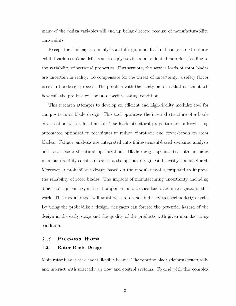
Except the challenges of analysis and design, manufactured composite structures
exhibit various unique defects such as ply waviness in laminated materials, leading to
the variability of sectional properties. Furthermore, the service loads of rotor blades
are uncertain in reality. To compensate for the threat of uncertainty, a safety factor
is set in the design process. The problem with the safety factor is that it cannot tell
how safe the product will be in a specific loading condition.
This research attempts to develop an efficient and high-fidelity modular tool for
composite rotor blade design. This tool optimizes the internal structure of a blade
cross-section with a fixed airfoil. The blade structural properties are tailored using
automated optimization techniques to reduce vibrations and stress/strain on rotor
blades. Fatigue analysis are integrated into finite-element-based dynamic analysis
and rotor blade structural optimization. Blade design optimization also includes
manufacturability constraints so that the optimal design can be easily manufactured.
Moreover, a probabilistic design based on the modular tool is proposed to improve
the reliability of rotor blades. The impacts of manufacturing uncertainty, including
dimensions, geometry, material properties, and service loads, are investigated in this
work. This modular tool will assist with rotorcraft industry to shorten design cycle.
By using the probabilistic design, designers can foresee the potential hazard of the
design in the early stage and the quality of the products with given manufacturing
condition.
1.2 Previous Work
1.2.1 Rotor Blade Design
Main rotor blades are slender, flexible beams. The rotating blades deform structurally
and interact with unsteady air flow and control systems. To deal with this complex
3

multidisciplinary design, many researchers have employed optimization techniques to
trade off among the disciplines of aerodynamics, dynamics, structure, acoustics, and
control. Optimization methods were introduced to helicopter design from the early
1980s [62]. Friedmann [24] summarized the early research of vibration reduction on
helicopters using structural optimization. Celi [14] and Ganguli [26] provided further
reviews of rotorcraft design optimization. A more recent review of multidisciplinary
design of rotor blades can be found in Ref. [49].
Yuan and Friedmann [107] and Ganguli and Chopra [25] focused on forward flight
vibratory load reduction at the hub subject to frequency and aeroelastic stability
constraints. Kim and Sarigul-Klijn [45, 46] developed a multidisciplinary optimiza-
tion method that strived for minimum weight and vibration and maximum mate-
rial strength of the blade with a constraint to avoid flutter. Soykasap [87] focused
on aeroelastic optimization for composite tilt rotor blades. Ozbay [65] investigated
the potential of the star cross-section to tailor extension-twist coupling for tilt-rotor
blades.
To deal with the complex rotor blade design problem, many researchers have relied
on the hierarchical decomposition of the design process into global and local levels of
optimization [17, 46, 53, 64, 98, 100, 107]. Walsh et al. [100] integrated aerodynam-
ics, dynamics and structural models into the rotor blade design optimization using a
multilevel decomposition method. The objective of the global level is to satisfy the
global performance requirements such as thrust, frequencies, and aeroelastic stability.
These global objectives for the blades can be translated into specific requirements on
their sectional properties, such as stiffnesses, moments of inertia, stress levels, and
locations of shear and/or mass center. The cross-sections that satisfy these require-
ments are found at the local level. Moreover, the blade structures are required to meet
the safety regulations enforced by FAA [1, 2] and ADS-27. The sectional properties
4

are a small set of parameters compared to the complete set of geometric and mate-
rial parameters associated with the cross-section. They serve as interface parameters
between the two levels, and thus simplify the whole design optimization, allowing
for modularization of design process. An efficient and high-fidelity modular tool can
significantly improve blade aeroelastic characteristics and reduce the computational
effort for the entire design cycle.
The optimization model includes design objectives, constraints, assumptions, and
variables. Currently, in rotor blade structural design, it is quite popular to assume
a specific topology of structural components inside a given airfoil shape. This sort
of assumption reduces the problem to a sizing optimization in which one varies di-
mensions, orientations, and locations of structural components to achieve the desired
sectional properties. For example, Ganguli and Chopra [25] varied skin thickness and
fiber orientations of a two-celled cross-section in order to obtain cross-sectional stiff-
nesses for aeroelastic optimization of helicopter rotor blades. In order to satisfy the
cross-sectional stiffness requirements, Orr and Hajela [64] considered a multi-cellular
cross-section with strengthened flanges in a multi-disciplinary tiltrotor design. Volovoi
et al. [67, 98, 99] assumed a cross-section with a D-spar and varied thicknesses, fiber
orientations, and D-spar locations to maintain the shear center and stiffness values
within a target range. Lemanski et al. [54] made similar use of a “C” wall and a
channel spar.
On the other hand, some researchers did not assume any specific connectivity and
designed the cross-section layout from scratch. This design concept is called “topol-
ogy optimization.” [81] Using this concept, Fanjoy and Crossley [22] minimized the
distance between the shear center and point of load application for a given airfoil;
but, as the authors pointed out, the computational load was significant. Arora and
Wang [7] reviewed alternative formulations for optimization of structural and mechan-
ical systems, including configuration and topology design, and discussed features of
5

various formulations. Compared to sizing optimization, topology optimization pro-
vides innovative cross-section layouts that can meet sophisticated requirements for
sectional properties. However, the resulting layouts from topology optimization need
to be refined by sizing or shape optimization [81]. As computing capability increases
continuously, topology optimization is attracting more attention.
1.2.2 Modeling of Composite Blades
Modern rotorcraft utilize composite materials to optimize the aeroelastic performance
of rotor blades. Composite rotor blades are generally modeled as initially curved and
twisted anisotropic beams. One of the critical steps of blade analysis is to generate
the equivalent 1D sectional properties from a blade 3D model. The flexible beams of
rotor blades undergo elastic deformations in bending and torsion. In normal operating
conditions, the deformations can be beyond the limits of linear beam theories. Thus,
moderately large nonlinear deformations need to be taken into account. Numerous
state-of-art composite blade modeling techniques have been proposed in the past two
decades. Hodges [35] reviewed the early stage of modeling techniques of composite
rotor blades. Yu [104] summarized more recent work on composite structure analysis.
In this section, the analysis models that have been applied to design optimization are
summarized.
Walsh et al. [100] used a thin-walled, box-beam model with isotropic materials in
the local level optimization of helicopter blade design. Because isotropic, thin-walled,
box-beams have simple closed-form formulations for cross-sectional properties, this
choice reduces the iteration time of design optimization. Instead of isotropic materials,
Lee and Hajela [53] used laminated composite materials with a box-beam model in
multi-disciplinary rotor blade design. To improve the optimization efficiency, they
applied a parallel implementation of the genetic algorithm (GA). The leading and
trailing parts of the airfoil section were not accounted for, leading to a reduction in the
6

accuracy of the cross-sectional properties. Furthermore, when laminated composite
(i.e. anisotropic) materials are used in design, the computational advantage of the
box-beam model becomes marginal.
To improve the accuracy of section analysis, designers have tried more advanced
theories and methods. Smith and Chopra [85] developed a Vlasov model, an analytical
beam formulation, for predicting the effective elastic stiffness and load deformation
behavior of composite box-beams. Deformation of the beam is described by exten-
sion, bending, torsion, transverse shearing, and torsion-related warping. Ganguli and
Chopra [25] applied the Vlasov model to two-cell composite blades for aeroelastic
optimization of a helicopter rotor. Orr and Hajela [64] adopted classical beam theory
and thin-walled, multi-celled beam theory to bending and torsional stiffness analysis,
respectively, for composite tiltrotor blade design.
Worndle [101] formulated a two-dimensional (2D), finite-element-based procedure
to determine shear center and warping functions. Lemanski et al. [54] used 3D FEM
procedure to analyze sectional properties of composite blades with realistic cross-
sections. Although 3D FEM is the most accurate approach to model realistic rotor
blades, it is not appropriate for preliminary design because of the large computational
overhead.
VABS is another section analysis tool. The concept of VABS was first proposed
by Hodges and his co-workers [33], and VABS is continually updated by the recent
research results of anisotropic beam theories [15, 95, 105, 106]. The mathematical
basis of VABS is the variational-asymptotic method [10], through which the gen-
eral 3D nonlinear elasticity problem of a beam-like structure is split into a 2D lin-
ear cross-sectional analysis and a 1D nonlinear beam analysis. VABS is capable of
capturing the trapeze and Vlasov effects and calculating the 1D sectional properties
with transverse shear refinement for any initially twisted and curved, inhomogeneous,
anisotropic beam with arbitrary geometry and material properties. In addition, VABS
7

can provide 3D stress and strain fields so that one can study stress concentrations and
interlaminar stresses. The accuracy of stresses recovered using VABS is comparable
to that of standard 3D FEM for sections that are not close to discontinuities or to the
ends of the beam, but with far smaller computing requirements [106]. The specific
theory and formulation of VABS can be found in [34].
Paik et al. [67] first attempted to use VABS to design a cross-section layout for
a composite blade. Volovoi et al. [98, 99] improved the methodology of cross-section
design and utilized this methodology for frequency placement in the design of a four-
bladed rotor. Li et al. [56] expanded the cross-section design to include manufactur-
ing constraints. Cesnik et al. [16] proposed a design framework of active twist rotor
blades using VABS. Patil and Johnson [68] developed closed-form formulations for
cross-sectional analysis of thin-walled composite beams with embedded strain actu-
ation. Volovoi et al. [96] compared recent composite beam theories for rotor blade
application, and VABS achieved the best match with experimental results.
Once the sectional analysis model has been determined, another challenging task
is to develop a parametric mesh generator that can rapidly generate a precise lay-
out with appropriate mesh given values of the design variables. Generally, a flexible
definition of geometry can be provided by CAD software, but a smooth transfer of
the geometric definition from CAD to FEM is presently very cumbersome and pro-
hibitively expensive from the computational standpoint. In recent years, many efforts
have been made in an attempt to improve this communication. Those efforts include
STEP project (ISO 10303) for a robust neutral file exchange, as well as proprietary
products such as “Design Space” from ANSYS [4]. Another method of parametrically
varying the geometry in FEM applications involves direct manipulation of the mesh.
For example, in Hyperworks the mesh is altered by automatically moving the nodes
in the existing mesh. In order to maintain fitness of the mesh, Hyperworks restricts
changes in the geometric configuration [42].
8

Life Locus
Durability (Life)
Time/Cycles
Normalized
stress level
1
Damage Tolerance (Remaining strength)
Life Locus
Durability (Life)
Time/Cycles
Normalized
stress level
1
Figure 1: Concepts and relationship associated with durability and damage tolerance
1.2.3 Fatigue of Composite Blades
Another critical and complicated problem is a proper modeling of fatigue damage and
durability of composite materials. Durability is relative to the life of a component
or material, while damage tolerance is a discussion of how much strength is left
after some periods of service and history of load application [79]. Figure 1 shows
the relationship of durability and damage tolerance [79]. Because vibration is a key
issue of rotor systems, the fatigue life of rotor blade under vibratory loads is mainly
concerned for the durability analysis.
Fatigue behavior of laminated materials is governed by many parameters. These
parameters include fiber and matrix type, fiber volume fraction, fiber orientation,
layer thickness, the number of layers, and the stacking sequence. Rotor blades made
of such materials exhibit various competing fatigue modes such as delamination, fiber
matrix debonding, fiber breakage, fiber pull-out, and matrix cracking. In addition,
fatigue life of laminated materials highly depends on fabrication methods and environ-
mental factors. Currently, the existing fatigue models for fiber-reinforced composites
9

can generally be classified into fatigue life models (S-N curves), damage accumulation
models, and phenomenological residual stiffness/strength models [19].
The damage accumulation models are usually associated with a specific failure
mode, such as matrix cracking. Tan and Nuismer [89] studied progressive matrix
cracking of composite laminates with a crack in 90 ply subject to uniaxial tensile
or shear loading. They obtained closed-form solutions for laminate stiffnesses and
Poisson’s ratio as a function of crack density or load level using a fracture mechanics
approach and elasticity theory. Flaggs and Laws [23] presented a simple mixed mode
analysis model for prediction tensile matrix failure using a strain energy release rate
fracture criteria and an approximate two-dimensional shear-lag model. Fatigue life
prediction based on this model required an input from non-destructive inspection
tests.
Phenomenological fatigue models generally define damage in terms of macroscopi-
cally measured properties such as strength or stiffness. These models utilize stress-life
fatigue data traditionally generated for design. The multi-axial loading problem is
often handled by introducing a static failure criterion (e.g. Tsai-Wu, Tsai-Hill) and
replacing the static strengths with the residual strengths in the criterion [43]. Schaff
[84] integrated a strength-based fatigue model with finite element analysis and ap-
plied to a helicopter tail rotor spar. The drawback of this approach is that the fatigue
strengths must be determined experimentally for different stress amplitudes, stress
ratios and bi-axial ratios [66]. Moreover, phenomenological models neither predict
the initiation or growth nor indicate the mechanisms of fatigue damage.
Due to the lack of a systematic approach for composite fatigue analysis, relatively
little research has been conducted to facilitate the integration of the fatigue analysis
into design optimization.
10

1.2.4 Manufacturing Uncertainty of Composite Blades
Imperfections in structures are undesirable because such imperfections can substan-
tially influence the response of aircraft structures [73, 58, 77]. Therefore, manufac-
turers spend immense effort in improving product quality and reliability, especially
in the aerospace industry. Although the aerospace engineering production process is
better controlled than other industries, small variations inevitably exist in structural
dimensions, geometric shape, and material properties. Moreover, the application of
composite materials to aircraft causes a host of new challenges because composite
structures compared to metallic structures, exhibit different behavior, defects, and
failure modes. Thomsen [90] discussed the potential advantages and challenges of
using composite materials in wind turbine blades. Pettit [72] presented a comprehen-
sive survey of uncertainty analysis in aeroelasticity. However, as known to the author,
those efforts on uncertainty analysis in aeroealsticity are related to fixed-wing aircraft
[47, 72, 77], little work is related to aircraft[63].
The manufacturing uncertainty associated with composite blades can be classified
into three categories: structural dimension variations, geometric shape uncertainty,
and material property variability. The nominal material properties of composites used
in the structural design are uncertain because of manufacturing process and lack of
precise experiments [88]. In fact, the manufacturing process can significantly influence
the in-service performance of a composite structural component [28, 40, 58, 103]. In
general, the normal and Weibull distribution [48] is used to study material strength
in tension and fatigue [48]. Assuming that the material properties satisfy normal
distributions, d’Ippolito et al. [20] studied the static performance of a composite wing,
whereas Murugan et al. investigated aeroelastic response of composite helicopter rotor
blade.
Structural dimension variations are generally perturbations around the given val-
ues of design variables in sizing problems. As a result, structural performance changes
11

due to variations in dimension can be explored mathematically derivative or by means
of design of experiment (DOE) [102]. Using analytical sensitivity derivatives, Rais-
Rohani and Xie [78] examined the influence of design variables on the reliability of
wing-spar structures. Using DOE, Li et al. [56] explored the sectional properties of
a rotor blade. For the convenience of quality control, the structural dimension is
denoted as Z+∆u−∆l . Here, Z means the exact value, ∆u + ∆l is manufacturing toler-
ance that measures the variability of the value. The dimension upper bound of the
products is Z + ∆u, and the lower bound is Z − ∆l.
In probabilistic design (reliability-based design and/or robust design), structural
dimensions are usually assumed to be random variables that follow normal distribu-
tions. In such a setting, the expectation usually corresponds to the designed value,
and the variance is estimated by the standard deviation decided by manufacturing
tolerance [32]. For a structural dimension specified as Z+∆u−∆l , the standard deviation
can be estimated as
σ =∆u + ∆l
F(1)
where parameter F depends on sample size or the number of parts produced. For
example, for the number of parts equal to 25, F = 4, whereas F = 5 for the number
of parts equal to 100. Equation (1) provides a connection between manufacturing
tolerance and structural reliability.
Using this approach as well as the assumption of independence, d’Ippolito et al.
[20] assessed the fatigue performance of a steel slate track with four random variables.
Meanwhile, they used Latin Hypercube sampling to shorten the computation time in
their research. Rais-Rohani and Xie [78] explored the influence of different probability
distribution assumptions for random variables on wing-spar reliability-based design,
but they did not mention which assumption was closer to manufacturing reality.
12

Figure 2: Cross-section of a composite rotor blade
As discussed above, structural dimension variations are relatively easy to deal
with in that only design variables are perturbed. In addition to adding perturbation
to design variables, the description of geometric shape uncertainty requires the in-
troduction of new variables. For instance, the outer surface of a realistic composite
rotor blade, shown in Figure 2 is very smooth, whereas the inner surface and the
intersurface between the skin and the filled core are wavy instead. Indeed, this wavy
structure is one of the most common phenomena in realistic composite structures.
The waviness occurring to the inner surface of laminates is called “ply waviness”,
which has been extensively studied [11, 76, 13, 55, 31, 27]. Ply waviness can be seri-
ously harmful, for it can greatly reduce the stiffness and the strength of a composite
structural component, especially the compressive performance [11, 76, 13].
Imperfections introduced in manufacturing processes as well as loading conditions
during service lead to structural design uncertainty. To ensure efficient and reliable
blade designs with low cost, uncertainty or randomness need to be accounted for in
the optimization procedure for blade design.
1.2.5 Optimization Methods of Structural Design
In addition to complicating the modeling process, composite materials also provide
many opportunities as well as challenges in the optimization of rotor blade design.
Composite materials can have a wide range in the ratio of Young’s modulus to shear
modulus. Furthermore, one can adjust the fiber orientations or stacking sequence
13

along with ply thicknesses to implement elastic tailoring. However, introducing a
large number of variables associated with composite materials complicates the design
optimization process and leads to increasing computational cost. The situation is
further exacerbated by the fact that many of the design variables will end up being
discrete because of manufacturing constraints such as those imposed on the minimum
ply thickness (increments of 0.005 in.) [54] and fiber orientation (increments of, say,
5). Because of the effects of fiber orientation or stacking sequence, the design space
of cross-section optimization problems is highly nonconvex. Therefore, to develop the
modular tool for cross-section design, it is necessary to require that the optimization
algorithm converge rapidly and be able to handle problems with a mix of continuous
and discrete variables.
The structural design of rotor blades is a nonlinear optimization problem. Avail-
able optimization algorithms for nonlinear problems can be categorized into gradient-
based and nongradient methods. Arora and Wang [7] reviewed alternative optimiza-
tion formulations and discussed gradient-based optimization techniques for structural
and mechanical systems. Hajela [30] provided a general overview of nongradient
methods in the optimal design of multidisciplinary systems, including the genetic al-
gorithm (GA) and simulated annealing (SA). Coello [18] discussed application of GA
in constrained optimization, and Trosset [91] explained application of SA in detail.
Gradient-based methods such as sequential quadratic programming (SQP) converge
to an optimal point much more rapidly than nongradient methods. Because gradient-
based methods need derivative information to decide a next point from the current
point, they can only be applied to continuous problems. Moreover, for an optimiza-
tion problem with nonconvex spaces, gradient-based methods do not provide a direct
means for finding the global optimum. Nongradient methods can handle design op-
timization problems with a mix of continuous, discrete, or integer design variables.
14

Volovoi et al. [99] compared the performance of SQP and GA when applied to cross-
section design. However, the convergence speed of nongradient methods is extremely
slow to obtain the sufficient precision of continuous variables. Furthermore, the re-
sulting optimal solutions from non-gradient methods are not guarantee to be global
optimum theoretically. Therefore, both of the two categories are not appropriate for
the large-scale rotor blade design with mixed continuous and discrete variables.
Another algorithm that can deal with discrete optimization is branch and bound
[51, 52]. The procedure of branch and bound is to solve a continuous variable problem
first, and its solution is considered as upper or lower bound of the mixed problem
dependent on concavity or convexity. Then, the mixed-variable problem is branched
by raising or decreasing one of the discrete variable to its next discrete value. The
bounding procedure is performed by recursively solving a sub-problem with the re-
maining variables. Such branching and bounding procedures keep continuing until
the optimum is obtained. Theoretically, the method of branch and bound can find
the global optimum, but the programming of this method is very complicate. An-
other disadvantage of this approach is that a multitude of nonlinear optimization
sub-problem must be solved [94]. The efficiency of this method depends critically on
the effectiveness of the branching and bounding algorithm. Bad choices could lead to
repeated branching until the sub-region becomes very small.
1.3 Present Work
1.3.1 A Critique of Current Methods
While the application of composites provide many opportunities to improve aircraft
flight performance, the application of composites introduces a host of new challenges
to researchers. Although rotor blades are designed with the properties of composites
in mind, their full potential is far from being explored. The primary reason is that
15

analysis methods for predicting the behavior of composite blade have not been vali-
dated to the point where the industry is comfortable to use them. Therefore, most
rotor blade design optimization employs a simplified box-beam model. The results of
such design is not accurate enough. Many necessary analyses and simulations have to
be conducted after optimization. Once the detailed analysis denies a design resulting
from the optimization, the design cycle has to start again. Therefore, the blade design
requires a relatively long cycle.
Previous efforts focusing on composite blade design ignored manufacturability
constraints so that the optimization was only dealt with continuous variables. As a
result, the optimal designs are difficult to implement in reality. In order to manufac-
ture such a blade, engineers will naturally round the ply angles and/or ply thicknesses
from the optimal solution to the closest ones that can be manufactured. This intuitive
rounding approach runs the risk of violating the structural requirements. To avoid
such potential risks and facilitate the manufacturing, a better way is to improve the
structural design optimization model by adding manufacturability constraints. Thus,
the resulting design optimization become an optimization problem with mixed dis-
crete continuous variables. However, the available single optimization algorithms can
not handle such nonlinear and non-convex structural optimization efficiently. The al-
gorithms that is feasible to mix-variable problems require a large number of function
evaluation, leading to low convert speed.
The vibration and fatigue of main rotor blade has been a key issue in helicopter
design for a long time. Numerous research work has focused on the reduction of
vibratory loads for rotor blades through structural optimization methods. However,
in traditional design practice, fatigue analysis is ignored during the structural opti-
mization and only conducted at a later stage of the design cycle. The drawback is
that the resulting blade may have short fatigue life and high life cycle cost. Life cycle
cost is an important factor of customers’ decision. If the life cycle cost is too high,
16

the blade is not competitive in the market. The blade structure has to be redesigned,
leading to a long development cycle.
Imperfections are inevitably introduced in manufacturing processes. As a result,
structural dimensions, shapes, and material properties deviate from their desired val-
ues. Such deviations can substantially influence the performance of the aircraft struc-
ture. In recent years, such potential hazard have been realized by many researchers.
Much work has been conducted to investigate and quantify the effects of uncertainties
on the global response of fixed-wing aircraft. However, little work has been done on
composite helicopter rotor blades. The primary reason is short of an efficient and
high-fidelity tool. The uncertainty of structures and materials are small in aerospace
industry due to the strict quality control. The tool must be capable of capturing the
small changes of blade structure performance resulting from the small perturbations.
To investigate and quantify the uncertainty influence, stochastic methods have to
be employed that generally require thousands and millions of simulations to obtain
confident solutions. Therefore, an efficient and high-fidelity tool is vital for this task.
1.3.2 Overview
In the past two decades, composite blade modeling has substantially improved. Par-
ticularly, VABS has become mature and its accuracy and efficiency have been accepted
in academic and industry. The objective of this thesis is to develop an efficient and
high-fidelity modular method for composite rotor blade design. This method includes
an efficient reliable cross-sectional analysis tool, VABS, and a parametric geometry
generator. The geometry generator can generate a typical realistic cross-section for
helicopter blades, and the VABS tool can best achieve the balance between the accu-
racy and efficiency for rotor blade analysis. Based on this design tool, three compre-
hensive design procedures for composite rotor blades are proposed. The first one is to
17

incorporate manufacturing constraints into the design optimization. The next is a de-
sign method that integrates fatigue analysis into current rotor blade structural design
optimization. Finally, the manufacturing uncertainty influence on rotor blade design
is explored and a probabilistic design method is proposed to manage the uncertainty
of blade structural performance.
The principal reason for the success of the modular design method is the use
of VABS. VABS is capable of handling composite beams with initial curvature and
twist as well as with realistic cross-sections. In chapter 2, we summarize the rotor
blade structural analysis, including the fundamental theory of VABS, the 3D stress
recovery relationship, the parametric geometry generator, and the coupling procedure
of the aeroelastic response and rotor trim. Next, a strength degradation fatigue
model is discussed. This fatigue model does not require microscopic information of
fatigue progress and is easily incorporated into the proposed structural design method.
Finally, we summarize a general optimization model for rotor blade structural sizing
problems.
In chapter 3, the blade structural sizing with manufacturing constraints is ex-
plored. Such sizing optimization requires an algorithm that can handle a mixed-
variable problem and provide a balance between efficiency and quality. Thus, a hybrid
optimization procedure is developed. This procedure combines the rapid convergence
advantage of sequential quadratic programming and the capability of mixed-variable
of generic algorithm. Although the optimal result may not be the global optimum,
the solution improves a lot relative to the baseline. We also investigate the effects
of design variables on sectional properties. The method of design of experiments is
employed to find the main factors for structural sizing.
In chapter 4, a VABS-based design method is presented that integrate fatigue
analysis in structural optimization. The method is demonstrated by a three-blade
hingeless rotor blade design. In the design, the frequencies of the rotor blades are
18

separated from the excitation frequencies of harmonic aerodynamic loads. The blade
is sized to provide required structural properties so that the aeroelastic performance
is improved. The aerodynamic loads are predicted by DYMORE, a FEM-based multi-
body dynamic analysis tool. Once the aerodynamic loads are obtained from the con-
verged trim solution, fatigue analysis is conducted based on a strength degradation
model.
In chapter 5, the VABS-based design approach is integrated with Monte Carlo
Simulation. The effects of blade shape uncertainty on blade structural characteris-
tics is investigated. The shape uncertainty is assumed to follow harmonic functions
according to one of the defect natures of composite structure. After the statistical
information has been collected from the simulation, a probabilistic design approach is
developed to improve the reliability of the blades. The comprehensive effects, result-
ing from shape, dimension, material, and service loads uncertainties, are investigated
as well.
Chapter 6 summarizes the conclusions of the thesis and future work.
19

CHAPTER II
ROTOR BLADE STRUCTURAL DESIGN
2.1 Rotor Blade Structural Analysis
2.1.1 Sectional Properties Analysis
Helicopter rotor blades are generally modeled as initially curved and twisted beams.
The calculation of the equivalent 1D beam properties is one critical aspect of rotor
dynamic analysis. For this purpose, the sectional analysis of composite blades is
conducted by VABS [33, 15, 106]. VABS, as an alternative to 3D FEM and with
substantial reduction in computational cost for a given level of accuracy, is capable
of modeling initially curved and twisted, non-homogeneous anisotropic beams with
arbitrary cross-sectional configurations.
The mathematical basis of VABS is the variational-asymptotic method (VAM)
[10], through which a complex 3D model is replaced by a reduced-order model in
terms of asymptotic series of certain small parameters inherent to the structure.
The methodology is demonstrated in Figure 3. For rotor blades, one can use the
VAM to split the original nonlinear 3D formulation into a 2D, linear, cross-sectional
analysis and a 1D nonlinear beam analysis for the reference line with the help of small
geometrical parameters a/l and a/R (where a is the characteristic size of the section,
l the characteristic wavelength of deformation along the beam axial coordinate and
R the characteristic radius of initial curvatures and twist of the beam.). Figure 4
demonstrates the idea of blade decomposition. A 1D constitutive law represented
by the stiffness matrix S can be obtained from the cross-sectional analysis. The
original 3D results can be recovered knowing the global deformation from the 1D
beam analysis and the warping field from the 2D cross-sectional analysis [104].
20

Figure 3: Overview of variational asymptotic beam modeling procedure
Figure 4: The decomposition of a three dimensional blade
21

VABS analysis formulations are derived by energy methods. The strain energy of
the cross-section, or the strain energy per unit length of a beam, can be written as
U =1
2
∫
A
ΓTD Γ
√g dydz (2)
where D is the 6 × 6 symmetric material matrix in a local Cartesian system of an
undeformed beam, and g is the determinant of the metric tensor for the undeformed
state. The 3D strain components are represented by the matrix
Γ = [Γ11 2Γ12 2Γ13 Γ22 2Γ23 Γ33]T (3)
The static 3D elastic beam problem is to minimize the strain energy of the cross-
section given in Equation (2) by varying the warping displacements. The warping
displacements wi (i = 1, 2, 3) must satisfy the following constraints:
∫
A
wi dydz = 0, i = 1, 2, 3 (4)
∫
A
(y w3 − z w2) dydz = 0 (5)
where y and z are coordinates of points at the cross-section. Equations (4) and
(5) imply that the warping does not contribute to the rigid-body motions of the
cross-section. By using the VAM, the strain energy can be expressed by a series of
asymptotically correct energy terms that correspond to different orders of the small
parameter inherent in a beam.
U = U0 + U1 + U2 + · · · (6)
where U0, U1, and U2 are zeroth-order, first-order, and second-order approximations
of the strain energy.
22

The second-order asymptotically correct energy accounts for the effects of ini-
tial twist and curvature. Once the first-order approximation of warping function is
obtained, the strain energy is asymptotically correct through second-order approx-
imation and can be expressed in terms of the generalized Timoshenko beam strain
measures. By differentiating with respect to the generalized Timoshenko 1D strain
measures, one can obtain the 1D constitutive law and the cross-sectional stiffness
matrix, shown in Equation (7).
F1
F2
F3
M1
M2
M3
=
S11 S12 S13 S14 S15 S16
S12 S22 S23 S24 S25 S26
S13 S23 S33 S34 S35 S36
S14 S24 S34 S44 S45 S46
S15 S25 S35 S45 S55 S56
S16 S26 S36 S46 S56 S66
γ11
2γ12
2γ13
κ1
κ2
κ3
(7)
where Fi and Mi (i = 1, 2, 3) are three forces and three and moments, respectively;
and γ1i and κi are the 1D strains and the curvature and twist measures of a beam,
respectively. The matrix S is called the generalized Timoshenko stiffness matrix.
To obtain the generalized shear center location, we need to find a point with
coordinates (ξ2, ξ3) through which any arbitrary transverse force results in zero twist.
ξ2 = −Φ34
Φ44
+Φ45
Φ44
(L − x) (8a)
ξ3 = −Φ24
Φ44
+Φ46
Φ44
(L − x) (8b)
where L and x are the length of a beam and the coordinate of the beam along the axis.
Φij are components of the flexibility matrix Φ, the inverse matrix of the generalized
23

Timoshenko matrix S in Equation (7).
For beams in which the bending-twist couplings vanish (Φ45 = Φ46 = 0), the shear
center is a cross-sectional property independent of x. In such a case, choosing the
locus of the shear centers as the beam reference line decouple not only shear and twist
but bending and twist as well. For composite beams, generally, Φ45 and Φ46 are not
equal to zero. One can generalize the definition of shear center by considering only the
twist caused by the shear forces and excluding the twist produced by the bending-
twist coupling. In such a case, the second terms of Equations (8) are drop out.
Further detail formulation used by VABS to compute the generalized Timoshenko
stiffness matrix and the location of shear center are available in [34].
After the sectional stiffness matrix and inertia matrix are obtained, the equivalent
beam model is built for the aeroelastic analysis and rotor trim. Before continuing to
discuss aeroelastic analysis, we need to discuss the cross-section geometry and mesh
generation. For one reason, this rotor blade structural design employs an automatic
optimization scheme that requires a parametric geometry generator to generate the
cross-section layout corresponding to the given values of design variables. Further-
more, VABS uses a finite element method to discretize 2D cross-section and calculate
sectional properties. The use of VABS cross-sectional analysis requires an appropriate
mesh necessitate.
2.1.2 Parametric Geometry Generator with a Realistic Cross-Section
The composite rotor blade cross-sectional optimization in this work is based on the
template illustrated in figure 5. Using this template, the structural design of rotor
blades reduces the errors resulting from geometrical discrepancies and increases the
fidelity of the preliminary design in the comparison with the simplistic box-beam mod-
els often used in the literature [53, 100, 25, 87, 46, 47, 63]. Based on this cross-sectional
geometry, a stand-alone, fully parameterized geometry generator is constructed for
24

Leading Cap
D-Spar
Skin
Web
Filled Core
d-loc
d-ang
ch_skin
y
z
ACSC
MC
h_D
h_web
q
skin
q
web
q
Db1-5q
Df1-5
Figure 5: The structural template for the blade cross-sectional “geometry generator”
cross-section design optimization.
The geometry generator automatically produces a layout of the cross-section given
the coordinates of control points on an airfoil and the values of design variables. In
the process of creating such a parametric model, the curves are produced by NURBS
(Non-Uniform Rational B-Splines) [75] because NURBS can accurately describe any
shape from a simple 2D line, arc, or curve to the most complex 3-D organic free-form
surface or solid. The amount of information required for a NURBS representation
of a piece of geometry is much smaller than the amount of information required by
common faceted approximations. A NURBS curve is defined by four things: degree,
control points, knots, and an evaluation rule. Figure 6 shows a NURBS defined by
control points. The NURBS curves are mathematically represented by the following
general form:
C(u) =k∑
i=1
Ri,nPi (9)
Ri,n =Ni,n(u)k∑
j=1
Nj,nwj
(10)
where k is the number of control points Pi and wj is the corresponding weights. Ri,n
25

Figure 6: Defining a curve with control points
is the rational basis function. The denominator in Equation (10) is a normalizing
factor that evaluates to one if all weights are one. Ni,n(u) is the basis functions, in
which i corresponds to the ith control point, n corresponds with the degree of the
basis function, and u denotes the parameter dependence.
The basis function Ni,n(u) is computed as
Ni,n = fi,nNi,n−1 + gi+1,nNi+1,n−1 (11)
where the function fi rises linearly from zero to one on the interval where Ni,n−1 is
non-zero; the function gi+1 falls from one to zero on the interval where Ni+1,n−1 is
non-zero.
A series of NURBS curves is also produced to define the interfaces between the
layers (i.e. the lamina) of a laminated material. The intersection of each lamina with
the cross-sectional plane is a planar surface bounded by two curves, referred to as the
inner and outer curves. The inward directed normal from the outer curve will intersect
the inner curve, and the lamina thickness can be defined as the distance between
these two intersections along the normal. When the curvature of a bounding curve is
small, the lamina thickness can be considered approximately constant along the outer
curve. In such a case the inner curve can be obtained by simply translating the outer
26

curve. However, shifts of curved lines parallel to themselves can create difficulties for
the regions of high curvature, such as at the leading edge. The thickness must be
adjusted to compensate for the increasing curvature. This is done by holding the local
area of the ply constant, implying that the local density of the material is preserved.
In mathematical terms this translates into a requirement for the local thickness h(s)
of the lamina to be a function of the local radius of curvature ρ(s) along the contour
dimension s, so that
h(s) = ρ(s) −√
ρ(s)2 − 2h∞ρ(s) (12)
where h∞ is the thickness of flat lamina.
While the template is producing the section layout, consistency with the geometric
constraints of the problem must be maintained. For example, the fixed outer shell
of the blade implies that while the D-spar is moved horizontally as a design variable
during the optimization process, its vertical dimension must be adjusted accordingly.
This and other such consistencies are maintained automatically.
Another feature of this geometry generator is fillet creation at the intersection
of two NURBS curves (or NURBS and a straight line). In addition, the geometry
generator is compatible with VABS. The geometry generator generates an appropriate
2D finite element mesh for VABS and laminated material information. Figure 7 and
8 show VABS layup and element conventions. The geometry generator with these
characteristics provides realistic layouts and suitable meshes for cross-sectional design
optimization.
2.1.3 Aeroelastic Analysis and Load Calculation
This section describes the formulation of blade aeroelastic response equations, vehicle
trim equations, and the calculations for the coupled trim procedure. Wind tunnel trim
is used in this work. The wind tunnel trim procedure involves adjusting the controls
27

Figure 7: VABS layup convention
5 2
6
3
7
1 5 2
6
3
7
1 2
34
5
6
7
8 9
1 2
34
5
6
7
8 9
Figure 8: VABS elements
28

to achieve zero first harmonic blade flapping and lag moments with a prescribed thrust
level. The rotor system loads depend on the blade response, so the determination
of vehicle trim and blade response is coupled together. A coupled trim iterative
procedure simultaneously solves for the blade responses and the trim equations until
the blade responses converge [69].
To carry out the dynamic analysis, the governing equations of the rotor system
are derived from the extended Hamilton’s principle, given by
∫ t1
t0
∫ l
0
(δU − δK − δW )dxdt = 0 (13)
where δK and δW are the kinetic energy per unit length and the virtual work of
the external forces acting on the blade. The aerodynamic forces are calculated by
the finite-state dynamic inflow theory [70, 71], and 28 finite states are used in the
dynamic inflow model.
For the convenience of numerical computation, the blade is discretized into a num-
ber of beam elements. Each element has four nodes (2 boundary nodes and 2 interior
nodes), and each node has six degrees of freedom that correspond to three displace-
ments and rotations. After the spatial discretization, the finite element equations are
transformed into the normal mode space by using the blade natural rotating vibration
modes. As a result, the equations of motion can be written in the form
Mq + Cq + Kq = F(q, q, t) (14)
where M, C, K, F, and q represent the mass matrix, gyroscopic/damping matrix,
stiffness matrix, the column matrix of generalized force, and the column matrix of
the generalized coordinates, respectively.
The solutions of the preceding equations are used to calculate the sectional loads of
the rotor blades. The blade loads are integrated over the blade span and transformed
from rotating frame to inertial frame to obtain the hub loads. The steady-state
29

components of hub loads are used for wind tunnel trim in which only rotor thrust is
trimmed and the blade flapping is trimmed such that the 1/rev flapping is eliminated.
The control variables are collective pitch and cyclic pitch. The auto-pilot control law
[69] is used in the trim. The following discrete equations are introduced to compute
the control outputs at each time step
uf = ui + ∆t J−1G(y − yf ) (15)
where ui and uf are the initial and final values of the state vector, respectively. ∆t,
J, G, y, and yf are the time step size, the Jacobian matrix, the diagonal gain matrix,
the specified target values and the present input values, respectively. The controls are
then individually perturbed to form the Jacobian matrix that is evaluated numerically
using a finite differencing process [9].
The blade aeroelastic responses (14) and the trim control settings (15) were solved
simultaneously to calculate the wind tunnel trim solutions. The trim solution and
blade responses are updated iteratively until the convergence criteria are reached [9].
Once the convergence trim solution is obtained, the steady-state loads history at the
specified position of the blade can be extracted for local stress analysis and fatigue
design.
2.1.4 Stress Analysis
Stress analysis is carried out by using VABS recovery theory [39]. The recover re-
lations express the 3D displacements, strain, and stresses in terms of local cross-
sectional coordinates (y, z) and 1D beam quantities, including sectional stress re-
sultants that have been obtained in last section. In addition, the calculation of the
3D strain/stress requires the warping functions, the generalized Timoshenko flexi-
bility matrix, and stress resultants that have been obtained in sectional analysis.
Because of the weak nonlinear relationship between the 1D stress resultants and 3D
30
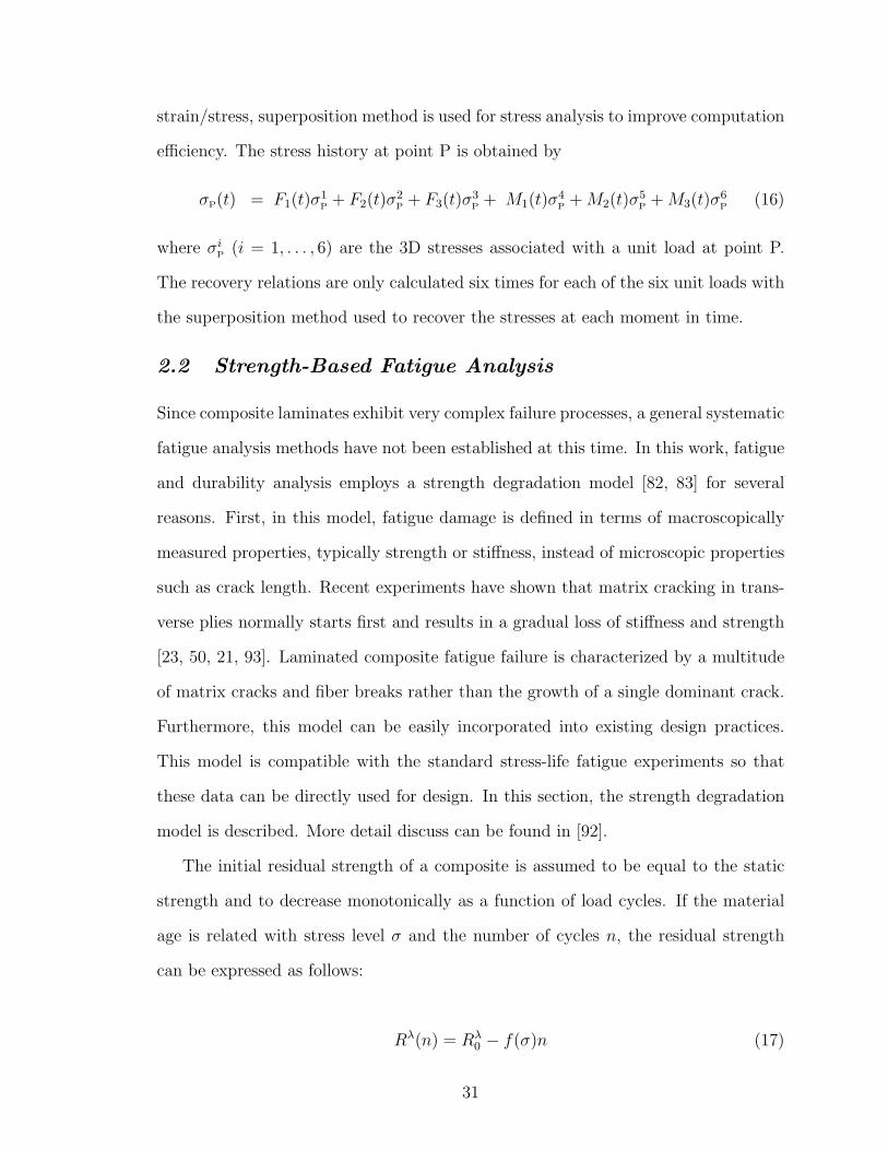
strain/stress, superposition method is used for stress analysis to improve computation
efficiency. The stress history at point P is obtained by
σP(t) = F1(t)σ1P
+ F2(t)σ2P
+ F3(t)σ3P
+ M1(t)σ4P
+ M2(t)σ5P
+ M3(t)σ6P
(16)
where σiP
(i = 1, . . . , 6) are the 3D stresses associated with a unit load at point P.
The recovery relations are only calculated six times for each of the six unit loads with
the superposition method used to recover the stresses at each moment in time.
2.2 Strength-Based Fatigue Analysis
Since composite laminates exhibit very complex failure processes, a general systematic
fatigue analysis methods have not been established at this time. In this work, fatigue
and durability analysis employs a strength degradation model [82, 83] for several
reasons. First, in this model, fatigue damage is defined in terms of macroscopically
measured properties, typically strength or stiffness, instead of microscopic properties
such as crack length. Recent experiments have shown that matrix cracking in trans-
verse plies normally starts first and results in a gradual loss of stiffness and strength
[23, 50, 21, 93]. Laminated composite fatigue failure is characterized by a multitude
of matrix cracks and fiber breaks rather than the growth of a single dominant crack.
Furthermore, this model can be easily incorporated into existing design practices.
This model is compatible with the standard stress-life fatigue experiments so that
these data can be directly used for design. In this section, the strength degradation
model is described. More detail discuss can be found in [92].
The initial residual strength of a composite is assumed to be equal to the static
strength and to decrease monotonically as a function of load cycles. If the material
age is related with stress level σ and the number of cycles n, the residual strength
can be expressed as follows:
Rλ(n) = Rλ0 − f(σ)n (17)
31

where R0 is the static strength of the composite. λ is a constant, and it is determined
by experimental data.
In general, material age also depends on frequency and stress ratio. For simplicity,
these two parameters are fixed in Equation (17). From the S-N curve relationship,
an expression for f(σ) is obtained as
N =1
Kσb=
βλ0
f(σ)(18)
f(σ) = βλ0 Kσb (19)
where N , b, and K are composite fatigue life and the two parameters of the classical
power law of the S-N curve, respectively. The static strength of composite samples
is assumed to have a two-parameter Weibull distribution [48]. β0 in Equation (19) is
the scale parameter of such a Weibull distribution.
The distribution of the static strength is written as
fX(x) =
α0
β0
(x
β0
)α0−1 exp[−(x
β0
)α0 ], if x > 0,
0, otherwise.
(20)
where α0 and β0 are the shape and the scale parameters, respectively.
The shape and scale parameters are estimated by a maximum likelihood method
[37]. Assuming the experimental static strength data xi (i = 1, 2, ·, n) from the same
distribution, α0 and β0 are solved from the following maximum likelihood equations:
n∑
i=1
xα0
i ln xi
n∑
i=1
xα0
i
− 1
α0
−
n∑
i=1
ln xi
n= 0 (21)
β0 =
[
1
n
n∑
i=1
xα0
i
] 1α0
(22)
32

The fatigue strength is assumed to satisfy a Weibull distribution as well. The
shape parameters of fatigue strength distribution is assumed to be the same for
all different stress levels. With these assumptions, the shape parameter of fatigue
strength, denoted as αf , can be estimated from the pooled fatigue data under the ith
level of stress xi1, xi2, · · · , xin:
yij =xij
βi
(23)
m∑
i=1
n∑
j=1
yαf
ij ln yij
m∑
i=1
n∑
j=1
yαf
ij
− 1αf
−
m∑
i=1
n∑
j=1
ln yij
nm= 0 (24)
βi =
[
1n
n∑
j=1
xαf
ij
] 1αf
, i = 1, 2, ...,m (25)
Once the parameters α0 and αf are obtained, the constant λ is defined by
λ =α0
αf
(26)
By substituting Equation (19) into Equation (17), one finds the residual strength
given by
Rλ(n) = Rλ0 − βλ
0 Kσbn (27)
The equations above are valid for the composites with the same stacking sequence.
Liu and Lessard [59] extended this idea and provided an approximate analytical for-
mulation for composite laminates with different stacking sequence. The unidirectional
properties can be computed from the coupon properties, shown in Equation (27), by
using the following approximate equations:
33

b0 = b (28a)
K0 = K
(σ
σ0
)b0
(28b)
where b0 and K0 are the two S-N curve constants of a unidirectional zero-degree-ply
laminate, respectively. The deriving details can be found in [59]. The data used for
computation are from [92, 59].
Once we obtain the unidirectional properties, the strength-based fatigue analysis
can be conducted layer by layer for laminates. When the applied stress equals or
exceeds the residual strength, failure occurs in terms of the Tsai-Wu failure criteria.
The Tsai-Wu failure criteria [29] is used for the multi-axial stress states in laminates.
The coupling fatigue strength analysis is conducted once per cycle until the fatigue
strength is equal to the applied stress.
2.3 General Optimization Model for Blade Structural De-
sign
When a helicopter flies, the deformed blades of main rotor interact with unsteady
air flow and control systems. In general, aerodynamic design focuses on optimizing
external shape, including airfoil shape, twist rate, taper ratio, and span. By con-
trast, structural design focuses on the internal structure of the blade and material
distribution, or the detail cross-section layout.
The cross-section design problem is posed as follows: Determine values of all
design variables including cross-sectional stiffness and inertia constants so as to satisfy
chosen constraints and minimize a chosen objective function. Ingredients for the
constraints and objective function may include such things as the local weight per
unit length, specific stiffness coefficients such as torsional or bending stiffness and
locations of the shear center (SC) or mass center (MC), all of which follow from a
cross-sectional analysis such as VABS. In order to improve the payload of aircraft, the
34

mass is generally expected to minimum. To avoid resonance conditions, the cross-
section design must guarantee bending and torsional stiffnesses to be in a desired
range. Another concern in helicopter rotor design is the dynamic coupling of bending
and torsional loads since this coupling is responsible for flutter and other dynamic
instabilities in rotor blades. The coupling depends on the lift (a transverse load) and
the distance between the SC and the aerodynamic center (AC). Hence, the cross-
section design attempts to minimize the distance between the SC and AC as well as
the distance between the mass center (MC) and the AC for similar reasons. Moreover,
the structure must perform without failure under specified service loads. Whether or
not failure occurs is measured by the Von Mises criterion for isotropic materials and
the Tsai-Wu criterion for anisotropic materials.
Figure 5 shows a template of blade cross-sections. The cross-sectional template
consists of four components: a leading-edge cap, a skin, a D-spar, and a web. These
components contribute to the sectional properties and carry forces. The thickness of
the leading cap is the same as that of the skin. The leading cap and the web are
always adjacent to the D-spar. As the D-spar and the web move along the y direction
or rotate, the length of D-spar and web automatically adjust to fit inside the airfoil.
A core material is filled in the back part of the cross-section, while no material is
filled in the D-spar. With all these assumption, the cross-section design presented
here is a sizing problem. That is, the outer configuration and the topology remain
fixed during the whole optimization process. Design variables include thicknesses of
the four components, the location and the orientation of the D-spar, and material
properties. If the components are made of laminated composites, the design variables
also include fiber orientations or stacking sequence.
The objective of the design is to minimize the following function:
35

z(x) = w1|e(x)|
c× 100% + w2
m(x)
mb
+ w31
gmin(x)+ w4
|d(x)|c
× 100% (29)
x = x1, x2, ..., xnT
where x is a design vector, the components of which are the design variables; N is
the number of variables; e and d are the offset of SC from AC and the offset of MC
from AC, respectively; m and gmin are the mass per unit length and the minimum
safety factor over the cross-section, respectively. The location of AC is assumed at
a quarter of chord, denoted c, in this research. If e > 0, SC is in front of AC;
e < 0, SC is behind AC, and d follows the same rule. The above objective function
combines several design requirements through cost ratios or weight factors, denoted
w1, w2, w3, w4.
The optimization is subject to the following constraints:
• Torsion stiffness and bending stiffness constraints
GJL ≤ GJ(x) ≤ GJU (30a)
EILjj ≤ EIjj(x) ≤ EIU
jj, j = 2, 3 (30b)
where ( )L and ( )U denote the lower and upper bounds of the variables, respec-
tively.
• Mass constraints
mL ≤ m(x) ≤ mU (31)
• Constraints for the coupling terms in stiffness matrix
g(Skl) ≤ gU , k, l = 1, ..., 6 (32)
where Skl are components of the generalized Timoshenko stiffness matrix from
the 1D constitutive law, shown in Equation (7).
36

• Structural integrity constraints
SFL ≤ gmin(x) (33)
gmin(x) = minΞ
(g(x)) (34)
where Ξ denotes the area occupied by the same materials. Safety factor g is
defined by Tsai-Wu failure criterion for composite materials and Von Mises
criterion for isotropic materials.
The Von Mises criterion [29] is written as
σeq =1
g=
1√2σa
√
(σ1 − σ2)2 + (σ2 − σ3)2 + (σ3 − σ1)2 (35)
where σ1, σ2, and σ3 are the principal stresses at the point of interest, σa is the
ultimate stress of the material. The physical meaning of 1/g is the equivalent
mono-axial stress normalized by material strength. When the safety factor g
is greater than one, or the equivalent stress smaller than material strength,
failure is assumed not to occur. Generally, the given safety factor of structures
is greater than unity, such as 1.5 used in the aerospace industry.
For composite materials, g is computed using the Tsai-Wu criteria [29].
σeq =1
g=
(
− 1
Xc
+1
Xt
)
σ1 +σ2
1
XcXt
+
(
− 1
Yc
+1
Yt
)
σ2
+σ2
2
YcYt
− σ1σ2√XcXtYcYt
+τ 212
S2(36)
where Xt, Yt, Xc, Yc and S are the ultimate tension, the compression stresses,
and shear stress of unidirectional laminated materials, respectively. σ1, σ2,
and τ12 are stresses along the two material directions and the shear stress,
respectively. The inverse safety factor 1/g with the Tsai-Wu failure criteria,
similar to Von Mises stress normalized by the ultimate strength, indicates a
dangerous level locally.
37

The nominal material properties of composites in Equation (36) and metals in
Equations (35) are uncertain because of the manufacturing process, environ-
mental conditions, and experimental error [11, 76, 88]. The applied stresses are
also uncertain because they depend on random design variables and uncertain
service loads.
• Manufacturability constraints
xi ∈
[xLi , xU
i ], for continuous variables;
feasible discrete values, for discrete variables;
38

CHAPTER III
STRUCTURAL SIZING WITH MANUFACTURABILITY
CONSTRAINTS
This chapter demonstrates the design methodology developed in chapter 2 for the
rotor blade design. The goal of design is to improve the baseline model by reducing
the weight of the blade, locating the shear center to the aerodynamic center, and
decreasing the stress level of the blade structure while the difference of the sectional
stiffnesses between the optimal blade and baseline is in the range of ±5% of the
baseline. In the first section of this chapter, we build the baseline of the blade. The
cross-section of the baseline is an objective of template, shown in 5. The specific
design variables are also discussed in this section. In the second and third sections,
two optimization examples are presented. The first example focuses on adjusting the
shear center; the second focuses on adjusting both shear and mass centers. In both
designs, manufacturability constraints are added so the fiber orientations are treated
as discrete variables. To search for the optimum design, a hybrid optimization method
is developed that is capable of rapidly obtaining the optimal solution for problems
having both continuous and discrete design variables. Finally, we explore the design
space around optimal design by the design of experiments and find the variables that
have most significant effects on sectional properties.
3.1 Baseline Model
The baseline is modeled using the NASA preliminary design report for a composite
blade retrofit for the XV-15 rotor [5]. The leading-edge cap was assumed to be made
of Titanium; and the D-spar, web and back part of the skin are made of the composite
39

material T300/5208. The back part of the section is filled with honeycomb. Design
variables are ply angles, thicknesses of the D-spar (hD), skin (hskin) and web (dweb),
as well as the web location (dloc) and orientation dang. Note that the trailing edge
part of the D-spar is connected with the web. The trailing edge part of the skin is
considered to have two balanced layers. Thus, there is only one design variable, θskin,
corresponding to the skin ply angle. The web is considered as a single layer θweb.
Finally, we assume that the D-spar has five plies of equal thicknesses. As a result,
the D-spar has a total of ten independent ply angle variables: five angles θDfthat
correspond to the leading edge portion of the D-spar, and five other angles θDbthat
correspond to the trailing edge part of the D-spar. Tables 1 and 2 summarize the
material properties [3, 74] and the baseline values of the design variables, respectively.
Figure 9 shows the geometry and mesh of the baseline layout.
A hingeless rotor in the hovering flight condition is assumed. The chord and the
length of the blade is 20.2 and 150 inches, respectively. Other parameters are air
density, 1.2 kg/m3; rotor angular speed, 25 rad/s; blade angle of attack, 10; blade
airfoil lift curve slope, a = 5.7; and blade airfoil drag coefficient, 0.01. Because
this chapter is to demonstrate the cross-section design, the representative values of
blade aerodynamic loads are estimated from blade-element/momentum theory [44]
for simplicity. The axial force at the blade root is calculated to be T = 11000 lb.
Under aerodynamic loads, the cross-section at the root of the blade suffers the most
severe state of stress; at the root of the blade these are Q2 = 8 lb and Q3 = 400 lb for
shear forces, and M2 = 45000 lb-in and M3 = 1000 lb-in for bending moments. Since
Q2 is too small to have any noticeable influence, it is ignored in the optimization.
The sectional properties are given in Table 3.
40

Table 1: Material Properties
Property Titanium T300/5208 Honeycomb
ρ (lb·s2/in4) 4.220×10⁻⁴ 1.497×10⁻⁴ 6.00×10⁻⁶
E11 (lb/in2) 1.495×10⁷ 2.625×10⁷ 2.8×10⁴
E22 (lb/in2) 1.495×10⁷ 1.494×10⁶ 2.8×10⁴
E33 (lb/in2) 1.495×10⁷ 1.494×10⁶ 2.8×10⁴
G12 (lb/in2) 5.578×10⁶ 1.040×10⁶ 4.7×10⁴
G13 (lb/in2) 5.578×10⁶ 1.040×10⁶ 4.7×10⁴
G23 (lb/in2) 5.578×10⁶ 1.040×10⁵ 4.7×10⁴
ν12 0.34 0.28 0.3
ν13 0.34 0.28 0.3
ν23 0.34 0.33 0.3
Failure criteria Von-Mises Tsai-Wu Tsai-Wu
Table 2: Geometric parameters of the baseline layout
Component Variable No. Value Feasible Range Units
skin hskin 1 0.04 [0.01, 0.05] inch
θskin 2 +45 θ = ±10i, i = 0, 1, ..., 9 degree
web hweb 3 0.04 [0.01, 0.05] inch
θweb 4 0 θ = ±10i, i = 0, 1, ..., 9 degree
D-spar hD 5 0.35 [0.1, 0.4] inch
dloc 6 −8.4025 [-8.6, -6.2] inch
dang 7 90 [60, 120] degree
θDf1−58-12 [+45,−45, 0, 0, 0] θ = ±10i, i = 0, 1, ..., 9 degree
θDb1−513-17 [+45,−45, 0, 0, 0] θ = ±10i, i = 0, 1, ..., 9 degree
41
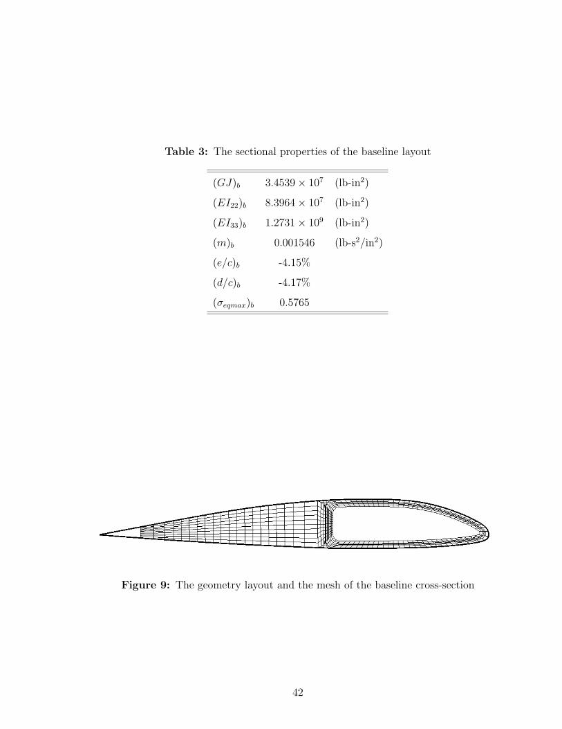
Table 3: The sectional properties of the baseline layout
(GJ)b 3.4539 × 10⁷ (lb-in2)
(EI22)b 8.3964 × 10⁷ (lb-in2)
(EI33)b 1.2731 × 10⁹ (lb-in2)
(m)b 0.001546 (lb-s2/in2)
(e/c)b -4.15%
(d/c)b -4.17%
(σeqmax)b 0.5765
Figure 9: The geometry layout and the mesh of the baseline cross-section
42

3.2 Minimizing the Distance from Shear Center to Aero-
dynamic Center
In this example the goal is to improve the baseline model by minimizing the distance
from shear center to aerodynamic center. The mass per unit length and the maximum
equivalent stress over the cross-section is minimized as well by using different weight
factor. The extension-torsion and bending-torsion coupling terms are restricted to be
small compared with the diagonal terms of the stiffness matrix. The fiber orientations
are discrete variables, the values of which assume multiples of 10 ranging from -90
to 90 due to manufacturing limitations. The objective function is shown in Equation
(30). The constraints are specified below.
• Mass per unit length of optimal cross-section is no more than that of the base-
line:
m(x)
mb
≤ 1.0 (37)
where ( )b denotes the value of the baseline.
• The stress level of optimal cross-section is less than that of the baseline:
σeqmax(x)
(σeqmax)b
≤ 1.0 (38)
• The sectional stiffnesses of optimal cross-section is in the range of ±5% of
baseline values:
0.95 ≤ GJ(x)
(GJ)b
≤ 1.05 (39a)
0.95 ≤ EI22(x)
(EI22)b
≤ 1.05 (39b)
0.95 ≤ EI33(x)
(EI33)b
≤ 1.05 (39c)
43

• The coupling stiffnesses of extension-twist and bending-twist are far smaller
than the stiffnesses they couple:
S14(x)2
S11(x)S44(x)≤ 0.01 (40a)
S45(x)2
S44(x)S55(x)≤ 0.01 (40b)
S46(x)2
S44(x)S66(x)≤ 0.01 (40c)
The reason of adding the coupling term constraints are that the effects of cou-
pling terms on rotor blade aeroelastic response have not been fully investigated.
Designers are not confident to use the coupling effects in design application.
• The feasible values of each design variables due to manufacturability constraints
are summarized in Table 2.
3.2.1 The Hybrid Optimization Method
Current cross-section design optimization is nonlinear optimization problem with
mixed continuous and discrete variables. Introducing fiber orientation leads to the
non-convexity of the cross-section design space. To solve the non-convex and non-
linear optimization problem with mixed variables, a hybrid optimization method is
developed. In the first stage, a continuous optimization problem is solved by using
SQP [12]. To increase the probability of achieving a global optimum, a population
of initial points is randomly selected in the design space before running SQP. The
optimal solution for the continuous model is the best one among all the local optima
resulting from SQP. After the optimal solution for continuous model is obtained, one
can find out between which two nearest discrete points the optimal solution is located
for each discrete variable. In the second stage, the GA [38] is used to determine which
combination has the best objective function and satisfies the constraints among all
combinations of these upper and lower bounds. Figure 10 shows the optimization
flow chart.
44

Stage I
1-D aerodynamic & dynamic analysis for blade sectional loads
Initiating GA
Selection, crossover, mutation
Storing the fittest designs
Convergent?The discrete optimum design
Computing the fitness of the promising designs
Cross-section layout & mesh generation
VABS section analysis for stiffness, SC, etc.
VABS 3-D recovery for stress & strain
YesNo
Randomly generating initial design values
Cross-section layout & mesh generation
Cross-section geometry template
VABS section analysis for stiffness, SC, etc.
1-D aerodynamic & dynamic analysis for blade sectional loads
Initial curvature & twist rate
Computing objective, constraints, gradients
Determining a next design point
Adding an optimum candidate
Comparing all the optimum candidates
The best optimum
Identifying the discrete design space around the best optimum
VABS 3-D recovery for stress & strain
Population enough?
Yes
No
No
Yes
Convergent?
Initial curvature & twist rate
Stage II
Figure 10: The optimization flow chart for composite blade design with mixedcontinuous and discrete variables due to manufacturability constraints
45

This hybrid method combines the advantages of SQP and GA. It utilizes the
rapid convergence of SQP and avoids slow convergence of GA for obtaining the op-
timal continuous solution. Once the optimal continuous solution is found, the GA
is restricted to search the optimal discrete solutions around the optimal continuous
one. Since the searching space of GA is much smaller than the entire design space,
the efficiency of optimization is improved significantly compared with a one-step GA,
albeit at the expense of less confidence in finding the global optimum. Accounting for
the computational load of SQP in the first stage, the total computational load of this
hybrid optimization scheme is smaller than that for a one-step GA. Instead of using
the GA, if one rounds the solution of SQP to the closest discrete values in the second
stage, one runs the risk of constraint violations and a suboptimal solution. These two
disadvantages are illustrated in the optimization example below. Therefore, by using
this hybrid scheme, one can efficiently and robustly solve cross-sectional optimization
problems with mixed continuous and discrete variables.
Some researchers have used a similar hybrid optimization technique but in the
reverse order of the present scheme. That is, the GA is used to search the global
optimum in the whole solution region to obtain a quasi-optimal solution, and then
resulting solutions are refined by SQP [60, 41, 97]. Although the reverse order has a
higher probability of achieving the global optimum, it cannot handle the optimization
problem with both continuous and discrete design variables.
3.2.2 Design Results
A cost ratio describes the relative importance of the factor it multiplies in the objec-
tive function. The larger the cost ratio, the more important the factor it multiplies
participates in the objective function calculation. Three sets of cost ratios are se-
lected for use in illustrating their effect on the optimization. The set of cost ratios
w = (1, 0, 0, , 0) is an extreme case, where only the offset between SC and AC is
46

Figure 11: The cross-sectional layout and the mesh of the optimal solution withweight factors w =(1, 0, 0, 0)
minimized in the optimization process. Because stresses and inertia are ignored in ob-
jective function, we turn them into hard constraints, as shown in Equations (38) and
(37). The other two sets of cost ratios mean that the weighted sum of the offset, the
mass and the maximum equivalent stress, is minimized, so these two constraints are
omitted. For the set of cost ratio w = (1/2, 1/4, 1/4, 0), the distance is more impor-
tant than the mass and the stress constraints, while the set of w = (1/3, 1/3, 1/3, 0)
implies the three factors are equally important.
In the first set of cost ratios, which can be denoted as w=(1, 0, 0, 0, 0), the
continuous solution not only satisfies all the stress, mass and stiffness constraints,
but the non-dimensional offset e is as small as 0.0155% chord. It is worth noting that
the maximum equivalent stress over the root cross-section is only 67.4% of the value of
baseline. The optimal cross-section layout is shown in Figure 11. Another interesting
observation is that the mass per unit length of the discrete solution is equal to that
of the continuous solution. The reason is that ply angles do not affect the mass per
unit length. This can also be concluded from the design space exploration in the last
section of this chapter.
The best discrete solution that GA found near the continuous one and the solution
rounded to the nearest discrete values are also summarized in Table 4. The omitted
values are unchanged compared to the continuous solution. The hybrid solution is
better overall than the one obtained by simple rounding. All the constraints are
satisfied for both discrete solutions in the case of cost ratio (1, 0, 0, 0). The value
of the objective function resulting from the hybrid approach is smaller than the one
47

Table 4: The optimization results of locating shear center to aerodynamic center
Design w =(1, 0, 0, 0) w =(1/2, 1/4, 1/4, 0) w =(1/3, 1/3, 1/3, 0)
variables cont. round 2-step cont. round 2-step cont. round 2-step
dc
(%) -4.12 -4.12 -4.12 -5.55 -5.55 -5.55 -2.87 -2.87 -2.87
ec
(%) -0.015 -0.098 -0.024 -0.077 -0.096 0.025 -0.496 0.445 -0.491
mmb
0.988 0.988 0.988 0.921 0.921 0.921 1.067 1.067 1.067
σeqmax
(σeqmax)b0.674 0.670 0.673 0.831 0.786 0.798 0.762 0.753 0.910
GJ(GJ)b
0.955 0.958 0.951 0.959 0.960 0.962 0.950 0.948 0.953
EI22(EI22)b
1.041 1.047 1.044 1.033 1.076 0.998 1.046 1.059 1.032
EI33(EI33)b
0.984 0.959 0.959 0.967 1.016 0.984 0.951 0.964 0.951
hskin 0.050 0.050 0.050
θskin 38.2 40 40 43.69 40 40 40.58 40 40
hweb 0.016 0.016 0.014 0.030
θweb 0.0 0 0 -1.03 0 0 0.37 0 10
dloc -7.67 -8.396 -7.267
dang 63.4 100.86 72.47
hD 0.329 0.270 0.399
θDf1 64.1 60 70 84.0 80 90 58.33 60 60
θDf2 -10.7 -10 -10 -12.42 -10 -10 -31.60 -30 -30
θDf3 0.0 0 0 1.83 0 0 1.22 0 0
θDf4 0.0 0 0 -0.41 0 0 1.69 0 0
θDf5 9.9 10 10 0.30 0 0 1.69 0 0
θDb1 87.5 90 90 85.83 90 90 90.00 90 90
θDb2 -19.9 -20 -20 -2.69 0 0 -32.00 -30 -30
θDb3 -5.7 -10 0 -0.19 0 0 0.00 0 0
θDb4 0.0 0 0 -0.20 0 0 0.00 0 0
θDb5 -1.8 0 -10 -0.14 0 0 0.00 0 0
48

Table 5: The comparison of approximate computation costs between the generalGA and the proposed hybrid optimization scheme
Proposed hybrid
General GA First stage (SQP) Second stage (GA)
Design space size 7.4 ×10²² 4096
Population size 80 30 8
iteration > 100 15 30
Function calls > 16000 7650 480
Total function calls > 16000 8130
from rounding, but slightly larger than the one from SQP. For the cost ratios (1/2,
1/4, 1/4, 0) and (1/3, 1/3, 1/3, 0), no constraints are violated for hybrid solution, but
one or two constraints are violated for the rounded solution. Sometimes the solution
rounded to the nearest discrete values does not violate the constraints, but sometimes
it does. Actually, one has 212, or 4096, options to round 12 discrete variables. Most
of them violate the constraints. The hybrid method, SQP followed by GA, always
chooses a discrete solution that does not violate the constraints. Although this “smart
rounding” adds some computational time, it is worth running the GA to get the best
discrete solution.
Table 5 compares the computation costs for the GA alone and for the present
hybrid method. The hybrid method has less computational cost. In this comparison,
each continous variable is represented with a five-bit string. Thus, the precisions of
skin thickness, web thickness, D-spar thickness, and D-spar orientation are 0.00063,
0.00063, 0.0094 and 0.075, respectively, in the general GA. In the hybrid method,
to avoid local optima, SQP was initiated randomly; and the best result from the 30
resulting optima was selected for the second-stage optimization.
49

Table 6: The optimization results of locating both mass and shear centers to aero-dynamic center
ec
-0.006% hskin 0.048 θDf3 22.550
dc
-2.443% θskin 25.076 θDf4 -0.320
m(m)b
1.000 hweb 0.018 θDf5 -18.285
σeqmax
(σeqmax)b1.024 θweb 36.206 θDb1 31.693
GJ(GJ)b
0.950 dloc -6.959 θDb2 -0.060
EI22(EI22)b
0.990 dang 86.595 θDb3 34.629
EI33(EI33)b
1.041 hD 0.389 θDb4 4.829
θDf2 1.371 θDf1 19.166 θDb5 -11.166
3.3 Locating Both Mass and Shear Centers to Aerodynamic
Center
In this example the objective is to improve the baseline model further, based on exam-
ple 1, so that the distance between the mass center (MC) and AC is also minimized.
The constraints remain the same as those of the example in the last section.
Table 6 summarized the optimization results of locating both MC and SC to AC.
Moving both MC and SC is more difficult than moving only the SC. Actually, it is not
possible to make the distance between MC and AC as small as the distance between
SC and AC while the stiffnesses are constrained to remain in the range specified.
This can be explained by the fact that both the torsional stiffness and the offset
between MC and AC and are sensitive to web location; see the sensitivity analysis
below. Changing the web location has counteracting effects on these two response
variables. To decrease the distance further, the web location must be moved forward
(dloc > −7.0 in); to satisfy the torsional stiffness, the web location has to be moved
backward (at least dloc < −7.0 in). One way to resolve this conundrum is add one or
more design variables, such as the chordwise location and mass of a non-structural
point mass near the leading edge.
50

3.4 Parametric Study and Sensitivity Analysis
Sensitivity analysis is an essential part of structural optimization. Sensitivity analysis
facilitates the understanding of the robustness of the design. One can know how
the change of constraints would affect the values of design variables. One can also
understand how each design variable affects the response variables. In industry, due
to manufacturing techniques and cost limitations, the optimal value of each design
variable might not be exactly attained. This could lead to some of the constraints
being violated and a failure to attain some of the design goals. In addition, one can
focus on some important design parameters based on the knowledge of how those
design variables would change the objective function and constraints. For example, if
the objective function is sensitive to a design parameter, one attempt to improve the
manufacturing precision of that parameter; otherwise, one may expend a lot of effort
and/or cost and wind up not improving the design. The design of experiments (DOE)
tool is used to find the main effects on the response variables in the whole design
space. The Eighth Fractional Factorial (16,384 function calls) and Box-Behnken
(561 function calls) experiment methods are used. Results from these two methods
are shown in Figures 12–17. The length of the bars in those figures represents the
contribution of the design variable to the response variables. Among the 17 design
variables, some of them contribute only slightly to all the response variables such
as the fiber orientations in the web. The web location, the skin thickness, the fiber
orientations in the skin and the D-spar thickness play important roles in determining
cross-sectional properties. Mass per unit length is affected by skin thickness, D-spar
thickness, web location, web thickness and web orientation. The first three factors
contribute more than 95% of the mass change, meaning that mass quite sensitive to
skin thickness, D-spar thickness and web location. The ply angles do not change the
blade mass because the fiber orientation neither increases nor decreases the amount
of material in the blade. The MC location is affected by design variables in a manner
51
quite similar to the mass per unit length. However, SC, equivalent stresses and
stiffnesses exhibit a quite different character, being sensitive to more factors. Some
of the ply angles play an important role in changing SC, stress and stiffnesses. For
example, fiber orientation in the skin has the largest contributions to SC and chord-
wise stiffness. Figures 18–21 show how the two most important variables affect the
mass per unit length, location of SC, torsional stiffness, and location of MC.
52

0%
5%
10%
15%
20%
25%
30%
35%
40%
45%
1 2 3 4 5 6 7 8 9 10 11 12 13 14 15 16 17
Design variable No.
Norm
aliz
ed e
ffects
Box-Behnken Eighth Fractional Factorial
Figure 12: The contribution of each design variable to mass per unit length
0%
5%
10%
15%
20%
25%
30%
35%
40%
45%
1 2 3 4 5 6 7 8 9 10 11 12 13 14 15 16 17Design variable No.
Norm
aliz
ed e
ffects
Box-Behnken Eighth Fractional Factorial
Figure 13: The contribution of each design variable to shear center
53

0%
5%
10%
15%
20%
25%
30%
35%
40%
45%
50%
1 2 3 4 5 6 7 8 9 10 11 12 13 14 15 16 17Design variable No.
Norm
aliz
ed e
ffects
Box-Behnken Eighth Fractional Factorial
Figure 14: The contribution of each design variable to torsional stiffness
0%
5%
10%
15%
20%
25%
1 2 3 4 5 6 7 8 9 10 11 12 13 14 15 16 17Design variable No.
Norm
aliz
ed e
ffects
Box-Behnken Eighth Fractional Factorial
Figure 15: The contribution of each design variable to flapwise stiffness
54

0%
10%
20%
30%
40%
50%
60%
70%
1 2 3 4 5 6 7 8 9 10 11 12 13 14 15 16 17Design variable No.
Norm
aliz
ed e
ffects
Box-Behnken Eighth Fractional Factorial
Figure 16: The contribution of each design variable to chordwise stiffness
0%
5%
10%
15%
20%
25%
30%
35%
40%
45%
50%
1 2 3 4 5 6 7 8 9 10 11 12 13 14 15 16 17
Design variable No.
No
rma
lize
d e
ffe
cts
Box-Behnken Eighth Fractional Factorial
Figure 17: The contribution of each design variable to mass center
55

0.60.65
0.65
0.7
0.7
0.75
0.750.8
0.80.85
0.85
0.9
0.9
0.95
0.951
1.051.1
1.15
D-spar location
D-s
part
hick
ness
-8.5 -8 -7.5 -7 -6.5
0.15
0.2
0.25
0.3
0.35
0.4
1.151.11.0510.950.90.850.80.750.70.650.6
Figure 18: Mass per unit length vs. D-spar thickness and web location
56

-0.04
-0.04
-0.03
-0.03
-0.02
-0.02
-0.02
-0.0
1
-0.01
-0.01
0
0
00
0.01
0.01
0.01
0.02
0.02
0.03
0.03
-0.02
0.01-0.01
D-spar location
Fib
eror
ient
atio
nin
skin
-8.5 -8 -7.5 -7 -6.5-90
-60
-30
0
30
60
90
0.040.030.020.010
-0.01-0.02-0.03-0.04-0.05
Figure 19: Non-dimensional SC offset from AC vs. fiber orientation in the skin andthe D-spar location
57

0.5
0.55
0.6
0.6
0.65
0.65
0.7
0.70.75
0.75
0.8
0.8
0.85
0.85
0.90.95
1
D-spar location
Ski
nth
ickn
ess
-8.5 -8 -7.5 -7 -6.5
0.02
0.03
0.04
0.05
1.0510.950.90.850.80.750.70.650.60.550.5
Figure 20: Torsional stiffness vs. skin thickness and D-spar location
58

-0.08
-0.07
-0.07
-0.06
-0.06
-0.05
-0.05
-0.04
-0.04
-0.03
D-spar location
D-s
part
hick
ness
-8.5 -8 -7.5 -7 -6.5
0.15
0.2
0.25
0.3
0.35
0.4
-0.02-0.03-0.04-0.05-0.06-0.07-0.08
Figure 21: Non-dimensional MC offset from AC vs. D-spar thickness and D-sparlocation
59

CHAPTER IV
STRUCTURAL DESIGN AGAINST FATIGUE FAILURE
In this chapter, we attempt to incorporate fatigue and durability analysis into rotor
blade design optimization. The optimization also includes the stiffness, weight, and
frequency constraints. A new optimization implementation procedure is developed
for blade structural design and applied to a three-blade hingeless-rotor case [36].
Fatigue life prediction employs VABS 3-D stress recovery relation and a strength-
based fatigue model, in which fatigue failure occurs when the residual strength is
equal to the applied stress. Failure is defined by the Tsai-Wu failure criterion, which
accounts for the interaction of all stress components. The relations of residual strength
characterizes in terms of unidirectional S-N data and laminate static strength.
4.1 Design Methodology
4.1.1 Cross-Section with Nonstructural Mass
In chapter 3, parametric study and design results have shown that based on the
cross-section template in Figure 5 it is difficult to locate both shear and mass center
at aerodynamic center. A nonstructural mass is added at the leading edge in the
new cross-section, shown in Figure 22, so that the mass center of the cross-section is
coincident with the aerodynamic center. The inertia effect of the mass is counted in
sectional inertia. However, the stiffness and strength effects of the mass are ignored in
the calculation of sectional stiffnesses. The sectional stiffness are mainly contributed
by four structural components: the skin, web, D-spar, and leading-edge cap. More-
over, these four components carry most the loads and significantly contribute to other
sectional properties. The skin, web, and D-spar have two, one, and four layers, re-
spectively, each with an independent ply angle. The vertical wall of the D-spar are
60

D-spar
q
web
q
Db1-4q
Df1-4
ACSC MC y
qskin1-2AA
BB
CC DD
AA
BB
CCDD
hskin
hweb h
D-spar
hD-spar
Filled Core
z
Skin Web
Leading Cap
dloc
Non-structural
Mass
ym1
Figure 22: The structural template of a typical blade cross-section with a non-structural mass
independent on the curve wall of the D-spar. AA, BB, CC, and DD of Figure 22 show
the detail sequence of composite layers in each components. The skin, the D-spar,
and the web are designed by T300/5208 laminated composite materials. The leading
cap is made of titanium for erosion protection.
4.1.2 Design Objectives and Constraints
The cross-section layout is designed to satisfy the requirements of stiffness, natural
frequencies, fatigue life, and strength. In order to improve the payload of aircraft,
the mass is generally expected to be minimized. To avoid resonance conditions, the
natural frequencies of the blade are selected to be spaced away from the rotation
speed and the integer times of rotation speed. Another concern of in helicopter rotor
design is the dynamic coupling of bending and torsional loads since this coupling is
responsible for flutter and other dynamic instabilities in rotor blades. The coupling
depends on the lift (a transverse load) and the distance between the shear center
(SC) and the aerodynamic center (AC). Hence, the cross-section design attempts
to minimize the distance between the SC and AC. Moreover, the structure must
perform without failure under specified service loads and have enough fatigue life.
Design variables include thicknesses of the four structural components, the location
61

and the orientation of the D-spar, and fiber orientations. The design variables and
material properties [74] are summarized in Tables 7 and 1, respectively.
Table 7: Design variables and feasible ranges
Component Variable Feasible range Units
skin hskin [0.0075, 0.035] inch
θskin1-2 [-90, 90] degree
web hweb [0.0075, 0.035] inch
θweb [-90, 90] degree
D-spar hD [0.04, 0.16] inch
dloc [-1.65, -0.2] inch
dang [80, 100] degree
θDf1−4 [-90, 90] degree
θDb1−4 [-90, 90] degree
The objective is to minimize the blade weight and locate shear center to aerody-
namic center. Weight factors are used to convert the multi-objective function into a
single objective function.
min: 10m(X) + 100|e(X)|
c(41)
X = X1, X2, ..., XnT
where x is a column matrix, and the components x1, x2, ..., xn are the design variables,
summarized in Table 7.
The design constraints are summarized below.
• The first six natural frequencies of the blade are placed away from the rotor
rotation speed and its integer times. The frequency constraints are written as
62

0.2 <f1(X)
Ω< 0.8 (42a)
1.08 <f2(X)
Ω< 1.7 (42b)
0.15 <fi(X)
Ω−⌊
fi(X)
Ω
⌋
< 0.85, i = 3, 4, 5, 6 (42c)
where fi is the ith frequency of the blade, and ⌊·⌋ implies the integer part of
the value.
• To reduce the dynamic coupling of bending and torsional loads, the distance
between SC and AC is restricted to be smaller than 0.1% chord, which is
|e(X)|c
< 0.1% (43)
where e is the offset from aerodynamic center to shear center, and c is the chord.
• The coupling terms of tension-twist and bending-twist are required to very small
in comparison with the diagonal terms in stiffness matrix shown in equation
(40).
• The structure must be safe under the service loads in terms of strength failure
criteria. For isotropic material, Von Misis criteria Equation (35) used, and Tsai-
Wu Equation (36) for laminated materials. The blade is designed for infinite
life using 10,000 hours as the cycle criteria.
• The manufacturing constraints are
XLi ≤ Xi ≤ XU
i , i = 1, ..., n (44)
where the superscript (·)L and (·)U indicate the lower and upper bounds of the
design variables.
63

4.1.3 Sectional Properties Analysis
In chapter 2, we have discussed the sectional properties analysis associated with the
cross-section without nonstructural mass. Since the nonstructural mass is assumed
not contribute to sectional stiffness, the generalized Timoshenko stiffness matrix is
the same as the case without nonstructural mass. Furthermore, the shear center that
computed based on the flexibility matrix is the same as the case without nonstructural
mass, too. Stress/strain analysis is also the same. However, the sectional mass is
altered by the non-structural mass, resulting in the change of the natural frequencies
and aeroelastic behavior of the blade.
The sectional inertia of the cross-section with nonstructural mass has two parts:
the inertia of non-structural mass and non-structural cross-section. The total sec-
tional mass is computed as
m = m0 + m1 (45)
ym0 =1
m0
∫
A
ρ y dydz (46)
where m0, m1, ρ, and ym0 are sectional mass without non-structural mass, non-
structural mass, material density, and y-coordinate of the mass center without non-
structural mass. m0 and ym0 have been determined in cross-sectional analysis without
nonstructural mass. ym0 < 0 implies that MC is behind aerodynamic center, which is
unstable. In this situation, a non-structural mass is added so that MC is coincidence
with AC. m1 is computed as
m1 =m0 ym0
ym1
(47)
where ym1, y-coordinate of the non-structural mass, is known.
The total mass moment of inertia is
Iyy = Iyy0 + m0 y2m0 + m1 y2
m1 (48)
64

where Iyy0 is the mass moment of inertia without the non-structural mass.
4.1.4 Aeroelastic Analysis and Rotor Trim
A three-bladed hingeless rotor [36], shown in Figure 23, is considered here. The
blade is assumed to be an elastic beam undergoing axial extension, flap bending, lag
bending, and elastic twist, with a rotation speed of Ω. The blade connects with a
flexural beam. The revolute joint provides the pitch control of the blade. Figure 24
shows the DYMORE topology model of the rotor system.
A comprehensive multi-body dynamic analysis code DYMORE developed by Bauchau
[9] is used to simulate the helicopter blade dynamic aeroelastic response. The aeroe-
lastic response equations developed in chapter 2 include centrifugal forces, gravity,
and aerodynamic forces. The aerodynamic forces are calculated by the unsteady
aerodynamic theory [70], and 28 finite states are used in the dynamic inflow model.
For the convenience of numerical computation, the blade is discretized into a
number of beam elements. Each element has four nodes (2 boundary nodes and 2
interior nodes), and each node has six degrees of freedom that correspond to three
displacements and rotations. After the spatial discretization, an eigenvalue problem
is solved for natural vibration modes of the rotor system. Then, the aeroelastic
response equations are solved. The blade loads are integrated over the blade span
and transformed from rotating frame to inertial frame to obtain the hub loads. The
steady-state components of hub loads are used for wind tunnel trim. Auto-pilot
control law [69] is used in the trim with a forward level flight speed 123 ft/sec and
the total lift 1500lb.
4.1.5 Stress and Fatigue Analysis
Once the converged trim solution is obtained, stress analysis is carried out by us-
ing VABS recovery theory [34]. The calculation of the 3D strain/stress requires the
65

12.2 ft
twist rate -10
0.64 ft
Figure 23: A three-bladed hingeless rotor
Blade
Spherical joint
Flex Beam
Root Extension
Revolute
Joint
Flex Joint
Hub
Shaft
Figure 24: The DYMORE topology model of the hingeless rotor
66

Table 8: Parameters for Fatigue Analysis
K0 b0 λ β0
2.38 × 10−58 17.3 9.231 598.4 MPa
warping function, the generalized Timoshenko compliance matrix, and curvature in-
formation that have been obtained in sectional analysis. To improve computation
efficiency, superposition method is employed in stress analysis.
Fatigue analysis is conducted layer by layer for laminates using a strength-based
fatigue model that have been discussed in chapter 2. The unidirectional parameters
are summarized in table 8 calculating based on the data from [92, 59]. When the
applied stress equals or exceeds the residual strength, failure occurs in terms of the
Tsai-Wu failure criteria [29]. Tsai-Wu failure criterion is used for the multi-axial
stress states in laminates. The coupling fatigue strength analysis is conducted once
a cycle until fatigue strength is equal to the applied stress.
4.1.6 Optimization Procedure
The optimal design, or the solution of the above equations, are searched using se-
quential quadratic programming optimization algorithm [80, 6]. During the design
optimization, the outer configuration and the connectivity of the structural compo-
nents remain fixed. Figure 25 shows the design procedure. In each iteration, the
values of design variables and material properties are passed to the geometry gener-
ator that generates the required cross-section layout and an appropriate mesh. The
geometry, mesh and initial twist information are used by VABS to compute the sec-
tional properties. The results of VABS are used to model the blade as one dimensional
rotating beam with a multy-body dynamics code DYMORE [9] being used to com-
pute the natural frequencies. If the frequencies satisfy the constraints, the rotor is
trimmed for a forward level flight condition. Otherwise, the optimizer determines the
next design point by perturbing the last point that satisfies all the constraints, and
67

new iteration begins. Once a convergent trim solution is obtained, VABS recovery
relation is used to compute the stress over the cross-section. By using the stress
history, fatigue life is predicted by strength degradation model. If fatigue life satisfies
the requirement, a candidate design is stored, then another iteration begins.
4.2 Design Results
As an example, the blade structural design is based on a three-bladed hingeless rotor.
The service rotation speed is 50.0 rad/sec. Loading condition is obtained using the
trim results for a forward level flight with a speed of 123 ft/sec and total lift 1500
lb. Because the coupling procedure of trim and aeroelastic response analysis takes
a long time, this procedure is conducted only when the basic design constraints are
satisfied during the optimization. To reduce the probability of the local optimum, the
optimization starts from a population of randomly initialized designs. There were 16
initial designs that resulted in five local optimums that satisfy the basic constraints.
The following figures and tables shows the results of the best local optimum in
terms of the sectional mass, stiffnesses, natural frequencies, and fatigue life. Figure
26 shows the optimization history of the objective function. Figures 27 to 31 show
the steady-state loads history at the root of section and stress history at the criti-
cal point over the root section. Table 9 shows the comparisons between the initial
design and optimal design. In the initial design, the frequency of the second flap
(the third mode) is 3.056 times the rotor angular speed. The design does not satisfy
the frequency constraints, so the aeroelastic response and fatigue analysis are not
conducted. Obviously, the amplitudes of dynamic responses are quite significant re-
sulting in a shorter fatigue life. The fatigue life for the optimal design is 4.531×10⁸
cycles or 1.58×10⁴ hours, satisfying the infinite life criterion. The accuracy of this
model should be tested by experimental data.
68

Random initial design values
Cross-section layout & mesh generation
Cross-section geometry template
VABS sectional analysis
Multibody dynamic analysis for natural frequencies
Initial curvature
Computing objective, constraints, gradients
Determining a next design point
Convergent?
Yes No
No
Triming helicopter for specifiied manuvers
Resonant?
Optimal blade structure
Yes
Perturbing the last point that satisfies all the cosntraints
VABS 3-D recovery for stress & strain
Strength degradation Fatigue analysis
Figure 25: The optimization flow chart for composite blade design with durabilityanalysis
69

0
0.1
0.2
0.3
0.4
0.5
0.6
0.7
1 2 3 4 5 6 7 8 9 10 11
R un No.
obj (e/c)*100%
Figure 26: Optimization history of the objective function
4,500
4,900
5,300
5,700
6,100
6,500
0 60 120 180 240 300 360
Azimuth (deg)
F1
(lb
)
Figure 27: Steady-state axial loads history at the root of the blade
70

-400
-300
-200
-100
0
100
200
300
400
0 60 120 180 240 300 360
Azimuth (deg)
Fo
rce
(lb
)
F 2 F 3
Figure 28: Steady-state shear forces history at the root of the blade
-500
-400
-300
-200
-100
0
100
0 60 120 180 240 300 360
Azimuth (deg)
Mo
me
nt
(lb
.ft)
M1 M2
Figure 29: Steady-state torsion and lag moments history at the root of the blade
71

-3,000
-2,000
-1,000
0
1,000
2,000
3,000
0 60 120 180 240 300 360
Azimuth (deg)
Mo
me
nt
(lb
.ft)
Figure 30: Steady-state flap moments history at the root of the blade
Azimuth (deg)
Stre
ss(lb
/in^2
)
0 60 120 180 240 300 360
0
2000
4000
6000
8000
S11S12S13S22S23S33
Figure 31: Steady-state stress history of the critical point over the root section
72

Table 9: The comparison between the initial design and the optimal design
Design variables Response variables
Name Initial Optimal Name Initial Optimal
hskin (in) 0.011 0.012 m (slug/ft) 0.031 0.029
θskin1 45.00 -0.342 m1 × 10−3 (slug/ft) 4.431 1.122
θskin2 -45.00 -22.879 ec× 100% 0.3 0.002
hweb (in) 0.011 0.008 EA (lb) 1.345 1.948
θweb 0.00 0.665 EIyy × 103 (lb-ft2) 8.875 1.265
hD (in) 0.114 0.150 EIzz × 105 (lb-ft2) 1.322 3.551
dloc (in) -1.141 -0.519 GJ × 103 (lb-ft2) 3.860 3.538
dang 90.00 103.028 f1
Ω0.690 0.752
θDf1 45.00 17.599 f2
Ω1.072 1.080
θDf2 0.00 0.03 f3
Ω3.056 3.217
θDf3 0.00 -0.237 f4
Ω5.133 6.619
θDf4 -45.00 14.138 f5
Ω6.188 6.849
θDb1 45.00 87.812 f6
Ω7.072 7.150
θDb2 0.00 1.277 Nf × 108 (cycles) N/A 4.531
θDb3 0.00 0.451
θDb4 -45.00 -88.026
73

CHAPTER V
PROBABILISTIC DESIGN
The uncertainty or randomness associated with the imperfections exists in all real-
life products. Although the aerospace engineering production processes are better
controlled than those of other industries, small variations inevitably exist in struc-
tural dimensions, geometric shape, and material properties. These imperfections can
substantially influence a rotor blade’s performance, stability margin and fatigue life.
The principal objective of this chapter is to find a probabilistic model for the sec-
tional properties of rotor blades due to geometric uncertainty and material property
variability. After that, we incorporate statistical information obtained from manufac-
turing and simulation into the design optimization to improve the reliability of the
blades. As a result of this study, engineers will better understand the actual effect
of manufacturing tolerances and material property variability. This study may assist
manufacturers in setting quality control standards for composite rotor blades.
5.1 Probabilistic Design Approach
To manage the manufacturing and environmental uncertainty, we employ a probabilis-
tic design approach in a composite rotor blade design. To conduct the probabilistic
design, one must clearly identify the inputs to the system and their consequent re-
sponses. In the structural design of composite blades, this implies the specification
of which design variables should be treated as random. For example, manufacturing
process and the choice of measurement device could lead to inaccuracy of shape and
size. The temperature and the moisture at which blades work could result in material
properties deviating from their designated values. The resulting uncertainty of de-
sign variables could be characterized by statistical parameters. Given the statistical
74

characteristics of the design variables, the probabilistic design optimizes the mean
performance of blades and minimizes performance changes subject to the reliability
constraints. The reliability constraints ensure that blades perform their intended func-
tion or maintain safety under normal conditions during the designed life time. The
following section will define the measure of mean performance, performance changes,
reliability constraints and Monte Carlo simulation methods.
5.1.1 Mean performance and performance variation
The structural performance of blades, including cross-sectional mass, stiffnesses, fre-
quencies, and safety, is determined by the geometry shape, component size, com-
ponent location, and materials that are chosen as design variables in blade design.
Mathematically, the performance is a function of these design variables. Since some
of the design variables are random variables, the values of performance function also
randomly change. Therefore, to represent the general significance of these unequal
values, given a performance function f , the mean performance is defined as
f(x) = E[f(x + δ, a)|x] (49)
=
∫ ∫
f(x + δ, a)p(δ, a|x) dδ da
where x is the vector of design variables; δ and a are random variables, representing
perturbations of the design variables and the variation of the working environment,
respectively; and function p(δ, a|x) is a joint conditioning PDF of the random vari-
ables. The performance change is measured through its variation, given by
Var(f(x)) = E[(
f(x + δ, a) − f(x))2
|x] (50)
=
∫ ∫ (
f(x + δ, a) − f(x))2
p(δ, a|x) dδ da
75

Material
Strength
Actual
Stress R
Failure
S
s
Figure 32: The concept of reliability and the event region of failure
5.1.2 Reliability constraints
As defined in the beginning of this section, reliability is associated with the safety
factor of the blade structure. The reliability can be evaluated through the probability
of failure. Typically, safety rules require the maximum response of a structure less
than its capacity such as material strength. Therefore, safety factor can be defined by
a normalized function. When the value of a safety factor function is less than unity,
failure occurs, which can be expressed as
g(R(x + δ, a),S) ≤ q (51)
where R and S, which are randomly varying in general, are stress or stain at a critical
point and material ultimate strength, respectively. The factor of safety g is a random
variable, associated with a certain failure criteria. The selection of failure criteria for
composite materials will be explained later. A constant q is the design safety factor.
It can be one, but usually it is greater than one and given by design regulations [1, 2].
76
Because of the uncertainty in manufacturing process and environmental condi-
tions, both the applied loads and material strength are random variables that follow
a certain probability distribution. Figure 32 shows the concept of reliability and
the event region of failure. A reliability constraint is formulated as a probabilistic
requirement for safety ratio, which is
Pf (x) ≤ PT (52)
Pf (x) = Prob(g(R,S) ≤ q|x) (53)
=
∫ ∫ ∫
︸ ︷︷ ︸
A
p(δ, a, S|x) dδ da dS
where A, PT and Pf are a failure region prescribed by g, the target failure probability
and the failure probability of the specified design, respectively. Mathematically, Pf is
the cumulative distribution function (CDF) of the safety factor g. In general, because
it is very difficult to perform the integration in Equation (49), (50), and (53), we have
to use numerical integration schemes such as Monte Carlo simulation.
5.1.3 Monte Carlo Simulation
Monte Carlo simulation (MCS) and direct sampling technique are used to calculate
the probability of failure in this design. MCS is most suitable to calculate the in-
tegration shown in Equation (53), in which the failure region is an implicit function
[57]. MCS is also capable to calculate high-dimensional integration resulting from
a system affected by a large number of uncertain factors. In addition, MCS is a
special stochastic method that simulates the system behavior without further mod-
ification of the existing deterministic model and analysis program. Therefore, MCS
is the most feasible uncertainty analysis technique for helicopter blade design, which
involves strong non-linearities and multiple disciplines [63].
The drawback of MCS is extensive computation. In order to improve the MCS
77
efficiency, different sampling strategies have been used in different structural prob-
lems [57, 78]. Reference [61] discussed the selection of sampling strategies and their
restrictions in detail. Because the design space of composite blade design is highly
nonlinear and non-convex, the advanced sampling strategies complicate the design.
Therefore, direct sampling technique is employed in this research.
If the number of simulation times is N and the number of failure times is Nf , then
the failure probability resulting from MCS is
Pf =Nf
N(54)
Obviously, the accuracy of the probability estimation is governed by the number of
simulation times. Given a confidence level C, the number of simulation times can be
estimated by
N >=− ln(1 − C)
Pf
(55)
For details on the implementation of MCS, please refer to [61].
5.2 Design Objectives and Constraints with Uncertainty
Compared with the deterministic design model, the probabilistic design model has
probabilistic constraints such as reliability and performance variation. The objective
of the probabilistic design is to minimize the mean performance:
min: 10 m(x) + 100|e(x)|
c+
1
gmin(x)(56)
where x is a design vector; (·) denotes mean value; m, e, and gmin are sectional mass,
the offset from SC to AC, and the minimum safety factor over the cross-section,
respectively.
Because MCS is computationally expensive, we do not set a very high reliability
level – only 0.85 – to improve the optimization efficiency. One reason is that we use a
78

conservative extreme load assumption so that the maximum values of all six sectional
load components are reached simultaneously. For preliminary design, efficiency is
more important. The objective of preliminary design is to filter out some very bad
designs and to find the best candidate for further analysis. In the reliability constraint,
the safety factor is defined by Tsai-Wu failure criteria that represents the interaction
of different stress components in composite failure mechanisms [29].
The safety factor g with Tsai-Wu criteria has been defined in equation (36). In
this equation, the values of Xt, Yt, Xc, Yc and S are uncertain because of the manufac-
turing process, environmental conditions, and experimental error [11, 76, 88]. Stresses
denoted with σ1, σ2, and τ12 are also uncertain because they depend on random design
variables and uncertain service loads.
Another sets of probabilistic constraints include the variation of sectional mass
and the stiffness of flap, lag, and torsional are less than five percent of the mean
values.
To ensure the blade have sufficient sectional stiffness, we constrain the first non-
rotating flapping frequency, torsional stiffness ratio, and lag stiffness ratio:
1.8752
Ω
(√
EI22
mL4
)
≤ 0.35 (57)
5 ≤(
EI33
EI22
)
≤ 80 (58)
0.1 ≤(
GJ
EI22
)
≤ 5 (59)
The frequency constraints are expressed in terms of average values:
In addition, the constraints of the frequencies Equations (42) and the coupling
terms Equations (40) are expressed in terms of averages values instead of the deter-
ministic value. The manufacturability constraints is the same as Equations (44).
79

5.3 Geometrical Uncertainty Effects
The inner surface of a realistic blade cross-section generally is not smooth, but it
typically has a wavy structure. To describe such a wavy structure, we introduce a
curvilinear coordinate. The wavy structure is modeled by harmonic functions with
some random parameters, such that
r(s) = r0 + A1 sin(f1s + φ1) + A2 sin(f2s + φ2) (60)
where amplitudes A1, A2, frequencies f1, f2, and phase angles φ1, φ2 are random
numbers, and s is a natural curvilinear coordinate.
Preliminary results presented herein are based on only hollow laminated blades
made from graphite/epoxy with stacking sequence [0, 45, -45, 0] from the in-
ner surface to the outer surface of the blade skin. In this preliminary investigation,
the material property variation resulting from ply waviness is ignored. Monte Carlo
simulation is carried out with the assumption that the amplitude follows a uniform
distribution between 0% and 0.35% chord, and the frequency follows a uniform dis-
tribution between 0 and 100 rad/s.
Simulation results show that the geometry uncertainty has little effects on the
stiffness and mass per unit length of blade cross-sections. However, the geometry
uncertainty can affect the stress distribution, the shear center, and the mass center
substantially. Figures 33 and 34 compare the stress level of a perfect symmetric
cross-section and a cross-section with geometry uncertainty. The stress level of a
cross-section with geometry uncertainty could be 25% higher than that of the perfect
section. Figures 5.3 and 36 compare the stress level of unsymmetric cross-sections
with geometry uncertainty and without uncerntainty. The stress level of the cross-
section with geometry unceratinty could be 30% higher tahtn that of the perfect
one.
In Figure 37, compared to the perfect section, the safety factor of the critical point
80

Y
Z
0 0.2 0.4 0.6 0.8 1-0.1
0
0.1 0.80.70.60.50.40.30.20.1
Figure 33: The normalized equivalent stress σeq distribution over a perturbed hollowcross-sections with NACA0015 airfoil. Perturbation amplitude parameters A1 and A2
are 3% and 7% skin thickness, respectively. Frequency parameters f1 and f2 are 78.8and 7.88, respectively. Phase angle φ is zero.
Y
Z
0 0.2 0.4 0.6 0.8 1-0.1
0
0.10.60.50.40.30.20.1
Figure 34: The normalized equivalent stress σeq distribution over the perfect sectionwith NACA0015 airfoil
81

Y
Z
0 0.2 0.4 0.6 0.8 1
0
0.1
0.20.90.80.70.60.50.40.30.20.1
Figure 35: The normalized equivalent stress σeq distribution over a perturbed hollowcross-sections with NACA1415 airfoil. Perturbation amplitude parameters A1 and A2
are 3% and 7% skin thickness, respectively. Frequency parameters f1 and f2 are 78.8and 7.88, respectively. Phase angle φ is zero.
Y
Z
0 0.2 0.4 0.6 0.8 1
0
0.1
0.20.60.50.40.30.20.1
Figure 36: The normalized equivalent stress σeq distribution over a perfect sectionwith NACA1415 airfoil
82

0.8 0.85 0.9 0.95 1 1.05 1.1 1.150
0.02
0.04
0.06
0.08
0.1
Normalized safety factors
Pro
babi
lity
NACA0015
0.75 0.8 0.85 0.9 0.95 1 1.05 1.10
0.1
0.2
0.3
0.4
Normalized safety factors
Pro
babi
lity
NACA1415
Figure 37: The histogram of the minimum safety factors gmin of perturbed cross-sections normalized with respect to that of the perfect section (vertical thin lines aremean values 0.969 and 0.984 for sections with NACA0015 and NACA1415 airfoils,respectively.)
83

Figure 38: Possible locations of point with minimum safety factor g, mass center,and shear center for perturbed hollow cross-sections with NACA0015 airfoil
Figure 39: Possible locations of point with minimum safety factor g, mass center,and shear center for perturbed hollow cross-sections with NACA1415 airfoil
84

in a perturbed section can reduce by up to 15% and 10% for sections with airfoils
NACA0015 and NACA1415, respectively, with the mentioned geometry uncertainty.
The average safety factors for the perturbed sections are 96.9% and 98.4% that of
the perfect section for sections with airfoils NACA0015 and NACA1415, respectively.
The impact of the geometrical uncertainty greatly depends on the section shapes.
Figures 38 and 39 shows the possible locations of point with minimum safety
factor, mass center, and shear center of the hollow cross-sections with geometry un-
certainty. The shear center is more sensitive to geometry uncertainty than the mass
center. Because the coupling of torsion and bending depends on the location of the
shear center, geometry uncertainty have substantial effects on the aeroelastic response
of the blade.
5.4 Design Results
Sequential quadratic programming is used in the proposed probabilistic design for
rotor blades. Figure 40 shows the optimization flow chart. During each iteration,
the sectional analysis and aeroelastic analysis of the composite blades without un-
certainty are conducted first. If the natural rotating frequencies are too close to the
integer times of rotation speed, resonance is assumed to happen and this iteration
stops without rotor trim. A refined design point is decided by perturbing the last
design point that satisfies all the constraints. If resonance does not occur, rotor trim
is conducted. After rotor trim, Monte Carlo simulation begins. Manufacturing uncer-
tainties are introduced to the perfect geometry layout, while service load uncertainties
are introduced to the rotor trim results. Then, the average, the variation, and the
reliability of blade performance are calculated to obtain the objective and constraints.
This optimization iteration is updated until the objective function is converged to the
minimal value. This implementation procedure assumes that the small perturbation
will not severely alter the blade sectional properties and natural frequencies. Figure
85

41 shows the optimization history of objective function value. Table 10 compare the
optimization results with uncertainty and without uncertainty.
The results show that the amount of uncertainty present in the design variables
and service loads significantly affect the design. When uncertainty is introduced,
moving the shear center close to the aerodynamic center in the range of 0.2% chord
cannot be achieved. Without uncertainty, the distance of SC and AC can be optimized
to only 0.01% chord. In contrast, in the case with uncertainty, the mean value of
probablistic design is 0.23% chord, and the coefficient of variance is 0.85. The mass
per unit length of the resulting optimal designs from deterministic methods and the
proposed probablisitic method do not differ significantly.
After the optimum design is obtained, a more accurate MCS simulation (6400) is
conduced to investigate the reliability of the resulting design. The failure probability
of the optimal design with the given uncertainty is 0.83%. The confidence level is
99.9%. The histogram of stiffnesses and frequencies is shown in Figures 42, 43, and
44, respectively. The statistical results are shown in Table 10.
The coefficient of variation of the extension, torsion, flap, and lag stiffnesses are
all less than the smallest coefficient of variation of the introduced uncertainties 5%.
The greatest coefficient of variation among the stiffnesses is lag stiffness 4.1%, the
smallest one is flap stiffness 3.0%.
Table 11 summarizes the frequencies of the optimal design resulting from prob-
abilistic approach. The coefficients of variation of the natural rotating frequencies
are less than those of nonrotating frequencies, which implies that the natural rotat-
ing frequencies are not so sensitive to the manufacturing uncertainties as those of
non-rotating frequencies. The explanation is that the centrifugal forces increase the
stiffnesse. The coefficient of variation of the first flap, torsion, and lag rotating modes
are 0.3%, 1.4%, and 1.1%, respectively. The flap modes are less sensitive to manufac-
truing uncertainties because the centrifugal stiffness has a large portion of the total
86

Random initial design values
Cross-section layout & mesh generation
Cross-section geometry template
VABS sectional analysis
Multibody dynamic analysis for natural frequencies
Initial curvature
Computing objective, constraints, gradients
Determining a next design point
Conducting sectional, dynamics, and stress/strain analysis for blades with uncertainties
Convergent?
Yes No
No
Triming helicopter for specifiied manuvers
Resonant?
Optimal blade structure
Yes
Monte Carlo Simulation generating manufactguring and service loads uncetainties
Calculating simulation results
Perturbing the last point that satisfies all the cosntraints
Figure 40: The flow chart of probabilistic approach for composite blade structuraldesign
87

Table 10: The comparison of optimization results between the design with andwithout uncertainties
Design variables Response variables
Name Determ. Prob. Name DeterministicProbabilistic
Mean Coef. Var.
hskin (in) 0.030 0.027 m (slug/ft) 0.03 0.03 0.026
θskin1 -1.37 -0.54 gmin 12.01 12.11 0.18
θskin2 -37.76 -36.66 ec× 100% 0.01 0.23 0.85
hweb (in) 0.020 0.020 EA (lb) 2.01 × 10⁷ 1.88 × 10⁷ 0.031
θweb 0.21 0.65 GJ (lb-ft2) 2.50 × 10³ 2.55 × 10³ 0.035
hD (in) 0.398 0.400 EIyy (lb-ft2) 1.32 × 10⁴ 1.23 × 10⁴ 0.030
dloc (in) -1.29 -1.49 EIzz (lb-ft2) 3.21 × 10⁵ 2.92 × 10⁵ 0.041
dang 80.00 84.81 f1
Ω 1L 0.80 0.80 0.011
θDf1 14.34 16.88 f2
Ω 1F 1.12 1.12 0.003
θDf2 -0.42 0.08 f3
Ω 2F 3.44 3.41 0.007
θDf3 -0.05 0.39 f4
Ω 1T 6.36 6.54 0.014
θDf4 9.10 11.68 f5
Ω 2L 6.78 6.73 0.012
θDb1 89.61 89.70 f6
Ω 3F 7.25 7.17 0.010
θDb2 0.81 1.11
θDb3 0.19 0.50
θDb4 -89.76 -89.93
88

Objective functionNormalized distance from shear center to aerodynamic centerInverse minimum safety factorSectional mass
Run Number
1086420
1.4
1.3
1.2
1.1
1
0.9
0.8
0.7
0.6
0.5
0.4
0.3
0.2
0.1
Figure 41: Optimization history of the objective function
Table 11: The frequencies of the optimal design
Nonrotating frequency Rotating frequency
Mean Coef. Var. Mean Coef. Var.
1L 0.78 0.013 0.8 0.011
1F 0.36 0.017 1.12 0.003
2F 2.21 0.017 3.41 0.007
1T 6.50 0.015 6.54 0.014
2L 6.35 0.013 6.73 0.012
3F 5.91 0.016 7.17 0.01
89

stiffness for flap modes. As the mode number increase, the portion for structural flap
stiffness is increase, so the effects of manufacturing uncertainties are increase, too.
Thus, the coefficient of variation of the first, second, and third flap modes are 0.3%,
0.7%, and 1.0%, respectively.
90

1.6 1.8 2 2.2
x 107
0
0.05
0.1
0.15
0.2
EA(lb)
Pro
babi
lity
2200 2400 2600 2800 30000
0.05
0.1
0.15
0.2
GJ(lb.ft2)
Pro
babi
lity
1.1 1.2 1.3 1.4
x 104
0
0.05
0.1
0.15
0.2
EI22
(lb.ft2)
Pro
babi
lity
2.5 3 3.5
x 105
0
0.05
0.1
0.15
0.2
EI33
(lb.ft2)
Pro
babi
lity
Figure 42: Probability histogram of sectional stiffness(thick black solid line is fittednormal distribution; vertical thin dash line is mean value of the design with introduceduncertainties)
91

0.34 0.36 0.38 0.40
0.05
0.1
0.15
0.2
Normalized frequency
Pro
babi
lity
f1
0.74 0.76 0.78 0.8 0.820
0.05
0.1
0.15
0.2
Normalized frequency
Pro
babi
lity
f2
2 2.1 2.2 2.3 2.40
0.05
0.1
0.15
0.2
Normalized frequency
Pro
babi
lity
f3
5.6 5.8 6 6.2 6.40
0.05
0.1
0.15
0.2
Normalized frequency
Pro
babi
lity
f4
6 6.2 6.4 6.6 6.80
0.05
0.1
0.15
0.2
Normalized frequency
Pro
babi
lity
f5
6 6.5 70
0.05
0.1
0.15
0.2
Normalized frequency
Pro
babi
lity
f6
Figure 43: Probability histogram of the first six nonrotating natural frequencies(thick black solid line is fitted normal distribution; vertical thin dash line is meanvalue of the design with introduced uncertainties)
92
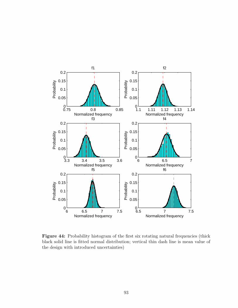
0.75 0.8 0.850
0.05
0.1
0.15
0.2
Normalized frequency
Pro
babi
lity
f1
1.1 1.11 1.12 1.13 1.140
0.05
0.1
0.15
0.2
Normalized frequency
Pro
babi
lity
f2
3.3 3.4 3.5 3.60
0.05
0.1
0.15
0.2
Normalized frequency
Pro
babi
lity
f3
6 6.5 70
0.05
0.1
0.15
0.2
Normalized frequency
Pro
babi
lity
f4
6 6.5 7 7.50
0.05
0.1
0.15
0.2
Normalized frequency
Pro
babi
lity
f5
6.5 7 7.50
0.05
0.1
0.15
0.2
Normalized frequency
Pro
babi
lity
f6
Figure 44: Probability histogram of the first six rotating natural frequencies (thickblack solid line is fitted normal distribution; vertical thin dash line is mean value ofthe design with introduced uncertainties)
93

CHAPTER VI
CONCLUSION AND FUTURE WORK
6.1 Conclusion
This research proposes a modular methodology for composite rotor blade structural
design. The method is applied to study three new aspects of the structural design.
The following conclusions are reached:
1. The proposed method is demonstrated by local cross-section optimization of
rotor blades. Compared with other the traditional design methods, this design
method is more efficient and accurate, and it can be easily plugged into other
multidisciplinary design.
2. The proposed method is applied to solve the structural optimization problem
with manufacturability constraints. This optimization problem is a mixed-
variable problem. To solve such a mixed-variable problem, a hybrid opti-
mization procedure is proposed that utilizes the advantages of both sequential
quadratic programming and genetic algorithm. The test example shows that
the optimal solution improves significantly with 1% less mass per unit length
and 32% less stress level in comparison with the baseline model. The offset
from shear center to aerodynamic center reduced from 4.17% chord of baseline
model to -0.0015% chord of optimal solution. All the stiffnesses are in the target
ranges. The computation cost is about half of the general genetic algorithm.
3. The sensitivity analysis show that shear center and stress level are very sensitive
to the variation of design variables. Moreover, using the cross-section template
without nonstructural mass, both the shear center and the mass center can be
94
moved close to the aerodynamic center without violating current stiffness con-
straints, but the mass center cannot be moved as close as the shear center. The
distance between mass center and aerodynamic center can be further reduced if
another design variable (e.g. a non-structural point mass near the leading edge)
is added.
4. A new design method is proposed for design against fatigue that combined
the above structural design method. The proposed method integrates with
sectional analysis, aeroelastic analysis, rotor trim, and durability analysis. Fa-
tigue life prediction employs the 3D stress recovery from VABS in conjunction
with a strength-based fatigue model. The proposed method is demonstrated
by a three-bladed hingeless-rotor structural design. The optimization mini-
mizes the sectional weight subject to constraints on stiffness, weight, frequency
and fatigue life. The resulting optimal solution meets the durability require-
ment that traditional design method requires multitude design optimization to
satisfy. Preliminary results indicate that this approach is promising for blade
structural design against fatigue failure.
5. The impacts of manufacturing uncertainties, especially the geometry pertur-
bation (the wavy ply and inner surface), are investigated by VABS sectional
properties analysis tool and Monte Carlo simulation. Harmonic functions are
used to model the wavy perturbation. Based on the preliminary results, the
effects of such geometry perturbations depend on the cross-section shape. The
effects on shear center are worse than mass center. The geometry perturbations
have few impacts on stiffness.
6. The combinatorial impacts of manufacturing uncertainties, including dimension,
geometry, and material properties, are investigated by Monte Carlo simulation.
95

Manufacturing uncertainties have significant impacts on the stiffness and aeroe-
lastic behavior of rotor blades. The rotating frequencies are less affected than
the non-rotating frequencies, especially for the flap modes because of centrifu-
gal forces. As the mode the number increases, the impacts of manufacturing
uncertainties become more serious as well.
7. Probabilistic approach is proposed to control the uncertainties. The uncertain-
ties introduced to the design include geometry, material properties, and service
loads. In this approach, the object is to minimize the average the structural
performance subject the constraints of stiffness, frequencies, performance vari-
ation, and reliability. The Monte Carlo simulation and the above structural
design method are combined. The probabilistic approach is also demonstrated
by a three-bladed hingeless-rotor design. The optimal design resulting from
probabilistic approach improves significantly, but not as good as the design
from deterministic approach. In the test example, the coefficient of variation
of stiffness, frequencies, mass per unit length are less than that of the intro-
duced uncertainties. The shear center is significantly affected by manufacturing
uncertainties. In the test example, the coefficient of variation is 85%. With
uncertainties, the shear center can be optimized to 0.01% chord; without un-
certainties, it can only be 0.23% chord.
6.2 Future Work
1. In the current design, the number of layers of composites is fixed, and each layer
has the same layer thickness. That is, the layer thickness is equal to the total
thickness divides by the number of layers. However, because the feasible values
of layer thickness are certain discrete numbers, this assumption possibly results
in the infeasible layer thickness. A better way is to choose layer thickness and
the number of layers as design variables. If the fiber orientations of all layers are
96
dependent design variables, the number of variables of the optimization problem
is changeable. The applicable algorithm for such problem is very difficult to find
in literature.
2. The fatigue life prediction is based on a strength-degradation fatigue model.
This model is easy to incorporate into the proposed structural optimization
procedure. However, the accuracy of this model requires a large number of
fatigue experimental data for various laminates layups. To simplify the fatigue
analysis, the material Young’s modulus is assumed to be constant with only the
strength decreasing. In fact, both the material Young’s modulus and strength
decrease. The former affects the blade sectional properties, and consequently
the blade aeroelastic response. As a result, the sectional, aeroelastic response,
trim and fatigue analysis become fully coupled and extremely challenging from
the computational standpoint. Further research needs to be conducted in order
to justify the validity and relative impact of time-dependent material properties,
and the appropriate corrections need to be made to the model.
3. The investigation of geometry uncertainty impacts ignores the material property
variability around the ply waviness. The geometry uncertainty model need be
calibrated by the realistic manufacturing data. The proposed method need to
be applied to the calibrated model and compared with the measured structural
performance data.
4. In this research, the impacts of manufacturing uncertainties of stiffnesses and
frequencies are investigated. The thorough investigation on aeroelastic response
such as stability needs to be conducted in the future.
5. Fatigue behavior is another important problem of rotor blades. Fatigue be-
haviors are governed by many factors including manufacturing process and im-
perfection. The proposed method of VABS in conjunction with strength-based
97

fatigue model can be used to study the impacts of manufacturing uncertainties
on fatigue behaviors.
98
REFERENCES
[1] “Damage tolerance and fatigue evalution of structure,” Tech. Rep. No. 25.571-1C, FAA Advisory Circular.
[2] “Fatigue of rotorcraft structure,” Tech. Rep. 20-95, FAA Advisory Circular,1995.
[3] “The material properties of commercial pure titanium,” 2004. http://www.
ife.no/media/446\_FactsTiAlloy.pdf.
[4] “Design space report,” 2005. http://www.ansys.com/products/downloads/
report1/report.htm.
[5] Alexander, H. R., Smith, K. E., McVeigh, M. A., Dixon, P. G., andMcManus, B. L., “Preliminary design study of advanced composite blade andhub and nonmechanical control system for the tilt-rotor aircraft,” Tech. Rep.CR-152336-1, NASA, November, 1979.
[6] Arora, J. S., “Computational design optimization: A review of future direc-tions,” Structural Safety, vol. 7, pp. 131–148, 1990.
[7] Arora, J. S. and Wang, Q., “Review of formulations for structural and me-chanical system optimization,” Structural and Multidisciplinary Optimization,vol. 30, no. 4, pp. 251–272, 2005.
[8] Bauchau, O., Bottasso, C., and Nikishkov, Y., “Modeling rotorcraft dy-namics with finite element multibody procedures,” Mathematical and ComputerModeling, vol. 33, pp. 1113–1137, 2001.
[9] Bauchau, O. A., “DYMORE user’s manual,” 2007. http://www.ae.gatech.edu/people/obauchau/.
[10] Berdichevsky, V. L., “Variational-asymptotic method of constructing a the-ory of shells,” Journal of Applied Mathematics and Mechanics (English trans-lation of Prikladnaya Matematika i Mekhanika), vol. 43, no. 4, pp. 664–687,1979.
[11] Bogetti, T. A., Gillespie, Jr., J. W., and Lamontia, M. A., “Influenceof ply waviness on the stiffness and strength reduction on composite laminates,”Journal of Thermoplastic Composite Materials, vol. 5, no. 4, pp. 344 – 369, 1992.
[12] Boggs, P. T. and Tolle, J. W., “Sequential quadratic programming,” ActaNumerica, vol. 4, pp. 1–15, 1996.
99

[13] Bradley, D. J., Adams, D. O., and Gascoigne, H. E., “Interlaminarstrains and compressive strength reductions due to nested layer waviness incomposite laminates,” Journal of Reinforced Plastics and Composites, vol. 17,no. 11, pp. 989–1011, 1998.
[14] Celi, R., “Recent applications of design optimization to rotorcrafta survey,”Journal of Aircraft, vol. 36, no. 1, pp. 176–189, 1999.
[15] Cesnik, C. E. S. and Hodges, D. H., “VABS: A new concept for compos-ite rotor blade cross-sectional modeling,” Journal of the American HelicopterSociety, vol. 42, no. 1, pp. 27–38, 1997.
[16] Cesnik, C. E. S., Mok, J., Parikh, A. S., and Shin, S., “Optimizationdesign framework for integrally twisted helicopter blades,” in Proceedings ofthe 45th AIAA/ASME/ASCE/AHS/ASC Structures, Structural Dynamics andMaterials Conference, vol. 4, (Palm Springs, CA.), pp. 2736–2750, 2004.
[17] Chattopadhyay, A., McCarthy, T., and Pagaldipti, N., “Multileveldecomposition procedure for efficient design optimization of helicopter rotorblades,” AIAA Journal, vol. 33, no. 2, pp. 223–230, 1995.
[18] Coello, C. A., “Theoretical and numerical constraint handling techniquesused with evolutionary algorithms: A survey of the state of the art,” ComputerMethods in Applied Mechanics and Engineering, vol. 191, no. 11-12, pp. 1245–1287, 2002.
[19] Degrieck, J. and Van, P. W., “Fatigue damage modelling of fibre-reinforcedcomposite materials: Review,” Applied Mechanics Reviews, vol. 54, no. 4,pp. 279–300, 2001.
[20] d’Ippolito, R., Donders, S., Hack, M., Tzannetakis, N., Linden,
G. V. D., and Vandepitte, D., “Reliability-based design optimizationof composite and steel aerospace structures,” in Proceedings of the 47thAIAA/ASME/ASCE/AHS/ASC Structures, Structural Dynamics, and Mate-rials Conference, (Newport, RI), May 1-4, 2006. AIAA 2006-2153.
[21] Dovrakand, G.J.and Laws, N., “Analysis of progressive matrix cracking incomposite laminates ii first ply failure,” Journal of Composite Materials, no. 21,pp. 309–329, 1987.
[22] Fanjoy, D. W. and Crossley, W. A., “Using a genetic algorithm for struc-tural topology design of helicopter rotor blades,” in Proceedings of the 42ndAIAA/ASME/ASCE/AHS/ASC Structures, Structural Dynamics and Mate-rials Conference and Exhibit, vol. 5, (Seattle, Washington), pp. 3110–3118,American Inst. Aeronautics and Astronautics Inc., Apr. 16-19, 2001. AIAA2001-1605.
100
[23] Flaggs, D. and Laws, N., “Prediction of tensile matrix failure in compositelaminates,” Journal of Composite Materials, vol. 19, no. 1, pp. 29–50, 1985.
[24] Friedmann, P. P., “Helicoptervibration reduction using structural optimiza-tion with aeroelastic/multidisciplinary constraintsa survey,” Journal of Aircraft,vol. 28, no. 1, pp. 8–21, 1991.
[25] Ganguli, R. and Chopra, I., “Aeroelastic optimization of a helicopter rotorwith two-cell composite blades,” AIAA Journal, vol. 34, no. 4, pp. 835–854,1996.
[26] Ganguli, R., “Survey of recent developments in rotorcraft design optimiza-tion,” Jounal of Aircraft, vol. 41, no. 3, pp. 493–510, 2004.
[27] Garnich, M. R. and Karami, G., “Localized fiber waviness and implica-tions for failure in unidirectional composites,” Journal of Composite Materials,vol. 39, no. 14, pp. 1225–1245, 2005.
[28] Guerdal, Z., Tamasino, A. P., and Biggers, S. B., “Effects of processinginduced defects on laminate response: Interlaminar tensile strength,” SAMPEJournal, vol. 27, pp. 3–49, 1991.
[29] Gurdal, Z., Haftka, R. T., and Hajela, P., Design and Optimization ofLaminated Composite Materials. New York: John Wiley Sons, Inc., 1999.
[30] Hajela, P., “Nongradient methods in multidisciplinary design optimization-status and potential,” Journal of Aircraft, vol. 36, no. 1, pp. 255–265, 1999.
[31] Hale, R. D. and Villa, M., “Influence of opposing wave nesting incompression-loaded composites,” Journal of Composite Materials, vol. 37,no. 13, pp. 1149–1166, 2003.
[32] Haugen, E. B., Probabilistic Mechanical Design. New York: Wiley, 1980. pp.91–188.
[33] Hodges, D. H., Atilgan, A. R., Cesnik, C. E. S., and Fulton, M. V.,“On a simplified strain energy function for geometrically nonlinear behaviour ofanisotropic beams,” Composites Engineering, vol. 2, no. 5-7, pp. 513–526, 1992.
[34] Hodges, D. H., Nonlinear Composite Beam Theory. Reston, Virginia: AIAA,2006. Chapter 4.
[35] Hodges, D., “A review of composite rotor blade modeling,” AIAA Journal,vol. 28, no. 3, pp. 561–565, 1990.
[36] Hoepfer, M., Laurendeau, B., Mishra, S., Shrotri, K., Sirirojvi-
suth, A., Suhr, C. S., Theel, T., Wu, L., and Yang, J., 23rd AHS AnnualStudent Design Competition Report–Rambler. Georgia Institute of Technology,2006.
101

[37] Hogg, R. V., McKean, J. W., and Craig, A. T., Introduction to Mathe-matical Statistics. Upper Saddle River, NJ: Pearson Education, sixth ed., 2004.
[38] Holland, J., Adaptation in Natural and Artificial Systems. Ann Arbor: Uni-versity of Michigan Press, 1975.
[39] Hong, X., Three-Dimensional Strain and Stress Recovery Theory for InitiallyCurved and Twisted Composite Beams. M.S., Georgia Institute of Technology,2001.
[40] Huang, H. and Talreja, R., “Effects of void geometry on elastic properties ofunidirectional fiber reinforced composites,” Composites Science and Technology,vol. 65, no. 13, pp. 1964–1981, 2005.
[41] Hughes, G. W. and McInnes, C. R., “Solar sail hybrid trajectory opti-mization for non-keplerian orbit transfers,” Journal of Guidance, Control, andDynamics, vol. 25, no. 3, pp. 602–604, 2002.
[42] HyperWorks7.0, Altair OptiStruct: Concept Design Using Topology and To-pography Optimization. Altair Engineering, Inc., 2004.
[43] Jen, M.-H. and Lee, C.-H., “Strength and life in thermoplastic compositelaminates under static and fatigue loads. part II: formulation,” InternationalJournal of Fatigue, vol. 20, no. 9, pp. 617–629, 1998.
[44] Johnson, W., Helicopter Theory. New York: Dover publications, Inc., 1994.
[45] Kim, J.-E. and Sarigul-Klijn, N., “Structural optimization forlight-weight articulated rotor blade,” in Proceedings of the 41stAIAA/ASME/ASCE/AHS/ASC Structures, Structural Dynamics, andMaterials Conference, (Atlanta, GA), Apr. 3-6, 2000. AIAA 2000-1520.
[46] Kim, J.-E. and Sarigul-Klijn, N., “Elastic-dynamic rotor blade design withmultiobjective optimization,” AIAA Journal, vol. 39, no. 9, pp. 1652–1661,2001.
[47] Kim, T. K. and Hwang, I. H., “Reliability analysis of composite wing sub-jected to gust loads,” Composite Structures, vol. 66, no. 1-4, pp. 527–531, 2004.
[48] Kottegoda, N. T. and Rosso, R., Statistics, Probability, and Reliability forCivil and Environmental Engineers. McGraw-Hill, 1997.
[49] Ku, J., Hybrid Optimization of Aeromechanical Stability for Rotorcraft withComposite Blades. Ph.D., Georgia Institute of Technology, 2007.
[50] K.W, G. and E., B. J., “Multiple transverse fracture in 90 crossply lami-nates of a glass fibre-reinforced polyester,” Journal of Material Science, no. 12,pp. 157–168, 1977.
102

[51] Land, A. and Doig, A., “An automatic method for solving discrete program-ming problems,” Econometrica, vol. 28, pp. 497–520, 1960.
[52] Lawler, E. and Wood, D., “Branch-and-bound methods: A survey,” opera-tions research, vol. 14, pp. 699–719, 1966.
[53] Lee, J. and Hajela, P., “Parallel genetic algorithm implementation in multi-disciplinary rotor blade design,” Journal of Aircraft, vol. 33, no. 5, pp. 962–969,1996.
[54] Lemanski, S. L., Weaver, P. M., and Hill, G. F. J., “Design of compositehelicopter rotor blades to meet given cross-sectional properties,” AeronauticalJournal, vol. 109, no. 1100, pp. 471–475, 2005.
[55] Li, J., “Flange delamination prediction in composite structures with ply wavi-ness,” AIAA Journal, vol. 38, no. 5, pp. 893–897, 2000.
[56] Li, L., Volovoi, V. V., and Hodges, D. H., “Cross-sectional design ofcomposite rotor blades considering manufacturing constraints,” in Proceedingsof the 63rd Annual Forum of the American Helicopter Society, (Virginia Beach,Virginia), 2007.
[57] Lian, Y. and Kim, N.-H., “Reliability-based design optimization of a tran-sonic compressor,” in Proceedings of the 41st AIAA/ASME/SAE/ASEE JointPropulsion Conference and Exhibit, (Tucson, Arizona), Jul. 10-13, 2005. AIAA2005-4021.
[58] Lindsley, N. J., Beran, P. S., and Pettit, C. L., “Effects of uncer-tainty on nonlinear plate aeroelastic response,” in Proceedings of the 43rdAIAA/ASME/ASCE/AHS/ASC Structures, Structural Dynamics, and Mate-rials Conference, (Denver, Colorado), Apr. 22-25, 2002. AIAA 2002-1271.
[59] Liu, B. and Lessard, L. B., “Fatigue and damage-tolerance analysis of com-posite laminates: Stiffness loss, damage-modelling, and life prediction,” Com-posites Science and Technology, vol. 51, pp. 43–51, 1994.
[60] Luo, Y.-Z., Tang, G.-J., Wang, Z.-G., and Li, H.-Y., “Optimization ofperturbed and constrained fuel-optimal impulsive rendezvous using a hybridapproach,” Engineering Optimization, vol. 38, no. 8, pp. 959–973, 2006.
[61] Melchers, R. E., Structural Reliability Analysis and Prediction. John Wileyand Sons, Inc., second ed., 1999. Chapter 3 and 5.
[62] Miura, H., “Applications of numerical optimization methods to helicopterdesign problemsa survey,” Vertica, vol. 9, no. 2, pp. 141–154, 1985.
[63] Murugan, S., Ganguli, R., and Harursampath, D., “Aeroelastic responseof composite helicopter rotor with random material properties,” Journal of Air-craft, vol. 45, no. 1, pp. 306–322, 2008.
103

[64] Orr, S. A. and Hajela, P., “A comprehensive model for multi-disciplinary design of a tiltrotor configuration,” in Proceedings of the 46thAIAA/ASME/ASCE/AHS/ASC Structures, Structural Dynamics, and Mate-rials Conference, (Austin, Texas), Apr. 18 - 21, 2005. AIAA 2005-2284.
[65] Ozbay, S., Extension-twist Coupling Optimization in Composite Rotor Blades.Ph.D., Georgia Institute of Technology, 2006.
[66] Paepegem, W. V. and Degrieck, J., “Modelling damage and permanentstrain in fibre-reinforced composites under in-plane fatigue loading,” CompositesScience and Technology, vol. 63, no. 5, pp. 677–694, 2003.
[67] Paik, J., Volovoi, V. V., and Hodges, D. H., “Cross-sectional siz-ing and optimization of composite blades,” in Proceedings of the 43rdAIAA/ASME/ASCE/AHS/ASC Structures, Structural Dynamics, and Mate-rials Conference, (Denver, Colorado), pp. 601–610, Apr. 22-25, 2002. AIAA2002-1322.
[68] Patil, M. J. and Johnson, E. R., “Cross-sectional analysis of anisotropic,thin-walled, closed-section beams with embedded strain actuation,” in Proceed-ings of the 46th AIAA/ASME/ASCE/AHS/ASC Structures, Structural Dy-namics and Materials Conference, (Austin, Texas), Apr. 18-21, 2005. AIAA2005-2037.
[69] Peters, D. and Barwey, D., “A general theory of rotorcraft trim,” in Pro-ceedings of the 36th AIAA/ASME/ASCE/AHS/ASC Structures, Structural Dy-namics, and Materials Conference and AIAA/ASME Adaptive Structures Fo-rum, (New Orleans, LA), pp. 2558–2590, 1995.
[70] Peters, D. and He., C., “Finite state induced flow models. part II: Three-dimensional rotor disk,” Journal of Aircraft, vol. 32, no. 2, pp. 323–333, 1995.
[71] Peters, D., Karunamoorthy, S., and Cao, W., “Finite state induced flowmodels. part I: Two dimensional thin airfoil,” Journal of Aircraft, vol. 32, no. 2,p. 313322, 1995.
[72] Pettit, C. L., “Uncertainty quantification in aeroelasticity: Recent resultsand research challenges,” Journal of Aircraft, vol. 41, no. 5, pp. 1217–1229,2004.
[73] Pettit, C. L. and Beran, P. S., “Effects of parametric uncertainty on airfoillimit cycle oscillation,” Journal of Aircraft, vol. 40, no. 5, pp. 1004–1006, 2003.
[74] Piatak, D. J., Nixon, M. W., and Kosmatka, J. B., “Stiffness character-istics of composite rotor blades with elastic couplings,” Tech. Rep. TP-3641,NASA, 1997.
[75] Piegl, L. and Tiller, W., The Nurbs Book. Berlin, New Jersey: Springer-Verlag, 2nd ed., 1997.
104

[76] Piggott, M., “The effect of fiber waviness on the mechanical properties ofunidirectional fiber composites – a review,” Composites Science Technology,vol. 53, pp. 201–205, 1995.
[77] Pradlwarter, H. J., Pellissetti, M. F., Schenk, C. A., Schuller,
G. I., Kreis, A., Fransen, S., Calvi, A., and Klein, M., “Realistic andefficient reliability estimation for aerospace structures,” Computer Methods inApplied Mechanics and Engineering, vol. 194, no. 12-16, pp. 1597–1617, 2005.
[78] Rais-Rohani, M. and Xie, Q., “Probabilistic structural optimization underreliability, manufacturability, and cost constraints,” AIAA Journal, vol. 43,no. 4, pp. 864–873, 2005.
[79] Reifsnider, K. L. and Case, S. W., Damage Tolerance and Durability ofMaterial Systems. New York: John Wiley & Sons, Inc., 2002.
[80] Rosen, J. B., “The gradient projection method for nonlinear programming,part one,” Journal SIAM, vol. 8, pp. 181–217, 1960.
[81] Rozvany, G., Topology Optimization in Structural Mechanics. New York:Springer, 1997.
[82] Schaff, J. R. and Davidson, B., “Life prediction methodology for compositestructures. part I - constant amplitude and two-stress level fatigue,” Journal ofComposite Materials, vol. 31, no. 2, 1997.
[83] Schaff, J. R. and Davidson, B., “Life prediction methodology for compositestructures. part II - spectrum fatigue,” Journal of Composite Materials, vol. 31,no. 2, 1997.
[84] Schaff, J. R., “Fatigue analysis of helicopter tail rotor spar,” in 39thAIAA/ASME/ASCE/ASC Structures, Structural Dynamics, and MaterialsConference, (Long Beach, CA), 1998.
[85] Smith, E. and Chopra, I., “Formulation and evaluation of an analyticalmodel for composite box beams,” Journal of the American Helicopter Society,vol. 36, no. 3, pp. 23–35, 1991.
[86] Sobieszczanski-Sobieski, J. and Haftka, R., “Multidisciplinary aerospacedesign optimization: Survey of recent developments,” in Proceedings of the 34thAerospace Sciences Meeting and Exhibit, (Reno, NV.), Jan.,, 1996. AIAA 96-0711.
[87] Soykasap, O., Aeroelastic Optimization of a Composite Tilt Rotor. Ph.D.,Georgia Institute of Technology, 1999.
105

[88] Talreja, R., “Effects of manufacturing induced defects on composite damageand failure,” in Proceedings of the 27th Riso International Symposium on Ma-terials Science: Polymer Composite Materials for Wind Power Turbine (Lil-
holt, H., Madsen, B., Andersen, T., Mikkelsen, L., and Thygesen,
A., eds.), (Roskilde, Denmark), Sep. 11-17, 2006.
[89] Tan, S. and Nuismer, R., “A theory for progressive matrix cracking in com-posite laminates,” Journal of Composite Materials, vol. 23, no. 10, pp. 1029–1047, 1989.
[90] Thomsen, O. T., “Sandwich materials for wind turbine blades,” in Proceed-ings of the 27th Riso International Symposium on Materials Science: PolymerComposite Materials for Wind Power Turbine (Lilholt, H., Madsen, B.,Andersen, T., Mikkelsen, L., and Thygesen, A., eds.), (Roskilde, Den-mark), Sep. 11–17, 2006.
[91] Trosset, M. W., “What is simulated annealing?,” Optimization and Engi-neering, vol. 2, no. 2, pp. 201–213, 2001.
[92] Tsai, S. W., Composites Design. Think composites, 3rd ed., 1987.
[93] Vallons, K., Zong, M., Lomov, S. V., and Verpoest, I., “Carbon com-posites based on multi-axial multi-ply stitched preforms - part 6. fatigue be-haviour at low loads: Stiffness degradation and damage development,” Compos-ites Part A: Applied Science and Manufacturing, vol. 38, no. 7, pp. 1633–1645,2007.
[94] VanderPlaats, G. N., Numerical Optimization Techniques for EngineeringDesign. Colorado Spring, Co.: Vanderplaats Research & Development, Inc.,4th ed., 2005. Chapter 9.
[95] Volovoi, V. V. and Hodges, D. H., “Theory of anisotropic thin-walledbeams,” Journal of Applied Mechanics, vol. 67, no. 3, pp. 453–459, 2000.
[96] Volovoi, V. V., Hodges, D. H., Cesnik, C. E. S., and Popescu, B.,“Assessment of beam modeling methods for rotor blade applications,” Mathe-matical and Computer Modelling, vol. 33, no. 10-11, pp. 1099–1112, 2001.
[97] Volovoi, V. V., Ku, J., and Hodges, D. H., “Coupling global and local as-pects of cross-sectional optimization for rotor blades,” in Proceedings of the 47thAIAA/ASME/ASCE/AHS/ASC Structures, Structural Dynamics and Materi-als Conference, vol. 4, (Newport, RI), pp. 2808–2821, American Inst. Aeronau-tics and Astronautics Inc., Reston, VA 20191-4344, United States, 2006.
[98] Volovoi, V. V., Li, L., Ku, J., and Hodges, D. H., “Multi-level struc-tural optimization of composite rotor blades,” in Proceedings of the 46thAIAA/ASME/ASCE/AHS/ASC Structures, Structural Dynamics, and Mate-rials Conference, (Austin, Texas), Apr. 18–21, 2005.
106

[99] Volovoi, V. V., Yoon, S., Lee, C.-Y., and Hodges, D. H., “Struc-tural optimization of composite rotor blades,” in Proceedings of the 45thAIAA/ASME/ASCE/AHS/ASC Structures, Structural Dynamics, and Mate-rials Conference, (Palm Springs, California), Apr. 19-22, 2004.
[100] Walsh, J. L., Young, K. C., Pritchard, J. I., Adelman, H. M., andMantay, W. R., “Integrated aerodynamic/dynamic/structural optimizationof helicopter rotor blades using multilevel decomposition,” Tech. Rep. 3465,NASA, Jan., 1995.
[101] Worndle, R., “Calculation of the cross section properties and the shearstresses of composite rotor blades,” Vertica, vol. 6, pp. 111–129, 1982.
[102] Wu, C. F. J. and Hamada, M., Experiments: Planning, Analysis, and Pa-rameter Design Optimization. New York: John Wiley & Sons, Inc., 2000.
[103] Yadav, D. and Verma, N., “Buckling of composite circular cylindrical shellswith random material properties,” Composite Structures, vol. 37, no. 3-4,pp. 385–391, 1997.
[104] Yu, W., Variational Asymptotic Modeling of Composite Dimensionally Re-ducible Structures. Ph.D., Georgia Institute of Technology, 2002.
[105] Yu, W., Hodges, D. H., Volovoi, V. V., and Cesnik, C. E. S., “Ontimoshenko-like modeling of initially curved and twisted composite beams,”International Journal of Solids and Structures, vol. 39, no. 19, pp. 5101–5121,2002.
[106] Yu, W., Hodges, D. H., Volovoi, V. V., and Hong, x., “Validation ofthe variational asymptotic beam sectional analysis (VABS),” AIAA Journal,vol. 40, no. 10, pp. 2105–2112, 2002.
[107] Yuan, K.-A. and Friedmann, P. P., “Aeroelasticity and structural opti-mization of composite helicopter rotor blades with swept tips,” Tech. Rep. CR4665, NASA, May, 1995.
107