Structural Breaks in Fiscal Performance: Did Fiscal Responsibility Laws Have

Anything to Do with Them?

Carlos Caceres, Ana Corbacho, and Leandro Medina

WP/10/248

© 2010 International Monetary Fund WP/10/248 IMF Working Paper Fiscal Affairs Department

Structural Breaks in Fiscal Performance: Did Fiscal Responsibility Laws Have Anything to Do with Them?

Prepared by Carlos Caceres, Ana Corbacho, and Leandro Medina

Authorized for distribution by Gerd Schwartz

November 2010

Abstract

This Working Paper should not be reported as representing the views of the IMF. The views expressed in this Working Paper are those of the author(s) and do not necessarily represent those of the IMF or IMF policy. Working Papers describe research in progress by the author(s) and are published to elicit comments and to further debate.

In recent years, many countries have adopted Fiscal Responsibility Laws to strengthen fiscal institutions and promote fiscal discipline in a credible, predictable and transparent manner. Still, results on the effectiveness of these laws remain tentative. In this paper, we test empirically whether fiscal performance, measured as the level of primary fiscal balances and their volatility, indeed improved after the implementation of Fiscal Responsibility Laws in a sample of Latin American and advanced economies. We show that traditional econometric approaches, which rely on the use of dummies in time series or panel regressions, yield biased estimates. In contrast, our empirical strategy recognizes that, a priori, the timing of the effect of these laws on fiscal performance is unknown, while controlling for the impact of the business and commodity cycles on fiscal outcomes. Overall, we find limited empirical evidence in support of the view that Fiscal Responsibility Laws have had a distinguishable effect on fiscal performance. However, Fiscal Responsibility Laws could still have other positive effects on the conduct of fiscal policy not analyzed here, for instance, through enhanced transparency and guidance in the budget process and lower risk premia. JEL Classification Numbers: C50, E02, E62, E65, H60 Keywords: Fiscal Responsibility Laws, Fiscal Institutions, Fiscal Performance. Author’s E-Mail Address: ccaceres@imf.org; acorbacho@iadb.org; lmedina@imf.org

2

Contents

Introduction ................................................................................................................................3

I. Testing for Structural Breaks ..................................................................................................5

II. Econometric Specification and Data .....................................................................................6

III. Results ..................................................................................................................................7 A. Traditional Approach: Regression Analysis using FRL Dummies ...........................7 B. Alternative Approach I: Testing for Breaks in the Level and Volatility of Fiscal Balances .........................................................................................................................8 C. Alternative Approach II: Markov Switching Model .................................................9

IV. Conclusions........................................................................................................................10 Annexes 1. Inconsistent Estimation of Dummy Variable Models in the Presence of Structural Breaks20 2. Markov Switching Model ....................................................................................................22 3. Data .....................................................................................................................................24

References ................................................................................................................................25

3

INTRODUCTION

Fiscal Responsibility Laws (FRLs) are becoming increasingly popular. FRLs have been enacted in many countries as permanent institutional devices to enhance the credibility, predictability, and transparency of fiscal policy. FRLs generally combine procedural rules to strengthen fiscal transparency and budget management, with numerical fiscal rules such as ceilings on fiscal deficits and public debt to impose fiscal discipline.1 In contrast to stand-alone fiscal rules, FRLs aim to provide a comprehensive framework to govern fiscal policy in a single piece of legislation. New Zealand was at the forefront of these reforms, adopting an FRL in 1994 with a strong emphasis on transparency requirements. Since then, FRLs have been implemented in several countries in Latin America, Europe, and Asia. However, changes in fiscal performance following the adoption of an FRL remain to be documented and analyzed systematically. It is widely accepted that the strength of fiscal institutions matters for fiscal performance. For instance, several studies support the notion that the quality of budget procedures and the presence of binding constraints on the size of fiscal deficits and debt are generally associated with better fiscal outcomes.2 However, while the literature on stand-alone fiscal rules or fiscal institutions more generally is vast, the evidence on FRLs thus far remains partial. In some countries, FRLs seem to have signaled a regime change towards fiscal responsibility. In other countries, fiscal performance has not shown meaningful improvement, also due to implementation problems.3 This paper studies whether FRLs can be linked to structural breaks in both the level and volatility of fiscal balances in a broad sample of countries. When analyzing the effect of a particular policy on fiscal performance, most researchers have been concerned with changes in the level of fiscal balances. However, fiscal volatility is widely perceived as detrimental to economic growth and welfare.4 Often, FRLs are offered as a potential solution to reduce

1 In this sense, FRLs are different than stand-alone numerical fiscal rules, which are defined as a permanent constraint on fiscal policy through simple numerical limits on budgetary aggregates (Kopits and Symansky, 1998). FRLs can be classified according to several characteristics, including the emphasis placed on procedural versus numerical fiscal rules, the jurisdictional coverage (e.g., central versus federal government), sanctions, escape clauses, and cyclical considerations. See Corbacho and Schwartz (2007) for a survey on FRLs. 2 For Latin America, examples include Alesina et al. (1999), Stein et al. (1999), and Filc and Scartascini (2005). For Europe, see for instance Von Hagen and Harden (1995), Gleigh (2003) and Hallerberg et al. (2007). Alt and Lowry (1994), Poterba (1994), and Bohn and Inmann (1996) concentrate on the US states. Kumar et al. (2009) provides a review of fiscal rules worldwide. 3 Thornton (2009) is one of few studies that estimate the effect of FRLs on fiscal performance. He concludes that FRLs have not contributed to improvements in fiscal outcomes. The empirical approach relies on “differences-in-differences” estimation and assumes an arbitrary “treatment date” for the control group in the sample. As discussed in this paper, the correct selection of break dates is critical to avoid estimation bias. 4 For instance, using cross-country data, Ramey and Ramey (1995) find that government-spending volatility has a negative impact on growth. Fatas and Mihov (2003, 2005) similarly conclude that the

(continued…)

4

fiscal volatility.5 This paper investigates whether FRLs can be associated with an improvement in primary fiscal balances and a decline in fiscal volatility in a wide-ranging sample of countries, including Argentina, Australia, Brazil, Colombia, Ecuador, New Zealand, Peru, and the United Kingdom. The empirical model controls for the effect of business and commodity cycles to capture changes in fiscal performance beyond those explained by economic conditions. The paper does not look into other potential beneficial effects of FRLs, such as increased accountability, transparency, and quality of fiscal policies. We use consistent tests for structural breaks that recognize the uncertainty inherent in the timing of the potential impact of an FRL on fiscal performance. Traditional econometric approaches present serious limitations when used to establish changes in fiscal performance before and after the adoption of a structural fiscal reform, such as an FRL. A particular challenge is determining the appropriate timing of the structural break. FRLs have often been preceded, accompanied, or followed by complementary reforms. When should one expect an impact from an FRL? When it was passed by the legislature, when it was legally implemented, or some time before or after? Uncertainty in the timing of the effect renders traditional tests for structural breaks biased, and the direction of the bias is unknown. Following the recent literature, the paper applies two techniques that take into consideration that the timing of the break is unknown: (i) the Quandt-Andrews approach to the consistent and sequential estimation of structural breaks; and (ii) Markov Switching models. We find significant breaks in fiscal performance in several countries, but in most cases these preceded the adoption of the FRL. For example, we find that fiscal volatility indeed declined in most countries, at least for some period of time. However, only in New Zealand this improvement coincided with the introduction of the FRL, while, in most countries, the breaks occurred much earlier. Similarly, only in Australia the FRL introduction corresponded exactly to a structural break in the level of primary fiscal balances. For various other countries (e.g. Brazil, Colombia, and the United Kingdom), the structural break occurred sometime before the introduction of the FRL. Overall, the evidence suggests that it is difficult to link improvements in fiscal performance to the adoption of an FRL. In fact, FRLs seem to have been introduced once the strengthening of fiscal discipline was already underway.6 This likely reflects political commitment to fiscal prudence, which may have prompted and supported structural reforms, including the introduction of an FRL.

volatility of fiscal policy has a direct and negative impact on long-term economic performance. De Ferranti et al. (2000) attribute one third of macro volatility in Latin America to fiscal and monetary policy volatility.

5 Perry (2004) looks at the particular case of fiscal rules. His paper brings to light the fact that policies may have an indirect effect on macroeconomic outcomes through a reduction in volatility, rather than a more direct effect such as changes in level or trend output. For US states, Fatas and Mihov (2006) suggest that strict budgetary restrictions lead to lower policy as well as macroeconomic volatility. 6 This is in line with Kumar et al. (2009), where authors conclude that fiscal rules are often introduced to lock-in earlier consolidation efforts rather than at the beginning of fiscal adjustment processes. In a similar vein, Ter-Minassian (2010) and Marcel (2010) suggest that fiscal rules may strengthen fiscal discipline in countries that have already shown a previous trajectory of fiscal responsibility.

(continued…)

5

The paper is organized as follows. Section II first describes the traditional approaches to estimating and testing for structural breaks and their drawbacks, and then presents alternative approaches that take into consideration that the timing of these breaks may be unknown. Section III discusses the econometric model and data used in the paper. Section IV presents the results both from the traditional approaches and the two alternative approaches, namely, the consistent and sequential estimation of structural breaks, and the estimation of regimes changes based on Markov switching models. Section V concludes.

I. TESTING FOR STRUCTURAL BREAKS

The theoretical interest in structural breaks has a long history. The Chow (1960) break test and derivatives are well known and established tools used for testing for structural breaks. However, the Chow break test is not suitable when the timing of these breaks is unknown. When the break date is not known a priori, the chi-square critical values used in the standard Chow test are inappropriate.7 Traditional econometric approaches present important limitations when testing for the impact of the adoption of an FRL on fiscal outcomes. In time series analysis, a break in a particular series is usually tested by using a dummy that captures a change before and after a particular event. For the purpose of the current analysis, a simple dummy representing the FRL could be used to assess changes in fiscal outcomes for specific countries. However, this approach may yield inconsistent results. The problem becomes more acute when the time series has one or more structural breaks, which could be completely unrelated to the FRL. If a structural break is present in the series, the dummy will, in most cases, try to control or account for this break, irrespective of whether the true break occurred at the date specified by the dummy. Therefore, the sign and magnitude of the dummy coefficient will vary depending on the number, magnitude, and direction of the structural breaks. In other words, the FRL dummy may in reality be capturing the effect of breaks in the series and not the effect of an FRL on fiscal outcomes, even when both events occur at distinct points in time (Annex 1). These problems persist when estimating panel data models, which are commonly used in the literature on fiscal institutions and reforms. This paper presents techniques that can be used for the consistent estimation of structural breaks when the timing of the break is unknown. One option is to evaluate the Chow statistic for all possible observations.8 Then, the candidate for the break date estimate is the date that

7 For volatility breaks, Andrews (1993) and Andrews and Ploberger (1994) provide tables of critical values, and Hansen (1997) provides a method to calculate the correct p-values. 8 See Andrews (1993) and Hansen (1997, 2001). In fact, not every possible date in the sample can be considered as a candidate break date. It is assumed that the break date cannot occur at the very beginning or at the very end of the sample. It is up to the researcher to impose criteria on what percentage of the sample should be excluded. As a rule of thumb, it is common practice in the literature to impose that every break should be at least 15 percent of the sample size apart from each other and from the sample limits. We also conducted the analysis imposing a distance of 10 percent of

(continued…)

6

yields the largest value of the Chow test sequence. In this paper, we present results using the Quandt-Andrews approach, which is based on a sequential application of the Chow break test.9 To test the robustness of the Quandt-Andrews results, we also estimate a Markov Switching model to determine the presence of breaks or, more generally, regime shifts. The Markov Switching model allows for simultaneous changes in the level and variance of fiscal outcomes and estimates the transition probability to different regimes.

II. ECONOMETRIC SPECIFICATION AND DATA

The econometric model focuses on the conditional mean and variance of the primary fiscal balance controlling for the economic and commodity cycles. The conditional mean of the primary fiscal balance is given by equation [1]. The dependent variable, Surplus, is the primary balance in percent of GDP; Gap refers to the output gap, that is the percentage deviation of real GDP from potential GDP;10 u is an i.i.d. disturbance; and subscript ‘t’ is the time index. Given that most countries in the sample are intensive commodity exporters, the regressions also control for a country specific commodity price index ICP.11 With this specification, we aim to capture the potential change in fiscal performance following an FRL beyond what could be explained by the effect of economic conditions.12

TtforuGapaICPaaSurplus tttt ,...,1210 [1]

Quarterly data are used in the analysis.13 High frequency data are required when estimating volatility breaks. High frequency data also improve the consistency of the estimators while

the sample size between breaks and obtained essentially the same results, suggesting the 15 percent mark is not binding. 9 A second possibility is to split the sample at each possible break date and estimate all other parameters using ordinary least squares. The candidate break date estimate is the date that minimizes the entire sample sum of squared residuals. Chong (1995) proves that despite the presence of multiple breaks, a single change point estimator would converge to one of the true change points, instead of a weighted average of them. This enables sequential estimation of all the breaks. 10 Potential GDP was estimated using a Hodrick-Prescott (HP) filter. The adjustment of the sensitivity of the trend to short-term fluctuations is achieved by modifying the multiplier Lambda. As is standard in the literature that uses quarterly data, we set the parameter Lambda equal to1600. 11 For details on this variable and the rest of the dataset see Annex 3 and Medina (2010). The log index of commodity prices was standardized, by taking a z-score transformation, so that the mean over the entire sample period is equal to zero. 12 See for instance Alesina et al. (2008), Gavin and Perotti (1997), Kaminsky et al. (2005), Talvi and Végh (2005), and Ilzetzki and Végh (2008) on the procyclicality of fiscal policy in developing countries. 13 Both the commodity price index and the output gap enter as contemporaneous variables in equation [1], which could give rise to endogeneity concerns. However, commodity prices tend to be determined globally and are thus not affected by fiscal balances of a given country. Budget deficits do tend to have an effect on the output gap. But this effect is unlikely to take place within one single

(continued…)

7

keeping the period of study constant. The countries in the sample are Argentina, Australia, Brazil, Colombia, Ecuador, New Zealand, Peru, and the United Kingdom (Table 1). In addition, we analyze a total of twelve different FRLs (two for Argentina, Colombia, Ecuador, and Peru, where the more recent FRLs incorporated important revisions). Given data limitations, most of the series are for the central government, except in Brazil, where the data cover the consolidated public sector, and New Zealand and the United Kingdom, where data cover the general government. In the case of New Zealand, we use the overall fiscal balance instead of the primary balance due to data constraints.14

III. RESULTS

This section presents the empirical results. First, we show the results using a traditional time series approach with an FRL dummy. Second, we discuss the findings under the Quandt-Andrews approach and Markov Switching models.

A. Traditional Approach: Regression Analysis using FRL Dummies

The traditional approach suggests that FRLs had a positive effect on fiscal balances in about half of the countries, but weakened fiscal performance in a few cases. Table 2 presents the results using a dummy for the FRL. A positive sign for the dummy coefficient indicates that the FRL had a positive effect on fiscal outcomes, with higher primary fiscal balances after the adoption of the FRL. In Australia, Brazil, Colombia, and New Zealand the FRL dummy is statistically significant and positive. The coefficients suggest that the effects are sizable from a macroeconomic point of view, with, in some cases, primary fiscal balances increasing by several percentage points of GDP following the introduction of an FRL. In Argentina and the United Kingdom, the FRL dummy is not statistically significant. And in Ecuador and Peru, the first FRLs seem to have weakened fiscal balances. As shown in the following subsections, these findings are misleading. In reality, the FRL dummy is capturing irregularities in the primary surplus series. The simple Chow break test is not a useful tool for detecting breaks around the FRL approval dates. If breaks are suspected to be a major source of problems when using FRL dummies, one could try to detect whether these breaks are indeed statistically significant. Table 3 reports Chow break tests around the FRL dates. The results suggest that the FRL coincided with a structural break in fiscal balances in all countries, except in Argentina. But as explained before, a Chow break test does not provide statistically valid results when using an

quarter. The precise timing depends on the nature of the change in the fiscal balance. In general, tax changes have the most immediate effect on output, but still with a lag of more than one quarter.

14 Furthermore, data on the overall balance on an accrual basis are available for an annual frequency only. The quarterly series were constructed using linear interpolation. When using annual data, the Markov Switching model yields similar patterns, but volatility breaks using the Quandt-Andrews approach appear earlier than when using quarterly data. However, the limited number of degrees of freedom reduces the robustness of these results.

8

arbitrary break date. When using the Quandt-Andrews approach, we find that most series indeed contain structural breaks. With a few exceptions, these do not coincide with the FRLs.

B. Alternative Approach I: Testing for Breaks in the Level and Volatility of Fiscal Balances

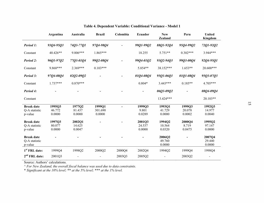
This section discusses the findings from the sequential estimation of structural breaks using the Quandt-Andrews approach. Table 4 presents the results on volatility breaks using model 1 represented by equations [2] and [3] below. In this model, we estimate the conditional mean of the primary fiscal balance as in equation [1] to obtain the least squares residuals ût. Then, the residuals squared, ût

2, are used as a volatility measure in a secondary regression represented by equation [3], which allows a volatility break to occur at time t0. Once a significant break is found, the process is repeated in each of the resulting sub-samples. This enables the sequential estimation of all breaks in fiscal volatility.

TtforuGapaICPaaSurplus tttt ,...,1210 [2]

tt ettIcttIcu )()(ˆ 02012 [3]

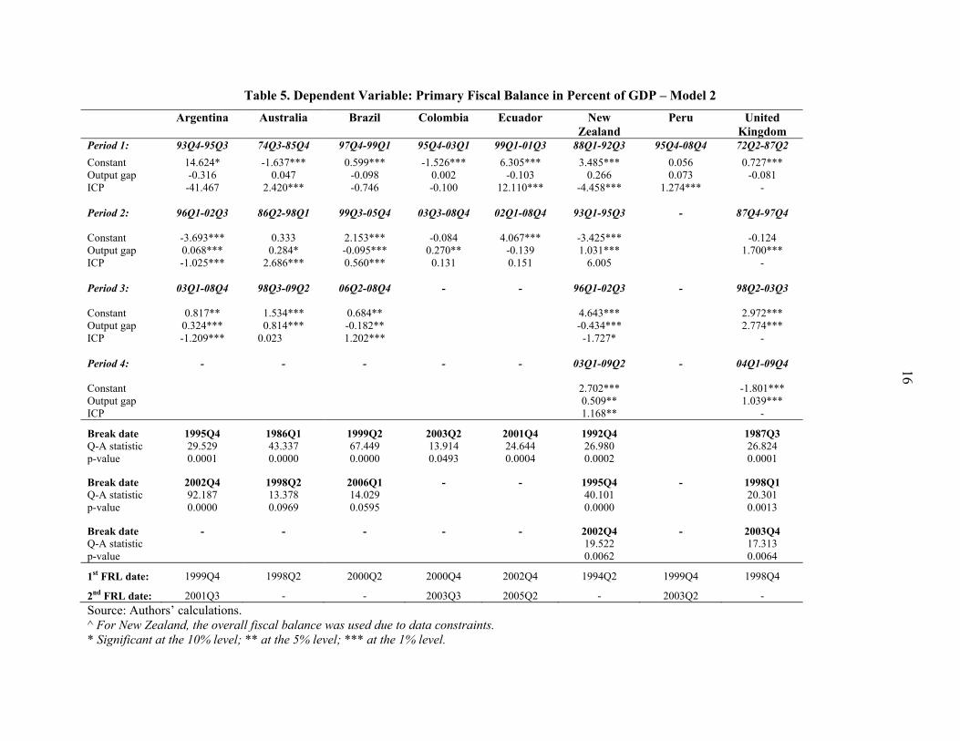
Significant breaks in fiscal volatility are found in most countries, but they generally do not coincide with the introduction of an FRL. In some countries (e.g. New Zealand, Peru and the United Kingdom) volatility initially increased following the first structural break, but then fell again after the second break (Table 4). In other countries (e.g. Argentina, Australia, and Ecuador) volatility has been continuously decreasing after each break. No change in fiscal volatility is found in Colombia. In most countries, volatility breaks precede the FRL dates. An exception is New Zealand, where a volatility break is detected in 1994Q2, which corresponds to the adoption date of the FRL. Overall, these results do not support the idea the FRLs have been generally associated with a reduction in fiscal volatility—that is, that they have made fiscal policy more predictable. Similar conclusions are drawn from looking at primary fiscal balances. Table 5 presents the structural breaks in the conditional mean of the primary fiscal balance based on model 2. This second model is represented by equations [4] and [5] below, and it allows for breaks in the conditional mean of the primary fiscal balance to occur at time t1. Some of the volatility breaks found using model 1 could be due to the presence of structural breaks in the primary regression. Thus model 2 takes these into account. The new residuals vt are obtained from the primary regression [4]. The squares of these residuals are subsequently used in the secondary regression (represented by equation [5]) to test for volatility breaks.

tttttt vttIGapbICPbbttIGapaICPaaSurplus )().()().( 12101210 [4]

tt ettIcttIcv )()( 02012 [5]

9

As suspected, several countries in the sample also exhibit at least one structural break in the primary fiscal balance. This strengthens the concern that the FRL dummy coefficients would be misleading, as these dummies may in fact be capturing the effects of structural breaks in the fiscal balance series, rather than the real effect (if any) of FRLs on fiscal outcomes. In most countries, the breaks in primary fiscal balances do not coincide with the timing of the FRL. Australia is the only case where the structural break coincides exactly with the FRL adoption date, and in Colombia the break occurs just one quarter before. In Brazil and the United Kingdom, the breaks precede the introduction of the FRL by a few quarters. In these countries, the FRLs seem to have accompanied a consolidation process that was already in place before the adoption of these laws.15 Overall, these results differ from those obtained using the traditional time series approach. The results from the traditional approach suggested that in about half of the countries in the sample primary fiscal balances were significantly higher post-FRL, both in a statistical and in an economic sense. However, the Quandt-Andrews results confirm that breaks in the level and variance of the primary fiscal balance generally preceded the introduction of the FRL.16 In some cases (e.g., Australia, Colombia, and New Zealand), the timing is reasonably close, and the adoption of the FRL seems to have coincided with a relative improvement in the fiscal outcomes in subsequent periods. But in most other countries, it would be difficult to link the breaks in fiscal performance to the FRL, as these breaks occurred years apart from the adoption of the law.

C. Alternative Approach II: Markov Switching Model

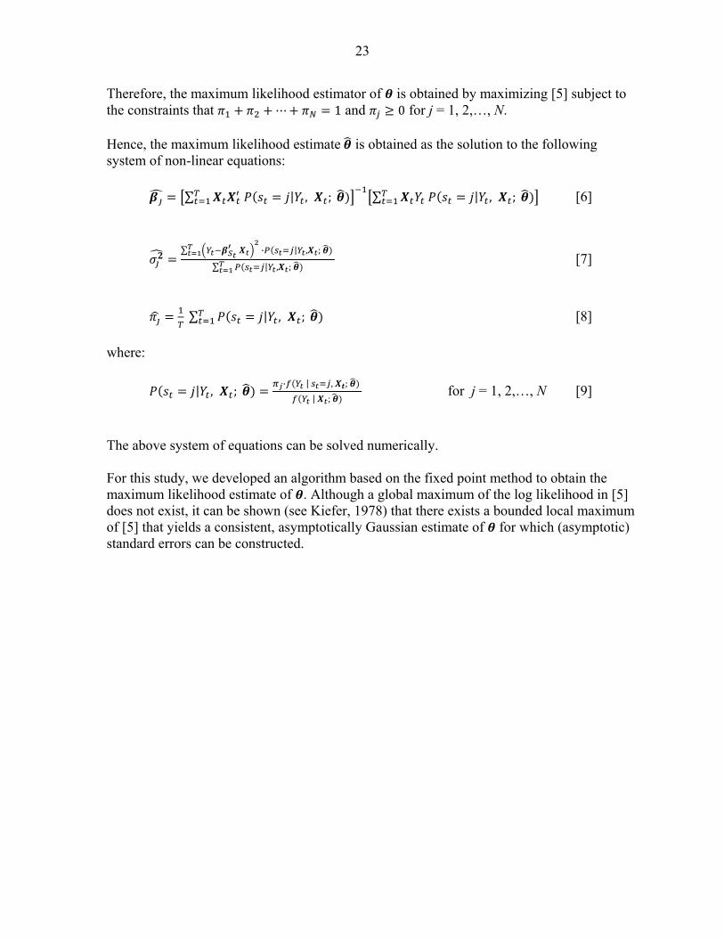
To test the robustness of the Quandt-Andrews results, we estimated a Markov Switching model to determine the presence of breaks or, more generally, regime shifts. Markov Switching models present several advantages. First, they allow for the estimation of structural breaks in the conditional mean and variance simultaneously.17 Second, one of the major limitations of the Quandt-Andrews approach is that the sub-samples between structural breaks require sufficient degrees of freedom, and hence a minimum number of data points. The Markov Switching model, instead, can handle structural breaks that occur at two successive data points. Finally, the Markov switching model assigns a given probability to a particular regime at every point in time, while the Quandt-Andrews approach assigns a probability one to a given regime for a given interval of time. An estimate of the probability of being in a certain regime (at every point in time) is also provided by this methodology.

15 The results on volatility breaks using model 2 were consistent with those using model 1, and are omitted for presentational purposes. 16 In the case of Peru, the traditional approach suggested that primary fiscal balances were lower after the first FRL. However, the Quandt-Andrews approach did not find any structural break in the primary fiscal balance, only in its volatility. 17 For instance in model 2, we use the Quandt-Andrews methodology to estimate breaks in the conditional mean. Once these breaks were identified, and the corresponding residuals from the model obtained, we applied the Quandt-Andrews test to estimate the breaks in volatility. The Markov switching model performs both steps simultaneously.

10

The model can be expressed as:

Surplust = a0St + a1St ICPt + a2St Gapt + чt [6]

st is a state variable which takes N different values (denoting N different regimes), and чt is a random error, normally distributed with mean zero and variance Ωst, which also depends on the regime. It is assumed that the probability that st equals some particular value j depends on the past only through the most recent value st-1:

18

ijttttt pisjsPksisjsP )|(,...),|( 121 [7]

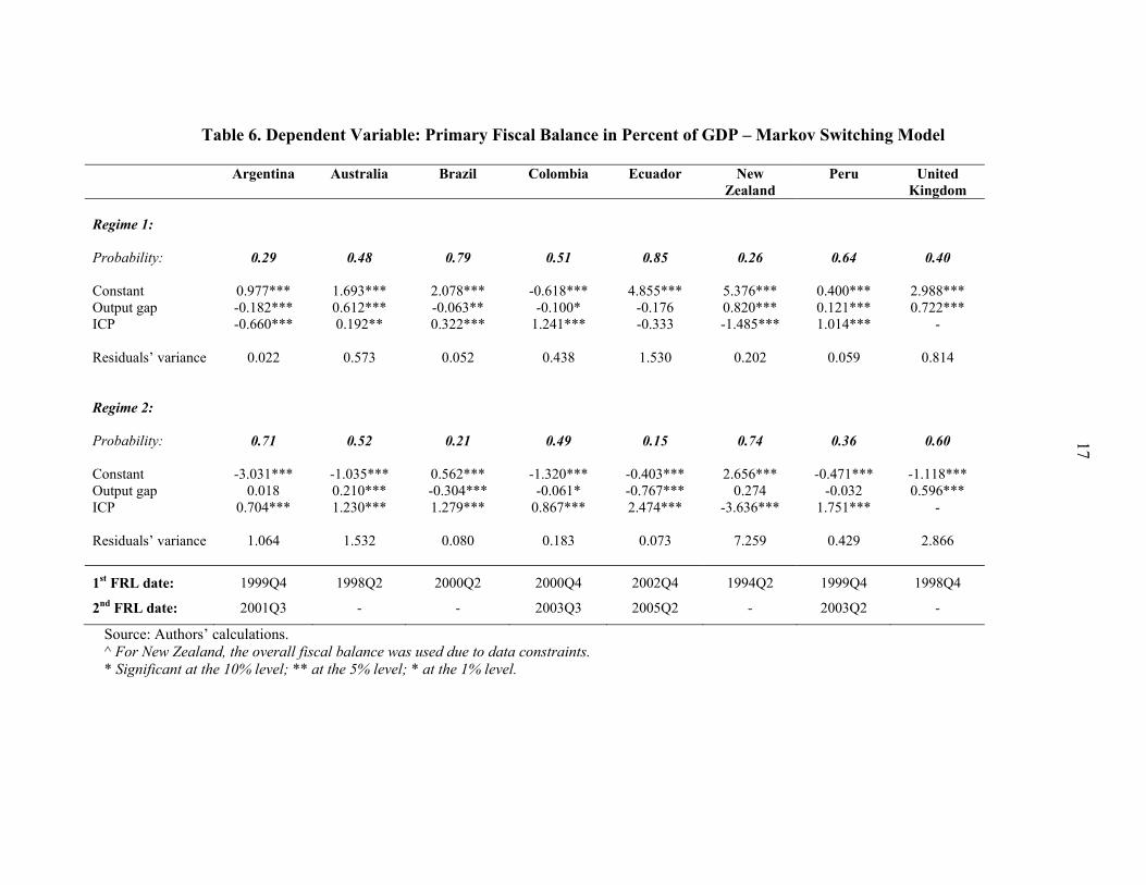
The above transition probabilities, together with the parameters and Ωst can be estimated using Maximum Likelihood Estimation (Annex 2).19 The results from the Markov Switching model are broadly consistent with those presented in the previous section. The estimates in Table 6 suggest that, in developed countries, regimes change according to business cycles, without a clear relationship with the FRL. For instance, Figure 1 shows that the probability of being in a different regime in Australia and the United Kingdom tracks closely the fluctuations in the output gap (left panel). A large deterioration in the output gap tends to be followed by a transition to State 2, – the “bad regime” in general, characterized by lower primary fiscal balances and higher volatility. With respect to the emerging economies, in Brazil, the regime shift coincides with the consolidation process that started some time before the FRL. This is in line with the Quandt-Andrews results, which found structural breaks that preceded the introduction of the FRL by several quarters. In Argentina, the regime shifts capture the mid-90s and early-2000s crises, with a transition to a “good regime” around 2004, as the economic recovery strengthened and the output gap closed. In other countries (e.g. Colombia and Peru), the adoption of the FRL do not seem to affect the number of transitions to State 2, nor the value of the probability of being in such regime. Overall, the results from the Markov Switching model appear consistent with the Quandt-Andrews ones. In most countries, the adoption of the FRL does not seem to be clearly associated with better fiscal outcomes. In several cases, the adoption of the FRL seems to have accompanied a process of improved fiscal policy that was already underway.

IV. CONCLUSIONS

The aim of this paper was to evaluate empirically whether FRLs can be linked to changes in fiscal performance, using consistent tests for structural breaks. The paper assessed the potential impact of an FRL on both the level and the volatility of primary fiscal balances in five Latin American countries and three advanced economies. The econometric model controls for the economic and commodity cycles and allows for the presence of structural

18 Such a process is described as an N-state Markov chain with transition probabilities Pij. 19 See Hamilton (1994) for details.

11

breaks in all coefficients and time periods. Traditional econometric approaches yield inconsistent results. These approaches, which rely on the use of dummies in time series or panel regressions, render estimates of the impact of FRLs that are biased when the underlying series have structural breaks. In other words, the dummy may be capturing any time-specific phenomena not necessarily contemporaneous to the FRL. The traditional approach would suggest that, in about half of the countries in the sample, primary fiscal balances increased considerably in the post-FRL period. These results were dismissed when using consistent methods for testing for structural breaks. When using consistent methods for the detection of structural breaks or regime shifts we find limited empirical evidence linking FRLs to changes in fiscal performance. All countries in the sample exhibit one or more structural breaks, either in the level or variance of the primary fiscal balance. But, in general, these breaks did not occur around the FRL adoption dates. In several cases, the structural breaks preceded the adoption of the FRL. The overall conclusions hold when using the Quandt-Andrews approach to estimate breaks sequentially, or when estimating Markov Switching models to determine the presence of regime shifts. In the developed economies analyzed, shifts seem to be mainly driven by business cycles, while in the developing countries in the sample the fiscal consolidation processes seem to have already been in place before the introduction of the FRLs. FRLs may have helped anchor efforts to strengthen fiscal policy, but do not seem to have been the driver of such efforts. FRLs could still have positive effects other than on fiscal balances. As mentioned earlier, the analysis centered around quantifying the potential impact of FRLs on the level and volatility of primary fiscal balances. Although empirically this did not seem to be the case in general, FRLs could still have other positive effects on the conduct of fiscal policy. For example, FRLs could play an important role in enhancing transparency and providing guidance in the budget process. They could also lower risk sovereign premia and facilitate access to government financing. These remain interesting areas for further research.

12

Table 1. Data Summary

Argentina Australia Brazil Colombia Ecuador New

Zealand Peru United

Kingdom 1st FRL date: 1999Q4 1998Q2 2000Q2 2000Q4 2002Q4 1994Q2 1999Q4 1998Q4 2nd FRL date: 2001Q3 - - 2003Q3 2005Q2 - 2003Q2 - Sample period: 93Q4-08Q4 74Q3-09Q2 97Q4-08Q4 95Q4-08Q4 99Q1-08Q4 88Q1-09Q2 95Q4-08Q4 72Q2-09Q4 Number of observations:

61 140 45 53 40 86 53 151

Frequency: quarterly quarterly quarterly quarterly quarterly quarterly quarterly quarterly

Source: National statistics; authors’ calculations; and Corbacho and Schwartz (2007). ^ For New Zealand, the series for the fiscal balance are available on an annual basis only. Quarterly series were obtained using linear interpolation.

13

Table 2a. Dependent Variable: Primary Fiscal Balance

(Percent of GDP)

Argentina Argentina Australia Brazil Colombia Colombia Constant -1.226** -1.577*** -0.056 1.072*** -1.441*** -1.349*** Output gap -0.043 -0.040 0.468*** -0.111** 0.025 0.026 ICP 1.037** 0.987* 0.422** 0.252*** 0.703*** 0.325* FRL dummy -0.895 -0.349 1.415*** 1.036*** 0.841*** 1.208*** FRL date 1999Q4 2001Q3 1998Q2 2000Q2 2000Q4 2003Q3

Table 2b: Dependent variable: Primary Fiscal Balance (Percent of GDP)

Ecuador Ecuador New

Zealand Peru Peru United

Kingdom Constant 4.973*** 4.394*** 1.033* 0.319* -0.022 0.977*** Output gap 0.046 -0.060 -0.265 0.033 0.100* 0.476*** ICP 0.450 1.000 -0.778* 1.350*** 1.150*** - FRL dummy -1.420* -1.939 5.114*** -0.422* 0.316 -0.655 FRL date 2002Q4 2005Q2 1994Q2 1999Q4 2003Q2 1998Q4 Source: Authors’ calculations. ^ For New Zealand, the overall fiscal balance was used due to data constraints. * Significant at the 10% level; ** at the 5% level; *** at the 1% level.

14

Table 3a. Chow Tests*

Argentina Argentina Australia Brazil Colombia Colombia FRL Date 1999Q4 2001Q3 1998Q2 2000Q2 2000Q4 2003Q3

Test Level Prob. Level Prob. Level Prob. Level Prob. Level Prob. Level Prob.

F-statistic 0.794 0.502 1.934 0.135 22.621 0.000 52.508 0.000 7.161 0.001 10.206 0.000

Log likelihood ratio 2.588 0.460 6.116 0.106 57.365 0.000 72.775 0.000 19.952 0.000 26.588 0.000

Wald Statistic 2.383 0.497 5.801 0.122 67.864 0.000 157.525 0.000 21.484 0.000 30.619 0.000

Table 3b. Chow Tests*

Ecuador Ecuador New Zealand Peru Peru United Kingdom FRL Date 2002Q4 2005Q2 1994Q2 1999Q4 2003Q2 1998Q4

Test Level Prob. Level Prob. Level Prob. Level Prob. Level Prob. Level Prob.

F-statistic 12.808 0.000 1.308 0.288 25.507 0.000 2.565 0.066 1.884 0.145 3.749 0.026

Log likelihood ratio 30.247 0.000 4.370 0.224 57.720 0.000 8.037 0.045 6.019 0.111 7.511 0.023

Wald Statistic 38.424 0.000 3.925 0.270 76.521 0.000 7.696 0.053 5.652 0.130 7.498 0.024 Source: Authors’ calculations. * Null hypothesis: no breaks at specified breakpoints. ^ For New Zealand, the overall fiscal balance was used due to data constraints.

15

Table 4. Dependent Variable: Conditional Variance - Model 1

Argentina Australia Brazil Colombia Ecuador New Zealand

Peru United Kingdom

Period 1: 93Q4-95Q3 74Q3-77Q1 97Q4-98Q4 - 99Q1-99Q2 88Q1-92Q4 95Q4-99Q2 72Q1-92Q2 Constant 40.426** 9.806*** 1.865*** 18.255 5.751** 0.302*** 3.944*** Period 2: 96Q1-97Q2 77Q3-01Q4 99Q2-08Q4 - 99Q4-01Q2 93Q2-94Q3 99Q3-00Q4 92Q4-95Q1 Constant 9.868*** 2.369*** 0.103*** 5.854** 38.152*** 1.653** 20.600*** Period 3: 97Q4-08Q4 02Q2-09Q2 - - 01Q4-08Q4 95Q1-06Q1 01Q1-08Q4 95Q3-07Q3 Constant 1.737*** 0.870*** 0.804* 3.443*** 0.185** 4.705*** Period 4: - - - - - 06Q3-09Q2 - 08Q4-09Q4 Constant 13.424*** 20.103** Break date 1995Q3 1977Q2 1999Q1 - 1999Q3 1993Q1 1999Q3 1992Q3 Q-A statistic 46.772 81.437 301.690 9.801 41.729 20.078 14.977 p-value 0.0000 0.0000 0.0000 0.0289 0.0000 0.0002 0.0040 Break date 1997Q3 2002Q1 - - 2001Q3 1994Q2 2000Q4 1995Q2 Q-A statistic 80.077 14.625 24.537 10.564 8.719 97.147 p-value 0.0000 0.0047 0.0000 0.0320 0.0475 0.0000 Break date - - - - - 2006Q2 - 2007Q4 Q-A statistic 49.760 29.440 p-value 0.0000 0.0000

1st FRL date: 1999Q4 1998Q2 2000Q2 2000Q4 2002Q4 1994Q2 1999Q4 1998Q4

2nd FRL date: 2001Q3 - - 2003Q3 2005Q2 - 2003Q2 -

Source: Authors’ calculations. ^ For New Zealand, the overall fiscal balance was used due to data constraints. * Significant at the 10% level; ** at the 5% level; *** at the 1% level.

16

Table 5. Dependent Variable: Primary Fiscal Balance in Percent of GDP – Model 2

Argentina Australia Brazil Colombia Ecuador New Zealand

Peru United Kingdom

Period 1: 93Q4-95Q3 74Q3-85Q4 97Q4-99Q1 95Q4-03Q1 99Q1-01Q3 88Q1-92Q3 95Q4-08Q4 72Q2-87Q2 Constant 14.624* -1.637*** 0.599*** -1.526*** 6.305*** 3.485*** 0.056 0.727*** Output gap -0.316 0.047 -0.098 0.002 -0.103 0.266 0.073 -0.081 ICP -41.467 2.420*** -0.746 -0.100 12.110*** -4.458*** 1.274*** - Period 2: 96Q1-02Q3 86Q2-98Q1 99Q3-05Q4 03Q3-08Q4 02Q1-08Q4 93Q1-95Q3 - 87Q4-97Q4 Constant -3.693*** 0.333 2.153*** -0.084 4.067*** -3.425*** -0.124 Output gap 0.068*** 0.284* -0.095*** 0.270** -0.139 1.031*** 1.700*** ICP -1.025*** 2.686*** 0.560*** 0.131 0.151 6.005 - Period 3: 03Q1-08Q4 98Q3-09Q2 06Q2-08Q4 - - 96Q1-02Q3 - 98Q2-03Q3 Constant 0.817** 1.534*** 0.684** 4.643*** 2.972*** Output gap 0.324*** 0.814*** -0.182** -0.434*** 2.774*** ICP -1.209*** 0.023 1.202*** -1.727* - Period 4: - - - - - 03Q1-09Q2 - 04Q1-09Q4 Constant 2.702*** -1.801*** Output gap 0.509** 1.039*** ICP 1.168** -

Break date

1995Q4

1986Q1

1999Q2

2003Q2

2001Q4

1992Q4

1987Q3 Q-A statistic 29.529 43.337 67.449 13.914 24.644 26.980 26.824 p-value 0.0001 0.0000 0.0000 0.0493 0.0004 0.0002 0.0001 Break date 2002Q4 1998Q2 2006Q1 - - 1995Q4 - 1998Q1 Q-A statistic 92.187 13.378 14.029 40.101 20.301 p-value 0.0000 0.0969 0.0595 0.0000 0.0013 Break date - - - - - 2002Q4 - 2003Q4 Q-A statistic 19.522 17.313 p-value 0.0062 0.0064

1st FRL date: 1999Q4 1998Q2 2000Q2 2000Q4 2002Q4 1994Q2 1999Q4 1998Q4

2nd FRL date: 2001Q3 - - 2003Q3 2005Q2 - 2003Q2 - Source: Authors’ calculations. ^ For New Zealand, the overall fiscal balance was used due to data constraints. * Significant at the 10% level; ** at the 5% level; *** at the 1% level.

17

Table 6. Dependent Variable: Primary Fiscal Balance in Percent of GDP – Markov Switching Model

Argentina Australia Brazil Colombia Ecuador New

Zealand Peru United

Kingdom Regime 1: Probability: 0.29 0.48 0.79 0.51 0.85 0.26 0.64 0.40 Constant 0.977*** 1.693*** 2.078*** -0.618*** 4.855*** 5.376*** 0.400*** 2.988*** Output gap -0.182*** 0.612*** -0.063** -0.100* -0.176 0.820*** 0.121*** 0.722*** ICP -0.660*** 0.192** 0.322*** 1.241*** -0.333 -1.485*** 1.014*** - Residuals’ variance 0.022 0.573 0.052 0.438 1.530 0.202 0.059 0.814 Regime 2: Probability: 0.71 0.52 0.21 0.49 0.15 0.74 0.36 0.60 Constant -3.031*** -1.035*** 0.562*** -1.320*** -0.403*** 2.656*** -0.471*** -1.118*** Output gap 0.018 0.210*** -0.304*** -0.061* -0.767*** 0.274 -0.032 0.596*** ICP 0.704*** 1.230*** 1.279*** 0.867*** 2.474*** -3.636*** 1.751*** - Residuals’ variance 1.064 1.532 0.080 0.183 0.073 7.259 0.429 2.866

1st FRL date: 1999Q4 1998Q2 2000Q2 2000Q4 2002Q4 1994Q2 1999Q4 1998Q4

2nd FRL date: 2001Q3 - - 2003Q3 2005Q2 - 2003Q2 -

Source: Authors’ calculations. ^ For New Zealand, the overall fiscal balance was used due to data constraints. * Significant at the 10% level; ** at the 5% level; * at the 1% level.

18

Figure 1a. Markov Switching Model 1/

1 The left panels show the probability of being in State 2 (generally the “bad regime” as described in Table 6) and the output gap. The right panels show the probability of being in State 2 and the primary fiscal balance. Dash lines indicate adoption of an FRL.

0.0

0.1

0.2

0.3

0.4

0.5

0.6

0.7

0.8

0.9

1.0

-4.0

-3.0

-2.0

-1.0

0.0

1.0

2.0

3.0

4.0

1997 1998 1999 2000 2001 2002 2003 2004 2005 2006 2007 2008 2009

BRAZIL

Probability State 2 (right scale) Output gap (%)

0.0

0.1

0.2

0.3

0.4

0.5

0.6

0.7

0.8

0.9

1.0

0.0

0.5

1.0

1.5

2.0

2.5

3.0

3.5

1997 1998 1999 2000 2001 2002 2003 2004 2005 2006 2007 2008 2009

BRAZIL

Probability State 2 (right scale) Primary balance (% of GDP)

0.0

0.1

0.2

0.3

0.4

0.5

0.6

0.7

0.8

0.9

1.0

-3.0

-2.0

-1.0

0.0

1.0

2.0

3.0

1974 1978 1982 1986 1990 1994 1998 2002 2006 2010

AUSTRALIA

Probability State 2 (right scale) Output gap (%)

0.0

0.1

0.2

0.3

0.4

0.5

0.6

0.7

0.8

0.9

1.0

-5.0

-4.0

-3.0

-2.0

-1.0

0.0

1.0

2.0

3.0

4.0

5.0

1974 1978 1982 1986 1990 1994 1998 2002 2006 2010

AUSTRALIA

Probability State 2 (right scale) Primary balance (% of GDP)

0.0

0.1

0.2

0.3

0.4

0.5

0.6

0.7

0.8

0.9

1.0

-12.0

-7.0

-2.0

3.0

8.0

1995 1996 1997 1998 1999 2000 2001 2002 2003 2004 2005 2006 2007 2008 2009

ARGENTINA

Probability State 2 (right scale) Output gap (%)

0.0

0.1

0.2

0.3

0.4

0.5

0.6

0.7

0.8

0.9

1.0

-8.0

-6.0

-4.0

-2.0

0.0

2.0

4.0

6.0

8.0

1995 1996 1997 1998 1999 2000 2001 2002 2003 2004 2005 2006 2007 2008 2009

ARGENTINA

Probability State 2 (right scale) Primary balance (% of GDP)

0.0

0.1

0.2

0.3

0.4

0.5

0.6

0.7

0.8

0.9

1.0

-4.0

-3.0

-2.0

-1.0

0.0

1.0

2.0

3.0

4.0

5.0

1995 1996 1997 1998 1999 2000 2001 2002 2003 2004 2005 2006 2007 2008 2009 2010

COLOMBIA

Probability State 2 (right scale) Output gap (%)

0.0

0.1

0.2

0.3

0.4

0.5

0.6

0.7

0.8

0.9

1.0

-3.0

-2.5

-2.0

-1.5

-1.0

-0.5

0.0

0.5

1.0

1.5

2.0

1995 1996 1997 1998 1999 2000 2001 2002 2003 2004 2005 2006 2007 2008 2009 2010

COLOMBIA

Probability State 2 (right scale) Primary balance (% of GDP)

19

Figure 1b. Markov Switching Model 1/

1 The left panels show the probability of being in State 2 (generally the “bad regime” as described in Table 6) and the output gap. The right panels show the probability of being in State 2 and the primary fiscal balance. Dash lines indicate adoption of an FRL.

0.0

0.1

0.2

0.3

0.4

0.5

0.6

0.7

0.8

0.9

1.0

-4.0

-3.0

-2.0

-1.0

0.0

1.0

2.0

3.0

4.0

1972 1976 1980 1984 1988 1992 1996 2000 2004 2008

UK

Probability State 2 (right scale) Output gap (%)

0.0

0.1

0.2

0.3

0.4

0.5

0.6

0.7

0.8

0.9

1.0

-8.0

-6.0

-4.0

-2.0

0.0

2.0

4.0

6.0

8.0

1972 1976 1980 1984 1988 1992 1996 2000 2004 2008

UK

Probability State 2 (right scale) Primary balance (% of GDP)

0.0

0.1

0.2

0.3

0.4

0.5

0.6

0.7

0.8

0.9

1.0

-6.0

-4.0

-2.0

0.0

2.0

4.0

6.0

1995 1996 1997 1998 1999 2000 2001 2002 2003 2004 2005 2006 2007 2008 2009 2010

ECUADOR

Probability State 2 (right scale) Output gap (%)

0.0

0.1

0.2

0.3

0.4

0.5

0.6

0.7

0.8

0.9

1.0

-2.0

-1.0

0.0

1.0

2.0

3.0

4.0

5.0

6.0

7.0

8.0

9.0

1995 1996 1997 1998 1999 2000 2001 2002 2003 2004 2005 2006 2007 2008 2009 2010

ECUADOR

Probability State 2 (right scale) Primary balance (% of GDP)

0.0

0.1

0.2

0.3

0.4

0.5

0.6

0.7

0.8

0.9

1.0

-5.0

-4.0

-3.0

-2.0

-1.0

0.0

1.0

2.0

3.0

4.0

5.0

1995 1996 1997 1998 1999 2000 2001 2002 2003 2004 2005 2006 2007 2008 2009 2010

PERU

Probability State 2 (right scale) Output gap (%)

0.0

0.1

0.2

0.3

0.4

0.5

0.6

0.7

0.8

0.9

1.0

-3.0

-2.0

-1.0

0.0

1.0

2.0

3.0

4.0

5.0

1995 1996 1997 1998 1999 2000 2001 2002 2003 2004 2005 2006 2007 2008 2009 2010

PERU

Probability State 2 (right scale) Primary balance (% of GDP)

0.0

0.1

0.2

0.3

0.4

0.5

0.6

0.7

0.8

0.9

1.0

-4.0

-3.0

-2.0

-1.0

0.0

1.0

2.0

3.0

4.0

1988 1990 1992 1994 1996 1998 2000 2002 2004 2006 2008 2010

NEW ZEALAND

Probability State 2 (right scale) Output gap (%)

0.0

0.1

0.2

0.3

0.4

0.5

0.6

0.7

0.8

0.9

1.0

-8.0

-6.0

-4.0

-2.0

0.0

2.0

4.0

6.0

8.0

1988 1990 1992 1994 1996 1998 2000 2002 2004 2006 2008 2010

NEW ZEALAND

Probability State 2 (right scale) Overall balance (% of GDP)

20

Annex 1. Inconsistent Estimation of Dummy Variable Models in the Presence of Structural Breaks

This annex illustrates how the presence of a structural break (e.g. level shift) at time 0t in the

true model may lead to incorrect results when including a dummy variable in the model used for estimation. First assume that the true data generating process (DGP) is given by the AR(1) process satisfying

ttttt uIyy )(1 0 [1]

where and are the true parameters, )( AI is the indicator function, equal to 1 when the

event A occurs and 0 otherwise, and tu is a sequence of martingale differences with respect

to a filtration Ft. Note that [1] shows that there is a true level shift at time 0t .

Now, assume that the model used for estimation is the following

TtforIyy ttttt ,...,1)(1 1 [2]

where 1t is different from 0t , and clearly )(),max( 10 TOtt .

Note that the use of model [2] reflects the belief that the level shift occurred at time 1t (for

example, due to the passing or ammendment of a particular law at time 1t ), while in reality there was none at this particular time. In addition, note that [1] and [2] can be rewritten as

t

Z

tttt uIyy

t

],[ )(1 0

[3]

and

t

X

tttt

t

Iyy

],[ )(1 1

[4]

respectively. Thus, using the model presented in [4] to estimate by OLS gives

YXXX 1)(ˆ [5] where ),...,( 1 TyyY is given by the true DGP in equation [3] as UZY . Hence, equation [5] can be rewritten as

UXXXZXXX 11 )()(ˆ [6]

Now, the second term on the right hand side in [6] is given by

21

T

tt t

T

t tt

T

tt t

T

tt t

T

t t

u

uy

tTy

yyUXXX

11

1 1 1

1

11

11

211)(

Caceres (2008, Lemma 5.3.1) showed that )1()( 1

poUXXX . In other words, this term

vanishes. This last result is true independently of the values of the parameters and . Therefore,

)1()(ˆ 1poZXXX [7]

Now, consider the term ZXXX 1)( , which is given by

),max()(

101

11

21

1

11

11

211

1

0

1

1

ttTy

yy

tTy

yyZXXX T

tt t

T

tt t

T

t t

T

tt t

T

tt t

T

t t

[8]

Thus, the presence of the structural break (i.e. denoted by the indicator )( 0ttI and 0 )

implies that the estimator of the coefficient for the ‘non-existent’ level shift at time 1t will be generally different than zero.

In particular, if )(),max( 10 Tott , then from equations [7] and [8], we have that P

ˆ (in

fact P

ˆ ). In this case, the estimator related to the non-existing level shift will be ‘estimating’ exactly the value of the true level shift , even though the latter occurred at a time 0t different than 1t .

22

Annex 2. Markov Switching Model20 This annex presents the methodology to estimate the Markov switching model used in this paper. First, consider the model: for t = 1, 2,…, T [1] where is the dependent variable, is a vector of pre-determined explanatory variables, is a i.i.d. 0, random error, is an unobserved state variable which can take N different values (denoting N different regimes). Let denote a vector of parameters that includes , … , and , … , .

The unobserved regime is assumed to have been generated by some probability distribution, for which the probability that takes on the value j is denoted by : | ; for j = 1, 2,…, N [2] The probabilities , … , are also included in , so that

, … , , , … , , , … , . Now, the density of conditional on the state variable taking on the value j is given by:

| , ; exp

[3]

Also, note that , | ; | , ; · | ; from Bayes’ law. Hence, combining equations [2] and [3], the density of can be found by summing

, | ; over all possible values for j:

| ; ∑ exp

[4]

Then, the log-likelihood for the observed data can be calculated from the above as: ∑ log | ; [5]

20 See Hamilton (1994) for more details.

23

Therefore, the maximum likelihood estimator of is obtained by maximizing [5] subject to the constraints that 1 and 0 for j = 1, 2,…, N. Hence, the maximum likelihood estimate is obtained as the solution to the following system of non-linear equations:

∑ | , ; ∑ | , ; [6]

∑ · | , ;

∑ | , ; [7]

∑ | , ; [8]

where:

| , ; · | , ;

| ; for j = 1, 2,…, N [9]

The above system of equations can be solved numerically. For this study, we developed an algorithm based on the fixed point method to obtain the maximum likelihood estimate of . Although a global maximum of the log likelihood in [5] does not exist, it can be shown (see Kiefer, 1978) that there exists a bounded local maximum of [5] that yields a consistent, asymptotically Gaussian estimate of for which (asymptotic) standard errors can be constructed.

24

Annex 3. Data This annex describes the series and underlying source used in the estimation.

Country-Specific Commodity Price Indices21

Authors’ estimations based on the IMF monthly commodity price indices and trade data from the Standard International Trade Classification, found in the World Integrated Trade Solution.

Real GDP

Data were obtained by Haver Analytics using primary data from each country’s authorities. When real data were not available, nominal data were deflated by each country’s GDP deflator.

Revenues and Primary Expenditures

Revenues encompass total revenues, and the institutional coverage depends on data availability for each country. Primary expenditures cover total expenditures (i.e., current plus capital expenditures) minus interest payments, with the institutional coverage also depending on the country’s definitions and data availability. Primary balances were computed as the difference between total revenues and primary expenditures. For Argentina, we use our estimations from nonfinancial public sector data, published by the Finance Ministry. For Australia, we use central government data published by the Reserve Bank of Australia. For Brazil, data cover the non-financial public sector level (including general government, public enterprises, and central bank), published by the central bank. For Colombia, data for the central government were gathered from the Finance Ministry’s CONFIS. For Ecuador, data cover the central government level as reported by the central bank. New Zealand data on government revenues and expenditures (accruals) were not available on a quarterly basis. We employed annual data on the general government from Statistics New Zealand through Haver Analytics. For Peru, data cover the central government level published by the central bank. Finally, data for the United Kingdom were obtained from Haver Analytics using primary data from the Office for National Statistics (ONS) at the general government level.

21 See Medina (2010) for details.

25

References Alesina, Alberto, Ricardo Hausmann, Rudolf Hommes, and Ernesto Stein, 1999, “Budget

institutions and Fiscal Performance in Latin America,” Journal of Development Economics, Vol 59, No.2, pp. 253-73.

Alesina, Alberto, Felipe Campante, and Guido Tabellini, 2008, “Why is Fiscal Policy Often

Procyclical?” Journal of the European Economic Association, Vol. 6. No. 5, September, pp. 1006-1086.

Alt, J.E. and Lowry, R.C. (1994), “Divided Government, Fiscal Institutions, and Budget Deficits:

Evidence from the States,” The American Political Science Review, No. 88 (4). Andrews, Donald W.K., 1993, “Tests for Parameter Instability and Structural Change with

Unknown Change Point”, Econometrica, Vol. 61, No. 4, pp. 821-856. Andrews, Donald W. K. and Werner Ploberger, 1994, “Optimal Tests When a Nuissance

Parameter is Present Only Under the Alternative.” Econometrica, Vol. 62, No.6, pp.1383-414.

Bohn, H. and Inman, P., 1996, “Balanced Budget Rules and Public Deficit: Evidence from the

US States,” Carnegie-Rochester Conference Series on Public Policy, 45. Caceres, Carlos, 2008, “Asymptotic Properties of Tests for Mis-specification.” Oxford

University, DPhil Thesis in Economics (January 20, 2008). Corbacho, Ana, and Gerd Schwartz, 2007, “Fiscal Responsibility Laws” in Promoting

Fiscal Discipline, ed. by Manmohan S. Kumar and Teresa Ter-Minassian (Washington: International Monetary Fund).

Chong, Terence Tai-leung, 1995, “Partial Parameter Consistency in a Misspecified Structural

Change Model,” Economics Letters, Vol. 49, No. 4, pp. 351-37. Chow, Gregory C, 1960, “Tests of Equality Between Sets of Coefficients in Two Linear

Regressions.” Econometrica, Vol. 28, No.3, pp.591-605. Fatas, Antonio, and Ilian Mihov, 2003, “The Case for Restricting Fiscal Policy Discretion.”

The Quarterly Journal of Economics, Vol. 118, No. 4, pp. 1419-1447. __________________________, 2005, “Policy Volatility, Institutions and Economic

Growth,” CEPRE Discussion Paper No. 5388. ___________________________, 2006, “The Macroeconomic Effects of Fiscal Rules in the US

States,” Journal of Public Economics, No. 90.

26

Filc, Gabriel, and Carlos Scartascini, 2005, “Budget Institutions and Fiscal Outcomes: Ten Years of Inquiry of Fiscal Matters at the Research Department of the Inter-American Development Bank.”International Journal of Public Debt, No. 59, pp. 81-138.

Gavin, Michael, and Roberto Perotti, 1997, “Fiscal Policy in Latin America,” in NBER

Macroeconomics Annual 1997, Vol. 12. Available via the Internet: http://www. nber.org/chapters/c11036.pdf.

Gleich, Holger, 2003, “Budget Institutions and Fiscal Performance in Central and Eastern

European Countries,” European Central Bank Working Paper No.215 (Frankfurt: European Central Bank).

Hallerberg, Mark, Rolf Strauch, and Jorgen Von Hagen, 2007, “The design of fiscal rules and

forms of governance in European Union countries.”European Journal of Political Economy, Vol. 23, No. 2, pp. 338-359.

Hamilton, J. D., 1994, Time Series Analysis, Princeton University Press, New Jersey. Hansen, Bruce E, 1997, “Approximate Asymptotic P Values for Structural-Change Tests.”

Journal of Business and Economic Statistics. Vol. 15, No.1, pp. 60-67. Hansen, Bruce E, 2001, “The New Econometrics of Structural Change: Dating Breaks in the

U.S. Labor Productivity”, The Journal of Economic Perspectives, Vol. 15, No.4, pp.117-128.

Kaminsky, Graciela L., Carmen M. Reinhart, and Carlos A. Végh, 2005, “When It Rains, It

Pours: Procyclical Capital Flows and Macroeconomic Policies,” in NBER Macroeconomics Annual 2004, Vol. 19 (Cambridge, Massachusetts: National Bureau of Economic Research, MIT Press).

Kiefer, N.M., 1978, “Discrete Parameter Variation: Efficient Estimation of a Switching Regression Model,” Econometrica 46, pp. 427-434.

Kopits, George, and Steven Symansky, 2008, “Fiscal Policy Rules,” Occasional Paper No. 162 (Washington: International Monetary Fund).

Kumar, M.S., E. Baldacci, A. Schaechter, C. Caceres, D. Kim, X. Debrun, J. Escolano, J. Jonas, P. Karam, I. Yakadina, and R. Zymek, 2009, “Fiscal Rules – Anchoring Expectations for Sustainable Public Finances,” IMF SM/09/274, (Washington: International Monetary Fund).

Ilzetzki, Ethan, and Carlos A. Végh, 2008, “Procyclical Fiscal Policy in Developing Countries: Truth or Fiction?” NBER Working Paper No. 14191 (Cambridge, Massachusetts: National Bureau of Economic Research).

27

Marcel, Mario, 2009, “La Regla de Balance Estructural en Chile: Diez Años, Diez Lecciones,” mimeo.

Medina, Leandro, 2010, “The Dynamic Effects of Commodity Prices on Fiscal Performance

in Latin America,” IMF Working Paper 10/192 (Washington: International Monetary Fund).

Perry, Guillermo, 2004, “Can fiscal Rules Help Reduce Macroeconomic Volatility?” Rules-

Based Fiscal Policy in Emerging Markets: background, analysis and prospects, Kopits G. ed., (New York: Palgrave Macmillan).

Poterba, J. (1994), “State Responses to Fiscal Crises: The Effects of Budgetary Institutions and

Politics,” Journal of Political Economy, No.102. Ramey, Garey, and Valerie Ramey, 1995, “Cross-country Evidence on the Link Between

Volatility and Growth.” The American Economic Review, Vol. 85. No. 5, pp. 1138-1151. Stein, Ernesto, Ernesto Talvi, and Alejandro Grisanti, 1999, “Institutional Arrangements and

Fiscal Performance: The Latin American Experience,” in Fiscal Institutions and Fiscal Performance, ed. James Poterba and Jurgen von Hagen (Chicago: University of Chicago Press).

Talvi, Ernesto, and Carlos A. Végh, 2005, “Tax Base Variability and Procyclical Fiscal

Policy in Developing Countries,” Journal of Development Economics, Vol. 78, No. 1, (October), pp. 156–90.

Ter-Minassian, Teresa, 2010, “Preconditions for a successful introduction of structural fiscal

balance-based rules in Latin America and the Caribbean,” mimeo. Thornton, John, 2009, “Do fiscal Responsibility Laws Matter? Evidence from Emerging

Market Economies Suggest Not,” Journal of Economic Policy Reform 12:2, pp. 127-132.

Von Hagen, Jurgen, and Ian Harden, 1995, “Budget Processes and Commitment to Fiscal

Discipline.” European Economic Review, No. 39, pp. 771-79.