arX

iv:h

ep-t

h/00

0518

3v1

19

May

200

0

hep-th/0005183CALT-68-2266

CITUSC/00-021

HUTP-00/A009

UCB-PTH-00/10

Strings in AdS3 and the SL(2, R) WZW Model.

Part 2: Euclidean Black Hole

Juan Maldacena∗, Hirosi Ooguri†1, and John Son∗

∗ Lyman Laboratory of Physics, Harvard University, Cambridge, MA 02138, USA

malda, json@pauli.harvard.edu

†Caltech-USC Center for Theoretical Physics, Mail Code 452-48

California Institute of Technology, Pasadena, CA 91125, USA

ooguri@theory.caltech.edu

Abstract

We consider the one-loop partition function for Euclidean BTZ black hole back-

grounds or equivalently thermal AdS3 backgrounds which are quotients of H3 (Eu-

clidean AdS3). The one-loop partition function is modular invariant and we can read

off the spectrum which is consistent to that found in hep-th/0001053. We see long

strings and discrete states in agreement with the expectations.

1On leave of absence from the University of California, Berkeley.

1 Introduction

In this paper we continue the investigation started in [1] of the SL(2, R) WZW model

describing string theory on AdS3 × M. For other work on this model, see [2]. Our

motivation is to understand string theories in curved spacetimes where the metric

component g00 is non-trivial, of which AdS3 is the simplest example. Moreover, it is

possible to construct black hole solutions as quotients of AdS3 [3], so understanding

string theory on AdS3 would lead to an understanding of strings moving near black

hole horizons.

In [1] the spectrum of SL(2, R) WZW model was studied, using spectral flow to

generate new representations from the standard ones. These new representations in-

clude states corresponding to long strings [5, 6], with a continuous energy spectrum, as

well as discrete states. The existence of spectral flow as a symmetry of the theory was

argued on the basis of classical and semi-classical analysis. Further support was given

by the fact that the seemingly arbitrary upper bound on the mass of string states in

AdS3 was removed, thus recovering the infinite tower of masses one expects from string

theory. We would like to verify these results by an explicit calculation of the one-loop

partition function. As shown in [4], the Euclidean black hole background is equivalent

to the thermal AdS3 background. So we will consider string theory on AdS3 at a finite

temperature, which is described by strings moving on a Euclidean AdS3 background

with the Euclidean time identified. The calculation of the partition function for this

geometry is a minor variation on the calculation of Gawedzki in [7]. From this we can

read off the spectrum of the theory in Lorentzian signature by interpreting the result

as the free energy of a gas of strings.

This paper is organized as follows. In section 2 we review the spectrum found in [1].

In section 3 we compute the one-loop partition function on thermal AdS3. In section 4

we read off the spectrum from the one-loop calculation. First we present a qualitative

analysis, which is then followed by a precise calculation. We explain how the different

parts of the spectrum arise from this calculation. We further show how the one-loop

result contains information about the SL(2, R) and Liouville reflection amplitudes.

2 The spectrum

We begin by briefly summarizing the results of [1], where a concrete proposal for the

spectrum of AdS3 string theory was made. We consider a critical bosonic string the-

ory on AdS3 × M. The Hilbert space of the SL(2, R) WZW model is generated by

the action of the left-moving and right-moving current algebra SL(2, R)L × SL(2, R)R,

and all the states form representations of this algebra. The simplest representations

are built by first choosing representations for the zero modes, then regarding them

1

as the primary states annihilated by J3,±n>0. The raising operators J3,±

n<0 are then used

to generate the representations of the current algebra. From harmonic analysis, i.e.

quantum mechanical limit, it is known that the left-right symmetric combinations

Cαj=1/2+is × Cα

j=1/2+is and D±j>1/2 × D±

j>1/2 form a complete basis in L2(AdS3), where

Cαj=1/2+is is the principal continuous representation and D±

j>1/2 the principal discrete

representation of SL(2, R). These representations are unitary, but the resulting cur-

rent algebra representations Cαj=1/2+is × Cα

j=1/2+is and D±j>1/2 × D±

j>1/2, constructed as

explained above, are not. This is not a surprise, for even in flat Minkowski space it is

not until one imposes the Virasoro constraints

(Ln + Ln − δn,0)|physical〉 = 0, n ≥ 0 (1)

that a unitary spectrum is obtained. Here Ln is the Virasoro generator for the internal

conformal field theory corresponding to M. The proposal of [1] is that one should

consider not just these representations but also those obtained by the spectral flow

J3n → J3

n = J3n − k

2wδn,0

J+n → J+

n = J+n+w (2)

J−n → J−

n = J−n−w.

The Virasoro generators, given by the Sugawara form, then become Ln = Ln +wJ3n −

k4w2δn,0. Imposing on D±

j>1/2 × D±j>1/2 the condition (1) with Ln one finds that these

states have a discrete energy spectrum

E = J30 + J3

0 = q + q + kw + 2j

= 1 + q + q + 2w +

√1 + 4(k − 2)

(Nw + h− 1 − 1

2w(w + 1)

), (3)

here Nw is defined to be the level of the current algebra after spectral flow by amount

w, Nw = N −wq, and N is the level before spectral flow. The state with energy (3) is

obtained from a lowest weight state by acting with the SL(2, R) currents∏J±

n≤0|j, j〉,with q the net number of ± signs in this expression. In other words, q is the number of

spacetime energy raising operators J+a minus the number of spacetime energy lowering

operators J−a that we have to apply to the lowest weight, lowest energy state |j, m = j〉

to get to the state whose spacetime energy is (3). q is the corresponding quantity for

the generators J±a . We also have a level matching condition of the form

Nw + h = Nw + h (4)

which implies that the angular momentum in AdS3, ℓ = J30 − J3

0 = q− q, is an integer.

We argued in [1] that j is further restricted to the range

1

2< j <

k − 1

2, (5)

2

which implies

k

4w2 +

1

2w < Nw + h− 1 +

1

4(k − 2)<k

4(w + 1)2 − 1

2(w + 1). (6)

A similar analysis on Cαj=1/2+is × Cα

j=1/2+is yields a continuous spectrum

E =k

2w +

1

w

(2s2 + 1

2

k − 2+ N + h+ ˜N + h− 2

), (7)

where s takes values over the real numbers and is interpreted as the momentum in

radial direction for the long strings. These states satisfy the level matching condition

N + h = ˜N + h+ w × (integer). (8)

In the rest of the paper we will do an independent calculation which will reproduce

this single string spectrum.

3 One-loop partition function

In this section we compute the worldsheet one-loop partition function. First we ex-

plain the relation between various useful coordinate systems. Then we consider thermal

AdS3 = H3/Z and show how the identification of Euclidean time in the global coor-

dinates translates into particular boundary conditions for the target space fields. The

partition function is then calculated by an explicit evaluation of the functional integral

following [7].

3.1 Coordinates on H3 and thermal AdS3.

The natural metric on H3 is given by

ds2 =k

y2(dy2 + dwdw), (9)

which is the Euclidean continuation of the Poincare metric on AdS3. By the coordinate

transformation

w = tanh ρet+iθ

w = tanh ρet−iθ (10)

y =et

cosh ρ

3

we obtain the cylindrical coordinates on Euclidean AdS3,

ds2

k= cosh2 ρdt2 + dρ2 + sinh2 ρdθ2. (11)

For the purpose of calculating the partition function, however, it is convenient to use

coordinates in which the metric reads [7]

ds2

k= dφ2 + (dv + vdφ)(dv + vdφ), (12)

which corresponds to the parametrization of H3 as

g =

[eφ(1 + |v|2) v

v e−φ

]. (13)

The coordinate transformation from (11) to (12) is

v = sinh ρeiθ

v = sinh ρe−iθ (14)

φ = t− log cosh ρ .

Thermal AdS3 is given by the identification

t+ iθ ∼ t+ iθ + β , (15)

where β represents the temperature T and the imaginary chemical potential iµ for the

angular momentum,

β = β + iµβ =1

T+ i

µ

T. (16)

The corresponding identifications in the coordinates (12) are

v ∼ veiµβ

v ∼ ve−iµβ (17)

φ ∼ φ+ β ,

which is a consistent symmetry of the WZW action,

S =k

π

∫d2z

(∂φ∂φ+ (∂v + ∂φv)(∂v + ∂φv)

). (18)

4

3.2 Computation of the partition function on thermal AdS3.

In this subsection we compute the partition function for string theory on thermal AdS3.

We consider a conformal field theory on a worldsheet torus with modular parameter τ

(z ∼ z+2π ∼ z+2πτ). The two-dimensional conformal field theory on the worldsheet

is the sum of three parts: the conformal field theory on H3, the internal conformal

field theory on M, and the (b, c) ghosts. First we start with the computation of the

partition function for the conformal field theory describing the three dimensions of

thermal AdS3 and then we will multiply the result by the partition function of the

ghosts and the internal conformal field theory.

Due to the identification (17), the string coordinates now satisfy the following bound-

ary conditions

φ(z + 2π) = φ(z) + βn, φ(z + 2πτ) = φ(z) + βm,

v(z + 2π) = v(z)einµβ , v(z + 2πτ) = v(z)eimµβ . (19)

The thermal circle is non-contractible and therefore we get two integers (n,m) charac-

terizing topologically nontrivial embeddings of the worldsheet in spacetime. In order

to implement these boundary conditions it is convenient to define new fields φ, v such

that they are periodic:

φ = φ+ βfn,m(z, z)

v = v exp(iµβfn,m(z, z)), (20)

with

fn,m(z, z) =i

4πτ2[z(nτ −m) − z(nτ −m)] . (21)

When we substitute this into the action (18), we get

S =kβ2

4πτ2|nτ −m|2 +

k

π

∫d2z

(|∂φ|2 +

∣∣∣∣(∂ +

1

2τ2Un,m + ∂φ

)ˆv∣∣∣∣2), (22)

where

Un,m(τ) =i

2π(β − iµβ)(nτ −m). (23)

We are interested in the functional integral

Z(β, µ; τ) =∫DφDvDve−S . (24)

This integral is evaluated as explained in [7]. We can first do the integral over v, ˆv

which is quadratic, giving the determinant

det

∣∣∣∣∂ +1

2τ2Un,m + ∂φ

∣∣∣∣−2

. (25)

5

We calculate the φ dependence on the determinants by realizing that we can view (25)

as an inverse of two fermion determinants. We can then remove φ from the determinants

by a chiral gauge transformation and using the formulas for chiral anomalies. The result

is

det∣∣∣∣∂ +

1

2τ2Un,m + ∂φ

∣∣∣∣−2

= e2π

∫d2z∂φ∂φ det

∣∣∣∣∂ +1

2τ2Un,m

∣∣∣∣−2

. (26)

The remaining integral over φ gives the usual result for a free boson, except that

k → k−2 due to (26). The functional integral for the thermal AdS3 partition function

then gives

Z(β, µ; τ)

=β(k − 2)

12

8π√τ2

∑

n,m

e−kβ2|m−nτ |2/4πτ2+2π(ImUn,m)2/τ2

| sin(πUn,m)|2|∏∞r=1(1 − e2πirτ )(1 − e2πirτ+2πiUn,m)(1 − e2πirτ−2πiUn,m)|2

=β(k − 2)

12

2π√τ2

(qq)−324

∑

n,m

e−kβ2|m−nτ |2/4πτ2+2π(ImUn,m)2/τ2

|ϑ1(τ, Un,m)|2 , (27)

where ϑ1 is the elliptic theta function and q = e2πiτ . The factor β(k − 2)12 comes from

the length of the circle in the φ direction. This partition function is explicitly modular

invariant after summing over (n,m)2.

We also need to include the contribution of the (b, c) ghosts and the internal CFT.

Partition function of the latter will be of the form

ZM = (qq)−cint24

∑

h,h

D(h, h)qhqh, (28)

where D(h, h) is the degeneracy at left-moving weight h and right-moving weight h, and

cint the central charge of the internal CFT. Modular invariance requires that h− h ∈ Z,

a fact which will be useful in the next section. Vanishing of the total conformal anomaly

gives

cSL(2,R) + cint = 26. (29)

We can calculate now the total contribution to the ground state energy. We found a

ground state energy of −3/24 in (27), the ghosts contribute with 2/24 and the internal

CFT with −cint/24 = (cSL(2,R) − 26)/24. Using cSL(2,R) = 3 + 6k−2

, we find the overall

factor3

(qq)−(1+cint)/24 = e4πτ2(1− 14(k−2)). (30)

2In our previous paper, there was a puzzle about the apparent lack of modular invariance of theSL(2, R) partition functions with J3 insertions (see Appendix B of [1]). Here we have found that, ifwe introduce the twist by considering the physical set-up of thermal AdS3, the result (27) turns outto be manifestly modular invariant. This resolves the puzzle raised in [1].

3Note that cint ≥ 0, k > 2, and (29) imply that there will always be a tachyon in the theory.

6

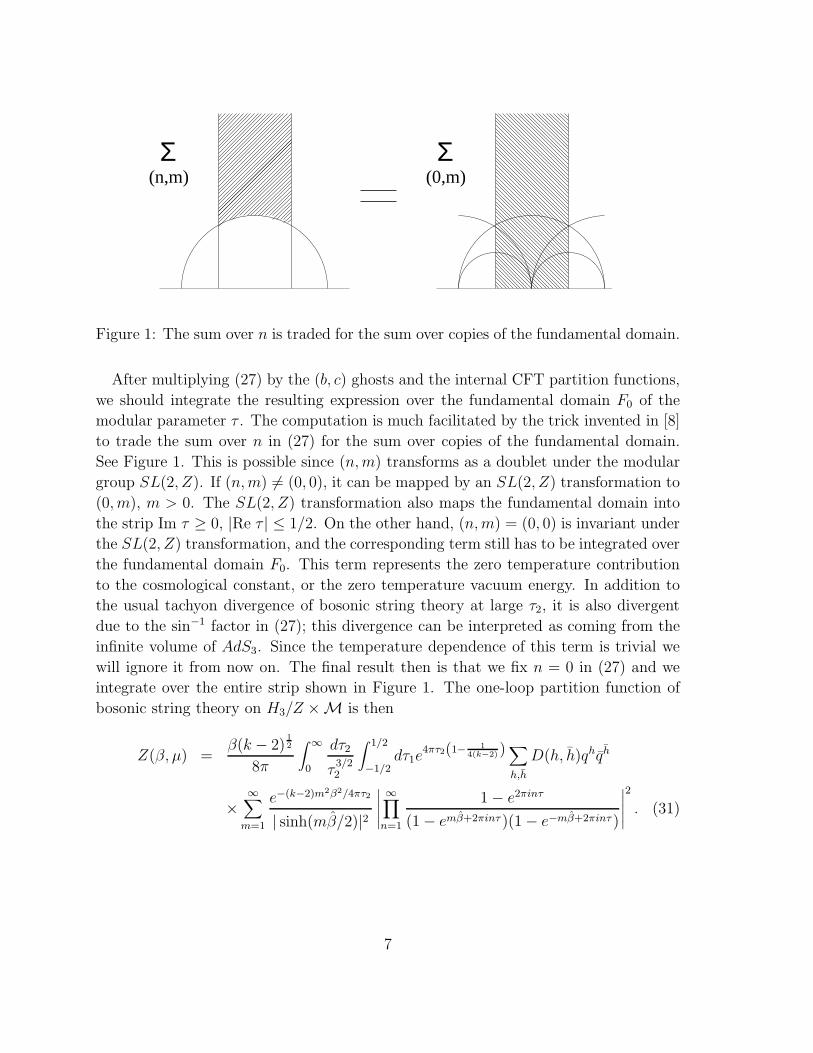
Σ Σ(0,m)(n,m)

Figure 1: The sum over n is traded for the sum over copies of the fundamental domain.

After multiplying (27) by the (b, c) ghosts and the internal CFT partition functions,

we should integrate the resulting expression over the fundamental domain F0 of the

modular parameter τ . The computation is much facilitated by the trick invented in [8]

to trade the sum over n in (27) for the sum over copies of the fundamental domain.

See Figure 1. This is possible since (n,m) transforms as a doublet under the modular

group SL(2, Z). If (n,m) 6= (0, 0), it can be mapped by an SL(2, Z) transformation to

(0, m), m > 0. The SL(2, Z) transformation also maps the fundamental domain into

the strip Im τ ≥ 0, |Re τ | ≤ 1/2. On the other hand, (n,m) = (0, 0) is invariant under

the SL(2, Z) transformation, and the corresponding term still has to be integrated over

the fundamental domain F0. This term represents the zero temperature contribution

to the cosmological constant, or the zero temperature vacuum energy. In addition to

the usual tachyon divergence of bosonic string theory at large τ2, it is also divergent

due to the sin−1 factor in (27); this divergence can be interpreted as coming from the

infinite volume of AdS3. Since the temperature dependence of this term is trivial we

will ignore it from now on. The final result then is that we fix n = 0 in (27) and we

integrate over the entire strip shown in Figure 1. The one-loop partition function of

bosonic string theory on H3/Z ×M is then

Z(β, µ) =β(k − 2)

12

8π

∫ ∞

0

dτ2

τ3/22

∫ 1/2

−1/2dτ1e

4πτ2(1− 14(k−2))

∑

h,h

D(h, h)qhqh

×∞∑

m=1

e−(k−2)m2β2/4πτ2

| sinh(mβ/2)|2

∣∣∣∣∣∞∏

n=1

1 − e2πinτ

(1 − emβ+2πinτ )(1 − e−mβ+2πinτ )

∣∣∣∣∣

2

. (31)

7

4 Reading off the spectrum

We will now extract the spectrum of Lorentzian string theory on AdS3 by interpreting

the one-loop partition function in the spacetime theory. The one-loop partition function

is the single particle contribution to the spacetime thermal free energy, Z(β, µ) = −βF .

To this each string state makes a contribution β−1 log(1 − e−β(E+iµℓ)), where E and ℓ

are the energy and the angular momentum of the state. The total free energy is the

sum over all such factors:

F (β, µ) =1

β

∑

string∈H

log(1 − e−β(Estring+iµℓstring)

)=

∞∑

m=1

f(mβ,mµ), (32)

where

f(β, µ) =1

β

∑

string∈H

e−β(Estring+iµℓstring). (33)

Here H is the physical Hilbert space of single string states. In both (31) and (32),

we have the sums over functions of (mβ,mµ). It is therefore sufficient to compare the

m = 1 terms in these expressions. In other words, we want to verify that Estring and

ℓstring extracted from the identification,

f(β, µ) =∑

string∈H

1

βe−β(Estring+iµℓstring)

=(k − 2)

12

8π

∫ ∞

0

dτ2

τ3/22

∫ 1/2

−1/2dτ1e

4πτ2(1− 14(k−2))

∑

h,h

D(h, h)qhqh

× e−(k−2)β2/4πτ2

| sinh(β/2)|2

∣∣∣∣∣∞∏

n=1

1 − e2πinτ

(1 − eβ+2πinτ )(1 − e−β+2πinτ )

∣∣∣∣∣

2

(34)

agree with the string spectrum found in our previous paper [1]. We will see that

the sum over the Hilbert space breaks up into a sum over the discrete states and an

integral over the continuous states, with the expressions for the energies that were

reviewed in section 2. Since the one-loop calculation presented here is independent of

the assumptions made in [1] about strings in Lorentzian AdS3, we can regard this as a

derivation of the spectrum starting from the well-defined Euclidean path integral.

4.1 Qualitative analysis

In this subsection we will analyze (34) in a qualitative way and explain where the

different contributions to the spectrum come from. To keep the notation simple, we

set µ = 0 in this subsection, leaving the exact computation for the next subsection.

As expected, in (34) there is an exponential divergence as τ2 → ∞, coming from

the tachyon. This is just as in the flat space case, where (mass)2 < 0 of the tachyon

8

causes its contribution to be weighted with a positive exponential. We will disregard

this divergence4. However, rather unexpectedly, the expression above has additional

divergences at finite values of τ . In string theory one might naively expect that di-

vergences come only from the corners of the fundamental domain in the τ -plane, but

in this case the divergence is coming from points in the interior of the fundamental

domain. Overcoming the initial panic, one realizes that these divergences are related

to the presence of long strings. In fact, as with any other string divergence, it can be

interpreted as an IR effect. This divergence is due to the fact that long strings feel a

flat potential as they go to infinity and therefore we get an infinite volume factor. To

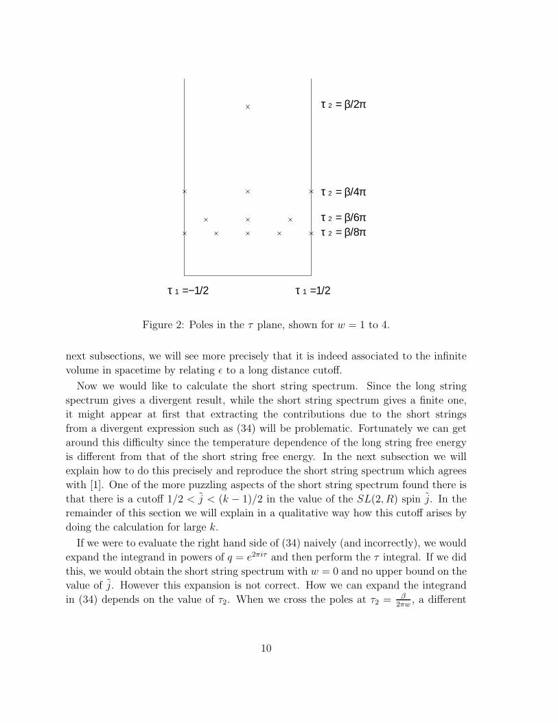
see this, note that near the pole (see Figure 2)

τ = τpole + ǫ, (35)

where

τpole =r

w+ i

β

2πw, (36)

we can expand the partition function and replace τ in all terms by its value at the

pole, except in the one term that has the pole. If we integrate (34) near the pole, i.e.

in the region ǫ < |τ − τpole| ≪ 1 , we find that it diverges as log ǫ with coefficient

1√wβ3

exp

[−β

(k

2w +

1

w(N + h+ ˜N + h− 2 +

1

2(k − 2))

)+

2πir

w(N + h− ˜N − h)

].

(37)

We now sum over r, with |r/w| ≤ 1/2, since these are the ones corresponding to the

poles in the strip5. This sum constrains N + h − ˜N − h to be an integer multiple of

w, as in (8), and it introduces an additional factor of w in (37). The log divergence in

τ -integral can therefore be expressed as

f(β, µ) ∼ 1

βlog ǫ

∫ ∞

0dse−βE(s) + · · · , (38)

where E(s) is the energy spectrum given by (7). Note that the s-integral and the sum

over r we mentioned above give the factor√w/β needed to match the prefactor in

(37) to that in (38). This reproduces the expected contribution from the long strings

in the left hand side of (34). The logarithmic divergence should be interpreted as a

volume factor due to the fact that the long string can be at any radial position. In the

4A skeptical reader could think that we are really doing the superstring partition function (thefermions included in the internal CFT, etc.). Then the tachyon divergence will disappear but onewould still find the divergences that we discuss below. Of course, the one-loop partition func-tion is non-vanishing even in the supersymmetric case since the thermal boundary conditions breaksupersymmetry.

5If some poles are on the boundaries of the strip, τ1 = ±1/2, then we only count them once.

9

τ 1 =−1/2 τ 1 =1/2

τ 2 = β/4π

τ 2 = β/2π

τ 2 = β/6πτ 2 = β/8π

Figure 2: Poles in the τ plane, shown for w = 1 to 4.

next subsections, we will see more precisely that it is indeed associated to the infinite

volume in spacetime by relating ǫ to a long distance cutoff.

Now we would like to calculate the short string spectrum. Since the long string

spectrum gives a divergent result, while the short string spectrum gives a finite one,

it might appear at first that extracting the contributions due to the short strings

from a divergent expression such as (34) will be problematic. Fortunately we can get

around this difficulty since the temperature dependence of the long string free energy

is different from that of the short string free energy. In the next subsection we will

explain how to do this precisely and reproduce the short string spectrum which agrees

with [1]. One of the more puzzling aspects of the short string spectrum found there is

that there is a cutoff 1/2 < j < (k − 1)/2 in the value of the SL(2, R) spin j. In the

remainder of this section we will explain in a qualitative way how this cutoff arises by

doing the calculation for large k.

If we were to evaluate the right hand side of (34) naively (and incorrectly), we would

expand the integrand in powers of q = e2πiτ and then perform the τ integral. If we did

this, we would obtain the short string spectrum with w = 0 and no upper bound on the

value of j. However this expansion is not correct. How we can expand the integrand

in (34) depends on the value of τ2. When we cross the poles at τ2 = β2πw

, a different

10

expansion should be used for the denominator:

1

1 − eβ+2πiwτ=

∞∑

q=0

eq(β+2πiwτ),

(τ2 >

β

2πw

),

= −∞∑

q=0

e−(q+1)(β+2πiwτ),

(τ2 <

β

2πw

). (39)

When τ2 is in the rangeβ

2π(w + 1)< τ2 <

β

2πw, (40)

the product over n in the first term in the denominator in (34) is broken up into

two factors, a product in 1 ≤ n ≤ w and a product in w + 1 ≤ n. The first factor

is expanded in powers of e−(β+2πinτ) and the second factor is expanded in powers of

eβ+2πinτ . Combining them together with the terms coming from the expansion of the

remaining products in (34), we get an exponent of the form6

−(

1

2+ q + w

)β + 2πiτ

(Nw − 1

2w(w + 1)

), (41)

for some integers q and Nw. There is a similar term for τ → τ . We are then to do the

τ -integral of the form,

∫ d2τ

τ3/22

e4πτ2(1− 1

4(k−2))−(k−2) β2

4πτ2−β(1+q+q+2w)+2πiτ(Nw+h− 1

2w(w+1))−2πiτ(Nw+h− 1

2w(w+1)),

(42)

over the region (40). The integral over τ1 produces the level matching condition (4).

Now we evaluate the integral over τ2 using the saddle point approximation. We find

that the saddle point is at

τsaddle =(k − 2)β

2π√

1 + 4(k − 2)(Nw + h− 1 − 12w(w + 1))

(43)

and the integral gives

1

βexp

−β

1 + q + q + 2w +

√

1 + 4(k − 2)(Nw + h− 1 − 1

2w(w + 1))

. (44)

This is the correct form of the contributions due to the short strings in the left hand

side of (34). Moreover we obtain the bound on j precisely, because τsaddle has to be in

the range (40) in order for the saddle point approximation to give a non-zero result. By

(43), this condition is the same as the bound on the spectrum (6), which is equivalent

6The first term −β/2 comes from expanding 1/ sinh(β/2) in (34).

11

to 1/2 < j < (k − 1)/2. (It is a bit surprising that we get all factors precisely right

from the saddle point approximation.) Notice then that the cutoff in j is associated to

the fact that we expand the integrand in (34) in different ways depending on the value

of τ . The value of τ making the biggest contribution to the integral depends on the

values of N and h of the string state.

4.2 A precise evaluation of the τ-integral

Now let us study the partition function (34) more systematically. In this subsection, we

go back to the general case with µ 6= 0. From what we saw in the previous subsection,

we expect to find the discrete states from the integral over the range (40), and the

continuous states from the poles after a suitable regularization.

In order to evaluate the τ -integral exactly, it is useful to introduce a new variable c

by

e−(k−2) β2

4πτ2 = −8πi

β

(τ2

k − 2

) 32∫ ∞

−∞dc c e−

4πτ2k−2

c2+2iβc . (45)

Now suppose τ2 is in the range,

β

2π(w + 1)< τ2 <

β

2πw, (46)

and expand the integrand in (34) as explained in the previous subsection. The right

hand side of (34) becomes a sum of terms like

4

β(k − 2)i

∫ ∞

−∞dc c

∫ β2πw

β

2π(w+1)

dτ2

∫ 1/2

−1/2dτ1

× exp[−β

(q + w +

1

2

)− ¯β(q + w +

1

2

)+ 2πiτ1(Nw + h− Nw − h)

+2icβ − 2πτ2

(h + h+Nw + Nw +

2c2 + 12

k − 2− w(w + 1) − 2

)]. (47)

The integral over τ1 gives a delta function enforcing Nw + h = Nw + h, which is the

level-matching condition (4). Integrating over τ2 in the range (46) gives

1

βπi

∫ ∞

−∞dc c

exp[2icβ − β

(q + w + 1

2

)− ¯β(q + w + 1

2

)]

c2 + 14

+ (k − 2)(Nw + h− 1 − 1

2w(w + 1)

)

×{− exp

[−β

w

(2Nw + 2h− 2 +

2c2 + 12

k − 2− w(w + 1)

)]

+ exp

[− β

w + 1

(2Nw + 2h− 2 +

2c2 + 12

k − 2− w(w + 1)

)]}(48)

12

where we used (4).

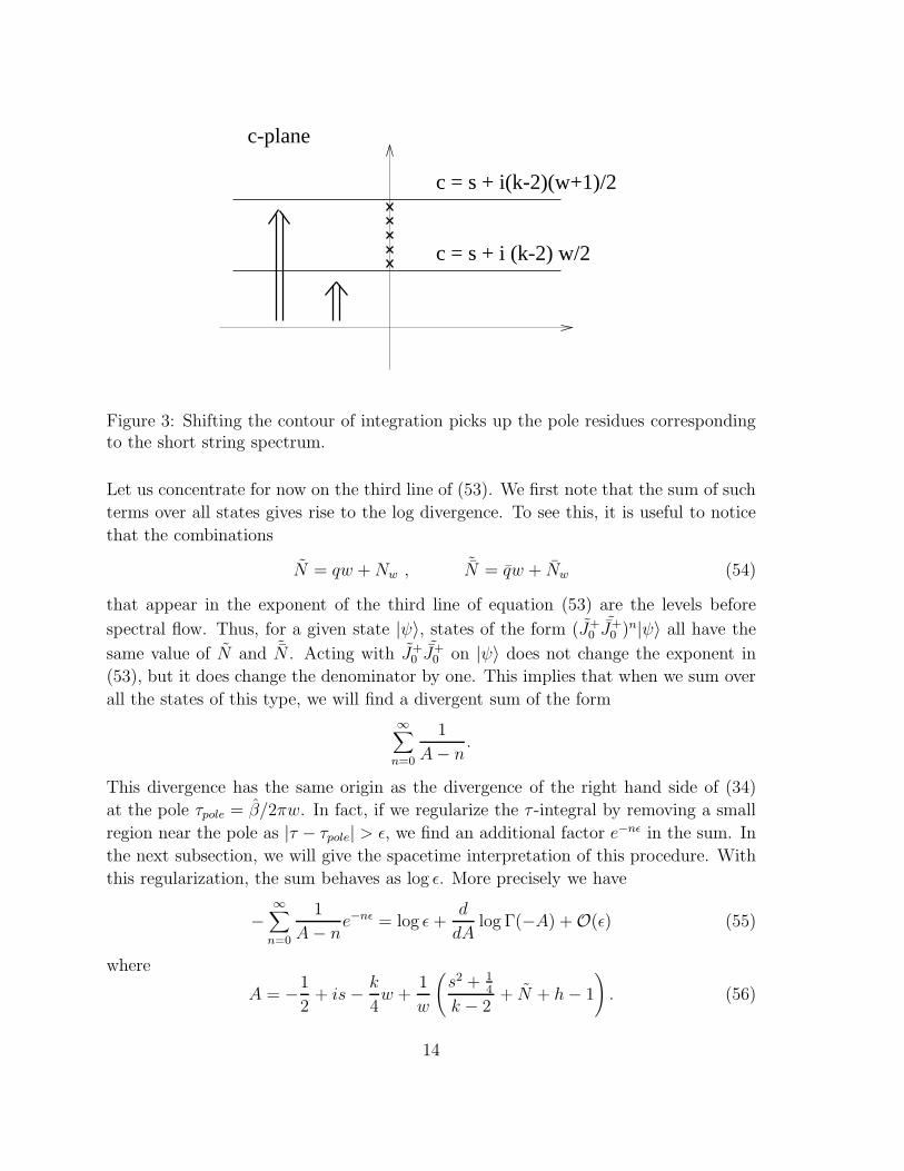
Let us first look at the first term (the second line) in (48). We note that the exponent

can be expressed in the form of a complete square if we set c = s + i2(k − 2)w. As

it will become clear shortly, it is natural to shift the contour of the c-integral from

Im c = 0 to Im c = 12(k − 2)w so that s becomes real. During this process the contour

crosses some poles in the integrand, picking up the residues of the poles in the range

0 < Im c < 12(k − 2)w. See Figure 3. The poles are located at

− c2

(k − 2)= Nw + h− 1

2w(w + 1) − 1 +

1

4(k − 2)<k − 2

4w2. (49)

Similarly, for the second exponential term (the third line) in (48) we shift the contour

to c = s + i2(k − 2)(w + 1) with s real. This picks up the poles at

− c2

(k − 2)= Nw + h− 1

2w(w + 1) − 1 +

1

4(k − 2)<k − 2

4(w + 1)2. (50)

It is important to note that the residues of these poles have a sign opposite to that of

the residues of the poles obeying (49). So the result is that we are left with only those

poles in the rangek − 2

2w < Im c <

k − 2

2(w + 1), (51)

with residues

1

βexp

−βq − ¯

βq − β

1 + 2w +

√

1 + 4(k − 2)(Nw + h− 1 − 1

2w(w + 1))

. (52)

This is the expected contribution of the short strings to the right hand side of (34),

and we see also that (51) translates into the correct bound on j (5).

It remains to examine the resulting integral over s. Notice that the term coming from

just above the pole at τ = β/2πw has a very similar w dependence in the exponent

as that coming from just below the pole. In other words, we combine the first term of

(48) with the second term of an expression similar to (48) but with w → w− 1 and we

find, after shifting the countours as above,

1

2πiβ

∫ ∞

−∞ds

(2s

w(k − 2)+ i

)

×

exp[−βq − ¯

βq − β(

k2w + 2

w

(s2+1/4

k−2+Nw−1 + h− 1

))]

12

+ is− k4w + 1

w

(Nw−1 + h− 1 + s2+1/4

k−2

)

−exp

[−βq − ¯

βq − β(

k2w + 2

w

(s2+1/4

k−2+Nw + h− 1

))]

−12

+ is− k4w + 1

w

(Nw + h− 1 + s2+1/4

k−2

)

. (53)

13

c-plane

c = s + i(k-2)(w+1)/2

c = s + i (k-2) w/2

Figure 3: Shifting the contour of integration picks up the pole residues correspondingto the short string spectrum.

Let us concentrate for now on the third line of (53). We first note that the sum of such

terms over all states gives rise to the log divergence. To see this, it is useful to notice

that the combinations

N = qw +Nw , ˜N = qw + Nw (54)

that appear in the exponent of the third line of equation (53) are the levels before

spectral flow. Thus, for a given state |ψ〉, states of the form (J+0

˜J+0 )n|ψ〉 all have the

same value of N and ˜N . Acting with J+0

˜J+0 on |ψ〉 does not change the exponent in

(53), but it does change the denominator by one. This implies that when we sum over

all the states of this type, we will find a divergent sum of the form

∞∑

n=0

1

A− n.

This divergence has the same origin as the divergence of the right hand side of (34)

at the pole τpole = β/2πw. In fact, if we regularize the τ -integral by removing a small

region near the pole as |τ − τpole| > ǫ, we find an additional factor e−nǫ in the sum. In

the next subsection, we will give the spacetime interpretation of this procedure. With

this regularization, the sum behaves as log ǫ. More precisely we have

−∞∑

n=0

1

A− ne−nǫ = log ǫ+

d

dAlog Γ(−A) + O(ǫ) (55)

where

A = −1

2+ is− k

4w +

1

w

(s2 + 1

4

k − 2+ N + h− 1

). (56)

14

Here we have assumed that˜N + h ≤ N + h, (57)

but it can be seen that the other case gives the same result.

Now we turn our attention to the second line of (53). In those terms we have one

less unit of spectral flow, as compared to the third line in (53) that we analyzed above.

In other words, now we will have that (w − 1)q + Nw−1 = N ′. These states are in

the spectral flow image of D+j . Since we want to combine these states with the states

coming from the third line in (53) it is convenient to do spectral flow one more time and

think of these states as in the spectral flow image of D−j under w units of spectral flow.

In this case we find that q+ N ′ = N where now N is the level of the D−j representation

before spectral flow. From now on the discussion is very similar to what we had above.

The states with (J−0

˜J−0 )n|ψ〉 all have the same energies but they will contribute to the

denominator of the second line in (53) with

∞∑

n=0

1

B + ne−nǫ = log ǫ− d

dBlog Γ(B) + O(ǫ) (58)

where

B =1

2+ is− k

4w +

1

w

(s2 + 1

4

k − 2+ ˜N + h− 1

), (59)

again assuming (57).

After we perform these two sums, we find that (53) can be written in the form

2

β

∫ ∞

0dsρ(s) exp

[−β

(E(s) + i

µ

w(N + h− ˜N − h)

)](60)

with E(s) the energy of long strings (7) and ρ(s) the density of states. We will later

see that the physical momentum p of a long string in the ρ direction is equal to p = 2s.

The angular momentum ℓ = (N + h− ˜N − h)/w is an integer since the states in (53)

were obeying (4) and the definition (54) ensures that (8) is satisfied. The density of

states ρ(s) derived from this analysis is

ρ(s) =1

2π2 log ǫ+

1

2πi

d

2dslog

(Γ(1

2− is+ ˜m)Γ(1

2− is− m)

Γ(12

+ is+ ˜m)Γ(12

+ is− m)

), (61)

where

m = −k4w+

1

w

(s2 + 1

4

k − 2+ N + h− 1

), ˜m = −k

4w+

1

w

(s2 + 1

4

k − 2+ ˜N + h− 1

). (62)

Note that, despite appearances to the contrary, (61) is actually symmetric under m↔˜m since m − ˜m = ℓ is an integer. In the next subsection we will show that this

15

density of states (61) is what is expected from the spacetime meaning of the cutoff

ǫ. In going from (53) to (60) we have states which could be interpreted as coming

from the spectral flow of the discrete representations D+j and D−

j , with the zero modes

essentially stripped off since they were explicitly summed over in (55) and (58). This

implies that the states we have in the end belong to the continuous representation.

Note also that the integral over s in (60) has only half the range in (53). We rewrote

it in this way using the fact that the exponent is invariant under s→ −s, and that is

the reason why we have four Gamma functions in (61). In going from (53) to (60) we

have also used that ddA

= 1dA(s)

ds

dds

in (56) and similarly in (59).

Combining eqns. (52) and (60), we have finally

f(β, µ) =1

β

∑D(h, h, N , ˜N,w)

∑

q,q

e−β(E+iµℓ) +∫ ∞

0dsρ(s)e−β(E(s)+iµℓ)

(63)

which is the free energy due to the short strings and the long strings, respectively.

4.3 The density of long string states

What remains to be shown is the interpretation of ρ(s) given by (61) as the density of

long string states. Whenever we have a continuous spectrum the density of states may

be calculated by first introducing a long distance cutoff which will make the spectrum

discrete, and then removing the cutoff. If the cutoff is related to the volume of the

system then the density of states will have a divergent part, proportional to the volume

and dependent only on the bulk physics, and a finite part which encodes information

about the scattering phase shift and also has some dependence on the precise cutoff

procedure. To see this, let us consider a one-dimensional quantum mechanical model on

the half line, ρ > 0, with a potential V (ρ). We assume that V (ρ) vanishes sufficiently

fast for large ρ, and that there is continuous spectrum above a certain energy level. To

define the density of states, it is convenient to introduce a long distance cutoff at large

ρ so that the spectrum becomes discrete. Let us first consider a cutoff by an infinite

wall at ρ = L. If L is sufficiently large, an energy eigenfunction ψ(ρ) near the wall can

be approximated by the plane wave

ψ(ρ) ∼ e−ipρ + eipρ+iδ(p), (64)

where δ(p) is the phase shift due to the original potential V (ρ). Imposing Dirichlet

boundary condition ψ(L) = 0 at the wall, we have

2pL+ δ(p) = 2π(n +

1

2

)(65)

16

for some integer n. If L is sufficiently large, there is a unique solution p = p(n) to this

equation for a given n. As we remove the cutoff by sending L → ∞, the spectrum of

p becomes continuous. We then define the density of states ρ(p) by

dn = ρ(p)dp. (66)

From (65), we obtain

ρ(p) =1

2π

(2L+

dδ

dp

). (67)

Thus the finite part of the density of states is given by the derivative of the phase shift.

Instead of the infinite wall at ρ = L, we may consider a more general potential

Vwall(ρ−L) which vanishes for ρ < L but rises steeply for L < ρ to confine the particle.

Let us denote by δwall(p) the phase shift due to scattering from Vwall(ρ). We then obtain

the condition on the allowed values of momenta by matching these two wavefunctions

and their derivatives at ρ = L as

ψ(ρ) ∼ e−ipρ + eipρ+iδ(p) ∼ A[e−ip(ρ−L) + eip(ρ−L)+iδwall(p)

], (ρ ∼ L). (68)

It follows that

pL+ δ(p) = −pL+ δwall(p) + 2πn. (69)

In the limit L→ ∞, the density of states given by dn = ρ(p)dp is then

ρ(p) =1

2π

(2L+

dδ

dp− dδwall

dp

). (70)

When we have the infinite wall, the phase shift due to the wall is independent of p

(δwall = π), and (70) reduces to (67).

In order to apply this observation to our problem, it is useful to first identify the

origin of the logarithmic divergence in the one-loop amplitude Z(β, µ) by examining

the functional integral (24) near the boundary of AdS3. In the cylindrical coordinates

(11), the string worldsheet action (18) for large ρ takes the form

S ∼ k

π

∫d2z

(∂ρ∂ρ+

1

4e2ρ|∂(θ − it)|2 + · · ·

). (71)

Because of the factor e2ρ, the functional integral for large ρ restricts (t, θ) to be a

harmonic map from the worldsheet to the target space. Since (t, θ) are coordinates on

the torus,

θ − it ∼ θ − it+ 2πn+ iβm, (n,m integers), (72)

17

the harmonic map from the torus to the torus is

θ − it = (2πw + iβm)σ1 + (2πr + iβn)σ2

=[(2πw + iβm)τ − (2πr + iβn)

] z

2iτ2

−[(2πw + iβm)τ − (2πr + iβn)

] z

2iτ2, (73)

where z = σ1 + τσ2 is the worldsheet coordinate and (r, w, n,m) are integers. In

particular, the map (θ− it) with (n,m) = (1, 0) becomes w-to-1 and holomorphic when

τ takes the special value

τpole =r

w+ i

β

2πw. (74)

On the other hand, if τ is not at one of these points, ∂(θ − it) cannot be set to zero7.

This gives rise to an effective potential e2ρ for ρ, which keeps the worldsheet from

growing towards the boundary. If τ is near τpole

τ = τpole + ǫ, (75)

the harmonic map (73) with (n,m) = (1, 0) gives

|∂(θ − it)|2 ∼(

2π2w2

β

)2

ǫ2. (76)

Thus the action (71) generates the Liouville potential ǫ2e2ρ. When we computed the

one-loop amplitude in sections 4.1 and 4.2, we regularized the τ -integral by removing

a small disk |τ − τpole| < ǫ around each of these special points. Near τ = τpole, this is

equivalent to adding the infinitesimal Liouville potential ǫ2e2ρ to the worldsheet action.

For |τ − τpole| ≫ ǫ, the worldsheet can never grow large enough and the effect of the

Liouville term is negligible. To be precise, the Gaussian functional integral of (t, θ)

shifts k → (k − 2) as in (26) and the effective action for ρ near τ = τpole is

SLiouville =k − 2

π

∫d2z

(∂ρ∂ρ+ ǫ2e2ρ

). (77)

Therefore, we find that our choice of regularization in (55) and (58) amounts to in-

troducing the Liouville wall which prevents the longs strings from going to very large

values of ρ. By looking at the potential in (77), we see that the effective length of the

interval is L ∼ log ǫ. The central charge of this Liouville theory is such that the e2ρ

term has conformal weight one,

cLiouville = 1 + 6(b+

1

b

)2

, b ≡ 1√k − 2

. (78)

7For any τ , we also have a trivial holomorphic map (t, θ) = const. The functional integral aroundsuch a map gives a result independent of β and we can neglect it in the following discussion.

18

The finite part of the density of states will be given through (70) by δ(s), the phase

shift in the SL(2, R) model, and δwall(s), the corresponding quantity in Liouville theory.

The first one was calculated in [9, 10],

iδ(s) = log

(Γ(1

2+ is− m)Γ(1

2+ is + ˜m)Γ(−2is)Γ( 2is

k−2)

Γ(12− is− m)Γ(1

2− is+ ˜m)Γ(2is)Γ(−2is

k−2)

), (79)

while the second one was obtained in [11, 12]8

iδwall(s) = log

(Γ(−2is)Γ( 2is

k−2)

Γ(2is)Γ(−2isk−2

)

). (80)

Using these two formulas we can check that indeed the density of states (61) is given

by (70). We can view this as an independent calculation of (79) or as an overall

consistency check. Notice that the physical momentum p of a long string along the ρ

direction is p = 2s. This can be seen by comparing the energy of a long string (7) with

the energy expected from (77) with spacetime momentum p along the radial direction,

p = (k − 2)wρ. We have chosen the variable s since it is conventional to denote by

j = 1/2 + is the SL(2, R) spin of a continuous representation.

Acknowledgements

H.O. would like to thank J. Schwarz and the theory group at Caltech for the kind

hospitality while this work was carried out.

The research of J.M. was supported in part by DOE grant DE-FGO2-91ER40654,

NSF grant PHY-9513835, the Sloan Foundation and the David and Lucile Packard

Foundations. The research of H.O. was supported in part by NSF grant PHY-95-

14797, DOE grant DE-AC03-76SF00098, and the Caltech Discovery Fund.

References

[1] J. Maldacena and H. Ooguri, “Strings in AdS3 and SL(2, R) WZW model. Part 1:

the spectrum,” hep-th/0001053.

[2] J. Balog, L. O’Raifeartaigh, P. Forgacs, and A. Wipf, “Consistency of string

propagation on curved space-time: an SU(1, 1) based counterexample,” Nucl.

Phys. B325 (1989) 225.

8In order to compare with the expressions in [11, 12] we use the value of b given in (78) and notethat the relevant values of α are α = Q/2 + isb.

19

L. J. Dixon, M. E. Peskin, and J. Lykken, “N = 2 superconformal symmetry and

SO(2, 1) current algebra,” Nucl. Phys. B325 (1989) 329-355.

P. M. S. Petropoulos, “Comments on SU(1, 1) string theory,” Phys. Lett. B236

(1990) 151.

N. Mohammedi, “On the unitarity of string propagating on SU(1, 1),” Int. J.

Mod. Phys. A5 (1990) 3201–3212.

I. Bars and D. Nemeschansky, “String propagation in backgrounds with curved

space-time,” Nucl. Phys. B348 (1991) 89–107.

S. Hwang, “No ghost theorem for SU(1, 1) string theories,” Nucl. Phys. B354

(1991) 100–112.

M. Henningson, S. Hwang, P. Roberts, and B. Sundborg, “Modular invariance of

SU(1, 1) strings,” Phys. Lett. B267 (1991) 350–355.

S. Hwang and P. Roberts, “Interaction and modular invariance of strings on

curved manifolds,” Proceedings of the 16th Johns Hopkins Workshop, Curent

Problems in Particle Theory (Goteborg, Sweden, 1992), hep-th/9211075.

S. Hwang, “Cosets as gauge slices in SU(1, 1) strings,” Phys. Lett. B276 (1992)

451–454, hep-th/9110039.

G. T. Horowitz and D. L. Welch, “Exact three-dimensional black holes in string

theory,” Phys. Rev. Lett. 71 (1993) 328-331, hep-th/9302126.

I. Bars, “Ghost-free spectrum of a quantum string in SL(2, R) curved

space-time,” Phys. Rev. D53 (1996) 3308–3323, hep-th/9503205.

M. Natsuume and Y. Satoh, “String Theory on three-dimensional black holes,”

Int. J. Mod. Phys. A13 (1998) 1229 - 1262, hep-th/9611041.

I. Bars, “Solution of the SL(2, R) string in curved spacetime,” Proceedings of the

conference, Strings 95 (USC, Los Angeles, 1995), hep-th/9511187.

Y. Satoh, “Ghost-free and modular invariant spectra of a string in SL(2, R)

curved space-time,” Nucl. Phys. B513 (1998) 213, hep-th/9705208.

H.J. de Vega, A.L. Larsen, and N. Sanchez, “Quantum string dynamics in the

conformal invariant SL(2, R) WZWN background: anti-de Sitter space with

torsion,” Phys. Rev. D58 (1998) 026001, hep-th/9803038.

A.L. Larsen and N. Sanchez, “From the WZWN model to the Liouville equation:

exact string dynamics in conformally invariant AdS background,” Phys. Rev.

D58 (1998) 126002, hep-th/9805173.

S. Hwang, “Unitarity of strings and non-compact hermitian symmetric spaces,”

20

Phys. Lett. B435 (1998) 331, hep-th/9806049.

J. M. Evans, M. R. Gaberdiel, and M. J. Perry, “The no-ghost theorem for AdS3

and the stringy exclusion principle,” Nucl. Phys. B535 (1998) 152,

hep-th/9806024.

A. Giveon, D. Kutasov, and N. Seiberg, “Comments on string theory on AdS3,”

Adv. Theor. Math. Phys. 2 (1998) 733–780, hep-th/9806194.

J. de Boer, H. Ooguri, H. Robins, and J. Tannenhauser, “String theory on AdS3,”

JHEP 12 (1998) 026, hep-th/9812046.

K. Hosomichi and Y. Sugawara, “Hilbert spce of space-time SCFT in AdS3

superstring and T 4kp/Skp SCFT,” JHEP 9901 (1999) 013, hep-th/9812100.

K. Hosomichi and Y. Sugawara, “Multistrings on AdS3 × S3 from matrix string

theory,” JHEP 9907 (1999) 027, hep-th/9905004.

D. Kutasov and N. Seiberg, “More comments on string theory in AdS3,”

hep-th/9903219.

I. Bars, C. Deliduman, and D. Minic, “String theory on AdS3 revisited,”

hep-th/9907087.

P. M. S. Petropoulos, “String theory on AdS3: some open questions,” Proceedings

of TMR European program meeting, Quantum Aspects of Gauge Theories,

Supersymmetry and Unification (Paris, France, 1999), hep-th/9908189.

G. Giribet and C. Nunez, “Interacting strings on AdS3,” JHEP 9911 (1999) 031,

hep-th/9909149.

A. Kato and Y. Satoh, “Modular invariance of string theory on AdS3,”

hep-th/0001063.

Y. Hikida, K. Hosomichi, and Y. Sugawara, “String theory on AdS3 as discrete

light cone Liouville theory,” hep-th/0005065.

N. Ishibashi, K. Okuyama, and Y. Satoh, “Path integral approach to string

theory on AdS3,” hep-th/0005152.

[3] M. Banados, M. Henneaux, C. Teitelboim, and J. Zanelli, “Geometry of the

2 + 1 black hole,” Phys. Rev. D48 (1993) 1506-1525, gr-qc/9302012.

[4] J. Maldacena and A. Strominger, “AdS3 black holes and a stringy exclusion

principle,” JHEP 9812 (1998) 005, hep-th/9804085.

[5] J. Maldacena, J. Michelson, and A. Strominger, “Anti-de Sitter fragmentation,”

JHEP 02 (1999) 011, hep-th/9812073.

21

[6] N. Seiberg and E. Witten, “The D1/D5 system and singular CFT,” JHEP 04

(1999) 017, hep-th/9903224.

[7] K. Gawedzki, “Noncompact WZW conformal field theories,” Proceedings of the

NATO Advanced Study Institute, New Symmetry Principles in Quantum Field

Theory (Cargese, France, 1991), hep-th/9110076.

[8] J. Polchinski, “Evaluation of the one loop string path integral,” Commun. Math.

Phys. 104 (1986) 37.

[9] J. Teschner, “On structure constants and fusion rules in the SL(2, C)/SU(2)

WZNW model,” Nucl. Phys. B546 (1999) 390, hep-th/9712256.

[10] A. B. Zamolodchikov, unpublished notes.

[11] H. Dorn and H. J. Otto, “Two and three point functions in Liouville theory,”

Nucl. Phys. B429 (1994) 375–388, hep-th/9403141.

[12] A. B. Zamolodchikov and A. B. Zamolodchikov, “Structure constants and

conformal bootstrap in Liouville field theory,” Nucl. Phys. B477 (1996) 577–605,

hep-th/9506136.

22