Stretch Processing

________________________________

-

Date 5/10/2013 3:43:00 PM 5/10/2013

To File

From Edward. C. Barile

Subject Stretch Processed Echoes – Wide to Medium Band Forms

ABSTRACT This memo provides a derivation of how Stretch Processing produces complex range profiles (complex I and Q echoes) from signals received by a radar after it illuminates a target. Stretch Processing is a means of obtaining a pulse compressed return when using a linear FM transmit pulse, in situations where it is impractical to do normal pulse compression using a crosscorrelation of the return signal with the transmit pulse. The memo then shows how to take stretch processed data, for a wide band radar, and perform operations on it to produce the stretch processed profiles for a medium or narrow band radar where the medium or narrow band is included within the original wide band. STRETCH PROCESSING FOR WIDEBAND RADAR Let us assume that a wideband radar has transmitted a Linear Frequency Modulated (LFM) pulse of form (see notational note in Appendix 1):

( ) ( ) ( )2exp 2 exp2w c w d

dx t i f t i t G tπ πµ = −

(1.1)

where the subscript “w” on any variable where it occurs indicates “wideband”, to distinguish the variable in question from a medium band variable which we shall subsequently need. Here, the

center frequency is cf , d is the pulse length, 2d

dG t

−

is a gate function of width d and

beginning at zero and ending at d (( )dG t is a gate symmetrical about t=0), and the LFM

parameter wµ is:

ww

B

dµ ≡ (1.2)

where wB is the bandwidth of the wideband signal.

Let us introduce the aspect angle dependent impulse response ( )nh t which depends on the aspect

angle which we can index using “n”. For multiple pulses, where the aspect angle of the target will, in general change between pulses, we will need to use a different impulse response for each pulse transmitted and the index “n” delineates them in this analysis. When we need to refer to it, by the way, we will call the Pulse Repetition Interval (PRI) for the wide band radar wT .

If, therefore, ( )wx t is transmitted and illuminates the target at aspect angle “n”, the signal

received, ( )ewx t , will be simply the convolution of ( )wx t with the impulse response( )nh t :

( ) ( ) ( )

( ) ( )( ) ( )( )2exp 2 exp

2

ew n w

n c w d

x t h x t d

dh i f t i t G t d

τ τ τ

τ π τ πµ τ τ τ

∞

−∞∞

−∞

= −

= − − − −

∫

∫

(1.3)

The superscript “e” on ( )ewx t indicates “echo”.

Notice that the transmit – scatter – receive process is linear, but not time invariant. It is not time invariant, because a pulse transmitted at a later time will encounter a different impulse response (different n). It is also not space-invariant, because if the transmitter/receiver, which are assumed collocated are moved to a different location relative to the target, a different aspect angle between the radar line of sight (RLOS) and the target axis will occur and hence a different impulse response will once again be necessary. In order to get better insight into stretch processing, let us use a simple point scatterer model for the impulse response ( )nh t , although it is not necessary to specialize our analysis to this case:

( ) ( )( )

1

2NS nn

n

r nh t A t

cσ

σσ

δ=

= −

∑ (1.4)

Here, we imply that for the nth aspect angle, the target has NS(n) scatterers located at ranges

( )r nσ with ( )1,2,... ( )NS nσ = (and these ranges are different for different aspects n) each with

reflectivity nAσ . This means that if we transmit an impulse at the target when it presents aspect n,

we get a set of delayed impulses each weighted by its reflectivity (and inversely to its range, which we ignore here) and at these arrive at times corresponding to the travel time from the radar to each scatterer and back. (The speed of light in free space is denoted here as “c”). In general, this model will be incomplete – there will be all kinds of other scattered signals due to multiple reflections and other effects, which will not correspond to a point scatterer model, but we will use this simple model for illustrative purposes only. Incidentally if the target rotates about a center of gravity, then the ranges ( )r nσ will vary with n

both due to the motion of the center of gravity and the rotation, each of which can change the actual aspect angle seen by the Radar line Of Sight (RLOS).

Our simple point scatterer model gives echo:

( ) ( ) ( )

( ) ( )( )

( )( )( )

( ) ( )

( )

1

2

( )

1

2

2exp 2

exp2

2exp 2

2 2exp

2

ew n w

NS nn

c

w d

NS nn

c

w d

x t h x t d

r nA i f t

c

di t G t d

r nA i f t

c

r n r n di t G t

c c

σσ

σ

σσ

σ

σ σ

τ τ τ

δ τ π τ

πµ τ τ τ

π

πµ

∞

−∞

∞

=−∞

=

= −

= − −

− − −

= −

− − −

∫

∑∫

∑

(1.5)

which is, as we expect, a reflectivity weighted sequence of replicas of the LFM transmit pulse shifted in time to the two way travel time of each scatterer, or scatterer delay time. The pulse length of each of these pulses, d, is much longer than the time difference of any of the scatterer delay times, so we need to compress the pulses to resolve the scatterer delay times. In fact, we really would like to get ( )e

wx t as close as possible to the actual impulse response, wherein the

resolution is infinitesimal. Note that if we were able to use crosscorrelation with the transmit pulse for range compression, we would have:

( ) ( ) ( ) ( ) ( ) ( )

( ) ( ) ( )

( ) ( )

( ) ( ) ( )

* *

*

*

e ew w w n w w

n w w

n ww

ww w w

x t x t dt dt h x t x t d

h d x t x t dt

h d

where

x t x t dt

ϕ σ σ τ τ σ τ

τ τ τ σ

τ ϕ σ τ τ

ϕ σ σ

∞ ∞ ∞

−∞ −∞ −∞

∞ ∞

−∞ −∞

∞

−∞

∞

−∞

≡ − = − −

= − −

= −

≡ −

∫ ∫ ∫

∫ ∫

∫

∫

(1.6)

is the autocorrelation of the transmit pulse. This function is usually very narrow and has low sidelobes, so that ( )e

wϕ σ is very close to the impulse response:

( ) ( ) ( ) ( ) ( )( )

1

2NS ne nw n ww n

r nh d h A t

cβ

ββ

ϕ σ τ ϕ σ τ τ σ δ∞

=−∞

= − ∝ = −

∑∫ (1.7)

Of course this is only approximate, but the main idea is to get the best resolution in range and this is accomplished by trying to estimate the impulse response. Instead of doing the match filtering or cross correlation with the transmit pulse described in (1.6) and (1.7), we look for another way to transform the received signal into an estimate of the impulse response. Let us repeat for convenience the received signal from (1.3):

( ) ( ) ( )

( ) ( )( ) ( )( )2exp 2 exp

2

ew n w

n c w d

x t h x t d

dh i f t i t G t d

τ τ τ

τ π τ πµ τ τ τ

∞

−∞

∞

−∞

= −

= − − − −

∫

∫

(1.8)

In stretch processing, we mix or modulate the received signal with a replica of the transmitted LFM pulse, only we let the pulse length be as long as the entire echo, which we take as D. So we define the “reference LFM pulse” ( )r

wx t :

( ) ( ) ( )2exp 2 exp2

rw c w D

Dx t i f t i t G t

D d

π πµ ≡ −

≫

(1.9)

and multiply the conjugate of the received signal by the reference signal to get the “deramped” signal ( )D

wx t :

( ) ( ) ( ) ( ) ( ) ( )

( ) ( ) ( ) ( )

* * *

* 2exp 2 exp exp 22 2

D e r rw w w n w w

n c w w d D

x t x t x t h x t x t d

d Dh i f i i t G t d G t

τ τ τ

τ π τ πµ τ πµ τ τ τ

∞

−∞

∞

−∞

≡ = −

= − − − −

∫

∫

(1.10)

We conjugate the impulse response even though we may assume it is real valued, for consistency and uniformity of notation. We now apply a weighting, typically a Taylor weighting whose frequency spectrum has low sidelobes and reasonable beamwidth (the lower the sidelobes, the fatter the beam and resolution gets worse). Let the weighting be denoted ( )wW t with Fourier transform [ ]wW f (brackets

denote frequency domain) and applying the weights to the deramped signal and taking the Fourier transform of it, we have:

[ ] ( ) ( ) ( ) ( )

( ) ( )

* 2exp 2 exp exp 2

exp 22 2

W n c w w

d D w

S f d h i f i dt i t

d DG t G t W t i ft

τ τ π τ πµ τ πµ τ

τ π

∞ ∞

−∞ −∞

≡ −

− − − −

∫ ∫ (1.11)

Let us consider the integral in J (1.11) defined as:

( ) ( ) ( ) ( )exp 2 exp 22 2w d D w

d DJ dt i t G t d G t W t i ftτ πµ τ τ τ π

∞

−∞

≡ − − − −

∫ (1.12)

We will assume that the weighting function has support that is smaller than the length D of the

reference pulse, so we can remove 2D

DG t −

from (1.12) since it is unity everywhere that the

weighting is non zero:

( ) ( ) { }( )exp 22d w w

dJ dtG t W t i f tτ τ π µ τ

∞

−∞

= − − − −

∫ (1.13)

Now we turn to our simple model of the impulse response and realize that the domain over which the impulse response is nonzero (its support) is the time between the return from the first and last scatter. Let us make the notational simplification for the scatterer delay times:

( )2n r n

cσ

στ ≡ (1.14)

If we make the weighting ( )wW t nonzero only in the interval:

( )( ) 1,n nNS nI dτ τ= + (1.15)

then the function 2d

dG t τ − −

will never be different from unity for any value of τ in the

integration domain, which covers the support of the impulse response, in (1.11). To see this, it is better to rewrite the gate function in terms of unit step functions:

( ) ( )1 12d

dG t u t u t dτ τ τ− −

− − = − − − −

(1.16)

Note that the last value of τ in the integral ( )J τ in (1.11) will be ( )

nNS nτ and that d >> ( )

nNS nτ - 1

nτ ,

the support of the impulse response. The interval over which the weighting function starts is at the time ( )

nNS nτ that the last scatterer returns the leading edge of its reflected pulse and ends right

when the signal from the first scatterer has ended ( 1n dτ + ). This means that the function

( ) ( )1 12d

dG t u t u t dτ τ τ− −

− − = − − − −

(1.17)

for:

( )( ) 1,n nNS nt I dτ τ∈ = + (1.18)

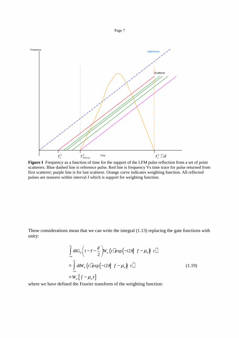
will always be unity as long as the weighting function is restricted to interval I. Figure I illustrates this. In Figure I, we show a plot of the frequency support of the received signal as a function of time. Since each return is a LFM pulse, we get a sequence of parallel lines each with slope defined by the FM parameter wµ and delayed in time by the scatterer’s delay

time. As seen, the pulse length d of the transmit pulse is much larger than the span of the scatterer delay times. Shown is a layover (for visualization only) of the weighting function, zero outside the interval I, and it is seen that all of the pulse returns are nonzero during the interval I, over which the weighting is defined and centered. The interval I is found by measuring the location in time of the first scatterer 1

nτ (when the echo starts to be detected) and the location in time of the trailing edge of the return from the last scatterer ( )

nNS n dτ + . The location of the beginning of the interval I is found by subtracting d from

the location in time of that trailing edge of the return from the last scatterer, and the end of the interval is found by adding d to the location in time of the leading edge of the return from the first scatterer. Once the interval is found, the weighting function is constructed to be centered at the midpoint of the interval and truncated at the ends.

Figure I Frequency as a function of time for the support of the LFM pulse reflection from a set of point scatterers. Blue dashed line is reference pulse. Red line is frequency Vs time trace for pulse returned from first scatterer; purple line is for last scatterer. Orange curve indicates weighting function. All reflected pulses are nonzero within interval I which is support for weighting function. These considerations mean that we can write the integral (1.13) replacing the gate functions with unity:

( ) { }( )

( ) { }( )[ ]

exp 22

exp 2

d w w

w w

w w

ddtG t W t i f t

dtW t i f t

W f

τ π µ τ

π µ τ

µ τ

∞

−∞

∞

−∞

− − − −

= − −

= −

∫

∫ (1.19)

where we have defined the Fourier transform of the weighting function:

1

nτ ( )nNS nτ 1

n dτ +

refererence

Scatterer returns

Time

Frequency

[ ] ( ) ( )exp 2w wW f W t i ft dtπ∞

−∞

≡ −∫ (1.20)

Then, we have for the Stretch Processed output:

[ ] ( ) ( ) ( ) [ ]* 2exp 2 expW n c w w wS f h i f i W f dτ π τ πµ τ µ τ τ∞

−∞

≡ − −∫ (1.21)

We note that if the weighting transform [ ]wW f is very narrow with low sidelobes, then

approximately we have:

[ ] ( ) ( ) ( ) [ ]* 2

2

exp 2 exp

exp 2 exp

W n c w w

cn

w w w

S f h i f i f d

f ff fh i i

τ π τ πµ τ δ µ τ τ

π πµ µ µ

∞

−∞

− −

= −

∫∼ (1.22)

If we transform the frequency variable so that 2 wf

c

µ ρ≡ then we have the complex stretch

processed range profile:

[ ]

( ) ( ) ( )* 2

2

2exp 2 exp

R wW W

n c w w w

S Sc

h i f i W dc

µ ρρ

ρτ π τ πµ τ µ τ τ∞

−∞

≡

= − −

∫ (1.23)

Again, using our simplified point scatterer model we have:

[ ] ( ) ( ) ( )

( ) ( ) ( ){ }

( )( ) ( )

( )* 2

1

2( )

*

1

2( )

*

1

2 2exp 2 exp

exp 4 exp 4 2

exp 2 exp 4

NS nR n

W c w w w

NS nn w

c w w

NS nn

c w

r nS A i f i W d

c c

r n r nA i f i W r n

c c c

r nA i k r n i

c

σσ

σ

σ σσ σ

σ

σσ σ

σ

ρρ δ τ π τ πµ τ µ τ τ

µπ πµ ρ

πµ

∞

=−∞

=

=

= − − −

= − −

= −

∑∫

∑

∑ ( ){ }2 wwW r n

c σµ ρ

−

(1.24)

where we have used the wavenumber 2 c

c

fk

c

π≡ for free space at the center frequency cf for the

transmit pulse. Let us examine this in detail:

[ ] ( )( ) ( ) ( ){ }2

( )*

1

exp 2 exp 4 2NS n

R n wW c w w

r nS A i k r n i W r n

c cσ

σ σ σσ

µρ πµ ρ=

= − − ∑ (1.25)

The term ( )( )exp 2 ci k r nσ is simply the phase term for the propagation to the scatterer at range

( )r nσ and back . Aside from the quadratic distortion term ( ) 2

exp 4 w

r ni

cσπµ

−

this

expression looks like the profile that would be obtained using matched filtering if the

autocorrelation of the transmit pulse were the Weighting function transform { }2 wwW

c

µ ρ

delayed in range to the location of each scatterer. The weighting is chosen so that it has low sidelobes and a sharp main lobe (is small when the argument is nonzero). To remove the effect of the quadratic distortion term, approximately, we notice that if we multiply the profile by a correction term:

[ ] [ ]

( )( ) ( ) ( ){ }

2

2 2( )*

1

exp 4

exp 2 exp 4 2

C RW W w

NS nn w

c w w

S S ic

r nA i k r n i W r n

c c cσ

σ σ σσ

ρρ ρ πµ

µρπµ ρ=

≡

= − − − ∑

(1.26)

then at the ranges ( )r nσρ = the quadratic distortion is cancelled and is relatively small for

ranges in between where the argument of the weighting function transform is nonzero. So the quadratic phase distortion corrected profile is:

[ ] ( ) ( )2

* 2 2exp 2 exp

2

CW n c w

w w

S h i f ic

W dc

ρρ τ π τ πµ τ

ρµ τ τ

∞

−∞

= − −

−

∫ (1.27)

The stretch processed profile for a medium band transmit pulse whose band lies within the wide band we have just discussed is obtained from (1.27) by replacing the center frequency with the medium band center frequency, the wide band LFM factor wµ with the medium band value

Mµ and the weighting function transform by its medium band version [ ]M MW µ τ , the details of

which we will present shortly, as we give a step by step procedure to transform (1.27) into the medium band version. Let us summarize and note that (1.27) can be written in simple symbolic form:

[ ] ( ) ( ) ( ){ }*

2 w

R e rW w w w

fc

S W t x t x tµ ρρ=

= ℑ (1.28)

where { }ℑ denotes the Fourier Transformation operator:

[ ] ( ){ } ( ) ( )exp 2x f x t x t i ft dtπ∞

−∞

= ℑ ≡ −∫ (1.29)

In other words, we take the received echo, conjugate it, multiply it by the reference pulse and the weighting and then inverse Fourier transform the result after which we transform the frequency

variable to change the argument into range, via 2 wf

c

µ ρ≡ . Then we multiply by the quadratic

phase correction term 2

exp 4 wic

ρπµ

as in (1.26) to get the corrected stretch processed

output. Let us see how to transform the wide band stretch processed profile [ ]R

WS ρ into a medium band

version [ ]RMS ρ . Basically we want to convert:

[ ] ( ) ( ) ( ){ }*

2 w

R e rW w w w

fc


= ℑ (1.30)

into:

[ ] ( ) ( ) ( ){ }*

2 M

R e rM M M M

fc


= ℑ (1.31)

1. Take wide band corrected profile [ ]CWS ρ and multiply it by

2

exp 4 wic

ρπµ −

to get

uncorrected wideband profile [ ]RWS ρ .

2. Take uncorrected wideband profile [ ]RWS ρ and change range variable to frequency via

2

2w

w

cff

c

µ ρ ρµ

≡ ⇔ = to get [ ]WS f

3. Because (1.30) involves the Fourier Transform, take the inverse Fourier Transform of

[ ]WS f to get:

( ) ( ) ( ) ( ) ( )*

1e r

W w w wg t S t x t x t W t≡ = (1.32)

4. Now calculate:

( ) ( )( ) ( )

( )( ) ( ) ( ) ( ) ( )* *1

2W e

w n wr rw w w w

g t S tk t x t h x t d

x t W t x t W tτ τ τ

∞

−∞

≡ = = = −∫ (1.33)

and conjugate it so that ( ) ( )*2 2g t k t=

This can be written as:

( ) ( ) ( )2 n wg t h x t dτ τ τ∞

−∞

= −∫ (1.34)

5. Now take the Fourier Transform of ( )2g t and get:

[ ] [ ] [ ]2 n wg f h f x f= (1.35)

6. Now divide [ ]2g f by [ ]wx f to find the spectrum of the impulse response, or the scatterer

transfer function [ ]nh f . Of course, we only can divide for those frequencies where the

transmit spectrum is nonzero. This, means that the radar only has access to the impulse response of the target for frequencies in the band of the transmit pulse, as well as only for the aspect angles seen during the interrogation of the target by the radar. So when we refer to the impulse response of the target as measured by the radar, it is not the complete impulse response, only the part as filtered out by the band of the transmit pulse. As long as the medium band pulse we wish to emulate is within the band of the originating wide band pulse, we will be able to derive the medium band response.

7. Having the spectrum of the impulse response (within the wide band wB ) we now start to

build the medium band profile. Multiply [ ]nh f by the spectrum of the medium band

transmitted waveform [ ]Mx f.

We can combine steps 6 and 7:

[ ] [ ][ ] [ ] [ ] [ ]2

3 M n Mw

g fg f x f h f x f

x f= ∼ (1.36)

where we have noted that

[ ][ ] [ ]M

Mw

x fx f

x f∼ (1.37)

because the wide band spectrum of a LFM pulse is very nearly unity within its band for a pulse with a large time-bandwidth product and the medium band spectrum is contained within its support. Equation (1.34) may be approximated by simply filtering out the medium band part of the spectrum of the wide band impulse response. If the wide band pulse does not have a large time-bandwidth product, then the expression for its spectrum must be used without the approximation in (1.35) which makes the procedure more involved. A discussion and derivation of the spectrum of the LFM pulse for large time-bandwidth product is given in Rihaczek, A.; Principles of High-Resolution Radar, McGraw-Hill, 1969 on page166, equation (6.26) and for any time-bandwidth product in section 7.2.

In order to emulate the effect of the medium band transmit pulse being of the same energy as the wideband transmit pulse, we could amplify the result of (1.34) by the ratio of the wideband to the medium band. By Parceval’s theorem, the wide band and amplified medium band pulse would then be equal in energy.

8. Take the Inverse Fourier Transform of this to get the medium band echo ( )eMx t

9. Now multiply the conjugated medium band echo by the medium band reference pulse ( )rMx t

to “deramp” the echo, and multiply this by the medium band weighting function ( )MW t .

10. Take the Fourier transform of this and get the medium band profile, after which one may multiply by the appropriate phase correction function to get the corrected stretch processed profile.

Obtaining the Stretch Processed Profile from XPATCH Data In the course of various studies, we need to generate the stretch processed complex profiles from XPATCH Computer generated scattering models. Typically, for a set of aspect angles, the harmonic scattered field is calculated for a dense set of frequencies within the band of interest. That is, if the transmit pulse has its spectrum in some band of frequencies, a calculation is made using a time harmonic excitation for each of a large group of frequencies within the transmit pulse spectral support (frequency band) and the response for the transmit signal is synthesized using this frequency response multiplied by the spectrum of the transmit signal. We wish to infer the profile that would be obtained using any transmit pulse whose spectrum lies within the band of the model and its stretch processed form. Let us return to equation (1.23) which gives the stretch processed profile in terms of the impulse response of the target:

[ ]

( ) ( ) ( )* 2

2

2exp 2 exp

R wW W

n c w w w

S Sc

h i f i W dc

µ ρρ

ρτ π τ πµ τ µ τ τ∞

−∞

≡

= − −

∫ (1.38)

In terms of frequency 2 wf

c

µ ρ≡ this is:

[ ] ( ) ( ) ( ) [ ]* 2exp 2 expW n c w w wS f h i f i W f dτ π τ πµ τ µ τ τ∞

−∞

= − −∫ (1.39)

Now we can expand the impulse response into its spectral components via the Fourier synthesis:

( ) [ ] ( )exp 2n nh h i dτ υ πυτ υ∞

−∞

= ∫ (1.40)

with conjugate (even though ( )nh τ is real)

( ) [ ] ( )* * exp 2n nh h i dτ υ πυτ υ∞

−∞

= −∫ (1.41)

which gives us for the profile:

[ ] [ ] { }( ) ( ) [ ]* 2exp 2 expW n c w w wS f h i f d i W f dυ π υ τ υ πµ τ µ τ τ∞ ∞

−∞ −∞

= − − − −∫ ∫ (1.42)

Now let us apply the quadratic phase correction to (1.39):

[ ] [ ]

[ ] { }( )( )

[ ]

2

22

*

exp

exp 2 exp

CW W

W

w

n c w ww

fS f S f i

fh i f d i W f d

πµ

µ τυ π υ τ υ π µ τ τ

µ

∞ ∞

−∞ −∞

=

− = − − − −

∫ ∫

(1.43)

If the Transform of the weighting [ ]w wW f µ τ− is very small (-35 dB or smaller) for wf µ τ≠

then since the exponential with the quadratic term is suppressed for wf µ τ≠ and unity for

wf µ τ= we can remove it, and approximately:

[ ] [ ] { }( ) [ ]

[ ] [ ] { }( )

*

*

exp 2

exp 2

CW n c w w

n w w c

S f h i f d W f d

h W f i f d d

υ π υ τ υ µ τ τ

υ µ τ π υ τ τ υ

∞ ∞

−∞ −∞∞ ∞

−∞ −∞

− − −

= − − −

∫ ∫

∫ ∫

∼

(1.44)

This is then in terms of the spectrum [ ]nh υ of the impulse response ( )nh t and the weighting

function ( )wW t the following:

[ ] [ ] [ ] ( ) { }

[ ] ( ) ( )

*

*

exp 2

exp 2

CW n w c

w w

c cn w

w w w

f dS f h W i f d

f f dh W i f

σ συ σ π υ υµ µ

υ υ υυ πµ µ µ

∞ ∞

−∞ −∞

∞

−∞

− = − − −

− − = − −

∫ ∫

∫

(1.45)

Let:

( ) [ ] ( )*n c

ww w

h fG W

υ υυ

µ µ−

≡ −

(1.46)

Then:

[ ] exp 2C cW

w w

fffS f G i π

µ µ

=

(1.47)

where:

[ ] ( ) ( )

( )

exp 2

exp 2

wf

tw

ft

w

w

fG G t G i t d

fG i d

µ

µυ πυ υ

µ

υ πυ υµ

=

∞

=−∞

∞

−∞

= = −

= −

∫

∫

(1.48)

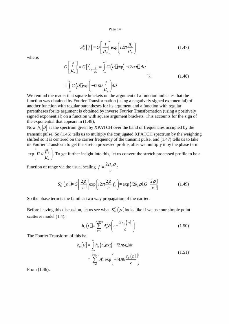
We remind the reader that square brackets on the argument of a function indicates that the function was obtained by Fourier Transformation (using a negatively signed exponential) of another function with regular parentheses for its argument and a function with regular parentheses for its argument is obtained by inverse Fourier Transformation (using a positively signed exponential) on a function with square argument brackets. This accounts for the sign of the exponential that appears in (1.48). Now [ ]nh υ is the spectrum given by XPATCH over the band of frequencies occupied by the

transmit pulse. So (1.46) tells us to multiply the conjugated XPATCH spectrum by the weighting shifted so it is centered on the carrier frequency of the transmit pulse, and (1.47) tells us to take its Fourier Transform to get the stretch processed profile, after we multiply it by the phase term

exp 2 c

w

ffi π

µ

. To get further insight into this, let us convert the stretch processed profile to be a

function of range via the usual scaling 2 wf

c

µ ρ= :

( ) ( )2 2 2exp 2 exp 2C

W c cS G i f i k Gc c c

ρ ρ ρρ π ρ = = (1.49)

So the phase term is the familiar two way propagation of the carrier. Before leaving this discussion, let us see what ( )C

WS ρ looks like if we use our simple point

scatterer model (1.4):

( ) ( )( )

1

2NS nn

n

r nh t A t

cσ

σσ

δ=

= −

∑ (1.50)

The Fourier Transform of this is:

[ ] ( ) ( )

( )( )

1

exp 2

exp 4

n n

NS nn

h h t i t dt

r nA i

cσ

σσ

υ πυ

πυ

∞

−∞

=

= −

= −

∫

∑ (1.51)

From (1.46):

( ) [ ] ( )

( ) ( )

*

( )*

1

1exp 4

n cw

w w

NS ncn

ww w

h fG W

r n fA i W

cσ

σσ

υ υυ

µ µ

υπυ

µ µ=

− ≡ −

− = −

∑

(1.52)

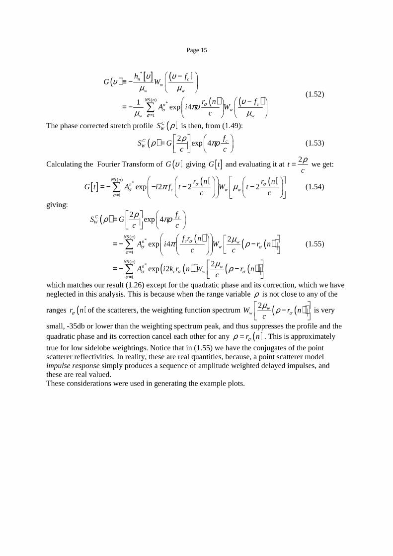
The phase corrected stretch profile ( )CWS ρ is then, from (1.49):

( ) 2exp 4C c

W

fS G

c c

ρρ πρ = (1.53)

Calculating the Fourier Transform of ( )G υ giving [ ]G t and evaluating it at 2

tc

ρ= we get:

[ ] ( ) ( )( )*

1

exp 2 2 2NS n

nc w w

r n r nG t A i f t W t

c cσ σ

σσ

π µ=

= − − − − ∑ (1.54)

giving:

( )

( ) ( )( )

( )( ) ( )( )

( )*

1

( )*

1

2exp 4

2exp 4

2exp 2

C cW

NS ncn w

w

NS nn w

c w

fS G

c c

f r nA i W r n

c c

A i k r n W r nc

σσ σ

σ

σ σ σσ

ρρ πρ

µπ ρ

µ ρ

=

=

=

= − −

= − −

∑

∑

(1.55)

which matches our result (1.26) except for the quadratic phase and its correction, which we have neglected in this analysis. This is because when the range variable ρ is not close to any of the

ranges ( )r nσ of the scatterers, the weighting function spectrum ( )( )2 wwW r n

c σµ ρ −

is very

small, -35db or lower than the weighting spectrum peak, and thus suppresses the profile and the quadratic phase and its correction cancel each other for any ( )r nσρ = . This is approximately

true for low sidelobe weightings. Notice that in (1.55) we have the conjugates of the point scatterer reflectivities. In reality, these are real quantities, because, a point scatterer model impulse response simply produces a sequence of amplitude weighted delayed impulses, and these are real valued. These considerations were used in generating the example plots.

Examples In the next group of figures we show some results of transforming wide band stretch processed profiles to their medium band versions, that is, the profiles that a radar would measure with a medium band interrogating pulse with energy the same as the wide band pulse.

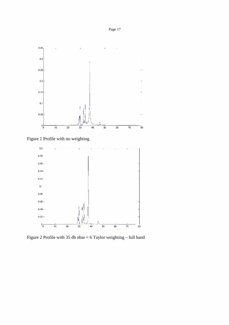
Figure 1 Profile with no weighting

Figure 2 Profile with 35 db nbar = 6 Taylor weighting – full band

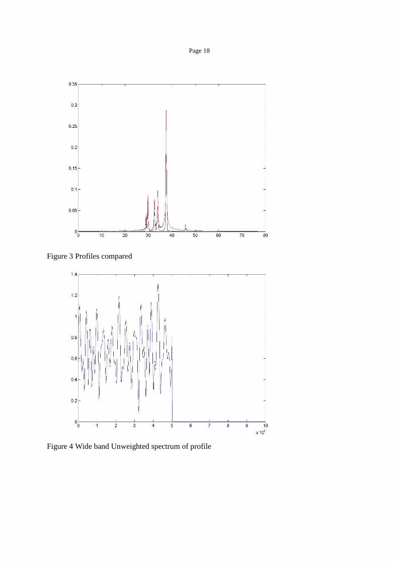
Figure 3 Profiles compared

Figure 4 Wide band Unweighted spectrum of profile

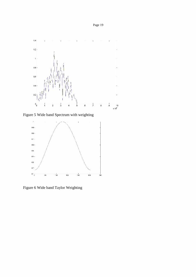
Figure 5 Wide band Spectrum with weighting

Figure 6 Wide band Taylor Weighting

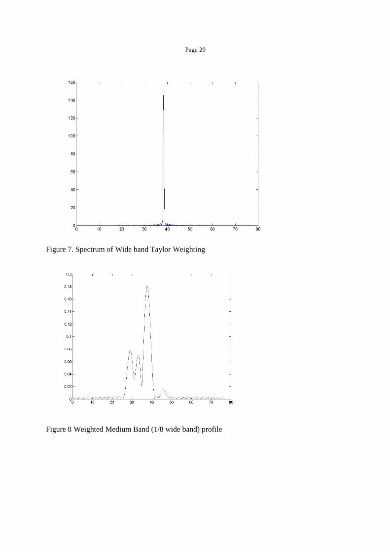
Figure 7. Spectrum of Wide band Taylor Weighting

Figure 8 Weighted Medium Band (1/8 wide band) profile

Figure 9 Comparison of Wideband unweighted and Medium band weighted profiles

Figure 10 Spectrum of Weighted Medium Band profile

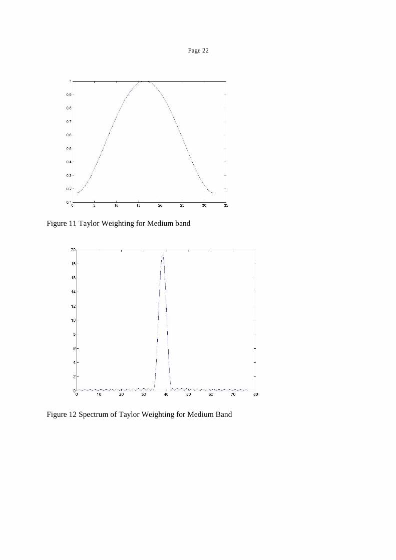
Figure 11 Taylor Weighting for Medium band

Figure 12 Spectrum of Taylor Weighting for Medium Band

Figure 13 Weighted Narrow Band (1/32 wideband) Profile

Figure 14 Comparison of Narrow band Weighted and unweighted wideband profiles

APPENDIX In this appendix, we discuss our logic behind choosing sign for ( )exp 2 ci f tπ in equation(1)

(rather than ( )exp 2 ci f tπ− ) and the exponential sign in the Fourier Decomposition and Synthesis

Integrals. We start with how we choose to define the Fourier integrals. The decomposition integral is chosen as:

[ ] ( ) ( )exp 2f f t i t dtυ πυ∞

−∞

≡ −∫ (1.56)

and the synthesis integral is:

( ) [ ] ( )exp 2f t f i t dυ πυ υ∞

−∞

≡ ∫ (1.57)

The reasoning for choosing these is as follows. In the synthesis integral (1.56) we are expressing a function ( )f t as a continuous linear combination of unit harmonic exponentials ( )exp 2i tπυ

each with positive frequency υ in Hz. So we synthesize ( )f t by adding together a weighted (by

[ ]f υ ) sum of exponential waveforms – one for each frequency υ . So the sign of the exponential

must be positive. This forces the sign in the decomposition or analysis integral to be opposite, or negative. The decomposition integral takes function ( )f t and resolves or decomposes it into unit exponentials,

one for each frequency, and the “component” of the function ( )f t at the frequency υ is [ ]f υ .

If ( )f t is treated as a vector defined in function space, then (1.55) gives the component of ( )f t

along the function space unit vector defined by ( )exp 2i tπυ and that is obtained by a dot product

of ( )f t with the adjoint ( )exp 2i tπυ− . The synthesis integral (1.56) is simply the construction

of the function space vector ( )f t by adding up its components.

If we are to adopt this interpretation of the Fourier integral expansions, then if we have a carrier wave with harmonic frequency cf , and we take its Fourier transform we have:

[ ] ( ) ( )

( ) ( )

[ ]( )[ ]

exp 2

exp 2 exp 2

exp 2

c

c

c

f f t i t dt

i f t i t dt

i f t dt

f

υ πυ

π πυ

π υ

δ υ

∞

−∞∞

−∞∞

−∞

= −

= ± −

= −

=

∫

∫

∫ ∓

∓

(1.58)

So, in order for the frequency in the signal to be positive in the frequency domain, we must choose the positive sign in ( )exp 2 ci f tπ and for any carrier frequency.

Stretch Processing

Documents

Transcript of Stretch Processing