Stress rate formulation for elastoplastic models withinternal variables based on augmented Lagrangian

regularisation

M. Cuomo*, L. Contrafatto

Istituto di Scienza delle Costruzioni, University of Catania, Facolta di Ingegneria, Viale A. Doria, 6, 95125, Catania, Italy

Received 30 October 1998; received in revised form 15 May 1999

Abstract

The constitutive laws of elasto-plasticity with internal variables are described through the de®nition of suitabledual potentials, which include various hardening models. A family of variational principles for inelastic problems isobtained using convex analysis tools. The structural problem is analysed using the complementary energy (Prager±Hodge) functional. The functional is regularised introducing an Augmented Lagrangian Regularisation for the

indicator function of the elastic domain so that a smooth optimisation problem is obtained. In the numericalsolution the discretised problem is reformulated in a ®nite step form using a fully implicit integration scheme andthe functional is rede®ned in the space of the self-equilibrated nodal stresses, after enforcing satisfaction of the

equilibrium equations in a weak form. Numerical tests have shown good performance on the part of the algorithm,which approaches the converged solution for a considerably smaller number of elements as compared with otheralgorithms. The method is equally available for perfect or hardening plasticity. 7 2000 Elsevier Science Ltd. All

rights reserved.

Keywords: Plasticity; Stress formulation; Mixed F.E.M; Augmented Lagrangian

1. Introduction

Mixed methods have gained growing interest in computational literature, especially in the ®eld of

solid mechanics. They allow locking phenomena to be avoided (Olson, 1983), they o�er better

performance with distorted elements and guarantee faster convergence rates (Berkovic and Mijuca,

International Journal of Solids and Structures 37 (2000) 3935±3964

0020-7683/00/$ - see front matter 7 2000 Elsevier Science Ltd. All rights reserved.

PII: S0020-7683(99 )00163-8

www.elsevier.com/locate/ijsolstr

* Corresponding author. Fax: +39-0957382297.

E-mail address: mcuomo@isc.ing.unict.it (M. Cuomo).

1998). One of the main advantages of mixed formulations is therefore the possibility of using coarsemeshes and low-order elements with a consequent reduction in computational e�ort.

After the pioneering work of Pian on assumed stress distributions (Pian and Sumihara, 1984), a majorimprovement was achieved following recognition of the equivalence of stress models to assumeddisplacement models (Simo and Rifai, 1990). Recent developments have extended the method to non-linear problems (Weissmann, 1992; Weissman and Jamjian, 1993). These methods are based on the ideaof deriving interpolations for the stress components that satisfy a priori the homogeneous part of theequilibrium equations. Simo et al. (1989) developed a method of analysis based on a mixed functionalon the stresses, internal forces, plastic multipliers and displacements evaluated at the end of the loadstep, whose variation yields the equilibrium equations and the consistent return algorithm for evaluationof the stresses. The implementation of the algorithm given by the authors is not suitable for perfectplasticity.

The main goal of the present work is to develop a method for the incremental analysis of elastic-plastic structures based on the complementary energy functional. Stress-based formulations havesometimes been used in limit analysis, but are not commonly employed for incremental analyses. Itseems, however, that the formulation presents several computational advantages. First of all, theproblem is set in the linear space of stress components, which is only required to be a subset of L2;moreover, stress components are bounded functions, whereas displacement components are generallynot (actually, in the case of perfect plasticity they belong to the space of bounded deformations). Non-uniqueness of the displacement ®eld is therefore not a problem for stress-based formulations, and this isvery useful in the analysis of structures with vanishing tension (masonry-like materials) or compression(cable structure) resistance. In these cases, indeed, it is possible for unde®ned displacements to occur inthose parts of the structure where zero stresses are present, while the remaining part of the structure isstill able to take increments in load.

The method proposed here di�ers from those mentioned previously inasmuch as only discretisedstresses are used as unknowns. The equilibrium equations are enforced by reformulating the problem inthe space of the self-stresses, satisfying a priori the non-homogeneous part of the equilibrium equations.Stresses are therefore continuous across elements and are evaluated directly at nodes, avoidingprojection procedures.

In order to obtain the relevant variational formulation of the problem, the elastic-plastic constitutiveequations have been stated in terms of dual (convex) potentials and a family of variational principleshas been derived embedding the plastic constraint in the stress potential. In the paper only smalldeformations are considered. The equilibrium conditions have been enforced in a weak sense startingfrom the generalised Hellinger±Reissner principle. The complementary energy functional thus obtainedis non-regular due to the presence of the indicator function of the yield condition. An original methodof regularisation is proposed, based on Augmented Lagrangian techniques, that have proved to behighly e�cient in unilateral problems (Cuomo and Ventura, 1998).

The main purposes of the work, therefore, can be summarised as follows:

. to present a variational formulation of plastic constitutive models in the context of internal variables,using the tools of convex analysis; the plastic ¯ow rule follows directly from Prager's consistencycondition;

. to derive a generalisation of variational principles for the case examined;

. to apply consistent Augmented Lagrangian Regularisation procedures to obtain smooth saddle pointproblems;

. to implement a numerical algorithm based on stress interpolations and on reduction of the unknownsto the elements of the kernel of the equilibrium operator.

An outline of the paper follows. The elastic-plastic constitutive equations, including some forms of

M. Cuomo, L. Contrafatto / International Journal of Solids and Structures 37 (2000) 3935±39643936

hardening models, are derived in section 2. In section 3 variational principles for rate and ®nite-stepformulations are given and the structural problem is de®ned. The regularisation technique is alsoillustrated. The ®nite-element discretisation of the complementary variational formulation is described insection 4 and the numerical procedure in section 5. In section 6 the numerical e�ciency of the method isillustrated through a classical example and comparisons are made with other methods. Section 7 endsthe paper with some considerations.

2. Elastic±plastic constitutive model

2.1. State variables

Let us consider a solid occupying a region BWR3 and let @Bq and @Bu be the loaded and restrainedparts of its boundary. The process is ruled by the following state variables, belonging to dual linearvector spaces:

u $U displacements f $U ' external forcese $D strains s $D ' stressesa $ I kinematic internal variables w $ I ' thermodynamic forces

The internal variables are associated with the distortion mechanisms of the microstructure. It isassumed that no interaction occurs between macro and micro deformations.

For the sake of convenience the external forces f will be split into b (external forces de®ned in internalpoints of B ), q (surface traction de®ned on @Bq) and r (surface traction de®ned on @Bu). Thedisplacements in B[ @Bq will be denoted with u, while �u will indicate the displacements imposed on @Bu.

In the following equations a dot will denote time di�erentiation. In the linear framework the velocityof deformations is thus simply _e:

The external and internal virtual power are given by the duality pairing between dual variables:

Pe � hf, _ui � hb, _ui0 � hq, _ui@Bq� hr, _�ui@Bu

��B

b _u dB��@Bq

q _u ds��@Bu

r_�u ds 8 _u 2 U, 8f 2 U 0

Pi � hs, _ei ��B

s_e dB 8_e 2 D, 8s 2 D 0

0 � hw, _ai ��B

w_a dB 8_a 2 I, 8w 2 I 0 �1�

where h,i0 is the inner product in L2 and h,i@B is the duality pairing between trace spaces. The productbetween local variables is the appropriate scalar product.

The hypothesis of in®nitesimal deformation implies additivity of the reversible and irreversible partsof strains and kinematic internal variables, denoted with the indexes `e' and `p', respectively:

e � ee � ep

M. Cuomo, L. Contrafatto / International Journal of Solids and Structures 37 (2000) 3935±3964 3937

a � ae � ap � 0:

The latter equality stems from the ful®lment of (1) for every volume element.The structural problem is de®ned by the following set of equations:

1. compatibility equations Cu=e;2. equilibrium equations C 's=f.

C:U4D and C ':D '4U ' are (linear) adjoint compatibility and equilibrium operators.3. Constitutive equations that describe the reversible and irreversible behaviour.

2.2. Reversible behaviour

Let F(e, a, T ) be the Helmoltz speci®c free energy functional. According to the generalised standardmaterial hypothesis of Halphen and Nguyen (1975), it is assumed that locally F is given by the sum oftwo lower semicontinuous convex potentials, depending, respectively, on the elastic deformations ee andon the internal variables ae only, i.e.

F�ee, ae, T � � j�ee, T � � p�ae, T �where j is the elastic potential and p is the hardening potential. They are in general non-di�erentiableand accordingly the generalised elastic relations are given by:�

s 2 @j�ee�w 2 @p�ae� ;

�ee 2 @j 0�s�ae 2 @p 0�w� �2�

In (2) j ' and p ' are the conjugate potentials in Fenchel's sense (Rockafellar, 1970):

j 0�s� � supee2D�see ÿ j�ee�� p 0�w� � sup

ae2I�wae ÿ p�ae�:

2.3. Irreversible behaviour

The evolution of an irreversible process is governed by the maximum entropy principle. In the presentcase it leads to the Clausius±Duhem inequality

s_ep � w_ap ÿ 1

TrThr0

where T is the temperature and h the heat ¯ux. The dissipated power D, which is given by the sum ofthe power dissipated in the plastic deformation and the power dissipated as heat, is accordingly:

D�_ep, _ap, T � � sup�s, w, h�

�s_ep � w_ap ÿ 1

TrTh

�In the following paragraphs isothermal processes are considered, so the dependence on the variable hvanishes.

It is assumed that the functional D is a potential with the properties of being convex, proper, lowersemicontinuous, positively homogeneous, and such that:

M. Cuomo, L. Contrafatto / International Journal of Solids and Structures 37 (2000) 3935±39643938

D�_ep, _ap�:D� I4 �R, �R � R [ f�1g,�D�0, 0� � 0D�_ep, _ap�r0 8�_ep, _ap� 2 D� I

This hypothesis leads to an associated constitutive law based on the existence of an elastic domain (Eveet al., 1990). Denoting by K the set

K � f�s, w� 2 D 0 � I 0:s_ep � w_apRD�_ep, _ap� 8�_ep, _ap� 2 D� I g

it results that:

1. D is the support function of K, i.e.

D�_ep, _ap� � supp K � sup�s, w�2K

�s_ep � w_ap�

2. K is given by the subdi�erential of D at the origin:

K � @D�0, 0�: �3�Indeed, by de®nition of subdi�erential, it is:

@D�_ep, _ap� �

8><>:�s, w� 2 D 0 � I 0:s�~_ep ÿ _ep� � w�~_ap ÿ _ap�RD�~_ep, ~_ap� ÿD�_ep, _ap�8�~_ep, ~_ap� 2 D� I

9>=>; �4�

Writing (4) for _ep � _ap � 0 the de®nition of K is recovered. Since from (3) the elements of K areconjugated to a plastic deformation equal to zero, it can immediately be concluded that

3. K is the elastic domain.

It is possible, through a Legendre transformation, to obtain the conjugate potential of D

D 0�s, w� � sup�_ep, _ap��s_ep � w_ap ÿD�_ep, _ap�� � ind K�s, w� �5�

so that the conjugate variables (s, w ) and �_ep, _ap� are related by Fenchel's equality

D�_ep, _ap� �D 0�s, w� � s_ep � w_ap

which implies:

�s, w� 2 @ supp K�_ep, _ap� , �_ep, _ap� 2 @ ind K�s, w�: �6�

Eq. (6) is a generalisation of the normality rule of classical plasticity.Irreversible behaviour can therefore be described by de®ning the dissipation functional or its

conjugate. In the latter case the elastic domain can be speci®ed by means of a convex yield function gsuch that

K � f�s, w�:g�s, w�R0gand the ¯ow rule becomes:

�_ep, _ap� 2 N�s, w�K � @ ind K � @ ind Rÿ�g�s, w��@g�s, w� � l@g�s, w�

where N (s,w )K is the outward normal cone of K at the point (s, w ) de®ned as:

M. Cuomo, L. Contrafatto / International Journal of Solids and Structures 37 (2000) 3935±3964 3939

N�s, w�K � f�_ep, _ap�:_ep� ~sÿ s� � _ap�~wÿ w�R0, 8� ~s, ~w� 2 K g

and Rÿ[ g(s, w )] is the set of non positive real values taken by g. The term @ ind Rÿ[ g(s, w )] is equal toa non negative scalar l such that:

l � 0 if g�s, w� < 0

lr0 if g�s, w� � 0: �7�Eqs. (7) are equivalent to the Kuhn±Tucker conditions:

lr0, gR0, lg � 0:

2.4. Rate elastic-plastic relations

Introducing the tangent elastic and hardening potentials, the rates of the stresses and thermodynamicforces are given by:

_s 2 @ _eejt�ee, _ee�

_w 2 @ _aept�ae, _ae�:

If j(ee) e p(ae) are twice Gateaux di�erentiable at any point, the tangent potentials coincide with thequadratic forms associated with the Hessian of the elastic potentials:

jt�ee, _ee� � 1

2r2

eej�ee�_ee_ee

pt�ae, _ae� � 1

2r2

aep�ae�_ae _ae: �8�

The rate form of the inelastic constitutive relation derives from the consistency condition whosegeneralisation in the present framework is (Romano et al., 1993):

� _s, _w� 2 T�s, w�K �9�

where TK is the tangent cone of the admissible stresses at the point (s, w ) de®ned as

T�s, w�K � f� _s�t�, _w�t��: _s~_ep � _w~_apR0 8�~_ep, ~_ap� 2 N

�s, w�K g �10�

and the time derivatives in (9) must be understood as right derivatives, i.e.

_s ��

dsdt

�Dt40�

_w ��

dwdt

�Dt40�

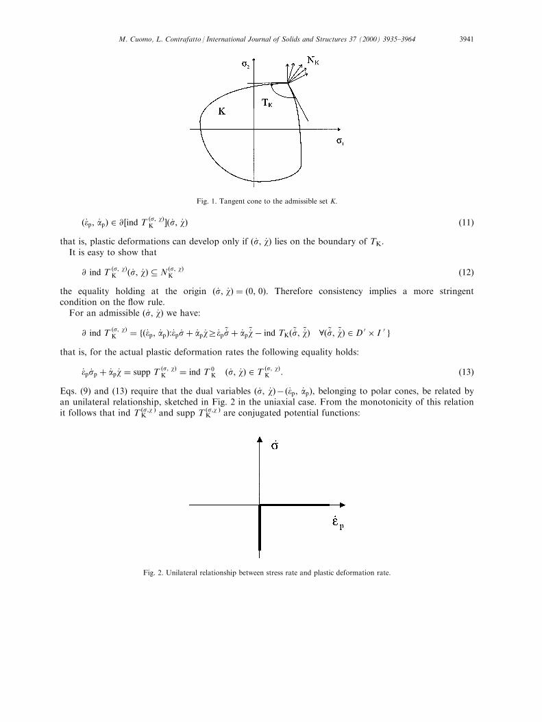
since the functions s(t ), w(t ) are ®rst-order discontinuous when the stress point reaches the boundary ofK. Eq. (10) is satis®ed for any � _s, _w� if NK(s, w )={;}, that is, if (s, w )$ int K. If (s, w ) lies on theboundary of K, (9) requires that the stress rate be internal to the tangent cone to K (Fig. 1).

The loading-unloading condition requires that

M. Cuomo, L. Contrafatto / International Journal of Solids and Structures 37 (2000) 3935±39643940

�_ep, _ap� 2 @ �ind T�s, w�K �� _s, _w� �11�

that is, plastic deformations can develop only if � _s, _w� lies on the boundary of TK.It is easy to show that

@ ind T�s, w�K � _s, _w� � N

�s, w�K �12�

the equality holding at the origin � _s, _w� � �0, 0�: Therefore consistency implies a more stringentcondition on the ¯ow rule.

For an admissible � _s, _w� we have:

@ ind T�s, w�K � f�_ep, _ap�:_ep _s� _ap _wr_ep

~_s� _ap~_wÿ ind TK� ~_s, ~_w� 8� ~_s, ~_w� 2 D 0 � I 0 g

that is, for the actual plastic deformation rates the following equality holds:

_ep _sp � _ap _w � supp T�s, w�K � ind T 0

K � _s, _w� 2 T�s, w�K : �13�

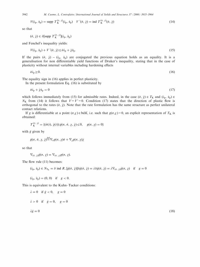
Eqs. (9) and (13) require that the dual variables � _s, _w�ÿ �_ep, _ap�, belonging to polar cones, be related byan unilateral relationship, sketched in Fig. 2 in the uniaxial case. From the monotonicity of this relationit follows that ind T (s,w )

K and supp T (s,w )K are conjugated potential functions:

Fig. 1. Tangent cone to the admissible set K.

Fig. 2. Unilateral relationship between stress rate and plastic deformation rate.

M. Cuomo, L. Contrafatto / International Journal of Solids and Structures 37 (2000) 3935±3964 3941

V�_ep, _ap� � supp T�s, w�K �_ep, _ap� V 0� _s, _w� � ind T

�s, w�K � _s, _w� �14�

so that

� _s, _w� 2 @ �supp T�s, w�K ��_ep, _ap�

and Fenchel's inequality yields:

V�_ep, _ap� � V 0� _s, _w�R _s_ep � _w_ap: �15�If the pairs � _s, _w� ÿ �_ep, _ap� are conjugated the previous equation holds as an equality. It is ageneralisation for non di�erentiable yield functions of Druker's inequality, stating that in the case ofplasticity without internal variables including hardening e�ects

_s_epr0: �16�The equality sign in (16) applies in perfect plasticity.

In the present formulation Eq. (16) is substituted by

_s_ep � _w_ap � 0 �17�which follows immediately from (15) for admissible rates. Indeed, in the case � _s, _w� 2 TK and �_ep, _ap� 2NK from (14) it follows that V=V '=0. Condition (17) states that the direction of plastic ¯ow isorthogonal to the rates � _s, _w�: Note that the rate formulation has the same structure as perfect unilateralcontact relations.

If g is di�erentiable at a point (s,w ) $ bdK, i.e. such that g(s,w )=0, an explicit representation of TK isobtained:

T�s, w�K � f� _s�t�, _w�t��: _g�s, _s, w, _w�R0, g�s, w� � 0g

with g.given by

_g�s, _s, w, _w��defrsg�s, w� _s� rwg�s, w�_w

so that

r� _s, _w� _g�s, w� � r�s, w�g�s, w�:The ¯ow rule (11) becomes:

�_ep, _ap� 2 NTK� @ ind Rÿ� _g� _s, _w��@ _g� _s, _w� � l@ _g� _s, _w� � lr� _s, _w� _g�s, w� if g � 0

�_ep, _ap� � �0, 0� if g < 0:

This is equivalent to the Kuhn±Tucker conditions:

l � 0 if _g < 0, g � 0

l > 0 if _g � 0, g � 0

l _g � 0 �18�

M. Cuomo, L. Contrafatto / International Journal of Solids and Structures 37 (2000) 3935±39643942

Conditions (18,7) fully de®ne the ¯ow rule equations.In the case of a corner point Kuhn±Tucker relations (18) hold for each yield surface:

li > 0, _giR0, li _gi � 0

where gg=0, i=1, . . . , n. Since convexity rules out the possibility of having an identical normal to twodi�erent yield surfaces, it follows that

giR0, i � 1, . . . , n, i 6� j, _gj � 0

so that only the j-th plastic mechanism will be activated.

2.5. Some forms of tangent elastic and hardening potentials

In this section we will state some forms of the free energy potential that will be used in theapplications.

2.5.1. The elastic tangent potentialFor the linear elastic potential j(ee) Eq. (8) yields:

jt�ee, _ee� � 1

2E_ee_ee

where E is the elastic tensor of the material, and the complementary elastic tangent potential is

j 0 t�s, _s� � sup_ee2D

�_s_ee ÿ 1

2E_ee_ee

�� 1

2E ÿ1 _s _s:

2.5.2. The hardening tangent potentialIsotropic, kinematic and mixed hardening are considered.Let a1 and a2 be the internal variables, associated with kinematic and isotropic hardening,

respectively, and w1 and w2 the dual thermodynamic forces. The yield function is written as:

g�s, w� � f�sÿ w1� ÿ �k� w2� k 2 R�

where w1 is the back-stress tensor and w2 is a scalar.In particular for the Von Mises elastic domain, the yield function is given by the expression:

g�s, w� �������������������������3

2J2�sÿ w1�

rÿ �k� w2�

where J2=tr[dev(sÿw1)]2 and k � ������������3=2J0p � s0, J0, being the second invariant of the deviatoric part of

the stress tensor in the uniaxial case and s0 the tensile resistance of the material. In a plain stress statewe have:

J2 � 2

3��sx ÿ w1x�2 � �sy ÿ w1y�2 ÿ �sx ÿ w1x��sy ÿ w1y� � 3�txy ÿ w1xy�2�:

An additive form is adopted for the hardening potential

p�ae� � p1�ae1 � � p2�ae2�

M. Cuomo, L. Contrafatto / International Journal of Solids and Structures 37 (2000) 3935±3964 3943

and for each term the following expression is used (Simo and Taylor, 1985):

p�ae� � 1

2Haeae � c1

�kaek � 1

ZeÿZkaek

�c1, Z > 0:

The ®rst term describes a linear hardening with modulus H; the second introduces a transitory nonlinear hardening with initial modulus c1Z.

From constitutive Eqs. (2) the internal forces are given by:

w1 � rae1p1 � H1ae1 �

c11

kae1k�1ÿ eÿZ1kae1

k�ae1

w2 � rae2p2 � H2ae2 �

c12

j ae2 j�1ÿ eÿZ2jae2

j�ae2 : �19�

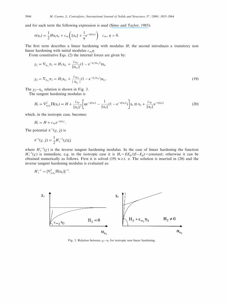
The w2ÿae2 relation is shown in Fig. 3.The tangent hardening modulus is

Ht � r2aeae

P�ae� � H� c1kaek2

�ZeÿZkaek ÿ 1

kaek�1ÿ eÿZkaek��ae ae � c1

kaekeÿZkaek �20�

which, in the isotropic case, becomes:

Ht � H� c1eÿZjaej:

The potential p 0 t�w, _w� is

p 0 t�w, _w� � 1

2H ÿ1t �w�_w_w

where Hÿ1t (w ) is the inverse tangent hardening modulus. In the case of linear hardening the functionHÿ1t (w ) is immediate, e.g. in the isotropic case it is Ht=EEp/(EÿEp)=constant; otherwise it can beobtained numerically as follows. First it is solved (19) w.r.t. a. The solution is inserted in (20) and theinverse tangent hardening modulus is evaluated as:

H ÿ1t � �r2aeae

P�ae��ÿ1:

Fig. 3. Relation between w2ÿa2 for isotropic non linear hardening.

M. Cuomo, L. Contrafatto / International Journal of Solids and Structures 37 (2000) 3935±39643944

3. Variational formulation

3.1. Rate formulation

The rate form of the state equations for the structural problem under investigation obtained in section2 is summarised as follows:

compatibility fC _u � _e

equilibrium fC 0 _s � _f

constitutive equations

8>>>><>>>>:_s 2 @ _ee

jt�ee, _ee�_w 2 @ _ae

pt�ae, _ae��_ep, _ap� 2 @ �ind T

�s, w�K �� _s, _w�

_f 2 @ Çugt� _u�

�21�

under the hypothesis of additive decomposition for kinematic variables:

_e � _ee � _ep

0 � _ae � _ap:

It has been assumed that the rate of external forces can be obtained through a local tangent potentialg t(u. ), which is concave in the case of convex boundary conditions.

The state Eqs. (21) are the stationarity conditions of the mixed functional (Romano and Alfano,1995)

O� _u, _f, _ee, _ep, _ae, _ap, _s, _w�hC _u, _si � G 0 t� _f� ÿ h _f, _ui ÿ h _s, _eei ÿ h _s, _epi ÿ h_w, _aei ÿ h_w, _api� Ft�ee, _ee� �Pt�ae, _ae� �

�B

supp T�s, w�K �_ep, _ap� dB

where the global potentials Ft�ee, _ee�, Pt�ae, _ae� are de®ned as follows:

Ft�ee, _ee� ��B

jt�ee, _ee� dB

Pt�ae, _ae� ��B

pt�ae, _ae� dB

and the global displacement rate potential Gt(u.) is:

Gt� _u� ��B

_b _u dB��@Bq

_q _u dsÿ�@Bu

indW ds

with

W � f _u: _uÿ _�u � 0 on @Bug:

M. Cuomo, L. Contrafatto / International Journal of Solids and Structures 37 (2000) 3935±3964 3945

Its dual potential is obtained through a Legendre transformation:

G 0 t� _f� � inf_ufh _f, _ui ÿ Gt� _u�g � inf

_u2U

(�B

_b _u dB��@Bq

_q _u ds��@Bu

_r _u dsÿ�B

_b _u dB

ÿ�@Bq

_q _u ds��@Bu

ind W ds

)� inf

_u2U

��@Bu

_r _u ds��@Bu

ind W ds

���@Bu

_r_�u ds � h_r_�ui@Bu: �22�

The functional O is convex w.r.t. �_ee, _ep, _ae, _ap�, concave w.r.t. f.and linear w.r.t. � _u, _s, _w�: The solution

of the structural problem is characterised as:

inf�_ee, _ep, _ae, _ap�

sup_f

stat� _u, _s, _w�

O� _u, _f, _ee, _ep, _ae, _ap, _s, _w�:

A 3-®eld functional, that generalises Hu±Washizu's principle, is obtained after an optimisation w.r.t. � _f,_ep, _ap�: By applying de®nitions (22, 5) we obtain:

OW� _u, _s, _w, _ee, _ae� � hC _u, _si ÿ Gt� _u� ÿ h _s, _eei ÿ h_w, _aei � Ft�ee, _ee� �Pt�ae, _ae�ÿ�B

ind T�s, w�K � _s, _w� dB

convex in � _u, _ee, _ae�, concave in � _s, _w�:A further optimisation w.r.t. the kinematic variables �_ee, _ae�, after applying Legendre transformations,

leads to a generalised form of the Hellinger±Reissner functional for inelastic rate problems:

OR� _u, _s, _w� � hC _u, _si ÿ Gt� _u� ÿ F 0 t�s, _s� ÿP 0 t�w, _w� ÿ�B

ind T�s, w�K � _s, _w� dB

where F 0 t�s, _s�eP 0 t�w, _w� are conjugate potentials. OR is concave in � _s, _w� and convex in u..

The generalised forms of the Prager±Hodge and Greenberg functionals are obtained afteroptimisation with respect to u

.or � _s, _w�: Since

sup_ufhC _u, _si ÿ Gt� _u�g � sup

_ufhC _u, _si ÿ h _f, _ui � h _f, _ui ÿ Gt� _u�g � G 0 t� _f� _s��

subject to

hC _u, _si ÿ h _f, _ui � 0

the Prager±Hodge functional becomes:

Oc� _s, _w� � ÿF 0 t�s, _s� ÿP 0 t�w, _w� � h_r, _�ui ÿ�B

ind T�s, w�K � _s, _w� dB

subject to equilibrium conditions

hC 0 _s, ~_ui � h _f, ~_ui 8~_u 2 U in B [ @Bq:

The relevant structural problem in terms of rates of stress and thermodynamic force can be formulatedas follows:

M. Cuomo, L. Contrafatto / International Journal of Solids and Structures 37 (2000) 3935±39643946

sup� _s, _w�2Q

Oc� _s, _w� Q � f� _s, _w�:hC 0 _s, ~_ui � h _f, ~_ui 8 ~_u 2 U g: �23�

For the Greenberg functional the following form is obtained:

Ou� _u� � Fep�C _u� ÿ Gt� _u�where

Fep� _u� � sup� _s, _w��hC _u, _si ÿ F 0 t�s, _s� ÿP 0 t�w, _w� ÿ

�B

ind T�s, w�K � _s, _w� dB �: �24�

This functional, convex in u., is the starting point for classical displacement methods. It can be proved

that the optimality condition of (24) leads to the generalised return mapping algorithm.

3.2. Formulations involving actual values of the variables

The variational principles of the previous section can be reformulated in terms of actual values of thevariables, rather than their rates. This formulation allows the total compatibility and equilibriumconditions to be satis®ed in the ®nal state, reducing in principle the approximation errors. However, it isnecessary to approximate the ¯ow rule that involves deformation rates.

Introducing a fully implicit integration scheme for the kinematic variables, one has

Dep � ep�t� Dt� ÿ ep0 � _ep�t� Dt�Dt

Dap � ap�t� Dt� ÿ ap0 � _ap�t� Dt�Dtep0

and ap0being their values at the end of the previous step. The ®nite increment form of the

constitutive relations is:�Dep

Dt,Dap

Dt

�2 @ indK�s�t�, w�t�� � NK�s�t�, w�t��: �25�

Since NK is a concave cone and Dtr0 (25) can be reformulated as:

�Dep, Dap� 2 @ ind K�s�t�, w�t�� � NK�s�t�, w�t��and the ®nite step problem is ruled by the functional:

O�u, f, ee, ep, ae, ap, s, w� � hCu, si � G 0� f � ÿ hf, ui ÿ hs, eei ÿ hs, epi � hs, ep0i � ÿhw, aeiÿ hw, api � hw, ap0i � Fe�ee, ee� �P�ae, ae� � supp K�ep ÿ ep0 , ap ÿ ap0 �:

The whole family of variational functionals described in section 3.1 can be consistently derived. Forinstance, the generalised ®nite increment forms of the Hellinger±Reissner and Prager±Hodge functionalsare:

OR�u, s, w� � hCu, si � hs, ep0i � hw, ap0i ÿ G�u� ÿ F 0�s� ÿP 0�w� ÿ�B

ind K�s, w� dB

Oc�s, w� � hs, ep0i � hw, ap0i ÿ F 0 t�s� ÿP 0�w� � G 0� f � ÿ�B

ind K�s, w� dB

M. Cuomo, L. Contrafatto / International Journal of Solids and Structures 37 (2000) 3935±3964 3947

subject to equilibrium conditions

hC 0s, ~ui � hf, ~ui 8 ~u 2 U in B [ @Bq:

3.3. Incremental formulations

A ®nite increment formulation will now be derived from the rate form of the Hellinger±Reissnerfunctional in section 3.1, which will be the starting point for the numerical algorithm illustrated insection 4.

The solution of the elastoplastic problem can be achieved if a subdivision of the load history into n®nite increments, corresponding to the instants t0, t1, . . . , tn, is introduced. All variable rates aresubstituted with ®nite increments in the step. At the time t+Dt the values of (s,w ) are given by:

s�t� Dt� � s�t� ��t�Dtt

_s�t� dt; w�t� Dt� � w�t� ��t�Dtt

_w�t� dt:

A similar formula can be introduced for the displacement u. For each variable the following integrationrule can be used:

s�t� Dt� � s�t� � ��1ÿ b� _s�t�� � b _s�t� Dt�ÿ�Dt 0RbR1:

If b=1 the fully implicit integration scheme is obtained (note that in (26) the left derivative appears):

s�t� Dt� � s�t� � _s�t� Dt�ÿDt � s�t� � Ds�t� Dt�: �26�This method ensures that the compatibility conditions are satis®ed at the end of the step and it will beused in what follows.

The increment of plastic deformations is given by:�Dep

Dap

���t�Dtt

�_ep

_ap

�dt:

The plastic rates are evaluated using the ¯ow rule (11) that contains the right derivative of the stresses,which is not known at time t+Dt (see Eq. (26)).

Therefore a relaxed form of the ¯ow rule is adopted, employing inclusion (12):�Dep

Dap

�2�t�Dtt

@ ind T�s, w�K � _s�, _w�� dt �

�t�Dtt

NK�s, w� dt ��t�Dtt

l@g�s, w� dt: �27�

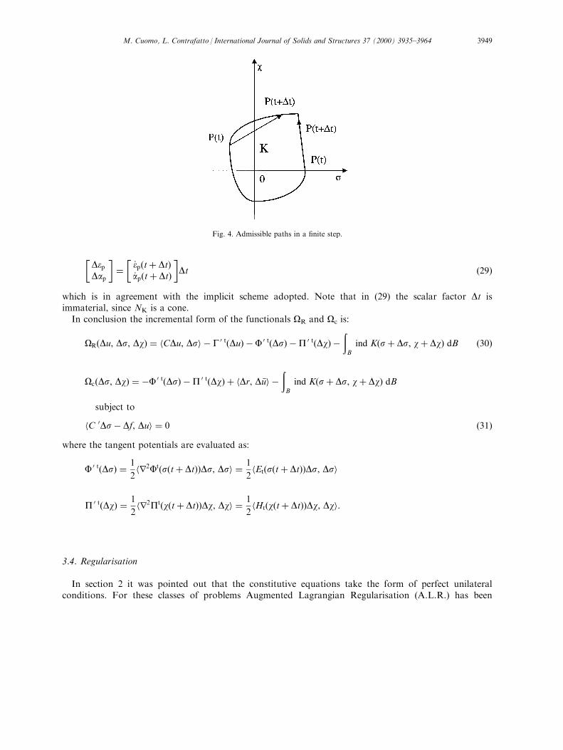
The integration has to be carried out along an admissible path. Hypothesis (26) requires that thisintegration be performed along a secant path from the point at time t to the point at time t+Dt. Fromthe convexity of K it follows that the stress path is non external to K and the integral in (27) is non zeroonly at the end of the interval, except for the special case of a ¯at boundary (see Fig. 4).

The result is therefore:�Dep

Dap

�2 l@g�s� Ds, w� Dw�: �28�

Formula (28) is equivalent to stating that

M. Cuomo, L. Contrafatto / International Journal of Solids and Structures 37 (2000) 3935±39643948

�Dep

Dap

���

_ep�t� Dt�_ap�t� Dt�

�Dt �29�

which is in agreement with the implicit scheme adopted. Note that in (29) the scalar factor Dt isimmaterial, since NK is a cone.

In conclusion the incremental form of the functionals OR and Oc is:

OR�Du, Ds, Dw� � hCDu, Dsi ÿ G 0 t�Du� ÿ F 0 t�Ds� ÿP 0 t�Dw� ÿ�B

ind K�s� Ds, w� Dw� dB �30�

Oc�Ds, Dw� � ÿF 0 t�Ds� ÿP 0 t�Dw� � hDr, D �ui ÿ�B

ind K�s� Ds, w� Dw� dB

subject to

hC 0Dsÿ Df, Dui � 0 �31�where the tangent potentials are evaluated as:

F 0 t�Ds� � 1

2hr2Ft�s�t� Dt��Ds, Dsi � 1

2hEt�s�t� Dt��Ds, Dsi

P 0 t�Dw� � 1

2hr2Pt�w�t� Dt��Dw, Dwi � 1

2hHt�w�t� Dt��Dw, Dwi:

3.4. Regularisation

In section 2 it was pointed out that the constitutive equations take the form of perfect unilateralconditions. For these classes of problems Augmented Lagrangian Regularisation (A.L.R.) has been

Fig. 4. Admissible paths in a ®nite step.

M. Cuomo, L. Contrafatto / International Journal of Solids and Structures 37 (2000) 3935±3964 3949

successfully introduced and it has several computational and analytical advantages (see, e.g. Glowinskiand Le Tallec, 1989).

First, by using an A.L. formulation one has a faster convergence rate than by using normalLagrangian functionals (Cuomo et al., 1997). More importantly, A.L.R. becomes especially e�ectivewhen the elastic deformations are much smaller than the inelastic ones, so they do not introduce enoughsmoothing on the problem, or when non-convex functionals are involved, as could be the case withsoftening. Below it will be shown that the use of A.L.R. leads to e�ective computational schemes thatcould achieve a substantial reduction in computational e�ort w.r.t. the usual Lagrangian methods.

The functional (31) is made di�erentiable through the Augmented Lagrangian Regularisation:

ind K�s� Ds, w� Dw� � suplr0

�1

2mg2 � lg

�� sup

l

�1

2m �g2 � l �g

��32�

l being the Lagrangian plastic multiplier, m a positive constant penalty parameter and

�g � max

�g, ÿ l

m

�:

The function �g converts the inequality constraint g(s+Ds, w+Dw ) R 0 into an equality one �g(s+Ds,w+Dw )=0, removing the sign restriction on the Lagrangian multiplier and preserving the functionalcontinuity in the neighbourhood of the solution (Bertsekas, 1982).

Problem (23) thus turns into a saddle point problem:

sup�Ds, Dw�2Q̂

inflOAL

c �Ds, Dw, l�

Q̂ � f�Ds, Dw�:C 0Ds � Df g

where OALc (Ds, Dw, l ) is the following di�erentiable functional:

OALc �Ds, Dw, l� � ÿ

1

2hE ÿ1t Ds, Dsi ÿ 1

2hH ÿ1t Dw, Dwi � hDr�Ds�, D �ui

ÿ�B

�1

2m �g2�s� Ds, w� Dw� � l �g�s� Ds, w� Dw�

�dB:

According to (28) the increments of the plastic deformations and internal variables are given by thefollowing expressions:

Dep � rs

�1

2m �g2 � l� �g

�� �mg� l��rsg � l�rsg

Dap � rw

�1

2m �g2 � l� �g

�� �mg� l��rwg � l�rwg

where l� is the value of the plastic multiplier at solution and the terms mgHsg and mgHwg vanish sincethe constraint is satis®ed � �g � g � 0).

M. Cuomo, L. Contrafatto / International Journal of Solids and Structures 37 (2000) 3935±39643950

4. Discrete structural problem

4.1. Discretised variational formulation

A discretisation into ne ®nite elements Be is introduced. The increments of the stresses,thermodynamic forces and displacements are thus given by

Ds � NsDs, Dw � NwDc, Du � NuDd, D �u � NÅuD Åd

Ns, Nw, Nu, Nu- being suitable shape function matrices.It is noticed that a necessary condition for the existence of a solution to the equilibrium equations is

that the dimension of the nodal stress space be greater than that of the nodal displacement space(Zienkievicz and Taylor, 1989).

The discretised form of the Hellinger±Reissner functional, given by Eq. (30), is:

OR�Dd, D Åd, Ds, Dc� ��B

CNuDd � NsDs dB��@Bu

CNÅuD Åd � NsDs dsÿ 1

2

�B

E ÿ1t NsDs � NsDs dB

ÿ�B

DbNuDd dB�ÿ�@Bq

DqNuDd dsÿ�@Bu

DrNÅuD Åd ds�ÿ�B

H ÿ1t NwDc � NwDc dB

ÿ�B

1

2m �g2�s� Ds, c� Dc� � l �g�s� Ds, c� Dc� dB

�33�

where D Åd are the displacements of the nodes belonging to the constrained part of the boundary.The variation of this functional w.r.t. Dd and Dd

-gives the discretised equilibrium equations:

CDs � Db� Dq � Dp in B [ @Bq

QDs � Dr on @Bu

The equilibrium operators C and Q are de®ned as:

C ��B

�CNu�TNs dB; Q ��@Bu

�CNÅu�TNs ds

and Dp and Dr are the nodal vectors of the external forces and the reactions, de®ned as:

Dp � Db� Dq ��B

NTuDb dB�

�@Bq

NTuDq ds

Dr ��@Bu

NTÅuDr ds:

The discretised form of the functional Oc(Ds, Dw ), given by Eq. (31), is:

M. Cuomo, L. Contrafatto / International Journal of Solids and Structures 37 (2000) 3935±3964 3951

Oc�Ds, Dc� � ÿ12

�B

NTsEÿ1t NsDsDs dBÿ 1

2

�B

NTwHÿ1t NwDcDc dB�

�@Bu

DrNÅuD Åd ds

ÿ�B

ind K�s� Ds, c� Dc� dB �34�

subject to the equilibrium conditions in the inside and on the boundary.Introducing the tangent ¯exibility and hardening matrices

F ��B

NTsEÿ1t Ns dB; G �

�B

NTwHÿ1t Nw dB

the functional (34) is written in compact form:

Oc�Ds, Dc� � ÿ12

FDsDsÿ 1

2GDcDc�QDsD Ådÿ

�B

ind K�s� Ds, c� Dc� dB

Ds 2 Y Y � fDs:CDs � Dp in B [ @Bq, QDs � Dr on @Bug �35�

Y being the set of nodal stresses satisfying the equilibrium equations in the weak sense.The equilibrium constraint for the functional Oc can be removed through a reduction of the variables

Ds to the self-equilibrated stresses Ds0. By re-arranging the columns of the matrix C, the followingpartition can be obtained:

C � �C0 C1�where C1 is square and non singular. If the same decomposition is carried out on Ds, the equilibriumequations in B[ @Bq can be written as

�C0 C1��Ds0Ds1

�� Dp

where Ds1 is a vector of nodal stress increments equilibrating the external load increments.As C1 is non singular, the following expression for Ds1 is obtained:

Ds1 � ÿCÿ11 C0Ds0 � Cÿ11 Dp � ÿ ÄC0Ds0 � D Äp: �36�In the numerical implementation CÄ 0 and DpÄ are obtained directly by means of a Gauss reduction of thematrix C and of the vector Dp such that C10I.

Introducing the reduced stress increments in (35)

Ds ��Ds0Ds1

���

Iÿ ÄC0

�Ds0 �

�0D Äp

�� RDs0 � Dv

the functional Oc(Ds, Dc) becomes:

Oc�Ds0, Dc� � ÿ12

RTFRDs0Dso ÿ 1

2GDcDcÿ RTFDvDs0 � RTQtD ÅdDs0 �ÿ1

2FDvDv�QDvD Åd

ÿ�B

ind K�s0 � Ds0, c� Dc� dB: �37�

The indicator function in formula (37) is regularised according to the Augmented Lagrangian scheme of

M. Cuomo, L. Contrafatto / International Journal of Solids and Structures 37 (2000) 3935±39643952

Eq. (32), that needs to be better speci®ed. It derives from the duality pairing hm �g+l, �gi where,elementwise, �g $ C0

0, l $ C '. Therefore the multipliers l are measures and the integral in (37) has to beunderstood in the distribution sense. It is numerically evaluated assuming a Dirac distribution for themultipliers with singularity at prescribed points, which play the role of check points for the plasticityconstraints:

hm �g� l, �gi �Xne

i�1

Xncpe

j�1

�1

2m �g2�s0 � Ds0, c� Dc� � l �g�s0 � Ds0, c� Dc�

�ij

�38�

where the sum is made on the ncpe check points of the element. Note the absence in (38) of the Jacobianterm.

The Gauss points of the elements were used as check points. The choice of the check points a�ectsthe convergence of the discretised solution, but this aspect is not addressed in the present paper.

Therefore, the functional Oc(Ds0, Dc), eliminating unessential constant terms and after a sign reversal,becomes:

OALc �Ds0, Dc, l� � 1

2RTFRDs0Ds0 � 1

2GDcDc� RTFDvDs0 ÿÿRTQTD ÅdDs0

�Xncp

j�1

�1

2m �g2�s0 � Ds0, c� Dc� � l �g�s0 � Ds0, c� Dc�

�j

�39�

ncp being the total number of check points in B. The solution of the structural problem is given by:

min�Ds0, Dc�

maxl

OALc �Ds0, Dc, l�: �40�

4.2. Displacement calculation

The variation w.r.t. DS of the discretised form of the Hellinger±Reissner functional (33) yields thekinematic compatibility equation:

CTDd � FDsÿQTD Åd�Xncp

j�1�NT

s�m �g� Dl��rs �g�j �41�

which means that the total deformation vector CTDd is obtained as the sum of the elastic and plasticparts minus QTDd

-, i.e. the deformations due to the imposed boundary displacements.

De®ning the deformation vectors as:

De � Dee � Dep, Dee � FDs, Dep �Xncp

j�1�NT

s�m �g� l��rs �g�j

and introducing the decomposition of matrix C shown in 4.1, relation (41) can be written as:"ÄC

T

0

I

#Dd �

�De0De1

�ÿ�

QT0

QT1

�D Åd �42�

where

M. Cuomo, L. Contrafatto / International Journal of Solids and Structures 37 (2000) 3935±3964 3953

�De0De1

���

F00 F01

F10 F11

��Ds0Ds1

��Xncp

j�1

24NTs0

NTs1

35�m �g� l��rs �g: �43�

It should be pointed out that Q0 and Q1 are the matrices that derive from rearrangement of thecolumns of the boundary equilibrium operator Q. In fact the Gauss reduction performed on the rows ofC to obtain the partition C=[CÄ 0 I] does not apply on Q or Dr.

The second equation of (42) allows the displacements of the unconstrained nodes to be evaluated inthe form:

Dd � De1 ÿQt1D Åd: �44�

The ®rst equation in (42) is an identity since it is the Euler±Lagrange equation of the functionalOALc (Ds0, Dc, l ) (Eq. (39)). Indeed, by substituting Dd as given by (44) into the ®rst equation in (42) one

has:

ÄCT

0De1 ÿ ÄCT

0QT1D Ådÿ De0 �QT

0D Åd � 0: �45�Introducing the expressions of De0 and De1 given by Eqs. (43) into (45) and using (36) we obtain:

RTFRDs0 � RTFDvÿ RTQTD Åd�Xncp

j�1�RTNT

s�m �g2 � l �g�rs �g�j � rDs0OALc � 0

which is the expression of the gradient w.r.t. Ds0 of the discretised functional OALc (Eq. (39)): at the

solution it is equal to zero.

5. Iterative solution scheme

In this section we will describe the numerical procedure employed to obtain the solution of theincremental problem (40). The procedure closely follows the one described in Cuomo and Ventura(1998) and is a particularisation to the problem at hand of the method described in Bertsekas (1982) andFletcher (1987).

The solution is obtained in two steps, iterating independently on the direct and dual variable sets,given, respectively, by the stress and thermodynamic force increments and by the plastic multipliers.Optimisation w.r.t. a set of variables is achieved keeping the values of the variables of the other set®xed. As the constrained function is convex on the whole direct variable space, the generalisedcomplementary energy functional Oc(Ds0, Dc) is also convex; moreover, as m > 0 and the Lagrangianmultipliers are non negative by the Kuhn and Tucker conditions, the Augmented Lagrangian functionalOALc (Ds0, Dc, l ), Eq. (39), is also convex w.r.t. (Ds0, Dc) for any penalty parameter value (Bertsekas,

1982) and concave w.r.t. l.In the numerical implementation the non-negativity of the Lagrangian multipliers is guaranteed if the

procedure is initialised at each stage by a Lagrangian multiplier update. Subsequently, the optimalvalues of the direct variables are sought with a classical Newton iteration scheme, usually using thefollowing elastic solution as the trial value:

Ds0 � �RTFR�ÿ1RT�QtD Ådÿ FDv�; Dc � 0:

The re®nement of the solution Dx=(Ds0, Dc) at the next step

M. Cuomo, L. Contrafatto / International Journal of Solids and Structures 37 (2000) 3935±39643954

Dxk�1 � Dxk ÿ �r2DxDxO

ALc �ÿ1k �rDxO

ALc �k

requires evaluation of the Hessian of the Augmented Lagrangian functional.The Lagrangian multipliers are updated keeping the value of the direct variables ®xed. Several

multiplier update formulas can be used, depending on the iterative scheme adopted for the dualproblem. First- or second-order formulas have been proposed, according to whether a steepest ascentoptimisation or a Newton-like technique is applied. A deeper examination of these alternatives, as wellas of the numerical iterative schemes and their physical meaning is to be found in Cuomo et al. (1998).In the present paper the ®rst-order Hestenes±Powell update formula (Hestenes, 1969; Powell, 1969) willbe used:

li�1j � lij � Dlij Dlij � mgj�s0 � Dsi0, c� Dci �

where j denotes the j-th check point.The direct and dual optimisations are performed sequentially until the constraints are met. This is

achieved when an appropriate norm of the indicator function of the domain K is reduced to zero. It hasbeen found that good convergence is achieved using the control:

maxj�1, ncp

������1

2m �g2 � l �g

������j

< g

where g is a ®xed tolerance.

6. Numerical tests

The algorithm described in the previous sections was implemented in an original code. Linear andnon linear isotropic and kinematic hardening models were used in various combinations.

The computational e�ciency of the algorithm was veri®ed with reference to the classical example ofthe Cook membrane, the results of which are widely known in literature (Simo et al., 1989; Weissmanand Jamjian, 1993). The geometrical and mechanical characteristics are given in Fig. 5.

The beam is clamped at one end and is acted upon by a permanent qper=0.0625 KN/mm and avariable rqacc=r0.0625 KN/mm tangential load distributed over the free end; r is a scalar in the ranger $ [0.1, 0.8]. The analysis was performed in plane-stress J2 plasticity with isotropic, kinematic and mixedhardening and in perfect plasticity. The following material properties were used:

. Young's modulus E=70 KN/mm2;

. Poisson's ratio n=1/3;

. uniaxial tensile yield stress s0=0.243 KN/mm2;

. linear isotropic hardening modulus Hiso=0.2 KN/mm2;

. linear kinematic hardening modulus Hkin=0.015 KN/mm2;

. non linear isotropic hardening modulus Hiso=0.135 KN/mm2;

. mixed linear hardening moduli Hiso=0.135 KN/mm2, Hkin=0.015 KN/mm2.

The membrane was discretised into an equal number of elements in the horizontal and verticaldirections. 4-node bilinear elements with one control point for plastic admissibility at their centre and 8-node serendipity elements with four control points were used; the number of elements per side rangedfrom 2 to 20.

The permanent load, equivalent to a resultant force of 1.0 KN, corresponds to an elastic state.

M. Cuomo, L. Contrafatto / International Journal of Solids and Structures 37 (2000) 3935±3964 3955

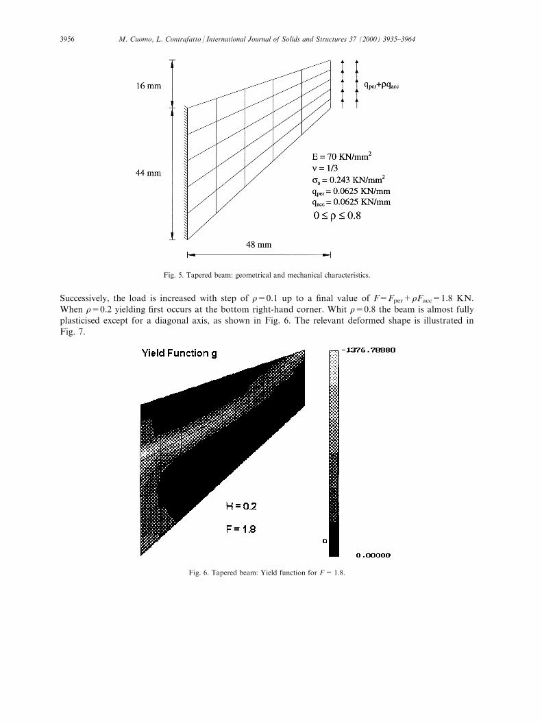
Successively, the load is increased with step of r=0.1 up to a ®nal value of F=Fper+rFacc=1.8 KN.

When r=0.2 yielding ®rst occurs at the bottom right-hand corner. Whit r=0.8 the beam is almost fully

plasticised except for a diagonal axis, as shown in Fig. 6. The relevant deformed shape is illustrated in

Fig. 7.

Fig. 6. Tapered beam: Yield function for F=1.8.

Fig. 5. Tapered beam: geometrical and mechanical characteristics.

M. Cuomo, L. Contrafatto / International Journal of Solids and Structures 37 (2000) 3935±39643956

Figs. 8(a) and (b) present the convergence of the vertical displacement of the top right-hand cornerversus the number of elements per side at the ®xed load level F=1.8 KN for linear isotropic and mixedhardening. In Fig. 8(a) the results of the present formulation are compared with the converged solutionand other algorithms: a classical displacement formulation with 4-node bilinear elements, a mixedformulation with 4-node elements (both implemented by means of the FEAP code (Taylor, 1998)) andthe mixed formulation of Simo et al. (1989), which uses the interpolation functions of Pian andSumihara (1984) for the stresses. The present stress formulation exhibits better convergence than thedisplacement method, reaching the same accuracy with a considerably smaller number of elements. Forexample, the stress formulation solution with 100 4-node elements and the displacement one with 1024elements have approximately the same accuracy. Moreover, the performance of the algorithm atconvergence is comparable with that of Simo's complementary formulation when 4-node elements areused and much better with 8-node elements.

In Fig. 9 the load-displacement curve is given for 25 and 64 element discretisations and for variousvalues of the isotropic hardening ratio E/Ep. It can be observed that no modi®cation in the algorithm isneeded to treat the perfect plastic case (Ep=0.0).

In order to highlight the performance of the procedure, Figs. 10 and 11 present the results for thesame membrane in the case of perfect plasticity. They are compared with those of the displacement andmixed methods. Fig. 10 shows, for a load level of F = 1.4 KN, that the convergence of the presentformulation is much faster than that of the competing methods.

Figs. 12 and 13 refer to the behaviour of the beam for cyclic imposed vertical displacement of the topcorner ÿ1.6 R v R 1.6 mm and for a cyclic load with ÿ1.6 R F R 1.6 KN. Isotropic hardening isassumed. In the non linear case the hardening exponent Z=0.1 was used.

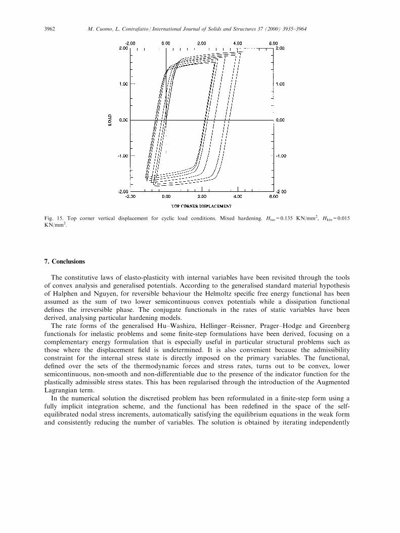
Cycles of increasing load values were considered in Figs. 14 and 15, showing the di�erent response forlinear kinematic hardening and for mixed hardening.

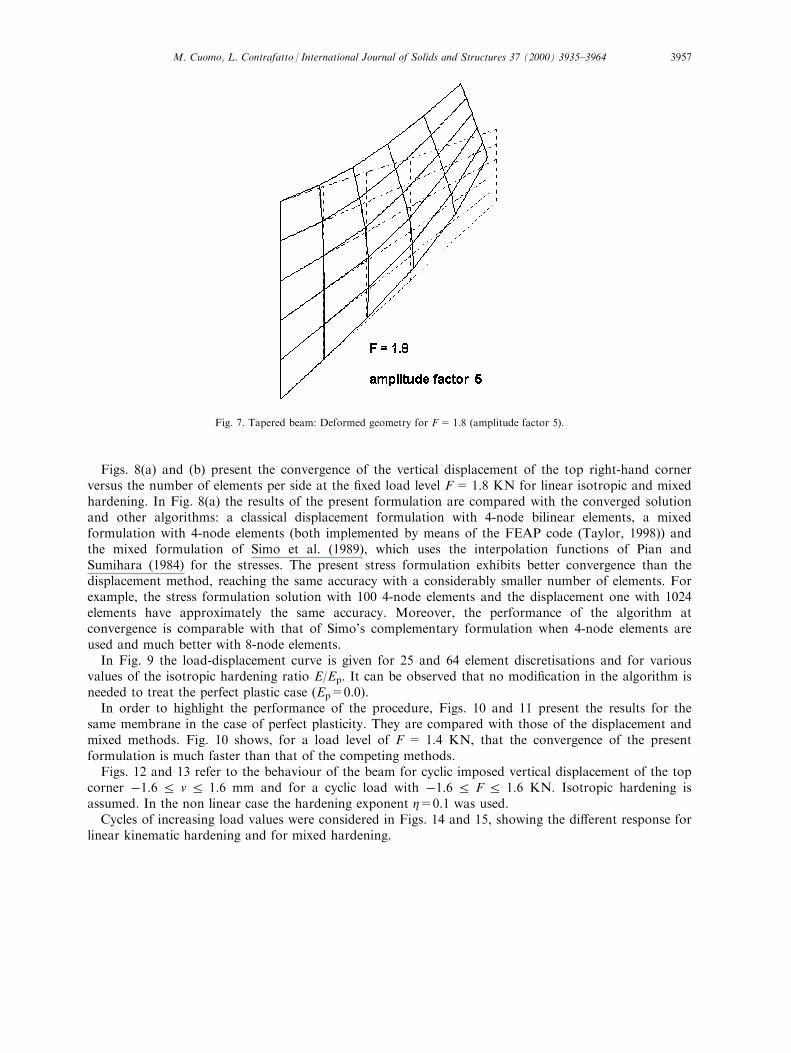
Fig. 7. Tapered beam: Deformed geometry for F=1.8 (amplitude factor 5).

M. Cuomo, L. Contrafatto / International Journal of Solids and Structures 37 (2000) 3935±3964 3957

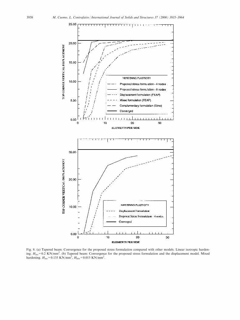
Fig. 8. (a) Tapered beam: Convergence for the proposed stress formulation compared with other models. Linear isotropic harden-

ing. Hiso=0.2 KN/mm2. (b) Tapered beam: Convergence for the proposed stress formulation and the displacement model. Mixed

hardening. Hiso=0.135 KN/mm2, Hkin=0.015 KN/mm2.

M. Cuomo, L. Contrafatto / International Journal of Solids and Structures 37 (2000) 3935±39643958

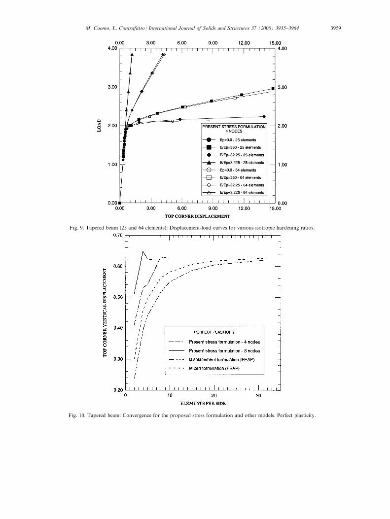
Fig. 9. Tapered beam (25 and 64 elements): Displacement-load curves for various isotropic hardening ratios.

Fig. 10. Tapered beam: Convergence for the proposed stress formulation and other models. Perfect plasticity.

M. Cuomo, L. Contrafatto / International Journal of Solids and Structures 37 (2000) 3935±3964 3959

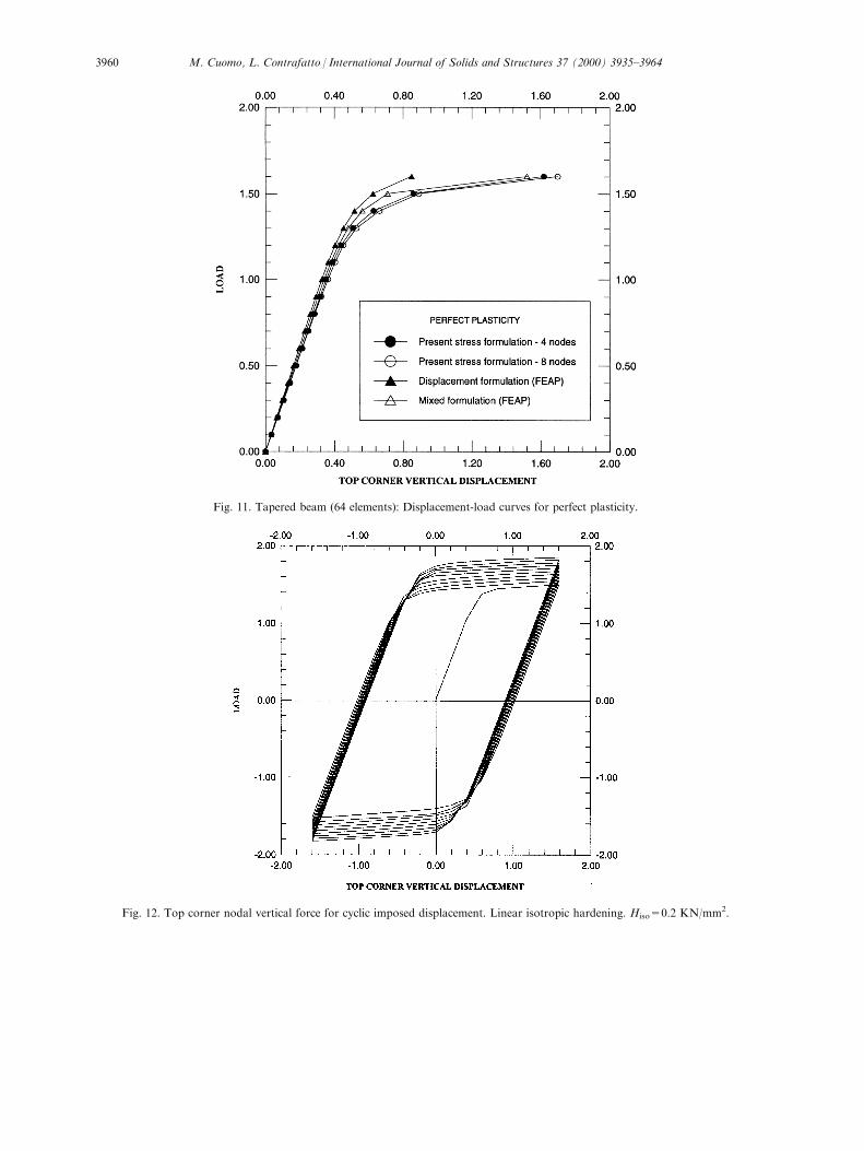
Fig. 11. Tapered beam (64 elements): Displacement-load curves for perfect plasticity.

Fig. 12. Top corner nodal vertical force for cyclic imposed displacement. Linear isotropic hardening. Hiso=0.2 KN/mm2.

M. Cuomo, L. Contrafatto / International Journal of Solids and Structures 37 (2000) 3935±39643960

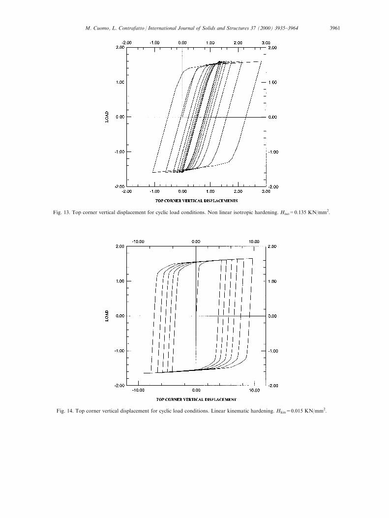
Fig. 13. Top corner vertical displacement for cyclic load conditions. Non linear isotropic hardening. Hiso=0.135 KN/mm2.

Fig. 14. Top corner vertical displacement for cyclic load conditions. Linear kinematic hardening. Hkin=0.015 KN/mm2.

M. Cuomo, L. Contrafatto / International Journal of Solids and Structures 37 (2000) 3935±3964 3961

7. Conclusions

The constitutive laws of elasto-plasticity with internal variables have been revisited through the toolsof convex analysis and generalised potentials. According to the generalised standard material hypothesisof Halphen and Nguyen, for reversible behaviour the Helmoltz speci®c free energy functional has beenassumed as the sum of two lower semicontinuous convex potentials while a dissipation functionalde®nes the irreversible phase. The conjugate functionals in the rates of static variables have beenderived, analysing particular hardening models.

The rate forms of the generalised Hu±Washizu, Hellinger±Reissner, Prager±Hodge and Greenbergfunctionals for inelastic problems and some ®nite-step formulations have been derived, focusing on acomplementary energy formulation that is especially useful in particular structural problems such asthose where the displacement ®eld is undetermined. It is also convenient because the admissibilityconstraint for the internal stress state is directly imposed on the primary variables. The functional,de®ned over the sets of the thermodynamic forces and stress rates, turns out to be convex, lowersemicontinuous, non-smooth and non-di�erentiable due to the presence of the indicator function for theplastically admissible stress states. This has been regularised through the introduction of the AugmentedLagrangian term.

In the numerical solution the discretised problem has been reformulated in a ®nite-step form using afully implicit integration scheme, and the functional has been rede®ned in the space of the self-equilibrated nodal stress increments, automatically satisfying the equilibrium equations in the weak formand consistently reducing the number of variables. The solution is obtained by iterating independently

Fig. 15. Top corner vertical displacement for cyclic load conditions. Mixed hardening. Hiso=0.135 KN/mm2, Hkin=0.015

KN/mm2.

M. Cuomo, L. Contrafatto / International Journal of Solids and Structures 37 (2000) 3935±39643962

on the direct variables with a classical Newton iteration scheme and updating the dual variables throughthe ®rst-order Hestenes±Powell formula.

The results of numerical experiments on the classical example of the Cook membrane have shownthat the algorithm performs better than classical displacement and mixed methods. It is also equallyapplicable to perfect or hardening plasticity.

Several issues have arisen from numerical tests, like the necessity of a reduced number of controlpoints in the elements to avoid lack of convergence. Similarly, the Lagrangian term should be correctlyintegrated in the distribution sense.

The numerical e�ciency of the method is, however, limited by the reduction strategy adopted toobtain the self-equilibrated stresses, which leads to sparse matrices. The analysis of tactics to improvethe computational e�ciency will be the subject of a subsequent paper.

References

Berkovic, M., Mijuca, D. 1998. An e�cient continuous stress mixed model based on the Reissners's principle. In: Idelsohn, S.,

OnÄ ate, E., Dvorkin, E. (Eds.), Computational Mechanics. CIMNE, Barcelona, Spain.

Bertsekas, D.P., 1982. Constrained Optimization and Lagrange Multiplier Methods. Academic Press, Boston.

Cuomo, M., Contrafatto, L., Ventura, G. 1997. Comparison of some numerical algorithms based on augmented Lagrangian

regularisation for elastic-plastic analysis. In: Owen, D.R.J., OnÄ ate, E., Hinton, E. (Eds.), Computational Plasticity. Pineridge

Press, Barcelona, pp. 2033±2038.

Cuomo, M., Contrafatto, L., Ventura, G., 1998. Numerical analysis of augmented Lagrangian algorithms applied to a

complementary formulation in elastoplasticity with internal variables. International Journal of Numerical Methods in

Engineering. Submitted for publication.

Cuomo, M., Ventura, G., 1998. Complementary energy approach to contact problems based on consistent Augmented Lagrangian

formulation. Mathematical and Computer Modelling 28 (48), 185±204.

Eve, R.A., Reddy, B.D., Rockafellar, R.T., 1990. An internal variable theory of elastoplasticity based on the maximum plastic

work inequality. Quarterly of Applied Mathematics 68 (1), 59±83.

Fletcher, R., 1987. Pratical Methods of Optimization. Wiley, New York.

Glowinski, R., Le Tallec, P., 1989. SIAM, Philadelphia.

Halphen, B., Nguyen, Q.S., 1975. Sur les mate riaux standards ge ne ralise s. Journal de Me canique 14, 39±63.

Hestenes, M.R., 1969. Multiplier and gradient methods. Journal of Optimization Theory and Applications 4, 303±320.

Olson, M.D. 1983. The mixed ®nite element method in elastic contact problems. In: Atluri, S.N., Callagher, R.H., Zienkiewicz,

O.C. (Eds.), Hybrid and Mixed Element Methods. Wiley, New York, pp. 19±49.

Pian, T.H.H., Sumihara, K., 1984. Rational approach for assumed stress ®nite elements. International Journal of Numerical

Methods in Engineering 20, 1685±1695.

Powell, M.J., 1969. A Method for Non Linear Constraint in Optimization Problems. Academic Press, London.

Rockafellar, R.T., 1970. Convex Analysis. Princeton University Press, Princeton.

Romano, G., Alfano, G. 1995. Variational principles, approximations and discrete formulations in plasticity. In: Owen, D.R.J.,

OnÄ ate, E., Hinton, E. (Eds.), Computational Plasticity. Pineridge Press, Barcelona, pp. 71±82.

Romano, G., Rosati, L., Marotti de Sciarra, F., 1993. A variational theory for ®nite-step elasto-plastic problems. International

Journal of Solids and Structures 30, 2317±2334.

Simo, J.C., Kennedy, J.G., Taylor, R.L., 1989. Complementary mixed ®nite element formulations for elastoplasticity. Computer

Methods in Applied Mechanics and Engineering 74, 177±206.

Simo, J.C., Rifai, M.S., 1990. A class of mixed assumed strain methods and the method of incompatible modes. International

Journal of Numerical Methods in Engineering 29, 1595±1638.

Simo, J.C., Taylor, R.L., 1985. Consistent tangent operators for rate-independent elastoplasticity. Computer Methods in Applied

Mechanics and Engineering 48, 101±118.

M. Cuomo, L. Contrafatto / International Journal of Solids and Structures 37 (2000) 3935±3964 3963

Taylor, R.L., 1998. A Finite Element Analysis Program Ð Version 6.4b.

Weissman, S.L., 1992. A mixed formulation of non linear-elastic problems. Computers and Structures 44 (4), 813±822.

Weissman, S.L., Jamjian, M., 1993. Two-dimensional elastoplasticity: approximation by mixed ®nite elements. International

Journal of Numerical Methods in Engineering 36, 3703±3727.

Zienkievicz, O.C., Taylor, R.L., 1989. The Finite Element Method, 4th ed. McGraw-Hill, London.

M. Cuomo, L. Contrafatto / International Journal of Solids and Structures 37 (2000) 3935±39643964