Streaming de Realite Virtuelle:Apprentissage pour Modeles Attentionnels et Optimisation Reseau

Miguel Fabian ROMERO RONDON

Laboratoire d’Informatique, Signaux et Systemes de Sophia Antipolis (I3S)

Presentee en vue de l’obtention Devant le jury compose de :

du grade de docteur en Informatique Alberto DEL BIMBO, Professeur, University of Firenze

d’Universite Cote d’Azur Ngoc Q. K. DUONG, Chercheur Senior, InterDigital R&D

Dirigee par : Frederic PRECIOSO / President: Patrick LE CALLET, Professeur, Universite de Nantes

Lucile SASSATELLI Laura TONI, Maıtresse de conference, University College London

Soutenue le : 23/09/2021

Streaming Virtual Reality:

Learning for Attentional Models and Network

Optimization

Jury :

Rapporteurs :

Prof. Alberto DEL BIMBO, Professeur des universites, University of Firenze, Italy

Dr. Ngoc Q. K. DUONG, Chercheur senior, InterDigital R&D, France

Examinateurs :

Prof. Patrick LE CALLET, Professeur des universites, Universite de Nantes, France

Dr. Laura TONI, Maıtresse de conference, University College London, United Kingdom

Directeurs :

Prof. Frederic PRECIOSO, Professeur des universites, Universite Cote d’Azur, France

Dr. Lucile SASSATELLI, Maıtresse de conference HDR, Universite Cote d’Azur, France

Invites :

Dr. Hui-Yin WU, Chargee de recherche, INRIA, France

Dr. Ramon APARICIO-PARDO, Maıtre de conference, Universite Cote d’Azur, France

AbstractVirtual Reality (VR) has taken off in the last years thanks to the democratization of afford-

able head-mounted displays (HMDs), giving rise to a new market segment along with sizable

research and industrial challenges. However, the development of VR systems is persistently

hindered by the difficulty to access immersive content through Internet streaming. To decrease

the amount of data to stream, a solution is to send in high resolution only the position of the

sphere the user has access to at each point in time, named the Field of View (FoV).

We develop a foveated streaming system for an eye-tracker equipped headset, which adapts

to the user’s fovea position by focusing the quality in the gaze target and delivering low-quality

blurred content outside, so as to reproduce and help the natural focusing process while reducing

bandwidth waste. This approach however requires to know the user’s head position in advance,

that is at the time of sending the content from the server.

A number of recent approaches have proposed deep neural networks meant to exploit the

knowledge of the past positions and of the 360◦ video content to periodically predict the next

FoV positions. We address the strong need for a comparison of existing approaches on common

ground with the design a framework that allows to prepare a testbed to assess comprehensively

the performance of different head motion prediction methods. With this evaluation framework

we re-assess the existing methods that use both past trajectory and visual content modalities,

and we obtain the surprising result that they all perform worse than baselines we design using

the user’s trajectory only.

We perform a root-cause analysis of the metrics, datasets and neural architectures that allows

us to uncover major flaws of existing prediction methods (in the data, the problem settings and

the neural architectures). The dataset analysis helps us to identify how and when should the

prediction benefit from the knowledge of the content. The neural architecture analysis shows

us that only one architecture does not degrade compared to the baselines when ground-truth

saliency is given to the model. However, when saliency features are extracted from the content,

none of the existing architectures can compete with the same baselines.

From the re-examination of the problem and supported with the concept of Structural-RNN,

we design a new deep neural architecture, named TRACK. TRACK achieves state-of-the-art

performance on all considered datasets and prediction horizons, outperforming competitors by

up to 20% on focus-type videos and prediction horizons of 2 to 5 seconds.

We also propose a white-box predictor model to investigate the connection between the vi-

sual content and the human attentional process, beyond above Deep Learning models, often

referred to as “black-boxes”. The new model we design is built on the physics of rotational

motion and gravitation, and named HeMoG.

The prediction error of the head position might be corrected by downloading again the same

segments in higher quality. Therefore, the consumed data rate depends on the prediction er-

ror (user’s motion), which in turn depends on the user’s attentional process and on possible

attention-driving techniques.

Film editing with snap-cuts can benefit the user’s experience both by improving the streamed

quality in the FoV and ensuring the user sees important elements of the content plot. However,

snap-cuts should not be too frequent and may be avoided when not beneficial to the streamed

quality. We formulate the dynamic decision problem of snap-cut triggering as a model-free Re-

inforcement Learning. We design Imitation Learning-based dynamic triggering strategies, and

show that only knowing the past user’s motion and video content, is possible to outperform the

controls without and with all cuts.

Keywords: Virtual reality, 360◦ videos, multimedia streaming, machine learning, deep learn-

ing, sequential decision making, imitation learning, visual attention prediction, gravitational

physics.

ResumeLa realite virtuelle (VR) a decolle ces dernieres annees grace a la democratisation des vi-

siocasques, donnant naissance a un nouveau segment de marche ainsi qu’a d’importants defis

industriels et de recherche. Cependant, le developpement des systemes de VR est constamment

entrave par la difficulte d’acceder a du contenu immersif via le streaming sur Internet. Pour

reduire la quantite de donnees a diffuser, une solution consiste a n’envoyer en haute resolution

que la zone correspondant au champ de vision.

Nous developpons un systeme de streaming pour un casque equipe d’un dispositif d’oculometrie,

qui s’adapte a la position de la fovea de l’utilisateur en focalisant la qualite dans la cible du re-

gard et en fournissant un contenu flou de faible qualite a l’exterieur, afin de reproduire et d’aider

le processus naturel de focalisation tout en reduisant le gaspillage de bande passante. Cette

approche necessite cependant de connaıtre a l’avance la position de la tete de l’utilisateur.

Un certain nombre d’approches recentes ont propose des reseaux neuronaux pour predire

periodiquement les prochaines positions du champ visuel. Nous repondons au fort besoin de

comparer les approches existantes sur un terrain commun en concevant un cadre qui permet de

preparer un banc d’essai pour evaluer de maniere exhaustive les performances des differentes

methodes de prediction du mouvement de la tete. Nous reevaluons les methodes existantes, et

nous obtenons le resultat surprenant qu’elles sont toutes moins performantes que les lignes de

base que nous concevons sans utiliser la modalite du contenu visuel.

Nous effectuons une analyse approfondie des causes qui nous permet de decouvrir les prin-

cipaux defauts des methodes de prediction existantes. L’analyse des ensembles de donnees nous

aide a identifier comment et quand la prediction doit beneficier de la connaissance du contenu.

L’analyse de l’architecture neuronale nous montre qu’une seule architecture ne se degrade pas

par rapport aux lignes de base lorsque la vraie saillance est donnee au modele. Cependant,

lorsque les caracteristiques de saillance sont extraites du contenu, aucune des architectures ex-

istantes ne peut rivaliser avec les memes lignes de base.

A partir du reexamen du probleme et en nous appuyant sur le concept de RNN-structurel,

nous concevons une nouvelle architecture neuronale profonde, appelee TRACK. TRACK at-

teint des performances de pointe sur tous les ensembles de donnees et horizons de prediction

consideres, surpassant ses concurrents jusqu’a 20% sur des videos de type focus et des horizons

de prediction de 2 a 5 secondes.

Nous proposons egalement un modele predictif fonde sur la physique du mouvement de

rotation et de la gravitation pour etudier le lien entre le contenu visuel et le processus attentionnel

humain, au-dela des modeles souvent appeles “boıtes noires”.

L’erreur de prediction de la position de la tete peut etre corrigee en telechargeant a nouveau

les memes segments dans une qualite superieure. Par consequent, le debit de donnees consomme

depend de l’erreur de prediction, qui depend a son tour du processus attentionnel de l’utilisateur

et d’eventuelles techniques de stimulation de l’attention.

L’edition video avec des coupures rapides peut etre benefique pour l’experience de l’utilisateur

en ameliorant la qualite du streaming dans le champ visuel et en garantissant que l’utilisateur

voit les elements importants de la trame du contenu. Cependant, les coupures rapides ne doivent

pas etre trop frequentes et peuvent etre evitees lorsqu’elles ne sont pas benefiques pour la qualite

du streaming. Nous concevons des strategies de declenchement dynamique des coupures rapi-

des basees sur l’apprentissage par imitation, et nous montrons qu’il est possible de surpasser

la performance des controles sans et avec toutes les coupures uniquement en connaissant le

mouvement passe de l’utilisateur et le contenu video.

Mots-Cle: Realite virtuelle, videos 360◦, streaming multimedia, apprentissage automatique,

apprentissage profond, prise de decision sequentielle, apprentissage par imitation, prediction de

l’attention visuelle, physique gravitationnelle.

AcknowledgementsFirst of all, I would like to express my very great appreciation to my PhD advisors. Professors

Lucile Sassatelli and Frederic Precioso. I want to thank you for all the time invested, the patience

and the support you gave me throughout the whole process of my PhD. I feel lucky of having

you leading my work during these years and I appreciate that, even if your schedule was busy,

you were constantly checking that everything was all right not only in my research but also in

my life. Thank you for your valuable and constructive suggestions during the development of

my research work and thanks for always having the perfect words to encourage me in difficult

times, and to cheer me up during each of our achievements. I admire you and I will always be

inspired by your work.

I would like to thank Professors Alberto Del Bimbo and Ngoc Q. K. Duong for accepting to

review my dissertation despite the amount of work this requires. I would also like to thank Dr.

Dario Zanca, for the openness to work and the willingness to help that made smoother and more

fruitful our collaboration. I wish to acknowledge Professors Patrick Le Callet and Laura Toni,

your research always reveals new paths to investigate, and it has been a constant inspiration

throughout my PhD.

My colleagues and unconditional friends Thomas, Eva, Ninad, Melissa and Fernando, thank

you so much for the deep and shallow conversations, for the unforgettable times we spent to-

gether. The pubs in Berlin, Genova, Valencia, New Delhi and Nice (special mention to Akathor

and Pompei) will remember the epic stories that developed there and how the bond of our friend-

ship grew stronger. Lola, Carlos and Margarita, my arrival and my life in Nice was much easier

thanks thanks to your help, I will always be grateful for all the support. I will try not to leave

anyone that helped me to forget how stressful a PhD can be: Davide, Pedro, Antonio, Panchito,

Mohit, Jean-Marie, Melpo, Vasilina, Quentin, Diana, Alessio, Andrea, Lucy, Yao, Amina and

Henrique. I tried to list the people that helped me during the development of my PhD, I’m sorry

if your name is not here, to include the contribution of everyone would be impossible.

My love Gaelle, thank you for being with me during the roller coaster of emotions that is a

PhD. Thank you for believing in me and comforting me when the results were not as expected

and for all the love and care that helped me get through it. Thank you for the happiness you

brought in my life. Thank you also for all the sweet moments we shared together with your

family. Florence, Stephane, Boris, Loriane and Elodie thanks for being there to celebrate vehe-

mently each of my achievements.

My sincere thanks to my parents Miguel Angel and Sandra. Thank you for your uncondi-

tional support, your wise words and loving advice encouraged me to undertake this journey.

Thank you for accompanying me in each of my achievements and for believing in me when

I felt down. My siblings Silvia and Gabriel, every time I look up, I see the stars, and above

them I see you. You are a source of inspiration for me and you never cease to surprise me with

your achievements. The admiration I feel for you fills me with energy that keeps me pushing

forward. To the rest of my family, my sister Leidy and my nieces. my tıas Lili, Ivonne, Adriana,

Martha, Esther and Lucila, my nonos Ligia and Jesus, my cousins Maria Alejandra, Isabella,

Mauricio, Pedro, Claudia, Leidy, my uncles Lucho and Eduardo, my siblings-in-law Mauricio

and Maribel, because despite the distance I always felt your support as if you were next to me.

Contents

Abstract v

Resume vii

Table of Contents xiii

List of Figures xviii

List of Acronyms xxvi

1 Introduction 11.1 Context . . . . . . . . . . . . . . . . . . . . . . . . . . . . . . . . . . . . . . 11.2 Challenge . . . . . . . . . . . . . . . . . . . . . . . . . . . . . . . . . . . . . 11.3 Motivation and Research Questions . . . . . . . . . . . . . . . . . . . . . . . 21.4 Contributions and Organization of the Manuscript . . . . . . . . . . . . . . . . 4

2 Related Work 92.1 Human Visual System . . . . . . . . . . . . . . . . . . . . . . . . . . . . . . . 9

2.1.1 Structure of the Eye . . . . . . . . . . . . . . . . . . . . . . . . . . . 92.1.2 Visual Attention . . . . . . . . . . . . . . . . . . . . . . . . . . . . . 102.1.3 Fixations and eye movements . . . . . . . . . . . . . . . . . . . . . . 112.1.4 Saliency Maps . . . . . . . . . . . . . . . . . . . . . . . . . . . . . . 12

2.2 Virtual Reality Systems . . . . . . . . . . . . . . . . . . . . . . . . . . . . . . 122.2.1 360◦ Videos . . . . . . . . . . . . . . . . . . . . . . . . . . . . . . . . 132.2.2 Head position representation . . . . . . . . . . . . . . . . . . . . . . . 142.2.3 Head Mounted Displays . . . . . . . . . . . . . . . . . . . . . . . . . 152.2.4 Vergence-Accomodation Conflict . . . . . . . . . . . . . . . . . . . . 152.2.5 Foveated Rendering . . . . . . . . . . . . . . . . . . . . . . . . . . . 162.2.6 Quality of Experience . . . . . . . . . . . . . . . . . . . . . . . . . . 16

2.3 Streaming of Virtual Reality . . . . . . . . . . . . . . . . . . . . . . . . . . . 172.3.1 HTTP Adaptive Streaming (HAS) . . . . . . . . . . . . . . . . . . . . 172.3.2 Viewport Adaptive Streaming . . . . . . . . . . . . . . . . . . . . . . 17

2.4 Viewport Orientation Prediction . . . . . . . . . . . . . . . . . . . . . . . . . 202.4.1 Recurrent Neural Networks . . . . . . . . . . . . . . . . . . . . . . . 202.4.2 Reinforcement Learning . . . . . . . . . . . . . . . . . . . . . . . . . 222.4.3 Visual Guidance Methods . . . . . . . . . . . . . . . . . . . . . . . . 23

xiii

Contents xiv

3 Foveated Streaming of Virtual Reality Videos 253.1 Related Work . . . . . . . . . . . . . . . . . . . . . . . . . . . . . . . . . . . 263.2 Architecture of the Foveated Streaming System . . . . . . . . . . . . . . . . . 27

3.2.1 FOVE Headset and Unity API . . . . . . . . . . . . . . . . . . . . . . 273.2.2 User’s Gaze Parameters and Foveal Cropping . . . . . . . . . . . . . . 28

3.3 Design and Implementation of the Foveated Streaming System . . . . . . . . . 293.3.1 Unity VideoPlayer Module for Streaming . . . . . . . . . . . . . . . . 293.3.2 Cropping the High-Resolution Segment . . . . . . . . . . . . . . . . . 303.3.3 Merging High-Resolution and Low-Resolution Frames . . . . . . . . . 32

3.4 Demonstration of the Foveated Streaming Prototype . . . . . . . . . . . . . . . 323.5 Conclusions . . . . . . . . . . . . . . . . . . . . . . . . . . . . . . . . . . . . 33

4 A Unified Evaluation Framework for Head Motion Prediction Methods in 360◦Videos 354.1 Existing Methods for Head Motion Prediction . . . . . . . . . . . . . . . . . . 36

4.1.1 Problem Formulation . . . . . . . . . . . . . . . . . . . . . . . . . . . 364.1.2 Methods for Head Motion Prediction . . . . . . . . . . . . . . . . . . 37

4.2 Uniform Data Formats . . . . . . . . . . . . . . . . . . . . . . . . . . . . . . 384.2.1 Make the Dataset Structure Uniform . . . . . . . . . . . . . . . . . . . 384.2.2 Analysis of Head Motion in each Dataset . . . . . . . . . . . . . . . . 41

4.3 Saliency Extraction . . . . . . . . . . . . . . . . . . . . . . . . . . . . . . . . 414.3.1 Ground-Truth Saliency Map . . . . . . . . . . . . . . . . . . . . . . . 424.3.2 Content-Based Saliency Maps . . . . . . . . . . . . . . . . . . . . . . 42

4.4 Evaluation of Original Methods . . . . . . . . . . . . . . . . . . . . . . . . . 434.5 Typical Usage of the Head Motion Prediction Framework . . . . . . . . . . . . 44

4.5.1 Metrics Used in Each Method . . . . . . . . . . . . . . . . . . . . . . 444.5.2 Training and Evaluation . . . . . . . . . . . . . . . . . . . . . . . . . 454.5.3 Examples of Usage . . . . . . . . . . . . . . . . . . . . . . . . . . . . 46

4.6 Conclusions . . . . . . . . . . . . . . . . . . . . . . . . . . . . . . . . . . . . 47

5 A Critical Analysis of Deep Architectures for Head Motion Prediction in 360◦ Videos 495.1 Taxonomy of Existing Head Prediction Methods . . . . . . . . . . . . . . . . . 49

5.1.1 Problem Formulation . . . . . . . . . . . . . . . . . . . . . . . . . . . 505.1.2 Taxonomy . . . . . . . . . . . . . . . . . . . . . . . . . . . . . . . . 51

5.2 Comparison of State of the Art Methods Against Two Baselines: Trivial-Staticand Deep-Position-Only . . . . . . . . . . . . . . . . . . . . . . . . . . . . . 535.2.1 Definition of the Trivial-Static Baseline . . . . . . . . . . . . . . . . . 535.2.2 Details of the Deep-Position-Only Baseline . . . . . . . . . . . . . . . 545.2.3 Results of Comparison Against State of the Art . . . . . . . . . . . . . 55

5.3 Root Cause Analysis: the Metrics in Question . . . . . . . . . . . . . . . . . . 575.3.1 Evaluation Metrics D (·) . . . . . . . . . . . . . . . . . . . . . . . . . 575.3.2 Q1: Can the Methods Perform Better than the Baselines for Some Spe-

cific Pieces of Trajectories or Videos? . . . . . . . . . . . . . . . . . . 595.4 Root Cause Analysis: the Data in Question . . . . . . . . . . . . . . . . . . . 61

5.4.1 Assumption (A1): the Position History is Informative of Future Positions 625.4.2 Definition of the Saliency-Only Baseline . . . . . . . . . . . . . . . . 635.4.3 Background on Human Attention in VR . . . . . . . . . . . . . . . . . 64

Contents xv

5.4.4 Assumption (A2): the Visual Content is Informative of Future Positions 665.4.5 Q2: Do the Datasets (Made of Videos and Motion Traces) Match the

Design Assumptions the Methods Built on? . . . . . . . . . . . . . . . 685.5 Root Cause Analysis: the Architectures in Question . . . . . . . . . . . . . . . 68

5.5.1 Answer to Q3 - Analysis with Ground-Truth Saliency . . . . . . . . . . 715.5.2 Answer to Q4 - Analysis with Content-Based Saliency . . . . . . . . . 72

5.6 TRACK: A new Architecture for Content-Based Saliency . . . . . . . . . . . . 755.6.1 Analysis of the Problem with CVPR18-Improved and Content-Based

Saliency (CB-sal) . . . . . . . . . . . . . . . . . . . . . . . . . . . . . 765.6.2 Designing TRACK . . . . . . . . . . . . . . . . . . . . . . . . . . . . 765.6.3 Evaluation of TRACK . . . . . . . . . . . . . . . . . . . . . . . . . . 775.6.4 Ablation Study of TRACK . . . . . . . . . . . . . . . . . . . . . . . . 81

5.7 Discussion . . . . . . . . . . . . . . . . . . . . . . . . . . . . . . . . . . . . . 815.8 Conclusion . . . . . . . . . . . . . . . . . . . . . . . . . . . . . . . . . . . . 85

6 HeMoG: A White-Box Model to Unveil the Connection Between Saliency Informa-tion and Human Head Motion in Virtual Reality 876.1 Related Work . . . . . . . . . . . . . . . . . . . . . . . . . . . . . . . . . . . 886.2 HeMoG: A Model of Head Motion in 360◦ videos . . . . . . . . . . . . . . . . 886.3 Comparing Deep Models with HeMoG . . . . . . . . . . . . . . . . . . . . . . 91

6.3.1 Experimental Setup . . . . . . . . . . . . . . . . . . . . . . . . . . . . 916.3.2 HeMoG Models well Head Motion Continuity and Attenuation . . . . . 926.3.3 HeMoG Combines well Past Motion and Accurate Content Information 936.3.4 HeMoG Behaves as the DL Model and Lowers the Impact of a Noisy

Saliency Estimate . . . . . . . . . . . . . . . . . . . . . . . . . . . . . 956.4 Impact of the Visual Saliency on Head Motion . . . . . . . . . . . . . . . . . . 96

6.4.1 Visual Saliency Impacts Head Motion Only for Certain Video Categories 966.4.2 Visual Saliency Impacts Head Motion Only After 3 Seconds . . . . . . 97

6.5 Discussion . . . . . . . . . . . . . . . . . . . . . . . . . . . . . . . . . . . . . 996.6 Conclusions . . . . . . . . . . . . . . . . . . . . . . . . . . . . . . . . . . . . 101

7 Control Mechanism for User-Adaptive Rotational Snap-Cutting in Streamed 360◦Videos 1037.1 User-Adaptive Rotational Cutting for Streamed 360◦ Videos . . . . . . . . . . 1047.2 Related works . . . . . . . . . . . . . . . . . . . . . . . . . . . . . . . . . . . 105

7.2.1 Directing Change of FoV . . . . . . . . . . . . . . . . . . . . . . . . . 1057.2.2 Adaptive Streaming for 360◦ Videos . . . . . . . . . . . . . . . . . . . 106

7.3 Problem Definition . . . . . . . . . . . . . . . . . . . . . . . . . . . . . . . . 1087.3.1 System Assumptions . . . . . . . . . . . . . . . . . . . . . . . . . . . 1087.3.2 Formulation of the Optimization Problem . . . . . . . . . . . . . . . . 110

7.4 Learning How to Trigger a Snap-Cut . . . . . . . . . . . . . . . . . . . . . . . 1117.4.1 Definition of Expert and Baseline . . . . . . . . . . . . . . . . . . . . 1117.4.2 P1: Prediction of Future Overlap . . . . . . . . . . . . . . . . . . . . . 1127.4.3 P2: Classification to Decide Whether to Trigger a Snap-Cut . . . . . . 1137.4.4 Training the Complete Framework . . . . . . . . . . . . . . . . . . . . 113

7.5 Evaluation . . . . . . . . . . . . . . . . . . . . . . . . . . . . . . . . . . . . . 1137.5.1 Simulator Settings . . . . . . . . . . . . . . . . . . . . . . . . . . . . 1137.5.2 Results . . . . . . . . . . . . . . . . . . . . . . . . . . . . . . . . . . 114

Contents xvi

7.5.3 Discussion . . . . . . . . . . . . . . . . . . . . . . . . . . . . . . . . 1157.6 Conclusions . . . . . . . . . . . . . . . . . . . . . . . . . . . . . . . . . . . . 116

8 Conclusions and Future Work 1178.1 Conclusions . . . . . . . . . . . . . . . . . . . . . . . . . . . . . . . . . . . . 1178.2 Future Works . . . . . . . . . . . . . . . . . . . . . . . . . . . . . . . . . . . 119

8.2.1 Foveated Tunnels: Future User Gaze Guidance Techniques . . . . . . . 1208.2.2 Future Head Motion Prediction Methods . . . . . . . . . . . . . . . . 1218.2.3 Future Strategies on Control Mechanisms for Attention Guidance . . . 1228.2.4 Emotional Maps and Future Perspective on Saliency Maps . . . . . . . 123

A Experimental Settings of Existing Methods 125A.1 PAMI18 [1] . . . . . . . . . . . . . . . . . . . . . . . . . . . . . . . . . . . . 125

A.1.1 Metric . . . . . . . . . . . . . . . . . . . . . . . . . . . . . . . . . . . 125A.1.2 Prediction horizon H . . . . . . . . . . . . . . . . . . . . . . . . . . . 126A.1.3 Train and Test Split . . . . . . . . . . . . . . . . . . . . . . . . . . . . 126

A.2 NOSSDAV17 [2] . . . . . . . . . . . . . . . . . . . . . . . . . . . . . . . . . 127A.2.1 Metric . . . . . . . . . . . . . . . . . . . . . . . . . . . . . . . . . . . 127A.2.2 Prediction Horizon H . . . . . . . . . . . . . . . . . . . . . . . . . . 128A.2.3 Train and Test Split . . . . . . . . . . . . . . . . . . . . . . . . . . . . 128

A.3 MM18 [3] . . . . . . . . . . . . . . . . . . . . . . . . . . . . . . . . . . . . . 129A.3.1 Metric . . . . . . . . . . . . . . . . . . . . . . . . . . . . . . . . . . . 129A.3.2 Prediction Horizon H . . . . . . . . . . . . . . . . . . . . . . . . . . 130A.3.3 Train and Test Split . . . . . . . . . . . . . . . . . . . . . . . . . . . . 130

A.4 ChinaCom18 [4] . . . . . . . . . . . . . . . . . . . . . . . . . . . . . . . . . 130A.4.1 Metric . . . . . . . . . . . . . . . . . . . . . . . . . . . . . . . . . . . 130A.4.2 Prediction Horizon H . . . . . . . . . . . . . . . . . . . . . . . . . . 131A.4.3 Train and Test Split . . . . . . . . . . . . . . . . . . . . . . . . . . . . 131

A.5 CVPR18 [5] . . . . . . . . . . . . . . . . . . . . . . . . . . . . . . . . . . . . 132A.5.1 Metric . . . . . . . . . . . . . . . . . . . . . . . . . . . . . . . . . . . 132A.5.2 Prediction Horizon H . . . . . . . . . . . . . . . . . . . . . . . . . . 133A.5.3 Train and Test Split . . . . . . . . . . . . . . . . . . . . . . . . . . . . 133A.5.4 Replica of CVPR18’s Architecture . . . . . . . . . . . . . . . . . . . . 134

B Derivative of the Quaternion, Angular Acceleration and Velocity 137B.1 Angular Velocity and Quaternion . . . . . . . . . . . . . . . . . . . . . . . . . 137B.2 Angular Acceleration and Quaternion . . . . . . . . . . . . . . . . . . . . . . 139

C Publications and Complementary Activities 141C.1 Publications . . . . . . . . . . . . . . . . . . . . . . . . . . . . . . . . . . . . 141

C.1.1 Journal Paper . . . . . . . . . . . . . . . . . . . . . . . . . . . . . . . 141C.1.2 International Conferences . . . . . . . . . . . . . . . . . . . . . . . . 141C.1.3 National Conferences . . . . . . . . . . . . . . . . . . . . . . . . . . . 142C.1.4 Oral Presentations . . . . . . . . . . . . . . . . . . . . . . . . . . . . 142

List of Figures

2.1 Schematic diagram of the different layers of the human eye. Image from [6]. . . 102.2 Distribution of rode and cone receptors across the human retina along a line

passing through the fovea and the blind spot of a human eye vs the angle mea-sured from the fovea. Image from [7]. . . . . . . . . . . . . . . . . . . . . . . 11

2.3 Saliency map of 360◦ videos categorized in four groups: Rides (top-left), Ex-ploration (top-right), Moving focus (bottom-left), Static focus (bottom-right).Image from [8]. . . . . . . . . . . . . . . . . . . . . . . . . . . . . . . . . . . 13

2.4 Layout of a Virtual Reality system with a wearable Head Mounted Display. . . 132.5 Three Degrees of Freedom: The viewers of 360◦ videos can rotate their heads

around three axis (yaw, pitch and roll). Image based on [9]. . . . . . . . . . . . 142.6 Schematic of the traditional VR HMD optical system. The HMD gives the sense

of immersion by projecting images on a display unit. Image based on [10]. . . . 152.7 Diagram of stereo viewing in natural scenes and the vergence accomodation

conflict on conventional stereo HMDs. Stereo viewing in VR HMDs createsinconsistencies between Vergence and accomodation (focal) distances. Imagefrom [11]. . . . . . . . . . . . . . . . . . . . . . . . . . . . . . . . . . . . . . 16

2.8 MPEG-DASH system overview. Image based on [12]. . . . . . . . . . . . . . . 182.9 Tile-based Adaptive Streaming for 360◦ Videos using MPEG-DASH. Image

based on [13]. . . . . . . . . . . . . . . . . . . . . . . . . . . . . . . . . . . . 192.10 Projection of the video sphere into four geometric layouts. Image from [14]. . . 202.11 Type of RNNs for different time-series applications. (a) One-to-many. (b)

Many-to-one. (c) Many-to-many. (d) Seq2Seq. A one-to-one architecture cor-responds to a traditional neural network. Image from [15]. . . . . . . . . . . . 21

2.12 Diagram of an LSTM cell and the equations that describe its gates. Image from[16]. . . . . . . . . . . . . . . . . . . . . . . . . . . . . . . . . . . . . . . . . 22

2.13 Formulation of a problem in the RL framework an agent reacts in an environ-ment to maximize some reward. . . . . . . . . . . . . . . . . . . . . . . . . . 23

3.1 Deformation of the circular foveal area (and its respective bounding box) whenthe video-sphere is mapped to a plane using the equirectangular projection. . . 29

3.2 Workflow of the Foveated Streaming System. The steps are in the followingorder: A. Determine the gaze position with the FOVE headset. B. Request a newsegment with the parameters of the gaze (Section 3.3.1). C. Select the segmentaccording to the request. D. Crop the high-resolution segment (Section 3.3.2).E. Merge the high- and low-resolution frames (Section 3.3.3). F. Render theresulting frame. . . . . . . . . . . . . . . . . . . . . . . . . . . . . . . . . . . 30

3.3 On the left: Resulting foveated streaming effect. On the right: Comparisonbetween total size of the frame against viewport size in red, and size of thecropped section of the foveated streaming system in blue. . . . . . . . . . . . . 33

xix

4.1 Head motion prediction: For each time-stamp t, the next positions until t + Hare predicted. . . . . . . . . . . . . . . . . . . . . . . . . . . . . . . . . . . . 36

4.2 Uniform dataset file structure . . . . . . . . . . . . . . . . . . . . . . . . . . . 404.3 Exploration of user “45”, in video “drive” from NOSSDAV17, represented in

the unit sphere. . . . . . . . . . . . . . . . . . . . . . . . . . . . . . . . . . . 404.4 Comparison between the original trace (left) and the sampled trace (right) for

user “m1 21” video “Terminator” in PAMI18 dataset. . . . . . . . . . . . . . . 414.5 Saliency maps computed for frame “98” in video “160” from CVPR18 dataset.

a) Original frame. b) Content-based saliency. c) Ground-truth saliency. . . . . 43

5.1 360◦ video streaming principle. The user requests the next video segmentat time t, if the future orientations of the user (θt+1, ϕt+1), ..., (θt+H , ϕt+H)were known, the bandwidth consumption could be reduced by sending in higherquality only the areas corresponding to the future FoV. . . . . . . . . . . . . . 50

5.2 The building blocks in charge, at each time step, of processing positional infor-mation Pt and content information Vt, that are visual features learned end-to-end or obtained from a saliency extractor module (omitted in this scheme). Left:MM18 [3]. Right: CVPR18. [5] . . . . . . . . . . . . . . . . . . . . . . . . . 53

5.3 The deep-position-only baseline based on an encoder-decoder (seq2seq) archi-tecture. . . . . . . . . . . . . . . . . . . . . . . . . . . . . . . . . . . . . . . 54

5.4 Left: Impact of the historic-window size. Right: Ground truth longitudinaltrajectory (for video “Diner”, user 4) is shown in black, colors are the non-lineartrajectories predicted by the position-only baseline from each time-stamp t. . . 55

5.5 Top: Comparison with MM18 [3], H =2.5 seconds. Bottom: Comparison withCVPR18 [5], prediction horizon H = 1 sec. CVPR18-repro is introduced inSec. 5.3.1, the model TRACK in Sec. 5.5.2. . . . . . . . . . . . . . . . . . . . 57

5.6 Left: Relationship between orthodromic distance and angular error. Right: Per-formance of the network on the MMSys18 dataset when predicting absolute fix-ation position Pt and when predicting fixation displacement ∆Pt using a resid-ual network, the performance gain when predicting fixation displacement ∆Ptis in the short-term prediction. . . . . . . . . . . . . . . . . . . . . . . . . . . 58

5.7 Left: Distribution of difficulty in the CVPR18 dataset. Right: Error as a functionof the difficulty for the CVPR18-repro model. . . . . . . . . . . . . . . . . . . 60

5.8 On the MM18 dataset: (Left) Distribution of difficulty in the dataset. (Right)Score of the MM18 method as a function of the difficulty. . . . . . . . . . . . . 60

5.9 Prediction error results for MM18-repro, CVPR18-repro and deep-position-onlybaseline, detailed for each test video of the MMSys18 dataset. The results ofMM18-repro and CVPR18-repro obtained with Ground Truth (GT) saliency. . . 61

5.10 Mutual information MI(Pt;Pt+s) between Pt and Pt+s (averaged over t andvideos) for all the datasets used in NOSSDAV17, PAMI18, CVPR18 and MM18,with the addition of MMSys18. . . . . . . . . . . . . . . . . . . . . . . . . . . 62

5.11 Motion distribution of the 4 datasets used in (a) NOSSDAV17, (b) PAMI18, (c)CVPR18 and (d) MM18, respectively. In (d) we show the distribution of theMMSys18 dataset from [17] and considered in the sequel. The x-axis corre-sponds to the motion from position at t to t+H in degrees. Legend is identicalin all sub-figures. . . . . . . . . . . . . . . . . . . . . . . . . . . . . . . . . . 63

5.12 Prediction error on the MMSys18 dataset. The deep-position-only baseline istested on the 5 videos above, and trained on the others (see Sec. 4.5.3 or [18]).Top left: Average results on all 5 test videos. Rest: Detailed result per videocategory (Exploration, Moving Focus, Ride, Static Focus). Legend is identicalin all sub-figures. . . . . . . . . . . . . . . . . . . . . . . . . . . . . . . . . . 65

5.13 Prediction error averaged on test videos of the datasets of NOSSDAV17 (left)and MM18 (right). We refer to the description in Appendix A or [18] for thetrain-test video split used for the deep-position-only baseline (identical to origi-nal methods). Legend is identical in both sub-figures. . . . . . . . . . . . . . . 66

5.14 Transfer Entropy (TE) TEV→P (t, s) between Vt+s and Pt+s (averaged over tand videos) for all the datasets used in NOSSDAV17, PAMI18, CVPR18 andMM18, with the addition of MMSys18. . . . . . . . . . . . . . . . . . . . . . 67

5.15 Prediction error on the dataset of PAMI18. We refer to the description in Ap-pendix A.1 or [18] for the train-test video split used for the deep-position-onlybaseline (identical to original method). Top left: Average on test videos. Rest:Results per video category (Exploration, Moving Focus, Ride, Static Focus).Legend is identical in all sub-figures. . . . . . . . . . . . . . . . . . . . . . . . 69

5.16 Prediction error on the dataset of CVPR18. We refer to the description in Ap-pendix A.5 or [18] for the train-test video split used for the deep-position-onlybaseline (identical to original method). Top left: Average on test videos. Rest:Results per video category (Exploration, Moving Focus, Ride, Static Focus).Legend is identical in all sub-figures. . . . . . . . . . . . . . . . . . . . . . . . 70

5.17 Average prediction error of the original and improved models of MM18 andCVPR18, all fed with GT-sal, compared with baselines. . . . . . . . . . . . . . 73

5.18 Prediction error for CVPR18-improved. Detailed result for each type of testvideo. Legend is identical in all sub-figures. . . . . . . . . . . . . . . . . . . . 74

5.19 Prediction error of Content-Based Saliency (CB-sal) CVPR18-improved (withContent-Based saliency) against GT-sal CVPR18-improved (with Ground-Truthsaliency) and baselines. . . . . . . . . . . . . . . . . . . . . . . . . . . . . . . 75

5.20 The dynamic head motion prediction problem cast as a spatio-temporal graph.Two specific edgeRNN corresponds to the brown (inertia) and blue (content)loops, a nodeRNN for the FoV encodes the fusion of both to result into the FoVposition. . . . . . . . . . . . . . . . . . . . . . . . . . . . . . . . . . . . . . . 77

5.21 The proposed TRACK architecture. The colors refer to the components in Fig.5.20: the building block (in purple) is made of a an Inertia RNN processing theprevious position (light brown), a Content RNN processing the content-basedsaliency (blue) and a Fusion RNN merging both modalities (dark brown). . . . 77

5.22 Comparison, on the MMSys18 dataset, of TRACK with baselines and both CB-sal CVPR18-improved and GT-sal CVPR18-improved. . . . . . . . . . . . . . 78

5.23 Evaluation results of the methods TRACK, MM18-improved, CVPR18-improvedand baselines, averaged over all test videos for the datasets of CVPR18, PAMI18MMSys18, NOSSDAV17 and MM18. Legend are the same in all figures. . . . 80

5.24 Top row (resp. bottom row): results averaged over the 10% test videos havinglowest entropy (resp. highest entropy) of the GT saliency map. For the MM-Sys dataset, the sorting has been made using the Exploration/Focus categoriespresented in Sec. 5.4.4. Legend and axis labels are the same in all figures. . . . 82

5.25 Example of performance on two individual test videos of type Focus and Ex-ploration for CVPR18 dataset [5]. On the frame, the green line represents theground truth trajectory, and the corresponding prediction by TRACK is shownin red . . . . . . . . . . . . . . . . . . . . . . . . . . . . . . . . . . . . . . . 82

5.26 Example of performance on two individual test videos of type Focus and Explo-ration for PAMI dataset [1]. On the frame, the green line represents the groundtruth trajectory, and the corresponding prediction by TRACK is shown in red . 83

5.27 Example of performance on two individual test videos of type Focus and Explo-ration for MMSys18 dataset [17]. On the frame, the green line represents theground truth trajectory, and the corresponding prediction by TRACK is shownin red . . . . . . . . . . . . . . . . . . . . . . . . . . . . . . . . . . . . . . . 83

5.28 Per-video results of TRACK and ablation study. The legend is identical for allsub-figures. . . . . . . . . . . . . . . . . . . . . . . . . . . . . . . . . . . . . 84

6.1 Gravitational model of the head position of a person exploring a VR scene. Thecenter of the FoV a(t) is modeled as a ball attached to a stick of fixed lengththat rotates with an angular velocity ω and with torque τ . . . . . . . . . . . . . 89

6.2 Interaction between the Field of forces of a synthetic image and the position ofthe head a(t). . . . . . . . . . . . . . . . . . . . . . . . . . . . . . . . . . . . 92

6.3 Prediction error of HeMoG with λ = 2.5 (and β = 0) compared with the deep-position-only baseline. The performance of HeMoG with other values of λ =0.5 and 0.05 are shown to illustrate the impact of the parameter. . . . . . . . . 93

6.4 Prediction error of HeMoG with λ = 2.5, β = 10−1 and ground-truth saliency(GT-Sal) input, compared with TRACK. Other values of β = 10−2 and 10−3

are shown to illustrate the impact of the parameter. . . . . . . . . . . . . . . . 946.5 Saliency map extraction from a frame of video ‘072’. (a) Original frame. (b)

Ground-truth saliency map. (c) Detected objects map. (d) Content-based saliencymap: moving objects map. . . . . . . . . . . . . . . . . . . . . . . . . . . . . 95

6.6 Prediction error of HeMoG with λ = 2.5, β = 10−5 and content-based saliency(CBSal), compared with TRACK using CBSal. The curves of HeMoG andTRACK with GTSal are shown for reference. Other values of β = 10−3, 10−4

are shown to illustrate the impact of the parameter. . . . . . . . . . . . . . . . 966.7 Some videos from [5], categorized into Exploratory, Static (focus), Moving (fo-

cus) and Rides . . . . . . . . . . . . . . . . . . . . . . . . . . . . . . . . . . . 976.8 Prediction error of HeMoG compared with TRACK grouped per category. Top-

left: Exploratory. Top-right: Rides. Bottom-left: Moving Focus. Bottom-right: Static Focus. . . . . . . . . . . . . . . . . . . . . . . . . . . . . . . . . 98

6.9 Results averaged over all video categories. HeMoG is set with γ(s) = 1−e(−βs)

and β = 10−5 for Exploratory and Rides videos, and γ(s) from Eq. 6.10 forMoving Focus and Static Focus videos, compared with TRACK. The curves ofHeMoG and TRACK with GTSal are shown for reference. . . . . . . . . . . . 99

6.10 Prediction error of HeMoG with λ = 2.5, β = 10−5, and content-based saliency(CBSal) computed from PanoSalNet [3], compared with TRACK using the sameCBSal-PanoSalNet. The curves of HeMoG and TRACK with GTSal are shownfor reference. Other values of β = 10−3, 10−4 are shown to illustrate the impactof the parameter. . . . . . . . . . . . . . . . . . . . . . . . . . . . . . . . . . 100

6.11 Saliency map extraction from a frame of video ‘072’. (left) Original frame.(center) PanoSalNet saliency map. (c) Ground-truth saliency map . . . . . . . 100

7.1 Streaming 360◦ videos: the sphere is tiled and each tile of the sphere is sent intolow or high quality depending on the user’s motion and network bandwidth. . . 103

7.2 Top left: Identification of the RoI targeted by the snap-change. Top right: De-scription of the list of snap-changes over the video as an XML file. Bottom:FoV re-positioning in front of the targeted RoI by the snap-change. . . . . . . . 106

7.3 Buffering process for a tiled 360◦ video. While segment n is being decodedat time t, segment n + B is being downloaded. Red (resp. blue) rectanglesrepresent tiles’ segments in HQ (resp. LQ). Idealistically, the tiles in HQ mustmatch the user’s FoV at their time of playback. . . . . . . . . . . . . . . . . . 107

7.4 Timing of the process: the tiles’ qualities displayed at time t have been down-loaded at time t − B. If segment n to be downloaded at time tdec and to beplayed at tdec + B, contains a possible snap-change c, either (i) this snap is nottriggered, then the quality in the user’s FoV at any t ∈ wfut2(tdec) is given byoverlap(t) = FoV (t)∩FoV (t−B), or (ii) it is triggered, then only HQ is dis-played in the FoV as the qualities fetched at t−B are based on the snap-change’sFoV FoVsnap(c). . . . . . . . . . . . . . . . . . . . . . . . . . . . . . . . . . 111

7.5 Reward, quality and snap frequency for the optimal prediction and for the con-trol baselines: always trigger (ONES) and never trigger (ZEROS). The param-eters are: FoV Area: 100◦x50◦, regular snap interval of 3 sec., G = 2, B = 4(Left) % = 0.2, (Right) % = 0.35. . . . . . . . . . . . . . . . . . . . . . . . . . 112

7.6 (Top) Average reward (QoE), (Center) fraction of triggered snap-changes and(Bottom) average quality in FoV, for each method in OPT: Optimal, GT: Usingthe groundtruth future overlap as features, TRACK: Using the overlap computedwith the prediction from TRACK (Sec. 5), PAST: Using the overlaps before thedecision, ZEROS: Never triggering a snap, ONES: Always triggering the snaps.The values are computed for each of the experiments, varying the buffer size B,and the penalty for triggering a snap-change %. . . . . . . . . . . . . . . . . . . 115

8.1 Foveated tunnel to attract the attention of the viewer towards the intended direction.1208.2 Illustration of future works to improve the building-block of TRACK’s archi-

tecture. The Concatenation layer is replaced by an Attention Mechanism, theFlatten layer is replaced by a Graph Convolutional Network and the LSTMs arereplaced by a Variational Approach. . . . . . . . . . . . . . . . . . . . . . . . 122

List of Acronyms

12K 11520× 6480 pixels

2D Two Dimensional

3D Three Dimensional

4K 4096× 2048 pixels

API Application Programming Interface

AVC Advanced Video Coding

BC Behavioral Cloning

CB Content-Based

CB-sal Content-Based Saliency

CDF Cumulative Distribution Function

CPU Central Processing Unit

CSV Comma-Separated Values

DASH Dynamic Adaptive Streaming over HTTP

DHP Deep Head Prediction

DL Deep Learning

DoF Degrees of Freedom

DRL Deep Reinforcement Learning

DT Decision Tree

xxvii

EEG Electroencephalogram

FC Fully Connected

FoV Field of View

FFmpeg Fast Forward Motion Picture Experts Group

GPU Graphics Processing Unit

GT Ground-Truth

GT-Sal Ground-Truth Saliency

HAS HTTP Adaptive Streaming

HEVC High Efficiency Video Coding

HMDs Head Mounted Displays

HQ High Quality

HVS Human Visual System

IL Imitation Learning

IoU Intersection over Union

LQ Low Quality

LQ Low Quality

MI Mutual Information

MP4 MPEG-4

MPD Media Presentation Description

OS Operating System

QoE Quality of Experience

QP Quantization Parameter

RAM Random Access Memory

RL Reinforcement Learning

RNN Recurrent Neural Networks

RoI Regions of Interest

SDK Software Development Kit

Seq2Seq Sequence-to-Sequence

SLERP Spherical Linear Interpolation

SRD Spatial Relationship Description

TE Transfer Entropy

URL Uniform Resource Locator

VAS Viewport Adaptive Streaming

VE Virtual Environment

VM Virtual Machine

VR Virtual Reality

XML Extensible Markup Language

Chapter 1

Introduction

1.1 Context

Immersive media are on the rise: the global market for Virtual Reality (VR) is projected to

continue growing from US$21.83 Billion in 2021 to US$69.6 Billion by 2028 [19]. VR has taken

off in the last years thanks to the democratization of affordable head-mounted displays (HMDs)

provided by almost all high-tech device companies, giving rise to a new market segment along

with sizable research and industrial challenges which are all increasing the interest for stable,

comfortable and enjoyable systems. 360◦ videos are an important modality of the Virtual Reality

ecosystem, providing the users the ability to freely explore an omnidirectional scene and also

providing a feeling of immersion when watched in a VR headset, with applications in story-

telling, journalism or remote education.

1.2 Challenge

Despite the exciting prospects and the multiple applications of VR, the technology is still

nascent and immature, entailing poor to downright sickening experience. The full rise of Virtual

Reality systems is persistently hindered by multiple hurdles, and can be cast into two categories.

On the one hand, a number of problematic components are intrinsic to the VR display sys-

tems. The currently fast-developing products for the general public deal with 360◦ framed video

content displayed on a virtual sphere, an inch away from the eyes through magnifying glasses.

The challenge in the design of HMDs comes mainly from the Induced Symptoms and Effects of

Virtual Reality. If the feeling of immersion is not sufficient, VR users could experience discom-

fort to a distressing level, possibly yielding disorientation and nausea [20].

On the other hand, another set of problems for the VR experience is the difficulty to access

immersive content through Internet streaming. A key aspect to ensure a high level of immersion

is the video resolution which must be at least 11520× 6480 pixels (12K) [14]. Given the closer

proximity of the screen to the eye and the width of the content (2π steradians in azimuth and

π in elevation angles), the required data rate is two orders of magnitude that of a regular video

1

Introduction 2

[21]. Given the human eye acuity, fooling our visual perception to give a feeling of immersion

would require a data rate of 5.2 Gbps considering the latest compression standards [22]. These

data rates cannot be supported by the current Internet accesses when the content is streamed

from remote servers. Furthermore, while such data rates are employed to send the video, most

of the delivered video signal is not displayed in the Head-Mounted Display (HMD).

1.3 Motivation and Research Questions

As mentioned above, the challenges of Virtual Reality systems can be cast into two cat-

egories. One is the discomfort yielded by current VR display systems and the other is the

difficulty to access immersive content through Internet streaming. Our motivation lies in the

multiple solutions that can arise, benefiting not only the multimedia streaming community but

also the filmmaking or gaming industry. For example, to reduce discomfort, 360◦ videos can

be stereoscopic to create a 3D effect, but those on main distribution platforms (YouTube 360,

Facebook 360, etc.) are mostly monoscopic to date. While the absence of a 3D effect limits the

sense of immersion, it also prevents a major hurdle to the proper rendering of stereoscopic views

in near-eye displays, which lies in the vergence/accommodation conflict [11]. A main set of so-

lutions to contribute to the feeling of immersion relies on so-called foveated rendering, where

clear content is rendered in a restricted radius around the fovea, while the rest is blurred away

to reproduce the natural focusing process in a real scene, thereby lowering the visual discomfort

and cognitive load [23]. This requires to constantly locate the gaze direction with an eye-tracker

integrated within the HMD and render the content in radially-decreasing quality from the fovea

to the eye’s periphery.

Likewise, as 360◦ video streaming is projected to require a network throughput of 1Gbps

(100 times higher than current throughput) [24], the multimedia network community has pro-

posed several solutions to cope with the discrepancy between the required video rate for best

quality and the available network bandwidth. A simple principle is to send the non-visible part

of the video sphere with lower quality. To do so, recent works have proposed to either segment

the video spatially into tiles and set the quality of the tiles according to their proximity to the

Field of View (FoV), or use projections enabling high resolutions of regions intersecting the

FoV and lower resolution in regions far from the viewers’ FoV. These approaches however re-

quire to know the user’s head position in advance, that is at the time of sending the content from

the server. This can go from a few tens of milliseconds (low network delay) to a few seconds

(extreme network delay or presence of a video playback buffer at the client to absorb network

rate variations). It is therefore crucial for an efficient 360◦ video streaming system to embed

an accurate head motion predictor which can periodically inform where the user will be likely

looking at over a future time horizon based on the past trajectory and on the 360◦ video content.

Introduction 3

To be able to model the way people explore virtual environments, it is key to understand

the connection between the audio-visual content and the human attentional process. The Hu-

man Visual system consists of a set of complex mechanisms that we have evolved to guide the

movement of our head and eyes to filter relevant areas in our visual field and center the fovea

towards certain locations [25]. Predicting the user’s head motion is difficult and can be done

accurately only over short horizons. The prediction error might be corrected when time pro-

gresses by downloading again the same segments in higher quality to replace their low quality

version close to the playout deadline. This however yields redundant transmissions and hence a

higher consumed network rate. The consumed data rate therefore depends on the prediction er-

ror (user’s motion), which in turn depends on the user’s attentional process. Instead of adapting

reactively by predicting the user’s attention, another solution is to proactively drive the users’

viewing direction towards the areas the director wants them to explore. Driving the user’s atten-

tion is critical for a director to ensure the story plot is understood. Film editing can be helpful for

streaming 360◦ videos by directing the user’s attention to specific pre-defined Regions of Inter-

est (RoI), thereby lowering the randomness of the user’s motion. Using the a-priori knowledge

of the RoIs in the streaming decisions can hence improve the degree of delight of the user in the

immersive experience, namely, the Quality of Experience (QoE). This has raised the interest of

attention driving techniques to the multimedia network community [26].

Virtual Reality systems raise several multidisciplinary questions centered at improving the

Quality of Experience.

From the perspective of the multimedia networking community important questions include:

• To define a protocol to stream VR content: Which algorithm should be used to decide the

frame rates and qualities transmitted for each region of the video sphere?

• How to anticipate the users’ trajectory in order to improve the transmission of VR content, and

how to compare the existing prediction techniques to find the best model of attention prediction?

From the filmmaking industry the questions are:

• To help to identify the impact of current storytelling techniques: How does the categorization

of VR content (e.g. exploration, moving focus, static focus, rides) impact the trajectories of the

users?

• To help to investigate new storytelling techniques: How to model the Human Visual System

and its attentional process?

• To optimize user-centered film editing techniques: How to automate and control the editing of

VR content centered at the user’s exploration?

• To help to model Quality of Experience: How to identify the spatial and temporal relationships

between the emotions provoked in an immersive experience and the exploration of users in a VR

setting?

The challenge consists in providing solutions that reconcile all these multi-disciplinary ques-

tions. From the questions above, the present dissertation contributes to all but the last. However,

Introduction 4

the last question on modeling the quality of experience with emotional maps is planned as future

work together with improvements to the approaches proposed in this thesis.

1.4 Contributions and Organization of the Manuscript

Our research goal is to build high-performing Virtual Reality streaming systems. In this work

we consider the problem of streaming stored 360◦ videos to a VR headset. The contributions

of this manuscript are gathered into three main topics: (Part 1) adapt to, (Part 2) predict and

(Part 3) guide the attentional and emotional trajectory of the user. For Part 1 (Chapter 3) we use

foveated streaming to help the natural focusing process in virtual scenes, enhancing the feeling

of immersion while improving bandwidth utilization. In Part 2 (Chapters 4, 5 and 6) prediction

techniques are proposed for viewport-adaptive streaming to anticipate the user’s attention and

potentially improve the QoE. In Part 3 (Chapter 7) we present attention driving techniques based

on foveal manipulation and rotational snap-cuts with a mechanism of control to ensure that the

story plot is understood and that the streaming process is optimal. Finally, Chapter 8 concludes

this dissertation.

Foveated Streaming of VR Videos (Chapter 3).We developed a streaming system based on the FOVE HMD that adapts to the user’s gaze

position by blurring away the regions not in the gaze’s target to reproduce and help the natural

focusing process while reducing the bandwidth waste. Instead of sending the whole frame from

the server to the client, we used different resolution levels to stream and project the content, (i) a

High-Resolution segment corresponding to the foveal area, (ii) a radially increasing blurred area

(blending area) covering the FoV and (ii) a Low-Resolution area that corresponds to the places

outside the FoV to avoid having blank sections in the sphere. Our specific contribution is:

• We build on the FOVE’s Unity API to design a gaze-adaptive streaming system. The client

is designed to inform the server of the current gaze position, receives the video sphere in low-

resolution and additionally the foveal region in high-resolution, and is responsible for the merg-

ing of textures. The server prepares the content upon reception of a request. It computes the

equirectangularly projected mask, crops the frame of the segment and formats the resulting piece

for transmission without overhead. To enable full freedom in future design, we provide the abil-

ity to apply different masks over each frame of a segment, and verify that the whole system can

work online.

A Unified Evaluation Framework for Head Motion Prediction Methods in 360◦ Videos(Chapter 4).

A complementary option to the foveated streaming system is to use prediction models to

estimate the future FoV positions. In the last years, several approaches have been proposed for

head motion prediction, none of them however compares with their counterparts aiming at the

Introduction 5

same prediction problem. We proposed a software framework to address the strong need for a

comparison of existing approaches on common ground, thus we made the following contribu-

tion:

• We built a framework that allows researchers to study the performance of their head motion

prediction methods and compare them with existing approaches on the same evaluation settings

(dataset, prediction horizon, and test metrics). This software framework therefore contributes to

progress towards efficient and reproducible results in 360◦ streaming systems.

A Critical Comparison of Deep Architectures for Head Motion Prediction in 360◦ Videos(Chapter 5).

We used our framework to study several head motion prediction models from the state-of-

the-art. We show that the relevant existing methods have hidden flaws, that we thoroughly

analyze to overcome with a new proposal establishing state of the art performance. We hence

make two main contributions.

• Uncovering hidden flaws of existing methods and performing a root-cause analysis:

After a review and taxonomy of the most relevant and recent methods (PAMI18 [1], CVPR18

[5], MM18 [3], ChinaCom18 [4] and NOSSDAV17 [2]), we compare them to common base-

lines. First, comparing against the trivial-static baseline, we obtain the intriguing result that

they all perform worse, on their exact original settings, metrics and datasets. Second, we show

it is indeed possible to outperform the trivial-static baseline (and hence the existing methods)

by designing a stronger baseline, named the deep-position-only baseline: it is an LSTM-based

architecture considering only the positional information, while the existing methods are meant

to benefit both from the history of past positions and knowledge of the video content. From

there, we carry out a thorough root-cause analysis to understand why the existing methods per-

form worse than baselines that do not consider the content information. Looking into the metrics

and the data, we show that: (i) evaluating only on some specific pieces of trajectories or spe-

cific videos, where the content is proved useful, does not change the comparison results, and

that (ii) the content can indeed inform the head position prediction, but for prediction horizons

longer than 2 to 3 sec (all these existing methods consider shorter horizons). Looking into the

neural network architectures, we identify that: (iii) when the provided content features are the

ground-truth saliency, the only architecture not degrading away from the baseline is the one with

a Recurrent Neural Network (RNN) layer dedicated to the positional input, but (iv) when fed

with saliency estimated from the content, the performance of this architecture degrades away

from the deep-position-only baseline again.

• Introducing a new deep neural architecture achieving state-of-the-art performance on all the

datasets of compared methods and all prediction horizons (0-5 sec.):

To overcome this difficulty, we re-examine the requirements on how both modalities (past posi-

tions and video content) should be considered given the structure of the problem. We support our

reasoning with the concept of Structural-RNN, modeling the dynamic head motion prediction

Introduction 6

problem as a spatio-temporal graph. We obtain a new deep neural architecture, that we name

TRACK. TRACK establishes state-of-the-art performance on all the prediction horizons 0-5 sec.

and all the datasets of the existing competitors. In the 2-5 sec. horizon, TRACK outperforms

the second-best method by up to 20% in orthodromic distance error on focus-type videos, i.e.,

videos with low-entropy saliency maps.

HeMoG: A White-Box Model to Unveil the Connection Between Saliency Informationand Human Head Motion in Virtual Reality (Chapter 6).

Deep Learning models, often referred to as “black-boxes” do not provide any insight on the

dependence and the interplay between head motion and the visual content. To further investigate

and explain the performance improvements of Deep Learning models, and to study the connec-

tion between saliency information and human head motion. In Chapter 6, we address 2 research

questions:

Q1: To which extent can we investigate the inner workings of these DL models with a white-box

model?

Q2: What knowledge can we obtain from a white-box model regarding the connection between

saliency information and head motion?

We made the following contribution:

•We design a new white-box model to predict head motion from the past head trajectories and

the 360◦ content. This model is built on the assumption that the head motion can be described by

gravitational physics laws driven by virtual masses created by the content. This model is named

HeMoG (Head Motion with Gravitational laws of attention). We evaluate the performance of

HeMoG in comparison with reference DL models to predict head motion from the exact same

inputs. When the prediction is made from past motion only (i.e., without content information),

we show that HeMoG and the reference DL models achieve comparable performance. We in-

terpret this as the DL model learning the curvature and friction dynamics of head motion that

HeMoG is explicitly built on (1st answer to Q1). When HeMoG is fed with saliency informa-

tion, it can achieve comparable or better performance than the reference DL model TRACK. We

interpret this as the state-of-the-art DL models performing a similar type of fusion as HeMoG,

which enables to benefit from both input modalities, past positions and visual content (2nd an-

swer to Q1). We discuss in which case the representation learning of the DL models is key. In

order to answer Q2, we take a closer look to the optimal hyper-parameters for HeMoG w.r.t.

(i) the semantic category of the 360◦ video and (ii) the prediction horizon. On videos where

the saliency maps render attractive areas (videos of categories Static Focus, Moving Focus and

Rides), the optimal weight assigned in the motion equation to the content masses is higher than

that when the video does not feature specific attractive areas (videos of category Exploration).

Furthermore, analyzing the evolution of the saliency weight over the prediction horizon of 5

sec., we identify that the head motion momentum is most important first, and the content infor-

mation starts being relevant only after 3 sec.

Introduction 7

Control Mechanism for User-Adaptive Rotational Snap-Cutting in Streamed 360◦ Videos(Chapter 7).

Instead of adapting in a reactive manner to the estimated users’ gaze position, we explore

ways to proactively change the viewing direction towards areas we want them to explore. A

direct and effective guidance technique is to add rotational snap-cuts in the 360◦ video. Whether

or not a cut will be beneficial depends on the user’s motion and on the network conditions, this

trade-off involves: (i) a snap-change guarantees that the user will see the FoV desired by the

director, and that High-Quality is displayed in this FoV, while (ii) not having a snap-change may

preserve the level of presence and keep low the probability of disorientation.

We consider the network conditions being fixed and investigate how to optimize cut trigger-

ing to obtain the best from this trade-off, by designing a user-adaptive control mechanism for

attention guidance techniques in 360◦ video streaming. Hence our contribution is:

•We model the dynamic decision problem of snap-change triggering as a model-free Reinforce-

ment Learning (RL), for which we model the user’s quality of experience as a reward function

based on the quality in FoV penalized by the cut frequency. We express the optimum cut trigger-

ing decisions computed offline with dynamic programming, when the user’s motion is known

before but also after the cut decision time. We adopt a machine learning framework from the

realm of Imitation Learning, namely Behavioral Cloning, to train different strategies aimed at

approaching optimal decisions. We show that it is possible to improve the quality of experience

by dynamically deciding to trigger snap-cuts, only knowing the past user’s motion and video

content, compared to the controls without and with all cuts.

Conclusion and Publications.Chapter 8 concludes this dissertation. The subject of this thesis is multi-disciplinary, involv-

ing concepts from Multimedia Communication and Networking, Machine Learning and Deep

Learning, Attentional Models and Perception. Our work has been proven to be relevant in the

context of international research. This work resulted in six publications. The complete list of

publications is presented in Appendix C.

Chapter 2

Related Work

The aim of this Chapter is to briefly describe the terminology used throughout the text con-

cerning the different approaches to improve the quality of experience with a proper modeling

of the human visual system and the different computational techniques to perform streaming of

immersive content.

2.1 Human Visual System

A number of problematic components are intrinsic to the VR display systems. Up to now,

almost all the solutions for Virtual Reality remain rarely pleasant after a few dozen of minutes,

current systems do not handle properly the cognitive overload.

When wearing a VR headset, unlike in the real world, users look at every detail of the VR

environment around them, which after a while may lead them to lose their sense of direction and

balance, and to feel nausea [27].

Understanding the connection between the audio-visual content and the human attentional

process is key for the design of immersive environments. In this section we introduce some

contents related to the Human Visual System (HVS) together with details of how the feeling of

immersion is provided by VR headsets.

Natural visual scenes are cluttered with objects and information that we cannot perceive

simultaneously. To efficiently perceive our environment, we have evolved different biological

mechanisms in our visual system. The HVS includes the eyes (as sensory organ) and a set of

complex mechanisms located in the central nervous system.

2.1.1 Structure of the Eye

The human eye is an almost spherical sensory organ that contains the structures responsible

for vision [28]. The eyeball can be divided in three layers as shown in Fig. 2.1.

9

Related Work 10

FIGURE 2.1: Schematic diagram of the different layers of the human eye. Image from [6].

The outermost layer is composed in its majority of a fibrous tissue (sclera) that provides

attachment to the muscles outside the eye that are responsible of its motion. However, the front

of this layer is a transparent tissue (cornea) that allows light rays to enter the eye.

The vascular layer is located immediately beneath the sclera and includes the iris, the ciliar

body and the choroid. The iris is a structure able to control the size of the pupil, the pupil is an

aperture at the centre of the iris; The ciliar body includes a set of muscles that control the shape

of the lens; and the choroid contains blood vessels that nourish the outer layers of the retina.

The inner layer is formed by the retina and contains light-sensitive neurons capable of trans-

mitting visual signals to the central nervous system. In Fig. 2.2 we present the distribution of

photoreceptors (cones and rods) across the human retina. The area with the highest amount of

photoreceptors is located in a depression at the centre of the retina and it is called the fovea

centralis. The fovea is therefore the area responsible for high acuity vision. The acuity radially

decreases from the fovea to the periphery of the eye.

2.1.2 Visual Attention

The HVS is in charge of performing several tasks related to the detection of objects of in-

terest, motion and pattern recognition among others, but perhaps the most important task of the

HVS is visual attention.

Visual attention is a set of cognitive operations that allow us to filter the relevant locations in

our visual field [29]. This mechanism also guides the movement of our head and eyes to center

the selected location in our fovea and therefore allows us to focus on the visual detail in the

selected area [25].

Related Work 11

FIGURE 2.2: Distribution of rode and cone receptors across the human retina along a linepassing through the fovea and the blind spot of a human eye vs the angle measured from the

fovea. Image from [7].

2.1.3 Fixations and eye movements

Eye movements are an essential mechanism of visual attention which allows to bring the

fovea to the region of the image to be fixated upon and processed with highest detail. There are

mainly four types of eye movements: saccade, smooth pursuit, vergence and vestibulo-ocular

movements [30].

Saccadic eye movements are fast, ballistic changes in the eye position that occur at a rate

of about 3-4 per second. Saccadic movements can be voluntary or involuntary. Due to the fast

motion of a saccade, the eye is blind during these movements. To be able to acquire information

we have to maintain the visual gaze on a single location. Fixations are relatively long episodes

(approximately 250 msec) [31] that occur during saccades on which the visual gaze is fixed

on a single point. During this long interval, information is acquired and the target for the next

saccade is calculated.

Smooth pursuits are voluntary movements slower than saccades that align a moving stimulus

with the fovea.

Vergence is the name assigned to the involuntary movement performed to align the fovea

with targets positioned at different focal distances. Unlike the previous movements, in this case

the eyes do not move in the same direction to perform vergence movements.

Vestibulo-ocular movements are reflexive movements that occur to compensate the position

of the eyes when the head is moving.

The Vergence movements and vestibulo-ocular movements drive the automatic occulomotor

response. Retinal blur is a visual cue that indicates the HVS to perform the occulomotor re-

sponse of accomodation to multiple depth stimuli, accomodation consists in the adjustment of

the eye’s lenses to minimize the blur. Similarly, retinal disparity is the visual cue that drives the

Related Work 12

involuntary movement of vergence.

2.1.4 Saliency Maps

The fixations movements characterize the objects that a person details within a scene. The

gaze points recorded by an eye-tracker across several users watching the same stimuli could be

processed to generate so-called saliency maps. A saliency map is a fixation density heatmap that

identifies what are the points in the scene that attract the attention of the viewers the most.

Several studies propose mechanisms based on exploiting features from the content to extract

saliency maps from 2D images and videos [32, 33]. With the arrival of HMDs with an embedded

eye-tracker, different works provided the extension of algorithms to compute saliency maps from

2D content to Virtual Reality content [34, 3, 35, 36].

Saliency maps are of capital importance to study the Visual Attention mechanism. Almquist

et al. [8] studied several saliency maps on different 360◦ video stimuli and identified (See

Fig. 2.3) the following main video categories for which they could discriminate significantly

different users’ behaviors: Exploration, Static focus, Moving focus and Rides. In Exploration

videos, the spatial distribution of the users’ head positions tends to be more widespread, making

harder to predict where the users will watch and possibly focus on. Static focus videos are made

of a single salient object (e.g., a standing-still person). In Moving focus videos, contrary to Static

focus videos, the Regions of Interest (RoIs) move over the sphere and hence the angular sector

where the FoV will be likely positioned changes over time. Rides videos are characterized by

substantial camera motion, the attracting angular sector being likely that of the direction of the

camera motion.

2.2 Virtual Reality Systems

The basic components to render a Virtual Reality scene are (i) the 3D scene where the entire

virtual world is designed and (ii) a camera that captures and displays the virtual world to the

viewer. The images captured by the cameras in the virtual world are then projected to the

screen. To provide the perception of being physically present in the virtual world, the screen

is positioned an inch away from the eyes through magnifying glasses. To give the stereoscopic

effect, two cameras are mapped to the position of the head in the virtual world and separated

at the same distance between the eyes of the viewer. The images captured by the cameras in

the virtual world are then projected to the Head Mounted Display (HMD). This VR system

would allow rotations and translations of the head that are then mapped to the virtual world,

such system is referred to as six Degrees of Freedom (DoF) VR application.

Related Work 13

FIGURE 2.3: Saliency map of 360◦ videos categorized in four groups: Rides (top-left), Explo-ration (top-right), Moving focus (bottom-left), Static focus (bottom-right). Image from [8].

FIGURE 2.4: Layout of a Virtual Reality system with a wearable Head Mounted Display.

2.2.1 360◦ Videos

360◦ videos are an important modality of the Virtual Reality ecosystem, providing the users

the ability to freely explore an omnidirectional pre-recorded scene and also providing a feeling

of immersion when watched in a VR headset. The virtual reality scene in this case consists on

a spherical video and the cameras that map the position of the head of the user are located at

the center of the sphere. The VR experience in 360◦ videos is therefore limited to three DoF

corresponding to the rotation (yaw, pitch and roll) of the head inside the content as depicted in

Fig. 2.4.

Related Work 14

FIGURE 2.5: Three Degrees of Freedom: The viewers of 360◦ videos can rotate their headsaround three axis (yaw, pitch and roll). Image based on [9].

2.2.2 Head position representation

2.2.2.1 3D Euclidean coordinates

A question that arises is how to represent the head orientation inside the video sphere. One

option is to use the 3D vector representing the direction of the FoV projected towards the unit

sphere and therefore 3D Euclidean coordinates (x, y, z) ∈ R3 are used to represent the head

position. The series of head positions can also be represented as the rotation from a fixed coor-

dinate frame.

2.2.2.2 Euler angles

Assuming a frame of reference with axis (i, j, k). Axis i, going through the viewer’s view-

port, axis j passing through the left ear and axis k going through the top of the head. The head

orientation can be represented as the rotation around each of these axis (See Fig. 2.5). The ro-

tation around i (also known as roll) is generally ignored for VR streaming, the head position is

then represented by the rotation around j (also known as pitch or elevation) and k (also called

yaw or azimuth).

2.2.2.3 Quaternions

Another option is to use quaternions to represent the series of head position in the unit sphere

as the rotation from a fixed point (e.g. (0, 0, 1)) to the actual head orientation point (x, y, z). A

rotation quaternion is a number generally represented as:

(A,Bi, Bj, Bk), (2.1)

where (i, j, k) represents the axis of spatial rotation and the angle of rotation ψ is given by

the values of A = cos (ψ/2) and B = sin (ψ/2).

Related Work 15

FIGURE 2.6: Schematic of the traditional VR HMD optical system. The HMD gives the senseof immersion by projecting images on a display unit. Image based on [10].

2.2.3 Head Mounted Displays

As already mentioned, the currently fast-developing products for the general public deal with

360◦ framed video content displayed on a virtual sphere, an inch away from the eyes through

magnifying glasses as shown in Fig. 2.6.

The challenge in the design of HMDs comes mainly from the Induced Symptoms and Effects

of Virtual Reality. If the feeling of immersion is not sufficient, VR users could experience

discomfort to a distressing level, possibly yielding disorientation and nausea [20].

To ensure immersion, 360◦ videos can be stereoscopic to create a 3D effect. However, a

major hurdle to the proper rendering of stereoscopic views in near-eye displays lies in the ver-

gence/accommodation conflict [11].

2.2.4 Vergence-Accomodation Conflict

In Sec. 2.1.3 we introduced the visual cues of retinal disparity and blur that drive the occulo-

motor responses of accomodation and vergence. However, there is also a parallel feedback loop

between the vergence and accomodation responses, and therefore one becomes a secondary cue

influencing the other [37]. As illustrated in Fig. 2.6, in a Virtual Reality Head Mounted Display,

the distance of the virtual image does not correspond to the distance of the image source.

In stereoscopic HMDs, the distance from the eyes to the screen remains constant, thus the

accomodation distance remains constant, while the distance of the virtual image varies depend-

ing on the content (projected in each display) which results in conflicting information within the

vergence-accomodation feedback cues as shown in Fig. 2.7.

Related Work 16

FIGURE 2.7: Diagram of stereo viewing in natural scenes and the vergence accomodationconflict on conventional stereo HMDs. Stereo viewing in VR HMDs creates inconsistencies

between Vergence and accomodation (focal) distances. Image from [11].

2.2.5 Foveated Rendering

Main distribution platforms (YouTube VR1, Facebook 3602, etc.) are mostly monoscopic

to date. While the absence of a 3D effect limits the sense of immersion, it prevents the effects

of the vergence-accomodation conflict. A main set of solutions to contribute to the feeling of

immersion relies on so-called foveated rendering, where clear content is rendered in a restricted

radius around the fovea, while the rest is blurred away to reproduce the natural focusing process

in a real scene, thereby lowering the visual discomfort and cognitive load [23]. This requires to

constantly locate the gaze direction with an eye-tracker integrated within the HMD and render

the content with radially-decreasing quality from the fovea to the eye’s periphery.

2.2.6 Quality of Experience

In Virtual Reality systems it is important to assess the level of discomfort (dizziness, sick-

ness, etc.) of a user and to design strategies that improve their Quality of Experience. The

Quality of Experience (QoE) is defined as the degree of delight or annoyance that the user of an

application experiences [38]. Hence, QoE is difficult to define and needs to be studied for each

particular application. In the case of video streaming, the multimedia community has devised

various metrics to measure the sensitivity of the user to certain aspects of the video [39]. For

instance, to measure the visual quality, metrics based on Peak Signal-to-Noise Ratio (PSNR)

exist such as Structural Similarity Index Measure (SSIM) or Video Quality Metric (VQM) [40],

other metrics that have been found to impact the QoE include the video startup delay and the

amplitude and frequency of quality variations [41].1https://vr.youtube.com/2https://facebook360.fb.com/

Related Work 17

In regular videos, a manifold of policies aiming to provide the client with the best QoE while

absorbing the network variations have been proposed, these techniques have been proven to

improve the QoE and have been extended to the streaming of Virtual Reality.

2.3 Streaming of Virtual Reality

To improve the experience of users exploring virtual environments, the VR system has to

satisfy human eye fidelity. Therefore, for streamed VR content, the quality of experience is

hindered by the difficulty to access immersive content through Internet. In this section we

first introduce the streaming mechanisms used to improve QoE in traditional 2D videos, we

then present the main challenges of using such traditional techniques for the streaming of 360◦

videos, finally we present the protocols and current solutions for Virtual Reality streaming.

2.3.1 HTTP Adaptive Streaming (HAS)

Modern (regular non-360◦) video streaming relies on the concept of HTTP Adaptive Stream-

ing, whose most wide spread version is the MPEG-DASH standard [42]. A schematic of the

operation in MPEG-DASH is shown in Fig. 2.8. The video file being chunked into temporal

segments of fixed duration (often 2 sec. or 5 sec.), each encoded into several quality levels,

that is at different bitrates (often corresponding to resolutions). A Media Presentation Descrip-

tion (MPD) file describing the available qualities for each video segment is stored in the server

and send to the client at the beginning of video reproduction. The client strives to (i) prevent

playback interruptions by maintaining a non-empty playback buffer where a certain number of

segments (or seconds of video) are stored in advance of playback, while (ii) fetching and dis-

playing qualities as high as possible. To do so, the client runs a so-called adaptive streaming

logic (or algorithm) which chooses which quality to request for every segment to the remote

server, based on the network bandwidth varying over time.

The challenge of streaming 360◦ videos using traditional Adaptive Streaming mechanisms

(e.g. HAS) becomes evident when we analyze the required data rates. Given the closer proximity

of the screen to the eye and the width of the content (2π steradians in azimuth and π in elevation

angles), the required data rate is two orders of magnitude that of a regular video [21]. Traditional

techniques are no longer feasible to stream VR videos.

2.3.2 Viewport Adaptive Streaming

A key aspect to ensure a high level of immersion is the video resolution which must be at

least 12K [14]. Given the human eye acuity, fooling our visual perception to give a feeling of

immersion would require a data rate of 5.2 Gbps considering the latest compression standards

[22]. These data rates cannot be supported by the current Internet accesses, when the content is

streamed from remote servers.

Related Work 18

FIGURE 2.8: MPEG-DASH system overview. Image based on [12].

To cope with the discrepancy between the required video rate for best quality and the avail-

able network bandwidth, a simple principle is to send the non-visible part of the video sphere

with lower quality. To do so, recent works have proposed to either segment the video spatially

into tiles and set the quality of the tiles according to their proximity to the FoV, or use projec-

tions enabling high resolutions of regions close to the FoV.

2.3.2.1 Tiling

In the case of 360◦ video streaming, a single segment does not correspond anymore to a

single entity (as is the case of 2D videos using HAS), but possibly to several tiles. Spatial Re-

lationship Description (SRD) is an approach that extends the MPD file in the MPEG-DASH

standard to describe spatial relationships between associated pieces of video content. SRD al-

lows to request and fetch only sub-parts of a video not only in time but also in space. The goal

is to reduce the required bandwidth to stream 360◦ videos by requesting high quality segments

for the tiles that will intersect the FoV of the user and low quality elsewhere. The qualities to

request for every tile of every segment must therefore adapt both to the network and the user

dynamics, as represented in Fig. 2.9.

2.3.2.2 Encoding

There are various competing video encoding standards for 360◦ videos [43]. The most pop-

ular are standard 2D encoding techniques as High Efficiency Video Coding (HEVC) also known

Related Work 19

FIGURE 2.9: Tile-based Adaptive Streaming for 360◦ Videos using MPEG-DASH. Imagebased on [13].

as H.265 [44] and AOMedia Video 1 (AV1) [45]. These standards are highly optimized for 2D

videos but are also used to encode 360◦ videos. Even the earlier Advanced Video Coding (AVC)

also known as H.264 [46] is still used for this purpose. Additionally, Versatile Video Coding

(VVC), also known as H.266, promises to add new capabilities to the existing standards [47].

360◦ videos are by nature more challenging to process, store and transmit than their tradi-

tional 2D counterparts. Current codecs cannot handle spherical formats, therefore to be able to

use state-of-the-art codecs the spherical video is first transformed in a 2D representation.

2.3.2.3 Projections

Currently, 360◦ videos need to be projected in two-dimensional frames to be able to be

encoded and transferred. Instead of tiling the video, one could take advantage of such projections

or use heterogeneous spatial quality encoding to ensure that important parts of the video are

encoded in higher quality than less important ones.

Fig. 2.10 illustrates different projections that have been proposed to map the video sphere

[14]. These projections map the points on the unit sphere to pixel positions in a 2D map, for

example, the azimuth and elevation angles in the unit sphere correspond to the horizontal and

vertical positions on the equirectangular map. The different layouts can over-sample pixels from

the sphere to certain regions of the planar shape, as is the case of equirectangular panoramic

images that over-sample pixels in the poles. On the contrary, other projection layouts under-

sample pixels from the video sphere, as is the case of pyramid layouts where some points in the

sphere (corresponding to the top of the pyramid) become under-represented in the planar shape.

Different versions of the video projected at each possible FoV position could be stored and

then streamed to reduce the amount of bandwidth waste by sending the version with a higher-

represented number of pixels in the area that covers the current FoV of the user. However,

Related Work 20

FIGURE 2.10: Projection of the video sphere into four geometric layouts. Image from [14].

the over- and under-sampling of these projections still cause distortion in the planar image and

therefore degrade the performance of traditional video encoders [48].

2.4 Viewport Orientation Prediction

Different approaches have been proposed to send in low resolution the portions of the sphere

outside of the FoV to reduce bandwidth waste. These approaches however require to know the

user’s head position in advance, that is at the time of sending the content from the server. This

can go from a few tens of milliseconds (low network delay) to a few seconds (extreme network

delay or presence of a video playback buffer at the client to absorb network rate variations). It is

therefore crucial for an efficient 360◦ video streaming system to embed an accurate head motion

predictor which can periodically inform where the user will be likely looking at over a future

time horizon, based on the past head trajectory and on the video content.

Current methods for viewport orientation prediction exploit Deep Learning techniques in-

cluding Recurrent Neural Networks (RNNs) and Reinforcement Learning paradigms.

2.4.1 Recurrent Neural Networks

A Recurrent Neural Network (RNNs) is a type of Artificial Neural Networks (ANN) suited

for learning operations with time sequences. The time-series can be decomposed in a set of

inputs for each time-step in the sequence. The architecture of a RNN contains feedback con-

nections allowing outputs at previous time-steps to be used as inputs for predictions in future

time-steps [15]. Several applications are derived from RNNs according to the way the architec-

ture is used. If we denote the length (in time) of the input by Tx and the length (in time) of the

output by Ty, the different RNN architectures illustrated in Fig. 2.11 are described as follows.

One-to-many: Tx = 1 and Ty > 1. From a single input a whole sequence is generated. This

architecture could be used for music generation or to provide image descriptions.

Many-to-one: Tx > 1 and Ty = 1. From a time-series input obtain a single output. This archi-

tecture is used for instance to perform sentiment classification.

Related Work 21

(a) (b)

(c) (d)

FIGURE 2.11: Type of RNNs for different time-series applications. (a) One-to-many. (b)Many-to-one. (c) Many-to-many. (d) Seq2Seq. A one-to-one architecture corresponds to a

traditional neural network. Image from [15].

Many-to-many: Tx = Ty. From each input in the time-series obtain an output. This architec-

ture could be used to classify words in a text.

Seq2Seq: Tx 6= Ty. From a time-series input produce another time-series (with possibly differ-

ent length). An application of this architecture is for Machine translation and it is also important

in the head motion prediction methods that are proposed in this dissertation.

A RNN is a block (Recurrent Unit) conformed by a Fully-Connected layer with feedback

connections allowing to inform about the state at previous time-steps in the input series.

2.4.1.1 Gated Recurrent Neural Networks

Instead of using a Fully-Connected ANN in the recurrent unit, a gating mechanism (e.g.

Wi � xi, where Wi are the weights of an ANN) could be used to perform specific tasks (e.g.

forget) inside the Recurrent Unit. An LSTM is a widely used gated RNN architecture that uses

gates to control the data flow and in theory avoids forgetting long-term information.

LSTMA common LSTM unit is composed of a state gate (g), input gate (i), output gate (o) and

a forget gate (f ). These gates regulate the flow of information that enters and leaves the cell

state. The specific LSTM unit is shown in Fig. 2.12, the equations for the LSTM are given in

Eq. 2.2:

Related Work 22

FIGURE 2.12: Diagram of an LSTM cell and the equations that describe its gates. Image from[16].

it = σ(xtUi + ht−1W

i)

ft = σ(xtUf + ht−1W

f )

ot = σ(xtUo + ht−1W

o)

Ct = tanh(xtUg + ht−1W

g)

Ct = σ(ft × Ct−1 + it × Ct)

ht = tanh(Ct × ot),

(2.2)

where (U i,W i), (Uf ,W f ), (Uo,W o), (Ug,W g) are the set of weights for the input, forget,output and state gates. Ct is the cell state, and Ct is the candidate cell state, ht is the hidden

state of the LSTM.

2.4.2 Reinforcement Learning

Reinforcement Learning (RL) is a branch of Machine Learning aimed at teaching an agent

(or several) to react to a dynamic environment to maximize some return [49]. As shown in

Fig. 2.13 the agent can stay in one of many states (s ∈ S) of the environment, and choose to

take one of many actions (a ∈ A) to switch from one state to another. Which state the agent

will arrive is decided by transition probabilities between states (P ). Once an action is taken

following the policy function π(s), the environment delivers a reward (r ∈ R) as feedback. The

formal objective of RL is finding a policy function π∗(.) such that:

π∗(.) = arg maxπ

Es∈S,a∼π(.)

[ ∞∑t=0

γtrt

](2.3)

Related Work 23

FIGURE 2.13: Formulation of a problem in the RL framework an agent reacts in an environ-ment to maximize some reward.

Where γ ∈ [0, 1] is a discounting factor that favours immediate rewards. If the transition

probabilities between states of the environment is known, the planning is done with perfect

information and methods like Dynamic Programming can be used to find the optimal solution.

If the model of the environment is not known, Reinforcement Learning methods are used to

learn the value of cummulative discounted rewards with incomplete information about the model

(model-free RL) or to learn the model explicitly (model-based RL). When Deep Learning is

used as function approximation methods in a Reinforcement Learning context, it is called Deep

Reinforcement Learning.

2.4.2.1 Imitation Learning

Imitation Learning consists in initializing the Deep Neural Network used to predict the cum-

mulative discounted rewards (called the Value Network) by supervised training on a set of tra-

jectories generated by an expert or a baseline policy.

2.4.3 Visual Guidance Methods

Predicting the user’s head motion is difficult and can be done accurately only over short hori-

zons (less than 2s). The prediction error might be corrected when time progresses, by download-

ing again the same segments in higher quality to replace their low quality version close to the

playout deadline. This however yields redundant transmissions and hence a higher consumed

network rate. It implies a dependency between the consumed data rate and the prediction error

(user’s motion), which in turn depends on the user’s attentional process.

Instead of adapting reactively by predicting the user’s attention, another solution is to proac-

tively motivate the user to change the viewing direction towards the areas the director wants

them to explore. Driving the user’s attention is critical for a director to ensure the story plot

is understood, however, attention driving techniques are also of interest from the perspective

of the multimedia network community. Film editing can be helpful for streaming 360◦ videos

Related Work 24

by directing the user’s attention to specific pre-defined Regions of Interest (RoI). The a-priori

knowledge of such RoIs could be exploited during the streaming decision.

Several methods have been proposed to drive the user attention in VR environments:

Different cues can be used to engage the user towards desired locations in a Virtual Reality

scene. Popular techniques include flickering effects in the user’s periphery, arrows pointing

towards the Regions of Interest (RoI) or saliency adjustments to the RoIs (i.e. modulations of

contrast, saturation and color variations) [50]. In [51] a character is inserted in the scene and

reflects an emotion associated with the region of interest to naturally incite the user to look at

the desired location.

In [52], a vibrotactile HMD is introduced. Electromecanical tractors on the fronthead are

instrumented to allow a natural, precise and rapid localization of the target in an immersive VR

setup.

The autopilot feature of the 360fly 4K 360◦ camera allows to automatically pan to the area

of footage that has the highest degree of motion [53], but is hence destined to viewing outside a

headset.

In [54] two methods are mentioned in future work to shift the user’s gaze to the required

region, for collaborative narrative tasks in VR. The first idea envisioned is the introduction of a

firefly in the FoV flying in the direction of the pre-set target region, until the users moves their

heads. The second idea is the rotation of the sphere to reposition the user, inspiring from film

techniques and implemented in [26] to improve streaming decisions.

Chapter 3

Foveated Streaming of Virtual RealityVideos

A main challenge to the massive adoption of Virtual Reality (VR) is the delivery through

streaming over the Internet. Several works have proposed to provision better qualities in the

restricted area the user can watch from the sphere, called the “viewport”, lowering the quality

of areas outside it [14].

Current VR systems are flawed on different aspects. First, it is hard for the Human Vi-

sual System (HVS) to focus naturally in current headsets, in particular owing to the vergence-

accomodation conflict [55], incurring visual discomfort and cognitive overload. One of the ma-

jor solutions envisioned to address this problem is foveated rendering. It exploits the radially-

decreasing human visual acuity between the fovea and the eye’s periphery [56]. Instead of

adapting to the wider viewport, foveated rendering adapts to the narrower user’s gaze position

by blurring away the regions not in the gaze’s target so as to reproduce and help the natural

focusing process. Second, high-end Head Mounted Displays (HMDs) (e.g., HTC Vive and Ocu-

lus Rift) currently require powerful hardware tethered to the headset for scene synthesis. These

hardware requirements can be reduced by employing foveated rendering [57].

There was no affordable (less than $1000) VR foveated rendering system until the second-

half of 2017, mainly because of the high costs of integrating an eye-tracker into the VR hard-

ware. This changed with the release of FOVE1. A number of works have looked at foveated

streaming to couple the visual and computational gains with bandwidth gains, yet not for in-

headset VR (e.g., see [58] and references therein).

In this Chapter, we consider the problem of streaming stored 360◦ videos to a VR headset

equipped with eye-tracking and foveated rendering capabilities (the FOVE headset). We present

our gaze-adaptive streaming prototype built on the FOVE’s Unity Application Programming

Interface (API). In one end, the client is designed to inform the server of the current gaze1http://getfove.com

25

Foveated Streaming 26

position, receives the video sphere in low-resolution and additionally the foveal region in high-

resolution, and is responsible for the merging of textures. On the other end, the server prepares

the content upon reception of a request. It computes the equirectangularly projected mask, crops

the frame of the segment and formats the resulting piece for transmission without overhead. To

enable full freedom in future design, we provide the ability to apply different masks over each

frame of a segment, and verify that the whole system can work online.

3.1 Related Work

Traditional Two Dimensional (2D) video streaming is still challenging due to the increase of

video demand. Despite the efforts made to enhance the performance of the networks, users are

still unsatisfied by the received video quality [59].

A solution envisioned to reduce the bandwidth usage while keeping a good quality of expe-

rience is to use HTTP Adaptive Streaming (HAS). HAS is a technique that consists in detecting

the network throughput in real time and adjust accordingly the version of the media file that

is sent from the server to the client [60]. In HAS-based video streaming, the original video

is partitioned into segments of the same temporal length. Each of these segments is encoded

in different versions that vary in quality or resolution. A manifest file, containing information

about the available representations of each video chunk is generated at the server and sent to

the client at the beginning of each streaming session. During the streaming of the video, the

client continuously checks its current network status and requests the next video segment(s)

to fill the playback buffer and prevent video stalls with the goal of optimizing the Quality of

Experience (QoE) [61].

The streaming of Virtual Reality videos is even more challenging than traditional 2D video

streaming. The data rates needed to provide good immersion are two orders of magnitude higher

than that of a regular video [21]. Furthermore, while such data rates are employed to send the

video, most of the delivered video signal is not displayed in the Head-Mounted Display (HMD).

Viewport Adaptive Streaming (VAS) is a solution to reduce the bandwidth waste by making

decisions not only in time but also in space to stream the 360◦ videos with heterogeneous quality

levels. Portions of the video closer to the viewport are sent in high quality, while regions far from

the viewers’ Field of View (FoV) are sent in lower quality.

The most popular approach to perform viewport adaptive streaming consists in splitting the

video spatially into tiles and send in high-quality tiles corresponding to the users’ FoV [62].

Instead of adapting to the wider viewport as in legacy Viewport Adaptive Streaming tech-

niques, our approach consists in adapting to the narrower user’s gaze by blurring away the

regions not in the gaze’s target so as to reproduce and help the natural focusing process while

further reducing the bandwidth waste.

Our work is mainly related to [58] and [63] addressing foveated streaming for mobile cloud

gaming (not VR) and in-headset VR without foveation, respectively.

Foveated Streaming 27

In [58], Illahi et al. live-encode frames by setting the Quantization Parameter (QP) of each

macroblock depending on the gaze location, consider a Gaussian-smoothed circular foveal re-

gion and assert the processing latency to be order of 20 ms. To prevent changing the encoder and

keep the complexity very low for the larger frames to be processed in 360◦, we use the MPEG-

Dynamic Adaptive Streaming over HTTP (DASH) principle and make the video available in 2

resolutions, cropping the foveal region from the high resolution for streaming. This threshold-

ing is chosen for simplicity in our prototype owing to the non-circularity of the foveal region in

the equirectangular projection. Generating one second-long segment made of 30 frames requires

about 700 ms in our CPU implementation (FFmpeg cannot access the GPU through Virtualbox),

amounting to about 23 ms per frame, which the same order as in [58].

In [63] (akin to [64]), VR videos are streamed with the viewport selected from high-resolution

tiles, and the client reassembles the different regions at the destination. We leverage the same

idea (with the same high-speed H.264 encoding flags) but develop the whole system for Unity

and the FOVE, and specifically design the cropping filters to allow dynamic foveation over one-

second segments to preserve the feeling of immersion.

3.2 Architecture of the Foveated Streaming System

In this section we introduce our working material: the FOVE headset and its Unity API with

the components employed, then we define the eye-tracking data and how they are used with our

FFmpeg-based cropping module.

3.2.1 FOVE Headset and Unity API

FOVE is a VR headset including an eye-tracker that allows to follow the user’s gaze. It pro-

vides two programming interfaces, one is the Unity Plugin and the other is the C++ Software

Development Kit (SDK). These APIs allow, among other tasks, to connect to the FOVE com-

positor, to capture the HMD orientation, to get the direction where the user is looking at, and to

know if the user is blinking. We decided to work with the Unity API, since the Unity engine is

a widely used industry standard that offers different resources built from a large community.

Unity2 is a game engine used to develop three-dimensional simulations across several plat-

forms. The basic components of a Unity simulation are a scene, where the entire virtual world

is designed, and a camera that captures and displays the virtual world to the viewer. To give

the stereoscopic effect, our Unity scene contains two cameras, mapped to the movements of the

user’s head through the FOVE SDK. To give the immersion illusion, the cameras are fixed in the

center of a sphere, where the 360◦ video is projected.

VR videos, which are spherical in nature, are mapped onto a planar texture, one of these

mappings is the commonly used equirectangular projection. With this panoramic projection we2http://unity3d.com

Foveated Streaming 28

can consider that the 360◦ video has the same rectangular shape as a regular video. In Unity,

a video can be considered as a 2D-texture that changes in time, to play the 360◦ video onto a

texture, we used the VideoPlayer component, since it supports the H.264 video codec when

playing a video from a Uniform Resource Locator (URL). The VideoPlayer component can

be tuned to playback videos streamed from a server, using the following event-handlers:

• prepareCompleted. Invoked when the VideoPlayer has downloaded some frames,

and reserved resources so that the video can be played.

• loopPointReached. Invoked after the VideoPlayer has finished the playback of the

video.

To provide adaptive streaming capabilities, the video needs to be segmented in time: we chop

the high-resolution video into segments with constant duration of 1 second. The VideoPlayer

component can be tuned to request each segment of the video from the server by manipulating

the requested URL, simply adding the id of the segment, and in our case, the user’s gaze param-

eters.

3.2.2 User’s Gaze Parameters and Foveal Cropping

The fovea of the viewer is modeled as a circle in the spherical coordinates system by the

parameters described in Table 3.1. We can communicate the current user’s gaze position to the

server by sending the tuple (θ, ϕ), and set the size of the fovea with the parameter α, thereby

controlling the ‘feeling’ of natural vision of the user and the bandwidth needed.

TABLE 3.1: Parameters of the user’s gaze in the spherical coordinate system

Param. Range Description

r ∈ R+ Radius of the sphere. In our experiments this is 1.θ ∈ [−π, π] Azimuth, also known as yaw axis.ϕ ∈ [−π

2 ,π2 ] Elevation, also known as pitch axis.

α ∈ R+ Controls the radius of the foveal area.

Since the video is projected with the equirectangular projection, even though the fovea has

a circular shape, it gets deformed depending on its location, and the size of the rectangular

bounding box enclosing it varies as shown in Figure 3.1.

Each segment request includes the timestamp t, the spherical angles (θt, ϕt) and the size of

the fovea αt. With this information, the server can crop each of the high-resolution segments to

fit only the bounding box of the foveal area. As segments are 1 second-long, we need to crop

and prepare the frames of each segment as low under a second as possible, for this purpose we

used Fast Forward Motion Picture Experts Group (FFmpeg) 3.3https://ffmpeg.org/

Foveated Streaming 29

FIGURE 3.1: Deformation of the circular foveal area (and its respective bounding box) whenthe video-sphere is mapped to a plane using the equirectangular projection.

3.3 Design and Implementation of the Foveated Streaming System

In this section we present how all the building blocks are composed to make the proposed

foveated streaming system. The full design of the system is shown in Figure 3.2. The client runs

under Windows 10, where the Unity engine is in charge of the following tasks:

• Read user’s gaze position from the FOVE HMD.

• Control the buffer to know when to request a new segment.

• Receive, decode and merge the high- and low-resolution frames.

• Project the result in the sphere.

• Use the Unity cameras to capture the viewport of the user in the sphere and render it in the

HMD.

The server side is simulated using a Virtual Machine (VM) with Ubuntu 16.04 where the videos

are stored in two resolutions: low-resolution (1024x512) and high-resolution (4096x2048). A

regular system would stream both the high-resolution and low-resolution segments over time,

but for the sake of simplicity, we have chosen to have the client fetching the complete low-

resolution video at the beginning, and then stream only the cropped high-resolution segments.

3.3.1 Unity VideoPlayer Module for Streaming

Using Unity in the client side, we assign one distinct VideoPlayer to each requested

segment to be able to load, prepare and play the segments independently. As described in Algo-

rithm 1, the data structure that holds the VideoPlayers also acts as the buffer of the system.

The event-handler Prepared is used to start the playback of the video and to play possible

Foveated Streaming 30

FIGURE 3.2: Workflow of the Foveated Streaming System. The steps are in the followingorder: A. Determine the gaze position with the FOVE headset. B. Request a new segment withthe parameters of the gaze (Section 3.3.1). C. Select the segment according to the request.D. Crop the high-resolution segment (Section 3.3.2). E. Merge the high- and low-resolution

frames (Section 3.3.3). F. Render the resulting frame.

subsequent unprepared segments, it also synchronizes the high-resolution and low-resolution

frames. Once the playback of the current segment is finished, the event-handler EndReached

allows to play the next segment if it is already prepared in the buffer, otherwise it pauses the play-

back of the low-resolution video, that would be played again in the Prepared event-handler.

The function RequestNextSegments() requests the next video segments, passing the pa-

rameters (θt, ϕt, αt, t) to the request url, starting from segment t until filling the buffer.

3.3.2 Cropping the High-Resolution Segment

The server side is implemented in Python. If the user requests the low-resolution video,

then it simply returns it. For the case when the user requests a high-resolution segment we

devised a smooth transcoder using FFmpeg which cuts on the fly the frames to contain only the

fovea of the user, the bounding box of the fovea is a rectangle (x, y, w, h) with origin (top-left

vertex) in the point (x, y), width w and height h. Since segment duration is 1 second-long,

we need to crop and prepare each segment as low under a second as possible. Importantly, we

design the FFmpeg filter not to simply crop a whole segment at once using the same mask, but

instead we want to provide the ability to apply different masks over each frame of a segment.

Indeed, we want to guarantee such full freedom to enable in our future work attention driving

with refined foveal region manipulations. For this purpose we implemented our own custom

FFmpeg filter called “gazecrop”, and it is executed using the following command:

ffmpeg -i input t.mp4 -vf gazecrop=“bbox expr=‘ θ0, ϕ0, α0, θ1, ϕ1, α1,

. . ., θn−1, ϕn−1, αn−1’” -vcodec ‘libx264’ -preset veryfast -tune

zerolatency -movflags ‘frag keyframe + empty moov’ -an -f mp4

pipe:1

Foveated Streaming 31

Algorithm 1: Basic Foveated Streaming ClientData: minBuffSize, maxBuffSize, serverUrl, θt, ϕt, αtt = 0; idxCurrSeg = 0; currBuffSize = 0;buffHighRes = new Array(maxBuffSize);RequestNextSegments();lowResVP = new VideoPlayer();lowResVP.url = serverUrl + ’lr’;

Function RequestNextSegments() dowhile minBuffSize < currBuffSize < maxBuffSize do

i = t mod maxBuffSize;buffHighRes[i] = new VideoPlayer();buffHighRes[i].loopPointReached = EndReached;buffHighRes[i].prepareCompleted = Prepared;buffHighRes[i].url = serverUrl + (θt, ϕt, αt, t);t = t + 1;currBuffSize = currBuffSize + 1;

endend

Function Prepared(VideoPlayer highResVP) doif highResVP.id == buffHighRes[idxCurrSeg].id then

highResVP.play(); lowResVP.play();end

end

Function EndReached(VideoPlayer highResVP) doidxCurrSeg = idxCurrSeg + 1;currBuffSize = currBuffSize - 1;RequestNextSegments();nextHighResVP = buffHighRes[t mod maxBuffSize];if nextHighResVP.isPrepared() then

nextHighResVP.play();else

lowResVP.pause();end

end

In the gazecrop filter, the string after bbox expr expresses the triplets (θi, ϕi, αi) of the

user’s gaze for each frame i, and n is the number of frames in each video segment. This filter

crops each frame i, after computing the foveal bounding box (x, y, w, h) using equations (3.1-

3.4) from [63]. This command is executed in Python, the output video is piped out to a Python

variable and then it can be simply written out as the response of the HTTP request.

The total server delay is about 700 ms per segment, that is ca. 23 ms per frame (with the

filters running on the CPU only, owing to the virtualized server implementation in the prototype).

Foveated Streaming 32

Algorithm 2: Merge high- and low-resolution framesData: LowResTex, HighResTex, MergedTex, θi, ϕi, αiforeach pixel p ∈ MergedTex do

p.color = LowResTex[p.texcoord];θp = 2π(p.texcoord.x)−π;ϕp = π(p.texcoord.y)−π

2 ;if cosαi ≤ cos(θp − θi) cos(ϕi) cos(ϕp) + sin(ϕi) sin(ϕp) then

p.color = HighResTex[p.texcoord];end

end

Pipelining the emission of frames before the completion of the segment is part of future work.

x =

θi − cos−1√

cos2 αi−sin2 ϕi

cosϕiif cos2 αi ≥ sin2 ϕi

0 otherwise(3.1)

w =

2θi − cos−1√

cos2 αi−sin2 ϕi

cosϕiif cos2 αi ≥ sin2 ϕi

2π otherwise(3.2)

y = ϕi − αi (3.3)

h = 2αi (3.4)

3.3.3 Merging High-Resolution and Low-Resolution Frames

When the client receives back the response from the server with the high-resolution and low-

resolution frames, before projecting it onto the sphere, it fuses both frames using a fragment

shader that follows the behavior of Algorithm 2. This algorithm assigns the value of the pixel in

the high-resolution texture if the condition is met, otherwise it sets the value of the pixel in the

low-resolution texture. An illustration of the result is shown in Figure 3.3.

3.4 Demonstration of the Foveated Streaming Prototype

In this section we present the details of the demo that was shown to the MMSys’18 confer-

ence attendees. We ran the client and the server in the same laptop using a virtual machine to

simulate the server, and to setup and control the network. The host machine was a laptop with

Intel Core i7 processor, 64 GB of Random Access Memory (RAM) powered by a Geforce GTX

1070 GPU and running Windows 10 Operating System (OS). The server (guest machine) used

the operating system Ubuntu 16.04, and contained the videos to be streamed, the high-resolution

video was divided into segments of 1 second. The users could select the video they wanted to

try from a list containing the description, the duration and a thumbnail of the 360◦ video. Then

Foveated Streaming 33

FIGURE 3.3: On the left: Resulting foveated streaming effect. On the right: Comparisonbetween total size of the frame against viewport size in red, and size of the cropped section of

the foveated streaming system in blue.

the user could wear the FOVE HMD. The first step before starting the playback of the video was

to calibrate the eye-tracker. To do this we ran the calibration process provided with the FOVE

SDK that consists in following, with the gaze, a green dot in a gray background. The calibration

of the headset takes around 20 seconds. Once the calibration was finished, the video started,

the user could interact with the HMD by moving her head and eyes in the desired direction to

explore the 360◦ video with the foveated streaming system working.

3.5 Conclusions

In this Chapter, we introduced our foveated streaming system, this system was presented in

the Demo Track of MMSys’18. The foveated streaming system registers constantly the viewer’s

gaze to request from a server two different streams of the same video, one version in low-

resolution of the entire 360◦ video and another version in high-resolution, cropped to fit only the

gaze within segments of 1 second-long. The frames are then merged at the client and rendered

in the HMD to emulate the naturalistic focusing process of the Human Visual System. To our

best knowledge, at the time of publication, there was no similar system in the literature. This

Chapter introduced our first step to make high-performing foveated streaming systems. Such

system raises several research questions in terms of proper prediction of the future gaze and

head position trajectories and foveal manipulation to anticipate and drive the user’s gaze with

foveated tunnels. Approaches to these questions will be studied in the following Chapters of

this dissertation.

Chapter 4

A Unified Evaluation Framework forHead Motion Prediction Methods in360◦ Videos

360◦ videos are an important part of the Virtual Reality (VR) ecosystem, providing the users

the ability to freely explore an omnidirectional scene and a feeling of immersion when watched

in a VR headset. Given the closer proximity of the screen to the eye and the width of the content,

the required data rate is two orders of magnitude that of a regular video [21]. To decrease the

amount of data to stream, a solution is to send in high resolution only the portion of the sphere

the user has access to at each point in time, either the Field of View (FoV) or the Foveal Area (as

introduced in Chapter 3). These approaches however require to know the user’s head position in

advance, that is at the time of sending the content from the server.

Owing to this acute need for head motion prediction in 360◦ video streaming, a number of

approaches have proposed deep neural networks meant to exploit the knowledge of the past po-

sitions and of the content to periodically predict the next positions over a given horizon (e.g.,

[2, 1, 5, 3]). Some of these works have similar evaluation metrics or even use the same dataset,

none of them however compares with their counterparts aiming the exact same prediction prob-

lem.

Our goal is to address the strong need for a comparison of existing approaches on common

ground. For this reason, we present in this Chapter a framework that allows researchers to study

the performance of their new head motion prediction methods when compared with existing

approaches on the same evaluation settings (dataset, prediction horizon, and test metrics). This

software framework therefore contributes to progress towards efficient 360◦ systems. The entire

material (code, datasets, neural network weights and documentation) is available at [18].

The Chapter is organized as follows. Section 4.1 introduces the definition of the problem of

head motion prediction and each of the methods considered for reproduction and comparison.

Section 4.2 describes the datasets used in these approaches and suggests an algorithm to create

35

A Unified Evaluation Framework for Head Motion Prediction Methods in 360◦ Videos 36

a uniform data structure from the heterogeneous dataset formats. Section 4.3 details the algo-

rithms used to compute the saliency maps estimated from the raw video content or from the

users’ statistics. Section 4.4 details how to run existing approaches on customizable settings,

and introduce two reference baselines. Section 4.5 presents how to prepare a testbed to assess

comprehensively a new prediction method (on various datasets against several competitors).

Finally, Section 4.6 concludes the Chapter.

4.1 Existing Methods for Head Motion Prediction

We first rigorously formulate the prediction problem which consists, at each video playback

time t, in predicting the future user’s head positions between t and t+H , as represented in Fig.

4.1, with the only knowledge of this user’s past positions and the (entire) video content. We then

provide a description and classification of each of the existing methods we compare with.

4.1.1 Problem Formulation

FIGURE 4.1: Head motion prediction: For each time-stamp t, the next positions until t + Hare predicted.

Let us first define some notation. Let Pt = [θt, ϕt] denote the vector coordinates of the

FoV at time t. Let Vt denote the considered visual information at time t: depending on the

models’ assumptions, it can either be the raw frame with each RGB channel, or a 2D saliency

map resulting from a pre-computed saliency extractor (embedding the motion information). Let

T be the video duration. We now refer to Fig. 4.1. Let H be the prediction horizon and M be

the history window. We define the terms prediction step and video time-stamp as predicting for

all prediction steps s ∈ [0, H] from video time-stamp t. For every time-stamp t ∈ [Tstart, T ],

we run predictions Pt+s, for all prediction steps s ∈ [0, H].

We formulate the problem of trajectory prediction as finding the best model F∗H verifying:

F∗H = arg minEt[D([

Pt+1, . . . ,Pt+H

],

FH(

[Pt,Pt−1, . . . ,Pt−M ,Vt+H ,Vt+H−1, . . . ,Vt−M ]))]

where D (·) is the chosen distance between the ground truth series of the future positions and

the series of predicted positions. For each s, we average the errors D(Pt+s,Pt+s) over all

t ∈ [Tstart, T ].

A Unified Evaluation Framework for Head Motion Prediction Methods in 360◦ Videos 37

4.1.2 Methods for Head Motion Prediction

Prior to the publication of our results in 2020, various approaches to predict user motion

in 360◦ video environments were published. Here we consider that the users’ statistics for the

specific video are not known at test time, hence we do not consider methods relying on these

per-video statistics, such as [65, 66]. Each considered method from the literature is named

according to the name of the conference or journal it was published in, appended with the year

of publication.

PAMI18: Xu et al. in [1] design a Deep Reinforcement Learning model to predict head motion.

Their deep neural network only receives the viewer’s FoV as a 42 × 42 input image, and must

decide to which direction and with which magnitude the viewer’s head will move. Features

obtained from convolutional layers processing each 360◦ frame cropped to the FoV are then

fed into an LSTM to extract direction and magnitude. The training is done end-to-end. The

prediction horizon is only one frame, i.e., 30ms. By only injecting the FoV, the authors make

the choice not to consider the positional information explicitly as input.

IC3D17: The strategy presented by Aladagli et al. in [67] simply extracts saliency from the

current frame with an off-the-shelf method, identifies the most salient point, and predicts the

next FoV to be centered on this most salient point. It then builds recursively. We therefore

consider that this method to be a sub-case of PAMI18, and that the comparison with PAMI18 is

thus more relevant.

ICME18: Ban et al. in [68] assume the knowledge of the users’ statistics, and hence assume

more information than our problem definition, which is to predict the user motion only based on

the user’s position history and the video content. We therefore do not consider this architecture

for comparison. A linear regressor is first learned to get a first prediction of the displacement,

which it then adjusts by computing the centroid of the k nearest neighbors corresponding to

other users’ positions at the next time-step.

CVPR18: In [5], Xu et al. predict the gaze positions over the next second in 360◦ videos

based on the gaze coordinates in the past second and the video content. The time series of past

head coordinates is processed by a doubly-stacked LSTMs. For the video information, spatial

and temporal saliency maps are first concatenated with the RGB image, then fed to Inception-

ResNet-V2 to obtain the “saliency features” denoted as V t+ 1. The gaze prediction problem is

formulated using the same notation as the head position prediction problem.

MM18: Nguyen et al. in [3] first construct a saliency model based on a deep convolutional

network and named PanoSalNet. The so-extracted saliency map is then fed, along with the

position encoded as a mask, into a doubly-stacked LSTM, to finally predict the tiles that pertain

to the FoV.

ChinaCom18: Li et al. in [4] present a similar approach as MM18, adding a correction module

to compensate for the fact that tiles predicted to be in the FoV with highest probability may not

correspond to the actual FoV shape (having even disconnected regions).

A Unified Evaluation Framework for Head Motion Prediction Methods in 360◦ Videos 38

NOSSDAV17: Fan et al. in [2] propose two LSTM-based networks, predicting the likelihood

that tiles pertain to future FoV. Visual features extracted from a pre-trained VGG-16 network are

concatenated with positional information, then fed into LSTM cells for the past M time-steps,

to predict the head orientations in the future H time-steps. The building block of NOSSDAV17

first concatenates flattened saliency map and position, and feeds it to a doubly-stacked LSTM

whose output is post-processed to produce the position estimate. An extended version of this

work has been published in [69].

Selected methods analyzed. From Sec. 4.2 we present the analysis of the following methods:

PAMI18, NOSSDAV17, MM18 and CVPR18, the remaining methods are either considered sub-

cases of the selected methods or assume there is more information available such as the viewers’

position statistics.

4.2 Uniform Data Formats

One of the challenges when evaluating a head motion prediction method across multiple

datasets is to adapt it to the specific attributes of each dataset. Consider the case of a model

trained with a specific sampling rate that is evaluated on a dataset with a different sampling

rate, or where the size or the format of the visual input is different. It is important to have a

convention on the structure of the datasets, as it becomes easier to read, sort, understand and

compare homogeneous data. In this section, we first describe how to use our framework to post-

process the datasets and get a uniform structure shared among all datasets considered in this

work. We then provide a way to analyze the datasets.

4.2.1 Make the Dataset Structure Uniform

The datasets used to evaluate the methods discussed in Chapter 5 contain visual and head

motion data for 360◦ videos, stored in different formats. The description of each of the datasets

analyzed in our repository is summarized in Table 4.1, and detailed here:

PAMI18: This dataset contains both head movement and eye movement data of 58 subjects on

76 360◦ videos of variable duration, from 10 to 80 seconds (25 seconds in average).

CVPR18: This dataset is made of 208 360◦ videos between 15 and 80 seconds (36s in average),

each video is viewed by at least 31 participants.

NOSSDAV17: This dataset consists of 10 360◦ videos with a duration of 60 seconds, along with

the identification number of the tiles that overlap with the FoV of the viewer according to the

head orientation data (the tile size considered is 192× 192). This dataset contains the traces of

50 participants, however, for the experiment performed in [2], the traces of only 25 participants

were used.

MM18: The dataset used in MM18 consists on the post-processing of two publicly available

datasets [72, 73]. The first dataset [73] includes 18 videos viewed by 48 users, from which 9

A Unified Evaluation Framework for Head Motion Prediction Methods in 360◦ Videos 39

Reference Head Pos. Log Format Saliency Maps Raw Videos Storage of Head Pos. Traces Code and Neural Network

NOSSDAV17 [2]Yaw, Pitch and Roll inrange [-180, 180].

A MP4 file pervideo of size1920× 3840.

No. A CSV file per trace. No.

PAMI18 [1]

Longitude and latitudein range [-180, 180]and [-180, 180] respec-tively.

Not provided. MP4 format.

MATLAB file with anentry per video, eachwith a matrix with acolumn per user and al-ternating longitude andlatitudes in the rows.

Found in [70].

CVPR18 [5]Longitude and latitudein range [-0, 1], originin bottom-left corner.

Not provided. MP4 format.A folder per user with atext file per trace.

No.

MM18 [3]3D position in the unitsphere, (x, y, z) in range[-0, 1].

A Python ar-ray per videoof size 9× 16.

No.

Python dictionary withan entry per video, eachwith a list with an entryper user.

Found in [71].

MMSys18 [17]longitude and latitudein range [-0, 1], originin top-left corner.

A binaryfile pervideo of size1024× 2048.

MP4 format.A CSV file with thetraces of all users pervideo.

N/A.

TABLE 4.1: Features of the file structure and format of the datasets used in each referencedmethod.

videos are selected. The second dataset [72] has five videos viewed by 59 users, from which 2

videos are used. From the chosen videos, a segment is selected such that there are one or more

events that introduce a new salient region (e.g. a scene change).

MMSys18: We also considered the dataset presented by David et al. in [17] and referred to as

MMSys18. It is made of 19, 360◦ videos of 20 seconds, along with the head positions of 57

participants starting their exploration at a random angular position.

Each dataset has a particular format and schema, some of them store the head position data

in language-specific formats (e.g. PAMI18 stores the data in a Matlab-file and MM18 stores

the data in a Python dictionary), others store the head position data in text files (e.g. CVPR18

groups the files in a folder per user, MMSys18 uses a Comma-Separated Values (CSV) file

per video, while NOSSDAV17 uses a CSV file per user and video). Some datasets contain the

saliency maps and the raw videos (MMSys18), others store only the saliency maps (NOSS-

DAV17, MM18) while others contain only the raw videos in MPEG-4 (MP4) file (PAMI18,

CVPR18).

We propose an algorithm that allows to read each of the datasets, with methods to cleanse the

data and produce traces in a uniform format, common for all the datasets. The uniform dataset

structure is shown in Fig. 4.2. The following command is used to run the analysis on each

dataset:

python {Fan_NOSSDAV_17, Nguyen_MM_18, Xu_PAMI_18}/Read_Dataset.py -analyze_data

A Unified Evaluation Framework for Head Motion Prediction Methods in 360◦ Videos 40

Thanks to the analysis on the original datasets, we found that: (i) there are a few miss-

ing entries in the PAMI18 dataset, (ii) when re-implementing the tile mapping algorithm from

NOSSDAV17, we found that there is a discrepancy in the tiles generated and the tile numbers

provided in the dataset, and (iii) when observing the time-stamps in MM18’s dataset, most of

the traces are splitted and concatenated, and there are intersections between the time-stamps.

By creating this dataset structure, we not only provide ways to read, parse and analyze the

different datasets, we also allow to sample the datasets with a common sampling rate (by default

0.2 seconds).

To subsample the datasets, we first transform the head position format from the original dataset

to the quaternion representation. Then, we perform the Spherical Linear Interpolation (SLERP)

of the rotations (represented as quaternions) with a constant angular velocity, the rotations are

interpolated at the rate of 0.2 seconds. Finally we transform the sampled quaternions into Three

Dimensional (3D) coordinates. We provide a method on each dataset to visualize the exploration

of the user in the unit sphere. For example, to obtain a plot similar to that of Fig. 4.3, the

following command can be used:

python Fan_NOSSDAV_17/Read_Dataset.py -plot_3d_traces

FIGURE 4.2: Uniform dataset file struc-ture FIGURE 4.3: Exploration of user “45”,

in video “drive” from NOSSDAV17,represented in the unit sphere.

In our repository [18] we provide a folder “sampled dataset” for each of the original datasets

(NOSSDAV17, CVPR18, PAMI18, MM18 and MMSys18), with a sub-folder per video. Inside,

a text file per user stores the head motion trace indicating the time-stamp, followed by the 3D

coordinates of the unit vector (x, y, z).

For example, to create the sampled dataset from the original dataset of PAMI18, the command

to use is:

python Xu_PAMI_18/Read_Dataset.py -creat_samp_dat

We also provide functions to plot and verify that the sampling is correctly done. For example,

the following command is used to compare the sampled trace against the original trace to get

plots similar to Fig. 4.4:

python Xu_PAMI_18/Read_Dataset.py -compare_traces

A Unified Evaluation Framework for Head Motion Prediction Methods in 360◦ Videos 41

0 10 20 30

−50

0

50

100

150

Time-stamp t (sec.)

Deg

rees

longitudelatitude

0 10 20 30

−50

0

50

100

150

Time-stamp t (sec.)

Deg

rees

longitude (sampled)latitude (sampled)

FIGURE 4.4: Comparison between the original trace (left) and the sampled trace (right) foruser “m1 21” video “Terminator” in PAMI18 dataset.

4.2.2 Analysis of Head Motion in each Dataset

We provide the code to compute the Cumulative Distribution Function (CDF) of the maxi-

mum angular distance from the head position at the start of the prediction window t for different

prediction window lengths H ∈ 0.2, 0.5, 1, 2, 5, 15 seconds. The following command can be

used to get these plots for each dataset:

python DatasetAnalysis/DatasetAnalysis_{CVPR18, MM18, MMSys18, NOSSDAV17, PAMI18}.py

The analysis of the plots for each dataset is shown in the next Chapter, Fig. 5.11. This figure

shows that in the MMSys18 dataset [17], 50% of the users have shifted their FoV by more

than its width (100◦) after 5 sec., while in the datasets of CVPR18, NOSSDAV17, MM18 and

PAMI18, the percentage is 30%, 20%, 20% and 15%.

4.3 Saliency Extraction

The saliency map is a heatmap (2D distribution) that identifies what are the points in the 360◦

scene that attract the attention of the viewers the most. Besides the time series of past positions,

the saliency map is one of the considered input modalities of the existing head motion prediction

methods. Each of these methods extract the visual features in a different way. If we want to

fairly compare different methods for head motion prediction, we would need to use the same

post-processing to obtain the salient visual features. In our framework, we propose an algorithm

to create saliency maps estimated from the video content using the same saliency detection

model for all the datasets considered for reproduction and comparison. In a second case, if we

want our evaluation to be independent from the imperfection of any saliency prediction model,

we use a method based on users’ statistics, namely Ground-Truth (GT) saliency map. It is the

heatmap of the viewing patterns, obtained at each point in time from the users’ traces. In this

section, we describe how to compute each of these saliency maps using our code.

A Unified Evaluation Framework for Head Motion Prediction Methods in 360◦ Videos 42

4.3.1 Ground-Truth Saliency Map

To be independent from the imperfection of any saliency predictor fed with the visual con-

tent, we consider here the ground-truth saliency: it is the heat map (2D distribution) of the

viewing patterns, obtained at each point in time from the users’ traces. To compute the ground-

truth saliency maps, we consider the point at the center of the viewport P tu,v for user u ∈ U and

video v ∈ V at time-stamp t ∈ [0, T ], where T is the length of the trace.

We can compute the orthodromic distance between the point at the center of the viewport P

and each pixel in the equirectangular frame Q using Eq. 4.1.

D(P,Q) = arccos (~P • ~Q), (4.1)

where • is the dot product operation, and ~P are the coordinates in the unit sphere of point P .

For a point P = (x, y), where x is the longitude and y is the latitude, the coordinates in the unit

sphere are ~P = (cosx cos y, sinx cos y, sin y).

For each head position P tu,v, we compute the orthodromic distance D(·) from P tu,v to each

point Qx,y at longitude x and latitude y in the equirectangular frame. Then, we use a modifi-

cation of the radial basis function (RBF) kernel shown in Eq. 4.2 to convolve the points in the

equirectangular frame and obtain the Ground-Truth Saliency (GT Sal) for user u on video v at

time t in image location (x, y):

GT Saltu,v,x,y = exp

(−D(P tu,v, Qx,y)

2

2σ2

), (4.2)

where D(P tu,v, Qx,y) is the orthodromic distance, computed using Eq. 4.1. A value of σ = 6◦ is

chosen so that the ground-truth saliency maps look qualitatively similar to those of PanoSalNet

[3] used in Sec. 5.5.2.

We compute saliency maps GT Saltu,v per user u ∈ U , video v ∈ V and time-stamp t by

convolving each head position P tu,v with the modified RBF function in Eq. 4.2. The saliency

map at time t of video v is calculated as GT Saltv = 1U

∑u∈U GT Saltu,v, where U is the total

number of users watching this video.

An example of the ground-truth saliency map is shown in Fig. 4.5. The file Read Dataset.py

under the folder of each dataset contains all the methods to create the ground-truth saliency

maps, for example, the command to compute and store the ground-truth saliency maps for

David MMSys 18 dataset is:

python David_MMSys_18/Read_Dataset.py -creat_true_sal

4.3.2 Content-Based Saliency Maps

To extract saliency maps from the content, we provide the workflow that uses PanoSalNet

[71, 3], also considered in MM18. The neural network of PanoSalNet is composed by nine

A Unified Evaluation Framework for Head Motion Prediction Methods in 360◦ Videos 43

FIGURE 4.5: Saliency maps computed for frame “98” in video “160” from CVPR18 dataset.a) Original frame. b) Content-based saliency. c) Ground-truth saliency.

convolution layers, the first three layers are initialized with the parameters of VGG16 [74], the

following layers are first trained on the images of the SALICON dataset [75], and finally the

entire model is re-trained on 400 pairs of video frames and saliency maps in equirectangular

projection.

To create the Content-Based (CB) saliency maps we first need to transform the videos into scaled

images. We provide a executable file to create images from each video with a rate of 5 samples

per second (the same sampling rate used to create our “sampled dataset” from Sec. 4.2). The

file for each dataset is:

{Xu_CVPR_18, Xu_PAMI_18, David_MMSys_18}/dataset/ creation_of_scaled_images.sh

The file panosalnet.py under the folder Extract Saliency contains the methods to create the

content-based saliency maps. As an example, we provide the command to create the saliency

map for each frame in each video in CVPR18’s dataset:

python Extract_Saliency/panosalnet.py -gpu_id 0 -dataset_name CVPR_18

However, for the datasets that do not provide the 360◦ videos, but directly the saliency maps

(NOSSDAV17 and MM18), we can create the content-based saliency maps using their provided

information. For example, this command can be used for MM18:

python Nguyen_MM_18/Read_Dataset.py -creat_cb_sal

An example of content-based saliency map is shown in Fig. 4.5.

4.4 Evaluation of Original Methods

We provide the algorithms to run the experiments of PAMI18, CVPR18, MM18, China-

Com18 and NOSSDAV17 with their original settings, evaluation metrics and datasets. To have

a common reference point on each evaluation experiment, we also present how to run two dif-

ferent baselines:

• trivial-static baseline: Simple baseline that assumes that the head of the user stays still during

the whole prediction horizon, no learning involved.

• deep-position-only baseline: Sequence-to-sequence LSTM-based architecture that exploits the

time series of past positions only (disregarding the video content), described in detail in Sec. 5.2.

The file Baselines.py under the folder of each dataset contains all the methods to run the

experimental setup of each of the works for a given method. Depending on the type of result

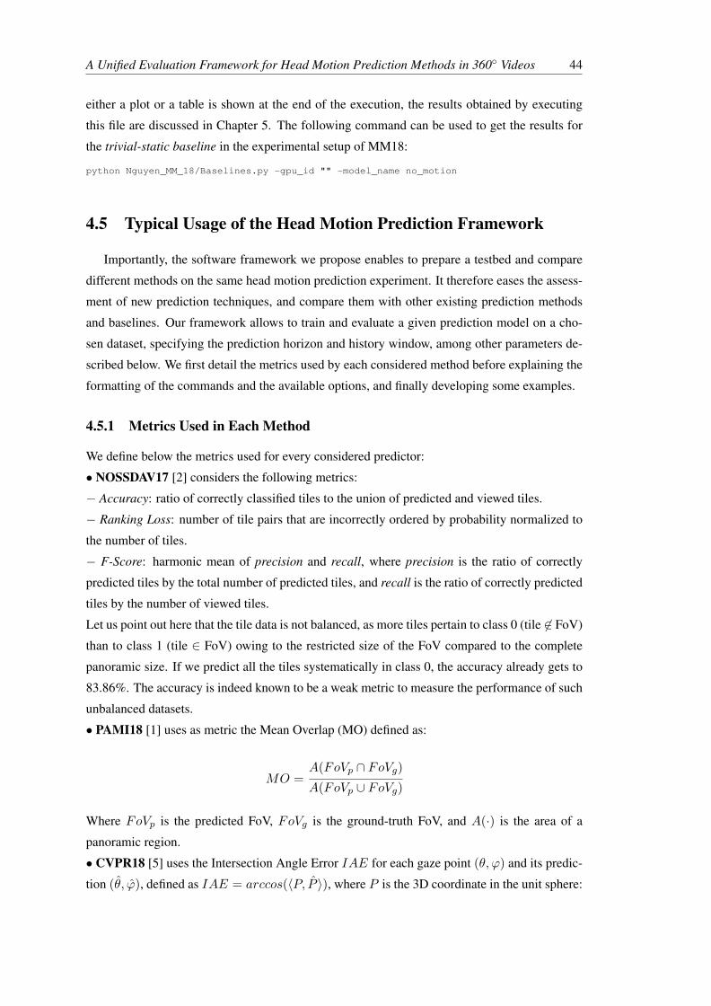
A Unified Evaluation Framework for Head Motion Prediction Methods in 360◦ Videos 44

either a plot or a table is shown at the end of the execution, the results obtained by executing

this file are discussed in Chapter 5. The following command can be used to get the results for

the trivial-static baseline in the experimental setup of MM18:

python Nguyen_MM_18/Baselines.py -gpu_id "" -model_name no_motion

4.5 Typical Usage of the Head Motion Prediction Framework

Importantly, the software framework we propose enables to prepare a testbed and compare

different methods on the same head motion prediction experiment. It therefore eases the assess-

ment of new prediction techniques, and compare them with other existing prediction methods

and baselines. Our framework allows to train and evaluate a given prediction model on a cho-

sen dataset, specifying the prediction horizon and history window, among other parameters de-

scribed below. We first detail the metrics used by each considered method before explaining the

formatting of the commands and the available options, and finally developing some examples.

4.5.1 Metrics Used in Each Method

We define below the metrics used for every considered predictor:

• NOSSDAV17 [2] considers the following metrics:

− Accuracy: ratio of correctly classified tiles to the union of predicted and viewed tiles.

− Ranking Loss: number of tile pairs that are incorrectly ordered by probability normalized to

the number of tiles.

− F-Score: harmonic mean of precision and recall, where precision is the ratio of correctly

predicted tiles by the total number of predicted tiles, and recall is the ratio of correctly predicted

tiles by the number of viewed tiles.

Let us point out here that the tile data is not balanced, as more tiles pertain to class 0 (tile 6∈ FoV)

than to class 1 (tile ∈ FoV) owing to the restricted size of the FoV compared to the complete

panoramic size. If we predict all the tiles systematically in class 0, the accuracy already gets to

83.86%. The accuracy is indeed known to be a weak metric to measure the performance of such

unbalanced datasets.

• PAMI18 [1] uses as metric the Mean Overlap (MO) defined as:

MO =A(FoVp ∩ FoVg)A(FoVp ∪ FoVg)

Where FoVp is the predicted FoV, FoVg is the ground-truth FoV, and A(·) is the area of a

panoramic region.

• CVPR18 [5] uses the Intersection Angle Error IAE for each gaze point (θ, ϕ) and its predic-

tion (θ, ϕ), defined as IAE = arccos(〈P, P 〉), where P is the 3D coordinate in the unit sphere:

A Unified Evaluation Framework for Head Motion Prediction Methods in 360◦ Videos 45

P = (x, y, z) = (cos(θ)cos(ϕ), cos(θ)sin(ϕ), sin(θ)). Let us mention that CVPR18 also con-

siders a deep-position-only baseline. However, ours appears stronger, likely due to the seq2seq

architecture. We readily apply our different predictors on the gaze data available in the CVPR18-

dataset.

• MM18 [3] takes the tile with the highest viewing probability as the center of the predicted

viewport, and assigns it and all the neighboring tiles that cover the viewport, with label 1.

Tiles outside the viewport are assigned 0. Then, the score is computed on these labels as

IoU = TP/TT (True Positive TP , True Total TT ). The Intersection over Union (IoU): the

intersection between prediction and ground-truth of tiles with label 1 (TP ) over the union of all

tiles with label 1 in the prediction and in the ground-truth (TT ).

• ChinaCom18 [4] uses the Accuracy and F-Score on the labels assigned to each predicted tile.

4.5.2 Training and Evaluation

To train or evaluate a given neural network in a specific dataset and configure some basic

settings, the following command can be used:

python training_procedure.py -{evaluate, train} -gpu_id GPU_ID -dataset_name

DATASET_NAME -model_name MODEL_NAME -init_window T_START -m_window M_WINDOW

-h_window H_WINDOW [-end_window T_END] -exp_folder FOLDER_NAME [-provided_videos]

-use_true_saliency -metric {orthodromic, mse}

Here is the detail of each option:

• -evaluate/-train: This option allows to decide if we want to train or evaluate the neural net-

work defined in MODEL NAME.

• -gpu id: Specify the ID of the Graphics Processing Unit (GPU) to load the neural network,

if the parameter is left empty, the neural network will be loaded on the Central Processing

Unit (CPU).

• -dataset name: Select the dataset to use with the parameter DATASET NAME, the options

are:

Xu PAMI 18, Xu CVPR 18, Fan NOSSDAV 17, Nguyen MM 18, Li ChinaCom 18 and

David MMSys 18.

• -model name: Select the model to train or evaluate, the options are: no motion, pos only,

CVPR18, MM18, TRACK, among others.

• -init window: In the experiment, the prediction will not be assessed over the first T START

time-stamps of the videos.

• -m window: The neural network takes into account the last M WINDOW time-stamps from

time t, also named history window in Fig. 4.1.

• -h window: The prediction horizon, we try to predict over the following H WINDOW time-

stamps from time t.

• -end window: The prediction is not assessed over the last T END time-stamps of the videos,

by default T END is equal to H WINDOW.

A Unified Evaluation Framework for Head Motion Prediction Methods in 360◦ Videos 46

• -exp folder: The folder to read the traces. The default value is “sampled dataset”, the folder

created when uniformly sampling all datasets in Sec. 4.2.

• -provided videos: Flag to use in case the partition into train and test videos are provided in

the original dataset.

• -use true saliency: Flag that tells whether to use true saliency, if not set, then content-based

saliency is used.

• -metric: Metric used for the evaluation, by default orthodromic distance (orthodromic), but

mean squared error (mse) can be used too. More metrics can be easily added by filling up the

Python dictionary “all metrics” in the script “Utils.py”.

4.5.3 Examples of Usage

We now present a few examples on how to use our framework to get the results for the

methods of CVPR18 and MM18 in an experimental setup where the prediction horizon isH = 5

seconds, the evaluation metric is the orthodromic distance, using the the ground-truth saliency in

the dataset of MMSys18 [17]. In this dataset we have a set of users U and a set of videos V . In

the validation stage, there is no intersection between the subsets Utrain×Vtrain and Utest×Vtest.This way we make sure that the network does not exploit any information about the behavior

of each user, or particular features of a video. All the plots and the analysis of the results are

discussed in more detail in Sec. 5.

CVPR18Since the code of CVPR18 is not publicly available, the neural network of CVPR18 used here

is a replica from the description in [5]. In our replica of CVPR18, we decided to prune the

Saliency Encoder Module and replace it directly with the ground-truth to be independent from

the imperfection of the saliency encoder module fed with the visual content, more details about

the replica is given in the Appendix A.5.4. The following command is used to get the results

for the replica of the neural network of CVPR18 on our experimental setup, trained and tested

with ground-truth saliency maps:

python training_procedure.py -evaluate -gpu_id 0 -dataset_name David_MMSys_18

-model_name CVPR18 -init_window 30 -m_window 5 -h_window 25 -exp_folder

original_dataset_xyz -provided_videos -use_true_saliency

MM18For the case of MM18, the model and weights are publicly available in [71]. Since the model

of MM18 predicts the head orientation at time t + H , we had to retrain the model for each

prediction step in the prediction horizon, i.e., for each s ∈ {0.2s, 0.4s, · · · , H = 5s}. To

get the results for the neural network of MM18 on our experimental setup, using ground-truth

saliency maps, use the following command:

python training_procedure.py -evaluate -gpu_id 0 -dataset_name David_MMSys_18

-model_name MM18 -init_window 30 -m_window 15 -h_window 25 -exp_folder

original_dataset_xyz -provided_videos -use_true_saliency

A Unified Evaluation Framework for Head Motion Prediction Methods in 360◦ Videos 47

4.6 Conclusions

In this Chapter we presented a framework to evaluate and compare different methods to

predict head position in 360◦ videos. In this framework, we propose an algorithm to create a

uniform data structure from each of the heterogeneous datasets evaluated in our work. We de-

scribed the algorithms used to compute the saliency maps either estimated from the raw video

content or from the users’ statistics, considering a kernel fitted for the equirectangular projec-

tion used to encode 360◦ videos. To compare each of the head motion prediction settings to

a common reference, we detailed the commands to estimate the performance of different ap-

proaches in each original evaluation context (prediction horizon, metrics and datasets). Finally,

we presented how to use our framework to prepare a testbed to assess comprehensively a new

prediction method (on various datasets against several competitors). This software framework

therefore contributes to progress towards efficient 360◦ streaming systems. The entire mate-

rial (codes, datasets, neural network weights and documentation) is available at [18]. In the

following Chapter we present the results of the plots and the analysis obtained by using this

framework.

Chapter 5

A Critical Analysis of DeepArchitectures for Head MotionPrediction in 360◦ Videos

In this Chapter, we consider the problem of predicting the user’s head motion in 360◦ videos

over a future horizon, based both and only on the past trajectory and on the video content. As

introduced in Chapter 4, various methods tackling this problem with deep neural networks have

been proposed (e.g., [1, 5, 3, 4, 2]). We show that the relevant existing methods have hidden

flaws, that we thoroughly analyze to overcome with a new proposal establishing state-of-the-art

performance.

This Chapter is organized as follows: Sec. 5.1 formulates the prediction problem considered,

and presents a taxonomy of the studied methods. Sec. 5.2 evaluates these methods against two

baselines, the trivial-static baseline and the deep-position-only baseline. Sec. 5.4 presents the

first part of the root-cause analysis by analyzing the data, introducing the saliency-only baseline.

Sec. 5.5 completes the root-cause analysis by analyzing the architectural choices. Sec. 5.6

presents our reasoning to obtain our new prediction method, TRACK, which establishes state-

of-the-art performance. Sec. 5.7 gives perspective and connects our work to most recent critical

re-examinations of deep learning-based approaches for other application domains. Sec. 5.8

concludes the Chapter.

5.1 Taxonomy of Existing Head Prediction Methods

This section reviews the existing methods relevant for the problem we consider. We start

by formulating the exact problem: it consists, at each video playback time t, in predicting the

future user’s head positions between t and t + H , as illustrated in Fig. 5.1 (also represented

in Chapter 4 Fig. 4.1), with the only knowledge of this user’s past positions and the (entire)

video content. We therefore do not consider methods aiming to predict the entire user trajectory

49

TRACK: A Multi-Modal Deep Architecture for Head Motion Prediction in 360◦ Videos 50

t+2

t+H

t+H

⋮

( )

( )

( )

, … ,

,

,

,

( ) ( )

θ

θ

θ

θ , θθ

θ

θ

( ),θ

,

t+2

t+1

t+1

t t0 0

00

t t

t+1 t+1

t+H t+H

Data transmission

FIGURE 5.1: 360◦ video streaming principle. The user requests the next video segment attime t, if the future orientations of the user (θt+1, ϕt+1), ..., (θt+H , ϕt+H) were known, thebandwidth consumption could be reduced by sending in higher quality only the areas corre-

sponding to the future FoV.

from the start based on the content and on the starting point as, e.g., targeted by the challenge in

[76] or summarizing a 360◦ video into 2D [77, 78]. As well, and importantly, we consider that

the users’ statistics for the video are not known at test time, hence we do not consider methods

relying on these per-video statistics, such as [65, 66]. Also, the domain of egocentric videos is

related to that of 360◦ video. However, the assumptions are not exactly the same: only part of

the scene and some regions likely to attract the users are available (video shot from a mobile

phone), contrary to a 360◦ video. We therefore do not compare with such works.

5.1.1 Problem Formulation

In this Chapter we keep the same notation defined in Chapter 4.1.1. Let Pt = [θt, ϕt] denote

the vector coordinates of the FoV at time t. Let Vt denote the considered visual information at

time t: depending on the models’ assumptions, it can either be the raw frame with each RGB

channel, or a 2D saliency map resulting from a pre-computed saliency extractor. Let T be the

video duration. The prediction is not assessed over the first Tstart seconds of video. To match

the settings of the works we compare with, Tstart is set to 0 sec. for all the curves generated

in Sec. 5.2. In order to skip the exploration phase, as explained in Sec. 5.4.4, and be more

favorable to all methods as they are not able to consider non-stationarity of the motion process,

we set Tstart = 6 sec. from Sec. 5.4 onward. Let H be the prediction horizon and M be the

history window. We define the terms prediction step s, and video time-stamp t, such that: at

every time-stamp t ∈ [Tstart, T ], we run predictions Pt+s, for all prediction steps s ∈ [0, H].

Except for the results in Fig. 5.7, for each s, we average the errors D(Pt+s,Pt+s) over

all t ∈ [Tstart, T ]. As considered in the existing methods we compare with, we make H vary

between 0.2 sec. and 2.5 sec., then extend H to 5 sec. as detailed from the analysis in Sec. 5.4.

TRACK: A Multi-Modal Deep Architecture for Head Motion Prediction in 360◦ Videos 51

5.1.2 Taxonomy

As presented in Chapter 4, various approaches to predict user motion in 360◦ video environ-

ments have been published. These methods are organized in Table 5.1. They consider different

objectives (col. 2 starting from the left), such as predicting the future head position, gaze posi-

tion or tiles in the FoV. The prediction horizons (col. 3) also span a wide range, from 30ms to

2.5 seconds. Some articles share common datasets for experiments (col. 4), while generally not

comparing with each other. Different types of input and output formats are considered (col. 5):

some consider the positional information implicitly by only processing the content in the FoV

(PAMI18), other consider the position separately, represented as a series of coordinates (e.g.,

CVPR18) or as a mask (e.g., MM18), with the last sample only (IC3D17) or various length of

history, some extract features from the visual content by employing some pre-trained saliency

extractors (e.g. NOSSDAV17, MM18) or training end-to-end representation layers made of

convolutional and max-pooling layers (e.g., PAMI18). Finally, most of the methods but the

first two in Table 5.1 rely on deep-learning approaches. A key aspect is the way they handle

the combination of the positional information (if they consider it individually) with the video

content information. As these two types of information are time series, those works all con-

sider the use of deep Recurrent Neural Networks (RNN), and all use Long Short Term Memory

(LSTM). However, whether the features are first extracted from each time series independently,

or whether the time series samples are first concatenated then fed to a common LSTM, depends

on each method. The positioning of the recurrent network in the whole architecture is the mul-

timodality fusion criterion we have selected (col. 6) to order the rows in Table 5.1 (within each

group, methods are ordered from the most recently published), thereby extracting 3 groups of

methods:

• if the positional information is not explicitly considered, then no combination is made and

a single LSTM processes the content of the FoV: PAMI18;

• combination is made after the single LSTM module in CVPR18: the LSTM processes

past positions, and its output gets fused with the video features through a fully connected

layer (see Fig. 5.2-Right);

• if the current saliency map extracted from the content is first concatenated with the current

position information, then the LSTM module handles both pieces of information modali-

ties simultaneously: NOSSDAV17, ChinaCom18, MM18 (see Fig. 5.2-Left).

The architectures tackling this dynamic head motion prediction problem have hence three

main objectives: (O1) extracting attention-driving features from the video content, (O2) pro-

cessing the time series of position, and (O3) combining (fusing) both information modalities

to produce the final position estimate. We depict the modules in charge of (O2) and (O3) of

methods MM18 and CVPR18 in Fig. 5.2.

TRACK: A Multi-Modal Deep Architecture for Head Motion Prediction in 360◦ Videos 52

Reference Objective Predictionhorizon

Dataset Inputs

RNNbefore/afterconcatenationof modalities

PAMI18[1]

headcoordinates 30ms 76 videos,

58 usersframe cropped toFoV

N/A(no fusion)

IC3D17[67]

headcoordinates 2s 16 videos,

61 usersPre-trained sal. inFoV

N/A(no fusion,no LSTM)

ICME18[68]

tilesin FoV 6s 18 videos,

48 usersPosition history,users’ distribution

N/A(no LSTM)

CVPR18[5]

gazecoordinates 1s 208 videos,

30+ users

Video frame,position history ascoordinates

before

MM18[3]

tilesin FoV 2.5s

11 videos, 48+users from [72, 73]with custom pre-processing

Pre-trainedsaliency,mask of positions

after

ChinaCom18[4]

tilesin FoV 1s NOSSDAV17’s

dataset

Pre-trainedsaliency,FoV tile history

after

NOSSDAV17[2]

tilesin FoV 1s 10 videos,

25 users

Pre-trainedsaliency,FoV position ortile history

after

TABLE 5.1: Taxonomy of existing dynamic head-prediction methods. References in bold areconsidered for comparison in Sec. 5.2.

These methods make for a wide range of deep network architectural choices. In particular

the fusion problem (O3) may be handled differently. MM18 and CVPR18 are selected as rep-

resentatives: combining both modalities before or after the recurrent (LSTM) unit, respectively.

There is no pairwise comparison between any of the above works. From the articles in Table 5.1,

the only works which provided their code and their deep neural networks for reproducibility are

PAMI18 and MM18. However, we could obtain all the datasets to compare with all (the datasets

not publicly available were kindly shared by the authors whom we have contacted).

TRACK: A Multi-Modal Deep Architecture for Head Motion Prediction in 360◦ Videos 53

Flatten

Concatenate

LSTM

Pt Vt+1

FC

ArgMax

Pt+1^

LSTM

Flatten

Concatenate

Pt Vt+1

FC

FC

Pt+1^

Add

LSTM

LSTM

FIGURE 5.2: The building blocks in charge, at each time step, of processing positional infor-mation Pt and content information Vt, that are visual features learned end-to-end or obtainedfrom a saliency extractor module (omitted in this scheme). Left: MM18 [3]. Right: CVPR18.

[5]

5.2 Comparison of State of the Art Methods Against Two Baselines:Trivial-Static and Deep-Position-Only

To compare the above recent proposals (PAMI18, CVPR18, MM18, ChinaCom18, NOSS-

DAV17) to a common reference, we first introduce the trivial-static baseline. First, we show

that all these methods on their original settings, metrics and datasets, are outperformed by this

trivial baseline. This is surprising and raises the question of whether it is actually possible to

learn anything meaningful with these settings (datasets and prediction horizons). To answer this

question, we then introduce the deep-position-only baseline, that we design as a sequence-to-

sequence LSTM-based architecture exploiting the time series of past positions only (disregard-

ing the video content). We show this new baseline is indeed able to outperform the trivial-static

baseline (establishing state-of-the-art performance). Later, Sec. 5.4 introduces a saliency-only

baseline.

5.2.1 Definition of the Trivial-Static Baseline

Different linear predictors can be considered as baselines. We consider here the simplest one

which predicts no motion:[Pt+1, . . . , Pt+H

]=[Pt, . . . ,Pt

].

More complex baselines exist. For example in [79], a Linear Regressor and a Neural Network

perform better than the trivial-static baseline. However, as we will see in Chapter 5, all existing

methods trying to leverage both the video content and the position to predict future positions

perform worse than the trivial-static baseline, without exception.

TRACK: A Multi-Modal Deep Architecture for Head Motion Prediction in 360◦ Videos 54

5.2.2 Details of the Deep-Position-Only Baseline

We now present an LSTM-based predictor which considers positional information only. An

LSTM enables non-linear shape of the motion and the memory effect due to inertia, as discussed

in [5] and shown by the generated trajectories in Fig. 5.4. The deep-position-only baseline

consists of a sequence-to-sequence LSTM-based architecture, with an encoder that processes

the history of head positions and a decoder that produces the outputs for the prediction horizon.

We select a Sequence-to-Sequence (Seq2Seq) architecture because it has proven powerful at

capturing complex dependencies and generating realistic sequences, as shown in text translation

for which it has been introduced [80].

Pt-M

FC

Pt-M+1 Pt-1 Pt

…

Pt+H-1^

Pt+1^

Pt+1^

Pt+2^

Pt+H^

FC FC

LSTM LSTM LSTM…

LSTM LSTM LSTM…1024 1024 1024 1024

10241024

2 2 2 2 2

1024

1024

2 2 2

…

2

FIGURE 5.3: The deep-position-only baseline based on an encoder-decoder (seq2seq) archi-tecture.

As depicted in Fig. 5.3, a seq2seq framework consists of an encoder and a decoder. The

encoder receives the historic window input (samples from t−M to t− 1 shown in Fig. 4.1) and

generates an internal representation. The decoder receives the output of the encoder and pro-

gressively produces predictions over the target horizon, by re-injecting the previous prediction

as input for the new prediction time-steps.

The encoder can be represented as:

lt = L(Pt, L(Pt−1, L(Pt−2, ...L(Pt−M+1, L(Pt−M , 0))))), (5.1)

where lt is the state of the LSTM at time t.

The decoder can be represented as:

ht+1, lt+1 = L(Pt, lt))

∆Pt+1 = Dm(ht+1)×Dd(ht+1)

Pt+1 = Pt⊕

∆Pt+1

(5.2)

A single LSTM L(·) with 1024 units is used for both the encoder and the decoder. At the

TRACK: A Multi-Modal Deep Architecture for Head Motion Prediction in 360◦ Videos 55

0.2 0.4 0.6 1.0 2.0 3.0 4.0 all0.85

0.9

0.95

Historic window [seconds]

Avg

.Ort

hodr

omic

Dis

t.

5 10 15 20

0

0.2

0.4

0.6

0.8

1

Video time stamp [seconds]

Nor

mal

ized

long

itude

FIGURE 5.4: Left: Impact of the historic-window size. Right: Ground truth longitudinaltrajectory (for video “Diner”, user 4) is shown in black, colors are the non-linear trajectories

predicted by the position-only baseline from each time-stamp t.

decoder, two fully connected layers D1, D2 with 2 neurons each are used to predict the magni-

tude and the direction of the displacement, to compute the new longitude and latitude given the

previous position Pt and the displacement ∆Pt+1, we add the angles with the function⊕

that

is able to handle the periodicity of the longitude and the latitude, as discussed in Sec. 5.3.1.

How Much Historic Information to Use?: Fig. 5.4-Left shows that the error progressively

reduces when increasing the historic window up to 1 sec. Beyond this value, no further im-

provement is obtained.

Training Settings: During both training and testing, the decoder unit is executed H times in a

loop to obtain all the predictions for the time-steps in the prediction horizon. The deep-position-

only baseline was developed using Keras and Scikit-Learn. We used Adam optimization algo-

rithm with a learning rate of 0.0005, and we select the best performing model after training for

500 epochs to produce each of the results in this work. The batch size was set to 128.

Generated Trajectories: We finally illustrate the type of head trajectories generated with our

baseline. As shown in Fig. 5.4-Right, the network is able to learn non-linear realistic trajectories

([−180◦, 180◦] is projected onto [0, 1], note that the jump from 1 to 0 only reflects the crossing

from 180◦ to −180◦). We also mention here that we observe the predicted motion tends to

vanish over time. This is a well-known drawback of the l1-type losses, where the network copes

with uncertainty increasing over time by averaging over possible modes, generating vanishing

motion or blur, as exhibited for segmentation prediction in [81] and 3D-skeleton pose prediction

in [82] (possibly remedied with adversarial losses, out of the scope of this work).

5.2.3 Results of Comparison Against State of the Art

We now present the comparisons of the state of the art methods presented in Sec. 5.1.2 with

the trivial-static baseline and deep-position-only baseline defined above.

We report the exact results of the original articles, along with the results of our baselines, the

deep-position-only baseline being trained and tested on the exact same train and test subsets of

TRACK: A Multi-Modal Deep Architecture for Head Motion Prediction in 360◦ Videos 56

Method KingKong SpaceWar2 StarryPolar Dancing Guitar BTSRun InsideCar RioOlympics Average

PAMI18 [1] 0.809 0.763 0.549 0.859 0.785 0.878 0.847 0.820 0.753trivial-static baseline 0.974 0.963 0.906 0.979 0.970 0.983 0.976 0.966 0.968

deep-position-only baseline 0.983 0.977 0.930 0.984 0.977 0.987 0.982 0.976 0.977TRACK 0.974 0.964 0.912 0.978 0.968 0.982 0.974 0.965 0.968

Method SpaceWar CMLauncher2 Waterfall Sunset BlueWorld Symphony WaitingForLove Average

PAMI18 [1] 0.626 0.763 0.667 0.659 0.693 0.747 0.863 0.753trivial-static baseline 0.965 0.981 0.973 0.964 0.970 0.968 0.978 0.968

deep-position-only baseline 0.976 0.989 0.984 0.973 0.979 0.976 0.982 0.977TRACK 0.965 0.981 0.972 0.964 0.970 0.969 0.977 0.968

TABLE 5.2: Comparison with PAMI18 [1]: Mean Overlap scores of FoV prediction, predictionhorizon H ≈ 30ms (1 frame). The model TRACK is introduced in Sec. 5.5.2.

trivial-static baseline deep-position-only baseline ChinaCom18Accuracy F-score Accuracy F-score Accuracy F-score

Hog Rider 96.29% 0.8858 96.97% 0.9066 77.09% 0.2742Driving with 95.96% 0.8750 96.59% 0.9843 77.34% 0.2821Shark Shipwreck 95.23% 0.8727 96.12% 0.8965 83.26% 0.5259Mega Coaster 97.20% 0.9144 97.71% 0.9299 88.90% 0.7011Roller Coaster 96.99% 0.9104 97.50% 0.9256 88.28% 0.6693Chariot-Race 97.07% 0.8802 96.91% 0.9056 87.79% 0.6040SFR Sport 96.00% 0.8772 96.91% 0.9054 89.29% 0.7282Pac-Man 96.83% 0.8985 97.16% 0.9089 87.45% 0.6826Peris Panel 95.60% 0.8661 96.54% 0.8947 89.12% 0.7246Kangaroo Island 95.35% 0.8593 96.54% 0.8954 82.62% 0.5308

Average 96.15% 0.8840 96.90% 0.9063 72.54% 0.5155

TABLE 5.3: Comparison with ChinaCom18 [4], prediction horizon H = 1 second.

Method Accuracy F-Score Rank Loss

NOSSDAV17-Tile [2] 84.22% 0.53 0.19NOSSDAV17-Orient. [2] 86.35% 0.62 0.14trivial-static baseline 95.79% 0.87 0.10deep-position-only baseline 96.30% 0.89 0.09TRACK 95.48% 0.85 0.15

TABLE 5.4: Comparison with NOSSDAV17: Performance of Tile- and Orientation-based net-works of [2] compared against our deep-position-only baseline, prediction horizon H = 1

second. The model TRACK is introduced in Sec. 5.5.2.

the original dataset as the original method (there is no training for the trivial-static baseline).

The benchmark metrics (discussed in Sec. 4.5.1 and related to predicting head or gaze positions,

or FoV tiles) are those from the original articles, so are the considered prediction horizons H .

Results for PAMI18 are shown in Table 5.2, for CVPR18 in Fig. 5.5-Bottom, for MM18 in

Fig. 5.5-Top, for ChinaCom18 in Table 5.3 and for NOSSDAV17 in Table 5.4. Let us mention

that none of these methods considered baselines identical to the trivial-static baseline and deep-

position-only baseline defined above. All perform worse than both our trivial-static and deep-

position-only baselines. Specifically, all but one (CVPR18) perform significantly worse.

TRACK: A Multi-Modal Deep Architecture for Head Motion Prediction in 360◦ Videos 57

0.5 1 1.5 2 2.5

0.5

0.6

0.7

0.8

Prediction step (sec.)

Scor

e(I

oU)

MM18 [5]trivial-static baselinedeep-pos-only baselineTRACK

0 5 10 15 20

0

0.1

0.2

0.3

0.4

0.5

0.6

Intersection Angle Error

Dat

aPr

opor

tion

CVPR18 [5]trivial-static baselinedeep-pos-only baselineCVPR18-reproTRACK

FIGURE 5.5: Top: Comparison with MM18 [3], H =2.5 seconds. Bottom: Comparison withCVPR18 [5], prediction horizon H = 1 sec. CVPR18-repro is introduced in Sec. 5.3.1, the

model TRACK in Sec. 5.5.2.

5.3 Root Cause Analysis: the Metrics in Question

We have shown that the existing methods assessed above, which try to leverage both posi-

tional information and video content to predict future positions, perform worse than a simple

baseline assuming no motion, which in turn can be outperformed by the deep-position-only

baseline (considering only positional information). This section and the next two (Sec. 5.4 &

Sec. 5.5) aim to identify the reasons why the existing approaches perform worse than the base-

lines. In this part, we focus on the possible causes due to the evaluation, specifically asking:

Q1 Metrics: Can the methods perform better than the baselines for some specific videos or

pieces of trajectories?

5.3.1 Evaluation Metrics D (·)

Let us first describe the losses and evaluation metrics considered from now on. The predic-

tion of the FoV motion can be cast as a classification problem, where pixels or tiles are classified

TRACK: A Multi-Modal Deep Architecture for Head Motion Prediction in 360◦ Videos 58

0 1 2 3

0

1

2

3

Orthodromic distance

Ang

ular

erro

r

0 1 2 3 4 50

0.5

1

1.5

Prediction horizon [seconds]

Ort

hodr

omic

Dis

t.

Seq2Seq-AbsoluteSeq2Seq-Residual

FIGURE 5.6: Left: Relationship between orthodromic distance and angular error. Right: Per-formance of the network on the MMSys18 dataset when predicting absolute fixation positionPt and when predicting fixation displacement ∆Pt using a residual network, the performance

gain when predicting fixation displacement ∆Pt is in the short-term prediction.

in or out of future FoV (as done in NOSSDAV17, MM18, ChinaCom18). However, this problem

is inherently imbalanced. Therefore, for the analysis, we choose to keep the original formula-

tion as a regression problem. The tracking problem on a sphere can be assessed by different

distances. Given two points on the surface of the unit sphere P1 = (θ1, ϕ1) and P2 = (θ2, ϕ2),

where θ is the longitude and ϕ is the latitude of the point, possible distances are:

•Mean squared error = ((θ1 − θ2)2 + (ϕ1 − ϕ2)2)/2

• Angular error =√

arctan(sin(∆θ)/ cos(∆θ))2 + (ϕ1 − ϕ2)2, where ∆θ = θ1 − θ2

• Orthodromic distance

= arccos (cos (ϕ1) cos (ϕ2) cos (∆θ) + sin (ϕ1) sin (ϕ2)) which is a reformulation of Eq. 4.1.

The latter two metrics are able to handle the periodicity of the latitude, which the first one

cannot. The difference between angular error and orthodromic distance is that the latter com-

putes the distance on the surface of the sphere, while the angular error computes the error of

each angle independently.

Fig. 5.6-Left shows that the relationship between the angular error and the orthodromic

distance is not bijective, and importantly that the orthodromic distance varies rather logarith-

mically with the angular error. The green dots are the points at the pole Ppole = (θ, π2 ) with

θ ∈ [−π, π]. We observe how the angular error as loss function penalizes points that are in

the same spot in the surface of the sphere but with different angles (the pole’s latitude described

a unique point for any longitude). The largest difference in orthodromic distance is the an-

tipodal point Pantipode = (π, 0), while for the angular error the largest distance occurs at the

poles Ppole = (π, π2 ). This is shown by the red dots which are all the points P = (π, ϕ) with

ϕ ∈ [0, π2 ]. Let us note how the angular error increases when the orthodromic distance de-

creases for these points. In general, for a point P = (θ, ϕ) the orthodromic distance decreases

and the angular error increases when we set θ fixed and move to either of the poles by varying

ϕ from 0 to π (or −π). Finally, owing to its fitness to the tracking problem on the unit sphere

TRACK: A Multi-Modal Deep Architecture for Head Motion Prediction in 360◦ Videos 59

with latitude and longitude as inputs, we choose the orthodromic distance as the train and test

metric with the input formatted with longitude and latitude (θ, ϕ) of the FoV’s center.

5.3.2 Q1: Can the Methods Perform Better than the Baselines for Some SpecificPieces of Trajectories or Videos?

The metrics used in Sec. 3 are averages over time trajectories and videos. The question

we ask is whether the methods can perform better than the baselines for some specific pieces of

trajectories or videos.

5.3.2.1 Specific Pieces of Trajectory

To evaluate whether the existing methods perform better than the baselines in some specific

pieces of the trajectory, we adopt the same approach as in [83, Sec. 4], introducing the Average

non-linear displacement error as a metric to evaluate the error around the non-linear regions

of the trajectory where most errors occur owing to human-content interactions. We therefore

quantify the difficulty of prediction with the second derivative of the trajectory, i.e., the radius

of curvature. To obtain detailed results (for each instant of time of each user and video pair),

we re-implement CVPR18 with the exact same architectural and training parameters as those

described in the article [5].1

The curve CVPR18-repro in Fig. 5.5-Bottom shows that we obtain similar results on the

original dataset (higher on the first half of the truncated CDF, then slightly lower on the second

half of the truncated CDF). This confirms the validity of our re-implementation. Fig. 5.7-Left

depicts the distribution of the prediction difficulty. Fig. 5.7-Right shows that for every difficulty

range, CVPR18-repro is not able to improve the prediction over the baselines.

We obtained similar qualitative results with MM18, Fig. 5.8-Left depicts the distribution of

the prediction difficulty, and Fig.5.8-Right shows that for every difficulty range, MM18 is not

able to improve the prediction over the baselines.

Considering CVPR18 and MM18 the two representative and best performing methods in

Sec. 3 (apart from the baselines).

We conclude that for more difficult parts of the trajectory, the CVPR18-repro or MM18

methods are not able to improve over the baselines.

5.3.2.2 Specific Videos

Fig. 5.7-Left shows that the majority of the data is in the 0-1 difficulty range, therefore, we

can think the models have difficulty to pay attention to the rarer cases of trajectory pieces where

the prediction difficulty is higher. To evaluate whether the existing methods perform better than

the baselines when the dataset (train and test sets) is properly balanced with videos where the1We had to replicate the architecture of CVPR18 because we could not find any official code and the authors did

not reply to our emails. Our reproduced code is available online at [18] and detailed in Appendix A.5.4.

TRACK: A Multi-Modal Deep Architecture for Head Motion Prediction in 360◦ Videos 60

0 1 2 3 4 5

0

0.05

0.1

0.15

Difficulty of prediction

Den

sity

0− 1 1− 2 2− 4 4− 6 6− 16

0

50

100

150

Difficulty of prediction

Inte

rsec

tion

Ang

leE

rror

CVPR18-reprotrivial-static baselinedeep-pos-only baseline

FIGURE 5.7: Left: Distribution of difficulty in the CVPR18 dataset. Right: Error as a functionof the difficulty for the CVPR18-repro model.

0 1 2 3 4 5

0

0.2

0.4

Difficulty of prediction

Den

sity

0− 1 1− 2 2− 4 4− 6 6− 16

0

0.2

0.4

0.6

0.8

1

Difficulty of prediction

Scor

e(I

oU)

MM18trivial-static baselinedeep-pos-only baseline

FIGURE 5.8: On the MM18 dataset: (Left) Distribution of difficulty in the dataset. (Right)Score of the MM18 method as a function of the difficulty.

content is proved to help, we consider the dataset prepared in Sec. 5.5.1. The details on the

usefulness of the content are given in Sec. 5.4.

The average performance of CVPR18-repro and MM18-repro on this dataset can be seen

in Fig. 5.17: they are never able to take advantage of the content as they are systematically

outperformed by the deep-position-only baseline.

Fig. 5.9 shows the performance of CVPR18-repro and MM18-repro on the MMSys18 dataset

per test video. It is important to mention that both models are fed with Ground Truth (GT)

saliency. The results show that these methods are not able to take advantage of the content

as they are outperformed, over the entire prediction horizon 0s-5s, by the deep-position-only

baseline even for the videos where the saliency is proved useful (Sec. 5.4.2).

TRACK: A Multi-Modal Deep Architecture for Head Motion Prediction in 360◦ Videos 61

0 1 2 3 4 50

π8

π4

3π8

π2

Prediction step s (sec.)

Avg

.Ort

hodr

omic

Dis

t.

PortoRiverside (Expl.)

deep-position-only baselineMM18-reproCVPR18-repro

0 1 2 3 4 50

π8

π4

3π8

π2

Prediction step s (sec.)

Avg

.Ort

hodr

omic

Dis

t.

PlanEnergyBioLab (Expl.)

deep-position-only baselineMM18-reproCVPR18-repro

0 1 2 3 4 5

π8

π4

Prediction step s (sec.)

Avg

.Ort

hodr

omic

Dis

t.

Waterpark (Ride.)

deep-position-only baselineMM18-reproCVPR18-repro

0 1 2 3 4 50

π8

π4

3π8

Prediction step s (sec.)

Avg

.Ort

hodr

omic

Dis

t.

Warship (Static Focus.)

deep-position-only baselineMM18-reproCVPR18-repro

FIGURE 5.9: Prediction error results for MM18-repro, CVPR18-repro and deep-position-onlybaseline, detailed for each test video of the MMSys18 dataset. The results of MM18-repro and

CVPR18-repro obtained with Ground Truth (GT) saliency.

Answer to Q1: No, the methods considering the video content do not perform better than the

deep-position-only baseline for specific pieces of trajectories or videos where the knowledge of

the content should improve the prediction.

5.4 Root Cause Analysis: the Data in Question

In this section, we focus on the possible causes due to the data. In Sec. 5.5, we analyze the

possible architectural causes. This section therefore aim to answer question Q2, whose answer

is provided at the end of the section:

Q2 Data: Do the datasets (made of videos and motion traces) match the design assumptions

the methods build on?

To answer Q2, we consider the assumptions at the core of the existing architectures attempting

to leverage the knowledge of position history and video content, and break them down into :

• Assumption (A1): the position history can inform the prediction of future positions

TRACK: A Multi-Modal Deep Architecture for Head Motion Prediction in 360◦ Videos 62

0 0.5 1 1.5 2 2.5 3 3.5 4 4.5 5

0.2

0.4

0.6

0.8

Prediction step s (sec.)

Mut

ualI

nfor

mat

ion

MMSys18 datasetNOSSDAV17 datasetMM18 datasetPAMI18 datasetCVPR18 dataset

FIGURE 5.10: Mutual information MI(Pt;Pt+s) between Pt and Pt+s (averaged over t andvideos) for all the datasets used in NOSSDAV17, PAMI18, CVPR18 and MM18, with the

addition of MMSys18.

• Assumption (A2): the visual content can inform the prediction of future positions

We identify whether these assumptions hold in the datasets and settings considered by the ex-

isting methods (Sec. 5.4.1 and 5.4.4), and introduce a new saliency-only baseline to do so (Sec.

5.4.2).

5.4.1 Assumption (A1): the Position History is Informative of Future Positions

The amount of information held by a process about another one can be quantified by the

Mutual Information (MI). This in turns informs on the degree of predictability of the target

process using the first process. MI has been used in [84] for inter-user analysis. Here, we

define the MI between head positions of a given user at time t and t + s by MI(Pt;Pt+s) =

DKL(Pr[Pt, Pt+s]||Pr[Pt]⊗Pr[Pt+s]), whereDKL(·) and

⊗stand for the Kullback–Leibler

divergence and convolutional product, respectively. For each of the datasets considered in

PAMI18, CVPR18, MM18, NOSSDAV17, and MMSys18, Fig. 5.10 represents MI normalized

and averaged over all videos and time stamp t, as a function of s ∈ [0, H = 5sec.]. The 2D-

coordinates have been discretized in 128 bins. This figure shows that position at time t+ s can

be predicted to a significant degree by Pt when s is low (e.g., lower than 2 sec.). As expected,

the further away the prediction step, the lowest the predictability of Pt+s from Pt.

To relate Mutual Information with a more intuitive characterization of the datasets, we con-

sider the motion continuity (inertia). Fig. 5.11 represents the Cumulative Distribution Function

(CDF) of the displacement within each prediction horizon H = 0.2s, . . . , 15s for the datasets

considered in PAMI18, CVPR18, MM18, NOSSDAV17, and MMSys18. Each point (x, y) on

a curve represents the fraction y of samples (among users’ traces) for which the displacement

TRACK: A Multi-Modal Deep Architecture for Head Motion Prediction in 360◦ Videos 63

0 50 100 150

0

0.2

0.4

0.6

0.8

1

Motion (◦)

Dat

apr

opor

tion

NOSSDAV17

0 50 100 150

0

0.2

0.4

0.6

0.8

1

Motion (◦)

Dat

apr

opor

tion

PAMI18

H = 0.2sH = 0.5sH = 1sH = 2sH = 5s

H = 15s0 50 100 150

0

0.2

0.4

0.6

0.8

1

Motion (◦)

Dat

apr

opor

tion

CVPR18

(a) (b) (c)

0 50 100 150

0

0.2

0.4

0.6

0.8

1

Motion (◦)

Dat

apr

opor

tion

MM18

0 50 100 150

0

0.2

0.4

0.6

0.8

1

Motion (◦)D

ata

prop

ortio

n

MMSys18

(d) (e)

FIGURE 5.11: Motion distribution of the 4 datasets used in (a) NOSSDAV17, (b) PAMI18, (c)CVPR18 and (d) MM18, respectively. In (d) we show the distribution of the MMSys18 datasetfrom [17] and considered in the sequel. The x-axis corresponds to the motion from position at

t to t+H in degrees. Legend is identical in all sub-figures.

within H seconds has been less than x degrees. If we consider a FoV to be about 100◦ wide

[2], Fig. 5.11 informs on how many seconds it takes for the FoV to shift by at least half of its

width for half of the samples. It takes respectively at least 5 seconds for all but CVPR18 (the

data of CVPR18 is the eye gaze positions), and for the MMSys18 dataset from [17] for which

it takes about 2s. Over the considered forecast window in each of the experiments of PAMI18,

CVPR18, MM18 and NOSSDAV17, the FoV has shifted by half of its width for less than 0.5%,

5%, 5% and 7% of the samples, respectively. These last datasets have therefore a low amount of

motion.

Does Assumption (A1) hold?: On the datasets and prediction horizons considered in the literature

(H ≤ 2 sec.), the position history is therefore strongly informative of the next positions. Another

element supporting this observation is the best performance obtained by our baseline exploiting

position only (see Sec. 5.2 above). A similar study was conducted in [79] showing that the

viewer motion has a strong temporal auto-correlation.

5.4.2 Definition of the Saliency-Only Baseline

To analyze Assumption A2 in Sec. 5.4.4 and assess how much gain can the consideration

of the content bring to the prediction, we first define a so-called saliency-only baseline. This

baseline is defined from an attentional heat map, either extracted from the visual content (heat

TRACK: A Multi-Modal Deep Architecture for Head Motion Prediction in 360◦ Videos 64

map then named Content-Based saliency) or directly from the position data of all the users (heat

map then named Ground-Truth saliency). For either type of heat map, the saliency-only baseline

provides an upper-bound on the prediction error that a more refined processing of the heat map,

in combination with the past positions, would make. In this section, we only consider heat maps

obtained from the users data, we therefore start by defining such heat maps. Only in Sec. 5.5.2

do we use the heat maps estimated from the video content.

5.4.2.1 Definition of the K-Saliency-Only Baseline

We extract the K highest peaks of the heat map for every prediction step t+ s (for all t, for

all s ∈ [0, H]). At every t+ s, the K-saliency-only baseline predicts Pt+s as the position of the

peak, amongst the K peaks, which is closest to the last known user’s position Pt.

Fig. 5.12 and 5.13 show the prediction error of the K-saliency-only baseline for K = 1, 2,

5. For low s, we verify that the higher K, the lower the error close to time t, because the more

the number of points of interest possibly considered. However, as the prediction step s increases

and t + s gets away from t, the error is lower for lower K. Indeed, if the user moves, then she

is more likely to get closer to a more popular point of interest, that is to a higher-ranked peak.

Each K-saliency-only baseline can be considered as an upper-bound on the error that the best

predictor optimally combining position and content modality could get. Therefore, for a given

κ, we define the saliency-only baseline as the minimum of these K-saliency-only baseline, for

K ∈ [1, κ] and for every s in [0, H]. In this Chapter, we set κ = 5. The saliency-only baseline

is shown in red in Fig. 5.16. From Fig. 5.16, we do not represent the K-saliency-only baselines

anymore, but only the saliency-only baseline.

5.4.3 Background on Human Attention in VR

Before analyzing Assumption (A2), let us first provide some characteristics of the human

attention in VR identified recently. It has been recently shown in [35] and [8] that, when pre-

sented with a new VR scene (the term “scene” is defined by Magliano and Zacks in [85] as

a period of the video between two edits with space discontinuity), a human first goes through

an exploratory phase that lasts for about 10 to 15 sec. ([8, Fig. 18], [35, Fig. 2]), before set-

tling down on so-called Regions of Interest (RoIs), that are salient areas of the content. The

duration and amplitude of exploration, as well as the intensity of RoI fixation, depend on the

video content itself. Almquist et al. [8] have identified the following main video categories for

which they could discriminate significantly different users’ behaviors: Exploration, Static fo-

cus, Moving focus and Rides. In Exploration videos, the spatial distribution of the users’ head

positions tends to be more widespread, making harder to predict where the users will watch and

possibly focus on. Static focus videos are made of a single salient object (e.g., a standing-still

person), making the task of predicting where the user will watch easier in the focus phase. In

Moving focus videos, contrary to Static focus videos, the RoIs move over the sphere and hence

TRACK: A Multi-Modal Deep Architecture for Head Motion Prediction in 360◦ Videos 65

0 1 2 3 4 50

π8

π4

3π8

Prediction step s (sec.)

Ave

rage

Ort

hodr

omic

Dis

tanc

e

Average

0 1 2 3 4 50

π8

π4

3π8

π2

Prediction step s (sec)

Ave

rage

Ort

hodr

omic

Dis

tanc

e

PortoRiverside (Expl.)

0 1 2 3 4 50

π8

π4

3π8

π2

Prediction step s (sec)

Ave

rage

Ort

hodr

omic

Dis

tanc

e

PlanEnergyBioLab (Expl.)

0 1 2 3 4 50

π8

π4

3π8

Prediction step s (sec)

Ave

rage

Ort

hodr

omic

Dis

tanc

e

Turtle (Moving Focus)

0 1 2 3 4 5

π8

π4

Prediction step s (sec)

Ave

rage

Ort

hodr

omic

Dis

tanc

e

Waterpark (Ride)

K-sal-only baseline, K=1K-sal-only baseline, K=2K-sal-only baseline, K=5trivial-static baselinedeep-pos-only baseline

0 1 2 3 4 5

π8

π4

3π8

Prediction step s (sec)

Ave

rage

Ort

hodr

omic

Dis

tanc

e

Warship (Static Focus)

FIGURE 5.12: Prediction error on the MMSys18 dataset. The deep-position-only baselineis tested on the 5 videos above, and trained on the others (see Sec. 4.5.3 or [18]). Top left:Average results on all 5 test videos. Rest: Detailed result per video category (Exploration,

Moving Focus, Ride, Static Focus). Legend is identical in all sub-figures.

TRACK: A Multi-Modal Deep Architecture for Head Motion Prediction in 360◦ Videos 66

0 1 2 3 4 50

π8

π4

Prediction step s (sec.)Ave

rage

Ort

hodr

omic

Dis

tanc

e NOSSDAV17

K-sal-only baseline, K=1K-sal-only baseline, K=2K-sal-only baseline, K=5trivial-static baselinedeep-position-only baseline

0 1 2 3 4 50

π8

π4

Prediction step s (sec.)

MM18

FIGURE 5.13: Prediction error averaged on test videos of the datasets of NOSSDAV17 (left)and MM18 (right). We refer to the description in Appendix A or [18] for the train-test videosplit used for the deep-position-only baseline (identical to original methods). Legend is identi-

cal in both sub-figures.

the angular sector where the FoV will be likely positioned changes over time. Rides videos are

characterized by substantial camera motion, the attracting angular sector being likely that of the

direction of the camera motion.

5.4.4 Assumption (A2): the Visual Content is Informative of Future Positions

We now analyze whether this assumption (A2) holds, and for which settings (datasets, pre-

diction horizons). As for (A1), we first quantify how much additional information can be

gained on Pt+s by knowing the visual content Vt+s at time t + s, given we already know

the past positions. This corresponds to the conditional MI MI(Pt+s;Vt+s|Pt), also named

Transfer Entropy (TE) and satisfying for every video: TEV→P (t, s) = MI(Pt+s;Vt+s|Pt) =

H(Pt+s|Pt)−H(Pt+s|Pt, Vt+s), where H(·) denotes the entropy. TE has been used in [84] but

not with saliency data. Fig. 5.14 represents TEV→P (t, s) averaged over all time stamps t and

videos of every dataset. The 2D-coordinates have been discretized in 128 bins and Vt+s is taken

as the Content-Based saliency defined in Sec. 5.5.2, the probability values being discretized into

256 bins. The TE values cannot be compared across the datasets, but the important observation

is that the TE value triples from s = 0 to s = 5 sec. It shows that the predictability of future

positions from the content, conditioned on the position history, is initially low then increases

with s. The results of MI in Fig. 5.10 and TE in Fig. 5.14 therefore show that short-term motion

is mostly driven by inertia from t, while the content saliency may impact the trajectory in the

longer-term. To cover both short-term and long-term, we set the prediction horizon H = 5

sec.. We confirm this and better quantify the durations of both phases for the different video

categories in the next results. We analyze A2 on the datasets used in NOSSDAV17, MM18,

CVPR18 and PAMI18. We also consider an additional dataset, referred to as MMsys18-dataset

TRACK: A Multi-Modal Deep Architecture for Head Motion Prediction in 360◦ Videos 67

0 0.5 1 1.5 2 2.5 3 3.5 4 4.5 5

0

0.5

1

1.5

2

2.5

3

Prediction step s (sec.)

Tran

sfer

Ent

ropy

MMSys18 datasetNOSSDAV17 datasetMM18 datasetPAMI18 datasetCVPR18 dataset

FIGURE 5.14: Transfer Entropy (TE) TEV→P (t, s) between Vt+s and Pt+s (averaged over tand videos) for all the datasets used in NOSSDAV17, PAMI18, CVPR18 and MM18, with the

addition of MMSys18.

[17]. All these datasets are detailed in Sec. 4.2.1. In MMsys18-dataset, the authors show that

the exploration phase in their videos lasts between 5 and 10s, and show that after this initial pe-

riod, the different users’ positions have a correlation coefficient reaching 0.4 [17, Fig. 4]. This

dataset is made of 12 Exploration videos, 4 Static focus videos (Gazafisherman, Sofa, Mattswift,

Warship), 1 Moving focus video (Turtle) and 2 Ride videos (Waterpark and Cockpit). Fig. 5.12,

5.13, 5.16 and 5.15 depict the prediction error for prediction steps s ∈ [0, H = 5 sec.], obtained

with the deep-position-only baseline and saliency-only baseline on the 4 previous datasets. We

remind that each point for every given step s, is an average over all the users and all time-stamp

t ∈ [Tstart, T ], with T the video duration and Tstart = 6 sec. from now on to skip the initial

exploration phase (presented right above in the beginning of this Sec. 5.4.4) and ensure that the

content can be useful for all time-stamps t. By analyzing the saliency-only baseline for every

prediction step s (saliency baseline in red in Fig. 5.16), the same phenomenon can be observed

on all the datasets: the saliency-only baseline has a higher error than the deep-position-only

baseline for prediction steps s lower than 2 to 3 seconds. This means that there is no guarantee

that the prediction error over the first 2 to 3 seconds can be lowered by considering the con-

tent. After 2 to 3 sec., on non-Exploration videos, we can see that relevant information can be

exploited from the heat maps to lower the prediction error compared to the deep-position-only

baseline. When we isolate the results per video type, e.g., in Fig. 5.12, for Exploration (Por-

toRiverside, PlanEnergyBioLab), a Ride (WaterPark) a Static focus (Warship) and a Moving

focus (Turtle) videos, we observe that the saliency information can significantly help predict the

position for prediction steps beyond 2 to 3 seconds.

We therefore conclude by answering

Q2 Data: Do the datasets (made of videos and motion traces) match the design assumptions

TRACK: A Multi-Modal Deep Architecture for Head Motion Prediction in 360◦ Videos 68

the methods build on?

5.4.5 Q2: Do the Datasets (Made of Videos and Motion Traces) Match the DesignAssumptions the Methods Built on?

Answer to Q2:

• Study of MI for assumption A1 confirms that the level of predictability of short-term position

from past position is significant, corresponding to the inertia effect and frequent low velocity in

some datasets.

• Considering the ground-truth saliency (attentional heat maps), we conclude on A2 by stating

that considering the content in the prediction can significantly help for non-Exploration videos

if the prediction horizon is longer that 2 to 3 sec.. There is no guarantee it can significantly or

easily help for shorter horizons. All the selected existing works considered prediction horizons

lower than 2.5 sec., making it very unlikely to outperform the deep-position-only baseline.

Having shown it is difficult to outperform the deep-position-only baseline on these short

horizons, next we investigate why most existing methods are however not able to match its

performance.

5.5 Root Cause Analysis: the Architectures in Question

In Sec. 5.4, we have analyzed the possible causes for the weakness of the existing predictors,

related to the metrics and the assumptions on the dataset. As they do not suffice to explain the

counter-performance of the existing methods compared with single-modality baselines, in this

section, we state and analyze the possible architectural causes. Let us recall the three main

objectives a prediction architecture must meet, as stated in Sec. 5.1.2: (O1) extracting attention-

driving features from the video content, (O2) processing the time series of position, and (O3)

fusing both information modalities to produce the final series of position estimates. Note that this

is a conceptual description, and does not necessarily correspond to a processing sequence: fusion

(O3) can be performed from the start and O1 and O2 may not be performed in distinguishable

steps or elements, as it is the case in NOSSDAV17 or MM18.

The main interrogation is: Why does the performance (of existing predictors compared

with baselines) degrade when both modalities are considered? To explore this question from the

architectural point of view, we divide this in two intermediate questions Q3 and Q4.

Q3 on ground-truth saliency: If O1 is solved perfectly by providing the ground-truth saliency,

what are good choices for O2 and O3?

That is, in comparison with the baselines considering each modality individually, choices whose

TRACK: A Multi-Modal Deep Architecture for Head Motion Prediction in 360◦ Videos 69

0 1 2 3 4 50

π16

π8

3π16

Prediction step s (sec.)

Ave

rage

Ort

hodr

omic

Dis

tanc

e

Average - PAMI18

0 1 2 3 4 50

π8

π4

Prediction step s (sec.)

Ave

rage

Ort

hodr

omic

Dis

tanc

e

SpaceWar2 (Exploration)

0 1 2 3 4 50

π8

π4

Prediction step s (sec.)

Ave

rage

Ort

hodr

omic

Dis

tanc

e

StarryPolar (Exploration)

0 1 2 3 4 50

π16

π8

3π16

Prediction step s (sec.)

Ave

rage

Ort

hodr

omic

Dis

tanc

e

WaitingForLove (Moving Focus)

0 1 2 3 4 50

π16

π8

Prediction step s (sec.)

Ave

rage

Ort

hodr

omic

Dis

tanc

e

InsideCar (Ride)

trivial-static baselinedeep-pos-only baselinesaliency-only baseline

0 1 2 3 4 50

π16

π8

3π16

Prediction step s (sec.)

Ave

rage

Ort

hodr

omic

Dis

tanc

e

KingKong (Static Focus)

FIGURE 5.15: Prediction error on the dataset of PAMI18. We refer to the description in Ap-pendix A.1 or [18] for the train-test video split used for the deep-position-only baseline (iden-tical to original method). Top left: Average on test videos. Rest: Results per video category

(Exploration, Moving Focus, Ride, Static Focus). Legend is identical in all sub-figures.

TRACK: A Multi-Modal Deep Architecture for Head Motion Prediction in 360◦ Videos 70

0 1 2 3 4 5

π8

π4

Prediction step s (sec.)

Ave

rage

Ort

hodr

omic

Dis

tanc

eAverage - CVPR18

0 1 2 3 4 5

π8

π4

Prediction step s (sec.)

Ave

rage

Ort

hodr

omic

Dis

tanc

e

30 (Exploration)

0 1 2 3 4 5

π8

π4

3π8

Prediction step s (sec.)

Ave

rage

Ort

hodr

omic

Dis

tanc

e

23 (Moving Focus)

0 1 2 3 4 5

π8

π4

Prediction step s (sec.)

Ave

rage

Ort

hodr

omic

Dis

tanc

e29 (Moving Focus)

0 1 2 3 4 5

π8

π4

3π8

Prediction step s (sec.)

Ave

rage

Ort

hodr

omic

Dis

tanc

e

62 (Ride)

trivial-static baselinedeep-pos-only baselinesaliency-only baseline

0 1 2 3 4 5

π8

π4

3π8

π2

Prediction step s (sec.)

Ave

rage

Ort

hodr

omic

Dis

tanc

e

70 (Static Focus)

FIGURE 5.16: Prediction error on the dataset of CVPR18. We refer to the description inAppendix A.5 or [18] for the train-test video split used for the deep-position-only baseline(identical to original method). Top left: Average on test videos. Rest: Results per videocategory (Exploration, Moving Focus, Ride, Static Focus). Legend is identical in all sub-

figures.

TRACK: A Multi-Modal Deep Architecture for Head Motion Prediction in 360◦ Videos 71

performance improves, or at least does not degrade, when considering both information modal-

ities.

5.5.1 Answer to Q3 - Analysis with Ground-Truth Saliency

In our taxonomy in Sec. 5.1.2, we have distinguished the prediction methods that consider

both input modalities, based on the way they handle the fusion: either both position and visual

information are fed to a single RNN, in charge of at least O3 and O2 at the same time (case

of MM18, ChinaCom18, NOSSDAV17), or the time series of positions are first processed with

a dedicated RNN, the output of which then gets fused with visual features (case of CVPR18).

To answer Q3, we consider their most recent representatives: the building blocks of MM18

and CVPR18 (see Fig. 5.2). We still consider that O1 is solved perfectly by considering the

ground-truth saliency introduced in Sec. 5.4.4.

Prediction horizon: From the answer to Q2, we consider the problem of predicting head po-

sitions over a prediction horizon longer than the existing methods (see Table 5.1), namely 0 to

H = 5 seconds. This way, both short-term where the motion is mostly driven by inertia at t,

and long-term where the content saliency impacts the trajectory, are covered.

Dataset: Given the properties of MMSys18-dataset, where users move significantly more (see

Sec. 5.4.1) and which comprises different video categories (introduced in Sec. 5.4.4), we select

this dataset for the next experiments investigating the architectures. In particular, we draw a

new dataset out of MMSys18-dataset, selecting 10 train and 4 test videos by making sure that

the sets are balanced between videos where the content is helpful (Static focus, Moving focus

and Rides) and those where it is not (Exploration). Specifically, the train set is made with

7 Exploration videos, 2 Static Focus and 1 Ride, while the test set has 2 Exploration, 1 Static

focus and 1 Ride videos. This number of videos is equivalent to the dataset considered in MM18,

ChinaCom18 and NOSSDAV17 (10). This dataset is therefore challenging but also well fitted

to assess prediction methods aiming to get the best out of positional and content information.

Auto-regressive framework: Our re-implementation of CVPR18, named CVPR18-repro, has

been introduced in Sec. 5.3.1. For MM18, we use the code provided by the authors in [71].

The evaluation metric is still the orthodromic distance as exposed in Sec. 5.4.4. We make

three modifications to CVPR18 and MM18 (shown in Fig. 5.2), which we refer to as CVPR18-

improved and MM18-improved, respectively. First, as for our deep-position-only baseline, we

add a sequence-to-sequence auto-regressive framework to predict over longer prediction win-

dows. We therefore embed each MM18 and CVPR18 building blocks into the sequence-to-

sequence framework. It corresponds to replacing every LSTM cell in Fig. 5.3 with the building

blocks represented in Fig. 5.2. Second, we train them with the mean squared error based on 3D

Euclidean coordinates (x, y, z) ∈ R3. This helps the convergence with a seq2seq framework

handling content, which is likely due to the removal of the discontinuity of having to use a mod-

ulo after each output in the training stage when Euler angles are considered. With 3D Euclidean

TRACK: A Multi-Modal Deep Architecture for Head Motion Prediction in 360◦ Videos 72

coordinates, the projection back onto the unit sphere is made only at test time. We however

retain the orthodromic distance as the benchmark metric. Third, instead of predicting the ab-

solute position as done by MM18, we predict the displacement (motion). This corresponds to

having a residual connection, which helps to reduce the error in the short-term, as also identified

by [82]. Specifically for the MM18 block, we also change (1) the saliency map that we grow

from 16× 9 to 256× 256, and (2) the output, i.e. the center of the FoV, which is defined by its

(x, y, z) Euclidean coordinates.

Training: We train each model for 500 epochs, with a batch size of 128, with Adam optimization

algorithm with a learning rate of 0.0005 and the mean squared error based on 3D Euclidean

coordinates (x, y, z) ∈ R3 as loss function.

Results: Fig. 5.17 shows the improved models of MM18 and CVPR18 perform better than

the original models. It also shows that MM18-improved is still not able to perform at least as

well as the deep-position-only baseline. However, it is noticeable that CVPR18-improved is

able to outperform the deep-position-only baseline for long-term prediction, approaching the

saliency-only baseline. CVPR18-improved is also able to stick to the same performance as the

deep-position-only baseline for short-term prediction. Fig. 5.18 provides the detailed results

of CVPR18-improved over the different videos in the test set, associated with their respective

category identified in [8]. While the average results show reasonable improvement towards

the saliency-only baseline, we observe that CVPR18-improved significantly improves over the

deep-position-only baseline for non-exploratory videos. Finally, we recall that the visual fea-

tures provided to CVPR18-improved are the ground-truth saliency (i.e., the heat maps obtained

from the users traces).

Answer to Q3: If O1 is solved perfectly by providing the ground-truth saliency, then O2 and

O3 are best achieved separately by having a dedicated recurrent unit to extract features from the

positional information only, before merging them in subsequent layers with visual features, as

CVPR18 does. If the same recurrent unit is both in charge of O2 and O3, as in MM18, it appears

to prevent from reaching the performance of the deep-position-only baseline.

Therefore, we next analyze:

Q4 on content-based saliency: If O1 is solved approximately by providing a saliency esti-

mate obtained from the video content only, do the good choices for Q3 still hold, or does the

performance degrade away from the baselines again? If so, how to correct?

5.5.2 Answer to Q4 - Analysis with Content-Based Saliency

We first summarize the findings of the root-cause analysis so far. In Q1, we found that even

though averaging the prediction error over the trajectory might benefit the baselines, it does not

and it is not a cause for the worse performance. In Q2, we have shown that the design assumption

of the predictors are met if the dataset is made of non-exploratory videos with sufficient motion,

TRACK: A Multi-Modal Deep Architecture for Head Motion Prediction in 360◦ Videos 73

0 1 2 3 4 50

π8

π4

3π8

Prediction step s (sec.)

Avg

.Ort

hodr

omic

Dis

t.

deep-position-only baselinesaliency-only baselineMM18-reproMM18-improvedCVPR18-reproCVPR18-improved

FIGURE 5.17: Average prediction error of the original and improved models of MM18 andCVPR18, all fed with GT-sal, compared with baselines.

and the prediction horizon is greater than 2 to 3 sec.. In Q3, on horizons and datasets verifying

the latter conditions, we have found that when the visual information is represented by ground-

truth saliency (O1 is perfectly solved), only the architecture of CVPR18 is able to exploit this

modality without degrading compared with the baselines.

In this section, we do not consider O1 perfectly solved anymore. We consider the saliency

information (i.e., heat map) is estimated from the video content only, not obtained from the

users’ statistics anymore. Our goal is not to find the best saliency extractor for O1, but instead

to uncover the impact of less accurate saliency information onto the architecture’s performance,

to then overcome this impact if necessary.

In the remainder of the Chapter, when the heat map fed to a method is obtained from the

video content (not from the users traces), the name of the method is prefixed with CB-sal (for

Content-Based saliency). Also, CB saliency-only baseline denotes the saliency-only baseline

defined in Sec. 5.4.2 when the heat map is obtained from the content, and not from the users

traces. Conversely, when the heat map fed to a method is obtained from the users traces (and not

estimated from the video content), the name of the method is prefixed with GT-sal (for Ground-

Truth saliency, defined in Sec. 4.3.1). The GT saliency-only baseline denotes the saliency-only

baseline defined in Sec. 5.4.2 when the heat map is obtained from the users traces.

Saliency extractor: We consider PanoSalNet [71, 3], also considered in MM18. The architec-

ture of PanoSalNet is composed by nine convolution layers, the first three layers are initialized

with the parameters of VGG16 [74], the following layers are first trained on SALICON[75],

and finally the entire model is re-trained on 400 pairs of video frames and saliency maps in

equirectangular projection. We exemplify the resulting saliency on a frame in Fig. 4.5.

TRACK: A Multi-Modal Deep Architecture for Head Motion Prediction in 360◦ Videos 74

0 1 2 3 4 50

π8

π4

3π8

π2

Avg

.Ort

hodr

omic

Dis

tanc

ePortoRiverside (Expl.)

deep-pos-only baselinesaliency-only baselineCVPR18-improved

0 1 2 3 4 50

π8

π4

3π8

π2

Avg

.Ort

hodr

omic

Dis

tanc

e

PlanEnergyBioLab (Expl.)

0 1 2 3 4 5

π8

π4

Prediction step s (sec.)

Avg

.Ort

hodr

omic

Dis

tanc

e

Waterpark (Ride)

0 1 2 3 4 5

π8

π4

Prediction step s (sec.)

Avg

.Ort

hodr

omic

Dis

tanc

e

Warship (Static Focus)

FIGURE 5.18: Prediction error for CVPR18-improved. Detailed result for each type of testvideo. Legend is identical in all sub-figures.

Results of CVPR18-improved: First, Fig. 5.19 shows the expected degradation using the

content-based saliency (obtained from PanoSalNet) compared with the ground-truth saliency:

the CB saliency-only baseline (dashed red line) is much less accurate than the GT saliency-only

baseline (solid red line).

Second, we observe that, despite performing well with ground-truth saliency, CVPR18-improved

fed with content-based saliency degrades again away from the deep-position-only baseline.

Specifically, two questions arise:

• Why does CB-sal CVPR18-improved degrades from Ground-Truth Saliency (GT-Sal)

CVPR18-improved for horizons H ≤ 2 sec., where the best to achieve is the deep-

position-only baseline according to Fig. 5.17?

The training losses are the same. The only difference is in the input values represent-

ing the saliency. We can show that the saliency CB-sal is less sparse than GT-sal, hence

there are more non-zero inputs, which are also less accurate (obviously, compared to the

GT). Therefore, the contribution of the CB-sal inputs should be nullified by the weights

TRACK: A Multi-Modal Deep Architecture for Head Motion Prediction in 360◦ Videos 75

0 1 2 3 4 50

π8

π4

3π8

π2

Prediction step s (sec.)

Avg

.Ort

hodr

omic

Dis

t.

deep-position-only baselineGT saliency-only baselineCB saliency-only baselineGT-sal CVPR18-improvedCB-sal CVPR18-improved

FIGURE 5.19: Prediction error of CB-sal CVPR18-improved (with Content-Based saliency)against GT-sal CVPR18-improved (with Ground-Truth saliency) and baselines.

of the fully-connected layer in charge of the fusion. It is simple to verify that when fully

connected layers have to cancel out part of their inputs acting as noise for the classifica-

tion task, the convergence of the training error degrades with the number of such inputs.

Such wrong performance in training indicates a sub-optimal architecture for the problem

at hand.

• Why does CB-sal CVPR18-improved degrade from original CVPR18 forH ∈ [0s, 1sec.]?

The first difference is the training loss, defined over a longer horizon for CB-sal CVPR18-

improved (H ∈ [0 sec.,5 sec.]), while it is only for H = 1 sec. in original CVPR18. The

former loss is therefore likely more difficult to explore and minimize. The second differ-

ence is the presence, in original CPVR18, of convolutional and pooling layers processing

various visual inputs including saliency before the fusion. Such layers can help decrease

the input level into the fusion layer. However, they are not sufficient to enable a fully-

connected layers to predict over [0s,Hs] for H ≥ 3 sec., as discussed in the next section.

Partial answer to Q4: If O1 is solved approximately by providing a saliency estimate obtained

from the video content only, the good choice for Q3 (CVPR18-improved) is not sufficient any-

more.

5.6 TRACK: A new Architecture for Content-Based Saliency

We now first complete the root-cause analysis by examining more detailedly the architectural

reasons for CVPR18-improved to degrade away again from the baselines with CB-sal. We

TRACK: A Multi-Modal Deep Architecture for Head Motion Prediction in 360◦ Videos 76

then propose our new deep architecture, TRACK, stemming from this analysis. Its evaluation

shows superior (once equal) performance on all the datasets of considered competitors and wider

prediction horizons.

5.6.1 Analysis of the Problem with CVPR18-Improved and Content-Based Saliency(CB-sal)

The fundamental characteristic of the problem at hand is: over the prediction horizon, the

relative importance of both modalities (past positions and content) varies. Indeed, we expect

the motion inertia to be more prominent first, and only then the content to possibly attract at-

tention and change the course of the motion. It is therefore crucial to have a way of combining

both modality features in a time-dependent manner to produce the final prediction. However,

in the best-performing architecture so far, CVPR18-improved, we notice that the single RNN

component enables this time-dependent modulation only for the positional features, while the

importance of the content cannot be modulated over time. Replacing the ground-truth saliency

with content-based saliency, the saliency map becomes much less correlated with the positions

to predict. It is therefore important to be able to attenuate its effect in the first prediction steps,

and give it more importance in the later prediction step.

5.6.2 Designing TRACK

From the latter analysis, a key architectural element to add is a RNN processing the visualfeatures (such as CB-sal), before combining it with the positional features. Furthermore, this

analysis connects with the seminal work of Jain et al., introducing Structural-RNN in [86]. It

consists in casting a spatio-temporal graph describing a problem’s structure into a rich RNN

mixture following well-defined steps. Though the connection with head motion prediction is

not direct, we can formulate our problem structure in the same terms. First, two contributing

factor components are involved: the user’s FoV and the video content. We can therefore express

the spatio-temporal graph of a human watching a 360◦ video in a headset as shown in Fig. 5.20.

Second, these two components are semantically different, and are therefore associated with: (i)

an edgeRNN and a nodeRNN for the FoV, (ii) an edgeRNN for the video (only one input to

the node), resulting in the architectural block shown in purple in Fig. 5.21. Embedded into a

sequence-to-sequence framework, we name this architecture TRACK.

Components of TRACK: The modules of TRACK are represented by (i) a doubly-stacked

LSTM with 256 units each, processing the flattened CB-saliency map pre-generated for each

time-stamp; (ii) another set of doubly-stacked LSTM with 256 units to process the head orien-

tation input; (iii) a third set of doubly-stacked LSTM with 256 units to handle the multimodal

fusion; and finally (iv) a Fully Connected (FC) layer with 256 and a FC layer with 3 neurons is

used to predict the (x,y,z) coordinates, as described in Sec. 5.5.

TRACK: A Multi-Modal Deep Architecture for Head Motion Prediction in 360◦ Videos 77

FIGURE 5.20: The dynamic head motion prediction problem cast as a spatio-temporal graph.Two specific edgeRNN corresponds to the brown (inertia) and blue (content) loops, a nodeRNN

for the FoV encodes the fusion of both to result into the FoV position.

Pt+H-1Vt-M+1Pt-M

Concatenate

LSTM

Concatenate

LSTM

Concatenate

LSTM …

Concatenate

LSTM

LSTM

LSTM

LSTM

LSTM

LSTM

LSTM

LSTM

LSTM

…

…

…

LSTM LSTM LSTM LSTM

…

LSTM LSTM LSTM LSTM…

… …

FlattenFlattenFlatten

…

LSTM LSTM LSTM … LSTM…

Pt+1^

Pt+H^

FC FC

FC FC

AddAdd

VtPt-1 Vt+1Pt Vt+H

Flatten

Building block

Inertia

RNN

3

256

256

3 3 3 3256x256 256x256 256x256 256x256

…

256

256

256

256

256

256

256

256

256

256

256

256

256

256

3

256

256

256

256

256

256

256

256

256

256

Content

RNN

Fusion

RNN

FIGURE 5.21: The proposed TRACK architecture. The colors refer to the components in Fig.5.20: the building block (in purple) is made of a an Inertia RNN processing the previous posi-tion (light brown), a Content RNN processing the content-based saliency (blue) and a Fusion

RNN merging both modalities (dark brown).

5.6.3 Evaluation of TRACK

5.6.3.1 Comparison with GT-sal CVPR18-Improved

On the MMSys18 dataset introduced in Sec. 5.5.1 (with higher user motion, and balanced

video categories) and for prediction horizons up to 5 sec., Fig. 5.22 compares the results of

TRACK: A Multi-Modal Deep Architecture for Head Motion Prediction in 360◦ Videos 78

0 1 2 3 4 50

π8

π4

3π8

π2

Prediction step s (sec.)

Avg

.Ort

hodr

omic

Dis

t.

deep-position-only baselineCB saliency-only baselineGT-sal CVPR18-improvedCB-sal CVPR18-improved

TRACK

FIGURE 5.22: Comparison, on the MMSys18 dataset, of TRACK with baselines and bothCB-sal CVPR18-improved and GT-sal CVPR18-improved.

TRACK with both CB-sal CVPR18-improved and GT-sal CVPR18-improved. Indeed, GT-sal

CVPR18-improved is considered as a lower-bound on the error of CVPR18, which does not

use PanoSalNet (and whose implementation is not available online nor was communicated on

request). We observe that TRACK outperforms CB-sal CVPR18-improved (as expected), and

equates to GT-sal CVPR18-improved, which is remarkable. This confirms the importance of the

additional architectural elements of TRACK, able to exploit the (approximated) CB-saliency.

5.6.3.2 Comparison with all Methods on their Original Metrics and H ≤ 2.5 sec.

The results of TRACK against all the considered existing methods, on their original metrics

and prediction horizons, were presented in Sec. 5.2. It can be seen that on every dataset, TRACK

(always with CB-saliency) establishes state-of-the-art performance: Fig. 5.5-Top shows that it

outperforms MM18 (which also uses PanoSalNet), Table 5.2 shows that it significantly outper-

forms PAMI18, as does Table 5.4 for NOSSDAV17. ChinaCom18 is trained with the leave-one-

out strategy, and the dataset is the same as NOSSDAV17. The results of TRACK listed against

NOSSDAV17 in Table 5.4 are thus a lower-bound to TRACK’s performance if it were trained

with the leave-one-out strategy, already outperforming ChinaCom18 by more than 30%. As ex-

pected from the answer to Q2 in Sec. 5.4.5, for such short prediction horizons (H ≤ 2.5 sec.),

TRACK does not outperform the deep-position-only baseline. Its slightly inferior performance

is due to the fact that we did not do any hyperparameter tuning for TRACK, while we did for the

deep-position-only baseline which is smaller (tuning the number of layers and neurons). When

training forH = 5 sec., the next results in Fig. 5.23 show that, for s ≤ 3 sec., TRACK is similar

to or even outperforms the deep-position-only baseline for 4 datasets in 5.

TRACK: A Multi-Modal Deep Architecture for Head Motion Prediction in 360◦ Videos 79

5.6.3.3 Exhaustive Cross-Comparison with all Methods on all Datasets with the Ortho-dromic Distance and H = 5 sec.

Average results: Fig. 5.23 presents the performance, on all 5 datasets (CVPR18, PAMI18,

MMSys18, MM18, NOSSDAV17) of every (re-)implemented method, all with CB-sal: TRACK,

CVPR18-improved, MM18-improved, deep-position-only baseline, trivial-static baseline. The

results are averaged over the videos in the respective test sets made of 42 videos for CVPR18,

16 for PAMI18, 4 for MMSys18, 2 for MM18 and 2 for NOSSDAV17.

• For prediction steps s ≥ 3 sec., TRACK outperforms all methods on all five datasets, except

for the NOSSDAV17 dataset where it equates to the best (likely because the saliency-only base-

line does not outperform the deep-position-only baseline on the NOSSDAV17 dataset, as shown

in Fig. 5.13).

• For s ≤ 3 sec., TRACK equates to the best method which is the deep-position-only baseline,

except on the CVPR18 dataset where it has a slightly inferior performance but equates to the

other methods.

Gains on video categories: The results in Sec. 5.4.4 have shown that the gains that can be

expected from a multimodal architecture over the deep-position-only baseline are different de-

pending on the video category: whether it is a focus-type or an exploratory video. The results

in Fig. 5.23, averaged over all the videos of a test set, are therefore not entirely representative

of the gains. To analyze the gains of TRACK over different video categories, we proceed as fol-

lows. First, we only focus on the CVPR18, PAMI18 and MMSys18 datasets to have a sufficient

number of videos in the test set. Then, for MMsys18, we group the test videos into a Focus

category (with Waterpark and Warship) and an Exploration category (with Portoriverside and

Energybiolab), as done in Sec. 5.4.4. Finally for CVPR18 and PAMI18, in order to apply this

binary categorization Focus vs Exploratory, we rely on the users behavior. Indeed, the more the

users tend to have a focusing behavior, the lower the entropy of the GT saliency map2. Thus we

consider the entropy of the GT saliency map of each video to assign the video to one category or

the other. We sort the videos of the test set in increasing entropy, and we represent in Fig. 5.24

the results averaged over the bottom 10% (focus-type videos) and top 10% (exploratory videos).

• On the low-entropy/focus-type videos and for s ≥ 3 sec., TRACK significantly outperforms

the second-best method: by 16% for PAMI18 to 20% for both CVPR18 and MMSys18 at

s = H = 5 sec.. TRACK performs similarly or better for s < 3 sec..

•On the high-entropy/exploratory videos, the gains of TRACK are much less significant: TRACK

often performs similarly or slightly worse than the deep-position-only baseline, yet never de-

grading significantly away from this baseline, as the other methods do. Such results are expected

from the observations drawn in Sec. 5.4.4 (Fig. 5.12,5.15,5.16) showing that the saliency-only

baseline does not outperform the deep-position-only baseline on exploratory videos.2The entropy of the 2D map is computed per frame, then averaged over all the frames for t ≥ 6 sec. to skip the

exploratory phase.

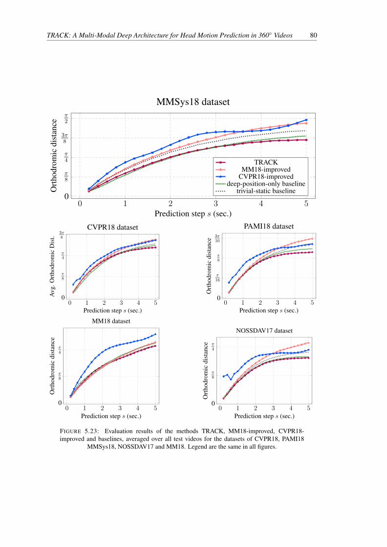
TRACK: A Multi-Modal Deep Architecture for Head Motion Prediction in 360◦ Videos 80

0 1 2 3 4 50

π8

π4

3π8

π2

Prediction step s (sec.)

Ort

hodr

omic

dist

ance

MMSys18 dataset

TRACKMM18-improved

CVPR18-improveddeep-position-only baseline

trivial-static baseline

0 1 2 3 4 50

π8

π4

3π8

Prediction step s (sec.)

Avg

.Ort

hodr

omic

Dis

t.

CVPR18 dataset

0 1 2 3 4 50

π16

π8

3π16

Prediction step s (sec.)

Ort

hodr

omic

dist

ance

PAMI18 dataset

0 1 2 3 4 50

π8

π4

Prediction step s (sec.)

Ort

hodr

omic

dist

ance

MM18 dataset

0 1 2 3 4 50

π8

π4

Prediction step s (sec.)

Ort

hodr

omic

dist

ance

NOSSDAV17 dataset

FIGURE 5.23: Evaluation results of the methods TRACK, MM18-improved, CVPR18-improved and baselines, averaged over all test videos for the datasets of CVPR18, PAMI18

MMSys18, NOSSDAV17 and MM18. Legend are the same in all figures.

TRACK: A Multi-Modal Deep Architecture for Head Motion Prediction in 360◦ Videos 81

Qualitative examples: In Figs. 5.25, 5.26 and 5.27, we exemplify the results on two low-entropy

videos per dataset, CVPR18, PAMI18 and MMSys18 respectively, also showing a representa-

tive frame with a user’s future trajectory and the prediction of TRACK. On focus-type videos,

TRACK outperforms significantly the second-best method: by up to 25% in the examples.

5.6.4 Ablation Study of TRACK

To confirm the analysis that led us to introduce this new architecture TRACK for dynamic

head motion prediction, we perform an ablation study of the additional elements we brought

compared to CVPR18-improved: we either replace the RNN processing the CB-saliency with

two FC layers (line named AblatSal in Fig. 5.28), or replace the fusion RNN with two FC layers

(line named AblatFuse).

Fig. 5.22 and 5.28 confirm the analysis in Sec. 5.6.1: the removal of the first extra RNN (not

present in CVPR18) processing the saliency input has more impact: AblatSal degrades away

from the deep-position-only baseline in the first time-steps. The degradation is not as acute as

in CVPR18-improved as the fusion RNN can still modulate over time the importance of CB-

saliency. However, it seems this fusion RNN cancels most of its input (position and saliency

features), as the performance of AblatSal is consistently similar to that of the trivial-static base-

line (not plotted for clarity). The AblatFuse line shows that the impact of removing the fusion

RNN is less important.

Answer to Q4: If O1 is solved approximately by providing a saliency estimate obtained from

the video content only, the good choice (CVPR18-improved) for Q3 is not sufficient anymore.

A RNN dedicated to processing the saliency must be added to prevent the prediction in the first

time-steps from degrading away from the deep-position-only baseline. Our new deep archi-

tecture, named TRACK, achieves state-of-the-art performance on all considered datasets and

prediction horizons.

5.7 Discussion

It is interesting to note that only a few architectures have been designed in the same way as

TRACK, and none for head motion prediction. Indeed, following up on [86], Sadeghian et al.

in [87] proposed a similar architecture to predict a pedestrian’s trajectory based on the image of

the environment, the past ego trajectory and the trajectories of others. Let us also mention that

the CVPR18 block is similar to an early architecture proposed for visual question answering in

2015 [88], and PAMI18 is similar to Komanda proposed in 2016 for autonomous driving [89].

This Chapter brings a critical analysis to existing deep architectures aimed to predict the

user’s head motion in 360◦ videos from past positions and video content. As we exhibit the

weaknesses of the evaluation scenarios considered by previous works (dataset and competitor

TRACK: A Multi-Modal Deep Architecture for Head Motion Prediction in 360◦ Videos 82

Low-entropy(Focus-typevideos)

0 1 2 3 4 50

π16

π8

3π16

π4

5π16

Avg

.Ort

hodr

omic

Dis

t.

CVPR18 dataset

0 1 2 3 4 50

π32

π16

3π32

π8

PAMI18 dataset

0 1 2 3 4 50

π8

π4

3π8

π2

MMSys18 dataset

High-entropy(Explo-ratoryvideos)

0 1 2 3 4 50

π8

π4

3π8

Prediction step s (sec.)

Avg

.Ort

hodr

omic

Dis

t.

0 1 2 3 4 50

π16

π8

3π16

π4

Prediction step s (sec.)

TRACKMM18-improved

CVPR18-improveddeep-position-only

trivial-static

0 1 2 3 4 50

π8

π4

3π8

π2

Prediction step s (sec.)

FIGURE 5.24: Top row (resp. bottom row): results averaged over the 10% test videos havinglowest entropy (resp. highest entropy) of the GT saliency map. For the MMSys dataset, thesorting has been made using the Exploration/Focus categories presented in Sec. 5.4.4. Legend

and axis labels are the same in all figures.

0 1 2 3 4 50

π8

π4

Prediction step s (sec.)

Ave

rage

Ort

hord

rom

icD

ista

nce

Video 072(Moving Focus)

TRACKMM18-improved

CVPR18-improveddeep-position-only baseline

trivial-static baseline

0 1 2 3 4 50

π4

π2

Prediction step s (sec.)

Ort

hodr

omic

dist

ance

Video 050(Exploration)

TRACKMM18-improved

CVPR18-improveddeep-position-only baseline

trivial-static baseline

FIGURE 5.25: Example of performance on two individual test videos of type Focus and Ex-ploration for CVPR18 dataset [5]. On the frame, the green line represents the ground truth

trajectory, and the corresponding prediction by TRACK is shown in red

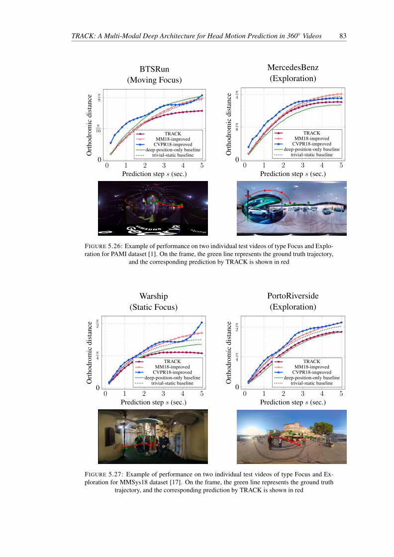
TRACK: A Multi-Modal Deep Architecture for Head Motion Prediction in 360◦ Videos 83

0 1 2 3 4 50

π16

π8

Prediction step s (sec.)

Ort

hodr

omic

dist

ance

BTSRun(Moving Focus)

TRACKMM18-improved

CVPR18-improveddeep-position-only baseline

trivial-static baseline

0 1 2 3 4 50

π8

π4

Prediction step s (sec.)

Ort

hodr

omic

dist

ance

MercedesBenz(Exploration)

TRACKMM18-improved

CVPR18-improveddeep-position-only baseline

trivial-static baseline

FIGURE 5.26: Example of performance on two individual test videos of type Focus and Explo-ration for PAMI dataset [1]. On the frame, the green line represents the ground truth trajectory,

and the corresponding prediction by TRACK is shown in red

0 1 2 3 4 50

π4

π2

Prediction step s (sec.)

Ort

hodr

omic

dist

ance

Warship(Static Focus)

TRACKMM18-improved

CVPR18-improveddeep-position-only baseline

trivial-static baseline

0 1 2 3 4 50

π4

π2

Prediction step s (sec.)

Ort

hodr

omic

dist

ance

PortoRiverside(Exploration)

TRACKMM18-improved

CVPR18-improveddeep-position-only baseline

trivial-static baseline

FIGURE 5.27: Example of performance on two individual test videos of type Focus and Ex-ploration for MMSys18 dataset [17]. On the frame, the green line represents the ground truth

trajectory, and the corresponding prediction by TRACK is shown in red

TRACK: A Multi-Modal Deep Architecture for Head Motion Prediction in 360◦ Videos 84

0 1 2 3 4 50

π8

π4

3π8

π2

Avg

.Ort

hodr

omic

Dis

t.PortoRiverside (Exploration)

0 1 2 3 4 50

π8

π4

3π8

π2

Avg

.Ort

hodr

omic

Dis

t.

PlanEnergyBioLab (Expl.)

0 1 2 3 4 50

π8

π4

3π8

Prediction step s (sec.)

Avg

.Ort

hodr

omic

Dis

t.

Waterpark (Ride)

0 1 2 3 4 50

π8

π4

3π8

Prediction step s (sec.)

Avg

.Ort

hodr

omic

Dis

t.

Warship (Static Focus)

deep-position-only baselineCB saliency-only baseline

TRACKTRACK AblatSal

TRACK AblatFuse

FIGURE 5.28: Per-video results of TRACK and ablation study. The legend is identical for allsub-figures.

baselines), it is important to mention that other such critical analyses have been made for other

application domains of deep learning very recently. Indeed, besides Martinez et al. mentioned

earlier who showed in [82] the weakness of existing architectures for 3D-skeleton pose predic-

tion, Ferrari Dacrema et. al. performed an analysis of recommendation systems in [90]. Not

only did they show the difficulty to reproduce the evaluated algorithms, but also that the state-

of-the-art methods could not outperform simple baselines. Similarly, the meta-analysis of Yang

et. al. [91] for information retrieval, and Musgrave et. al. [92] for loss functions, show that,

contrary to the claims of the authors of multiple recent papers, there has been no actual im-

provement in several years of proposed neural networks to solve the problem in each of these

fields.

In [93], Blalock et. al. show that the difficulty to reproduce, measure and compare the perfor-

mances of different algorithms makes it difficult to determine how much progress has been made

in a field, and this difficulty grows when each work uses different datasets, different performance

metrics and different baselines. In the this Chapter, we have faced the same difficulties. From

TRACK: A Multi-Modal Deep Architecture for Head Motion Prediction in 360◦ Videos 85

the entire reproducible framework introduced in Sec. 4 we have made to enable replication and

comparison, we could perform a critical and constructive analysis.

Our approach and findings are therefore aligned with other critical re-examinations of exist-

ing works in other application domains of deep learning.

5.8 Conclusion

This Chapter has brought two main contributions. First, we carried out a critical and princi-

pled re-examination of the existing deep learning-based methods to predict head motion in 360◦

videos, with the knowledge of the past user’s position and the video content. We have shown

that all the considered existing methods are outperformed, on their datasets and with their test

metrics, by baselines exploiting only the positional modality. To understand why, we have an-

alyzed the datasets to identify how and when should the prediction benefit from the knowledge

of the content. We have analyzed the neural architectures and shown there is only one whose

performance does not degrade compared with the baselines, provided that ground-truth saliency

information is provided, and none of the existing architectures can be trained to compete with

the baselines over the 0-5 sec. horizon when the saliency features are extracted from the content.

Second, decomposing the structure of the problem and supporting our analysis with the concept

of Structural-RNN, we have designed a new deep neural architecture, named TRACK. TRACK

establishes state-of-the-art performance on all the prediction horizons H ∈ [0 sec.,5 sec.] and

all the datasets of the existing competitors. In the 2-5 sec. horizon, TRACK outperforms the

second-best method by up to 20% on focus-type videos, i.e., videos with low-entropy saliency

maps.

The Deep Learning models studied in this Chapter are often referred to as “black-boxes”

since they do not provide any insight on the dependence and interplay between head motion and

the visual content. In the next Chapter we investigate the human head motion process by means

of a “white-box” model that allows us to get knowledge regarding the connection between visual

saliency information and head motion.

Chapter 6

HeMoG: A White-Box Model to Unveilthe Connection Between SaliencyInformation and Human Head Motionin Virtual Reality

Immersive environments for entertainment or training are gaining traction, in particular Vir-

tual Reality (VR) for applications related to, e.g., gaming, museums, journalism, or rehabilita-

tion. Designing VR experiences that are both interactive, comfortable and engaging is key to

create immersive personalized environments. The challenge is to identify, adapt to and guide

the attentional and emotional trajectory of the user. Visual attention is already considered in

a number of such systems, be it for cinematic VR with 360◦ videos [26] or 3D-interactive en-

vironments [94], or to enable efficient VR streaming by predicting where the user is going to

look at and send in high-quality only the attended Field of View (FoV) to save data rate (See

Chapter 5).

Understanding the connection between the audio-visual content and the human attentional

process is therefore key for the design of immersive and personalized environments. Focusing

only on the visual aspect, visual attention is a set of cognitive operations that allow us to filter

the relevant locations in our visual field [29]. This mechanism also guides the movement of our

head and eyes to center the selected location in our fovea, that is the area of the retina with the

highest amount of photoreceptors and therefore allows sharp central vision [25].

Recently, VR in the form of 360◦ videos has been considered to study how people explore

360◦ environments with 3 DoF. The work of [35] collects user data to analyze and identify

first properties (e.g., user congruence, the existence of an initial exploratory phase for ca. 18

sec. before a user focuses). Other works such as [3] aim at extracting the saliency maps, i.e.,

2D-distributions of head positions, from the content. To dynamically predict the head motion

over a certain time prediction horizon, several Deep Learning (DL) models have been proposed,

87

HeMoG: White Box Model to Unveil the Connection Between Saliency Information and HumanHead Motion with Gravitational Laws of Attention 88

such as [5], [1] or TRACK (See Chapter 5).

These models, often referred to as “black-boxes”, however do not provide any insight on the

dependence of the head motion on the visual content. In this Chapter, we address 2 researchquestions:

Q1: To which extent can we investigate the inner workings of these Deep Learning (DL) models

with a white-box model?

Q2: What knowledge can we obtain from a white-box model regarding the connection between

saliency information and head motion?

6.1 Related Work

Several DL models have been proposed to predict head or gaze motion in 360◦ videos

[2, 1, 4, 5]. In Chapter 5, we made a critical study of existing DL models, showing system-

atic weaknesses by comparing their performance with simple yet stronger baselines. We also

proposed a new DL model, named TRACK, that establishes state-of-the-art performance on

several datasets. We therefore consider TRACK as the DL model our proposed HeMoG model

must be compared with.

All these DL models are black-box models whose, to the best of our knowledge, explanability

has not been studied. Explainability and interpretability of DL models decisions and predictions

is a wide and highly active research area (see, e.g., [95]). In this work, our goal is not only to

understand what type of inductive bias is exploited by existing DL models, but rather to design

a white-box model that we can leverage both to gain insight on what the DL model learns, and

unveil the connection between visual content and head motion.

Finally, for regular 2D videos, [96] recently proposed a gravitational model to generate

human-plausible visual scanpaths. We take inspiration from this model to design HeMoG,

which, contrary to [96], is built on a 3D-rotational motion description with specific terms re-

lated to head/neck fatigue.

6.2 HeMoG: A Model of Head Motion in 360◦ videos

In this section we present a new model of head motion in 360◦ videos named Head Motion

with Gravitational laws of attention (HeMoG). We formulate the shift in human attention as the

analogous mechanics of a ball rotating around a fixed origin. As shown in Fig. 6.1, the red ball

represents the center of the FoV of a user exploring a virtual environment. All elements in a

visual scene compete as attractors for the human attention process. This concept of attraction

can be effectively described by means of gravitational models, where each location in the scene

is associated with a virtual mass that is capable of attracting attention.

HeMoG: White Box Model to Unveil the Connection Between Saliency Information and HumanHead Motion with Gravitational Laws of Attention 89

a

a

FIGURE 6.1: Gravitational model of the head position of a person exploring a VR scene. Thecenter of the FoV a(t) is modeled as a ball attached to a stick of fixed length that rotates with

an angular velocity ω and with torque τ .

The fundamental equation of rotational motion is:

L = τ , (6.1)

where:

• L is the angular momentum, expressed as L = Iω, with ω the angular velocity and I the

moment of inertia. For a ball attached to a fixed point (red dot in Fig. 6.1), I can be expressed

as the product of the ball’s mass with |a(t)|. There is not such a valid analogy in our modeling

of the center of focus, and we shall keep I as a parameter in what follows.

• τ represents the torque applied to the system. This torque results from various forces, as

described below.

We therefore have τ = d(Iω)dt = Iω + Iω. Having constrained the attention on the unit sphere,

the norm of a(t) does not change over time, resulting in I = 0. Therefore we obtain

Iω = τ . (6.2)

Modeling of τ : The torque is the turning effectiveness of a force. To model head rotation, we

assume that two types of forces are at play:

• forces that drive the head focus to salient areas of the 360◦ content. Every 360◦ frame therefore

generates a field of force

E(a) =

∫r∈Υ

FE(r,a)dr, (6.3)

where Υ is the set of points in the sphere. Given the virtual mass µ(r, t) of every point r at time

t, the force exerted at the current focus point a(t) is assumed to decrease radially as:

FE(r,a) = γ(t)1

||r− a||2µ(r, t)(r− a) . (6.4)

HeMoG: White Box Model to Unveil the Connection Between Saliency Information and HumanHead Motion with Gravitational Laws of Attention 90

The parameter γ(t) weights the importance of the attraction force over time. We set

γ(t) = 1− e(−βt),

with parameter β to be a model parameter. This models the growing importance of the content

over the prediction horizon: the motion continuity should be most important for short-term

prediction, while the content diverts attention after a few seconds. The model input µ(r, t) for

every pair (r, t) can be set in different ways. Three cases are considered in this Chapter. In Sec.

6.3.2, µ(r, t) is set to 0. In Sec. 6.3.3, µ(r, t) is set to the so called ground-truth saliency map

salgt(r, t). In Sec. 6.3.4, µ(r, t) is set to the element-wise product so(r, t)⊙of(r, t), with

so(r, t) being a 0-1 pixel map of bounding boxes (1 inside, 0 outside) of detected objects, and

of(r, t) the optical flow at this pixel.

• a torque modeled as−λω, corresponding to a force of friction modeling the energy dissipation

when a user continues on their momentum, equivalently the fatigue or the principle of least effort

in which humans tend to return static.

Computation of a(t): The final motion equation is therefore:

Iω =

(∫r∈Υ

a× FE(r,a)dr

)− λω , (6.5)

where the first term in the right-hand-side is the torque associated with the field of force, ×denoting the vector product. In the implementation, we drop I as parameters γ(t) and λ in

the right-hand-side can compensate for it. The evolution of a(t) is computed with quaternion

rotations at each time instant:

a = q ⊗ ax ⊗ q−1, (6.6)

where ax is a constant unit vector, and ⊗ is the quaternion multiplication. As a consequence,

considering the second order derivatives of the quaternion q:

q = q ⊗ q−1 ⊗ q +1

2ω ⊗ q. (6.7)

The relation between quaternions and angular velocity and angular acceleration is derived and

studied in depth in Appendix B. We can now describe the dynamics of the system, by introducing

the auxiliary variable z(t) = ddt(ax), with the system of first order differential equations:

a(t) = q(t)⊗ ax ⊗ q−1(t)

q(t) = z(t)

z(t) = q(t)⊗ q−1(t)⊗ q(t) + 12 ω ⊗ q(t),

(6.8)

HeMoG: White Box Model to Unveil the Connection Between Saliency Information and HumanHead Motion with Gravitational Laws of Attention 91

subject to the boundary conditions a(t0) = a0, ax = (1, 0, 0) and z(t0) = z0. If we pose

y = (q, z), then system (6.8) can be compactly re-written in the canonical form:

y = Φ(y, µ, γ, λ), (6.9)

that can be solved numerically by classic methods like Euler’s and Runge-Kutta’s. In this system

of equations there are three parameters that are key in defining the head motion process:

• λ : models the fatigue of the user or the tendency to return to rest.

• γ(t, β) : models the strength of the forces from the visual input at each time-step.

• µ : the virtual masses generated from the visual input.

We vary these parameters throughout the Chapter to explain the usage of HeMoG to properly

model the dynamics of head motion.

6.3 Comparing Deep Models with HeMoG

In this section, we address Q1: To which extent can we investigate the inner workings of

these DL models with a white-box model? To do so, we compare the performance of HeMoG

with the reference DL models of TRACK (introduced in Chapter 5).

6.3.1 Experimental Setup

6.3.1.1 Dataset

We selected the publicly available dataset of [5] to perform our experiments. This dataset

consists of 208 omnidirectional videos. The duration of each video ranges between 15 and 80

seconds long (36s in average), each video is viewed by at least 31 participants. To perform the

parameter estimation, we randomly selected a subportion of the traces of 166 videos (80%) and

15 users (50%) from the dataset, and exploited them to estimate the model parameters. Then the

model with the parameters found is tested in the remaining traces (42 videos and 16 users), there

is no overlap between videos or users in the train and test set. We subsampled all the videos in

the dataset to 5 frames per second. The frames are resized to a resolution of 952× 476.

Instead of using the equirectangular frame as visual input where the pixels in the poles

are oversampled, the Vogel method [97] is employed to generate approximately uniformly dis-

tributed points on the sphere, as proposed in [98]. As illustration of the uniform sampling of the

equirectangular frame using the Vogel method, the sampling of 200 points is shown in Fig. 6.2.

In our experiments we used a sampling of 10000 points. Fig. 6.2 also shows the interaction

between the field of forces µ(r, t), the position of the head a(t), the angular velocity ω and the

torque τ .

The integration of Eq. 6.9 that drives the focus of attention trajectory is based on the odeint

function of Python SciPy library. The function is based on LSODA, which is a general purpose

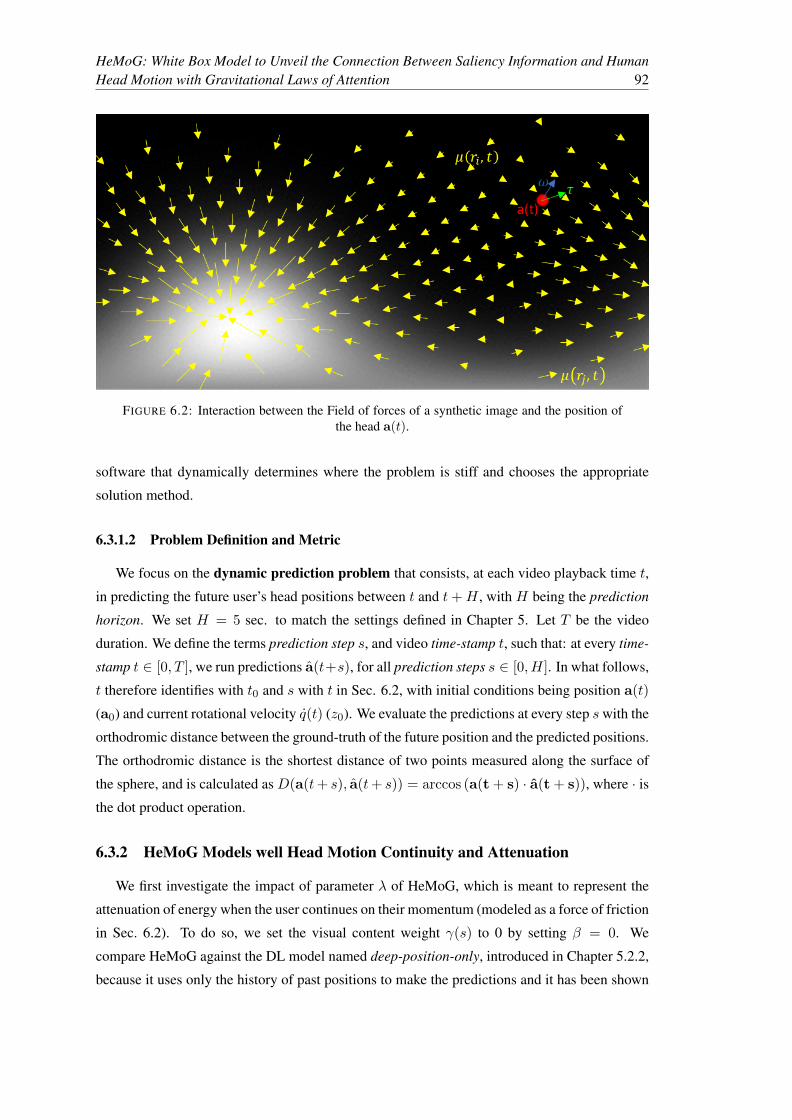
HeMoG: White Box Model to Unveil the Connection Between Saliency Information and HumanHead Motion with Gravitational Laws of Attention 92

FIGURE 6.2: Interaction between the Field of forces of a synthetic image and the position ofthe head a(t).

software that dynamically determines where the problem is stiff and chooses the appropriate

solution method.

6.3.1.2 Problem Definition and Metric

We focus on the dynamic prediction problem that consists, at each video playback time t,

in predicting the future user’s head positions between t and t+H , with H being the prediction

horizon. We set H = 5 sec. to match the settings defined in Chapter 5. Let T be the video

duration. We define the terms prediction step s, and video time-stamp t, such that: at every time-

stamp t ∈ [0, T ], we run predictions a(t+s), for all prediction steps s ∈ [0, H]. In what follows,

t therefore identifies with t0 and s with t in Sec. 6.2, with initial conditions being position a(t)

(a0) and current rotational velocity q(t) (z0). We evaluate the predictions at every step swith the

orthodromic distance between the ground-truth of the future position and the predicted positions.

The orthodromic distance is the shortest distance of two points measured along the surface of

the sphere, and is calculated as D(a(t+ s), a(t+ s)) = arccos (a(t + s) · a(t + s)), where · isthe dot product operation.

6.3.2 HeMoG Models well Head Motion Continuity and Attenuation

We first investigate the impact of parameter λ of HeMoG, which is meant to represent the

attenuation of energy when the user continues on their momentum (modeled as a force of friction

in Sec. 6.2). To do so, we set the visual content weight γ(s) to 0 by setting β = 0. We

compare HeMoG against the DL model named deep-position-only, introduced in Chapter 5.2.2,

because it uses only the history of past positions to make the predictions and it has been shown

HeMoG: White Box Model to Unveil the Connection Between Saliency Information and HumanHead Motion with Gravitational Laws of Attention 93

0 1 2 3 4 50

π16

π8

3π16

π4

5π16

3π8

Prediction step s (sec.)

Ave

rage

Ort

hodr

omic

Dis

tanc

e

HeMoG λ = 2.5HeMoG λ = 0.5HeMoG λ = 0.05deep-position-only

FIGURE 6.3: Prediction error of HeMoG with λ = 2.5 (and β = 0) compared with the deep-position-only baseline. The performance of HeMoG with other values of λ = 0.5 and 0.05 are

shown to illustrate the impact of the parameter.

to outperform all previously existing DL models over all prediction steps. It is a Sequence-to-

Sequence LSTM framework consisting in an encoder and a decoder that does not consider any

visual input. The encoder receives the historic window input of past head positions and generates

an internal representation that initializes the decoder producing the series of predictions.

6.3.2.1 Results

Fig. 6.3 depicts the results of HeMoG in the test set with the parameter λ = 2.5 tuned in

the train set. We observe that λ = 2.5 yields performance of HeMoG close to that of the deep-

position-only baseline. Fig. 6.3 also presents the results of HeMoG with other values of λ, a

lower value of λ represents lower fatigue (more volatility), while a higher value of λ represents

higher fatigue (motion reduced more quickly).

First, it is remarkable that such a white-box model predicts head motion as well as a DL

model. Second, we interpret this as the DL model deep-position-only learning the curvatureand friction dynamics of head motion that HeMoG is explicitly built on. This is the first

element of answer to question Q1.

6.3.3 HeMoG Combines well Past Motion and Accurate Content Information

We study whether HeMoG correctly models the fusion between visual information and his-

tory of head positions. To do so, we keep λ set to 2.5 following the previous results. To be

independent from the imperfection of any saliency predictor fed with the visual content, we

HeMoG: White Box Model to Unveil the Connection Between Saliency Information and HumanHead Motion with Gravitational Laws of Attention 94

0 1 2 3 4 50

π16

π8

3π16

π4

5π16

Prediction step s (sec.)

Ave

rage

Ort

hodr

omic

Dis

tanc

e

HeMoG-GTSal β = 10−1

HeMoG-GTSal β = 10−2

HeMoG-GTSal β = 10−3

HeMoG-GTSal β = 0TRACK-GTSal

FIGURE 6.4: Prediction error of HeMoG with λ = 2.5, β = 10−1 and ground-truth saliency(GT-Sal) input, compared with TRACK. Other values of β = 10−2 and 10−3 are shown to

illustrate the impact of the parameter.

consider here the ground-truth saliency: it is the heat map (2D-distribution) of the viewing pat-

terns, obtained at each point in time from the users’ traces. Here we compare HeMoG with the

complete DL model TRACK. To compare HeMoG and TRACK fairly, we specify that TRACK

is fed with the same type of visual content information as HeMoG.

6.3.3.1 Results

Fig. 6.4 presents the results of HeMoG fed with ground-truth saliency (named GTSal) with

the value of β = 0.1 found in the train set. With β = 0.1, HeMoG performs similarly or slightly

better than the DL model TRACK, which was shown to efficiently fuse the multi-modal inputs

(See Chapter 5.6.3.3). Fig. 6.4 also presents the results of HeMoG for lower values of β. The

value of β affects the coefficient of the attraction force γ(s) (the coefficient of the visual input)

through γ(s) = 1− e(−βs). The higher the value of β the faster the growth of importance of the

visual coefficient.

Given that TRACK features a dedicated recurrent neural unit for each of both input modal-

ities (past position and frame saliency) and a recurrent neural unit for the fusion of the so-

obtained embeddings, TRACK has the flexibility to learn various ways of combining both

modalities. The fact that HeMoG, with its fixed fusion scheme shown in Eq. 6.5 performsas well or better can be interpreted as TRACK performing a similar type of fusion asHeMoG, which enables to benefit from both types of information (the lowest curves in Fig. 6.4

are lower than those with the positional modality only in Fig. 6.3). This is the second element

of answer to Q1.

HeMoG: White Box Model to Unveil the Connection Between Saliency Information and HumanHead Motion with Gravitational Laws of Attention 95

6.3.4 HeMoG Behaves as the DL Model and Lowers the Impact of a Noisy SaliencyEstimate

In a non-ideal case where the saliency is not obtained from the viewing patterns but rather

estimated from the content, we analyze the performance of HeMoG in comparison with TRACK.

The extraction of visual saliency in 360◦ videos has been studied as an extension of image

saliency [3]. However, additionally to the salient objects that can be found in images and videos,

the motion of objects in the scene becomes an important cue specifically for videos [99]. For

this reason we considered the moving objects as important cues to extract saliency from the

360◦ video content. The objects in each FoV of the scene are detected using YOLOv4 [100],

the aggregation of all detected objects in all FoVs provides a binary map, shown in Fig. 6.5(c).

To obtain the moving objects map shown in Fig. 6.5(d), we perform the element-wise product

of the binary map and the norm of the pixel velocities computed in the 360◦ scene. This moving

objects map obtained from the visual content is named the content-based saliency (CBSal).

(A) Original Frame (B) GT SalMap

(C) Detected Objects (D) CB SalMap

FIGURE 6.5: Saliency map extraction from a frame of video ‘072’. (a) Original frame. (b)Ground-truth saliency map. (c) Detected objects map. (d) Content-based saliency map: moving

objects map.

6.3.4.1 Results

In Fig. 6.6, we present the results of our model HeMoG against the DL model TRACK using

the same visual information CBSal as input. First, we observe that both models increase their

error significantly when they use a noisy input for the visual saliency. Second, contrary to what

occurred with ground-truth saliency, HeMoG performance improves by reducing the value of

β, in other words, by minimizing the impact of the CBSal input. Using a value of β = 10−5,

HeMoG approaches the performance of TRACK. This reinforces the hypothesis that TRACKand HeMoG perform the same type of fusion.

HeMoG: White Box Model to Unveil the Connection Between Saliency Information and HumanHead Motion with Gravitational Laws of Attention 96

0 1 2 3 4 50

π16

π8

3π16

π4

5π16

Prediction step s (sec.)

Ave

rage

Ort

hodr

omic

Dis

tanc

e

TRACK-CBSalTRACK-GTSalHeMoG-CBSal β = 10−3

HeMoG-CBSal β = 10−4

HeMoG-CBSal β = 10−5

HeMoG-GTSal β = 10−1

FIGURE 6.6: Prediction error of HeMoG with λ = 2.5, β = 10−5 and content-based saliency(CBSal), compared with TRACK using CBSal. The curves of HeMoG and TRACK with GTSalare shown for reference. Other values of β = 10−3, 10−4 are shown to illustrate the impact of

the parameter.

6.4 Impact of the Visual Saliency on Head Motion

In this section, we address Q2 by analyzing the impact of the visual saliency on head motion,

in terms of the video category and the time-step in the prediction horizon.

6.4.1 Visual Saliency Impacts Head Motion Only for Certain Video Categories

The videos from the dataset of [5], contain heterogeneous scenes including music shows,

documentaries, sports, movies, etc. More generally, [8] have identified the following main

video categories for which they could discriminate significantly different users’ behaviors: Ex-

ploration, Static Focus, Moving Focus and Rides. In Exploration videos, there is no specific

attraction point and the spatial distribution tends to be more widespread and hence individual

trajectories more difficult to predict. Static Focus videos are made of a single or few attraction

areas (e.g., a standing person in an empty room). In Moving Focus videos, the attraction points

move over the sphere. Rides videos are shot with the 360◦ camera moving. In this case, the at-

traction point for the user is usually the camera moving direction to minimize motion sickness.

We categorized each of the videos in the dataset of [5] into one of the four groups: Explo-

ration, Static Focus, Moving Focus or Rides. The number of videos belonging to each of the

classes is: 16 videos of Rides, 100 Exploratory videos, 74 Moving Focus and 18 Static Focus

videos. In Fig. 6.7, we show some of the videos from the dataset with their respective category.

In Fig. 6.8, we present the results of HeMoG per video category, with CBSal and for different

values of β. We expect that there is no much information for CBSal to capture from Exploration

HeMoG: White Box Model to Unveil the Connection Between Saliency Information and HumanHead Motion with Gravitational Laws of Attention 97

Exploratory Static Moving Rides

FIGURE 6.7: Some videos from [5], categorized into Exploratory, Static (focus), Moving (fo-cus) and Rides

videos, and that CBSal cannot capture the relevant information from Rides videos. Indeed,

CBSal is the product of the optical flow with the objects bounding boxes, and hence the camera

direction where the optical flow is minimum cannot be highlighted as salient this way. Fig. 6.8

confirms that the lowest values of β are those providing best results for Exploration and Rides

videos. HeMoG therefore reduces the weight of the saliency information in these cases (as it is

also possibly the behavior of the DL model TRACK given its curve).

For the Moving Focus and Static Focus categories, we observe that when we increase the

value of β, the error in the long-term decreases, showing the relevance of the saliency informa-

tion for longer-term prediction. However, the error in the short-term increases, which we discuss

in the next section. These results with different optimal values of β per video category showthat the impact of saliency on head motion is stronger for Static Focus and Moving Focus

(and likely for Rides too) than for the Exploration category.

6.4.2 Visual Saliency Impacts Head Motion Only After 3 Seconds

As discussed above, increasing β in Static Focus and Moving Focus videos lowers the er-

ror in the long-term prediction steps but degrades it in the short-term. This reveals a possibly

not optimal choice of the γ(s) function that controls the rapidity of importance growth of the

saliency information over s. For now we have set, from Sec. 6.2, γ(s) = 1 − e(−βs). We ran

numerical searches and identified that the values of γ(s) that give the best performance of the

HeMoG: White Box Model to Unveil the Connection Between Saliency Information and HumanHead Motion with Gravitational Laws of Attention 98

0 1 2 3 4 50

π16

π8

3π16

π4

5π16

3π8

Prediction step s (sec.)

Ave

rage

Ort

hodr

omic

Dis

tanc

eExploratory

TRACK-CBSalTRACK-GTSalHeMoG-CBSal β = 10−3

HeMoG-CBSal β = 10−4

HeMoG-CBSal β = 10−5

0 1 2 3 4 50

π16

π8

3π16

π4

5π16

3π8

7π16

Prediction step s (sec.)

Ave

rage

Ort

hodr

omic

Dis

tanc

e Rides

TRACK-CBSalTRACK-GTSalHeMoG-CBSal β = 10−3

HeMoG-CBSal β = 10−4

HeMoG-CBSal β = 10−5

0 1 2 3 4 50

π16

π8

3π16

π4

5π16

Prediction step s (sec.)

Ave

rage

Ort

hodr

omic

Dis

tanc

e

Moving Focus

TRACK-CBSalTRACK-GTSalHeMoG-CBSal β = 10−3

HeMoG-CBSal β = 10−4

HeMoG-CBSal β = 10−5

0 1 2 3 4 50

π16

π8

3π16

π4

5π16

Prediction step s (sec.)

Ave

rage

Ort

hodr

omic

Dis

tanc

e Static Focus

TRACK-CBSalTRACK-GTSalHeMoG-CBSal β = 10−3

HeMoG-CBSal β = 10−4

HeMoG-CBSal β = 10−5

FIGURE 6.8: Prediction error of HeMoG compared with TRACK grouped per category. Top-left: Exploratory. Top-right: Rides. Bottom-left: Moving Focus. Bottom-right: Static Focus.

gravitational model per time-step are:

γ(s) =

10−5 if 0 < s <= 3

10−1 if 3 < s <= 5,(6.10)

from which we draw two conclusions. First, the motion momentum is more important thanthe visual content in the first 2.5 seconds of the prediction horizon, and the visual contentcan inform the head motion prediction model only for horizons longer than 3 seconds. Sec-

ond, that a sigmoid-like function γ(s) = C1+exp (−β(s−S)) with additional parameters C for the

scaling and S to center the transition from 0 to 1, would be a better fit. This is confirmed in

Fig. 6.9 with the comparison of HeMoG when the parameters are set properly for the different

categories and for each prediction step s. Let us note that this also shows that the DL model

HeMoG: White Box Model to Unveil the Connection Between Saliency Information and HumanHead Motion with Gravitational Laws of Attention 99

0 1 2 3 4 50

π16

π8

3π16

π4

5π16

Prediction step s (sec.)

Ave

rage

Ort

hodr

omic

Dis

tanc

e

TRACK-CBSalTRACK-GTSalHeMoG-CBSalHeMoG-GTSal

FIGURE 6.9: Results averaged over all video categories. HeMoG is set with γ(s) = 1−e(−βs)and β = 10−5 for Exploratory and Rides videos, and γ(s) from Eq. 6.10 for Moving Focus andStatic Focus videos, compared with TRACK. The curves of HeMoG and TRACK with GTSal

are shown for reference.

TRACK is capable to learn and adapt to the different video categories, while the white-box ap-

proach is limited by the right choices of parameters. However, we show here that the differential

equation model of HeMoG captures the main dynamics and yields performance similar to the

DL models in average.

6.5 Discussion

Comparison of HeMoG with Deep Learning models: The main difference between both

types of models is as follows. The latter are equipped with representation learning capability

(learning how to extract relevant features from the saliency map they are fed) and able to mod-

ulate the weights assigned to momentum and saliency features in the fusion depending on the

saliency and motion information (capabilities detailed in [101]). In comparison, HeMoG is able

to properly fuse both types of information for any video, provided that the saliency information

is the ground-truth. When it is not the ground-truth anymore (when fed with CB-sal), then the

saliency weight β in the HeMoG model must be adapted to the video category. Also, we men-

tion that when using other types of saliency extracted from the content, for example the saliency

maps obtained from PanoSalNet [3], the performance of HeMoG shown in Fig. 6.10 is slightly

worse than that of TRACK, which we explained by the lower level of information present in

the estimated saliency map in relation with the user motion. On focus-type videos, TRACK is

able to extract some useful information (improvement compared with deep-position-only), while

HeMoG is not.

HeMoG: White Box Model to Unveil the Connection Between Saliency Information and HumanHead Motion with Gravitational Laws of Attention 100

0 1 2 3 4 50

π16

π8

3π16

π4

5π16

3π8

Prediction step s (sec.)

Ave

rage

Ort

hodr

omic

Dis

tanc

e

TRACK-CBSalTRACK-GTSalHeMoG-CBSal β = 10−3

HeMoG-CBSal β = 10−4

HeMoG-CBSal β = 10−5

HeMoG-GTSal β = 10−1

FIGURE 6.10: Prediction error of HeMoG with λ = 2.5, β = 10−5, and content-basedsaliency (CBSal) computed from PanoSalNet [3], compared with TRACK using the sameCBSal-PanoSalNet. The curves of HeMoG and TRACK with GTSal are shown for reference.

Other values of β = 10−3, 10−4 are shown to illustrate the impact of the parameter.

Indeed, the Content-Based saliency obtained from PanoSalNet can be noisy, as we show in

Fig. 6.11 with an original frame of video ‘072’ and its extracted saliency with PanoSalNet, and

the Ground-truth saliency from user statistics on this frame. While the salient object in the frame

is the human, low-level features like the lights reflected in the floor and high-level features like

the text written in the floor are taken into account by the saliency extractor, making the resulting

saliency map noisy and more difficult to get motion-relevant information from.

FIGURE 6.11: Saliency map extraction from a frame of video ‘072’. (left) Original frame.(center) PanoSalNet saliency map. (c) Ground-truth saliency map

Generalizing to more comprehensive saliency maps: While the study of this Chapter has

been restricted to saliency attractors based on moving objects, we can consider extending to

static objects whose importance can be ranked, meaning that the trajectory of focus of attention

is also subjected to a gravitational field created by static objects [102, 103]. We can also study

how to improve for the case of Rides scenes characterized by camera motion. To have more solid

estimates of pixel velocities, methods for camera motion estimation [104] are already present in

HeMoG: White Box Model to Unveil the Connection Between Saliency Information and HumanHead Motion with Gravitational Laws of Attention 101

the literature and can help in creating more suitable saliency estimates for the proposed model.

The treatment of such complex scenes is left for future work.

6.6 Conclusions

In this Chapter we have investigated the human head motion process driven by attention

when a user experiences an immersive 360◦ video. We have first introduced a new computational

model named HeMoG, enabling to predict future head positions from the user’s past positions

and the visual content. HeMoG is built on differential equations obtained from the physics

of rotational motion where the attractive salient areas in the 360◦ frames are represented as

virtual masses. HeMoG is hence a white-box model and its (time-varying) parameters control

the connection between visual content and head motion process. The performance of HeMoG

are comparable with those of DL predictors, which we interpret as the DL models learning the

same type of fusion as HeMoG: curvature continuity and momentum attenuation from friction

in the short-term, diversion of motion with saliency attraction in the longer-term. The evolution

of best parameter values in terms of video categories and horizon reveals that, on videos that

are not exploratory, the initial motion momentum is most important until ca. 3s, after which

the saliency weights more in the motion equation. Future works include refining the saliency

extractor to feed the model with, and incorporating these findings into an attention-driven system

to produce personalized immersive environments.

Chapter 7

Control Mechanism for User-AdaptiveRotational Snap-Cutting in Streamed360◦ Videos

Predicting the user’s head motion is difficult and can be done accurately only over short

horizons (less that 2s, see [3] and Sec. 5). If the server makes an error in prediction and the

level of bandwidth is sufficient to attempt sending again in High Quality (HQ) tiles previously

sent in Low Quality (LQ), then the prediction error translates into a higher level of network

bandwidth consumption. In 360◦ video streaming, the consumed data rate therefore depends on

the prediction error, that is on the user’s motion, which in turn depends on the user’s attentional

process and hence on attention driving techniques. Fig. 7.1 depicts this interplay, from which

can arise interdisciplinary approaches to jointly design 360◦ video streaming algorithms and

360◦ film editing techniques.

If driving the user’s attention is critical for a director to ensure the story plot is understood, in

this Chapter we investigate attention driving techniques from a different perspective: that of the

multimedia networking community. After presenting attention driving techniques based on user-

adaptive rotational cuts in Sec. 7.1, related works are introduced in Sec. 7.2. Sec. 7.3 presents

the problem formulation. The design of the learning approaches is presented in Sec. 7.4, and

FIGURE 7.1: Streaming 360◦ videos: the sphere is tiled and each tile of the sphere is sent intolow or high quality depending on the user’s motion and network bandwidth.

103

User-Adaptive Rotational Snap-Cutting for Streamed 360◦Videos 104

Sec. 7.5 gathers the results and their analysis. Finally, the limitations of this preliminary work

are discussed in Sec. 7.5.3, and conclusions are given in Sec. 7.6.

7.1 User-Adaptive Rotational Cutting for Streamed 360◦ Videos

The question of designing editing cuts to drive the user’s attention in cinematic Virtual Re-

ality (VR) has been under active investigation for the last 3 to 4 years.

In [26], for the first time, Dambra et al. have showed that film editing can be helpful for

streaming 360◦ videos by directing the user’s attention to specific pre-defined Regions of Interest

(RoI), thereby lowering the randomness of the user’s motion and using this a-priori knowledge

in the streaming decisions (consisting, at each point in time, in deciding which area/tile of which

video segment to send in which quality). This is done by periodically regaining control on the

user’s FoV using so-called snap-changes, which are a type of intra-scene rotational cuts. They

are interchangeably called snap-cuts. The details of the method and its positioning with respect

to the relevant literature are provided in Sec. 7.2. Dambra et al. showed that it is beneficial both

for application-level metrics (level of quality in FoV, consumed bandwidth) and user-experience

metrics (user’s angular speed, story understanding). Their results are a proof-of-concept where

the set of cuts is pre-defined in an Extensible Markup Language (XML) file by, e.g., the film

director, and all cuts are executed at their corresponding time instants. However, snap-cuts are

forced re-positioning corresponding to momentaneously taking some freedom off of the user.

These intra-scene cuts can hence be envisioned as levers that the 360◦ video player can leverage

to cope with an insufficient bandwidth and still succeeding in displaying HQ in the user’s FoV

(which gets re-positioned in front of the HQ area). Every cut may hence not always be necessary:

• if the user will be close enough to the FoV targeted by the cut: this is implemented by the

30◦rule already implemented in the original method [26] (with a moderate impact on the

quality downloading decision)

• if the network bandwidth is high enough so that replacements are possible and not costly,

and/or

• if the user moves slowly enough that the spatial qualities fetched earlier for each area/tile

overlap sufficiently the FoV at the time of playback (so the cut will not help increase the

quality in the FoV).

Whether or not a cut will be beneficial therefore depends on the user’s motion and on the network

conditions. Specifically, the trade-off involves: (i) a snap-change guarantees that the user will

see the FoV desired by the director, and that HQ is displayed in this FoV, while (ii) not having a

snap-change may preserve the level of presence and keep low the probability of disorientation.

User-Adaptive Rotational Snap-Cutting for Streamed 360◦Videos 105

In this Chapter, we consider the network conditions being fixed and investigate how to opti-

mize cut triggering to obtain best trade-off, by designing a user-adaptive editing policy for 360◦

video streaming.

7.2 Related works

This section reviews the main categories of existing works relevant to the problem at hand.

We provide successfully an overview of techniques to partly control the user’s FoV, introduce

the concept of adaptive 360◦ video streaming and the required adaptation to the user, and finally

review some ML-based approaches for various questions arising with 360◦ videos.

7.2.1 Directing Change of FoV

The works presented in [105, 106, 107] are aimed at assisting the user in moving in the

virtual environment to increase comfort and/or lower sickness, while those presented in [108,

109, 110, 111, 26] consist in operating FoV changes independently from the user’s motion or

will. In [106], amplified and guided head rotation are introduced for seated use of VR in HMDs:

physical head rotation angles are magnified in the Virtual Environment (VE) so that physically

turning in a (limited) comfortable range can allow wider range. In [107], Farmani et al. show that

it is possible to artificially reduce vection − the illusion of self-motion, which is connected to

cybersickness − by snapping the viewpoint, reducing continuous viewpoint motion by skipping

frames. They show that both rotational and translational snapping reduce cybersickness by 40%

and 50 %, respectively. In [112], the authors compare an auto-pilot mode deciding which FoV

is exposed to a seated user, independently of the user movements, with assisting the user by

displaying an arrow of where to look. In [108] and [109], user-initiated (by pressing a button)

and system-initiated rotational re-positioning of FoV are performed, independently of the user

motion. The re-positioning is progressive and while participants could most easily track scene

changes, they generally and unsurprisingly experienced sickness due to rotational vection. Much

interestingly, it has been uncovered in [110] that participants can automatically update their

sense of spatial orientation during rotation using only visual cues, and that the accompanying

physical rotation may not be necessary for fast and reflexive updating. Also, how cut frequency

influences viewers’ sense of disorientation and their ability to follow the story has been studied

in [113]. The results show that high editing cut frequency can be very well received, as long as

the user’s attention is appropriately guided at the point of cut. In [111, 26], the authors introduce

so-called dynamic editing with (rotational) snap-changes, combining the positive aspects of the

above methods: to periodically regain control over the user’s FoV at the time of 360◦ video

playback (these intra-scene cuts are hence not built into the video file), the FoV is repositioned,

in a snap, that is from one frame (image) to the next, in front of a pre-determined FoV (possibly

decided by the director). To do so, only an additional XML file has to be downloaded at the

User-Adaptive Rotational Snap-Cutting for Streamed 360◦Videos 106

begining of the video, and the custom player [114] implements the snap-changes at the indicated

times in front of the indicated angular sectors. Fig. 7.2 depicts the effect of a snap-change on the

FoV. It is shown in [26] that this strategy enables to reduce the average head motion speed by up

to 30%, that these repositionings are mostly not noticed by the users when performed towards

a meaningful RoI (possibly perceived as fast-cutting, which may sometimes feel like missing

in cinematic VR), and when they notice it, no discomfort or sickness are yielded as no motion

is sensed, and the vestibular system is not involved. It is also shown that incorporating the

knowledge of the future snap-changes into the adaptive streaming algorithm enables bandwidth

savings, as described below.

FIGURE 7.2: Top left: Identification of the RoI targeted by the snap-change. Top right: De-scription of the list of snap-changes over the video as an XML file.

Bottom: FoV re-positioning in front of the targeted RoI by the snap-change.

7.2.2 Adaptive Streaming for 360◦ Videos

Modern (regular non-360◦) video streaming relies on the concept of HTTP Adaptive Stream-

ing, whose most wide spread version is the MPEG-DASH standard [42]. It consists in the video

file being chunked into temporal segments of fixed duration (often 2 sec. or 5 sec.), each en-

coded into several quality levels, that is at different bitrates (often corresponding to resolutions).

The client strives to (i) prevent playback interruptions by maintaining a non-empty playback

buffer where a certain number of segments (or seconds of video) are stored in advance of play-

back, while (ii) fetching and displaying qualities as high as possible. To do so, the client runs

a so-called adaptive streaming logic (or algorithm) which chooses which quality to request for

every segment to the remote server, based on the network bandwidth varying over time. In the

case of 360◦ video streaming, a single segment does not correspond anymore to a single entity,

but possibly to several tiles. The goal is to reduce the required bandwidth to stream 360◦ videos

User-Adaptive Rotational Snap-Cutting for Streamed 360◦Videos 107

by requesting high quality for the tiles that will intersect the FoV of the user. The qualities to

request for every tile of every segment must therefore adapt both to the network and the user

dynamics, as represented in Fig. 7.3. The challenge is that at the time of the decision, the fu-

ture of the network bandwidth (which will support the currently decided object to download)

and the user motion (which will determine where will the FoV be at the time this segment is

played out) are unknown. Most recent examples of strategies addressing this difficult problem

are [115, 116], which strive to predict network bandwidth and user’s motion with recurrent deep

neural networks. The innovative interdisciplinary approach presented in [26] consisted in not

trying to predict the future user’s motion (which is much difficult to do as presented in Sec. 5),

but instead in designing a 360◦ adaptive streaming algorithm which benefits from the knowledge

of the future rotational cuts to better target which tile must be fetched in HQ. The bandwidth

savings yielded by such approach have been shown to be substantial (up to 25%). In [117], a

first attempt of learning how to trigger snap-changes of [26] is demoed. It implements a deep

Reinforcement Learning (RL) strategy to adapt to the user’s motion, without proving that it can

work better than a simple baseline, nor quantifying the gains. In the present Chapter, we present

the design of a complete learning framework addressing the problem of FoV overlap (quality)

prediction and snap-change triggering decision, to best trade between quality in FoV and user’s

freedom while streaming a 360◦ video over a bandwidth-limited network.

FIGURE 7.3: Buffering process for a tiled 360◦ video. While segment n is being decodedat time t, segment n + B is being downloaded. Red (resp. blue) rectangles represent tiles’segments in HQ (resp. LQ). Idealistically, the tiles in HQ must match the user’s FoV at their

time of playback.

User-Adaptive Rotational Snap-Cutting for Streamed 360◦Videos 108

7.3 Problem Definition

In this section, we first expose, in Sec. 7.3.1 all the system and model assumption we make

(that we implement in our simulator used for training and analysis in 7.4 and Sec. 7.5), before

formally describing the optimization problem in Sec. 7.3.2. The notations are provided in Table

7.1.

7.3.1 System Assumptions

System assumptions: As aforementioned, a 360◦ streaming strategy has to be both network-

and user-adaptive. In this work, we focus on how to adapt the frequency of the snap-changes

to the user’s motion and maximize their level of experience − a Quality of Experience (QoE)

function defined in Sec. 7.3.2. Therefore, we set fix the underlying streaming strategy, detailed

in Algo. 3, working as follows. We consider (wlog) that 2 quality levels are available. The

qualities (HQ or LQ) for every tile of every segment are decided based on the current user’s FoV

at the time of downloading this tile (HQ for the tiles intersecting the FoV, LQ for the others).

The tile’s download can occur up to B seconds before its playback, where B is the size of the

playback buffer. We consider the time to download a tile negligible. The downloading process

pauses when the buffer is full, and resumes when at least one segment has been dequeued and

fed to the video decoder. We consider that the list C of potential snap-changes is loaded with

the video description file before the playback starts (each snap-change is described as depicted

in Fig. 7.2-top right). We then augment the streaming strategy as described in Algo. 3: when

the first tile of a new segment is about to be downloaded, if the list of possible snap-changes

indicates that a snap-change may be trigger at this segment, then a decision function is called

to decide whether this snap-change should be triggered to maximize the objective function de-

scribed below. Designing such a snap-triggering decision function is the subject of this Chapter.

7.3.1.1 QoE Model Assumptions

We model the user’s reaction to the triggering of a snap-change. It has been shown in [26,

Fig. 11], with user experiments, that snap-changes decrease the head motion speed of users by

up to 30%. In the simulations used in this Chapter (later used to train classifiers), we use the user

motion dataset presented in [17], which contains the head tracking data of 57 users exploring

19 videos. In this dataset, considering a FoV to be about 100◦ wide [2], it takes about 5 sec.

for 50% of the users to shift their FoV entirely. This can be seen in Sec. 5.4.1[Fig. 5.11]. In

this Chapter, we adopt a preliminary simplistic user model: considering that a 30% decrease in

angular speed would add 1.5 sec. to shift the field of view of half of these users, we consider

in our simulator that right after each triggered snap-change, repositioning the user in front of a

meaningful/interesting FoV, every user pauses for 2 sec. before resuming her motion.

User-Adaptive Rotational Snap-Cutting for Streamed 360◦Videos 109

System param. Definition

N (N), W (W) number (set) of segments, tilesC (C) number (set) of possible snap-changesB playback buffer size (in sec.)qm(n) ∈ {0, 1} quality level of tile w at segment nbufm(t) num. of sec. stored in buffer of tile w at time ttime(c) playback time of snap-change cFoVsnap(c) FoV targeted by snap-change cflagdecided(c) = 1 if the decision for c is made, = 0 ow.flagtrigger(c) = 1 if c has been decided to be triggered, = 0 ow.wpast(t) time interval [0, t]wfut1(t) time interval ]t, t+B]wfut2(t) time interval ]t+B, t+B +G]

Model param. Definition

G duration of snap-cut impact on user’s motion% penalty for triggering a snap-change

TABLE 7.1: Notation of the system and model parameters.

Algorithm 3: Downloading process: quality allocation and snap-change triggering de-cisions

Data: Current playback time t. Buffer states bufw(t), ∀w ∈W. List of possible snap-changesc ∈ C. Initially flagdecided(c) = 0 and flagtrigger(c) = 0, ∀s ∈ C.

Result: which segment n of which tile w to download next in which quality qw(n), whether totrigger a snap-change if n has one not decided yet, ∀w ∈W, n ∈ N, qw(n) ∈ {0, 1}

if all W buffers are full thenstay idle;

elseset w to the tile index with the least full buffer;set n to the lowest value not having entered buffer m yet;qw(n) = 0 # initialize with LQ;if there exists a snap-change c such that time(c)= n andflagdecided(c) = 0 then

# Whether this snap-change will be triggered at time time(c) must be decided now;form environment state state(t);flagtrigger(c) =decision(state(t));flagdecided(c) = 1;

identify the highest snap index clast with flagtrigger(slast) = 1;if clast not empty and t ≤time(clast)≤ n then

if w intersects snap-change’s FoVsnap(clast) thenqw(n) = 1 # download in HQ;

elseif w intersects current user’s FoV(t) then

qw(n) = 1 # download in HQ;

User-Adaptive Rotational Snap-Cutting for Streamed 360◦Videos 110

7.3.2 Formulation of the Optimization Problem

To formulate the decision problem, we adopt a model for the level of user’s experience under

adaptive 360◦ streaming and snap-changes. We define an instantaneous reward obtained after

the playout of segment n (of duration 1s in the simulator):

r(n) = qFoV (n)− %t(n)−tlast(n) . (7.1)

The components are as follows. We define the average quality in the FoV over segment n’s

duration as qFoV (n) =∑W

w=1 qw(n)Fr(n,w), with qw(n) the quality level of tile w at segment

n, and Fr(n,w) the average fraction of FoV at segment n occupied by tile w. The second

component represents the penalty incurred by triggering snap-changes: % is a penalty parameter,

t(n) is the playback time of segment n (close to n depending on playback interruption), and

tlast(n) is the time of the last triggered snap-change.

Let us denote by Su the state of the streaming process (tiles’ qualities stored in the buffer)

and user’s state (past head coordinates but also fatigue, likeliness to move) at the time of de-

ciding for snap-change c. Given that the decision of triggering each snap is taken at the time

of downloading it, hence of it entering the playback buffer, Su+1 is independent of what hap-

pened before u conditionally on Su, and hence the Markov property is verified. The snap trig-

gering problem is therefore a Markov Decision Process defined by the tuple (S,A,P,R, γ),

where P ass′ = Pr[Su+1 = s′|Su = s,Au = a], Ras = E[Ru|Su = s,Au = a]. The

time is paced with snap-triggering decisions, a ∈ {0, 1}, and Ru =∑

n∈N(u) r(n)/|N(u)|where N(u) is the segments played between both snaps decided at u and u + 1. We define

π(a|s) = Pr[Au = a|Su = s] and formulate the snap-change triggering optimization problem

as:

π? = arg maxE[ C−1∑u=0

γuRu]. (7.2)

The optimal snap-triggering strategy must therefore trigger a snap-change when the contribu-

tion, to the cumulative reward, of the quality increase due to this snap exceeds the incurred

penalty. It therefore must trigger depending on the user’s motion. The transition probability

distribution P ass′ is unknown as, to take online decisions sequentially, we cannot know how the

user is going to move and react, given a certain state. The decision-making problem is hence

that of model-free RL.

Finally, it is interesting to notice that other forms of similar problems have appeared in

much different application domains. In [118], Pineau et al. present how to automatically learn

an optimal neurostimulation strategy for the treatment of epilepsy. The goal is to trigger the

minimum amount of neurostimulation (electric discharge from intra-cerebral electrodes) as a

function of the Electroencephalogram (EEG) signal, so as to minimize the number of seizures.

User-Adaptive Rotational Snap-Cutting for Streamed 360◦Videos 111

7.4 Learning How to Trigger a Snap-Cut

For the reasons exposed in Sec. 7.3.2, deciding dynamically during the video playback how

to trigger a snap-change is a model-free RL problem. However, rather than designing an RL

agent learning from its own observations, we instead leverage here the principle of learning

from expert’s demonstration, also known as Imitation Learning (IL) [119]. In our case, for the

short videos considered, we indeed have access to an expert which is the offline optimal defined

below in Sec. 7.4.1. We consider in this Chapter the simplest version of IL, known as Behavioral

Cloning (BC) [119]. It consists in supervising the training of the action policy/decision classifier

(deciding whether or not to trigger the next snap-change), with the trigger labels provided by

the offline optimal. A major design difficulty is the possibly loose correlation between the past

motion at time t, and the decision to trigger snap c decided at time t but impacting user’s motion

only from time t+B, as represented in Fig. 7.4. We therefore split the snap-triggering problem

at time t into 2 sub-problems: (P1) predicting the FoV overlap over wfut2(t) from wpast(t) (as

defined in Table. 7.1 and shown in Fig. 7.4), and (P2) deciding whether to trigger based on the

series of predicted overlaps.

FIGURE 7.4: Timing of the process: the tiles’ qualities displayed at time t have been down-loaded at time t−B. If segment n to be downloaded at time tdec and to be played at tdec +B,contains a possible snap-change c, either (i) this snap is not triggered, then the quality in theuser’s FoV at any t ∈ wfut2(tdec) is given by overlap(t) = FoV (t) ∩ FoV (t − B), or (ii) itis triggered, then only HQ is displayed in the FoV as the qualities fetched at t − B are based

on the snap-change’s FoV FoVsnap(c).

7.4.1 Definition of Expert and Baseline

We consider supervised learning and the labels being the optimal decisions. With the perfect

knowledge of the user’s motion over the entire video, we are able to compute the set of optimal

User-Adaptive Rotational Snap-Cutting for Streamed 360◦Videos 112

Avg.Reward(QoE)

Qualityin FoV

Fractionof triggers

0

0.2

0.4

0.6

0.8

1 OPTZEROSONES

Avg.Reward(QoE)

Qualityin FoV

Fractionof triggers

0

0.2

0.4

0.6

0.8

1 OPTZEROSONES

FIGURE 7.5: Reward, quality and snap frequency for the optimal prediction and for the controlbaselines: always trigger (ONES) and never trigger (ZEROS). The parameters are: FoV Area:

100◦x50◦, regular snap interval of 3 sec., G = 2, B = 4 (Left) % = 0.2, (Right) % = 0.35.

decisions for each trace, corresponding to a given user watching a given video. This offline

optimal solution is computed with Dynamic Programming. This is feasible in reasonable time

only if the number of decisions is not too high. In Sec. 7.5, we consider 20 sec-long videos with

a possible snap-changes every 3 sec., hence a total of 7 snap-changes. Fig. 7.5 illustrates, for

B = 4 and % = 0 and 0.2, the gain of the offline optimal (OPT in legend) over two baselines:

ZEROS where no snap-change is triggered, and ONES where every snap-change is triggered.

Let us now present how to design online decision strategies able to outperform the baselines and

approach the offline optimal as much as possible.

7.4.2 P1: Prediction of Future Overlap

As shown in Fig. 7.4 and defined in Sec. 7.3.2, the quality in the user’s FoV at any time

t is given by overlap(t) = FoV (t) ∩ FoV (t − B). One set of inputs we feed the decision

classifier with at the decision time tdec, is therefore the prediction of the D values of overlap

over wfut2(tdec), i.e., FoV (tdec +B+w−B)∩FoV (tdec +B+w) for w ∈ {0, . . . , G}. We

consider two options to solve P1.

Past Overlap as estimate of future overlap: The D overlap values anterior to tdec are consid-

ered as those over wfut2(tdec).

Future overlap estimation from FoV prediction: The deep neural network architecture named

TRACK and introduced in Sec. 5 is used to predict the series of FoV positions between tdec and

tdec + B + G, from (i) the series of FoV positions anterior to tdec and (ii) the visual saliency

extracted from the video content available for the entire video (streaming of pre-recorded con-

tent).

User-Adaptive Rotational Snap-Cutting for Streamed 360◦Videos 113

7.4.3 P2: Classification to Decide Whether to Trigger a Snap-Cut

The goal of the decision step is to classify whether the snap-cut should be triggered (1) or

not (0). A Decision Tree (DT) is used to perform this classification, as it provides a simple yet

informative structure that allows to investigate how the different configurations of the environ-

ment change the way the input features are used. The inputs are set to be as close as possible

to the reward’s components defined in Eq. 7.1: the overlap values predicted over wfut2(tdec) as

described above, and input describing the relative snap position in time. The latter is made of

the elapsed time since the last snap-cut triggered (t(n)− tlast(n) in Eq. 7.1), and the remaining

playback time after the playback time of the snap (to represent the likely impact of the snap,

impacting less the cumulative reward as we reach the end of the video).

7.4.4 Training the Complete Framework

The training of the snap-cut decision framework is not in an end-to-end manner. TRACK

is pre-trained to provide the overlap predictions, the DT decision classifier is trained on top.

The dataset is split into 70% for training, 20% for testing and 10% for validation. The training,

validation and test sets are the same for both overlap prediction and decision layers. We perform

hyper-parameter tuning by varying the maximum tree depth in the range [1, 10), and selecting

the depth yielding the highest F1-Score (defined as the harmonic mean of precision and recall)

on the validation set. During train, the t(n)−tlast(n) input above is fed from the offline optimal.

However at test time, the input is determined from the previous decisions already made. The

test is therefore made in an iterative process, where the previous decision will affect the future

ones.

7.5 Evaluation

We present here the performance in terms of reward, quality in FoV and fraction of snap-

cut triggered, for the different baselines and proposed dynamic methods for different values

of buffer size (B in sec.) and snap-cut penalty %. We identify the difficulties and discuss the

limitations in Sec. 7.5.3.

7.5.1 Simulator Settings

The results in this section are generated with an emulated streaming process developed in

Python and serving as training and testing environment. Given the simple user’s behavior model

introduced in Sec. 7.3.1 where the user’s reaction does not depend on the FoV targeted by the

snap-cut, we consider equally spaced possible snap-changes to trigger, with the FoV for each

picked uniformly at random in [−180◦, 180◦[. From Sec. 7.3.1, the snap-cut impact duration is

G = 2s. One video segment corresponds to one second of playback. Playback starts at second

0, the first possible snap at second 1, and possible snap-changes are evenly spaced every 3s.

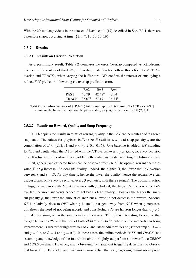
User-Adaptive Rotational Snap-Cutting for Streamed 360◦Videos 114

With the 20 sec-long videos in the dataset of David et al. [17] described in Sec. 7.3.1, there are

7 possible snaps, occurring at times {1, 4, 7, 10, 13, 16, 19}.

7.5.2 Results

7.5.2.1 Results on Overlap Prediction

As a preliminary result, Table 7.2 compares the error (overlap computed as orthodromic

distance of the centers of the FoVs) of overlap prediction for both methods for P1 (PAST-Past

overlap and TRACK), when varying the buffer size. We confirm the interest of employing a

refined FoV predictor in lowering the overlap prediction error.

B=2 B=3 B=4PAST 40.79◦ 42.42◦ 45.54◦

TRACK 36.07◦ 37.17◦ 36.74◦

TABLE 7.2: Absolute error of (TRACK) future overlap prediction using TRACK or (PAST)estimating the future overlap from the past overlap, varying the buffer size B ∈ {2, 3, 4}.

7.5.2.2 Results on Reward, Quality and Snap Frequency

Fig. 7.6 depicts the results in terms of reward, quality in the FoV and percentage of triggered

snap-cuts. The values for playback buffer size B (still in sec.) and snap penalty % are the

combination of B ∈ {2, 3, 4} and % ∈ {0.2, 0.3, 0.35}. One baseline is added: GT, standing

for Ground Truth, when the DT is fed with the GT overlap over wfut2(tdec), for every decision

time. It refines the upper-bound accessible by the online methods predicting the future overlap.

First, general and expected trends can be observed from OPT. The optimal reward decreases

when B or % increase. So does the quality. Indeed, the higher B, the lower the FoV overlap

between t and t − B, for any time t, hence the lower the quality, hence the reward (we can

trigger a snap only every 3 sec., i.e., every 3 segments, with these settings). The optimal fraction

of triggers increases with B but decreases with %. Indeed, the higher B, the lower the FoV

overlap, the more snap-cuts needed to get back a high quality. However the higher the snap-

cut penalty %, the lower the amount of snap-cut allowed to not decrease the reward. Second,

GT is relatively close to OPT when % is small, but gets away from OPT when % increases:

this shows the need of not being myopic and considering a future horizon longer than wfut2()

to make decisions, when the snap penalty % increases. Third, it is interesting to observe that

the gap between OPT and the best of both ZEROS and ONES, where online methods can bring

improvement, is greater for higher values ofB and intermediate values of % (for example,B = 3

and % = 0.2, or B = 4 and % = 0.3). In these cases, the online methods PAST and TRACK (not

assuming any knowledge of the future) are able to slightly outperform (in reward) the ZEROS

and ONES baselines. However, when observing their snap-cut triggering decisions, we observe

that for % ≥ 0.3, they often are much more conservative than GT, triggering almost no snap-cut.

User-Adaptive Rotational Snap-Cutting for Streamed 360◦Videos 115

In such case of high %, for high B (3 and even more so 4), the quality is much impacted by the

lower accuracy of future prediction.

B:2%:.20

B:2%:.30

B:2%:.35

B:3%:.20

B:3%:.30

B:3%:.35

B:4%:.20

B:4%:.30

B:4%:.35

0.4

0.5

0.6

0.7

Ave

rage

rew

ard

(QoE

)

OPT GT TRACK PAST ZEROS ONES

B:2%:.20

B:2%:.30

B:2%:.35

B:3%:.20

B:3%:.30

B:3%:.35

B:4%:.20

B:4%:.30

B:4%:.35

0

0.2

0.4

0.6

0.8

1

Frac

tion

oftr

igge

rs

OPT GT TRACK PAST ZEROS ONES

B:2%:.20

B:2%:.30

B:2%:.35

B:3%:.20

B:3%:.30

B:3%:.35

B:4%:.20

B:4%:.30

B:4%:.35

0.5

0.6

0.7

Ave

rage

qual

ityin

FoV

OPT GT TRACK PAST ZEROS ONES

FIGURE 7.6: (Top) Average reward (QoE), (Center) fraction of triggered snap-changes and(Bottom) average quality in FoV, for each method in OPT: Optimal, GT: Using the groundtruthfuture overlap as features, TRACK: Using the overlap computed with the prediction fromTRACK (Sec. 5), PAST: Using the overlaps before the decision, ZEROS: Never triggeringa snap, ONES: Always triggering the snaps. The values are computed for each of the experi-

ments, varying the buffer size B, and the penalty for triggering a snap-change %.

7.5.3 Discussion

In this Chapter we define and investigate how to learn to trigger (rotational) snap-cuts meant

to jointly benefit the user and the streaming algorithm to increase the user’s QoE. It is however

a preliminary work, suffering from several limitations. First, in comparison with GT, we can

observe that the performance of the proposed method TRACK (even more so PAST) is limited

User-Adaptive Rotational Snap-Cutting for Streamed 360◦Videos 116

by the difficulty of predicting the overlap (the prediction horizon is B + G sec., 4 to 6 sec.

here). To overcome this difficulty, it will be important to extract less volatile features that can

be exploited in deciding to trigger, particularly user or video profiles. Second, the considered

model of user’s reactions to a snap-cut (freezing for G sec.) and the QoE model (for the reward)

are simplistic. Future work should carry out user experiments to determine accurate models, and

considering complex or unknown reaction models will require to adopt other types of learning

approaches (RL approaches where the test set is collected using a behavior policy different from

the target policy). Finally, the snap-cuts are modulated here to help the streaming process (using

a playback buffer). However, we have considered the network state fix and the streaming logic

independent of the available bandwidth. Future work will design advanced network-adaptive

strategies making use of user- and content-adaptive snap-cutting strategies.

7.6 Conclusions

In this Chapter, we have investigated user-centric film editing rotational snap-cut techniques

to guide the user’s attention. We have studied control mechanisms to learn how to dynamically

trigger rotational snap-cuts that re-position a user in front of new FoV, when watching a VR

content streamed over the Internet. These snap-cuts can benefit the user’s experience both by

helping stream and improve the quality in the FoV, and ensuring the user sees RoIs important

for the story plot. However, snap-cuts should not be too frequent and may be avoided when

not beneficial to the streamed quality. We have formulated the snap-cut triggering optimization

problem and investigated possible gains in quality of experience. We have shown that learning

approaches are relevant to design online snap-cut triggering strategies to outperform baselines.

Finally, we have identified the limitations of this preliminary work and the future steps to take.

Chapter 8

Conclusions and Future Work

8.1 Conclusions

In this dissertation we present our comprehensive processing chain tailored to the streaming

of Virtual Reality videos. We contributed to VR streaming systems with prediction and opti-

mization of guidance techniques to maximize the streaming quality. We split this work into six

main contributions.

The first contribution in this processing chain is the design of a reactive transcoder to struc-

ture the VR content and decide what to send and when driven by the user’s gaze position.

Chapter 3 introduced our first step to make high-performing foveated streaming systems.

Our streaming architecture adapts to the user’s gaze position by focusing the quality in the gaze

target and delivering low-quality blurred content outside, so as to reproduce and help the natural

focusing process while reducing bandwidth waste. This prototype is based on the FOVE headset,

one of the first commercially available headsets with an integrated eye-tracker. We build on the

FOVE’s Unity API to design a gaze-adaptive streaming system compatible with the MPEG-

DASH principle. We propose to generate at the server side two video representations (low- and

high-resolution segments) that can be transcoded using information about the gaze position of

the viewer to crop the high-resolution segments around the fovea using per-frame filters. The

cropped high-resolution segment and the entire low-resolution video sphere are then merged at

the client and rendered in the HMD to emulate the naturalistic focusing process of the Human

Visual System. The entire foveated streaming system runs in real-time and our prototype was

presented in the Demo Track of MMSys’18.

A high-performing foveated streaming system requires to anticipate the future user’s head

positions at the time of sending the content from the server. Owing to this acute need for head

motion prediction in 360◦video streaming, a number of recent approaches have proposed deep

neural networks meant to exploit the knowledge of the past positions and of the 360◦ video

content to periodically predict the next positions over a given time horizon.

117

Conclusions 118

The second contribution is the development of a tool to obtain solid results for head motion

estimation and progress towards efficient 360◦ streaming systems.

In Chapter 4, we proposed a framework to evaluate and compare different methods to predict

head position in 360◦ videos. This framework is composed by an algorithm to create a uniform

data structure from each of the current heterogeneous datasets of head and gaze traces. We de-

scribe the algorithms used to compute the saliency maps either estimated from the raw video

content or from the users’ statistics, considering a kernel fitted for the equirectangular projec-

tion used to encode 360◦ videos. To compare each of the head motion prediction settings to a

common reference, we detail the commands to estimate the performance of different approaches

in each original evaluation context (prediction horizon, metrics and datasets). This framework

allows to prepare testbeds to assess comprehensively different prediction methods (on various

datasets against several competitors).

This software framework led to uncover major flaws of existing prediction methods, we

therefore examined these flaws to be able to propose Deep Learning architectures that are better

suited for head motion estimation.

Chapter 5 brought two main contributions:

For our third contribution, we carried out a critical and principled re-examination of the exist-

ing deep learning-based methods to predict head motion in 360◦ videos. We showed that all

the considered existing methods are outperformed, on their datasets and with their test metrics,

by baselines not considering the visual input and exploiting only the past trajectory of head

positions. To understand why, we analyzed the datasets to identify how and when should the

prediction benefit from the knowledge of the content. We analyzed the neural architectures pro-

posed in the state of the art and showed there is only one whose performance does not degrade

compared with the baselines, given that ground-truth saliency information is provided, and none

of the existing architectures can be trained to compete with the baselines over the 0-5 sec. hori-

zon when the saliency features are extracted from the content.

The fourth contribution is the design of a deep neural architecture named TRACK, built by

decomposing the structure of the problem and supporting our analysis with the concept of

Structural-RNN. TRACK is proved to establish state-of-the-art performance on all the prediction

horizons H ∈ [0 sec.,5 sec.] and all the datasets of the existing competitors.

The Deep Learning models studied in Chapter 5, often referred to as “black-boxes” do not

provide any insight on the dependence and the interplay between head motion and the visual

content.

The fifth contribution is the development of a white-box predictor model to investigate the

connection between the visual content and the human attentional process.

In Chapter 6 we have investigated the human head motion process driven by attention when

a user experiences an immersive 360◦ video. We have first introduced a new computational

model named HeMoG, enabling to predict future head positions from the user’s past positions

and the visual content. HeMoG is built on differential equations obtained from the physics of

Conclusions 119

rotational motion where the attractive salient areas in the 360◦ frames are represented as virtual

masses. HeMoG is hence a white-box model and its (time-varying) parameters control the

connection between visual content and head motion process. The performance of HeMoG can

be comparable with those of DL predictors, which we interpret as the DL models learning the

same type of fusion as HeMoG: curvature continuity and momentum attenuation from friction

in the short-term, diversion of motion with saliency attraction in the longer-term. The evolution

of best parameter values in terms of video categories and horizon reveals that, on videos that

are not exploratory, the initial motion momentum is most important until ca. 3s, after which the

saliency weights more in the motion equation.

Another approach instead of adapting reactively to the estimation of the future attention tra-

jectories is to exploit gaze guidance techniques, the goal is to change the users’ viewing direction

towards the areas the director wants them to explore. If driving the user’s attention is critical

for a director to ensure the story plot is understood, in this dissertation we investigated attention

driving techniques from a different perspective: that of the multimedia network community.

The sixth contribution of the thesis is to design a user-adaptive control scheme to automati-

cally trigger VR cuts, named snap-cuts.

In Chapter 7, we have studied control mechanisms for guidance techniques, specifically

applied to learn how to dynamically trigger rotational snap-cuts that re-position a user in front

of a new FoV, when watching a VR content streamed over the Internet. These snap-cuts can

benefit the user’s experience both by helping stream and improve the quality in the FoV, and

ensuring the user sees RoIs important for the story plot. However, snap-cuts should not be

too frequent and may be avoided when they are not beneficial to the streamed quality. We

have formulated the snap-cut triggering optimization problem and investigated possible gains

in quality of experience. We have shown that learning approaches are relevant to design online

snap-cut triggering strategies to outperform different baselines.

8.2 Future Works

In this section we present the future steps that could be taken to continue towards the goal

of optimizing the streaming of VR content. We will first discuss about new strategies to guide

the user’s attention and we thus present the work carried out to advance in this perspective, a

guidance technique based on our foveated streaming system. We then present future research

perspectives in the area of trajectory prediction with attention and uncertainty quantification.

Then, we identify the limitations of the preliminary work on control mechanisms for gaze guid-

ance techniques and the future works to overcome these limitations. Finally, we introduce pos-

sible research directions to refine the current saliency maps in VR videos with the creation of

emotional maps to quantify the effect of emotions in the attention mechanism.

Conclusions 120

FIGURE 8.1: Foveated tunnel to attract the attention of the viewer towards the intended direc-tion.

8.2.1 Foveated Tunnels: Future User Gaze Guidance Techniques

A direct usage of our foveated streaming system (introduced in Chapter 3) is to reactively

send in high quality the areas that are close to the user’s gaze to improve the QoE and bandwidth

usage. However, we also considered another perspective, it is to investigate attention-driving

techniques to attract proactively the user’s gaze by using the foveated region.

Attention driving techniques can be helpful for the streaming of 360◦ videos by directing the

user’s attention to specific pre-defined Regions of Interest (RoI), thereby lowering the random-

ness of the user’s motion. The user’s attention in VR is however a complex process difficult

to harness. We describe here the work already started to properly direct the user’s attention by

using some components involved into the user’s experience (spatial qualities, depth and lumi-

nance) based on the works of [105, 106, 107, 108, 109, 110]. Future work should carry out user

experiments to evaluate the performance of foveal tunnels as a novel gaze-driving technique.

We make the hypothesis that the eye will be attracted by a high resolution area that moves

in an appropriate manner to redirect the attention. The foveal tunnel corresponds to the circular

zone (a tunnel when we consider the time dimension) on the sphere on which the video is

projected in high quality as shown in Fig. 8.1. This tunnel moves every frame to attract the

viewer’s gaze towards the desired position. The movement strategies of the foveal tunnel are

inspired by real eye movements to resemble as much as possible a natural gaze movement.

The possible voluntary motions of the eye are therefore smooth pursuit where the gaze follows

smoothly the motion of an object of interest and keeps focusing on it, and saccade where there

is a rapid gaze movement to focus on a new object (not in the fovea).

Other strategies allowing the responsiveness of the tunnel to the actual movement and po-

sition of the user’s gaze are used in parallel. We adopted two strategies Stay in FoV and Shift.

The former prevents the tunnel to go out of the user’s FoV by blocking it at the edge. The latter

corrects the path of the tunnel when the user ignores it, it is implemented by bringing the tunnel

to the user’s current gaze position if the gaze moves away x degrees or t seconds, thus too far or

for too long time from the tunnel.

Conclusions 121

To create a system that allows us to use the foveated tunnel proactively, that is, not just

reacting to the user’s gaze but also anticipating it. We decided to use the clustering strategy

proposed by Rossi et al. [66]. The trajectories of other users that have observed the video are

grouped into clusters and then we obtain the average trajectory corresponding to each cluster

to represent the trajectory of each group of users. During user experiments (planned for future

work), the trajectory of the user will be categorized into one of the clusters and the foveated

tunnel corresponding to the average trajectory will be used to drag the attention of the current

user.

To implement these ideas, we have supervised a Master-2 project of four students that worked

during five months on an initial implementation of the foveated tunnels. This work was then

followed up by another Master-2 internship of six months. A Unity implementation of the

proposed system has therefore already been made and its test with user experiments is planned

for future work.

8.2.2 Future Head Motion Prediction Methods

Efforts could also be directed to improve the architecture of TRACK proposed in Chapter 5

and illustrated in Fig. 8.2. We started advancing in this regard with the supervision of an in-

ternship of a student that worked during three months on the investigation of deep attention

mechanisms to refine the time- and space-varying fusion of modalities. We studied the incorpo-

ration into TRACK of an attention mechanism based on [120] and on the multi-headed attention

mechanism proposed in [121]. Future works will also consider variational approaches with the

use of Variational Recurrent Neural Networks [122] or Memory Networks [123, 124] to obtain

confidence on the prediction of multiple trajectories, as has been proposed in the analogous

task of trajectory prediction in autonomous driving [125]. Another important consideration in

TRACK is the embedding of the visual input. As the shape of the video is spherical, regular

convolutional layers need to be adapted to vary the filters to match the distorted shape of the

2D projections [126]. An important investigation is the use of Graph Neural Networks and its

generalized version of Convolutional Neural Networks for non-Euclidean structured data called

Graph Convolutional Networks [127] to create the embedding from the spherical visual input.

Given the performance of HeMoG, described in Chapter 6, we could build new Deep Learn-

ing Architectures based on the attributes of HeMoG to fuse the different input modalities. For

instance, the operation to obtain the gravitational field of forces (Eq. 6.3) can be compactly

re-written using the convolution operator E(a) = −(e⊗µ). Let r ∈ Υ be any point in the

sphere and a(t) be the position of the head at time t. Indeed, to compute the overall field of

forces, a convolution operator is applied between the distance matrix e(r, a(t)) = 12π

r−a(t)||r−a(t)||2

and the saliency map µ(r, t). This convolution could be directly replaced by a convolutional

layer or, as described above, by a Graph Convolutional Network for which the parameters of

the kernel will be learned. Another choice is to formalize the problem to be able to replace the

Conclusions 122

FIGURE 8.2: Illustration of future works to improve the building-block of TRACK’s archi-tecture. The Concatenation layer is replaced by an Attention Mechanism, the Flatten layeris replaced by a Graph Convolutional Network and the LSTMs are replaced by a Variational

Approach.

ODE solver (LSODA) by a Neural-ODE model, a novel Deep Neural Network model to solve

Ordinary Differential Equations [128].

To further improve the performance of HeMoG, in future works we can study better mech-

anisms to compute saliency maps from the content. While the study of Chapter 6 has been

restricted to saliency attractors based on moving objects, we can consider extending to static

objects whose importance can be ranked, meaning that the trajectory of focus of attention is also

subjected to a gravitational field created by static objects [102, 103]. We can also study how

to improve for the case of Rides scenes characterized by camera motion. To have more solid

estimates of pixel velocities, methods for camera motion estimation [104] are already present in

the literature and can help in creating more suitable saliency estimates for the proposed model.

8.2.3 Future Strategies on Control Mechanisms for Attention Guidance

A key aspect in VR streaming is that the consumed data rate depends on the motion of the

user: the higher the motion, the more data needs to be sent from the server. Therefore, to lower

the required data rate, new levers have been created to reduce the user’s motion. In Chapter 7 we

defined and investigated how to learn to trigger (rotational) snap-cuts meant to jointly benefit the

user and the streaming algorithm to increase the user’s QoE. It is however a preliminary work,

suffering from several limitations.

First, in comparison with the upper-bound using Ground-Truth information, we observed that

the performance of the proposed method is limited by the difficulty of predicting the overlap (the

prediction horizon is 4 to 6 seconds). To overcome this difficulty, it will be important in future

works to extract less volatile features that can be exploited in the decision to trigger the cuts.

Particularly it is important to study ways to categorize the trajectories of users and to define new

Conclusions 123

video profiles to classify how the video content affects the user trajectories, and subsequently

use these classifications as features for the snap-cut decision process.

Second, the considered model of user’s reactions to a snap-cut (freezing for 2 seconds) and

the QoE model (for the reward) are simplistic. Future work should carry out user experiments

to determine more accurate models, and considering complex or unknown reaction models will

require to adopt other types of learning approaches. An exciting prospect is to use Reinforce-

ment Learning approaches where the test set is collected using a behavior policy different from

the target policy. Another important idea is to simulate the reaction model based on an enhanced

version of HeMoG (Head Motion with Gravitational laws, introduced in Chapter 6) and taking

inspiration from [120] where the human behavior is controlled by a physics based simulator

[129].

Third, the snap-cuts were modulated to help the streaming process (using a playback buffer).

However, we have considered the network state fixed and the streaming logic independent of

the available bandwidth. Future work will design advanced network-adaptive strategies based

on network bandwidth traces making use of user- and content-adaptive snap-cutting strategies.

Finally, more levers should be considered to improve the attention-guidance toolbox such as

dynamic foveated streaming (discussed in Sec. 8.2.1), slow-down the video [130] or prevent the

user from seeing certain sectors of the sphere [131]. In a real-world environment, these levers

must be smartly triggered so that they can optimize the complex user’s experience models. For

instance, we would trigger a rotational cut or restrict the field of view only when the network

rate is not sufficient to grant the user full freedom and only if the current scene is suitable for

such effect, or if the user’s attentional or sickness level requires it. Therefore we need to choose,

for each piece of content to send from the server to the client, which lever can be activated, and

whether it needs to be activated, depending on the user’s motion and sickness state, the available

network rate, and the type of scene. This is a very difficult dynamic optimization problem

where decisions must be taken based on random time series partly unknown (user’s motion,

available network rate, video frames). Machine learning, and deep neural networks specifically,

are therefore key to design smart dynamic streaming strategies targeting a fluid experience of

the VR content even in limited network conditions.

8.2.4 Emotional Maps and Future Perspective on Saliency Maps

In Virtual Reality, compared to traditional 2D videos, the user’s senses are immersed in the

experience and therefore elicits a more intense emotional response. The emotional response is

defined in neuroscience as the combination of levels of valence and arousal, measured through

biological responses such as pulse and skin conductance that can be obtained with physiological

sensors [132].

To edit and deliver content tailored to VR, it is critical to understand the user experience

and, in particular, to predict which parts of the 360◦ sphere will be attended by the user. Until

Appendix A 124

now, saliency maps are the main visual tool used to predict where the user is likely to look at.

However, as shown in Chapter 6, these saliency maps are only partially informative and can be

noisy and more difficult to get information from.

To address the strong need of more informative saliency maps, future work will have to

include solid estimates of maps extracted from the content adding the emotional value of an

object. Future works should be directed towards emotional maps to investigate (i) the spatial

and temporal relationships between the physiological data (levels of arousal and valence) and

head and gaze movements regardless of the content, extending the work in [133, 134], and (ii)

the correlation between arousal and the characteristics of objects in 360◦ videos, applying the

normalization used in [135] to obtain the actual interest in objects and study if arousal correlates

with low-level or normalized-high-level saliency.

Another important modality, which highly impacts the direction of attention and has not been

considered yet in any approach, is directional sound. Recent advances have been made to detect

the source of the sound in a video [136, 137]. These works are useful to create sound maps of

VR environments and refine the saliency maps obtained only from the visual content.

Appendix A

Experimental Settings of ExistingMethods

Except for PAMI18 and MM18, none of the methods we studied came with publicly avail-

able code to reproduce the results, we had to reproduce each of the original experiments. In

this section, we detail the specific configurations we used to replicate the original experiments

of PAMI18, NOSSDAV17, CVPR18, MM18 and ChinaCom18 with the description given in

the papers. In case further information is needed, we provide our code (with detailed expla-

nations and reproducible figures) in a publicly available repository https://gitlab.com/

miguelfromeror/head-motion-prediction.

To prove fairness in our comparison, we justify each of the decisions we made in our code

by presenting some quotes written in the description of the original works. The only changes

we made with respect to these citations are the notation and the reference number.

To describe each of the experiments we first detail the metrics used in each method, second

we show the prediction horizon used in these works, and third we present the dataset used in

each work and the split in train and test sets.

A.1 PAMI18 [1]

A.1.1 Metric

The authors of PAMI18 use the metric mean overlap, here is a description of this metric,

given in [1]:

The metric of mean overlap (MO), which measures how close the predicted HM

position is to the ground-truth HM position. MO ranges from 0 to 1, and a larger

MO indicates a more precise prediction. Specifically, MO is defined as,

MO =A(FoVp ∩ FoVg)A(FoVp ∪ FoVg)

, (A.1)

125

Appendix A 126

where FoVp and FoVg represent the FoVs at the predicted and ground-truth HM

positions, respectively.

A represents the area of a panoramic region, which accounts for number of pixels.

In this article the authors also express that they used this metric to measure the performance

of their network:

For evaluating the performance of online-Deep Head Prediction (DHP), we com-

pared our approach with [138] and two baseline approaches. The same as [138],

MO of (A.1) is measured as the metric to evaluate the accuracy of online predic-

tion in HM positions. Note that a larger value of MO means a more accurate online

prediction in HM positions. Since the Deep Reinforcement Learning (DRL) net-

work of offline-DHP was learned over 61 training sequences and used as the initial

model of online-DHP, our comparison was conducted on all 15 test sequences of

our PVS-HM database.

We used the metric MO from the code of PAMI18 authors, provided in their repository1.

The file was copied to our repository and used to measure the performance of our baselines.

A.1.2 Prediction horizon H

From [1]:

The online-DHP approach refers to predicting a specific subject’s HM position

(θt+1, ϕt+1) at frame t + 1, given his/her HM positions (theta1, ϕ1), ..., (θt, ϕt)

till frame t. [...] the output is the predicted HM position (θt+1, ϕt+1) at the next

frame for the viewer. Stage II: Prediction: [...] When entering the prediction stage,

the DRL model trained in the first stage is used to produce the HM position as fol-

lows. [...] the HM position (θt+1, ϕt+1) can be predicted, given the ground-truth

HM position (θt, ϕt) and the estimated HM scanpath (∆ ˆ(θ, ϕ), vt) at frame t.

Meaning that the ground-truth of the previous HM position is used to predict each HM posi-

tion frame by frame.

This is clear in Table 5 of [1]. The authors explicitly say:

Both the online-DHP approach and baseline make predictions based on the ground-

truth previous frames.

A.1.3 Train and Test Split

From [1]:1https://github.com/YuhangSong/DHP/blob/master

Appendix A 127

Since the DRL network of offline-DHP was learned over 61 training sequences and

used as the initial model of online-DHP, our comparison was conducted on all 15

test sequences of our PVS-HM database.

We can find in Table 5 of [1], the 15 videos that were used to test:

BlueWorld, BTSRun, CMLauncher2, Dancing, Guitar, InsideCar, KingKong, RioOlympics,

SpaceWar, SpaceWar2, StarryPolar, Sunset, Symphony, WaitingForLove and Waterfall

Therefore, we can deduce that the 61 training sequences that correspond to the 61 videos in

the train set are:

A380, AcerEngine, AcerPredator, AirShow, BFG, Bicycle, Camping, CandyCarnival, Cas-

tle, Catwalks, CMLauncher, CS, DanceInTurn, DrivingInAlps, Egypt, F5Fighter, Flight, Galaxy-

OnFire, Graffiti, GTA, HondaF1, IRobot, KasabianLive, Lion, LoopUniverse, Manhattan, MC,

MercedesBenz, Motorbike, Murder, NotBeAloneTonight, Orion, Parachuting, Parasailing, Pearl,

Predator, ProjectSoul, Rally, RingMan, Roma, Shark, Skiing, Snowfield, SnowRopeway, Square,

StarWars, StarWars2, Stratosphere, StreetFighter, Supercar, SuperMario64, Surfing, Surfin-

gArctic, TalkingInCar, Terminator, TheInvisible, Village, VRBasketball, Waterskiing, Western-

Sichuan and Yacht.

We made this partition of the dataset in our repository [18], the traces appear in the folder

Song PAMI 18/orig dataset partition.

A.2 NOSSDAV17 [2]

A.2.1 Metric

Our experiment follows the specifications in NOSSDAV17’s paper [2], where we find a

description of the formatting of the output:

The ground-truth of the fixation prediction networks are the tiles viewed by the

viewers at each frame. Using the dataset collected [139], we sample the points

within the FoV by mapping the orientation on the sphere to the equirectangular

model. Then, the viewed tiles are the tiles that are overlapped with the mapped

points. For a single video frame, each tile is either watched or not, i.e., it has a

boolean viewing probability.

We fix the Quantization Parameter (QP) and resolution of all tiles at 28 and 192 ×192 respectively.

In the file Fan NOSSDAV 17/TileMappingReplica.py of our repository [18], we have imple-

mented the tile mapping algorithm.

We also provide the file Fan NOSSDAV 17/CompareTileInfoWithReplica.py, to evaluate how

good is our replica of the tile mapping algorithm, since the original is not provided. We used a

Appendix A 128

FoV of size 120◦ , to better match the original tiles, however, using a FoV of size 100◦ does not

vary the results.

The authors also introduce the metrics used:

To select the optimal parameters of the two models, we consider three metrics:

(i) accuracy, which is the ratio of correctly classified tiles to the union of predicted

and viewed tiles,

(ii) F-score, which is the harmonic mean of prediction and recall, where the preci-

sion and recall are the ratios of correctly predicted tiles to the predicted and viewed

tiles, respectively, and,

(iii) ranking-loss, which is the number of tile pairs that are incorrectly ordered by

probability normalized to the number of tiles.

The metrics we used correspond to the implementation of the Scikit-Learn package:

sklearn.metrics: accuracy_score, f1_score, label_ranking_loss

And according to the authors:

We consider the fixation prediction on tiles as a multi-label classification problem

and have implemented the neural networks using Scikit-Learn and Keras.

A.2.2 Prediction Horizon H

From [2]:

Both networks take features of M past video frames in a sliding window as in-

puts, and predict the viewing probability of tiles with H future video frames in a

prediction window as outputs.

We let both the sliding window size M and prediction window size H to be 30

[frames].

The prediction horizon H is therefore 1 second.

A.2.3 Train and Test Split

From [2], the composition of the dataset is:

We download ten 360◦ videos from YouTube, which are in 4096×2048 pixels (4K)

resolution with a frame rate of 30 Hz. [...] Each video lasts for one minute. We

recruit 25 viewers for dataset collections.

Appendix A 129

We use the traces from 12 viewers (training set) to train the two proposed fixation

prediction networks. Among the traces, we randomly divide them into 80% and

20% for training and validation, respectively.

Therefore, the training set is composed by the 120 traces of 12 viewers watching 10 videos,

and is further subdivided in train and validation, with 80% of the 120 traces (96 traces) used to

train the networks and 20% of the traces (24 traces) are used to validate.

The remaining 13 traces, from the dataset with traces of 25 users, are used for another ex-

periment, this is clear in the paper:

Some pilot simulation runs with |U | = 13 viewers (testing set), B = 150 Mbps,

Dl = 2 secs, and M = 30.

In summary, we have to select 12 viewers from the dataset, and randomly select from their

traces 96 traces to train and 24 traces to validate.

We made this partition of the dataset in the folder Fan NOSSDAV 17/orig dataset partition

in our repository [18].

A.3 MM18 [3]

A.3.1 Metric

Our experiment follows the specifications in MM18’s paper [3], the recommendations of the

authors in the public repository [71] and some extra clarifications made by the authors when

contacted by mail:

In [3]:

The evaluation metric is the accuracy of head movement prediction. Accuracy

is calculated based on the ratio of the number of overlapping tiles between pre-

dicted and ground-truth head orientation map over the total number of predicted

and viewed tiles.

According to the authors:

The accuracy defined in this paper is neither a traditional sense of accuracy nor

precision. We followed the definition in reference [2]. For example, if we predict

two tiles, but only one of them matches with the two viewed tiles, the accuracy will

be the number of intersected tiles (between the two predicted and two viewed tiles)

over the number of unioned tiles, i.e., 1/3.

The metrics we used in this case do not correspond to the implementation of the Scikit-Learn

package: sklearn.metrics: accuracy score, we implemented the metric given the specifications

of the authors, in our repository we provide the file Nguyen MM 18/AccuracyMetricIoU.py.

Appendix A 130

For the computation of the output head position probability map, the authors provide insights

on how it is computed in their source code [71]. In our code is implemented in Nguyen MM 18/

TileMappingReplica.py following the specification from the paper that “the equirectangular

frame is spatially configured into 16× 9 tiles.”

A.3.2 Prediction Horizon H

From [3]:

We use the input feature from the past one second to predict the head orientation in

the future.

The default prediction window H is set to be 0.5 seconds.

To explore the effect of prediction window H on the accuracy of the proposed

model and other three benchmarks, we vary H from 0.5 seconds to 2.5 seconds.

A.3.3 Train and Test Split

From [3], about the compositon of the dataset

For each video, we select one segment with a length of 20-45 seconds. The video

segment is selected such that there are one or more events in the video that introduce

new salient regions (usually when new video scene is shown and lead to fast head

movement of users. We extract the timestamped saliency maps and head orientation

maps from these videos, generating a total of 300,000 data samples from 432 time

series using viewing logs of 48 users.

We use 5 videos from our dataset for model training and another 4 videos for model

validation.

We made this partition of the dataset in the folder Nguyen MM 18/orig dataset partition.

A.4 ChinaCom18 [4]

A.4.1 Metric

Our experiment follows the specifications in ChinaCom18’s paper [4], where we find a de-

scription of the formatting of the metrics used:

Table 1 provides the specific measurement of accuracy and F-score of the predic-

tion on each video. Accuracy presents the primary performance of the prediction

model by calculating the ratio of tiles correctly classified to all tiles. F-score is the

Appendix A 131

weighted mean of the precision and recall (precision is the ratio of tiles classified

to be positive correctly to all positive classified tiles, and recall is the ratio of tiles

classified to be positive to all viewed tiles)

The metrics we used correspond to the implementation of the Scikit-Learn package:

sklearn.metrics: accuracy_score, f1_score.

A.4.2 Prediction Horizon H

From [4]:

When omnidirectional videos are partitioned intoN tiles, our model provides short-

term prediction results Predshort = pN1 and additional long-term prediction results

Predlong = pN1 to adapt to the variation of user’s FoV in the prediction window.

The sliding window is set to be 1 second, as well as the size of short-term and

long-term prediction window.

Meaning that the prediction horizon is 1 second in the long-term and 0.03 seconds (1 frame)

in the short-term. In the paper there is no description of a longer-term prediction horizon than 1

second.

A.4.3 Train and Test Split

From [4], the composition of the dataset is:

The LSTM network of the prediction model has to be trained by the omnidirec-

tional video dataset [139]. The dataset has ten omnidirectional videos all lasting

one minute. All videos are of 4K resolution with 30 fps. The videos are projected

with equirectangular projection. Each video is viewed by 30 viewers wearing HMD

and the orientation of each frame has been collected by Open Track and presented

in both Cartesian coordinates and Euler angles. The omnidirectional video is parti-

tioned into 10× 20 tiles, which are labeled whether is viewed by the user.

So, we need to select the traces of 30 viewers from the dataset of [2] as stated in [4]:

We divide the dataset into 80% and 20% for training and validation respectively.

Different videos are trained and validated separately, so that a unique prediction

network is trained for each video

This means that there should be 10 partitions of the dataset, in each partition we consider the

data for a single video, the traces of all 30 viewers on each video are splitted into 80% and 20%

for training and validation respectively.

Appendix A 132

In summary, we have to select 30 viewers from the dataset, then, we iterate per video and

partition the 30 traces (of each video) into 24 traces to train and 6 traces to validate.

We made these partitions of the dataset in the folders:

• orig dataset partition coaster

• orig dataset partition coaster2

• orig dataset partition diving

• orig dataset partition drive

• orig dataset partition game

• orig dataset partition landscape

• orig dataset partition pacman

• orig dataset partition panel

• orig dataset partition ride

• orig dataset partition sport

A.5 CVPR18 [5]

A.5.1 Metric

Our experiment follows the specifications in CVPR18’s paper [5], where we find a descrip-

tion of the metric:

Since our goal aims at predicting a sequential gaze points in a video for each user,

so we use the Mean Intersection Angle Error (MA) over all videos and all users

to measure the performance. For the gaze point in the ith frame (i = 1, ..., T ) with

ground-truth (xpi , ypi ) and prediction (θpi , ϕpi ), the viewing angle between them can

be represented as di (the way to compute d i will be provided in supplementary

material), then MIAE can be calculated as follows MIAE = 1TP

∑i,p di. Here P

is the total number of users watching this video. We then average MAE over all

videos. Following the work of face alignment, we also use cumulative distribution

function (CDF) of all gaze points for performance evaluation. A higher CDF curve

corresponds to a method with smaller MAE.

According to the supplementary material of [5]:

For a given gaze point (θ, ϕ), where θ is latitude and ϕ is longitude, its coordinate

in the unit sphere is P = (cosx cos y, cosx sin y, sinx), then for a ground-truth

gazepoint (θ, ϕ) and its predicted gaze point (θ, ϕ), we can get corresponding co-

ordinates in unit sphere as P and P , the intersection angle error between them can

be computed as d = arccos(< P, P >) where <,> is inner product.

Appendix A 133

The file to compute the Intersection angle error according to this definition is given in

Xu CVPR 18/ IntersectionAngleError.py.

A.5.2 Prediction Horizon H

From [5]:

We propose to use the history gaze path in the first five frames to predict the gaze

points in next five frames (M = 5 and H = 5). We use the observation (the results

of gaze tracking) in the first 1 second to predict the gaze points in the frames of

upcoming 1 second.

However, according to the problem formulation:

We formulate gaze prediction as a task of learning nonlinear mapping function F

which maps the history gaze and image contents to the coordinates.

F is the deep neural network of CVPR18, therefore, from the problem formulation the neural

network consider a prediction horizon of 1 frame, since in the same problem formulation the

authors propose to use “the current frame and next frame and the history gaze path as input

when we predict the gaze point in the next frame”.

Following the common setting in trajectory prediction for crowd, we downsam-

ple one frame from every five frames for model training and performance evalua-

tion. In this way, the interval between two neighboring frames in our experiments

corresponds to 525 seconds, and such setting makes our gaze prediction task more

challenging than that for the neighboring frames in original videos.

Finally, to avoid the confusion about the actual prediction horizon, we consider the larger

prediction horizons of 5 frames, that corresponds to 1s.

A.5.3 Train and Test Split

From [5], the partition of the dataset is:

In our experiments, we randomly select 134 videos as training data, and use the

remaining 74 videos as testing. Some participants are shared in training and testing,

but the videos in training/testing have no overlap.

In the dataset [140] we can find the partition of the data in the file dataset/train test set.xlsx.

So, the 134 videos for the train set are:

1, 2, 3, 4, 5, 6, 7, 8, 9, 10, 11, 12, 13, 14, 15, 16, 17, 18, 19, 20, 21, 22, 35, 37, 38, 39, 40,

41, 42, 43, 44, 45, 46, 47, 48, 49, 50, 51, 52, 53, 54, 55, 56, 57, 72, 73, 74, 75, 76, 77, 78, 79,

Appendix A 134

80, 81, 82, 83, 85, 87, 88, 89, 90, 91, 92, 93, 94, 95, 109, 110, 111, 112, 113, 114, 115, 116,

117, 118, 119, 120, 121, 122, 123, 124, 125, 126, 127, 128, 129, 130, 144, 145, 146, 147, 148,

149, 150, 151, 152, 153, 154, 155, 156, 157, 158, 159, 160, 161, 162, 163, 164, 165, 179, 180,

181, 182, 183, 184, 185, 186, 187, 188, 189, 190, 191, 192, 193, 194, 195, 196, 197, 198, 199,

200, 201, 202

While the 74 videos in the test set are:

23, 24, 25, 26, 27, 28, 29, 30, 31, 32, 33, 34, 58, 59, 60, 62, 63, 64, 65, 66, 67, 68, 69, 70,

71, 96, 97, 98, 99, 100, 101, 102, 103, 104, 105, 106, 131, 132, 133, 134, 135, 136, 137, 138,

139, 140, 141, 142, 143, 166, 167, 168, 169, 170, 171, 172, 173, 174, 175, 176, 177, 178, 203,

204, 205, 206, 208, 209, 210, 211, 212, 213, 214, 215

We made this partition of the dataset in the folder Xu CVPR 18/orig dataset partition in our

repository [18].

A.5.4 Replica of CVPR18’s Architecture

Here we describe our re-implementation of CVPR18, we kept the exact same architectural

and training parameters as those described in [5]. Citing the authors of CVPR18:

The network consists of a Trajectory Encoder module, a Saliency Encoder module

and a Displacement Prediction module.

A.5.4.1 Trajectory Encoder Module

From the manuscript [5]:

Trajectory encoder module is designed to encode the history gaze path of a user.

[...] We employ an LSTM network to encode the gaze pattern along the time. For

each video clip, we sequentially feed the gaze points (P ut ) corresponding to history

frames in this video sequence into a stacked LSTM, and denote the output of stacked

LSTM fut+1 at (t+ 1)th frames,

fut+1 = h(P u1 , Pu2 , ..., P

ut ) (A.2)

Here the function h(·) represents the input-output function of stacked LSTM. In

addition, the function h is stacked LSTMs with 2 LSTM layers, both with 128

neurons.

Therefore our Trajectory Encoder Module consists of a doubly-stacked LSTM with 128 neu-

rons each.

Appendix A 135

A.5.4.2 Saliency Encoder Module

For the Saliency Encoder Module, to be independent from the imperfection of any saliency

predictor fed with the visual content, we consider the ground-truth saliency as output of the

Saliency Encoder module. When we compare the architectural choices of the different methods,

to be independent of the particular saliency extraction choice we used the saliency map extracted

from PanoSalNet [3] directly as output of the Saliency Encoder module.

gut+1 = z(V u1 , V

u2 , ..., V

ut , ..., Vt+1), (A.3)

where z(·) represents the saliency extractor (either ground-truth or PanoSalNet).

A.5.4.3 Displacement Prediction Module

Citing [5]:

The displacement prediction module takes the output of saliency encoder module

and trajectory encoder module, use another two fully connected layer to estimate

the displacement between the gaze point at time t+ 1 and gaze point at time t:

∆P ut+1 = r([fut+1; gut+1]), (A.4)

where r(·) represents two connected layers. The function r contains two fully con-

nected layers with 1000, 2 neurons, respectively.

Therefore to replicate the Displacement Prediction Module, we used 2 fully connected layers

with 1000 neurons for the hidden layer and 2 neurons in the output layer.

A.5.4.4 Loss function

Citing [5]:

Once we get the location displacement, we can compute the gaze coordinate P ut+1

at time t+ 1

We used a residual link from the input position P ut to the output of the Displacement Pre-

diction Module ∆P ut+1, and compute P ut+1 = P ut + ∆P ut+1. Citing [5]: “We train the model by

minimizing this loss across all the persons and all video clips in the training-set.”

Citing [5]:

Mathematically, we formulate the objective of gaze tracking as follows:

F ∗ = arg minF

M+H−1∑t=M

||Pt+1 − (Pt + F (Vt:t+1, P1:t))|| (A.5)

Appendix B 136

Given this, we set the loss function as the mean squared error between Pt+1 and Pt+1.

We train our network with the following hyper-parameters setting: mini-batch size (128),

learning rate (0.1), momentum (0.9), weight decay (0.0005), and the number of epochs (5000).

The only setting we changed with respect to the original experiment was the mini-batch size, it

is set to 8 in the original experiment.

Appendix B

Derivative of the Quaternion, AngularAcceleration and Velocity

B.1 Angular Velocity and Quaternion

We define a differential equation that relates the time derivative of the quaternion q and the

angular velocity vector ω [141].

Tangential velocity v⊥ is defined as:

v⊥ =d

dta = ω × a, (B.1)

where ω is the orbital angular velocity. We can consider the quaternions ωq and aq, where

the scalar part of ωq is equal to zero (since ω and a are perpendicular, their dot product is zero),

and the vector part of ωq corresponds to ω; similarly for aq = [0, ax, ay, az], where the position

vector a = [ax, ay, az] is represented in 3d coordinates in the unit sphere.

We can then write Eq. (B.1) in quaternion form:

a = ω ⊗ a, (B.2)

where ⊗ is the quaternion multiplication.

We can also represent the position at each time instant as a quaternion rotation from a con-

stant vector a0 (set to an arbitrary axis, for example a0 = [x = 1, y = 0, z = 0]).

a = q⊗ a0 ⊗ q−1, (B.3)

And therefore,

d

dta =

d

dt[q⊗ a0 ⊗ q−1] (B.4)

137

Appendix B 138

d

dt[q⊗ a0 ⊗ q−1] =

d

dt[q]⊗ a0 ⊗ q−1 + q⊗ a0 ⊗

d

dt[q−1] (B.5)

Given that q⊗ q−1 = 1, then ddt(q⊗ q−1) = 0:

d

dt[q]⊗ q−1 + q ⊗ d

dt[q−1] = 0 (B.6)

d

dt[q−1] = −q−1 ⊗ d

dt[q]⊗ q−1 (B.7)

From Eq. (B.3), we can get a0 in terms of a:

a0 = q−1 ⊗ a⊗ q (B.8)

Replacing Eq. (B.8) in Eq. (B.5):

d

dt[q⊗ a0 ⊗ q−1] =

d

dt[q]⊗ q−1 ⊗ a⊗ q⊗ q−1 + q⊗ q−1 ⊗ a⊗ q⊗ d

dt[q−1] (B.9)

Substituting Eq. (B.7) in Eq. (B.9):

d

dt[q⊗ a0⊗q−1] = q⊗q−1⊗ a⊗q⊗q−1 +q⊗q−1⊗ a⊗q⊗−q−1⊗ q⊗q−1 (B.10)

Simplifying q ⊗ q−1 and using Eq. B.2:

d

dta =

d

dt[q⊗ a0 ⊗ q−1] = q⊗ q−1 ⊗ a−⊗a⊗ q⊗ q−1 = ω ⊗ a (B.11)

Using the quaternion commutator operation: [p, q] = p⊗ q− q⊗ p = [0, 2(p1×p2)], when

both q and p are quaternions without scalar part, [p,q] = 2(q1 × q2) = 2(q1 ⊗ q2).

q⊗ q−1 ⊗ a−⊗a⊗ q⊗ q−1 = ω ⊗ a (B.12)

[q⊗ q−1,a] = ω ⊗ a (B.13)

2q⊗ q−1 ⊗ a = ω ⊗ a (B.14)

q =1

2ω ⊗ q (B.15)

Appendix C 139

B.2 Angular Acceleration and Quaternion

Now we need to define a differential equation that relates the second time derivative of the

quaternion q and the angular acceleration vector dwdt .

Using Eq. (B.15):

ω = 2q⊗ q−1 (B.16)

The second derivative of the quaternion (from Eq. (B.15)) is:

q =1

2(ω ⊗ q + ω ⊗ q) (B.17)

Replacing Eq. (B.16) in Eq. (B.17):

q =1

2(2q⊗ q−1 ⊗ q + ω ⊗ q) (B.18)

q = q⊗ q−1 ⊗ q +1

2ω ⊗ q (B.19)

Appendix C

Publications and ComplementaryActivities

C.1 Publications

The subject of this thesis is multi-disciplinary (involving concepts from Multimedia Com-

munication and Networking, Machine Learning and Deep Learning, Attentional Models and

Perception). Our work has been proven to be relevant in the context of international research.

We have published our research in the following journals, international conferences and work-

shops.

C.1.1 Journal Paper

Romero Rondon, M. F., Sassatelli, L., Aparicio-Pardo, R., & Precioso, F. (2021). TRACK: A

New Method from a Re-examination of Deep Architectures for Head Motion Prediction in 360◦

Videos. IEEE Transactions on Pattern Analysis and Machine Intelligence (TPAMI).

C.1.2 International Conferences

Romero Rondon, M. F., Zanca, D., Melacci, S., Gori, M. & Sassatelli, L. (2021, November).

HeMoG: A White Box Model to Unveil the Connection Between Saliency Information and Hu-

man Head Motion in Virtual Reality. In IEEE International Conference on Artificial Intelligence

and Virtual Reality (AIVR).

Romero Rondon, M. F., Sassatelli, L., Precioso, F., & Aparicio-Pardo, R. (2018, June). Foveated

Streaming of Virtual Reality Videos. In Proceedings of the 9th ACM Multimedia Systems Con-

ference, (MMSys) Demo track (pp. 494-497).

Romero Rondon, M. F., Sassatelli, L., Aparicio-Pardo, R., & Precioso, F. (2020, May). A Unified

Evaluation Framework for Head Motion Prediction Methods in 360◦ Videos. In Proceedings of

141

Appendix C 142

the 11th ACM Multimedia Systems Conference, (MMSys) ODS track (pp. 279-284).

Romero Rondon, M. F., Sassatelli, L., Aparicio-Pardo, R., & Precioso, F. (2020, May). User-

Adaptive Rotational Snap-Cutting for Streamed 360◦ Videos. In EUROGRAPHICS Workshop

on Intelligent Cinematography and Editing (WICED).

Romero Rondon, M. F., Sassatelli, L., Aparicio-Pardo, R., & Precioso, F. (2020, October).

TRACK: A Multi-Modal Deep Architecture for Head Motion Prediction in 360◦ Videos. In 2020

IEEE International Conference on Image Processing (ICIP) (pp. 2586-2590). IEEE.

C.1.3 National Conferences

Romero Rondon M. F., Sassatelli L., Aparicio-Pardo R., & Precioso F. (2021, November). Une

approche multi-modale a la prediction des mouvements de tete en realite virtuelle. In 21e edition

du colloque COmpression et REpresentation des Signaux Audiovisuels (CORESA).

C.1.4 Oral Presentations

The work “Head Motion Prediction in 360 Virtual Reality Videos” was presented at the GdR

ISIS meeting on “Compression and quality of 360 content, light field and point cloud (3D)”

at INSA Rennes in March 2019. The different works in Sec. C.1.2 have been presented in the

respective conferences and the work in Sec. C.1.3 will be presented in November 2021.

Bibliography

[1] M. Xu, Y. Song, J. Wang, M. Qiao, L. Huo, and Z. Wang, “Predicting head movement in

panoramic video: A deep reinforcement learning approach,” IEEE Trans. on PAMI, 2018.

[2] C.-L. Fan, J. Lee, W.-C. Lo, C.-Y. Huang, K.-T. Chen, and C.-H. Hsu, “Fixation predic-

tion for 360 video streaming in head-mounted virtual reality,” in ACM NOSSDAV, 2017,

pp. 67–72.

[3] A. Nguyen, Z. Yan, and K. Nahrstedt, “Your attention is unique: Detecting 360◦ video

saliency in head-mounted display for head movement prediction,” in ACM Int. Conf. on

Multimedia, 2018, pp. 1190–1198.

[4] Y. Li, Y. Xu, S. Xie, L. Ma, and J. Sun, “Two-layer FoV prediction model for viewport de-

pendent streaming of 360◦ videos,” in EAI Int. Conf. on Communications and Networking

(ChinaCom), Chengdu, China, Oct. 2018.

[5] Y. Xu, Y. Dong, J. Wu, Z. Sun, Z. Shi, J. Yu, and S. Gao, “Gaze prediction in dynamic

360◦ immersive videos,” in IEEE CVPR, 2018, pp. 5333–5342.

[6] C. E. Willoughby, D. Ponzin, S. Ferrari, A. Lobo, K. Landau, and Y. Omidi, “Anatomy

and physiology of the human eye: effects of mucopolysaccharidoses disease on structure

and function–a review,” Clinical & Experimental Ophthalmology, vol. 38, pp. 2–11, 2010.

[7] B. Wandell and S. Thomas, “Foundations of vision,” Psyccritiques, vol. 42, no. 7, 1997.

[8] M. Almquist, V. Almquist, V. Krishnamoorthi, N. Carlsson, and D. Eager, “The prefetch

aggressiveness tradeof in 360 video streaming,” in ACM Int. Conf. on Multimedia Systems

(MMSys), 2018.

[9] E. N. A. Neto, R. M. Barreto, R. M. Duarte, J. P. Magalhaes, C. A. Bastos, T. I. Ren, and

G. D. Cavalcanti, “Real-time head pose estimation for mobile devices,” in International

Conference on Intelligent Data Engineering and Automated Learning. Springer, 2012,

pp. 467–474.

[10] K. Yin, Z. He, J. Xiong, J. Zou, K. Li, and S.-T. Wu, “Virtual reality and augmented

reality displays: advances and future perspectives,” Journal of Physics: Photonics, 2021.

145

Bibliography 146

[11] T. Shibata, J. Kim, D. M. Hoffman, and M. S. Banks, “Visual discomfort with stereo

displays: effects of viewing distance and direction of vergence-accommodation conflict,”

in Stereoscopic Displays and Applications XXII, vol. 7863. International Society for

Optics and Photonics, 2011, p. 78630P.

[12] S. Zhao and D. Medhi, “Sdn-assisted adaptive streaming framework for tile-based im-

mersive content using mpeg-dash,” in 2017 IEEE Conference on Network Function Vir-

tualization and Software Defined Networks (NFV-SDN). IEEE, 2017, pp. 1–6.

[13] H.-W. Kim and S.-H. Yang, “Region of interest–based segmented tiled adaptive streaming

using head-mounted display tracking sensing data,” International Journal of Distributed

Sensor Networks, vol. 15, no. 12, p. 1550147719894533, 2019.

[14] X. Corbillon, G. Simon, A. Devlic, and J. Chakareski, “Viewport-adaptive navigable 360-

degree video delivery,” in 2017 IEEE international conference on communications (ICC).

IEEE, 2017, pp. 1–7.

[15] A. Amidi and S. Amidi, “Vip cheatsheet: Recurrent neural networks,” 2018.

[16] S. Varsamopoulos, K. Bertels, and C. G. Almudever, “Comparing neural network based

decoders for the surface code,” IEEE Transactions on Computers, vol. 69, no. 2, pp.

300–311, 2019.

[17] E. J. David, J. Gutierrez, A. Coutrot, M. P. Da Silva, and P. L. Callet, “A dataset of head

and eye movements for 360◦ videos,” in ACM Int. Conf. on Multimedia Systems (MMSys),

2018, pp. 432–437.

[18] M. F. Romero-Rondon, L. Sassatelli, R. Aparicio-Pardo, and F. Precioso, “head-motion-

prediction,” https://gitlab.com/miguelfromeror/head-motion-prediction/tree/master,

2020.

[19] Grand View Research, Inc., “Virtual Reality Market Share & Trends Report, 2021-2028,”

Industry report, 2021.

[20] S. Sharples, S. Cobb, A. Moody, and J. R. Wilson, “Virtual reality induced symptoms

and effects (vrise): Comparison of head mounted display (hmd), desktop and projection

display systems,” Displays, vol. 29, no. 2, pp. 58–69, 2008.

[21] J. Park, P. A. Chou, and J.-N. Hwang, “Rate-utility optimized streaming of volumetric

media for augmented reality,” IEEE Journal on Emerging and Selected Topics in Circuits

and Systems, vol. 9, no. 1, pp. 149–162, 2019.

[22] E. Bastug, M. Bennis, M. Medard, and M. Debbah, “Toward interconnected virtual real-

ity: Opportunities, challenges, and enablers,” IEEE Communications Magazine, vol. 55,

no. 6, pp. 110–117, 2017.

Bibliography 147

[23] A. Caputo, A. Giachetti, S. Abkal, C. Marchesini, and M. Zancanaro, “Real vs simulated

foveated rendering to reduce visual discomfort in virtual reality,” in Proceedings of the

18th International Conference promoted by the IFIP Technical Committee 13 on Human-

Computer Interation - INTERACT 2021. INTERACT 2021, 2021.

[24] S. Mangiante, G. Klas, A. Navon, Z. GuanHua, J. Ran, and M. D. Silva, “Vr is on the

edge: How to deliver 360 videos in mobile networks,” in Proceedings of the Workshop on

Virtual Reality and Augmented Reality Network, 2017, pp. 30–35.

[25] O. Le Meur, P. Le Callet, and D. Barba, “Predicting visual fixations on video based on

low-level visual features,” Vision research, vol. 47, no. 19, pp. 2483–2498, 2007.

[26] S. Dambra, G. Samela, L. Sassatelli, R. Pighetti, R. Aparicio-Pardo, and A.-M. Pinna-

Dery, “Film editing: New levers to improve vr streaming,” in Proceedings of the 9th

ACM Multimedia Systems Conference, 2018, pp. 27–39.

[27] M. Lambooij, M. Fortuin, I. Heynderickx, and W. IJsselsteijn, “Visual discomfort and

visual fatigue of stereoscopic displays: A review,” Journal of imaging science and tech-

nology, vol. 53, no. 3, pp. 30 201–1, 2009.

[28] M. F. Land, “The human eye: Structure and function,” Nature Medicine, vol. 5, no. 11,

pp. 1229–1229, 1999.

[29] S. A. McMains and S. Kastner, Visual Attention. Berlin, Heidelberg: Springer

Berlin Heidelberg, 2009, pp. 4296–4302. [Online]. Available: https://doi.org/10.1007/

978-3-540-29678-2 6344

[30] E. Kowler, “Attention and eye movements,” in Encyclopedia of neuroscience. Elsevier

Ltd, 2009, pp. 605–616.

[31] J. E. Hoffman, “Visual attention and eye movements,” Attention, vol. 31, no. 2, pp. 119–

153, 1998.

[32] M. Cornia, L. Baraldi, G. Serra, and R. Cucchiara, “A deep multi-level network for

saliency prediction,” in 2016 23rd International Conference on Pattern Recognition

(ICPR). IEEE, 2016, pp. 3488–3493.

[33] J. Pan, C. C. Ferrer, K. McGuinness, N. E. O’Connor, J. Torres, E. Sayrol, and X. Giro-i

Nieto, “Salgan: Visual saliency prediction with generative adversarial networks,” arXiv

preprint arXiv:1701.01081, 2017.

[34] Y. Fang, J. Wang, M. Narwaria, P. Le Callet, and W. Lin, “Saliency detection for stereo-

scopic images,” IEEE Transactions on Image Processing, vol. 23, no. 6, pp. 2625–2636,

2014.

Bibliography 148

[35] V. Sitzmann, A. Serrano, A. Pavel, M. Agrawala, D. Gutierrez, B. Masia, and G. Wet-

zstein, “Saliency in VR: How do people explore virtual environments?” IEEE Trans. on

Visualization and Computer Graphics, vol. 24, no. 4, pp. 1633–1642, 2018.

[36] M. Assens Reina, X. Giro-i Nieto, K. McGuinness, and N. E. O’Connor, “Saltinet: Scan-

path prediction on 360 degree images using saliency volumes,” in Proceedings of the

IEEE International Conference on Computer Vision Workshops, 2017, pp. 2331–2338.

[37] G. Kramida, “Resolving the vergence-accommodation conflict in head-mounted dis-

plays,” IEEE transactions on visualization and computer graphics, vol. 22, no. 7, pp.

1912–1931, 2015.

[38] M. S. Anwar, J. Wang, A. Ullah, W. Khan, Z. Li, and S. Ahmad, “User profile analysis

for enhancing qoe of 360 panoramic video in virtual reality environment,” in 2018 In-

ternational Conference on Virtual Reality and Visualization (ICVRV). IEEE, 2018, pp.

106–111.

[39] X. Yin, A. Jindal, V. Sekar, and B. Sinopoli, “A control-theoretic approach for dynamic

adaptive video streaming over http,” in Proceedings of the 2015 ACM Conference on

Special Interest Group on Data Communication, 2015, pp. 325–338.

[40] M. H. Pinson and S. Wolf, “A new standardized method for objectively measuring video

quality,” IEEE Transactions on broadcasting, vol. 50, no. 3, pp. 312–322, 2004.

[41] G. Calvigioni, R. Aparicio-Pardo, L. Sassatelli, J. Leguay, P. Medagliani, and S. Paris,

“Quality of experience-based routing of video traffic for overlay and isp networks,” in

IEEE INFOCOM 2018-IEEE Conference on Computer Communications. IEEE, 2018,

pp. 935–943.

[42] MPEG Dynamic adaptive streaming over HTTP (DASH), “Iso/iec 23009-1:2014,” 2014.

[Online]. Available: https://www.iso.org/standard/65274.html

[43] F. Chiariotti, “A survey on 360-degree video: Coding, quality of experience and stream-

ing,” arXiv preprint arXiv:2102.08192, 2021.

[44] V. Sze, M. Budagavi, and G. J. Sullivan, “High efficiency video coding (hevc),” in In-

tegrated circuit and systems, algorithms and architectures. Springer, 2014, vol. 39,

p. 40.

[45] Y. Chen, D. Murherjee, J. Han, A. Grange, Y. Xu, Z. Liu, S. Parker, C. Chen, H. Su,

U. Joshi et al., “An overview of core coding tools in the av1 video codec,” in 2018 Picture

Coding Symposium (PCS). IEEE, 2018, pp. 41–45.

[46] I. Bauermann, M. Mielke, and E. Steinbach, “H. 264 based coding of omnidirectional

video,” in Computer vision and graphics. Springer, 2006, pp. 209–215.

Bibliography 149

[47] Y. Ye, J. M. Boyce, and P. Hanhart, “Omnidirectional 360◦ video coding technology in

responses to the joint call for proposals on video compression with capability beyond

hevc,” IEEE Transactions on Circuits and Systems for Video Technology, vol. 30, no. 5,

pp. 1241–1252, 2019.

[48] M. Yu, H. Lakshman, and B. Girod, “A framework to evaluate omnidirectional video cod-

ing schemes,” in 2015 IEEE International Symposium on Mixed and Augmented Reality.

IEEE, 2015, pp. 31–36.

[49] R. S. Sutton and A. G. Barto, Reinforcement learning: An introduction. MIT press,

2018.

[50] A. Schmitz, A. MacQuarrie, S. Julier, N. Binetti, and A. Steed, “Directing versus attract-

ing attention: Exploring the effectiveness of central and peripheral cues in panoramic

videos,” in 2020 IEEE Conference on Virtual Reality and 3D User Interfaces (VR). IEEE,

2020, pp. 63–72.

[51] N. Q. K. Duong, J. Sirot, G. Marquant, and C.-H. Demarty, “Method and apparatus for

inciting a viewer to rotate toward a reference direction when consuming an immersive

content item,” Aug. 18 2020, uS Patent 10,748,321.

[52] V. A. de Jesus Oliveira, L. Brayda, L. Nedel, and A. Maciel, “Designing a vibrotactile

head-mounted display for spatial awareness in 3d spaces,” IEEE transactions on visual-

ization and computer graphics, vol. 23, no. 4, pp. 1409–1417, 2017.

[53] 360fly, “360fly - 4k user guide,” 2016. [Online]. Available: https://www.360fly.com

[54] C. Brown, G. Bhutra, M. Suhail, Q. Xu, and E. D. Ragan, “Coordinating attention and

cooperation in multi-user virtual reality narratives,” in 2017 IEEE Virtual Reality (VR).

IEEE, 2017, pp. 377–378.

[55] K. Carnegie and T. Rhee, “Reducing visual discomfort with hmds using dynamic depth

of field,” IEEE computer graphics and applications, vol. 35, no. 5, pp. 34–41, 2015.

[56] A. Patney, M. Salvi, J. Kim, A. Kaplanyan, C. Wyman, N. Benty, D. Luebke, and

A. Lefohn, “Towards foveated rendering for gaze-tracked virtual reality,” ACM Trans-

actions on Graphics (TOG), vol. 35, no. 6, pp. 1–12, 2016.

[57] A. Patney, J. Kim, M. Salvi, A. Kaplanyan, C. Wyman, N. Benty, A. Lefohn, and D. Lue-

bke, “Perceptually-based foveated virtual reality,” in ACM SIGGRAPH 2016 Emerging

Technologies, 2016, pp. 1–2.

[58] G. Illahi, M. Siekkinen, and E. Masala, “Foveated video streaming for cloud gaming,”

in 2017 IEEE 19th international workshop on multimedia signal processing (MMSP).

IEEE, 2017, pp. 1–6.

Bibliography 150

[59] Z. Ye, “Performance analysis of http adaptive video streaming services in mobile net-

works,” Ph.D. dissertation, Universite d’Avignon, 2017.

[60] A. Bentaleb, B. Taani, A. C. Begen, C. Timmerer, and R. Zimmermann, “A survey on bi-

trate adaptation schemes for streaming media over http,” IEEE Communications Surveys

Tutorials, vol. 21, no. 1, pp. 562–585, 2019.

[61] A. Yaqoob, T. Bi, and G.-M. Muntean, “A dash-based efficient throughput and buffer

occupancy-based adaptation algorithm for smooth multimedia streaming,” in 2019 15th

International Wireless Communications Mobile Computing Conference (IWCMC), 2019,

pp. 643–649.

[62] X. Corbillon, A. Devlic, G. Simon, and J. Chakareski, “Optimal set of 360-degree videos

for viewport-adaptive streaming,” in Proceedings of the 25th ACM international confer-

ence on Multimedia, 2017, pp. 943–951.

[63] P. Rondao Alface, M. Aerts, D. Tytgat, S. Lievens, C. Stevens, N. Verzijp, and J. F. Macq,

“16k cinematic vr streaming,” in ACM Multimedia Conf. (MM), 2017.

[64] J. Ryoo, K. Yun, D. Samaras, S. R. Das, and G. Zelinsky, “Design and evaluation of a

foveated video streaming service for commodity client devices,” in ACM Int. Conf. on

Multimedia Sys. (MMSys), 2016.

[65] S. Petrangeli, G. Simon, and V. Swaminathan, “Trajectory-based viewport prediction for

360◦ virtual reality videos,” in IEEE Int. Conf. on Artificial Intelligence and Virtual Re-

ality (AIVR), Dec 2018, pp. 157–160.

[66] S. Rossi, F. De Simone, P. Frossard, and L. Toni, “Spherical clustering of users navigating

360 content,” in ICASSP 2019-2019 IEEE International Conference on Acoustics, Speech

and Signal Processing (ICASSP). IEEE, 2019, pp. 4020–4024.

[67] A. D. Aladagli, E. Ekmekcioglu, D. Jarnikov, and A. Kondoz, “Predicting head trajecto-

ries in 360◦ virtual reality videos,” in IEEE Int. Conf. on 3D Immersion (IC3D), 2017.

[68] Y. Ban, L. Xie, Z. Xu, X. Zhang, Z. Guo, and Y. Wang, “Cub360: Exploiting cross-users

behaviors for viewport prediction in 360 video adaptive streaming,” in IEEE Int. Conf. on

Multimedia and Expo (ICME), 2018.

[69] C.-L. Fan, S.-C. Yen, C.-Y. Huang, and C.-H. Hsu, “Optimizing fixation prediction us-

ing recurrent neural networks for 360◦ video streaming in head-mounted virtual reality,”

IEEE Transactions on Multimedia, 2019.

[70] M. Xu, Y. Song, J. Wang, M. Qiao, L. Huo, and Z. Wang, “Dataset for predicting head

movement in panoramic video: A deep reinforcement learning approach (pami 2018),”

https://github.com/YuhangSong/DHP, 2018.

Bibliography 151

[71] A. Nguyen, Z. Yan, and K. Nahrstedt, “PanoSalNet - source code for Your Attention

is Unique: Detecting 360◦ video saliency in head-mounted display for head movement

prediction,” https://github.com/phananh1010/PanoSalNet, 2019.

[72] X. Corbillon, F. De Simone, and G. Simon, “360◦ video head movement dataset,” in ACM

Int. Conf. on Multimedia Systems (MMSys), 2017, pp. 199–204.

[73] C. Wu, Z. Tan, Z. Wang, and S. Yang, “A dataset for exploring user behaviors in VR

spherical video streaming,” in ACM Int. Conf. on Multimedia Systems (MMSys), 2017,

pp. 193–198.

[74] K. Simonyan and A. Zisserman, “Very deep convolutional networks for large-scale image

recognition,” arXiv preprint arXiv:1409.1556, 2014.

[75] X. Huang, C. Shen, X. Boix, and Q. Zhao, “Salicon: Reducing the semantic gap in

saliency prediction by adapting deep neural networks,” in IEEE Int. Conf. on Computer

Vision (ICCV), 2015, pp. 262–270.

[76] J. Gutierrez, E. J. David, A. Coutrot, M. P. Da Silva, and P. Le Callet, “Introducing

un salient360! benchmark: A platform for evaluating visual attention models for 360◦

contents,” in IEEE Int. Conf. on Quality of Multimedia Exp. (QoMEX), 2018.

[77] Y. Su and K. Grauman, “Making 360 video watchable in 2d: Learning videography for

click free viewing,” in IEEE CVPR, July 2017, pp. 1368–1376.

[78] Y. Yu, S. Lee, J. Na, J. Kang, and G. Kim, “A deep ranking model for spatio-temporal

highlight detection from a 360 video,” in AAAI, 2018.

[79] Y. Bao, H. Wu, T. Zhang, A. A. Ramli, and X. Liu, “Shooting a moving target: Motion-

prediction-based transmission for 360◦ videos,” in IEEE Int. Conf. on Big Data (Big

Data). IEEE, 2016, pp. 1161–1170.

[80] I. Sutskever, O. Vinyals, and Q. V. Le, “Sequence to sequence learning with neural net-

works,” in Adv. in Neural Info Proc. Sys. (NEURIPS), 2014, pp. 3104–3112.

[81] P. Luc, N. Neverova, C. Couprie, J. Verbeek, and Y. LeCun, “Predicting deeper into the

future of semantic segmentation,” in IEEE ICCV, 2017.

[82] J. Martinez, M. J. Black, and J. Romero, “On human motion prediction using recurrent

neural networks,” in IEEE CVPR, 2017, pp. 4674–4683.

[83] A. Alahi, K. Goel, V. Ramanathan, A. Robicquet, L. Fei-Fei, and S. Savarese, “Social

LSTM: Human trajectory prediction in crowded spaces,” in IEEE CVPR, 2016.

Bibliography 152

[84] S. Rossi and L. Toni, “Understanding user navigation in immersive experience: An

information-theoretic analysis,” in ACM Int. Workshop on Immersive Mixed and Virtual

Environment Systems, ser. MMVE ’20, 2020, p. 19–24.

[85] J. P. Magliano and J. M. Zacks, “The impact of continuity editing in narrative film on

event segmentation,” Cognitive Science, vol. 35, no. 8, pp. 1489–1517, 2011.

[86] A. Jain, A. R. Zamir, S. Savarese, and A. Saxena, “Structural-RNN: Deep learning on

spatio-temporal graphs,” in Proceedings of the ieee conference on computer vision and

pattern recognition, 2016, pp. 5308–5317.

[87] A. Sadeghian, A. Alahi, and S. Savarese, “Tracking the untrackable: Learning to track

multiple cues with long-term dependencies,” in IEEE ICCV, 2017, pp. 300–311.

[88] A. Agrawal, J. Lu, S. Antol, M. Mitchell, C. L. Zitnick, D. Batra, and D. Parikh, “VQA:

Visual Question Answering,” in IEEE ICCV, 2015.

[89] 1st Rank in Udacity Challenge, “Team komanda,” https://github.com/udacity/

self-driving-car/tree/master/steering-models/community-models/komanda, 2016.

[90] M. F. Dacrema, P. Cremonesi, and D. Jannach, “Are we really making much progress?

A worrying analysis of recent neural recommendation approaches,” in ACM Conf. on

Recommender Systems, 2019, pp. 101–109.

[91] W. Yang, K. Lu, P. Yang, and J. Lin, “Critically examining the “neural hype” weak base-

lines and the additivity of effectiveness gains from neural ranking models,” in ACM SIGIR

Conf. on Research and Development in Information Retrieval, 2019, pp. 1129–1132.

[92] K. Musgrave, S. Belongie, and S.-N. Lim, “A metric learning reality check,” arXiv

preprint arXiv:2003.08505, 2020.

[93] D. Blalock, J. J. G. Ortiz, J. Frankle, and J. Guttag, “What is the state of neural network

pruning?” arXiv preprint arXiv:2003.03033, 2020.

[94] H.-Y. Wu, T.-Y. Li, and M. Christie, “Logic control for story graphs in 3d game narra-

tives,” in Smart Graphics, Y. Chen, M. Christie, and W. Tan, Eds. Cham: Springer

International Publishing, 2017, pp. 111–123.

[95] N. Xie, G. Ras, M. van Gerven, and D. Doran, “Explainable deep learning: A

field guide for the uninitiated,” CoRR, vol. abs/2004.14545, 2020. [Online]. Available:

https://arxiv.org/abs/2004.14545

[96] D. Zanca, M. Gori, S. Melacci, and A. Rufa, “Gravitational models explain shifts on

human visual attention,” Scientific Reports, vol. 10, no. 1, pp. 1–9, 2020.

Bibliography 153

[97] R. Swinbank and R. J. Purser, “Fibonacci grids,” in AMS 13th Conference on Numerical

Weather Prediction, vol. 13, 1999, p. 125.

[98] H. Fassold, “Adapting computer vision algorithms for omnidirectional video,” in Pro-

ceedings of the 27th ACM International Conference on Multimedia, 2019, pp. 1026–1028.

[99] L. Maczyta, P. Bouthemy, and O. Le Meur, “Unsupervised motion saliency map estima-

tion based on optical flow inpainting,” in 2019 IEEE International Conference on Image

Processing (ICIP). IEEE, 2019, pp. 4469–4473.

[100] A. Bochkovskiy, C.-Y. Wang, and H.-Y. M. Liao, “Yolov4: Optimal speed and accuracy

of object detection,” arXiv preprint arXiv:2004.10934, 2020.

[101] D. Alvarez-Melis and T. S. Jaakkola, “Towards robust interpretability with self-explaining

neural networks,” in Proceedings of the 32nd International Conference on Neural Infor-

mation Processing Systems, ser. NIPS’18. Red Hook, NY, USA: Curran Associates Inc.,

2018, p. 7786–7795.

[102] G. Ma, S. Li, C. Chen, A. Hao, and H. Qin, “Stage-wise salient object detection in 360◦

omnidirectional image via object-level semantical saliency ranking,” IEEE Transactions

on Visualization and Computer Graphics, vol. 26, no. 12, pp. 3535–3545, 2020.

[103] J. Li, J. Su, C. Xia, and Y. Tian, “Distortion-adaptive salient object detection in 360◦

omnidirectional images,” IEEE Journal of Selected Topics in Signal Processing, vol. 14,

no. 1, pp. 38–48, 2019.

[104] D. Kim, S. Pathak, A. Moro, A. Yamashita, and H. Asama, “Selfsphnet: Motion es-

timation of a spherical camera via self-supervised learning,” IEEE Access, vol. 8, pp.

41 847–41 859, 2020.

[105] R. Yu, W. S. Lages, M. Nabiyouni, B. Ray, N. Kondur, V. Chandrashekar, and D. A.

Bowman, “Bookshelf and bird: Enabling real walking in large vr spaces through cell-

based redirection,” in 2017 IEEE Symposium on 3D User Interfaces (3DUI), 2017, pp.

116–119.

[106] S. P. Sargunam, K. R. Moghadam, M. Suhail, and E. D. Ragan, “Guided head rotation

and amplified head rotation: Evaluating semi-natural travel and viewing techniques in

virtual reality,” in 2017 IEEE Virtual Reality (VR), 2017, pp. 19–28.

[107] Y. Farmani and R. J. Teather, “Evaluating discrete viewpoint control to reduce cybersick-

ness in virtual reality,” Springer Virtual Reality, 2020.

[108] A. Pavel, B. Hartmann, and M. Agrawala, “Shot orientation controls for interactive

cinematography with 360 video,” in Proceedings of the 30th Annual ACM Symposium

Bibliography 154

on User Interface Software and Technology, ser. UIST ’17. New York, NY, USA:

Association for Computing Machinery, 2017, p. 289–297. [Online]. Available:

https://doi.org/10.1145/3126594.3126636

[109] K. Rahimi Moghadam, C. Banigan, and E. D. Ragan, “Scene transitions and teleportation

in virtual reality and the implications for spatial awareness and sickness,” IEEE Transac-

tions on Visualization and Computer Graphics, pp. 1–1, 2018.

[110] B. E. Riecke, M. V. D. Heyde, and H. H. Bulthoff, “Visual cues can be sufficient for

triggering automatic, reflexlike spatial updating,” ACM Trans. Appl. Percept., vol. 2, no. 3,

p. 183–215, Jul. 2005. [Online]. Available: https://doi.org/10.1145/1077399.1077401

[111] L. Sassatelli, A.-M. Pinna-Dery, M. Winckler, S. Dambra, G. Samela, R. Pighetti,

and R. Aparicio-Pardo, “Snap-changes: A dynamic editing strategy for directing

viewer’s attention in streaming virtual reality videos,” in Proceedings of the 2018

International Conference on Advanced Visual Interfaces, ser. AVI ’18. New York,

NY, USA: Association for Computing Machinery, 2018. [Online]. Available:

https://doi.org/10.1145/3206505.3206553

[112] Y.-C. Lin, Y.-J. Chang, H.-N. Hu, H.-T. Cheng, C.-W. Huang, and M. Sun, “Tell me

where to look: Investigating ways for assisting focus in 360◦ video,” in Proceedings of

the 2017 CHI Conference on Human Factors in Computing Systems, ser. CHI ’17. New

York, NY, USA: Association for Computing Machinery, 2017, p. 2535–2545. [Online].

Available: https://doi.org/10.1145/3025453.3025757

[113] T. Kjær, C. B. Lillelund, M. Moth-Poulsen, N. C. Nilsson, R. Nordahl, and S. Serafin,

“Can you cut it? an exploration of the effects of editing in cinematic virtual reality,”

in Proceedings of the 23rd ACM Symposium on Virtual Reality Software and Technology,

ser. VRST ’17. New York, NY, USA: Association for Computing Machinery, 2017.

[Online]. Available: https://doi.org/10.1145/3139131.3139166

[114] S. Dambra, G. Samela, L. Sassatelli, R. Pighetti, R. Aparicio-Pardo, and A.-M.

Pinna-Dery, “TOUCAN-VR,” Software, DOI: 10.5281/zenodo.1204442 2018. [Online].

Available: https://github.com/UCA4SVR/TOUCAN-VR

[115] Y. Zhang, P. Zhao, K. Bian, Y. Liu, L. Song, and X. Li, “Drl360: 360-degree video stream-

ing with deep reinforcement learning,” in IEEE INFOCOM 2019 - IEEE Conference on

Computer Communications, 2019, pp. 1252–1260.

[116] S. Park, A. Bhattacharya, Z. Yang, M. Dasari, S. R. Das, and D. Samaras, “Advanc-

ing user quality of experience in 360-degree video streaming,” in 2019 IFIP Networking

Conference (IFIP Networking), 2019, pp. 1–9.

Bibliography 155

[117] L. Sassatelli, M. Winckler, T. Fisichella, and R. Aparicio, “User-adaptive editing for

360 degree video streaming with deep reinforcement learning,” in Proceedings of the

27th ACM International Conference on Multimedia, ser. MM ’19. New York, NY,

USA: Association for Computing Machinery, 2019, p. 2208–2210. [Online]. Available:

https://doi.org/10.1145/3343031.3350601

[118] J. Pineau, A. Guez, R. Vincent, G. Panuccio, and M. Avoli, “Treating epilepsy via adap-

tive neurostimulation: a reinforcement learning approach,” International journal of neu-

ral systems, vol. 19, no. 4, pp. 227–240, 2009.

[119] T. Osa, J. Pajarinen, G. Neumann, J. Bagnell, P. Abbeel, and J. Peters, “An algorithmic

perspective on imitation learning,” Foundations and Trends in Robotics, vol. 7, no. 1-2,

pp. 1–179, 2018.

[120] C. Chen, Y. Liu, S. Kreiss, and A. Alahi, “Crowd-robot interaction: Crowd-aware robot

navigation with attention-based deep reinforcement learning,” in 2019 International Con-

ference on Robotics and Automation (ICRA). IEEE, 2019, pp. 6015–6022.

[121] A. Vaswani, N. Shazeer, N. Parmar, J. Uszkoreit, L. Jones, A. N. Gomez, Ł. Kaiser, and

I. Polosukhin, “Attention is all you need,” in Advances in neural information processing

systems, 2017, pp. 5998–6008.

[122] O. Fabius and J. R. Van Amersfoort, “Variational recurrent auto-encoders,” arXiv preprint

arXiv:1412.6581, 2014.

[123] F. Marchetti, F. Becattini, L. Seidenari, and A. Del Bimbo, “Multiple trajectory prediction

of moving agents with memory augmented networks,” IEEE Transactions on Pattern

Analysis and Machine Intelligence, 2020.

[124] L. Berlincioni, F. Becattini, L. Seidenari, and A. Del Bimbo, “Multiple future predic-

tion leveraging synthetic trajectories,” in 2020 25th International Conference on Pattern

Recognition (ICPR). IEEE, 2021, pp. 6081–6088.

[125] F. Marchetti, F. Becattini, L. Seidenari, and A. Del Bimbo, “Mantra: Memory augmented

networks for multiple trajectory prediction,” in Proceedings of the IEEE/CVF Conference

on Computer Vision and Pattern Recognition, 2020, pp. 7143–7152.

[126] Y.-C. Su and K. Grauman, “Learning spherical convolution for fast features from 360

imagery,” Advances in Neural Information Processing Systems, vol. 30, pp. 529–539,

2017.

[127] J. Xu, W. Zhou, and Z. Chen, “Blind omnidirectional image quality assessment with view-

port oriented graph convolutional networks,” IEEE Transactions on Circuits and Systems

for Video Technology, vol. 31, no. 5, pp. 1724–1737, 2020.

Bibliography 156

[128] R. Chen, Y. Rubanova, J. Bettencourt, and D. Duvenaud, “Neural ordinary differential

equations (neurips),” 2018.

[129] J. Van Den Berg, S. J. Guy, M. Lin, and D. Manocha, “Reciprocal n-body collision avoid-

ance,” in Robotics research. Springer, 2011, pp. 3–19.

[130] L. Sassatelli, M. Winckler, T. Fisichella, A. Dezarnaud, J. Lemaire, R. Aparicio-Pardo,

and D. Trevisan, “New interactive strategies for virtual reality streaming in degraded

context of use,” Computers & Graphics, vol. 86, pp. 27–41, 2020.

[131] L. Sassatelli, M. Winckler, T. Fisichella, R. Aparicio, and A.-M. Pinna-Dery, “A new

adaptation lever in 360◦ video streaming,” in Proceedings of the 29th ACM Workshop on

Network and Operating Systems Support for Digital Audio and Video, 2019, pp. 37–42.

[132] B. J. Li, J. N. Bailenson, A. Pines, W. J. Greenleaf, and L. M. Williams, “A public

database of immersive vr videos with corresponding ratings of arousal, valence, and cor-

relations between head movements and self report measures,” Frontiers in psychology,

vol. 8, p. 2116, 2017.

[133] H. Jun, M. R. Miller, F. Herrera, B. Reeves, and J. N. Bailenson, “Stimulus sampling

with 360-videos: Examining head movements, arousal, presence, simulator sickness, and

preference on a large sample of participants and videos,” IEEE Transactions on Affective

Computing, 2020.

[134] W. Tang, S. Wu, T. Vigier, and M. P. Da Silva, “Influence of emotions on eye behav-

ior in omnidirectional content,” in 2020 Twelfth International Conference on Quality of

Multimedia Experience (QoMEX). IEEE, 2020, pp. 1–6.

[135] S. Chaabouni and F. Precioso, “Impact of saliency and gaze features on visual control:

gaze-saliency interest estimator,” in Proceedings of the 27th ACM International Confer-

ence on Multimedia, 2019, pp. 1367–1374.

[136] S. Essid, S. Parekh, N. Q. K. Duong, R. Serizel, A. Ozerov, F. Antonacci, and A. Sarti,

“Multiview approaches to event detection and scene analysis,” in Computational Analysis

of Sound Scenes and Events. Springer, 2018, pp. 243–276.

[137] S. Parekh, A. Ozerov, S. Essid, N. Q. K. Duong, P. Perez, and G. Richard, “Identify,

locate and separate: Audio-visual object extraction in large video collections using weak

supervision,” in 2019 IEEE Workshop on Applications of Signal Processing to Audio and

Acoustics (WASPAA). IEEE, 2019, pp. 268–272.

[138] H.-N. Hu, Y.-C. Lin, M.-Y. Liu, H.-T. Cheng, Y.-J. Chang, and M. Sun, “Deep 360 pilot:

Learning a deep agent for piloting through 360 sports videos,” in 2017 IEEE Conference

on Computer Vision and Pattern Recognition (CVPR). IEEE, 2017, pp. 1396–1405.

Bibliography 157

[139] W.-C. Lo, C.-L. Fan, J. Lee, C.-Y. Huang, K.-T. Chen, and C.-H. Hsu, “360 video viewing

dataset in head-mounted virtual reality,” in Proceedings of the 8th ACM on Multimedia

Systems Conference, 2017, pp. 211–216.

[140] Y. Xu, Y. Dong, J. Wu, Z. Sun, Z. Shi, J. Yu, and S. Gao, “Github repository of:

Gaze prediction in dynamic 360◦ immersive videos,” https://github.com/xuyanyu-shh/

VR-EyeTracking, 2018.

[141] M. Boyle, “The integration of angular velocity,” Advances in Applied Clifford Algebras,

vol. 27, no. 3, pp. 2345–2374, 2017.