Strategic, Sincere and Heuristic Voting under Four Election Rules: An Experimental Study

09-065

Research Group: Behavioral and Experimental Economics July 23, 2009

Strategic, Sincere and Heuristic Voting under Four Election Rules:

An Experimental Study

ANDRÉ BLAIS, JEAN-FRANÇOIS LASLIER, NICOLAS SAUGER

AND KARINE VAN DER STRAETEN

Strategic, Sincere and Heuristic Voting underFour Election Rules: An Experimental Study

André Blais, Université de Montréal, CanadaJean-François Laslier, Ecole Polytechnique, FranceNicolas Sauger, CEVIPOF, Sciences Po., France

Karine Van der Straeten∗, Toulouse School of Economics, France

July 23, 2009

Abstract

We report on laboratory experiments on voting. In a setting where subjectshave single-peaked preferences we find that the rational choice theory providesvery good predictions of actual individual behavior in one-round and approvalvoting elections, but fares poorly in explaining vote choice under two-roundelections. We conclude that voters behave strategically as far as strategic com-putations are not too demanding, in which case they rely on simple heuristics(in two-round elections) or they just vote sincerely (in single transferable voteelections).

1 Introduction

One of the most celebrated pieces of work in political science is due to Maurice Du-verger whose comparison of electoral systems in the 1950s showed that proportionalrepresentation creates conditions favourable to foster multi-party development, whilethe plurality system tends to favour a two-party pattern (Duverger 1951). To explainthese differences, Duverger drew a distinction between mechanical and psychological

∗Corresponding author. Karine Van der Straeten, Toulouse School of Economics, CNRS-GREMAQ & IDEI, Manufacture des Tabacs Aile Jean Jacques Laffont, 21 Allée de Brienne, 31000Toulouse, France, Tel: 33 5 61 12 86 03, Fax: 33 5 61 22 55 63, [email protected] &Paris School of Economics, Associate professor, 48 boulevard Jourdan, 75014 Paris, France.

1

effects. The mechanical effect corresponds to the transformation of votes into seats.The psychological effect can be viewed as the anticipation of the mechanical system:voters are aware that there is a threshold of representation (Lijphart 1994), and theydecide not to support parties that are likely to be excluded because of the mechanicaleffect.Since then, strategic voting has been considered as the central explanation of

the psychological effect (Cox 1997). The assumption of rational individuals votingstrategically has been intensively used as a tool in formal models, which inspire mostof the contemporary works on electoral systems (Taagepera 2007). In this vein,Myerson & Weber (1993) and Cox (1997) have provided models of elections usingthe assumption of strategic voters which yield results compatible with Duverger’sobservations.These models have had widespread appeal but are simultaneously extensively

debated (Green & Shapiro 1994). In particular, the assumption of rational forward-looking voters seems to be at odd with a number of empirical studies of voters’behavior. Following the lines of the pessimistic view of the 19th century elitisttheories, decades of survey research have concluded to the limited capacities of theelectorate to behave rationally, lacking coherence of preferences (Lazarsfeld & al.1948), basic information about political facts (Delli Caprini & Keeter 1991), andcognitive skills to elaborate strategies (for comprehensive and critical review, seeKinder 1983, Sniderman 1993 and Kuklinski & Quirk 2000). In his survey of strategicvoting in the U.K., Fisher (2004 : 163) posits that “no one fulfils the abstractconception of a short-term instrumentally rational voter in real life”. Yet, Rikerclaims that “the evidence renders it undeniable that a large amount of sophisticatedvoting occurs — mostly to the disadvantage of the third parties nationally — so thatthe force of Duverger’s psychological factor must be considerable” (Riker 1982: 764).There is an obvious contradiction between these two streams of literature. Yet,

testing the existence of rational strategic behavior at the individual level with surveydata is fraught with difficulties. Indeed, rational choice theory postulates that voterscast their vote in order to maximize some expected utility function, given their beliefson how other voters will behave in the election. Testing for this kind of behaviorrequires measuring voters’ preferences among the various candidates as well as theirbeliefs on how their own vote will affect the outcome of the election.One route to test for rational strategic behavior from electoral survey data has

been to use proxies for voters’ relevant beliefs such as the viability of candidates(Alvarez & Nagler 2000, Blais & Bodet 2006). The basic approach is to deter-mine whether the so-called viability of candidates (the likelihood that they win theelection) is significant when modelling individual vote choice. This is generally con-

2

sidered as an approximation of the core idea of the rational choice theory of voting,i.e. that voters try to maximize the utility of their vote. However, these proxies area ’far cry’ from the concept of a pivotal vote, which is central in the rational choicemodel (Aldrich 1993).To overcome these difficulties, this paper proposes to studystrategic voting in the laboratory. We have conducted a series of experiments wheresubjects are voters, asked to vote to elect a candidate from a fixed set of five candi-dates. This experimental setting allows us to control for individual preferences forthe various candidates (which are monetary induced) and for the information theyhave regarding the respective chances of the various candidates (thanks to repeatedelections).The aim of this paper is to test whether the behavior of individuals, in such

a favourable context, complies with expectations built on rational choice theory.Our hypothesis is that it all depends on the complexity of the strategic reasoningentailed by the voting rule. Four different electoral systems are used as treatments.Besides the one-round plurality (labeled 1R in the sequel) and two-round majority(2R) voting rules we were primarily interested in, we also run some experiments underapproval voting (AV) and the single transferable vote with Hare transfers (STV), alsoknown as the alternative vote1, to add additional evidence about the importance ofthe level of complexity – the idea being that strategic calculi are quite easy underAV and extremely difficult under STV.Under one round plurality voting rule, the recommendations of the strategic the-

ory at the individual level are quite simple. The voter should vote for the candidateyielding the highest utility among the viable candidates. In two-round elections also,there is no point in voting for a non-viable candidate, but this must be completedby more complex reasoning. For example, there is as well no point in voting for acandidate which is sure to make it to the second round. Indeed, one might considerthat if her vote is pivotal, this is more likely between the second and third rankedcandidates. Besides, if one is sure that a candidate that she likes will make it to thesecond round, it might be in her interest to vote for a candidate that she does notlike if this candidate will more surely be defeated in the second round, thus fosteringthe chances of her favoured candidate. Such complex and counter-intuitive consid-erations may be beyond the cognitive skills of ordinary voters, or may simply notconvince them. The assumption we want to test is that when strategic considera-tions are simple to compute and formulate, strategic voting is a good description ofindividual behavior, but that it fails to account for individual choices when it implies

1Although the latter label is more common in political science, we use in the text the label”single transferable vote”. It is the label we used in the experiment, because we thought it mighthelp subjects understand the mechanism of vote transfers.

3

too demanding computations, as under the two round voting rule. Furthermore, insituations where the rational choice model performs poorly, we want to know if votersvote sincerely, or if they rely on simpler rules of thumb or heuristics.Closely related to our work are a series of experiments on voting rules in three

candidate elections, which examine under which conditions the minority-preferredcandidate wins in elections where a majority of voters is split between two majority-preferred candidates. Felsenthal et al. (1988), Forsythe & al. (1993 and 1996), underthe plurality voting rule, study various public coordinating signals, such as pre-election polls or repeated elections, making it certain that majority voters successfullycoordinate on one of the majority-preferred candidates. Morton and Rietz (2008)examine the effects of runoff elections in these split-majority electorate, showing thatunder two-round voting rules, a minority-preferred candidate has much fewer chancesof winning the election that under plurality (even with public coordinating signals).Forsythe & al. (1996) study approval voting and the Borda rule as well; again, theminority candidate is more often defeated than under plurality.2

Contrary to those experiments, we are interested in a symmetrically distributedelectorate and a more fragmented set of options from which to select (five candidatesinstead of three), and we have a larger electorate (21 or 63 voters compared to 14 inmost of those experiments). The preference profile we use does not stem from theliterature on voting paradoxes but mimics a simple one-dimensional political land-scape. It turns out that, in this familiar setting, strategic behavior may be morecomplex than in the three-way races previously studied.3 And indeed, our conclu-sion sharply differs from that of Rietz (2008) when summarizing the main lessons tobe drawn from those experiments, namely that ”Again, in the experimental tests,voters’ actions appear largely rational and equilibria appear consistent with rationalmodelling” (p. 895). We will rather conclude that indeed, when strategic recom-mendations are simple, as in one-round elections, voters’ behavior is satisfactorilyexplained by rational choice theory, but this result does not hold under two-roundelections with a preference profile and a set of candidates generating more complexcomputations.Also related to our work are experiments exploring voters’ strategic decisions in

other voting settings, such as strategic participation and voter turnout, or strategic

2Also with three candidates, Béhue, Favardin and Lepelley (2008) demonstrate that the notion of“manipulation” or “strategic voting” must be defined as a dynamic concept, as the voter’s reactionto her information. Under the Borda rule, Kube and Puppe (2009) show that voters tend to votestrategically if they have information about the other voters’ votes.

3For example, in Morton and Rietz (2008) analysis of two-round elections, voting sincerely forone’s preferred candidate is a dominating strategy for minority voters, but this phenomenon doesnot exist in our one-dimensional setting.

4

voting and information aggregation in committees. For a survey on these experi-ments, see Palfrey (2006). In particular, more closely related to our project is anexperiment by Herzberg and Wilson (1988) focussing on the impact of complexityon the prevalence of strategic behavior in the context of agenda-controlled commiteedecisions. Seminal experiments by Plott and Levine (1978) concluded that in a fixedagenda single meeting committee, myopic-voting rules yielded accurate descriptionof voters’ behavior. Herzberg and Wilson (1988) explicitly test whether complexityaffects individuals’ strategic choices by varying the length of the agenda, startingwith the hypothesis that the longer the agenda, the more difficult strategic compu-tations are. Unexpectedly, they find little evidence supporting their conjecture aboutthe impact of complexity on strategic choices. Rather, it seems that the frequencyof sophisticated choices by voters is bell-shaped in the level of complexity. In ourexperiment we are also interested in varying the level of complexity of the strategicdecisions, but rather than using the length of an agenda in a sequential voting game,we use various voting rules.The rest of the paper is structured as follows. The next section (2) describes

the experiments. Section 3 presents the aggregate results. The following section(4) proposes our models of individual voting for one round and two round elections.Section 5 tests the models with the individual data and presents a cognitive expla-nation to our findings. Section 6 corroborates the findings using evidence from AVand STV elections, and section 7 concludes. A Technical Appendix contains somefurther details about the data analysis.

2 The experimental protocol

The basic protocol is as follows. 21 (63, in six sessions) subjects vote among fivealternative candidates, labeled candidates A, B, C, D and E, symmetrically locatedat five distinct points on an axis, presented as going from left to right, from 0 to 20:an extreme left candidate (A, in position 1), a moderate left (B, in position 6), acentrist (C, in position 10), a moderate right (D, in position 14), and an extremeright (E, in position 19).Each subject is randomly assigned a position on this axis (see below for a descrip-

tion of this assignment). The monetary incentive for a subject is that the electedcandidate be as close as possible to her position. Subjects are informed that theywill be paid 20 Euros (or Canadian dollars) minus the distance between the electedcandidate’s position and their own position. For instance (this is the example givenin the instructions), a voter whose assigned position is 11 will receive 10 euros ifcandidate A wins, 12 if E wins, 15 if B, 17 if D, and 19 if C.

5

The set of options and the payoff scheme are identical for all elections. The maintreatment is to vary the electoral system. In each group, the first two series of fourelections are alternatively held under one-round (1R) and two round (2R) votingrules. In some sessions, one more series is held under approval voting (AV) or singletransferable vote (STV). The four elections in each series are held with the samevoting rule, this being explained at the beginning of each series. For each series,participants are assigned a randomly drawn position on the 0 to 20 axis. Thereare a total of 21 positions, and each participant has a different position. (For largegroups three subjects have the same position.) The participants are informed aboutthe distribution of positions: they know their own position, they know that eachpossible position is filled exactly once (or thrice in sessions with 63 students) butthey do not know by whom. Voting is anonymous. After each election, ballots arecounted and the results (the five candidates’ scores) are publicly announced.4

After the initial series of four elections, the participants are assigned new positionsand the group moves to the second set of four elections, held under a different ruleand, in some sessions, to a third series of four elections. The participants are informedfrom the beginning that one of the eight or twelve elections will be randomly drawn asthe “decisive” election, the one which will actually determine payoffs.5 Cooperationand communication among voters are banned.

We performed 23 such sessions in Lille, France (4 sessions, of which two featuring63 subjects6), Montreal, Canada (8 sessions, of which four featuring 63 subjects),and Paris, France (11 sessions, of which six sessions include a third series under AV,and four sessions include a third series under STV), with a total of 734 participants.7

Information about each experiment (date, location, number of subjects, treatments)is provided in Table 1.8

Before turning to the individual level analysis of the data, which is the main focusof the paper, we briefly present the aggregate electoral outcomes.

4In STV elections, the whole counting process occurs publicly in front of the subjects, eliminatingthe candidate with the lowest score and transferring ballots from one candidate to the others.

5This is customary in experimental economics; this has the advantage of keeping the subjectsequally interested in all elections and of avoiding insurance effects; see Davis & Holt (1993).

6In fact, large groups in Lille were composed of 61 and 64 students, because of technical problems.This does not seem to have any effect on the quality of the data.

7In Montreal and Paris, subjects are students (from all fields) recruited from subject pools(subject pool from the CIRANO experimental economics laboraratory in Montreal, and from theLaboratoire d’économie expérimentale de Paris in Paris). In Lille, the experiments took place inclassrooms, during a first year course in political science.

8The full instructions that were delivered to subjects are available from the authors upon request.

6

3 Aggregate electoral outcomes

We first describe how many of the elections were won by the various candidates.Whatever the voting rule, the extremist candidates (A and E) are never elected.In 1R, respectively 2R elections, candidate C (the centrist candidate, a Condorcetwinner in our case) is elected in 49%, respectively 54%, of the elections. Things arequite different in AV and STV elections. In AV elections, C is almost always elected(79% of the elections), and in STV elections, C is never elected.Figure 1 indicates the percentage of votes (averaged over our 23 sessions) obtained

by the candidates ranked first, second, third, fourth and last over the course of thefour elections held under the same voting rule (from first to last), for each electoralsystem. In the case of 2R elections we consider only the first round. For ApprovalVoting, the figures represent the percentage of voters who vote for the candidate(these percentages do not sum to 100). Single Transferable Vote is not a scoremethod, but one can compute the Borda scores of the candidates in the STV ballotsand this is how the graph pertaining to STV is constructed.One can see that as time goes, votes gather on two (for 1R elections) or three

(for 2R elections) candidates. The three viable candidates are always the same for2R elections (candidates B,C,D), but for 1R elections the pair of viable candidatesis not the same in all elections (the pairs of viable candidates are always composedof two candidates among the set B, C, D). The pictures for AV and STV do notshow any time-dependence effect.These aggregate results show that our protocol is able to implement in the labo-

ratory several of the theoretical issues about voting rules: with the same preferenceprofile, voting rules designate the Condorcet winner (Approval Voting), or not (STV),or designate a candidate which depends on history (1R and 2R). For additional analy-ses of those aggregate results, see Blais & al. (2007, 2008).

4 Strategic, sincere, and heuristic voting in 1Rand 2R elections

We start with an analysis of individual behavior for 1R and 2R elections. We firstdescribe our model of strategic voting; a more detailed and technical presentationof the model is presented in the technical appendix. As a benchmark to whichcompare the performance of the strategic model, we also describe the sincere votingmodel. We also introduce another model of individual behavior combining propertiesfrom the first two models, labelled heuristics voting. Section 5 tests the models

7

with the individual data coming from the experiments, and ascertain their relativeperformance.Note that in a second round of a two-round election, the choice faced by voters is

very simple: they have to vote for one candidate among the two run-off candidates. Inparticular, voting for the candidate associated with the highest monetary payoff is adominant strategy. Therefore, the models we propose below are intended to describebehavior in the first round of 2R elections; in the sequel, when we talk about behaviorand scores in 2R elections, unless otherwise specified, we mean behavior and scoresin the first round.

4.1 Strategic voting

By strategic behavior we mean that an individual, at a given date t, chooses an action(a vote) which maximizes her expected utility given her belief about how the othervoters will vote in the same election. Strategic voting is understood, in this paper, inthe strict rational choice perspective (see Downs 1957, Myerson &Weber 1993).9 Weassume that voters are purely instrumental and that there is no expressive voting,so that the only outcome that matters is who wins the election. Besides, the utilityof a voter is her monetary payoff.For each candidate v, voters evaluate the likelihood of the potential outcomes of

the election (who wins the election) if they vote for candidate v, and they computethe associated expected utility. They vote for the candidate yielding the highestexpected utility.To be more specific, we introduce the following notation: there are I voters,

i = 1, 2, ..., I, and 5 candidates : c = A,B,C,D,E. The monetary payoff received byvoter i if candidate c wins the election is denoted by ui(c). Let us denote by pi(c, v)the subjective probability that voter i assigns to the event “candidate c wins theelection”, conditional on her casting her ballot for candidate v. Given these beliefs,if voter i votes for candidate v, she gets the expected utilityWi(v) =

Pc pi(c, v)ui(c).

Voter i votes for a candidate v∗ s. t.: Wi(v∗) = maxv∈{A,B,C,D,E}Wi(v).

For example, if candidate c is perceived to be a sure winner, then whatever thevote decision v of voter i, pi(c, v) = 1 and pi(c

0, v) = 0, for all c0 other that c.In such a case, voter i gets the same expected utility whoever she votes for, since

9Note that the definition of strategic voting we use here does not coincide with that whichis sometimes given in the literature in political science. Indeed, this literature has traditionallyopposed a sincere and a strategic (or sophisticated) voter, where a voter is said to be strategic onlywhen she deserts her preferred option (Alvarez & Nagler 2000). Such strategic voting needs not beutility maximizing.

8

candidate c will be elected no matter what she does. In that case, Wi(v) = ui(c),for all v ∈ {A,B,C,D,E}. Any vote is compatible with the strategic model in thatcase. That is why the empirical analysis will be restricted to unique predictions (seebelow).This model leaves open the question of the form of the probabilities pi(c, v), which

reflect the predictions that voter imakes regarding other voters’ behavior. We have tomake assumptions regarding these probabilities. We will assume here that voters areable to correctly predict other voters’ behavior (“rational expectation” assumption).This assumption is common in economic theory. It lacks realism because it amountsto postulate that the voter “knows” something which has not taken place yet. Butit is theoretically attractive because it avoids the difficult question of the beliefformation process. Note that under this assumption, the only case where a voter ispivotal in 1R elections for example– and thus where she is not indifferent betweenvoting for any candidate– is when the vote gap between the first two candidates(not taking into account her own vote) is strictly less that 2 (either 1 or 0). To allowthe model to make more unique predictions, we draw on the refinement literaturein game theory and consider “trembled” beliefs (Selten, 1975; Myerson, 1991 ch.5), and assume that each voter considers that with a small probability ε, one voterexactly is going to make a ”mistake”, by deviating from her actual action and votingwith an equal probability for any of the remaining four candidates. The introductionof a small noise increases the chances that any voter becomes pivotal: under thisassumption, a voter can be pivotal when the vote gap between the first two candidatesin strictly less that 4. When there is a unique best response for the voter under theformer "noiseless" assumption, this action is still the unique best response with small“trembles” in other voters’ votes (ε small); but when the best response under thenoiseless assumption is not unique, considering small trembles may break ties amongthe candidates in this set.Other assumptions are possible about voters’ beliefs: they might for example also

have “myopic”, or adaptive, anticipations. In the appendix, we discuss this possi-bility, precisely describe how to compute the pi(c, v) under the various assumptions,and compare their performance, which happen to be quite similar. For ease of ex-position, we report in the main text only the findings based on the ”noisy rationalexpectation” assumption.

4.2 Sincere voting

For 1R and 2R elections, the simplest behavior that can be postulated is “sin-cere” voting, which means that the individual votes for the candidate whose po-

9

sition is closest to her own position. With our notation, in plurality one roundand majority two round elections, individual i votes for a candidate v∗ such that:ui(v

∗) = maxv∈{A,B,C,D,E} ui(v).

This model makes a unique prediction as to how a voter should vote, except ifthe voter’s position is equally distant from two adjacent candidates, which is the caseof voters on the 8th and 12th position on our axis. The sincere prediction does notdepend on history.

4.3 Heuristic voting

The general idea of the heuristic voting model we propose is that voters vote sincerelyin the set of ”viable” candidates. The viability of candidates is defined by a generalrule, specified in each electoral system. Inspired by the rule given by Gary Cox (1997)that there areM +1 viable candidates, M being the district magnitude, we test twoheuristics. The “Top-Two heuristics” posits that voters choose the candidate theyfeel closer among the candidates who obtained the two highest scores, either in theprevious election (under the ”myopic” assumption) or in the current election (underthe ”rational expectations” assumption). This rule should apply to 1R electoralsystems. The “Top-Three heuristics” (either myopic or rational) posits that voterschoose the candidate they feel the closest to, among the top three candidates. Thisheuristics should apply to 2R electoral systems since the first round of a 2R systemcan be viewed as having a magnitude of two, two candidates moving to the secondround.

Note that in 1R elections, the Strategic and Top-Two models are almost identical,both in principle and in practice; the difference is that the strategic theory (in theversion we use) does not provide a unique recommendation when the first-rankedcandidate is four or more votes ahead of the second-ranked one, whereas the top-twotheory does.10

10Over the past two decades, several authors have discussed the implications of citizen’s limitedcompetence and widespread political ignorance, and discussed the possible use of heuristics. AsSniderman et al. (1991) have argued, it is possible for people to reason about politics withouta large amount of knowledge thanks to heuristics. Heuristics, in this context, can be defined as‘judgemental shortcuts, efficient ways to organize and simplify political choice’. The heuristics weconsider here are linked to the structure of competition rather than policies or issues.

10

5 Test of the models

The general approach is to compare the predictions of the theoretical models withthe observations. It consists in computing for each theory the predictions in termsof individual voting behavior and to determine how many times these predictionscoincide with observations (Hildebrand & al. 1977).

5.1 Results for One-Round elections

The columns of the top part of Table 2 indicate the percentage of correct predic-tions, at different dates, for the various models with respect to 1R elections. Eachpercentage is computed with respect to the cases where the theory makes a uniqueand testable prediction.Sincere voting makes a unique prediction except if the voter’s position is precisely

in between two adjacent candidates. If we restrict attention to the cases of uniquepredictions, we observe that the sincere voting theory perfors rather poorly: it ex-plains about 69% of the votes in the initial election, but this percentage is decreasingto 45 % in the last election. Except for the initial elections, sincere voting is not agood model.The Strategic model performs very well when elections are repeated. This is in

line with previous experiments by Forsythe et al. (1993, 1996) on plurality elec-tions, showing that repeated elections allow convergence on two main candidates, aspredicted by Duverger’s law.The Top-Two model also performs very well. As already noted, the strategic and

Top-Two models yield almost identical predictions. Maybe surprisingly, the Top-Three model works quite well too, especially in early rounds where it outperformsthe Top-Two model. To explain this fact, note that the Top-Two and Top-Threemodels very often make the same recommendations. They differ when the voter’spreferred candidate among candidates B, C, and D (which were in most sessions thethree candidates gathering the most votes) is ranked third. This is for instance thecase for an extreme-right voter when D is ranked third after B and C. In such acase, the Top-Two model recommends voting for C whereas the Top-Three modelrecommends voting for D. If in such a situation a voter deserts her sincere choice Ebut moves to support moderate candidate D, instead of C, the Top-Three theory willbetter explain her behavior than the Top-Two theory. It seems that in early elections,this behavior was more frequent; in the last elections, extreme voters where readyto move further away from their preferred candidates, in line with the prescriptionsof the Top-Two theory (which successfully explains 80% of the decisions in case of

11

unique predictions against 67% for the Top-Three theory).In repeated 1R elections, then, the strategic and heuristic models clearly out-

perform the sincere model. The heuristic model is satisfactory even if it does notimprove over the better theoretically anchored strategic model.

5.2 Results for Two-Round elections

The bottom part of Table 2 indicates the percentage of correct predictions for 2Relections, at different dates, for the same models.Again, sincere voting is not satisfactory, except for the initial election. But,

contrary to 1R elections, the strategic model does not perform well either. In thiscase, the Top-Three heuristic model is clearly the most appropriate. Why?One point is in common to strategic behavior in 1R and 2R elections: one should

not vote for a candidate who has no chance to play a role in the election. In 1R elec-tions, the strategic recommendation almost coincides with voting for one’s preferredcandidate among the two strongest candidates. But much more complex computa-tions, including anticipations about the second round of the election, are involved in2R elections.Consider for instance a voter at position 7, in an election where she perceives the

extreme candidates A and E as having no chance of making it to the second round.Such a voter should therefore vote either for B, C, or D. She earns 19, 17 or 13 eurosrespectively, depending on whether B, C or D is elected. According to our strategicmodel, she anticipates that she will earn 17 euros if C goes to the second roundbecause C will then be elected. If the second round is B against D, each candidatewins with probability one half, and her expected utility is: (19 + 13)/2 = 16 euros.Such a voter should rationally vote for C because promoting C to the second roundis the best way to avoid the election of the worst candidate D. This kind of reasoningis not followed by our subjects. Restricting attention to such voters located eitherin position 7 or 13, who in 2R elections should desert their preferred (moderate)candidate to vote for the centrist candidate C, we observe that 80% voted for theirpreferred candidate. See the Appendix for further analyses.Even though the strategic model fares poorly in two-round elections, individuals

do desert the candidate they are the closest to. In what circumstances and in favorof which candidates? Remember that strategic behavior in both 1R and 2R electionsrequires not to vote for a candidate who has no chance to play a role in the election.The Top-Three heuristics retains only this aspect of the strategic recommendation,namely not to vote for an un-viable candidate. It is shown to perform quite well in2R elections.

12

6 Additional evidence in AV and STV elections

Results of the previous section suggest that our subjects vote strategically whenthe strategic recommendation is simply to desert a candidate who is performingpoorly, but they do not vote strategically when strategic reasoning asks for a moresophisticated or counter-intuitive calculus. A brief review of the individual behaviorin AV and STV elections lends support to this conclusion.

6.1 Results for Approval Voting

In order to make strategic predictions at the individual level for AV, we use a slightlydifferent scheme from the one used for 1R and 2R elections. The reason is that, withthis voting rule, the voter is asked to provide a vote (positive or negative) about allcandidates, including those who have virtually no chance of winning according to thevoter’s own beliefs. When a candidate is perceived as having no chance of winning, astrategic voter is indifferent between approving and not approving such a candidate.In 1R and 2R elections, under the noisy assumption as we defined it, the level of noisewas limited: a voter assumed that with a small probability, one voter exactly wouldmake a mistake (from the reference situation). The probability of higher “orders ofmistakes” (two voters exactly make a mistake, three voters exactly make a mistake,...) was zero. This left lowest-score candidates with a zero probability of beingelected11 Under AV, such a model does not produce unique predictions as to how avoter should fill her ballot.This is why we use in the case of AV a model with higher levels of uncertainty, by

ascribing some positive probabilities to all possible events (although the probabilityis exponentially decreasing with the number of “mistakes”). Contrary to what wehave done for 1R and 2R elections, we do not compute the probabilities of thevarious outcomes, but instead borrow from the literature on strategic voting underAV (Laslier 2009). It turns out that the maximization of expected utility with such abelief is easy to perform and often provides a unique strategic recommendation. Thisprediction can be described as follows. The voter focuses on the candidate who isobtaining the largest number of votes, say c1. All other candidates are evaluated withrespect to this leading candidate c1: the voter approves all candidates she prefers toc1 and disapproves all candidates she finds worse than c1. The leading candidate isevaluated by comparison with the second-ranked candidate (the “main challenger”):the voter approves the leading candidate if and only if she prefers this candidate to

11Yet the model yielded unique predictions because what mattered to the voter was being pivotalwith regards to high-score candidates.

13

the main challenger.Details of this “leading candidate” model are provided in the Appendix. Again it

can defined using myopic or rational anticipations. We use the rational anticipationvariant. This produces 2386 unique predictions for 21 ∗ 6 ∗ 5 ∗ 4 = 2520 votes (21voters in 6 sessions, approving or not of 5 candidates, in 4 elections). The top part ofTable 3.shows that this model quite satisfactorily explains voters’ choices (in about87% of the cases) and that this is quite stable over time.The predictive power of the strategic voting theory is thus very high in this

instance. Note that the strategic model described above leads to behavioral recom-mendations which are very simple: place your “Approval threshold” around the maincandidate, either just above or just below. Therefore, we suspect that any simpleheuristic based on the viability of candidates (as are the Top-Two or Top-Threeheuristics used for 1R and 2R elections) would yield similar recommendations.In the AV case, the notion of “sincere voting” does not provide a predictive

theory. Indeed, the definition of “sincere” voting under AV is that a voting ballot issincere if and only if there do not exist two candidates c and c0 such that the voterstrictly prefers c to c0 and nevertheless approves of c0 and not of c. This definitionof sincere voting therefore leaves one degree of freedom to the voter since it doesnot specify at which level, given her own ranking of the candidates, the voter shouldplace her threshold of approval. With 5 candidates most voters have 6 sincere ballots(including the equivalent “full” and the ”empty” ballots). Consequently the notion of“sincere voting” does not provide clear predictions. Nevertheless, with this definitionwe can count in our data, at each election and for each voter, the number of pairs(c, c0) of candidates such as a violation of sincere voting is observed. Such violationsof sincere voting are very rare in our data: 78 observed pairs out of 5040 (10, 20,22 and 26 observed pairs at t = 1, 2, 3, 4), that is 1.5% on average. But as noticedabove, this does not mean that the predictive power of sincere voting is 98.5%.

6.2 Results for the Single Transferable Vote

Under STV, voters have many different ballots at their disposal since they are askedto submit a complete ranking of candidates. For 5 candidates, there are 121 possibleballots. We look for violations of sincere voting by counting the number of pairs ofcandidates (c, c0) with c < c0such that a voter strictly prefers c to c0 but neverthelessranks c0 higher than c in her ballot. There are 10 such pairs for each ballot. Overallwe observe 2986 pairs, of which only 300, that is 9%, violate sincerity. (See thebottom part of Table 3). We therefore find that sincerity is satisfied at 91% for thisvoting rule.

14

This simple observation enables us to understand what went on in STV elections.Since voters vote (approximately) sincerely, given our preference profile, candidatesin the set A, E, or C are eliminated first and second. If C is not eliminated at thesecond round, then for the third round of the vote transfers the two moderate candi-dates have more votes than the centrist candidate, who has received no transferredvotes. Therefore the centrist candidate, despite being a Condorcet winner, is alwayseliminated before the fourth round.Sincere voting is clearly a satisfactory theory here. Note that the published liter-

ature on this voting rule does not propose, to our knowledge, a practical solution tothe question of individual strategic voting under STV with five candidates. We havenot attempted to compute the rational strategic recommendation at the individuallevel for this voting rule, as we have done for the other rules. These computationswould be similar to, but much more complex than, those for 2R elections. In par-ticular, the computations would entail specifying each voter’s beliefs regarding howother voters will rank all the candidates (in order to be able to proceed to the suc-cessive elimination of candidates). The assumption of fully rational expectations inthis case seems particularly implausible. The myopic version would entail specifyingvoters’ beliefs about each individual’s rank ordering of the candidates, a point theydid not fully learn in previous counts (indeed, although the whole counting processoccurs in front of the subjects, only a small part of the relevant information is madeavailable). Therefore, we did not attempt to test the strategic model for this votingrule.Our conclusion regarding the single transferable vote is that the sincere model

is satisfactory. This is in line with the actual practice in countries where partiesrecommend a whole ranking of the candidates, therefore relieving voters from havingto elaborate some strategic reasoning (see Farrell & McAllister 2006).

7 Conclusion

Reporting on a series of laboratory experiments, this article has ascertained theperformance of the strategic voting theory in explaining individual behavior underdifferent voting rules. Strategic voting is defined following the rational choice para-digm as the maximization of expected utility, given a utility function and a subjectiveprobability distribution (“belief”) on the possible consequences of actions. Utilitiesare controlled as monetary payoffs. Beliefs are endogenous to the history of elections.We showed that the strategic model performs very well in explaining individual

vote choice in one-round plurality elections, but that it fails to account for individualbehavior in two-round majority elections.

15

How can we explain voting decisions in two-round elections? We first observethat un-viable candidates are massively deserted (which invalidates sincere voting).Rather, voters rely on a simple heuristics; their behavior is well accounted for by a“Top-Three heuristics”, whereby voters vote for their preferred candidate among thethree candidates who are perceived as the most likely to win.We therefore conclude that voters tend to vote strategically if and only if the

strategic reasoning is not too complex, in which case they rely on simple heuristics.Our observations on Approval voting and Single Transferable vote confirm this hy-pothesis. In the case of Approval voting, strategic voting is simple and produces noparadoxical recommendations; we observe that our subjects vote strategically underthis system. On the contrary, voting strategically under STV is a mathematicalpuzzle, and we observe that voters vote sincerely.These findings have to be compared to those based on survey analysis. Rather

than estimating the role of different factors in the econometric “vote equation” asis usual in this strand of literature, we have proposed to compute predictions ofindividual behavior according to three models (sincere voting, strategic voting andvoting according to behavioral heuristics). The amount of “insincere” voting ob-served in our experiments appears to be higher than that reported in studies basedon surveys (see, especially, the summary table provided in Alvarez and Nagler 2000),though such comparisons are difficult to make because sincere and strategic choicesare not defined the same way. Why is this amount of insincere voting so high on ourset-up? We would suggest three possibilities. First the amount of insincere votingmay depend on the number of candidates. We had five candidates in our set-up.Further work is needed, both experimental and survey-based, to determine how thepropensity to vote sincerely is affected by the number of candidates. Secondly, ourfindings show that the amount of sincere voting declines over time in 1R and 2Relections, which indicates that some of our participants learn that they may be bet-ter off voting insincerely. This raises the question whether voters in real life manageto learn over time. On one hand, a real election is not immediately followed byanother identical one, as was the case in our experiments. On the other hand, a realelection is one element of a stream of political events about which voters have sometime to learn.Third, in our set-up participants had a clear rank order of preferencesamong the five candidates. Blais (2002) has speculated that many voters may have aclear preference for one candidate and are rather indifferent among the other options,which weakens any incentive to think strategically. We need better survey evidenceon that matter, and also other experiments in which some voters are placed in suchcontexts.The properties of electoral systems crucially depend on voters’ behavior. Elec-

16

toral outcomes critically hinge on whether people vote sincerely, strategically, orfollow another behavioral rule. Our experiments show that the appropriate assump-tion about voters’ behavior is likely to depend on the voting rule. We conclude thatthe sincere model works best for very complex voting systems where strategic com-putations appear to be insurmountable, that the strategic model performs well insimple systems, and that the heuristic perspective is most relevant in situations ofmoderate complexity.

8 References

Aldrich, John (1993) “Rational choice and turnout”, American Journal of PoliticalScience, 37, 246-278.Alvarez, Rafael and Nagler, Jonathan (2000) “A new approach for modelling strategicvoting in multiparty elections”, British Journal of Political Science, 30, 57-75.Béhue, Virginie; Favardin, Pierre and Lepelley, Dominique (2008) “La manipulationstratégique des règles de vote: Une étude expérimentale”, forthcoming in RecherchesEconomique de Louvain.Blais, André (2002) “Why Is There So Little Strategic Voting in Canadian PluralityRule Elections?”, Political Studies, 50, 445-454.Blais, André and Bodet, Marc André (2006) “Measuring the propensity to votestrategically in a single-member district plurality system”, mimeo, University of Mon-tréal.Blais, André; Laslier, Jean-François; Laurent, Annie; Sauger, Nicolas and Van derStraeten, Karine (2007) “One round versus two round elections: an experimentalstudy”, French Politics, 5, 278-286.Blais, André; Labbé-St-Vincent, Simon; Laslier, Jean-François; Sauger, Nicolas andVan der Straeten, Karine (2008) “Vote choice in one round and two round elections”,mimeo, University of Montréal..Cox, Gary (1997) Making Votes Count : Strategic Coordination in the World’s Elec-toral Systems, Cambridge, Cambridge University Press.Davis, Douglas and.Holt, Charles (1993) Experimental Economics, Princeton, Prince-ton University Press.Delli Caprini, Michael and Keeter, Scott (1991) “Stability and change in the USpublic’s knowledge of politics”, Public Opinion Quarterly, 55, 581-612.Downs, Anthony (1957) An Economic Theory of Democracy, New York, Harper andRow.Duverger, Maurice (1951) Les partis politiques, Paris, Armand Colin.

17

Farrell, David and McAllister, Ian (2006) The Australian Electoral System: Origins,Variations, and Consequences, Sydney, University of New South Wales Press.Felsenthal, Dan; Rapoport, Amnon and Maoz, Zeev (1988) "Tacit Cooperation inThree Alternative Noncooperative Voting Games: A New Model of SophisticatedBehavior under the Plurality Procedure", Electoral Studies, 7, 143-161.Fisher, Steve (2004) "Definition and measurement of tactical voting: the role ofrational choice", British Journal of Political Science, 34, 152-66.Forsythe, Robert; T. A. Rietz; R. Myerson and Weber,Robert (1993) “An Exper-iment on Coordination in Multicandidate Elections: the Importance of Polls andElection Histories”, Social Choice and Welfare, 10, 223-247Forsythe, Robert; Rietz, Thomas; Myerson, Roger and Weber, Robert (1996) “AnExperimental Study of Voting Rules and Polls in Three-Way Elections”, Interna-tional Journal of Game Theory, 25, 355-383.Green, Donald and Shapiro, Ian (1994) Pathologies of Rational Choice Theory : ACritique of Applications in Political Science, New Haven, Yale University Press.Herzberg, Roberta and Wilson, Rick (1988) “Results on Sophisticated Voting in anExperimental Setting ”, Journal of Politics, 50, 471-486.Hildebrand, David; Laing, James and Rosenthal, Howard (1977) Prediction Analysisof Cross Classifications, New York, Wiley.Kinder, Donald (1983) “Diversity and complexity in American public opinion”. InFinifter, A. (Ed.) Political Science: the State of the Discipline. Washington, Amer-ican Political Science Association.Kube, Sebastian and Puppe, Clemens (2009) “(When and how) do voters try tomanipulate? Experimental evidence from Borda elections”, Public Choice, 139, 39-52.Kuklinski, James and Quirk, Paul (2000). “Reconsidering the Rational Public: Cog-nition, Heuristics, and Mass Opinion”, In Lupia, Arthur; McCubbins, Mathew andPopkin, Samuel (Eds.) Elements of Reason: Cognition, Choice, and the Bounds ofRationality, Cambridge University Press, Cambridge.Laslier, Jean-François (2009) “The Leader Rule: A model of strategic approval votingin a large electorate”, Journal of Theoretical Politics, 21, 113-136.Lazarsfeld, Paul; Berelson, Bernard and Gaudet, Hazel (1948) The People’s Choice:How the voter makes up his mind in a presidential campaign, New York, ColumbiaUniversity Press.Lijphart, Arend (1994) Electoral Systems and Party Systems: A Study of Twenty-Seven Democracies, 1945-1990, Oxford, Oxford University Press.Morton, Rebecca. and Rietz, Thomas (2008) “Majority requirements and minorityrepresentation”, New York University Annual Survey of American Law, 63, 691-726.

18

Myerson, Roger (1991) Game Theory: Analysis of Conflict, Harvard UniversityPress.Myerson, Roger and Weber, Robert (1993) “A theory of voting equilibria”,. Ameri-can Political Science Review, 87, 102-114.Palfrey, Thomas (2006). “Laboratory Experiments”, InWeingast, Barry andWittman,Donald (Eds.) Handbook of Political Economy, Oxford University Press, Oxford,915-936.Plott, Charles and Levine, Michael (1978) "A model of agenda influence on commit-tee decisions", American Economic Review, 68, 146-60.Rietz, Thomas (2008). “Three-way Experimental election Results: Strategic VotingCoordinated Outcomes and Duverger’s Law”, In Plott, Charles and Smith, Vernon(Eds.) The Handbook of Experimental Economic Results, Elsevier Science, Amster-dam, 889-897.Riker , William (1982) Liberalism Against Populism: A confrontation between thetheory of democracy and the theory of social choice, San Francisco, W.H. Freeman.Selten, Reinhard (1975) “Re-examination of the perfectness concept for equilibriumpoints in extensive games”, International Journal of Game Theory, 4, 25-55.Sniderman, Paul (1993) “The new look in public opinion research”, In Finifter, Ada(Ed.) Political Science: the State of the Discipline II. Washington, American Politi-cal Science Association.Taagepera, Rein (2007) “Electoral systems”, In Boix, Carles and Stokes, Susan (Eds.)The Oxford Handbook of Comparative Politics, Oxford, Oxford University Press.

19

TECHNICAL APPENDIX

A Complements on aggregate results

The following tables provide further information about the outcomes of the elections,with regards to the electoral rule.

t=1 t=2 t=3 t=4B 4 9 10 8C 13 8 12 12D 6 6 1 3total 23 23 23 23

Table 1: Elections Won by date, One-Round

t=1 t=2 t=3 t=4B 5 5 7 6C 15 12 13 11D 3 6 3 6total 23 23 23 23

Table 2: Elections Won by date, Two-Round

t=1 t=2 t=3 t=4B 3 2 0 0C 3 4 6 6D 0 0 0 0total 6 6 6 6

Table 3: Elections Won by date, AV

20

t=1 t=2 t=3 t=4B 4 2 3 2C 0 0 0 0D 0 2 1 2total 4 4 4 4

Table 4: Elections Won by date, STV

B One Round elections

B.1 Sincere voting theory (1R)

B.1.1 Description

Individuals vote for any candidate that yields the highest payoff if elected. Individuali votes for a candidate v∗ such that:

ui(v∗) = max

v∈{A,B,C,D,E}ui(v).

B.1.2 Predictions

Sincere Voting is independent of time. For all voters except those in position 8and 12, this theory makes a unique prediction. Voters in position 8 are indifferentbetween B and C and voters in position 12 are indifferent between D and C.

B.1.3 Test

When we restrict ourselves to unique testable predictions12, this theory correctlypredicts behaviour on 54% of the observations, but this figure hides an importanttime-dependency: the predictive quality of the theory is decreasing from 69% at thefirst election to 45% at the fourth one; see Table 5

12A prediction, even unique, is not testable in the case of a missing or spoiled ballot, whichexplains why the denominators in Table 5 are not exactly the same. We should have 664 sincerepredictions at each date, that is 2656 on the whole. There are very few missing or spoiled ballots(about 0.3%).

21

(1R) t = 1 t = 2 t = 3 t = 4 totalTestable predictions 662 662 661 662 2647

Correct predictions455=69%

363=55%

322=49%

296=45%

1436=54%

Table 5: Sincere Voting for one-round elections

B.2 Strategic models in 1R elections

B.2.1 Strategic behaviour under the noiseless assumption (1R)

Description with Rational Anticipations. Assumption 1 (Noiseless, Ra-tional Anticipations) : Each individual has a correct, precise anticipation of otherindividuals’ votes at the current election.In that case,the subjective probabilities pi(c, v) are constructed as follows.Consider voter i at t-th election in a series (t = 1, 2, 3, 4). Voter i correctly

anticipates the scores of the candidates in election t, net of her own vote. The sub-jective probabilities pi(c, v) are then easily derived. Let us denote by C1

i the set offirst-ranked candidates (the leading candidates), and by C2

i the set of closest follow-ers (considering only other voters’ votes). (i) If the follower(s) is (are) at least twovotes away from the leading candidate(s), if voter i votes for (one of) the leadingcandigate(s), this candidate is elected with probability 1, if she votes for any othercandidate, there is a tie between the leading candidates (if there is only one leadingcandidate, he is elected for sure).13 (ii) If now the two sets of candidates C1

i andC2i are exactly one vote away: if voter i votes for (one of) the leading candigate(s),this candidate is elected for sure; if she votes for (one of) the followers, there is atie between this candidate and the leading candidates; if she votes for any othercandidate, there is a tie between the leading candidates.14

Predictions. Under these assumptions regarding the pi(c, v) , we compute (usingMathematica software) for each election (starting from the second election in each

13Formally,if v ∈ C1i : pi(v, v) = 1 and pi(c, v) = 1 for all c 6= v,if v /∈ C1i : pi(c, v) =

1

|C1i | if c ∈ C1i and pi(c, v) = 0 for all c /∈ C1i , where

¯̄C1i¯̄is the number of

leading candidates.14Formally,if v ∈ C1i : pi(v, v) = 1 and pi(c, v) = 1 for all c 6= v,if v ∈ C2i : pi(c, v) =

1

|C1i |+1 if c ∈ C1i ∪ {v} and pi(c, v) = 0 for all c /∈ C1i ∪ {v},

if v /∈ C1i ∪C2i : pi(c, v) = 1

|C1i | if c ∈ C1i and pi(c, v) = 0 for all c /∈ C1i .

22

1 2 3 4 5 total823 18 30 343 1722 2936

28.0% 0.6% 1.0% 11.7% 58.7% 100%

Table 6: Multiple Predictions, Noiseless rational anticipations, 1R

(1R) t = 2 t = 3 t = 4 totalTestable predictions 212 269 157 638

Correct predictions149= 70%

211= 78%

139= 89%

499= 78%

Table 7: Testing strategic noiseless theory, rational anticipations, 1R

session) and for each individual, her expected utility when she votes for candidatev ∈ {A,B,C,D,E}: that is

Pc pi(c, v)ui(c). We then take the maximum of these

five values. If this maximum is reached for only one candidate, we say that for thisvoter at that time, the theory makes a unique prediction regarding how she shouldvote. If this maximum is reached for several candidates, the theory only predictsa subset (which might be the whole set) of candidates from which the voter shouldchoose.The table 6 gives the statistics regarding the number of candidates in this subset.

These figures are obtained considering all four dates 1 to 4. The total number ofobservations is thus 734× 4 = 2936.In 823 cases, the theory makes a unique prediction as to vote behaviour and in

1722 cases any observation is compatible with the theory. Note that in 343 cases, itrecommends not to vote for a given candidate.

Test We restrict attention to the last three elections of each series, since we areinterested in comparing the performance of the rational anticipations and myopicanticipations assumptions, the latter making predictions only for the last three elec-tions. This theory makes unique predictions in 638 testable cases, of which 499 arecorrect, that is 78%. See Table 7.

Comparison with Myopic Anticipations. The “Myopic” version of the theoryis very similar to the “Rational Anticipations” but Assumption 1 becomes:Assumption 1bis (Noiseless, Myopic Anticipations) : Each individual as-sumes that during the current election, all voters but herself will vote exactly as theydid in the previous election.

23


Correct predictions125= 69%

167= 79%

235= 87%

527= 79%

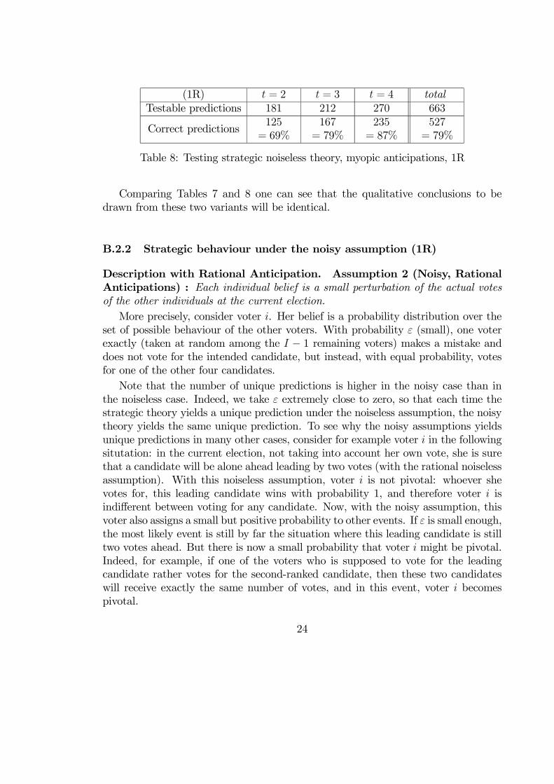
Table 8: Testing strategic noiseless theory, myopic anticipations, 1R

Comparing Tables 7 and 8 one can see that the qualitative conclusions to bedrawn from these two variants will be identical.

B.2.2 Strategic behaviour under the noisy assumption (1R)

Description with Rational Anticipation. Assumption 2 (Noisy, RationalAnticipations) : Each individual belief is a small perturbation of the actual votesof the other individuals at the current election.More precisely, consider voter i. Her belief is a probability distribution over the

set of possible behaviour of the other voters. With probability ε (small), one voterexactly (taken at random among the I − 1 remaining voters) makes a mistake anddoes not vote for the intended candidate, but instead, with equal probability, votesfor one of the other four candidates.Note that the number of unique predictions is higher in the noisy case than in

the noiseless case. Indeed, we take ε extremely close to zero, so that each time thestrategic theory yields a unique prediction under the noiseless assumption, the noisytheory yields the same unique prediction. To see why the noisy assumptions yieldsunique predictions in many other cases, consider for example voter i in the followingsitutation: in the current election, not taking into account her own vote, she is surethat a candidate will be alone ahead leading by two votes (with the rational noiselessassumption). With this noiseless assumption, voter i is not pivotal: whoever shevotes for, this leading candidate wins with probability 1, and therefore voter i isindifferent between voting for any candidate. Now, with the noisy assumption, thisvoter also assigns a small but positive probability to other events. If ε is small enough,the most likely event is still by far the situation where this leading candidate is stilltwo votes ahead. But there is now a small probability that voter i might be pivotal.Indeed, for example, if one of the voters who is supposed to vote for the leadingcandidate rather votes for the second-ranked candidate, then these two candidateswill receive exactly the same number of votes, and in this event, voter i becomespivotal.

24

1 2 3 4 5 total1977 28 12 153 766 293667.3% 1.0% 0.4% 5.2% 26.1% 100%

Table 9: Multiple Predictions, Noisy rational anticipations, 1R


Correct predictions374

= 64.2%382

= 74.6%228

= 86.7%984

= 72.5%

Table 10: Testing strategic noisy theory, rational anticipations, 1R

Predictions. In that case, the probabilities pi(c, v) are harder to write down in anexplicit way. But they can easily be computed using Mathematica software. Underthese assumptions regarding the pi(c, v), we compute for each election (starting fromthe second election in each session) and each individual, heer expected utility whenshe votes for candidate v ∈ {A,B,C,D,E}: that is,

Pc pi(c, v)ui(c). We then take

the maximum of these five values. If this maximum is reached for only one candidate,we say that for this voter at that time, the theory makes a unique prediction regardinghow she should vote. If this maximum is reached for several candidates, the theoryonly predicts a subset of candidates from which the voter should choose.Table 9 gives the statistics regarding the number of candidates in this subset.

These figures are obtained considering all four dates 1 to 4. The total number ofobservations is thus 734× 4 = 2936.In 1977 cases, that is 67.3%, the theory makes a unique prediction as to vote be-

haviour. This is much more than what we had with the no-noise assumption (28.0%).

Test. We restrict attention to the last three elections of each series. This theorymakes unique predictions in 1358 testable cases, of which 984 are correct, that is72.5%. See Table 10.

Comparison with the myopic version. The “Myopic” version of the theory isvery similar to the “Rational Anticipations” but the assumption 2 becomes :Assumption 2bis (Noisy, Myopic Anticipations) : Each individual belief isa small perturbation of the actual the vote of the other individuals at the previouselection. We use exactly the same model for the perturbation as before, but thereference scores are now the scores obtained at the previous election, instead of the

25



= 63.9%431

= 74.1%426

= 83.0%1247

= 73.1%

Table 11: Testing strategic noisy theory, myopic anticipations, 1R

current one.Comparing Tables 10 and 11, one can see that the qualitative conclusions to be

drawn from these two variants will be identical.

B.3 “Top two” theory (1R)

B.3.1 Description.

Individuals vote for their preferred candidate among the two candidates that get thehighest two numbers of votes in the current (“Rational Anticipation” version) or theprevious (“Myopic” version) election.More precisely, consider individual i and denote by si(c) is the score (number of

votes) that candidate c obtains in the reference election (the current or the previousone), taking into account the ballots of all voters but i. Voter i ranks the fivecandidates according to those scores. If two candidates at least rank in the firstplace, then individual i votes for her preferred candidate among them. If only onecandidate ranks first, she votes for her preferred candidate among the set consitutedof this first-ranked candidate and the candidate(s) getting the second highest score.

B.3.2 Predictions.

This theory makes unique predictions in almost all cases, double predictions mayoccur when a voter’s position is just between two candidates.

B.3.3 Test.

This theory correctly predicts behaviour on approximately 70% of the observations.Tables 12 and 13 show the time-evolution, and show again that the two versions“rational anticipations” and “myopic anticipations” are similar.

26



= 60.7%523

= 75.3%555

= 80.1%1500

= 72.0%

Table 12: Testing Top-Two theory, rational anticipations, 1R



= 59.5%494

= 71.2%573

= 82.3%1479

71.0= %

Table 13: Testing Top-Two theory, myopic anticipations, 1R

B.4 “Top three” theory (1R)

B.4.1 Description.

Individuals vote for their preferred candidate among the three candidates that gotthe highest three numbers of votes in the reference (current or previous) election.More precisely,- if three candidates at least rank in the first place, the individual votes for her

preferred candidate among them,- if two candidates exactly rank in the first place, the individual votes for her

preferred candidate among the set consituted of those two first-ranked candidatesand the candidate(s) getting the second highest score,- if one candidate exactly ranks in the first place, and at least two candidates rank

second, the individual votes for her preferred candidate among the set consituted ofthis first-ranked candidate and the candidate(s) getting the second highest score,- if one candidate exactly ranks in the first place and one candidate exactly ranks

scond, the individual votes for her preferred candidate among the set consitutedof this first-ranked candidate, this second-ranked candidate and the candidate(s)getting the third highest score.

B.4.2 Predictions.


27



= 71.2%464

= 69.5%446

= 66.8%1383

= 69.1%

Table 14: Testing Top-Three theory, rational anticipations, 1R



= 73.6%455

= 68.6%453

= 67.7%1399

70.0= %

Table 15: Testing Top-Three theory, myopic anticipations, 1R

B.4.3 Test.

In 1R elections, this theory correctly predicts behaviour on about 70% of the ob-servations. Tables 14 and 15 show the time-evolution, and show again that the twoversions “rational anticipations” and “myopic anticipations” are similar.

C Two Round elections

C.1 Sincere voting theory in 2R elections

C.1.1 Description.

Exactly the same as for One-round elections. Individuals vote for any candidate thatyields the highest payoff if elected. Individual i votes for a candidate v∗ such that:

u(v∗) = maxv∈{A,B,C,D,E}

ui(v).

C.1.2 Predictions.

Sincere Voting is independent of time. For all voters except those in position 8and 12, this theory makes a unique prediction. Voters in position 8 are indifferentbetween B and C, and voters in position 12 are indifferent between D and C.

28

(2R) t = 1 t = 2 t = 3 t = 4 totalTestable predictions 657 663 663 663 2646


= 74%%406= 61%

385= 58%

363= 55%

1643= 62%

Table 16: Sincere Voting for single-name elections

C.1.3 Test.

See Table 13. At the first date, this theory correctly predicts behaviour for 74% ofthe observation. This percentage decreases to 55% for fourth elections.15

C.2 Strategic models in 2R elections

Note first that in two-round elections, in the second round with two run-off can-didates, voting for the candidate associated with the highest monetary payoff is adominant strategy. Therefore, we only study strategic behaviour at the first round.As in the one-round elections, we assume that voters are purely instrumental and

that they select a candidate v∗ such that:

v∗ ∈ argmaxv∈{A,B,C,D,E}Xc

pi(c, v)ui(c),

where pi(c, v) is the subjective probability that voter i assigns to the event ”candidatec wins the election”, conditional on her casting a ballot for candidate v at the firstround.Note that these pi(c, v) involve both beliefs as to how voters will behave at the

second round (if any), and beliefs as to how voters will behave at the first round.We can decompose this probability pi(c, v) into a sum of two probabilities: theprobability that c wins at the first round (that is, c gets an absolute majority at thefirst round) plus the probability of the event ”c makes it to the second round andwins the second round”. Formally, this can be decomposed as:

pi(c, v) =Xc0

πi({c, c0}, v)r(c, {c, c0}),

where for c0 6= c, πi({c, c0}, v) is the probability that the unordered pair {c, c0} willmake it to the second round, conditional on voter i voting for candidate v and

15To compare with the other Tables, the figures in the main text are computed for dates 2 to 4.That is 1154/1989 = 58.0% for 2R.

29

r(c, {c, c0}) is voter i’s subjective probability that candidate c wins the run-off electionwhen the pair {c, c0} is vying at the second round16. To save on notation, we defineπi({c, c}, v) as the probability that c wins at the first round if i votes for v andr(c, {c, c}) = 1.Let us first describe the r(c, {c, c0}) when c0 6= c. In all that follows, we assume

that each voter anticipates that at the second-round (if any), each voter will vote forthe candidate closest to her position, and will toss a coin if the two run-off candidatesare equally close to her position:- the centrist candidateC defeats any other candidate in the second round: r(C, {C, c}) =1 for c 6= C,- a moderate candidate (B or D) defeats any extremist candidate (A or E) in thesecond round: r(B, {B, c}) = r(D, {D, c}) = 1 for c ∈ {A,E},- a second round between either the two moderate candidates or the two extrem-ist candidates results in a tie: r(B, {B,D}) = r(D, {B,D}) = r(A, {A,E}) =r(E, {A,E}) = 1/2.In all that follows, we assume that to compute the πi({c, c0}, v), each voter forms

some beliefs about how other voters will behave in the current election, based onthe results of the reference (previous or current) election. Just as we proceeded in1R-elections, we assume that each voter simply thinks that other voters will behaveat the first-round in the current election either exactly as they did at the first-roundof the reference election, or approximately so.We now describe more precisely how we compute the pi(c, v) probabilities under

these alternative assumptions, and test this theory.

C.2.1 Strategic behaviour under the noiseless assumption (2R)

Description with Rational Anticipations Assumption 1 (Noiseless, Ra-tional Anticipations) : Each individual has a correct, precise anticipation of thevote of the other individuals at the current election.In that case, the subjective probabilities pi(c, v) are more difficult to write down

explicitly than they were in One-round elections. Given the scores si(c) (numberof votes) that candidate c obtains in the first round of the current election, takinginto account the ballots of all voters but i, with

Pc si(c) = I − 1, what is the

probability πi({c1, c2}, v) that the unordered pair {c1, c2} will make it to the secondround, conditional on voter i voting for candidate v?

16There is no subcript i because all voters have the same beliefs regarding the secound round.See below.

30

We introduce some further notation. Let us denote by si(c, v) is the score (num-ber of votes) that candidate c obtains in the reference election, if voter i votesfor candidate v and all other voters vote exactly as they do in the refernce elec-tion. Let us denote by ski (v), k = 1, 2, ..., 5 the k-th largest number in the vector(si(c, v), c ∈ {A,B,C,D,E}). For example, if si(A, v) = 3, si(B, v) = 5, si(C, v) = 6,si(D, v) = 5, si(E, v) = 2, then s1i (v) = 6, s

2i (v) = 5, s

3i (v) = 5, s

4i (v) = 3, s

5i (v) = 2.

Definition of the probability that candidate c1 wins in the first round,πi({c1, c2}, v), c1 = c2,

- if si(c1, v) > E[I/2] then πi({c1, c2}, v) = 1,- in all other cases, πi({c1, c2}, v) = 0.Definition of the πi({c1, c2}, v), c1 6= c2, s

1i (v) < E[I/2]

- if si(c1, v) > s3i (v) and si(c2, v) > s3i (v), then πi({c1, c2}, v) = 1- if si(c1, v) = si(c2, v) = s1i (v) = s3i (v) > s4i (v), then πi({c1, c2}, v) = 1/3- if si(c1, v) = si(c2, v) = s1i (v) = s4i (v) > s5i (v), then πi({c1, c2}, v) = 1/6- if si(c1, v) = si(c2, v) = s1i (v) = s5i (v), then πi({c1, c2}, v) = 1/10- if si(c1, v) = s1i (v) > si(c2, v) = s2i (v) = s3i (v) > s4i (v), or si(c2, v) = s1i (v) >si(c1, v) = s2i (v) = s3i (v) > s4i (v), then πi({c1, c2}, v) = 1/2,- if si(c1, v) = s1i (v) > si(c2, v) = s2i (v) = s4i (v) > s5i (v), or si(c2, v) = s1i (v) >si(c1, v) = s2i (v) = s4i (v) > s5i (v), then πi({c1, c2}, v) = 1/3,- if si(c1, v) = s1i (v) > si(c2, v) = s2i (v) = s5i (v), or si(c2, v) = s1i (v) > si(c1, v) =s2i (v) = s5i (v), then πi({c1, c2}, v) = 1/4,- in all other cases, πi({c1, c2}, v) = 0.Now for each pair, a voter can anticipate the outcome of the second round, see

above. And thus this fully describes the pi(c, v).

Predictions. Under these assumptions, we can compute pi(c, v).We compute (us-ingMathematica software) for each election and each individual, her expected utilitywhen she votes for candidate v ∈ {A,B,C,D,E}: that is,

Pc pi(c, v)ui(c). We then

take the maximum of these five values. If this maximum is reached for only one can-didate, we say that for this voter at that time, the theory makes a unique predictionregarding how she should vote. If this maximum is reached for several candidates,the theory only predicts a subset of candidates from which the voter should choose.The table 17 provides statistics regarding the number of candidates in this sub-

set. These figures are obtained considering all dates 1 to 4. The total number ofobservations is thus 734× 4 = 2936.One can see that this theory is of little use since it only make a sharp prediction

for 6.6% of the observations.

31

1 2 3 4 5 total194 2 4 160 2576 29366.6% 0.1% 0.1% 5.4% 87.7% 100%

Table 17: Multiple predictions, Noiseless rational anticipations, 2R



= 32.2%34

= 72.3%18

= 48.6%62

= 53.9%

Table 18: Testing strategic noiseless theory, rational anticipations, 2R

Test. For the sake of completeness, Tables 18 and 19 provide the tests of thistheory in the two versions (Rational and Myopic anticipations) for the last threedates.

C.2.2 Strategic behaviour under the noisy assumption (2R)

Description with Rational Anticipation. Assumption 2 (Noisy, RationalAnticipations) : Each individual belief is a small perturbation of the actual voteof the other individuals at the current election. The perturbations are introduced inthe model exactly as for One-Round elections (see above).

Predictions. The Table 20 provides statistics regarding the number of multiplepredictions. These figures are obtained considering all four dates 1 to 4. The totalnumber of observations is thus 734× 4 = 2936.In 576 cases, that is 19.6%, the theory makes a unique prediction as to vote

behaviour. This is much more than what we had with the no-noise assumption (194,that is 6.6%).



= 61.0%12

= 38.7%31

= 64.6%90

= 57.7%

Table 19: Testing strategic noiseless theory, myopic anticipations, 2R

32

1 2 3 4 5 total576 60 36 196 2068 2936

19.6% 2.0% 1.2% 6.7% 70.4% 100%

Table 20: Multiple predictions, Noisy rational anticipations, 2R



= 53.5%75

= 61.0%79

= 63.2%222

= 59.2%

Table 21: Testing strategic noisy theory, rational anticipations, 2R

Test. See Table 21. We restrict attention to the last three elections of each series.This theory makes unique predictions in 375 testable cases, of which 222 are correct,that is 59.2%, and this figure is increasing with time.

Comparison withe the “Myopic” version. Assumption 2 becomes :Assumption 2bis (Small noise, Myopic Anticipations) : Each individual beliefis a small perturbation of the actual the vote of the other individuals at the previouselection. More precisely, we use exactly the same model for the perturbation asbefore, but the reference scores are now the scores obtained at the previous electionnot the current one.Comparing Tables 21 and 22 one can see that the qualitative conclusions to be

drawn from these two variants will be identical.

C.3 “Top-Two” theory (2R)

C.3.1 Description.

Same theory as for One-round elections. Individuals vote for their preferred candi-date among the two candidates that obtain the highest two numbers of votes in the



= 53.3%66

= 52.4%72

= 58.1%244

= 54.3%

Table 22: Testing strategic noisy theory, myopic anticipations, 2R

33



= 55.9%424

= 61.1%466

= 67.1%1276

= 61.1%

Table 23: Testing the Top-Two theory, rational anticipations, 2R



= 54.0%438

= 63.5%447

= 64.3%1255

= 60.6%

Table 24: Testing the Top-Two theory, myopic anticipations, 2R

reference election. The reference election is the current one (in the “rational antici-pations” version) or the first round of the previous one (in the “myopic anticipations”version).

C.3.2 Predictions.


C.3.3 Test.

This theory correctly predicts behaviour on approximately 60% of the observations.Tables 23 and 24 show the time-evolution: the percentage of correct predictionsincreases. One can verify again again that the two versions “rational anticipations”and “myopic anticipations” are similar.

C.4 “Top-Three” theory (2R)

C.4.1 Description.

Same theory as for One-round elections. Individuals vote for their preferred candidateamong the three candidates that get the highest two numbers of votes in the referenceelection. The reference election is the current one (in the “rational anticipations”version) or the first round of the previous one (in the “myopic anticipations” version).

34



= 70.6%476

= 72.0%501

= 75.6%1445

= 72.7%

Table 25: Testing the Top-Three theory, rational anticipations, 2R



= 70.3%483

= 72.9%494

= 74.7%1444

= 72.6%

Table 26: Testing the Top-Three theory, myopic anticipations, 2R

C.4.2 Predictions.


C.4.3 Test.

This theory correctly predicts behaviour on approximately 73% of the observations.Tables 25 and 26 show the time-evolution: the percentage of correct predictionsincreases. One can verify again that the two versions “rational anticipations” and“myopic anticipations” are similar.

D Approval voting

The strategic behaviour in that case is derived from the theory in Laslier (2009),slightly adapted to take care of ties. If there are no ties the behaviour is easilydescribed: the voter has in mind a reference election (the current election under therational anticipation assumption or the previous one under the myopic anticipationassumption). She compares the leading candidate to the second-ranked one, and sheapproves all candidates she prefers to the leader, and no candidate she finds worsethan the leader.Here is a complete description of this theory. Like in the case of 1R or 2R elections,

si(c) is the total number of votes obtained by candidate c in the reference election,from voters other than i herself. Denote by

C1i = argmax si

35

the set of candidates who tie at the first place in the score vector si and by |C1i | their

number. If i decides to approve of no candidate and the other voters vote like in thereference election then the winner of the election will be chosen at random in C1

i .Likewise, denote by C2

i the set of second-ranked candidates in si.

First case If a single candidate, say c1, has the highest score in the vector si theni considers the utility she attaches to this candidate

u1i = ui(c1).

For the other candidates c 6= c1, if ui(c) > u1i , i approves c, and if ui(c) < u1i , idisapproves of c. For candidate c = c1 himself, as well as for any other candidatec such that ui(c) = u1i , i compares c with the second-ranked candidates: let

u2i =1

|C2i |Xc∈C2i

ui(c),

if u1i > u2i , i approves c1, if u1i < u2i , i disapproves c

1, and if c is such thatui(c) = u2i , i can either approve c

∗ or not (no unique prediction).

Second case If two or more candidates have the same highest score in the vectorsi then i considers the average utility she attaches to these candidates

u1i =1

|C1i |Xc∈C1i

ui(c).

Then if ui(c) > u1i , i approves c, if ui(c) < u1i , i disapproves of c, and if c issuch that ui(c) = u1i , i can either approve c or not (no unique prediction).

With this definition one makes one or several prediction for each vote of a voterabout a candidate. An individual ballot is made of the five votes for the five candi-dates.

E The sincere-strategic dilemma in 1R and 2Relections

We provide here further evidence on deviations from strict rationality in 2R elec-tions. We restrict our attention to the cases when sincere voting is unique but is not

36

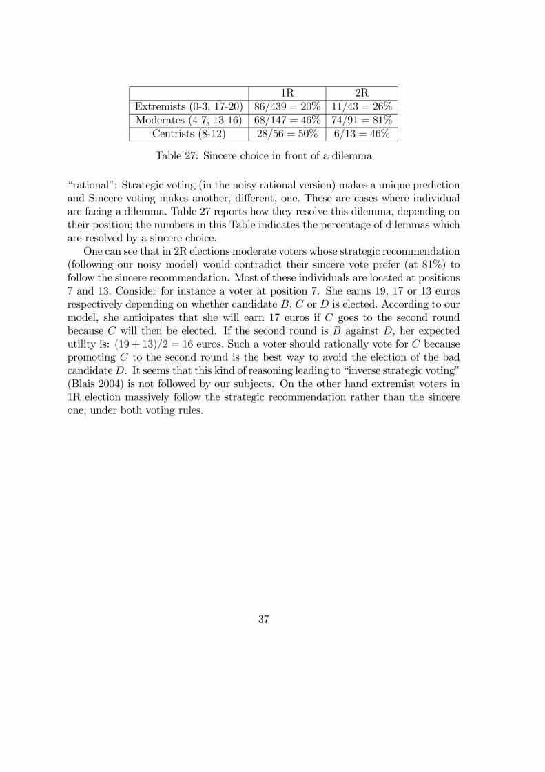
1R 2RExtremists (0-3, 17-20) 86/439 = 20% 11/43 = 26%Moderates (4-7, 13-16) 68/147 = 46% 74/91 = 81%Centrists (8-12) 28/56 = 50% 6/13 = 46%

Table 27: Sincere choice in front of a dilemma

“rational”: Strategic voting (in the noisy rational version) makes a unique predictionand Sincere voting makes another, different, one. These are cases where individualare facing a dilemma. Table 27 reports how they resolve this dilemma, depending ontheir position; the numbers in this Table indicates the percentage of dilemmas whichare resolved by a sincere choice.One can see that in 2R elections moderate voters whose strategic recommendation

(following our noisy model) would contradict their sincere vote prefer (at 81%) tofollow the sincere recommendation. Most of these individuals are located at positions7 and 13. Consider for instance a voter at position 7. She earns 19, 17 or 13 eurosrespectively depending on whether candidate B, C or D is elected. According to ourmodel, she anticipates that she will earn 17 euros if C goes to the second roundbecause C will then be elected. If the second round is B against D, her expectedutility is: (19 + 13)/2 = 16 euros. Such a voter should rationally vote for C becausepromoting C to the second round is the best way to avoid the election of the badcandidateD. It seems that this kind of reasoning leading to “inverse strategic voting”(Blais 2004) is not followed by our subjects. On the other hand extremist voters in1R election massively follow the strategic recommendation rather than the sincereone, under both voting rules.

37

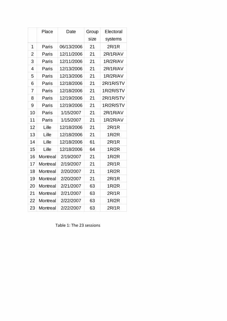
Table 1: The 23 sessions

Place Date Group Electoralsize systems

1 Paris 06/13/2006 21 2R/1R2 Paris 12/11/2006 21 2R/1R/AV3 Paris 12/11/2006 21 1R/2R/AV4 Paris 12/13/2006 21 2R/1R/AV5 Paris 12/13/2006 21 1R/2R/AV6 Paris 12/18/2006 21 2R/1R/STV7 Paris 12/18/2006 21 1R/2R/STV8 Paris 12/19/2006 21 2R/1R/STV9 Paris 12/19/2006 21 1R/2R/STV10 Paris 1/15/2007 21 2R/1R/AV11 Paris 1/15/2007 21 1R/2R/AV12 Lille 12/18/2006 21 2R/1R13 Lille 12/18/2006 21 1R/2R14 Lille 12/18/2006 61 2R/1R15 Lille 12/18/2006 64 1R/2R16 Montreal 2/19/2007 21 1R/2R17 Montreal 2/19/2007 21 2R/1R18 Montreal 2/20/2007 21 1R/2R19 Montreal 2/20/2007 21 2R/1R20 Montreal 2/21/2007 63 1R/2R21 Montreal 2/21/2007 63 2R/1R22 Montreal 2/22/2007 63 1R/2R23 Montreal 2/22/2007 63 2R/1R

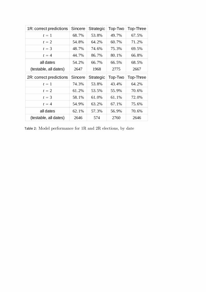
Table 2: Model performance for 1R and 2R elections, by date

1R: correct predictions Sincere Strategic Top-Two Top-Threet 1 68.7% 53.8% 49.7% 67.5%t 2 54.8% 64.2% 60.7% 71.2%t 3 48.7% 74.6% 75.3% 69.5%t 4 44.7% 86.7% 80.1% 66.8%

all dates 54.2% 66.7% 66.5% 68.5%(testable, all dates) 2647 1968 2775 2667

2R: correct predictions Sincere Strategic Top-Two Top-Threet 1 74.3% 53.8% 43.4% 64.2%t 2 61.2% 53.5% 55.9% 70.6%t 3 58.1% 61.0% 61.1% 72.0%t 4 54.9% 63.2% 67.1% 75.6%

all dates 62.1% 57.3% 56.9% 70.6%(testable, all dates) 2646 574 2760 2646

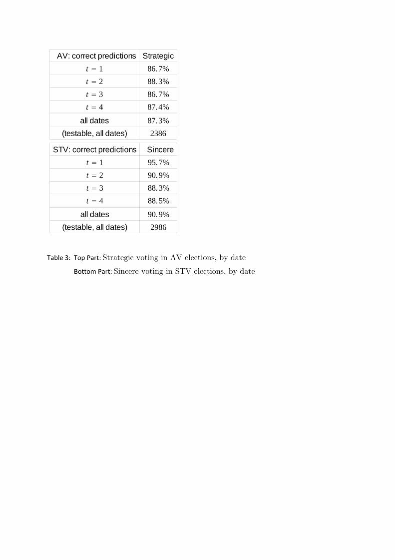
Table 3: Top Part: Strategic voting in AV elections, by date

Bottom Part: Sincere voting in STV elections, by date

AV: correct predictions Strategict 1 86.7%t 2 88.3%t 3 86.7%t 4 87.4%

all dates 87.3%(testable, all dates) 2386

STV: correct predictions Sinceret 1 95.7%t 2 90.9%t 3 88.3%t 4 88.5%

all dates 90.9%(testable, all dates) 2986

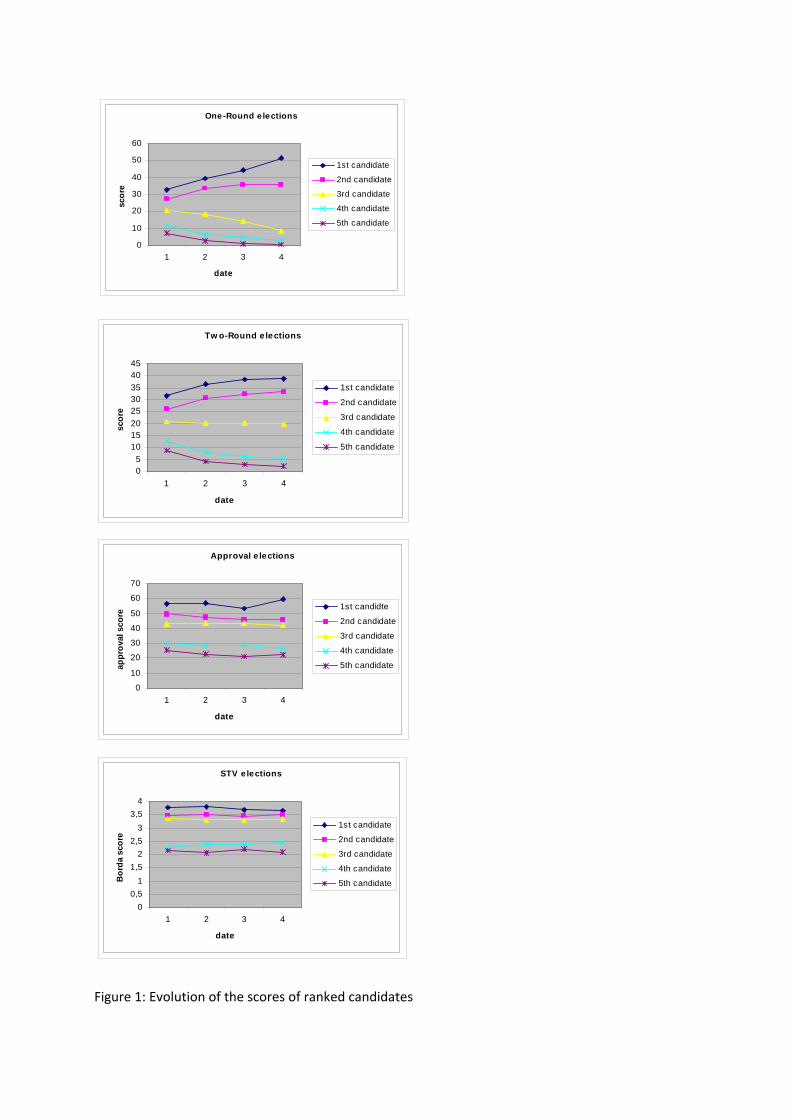
Figure 1: Evolution of the scores of ranked candidates

One-Round e lections

0

10

20

30

40

50

60

1 2 3 4

date

scor

e

1st candidate

2nd candidate

3rd candidate

4th candidate

5th candidate

Tw o-Round e lections

05

1015202530354045

1 2 3 4

date

scor

e

1st candidate

2nd candidate

3rd candidate

4th candidate

5th candidate

Approval e lections

0

10

20

30

40

50

60

70

1 2 3 4

date

appr

oval

sco

re

1st candidte

2nd candidate

3rd candidate

4th candidate

5th candidate

STV e lections

00,5

11,5

22,5

33,5

4

1 2 3 4

date

Bor

da s

core

1st candidate

2nd candidate

3rd candidate

4th candidate

5th candidate

Strategic, Sincere and Heuristic Voting under Four Election Rules: An Experimental Study

Documents

Transcript of Strategic, Sincere and Heuristic Voting under Four Election Rules: An Experimental Study