Strategic Investment in Technology Standards*

Nalin Kulatilaka nalink@bu.edu

and

Lihui Lin

lhlin@bu.edu

May 2004

Abstract Developing technology standards require significant upfront investment expenditures. The value of the resulting technology depends on how it is deployed (e.g., proprietary use versus licensing) and remains uncertain. Hence, the rules governing investments in technology development must be conditioned on the subsequent deployment strategy (e.g. licensing fee) and the nature of uncertainty. In this paper, we consider a single firm that has a temporary monopoly over an investment opportunity. By committing the investment, the firm establishes a technology standard that can be licensed to a potential competitor who can either adopt this standard or develop an incompatible standard. We find that there exists a unique optimal licensing fee that results in a single standard. Surprisingly, for technologies that create network effect, the optimal licensing fee may even be lower than that needed to deter the competitor from developing its own standard. Finally, we solve for the investment threshold as the expected future size of the market at which the firm is indifferent between investing immediately and postponing the investment. The investment threshold is found to be monotonically decreasing in both the intensity of network effects and the level of uncertainty.

* We would like to thank Robert Kauffman, Frederick Riggins, Hamid Mohtadi, John Henderson, and other seminar participants at the University of Minnesota, Twin Cities, Boston College, and Boston University for their insightful comments. Funding was provided by the Boston University Institute for Leading in a Dynamic Economy. All errors and omissions are ours.

1 Introduction

Technological innovation does not always lead to business success. The value of a

technology depends vitally on how it is deployed. Hence, when making R&D investment

decisions under uncertainty firms must look ahead to consider the optimal deployment strategy

for the resulting technology. Often the alternative strategies involve either being the sole

developer of products and services by keeping the technology as proprietary, or to license the

technology to others, including potential competitors. The choice between these alternatives

depends critically on the terms of the license. Should the licensing fee be a subsidy? If so, how

large a subsidy? Or, should the technology be offered free and create an open standard? Or,

should a positive fee be charged? If so, how much? For instance, the licensing fee can be used to

induce others to adopt your technology rather than develop their own. This makes choosing the

optimal licensing fee an integral part of the investment decision.

While others have studied such investment and licensing problems in isolation, we allow

the licensing decision to influence the resulting market structure and thereby, integrate the

investment and licensing models. We also choose a particularly interesting and topical setting

where the technology builds standards. Licensing the standard to others can promote wider

adoption of the standard and thereby create substantial network effects. Consumers of network

goods reap utility not only from its standalone use, but also from the ability to connect and

collaborate with other users.1

Often a single firm may enjoy a temporary leadership in developing a standard for a new

technology due to previous knowledge, technological breakthroughs, or familiarity of the market.

Such firms must then decide whether maintain a proprietary standard, or allow competitors

1 See for example, Katz and Shapiro (1985); Leibowitz and Margolis (1994); Shapiro and Varian (1999).

1

access to it and, thereby, establish an industry-wide standard. Allowing other firms to build

compatible products and services will create a larger network around the standard, realizing

higher network value. Establishing a standard can provide a strategic advantage by dissuading

the development of competing standards and enticing users to switch out of existing standards.

For example, in order to support the worldwide adoption of its CDMA technology, Qualcomm

authorizes infrastructure and mobile phone suppliers such as Lucent, Motorola, Nokia, Sony and

TCL, to design, manufacture and sell products utilizing its CDMA technology. Another example

is the General Motors’s OnStar system, which provides a wide range of in-vehicle safety,

communication and information services, and is attempting to forge a worldwide standard for

automobile telematics.2 OnStar was originally only offered in a few high-end Cadillac models in

1996, but by 2003, it was available on 44 of GM’s vehicle models, and was adopted by several

competing automobile makers.3

When a firm makes a strategic investment in a network with the aim of establishing a

standard, it needs to devise a mechanism through which other firms may use the standard and for

parties to share the value. In the example of Qualcomm, wireless suppliers can license part or all

of its CDMA patent portfolio and the licensees pay royalty fees to Qualcomm for producing

CDMA equipment and mobile phones. In the case of OnStar, adopters pay GM subscription fees

to access the OnStar network, while buyers of cars with OnStar installed also pay a subscription

fee on a monthly basis for OnStar services.

Licensing a standard and charging the appropriate fee to potential competitors can be

crucial to the success of a standard. Just as a successful licensing strategy may help a firm rise to

2 The OnStar system derives network value from complementary services. The more cars installed with OnStar, the more services (especially concierge services) are likely to be provided, increasing its value to each user. 3 See Venaktraman (2001) for a description of the OnStar strategy and the automobile telematics industry. As of early 2004, Acura, Audi, Volkswagen, and Subaru offer OnStar services. Several other competing firms (e.g., Toyota) are testing and experimenting with OnStar.

2

its prominence in a market, a failed licensing strategy can spell its doom. Google licensed its

search results to other search engines such as Yahoo in the late 1990s, which helped to build

Google’s instant popularity. In contrast, Sony had a head start in developing videocassette

recorders and invited Matsushita and JVC to license its Betamax technology in December 1974.4

JVC and Matsushita declined the offer. Although Sony enjoyed a virtual monopoly in the VCR

market for a year, in 1976 JVC introduced the VHS format and launched the VCR standards war,

which eventually established VHS as the global standard.5 Similar battles surrounding standards

have occurred (and continue to be fought) in computer operating systems, high definition

television, web services, instant messaging, and numerous other technologies.

In this paper, we explore the investment in networks with explicit treatment of network

effects and the strategic benefits of network standards. In particular, we show how a firm that

has invested in a network can design licensing contracts to deter competing standards and

maximize its profits. An important feature of our model is the treatment of uncertainty.

Investments in networks, while presenting strategic advantages, involve tremendous uncertainty

and raise questions about the validity of conventional investment decisions rules.6 Kulatilaka

and Perotti (1998 and 2000) and Grenadier (1996) have found that the presence of strategic

benefits offsets the postponement incentives introduced by the option to defer the commitment of

investment. In their models, the mechanisms to capture the strategic benefits arise from cost or

timing advantages. In this paper, by including the possibility of licensing the standard to

potential competitors, we introduce a much more versatile setting to study the investments in

technology industries that exhibit network effects.

4 “The Format War,” Video Magazine, April 1988, pp50-54 5 “Whatever Happened to Betamax?”, Consumers' Research, May 1989, p28 6 McDonald and Siegel (1985) first modeled this investment-timing problem in the context of real options. A review of the ensuing literature is in Dixit and Pindyck (1994).

3

Before presenting a formal model, we will elucidate the logic behind our model. We

know that firms often face the challenge of investing in a network technology while the prospect

of the market is fraught with uncertainty. Furthermore, developing technology standards for

networks usually involves enormous expenditures in research and development. Since the

investing firm intends to license its standard, the investment also includes other less obvious

expenditures such as legal and administrative costs in developing contractual arrangements that

protect the intellectual property, selling the product to early adopters below marginal cost, and

advertising to promote the technology standard. However, at the time the investment is

committed, the firm still faces much uncertainty around the potential number of consumers who

will adopt the standard and hence, the potential value resulting from the investment. In other

words, large and irreversible investments must be committed well ahead of widespread customer

adoption.7

The irreversibility of the investment and the uncertainty surrounding the benefits makes it

difficult to assess whether the firm should use its temporary technological lead to develop a

standard or wait until some of the uncertainty is resolved. Investing immediately has both costs

and benefits when compared to postponing the investment until some of the uncertainty is

resolved. On the one hand, if the firm commits an investment to develop a standard before the

resolution of uncertainty, it can deter competitors from developing different (incompatible)

standards and improve the ability to establish its standard.8 Competitors must either license your

7 Early adopters of the standard only receive small network benefits in the beginning. As a result, consumers will remain unconvinced about the full value of the network good until the network reaches maturity. The adoption decision of consumers exacerbates the uncertainty regarding the potential demand for the network good. The uncertainty is exacerbated when multiple firms compete to establish a network standard and when multiple components in a complementary network system must be developed in order to deliver the network good. 8 The commitment of investment preempts potential competitors and yields various competitive advantages. For isntance the early commitment of investment often allows firms to gain cost advantages (e.g., due to learning) that can be used to dissuade potential entrants. For example, see Dixit (1980) and Spence (1984) for models of entry dissuasion through cost advantages.

4

standard by paying a fee or develop a new standard. Since the magnitude of the network effect

increases with the number of consumers adopting a standard, having multiple standards will

result in smaller fragmented networks yielding lower network effects. This will act as a further

incentive to move early and invest to develop technology standards. However, benefits from the

investment may not be realized if the market condition turns out to be unfavorable. On the other

hand, if the firm does not commit the investment prior to the resolution of uncertainty, it can

avoid regret if the standard does not attract sufficient consumers. Delaying the investment would

cost the firm the temporary lead and place it on par with competitors. This poses a difficult

dilemma about the timing of the investment to firms developing technology standards.

We stylize the facts to build a model with two time points. At the current time, a single

firm (M) has a monopoly over an investment opportunity but is uncertain about the demand for

the network good at some future time. Early investment allows M to establish a network

standard, and if M decides to license its standard to N, it sets a per-unit license fee. Then N has

the choice of adopting M’s standard by paying the fee or investing in a new standard. If N does

not accept the licensing proposal, it can invest in a different standard leading to two smaller

incompatible networks.9 If M passes the investment opportunity and does not invest

immediately, M and N will be identical when the uncertainty is resolved later. In this case, they

may choose to invest but are unable to coordinate on a single standard and two incompatible

network standards will emerge.

One of our main results concerns the impact of network effects and uncertainty on the

level of optimal licensing fee. The optimal licensing fee is obtained as M’s choice that

maximizes its profits while recognizing N’s ability to invest in a new network standard. We find

that, surprisingly, M does not always charge the highest licensing fee N will accept. In 9 A similar situation results when M commits an early investment but does not offer a licensing opportunity to N.

5

particular, as the network effect increases in intensity, M may charge a fee lower than that would

be accepted by N. This is because as the intensity of the network effect grows, M is willing to

lower the licensing fee to induce N to produce more compatible products to get the bandwagon

rolling even though N is willing to accept a higher fee because of higher network benefits. We

also find that the optimal licensing fee is monotonically increasing in the level of uncertainty.

This is because M has the incentive to raise the licensing fee to share the risks with N while N

can accept a higher fee since its alternative, investing in its own standard, is also less attractive

due to the higher the risks.

Our model also shows the relationship between investment and market structure. We

find that in equilibrium, early investment always leads to a single standard: if M invests in the

network technology, it offers to license the technology standard to N charging the optimal fee

and subsequently N accepts this offer and joins M’s network. The correct licensing fee, in effect,

is used to “tip” the users to M’s standard.

Finally, we complete our study by deriving the investment rule. The investment

threshold is defined as the level of expected demand at which M is indifferent between investing

immediately and postponing the investment. That is, if the expected demand is greater than the

threshold level, the firm will commit the investment immediately. We show that the investment

threshold is monotonically decreasing in both the intensity of the network effect and the level of

uncertainty.

The rest of the paper is organized as follows: Section 2 presents the model setup and

introduces network effects through its impact on the demand function. Section 3 shows the

production decision. In Section 4, we solve for the optimal licensing fee and the impact of

network effects and uncertainty on the choice of licensing fee. We then derive the investment

6

threshold in Section 5. Section 6 discusses the implications of our results and provides some

concluding remarks.

2 The Model

2.1 Sequence of Events

We consider a single firm, M, that has a temporary monopoly over the investment

opportunity. Firm M may make an irreversible investment, I, to establish a technology standard

around which a product or service that exhibits network effects can be built. We can think of

this investment as R&D or some other fixed “entry fee”.10

Firm M faces the decision to invest now (t=0) or later (t=1). These two time points are

defined by the degree of uncertainty around the market demand for the network good, θ.

Between time 0 and time 1, some amount of uncertainty is resolved. For purposes of modeling,

we assume that all uncertainty is resolved at t=1. The sequence of events is depicted in Figure 1.

If M invests at t=0, it establishes a standard that may be offered as a for-fee license to

another firm, N, which does not have the ability to establish its own standard at t=0. If M offers

to license its standard to N, M also gets to set the per-unit licensing fee l. Firm N then has the

choice of adopting M’s standard and paying the licensing fee, or rejecting the offer and retaining

the option to develop a new standard later at time 1. Firm N makes this choice knowing that it

would have an investment opportunity at time 1. If N chooses to adopt M’s standard, it saves the

cost of investment to develop a new standard. Furthermore, when the uncertainty around the

demand θ is resolved and the market opens at time 1, both firms make production decisions

based on the fact that all customers would attach a higher value to the compatible products. In

other words, users of both products form a single, larger network instead of two smaller

10 Since we deal only with a fixed amount of investment, and not one that varies with the amount of production, I is unlikely to be incurred in building production capacity.

7

incompatible networks, allowing consumers to enjoy higher network benefits. This path “M

invests M offers l N accepts” (Branch A in Figure 1) is exemplified by cases such as

OnStar. GM was the leader in the automobile telematics market and invested significant

amounts of resources in order to establish a standard for the telematics industry. It offered

OnStar services at attractive rates to other carmakers. Although it is too early to declare a

winner-take-all outcome, Honda, Volkswagen, and Subaru have adopted OnStar as their

telematics standard and stopped developing their own standards.

If M invests and offers to license its standard but N chooses to reject it, then N retains the

option to invest in a new standard at time 1 after uncertainty regarding θ is fully resolved

(Branch B in Figure 1). The investment opportunity available to N at time 1 requires investing I

to be able to produce a network good that is a perfect substitute (in its standalone value) to M’s

product. If the realized market demand justifies N’s investment, N will invest and develop a new

standard incompatible with M’s.11 Consequently, both firms will make production decisions

knowing that buyers of products made by different firms will belong to different networks and

the network value realized is lower than that if the two firms adopted the same standard and

effectively formed one network. 12 If the realized market demand is too low for N to invest then

N will not enter and M will be the only firm in the market. This path is probably best illustrated

by the VCR standards war. Sony was the first-mover in the VCR market and offered to license

its Betamax technology to Matsushita and JVC. JVC and Matsushita declined the offer and

developed the incompatible VHS standard.

11 Why M and N cannot develop compatible standards? The reasons may be that coordination costs are too high and that there may be asymmetric information between M and N (M does not reveal details needed to coordinate). 12 Customers of both firms would be willing to pay a higher price if the products are compatible as they could interact with users of the other firm’s product.

8

If M invests in a standard but chooses to keep it proprietary and not license it to N, then

N will still have the option to invest in a new standard at time 1 (Branch C in Figure 1). The

investment opportunity N faces at time 1 will be identical to that in Branch B. Apple computer

followed such a strategy of keeping its leading technology proprietary by refusing to license the

original Macintosh technology. More recently, Apple Computer seems to go down a similar path

by refusing to open up its digital-music standard iTunes.13

If M does not commit the investment at time 0, then it can still invest I at time 1, develop

a new standard and subsequently produce the network product. However, now M is in an

identical position as firm N in establishing its standard. The two firms will make investment

decisions simultaneously after the uncertainty is resolved.14 We again assume that it is

impossible for them to coordinate on a single standard. When the realized demand θ is large

enough to trigger investment at time 1, both firms will invest and produce incompatible products,

resulting in two smaller networks.

In all of the above situations, when the uncertainty resolves and the market opens at time

1, firms make production decisions based on the realized demand, consumers’ utility functions

for the network good, and the variable production cost.

Firms incur some cost in producing the network good. We assume that the unit cost

remains constant regardless of the identity of the firm and the time of the investment.15 The unit

cost is a combination of all production costs and may be a function of the output, which we

denote by k(q). For a network good, k(q) is likely to be decreasing in q, leading to increasing

13 Apple has a closed system: The only portable device on which songs purchased on iTunes can be played is the iPod, and the only online music site that the iPod works with is iTunes. Competitors including RealNetworks have been publicly calling for Apple to open its standard, but refused by Apple. Source: “Music Rivals Propose a Combo, Apple Doesn’t Want to Hear It,” by Nick Wingfield and Pui-wing Tam, Wall Street Journal, April 16, 2004 14 Although we treat M and N as identical if they both make investment decisions at time 1, in practice there exist other factors (e.g. cost, timing) creating heterogeneity and markets often end up “tipping”. 15 Kulatilaka and Perotti (1998) model allows for the early commitment of investment to lower the cost k(q).

9

return to scale on the supply side. However, in order to isolate the network effects arising from

the demand side, we assume the variable cost of production to be constant, i.e., k(q)=k.

Notes: Real life cases are inherently more complex than our stylized model: There can

be multiple players, possibility of coordination, multiple opportunities (i.e., richer than the two

time points), involve complementary networks. However, our model of licensing isolates the

principal mechanism through which firms establish network standards.

“C”

“B”

“A”

Figure 1: Sequence of Events

N’s decision nodeM’s decision node

0 standard 0 production

M’s standard: M, N produce (q1+q2)

t=1 t=0

q1q2

Not Invest

Invest

Not Invest

Invest

Invest

Not Invest

Invest

Not Invest

Invest

Offer l

No Offer

Accept

Not Accept

q1

q1 q2

q1

q2 Invest

Not Invest

Not Invest

q1q2

q1q2

q1

M, N’s standards M, N produce q1, q2 respectively M’s Standard M produce q1

M’s standard M produce q1

M, N’s standards M, N produce q1, q2 respectively

N’s standard N produce q2

M, N’s standards M, N produce q1, q2 respectively

M’s standard M produce q1

10

2.2 The Demand for Network Goods and the Intensity of Network Effect

A canonical linear demand function for a normal good can be represented by:

P q,θ( )= θ − q

where q is the quantity demanded for the good. The random variable, θ, can be interpreted as

the maximum potential demand and captures the uncertainty surrounding the size of the future

market. Such a demand function implies that consumers are heterogeneous in their willingness

to pay for the product.

For a network good, consumers realize an additional value from the presence of others in

the network.16 This additional value, which we call network value, depends on the number of

other consumers using this good. Despite the fact that consumers make their purchasing

decisions independent of each other and join the network at different times, they do not base

their decisions on the actual number of users at the time they join the network, but on the

expected size of the network. We assume that the expectation is exogenously given.17 We also

assume that the consumers are homogenous in their valuation of network benefits,18 and the

network value is additive to the standalone value of the good. Therefore, we can write the

demand function for a network good as19,

16 Although network effects are the easiest to visualize in cases where users derive value from connecting to other users, network effects also arise in systems of complementary goods (e.g., video game consoles and games, cars, gas stations, and repair shops). The literature refers to the former as direct network effects and the latter as indirect network effects. See Leibowitz and Margolis (1994), Economides (1996), and Katz and Shapiro (1994). The value in complementary systems comes from the proliferation of variety in future periods. Nevertheless, it has a similar network effect in that as the total number of users increases, so does the value to each user. The mechanism of the network effect is indirect, in that, the larger number of users of the standard provides incentives for complementors to innovate more variety. 17 The expectation may be based on predictions made by government agencies or market research firms. 18 There is both good reason and empirical evidence that supports the possibility that different consumers will contribute different amounts of network value. For instance, one would derive substantial value from having your close friends, family, and colleagues who use the same standard word processor or instant messaging system. A much lower value would be derived when whose who you have no need to communicate with adopt compatible standards. However, the total number of consumers will induce other firms to develop a greater variety of complementary products and, thereby, increase the indirect network effects. 19 Katz and Shapiro (1985) use a similar specification for the demand function.

11

( ) ( ) qqvqqP ee −+= θθ,,

where q is consumers’ time-0 expectation regarding the size of the network. The term e ( )eqv

represents an individual user’s willingness to pay for the network value of the good, and is an

increasing function of qe, i.e.,v'> 0.

θ now represents the maximum potential market demand for the standalone use of the

network good. We study the set of distribution functions of θ with a strictly positive support on

θ where higher mean implies first order stochastic dominance. We refer to these distributions as

“well-behaved distributions”.

There is a growing literature from which we can draw inferences about the form of the

v(q) function. The best known network value proposition in the networking literature is

characterized by the Metcalfe’s Law, which states that the total value of a network increases in

proportion to the square of the number of users in the network (Gilder 2000). With homogenous

consumers, Metcalfe’s Law translates into a linear v(q) function,20

v q( )= βq

The parameter β reflects an intrinsic property of a network: for two networks with equal

size, the network with a higher β endows its users with higher network benefits. We define β as

the intensity of the network effect. At one extreme where β =0, v(q)=0 and the demand collapses

to that for a normal good where consumers only realize the standalone value. At the other

extreme, in order to maintain the downward-sloping property of the demand function, we restrict

β <1.

20 Note that the total value of the network is q v q( )= βq 2which corresponds to the familiar depiction of Metcalfe’s Law. More generally, we know that network benefits tend to level off after it reaches sufficiently large size. In fact, in some cases very large networks may even become cumbersome to navigate and create congestion, so that user benefits may decline beyond a certain scale. These effects can be modeled by a more general function of the form, v q( )= βqα .

12

Networks are different in the intensity of network effect. For example, the network of

online game players has a higher intensity of network effect than the network created by an

online bookstore. A player of an online game benefits significantly from the existence of other

players since she can interact with more players and it is more likely for her to meet a player

with equal level of skills. On the other hand, while customers of the same online bookstore may

benefit from each others’ reviews of the store and the books, the network effect may not be as

strong as in the case of online game. In other words, the network of online game players has a

higher β than the network of online bookstore consumers.

Providers of network goods and services may also change the intensity of network effects

through business decisions. In the case of wireless services, a provider often offers services that

only apply to its own customers, which in effect creates its own network. For example, Sprint

PCS offers free PCS-to-PCS calls, therefore each PCS subscriber gains from the existence of

other PCS subscribers. If Sprint offers more services, such as a service similar to the Walkie-

Talkie feature on Nextel phones, available between its own customers, then each subscriber will

get higher network value even if the size of the network remains the same. By offering more

services, a provider can increase the intensity of network effect.

The presence of network effects plays a vital role in M’s choice of the licensing fee, N’s

adoption decision, and hence, M’s investment timing decision. When N licenses M’s standard,

M and N together will create a larger market, and will be in position to charge a higher price for

the product because of higher network value. Thus, by investing early and setting the

appropriate licensing fee, M can establish its standard as the industry standard and collect a

licensing fee from the other firm in addition to producing a good that has a greater network

13

value. Early investment is a mechanism that enables M to establish an industry-wide standard,

internalizing the network effects through pricing and licensing agreement.

3 Production Decisions

We solve the model by backward induction. In this section, we study the production

decisions of firms M and N in different scenarios given the decisions made in earlier stages.

Later we will solve for the optimal licensing fee decided by the interactions between M and N

assuming that M has invested at t=0, and M’s investment threshold at t=0.

First, suppose M has built a standard at t=0 and then offers a contract to N with a unit

licensing fee, l. If N accepts the contract and adopts M’s standard, then when the market opens

the consumers of both firms form one large network, and the market price is given by:

( ) 2121 qqqqvP ee −−++= θ

M earns profits by selling its own product and collecting licensing revenue from N:

( )[ ] lqkqqqqvq ee2212111 +−−−++= θπ

N’s profit is given by:

( )[ ]klqqqqvq ee −−−−++= 212122 θπ

We solve M’s and N’s profit maximization problems and impose a fulfilled expectation

equilibrium (FEE) condition. In FEE, when the market opens, M and N choose the optimal

quantity of the network good by maximizing profits and setting the quantity equal to

corresponding expected quantities. We can thus obtain the equilibrium quantities and profits:

, (corresponding to the top branch in Figure 1), which are summarized in Table 1.

We allow for a general specification of the licensing fee that can be positive (royalty), zero (open

standard), or negative (subsidies). We later prove that the optimal licensing fee is positive and

therefore, our subsequent discussion is restricted to the case of positive licensing fees.

*2

*1 ,qq *

2*1 ,ππ

14

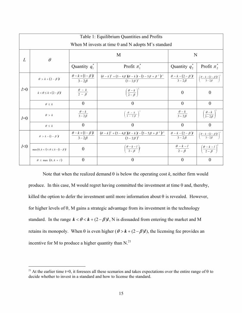
Table 1: Equilibrium Quantities and Profits

When M invests at time 0 and N adopts M’s standard

M N L θ

Quantity *1q Profit *

1π Quantity *2q Profit *

2π

( )lk βθ −+> 2 ( )β

βθ231

−−+− lk ( ) ( )( ) ( )

( )2

222

235545

βββθβθ

−

+−−−−+− llkk ( )β

βθ232

−−−− lk ( ) 2

232

−

−−−β

βθ lk

( )lkk βθ −+≤< 2 β

θ−−

2k 2

2

−−

βθ k 0 0 l>0

k≤θ 0 0 0 0

k>θ βθ

23 −− k 2

23

−

−β

θ k β

θ23 −

− k 2

23

−−

βθ k

l=0 k≤θ 0 0 0 0

( )lk βθ −−> 1 ( )β

βθ231

−−+− lk ( ) ( )( ) ( )

( )2

222

235545

βββθβθ

−

+−−−−+− llkk ( )β

βθ232

−−−− lk ( ) 2

232

−

−−−β

βθ lk

( ) ( lklk )βθ −−≤<+ 1,0max 0 llk

−

−−β

θ2

β

θ−

−−2

lk 2

2

−

−−β

θ lk l<0

( )lk +≤ ,0maxθ 0 0 0 0

Note that when the realized demand θ is below the operating cost k, neither firm would

produce. In this case, M would regret having committed the investment at time 0 and, thereby,

killed the option to defer the investment until more information about θ is revealed. However,

for higher levels of θ, M gains a strategic advantage from its investment in the technology

standard. In the range k < θ < k + (2 − β )l , N is dissuaded from entering the market and M

retains its monopoly. When θ is even higher (θ > k + (2 − β )l ), the licensing fee provides an

incentive for M to produce a higher quantity than N.21

21 At the earlier time t=0, it foresees all these scenarios and takes expectations over the entire range of θ to decide whether to invest in a standard and how to license the standard.

15

We can see that the choice of the licensing fee can influence the resulting market

structure. In particular, charging a higher licensing fee allows M to be the monopolist over a

wider range of realized θ. The intensity of network effects also influences the market structure.

If the intensity of network effects increases while the licensing fee remains the same, then M

retains its monopoly power for a smaller range of θ.

Now consider the case where firm N does not accept the licensing fee. We notice that the

decision nodes in this branch are identical to those in the case where M does not offer N the

license. Therefore, the production decisions for M and N in these two cases (middle branches of

Figure 1) are the same. Given N invests at t=1, M and N will have incompatible standards.

Since M and N’s products are perfect substitutes in their standalone value, the prices for the

products are given by:

( ) 2,1,21 =−−+= iqqqvP eii θ

The profits are given by:

( )[ ] 2,121 =−−−+= ikqqqvq eiii θπ

We obtain , as functions of θ by solving for the profit maximizing

conditions under FEE. The resulting equilibrium quantities, prices, and profits are given in

Table 2. As before, neither produces if

**2

**1 ,qq **

2**

1 ,ππ

θ ≤ k . For θ > k , the two firms engage in symmetric

Cournot competition and produce identical quantities.

Finally, we turn to the case where M does not invest at time 0 (lower branches of Figure

1.) At time 1, M no longer has a comparative advantage vis-à-vis firm N. Firms M and N will

make identical decisions of whether or not to invest, and if they invest, the optimal quantities to

produce. The optimal quantities and associated profits are , (see Table 3). ***2

***1 , qq ***

2***

1 , ππ

16

Table 2: Equilibrium Quantities and Profits when M invests at time 0 but N develops new standard at time 1

M N

θ Quantity **1q Profit

**1π

Quantity **2q Profit **

2π

k>θ βθ

−−

3k 2

3

−−

βθ k

βθ

−−

3k 2

3

−−

βθ k

k≤θ 0 0 0 0

Table 3: Equilibrium Quantities and Profits

When M does not invest at time 0, M and N develop their own standards at time 1

M N

θ Quantity ***1q Profit ***

1π Quantity

***2q

Profit ***2π

k>θ βθ

−−

3k 2

3

−−

βθ k

βθ

−−

3k 2

3

−−

βθ k

k≤θ 0 0 0 0

Comparing values in Tables 2 and 3, we note that the end market will result in either no

production (when θ<k) or M and N producing identical symmetric Cournot output levels.

However, it must be kept in mind that in the latter case both firms must make their investment

decisions at time 1, while in the former case, only firm N needs to invest at time 1. Hence, the

range of θ over which the expected profits are computed differs between the cases. We will

defer a discussion of this issue to a later point when we examine the optimal investment

threshold.

17

4 Optimal Licensing Decisions

The decisions on licensing are made after M has invested but before the uncertainty is

resolved and production begins. M and N evaluate different licensing strategies, taking

expectations of the profits derived in Section 3. In our model, M decides whether to license the

standard to N, and if so, chooses the level of the licensing fee. Then N, if offered a licensing

contract, decides whether to take it or reject it. Again, we solve the licensing problem

backwards in time.

Let us suppose that M has offered N a contract with a per-unit licensing fee of l. If N

accepts it and adopts M’s standard, the expected profits for M and N are and

, respectively.

E π1* l( )( +)

)E π 2* l( )( + 22 If N rejects M’s offer, M’s and N’s expected values are E π1

**( )+and

. Thus, given l, N’s decision rule is to accept M’s offer and license M’s standard if

and only if E . Otherwise, N rejects the offer. We assume that N accepts

the standard when indifferent.

E π 2** − I( )

)

+

π 2* l( )( )+

≥ E π 2** − I( +

23

We now step back to M’s decision on whether or not to license the standard to N and the

choice of the licensing fee l. In equilibrium, these decisions take into account N’s reaction

(accept or reject). If M does not offer N the choice to license the standard, M expects to earn

, which is the same payoff it gets if an offer of l is made but declined by N. Therefore,

in making the decisions on the licensing fee, M only needs to compare the highest possible

payoff from an accepted licensing fee, with the payoff from not offering a licensing opportunity

to N. We find that by choosing the optimal fee, M is always better off licensing its standard. To

E π1**( )+

22 E(π )+ denotes expectations that are taken over the positive values of π. 23 Since we take expectations over the positive range, the strategy for N to stay out of the market with a reservation utility of zero is dominated and will not be chosen.

18

prove this, we first derive the highest payoff M can earn with a licensing contract that is

acceptable to N.

4.1 The Optimal Licensing Fee

We define the optimal licensing fee l as the level that not only maximizes M’s payoff

but also satisfies N’s acceptance condition. Formally, the optimal licensing fee is determined as

the solution to the following constrained maximization problem:

*

Maxl ∈ −∞,+∞( )

E π1* l( )( +) (M’s profit maximization condition)

s.t. E π 2* l( )( )+

≥ E π 2** − I( )+

(N’s acceptance constraint)

Before solving for , we will examine each firm’s criterion separately. *l

Definition 1: l is the solution to M’s unconstrained profit maximization

probleml

.

*1

π1*Max

∈ −∞,+∞( )E l( )( )+

Definition 2: l is the licensing fee such that N’s acceptance condition is binding, i.e.

.

*2

I( )+E π 2

* l2*( )( )+

= E π 2** −

Lemmas 1 and 2 give the properties of (see Appendix 1 for proofs). *1l

Lemma 1: is positive. *1l

We did not impose an a priori restriction on the sign of l. In particular, l could have been

negative, implying a subsidy offered to competitors who adopt M’s standard. Also, we allow l to

be zero, reflecting an open standard. Lemma 1 proves that in our setting the optimal licensing

fee is, in fact, positive.

Lemma 2: For well-behaved distribution functions of θ, ( )( )+> 0*

1 lE π is either

constantly increasing in l, or has a unique and finite maximizer.

19

Lemma 2 shows that regardless of N’s reaction it may not be in the best interest of M to

always charge an infinitely high licensing fee. M may charge a finite licensing fee, not to deter

N from developing a new standard but because M can earn higher profits in a single network.24

The reason for this counter-intuitive result lies in several offsetting effects of the

licensing fee on M’s expected profit. Given the level of licensing fee and the realized demand θ,

M’s profit at time 1 is determined. At time 0 before the uncertainty is resolved, for any fixed

level of licensing fee, M takes expectation of its profit over the entire range of possible θ. We

examine the impact of a change in the licensing fee on profits for the range over which θ is

distributed.

Suppose that M raises the licensing fee from l to l’. First, the increase in the licensing fee

extends the range of θ over which M retains a monopoly and N’s entry is deterred. As Figure 2

shows, the range of θ over which M retains a monopoly extends from ( )( )lkk β−+ 2, to

( )( '2, lkk )β−+

( )( ,2 lk

. This has two opposite effects on M’s profits. On the one hand, for

( ) '2 lk )ββθ −+−+∈ M now owns the entire market instead of sharing it with N, and

therefore produces a higher quantity, earning higher profits from its own production. On the

other hand, since N no longer produces when ( ) ( )( )'l2,2 klk ββθ −+−+∈ , M loses the

licensing revenue in this range of θ.

Second, the increase in licensing fee also increases the quantity M produces when both M

and N are in the market. For ( )2 lk 'βθ −+> , M produces a quantity of ( )β

βθ23

'1−

−+− lk while

24 Creating two smaller networks will lower M’s profits.

20

charging l , which is higher than the quantity it produces while charging l, ' ( )β

βθ231

−−+− lk (see

Figure 2). This effect increases M’s profits.

β2 −

Third, l affects the licensing revenue that M collects from N. As Figure 2 shows, when

M charges l , N enters the market when ' ( )2 lk 'βθ −+> , and produces the quantity of

( )βθ23

'−−− lk for any θ in this range. The licensing revenue to M is determined by the

product of the per-unit licensing fee and the level of N’s production, i.e., ( )β

βθ23

'2'−

−−−⋅

lkl .

Therefore, increasing the licensing fee has two effects on M’s licensing revenue: the per-unit

royalty is higher, but the quantity based on which the royalty is collected is reduced.

Figure 2: M’s and N’s production under Licensing Fees l and l’

( ) ( )β

βθ231*

1 −−+−

=lklq

βθ

−−

=2

*1

kq

( ) ( )β

βθ23

'1'*1 −

−+−=

lklq

( ) ( )β

βθ232*

2 −−−− lklq

( ) ( )β

βθ23

'2'*2 −

−−−=

lklq

θ

k+(2-β)l’k+(2-β)l k

q

The net of these effects is that M’s expected profit may or may not increase when the

level of licensing fee is raised. Lemma 2 shows that M’s expected profit either is a constantly

21

increasing function, or has a single peak that occurs at , which, according to Corollary 1 in

Appendix 1, is determined implicitly by

*1l

( )( )

( )[ ]( )[ ] 02Pr

2

55245

*1

*1

2*1 =

−−+≥

−+≥

−−

− klk

lkEl

βθ

βθθ

β +ββ .

The properties of are given by Lemmas 3 and 4 (proofs in Appendix 1). *2l

Lemma 3: , defined by Definition 2, is unique and positive. *2l

Lemma 4: For any well-behaved distribution function of θ, for any , N’s

acceptance constraint holds with “>”. For any , N’s acceptance

constraint does not hold.

*2ll <

( )( ) ( ++−≥ IElE **

2*2 ππ )

)

)

*2ll >

The intuition behind Lemmas 3 and 4 is straightforward. N’s expected profit from

rejecting the licensing offer and developing its own standards is given by , which is

independent of l. However, N’s expected profit from accepting the licensing fee, ,

depends on l. Not surprisingly, is a decreasing function of l: the higher the licensing

fee N has to pay M, the lower N’s expected profit. Therefore, there is a unique level of licensing

fee, , such that the two choices yield the same expected profit, i.e.

( +− IE **

2π

E π ( )( )+l*2

( )( +lE *2π

*2l ( )( ) (+

= El *2

*2 π )+

− I*

*2

E *2π .

Lemma 3 further proves that l is positive. N will accept any licensing fee lower than l but

reject any level that is higher.

*2

The optimal licensing fee l is the interaction between l and l , which is formerly

presented and proved in Proposition 1.

* *1

*2

Proposition 1: For well-behaved distributions of θ there exists a unique and positive

optimal licensing fee . l* = Min(l1*,l2

*)

Proof: See Appendix 1.

22

Proposition 1 shows that the optimal licensing fee is only sometimes decided entirely by

N’s acceptance of the licensing contract. Under some circumstances, M’s choice of licensing fee

is limited by N’s reaction; but under other circumstances, in order to maximize its own profit M

is willing to lower the licensing fee to a level below what N is willing to accept. Next, we

investigate how the characteristics of network effect and uncertainty shape the choice of optimal

licensing fee.

4.2 The Impact of Network Effect and Uncertainty on the Optimal Licensing Fee

We first examine the impact of the intensity of network effect on the optimal licensing

fee. In order to develop intuition, we consider the production decisions for different intensities

of network effect over the entire range of possible θ. Figure 3 depicts the quantities that M and

N produce for two different intensities of network effects, β1 and β2 (β2 > β1).25 Ceteris paribus,

a higher intensity of network effect causes the range of θ over which M retains monopoly to

shrink to the left, but leads M to produce higher quantity in this smaller range. For the range of θ

where both M and N are in the market, M’s quantity increases with θ at a higher rate under β2

than under β1 while N always produces higher quantities under β2 than under β126.

Suppose the licensing fee depicted in Figure 3 is the optimal licensing fee under β1. If

the intensity of network effect increases to β2, then the optimal licensing fee is likely to change.

Considering the impacts that a change in licensing fee has on M’s profit (discussed in 4.1), under

stronger network effect, a higher licensing fee gives rise to more losses than benefits to M. This

is primarily because N tends to produce more under stronger network effect, and thus a raise in

)

25 The licensing fee is held constant. 26 Figure 3 depicts the case where M’s quantity is always higher under β2 than under β1. However, this is not always true and the segmented function may fall below ( 2

*1 βq ( )1

*1 βq when both M and N are in the market; but as θ

increases, will eventually exceed ( 2*1 βq ) ( )1

*1 βq .

23

licensing fee causes significant loss in licensing revenue. Therefore, the licensing fee that M

wants to charge, l , tends to decrease with the intensity of network effect. *1

k k+(2-β1)l k+(2-β2)l

( ) ( )1

11

*1 23

1β

βθβ−

−+−=

lkq( )

11

*1 2 β

θβ−−

=kq

( ) ( )2

22

*1 23

1β

βθβ−

−+−=

lkq

( ) ( )1

11

*2 23

2β

βθβ−

−−−=

lkq

( ) ( )2

22

*2 23

2β

βθβ−

−−−=

lkq

( )2

2*1 2 β

θβ−−

=kq

θ

Figure 3: Impact of Change in Intensity of Network Effect on M’s and N’s Production (β2>β1)

q

For N, who trades off between adopting M’s standard and developing its own standard,

higher intensity of network effect makes both choices more valuable, but the effect on the former

dominates that on the latter, and therefore N leans more toward adopting and is willing to accept

a higher licensing fee.

The optimal licensing fee l is determined by the minimum of l and . According to

our analysis, and change with β in offsetting directions. Typically, for a given distribution

of θ, when β is low, Μ wants to charge a high licensing fee while N only accepts a much lower

fee. Since N’s acceptance constraint must be satisfied, the optimal licensing fee l is determined

by . As β increases, Μ is willing to lower the licensing fee while N is willing to accept a

higher fee, narrowing the gap between and . But as long as l , l equals to l .

* *1

*2

*2l

*1l

*2l

*

*2l

*1l

*2l

*1 l> * *

2

24

Therefore, for l , the behavior of the optimal licensing fee l resembles that of l , which

means increases with the intensity of network effect, β.

*2

*1 l> *

*

*

*2

*l

θ0

*1l

As β increases even further, l and l will eventually cross and for any β that increases

beyond the crossing point, . For any β such that l , l equals to l , and therefore,

decreases with intensity of network effect, β.

*1

*2

*2

*1 ll < *

2*1 l< *

1*l

To illustrate the impact of network effect on the optimal licensing fee (and later the

impact of uncertainty), we simulate the behavior of , and l under the assumption that θ is

lognormal distributed i.e., l

*1l l2

*

n θ

θ0

~ N −

12

σ 2, σ 2

such that the expected value of θ is θ 0, i.e.

E θ( )= .27 However, it must be noted that the qualitative properties remain the same for any

well-behaved distribution function of θ.

Given θ 0 is sufficiently large to justify M’s investment at t=0, Table 4a shows how l

changes with β and σ. Holding σ constant (reading down the columns), we see that decreases

in β. This is consistent with our analysis. Intuitively, in the presence of a stronger network

effect, a monopoly will charge a lower licensing fee to entice the entrant to adopt its standard and

contribute to the network size. The increased network size allows the monopoly to profit more

from its own production and gain more licensing fees.

*1

The simulation results also show that l , the licensing fee under which N is indifferent

between adopting M’s standard and developing new standard, increases in β for any given σ (see

Table 4b), which again confirms our analysis. The entrant N is willing to accept a higher

licensing fee when the intensity of network effect increases, because it becomes more profitable

*2

27 This allows us to perform mean-preserving changes to the level of uncertainty by examining the sensitivity to σ.

25

to produce a compatible good for a large network than to develop a new standard and operate a

smaller network.

Table 4: Optimal Licensing Fee (a) *

1l σ β 0.1 0.2 0.3 0.4 0.5 0.6 0.7 0.8 0.9 1 0.1 1.363 ∞ ∞ ∞ ∞ ∞ ∞ ∞ ∞ ∞ 0.2 1.158 1.793 4.786 ∞ ∞ ∞ ∞ ∞ ∞ ∞ 0.3 1.109 1.433 2.273 4.370 11.369 ∞ ∞ ∞ ∞ ∞ 0.4 1.096 1.285 1.757 2.770 5.013 10.398 27.034 64.850 ∞ ∞ 0.5 1.098 1.210 1.504 2.092 3.237 5.559 10.567 22.232 52.421 136.2950.6 1.103 1.166 1.355 1.726 2.396 3.613 5.910 10.469 20.056 41.517 0.7 1.106 1.136 1.255 1.495 1.911 2.616 3.825 5.967 9.921 17.561 0.8 1.098 1.109 1.177 1.328 1.590 2.014 2.694 3.801 5.650 8.840 0.9 1.069 1.071 1.103 1.189 1.346 1.596 1.981 2.569 3.477 4.909

(b) l *

2

σ β 0.1 0.2 0.3 0.4 0.5 0.6 0.7 0.8 0.9 1 0.1 1.645 1.797 1.929 2.030 2.096 2.123 2.111 2.064 1.994 1.918 0.2 1.684 1.853 2.001 2.123 2.215 2.278 2.314 2.333 2.348 2.383 0.3 1.733 1.918 2.085 2.232 2.358 2.465 2.562 2.661 2.785 2.962 0.4 1.788 1.993 2.185 2.363 2.530 2.694 2.867 3.068 3.329 3.692 0.5 1.853 2.083 2.305 2.522 2.742 2.976 3.245 3.577 4.016 4.627 0.6 1.931 2.192 2.451 2.717 3.004 3.329 3.722 4.225 4.901 5.847 0.7 2.025 2.324 2.630 2.960 3.333 3.778 4.335 5.066 6.064 7.475 0.8 2.142 2.488 2.856 3.269 3.757 4.359 5.137 6.181 7.631 9.707 0.9 2.291 2.697 3.145 3.669 4.312 5.131 6.217 7.706 9.810 12.871

(c) (Numbers in bold: ; Numbers in italics: l ) ),( *

2*1

* llMinl = *1

* ll = *2

* l= σ β 0.1 0.2 0.3 0.4 0.5 0.6 0.7 0.8 0.9 1 0.1 1.363 1.797 1.929 2.030 2.096 2.123 2.111 2.064 1.994 1.918 0.2 1.158 1.793 2.001 2.123 2.215 2.278 2.314 2.333 2.348 2.383 0.3 1.109 1.433 2.085 2.232 2.358 2.465 2.562 2.661 2.785 2.962 0.4 1.096 1.285 1.757 2.363 2.530 2.694 2.867 3.068 3.329 3.692 0.5 1.098 1.210 1.504 2.092 2.742 2.976 3.245 3.577 4.016 4.627 0.6 1.103 1.166 1.355 1.726 2.396 3.329 3.722 4.225 4.901 5.847 0.7 1.106 1.136 1.255 1.495 1.911 2.616 3.825 5.066 6.064 7.475 0.8 1.098 1.109 1.177 1.328 1.590 2.014 2.694 3.801 5.650 8.840 0.9 1.069 1.071 1.103 1.189 1.346 1.596 1.981 2.569 3.477 4.909

26

Table 4c shows the optimal licensing fee , which is determined by the minimum of l

and l in the same cell, and Figure 4 provides a visual representation of Table 4c. When the

uncertainty level is fixed and the intensity of network effect changes, the optimal licensing fee

increases in β when determined by and decreases when determined by . For example, when

σ=0.5, for β≤0.5, l is decided by l and is increasing in β; for β≥0.6, l is decided by and is

decreasing in β. The pattern is the same for β=0.9. When σ=0.1, since l for the smallest β,

the optimal licensing fee is determined solely by l , thus decreases in β.

*l

*1

*1

*2

*2l

*2

*1l

* <

* *

1

*1l

*2l

0

1

2

3

4

5

6

7

0 0.2 0.4 0.6 0.8 1

Figure 4: Impact of Network Intensity on Optimal Licensing fee: Solid line indicates l* determined by l ; Dotted line indicates l* determined by l . *

1*2

l* σ=0.9

σ=0.7

σ=0.5 σ=0.3

σ=0.1

β

Next, we study the impact of uncertainty on the optimal licensing fee. Under the log-

Normality assumption, the impact of uncertainty can be studied in isolation, because we can

change the shape parameter of the lognormal distribution, σ, without changing the mean of θ, θ

0.28

27

28 The variance of θ is given by ( )( )1exp 22

0 −σθ .

The simulation results show that under a fixed β, monotonically increases in σ (see

Table 4a). The reason can be understood with the aid of Figure 5. When σ increases, the tail of

the distribution becomes thicker and the positive impact of higher licensing fee on M’s profit

exceeds the negative impact. Therefore, M has incentive to increase the licensing fee it charges.

*1l

( (

Figure 5: Different Distribution of θ and M’s and N’s production σ2>σ1

q f θ;σ2) f θ;σ1)

θk+(2-β)l k+(2-β)l’k

The simulation results also examine the behavior of l under changes in σ for any given

β (see Table 4b). The impact of uncertainty on l is not straightforward. Since N is trading-off

two alternatives: to invest in its own standard or to adopt M’s standard, the impact of uncertainty

on depends on the impact of σ on the relative values of the two alternatives, which in turn

depends on the intensity of network effect. Investing in one’s own standard involves trading-off

between two options: the growth option due to the network effect and the wait-to-invest option

due to the unresolved uncertainty. When the network effect is weak (β low), as uncertainty

(represented by σ) increases, the effect of the wait-to-invest option first dominates. As σ further

*2

*2

*2l

28

increases, eventually the growth option dominates. Therefore, the benefits of developing a

standard first decrease and then increase with increasing σ. When the network effect is strong (β

high), the growth option dominates, and as σ increases the benefits of developing its own

standard increase. Adopting M’s standard means that N does not need to invest, which implies it

is simply a growth option for N. Therefore, an increase in uncertainty (σ) always makes the

alternative of adopting more valuable.

The change in depends on the relative magnitude of the changes in the values of the

alternatives. When the network effect is weak (in Table 4b, β =0.1), the impact of uncertainty on

the value of developing N’s own standard dominates that on the value of adopting M’s standard.

Therefore, for β =0.1, when the value of developing its own standard decreases withσ, N is

willing to accept higher licensing fee ( increases in σ for low range of σ); when the value of

developing its own standard increases with σ, N demands a lower licensing fee ( l decreases in

σ for high range of σ).

*2l

*2l

*2

29 When the network effect is strong (β high), both alternatives become

more valuable as σ increases. However, increasing uncertainty has a stronger impact on the

expected profits from adopting M’s standard, therefore, N is willing to accept higher licensing

fees, causing to increase with σ. *2l

Overall, the intensity of network effect and the level of uncertainty have inter-related

impacts on the optimal licensing fee.

When the network effect is significant and uncertainty low (the bottom left triangle in

Table 4c, with high β and low σ), l is determined by l and N’s acceptance constraint is not

binding. In other words, M charges a low fee even though N would accept a higher one. As the

* *1

29 The value of adopting M’s standard increases withσ, which enhances the effect for lower σ but offsets the effect for higher σ, but overall it is dominated.

29

network effect becomes less significant or as uncertainty increases (moves toward the upper-

right triangle in Table 4c, with low β or high σ), M wants to charge a higher licensing fee, and

N’s acceptance constraint starts binding.

The lowest optimal licensing fee occurs when intensity of network effect is the highest

while the uncertainty is the lowest. When σ is low, it is highly unlikely for a large θ to occur,

and a high licensing fee means that the market condition for N to produce is highly unlikely to

happen, and thus the total expected licensing income with higher per-unit fee may be too small to

compensate for the loss of licensing income when N is not producing. When β is high, due to

the strong network effect, the advantage of being a monopoly becomes less significant, because a

firm can charge a higher price for a product with a larger network, even if the larger network is a

result of other firms producing compatible products. On the other hand, the disadvantage of

being a monopoly, i.e. the loss of licensing revenue from competitors is more significant,

because under higher β, N would produce more if it were. Therefore, M will choose a lower

licensing fee to take advantage of the network effect and avoid being a monopoly when it does

not payoff.

4.3 M’s Decision to License the Technology to a Potential Competitor

Now that we have determined the optimal result that M can achieve with a licensing

contract, we turn to M’s decision of whether to offer a license to N. We have shown that M’s

expected profit from the optimal licensing contract is E π1* l*( )( )+

and M will choose to license its

standard to N rather than not if and only if E π1* l*( )( )+

≥ E π1**( )+

. The proof of Proposition 2

shows that E is always satisfied. Thus, as long as M has invested at time 0, it

will always license the standard to N, resulting in a single network standard.

π1* l*( )( )+

≥ E π1**( )+

30

Proposition 2: If M invests at t=0, then M chooses to license its standard to N with a

licensing fee of l*, as specified in Proposition 2, and N accepts and adopts M’s standard.

Proof: See Appendix 2.

Proposition 2 illustrates the decision path along the game tree in Figure 1. We have

shown that when M commits the investment at time 0, it will always choose to offer to license its

standard to N. Previously we have shown that the licensing fee can be chosen to ensure that N

adopts M’s standard. Therefore, an optimally managed investment will result in a single

network. In other words, failure to set the correct licensing fee or the decision not to license the

standard will result in suboptimal value. In effect, the licensing fee is acting as a control

variable through which M can influence N’s decision and the subsequent evolutionary path of the

standard. We now turn to M’s investment decision at time 0, given that the subsequent

management of the investment will be optimal.

5 Investment Threshold

We know from Proposition 2 that if M invests, M will offer the optimal licensing fee l* to

N and subsequently N will accept and adopt M’s standard. When M makes its investment

decision at t=0, its expected net payoff from investing is ( )( ) IlE −+**

1π , which is a function of

( )θθ 00 E= .

Proposition 3: For well-behaved distributions of θ, there exists a unique investment

threshold above which M will choose to commit the investment at time 0. is the solution

to: .

*0θ

l*( )( )

*0θ

E π1* +

− I = E π1*** − I( )+

Proof: See Appendix 3.

31

Figure 6 illustrates the investment threshold as a function of σ for three different levels of

β. An interesting interpretation of the results comes from drawing an options analogy. Investing

immediately can be thought of as the acquisition of a growth option the value of which is given

by . In contrast, postponing the investment decision until time 1 retains the value of

the wait-to-invest option, represented by

( )( +**1 lE π )

( )+− IE ***

1π .

Figure 6: M’s Investment Threshold with Imperfect Competition

0

0.2

0.4

0.6

0.8

1

1.2

1.4

1.6

1.8

2

0 0.2 0.4 0.6 0.8

5.0=β

1.0=β

*0

Ceteris paribus, the investment threshold declines with ri

implies that when a market exemplifies stronger network effects,

to invest in a standard will take the opportunity and commit the i

expected future demand. Owning a standard will allow the firm

to adopt its standard and thereby collect royalty fees. The produ

enlarge the network, which also translates into higher prices and

the option analogy, higher intensity of network effects raises the

than it does to the value of the wait-to-invest option.

32

9.0=β

θ

1 1.2

σ

sing network effect. This

a firm with the monopoly right

nvestment at lower levels of

to persuade future competitors

ction from competitors helps

profits for the investing firm. In

value of the growth option more

The investment threshold is also decreasing in level of uncertainty. Even though higher

level of uncertainty increases the value of the wait-to-invest option, the monopolist anticipates

that it can license its standard at the optimal fee level to its potential competitor to induce it to

adopt the standard, thus, sharing the market and the associated risks. Thus increasing uncertainty

leads to lower investment threshold.

6 Concluding Remarks

In this paper, we study the strategic impact of investing in a network under an imperfectly

competitive market structure. The strategic value of early investment arises from the

establishment of a network standard that can be licensed out. The choice of the licensing fee

plays a vital role in the adoption decision by the competitors. We show that there is a unique

level for the optimal fee at which the profits of the firm committing the investment to establish a

network standard are maximized and the competitors choose to adopt this single standard.

Setting too high a licensing fee can result in incompatible networks and will be suboptimal for

the network builders. The optimal licensing fees are also affected by the intensity of the network

effect and the level of uncertainty regarding future demand.

When the uncertainty is very low, the optimal licensing fee becomes very small. In the

limit, if there is no uncertainty, then open standards can lead to the largest networks and highest

profits to the network-building firms. The impact of the intensity of the network effect on the

optimal licensing fee leads to more interesting implications. For very low uncertainty, the

licensing fee is determined by the investing firm’s profit maximization and monotonically

decreases with increasing intensity of network effects. For higher levels of uncertainty, the

licensing fee is determined by the competitor’s adoption decision for low levels of network

intensity. In such cases, as the network increases the competitor is willing to accept a higher

33

licensing fee. However, for further increases in the network effect it becomes in the investing

monopolist’s interest to limit the licensing fee. When this condition is binding the optimal

licensing fee falls with network intensity.

These results highlight the critical importance of setting the license fee in environments

with high uncertainty and high network effects. An investor may be tempted to charge a higher

licensing fee simply because competitors are showing willingness to adopt the standard.

However, it would be in their best interest to charge a lower licensing fee and grow the network

to realize larger network profits. This is consistent with the view that opening the standards to

competitors can have a bandwagon effect.30

Once the optimal licensing fees are determined, we also solve for the expected demand

threshold at which the early investment should be committed. The investment threshold is

decreasing in network intensity, β. The investment threshold also decreases monotonically with

increasing uncertainty (σ) because the optimal licensing fee takes into account the impact of the

network intensity. This result shows that with the strategic effects of licensing a network

standard, a firm with a technology lead and an investment opportunity has even higher

propensity to invest when the environment is more certain.

References Dixit, Avinash. 1980. The role of investment in entry deterrence. Economic Journal. Vol. 90, 95-106 Dixit, Avinash and Robert S. Pindyck. 1994. Investment Under Uncertainty, Princeton University Press, Princeton, New Jersey. Economides, Nicholas. 1996. The economics of networks. International Journal of Industrial Organization, Vol. 14, No. 6, 673-699. 30 For instance, Shapiro and Varian (1999) argue that “Openness is a more cautious strategy than control. The underlying idea is to forsake control over the technology to get the bandwagon rolling.” (p199)

34

Gilder, George F. 2000. Telecosm: how infinite bandwidth will revolutionize our world, Free Press, First edition, New York, New York. Grenadier, Steven R. 1996. The Strategic Exercise of Options: Development Cascades and Overbuilding in Real Estate Markets, The Journal of Finance, Vol. 51, No. 5 (Dec.) 1653-1679 Katz, Michael L., Carl Shapiro. 1994. Systems competition and network effects, The Journal of Economic Perspectives, Vol. 8, No. 2, 93-115. Katz, Michael L., Carl Shapiro. 1985. “Network externalities, competition, and compatibility”, American Economic Review Vol. 75, No. 3 (Jun) 424-440 Kulatilaka, Nalin, Enrico Perotti. 1998. Strategic Growth Options, Management Science, Vol. 44, No. 8 (August), 1021-1031. Kulatilaka, Nalin, Enrico Perotti. 2000. Time-to-Market Advantage as a Stackelberg Growth Option, in E. Schwartz and L. Trigeorgis (eds) Innovation and Strategy: New Developments and Applications in Real Options, Oxford University Press Leibowitz, Stan J., Stephen E. Margolis. 1994. Network externality: an uncommon tragedy, Journal of Economic Perspectives, Vol. 8, No. 2, 133-150. McDonald, Robert L. and Daniel R. Siegel. 1986. The Value of Waiting to Invest, Quarterly Journal of Economics, Vol. 101, No. 4, 707-728 Shapiro, Carl and Hal Varian. 1999. Information Rules: A Strategic Guide to the Network Economy, Harvard Business School Press, Boston, Massachusetts. Spence, A. Michael. 1984. Cost Reduction, Competition, and Industry Performance, Econometrica, Vol. 52, No. 1 (Jan.), 101-122 Standage, Tom. 1998. The Victorian Internet: The remarkable story of the telegraph and the nineteenth century's on-line pioneers, Walker & Co, New York, New York. Appendices

Appendix 1: Proofs of Lemmas 1-4, Corollary 1 and Proposition 1

Lemma 1: l is positive. *1

Proof: We prove the following sufficient condition for : 0*1 >l

( ) ( ) ( )0

*1

0

*1

0

*1

<

+

=

+

>

+>>

lllEEE πππ .

35

From Table 2, we have:

( )( )

( ) ( )( )

( )( )( ) ( ) ( )( )

( )∫

∫∞

−+

−+

>

+

−−−

−+−+−

−+

−−

=

lk

lk

kl

dfllklk

dfkE

β

β

θθβθβ

βθβ

θθθβ

π

2

22

2 22

0

*1

223

11231

21

( )

( ) ==

+

0

*1

lE π

( )( ) ( )∫

∞−

− kdfk θθθ

β2

2231

and

( ) ( ) ( ) ( )( )

( )( )( ) ( ) ( )( )

( )∫

∫∞

−+

−+

+<

−−−

−+−+−

−+

−−−

=

lk

lk

lkl

dfllklk

dlflkE

1

22

1

),0max(0

*1

223

11231

21

β

β

θθβθβ

βθβ

θθθβ

π

( )

It can be easily proved that ( ) ( ) ( )0

*1

0

*1

0

*1

<

+

=

+

>

+>>

lllEEE πππ . Q.E.D.

Lemma 2: For well-behaved distribution functions of θ, ( )( )+> 0*

1 lE π is either

constantly increasing in l, or has a unique and finite maximizer.

Proof: Based on Lemma 1, ( )( )+lE *1π

)

is maximized in the positive range of l. The first-

order condition for is: ( )( +

>lEMax

l

*10

π

( )( )( )

( ) ( )( )∫

∞

−+

+

−

+−−−

−−

=∂

>∂lk

dflkllE

βθθ

βββθ

ββπ

2

2

2

*1

45552

23450

First, it can be proved that ( )( )llE

∂>∂

+0*1π is continuous in l.

Second, ( )( )( )

[ ] ( ) 023450

2

0

*1 >−

−−

=∂

>∂∫

∞

+→

+

kl

dfkllE θθθ

ββπ .

36

Third, we show that ( )( )llE

∂>∂

+0*1π is constantly decreasing in l. Since

( )( )( )

( ) ( )( )∫

∞

−+

+

−

+−−−

−−

=∂

>∂lk

dflkllE

βθθ

βββθ

ββπ

2

2

2

*1

45552

23450 , ( ) 0

45552 2

>−

+−βββ for

10 << β and ( ) ( )+∞∞−∈> ,for 0 θθf , when l increases, both the integrand and the integration

interval are reduced. Therefore, ( )( )ll >

+0E∂

∂ *1π decreases in l for ( )+∞∈ ,0l .

Although ( )( )llE

∂>∂

+0*1π is decreasing in l, it is possible that it remains positive and

( )( ) 00*1 >∂

>∂+

llE π for any l . This may happen for sufficiently small β and a density

function f(θ) with a sufficiently thick tail. This means that Firm M’s expected profit is

monotonically increasing in l (though at a diminishing rate), which implies that there is no

interior solution to , i.e. l .

( +∞∞−∈ ,

( )( )+l*1π *

1

)

>EMax

l 0∞→ 31

It is also possible that ( )( )llE

∂>∂

+0*1π

( )( )

decreases to the negative range and there exists a

finite l such that *1 ( )

( ) ( )( )

045

55223450

*1

*1

2

*1

2

2

*1 =

−

+−−−

−−

=∂

>∂∫

∞

−+=

+

lkll

dflkllE

βθθ

βββθ

ββπ

*1l 10

.

We prove that such a finite may exist. Since << β , ( )ββββ

455522

2

−+−

<− , therefore, for

31 Recall that ( )

( )( ) ( )∫

∞

∞→

+−

−=

kldfkE θθθ

βπ 2

2*1 2

1

( ) ( )( )( )

. The above condition is equivalent to: for any

, +∞∞−∈ ,l ( ) (∫∞+

−−

<k

dfklE θθβ

π 22

*1 2

1 ) θ , then . ∞→*1l

37

( ) ( )

−

+−+−+∈ lklk

ββββθ

45552,2

2

( )

, the integrand in the above integration is negative, while

for

+∞

−+−

+∈ ,45

552 2

lkβββθ

( )( )

the integrand is positive. For some f(θ), there exists a finite l

such that

*1

00

*1

*1 =∂

>∂

=

+

llllE π

( )( )

.

llE

∂>∂

+0*1π

( )( ) 00

*1

*1 =∂

>∂

=

+

llllE π

( )( ) Pr552

452

*1

+−−

−E

lθ

θθ

βββ

( )( )( )23

450

*1

22

*1

−−

=∂

>∫

∞

+=

+

kll

ll

ββπ

( )( ) Pr55

452

≥

≥

+−−

k

E

θ

θθ

βββ

Since is constantly decreasing in l, the finite such that *1l

is the unique maximizer of ( )( )+> 0*

1 lE π .

Q.E.D.

Corollary 1: The unique and finite is given by: *1l

( )[ ]( )[ ] 02

2*1

*1

=

−−+≥

−+≥k

lk

lk

β

β

Proof: From the proof of Lemma 2, we know that the unique and finite is given by *1l

. This is equivalent

to ( )[ ]( )[ ] 02

2

2 *1

*1*

1 =

−−+

−+− k

l

lk

β

βl .

( ) ( )( )

045

552*1

*1

2

=

−

+−−−

∂− l

dflkEβ

θθβββθ

Q.E.D.

Lemma 3: l , defined by Definition 2, is unique and positive. *2

Proof: From Table 2, we have:

38

( )( )( ) ( ) ( )

( )

( ) ( )( )

≥

−

−−−

<

−

−−−+

−

−−

=

∫

∫∫∞

−+

∞

−+

−+

++

lk

lk

lk

lk

ldflk

ldflkdflk

E

β

β

β

θθβ

βθ

θθβ

βθθθβ

θ

π

2

2

1

21

),0max(

2

*2

0232

0,232

2

It can be easily proved that ( )+*2πE is a continuous (but not differentiable at 0), globally

decreasing function of l. We have:

( ) ( )∫∞

=

+

−−

=kl

dfkE θθβ

θπ2

0

*2 23

( ) ( )( )∫

∞

−+

+

−

−−

=−Ik

dfIkIEβ

θθβ

θπ3

2**

2 3

Thus, ( ) ( )+

=

+−> IEE

l

**2

0

*2 ππ .

We also have ( ) 0*2 =

∞→

+

lE π .

Therefore, there is one and only one positive l such that ( ) ( ++−= IEE **

2*2 ππ ) , which

means that is unique and positive. *2l

Q.E.D.

Lemma 4: For any l , N’s acceptance constraint *2l< ( )( ) ( ++

−≥ IElE **2

*2 ππ ) holds with

“>”. For any l , N’s acceptance constraint does not hold. *2l>

Proof: Because is a strictly decreasing function, in particular, ( )+*2πE ( ) 0

0

*2 <

∂∂

>

+

ll

E π and

( ) 00

*2 <

∂∂

<

+

ll

E π , thus for any l , *2l< ( ) ( )++

−> IEE **2

*2 ππ and for any ,

. Q.E.D.

*2ll >

( ) (+< EE **

2*2 ππ )+

− I

39

Proposition 1: For well-behaved distributions of θ there exists an unique and positive

optimal licensing fee . l* = Min(l1*,l2

*)

Proof: The optimal licensing fee l* is the solution to:

( )

( )( )+

+∞∞−∈lEMax

l

*1,

π(A1)

s.t. (N’s acceptance constraint) ( )( ) ( ++−≥ IElE **

2*2 ππ )

Based on Lemmas 1 and 3, we can focus on the positive range.

Lemmas 2 and 3 prove that finite l (interior solution) and are unique. Lemma 4

proves that N only accepts a licensing fee that is less than or equal to l .

*1

*2l

*2

Therefore, for l , obviously due to N’s binding acceptance constraint. For

the unique finite and , when , because is optimal for M and N will accept it

(gladly). When , , because N’s acceptance constraint must be satisfied. When

, trivially. So overall,

∞→*1

*2l

*2l

* ll =

*2

* ll =

*1

* ll =

*

*1l

*1l

*2l

*2

*1 ll < *

1l

> *2

*2

*1 ll = *

1* ll == l = Min(l1

*,l2*) . Since l and are positive by

Lemmas 1 and 3, is positive. And the uniqueness of l and guarantees the uniqueness of

. Q.E.D.

*1

*2l

*2l

*l

)

*1

l* = Min(l1*,l2

*

Appendix 2: The proof of Proposition 2.

Proposition 2: If M invests at t=0, then M chooses to license its standard to N with a

licensing fee of l*, as specified in Proposition 2, and N accepts and adopts M’s standard.

Proof: The acceptance constraint in the solving for the optimal licensing fee guarantees

that N accepts the optimal licensing fee l*. Thus to prove Proposition 2, we only need

. E1 π1* l*( )( )+

≥ E1 π1**( )+

By Lemma 1, ( ) ( )0

*1

0

*1

=

+

>

+>

llEE ππ . Since l*>0, ( ) ( )

0

*1

*1 * =

+

=

+>

lllEE ππ .

40

We have

( )( )

( ) ( )∫∞

=

+−

−=

kldfkE θθθ

βπ 2

20

*1 23

1 ,

( )( )

( ) ( )∫∞+

−−

=k

dfkE θθθβ

π 22

**1 3

1

Obviously, ( ) ( )+

=

+≥ **

10

*1 ππ EE

l. Thus, ( )( ) ( )++

≥ **1

**1 ππ ElE .

Q.E.D.

Appendix 3: The proof of Proposition 3.

Proposition 3: For well-behaved distributions of θ, there exists a unique investment

threshold above which M will choose to commit the investment at time 0. is the solution

to: .

*0θ

l*( )( )

*0θ

E π1* +

− I = E π1*** − I( )+

Proof: By Proposition 2, we know that if M invests at time 0, then M will license its

standard to N with a licensing fee of l*, and N accepts and adopts M’s standard. Thus the

expected payoff for investment is ( )( )+**1 lE π , which is a function of θ0. Since M has to make the

investment upfront, the net payoff is ( )( ) I−+lE **

1π .

If M does not invest at time 0, then at time 1 M decides simultaneously with N whether to

invest and produce the network goods. Thus the expected payoff for not investing is

(no information on θ is revealed between time 0 and 1). ( +− IE ***

1π )

Therefore, the investment threshold is the solution to: *0θ ( )( ) ( ++

−=− IEIlE ***1

**1 ππ )

.

For well-behaved distributions of θ, is unique. *0θ 32

Q.E.D.

32 Detailed proof is available upon request.

41