
Forbidden patterns, permutation entropy and stock market inefficiency
Upload
khangminh22Category
view
1download
0
WORK ING PAPER SER I E SNO 1366 / AUGUST 2011
by Filippo di Mauro, Fabio Fornari and Dario Mannucci
STOCK MARKET FIRM-LEVEL INFORMATION AND REAL ECONOMIC ACTIVITY

WORKING PAPER SER IESNO 1366 / AUGUST 2011
STOCK MARKET FIRM-LEVEL
INFORMATION AND REAL
ECONOMIC ACTIVITY 1
by Filippo di Mauro 2, Fabio Fornari 2
and Dario Mannucci 3
1 Thanks are due to an anonymous referee, Hashem Pesaran, Neil Ericsson, Marco Lombardi, Michael Binder, Til Schuermann, George Kapetanios,
Carlo Favero and participants at seminars held at the ECB and the IMF as well as at a conference
in Honour of Hashem Pesaran (Cambridge, UK, 1-2 July 2011).
2 European Central Bank, Kaiserstrasse 29, D-60311 Frankfurt am Main, Germany;
e-mails: [email protected] and [email protected]
3 Prometeia, Via G. Marconi 43, 40122 Bologna, Italy;
e-mail: [email protected]
This paper can be downloaded without charge from http://www.ecb.europa.eu or from the Social Science Research Network electronic library at http://ssrn.com/abstract_id=1904833.
NOTE: This Working Paper should not be reported as representing the views of the European Central Bank (ECB). The views expressed are those of the authors
and do not necessarily reflect those of the ECB.In 2011 all ECB
publicationsfeature a motif
taken fromthe €100 banknote.

© European Central Bank, 2011
AddressKaiserstrasse 2960311 Frankfurt am Main, Germany
Postal addressPostfach 16 03 1960066 Frankfurt am Main, Germany
Telephone+49 69 1344 0
Internethttp://www.ecb.europa.eu
Fax+49 69 1344 6000
All rights reserved.
Any reproduction, publication and reprint in the form of a different publication, whether printed or produced electronically, in whole or in part, is permitted only with the explicit written authorisation of the ECB or the authors.
Information on all of the papers published in the ECB Working Paper Series can be found on the ECB’s website, http://www.ecb.europa.eu/pub/scientific/wps/date/html/index.en.html
ISSN 1725-2806 (online)

3ECB
Working Paper Series No 1366August 2011
Abstract 4
Non-technical summary 5
1 Introduction 7
2 Methodology 9
3 Data and in sample evidence 11
4 Firm level information and business cycle predictability 12
4.1 Concentration in predictive power 12
4.2 Domestic predictability and spillovers 13
4.3 Country patterns 16
5 Characteristics of the fi rms and predictability 17
5.1 Sectoral patterns 17
5.2 Balance sheet items 18
6 Robustness of results 21
7 Implications for macroeconomic and fi nancial stability 23
8 Conclusions 24
References 25
Figures 27
CONTENTS

4ECBWorking Paper Series No 1366August 2011
Abstract
We provide evidence that changes in the equity price and volatility of individual firms (mea-sures that approximate the definition of ’granular shock’ given in Gabaix, 2010) are key toimprove the predictability of aggregate business cycle fluctuations in a number of countries.Specifically, adding the return and the volatility of firm-level equity prices to aggregate financialinformation leads to a significant improvement in forecasting business cycle developments in foureconomic areas, at various horizons. Importantly, not only domestic firms but also foreign firmsimprove business cycle predictability for a given economic area. This is not immediately visiblewhen one takes an unconditional standpoint (i.e. an average across the sample). However, con-ditioning on the business cycle position of the domestic economy, the relative importance of thetwo sets of firms - foreign and domestic - exhibits noticeable swings across time. Analogously, thesectoral classification of the firms that in a given month retain the highest predictive power forfuture IP changes also varies significantly over time as a function of the business cycle positionof the domestic economy. Limited to the United States, predictive ability is found to be relatedto selected balance sheet items, suggesting that structural features differentiate the firms thatcan anticipate aggregate fluctuations from those that do not help to this aim. Beyond the purelyforecasting application, this finding may enhance our understanding of the underlying origins ofaggregate fluctuations. We also propose to use the cross sectional stock market information tomacro-prudential aims through an economic Value at Risk.
JEL Classification: C53; C58; F37; G15
Keywords: Business cycle forecasting; granular shock ; international linkages.

5ECB
Working Paper Series No 1366August 2011
Non-technical summary
Real developments, as measured for example by changes in GDP or Industrial
Production (IP) Indices over selected horizons, are typically forecast through a
combination of macroeconomic variables, financial variables and confidence
indicators.
These three sets of variables have been so far typically selected at the aggregate level,
i.e. no firm-level information has been regularly employed to forecast business cycle
developments. The reason for this is that firm-level shocks should wash out with each
other in the aggregate and therefore they should not affect the overall economy.
However, it has been recently shown (Gabaix, 2010) that the cross sectional
distribution of firms’ size matters a lot for the validity of this assumption. If the
distribution of firms’ size has fat tails, then firm-level shocks may propagate to the
overall economy. Gabaix indeed showed that the idiosyncratic shocks to the rate of
growth in the sales of the largest US firms can predict the one-quarter-ahead growth
rate of the US GDP.
In this paper we analyse in more detail the implications of Gabaix’s theory, taking as
well an international perspective that looks at four economic areas. However, we do
not restrict ourselves to considering big firms. Rather, we analyse the predictive
power stemming from a large cross section of firms’equity prices with the key finding
that, in a given month, it is only a small subset of these firms that help improve
predictability. Overall, the composition of the set of most predictive firms remains
stable for around half a year. It is only after this identification has been made that we
investigate which are the firms’ characteristics that are associated with an high
predictive power for subsequent changes in the IP indices.
Among other results we show that i) idiosyncratic shocks to firm-level equity returns
and variances can noticeably improve the prediction of the growth rate in the IP
indices especially at horizons between 12 and 24 months; ii) for a given economic
area, domestic firms and foreign firms are equally important to improve the forecast
and their relative ability to do so changes a lot across the cycle; iii) among the features

6ECBWorking Paper Series No 1366August 2011
which make firms helpful in anticipating real growth, size does not seem to be a key
factor. Rather the sector in which firms operate as well as other balance sheet items
related to the performance of the firms, their investments as well as their international
activity seem to be more prominent.
Taken together these findings can help shed more light of the key factors behind
aggregate fluctuations.

7ECB
Working Paper Series No 1366August 2011
1 Introduction
The recent recession episode that started in the United States in December 2007 stood as anotherchallenge for our ability to anticipate the timing and the amplitude of business cycle fluctuations.Throughout 2007, almost all the forecasts computed by central banks, academics and market par-ticipants were not able to detect the approaching sharp decline in real GDP, even when producedaround end-2008, right ahead of remarkably negative GDP growth figures. The highly coincident andsharply negative GDP growth rates recorded almost worldwide through the recession, and especiallyin 2008Q4 and 2009Q1, contribute to make the failure in forecasting even more serious and call, atthe very least, for a critical review of the mainstream forecasting methodologies. This paper aims tomake some steps in this direction.
So far, economic fluctuations have been predicted almost exclusively through the aggregate infor-mation conveyed either by i) macro variables (labor market conditions, money, credit, lagged growth),ii) financial indicators (aggregate stock market returns and variances, slope of the yield curve, creditspreads) or iii) confidence (households or business) indicators. Focusing on models including aggre-gate financial variables, which are also the focus of the present paper, a broad conclusion reached byanalyses carried out so far is that their predictive power is broadly unstable over time and also thatthe set of indicators which are key to improve the forecast of business cycle developments tends tochange composition over time.
Fornari and Mele (2009) provide a detailed assessment of the out of sample forecasting ability ofunivariate linear and non linear models which rely on financial indicators. Overall, their conclusion isthat the term spread, together with a time-varying measure of stock market volatility, does a rathergood job in anticipating the rates of change in the US post-War industrial production index. However,nearly all of the combinations of variables they look at have their moment of popularity, so that whatis eventually judged to be the best model is not the best model consistently across the sample. Thisfinding cannot but confirm that recessions are intrinsically different, both as concerns their roots andthe way in which the originating shock propagates across the economy.
But, if recessions are different and shocks transmit both domestically and internationally in atime varying fashion, should not we employ a broader set of regressors - and potentially models - tobetter track this variability across time? For example, many recent approaches to forecasting considerpooling the individual forecasts stemming from a large number of models, each differing from the otheras concerns for example the lag specification, the sample over which estimation is carried out, thenumber of variables included. This has been the way in which the so-called uncertain instabilities havebeen dealt with in weather forecasting, an approach which has recently spilled over to macroeconomicand financial forecasting (see Amisano and Geweke, 2009; Clark and McCracken, 2006; Jore et al.,2008).
In this paper we come closer to this strategy as we test the hypothesis that a linear combination ofselected past idiosyncratic shocks recorded by the equity price of a given firm helps track and forecastaggregate business cycle fluctuations. At this stage we like to anticipate, however, that, somewhatagainst the benefit achieved by pooling many forecasts suggested by this strand of literature, ourconclusions are that pooling individual information does not typically represent a good alternativeto a situation in which instead a small number of regressors (i.e. a subset of the full information setwhose composition changes over time) are selected according to some real-time criterion of fit. Inother words, the largest part of the improvement in predictive ability which is found inside the largecross section of equity prices that we look at comes, at each point in time, from the idiosyncraticequity price movement recorded by a handful of firms out the large number which composes the cross

8ECBWorking Paper Series No 1366August 2011
section.Firm-level information did not receive big attention in macro forecasting so far (see, however,
Gilchrist et al., 2009, for an application in which firm-level credit spreads are used for business cycleforecasting)1 primarily as the idiosyncratic fluctuations of a given equity price should be irrelevant inan aggregate economy characterised by a large number of firms. This assumption, however, heavilydepends on the empirical distribution of firms’ size having thin tails, i.e. finite variance. However, a fattailed distribution may be a better proxy of reality, consistently also with the industrial structure ofmodern economies, in which the weight of large corporations and multinationals has been significantlyon the rise over at least the last two decades. It is exactly under the latter conditions that Gabaix(2010) derived his so-called granular explanation of aggregate fluctuations.2 Basically, his empiricalevidence shows that the aggregated shock to the rate of growth of the sales made by the 100 largestUS firms anticipates the rate of growth of the US GDP over the subsequent quarter and has a powerwhich remains robust to the various controls that he applies. We anticipate, however, that we do notfind size (as measured by sales in the empirical evidence in Gabaix) to be the key reason behind thepredictive power for aggregate fluctuations that we find in the equity price of specific firms. We alsoshow that the gain in the predictability of business cycle conditions that we find in the cross sectionof equity prices does not come randomly from any given firm. Rather, it is highly concentrated withina limited subset of these firms whose size, as measured by more than one criterion, is however veryscattered. If any, a sector-related explanation has more empirical support than size. In this paper wealso consider the international dimension of the granularity hypothesis, i.e. whether the idiosyncraticequity price movement of firms in a given country i matter to explain the aggregate fluctuations inanother country, j, controlling for some 𝑗-related pieces of information. As for countries, we look atthe United States, the United Kingdom, Japan and a subset of the euro area represented by Germany,France and Italy.
Before moving forward let us also point out that predictive power of firm specific shocks foraggregate fluctuations is also hinted in the news shocks - animal spirit shocks interpretation of theinnovations to consumer confidence provided in Barsky and Sims (2010). They find that shocks toconsumer confidence, while orthogonal to current consumption and growth, give rise to persistentincreases in such variables over time. In other words, unexpected developments in confidence seemto be clean signals of future rises in productivity. We conjecture that a similar role could be playedby the shocks to individual (and aggregate) equity prices. For example, an unexpected decline inthe equity price of a firm could stem from the postponement of some of the firms’ projects - due forexample to lack of demand for its products or tight credit availability - which some market analystsfirst - and eventually the market as a whole - interprets as a bad signal about the future profitabilityof the firm. Of course, being firm-specific, this shock will be irrelevant for most of the remaining firmsas well as for the aggregate economy in the specific moment in which it is realized. Nonetheless, itmay be capturing the first signs of of macroeconomic or financial shocks that later on will eventuallyspread through the whole economy. The fact that our regressions evidence that the predictability ofthe changes in the industrial production indices peaks at longer horizons rather than at very shortones would suggest that also shocks to equity price are almost orthogonal to current growth, whileanticipating future developments in business cycle conditions over more distant horizons.3
1This paper points out that not any corporate bond spread helps forecast business cycle developments. Rather theforecasting power of corporate bonds with too high or too low rating is poorer than for bonds with a ’average’ rating.
2Similarly to what Gabaix proposes, Carvalho, 2009, shows that network effects among sectors generate significantpropagation effects. There is also an established literature exploring the impact of microeconomic shocks on aggregatefluctuations, as Jovanovic, 1987; Durlauf, 1993; Horvath, 1998, 2000; Conley and Dupor, 2003.
3Always with reference to equity price shocks, Beaudry et al., (2010) analyze the international spillover of news

9ECB
Working Paper Series No 1366August 2011
The paper is organized as follows. In Section 2 we describe the data and the econometric method-ology. In section 3 we report some unconditional evidence of the relationships between real activity,aggregate information and firm level variables, in the countries that we consider. This evidence isintended to give a preliminary flavour of the results presented in the remainder of the paper. Section4 investigates the domestic and the international dimension of the granularity hypothesis through anout of sample econometric exercise. Section 5 looks at the sector-wise composition of the predictivedistribution of the firms as well as - limited to the United States - it analyzes whether characteristicsof the firms, as captured by key balance sheet items, are related to their predictive power for businesscycle developments. Section 6 looks at some robustness issues while Section 7 evidences how the crosssectional equity market information could be used from a macro-financial stability perspective.
2 Methodology
The hypothesis that we want to test is whether real economic activity - proxied by industrial produc-tion - can be better anticipated when one looks at firm level information4 in addition to aggregateinformation. Beyond lagged industrial production, our aggregate variables include the term spread(𝑇𝑒𝑟𝑚) and the return and the variance of the stock market index (𝑀𝑘𝑡𝑅𝑒𝑡 and 𝑀𝑘𝑡𝑉 𝑎𝑟). Admit-tedly we do not consider too large a set of macroeconomic indicators and there are two main reasonsto do so. First of all, financial variables have been typically found to quickly embody informationreleases about a broad set of macroeconomic variables. In this respect, we expect financial variables tobe good substitutes for macroeconomic information at the monthly frequency we adopt in the paper.In addition, a large body of literature has evidenced that financial variables do a good job in fittingand anticipate business cycle phases (Estrella, 2005). Second, as we take a real-time standpoint inperforming the predictive regressions, the different release dates of macroeconomic variables shouldbe properly handled and would need to be examined within a setup similar to Aruoba et al. (2009),leading to a much more complex framework than the simple linear regressions we employ.5 AlthoughStock and Watson (2003) are frequently reported as evidence against the existence of predictive powerin financial variables, we rely on them especially as the results in Espinoza et al. (2011) point to fi-nancial information i) being not useless when one takes an out of sample standpoint and ii) beingmore important in improving the forecasts in periods characterized by financial turbulence.
We forecast developments in the growth rate of the Industrial Production index in a given coun-try/economic area over ℎ months through the following simple univariate regression:
shocks and conclude that a news shock in a large country can create national business cycles and international businesscycles, thereby providing motivation for our research, although in their analysis the spillover of the news shock is relatedto a concept of geographical proximity.
4The firm level variables that we use are the return and the variance of selected equity prices (𝑅𝑒𝑡𝑖, 𝑉 𝑎𝑟𝑖), whichmatch the aggregate information we look at.
5See also Giannone et al., 2008, for a related approach.

10ECBWorking Paper Series No 1366August 2011
Δℎ ln(𝑖𝑝)𝑡 = 𝛼+
+𝑚∑
𝑗=1
𝛽1,𝑗Δℎ ln(𝑖𝑝)𝑡−𝑓(ℎ) +𝑚∑
𝑗=1
𝛽2,𝑗𝑇𝑒𝑟𝑚𝑡−𝑓(ℎ)
+𝑚∑
𝑗=1
𝛽3,𝑗𝑀𝑘𝑡𝑅𝑒𝑡𝑡−𝑓(ℎ) +𝑚∑
𝑗=1
𝛽4,𝑗𝑀𝑘𝑡𝑉 𝑎𝑟𝑡−𝑓(ℎ)
+𝑚∑
𝑗=1
𝛾𝑖1,𝑗𝑅𝑒𝑡
𝑖𝑡−𝑓(ℎ) +
𝑚∑
𝑗=1
𝛾𝑖2,𝑗𝑉 𝑎𝑟
𝑖𝑡−𝑓(ℎ)+
+ 𝜀𝑡
(1)
with size(f(h))=m and where ℎ, the forecast horizon, is equal to 6, 12, 18 or 24 months and𝑓(ℎ) = (ℎ+6, ℎ+12, ℎ+18) represents the lag structure chosen for the regressors; 𝑖𝑝𝑡 is the IndustrialProduction index, 𝑇𝑒𝑟𝑚 and 𝑀𝑘𝑡𝑅𝑒𝑡 and 𝑀𝑘𝑡𝑉 𝑎𝑟 are - respectively - the term spread and the returnand the variance of the overall stock market index. As said, 𝑅𝑒𝑡𝑖 and 𝑉 𝑎𝑟𝑖 are the return and thevariance of the equity price of selected firms. Given the overlapping nature of the data, regressions arealways corrected via a heteroskedasticity consistent Newey and West estimator based on a window ofdata which is a function of ℎ. The choice for 𝑓(ℎ) made above is of course arbitrary in our regressions.We tried different combinations and always reached the conclusion that long lags are needed tosignificantly improve forecasts (see also, concerning this choice, the impulse responses of GDP touncertainty shocks in Bloom, 2009). As said, the inclusion of the term spread and the stock marketreturn and volatility in the regressors is motivated by the remarkable success of these variables reportedin the literature (see Estrella, 2005; Fornari and Mele, 2009). Overall, they convey information aboutfinancial risk, economic risk premiums and monetary policy. During expansions, market participantsexhibit increasing risk appetite and the the risk premiums for long term investments declines. For thisreason, and also because monetary policy is typically counter-cyclical, the term spread is expected tobe negatively correlated to the economic activity. Stock market volatility, on the other hand, conveysinformation about the riskiness of financial markets and, more generally, of the overall macroeconomicenvironment. A riskier environment typically leads firms to under-invest and under-hire (Bloom, 2009),ultimately affecting economic activity, so that higher stock market volatility is expected to lead tolower economic growth. Households are also typically found to postpone spending decisions at timesof heightened uncertainty. The aggregate stock market return is included in the regressions mainlyto filter out the part of a firm equity return that stems from its systematic co-movement with themarket. In fact, what we look at are the idiosyncratic movements of the firms’ returns and returnsvolatilities, relative to the market index. Basically, rather than pre-filtering firms’ returns with themarket return and firms’ variances with the market variance, and having therefore to deal with theproblems induced by generated regressors, we directly insert the aggregate market return and variancein the above equation (more on this aspect is in the Robustness section). We insert in the regressionsinformation about one firm at a time, so to assess the significance and extent of every marginal pieceof information added by individual firms. We carry out the analysis both at a purely domestic level,i.e. considering how business cycles in the four economic areas we analyze are anticipated by the setof domestic firms only, and at the international level, i.e. consider cross-country interactions. In thisway we can ascertain the extent in which global information dominates/is dominated by domesticinformation. To anticipate, we find that foreign firms can anticipate domestic real developmentsbut on average they can do no better than domestic firms. However, we also show that the relative

11ECB
Working Paper Series No 1366August 2011
Sector US UK JP EA Tot
1) Oil & Gas 25 3 5 2 352) Basic Materials 20 6 71 8 1053) Industrials 68 47 127 29 2714) Consumer Goods 42 17 91 19 1695) Health Care 17 2 19 1 396) Consumer Services 31 25 29 12 977) Telecommunications 4 - - 1 58) Utilities 42 - 14 5 619) Financials 40 64 29 23 15610) Technology 17 2 12 1 32
Total 306 166 397 101 970
Table 1: Firms distribution across sectors and countries.
importance of domestic and foreign firms in affecting real developments relates to the business cycleposition of the domestic country.
3 Data and In Sample Evidence
The firm level information that we consider comes from the equity prices of a large set of firms sharingthe following characteristics: i) they are based in the United States, the United Kingdom, Japan,France, Germany or Italy; ii) they have been continuously listed in the respective stock exchangessince 1973, the first year for which Thomson Reuters Datastream provides historical data. This resultsin a set of 𝑛 = 970 firms. They belong to all the industrial sectors of the respective economies, i.e.we do not rule out any sector, a priori, so to maximise our chances of detecting firms with highforecasting power. We consider the so-called level-3 Industry Classification Benchmark - the standardcompany classification system developed by Dow Jones and FTSE - i.e. a 10-sector classification.Table 1 provides a brief description of the sectoral structure in the dataset. There is a large crosscountry heterogeneity as for relative sectoral weights, with the industrial and the financial sectorsstanding out as the most represented. For each firm we collect the daily stock prices and build theend-month realized returns and realized volatilities over various horizons (6, 12, 18 and 24 months)between January 1973 and December 2009. The use of realized volatilities builds on the large literatureinitiated by Andersen et al. (2003), and basically uses sums of daily absolute equity returns computedwithin each calendar month. It is important to highlight here that the firms we look at certainlysuffer from a survivorship bias. However, considering just the pure forecasting exercise, we couldonly improve upon the results we present in this paper by considering additional firms. On the otherside, we could miss some factors when trying to provide a structural explanation to our forecastingresults. For example, we could miss the fact that predictability increases or decreases when defaultrisk reaches critical values, a thing which most likely occurs for the firms which are likely to be aboutto leave the aggregate index we look at.

12ECBWorking Paper Series No 1366August 2011
As said before, the industrial production index (IP) is our measure of real activity in the selectedcountries. We also collect daily composite stock market indices, from which we compute end-monthrealized returns and realized variances (in the same way as for individual firms), as well as the termspread (the difference between the ten-year government bond yield and the three-month T-bills oreurodeposit rate). For convenience we aggregate French, German and Italian series into corresponding𝑝𝑠𝑒𝑢𝑑𝑜 euro-area series via weighted averages, with fixed weights based on 1999 GDPs, thus endingup with four main economic areas.
To give a preliminary flavour of what kind of results we will get, we present here the unconditionalrelationship between real activity, aggregate information and firm level variables. In practice, weestimate model (1) throughout the whole sample and look at the firms’ performance as summarizedby the regressions’ corrected 𝑅2 in Figure 1.6 For each economic area, the horizontal line representsthe corrected 𝑅2 from the regression of the year-on-year growth rate of the Industrial Productionon aggregate information only (lagged IP growth, term spread, aggregate stock market return andvariance). The other (downwards sloping) lines in the figure depict the (sorted) corrected 𝑅2 after theinclusion of firm level returns and variances, one firm at a time, on top of aggregate information. Aquite remarkable feature is that nearly every firm can increase the predictability of real developmentsrelative to aggregate variables. In general, returns seem to be slightly more powerful than variancesand when the two variables are jointly included in the model the 𝑅2 is, on average, some 50% higherthan what provided by aggregate variables only (unreported results confirm the consistency of suchfindings across different forecast horizons). These unconditional results somewhat anticipate theextent in which firm-level information can improve the predictability of business cycle developments,although important information as the changing role of the firms across the cycle as well as a properconsideration of the data mining issue requires these findings to be confirmed by an out-of-sampleexercise, which we tackle in the next section.
4 Firm Level Information and Business Cycle Predictability
4.1 Concentration in Predictive Power
We measure the amount of business cycle predictability that is associated to firm-level information,for each of the four economic areas that we consider, via out-of-sample predictions of the growth rateof the Industrial Production index through equation (1). For each month between June 1985 andDecember 2009 (the in sample regression goes back to January 1973) we estimate model (1) overten-year windows (always using one equation for each forecasting horizon, i.e. a direct forecastingapproach rather than iterated forecasting) and make predictions for the IP growth rate over thesubsequent 6, 12, 18 or 24 months. We run these regressions for all the n=970 firms but we keepresults for domestic and foreign firms separated.
Important for understanding our results, when we report the results of these regressions we switchfrom the firm-level standpoint (how the predictive power of a given firm evolves across time) to whatwe call a model-level standpoint, i.e. we aggregate firm-level results that are relatively close eachother, over time, into a 𝑚𝑜𝑑𝑒𝑙. To do this we need a criterion to rank the 𝑙𝑜𝑐𝑎𝑙 performances of then=970 firms in each month. Standing for example in month 𝑡−ℎ we rank the firms according to their
6We report corrected 𝑅2 coefficients but the difference in regressors between the specification with aggregate infor-mation only and with aggregate and firm-specific information is not particularly large as only one firm at a time isconsidered and the additional variables are only two with three lags each, quite a minor difference with more than 400observations.

13ECB
Working Paper Series No 1366August 2011
forecasting performance, for the specific horizon ℎ, recorded over the previous 6 months, as measuredby the RMSE.7 Before ranking the models in this way we need to make sure that this 𝑏𝑎𝑐𝑘𝑤𝑎𝑟𝑑𝑠𝑙𝑜𝑜𝑘𝑖𝑛𝑔 RMSE (as said computed between 𝑡−ℎ−6 and 𝑡−ℎ when standing in 𝑡) is strongly correlatedwith the actual predictive ability of the firms in 𝑡, for any given forecast horizon ℎ (of course, theforecasting performance of the firms in month 𝑡 will be only known only ex-post). We do not reportthese results in order to save space but we indeed find an almost one-to-one relationship between thebackward looking RMSE and the subsequent actual predictive ability for almost all the firms. Thepresence of short-term persistence in the predictive power for future IP developments at the firm levelis therefore key in allowing us to identify the firms which in a given point in time are more likely tohave high predictive power over the subsequent few months. We stress also that the computation ofthe 6-month backwards RMSE is obviously irrelevant to the aim of producing the actual forecasts. Itonly has the role of providing a criterion to aggregate, in each given month, the many firm-level basedforecasts of future IP growth rates into 𝑚𝑜𝑑𝑒𝑙𝑠.
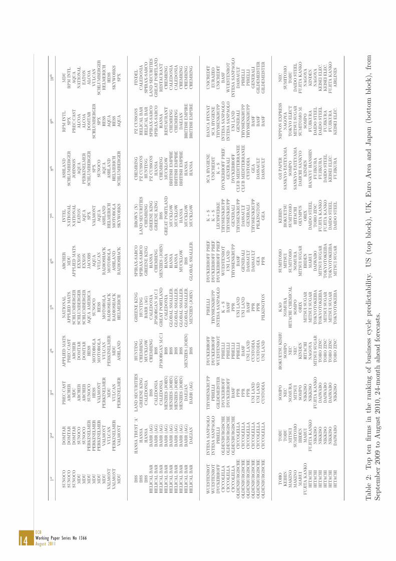
Based on this backwards looking measure of RMSE and abstracting for the moment from theactual forecasting power exhibited by the firms, Figure 2 (black solid line) shows how many timeseach of the domestic firms shows up in the first decile of the predictive distribution for the respectivecountry’s economic activity. It also compares the actual occurrences to a confidence interval for thosethat we would see if firms were instead randomly selected through uniform odds, both cross sectionallyand across time (i.e. we compare the actual number of times a given firm shows up in the top decilewith the number that could be expected if all firms had the same chance to be extracted in any givenmonth).8 We find that two small sets of firms are significantly different from all the others. The firstset includes firms that show up too few times relative to a random selection, while the second setcomprises firms that show up too many times relative to this benchmark. We may less formally findthe same result browsing through the names of the firms which ranked in the top ten positions ofthe predictive distribution, as firms’ names tend to remain stable, on average, for a relatively largenumber of months. A snapshot for the period between September 2009 and August 2010 is reportedin Table 2. The existence of short-term persistence in the relative predictive power supports the viewthat some firm are different from others and that randomness does not represent the main driver ofour results (see Section 6 for additional support). It can be noticed from the Table that once a firmbegins to exhibit high predictive power for developments in economic activity (i.e. it belongs to thetop 10 firms in terms of predictability), it continues to do so for around six months, before beginningto lose importance. Overall, these 𝑠𝑝𝑒𝑐𝑖𝑎𝑙 firms are around one tenth of the population of domesticfirms in each country. Such findings would support a granular interpretation of aggregate fluctuations,with aggregate economic activity dynamics being embedded in the grains represented by the smallset of highly predictive firms that we have identified.
4.2 Domestic Predictability and Spillovers
Figure 3 shows the actual RMSE split across domestic and foreign firms. Each RMSE value refersto a given 𝑚𝑜𝑑𝑒𝑙, as explained in the previous sub-section. For example, model number 𝑤 is the
7The choice of 6 months is of course arbitrary. Ideally we would like to have a measure of instantaneous fit andthis is the main reason to choose 6 months. In this way we can reduce the complexity which we would encounter inchoosing one forecast or a subset of forecasts out of the large number of forecasts that we produce (more than 900 foreach month in each economic area when we look at the full set of domestic and foreign firms). In each month, theRMSE computed over a small number of previous months could be employed also to produce a weighted pooling of theindividual forecasts, similarly to the log-score criterion used in, among others, Amisano and Geweke (2009).
8Details available on request.
14ECBWorking Paper Series No 1366August 2011
1𝑠𝑡
2𝑛𝑑
3𝑟𝑑
4𝑡ℎ
5𝑡ℎ
6𝑡ℎ
7𝑡ℎ
8𝑡ℎ
9𝑡ℎ
10𝑡ℎ
SU
NO
CO
DO
MTA
RP
RE
C.C
AST
AP
PLIE
DM
AT
S.
NA
TIO
NA
LA
RC
HE
RIN
TE
LA
SH
LA
ND
RP
MIN
TL.
MD
USU
NO
CO
DO
MTA
RA
RC
HE
RP
RE
C.C
AST
AP
PLIE
DM
AT
S.
MD
UN
AT
ION
AL
SC
HLU
MB
ER
GE
RSP
XR
PM
INT
L.
SU
NO
CO
DO
MTA
RM
DU
AR
CH
ER
SC
HLU
MB
ER
GE
RA
PP
LIE
DM
AT
S.
NA
TIO
NA
LJO
HN
SO
NP
RE
C.C
AST
AQ
UA
MD
USU
NO
CO
AR
CH
ER
DO
MTA
RSC
HLU
MB
ER
GE
RE
XX
ON
EA
TO
NA
QU
AA
LC
OA
NA
TIO
NA
LM
DU
SU
NO
CO
AR
CH
ER
DO
MTA
RSC
HLU
MB
ER
GE
RE
XX
ON
AQ
UA
PE
RK
INE
LM
ER
ALC
OA
EA
TO
NM
DU
PE
RK
INE
LM
ER
SU
NO
CO
HE
SS
AQ
UA
AM
ER
ICA
JA
CO
BS
SP
XSC
HLU
MB
ER
GE
RD
OM
TA
RA
LC
OA
MD
UP
ER
KIN
ELM
ER
HE
SS
MO
TO
RO
LA
SU
NO
CO
AQ
UA
VA
LM
ON
TSP
XSC
HLU
MB
ER
GE
RV
ULC
AN
MD
UP
ER
KIN
ELM
ER
VA
LM
ON
TM
OT
OR
OLA
HE
SS
VU
LC
AN
AQ
UA
SU
NO
CO
SP
XSC
HLU
MB
ER
GE
RM
DU
VA
LM
ON
TP
ER
KIN
ELM
ER
VU
LC
AN
MO
TO
RO
LA
RA
DIO
SH
AC
KA
SH
LA
ND
AQ
UA
HE
SS
HE
LM
ER
ICH
VA
LM
ON
TV
ULC
AN
MD
UP
ER
KIN
ELM
ER
RA
DIO
SH
AC
KM
OT
OR
OLA
HE
LM
ER
ICH
ASH
LA
ND
AQ
UA
HE
SS
VA
LM
ON
TP
ER
KIN
ELM
ER
VU
LC
AN
MD
UR
AD
IOSH
AC
KA
SH
LA
ND
MO
TO
RO
LA
HE
LM
ER
ICH
HE
SS
SK
YW
OR
KS
MD
UVA
LM
ON
TP
ER
KIN
ELM
ER
ASH
LA
ND
HE
LM
ER
ICH
RA
DIO
SH
AC
KSK
YW
OR
KS
SC
HLU
MB
ER
GE
RA
QU
ASP
X
BSS
HA
NSA
TR
UST
’A’
LA
ND
SE
CU
RIT
IES
HU
NT
ING
GR
EE
NE
KIN
GSP
IRA
X-S
AR
CO
BR
OW
N(N
)C
HE
MR
ING
PZ
CU
SSO
NS
FIN
DE
LB
SS
HA
NSA
GR
EE
NE
KIN
GC
HE
MR
ING
HU
NT
ING
SP
IRA
X-S
AR
CO
LA
ND
SE
CU
RIT
IES
PZ
CU
SSO
NS
HE
LIC
AL
BA
RC
ALE
DO
NIA
BSS
HA
NSA
CA
LE
DO
NIA
MU
CK
LO
WB
AR
R(A
G)
GR
EE
NE
KIN
GC
HE
MR
ING
HU
NT
ING
HE
LIC
AL
BA
RSP
IRA
X-S
AR
CO
HE
LIC
AL
BA
RB
AR
R(A
G)
BSS
CH
EM
RIN
GC
ALE
DO
NIA
HA
NSA
GR
EE
NE
KIN
GP
ZC
USSO
NS
SP
IRA
X-S
AR
CO
LA
ND
SE
CU
RIT
IES
HE
LIC
AL
BA
RB
AR
R(A
G)
CA
LE
DO
NIA
BSS
JP
MO
RG
AN
M.C
.IC
HE
MR
ING
GR
EE
NE
KIN
GH
AN
SA
SP
IRA
X-S
AR
CO
GR
EA
TP
ORT
LA
ND
HE
LIC
AL
BA
RB
AR
R(A
G)
CA
LE
DO
NIA
JP
MO
RG
AN
M.C
.IG
RE
AT
PO
RT
LA
ND
ME
NZIE
S(J
OH
N)
BSS
CH
EM
RIN
GH
AN
SA
RE
STA
UR
AN
TH
ELIC
AL
BA
RB
AR
R(A
G)
ME
NZIE
S(J
OH
N)
BSS
CA
LE
DO
NIA
HA
NSA
GR
EA
TP
ORT
LA
ND
MU
CK
LO
WR
ESTA
UR
AN
TC
HE
MR
ING
HE
LIC
AL
BA
RB
AR
R(A
G)
ME
NZIE
S(J
OH
N)
BSS
GLO
BA
LSM
ALLE
R.
HA
NSA
MU
CK
LO
WB
RIT
ISH
EM
PIR
EC
HE
MR
ING
CA
LE
DO
NIA
HE
LIC
AL
BA
RB
AR
R(A
G)
ME
NZIE
S(J
OH
N)
BSS
GLO
BA
LSM
ALLE
R.
HA
NSA
MU
CK
LO
WB
RIT
ISH
EM
PIR
EC
HE
MR
ING
CA
LE
DO
NIA
HE
LIC
AL
BA
RB
AR
R(A
G)
ME
NZIE
S(J
OH
N)
BSS
GLO
BA
LSM
ALLE
R.
MU
CK
LO
WH
AN
SA
BR
ITIS
HE
MP
IRE
DA
EJA
NC
HE
MR
ING
HE
LIC
AL
BA
RB
AR
R(A
G)
DA
EJA
NM
EN
ZIE
S(J
OH
N)
GLO
BA
LSM
ALLE
R.
BSS
MU
CK
LO
WH
AN
SA
BR
ITIS
HE
MP
IRE
CH
EM
RIN
GH
ELIC
AL
BA
RD
AE
JA
NB
AR
R(A
G)
BSS
ME
NZIE
S(J
OH
N)
GLO
BA
LSM
ALLE
R.
MU
CK
LO
WH
AN
SA
BR
ITIS
HE
MP
IRE
CH
EM
RIN
G
WU
EST
EN
RO
TIN
TE
SA
SA
NPA
OLO
TH
YSSE
NK
RU
PP
DY
CK
ER
HO
FF
PIR
ELLI
DY
CK
ER
HO
FF
PR
EF.
K+
SSC
AH
YG
IEN
EB
AN
CA
FIN
NA
TU
NIC
RE
DIT
WU
EST
EN
RO
TIN
TE
SA
SA
NPA
OLO
PIR
ELLI
DY
CK
ER
HO
FF
TH
YSSE
NK
RU
PP
DY
CK
ER
HO
FF
PR
EF.
K+
SU
NIC
RE
DIT
SC
AH
YG
IEN
EE
UR
AZE
OD
YC
KE
RH
OFF
PIR
ELLI
GIL
DE
ME
IST
ER
WU
EST
EN
RO
TIN
TE
SA
SA
NPA
OLO
DY
CK
ER
HO
FF
PR
EF.
LE
CH
WE
RK
EK
+S
TH
YSSE
NK
RU
PP
UN
ICR
ED
ITC
ICC
OLE
LLA
OLD
EN
BU
RG
ISC
HE
DY
CK
ER
HO
FF
PIR
ELLI
K+
SW
UE
ST
EN
RO
TT
HY
SSE
NK
RU
PP
DY
CK
ER
HO
FF
PR
EF.
INT
ESA
SA
NPA
OLO
BA
SF
CIC
CO
LE
LLA
OLD
EN
BU
RG
ISC
HE
DY
CK
ER
HO
FF
PIR
ELLI
BA
SF
UN
ILA
ND
TH
YSSE
NK
RU
PP
GE
NE
RA
LI
INT
ESA
SA
NPA
OLO
WU
EST
EN
RO
TC
ICC
OLE
LLA
OLD
EN
BU
RG
ISC
HE
BA
SF
PIR
ELLI
PP
RT
HY
SSE
NK
RU
PP
GE
NE
RA
LI
DY
CK
ER
HO
FF
UN
ILA
ND
INT
ESA
SA
NPA
OLO
OLD
EN
BU
RG
ISC
HE
CIC
CO
LE
LLA
PP
RP
IRE
LLI
UN
ILA
ND
BA
SF
TH
YSSE
NK
RU
PP
CLU
BM
ED
ITE
RR
AN
EE
GE
NE
RA
LI
DA
SSA
ULT
OLD
EN
BU
RG
ISC
HE
CIC
CO
LE
LLA
PP
RB
ASF
UN
ILA
ND
GE
NE
RA
LI
DA
SSA
ULT
CLU
BM
ED
ITE
RR
AN
EE
TH
YSSE
NK
RU
PP
PIR
ELLI
OLD
EN
BU
RG
ISC
HE
CIC
CO
LE
LLA
PP
RU
NI
LA
ND
BA
SF
DA
SSA
ULT
GE
NE
RA
LI
CU
ST
OD
IAT
HY
SSE
NK
RU
PP
PIR
ELLI
OLD
EN
BU
RG
ISC
HE
CIC
CO
LE
LLA
UN
ILA
ND
CU
ST
OD
IAP
PR
DA
SSA
ULT
TH
YSSE
NK
RU
PP
GE
AB
ASF
GE
NE
RA
LI
OLD
EN
BU
RG
ISC
HE
CIC
CO
LE
LLA
UN
ILA
ND
CU
ST
OD
IAP
PR
GE
AP
ILK
ING
TO
ND
ASSA
ULT
BA
SF
GIL
DE
ME
IST
ER
OLD
EN
BU
RG
ISC
HE
CIC
CO
LE
LLA
CU
ST
OD
IAU
NI
LA
ND
PIL
KIN
GT
ON
PP
RG
EA
DA
SSA
ULT
BA
SF
GIL
DE
ME
IST
ER
TO
HO
TO
BU
SO
MP
OH
OK
UE
TSU
KIS
HU
KA
OSU
MIT
OM
OK
EIH
INO
JI
PA
PE
RN
IPP
ON
EX
PR
ESS
NE
CK
EIH
INT
OB
UN
EC
SO
MP
ON
OM
UR
AM
ITSU
IH
OK
UE
TSU
SA
NK
YO
-TA
TE
YA
MA
NA
GO
YA
SU
MIT
OM
OM
AK
INO
MIT
SU
IN
OM
UR
AN
EC
HIT
AC
HI
CH
EM
ICA
LSU
MIT
OM
OSU
MIT
OM
OSO
MP
OT
OK
YO
ELE
CT
TO
BU
MA
KIN
OSU
MIT
OM
OM
ITSU
IN
EC
SO
MP
ON
OM
UR
AH
ITA
CH
ISA
NK
YO
-TA
TE
YA
MA
MIT
SU
ISU
GA
RD
AID
OST
EE
LM
AR
UI
IBID
EN
SO
MP
OK
IND
EN
OR
IXM
ITSU
ISU
GA
RO
LY
MP
US
DA
IIC
HI
SA
NK
YO
SU
MIT
OM
OM
.FU
JIT
AK
AN
KO
FU
JIT
AK
AN
KO
MA
RU
IN
IKK
ISO
HIT
AC
HI
MIT
SU
ISU
GA
RIB
IDE
NO
RIX
KIN
DE
NSO
MP
ON
AG
OY
AH
ITA
CH
IFU
JIT
AK
AN
KO
NIK
KIS
ON
AG
OY
AM
ITSU
ISU
GA
RM
AR
UI
DA
IDO
ST
EE
LH
AN
KY
UH
AN
SH
INFU
JIK
UR
AK
IND
EN
HIT
AC
HI
NIK
KIS
OFU
JIT
AK
AN
KO
MIT
SU
ISU
GA
RT
OK
YO
TO
KE
IBA
DA
IWA
BO
TO
HO
ZIN
CFU
JIK
UR
AD
AID
OST
EE
LN
AG
OY
AH
ITA
CH
IN
IKK
ISO
DA
IWA
BO
TO
HO
ZIN
CT
OK
YO
TO
KE
IBA
MIT
SU
ISU
GA
RFU
JIT
AK
AN
KO
FU
JIK
UR
AD
AID
OST
EE
LK
EIS
EI
ELE
C.
HIT
AC
HI
NIK
KIS
OD
AIW
AB
OT
OH
OZIN
CM
ITSU
ISU
GA
RT
OK
YO
TO
KE
IBA
FU
JIT
AK
AN
KO
DA
IDO
ST
EE
LFU
JIK
UR
AK
EIS
EI
ELE
C.
HIT
AC
HI
NIK
KIS
OD
AIW
AB
OT
OH
OZIN
CM
ITSU
ISU
GA
RT
OK
YO
TO
KE
IBA
DA
IDO
ST
EE
LK
EIS
EI
ELE
C.
FU
JIK
UR
AFU
JIT
AK
AN
KO
HIT
AC
HI
DA
IWA
BO
NIK
KIS
OT
OH
OZIN
CT
OK
YO
TO
KE
IBA
MIT
SU
ISU
GA
RD
AID
OST
EE
LFU
JIK
UR
AK
EIS
EI
ELE
C.
AIR
LIN
ES
Tab
le2:
Toptenfirm
sin
therankingof
businesscyclepredictability.
US(topblock),
UK,Euro
Areaan
dJapan(bottom
block),
from
September
2009to
August
2010,24
-month
aheadforecasts.

15ECB
Working Paper Series No 1366August 2011
model that considers the IP forecasts originating from those firms that in each month ranked 𝑤 − 𝑡ℎin the distribution of the 𝑏𝑎𝑐𝑘𝑤𝑎𝑟𝑑𝑠 𝑙𝑜𝑜𝑘𝑖𝑛𝑔 RMSE. Each of the models is therefore a collection ofpotentially a large number of firms over the long sample we examine. The regressions run for theforeign firms are identical to equation (1) but the firms we look at are only those that do not belongto the country under examination. More specifically, we assess the predictive power for the rates ofchange in the IP index in country 𝑖 coming from the equity prices and variances of firms in country 𝑗.Figure 3 shows that based on the RMSEs a large number of models induce a remarkable improvementin the forecasting performance relative to models looking at aggregate information only (the horizontalstraight lines in the Figure). This is true especially of the euro area, although spillovers seem to beimportant in all the four economies, including the United States. While adding foreign firms cansignificantly improve the prediction of domestic business cycles over and above aggregate information,the best foreign model (i.e. the collection of the best foreign firms over time) has approximately thesame predictive power as the best domestic model (i.e. the collection of the best domestic firms overtime). Figure 4 reports a more formal assessment of the relative performance of the firms againstaggregate information only and is based on the Diebold and Mariano (1995) test for equal predictiveability. The test is computed as the t-ratio of the constant in a regression of the difference betweenthe absolute values of the error series produced by the competing models on a constant.9
Comparing Figure 2 in sub-section 4.1 to Figures 3 (RMSE) and 4 (Diebold and Mariano test)seems to suggest that the number of firms that outperform aggregate information is by and largeoverestimated in these latter two Figures.10 While we deal with this data-snooping bias more formallyin Section 6, we also notice here that one thing that may additionally bias the findings for foreignfirms is that in constructing the RMSEs for these firms we do not consider that a part of theirpredictive power could derive from information common also to domestic firms. To control for thedomestic component of the predictive power exhibited by foreign firms we should run a large numberof regressions (around half a million with 970 firms) and therefore we explore a simpler but possiblyless effective, alternative. In each month, and for each country, we compute through the backwardslooking RMSE-based ranking of the domestic firms (introduced in section 4.1) two domestic factors(one return and one volatility factor), as simple averages of the return and the volatility of the first10 firms in this ranking. Being built in real time, these factors should maximize predictability andtherefore, as just explained, reduce significantly the information content of the foreign firms, shouldit be overlapping with domestic information. The specification of these regressions is analogous to eq.(1), i.e.:
9The Diebold and Mariano (DM) test is not suited for the comparison of nested models, as we have in this paper.In this case in fact the properties of the statistic collapse, as numerator and denominator are asymptotically the same.Clark and McCracken (2001) examine empirically the properties of the DM test when dealing with nested models andconclude that when the out-of-sample estimation is based on rolling windows, as we do, the test if still reliable, althoughmodestly inferior to the test they propose, in which critical values have to be bootstrapped from the specific predictiveregression employed. Based on this evidence we chose to continue to use the Diebold and Mariano test and the normalcritical values, as computation times for the bootstrap would be extremely large with the sample size and the crosssectional dimension that we employ.
10The RMSE of the model including only the lagged change in the IP index is not far from the RMSE obtainedincluding also aggregate financial information. A random walk forecast does instead much worse, as we consider ratherlong forecasting horizons. We do not report results for the random walk in the text but for example for the UnitedStates it is only at the 12 month horizon that the random walk has approximately the same RMSE of the model thatuses only lagged changes in the IP. At the same time its RMSE remains much higher than the for the model thatemploys the slope of the yield curve and the variance of the stock market. Its performance at all three remainingforecast horizons is much worse than the other models that use only aggregate information and therefore also of thebest models that consider firm-specific variables.

16ECBWorking Paper Series No 1366August 2011
Δℎ ln(𝑖𝑝)𝑡 = 𝛼 +𝑚∑
𝑗=1
𝛽1,𝑗Δℎ ln(𝑖𝑝)𝑡−𝑓(ℎ)
+𝑚∑
𝑗=1
𝛽2,𝑗𝑇𝑒𝑟𝑚𝑡−𝑓(ℎ) +𝑚∑
𝑗=1
𝛽3,𝑗𝑀𝑘𝑡𝑅𝑒𝑡𝑡−𝑓(ℎ)
+𝑚∑
𝑗=1
𝛽4,𝑗𝑀𝑘𝑡𝑉 𝑎𝑟𝑡−𝑓(ℎ)
+𝑚∑
𝑗=1
𝛾𝑖1,𝑗𝑅𝑒𝑡
𝑖𝑡−𝑓(ℎ) +
𝑚∑
𝑗=1
𝛾𝑖2,𝑗𝑉 𝑎𝑟
𝑖𝑡−𝑓(ℎ)+
+𝑚∑
𝑗=1
𝜙𝑗𝐷𝑅𝑒𝑡𝑡−𝑓(ℎ) +𝑚∑
𝑗=1
𝑗𝐷𝑉 𝑎𝑟𝑡−𝑓(ℎ) + 𝜀𝑡
(2)
where 𝐷𝑅𝑒𝑡 and 𝐷𝑉 𝑎𝑟 are the domestic return and variance factors built as just described andthe other variables are the same as defined in equation (1). We overall find (results are just describedto save space) that the RMSEs produced by foreign firms and reported in Figure 3 do not changemuch when domestic factors are also considered, therefore supporting the view that foreign firms canprovide significant information beyond domestic aggregate information. At the same time, however,as already mentioned, Figures 3 and 4 also evidence that foreign firms hardly provide informationin addition to the best domestic firms (i.e. the blue line - foreign firms - is never below the blackline - domestic firms - for the firms providing the lowest RMSEs, those in the left hand side of theFigure). This consideration however applies to the average month in the sample. In fact, as we showin the next subsection, the monthly ranking of the firms evidences significant changes over time inthe relative importance of domestic and foreign firms.
4.3 Country patterns
Figure 5 shows the country breakdown for the firms that rank in the first decile of the predictivedistribution for each of the four economic areas. These breakdowns are generated through model (2),i.e. controlling foreign firms for the information already embodied in domestic factors11. Unlike whatsample averages suggest, the relative weights of the foreign countries - for each given domestic country- recorded significant variations through time. The swings in the foreign weights have at times beencommon (so that a global factor seems to have been influencing real developments in all the areasanalyzed) while in other periods some specific country has tended to gain relatively more weight. Tomention a few interesting cases it is worthwhile looking at Japan, where domestic firms were keyto explain the recession recorded around the end of the 90s, but almost irrelevant to anticipate therecent episode, with euro area and UK firms having instead a much more relevant role. The 2001US recessions could have been anticipated almost equally likely by looking at US, UK or euro areafirms; however, standing in December 2006, the US recession that would have started twelve monthslater could have been anticipated more by UK firms than by US firms. Identifying the reasons behindthe observed changes in the relative weights of the countries goes beyond the aim of this paper (but
11As explained in the previous sub-section, these factors are the average return and its variance computed for theten domestic firms that in a given month have exhibited the highest predictive ability

17ECB
Working Paper Series No 1366August 2011
see section 5.2 for some attempts on this respect with reference for the domestic firms in the UnitedStates only).
With the aim of analyzing the different information about future economic developments that areconveyed by different firms, Figures 6 and 7 present range forecasts for the US and euro area 12-monthgrowth rate in the IP index that come from different types of firms, i.e. those in the top 20 percentand bottom 20 percent of the predictive distribution (i.e. from top and bottom quintiles). Forecastranges for IP are built - for each quintile - by taking the forecasts provided by the top and bottom 10percent of firms, respectively, within the quintile. We present the forecasts ranges split by domesticand foreign firms, each of them being also computed as just described. Results are presented for the12-month horizon only, but they are broadly similar for the remaining three forecast horizons andare not reported to save space. Two things are worth evidencing. First, there exist large differencesin the fit provided by firms in the first and fifth quintiles, for both the United States and the euroarea. While we are not surprised by the different performances of the two sets of firms, as they havebeen selected precisely according to a forecasting accuracy criterion, still it seems remarkable thatsuch different forecasting performances can be achieved through firms belonging to the same stockmarket index. Second, looking at the top quintile (top panel in both Figures) the confidence intervalsfor the IP forecast (at the 12-month horizon) are nearly always including the actual rate of growthin the IP index and are rather tight around it, although with some time variation reflecting changesin the volatility of the IP growth rates. Overall there are no big differences across the confidenceintervals provided by domestic and foreign firms in the top quintile of the predictive distribution,while predictive power is slightly higher for foreign firms in the bottom quintile, although this islargely irrelevant to the aim of selecting good forecasts. Visual inspection of the forecast rangesassociated to firms in the bottom quintile evidences instead large errors throughout the majority ofthe sample as well as a bigger width of the confidence intervals relative to those produced by the firmsin the top quintile.
One last thing to be pointed out is that focusing on the comparison of the IP forecasts acrossdomestic and foreign firms or between firms in the top and the bottom quintile hides the gain inpredictive power that the firm-level information provides relative to aggregate information. Figure 8shows the actual values of the 12-month rate of change in the US IP index over the out-of-sampleperiod (red line), along with its forecast based on aggregate information (black line) and the rangeforecast (as said above the 10-th and 90-th percentile inside the top quintile) coming from the topquintile of the firms (blue lines). Focusing for example on the 1990/1991 recession, one can see thataggregate information was broadly irrelevant to anticipate the coming slowdown in activity. At thesame time, a significant number of models (i.e. those in the top decile of (the top quintile) of firms)could anticipate it rather well. Similar episodes can be detected also in phases of positive economicgrowth as well as in the other US two recession episodes included in the out-of-sample period.
5 Characteristics of the Firms and Predictability
5.1 Sectoral Patterns
Having established that the returns and the variances of domestic and foreign equity prices boostthe predictability of aggregate fluctuations at various horizons, we look more in detail at how thepredictive power is split across sectors within a given country. As the message conveyed by the jointobservation of Figures 2-4 is that only a relatively small number of firms (domestic and foreign) cansizeably improve business cycle forecasting, asking ourselves whether these firms are special due to

18ECBWorking Paper Series No 1366August 2011
the particular sector in which they operate is quite a straightforward question. The bottom line hereis that the conditional standpoint is again key to unveil the existence of sectoral patterns.
Figure 9 reports the weight of each of the ten sectors in the first and the last deciles of thepredictive distribution for future IP changes averaged over time, along with the corresponding actualweight of the sector in the sample. From this unconditional perspective no sector shows up in thetop and bottom deciles with a different proportion than it has in the sample. In other words, eachof the ten sectors can successfully forecast business cycle fluctuations proportionally to its weight inthe sample. As anticipated, instead, once a conditional standpoint is taken, the sector to which firmsbelong emerges as an important feature of their forecasting performance, with sectors having firmswith returns and variances that tend to anticipate recessions but not expansions while other sectorshave firms that display more power in anticipating expansions.
Figure 10 provides a description of the sectoral patterns evidenced within the (12-month ahead)predictive distribution of the firms, focusing for brevity on the largest sectors in the sample only.Financial firms seem to have some success in predicting recessions especially in the United States andin Japan and remarkably so for the last episode. The same sectoral pattern, however, is not evidencedaround the burst of the dot-com bubble around late 1999, when especially firms within the ConsumerGoods and Consumer Services sector were more predominant in anticipating real developments. Asfor other sectors a broad finding is that industrial firms seem to be good predictors of economicexpansions while Consumer Goods are not strongly associated to the observed movements in the IPindices. 12
5.2 Balance Sheet Items
The industrial sector, a proxy for the core business of the firms, is only one of the many variableswhich capture their characteristics, other choices being for instance the value of their assets, sales,revenues or debt, their size as measured for example by the number of employees and so on. To shedlight on the importance of other key characteristics of the firms on their ability to anticipate businesscycle developments we collect, from Worldscope, yearly data for a number of key balance sheet itemsover the longest available sample for each of the firms included in the regressions presented so far.These data have been retrieved for US firms only as the corresponding information is richer, between1985 and 2009. We aim to identify a relationship between balance sheet items and economic activityby regressing the h-month rate of change in the US Industrial Production index (where, as before,h=6,12,18 and 24 months) on the same set of aggregate variables as in eq. (1) and on a single balancesheet item in turn, i.e.:
12As forecasts are made 12 months before the start of a recession, the returns and the volatilities recorded withinsome sectors relative to others seem to be able to capture signs of forthcoming changes in business cycle conditions.

19ECB
Working Paper Series No 1366August 2011
Δℎ ln(𝑖𝑝)𝑡 =
𝛼 +𝑚∑
𝑗=1
𝛽1,𝑗Δℎ ln(𝑖𝑝)𝑡−𝑓(ℎ)
+𝑚∑
𝑗=1
𝛽2,𝑗𝑇𝑒𝑟𝑚𝑡−𝑓(ℎ)
+𝑚∑
𝑗=1
𝛽3,𝑗𝑀𝑘𝑡𝑅𝑒𝑡𝑡−𝑓(ℎ)
+𝑚∑
𝑗=1
𝛽4,𝑗𝑀𝑘𝑡𝑉 𝑎𝑟𝑡−𝑓(ℎ)
+ 𝛾𝑖1𝐵𝑆
𝑖,𝑡𝑜𝑝𝑡−ℎ + 𝛾𝑖
2𝐵𝑆𝑖,𝑏𝑜𝑡𝑡𝑜𝑚𝑡−ℎ + 𝜀𝑡
(3)
with i=1,...,34 balance sheet indicators. In this regression the terms BS measure the differencebetween the average value of the 𝑖 − 𝑡ℎ balance sheet item recorded by, respectively, the ten topand the ten bottom firms in the predictive distribution for future IP growth, as of the end of theprevious calendar year (i.e when considering the IP growth recorded in March 2007, the difference ina given balance sheet item refers to 31 December 2005, if the 6-month horizon is examined). Althoughbalance sheet items are available only yearly, the ranking of the firms as a function of their predictivepower changes potentially in each month (see Table 2 for a snapshot referred to the United States)and therefore the balance sheet indicator records nonetheless a noticeable monthly variation.13 Noticethat the balance sheet items in these regressions are dated 𝑡 − ℎ and as such they are lagged by asmuch as the forecast horizon, consistently also with the fact that it is based on the ranking of thefirms made in 𝑡 − ℎ − 1, when forecasting at the h-month ahead horizon. However, one could alsosuppose that some given firms are more able than others to capture future developments in businesscycle conditions because of their balance sheet characteristics at time 𝑡, rather than at 𝑡 − ℎ. Onthis respect we also ran regressions (3) placing the balance sheet information at time 𝑡, i.e. as 𝐵𝑆𝑡.Despite some changes in the size of the coefficients there did not seem to be particular variations inthe significance pattern in Table 3 below.
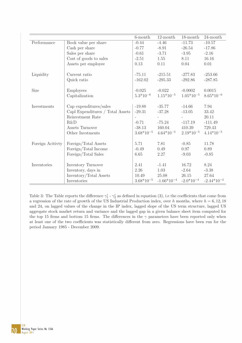
Basically regression (3) allows us to verify whether gaps in balance sheet items across US firms,given the ranking of these firms in the predictive distribution for future US IP changes, can accountfor the difference in their predictive power. Results are reported in Table 3, where we groupedthe significant balance sheet items into a few categories (Performance, Liquidity, Size, Investments,Foreign Activity, Inventories). The items displayed in the Table are only those (out of 34 selecteditems) for which either 𝛾1 or 𝛾2 (see equation (3)) were significant. It seems to be especially crosssectional divergences in items capturing Performance and Investments to be connected to subsequentreal developments. Differences in Inventories and in the International Activity of the firms seems tobe also able to anticipate business cycle developments. Measures of firm liquidity and indebtednessare also significant as well as some measures of size, i.e. employees and capitalization.
13Balance sheet data are at times missing for some firms or availability starts later than the beginning of our sample.Therefore there may not be a complete match between the IP predictions and the features of the top firms that havegenerated it.
20ECBWorking Paper Series No 1366August 2011
6-month 12-month 18-month 24-monthPerformance Book value per share -0.44 -4.46 -11.73 -10.57
Cash per share -0.77 -8.91 -26.54 -17.86Sales per share -0.61 -3.71 -3.95 -2.16Cost of goods to sales -2.51 1.55 8.11 16.16Assets per employee 0.13 0.11 0.04 0.01
Liquidity Current ratio -75.11 -215.51 -277.83 -253.66Quick ratio -162.02 -295.33 -292.86 -287.85
Size Employees -0.025 -0.022 -0.0002 0.0015Capitalization 5.3*10−6 1.15*10−5 1.05*10−5 8.65*10−6
Investments Cap expenditures/sales -19.88 -35.77 -14.66 7.94Capl Expenditures / Total Assets -29.31 -37.28 -13.05 33.42Reinvstment Rate - - - 20.11R&D -0.71 -75.24 -117.19 -111.49Assets Turnover -38.13 160.04 410.39 729.43Other Invstments 3.68*10−5 4.64*10−5 2.19*10−5 4.14*10−5
Foreign Acitivty Foreign/Total Assets 5.71 7.81 -0.85 11.78Foreign/Total Income -0.49 0.49 0.97 0.89Foreign/Total Sales 6.65 2.27 -9.03 -0.85
Inventories Inventory Turnover 2.41 -1.41 16.72 8.24Inventory, days in 2.26 1.03 -2.64 -3.38Inventory/Total Assets 10.49 25.08 26.15 27.64Inventories 3.68*10−5 -1.66*10−4 -2.0*10−4 -2.44*10−4
Table 3: The Table reports the difference 𝛾𝑖1 - 𝛾𝑖2 as defined in equation (3), i.e the coefficients that come from
a regression of the rate of growth of the US Industrial Production index, over ℎ months, where ℎ = 6, 12, 18and 24, on lagged values of the change in the IP index, lagged slope of the US term structure, lagged USaggregate stock market return and variance and the lagged gap in a given balance sheet item computed forthe top 15 firms and bottom 15 firms. The differences in the 𝛾 parameters have been reported only whenat least one of the two coefficients was statistically different from zero. Regressions have been run for theperiod January 1985 - December 2009.
21ECB
Working Paper Series No 1366August 2011
6 Robustness of results
In this section we try to i) to better understand the origin of the higher predictive power found for somefirms and ii) to make sure that the advantages in looking at firm level information beyond aggregateseries are indeed statistically significant and not driven by randomness. As for the first issue, havingincluded both the aggregate stock market return and variance in regression (1) we capture firm-levelinformation that reflects only the idiosyncratic movement of their equity prices. However, one couldwonder about how firms that help predict future business cycle developments behave, relative to themarket, when compared to firms that do not help in forecasting aggregate real developments. Toshed light on this, for each given month in the out of sample period, i.e. 1985 - 2009, and withreference only to the top and bottom 30 firms in the predictive distribution for future IP changes, weperform the following exercise. We cast the equity return of each firm in turn and the aggregate stockmarket return into a bivariate garch(1,1) model, which is estimated via DCC (Cappiello et al., 2006)14
over fixed-length windows of 60 months. In this bivariate model, the mean equations are specifiedso that each of the endogenous variables (the firm’s return and the market return) include the firstown lag as well as the first lag of the other variable. Once the DCC is estimated we store the firm’sidiosyncratic variance, its correlation with the market return and its beta coefficient always relativeto the market.15 For each rolling sample, these three measures are stored in relation to the three lagsemployed in regression (1), i.e. the lags specified by the f(h) functions. The three measures are thenaggregated over, respectively, the top and bottom 30 firms (identified in the previous sections throughthe 𝑏𝑎𝑐𝑘𝑤𝑎𝑟𝑑𝑠 𝑙𝑜𝑜𝑘𝑖𝑛𝑔 RMSE) so to have their averages across firms with high or low predictive powerfor future industrial production. Looking at the 12-month forecasting horizon (the remaining threehorizons broadly provide the same picture), the differences in the three measures across the twogroups of firms are significantly related to GDP developments and we evidence this via the followingregression, where only the first lag for each of the three measures (12 months, as we are focusing onthe 12-month predictive horizon) has been employed, as they were rather highly autocorrelated:
𝑙𝑜𝑔𝐼𝑃𝑡
𝐼𝑃𝑡−12
= 𝛼0 + Σ𝑖=1,3𝛼𝑗𝑋𝑗,𝑡−12 + 𝜀𝑡 (4)
where the vector X collects the three variables computed above (variances, correlations, betas)across the two groups of firms (top 30 and bottom 30).
𝑙𝑜𝑔𝐼𝑃𝑈𝑆
𝑡
𝐼𝑃𝑈𝑆𝑡−12
= 0.018∗∗ − 0.44∗∗𝐷𝑖𝑓𝑓𝑉 𝑎𝑟𝑡−12 + 0.063∗∗𝐷𝑖𝑓𝑓𝐶𝑜𝑟𝑟𝑡−12 + 0.004𝐷𝑖𝑓𝑓𝐵𝑒𝑡𝑡−12
𝑙𝑜𝑔𝐼𝑃𝑈𝐾
𝑡
𝐼𝑃𝑈𝐾𝑡−12
= 0.004∗∗ − 0.37∗∗𝐷𝑖𝑓𝑓𝑉 𝑎𝑟𝑡−12 − 0.035𝐷𝑖𝑓𝑓𝐶𝑜𝑟𝑟𝑡−12 + 0.002𝐷𝑖𝑓𝑓𝐵𝑒𝑡𝑡−12
𝑙𝑜𝑔𝐼𝑃𝐸𝐴
𝑡
𝐼𝑃𝐸𝐴𝑡−12
= 0.007∗∗ − 0.42∗𝐷𝑖𝑓𝑓𝑉 𝑎𝑟𝑡−12 + 0.238∗∗𝐷𝑖𝑓𝑓𝐶𝑜𝑟𝑟𝑡−12 − 0.110∗∗𝐷𝑖𝑓𝑓𝐵𝑒𝑡𝑡−12
𝑙𝑜𝑔𝐼𝑃 𝐽𝑃
𝑡
𝐼𝑃 𝐽𝑃𝑡−12
= 0.010∗∗ − 0.82∗𝐷𝑖𝑓𝑓𝑉 𝑎𝑟𝑡−12 + 0.023𝐷𝑖𝑓𝑓𝐶𝑜𝑟𝑟𝑡−12 − 0.022𝐷𝑖𝑓𝑓𝐵𝑒𝑡𝑡−12
In these regressions DiffVar is the difference in average idiosyncratic variances among the top30 and the bottom 30 firms and DiffCor and DiffBet are the corresponding differences among the
14DCC stands for Dynamic Conditional Correlation and is a convenient and quick way to estimate a multivariateconditionally heteroskedastic model.
15The beta is typically used in finance to measure the sensitivity of an asset relative to the market.

22ECBWorking Paper Series No 1366August 2011
correlations and the beta coefficients of the firms’ idiosyncratic return with respect to the marketreturn. The equations show that indeed aggregate business cycle developments between time t − 12and time t are related to differences in the conditional variances of the top 30 and bottom 30 firmsas measured at t − 12, with a negative relationship prevailing in the four economic areas (i.e anhighest variance of the top 30 firms relative to the bottom 30 firms tends to anticipate recessions).Differences in correlations are significant in the United States and in the euro area only, and differencesin betas are much less significant. In a nutshell, these regressions suggest that it is not the existenceof differences in the relationships with the market return, the betas or the correlations, to drive firms’predictive power. Rather, the latter seem to depend on the cross sectional gap among the firm-levelidiosyncratic stock return volatilities.
As for the second point, the so-called data-snooping problem may seriously undermine the signif-icance of the results presented in the previous sections. This issue was first raised by White (2000)and further addressed by Hansen (2005) via a test for superior predictive ability (SPA).15 Hansen’s(2005) improvement to the White (2000) reality check test has to do with the fact that the latterwas shown to be negatively affected when a large number of models representing poor and irrelevantalternatives were added to the comparisons. In fact, adding useless models, ®
m, which is used as a
significance threshold, where ® is the chosen significance level, can be arbitrarily pushed towards zero.The test for superior predictive ability is based on the relative performance of two models, defined
as
dk,t = L(»t, ±0,t−ℎ)− L(»t, ±k,t−ℎ) (5)
where k = 1, ...,m, so that dk,t measures the performance of model k relative to the benchmarkat time t. When the pairwise comparisons between the m models and the benchmark are collectedinto the vector d, the null hypothesis can be cast as H0 : d ≤ 0. As the derivation of the testassumes asymptotic normality for d, then a quadratic form of the test could be employed but thisis difficult to implement for large m. Therefore, only the diagonal elements of the covariance matrixΩ are considered and, due to this nuisance, a bootstrapped derivation of the test statistics must beadopted. In a nutshell the test statistics proposed is
T SPAn = max k = 1, ..,m[
n0.5dkwk
, 0] (6)
where w2 is a consistent estimator of var(n−0.5dk). The null distribution is based on a meancomputed as
¹c =dk1n
−0.5dkwk
≤√
2 log log(n) (7)
for k = 1, 2, ...m.For our case (results are just discussed to save space) the p-values of the SPA test are ranging
between p=0.01 and p=0.15 (depending on which of the three versions of the tests proposed inHansen, 2005, is used). In any case, the test suggests that it is very likely that some firms indeed
15In principle, the Diebold and Mariano test (1995) (see Figure 4) should be able to tell whether a model provides ornot the same predictive ability of another model for a given variable of interest. However, the DM test is derived underthe null of equal predictive ability (EPA) while testing for superior predictive ability (SPA) is more complex. In factEPA involves a simple null hypothesis while SPA leads to composite hypotheses and is known to involve asymptoticdistributions which are affected by nuisance parameters (and a a result the null hypothesis is not unique).
23ECB
Working Paper Series No 1366August 2011
have additional predictive power for future IP changes relative to aggregate information as well as toother firms and predictability does not seem to be driven by the randomness in the data.
7 Implications for Macroeconomic and Financial Stability
Beyond improving our ability to anticipate business cycle developments, could the same firm levelinformation used so far be useful also to financial stability aims? In other words, can we derive macro-financial stability considerations from the cross sectional dispersion of the monthly IP forecasts for agiven horizon ℎ?
As explained in the previous sections, in each month and for each of the four economic areas,we generate almost 1000 IP forecasts, for each of the four horizons considered (h=6, 12, 18 and24 months), based on aggregate financial information and firm level equity returns and volatilities.Once eliminated some outliers in the predicted IP growth rates, typically associated to exceptionaldeclines or gains recorded by a few equity prices (for example trimming the data above and belowpre-assigned thresholds, with plus and minus 70 percent monthly equity price changes having beenused in the paper), we can for example i) compute the probability density function of the IP forecastsat horizon ℎ via a kernel estimator, ii) construct range forecasts associated to selected percentiles ofthis distribution and last iii) compute a monthly Value at Risk (V aRp), with p being a pre-specifiedp-value, for the IP growth rate. 16 Last, the returns and the variances of the firms that form a givenmodel could be used17 to filter the time series of a number of unobserved leading indicators18 for thebusiness cycle at the selected horizon.
What is worth noticing in the construction of this economic VaR is that it does not come, astraditional VaR measures, from a simulation carried out via an single equation or a multivariatemodel describing the dynamic behavior of the IP index (see Manganelli and Engle, 2001, for the typicalapproaches to measuring Value at Risk, and De Nicolo’ and Lucchetta, 2010, for a related model).Rather it exploits the cross sectional information of the equity returns, so that the uncertainty aboutfuture IP rates of change does not relate to the density of the past forecast errors in predicting such IPchanges but rather from the current configuration of the cross sectional equity returns and variances.In principle a mixed approach could also be employed whereby, as V aR is typically computed, futurepaths of the IP rate of change would be bootstrapped out of each firm-level regression and then thesepredictive densities would be averaged, either using equal weights or by means of the RMSE criterionthat we have been using so far. Whether one strategy dominates over the other is an empirical issuethat we do not tackle, to save space, in this paper.19
For illustrative purposes, Figure 11 reports the 5 percent Value at Risk (the negative rate ofchange in the IP index that can be observed with a 5 percent probability over the next 12 months)for the IP growth at the 12-month horizon for the four areas, while Figure 12 reports, for the UnitedStates only, the 12-month changes in the IP index as well as the 1- and 5-percent VaR. Also, Figure13 reports, for the US only, four predictive density functions for IP growth over the subsequent 12
16As each individual IP forecast is associated to a RMSE criterion, the forecast ranges associated to each, say, quintilecan be assigned a probability value. These can be used to assess the distance in the expected fit of the models.
17See Table 2 to recall how firms are related to models.18Potentially there are as many as the number of firms in the cross section.19Although some of the firms we identify provide the highest local predictability to subsequent developments in the
IP indices, we cannot conclude that they are also systemically important firms, able to spread a given shock to theremaining firms in the economy (see for example the VAR for VaR described in White et al., 2011). Basically, we useindividual equity prices just as filtering devices for a set of unobservable shocks, with no implications for the causalrelationships among the set of firms.

24ECBWorking Paper Series No 1366August 2011
months referred to dates spanning the last three recession episodes. For the 1990-1991 and the 2001recessions the density correctly had a negative median as well as negative skewness for the centralmonths of the recession episodes. For the last recession, the economic slowdown is instead capturedwith some delay (see also Figure 6), as the median of the density becomes negative only in December2008, i.e. one year after the official start of the recession, as computed by the NBER. It has to besaid, on this respect, that sharply negative GDP growth figures were recorded exactly in 2008Q4 andin 2009Q1 so that at least from the nowcasting standpoint the VaR predicted by the model wouldhave nonetheless been useful.
8 Conclusions
This paper has shown, with reference to four economic areas and using a sample that for the out ofsample exercise starts in 1985, that the idiosyncratic returns and variances of individual equity pricescontain the seeds of future real developments. Importantly, the forecasting ability of a given firm isfound to be persistent, averaging around six months, which leads to exclude that randomness is adriver of the forecasting power, as also confirmed by ad-hoc tests. Domestic firms as well foreign firmsare successful in predicting domestic real developments but the relative weight of the two sets of firmsdepends significantly on the cyclical position of the domestic country. We do not find size, as Gabaix(2010) proposes, to be the key factor behind predictability. We unveil that some sectoral patterns arerelated to predictability as well as that some balance sheet items are related to the observed predictivepower of the firms. However, we feel that additional efforts must be undertaken to shed more lighton this challenging and promising issues.

25ECB
Working Paper Series No 1366August 2011
References
[1] G. Amisano and J. Geweke. Optimal prediction pools. ECB Working Paper, No. 1017, 2009.
[2] T. Andersen, T. Bollerslev, F. X. Diebold, and P. Labys. Modelling and forecasting realizedvolatility. Econometrica, 71:529–626, 2003.
[3] S. B. Aruoba, F. X. Diebold, and C. Scotti. Real-time measurement of business conditions.Journal of Business and Economic Statistics, 27:417–427, 2009.
[4] R. B. Barsky and E. Sims. Information, animal spirits, and the meaning of innovations inconsumer confidence. American Economic Review, forthcoming, 2010.
[5] P. Beaudry, M. Dupaigne, and F. Portier. Propagation of international news shocks. Review ofEconomic Dynamics, 14, 2011.
[6] N. Bloom. The impact of uncertainty shocks. Econometrica, 77:623–685, 2009.
[7] R. Cappiello, L., R.F. Engle, and K. Sheppard. Asymmetric dynamics in the correlations ofglobal equity and bond returns. Journal of Financial Econometrics, 4:537–572, 2006.
[8] V. Carvalho. Aggregate fluctuations and the network structure of intersectoral trade. WorkingPaper CREI, Universitat Pompeu Fabra, Barcelona, 2009.
[9] T. E. Clark and M. W. McCracken. Tests of equal forecast accuracy and ecompassing for nestedmodels. Journal of Econometrics, 105:85–110, 2001.
[10] T. E. Clark and M. W. McCracken. Averaging forecasts from VARs with uncertain instabilities.Federal Reserve Bank of Kansas City, Working Paper 06-12, 2006.
[11] T. Conley and B. Dupor. A spatial analysis of sectoral complementarity. Journal of PoliticalEconomy, 111:311–352, 2003.
[12] G. De Nicolo’ and M. Lucchetta. Systemic risks and the macroeconomy. International MonetaryFund, Working Paper, No. 10/29, 2010.
[13] F. X. Diebold and R. Mariano. Comparing predictive accuracy. Journal of Business and EconomicStatistics, 13:253–265, 2005.
[14] R. Espinoza, F. Fornari, and M. J. Lombardi. The role of financial variables in predictingeconomic activity. Journal of Forecasting, 2011.
[15] A. Estrella. Why does the yield curve predict output and inflation? The Economic JOurnal,115:722–744, 2005.
[16] F. Fornari and A. Mele. Financial volatility and economic activity. Working Paper, 2009.
[17] X. Gabaix. The granular origins of aggregate fluctuations. Econometrica, 79:733–772, 2010.
[18] D. Giannone, L. Reichlin, and D. Small. Nowcasting: The real time informational content ofmacroeconomic data releases. Journal of Monetary Economics, 55:665–676, 2008.

26ECBWorking Paper Series No 1366August 2011
[19] S. Gilchrist, V. Yankov, and E. Zakrajsek. Credit market shocks and economic fluctuations:Evidence from corporate bond and stock markets. Journal of Monetary Economics, 56:471–493,2009.
[20] White H. A reality check for data snooping. Econometrica, 68:1097–1127, 2000.
[21] White H., T-H. Kim, and S. Manganelli. A VAR for VaR: Measuring systemic risk using multi-variate regression quantiles. ECB Working Paper Series, forthcoming, 2011.
[22] P. R. Hansen. A test for superior predictive ability. Journal of Business and Economic Statistics,23:365–380, 2005.
[23] M. Horvath. Cyclicality and sectoral linkages: Aggregate fluctuations from sectoral stocks. Reviewof Economic Dynamics, 1:781–808, 1998.
[24] M. Horvath. Sectoral shocks and aggregate fluctuations. Journal of Monetary Economics, 45:69–106, 2000.
[25] A-S. Jore, J. Mitchell, and S. P. Vaheyc. Combinign forecast densities from VARs with uncertaininstabilities. Norges Central Bank, Working Paper 08-01, 2008.
[26] B. Jovanovic. Micro shocks and aggregate risk. Quarterly Journal of Economics, 102:395–409,1987.
[27] S. Manganelli and R. F. Engle. Value at risk models in finance. European Central Bank, WorkingPaper No.75, 2001.
[28] J. Stock and M. W. Watson. Forecasting output and inflation: the role of asset prices. Journalof Economic Literature, 41:788–829, 2003.
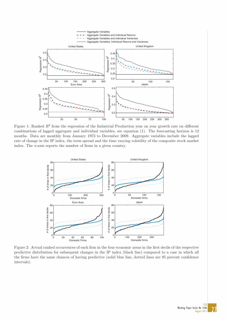
27ECB
Working Paper Series No 1366August 2011
50 100 150 200 250 300
0.2
0.3
0.4
0.5
Reg
ress
ion
R2
United States
50 100 1500.2
0.25
0.3
0.35
0.4
0.45
Reg
ress
ion
R2
United Kingdom
25 50 75 100
0.2
0.25
0.3
0.35
0.4
0.45
Reg
ress
ion
R2
Euro Area
50 100 150 200 250 300 350
0.2
0.3
0.4
0.5
Japan
Reg
ress
ion
R2
Aggregate VariablesAggregate Variables and Individual ReturnsAggregate Variables and Individual VariancesAggregate Variables, Individual Returns and Variances
Figure 1: Ranked 𝑅2 from the regression of the Industrial Production year on year growth rate on differentcombinations of lagged aggregate and individual variables, see equation (1). The forecasting horizon is 12months. Data are monthly from January 1973 to December 2009. Aggregate variables include the laggedrate of change in the IP index, the term spread and the time varying volatility of the composite stock marketindex. The x-axis reports the number of firms in a given country.
0 100 200 3000
20
40
60
80United States
Domestic firms
# of
tim
es in
firs
t dec
ile
0 50 100 1500
20
40
60
80United Kingdom
Domestic firms
# of
tim
es in
firs
t dec
ile
0 20 40 60 80 1000
20
40
60
80Euro Area
Domestic Firms
# of
tim
es in
firs
t dec
ile
0 100 200 3000
20
40
60
80Japan
Domestic firms
# of
tim
es in
firs
t dec
ile
Figure 2: Actual ranked occurrences of each firm in the four economic areas in the first decile of the respectivepredictive distribution for subsequent changes in the IP index (black line) compared to a case in which allthe firms have the same chances of having predictive (solid blue line, dotted lines are 95 percent confidenceintervals).
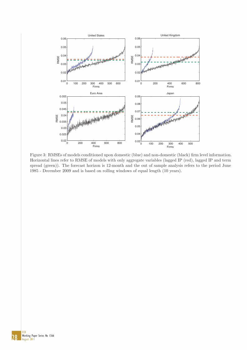
28ECBWorking Paper Series No 1366August 2011
0 100 200 300 400 500 6000.01
0.02
0.03
0.04
0.05
0.06United States
Firms
RM
SE
0 200 400 600 8000.01
0.02
0.03
0.04
0.05
0.06United Kingdom
Firms
RM
SE
0 200 400 600 8000.02
0.025
0.03
0.035
0.04
0.045
0.05
0.055Euro Area
Firms
RM
SE
0 100 200 300 400 5000.03
0.04
0.05
0.06
0.07
0.08
0.09Japan
Firms
RM
SE
Figure 3: RMSEs of models conditioned upon domestic (blue) and non-domestic (black) firm level information.Horizontal lines refer to RMSE of models with only aggregate variables (lagged IP (red), lagged IP and termspread (green)). The forecast horizon is 12-month and the out of sample analysis refers to the period June1985 - December 2009 and is based on rolling windows of equal length (10 years).
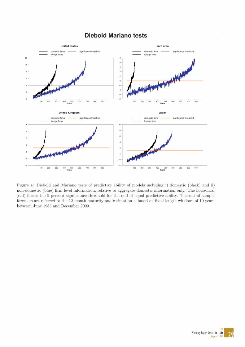
29ECB
Working Paper Series No 1366August 2011
Diebold Mariano tests
United States
domestic firmsforeign firms
significance threshold
firms100 200 300 400 500 600 700 800 900
-10
-5
0
5
10
15
20
United Kingdom
domestic firmsforeign firms
significance threshold
firms100 200 300 400 500 600 700 800 900
-15
-10
-5
0
5
10
15
euro area
domestic firmsforeign firms
significance threshold
firms100 200 300 400 500 600 700 800 900
-10
-8
-6
-4
-2
0
2
4
6
8
Japan
domestic firmsforeign firms
significance threshold
firms100 200 300 400 500 600 700 800 900
-15
-10
-5
0
5
10
15
20
Figure 4: Diebold and Mariano tests of predictive ability of models including i) domestic (black) and ii)non-domestic (blue) firm level information, relative to aggregate domestic information only. The horizontal(red) line is the 5 percent significance threshold for the null of equal predictive ability. The out of sampleforecasts are referred to the 12-month maturity and estimation is based on fixed-length windows of 10 yearsbetween June 1985 and December 2009.
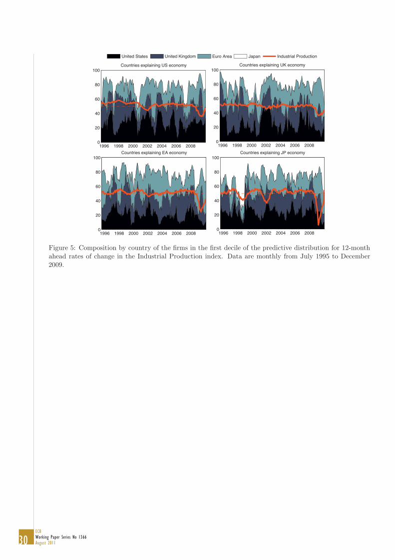
30ECBWorking Paper Series No 1366August 2011
1996 1998 2000 2002 2004 2006 20080
20
40
60
80
100Countries explaining US economy
1996 1998 2000 2002 2004 2006 20080
20
40
60
80
100Countries explaining UK economy
1996 1998 2000 2002 2004 2006 20080
20
40
60
80
100Countries explaining EA economy
1996 1998 2000 2002 2004 2006 20080
20
40
60
80
100Countries explaining JP economy
United States United Kingdom Euro Area Japan Industrial Production
Figure 5: Composition by country of the firms in the first decile of the predictive distribution for 12-monthahead rates of change in the Industrial Production index. Data are monthly from July 1995 to December2009.
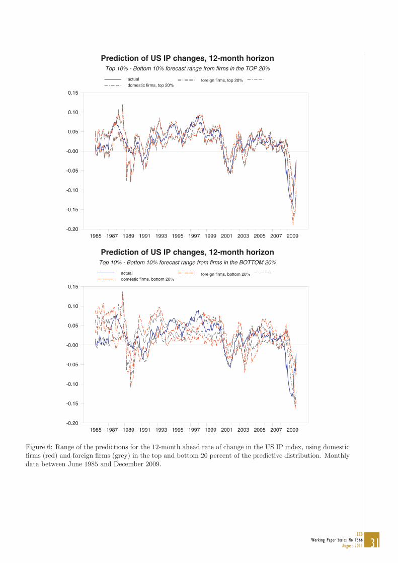
31ECB
Working Paper Series No 1366August 2011
Prediction of US IP changes, 12-month horizonTop 10% - Bottom 10% forecast range from firms in the TOP 20%
actualdomestic firms, top 20%
foreign firms, top 20%
1985 1987 1989 1991 1993 1995 1997 1999 2001 2003 2005 2007 2009-0.20
-0.15
-0.10
-0.05
-0.00
0.05
0.10
0.15
Prediction of US IP changes, 12-month horizonTop 10% - Bottom 10% forecast range from firms in the BOTTOM 20%
actualdomestic firms, bottom 20%
foreign firms, bottom 20%
1985 1987 1989 1991 1993 1995 1997 1999 2001 2003 2005 2007 2009-0.20
-0.15
-0.10
-0.05
-0.00
0.05
0.10
0.15
Figure 6: Range of the predictions for the 12-month ahead rate of change in the US IP index, using domesticfirms (red) and foreign firms (grey) in the top and bottom 20 percent of the predictive distribution. Monthlydata between June 1985 and December 2009.
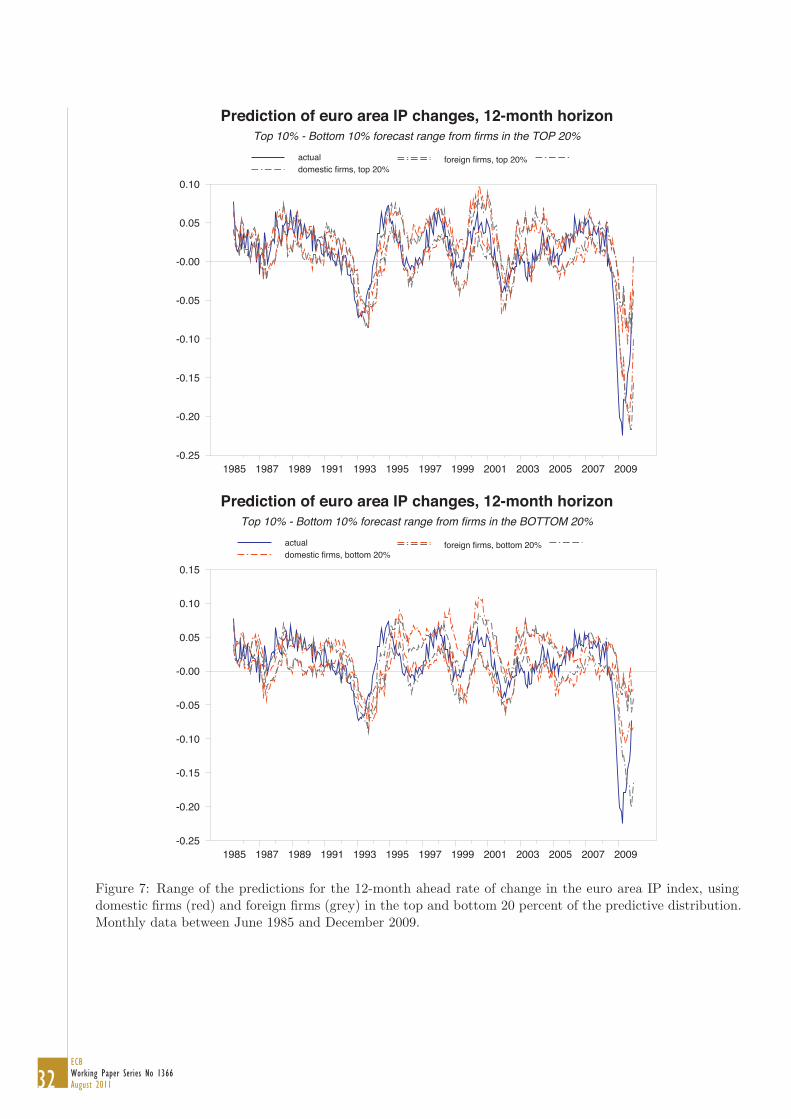
32ECBWorking Paper Series No 1366August 2011
Prediction of euro area IP changes, 12-month horizonTop 10% - Bottom 10% forecast range from firms in the TOP 20%
actualdomestic firms, top 20%
foreign firms, top 20%
1985 1987 1989 1991 1993 1995 1997 1999 2001 2003 2005 2007 2009-0.25
-0.20
-0.15
-0.10
-0.05
-0.00
0.05
0.10
Prediction of euro area IP changes, 12-month horizonTop 10% - Bottom 10% forecast range from firms in the BOTTOM 20%
actualdomestic firms, bottom 20%
foreign firms, bottom 20%
1985 1987 1989 1991 1993 1995 1997 1999 2001 2003 2005 2007 2009-0.25
-0.20
-0.15
-0.10
-0.05
-0.00
0.05
0.10
0.15
Figure 7: Range of the predictions for the 12-month ahead rate of change in the euro area IP index, usingdomestic firms (red) and foreign firms (grey) in the top and bottom 20 percent of the predictive distribution.Monthly data between June 1985 and December 2009.
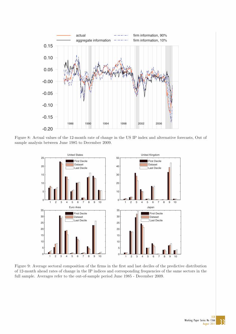
33ECB
Working Paper Series No 1366August 2011
actualaggregate information
firm information, 90%firm information, 10%
-0.20
-0.15
-0.10
-0.05
-0.00
0.05
0.10
0.15
1986 1990 1994 1998 2002 2006
Figure 8: Actual values of the 12-month rate of change in the US IP index and alternative forecasts, Out ofsample analysis between June 1985 to December 2009.
1 2 3 4 5 6 7 8 9 100
5
10
15
20
25United States
First DecileDatasetLast Decile
1 2 3 4 5 6 7 8 9 100
10
20
30
40
50United Kingdom
First DecileDatasetLast Decile
1 2 3 4 5 6 7 8 9 100
5
10
15
20
25
30
35Euro Area
First DecileDatasetLast Decile
1 2 3 4 5 6 7 8 9 100
5
10
15
20
25
30
35Japan
First DecileDatasetLast Decile
Figure 9: Average sectoral composition of the firms in the first and last deciles of the predictive distributionof 12-month ahead rates of change in the IP indices and corresponding frequencies of the same sectors in thefull sample. Averages refer to the out-of-sample period June 1985 - December 2009.
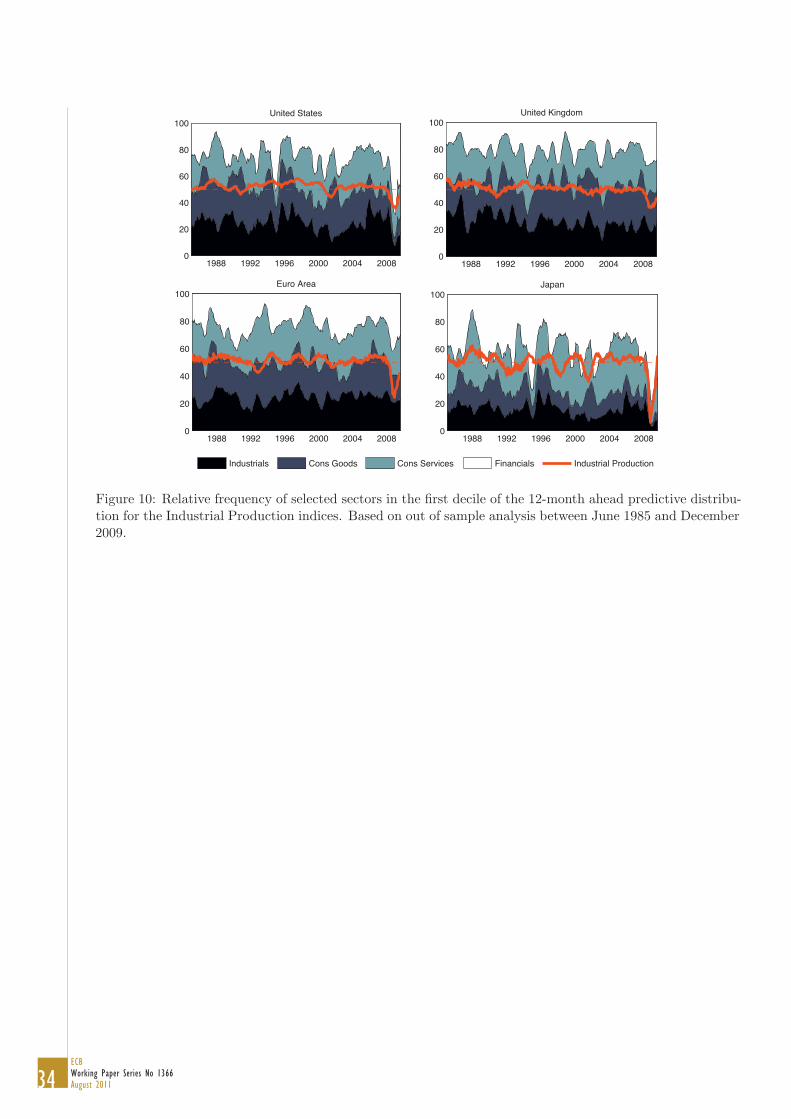
34ECBWorking Paper Series No 1366August 2011
1988 1992 1996 2000 2004 20080
20
40
60
80
100United States
1988 1992 1996 2000 2004 20080
20
40
60
80
100United Kingdom
1988 1992 1996 2000 2004 20080
20
40
60
80
100Euro Area
1988 1992 1996 2000 2004 20080
20
40
60
80
100Japan
Industrials Cons Goods Cons Services Financials Industrial Production
Figure 10: Relative frequency of selected sectors in the first decile of the 12-month ahead predictive distribu-tion for the Industrial Production indices. Based on out of sample analysis between June 1985 and December2009.
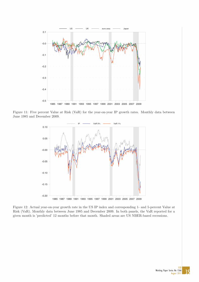
35ECB
Working Paper Series No 1366August 2011
US UK euro area Japan
1985 1987 1989 1991 1993 1995 1997 1999 2001 2003 2005 2007 2009-0.5
-0.4
-0.3
-0.2
-0.1
-0.0
0.1
Figure 11: Five percent Value at Risk (VaR) for the year-on-year IP growth rates. Monthly data betweenJune 1985 and December 2009.
IP VaR 5% VaR 1%
1985 1987 1989 1991 1993 1995 1997 1999 2001 2003 2005 2007 2009-0.20
-0.15
-0.10
-0.05
-0.00
0.05
0.10
Figure 12: Actual year-on-year growth rate in the US IP index and corresponding 1- and 5-percent Value atRisk (VaR). Monthly data between June 1985 and December 2009. In both panels, the VaR reported for agiven month is ’predicted’ 12 months before that month. Shaded areas are US NBER-based recessions.

36ECBWorking Paper Series No 1366August 2011
July 1990 - March 1991 recession
Jan 90Mar 90
May 90Dec 90
year on year IP growth rate
abso
lute
fre
qu
enci
es
-0.100 -0.075 -0.050 -0.025 -0.000 0.025 0.050 0.075
0
5
10
15
20
25
30
March 2001 - November 2001 recession
Jan 01Mar 01
Jun 01Mar 02
year on year IP growth rate
abso
lute
fre
qu
enci
es
-0.100 -0.075 -0.050 -0.025 -0.000 0.025 0.050 0.075
0
5
10
15
20
25
30
35
December 2007 - June 2009 recession
Dec 07Jun 08
Dec 08Mar 09
year on year IP growth rate
abso
lute
fre
qu
enci
es
-0.15 -0.10 -0.05 0.00 0.05 0.10
0
10
20
30
40
50
60
70
Figure 13: Distribution of the expected year-on-year growth of the US IP index at selected dates around thelast three recession episodes.

WORK ING PAPER SER I E SNO 1366 / AUGUST 2011
by Filippo di Mauro, Fabio Fornari and Dario Mannucci
STOCK MARKET FIRM-LEVEL INFORMATION AND REAL ECONOMIC ACTIVITY
Copyright © 2022 FDOKUMEN