Stochastic velocity inversion of seismic reflection/refraction traveltime data for rift structure of...

$: Stochastic velocity inversion of seismic reflection/refraction traveltime data for rift structure of the southwest Barents Sea$
Tectonophysics 593 (2013) 135–150

Contents lists available at SciVerse ScienceDirect

Tectonophysics

j ourna l homepage: www.e lsev ie r .com/ locate / tecto

Stochastic velocity inversion of seismic reflection/refraction traveltime data for riftstructure of the southwest Barents Sea

Stephen A. Clark a,⁎,1, Jan Inge Faleide a, Juerg Hauser b,2, Oliver Ritzmann a,3, Rolf Mjelde c, Jörg Ebbing d,Hans Thybo e, Ernst Flüh f

a Department of Geosciences, University of Oslo, Norwayb NORSAR, Norwayc Department of Earth Science, University of Bergen, Norwayd NGU, The Geological Survey of Norway, Trondheim, Norwaye Department of Geography and Geology, University of Copenhagen, Denmarkf IFM-GEOMAR, University of Kiel, Germany

⁎ Corresponding author at: Jonsvannsveien 476, 705748178792.

E-mail address: [email protected] (S.A. Clark).1 Now at: Statoil Research, Norway.2 Now at: CSIRO, Australia.3 Now at: Wintershall, Germany

0040-1951/$ – see front matter © 2013 Elsevier B.V. Allhttp://dx.doi.org/10.1016/j.tecto.2013.02.033

a b s t r a c t
a r t i c l e i n f o
Article history:Received 21 May 2012Received in revised form 14 February 2013Accepted 23 February 2013Available online 4 March 2013

Keywords:Barents SeaTransform marginContinental riftingCrustal structureReflection refraction velocity modelingStretching and thinning factors

We present results from an active-source, onshore–offshore seismic reflection/refraction transect acquired aspart of the PETROBAR project (Petroleum-related studies of the Barents Sea region). The 700 km-long profileis oriented NW–SE, coincident with previously published multichannel seismic reflection profiles. We utilizelayer-based raytracing in a Markov Chain Monte Carlo (MCMC) inversion to determine a probabilistic velocitymodel constraining the sedimentary rocks, crystalline crust, and uppermostmantle in a complex tectonic regime.The profile images a wide range of crustal types and ages, from Proterozoic craton to Paleozoic to early Cenozoicrift basins; and volcanics related to Eocene continental breakupwith Greenland. Our analyses indicate a complexarchitecture of the crystalline crust along the profile, with crystalline crustal thicknesses ranging from 43 kmbe-neath theVaranger Peninsula to 12 kmbeneath the Bjørnøya Basin. Assuming an original, post-Caledonide crust-al thickness of 35 km in the offshore area, we calculate the cumulative thinning (β) factors along the entireprofile. The average β factor along the profile is 1.7 ± 0.1, suggesting 211–243 km of extension, consistentwith the amount of overlap derived from published plate reconstructions. Local β factors approach 3, whereBjørnøya Basin reaches a depth of more than 13 km. Volcanics, carbonates, salt, diagenesis and metamorphismmake deep sedimentary basin fill difficult to distinguish from original, pre-rift crystalline crust, and thus actualstretching may in places exceed our estimates.

© 2013 Elsevier B.V. All rights reserved.

1. Introduction

Continental extension leading to breakup and subsequent oce-anic accretion is a complex tectonic process. Variations in structure, du-ration, and episodicity are observed not only between different riftedmargins globally, but also along strike and between conjugate marginpairs (e.g., Blaich et al., 2011; Crosby et al., 2008; Mjelde et al., 2008;Tsikalas et al., 2008). Lithospheric strength is the primary control onthese variations, generally agreed upon to be a function of crustand mantle thicknesses and compositions, temperature, melting,and rate of extension (Buck, 1991; Ziegler and Cloetingh, 2004).Increasingly complex numerical modeling studies of rifting explore the

Jonsvatnet, Norway. Tel.: +47

rights reserved.

relative influence and evolution of these parameters (Huismans et al.,2005; Lavier and Manatschal, 2006; Rosenbaum et al., 2008), but theycontinue to be debated. Observational constraint in as many locationsandwith asmuchdetail as possible remains critical to evaluating and im-proving our understanding of geodynamic processes.

ThewesternBarents Seamargin is predominantly a transformmargin,where final breakup occurred during the early Cenozoic along the dextraltransform De Geer Zone between northwest Eurasia and northeastGreenland, eventually evolving into the obliquely-spreading KnipovichRidge (Engen et al., 2008; Faleide et al., 1993a). Prior to breakup, how-ever, the long-term rifting between Norway and east Greenland thatwould eventually form the Norwegian–Greenland Sea continued along-strike hundreds of kilometers northeast into the Barents Sea region(Faleide et al., 1993a). Because the line of final breakup followed thetransform zone instead of the rift axis, most of the rift-related structuresremain on the Barents side, with no major rift basins observed at thetransform-margin conjugate in northeast Greenland (Faleide et al.,2008). As such, these rift structures are highly asymmetric, withrifting progressively shifting from near-orthogonal extension to pre-dominantly transform breakup.

http://dx.doi.org/10.1016/j.tecto.2013.02.033

mailto:[email protected]

http://dx.doi.org/10.1016/j.tecto.2013.02.033

http://www.sciencedirect.com/science/journal/00401951

180°

160°E

140°°0

21100°

80°

60°

40°20°

0°

20°

40°

60°

80°

100°

120°

140° 160°

70°N

Barents Sea

80°N

Carboniferous-Permian

Late Jurassic-Early CretaceousLate Cretaceous-Paleogene

Rift/Subsidence Phases

Late Permian-Triassic

OBNB

LH

FPSF

Z

HF

Z

BB

VVP

VPCOB

COB

MR

KR

0˚10

˚

20˚

30˚

70˚

75˚

a

b

c

TB HB

SH

Fig. 1. Regional map of the Arctic (Jakobsson et al., 2008) with study area outlined in white (above) and basemap of the southwestern Barents Sea (below). Major faults shown as black lines(Faleide et al., 2008). Local highs shown as dashed black lines. Near-normal incidence seismic reflection profile (Fig. 2) shown as orange line.Wide-angle profile shots (gray line) and record-ing instruments (yellow triangles) also shown; labeled, red triangles correspond to record section examples shown in Fig. 3. MR: Mohns Ridge, KR: Knipovich Ridge, COB: continent–oceanboundary, HFZ: Hornsund Fault Zone, SFZ: Senja Fracture Zone, VVP: Vestbakken Volcanic Province, BB: Bjørnøya Basin, LH: Loppa High/Selis Ridge, SH: Stappen High, TB: Tromsø Basin, OB:Ottar Basin, HB: Hammerfest Basin, NB: Nordkapp Basin, FP: Finnmark Platform, VP: Varanger Peninsula.

136 S.A. Clark et al. / Tectonophysics 593 (2013) 135–150

137S.A. Clark et al. / Tectonophysics 593 (2013) 135–150

The subsurface architecture of the southwest Barents Sea comprisesa fan-shaped array of extremely deep (~15 km) sedimentary basinsseparated by crystalline or older sedimentary highs at or near the sea-floor (Figs. 1 and 2) (Faleide et al., 1993a,b; Gudlaugsson et al., 1998;Mjelde et al., 2002). Due to chemical compaction and low-grade meta-morphism of sedimentary rocks at such depths, deep basin structure isdifficult to resolve using seismic methods alone, as the P-wave veloci-ties of such sedimentary rocks are approximately equal to uppermostcrystalline crustal velocities (Breivik et al., 2005). Imaging challengesare further exacerbated by the presence of high-velocity salt, carbon-ates, and volcanics.

In this paper we resolve the deep basin configuration, crustalstructure, and Moho topography underlying the southwest BarentsSea along a 700 km-long transect extending from the Baltic cratonto the continent–ocean boundary (Fig. 1). We implement an MCMCtechnique for wide-angle reflection/refraction and normal-incidencereflection traveltime data inversion for crustal-scale P-wave velocitystructure, constraining the uncertainties in our results. Monte Carlotechniques have recently been applied to active source crustal-scaleprofiling by varying the starting model and traveltime data as inputsto a regularized grid inversion (White and Smith, 2009). In contrast,our methodology uses a guided, randomized perturbation of the modelitself as the inversion technique, producing not a single, best-fittingmodel, but a range of models which fit the data, and form the basis forprobabilistic uncertainty estimation.

We show our results to be compatible with recently published 3Dpotential fields modeling (Barrère et al., 2009, 2011; Marello et al.,

0

1

2

3

4

5

6

7s

0

1

2

3

4

5

6

7s

−100 0 100

COB

KnipovichRidge

D7HB3-96ANWVestbakken Volcanic Bjørnøya BProvince

Fig. 2. Near-normal incidence, multi-channel seismic reflection profiles (names labeled in(shaded colors: yellow, Late Cretaceous to Paleozoic P2P; blue, Late Jurassic to Early Cretacand every 5th reflection traveltime pick (with height equal to +/− assigned uncertainty of 5region shows continuation to spreading ridge not covered by wide-angle data.

2010). Using crustal thicknesses along our profile, we estimate thecumulative crustal thinning factor (β) along the profile relative toan idealized pre-rift continental crustal thickness of 35 km. Threemajor tectonic phases constrained by the basin stratigraphy arereflected in the crustal architecture and the local β-factors. A widearea of Triassic subsidence with little apparent rift-related faultingdoes not coincide with significant crustal thinning. These resultsdocument the northwestward migration of the rift axis and the pro-gression from a wide-rifting mode linked to the early stages of NorthAtlantic rifting, to a narrow-rifting mode approaching breakup.However, maximum thinning did not focus at the location of even-tual breakup, but instead at the Caledonian suture between Laurentiaand Baltica, suggesting that inherited post-orogenic structure played aprimary role in this rifted margin's architecture (Dore, 1991; Gabrielsen,1984; Gudlaugsson et al., 1998; Ritzmann and Faleide, 2007).

2. Geologic setting

The geology of the southwest Barents Sea represents the productof a full Wilson Cycle (Wilson, 1966), from collisional orogeny, to pro-gressive rifting, and finally to continental breakup along a transformmargin. The regional tectonic evolution was recently described in de-tail by Faleide et al. (2008). We present a brief summary of this evo-lution, then describe the geologic features along the profile.

Upon closure of the Iapetus Ocean, the Precambrian Baltic Shieldcollided with and partially subducted beneath Laurentia during theCambrian-Devonian, producing the Caledonian Orogen (Roberts, 2003;

200 300 400 500 kmIKU-84-B SEasin Loppa High Ottar Basin Nordkapp Basin

orange) coincident with the PETROBAR-07 wide-angle seismic profile. Interpretationeous P3P; purple, latest Permian to Triassic P4P; green, Carboniferous to Permian P5P)0 ms and color according to phase, see Table 1) overlain on lower panel. Uninterpreted

Table 1Phase, number of picks, rms uncertainty, number of calculated arrivals in mean model,rms misfit of mean model arrivals, normalized χ2 misfit of mean model arrivals. Colorcoding corresponds to picks in Figs. 2 and 3, and rays and layers in Figs. 2, 7, and 8.

Phase P2 P2P P3 P3P P4 P4P P5 P5P Pg PmP Pn Total

Num picks

93 347 550 381 466 321 494 469 6261 2999 1321 13702

Uncert (ms)

51 50 101 69 64 50 107 86 140 153 157 101

Num calc

89 343 511 366 453 317 477 459 5869 2843 1304 13031

Misfit (ms)

160 111 152 172 143 106 110 145 165 270 239 196

χ2/N 10.3 5.0 4.3 9.5 7.2 4.5 1.8 6.1 2.4 4.7 3.3 3.7


Roberts and Gee, 1985). Distinct, obducted nappe packages bounded bynorth-striking main thrust faults are mapped onshore Norway (Mosar,2003; Sigmond, 2002), and are interpreted to extend northward intothe Barents Sea, possibly forming multiple branches from the FinnmarkPlatform to the present continent–ocean boundary (Barrère et al.,2009; Breivik et al., 2005; Ritzmann and Faleide, 2007). Most ofthe crystalline basement of the western Barents Sea is interpretedto derive from Caledonian metamorphic rocks, although Archean-Proterozoic rocks and younger volcanics are also present (Barrèreet al., 2009; Ritzmann and Faleide, 2007).

Following the Caledonian orogeny and a subsequent orogenic collapse(Breivik et al., 2002, 2005; Gudlaugsson et al., 1998; Hartz and Andresen,1997), regional stratigraphic unconformities and a fan-shaped array ofblock-faulted basins define an episodic rift history leading to final break-up (Fig. 1) (Faleide et al., 1993a,b, 2008). The initial stage of rifting beganin the Carboniferous, forming evaporite-filled basins such as Nordkappand Ottar basins in the topographic lows of NE-striking half-grabens(Breivik et al., 1995; Embry and Mørk, 2006; Gudlaugsson et al., 1998).Capping these basins is a Barents-wide Upper Carboniferous–LowerPermian shallow-water carbonate platform (Faleide et al., 1984; Larssenet al., 2005).

The latest Permian through Triassic is characterized by regional subsi-dence and sediment accumulation throughout the greater Barents shelf(Glørstad-Clark et al., 2010). This phase of basin development is often as-sociated with an inferred extensional event (Dore, 1991; Johansen et al.,1993, 1994; O'Leary et al., 2004; Wood et al., 1989; Ziegler, 1988), buttypical rift-related faulting is notably absent. Most of the sedimentary ac-cumulation is characterized bywide, regional sag subsidence, particularlyin the Eastern Barents Basin (Johansen et al., 1993) but also inthe western Barents region in the vicinity of Loppa High (Fig. 1)(Glørstad-Clark et al., 2010). The only clear evidence of normal faultingat this time is at the western flank of the Loppa High/Selis Ridge(Gabrielsen et al., 1990; Glørstad-Clark, 2011), active from the LatePermian to the Middle Triassic. However, throughout the Late Triassic,even the paleo-high was a depocenter (Glørstad-Clark et al., 2010).

The Late Jurassic to Early Cretaceous marks the second majorphase of block faulting and half-graben infill associated with activerifting (Faleide et al., 1993a,b). Predominantly west-dipping normalfaults provided accommodation space for relatively narrow, very deepbasins, such as Bjørnøya and Tromsø basins, which exceed 15 kmdepth (Breivik et al., 1998; Faleide et al., 1993a,b). These basins are con-tinuous along strike with the late Paleozoic basins of the initial riftphase, and likely formed by reactivation of the same basin-boundingfaults (Faleide et al., 1993a,b). However, these basins aremore localizedand do not extend as far northeast as the Paleozoic rift basins (Fig. 1).

The final rifting phase began in the Late Cretaceous and continuedto the predominantly transform breakup in the earliest Eocene, coevalwith the onset of seafloor spreading in the North Atlantic to the southand the Eurasia Basin to the north (Faleide et al., 1993a, 2008). The

late rift basins are localized along the nascent margin within thetranstensional strike–slip zone (Fig. 1) (Faleide et al., 1993a). Thetransform margin is divided into two segments, the Senja FractureZone in the south and the Hornsund Fault Zone in the north, separatedby a volcanic rifted margin segment in a releasing bend of the margin.The volcanic rifted margin segment consists of the Eocene VestbakkenVolcanic Province igneous extrusive/intrusive complex and associat-ed Late Cretaceous–Paleogene pull-apart structures (Faleide et al., 2008;Ryseth et al., 2003).

A sharp, Barents-wide unconformity associated with uplift andglacial erosion caps the top of the rift- and breakup-related sedimen-tary succession. Thin accumulations of Plio-Pleistocene sediments onthe Barents shelf transition to the west and north into large subma-rine glacial fans and slide complexes on the margin slopes (Dimakiset al., 1998; Faleide et al., 1996; Hjelstuen et al., 2007; Rise et al.,2005; Vorren et al., 1991).

The PETROBAR-07 profile provides distinct examples of the geologyassociated with all the major tectonic phases of the southwest BarentsSea crustal development. Fig. 2 shows a composite seismic reflectionprofile coincident with the PETROBAR-07 profile and extending to theKnipovich spreading ridge. From the northwest, or from distal to prox-imal margin, the PETROBAR-07 profile starts 16 km landward of theocean–continent boundary in the Vestbakken Volcanic Province. Theprofile then crosses Bjørnøya Basin, Loppa High, Ottar Basin, NordkappBasin, Finnmark Platform, and the Caledonide frontal thrust. Thesoutheast end of the profile follows the northern coast of the Varangerpeninsula, where the Proterozoic Baltic Shield is exposed.

3. Data

The PETROBAR-07 profile (Fig. 1) was acquired by the R/V HåkonMosby of the University of Bergen in August 2007. The 700 km-longprofile comprises 4157 shots from a 78 l. (4800 cu. in.), four-airgunsource array fired at 200 m intervals. The shots were recorded by 20ocean-bottom stations (OBS; 19 four-component instrument and 1single-component hydrophone instrument) operated by IFM-GEOMARand 60 “Texan” land seismometers deployed by the University of Copen-hagen. The profile was acquired in two overlapping sections to achievean OBS spacing of 15–20 km, although in some locations the spacing is30 km due to instrument failure. Land instruments were groupedinto 10 locations of 6 Texans each. Spacing of the land stations was7–34 km, restricted by the rugged topography of the coastline. Theaverage receiver spacing along the entire profile is 18 km.

Clock drift corrections were applied to all OBSs and Texans afterrecovery. OBS locations were recalculated based on water wave ar-rivals and closest approaches of the ship. We estimate a maximum lo-cation error of 20 m based on the average water depth of 330 m alongthe profile and the limitations of the relocation algorithm. Predictivedeconvolution with a correlation window of 11 s and a lag of 8 mswas applied to the OBS data to reduce water column noise. Datafrom the hydrophone channel of the 4-component OBSs had consis-tently higher signal-to-noise ratios (SNR) than the vertical geophonechannel. Data from the six Texans at each land station were stacked.

Using these data, we picked refracted P-wave arrivals for four sed-imentary phases (P2–5), a crystalline crustal phase (Pg), and an upper-most mantle phase (Pn). We also picked reflected P-wave arrivals forthe base of some sedimentary layers (P3/5P) and the Moho (PmP).Traveltime uncertainties were assigned to range from 50 to 250 ms,increasing with decreasing SNR (Zelt and Forsyth, 1994). Picks werethen binned at a 1 km spacing. Table 1 lists the number of picks andaverage uncertainty for each phase. Fig. 3 shows example record sec-tions from two OBSs and a Texan (for locations, see Fig. 1). Every fifthbinned pick is overlain, with heights equal to +/− the assigned un-certainties, and colors corresponding to Table 1.

The PETROBAR-07wide-angle seismic profile overlapsmultichannelseismic reflection profile IKU-84-B (Gudlaugsson et al., 1987; Ritzmann

0

1

2

3

4

5

6

7

8

9

10

Tra

velti

me−

x/8

(s)

0

1

2

3

4

5

6

7

8

9

10

Tra

velti

me−

x/8

(s)

−100 −50 0 50 100 150 200

−250 −200 −150 −100 −50 0 50 100

0

1

2

3

4

5

6

7

8

9

10

Tra

velti

me−

x/8

(s)

100500

a)

c)

b)

Offset (km)

Offset (km)

Offset (km)

Fig. 3. a) OBS 35; b) OBS 04; c) TEXAN 103. Every 5th pick shown with height equal to +/− assigned uncertainty and colored according to assigned phase (see Table 1).


image of Fig.�3


and Faleide, 2007, 2009) acquired in 1984 by the Continental Shelf Insti-tute (now SINTEF). Our profile also closely coincides with two otherMCS profiles, D7 (Breivik et al., 1995) and HB3-96A (Hjelstuen et al.,2007). We picked unmigrated, normal-incidence P-wave reflectiontraveltimes for four horizons (P2–5P) interpreted asfirst-order sequenceboundaries (Table 1 and Fig. 2). The horizons were sampled at 1 km in-tervals along the profile and included as zero-offset traveltime picks inthe modeling procedure to better constrain the sedimentary layers.We assigned these picks an uncertainty of 50 ms.

4. Methods

We modeled the P-wave velocity structure along the profileusing the RAYINVR raytracing code of Zelt and Smith (1992) to pre-dict traveltimes, coupled with a Markov Chain Monte Carlo (MCMC)

a)

b)

c)

0

10

20

30

40

50

Dep

th (

km)

Distan

km/s

0

10

20

30

40

50

Dep

th (

km)

Distan

km/s

0

10

20

30

40

50

Dep

th (

km)

0 100 200 300

0 100 200 300

0 100 200 300

Distan

2 3 4 5 6 7 8

2 3 4 5 6 7 8

2 3 4 5 6 7 8

km/s

Fig. 4. a) Starting model (see Table 2). b) Model after 50,000 iterations of the base sampler,data constraint. VE = 5.

inversion algorithm(Hauser et al., 2011). RAYINVR is a widely used,freely available code for modeling crustal-scale velocity structurefrom active source seismic data. The code traces rays and calculatestraveltimes through a 2D layered velocity model defined by layerboundary depths and a linear gradient between the top- and base-of-layer velocities. We chose the RAYINVR model parameterizationrather than a regularized grid approach for three reasons: 1) it pro-vides a good tradeoff between capturing resolvable model complex-ity and limiting the number of free parameters, 2) it allows for arange of reflected and refracted phases to be interpreted and modeled,and 3) it includes multiple interfaces with geologically realistic velocitycontrasts across them. We first created a simple starting velocitymodel (Fig. 4), then applied the MCMC inversion scheme to determinea set of models which fit the data similarly well. Statistical analysis ofthese models provides a robust uncertainty estimate for each model

ce (km)

ce (km)

400 500 600 700

400 500 600 700

400 500 600 700

ce (km)

without data constraint. c) Model after 100,000 iterations of the base sampler, without

Table 2Starting model layer velocities and depth/velocity node perturbation constraints. Color coding corresponds to rays and layers in Figs. 2, 7, and 8.

Layer 1 2 3 4 5 6 7 8

Lithology Water Post-breakup

seds

Late rift

phase seds,

volcanics

Sag phase seds Early rift

phase seds

Upper crystalline

crust

Lower crystalline

crust

Upper mantle

Start top velocity

(km/s)

1.48 2.00 3.00* 4.00 5.00 6.00 6.50 8.00

Start base velocity

(km/s)

1.48 2.50 3.50** 4.50 5.50 6.50 7.00 8.50

Range (km depth) − − sf:17.5 sf:17.5 sf:17.5 sf:17.5 − 17.5 : 50

Max step size

(km depth)

− − 0.5 0.5 0.5 0.5 − 2.5

Range (km/s velocity) − 1.5 : 6.0 1.5 : 6.0 1.5 : 6.0 1.5 : 6.0 5.0 : 7.9 5.0 : 7.9 7.5 : 8.9

Max step size

(km/s vel)

− 0.2 0.2 0.2 0.2 0.2 0.2 0.2

* 5.00 for volcanic province.** 5.50 for deep basin and volcanic provinces.


parameter, representing a major improvement over previous RAYINVRuncertainty estimates determined by varying a single parameter or sub-set of parameters at a time (Breivik et al., 1995, 2005; Holbrook et al.,1994).

4.1. Model parameterization

We define a water layer, four sedimentary layers, two crystallinecrustal layers, and an uppermost mantle layer (Table 1). Numberedafter the water layer (1), the sedimentary layers (2–5) correspondto distinct stratigraphic megasequences interpreted from the normal-incidence reflection profile, because the unconformities likely representvelocity discontinuities. The sedimentary layers represent: 2) post-breakup (Recent to Eocene), 3) the later rift stages (Paleocene toLate Jurassic), 4) the regional sag basin (Triassic to Late Permian),and 5) the initial rift/post-orogenic collapse stages (Late Permianto Carboniferous).

Because there is no sharp change in Pg gradient or clear mid-crustalreflection, themid-crustal layer boundary is fixed at a constant 17.5 kmdepth. This value was chosen because it represents half the value of anidealized 35 km-thick crust, it is greater than the deepest basin depth,and it is less than the shallowest Moho depth along the profile. Thereis no velocity discontinuity across the boundary, thus allowing for amid-crustal velocity node and two vertical velocity gradients withinthe crust instead of one.

To create the starting model (Fig. 4a), we first created a velocitymodel in two-way traveltime (twt) using the normal-incidence re-flection data horizons for the layer boundaries. For each layer, weassigned a constant value for the top-of-layer velocity and a constant

value 0.5 km/s higher for the base-of layer velocity, with the excep-tion of layer 3, where a volcanic province and a deep basin provincereceived higher starting velocities (Table 2). Our starting model definessedimentary layer pinchouts which remain fixed when perturbing themodel. This honors layer geometry constraints observed in the normal-incidence reflection data, but precludes smoothing of the layer bound-aries within RAYINVR because this would cause boundaries to crossnear the pinchouts. We used the starting velocities to convert the layerboundaries from time to depth. For theMoho, whichwas not clearly im-aged in the normal-incidence reflection data, we used a constant 35 kmdepth.

Depth and velocity nodes for each layer do not have to be equally orregularly spaced in RAYINVR; however, we used a regular spacing tominimize interpreter bias. Our velocity model was defined with a hori-zontal node spacing of 10 km for sedimentary velocities and layerdepths, and 25 km for crystalline crustal velocities, Moho depth and up-permost mantle velocities. The resultingmodel has 628 free parameters:177 depth nodes, 211 top-of-layer velocity nodes, and 240 base-of-layervelocity nodes (with the mid-crustal velocity defined as the base of theupper crustal layer).

4.2. Model evaluation

Our startingmodel is the first model in a Markov Chain, the series ofmodels produced by our MCMC inversion. Our methodology uses aMetropolis–Hastings algorithm based on that of Mosegaard andTarantola (1995) as implemented by Hauser et al. (2011). A sim-ple Monte Carlo approach exhaustively explores model space byperturbing the model completely at random, allowing any model


in the prior distribution (the set of all plausible models regardless of dataconstraint). In order to improve efficiency, the MCMC approach builds aMarkov Chain by focusing the exploration of model space towards sam-pling the posterior distribution (the subset of the prior distributionwhich fit the data). This is achieved by evaluating the proposedmodel relative to the previously accepted model at each iteration,taking advantage of Bayes' theorem; given a model m and observeddata d, the prior ρ(m) and posterior P(m|d) distributions are relatedby a likelihood function, L(m):

P m dj Þ∝ρ mð ÞL mð Þ:ð ð1Þ

A proposed model is created by randomly perturbing the previ-ously accepted model using a base sampler. The proposed model isthen evaluated relative to the previously accepted model based onfit to the data. If calculated traveltimes through the proposed modelimprove the fit to the data, the proposed model is always accepted.To avoid getting trapped in local minima and more fully explore thesolution space, some proposed models which worsen the fit are alsorandomly accepted, with the likelihood of rejection increasing withrelative misfit.

If a model is accepted, it is added to the posterior samples and usedto create the next proposed model. If a model is rejected, another copyof the previously acceptedmodel is added to the posterior samples andused again to create a new proposedmodel. If a model causes RAYINVRto crash, the model is considered invalid (not included in the prior dis-tribution, and therefore neither accepted nor rejected), and a newmodel is proposed for that iteration in the chain.

RAYINVR typically does not succeed in tracing rays for everytraveltime pick, posing a challenge for traditional MCMC schemes.Two different models generally fail to trace exactly the same rays,so the number of observations predicted and the overall goodness of fitvary considerably with raytracing success. The traditional chi-squaretest of the data misfit is given as:

χ2 ¼XNi¼1

dpred;i−dobs;i

� �2σ2

i

ð2Þ

where dpred,i is the predicted data, dobs,i is the observed data, and σi

is the uncertainty. If N is variable, a model with fewer successfully-traced rays (and therefore fewer data) will have a lower totalchi-square misfit than a model with more rays traced, given a similarfit of the successfully-traced rays. Because of this, RAYINVR model fitis measured using a chi-square value normalized by 1/N (Zelt andSmith, 1992).

When data constraint is fixed, the corresponding likelihood func-tion is given by:

L mð Þ∝ exp −χ2

2

!: ð3Þ

However, since the data are not fixed, inversion using this likelihoodfunctionwould necessarily converge on a posterior set of models whichtrace only a few rays. To account for this, we use the normalized misfitand the fraction of observed data successfully predicted to define amodified likelihood function, which increases as data fit and raytracingsuccess improves:

L mð Þ∝ exp − kχ2

Nσ2rel

!: ð4Þ

We define k as an adjustable punishment factor for the fraction ofobserved data that the model fails to predict, and σrel as an uncertain-ty parameter which scales the relative likelihood of differing models.

For each proposedmodelmj and previously accepted modelmi, ifL(mj) ≥ L(mi), the proposed model is accepted. If L(mj) b L(mi),then the proposed model is accepted only if the relative likelihoodL(mj)/L(mi) is larger than a random number drawn from a uniformdistribution between 0 and 1. Thus, the probability that a proposedmodel is rejected increases as the data fit worsens. The scaling fac-tors k and σrel control the probability of acceptance, and must betuned in order to make sure that model space is fully explored.

For example, if a proposed model increases the normalized χ2

misfit by 1 relative to the previous model, and the fraction of rays suc-cessfully traced remains the same, a σrel equal to 1 (effectively no σrel

scaling) would mean that the proposed model has a 10% chance ofbeing accepted. A high value for σrel results in a chain that acceptstoo manymodels and does not converge on the posterior distribution.After tuning, we found a σrel equal to 0.1 to be appropriate, meaning aproposed model which increases the normalized χ2 misfit by 0.01 hasa 10% chance of acceptance, if the ray fraction remains constant.

Similarly, kwas tuned to punish proposedmodelswhich fail to traceas many rays as the previously accepted model, while still accepting areasonable number of such models. Our value of k is set to 1 for 100%of observed rays successfully traced and increases linearly by 1 forevery 10% reduction in rays traced. Given an equal normalizedχ2 misfitto the data, a failure of 1%more rays relative to the previous model willscale the normalized χ2 misfit 10% higher. Thus, the punishment isharsher for higher misfits, pushing the model early in the inversion to-wards solutionswith amaximumnumber of rays successfully traced. Asthe Markov Chain converges on a posterior distribution with a mini-mized misfit, the punishment relaxes, allowing greater exploration ofmodels which fail to trace some of the rays.

Inappropriate values of σrel or k result in either 1) near-zero accep-tance rates at equilibrium, indicating that the model is trapped in alocal minimum, or 2) a failure to maintain equilibrium, or “leaking,”where the misfit gradually increases after reaching a minimum. Propertuning of these valueswill result in a chainwhich converges on the pos-terior distribution and explores it without excessive rejection of pro-posed models or increasing misfit over time.

4.3. Model perturbation

The key to any MCMC scheme is the base sampler, which perturbsthe model at each iteration. The base sampler must propose reasonablemodels to evaluate against the data. Model perturbation must be bal-anced to sufficiently explore model space without deviating too farfrom the previously acceptedmodel. At each iteration,we perturb a sin-gle node. The size and sign of the perturbation are random, limited by amaximum step size and a range of possible values (Table 2).

To avoid sharp lateral variations in velocity or depth of layers, theperturbations are smoothed laterally, with one node on each side ofthe perturbed node receiving half the perturbation value. We also im-pose the condition that velocity cannot decrease with increasing depth,within or across layers, except for across crustal layer 6/7, where no ve-locity contrast is allowed. Pinchouts defined in the starting model arepreserved.

We ran the MCMC code on the TITAN III high performance com-puting system at the University of Oslo. Because ray traveltime calcu-lations through a given model are independent of one another, theforward problem can be easily parallelized. We calculated the pre-dicted traveltimes for each model in four parallel RAYINVR runs. Weinitially ran a dataset decimated by a factor of 5 for tuning purposes.The final run of 100,000 iterations required 88 h of computation timeusing four cores.

To evaluate howmany iterations would be required to fully exploremodel space using our base sampler, we ran a test of theMCMC schemein which we accepted all proposed models. Absent data constraint, asufficient number of iterations should diverge sufficiently from thestarting model so that it is no longer recognizable in the proposed

0.00.10.20.30.40.50.60.70.80.9

0.0

0.2

0.4

0.6

0.8

1.0

win

dow

ed r

ejec

tion

rate

10

20

30

40

50

60

norm

aliz

ed x

2 m

isfit

iterations

all proposed models

models which decrease likelihood function

0.90

0.95

1.00

frac

tion

of p

icke

d ra

ys tr

aced

0 10000 20000 30000 40000 50000 60000 70000 80000 90000 100000

0 10000 20000 30000 40000 50000 60000 70000 80000 90000 100000

0 10000 20000 30000 40000 50000 60000 70000 80000 90000 100000

0 10000 20000 30000 40000 50000 60000 70000 80000 90000 100000

all proposed models

all proposed models

all proposed modelsaccepted models

accepted models

accepted models

a)

d)

b)

c)

rms

mis

fit (

s)

Fig. 5. Statistics of the MCMC inversion. a) The rejection rate calculated for a moving average of 1000 iterations, for all proposed models (red) and proposed models which increasethe misfit or decrease the fraction of rays successfully traced (blue). b) The fraction of picked rays successfully traced through all proposed models (red) and models accepted intothe posterior set (black). c) The rms traveltime misfit in seconds for rays traced through all proposed models (red) and accepted models (black). d) The normalized χ2 misfit fortraveltimes calculated through all proposed models (red) and accepted models (black).


models. Based on trial and error, we estimate that 100,000 iterationsensure a robust result. Fig. 4 shows the proposed model after 50,000(b) and 100,000 (c) iterations of the base sampler, accepting allmodels which trace rays without crashing. While the pinchouts arepreserved, the models show no evidence of the starting model inthe free parameters, confirming that we escape the influence of thestarting model and explore the prior distribution effectively.

5. Results

Statistics from our final run of the MCMC inversion are shown inFig. 5, with accepted models shown in black and all proposed modelsshown in red. The normalized rms misfit of our starting model is610 ms, with 90% of the picked arrivals successfully traced and a nor-malized χ2 misfit of 80. After ~10,000 iterations, the inversion reducesthe rms misfit to 200 ms, the normalized χ2 misfit to 4, and increasesthe fraction of rays traced to 95. Upon reaching this equilibrium, the

posterior distribution of model space is explored without significantlyreducing fit to the data or the percentage of rays traced. The rejectionrate, calculated with a moving window of 1000 iterations, oscillates be-tween 50% and 70%, confirming that a range of proposedmodels contin-ue to be accepted.

If we assume a normal distribution of model parameters, a simplestatistical evaluation of all the accepted models comprising our sampleof the posterior distribution characterizes our result. Our “preferred” ve-locity model is the mean of all the models making up the set of samplesof the posterior distribution, themodels accepted after reaching conver-gence. We define the uncertainty of each velocity or depth value as onestandard deviation of that node for all the models in the posterior set.This robustly accounts for depth-velocity tradeoffs throughout the entiremodel in a way that previous methods of estimating uncertainty do not.

Fig. 6a shows the mean of all the models in the posterior set. Thenumber of calculated arrivals, the rms traveltime misfit, and the nor-malized χ2 misfit for rays traced through the mean model are listed

image of Fig.�5

0

10

20

30

40

50

Dep

th (

km)

Distance (km)

km/s

0

10

20

30

40

50

Dep

th (

km)

Distance (km)

km/s

0

10

20

30

40

50

Dep

th (

km)

Distance (km)

km/s

0

10

20

30

40

50

Dep

th (

km)

Distance (km)

0 100 200 300 400 500 600 700

2 3 4 5 6 7 8

0 100 200 300 400 500 600 700

2 3 4 5 6 7 8

0 100 200 300 400 500 600 700

2 3 4 5 6 7 8

0 100 200 300 400 500 600 700

0.0 0.1 0.2 0.3 0.4

km/s

a)

d)

b)

c)

VVP BB LH OB NB FP VP

Fig. 6. a) Mean velocity model. VVP, Vestbakken Volcanic Province; BB, Bjørnøya Basin; LH, Loppa High; OB, Ottar Basin; NB, Nordkapp Basin; FP, Finnmark Platform; VP, VarangerPeninsula. b) Estimated uncertainty based on one standard deviation of the posterior set. c) A “minimum” model based on the mean model minus one standard deviation of allparameters. d) A “maximum” model based on the mean model plus one standard deviation of all parameters.


Distance (km)

Dep

th (

km)

Tra

velti

me-

x/8

(s)

82

08

66

44

20

4030

2010

040

3020

100

Dep

th (

km)

0 25 50 75 100 125 150 175 200 225 250 275 300 325 350 375 400 425 450 475 500 525 550 575 600 625 650 675 700

0 25 50 75 100 125 150 175 200 225 250 275 300 325 350 375 400 425 450 475 500 525 550 575 600 625 650 675 700

Distance (km)

Tra

velti

me-

x/8

(s)

a)

d)

c)

b)

Fig. 7. Ray diagrams and traveltimes for refracted (a and b) and reflected (c and d) phases through the mean model. Rays, picks, and layers are colored according to phase (seeTables 1 and 2 and Figs. 2 and 3).


for each phase in Table 1. Ray coverage and traveltimes for picked andcalculated arrivals are shown separately for refracted (a and b) andreflected (c and d) phases in Fig. 7. We describe the velocity, depth,and uncertainty results layer by layer below.

Sedimentary layer 2, representing the youngest, least compactedsedimentary strata from breakup to recent age, range in velocity from1.8 to 2.6 km/s. Southeast of km100 along the profile, the layer becomes

thinner than 1 km, making velocities more difficult to resolve, as turn-ing rays bottom out before reaching significant offsets. This layer hasthe highest χ2 misfit of any arrivals calculated through the meanmodel (Table 1), a value of 10.3 for the refracted phase P2. The highvalue is likely due to the relatively low number of picks for this phase,and the low uncertainty assigned to those picks. Since all the otherrays through the model travel through this layer, a lower overall misfit


can be achieved by decreasing themisfit of the deeper phases at the costof increasing the misfit of layer 2.

Sedimentary layer 3, sedimentary and volcanic rocks from the laterrift phases, varies more in velocity and depth along the profile thanany other layer. From km 0 to km 90, in the Vestbakken Volcanic Prov-ince, layer 3 represents extrusive and intrusive igneous rocks, and ve-locities range from 4.8 to 5.6 km/s. The base of layer 3 is not clearlyvisible on the normal-incidence seismic reflection section (Fig. 2), sothe thickness of this layer is only constrained by wide-angle reflectionson three OBSs (Figs. 3a, 7d). Because the age of this reflector is notknown, we can only tentatively define it as the base of the later riftstages sedimentary strata. Heavily-intruded, high velocity sedimentaryrocks also corresponding to the later rift phase, as well as older sedi-mentary successions, may underlie this layer boundary and be indistin-guishable from crystalline basement.

Southeast of Vestbakken Volcanic Province, layer 3 velocities are3.0–3.4 km/s at the top and 3.3–5.6 km/s at the base of the layer, withlarger values corresponding to greater depths. At km 180, the BjørnøyaBasin reaches a depth of 13.1 km, the deepest sedimentary layer bound-ary in the model. However, relative to the normal-incidence reflectiondata, the bottom of the basin has been flattened and smoothed by theinversion in order to avoid complicated geometry and successfullytrace as many rays as possible. As a result, the χ2 misfit of reflectedP3P phase arrivals has a relatively high value of 9.5 (Table 1; Fig. 7d).The depth of sedimentary rocks from the later rift phases in BjørnøyaBasin undoubtedly exceeds 13.1 km. Moreover, the presence of salt di-apirs in the basin (Faleide et al., 1984) and thickening of Triassic succes-sions northwestward onto Loppa High (Glørstad-Clark et al., 2010)suggest that older, sag and early rift phase sedimentary sequences un-derlie the imaged base of the basin, and are again unresolveable fromcrystalline basement.

Although Triassic and older sediments likely exist beneath thelater phases rift basins northwest of Loppa High, these layers areunconstrained by data, and therefore sedimentary layers 4 and 5are modeled as zero-thickness layers along this portion of the profile(Fig. 6a, km 0–220). These layers are more clearly imaged at LoppaHigh, Ottar Basin, and Nordkapp Basin (km 230–530), though the in-terface between the deepest sediments and crystalline basement is

C

Oceanic Crust

Mantle

2.0 3.0 4.0 5.0 6.0 7.0 8.0

km/s

05

101520253035404550

Dep

th (

km)

Distan

05

101520253035404550

Dep

th (

km)

KR COB VVP BB

−150 −100 −50 0 50 100 150 200 250

−150 −100 −50 0 50 100 150 200 250

Distan

?

?

????? ???

Fig. 8. Velocity profile (upper panel) and geologic cross-section (lower panel) of PETROBAR(2003). Question marks denote the possibility of sedimentary rocks within the modeled cVestbakken Volcanic Province; BB, Bjørnøya Basin; LH, Loppa High; OB, Ottar Basin; NB, No

again uncertain. Sedimentary layer 4, the wide Permo-Triassic sagbasin infill, ranges in velocity from 3.7 to 5.1 km/s, with values above4.5 m/s localized on the western flank of Loppa High (km 230). Sedi-mentary layer 5, the oldest successions relating to orogenic collapseand early rifting in the Carboniferous and Permian, have velocities of5.1–5.6 km/s. The base of layer 5 is flattened in the deepest parts ofthe Ottar (km 350) and Nordkapp (km 430) basins (Fig. 7d), in similarfashion to the Bjørnøya Basin.

Layers 6 and 7 collectively constitute the crystalline crustal layer, butalso likely include some unresolveable sedimentary successions, as pre-viously noted. We found velocities of 5.4–6.4 km/s for the top of thelayer, 6.0–6.9 km/s for the middle of the layer, and 6.4–7.4 km/s forthe base of the layer. Crustal velocities generally increase from the cratontowards the ocean. The crust beneath Nordkapp Basin (km 425–450) isanomalously low in velocity (5.5 km/s at layer top, 6.5 km/s at layerbase), while the lowermost crust beneath Loppa High and Ottar Basin(km 250–350) as well as the crust beneath northwestern VestbakkenVolcanic Province (km 0–50) are anomalously high (>7.0 km/s).

Fig. 8 shows a geologic cross-section based on the results of our ve-locitymodel. Themodel has been extended toKnipovichRidge based ona deep seismic reflection profile (Fig. 2) and the nearest published oce-anic wide-angle velocity model (Breivik et al., 2003). Crystalline crustalthickness along the profile generally increases towards the craton. Be-neath Vestbakken Volcanic Province, themeanmodel crystalline crustalthickness is 13–14 km, and the Moho is at a depth of 20 km. TowardsBjørnøya Basin, crustal thickness increases to 20 km before decreasingabruptly to 12 km beneath the deepest portion of the basin. BeneathLoppa High, the Moho deepens smoothly to 37 km roughly in parallelwith the top of basement, and crustal thickness abruptly doubles to24 km, then more smoothly increases to 31 km. Beneath Ottar andNordkapp basins, Moho shoals to 28 km, and the crust thins to 18 km.Crustal thickness and Moho depth are roughly equal beneath FinnmarkPlatform and Varanger Peninsula, increasing to a maximum of 43 kmbefore decreasing to 36 km at the southeastern edge of the model.

Uppermost mantle velocities range from 7.7 to 8.2 km/s at thetop of the layer and 8.0–8.6 km/s at the base of the model. The man-tle velocities are relatively low (b8 km/s) beneath Vestbakken Vol-canic Province and Ottar and Nordkapp basins, whereas beneath

ontinental Crust

ce (km)

LH OB NB FP VP

300 350 400 450 500 550 600 650 700

300 350 400 450 500 550 600 650 700

ce (km)

? ??

??

??

? ?

-07 profile extended to the Knipovich Ridge. Oceanic velocities based on Breivik et al.rystalline basement layer. KR, Knipovich Ridge; COB, continent–ocean boundary; VVP,rdkapp Basin; FP, Finnmark Platform; VP, Varanger Peninsula. VE = 4.

0

60

120

Observed Calculated

Mag

netic

s (n

T)

-100

0

100

200

300

Observed CalculatedD

epth

(km

) G

ravi

ty (

mG

al)

10

0

Distance (km)VE = 40 200 400 600

Dep

th (

km)

50

40

30

20

10

0

0.01 0.04 0.070.0010.0001Susceptibility [SI]

3330

310031003310

32903280

3270

2960

2950

2900

2700

2800

272027502750

28002770 2700

275026502800 2550

26002650

25002200

Densities in kg/m

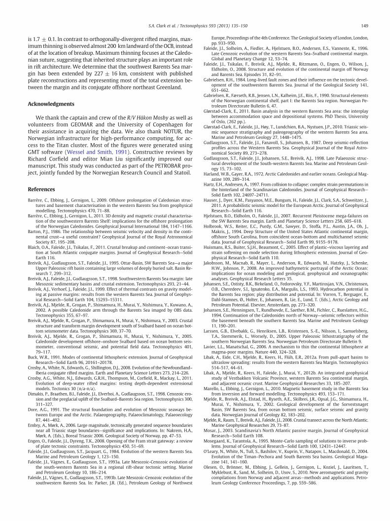
Fig. 9.Magnetic and gravity data (Olesen et al., 2010) and models of the magnetic susceptibility and density along the PETROBAR-07 profile (after Barrère et al., 2009, 2011; Breiviket al., 1999; Marello et al., 2010). VE = 4.

1.0

1.5

2.0

2.5

3.0

3.5

4.0

4.5

5.0

5.5

0 50 100 150 200 250 300 350 400 450 500 550

β-fa

cto

r

Distance (km)

Crustal Thicknes

Fig. 10. Estimated β-factors based on the mean model crustal thickness (black line),minimum and maximum crustal thickness from one standard deviation of the meanmodel (bright red swath), and minimum crustal thickness with an additional 5 km at-tributed to deep sedimentary rocks and volcanics (faded red swath).


Loppa High and Varanger Peninsula, velocities are relatively high(>8 km/s).

One of the most useful features of our MCMC inversion is the quan-tification of uncertainties in the model. We assume a normal distribu-tion of each parameter and define the uncertainty as one standarddeviation of the parameter in the posterior set. Fig. 6b plots the velocityand depth uncertainty values. Fig. 6 also shows “minimum” (c) and“maximum” (d) models based on subtracting and adding the uncer-tainties to the mean model.

Velocity uncertainties range from 0 to 0.5 km/s, with most in therange of 0.1–0.2 km/s. Sedimentary velocity uncertainties are higher inplaces than those of the crust and upper mantle, probably due to atradeoffwith the increased lateral node spacing anddecreased traveltimepick constraint. Depth uncertainties are generally very low, 100–400 m,for layer boundaries with normal-incidence reflection constraint, withthe highest values corresponding to the deepest portions of the basins.Without such constraint, uncertainties increase to 400–800 m beneathVestbakken Volcanic Province, and 300–2100 m at the Moho.

A fundamental expectation of the uncertainties is that they shouldincrease in areas of poor ray coverage (see Fig. 7a and c), particularlyat the lateral edges of the model. This is clearly observed at km 0 andkm 700, where layer velocity and depth uncertainties consistentlyincrease. To first order, velocity uncertainties should correspond torefracted ray coverage (Fig. 7a) and depth uncertainties to reflectedray coverage (Fig. 7c). Relatively high velocity uncertainties in thesedimentary layers at kms 90, 230, and 440–550 clearly correspondto poor refracted ray coverage. However, low uncertainty at km 170,where ray coverage is not good, suggests velocity constraint by thereflected arrivals, possibly due to ray tracing failure against the steeplydipping basin edge. Conversely, high uncertainties at km 130–160,where ray coverage is very good, suggest a possible trade-off between

velocity and layer depth. Relative highs in uncertainty for the crustand upper mantle layers (e.g., km 175) also correspond to decreasedray coverage.

In order to test our results against independent datasets, we usedthe velocity model to develop forward models of the magnetic andgravity data along the profile (Fig. 9). The intent of our study is not a de-tailed account of the density andmagnetic properties of the rocks along


PETROBAR-07, but simply a confirmation that our model is compatiblewith previous results. Direct conversion of P-wave velocities to densi-ties is of limited valuewhenmodeling gravity (Barton, 1986), so insteadwe used the layer boundaries and lateral velocity changes as a guide todefine the boundaries of density and magnetic susceptibility polygons.Values used are in good agreement with the recently published 2D and3D potential fields models of Barrère et al. (2009, 2011) and Marelloet al. (2010). The mantle density structure was modeled after Breiviket al. (1999). A close fit to the observed magnetic and gravity data isobtained using the structure of our velocity model, confirming that ourresults are consistent with independent data.

6. Discussion

6.1. Rift geometry

The multi-phase rift history of the southwest Barents Sea is clearlyreflected in the crustal architecture imaged in the PETROBAR-07 veloc-ity profile. By assuming an original pre-rift crustal thickness of 35 km,we estimate the cumulative crustal thinning (β) factors along the pro-file by dividing the current thickness (Tpostrift) into the assumed originalthickness (Tprerift):

β ¼ TpreriftTpostrift

: ð5Þ

Such an assumption is clearly simplistic, as post-Caledonian crustwas unlikely a uniform 35 km in thickness, but it serves to highlightvariations along the profile and provide a first-order estimate of thin-ning, and by proxy, stretching.

In addition, because of the difficulty in distinguishing the deepestsedimentary strata from crystalline basement, the postrift crustal thick-ness may be overestimated in places, and the β factor consequentlyunderestimated. Since the deepest and oldest sedimentary rocks reachtemperatures andpressureswhere diagenesis and even low-grademeta-morphism give them P-wave velocities in excess of 5.5 km/s, they be-come indistinguishable from uppermost crystalline crust. This effect isexacerbated by the presence of high-velocity carbonates, salt, and intru-sive and extrusive volcanic rocks, all of which complicate the interpreta-tion of pre-rift crystalline basement. As such, the depth to crystallinebasement on our profile should be considered a minimum estimate, asit corresponds to the deepest continuous, parallel, layered reflectivity ob-served on the normal-incidence profiles.

Fig. 10 shows the estimated β factors along the profile (km 0–550;craton not included).We propagate the depth uncertainties to theβ fac-tors by calculating them from the mean, minimum, and maximumcrustal thicknesses. In addition, to account for the possible presence ofsedimentary rocks in our crustal layer, we calculate β factors for theminimum crustal thickness thinned by an additional 5 km (Fig. 10,light red swath). Since early rift basins probably did not exhibit a uni-form thickness across the entire profile, these β values should be con-sidered locally possible but not likely for the entire profile.

Based on themeanmodel, local β factors reach 2.5 at the VestbakkenVolcanic Province and approach 3 at Bjørnøya Basin (for locations, seeFig. 1). The sag subsidence along LoppaHigh andOttar Basin is associatedwith low β values of 1.2–1.4. β factors limited to the early rift phases re-sponsible for forming Ottar and Nordkapp basins are lower than the βfactors west of Loppa High, but locally approach a maximum of 2.

The β factors along the profile generally increase towards theocean–continent boundary (OCB), consistent with observations ofrifted margins globally (Crosby et al., 2011). Maximum thinning isusually coincident with the location of breakup, but here the highestβ factors are observed at Bjørnøya Basin, 200 km southeast of theOCB. This is probably due to the transform nature of the late-stagerifting and breakup. As the obliquity of rifting increased, thinning andstretching actually decreased towards eventual continental breakup.

Furthermore, Late Cretaceous to Paleocene thinning in Vestbakken Vol-canic Province was influenced by pull-apart formation in the releasingbend of the nascent transform line of breakup (Libak et al., 2012b);~100 km to the north, and probably along much of the transformmar-gin edge, β factors are less than 2 (Libak et al., 2012a).

6.2. Crustal extension

Ifwe assume conservationof cross-sectional area,we canuse thinningas a proxy for extension and propagate themodel uncertainties to the ex-tension estimates. The average β factor along the profile is 1.7 ± 0.1,suggesting a pre-extension length of 323 ± 16 km and a total extensionof 227 ± 16 km. With sedimentary rocks in the modeled crustal layer,the average β factor total extension could be even higher.

Paleo-reconstruction of the Baltica and Laurentia plates suggests anoverlap of ~300 km between northeast Greenland and the southwestBarents Sea in the Permian (Torsvik and Cocks, 2005). The geometryof transform breakup produces asymmetry in the conjugates, leavingmost of the extended rift structures in this case on the Barents Seamargin. Our estimate of >200 km of extension is consistent withasymmetric final breakup and the absence of significant rift struc-tures off northeast Greenland at the location conjugate to our pro-file. In contrast, rift-related structures further to the southwest, onthe opposite side of the transform zone, are more prevalent offshoreNE Greenland, and limited on the conjugate Lofoten–Vesterålenmargin(Faleide et al., 2008).

6.3. Caledonian basement

A number of previous authors have interpreted the Caledoniannappes exposed onshore northern Norway to extend beneath the riftbasin architecture of the southwest Barents Sea (Barrère et al., 2009;Breivik et al., 2002; Gudlaugsson et al., 1987; Harland and Gayer, 1972;Marello et al., 2010; Ritzmann and Faleide, 2007). Although the locationand orientation of interpreted Caledonian branches to the north remainsthe subject of debate, it is generally agreed that the Laurentia–Baltica su-ture coincideswith themain fault complex separating the deep BjørnøyaBasin and the LoppaHigh along our profile. Since this also coincideswithmaximum thinning along our profile, we speculate that stretching fo-cused towards the inherited zone of weakness along the suture, andpost-orogenic crustal structure was a strong control on subsequent riftmechanics.

The LoppaHigh has undergone a complex evolution of uplift and sub-sidence phases (Glørstad-Clark, 2011) that cannot be explained by stan-dard riftingmodels. Potentialfieldsmodeling has suggested the presenceof a high-density body beneath LoppaHigh, interpreted alternatively as aCaledonian orogenic retro-wedge of high-grade metamorphic rocks(Ritzmann and Faleide, 2007), a post-Caledonian, rift-related core com-plex (Barrère et al., 2009, 2011), or magmatic intrusions (Marello et al.,2010). High P-wave velocities beneath Loppa High and the results of po-tential fields modeling along the profile are consistent with high densitylower crust here. However, P-wave velocities are insufficient to furtherconstrain its chemical composition and timing of emplacement.

7. Conclusions

We resolve the crustal-scale velocity structure along a profile inthe southwest Barents Sea using stochastic inversion of seismic re-flection and refraction data. Our resultant velocity model is consistentwith previously published potential fields modeling results. Uncer-tainties in the velocity model are propagated to estimates for cumula-tive crustal thinning and total extension of the rift-transform margin.The mean model resolves β factors approaching 3, but uncertainty inthe boundary between sedimentary rocks and crystalline basementsuggests that values may exceed 5. Assuming that modeled crystal-line basement is correct, the average β factor along the entire profile


is 1.7 ± 0.1. In contrast to orthogonally-divergent rifted margins, max-imum thinning is observed almost 200 km landward of theOCB, insteadof at the location of breakup. Maximum thinning focuses at the Caledo-nian suture, suggesting that inherited structure plays an important rolein rift architecture. We determine that the southwest Barents Sea mar-gin has been extended by 227 ± 16 km, consistent with publishedplate reconstructions and representing most of the total extension be-tween the margin and its conjugate offshore northeast Greenland.

Acknowledgments

We thank the captain and crew of the R/V Håkon Mosby as well asvolunteers from GEOMAR and the University of Copenhagen fortheir assistance in acquiring the data. We also thank NOTUR, theNorwegian infrastructure for high-performance computing, for ac-cess to the Titan cluster. Most of the figures were generated usingGMT software (Wessel and Smith, 1991). Constructive reviews byRichard Corfield and editor Mian Liu significantly improved ourmanuscript. This study was conducted as part of the PETROBAR pro-ject, jointly funded by the Norwegian Research Council and Statoil.

References

Barrère, C., Ebbing, J., Gernigon, L., 2009. Offshore prolongation of Caledonian struc-tures and basement characterisation in the western Barents Sea from geophysicalmodelling. Tectonophysics 470, 71–88.

Barrère, C., Ebbing, J., Gernigon, L., 2011. 3D density and magnetic crustal characterisa-tion of the southwestern Barents Shelf: implications for the offshore prolongationof the Norwegian Caledonides. Geophysical Journal International 184, 1147–1166.

Barton, P.J., 1986. The relationship between seismic velocity and density in the conti-nental crust—a useful constraint? Geophysical Journal of the Royal AstronomicalSociety 87, 195–208.

Blaich, O.A., Faleide, J.I., Tsikalas, F., 2011. Crustal breakup and continent–ocean transi-tion at South Atlantic conjugate margins. Journal of Geophysical Research—SolidEarth 116.

Breivik, A.J., Gudlaugsson, S.T., Faleide, J.I., 1995. Ottar-Basin, SW Barents Sea—a majorUpper Paleozoic rift basin containing large volumes of deeply buried salt. Basin Re-search 7, 299–312.

Breivik, A.J., Faleide, J.I., Gudlaugsson, S.T., 1998. Southwestern Barents Sea margin: lateMesozoic sedimentary basins and crustal extension. Tectonophysics 293, 21–44.

Breivik, A.J., Verhoef, J., Faleide, J.I., 1999. Effect of thermal contrasts on gravity model-ing at passive margins: results from the western Barents Sea. Journal of Geophys-ical Research—Solid Earth 104, 15293–15311.

Breivik, A.J., Mjelde, R., Grogan, P., Shimamura, H., Murai, Y., Nishimura, Y., Kuwano, A.,2002. A possible Caledonide arm through the Barents Sea imaged by OBS data.Tectonophysics 355, 67–97.

Breivik, A.J., Mjelde, R., Grogan, P., Shimamura, H., Murai, Y., Nishimura, Y., 2003. Crustalstructure and transform margin development south of Svalbard based on ocean bot-tom seismometer data. Tectonophysics 369, 37–70.

Breivik, A.J., Mjelde, R., Grogan, P., Shimamura, H., Murai, Y., Nishimura, Y., 2005.Caledonide development offshore–onshore Svalbard based on ocean bottom seis-mometer, conventional seismic, and potential field data. Tectonophysics 401,79–117.

Buck, W.R., 1991. Modes of continental lithospheric extension. Journal of GeophysicalResearch—Solid Earth 96, 20161–20178.

Crosby, A., White, N., Edwards, G., Shillington, D.J., 2008. Evolution of the Newfoundland–Iberia conjugate rifted margins. Earth and Planetary Science Letters 273, 214–226.

Crosby, A.G., White, N.J., Edwards, G.R.H., Thompson, M., Corfield, R., Mackay, L., 2011.Evolution of deep-water rifted margins: testing depth-dependent extensionalmodels. Tectonics 30 (n/a-n/a).

Dimakis, P., Braathen, B.I., Faleide, J.I., Elverhoi, A., Gudlaugsson, S.T., 1998. Cenozoic ero-sion and the preglacial uplift of the Svalbard–Barents Sea region. Tectonophysics 300,311–327.

Dore, A.G., 1991. The structural foundation and evolution of Mesozoic seaways be-tween Europe and the Arctic. Palaeogeography, Palaeoclimatology, Palaeoecology87, 441–492.

Embry, A., Mørk, A., 2006. Large magnitude, tectonically generated sequence boundariesnear all Triassic stage boundaries—significance and implications. In: Nakrem, H.A.,Mørk, A. (Eds.), Boreal Triassic 2006. Geological Society of Norway, pp. 47–53.

Engen, O., Faleide, J.I., Dyreng, T.K., 2008. Opening of the Fram strait gateway: a reviewof plate tectonic constraints. Tectonophysics 450, 51–69.

Faleide, J.I., Gudlaugsson, S.T., Jacquart, G., 1984. Evolution of the western Barents Sea.Marine and Petroleum Geology 1, 123–150.

Faleide, J.I., Vågnes, E., Gudlaugsson, S.T., 1993a. Late Mesozoic-Cenozoic evolution ofthe south-western Barents Sea in a regional rift-shear tectonic setting. Marineand Petroleum Geology 10, 186–214.

Faleide, J.I., Vågnes, E., Gudlaugsson, S.T., 1993b. Late Mesozoic-Cenozoic evolution of thesouthwestern Barents Sea. In: Parker, J.R. (Ed.), Petroleum Geology of Northwest

Europe, Proceedings of the 4th Conference. The Geological Society of London, London,pp. 933–950.

Faleide, J.I., Solheim, A., Fiedler, A., Hjelstuen, B.O., Andersen, E.S., Vanneste, K., 1996.Late Cenozoic evolution of the western Barents Sea–Svalbard continental margin.Global and Planetary Change 12, 53–74.

Faleide, J.I., Tsikalas, F., Breivik, A.J., Mjelde, R., Ritzmann, O., Engen, O., Wilson, J.,Eldholm, O., 2008. Structure and evolution of the continental margin off Norwayand Barents Sea. Episodes 31, 82–91.

Gabrielsen, R.H., 1984. Long-lived fault zones and their influence on the tectonic devel-opment of the southwestern Barents Sea. Journal of the Geological Society 141,651–662.

Gabrielsen, R., Færseth, R.B., Jensen, L.N., Kalheim, J.E., Riis, F., 1990. Structural elementsof the Norwegian continental shelf, part I: the Barents Sea region. Norwegian Pe-troleum Directorate Bulletin 6, 47.

Glørstad-Clark, E., 2011. Basin analysis in the western Barents Sea area: the interplaybetween accommodation space and depositional systems. PhD Thesis, Universityof Oslo, (262 pp.).

Glørstad-Clark, E., Faleide, J.I., Høy, T., Lundchien, B.A., Nystuen, J.P., 2010. Triassic seis-mic sequence stratigraphy and paleogeography of the western Barents Sea area.Marine and Petroleum Geology 27, 1448–1475.

Gudlaugsson, S.T., Faleide, J.I., Fanavoll, S., Johansen, B., 1987. Deep seismic-reflectionprofiles across the Western Barents Sea. Geophysical Journal of the Royal Astro-nomical Society 89, 273–278.

Gudlaugsson, S.T., Faleide, J.I., Johansen, S.E., Breivik, A.J., 1998. Late Palaeozoic struc-tural development of the South-western Barents Sea. Marine and Petroleum Geol-ogy 15, 73–102.

Harland, W.B., Gayer, R.A., 1972. Arctic Caledonides and earlier oceans. Geological Mag-azine 109, 289–314.

Hartz, E.H., Andresen, A., 1997. From collision to collapse: complex strain permutations inthe hinterland of the Scandinavian Caledonides. Journal of Geophysical Research—Solid Earth 102, 24697–24711.

Hauser, J., Dyer, K.M., Pasyanos, M.E., Bungum, H., Faleide, J.I., Clark, S.A., Schweitzer, J.,2011. A probabilistic seismic model for the European Arctic. Journal of GeophysicalResearch—Solid Earth 116.

Hjelstuen, B.O., Eldholm, O., Faleide, J.I., 2007. Recurrent Pleistocene mega-failures onthe SW Barents Sea margin. Earth and Planetary Science Letters 258, 605–618.

Holbrook, W.S., Reiter, E.C., Purdy, G.M., Sawyer, D., Stoffa, P.L., Austin, J.A., Oh, J.,Makris, J., 1994. Deep Structure of the United States Atlantic continental margin,offshore South Carolina, from coincident ocean-bottom and multichannel seismicdata. Journal of Geophysical Research—Solid Earth 99, 9155–9178.

Huismans, R.S., Buiter, S.J.H., Beaumont, C., 2005. Effect of plastic–viscous layering andstrain softening on mode selection during lithospheric extension. Journal of Geo-physical Research—Solid Earth 110.

Jakobsson, M., Macnab, R., Mayer, L., Anderson, R., Edwards, M., Hatzky, J., Schenke,H.W., Johnson, P., 2008. An improved bathymetric portrayal of the Arctic Ocean:implications for ocean modeling and geological, geophysical and oceanographicanalyses. Geophysical Research Letters 35.

Johansen, S.E., Ostisty, B.K., Birkeland, O., Fedorovsky, Y.F., Martirosjan, V.N., Christensen,O.B., Cheredeev, S.I., Ignatenko, E.A., Margulis, L.S., 1993. Hydrocarbon potential inthe Barents Sea region; play distribution and potential. In: Vorren, T., Bergsager, E.,Dahl-Stamnes, Ø., Holter, E., Johansen, B., Lie, E., Lund, T. (Eds.), Arctic Geology andPetroleum Potential. Elsevier, Amsterdam, pp. 273–320.

Johansen, S.E., Henningsen, T., Rundhovde, E., Saether, B.M., Fichler, C., Rueslatten, H.G.,1994. Continuation of the Caledonides north of Norway—seismic reflectors withinthe basement beneath the southern Barents Sea. Marine and Petroleum Geology11, 190–201.

Larssen, G.B., Elvebakk, G., Henriksen, L.B., Kristensen, S.-E., Nilsson, I., Samuelsberg,T.A., Stemmerik, L., Worsely, D., 2005. Upper Paleozoic lithostratigraphy of thesouthern Norwegian Barents Sea. Norwegian Petroleum Directorate Bulletin 9.

Lavier, L.L., Manatschal, G., 2006. A mechanism to thin the continental lithosphere atmagma-poor margins. Nature 440, 324–328.

Libak, A., Eide, C.H., Mjelde, R., Keers, H., Flüh, E.R., 2012a. From pull-apart basins toultraslow spreading: results from the western Barents Sea Margin. Tectonophysics514–517, 44–61.

Libak, A., Mjelde, R., Keers, H., Faleide, J., Murai, Y., 2012b. An integrated geophysicalstudy of Vestbakken Volcanic Province, western Barents Sea continental margin,and adjacent oceanic crust. Marine Geophysical Researches 33, 185–207.

Marello, L., Ebbing, J., Gernigon, L., 2010. Magnetic basement study in the Barents Seafrom inversion and forward modelling. Tectonophysics 493, 153–171.

Mjelde, R., Breivik, A.J., Elstad, H., Ryseth, A.E., Skilbrei, J.R., Opsal, J.G., Shimamura, H.,Murai, Y., Nishimura, Y., 2002. Geological development of the SorvestsnagetBasin, SW Barents Sea, from ocean bottom seismic, surface seismic and gravitydata. Norwegian Journal of Geology 82, 183–202.

Mjelde, R., Raum, T., Breivik, A.J., Faleide, J.I., 2008. Crustal transect across the North Atlantic.Marine Geophysical Researches 29, 73–87.

Mosar, J., 2003. Scandinavia's North Atlantic passive margin. Journal of GeophysicalResearch—Solid Earth 108.

Mosegaard, K., Tarantola, A., 1995. Monte-Carlo sampling of solutions to inverse prob-lems. Journal of Geophysical Research—Solid Earth 100, 12431–12447.

O'Leary, N., White, N., Tull, S., Bashilov, V., Kuprin, V., Natapov, L., Macdonald, D., 2004.Evolution of the Timan–Pechora and South Barents Sea basins. Geological Maga-zine 141, 141–160.

Olesen, O., Brönner, M., Ebbing, J., Gellein, J., Gernigon, L., Koziel, J., Lauritsen, T.,Myklebust, R., Sand, M., Solheim, D., Usov, S., 2010. New aeromagnetic and gravitycompilations from Norway and adjacent areas—methods and applications. Petro-leum Geology Conference Proceedings, 7, pp. 559–586.


Rise, L., Ottesen, D., Berg, K., Lundin, E., 2005. Large-scale development of the mid-Norwegian margin during the last 3 million years. Marine and Petroleum Geology22, 33–44.

Ritzmann, O., Faleide, J.I., 2007. Caledonian basement of the western Barents Sea. Tec-tonics 26, 417–435.

Ritzmann, O., Faleide, J.I., 2009. The crust and mantle lithosphere in the Barents Sea/KaraSea region. Tectonophysics 470, 89–104.

Roberts, D., 2003. The Late Riphean Porsangerhalvoyan tectonometamorphic event inthe North Norwegian Caledonides: a comment on nomenclature. Norwegian Jour-nal of Geology 83, 275–277.

Roberts, D., Gee, D.G., 1985. An introduction to the structure of the ScandinavianCaledonides. In: Gee, D.G., Sturt, B.A. (Eds.), The Caledonide Orogen—Scandinaviaand related areas. Wiley, Chichester, pp. 55–68.

Rosenbaum, G., Weinberg, R.F., Regenauer-Lieb, K., 2008. The geodynamics of litho-spheric extension. Tectonophysics 458, 1–8.

Ryseth, A., Augustson, J.H., Charnock, M., Haugerud, O., Knutsen, S.-M., Midbøe, P.S., Opsal,J.G., Sundsbø, G., 2003. Cenozoic stratigraphy and evolution of the SørvestsnagetBasin, southwestern Barents Sea. Norwegian Journal of Geology 83, 107–130.

Sigmond, E.M.O., 2002. Geologisk Kart over land- og havområder i Nordeuropa,målestokk 1:4000000. Norges Geologiske Undersøkelse, Trondheim.

Torsvik, T.H., Cocks, L.R.M., 2005. Norway in space and time: a centennial cavalcade.Norwegian Journal of Geology 85, 73–86.

Tsikalas, F., Faleide, J.I., Kusznir, N.J., 2008. Along-strike variations in rifted margin crustalarchitecture and lithosphere thinning between northern Voring and Lofoten marginsegments off mid-Norway. Tectonophysics 458, 68–81.

Vorren, T.O., Richardsen, G., Knutsen, S.-M., Henriksen, E., 1991. Cenozoic erosion and sed-imentation in the western Barents Sea. Marine and Petroleum Geology 8, 317–340.

Wessel, P., Smith, W.H.F., 1991. Free software helps map and display data. EOS. Trans-actions of the American Geophysical Union 72.

White, R.S., Smith, L.K., 2009. Crustal structure of the Hatton and the conjugate eastGreenland rifted volcanic continental margins, NE Atlantic. Journal of GeophysicalResearch—Solid Earth 114.

Wilson, J.T., 1966. Did the Atlantic close and then reopen? Nature 211, 676–681.Wood, R.J., Edrich, S.P., Hutchison, I., 1989. Influence of North Atlantic tectonics on the

large-scale uplift of the Stappen High and Loppa High, western Barents Shelf. In:Tankard, A.J., Balkwill, H.R. (Eds.), Extensional Tectonics and Stratigraphy of theNorth Atlantic Margins, pp. 559–566.

Zelt, C.A., Forsyth, D.A., 1994. Modeling wide-angle seismic data for crustal structure—southeastern Grenville Province. Journal of Geophysical Research—Solid Earth 99,11687–11704.

Zelt, C.A., Smith, R.B., 1992. Seismic traveltime inversion for 2-D crustal velocity struc-ture. Geophysical Journal International 108, 16–34.

Ziegler, P.A., 1988. Evolution of the Arctic–North Atlantic and the Western Thetys.Ziegler, P.A., Cloetingh, S., 2004. Dynamic processes controlling evolution of rifted basins.

Earth-Science Reviews 64, 1–50.

Stochastic velocity inversion of seismic reflection/refraction traveltime data for rift structure of...

Documents

Transcript of Stochastic velocity inversion of seismic reflection/refraction traveltime data for rift structure of...