Stereo Vision Tracking of Multiple Objects in Complex Indoor Environments
23
Sensors 2010, 10, 8865-8887; doi:10.3390/s101008865 sensors ISSN 1424-8220 www.mdpi.com/journal/sensors Article Stereo Vision Tracking of Multiple Objects in Complex Indoor Environments Marta Marrón-Romera 1, *, Juan C. Garcí a 1 , Miguel A. Sotelo 1 , Daniel Pizarro 1 , Manuel Mazo 1 , José M. Cañas 2 , Cristina Losada 1 and Álvaro Marcos 1 1 Electronics Department, University of Alcalá , Campus Universitario s/n, 28805, Alcalá de Henares, Madrid, Spain; E-Mails: [email protected] (J.G.); [email protected] (M.S.); [email protected] (D.P.); [email protected] (M.M.); [email protected] (C.L.); [email protected] (A.M.) 2 Departamento de Sistemas Telemá ticos y Computación, Universidad Rey Juan Carlos, C/Tulipán s/n, 28933, Móstoles, Madrid, Spain; E-Mail: [email protected] (J.C.) * Author to whom correspondence should be addressed; E-Mail: [email protected]; Tel.: +34-918856586; Fax: +34-918856591. Received: 31 August 2010; in revised form: 7 September 2010 / Accepted: 25 September 2010 / Published: 28 September 2010 Abstract: This paper presents a novel system capable of solving the problem of tracking multiple targets in a crowded, complex and dynamic indoor environment, like those typical of mobile robot applications. The proposed solution is based on a stereo vision set in the acquisition step and a probabilistic algorithm in the obstacles position estimation process. The system obtains 3D position and speed information related to each object in the robot’s environment; then it achieves a classification between building elements (ceiling, walls, columns and so on) and the rest of items in robot surroundings. All objects in robot surroundings, both dynamic and static, are considered to be obstacles but the structure of the environment itself. A combination of a Bayesian algorithm and a deterministic clustering process is used in order to obtain a multimodal representation of speed and position of detected obstacles. Performance of the final system has been tested against state of the art proposals; test results validate the authors’ proposal. The designed algorithms and procedures provide a solution to those applications where similar multimodal data structures are found. Keywords: 3D tracking; Bayesian estimation; stereo vision sensor; mobile robots OPEN ACCESS
Transcript of Stereo Vision Tracking of Multiple Objects in Complex Indoor Environments
Sensors 2010, 10, 8865-8887; doi:10.3390/s101008865
sensors ISSN 1424-8220
www.mdpi.com/journal/sensors
Article
Stereo Vision Tracking of Multiple Objects in Complex
Indoor Environments
Marta Marrón-Romera 1,*, Juan C. García
1, Miguel A. Sotelo
1, Daniel Pizarro
1, Manuel Mazo
1,
José M. Cañas 2, Cristina Losada
1 and Álvaro Marcos
1
1 Electronics Department, University of Alcalá, Campus Universitario s/n, 28805, Alcalá de Henares,
Madrid, Spain; E-Mails: [email protected] (J.G.); [email protected] (M.S.);
[email protected] (D.P.); [email protected] (M.M.); [email protected] (C.L.);
[email protected] (A.M.) 2 Departamento de Sistemas Telemáticos y Computación, Universidad Rey Juan Carlos, C/Tulipán
s/n, 28933, Móstoles, Madrid, Spain; E-Mail: [email protected] (J.C.)
* Author to whom correspondence should be addressed; E-Mail: [email protected];
Tel.: +34-918856586; Fax: +34-918856591.
Received: 31 August 2010; in revised form: 7 September 2010 / Accepted: 25 September 2010 /
Published: 28 September 2010
Abstract: This paper presents a novel system capable of solving the problem of tracking
multiple targets in a crowded, complex and dynamic indoor environment, like those typical
of mobile robot applications. The proposed solution is based on a stereo vision set in the
acquisition step and a probabilistic algorithm in the obstacles position estimation process.
The system obtains 3D position and speed information related to each object in the robot’s
environment; then it achieves a classification between building elements (ceiling, walls,
columns and so on) and the rest of items in robot surroundings. All objects in robot
surroundings, both dynamic and static, are considered to be obstacles but the structure of
the environment itself. A combination of a Bayesian algorithm and a deterministic
clustering process is used in order to obtain a multimodal representation of speed and
position of detected obstacles. Performance of the final system has been tested against state
of the art proposals; test results validate the authors’ proposal. The designed algorithms and
procedures provide a solution to those applications where similar multimodal data
structures are found.
Keywords: 3D tracking; Bayesian estimation; stereo vision sensor; mobile robots
OPEN ACCESS
Sensors 2010, 10
8866
1. Introduction
Visual tracking is one of the areas of greater interest in robotics as it is related with topics such as
visual surveillance or mobile robots navigation. Multiple approaches to this problem have been
developed by research community during last decades [1]. Among them, a sorting can be done
according to methods used to detect or extract information from the image about objects in the scene:
With static cameras: background subtraction is generally applied to extract image information
corresponding to dynamic objects in the scene. This method is wide spread among the research
community [2-4], mainly in surveillance applications.
With a known model of the object to be tracked: this situation is very common in tracking
applications, either using static cameras [3,4] or dynamic ones [5,6]. The detection process is
computational more expensive, but the number of false alarms and the robustness of the detector
are bigger than if looking for any kind of objects.
All the referred works solve the detection problem quite easily, thanks to the application of the
mentioned restrictions. However, an appropriate solution is more difficult to find when the problem to
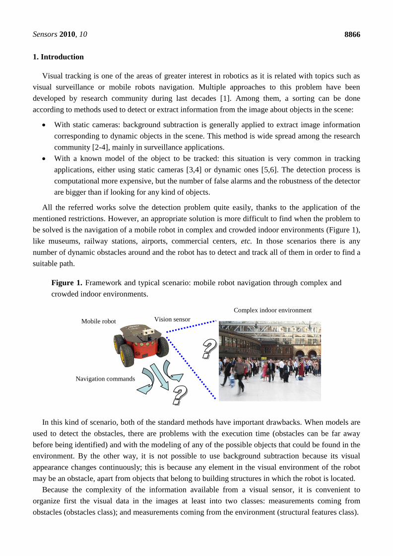
be solved is the navigation of a mobile robot in complex and crowded indoor environments (Figure 1),
like museums, railway stations, airports, commercial centers, etc. In those scenarios there is any
number of dynamic obstacles around and the robot has to detect and track all of them in order to find a
suitable path.
Figure 1. Framework and typical scenario: mobile robot navigation through complex and
crowded indoor environments.
In this kind of scenario, both of the standard methods have important drawbacks. When models are
used to detect the obstacles, there are problems with the execution time (obstacles can be far away
before being identified) and with the modeling of any of the possible objects that could be found in the
environment. By the other way, it is not possible to use background subtraction because its visual
appearance changes continuously; this is because any element in the visual environment of the robot
may be an obstacle, apart from objects that belong to building structures in which the robot is located.
Because the complexity of the information available from a visual sensor, it is convenient to
organize first the visual data in the images at least into two classes: measurements coming from
obstacles (obstacles class); and measurements coming from the environment (structural features class).
Navigation commands
Complex indoor environment
Mobile robot Vision sensor
Sensors 2010, 10
8867
Once this information is available, data classified in the environment class can be used to make a
reconstruction of robot surroundings structure. This process is especially interesting for robot
navigation, as it can be used in a SLAM (Simultaneous Localization and Mapping [7]) task.
At the same time, data assigned to the obstacles class can be used as an input for any of the tracking
algorithms proposed by the scientific community. Taking into account the measurements
characteristics, the position tracker has to consider the noise related to them in order to achieve reliable
tracking results. Probabilistic algorithms, such as particle filters (PFs, [8-10]) and Kalman filters
(KFs, [11,12]), can be used to develop this task as they include this noisy behavior in the estimation
process by means of a probabilistic model.
Anyway, the objective is to calculate the posterior probability (also called belief, ) of the
state vector and upon the output one , which informs about the position of the target, by means of
the Bayes rule, and through a recursive two steps estimation process (prediction-correction), in which
some of the involved variables are stochastic.
Most solutions to this multi-tracking problem use one estimator for each object to be tracked [12,13].
These techniques are included in what is called MHT (Multi-Hypothesis Tracking) algorithm. It is also
possible to use a single estimator for all the targets if the state vector size is dynamically adapted to
include the state variables of the objects’ model as they appear or disappear in the scene [14,15].
Nevertheless, both options are computationally very expensive in order to use them in real
time applications.
Then, the most suitable solution is to exploit the multimodality of the probabilistic algorithms in
order to include all needed estimations in a single density function. With this idea, a PF is used as a
multimodal estimator [16,17]. This idea has not been exploited by the scientific community adducing
to the inefficiency of the estimation, due to the impoverishment problem that the PF suffers when
working with multimodal densities [18,19].
Anyway, an association algorithm is needed. The association problem is easier if a single
measurement for each target is available at each sample time [20]. In contrast, the biggest the amount
of information from each model is, the most reliable the estimation will be.
In the work presented here, the source of information is a vision system in order to obtain as more
position information from each tracked object as possible. Thus, the needed association algorithm has
also a high computational load but the reliability of the tracking process is increased.
The scientific community has tested different alternatives for the association task, including
Maximum Likelihood (ML), Nearest Neighbor (NN) and Probabilistic Data Association (PDA) [20].
In our case, we have selected the NN solution due to its deterministic character. Finally, not all
proposals referred to in this introduction are appropriate if the number of objects to track is variable: it
is necessary an extension of the previously mentioned algorithms.
In our work, the multimodal ability of the PF is used, and its impoverishment problem is mitigated
by using a deterministic NN clustering process that, used as association process, is combined with the
probabilistic approach in order to obtain efficient multi-tracking results. We use an extended version of
a Bootstrap particle filter [9], called XPFCP (eXtended Particle Filter with Clustering Process), to
achieve the position estimation task with a single filter, in real time, and for tracking a variable number
of objects detected with the on-board stereo vision process. Figure 2 shows a functional description of
the whole tracking application.
tt yxp :1
tx
ty

Sensors 2010, 10
8868
Figure 2. General description of the global stereo vision based tracking system.
Data classified as belonging to the structural features class can be used by standard SLAM
algorithms for environmental reconstruction tasks; however, this question is out of the scope of present
paper as well as a detailed description of the stereo vision system.
This paper will describe the functionality of the two main processes of the multi-tracking proposal:
Section 2 will detail the object detector, classifier and 3D locator; Section 3 will describe the multiple
obstacles tracker, the XPFCP algorithm. Section 4 will show the obtained results under a set of testing
scenarios. Finally, the paper ends with conclusions about the whole system behavior and the
obtained results.
2. Detection, Classification and Localization Processes
A stereo vision subsystem is considered as one of the most adequate ways to acquire important
information about the different elements found in a dynamic environment. That is because:
The amount of information that can be extracted from an image is much bigger than the one that
can be obtained from any other kind of sensor, such as laser or sonar [21].
As the environmental configuration changes with time, with a single camera is not possible to
obtain the depth coordinate of the objects’ position vector, and thus a stereo vision arrangement
is needed.
An alternative to this visual sensor configuration could be to use a Time-Of-Flight (TOF) camera that
provides depth information. However, currently these cameras are not available at an affordable price
and the information obtained with this sensor is still far from versatile (not valid for long distances) and
accurate (post-acquisition process is normally needed in order to compensate reflection effects).
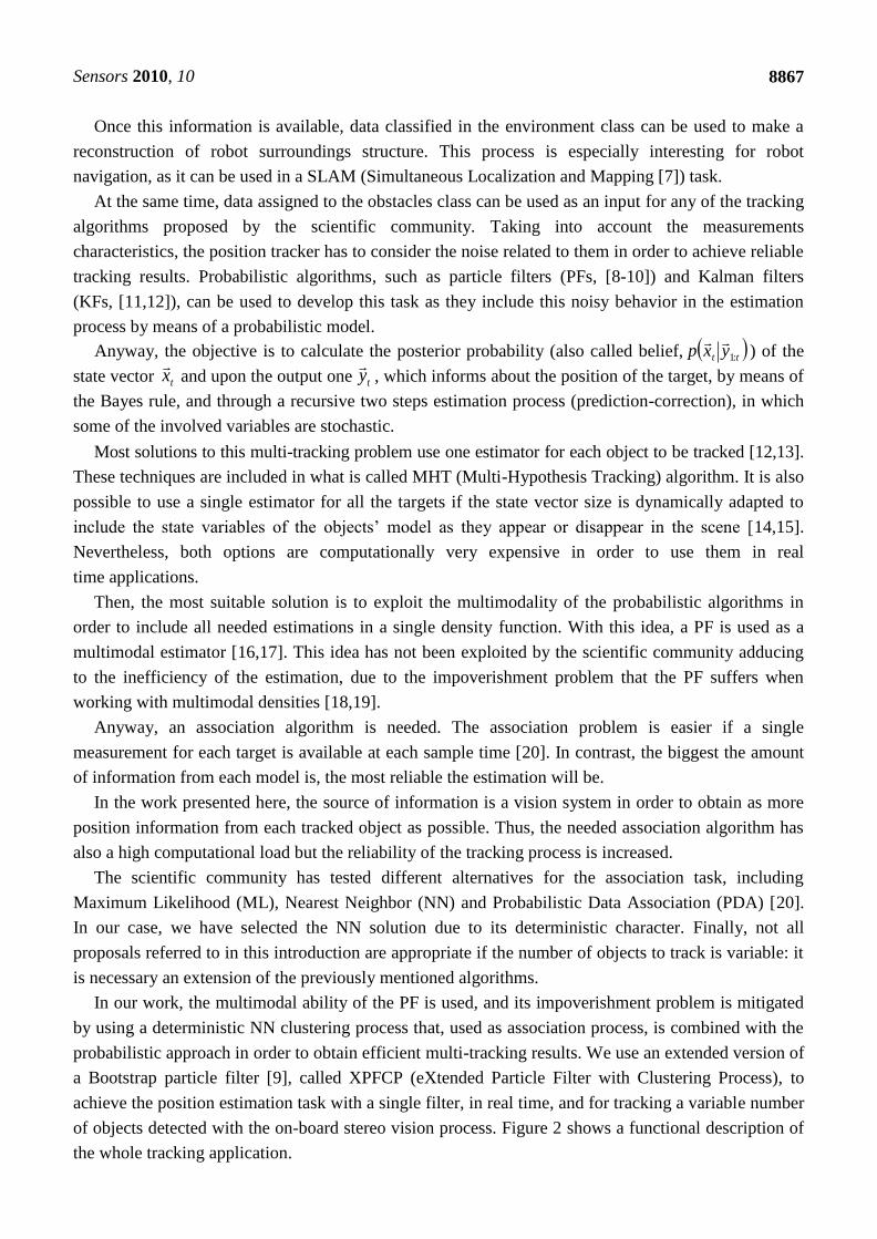
A matching process based on the stereo vision system epipolar geometry allows obtaining the
desired 3D position input information of a point Pt from its projections, pl,t and pr,t,
in a pair of synchronized images ( , ), as shown in Figure 3.
Ttptptp zyx ,,,
Ttpltpltl vuI ,,,,, Ttprtprtr vuI ,,,,,
Stereo Vision System
Object Detection.
Classification: Obstacle/ Environment.
3D Localization
Local Environmental
Reconstruction
Multiple Obstacles’ Tracker:
the XPFCP
Structural features class
Obstacle class
Input measurements
Sensors 2010, 10
8869
Figure 3. Functional description of the stereo vision data extraction process.
In this work, the left-right image matching process is solved with a Zero Mean Normalized Cross
Correlation (ZNCC), due to its robustness [22]. Each sampling time, t, for every pixel of interest (i.e.,
in the left image ), this process consists on looking for a similar gray level among the
pixels in the epipolar line at the paired image (the right one ). 3D location of paired pixels can be
found if, after a careful calibration process of both cameras location, the geometric extrinsic
parameters of rotation, , and translation, , are known.
As it can be expected, this process is very time consuming. Therefore the 3D information to be
obtained should be limited to set of points of interest in both images. In the case of this work, points
coming from objects edges have enough information to develop the tracking task. Moreover, just the
edges information will enable the possibility of partially reconstructing the structure of the
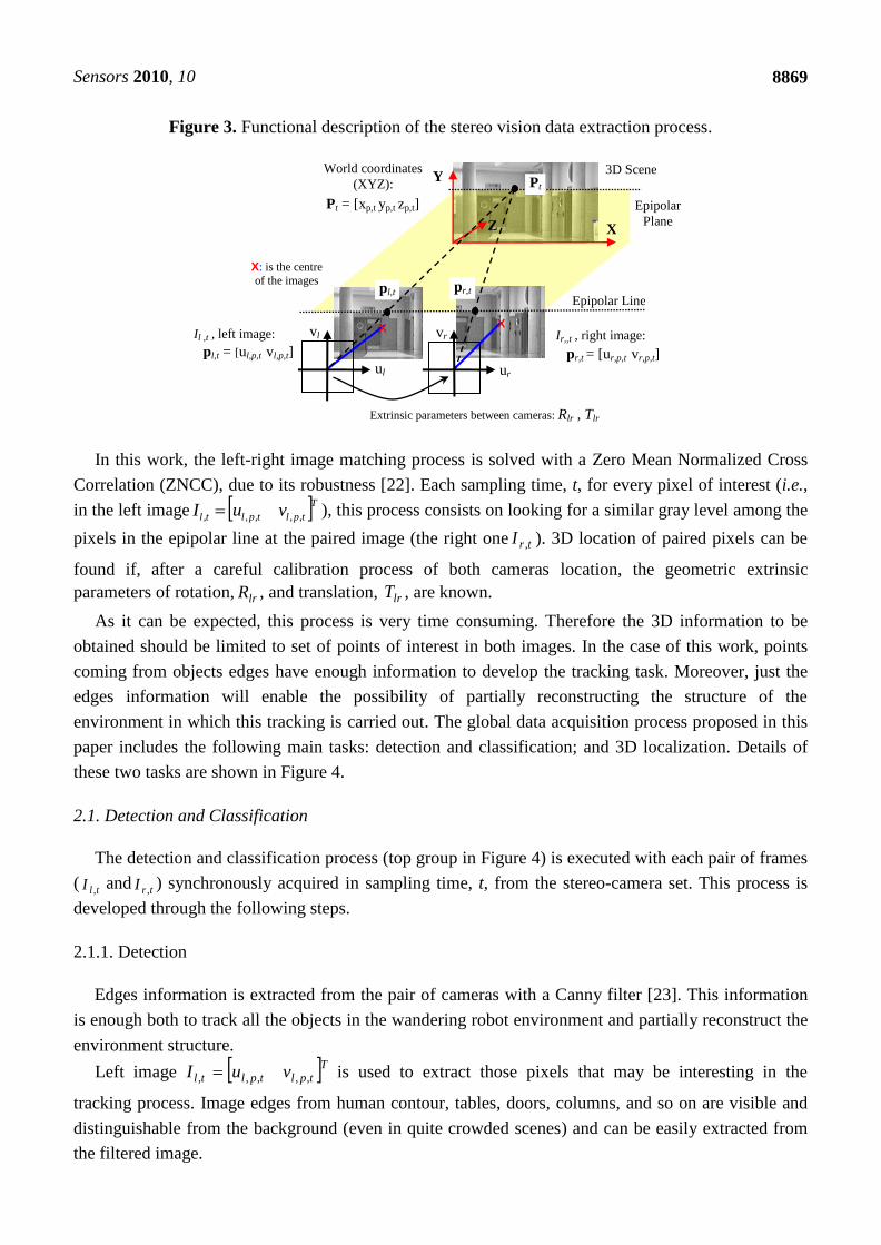
environment in which this tracking is carried out. The global data acquisition process proposed in this
paper includes the following main tasks: detection and classification; and 3D localization. Details of
these two tasks are shown in Figure 4.
2.1. Detection and Classification
The detection and classification process (top group in Figure 4) is executed with each pair of frames
( and ) synchronously acquired in sampling time, t, from the stereo-camera set. This process is
developed through the following steps.
2.1.1. Detection
Edges information is extracted from the pair of cameras with a Canny filter [23]. This information
is enough both to track all the objects in the wandering robot environment and partially reconstruct the
environment structure.
Left image is used to extract those pixels that may be interesting in the
tracking process. Image edges from human contour, tables, doors, columns, and so on are visible and
distinguishable from the background (even in quite crowded scenes) and can be easily extracted from
the filtered image.
Ttpltpltl vuI ,,,,,
trI ,
lrR lrT
tlI , trI ,
Ttpltpltl vuI ,,,,,
Extrinsic parameters between cameras: Rlr , Tlr
ul
vl
Epipolar Line
pl,t = [ul,p,t vl,p,t] pr,t = [ur,p,t vr,p,t]
Il ,t , left image:
Y
Z
Epipolar
Plane
X
X: is the centre
of the images
X
Ir,,t , right image:
Pt = [xp,t yp,t zp,t]
ur
X vr
World coordinates
(XYZ): Pt
pl,t pr,t
3D Scene
Sensors 2010, 10
8870
Figure 4. Flowchart of the data acquisition subsystem, based on a stereo vision process.
Main tasks are: detection and classification (blocks at the top); and 3D localization (blocks
at the bottom). Inner structure of each main task is highlighted and detailed.
In order to robustly find structural features, the Canny image is zeroed in the Regions Of Interest
(ROIs) where an obstacle is expected to appear. Therefore, the classification step is run over a partial
Canny image , though the full image is recovered to develop the
3D localization.
2.1.2. Classification: Structural and Non-Structural Features
Within the partial Canny image , edges corresponding with environmental structures have
the characteristic of forming long lines. Thus, the classification process starts seeking structural shapes
in the resulting image, through these typical features. Hough transform is used to search these long line
segments in the partial Canny image.
The function cvHoughLines2 [24] from OpenCV [25] library is used to accomplish the probabilistic
Hough transform. This version of the Hough transform made by OpenCV allows finding line segments
Tmcannyitlitlitlcanny vuI
:1,,,,,,
tlcannyI ,,
DETECTION:
Canny Left –
ROI obstacles position
3D LOCALIZATION
of Obstacles’ Features
Epipolar Matching
(ZNCC Correlation)
Stereo vision Camera Set
Capture Left – Right frame
Obstacles’ Features in 3D
3D LOCALIZATION
of Structural Features
Epipolar Matching
(ZNCC Correlation)
Structural
Features in 3D
To the Multi-Obstacles Tracker
mitritli
tritli
vv
uu
:1,,,,
,,,,
mcannyitli
tli
tlcannyv
uI
:1,,
,,
,,
mstructureitli
tli
tlstructurev
uI
:1,,
,,
,,
mobstaclesiti
ti
ti
tobstacles
z
y
x
Y
:1,
,
,
,
mstructureiti
ti
ti
tstructure
z
y
x
Y
:1,
,
,
,
mobstaclesitli
tli
tlobstaclesv
uI
:1,,
,,
,,
CLASSIFICATION:
Hough 2D in Canny Left - ROI
Looking for LongLines
Environmental structures: LongLines
Obstacles: Left – LongLines + ROI
DETECTION & CLASSIFICATION
TASK
FILTERING
Obstacles Features’
XZ Neighborhood Filter
+ Height Noise Filter
3D LOCALIZATION
TASK

Sensors 2010, 10
8871
instead of whole ones if the image contains few long linear segments. This is the case of present
application when obstacles in front of the camera set may occlude the structural elements of the scene.
This probabilistic version of Hough transform has five parameters to be tuned:
rho and theta are respectively the basic Hough transform distance and angle resolution
parameters in pixels and radians.
threshold is the basic limit to overpass by the Hough accumulator in order to consider that a line
exists.
length is needed in the probabilistic version of Hough transform, and is the minimum line
length, in pixels, for the detector of segments. This parameter is very important in the related
work as it allows taking into account a line made by very short segments, like those generated in
scenes with many occlusions.
gap is also needed in the probabilistic version of Hough transform. This is the maximum gap
in pixels between segment lines to be treated as a single line segment. This parameter is
significant here, because it allows generating valid lines with very separated segments, due to
occluding obstacles.
Due to the diversity of conditions that may appear in the experimental conditions an analytical
study cannot be performed and thus all parameters have been empirically set. As a result of the
challenging situation of obstacles in present application, not all lines related to structural elements in
the environment are classified as structural features. In any case, the algorithm detects well enough the
structural features existing in the scene: walls, columns, ceiling, floor, windows and so on. In the same
way, it can also generate an obstacles features’ class neat enough to be used in the tracking step.
At the end of this classification step, two images are, therefore, obtained using the described process:
with the environmental structures, formed by the long lines
found at the partial Canny image.
with the full Canny image zeroed at the environmental
structures.
2.2. 3D Localization of Structural and Obstacles’ Features
Both images are the inputs to a 3D localization process to obtain the 3D coordinates of structural
and obstacles’ features .
This is done in two phases by a matching process based on the epipolar geometry of the vision system;
these phases are: 3D localization and obstacles’ features filtering.
2.2.1. Phase 1: 3D Localization
Features’ classes and are respectively obtained calculating the ZNCC value for
each non-zero pixel at the corresponding modified left images, and and using the
full right image . Those features whose ZNCC values reaches a threshold are validated and finally
classified in the corresponding features’ classes, or .
Tmstructureitlitlitlstructure vuI
:1,,,,,,
Tmobstaclesitlitlitlobstacles vuI:1,,,,,,
Tmstructureititititstructure zyxY:1,,,,
Tmobstaclesititititobstacles zyxY:1,,,,
tstructureY , tobstaclesY ,
tlstructureI ,, tlobstaclesI ,,
trI ,
tstructureY , tobstaclesY ,
Sensors 2010, 10
8872
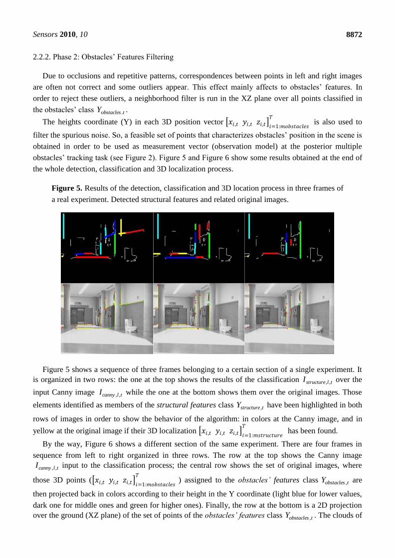
2.2.2. Phase 2: Obstacles’ Features Filtering
Due to occlusions and repetitive patterns, correspondences between points in left and right images
are often not correct and some outliers appear. This effect mainly affects to obstacles’ features. In
order to reject these outliers, a neighborhood filter is run in the XZ plane over all points classified in
the obstacles’ class .
The heights coordinate (Y) in each 3D position vector 𝑥𝑖 ,𝑡 𝑦𝑖 ,𝑡 𝑧𝑖 ,𝑡 𝑖=1:𝑚𝑜𝑏𝑠𝑡𝑎𝑐𝑙𝑒𝑠
𝑇 is also used to
filter the spurious noise. So, a feasible set of points that characterizes obstacles’ position in the scene is
obtained in order to be used as measurement vector (observation model) at the posterior multiple
obstacles’ tracking task (see Figure 2). Figure 5 and Figure 6 show some results obtained at the end of
the whole detection, classification and 3D localization process.
Figure 5. Results of the detection, classification and 3D location process in three frames of
a real experiment. Detected structural features and related original images.
Figure 5 shows a sequence of three frames belonging to a certain section of a single experiment. It
is organized in two rows: the one at the top shows the results of the classification over the
input Canny image while the one at the bottom shows them over the original images. Those
elements identified as members of the structural features class have been highlighted in both
rows of images in order to show the behavior of the algorithm: in colors at the Canny image, and in
yellow at the original image if their 3D localization 𝑥𝑖 ,𝑡 𝑦𝑖 ,𝑡 𝑧𝑖 ,𝑡 𝑖=1:𝑚𝑠𝑡𝑟𝑢𝑐𝑡𝑢𝑟𝑒
𝑇 has been found.
By the way, Figure 6 shows a different section of the same experiment. There are four frames in
sequence from left to right organized in three rows. The row at the top shows the Canny image
input to the classification process; the central row shows the set of original images, where
those 3D points ( 𝑥𝑖 ,𝑡 𝑦𝑖 ,𝑡 𝑧𝑖 ,𝑡 𝑖=1:𝑚𝑜𝑏𝑠𝑡𝑎𝑐𝑙𝑒𝑠
𝑇) assigned to the obstacles’ features class are
then projected back in colors according to their height in the Y coordinate (light blue for lower values,
dark one for middle ones and green for higher ones). Finally, the row at the bottom is a 2D projection
over the ground (XZ plane) of the set of points of the obstacles’ features class . The clouds of
tobstaclesY ,
tlstructureI ,,
tlcannyI ,,
tstructureY ,
tlcannyI ,,
tobstaclesY ,
tobstaclesY ,
Sensors 2010, 10
8873
points in the 2D projection allow perform the tracking task of the four persons found in the
original sequence.
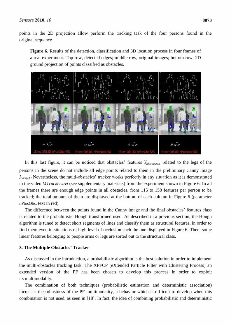
Figure 6. Results of the detection, classification and 3D location process in four frames of
a real experiment. Top row, detected edges; middle row, original images; bottom row, 2D
ground projection of points classified as obstacles.
In this last figure, it can be noticed that obstacles’ features related to the legs of the
persons in the scene do not include all edge points related to them in the preliminary Canny image
Icanny,l,t Nevertheless, the multi-obstacles’ tracker works perfectly in any situation as it is demonstrated
in the video MTracker.avi (see supplementary materials) from the experiment shown in Figure 6. In all
the frames there are enough edge points in all obstacles, from 115 to 150 features per person to be
tracked; the total amount of them are displayed at the bottom of each column in Figure 6 (parameter
nPtosObs, text in red).
The difference between the points found in the Canny image and the final obstacles’ features class
is related to the probabilistic Hough transformed used. As described in a previous section, the Hough
algorithm is tuned to detect short segments of lines and classify them as structural features, in order to
find them even in situations of high level of occlusion such the one displayed in Figure 6. Then, some
linear features belonging to people arms or legs are sorted out to the structural class.
3. The Multiple Obstacles’ Tracker
As discussed in the introduction, a probabilistic algorithm is the best solution in order to implement
the multi-obstacles tracking task. The XPFCP (eXtended Particle Filter with Clustering Process) an
extended version of the PF has been chosen to develop this process in order to exploit
its multimodality.
The combination of both techniques (probabilistic estimation and deterministic association)
increases the robustness of the PF multimodality, a behavior which is difficult to develop when this
combination is not used, as seen in [18]. In fact, the idea of combining probabilistic and deterministic
tobstaclesY ,
Sensors 2010, 10
8874
techniques for tracking multiple objects has been proposed in different previous works, such as [6]
or [26]. However none of them faced the idea of reinforcing the PF multimodality within the
deterministic framework.
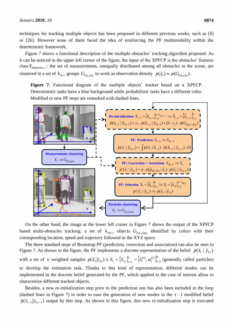
Figure 7 shows a functional description of the multiple obstacles’ tracking algorithm proposed. As
it can be noticed in the upper left corner of the figure, the input of the XPFCP is the obstacles’ features
class : the set of measurements, unequally distributed among all obstacles in the scene, are
clustered in a set of groups to work as observation density .
Figure 7. Functional diagram of the multiple objects’ tracker based on a XPFCP.
Deterministic tasks have a blue background while probabilistic tasks have a different color.
Modified or new PF steps are remarked with dashed lines.
On the other hand, the image at the lower left corner in Figure 7 shows the output of the XPFCP
based multi-obstacles tracking: a set of objects identified by colors with their
corresponding location, speed and trajectory followed in the XYZ space.
The three standard steps of Bootstrap PF (prediction, correction and association) can also be seen in
Figure 7. As shown in the figure, the PF implements a discrete representation of the belief
with a set of weighted samples (generally called particles)
to develop the estimation task. Thanks to this kind of representation, different modes can be
implemented in the discrete belief generated by the PF, which applied to the case of interest allow to
characterize different tracked objects.
Besides, a new re-initialization step prior to the prediction one has also been included in the loop
(dashed lines in Figure 7) in order to ease the generation of new modes in the modified belief
output by this step. As shown in this figure, this new re-initialization step is executed
tobstaclesY ,
tink , intkG
,:1)()(
,:1 intkt Gpyp
toutk , outtkG
,:1
)|( :1 tt yxp
n ni
it
it
n
itittt wxsSyxp1
)()(
1,:1 ,)(
1t
)( 1:11 tt yxp
PF: Correction + Asociation '
1| ttt SS
)|()|()|(' 1:1|,:1:1 tttintktt yxpxgpyxp
PF: Prediction 1|1 ttt SS
xyxpxxpyxp tttttt
)|()|()|( 1:1111:1
Measurements clustering
intkt GY,:1
PF: Selection tmnn
itit
n
itit sSsS ,
1,1
',
'
)|()|(' :1:1 tttt yxpyxp
Re-inicialization nitit
tmnn
itit sSsS11,1
1,11,1
)()1()|()|(1,:11:111:11 intktttttt Gpyxpyxp
x z
Particles clustering
outtkt GS,:1
x z
y
y
Sensors 2010, 10
8875
using the clusters segmented from the XPFCP input data set of obstacles’ features , therefore
including in the tracking task a deterministic framework (blocks in blue in Figure 7).
The set is also used at the correction step of the XPFCP, modifying the standard step of the
Bootstrap PF, as displayed in Figure 7 (dashed lines). At this point, the clustering process works as a
NN association one, reinforcing the preservation of multiple modes (as many as obstacles being
tracked at each moment) in the output of the selection step: the final belief .
The deterministic output is obtained organizing in clusters the set of particles
that characterizes the belief at the end of the XPFCP selection step. This
new clustering process discriminates the different modes or maximum probability peaks in ,
representing the state of all objects being tracked by the probabilistic filter at that moment.
The following subsections extend the description of XPFCP functionality.
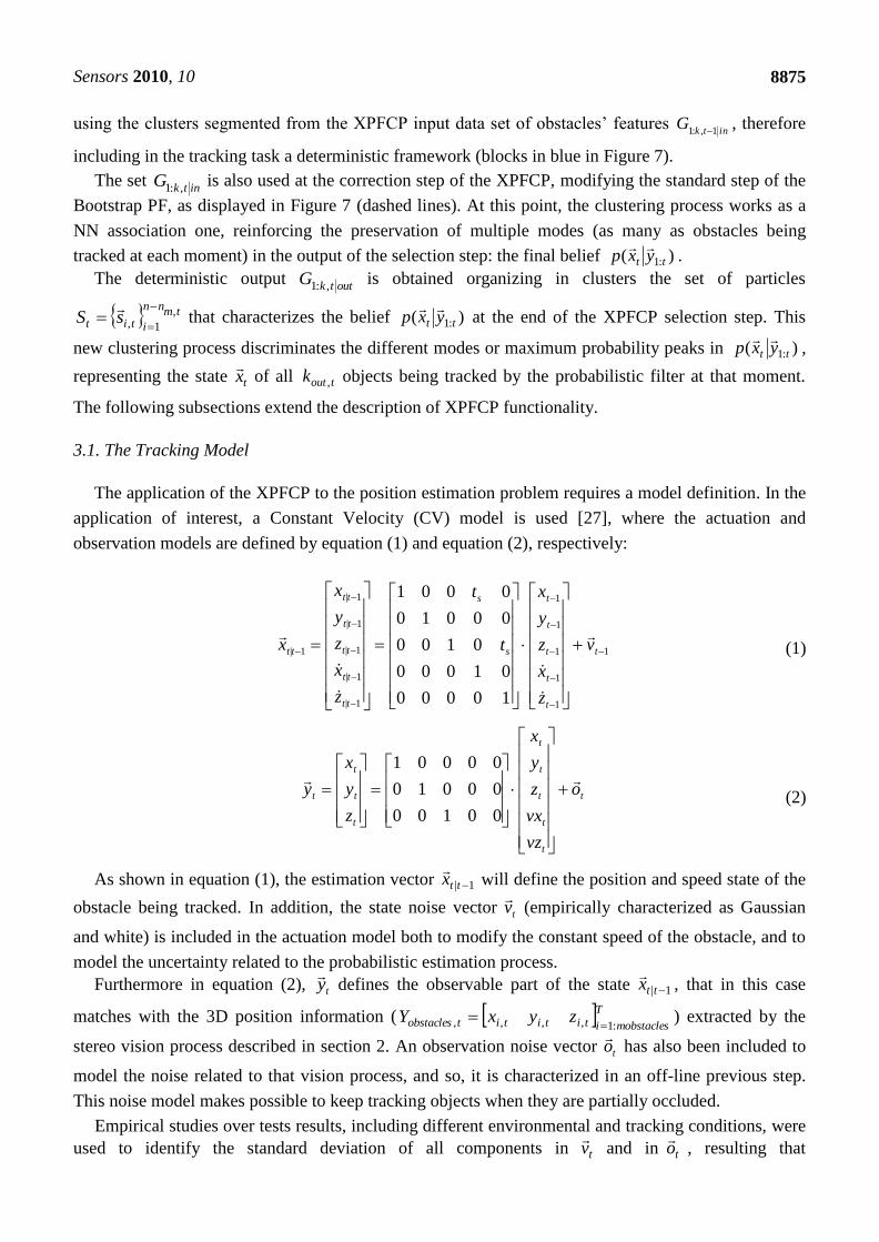
3.1. The Tracking Model
The application of the XPFCP to the position estimation problem requires a model definition. In the
application of interest, a Constant Velocity (CV) model is used [27], where the actuation and
observation models are defined by equation (1) and equation (2), respectively:
As shown in equation (1), the estimation vector will define the position and speed state of the
obstacle being tracked. In addition, the state noise vector (empirically characterized as Gaussian
and white) is included in the actuation model both to modify the constant speed of the obstacle, and to
model the uncertainty related to the probabilistic estimation process.
Furthermore in equation (2), defines the observable part of the state , that in this case
matches with the 3D position information ( ) extracted by the
stereo vision process described in section 2. An observation noise vector has also been included to
model the noise related to that vision process, and so, it is characterized in an off-line previous step.
This noise model makes possible to keep tracking objects when they are partially occluded.
Empirical studies over tests results, including different environmental and tracking conditions, were
used to identify the standard deviation of all components in and in , resulting that
intkG
1,:1
intkG
,:1
)( :1 tt yxp
outtkG
,:1
tmnn
itit sS ,
1,
)( :1 tt yxp
)( :1 tt yxp
tx
toutk ,
1| ttx
tv
ty
1| ttx
Tmobstaclesititititobstacles zyxY
:1,,,,
to
tv
to
(1)
(2)
1
1
1
1
1
1
1|
1|
1|
1|
1|
1|
10000
01000
0100
00010
0001
t
t
t
t
t
t
s
s
tt
tt
tt
tt
tt
tt v
z
x
z
y
x
t
t
z
x
z
y
x
x
t
t
t
t
t
t
t
t
t
t o
vz
vx
z
y
x
z
y
x
y
00100
00010
00001
Sensors 2010, 10
8876
and . Besides, the study of sensibility
concluded that a modification of a 100% in any of generates an increase in the tracking error of
around 24%, while the same modification in any of generates ten times lower figures. This result
indicates the importance of the observation noise vector in the multi-obstacles’ tracking task.
3.2. Steps of the XPFCP
3.2.1. Clustering Measurements
The clustering process is done over the 3D position data set extracted by the stereo vision
process. The output set of groups generated by this process is then used in the re-initialization
and correction steps of the XPFCP.
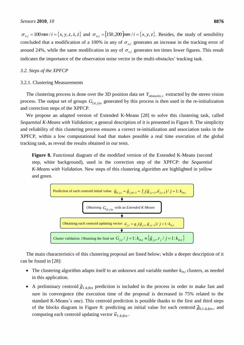
We propose an adapted version of Extended K-Means [28] to solve this clustering task, called
Sequential K-Means with Validation; a general description of it is presented in Figure 8. The simplicity
and reliability of this clustering process ensures a correct re-initialization and association tasks in the
XPFCP, within a low computational load that makes possible a real time execution of the global
tracking task, as reveal the results obtained in our tests.
Figure 8. Functional diagram of the modified version of the Extended K-Means (second
step, white background), used in the correction step of the XPFCP: the Sequential
K-Means with Validation. New steps of this clustering algorithm are highlighted in yellow
and green.
The main characteristics of this clustering proposal are listed below; while a deeper description of it
can be found in [28]:
The clustering algorithm adapts itself to an unknown and variable number kin,t clusters, as needed
in this application.
A preliminary centroid g 1:k,t 𝑖𝑛 prediction is included in the process in order to make fast and
sure its convergence (the execution time of the proposal is decreased in 75% related to the
standard K-Means’s one). This centroid prediction is possible thanks to the first and third steps
of the blocks diagram in Figure 8: predicting an initial value for each centroid g 0,1:k,t 𝑖𝑛 , and
computing each centroid updating vector 𝑢 1:k,t 𝑖𝑛 .
zxzyximmiv ,,,,/100, zyximmio ,,/200,150,
io,
iv,
tobstaclesY ,
intkG
,:1
Cluster validation. Obtaining the final set tinjtjtintj kjgkjG ,,,, :1/,:1/
Obtaining intk
G,:1
with an Extended K-Means
Obtaining each centroid updating vector: tintjtjjtj kjgggu ,1,,, :1/),(
Prediction of each centroid initial value: tintjtjjttjtj kjugfgg ,1,1,1|,,,0 :1/),(
Sensors 2010, 10
8877
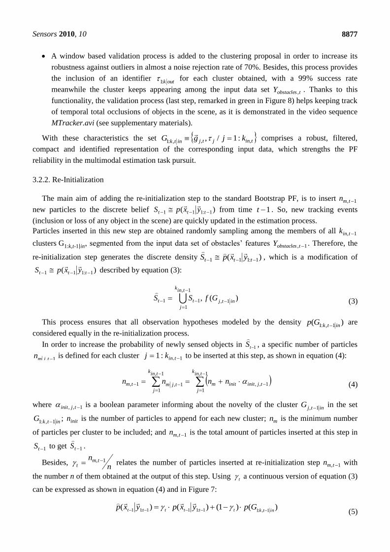
A window based validation process is added to the clustering proposal in order to increase its
robustness against outliers in almost a noise rejection rate of 70%. Besides, this process provides
the inclusion of an identifier for each cluster obtained, with a 99% success rate
meanwhile the cluster keeps appearing among the input data set . Thanks to this
functionality, the validation process (last step, remarked in green in Figure 8) helps keeping track
of temporal total occlusions of objects in the scene, as it is demonstrated in the video sequence
MTracker.avi (see supplementary materials).
With these characteristics the set comprises a robust, filtered,
compact and identified representation of the corresponding input data, which strengths the PF
reliability in the multimodal estimation task pursuit.
3.2.2. Re-Initialization
The main aim of adding the re-initialization step to the standard Bootstrap PF, is to insert
new particles to the discrete belief from time . So, new tracking events
(inclusion or loss of any object in the scene) are quickly updated in the estimation process.
Particles inserted in this new step are obtained randomly sampling among the members of all
clusters G1:k,t-1 in , segmented from the input data set of obstacles’ features . Therefore, the
re-initialization step generates the discrete density , which is a modification of
described by equation (3):
This process ensures that all observation hypotheses modeled by the density are
considered equally in the re-initialization process.
In order to increase the probability of newly sensed objects in , a specific number of particles
is defined for each cluster to be inserted at this step, as shown in equation (4):
where is a boolean parameter informing about the novelty of the cluster in the set
; is the number of particles to append for each new cluster; is the minimum number
of particles per cluster to be included; and is the total amount of particles inserted at this step in
to get .
Besides, relates the number of particles inserted at re-initialization step with
the number n of them obtained at the output of this step. Using a continuous version of equation (3)
can be expressed as shown in equation (4) and in Figure 7:
outk:1
tobstaclesY ,
tinjtjintkkjgG ,,,:1
:1/,
1, tmn
)( 1:111 ttt yxpS
1t
1, tink
1, tobstaclesY
)( 1:111 ttt yxpS
)( 1:111 ttt yxpS
)(1,:1 intk
Gp
1tS
1, tjmn 1,:1 tinkj
1,, tjinitintj
G1,
intkG
1,:1 initn mn
1, tmn
1tS 1tS
nn tm
t1, 1, tmn
t
(3)
(4)
(5)
1,
1
1,11 )(,
tink
j
intjtt GfSS
1,
1
1,,
1,
11,1,
tink
j
tjinitinitm
tink
jtjmtm nnnn
)()1()()(1,:11:111:11 intktttttt Gpyxpyxp
Sensors 2010, 10
8878
The deterministic specification of for each helps shortcoming the
impoverishment problem of the PF in its multimodal application. This process ensures the particles
diversification among all tracking hypotheses in the density estimated by the PF and increases the
probability of newest ones, that otherwise would disappear along the filter evolution. Results included
in section 4 demonstrates this assertion for a quite low value of , that maintains the mathematical
recursive rigor of the Bayesian algorithm.
This re-initialization step has a similar behavior that the one of the MCMC step (used i.e., in [15])
which moves the discrete density towards high likelihood areas in the probability space.
In order to maintain constant the number of particles in along the time (and thus the XPFCP
execution time), the of them that are to be inserted at the re-initialization step at time are
wisely erased at the selection step at time .
3.2.3. Prediction
The set of n particles generated by the re-initialization step is updated through
the actuation model, to obtain a discrete version of the prior .
In this case, the actuation model used is defined in section 3.1, and so, the last
expression in equation (6) can be replaced by equation (1).
Thus, the state noise component is included in the particles’ state prediction with two main
objectives: to create a small dispersion of the particles in the state space (needed to avoid degeneracy
problems of the set [9]); and a slight modification of the speed components in the state vector (needed
to provide movement to the tracking hypothesis when using the CV model [27]).
The simplicity of the CV model proposed eases its use for all objects to be tracked, no care its type
or dynamics and without the help of an association task. Each particle
evolves according to the object’s dynamics that represents in the belief, as the related state vector
includes the object speed components.
3.2.4. Correction and Association
Particles’ weights are computed at the correction step, using the expressions at
equation (7), including a final normalization:
1, tjmn 1,:1 tinkj
t
)( 1:11 tt yxp
tS
1, tmn t
1t
)( 1:111 ttt yxpS
)( 1:11| tttt yxpS
)( 1tt xxp
1tv
niwxsn
i
it
itti :1/,
1
)()(,
ni
itt ww
1
)(~
(6)
(7)
)(11
)(1|
1
)(1|1|
1|1:1111:1
)(1,
)|()|()|(
ittt
itt
n
i
itttt
tttttttt
xxxpxn
xS
Sxyxpxxpyxp
nigxhdd
ni
w
ww
niewxgpww
intj
itt
kjti
n
i
it
iti
t
Oti
d
it
itintk
it
it
:1/),(min
:1/~
:1/)(
,
)(1|
:1,min,
1
)(
)()(
2
2,min,
)(1
)(,:1
)(1
)(
Sensors 2010, 10
8879
where is the shortest distance in the observation space (XYZ in this case), for particle ,
between the projection in this space of the predicted state vector represented by the particle ,
and all centroids in the cluster set , obtained from the objects’ observations set .
The use of cluster centroids guarantees that the observation model applied is filtered, robust and
accurate whatever the reliability of the observed object.
As shown in equation (7), in order to obtain the likelihood used to compute the
weights array ,the observation model defined by (2) has to be utilized, as . Besides,
is the covariance matrix that characterizes the observation noise defined in the same model. This
noise models the modifications of positions in the clusters centroid , when tracking objects
that are partially occluded.
The equally weighted set output from the prediction step is therefore converted
in the set .
The mentioned definition of involves a NN association between the cluster , whose
centroid is used in the particle’s weight computation and the tracking hypothesis
represented by the particle itself. In fact, this association means that is obtained from the
observations generated by the tracking hypothesis represented by .
This association procedure and the re-initialization step remove the impoverishment problem that
appears when a single PF is used to estimate different state vector values: all particles tend to be
concentrated next to the most probable one, leaving the rest of its values without probabilistic
representation at the output density. In [17], the approximate number of efficient particles is used
as a quality factor to evaluate the efficiency of every particle in the set. According this factor,
should be above 66% in order to prevent the impoverishment risk at the particle set. This parameter is
included among the results presented in next section in order to demonstrate how the XPFCP solves
the impoverishment problem.
3.2.5. Selection
Each particle of the set output from the correction step is
resampled at the selection step (also called resampling step) according to the generated weight. As a
result, an equally weighted particle set is obtained, representing a
discrete version of the final belief estimated by the Bayes filter . This final set is formed
by particles, in order to have inserted at the next re-initialization step.
3.2.6. Clustering Particles
From the discrete probabilistic distribution output by the selection step, a
deterministic solution has to be generated by the XPFCP. This problem consists on finding the
tid ,min, 1|, ttis
)( )(1|
ittxh
intkg
,:1
intk
G,:1 tobstaclesY ,
)( )(,:1
itintk
xgp
tw )()(
1| )( it
itt yxh
O
intjG
, intjg
,
ni
itttt n
xS1
)(1|1|
1,
ni
it
ittt wxS
1
)()(1|
~,
tid ,min, intjG
,
intjg
,
)(~ itw
1|, ttis
intjg
,
1|, ttis
effn
effn
)(~, :11
)()(1| tt
n
i
it
ittt yxpwxS
tmnn
itm
itt nn
xS,
1,
)(
)(1,
)( :1 tt yxptS
tmnn , tmn ,
)( :1 ttt yxpS
Sensors 2010, 10
8880
different modes included in the multimodal density represented by the particle set ; it has
not an easy solution if those modes are not clearly different in that distribution.
Diverse proposals have been included in the XPFCP in order to achieve this differentiation. This is
because keeping this multimodality in , while avoiding impoverishment problems in it, is the
principal aim of all techniques proposed in this paper. Following section shows empirical results that
demonstrates this.
Once ensured the differentiation, a simple algorithm can be used to segment in clusters the belief
at the end of the XPFCP loop. Therefore, these groups will become the
deterministic representation of the multiple obstacles’ hypotheses detected by the stereo
vision algorithm described in Section 2.
In this work, the same Sequential K-Means with Validation, described in Figure 8, is used in order
to obtain from . Therefore, the deterministic representation of each tracked
hypothesis will be a cluster with centroid , with the same components as the state vector
defined in (1), and an identification parameter .
4. Results
Different tests have been done in unstructured indoor environments, whose results are shown in this
section. The stereo vision system used in the experiments is formed by two black and white digital
cameras located in a static mounting arrangement, with a gap of 30 cm between them, and at a height
of around 1.5 m from the floor. Vision processes have been developed using OpenCV libraries [25]
and run on a general purpose computer (Intel DUO 1.8GHz).
The global tracking algorithm described in this paper has been implemented on a mobile 4-wheeled
robot platform. Specifically a Pioneer2AT from MobileRobots© [29] has been used for the different
tests. The robot includes a control interface to be guided around the environment, which can be used
within the Player Control GNU Software, from the Player Project [30].
Figure 9 displays the functionality of the multi-tracking process in one of the tested situations.
Three instants of the same experiment are shown in the figure. Each column presents the results
obtained from a single capture; upper row are the input images, while lower row are 2D
representations of objects’ data over the XZ ground plane.
Different data coming from the detected objects are found into each plot. According to the
identification generated by the output clustering process, each group has got a different and
unique color. These groups are identified with a cylinder, thus this is shown as rectangles in the images
and as circles in the ground projections. In both graphics, an arrow (with the same color than the
corresponding group) shows the estimated speed of every obstacle being tracked at each situation, both
in magnitude and in direction.
Particles’ state (taken from the final set generated by the XPFCP) and 3D position of
data set are represented by red and green dots, respectively, in each plot. Besides, the
estimated values of position and speed (if non zero) of each obstacle are also depicted below its
appearance in top row images.
)( :1 tt yxptS
)( :1 tt yxp
)( :1 tt yxpouttk
G,:1
tobstaclesY ,
outtkG
,:1 tStoutkj ,:1
outtjG
, outtjg
,
outj
outtkG
,:1
),( tmnn
tx
tS
tobstaclesY ,
Sensors 2010, 10
8881
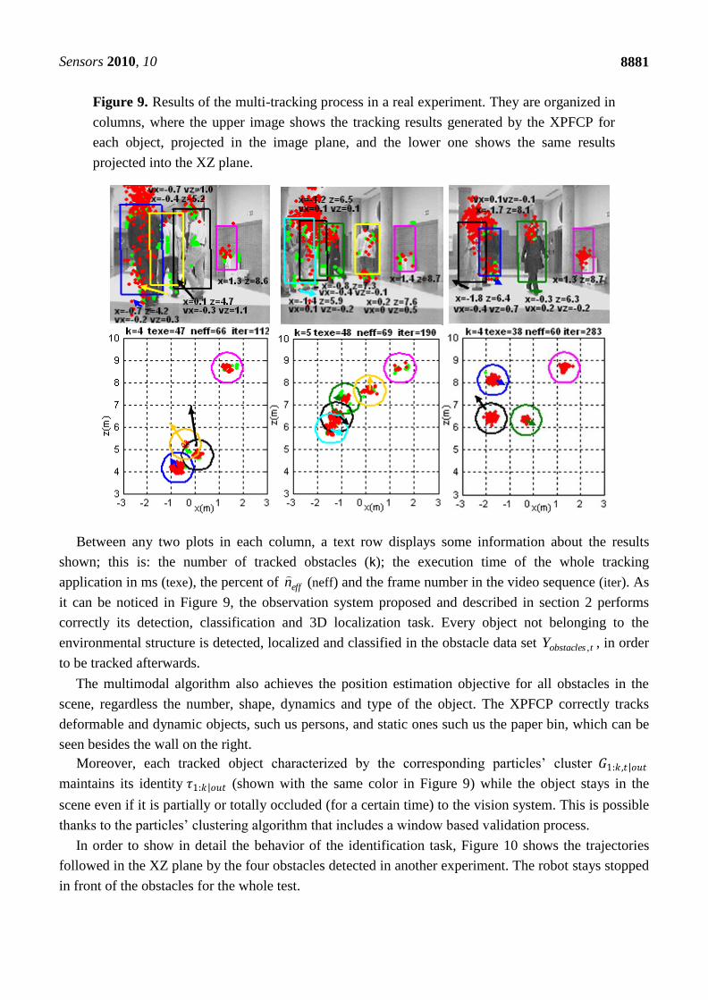
Figure 9. Results of the multi-tracking process in a real experiment. They are organized in
columns, where the upper image shows the tracking results generated by the XPFCP for
each object, projected in the image plane, and the lower one shows the same results
projected into the XZ plane.
Between any two plots in each column, a text row displays some information about the results
shown; this is: the number of tracked obstacles (k); the execution time of the whole tracking
application in ms (texe), the percent of (neff) and the frame number in the video sequence (iter). As
it can be noticed in Figure 9, the observation system proposed and described in section 2 performs
correctly its detection, classification and 3D localization task. Every object not belonging to the
environmental structure is detected, localized and classified in the obstacle data set , in order
to be tracked afterwards.
The multimodal algorithm also achieves the position estimation objective for all obstacles in the
scene, regardless the number, shape, dynamics and type of the object. The XPFCP correctly tracks
deformable and dynamic objects, such us persons, and static ones such us the paper bin, which can be
seen besides the wall on the right.
Moreover, each tracked object characterized by the corresponding particles’ cluster 𝐺1:𝑘 ,𝑡 𝑜𝑢𝑡
maintains its identity 𝜏1:𝑘 𝑜𝑢𝑡 (shown with the same color in Figure 9) while the object stays in the
scene even if it is partially or totally occluded (for a certain time) to the vision system. This is possible
thanks to the particles’ clustering algorithm that includes a window based validation process.
In order to show in detail the behavior of the identification task, Figure 10 shows the trajectories
followed in the XZ plane by the four obstacles detected in another experiment. The robot stays stopped
in front of the obstacles for the whole test.
effn
tobstaclesY ,
Sensors 2010, 10
8882
Figure 10. Trajectory followed in the ground plane (XZ) by four obstacles according to the
XPFCP estimation results in a real experiment.
Each colored spot represents during consecutive iterations the centroid position g 1:4 out of the cluster
related to the corresponding obstacle 𝐺1:4,𝑡 𝑜𝑢𝑡 ; each color reflects the cluster identity . A dashed
oriented arrow over each g 1:4 out trace illustrates the ground truth of the path followed by the real
obstacles. It can be hence conclude, that the correct identification of each object is maintained
with a 100% of reliability, even when partial and total occlusions occur; this is the case shown on
traces from obstacles three (in pink) and four (in light blue).
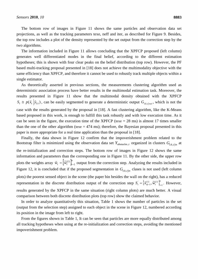
Figure 11 demonstrates graphically the multimodal capability of the XPFCP proposal in a multi-
tracking task. In this figure, the XPFCP functionality is compared to that of another multimodal multi-
tracking proposal, described in [18].
Figure 11. Results of the multi-tracking process in a real experiment: left column shows
the results generated by the XPFCP; the right column shows the results of the proposal
presented in [18].
out4:1
out4:1
outg
2
outg
3
outg
4
outg
1
Sensors 2010, 10
8883
The bottom row of images in Figure 11 shows the same particles and observation data set
projections, as well as the tracking parameters texe, neff and iter, as described for Figure 9. Besides,
the top row includes a plot of the density represented by the set output from the correction step by the
two algorithms.
The information included in Figure 11 allows concluding that the XPFCP proposed (left column)
generates well differentiated modes in the final belief, according to the different estimation
hypotheses; this is shown with four clear peaks on the belief distribution (top row). However, the PF
based multi-tracking proposal presented in [18] does not achieve the multimodality objective with the
same efficiency than XPFCP, and therefore it cannot be used to robustly track multiple objects within a
single estimator.
As theoretically asserted in previous sections, the measurements clustering algorithm used as
deterministic association process have better results in the multimodal estimation task. Moreover, the
results presented in Figure 11 show that the multimodal density obtained with the XPFCP
, can be easily segmented to generate a deterministic output , which is not the
case with the results generated by the proposal in [18]. A fast clustering algorithm, like the K-Means
based proposed in this work, is enough to fulfill this task robustly and with low execution time. As it
can be seen in the figure, the execution time of the XPFCP (texe = 28 ms) is almost 17 times smaller
than the one of the other algorithm (texe = 474 ms); therefore, the Bayesian proposal presented in this
paper is more appropriate for a real time application than the proposal in [18].
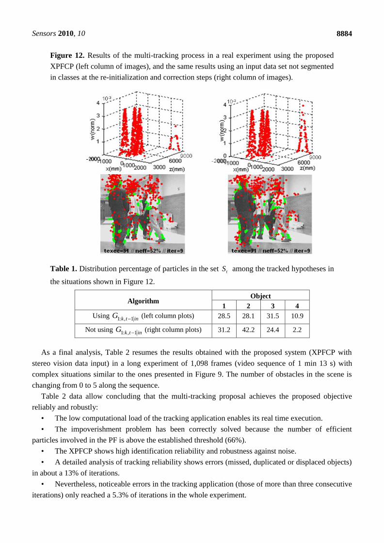
Finally, the data shown in Figure 12 confirm that the impoverishment problem related to the
Bootstrap filter is minimized using the observation data set organized in clusters at
the re-initialization and correction steps. The bottom row of images in Figure 12 shows the same
information and parameters than the corresponding one in Figure 11. By the other side, the upper row
plots the weights array output from the correction step. Analyzing the results included in
Figure 12, it is concluded that if the proposed segmentation in clases is not used (left column
plots) the poorest sensed object in the scene (the paper bin besides the wall on the right), has a reduced
representation in the discrete distribution output of the correction step . However,
results generated by the XPFCP in the same situation (right column plots) are much better. A visual
comparison between both discrete distribution plots (top row) show the claimed behavior.
In order to analyze quantitatively this situation, Table 1 shows the number of particles in the set
(output from the selection step) assigned to each object in the scene in Figure 12, numbered according
its position in the image from left to right.
From the figures shown in Table 1, It can be seen that particles are more equally distributed among
all tracking hypotheses when using at the re-initialization and correction steps, avoiding the mentioned
impoverishment problem.
)( :1 ttt yxpS
outtk
G,:1
tobstaclesY , intkG
,:1
ni
itt ww
1
)(~
intkG
,:1
ni
i
t
i
ttt wxS1
)()(
1|
' ~,
Sensors 2010, 10
8884
Figure 12. Results of the multi-tracking process in a real experiment using the proposed
XPFCP (left column of images), and the same results using an input data set not segmented
in classes at the re-initialization and correction steps (right column of images).
Table 1. Distribution percentage of particles in the set among the tracked hypotheses in
the situations shown in Figure 12.
Algorithm Object
1 2 3 4
Using (left column plots) 28.5 28.1 31.5 10.9
Not using (right column plots) 31.2 42.2 24.4 2.2
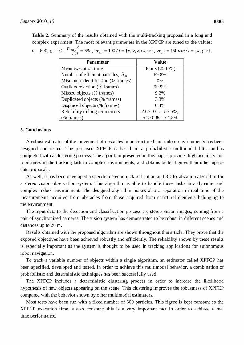
As a final analysis, Table 2 resumes the results obtained with the proposed system (XPFCP with
stereo vision data input) in a long experiment of 1,098 frames (video sequence of 1 min 13 s) with
complex situations similar to the ones presented in Figure 9. The number of obstacles in the scene is
changing from 0 to 5 along the sequence.
Table 2 data allow concluding that the multi-tracking proposal achieves the proposed objective
reliably and robustly:
• The low computational load of the tracking application enables its real time execution.
• The impoverishment problem has been correctly solved because the number of efficient
particles involved in the PF is above the established threshold (66%).
• The XPFCP shows high identification reliability and robustness against noise.
• A detailed analysis of tracking reliability shows errors (missed, duplicated or displaced objects)
in about a 13% of iterations.
• Nevertheless, noticeable errors in the tracking application (those of more than three consecutive
iterations) only reached a 5.3% of iterations in the whole experiment.
tS
intkG
1,:1
intkG
1,:1
Sensors 2010, 10
8885
Table 2. Summary of the results obtained with the multi-tracking proposal in a long and
complex experiment. The most relevant parameters in the XPFCP are tuned to the values:
n = 600, γt = 0.2, , , .
Parameter Value
Mean execution time 40 ms (25 FPS)
Number of efficient particles, 69.8%
Mismatch identification (% frames) 0%
Outliers rejection (% frames) 99.9%
Missed objects (% frames) 9.2%
Duplicated objects (% frames) 3.3%
Displaced objects (% frames) 0.4%
Reliability in long term errors
(% frames)
t > 0.6s 3.5%,
t > 0.8s 1.8%
5. Conclusions
A robust estimator of the movement of obstacles in unstructured and indoor environments has been
designed and tested. The proposed XPFCP is based on a probabilistic multimodal filter and is
completed with a clustering process. The algorithm presented in this paper, provides high accuracy and
robustness in the tracking task in complex environments, and obtains better figures than other up-to-
date proposals.
As well, it has been developed a specific detection, classification and 3D localization algorithm for
a stereo vision observation system. This algorithm is able to handle those tasks in a dynamic and
complex indoor environment. The designed algorithm makes also a separation in real time of the
measurements acquired from obstacles from those acquired from structural elements belonging to
the environment.
The input data to the detection and classification process are stereo vision images, coming from a
pair of synchronized cameras. The vision system has demonstrated to be robust in different scenes and
distances up to 20 m.
Results obtained with the proposed algorithm are shown throughout this article. They prove that the
exposed objectives have been achieved robustly and efficiently. The reliability shown by these results
is especially important as the system is thought to be used in tracking applications for autonomous
robot navigation.
To track a variable number of objects within a single algorithm, an estimator called XPFCP has
been specified, developed and tested. In order to achieve this multimodal behavior, a combination of
probabilistic and deterministic techniques has been successfully used.
The XPFCP includes a deterministic clustering process in order to increase the likelihood
hypothesis of new objects appearing on the scene. This clustering improves the robustness of XPFCP
compared with the behavior shown by other multimodal estimators.
Most tests have been run with a fixed number of 600 particles. This figure is kept constant so the
XPFCP execution time is also constant; this is a very important fact in order to achieve a real
time performance.
%5n
ninit },,,,{/100, vzvxzyxiiv },,{/150, zyximmio
effn
Sensors 2010, 10
8886
The designed XPFCP is based on simple observation and actuation models, and therefore it can be
easily adapted to handle data coming up from different kinds of sensors and different types of
obstacles to be tracked. This fact demonstrates that our tracking proposal is more flexible than other
solutions found in the related literature, based on rigid models for the input data set.
Acknowledgements
This work has been supported by the Spanish Ministry of Science and Innovation under projects
VISNU (ref. TIN2009-08984) and SDTEAM-UAH (ref. TIN2008-06856-C05-05).
References
1. Jia, Z.; Balasuriya, A.; Challa, S. Autonomous vehicles navigation with visual target tracking:
Technical approaches. Algorithms 2008, 1, 153-182.
2. Khan, Z.; Balch, T.; Dellaert, F. A Rao-Blackwellized particle filter for eigen tracking. In
Proceedings of the Third IEEE Conference on Computer Vision and Pattern Recognition,
Washington, DC, USA, June 2004; pp. 980-986.
3. Isard, M.; Blake, A. Icondensation: Unifying low-level and high-level tracking in a stochastic
framework. In Proceedings of the Fifth European Conference on Computer Vision, Freiburg,
Germany, June 1998; Volume 1, pp. 893-908.
4. Chen, Y.; Huang, T.S.; Rui, Y. Mode-based multi-hypothesis head tracking using parametric
contours. In Proceedings of the Fifth IEEE International Conference on Automatic Face and
Gesture Recognition, Washington, DC, USA, May 2002.
5. Odobez, J.M.; Gatica-Perez. D. Embedding motion model-based stochastic tracking. In
Proceedings of the Seventeenth International Conference on Pattern Recognition, Cambridge,
UK, August 2004; Volume 2, pp. 815-818.
6. Okuma, K.; Taleghani, A.; De Freitas, N.; Little, J.J.; Lowe, D.G. A boosted particle filter:
Multi-target detection and tracking. In Proceedings of the Eighth European Conference on
Computer Vision, Prague, Czech Republic, May 2004; Volume 3021, Part I, pp. 28-39.
7. Thrun, S. Probabilistic algorithms in robotics. AI Mag. 2000, 21, 93-109.
8. Arulampalam, M.S.; Maskell, S.; Gordon, N.; Clapp, T. A tutorial on particle filters for online
nonlinear non-gaussian bayesian tracking. IEEE Trans. Signal. Proces. 2002, 50, 174-188.
9. Gordon, N.J.; Salmond, D.J.; Smith. A.F.M. Novel approach to nonlinear/non-gaussian bayesian
state estimation. IEEE Proc. F 1993, 140, 107-113.
10. Wang, X.; Wang, S.; Ma, J.-J. An improved particle filter for target tracking in sensor systems,
Sensors 2007, 7, 144-156.
11. Welch, G.; Bishop, G. An Introduction to the Kalman Filter. Technical Report: TR95-041; ACM
SIGGRAPH: Los Angeles, CA, USA, 2001; Available online: http://www.cs.unc.edu/~tracker/
ref/s2001/kalman/ (accesed on 30 June 2010).
12. Reid, D.B. An algorithm for tracking multiple targets. IEEE Trans. Automat. Contr. 1979, 24,
843-854.
13. Tweed, D.; Calway, A. Tracking many objects using subordinated condensation. In Proceedings
of the British Machine Vision Conference, Cardiff, UK, October 2002; pp. 283-292.
Sensors 2010, 10
8887
14. Smith, K.; Gatica-Perez, D.; Odobez, J.M. Using particles to track varying numbers of interacting
people. In Proceedings of the Fourth IEEE Conference on Computer Vision and Pattern
Recognition, San Diego, CA, USA, June 2005; pp. 962-969.
15. MacCormick, J.; Blake, A. A probabilistic exclusion principle for tracking multiple objects. In
Proceedings of the Seventh IEEE International Conference on Computer Vision, Corfu, Greece,
September 1999; pp. 572-578.
16. Schulz, D.; Burgard, W.; Fox, D.; Cremers, A.B. Tracking multiple moving targets with a mobile
robot using particle filters and statistical data association. Int. J. Robot. Res. 2003, 22, 99-116.
17. Hue, C.; Le Cadre, J.P.; Pérez, P. A particle filter to track multiple objects. IEEE Trans. Aero.
Elec. Sys. 2002, 38, 791-812.
18. Koller-Meier, E.B.; Ade, F. Tracking multiple objects using a condensation algorithm. J. Robot.
Auton. Syst. 2001, 34, 93-105.
19. Schulz, D.; Burgard, W.; Fox, D.; Cremers, A.B. People tracking with mobile robots using
sample-based joint probabilistic data association filters. Int. J. Robot. Res. 2003, 22, 99-116.
20. Bar-Shalom, Y.; Fortmann, T. Tracking and Data Association; Academic Press: New York, NY,
USA, 1988.
21. Burguera, A.; González, Y.; Oliver, G. Sonar semsor models and their application to mobile robot
localization. Sensors 2009, 9, 10217-10243.
22. Boufama, B. Reconstruction Tridimensionnelle en Vision par Ordinateur: Cas des Cameras non
Etalonnees. Ph.D. Thesis, Institut National Polytechnique de Grenoble: Grenoble, France, 1994.
23. Canny, F.J. A computational approach to edge detection. IEEE Trans. Pattern Anal. 1986, 8,
pp. 679-698.
24. Documentation of function cvHoughLines2. Available online: http://opencv.willowgarage.com/
documentation/feature_detection.html (accessed on 27 August 2010).
25. Project OpenCV. Available online: http://sourceforge.net/projects/opencvlibrary/ (accesed on 27
August 2010).
26. Vermaak, J.; Doucet, A.; Perez, P. Maintaining multimodality through mixture tracking. In
Proceedings of the Ninth IEEE International Conference on Computer Vision, Nice, France, June
2003; pp. 1110-1116.
27. Marrón, M.; Sotelo, M.A.; García, J.C.; Broddfelt, J. Comparing improved versions of ‘K-Means’
and ‘Subtractive’ clustering in a tracking applications. In Proceedings of the Eleventh
International Workshop on Computer Aided Systems Theory, Las Palmas de Gran Canaria, Spain,
February 2007; pp. 252-255.
28. Bar Shalom, Y.; Li, X.R. Estimation and Tracking Principles Techniques and Software; Artech
House: Boston, MA, USA, 1993.
29. MobileRobots. Available online: http://www.mobilerobots.com/Mobile_Robots.aspx (accessed on
27 August 2010).
30. The Player Project. Available online: http://playerstage.sourceforge.net/ (accessed on 27
August 2010).
© 2010 by the authors; licensee MDPI, Basel, Switzerland. This article is an open access article
distributed under the terms and conditions of the Creative Commons Attribution license
(http://creativecommons.org/licenses/by/3.0/).