
Stefano Crespi Reghizzi Luca Breveglieri Angelo Morzenti Second ...
408
Texts in Computer Science Formal Languages and Compilation Stefano Crespi Reghizzi Luca Breveglieri Angelo Morzenti Second Edition
-
Upload
khangminh22 -
Category
Documents
-
view
1 -
download
0
Transcript of Stefano Crespi Reghizzi Luca Breveglieri Angelo Morzenti Second ...

Texts in Computer Science
Formal Languages and Compilation
Stefano Crespi ReghizziLuca BreveglieriAngelo Morzenti
Second Edition

Texts in Computer Science
EditorsDavid GriesFred B. Schneider
For further volumes:www.springer.com/series/3191


Stefano Crespi Reghizzi � Luca Breveglieri �
Angelo Morzenti
Formal Languagesand Compilation
Second Edition

Stefano Crespi ReghizziDipartimento Elettronica
Informazione e BioingegneriaPolitecnico di MilanoMilan, Italy
Luca BreveglieriDipartimento Elettronica
Informazione e BioingegneriaPolitecnico di MilanoMilan, Italy
Angelo MorzentiDipartimento Elettronica
Informazione e BioingegneriaPolitecnico di MilanoMilan, Italy
Series EditorsDavid GriesDepartment of Computer ScienceCornell UniversityIthaca, NY, USA
Fred B. SchneiderDepartment of Computer ScienceCornell UniversityIthaca, NY, USA
ISSN 1868-0941 ISSN 1868-095X (electronic)Texts in Computer ScienceISBN 978-1-4471-5513-3 ISBN 978-1-4471-5514-0 (eBook)DOI 10.1007/978-1-4471-5514-0Springer London Heidelberg New York Dordrecht
© Springer-Verlag London 2009, 2013This work is subject to copyright. All rights are reserved by the Publisher, whether the whole or part ofthe material is concerned, specifically the rights of translation, reprinting, reuse of illustrations, recitation,broadcasting, reproduction on microfilms or in any other physical way, and transmission or informationstorage and retrieval, electronic adaptation, computer software, or by similar or dissimilar methodologynow known or hereafter developed. Exempted from this legal reservation are brief excerpts in connectionwith reviews or scholarly analysis or material supplied specifically for the purpose of being enteredand executed on a computer system, for exclusive use by the purchaser of the work. Duplication ofthis publication or parts thereof is permitted only under the provisions of the Copyright Law of thePublisher’s location, in its current version, and permission for use must always be obtained from Springer.Permissions for use may be obtained through RightsLink at the Copyright Clearance Center. Violationsare liable to prosecution under the respective Copyright Law.The use of general descriptive names, registered names, trademarks, service marks, etc. in this publicationdoes not imply, even in the absence of a specific statement, that such names are exempt from the relevantprotective laws and regulations and therefore free for general use.While the advice and information in this book are believed to be true and accurate at the date of pub-lication, neither the authors nor the editors nor the publisher can accept any legal responsibility for anyerrors or omissions that may be made. The publisher makes no warranty, express or implied, with respectto the material contained herein.
Printed on acid-free paper
Springer is part of Springer Science+Business Media (www.springer.com)

Preface
The textbook derives from the well-known identically titled volume1 published in2009: two younger co-authors have brought their experience to enrich and stream-line the book, without dulling its original structure. The selection of materials andthe presentation style have not substantially changed. The book reflects many yearsof teaching compiler courses and of doing research on formal language theory andformal methods, on compiler and language technology, and to a lesser extent onnatural language processing. The more important change concerns the central topicof language parsing. It is a completely new, systematic, and unified presentation ofthe most important parsing algorithms, including also parallel parsing.
Goals In the turmoil of information technology developments, the subject of thebook has kept the same fundamental principles since half a century, and has pre-served its conceptual importance and practical relevance. This state of affairs in atopic that is central to computer science and is based on established principles, mightlead some people to believe that the corresponding textbooks are by now consoli-dated, much as the classical books on mathematics and physics. In reality, this is notthe case: there exist fine classical books on the mathematical aspects of language andautomata theory, but for what concerns the application to compiling, the best booksare sort of encyclopedias of algorithms, design methods, and practical tricks usedin compiler design. Indeed, a compiler is a microcosm, and features many differentaspects ranging from algorithmic wisdom to computer hardware. As a consequence,the textbooks have grown in size, and compete with respect to their coverage of thelast developments on programming languages, processor architectures and clevermappings from the former to the latter.
To put things in order, it is better to separate such complex topics into two parts,basic and advanced, which to a large extent correspond to the two subsystems thatmake a compiler: the user-language specific front-end, and the machine-languagespecific back-end. The basic part is the subject of this book. It covers the principlesand algorithms to be used for defining the syntax of languages and for implementingsimple translators. It does not include: the specialized know-how needed for variousclasses of programming languages (imperative, functional, object oriented, etc.), thecomputer architecture related aspects, and the optimization methods used to improvethe machine code produced by the compiler.
1S. Crespi Reghizzi, Formal Languages and Compilation (Springer, London, 2009).
v

vi Preface
Organization and Features In other textbooks the bias towards practical aspectshas reduced the attention to fundamental concepts. This has prevented their authorsfrom taking advantage of the improvements and simplifications made possible bydecades of extensive use, and from avoiding the irritating variants and repetitionsthat are found in the original papers. Moving from these premises, we decided topresent, in a simple minimalist way, the principles and methods used in designinglanguage syntax and syntax-directed translators.
Chapter 2 covers regular expressions and context-free grammars, with emphasison the structural adequacy of syntactic definitions and a careful analysis of ambigu-ity and how to avoid it.
Chapter 3 presents finite-state recognizers and their conversion back and forth toregular expressions and grammars.
Chapter 4 presents push-down machines and parsing algorithms, focusing atten-tion on the LL, LR and Earley methods. We have substantially improved the standardpresentation of such algorithms, by unifying the concepts and notations used in var-ious approaches, and by extending the method coverage with a reduced definitionalapparatus. An example that expert readers and instructors should appreciate, is theunification of the top-down (LL) and bottom-up (LR) parsing algorithms, as well asthe tabular (Early) one, within a novel practical framework. In this way, the effortand space spared have made room for advanced methods typically not present insimilar textbooks. First, our parsing algorithms apply to the Extended BNF gram-mars, which are the de facto standard in the language reference manuals. Second,we provide a parallel parsing algorithm that takes advantage of the many processingunits of modern microprocessors, to speed-up the analysis of large files.
The book is not restricted to syntax: Chap. 5, the last one, studies translations,semantic functions (attribute grammars), and the static program analysis by dataflow equations. This provides a comprehensive understanding of the compilationprocess, and covers the essential elements of a syntax-directed translator.
The presentation is illustrated by many small yet realistic examples and pictures,to ease the understanding of the theory and the transfer to application. Theoret-ical models of automata, transducers and formal grammars are extensively used,whenever practical motivations exist, without insisting too much on their formaldefinition. Algorithms are described in a pseudo-code to avoid the disturbing detailsof a programming language, yet they are straightforward to convert to executableprocedures.
This book should be welcome by those willing to teach or to learn the essentialconcepts of syntax-directed compilation, without the need of relying on softwaretools and implementations. We believe that learning by doing is not always the bestapproach, and that over-commitment to practical work may sometimes obscure theconceptual foundations. In the case of formal languages, the elegance and simplicityof the underlying theory allows the students to acquire the fundamental paradigmsof language structures, to avoid pitfalls such as ambiguity, and to adequately mapstructure to meaning. In this field, the relevant algorithms are simple enough to bepracticed by paper and pencil. Of course, students should be encouraged to enroll ina hands-on laboratory and to experiment syntax-directed tools (like flex and bison)on realistic cases.

Preface vii
Intended Audiences This is primarily a textbook targeted to graduate (or upper-division undergraduate) students in computer science or computer engineering. Welist as prerequisites: familiarity with some programming language models and withalgorithm design; and the ability to use elementary mathematical and logical no-tation. If the reader or student has already taken a course on theoretical computerscience including a few elements of formal language and automata theory, the timeand effort needed to learn the first chapters can be reduced. But it is fair to say thatthis book does not compete with the many available books on the theory of formallanguages and computation: we usually do not include mathematical proofs of prop-erties, and we rely instead on examples and informal arguments. Yet mathematicallyoriented readers will find here many motivating examples and applications.
A large collection of problems and solutions complementing the numerous exam-ples in the book is available on the authors’ course web site at Politecnico di Milano.Similarly, a comprehensive set of lecture slides is also available on the course website.
The Authors Thank The colleagues who have taught this book to computerengineering students, Giampaolo Agosta and Licia Sbattella; the Italian NationalResearch Group on Formal Languages, in particular Antonio Restivo, Alessan-dra Cherubini, Dino Mandrioli, Matteo Pradella and Pierluigi San Pietro; our pastand present Ph.D. students and teaching assistants, Alessandro Barenghi, MarcelloBersani, Andrea Di Biagio, Simone Campanoni, Silvia Lovergine, Michele Scan-dale, Ettore Speziale, Martino Sykora and Michele Tartara. We also acknowledgethe support of ST Microelectronics Company for R.&D. projects on compilers foradvanced microprocessor architectures.
The first author remembers the late Antonio Grasselli, a pioneer of computerscience studies, who first fascinated him with a subject combining linguistic, math-ematical, and technological aspects.
Stefano Crespi ReghizziLuca BreveglieriAngelo Morzenti
Milan, ItalyJuly 2013

Contents
1 Introduction . . . . . . . . . . . . . . . . . . . . . . . . . . . . . . . 11.1 Intended Scope and Audience . . . . . . . . . . . . . . . . . . . 11.2 Compiler Parts and Corresponding Concepts . . . . . . . . . . . 2
2 Syntax . . . . . . . . . . . . . . . . . . . . . . . . . . . . . . . . . . 52.1 Introduction . . . . . . . . . . . . . . . . . . . . . . . . . . . . 5
2.1.1 Artificial and Formal Languages . . . . . . . . . . . . . 52.1.2 Language Types . . . . . . . . . . . . . . . . . . . . . . 62.1.3 Chapter Outline . . . . . . . . . . . . . . . . . . . . . . 7
2.2 Formal Language Theory . . . . . . . . . . . . . . . . . . . . . 72.2.1 Alphabet and Language . . . . . . . . . . . . . . . . . . 72.2.2 Language Operations . . . . . . . . . . . . . . . . . . . 112.2.3 Set Operations . . . . . . . . . . . . . . . . . . . . . . . 132.2.4 Star and Cross . . . . . . . . . . . . . . . . . . . . . . . 142.2.5 Quotient . . . . . . . . . . . . . . . . . . . . . . . . . . 16
2.3 Regular Expressions and Languages . . . . . . . . . . . . . . . 172.3.1 Definition of Regular Expression . . . . . . . . . . . . . 172.3.2 Derivation and Language . . . . . . . . . . . . . . . . . 192.3.3 Other Operators . . . . . . . . . . . . . . . . . . . . . . 222.3.4 Closure Properties of REG Family . . . . . . . . . . . . 23
2.4 Linguistic Abstraction . . . . . . . . . . . . . . . . . . . . . . . 242.4.1 Abstract and Concrete Lists . . . . . . . . . . . . . . . . 25
2.5 Context-Free Generative Grammars . . . . . . . . . . . . . . . . 282.5.1 Limits of Regular Languages . . . . . . . . . . . . . . . 292.5.2 Introduction to Context-Free Grammars . . . . . . . . . 292.5.3 Conventional Grammar Representations . . . . . . . . . 322.5.4 Derivation and Language Generation . . . . . . . . . . . 332.5.5 Erroneous Grammars and Useless Rules . . . . . . . . . 352.5.6 Recursion and Language Infinity . . . . . . . . . . . . . 372.5.7 Syntax Trees and Canonical Derivations . . . . . . . . . 382.5.8 Parenthesis Languages . . . . . . . . . . . . . . . . . . . 412.5.9 Regular Composition of Context-Free Languages . . . . 432.5.10 Ambiguity . . . . . . . . . . . . . . . . . . . . . . . . . 452.5.11 Catalogue of Ambiguous Forms and Remedies . . . . . . 47
ix

x Contents
2.5.12 Weak and Structural Equivalence . . . . . . . . . . . . . 542.5.13 Grammar Transformations and Normal Forms . . . . . . 56
2.6 Grammars of Regular Languages . . . . . . . . . . . . . . . . . 672.6.1 From Regular Expressions to Context-Free Grammars . . 672.6.2 Linear Grammars . . . . . . . . . . . . . . . . . . . . . 682.6.3 Linear Language Equations . . . . . . . . . . . . . . . . 71
2.7 Comparison of Regular and Context-Free Languages . . . . . . . 732.7.1 Limits of Context-Free Languages . . . . . . . . . . . . 762.7.2 Closure Properties of REG and CF . . . . . . . . . . . . 782.7.3 Alphabetic Transformations . . . . . . . . . . . . . . . . 792.7.4 Grammars with Regular Expressions . . . . . . . . . . . 82
2.8 More General Grammars and Language Families . . . . . . . . . 852.8.1 Chomsky Classification . . . . . . . . . . . . . . . . . . 86
References . . . . . . . . . . . . . . . . . . . . . . . . . . . . . . . . 90
3 Finite Automata as Regular Language Recognizers . . . . . . . . . 913.1 Introduction . . . . . . . . . . . . . . . . . . . . . . . . . . . . 913.2 Recognition Algorithms and Automata . . . . . . . . . . . . . . 92
3.2.1 A General Automaton . . . . . . . . . . . . . . . . . . . 933.3 Introduction to Finite Automata . . . . . . . . . . . . . . . . . . 963.4 Deterministic Finite Automata . . . . . . . . . . . . . . . . . . . 97
3.4.1 Error State and Total Automata . . . . . . . . . . . . . . 983.4.2 Clean Automata . . . . . . . . . . . . . . . . . . . . . . 993.4.3 Minimal Automata . . . . . . . . . . . . . . . . . . . . . 1003.4.4 From Automata to Grammars . . . . . . . . . . . . . . . 103
3.5 Nondeterministic Automata . . . . . . . . . . . . . . . . . . . . 1043.5.1 Motivation of Nondeterminism . . . . . . . . . . . . . . 1053.5.2 Nondeterministic Recognizers . . . . . . . . . . . . . . . 1073.5.3 Automata with Spontaneous Moves . . . . . . . . . . . . 1093.5.4 Correspondence Between Automata and Grammars . . . 1103.5.5 Ambiguity of Automata . . . . . . . . . . . . . . . . . . 1113.5.6 Left-Linear Grammars and Automata . . . . . . . . . . . 112
3.6 Directly from Automata to Regular Expressions: BMC Method . 1123.7 Elimination of Nondeterminism . . . . . . . . . . . . . . . . . . 114
3.7.1 Construction of Accessible Subsets . . . . . . . . . . . . 1153.8 From Regular Expression to Recognizer . . . . . . . . . . . . . 119
3.8.1 Thompson Structural Method . . . . . . . . . . . . . . . 1193.8.2 Berry–Sethi Method . . . . . . . . . . . . . . . . . . . . 121
3.9 Regular Expressions with Complement and Intersection . . . . . 1323.9.1 Product of Automata . . . . . . . . . . . . . . . . . . . . 134
3.10 Summary of Relations Between Regular Languages, Grammars,and Automata . . . . . . . . . . . . . . . . . . . . . . . . . . . 138
References . . . . . . . . . . . . . . . . . . . . . . . . . . . . . . . . 139

Contents xi
4 Pushdown Automata and Parsing . . . . . . . . . . . . . . . . . . . 1414.1 Introduction . . . . . . . . . . . . . . . . . . . . . . . . . . . . 1414.2 Pushdown Automaton . . . . . . . . . . . . . . . . . . . . . . . 142
4.2.1 From Grammar to Pushdown Automaton . . . . . . . . . 1434.2.2 Definition of Pushdown Automaton . . . . . . . . . . . . 146
4.3 One Family for Context-Free Languages and Pushdown Automata 1514.3.1 Intersection of Regular and Context-Free Languages . . . 1534.3.2 Deterministic Pushdown Automata and Languages . . . . 154
4.4 Syntax Analysis . . . . . . . . . . . . . . . . . . . . . . . . . . 1624.4.1 Top-Down and Bottom-Up Constructions . . . . . . . . . 163
4.5 Grammar as Network of Finite Automata . . . . . . . . . . . . . 1654.5.1 Derivation for Machine Nets . . . . . . . . . . . . . . . 1714.5.2 Initial and Look-Ahead Characters . . . . . . . . . . . . 173
4.6 Bottom-Up Deterministic Analysis . . . . . . . . . . . . . . . . 1764.6.1 From Finite Recognizers to Bottom-Up Parser . . . . . . 1774.6.2 Construction of ELR(1) Parsers . . . . . . . . . . . . . . 1814.6.3 ELR(1) Condition . . . . . . . . . . . . . . . . . . . . . 1844.6.4 Simplifications for BNF Grammars . . . . . . . . . . . . 1974.6.5 Parser Implementation Using a Vector Stack . . . . . . . 2014.6.6 Lengthening the Look-Ahead . . . . . . . . . . . . . . . 205
4.7 Deterministic Top-Down Parsing . . . . . . . . . . . . . . . . . 2114.7.1 ELL(1) Condition . . . . . . . . . . . . . . . . . . . . . 2144.7.2 Step-by-Step Derivation of ELL(1) Parsers . . . . . . . . 2174.7.3 Direct Construction of Top-Down Predictive Parsers . . . 2314.7.4 Increasing Look-Ahead . . . . . . . . . . . . . . . . . . 240
4.8 Deterministic Language Families: A Comparison . . . . . . . . . 2424.9 Discussion of Parsing Methods . . . . . . . . . . . . . . . . . . 2464.10 A General Parsing Algorithm . . . . . . . . . . . . . . . . . . . 248
4.10.1 Introductory Presentation . . . . . . . . . . . . . . . . . 2494.10.2 Earley Algorithm . . . . . . . . . . . . . . . . . . . . . 2524.10.3 Syntax Tree Construction . . . . . . . . . . . . . . . . . 261
4.11 Parallel Local Parsing . . . . . . . . . . . . . . . . . . . . . . . 2684.11.1 Floyd’s Operator-Precedence Grammars and Parsers . . . 2694.11.2 Sequential Operator-Precedence Parser . . . . . . . . . . 2744.11.3 Parallel Parsing Algorithm . . . . . . . . . . . . . . . . . 277
4.12 Managing Syntactic Errors and Changes . . . . . . . . . . . . . 2834.12.1 Errors . . . . . . . . . . . . . . . . . . . . . . . . . . . 2844.12.2 Incremental Parsing . . . . . . . . . . . . . . . . . . . . 289
References . . . . . . . . . . . . . . . . . . . . . . . . . . . . . . . . 290
5 Translation Semantics and Static Analysis . . . . . . . . . . . . . . 2935.1 Introduction . . . . . . . . . . . . . . . . . . . . . . . . . . . . 293
5.1.1 Chapter Outline . . . . . . . . . . . . . . . . . . . . . . 2945.2 Translation Relation and Function . . . . . . . . . . . . . . . . . 2955.3 Transliteration . . . . . . . . . . . . . . . . . . . . . . . . . . . 298

xii Contents
5.4 Purely Syntactic Translation . . . . . . . . . . . . . . . . . . . . 2985.4.1 Infix and Polish Notations . . . . . . . . . . . . . . . . . 3005.4.2 Ambiguity of Source Grammar and Translation . . . . . 3035.4.3 Translation Grammars and Pushdown Transducers . . . . 3055.4.4 Syntax Analysis with Online Translation . . . . . . . . . 3105.4.5 Top-Down Deterministic Translation by Recursive
Procedures . . . . . . . . . . . . . . . . . . . . . . . . . 3115.4.6 Bottom-Up Deterministic Translation . . . . . . . . . . . 3135.4.7 Comparisons . . . . . . . . . . . . . . . . . . . . . . . . 320
5.5 Regular Translations . . . . . . . . . . . . . . . . . . . . . . . . 3215.5.1 Two-Input Automaton . . . . . . . . . . . . . . . . . . . 3235.5.2 Translation Functions and Finite Transducers . . . . . . . 3275.5.3 Closure Properties of Translations . . . . . . . . . . . . . 332
5.6 Semantic Translations . . . . . . . . . . . . . . . . . . . . . . . 3335.6.1 Attribute Grammars . . . . . . . . . . . . . . . . . . . . 3355.6.2 Left and Right Attributes . . . . . . . . . . . . . . . . . 3385.6.3 Definition of Attribute Grammar . . . . . . . . . . . . . 3415.6.4 Dependence Graph and Attribute Evaluation . . . . . . . 3435.6.5 One Sweep Semantic Evaluation . . . . . . . . . . . . . 3475.6.6 Other Evaluation Methods . . . . . . . . . . . . . . . . . 3515.6.7 Combined Syntax and Semantic Analysis . . . . . . . . . 3525.6.8 Typical Applications of Attribute Grammars . . . . . . . 360
5.7 Static Program Analysis . . . . . . . . . . . . . . . . . . . . . . 3695.7.1 A Program as an Automaton . . . . . . . . . . . . . . . . 3705.7.2 Liveness Intervals of Variables . . . . . . . . . . . . . . 3735.7.3 Reaching Definitions . . . . . . . . . . . . . . . . . . . 380
References . . . . . . . . . . . . . . . . . . . . . . . . . . . . . . . . 387
Index . . . . . . . . . . . . . . . . . . . . . . . . . . . . . . . . . . . . . 389

1Introduction
1.1 Intended Scope and Audience
The information technology revolution was made possible by the invention of elec-tronic digital machines, but without programming languages their use would havebeen restricted to the few people able to write binary machine code. A programminglanguage as a text contains features coming both from human languages and frommathematical logic. The translation from a programming language to machine codeis known as compilation.1 Language compilation is a very complex process, whichwould be impossible to master without systematic design methods. Such methodsand their theoretical foundations are the argument of this book. They make up aconsistent and largely consolidated body of concepts and algorithms, which are ap-plied not just in compilers, but also in other fields. Automata theory is pervasivelyused in all branches of informatics to model situations or phenomena classifiable astime and space discrete systems. Formal grammars on the other hand originated inlinguistic research and are widely applied in document processing, in particular forthe Web.
Coming to the prerequisites, the reader should have a good background in pro-gramming, but the detailed knowledge of a specific programming language is notrequired, because our presentation of algorithms uses self-explanatory pseudo-code.The reader is expected to be familiar with basic mathematical theories and notation,namely set theory, algebra, and logic. The above prerequisites are typically met bycomputer science/engineering or mathematics students with two or more years ofuniversity education.
The selection of topics and the presentation based on rigorous definitions andalgorithms illustrated by many motivating examples should qualify the book fora university course, aiming to expose students to the importance of good theoriesand of efficient algorithms for designing effective systems. In our experience about50 hours of lecturing suffice to cover the entire book.
1This term may sound strange; it originates in the early approach to the compilation of tables ofcorrespondence between a command in the language and a series of machine operations.
S. Crespi Reghizzi et al., Formal Languages and Compilation,Texts in Computer Science, DOI 10.1007/978-1-4471-5514-0_1,© Springer-Verlag London 2013
1

2 1 Introduction
The authors’ long experience in teaching the subject to different audiences bringsout the importance of combining theoretical concepts and examples. Moreover it isadvisable that the students take advantage of well-known and documented softwaretools (such as classical Flex and Bison), to implement and experiment the mainalgorithm on realistic case studies.
With regard to the reach and limits, the book covers the essential concepts andmethods needed to design simple translators based on the syntax-directed paradigm.It goes without saying that a real compiler for a programming language includesother technological aspects and know-how, in particular related to processor andcomputer architecture, which are not covered. Such know-how is essential for au-tomatically translating a program to machine instructions and for transforming aprogram in order to make the best use of the computational resources of a computer.The study of program transformation and optimization methods is a more advancedtopic, which follows the present introduction to compiler methods. The next sectionoutlines the contents of the book.
1.2 Compiler Parts and Corresponding Concepts
There are two external interfaces to a compiler: the source language to be analyzedand translated, and the target language produced by the translator.
Chapter 2 describes the so-called syntactic methods that are generally adoptedin order to provide a rigorous definition of the texts (or character strings) writtenin the source language. The methods to be presented are regular expressions andcontext-free grammars. Both belong to formal language theory, a well-establishedchapter of theoretical computer science.
The first task of a compiler is to check the correctness of the source text, that is,whether it complies with the syntactic definition of the source language by certaingrammar rules. In order to perform the check, the algorithm scans the source textcharacter by character and at the end it rejects or accepts the input depending on theresult of the analysis. By a minimalist approach, such recognition algorithms can beconveniently described as mathematical machines or automata, in the tradition ofthe well-known Turing machine.
Chapter 3 covers finite automata, which are machines with a finite random accessmemory. They are the recognizers of the languages defined by regular expressions.Within compilation they are used for lexical analysis or scanning, to extract fromthe source text keywords, numbers, and in general the pieces of text correspondingto the lexical units or lexemes (or tokens) of the language.
Chapter 4 is devoted to the recognition problem for languages defined bycontext-free grammars. Recognition algorithms are first modeled as finite automataequipped with unbounded last-in-first-out memory or pushdown stack. For a com-piler, the language recognizer is an essential component known as the syntax ana-lyzer or parser. Its job is to check the syntactic correctness of a source text alreadysubdivided into lexemes, and to construct a structural representation called a syntaxtree. To reduce the parsing time for very long texts, the parser can be organized as aparallel program.

1.2 Compiler Parts and Corresponding Concepts 3
The ultimate job of a compiler is to translate a source text to another language.The module responsible for completing the verification of the source language rulesand for producing the translation is called the semantic analyzer. It operates on thestructural representation produced by the parser.
The formal models of translation and the methods used to implement semanticanalyzers are in Chap. 5, which describes two kinds of transformations. Pure syn-tactic translations are modeled by finite or pushdown transducers. Semantic transla-tions are performed by functions or methods that operate on the syntax tree of thesource text. Such translations will be specified by a practical extension to context-free grammars, called attribute grammars. This approach, by combining the accu-racy of formal syntax and the flexibility of programming, conveniently expressesthe analysis and translation of syntax trees.
To give a concrete idea of compilation, typical simple examples are included:the type consistency check between variables declared and used in a program-ming language, the translation of high-level statements to machine instructions, andsemantic-directed parsing.
For sure compilers do much more than syntax-directed translation. Static pro-gram analysis is an important example, consisting in examining a program to deter-mine, ahead of execution, some properties, or to detect errors not covered by seman-tic analysis. The purpose is to improve the robustness, reliability, and efficiency ofthe program. An example of error detection is the identification of uninitialized vari-ables. For code improvement, an example is the elimination of useless assignmentstatements.
Chapter 5 terminates with an introduction to the static analysis of programs mod-eled by their control-flow graph, viewed as a finite automaton. Several interestingproblems can be formalized and statically analyzed by a common approach basedon flow equations, and their solution by iterative approximations converging to theleast fixed point.

2Syntax
2.1 Introduction
2.1.1 Artificial and Formal Languages
Many centuries after the spontaneous emergence of natural language for humancommunication, mankind has purposively constructed other communication sys-tems and languages, to be called artificial, intended for very specific tasks. A fewartificial languages, like the logical propositions of Aristotle or the music sheet nota-tion of Guittone d’Arezzo, are very ancient, but their number has exploded with theinvention of computers. Many of them are intended for man-machine communica-tion, to instruct a programmable machine to do some task: to perform a computation,to prepare a document, to search a database, to control a robot, and so on. Other lan-guages serve as interfaces between devices, e.g., Postscript is a language producedby a text processor commanding a printer.
Any designed language is artificial by definition, but not all artificial languagesare formalized: thus a programming language like Java is formalized, but Esperanto,although designed by man, is not.
For a language to be formalized (or formal), the form of sentences (or syntax)and their meaning (or semantics) must be precisely and algorithmically defined.In other words, it should be possible for a computer to check that sentences aregrammatically correct, and to determine their meaning.
Meaning is a difficult and controversial notion. For our purposes, the meaning ofa sentence can be taken to be the translation to another language which is knownto the computer or the operator. For instance, the meaning of a Java program is itstranslation to the machine language of the computer executing the program.
In this book the term formal language is used in a narrower sense that excludessemantics. In the field of syntax, a formal language is a mathematical structure,defined on top of an alphabet, by means of certain axiomatic rules (formal grammar)or by using abstract machines such as the famous one due to A. Turing. The notionsand methods of formal language are analogous to those used in number theory andin logic.
S. Crespi Reghizzi et al., Formal Languages and Compilation,Texts in Computer Science, DOI 10.1007/978-1-4471-5514-0_2,© Springer-Verlag London 2013
5

6 2 Syntax
Thus formal language theory is only concerned with the form or syntax of sen-tences, not with meaning. A string (or text) is either valid or illegal, that is, it eitherbelongs to the formal language or does not. Such theory makes a first important steptowards the ultimate goal: the study of language translation and meaning, which willrequire additional methods.
2.1.2 Language Types
A language in this book is a one-dimensional communication medium, made by se-quences of symbolic elements of an alphabet, called terminal characters. Actuallypeople often refer to language as other not textual communication media, which aremore or less formalized by means of rules. Thus iconic languages focus on roadtraffic signs or video display icons. Musical language is concerned with sounds,rhythm, and harmony. Architects and designers of buildings and objects are inter-ested in their spatial relations, which they describe as the language of design. Earlychild drawings are often considered as sentences of a pictorial language, which canbe partially formalized in accordance with psychological theories. The formal ap-proach to the syntax of this chapter has some interest for non-textual languagestoo.
Within computer science, the term language applies to a text made by a set ofcharacters orderly written from, say, left to right. In addition the term is used torefer to other discrete structures, such as graphs, trees, or arrays of pixels describinga discrete picture. Formal language theories have been proposed and used to variousdegrees also for such non-textual languages.1
Reverting to the main stream of textual languages, a frequent request directed tothe specialist is to define and specify an artificial language. The specification mayhave several uses: as a language reference manual for future users, as an officialstandard definition, or as a contractual document for compiler designers to ensureconsistency of specification and implementation.
It is not an easy task to write a complete and rigorous definition of a language.Clearly the exhaustive approach, to list all possible sentences or phrases, is unfea-sible because the possibilities are infinite, since the length of sentences is usuallyunbounded. As a native language speaker, a programmer is not constrained by anystrict limit on the length of phrases to be written. The problem to represent an in-finite number of cases by a finite description can be addressed by an enumerationprocedure, as in logic. When executed, the procedure generates longer and longersentences, in an unending process if the language to be modeled is not finite.
This chapter presents a simple and established manner to express the rules of theenumeration procedure in the form of rules of a generative grammar (or syntax).
1Just two examples and references: tree languages [5] and picture (or two-dimensional) languages[4, 6].

2.2 Formal Language Theory 7
2.1.3 Chapter Outline
The chapter starts with the basic components of language theory: alphabet, string,and operations, such as concatenation and repetition, on strings and sets of strings.
The definition of the family of regular languages comes next.Then the lists are introduced as a fundamental and pervasive syntax structure in
all kinds of languages. From the exemplification of list variants, the idea of linguis-tic abstraction grows out naturally. This is a powerful reasoning tool to reduce thevarieties of existing languages to a few paradigms.
After discussing the limits of regular languages, the chapter moves to context-free grammars. Following the basic definitions, the presentation focuses on struc-tural properties, namely, equivalence, ambiguity, and recursion.
Exemplification continues with important linguistic paradigms such as: hierar-chical lists, parenthesized structures, polish notations, and operator precedence ex-pressions. Their combination produces the variety of forms to be found in artificiallanguages.
Then the classification of some common forms of ambiguity and correspondingremedies is offered as a practical guide for grammar designers.
Various transformations of rules (normal forms) are introduced, which shouldfamiliarize the reader with the modifications often needed for technical applications,to adjust a grammar without affecting the language it defines.
Returning to regular languages from the grammar perspective, the chapter evi-dences the greater descriptive capacity of context-free grammars.
The comparison of regular and context-free languages continues by consider-ing the operations that may cause a language to exit or remain in one or the otherfamily. Alphabetical transformations anticipate the operations studied in Chap. 5 astranslations.
A discussion of unavoidable regularities found in very long strings, completesthe theoretical picture.
The last section mentions the Chomsky classification of grammar types and ex-emplifies context-sensitive grammars, stressing the difficulty of this rarely usedmodel.
2.2 Formal Language Theory
Formal language theory starts from the elementary notions of alphabet, string op-erations, and aggregate operations on sets of strings. By such operations complexlanguages can be obtained starting from simpler ones.
2.2.1 Alphabet and Language
An alphabet is a finite set of elements called terminal symbols or characters. LetΣ = {a1, a2, . . . , ak} be an alphabet with k elements, i.e., its cardinality is |Σ | = k.

8 2 Syntax
A string (also called a word) is a sequence (i.e., an ordered set possibly with repeti-tions) of characters.
Example 2.1 Let Σ = {a, b} be the alphabet. Some strings are: aaba, aaa, abaa, b.
A language is a set of strings on a specified alphabet.
Example 2.2 For the same alphabet Σ = {a, b} three examples of languages follow:
L1 = {aa, aaa}L2 = {aba, aab}L3 = {ab, ba, aabb, abab, . . . , aaabbb, . . .}
= set of strings having as many a’s as b’s
Notice that a formal language viewed as a set has two layers: at the first levelthere is an unordered set of non-elementary elements, the strings. At the secondlevel, each string is an ordered set of atomic elements, the terminal characters.
Given a language, a string belonging to it is called a sentence or phrase. Thusbbaa ∈ L3 is a sentence of L3, whereas abb /∈ L3 is an incorrect string.
The cardinality or size of a language is the number of sentences it contains. Forinstance, |L2| = |{aba, aab}| = 2. If the cardinality is finite, the language is calledfinite, too. Otherwise, there is no finite bound on the number of sentences, and thelanguage is termed infinite. To illustrate, L1 and L2 are finite, but L3 is infinite.
One can observe a finite language is essentially a collection of words2 sometimescalled a vocabulary. A special finite language is the empty set or language ∅, whichcontains no sentence, |∅| = 0. Usually, when a language contains just one element,the set braces are omitted writing e.g., abb instead of {abb}.
It is convenient to introduce the notation |x|b for the number of characters b
present in a string x. For instance:
|aab|a = 2, |aba|a = 2, |baa|c = 0
The length |x| of a string x is the number of characters it contains, e.g.: |ab| = 2;|abaa| = 4.
Two strings
x = a1a2 . . . ah, y = b1b2 . . . bk
are equal if h = k and ai = bi , for every i = 1, . . . , h. In words, examining thestrings from left to right their respective characters coincide. Thus we obtain
aba �= baa, baa �= ba
2In mathematical writings the terms word and string are synonymous, in linguistics a word is astring having a meaning.

2.2 Formal Language Theory 9
2.2.1.1 String OperationsIn order to manipulate strings it is convenient to introduce several operations. Forstrings
x = a1a2 . . . ah, y = b1b2 . . . bk
concatenation3 is defined as
x.y = a1a2 . . . ahb1b2 . . . bk
The dot may be dropped, writing xy in place of x.y. This essential operation forformal languages plays the role addition has in number theory.
Example 2.3 For strings
x =well, y = in, z= formed
we obtain
xy =wellin, yx = inwell �= xy
(xy)z=wellin.formed= x(yz)=well.informed=wellinformed
Concatenation is clearly non-commutative, that is, the identity xy �= yx does nothold in general. The associative property holds:
(xy)z= x(yz)
This permits to write without parentheses the concatenation of three or more strings.The length of the result is the sum of the lengths of the concatenated strings:
|xy| = |x| + |y| (2.1)
2.2.1.2 Empty StringIt is useful to introduce the concept of empty (or null) string, denoted by Greekepsilon ε, as the only string satisfying the identity
xε = εx = x
for every string x. From equality (2.1) it follows the empty string has length zero:
|ε| = 0
From an algebraic perspective, the empty string is the neutral element with respectto concatenation, because any string is unaffected by concatenating ε to the left orright.
3Also termed product in mathematical works.

10 2 Syntax
The empty string should not be confused with the empty set: in fact ∅ as a lan-guage contains no string, whereas the set {ε} contains one, the empty string.
A language L is said to be nullable iff it includes the empty string, i.e., iff ε ∈ L.
2.2.1.3 SubstringsLet x = uyv be the concatenation of some, possibly empty, strings u,y, v. Then y
is a substring of x; moreover, u is a prefix of x, and v is a suffix of x. A substring(prefix, suffix) is called proper if it does not coincide with string x.
Let x be a string of length at least k, |x| ≥ k ≥ 1. The notation Inik(x) denotesthe prefix u of x having length k, to be termed the initial of length k.
Example 2.4 The string x = aabacba contains the following components:prefixes: a, aa, aab, aaba, aabac, aabacb, aabacba
suffixes: a, ba, cba, acba, bacba, abacba, aabacba
substrings: all prefixes and suffixes and the internal strings such as a, ab, ba,
bacb, . . .
Notice that bc is not a substring of x, although both b and c occur in x. The initialof length two is Ini2(aabacba)= aa.
2.2.1.4 Mirror ReflectionThe characters of a string are usually read from left to right, but it is sometimesrequested to reverse the order. The reflection of a string x = a1a2 . . . ah is the stringxR = ahah−1 . . . a1. For instance, it is
x = roma xR = amor
The following identities are immediate:
(xR
)R = x (xy)R = yRxR εR = ε
2.2.1.5 RepetitionsWhen a string contains repetitions it is handy to have an operator denoting them.The mth power (m ≥ 1, integer) of a string x is the concatenation of x with itselfm− 1 times:
xm = xx . . . x︸ ︷︷ ︸m times
By stipulation the zero power of any string is defined to be the empty string.The complete definition is
{xm = xm−1x, m > 0
x0 = ε

2.2 Formal Language Theory 11
Examples:
x = ab x0 = ε x1 = x = ab x2 = (ab)2 = abab
y = a2 = aa y3 = a2a2a2 = a6
ε0 = ε ε2 = ε
When writing formulas, the string to be repeated must be parenthesized, if longerthan one. Thus to express the second power of ab, i.e., abab, one should write (ab)2,not ab2, which is the string abb.
Expressed differently, we assume the power operation takes precedence over con-catenation. Similarly reflection takes precedence over concatenation: e.g., abR re-turns ab, since bR = b, while (ab)R = ba.
2.2.2 Language Operations
It is straightforward to extend an operation, originally defined on strings, to an entirelanguage: just apply the operation to all the sentences. By means of this generalprinciple, previously defined string operations can be revisited, starting from thosehaving one argument.
The reflection of a language L is the set of strings that are the reflection of asentence:
LR = {x | x = yR ∧ y ∈ L
︸ ︷︷ ︸characteristic predicate
}
Here the strings x are specified by the property expressed in the so-called character-istic predicate.
Similarly the set of proper prefixes of a language L is
Prefixes(L)= {y | x = yz∧ x ∈ L∧ y �= ε ∧ z �= ε}
Example 2.5 (Prefix-free language) In some applications the loss of one or morefinal characters of a language sentence is required to produce an incorrect string.The motivation is that the compiler is then able to detect inadvertent truncation of asentence.
A language is prefix-free if none of the proper prefixes of sentences is in thelanguage; i.e., if the set Prefixes(L) is disjoint from L.
Thus the language L1 = {x | x = anbn ∧ n≥ 1} is prefix-free since every prefixtakes the form anbm,n > m≥ 0 and does not satisfy the characteristic predicate.
On the other hand, the language L2 = {ambn |m > n≥ 1} contains a3b2 as wellas its prefix a3b.
Similarly, operations on two strings can be extended to two languages, by lettingthe first and second argument span the respective language, for instance concatena-

12 2 Syntax
tion of languages L′ and L′′ is defined as
L′L′′ = {xy | x ∈ L′ ∧ y ∈ L′′
}
From this the extension of the mth power operation on a language is straightforward:
Lm = Lm−1L, m > 0
L0 = {ε}Some special cases follow from previous definitions:
∅0 = {ε}L.∅ = ∅.L= ∅
L.{ε} = {ε}.L= L
Example 2.6 Consider the languages:
L1 ={ai | i ≥ 0, even
}= {ε, aa, aaaa, . . .}L2 =
{bja | j ≥ 1,odd
}= {ba, bbba, . . .}We obtain
L1L2 ={ai.bj a | (i ≥ 0, even)∧ (j ≥ 1,odd)
}
= {εba, a2ba, a4ba, . . . , εb3a, a2b3a, a4b3a, . . .
}
A common error when computing the power is to take m times the same string.The result is a different set, included in the power:
{x | x = ym ∧ y ∈ L
}⊆ Lm, m≥ 2
Thus for L = {a, b} with m = 2 the left part is {aa, bb} and the right part is{aa, ab, ba, bb}.
Example 2.7 (Strings of finite length) The power operation allows a concise defi-nition of the strings of length not exceeding some integer k. Consider the alphabetΣ = {a, b}. For k = 3 the language
L = {ε, a, b, aa, ab, ba, bb, aaa, aab, aba, abb, baa, bab, bba, bbb}= Σ0 ∪Σ1 ∪Σ2 ∪Σ3
may also be defined as
L= {ε, a, b}3Notice that sentences shorter than k are obtained using the empty string of the baselanguage.

2.2 Formal Language Theory 13
Slightly changing the example, the language {x | 1 ≤ |x| ≤ 3} is defined, usingconcatenation and power, by the formula
L= {a, b}{ε, a, b}2
2.2.3 Set Operations
Since a language is a set, the classical set operations, union (∪), intersection (∩),and difference (\), apply to languages; set relations, inclusion (⊆), strict inclusion(⊂), and equality (=) apply as well.
Before introducing the complement of a language, the notion of universal lan-guage is needed: it is defined as the set of all strings of alphabet Σ , of any length,including zero.
Clearly the universal language is infinite and can be viewed as the union of allthe powers of the alphabet:
Luniversal =Σ0 ∪Σ ∪Σ2 ∪ · · ·The complement of a language L of alphabet Σ , denoted by ¬L, is the set differ-ence:
¬L= Luniversal \L
that is, the set of the strings of alphabet Σ that are not in L. When the alphabetis understood, the universal language can be expressed as the complement of theempty language,
Luniversal =¬∅
Example 2.8 The complement of a finite language is always infinite, for instancethe set of strings of any length except two is
¬({a, b}2)= ε ∪ {a, b} ∪ {a, b}3 ∪ · · ·On the other hand, the complement of an infinite language may or may not be finite,as shown on one side by the complement of the universal language, on the other sideby the complement of the set of even-length strings with alphabet {a}:
L= {a2n | n≥ 0
} ¬L= {a2n+1 | n≥ 0
}
Moving to set difference, consider alphabet Σ = {a, b, c} and languages
L1 ={x | |x|a = |x|b = |x|c ≥ 0
}
L2 ={x | |x|a = |x|b ∧ |x|c = 1
}
Then the differences are
L1 \L2 = ε ∪ {x | |x|a = |x|b = |x|c ≥ 2
}
14 2 Syntax
which represents the set of strings having the same number, excluding 1, of occur-rences of letters a, b, c:
L2 \L1 ={x | |x|a = |x|b �= |x|c = 1
}
the set of strings having one c and the same number of occurrences of a, b, exclud-ing 1.
2.2.4 Star and Cross
Most artificial and natural languages include sentences that can be lengthened atwill, causing the number of sentences in the language to be unbounded. On theother hand, all the operations so far defined, with the exception of complement, donot allow to write a finite formula denoting an infinite language. In order to enablethe definition of an infinite language, the next essential development extends thepower operation to the limit.
The star4 operation is defined as the union of all the powers of the base language:
L∗ =⋃
h=0...∞Lh = L0 ∪L1 ∪L2 ∪ · · · = ε ∪L∪L2 ∪ · · ·
Example 2.9 For L= {ab, ba}L∗ = {ε, ab, ba, abab, abba, baab, baba, . . .}
Every string of the star can be segmented into substrings which are sentences of thebase language L.
Notice that starting with a finite base language, L, the “starred” language L∗ isinfinite.
It may happen that the starred and base language are identical as in
L= {a2n | n≥ 0
}L∗ = {
a2n | n≥ 0}≡ L
An interesting special case is when the base is an alphabet Σ , then the star Σ∗contains all the strings5 obtained by concatenating terminal characters. This lan-guage is the same as the previous universal language of alphabet Σ .6
4Also known as Kleene’s star and as closure by concatenation.5The length of a sentence in Σ∗ is unbounded but it may not be considered to be infinite. A spe-cialized branch of this theory (see Perrin and Pin [11]) is devoted to so-called infinitary or omega-languages, which include also sentences of infinite length. They effectively model the situationswhen an eternal system can receive or produce messages of infinite length.6Another name for it is free monoid. In algebra a monoid is a structure provided with an associativecomposition law (concatenation) and a neutral element (empty string).

2.2 Formal Language Theory 15
It is clear that any formal language is a subset of the universal language of thesame alphabet; the relation:
L⊆Σ∗
is often written to say that L is a language of alphabet Σ .A few useful properties of the star:
L⊆ L∗ (monotonicity)
if(x ∈ L∗ ∧ y ∈ L∗
)then xy ∈ L∗ (closure by concatenation)
(L∗
)∗ = L∗ (idempotence)(L∗
)R = (LR
)∗ (commutativity of star and reflection)
Example 2.10 (Idempotence) The monotonicity property affirms any language isincluded in its star. But for language L1 = {a2n | n ≥ 0} the equality L1
∗ = L1
follows from the idempotence property and the fact that L1 can be equivalentlydefined by the starred formula {aa}∗.
For the empty language and empty string we have the identities:
∅∗ = {ε}, {ε}∗ = {ε}
Example 2.11 (Identifiers) Many artificial languages assign a name or identifier toeach entity (variable, file, document, subprogram, object, etc.). A usual naming ruleprescribes that an identifier should be a string with initial character in {A,B, . . . ,Z}and containing any number of letters or digits {0,1, . . . ,9}, such as CICLO3A2.
Using the alphabets
ΣA = {A,B, . . . ,Z}, ΣN = {0,1, . . . ,9}
the language of identifiers I ⊆ (ΣA ∪ΣN)∗ is
I =ΣA(ΣA ∪ΣN)∗
To introduce a variance, prescribe that the length of identifiers should not exceed 5.Defining Σ =ΣA ∪ΣN , the language is
I5 =ΣA
(Σ0 ∪Σ1 ∪Σ2 ∪Σ3 ∪Σ4)=ΣA
(ε ∪Σ ∪Σ2 ∪Σ3 ∪Σ4)
The formula expresses concatenation of language ΣA, whose sentences are singlecharacters, with the language constructed as the union of powers. A more elegantwriting is
I5 =ΣA(ε ∪Σ)4

16 2 Syntax
Cross A useful though dispensable operator, derived from the star, is the cross:7
L+ =⋃
h=1...∞Lh = L∪L2 ∪ · · ·
It differs from the star because the union is taken excluding power zero. The follow-ing relations hold:
L+ ⊆ L∗
ε ∈ L+ if and only if ε ∈ L
L+ = LL∗ = L∗L
Example 2.12 (Cross)
{ab, bb}+ = {ab, b2, ab3, b2ab, abab, b4, . . .
}
{ε, aa}+ = {ε, a2, a4, . . .
}= {a2n | n≥ 0
}
Not surprisingly a language can usually be defined by various formulas, thatdiffer by their use of operators.
Example 2.13 The strings four or more characters long may be defined by:• concatenating the strings of length four with arbitrary strings: Σ4Σ∗• or by constructing the fourth power of the set of nonempty strings: (Σ+)4
2.2.5 Quotient
Operations like concatenation, star, or union lengthen the strings or increase thecardinality of the set of strings they operate upon. Given two languages, the (right)quotient operation shortens the sentences of the first language by cutting a suffix,which is a sentence of the second language. The (right) quotient of L′ with respectto L′′ is defined as
L= L′/RL′′ = {y | ∃z such that yz ∈ L′ ∧ z ∈ L′′
}
Example 2.14 Let
L′ = {a2nb2n | n > 0
}, L′′ = {
b2n+1 | n≥ 0}
The quotients are
L′/RL′′ = {arbs | (r ≥ 2, even )∧ (1≤ s < r, s odd )
}= {a2b, a4b, a4b3, . . . .
}
L′′/RL′ = ∅
7Or nonreflective closure by concatenation.

2.3 Regular Expressions and Languages 17
A dual operation is the left quotient L′′/LL′ that shortens the sentences of thefirst language by cutting a prefix which is a sentence of the second language.
Other operations will be introduced later, in order to transform or translate a for-mal language by replacing the terminal characters with other characters or strings.
2.3 Regular Expressions and Languages
Theoretical investigation on formal languages has invented various categories oflanguages, in a way reminiscent of the classification of numerical domains intro-duced much earlier by number theory. Such categories are characterized by mathe-matical and algorithmic properties.
The first family of formal languages is called regular (or rational) and can bedefined by an astonishing number of different approaches. Regular languages havebeen independently discovered in disparate scientific fields: the study of input sig-nals driving a sequential circuit8 to a certain state, the lexicon of programming lan-guages modeled by simple grammar rules, and the simplified analysis of neuralbehavior. Later such approaches have been complemented by a logical definitionbased on a restricted form of predicates.
To introduce the family, the first definition will be algebraic, using the union,concatenation, and star operations; then the family will be defined by certain sim-ple grammar rules; last, Chap. 3 describes the algorithm for recognizing regularlanguages in the form of an abstract machine or automaton.9
2.3.1 Definition of Regular Expression
A language of alphabet Σ = {a1, a2, . . . , an} is regular if it can be expressed byapplying a finite number of times the operations of concatenation, union, and star,starting with the unitary languages10 {a1}, {a2}, . . . , {an} or the empty language ∅.
More precisely a regular expression (r.e.) is a string r containing the terminalcharacters of alphabet Σ and the metasymbols:11
. concatenation ∪ union ∗ star ∅ empty set ( )
in accordance with the following rules:1. r = ∅2. r = a, a ∈Σ
8A digital component incorporating a memory.9The language family can also be defined by the form of the logical predicates characterizinglanguage sentences, as e.g., in [13].10A unitary language contains one sentence.11In order to prevent confusion between terminals and metasymbols, the latter should not be in thealphabet. If not, metasymbols must be suitably recoded to make them distinguishable.

18 2 Syntax
Table 2.1 Language denotedby a regular expression
Expression r Language Lr
1. ε {ε}2. a ∈Σ {a}3. s ∪ t or also s | t Ls ∪Lt
4. s.t or also st Ls .Lt
5. s∗ L∗s
3. r = (s ∪ t)
4. r = (s.t) or r = (st)
5. r = (s)∗where s and t are r.e.
Parentheses may often be dropped by imposing the following precedence whenapplying operators: first star, then concatenation, and last union.
For improving expressivity, the symbols ε (empty string) and cross may be usedin an r.e., since they are derived from the three basic operations by the identitiesε = ∅∗ and s+ = s(s)∗.
It is customary to write the union cup ‘∪’ symbol as a vertical slash ‘|’, calledalternative.
Rules (1) to (5) compose the syntax of r.e., to be formalized later by means of agrammar (Example 2.31, p. 30).
The meaning or denotation of an r.e. r is a language Lr over alphabet Σ , definedby the correspondence in Table 2.1.
Example 2.15 Let Σ = {1}, where 1 may be viewed as a pulse or signal. The lan-guage denoted by expression:
e= (111)∗
contains the sequences multiple of three:
Le ={1n | n mod 3= 0
}
Notice that dropping the parentheses the language changes, due to the precedenceof star over concatenation:
e1 = 111∗ = 11(1)∗, Le1 ={1n | n≥ 2
}
Example 2.16 (Integers) Let Σ = {+,−, d} where d denotes any decimal digit0,1, . . . ,9. The expression
e= (+∪−∪ ε)dd∗ ≡ (+ | − | ε)dd∗
produces the language
Le = {+,−, ε}{d}{d}∗of integers with or without a sign, such as +353,−5,969,+001.

2.3 Regular Expressions and Languages 19
Actually the correspondence between r.e. and denoted language is so direct thatit is customary to refer to the language Le by the r.e. e itself.
A language is regular if it is denoted by a regular expression. The collection ofall regular languages is called the family REG of regular languages.
Another simple family of languages is the collection of all finite languages, FIN.A language is in FIN if its cardinality is finite, as for instance the language of 32-bitbinary numbers.
Comparing the REG and FIN families, it is easy to see that every finite lan-guage is regular, FIN ⊆ REG. In fact, a finite language is the union of finitely manystrings x1, x2, . . . , xk , each one being the concatenation of finitely many characters,xi = a1a2 . . . ani
. The structure of the r.e. producing a finite language is then a unionof k terms, made by concatenation of ni characters. But REG includes nonfinitelanguages too, thus proving strict inclusion of the families, FIN ⊂ REG.
More language families will be introduced and compared with REG later.
2.3.2 Derivation and Language
We formalize the mechanism by which an r.e. produces a string of the language.Supposing for now the given r.e. e is fully parenthesized (except for atomic terms),we introduce the notion of subexpression (s.e.) in the next example:
e0 =( e1︷ ︸︸ ︷((
a ∪ (bb))∗)
e2︷ ︸︸ ︷((c+
)∪ (a ∪ (bb)
)
︸ ︷︷ ︸s
))
This r.e. is structured as concatenation of two parts e1 and e2, to be called subexpres-sions. In general an s.e. f of an r.e. e is a well-parenthesized substring immediatelyoccurring inside the outermost parentheses. This means no other well-parenthesizedsubstring of e contains f . In the example, the substring labeled s is not s.e. of e0 butis s.e. of e2.
When the r.e. is not fully parenthesized, in order to identify the subexpressionsone has to insert (or to imagine) the missing parentheses, in agreement with operatorprecedence.
Notice that three or more terms, combined by union, need not to be pairwiseparenthesized, because the operation is associative, as in
(c+ ∪ a ∪ (bb)
)
The same applies to three or more concatenated terms.A union or repetition (star and cross) operator offers different choices for produc-
ing strings. By making a choice, one obtains an r.e. defining a less general language,which is included in the original one. We say an r.e. is a choice of another one in thefollowing cases:

20 2 Syntax
1. ek,1≤ k ≤m, is a choice of the union (e1 ∪ · · · ∪ ek ∪ · · · ∪ em)
2. em = e . . . e︸ ︷︷ ︸m times
,m≥ 1, is a choice of the expressions e∗, e+
3. the empty string is a choice of e∗Let e′ be an r.e.; an r.e. e′′ can be derived from e′ by substituting some choice for e′.The corresponding relation called derivation between two regular expressions e′, e′′is defined next.
Definition 2.17 (Derivation12) We say e′ derives e′′, written e′ ⇒ e′′, if:
e′′ is a choice of e′
or
e′ = e1 . . . ek . . . em and e′′ = e1 . . . e′′k . . . em
where e′′k is a choice of ek,1≤ k ≤m
A derivation can be applied two or more times in a row. We say e0 derives en in n
steps, written:
e0n⇒ en
if:
e0 ⇒ e1, e1 ⇒ e2, . . . , en−1 ⇒ en
The notation:
e0+⇒ en
states that e0 derives en in some n ≥ 1 steps. The case n = 0 corresponds to theidentity e0 = en and says the derivation relation is reflective. We also write
e0∗⇒ en for (e0
+⇒ en)∨ (e0 = en)
Example 2.18 (Derivations) Immediate derivations:
a∗ ∪ b+ ⇒ a∗, a∗ ∪ b+ ⇒ b+,(a∗ ∪ bb
)∗ ⇒ (a∗ ∪ bb
)(a∗ ∪ bb
)
Notice that the substrings of the r.e. considered must be chosen in order from ex-ternal to internal, if one wants to produce all possible derivations. For instance, itwould be unwise, starting from e′ = (a∗ ∪ bb)∗, to choose (a2 ∪ bb)∗, because a∗ isnot an s.e. of e′. Although 2 is a correct choice for the star, such premature choicewould rule out the derivation of a valid sentence such as a2bba3.
Multi-step derivations:
a∗ ∪ b+ ⇒ a∗ ⇒ ε that is a∗ ∪ b+ 2⇒ ε or also a∗ ∪ b+ +⇒ ε
a∗ ∪ b+ ⇒ b+ ⇒ bbb or also(a∗ ∪ b+
) +⇒ bbb
12Also called implication.

2.3 Regular Expressions and Languages 21
Some expressions produced by derivation from an expression r contain the meta-symbols union, star, and cross; some others just terminal characters or the emptystring (and maybe some redundant parentheses which can be canceled). The latterexpressions compose the language denoted by the r.e.
The language defined by a regular expression r is
Lr ={x ∈Σ∗ | r ∗⇒ x
}
Two r.e. are equivalent if they define the same language.The coming example shows that different orders of derivation may produce the
same sentence.
Example 2.19 Consider the derivations:1. a∗(b ∪ c ∪ d)f+ ⇒ aaa(b ∪ c ∪ d)f+ ⇒ aaacf+ ⇒ aaacf
2. a∗(b ∪ c ∪ d)f+ ⇒ a∗cf+ ⇒ aaacf+ ⇒ aaacf
Compare derivations (1) and (2). In (1) the first choice takes the leftmost s.e. (a∗),whereas in (2) another s.e. (b ∪ c ∪ d) is taken. Since the two steps are independentof each other, they can be applied in any order. By a further step, we obtain r.e.aaacf+, and the last step produces sentence aaacf . The last step, being indepen-dent from the others, could be performed before, after, or in between.
The example has shown that many different but equivalent orders of choice mayderive the same sentence.
2.3.2.1 Ambiguity of Regular ExpressionsThe next example conceptually differs from the preceding one with respect to theway different derivations produce the same sentence.
Example 2.20 (Ambiguous regular expression) The language of alphabet {a, b},characterized by the presence of at least one a, is defined by
(a ∪ b)∗a(a ∪ b)∗
where the compulsory presence of a is evident. Now sentences containing two ormore occurrences of a can be obtained by multiple derivations, which differ withrespect to the character identified with the compulsory one of the r.e. For instance,sentence aa offers two possibilities:
(a ∪ b)∗a(a ∪ b)∗ ⇒ (a ∪ b)a(a ∪ b)∗ ⇒ aa(a ∪ b)∗ ⇒ aaε = aa
(a ∪ b)∗a(a ∪ b)∗ ⇒ εa(a ∪ b)∗ ⇒ εa(a ∪ b)⇒ εaa = aa
A sentence (and the r.e. deriving it) is said to be ambiguous, if and only if can beobtained through two structurally different derivations. Thus, sentence aa is am-biguous, while sentence ba is not ambiguous, because there exists only one set ofchoices, corresponding to derivation:
(a ∪ b)∗a(a ∪ b)∗ ⇒ (a ∪ b)a(a ∪ b)∗ ⇒ ba(a ∪ b)∗ ⇒ baε = ba

22 2 Syntax
We next provide a simple sufficient condition for a sentence (and its r.e.) to beambiguous. To this end, we number the letters of a r.e. f , obtaining a numbered r.e.:
f ′ = (a1 ∪ b2)∗a3(a4 ∪ b5)
∗
which defines a regular language of alphabet {a1, b2, a3, a4, b5}.An r.e. f is ambiguous if the language defined by the corresponding numbered
r.e. f ′ contains distinct strings x, y such that they become identical when the num-bers are erased.13 For instance, strings a1a3 and a3a4 of language f ′ prove theambiguity of aa.
Ambiguous definitions are a source of trouble in many settings. They shouldbe avoided in general, although they may have the advantage of concision overunambiguous definitions. The concept of ambiguity will be thoroughly studied forgrammars.
2.3.3 Other Operators
When regular expressions are used in practice, it may be convenient to add to thebasic operators (union, concatenation, star) the derived operators power and cross.
For further expressivity other derived operators may be practical:Repetition from k to n > k times: [a]nk = ak ∪ ak+1 ∪ · · · ∪ an
Option: [a] = (ε ∪ a)
Interval of ordered set: to represent any digit in the ordered set 0,1, . . . ,9 theshort notation is (0 . . .9). Similarly the notation (a . . . z) and (A . . .Z) stand forthe set of lower (respectively, upper) case letters.
Sometimes, other set operations are also used: intersection, set difference, and com-plement. Expressions using such operators are called extended r.e., although thename is not standard, and one has to specify the allowed operators.
Example 2.21 (Extended r.e. with intersection) This operator provides a straight-forward formulation of the fact that valid strings must simultaneously obey twoconditions. To illustrate, let {a, b} be the alphabet and assume a valid string must(1) contain substring bb and (2) have even length. The former condition is imposedby the r.e.:
(a | b)∗bb(a | b)∗
the latter by the r.e.:((a | b)2)∗
and the language by the r.e. extended with intersection:((a | b)∗bb(a | b)∗
)∩ ((a | b)2)∗
13Notice that the above sufficient condition does not cover cases where an empty (sub)string isgenerated through distinct derivations, as happens, for instance, with the r.e. (a∗ | b∗)c.

2.3 Regular Expressions and Languages 23
The same language can be defined by a basic r.e., without intersection, but the for-mula is more complicated. It says substring bb can be surrounded by two strings ofeven length or by two strings of odd length:
((a | b)2)∗bb
((a | b)2)∗ | (a | b)
((a | b)2)∗bb(a | b)
((a | b)2)∗
Furthermore it is sometimes simpler to define the sentences of a language exnegativo, by stating a property they should not have.
Example 2.22 (Extended r.e. with complement) Consider the set L of strings ofalphabet {a, b} not containing aa as substring. The complement of the language is
¬L= {x ∈ (a | b)∗ | x contains substring aa
}
easily defined by the r.e.: (a | b)∗aa(a | b)∗, whence the extended r.e.
L=¬((a | b)∗aa(a | b)∗
)
The definition by a basic r.e.:
(ab|b)∗(a | ε)is, subjectively, less readable.
Actually it is not by coincidence that both preceding examples admit also an r.e.without intersection or complement. A theoretical result to be presented in Chap. 3states that an r.e. extended with complement and intersection produces always aregular language, which by definition can be defined by a non-extended r.e. as well.
2.3.4 Closure Properties of REG Family
Let op be an operator to be applied to one or two languages, to produce anotherlanguage. A language family is closed by operator op if the language, obtainedapplying op to any languages of the family, is in the same family.
Property 2.23 The family REG of regular languages is closed by the operatorsconcatenation, union, and star (therefore also by derived operators such as cross).
The property descends from the very definition of r.e. and of REG (p. 19). Inspite of its theoretical connotation, the property has practical relevance: two regularlanguages can be combined using the above operations, at no risk of losing thenice features of the class of regular languages. This will have an important practicalconsequence, to permit compositional design of algorithms used to check if an inputstring is valid for a language. Furthermore we anticipate the REG family is closedby intersection, complement, and reflection too, which will be proved later.
The next statement provides an alternative definition of family REG.

24 2 Syntax
Property 2.24 The family REG of regular languages is the smallest language fam-ily such that: (i) it contains all finite languages and (ii) it is closed by concatenation,union, and star.
The proof is simple. Suppose by contradiction a family exists F ⊂ REG, whichis closed by the same operators and contains all finite languages. Consider any lan-guage Le defined by an r.e. e; the language is obtained by repeated applications ofthe operators present in e, starting with some finite languages consisting of singlecharacters. It follows from the hypothesis that language L(e) belongs also to fam-ily F , which then contains any regular language, contradicting the strict inclusionF ⊂ REG.
We anticipate other families exist which are closed by the same operators ofProperty 2.23. Chief among them is the family CF of context-free languages, to beintroduced soon. From Statement 2.24 follows a containment relation between thetwo families, REG⊂ CF.
2.4 Linguistic Abstraction
If one recalls the programming languages he is familiar with, he may observe that,although superficially different in their use of keywords and separators, they areoften quite similar at a deeper level. By shifting focus from concrete to abstract syn-tax we can reduce the bewildering variety of language constructs to a few essentialstructures. The verb “to abstract” means:14
consider a concept without thinking of a specific example.
Abstracting away from the actual characters representing a language construct weperform a linguistic abstraction. This is a language transformation that replaces theterminal characters of the concrete language with other ones taken from an abstractalphabet. Abstract characters should be simpler and suitable to represent similarconstructs from different artificial languages.15
By this approach the abstract syntax structures of existing artificial languages areeasily described as composition of few elementary paradigms, by means of standardlanguage operations: union, iteration, substitution (later defined). Starting from theabstract language, a concrete or real language is obtained by the reverse transforma-tion, metaphorically called coating with syntax sugar.
Factoring a language into its abstract and concrete syntax pays off in severalways. When studying different languages it affords much conceptual economy.When designing compilers, abstraction helps for portability across different lan-guages, if compiler functions are designed to process abstract, instead of concrete,
14From WordNet 2.1.15The idea of language abstraction is inspired by research in linguistics aiming at discovering theunderlying similarities of human languages, disregarding morphological and syntactic differences.

2.4 Linguistic Abstraction 25
language constructs. Thus parts of, say, a C compiler can be reused for similar lan-guages like FORTRAN or Pascal.
The surprisingly few abstract paradigms in use, will be presented in this chapter,starting from the ones conveniently specified by regular expressions, the lists.
2.4.1 Abstract and Concrete Lists
An abstract list contains an unbounded number of elements e of the same type. It isdefined by the r.e. e+ or e∗, if elements can be missing.
An element for the moment should be viewed as a terminal character; but in laterrefinements, the element may become a string from another formal language: thinke.g., of a list of numbers.
Lists with Separators and Opening/Closing Marks In many concrete cases,adjacent elements must be separated by strings called separators, s in abstract syn-tax. Thus in a list of numbers, a separator should delimit the end of a number andthe beginning of the next one.
A list with separators is defined by the r.e. e(se)∗, saying the first element can befollowed by zero or more pairs se. The equivalent definition (es)∗e differs by givingevidence to the last element.
In many concrete cases there is another requirement, intended for legibility orcomputer processing: to make the start and end of the list easily recognizable byprefixing and suffixing some special signs: in the abstract, the initial character oropening mark i, and the final character or closing mark f .
Lists with separators and opening/closing marks are defined as
ie(se)∗f
Example 2.25 (Some concrete lists) Lists are everywhere in languages, as shownby typical examples.Instruction block:
begin instr1; instr2; . . . instrn end
where instr possibly stands for assignment, go to, if-statement, write-statement, etc. Corresponding abstract and concrete terms are
Abstract alphabet Concrete alphabet
i begine instrs ;f end

26 2 Syntax
Procedure parameters: as in
procedure WRITE(︸ ︷︷ ︸
i
par1︸︷︷︸e
,︸︷︷︸s
par2, . . . ,parn )︸︷︷︸f
Should an empty parameter list be legal, as e.g., procedure WRITE(), the r.e.becomes i[e(se)∗]f .
Array definition:
array MATRIX′[′︸ ︷︷ ︸
i
int1︸︷︷︸e
,︸︷︷︸s
int2, . . . , intn′]′︸︷︷︸f
where each int is an interval such as 10 . . .50.
2.4.1.1 SubstitutionThe above examples illustrate the mapping from concrete to abstract symbols. Lan-guage designers find it useful to work by stepwise refinement, as done in any branchof engineering, when a complex system is divided into its components, atomic orotherwise. To this end, we introduce the new language operation of substitution,which replaces a terminal character of a language termed the source, with a sen-tence of another language called the target. As always Σ is the source alphabetand L⊆Σ∗ the source language. Consider a sentence of L containing one or moreoccurrences of a source character b:
x = a1a2 . . . an where for some i, ai = b
Let Δ be another alphabet, called target, and Lb ⊆Δ∗ be the image language of b.The substitution of language Lb for b in string x produces a set of strings, that is,a language of alphabet (Σ \ {b})∪Δ, defined as
{y | y = y1y2 . . . yn ∧ (if ai �= b then yi = ai else yi ∈ Lb)
}
Notice all characters other than b do not change. By the usual approach the substi-tution can be defined on the whole source language, by applying the operation toevery source sentence.
Example 2.26 (Example 2.25 continued) Resuming the case of a parameter list, theabstract syntax is
ie(se)∗f
and the substitutions to be applied are tabulated below:
Abstract char. Imagine
i Li = procedure 〈procedure identifier〉(e Le = 〈parameter identifier〉s Ls =,
f Lf =)

2.4 Linguistic Abstraction 27
For instance, the opening mark i is replaced with a string of language Li , where theprocedure identifier has to agree with the rules of the technical language.
Clearly the target languages of the substitution depend on the syntax sugar of theconcrete language intended for.
Notice the four substitutions are independent and can be applied in any order.
Example 2.27 (Identifiers with underscore) In certain programming languages,long mnemonic identifier names can be constructed by appending alphanumericstrings separated by a low dash: thus LOOP3_OF_35 is a legal identifier. More pre-cisely the first string must initiate with a letter, the others may contain letters anddigits, and adjacent dashes are forbidden, as well as a trailing dash.
At first glance the language is a nonempty list of strings s, separated by a dash:
s(_s)∗
However, the first string should be different from the others and may be taken to bethe opening mark of a possibly empty list:
i(_s)∗
Substituting to i the language (A . . .Z)(A . . .Z | 0 . . .9)∗, and to s the language(A . . .Z | 0 . . .9)+, the final r.e. is obtained.
This is an overly simple instance of syntax design by abstraction and stepwiserefinement, a method to be further developed now and after the introduction of gram-mars.
Other language transformations are studied in Chap. 5.
Hierarchical or Precedence Lists A recurrent construct is a list such that eachelement is in turn a list of a different type. The first list is attached to level 1, thesecond to level 2, and so on. The present abstract structure, called a hierarchicallist, is restricted to lists with a bounded number of levels. The case when levels areunbounded is studied later using grammars, under the name of nested structures.
A hierarchical list is also called a list with precedences, because a list at level k
bounds its elements more strongly than the list at level k − 1; in other words theelements at higher level must be assembled into a list, and each becomes an elementat next lower level.
Each level may have opening/closing marks and a separator; such delimiters areusually distinct level by level, in order to avoid confusion.
The structure of a k ≥ 2 levels hierarchical list is
list1 = i1list2(s1list2)∗f1
list2 = i2list3(s2list3)∗f2
. . .
listk = ikek(skek)∗fk

28 2 Syntax
Notice the last level alone may contain atomic elements. But a common variantpermits at any level k atomic elements ek to occur side by side with lists of levelk + 1. Some concrete examples follow.
Example 2.28 (Two hierarchical lists)Block of print instructions:
begin instr1; instr2; . . . instrn end
where instr is a print instruction, WRITE(var1, var2, . . . , varn), i.e., a list (fromExample 2.25). There are two levels:• Level 1: list of instructions instr, opened by begin, separated by semicolon
and closed by end.• Level 2: list of variables var separated by comma, with i2 = WRITE(and
f2 =).Arithmetic expression not using parentheses: the precedence levels of operators
determine how many levels there are in the list. For instance, the operators ×, ÷and +, − are layered on two levels and the string
3+ 5× 7× 4︸ ︷︷ ︸term1
−8× 2÷ 5︸ ︷︷ ︸term2
+8+ 3
is a two-level list, with neither opening nor closing mark. At level one we finda list of terms (e1 = term) separated by the signs + and −, i.e., by lower prece-dence operators. At level two we see a list of numbers, separated by higher prece-dence signs ×, ÷. One may go further and introduce a third level having theexponentiation sign “∗∗” as separator.
Hierarchical structures are of course omnipresent in natural languages as well.Think of a list of nouns:
father, mother, son, and daughter
Here we may observe a difference with respect to the abstract paradigm: the penul-timate element has a distinct separator, possibly in order to warn the listener of anutterance that the list is approaching the end. Furthermore, items in the list may beenriched by second-level qualifiers, such as a list of adjectives.
In all sorts of documents and written media, hierarchical lists are extremely com-mon. For instance, a book is a list of chapters, separated by white pages, between afront and back cover. A chapter is a list of sections; a section a list of paragraphs,and so on.
2.5 Context-Free Generative Grammars
We start the study of the context-free language family, which plays the central rolein compilation. Initially invented by linguists for natural languages in the 1950s,context-free grammars have proved themselves extremely useful in computer sci-

2.5 Context-Free Generative Grammars 29
ence applications: all existing technical languages have been defined using suchgrammars. Moreover, since the early 1960s efficient algorithms have been found toanalyze, recognize, and translate sentences of context-free languages. This chapterpresents the relevant properties of context-free languages, illustrates their applica-tion by many typical cases, and lastly positions this formal model in the classicalhierarchy of grammars and computational models due to Chomsky.
2.5.1 Limits of Regular Languages
Regular expressions, though quite practical for describing list and related paradigms,falls short of the capacity needed to define other frequently occurring constructs.A case are the block structures (or nested parentheses) offered by many technicallanguages, schematized by
begin begin begin . . . end︸ ︷︷ ︸
begin . . . end︸ ︷︷ ︸
. . . end︸ ︷︷ ︸
end
Example 2.29 (Simple block structure) In brief, let {b, e} be the alphabet, and con-sider a somewhat limited case of nested structures, such that all opening marks pre-cede all closing marks. Clearly, opening/closing marks must have identical count:
L1 ={bnen | n≥ 1
}
We argue that this language cannot be defined by a regular expression, deferring theformal proof to a later section. In fact, since strings must have all b’s left of any e,either we write an overly general r.e. such as b+e+, which accepts illegal stringslike b3e5; or we write a too restricted r.e. that exhaustively lists a finite sample ofstrings up to a bounded length. On the other hand, if we comply with the conditionthat the count of the two letters is the same by writing (be)+, illegal strings likebebe creep in.
For defining this and other languages, regular or not, we move to the formalmodel of generative grammars.
2.5.2 Introduction to Context-Free Grammars
A generative grammar or syntax16 is a set of simple rules that can be repeatedlyapplied in order to generate all and only the valid strings.
16Sometimes the term grammar has a broader connotation than syntax, as when rules for com-puting the meaning of sentences are added to rules for enumerating them. When necessary, theintended meaning of the term will be made clear.

30 2 Syntax
Example 2.30 (Palindromes) The language to be defined:
L= {uuR | u ∈ {a, b}∗}= {ε, aa, bb, abba, baab, . . . , abbbba, . . .}
contains even-length strings having specular symmetry, called palindromes. The fol-lowing grammar G contains three rules:
pal→ ε pal→ a pal a pal→ b pal b
The arrow ‘→’ is a metasymbol, exclusively used to separate the left from the rightpart of a rule.
To derive the strings, just replace symbol ‘pal’, termed nonterminal, with theright part of a rule, for instance:
pal⇒ a pal a⇒ ab pal ba⇒ abb pal bba⇒ . . .
The derivation process can be chained and terminates when the last string obtainedno longer contains a nonterminal symbol; at that moment the generation of the sen-tence is concluded. We complete the derivation:
abb pal bba⇒ abbεbba = abbbba
(Incidentally the language of palindromes is not regular.)Next we enrich the example into a list of palindromes separated by commas,
exemplified by sentence abba, bbaabb, aa. The grammar adds two list-generatingrules to the previous ones:
list→ pal, list pal→ ε
list→ pal pal→ a pal a
pal→ b pal b
The first rule says: the concatenation of palindrome, comma, and list produces a(longer) list. The second says a list can be made of one palindrome.
Now there are two nonterminal symbols: list and pal; the former is termed ax-iom because it defines the designated language, the latter defines certain componentsubstrings, also called constituents of the language, the palindromes.
Example 2.31 (Metalanguage of regular expressions) A regular expression defin-ing a language over a fixed terminal alphabet, say Σ = {a, b}, is a formula, that is,a string over the alphabet Σr.e. = {a, b,∪,∗ ,∅, (, )}; such strings can be viewed inturn as sentences of a language.
Following the definition of r.e. on p. 17, this language is generated by the follow-ing syntax Gr.e.:1. expr→∅2. expr→ a
3. expr→ b
4. expr→ (expr ∪ expr)5. expr→ (expr expr)6. expr→ (expr)∗

2.5 Context-Free Generative Grammars 31
where numbering is only for reference. A derivation is
expr⇒4 (expr ∪ expr)⇒5((expr expr)∪ expr
)⇒2((a expr)∪ expr
)⇒6
⇒ ((a(expr)∗
)∪ expr)⇒4
((a((expr ∪ expr)
)∗)∪ expr)⇒2
⇒ ((a((a ∪ expr)
)∗)∪ expr)⇒3
((a((a ∪ b)
)∗)∪ expr)⇒3
⇒ ((a((a ∪ b)
)∗)∪ b)= e
Since the generated string can be interpreted as an r.e., it defines a second languageof alphabet Σ :
Le = {a, b, aa, ab, aaa, aba, . . .}the set of strings starting with letter a, plus string b.
A word of caution: this example displays two levels of languages, since the syn-tax defines certain strings to be understood as definitions of other languages. Toavoid terminological confusion, we say the syntax stays at the metalinguistic level,that is, over the linguistic level; or that the syntax is a metagrammar.
To set the two levels apart, it helps to consider the alphabets: at meta-level thealphabet is Σr.e. = {a, b,∪,∗ ,∅, (, )}, whereas the final language has alphabet Σ ={a, b}, devoid of metasymbols.
An analogy with human language may also clarify the issue. A grammar of Rus-sian can be written in, say, English. Then it contains both Cyrillic and Latin charac-ters. Here English is the metalanguage and Russian the final language, which onlycontains Cyrillic characters.
Another illustration of language versus metalanguage is provided by XML, themetanotation used to define a variety of Web document types.
Definition 2.32 A context-free (CF) (or type 2 or BNF17) grammar G is defined byfour entities:1. V , nonterminal alphabet, a set of symbols termed nonterminals (or metasym-
bols).2. Σ , terminal alphabet.3. P , a set of syntactic rules (or productions).4. S ∈ V , a particular nonterminal termed axiom.A rule of P is an ordered pair X→ α, with X ∈ V and α ∈ (V ∪Σ)∗.
Two or more rules:
X→ α1, X→ α2, . . . , X→ αn
with the same left part X can be concisely grouped in
X→ α1 | α2 | . . . | αn or X→ α1 ∪ α2 ∪ · · · ∪ αn
We say α1, α2, . . . , αn are the alternatives of X.
17Type 2 comes from Chomsky’s classification. The Backus Normal Form, or also Backus NaurForm, comes from the names of John Backus and Peter Naur, who pioneered the use of suchgrammars for programming language definition.

32 2 Syntax
Table 2.2 Different styles for writing grammars
Nonterminals Terminals Examples
Words between angle brackets,for instance: < sentence >,< list of sentences >
Written as theyare, withoutspecial marks
< if sentence >→if < cond > then < sentence >
else < sentence >
Words written as they are,without special marks; maynot contain blank spaces, forinstance: sentence,list_of _sentences
Written in black,in italic or quoted,for instance:a then′a′ ′then′
if _sentence→if cond then sentence else sentenceorif _sentence→′if ′ cond ′then′ sentence ′else′ sentence
Uppercase Latin letters;terminal and nonterminalalphabets disjoint
Written as theyare, withoutspecial marks
F → if C then D else D
2.5.3 Conventional Grammar Representations
To prevent confusion, the metasymbols ‘→’, ‘|’, ‘∪’, ‘ε’ should not be used for ter-minal and nonterminal symbols; moreover, the terminal and nonterminal alphabetsshould be disjoint. In professional and scientific practice a few different styles areused to represent terminals and nonterminals, as specified in Table 2.2.
The grammar of Example 2.30 in the first style becomes:
< sentence >→ ε
< sentence >→ a < sentence > a
< sentence >→ b < sentence > b
Alternative rules may be grouped together:
< sentence >→ ε | a < sentence > a | b < sentence > b
If a technical grammar is large, of the order of some hundred rules, it should be writ-ten with care in order to facilitate searching for specific definitions, making changes,and cross referencing. Nonterminals should be identified by self-explanatory namesand rules should be divided into sections and numbered for reference.
On the other hand, in very simple examples, the third style is more suitable, i.e.,to have disjoint short symbols for terminals and nonterminals.
In this book, we often adopt for simplicity the following style:• lowercase Latin letters near the beginning of the alphabet {a, b, . . .} for terminal
characters;• uppercase Latin letters {A,B, . . . ,Z} for nonterminal symbols;• lowercase Latin letters near the end of the alphabet {r, s, . . . , z} for strings over
Σ∗ (i.e. including only terminals);• lowercase Greek letters {α,β, . . .} for strings over the combined alphabets
(V ∪Σ)∗.

2.5 Context-Free Generative Grammars 33
Table 2.3 Classification of grammar rules
Class and description Examples
Terminal: RP contains terminals or the empty string → u | εEmpty (or null): RP is empty → ε
Initial: LP is the axiom S→Recursive: LP occurs in RP A→ αAβ
Left-recursive: LP is prefix of RP A→Aβ
Right-recursive: LP is suffix of RP A→ βA
Left and right-recursive: conjunction of two previous cases A→AβA
Copy or categorization: RP is a single nonterminal A→ B
Linear: at most one nonterminal in RP → uBv |wRight-linear (type 3): as linear but nonterminal is suffix → uB |wLeft-linear (type 3): as linear but nonterminal is prefix → Bv |wHomogeneous normal: n nonterminals or just one terminal →A1 . . .An | aChomsky normal (or homogeneous of degree 2): two nonterminals orjust one terminal
→ BC | a
Greibach normal: one terminal possibly followed by nonterminals → aσ | bOperator normal: two nonterminals separated by a terminal (operator);more generally, strings devoid of adjacent nonterminals
→AaB
Types of Rules In grammar studies rules may be classified depending on theirform, with the aim of making the study of language properties more immediate. Forfuture reference we list in Table 2.3 some common types of rules along with theirtechnical names. Each rule type is next schematized, with symbols adhering to thefollowing stipulations: a, b are terminals, u,v,w denote possibly empty strings ofterminals, A,B,C are nonterminals, α,β denote possibly empty strings containingterminals and nonterminals; lastly σ denotes a string of nonterminals.
The classification is based on the form of the right part RP of a rule, exceptingthe recursive classes that also consider the left part LP. We omit any part of a rulethat is irrelevant for the classification.
Left- and right-linear forms are also known as type 3 grammars from Chomskyclassification. Most rule types will occur in the book; the remaining ones are listedfor general reference.
We shall see that some of the grammar forms can be forced on any given gram-mar, leaving the language unchanged. Such forms are called normal.
2.5.4 Derivation and Language Generation
We reconsider and formalize the notion of string derivation. Let β = δAη be a stringcontaining a nonterminal, where δ and η are any, possibly empty strings. Let A→ α
be a rule of G and let γ = δαη be the string obtained replacing in β nonterminal A
with the right part α.

34 2 Syntax
The relation between such two strings is called derivation. We say that β derivesγ for grammar G, written:
β ⇒G
γ
or more simply β ⇒ γ when the grammar name is understood. Rule A → α isapplied in such derivation and string α reduces to nonterminal A.
Consider now a chain of derivations of length n≥ 0:
β0 ⇒ β1 ⇒ ·· ·⇒ βn
shortened to
β0n⇒ βn
If n= 0, for every string β we posit β0⇒ β , that is, the derivation relation is reflex-
ive.To express derivations of any length we write:
β0∗⇒ βn (resp. β0
+⇒ βn)
if the length of the chain is n≥ 0 (resp. n≥ 1).The language generated or defined by a grammar G starting from nonterminal
A is
LA(G)= {x ∈Σ∗ |A +⇒ x
}
It is the set of terminal strings deriving in one or more steps from A.If the nonterminal is the axiom S, we have the language generated by G:
L(G)= LS(G)= {x ∈Σ∗ | S +⇒ x
}
In some cases we need to consider derivations producing strings still containing non-terminals. A string form generated by G starting from nonterminal A ∈ V is a stringα ∈ (V ∪Σ)∗ such that A
∗⇒ α. In particular, if A is the axiom, the string is termedsentential form. Clearly a sentence is a sentential form devoid of nonterminals.
Example 2.33 (Book structure) The grammar defines the structure of a book, con-taining a front page (f ) and a nonempty series (derived from nonterminal A) ofchapters; each one starts with a title (t) and contains a nonempty series (derivedfrom B) of lines (l). Grammar Gl :
S→ f A
A→AtB | tBB → lB | l
Some derivations are listed. From A the string form tBtB and the string t llt l ∈LA(Gl); from the axiom S sentential forms f AtlB,f tBtB and sentence f tlt lll.

2.5 Context-Free Generative Grammars 35
The language generated from B is LB(Gl)= l+; the language L(Gl) generatedby Gl is defined by the r.e. f (tl+)+, showing the language is in the REG family. Infact, this language is a case of an abstract hierarchical list.
A language is context-free if a context-free grammar exists that generates it. Thefamily of context-free languages is denoted by CF.
Two grammars G and G′ are equivalent if they generate the same language, i.e.,L(G)= L(G′).
Example 2.34 The next grammar Gl2 is clearly equivalent to Gl of Example 2.33:
S→ f X
X→XtY | tYY → lY | l
since the only change affects the way nonterminals are identified. Also the followinggrammar Gl3:
S→ f A
A→AtB | tBB → Bl | l
is equivalent to Gl . The only difference is in row three, which defines B by a left-recursive rule, instead of the right-recursive rule used in Gl . Clearly any derivationsof length n≥ 1:
Bn⇒Gl
ln and Bn⇒
Gl3ln
generate the same language LB = l+.
2.5.5 Erroneous Grammars and Useless Rules
When writing a grammar attention should be paid that all nonterminals are definedand that each one effectively contributes to the production of some sentence. In fact,some rules may turn out to be unproductive.
A grammar G is called clean (or reduced) under the following conditions:1. Every nonterminal A is reachable from the axiom, i.e., there exists derivation
S∗⇒ αAβ .
2. Every nonterminal A is well-defined, i.e., it generates a nonempty language,LA(G) �= ∅.
It is often straightforward to check by inspection whether a grammar is clean. Thefollowing algorithm formalizes the checks.
Grammar Cleaning The algorithm operates in two phases, first pinpointing theundefined nonterminals, then the unreachable ones. Lastly the rules containing non-terminals of either type can be canceled.

36 2 Syntax
Phase 1. Compute the set DEF ⊆ V of well-defined nonterminals.The set DEF is initialized with the nonterminals of terminal rules, those havinga terminal string as right part:
DEF := {A | (A→ u) ∈ P, with u ∈Σ∗}
Then the next transformation is applied until convergence is reached:
DEF :=DEF ∪ {B | (B →D1D2 . . .Dn) ∈ P
}
where every Di is a terminal or a nonterminal symbol present in DEF.At each iteration two outcomes are possible:• a new nonterminal is found having as right part a string of symbols that are
well-defined nonterminals or terminals, or else• the termination condition is reached (no new nonterminal is found).The nonterminals belonging to the complement set V \ DEF are undefined andshould be eliminated.
Phase 2. A nonterminal is reachable from the axiom, if, and only if, there existsa path in the following graph, which represents a relation between nonterminals,called produce:
Aproduce−→ B
saying that A produces B if, and only if, there exists a rule A→ αBβ , whereA,B are nonterminals and α,β are any strings.Clearly C is reachable from S if, and only if, in this graph there exists an orientedpath from S to C. The unreachable nonterminals are the complement with respectto V . They should be eliminated because they do not contribute to the generationof any sentence.
Quite often the following requirement is added to the above cleanness conditions.
• G should not permit circular derivations A+⇒A.
The reason is such derivations are inessential because, if string x is obtained bymeans of a circular derivation A⇒ A⇒ x, it can also be obtained by the shorterderivation A⇒ x.
Moreover, circular derivations cause ambiguity (a negative phenomenon laterdiscussed).
In this book we assume grammars are always clean and non-circular.
Example 2.35 (Unclean examples)• The grammar with rules {S→ aASb,A→ b} generates nothing.• The grammar G with rules {S→ a,A→ b} has an unreachable nonterminal A;
the same language L(G) is generated by the clean grammar {S→ a}.• Circular derivation: The grammar with rules {S → aASb | A, A → S | c}
presents the circular derivation S ⇒ A⇒ S. The grammar {S → aSSb | c} isequivalent.

2.5 Context-Free Generative Grammars 37
• Notice that circularity may also come from the presence of an empty rule, as forinstance in the following grammar fragment:
X→XY | . . . Y → ε | . . .
Finally we observe that a grammar, although clean, may still contain redundantrules, as the next one:
Example 2.36 (Double rules)1. S→ aASb
2. S→ aBSb
3. S→ ε
4. A→ c
5. B → c
One of the pairs (1,4) and (2,5), which generate exactly the same sentences, shouldbe deleted.
2.5.6 Recursion and Language Infinity
An essential property of most technical languages is to be infinite. We study how thisproperty follows from the form of grammar rules. In order to generate an unboundednumber of strings, the grammar must be able to derive strings of unbounded length.To this end, recursive rules are necessary, as next argued.
An n ≥ 1 steps derivation An⇒ xAy is called recursive (immediately recursive
if n = 1); similarly nonterminal A is called recursive. If x (resp. y) is empty, therecursion is termed left (resp. right).
Property 2.37 Let G be a grammar clean and devoid of circular derivations. Thelanguage L(G) is infinite if, and only if, G has a recursive derivation.
Proof Clearly without recursive derivations, any derivation has bounded length,therefore L(G) would be finite.
Conversely, assume G offers a recursive derivation An⇒ xAy, with not both x
and y empty by the non-circularity hypothesis. Then the derivation A+⇒ xmAym
exists, for every m ≥ 1. Since G is clean, A can be reached from the axiom by a
derivation S∗⇒ uAv, and also A derives at least one terminal string A
+⇒ w. Com-bining the derivations, we obtain
S∗⇒ uAv
+⇒ uxmAymv+⇒ uxmwymv (m≥ 1)
that generates an infinite language.In order to see whether a grammar has recursions, we examine the binary relation
produce of p. 36: a grammar does not have a recursion if, and only if, the graph ofthe relation has no circuit. �

38 2 Syntax
We illustrate by two grammars generating a finite and infinite language.
Example 2.38 (Finite language)
S→ aBc B → ab | Ca C→ c
The grammar does not have a recursion and allows just two derivations, defining thefinite language {aabc, acac}.
The next example is a most common paradigm of so many artificial languages. Itwill be replicated and transformed over and over in the book.
Example 2.39 (Arithmetic expressions) The grammar:
G= ({E,T ,F }, {i,+,∗, ), (}, P , E)
contains the rules:
E→E + T | T T → T ∗ F | F F → (E) | iThe language
L(G)= {i, i + i + i, i ∗ i, (i + i) ∗ i, . . .
}
is the set of arithmetic expressions over the letter i, with signs of sum and productand parentheses. Nonterminal F (factor) is non-immediately recursive; T (term)and E (expression) are immediately recursive, both to the left. Such properties areevident from the circuits in the graph of the produce relation:
Since the grammar is clean and non-circular, the language is infinite.
2.5.7 Syntax Trees and Canonical Derivations
The process of derivation can be visualized as a syntax tree for better legibility.A tree is an oriented and ordered graph not containing a circuit, such that every pairof nodes is connected by exactly one oriented path. An arc 〈N1 → N2〉 defines the〈father, son〉 relation, customarily visualized from top to bottom as in genealogicaltrees. The siblings of a node are ordered from left to right. The degree of a node isthe number of its siblings. A tree contains one node without father, termed root.
Consider an internal node N : the subtree with root N is the tree having N as rootand containing all siblings of N , all of their siblings, etc., that is, all descendants

2.5 Context-Free Generative Grammars 39
Fig. 2.1 Grammar rules andcorresponding tree fragments
of N . Nodes without sibling are termed leaves or terminal nodes. The sequence ofall leaves, read from left to right, is the frontier of the tree.
A syntax tree has as root the axiom and as frontier a sentence.To construct the tree consider a derivation. For each rule A0 → A1A2 . . .Ar ,
r ≥ 1 used in the derivation, draw a small tree having A0 as root and siblingsA1A2 . . .Ar , which may be terminals or nonterminals. If the rule is A0 → ε, drawone sibling labeled with epsilon. Such trees are then pasted together, by uniting eachnonterminal sibling, say Ai , with the root node having the same label Ai , which isused to expand Ai in the subsequent step of the derivation.
Example 2.40 (Syntax tree) The grammar is reproduced in Fig. 2.1 numbering therules for reference in the construction of the syntax tree.
The derivation:
E ⇒1
E + T ⇒2
T + T ⇒4
F + T ⇒6
i + T ⇒3
i + T ∗ F ⇒4
i + F ∗ F ⇒6
i + i ∗ F ⇒6
i + i ∗ i (2.2)
corresponds to the following syntax tree:
where the labels of the rules applied are displayed. Notice that the same tree repre-sents other equivalent derivations, like the next one:
E ⇒1
E + T ⇒3
E + T ∗ F ⇒6
E + T ∗ i⇒4
E + F ∗ i⇒6
E + i ∗ i⇒2
T + i ∗ i⇒4
F + i ∗ i⇒6
i + i ∗ i (2.3)

40 2 Syntax
and many others, which differ in the order rules are applied. Derivation (2.2) istermed left and derivation (2.3) is termed right.
A syntax tree of a sentence x can also be encoded in a text, by enclosing eachsubtree between brackets.18 Brackets are subscripted with the nonterminal symbol.Thus the preceding tree is encoded by the parenthesized expression:
[[[[i]F]T
]E+ [[[i]F
]T∗ [i]F
]T
]E
or by
i︸︷︷︸F︸︷︷︸T︸︷︷︸E
+ i︸︷︷︸F︸︷︷︸T
∗ i︸︷︷︸F
︸ ︷︷ ︸T︸ ︷︷ ︸
E
The representation can be simplified by dropping the nonterminal labels, thus ob-taining a skeleton tree (left):
or the corresponding parenthesized string:
[[[[i]]]+ [[[i]] ∗ [i]]]
A further simplification of the skeleton tree consists in shortening non-bifurcatingpaths, resulting in the condensed skeleton tree (right). The nodes fused togetherrepresent copy rules of the grammar. The corresponding parenthesized sentence is
[[i] + [[i] ∗ [i]]]
Some approaches tend to view a grammar as a device for assigning structure tosentences. From this standpoint a grammar defines a set of syntax trees, that is,a tree language instead of a string language.19
18Assuming brackets not to be in the terminal alphabet.19A reference to the theory of tree languages is [5].

2.5 Context-Free Generative Grammars 41
2.5.7.1 Left and Right DerivationsA derivation:
β0 ⇒ β1 ⇒ ·· ·⇒ βp
where:
βi = δiAiηi and βi+1 = δiαiηi
is called right or rightmost (resp. left or leftmost) if, for all 0 ≤ i ≤ p − 1, it isηi ∈Σ∗ (resp. δi ∈Σ∗).
In words, a right (resp. left) derivation expands at each step the rightmost (resp.leftmost) nonterminal. A letter r or l may be subscripted to the arrow sign, to makeexplicit the order of the derivation.
Observe that other derivations exist which are neither right nor left, because thenonterminal symbol expanded is not always either rightmost or leftmost, or becauseit is at some step rightmost and at some other step leftmost.
Returning to the preceding example, the derivation (2.2) is leftmost and is de-
noted by E+⇒l
i + i ∗ i. The derivation (2.3) is rightmost, whereas the derivation
E ⇒l,r
E + T ⇒r
E + T ∗ F ⇒l
T + T ∗ F ⇒ T + F ∗ F ⇒r
T + F ∗ i⇒l
F + F ∗ i⇒r
F + i ∗ i⇒r
i + i ∗ i (2.4)
is neither right nor left. The three derivations are represented by the same tree.This example actually illustrates an essential property of context-free grammars.
Property 2.41 Every sentence of a context-free grammar can be generated by a left(or right) derivation.
Therefore it does no harm to use just right (or left) derivations in the definition(p. 34) of the language generated by a grammar.
On the other hand, other more complex types of grammars, as the context-sensitive ones, do not share this nice property, which is quite important for obtainingefficient algorithms for string recognition and parsing, as we shall see.
2.5.8 Parenthesis Languages
Many artificial languages include parenthesized or nested structures, made bymatching pairs of opening/closing marks. Any such occurrence may contain othermatching pairs.
The marks are abstract elements that have different concrete representations indistinct settings. Thus Pascal block structures are enclosed within ‘begin’ . . . ‘end’,while in language C curly brackets are used.

42 2 Syntax
A massive use of parenthesis structures characterizes the mark-up languageXML, which offers the possibility of inventing new matching pairs. An example is〈title〉 . . . 〈/title〉 used to delimit the document title. Similarly, in the LaTeX notation,a mathematical formula is enclosed between the marks \begin{equation} . . .\end{equation}.
When a marked construct may contain another construct of the same kind, itis called self-nested. Self-nesting is potentially unbounded in artificial languages,whereas in natural languages its use is moderate, because it causes difficulty ofcomprehension by breaking the flow of discourse. Next comes an example of acomplex German sentence20 with three nested relative clauses:
der Mann der die Frau die das Kind das die Katze füttert︸ ︷︷ ︸
sieht︸ ︷︷ ︸
liebt
︸ ︷︷ ︸
schläft
Abstracting from concrete representation and content, this paradigm is known as aDyck language. The terminal alphabet contains one or more pairs of opening/closingmarks. An example is alphabet Σ = {′)′,′ (′,′ ]′,′ [′} and sentence [ ] ( ( [ ] ( ) ) ).
Dyck sentences are characterized by the following cancelation rule that checksparentheses are well nested: given a string, repeatedly substitute the empty stringfor a pair of adjacent matching parentheses:
[ ] ⇒ ε ( )⇒ ε
thus obtaining another string. Repeat until the transformation no longer applies; theoriginal string is correct if, and only if, the last string is empty.
Example 2.42 (Dyck language) To aid the eye, we encode left parentheses asa, b, . . . and right parentheses as a′, b′, . . . . With alphabet Σ = {a, a′, b, b′}, theDyck language is generated by grammar:
S→ aSa′S | bSb′S | εNotice we need nonlinear rules (the first two) to generate this language. To seethat, compare with language L1 of Example 2.29 on p. 29. The latter, recodingits alphabet {b, e} as {a, a′}, is strictly included in the Dyck language, since L1
disallows any string with two or more nests, e.g.:
a a aa′︸︷︷︸a′︸ ︷︷ ︸
a a aa′︸︷︷︸a′︸ ︷︷ ︸
a′
︸ ︷︷ ︸
a′
Such sentences have a branching syntax tree that requires nonlinear rules for itsderivation.
20The man who loves the woman (who sees the child (who feeds the cat)) sleeps.

2.5 Context-Free Generative Grammars 43
Another way of constraining the grammar to produce nested constructs is to forceeach rule to be parenthesized.
Definition 2.43 (Parenthesized grammar) Let G = (V ,Σ,P,S) be a grammarwith an alphabet Σ not containing parentheses. The parenthesized grammar Gp
has alphabet Σ ∪ {′(′,′ )′} and rules:
A→ (α) where A→ α is a rule of G
The grammar is distinctly parenthesized if every rule has form:
A→ (Aα)A B → (Bα)B
where (A and )A are parentheses subscripted with the nonterminal name.
Clearly each sentence produced by such grammars exhibits parenthesized struc-ture.
Example 2.44 (Parenthesis grammar) The parenthesized version of the grammar forlists of palindromes (p. 30) is
list→ (pal, list) pal→ ()
list→ (pal) pal→ (a pal a)
pal→ (b pal b)
The original sentence aa becomes the parenthesized sentence ((a( )a)).
A notable effect of the presence of parentheses is to allow a simpler checking ofstring correctness, to be discussed in Chap. 4.
2.5.9 Regular Composition of Context-Free Languages
If the basic operations of regular languages, union, concatenation, and star, are ap-plied to context-free languages, the result remains a member of the CF family, to beshown next.
Let G1 = (Σ1,V1,P1, S1) and G2 = (Σ2,V2,P2, S2) be the grammars defininglanguages L1 and L2. We need the unrestrictive hypothesis that nonterminal sets aredisjoint, V1 ∩ V2 = ∅. Moreover, we stipulate that symbol S, to be used as axiom ofthe grammar under construction, is not used by either grammar, S /∈ (V1 ∪ V2).Union: The union L1 ∪L2 is defined by the grammar containing the rules of both
grammars, plus the initial rules S→ S1 | S2. In formulas, the grammar is
G= (Σ1 ∪Σ2, {S} ∪ V1 ∪ V2, {S→ S1 | S2} ∪ P1 ∪ P2, S
)
44 2 Syntax
Concatenation: The concatenation L1L2 is defined by the grammar containingthe rules of both grammars, plus the initial rule S→ S1S2. The grammar is
G= (Σ1 ∪Σ2, {S} ∪ V1 ∪ V2, {S→ S1S2} ∪ P1 ∪ P2, S
)
Star: The grammar G of the starred language (L1)∗ includes the rules of G1 and
rules S→ SS1 | ε.Cross: From the identity L+ = L.L∗, the grammar of the cross language could be
written applying the concatenation construction to L and L∗, but it is better toproduce the grammar directly. The grammar G of language (L1)
+ contains therules of G1 and rules S→ SS1 | S1.
From all this we have the following.
Property 2.45 The family CF of context-free languages is closed by union, con-catenation, star, and cross.
Example 2.46 (Union of languages) The language
L= {aibic∗ | i ≥ 0
}∪ {a∗bici | i ≥ 0
}= L1 ∪L2
contains sentences of the form aibj ck with i = j ∨ j = k, such as
a5b5c2, a5b5c5, b5c5
The rules for the component languages are straightforward:
G1 G2
S1 →XC S2 →AY
X→ aXb | ε Y → bYc | εC→ cC | ε A→ aA | ε
We just add alternatives S→ S1 | S2, to trigger derivation with either grammar.
A word of caution: if the nonterminal sets overlap, this construction produces agrammar that generates a language typically larger than the union. To see it, replacegrammar G2 with the trivially equivalent grammar: G′′:
S′′ →AX X→ bXc | ε A→ aA | ε
Then the putative grammar of the union, {S→ S1 | S′′} ∪P1∪P ′′, would also allowhybrid derivations using rules from both grammars, thus generating for instanceabcbc, which is not in the union language.
Notably, Property 2.45 holds for both families REG and CF, but only the formeris closed by intersection and complement, to be seen later.

2.5 Context-Free Generative Grammars 45
Grammar of Mirror Language Examining the effect of string reversal on thesentences of a CF language, one immediately sees the family is closed with respectto reversal (the same as family REG). Given a grammar, the rules generating themirror language are obtained reversing every right part of a rule.
2.5.10 Ambiguity
The common linguistic phenomenon of ambiguity in natural language shows upwhen a sentence has two or more meanings. Ambiguity is of two kinds, semanticor syntactic. Semantic ambiguity occurs in the clause a hot spring, where thenoun denotes either a coil or a season. A case of syntactic (or structural) ambiguityis half baked chicken, having different meanings depending on the structureassigned:
[[half baked] chicken] or [half [baked chicken]].
Although ambiguity may cause misunderstanding in human communication,negative consequences are counteracted by availability of non-linguistic clues forchoosing the intended interpretation.
Artificial languages too can be ambiguous, but the phenomenon is less deep thanin human languages. In most situations ambiguity is a defect to be removed or coun-teracted.
A sentence x defined by grammar G is syntactically ambiguous, if it is generatedwith two different syntax trees. Then the grammar too is called ambiguous.
Example 2.47 Consider again the language of arithmetic expressions of Exam-ple 2.39, p. 38, but define it with a different grammar G′ equivalent to the previousone:
E→E +E |E ∗E | (E) | iThe left derivations:
E⇒E ∗E⇒E +E ∗E⇒ i +E ∗E⇒ i + i ∗E ⇒ i + i ∗ i (2.5)
E⇒E +E⇒ i +E⇒ i +E ∗E⇒ i + i ∗E ⇒ i + i ∗ i (2.6)
generate the same sentence, with different trees:
The sentence i + i ∗ i is therefore ambiguous.Pay attention now to the meaning of the two readings of the same expression. The
left tree interprets the sentence as (i + i) ∗ i, the right tree assigns the interpretation

46 2 Syntax
i + (i ∗ i). The latter is likely to be preferable, because it agrees with the traditionalprecedence of operators. Another ambiguous sentence is i + i + i, having two treesthat differ in the order of association of subexpressions: from left to right, or theother way. As a consequence grammar G′ is ambiguous.
A major defect of this grammar is that it does not force the expected precedenceof product over sum.
On the other hand, for grammar G of Example 2.39 on p. 38 each sentence hasonly one left derivation, therefore all sentences are unambiguous, and the grammaras well.
It may be noticed that the new grammar G′ is smaller than the old one G: thismanifests a frequent property of ambiguous grammars, their conciseness with re-spect to equivalent unambiguous ones. In special situations, when one wants thesimplest possible grammar for a language, ambiguity may be tolerated, but in gen-eral conciseness cannot be bought at the cost of equivocation.
The degree of ambiguity of a sentence x of language L(G) is the number ofdistinct syntax trees deriving the sentence. For a grammar the degree of ambiguityis the maximum degree of any ambiguous sentence. The next derivation shows suchdegree may be unbounded.
Example 2.48 (Example 2.47 continued) The degree of ambiguity is 2 for sentencei + i + i; it is 5 for i + i ∗ i + i, as one sees from the skeleton trees:
i + i︸︷︷︸∗ i + i︸︷︷︸︸ ︷︷ ︸
, i + i ∗ i︸︷︷︸︸ ︷︷ ︸
+i
︸ ︷︷ ︸
, i + i ∗ i︸︷︷︸+i
︸ ︷︷ ︸︸ ︷︷ ︸
, i + i ∗ i + i︸︷︷︸︸ ︷︷ ︸
︸ ︷︷ ︸
, i + i︸︷︷︸∗i︸ ︷︷ ︸
+i
︸ ︷︷ ︸
It is easy to see that longer sentences cause the degree of ambiguity to grow un-bounded.
An important practical problem is to check a given grammar for ambiguity. Thisis an example of a seemingly simple problem, for which no general algorithm exists:the problem is undecidable.21 This means that any general procedure for checkinga grammar for ambiguity may be forced to examine longer and longer sentences,without ever reaching the certainty of the answer. On the other hand, for a spe-cific grammar, with some ingenuity, one can often prove non-ambiguity by applyingsome form of inductive reasoning.
In practice this is not necessary, and two approaches usually suffice. First, a smallnumber of rather short sentences are tested, by constructing their syntax trees andchecking that they are unique. If the test is passed, one has to check whether thegrammar complies with certain conditions characterizing the so-called deterministiccontext-free languages, to be fully studied in Chap. 4. Such conditions are sufficientto ensure non-ambiguity. Even better is to prevent the problem when a grammar isdesigned, by avoiding some common pitfalls to be explained next.
21A proof can be found in [8].

2.5 Context-Free Generative Grammars 47
2.5.11 Catalogue of Ambiguous Forms and Remedies
Following the definition, an ambiguous sentence displays two or more structures,each one possibly associated with a sensible interpretation. Though the cases of am-biguity are abundant in natural language, clarity of communication is not seriouslyimpaired because sentences are uttered or written in a living context (gestures, in-tonation, presuppositions, etc.) that helps in selecting the interpretation intended bythe author. On the contrary, in artificial languages ambiguity cannot be toleratedbecause machines are not as good as humans in making use of context, with thenegative consequence of unpredictable behavior of the interpreter or compiler.
Now we classify the most common types of ambiguity and we show how toremove them by modifying the grammar, or in some cases the language.
2.5.11.1 Ambiguity from Bilateral RecursionA nonterminal symbol A is bilaterally recursive if it is both left and right-recursive
(i.e., it offers derivations A+⇒ Aγ and A
+⇒ βA). We distinguish the case the twoderivations are produced by the same or by different rules.
Example 2.49 (Bilateral recursion from the same rule) The grammar G1:
E→E +E | i
generates string i + i + i with two different left derivations:
E⇒E +E⇒E +E +E⇒ i +E +E⇒ i + i +E⇒ i + i + i
E⇒E +E⇒ i +E⇒ i +E +E⇒ i + i +E⇒ i + i + i
Ambiguity comes from the absence of a fixed order of generation of the string, fromthe left or from the right. Looking at the intended meaning as arithmetic formulas,this grammar does not specify the order of application of operations.
In order to remove ambiguity, observe this language is a list with separatorsL(G1) = i(+i)∗, a paradigm we are able to define with a right-recursive rule,E→ i +E | i; or with a left-recursive rule E→E + i | i. Both are unambiguous.
Example 2.50 (Left and right recursions in different rules) A second case of bilat-eral recursive ambiguity is grammar G2:
A→ aA |Ab | c
This language too is regular: L(G2) = a∗cb∗. It is the concatenation of two lists,a∗ and b∗, with c interposed. Ambiguity disappears if the two lists are derived byseparate rules, thus suggesting the grammar:
S→AcB A→ aA | ε B → bB | ε

48 2 Syntax
An alternative remedy is to decide the first list should be generated before the secondone (or conversely):
S→ aS |X X→Xb | c
Remark: a double recursion on the same nonterminal by itself does not causeambiguity, if the two recursions are not left and right. Observe the grammar:
S→+SS | ×SS | ithat defines so-called prefix polish expressions with signs of sum and product (fur-ther studied in Chap. 5), such as + + ii × ii. Although two rules are doubly re-cursive, since one recursion is right but the other is not left, the grammar is notambiguous.
2.5.11.2 Ambiguity from UnionIf languages L1 = L(G1) and L2 = L(G2) share some sentences, that is, their in-tersection is not empty, the grammar G of the united languages, constructed as ex-plained on p. 43, is ambiguous. (No need to repeat the two component grammarsshould have disjoint nonterminal sets.)
Take a sentence x ∈ L1∩L2. It is obviously produced by two distinct derivations,one using rules of G1, the other using rules of G2. The sentence is ambiguous forgrammar G that contains all the rules. Notice that a sentence x belonging to the firstbut not the second language, x ∈ L1 \ L2, is derived by rules of G1 only, hence isnot ambiguous (if the first grammar is so).
Example 2.51 (Union of overlapping languages) In language and compiler designthere are various causes for overlap.1. When one wants to single out a special pattern requiring special processing,
within a general class of phrases. Consider additive arithmetic expressions withconstants C and variables i. A grammar is
E→E+C |E+ i | C|i C→ 0 | 1D | . . . | 9D D→ 0D | . . . | 9D | εNow assume the compiler has to single out such expressions as i + 1 or 1+ i,because they have to be translated to machine code, using increment instead ofaddition. To this end we add the rules:
E→ i + 1 | 1+ i
Unfortunately, the new grammar is ambiguous, since a sentence like 1 + i isgenerated by the original rules too.
2. When the same operator is overloaded, i.e. used with different meanings indifferent constructs. In the language Pascal the sign ‘+’ denotes both additionin
E→E + T | T T → V V → ·· ·

2.5 Context-Free Generative Grammars 49
and set union in
Eset →Eset + Tset | Tset Tset → V
Such ambiguities need severe grammar surgery to be eliminated: either the two am-biguous constructs are made disjoint or they are fused together. Disjunction of con-structs is not feasible in the previous examples, because the string ‘1’ cannot beremoved from the set of integer constants derived from nonterminal C. To enforce aspecial treatment of the value ‘1’, if one accepts a syntactic change to the language,it suffices to add operator inc (for increment by 1) and replace rule E→ i+1 | 1+ i
with rule E→ inc i.In the latter example ambiguity is semantic, caused by the double meaning (pol-
ysemy) of operator ‘+’. A remedy is to collapse together the rules for arithmeticexpressions (generated from E) and set expressions (generated from Eset), thus giv-ing up a syntax-based separation. The semantic analyzer will take care of it. Alter-natively, if modifications are permissible, one may replace ‘+’ by the character ‘∪’in set expressions.
In the following examples removal of overlapping constructs actually succeeds.
Example 2.52 (McNaughton)1. Grammar G:
S→ bS | cS |D D→ bD | cD | εis ambiguous since L(G)= {b, c}∗ = LD(G). The derivations:
S+⇒ bbcD⇒ bbc S⇒D
+⇒ bbcD⇒ bbc
produce the same result. Deleting the rules of D, which are redundant, we haveS→ bS | cS | ε.
2. Grammar:
S→ B |D B → bBc|ε D→ dDe | εwhere B generates bncn,n ≥ 0, and D generates dnen,n ≥ 0, has just oneambiguous sentence: ε. Remedy: generate it directly from the axiom:
S→ B |D | ε B→ bBc | bc D→ dDe | de
2.5.11.3 Ambiguity from ConcatenationConcatenating languages may cause ambiguity, if a suffix of a sentence of languageone is also a prefix of a sentence of language two.
Remember the grammar G of concatenation L1L2 (p. 44) contains rule S →S1S2 in addition to the rules of G1 and G2 (by hypothesis not ambiguous). Ambi-guity arises in G if the following sentences exist in the languages:
u′ ∈ L1 u′v ∈ L1 vz′′ ∈ L2 z′′ ∈ L2

50 2 Syntax
Then string u′vz′′ of language L1.L2 is ambiguous, via the derivations:
S⇒ S1S2+⇒ u′S2
+⇒ u′vz′′ S⇒ S1S2+⇒ u′vS2
+⇒ u′vz′′
Example 2.53 (Concatenation of Dyck languages) For the concatenation L= L1L2
of the Dyck languages (p. 42) L1 and L2 over alphabets (in the order given){a, a′, b, b′} and {b, b′, c, c′}, a sentence is aa′bb′cc′. The standard grammar of L is
S→ S1S2 S1 → aS1a′S1 | bS1b
′S1 | ε S2 → bS2b′S2 | cS2c
′S2 | ε
The sentence is derived in two ways:
S1︷ ︸︸ ︷aa′bb′
S2︷︸︸︷cc′
S1︷︸︸︷aa′
S2︷ ︸︸ ︷bb′cc′
To remove this ambiguity one should block the movement of a string from thesuffix of language one to the prefix of language two (and conversely).
If the designer is free to modify the language, a simple remedy is to interposea new terminal as separator between the two languages. In our example, with � asseparator, the language L1�L2 is easily defined without ambiguity by a grammarwith initial rule S→ S1�S2.
Otherwise, a more complex unambiguous solution would be to write a grammar,with the property that any string not containing c, such as bb′, is in language L1 butnot in L2. Notice that string bcc′b′ is, on the other hand, assigned to language two.
2.5.11.4 Unique DecodingA nice illustration of concatenation ambiguity comes from the study of codes ininformation theory. An information source is a process producing a message, i.e.,a sequence of symbols from a finite set Γ = {A,B, . . . ,Z}. Each such symbol isthen encoded into a string over a terminal alphabet Σ (typically binary); a codingfunction maps each symbol into a short terminal string, termed its code.
Consider for instance the following source symbols and their mapping into binarycodes (Σ = {0,1}):
Γ = {01
︷︸︸︷A ,
10︷︸︸︷C ,
11︷︸︸︷E ,
001︷︸︸︷R }
Message ARRECA is encoded as 01 001 001 11 10 01; by decoding this string theoriginal text is the only one to be obtained. Message coding is expressed by gram-mar G1:
Mess→A Mess | C Mess |E Mess |R Mess |A | C |E |R
A→ 01 C→ 10 E→ 11 R→ 001

2.5 Context-Free Generative Grammars 51
The grammar generates a message such as AC by concatenating the correspondingcodes, as displayed in the syntax tree:
Mess︷ ︸︸ ︷
A︷︸︸︷01
Mess︷︸︸︷
C︷︸︸︷10
As the grammar is clearly unambiguous, every encoded message, i.e., every sen-tence of language L(G1), has one and only one syntax tree corresponding to thedecoded message.
On the contrary, the next bad choice of codes:
Γ = {00
︷︸︸︷A ,
01︷︸︸︷C ,
10︷︸︸︷E ,
010︷︸︸︷R }
renders ambiguous the grammar:
Mess→A Mess | C Mess |E Mess |R Mess |A | C |E |RA→ 00 C→ 01 E→ 10 R→ 010
Consequently, message 00010010100100 can be deciphered in two ways, asARRECA or as ACAEECA.
The defect has two causes: the identity:
01︸︷︷︸first
.00.10= 010︸︷︷︸first
.010
holds for two pairs of concatenated codes; and the first codes, 01 and 010, are oneprefix of the other.
Code theory studies these and similar conditions that make a set of codesuniquely decipherable.
2.5.11.5 Other Ambiguous SituationsThe next case is similar to the ambiguity of regular expressions (p. 21).
Example 2.54 Consider the grammar:
S→DcD D→ bD | cD | εRule one says a sentence contains at least one c; the alternatives of D gener-ate {b, c}∗. The same language structure would be defined by regular expression{b, c}∗ c{b, c}∗, which is ambiguous: every sentence with two or more c is ambigu-ous since the distinguished occurrence of c is not fixed. This defect can be repairedimposing that the distinguished c is, say, the leftmost one:
S→ BcD D→ bD | cD | ε B→ bB | εNotice that B may not derive a string containing c.

52 2 Syntax
Example 2.55 (Setting an order on rules) In grammar:
S→ bSc | bbSc | εthe first two rules may be applied in one or the other order, producing the ambiguousderivations:
S⇒ bbSc⇒ bbbScc⇒ bbbcc S⇒ bSc⇒ bbbScc⇒ bbbcc
Remedy: oblige rule one to precede rule two:
S→ bSc |D D→ bbDc | ε
2.5.11.6 Ambiguity of Conditional StatementsA notorious case of ambiguity in programming languages with conditional instruc-tions occurred in the first version of language Algol 60,22 a milestone for applica-tions of CF grammars. Consider grammar:
S→ if b then S else S | if b then S | awhere b stands for a boolean condition and a for any non-conditional instruction,both left undefined for brevity. The first alternative produces a two legs conditionalinstruction, the second a one-leg construct.
Ambiguity arises when two sentences are nested, with the outermost being atwo-way conditional. For instance, examine the two readings:
︷ ︸︸ ︷
if b then︷ ︸︸ ︷if b then a else a
︷ ︸︸ ︷
if b then︷ ︸︸ ︷if b then a else a
caused by the “dangling” else.It is possible to eliminate the ambiguity at the cost of complicating the gram-
mar. Assume we decide to choose the left skeleton tree that binds the else to theimmediately preceding if . The corresponding grammar is
S→ SE | ST SE → if b then SE else SE | aST → if b then SE else ST | if b then S
Observe the syntax class S has been split into two classes: SE defines a two-legsconditional such that its nested conditionals are in the same class SE . The othersyntax class ST defines a one-leg conditional, or a two-legs conditional such thatthe first nested conditional is of class SE and the second is of class ST ; this excludesthe combinations:
if b then ST else ST and if b then ST else SE
22The following official version [10] removed the ambiguity.

2.5 Context-Free Generative Grammars 53
The facts that only SE may precede else, and that only ST defines a one-leg condi-tional, disallow derivation of the right skeleton tree.
If the language syntax can be modified, a simpler solution exists: many languagedesigners have introduced a closing mark for delimiting conditional constructs. Seethe next use of mark end−if :
S→ if b then S else S end−if | if b then S end−if | aIndeed this is a sort of parenthesizing (p. 43) of the original grammar.
2.5.11.7 Inherent Ambiguity of LanguageIn all preceding examples we have found that a language is defined by equivalentgrammars, some ambiguous some not. But this is not always the case. A languageis called inherently ambiguous if every grammar of the language is ambiguous. Sur-prisingly enough, inherently ambiguous languages exist!
Example 2.56 (Unavoidable ambiguity from union) Recall Example 2.46 on p. 44:
L= {aibj ck | (i, j, k ≥ 0)∧ (
(i = j)∨ (j = k))}
The language can be equivalently defined by means of the union:
L= {aibic∗ | i ≥ 0
}∪ {a∗bici | i ≥ 0
}= L1 ∪L2
of two non-disjoint languages.We intuitively argue that any grammar of this language is necessarily ambiguous.
The grammar on p. 44 unites the rules of the component grammars, and is obviouslyambiguous for every sentence x ∈ {ε, abc, . . . aibici . . .}, shared by both languages.Any such sentence is produced by G1 using rules checking that |x|a = |x|b , a checkonly possible for a syntax structure of the type:
a . . . a ab︸︷︷︸b
︸ ︷︷ ︸. . . b
︸ ︷︷ ︸
cc . . . c
Now the same string x, viewed as a sentence of L2, must be generated with a struc-ture of type
a . . . aa b . . . b bc︸︷︷︸ c
︸ ︷︷ ︸. . . c
︸ ︷︷ ︸
in order to perform the equality check |x|b = |x|c .No matter which variation of the grammar we make, the two equality checks on
the exponents are unavoidable for such sentences and the grammar remains ambigu-ous.
In reality, inherent language ambiguity is rare and hardly, if ever, affects technicallanguages.

54 2 Syntax
2.5.12 Weak and Structural Equivalence
It is not enough for a grammar to generate the correct sentences; it should alsoassign to each one a suitable structure, in agreement with the intended meaning. Thisrequirement of structural adequacy has already been invoked at times, for instancewhen discussing operator precedence in hierarchical lists.
We ought to reexamine the notion of grammar in the light of structural adequacy.Recall the definition on p. 35: two grammars are equivalent if they define the samelanguage, L(G)= L(G′). Such definition, to be qualified now as weak equivalence,poorly fits with the real possibility of substituting one grammar for the other in tech-nical artifacts such as compilers. The reason is the two grammars are not guaranteedto assign the same meaningful structure to every sentence.
We need a more stringent definition of equivalence, which is only relevant forunambiguous grammars. Grammars G and G′ are strongly or structurally equiva-lent, if L(G)= L(G′) and in addition G and G′ assign to each sentence two syntaxtrees, which may be considered structurally similar.
The last condition should be formulated in accordance with the intended appli-cation. A plausible formulation is: two syntax trees are structurally similar if thecorresponding condensed skeleton trees (p. 40) are equal.
Strong equivalence implies weak equivalence, but the former is a decidable prop-erty, unlike the latter.23
Example 2.57 (Structural adequacy of arithmetic expressions) The difference be-tween strong and weak equivalence is manifested by the case of arithmetic expres-sions, such as 3+ 5× 8+ 2, first viewed as a list of digits separated by plus andtimes signs.• First grammar G1:
E→E +C E→E ×C E→ C
C→ 0 | 1 | 2 | 3 | 4 | 5 | 6 | 7 | 8 | 9The syntax tree of the previous sentence is
In the condensed skeleton (right), nonterminals and copy rules have beendropped.
23The decision algorithm, e.g., in [12], is similar to the one for checking the equivalence of finiteautomata, to be presented in next chapter.

2.5 Context-Free Generative Grammars 55
• A second grammar G2 for this language is
E→E + T E→ T T → T ×C T → C
C→ 0 | 1 | 2 | 3 | 4 | 5 | 6 | 7 | 8 | 9The two grammars are weakly equivalent. Observing now the syntax tree of thesame sentence:
we see its skeleton differs from the previous one: it contains a subtree withfrontier 5× 8, associated with a multiplication. Therefore the grammars are notstructurally equivalent.
Is either one of the grammars preferable? Concerning ambiguity, both grammarsare all right. But only grammar G2 is structurally adequate, if one considers alsomeaning. In fact, the sentence 3+ 5× 8+ 2 denotes a computation, to be executedin the traditional order: 3+ (5× 8)+ 2= (3+ 40)+ 2= (43+ 2)= 45: this is thesemantic interpretation. The parentheses specifying the order of evaluation ((3 +(5× 8))+ 2) can be mapped on the subtrees of the skeletal tree produced by G2.
On the contrary, grammar G1 produces the parenthesizing (((3 + 5)× 8) + 2)
which is not adequate, because by giving precedence to the first sum over the prod-uct, it returns the wrong semantic interpretation, 66. Incidentally, the second gram-mar is more complex because enforcing operator precedence requires more nonter-minals and rules.
It is crucial for a grammar intended for driving a compiler to be structurallyadequate, as we shall see in the last chapter on syntax-directed translations.• A case of structural equivalence is illustrated by the next grammar G3:24
E→E + T | T + T | C + T |E +C | T +C | C +C | T ×C | C ×C | CT → T ×C | C ×C | CC→ 0 | 1 | 2 | 3 | 4 | 5 | 6 | 7 | 8 | 9
Now the condensed skeleton trees of any arithmetic expression coincide forgrammars G2 and G3. They are structurally equivalent.
24This grammar has more rules because it does not exploit copy rules to express inclusion of syntaxclasses. Categorization and ensuing taxonomies reduce the complexity of descriptions in any areaof knowledge.

56 2 Syntax
2.5.12.1 Generalized Structural EquivalenceSometimes a looser criterion of similarity than strict identity of condensed skeletontrees is more suitable. This consists in requesting that the two corresponding treesshould be easily mapped one on the other by some simple transformation. The ideacan be differently materialized: one possibility is to have a bijective correspondencebetween the subtrees of one tree and the subtrees of the other. For instance, thegrammars:
{S→ Sa | a} and {X→ aX | a}are just weakly equivalent in generating L= a+, since the condensed skeleton treesdiffer, as in the example of sentence aa:
a︸︷︷︸a
︸ ︷︷ ︸and a a︸︷︷︸
︸ ︷︷ ︸
However, the two grammars may be considered structurally equivalent in a gen-eralized sense because each left-linear tree of the first grammar corresponds to aright-linear tree of the second. The intuition that the two grammars are similar issatisfied because their trees are specularly identical, i.e., they become coincident byturning left-recursive rules into right-recursive (or conversely).
2.5.13 Grammar Transformations and Normal Forms
We are going to study a range of transformations that are useful to obtain grammarshaving certain desired properties, without affecting the language. Normal forms arerestricted rule patterns, yet allowing any context-free language to be defined. Suchforms are widely used in theoretical papers, to simplify statements and proofs oftheorems. Otherwise, in applied work, grammars in normal form are rarely usedbecause they are larger and less readable. However some normal forms have prac-tical uses for language analysis in Chap. 4, in particular the non-left-recursive formis needed by top-down deterministic parsers, and the operator form is exploited byparallel parsing algorithms.
We start the survey of transformations from simple ones.Let grammar G= (V ,Σ,P,S) be given.
2.5.13.1 Nonterminal ExpansionA general-purpose transformation preserving language is nonterminal expansion,consisting of replacing a nonterminal with its alternatives.
Replace rule A→ αBγ with rules:
A→ αβ1γ | αβ2γ | . . . | αβnγ
where B → β1 | β2 | . . . | βn are all the alternatives of B . Clearly the language doesnot change, since the two-step derivation A⇒ αBγ ⇒ αβiγ becomes the immedi-ate derivation A⇒ αβiγ , to the same effect.

2.5 Context-Free Generative Grammars 57
2.5.13.2 Axiom Elimination from Right PartsAt no loss of generality, every right part of a rule may exclude the presence of theaxiom, i.e., be a string over alphabet (Σ ∪ (V \ {S})). To this end, just introduce anew axiom S0 and rule S0 → S.
2.5.13.3 Nullable Nonterminals and Elimination of Empty RulesA nonterminal A is nullable if it can derive the empty string, i.e., A
+⇒ ε.Consider the set named Null ⊆ V of nullable nonterminals. The set is computed
by the following logical clauses, to be applied in any order until the set ceases togrow, i.e., a fixed point is reached:
A ∈ Null if A→ ε ∈ P
A ∈ Null if(A→A1A2 . . .An ∈ P with Ai ∈ V \ {A})∧ ∀Ai(Ai ∈ Null)
Row one finds the nonterminals that are immediately nullable; row two finds thosewhich derive a string of nullable nonterminals.
Example 2.58 (Computing nullable nonterminals)
S→ SAB |AC A→ aA | ε B → bB | ε C→ cC | cResult: Null= {A,B}.
Notice that, if rule S→AB were added to the grammar, the result would includeS ∈ Null.
The normal form without nullable nonterminals, for brevity non-nullable, is de-fined by the condition that no nonterminal other than the axiom is nullable. More-over, the axiom is nullable if, and only if, the empty string is in the language.
To construct the non-nullable form, first compute the set Null, then do as follows:• for each rule A→ A1A2 . . .An ∈ P , with Ai ∈ V ∪Σ , add as alternatives the
strings obtained from the right part, deleting in all possible ways any nullablenonterminal Ai ;
• remove the empty rules A→ ε, for every A �= S.If the grammar thus obtained is unclean or circular, it should be cleaned with theknown algorithms (p. 35).
Example 2.59 (Example 2.58 continued) In Table 2.4, column one lists nullability.The other columns list the original rules, those produced by the transformation, andthe final clean rules.
2.5.13.4 Copies or Subcategorization Rules and Their EliminationA copy (or subcategorization) rule has the form A→ B , with B ∈ V , a nonterminalsymbol. Any such rule is tantamount to the relation LB(G) ⊆ LA(G): the syntaxclass B is included in the class A.

58 2 Syntax
Table 2.4 Elimination of copy rules
Nullable G original G′ to be cleaned G′ non-nullable normal
F S→ SAB |AC S→ SAB | SA | SB | S |AC | C S→ SAB | SA | SB |AC | CV A→ aA | ε A→ aA | a A→ aA | aV B → bB | ε B → bB | b B → bB | bF C→ cC | c C→ cC | c C→ cC | c
For a concrete example, the rules
iterative_phrase→ while_phrase | for_phrase | repeat_phrase
introduce three subcategories of iterative phrases: while, for, and repeat.Although copy rules can be eliminated, many more alternatives have to be in-
troduced and grammar legibility usually deteriorates. Notice that copy eliminationreduces the height of syntax trees by shortening derivations.
For grammar G and nonterminal A, we define the set Copy(A)⊆ V containingthe nonterminals that are immediate or transitive copies of A:
Copy(A)= {B ∈ V | there is a derivation A∗⇒ B}
Note: if nonterminal C is nullable, the derivation may take the form:
A+⇒ BC⇒ B
For simplicity we assume the grammar is non-nullable and the axiom does not occurin a right part.
To compute the set Copy, apply the following logical clauses until a fixed pointis reached:
A ∈ Copy(A) −− initialization
C ∈ Copy(A) if(B ∈ Copy(A)
)∧ (B → C ∈ P)
Then construct the rules P ′ of a new grammar G′, equivalent to G and copy-free, asfollows:
P ′ := P \ {A→ B |A,B ∈ V } −− copy cancelation
P ′ := P ′ ∪ {A→ α | α ∈ (
(Σ ∪ V )∗ \ V)}
where (B → α) ∈ P ∧B ∈ Copy(A)
The effect is that the old grammar derivation A+⇒ B ⇒ α shrinks to the immediate
derivation A⇒ α.Notice the transformation keeps all original non-copy rules. In Chap. 3 the same
transformation will be applied to remove spontaneous moves from an automaton.

2.5 Context-Free Generative Grammars 59
Example 2.60 (Copy-free rules for arithmetic expressions) Applying the algorithmto grammar G2:
E→E + T | T T → T ×C | CC→ 0 | 1 | 2 | 3 | 4 | 5 | 6 | 7 | 8 | 9
we obtain
Copy(E)= {E,T ,C}, Copy(T )= {T ,C}, Copy(C)= {C}The equivalent copy-free grammar is
E→E + T | T ×C | 0 | 1 | 2 | 3 | 4 | 5 | 6 | 7 | 8 | 9T → T ×C | 0 | 1 | 2 | 3 | 4 | 5 | 6 | 7 | 8 | 9C→ 0 | 1 | 2 | 3 | 4 | 5 | 6 | 7 | 8 | 9
It is worth repeating that copy rules are very convenient for reusing certain blocksof rules, corresponding to syntactic subcategories; the grammar is concise and evi-dences the generalization and specialization of language constructs. For these rea-sons, reference manuals of technical languages cannot do without copy rules.
2.5.13.5 Repeated Right Parts and Invertible GrammarsIn Example 2.60 the last grammar contains two rules with repeated right part:E → T × C and T → T × C. On the other hand, a grammar, such as G2, thatdoes not include any rules with repeated right parts (RRP) is qualified as invert-ible. Before showing that every grammar admits an equivalent invertible form, wediscuss the role of RRP’s in grammars.
A convenient use of RRP’s is when two nonterminals C1,C2 include in their lan-guages a common part R and also two idiosyncratic parts, respectively denoted A1and A2, schematically: C1 → R | A1, C2 → R | A2. Since R can be the root of ar-bitrarily complex constructs, the use of the RRP may save considerable duplicationin the grammar rules. A concrete example occurs in many programming languages:two constructs for assignment statements exist, one of general use and the other re-stricted to variable initialization, say by assigning constant values. Clearly the latteroffers a subset of the possibilities of the former, and some saving of grammar rulesmay result from having a nonterminal R for the common subset.
On the other hand, the presence of RRP rules moderately complicates syntaxanalysis, when the algorithm is of the simplest bottom-up type, in particular theoperator precedence analyzer to be presented in Chap. 4.
We show25 how to convert every grammar G= (V ,Σ,P,S) into an equivalentinvertible grammar G′ = (V ′,Σ,P ′, S′). Without loss of generality we assume thatgrammar G is non-nullable, i.e., free from empty rules (except S → ε if needed).
25We refer to the book by Harrison [7] for more details and a correctness proof.

60 2 Syntax
The nonterminals of G and G′ (apart the axioms S and S′) are respectively denotedby letters B,B1, . . . ,Bm and A,A1, . . . ,An. Moreover, apart from S′, each nonter-minal of G′ is uniquely identified by a nonempty subset of V , i.e., V ′ = {S′} ∪ V ′′,where V ′′ is the set of nonempty subsets of V ; to emphasize that subsets of V areused as identifiers for nonterminals of G′, we denote them enclosing the subset ele-ments between square brackets. (A similar convention will be adopted in Sect. 3.7.1in the construction of accessible subsets for the determinization of finite automata.)For grammar G′, we construct the rules specified by the next clauses (2.7) and (2.8).
{S′ →A |A is a subset of V that contains axiom S
}. (2.7)
For each rule of G of form B→ x0 B1 x1 . . .Br xr
with r ≥ 0, B1, . . . ,Br ∈ V, x0, x1 . . . , xr ∈Σ∗,
for each A1 . . .Ar ∈ V ′′,
A→ x0A1x1 . . .Arxr ,
where nonterminal A is identified by the set
[C | C→ x0C1x1 . . .Crxr is in P for some C1, . . . ,Cr with each Ci ∈Ai](2.8)
Notice that this construction typically produces also useless rules and nonterminals,which can be later eliminated.
Example 2.61 (Elimination of RRP’s) We apply the construction to the non-invertible grammar G:
S→ aB1 | bB2, B1 → aB1 | aS | bB2, B2 → a | bWe first use clause (2.7) and obtain the rules
S′ → {S} | {B1, S} | {B2, S} | {B1,B2, S}Then, applying clause (2.8), we have
V ′′ = {{B1}, {B2}, {S}, {B1,B2}, {B1, S}, {B2, S}, {B1,B2, S}}
and we consider the groups of rules of G that have the same pattern of terminalsymbols in their right part, yielding the rules on the following table.
Original rules Rules created
B1 → bB2 and S→ bB2 [B1, S]→ b[B2] | b[B1, S] | b[B2, S] | a[B1,B2, S]B1 → aB1 | aS andS→ aB1
[B1, S]→ a[B1] | a[B1,B2] | a[B1, S] | a[B1,B2, S][B1]→ a[S] | a[B2, S]
B2 → a [B2]→ a
B2 → b [B2]→ b

2.5 Context-Free Generative Grammars 61
After cleanup, P ′ reduces to
P ′ = {S′ → [B1, S], [B1, S]→ a[B1, S] | bB2, [B2]→ a | b}
As an alternative implementation of the construction, it is quicker to obtain theequivalent invertible grammar G′ starting from the terminal rules, and consideringonly the nonterminals (= subsets of V ) that are created (as the other ones generatethe empty language ∅); in this way we do not have to exhaustively examine all thesubsets. We tabulate the nonterminals and rules created step by step:
Clause Original rules Rules created
(2.8) B2 → a | b [B2]→ a | b(2.8) B1 → bB2 and S→ bB2 [B1, S]→ b[B2](2.8) B1 → aB1 | aS and S→ aB1 [B1, S]→ a[B1, S]Adopting the same criterion, of considering only the subsets already obtained as theother ones generate ∅, we apply clause (2.7) obtaining the following axiomatic rule:
S′ → [B1, S]Notice that the invertible grammar preserves the syntactic structure; however, in
principle, it may contain many more nonterminals, although in practice this doesnot happen for technical grammars.
2.5.13.6 Chomsky and Binary Normal FormIn Chomsky’s normal form there are two types of rules:1. homogeneous binary: A→ BC, where B,C ∈ V
2. terminal with singleton right part: A→ a, where a ∈Σ
Moreover, if the empty string is in the language, there is rule S → ε but the axiomis not allowed in any right part.
With such constraints any internal node of a syntax tree may have either twononterminal siblings or one terminal son.
Given a grammar, by simplifying hypothesis without nullable nonterminals, weexplain how to obtain a Chomsky normal form. Each rule A0 → A1A2 . . .An oflength n > 2 is converted to a length 2 rule, singling out the first symbol A1 andthe remaining suffix A2 . . .An. Then a new ancillary nonterminal is created, named〈A2 . . .An〉, and the new rule:
〈A2 . . .An〉→A2 . . .An
Now the original rule is replaced by
A0 →A1〈A2 . . .An〉If symbol A1 is terminal, we write instead the rules:
A0 →〈A1〉〈A2 . . .An〉 〈A1〉→A1
where 〈A1〉 is a new ancillary nonterminal.

62 2 Syntax
Continue applying the same series of transformations to the grammar thus ob-tained, until all rules are in the form requested.
Example 2.62 (Conversion to Chomsky normal form) The grammar:
S→ dA | cB A→ dAA | cS | c B→ cBB | dS | dbecomes:
S→〈d〉A | 〈c〉B A→〈d〉〈AA〉 | 〈c〉S | c B→〈c〉〈BB〉 | 〈d〉S | d〈d〉→ d 〈c〉→ c 〈AA〉→AA 〈BB〉→ BB
This form is used in mathematical essays, but rarely in practical work. We ob-serve that an almost identical transformation would permit to obtain a grammar suchthat each right part contains at most two nonterminals.
2.5.13.7 Operator GrammarsA grammar is in operator form if at least one terminal character is interposed be-tween any two nonterminal symbols occurring in the right part of every rule, informula:
for every rule A→ α : α ∩ ((Σ ∪ V )∗V V (Σ ∪ V )∗
)= ∅.Since the operator form of grammars is used in some efficient language parsingalgorithms, we explain how to convert a grammar to such form. In reality, mosttechnical languages include a majority of rules that already comply with the operatorform, and a few rules that need to be transformed. For instance the usual grammarof arithmetic expression is already in operator form:
E→E + T | T , T → T × F | F, F → a | (E)
whereas in the next grammar of prefix Boolean expressions, in the sense that everyoperator precedes its operand(s), the first rule is not in operator form:
E→ BEE | ¬E | a, B →∧ | ∨Consider a grammar G, which we assume for simplicity to be in a form, slightlymore general than Chomsky normal form, such that every rule contains at most twononterminals in its right part. We explain26 how to obtain an equivalent grammar H
in operator form.1. For each existing nonterminal X and for each terminal a, we create a new
nonterminal, denoted Xa , with the stipulation that Xa generates a string u if,and only if, X generates string ua.
26Following [1] where a proof of correctness of the transformation can be found.

2.5 Context-Free Generative Grammars 63
Therefore, for the languages respectively generated by nonterminals X andXa using the rules of grammar G and H , the identity holds:
LG(X)= LH (Xa)a ∪LH (Xb)b ∪ · · · ∪ {ε}where the union spans all terminals and the empty string is omitted if it is notin LG(X). Clearly, if in LG(X) no string ends by, say, b, the language LH (Xb)
is empty, therefore Xb is useless.2. For every rule A→ α of G, for every nonterminal X occurring in the right
part α, for all terminals a, b, . . . , replace X by the set of strings:
Xaa,Xbb, . . . , ε (2.9)
where string ε is only needed if X is nullable.3. To finish the construction, for every rule X→ αa computed at (2.9), we create
the rule Xa → α.As in similar cases, the construction may produce also useless nonterminals.
Example 2.63 (From [1]) The grammar G= {S→ aSS | b} is not in operator form.The nonterminals created at step 1 are Sa,Sb. The rules created by (2.9) are
S→ aSaaSaa | aSaaSbb | aSbbSaa | aSbbSbb | bNotice that the empty string is not in LG(S).
Then we obtain from step 3 the rules:
Sa → aSaaSa | aSbbSa and Sb → aSaaSb | aSbbSb | εAt last, since Sa generates nothing, we delete rules Sa → aSaaSa | aSbbSa andSb → aSaaSb, thus obtaining grammar:
H = {S→ aSbbSbb | b,Sb → aSbbSb | ε}.
The operator form of the rules, combined with a sort of precedence relation be-tween terminal characters, yields the class of Operator Precedence grammars, to bestudied in Chap. 4 for their nice application in parallel parsing algorithms.
2.5.13.8 Conversion of Left to Right RecursionsAnother normal form termed not left-recursive is characterized by the absence ofleft-recursive rules or derivations (l-recursions); it is indispensable for the top-downparsers to be studied in Chap. 4. We explain how to transform l-recursions to rightrecursions.
Transformation of Immediate l-Recursions The more common and easier caseis when the l-recursion to be eliminated is immediate. Consider the l-recursive al-ternatives of a nonterminal A:
A→Aβ1 |Aβ2 | . . . |Aβh, h≥ 1

64 2 Syntax
where no βi is empty, and let
A→ γ1 | γ2 | . . . | γk, k ≥ 1
be the remaining alternatives.Create a new ancillary nonterminal A′ and replace the previous rules with the
next ones:
A→ γ1A′ | γ2A
′ | . . . | γkA′ | γ1 | γ2 | . . . | γk
A′ → β1A′ | β2A
′ | . . . | βhA′ | β1 | β2 | . . . | βh
Now every original l-recursive derivation, as for instance:
A⇒Aβ2 ⇒Aβ3β2 ⇒ γ1β3β2
is replaced with the equivalent right-recursive derivation:
A⇒ γ1A′ ⇒ γ1β3A
′ ⇒ γ1β3β2
Example 2.64 (Converting immediate l-recursions to right recursion) In the usualgrammar of expressions:
E→E + T | T T → T ∗ F | F F → (E) | inonterminals E and T are immediately l-recursive. Applying the transformation,the right-recursive grammar is obtained:
E→ T E′ | T E′ →+T E′ | +T
T → FT ′ | F T ′ → ∗FT ′ | ∗F F → (E) | iActually, in this case, but not always, a simpler solution is possible, to specularlyreverse the l-recursive rules, obtaining
E→ T +E | T T → F ∗ T | F F → (E) | i
Transformation of Non-immediate Left Recursions The next algorithm is usedto transform non-immediate l-recursions. We present it under the simplifying as-sumptions that grammar G is homogeneous, non-nullable, with singleton terminalrules; in other words, the rules are like in Chomsky normal form, but more than twononterminals are permitted in a right part.
There are two nested loops; the external loop employs nonterminal expansion tochange non-immediate into immediate l-recursions, thus shortening the length ofderivations. The internal loop converts immediate l-recursions to right recursions;in so doing it creates ancillary nonterminals.
Let V = {A1,A2, . . . ,Am} be the nonterminal alphabet and A1 the axiom. Fororderly scanning, we view the nonterminals as an (arbitrarily) ordered set, from 1to m.

2.5 Context-Free Generative Grammars 65
Table 2.5 Turning recursion from left to right
i j Grammar
1 Eliminate immediate l-recursions ofA1 (none)
idem
2 1 Replace A2 →A1d with the rulesconstructed expanding A1, obtaining
A1 →A2a | bA2 →A2c |A2ad | bd | e
Eliminate the immediate l-recursion,obtaining G′3:
A1 →A2a | bA2 → bdA′2 | eA′2 | bd | eA′2 → cA′2 | adA′2 | c | ad
Algorithm for Left Recursion Eliminationfor i := 1 to m do
for j := 1 to i − 1 doreplace every rule of type Ai →Ajα, where i > j , with the rules:Ai → γ1α|γ2α| . . . |γkα
(– – possibly creating immediate l-recursions)where Aj → γ1 | γ2| . . . |γk are the alternatives of nonterminal Aj
end doeliminate, by means of the previous algorithm, any immediate l-recursionthat may have arisen as alternative of Ai , creating the ancillary nonterminal A′i
end do
The idea27 is to modify the rules in such a way that, if the right part of a ruleAi →Aj . . . starts with a nonterminal Aj , then it is j > i, i.e., the latter nonterminalfollows in the ordering.
Example 2.65 Applying the algorithm to grammar G3:
A1 →A2a | b A2 →A2c |A1d | ewhich has the l-recursion A1 ⇒A2a⇒A1da, we list in Table 2.5 the steps produc-ing grammar G′3, which has no l-recursion.
It would be straightforward to modify the algorithm to transform right recursionsto left ones, a conversion sometimes applied to speed up the bottom-up parsingalgorithms of Chap. 4.
2.5.13.9 Greibach and Real-Time Normal FormIn the real-time normal form every rule starts with a terminal:
A→ aα where a ∈Σ, α ∈ {Σ ∪ V }∗
27A proof of correctness may be found in [8] or in [3].

66 2 Syntax
A special case of this is the Greibach normal form:
A→ aα where a ∈Σ, α ∈ V ∗
Every rule starts with a terminal, followed by zero or more nonterminals.To be exact, both forms exclude the empty string from the language.The designation ‘real time’ will be later understood, as a property of the parsing
algorithm: at each step it reads and consumes a terminal character, thus the totalnumber of steps equals the length of the string to be parsed. Assuming for simplicitythe given grammar to be non-nullable, we explain how to proceed to obtain theabove forms.
For the real-time form: first eliminate all left-recursions; then, by elementarytransformations, expand any nonterminal that occurs in first position in a right part,until a terminal prefix is produced. Then continue for the Greibach form: if in anyposition other than the first, a terminal occurs, replace it by an ancillary nonterminaland add the terminal rule that derives it.
Example 2.66 The grammar:
A1 →A2a A2 →A1c | bA1 | dis converted to Greibach form by the following steps.1. Eliminate l-recursions by the step:
A1 →A2a A2 →A2ac | bA1 | dand then:
A1 →A2a A2 → bA1A′2 | dA′2 | d | bA1 A′2 → acA′2 | ac
2. Expand the nonterminals in first position until a terminal prefix is produced:
A1 → bA1A′2a | dA′2a | da | bA1a A2 → bA1A
′2 | dA′2 | d | bA1
A′2 → acA′2 | ac
3. Substitute ancillary nonterminals for any terminal in a position other than one:
A1 → bA1A′2〈a〉 | dA′2〈a〉 | d〈a〉 | bA1〈a〉 A2 → bA1A
′2 | dA′2 | d | bA1
A′2 → a〈c〉A′2 | a〈c〉〈a〉→ a 〈c〉→ c
Halting before the last step, the grammar would be in real-time but not in Greibach’sform.
Although not all preceding transformations, especially not the Chomsky andGreibach ones, will be used in this book, practicing with them is recommended as anexercise for becoming fluent in grammar design and manipulation, a skill certainlyneeded in language and compiler engineering.

2.6 Grammars of Regular Languages 67
Table 2.6 Fromsubexpressions to grammarrules
Subexpression Grammar rule
1 r = r1.r2 . . . rk E→E1E2 . . .Ek
2 r = r1 ∪ r2 ∪ · · · ∪ rk E→E1 |E2 | . . . |Ek
3 r = (r1)∗ E→EE1 | ε or E→E1E | ε
4 r = (r1)+ E→EE1 |E1 or E→E1E |E1
5 r = b ∈Σ E→ b
6 r = ε E→ ε
2.6 Grammars of Regular Languages
Since regular languages are a rather limited class of context-free languages, it isnot surprising that their grammars admit severe restrictions, to be next considered.Furthering the study of regular languages, we shall also see that longer sentencespresent unavoidable repetitions, a property that can be exploited to prove that certaincontext-free languages are not regular. Other contrastive properties of the REG andCF families will emerge in Chaps. 3 and 4 from consideration of the amount ofmemory needed to check whether a string is in the language, which is finite for theformer and unbounded for the latter family.
2.6.1 From Regular Expressions to Context-Free Grammars
Given an r.e. it is straightforward to write a grammar for the language, by analyzingthe expression and mapping its subexpressions into grammar rules. At the heart ofthe construction, the iterative operators (star and cross) are replaced by unilaterallyrecursive rules.
Algorithm 2.67 (From r.e. to grammar) First we identify and number the subex-pressions contained in the given r.e. r . From the very definition of the r.e., the pos-sible cases and corresponding grammar rules (with uppercase nonterminals) are inTable 2.6. Notice we allow the empty string as term.
For shortening the grammar, if in any row a term ri is a terminal or ε, we do notintroduce a corresponding nonterminal Ei , but write it directly in the rule.
Notice that rows 3 and 4 offer the choice of left or right-recursive rules. To applythis conversion scheme, each subexpression label is assigned as a distinguishingsubscript to a nonterminal. The axiom is associated with the first step, i.e., to thewhole r.e. An example should suffice to understand the procedure.
Example 2.68 (From r.e. to grammar) The expression:
E = (abc)∗ ∪ (ff )+

68 2 Syntax
Table 2.7 Mapping the r.e.of Example 2.68 on grammarrules
Mapping Subexpression Grammar rule
2 E1 ∪E2 E0 →E1 |E2
3 E∗3 E1 →E1E3 | ε4 E+4 E2 →E2E4 |E4
1 abc E3 → abc
1 ff E4 → ff
is analyzed into the arbitrarily numbered subexpressions shown in the tree, which isa sort of syntax tree of the r.e. with added numbering:
We see that E0 is union of subexpressions E1 and E2, E1 is star of subexpres-sion E3, etc.
The mapping scheme of Table 2.6 yields the rules in Table 2.7. The axiom derivesthe sentential forms E1 and E2; nonterminal E1 generates the string forms E∗3 , andfrom them (abc)∗. Similarly E2 generates strings E+4 and finally (ff )+.
Notice that if the r.e. is ambiguous (p. 21), the grammar is so (see Example 2.72on p. 69).
We have thus seen how to map each operator of an r.e. on equivalent rules, togenerate the same language. It follows that every regular language is context-free.Since we know of context-free languages which are not regular (e.g., palindromesand Dyck language), the following property holds.
Property 2.69 The family of regular languages REG is strictly included in thefamily of context-free languages CF, that is, REG⊂ CF.
2.6.2 Linear Grammars
Algorithm 2.67 converts an r.e. to a grammar substantially preserving the structureof the r.e. But for a regular language it is possible to constrain the grammar to avery simple form of rules, called unilinear or of type 3. Such form gives evidenceto some fundamental properties and leads to a straightforward construction of theautomaton which recognizes the strings of a regular language.
We recall a grammar is linear if every rule has the form
A→ uBv where u,v ∈Σ∗, B ∈ (V ∪ ε)
i.e., at most one nonterminal is in the right part.

2.6 Grammars of Regular Languages 69
Visualizing a corresponding syntax tree, we see it never branches into two sub-trees but it has a linear structure made by a stem with leaves directly attached toit. Linear grammars are not powerful enough to generate all context-free languages(an example is Dyck language), but already exceed the power needed for regularlanguages. For instance, the following well-known subset of Dyck language is gen-erated by a linear grammar but is not regular (to be proved on p. 77).
Example 2.70 (Non-regular linear language)
L1 ={bnen | n≥ 1
}= {be, bbee, . . .}
Linear grammar: S→ bSe | be
Definition 2.71 (Left- and right-linearity) A rule of the following form is calledright-linear:
A→ uB where u ∈Σ∗, B ∈ (V ∪ ε)
Symmetrically, a left-linear rule has the form
A→ Bu, with the same stipulations.
Clearly both cases are linear and are obtained by deleting on either side a terminalstring embracing nonterminal B .
A grammar such that all the rules are right-linear or all the rules are left-linear istermed unilinear or of type 3.28
For a right-linear grammar every syntax tree has an oblique stem oriented towardsthe right (towards the left for a left-linear grammar). Moreover, if the grammar isrecursive, it is necessarily right-recursive.
Example 2.72 The strings containing aa and ending with b are defined by the (am-biguous) r.e.:
(a | b)∗aa(a | b)∗b
The language is generated by the unilinear grammars:1. Right-linear grammar Gr :
S→ aS | bS | aaA A→ aA | bA | b
2. Left-linear grammar Gl :
S→Ab A→Aa |Ab | Baa B→ Ba | Bb | ε
28Within Chomsky hierarchy (p. 86).

70 2 Syntax
An equivalent non-unilinear grammar is constructed by the algorithm on p. 67:
E1 →E2aaE2b E2 →E2a |E2b | εWith grammar Gl the leftwards syntax trees of the ambiguous sentence baaab are
Example 2.73 (Parenthesis-free arithmetic expressions) The language
L= {a, a + a, a ∗ a, a + a ∗ a, . . .}is defined by the right-linear grammar Gr :
S→ a | a + S | a ∗ S
or by the left-linear grammar Gl :
S→ a | S + a | S ∗ a
By the way, neither grammar is adequate to impose the precedence of arithmeticoperations.
Strictly Unilinear Grammars The unilinear rule form can be further con-strained, with the aim of simplifying the coming discussion of theoretical propertiesand the construction of language recognizing automata. A grammar is strictly uni-linear if every rule contains at most one terminal character, i.e., if it has the form
A→ aB (or A→ Ba), where a ∈ (Σ ∪ ε), B ∈ (V ∪ ε)
A further simplification is possible: to impose that the only terminal rules are emptyones. In this case we may assume the grammar contains just the following rule types:
A→ aB | ε where a ∈Σ, B ∈ V
Summarizing the discussion, we may indifferently use a grammar in unilinear formor strictly unilinear form, and we may additionally choose to have as terminal rulesonly the empty ones.
Example 2.74 (Example 2.73 continued) By adding ancillary nonterminals, theright-linear grammar Gr is transformed to the equivalent strictly right-linear gram-

2.6 Grammars of Regular Languages 71
mar G′r :
S→ a | aA A→+S | ∗Sand also to the equivalent grammar with null terminal rules:
S→ aA A→+S | ∗S | ε
2.6.3 Linear Language Equations
Continuing the study of unilinear grammars, we show the languages they generateare regular. The proof consists of transforming the rules to a set of linear equations,having regular languages as their solution. In Chap. 3 we shall see that every regularlanguage can be defined by a unilinear grammar, thus proving the identity of thelanguages defined by r.e. and by unilinear grammars.
For simplicity take a grammar G= (V ,Σ,P,S) in strictly right-linear form (thecase of left-linear grammar is analogous) with null terminal rules.
Any such rule can be transcribed into a linear equation having as unknowns thelanguages generated from each nonterminal, that is, for nonterminal A:
LA ={x ∈Σ∗ |A +⇒ x
}
and in particular, L(G)≡ LS .A string x ∈Σ∗ is in language LA if:
• x is the empty string and P contains rule A→ ε;• x is the empty string, P contains rule A→ B and ε ∈ LB ;• x = ay starts with character a, P contains rule A→ aB and string y ∈Σ∗ is in
language LB .Let n= |V | be the number of nonterminals. Each nonterminal Ai is defined by a setof alternatives:
Ai → aA1 | bA1 | . . . | . . . | aAn | bAn | . . . |A1 | . . . |An | ε
some possibly missing.29 We write the corresponding equation:
LAi= aLA1 ∪ bLA1 ∪ · · · ∪ aLAn ∪ bLAn ∪ · · · ∪LA1 ∪ · · · ∪LAn ∪ ε
The last term disappears if the rule does not contain the alternative Ai → ε.This system of n simultaneous equations in n unknowns (the languages gener-
ated by the nonterminals) can be solved by the well-known method of Gaussianelimination, by applying the following formula to break recursion.
29In particular, alternative Ai →Ai is never present since the grammar is noncircular.

72 2 Syntax
Property 2.75 (Arden identity) The equation
X =KX ∪L (2.10)
where K is a nonempty language and L any language, has one and only one solution:
X =K∗L (2.11)
It is simple to see language K∗L is a solution of (2.10) because, substituting itfor the unknown in both sides, the equation turns into the identity:
K∗L= (KK∗L
)∪L
It would also be possible to prove that equation (2.10) has no solution other than(2.11).
Example 2.76 (Language equations) The right-linear grammar:
S→ sS | eA A→ sS | εdefines a list of (possibly missing) elements e, divided by separator s. It is tran-scribed to the system:
{LS = sLS ∪ eLA
LA = sLS ∪ ε
Substitute the second equation into the first:
{LS = sLS ∪ e(sLS ∪ ε)
LA = sLS ∪ ε
Then apply the distributive property of concatenation over union, to factorize vari-able LS as a common suffix:
{LS = (s ∪ es)LS ∪ e
LA = sLS ∪ ε
Apply the Arden identity to the first equation, obtaining{
LS = (s ∪ es)∗eLA = sLS ∪ ε
and then LA = s(s ∪ es)∗e ∪ ε.
Notice that it is straightforward to write the equations also for unilinear gram-mars, which are not strictly unilinear. We have thus proved that every unilinearlygenerated language is regular.
An alternative method for computing the r.e. of a language defined by a finiteautomaton will be described in Chap. 3.

2.7 Comparison of Regular and Context-Free Languages 73
2.7 Comparison of Regular and Context-Free Languages
It is important to understand the scope of regular languages, in order to realize whichconstructs can be thus defined, and which require the full power of context-freegrammars. To this end we present a structural property of regular languages. Recallfirst that, in order to generate an infinite language, a grammar must be recursive
(Property 2.37, p. 37), because only recursive derivations, such as A+⇒ uAv, can
be iterated n (unbounded) times, producing the string unAvn. This fact leads tothe observation that any sufficiently large sentence necessarily includes a recursivederivation in its generation; therefore it contains certain substrings that can be un-boundedly repeated, producing a longer sentence of the language.
This observation will be stated more precisely, first for unilateral, then forcontext-free grammars.
Property 2.77 (Pumping of strings) Take a unilinear grammar G. For any suffi-ciently long sentence x, meaning of length greater than some grammar dependentconstant, it is possible to find a factorization x = tuv, where string u is not empty,such that, for every n ≥ 0, the string tunv is in the language. (It is customary tosay the given sentence can be “pumped” by injecting arbitrarily many times thesubstring u.)
Proof Take a strictly right-linear grammar and let k be the number of nonterminalsymbols. Observe the syntax tree of any sentence x of length k or more; clearly twonodes exist with the same nonterminal label A:
Consider the factorization into t = a1a2 . . . , u = b1b2 . . . , and v = c1c2 . . . cm.Therefore there is a recursive derivation:
S+⇒ tA
+⇒ tuA+⇒ tuv
that can be repeated to generate the strings tuuv, tu . . . uv and tv. �
This property is next exploited to demonstrate that a language is not regular.
Example 2.78 (Language with two equal powers) Consider the familiar context-free language:
L1 ={bnen | n≥ 1
}

74 2 Syntax
and assume by contradiction it is regular. Take a sentence x = bkek , with k largeenough, and decompose it into three substrings, x = tuv, with u not empty. De-pending on the positions of the two divisions, the strings t, u, and v are as in thefollowing scheme:
b . . . b︸ ︷︷ ︸t
b . . . b︸ ︷︷ ︸u
b . . . be . . . e︸ ︷︷ ︸v
b . . . b︸ ︷︷ ︸t
b . . . be . . . e︸ ︷︷ ︸u
e . . . e︸ ︷︷ ︸v
b . . . be . . . e︸ ︷︷ ︸t
e . . . e︸ ︷︷ ︸u
e . . . e︸ ︷︷ ︸v
Pumping the middle string will lead to contradiction in all cases. For row one, if u isrepeated twice, the number of b exceeds the number of e, causing the pumped stringnot to be in the language. For row two, repeating twice u, the string tuuv containsa pair of substrings be and does not conform to the language structure. Finally forrow three, repeating u, the number of e exceeds the number of b. In all cases thepumped strings are not valid and Property 2.77 is contradicted. This completes theproof that the language is not regular.
This example and the known inclusion of the families REG ⊆ CF justify thefollowing statement.
Property 2.79 Every regular language is context-free and there exist context-freelanguages which are not regular.
The reader should be convinced by this example that the regular family is toonarrow for modeling some typical simple constructs of technical languages. Yet itwould be foolish to discard regular expressions, because they are perfectly fit formodeling some most common parts of technical languages: on one hand there arethe substrings that make the so-called lexicon (for instance, numerical constantsand identifiers), on the other hand, many constructs that are variations over the listparadigm (e.g., lists of procedure parameters or of instructions).
Role of Self-nested Derivations Having ascertained that regular languages are asmaller family than context-free ones, it is interesting to focus on what makes sometypical languages (as the two powers language, Dyck or palindromes) not regular.Careful observation reveals that their grammars have a common feature: they all usesome recursive derivation which is neither left nor right, but is called self-nested:
A+⇒ uAv u �= ε and v �= ε
On the contrary, such derivations cannot be obtained with unilinear grammars whichpermit only unilateral recursions.

2.7 Comparison of Regular and Context-Free Languages 75
Now, it is the absence of self-nesting recursion that permitted us to solve linearequations by Arden identity. The higher generative capacity of context-free gram-mars essentially comes from such derivations, as next stated.
Property 2.80 Any context-free grammar not producing self-nesting derivationsgenerates a regular language.
Example 2.81 (Not self-nesting grammar) The grammar G:
S→AS | bA A→ aA | ε
though not unilinear, does not permit self-nested derivations. Therefore L(G) isregular, as we can see by solving the language equations.
{LS = LALS ∪ bLA
LA = aLA ∪ ε
{LS = LALS ∪ bLA
LA = a∗
LS = a∗LS ∪ ba∗
LS =(a∗
)∗ba∗
Context-Free Languages of Unary Alphabet The converse of Property 2.80 isnot true in general: in some cases self-nesting derivations do not cause the languageto be non-regular. On the way to illustrate this fact, we take the opportunity to men-tion a curious property of context-free languages having a one-letter alphabet.
Property 2.82 Every language defined by a context-free grammar over a one-letter(or unary) alphabet, |Σ | = 1, is regular.
Observe that the sentences x with unary alphabet are in bijective correspondencewith integer numbers, via the mapping x⇔ n, if and only if |x| = n.
Example 2.83 The grammar:
G= {S→ aSa | ε}
has the self-nesting derivation S⇒ aSa, but L(G)= (aa)∗ is regular. A right-linear,equivalent grammar is easily obtained, by shifting to suffix the nonterminal that is,positioned in the middle of the first rule:
{S→ aaS | ε}

76 2 Syntax
2.7.1 Limits of Context-Free Languages
In order to understand what cannot be done with context-free grammars, we studythe unavoidable repetitions which are found in longer sentences of such languages,much as we did for regular languages. We shall see that longer sentences necessarilycontain two substrings, which can be repeated the same unbounded number of timesby applying a self-nested derivation. This property will be exploited to prove thatcontext-free grammars cannot generate certain languages where three or more partsare repeated the same number of times.
Property 2.84 (Language with three equal powers) The language
L= {anbncn | n≥ 1
}
is not context-free.
Proof By contradiction, assume grammar G of L exists and imagine the syntaxtree of sentence x = anbncn. Focus now on the paths from the root (axiom S)to the leaves. At least one path must have a length that increases with the lengthof sentence x, and since n can be arbitrarily large, such path necessarily traversestwo nodes with identical nonterminal label, say A. The situation is depicted in thescheme:
where t, u, v,w, z are terminal strings. This scheme denotes the derivation
S+⇒ tAz
+⇒ tuAwz+⇒ tuvwz
This contains a recursive subderivation from A to A, which can be repeated anynumber j of times, producing strings of type
y = t
j︷ ︸︸ ︷u . . . u v
j︷ ︸︸ ︷w . . .w z
Now, examine all possible cases for strings u,w:• Both strings contain just one and the same character, say a; therefore, as j
increases, string y will have more a than b, hence cannot be in the language.• String u contains two or more different characters, for instance u = . . . a . . .
b . . . . Then, by repeating the recursive part of the derivation, we obtain uu =. . . a . . . b . . . a . . . b . . . , where characters a and b are mixed up, hence y is notin the language. We do not discuss the analogous case when string w containstwo different characters.

2.7 Comparison of Regular and Context-Free Languages 77
• String u contains only one character, say a, and string w only one differentcharacter, say b. When j increases, string y contains a number of a greater thanthe number of c, hence it is not valid. �
This reasoning exploits the possibility of pumping the sentences by repeating arecursive derivation. It is a useful conceptual tool for proving that certain languagesare not in the CF family.
Although the language with three equal powers has no practical relevance, itillustrates a kind of agreement or concordance that cannot be enforced by context-free rules. The next case considers a construct more relevant for technical languages.
Language of Copies or Replica An outstanding abstract paradigm is the replica,to be found in many technical contexts, whenever two lists contain elements thatmust be identical or more generally must agree with each other. A concrete caseis provided by procedure declaration/invocation: the correspondence between theformal parameter list and the actual parameter list. An example inspired by Englishis: cats, vipers, crickets, and lions are respectively mammals, snakes, insects, andmammals.
In the most abstract form the two lists are made with the same alphabet and thereplica is the language
Lreplica ={uu | u ∈Σ+}
Let Σ = {a, b}. A sentence x = abbbabbb = uu is in some respect analogous toa palindrome y = abbbbbba = uuR , but string u is copied in the former language,specularly reversed in the latter. We may say the symmetry of sentences Lreplica istranslational, not specular. Strange enough, whereas palindromes are a most simplecontext-free language, the language of replicas is not context-free. This comes fromthe fact that the two forms of symmetry require quite different control mechanisms:a LIFO (last in first out) push-down stack for specular, and a FIFO (first in first out)queue for translational symmetry. We shall see in Chap. 4 that the algorithms (orautomata) recognizing context-free languages use a LIFO memory.
In order to show that replica is not in CF, one should apply again the pumpingreasoning; but before doing so, we have to filter the language to render it similar tothe three equal powers language.
We focus on the following subset of Lreplica, obtained by means of intersectionwith a regular language
Labab ={ambnambn |m,n≥ 1
}= Lreplica ∩ a+b+a+b+
We state (anticipating the proof on p. 153) that the intersection of a context-freelanguage with a regular one is always a context-free language. Therefore, if weprove that Labab is not context-free, we may conclude the same for Lreplica.
For brevity, we omit the analysis of the possible cases of the strings to be pumped,since it closely resembles the discussion in the previous proof (p. 76).
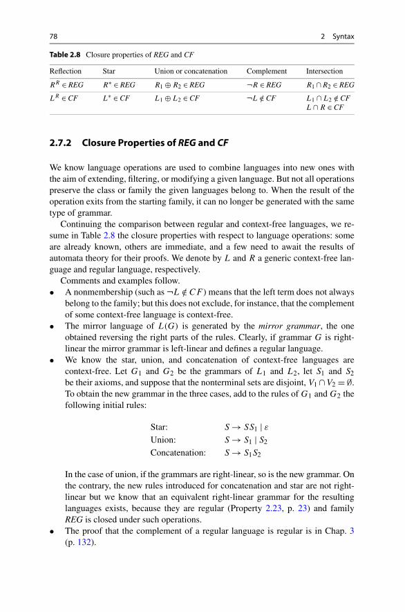
78 2 Syntax
Table 2.8 Closure properties of REG and CF
Reflection Star Union or concatenation Complement Intersection
RR ∈ REG R∗ ∈ REG R1 ⊕R2 ∈ REG ¬R ∈ REG R1∩R2 ∈ REG
LR ∈ CF L∗ ∈ CF L1 ⊕L2 ∈ CF ¬L /∈ CF L1 ∩L2 /∈ CFL∩R ∈ CF
2.7.2 Closure Properties of REG and CF
We know language operations are used to combine languages into new ones withthe aim of extending, filtering, or modifying a given language. But not all operationspreserve the class or family the given languages belong to. When the result of theoperation exits from the starting family, it can no longer be generated with the sametype of grammar.
Continuing the comparison between regular and context-free languages, we re-sume in Table 2.8 the closure properties with respect to language operations: someare already known, others are immediate, and a few need to await the results ofautomata theory for their proofs. We denote by L and R a generic context-free lan-guage and regular language, respectively.
Comments and examples follow.• A nonmembership (such as ¬L /∈ CF ) means that the left term does not always
belong to the family; but this does not exclude, for instance, that the complementof some context-free language is context-free.
• The mirror language of L(G) is generated by the mirror grammar, the oneobtained reversing the right parts of the rules. Clearly, if grammar G is right-linear the mirror grammar is left-linear and defines a regular language.
• We know the star, union, and concatenation of context-free languages arecontext-free. Let G1 and G2 be the grammars of L1 and L2, let S1 and S2
be their axioms, and suppose that the nonterminal sets are disjoint, V1∩V2 = ∅.To obtain the new grammar in the three cases, add to the rules of G1 and G2 thefollowing initial rules:
Star: S→ SS1 | εUnion: S→ S1 | S2
Concatenation: S→ S1S2
In the case of union, if the grammars are right-linear, so is the new grammar. Onthe contrary, the new rules introduced for concatenation and star are not right-linear but we know that an equivalent right-linear grammar for the resultinglanguages exists, because they are regular (Property 2.23, p. 23) and familyREG is closed under such operations.
• The proof that the complement of a regular language is regular is in Chap. 3(p. 132).

2.7 Comparison of Regular and Context-Free Languages 79
• The intersection of two context-free languages is not context-free (in general),as witnessed by the known language with three equal powers (Example 2.84 onp. 76):
{anbncn | n≥ 1
}= {anbnc+ | n≥ 1
}∩ {a+bncn | n≥ 1
}
where the two components are easily defined by context-free grammars.• As a consequence of De Morgan identity, the complement of a context-free
language is not context-free (in general): since L1 ∩ L2 = ¬(¬L1 ∪ ¬L2), ifthe complement were context-free, a contradiction would ensue since the unionof two context-free languages is context-free.
• On the other hand, the intersection of a context-free and a regular language iscontext-free. The proof will be given on p. 153.
The last property can be applied, in order to make a grammar more discriminatory,by filtering the language with a regular language which forces some constraints onthe original sentences.
Example 2.85 (Regular filters on Dyck language (p. 42)) It is instructive to see howthe freely parenthesized sentences of a Dyck language LD of alphabet Σ = {a, a′}can be filtered, by intersecting with the regular languages:
L1 = LD ∩¬(Σ∗a′a′Σ∗)= (
aa′)∗
L2 = LD ∩¬(Σ∗a′aΣ∗)= {
an(a′
)n | n≥ 0}
The first intersection preserves the sentences that do not contain substring a′a′, i.e.,it eliminates all the sentences with nested parentheses. The second filter preservesthe sentences having exactly one nest of parentheses. Both results are context-freelanguages, but the former is also regular.
2.7.3 Alphabetic Transformations
It is a common experience to find conceptually similar languages that differ by theconcrete syntax, i.e., by the choice of terminals. For instance, multiplication may berepresented by sign ×, by an asterisk, or by a dot in different languages. The termtransliteration or alphabetic homomorphism refers to the linguistic operation thatreplaces individual characters by other ones.
Definition 2.86 (Transliteration (or alphabetic homomorphism30)) Consider twoalphabets: source Σ and target Δ. An alphabetic transliteration is a function:
h :Σ →Δ∪ {ε}
30This is a simple case of the translation functions to be studied in Chap. 5.

80 2 Syntax
The transliteration or image of character c ∈ Σ is h(c), an element of the targetalphabet. If h(c)= ε, character c is erased. A transliteration is nonerasing if, for nosource character c, it is h(c)= ε.
The image of a source string a1a2 . . . an, ai ∈Σ is the string h(a1)h(a2) . . . h(an)
obtained concatenating the images of individual characters. Notice the image of theempty string is itself.
Such transformation is compositional: the image of the concatenation of twostrings v and w is the concatenation of the images of the strings:
h(v.w)= h(v).h(w)
Example 2.87 (Printer) An obsolete printer cannot print Greek characters and in-stead prints the special character �. Moreover, the test sent to the printer may con-tain control characters (such as start-text, end-text) that are not printed.The text transformation (disregarding uppercase letters) is described by the translit-eration:
h(c)= c if c ∈ {a, b, . . . , z,0,1, . . . ,9};h(c)= c if c is a punctuation mark or a blank space;h(c)=� if c ∈ {α,β . . . ,ω};h(start-text)= h(end-text)= ε.
An example of transliteration is
h(start-text the const. π has value 3.14 end-text︸ ︷︷ ︸source string
)= the const. � has value 3.14︸ ︷︷ ︸target string
An interesting special case of erasing homomorphism is the projection: it is afunction that erases some source characters and leaves the others unchanged.
Transliteration to Words The preceding qualification of transliteration as alpha-betic means the image of a character is a character (or the empty string), not a longerstring. Otherwise the transliteration or homomorphism may no longer be qualifiedas alphabetic. An example is the conversion of an assignment statement a← b+ c
to the form a := b+ c by means of a (non-alphabetical) transliteration:
h(←)= ‘ := ’ h(c)= c for any other c ∈Σ
This case is also called transliteration to words.Another example: vowels with umlaut of the German alphabet have as image a
string of two characters:
h(ä)= ae, h(ö)= oe, h(ü)= ue

2.7 Comparison of Regular and Context-Free Languages 81
Language Substitution A further generalization leads us to a language trans-formation termed substitution (already introduced in the discussion of linguisticabstraction on p. 26). Now a source character can be replaced by any string of aspecified language. Substitution is very useful in early language design phases, inorder to leave a construct unspecified in the working grammar. The construct is de-noted by a symbol (for instance 〈identifier〉). As the project progresses, the symbolwill be substituted with the definition of the corresponding language (for instancewith (a . . . z)(a . . . z | 0 . . .9)∗).
Formally, given a source alphabet Σ = {a, b, . . .}, a substitution h associates eachcharacter with a language h(a)= La,h(b)= Lb, . . . of target alphabet Δ. Applyingsubstitution h to a source string a1a2 . . . an, ai ∈Σ we obtain a set of strings:
h(a1a2 . . . an)= {y1y2 . . . yn | yi ∈ Lai}
We may say a transliteration to words is a substitution such that each image languagecontains one string only; if the string has length one or zero, the transliteration isalphabetic.
2.7.3.1 Closure Under Alphabetic TransformationLet L be a source language, context-free or regular, and h a substitution such thatfor every source character, its image is a language in the same family as the sourcelanguage. Then the substitution maps the set of source sentences (i.e., L) on a set ofimage strings, called the image or target language, L′ = h(L). Is the target languagea member of the same family as the source language? The answer is yes, and willbe given by means of a construction that is, valuable for modifying without effortthe regular expression or the grammar of the source language.
Property 2.88 The family CF is closed under the operation of substitution withlanguages of the same family (therefore also under the operation of transliteration).
Proof Let G be the grammar of L and h a substitution such that, for every c ∈Σ ,Lc is context-free. Let this language be defined by grammar Gc with axiom Sc.Moreover, we assume the nonterminal sets of grammars G,Ga,Gb, . . . are pairwisedisjoint (otherwise it suffices to rename the overlapping nonterminals).
Next we construct the grammar G′ of language h(L) by transliterating the rulesof G with the following mapping f :
f (c)= Sc, for every terminal c ∈Σ;f (A)=A, for every nonterminal symbol A of G.
The rules of grammar G′ are constructed next:• to every rule A→ α of G apply transliteration f , to the effect of replacing each
terminal character with the axiom of the corresponding target grammar;• add the rules of grammars Ga,Gb, . . .
It should be clear that the new grammar generates language h(L(G)). �

82 2 Syntax
In the simple case where the substitution h is a transliteration, the constructionof grammar G′ is more direct: replace in G any terminal character c ∈ Σ with itsimage h(c).
For regular languages an analogous result holds.
Property 2.89 The family REG is closed under substitution (therefore also undertransliteration) with regular languages.
Essentially the same construction of the proof of Property 2.88 can be applied tothe r.e. of the source language, to compute the r.e. of the target language.
Example 2.90 (Grammar transliterated) The source language i(; i)∗, defined byrules:
S→ i;S | ischematizes a program including a list of instructions i separated by semicolon.Imagine that instructions have to be now defined as assignments. Then the followingtransliteration to words is appropriate:
g(i)= v← e
where v is a variable and e an arithmetic expression. This produces the grammar:
S→A;S |A A→ v← e
As next refinement, the definition of expressions can be plugged in by means ofa substitution h(e) = LE , where the image language is the well-known one. Sup-pose it is defined by a grammar with axiom E. The grammar of the language afterexpression expansion is
S→A;S |A A→ v←E E→ ·· · −− usual rules for arith. expr.
As a last refinement, symbol v, which stands for a variable, should be replaced withthe regular language of identifier names.
2.7.4 Grammars with Regular Expressions
The legibility of an r.e. is especially good for lists and similar structures, and itwould be a pity to do without them when defining technical languages by meansof grammars. Since we know recursive rules are indispensable for parenthesis struc-tures, the idea arises to combine r.e. and grammar rules in a notation, called extendedcontext-free grammar, or EBNF,31 that takes the best of each formalism: simply
31Extended BNF.
2.7 Comparison of Regular and Context-Free Languages 83
enough we allow the right part of a rule to be an r.e. Such grammars have a nicegraphical representation, the syntax charts to be shown in Chap. 4 on p. 169, whichrepresents the blueprint of the flowchart of the syntax analyzer.
First observe that, since family CF is closed by all the operations of r.e., thefamily of languages defined by EBNF grammars coincide with family CF.
In order to appreciate the clarity of extended rules with respect to basic ones, weexamine a few typical constructs of programming languages.
Example 2.91 (EBNF grammar of a block language: declarations) Consider a listof variable declarations:
char text1, text2; real temp, result; int alpha, beta2, gamma;
to be found with syntactic variations in most programming languages.The alphabet is Σ = {c, i, r, v,′ ,′ ,′ ;′ }, where c, i, r stand for char, int, real and
v for a variable name. The language of lists of declarations is defined by r.e. D:((c | i | r)v(, v)∗; )+
The iteration operators used to generate lists are dispensable: remember any regularlanguage can be defined by a grammar, even a unilinear one.
The lists can be defined by the basic grammar:
D→DE |E E→AN; A→ c | i | r N → v,N | vwith two recursive rules (for D and N ). The grammar is a bit longer than the r.e. andsubjectively less perspicuous in giving evidence to the two-level hierarchical struc-ture of declarations, which is evident in the r.e. Moreover, the choice of metasymbolsA,E,N is to some extent mnemonic but arbitrary and may cause confusion, whenseveral individuals jointly design a grammar.
Definition 2.92 An extended context-free or EBNF grammar G = (V ,Σ,P,S)
contains exactly |V | rules, each one in the form A→ α , where A is a nonterminaland α is an r.e. of alphabet V ∪Σ .
For better legibility and concision, other derived operators (cross, power, option)too may be permitted in the r.e.
We continue the preceding example, adding typical block structures to the lan-guage.
Example 2.93 (Algol-like language) A block B embraces an optional declarativepart D followed by the imperative part I , between the marks b (begin) and e (end):
B→ b[D]Ie
The declarative part D is taken from the preceding example:
D→ ((c | i | r)v(, v)∗; )+

84 2 Syntax
The imperative part I is a list of phrases F separated by semicolon:
I → F(;F)∗
Last, a phrase F can be an assignment a or a block B:
F → a | BAs an exercise, yet worsening legibility, we eliminate as many nonterminals as pos-sible by applying nonterminal expansion to D:
B → b[(
(c | i | r)v(, v)∗; )+]Ie
A further expansion of I leads to
B→ b((c | i | r)v(, v)∗; )∗F(;F)∗e
Last F can be eliminated obtaining a one-rule grammar G′:
B→ b((c | i | r)v(, v)∗; )∗(a | B)
(; (a | B))∗
e
This cannot be reduced to an r.e. because nonterminal B cannot be eliminated, asit is needed to generate nested blocks (bb . . . ee) by a self-nesting derivation (inagreement with Property 2.80, p. 75).
Usually, language reference manuals specify grammars by EBNF rules, but be-ware that excessive grammar conciseness is often contrary to clarity. Moreover, ifa grammar is split into smaller rules, it may be easier for the compiler writer toassociate simple specific semantic actions to each rule, as we shall see in Chap. 5.
2.7.4.1 Derivations and Trees in Extended Context-Free GrammarsThe right part α of an extended rule A → α of grammar G is an r.e., which ingeneral derives an infinite set of strings: each one can be viewed as the right part ofa nonextended rule having unboundedly many alternatives.
For instance, A→ (aB)+ stands for a set of rules:
A→ aB | aBaB | . . .The notion of derivation can be defined for extended grammars too, via the notionof derivation for r.e. introduced on p. 19.
Shortly, for an EBNF grammar G consider a rule A→ α, where α is an r.e. pos-sibly containing choice operators (star, cross, union, and option); let α′ be a stringderiving from α (using the definition of the derivation of an r.e.), not containingany choice operator. For any (possibly empty) strings δ and η there is a one-stepderivation:
δAη⇒G
δα′η
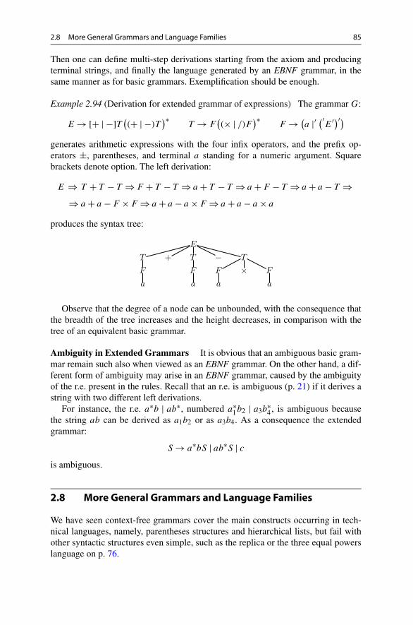
2.8 More General Grammars and Language Families 85
Then one can define multi-step derivations starting from the axiom and producingterminal strings, and finally the language generated by an EBNF grammar, in thesame manner as for basic grammars. Exemplification should be enough.
Example 2.94 (Derivation for extended grammar of expressions) The grammar G:
E→[+ | −]T ((+ | −)T
)∗T → F
((× | /)F )∗
F → (a |′ (′E′)′)
generates arithmetic expressions with the four infix operators, and the prefix op-erators ±, parentheses, and terminal a standing for a numeric argument. Squarebrackets denote option. The left derivation:
E ⇒ T + T − T ⇒ F + T − T ⇒ a + T − T ⇒ a + F − T ⇒ a + a − T ⇒⇒ a + a − F × F ⇒ a + a − a × F ⇒ a + a − a × a
produces the syntax tree:
Observe that the degree of a node can be unbounded, with the consequence thatthe breadth of the tree increases and the height decreases, in comparison with thetree of an equivalent basic grammar.
Ambiguity in Extended Grammars It is obvious that an ambiguous basic gram-mar remain such also when viewed as an EBNF grammar. On the other hand, a dif-ferent form of ambiguity may arise in an EBNF grammar, caused by the ambiguityof the r.e. present in the rules. Recall that an r.e. is ambiguous (p. 21) if it derives astring with two different left derivations.
For instance, the r.e. a∗b | ab∗, numbered a∗1b2 | a3b∗4 , is ambiguous because
the string ab can be derived as a1b2 or as a3b4. As a consequence the extendedgrammar:
S→ a∗bS | ab∗S | cis ambiguous.
2.8 More General Grammars and Language Families
We have seen context-free grammars cover the main constructs occurring in tech-nical languages, namely, parentheses structures and hierarchical lists, but fail withother syntactic structures even simple, such as the replica or the three equal powerslanguage on p. 76.

86 2 Syntax
Such shortcomings have motivated, from the early days of language theory, muchresearch on more powerful formal grammars. It is fair to say that none of the formalmodels have been successful; the more powerful are too obscure and difficult touse, and the models marginally superior to the context-free do not offer significantadvantages. In practice, application of such grammars to compilation32 has beenepisodic and was quickly abandoned. Since the basis of all subsequent developmentsis the classification of grammars due to the linguist Noam Chomsky, it is appropriateto briefly present it for reference, before moving on to more applied aspects in thecoming chapters.
2.8.1 Chomsky Classification
The historical classification of phrase structure grammars based on the form of therewriting rules is in Table 2.9. Surprisingly enough, very small difference in the ruleform, determine substantial changes in the properties of the corresponding familyof languages, both in terms of decidability and algorithmic complexity.
A rewriting rule has a left part and a right part, both strings on the terminalalphabet Σ and nonterminal set V . The left part is replaced by the right part. Thefour types are characterized as follows:• a rule of type 0 can replace an arbitrary not empty string over terminals and
nonterminals, with another arbitrary string;• a rule of type 1 adds a constraint to the form of type 0: the right part of a rule
must be at least as long as the left part;• a rule of type 2 is context-free: the left part is one nonterminal;• a rule of type 3 coincides with the unilinear form we have studied.For completeness Table 2.9 lists the names of the automata (abstract string recog-nition algorithms) corresponding to each type, although the notion of automata willnot be introduced until next chapter.
The language families are strictly included one into the next from bottom to top,which justifies the name of hierarchy.
Partly anticipating later matters, the difference between rule types is mirroredby differences in the computational resources needed to recognize the strings. Con-cerning space, i.e., memory complexity for string recognition, type 3 uses a finitememory, the others need unbounded memory.
Other properties are worth mentioning, without any claim to completeness. Allfour language families are closed under union, concatenation, star, reflection, andintersection with a regular language. But for other operators, properties differ: forinstance families 1 and 3, but not 0 and 2, are closed under complement.
Concerning decidability of various properties, the difference between the appar-ently similar types 0 and 1 is striking. For type 0 it is undecidable (more preciselysemi-decidable) whether a string is in the language generated by a grammar. For
32In computational linguistic some types of grammars more powerful than the context-freehave gained acceptance; we mention the best known example, Joshi’s Tree Adjoining Grammar(TAG) [9].

2.8 More General Grammars and Language Families 87
Table 2.9 Chomsky classification of grammars and corresponding languages and machines
Grammar Form of rules Languagefamily
Type of recognizer
Type 0 β→ α whereα,β ∈ (Σ ∪ V )+ and β �= ε
Recursivelyenumerable
Turing machine
Type 1 contextdependent (orcontextsensitive)
β→ α whereα,β ∈ (Σ ∪ V )+ and|β| ≤ |α|
Contextual orcontext-dependent
Turing machine withspace complexitylimited by the lengthof the source string
Type 2context-free orBNF
A→ α where A is anonterminal andα ∈ (Σ ∪ V )∗
Context-free CFor algebraic
Push-downautomaton
Type 3 unilinear(right-linear orleft-linear)
Right-linear: A→ uB
Left linear: A→ Bu, whereA is a nonterminal, u ∈Σ∗and B ∈ (V ∪ ε)
Regular REG orrational orfinite-state
Finite automaton
type 1 grammars the problem is decidable, though its time complexity is not polyno-mial. Last, only for type 3 the equivalence problem for two grammars is decidable.
We finish with two examples of type 1 grammars and languages.
Example 2.95 (Type 1 grammar of the three equal powers language) The language,proved on p. 76 to be not CF, is
L= {anbncn | n≥ l
}
It is generated by the context-sensitive grammar:1. S→ aSBC
2. S→ abC
3. CB → BC
4. bB→ bb
5. bC→ bc
6. cC→ cc
For type 0 and 1 grammars a derivation cannot be represented as a tree, because theleft part of a rule typically contains more than one symbol. However, the derivationcan be visualized as a graph, where the application of a rule such as BA→ AB isdisplayed by a bundle of arcs (hyper-edge) connecting the left part nodes to the rightpart ones.
Coming from our experience with context-free grammars, we would expect to beable to generate all sentences by left derivations. But if we try to generate sentenceaabbcc proceeding from left to right:
S⇒ aSBC⇒ aabCBC⇒ aabcBC⇒ block!
surprisingly, the derivation is stuck, before all nonterminal symbols are eliminated.In order to generate this string we need a not leftmost derivation, shown in Fig. 2.2.

88 2 Syntax
Fig. 2.2 Graphrepresentation of acontext-sensitive derivation(Example 2.95)
Intuitively the derivation produces the requested number of a with rule 1 (a type2 self-nesting rule) and then with rule (2). In the sentential form, letters b, B , andC appear with the correct number of occurrences, but mixed up. In order to producethe valid string, all C’s must be shifted to the right, using rule (3) CB → BC, untilthey reach the suffix position.
The first application of (3) reorders the sentential form, to the aim that B becomesadjacent to b. This enables derivation (4) bB ⇒ bb. Then the derivation continuesin the same manner, alternating steps (3) and (4), until the sentential form is leftwith just C as nonterminal. The occurrences of C are transformed to terminals c, bymeans of rule bC→ bc, followed by repeated applications of rule cC→ cc.
We stress the finding that the language generated by type 1 grammars may not co-incide with the sentences generated by left derivations, unlike for type 2 grammars.This is a cause of difficulty in string recognition algorithms.
Type 1 grammars have the power to generate the language of replicas, or listswith agreement between elements, a construct that we have singled out as practicallyrelevant and exceeding the power of context-free grammars.
Example 2.96 (Type 1 grammar of replica with center) Language L = {ycy | y ∈{a, b}+} contains sentences such as aabcaab, where a prefix and a suffix, dividedby the central separator c, must be equal.

2.8 More General Grammars and Language Families 89
To simplify the grammar, we assume sentences are terminated to the right by theend-of-text character or terminator, �. Grammar:
S→X � XA→XA′ A′A→AA′ A′ �→ a B ′a→ ba
X→ aXA XB→XB ′ A′B→ BA′ B ′ �→ b B ′b→ bb
X→ bXB B ′A→AB ′ A′a→ aa Xa→ ca
B ′B→ BB ′ A′b→ ab Xb→ cb
To generate a sentence, the grammar follows this strategy: it first generates a palin-drome, say aabXBAA, where X marks the center of the sentence and the secondhalf is in uppercase. Then the second half, modified as B ′AA, is reflected and con-verted in several steps to A′A′B ′. Last, the primed uppercase symbols are rewrittenas aab and the center symbol X is converted to c. We illustrate the derivation ofsentence aabcaab. For legibility, at each step we underline the left part of the rulebeing applied:
S ⇒ X �⇒ aXA �⇒ aaXAA �⇒ aabXBAA �⇒aabXB ′AA �⇒ aabXAB ′A �⇒ aabXA′B ′A �⇒aabXA′AB ′ �⇒ aabXAA′B ′ �⇒ aabXA′A′B ′ �⇒aabXA′A′b⇒ aabXA′ab⇒ aabXaab⇒ aabcaab
We observe that the same strategy used in generation, if applied in reverse order,would allow to check whether a string is a valid sentence. Starting from the givenstring, the algorithm should store on a memory tape the strings obtained after eachreduction (i.e., the reverse of derivation). Such procedure is essentially the compu-tation of a Turing machine that never goes out of the portion of tape containing theoriginal string, but may overprint its symbols.
Such examples should have persuaded the reader of the difficulty to design andapply context-sensitive rules even for very simple languages. The fact is that inter-action of grammar rules is hard to understand and control.
In other words, type 1 and 0 grammars can be viewed as a particular notation forwriting algorithms. All sorts of problems could be programmed in this way, evenmathematical ones, by using the very simple mechanism of string rewriting.33 It isnot surprising that using such an elementary mechanism as only data and controlstructure makes the algorithm description very entangled.
Undoubtedly the development of language theory towards models of higher com-putational capacity has mathematical and speculative interests but is almost irrele-vant for language engineering and compilation.34
33An extreme case is a type 1 grammar presented in [12] to generate prime numbers encoded inunary base, i.e., the language {an | n prime number}.34For historical honesty, we mention that context-sensitive grammars have been occasionally con-sidered by language and compiler designers. The language Algol 68 has been defined with a specialclass of type 1 grammars termed 2-level grammars, also known as VW-grammars from Van Wijn-garten [14]; see also Cleaveland and Uzgalis [2].
90 2 Syntax
In conclusion, we have to admit that the state of the art of formal language theorydoes not entirely satisfy the need of a powerful and practical formal grammar model,capable of accurately defining the entire range of constructs found in technical lan-guages. Context-free grammars are the best available compromise between expres-sivity and simplicity. The compiler designer will supplement their weaknesses byother methods and tools, termed semantic, coming from general-purpose program-ming methods. They will be introduced in Chap. 5.
References
1. J. Autebert, J. Berstel, L. Boasson, Context-free languages and pushdown automata, inHandbook of Formal Languages, vol. 1: Word, Language, Grammar, ed. by G. Rozenberg,A. Salomaa (Springer, New York, 1997), pp. 111–174
2. J. Cleaveland, R. Uzgalis, Grammars for Programming Languages (North-Holland, Ams-terdam, 1977)
3. S. Crespi Reghizzi, P. Della Vigna, C. Ghezzi, Linguaggi Formali e Compilatori (ISEDI,Milano, 1976)
4. S. Crespi Reghizzi, M. Pradella, Tile rewriting grammars and picture languages. Theor.Comput. Sci. 340(2), 257–272 (2005)
5. F. Gecseg, M. Steinby, Tree languages, in Handbook of Formal Languages, vol. 3: BeyondWords, ed. by G. Rozenberg, A. Salomaa (Springer, New York, 1997), pp. 1–68
6. D. Giammarresi, A. Restivo, Two-dimensional languages, in Handbook of Formal Lan-guages, vol. 3: Beyond Words, ed. by G. Rozenberg, A. Salomaa (Springer, New York,1997), pp. 215–267
7. M. Harrison, Introduction to Formal Language Theory (Addison-Wesley, Reading, 1978)8. J. Hopcroft, J. Ullman, Formal Languages and Their Relation to Automata (Addison-
Wesley, Reading, 1969)9. D. Jurafsky, J.H. Martin, Speech and Language Processing: An Introduction to Natural
Language Processing, Speech Recognition, and Computational Linguistics (Prentice-Hall,Englewood Cliffs, 2009)
10. P. Naur, Revised report on the algorithmic language ALGOL 60. Commun. ACM 6, 1–33(1963)
11. D. Perrin, J.E. Pin, Infinite Words (Elsevier, New York, 2004)12. A. Salomaa, Formal Languages (Academic Press, New York, 1973)13. W. Thomas, Languages, automata, and logic, in Handbook of Formal Languages, vol. 3:
Beyond Words, ed. by G. Rozenberg, A. Salomaa (Springer, New York, 1997), pp. 389–45514. A. Van Wijngarten, Report on the algorithmic language ALGOL 68. Numer. Math. 22, 79–
218 (1969)

3Finite Automata as Regular LanguageRecognizers
3.1 Introduction
Regular expressions and grammars are widely used in technical specifications oflanguages but the actual design and implementation of a compiler needs a way todescribe the algorithms, termed recognizers or acceptors, which examine a stringand decide if it is a valid sentence of the language. In this chapter we study therecognizers for regular languages and in the next two chapters those of context-freelanguages.
The need to recognize if a text is valid for a given language is quite common,especially as a first step for text processing or translation. A compiler analyzes asource program to check its correctness; a document processor makes a spell checkon words, then verifies syntax; and a graphic user interface must check that the dataare correctly entered. Such control is done by a recognition procedure, which canbe conveniently specified using minimalist models, termed abstract machines or au-tomata. The advantages are that automata do not depend on programming languagesand techniques, i.e., on implementation, and that their properties (such as time andmemory complexity) are in this way more clearly related with the family of thesource language.
In this chapter we briefly introduce more general automata, then focus on thosehaving a finite memory that match the regular language family and have countlessapplications in computer science and beyond. First we consider the deterministicmachines and describe useful methods for cleaning and minimizing. Then we mo-tivate and introduce nondeterministic models, and we show they correspond to theunilinear grammars of the previous chapter. Conversion back to deterministic mod-els follows.
A central section deals with transformations back and forth from regular expres-sions to automata. On the way to proving their convertibility, we introduce the sub-family of local regular languages, which have a simpler recognition procedure mak-ing use of a sliding window.
Then we return to the operations of complement and intersection on regular lan-guages from the standpoint of their recognizers, and present the composition of au-
S. Crespi Reghizzi et al., Formal Languages and Compilation,Texts in Computer Science, DOI 10.1007/978-1-4471-5514-0_3,© Springer-Verlag London 2013
91

92 3 Finite Automata as Regular Language Recognizers
tomata by Cartesian product. The chapter ends with a summary of the interrelationbetween finite automata, regular expressions, and grammars.
In compilation finite automata have several uses to be described especially inChap. 4: in lexical analysis to extract the shortest meaningful strings from a text, formaking simple translations, and for modeling and analyzing program properties instatic flow analysis and optimization.
3.2 Recognition Algorithms and Automata
To check if a string is valid for a specified language, we need a recognition algo-rithm, a type of algorithm producing a yes/no answer, commonly referred to in com-putational complexity studies as a decision algorithm. For instance, a famous prob-lem is to decide if two given graphs are isomorphic: the problem domain (a pair ofgraphs) differs from the case of language recognition, but the answer is again yes/no.
For the string membership problem, the input domain is a set of strings of alpha-bet Σ . The application of a recognition algorithm α to a given string x is denotedas α(x). We say string x is recognized or accepted if α(x) = yes, otherwise it isrejected. The language recognized, L(α), is the set of accepted strings:
L(α)= {x ∈Σ∗ | α(x)= yes
}
The algorithm is usually assumed to terminate for every input, so that the mem-bership problem is decidable. However, it may happen that, for some string x, thealgorithm does not terminate, i.e., the value of α(x) is not defined, hence x is not avalid sentence of language L(α). In such case we say that the membership problemfor L is semidecidable, or also that L is recursively enumerable.
In principle, if for an artificial language the membership problem is semidecid-able, we cannot exclude that the compiler falls into an endless loop, for some inputstrings. In practice we do not have to worry about such decidability issues, centralas they are for the theory of computation,1 because in language processing the onlylanguage families of concern are decidable, and efficiently so.
Incidentally, even within the family of context-free languages, some decisionproblems, different from string membership, are not decidable: we have mentionedin Chap. 2 the problem of deciding if two grammars are weakly equivalent, and ofchecking if a grammar is ambiguous.
In fact, recognizing a string is just the first step of the compilation process. InChap. 5 we shall see the translation from a language to another: clearly the codomainof a translation algorithm is much more complex than a pure yes/no, since it is itselfa set of strings, the target language.
Algorithms, including those for string recognition, may be ranked in complexityclasses, measured by the amount of computational resources (time or memory i.e.,space) required to solve the problem. In the field of compilation it is common to
1Many books cover the subject, e.g., Bovet and Crescenzi [3], Floyd and Beigel [4], Hopcroft andUllman [7], Kozen [8], Mandrioli and Ghezzi [9], and McNaughton [10]).

3.2 Recognition Algorithms and Automata 93
consider time rather than space complexity. With rare exceptions, all the problemsof interest for compilation have low time complexity: linear or at worst polynomialwith respect to the size of the problem input. Time complexity is closely relatedwith electric power consumption, which is an important attribute for portable pro-grammed devices.
A tenet of the theory of computation is that the complexity of an algorithm shouldbe measured by the number of steps, rather than by the actual execution time spentby a program implementing the algorithm. The reason is that the complexity shouldbe a property of the algorithm and should not depend on the actual implementationand processing speed of a particular computer. Even so, several choices are openfor computational steps: they may range from a Turing machine move to a machineinstruction or to a high-level language statement. Here we consider a step to bean elementary operation of an abstract machine or automaton, as customary in allthe theoretical and applied studies on formal languages. This approach has severaladvantages: it gives evidence to the relation between the algorithmic complexity andthe family of languages under consideration; it allows to reuse optimized abstractalgorithms with a low cost of adaptation to the language, and it avoids prematurecommitment and tedious details of implementation. Moreover, sufficient hints willbe given for a programmer to easily transform the automaton into a program, byhand or by using widespread compiler generation tools.
3.2.1 A General Automaton
An automaton or abstract machine is an ideal computer featuring a very small setof simple instructions. Starting from the Turing machine of the 1930s, research onabstract machines has spawned many models, but only a few are important for lan-guage processing.2 In its more general form a recognizer is schematized in Fig. 3.1.It comprises three parts: input tape, control unit, and (auxiliary) memory.
The control unit has a limited store, to be represented as a finite set of states;the auxiliary memory, on the other hand, has unbounded capacity. The upper tapecontains the given input or source string, which can be read but not changed. Eachcase of the tape contains a terminal character; the cases to the left and right ofthe input contain two delimiters, the start of text mark � and the end of text markor terminator �. A peculiarity of automata is that the auxiliary memory is also atape (instead of the random access memory used in other computational models),containing symbols of another alphabet.
The automaton performs at discrete time instants the following actions: read thecurrent character ai from input, shift the reading head, read from memory the cur-rent symbol Mj and replace it with another symbol, move the memory head, andchange the current state of the control unit to the next one.
2Other books have a broader and deeper coverage of automata theory, such as Salomaa [14],Hopcroft and Ullman [6, 7], Harrison [5], and the handbook [12]; for finite automata a specificreference is Sakarovich [13].

94 3 Finite Automata as Regular Language Recognizers
Fig. 3.1 General automaton
The automaton examines the source by performing a series of moves; the choiceof a move depends on the current two symbols (input and memory) and on thecurrent state. A move may have some of the following effects:• shift the input head left or right by one position;• overwrite the current memory symbol with another one, and shift the memory
head left or right by one position;• change the state of the control unit.A machine is unidirectional if the input head only moves from left to right: this isthe model to be considered in the book, because it well represents text processingby a single scan. For unidirectional machines the start of text mark is superfluous.
At any time the future behavior of the machine depends on a 3-tuple, called an(instantaneous) configuration: the suffix of the input string still to be read, that is,laying to the right of the head; the contents of the memory tape and the position ofthe head; the state of the control unit. The initial configuration has: the input headpositioned on character a1 (i.e., right of the start of text mark), the control unit inan initial state, and the memory containing a specific symbol (or sometimes a fixedstring).
Then the machine performs a computation, i.e., a sequence of moves, that leadsto new configurations. If for a configuration at most one move can be applied, thechange of configuration is deterministic. A nondeterministic (or indeterministic) au-tomaton is essentially a manner of representing an algorithm that in some situationmay explore alternative paths.
A configuration is final if the control is in a state specified as final, and the inputhead is on the terminator. Sometimes, instead of, or in addition to being in a finalstate, a final configuration is qualified by the fact that the memory tape contains aspecified symbol or string: a frequent choice is for memory to be empty.

3.2 Recognition Algorithms and Automata 95
The source string x is accepted if the automaton, starting in the initial config-uration with x � as input, performs a computation leading to a final configuration(a nondeterministic automaton can possibly reach a final configuration by differentcomputations). The language accepted or recognized by the machine is the set ofaccepted strings.
Notice a computation terminates either when the machine has entered a final con-figuration or when in the current configuration no move can be applied. In the lattercase the source string is not accepted by that computation (but perhaps accepted byanother computation if the machine is indeterministic).
Two automata accepting the same language are called equivalent. Of course twomachines, though equivalent, may belong to different models or have different com-putational complexities.
Turing Machine The preceding description substantially reproduces the automa-ton introduced by A. Turing in 1936 and widely taken as the best available for-malization of any sequential algorithm. The family of languages accepted is termedrecursively enumerable. In addition, a language is termed decidable (or recursive)if there exists a Turing machine accepting it and halting for every input string. Thefamily of decidable languages is smaller than the one of recursively enumerablelanguages.
Such machine is the recognizer of two of the language families of Chomskyclassification (p. 86). The languages generated by type 0 grammars are exactly therecursively enumerable. The languages of context-sensitive or type 1 grammars, onthe other hand, correspond to the languages accepted by a Turing machine that isconstrained in its use of memory: the length of the memory tape is bounded by thelength of the input string.
Turing machines are not relevant for practical applications but are a significantterm of comparison for the efficient machine models used to recognize and trans-form technical languages. Such models can be viewed as Turing machines withsevere limitation on memory. When no auxiliary memory is available, we have thefinite-state or simply finite automaton, the most fundamental type of computing ma-chine which corresponds to the regular languages. If the memory is organized asLIFO (last in first out) store, the machine is termed a pushdown automaton and isthe recognizer of context-free languages.
The memory limitations have a profound effect on the properties and in partic-ular the performance of the automata. Considering the worst-case time complexity,which is a primary parameter for program efficiency, a finite automaton is able torecognize a string in linear time, or more exactly in real time, that is, with a numberof steps equal to the input length. In contrast the space bounded Turing machinemay take a non-polynomial time to recognize a context-sensitive language, anotherreason making it unpractical to use. Context-free language recognizers are somehowin between: the number of steps is bounded by a polynomial of small degree of theinput string length.

96 3 Finite Automata as Regular Language Recognizers
3.3 Introduction to Finite Automata
Finite automata are surely the simplest and most fundamental abstract computa-tional device. Their mathematical theory is very stable and deep and is able to sup-port innumerable applications in diverse areas, from digital circuit design to systemmodeling and communication protocols, to mention just a few. Our presentation willbe focused on the aspects that are important for language and compiler design, butin order to make the presentation self-contained we briefly introduce some essentialdefinitions and theoretical results.
Conforming to the general scheme, a finite automaton comprises: the input tapewith the source string x ∈ Σ∗; the control unit; the reading head, initially placedon the first character of x, scanning the string until its end, unless an error occursbefore. Upon reading a character, the automaton updates the state of the controlunit and advances the reading head. Upon reading the last character, the automatonaccepts x if and only if the state is an accepting one.
A well-known representation of an automaton is by a state-transition diagram orgraph. This is a directed graph whose nodes are the states of the control unit. Eacharc is labeled with a terminal and represents the change of state or transition causedby reading the terminal.
Example 3.1 (Decimal constants) The set L of decimal constants has the alphabetΣ =Δ∪ {0,•} where Δ= {1,2,3,4,5,6,7,8,9} is a digit other than zero. The r.e.is
L= (0∪Δ(0∪Δ)∗
) • (0∪Δ)+
The recognizer is specified by the state-transition diagram or by the equivalentstate-transition table in Fig. 3.2.
Fig. 3.2 State-transition diagram or graph (left) and table (right) for decimal constants (Exam-ple 3.1)

3.4 Deterministic Finite Automata 97
Notice that if several arcs span the same two nodes, only one is drawn: e.g., arc(q0 → q1) represents a bundle of 9 arcs with labels 1,2, . . . ,9. The initial state q0is marked by an ingoing arrow; the final state q4 by an outgoing arrow. The transi-tion table is the incidence matrix of the graph: for each pair (current state, currentcharacter) the entry contains the next state. Notice the arrows giving evidence toinitial/final states.
Given the source string 0•2•, the automaton transits through the states q0, q2, q3,q4. In the last state, since no transition allows reading a • character, the computationstops before the entire input has been consumed. As a consequence, the source stringis not accepted. On the other hand, input 0 • 21 would be accepted.
If we prefer to modify the language so that constants such as 305• ending with adecimal point are legal, the state q3 too must be marked as final.
We have seen an automaton may have several final states, but only one initialstate (otherwise it would not be deterministic).
3.4 Deterministic Finite Automata
The previous ideas are formalized in the next definition.A finite deterministic automaton M comprises five items:
1. Q, the state set (finite and not empty)2. Σ , the input or terminal alphabet3. the transition function δ : (Q×Σ)→Q
4. q0 ∈Q, the initial state5. F ⊆Q, the set of final states.Function δ specifies the moves: the meaning of δ(q, a) = r is that machine M inthe current state q reads a and moves to next state r . If δ(q, a) is undefined, theautomaton stops and we can assume it enters the error state; more on that later. Asan alternative notation we indicate the move, from state q to state r reading symbola, as q
a→ r , which intuitively recalls the corresponding arc on the state-transitiondiagram.
The automaton processes a not empty string x by a series of moves. Take x = ab;reading the first character, the first step δ(q0, a)= q1 leads to state q1, then to q2 bythe second step δ(q1, b)= q2.
In short, instead of writing δ(δ(q0, a), b) = q2, we combine the two steps intoδ(q0, ab)= q2, to say that reading string ab the machine moves to state q2. Noticethat the second argument of function delta is now a string.
A special case is the empty string, for which we assume no change of state:
∀q ∈Q : δ(q, ε)= q
Following these stipulations, the domain of the transition function is (Q×Σ∗) andthe definition is
δ(q, ya)= δ(δ(q, y), a
), where a ∈Σ and y ∈Σ∗

98 3 Finite Automata as Regular Language Recognizers
Looking at the graph, if δ(q, y)= q ′, then, and only then, there exists a path fromnode q to node q ′, such that the concatenated labels of the arrows make string y.We say y is the label of the path and the path represents a computation.
A string x is recognized or accepted by the automaton if it is the label of a pathfrom the initial state to a final state, δ(q0, x) ∈ F .
Notice the empty string is recognized if, and only if, the initial state is also final,q0 ∈ F .
The language recognized or accepted by automaton M is
L(M)= {x ∈Σ∗ | x is recognized by M
}
The languages accepted by such automata are termed finite-state recognizable.Two automata are equivalent if they accept the same language.
Example 3.2 (Example 3.1 continued) The automaton M of p. 96 is defined by
Q = {q0, q1, q2, q3, q4}Σ = {1,2,3,4,5,6,7,8,9,0,•}q0 = q0
F = {q4}Examples of transitions:
δ(q0,3•1)= δ(δ(q0,3•),1
)= δ(δ(δ(q0,3),•),1
)= δ(δ(q1,•),1
)= δ(q3,1)= q4
Since q4 ∈ F , string 3 • 1 is accepted. On the contrary, since δ(q0,3•) = q3 isnot final, string 3• is rejected, as well as string 02 because function δ(q0,02) =δ(δ(q0,0),2)= δ(q2,2) is undefined.
Observing that for each input character the automaton executes one step, the totalnumber of steps is exactly equal to the length of the input string. Therefore suchmachines are very efficient as they can recognize strings in real time by a singleleft-to-right scan.
3.4.1 Error State and Total Automata
If the move is not defined in state q when reading character a, we say that theautomaton falls into the error state qerr. The error state is such that for any characterthe automaton remains in it, thus justifying its other name of sink or trap state.Obviously the error state is not final.
The state-transition function can be made total by adding the error state and thetransitions from/to it:
∀ state q ∈Q and ∀a ∈Σ, if δ(q, a) is undefined set δ(q, a)= qerr∀a ∈Σ set δ(qerr, a)= qerr

3.4 Deterministic Finite Automata 99
Fig. 3.3 Recognizer ofdecimal constants completedwith sink (error or trap) state
The recognizer of decimal constants, completed with error state, is shown inFig. 3.3.
Clearly any computation reaching the error state gets trapped in it and cannotreach a final state. As a consequence, the total automaton accepts the same languageas the original one. It is customary to leave the error state implicit, neither drawinga node nor specifying the transitions for it.
3.4.2 Clean Automata
An automaton may contain useless parts not contributing to any accepting compu-tation, which are best eliminated. Notice the following concepts hold as well fornondeterministic finite automata, and in general for any kind of abstract machine.
A state q is reachable from state p if a computation exists going from p to q .A state is accessible if it can be reached from the initial state; it is postaccessibleif a final state can be reached from it. A state is called useful if it is accessible andpostaccessible; otherwise it is useless. In other words a useful state lays on somepath from the initial state to a final one.
An automaton is clean (or reduced) if every state is useful.
Property 3.3 For every finite automaton there exists an equivalent clean automa-ton.
The construction of the clean machine consists of identifying and deleting uselessstates, together with adjoining transitions.

100 3 Finite Automata as Regular Language Recognizers
Fig. 3.4 Useless states (top)and their eliminationobtaining a clean automaton(bottom)
Example 3.4 (Elimination of useless states) Figure 3.4 shows a machine with use-less states and the corresponding clean machine.
Notice the error state is never postaccessible, hence always useless.
3.4.3 Minimal Automata
We focus on properties of the automata recognizing the same language. Their statesets and transition functions are in general different but their computations areequivalent. A central property is that, among such equivalent machines, there ex-ists only one which is the smallest in the following sense.
Property 3.5 For every finite-state language, the (deterministic) finite recognizerminimal with respect to the number of states is unique (apart from renaming ofstates).
Conceptually the statement is fundamental as it permits to represent a collectionof equivalent machines by a standard one which, moreover, is minimal. In practicethis is not so important for compiler applications, nevertheless we describe for self-consistency the standard minimization algorithm.
First we need to introduce an algebraic relation between equivalent states, to becomputed by the algorithm.3
Although we assume the given automaton is clean, some of its states may beredundant, in the sense that they can be fused together at no consequence for stringsaccepted or rejected. Any two such states are termed indistinguishable from each
3Other more efficient and subtle algorithms have been invented. We refer the reader to the surveyin [16].

3.4 Deterministic Finite Automata 101
Fig. 3.5 Automaton M to beminimized (Example 3.7)
other, and the corresponding binary relation is termed indistinguishability (or ofNerode type).
Definition 3.6 The states p and q are indistinguishable if, and only if, for everystring x ∈Σ∗, either both states δ(p, x) and δ(q, x) are final, or neither one is. Thecomplementary relation is termed distinguishability.
Spelling out the condition, two states p and q are indistinguishable if, startingfrom them and scanning the same arbitrarily chosen input string x, it never happensthat a computation reaches a final state and the other does not.
Notice that:1. the sink state qerr is distinguishable from every state p, since for any state
there exists a string x such that δ(p, x) ∈ F , while for every string x it isδ(qerr, x)= qerr;
2. p and q are distinguishable if p is final and q is not, because δ(p, ε) ∈ F andδ(q, ε) /∈ F ;
3. p and q are distinguishable if, for some character a, the next states δ(p, a) andδ(q, a) are distinguishable.
In particular, p is distinguishable from q if the set of labels attached to the outgo-ing arrows from p and the similar set from q are different: in that case there existsa character a such that the move from state p reaches state p′, while the move fromq is not defined (i.e., it reaches the sink); from condition (3). the two states aredistinguishable.
Indistinguishability as a relation is symmetric, reflexive, and transitive, i.e., it isan equivalence relation, whose classes are computed by a straightforward procedureto be described next by means of an example.
Example 3.7 (Equivalence classes of indistinguishable states) For automaton M ofFig. 3.5, we construct a table of size |Q|× |Q|, representing the indistinguishabilityrelation; but, since the relation is symmetric, we do not have to fill the cases on andabove the principal diagonal.
The procedure will mark with X the case at position (p, q), when it discoversthat the states p and q are distinguishable. We initialize with X the cases such thatone state only is final:
q1 – –q2 X X –q3 X X
q0 q1 q2

102 3 Finite Automata as Regular Language Recognizers
Then we examine every case (p, q) still unmarked and, for every character a, weconsider the next states r = δ(p, a) and s = δ(q, a). If case (r, s) already con-tains X, meaning that r is distinguishable from s, then also p and q are so, thereforecase (p, q) is marked X. Otherwise, if (r, s) is not marked X, the pair (r, s) is writ-ten into case (p, q), as a future obligation, if case (r, s) will get marked, to markcase (p, q) as well.
The pairs of next states are listed in the table to the left. The result of this step isthe table to the right. Notice that case (1,0) is marked because the pair (0,2)≡ (2,0)
was already marked:
q1 (1,1), (0,2) – –q2 X X –q3 X X (3,3), (2,2)
q0 q1 q2
q1 X – –q2 X X –q3 X X (3,3), (2,2)
q0 q1 q2
Now all cases (under the principal diagonal) are filled and the algorithm terminates.The cases not marked with X identify the indistinguishable pairs, in our exampleonly the pair (q2, q3).
An equivalence class contains all the pairwise indistinguishable states. In theexample the equivalence classes are [q0], [q1], [q2, q3].
It is worthwhile analyzing another example where the transition function isnot total. To this end, we modify automaton M of Fig. 3.5, erasing the self-loopδ(q3, a) = q3, i.e., redefining the function as δ(q3, a) = qerr. As a consequence,states q2 and q3 become distinguishable, because δ(q2, a)= q3 and δ(q3, a)= qerr.Now every equivalence class is a singleton, meaning the automaton is already min-imal.
3.4.3.1 Construction of Minimal AutomatonThe minimal automaton M ′, equivalent to the given M , has for states the equiva-lence classes of the indistinguishability relation. It is simple to construct its transi-tion function: M ′ contains the arc:
C1︷ ︸︸ ︷[. . . , pr , . . .] b−→
C2︷ ︸︸ ︷[. . . , qs, . . .]
between equivalence classes C1 and C2, if, and only if, M contains an arc:
prb−→ qs
between two states, respectively, belonging to the two classes. Notice that the samearc of M ′ may derive from several arcs of M .
Example 3.8 (Example 3.7 continued) The minimal automaton M ′ is in Fig. 3.6.This has the least number of states of all equivalent machines. In fact, we couldeasily check that merging any two states, the resulting machine would not be equiv-alent, but it would accept a larger language than the original.
3.4 Deterministic Finite Automata 103
Fig. 3.6 Result M ′ ofminimization of automatonM of Fig. 3.5
The example has constructively illustrated Property 3.5: that the minimal au-tomaton is unique. From this it is a straightforward test to check whether two givenmachines are equivalent. First minimize both machines; then compare their state-transition graphs to see if they are identical (i.e., isomorphic and with correspondinginitial and final states), apart from a change of name of the states.4
In practical use, obvious economy reasons make the minimal machine a prefer-able choice. But the saving is often negligible for the cases of concern in com-piler design. What is more, in certain situations state minimization of the recognizershould be avoided: when the automaton is enriched with actions computing an out-put function, to be seen in Chap. 5, two states that are indistinguishable for therecognizer, can be associated with different output actions. Then merging the stateswould spoil the intended translation.
Finally we anticipate that the uniqueness property of the minimal automaton doesnot hold for the nondeterministic machines to be introduced next.
3.4.4 From Automata to Grammars
Without much effort we are going to realize that finite automata and unilinear (ortype 3) grammars of p. 69 are alternative but equivalent notations defining the samelanguage family.
First we show how to construct a right-linear grammar equivalent to an automa-ton. Grammar G has as nonterminal set the states Q of the automaton, and the axiomis the initial state. For each move q
a−→ r the grammar has the rule q → ar . If stateq is final, it has also the terminal rule q→ ε.
It is evident that there exists a bijective correspondence between the computa-tions of the automaton and the derivations of the grammar: a string x is accepted by
the automaton if, and only if, it is generated by a derivation q0+⇒ x.
Example 3.9 (From the automaton to the right-linear grammar) The automaton andcorresponding grammar are
4Other more efficient equivalence tests do without first minimizing the automata.

104 3 Finite Automata as Regular Language Recognizers
Sentence bca is recognized in 3 steps by the automaton and it derives from theaxiom in 3+ 1 steps:
q0 ⇒ bq1 ⇒ bcq0 ⇒ bcaq0 ⇒ bcaε
Observe the grammar contains empty rules but of course it can be turned into thenon-nullable normal form by means of the transformation on p. 57.
For the example, first we find the set of nullable nonterminals Null = {q0, q2};then we construct the equivalent rules:
q0 → aq0 | bq1 | a | ε q1 → cq0 | aq2 | bq2 | a | b | cNow q2 is eliminated because its only rule is empty. Finally, grammar cleaningproduces the rules:
q0 → aq0 | bq1 | a | ε q1 → cq0 | a | b | cOf course the empty rule q0 → ε must stay there because q0 is the axiom, whichcauses the empty string to be a sentence.
In this normal form of the grammar it is evident that a move entering a finalstate r :
qa−→ r →
may correspond to two rules q → ar | a, one producing the nonterminal r , the otherof the terminal type.
The conversion from automaton to grammar has been straightforward, but tomake the reverse transformation from grammar to automaton, we need to modifythe machine definition by permitting nondeterministic behavior.
3.5 Nondeterministic Automata
A right-linear grammar may contain two alternative rules:
A→ aB | aC where a ∈Σ,A,B,C ∈ V
starting with the same character a. In this case, converting the rules to machinetransitions, two arrows with identical label would exit from the same state A andenter two distinct states B and C. This means that in state A, reading character a,the machine can choose which one of the next states to enter: its behavior is notdeterministic. Formally the transition function takes two values, δ(A,a)= {B,C}.
Similarly a copy rule:
A→ B where B ∈ V

3.5 Nondeterministic Automata 105
Fig. 3.7 R.e. and corresponding nondeterministic machine N2 checking the penultimate characteris b
would be converted into an unusual machine transition from state A to state B ,which does not read any terminal character (it would be odd to say it reads theempty string).
A machine move that does not read an input character is termed spontaneous oran epsilon move. Spontaneous moves too cause the machine to be nondeterministic,as in the following situation:
where in state A the automaton can choose to move spontaneously (i.e., withoutreading) to B , or to read a character, and if it is an a, to move to C.
3.5.1 Motivation of Nondeterminism
The mapping from grammar rules to transitions pushed us to introduce some transi-tions with multiple destinations and spontaneous moves, which are the main formsof indeterminism. Since this might appear as a useless theoretical concept, we hastento list several advantages.
3.5.1.1 ConcisionDefining a language with a nondeterministic machine often results in a more read-able and compact definition, as in the next example.
Example 3.10 (Penultimate character) A sentence, like abaabb, is characterizedby the presence of letter b in the penultimate position. The r.e. and nondeterministicrecognizer are in Fig. 3.7.
We have to explain how machine N2 works: given an input string, the machineseeks a computation, i.e., a path from the initial state to the final, labeled with theinput characters; if it succeeds, the string is accepted. Thus string baba is recognizedwith the computation:
q0b→ q0
a→ q0b→ q1
a→ q2
Notice other computations are possible, for instance the path:
q0b→ q0
a→ q0b→ q0
a→ q0
fails to recognize, because it does not reach the final state.

106 3 Finite Automata as Regular Language Recognizers
Fig. 3.8 Deterministicrecognizer M2 of stringshaving b next to last
The same language is accepted by the deterministic automaton M2 in Fig. 3.8.Clearly this machine is not just more complicated than the nondeterministic typein Fig. 3.7, but the latter makes it more perspicuous that the penultimate charactermust be b.
To strengthen the argument consider a generalization of language L2 to lan-guage Lk , such that, for some k ≥ 2, the kth character before the last is b. Withlittle thought we see the nondeterministic automaton would have k+ 1 states, whileone could prove that the number of states of the minimal deterministic machine isan exponential function of k.
In conclusion nondeterminism sometimes allows much shorter definitions.
3.5.1.2 Left Right Interchange and Language ReflectionNondeterminism also arises in string reversal when a given deterministic machineis transformed to recognize the reflection LR of language L. This is sometimesrequired when for some reason strings must be scanned from right to left.
The new machine is straightforward to derive: interchange initial and final states5
and reverse all the arrows. Clearly this may give birth to nondeterministic transi-tions.
Example 3.11 The language having b as penultimate character (L2 of Fig. 3.7) isthe reflection of the language having the second character equal to b:
L′ = {x ∈ {a, b}∗ | b is the second character of x
}L2 =
(L′
)R
L′ is recognized by the deterministic automaton (left):
5If the machine has several final states, multiple initial states result thus causing another form ofindeterminism to be dealt with later.

3.5 Nondeterministic Automata 107
Transforming the deterministic automaton for L′ as explained above, we obtain thenondeterministic machine for L2 (right), which by the way is identical to the one inFig. 3.7.
As a further reason, we anticipate that nondeterministic machines are the in-termediate product of procedures for converting r.e. to automata, widely used fordesigning lexical analyzers or scanners.
3.5.2 Nondeterministic Recognizers
We precisely define the concept of nondeterministic finite-state computation, firstwithout spontaneous moves. A nondeterministic finite automaton N , without spon-taneous moves, is defined by• the state set Q
• the terminal alphabet Σ
• two subsets of Q: the set I of the initial states and the set F of final states• the transition relation δ, a subset of the Cartesian product Q×Σ ×Q
Remark This machine may have several initial states. In the graphic representationa transition q1
a→ q2 is an arc labeled a, from the first to the second state.
As before, a computation is a series of transitions such that the origin of each onecoincides with the destination of the preceding one:
q0a1→ q1
a2→ q2 · · · an→ qn
The computation origin is q0, the termination is qn, and the length is the number n oftransitions or moves. A computation of length 1 is just a transition. The computationlabel is the concatenation a1a2 . . . an of the characters read by each transition. In
brief, the computation is also written q0a1a2...an−→ qn.
A string x is recognized or accepted by the automaton, if it is the label of acomputation originating in some initial state, terminating in some final state, andhaving label x.
Let us focus on the empty string. We stipulate that every state is the origin andtermination of a computation of length 0, having the empty string ε as label. Itfollows that the empty string is accepted by an automaton if, and only if, thereexists an initial state which is also final.
The language L(N) recognized by automaton N is the set of accepted strings:
L(N)= {x ∈Σ∗ | q x→ r with q ∈ I, r ∈ F
}
Example 3.12 (Searching a text for a word) Given a string or word y and a text x,does x contain y as substring? The following machine recognizes the texts whichcontain one or more occurrences of y, that is, the language (a | b)∗y(a | b)∗. We

108 3 Finite Automata as Regular Language Recognizers
illustrate with the word y = bb:
String abbb is the label of several computations originating in the initial state:
pa→ p
b→ pb→ p
b→ p pa→ p
b→ pb→ p
b→ q
pa→ p
b→ pb→ q
b→ r pa→ p
b→ qb→ r
b→ r
The first two computations do not find the word looked for. The last two find theword, respectively, at position ab bb︸︷︷︸ and a bb︸︷︷︸b.
3.5.2.1 Transition FunctionThe moves of a nondeterministic automaton can still be considered as a finite func-tion, but one computing sets of values. For a machine N = (Q,Σ, δ, I,F ), devoidof spontaneous moves, the functionality of the state-transition function δ is the fol-lowing:
δ :Q× (Σ ∪ {ε})→ ℘(Q)
where symbol ℘(Q) indicates the powerset of set Q, i.e., the set of all the subsetsof Q. Now the meaning of δ(q, a) = [p1,p2, . . . , pk] is that the machine readinga in the current state q , can arbitrarily move to any of the states p1, . . . , pk . As wedid for deterministic machines, we extend the function to any string y including theempty one:
∀q ∈Q : δ(q, ε)= [q]∀q ∈Q,y ∈Σ∗ : δ(q, y)= [p | q y→ p]
In other words, it is p ∈ δ(q, y) if there exists a computation labeled y from q to p.The previous definitions allow a reformulation of the language accepted by au-
tomaton N :
L(N)= {x ∈Σ∗ | ∃q ∈ I : δ(q, x)∩ F �= ∅}
i.e., the set computed by function delta must contain a final state, for a string to berecognized.
Example 3.13 (Example 3.12 continued)
δ(p, a)= [p], δ(p, ab)= [p,q], δ(p, abb)= [p,q, r]

3.5 Nondeterministic Automata 109
Fig. 3.9 Decimal constant definition with spontaneous moves (Example 3.14)
3.5.3 Automata with Spontaneous Moves
Another kind of nondeterministic behavior occurs when an automaton changes statewithout reading a character, thus performing a spontaneous move, to be depicted inthe state-transition diagram as an arc labeled ε (named ε-arc). Such arcs will proveto be expedient for assembling the automata recognizing a regular composition offinite-state languages. The next example illustrates the case for union and concate-nation.
Example 3.14 (Compositional definition of decimal constants) This language in-cludes constants such as 90 • 01. The part preceding the decimal point may be miss-ing (as in •02); but it may not contain leading zeroes. Trailing zeroes are permittedat the end of the fractional part. The language is defined by the r.e.:
L= (0 | ε |N) • (0 . . .9)+ where N = (1 . . .9)(0 . . .9)∗
The automaton in Fig. 3.9 mirrors the structure of the expression. Notice that thepresence of spontaneous moves does not affect the way a machine performs recog-nition: a string x is recognized by a machine with spontaneous moves if it is thelabel of a computation originating in an initial state and terminating in a final state.
Observe that taking the spontaneous move from A to C, the integer part N van-ishes. The string 34 • 5 is accepted with the computation:
A3→ B
4→ Bε→ C
•→D5→E
But the number of steps of the computation (i.e., the length of the path in thegraph) can exceed the length of the input string, because of the presence of ε-arcs.As a consequence, the recognition algorithm no longer works in real time. Yet timecomplexity remains linear, because it is possible to assume that there are no cyclesof spontaneous moves in any computation.
The family of languages recognized by such nondeterministic automata is alsocalled finite-state.
3.5.3.1 Uniqueness of Initial StateThe official definition of nondeterministic machine allows two or more initial states,but it is easy to construct an equivalent machine with only one: add to the machine

110 3 Finite Automata as Regular Language Recognizers
a new state q0, which will be the only initial state, and the ε-arcs going from itto the former initial states of the automaton. Clearly any computation on the newautomaton accepts a string if, and only if, the old automaton does so.
The transformation has changed one form of indeterminism, linked with multipleinitial states, to another form related to spontaneous moves. We shall see on p. 114that such moves can be eliminated.
3.5.4 Correspondence Between Automata and Grammars
We collect in Table 3.1 the mapping between nondeterministic automata, also withspontaneous moves, and unilinear grammars. The correspondence is so direct that itwitnesses the two models are essentially notational variants.
Consider a right-linear grammar G = (V ,Σ,P,S) and a nondeterministic au-tomaton N = (Q,Σ, δ, q0,F ), which we may assume from the preceding discus-sion to have a single initial state. First assume the grammar rules are strictly unilin-ear (p. 70). The states Q of the automaton match the nonterminals V of the grammar.The initial state corresponds to the axiom. Notice (row 3) that the pair of alterna-tives p→ aq | ar correspond to two nondeterministic moves. A copy rule (row 4)matches a spontaneous move. A final state (row 5) matches a nonterminal having anempty rule.
It is easy to see that every grammar derivation matches a machine computation,and conversely, so that the following statement ensues.
Property 3.15 A language is recognized by a finite automaton if, and only if, it isgenerated by a unilinear grammar.
Notice that the statement concerns also left-linear grammars, since we know fromChap. 2 they have the same capacity as right-linear grammars.
If the grammar contains non-empty terminal rules of type p→ a where a ∈Σ ,the automaton is modified, to include a new final state f , different from those pro-
duced by row 5 of Table 3.1, and the move .
Table 3.1 Correspondencebetween finitenondeterministic automataand right-linear grammars
Right-linear grammar Finite automaton
1 Nonterminal set V Set of states Q= V
2 Axiom S = q0 Initial state q0 = S
3 p→ aq, where a ∈Σ and p,q ∈ V
4 p→ q, where p,q ∈ V
5 p→ ε

3.5 Nondeterministic Automata 111
Example 3.16 (Right-linear grammar and nondeterministic automaton) The gram-mar matching the automaton of decimal constants (Fig. 3.9 on p. 109) is
A→ 0C | C | 1B | . . . | 9B B → 0B | . . . | 9B | CC→•D D→ 0E | . . . | 9E
E→ 0E | . . . | 9E | εwhere A is the axiom.
Next we drop the assumption of unilinearity in the strict sense. Observe the right-linear grammar (left) and matching automaton (right) below:
The not strictly right-linear rule S → aaX is simply converted to a cascade of twoarcs, with an intermediate state q after the first a. Moreover, the new final state f
has been added to mirror the last step of a derivation using rule X→ b.
3.5.5 Ambiguity of Automata
An automaton isambiguous if it accepts a string with two different computations.Clearly it follows from the definition that a deterministic automaton is never am-biguous. It is interesting to link the notion of ambiguity for automata and for uni-linear grammars. Knowing that there is a bijective correspondence between com-putations and grammar derivations, it follows that an automaton is ambiguous if,and only if, the right-linear equivalent grammar is ambiguous, i.e., if it generates asentence with two distinct syntax trees.
Example 3.17 (Ambiguity of automaton and grammar) The automaton of Exam-ple 3.12 on p. 107, reproduced below:
recognizes string abbb in two ways. The equivalent grammar (right) generates thesame string with the trees:

112 3 Finite Automata as Regular Language Recognizers
3.5.6 Left-Linear Grammars and Automata
Remember that the REG family can also be defined using left-linear grammars. Byinterchanging left with right, it is simple to discover the mapping between suchgrammars and automata. Observe the forms of left-linear rules:
A→ Ba, A→ B, A→ ε
Consider such a grammar G and the specular language LR = (L(G))R : this lan-guage is generated by the reflected grammar, denoted GR , obtained (p. 78) trans-forming the rules of the first form to A→ aB , while the remaining two forms donot change. Since the reflected grammar GR is right-linear, we know how to con-struct a finite automaton NR for LR . In order to obtain the automaton of the originallanguage L, we modify NR , reversing the arrows of transitions and interchanginginitial and final states.
Example 3.18 (From left-linear grammar to automaton) Given grammar G:
S→Aa |Ab A→ Bb B → Ba | Bb | εthe reflected grammar GR is
S→ aA | bA A→ bB B → aB | bB | εThe corresponding automaton NR recognizing the mirror language and the recog-nizer N for language L(G) are
Incidentally, the language has a b in the position before the last.
3.6 Directly from Automata to Regular Expressions: BMCMethod
In applied work one has sometimes to compute an r.e. for the language definedby a machine. We already know a rather indirect method: since an automaton iseasily converted to an equivalent right-linear grammar, the r.e. of the language canbe computed solving the linear simultaneous equations, seen on p. 71. The nextdirect elimination method BMC is named after Brzozowski and McCluskey.
Suppose for simplicity the initial state i is unique and no arc enters in it; similarlythe final state t is unique and without outgoing arcs. Otherwise, just add a new initial

3.6 Directly from Automata to Regular Expressions: BMC Method 113
Fig. 3.10 Deleting a node and compensating with new generalized arcs
Fig. 3.11 Automaton before(left) and after (right)normalization (Example 3.19)
state i connected by spontaneous moves to the ex-initial states; similarly introducea new unique final state t . Every state other than i and t is called internal.
We construct an equivalent automaton, termed generalized, which is more flex-ible as it allows arc labels to be not just terminal characters, but also regular lan-guages (i.e., a label can be an r.e.). The idea is to eliminate one by one the internalstates, while compensating by introducing new arcs labeled with r.e., until only theinitial and final states are left. Then the label of arc i→ t is the r.e. of the language.
Observe in Fig. 3.10 to the left an internal state q with all adjoining arcs; to theright, the same fragment of machine, after eliminating state q and with compen-satory arcs labeled with the same strings produced when traversing state q .
To avoid too many superpositions some labels are not printed, but of course, for
every pair of states pi and rj there should be an arc pi
HiJ∗Kj−→ rj . Notice that in the
scheme some states pi, rj may coincide. It is evident that the set of strings whichmay be read when the original automaton moves from state pi to state rj , coincidewith the language labeling the arc pi → rj of the new automaton.
In order to compute the r.e. of the language of a given automaton, the abovetransformation is applied over and over eliminating each time an internal state.
Example 3.19 (From Sakarovich) The automaton is shown in Fig. 3.11 before andafter normalization.

114 3 Finite Automata as Regular Language Recognizers
Fig. 3.12 Left to right: theautomaton of Fig. 3.11 afterelimination of node q ,simplification of r.e., andelimination of node p
We trace in Fig. 3.12 the execution of the BMC algorithm, eliminating the statesin the order q,p.
The elimination order does not affect the result, but, as in the solution of simul-taneous equations by elimination, it may yield more or less complex yet equivalentsolutions. For instance, the order p,q would produce the r.e. (a∗b)+a+ | a∗.
3.7 Elimination of Nondeterminism
We have argued for the use of nondeterministic machines in language specificationsand transformations, but the final stage of a project usually requires an efficient im-plementation, which can only be provided by a deterministic machine. There arerare exceptions, like when the cost to be minimized is the time needed to constructthe automaton, instead of the time spent to recognize strings: this happens for in-stance in a text editor, when implementing a searching algorithm by means of anautomaton to be used only one time to find a string in a text.
Next we describe a procedure for turning a nondeterministic automaton into anequivalent deterministic one; as a corollary every unilinear grammar can be madenon-ambiguous. The next transformation operates in two phases:1. Elimination of spontaneous moves, obtaining a machine that in general is non-
deterministic. We recall that, if the machine has multiple initial states, an equiv-alent machine can be obtained with one initial state, which is connected to theformer initial states via spontaneous moves.
2. Replacing several not deterministic transitions with one transition entering anew state: this phase is called powerset construction, because the new statescorrespond to the subsets of the set of states.
We anticipate that a different algorithm combining the two phases into one, theBerry–Sethi method, is described in Sect. 3.8.2.4 (p. 130).
Elimination of Spontaneous Moves Because spontaneous moves match the copyrules of the equivalent right-linear grammar, one way to eliminate such moves is touse the grammar transformation that removes copy rules (p. 57). But first we showhow to directly eliminate ε-arcs on the graph of the automaton.
For the automaton graph, we call ε-path a path made by ε-arcs. The next algo-rithm initially enriches the automaton with a new ε-arc between any two states that

3.7 Elimination of Nondeterminism 115
are connected by an ε-path. Then, for any length-2 path made by an ε-arc followedby a non-ε-arc, also to be called a scanning move, the algorithm adds the arc thatscans the same terminal character. Finally, any state linked to a final state by a ε-arcis made final, all spontaneous arcs are deleted, as well as all useless states.
Algorithm 3.20 (Direct elimination of spontaneous moves) Let δ be the originaltransition graph, and F ⊆Q be the final states.1. Transitive closure of ε-paths:
repeatadd to δ the arc p
ε−→ r if δ contains a path pε−→ q
ε−→ r , where p,q, r
are distinct states;until no more arcs have been added in the last iteration.
2. Backwards propagation of scanning moves over ε-moves:
repeat add to δ the arc pb−→ r if δ contains a path p
ε−→ qb−→ r , where
p and q are distinct states;until no more arcs have been added in the last iteration.
3. New final states:
F := F ∪ {q | q ε−→ f is in δ and f ∈ F }.
4. Clean-up: delete all ε-arcs and the states that are not accessible from the initialstate.
Example 3.21 For the automaton in Fig. 3.13 (top left), the graph resulting af-ter transitive closure of
ε−→ is shown to the right, and the final automaton, aftersteps (2) and (3) of Algorithm 3.20, and the elimination of ε-arcs is below. Noticethat state B is useless.
As said, an alternative way to solve the problem transforms the automaton intoa right-linear grammar, from which the copy rules are then eliminated as explainedon p. 57.6 The bottom part of Fig. 3.13 shows the details.
After this machine transformation, if the result is not deterministic, the next trans-formation must be applied.
3.7.1 Construction of Accessible Subsets
Given N , a nondeterministic automaton without spontaneous moves, we explainhow to construct an equivalent deterministic machine M ′. The main idea is that, if
6The copy rule elimination algorithm works for right-linear grammars although the grammar con-tains empty rules.

116 3 Finite Automata as Regular Language Recognizers
Fig. 3.13 Automaton with spontaneous moves (top left), with arcs added by transitive closure (topright), and after steps (2) and (3) of Algorithm 3.20 (middle). Equivalent grammar before and aftercopy rule elimination (bottom)
N contains the moves:
pa→ p1, p
a→ p2, . . . , pa→ pk
after reading a, machine N can be in any one of the next states p1,p2, . . . , pk , i.e.,it is in a state of uncertainty. Then we create in M ′ a new collective state named:
[p1,p2, . . . , pk]
that will simulate the uncertainty.To connect the new state to the others, we construct the outgoing arcs according
to the following rule. If a collective state contains the states p1,p2, . . . , pk , for each

3.7 Elimination of Nondeterminism 117
one we consider in N the outgoing arcs labeled with the same letter a:
p1a→[q1, q2, . . .], p2
a→[r1, r2, . . .], etc.
and we merge together the next states:
[q1, q2, . . .] ∪ [r1, r2, . . .] ∪ · · ·thus obtaining the collective state reached by transition:
[p1,p2, . . . , pk] a→[q1, q2, . . . , r1, r2, . . .]If such state does not exist in M ′, it is added to the current state set.
Algorithm 3.22 (Powerset construction) The deterministic automaton M ′ equiva-lent to N is defined by1. state set Q′ is the powerset of Q, i.e., Q′ = ℘(Q)
2. final states F ′ = {p′ ∈Q′ | p′ ∩ F �= ∅}, which are the states containing a finalstate of N
3. initial state7 [q0]4. transition function δ′:
for all p′ ∈Q′ and for all a ∈Σ
p′ a→ [s | q ∈ p′ ∧ (arcq
a→ s is in N)]
In step (4), if an arc qa→ qerr leads to the error state, it is not added to the col-
lective state: in fact, any computation entering the sink never recognizes any stringand can be ignored.
Because the states of M ′ are the subsets of Q, the cardinality of Q′ is in the worstcase exponentially larger than the cardinality of Q. This confirms previous findingsthat deterministic machines may be larger: remember the exponential explosion ofthe number of states in the language having a specific character k positions beforethe last (p. 105).
The algorithm can be improved: M ′ often contains states inaccessible from theinitial state, hence useless. Instead of erasing them with the clean-up procedure, itis better to altogether avoid their creation: we draw only the collective states whichcan be reached from the initial state.
Example 3.23 The nondeterministic automaton in Fig. 3.14 (top) is transformed tothe deterministic one below.
Explanations: from δ(A,b) = {A,B} we draw the collective state [A,B]; fromthis the transitions:
7If the given automaton N has several initial states, the initial state of M ′ is the set of all initialstates.

118 3 Finite Automata as Regular Language Recognizers
Fig. 3.14 From nondeterministic N (top) to deterministic M ′ (bottom)
[A,B] a→ (δ(A,a)∪ δ(B,a)
)= [A][A,B] b→ (
δ(A,b)∪ δ(B,b))= [A,B,C]
Then we create the transitions originating from the new collective state [A,B,C]:[A,B,C] a→ (
δ(A,a)∪ δ(B,a)∪ δ(C,a))= [A,C,D], final collective state
[A,B,C] b→ (δ(A,b)∪ δ(B,b)∪ δ(C,b)
)= [A,B,C], self-loop
etc. The algorithm ends when step (4), applied to the current set Q′ of states, doesnot generate any new state. Notice that not all subsets of Q correspond to an acces-sible state: e.g., the subset and state [A,C] would be useless.
To justify the correctness of the algorithm, we show that a string x is recognizedby M ′ if, and only if, it is accepted by N .
If a computation of N accepts x, there exists a labeled path x from the initial stateq0 to a final state qf . The algorithm ensures then that in M ′ there exists a labeledpath x from [q0] to a state [. . . , qf , . . .] containing qf .
Conversely, if x is the label of a valid computation of M ′, from [q0] to a finalstate p ∈ F ′, then by definition p contains at least one final state qf of N . Byconstruction there exists in N a labeled path x from q0 to qf .
We summarize with a fundamental statement.
Property 3.24 Every finite-state language can be recognized by a deterministicautomaton.
This property ensures that the recognition algorithm of finite-state languagesworks in real time, i.e., completes the job within a number of transitions equal to thelength of the input string (fewer if an error occurs before the string has been entirelyscanned).

3.8 From Regular Expression to Recognizer 119
As a corollary, for every language recognized by a finite automaton, there existsan unambiguous unilinear grammar, the one naturally (p. 103) corresponding tothe deterministic automaton. This also says that for any regular language we havea procedure to eliminate ambiguity from the grammar, in other words a regularlanguage cannot be inherently ambiguous (p. 53).
3.8 From Regular Expression to Recognizer
When a language is specified with a regular expression, instead of a unilinear gram-mar, we do not know how to construct its automaton. Since this requirement isquite common in applications such as compilation and document processing, sev-eral methods have been invented. They differ with respect to the automaton beingdeterministic or not, with or without spontaneous moves, as well as regarding thealgorithmic complexity of the construction.
We describe two construction methods. The first, due to Thompson, is termedstructural or modular, because it analyzes the expression into smaller and smallersubexpressions until the atomic ones. Then the recognizers of subexpressions areconstructed and interconnected into a graph that implements the language operations(union, concatenation, and star) present in the expression. The result is in generalnondeterministic with spontaneous moves.
The second method, named after Berry and Sethi, builds a deterministic machine,though possibly non-minimal in the number of states.
The Thompson method can be combined with previous determinization algo-rithms, to the effect of directly producing a deterministic automaton.
Eventually we will be able to transform language specifications back and forthfrom automata, grammars and regular expressions, thus proving the three modelsare equivalent.
3.8.1 Thompson Structural Method
Given an r.e. we analyze it into simple parts, we produce corresponding componentautomata, and we interconnect them to obtain the complete recognizer.
In this construction each component machine is assumed to have exactly oneinitial state without incoming arcs and one final state without outgoing arcs: if notso, simply introduce two new states, as for the BMC algorithm of p. 112.
The Thompson algorithm8 incorporates the mapping rule between simple r.e. andautomata schematized in Table 3.2.
Observing the machines in Table 3.2 one sees many nondeterministic bifurca-tions, with outgoing ε-arcs.
8Originally presented in [15]. It forms the base of the popular tool lex (or GNU flex) used forbuilding scanners.

120 3 Finite Automata as Regular Language Recognizers
Table 3.2 From component subexpression to component subautomata. A rectangle depicts a com-ponent subautomaton with its unique initial (left) and final (right) states
Atomic expressions:
Concatenation of expressions:
Union of expressions:
Star of expression:
Fig. 3.15 The automatonobtained with the structural(Thompson) method from r.e.(a ∪ ε).b∗
The validity of Thompson’s method comes from it being an operational refor-mulation of the closure properties of regular languages under concatenation, union,and star (stated in the preceding chapter, p. 23).
Example 3.25 Take the r.e. (a ∪ ε).b∗ and decompose it into the subexpressions:
E0,11︷ ︸︸ ︷
E1,6︷ ︸︸ ︷
(
E2,3︷︸︸︷a ∪
E4,5︷︸︸︷ε ) .
E7,10︷ ︸︸ ︷E8,9︷︸︸︷b ∗
Then apply the mapping to each subexpression, producing the automaton ofFig. 3.15.
Notice that we have moderately simplified the constructions to avoid the prolif-eration of states. Of course, several states are redundant and could be coalesced.
Existing tools use improved versions of the algorithm to avoid constructing re-dundant states. Other versions combine the algorithm with the one for eliminationof spontaneous moves.

3.8 From Regular Expression to Recognizer 121
It is interesting to look at the Thompson algorithm as a converter from the nota-tion of r.e. to the state-transition graph of the machine. From this standpoint this is atypical case of syntax-directed analysis and translation, where the syntax is the oneof r.e.; such approach to translator design is presented in Chap. 5.
3.8.2 Berry–Sethi Method
Another classical method, due to Berry and Sethi [1] derives a deterministic au-tomaton recognizing the language of a given regular expression. To justify this con-struction, we preliminary introduce9 local languages, a simple subfamily of regularlanguages, and the related notions of local automata and linear regular expressions.
3.8.2.1 Locally Testable Languages and Local AutomataSome regular languages are extremely simple to recognize, because it suffices totest if certain short substrings are present. An example is the set of strings startingwith b, ending with a or b, and containing ba or ab as substrings.
Definition 3.26 For a language L of alphabet Σ , the set of initials is
Ini(L)= {a ∈Σ | aΣ∗ ∩L �= ∅}
i.e., the starting characters of the sentences of L.The set of finals is
Fin(L)= {a ∈Σ |Σ∗a ∩L �= ∅}
i.e., the last characters of the sentences of L.The set of digrams (or factors) is
Dig(L)= {x ∈Σ2 |Σ∗xΣ∗ ∩L �= ∅}
i.e., the substrings of length 2 present in the sentences of L. The complementarydigrams are
Dig(L)=Σ2 \Dig(L)
The three sets will be called local.
Example 3.27 (Locally testable language) The local sets for language L1 = (abc)∗are
Ini(L1)= a Fin(L1)= c Dig(L1)= {ab, bc, ca}and the complement of the digram set is
Dig(L1)= {aa, ac, ba, bb, cb, cc}
9Following the conceptual path of Berstel and Pin [2].

122 3 Finite Automata as Regular Language Recognizers
We observe that the non-empty sentences of this language are precisely definedby the three sets, in the sense of the following identity:
L1 \ {ε} ={x | Ini(x) ∈ {a} ∧ Fin(x) ∈ {c} ∧Dig(x)⊆ {ab, bc, ca}}
Definition 3.28 A language L is called local (or locally testable) if it satisfies thefollowing identity:
L \ {ε} = {x | Ini(x) ∈ Ini(L)∧ Fin(x) ∈ Fin(L)∧Dig(x)⊆Dig(L)
}(3.1)
Notice that the above definition of local language only refers to its non-emptystrings, hence the inclusion of the ε string in any language L is immaterial to L
being local; for instance, language L2 = (abc)+ = L1 \ {ε} is also local.Although not all languages are local, it should be clear that any language L satis-
fies a modified condition (3.1) where the equal sign is substituted by the inclusion.In fact, by definition every sentence starts (resp. ends) with a character of Ini(L)
(resp. of Fin(L)) and its digrams are included in the set Dig(L). But such condi-tions may be satisfied by some strings that do not belong to the language: in thiscase the language is not local, because it does not include all strings that can begenerated from Ini, Dig, and Fin.
Example 3.29 (Nonlocal regular language) For L2 = b(aa)+b we have
Ini(L2)= Fin(L2)= {b} Dig(L2)= {aa, ab, ba} Dig(L2)= {bb}The sentences of L2 have even length, but among the strings starting and terminat-ing with b, which do not contain bb as digram, there are those of odd length, such asbaaab, and those containing some b’s surrounded by a’s, such as babaab. There-fore the language defined by condition (3.1) strictly includes L2, which therefore isnot local.
Automata Recognizing Local Languages Our present interest10 for local lan-guages comes from the notable simplicity of their recognizers. To recognize a string,the machine scans it from left to right, it checks that the initial character is in Ini, itverifies that any pairs of adjacent characters are in Dig, and finally it checks that thelast character is in Fin. These checks are easily performed by a finite automaton.
An automaton recognizing a local language L⊆Σ∗, specified by the local setsIni,Fin,Dig, is therefore easily obtained, as next specified.
Construction 3.30 (Recognizer of a local language specified by its local sets)• The states are q0 ∪Σ , meaning that each one of the latter states is identified by
a terminal character.
10In Chap. 5 local languages and automata are also used to model the control-flow graph of aprogram.

3.8 From Regular Expression to Recognizer 123
Fig. 3.16 Local automatonrecognizing language (abc)∗
• The final states include Fin, and, if the empty string is in the language, also q0;no other state is final.
• The transitions are q0a−→ a if a ∈ Ini; a
b→ b if ab ∈Dig.
The deterministic automata produced by this construction have certain featuresthat characterize the family of local automata, to be next defined.
Definition 3.31 A deterministic automaton A= (Q,Σ, δ, q0,F ) is local if all tran-sitions labeled by the same symbol a ∈Σ enter the same state, i.e., if
∀a ∈Σ∣∣{δ(q, a) | q ∈Q
}∣∣≤ 1
Moreover, notice that a local automaton obtained by Construction 3.30 enjoyssome additional properties:
The non-initial states correspond one-to-one to the terminals (3.2)
(i.e., there are |Q| = |Σ | + 1 states)
No arc enters the initial state q0 (3.3)
The local automata that additionally satisfy conditions (3.2) and (3.3) are termednormalized. Clearly a normalized local automaton recognizes a local language.Intuitively, such automaton is in the state b if, and only if, the last scanned characteris b: we may think that the machine has a sliding window two characters wide,which triggers the transition from the previous state to the current one if the digramis listed in Dig. Therefore the following equivalence holds.
Proposition 3.32 For a language L, the two conditions of being a local languageand of being recognized by a normalized local automaton are equivalent.
Example 3.33 The normalized local automaton accepting the language (abc)∗ ofExample 3.27 is shown in Fig. 3.16.
Composition of Local Languages with Disjoint Alphabets Before we applythe sliding window idea to a generic regular expression, another conceptual stepis needed, based on the following observation: the basic language operations pre-serve the property of being a local language, provided the terminal alphabets of thelanguages to be combined are disjoint.
Property 3.34 Given local languages L′ and L′′ with disjoint alphabets, i.e.,Σ ′ ∩Σ ′′ = ∅, the union L′ ∪ L′′, concatenation L′.L′′ and star L′ ∗ (and cross L+too) are local languages.

124 3 Finite Automata as Regular Language Recognizers
Proof it is immediate to construct a normalized local automaton for the resultinglanguage by combining the component machines (also to be called L′ and L′′ with aslight abuse) as next explained. Let q ′0, q ′′0 be the respective initial states and F ′,F ′′the sets of final states of the component machines. In general the normalized localautomaton contains the states of the component machines, with some adjustmentson the initial and final states and their arcs, as next described.
Construction 3.35 (Composition of normalized local automata over disjoint alpha-bets) For the union L′ ∪L′′:• the initial state q0 is obtained merging the initial states q ′0 and q ′′0 ;• the final states are those of the component machines, F ′ ∪ F ′′; if the empty
string belongs to either one or both languages, the new state q0 is marked asfinal.
For the concatenation L′.L′′:• the initial state is q ′0;• the arcs of the recognizer are:
– the arcs of L′ plus– the arcs of L′′, except those exiting from the initial state q ′′0– the latter are substituted by the arcs q ′ a→ q ′′, from every final state q ′ ∈ F ′
to a state q ′′ such that there is in L′′ an arc q ′′0a→ q ′′;
• the final states are F ′′, if ε /∈ L′′; otherwise the final states are F ′ ∪ F ′′.For the star L′ ∗:
• from each final state q ∈ F ′ we draw the arc qa→ r if machine L′ has arc q ′0
a→ r
(exiting from the initial state);• state q ′0 is added to the final states F ′.
It is straightforward to see that the above steps correctly produce the recognizerof the union, concatenation, or star of a local language. Clearly such machines haveby construction the characteristic properties of normalized local automata. �
Example 3.36 We illustrate in Fig. 3.17 the Construction 3.35 of the normalizedlocal recognizer for the r.e. (ab ∪ c)∗, which is obtained, starting with the atomicsubexpressions, by the steps:
concatenate a and b; unite with c; apply star to (ab ∪ c).
3.8.2.2 Linear Regular Expressions and Their Local SetsIn a generic r.e. a terminal character may of course be repeated. An r.e. is calledlinear if no terminal character is repeated. For instance, (abc)∗ is linear whereas(ab)∗a is not, because character a is repeated.
Property 3.37 The language defined by a linear r.e. is local.
Proof From the hypothesis of linearity it follows that the subexpressions have dis-joint alphabets. Since the r.e. is obtained by composition of the local languages ofthe subexpressions, Property 3.34 ensures that the language it defines is local. �

3.8 From Regular Expression to Recognizer 125
Fig. 3.17 Step-by-step composition of normalized local automata for the linear r.e. (ab ∪ c)∗ ofExample 3.36
Notice that linearity of a regular expression is a sufficient condition for its lan-guage to be local, but it is not necessary: the regular expression (ab)∗a, though notlinear, defines a local language.
Having ascertained that the language of a linear r.e. is local, the problem of con-structing its recognizer melts down to the computation of the sets Ini, Fin, and Digof the language. We next explain how to orderly perform the job.
Computing Local Sets of Regular Languages We list in Table 3.3 the rules forcomputing the three local sets of any regular expression.
First we must check if an r.e. e is nullable, i.e., if ε ∈ L(e). To this end we definethe predicate Null(e) inductively on the structure of e through the rules in Table 3.3,top. To illustrate, we have
Null((a ∪ b)∗ba
)= Null((a ∪ b)∗
)∧Null(ba)
= true∧ ((Null(b)∧Null(a)
))= true∧ (false∧ false)= false
We observe that the above rules are valid for any r.e., but we will apply them onlyto linear expressions.

126 3 Finite Automata as Regular Language Recognizers
Table 3.3 Rules for computing predicate Null and the local sets Ini, Fin, and Dig
Null(ε)= true Null(∅)= false
Null(a)= false for every terminal a Null(e ∪ e′)= Null(e)∨Null(e′)Null(e.e′)= Null(e)∧Null(e′) Null(e∗)= true
Null(e+)= Null(e)
Initials Finals
Ini(∅)= ∅ Fin(∅)= ∅Ini(ε)= ∅ Fin(ε)= ∅Ini(a)= {a} for every terminal a Fin(a)= {a} for every terminal a
Ini(e ∪ e′)= Ini(e)∪ Ini(e′) Fin(e ∪ e′)= Fin(e)∪ Fin(e′)Ini(e.e′)= if Null(e)then Ini(e)∪ Ini(e′) else Ini(e)
Fin(e.e′)= if Null(e′)then Fin(e)∪ Fin(e′) else Fin(e′)
Ini(e∗)= Ini(e+)= Ini(e) Fin(e∗)= Fin(e+)= Fin(e)
Digrams
Dig(∅)= ∅Dig(ε)= ∅Dig(a)= ∅, for every terminal a
Dig(e ∪ e′)=Dig(e)∪Dig(e′)Dig(e.e′)=Dig(e)∪Dig(e′)∪ Fin(e)Ini(e′)Dig(e∗)=Dig(e+)=Dig(e)∪ Fin(e)Ini(e)
Given a linear regular expression, the finite automaton recognizing its languagecan be constructed by computing its local sets and then applying Construction 3.30(p. 122), which allows one to derive an automaton recognizing a local languagegiven its local sets.
Example 3.38 (Recognizer of linear r.e.) For the linear regular expression a(b∪c)∗the local sets are
Ini= a Fin= {b, c} ∪ a = {a, b, c} Dig= {ab, ac} ∪ {bb, bc, cb, cc}Applying Construction 3.30 of p. 122, we produce the local automaton in Fig. 3.18.where the property that all arcs labeled by the same symbol enter the same state iseasily checked.
Numbered Regular Expressions Given any regular expression e over alpha-bet Σ , we obtain from it a linear regular expression e′ as follows: we make allterminals distinct by progressively numbering them, say from left to right, with aninteger subscript; the alphabet of e′ is denoted as ΣN . Thus, for instance, the regularexpression e= (ab)∗a becomes e′ = (a1b2)
∗a3, and ΣN = {a1, b2, a3}.

3.8 From Regular Expression to Recognizer 127
Fig. 3.18 Local automatonof Example 3.38, recognizingthe language a(b ∪ c)∗
3.8.2.3 From Generic Regular Expressions to Deterministic RecognizersWe are ready to present a construction for obtaining a deterministic recognizer forany regular expression, through a sequence of steps based on previous results forlocal languages and linear expressions.
Construction 3.39 (Deterministic automaton recognizing the language of a regularexpression)1. From the original r.e. e over alphabet Σ derive the linear expression e′ �, where
e′ is the numbered version of e and � is a string terminator symbol, with � /∈Σ .2. Build the local automaton recognizing the local language L(e′ �): this automa-
ton includes the initial state q0, one non-initial and non-final state for eachelement of ΣN , and a unique final state �.
3. Label each state of the automaton with the set of the symbols on its outgoingedges. The initial state q0 is labeled with Ini(e′ �), the final state � is labeledwith the empty set ∅. For each non-initial and non-final states c, c ∈ΣN , theset labeling that state is called the set of followers of symbol c, Fol(c), in theexpression e′ �; it is derived directly from the local set of Digrams as follows:Fol(ai)= {bj | aibj ∈Dig(e′ �)}. Fol is equivalent to the Dig local set and, to-gether with the other two local sets Ini and Fin, characterizes a local language.
4. Merge any existing states of the automaton that are labeled by the same set. Theobtained automaton is equivalent to the previous one: since the recognized lan-guage is local, states marked with equal sets of followers are indistinguishable(see Definition 3.6, p. 101).
5. Remove the numbering from the symbols that label the transitions of the au-tomaton: the resulting automaton, which may be nondeterministic, accepts byconstruction the language L(e �).11
6. Derive a deterministic, equivalent automaton by applying the construction ofAccessible Subsets (Sect. 3.7.1, p. 115); label the sets resulting from the unionof several states of the previous nondeterministic automaton with the unionof the sets labeling the merged states. The resulting deterministic automatonrecognizes L(e �).
7. Remove from the automaton the final state (labeled by ∅) and all arcs enteringit (i.e., all arcs labeled by �); define as final states of the resulting automatonthose labeled by a set that includes the � symbol; the resulting automaton isdeterministic and recognizes L(e).
11This is an example of transliteration (homomorphism) defined on p. 79.

128 3 Finite Automata as Regular Language Recognizers
Fig. 3.19 Phases of Berry–Sethi Construction 3.39 of the recognizer for languagee= (a ∪ bb)∗(ac)+ of Example 3.40
It is worth noticing that restricting the above construction to steps (1), (2),(5), and (7) yields another classical method called GMY (due to Glushkov andto McNaughton and Yamada) to obtain a machine recognizing the language ofa generic r.e. Now each state corresponds to one letter of the numbered alpha-bet ΣN of e′; there are no spontaneous moves. However, in contrast to the re-sult of Construction 3.39, the machine may be nondeterministic: for instance,from a ∪ ab, numbered a1 ∪ a2b3, the arcs q0
a−→ a1 and q0a−→ a2 are ob-
tained.
Example 3.40 We apply Construction 3.39 to r.e. e = (a ∪ bb)∗(ac)+, obtainingthe intermediate results shown in Fig. 3.19 and listed next.1. The numbered version of e is e′ = (a1 | b2b3)
∗(a4c5)+ and its alphabet is ΣN =
{a1, b2, b3, a4, c5}.2. The local sets needed for building the local automaton are
Ini(e′ �)= {a1, b2, a4}

3.8 From Regular Expression to Recognizer 129
Dig(e′ �)= {a1a1, a1b2, b2b3, b3a1, a1a4, b3a4, a4c5, b3b2, c5a4, c5 �}Fin(e′ �)= {�}
and the normalized local automaton is A1 (Fig. 3.19).3. The initial state q0 is labeled with Ini(e′ �)= {a1, b2, a4}. The automaton with
states labeled with the sets of followers is A2 of the same figure. Notice thatthree distinct states are labeled by the same set of symbols, because Ini(e′ �)=Fol(a1)= Fol(b3)= {a1, a4, b2}.
4. The automaton obtained by merging identically labeled states is A3.5. The automaton A4 recognizes L((a | bb)∗(ac)+ �) and is nondeterministic due
to the two a-labeled arcs outgoing from the initial state.6. The deterministic automaton A5 recognizes L(e �).7. The deterministic automaton recognizing e = (a | bb)∗(ac)+ is A6; the
(unique) final state is the one labeled with set {a4 �}.
3.8.2.4 Deterministic Recognizer by Berry and Sethi AlgorithmThe Construction 3.39 (p. 127) for building a deterministic recognizer of the lan-guage of a generic regular expression can be optimized thus obtaining the Berryand Sethi Algorithm.12 For the reader’s convenience we remind the reader that thenumbered version of a r.e. e of alphabet Σ is denoted by e′ and by e′ � when fol-lowed by the end of text mark; by construction e′ � is a linear r.e., whose alphabet isΣN ∪ {�}. For any symbol ai ∈ΣN the set of ai ’s followers Fol(ai)⊆ (ΣN ∪ {�})is defined as Fol(ai)= {bj | aibj ∈Dig(e′ �)}.
Instead of starting from the local automaton for the linear expression e′ � andtransforming it into an equivalent deterministic automaton, the optimized algorithmgenerates incrementally the states of the final deterministic machine, each one iden-tified by the set of followers of the last letter that has been read. The constructionthus avoids state duplication and performs on the fly the determinization by mergingthe states reached through distinctly subscripted versions bi, bj ∈ΣN of the sameletter b ∈Σ .
Algorithm 3.41 (Algorithm BS (Berry and Sethi)) Each state is denoted by asubset of (ΣN ∪ {�}). When a state is examined, it is marked as visited to preventthe algorithm from reexamining it. Final states are exactly those containing the ele-ment �.q0 := Ini(e′ �)
Q := {q0}δ := ∅while a not yet visited state q exists in Q do
mark q as visitedfor every character b ∈Σ do
12For a thorough justification of the method we refer to [1].

130 3 Finite Automata as Regular Language Recognizers
q ′ :=⋃
∀bi∈ΣN s.t. bi∈q
Fol(bi)
if q ′ �= ∅ thenif q ′ /∈Q then
set q ′ as a new unmarked stateQ :=Q∪ {
q ′}
end if
δ := δ ∪ {q
b→ q ′}
end ifend do
end do
Example 3.42 Apply the Berry and Sethi Algorithm to the r.e. e = (a | bb)∗(ac)+already considered in Example 3.40 at p. 128. The deterministic automaton is shownin Fig. 3.20.
For the numbered r.e. e′ �, the initials and followers are
e′ �= (a1 | b2b3)∗(a4c5)
+ �Ini(e′ �)= {a1, b2, a4}
x Fol(x)
a1 a1, b2, a4b2 b3b3 a1, b2, a4a4 c5c5 a4,�
We mention that the automata thus produced may contain more states than neces-sary, but of course can be minimized by the usual method.
Use for Determinizing an Automaton Another use of algorithm BS is as an al-ternative to the powerset construction, for converting a nondeterministic machineN into a deterministic one M . This approach is actually more flexible since it ap-
Fig. 3.20 Direct construction of the deterministic automaton for (a | bb)∗(ac)+ (Example 3.42)

3.8 From Regular Expression to Recognizer 131
Fig. 3.21 Automaton N
(top) with spontaneous movesand numbered version N ′(middle). Deterministicmachine constructed by theBS algorithm (bottom)(Example 3.44)
plies to all forms of nondeterminism, including multiple initial states and ε-arcs. Weproceed as follows.
Construction 3.43 (Determinization of a finite automaton)1. Distinctly number the labels of non-ε arcs of N , obtaining automaton N ′.2. Compute the local sets Ini,Fin, and Fol for the language L(N ′). These can
be easily derived from the transition graph, possibly exploiting the identityεa = aε = a.
3. Applying the BS construction to the sets Ini,Fin, and Fol, produce the deter-ministic automaton M .
The validity of this construction is justified by noting that the language recog-nized by automaton N ′ corresponds to all its successful computations (i.e., to allpaths from an initial state to a final state), and the sets Ini, Fin, and Fol, derivedfrom the transition graph, characterize exactly the labels of such successful com-putations. Therefore, the language accepted by N ′ coincides with the set of stringsthat can be obtained from the local sets in all possible ways, hence it satisfies con-dition (3.1) (p. 122) and is a local language.
It is sufficient to illustrate this application with an example.
Example 3.44 Given the nondeterministic automaton N of Fig. 3.21 (top), num-bering the arc labels we obtain automaton N ′ (bottom).
Its language is local and not nullable. Then compute the initials:
Ini(L
(N ′) �)= {b1, a3, a4}

132 3 Finite Automata as Regular Language Recognizers
and note that εa4 = a4 and εa3 = a3. Continue with the set of followers:
x Fol(x)
b1 b2, b5,�b2 b1, a3, a4a3 b2, b5,�a4 a3, a4b5 a3, a4
Finally apply algorithm BS to construct the deterministic automaton M of Fig. 3.21,bottom.
3.9 Regular Expressions with Complement and Intersection
Before leaving regular languages, we complete the study of operations that were leftsuspended in Chap. 2: complement, intersection, and set difference. This will allowus to extend regular expressions with such operations, to the purpose of writingmore concise or expressive language specifications. Using the properties of finiteautomata, we can now state and prove a property anticipated in Chap. 1.
Property 3.45 (Closure of REG by complement and intersection) Let L and L′be regular languages. The complement ¬L and the intersection L ∩ L′ are regularlanguages.
First we show how to build the recognizer of the complement ¬L=Σ∗ \L. Weassume the recognizer M of L is deterministic, with initial state q0, state set Q, finalstate set F , and transition function δ.
Algorithm 3.46 (Construction of deterministic recognizer M of complement) Firstwe complete the automaton M , in order to make its function total, by adding theerror or sink state p and the arcs to and from it.1. Create a new state p /∈Q, the sink; the states of M are Q∪ {p}2. the transition function δ is
(a) δ(q, a)= δ(q, a), where δ(q, a) ∈Q;(b) δ(q, a)= p, where δ(q, a) is not defined;(c) δ(p, a)= p, for every character a ∈Σ ;
3. the final states are F = (Q \ F)∪ {p}.Notice the final and non-final states have been interchanged.
To justify the construction, first observe that, if a computation of M accepts astring x ∈ L(M), then the corresponding computation of M terminates in a non-final state, so that x /∈ L(M).
Second, if a computation of M does not accept y, two cases are possible: eitherthe computation ends in a non-final state q , or it ends in the sink p. In both casesthe corresponding computation of M ends in a final state, meaning y is in L(M).

3.9 Regular Expressions with Complement and Intersection 133
Fig. 3.22 Construction of recognizer of complement (Example 3.47)
Finally, in order to show that the intersection of two regular languages is regular,it suffices to quote the well-known De Morgan identity:
L∩L′ = ¬(¬L∪¬L′)
because, knowing that the languages ¬L and ¬L′ are regular, their union too isregular as well as its complement.
As a corollary, the set difference of two regular languages is regular because ofthe identity:
L \L′ = L∩¬L′
Example 3.47 (Automaton of complement) Figure 3.22 shows three machines: thegiven one M , the intermediate completed with sink, and the recognizer M of com-plement.
For the construction to work the original machine must be deterministic, other-wise the language accepted by the constructed machine may be nondisjoint fromthe original one, which would violate the characteristic property of complement,L∩¬L= ∅. See the following counterexample where the pseudo-complement ma-chine mistakenly accepts string a, which is in the original language.

134 3 Finite Automata as Regular Language Recognizers
Finally we mention the construction may produce unclean or non-minimal ma-chines.
3.9.1 Product of Automata
A frequently used technique consists in simulating two (or more) machines by a sin-gle one having as state set the Cartesian product of the two state sets. We present thetechnique for the case of the recognizer of the intersection of two regular languages.
Incidentally, the proof of the closure of family REG under intersection based onDe Morgan identity (p. 133) already gives a procedure for recognizing the inter-section: given two finite deterministic recognizers, first construct the recognizers ofthe complement languages, then the recognizer of their union (by the method ofThompson on p. 119). From the latter (after determinization if needed), constructthe complement machine, which is the desired result.
More directly, the intersection of two regular languages is accepted by the Carte-sian product of the given machines M ′ and M ′′. We assume the machines to be freefrom spontaneous moves, but not necessarily deterministic.
The product machine M has state set Q′ × Q′′, the Cartesian product of thetwo state sets. This means each state is a pair 〈q ′, q ′′〉, where the first (second)component is a state of the first (second) machine. For such pair or state we constructthe outgoing arc:
〈q ′, q ′′〉 a−→ 〈r ′, r ′′〉if, and only if, there exist arcs q ′ a→ r ′ in M ′ and q ′′ a→ r ′′ in M ′′. In other wordssuch an arc exists in M if, and only if, its projection on the first (resp. second)component exists in M ′ (resp. in M ′′).
The initial states I of M are the product I = I ′ × I ′′ of the initial states ofthe component machines; the final states are the product of the final states, i.e.,F = F ′ × F ′′.
To justify the correctness of the construction consider any string x in the inter-section. Since x is accepted by a computation of M ′ as well as by a computationof M ′′ it is also accepted by the computation of M that traverses the pairs of statesrespectively traversed by the two computations.
Conversely, if x is not in the intersection, at least one of the computations by M ′or by M ′′ does not reach a final state, hence the computation of M does not reach afinal state because the latter are pairs of final states.
Example 3.48 (Intersection and product machine (Sakarovich)) The recognizer ofthe strings containing as substrings both ab and ba is quite naturally specifiedthrough the intersection of languages L′,L′′:
L′ = (a | b)∗ab(a | b)∗ L′′ = (a | b)∗ba(a | b)∗
The Cartesian product of the recognizers of the component languages is shown inFig. 3.23.

3.9 Regular Expressions with Complement and Intersection 135
Fig. 3.23 Recognizers ofcomponent languages (topand left) and product machinerecognizing their intersection(Example 3.48)
As usual the pairs of the Cartesian product, which are not accessible from theinitial state, can be discarded.
The Cartesian product method can be exploited for operations different fromintersection, such as union or exclusive union. In the case of union, it would beeasy to modify the product machine construction to accept a string if at least one(instead of both as in the intersection) component machine accepts it. This wouldgive us an alternative construction of the recognizer of the union of two languages.But the size of the product machine may be much larger than the size of the machineobtained with the Thompson method: the number of states would be in the order ofthe product of the sizes of the machines, instead of the sum of the sizes.
3.9.1.1 Extended and Restricted Regular ExpressionsA regular expression is extended if it uses other operators beyond the basic ones (i.e.,union, concatenation, star, cross): complement, intersection, and set difference.
For instance, the strings containing one or multiple occurrences of aa as sub-string and not ending with bb are defined by the extended r.e.:
((a | b)∗aa(a | b)∗
)∩¬((a | b)∗bb
)
The next realistic example shows the practicality of using extended expressions forgreater expressivity.

136 3 Finite Automata as Regular Language Recognizers
Example 3.49 (Identifiers) Suppose the valid identifiers may contain letters a . . . z,digits 0 . . .9 (not in first position) and the dash ′−′ (neither in first nor in last posi-tion). Adjacent dashes are not permitted. A sentence of this language is after-2nd-test.
The next extended r.e. prescribes that (i) every string starts with a letter, (ii) itdoes not contain consecutive dashes, and (iii) it does not end with a dash:
(a . . . z)+(a . . . z | 0 . . .9 | −)∗︸ ︷︷ ︸(i)
∩
¬((a . . . z | 0 . . .9 | −)∗ −−(a . . . z | 0 . . .9 | −)∗
)
︸ ︷︷ ︸(ii)
∩
¬((a . . . z | 0 . . .9 | −)∗−)
︸ ︷︷ ︸(iii)
When a language is specified by an extended r.e. we can of course constructits recognizer by applying the complement and Cartesian product methods. Then anon-extended r.e. can be obtained if desired.
3.9.1.2 Star-Free LanguagesWe know the addition of complement and intersection operators to r.e. does not en-large the family of regular languages, because they can be eliminated and replacedby basic operators. On the other hand, removing the star from the permitted op-erators causes a loss of generative capacity: the family of languages shrinks intoa subfamily of the REG family, variously named as aperiodic or star-free or non-counting. Since such family is rarely considered in the realm of compilation, a shortdiscussion suffices.
Consider the operator set comprising union, concatenation, intersection, andcomplement. Starting with the terminal elements of the alphabet and the empty set ∅,we can write a so-called star-free r.e. using only these operators. Notice the presenceof intersection and complement is essential to compensate somehow for the loss ofthe star (and the cross), otherwise just finite languages would be defined.
A language is called star-free if there exists a star-free r.e. that defines it.First, observe the universal language of alphabet Σ is star-free, since it is the
complement of the empty set, i.e., it is defined by the star-free r.e. Σ∗ = ¬∅.Second, a useful subclass of star-free languages has already been studied without
even knowing the term: the local languages on p. 121 can indeed be defined withoutstars or crosses. Recall that a local language is specified by three local sets: initials,finals, and permitted (or forbidden) digrams. Its specification can be directly mappedon the intersection of three star-free languages as next illustrated.
Example 3.50 (Star-free r.e. of local and nonlocal languages) The sentences of lo-cal language (abc)+ (Example 3.27 on p. 121) start with a, end with c, and donot contain any digram from {aa | ac | ba | bb | cb | cc}. The language is therefore

3.9 Regular Expressions with Complement and Intersection 137
specified by the star-free r.e.:
(a¬∅)∩ (¬∅c)∩ (¬(¬∅(aa | ac | ba | bb | cb | cc)¬∅))
Second example. The language L2 = a∗ba∗ is star-free because it can be convertedto the equivalent star-free r.e.:
a∗︷ ︸︸ ︷¬(¬∅b¬∅)
b︷︸︸︷b
a∗︷ ︸︸ ︷¬(¬∅b¬∅)
On the other hand, this language is not local because the local sets do not sufficeto eliminate spurious strings. Amidst the strings that, as prescribed by L2, start andend with a or b and may contain the digrams {aa | ab | ba}, we find the string, say,abab, which does not belong to L2.
The family of star-free languages is strictly included in the family of regularlanguages. It excludes in particular the languages characterized by certain countingproperties that justify the other name “non-counting” of the family. An example isthe regular language:
{x ∈ {a | b}∗ | |x|a is even
}
which is accepted by a machine having in its graph a length-2 circuit, i.e., a modulo 2counter (or flip-flop) of the letters a encountered. This language cannot be definedwith an r.e not using star or cross.
An empirical observation is that, in the panorama of artificial and human lan-guages, the operation of counting letters or substrings modulo some integer con-stant (in the intuitive sense of the previous example) is rarely if ever needed. Inother words, the classification of strings based on the classes of congruences mod-ulo some integer is usually not correlated with their being valid sentences or not.For reasons which may have to do with the organization of the human mind or per-haps with robustness of noisy communication, none of the existing technical lan-guages discriminates sentences from illegal strings on the basis of modulo count-ing properties: indeed it would be strange if a computer program were consideredvalid depending on the number of its instructions being, say, a multiple of three ornot!
Therefore, in principle, it would be enough to deal with the subfamily of ape-riodic or non-counting regular languages when modeling compilation and artificiallanguages. But on one side star-free r.e. are often less readable than basic ones.On the other side, in different fields of computer science, counting is of utter-most importance: for instance, a most common digital component is the flip-flopor modulo 2 counter, which recognizes the language (11)∗, obviously not a star-freeone.13
13For the theory of star-free languages we refer to McNaughton and Papert [11].

138 3 Finite Automata as Regular Language Recognizers
Fig. 3.24 Conversion methods between r.e. and finite automata deterministic and not
Fig. 3.25 Correspondencebetween right-lineargrammars and finite automata
3.10 Summary of Relations Between Regular Languages,Grammars, and Automata
As we leave the topic of regular languages and finite automata, it is convenient torecapitulate the relations and transformations between the various formal modelsassociated with this family of languages. Figure 3.24 represents by means of a flowgraph the conversion methods back and forth from regular expressions and automataof different types.
For instance, we read that algorithm GMY converts an r.e. to an automaton de-void of spontaneous moves.

References 139
Fig. 3.26 Correspondencebetween regular expressionand grammars
Figure 3.25 represents the direct correspondence between right-linear grammarsand finite automata.
The relations between automata and left-linear grammars are not listed, becausethey are essentially identical, thanks to the left/right duality of grammar rules andthe arrow reversing transformation of automaton moves.
Finally, Fig. 3.26 lists the relations between regular expressions and grammars.The three figures give evidence to the equivalence of the three models used for
regular languages: regular expressions, finite automata, and unilinear grammars.Finally we recall that regular languages are a very restricted subset of the context-
free, which are indispensable for defining artificial languages.
References
1. G. Berry, R. Sethi, From regular expressions to deterministic automata. Theor. Comput. Sci.48(1), 117–126 (1986)
2. J. Berstel, J.E. Pin, Local languages and the Berry–Sethi algorithm. Theor. Comput. Sci.155(2), 439–446 (1996)
3. D. Bovet, P. Crescenzi, Introduction to the Theory of Complexity (Prentice-Hall, EnglewoodCliffs, 1994)
4. R. Floyd, R. Beigel, The Language of Machines: An Introduction to Computability andFormal Languages (Computer Science Press, New York, 1994)
5. M. Harrison, Introduction to Formal Language Theory (Addison Wesley, Reading, 1978)6. J. Hopcroft, J. Ullman, Formal Languages and Their Relation to Automata (Addison-
Wesley, Reading, 1969)7. J. Hopcroft, J. Ullman, Introduction to Automata Theory, Languages, and Computation
(Addison-Wesley, Reading, 1979)8. D. Kozen, Theory of Computation (Springer, London, 2007)9. D. Mandrioli, C. Ghezzi, Theoretical Foundations of Computer Science (Wiley, New York,
1987)10. R. McNaughton, Elementary Computability, Formal Languages and Automata (Prentice-
Hall, Englewood Cliffs, 1982), p. 40011. R. McNaughton, S. Papert, Counter-Free Automata (The MIT Press, Cambridge, 1971)12. G. Rozenberg, A. Salomaa (eds.), Handbook of Formal Languages, vol. 1: Word, Language,
Grammar (Springer, New York, 1997).

140 3 Finite Automata as Regular Language Recognizers
13. J. Sakarovich, Elements of Automata Theory (Cambridge University Press, Cambridge,2009)
14. A. Salomaa, Formal Languages (Academic Press, New York, 1973)15. K. Thompson, Regular expression search algorithm. Commun. ACM 11(6), 419–422 (1968)16. B. Watson, A taxonomy of finite automata minimization algorithms. Report, Department
of Mathematics and Computing Science, Eindhoven University of Technology, Eindhoven,The Netherlands (1994)

4Pushdown Automata and Parsing
4.1 Introduction
The algorithms for recognizing if a string is a legal sentence require more memoryand time resources for context-free than for regular languages. This chapter presentsseveral algorithms, first as abstract automata with a pushdown memory stack, then asparsing1 (or syntax analysis) procedures that produce the syntax tree of a sentence.Incidentally, parsing has little interest for regular languages because their syntaxstructure is usually predeterminate (left- or right-linear), whereas for context-freelanguages any tree structure is possible.
Similarly to unilinear grammars, also context-free grammar rules can be madeto correspond to the moves of an automaton, which is no longer a pure finite-statemachine but also has a pushdown stack memory. In contrast to the finite-state case,a deterministic pushdown machine exists only for a subfamily of context-free lan-guages known as deterministic, DET. Moreover, the presence of two memories, i.e.,states and a stack, introduces a variety of functioning modes, which complicate thetheoretical study of such machines.
The chapter starts with the essentials of pushdown automata, and compares thegeneral and the deterministic case in terms of expressivity and of closure with re-spect to language operations.
Then several useful parsing algorithms are described, which altogether meet therequirements of compiler writing. It is traditional to classify the algorithms as push-down stack-based and tabular (or general). Of the former we only deal with thedeterministic ones, which are further divided into the classes of bottom-up (alsoknown as LR(k) or shift–reduce) and top-down (also named LL(k) or predictive),depending on the construction order of syntax tree. Both types make the assumptionthat the language is DET and impose specific restrictions on the form of grammarrules. On the other hand, the general algorithms typically use tables instead of astack and are able to cope with ambiguous and nondeterministic grammars, but theypay the price of non-linear time complexity.
1From Latin pars, partis, in the sense of dividing a sentence into its parts or constituents.
S. Crespi Reghizzi et al., Formal Languages and Compilation,Texts in Computer Science, DOI 10.1007/978-1-4471-5514-0_4,© Springer-Verlag London 2013
141

142 4 Pushdown Automata and Parsing
To avoid the tedious and irrelevant diversity of the historical parsing methods,we unify their presentation. Our approach is based on representing the grammar asa network of finite automata. Such automata networks are the natural representationfor grammars with regular expressions in the right parts of their rules, the extendedcontext-free form or EBNF (p. 82) frequently used in language reference manuals.Accordingly, all the sequential parsers to be presented are qualified as extended.Starting from the bottom-up deterministic methods, we are able to incrementallydevelop the top-down and the general algorithms, respectively, as specialization andas generalization of the bottom-up method.
Then we address the problem of improving performance of parsing procedures onmulti-processor computers. To enable parallel execution of parsing steps, the parsermust be able to make parsing decisions examining a limited part of the source text,so that several workers can independently analyze different text segments. A parallelalgorithm using Floyd’s operator-precedence method is presented, which performswell on very large texts.
The chapter proceeds as follows. After the automata theoretic foundations, wefocus on the representation of a grammar as a network of finite automata. For themwe present three cases: deterministic algorithms, bottom-up ELR(1) parsers and top-down ELL(1) parsers as special case allowing an elegant recursive implementation;and the general non-deterministic Early parser. We show how to adjust a grammarto deterministic parsing and how to make a deterministic parser more selective byusing longer prospection. Then, returning to the theory, we compare the languagefamilies that correspond to the various parsers considered. Then the parallel parsingalgorithm is presented. After a brief presentation of error recovery in parsing, wefinish with a discussion of choice criteria for parsers.
4.2 Pushdown Automaton
Any compiler includes a recognition algorithm which is essentially a finite automa-ton enriched with an auxiliary memory organized as a pushdown or LIFO stack ofunbounded capacity, which stores the symbols:
bottomsymbol︷︸︸︷A1 A2 . . .
topsymbol︷︸︸︷Ak
The input or source string, delimited on the right end by an end-marker �, is
a1a2 . . .
currentcharacter︷︸︸︷
ai . . . an �The following operations apply to a stack:pushing: push(B) inserts symbol B on top, i.e., to the right of Ak ; several push
operations can be combined in a single command push(B1B2 . . .Bn) that insertsBn on top

4.2 Pushdown Automaton 143
emptiness test: empty, the predicate is true if, and only if, k = 0popping: pop, if the stack is not empty it removes the top symbol Ak
It is sometimes convenient to imagine that a special symbol is painted on the bottomof the stack, denoted Z0 and termed the bottom. Such a symbol may be read butneither pushed nor popped. The presence of Z0 on top of the stack means that thestack is empty.
The machine reads the source characters from left to right by using a readinghead. The character under the reading head is termed current. At each instant themachine configuration is specified by: the remaining portion of the input string stillto be read; the current state; and the stack contents. With a move the automatonmay:• read the current character and shift the reading head, or perform a spontaneous
move without reading• read the top symbol and pop it, or read the bottom Z0 if the stack is empty• compute the next state from the values of current state, current character and
stack symbol• push one or more symbols onto the stack (or none)
4.2.1 From Grammar to Pushdown Automaton
We show how grammar rules can be interpreted as instructions of a non-deterministicpushdown machine that recognizes the grammar language. The machine is so sim-ple that it works without any internal state, but only uses the stack for memory.Intuitively, the machine operation is predictive or goal oriented: the stack serves asan agenda of predicted future actions. The stack symbols are nonterminal and ter-minal characters of the grammar. If the stack contains symbols Ak . . .A1 from topto bottom, the machine first executes the action prescribed by Ak , then the actionfor Ak−1, and so on until the last action for A1. The action prescribed by Ak hasto recognize if the source string, starting from the current character ai , contains asubstring w that derives from Ak . If so, the action will eventually shift the readinghead of |w| positions. Naturally enough, the goal may recursively spawn subgoalsif, for recognizing the derivation from Ak , it is necessary to recognize other terminalor nonterminal symbols. Initially, the first goal is the axiom of the grammar: the taskof the machine is to recognize if the source string derives from the axiom.
Algorithm 4.1 (From the grammar to the nondeterministic one-state pushdown ma-chine) Given a grammar G = (V ,Σ,P,S), Table 4.1 explicates the correspon-dence between rules and moves. Letter b denotes a terminal, letters A and B denotenonterminals, and letter Ai can be any symbol.
The form of a rule shapes the move. For rule (2), the right-hand side starts witha terminal and the move is triggered by reading it. On the contrary, rules (1) and (3)give rise to spontaneous moves that do not check the current character. Move (4)checks that a terminal, when it surfaces on the stack top (being previously pushedby a move of type (1) or (2)), matches the current character. Lastly, move (5) acceptsthe string if the stack is empty upon reading the end-marker.

144 4 Pushdown Automata and Parsing
Table 4.1 Correspondence between grammar rules and moves of a nondeterministic pushdownmachine with one state; the current input character is represented by cc
# Grammar rule Automaton move Comment
1 A→ BA1 . . .An withn≥ 0
If top=A then pop; push(An . . .A1B)
To recognize A firstrecognize BA1 . . .An
2 A→ bA1 . . .An withn≥ 0
If cc= b and top=A thenpop; push (An . . .A1); shiftreading head
Character b was expected asnext one and has been readso it remains to recognizeA1 . . .An
3 A→ ε If top=A then pop The empty string derivingfrom A has been recognized
4 For every characterb ∈Σ
If cc= b and top= b thenpop; shift reading head
Character b was expected asnext one and has been read
5 – If cc=� and the stack isempty then accept; halt
The string has been entirelyscanned and the agendacontains no goals
Initially the stack contains the bottom symbol Z0 and the grammar axiom S,and the reading head is on the first input character. At each step the automaton (notdeterministically) chooses a move, which is defined in the current configuration,and executes it. The machine recognizes the string if there exists a computation thatends with move (5). Accordingly we say this machine model recognizes a sentenceby empty stack.
Surprisingly enough, this automaton never changes state and the stack is its onlymemory. Later on, we will be obliged to introduce states in order to make determin-istic the behavior of the machine.
Example 4.2 (From a grammar to a pushdown automaton) The moves of the rec-ognizer of the language L
L= {anbm | n≥m≥ 1
}
are listed in Table 4.2 next to the grammar rules. The choice between moves 1 and 2is not deterministic, since move 2 may be taken also when character a is the currentone; similarly for the choice between moves 3 and 4.
It is not difficult to see that a string is accepted by this machine if, and only if,it is generated by the grammar. In fact, for each accepting computation there existsa corresponding derivation and conversely; in other words the automaton simulatesthe leftmost derivations of the grammar. For instance, the derivation
S⇒A⇒ aAb⇒ aabb
mirrors the successful trace in Fig. 4.1 (left).

4.2 Pushdown Automaton 145
Table 4.2 Pushdown machine moves for the grammar rules of Example 4.2
# Grammar rule Automaton move
1 S→ aS If cc= a and top= S then pop; push (S); shift
2 S→A If top= S then pop; push (A)
3 A→ aAb If cc= a and top=A then pop; push (bA); shift
4 A→ ab If cc= a and top=A then pop; push (b); shift
5 If cc= b and top= b then pop; shift
6 If cc=� and the stack is empty then accept; halt
Fig. 4.1 Two computations: accepting (left) and rejecting by error (right)
But Algorithm 4.1 does not have any a priori information about which deriva-tion of the possible ones will succeed, if any at all, and thus it has to explore allpossibilities, including the computations that end in error as the one traced (right).Moreover, the source string is accepted by different computations if, and only if, itis generated by different left derivations, i.e., if it is ambiguous for the grammar.
With some thought we may see that the mapping of Table 4.1 on p. 144 is bidi-rectional and can be applied the other way round, to transform the moves of a push-down machine (of the model considered) into the rules of an equivalent grammar.This remark permits us to state an important theoretical fact, which links grammarsand pushdown automata.
Property 4.3 The family CF of context-free languages coincides with the family ofthe languages accepted with empty stack by a nondeterministic pushdown machinehaving one state.

146 4 Pushdown Automata and Parsing
We stress that the mapping from automaton to grammar does not work when thepushdown automaton has a set of states; other methods will be developed in thatcase.
It may appear that in little space and effort we have already reached the objec-tive of the chapter: to obtain a procedure for building the recognizer of a languagedefined by a grammar. Unfortunately, the automaton is non-deterministic and in theworst case it is forced to explore all computation paths, with a time complexity non-polynomial with respect to the length of the source string; more efficient algorithmsare wanted for practical application.
4.2.1.1 Computational Complexity of Pushdown AutomataWe compute an upper bound on the number of steps needed to recognize a stringwith the previous pushdown machine in the worst case. For simplicity we considera grammar G in the Greibach normal form (p. 65), which as we know features rulesstarting with a terminal and not containing other terminals. Therefore the machineis free from spontaneous moves (types (1) and (3) of Table 4.1 on p. 144) and itnever pushes a terminal character onto the stack.
For a string x of length n the derivation S+⇒ x has exactly n steps, if it exists.
The same number of moves is performed by the automaton to recognize string x.For any grammar nonterminal let K be the maximum number of alternative rulesA→ α1 | α2 | . . . | αk . At each step of a leftmost derivation, the leftmost nonterminalis rewritten by choosing one out of k ≤K alternatives. It follows that the number ofpossible derivations of length n is at most Kn. Since in the worst case the algorithmis forced to compute all derivations before finding the accepting one or declaring afailure, the time complexity is exponential in n.
However, this result is overly pessimistic. At the end of this chapter a cleveralgorithm for string recognition in polynomial time will be described, which usesother data structures instead of a LIFO stack.
4.2.2 Definition of Pushdown Automaton
We are going to define several pushdown machine models. We trust the reader toadapt to the present context the analogous concepts already seen for finite automata,in order to expedite the presentation.
A pushdown automaton M is defined by seven items:1. Q, a finite set of states of the control unit2. Σ , an input alphabet3. Γ , a stack (or memory) alphabet4. δ, a transition function5. q0 ∈Q, an initial state6. Z0 ∈ Γ , an initial stack symbol7. F ⊆Q, a set of final states

4.2 Pushdown Automaton 147
Such a machine is in general non-deterministic. The domain and range of the tran-sition function are made of Cartesian products:
Domain Range
Q× (Σ ∪ {ε})× Γ ℘(Q× Γ ∗) i.e., the power set of the set Q× Γ ∗
The moves, i.e., the values of the function δ, fall into the following cases:reading move
δ(q, a,Z)= {(p1, γ1), (p2, γ2), . . . , (pn, γn)
}
with n≥ 1, a ∈Σ , Z ∈ Γ and with pi ∈Q, γi ∈ Γ ∗.The machine, in the state q with Z on top of the stack, reads character a andenters one of the states pi , with 1 ≤ i ≤ n, after performing these operations:pop and push (γi ).Notes: the choice of the ith action among n possibilities is not deterministic; thereading head automatically shifts forward; the top symbol is always popped; andthe string pushed onto the stack may be empty.
spontaneous move
δ(q, ε,Z)= {(p1, γ1), (p2, γ2), . . . , (pn, γn)
}
with the same stipulations as before.The machine, in the state q with Z on top of the stack and without reading aninput character, enters one of the states pi , with 1≤ i ≤ n, after performing theseoperations: pop and push (γi ).
From the definition it is clear that the behavior can be non-deterministic for twocauses: the range of the transition function comprises a set of alternative actions andthe machine may contain spontaneous moves.
The instantaneous configuration of a machine M is a 3-tuple:
(q, y, η) ∈Q×Σ∗ × Γ +
which specifies:• q , the current state• y, the remaining portion (suffix) of the source string x to be read• η, the stack contentThe initial configuration of machine M is (q0, x,Z0) or (q0, x �,Z0), if the end-marker is there.
Applying a move, a transition from a configuration to another occurs, to be de-noted as (q, y, η) �→ (p, z,λ). A computation is a chain of zero or more transitions,
denoted by∗�→. As customary, the cross instead of the star denotes a computation
with at least one transition.Depending on the move the following transitions are possible:
Current conf. Next conf. Applied move
(q, az, ηZ) (p, z, ηγ ) Reading move δ(q, a,Z)= {(p, γ ), . . .}(q, az, ηZ) (p, az, ηγ ) Spontaneous move δ(q, ε,Z)= {(p, γ ), . . .}

148 4 Pushdown Automata and Parsing
Although a move erases the top symbol, the same symbol can be pushed again bythe move itself if the computation needs to keep it on stack.
A string x is recognized (or accepted) with final state if there exists a computationthat entirely reads the string and terminates in a final state:
(q0, x,Z0)∗�→ (q, ε, λ) q is a final state and λ ∈ Γ ∗
The language recognized is the set of accepted strings.Notice that when the machine recognizes and halts, the stack contains some string
λ not further specified, since the recognition modality is by final state; in particularstring λ is not necessarily empty.
4.2.2.1 State-Transition Diagram for Pushdown AutomataThe transition function of a finite automaton can be graphically presented, althoughits readability is somewhat lessened by the need to specify stack operations. This isshown in the next example.
Example 4.4 (Language and automaton of palindromes) The language L= {uuR |u ∈ {a, b}∗} of the palindromes (p. 30) of even length is accepted with final state bythe pushdown recognizer
The stack alphabet has three symbols: the initial symbol Z0; and symbols A, B ,respectively, indicating that a character a or b has been read. For instance, the arc
q0
a,BBA−→ q0 denotes the reading move (q0,BA) ∈ δ(q0, a,B).
A non-deterministic behavior occurs in the state q0 when reading character a
from input and symbol A from stack: the machine may stay in q0 and push a pairAA, or go to q1 and push nothing.
In Fig. 4.2 we trace two among other possible computations for string x = aa.Since the computation (right) entirely reads string aa and reaches a final state, thestring is accepted. Another example is the empty string, recognized by the movecorresponding to the arc from q0 to q2.
4.2.2.2 Varieties of Pushdown AutomataIt is worth noticing that the pushdown machine of the definition differs in two as-pects from the one obtained from a grammar by the mapping of Table 4.1 on p. 144:

4.2 Pushdown Automaton 149
Fig. 4.2 Two computations of Example 4.4 for input x = aa
it performs state transitions and checks if the current state is final to recognize astring. These and other differences are discussed next.
Accepting Modes Two different manners of deciding acceptance when a com-putation ends have been encountered so far: when the machine enters a final stateor when the stack is empty. The former mode with final state disregards the stackcontent; on the other hand, the latter mode with empty stack disregards the currentstate of the machine.
The two modes can also be combined into recognition with final state and emptystack. A natural question is whether these and other acceptance modes are equiva-lent.
Property 4.5 For the family of non-deterministic pushdown automata, the accep-tance modes• with empty stack• with final state• combined (empty stack and final state)have the same capacity with respect to language recognition.
The statement says that any one of the three acceptance modes can be simulatedby any other. In fact, if the automaton recognizes with final state, it is easy to modifyit by adding new states so that it recognizes with empty stack: simply, when theoriginal machine enters a final state, the second machine enters a new state and therestays while it empties the stack by spontaneous moves until the bottom symbol popsup.
Vice versa, to convert an automaton recognizing with empty stack to the finalstate mode, do the following:• whenever the stack becomes empty, add a new final state f and a move leading
to it• on performing a move to state q , when the stack of the original machine ceases
to be empty, let the second machine move from state f to state q
Similar considerations could be made for the third acceptance mode.

150 4 Pushdown Automata and Parsing
Spontaneous Loops and On-line Functioning In principle an automaton canperform an unbounded series of spontaneous moves, i.e., a long computation with-out reading the input. When this happens we say the machine has entered a sponta-neous loop. Such a loop may cause the machine not to read entirely the input, or itmay trigger an unbounded computation after the input has been entirely scanned be-fore deciding for acceptance or not. Both situations are in some sense pathological,as it would be for a program to enter a never-ending loop; they can be eliminatedfrom pushdown machines without loss of generality.
The following reasoning2 outlines how to construct an equivalent machine, freefrom spontaneous loops. Moreover, such a machine will always scan the entiresource string and immediately halt after reading the last character.
First, we can easily modify the given machine by introducing a sink state, so thatit never stops until the input is entirely read.
Suppose this machine has a spontaneous loop, i.e., a computation that can berepeated forever. By necessity this computation visits a configuration with state p
and stack γA, such that the automaton can perform unboundedly many spontaneousmoves without consuming the top stack symbol A. Then we modify the machine andadd two new states as next explained. If during the spontaneous loop the automatondoes not enter a final configuration, we add the new error state pE and the move:
p
ε,AA−→ pE
Otherwise we add the new final state pF and the moves:
p
ε,AA−→ pF pF
ε,AA−→ pE
To complete the conversion, the error state pE should be programmed to consumethe remaining suffix of the input string.
A machine is said to function on line if upon reading the last input character, itdecides at once to accept or reject the string without any further computation.
Any pushdown machine can always be transformed so as to work on line. Sincewe know that spontaneous loops can be removed, the only situation to be consideredis when the machine, after reading the last character, enters state p and performs afinite series of moves. Such moves will examine a finite top-most stack segment ofmaximal length k before accepting or rejecting; the segment is accordingly qualifiedas accepting or rejecting. Since the stack segment is finite, the corresponding infor-mation can be stored in the state memory. This requires to multiply the states, sothat in any computation the top-most stack segment of length k is also representedin the current state.
Whenever the original machine entered state p, the second machine will enter astate that represents the combination of p and the stack segment. If the segment ofthe original machine is accepting then the second machine accepts as well, otherwiseit rejects the input.
2For a thorough discussion of this point and the next one, we refer to, e.g., [18, 29].

4.3 One Family for Context-Free Languages and Pushdown Automata 151
4.3 One Family for Context-Free Languages and PushdownAutomata
We are going to show that the language accepted by a pushdown machine usingstates is context-free. Combined with the property (p. 145) that a context-free lan-guage can be recognized by a pushdown machine, this leads to the next central char-acterization of context-free languages, analogous to the characterization of regularlanguages by finite automata.
Property 4.6 The family CF of context-free languages coincides with the set ofthe languages recognized by pushdown automata.
Proof Let L= L(M) be the language recognized by a pushdown machine M withthe following stipulations: it has only one final state; it accepts only if the stack isempty; and each transition has either form
or
where a is a terminal or the empty string, and A, B , C are stack symbols. Thus amove pushes either two symbols or none. It turns out that this assumption does notreduce the generality of the machine. The initial stack symbol and state are Z andq0, respectively.
We are going to construct a grammar G equivalent to this machine. The con-struction may produce useless rules that later can be removed by cleaning. In theresulting grammar the axiom is S and all other nonterminal symbols are formed bya 3-tuple containing two states and a stack symbol, written as 〈qi,A,qj 〉.
Grammar rules are constructed in such a way that each computation represents aleftmost derivation. The old construction for stateless automata (Table 4.1, p. 144)created a nonterminal for each stack symbol. But now we have to take care of thestates as well. To this end, each stack symbol A is associated with multiple nonter-minals marked with two states that have the following meaning. From nonterminal〈qi,A,qj 〉 string z derives if, and only if, the automaton starting in state qi with A
on top of the stack performs a computation that reads string z, enters state qj anddeletes A from the stack. According to this principle, the axiom rewriting rules ofthe grammar have the form
S→〈q0,Z, qf 〉where Z is the initial stack symbol, and q0, qf are the initial and final states, respec-tively.
The other grammar rules are obtained as next specified.
1. Moves of the form where the two states may coincide and a
may be empty, are converted to rule 〈qi,A,qj 〉→ a.

152 4 Pushdown Automata and Parsing
Fig. 4.3 Pushdown automaton (left) and grammar (right) for Example 4.7
2. Moves of the form where the two states may coincide, are
converted to the set of rules:
{〈qi,A,qx〉→ a〈qj ,B,qy〉〈qy,C,qx〉 | for all states qx and qy of M}
Notice that the non-empty grammar rules obtained by points (1) and (2) above arein the Greibach normal form. �
We omit the correctness proof 3 of the construction and move to an example.
Example 4.7 (Grammar equivalent to a pushdown machine.4) The language L
L= {anbm | n > m≥ 1
}
is accepted by the pushdown automaton M in Fig. 4.3. The automaton reads a char-acter a and stores it as a symbol A on the stack. Then it pops a stack symbol foreach character b. At the end it checks that at least one symbol A is left and emptiesthe stack (including the initial symbol Z).
The grammar rules are listed under the automaton: notice the axiom is 〈q0,Z, q3〉.The useless rules created by step (2), such as
〈q0,A,q1〉→ a〈q0,A,q3〉〈q3,A,q1〉which contains the undefined nonterminal 〈q0,A,q3〉, are not listed.
3See for instance [18, 23, 24, 34].4This example has been prepared using JFLAP, the formal language and automata package ofRodger and Finley [32].

4.3 One Family for Context-Free Languages and Pushdown Automata 153
Fig. 4.4 A computation of machine M (left) and the corresponding derivation tree for Example 4.7(right)
To understand the mapping between the two models, it helps to compare thecomputation and the leftmost derivation:
〈0, aab,Z〉 5�→ 〈3, ε, ε〉 〈q0,Z, q3〉 5⇒ aab
The computation and the corresponding derivation tree with steps numbered are inFig. 4.4, where the nonterminal names are simplified to, say, 0Z3. The followingproperties hold at each computation and derivation step:• the string prefixes read by the machine and generated by the derivation are iden-
tical• the stack contents are the mirror of the string obtained by concatenating the
middle symbols (A,Z) of each 3-tuple occurring in the derived string• any two consecutive 3-tuples in the derived string are chained together by the
identity of the states, which are marked by the same arrow style as in the line
↓ ↓ ⇓ ⇓0Z3
+⇒ aa 0A1 1A 2 2 Z3
Such a stepwise correspondence between transition and derivation, ensures the twomodels define the same language.
4.3.1 Intersection of Regular and Context-Free Languages
As an illustration of previous results, we prove the property stated in Chap. 2 atTable 2.8 on p. 78: that the intersection of a context-free and a regular languageis context-free. Take a grammar G and a finite automaton A; we explain how toconstruct a pushdown automaton M to recognize the language L(G)∩L(A).
First we construct the one-state automaton N that recognizes the language L(G)
with empty stack, by using the simple method on p. 144. Then we construct theCartesian product machine M , to simulate the respective computations of machines

154 4 Pushdown Automata and Parsing
Fig. 4.5 Product machine for the intersection of the Dyck language and the regular languagea∗a′+ (Example 4.8)
N and A. The construction is essentially the same explained for two finite machines(p. 134), with the difference of the presence of a stack. The state set is the Carte-sian product of the state sets of the component machines. The product machineM performs the same operations on the stack as the component machine N does.Recognition is with final state and empty stack; the final states of M are those con-taining a final state of the finite machine A. The product machine is deterministic ifboth component machines are so.
It is easy to see that a computation of M empties the stack and enters a final state,i.e., it recognizes a string if, and only if, the string is accepted with empty stack byN and is accepted also by A, which reaches a final state. It follows that machine M
accepts the intersection of the two languages.
Example 4.8 (Intersection of a context-free and a regular language) We want (as inExample 2.85 on p. 79) the intersection of the Dyck language with alphabet Σ ={a, a′} and the regular language a∗a′+. The result is the language {ana′n | n≥ 1}.
It is straightforward to imagine a pushdown machine with one state that acceptsthe Dyck language with empty stack. This Dyck machine, the finite automaton, andthe resulting product machine are depicted in Fig. 4.5.
Clearly the resulting machine simulates both component machines step-by-step.For instance, the arc from {q, s} to {r, s} associated with a reading move of a′, op-erates on the stack exactly as automaton N : it pops A and goes from state q tostate r exactly as the finite automaton. Since the component pushdown machine ac-cepts with empty stack and the finite machine recognizes in final state r , the productmachine recognizes with empty stack in final state (r, s).
4.3.2 Deterministic Pushdown Automata and Languages
It is important to further the study of deterministic recognizers and correspondinglanguages because they are widely adopted in compilers thanks to their computa-

4.3 One Family for Context-Free Languages and Pushdown Automata 155
tional efficiency. Observing a pushdown machine (as defined on p. 146), we mayfind three forms of non-determinism, namely uncertainty between:1. reading moves, if for a state q , a character a and a stack symbol A, the transition
function has two or more values: |δ(q, a,A)|> 12. a spontaneous move and a reading move, if both moves δ(q, ε,A) and
δ(q, a,A) are defined3. spontaneous moves, if for some state q and symbol A, the function δ(q, ε,A)
has two or more values: |δ(q, ε,A)|> 1If none of the three forms occurs in the transition function, the pushdown machineis deterministic. The language recognized by a deterministic pushdown machine iscalled (context-free) deterministic, and the family of such languages is named DET.
Example 4.9 (Forms of non-determinism) The one-state recognizer (p. 144) of thelanguage L= {anbm | n≥m > 0} is non-deterministic of form (1):
δ(q0, a,A)= {(q0, b), (q0, bA)
}
and also of form (2):
δ(q0, ε, S)= {(q0,A)
}δ(q0, a, S)= {
(q0, S)}
The same language is accepted by the deterministic machine:
M2 =({q0, q1, q2}, {a, b}, {A,Z}, δ, q0,Z, {q2}
)
Intuitively, the machine M2 pushes every incoming character a, encoded as A. Uponreading the first character b, it pops an A and goes to state q1. Then it pops an A
for any character b found in the input. If there are more characters b than a, thecomputation ends in error. Upon reading the end-marker, the machine moves tofinal state q2 irrespectively of the stack top symbol.
Although we have been able to find a deterministic pushdown machine for thelanguage of the example, this is impossible for other context-free languages. In otherwords the family DET is a subfamily of CF, as we shall see.
4.3.2.1 Closure Properties of Deterministic LanguagesDeterministic languages are a subclass of context-free languages and have specificproperties. Starting from the known properties (Table 2.8 on p. 78), we list the prop-erties of deterministic languages in Table 4.3. We symbolize a language belongingto the family CF, DET, REG with L, D, R, respectively.

156 4 Pushdown Automata and Parsing
Table 4.3 Closure propertiesof families DET, REG and CF
Operation Property (Already known property)
Reversal DR /∈DET DR ∈ CF
Star D∗ /∈DET D∗ ∈ CF
Complement ¬D ∈DET ¬L /∈ CF
Union D1 ∪D2 /∈DETD ∪R ∈DET
D1 ∪D2 ∈ CF
Concatenation D1 ·D2 /∈DETD ·R ∈DET
D1 ·D2 ∈ CF
Intersection D ∩R ∈DET D1 ∩D2 /∈ CF
Next we argue for the listed properties and support them by examples.5
reversal (or mirror) The language
L= {anbne
}∪ {anb2nd
}for n≥ 1
satisfies the two equalities: |x|a = |x|b if the sentence ends with e; and2|x|a = |x|b if it ends with d . The language L is not deterministic, but the re-versed language LR is so. In fact, it suffices to read the first character to decidewhich equality has to be checked.
complement The complement of a deterministic language is deterministic. Theproof (similar to the one for regular languages on p. 132) constructs the recog-nizer of the complement by creating a new sink state and interchanging finalnon-final states.6 It follows that if a context-free language has a non-context-freeone as complement, it cannot be deterministic.
union Example 4.12 on p. 158 shows the union of deterministic languages (as L′and L′′ obviously are) is in general non-deterministic.From the De Morgan identity it follows that D ∪ R = ¬(¬D ∩ ¬R), which isa deterministic language, for the following reasons: the complement of a deter-ministic language (regular) is deterministic (regular); and the intersection of adeterministic language and a regular one is deterministic (discussed next).
intersection D ∩R The Cartesian product of a deterministic pushdown machineand a deterministic finite automaton is deterministic. To show the intersectionof two deterministic languages may go out of DET, recall the language withthree equal exponents (p. 76) is not context-free; but it can be defined by theintersection of two languages, both deterministic:
{anbncn | n≥ 0
}= {anbnc∗ | n≥ 0
}∩ {a∗bncn | n≥ 0
}
5It may be superfluous to recall that a statement such as DR /∈ DET means there exists somelanguage D such that DR is not deterministic.6See for instance [18, 23]; alternatively there is a method [21] for transforming the grammar of adeterministic language to the grammar of its complement.

4.3 One Family for Context-Free Languages and Pushdown Automata 157
concatenation and star When two deterministic languages are concatenated, itmay happen that a deterministic pushdown machine cannot localize the fron-tier between the strings of the first and second language. Therefore it is unable todecide the point for switching from the first to the second transition function. Asan example, take the languages
L1 ={aibiaj | i, j ≥ 1
}L2 =
{aibj aj | i, j ≥ 1
}and R = {
c, c2}
and notice the language L = c · L1 ∪ L2 is deterministic, but the concatenationR · L is not.7 In fact, the presence of a prefix cc can be alternatively interpretedas coming either from c · c ·L1 or from c2 ·L2.The situation for the star of a deterministic language is similar.
concatenation with a regular language The recognizer of D · R can be con-structed by cascade composition of a deterministic pushdown machine and adeterministic finite automaton. More precisely, when the pushdown machine en-ters the final state that recognizes a sentence of D, the new machine moves to theinitial state of the finite recognizers of R and simulates its computation until theend.
Table 4.3 witnesses that the basic operations of regular expressions may spoil de-terminism when applied to a deterministic language. This creates some difficulty tolanguage designers: when two existing technical languages are united, there is noguarantee the result will be deterministic (it may even be ambiguous). The samedanger threatens the concatenation and star or cross of deterministic languages. Inpractice, the designer should check that after transforming the language under de-velopment, determinism is not lost.
It is worth mentioning another important difference of DET and CF. While theequivalence of two CF grammars or pushdown automata is undecidable, an algo-rithm exists for checking if two deterministic automata are equivalent.8
4.3.2.2 Non-deterministic LanguagesUnlike regular languages, there exist context-free languages that cannot be acceptedby a deterministic automaton.
Property 4.10 The family DET of deterministic languages is strictly included inthe family CF of context-free languages.
The statement follows from two known facts: first, the inclusion DET ⊆ CF isobvious since a deterministic pushdown automaton is a special case of the non-deterministic one; second, we have DET �= CF because certain closure properties(Table 4.3) differentiate a family from the other.
This completes the proof, but it is worthwhile exhibiting a few typical non-deterministic context-free languages in order to evidence some language paradigmsthat ought to be carefully avoided by language designers.
7The proof can be found in [18].8The algorithm is fairly complex, see [36].

158 4 Pushdown Automata and Parsing
Lemma of Double Service A valuable technique for proving that a context-freelanguage is not deterministic is based on the analysis of the sentences that are prefixof each other.
Let D be a deterministic language, let x ∈D a sentence, and suppose there existsanother sentence y ∈D that is a prefix of x, i.e., we have x = yz, where any stringsmay be empty.
Now we define another language called the double service of D, obtained byinserting a new terminal—the sharp sign �—between strings y and z:
ds(D)= {y�z | y ∈D ∧ z ∈Σ∗ ∧ yz ∈D
}
For instance, for language F = {a, ab, bb} the double service language is:
ds(F )= {a�b, a�, ab�, bb�}
Notice the original sentences are terminated by � and may be followed or not by asuffix. It holds D�⊆ ds(D) and in general the containment is strict.
Lemma 4.11 If language D is deterministic, then also its double service languageds(D) is deterministic.
Proof 9 We are going to transform the deterministic recognizer M of D into a deter-ministic one M ′ of the double service language of D. To simplify the construction,we assume automaton M functions on line (p. 150). This means that as it scansthe input string, it can at once decide if the scanned string is a sentence. Now con-sider the computation of M that accepts string y. If string y is followed by a sharpsign then the new machine M ′ reads the sharp, and accepts if the input is finished(because y� ∈ ds(D) if y ∈ D). Otherwise the computation of M ′ proceeds deter-ministically, and scans string z exactly as machine M would do in order to recognizestring yz. �
The reason for the curious name of the language is now clear: the automatonsimultaneously performs two services inasmuch as it has to recognize a prefix and alonger string.
The lemma has the practical implication that if the double service of a CF lan-guage L is not CF, then the language L itself is not deterministic.
Example 4.12 (Non-deterministic union of deterministic languages) The language
L= {anbn | n≥ 1
}∪ {anb2n | n≥ 1
}= L′ ∪L′′
which is the union of two deterministic languages, is not deterministic.
9See Floyd and Beigel [15] for further reading.

4.3 One Family for Context-Free Languages and Pushdown Automata 159
Intuitively the automaton has to read and store one or more characters a on thestack. Then if the string (e.g., aabb) is in the first set, it must pop an a upon readinga b; but if the string is in the second set (e.g., aabbbb), it must read two letters b
before popping one a. Since the machine does not know which the correct choice is(for that it should count the number of b while examining an unbounded substring),it is obliged to carry on both computations non-deterministically.
More rigorously, assume by contradiction that language L is deterministic. Thenalso its double service language ds(L) would be deterministic, and from the closureproperty of DET (p. 155) under intersection with regular languages, the language:
LR = ds(L)∩ (a+b+�b+
)
is deterministic, too. But language LR is not context-free, hence certainly not adeterministic one because its sentences have the form aibi�bi , for i ≥ 1, with threeequal exponents (p. 76), a well-known non-context-free case.
The next example applies the same method to the basic paradigm of palindromicstrings.
Example 4.13 (Palindromes) The language L of palindromes is defined by gram-mar:
S→ aSa | bSb | a | b | εTo prove that language L is not deterministic, we intersect its language of doubleservice with a regular one, with the aim of obtaining a language that is not in CF.Consider the language:
LR = ds(L)∩ (a∗ba∗�ba∗
)
A string of the form aibaj �bak is in LR if, and only if, condition j = i ∧ k = i
holds. But then this language LR is again the well-known non-CF one with threeequal exponents.
4.3.2.3 Determinism and Unambiguity of LanguageIf a language is accepted by a deterministic automaton, each sentence is recognizedwith exactly one computation and it is provable that the language is generated by anon-ambiguous grammar.
The construction of p. 151 produces a grammar equivalent to a pushdown au-tomaton, which simulates computations by derivations: the grammar generates asentence with a leftmost derivation if, and only if, the machine performs a compu-tation that accepts the sentence. It follows that two distinct derivations (of the samesentence) correspond to distinct computations, which on a deterministic machinenecessarily scan different strings.
Property 4.14 Let M be a deterministic pushdown machine; then the correspond-ing grammar of L(M) obtained by the construction on p. 151 is not ambiguous.

160 4 Pushdown Automata and Parsing
But of course other grammars of L(M) may be ambiguous.A consequence is that any inherently ambiguous context-free language is non-
deterministic: suppose by contradiction it is deterministic, then the preceding prop-erty states a non-ambiguous equivalent grammar does exist. This contradicts thevery definition of inherent ambiguity (p. 53) that every grammar of the languageis ambiguous. In other words, an inherently ambiguous language cannot be recog-nized by a deterministic pushdown machine. The discussion confirms what has beenalready said about the irrelevance of inherently ambiguous languages for technicalapplications.
Example 4.15 (Inherently ambiguous language and indeterminism) The inherentlyambiguous language of Example 2.56 (p. 53) is the union of two languages:
LA ={aibic∗ | i ≥ 0
}∪ {a∗bici | i ≥ 0
}= L1 ∪L2
which are both deterministic (by the way another proof that family DET is not closedby union).
Intuitively, to recognize language LA two different strategies must be adopted forthe strings of each language. In the former the letters a are pushed onto the stack andpopped from it upon reading b; the same happens in the latter case but for lettersb and c. Therefore any sentence belonging to both languages is accepted by twodifferent computations and the automaton is non-deterministic.
The notion of ambiguity applies to any kind of automata. An automaton is am-biguous if a sentence exists, such that it is recognized by two distinct computations.
We observe the condition of determinism is more stringent than the absence ofambiguity: the family of deterministic pushdown automata is strictly contained inthe one of non-ambiguous pushdown automata. To clarify the statement, we showtwo examples.
Example 4.16 (Relation between nondeterminism and unambiguity) The languageLA of the previous example is non-deterministic and also ambiguous because cer-tain sentences are necessarily accepted by different computations. On the otherhand, the language of Example 4.12 on p. 158:
LI ={anbn | n≥ 1
}∪ {anb2n | n≥ 1
}= L′ ∪L′′
although non-deterministic (as argued there) is unambiguous. In fact, each one of thetwo sub-languages L′ and L′′ is easily defined by an unambiguous grammar, and theunion remains unambiguous because the components are disjoint. The two recog-nition strategies described on p. 158 are implemented by distinct computations, butone at most of them may succeed for any given string.
4.3.2.4 Subclasses of Deterministic Pushdown AutomataThe family DET is by definition associated with the most general type of deter-ministic pushdown machine, the one featuring several states and using final statesfor acceptance. Various limitations on the internal states and acceptance modes,

4.3 One Family for Context-Free Languages and Pushdown Automata 161
which have no consequence in the indeterministic case, cause a restriction of thelanguage family recognized by a deterministic machine. The main cases are brieflymentioned.10
automaton with only one state Acceptance is necessarily with empty stack and itis less powerful than recognition with final state.
limitation on the number of states The family of languages is more restricted thanDET; a similar loss is caused if a limit is imposed on just the number of finalstates; or, more generally, on the number of final configurations of the machine.
real-time functioning, i.e., without spontaneous moves It restricts the family ofrecognizable languages.
4.3.2.5 Some Simple Deterministic SubfamiliesIn many practical situations, technical languages are designed so that they are de-terministic. For instance, this is the case for almost all programming languages andfor the family XML of mark-up languages of the Internet. Different approaches ex-ist for ensuring that a language is deterministic by imposing some conditions on thelanguage or on its grammar. Depending on the conditions, one obtains different sub-families of DET. Two simple cases are next described to introduce the topic; others,much more important for applications, will be obtained with the LL(k) and LR(k)
conditions.
Simple Deterministic Languages A grammar is called simple deterministic if itsatisfies the next conditions:1. every right part of a rule starts with a terminal character (hence there are no
empty rules)2. for any nonterminal A, alternatives do not exist starting with the same charac-
ter, i.e.
�A→ aα | aβ with a ∈Σ α,β ∈ (Σ ∪ V )∗ α �= β
An example is the simple deterministic grammar S→ aSb | c.Clearly, if we construct the pushdown machine from a simple deterministic gram-
mar by means of the method in Table 4.1 on p. 144, the result is a deterministic ma-chine. Moreover, this machine consumes a character with each move, i.e., it worksin real-time, which follows from the fact that such grammars are (almost) in theGreibach normal form.
We hasten to say that anyway the simple deterministic condition is too inconve-nient for a practical use.
Parenthesis Languages It is easy to check that the parenthesized structures andlanguages, introduced in Chap. 2 on p. 41, are deterministic. Any sentence generatedby a parenthesized grammar has a bracketed structure that marks the start and end ofthe right part of each rule used in the derivation. We assume the grammar is distinctly
10For further reading, see [18, 37].

162 4 Pushdown Automata and Parsing
parenthesized (p. 43); otherwise, if just one type of parentheses is used, we assumerules do not exist with identical right-hand sides. Either assumption ensures that thegrammar is unambiguous.
A simple recognition algorithm scans the string and localizes a substring thatdoes not contain parentheses and is enclosed between a matching pair of parenthe-ses. Then the relevant set of the right parts of grammar rules is searched for theparenthesized substring. If none matches, the source string is rejected. Otherwisethe parenthesized substring is reduced to the corresponding nonterminal (the leftpart of the matching rule), thus producing a shorter string to be recognized. Thenthe algorithm resumes scanning the new string in the same way, and finally it rec-ognizes when the string is reduced to the axiom. It is not difficult to encode thealgorithm by means of a deterministic pushdown machine.
If a grammar defines a non-deterministic language or if it is ambiguous, thetransformation into a parenthesized grammar removes both defects. For instance,the language of palindromes S → aSa | bSb | a | b | ε on p. 159 is changed into adeterministic one when every right part of a rule is parenthesized:
S→ (aSa) | (bSb) | (a) | (b) | ()
Web documents and semi-structured databases are often encoded in the mark-uplanguage XML. Distinct opening and closing marks are used to delimit the parts ofa document in order to allow an efficient recognition and transformation. Thereforethe XML language family is deterministic. The XML grammar model11 (technicallyknown as Document Type Definition or DTD) is similar to the case of parenthe-sized grammars, but as a distinguishing feature it uses various regular expressionoperators in the grammar rules.
4.4 Syntax Analysis
The rest of the chapter makes the distinction between top-down and bottom-up sen-tence recognition, and systematically covers the practical parsing algorithms usedin the compilers, also for grammars extended with regular expressions.
Consider a grammar G. If a source string is in the language L(G), a syntax ana-lyzer or parser scans the string and computes a derivation or syntax tree; otherwiseit stops and prints the configuration where the error was detected (diagnosis); af-terwards it may resume parsing and skip the substrings contaminated by the error(error recovering), in order to offer as much diagnostic help as possible with a singlescan of the source string. Thus an analyzer is simply a recognizer capable of record-ing a string derivation and possibly of offering error treatment. Therefore, when thepushdown machine performs a move corresponding to a grammar rule, it has to save
11Such DTD grammars generate context-free languages, but differ from context-free grammars inseveral ways; see [8] for an initial comparison.

4.4 Syntax Analysis 163
the rule label into some kind of data structure. Upon termination, the data structurewill represent the syntax tree.
If the source string is ambiguous, the result of the analysis is a set of trees. Inthat case the parser may decide to stop when the first derivation has been found, orto exhaustively produce all of them.
4.4.1 Top-Down and Bottom-Up Constructions
We know the same (syntax) tree corresponds to many derivations, notably the left-most and rightmost ones, as well as to less relevant others that proceed in a zigzagorder. Depending on the derivation being leftmost or rightmost and on the order itis constructed, we obtain two important parser classes.top-down analysis Constructs the leftmost derivation by starting from the axiom,
i.e., the root of the tree, and growing the tree towards the leaves; each step of thealgorithm corresponds to a derivation step.
bottom-up analysis Constructs the rightmost derivation but in the reversed order,i.e., from the leaves to the root of the tree; each step corresponds to a reduction.
The complete algorithms are described in the next sections. Here their functioningis best explained by an example.
Example 4.17 (Tree visit orders) Consider the grammar
⎧⎪⎨
⎪⎩
1 : S→ aSAB 2 : S→ b
3 :A→ bA 4 :A→ a
5 : B→ cB 6 : B→ a
and the sentence a2b3a4. The orderings corresponding to the top-down and bottom-up visits are shown in Fig. 4.6. In each node the framed number gives the visit orderand the subscript of the nonterminal indicates the grammar rule applied. A top-downanalyzer grafts the right part of a rule under the corresponding left part, i.e., leftnonterminal. If the right part contains terminal symbols, these have to orderly matchthe characters of the source string. The procedure terminates when all nonterminalsymbols have been transformed into terminal ones (or into empty strings).
On the other hand, starting with the source text, a bottom-up analyzer reduces to anonterminal the substrings matching the right part of a rule, as they are encounteredin a left-to-right scan. After each reduction, the modified text is again scanned tofind the next reduction until the text is reduced to the axiom.
The dichotomy bottom-up/top-down can be made to apply to extended BNFgrammars, too, and we postpone the discussion to later sections. In principle, bothanalysis approaches also work from right to left, by scanning the reversed sourcestring, but in reality all existing languages are designed for left-to-right processing,

164 4 Pushdown Automata and Parsing
Fig. 4.6 Left-to-right visit orders of a syntax tree for Example 4.17
as happens in the natural language where the reading direction corresponds to theuttering order by a speaker. Incidentally, reversing the scanning direction may dam-age the determinism of a language because the DET family is not closed by reversal(p. 156).

4.5 Grammar as Network of Finite Automata 165
Finally, the general adoption of parallel processing technology motivates thestudy of new algorithms that would parse a long text—such as a web page source—by means of multiple parallel processes, each one acting on a subtext.
4.5 Grammar as Network of Finite Automata
We are going to represent a grammar as a network of finite machines. This form hasseveral advantages: it offers a pictorial representation, gives evidence to the similar-ities across different parsing algorithms, permits to directly handle grammars withregular expressions, and maps quite nicely on a recursive-descent parser implemen-tation.
In a grammar, each nonterminal is the left part of one or more alternatives. On theother hand, if a grammar G is in the extended context-free form (or EBNF) of p. 82,the right part of a rule may contain the union operator, which makes it possible foreach nonterminal to be defined by just one rule like A→ α, where the right α isan r.e. over the alphabet of terminals and nonterminals. The r.e. α defines a regularlanguage, whose finite recognizer MA can be easily constructed with the methodsof Chap. 3.
In the trivial case when the string α contains just terminal symbols, the automatonMA recognizes the language LA(G) generated by grammar G starting from nonter-minal A. But since in general the right part α includes nonterminal symbols, wenext examine what to do with an arc labeled by a nonterminal B . This case can bethought of as the invocation of another automaton, namely the one associated withrule B→ β . Notice that the symbol B may coincide with A, causing the invocationto be recursive.
In this chapter, to avoid confusion we call such finite automata as “machines” ,and we reserve the term “automaton” for the pushdown automaton that accepts thelanguage L(G). It is convenient though not strictly necessary that the machines bedeterministic; if not, they can be made deterministic by the methods of Chap. 3.
Definition 4.18 (Recursive net of finite deterministic machines)• Let Σ and V = {S,A,B, . . .} be, respectively, the terminal alphabet and non-
terminal alphabet, and S be the axiom of an extended context-free grammar G.• For each nonterminal A there is exactly one (extended) grammar rule A→ α
and the right part α of the rule is an r.e. over the alphabet Σ ∪ V .• Let the grammar rules be denoted by S→ σ , A→ α, B → β , . . . . The symbols
RS , RA, RB , . . . denote the regular languages over the alphabet Σ ∪V , definedby the r.e. σ , α, β , . . . , respectively.
• The symbols MS , MA, MB , . . . are the names of the (finite deterministic) ma-chines accepting the corresponding regular languages RS , RA, . . . . The set ofall such machines, i.e., the net, is denoted by symbol M.
• To prevent confusion, the names of the states of any two machines are madedisjoint, say, by appending the machine name as a subscript. The state set of amachine MA is denoted QA = {0A, . . . , qA, . . .}, its only initial state is 0A and

166 4 Pushdown Automata and Parsing
its set of final states is FA ⊆QA. The state set Q of a net M is the union of allstates:
Q=⋃
MA∈MQA
The transition function of all machines, i.e., of the whole net, will be denotedby the same name δ as for the individual machines, at no risk of confusion asthe machine state sets are all disjoint.
• For a state qA, the symbol R(MA,qA) or for brevity R(qA), denotes the regularlanguage over the alphabet Σ ∪ V , accepted by the machine MA starting fromstate qA. For the initial state, we have R(0A)≡RA.
• It is convenient to stipulate that for every machine MA, there is no arc as
with c ∈Σ ∪ V , which enters the initial state 0A. Such a nor-
malization ensures that the initial state is not visited twice, i.e., it is not recircu-lated or re-entered, within a computation that does not leave machine MA.
We observe that a rule A→ α is adequately represented by machine MA, dueto the one-to-one mapping from the strings over Σ ∪ V defined by the r.e. α, andthe paths of machine MA that go from the initial state to a final one.12 Thereforea machine net M= {MS,MA, . . .} is essentially a notational variant of a grammar,and we may go on using already known concepts such as derivation and reduction.In particular, the terminal language L(M) (over the alphabet Σ ) defined (or recog-nized) by the machine net, coincides with the language generated by the grammar,i.e., with L(G).
We need to consider also the terminal language defined by a generic machineMA, when starting from a state possibly other than the initial one. For any state qA,not necessarily initial, we write as
L(MA,qA)= L(qA)= {y ∈Σ∗ | η ∈R(qA)∧ η
∗⇒ y}
The formula above contains a string η over terminals and nonterminals, acceptedby machine MA when starting in the state qA. The derivations originating from η
produce all the terminal strings of language L(qA).In particular, from previous stipulations it follows that
L(MA,0A)= L(0A)≡ LA(G)
and for the axiom it is:
L(MS,0S)= L(0S)= L(M)≡ L(G)
12Of course two different but equivalent r.e. can be represented by the same normalized ma-chine (or by equivalent machines). A machine net represents all grammars having the same non-terminals S,A,B, . . . and different though equivalent rules S → σ, . . . versus S → σ ′, . . . withR(σ) = R(σ ′). Any one of them can be taken whenever we talk of a grammar correspondingto M.

4.5 Grammar as Network of Finite Automata 167
Fig. 4.7 Machine net of Example 4.19; machine MT is shown in the minimal form (left) and afternormalizing its initial state (right)
Example 4.19 (Machine net for arithmetic expressions) The EBNF grammar belowhas alphabet {+,−,×, /, a, ‘(’, ‘)’}, three nonterminals E, T and F (axiom E), andtherefore three rules:
⎧⎪⎪⎨
⎪⎪⎩
E→[+ | −]T ((+ | −)T
)∗
T → F((× | /)F )∗
F → a | ‘(’E‘)’
Figure 4.7 shows the machines of net M.We list a few languages defined by the net and by component machines, to illus-
trate the definitions.
R(ME,0E) = R(ME)= [+ | −]T ((+ | −)T
)∗
R(MT ,1T ) = R(1T )= ((× | /)F )∗
L(ME,0E) = L(0E)= LE(G)= L(G)= L(M)
= {a, a + a, a × (a − a), . . .
}

168 4 Pushdown Automata and Parsing
Fig. 4.8 EBNF grammar G and net M of the running example (Example 4.20)
L(MF ,0F ) = L(0F )= LF (G)= {a, (a), (−a + a), . . .
}
L(MF ,2F ) = L(2F )= {‘)’
}
A few derivation examples (as defined in Chap. 2, p. 41) and the correspondingreductions arederivations
T − T ⇒ F × F × F − T and T − T+⇒ a × F × F − T
reductions
F × F × F − T reduces to T − T denoted F × F × F − T � T − T
a × F × F − T+� T − T
which show how it works.
Example 4.20 (Running example) The grammar G and machine net M are shownin Fig. 4.8. The language can be viewed as obtained from the Dyck language byallowing a character a to replace a well-parenthesized substring; alternatively, it canbe viewed as a set of simple expressions, with terms a, a concatenation operationwith the operator left implicit, and parenthesized subexpressions.
All the machines in M are deterministic and their initial states are not re-entered.Most features needed to exercise different aspects of parsing are present: self-nesting, iteration, branching, multiple final states, and a nullable nonterminal.

4.5 Grammar as Network of Finite Automata 169
To illustrate we list some of the languages defined by the machine net, along withtheir aliases:
R(ME,0E) = R(0E)= T ∗
R(MT ,1T ) = R(1T )=E)
L(ME,0E) = L(0E)= L(G)= L(M)
= {ε, a, aa, (), aaa, (a), a(), ()a, ()(), . . .
}
L(MT ,0T ) = L(0T )= LT (G)= {a, (), (a), (aa), (()), . . .
}
which show how it works.
To identify the machine states, an alternative convention quite used for BNF(non-extended) grammars, relies on marked grammar rules. For instance, the statesof machine MT have the following aliases:
0T ≡ T →•a | •(E) 2T ≡ T → (E•)1T ≡ T → (•E) 3T ≡ T → a• | (E)•
where the bullet • is a character not in the terminal alphabet Σ .
Syntax Charts As a short intermission, we cite the use of machine nets for thedocumentation of technical languages. In many branches of engineering it is cus-tomary to use graphics for technical documentation in addition to textual documents,which in our case are grammars and regular expressions. The so-called syntax chartsare frequently included in the language reference manuals, as a pictorial representa-tion of extended context-free grammars; and under the name of transition networksthey are used in computational linguistics to represent the grammars of natural lan-guages. The popularity of syntax charts derives from their readability as well asfrom the fact that this representation serves two purposes at once: to document thelanguage and to describe the control flow of parsing procedures, as we shall see.
Actually syntax charts differ from machine nets only with respect to their graphicstyle and naming. First, every finite machine graph is converted to the dual graphor chart by interchanging arcs and nodes. The nodes of a chart are the symbols(terminal and non-) occurring in the right part of a rule A→ α. In a chart the arcs arenot labeled; this means the states are not distinguished by a name, but only by theirposition in the graph. The chart has one entry point tagged by a dart with the chartnonterminal A, and one exit point similarly tagged by a dart, but corresponding toone or more final states. Different graphic styles are found in the manuals to visuallydifferentiate the two classes of symbols, i.e., terminal and nonterminal.
Example 4.21 (Syntax charts of arithmetic expressions (Example 4.19)) The ma-chines of the net (Fig. 4.7) are redrawn as syntax charts in Fig. 4.9. The nodes are

170 4 Pushdown Automata and Parsing
Fig. 4.9 Syntax charts equivalent to the machine net in Fig. 4.7
grammar symbols with dashed and solid shapes around for nonterminals and termi-nals, respectively. The machine states are not drawn as graph nodes nor do they beara label.
Syntax charts are an equivalent representation of a grammar or machine net.
In traversing a chart from entry to exit, we obtain any possible right part of thecorresponding syntax rule. For instance, a few traversing paths (some with loops) inthe chart of nonterminal E are the following:
T + T T + T − T + T − T . . .
It should be clear how to construct the syntax charts of a given EBNF grammar: bymeans of known methods, first construct the finite recognizer of each r.e. occurringas the right part of a grammar rule, then adjust the machine graphic representationto the desired convention.

4.5 Grammar as Network of Finite Automata 171
4.5.1 Derivation for Machine Nets
For EBNF grammars and machine nets, the preceding definition of derivation, whichmodels a rule such as E → T ∗ as the infinite set of BNF alternative rules E →ε | T | T T | . . . , has shortcomings because a derivation step, such as E ⇒ T T T ,replaces a nonterminal E by a string of possibly unbounded length; thus a multi-stepcomputation inside a machine is equated to just one derivation step. For applicationto parsing, a more analytical definition is needed to split such a large step into aseries of state transitions.
We recall that a BNF grammar is right-linear (RL) (see Definition 2.71 at p. 69)if every rule has the form A→ uB or A→ ε, where u ∈ Σ∗ and B ∈ V (B maycoincide with A). Every finite-state machine can be represented by an equivalentRL grammar (see Sect. 3.4.4 at p. 103) that has the machine states as nonterminalsymbols.
4.5.1.1 Right-Linearized GrammarFor each machine MA ∈M, it is straightforward to write the RL grammar equivalentwith respect to the regular language R(MA,0A)⊆ (Σ ∪ V )∗, to be denoted as GA.
The nonterminals of GA are the states of QA, so its axiom is 0A. If an arc pAX−→ rA
is in the transition function δ of MA, in GA there exists a rule pA →XrA (for anyterminal or nonterminal symbol X ∈Σ ∪ V ); and if pA is a final state of MA, theempty rule pA→ ε exists.
Notice that X may be a nonterminal B , therefore a rule of GA can have the formpA → BrA, which is still RL since the first (leftmost) symbol of the right part isviewed as a “terminal” symbol for grammar GA. With this provision, the identityL(GA)=R(MA,0A) clearly holds.
Next, for every RL grammar of the net, we replace by 0B every symbol B ∈ V
occurring in a rule such as pA→ BrA, thus obtaining rules of the form pA→ 0BrA.The resulting BNF grammar is denoted G and named the right-linearized grammar(RLZ) of the net: it has terminal alphabet Σ , nonterminal set Q and axiom 0S .
The right parts have length zero or two, and may contain two nonterminal sym-bols, thus the grammar is not RL. Obviously, G and G are equivalent, i.e., they bothgenerate language L(G).
Example 4.22 (Right-linearized grammar G of the running example)
GE
{0E → 0T 1E | ε1E → 0T 1E | ε
GT
⎧⎪⎪⎪⎪⎨
⎪⎪⎪⎪⎩
0T → a3T | ‘(’ 1T
1T → 0E2T
2T → ‘)’ 3T
3T → ε
As said, in the right-linearized grammars we choose to name nonterminals by theiralias states; an instance of non-RL rule is 1T → 0E2T .

172 4 Pushdown Automata and Parsing
Using the right-linearized grammar G instead of G, we obtain derivations whosesteps are elementary state transitions instead of multi-step transitions on a machine.An example should suffice to clarify.
Example 4.23 (Derivation of a right-linearized grammar) For grammar G the “clas-sical” leftmost derivation:
E⇒G
T T ⇒G
aT ⇒G
a(E)⇒G
a() (4.1)
is expanded into the series of truly atomic derivation steps of the right-linearizedgrammar G:
0E ⇒G
0T 1E ⇒G
a1E ⇒G
a0T 1E
⇒G
a(1T 1E ⇒G
a(0E2T 1E ⇒G
a(ε2T 1E
⇒G
a()3T 1E ⇒G
a()ε1E ⇒G
a()ε
= a() (4.2)
which show how it works.
We may also consider reductions, such as a(1T 1E � a0T 1E .
4.5.1.2 Call Sites and Machine ActivationAn arc with nonterminal label, qA
B−→ rA, is also named a call site for machine MB ,and its destination rA is the corresponding return state. Parsing can be viewed as aprocess that activates the specified machine whenever it reaches a call site. Then theactivated machine performs scanning operations and further calls on its own graph,until it reaches a final state; then it performs a reduction and finally goes back to thereturn state. The axiomatic machine MS is initially activated by the program thatinvokes the parser.
Observing the left-linearized derivations, we see that at every step the nonter-minal suffix of the derived string contains the current state of the active machine,followed by the return states of the suspended ones; such states are ordered fromright to left according to the machine activation sequence.
Example 4.24 (Derivation and machine return points) When looking at deriva-tion (4.2), we find derivation 0E
∗⇒ a(0E2T 1E : machine ME is active and its currentstate is 0E ; previously machine MT was suspended and will resume in state 2T ; anearlier activation of machine ME was also suspended and will resume in state 1E .

4.5 Grammar as Network of Finite Automata 173
Fig. 4.10 Grammar and network for computing a few follow sets
4.5.2 Initial and Look-Ahead Characters
The deterministic parsers to be presented implement a pushdown automaton (PDA)and, to choose the next move, they use the stack contents (actually just the topsymbol), the PDA state, and the next input character (the token or lexeme returnedby the lexical analyzer). To make the choice deterministic, such parsers rely oninformation obtained by preprocessing the grammar, which consists of the sets oftokens that may be encountered for each possible move.
For instance in the current state pA, suppose there are two outgoing arcs:
qAB← pA
C→ rA
To choose the arc to follow, it helps to know which tokens may start languagesL(0B) and L(0C). Such token sets are named initial.
Moreover another situation occurs in bottom-up parsing, when the PDA com-pletely scans the right part α of a rule A→ α and thus reaches the final state fA
of machine MA. Then to confirm that the reduction is due, it helps to know whichtokens may follow nonterminal A in a derivation. Concretely, consider the machinenet in Fig. 4.10.
After scanning substring ab, the PDA can be either in state fA or in state fB , andthe reduction to be applied can be either ab � A or b � B . How do we choose?By checking if the next input token is character c or d , respectively. To enable thePDA to perform such checks, we precalculate the token sets, and we assume that thestrings are always followed by the end-of-text token. Nonterminal A can be followedby {c,�} and nonterminal B by {d}. Such sets are named follow sets.
However, the information provided by the follow sets can be made more accurate.We observe that nonterminal A cannot be followed by c if the input string is eab.A sharper definition should take into account the previous computation, i.e., the

174 4 Pushdown Automata and Parsing
PDA configuration. Thus the exact sets, to be named look-ahead sets, associated toeach configuration, are as follows: set {c} for nonterminal A with configuration 1S ;set {�} for nonterminal A with configuration fS ; while for the nonterminal B withconfiguration 3S (the only existing one), the look-ahead set is {d}.
The sets of initial and look-ahead tokens are now formalized by means of proce-dural definitions.
Initials We need to define the set of the initial characters for the strings recog-nized starting from a given state.
Definition 4.25 Set Ini of initials.
Ini(qA)= Ini(L(qA)
)= {a ∈Σ | aΣ∗ ∩L(qA) �= ∅}
Notice that set Ini cannot contain the null string ε. A set Ini(qA) is empty if, andonly if, we have L(qA)= {ε} (the empty string is the only sentence).
Let symbol a be a terminal, symbols A, B be nonterminals, and states qA, rAbe of the same machine. Set Ini can be computed by applying the following logicalclauses until a fixed point is reached. It holds a ∈ Ini(qA) if, and only if, at least oneof the following conditions holds:
∃ arcqAa−→ rA
∃ arcqAB−→ rA ∧ a ∈ Ini(0B)
∃ arcqAB−→ rA ∧L(0B) is nullable ∧ a ∈ Ini(rA)
For the running example, we have Ini(0E)= Ini(0T )= {a, ‘(’}.
Look-Ahead As said, a set of look-ahead characters is associated to each PDAparser configuration. Without going into details, we assume that such configurationis encoded by one or more machine states. Remember that multiple such states arepossibly entered by the parser after processing some text. In what follows we con-sider the look-ahead set of each state separately.
A pair 〈state, token〉 is named a candidate (also known as item). More preciselya candidate is a pair 〈qB, a〉 in Q× (Σ ∪ {�}). The intended meaning is that tokena is a legal look-ahead for the current activation of machine MB in state qB . Whenparsing begins, the initial state of the axiomatic machine MS is encoded by candi-date 〈0S,�〉, which says that the end-of-text character is expected when the entireinput is reduced to the axiom S.
To calculate the candidates for a given grammar or machine net, we use a functiontraditionally named closure.
Definition 4.26 (Closure function) Let C be a set of candidates. The closure of C
is the function defined by applying the following clause (4.3) until a fixed point is

4.5 Grammar as Network of Finite Automata 175
reached:
K := C
repeatK :=K ∪ {〈0B, b〉 such that ∃〈q, a〉 ∈K and
∃ arcqB→ r in M and b ∈ Ini
(L(r) · a)}
until nothing changesclosure(C) :=K
(4.3)
Thus function closure computes the set of the machines that are reached from agiven state q through one or more invocations, without any intervening state tran-sition. For each reachable machine MB (represented by the initial state 0B ), thefunction returns also any input character b that can legally occur when such ma-chine terminates; such a character is part of the look-ahead set. Notice the effectof term Ini(L(r) · a) when state r is final, i.e., when ε ∈ L(r) holds: character a isincluded in the set.
When clause (4.3) terminates, the closure of C contains a set of candidates, withsome of them possibly associated to the same state q , as follows:
{〈q, a1〉, . . . , 〈q, ak〉}
For conciseness we group together such candidates and we write
⟨q, {a1, . . . , ak}
⟩
instead of {〈q, a1〉, . . . , 〈q, ak〉}.The collection {a1, a2, . . . , ak} is termed the look-ahead set of state q in the clo-
sure of C. By construction the look-ahead set of a state is never empty. To simplifythe notation of singleton look-ahead, we write 〈q, b〉 instead of 〈q, {b}〉.
Example 4.27 We list a few values computed by the closure function for the gram-mar of Example 4.20 (Fig. 4.8 on p. 168):
C Function closure (C)
〈0E,�〉 〈0E,�〉 〈0T , {a, ‘(’,�}〉〈1T ,�〉 〈1T ,�〉 〈0E, ‘ )’〉 〈0T , {a, ‘(’, ‘)’}〉
For the top row we explain how the closure of candidate 〈0E,�〉 is obtained. First,
it trivially contains itself. Second, since arc 0ET→ 1E calls machine MT with initial
state 0T , by clause (4.3) the closure contains the candidate with state 0T and withlook-ahead set computed as Ini(L(1E) �). Since language L(1E) is nullable, char-acter � is in the set as well as the initials of L(1E), i.e., characters a and ‘(’. Thefixed point is now reached since from 0T no nonterminal arcs depart, hence furtherapplication of closure would be unproductive.

176 4 Pushdown Automata and Parsing
In the bottom row the result contains 〈1T ,�〉 by reflexivity, and 〈0E, ‘ )’〉 because
arc 1TE→ 2T calls machine ME and Ini(L(2T )) = {‘)’}. The result contains also
〈0T , {a, ‘(’, ‘)’}〉 because arc 0ET→ 1E calls machine MT , language L(2T ) is nul-
lable and we have {a, ‘ (’, ‘)’} = Ini(L(1E)‘)’). Three applications of clause (4.3)are needed to reach the fixed point.
The closure function is a basic component for constructing the ELR(1) parsers tobe next presented.
4.6 Bottom-Up Deterministic Analysis
We outline the construction of the deterministic bottom-up algorithms that is widelyapplied to automatically implement parsers for a given grammar. The formal con-dition allowing such a parser to work was defined and named LR(k) by its inventorKnuth [25]. The parameter k ≥ 0 specifies how many consecutive characters are in-spected to let the parser move deterministically. Since we consider EBNF grammarsand we assume (in accordance with common use) to be k = 1, the condition is re-ferred to as ELR(1). The language family accepted by the parsers of type LR(1) (orELR(1)) is exactly the family DET of deterministic context-free languages; more ofthat in Sect. 4.8.
The ELR(1) parsers implement a deterministic automaton equipped with a push-down stack and with a set of internal states, to be named macro-states (for shortm-states) to prevent confusion with the machine net states. An m-state consists of aset of candidates (from p. 174). The automaton performs a series of moves of twotypes. A shift move reads an incoming character, i.e., token or lexeme, and appliesa state-transition function to compute the next m-state; then the token and the nextm-state are pushed onto the stack. A reduce move applies as soon as the sequence oftop-most stack symbols matches the sequence of character labels of a recognizingpath in a machine MA, upon the condition that the current token is present in thecurrent look-ahead set.
The first condition for determinism is that, in every parser configuration, if ashift is permitted then a reduction is impossible. The second condition is that inevery configuration at most one reduction be possible.
A reduction move is also in charge of growing the fragment of the syntax tree thatthe parser has so far computed; more precisely the tree is in general a forest, sincemultiple subtrees may be still disconnected from the root that will be eventuallycreated.
To update the stack, a reduction move performs several actions: it pops thematched top-most part (the so-called handle) of the stack, then it pushes onto thestack the nonterminal symbol recognized and the next m-state. Notice that a reduc-tion does not consume the current token, which will be checked and consumed bythe subsequent shift move that scans the input.

4.6 Bottom-Up Deterministic Analysis 177
Fig. 4.11 Grammar G1 and network M1 for Example 4.28 (two-level list)
The PDA accepts the input string if the last move reduces the stack to the initialconfiguration and the input has been entirely scanned; the latter condition can beexpressed by saying that the special end-marker character � is the current inputtoken.
Since the parser construction is quite complex to understand in its full generality,we start from a few simple cases.
4.6.1 From Finite Recognizers to Bottom-Up Parser
To start from known ground, we view a r.e. e as an EBNF grammar that has onlyone nonterminal and one rule S → e. The methods of Chap. 3, especially that byBerry and Sethi, construct a finite deterministic automaton that recognizes the regu-lar language L(S)= L(e). Next we slightly generalize such grammar by introducingseveral nonterminals, while still remaining within the domain of regular languages.Hierarchical lists (Chap. 2, p. 27) are a natural example, where at each level a dif-ferent nonterminal specified by a r.e. generates a list.
Example 4.28 (Bottom-up parser of hierarchical lists) A sentence is a list of lists,with the outer list S using letter s as separator, and with the inner lists I using lettera as element and letter t as separator as well as end-marker. All such lists are notempty. The EBNF grammar G1 and machine net M1 are shown in Fig. 4.11.
Although language L(G1) is regular, the methods of Chap. 3 do not allow to con-struct a recognizer, unless we eliminate nonterminal I to derive a one rule grammar,which we do not intend to do. Instead we construct a deterministic PDA directlyfrom the network. To find the information to be kept in a PDA state, consider theinput string atatsat �. The automaton is in the initial state 0S , whence an I -labeledarc originates: this signifies the PDA has to recognize a string deriving from non-terminal I . Therefore the automaton enters the initial state of machine MI withoutreading any character, i.e., by a spontaneous transition. As conventional with spon-taneous moves, we say that the PDA is in one of the states {0S,0I } and we name thisset a macro-state (m-state). The reader should notice the similarity between the con-cepts of m-state and of accessible state subset of a finite non-deterministic machine(Chap. 3, p. 117).

178 4 Pushdown Automata and Parsing
Table 4.4 Parsing trace of string x = atatsat � (Example 4.11)
The PDA stores the current m-state {0S,0I } on the stack for re-entering it in thefuture, after a series of transitions. Then it performs a shift operation associated tothe transition 0I
a−→ 1I of machine MI . The operation shifts the current token a,
and pushes the next m-state {1I } onto the stack. Then, after the transition 1It−→ 2I ,
the stack top is {2I } and the current token is t .

4.6 Bottom-Up Deterministic Analysis 179
These and the subsequent moves until recognition are listed in Table 4.4. At eachstep, the first row shows the input tape and the second one shows the stack contents;the already scanned prefix of the input is shaded in gray; since the stack bottom{0S,0I } does not change, it is represented only once in the first column; steps 1 and14 perform the initialization and the acceptance test, respectively; the other stepsperform shift or reduction as commented aside.
Returning to the parsing process, two situations require additional informationto be kept in the m-states for the process to be deterministic: first, when there isa choice between a shift and a reduction, known as potential shift–reduce conflict;and second, when the PDA has decided for a reduction but the handle still has to beidentified, known as potential reduce–reduce conflict.
The first time that the need occurs to choose between shift (of a) or reduction(to I ) is at step 4, since the m-state {2I } contains the final state of machine MI .To arbitrate the conflict, the PDA makes use of look-ahead set (defined on p. 174),which is the set of tokens that may follow the reduction under consideration. Thelook-ahead set of m-state {2I } contains the tokens s and �, and since the next tokena differs from them, the PDA rules out a reduction to I and shifts token a. After onemore shift on t , the next shift/reduce choice occurs at step 6; the reduction to I isselected because the current token s is in the look-ahead set of state 2I . To locatethe handle, the PDA looks for a top-most stack segment that is delimited on the leftby a stack symbol containing the initial state of machine MI . In this example thereis just the following possibility:
But more complex situations occur in other languages.The reduction atat � I denotes a subtree, the first part of the syntax tree pro-
duced by the parser. To make the stack contents consistent after reducing, the PDAperforms a nonterminal shift, which is a sort of shift move where a nonterminal isshifted, instead of a terminal. The justification is that a string that derives from non-terminal I has been found, hence parsing resumes from m-state {0S,0I } and applies
the corresponding transition 0SI−→ 1S of machine MS .
In Table 4.4, whenever a reduction to a nonterminal, say I , is performed, thecovered input substring is replaced by I . In this way the nonterminal shift movethat follows a reduction, appears to read such a nonterminal as if it were an inputsymbol.
Steps 8–9. After shifting separator s, a new inner list (deriving from I ) is ex-pected in the state 2S ; this causes the initial state 0I of MI to be united with 2S toform the new m-state. A new situation occurs in the steps 10–12. Since � belongsto the look-ahead set of state 2I , the reduction . . . � I is chosen; furthermore, thetop-most stack segment congruent with a string in the language L(0I ) is found tobe string at (disregarding the intervening m-states in the stack).

180 4 Pushdown Automata and Parsing
Fig. 4.12 Grammar G2 and network M2 for Example 4.29
Step 12 shifts nonterminal I and produces a stack where a reduction is applied tononterminal S. In the last PDA configuration the input has been entirely consumedand the stack contains only the initial m-state. Therefore the parser stops and acceptsthe string as valid, with the syntax tree
which has been grown bottom-up by the sequence of reduction moves.
Unfortunately, finding the correct reduction may be harder than in the previousexample. The next example shows the need for more information in the m-states, toenable the algorithm to uniquely identify the handle.
Example 4.29 (Grammar requiring more information to locate handles) In this con-trived example, machine MS of net M2 in Fig. 4.12 recognizes by separate compu-tations the strings L(0E)= (aa)+ of even length and those of odd length a ·L(1S).After processing string aaa, the stack configuration of the PDA is as
top
{0S0E}a{1S1E0E}a{2E1E}a{1E2E}An essential ability of ELR(1) parsers is to carry on multiple tentative analyzes atonce. After shifting a, the presence of three states in m-state {1S,1E,0E} says thatthe PDA has found three different computations for analyzing the first token a:
0Sa−→ 1S 0S
ε−→ 0Ea−→ 1E 0S
a−→ 1Sε−→ 0E
The PDA will carry on the multiple candidates until one, and only one, of themreaches a final state that commands a reduction; at that moment all remaining at-tempts are abandoned.

4.6 Bottom-Up Deterministic Analysis 181
Observe again the stack: since the m-states are mathematical sets, the two m-states {2E,1E} and {1E,2E} are identical. Let now � be the next token; since state2E is final, a reduction . . . � E is commanded, which raises the problem of lo-cating the handle in the stack. Should the reduction start from slot {0S,0E} or slot{1S,1E,0E}? Clearly there is not enough information in the stack to make a deci-sion, which ultimately depends on the parity class—odd versus even—of the stringhitherto analyzed.
Different ways out of this uncertainty exist, and here we show how to use alinked list to trace simultaneous computation threads. In the stack a pointer chain(solid arrows) that originates from each non-initial state of machine ME , reachesthe appropriate initial state of the same machine. Similarly a pointer chain (dashedarrows) is created for the transitions of machine MS . For evidence, the final states(here only 2E) are encircled and a divisor separates the initial and non-initial states(if any):
With such structure, the PDA, starting from the top final state 2E , locates the handleaa � E by following the chain 2E → 1E → 0E .
At first glance, the parser enriched with pointers may appear to trespass the powerof an abstract pushdown automaton, but a closer consideration shows the contrary.Each pointer that originates in the stack position i points to an item present in posi-tion i − 1. The number of such items has a bound that does not depend on the inputstring, but only on the grammar: an m-state can contain at most all the network states(here we disregard the presence of look-ahead information, which is also finite). Toselect one out of the states present in an m-state, we need a finite number of pointervalues. Therefore a stack element is a collection of pairs (state, pointer) taken outof a finite number of possible values. The latter can be viewed as the symbols of thestack alphabet of a PDA.
After this informal illustration of several features of deterministic parsers, in thenext sections we formalize their construction.
4.6.2 Construction of ELR(1) Parsers
Given an EBNF grammar represented by a machine net, we show how to constructan ELR(1) parser if certain conditions are met. The method operates in three phases:

182 4 Pushdown Automata and Parsing
1. From the net we construct a DFA, to be called a pilot automaton.13 A pilot state,named macro-state (m-state), includes a non-empty set of candidates, i.e., ofpairs of states and terminal tokens (look-ahead set).
2. The pilot is examined to check the conditions for deterministic parsing, byinspecting the components of each m-state and the arcs that go out from it.Three types of failure may occur: a shift–reduce conflict signifies that both ashift and a reduction are possible in a parser configuration; a reduce–reduceconflict signifies that two or more reductions are similarly possible; and aconvergence conflict occurs when two different parser computations that sharea look-ahead token, lead to the same machine state.
3. If the previous test is passed, then we construct the deterministic PDA, i.e.,the parser. The pilot DFA is the finite-state controller of PDA, to which it isnecessary to add certain features for pointer management, which are needed tocope with the reductions with handles of unbounded length.
Finally, it would be a simple exercise to encode the PDA in a programming languageof some kind.
Now we prepare to formally present the procedure (Algorithm 4.30) for con-structing the pilot automaton. Here are a few preliminaries and definitions. The pilotis a DFA, named P , defined by the following entities:• the set R of m-states• the pilot alphabet is the union Σ ∪V of the terminal and nonterminal alphabets,
to be also named the grammar symbols• the initial m-state, I0, is the set I0 = closure(〈0S,�〉), where the closure func-
tion was defined on p. 174• the m-state set R = {I0, I1, . . .} and the state-transition function ϑ : R × (Σ ∪
V )→R are computed starting from I0 as next specifiedLet 〈pA,ρ〉, with pA ∈Q and ρ ⊆ Σ ∪ {�}, be a candidate and X be a grammarsymbol. The shift under X, qualified as terminal/nonterminal depending on the na-ture of X, is as follows:
{ϑ
(〈pA,ρ〉,X)= 〈qA,ρ〉 if the arc pAX−→ qA exists
the empty set otherwise
For a set C of candidates, the shift under a symbol X is the union of the shifts of thecandidates in C:
ϑ(C,X)=⋃
∀ candidate γ∈C
ϑ(γ,X)
13For the readers acquainted with the classical theory of LR(1) parsers, we give the terminologicalcorrespondences. The pilot is named “recognizer of viable LR(1) prefixes” and the candidates are“LR(1) items”. The macro-state-transition function that we denote by theta (to avoid confusionwith the state-transition function of the network machine denoted delta) is traditionally named the“go to” function.

4.6 Bottom-Up Deterministic Analysis 183
Algorithm 4.30 (Construction of the ELR(1) pilot graph) Computation of the m-state set R = {I0, I1, . . .} and of the state-transition function ϑ (the algorithm usesauxiliary variables R′ and I ′):
R′ := {I0} - - prepare the initial m-state I0
- - loop that updates the m-state set and the state-transition functiondo
R :=R′ - - update the m-state set R
- - loop that computes possibly new m-states and arcs
for (each m-state I ∈R and symbol X ∈Σ ∪ V ) do- - compute the base of an m-state and its closure
I ′ := closure(ϑ(I,X))
- - check if the m-state is not empty and add the arc
if (I ′ �= ∅) then
add arc IX−→ I ′ to the graph of ϑ
- - check if the m-state is a new one and add it
if (I ′ /∈R) thenadd m-state I ′ to the set R′
end ifend if
end forwhile (R �=R′) - - repeat if the graph has grown
It helps to introduce a classification for the m-states and the pilot moves.
4.6.2.1 Base, Closure, and Kernel of m-StateFor an m-state I the set of candidates is assigned to two classes, named base andclosure. The base includes the non-initial candidates:
I|base ={〈q,π〉 ∈ I | q is not an initial state
}
Clearly for the m-state I ′ computed in the algorithm, the base I ′|base coincides withthe pairs computed by ϑ(I,X).
The closure contains the remaining candidates of m-state I :
I|closure ={〈q,π〉 ∈ I | q is an initial state
}
Notice that by this definition the base of the initial m-state I0 is empty and all otherm-states have a non-empty base, while their closure may be empty.
Sometimes we do not need the look-ahead sets; the kernel of an m-state is theprojection on the first component of every candidate:
I|kernel ={q ∈Q | 〈q,π〉 ∈ I
}

184 4 Pushdown Automata and Parsing
Two m-states that have the same kernel, i.e., differing just for some look-aheadsets, are called kernel-equivalent. Some simplified parser constructions to be laterintroduced, rely on kernel equivalence to reduce the number of m-states. We observethat for any two kernel-equivalent m-states I and I ′, and for any grammar symbolX, the next m-states ϑ(I,X) and ϑ(I ′,X) are either both defined or neither one,and are kernel-equivalent.
The next condition that may affect determinism occurs when two states withinan m-state have outgoing arcs labeled with the same grammar symbol.
Definition 4.31 (Multiple-Transition Property and Convergence) A pilot m-state I
has the multiple-transition property (MTP) if it includes two candidates 〈q,π〉 and〈r, ρ〉 with q �= r , such that for some grammar symbol X both transitions δ(q,X)
and δ(r,X) are defined.Then the m-state I and the transition (i.e., pilot arc) ϑ(I,X) are called con-
vergent if we have δ(q,X) = δ(r,X). A convergent transition has a convergenceconflict if π ∩ ρ �= ∅, meaning that the look-ahead sets of the two candidates over-lap.
It is time to illustrate the previous construction and definitions by means of therunning example.
Example 4.32 (Pilot graph of the running example) The pilot graph P of the ma-chine net of Example 4.20 (see Fig. 4.8, p. 168) is shown in Fig. 4.13. Each m-stateis split by a double line into the base (top) and the closure (bottom). Either partcan be missing: I0 has no base and I2 has no closure. The look-ahead tokens aregrouped by state and the final states are encircled. Macro-states I1 and I4 are kernel-equivalent, and we observe that any two equally labeled arcs leaving I1 and I4 reachtwo kernel-equivalent m-states. None of the m-states has the MTP, therefore no arcof the pilot graph is convergent.
In the next section determinism is examined in depth and a determinism conditionis formulated. A few examples illustrate the cases when the condition is satisfied orviolated, in the possible ways.
4.6.3 ELR(1) Condition
The presence of a final candidate fA in m-state I , instructs the parser to examinea possible reduction. The look-ahead set specifies which tokens should occur next,to confirm the decision to reduce. Clearly to avoid a conflict, any such token shouldnot label an arc going out from I . In general two or more paths can lead from theinitial state of a machine to the same final state, therefore two or more reductionsmay be applied when the parser enters m-state I . To choose the correct reduction,the parser has to store additional information in the stack, as later explained; heretoo potential conflicts must be excluded. The next conditions ensure that all stepsare deterministic.

4.6 Bottom-Up Deterministic Analysis 185
Fig. 4.13 ELR(1) pilot graph P of the machine net in Fig. 4.8
Definition 4.33 (ELR(1) condition) An EBNF grammar or its machine net meetsthe condition ELR(1) if the corresponding pilot satisfies the two following require-ments:1. Every m-state I satisfies the next two clauses:
no shift–reduce conflict:
for all the candidates 〈q,π〉 ∈ I s.t. state q is final
and for all the arcs Ia−→ I ′ that go out from I with terminal label a
it must hold a /∈ π (4.4)
no reduce–reduce conflict:
for all the candidates 〈q,π〉, 〈r, ρ〉 ∈ I s.t. states q, r are finalit must hold π ∩ ρ = ∅ (4.5)

186 4 Pushdown Automata and Parsing
Fig. 4.14 Grammar with net and pilot with shift–reduce conflict (Example 4.34)
2. No transition of the pilot graph has a convergence conflict.
If the grammar is purely BNF, then the previous condition is referred to asLR(1)14 instead of ELR(1). We anticipate that convergence conflicts never occurin the BNF grammars.
The running example (Fig. 4.13) does not have either shift–reduce or reduce–reduce conflicts. First, consider requirement (1). Clause (4.4) is met in every m-state that contains a final state; for instance in I6, the look-ahead set associated toreduction is disjoint from the labels of the outgoing arcs. Clause (4.5) is trivially metas there is not any m-state that contains two or more final states. Second, notice thatno pilot arc is convergent, as already observed, so also requirement (2) is satisfied.
To clarify the different causes of conflict, we examine a few examples. To start,the contrived Example 4.34 illustrates shift–reduce conflicts.
Example 4.34 (Shift–reduce conflicts) The grammar of Fig. 4.14 has a shift–reduceconflict in the m-state I1, where character b occurs in the look-ahead set of the finalstate 1A and also as the label of the arc going out to m-state 2S .
14The original acronym comes for “Left-to-right Rightmost” [25].

4.6 Bottom-Up Deterministic Analysis 187
Next in Example 4.35, we consider a grammar with a pilot that has m-states withtwo reductions, some of which give rise to a reduce–reduce conflict.
Example 4.35 (Reduce–reduce conflicts in a non-deterministic language) Considerthe nondeterministic language:
L= {anbn | n≥ 1
}∪ {a2nbn | n≥ 1
}
generated by the grammar
S→A | B A→ aAb | ab B→ aaBb | aab
Since language L is nondeterministic, every grammar that generates it necessarilyhas conflicts. Figure 4.15 shows the pilot graph of the grammar.
The pilot graph has a reduce–reduce conflict in the m-state I12 since the finalstates 3A and 4B have identical look-ahead sets {b}. To understand how this affectsparsing, consider the analysis of string aaaabb: after reading its prefix aaaa, thenext token b is compatible with both reductions ab � A and aab � B , which makesthe analysis nondeterministic.
Finally in Example 4.36 we show the case of convergent transitions and con-vergence conflicts, which are a characteristic of EBNF grammars not possessed bypurely BNF grammars.
Example 4.36 (Convergence conflicts) Consider the EBNF grammar and the cor-responding machines in Fig. 4.16. To illustrate the notion of convergent transi-tion with and without conflict, we refer to the pilot in Fig. 4.16. Macro-stateI5 = {〈2S,�〉, 〈4S, e〉} satisfies the multiple-transition property, since the two arcsδ(2S, c) and δ(4S, c) are present in the net of Fig. 4.16. In the pilot graph, the twoarcs are fused into the arc ϑ(I5, c), which is therefore convergent. Anyway thereis not any convergence conflict as the two look-ahead sets {�} and {e} are disjoint.Similarly m-state I8 has the MTP, but this time there is a convergence conflict, be-cause the look-ahead set is the same, i.e., {e}.
The pilot in Fig. 4.16 does not have any shift–reduce conflicts and is triviallyfree from reduce–reduce conflicts, but having a convergence conflict, it violates theELR(1) condition.
Similarly Fig. 4.19 shows a grammar, its machine net representation and the cor-responding pilot graph. The pilot has a convergent transition that is not conflicting,as the look-ahead sets are disjoint.
4.6.3.1 Parser AlgorithmGiven the pilot DFA of an ELR(1) grammar or machine net, we explain how toobtain a deterministic pushdown automaton DPDA that recognizes and parses thesentences.

188 4 Pushdown Automata and Parsing
Fig. 4.15 Grammar with net and pilot with reduce–reduce conflict (Example 4.35)

4.6 Bottom-Up Deterministic Analysis 189
Fig. 4.16 Grammar with net and pilot (Example 4.36); the double-line arcs in the pilot are con-vergent; the pilot has a convergence conflict
At the cost of some repetition, we recall the three sorts of abstract machinesinvolved: the net M of DFA’s MS,MA, . . . with state set Q = {q, . . .} (states aredrawn as circular or oval nodes); the pilot DFA P with m-state set R = {I0, I1, . . .}(drawn as rectangular nodes); and the DPDA to be next defined. As said, the DPDAstores in the stack the series of m-states entered during the computation, enrichedwith additional information used in the parsing steps. Moreover the m-states are

190 4 Pushdown Automata and Parsing
interleaved with grammar symbols. The current m-state, i.e., the one on top of stack,determines the next move: either a shift that scans the next token, or a reduction ofa top-most stack segment (handle) to one of the final states (i.e., a nonterminal)included in the current m-state. The absence of shift–reduce conflicts makes thechoice between shift and reduction deterministic. Similarly the absence of reduce–reduce conflicts allows the parser to uniquely identify the final state of a machine.However, this leaves open the problem to find the stack portions to be used as handle.For that two designs will be presented: the first uses a finite pushdown alphabet; thesecond uses unbounded integer pointers and, strictly speaking, no longer qualifiesas a pushdown automaton.
First we specify the pushdown stack alphabet. Since for a given net M there arefinitely many different candidates, the number of m-states is bounded; the numberof candidates in any m-state is bounded by |Q|, by assuming that all the candidateswith the same state are coalesced. Moreover we assume that the candidates in anm-state are (arbitrarily) ordered, so that each one occurs at a position (or offset),which will be referred to by other m-states using a pointer named candidate identi-fier (cid).
The DPDA stack elements are of two types: grammar symbols, i.e., elementsof Σ ∪ V , and stack m-states (sms). An sms, which is denoted by J , contains anordered set of triples, named stack candidates, of the form
〈qA,π, cid〉 where
⎧⎪⎨
⎪⎩
qA ∈Q (state)
π ⊆Σ ∪ {�} (look-ahead set)
1≤ cid ≤ |Q| or cid=⊥ (candidate identifier)
where ⊥ represents the nil value for the cid pointer. For readability, a cid value willbe prefixed by a � marker, e.g., �1, �2, etc.
We introduce a natural surjective mapping, to be denoted by μ, from the set ofsms to the set of m-states defined by μ(J )= I if, and only if, by deleting the thirdfield (cid) from the stack candidates of J , we obtain exactly the candidates of I . Assaid, in the stack the sms are interleaved with grammar symbols.
Algorithm 4.37 (ELR(1) parser A as a DPDA) Let the current stack be as follows:
J [0]a1J [1]a2 . . . ak
topJ [k]
where ai is a grammar symbol.initialization The initial stack just contains the sms
J0 ={s | s = 〈q,π,⊥〉 for every candidate 〈q,π〉 ∈ I0
}
(thus μ(J0)= I0, the initial m-state of the pilot).shift move Let the top sms be J and I = μ(J ); and let the current token be a ∈Σ .

4.6 Bottom-Up Deterministic Analysis 191
Assume that m-state I has transition ϑ(I, a) = I ′. The shift move does as fol-lows:1. push token a on stack and get the next token2. push on stack the sms J ′ computed as follows:
J ′ = {⟨q ′A,ρ, �i
⟩ | 〈qA,ρ, �j〉 is at position i in J and qAa→ q ′A ∈ δ
}
(4.6)
∪ {〈0A,σ,⊥〉 | 〈0A,σ 〉 ∈ I ′|closure
}(4.7)
(thus μ(J ′)= I ′)(note: by the last condition in (4.6), state q ′A is of the base of I ′)
reduction move (non-initial state) The current stack is as follows:
J [0]a1J [1]a2 . . . akJ [k]and let the corresponding m-states be I [i] = μ(J [i]) with 0≤ i ≤ k; also let thecurrent token be a.Assume that by inspecting I [k], the pilot chooses the reduction candidate c =〈qA,π〉 ∈ I [k], where qA is a final but non-initial state. Let tk = 〈qA,ρ, �ik〉 ∈J [k] be the (only) stack candidate such that the current token a satisfies a ∈ ρ.From ik a cid chain starts, which links stack candidate tk to a stack candidatetk−1 = 〈pA,ρ, �ik−1〉 ∈ J [k − 1], and so on until a stack candidate th ∈ J [h] isreached that has a nil cid (therefore its state is initial):
th = 〈0A,ρ,⊥〉The reduction move does as follows:1. grow the syntax forest by applying the following reduction:
ah+1ah+2 . . . ak � A
2. pop the following stack symbols:
J [k]akJ [k − 1]ak−1 . . . J [h+ 1]ah+1
3. execute the nonterminal shift move ϑ(J [h],A) (see below)reduction move (initial state) It differs from the preceding case in the state of the
chosen candidate c = 〈0A,π,⊥〉, which is final and initial. The parser movegrows the syntax forest by the reduction ε � A and performs the nonterminalshift move corresponding to ϑ(I [k],A).
nonterminal shift move It is the same as a shift move, except that the shifted sym-bol A is a nonterminal. The only difference is that the parser does not read thenext input token at line (1) of Shift move.
acceptance The parser accepts and halts when the stack is J0, the move is thenonterminal shift defined by ϑ(I0, S) and the current token is �.

192 4 Pushdown Automata and Parsing
Fig. 4.17 From left to right: machine transition qAa→ q ′A, shift move I
a→ I ′ and stack config-uration. The cid value �i in the top-most stack m-state, points to the candidate at offset i in theunderlying stack m-state
For shift moves, we note that the set computed at line (4.6), contains multiplecandidates that have the same state whenever arc ϑ(I, a) is convergent. It may helpto look at the situation of a shift move (Eqs. (4.6) and (4.7)) schematized in Fig. 4.17.
Example 4.38 (Parsing trace) The step-by-step execution of the parser on inputstring (()a) produces the trace shown in Fig. 4.18. For clarity there are two paralleltracks: the input string, progressively replaced by the nonterminal symbols shiftedon the stack; and the stack, containing stack m-states.
The stack has one more entry than the scanned prefix; the suffix yet to be scannedis to the right of the stack. Inside a stack element J [k], each 3-tuple is identified byits ordinal position, starting from 1 for the first 3-tuple; a value �i in a cid field ofelement J [k + 1] encodes a pointer to the ith 3-tuple of J [k].
For readability the m-state number appears framed in each stack element, e.g., I0
is denoted 0 ; the final candidates are encircled, e.g., . To avoid clogging, the
look-ahead sets are not shown but can be found in the pilot graph at p. 185 (they areonly needed for convergent transitions, which do not occur here).
Figure 4.18 highlights the shift moves as dashed forward arrows that link twotop-most stack candidates. For instance the first (from the figure top) terminal shift,
on ‘(’, is 〈0T ,⊥〉 (→〈1T , �2〉. The first nonterminal shift is the third one, on E, i.e.,
〈1T , �3〉 E→〈2T , �1〉, soon after the null reduction ε � E.In the same figure, the reduction handles are evidenced by means of solid back-
ward arrows that link the candidates involved. For instance, for reduction (E) � T
the stack configuration shows the chain of three pointers �1, �1 and �3—these threestack elements form the handle and are popped—and finally the nil pointer ⊥—thisstack element is the reduction origin and is not popped. The nil pointer marks theinitial candidate 〈0T ,⊥〉. In the same stack element, a dotted arrow from candidate〈0T ,⊥〉 to candidate 〈0E,⊥〉 points to the candidate from which the subsequentshift on T starts: see the dashed arrow in the stack configuration below. The solidself-loop on candidate 〈0E,⊥〉 (at the second shift move on ‘(’—see the effect onthe line below) highlights the null reduction ε � E, which does not pop anythingfrom the stack, and immediately triggers a shift on E.

4.6 Bottom-Up Deterministic Analysis 193
Fig. 4.18 Parsing steps for string (()a); the grammar and the ELR(1) pilot are in Figs. 4.8and 4.13, p. 185; the name Jh of a sms maps onto the corresponding m-state μ(Jh)= Ih
We observe that the parser must store on stack the scanned grammar symbols,because in a reduction move, at step (2) of the algorithm, they may be necessary forselecting the correct reduction.

194 4 Pushdown Automata and Parsing
Returning to the example, the reductions are executed in the order:
ε � E (E) � T a � T T T � E (E) � T T � E
which matches a rightmost derivation but in reversed order.
We examine more closely the case of convergent conflict-free arcs. Going backto the scheme in Fig. 4.17 (p. 192), notice that the stack candidates linked by a cidchain are mapped onto m-state candidates that have the same machine state (herethe stack candidate 〈q ′A,ρ, �i〉 is linked via �i to 〈qA,ρ, �j 〉): the look-ahead set π
of such m-state candidates is in general a superset of the set ρ included in the stackcandidate, due to the possible presence of convergent transitions; the two sets ρ andπ coincide when no convergent transition is taken on the pilot automaton at parsingtime.
An ELR(1) grammar with convergent arcs is studied next.
Example 4.39 (Convergent arcs in the pilot) The net, the pilot graph, and the traceof a parse are shown in Fig. 4.19, where for readability the cid values in the stackcandidates are visualized as backward pointing arrows. Stack m-state J3 containstwo candidates, which just differ in their look-ahead sets. In the corresponding pilotm-state I3, the two candidates are the targets of a convergent non-conflicting m-statetransition (highlighted with a double line in the pilot graph).
Quite frequently the base of some m-state includes more than one candidate.Since this feature distinguishes the bottom-up parsers from the top-down ones to belater studied, we present an example (Example 4.40).
Example 4.40 (Several candidates in the base of a pilot m-state) We refer toFig. 4.34, on p. 217. The grammar
S→ a∗N N → aNb | εgenerates the language {anbm | n ≥m≥ 0}. The base of m-states I1, I2, I4 and I5,includes two candidates. The pilot satisfies the ELR(1) condition for the followingreasons:• At most one reduction candidate is present in any m-state, therefore reduce–
reduce conflicts are ruled out.• No shift–reduce conflict is present, because for every m-state that includes a
reduction candidate with look-ahead set ρ, no outgoing arc is labeled with atoken that is in ρ. We check this: for m-states I0, I1, and I2, the label a of theoutgoing arcs is not included in the look-ahead sets for those m-states; for m-states I4 and I5, token b, labeling the outgoing arcs, is not in the look-ahead ofthe final candidates.
A step-by-step analysis of string aaab with the pilot in Fig. 4.34, would show thatseveral parsing attempts proceed simultaneously, which correspond to paths in themachines MS and MN of the net.

4.6 Bottom-Up Deterministic Analysis 195
Fig. 4.19 ELR(1) net and pilot with convergent arcs (double line), and parsing trace of stringabed �

196 4 Pushdown Automata and Parsing
Fig. 4.20 Grammar with net and pilot with non-conflicting reductions
Next we illustrate the case of non-conflicting reductions in the same m-state.
Example 4.41 (Multiple reductions in an ELR(1) m-state) Figure 4.20 shows thegrammar of a finite language, along with its machine network representation and thecorresponding pilot automaton.
In the pilot of Fig. 4.20, the m-states I3 and I6 include two final candidates,but no reduce–reduce conflict is present as the look-ahead sets of any two finalcandidates that are in the same m-state are disjoint. Referring to m-state I3, if sym-bol � is scanned after reading a letter a, then the reduction a � A must be exe-cuted, corresponding to the derivation S⇒A⇒ a; instead, if a second a is scannedafter the first one, then the correct reduction is a � B because the derivation isS⇒ Ba⇒ aa.

4.6 Bottom-Up Deterministic Analysis 197
Similarly but with reference to m-state I6, if the input symbol is � after readingstring ba, then a reduction a � B must be performed and the derivation is S ⇒bB ⇒ ba; otherwise, if after prefix ba the input is a, then the correct reduction isa � A and the derivation is S⇒ bAa⇒ baa.
4.6.4 Simplifications for BNF Grammars
Historically the original theory of shift–reduce parsers applied only to pure BNFgrammars and, although attempts were made to extend it to EBNF grammars, to ourknowledge the present one is the first systematic presentation of ELR(1) parsers,based on the machine net representation of EBNF grammars. Since the widespreadparser generation tools (such as Bison) as well as the best known textbooks stilluse non-extended grammars, we briefly comment on how our approach relates tothe classical theory.15 The reader more interested in practical parser design shouldjump to p. 201, where we indicate the useful simplifications made possible by pureBNF grammars.
4.6.4.1 ELR(1) Versus Classical LR(1) DefinitionsIn a BNF grammar each nonterminal A has finitely many alternative rules A→ α |β | . . . . Since an alternative does not contain iterative, i.e., star, or union operations,it is straightforward to represent nonterminal A as a nondeterministic finite machine(NFA) NA that has a very simple acyclic graph: from the initial state 0A as many legsoriginate as there are alternative rules for A. Each leg exactly reproduces an alter-native and ends in a different final state. Therefore the graph has the form of a tree,such that the only one branching node is the initial state. Such a machine is non-deterministic if two alternatives start with the same grammar symbol. We comparesuch an NFA with the DFA machine MA we would build for the same set of alter-native rules. First we explain why the LR(1) pilot constructed with the traditionalmethod is substantially equivalent to our pilot from the point of view of its use ina parser. Then we show that no m-state in the traditional LR(1) pilot can exhibitthe multiple-transition property (MTP). Therefore the only pertinent conditions forparser determinism are the absence of shift–reduce and reduce–reduce conflicts; seeclauses (4.4) and (4.5) of Definition 4.33 on p. 185.
Our machine MA may differ from NA in two ways: determinism and minimality.First, machine MA is assumed to be deterministic, but this assumption is made outof convenience, not of necessity. For instance, consider a nonterminal C with twoalternatives: C→ if E then I | if E then I else I . Determinization has the effect ofnormalizing the alternatives by left factoring the longest common prefix; this yieldsthe equivalent EBNF grammar C→ if E then I (ε | else I ). The pilots constructedfor the original and for the extended grammar are equivalent in the sense that eitherboth ones have a conflict, or neither one has it.
15We mainly refer to the original paper by Knuth [25] and to its dissemination in many classi-cal textbooks such as [1, 17]. There have been numerous attempts to extend the theory to EBNFgrammars; we refer to the recent critical survey in [22].

198 4 Pushdown Automata and Parsing
Fig. 4.21 BNF and EBNF grammars and their machine nets NS (left), MS (right), and NA =MA
(bottom)
Second, we allow and actually recommend that the graph of machine MA beminimal with respect to the number of states, provided that the initial state is notre-entered. Clearly in the graph of machine NA, no arc may reenter the initial state,exactly as in machine MA; but the final states of the grammar alternatives are alldistinct in NA, while in MA they are merged together by determinization and stateminimization. Moreover, also several non-final states of NA are possibly coalescedif they are undistinguishable for MA.
The effect of such a state reduction on the pilot is that some pilot arcs may be-come convergent. Therefore in addition to checking conditions (4.4) and (4.5), Def-inition 4.33 imposes that any convergent arc be free from conflicts. Since this pointis quite subtle, we illustrate it by the next example.
Example 4.42 (State reduction and convergent transitions) Consider the equivalentBNF and EBNF grammars and the corresponding machines in Fig. 4.21.
After determinizing, the states 31S , 32S , 33S , 34S of machine NS are equivalentand are merged into the state 3S of machine MS . Turning our attention to the LR andELR conditions, we find that the BNF grammar has a reduce–reduce conflict causedby the derivations
S⇒Ae⇒ aSe⇒ abce and S⇒Ae⇒ aSe⇒ aabce
On the other hand, for the EBNF grammar the pilot P{MS,MA}, already shown inFig. 4.16 on p. 189, has two convergent arcs (double line), one with a conflict and

4.6 Bottom-Up Deterministic Analysis 199
Fig. 4.22 An EBNF grammar that is ELR(1) (Example 4.43)
the other without. Arc I8c→ I11 violates the ELR(1) condition because the look-
ahead sets of 2S and 4S in I8 are not disjoint.
Thus the state minimization of the net machines may cause the ELR pilot to havea convergence conflict whereas the LR pilot has a reduce–reduce conflict. On theother hand, shift–reduce conflicts equally affect the LR and ELR pilots.
From these findings it is tempting to assert that, given a BNF grammar and anequivalent net, either both ones are conflict-free or both ones have conflicts (al-though not always of the same type). But the assertion needs to be made moreprecise, since starting from an ELR(1) net, several equivalent BNF grammars canbe obtained by removing the regular expression operations in different ways. Suchgrammars may or may not be LR(1), but at least one of them is LR(1): the right-linearized grammar (p. 171).16
To illustrate the discussion, it helps us consider a simple example where the ma-chine net is ELR(1), yet another equivalent grammar obtained by a fairly naturaltransformation has conflicts.
Example 4.43 (Grammar transformation may not preserve ELR(1)) A phrase S
has the structure E(sE)∗, where a construct E has either the form b+bnen or theform bnene, with n≥ 0. The language is defined by the EBNF grammar and net inFig. 4.22, which are ELR(1).
16A rigorous presentation of these and other theoretical properties is in [20].

200 4 Pushdown Automata and Parsing
Fig. 4.23 An equivalent network that has conflicts (Example 4.43)
On the contrary, there is a conflict in the equivalent BNF grammar
S→EsS |E E→ BF | Fe F → bFe | ε B→ bB | bIn fact, consider the corresponding net (only the part that has changed is redrawn)and its partial pilot graph (the whole pilot has many more m-states and arcs whichhere do not matter) shown in Fig. 4.23.
The m-state I1 has a shift–reduce conflict due to the indecision whether in ana-lyzing a legal string of the language such as bbe, the parser, after shifting the firstcharacter b, should perform a reduction b � B or shift the second character b.
On the other hand, the right-linearized grammar below (derived from the originalELR(1) net), which is BNF by construction:
0S → 0E1S 0E → b1E | 0F 3E 0F → ε | b1F
1S → ε | s2S 1E → b1E | 0F 2E 1F → 0F 2F
2S → 0E1S 2E → ε 2F → e3F
3E → e4E 3F → ε
4E → ε

4.6 Bottom-Up Deterministic Analysis 201
is surely of type LR(1). Notice in fact that it postpones any reduction decision aslong as possible, and thus avoids any conflicts.
4.6.4.2 Superfluous FeaturesFor LR(1) grammars that do not use regular expressions in the rules, some featuresof the ELR(1) parsing algorithm (p. 190) become superfluous. We briefly discussthem to highlight the differences between extended and basic shift–reduce parsers.Since the graph of every machine is a tree, two arcs originating from distinct statesmay not enter the same state, therefore in the pilot the convergent arcs never occur.Moreover, if the alternatives A→ α | β | . . . are recognized in distinct final statesqα,A, qβ,A, . . . of machine MA, the bookkeeping information needed for reductionsbecomes useless: if the candidate chosen by the parser corresponds to state qα,A,the reduction move simply pops 2× |α| stack elements and performs the reductionα � A. Since the pointers to a preceding stack candidate are no longer needed, thestack m-states coincide with the pilot ones.
Second, for a related reason the parser can do without the interleaved grammarsymbols on the stack, because the pilot of an LR(1) grammar has the well-knownproperty that all the arcs entering an m-state carry the same terminal/nonterminallabel. Therefore, when in the current m-state the parser decides to reduce by usinga certain final candidate, the reduction handle is uniquely determined by the finalstate contained in the candidate.
The above simplifications have another consequence: for BNF grammars the useof machine nets and their states becomes subjectively less attractive than the classi-cal notation based on marked grammar rules.
4.6.5 Parser Implementation Using a Vector Stack
Before finishing with bottom-up parsing, we present a parser implementation alter-native to Algorithm 4.37, p. 190, where the memory of the analyzer is a vector stack,i.e., an array of elements such that any element can be directly accessed by meansof an integer index. There are two reasons for presenting the new implementation:this technique anticipates the implementation of non-deterministic tabular parsers(Sect. 4.10); and it is potentially faster. On the other hand, a vector stack as data-type is more general than a pushdown stack, therefore this parser cannot be viewedas a pure DPDA.
As before, the elements in the vector stack are of two alternating types: vector-stack m-states, vsms and grammar symbols. A vsms, denoted by J , is a set ofpairs, named vector-stack candidates, the form 〈qA, elemid〉 of which simply dif-fers from the earlier stack candidates because the second component is a positiveinteger named element identifier (elemid) instead of the candidate identifier (cid).Notice also that now the set is not ordered. The surjective mapping from vector-stack m-states to pilot m-states is denoted μ, as before. Each elemid points back tothe vector-stack element containing the initial state of the current machine, so thatwhen a reduction move is performed, the length of the string to be reduced—andthe reduction handle—can be obtained directly without inspecting the stack ele-

202 4 Pushdown Automata and Parsing
ments below the top one. Clearly the value of elemid ranges from 1 to the maximumvector-stack height, which linearly depends on the input length.
Algorithm 4.44 (ELR(1) parser that uses a vector stack) The current (vector-)stackis denoted by
J [0]a1J [1]a2 . . . akJ [k]with k ≥ 0, where the top element is J [k].initialization The analysis starts by pushing on the stack the following element:
J0 ={s | s = 〈q,π,0〉 for every candidate 〈q,π〉 ∈ I0
}
shift move Assume that the top element is J with I = μ(J ), the variable k storesthe index of the top stack element, and the current input character is a. Assumethat by inspecting I , the shift ϑ(I, a) = I ′ has been chosen. The parser movedoes the following:1. push token a on stack and get next token2. push on stack the vsms J ′ (more precisely do k + + and J [k] := J ′) that
contains the following candidates:
ifcand. c= 〈qA,ρ, i〉 ∈ J and
qAa→ q ′A ∈ δ
thenJ ′ contains cand. 〈q ′A,ρ, i〉
end if
ifcand. c= 〈0A,π〉 ∈ I ′|closure
thenJ ′ contains cand. 〈0A,π, k〉
end if
(thus μ(J ′)= I ′)nonterminal shift move It applies after a reduction move that started in a final state
of machine MB . It is the same as a shift move, except that the shifted symbol B
is a nonterminal, i.e., ϑ(I,B)= I ′. The difference with respect to a shift move isthat the parser does not read the next token.
reduction move (non-initial state) The stack is as follows:
J [0]a1J [1]a2 . . . akJ [k]and let the corresponding m-states be I [0]I [1] . . . I [k]. Assume that the pilotchooses the reduction candidate c= 〈qA,π〉 ∈ I [k], where qA is a final but non-initial state of machine MA; let 〈qA,ρ,h〉 be the (only) candidate in J [k] corre-sponding to c. The reduction move does:1. pop the following vector-stack elements:
J [k]akJ [k − 1]ak−1 . . . J [h+ 1]2. build a portion of the syntax forest by applying the following reduction:
ah+1 . . . ak � A
3. execute the nonterminal shift move ϑ(J [h],A)

4.6 Bottom-Up Deterministic Analysis 203
Fig. 4.24 Tabulation of parsing steps for string (()a); the parser uses a vector stack and is gener-ated by the grammar in Fig. 4.8 with the ELR(1) pilot in Fig. 4.13

204 4 Pushdown Automata and Parsing
Fig. 4.25 Parsing steps of the parser using a vector stack for string abed � recognized by the netin Fig. 4.19, with the pilot here reproduced for convenience
reduction move (initial state) It differs from the preceding case in that, for thechosen reduction candidate c= 〈0A,π, i〉 ∈ J [k], state 0A is initial and final; thennecessarily the elemid field i is equal to k, the current top stack index. Thereforereduction ε � A has to be applied. The parser move does the following:1. build a portion of the syntax forest corresponding to this reduction2. go to the nonterminal shift move ϑ(I,A)

4.6 Bottom-Up Deterministic Analysis 205
acceptance The parser accepts and halts when the stack is J0, the move is thenonterminal shift defined by ϑ(I0, S) and the current token is �.
Although the algorithm uses a stack, it cannot be viewed as a PDA because thestack alphabet is unbounded since a vsms contains integer values.
Example 4.45 (Parsing trace) Figure 4.24, to be compared with Fig. 4.18 on p. 193,shows the same step-by-step execution of the parser as in Example 4.38, on inputstring (()a); the graphical conventions are the same.
In every vsms on the stack, the second field of each candidate is the elemid index,which points back to some inner position of the stack. Index elemid is equal to thecurrent stack position for all the candidates in the closure part of a stack element,and it points to some previous position for the candidates of the base. The reductionhandles are highlighted by means of solid backward pointers, and by a dotted arrowto locate the candidate to be shifted soon after reducing. Notice that now the arrowsspan a longer distance than in Fig. 4.18, as index elemid goes directly to the originof the reduction handle. The forward shift arrows are the same as those in Fig. 4.18and are not shown.
The results of the analysis, i.e., the execution order of the reductions and theobtained syntax tree, are identical to those of Example 4.38.
To complete the exemplification, we apply the vector-stack parser to a previousnet featuring a convergent arc (Fig. 4.19, p. 195): the parsing traces are shown inFig. 4.25, where the integer pointers are represented by backward pointing solidarrows.
4.6.6 Lengthening the Look-Ahead
More often than not, technical grammars meet the ELR(1) condition, but one mayfind a grammar that needs some adjustment. Here we consider the case of BNFgrammars, because it is the only one discussed in the scientific literature. For suchgrammars, the ELR property is equivalent to the classical LR one, therefore herewe consider the latter. Remember, however, that an EBNF grammar can always betransformed into an equivalent BNF one: for instance into the right-linearized form;see Sect. 4.5.1.1 on p. 171.
In Sect. 4.6 on p. 176, we have intuitively hinted what a look-ahead of length two(or more) means: two (or more) consecutive characters are inspected to let the parsermove deterministically. For instance, suppose that a grammar has an alternative forthe axiom: S → Acd | Bce; and that both nonterminals A and B are nullable, i.e.,A→ ε and B → ε. Then in the initial m-state I0 of the pilot, there obviously is aconflict between the reductions of A and B , since both ones have look-ahead c ifwe limit ourselves to look at only one character after them, that is, if we set k = 1.But if we look at two consecutive characters that may follow nonterminals A andB , that is, if we set k = 2, then we, respectively, see strings cd and ce, which are

206 4 Pushdown Automata and Parsing
Fig. 4.26 BNF grammar not of type LR(1) with a reduce–reduce conflict
different and so make the conflict vanish. The situation would be more involved ifd and e were nonterminals, say D and E, since then we should inspect their initialcharacters; but the next examples will help to understand. Thus a BNF grammaris of type LR(k), for some value k ≥ 1, if it has a deterministic bottom-up syntaxanalyzer that uses a look-ahead of length k.
The interesting case is when we have a grammar that is of type LR, but with alook-ahead of length k equal to two or more, i.e., LR(k) with k > 1. In this casewe may wish to lower the look-ahead length parameter k, possibly down to k = 1.In principle this target can always be achieved; see Sect. 4.8 on p. 242. Here we showa few useful BNF grammar transformations from LR(2) down to LR(1), which donot pretend of being exhaustive.
From Sect. 4.6.4.1 we know that confining to BNF grammars, means that thenet machines do not have any circuits and that their state-transition graphs aretrees, where the root-to-leaf paths of a machine MA are in one-to-tone correspon-dence with the alternative rules of nonterminal A; see for instance the machines inFig. 4.27. First we introduce two transformations useful for lowering the value ofthe look-ahead length parameter k in the BNF case, then we hint a possible trans-formation for non-LR(k) grammars.17
Grammar with a Reduce–Reduce Conflict Suppose a BNF grammar is of typeLR(2), but not LR(1). The situation is as in Fig. 4.26, where we see two rules A→ α
and B→ β , their machines and an m-state of the pilot. We consider a reduce–reduceconflict, which is apparent as the m-state contains two reduction candidates, withfinal states, fA and fB , that have the same look-ahead, say character a.
Since the grammar is BNF, we can conveniently represent the conflict by meansof marked rules with look-ahead instead of state candidates, as was suggested in
17For a broader discussion of all such grammar transformations, we refer to [11].

4.6 Bottom-Up Deterministic Analysis 207
Sect. 4.5 on p. 169. In this case we have
Reduction Reduction Representation
A→ α•, {a} B→ β•, {a} Marked rule〈fA,a〉 〈fB,a〉 State candidate
Both marked rules are reductions as the bullet • is at their end, and have the samelook-ahead set {a} with a common character a. However, since the grammar is as-sumed to be of type LR(2), the candidates are surely discriminated by the charactersthat follow the look-ahead character a.
To obtain an equivalent LR(1) grammar, we apply a transformation called earlyscanning. The idea is to lengthen the right part of certain rules by appending to themthe conflict causing character a. In this way the new rules will have in their look-ahead sets the characters that follow symbol a, which from the LR(2) hypothesis donot overlap.
More precisely, the transformation introduces the two new nonterminals 〈Aa〉,〈Ba〉, and their rules, as
〈Aa〉→ αa 〈Ba〉→ βa
For preserving grammar equivalence, we then have to adjust the rules containingnonterminals A or B in their right parts. The transformation must ensure that thederivation
〈Aa〉 +⇒ γ a
exists if, and only if, the original grammar has the following derivation:
A+⇒ γ
and character a can follow nonterminal A. The next Example 4.46, with bothmarked rules and pilot graphs, instances an early scanning case.
Example 4.46 (Early scanning) Consider the BNF grammar G1
S→Abb A→ aA A→ a
S→ Bbc B→ aB B→ a
Grammar G1 is of type LR(2), but not LR(1) because it clearly has a reduce–reduceconflict between marked rules A→ a•, {b} and B → a•, {b}: the look-ahead is b
for both ones. The situation is as in Fig. 4.27, where the conflict appears in the pilotm-state I1.
By increasing the length parameter to k = 2, we see that such reductions respec-tively have look-ahead {bb} and {bc}, which are disjoint strings. Thus by applyingearly scanning, we obtain the LR(1) grammar
S→〈Ab〉b 〈Ab〉→ a〈Ab〉 〈Ab〉→ ab
S→〈Bb〉c 〈Bb〉→ a〈Bb〉 〈Bb〉→ ab

208 4 Pushdown Automata and Parsing
Fig. 4.27 BNF grammar G1 before early scanning
The two reduction marked rules are 〈Ab〉 → ab•, {b} and 〈Bb〉 → ab•, {c}, whichdo not conflict because their look-ahead sets are disjoint. Now the situation becomesas in Fig. 4.28, where there is not any conflict in the m-states I1 or I2, which replacethe original conflicting one.
Therefore after the early scanning transformation, the reduce–reduce conflict hasvanished and the grammar has become of type LR(1).
Grammar with a Shift–Reduce Conflict Another common source of conflictoccurs when an m-state of the pilot contains two marked rules, which are a shift anda reduction candidate, as
A→ α • aβ,π B→ γ •, {a}
These candidates cause a shift–reduce conflict, due to character a: a shift on charac-ter a is enabled by candidate A→ α •aβ; and character a belongs to the look-aheadset {a} of the reduction candidate B → γ • (the look-ahead set π of the shift candi-date is not relevant for causing the conflict).
How to fix the conflict: create a new nonterminal 〈Ba〉 to do the same service asnonterminal B followed by terminal a; and replace rule B → γ with rule 〈Ba〉 →

4.6 Bottom-Up Deterministic Analysis 209
Fig. 4.28 BNF grammar G1 after early scanning
γ a. For consistency, adjust all the rules having nonterminal B in their right parts soas to preserve grammar equivalence. For instance, if there is a rule like X→ Bac,replace it with rule X→〈Ba〉c. Since we assume the grammar is of type LR(2), thelook-ahead set of rule 〈Ba〉→ γ a may not include character a,18 and so the conflictvanishes.
The transformation is more involved if character a, which causes the conflictbetween candidates A→ α•aβ,π and B→ γ •, {a}, is produced as initial characterby a derivation from nonterminal C, which immediately follows nonterminal B in asentential form, like
S+⇒ . . .BC . . .
+⇒ . . .Ba . . .
18More generally, in this case the LR(2) assumption implies that the look-ahead set (with k = 1)of rule 〈Ba〉→ γ a and the set Ini(L(β) · π), may not overlap.

210 4 Pushdown Automata and Parsing
Transformation: create a new nonterminal, named 〈a/LC〉, to generate the stringsobtained from those derived from C by cutting prefix a. Formally:
〈a/LC〉 +⇒ γ if and only if C+⇒ aγ in the original grammar
Then the affected grammar rules are adjusted so as to preserve equivalence. Nowthe grammar thus obtained is amenable to early scanning, which will remove theconflict. This transformation is called left quotient, since it is based on the operation/L of the same name, defined on p. 17.
The next Example 4.47 shows the transformation. For simplicity, we represent itonly with marked rules (with state candidates it goes the same).
Example 4.47 (Left quotient preparation for early scanning) Consider the BNFgrammar G2
S→Ad A→ ab
S→ BC B→ a C→ bC C→ c
Grammar G2 is of type LR(2), but not LR(1) as evidenced by the following shift–reduce conflict, due to character b:
A→ a • b, {d} B → a•, {b, c}After a left quotient transformation applied to nonterminal C, we obtain the gram-mar below (nonterminal C is left-quotiented by b and c):
S→Ad A→ ab
S→ Bb〈b/LC〉 B→ a 〈b/LC〉→ b〈b/LC〉 〈b/LC〉→ c
S→ Bc〈c/LC〉 〈c/LC〉→ ε
Now the shift–reduce conflict can be removed by applying the early scanning trans-formation, as done in Example 4.46, by means of two more nonterminals 〈Bb〉 and〈Bc〉, as follows:
S→Ad A→ ab
S→〈Bb〉〈b/LC〉 〈Bb〉 → ab 〈b/LC〉→ b〈b/LC〉 〈b/LC〉→ c
S→〈Bc〉〈c/LC〉 〈Bc〉 → ac 〈c/LC〉→ ε
The shift–reduce conflict has vanished, and there are not any reduce–reduce con-flicts. In fact the only rules that reduce together are A → ab•, {d} and 〈Bb〉 →ab•, {b, c}, but their look-ahead sets (with k = 1) are disjoint. Therefore the gram-mar has eventually become of type LR(1).
Finally we observe that a grammar transformation based on left quotient andearly scanning, can also be used when the grammar meets the LR condition for avalue of the look-ahead length parameter k larger than two.

4.7 Deterministic Top-Down Parsing 211
Transformation of Non-LR(k) Grammars It is known that for every LR(k)
grammar with k > 1, there is an equivalent LR(1) grammar; see Property 4.73 onp. 245. We have seen some grammar transformations that allow to lower the look-ahead length parameter k. Anyway, if the language is deterministic yet the givengrammar is not of type LR(k) for any k ≥ 1, then we do not have any systematictransformations to turn it into a LR(k) one for some k ≥ 1. However, we may try tostudy the languages generated by the critical nonterminals, to identify the conflictsources, and finally to adjust such sub-grammars and make them of type LR(1).
Quite often, an effective grammar transformation is to turn left-recursive rulesor derivations into right-recursive ones; see Sect. 2.5.13.8 on p. 63. The reasonstems from the fact that a LR parser carries on multiple computations until one ofthem reaches a reduction, which is deterministically decided and applied. A right-recursive rule (more generally a derivation) has the effect of delaying the decisionmoment, whereas a left-recursive rule does the opposite. In other words, with right-recursive rules the automaton accumulates more information on stack before reduc-ing. Truly the stack grows larger with right-recursive rules, but such an increase inmemory occupation is negligible for modern computers.
4.7 Deterministic Top-Down Parsing
A simpler and very flexible top-down parsing method, traditionally called ELL(1),19
applies if an ELR(1) grammar satisfies further conditions. Although less generalthan the ELR(1), this method has several assets, primarily the ability to anticipateparsing decisions thus offering a better support for syntax-directed translation, andto be implemented by a neat modular structure made of recursive procedures thatmirror the graphs of network machines.
We informally introduce the idea by an example.
Example 4.48 (List of balanced strings) The machine net in Fig. 4.29, equivalentto the EBNF grammar:
S→ P(‘,’P
)∗P → aPa | c
generates the language {ancan | n≥ 0}(‘,’{ancan | n≥ 0})∗.
19The acronym means Extended, Left to right, Leftmost, with length of look-ahead equal to one.Deterministic top-down parsers were among the first to be constructed by compilation pioneers,and their theory for BNF grammars was shortly after developed by [26, 33]. A sound methodto extend such parsers to EBNF grammars was popularized by [41] recursive-descent compiler,systematized in the book [28], and included in widely known compiler textbooks, e.g., [1], wheretop-down deterministic parsing is presented independently of shift–reduce methods. Taking a novelapproach from [9], this section shows that top-down parsing for EBNF grammars is a corollary ofthe ELR(1) parser construction that we have just presented. For pure BNF grammars the relation-ship between LR(k) and LL(k) grammar and language families has been carefully investigated inthe past, in particular by [7].

212 4 Pushdown Automata and Parsing
Fig. 4.29 Machine net for lists of balanced strings (Example 4.48). On the arcs and final dartsexiting furcating nodes, the tokens within braces (so-called guide sets, see p. 227 or p. 233) tell theparser which branch to follow
Intuitively, a deterministic top-down parser is a goal-oriented or predictive algo-rithm. Given a source string x, the initial goal is to find a leftmost derivation fromaxiom S to x, which entails to choose one of the arcs leaving 0S . Clearly, the choicemust agree with the current input token: thus, for string x = aca �, current parser
state 0S and current token a, the only possibility is arc 0SP→ 1S , which invokes
machine MP , i.e., the activation of machine MS is suspended in the state 0S , to benamed the return state, and state 0P becomes active.
Two moves of MP are open, but only arc 0Pa→ 1P agrees with the input token,
which is then consumed. In the state 1P with token c, machine MP is invoked asecond time (notice that the preceding activation of MP has not been completed),setting state 1P as return state; the parser enters state 0P , this time choosing move0P
c→ 3P . The steps made so far spell the derivation S⇒ P . . .⇒ aP . . .⇒ ac . . . .Since the current state 3P is final, the last activation of MP terminates, and the parserreturns to the (most recent) return state, 1P , reactivating machine MP , and moves
over arc 1PP→ 2P to 2P . The next move consumes token a (the last), and enters
state 3P , final. The only pending return state 0S is resumed, moving over arc 0SP→
1S to 1S , final. The string is accepted as legal since it has been entirely scanned(equivalently the current token is �), the current state is final for the axiom machine,and there are no pending return states. The complete leftmost derivation is S ⇒P ⇒ aPa ⇒ aca. On the other hand, if the input were aca, c �, after processingaca the parser is in the state 1S , the next token is a comma, and arc 1S
,→ 0S istaken.
Syntactic Procedures Our wording in terms of machines invoked, suspended andreturned to, suggests that a machine is similar to a subroutine and hints to an im-plementation of the top-down parser by means of a set of procedures, which corre-spond to the nonterminal symbols. The syntactic procedures for the net in Fig. 4.29are listed in Fig. 4.30.
Parsing starts in the axiomatic procedure S and scans the first character of thestring. Function next invokes the scanner or lexical analyzer, and returns the next in-put token. Comparing the procedure and the corresponding machine, we see that theprocedure control-flow graph reproduces (details apart) the machine state-transitiongraph. We make the correspondence explicit. A machine state is the same as a pro-

4.7 Deterministic Top-Down Parsing 213
Fig. 4.30 Syntactic procedures of a recursive-descent parser (Example 4.48)
gram point inside the procedure code, a nonterminal label on an arc is the same as aprocedure call, and the return-state corresponds to the program point following thecall; furcation states correspond to conditional statements. The analogy goes further:an invoked procedure, like a machine, can call another procedure, and such nestedcalls can reach unbounded depth if the grammar has recursive rules. Accordingly,we say that the parsers operate by recursive descent.
Deterministic Choice at Furcation Points We have skipped over a critical point:if the current state bifurcates on two arcs such that at least one label is nonterminal,how do we decide the branch to be taken? Similarly, if the state is final and an arcoriginates from it, how do we decide whether to terminate or to take the arc? Moregenerally, how can we make sure that the goal-directed parser is deterministic inevery furcating state? Deferring to later sections the full answer, we anticipate somesimple examples that hint to the necessity of restrictive conditions to be imposed onthe net, if we want the parser to be deterministic.
Example 4.49 (Choices at furcating states) The net in Fig. 4.31 defines language{a∗anbn | n ≥ 0}. In the state 0S with an a as current token, the choice of eitherarc leaving the state is nondeterministic, since the arc invoking N transfers controlto state 0N , from where the a-labeled arc to 1N originates. Differently stated, thesyntactic procedure S is unable to decide whether to call procedure N or to moveover arc 0S
a→ 1S , since both choices are compatible with an input string such asaaab . . . . To make the right decision, one has to look a long distance ahead of thecurrent token, to see if the string is, say, aaab � or aaabbb �. We shall see that thisconfusing situation is easily diagnosed by examining the macro-states of the ELR(1)
pilot.

214 4 Pushdown Automata and Parsing
Fig. 4.31 Net of Example 4.49. The bifurcation in the node 0S causes a nondeterministic choice(see also the ELR(1) pilot graph on p. 217)
Fig. 4.32 A left-recursive grammar and machine that makes top-down deterministic choices im-possible. The case of left-recursive grammars is discussed at length on p. 236
The next example of nondeterministic bifurcation point is caused by a left-recursive rule in the grammar depicted in Fig. 4.32. In the state 0E , both arcs agreewith current token a, and the parser cannot decide whether to call machine ME orto move to state 3E by a terminal shift.
Both examples exhibit non-ambiguous grammars that are ELR(1), and thus wit-ness that the deterministic top-down method is less general than the bottom-up one.We are going to state further conditions (named ELL(1)) on the ELR(1) pilot graphthat ensure deterministic top-down parsing.
4.7.1 ELL(1) Condition
Before we state the definition of top-down deterministically parsable grammaror network, we recall the multiple-transition and convergence property. Given anELR(1) net M and its ELR(1) pilot P , a macro-state has the multiple-transitionproperty (p. 184) MTP if it contains two candidates such that from their states twoidentically labeled arcs originate. Here we are more interested in the opposite caseand we say that an m-state has the single-transition property (STP) if the MTP doesnot hold for the m-state.
Definition 4.50 (ELL(1) condition)20 A machine net M meets the ELL(1) condi-tion if the following three clauses are satisfied:
20The historical acronym “ELL(1)” has been introduced over and over in the past by several authorswith slight differences. We hope that reusing again the acronym will not be considered an abuse.

4.7 Deterministic Top-Down Parsing 215
Fig. 4.33 Machine net (reproduced from Fig. 4.29 on p. 212) and its ELR(1) pilot. The ELL(1)
condition is satisfied
1. there are no left-recursive derivations2. the net meets the ELR(1) condition, i.e., it does not have either shift–reduce, or
reduce–reduce, or convergence conflicts (p. 184)3. the net has the single-transition property (STP)
Example 4.51 (Clauses of the ELL(1) condition) We check that the machine net thatintroduced top-down parsing on p. 212, and reproduced in Fig. 4.33, meets the threeconditions. First, the grammar does not admit any left-recursive derivation, sinceneither nonterminal S nor nonterminal P derives a string that starts with S andP , respectively. Second, the pilot shown in Fig. 4.33 does not have any conflicts,

216 4 Pushdown Automata and Parsing
therefore it meets the ELR(1) condition. Third, every m-state of the pilot has theSTP. Let us check it just on the arcs outgoing from m-state I3: the arc to I4 matches
only one arc of the net, i.e., 1PP→ 2P ; similarly, the arc to I6 matches 0P
a→ 1P ,and the arc to I8 matches 0P
c→ 3P only.We have seen the recursive-descent parser for this net in Fig. 4.30.
The previous examples that raised difficulties for deterministic decisions at fur-cation points are now revisited to illustrate violations of the ELL(1) condition.
Clause 1: the grammar in Fig. 4.32, p. 214, has an immediate left-recursivederivation on nonterminal E; but also non-immediate left-recursive derivations areexcluded by clause 1. To check if a grammar or net has a left-recursive derivations,we can use the simple method described in Chap. 2, p. 37. We mention that certaintypes of left-recursive derivations necessarily violate also clause 3 or clause 2; inother words, the three clauses overlap to some extent.
Moreover if a grammar violates clause 1, it is always possible to change it in sucha way that left-recursive derivations are turned into right-recursive ones, by applyingthe conversion method presented on p. 63. Therefore, in practice the condition thatexcludes left-recursive derivations is never too compelling for the compiler designer.
Discussion of the Single-Transition Property The last clause of Definition 4.50states that the net must enjoy STP; we discuss some cases of violation.
Example 4.52 (Violations of STP in ELR(1) nets) Three cases are examined, noneof them left recursive. First, the net in Fig. 4.34 has two candidates in the base of m-state I1 (and also in other m-states). This says that the bottom-up parser has to carryon two simultaneous attempts at parsing until a reduction takes place, which bythe ELR(1) property is unique, since the pilot does not have either shift–reduce, orreduce–reduce, or convergence conflicts. The failure of the STP clause is consistentwith the fact that a top-down parser cannot carry on more than one parsing attemptat a time, since just one syntactic procedure is active at any time, and its runtimeconfiguration consists of only one machine state.
Second, an older example, the net in Fig. 4.19 on p. 195 illustrates the case ofmultiple candidates in the base of an m-state, I3, that has a convergent arc.
Third, we observe the net of grammar S → b(a | Sc) | a in Fig. 4.35. The pilothas two convergent transitions, therefore it does not have the STP, yet it containsonly one candidate in each m-state base.
For a given grammar, the STP condition has two important consequences: first,the range of parsing choices at any time is restricted to one; second, the presenceof convergent arcs in the pilot is automatically excluded. Therefore, some technicalcomplications needed in bottom-up parsing can be dispensed with, as we shall see.
Now, the book offers two alternative reading paths:1. Path one goes through Sect. 4.7.2 and continues the bottom-up shift–reduce
theory of previous sections; it introduces, step-by-step, the parser simplifica-tions that are made possible by ELL(1) conditions.

4.7 Deterministic Top-Down Parsing 217
Fig. 4.34 ELR(1) net of Example 4.52 with multiple candidates in the m-state base of I1, I2, I4and I5
2. On the other hand, path two bypasses the step-by-step development and jumpsto the construction of top-down deterministic parsers directly from the gram-mar or machine net.
Readers aiming for immediate practical indications for building such parsers, shouldskip Sect. 4.7.2 and jump ahead to Sect. 4.7.3, p. 231. Conversely, readers interestedin understanding the relationship between bottom-up and top-down parsers, shouldcontinue reading the next section.
4.7.2 Step-by-Step Derivation of ELL(1) Parsers
Starting from the familiar bottom-up parser, we derive step-by-step the structuralsimplifications that become possible, as we add one by one the STP and the noleft-recursion conditions to the ELR(1) condition.21
21The reader is referred to [9] for a more formal presentation of the various steps, including theproofs of their correctness.
218 4 Pushdown Automata and Parsing
Fig. 4.35 ELR(1) net of Example 4.52 with just one candidate in each m-state base, yet withconvergent arcs (evidenced by double arrows)
To start, we focus on and show two important effects. First, condition STP per-mits to greatly reduce the number of m-states, to the number of net states. Second,convergent arcs disappear and consequently the chain of stack pointers can be elim-inated from the parser.
Then, we add the requirement that the grammar is not left recursive, and weobtain a parser specified by a parser control-flow graph or PCFG, essentially iso-morphic to the machine net graphs. The result is a top-down predictive parser of thetype already considered, which is able to construct the syntax tree in pre-order as itproceeds.
4.7.2.1 Single-Transition Property and Pilot CompactionRecall that the kernel of an m-state (defined on p. 183) is the projection on thefirst component of every candidate, i.e., the result of deleting the look-ahead sets.The relation between kernel-identical m-states is an equivalence and the set of allkernel-equivalent states forms an equivalence class.

4.7 Deterministic Top-Down Parsing 219
We show that kernel-identical m-states can be safely coalesced into an m-stateand that the resulting smaller pilot behaves as the original one, when used to controla parser. We hasten to say that in general such a transformation does not work foran ELR(1) pilot, but it turns out to be correct under the STP hypothesis.
The next algorithm defines the merging operation, which coalesces two kernel-identical m-states I1 and I2, suitably adjusts the pilot graph and then possiblymerges more kernel-identical m-states.
Algorithm 4.53 (Operation Merge(I1, I2))1. replace m-states I1 and I2 by a new kernel-identical m-state, denoted by I1,2,
where for each candidate the look-ahead set is the union of the correspondingones in the merged m-states:
〈p,π〉 ∈ I1,2 ⇐⇒ 〈p,π1〉 ∈ I1 and 〈p,π2〉 ∈ I2 and π = π1 ∪ π2
2. m-state I1,2 becomes the target for all the labeled arcs that entered I1 or I2:
IX−→ I1,2 ⇐⇒ I
X−→ I1 or IX−→ I2
3. for each pair of arcs leaving I1 and I2, labeled X, the target m-states (whichnecessarily are kernel-identical) are merged:
if ϑ(I1,X) �= ϑ(I2,X) then call Merge(ϑ(I1,X),ϑ(I2,X)
)
Clearly the merge operation terminates and produces a graph with fewer nodes.We observe that the above procedure resembles the one for minimizing deterministicfinite automata.
By applying Merge (Algorithm 4.53) to the members of every equivalence class,we construct a new graph called the compact pilot,22 denoted by C.
Example 4.54 (Compact pilot) We reproduce (from the running example on p. 168and 185) in Fig. 4.36 the machine net, the original ELR(1) pilot and, in the bottompart, the compact pilot, where the m-states have been renumbered to give evidenceto the correspondence with the net states. More precisely, the mapping from the m-state bases (which by the STP hypothesis are singletons) to the machine states thatare not initial is one-to-one: for instance m-state K1T
is identified by state 1T . Onthe other hand, the initial states 0E and 0T repeatedly occur in the closure part ofseveral m-states. To obtain a complete one-to-one mapping including also the initialstates, we will in a moment extract the initial states from the m-states, to obtain thealready mentioned parser control-flow graph.
22For the reader acquainted with the classical theory: LR(0) and LALR(1) pilots (which are histori-cal simpler variants of LR(1) parsers not considered here, see for instance [1]) have in common withcompact pilots the property that kernel-identical m-states cannot exist. However, neither LR(0) norLALR(1) pilots have to comply with the STP condition.

220 4 Pushdown Automata and Parsing
The look-ahead sets in the compact pilot C are larger than in P : e.g., in K1Tthe
set in the first row is the union of the corresponding look-ahead sets in the mergedm-states I3 and I6. This loss of precision is not harmful for parser determinism,thanks to the stronger constraints imposed by STP.
The following statement says that the compact pilot can be safely used as a parsercontroller.
Property 4.55 Let pilots P and C be, respectively, the ELR(1) pilot and the com-pact pilot of a net M satisfying STP. The ELR(1) parsers controlled by P and by Care equivalent, i.e., they recognize language L(M) and construct the same syntaxtree for every string x ∈ L(M).
We omit a complete proof23 and we just offer some justification. First, it ispossible to prove that if pilot C has an ELR(1) conflict, then also pilot P has,which is excluded by hypothesis. In particular, it is easy to see that an m-stateI1,2 = Merge(I1, I2) cannot contain a reduce–reduce conflict between two candi-dates 〈p,π〉 and 〈r, ρ〉, with π ∩ ρ �= ∅, such that states p and r are final and non-initial, because the STP rules out the presence of two candidates in the base of I1and I1,2 has the same kernel.
Having excluded the presence of conflicts in pilot C, we argue that the parserscontrolled by C and P recognize the same language. Consider a string accepted bythe latter parser. Since any m-state created by Merge encodes exactly the same casesfor reduction and for shift as the merged m-states of P , the two parsers will performexactly the same moves. Moreover, the stack m-states and their stack candidates(p. 187) of the two parsers can only differ in the look-ahead sets, which are hereirrelevant. In particular, the chains of candidate identifiers cid created by the parsersare identical, since the offset of a candidate 〈q, {. . .}〉 inside an m-state remains thesame after merging. Therefore, at any time the two parser stacks store the sameelements, and the compact parser recognizes the same strings and constructs thesame tree.
To finish, it is impossible that an illegal string is accepted by the C-based parserand rejected by the original parser, because, the first time that the P-based parserstops by error, say, for an impossible terminal shift, also the C parser will stop withthe same error condition.
At the risk of repetition, we stress that Property 4.55 does not hold in generalfor an ELR(1) but not STP-compliant pilot, because the graph obtained by mergingkernel-equivalent m-states is not guaranteed to be free from conflicts.
4.7.2.2 Candidate Identifiers or Pointers UnnecessaryThanks to the STP property, Algorithm 4.37 (p. 190) will be further simplified toremove the need for cid’s (or stack pointers). We recall that a cid was needed tofind the reach of a non-empty reduction move into the stack: elements were popped
23It can be found in [9].
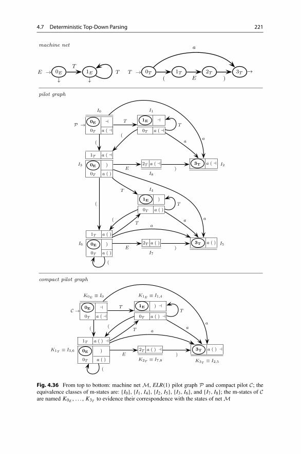
4.7 Deterministic Top-Down Parsing 221
Fig. 4.36 From top to bottom: machine net M, ELR(1) pilot graph P and compact pilot C; theequivalence classes of m-states are: {I0}, {I1, I4}, {I2, I5}, {I3, I6}, and {I7, I8}; the m-states of Care named K0E
, . . . , K3Tto evidence their correspondence with the states of net M

222 4 Pushdown Automata and Parsing
until the cid chain reached an initial state, the end-of-list sentinel. Under the STPhypothesis, that test is now replaced by a simpler device, to be later incorporatedin the final ELL(1) parser (Algorithm 4.68 on p. 237). With reference to the “old”Algorithm 4.37, only shift and reduction moves are modified.
First, let us focus on the situation when the old parser, with element J on top ofstack and J|base = 〈qA, . . .〉, performs the shift of X (terminal or non-) from stateqA, which is necessarily non-initial; the shift would require to compute and record anon-null cid into the sms J ′ to be pushed on stack. In the same situation, the “new”parser behaves differently: it cancels from the top-of-stack element J all candidatesother than 〈qA, . . .〉, since they correspond to discarded parsing alternatives. Noticethat the STP implies that the canceled candidates are necessarily in the closure of J ,hence they contain only initial states. Having eliminated from the sms the irrelevantcandidates, the new parser can identify the reduction to be made when a final stateof machine MA is entered, using a simple rule: keep popping the stack until the firstoccurrence of initial state 0A is found.
Second, consider a shift of X (terminal or non-) from an initial state 〈0A,π〉,which is necessarily in the closure of element J . Notice that in this case the newparser leaves element J unchanged and pushes the element ϑ(J,X) on the stack.The other candidates present in J are not canceled because they may be the originof future nonterminal shifts.
Since cid’s are not used by the new parser, a stack element is identical to an m-state (of the compact pilot). Thus, a shift move first trims the top of stack elementby discarding some candidates, then it pushes the input token and the next m-state.The next algorithm lists only the moves that differ from Algorithm 4.37.
Algorithm 4.56 (Pointerless parser APL) Let the pilot be compacted; m-states aredenoted Ki and stack symbols Hi ; the set of candidates of Hi is weakly includedin Ki .shift move Let the current character be a, H be the top of stack element, contain-
ing candidate 〈qA,π〉. Let qAa→ q ′A and ϑ(K,a)=K ′ be, respectively, the state
transition and m-state transition, to be applied. The shift move does:1. if qA ∈K|base (i.e., state qA is not initial), eliminate all other candidates from
H , i.e., set H equal to K|base2. push token a on stack and get next token3. push H ′ =K ′ on stack
reduction move (non-initial state) Let the stack be as follows:
H [0]a1H [1]a2 . . . akH [k]Assume that the pilot chooses the reduction candidate 〈qA,π〉 ∈ K[k], wherestate qA is final but non-initial. Let H [h] be the top-most stack element such that0A ∈K[h]|kernel. The move does:1. grow the syntax forest by applying the reduction:
ah+1ah+2 . . . ak � A

4.7 Deterministic Top-Down Parsing 223
and pop the stack symbols:
H [k]akH [k − 1]ak−1 . . .H [h+ 1]ah+1
2. execute the nonterminal shift move ϑ(K[h],A)
reduction move (initial state) It differs from the preceding case in that, for thechosen reduction candidate 〈0A,π〉, the state is initial and final. Reduction ε � A
is applied to grow the syntax forest. Then the parser performs the nonterminalshift move ϑ(K[k],A).
nonterminal shift move It is the same as a shift move, except that the shifted sym-bol is a nonterminal. The only difference is that the parser does not read the nextinput token at line 2 of shift move.
Clearly this reorganization removes the need of the cid (or of the vector stack)used in previous algorithms.
Property 4.57 If the ELR(1) pilot (compact or not) of an EBNF grammar or ma-chine net satisfies the STP condition, the pointerless parser APL of Algorithm 4.56is equivalent to the ELR(1) parser A of Algorithm 4.37.
It is useful to support this statement by some arguments to better understand howthe two algorithms are related.
First, after parsing the same string, the stacks of parsers A and APL contain thesame number k of stack elements, respectively J [0] . . . J [k] and K[0] . . .K[k]. Forevery pair of corresponding elements, the set of states included in K[i] is a subsetof the set of states included in J [i] because Algorithm 4.56 may have discarded afew candidates.
Second, we examine the stack elements at the same positions i and i − 1. Thefollowing relations hold:
in J [i], candidate 〈qA,π, �j〉 points to 〈pA,π, �l〉 in J [i − 1]|base
if and only ifcandidate 〈qA,π〉 ∈K[i] and the only candidate in K[i − 1] is 〈pA,π〉in J [i], candidate 〈qA,π, �j〉 points to 〈0A,π,⊥〉 in J [i − 1]|closure
if and only ifcandidate 〈qA,π〉 ∈K[i]and elem. K[i − 1] equals the projection of J [i − 1] on 〈state, look-ahead〉
Then by the way the reduction moves operate, parser A performs reductionah+1ah+2 . . . ak � A if and only if parser APL performs the same reduction.
To complete the presentation of the new parser, we list an execution trace.
Example 4.58 (Pointerless parser trace for the compact pilot (Fig. 4.36, p. 221))Given the input string (()a) �, Fig. 4.37 shows the execution trace, which shouldbe compared with the one of the ELR(1) parser in Fig. 4.18, p. 193, where cid’s are

224 4 Pushdown Automata and Parsing
used. The same graphical conventions are used: the m-state (of the compact pilot) ineach cell is framed, e.g., K0S
is denoted 0S , etc.; the final candidates are encircled,
e.g., , etc.; and the look-ahead is omitted to avoid clogging. So a candidateappears as a pure machine state. Of course here there are no pointers, and the initialcandidates canceled by Algorithm 4.56 from an m-state are striked out.
Notice that, if initial candidates had not been canceled, several instances of theinitial state of the active machine would occur in the stack m-states to be poppedwhen a reduction starts, thus causing a loss of determinism. For instance, the first(from the figure top) reduction (E) � T of machine MT , pops the three stack ele-ments K3T
, K2T, K1T
, and the last one would have contained the (now striked out)candidate 0T , which is initial for machine MT , but is not the correct initial statefor the reduction: the correct one, unstriked, is below in the stack, in m-state K1T
,which is not popped and is the origin of the nonterminal shift on T following thereduction.
We point out that Algorithm 4.56 avoids to cancel an initial candidate from astack element, if a shift move is to be later executed starting from it: see the Shiftmove case in Algorithm 4.56. The motivation for not canceling is twofold. First,these candidates will not cause any premature stop of the series of pop moves in thereductions that may come later, or put differently, they will not break any reductionhandle. For instance, the first (from the figure top) shift on ‘(’ of machine MT , keepsboth initial candidates 0E and 0T in the stack m-state K1T
, as the shift originatesfrom the initial candidate 0T . This candidate will instead be canceled (i.e., it willshow striked) when a shift on E is executed (soon after reduction T T � E), asthe shift originates from the non-initial candidate 1T . Second, some of such initialcandidates may be needed for a subsequent nonterminal shift move.
To sum up, we have shown that condition STP permits to construct a simplershift–reduce parser, which has a smaller stack alphabet and does not need pointersto manage reductions. The same parser can be further simplified, if we make anotherhypothesis: that the grammar is not left recursive.
4.7.2.3 Stack Contraction and Predictive ParserThe last development to be presented transforms the already compacted pilot graphinto the Control-Flow Graph of a predictive or goal-oriented parser. The way theparser uses the stack differs from the previous two models, the shift–reduce and thepointerless parsers. More precisely, now a terminal shift move, which always exe-cutes a push operation in the previous parsers, is sometimes implemented without apush and sometimes with multiple pushes. The former case happens when the shiftremains inside the same machine: the predictive parser does not push an elementupon performing a terminal shift, but it updates the top of stack element to recordthe new state of the active machine. Multiple pushes happen when the shift deter-mines one or more transfers from the current machine to others: the predictive parserperforms a push for each transfer.

4.7 Deterministic Top-Down Parsing 225
Fig. 4.37 Steps of the pointerless parsing Algorithm 4.56 APL; irrelevant and potentially confus-ing initial candidates are canceled by shift moves as explained in the algorithm

226 4 Pushdown Automata and Parsing
Now the essential information to be kept on stack is the sequence of machinesthat have been activated and have not reached a final state (where a reduction oc-curs). At each parsing time, the current or active machine is the one that is doingthe analysis, and the current state is kept in the top of stack element. Previous non-terminated activations of the same or other machines are in a suspended state. Foreach suspended machine MA, a stack entry is needed to store the state qA, fromwhere the machine will resume the computation when control is returned after per-forming the relevant reductions. A major advantage of predictive parsing is that theconstruction of the syntax tree can be anticipated: the parser can generate on-linethe left derivation of the input.
Parser Control-Flow Graph Moving from the above considerations, we adjustthe compact pilot graph C to make it isomorphic to the original machine net M,and thus we obtain a graph named parser control-flow graph or PCFG, because itrepresents the blueprint of the parser code. First, every m-node of C that containsmany candidates is split into as many nodes. Second, the kernel-equivalent nodesare coalesced and the original look-ahead sets are combined into one. The third stepcreates new arcs, named call arcs, which represent the transfers of control from amachine to another. Finally, each call arc is labeled with a set of terminals, namedguide set, which will determine the parser decision to transfer control to the calledmachine.
Definition 4.59 (Parser Control-Flow Graph or PCFG) Every node of the PCFG,denoted by F , is identified and denoted (at no risk of confusion) by a state q ofmachine net M. Moreover, every final node fA additionally contains a set π ofterminals, named prospect set.24 Such nodes are therefore associated to the pair〈fA,π〉. The prospect set is the union of the look-ahead sets πi of every candidate〈fA,πi〉 existing in the compact pilot graph C, as follows:
π =⋃
∀〈fA,πi 〉∈Cπi (4.8)
The arcs of pilot F are of two types, named shift and call (respectively depicted assolid and dashed arrows):
1. There exists in F a shift arc qAX→ rA with X terminal or non-, if the same arc
is in the machine MA.
2. There exists in F a call arc qA
γ1��� 0A1 , where A1 is a nonterminal possibly
different from A, if arc qAA1→ rA is in the machine MA, hence necessarily
some m-state K of pilot C contains candidates 〈qA,π〉 and 〈0A1, ρ〉; and thenext m-state ϑ(K,A1) contains candidate 〈rA,πrA〉.
24Although traditionally the same word “look-ahead” has been used for both shift–reduce andtop-down parsers, the sets differ and we prefer to differentiate their names.

4.7 Deterministic Top-Down Parsing 227
The call arc label γ1 ⊆ Σ ∪ {�}, named guide set, is specified in the next def-inition, which also specifies the guide sets of terminal shift arcs and of the arrows(darts) that mark final states.
Definition 4.60 (Guide set)
1. For every call arc qA
γ1��� 0A1 associated with a nonterminal shift arc qAA1→ rA,
a terminal b is in the guide set γ1, also written as b ∈Gui(qA ��� 0A1), if, andonly if, one of the following conditions holds:
b ∈ Ini(L(0A1)
)(4.9)
A1 is nullable and b ∈ Ini(L(rA)
)(4.10)
A1 and L(rA) are both nullable and b ∈ πrA (4.11)
∃ in F a call arc 0A1
γ2��� 0A2 and b ∈ γ2 (4.12)
2. For every terminal shift arc pa→ q (with a ∈Σ ), we set Gui(p
a→ q) := {a}.3. For every dart that tags a final node containing candidate 〈fA,π〉 (with fA
final), we set Gui(fA →) := π .
Guide sets are usually represented as arc labels enclosed within braces.Relations (4.9), (4.10), and (4.11) are not recursive and, respectively, consider
that terminal b is generated by MA1 called by MA; or by MA but starting from staterA; or that terminal b follows machine MA. Relation (4.12) is recursive and traversesthe net as far as the chain of call sites activated. We observe that relation (4.12)induces the set inclusion relation γ1 ⊇ γ2 between any two concatenated call arcs
qA
γ1��� 0A1
γ2��� 0A2 .Next we move to a procedural interpretation of a PCFG: all the arcs (except
nonterminal shifts) can be viewed as conditional instructions, enabled if the currentcharacter cc belongs to the associated guide set: thus a terminal shift arc labeled with{a} is enabled by predicate cc ∈ {a}, simplified to cc = a; a call arc labeled withset γ represents the procedure invocation conditioned by predicate cc ∈ γ ; a finalnode dart labeled with set π is interpreted as a conditional return-from-procedureinstruction to be executed if cc ∈ π . The remaining PCFG arcs are nonterminalshifts, which are viewed as unconditional return-from-procedure instructions.
The essential properties of guide sets are next stated (see [9] for a proof).
Property 4.61 (Disjointness of guide sets)1. For every node q of the PCFG of a grammar that satisfies the ELL(1) condition,
the guide sets of any two arcs originating from q are disjoint.2. If the guide sets of a PCFG are disjoint, then the machine net satisfies the
ELL(1) condition of Definition 4.50.
The first statement says that, for the same state, membership in different guidesets is mutually exclusive. The second statement is the converse of the first; it makesthe condition of having disjoint guide sets, a characteristic property of ELL(1) gram-

228 4 Pushdown Automata and Parsing
Fig. 4.38 The Parser Control-Flow Graph F (PCFG) of the running example, from the net andthe compact pilot
mars. We will later see that this condition can be directly checked on the PCFG, thussaving the effort to build the ELR(1) pilot.
It is time to illustrate the previous definitions and properties.
Example 4.62 (PCFG of the running example) The PCFG of the running exampleis represented in Fig. 4.38, with the same layout as the machine net for comparabil-ity.
In the PCFG there are new nodes (here only node 0T ), which derive from theinitial candidates (except those containing the axiom 0S ) extracted from the closurepart of the m-states of the compact pilot C. Having created such new nodes, theclosure part of the nodes of C (except node I0) becomes redundant and is eliminatedfrom the contents of the PCFG nodes.
As said, the prospect sets are needed only in the final states and have the follow-ing properties (see also relation (4.8)):

4.7 Deterministic Top-Down Parsing 229
Fig. 4.39 Grammar and net of Example 4.63
• The prospect set of a final state that is not initial, coincides with the look-aheadset of the corresponding node in the compact pilot C. This is the case of nodes1E and 3T .
• The prospect set of a final state that is also initial, e.g., 0E , is the union ofthe look-ahead sets of every candidate 〈0E,π〉 occurring in C. For instance,〈0E, {‘)’,�}〉 takes terminal ‘)’ from m-state K1T
and � from K0E.
Solid arcs represent the shifts, already present in the machine net and in the pilotgraph. Dashed arcs represent the calls, labeled by guide sets, the computation ofwhich follows:• the guide set of call arc 0E ��� 0T (and of 1E ��� 0T as well) is {a, ‘(’}, since
both terminals a and ‘(’ can be shifted starting from state 0T , which is the callarc destination (see relation (4.9))
• the guide set of call arc 1T ��� 0E includes the following terminals:– a and ‘(’, since from state 0E (the call arc destination) one more call arc
goes out to 0T and has guide set {a, ‘(’} (see relation (4.12))
– ‘)’, since the shift arc 1TE→ 2T (associated with the call arc) is in ma-
chine MT , language L(0E) is nullable and we have ‘)’ ∈ Ini(2T ) (see rela-tion (4.11)).
Observe the chain of two call arcs, 1T ��� 0E and 0E ��� 0T ; relation (4.12)implies that the guide set of the former arc includes that of the latter.
In accordance with Property 4.61, the terminal labels of all the arcs (shift andcall) that originate from the same node, do not overlap.
Since relation (4.10) has not been used, we illustrate it in the next example.
Example 4.63 Consider the EBNF grammar G and net M in Fig. 4.39.The machine net M is ELL(1); its pilot P in Fig. 4.40, does not have any ELR(1)
conflicts and also satisfies the ELL condition. The PCFG of net M, derived fromP , is shown in Fig. 4.41.

230 4 Pushdown Automata and Parsing
Fig. 4.40 ELR(1) pilot of the machine net in Fig. 4.39
We check that the prospect sets in the PCFG states that result from merging them-states of the pilot graph are the union of their look-ahead sets (see relation (4.8)):• the prospect set of state 0X is π0X
= {b, d}, and is the union of the look-aheadset {b} of candidate 〈0X, {b}〉 in m-state I7, and of the look-ahead set {d} ofcandidate 〈0X, {d}〉 in m-state I0
• similarly, the prospect set π1X= {b, d} is the union of the look-ahead sets of
candidates 〈1X, {b}〉 in I8 and 〈1X, {d}〉 in I3• the prospect set π3X
= {b, d} derives from candidates 〈3X, {b}〉 in I10 and〈3X, {d}〉 in I5
Next, we explain how the guide sets on the call arcs are computed:• Gui(0S ��� 0X) is the union of terminal a on the shift arc from 0X (see rela-
tion (4.9)) and of terminal d on the shift arc from 1S , which is a successor of the
nonterminal shift arc 0SX→ 1S associated with the call arc, because nonterminal
X is nullable (see relation (4.10))• Gui(2S ��� 0X) is the union of terminal a on the shift arc from 0X (see rela-
tion (4.9)) and of terminal d on the shift arc from 1S , which is a successor of the
nonterminal shift arc 2SX→ 1S associated with the call arc, because nonterminal
X is nullable (see relation (4.10))• Gui(1Y ��� 0X) is the union of terminal a on the shift arc from 0X (see rela-
tion (4.9)) and of terminal b in the prospect set of 2Y , which is the destination
state of the nonterminal shift arc 1YX→ 2Y associated with the call arc, because

4.7 Deterministic Top-Down Parsing 231
Fig. 4.41 Parser control-flow graph derived from the pilot graph in Fig. 4.40
nonterminal X is nullable and additionally state 2Y is final, i.e., language L(2Y )
is nullable (see relation (4.11))• Gui(1X ��� 0Y ) includes only the terminals a and c that label the shift arcs
from state 0Y (see relation (4.9)); it does not include terminal b since Y is notnullable.
Notice the two call arcs 0S ��� 0X and 2S ��� 0X , and the one call arc 1Y ��� 0X ,although directed to the same machine MX , have different guide sets, because theyare associated with different call sites.
In this example we have used three relations (4.9), (4.10) and (4.11) for comput-ing the guide sets on call arcs. Relation (4.12) is not used as in the PCFG concate-nated call arcs do not occur (that case has been already illustrated in the precedingexample in Fig. 4.38).
Having thus obtained the PCFG of a net, a short way remains to construct thedeterministic predictive parser.
4.7.3 Direct Construction of Top-Down Predictive Parsers
Section 4.7.2 has rigorously derived step-by-step the PCFG starting from theELR(1) pilot graph of the given machine net, by assuming it complies with theELL(1) condition on p. 214. As promised, we indicate a way to check the ELL(1)
condition and then to derive the PCFG directly from the net, bypassing the calcula-tion of the pilot.

232 4 Pushdown Automata and Parsing
For the theoretically interested reader, we add that the next formulation of theELL(1) condition includes some marginal cases that violate the STP clause of thepilot-based Definition 4.50. We exhibit a contrived example, where a violation ofSTP, due to the multiple candidates in the base of an m-state, does not hinder atop-down parser from working deterministically [7]. Consider the LR(1) grammarS → Aa | Bb, A→ C, B → C and C → ε. Without having to draw the pilot, it isevident that one of the m-states has two candidates in the base: 〈A→ C•, a〉 and〈B → C•, b〉 (here we use marked rules instead of machine states). Yet the choicebetween the alternatives of the axiom S is determined by the following character, a
or b. A necessary condition for such a situation to occur is that the language derivedfrom some nonterminal of the grammar consists only of the empty string. However,this case can be usually removed without penalty in all grammar applications: thus,the grammar above can be replaced by the equivalent simpler grammar S→A | B ,A→ a and B→ b, which complies with STP and is ELL(1).
From the Net to the Parser Control-Flow Graph For the reader who has notgone through the formal steps of Sect. 4.7.2, we briefly introduce the notion of parsercontrol-flow graph. The PCFG, denoted by F , of a machine net M, is a graph thathas the same nodes and includes the same arcs as the original graph of the net; thuseach node corresponds to a machine state. In F the following elements are alsopresent, which do not occur in the net M:call arcs An arc (depicted as dashed) links every node q that is the origin of a
nonterminal shift qB−→ r , to the initial state of machine MB . The label of such
a call arc is a set of terminals, named a guide set. Intuitively, such a call arcrepresents a (possibly recursive) conditional invocation of the parsing procedureassociated with machine MB , subject to the condition that the current input tokenis in the guide set. Node r is named the return state of the invocation.
prospect sets In F every final node qA carries a prospect set as additional infor-mation. The set contains every token that can immediately follow the recogni-tion of a string that derives from nonterminal A; its precise definition follows inEqs. (4.13), (4.14) on p. 233.
guide sets Let us name arrow a terminal shift arc, a call arc, and also a danglingarrow (named dart) that exits a final state; a guide set is a set of terminals, to beassociated with every arrow in F :• for a shift of terminal b, the guide set coincides with {b}• for a call arc qA ��� 0B , the guide set indicates the tokens that are consistent
with the invocation of machine MB ; the guide set γ of call arc qA ��� 0B
is indicated by writing qA
γ��� 0B or, equivalently, γ = Gui(qA ��� 0B); its
exact computation follows in Eq. (4.15) on p. 233• for the dart of a final state, the guide set equals the prospect setNotice that nonterminal shift arcs have no guide set.
After the PCFG has been constructed, the ELL(1) condition can be checked usingthe following test (which rephrases Property 4.61, p. 227).

4.7 Deterministic Top-Down Parsing 233
Definition 4.64 (Direct ELL(1) test) A machine network satisfies the direct ELL(1)
condition if in the corresponding parser control-flow graph, for every pair of arrowsoriginating from the same state q , the associated guide sets are disjoint.
We list the rules for computing the prospect and guide sets.
Equations for Prospect Sets We use a set of recursive equations to compute theprospect and guide sets for all the states and arcs of the PCFG; the equations areinterpreted as instructions to iteratively compute the sets. To compute the prospectsets of the final states, we need to compute also the prospect sets of the other states,which are eventually discarded.
1. If the graph includes any nonterminal shift arc qiA→ ri (therefore also the call
arc qi ��� 0A), then the prospect set π0Afor the initial state 0A of machine MA
is computed as
π0A:= π0A
∪⋃
qiA→ri
(Ini
(L(ri)
)∪ if Nullable(L(ri)
)then πqi
else ∅) (4.13)
2. If the graph includes any terminal or nonterminal shift arc piXi→ q , then the
prospect set πq of state q is computed as
πq :=⋃
pi
Xi→q
πpi(4.14)
The two sets of rules apply in an exclusive way to disjoints sets of nodes, becausein a normalized machine no arc enters the initial state. To initialize the computation,we assign the end-marker to the prospect set of 0S : π0S
:= {�}. All other sets areinitialized to empty.
Equations for Guide Sets The equations make use of the prospect set.
1. For each call arc qA ��� 0A1 associated with a nonterminal shift arc qAA1→ rA,
such that possibly other call arcs 0A1 ��� 0Bidepart from state 0A1 , the guide
set Gui(qA ��� 0A1) of the call arc is defined as follows, see also rules (4.9)–(4.12) at p. 227:
Gui(qA ��� 0A1) :=⋃
⎧⎪⎪⎪⎪⎪⎪⎪⎪⎨
⎪⎪⎪⎪⎪⎪⎪⎪⎩
Ini(L(A1)
if Nullable(A1) then Ini(L(rA))
else ∅ endifif Nullable(A1)∧Nullable(L(rA)) then πrA
else ∅ endif⋃
0A1���0Bi
Gui(0A1 ��� 0Bi)
(4.15)

234 4 Pushdown Automata and Parsing
2. For a final state fA ∈ FA, the guide set of the tagging dart equals the prospectset:
Gui(fA→) := πfA(4.16)
3. For a terminal shift arc qAa→ rA with a ∈Σ , the guide set is simply the shifted
terminal:
Gui(qA
a→ rA) := {a} (4.17)
Initially all the guide sets are empty.To compute the solution for prospect and guide sets, the above rules are repeat-
edly applied until none of the sets has changed in the last iteration; at that momentthe set values give the solution.
Notice that the rules for computing the prospect sets are consistent with the def-inition of look-ahead set given in Sect. 4.5.2; furthermore, the rules for computingthe guide sets are consistent with the definition of parser control-flow graph listedin Definition 4.59 on p. 226.
Example 4.65 (PCFG for list of balanced strings) The net in Fig. 4.29, p. 212, isnow represented by the PCFG in Fig. 4.42.
The following table shows the computation of the prospect sets for the PCFG.
Node Init. Equation Arc instance Prospect set
0S {�} {�}1S ∅ (4.14) 0S
P−→ 1S {�}2S ∅ (4.14) 1S
‘,’−→ 2S {�}0P ∅ (4.13) 0S
P−→ 1S
2SP−→ 1S
1PP−→ 2P
{‘,’} ∪ {�} ∪{‘,’} ∪ {�} ∪{a} ∪ ∅ = {a, ‘,’,�}
1P ∅ (4.14) 0Pa−→ 1P {a, ‘,’,�}
2P ∅ (4.14) 1PP−→ 2P {a, ‘,’,�}
3P ∅ (4.14) 2PP−→ 3P
0PP−→ 3P
{a, ‘,’,�} ∪{a, ‘ ,’,�} = {a, ‘,’,�}
The guide sets are computed by three equations, but the last two are trivial and wecomment only Eq. (4.15) that applies to the three call arcs of the graph. The guideset of the call arc 0S ��� 0P is simply Ini((0P ))= {a, c} since nonterminal P is notnullable and the call arc is not concatenated with other call arcs. Similarly, the guidesets of 2S ��� 0P and 1P ��� 0P have the same value.
Finally, it is immediate to check that the guide sets of bifurcating arrows aremutually disjoint, therefore the net is ELL(1). This confirms the earlier empiricalanalysis of the same net.

4.7 Deterministic Top-Down Parsing 235
Fig. 4.42 Parser control-flow graph (PCFG) for Example 4.65 (formerly Example 4.48, p. 211);the call arcs are dashed; the guide sets are in braces
Fig. 4.43 The parser control-flow graph (PCFG) of the running example
The running example that follows illustrates the cases not covered and permitsto compare the alternative approaches, based on the pilot graph or on the guide sets,for testing the ELL(1) condition.
Example 4.66 (Running example: computing the prospect and guide sets) The fol-lowing two tables show the computation of most prospect and guide sets for thePCFG of Fig. 4.38 (p. 228) here reproduced in Fig. 4.43. For both tables, the com-putation is completed at the third step.
Prospect sets of states0E 1E 0T 1T 2T 3T
� ∅ ∅ ∅ ∅ ∅) � ) � a() � a() � a() � a() �) � ) � a() � a() � a() � a() �

236 4 Pushdown Automata and Parsing
Guide sets of call arcs0E ��� 0T 1E ��� 0T 1T ��� 0E
∅ ∅ ∅a( a( a()
a( a( a()
The disjointness test on guide sets confirms that the net is top-down deterministic.
We examine the guide sets of the cascaded call arcs 1T
γ1��� 0E
γ2��� 0T , and weconfirm the general property that the guide set upstream (γ1) includes the one down-stream (γ2).
Violations of ELL(1) Condition We know that the failure of the ELL(1) condi-tion for a net that is ELR(1) can be due to two causes: the presence of left-recursivederivations, and the violation of the single-transition property in the pilot graph.First, we argue that left recursion implies non-disjointness of guide sets. Considerin the PCFG the bifurcation shown
By Eq. (4.15) the guide set γ of the call arc qA ��� 0A includes set Ini(L(A)),which includes terminal b, hence it overlaps with the guide set of the terminal shiftunder b.
Second, the next example shows the consequence of STP violations.
Example 4.67 (Guide sets in a non-ELL(1) grammar) The grammar with rulesS → a∗N and N → aNb | ε of Example 4.52 (p. 216), violates the singleton baseproperty as shown in Fig. 4.34, hence it is not ELL(1). This can be verified alsoby computing the guide sets on the PCFG. We have Gui(0S ��� 0N) ∩ Gui(0S
a→1S) = {a} �= ∅ and Gui(1S ��� 0N) ∩ Gui(1S
a→ 1S) = {a} �= ∅: the guide sets onthe arcs departing from states 0S and 1S are not disjoint.
4.7.3.1 Predictive ParserPredictive parsers come in two styles, as deterministic push-down automata(DPDA), and as recursive syntactic procedures. Both are straightforward to obtainfrom the PCFG.
For the automaton, the pushdown stack elements are the nodes of the PCFG:the top of stack element identifies the state of the active machine, while inner stackelements refer to return states of suspended machines, in the correct order of sus-pension. There are four sorts of moves. A scan move, associated with a terminal

4.7 Deterministic Top-Down Parsing 237
shift arc, reads the current token, cc, as the corresponding machine would do. A callmove, associated with a call arc, checks the enabling predicate, saves on stack thereturn state and switches to the invoked machine without consuming token cc. A re-turn move is triggered when the active machine enters a final state, the prospectset of which includes token cc: the active state is set to the return state of the mostrecently suspended machine. A recognizing move terminates parsing.
Algorithm 4.68 (Predictive recognizer as DPDA A)• The stack elements are the states of PCFG F . The stack is initialized with
element 〈0S〉.• Let 〈qA〉 be the top of stack element, meaning that the active machine MA is in
state qA. Different move types are next specified.scan move if the shift arc qA
cc−→ rA exists, then scan the next token andreplace the stack top by 〈rA〉 (the active machine does not change)
call move if there exists a call arc qA
γ��� 0B such that cc ∈ γ , let qA
B→ rAbe the corresponding nonterminal shift arc; then pop, push element 〈rA〉 andpush element 〈0B〉
return move if qA is a final state and token cc is in the prospect set associatedwith qA, then pop
recognition move if MA is the axiom machine, qA is a final state and cc=�,then accept and halt
– in any other case, reject the string and halt
It should be clear that, since the guide sets at bifurcating arrows are disjoint(Property 4.61 or Definition 4.64), in every parsing configuration at most one moveis possible, i.e., the algorithm is deterministic.
Computing Leftmost Derivations To construct the syntax tree, the recognizer isextended with an output function, thus turning the DPDA into a so-called pushdowntransducer (a model studied in Chap. 5). The algorithm produces the sequence ofgrammar rules of the leftmost derivation of the input string, but since the grammar G
is in EBNF form, we have to use the rules of the equivalent right-linearized (RLZ)grammar G, as anticipated in Sect. 4.5.1, p. 171. The reason why we do not useEBNF derivations is that a derivation step may consist of an unbounded numberof moves of the parser. Using the RLZ grammar, such a large derivation step isexpanded into a series of derivation steps that match the parser moves. We recallthat the syntax tree for grammar G is essentially an encoding of the syntax tree forthe EBNF grammar G, such that each node has at most two children.
For each type of parser move, Table 4.5 reports the output action, i.e., the rule ofG, which is printed.
The correspondence is so straightforward that it does not need justification andan example suffices.

238 4 Pushdown Automata and Parsing
Table 4.5 Derivation steps computed by a predictive parser; the current token is cc= b
Parser move RL rule used
Scan move for transition qAb−→ rA qA =⇒
G
brA
Call move for call arc qA
�� 0B and trans. qA
0B→ rA qA =⇒G
0BrA
Return move from state qA ∈ FA qA =⇒G
ε
Example 4.69 (Running example: trace of predictive parser DPDA) The RLZ gram-mar (from Example 4.22, p. 171) is the following:
0E → 0T 1E | ε 1E → 0T 1E | ε0T → a3T | ‘(’1T 1T → 0E2T
2T → ‘)’3T 3T → ε
For the input string x = (a), we simulate the computation including (from left toright) the stack content and the remaining input string, the test (predicate) on theguide set, and the rule used in the left derivation. Guide and prospect sets are thoseof the PCFG of Fig. 4.43, p. 235.
Stack x Predicate Left derivation
〈0E〉 (a) � (∈ γ = {a(} 0E ⇒ 0T 1E
〈1E〉〈0T 〉 (a) � scan 0E+⇒ (1T 1E
〈1E〉〈1T 〉 a) � a ∈ γ = {a(} 0E+⇒ (0E2T 1E
〈1E〉〈2T 〉〈0E〉 a) � a ∈ γ = {a(} 0E+⇒ (0T 1E2T 1E
〈1E〉〈2T 〉〈1E〉〈0T 〉 a) � scan 0E+⇒ (a3T 1E2T 1E
〈1E〉〈2T 〉〈1E〉〈3T 〉 ) � ) ∈ π = {a() �} 0E+⇒ (aε1E2T 1E
〈1E〉〈2T 〉〈1E〉 ) � ) ∈ π = {) �} 0E+⇒ (aε2T 1E
〈1E〉〈2T 〉 ) � scan 0E+⇒ (a)3T 1E
〈1E〉〈3T 〉 � �∈ π = {a() �} 0E+⇒ (a)ε1E
〈1E〉 � �∈ π = {) �} accept 0E+⇒ (a)ε
For the original EBNF grammar, the corresponding derivation is:
E⇒ T ⇒ (E)⇒ (T )⇒ (a)
Parser Implementation by Recursive Procedures We have seen in the introduc-tion to predictive parsers at p. 212 that they are often implemented using recursiveprocedures. Each machine is transformed into a parameter-less syntactic procedure,

4.7 Deterministic Top-Down Parsing 239
Fig. 4.44 Main program and syntactic procedures of a recursive-descent parser (Example 4.70 andFig. 4.43); function next is the programming interface to the lexical analyzer or scanner; functionerror is the messaging interface
having a control-flow graph matching the corresponding PCFG subgraph, so thatthe current state of a machine is encoded at runtime by the value of the programcounter. Parsing starts in the axiom procedure and successfully terminates when theinput has been exhausted, unless an error has occurred before. The standard run-time mechanisms of procedure invocation and return from procedure, respectively,implement the call and return moves. An example should suffice to show how theprocedure pseudo-code is obtained from the PCFG.
Example 4.70 (Recursive-descent parser) From the PCFG of Fig. 4.43, p. 235,we obtain the syntactic procedures shown in Fig. 4.44. The pseudo-code can beoptimized in several ways, which we leave out.

240 4 Pushdown Automata and Parsing
Any practical parser has to cope with input errors, provide a reasonable errordiagnosis, and be able to resume parsing after an error. A few hints on error man-agement in parsing will be presented in Sect. 4.12.
4.7.4 Increasing Look-Ahead
A pragmatic approach for obtaining a deterministic top-down parser when the gram-mar does not comply with condition ELL(1) is to look ahead of the current characterand examine the following ones. This often suffices to make deterministic the choiceat bifurcation points, and has the advantage of not requiring annoying modificationsof the original grammar.
Algorithm 4.68 on p. 237 (or its recursive-descent version) has to be slightlymodified, in order to examine in a bifurcation state the input characters located atk > 1 positions ahead of the current one, before deciding the move. If such a testsucceeds in reducing the choices to one, we say the state satisfies condition ELL(k).
A grammar has the ELL(k) property if there exists an integer k ≥ 1 such that, forevery net machine and for every state, at most one choice among the outgoing arrowsis compatible with the characters that may occur ahead of the current character, at adistance less than or equal to k.
For brevity, we prefer not to formalize the definition of the guide set of order k,since it is a quite natural extension of the basic case, and we directly proceed to acomputation example of a few guide sets of length k = 2.
Example 4.71 (Conflict between instruction labels and variable names) A smallfragment of a programming language includes lists of instructions (variable assign-ments, for statements, etc.), with or without a label. Both labels and variable namesare identifiers. The EBNF grammar of this language fragment, just sketched for theexample, is as follows (axiom progr):25
〈progr〉 → [〈label〉‘:’]〈stat〉(‘;’〈stat〉)∗
〈stat〉 → 〈assign_stat〉 | 〈for_stat〉 | . . .〈assign_stat〉 → id‘=’〈expr〉
〈for_stat〉 → for id . . .
〈label〉 → id
〈expr〉 → . . .
The net machines are depicted in Fig. 4.45 with the relevant guide sets. To avoidclogging the PCFG, only two call arcs are represented with their guide sets of orderk = 1,2, the latter framed. The other guide sets are on the shift arcs and final darts
25The symbols in the hook brackets 〈〉 are nonterminals, all the others are terminals or are assumedto be terminals; and the square brackets mean their contents are optional.

4.7 Deterministic Top-Down Parsing 241
Fig. 4.45 Machine net and the relevant parts of the parser control-flow graph of Example 4.71.With look-ahead length k = 2 the graph gets deterministic
exiting the furcation nodes. The states are simply enumerated and the hooks aroundthe nonterminal names are omitted.
Clearly state 0 is not ELL(1): the guide sets of length k = 1 (not framed) onthe two call arcs that leave state 0, share the terminal symbol id; thus these guidesets are not disjoint. By refining the analysis, we observe that if the identifier is an
instruction label, i.e., arc 0label−→ 1, then it is followed by a colon ‘:’ character. On
the other hand, in the case of arc 0stat−→ 3, the identifier is the left variable of an
assignment statement and is followed by an equal ‘=’ character.26 We have thusascertained that inspecting the second next character, suffices to deterministicallyresolve the choice of the move from state 0, which therefore satisfies conditionELL(2). In the PCFG, the call arcs leaving state 0 are labeled with the guide setsof length k = 2 (framed), which are disjoint. Such pre-computed sets will be usedat runtime by the parser. Notice that in the bifurcation states 3 and 4, a look-aheadlength k = 1 suffices to make the choice deterministic; in fact see that the guide sets
26In the case of the for statement, for simplicity we assume that the lexeme for is a reserved key-word, which may not be used as a variable or label identifier.

242 4 Pushdown Automata and Parsing
on the outgoing shift arcs and on the final dart are disjoint. It would be wasteful touse the maximal look-ahead length everywhere in the parser.
Formally the elements of an ELL(k) guide set are strings of length up to k termi-nals.27 In practice, parsers use different look-ahead lengths with an obvious econ-omy criterion: in each bifurcation state, the minimum length m≤ k needed to arbi-trate the choice of the branches should be used.
Some top-down parsers that are more powerful, though computationally less ef-ficient, have also been designed. A well-known example is the ANTLR parser [30],which uses a look-ahead with variable and unbounded length, depending on the cur-rent state. Other parsers, if the choice in a bifurcation state remains uncertain, takeother cues into consideration. One possibility is to compute some semantic condi-tion, an idea to be worked out in the last chapter. Of course, such parsers can nolonger be considered as deterministic pushdown automata, because they use otherinformation pieces in addition to the stack contents and, in the case of unlimitedlook-ahead, they are able to perform multiple scans on the input.
4.8 Deterministic Language Families: A Comparison
The family DET of deterministic (context-free) languages, characterized by the de-terministic pushdown automaton as their recognizer, was defined in Sect. 4.3.2,p. 154, as well as the subclasses of simple deterministic (p. 161) and parenthesislanguages. To complete the theoretical picture of deterministic families, we includein the comparison the families of deterministic bottom-up and top-down parsablelanguages. In this section we do not use EBNF grammars and machine nets sys-tematically, because in the literature language theoretic properties have been mostlyinvestigated for the basic BNF grammar model. Notice, however, that, since thefamilies ELR and ELL of extended grammars strictly include those of non-extendedgrammars (LR and LL), some properties that hold for the latter are obviously ex-tended to the former.
As we proceed, we have to clarify what we actually compare: grammar familiesor language families? An instance of the first case is the statement that every LL(1)
grammar is also an LR(1) grammar; for the second case, an instance is that thefamily of the languages generated by LL(1) grammars is included in the DET family.
The inclusion relationships between grammar families and between languagefamilies are depicted in Figs. 4.46 and 4.47, respectively, and are now discussedcase by case. Notice that some facts already known from previous chapters and sec-tions are not repeated here.
We briefly comment the inclusions in Fig. 4.46, which are quite immediate. Inthe simple deterministic case, for every nonterminal A the grammar rules must startwith distinct terminals, i.e., they are A→ bβ and A→ cγ with b �= c. Therefore
27They may be shorter than k only when they end with the end-marker �.

4.8 Deterministic Language Families: A Comparison 243
Fig. 4.46 Inclusion relationships between families of grammars
Fig. 4.47 Inclusion relationships between families of languages; all the inclusions are strict; thenumbers refer to the comments
the guide sets of the corresponding bifurcation from the initial state of machineMA are disjoint, thus proving that the grammar is LL(1). The fact that every LL(1)
grammar is also LR(1) is obvious, since the former condition is a restriction of thelatter. Moreover the inclusion is strict: it suffices to recall that a grammar with left-

244 4 Pushdown Automata and Parsing
recursive rules surely cannot be LL(1), but it may be LR(1). It is also obvious thatevery LR(1) grammar is non-ambiguous.
It remains to comment the inclusions between the subfamilies LL(k) and LR(k),with k ≥ 1. Although they have not been formally defined in this book, it is enoughto think of them as obtained by extending the length of look-ahead from 1 to k
characters, as we did in Sects. 4.6.6 and 4.7.4 for the LR(2) and the LL(2) case,respectively. In this way, we step up from the original conditions for k = 1, to theaugmented conditions that we name LR(k) and LL(k) (dropping the “E” of ELR /ELL since the grammars are not extended). The fact that every LR(k) (respectivelyLL(k)) grammar is also LR(k + 1) (respectively LL(k + 1)) is trivial; moreover, thegrammar in Fig. 4.45 witnesses the strict inclusion ELL(1)⊂ ELL(2), and after thenatural conversion to BNF, also LL(1)⊂ LL(2).
We state without justification (the books [38, 39] cover such properties in depth)that the cross inclusion of LL(k) within LR(k), which we already know to hold fork = 1, is valid for any value of k.
We compare several language families in Fig. 4.47 (disregarding the marginalsimple deterministic family, which fits between families REG and LL(1)). For twogeneric families X and Y , which are characterized by certain grammar or automatonmodels, the proof that family X is included in Y , consists of showing that everygrammar (or automaton) of type X can be converted to a grammar (or automaton)of type Y . For a broad introduction to such comparison methods, we refer to [18].
Before we analyze the relationships among language families, we have to statemore precisely a fundamental property of deterministic languages, which we havevaguely anticipated.
Property 4.72 The family DET of deterministic context-free languages coincideswith the family of the languages generated by LR(1) grammars.
This important statement (due to Knuth [25]) essentially says that the shift–reduce parsing approach with look-ahead length k = 1, perfectly captures the idea ofdeterministic recognition, using as automaton a machine with a finite memory andan unbounded stack. Obviously, this does not say that every grammar generating adeterministic language enjoys the LR(1) property. For instance, the grammar mightbe ambiguous or require a look-ahead longer than one. But for sure there exists anequivalent grammar that is LR(1). Notice that, since the family LR(1) is included inthe ELR(1) one, the latter too coincides with DET. On the other hand, any context-free language that is not deterministic, as the cases in Sect. 4.3.2.2, p. 157, cannotbe generated by an LR(1) grammar.
Consider now extending the look-ahead length, as we did in Sect. 4.6.6. Trustingthe reader’s intuition (or going back to Sect. 4.6.6 for a few enlightening examples),we talk about ELR(k) grammars and parsers without formally defining them. Sucha parser is driven by a pilot with look-ahead sets that contain strings of length k > 1.Clearly the pilot may have more m-states than a pilot with length k = 1, becausesome m-states of the latter pilot are split, due to the look-ahead sets with k = 2becoming different. However, since after all an ELR(k) parser is nothing more than

4.8 Deterministic Language Families: A Comparison 245
a deterministic pushdown automaton, no matter how large parameter k is, with theonly peculiarity of possibly having more internal states than an ELR(1) parser, fromthe preceding property (Property 4.72) we have the following one:
Property 4.73 For every integer k > 1, the family of the languages generated byELR(k) grammars coincides with the family of the languages generated by ELR(1)
grammars, hence also with the DET family.
Now a question arises: since every deterministic language can be defined bymeans of an LR(1) grammar, what is the use of taking higher values of the length pa-rameter k? The answer comes from the consideration of the families of grammars inFig. 4.46, where we see that there exist grammars having the LR(2) property, but notthe LR(1) one, and more generally that there exists an infinite inclusion hierarchybetween the LR(k) and LR(k+1) grammar families (k ≥ 1). Although Property 4.73ensures that any LR(k) grammar, with k > 1, can be replaced by an equivalent LR(1)
grammar, the latter grammar is sometimes less natural or simply bigger, as seen inSect. 4.6.6 where a few grammar transformations from LR(2) down to LR(1) areillustrated.
We complete this comparison topic with a twofold negative statement.
Property 4.74 For a generic context-free grammar, it is undecidable if there existsan integer k ≥ 1 such that the grammar has the LR(k) property. For a generic non-deterministic pushdown automaton, it is undecidable if there exists an equivalentdeterministic pushdown automaton; this is the same as saying that it is undecidableif a context-free language (presented by means of a generic grammar or pushdownautomaton) is deterministic.
However, if the look-ahead length k is fixed, then it is possible to check whetherthe grammar is LR(k) by constructing the pilot and verifying that there are not anyconflicts: this is what we have done for k = 1 in a number of cases. Furthermore,it is not excluded that for some specific nondeterministic pushdown automaton, itcan be decided if there exists a deterministic one accepting the same language; or(which is the same thing) that for some particular context-free language, it can bedecided if it is deterministic; but general algorithms for answering these decisionproblems in all cases, do not exist.
The following comments are keyed to the numbered relationships among lan-guages, shown in Fig. 4.47.1. Since every regular language is recognized by a DFA, consider its state-
transition graph and normalize it so that no arcs enter the initial state: sucha machine only has terminal shifts and is clearly ELL(1). To show that it isLL(1), it suffices to take the grammar that encodes each arc p
a→ q as a right-linear rule p→ aq , and each final state f as f → ε. Such a grammar is easilyLL(1) because every guide set coincides with the arc label, except the guide setof a final state, which is the end-marker �.

246 4 Pushdown Automata and Parsing
2. Every LL(k) language with k ≥ 1 is deterministic, hence also LR(1) by Prop-erty 4.72. Of course this is consistent with the fact that the top-down parser ofan LL(k) language is a deterministic pushdown automaton. It remains to arguethat the inclusion is strict, i.e., for every value of k there exist deterministic lan-guages that cannot be defined with an LL(k) grammar. A good example is thedeterministic language {a∗anbn | n≥ 0}, studied in Fig. 4.34, p. 217, where thegrammar with rules S → a∗N and N → aNb | ε, and the equivalent machinenet have been found to be ELR(1), but to violate the ELL(1) condition. Thereason is that, in the initial state of the net with character a as current token,the parser is unable to decide whether to simply scan character a or to invokemachine MN . Quite clearly, we see that lengthening the look-ahead does notsolve the dilemma, as witnessed by the sentences a . . . aanbn where the bal-anced part of the string is preceded by unboundedly many letters a. A naturalquestion is the following: can we find an equivalent ELL(k) grammar for thislanguage? The answer, proved in [6], is negative.
3. The collection of language families defined by LL(k) grammars, for k =1,2, . . . , form an infinite inclusion hierarchy, in the sense that, for any inte-ger k ≥ 1, there exists a language that meets the LL(k + 1) condition, but notthe LL(k) one (we refer again to [6, 38, 39]). Notice the contrast with the LR(k)
collection of language families, which all collapse into DET for every value ofthe parameter k.
To finish with Fig. 4.47, the fact that a deterministic language is unambiguous isstated in Property 4.14 on p. 159.
4.9 Discussion of Parsing Methods
We briefly discuss the practical implications of choosing top-down or bottom-updeterministic methods, then we raise the question of what to do if the grammar isnondeterministic and neither parsing method is adequate.
For the primary technical languages, compilers exist that use both top-down andbottom-up deterministic algorithms, which proves that the choice between the twois not really critical. In particular, the speed differences between the two algorithmsare small and often negligible. The following considerations provide a few hints forchoosing one or the other technique.
We know from Sect. 4.8 (p. 242 and following) that the family DET of determin-istic languages, i.e., the LR(1) ones, is larger than the family of LL(k) languages,for any k ≥ 1. Therefore there are LR(1) grammars that cannot be converted intoLL(k) grammars, no matter how large the guide set length k may be. In the practicethis case is unfrequent. Truly, quite often the grammar listed in the official languagereference manual violates the ELL(1) condition because of the presence of left-recursive derivations, or in other ways, and choosing top-down parsing forces thedesigner to use a longer look-ahead, or to transform the grammar. The first optionis less disturbing, if it is applicable. Otherwise, some typical transformations fre-quently suffice to obtain an LL(k) grammar: moving left recursions to the right and

4.9 Discussion of Parsing Methods 247
re-factoring the alternative grammar rules, so that the guide sets become disjoint.For instance, the rules X → A | B , A→ a | cC and B → b | cD are re-factoredas X→ a | b | c(C |D), thus eliminating the overlap between the guide sets of thealternatives of X. Unfortunately the resulting grammar is typically quite differentfrom the original one, and often less readable. Add to it that having two grammarversions to manage, carries higher maintenance costs when the language evolvesover time.
Another relevant difference is that a software tool (such as Bison) is neededto construct a shift–reduce parser, whereas recursive-descent parsers can be eas-ily coded by hand, since the layout of each syntax procedure essentially mirrors thegraph of the corresponding machine. For this reason the code of such compilers iseasier to understand and may be preferred by the non-specialist. Actually, tools havebeen developed (but less commonly used) for helping in designing ELL(1) parsers:they compute the guide sets and generate the stubs of the recursive syntactic proce-dures.
With respect to the form of the grammar, EBNF or pure BNF, we have presentedparser generation methods that handle extended BNF rules, not just for top-downas done since many years, but also for bottom-up algorithms. However, the con-struction of the pilot automaton can be done by hand only for toy grammars and atpresent we only know of tools for pure BNF grammars. At the moment, the practi-cal advantage of the top-down approach is its direct handling of EBNF grammars,in contrast to the current limitation of the popular LR parser generation tools that donot accept EBNF rules. Awaiting for some new ELR(1) parser generators to come,the annoying but not serious consequence is that the regular expressions present inthe rules must be eliminated by means of standard transformations.
A parser is not an isolated application, but it is always interfaced with a transla-tion algorithm (or semantic analyzer) to be described in the next chapter. Anticipat-ing some discussion, top-down and bottom-up parsers differ with respect to the typeof translation they can support. A formal property of the syntax-directed translationmethodology, to be presented later, makes top-down parsers more convenient fordesigning simple translation procedures, obtained by inserting output actions intothe body of parsing procedures. Such one-pass translators are less expressive andless convenient to implement on top of bottom-up parsers.
If the reference grammar of the source language violates the ELR (hence also theELL) condition, the compiler designer has several choices:1. to modify the grammar2. to adopt a more general parsing algorithm3. or to leverage on semantic informationActually this situation is more common for natural language processing (compu-tational linguistic) than for programming and technical languages, because naturallanguages are much more ambiguous than the artificial ones. So skipping case 1, wediscuss the remaining ones.
Case 2: The parsing problem for general context-free grammars (including theambiguous case) has attracted much attention, and well-known algorithms exist thatare able to parse any string in cubic time. The leading algorithms are named CYK

248 4 Pushdown Automata and Parsing
(from its inventors Coke–Younger–Kasami) and Earley (see for instance [17]); thelatter is the object of the next section.
We should mention that other parsing algorithms exist that fall in between de-terministic parsers and general parsers with respect to generality and computationalperformance. Derived from the ELL(k) top-down algorithms, parser generators ex-ist, like ANTLR, that produce more general parsers: they may perform unboundedlook-ahead in order to decide the next move. For bottom-up parsing, a practical al-most deterministic algorithm existing in several variants is due to Tomita [40]. Theidea is to carry on in parallel only a bounded number of alternative parsing attempts.But the designer should be aware that any general parser more general than the de-terministic ones, will be slower and more memory demanding.
Case 3: Sometimes, an entirely different strategy for curtailing the combinatorialexplosion of nondeterministic attempts is followed, especially when the syntax ishighly ambiguous, but only one semantic interpretation is possible. In that case, itwould be wasteful to construct a number of syntax trees, just to delete, at a later time,all but one of them using semantic criteria. It is preferable to anticipate semanticchecks during parsing, and thus to prevent meaningless syntactic derivations to becarried on. Such a strategy, called semantics-directed parsing, is presented in thenext chapter within the semantic model named attribute grammars.
4.10 A General Parsing Algorithm
The LR and LL parsing methods are inadequate for dealing with ambiguous andnondeterministic grammars. In his seminal work [13], J. Earley introduced an al-gorithm for recognizing the strings of arbitrary context-free grammars, which has acubic time complexity in the worst case. His original algorithm does not constructthe (potentially numerous) syntax trees of the source string, but later certain effi-cient representations of parse forests have been invented, which avoid to duplicatethe common subtrees and thus achieve a polynomial time complexity for the treeconstruction problem [35]. Until very recently [2], the Earley parsers computed thesyntax tree in a second pass, after string recognition [17].
Concerning the use of EBNF grammars, J. Earley already gave some hints abouthow to do, and later a few parser generators have been implemented.
Another long-standing discussion concerns the pros and cons of using look-aheadto filter parser moves. Since experiments have indicated that the look-ahead-lessalgorithms can be faster, at least for programming languages [3], we present thesimpler version that does not use look-ahead at all. This is in line with the classicaltheoretical presentations of the Earley parsers for non-extended grammars (BNF),e.g., in [17, 31].
We present a version of the Earley parser for arbitrary EBNF grammars, includ-ing the nondeterministic and ambiguous ones. But for the computation of the syntaxtree, we restrict our presentation to unambiguous grammars, because this book fo-cuses on programming languages, which are well-defined unambiguous formal no-tations, unlike the natural languages. Thus, our procedure for building syntax trees

4.10 A General Parsing Algorithm 249
works for nondeterministic unambiguous grammars, and it does not deal with mul-tiple trees or parse forests.
The section continues with an introductory presentation by example, then thepure recognizer algorithm is defined and illustrated, and the algorithm for buildingthe syntax tree is presented. At the end, we mention some extensions of the Earleyalgorithm and other related issues.
4.10.1 Introductory Presentation
The data structures and operations of the Earley and ELR(1) parsers are in manyways similar. In particular, the vector stack used by the parser implementation inSect. 4.6.5, p. 201, is a good analogy to the Earley vector to be next introduced.When analyzing a string x = x1 . . . xn or x = ε of length n≥ 0, the algorithm usesa vector E[0 . . . n] of n+ 1 elements. Every element E[i] is a set of pairs, 〈qX, j 〉,where qX is a state of machine MX , and j (0 ≤ j ≤ i ≤ n) is an integer pointerthat indicates an element E[j ], which precedes or coincides with E[i], and containsa pair 〈0X, j 〉, with the same machine MX and the same integer j . This pointerj marks the position ↑ in the input string x from where the current derivation ofnonterminal X has started, i.e., x1 . . . xj ↑ xj+1 . . . xi
X
. . . xn, namely from character
xj , excluded, to the right as far as character xi , included (case j = i is for the nullstring x = ε).
Thus a pair has the form 〈qX, j 〉 and is named initial or final depending on thestate qX being, respectively, initial or final; a pair is called axiomatic if nonterminalX is the grammar axiom S.
An intuitive example familiarizes us with the Earley method. It embodies con-cepts but leaves out refinements, which are added later in a formal way.
Example 4.75 (Introduction to the Earley method) The non-deterministic language:{anbn | n≥ 1
}∪ {a2nbn | n≥ 1
}
is defined by the grammar and machine net in Fig. 4.48, which violate the ELR(k)
condition, as any other equivalent grammar would do (the ELR(k) pilot is inFig. 4.15 on p. 188).
Suppose the string to be analyzed is x = x1x2x3x4 = aabb with length n = 4.We prepare the Earley vector E, with the elements E[0], . . . ,E[4], all initialized toempty, except E[0] = 〈0S,0〉. In this pair, the state is set to 0S , i.e., to the initialstate of machine MS , and the pointer is set to 0, which is the position that precedesthe first character x1 of string x. As parsing proceeds, when the current character isxi , the current element E[i] will be filled with one or more pairs. The final Earleyvector is shown in Table 4.6, with all the pairs progressively put into it.
In broad terms, three operations types, to be next applied and explained on theexample, can be carried out on the current element E[i]: closure, terminal shift, andnonterminal shift; their names are remindful of the similar ELR operations (p. 174).

250 4 Pushdown Automata and Parsing
Fig. 4.48 Grammar and machine net of Example 4.75
Closure It applies to a pair with a state from where an arc with a nonterminallabel X originates. Suppose that the pair 〈p, j 〉 is in the element E[i] and that the
net has an arc pX→ q with a nonterminal label X; the destination state q of the arc
is not relevant. The operation adds a new pair 〈0X, i〉 to the same element E[i]. Thestate of this pair is the initial one 0X of the machine MX of that nonterminal X, andthe pointer has value i, which means that the pair is created at step i starting from apair already in the element E[i].
The effect of closure is to add to element E[i] all the pairs with the initial statesof the machines that can recognize a substring starting from the next character xi+1.In our example, the closure writes into E[0] the pairs:
〈0A,0〉 〈0B,0〉Since a further application of the closure to the new pairs does not create new pairs,the algorithm moves to the second operation.
Terminal Shift The operation applies to a pair with a state from where a terminalshift arc originates. Suppose that pair 〈p, j 〉 is in element E[i − 1] and that the net
has arc pxi→ q labeled by current token xi . The operation writes into element E[i]
the pair 〈q, j 〉, where the state is the destination of the arc and the pointer equalsthat of the pair in E[i − 1], to which terminal shift applies. Having scanned xi , thecurrent token becomes xi+1.
Here, with i = 1 and x1 = a, from element E[0] terminal shift puts into elementE[1] the pairs:
〈1A,0〉 〈1B,0〉Then closure applies again to the new pairs in element E[1], with the effect ofadding to E[1] the pair (where we notice the pointer has value 1):
〈0A,1〉

4.10 A General Parsing Algorithm 251
If at step i no terminal shift can be applied to a pair in element E[i − 1], thuscausing the next element E[i] to remain empty, then the algorithm stops and rejectsthe string. In the example, however, this never happens.
Continuing from element E[1] and scanning character x2 = a, through terminalshift we put into E[2] the pairs:
〈2B,0〉 〈1A,1〉and, through their closure, we add to E[2] the pairs:
〈0B,2〉 〈0A,2〉Scanning the next character x3 = b, through terminal shift we write into E[3] thepairs:
〈4B,0〉 〈3A,1〉Now the third operation, which is the most complex, comes into play.
Nonterminal Shift The operation is triggered by the presence in E[i] of a finalpair 〈fX, j 〉, to be qualified as enabling. Then, to locate the pairs to be shifted,the operation goes back to the element E[j ] referred to the pointer of the enablingpair. In this example the pointer always directs to a preceding element, i.e., we havej < i. However, if the grammar contains nullable nonterminals, the pointer j mayalso direct to E[i], as we will see.
In the element E[j ], the nonterminal shift operation searches for a pair 〈p, l〉such that the net contains an arc p
X→ q , with a label that matches the machine ofstate fX in the enabling pair. The pointer l may range in the interval 0 ≤ l ≤ j . Itis certain that the search will find at least one such pair, and the nonterminal shiftapplies to it. The operation writes the pair 〈q, l〉 into E[i]; notice that state q is thetarget of the arc and the pointer value is copied. If the search in E[j ] finds two ormore pairs that fit, then the operation is applied to each one, in any order.
Here, the final pairs 〈4B,0〉 and 〈3A,1〉 in E[3] enable the nonterminal shifts onsymbols B and A, respectively. The pointer in pair 〈4B,0〉 links to element E[0],which, intuitively, is the point where the parser began to recognize nonterminal B .
In E[0] we find pair 〈0S,0〉, and we see that the net has arc 0SB→ 1S from state 0S
with nonterminal label B . Then we put into element E[3] the pair:
〈1S,0〉Similarly, for the other enabling pair 〈3A,1〉, we find the pair 〈1A,0〉 in the element
E[1] pointed to by 1; since the net has arc 1AA→ 2A, we write into E[3] the pair:
〈2A,0〉We pause to compare terminal and nonterminal shift: the former works from
E[i − 1] to E[i], two adjacent elements, and uses an arc pxi→ q , which scans token
xi ; the latter works from element E[j ] to E[i], which can be separated by a long

252 4 Pushdown Automata and Parsing
Table 4.6 Earley parsing trace of string aabb for Example 4.75
distance, and uses arc pX→ q , which corresponds to analyze the string derived from
nonterminal X, i.e., all the tokens between the two elements.We resume the example. If string x ended at this point, then its prefix aab
scanned hitherto would be accepted: acceptance is demonstrated by the presencein element E[3] of the final axiomatic pair 〈1S,0〉, with the pointer set to zero. Ac-tually one more character x4 = b is scanned, and from element E[3] the terminalshift writes into element E[4] the pair 〈3A,0〉. Since the pair is final, it enables anonterminal shift that goes back to element E[0], finds pair 〈0S,0〉 such that the
net has arc 0SA→ 1S , and finally puts the pair 〈1S,0〉 into element E[4]. This pair
causes the whole string x = aabb to be accepted. The whole computation trace is inTable 4.6.
The divider on vector elements separates the pairs obtained from the precedingelement through terminal shift (top group), from those obtained through closure andnonterminal shift (bottom group); such a partitioning is just for visualization (anelement is an unordered set); of course in the initial element E(0) the top group isalways missing. The final states are highlighted as visual help.
4.10.2 Earley Algorithm
The Earley algorithm for EBNF grammars uses two procedures, Completion andTerminalShift. The input string is denoted x = x1 . . . xn or x = ε, with |x| = n≥ 0.Here is Completion:
Completion(E, i) - - with index 0≤ i ≤ n
do
- - loop that computes the closure operation- - for each pair that launches machine MX
for (each pair 〈p, j 〉 ∈E[i] and X,q ∈ V,Q s.t. pX→ q) do
add pair 〈0X, i〉 to element E[i]

4.10 A General Parsing Algorithm 253
end for
- - nested loops that compute the nonterminal shift operation- - for each final pair that enables a shift on nonterminal X
for (each pair 〈f, j 〉 ∈E[i] and X ∈ V such that f ∈ FX) do
- - for each pair that shifts on nonterminal X
for (each pair 〈p, l〉 ∈E[j ] and q ∈Q s.t. pX→ q) do
add pair 〈q, l〉 to element E[i]end for
end for
while (some pair has been added)
The Completion procedure adds new pairs to the current vector element E[i], byapplying one or more times closure and nonterminal shift as long as pairs can beadded to it. The outer loop (do-while) runs once at least, exits after the first run if itcannot add any pair, or more generally exits after a few runs when closure and non-terminal shift cease to produce effect. Notice that Completion processes the nullablenonterminals by applying to them a combination of closures and nonterminal shifts.Here is TerminalShift:
TerminalShift(E, i) - - with index 1≤ i ≤ n
- - loop that computes the terminal shift operation- - for each preceding pair that shifts on terminal xi
for (each pair 〈p, j 〉 ∈E[i − 1] and q ∈Q s.t. pxi→ q) do
add pair 〈q, j 〉 to element E[i]end for
The TerminalShift procedure adds to the current element E[i], the new pairs ob-tained from the previous element E[i − 1] through a terminal shift scanning tokenxi (1≤ i ≤ n).
Remarks TerminalShift may fail to add any pair to the element, which so remainsempty. A nonterminal that exclusively generates the empty string ε never undergoesterminal shift (it is processed only by completion).
Notice that both procedures correctly work also when the element E[i] or, re-spectively, E[i − 1], is empty, in which case the procedures do nothing.
Algorithm 4.76 (Earley syntactic analysis)- - analyze the terminal string x for possible acceptance- - define the Earley vector E[0 . . . n] with |x| = n≥ 0
E[0] := {〈0S,0〉} - - initialize the first elem. E[0]

254 4 Pushdown Automata and Parsing
for i := 1 to n do - - initialize all elem.s E[1 . . . n]E[i] := ∅
end for
Completion(E,0) - - complete the first elem. E[0]i := 1
- - while the vector is not finished and the previous elem. is not empty
while (i ≤ n ∧ E[i − 1] �= ∅) do
TerminalShift(E, i) - - put into the current elem. E[i]Completion(E, i) - - complete the current elem. E[i]i ++
end while
At start, the algorithm initializes E[0] with the axiomatic pair 〈0S,0〉 and sets theother elements (if any) to empty. Soon after the algorithm completes element E[0].Then, if n ≥ 1, i.e., string x is not empty, the algorithm loops on each subsequentelement from E[1] to E[n], puts pairs (if any) into the current element E[i] throughTerminalShift, and finishes element E[i] through Completion (1≤ i ≤ n). If Termi-nalShift fails to put any pairs into E[i], then Completion runs idle on it. Usually theloop iterates as far as the last element E[n], but it may terminate prematurely if anelement was left empty in a loop iteration; then it leaves empty all the followingelements. We do not comment the case n= 0, which is simpler.
Notice the analogy between Algorithm 4.30 on p. 183, which constructs the pi-lot graph, and the present algorithm. The former builds a pilot m-state: it shiftscandidates into the base and computes closure. The latter builds a vector element:it shifts pairs into the element and computes completion, which includes closure.The analogy is partial and there are differences, too: a candidate has a look-aheadand a pair does not; a pair has a pointer and a candidate does not; and processingnonterminals through shift is not identical either. But the major difference is concep-tual: Algorithm 4.30 is a tool that constructs the data structures which will controlthe parser, whereas the present algorithm constructs similar data structures duringparsing. Therefore, such a construction time does not impact on the ELR parser per-formance, but is the reason of the higher computational complexity of the Earleyparser.
We specify how Algorithm 4.76 decides whether the input string x is legal forlanguage L(G). If the algorithm terminates prematurely, before filling the wholevector E, then string x is obviously rejected. Otherwise the acceptance conditionbelow applies.
Property 4.77 When the Earley algorithm (Algorithm 4.76) terminates, the stringx is accepted if and only if the last element E[n] of vector E contains a final ax-iomatic pair with zero pointer, i.e., a pair of the form 〈fS,0〉where we have fS ∈ FS .

4.10 A General Parsing Algorithm 255
Fig. 4.49 Non-deterministic EBNF grammar G and network of Example 4.78
We have seen a complete run of the algorithm in Table 4.6, but that grammaris too simple to illustrate other interesting points: iterations in the EBNF grammar(circuits in the net), and nullable nonterminals.
Example 4.78 (Non-deterministic EBNF grammar with iterative operators and a nul-lable nonterminal) Figure 4.49 lists an unambiguous nondeterministic grammar(EBNF) with the corresponding machine net. The string aabbaa is analyzed andits Earley vector is shown in Fig. 4.50. Since the last element, E[6], contains theaxiomatic final pair 〈4S,0〉, with pointer 0, the string is accepted as from Prop-erty 4.77.
The arcs represented in Fig. 4.50 permit to follow the operations that lead toacceptance. A dotted arc indicates a closure, e.g., 〈2S,0〉 → 〈0B,3〉. A solid arccan indicate a terminal shift, e.g., 〈0B,3〉→ 〈1B,3〉 on b. A dashed arc and a solidarc that join into the same destination, together indicate a nonterminal shift: thesource of the dashed arc is the enabling pair, that of the solid arc is the pair to beshifted, and the common destination of the two arcs is the operation result; e.g.,〈3B,3〉→ 〈3S,0〉 (dashed) along with 〈2S,0〉→ 〈3S,0〉 on B (solid). The label oneach solid arc identifies the shift type, terminal or nonterminal.
An arc path starting with a (dotted) closure arc, continued by one or more (solid)shift arcs (terminal and non), and ended by a (dashed) nonterminal arc, representsa complete recognizing path within the machine of the nonterminal. The solid non-terminal shift arc, which has the same origin and destination as the path, cuts short

256 4 Pushdown Automata and Parsing
Fig. 4.50 Parse trace of string aabbaa with the machine net in Fig. 4.49
the whole derivation. See for instance:
〈2S,0〉 closure−→(dotted)
〈0B,3〉 b→(sl.)〈1B,3〉 B→
(sl.)〈2B,3〉 a→
(sl.)〈3B,3〉 n.t. shift−→
(dashed)〈3S,0〉
〈2S,0〉 (solid)−→nonterminal shift on B
〈3S,0〉
Notice the self-loop on pair 〈0B,4〉 with label ε, as state 0B is both initial and finalor equivalently nonterminal B is nullable. It means that here machine MB starts andimmediately finishes the computation. Equivalently it indicates that the correspond-ing instance of B immediately generates the empty string, like for instance the innerB in the arc above does.
A (solid) shift arc labeled by a nonterminal that generates the empty string, ulti-mately, i.e., immediately or after a few derivation steps, has its source and destina-tion in the same vector element. See for instance in E[4]:
〈1B,3〉 closure−→(dotted)
〈0B,4〉 ε−→(solid)
〈0B,4〉 n.t. shift−→(dashed)
〈2B,3〉
〈1B,3〉 (solid)−→nonterminal shift on B
〈2B,3〉
In fact if the nonterminal shift arc 〈1B,3〉 B→〈2B,3〉 spanned a few vector elements,then nonterminal B would generate the terminals in between, not the empty string.

4.10 A General Parsing Algorithm 257
Fig. 4.51 Syntax tree for the string aabbaa of Example 4.78
In practice the complete thread of arcs in Fig. 4.50 represents the syntax tree ofthe string, which is explicitly shown in Fig. 4.51. The nodes of the top tree are themachine transitions that correspond to the solid shift arcs (terminal and nontermi-nal), while the bottom tree is the projection of the top one over the total alphabetof the grammar (terminals and nonterminals), and is the familiar syntax tree of thestring for the given grammar.
Correctness and Completeness of the Earley Algorithm Property 4.79 linkscertain pairs in the elements of the Earley vector with the existence of a leftmostderivation for the string prefix analyzed so far. Along with the consequential Prop-erty 4.80 it states the correctness of the method: if a string is accepted by Algo-rithm 4.76 for an EBNF grammar G, then it belongs to language L(G). Both prop-erties are simple and it suffices to illustrate them by short examples.
Property 4.79 If we have 〈q, j 〉 ∈ E[i], which implies inequality j ≤ i, withq ∈QX , i.e., state q belongs to the machine MX of nonterminal X, then we have

258 4 Pushdown Automata and Parsing
〈0X, j 〉 ∈ E[j ] and the right-linearized grammar G admits a leftmost derivation0X
∗⇒ xj+1 . . . xiq if j < i or 0X∗⇒ q if j = i.
For instance: in Example 4.75 we have 〈3A,1〉 ∈ E[3] with q = 3A and 1 =j < i = 3, then we have 〈0A,1〉 ∈ E[1] and grammar G admits a derivation 0A ⇒a1A ⇒ ab3A; in Example 4.78 we have 〈0B,4〉 ∈E[4] with q = 0B and j = i = 4,then the property holds because state q itself is initial already.
Property 4.80 If the Earley acceptance condition (Property 4.77) is satisfied, i.e.,
〈f,0〉 ∈ E[n] with f ∈ FS , then the EBNF grammar G admits a derivation S+⇒ x,
i.e., x ∈ L(S), and string x belongs to language L(G).
For instance, again in Example 4.75 we have 〈1S,0〉 ∈ E[4] (n = 4) withf = 1S ∈ FS , then the right-linearized and EBNF grammars G and G admit deriva-tions 0S
∗⇒ aabb1S and S∗⇒ aabb, respectively, hence we have aabb ∈ L(S) and
string aabb belongs to language L(G). In fact condition 〈1S,0〉 ∈ E[4] is the Ear-ley acceptance one, as 1S is a final state for the axiomatic machine MS . So Algo-rithm 4.76 is shown to be correct.
Property 4.81 has two points 1 and 2 that are the converse of Properties 4.79and 4.80, respectively, and states the completeness of the method: given an EBNFgrammar G, if a string belongs to language L(G), then it is accepted by Algo-rithm 4.76 executed for G.
Property 4.81 Take an EBNF grammar G and a string x = x1 . . . xn of length n
that belongs to language L(G). In the right-linearized grammar G, consider anyleftmost derivation d of a prefix x1 . . . xi (i ≤ n) of x, that is:
d : 0S+⇒ x1 . . . xiqW
with q ∈QX and W ∈Q∗. The two points below apply:1. if we have W �= ε, i.e., W = rZ for some r ∈QY , then we have ∃j0 ≤ j ≤ i
and ∃p ∈ QY such that the machine net has an arc pX→ r and grammar
G admits two leftmost derivations d1 : 0S+⇒ x1 . . . xjpZ and d2 : 0X
+⇒xj+1 . . . xiq , so that derivation d decomposes as follows:
d : 0Sd1⇒ x1 . . . xjpZ
p→0Xr=⇒ x1 . . . xj 0XrZ
d2⇒ x1 . . . xj xj+1 . . . xiqrZ = x1 . . . xiqW
as an arc pX→ r in the net maps to a rule p→ 0Xr in grammar G
2. this point is split into two steps, the second being the crucial one:a. if we have W = ε, then we have X = S, i.e., nonterminal X is the axiom,
q ∈QS and 〈q,0〉 ∈E[i]

4.10 A General Parsing Algorithm 259
b. if it also holds x1 . . . xi ∈ L(G), i.e., the prefix also belongs to languageL(G), then we have q ∈ FS , i.e., state q is final for the axiomatic machineMS , and the prefix is accepted (Property 4.77) by the Earley algorithm
Limit cases: if we have i = 0 then we have x1 . . . xi = ε; if we have j = i then wehave xj+1 . . . xi = ε; and if we have x = ε (so n = 0) then both cases hold, i.e.,j = i = 0.
We skip over Property 4.81 as entirely evident.If the prefix coincides with the whole string x, i.e., i = n, then step b implies that
string x, which by hypothesis belongs to language L(G), is accepted by the Earleyalgorithm, which therefore is complete.
We have already observed that the Earley algorithm unavoidably accepts also allthe prefixes that belong to the language, whenever in an element E[i] before the lastone E[n] (i < n) the acceptance condition of Property 4.77 is satisfied. For instancein Example 4.78 we have 〈5S,0〉 ∈ E[4] with state 5S final, so the correspondingprefix aabb of length 4 is accepted and it actually belongs to language L(G).
In conclusion, according to Properties 4.79, 4.80, and 4.81, Algorithm 4.76 isboth correct and complete. Hence it performs the syntax analysis of EBNF gram-mars with no exceptions.
Computational Complexity We have seen that the Earley parser of Algo-rithm 4.76 does much more work than the deterministic top-down and bottom-upparsers do, which we know to have a time complexity linear with respect to thelength of the input string. But how much more does it work? It is not difficult tocompute the asymptotic time complexity in the worst case. We stepwise examinethe algorithm.
For the Earley parser, the chosen grammar is fixed and the input to analyze isa string. For a generic string of length n ≥ 1, we estimate the numbers of pairs〈state,pointer〉 in the Earley vector E and of basic operations performed on themto fill the vector. A basic operation consists of checking if a pair has a certain stateor pointer, or of adding a new pair. We can assume all the basic operations to have aconstant computational cost, i.e., O(1). Then:1. A vector element E[i] (0 ≤ i ≤ n) contains a number of pairs 〈q, j 〉 that is
linear in i, as the number of states in the machine net is a constant and we havej ≤ i. Since we also have i ≤ n, we conservatively assume that the number ofpairs in E[i] is linearly bounded by n, i.e., O(n).
2. For a pair 〈p, j 〉 checked in the element E[i − 1], the terminal shift operationadds one pair to E[i]. So, for the whole E[i − 1], the TerminalShift procedureneeds no more than O(n)×O(1)=O(n) basic operations.
3. The Completion procedure iterates the operations of closure and nonterminalshift as long as they can add some new pair, that is, until the element saturates.So to account for all loop iterations, we examine the two operations on thewhole set E[i]:

260 4 Pushdown Automata and Parsing
a. For a pair 〈q, j 〉 checked in E[i], the closure adds to E[i] no more pairsthan the number |Q| of states in the machine net, i.e., O(1). So, for thewhole E[i], the closure needs no more than O(n)×O(1) = O(n) basicoperations.
b. For a final pair 〈f, j 〉 checked in E[i], the nonterminal shift first searchespairs 〈p, l〉 with certain states p through E[j ], which has a size O(n), andthen adds to E[i] as many pairs as it has found, which are no more thanthe size of E[j ], i.e., O(n). So, for the whole E[i], it needs no more thanO(n)×O(n)+O(n)=O(n2) basic operations.
Therefore, for the whole set E[i], the Completion procedure in total needs nomore than O(n)+O(n2)=O(n2) basic operations.
4. By summing up the numbers of basic operations performed by the proceduresTerminalShift and Completion for i from 0 to n, we obtain:
Earley cost = TerminalShift× n+Completion× (n+ 1)
= O(n)× n+O(n2)× (n+ 1)=O
(n3)
The time cost estimate is also conservative as the algorithm may stop beforecompletely filling the vector when it rejects the string.
The limit case of analyzing the empty string ε, i.e., n= 0, is trivial. The Earley al-gorithm just calls the Completion procedure once, which only works on the elementE[0]. Since all the pairs in E[0] have a pointer of value 0, their number is no morethan |Q|. So the cost of the whole algorithm only depends on the network size.
Property 4.82 The asymptotic time complexity of the Earley algorithm in theworst case is cubic, i.e., O(n3), where n is the length of the string analyzed.
4.10.2.1 Remarks on Complexity and OptimizationsIn practice the Earley algorithm (Algorithm 4.76) performs faster in some realisticsituations. For the non-extended (BNF) grammars that are not ambiguous, the worst-case time complexity was proved to be quadratic, i.e., O(n2), by Earley himself [13].For the non-extended (BNF) grammars that are deterministic, it approaches a lineartime, i.e., O(n), in most cases [17].
It is worthy hinting how the non-ambiguous case might work. If the grammar isnot ambiguous, then a pair 〈q, j 〉 is never added twice or more times to a vectorelement E[i] (0 ≤ j ≤ i ≤ n). In fact if it happened so, then the grammar wouldhave a few different ways to generate a string and thus it would be ambiguous. Thensuppose to rearrange each element and merge all the pairs contained in it that havethe same state q , into a single tuple of t + 1 items: a state q and a series of t ≥ 1pointers, i.e., 〈q, j1, . . . , jt 〉. Since while the element builds, each pair adds onlyonce to it, a tuple may not have any identical pointers and therefore inequality t ≤n+ 1 holds. Shifting now simply means to search and find a tuple in an element, toupdate the tuple state and to copy the modified tuple into a subsequent element. If thedestination element already has a tuple with the same state, both pointer series mustbe concatenated but, as explained before, the resulting tuple will not contain any

4.10 A General Parsing Algorithm 261
duplicated pointers; the pointer series may be unordered, but this does not matter.So the rearrangement is kept and makes sense.
Now we can estimate the complexity. Say constant s = |Q| is the number ofstates in the machine net. Since in a vector element each tuple has a different state,the number of tuples in there is bounded by s, i.e., a constant. Thus the number ofpointers in an element is bounded by s × t ≤ s × (n+ 1), i.e., linear. The terminalshift and closure operations take a linear time per element, as before. But the nonter-minal shift operation gets lighter. Suppose to process an element: searching tuplesin the previous elements needs a number of state checks bounded by s2 × (n+ 1),i.e., linear; and copying the modified tuples cannot add to the element more than alinear number of pointers, for else duplication occurs. So the three operations alto-gether take a linear time per element, and quadratic for the vector. Hence the Earleyalgorithm for non-ambiguous non-extended (BNF) grammars has a worst-case timecomplexity quadratic in the string length, while before it was cubic (Property 4.82).
This justification is independent of the grammar being non-extended, and reason-ably holds for non-ambiguous extended (EBNF) grammars as well. But rememberthat the element contents need a suitable rearrangement.
We also mention the issue of the nullable nonterminals. As explained before, inthe Earley algorithm these are processed through a cascade of closure and nontermi-nal shift operations in procedure Completion. We can always put an EBNF grammarinto non-nullable form and get rid of this issue, yet the grammar may get larger andless readable; see Sect. 2.5.13.3. But an optimized algorithm can be designed to pro-cess the nullables of BNF grammars in only one step; see [3]. The same authors alsodefine optimized procedures for building the syntax tree with nullables, which areadjustable for our version of the Earley algorithm and could work with EBNF gram-mars as well. See also [17] for an overview of a few parsing methods and practicalvariants.
4.10.3 Syntax Tree Construction
The next function BuildTree BT builds the syntax tree of an accepted string, usingthe vector E computed by Earley algorithm. For simplicity, BT works under the as-sumption that the grammar is unambiguous, and returns the unique syntax tree. Thetree is represented as a parenthesized string, where two matching parentheses de-limit a subtree rooted at some nonterminal node (such a representation is describedin Chap. 2, p. 41).
Take an EBNF grammar G= (V ,Σ,P,S) and machine net M. Consider a stringx = x1 . . . xn or x = ε of length n≥ 0 that belongs to language L(G), and supposeits Earley vector E with n+ 1≥ 1 elements is available.
Function BT is recursive and has four formal parameters: nonterminal X ∈ V ,state f , and two nonnegative indices j and i. Nonterminal X is the root of the(sub)tree to be built. State f is final for machine MX; it is the end of the computationpath in MX that corresponds to analyzing the substring generated by X. Indices j
and i satisfy the inequality 0 ≤ j ≤ i ≤ n; they, respectively, specify the left and

262 4 Pushdown Automata and Parsing
right ends of the substring generated by X:
X+=⇒G
xj+1 . . . xi if j < i X+=⇒G
ε if j = i
Grammar G admits derivation S+⇒ x1 . . . xn or S
+⇒ ε, and the Earley algorithmaccepts string x. Thus, element E[n] contains the final axiomatic pair 〈f,0〉. Tobuild the tree of string x with root node S, function BT is called with parametersBuildTree(S,f,0, n); then the function will recursively build all the subtrees andwill assemble them in the final tree. The commented code follows.
Algorithm 4.83 (Earley syntax tree construction)BuildTree(X,f, j, i)
- - X is a nonterminal, f is a final state of MX and 0≤ j ≤ i ≤ n
- - return as parenthesized string the syntax tree rooted at node X
- - node X will have a list C of terminal and nonterminal child nodes- - either list C will remain empty or it will be filled from right to left
C := ε - - set to ε the list C of child nodes of X
q := f - - set to f the state q in machine MX
k := i - - set to i the index k of vector E
- - walk back the sequence of term. & nonterm. shift oper.s in MX
while (q �= 0X) do - - while current state q is not initial
- - try to backwards recover a terminal shift move pxk→ q , i.e.,
- - check if node X has terminal xk as its current child leaf
(a) if
(∃h= k− 1 ∃p ∈QX such that
〈p, j 〉 ∈E[h] ∧ net has pxk→ q
)
then
C := xk · C - - concatenate leaf xk to list Cend if
- - try to backwards recover a nonterm. shift oper. pY→ q , i.e.,
- - check if node X has nonterm. Y as its current child node
(b) if
(∃Y ∈ V ∃e ∈ FY ∃hj ≤ h≤ k ≤ i ∃p ∈QX s.t.
〈e,h〉 ∈E[k] ∧ 〈p, j 〉 ∈E[h] ∧ net has pY→ q
)
then
- - recursively build the subtree of the derivation:
- - Y+⇒G
xh+1 . . . xk if h < k or Y+⇒G
ε if h= k
- - and concatenate to list C the subtree of node Y
C := BuildTree(Y, e,h, k) · C
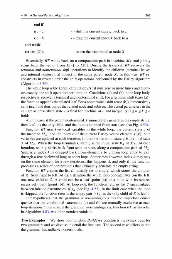
4.10 A General Parsing Algorithm 263
end if
q := p - - shift the current state q back to p
k := h - - drag the current index k back to h
end while
return (C)X - - return the tree rooted at node X
Essentially, BT walks back on a computation path in machine MX and jointlyscans back the vector from E[n] to E[0]. During the traversal, BT recovers theterminal and nonterminal shift operations to identify the children (terminal leavesand internal nonterminal nodes) of the same parent node X. In this way, BT re-constructs in reverse order the shift operations performed by the Earley algorithm(Algorithm 4.76).
The while loop is the kernel of function BT: it runs zero or more times and recov-ers exactly one shift operation per iteration. Conditions (a) and (b) in the loop body,respectively, recover a terminal and nonterminal shift. For a terminal shift (case (a)),the function appends the related leaf. For a nonterminal shift (case (b)), it recursivelycalls itself and thus builds the related node and subtree. The actual parameters in thecall are as prescribed: state e is final for machine MY , and inequality 0≤ h≤ k ≤ n
holds.A limit case: if the parent nonterminal X immediately generates the empty string,
then leaf ε is the only child, and the loop is skipped from start (see also Fig. 4.53).Function BT uses two local variables in the while loop: the current state q of
the machine MX; and the index k of the current Earley vector element E[k]; bothvariables are updated at each iteration. In the first iteration, state q is the final statef of MX . When the loop terminates, state q is the initial state 0X of MX . At eachiteration, state q shifts back from state to state, along a computation path of MX .Similarly, index k is dragged back from element i to j from loop entry to exit,through a few backward long or short hops. Sometimes however, index k may stayon the same element for a few iterations; this happens if, and only if, the functionprocesses a series of nonterminals that ultimately generate the empty string.
Function BT creates the list C, initially set to empty, which stores the childrenof X, from right to left. At each iteration the while loop concatenates (on the left)one new child to C. A child can be a leaf (point (a)) or a node with its subtreerecursively built (point (b)). At loop exit, the function returns list C encapsulatedbetween labeled parentheses: (C)X (see Fig. 4.53). In the limit case when the loopis skipped, the function returns the empty pair (ε)X , as the only child of X is leaf ε.
Our hypothesis that the grammar is non-ambiguous has the important conse-quence that the conditional statements (a) and (b) are mutually exclusive at eachloop iteration. Otherwise, if the grammar were ambiguous, function BT, as encodedin Algorithm 4.83, would be nondeterministic.
Two Examples We show how function BuildTree constructs the syntax trees fortwo grammars and we discuss in detail the first case. The second case differs in thatthe grammar has nullable nonterminals.

264 4 Pushdown Automata and Parsing
Fig. 4.52 Actions and calls of function BuildTree on the shifts for Example 4.75

4.10 A General Parsing Algorithm 265
Example 4.84 (Construction of the syntax tree from the Earley vector) We repro-duce the machine net of Example 4.75 in Fig. 4.52, top left. For input stringx1 . . . x4 = aabb the figure displays, from top to bottom, the syntax tree, the calltree of the invocations of function BuildTree, and the vector E returned by Earleyalgorithm (Algorithm 4.76). The Earley vector (the same as in Table 4.6) is com-mented with three boxes, which contain the conditions of the two nonterminal shifts,and the conditions of one (out of four) terminal shift. The arrows are reversed withrespect to those in Fig. 4.50, and trace the terminal and nonterminal shifts.
The string is accepted thanks to pair 〈1S,0〉 in element E[4] (Property 4.77).The initial call to function BuildTree is BT(S,1S,0,4), which builds the tree for thewhole string x1 . . . x4 = aabb.
The axiomatic machine MS has an arc 0SA→ 1S . Vector E contains the two pairs:
〈3A,0〉 ∈ E[4], which has a final state of machine MA and so enables a shift oper-ation on nonterminal A; and 〈0S,0〉 ∈ E[0], which has a state with an arc directedto state 1S and labeled with nonterminal A. Thus, condition (b) in the while loopof Algorithm 4.83 is satisfied. Therefore, the first recursive call BT(A,3A,0,4) isexecuted, which builds the subtree for the (still whole) (sub)string x1 . . . x4 = aabb.
This invocation of function BuildTree walks back vector E from element E[4]to E[1], and recovers the terminal shift on b, the nonterminal shift on A and theterminal shift on a. When processing the nonterminal shift on A with referenceto element E[3], another recursive call occurs because vector E contains the two
pairs 〈3A,1〉 ∈ E[3] and 〈1A,0〉 ∈ E[1], and machine MA has an arc 1AA→ 2A.
Therefore, condition (b) in the while loop is satisfied and the second recursive callBT(A,3A,1,3) is executed, which builds the subtree for substring x2x3 = ab.
The two boxes at the bottom of Fig. 4.52 explain the nonterminal shifts (point (b)in Algorithm 4.83), pointed to by a double arrow. In detail, the formal parametersX and j (upper side) have the actual values of the current invocation of BuildTree.Local variables q and k (lower side) have the values of the current iteration of thewhile loop. Inside a box we find in order: the values assumed by nonterminal Y ,final state e, index h and state p; second, some logical conditions on pairs andarc; and, last, the call to BT with its actual parameters. Each box so justifies oneiteration, where condition (b) is satisfied, whence a call to BT occurs and a subtreeis constructed.
For terminal shifts the situation is simpler: consider the comment box in Fig. 4.52and compare it with the if-then statement (a) in Algorithm 4.83. Three more terminalshifts take place, but we do not describe them.
Example 4.85 (Syntax tree with nullable nonterminals) Figure 4.53 shows the calltree of function BuildTree of Example 4.78. The corresponding parse trace is inFig. 4.50, p. 256: to see how function BT walks back the Earley vector and con-structs the syntax tree, imagine to reverse the direction of solid and dashed arcs (thedotted arcs of closure are not relevant). Figure 4.53 also shows the parenthesizedsubtrees returned by each call to BT.

266 4 Pushdown Automata and Parsing
Fig. 4.53 Calls and return values of BuildTree for Example 4.78
The innermost call to the function BuildTree in Fig. 4.53 is BT(B,0B,4,4),which constructs the subtree of an instance of nonterminal B that immediately gen-erates the empty string ε. In fact, the two indices j and i are identical to 4 and theirdifference is zero; this means that the call is on something nullable inserted betweenterminals b4 and a5.
Computational Complexity The worst-case computational complexity of func-tion BuildTree can be estimated by computing the size of the constructed syntax tree,the total number of nodes and leaves. Such total is directly related to the number ofterminal and nonterminal shifts that function BT has to recover.
The tree to be built is only one for the string accepted, as the grammar is non-ambiguous. Since the grammar is also clean and free from circular derivations, fora string of length n the number of tree nodes is linearly bounded by n, i.e., O(n).The basic operations are those of checking the state or pointer of a pair, and ofconcatenating one leaf or node (i.e., its parenthesized representation) to the childlist; both operations take a constant time, for a suitable parenthesized representationof the tree. The following analysis mirrors the complexity analysis of the Earleyalgorithm (function BT uses k as current index to vector E):1. A vector element E[k] (0 ≤ k ≤ n) contains a number of pairs of magnitude
O(n).2. Checking the condition of the if-then statement (a) of Algorithm 4.83 takes a
constant time, i.e., O(1). The possible enlisting of one leaf takes a constanttime as well. So, processing the whole E[k − 1] takes a time of magnitudeO(n)×O(1)+O(1)=O(n).
3. Checking the condition (b) needs to identify the pairs: (1) 〈e,h〉 in E[k]; and(2) 〈p, j 〉 in E[h]. For each potential candidate pair (1) in E[k], the wholeE[h] has to be searched to find the corresponding candidate pair (2) (if any);

4.10 A General Parsing Algorithm 267
the search takes a time of magnitude O(n). The possible enlisting of one (non-terminal) node takes a constant time, i.e., O(1). So, processing the whole E[k]takes a time of magnitude O(n)×O(n)+O(1)=O(n2).
4. Since the total number of terminal plus nonterminal shifts (a) and (b) to berecovered is bounded by the number of tree nodes, i.e., O(n), the total timecost of function BT is no more than:
BT cost = (if-then (a)+ if-then (b)
)× # of tree nodes
= (O(n)+O
(n2))×O(n)=O
(n3)
Property 4.86 The asymptotic time complexity of function BuildTree to constructa syntax tree for a non-ambiguous grammar (Algorithm 4.83) is cubic in the worstcase, i.e., O(n3), where n is the length of the string accepted.
The above complexity can be improved if we consider that function BuildTree(Algorithm 4.83) just reads the Earley vector E and does not write it. Thereforeits complexity can be lowered by pre-ordering the vector. Suppose every elementE[k] is independently ordered: pairs 〈q, j 〉 are ranked by pointer j (0 ≤ j ≤ n);ranking by state q does not matter as the number of states is a constant. Orderingeach element takes a time O(n logn), e.g., by the QuickSort algorithm. So orderingall the elements takes a time (n+ 1)×O(n logn)=O(n2 logn). After ordering theelements, function BT can regularly run as before.
The benefit of pre-ordering is mainly for the time cost of the if-then statement (b)in function BuildTree. Now finding a pair with some final state e and pointer h inE[k], takes a time O(n); and consequently searching the related pair with a fixedpointer j in E[h], takes a time O(logn), e.g., by the Binary Search algorithm. Sostatement (b) takes a time O(n logn). Similarly, in the if-then statement (a) we canuse Binary Search for searching a pair with fixed pointer j in E[h]|h=k−1, so state-ment (a) takes a time O(logn). Therefore the total time cost of function BT becomes
BT cost = pre-ordering E + (if-then (a)+ if-then (b)
)× # of tree nodes
= O(n2 logn
)+ (O(logn)+O(n logn)
)×O(n)=O(n2 logn
)
This new complexity of BuildTree, for non-ambiguous grammars, is lower than theprevious cubic one without pre-ordering (Property 4.86), and approaches that of theEarley algorithm rearranged for non-ambiguous grammars.
A practical parser for a programming language usually works on a syntax treerepresented as a graph, with variables that model nodes and leaves, and pointersthat connect them; not on a tree represented as a parenthesized string. The functionBuildTree in Algorithm 4.83 can be easily adapted to build such a tree, withoutchanging its algorithmic structure. Here is how to recode the three crucial state-ments of BT (the rest is unmodified):

268 4 Pushdown Automata and Parsing
Original encoding Recoded for a pointer-connected tree
C := xk · C Create leaf xk and attach it to node X
C := BuildTree(Y, e,h, k) · C Create node Y , call BuildTree(Y, . . .)
and attach node Y to node X
return(C)X Return the pointer to node X
If upon return node X does not have any child nodes or leaves yet, leaf ε has to beattached to it. It is not difficult to encode the instructions above by some libraryfor the management of graph structures, as many are available. The worst-case timecomplexity of this variant of BuildTree is still cubic.
We conclude by warning again that the version of function BuildTree presentedhere is not designed to properly work with ambiguous grammars. Anyway, since thegrammars of programming languages are usually non-ambiguous, such a limitationis not relevant for compilation. However, ambiguous grammars deserve interest inthe processing of natural languages. There the main difficulty is how to compactlyrepresent all the syntax trees the string may have, the number of which may beexponential—and even unbounded if there are nullable nonterminals—in the stringlength. This can be done by using a so-called Shared Packed Parse Forest (SPPF),which is a graph type more general than a tree but that still takes a worst-case cubictime for building; see [35] for how to proceed in such more general cases.
4.11 Parallel Local Parsing
In many application areas, algorithms that originally had been designed for sequen-tial execution, later have been transformed into parallel algorithms, to take advan-tage of the available multiple processors on current computers for reducing runningtime. For language parsing, a straightforward approach is to split the source text intoas many segments (substrings) as the number of available processors, to parse eachsegment on a different processor by using a sequential parser, and then to recom-bine the resulting partial parse trees into the complete tree. In principle the speed-upobtained with respect to the original sequential algorithm scales with the number ofprocessors, but there are conceptual and practical obstacles on this way.
First and foremost, the deterministic sequential parsing algorithms cannot beeasily transformed into parallel programs because they need to scan the text se-quentially from left to right and their decisions, whether to shift or to reduce, maydepend on distant past decisions. Therefore the parser of, say, the second segment,may be unable to proceed (deterministically) until the parser of segment one hasfinished, which thus defeats the benefit of parallelization. To illustrate, observe thedeterministic (hence LR(1)) language
L=L1︷ ︸︸ ︷{
c∗oc∗anbn | n≥ 1}∪
L2︷ ︸︸ ︷{c∗tc∗anb2n | n≥ 1
}

4.11 Parallel Local Parsing 269
such that the presence of letter o (respectively t) announces that each later letter a
will be followed by one letter b (respectively two b’s). Imagine to parse the follow-ing text subdivided into two segments, as shown here:
segment 1︷ ︸︸ ︷cc . . . ctcc . . . c
segment 2︷ ︸︸ ︷aa . . . abb . . . b
The second parser does not know whether the first one has encountered a letter o
or t , and so faces the task of analyzing language {anbn | n ≥ 1} ∪ {anb2n | n ≥ 1},which is non-deterministic (as explained on p. 156 for a similar case). Notice thatan arbitrary distance separates the positions of substrings o (or t) and abb, wherethe choice of the reduction ab � . . . or abb � . . . is due. This example shows that,if we want to be able to deterministically parse separate text segments, we mustexclude the deterministic languages that exhibit such a long-distance dependencebetween operations performed by independent parsers. In other words, to be suitablefor parallel parsing, a grammar, besides being LR(1), should not require parsingstate information to be carried to another substring over a long stretch of text. Weloosely call “local parsability” such a grammar property.
We describe a parsing algorithm that bases its parsing decisions on the localproperties of the text, thereby it lends itself to parallel execution.
4.11.1 Floyd’s Operator-Precedence Grammars and Parsers
Floyd [12, 14], a pioneer of compiler techniques, took inspiration from the tradi-tional notion of precedence between arithmetic operators, in order to define a classof languages such that the shape of the parse tree is solely determined by a binary re-lation between terminals that are consecutive, or that become consecutive after a fewbottom-up reduction steps. Floyd’s approach assumes that the grammar has beennormalized in the operator form (see Sect. 2.5.13.7 on p. 62); we recall that a rule isin the operator form if any two nonterminals that occur in the right part of the rule areseparated by at least one terminal character. Many practical grammars are alreadyin the operator form, e.g., the grammar of the Dyck language: S→ bSeS | bSe | be.Otherwise we have seen in Chap. 2 how to construct an equivalent grammar in theoperator form.
All the grammars in this section are purely BNF in the operator form, and freefrom empty rules.
Precedence Relations We introduce the concept of precedence relation: this termactually means three partial binary relations over the terminal alphabet, named:� yields precedence� takes precedence= equal in precedenceFor a given grammar and any pair of terminal characters a, b ∈Σ , the precedencerelation may take one or more of the above three values, or may be undefined. Butfor the operator-precedence grammars to be soon defined, for every character paira, b, the relation, if it is defined, is unique.

270 4 Pushdown Automata and Parsing
To grasp the intended meaning of the relations, it helps to consider the languageof the arithmetic expressions with the operators plus “+” (addition) and times “×”(multiplication). Since traditionally times takes precedence over plus, these two re-lations hold: × � + and + �×. The former relation means that in an expressionsuch as 5× 3+ 7, the first reduction to apply is 5× 3 � · · · . Similarly the fact thatplus yields precedence to times (latter relation), says that in an expression such as5+ 3× 7, the first reduction to apply is 3× 7 � · · · .
We are going to extend this traditional sense of precedence from the arithmeticoperators to any terminal characters. Moreover we introduce the “equal in prece-dence” relation =, to mean that the two related characters are adjacent in a gram-mar rule: thus the left and the right parentheses are related by “(”=“)” in the ruleE→ (F ) for parenthesized arithmetic expressions.
A word of warning: none of the relations enjoys the mathematical properties ofreflexivity, symmetry, and transitivity, of the numerical order relations <, > and =,notwithstanding the similarity of the signs.
To construct a precedence parser for a given grammar, we have to compute theprecedence relations and to check that they do not conflict in a sense to be explained.To formalize precedences we introduce two sets, which are similar to the sets ofinitial and final characters of a string, but differ because the nonterminal symbolsare considered to be always nullable.
We observe that for an operator grammar, every string β that derives from anonterminal has the property that any two nonterminals are separated by one ormore terminal characters. More precisely we have
if A∗⇒ β then β ∈Σ∗(VNΣ+)∗ ∪Σ∗(VNΣ+)∗
VN
We also say that such strings β are in the operator form. More explicitly a string inthe operator form takes one of the forms
a ∈Σ or A ∈ V or BσC
where B , C are nonterminals possibly null, and the string σ in operator form startsand ends with a terminal character.
Definition 4.87 The left and right terminal sets, denoted L,R, of a string in theoperator form are recursively defined by
L(a) = {a} R(a) = {a}
L(A) = ⋃
∀rule A→α
L(α) R(A) = ⋃
∀rule A→α
R(α)
L(AσC) = Ini(σ )∪L(A) R(AσC) = Fin(σ )∪R(C)
(4.18)
where Ini and Fin denote the initial and final character of a string.

4.11 Parallel Local Parsing 271
Fig. 4.54 Floyd grammar forcertain arithmetic expressionsand its operator-precedencematrix (read a matrix entry asrow rel. col, e.g., n�+, etc.)
Table 4.7 Some left andright terminal sets for thegrammar in Fig. 4.54
String Left terminal set L Right terminal set R
n n n
B × n {n,×} n
B {n,×} n
B +B {n,×,+} {n,+}A+B {n,×,+} {n,+}A {n,×,+} {n,+}S {n,×,+} {n,+}
Example 4.88 (Grammar of arithmetic expressions) A grammar G for certain arith-metic expressions is shown in Fig. 4.54, left.
The left/right terminal sets of the strings that occur in the grammar as left- orright-hand sides, computed by Eq. (4.18), are listed in Table 4.7.
To compute the precedence relations we need the following definition.
Definition 4.89 (Precedence relations) There are three operator-precedence (OP)relations over Σ ×Σ :
takes precedence: a � b iff some rule contains Db,D ∈ V and a ∈R(D)
yields precedence: a � b iff some rule contains aD,D ∈ V and b ∈ L(D)
equal in precedence: a.= b iff some rule contains aBb,B ∈ V ∪ ε
The operator-precedence matrix (OPM) M is a square array of size |Σ | ≥ 1 thatassociates to each ordered pair (a, b) the set Ma,b of OP relations holding betweenterminals a and b.
A grammar has the operator-precedence property (we also say it is a Floydoperator-precedence grammar) if, and only if, each matrix entry contains one re-lation at most. In that case, the matrix qualifies as conflict-free.
To illustrate the definitions of the relations, we refer the reader to Fig. 4.55.As said, the precedence relations are not necessarily symmetric, in the sense that
relation a � b does not imply that relation b� a holds; similarly relation a =b doesnot imply that relation b =a holds.
For the current Example 4.88 the OPM in Fig. 4.54, right, is computed by in-specting the rules and the left/right terminal sets listed in Table 4.7.

272 4 Pushdown Automata and Parsing
Fig. 4.55 Precedence relations made apparent in the derivations of Example 4.88
Rule Terminal set Precedence relations
· · · →A+ · · · R(A)= {n,+} n�+ and +�+· · ·→ B + · · · R(B)= {n} n�+· · ·→ · · · +B L(B)= {n,×} +� n and +�×· · ·→ · · · × n ×=n
The grammar has the operator-precedence property since its OPM is conflict-free.We comment the meaning of a few relations. The OPM entries +� n and n�+
indicate that, when parsing a string containing the pattern . . .+n+ . . . , the right partn of rule B→ n has to be reduced to nonterminal B . The OPM entry (n,n) is emptybecause in a valid string, terminal n is never adjacent to another n, or separated by anonterminal as in the patterns . . . nAn . . . or . . . nBn . . . ; in other words no sententialform may contain such patterns. Similarly, there is no relation between the operators× and + because none of the patterns . . .×+ . . . , . . .×A+ . . . and . . .× B + . . .
ever occurs in a sentential form.The next example refers to a real language, which turns out to have a syntax ideal
for precedence parsing.
Example 4.90 (Grammar of JSON) The JavaScript Object Notation (JSON) is alightweight data-interchange format, which is easy for humans to read and write, andefficient for machines to parse and generate. The grammar and precedence matrixof JSON are shown in Fig. 4.56. The symbol number is a numeric constant and thesymbol bool stands for “true”, “false” or “null”. The symbol char denotes any 8 bitcharacter, except those listed in the matrix. The very large size of the typical datafiles represented in JSON, and the fact that the official grammar is essentially in theoperator form and without precedence conflicts, make parallel parsing attractive.
4.11.1.1 Comparison with Deterministic LanguagesWe present a few examples to compare the languages of operator-precedence gram-mars and those of LL(1) and LR(1) grammars.

4.11 Parallel Local Parsing 273
Fig. 4.56 Official JSON grammar. Uppercase (respectively lowercase) words denote nontermi-nals and terminals; in the OPM void cases are left empty. The only rule modified to cast thegrammar into operator form is underlined
A grammar that is deterministic but not OP, and that generates the language{anban | n≥ 0}, is
S→ aSa | b with matrix
There are conflicts in the matrix entry [a, a], yet the grammar meets the LL(1) andtherefore also the LR(1) condition.
The OP grammars have the peculiar property of symmetry with respect to mirrorreversal, in the sense that the grammar obtained by reversing the right parts of therules, is also an OP grammar. Its precedence matrix simply interchanges the “yield”

274 4 Pushdown Automata and Parsing
and “take” relations of the original grammar, and reverses the “equal in precedence”relations. To illustrate we list another grammar G:
G
{S→Xb
X→ aXb | abwith OPM :
The reversed language (L(G))R is generated by the OP grammar GR :
GR
{S→ bX
X→ bXa | bawith OPM :
On the other hand, in general neither a LL(1) nor a LR(1) grammar remains suchwhen is reversed. For instance grammar G has the LL(1) property, but the reversedgrammar GR does not. The case of a language L that ceases to be deterministicupon reversal is illustrated by
L= {oanbn | n≥ 1
}∪ {ta2nbn | n≥ 1
}
Here the first character (o or t) determines whether the string contains one a perb or two a’s per b. This property is lost in the reversed language: LR containssentences of two types, say, b4a4o and b4a8t . A deterministic pushdown machinecannot decide when to pop a letter b upon reading an a.
The next statement generalizes the preceding findings.
Property 4.91 (Comparison of OP languages)• The family of languages defined by Floyd OP grammars is strictly included in
the family of deterministic (LR(1)) languages.• Every OP grammar has the property that the mirror reversed grammar is also
an OP grammar (so the mirror language remains deterministic).• The families of languages defined by LL(1) and by OP grammars are not com-
parable.
In practice OP grammars can be used to define quite a few existing technical lan-guages, if their grammar has been converted into operator form. But there are lan-guages where the use of the same terminal character in different constructs causesprecedence conflicts, which may or may not be removed by suitable grammar trans-formation.
4.11.2 Sequential Operator-Precedence Parser
Precedence relations precisely control whether a substring that matches the rightpart of a rule (also referred to as the handle) has to be reduced to the left part non-

4.11 Parallel Local Parsing 275
terminal. This test is very efficient and, unlike the conditions examined by LR(1)
parsers, does not rely on long-distance information. However, a minor difficulty re-mains, if the grammar includes two rules such as A→ x and B→ x with a repeatedright part: how to choose between nonterminals A and B when string x has beenselected for reduction. This uncertainty could be propagated until just one choiceremains, but to simplify matters, we assume that the grammar does not have anyrepeated right parts, i.e., it is invertible, a property that can be always satisfied bythe transformation presented in Chap. 2, p. 59.
Operator-precedence grammars are an ideal choice for parallel parsing. For se-quential parsing, they are occasionally adopted, in spite of their limitations withrespect to ELR(1) grammars, because the parsers can be very efficient and are easyto construct. As the parallel algorithm stems directly from the sequential one, westart from the latter.
The key idea driving the algorithm is simple: wherever a series of = precedencerelations enclosed by the relation pair �, � is found between consecutive terminals,the enclosed substring is a reduction handle. To find handles, the parser uses theOPM and a pushdown stack S to discover the substring to be reduced, as soon asthe next � relation occurs.
It is convenient to assume that the input string is enclosed by the special character#, such that a # yields precedence to every other character and every character takesprecedence over #: this is tantamount to adding the new axiom S0 and the axiomaticrule S0 → #S#.
To prepare for its parallel use, we enable the parsing algorithm to analyze alsostrings that may contain nonterminal characters. Such strings begin and end withterminal characters (or with character #), and are in the operator form. This settingis only needed when the parallel algorithm is called to parse internal text segments.
The algorithm uses a stack S containing symbols that are couples of type (x,p),where x ∈Σ ∪V and p is one of the precedence relations {�,
.=,�} or is undefined(denoted by ⊥). The second component is used to encode the precedence relationexisting between two consecutive symbols; conventionally it is always p = ⊥ fornonterminals. We assume that the stack grows rightwards.
Algorithm 4.92 (Operator-precedence sequential parser)28
OPparser(S, u,head, end)
S : stack of couples u: string to analyze head, end: pointers in u
conventions and settingsdenote u= u1u2 . . . um and s = u2 . . . um−1 with m > 2
denote u1 = a and um = b where a and b are terminal
for sequential use only:
denote the initial stack contents as S = (a,⊥)
set the initial pointers head := 2 and end :=m
28See [4, 5] for further reading.

276 4 Pushdown Automata and Parsing
begin1. let x = uhead be the symbol currently pointed by head and consider the prece-
dence relation between x and the top-most terminal y in the stack S2. if x is a nonterminal then
push (x,⊥) head++3. else if y � x then
push (x,�) head++4. else if y
.= x thenpush (x,
.=) head++5. else if y � x then
a. if stack S does not contain � thenpush (x,�) head++
b. elselet the stack S be (z0,p0) . . . (zi−1,pi−1)(zi,�) . . . (zn,pn) where zi
(more precisely pi ) is the top-most � relation, i.e., for every stack elementon the right of zi the precedence relation is = or ⊥
i. if zi−1 is a nonterminal and ∃rule A→ zi−1zi . . . zn thenreplace (zi−1,pi−1)(zi ,�) . . . (zn,pn) in S with (A,⊥)
ii. else if zi−1 is a terminal or # and ∃rule A→ zi . . . zn thenreplace (zi ,�) . . . (zn,pn) in S with (A,⊥)
iii. elsestart an error recovery procedure29
end ifend if
end if6. if head < end or ( head = end and S �= (a,⊥)(B,⊥) ) for any nonterminal B
then goto step (1) else return S end ifend
Upon the normal termination of the algorithm, its configuration can be no longerchanged either by shift or by reduce actions, and we say it is irreducible.
When used sequentially and not as a part of the parallel version to be next pre-sented, the algorithm is called with parameters u= #s# and S = (#,⊥) (so a = #),never performs step (2), never pushes (x,�) onto the stack, and accepts the inputstring only if the stack is S = (#,⊥)(S,⊥).
We comment a few steps of the parsing trace shown in Fig. 4.57. Step 1 shiftstoken n on the stack, then step 2 detects the pattern �n� and reduces the handlen to B . At step 3 the top-most terminal on stack is #, which yields precedence tothe current token + that is shifted. Skipping to step 7, the stack top × equals inprecedence token n, which is therefore shifted. Step 8 identifies the handle B × n
29An error is detected either when the handle, i.e., the portion of string included between relations� and �, does not match any r.h.s., or when no precedence relation holds between two consecutiveterminal characters.

4.11 Parallel Local Parsing 277
Fig. 4.57 Steps of a Floyd sequential parser for sentence a + a × a (grammar and OPM inFig. 4.54)
in the pattern �B × =n�; notice that the handle includes a nonterminal B , whichoccurs between the terminal characters related by +�×.
4.11.3 Parallel Parsing Algorithm
At the level of abstraction that is usually adopted in parsing, the input text con-sists of a stream of symbols (also known as lexemes or tokens), which are terminalelements of the grammar. As we know, the sequential parser invokes the lexical an-alyzer (scanner) to obtain the next input token. To accommodate multiple parsersthat operate in parallel, such an organization, which relies on a scanning subroutineinvoked by the parser, has to be slightly revised in order to avoid that a token, sayCYCLE27, stretching over consecutive text segments assigned to different parsers,may be split into two tokens, say CYCL and E27. Since this problem is marginal forthe parallel parsing method we are interested in, we assume that the input text hasbeen entirely scanned before parallel parsing starts.
Thus our data-parallel algorithm splits the load among workers by dividing thetext into k ≥ 1 segments, where k is the number of physical processors. How thetext is split is irrelevant, provided that the substring lengths are approximately equalto ensure load balancing. In contrast, other parallel parsers have been proposed thatperform a language dependent split, and require the text to be segmented at spe-

278 4 Pushdown Automata and Parsing
Fig. 4.58 Partial trees and corresponding stacks after the first parsing phase of textn+ n+ n× n× n+ n× n+ n by using three workers
cific positions where a token (such as begin) occurs, that parts a large syntacticconstituent of the language.
Then we apply Algorithm 4.92 to each substring, by using a separate stack perworker. Each worker returns a stack, which is guaranteed to be correct indepen-dently of the stacks of the other workers. In practice, the set of reductions operatedby each parser makes a final fragment of the parse tree. The local parsability prop-erty of OP grammars manifests itself in that each parser bases its decisions on alook-ahead/look-back of length one, to evaluate the precedence relations betweenconsecutive terminal characters. Therefore in the split text, we overlap by one tokenany two consecutive segments, i.e., the last terminal of a segment coincides with thefirst terminal of the next segment.
Example 4.93 (Parallel parsing) Reconsider the grammar of Example 4.88, p. 271,and the source text
#n+ n+ n× n× n+ n× n+ n#
Assume that there are k = 3 workers and the segmented text is as
1︷ ︸︸ ︷n+ n+
2︷ ︸︸ ︷n× n× n+n
3︷ ︸︸ ︷×n+ n
where the marks # are left implicit, and the symbols + and n not embraced areshared by the two adjacent segments.
After each sequential parser has processed its segment, the partial trees and thestacks are shown in Fig. 4.58.
Notice that stack S1 contains the shortest possible string: a nonterminal symbolembraced by the two terminals that are always present on the stack ends. Such astack is called quasi-empty. Stacks S2 and S3 are not quasi-empty since they havealso terminal symbols in their inner part.

4.11 Parallel Local Parsing 279
Stack Combination To complete parsing, we need an algorithm that joins theexisting k stacks and launches one or more sequential parsers on the combinedstack(s). Different strategies are possible:serial One new stack is produced by joining all the stacks (and by taking care
of canceling one of the duplicated symbols at each overlapping point). The nextphase uses just one worker, i.e., it is sequential.
dichotomic A new stack is created by joining every pair of consecutive stacks atpositions 1–2, 3–4, etc., so that the number of stacks of phase one is halved, aswell as the number of workers.
opportunistic Two or more consecutive stacks are joined, depending on theirlength. In particular a quasi-empty stack is always joined to a neighboring stack.The number of stacks is guaranteed to decrease by one, or more rapidly if a fewstacks are quasi-empty.
If the output of phase two consists of more than one stack, then the last two strategiesrequire further phases, which can employ the serial or again a parallel strategy. Ofcourse, at the end all the strategies compute the same syntax tree and they only differwith respect to their computation speed.
The serial strategy is convenient if the stacks after phase one are short, so thatit would be wasteful to parallelize phase two. We do not need to describe phasetwo since it reuses the sequential algorithm. The dichotomic strategy fixes the num-ber of workers of phase two without considering the remaining amount of work,which is approximately measured by the length of each combined stack, and thuscauses a useless overhead when a worker is assigned a short or quasi-empty stack toanalyze. The opportunistic approach, to be described, offers more flexibility in thecombination of stacks and their assignment to the workers of phase two.
We recall that Algorithm 4.92 has two main parameters: stack S and input stringu. Therefore, we describe how to initialize these two parameters for each workerof phase two (no matter the strategy). Each stack S returned by phase one, if it isnot quasi-empty, is split into a left and a right part, respectively denoted as SL andSR , such that SL does not contain any � relation and SR does not contain any �relation; of course = relations may occur in both parts.
Thus, stack S2 is divided into SL2 = (+,⊥)(B,⊥)(+,�) and SR
2 = (n,�). Ifseveral cut points satisfy the condition, then we arbitrarily choose one of them.Notice that the sequential parser can maintain a pointer to the stack cut point with anegligible overhead, so we can assume that the stack returned by Algorithm 4.92 isbipartite.
To initialize the two parameters (stack and input string) for a worker, the parallelalgorithm combines two consecutive bipartite stacks, as next explained. Notice thatthe input string thus obtained, contains terminal and nonterminal symbols (com-puted in the reductions of phase one).
Let W and W ′ be consecutive workers of the previous phase, and let their bipar-tite stacks be SLSR and S ′LS ′R . The initial configuration for a worker of the nextphase is obtained as shown in Fig. 4.59. More precisely we define the followingfunctions:

280 4 Pushdown Automata and Parsing
Fig. 4.59 Scheme of the initial configuration of a worker of the next phase: the stack is S and theinput string is u′
1. Stack initialization:
Scombine(SL,SR
)= (a,⊥)SR where a is the top symbol of SL
Notice that the precedence value listed with a, becomes undefined because inthe new stack the a is not preceded by a terminal symbol.
2. Input string initialization. The function ucombine(S ′L) returns the string u′ ob-tained from the stack part S ′L by dropping the precedence signs and deletingthe first element (which is redundant as it is on top of SR).

4.11 Parallel Local Parsing 281
There are a few simple special but important cases. When S ′ contains only � and.=
precedence relations, the number of stacks can be reduced. Since in the neighboringstack, part SR too contains only � and = relations, we concatenate three piecesto obtain the new stack: SRS ′R , and the left part, denoted S ′′L, of the worker thatcomes after W ′. As said, we need to keep only one of the overlapping elements: thelast symbol of SR , but not the identical first symbol of S ′.
Similarly, if S = (a,⊥)(A,⊥)(b,�) or S = (a,⊥)(A,⊥)(b, =) is a quasi-empty stack, the next stack part S ′L is appended to it. Notice that the case of aquasi-empty stack (a,⊥)(A,⊥)(b,�) belongs to the previous discussion.
The outline of the parallel parsing algorithm comes next. Notice that for brevitythe special cases discussed above are not encoded in this outline.
Algorithm 4.94 (Operator-precedence parallel parser)
1. split the input string u into k substrings: #u1u2 . . . uk#2. launch k instances of Algorithm 4.92 where for each index i with 1 ≤ i ≤ k
the parameters of the ith instance are as
denote as a the last symbol of ui−1
denote as b the first symbol of ui+1
denote u0 = uk+1 = #
S := (a,⊥)
u := uib
head := |u1u2 . . . ui−1|end := |u1u2 . . . ui | + 1
the result of this phase are k bipartite stacks SLi SR
i
3. repeat
for each non-quasi-empty bipartite stacks SLi SR
i and SLi+1SR
i+1 do
launch an instance of Algorithm 4.92 with these parameters:
S := Scombine(SL
i ,SRi
)
s := ucombine(SL
i+1
)
head := 1
end := |u|end for
until (there is only one stack S and the configuration is irreducible ) or anerror is detected (triggering recovery actions not specified here)
4. return stack S
Example 4.95 (Parallel parsing steps) We resume from the configuration shown inFig. 4.58, where three bipartite stacks, computed by three workers, are present.

282 4 Pushdown Automata and Parsing
(#,⊥) (A,⊥) (+,�) S1
(+,⊥) (B,⊥) (+,�)
SR2︷ ︸︸ ︷
(n,�) S2
(n,⊥) (×,�) (n,.=) (+,�) (B,⊥) (#,�) S3 = SL
3
Notice that stack S1 is quasi-empty. In reality the stacks are so short that the serialstrategy should be applied, which simply concatenates the three stacks and takescare of the overlaps. For the sake of illustrating the other strategies, we combinestacks 2 and 3. We observe that the stack part SR
3 is void, hence S3 ≡ SL3 holds.
Step 3, repeat, launches Algorithm 4.92 on every initial configuration constructed asshown in Fig. 4.59. Here there is just one instance, namely the parser that combinesthe outcome of workers 2 and 3, starting from the initial configuration:
Scombine(SL2 ,SR
2 )︷ ︸︸ ︷(+,⊥)(n,�)
ucombine(SL3 )
︷ ︸︸ ︷×n+B#
In the order, the following reductions are performed:
n � B B × n � B
thus obtaining the stack: S = (+,⊥)(B,⊥)(+,�)(B,⊥)(#,�). The situation be-fore the final round is
(#,⊥) (A,⊥) (+,�) (B,⊥) (+,�) S1SL2
(+,⊥) (B,⊥) (+,�) (B,⊥) (#,�) S
The parser can use as input string simply a # and the stack obtained by concatenatingthe existing stacks:
(#,⊥)(A,⊥)(+,�)(B,⊥)(+,�)(B,⊥)(+,�)(B,⊥)
Three successive reductions A+B � A, followed by A � S, complete the analysis.
We mention a possible improvement to the strategy, which mixes the serial andparallel approaches. At step 3, if the sum of the lengths of a series of consecutivestacks is deemed short enough, then the algorithm can join all of them at once intoone stack, thus applying the serial strategy to that portion of the remaining work.This strategy is advantageous when the remaining work needed to join the stacksand to synchronize the workers, outbalances the useful work effectively spent tocomplete the construction of the syntax tree.

4.12 Managing Syntactic Errors and Changes 283
4.11.3.1 ComplexityParallel parsing techniques are mainly motivated by possible speed gains over se-quential algorithms. We briefly analyze the performance of the parallel parser, as-suming that after the first phase of segment parsing, all the resulting stacks are joinedat once into one stack (as discussed above).
In terms of asymptotic complexity, we are going to argue that the parallel algo-rithm achieves these requirements:1. a best-case linear speed-up with respect to the number of processors2. a worst-case performance that does not exceed the complexity of a complete
sequential parsingTo meet these requirements, it is essential that the combination of stacks Si andSi+1 inside step (3)(a) of Algorithm 4.94, takes O(1) time, hence O(k) overall timefor k workers. This goal is easily achieved by maintaining at runtime a marker thatkeeps track of the separation between the two parts SL and SR of each bipartitestack. The marker is initialized at the position where the first relation � is detectedand then updated every time a reduction is applied and a new element is shifted onthe stack as a consequence of a new relation �. For instance in the case of S2 inFig. 4.58, the marker is initialized at the position of the first + symbol and thereremains after the reductions n � B , B × n � B and B × n � B , because +� n
and +�× hold. Then, when the second + within this segment is shifted (the first+ remains because the � between the two + is not matched by a corresponding �at its left), the marker is advanced to the position of the second +, because +� n
holds. In such a position the marker indicates the beginning of SR2 .
These operations require a time O(1), irrespectively of whether we implementthe stacks by means of arrays or of more flexible linked lists. It follows that theoverhead due to stack combination (linearly) depends on k but not on the sourcetext length, thus proving that the worst-case asymptotic complexity is the same asin the sequential algorithm.
Truly such analysis neglects the synchronization and communication costs be-tween workers, which may deteriorate the performances of parallel algorithms. Suchcosts tend to outbalance the benefit of parallelization when the load assigned to aworker becomes too small. In our case this happens when the text, i.e., the inputstack assigned to a worker, is too small. The cost also depends on the implementa-tion techniques used for synchronization and communication, and on their supportby the hardware operations provided by the computer. Experiments [4] indicate thatparsing large texts in parallel on the current multi-processor and multi-core comput-ers, achieves a significant speed-up.
4.12 Managing Syntactic Errors and Changes
In this section we address two additional features that are sometimes requested froma parser: the capability to manage user errors in a text, and the ability to efficientlyre-parse the modified text when the errors are fixed, or more generally when somechanges have been made.

284 4 Pushdown Automata and Parsing
4.12.1 Errors
In human communication the hearer usually tries to correct the errors that quite fre-quently occur in utterances, to assign a likely meaning to the sentence; if he fails, hemay prompt the utterer for a correction. On the other hand, for artificial languagesthe communication partners can be human beings and machines, and it helps to sep-arate three cases: machine-to-human (as in automatic answering systems), machine-to-machine (e.g. XML), and human-to-machine, where programming languages arethe typical case. Since “errare humanum est”, but machines are supposed not tomake mistakes, we have to deal only with the last case: a hand-written documentor program is likely to contain errors and the machine has to be capable to suitablyreact.
The simplest reaction is to stop processing the text as soon as the machine detectsan error, and to display a diagnostic message for the author. A more complete reac-tion involves recovery from error, i.e., the capability to resume processing the text.Yet more ambitious, but harder to obtain, is the capability to automatically correctthe error.
Historically, in the old times when a central computer slowly processed batchesof texts submitted by many users, the ability to detect all or most errors in a singlecompilation was a must, in order to avoid time-consuming delays caused by re-peated compilations after a single error had been corrected by the user. Nowadays,compilers are interactive and faster, and a treatment of all the errors at once is nolonger requested, while it remains important to provide an accurate diagnostic forhelping the user to fix the error.
In the following, first we classify the error types, then we outline some simplestrategies for error recovery in parsers.
4.12.1.1 Error TypesThe errors a person makes in writing can be subjective or objective. In a subjectiveerror, the text remains formally correct both syntactically and semantically, but itdoes not reflect the author’s intended meaning. For instance, the typo x − y + z
instead of x × y + z is a subjective error, which will alter the program behaviorat runtime in rather unpredictable ways, yet it cannot be catched at compile time.A human error is objective if it causes a violation of the language syntax or semanticspecifications.
Sometimes, undetected errors cause the compiled program to raise fault condi-tions at runtime, such as memory errors (segmentation, overflow, etc.) or nontermi-nation. In such cases we say the program violates the dynamic (or runtime) semanticof the language. On the other hand, the errors that can be detected by the compileror by the static semantic analyzer (described in the next chapter) are called static. Itpertains to the runtime support (interpreter, virtual machine or operating system) ofthe language to detect and recover from dynamic errors, perhaps by invoking suit-able exception handlers. The methods used to detect subjective errors and to managethe dynamic errors they induce, belong to software engineering, to operating systemand virtual machine design, and are out of scope for this book.

4.12 Managing Syntactic Errors and Changes 285
Therefore, we only deal with objective static errors, which can be further classi-fied as syntactic and semantic. A syntactic error violates the context-free grammarthat defines the language structure, or the regular expression that defines the lexicon.A semantic error violates some prescription included in the language reference man-ual, but not formulated as a grammar rule. Typically, such prescriptions are specifiedin English; less frequently, they are formalized using a formal or semi-formal no-tation (the attribute grammars of Chap. 5 are an example). For languages such asJava, the so-called type violations are a primary kind of semantic error: e.g., usingas real a variable that was declared to be boolean; or using three subscripts to accessa one-dimensional array; and many others. To detect and manage static semantic er-rors, the compiler builds certain data structures, called symbol tables, that encodethe properties of all the objects that are declared or used in a program.
Since this chapter deals with parsing, we present some basic ideas for the de-tection, diagnosis, and recovery of syntactic errors. A general discussion of errorprocessing in parsers is in [17].
4.12.1.2 Syntactic ErrorsWe examine how a parser detects a syntactic error. To keep our analysis generalenough, we avoid implementation details and we represent the parser as a push-down automaton, which scans the input from left to right until either the end-of-textis reached or the move is not defined in the current configuration, then to be callederroneous. The current token, for which the move is undefined, is named the errortoken. From a subjective point of view, the human mistake or typo the author madein writing the text, may have occurred at a much earlier moment. A negative con-sequence is that the parser diagnosis of the erroneous configuration may have littleresemblance with the author’s subjective mistake. In fact, the input string that ter-minates with the token that the human erroneously typed, though different from theone the author had in mind, may be the initial part (prefix) of a legal sentence of thelanguage, as next illustrated.
Example 4.96 (Human error and error token) In the FORTRAN language a loopsuch as DO110J= 9,20 is defined by the following rule:
〈iterative instruction〉→ DO〈label〉‘=’〈initial value〉‘,’〈step〉
Suppose the human error is to omit the blank spaces around the label and so towrite DO110J= 9,20; now token DO110J is a legal variable identifier and the stringDO110J= 9 hitherto analyzed is a legal assignment of value 9 to it. The parser willdetect the error on reading the comma. The delay between the first human error andthe recognized error token is: DO 110J= 9︸ ︷︷ ︸
delay
,20.
A more abstract example from the regular language
L= db∗aa∗ ∪ eb∗cc∗

286 4 Pushdown Automata and Parsing
happens with the illegal string x = dbb . . . b↓cccccc, where the first error token
is marked by the arrow, whereas it is likely that the human error was to typed for e, because for the two ways to correct x into x′ = e bb . . . b︸ ︷︷ ︸
delay
cccccc or
x′′ = dbb . . . baaaaaa, string x′ requires a single change, but string x′′ needs asmany as six changes. Assuming the more likely correction, the delay between hu-man error and error token is unbounded.
The second example has introduced the idea of measuring the differences be-tween the illegal string and the presumably correct one, and thus of obtaining a met-ric called editing or Levenshtein distance. In the example, the distance of x′ from x
is one and of x′′ from x is six. Moreover, we say that string x′ is the interpretationat minimal distance from x, as no other sentence of language L has distance onefrom x. To give a precise definition of editing distance, one has to indicate whichediting operations are considered.
A typical choice for typed texts includes the following operations, which corre-spond to frequent typing mistakes: substituting a character for another; erasing acharacter; and inserting a character. After detecting an erroneous token, it would bedesirable to compute a minimal distance interpretation, which is a legal sentence assimilar as possible to the scanned illegal string. Such a sentence is a reconstructionof what the typist intended to write, in accordance with a model that assigns a lowerprobability to the mutations involving many editing changes.
Unfortunately the problem of computing a minimal distance interpretation forcontext-free languages is computationally complex because of the unlimited spatialdistance between the error token and the position where the editing corrections aredue. A further difficulty comes from that it is not known how the string will continue,thus what is a minimal distance interpretation so far, may turn out to necessitate toomany editing changes when the input is further scanned. Therefore the typical errorrecovery techniques used by compilers, renounce to the minimal distance goal, yetthey attempt to stay away from the opposite case necessitating as many correctionsas the string length.
A Parser with Basic Error Recovery In Fig. 4.60 we represent the parser asa deterministic PDA. By definition of error token, the parser cannot move ahead,i.e., the transition function is undefined for the input b0 and the top symbol An. Astraightforward (but not very informative) diagnostic message is: “token b0 is notacceptable at line n”. This message can be made more precise by reporting theparser configuration, as we next explain for the case of a deterministic top-downparser.
As we know, each symbol Ai in the stack carries two pieces of information: anonterminal symbol of the grammar (i.e., a net machine or a recursive procedure);and an internal state of that machine (i.e., the label of a procedure statement). Weassume that the active machine is associated to An. For the current instruction twocases are possible: the instruction scans a token e; or the instruction invokes a ma-

4.12 Managing Syntactic Errors and Changes 287
Fig. 4.60 PDA parser configuration when an error is detected. The input string is z = wb0y �,character b0 is the error token, string w is the already scanned prefix, and string y = b1 . . . bm isthe suffix still to be scanned. The pushdown stack contains α = A1A2 . . .An, where An is the topsymbol
chine/nonterminal E with guide set Gui(E). Then the message says: “at line n Iexpected token e (or the tokens in Gui(E) in the latter case) instead of token b0”.
Even with this improvement, such error messages can be misleading. Imaginethat the subjective error omitted the first begin token in a string made of nestedbegin . . . end blocks. The first error configuration of the parser occurs when sym-bol b0 is the last end token of the series, while the parser expects to be outsideof any block. The previous message tells only that token end is out of place, butgives no cue for finding the subjective error: the missing token begin could be inmany possible positions in the text. To produce a more useful diagnostic help, someparsers incorporate a language-specific knowledge, such as statistics about the mostfrequent errors.
Error Recovery To complete this brief discussion, we outline a simple techniquefor error recovery. To resume parsing after an error, we need to intervene on one atleast of the arguments (input token and top of stack symbol) of the PDA transitionfunction, which is undefined in the current configuration. Notice that parsers ofdifferent types may have as third argument the internal state of the PDA, whichis irrelevant in the case we are considering. It is easy to modify such arguments tomake the next move possible, but it is more difficult to ensure that the followingmoves do not sink the parser into a new error configuration, or worse into a seriesof errors and meaningless diagnostics.
A most elementary recovery technique, named panic mode, keeps skipping thenext tokens b1, b2, . . . , �, until for some token bj the transition function becomesdefined for arguments bj and An, as this technique does not modify the stack. Theintervening tokens from b1 to bj−1 are ignored, thus causing the compiler to skipthe analysis of potentially large text sections.
Example 4.97 (Panic mode) Consider a toy language containing two statementtypes: assignments such as i = i + i + i, where symbol i denotes a variable orprocedure identifier; and procedure calls with actual parameters, such as call i(i +i, i, i + i + i). We illustrate the panic mode error recovery for the following (erro-neous) text:
scannedtext︷ ︸︸ ︷
call i
panic-skipped text︷ ︸︸ ︷error= i + i . . .+ i � (4.19)

288 4 Pushdown Automata and Parsing
The error is detected after correctly scanning two tokens, call and i. The parser re-acts to the error event in this way: first it writes the diagnostic “I expected a leftparenthesis and found an equal sign =”; then it panics and skips over a substringof unbounded length (including the error token), possibly generating useless diag-nostics, as far as the very end of the text. So it can eventually recover a procedurecall without parameters, call i, which may be the author’s intended meaning or not.However, skipping has the annoying effect that long text portions, which may con-tain more errors, are not analyzed; discovering such errors would require repeatedcompilation.
Notice that the text admits legal interpretations at small editing distance: deletingtoken call yields the assignment i = i+ i . . .+ i; and substituting token ‘=’ with ‘(’and then inserting token ‘)’ at the end before ‘ �’, yields the invocation call i(i +i . . .+ i) of a procedure with one parameter.
To suggest possible improvements over the panic technique, we observe that toexit the error configuration shown in (4.19), it suffices to let the parser insert tokens,according to its grammatical expectations. In fact, starting again from text (4.19),the parser is processing a statement belonging to the syntactic class of procedurecalls, since it has already correctly scanned the call and i tokens when it hits theerroneous equal sign ‘=’. Inserting before the error token a left parenthesis token‘(’, which is what the parser expects at this point instead of the equal sign ‘=’,yields:
call iinserted
( = i + i . . .+ i �and thus allows one more parsing step, which scans the inserted token. Then theparser hits again the equal sign ‘=’, which is the error token:
call i(error= i + i . . .+ i �
Now the parser, having already inserted and not wanting to alter the original texttoo much, resorts to the panic technique, skips over the equal sign ‘=’ (or simplydeletes it), and correctly parses the following piece of text i + · · · + i since thispiece fits as actual parameter for the procedure, without any further errors as far asthe end-of-text ‘�’, which becomes the new error token:
call i(
skipped(deleted)= i + i . . .+ i
error�The last action is to insert a right parenthesis ‘)’ before the end-of-text ‘�’, as ex-pected (since now the syntactic class is that of a parameter list):
call i(i + i . . .+ iinserted
) �Then the analysis concludes correctly and recovers a procedure call that has anexpression as its actual parameter: call i(i + i . . .+ i). In total the parser performstwo insertions and one deletion, and the loss of text is limited. We leave to the

4.12 Managing Syntactic Errors and Changes 289
reader to imagine the suitable diagnostic messages to be produced each time theparser intervenes on the error configuration.
We have seen that a careful combination of token insertions and skips (or dele-tions), and possibly also of token substitutions, can reduce the substrings that areskipped, and produce more accurate diagnostics. An interesting method for errorrecovery suitable to LL and LR parsing is in [10].
4.12.2 Incremental Parsing
In some situations another capability is requested from a parser (more generallyfrom a compiler): to be able to incrementally process the grammar or the inputstring. As a matter of fact, the concept of incremental compilation takes two differ-ent meanings.incrementality with respect to the grammar This situation occurs when the source
language is subjected to change, implying the grammar is not fixed. Whenchanges are maybe minor but frequent, it is rather annoying or even impossi-ble to create a new parser after each change. Such is the case of the so-calledextensible languages, where the language user may modify the syntax of someconstructs or introduce new instructions. It is then mandatory to be able to auto-matically construct the new parser, or better to incrementally modify the existingone after each syntax change.30
incrementality with respect to the source string A more common requirement isto quickly reconstruct the syntax tree after some change or correction of the inputstring has taken place.
A good program construction environment should interact with the user and allowhim to edit the source text and to quickly recompile it, so minimizing time and effort.In order to reduce the recompilation time after a change, incremental compilationmethods have been developed that are based on special algorithms for syntax andsemantic analysis. Focusing on the former, suppose the parser has analyzed a text,identified some kind of error, and produced an error message. Then the author hasmade some corrections, typically in a few points of the text.
A parser qualifies as incremental if the time it takes for analyzing the correctedtext is much shorter than the time for parsing it the first time. To this end, the algo-rithm has to save the result of the previous analysis in such a form that updates canbe just made in the few spots affected by changes. In practice, the algorithm savesthe configurations traversed by the pushdown automaton in recognizing the previoustext, and rolls back to the most recent configuration that has not been affected bythe changes to the text. From there the algorithm resumes parsing.31 We notice thatthe local parsability property of Floyd’s Operator-Precedence grammars (exploitedin Sect. 4.11.1 for parallel parsing), makes incremental parsing too straightforward.
30For this problem see [19].31The main ideas on incremental parsing can be found in [16, 27].

290 4 Pushdown Automata and Parsing
References
1. A. Aho, M. Lam, R. Sethi, J. Ullman, Compilers: Principles, Techniques and Tools(Prentice-Hall, Englewood Cliffs, 2006)
2. J. Aycock, A. Borsotti, Early action in an Earley parser. Acta Inform. 46(8), 549–559 (2009)3. J. Aycock, R. Horspool, Practical Earley parsing. Comput. J. 45(6), 620–630 (2002)4. A. Barenghi, E. Viviani, S. Crespi Reghizzi, D. Mandrioli, M. Pradella, PAPAGENO: a par-
allel parser generator for operator precedence grammars, in SLE, ed. by K. Czarnecki,G. Hedin. Lecture Notes in Computer Science, vol. 7745 (Springer, Berlin, 2012), pp. 264–274
5. A. Barenghi, S. Crespi Reghizzi, D. Mandrioli, M. Pradella, Parallel parsing of operatorprecedence grammars. Inf. Process. Lett. 113(7), 245–249 (2013)
6. J.C. Beatty, Two iteration theorems for the LL(k) languages. Theor. Comput. Sci. 12, 193–228 (1980)
7. J.C. Beatty, On the relationship between the LL(1) and LR(1) grammars. J. ACM 29(4),1007–1022 (1982)
8. J. Berstel, L. Boasson, Formal properties of XML grammars and languages. Acta Inform.38, 115–125 (2002)
9. L. Breveglieri, S. Crespi Reghizzi, A. Morzenti, Parsing methods streamlined. CoRR,arXiv:1309.7584 [cs.FL] (2013)
10. M.G. Burke, G.A. Fisher, A practical method for LR and LL syntactic error diagnosis. ACMTrans. Program. Lang. Syst. 9(2), 164–197 (1987)
11. N.P. Chapman, LR Parsing: Theory and Practice (Cambridge University Press, Cambridge,1987)
12. S. Crespi Reghizzi, D. Mandrioli, D.F. Martin, Algebraic properties of operator precedencelanguages. Inf. Control 37(2), 115–133 (1978)
13. J. Earley, An efficient context-free parsing algorithm. Commun. ACM 13(2), 94–102 (1970)14. R.W. Floyd, Syntactic analysis and operator precedence. J. ACM 10(3), 316–333 (1963)15. R. Floyd, R. Beigel, The Language of Machines: An Introduction to Computability and
Formal Languages (Computer Science Press, New York, 1994)16. C. Ghezzi, D. Mandrioli, Incremental parsing. ACM Trans. Program. Lang. Syst. 1(1), 58–
70 (1979)17. D. Grune, C. Jacobs, Parsing Techniques: A Practical Guide, 2nd edn. (Springer, London,
2009)18. M. Harrison, Introduction to Formal Language Theory (Addison Wesley, Reading, 1978)19. J. Heering, P. Klint, J. Rekers, Incremental generation of parsers. IEEE Trans. Softw. Eng.
16(12), 1344–1351 (1990)20. S. Heilbrunner, On the definition of ELR(k) and ELL(k) grammars. Acta Inform. 11, 169–
176 (1979)21. S. Heilbrunner, A direct complement construction for LR(1) grammars. Acta Inform. 33(8),
781–797 (1996)22. K. Hemerik, Towards a taxonomy for ECFG and RRPG parsing, in Language and Automata
Theory and Applications, Third Int. Conf., LATA 2009, ed. by A.H. Dediu, A.-M. Ionescu,C. Martín-Vide. Lecture Notes in Computer Science, vol. 5457 (Springer, Berlin, 2009), pp.410–421
23. J. Hopcroft, J. Ullman, Formal Languages and Their Relation to Automata (Addison-Wesley, Reading, 1969)
24. J. Hopcroft, J. Ullman, Introduction to Automata Theory, Languages, and Computation(Addison-Wesley, Reading, 1979)
25. D.E. Knuth, On the translation of languages from left to right. Inf. Control 8, 607–639(1965)
26. D.E. Knuth, Top-down syntax analysis. Acta Inform. 1, 79–110 (1971)27. J. Larchevêque, Optimal incremental parsing. ACM Trans. Program. Lang. Syst. 17(1), 1–15
(1995)

References 291
28. J. Lewi, K. De Vlaminck, J. Huens, M. Huybrechts, A Programming Methodology in Com-piler Construction, I and II (North-Holland, Amsterdam, 1979)
29. D. Mandrioli, C. Ghezzi, Theoretical Foundations of Computer Science (Wiley, New York,1987)
30. R. Quong, T. Parr, ANTLR: a predicated-LL(k) parser generator. Softw. Pract. Exp. 25,789–810 (1995)
31. G. Révész, Introduction to Formal Languages (Dover, New York, 1991)32. S. Rodger, T.W. Finley, JFLAP: An Interactive Formal Language and Automata Package
(Jones and Bartlett, Sudbury, 2006)33. D.J. Rosenkrantz, R.E. Stearns, Properties of deterministic top-down parsing. Inf. Control
17(3), 226–256 (1970)34. A. Salomaa, Formal Languages (Academic Press, New York, 1973)35. E. Scott, SPPF-style parsing from Earley recognizers. Electron. Notes Theor. Comput. Sci.
203(2), 53–67 (2008)36. G. Senizergues, L(A) = L(B)? A simplified decidability proof. Theor. Comput. Sci. 281,
555–608 (2002)37. D. Simovici, R. Tenney, Theory of Formal Languages with Applications (World Scientific,
Singapore, 1999)38. S. Sippu, E. Soisalon-Soininen, Parsing Theory, vol. 1: Languages and Parsing (Springer,
Berlin, 1988)39. S. Sippu, E. Soisalon-Soininen, Parsing Theory, vol. 2: LR(k) and LL(k) (Springer, Berlin,
1990)40. M. Tomita, Efficient Parsing for Natural Language: A Fast Algorithm for Practical Systems
(Kluwer Academic, Boston, 1986)41. N. Wirth, Algorithms + Data Structures = Programs (Prentice-Hall, Englewood Cliffs,
1975)

5Translation Semantics and Static Analysis
5.1 Introduction
In addition to recognition and parsing, most language processing tasks performsome kind of transformation of the original sentence. For instance, a compiler trans-lates a program from a high-level programming language, e.g., Java, to the machinecode of some microprocessor. This chapter presents a progression of translationmodels and methods.
A translation is a function or more generally a mapping from the strings of thesource language to the strings of the target language. As for string recognition, twoapproaches are possible. The generative point of view relies on two coupled gram-mars, termed a syntactic translation scheme, to generate a pair of strings that corre-spond to each other in the translation. The other approach uses a transducer, whichis similar to a recognizer automaton but differs from it by its capability to emit atarget string.
Such methods may be termed (purely) syntactic translations. They extend andcomplete the language definition and the parsing methods of previous chapters, butwe hasten to say they are not adequate for implementing the rather involved transla-tions required for typical compilers. What is lacking in the purely syntactic methodsis the concern for the meaning or semantics of the language. For that we shall presentthe attribute grammar model, which is a valuable software engineering method fordesigning well-structured translators by taking advantage of the syntactic modular-ity of grammar rules.
We are going to clarify the distinction between the syntax and semantics of alanguage. The etymology of the two terms says rather vaguely that the former has todo with the structure and the latter with the meaning or the message to be commu-nicated. In linguistics the two terms have often been taken as emblems representingforms and contents, respectively, but this reference to the studies in the human sci-ences does not make the distinction any more precise or formal.
In the case of computer languages, there is a sort of consensus on a demarcationline between syntactic and semantic methods. The first difference comes from thedomains of the entities and operations used by syntax versus semantics. Syntax usesthe concepts and operations of formal language theory and represents algorithms as
S. Crespi Reghizzi et al., Formal Languages and Compilation,Texts in Computer Science, DOI 10.1007/978-1-4471-5514-0_5,© Springer-Verlag London 2013
293
294 5 Translation Semantics and Static Analysis
automata. The entities are alphabets, strings and syntax trees; the operations are con-catenation, morphisms on characters and strings, and tree construction primitives.On the negative side, the concepts of number and arithmetic operation (sum, prod-uct, etc.) are extraneous to syntax. On the other hand, in semantics the entities arenot a priori limited: numbers and any type of data structures available to program-mers (such as tables or linked lists), may be defined and used as needed by semanticalgorithms. These can take advantage of the syntactic structure as a skeleton fororderly processing the language components.
The second difference is the higher computational complexity of the semanticalgorithms with respect to the syntactic ones. We recall that the formal languagesof concern for compilers, belong almost exclusively to the regular and deterministiccontext-free families. String recognition, parsing, and syntactic translation are typi-cal syntactic tasks and can be performed in a linear time, i.e., in a time proportionalto the length of the source text. But such very efficient algorithms fall short of allthe controls required to check program correctness with respect to the language ref-erence manual. For instance, with a parser it is impossible to check that an objectused in a Java expression has been consistently defined in a declaration. As a matterof fact, such a control cannot be done in a linear time. This and similar operationsare performed by a compiler subsystem usually referred to as a semantic analyzer.
Going deeper into the comparison, the distinction between syntactic and seman-tic models is imposed by pragmatic considerations. In fact, it is well-known fromcomputation theory that any computable function, such as the one deciding whethera source string is a valid Java program, in principle can be realized by a Turingmachine. This is for sure a syntactic formalism, since it operates just on strings anduses the basic operations of formal language theory. But in the practice a Turingmachine is too complicated to be programmed for any realistic problem, let compi-lation alone.
Years of attempts at inventing grammars or automata that would allow some ofthe usual semantic controls to be performed by the parser have shown that the legi-bility and convenience of syntactic methods rapidly decay, as soon as the model goesbeyond the context-free languages and enters the domain of the context-dependentlanguages (p. 86). In other words, practical syntactic methods are limited to thecontext-free domain.
5.1.1 Chapter Outline
The word translation signifies a correspondence between two texts that have thesame meaning, but that are written in different languages. Many cases of translationoccur with artificial languages: the compilation of a programming language intomachine code; the transformation of an HTML document into the PDF format usedfor portable documents; etc. The given text and language are termed the source, andthe other text and language are the target.
In our presentation, the first and most abstract definition of translation to be con-sidered, will be a mapping between two formal languages. The second kind of trans-lation is that obtained by applying local transformations to the source text, such asreplacing a character with a string in accordance with a transliteration table. Then

5.2 Translation Relation and Function 295
two further, purely syntactic methods of defining a translation, will be presented: thetranslation grammar and the translation regular expression. Such translation modelsare also characterized by the abstract machines that compute them, respectively: thepushdown transducer, which can be implemented on top of the parsing algorithms;and the finite transducer, which is a finite automaton enriched with an output func-tion.
The purely syntactic translation models fall short of the requirements of compi-lation, as various typical transformations to be performed cannot be expressed withsuch methods. Nevertheless, the syntactic translation models are important as a con-ceptual foundation of the actual methods used in compilation. Moreover, they haveanother use as methods for abstracting from the concrete syntax in order to exposesimilarities between languages.
It is enlightening to show a structural analogy between the theories of the previ-ous chapters and those of the present one. At the level of set theoretical definition:the set of the sentences of the source language becomes the set of the matching pairs(source string and target string) of the translation relation. At the level of genera-tive definition: the language grammar becomes a translation grammar that generatespairs of source/target strings. Finally, at the level of operational definition: the finiteor pushdown automaton or parser that recognizes a language, becomes a transla-tor that computes the transformation. Such conceptual correspondences will clearlysurface in this chapter.
The fifth and last conceptual model is the syntax-directed semantic translation, asemiformal approach based on the previous models. This makes a convenient engi-neering method for designing well-structured modular translators. Its presentationrelies on attribute grammars, which consist of a combination of syntax rules andsemantic functions.
Several typical examples will be presented. A lexical analyzer or scanner is spec-ified by the addition of simple semantic attributes and functions to a finite trans-ducer. Other important examples are: type checking in the expressions; translationof conditional instructions into jumps; and semantics-directed parsing.
The last part of the chapter presents another central method used to compileprogramming languages, namely static program analysis. This analysis applies toexecutable programs rather than to generic technical languages. The flowchart orcontrol-flow graph of the program to be analyzed is viewed as a finite automaton.Static analysis detects on this automaton various properties of the program, whichare related to its correctness or are needed to perform program optimizations. Thisfinal topic completes the well-balanced exposition of the elementary compilationmethods.
5.2 Translation Relation and Function
We introduce some notions from the mathematical theory of translations,1 whichsuffice for the scope of the book. Let the source and target alphabets be denoted by
1A rigorous presentation can be found in Berstel [5] and in Sakarovich [12].

296 5 Translation Semantics and Static Analysis
Σ and Δ, respectively. A translation is a correspondence between source and targetstrings, to be formalized as a binary relation between the universal languages Σ∗and Δ∗, that is, as a subset of the cartesian product Σ∗ ×Δ∗ between the sourceand target universal languages.
A translation relation ρ is a set of pairs of strings (x, y), with x ∈Σ∗ and y ∈Δ∗, as follows:
ρ = {(x, y), . . .
}⊆Σ∗ ×Δ∗
We say that the target string y is the image or translation (or sometimes destination)of the source string x, and that the two strings correspond to each other in the trans-lation. Given a translation relation ρ, the source language L1 and target languageL2 are, respectively, defined as the projections of the relation on the first and secondcomponent, as follows:
L1 ={x ∈Σ∗ | for some string y such that (x, y) ∈ ρ
}
L2 ={y ∈Δ∗ | for some string x such that (x, y) ∈ ρ
}
Alternatively a translation can be formalized by taking the set of all the images of asource string. Then a translation is modeled as a function τ :
τ : Σ∗ → ℘(Δ∗
)τ(x)= {
y ∈Δ∗ | (x, y) ∈ ρ}
where symbol ρ is a translation relation.2 Function τ maps each source string onthe set of the corresponding images, that is, on a language.
Notice that the application of the translation function to every string of the sourcelanguage L1 produces a set of languages, and their union yields the target languageL2, as follows:
L2 = τ(L1)=⋃
x∈Σ∗τ(x)
In general a translation function is not total, i.e., it is partial: for some strings overthe source alphabet the function may be undefined. A simple expedient for makingit total is to posit that where the application of function τ to string x is undefined, itis assigned the special value error. A particular but practically most important case,occurs when every source string has no more than one image, and in this case thetranslation function is τ : Σ∗ →Δ∗.
The inverse translation τ−1 is a function that maps a target string on the set ofthe corresponding source strings:3
τ−1 : Δ∗ → ℘(Σ∗) τ−1(y)= {
x ∈Σ∗ | y ∈ τ(x)}
2Remember that given a set X, symbol ℘(X) denotes the power set of X, i.e., the set of all thesubsets of X.3Given a translation relation ρ, the inverse translation relation ρ−1 is obtained by swapping corre-sponding source and target strings, i.e., ρ−1 = {(y, x) | (x, y) ∈ ρ}; it is equivalent to the inversetranslation function τ−1.

5.2 Translation Relation and Function 297
Depending on the mathematical properties of the function, the following cases arisefor a translation:total every source string has one or more imagespartial one or more source strings do not have any imagesingle-valued no string has two distinct imagesmulti-valued one or more source strings have more than one imageinjective distinct source strings have distinct images or, differently stated, any
target string corresponds to at most one source string; only in this case the inversetranslation is single valued
surjective the image of the translation coincides with the range, i.e., every stringover the target alphabet is the image of at least one source string; only in this casethe inverse translation is total
bijective (or simply one-to-one) the correspondence between the source and tar-get strings is both injective and surjective, i.e., it is one-to-one; only in this casethe inverse translation is bijective as well
To illustrate, consider a high-level source program, say in Java, and its image inthe code of a certain machine. Clearly the translation is total because any validprogram can be compiled into machine code and any incorrect program has thevalue error, i.e., a diagnostic, for image. Such a translation is multi-valued becauseusually the same Java statement admits several different machine code realizations.The translation is not injective because two source programs may have the samemachine code image: just think of two while and for loops translated to the samecode that uses conditional and unconditional jumps. The translation is not surjectivesince some machine programs that operate on special hardware registers cannot beexpressed by Java programs.
On the other hand, if we consider a particular compiler from Java into ma-chine code, the translation is totally defined, as before, and in addition it is sin-gle valued, because the compiler chooses exactly one out of the many possi-ble machine implementations of the source program. The translation is not nec-essarily injective (for the same reasons as above) and certainly it is not sur-jective, because a typical compiler does not use all the instructions of a ma-chine.
A decompiler reconstructs a source program from a given machine program. No-tice that this translation is not the reverse translation of the compilation, becausecompiler and decompiler are algorithms independently designed, and they are un-likely to make the same design decisions for their mappings. A trivial example:given a machine program τ(x) produced by the compiler τ , the decompiler δ willoutput a Java program δ(τ (x)) that almost certainly differs from program x withrespect to the presence of blank spaces!
Since compilation is a mapping between two languages that are not finite, itcannot be specified by the exhaustive enumeration of the corresponding pairs ofsource/target strings. The chapter continues with a gradual presentation of the meth-ods to specify and implement such infinite translations.

298 5 Translation Semantics and Static Analysis
5.3 Transliteration
A naive way to specify a text transformation is to apply a local mapping in eachposition of the source string. The simplest transformation is the translitteration oralphabetic homomorphism, introduced in Chap. 2, p. 79. Each source character istransliterated to a target character or more generally to a string.
Let us read Example 2.87 on p. 80 anew. The translation defined by an alphabetichomomorphism is clearly single valued, whereas the inverse translation may or maynot be single valued. In that example the little square � is the image of any Greekletter, hence the inverse translation is multi-valued:
h−1(�)= {α, . . . ,ω}If the homomorphism erases a letter, i.e., maps the letter to the empty string, asit happens with characters start-text and end-text, the inverse translation is multi-valued because any string made of erasable characters can be inserted in any textposition.
If the inverse function too is single valued, the source/target mapping is a one-to-one or bijective function, and it is possible to reconstruct the source string froma given target string. This situation occurs when encryption is applied to a text.A historical example defined by transliteration is Julius Caesar’s encryption method,which replaces a letter in the position i of the Latin alphabetical ordering with 26letters (i = 0, . . . ,25), by the letter in the position (i + k) mod 26 at alphabeticaldistance k, where constant k is the ciphering secret key (1≤ k ≤ 25).
To finish we stress that transliteration transforms a letter into another one andtotally ignores the occurrence context. It goes without saying that such a processfalls short of the needs of compilation.
5.4 Purely Syntactic Translation
When the source language is defined by a grammar, a typical situation for program-ming languages, it is natural to consider a translation model where each syntacticcomponent, i.e., a subtree, is individually mapped on a target component. The latterare then assembled into the target syntax tree that represents the translation. Such astructural translation is now formalized as a mapping scheme, by relating the sourceand target grammar rules.
Definition 5.1 A translation grammar Gτ = (V ,Σ,Δ,P,S) is a context-freegrammar that has as terminal alphabet a set C ⊆ Σ∗ × Δ∗ of pairs (u, v) ofsource/target strings, also written as a fraction u
v.
The translation relation ρG defined by grammar Gτ is the following:
ρGτ ={(x, y) | ∃z ∈ L(Gτ )∧ x = hΣ(z)∧ y = hΔ(z)
}
where hΣ : C→Σ and hΔ : C→Δ are the projections from the grammar terminalalphabet to the source and target alphabets, respectively.

5.4 Purely Syntactic Translation 299
Intuitively a pair of corresponding source/target strings is obtained by takinga sentence z generated by Gτ and by projecting it on the two alphabets. Such atranslation is termed context-free or algebraic.4
The syntactic translation scheme associated with the translation grammar is theset of pairs of source and target syntax rules, obtained by, respectively, cancelingfrom the rules of Gτ the characters of the target alphabet or of the source alphabet.The set of source/target rules comprises the source grammar G1 and the targetgrammar G2 of the translation scheme. A translation grammar and a translationscheme are just notational variations of the same conceptual model. Example 5.2shows a translation grammar as of Definition 5.1.
Example 5.2 (Translation grammar for string reversal) Take for instance string aab.Its translation is the mirror string baa. The translation grammar Gτ for string rever-sal is as follows:
Gτ : S→ a
εS
ε
a| b
εS
ε
b| ε
ε
Equivalently, the translation grammar Gτ can be replaced by the following transla-tion scheme (G1,G2):
source grammar G1 target grammar G2S→ aS S→ Sa
S→ bS S→ Sb
S→ ε S→ ε
The two columns list the source and target grammars, and each row contains twocorresponding rules. For instance, the second row is obtained by the source/targetprojections hΣ and hΔ (see Definition 5.1), as follows:
hΣ
(S→ b
εS
ε
b
)= S→ bS hΔ
(S→ b
εS
ε
b
)= S→ Sb
To obtain a pair of strings that correspond in the translation relation, we construct aderivation, like
S⇒ a
εS
ε
a⇒ a
ε
a
εS
ε
a
ε
a⇒ a
ε
a
ε
b
εS
ε
b
ε
a
ε
a⇒ a
ε
a
ε
b
ε
ε
ε
ε
b
ε
a
ε
a= z
and then we project the sentence z of L(Gτ ) on the two alphabets, this way:
hΣ(z)= aab hΔ(z)= baa
Otherwise, using the translation scheme, we generate a source string by a derivationof G1, and its image by a derivation of G2; and we pay attention to use correspond-ing rules at each step.
4Another historical name for such translations is simple syntax-directed translations.

300 5 Translation Semantics and Static Analysis
The reader may have noticed that the preceding translation grammar Gτ of Ex-ample 5.2 is almost identical to the grammar of even-length palindromes. By mark-ing with a prime the characters in the second half of a string, the palindrome gram-mar becomes the following grammar Gp:
Gp : S→ aSa′ | bSb′ | εRecoding strings a
εas a, b
εas b, ε
aas a′ and ε
bas b′, the two grammars Gτ and Gp
coincide. This remark leads to the next property.
Property 5.3 (Context-free language and translation) The following conditions areequivalent:1. The translation relation ρGτ ⊆ Σ∗ × Δ∗ is defined by a translation gram-
mar Gτ .2. There exist an alphabet Ω , a context-free language L over Ω , and two al-
phabetic homomorphisms (transliterations) h1 : Ω → Σ ∪ {ε} and h2 : Ω →Δ∪ {ε}, such that
ρGτ ={(
h1(z), h2(z)) | z ∈ L
}
Example 5.4 (String reversal continued from Example 5.2) We illustrate with thetranslation of string x ∈ (a | b)∗ to its mirror. From the condition (2) of Property 5.3,the translation ρGτ can be expressed by using the alphabet Ω = {a, b, a′, b′}, andthe following context-free language L, quite similar to the palindromes:
L= {u(uR
)′ | u ∈ (a | b)∗}= {
ε, aa′, . . . , abbb′b′a′, . . .}
where string (v)′ is the primed copy of string v. The homomorphisms h1 and h2 arethe following:
Σ h1 h2
a a ε
b b ε
a′ ε a
b′ ε b
Then the string abb′a′ ∈ L is transliterated to the two strings(h1
(abb′a′
), h2
(abb′a′
))= (ab, ba)
that belong to the translation relation ρGτ .
5.4.1 Infix and Polish Notations
A relevant application of context-free translation is to convert back and forth be-tween various representations of arithmetic (or logical) expressions, which differ bythe relative positions of their operands and signs, and by the use of parentheses orother delimiters.

5.4 Purely Syntactic Translation 301
The degree of an operator is the number of arguments or operands the operatormay have. The degree can be fixed or variable, and in the latter case the operator iscalled variadic. Having a degree two, i.e., using binary operators, is the most com-mon case. For instance the comparison operators such as equality ‘=’ and difference‘ �=’ are binary. Arithmetic addition has a degree ≥2, but in a typical machine lan-guage the add instruction is just binary, since it adds two registers. Moreover, sinceaddition is usually assumed to satisfy the associative property, a many-operand ad-dition can be decomposed into a series of binary additions to be performed, say,from left to right.
Arithmetic subtraction provides an example of noncommutative binary opera-tion, whereas a change of sign (as in −x) is an example of unary operation. If thesame sign ‘−’ is used to denote both operations, the operator becomes variadic withdegree one or two.
Examining now the relative positions of signs and operands, we have the follow-ing cases. An operator is prefix if it precedes its arguments, and it is postfix if itfollows them.
A binary operator is infix if it is placed between its arguments. One may alsogeneralize the notion of being infix, to operators with higher degree. An operatorof degree n≥ 2 is mixfix if its representation can be segmented into n+ 1 parts, asfollows:
o0 arg1 o1 arg2 . . . on−1 argn on
that is, if the argument list starts with an opening mark o0, then it is followed by n−1(possibly different) separators oi and terminates with a closing mark on. Sometimesthe opening and closing marks are missing.
For instance, the conditional operator of many programming languages is mixfixwith degree two, or three if the else clause is present:5
if arg1 then arg2 [else arg3]Because of the varying degree, this representation is ambiguous if the second argu-ment can be in turn a conditional operator (as seen on p. 52). To remove ambigu-ity, in certain languages the conditional construct is terminated by a closing markend_if, e.g., in ADA.
In machine language the binary conditional operator is usually represented inprefix form by an instruction such as
jump_if_false arg1,arg2
Considering machine language operations, every machine instruction is of the prefixtype as it begins with an operation code. The degree is fixed for each code and ittypically ranges from zero, e.g., in a nop instruction, to three, e.g., in a three-registeraddition instruction add r1, r2, r3.
5Some languages may have a closing mark end_if as well.

302 5 Translation Semantics and Static Analysis
A representation is called polish6 if it does not use parentheses, and if the opera-tors are either all prefix or all postfix. The elementary grammar of polish expressionsis printed on p. 48.
The next example (Example 5.5) shows a frequent transformation performedby compilers to eliminate parentheses, through converting an arithmetic expressionfrom infix to polish notation. For simplicity we prefer to use disjoint source/targetalphabets, and thus to avoid the need of fractions in the rules.
Example 5.5 (From infix to prefix operators) The source language comprises arith-metic expressions with (infix) addition and multiplication, parentheses, and the ter-minal i that denotes a variable identifier (or a number). The translation is to polishprefix: operators are moved to the prefix position, parentheses disappear and identi-fiers are transcribed to i′. Source and target alphabets:
Σ = {+,×, ‘(’, ‘)’, i}
Δ= {add,mult, i′
}
Translation grammar (axiom E):
Gτ
⎧⎪⎪⎨
⎪⎪⎩
E→ add T +E | TT →mult F × T | FF → ‘(’E‘)’ | ii′
Notice that rule E → add T + E abridges rule E → εaddT +
εE, with no danger of
confusion because the source/target alphabets are disjoint.The equivalent translation scheme is the following:
source grammar G1 target grammar G2E→ T +E E→ add T E
E→ T E→ T
T → F × T T →mult FT
T → F T → F
F → ‘(’E‘)’ F →E
F → i F → i′
An example of translation is the source-target syntax tree in Fig. 5.1.Imagine to erase the dashed part of the tree: then the source syntax tree of ex-
pression (i + i)× i shows up, as the parser would construct it by using the sourcegrammar G1. Conversely, erasing from the tree the leaves of the source alphabet andtheir edges, we would see the tree generated by the target grammar for the imagestring mult add i′i′i′.
Construction of Target Syntax Tree In a translation scheme the rules of the twogrammars are in one-to-one correspondence. We observe that corresponding rules
6From the nationality of the logician Jan Lukasiewicz, who proposed its use for compacting andnormalizing logical formulas.

5.4 Purely Syntactic Translation 303
Fig. 5.1 Source-target tree generated by the translation grammar of Example 5.5
have identical left parts and that the nonterminal symbols occur in the same order intheir right parts.
Given a translation grammar, we do the following to compute the image of asource sentence x. First we parse the string with source grammar G1 and we con-struct the source syntax tree tx of x, which is unique if the sentence is unambiguous.Then we traverse tree tx in some suitable order, such as the pre-order. At each step,if the current node of the tree has a certain grammar rule of G1, then we apply thecorresponding rule of target grammar G2 and thus we append a few child nodes tothe target tree. At the end of the visit the target tree is complete.
Abstract Syntax Tree Syntactic translations are a convenient method for trim-ming and transforming source syntax trees, in order to remove the elements thatare irrelevant for the later stages of compilation, and to reformat the tree as needed.This transformation is an instance of language abstraction (p. 24). A case has al-ready been considered: the elimination of parentheses from arithmetic expressions.One can easily imagine other cases, such as the elimination or recoding of sepa-rators between the elements of a list; or of the mixfix keywords of the conditionalinstructions like if . . . then . . .else . . .end_if. The result of such transformations iscalled an abstract syntax tree.
5.4.2 Ambiguity of Source Grammar and Translation
We have already observed that most applications are concerned with single-valuedtranslations. However, if the source grammar is ambiguous, then a sentence admits

304 5 Translation Semantics and Static Analysis
two different syntax trees, each one corresponding to a target syntax tree. Thereforethe sentence will have two images, generally different.
The next example (Example 5.6) shows the case of a translation that is multi-valued because of the ambiguity of its source component.
Example 5.6 (Redundant parentheses) A case of multi-valued translation is theconversion from prefix polish to infix notation, the latter with parentheses. It isimmediate to write the translation scheme, as it is the inverse translation of Exam-ple 5.5 on p. 302. Therefore it suffices to interchange source and target grammars,and thus to obtain
source grammar G1 target grammar G2E→ add T E E→ T +E
E→ T E→ T
T →mult FT T → F × T
T → F T → F
F →E F → ‘(’E‘)’F → i′ F → i
Here the source grammar G1 has an ambiguity of unbounded degree, which comesfrom the following circular derivation (made of copy rules):
E⇒ T ⇒ F ⇒E
For instance, consider the following multiple derivations of source string i′:
E⇒ T ⇒ F ⇒ i′ E⇒ T ⇒ F ⇒E⇒ T ⇒ F ⇒ i′ . . .
each one of which produces a distinct image, as follows:
E⇒ T ⇒ F ⇒ i E⇒ T ⇒ F ⇒ (E)⇒ (T )⇒ (F )⇒ (i) . . .
The fact is scarcely surprising since in the conversion from prefix to infix, one caninsert as many pairs of parentheses as he wishes, but the translation scheme doesnot prescribe their number and allows the insertion of redundant parentheses.
On the other hand, suppose the source grammar is unambiguous, so that eachsentence has only one syntax tree. Yet it may happen that the translation is multi-valued, if in the translation scheme different target rules correspond to the samesource rule. An example is the next translation grammar:
S→ a
bS S→ a
cS S→ a
d
where the source grammar S→ aS | a is unambiguous, yet the translation τ(aa)={bd, cd} is not single valued, because the first two rules of the translation grammarcorrespond to the same source rule S→ aS.
The next property (Property 5.7) gives sufficient conditions for avoiding ambi-guity in a translation grammar.
5.4 Purely Syntactic Translation 305
Property 5.7 (Unambiguity conditions for translation) Let Gτ = (G1,G2) be atranslation grammar such that:1. the source grammar G1 is unambiguous, and2. no two rules of the target grammar G2 correspond to the same rule of G1Then the translation specified by grammar Gτ is single valued and defines a trans-lation function.
In the previous discussion on ambiguity, we have not considered the ambiguityof the translation grammar Gτ itself, but only of its source/target components sepa-rately, because it is not relevant to ensure the single-valued translation property. Thenext example (Example 5.8) shows that an unambiguous translation grammar mayhave an ambiguous source grammar, and thus cause the translation to be ambiguous.
Example 5.8 (End mark in conditional instruction) The translation mandatorilyplaces an end mark end_if after the conditional instruction if . . . then . . . [else]. Thetranslation grammar
S→ if
if
c
c
then
thenS
ε
end_if| if
if
c
c
then
thenS
else
elseS
ε
end_if| a
is unambiguous. Yet the underlying source grammar, which defines the conditionalinstruction without end mark, is a typical case of ambiguity (p. 52). The translationproduces two images of the same source string, as follows:
if c then if c then aend_if↓ else a
end_if↓ ↑end_if end_if
which are obtained by inserting the end marks in the positions indicated by thevertical darts either over or under the line.
Compiler designers ought to pay attention to avoid translation grammars thatcause the translation to become multi-valued. Parser construction tools help be-cause they routinely check the source grammar for determinism, which excludesambiguity.
5.4.3 Translation Grammars and Pushdown Transducers
Much as the recognizer of a context-free language, context-free transducers too needa pushdown or LIFO store.
A pushdown transducer or IO-automaton is like a pushdown automaton, en-riched with the capability to output zero or more characters at each move. Moreprecisely, eight items have to be specified to define such a machine:Q set of statesΣ source alphabetΓ pushdown stack alphabet

306 5 Translation Semantics and Static Analysis
Fig. 5.2 Scheme of the move of a pushdown transducer
Δ target alphabetδ state-transition and output functionq0 ∈Q initial stateZ0 ∈ Γ initial symbol on the stackF ⊆Q set of final statesThe function δ is defined in the domain Q × (Σ ∪ {ε}) × Γ and has the setQ×Γ ∗ ×Δ∗ as range.7 The meaning of the function is the following: if the currentstate, input character and stack top, respectively, are q ′, a, and Z, and if we haveδ(q ′, a,Z)= (q ′′, γ, y), then the machine reads character a from the input and sym-bol Z from the stack top, enters the next state q ′′, and writes sequence γ on top ofthe stack and character y to the output. If the automaton recognizes the source stringby empty stack, then the set of final states coincides with Q. The function meaningis schematized in Fig. 5.2.
The subjacent automaton of the translator is obtained by erasing the target alpha-bet symbols and the output string actions from the definitions.
The formalization of the translation computed by a pushdown translator, followsthe same lines as the definition of acceptance by the subjacent pushdown automa-ton, as stated in Sect. 4.2.2, p. 146. The instantaneous configuration of the push-down transducer is defined as a 4-tuple (q, y, η, z) ∈ (Q×Σ∗ ×Γ ∗ ×Δ∗), includ-
7It is also possible to specify the output by a separate output function (usually denoted λ). We skipthe formalization of the case of nondeterministic transducer: the range of function δ would becomethe powerset ℘ of the preceding cartesian product.
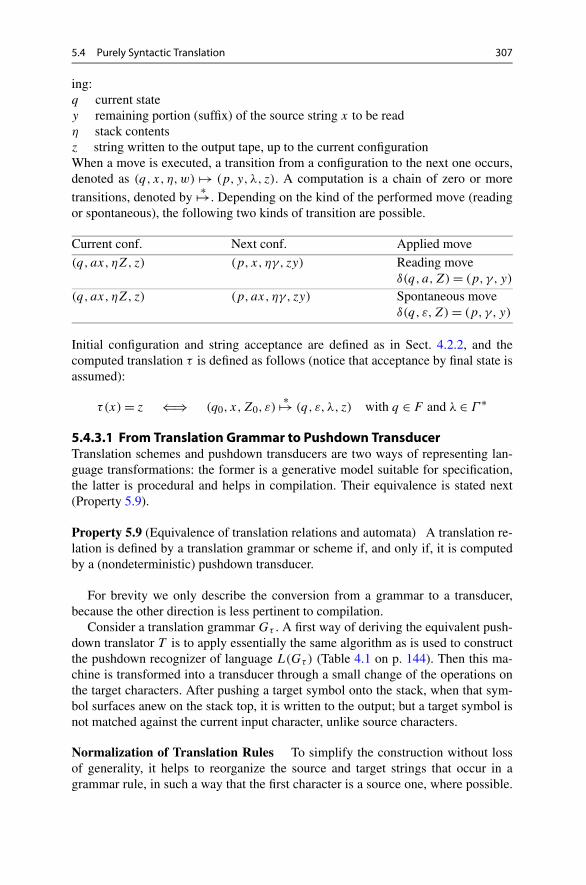
5.4 Purely Syntactic Translation 307
ing:q current statey remaining portion (suffix) of the source string x to be readη stack contentsz string written to the output tape, up to the current configurationWhen a move is executed, a transition from a configuration to the next one occurs,denoted as (q, x, η,w) �→ (p, y,λ, z). A computation is a chain of zero or more
transitions, denoted by∗�→. Depending on the kind of the performed move (reading
or spontaneous), the following two kinds of transition are possible.
Current conf. Next conf. Applied move
(q, ax, ηZ, z) (p, x, ηγ, zy) Reading moveδ(q, a,Z)= (p, γ, y)
(q, ax, ηZ, z) (p, ax, ηγ, zy) Spontaneous moveδ(q, ε,Z)= (p, γ, y)
Initial configuration and string acceptance are defined as in Sect. 4.2.2, and thecomputed translation τ is defined as follows (notice that acceptance by final state isassumed):
τ(x)= z ⇐⇒ (q0, x,Z0, ε)∗�→ (q, ε, λ, z) with q ∈ F and λ ∈ Γ ∗
5.4.3.1 From Translation Grammar to Pushdown TransducerTranslation schemes and pushdown transducers are two ways of representing lan-guage transformations: the former is a generative model suitable for specification,the latter is procedural and helps in compilation. Their equivalence is stated next(Property 5.9).
Property 5.9 (Equivalence of translation relations and automata) A translation re-lation is defined by a translation grammar or scheme if, and only if, it is computedby a (nondeterministic) pushdown transducer.
For brevity we only describe the conversion from a grammar to a transducer,because the other direction is less pertinent to compilation.
Consider a translation grammar Gτ . A first way of deriving the equivalent push-down translator T is to apply essentially the same algorithm as is used to constructthe pushdown recognizer of language L(Gτ ) (Table 4.1 on p. 144). Then this ma-chine is transformed into a transducer through a small change of the operations onthe target characters. After pushing a target symbol onto the stack, when that sym-bol surfaces anew on the stack top, it is written to the output; but a target symbol isnot matched against the current input character, unlike source characters.
Normalization of Translation Rules To simplify the construction without lossof generality, it helps to reorganize the source and target strings that occur in agrammar rule, in such a way that the first character is a source one, where possible.

308 5 Translation Semantics and Static Analysis
More precisely, we make the following hypotheses on the form of the source/targetpairs u
vthat occur in the rules,8 where u ∈Σ∗ and v ∈Δ∗:
1. For any pair uv
we have |u| ≤ 1, i.e., the source u is a single character a ∈Σ orthe empty string. Clearly this is not a limitation because if the pair a1a2
voccurs
in a rule, it can be replaced by the pairs a1v
a2ε
without affecting the translation.2. No rule may contain the following substrings:
ε
v1
a
v2or
ε
v1
ε
v2where v1, v2 ∈Δ∗
Should such combinations be present in a rule, then they can be, respectively,replaced by the equivalent pairs a
v1v2or ε
v1v2.
We are ready to describe the correspondence between the rules of grammar Gτ =(V ,Σ,Δ,P,S) and the moves of the so-called predictive transducers.
Algorithm 5.10 (Construction of the (nondeterministic) predictive pushdown trans-ducer) Let C be the set of the pairs of type ε
vwith v ∈ Δ+, and of type b
wwith
b ∈ Σ and w ∈ Δ∗, occurring in some grammar rule. The transducer moves areconstructed as described in Table 5.1. Rows 1, 2, 3, 4, and 5 apply when the stacktop is a nonterminal symbol. In case 2 the right part begins with a source terminaland the move is conditioned by its presence in the input. Rows 1, 3, 4 and 5 giverise to spontaneous moves, which do not shift the reading head. Rows 6 and 7 applywhen a pair surfaces on top of stack. If the pair contains a source character (row 7),it must coincide with the current input character; if it contains a target string (rows 6and 7), the latter is output.
Initially the stack contains the axiom S, and the reading head is positioned onthe first character of the source string. At each step the automaton (nondetermin-istically) chooses an applicable rule and executes the corresponding move. Finallyrow 8 accepts the string if the stack is empty and the current character marks theend of text.
Notice the automaton does not make use of states, i.e., the stack is the only mem-ory used. As we did for recognizers, we will later enrich the machine with states inorder to obtain a more efficient deterministic algorithm.
The next example (Example 5.11) shows a simple translation a computed by anondeterministic pushdown transducer.
Example 5.11 (Nondeterministic pushdown transducer) Consider the source lan-guage L,
L= {a∗ambm |m > 0
}
8For completeness we mention that sometimes in the scientific literature on formal languages, thesource/target fractions u
vin the grammar rules are denoted as u{v}, e.g., X→ αu{v}β instead of
X→ α uvβ; but such a notation is not used in this book.

5.4 Purely Syntactic Translation 309
Table 5.1 Correspondence between translation grammar rules and pushdown translator moves(if n= 0 then the sequence A1 . . .An is absent)
# Rule Move Comment
1 A→ εvBA1 . . .An
n≥ 0v ∈Δ+ B ∈ V
Ai ∈ (C ∪ V )
If top=A then write (v);pop; push (An . . .A1B)
Emit the target string v andpush on stack the predictionstring BA1 . . .An
2 A→ bw
A1 . . .An
n≥ 0b ∈Σ w ∈Δ∗Ai ∈ (C ∪ V )
If cc= b ∧ top=A thenwrite (w); pop; push(An . . .A1); advance thereading head
Char b was the next expectedand has been read; emit thetarget string w; push theprediction string A1 . . .An
3 A→ BA1 . . .An
n≥ 0 B ∈ V
Ai ∈ (C ∪ V )
If top=A then pop; push(An . . .A1B)
Push the prediction stringBA1 . . .An
4 A→ εv
v ∈Δ+ If top=A then write (v); pop Emit the target string v
5 A→ ε If top=A then pop
6 For every pair εv∈ C If top= ε
vthen write (v); pop The past prediction ε
vis now
completed by writing v
7 For every pair bw∈ C If cc= b ∧ top= b
wthen
write (w); pop; advance thereading head
The past prediction bw
is nowcompleted by reading b andwriting w
8 – If cc=� ∧ stack is emptythen accept; halt
The source string has beenentirely scanned and no goalis present in the stack
Table 5.2 Moves of a nondeterministic pushdown transducer
# Rule Move
1 S→ aεS ε
cIf cc= a ∧ top= S then pop; push ( ε
cS); advance the reading head
2 S→A If top= S then pop; push (A)
3 A→ adAb
εIf cc= a ∧ top=A then pop; write (d); push ( b
εA); advance the reading head
4 A→ ad
bε
If cc= a ∧ top=A then pop; write (d); push ( bε
); advance the reading head
5 – If top= εc
then pop; write (c)
6 – If cc= b ∧ top= bε
then pop; advance the reading head
7 – If cc=� ∧ stack is empty then accept; halt
and define the following translation τ on L:
τ(akambm
)= dmck where k ≥ 0 and m > 0
The translation τ first changes letter b to letter d , then it transcribes to letter c anyletter a that exceeds the number of b’s. The moves of the transducer are listed inTable 5.2 next to the corresponding rules of the translation grammar.

310 5 Translation Semantics and Static Analysis
The choice of moves 1 or 2 in Table 5.2 is not deterministic, and so is the choiceof moves 3 or 4. Move 5 outputs a target character that had been pushed by move 1.Move 6 just scans an input character and move 7 is for acceptance. The subjacentpushdown automaton is not deterministic.
The following example (Example 5.12) shows that not all context-free transla-tions can be computed by a pushdown transducer of the deterministic kind. A similarproperty, holding for regular translations and finite transducers, will be illustrated inSect. 5.5.2.
Example 5.12 (Context-free nondeterministic translation) The translation func-tion τ ,
τ(u)= uRu where u ∈ {a, b}∗maps every string into a reversed copy followed by the same string. Function τ iseasily specified by the following scheme:
translation gram. Gτ source gram. G1 target gram. G2S→ ε
aS a
aS→ Sa S→ aSa
S→ εbS b
bS→ Sb S→ bSb
S→ εε
S→ ε S→ ε
The translation cannot be deterministically computed by a pushdown machine. Thereason is that such a machine should output the mirror copy of the input before thedirect copy of the input.9 The only way to reverse a string by means of a pushdowndevice is to store the string in the stack and to output it in the order it is popped.But popping destroys the stored string and makes it unavailable for copying to theoutput at a later moment.
Nondeterministic algorithms are used infrequently in compilation. In the nextsection we develop translator construction methods suitable for use with thewidespread deterministic parsers.
5.4.4 Syntax Analysis with Online Translation
Given a context-free translation scheme, the previous construction produces a push-down transducer that is often nondeterministic and generally unpractical to be usedin a compiler. To construct an efficient and well-engineered translator, it is conve-nient to resume from the point reached in Chap. 4 with the construction of determin-istic parsers, and to enrich them with output actions. Given a context-free translationgrammar or scheme, we make the assumption that the source grammar is suitable
9For a proof see [1, 2].

5.4 Purely Syntactic Translation 311
for deterministic parsing. To compute the image of a string, the parser emits thecorresponding translation as it completes a syntactic subtree.
We know that bottom-up and top-down parsers differ in the construction orderof the syntax tree. A question to be investigated is how the order interferes withthe possibility of correctly producing the target image. The main result will be thatthe top-down parsing order is fully compatible, whereas the bottom-up order placessome restrictions on the translation.
5.4.5 Top-Down Deterministic Translation by Recursive Procedures
We recall there are two techniques for building efficient top-down deterministicparsers: as pushdown automata or as recursive descent procedures. Both techniquescan be simply extended toward the construction of translators. We next focus on theapproach based on the recursive descent translator.
In order to streamline the design of syntactic translation algorithms for grammarsextended with regular expressions, it is convenient to represent the source grammarG1 by means of a recursive network of finite machines, as we did in Chap. 4. Assum-ing the source grammar is ELL(k) with k = 1 or larger, we recall the organizationof the recursive descent parser. For each nonterminal symbol, a procedure has thetask of recognizing the substrings derived from it. The procedure body blueprint isidentical to the state-transition graph of the corresponding machine in the networkthat represents the grammar. For computing the translation, we simply insert a writetransition in the machine and a corresponding write instruction in the procedurebody.
An example (Example 5.13) should be enough to explain such a straightforwardmodification of a recursive descent parser.
Example 5.13 (Recursive descent translator from infix to postfix) The source lan-guage consists of arithmetic (infix) expressions with two levels of operators andwith parentheses, and the translation converts such expressions to the postfix polishnotation as exemplified by
v× (v + v) ⇒ vvv add mult
The source language is defined by the extended BNF grammar G1 (axiom E):
G1
⎧⎪⎪⎨
⎪⎪⎩
E→ T (+T | −T )∗
T → F(×F | ÷F)∗
F → v | ‘(’E‘)’
Figure 5.3 (left) represents the machine for nonterminal E: the machine meets theELL(1) condition and the relevant guide sets are written in braces.
The recursive descent procedure for nonterminal E is immediately derived andshown in Fig. 5.4 (left); we recall that function next returns the current input token;and for simplicity, the check of the error cases is omitted.

312 5 Translation Semantics and Static Analysis
Fig. 5.3 Machine ME that represents the EBNF axiomatic rule E→ T (+T | −T )∗ of the sourcegrammar in Example 5.13 (left), and the same machine ME augmented with write actions andstates where necessary (right)
Fig. 5.4 Recursive descent syntactic procedures for nonterminal E, without (left) and with (right)write instructions, which are framed
Notice that the procedure could be refined so that at loop exit it checks if thecurrent character is in the guide set {‘)’,�}, and thus anticipates error detection.Similar procedures for nonterminals T and F can be derived.

5.4 Purely Syntactic Translation 313
In Fig. 5.3 (right) we add to the machine for nonterminal E, a few suitable statesand transitions that encode the write actions to output the operators in postfix posi-tion. From this augmented machine the next recursive procedure with write instruc-tions is easily derived and is also shown in Fig. 5.4 (right). Similarly the proceduresfor nonterminals T and F can be augmented to write the other target symbols, butfor brevity here they are omitted.
The machines and procedures that compute the complete translation correspondto the following extended BNF translation grammar Gτ (axiom E):
Gτ
⎧⎪⎪⎪⎪⎪⎪⎪⎪⎨
⎪⎪⎪⎪⎪⎪⎪⎪⎩
E→ T
(+ε
Tε
add| −
εT
ε
sub
)∗
T → F
(×ε
Fε
mult| ÷
εF
ε
div
)∗
F → v
v| ‘(’
εE
‘)’
ε
where the source and target alphabets Σ and Δ are as follows:
Σ = {‘+ ’, ‘− ’, ‘× ’, ‘÷ ’, v, ‘(’, ‘)’
}
Δ= {add, sub,mult,div, v}and the round parentheses do not appear translated in the target alphabet Δ, sincethey are unnecessary in the postfix polish form.
In the grammar rules, the elements of the target string, i.e., the characters ofalphabet Δ, appear in the denominators of the fractions.
Notice that we have not formally defined the concept of extended BNF translationgrammar, but we rely upon the reader’s intuition for it.
5.4.6 Bottom-Up Deterministic Translation
Consider again a context-free translation scheme and assume the source grammar issuitable for bottom-up deterministic parsing, by the ELR(1) condition, p. 185 (ac-tually by the LR(1) condition since this time the grammar is not extended). Unlikethe top-down case, it is not always possible to extend the parser with the write ac-tions that compute the translation, without jeopardizing determinism. Intuitively theimpediment is simple to understand. We know the parser works by shifts and reduc-tions. A shift pushes on stack a macro-state of the pilot finite automaton, i.e., a setof states of some machines. Of course, when a shift is performed the parser does notknow which rule will be used in the future for a reduction, and conservatively keepsall the candidates open. Imagine two distinct machine states occur as candidates inthe current macro-state, and make the likely hypothesis that different output actionsare associated with them. Then when the parser shifts, the translator should perform

314 5 Translation Semantics and Static Analysis
Fig. 5.5 Machine net of the BNF translation grammar of Example 5.14
two different and contradictory write actions, which is impossible for a determinis-tic transducer. This reasoning explains the impediment to emit the output during ashift move of the translator.
On the other hand, when a reduction applies, exactly one source grammar rule hasbeen recognized, i.e., the final state of the corresponding machine has been entered.Since the mapping between source and target rules in the translation scheme is atotal function, a reduction identifies exactly one target rule and can safely output theassociated target string.
We present a case (Example 5.14) where the translation grammar (not extended)has rules that contain output symbols at the rule end, so that the pilot automaton canbe enriched with write actions in the reduction m-states.
Example 5.14 (Translation of expressions to postfix notation) The BNF translationgrammar below, which specifies certain formulas that use two infix signs10 to betranslated to postfix operators, is represented as a machine network (axiom E) inFig. 5.5:
E→E+ε
Tε
add| T T → T
×a
ε
ε
a mult| a
ε
ε
a
Notice that care has been taken to position all the target characters as suffix at therule end (some rule may have none at all). The ELR(1) pilot graph can be easilyupgraded for translation by inserting the output actions in the reductions, as shownin Fig. 5.6. Of course, the parser will execute a write action when it performs theassociated reduction.
On the contrary, in the next case (Example 5.15) the presence of write actions onshift moves makes the translation incorrect.
10More precisely, two-level infix arithmetic expressions of type sum-of-product, with variables a
but without parentheses.

5.4 Purely Syntactic Translation 315
Fig. 5.6 Pilot of the translator of Example 5.14 with write actions in the reduction m-states. Theclosure of m-states I0 and I2 is shown step-by-step
Example 5.15 (Translation of parenthesized expressions) The BNF grammar Gτ
below specifies a translation of a language similar to the Dyck one, where every pairof matching “parentheses” a, c is translated to the pair b, e, but with one exception:no translation is performed for the innermost pair of symbols a, c, which is justerased. We have
Gτ : S→ a
bS
c
eS | a
ε
c
ε
τ(aaccac) = be
τ(ac) = ε
Figure 5.7 shows the machine net of the source grammar G1 of Gτ . The final statesare separate in order to identify which alternative rule has been analyzed, as eachrule has a distinct output.
In Fig. 5.7 an attempt is made to obtain an ELR(1) pilot with write actions; forbrevity the construction is partial. Yet the attempt aborts almost immediately: eitherthe write actions are premature, as in the m-state I1 where it is unknown whetherthe letter a that has just been shifted, belongs to an innermost pair or not; or theyare too late, as in the m-state I5.
5.4.6.1 Postfix Normal FormIn practice, when specifying a context-free translation intended for bottom-up pars-ing, it is necessary to put the translation grammar into a form (Definition 5.16) thatconfines write actions within reduction moves.

316 5 Translation Semantics and Static Analysis
Fig. 5.7 Machine net and tentative partial pilot with write actions (Example 5.15)
Definition 5.16 (Postfix translation grammar) A translation grammar or scheme isin the postfix normal form if every target grammar rule has the form A→ γw, whereγ ∈ V ∗ and w ∈Δ∗.
Differently stated, no target string may occur as an inner substring of a rule, butonly as a suffix. Example 5.2 (p. 299) is in the postfix form, while Examples 5.12(p. 310) and 5.15 (p. 315) are not.
One may wonder what loss, if any, is caused by the postfix condition. From thestandpoint of the family of translation relations that can be specified, it is easy toshow that postfix grammars have the same expressivity as the general context-freetranslation grammars do, sometimes at the cost of some obscurity. In Algorithm 5.17we explain the transformation of a generic translation grammar into postfix normalform.
Algorithm 5.17 (Converting a translation grammar to postfix form) Consider inturn each rule A→ α of the given translation grammar. If the rule violates the post-fix condition, find the longest target string v ∈Δ+ that occurs in the rightmost po-sition in α, and transcribe the rule as
A→ γε
vη

5.4 Purely Syntactic Translation 317
where γ is any string, and η is a nonempty string devoid of target characters. Replacethis rule with the next ones:
A→ γ Yη Y → ε
v
where symbol Y is a new nonterminal. The second rule complies with the postfixcondition; if the first rule does not (yet), find anew the rightmost target string withinγ and repeat the transformation. Eventually all the target elements that occur inthe middle of a rule, will have been moved to suffix positions, and so the resultinggrammar is in the postfix normal form.
The next example (Example 5.18) illustrates the transformation to postfix, and itshould convince the reader that the original and transformed grammars define thesame translation.
Example 5.18 (Grammar transformation to postfix normal form) Examining thetranslation grammar Gτ : S→ a
bS c
eS | ac of the previous example (Example 5.15),
we notice that in the target grammar G2 the pointed letters of the axiomatic rule
↓ ↓S → b S e S
violate the postfix form. We apply the normalization algorithm (Algorithm 5.17)and we introduce two new nonterminals: A to represent the left parenthesis b; andB for the right one e; as follows:
Gτ : S→ASCS | ac A→ a
bC→ c
e
G2postfix: S→ASCS | ε A→ b C→ e
It is easy to check that the target grammar G2postfix defines the same translation asthe original target grammar G2 does. The machine net in Fig. 5.8 represents thetranslation grammar normalized to postfix form. Since the grammar is BNF andthe two alternative rules of the axiom S do not have any output, the two recognizingpaths of the axiomatic machine MS may end at the same one final state 4S . The pilotof the postfix grammar, partially shown in Fig. 5.8, writes the translation output onlyat reduction.
Now the write actions in the pilot automaton are, respectively, associated with thereduction states 1A and 1C of nonterminals A and C, which correspond to parenthe-sis pairs that are not innermost. Also notice that there is not any write action in them-state I5, which includes the final state 4S and hence specifies a reduction to non-terminal S, because the symbol c just shifted to reach m-state I5, certainly belongsto an innermost pair.
We summarize the previous discussion on bottom-up translators with a sufficientcondition (Property 5.19) for being deterministic.

318 5 Translation Semantics and Static Analysis
Fig. 5.8 Translation grammar Gτ in the postfix form, machine net with output, and partial pilotwith write actions (Example 5.18)
Property 5.19 (Determinism of bottom-up transducers) A translation defined bya BNF (not extended) translation grammar in the postfix normal form, such thatthe source grammar satisfies condition LR(k) with k ≥ 1, can be computed by adeterministic bottom-up parser, which only writes on the output at reduction moves.
In essence the postfix form allows the parser to defer its write actions until itreaches a state where the action is uniquely identified.
This method has some inconveniences. The introduction of new nonterminalsymbols, such as A and B in Example 5.18, makes the new grammar less read-able. Another nuisance may come from rule normalization, when empty rules suchas Y → ε are added to the source grammar. Empty rules tend to increase the lengthk of the look-ahead needed for parsing; and in some cases the LR(k) property maybe lost, as the next example (Example 5.20) shows.

5.4 Purely Syntactic Translation 319
Fig. 5.9 Machine net with output of a BNF translation grammar normalized in the postfix form(Example 5.20)
Example 5.20 (Loss of LR(1) property caused by normalization) The translationof an infix expression11 to prefix form is specified by the grammar Gτ below. Bylooking at the target grammar G2, we ascertain that the first rule of Gτ is not in thepostfix form.
Gτ original G1 G2
E→ εaddE+a
aE→E + a E→ add Ea
E→ aa
E→ a E→ a
Here is the postfix form G′τ of grammar Gτ , obtained by applying the normalizationalgorithm (Algorithm 5.17):
G′τ postfix G′1 G′2E→ YE+a
εεa
E→ YE + a E→ YEa
E→ aε
εa
E→ a E→ a
Y → εadd Y → ε Y → add
The machine net of the postfix version G′τ is in Fig. 5.9. It is easy to check thatgrammar G′τ defines the same translation as the original one Gτ . However, whilethe original source grammar G1 satisfies the LR(1) condition, the new rule Y → ε
of the postfix source grammar G′1, i.e., the fact that state 0Y is both initial and final,causes an LR(1) shift–reduce conflict in the macro-states I0, I1 and I6 of the pilotshown in Fig. 5.10.
Fortunately, in many practical situations grammar normalization to postfix formdoes not hinder deterministic parsing.
5.4.6.2 Syntax Tree as TranslationA common utilization of syntactic translation (both top-down and bottom-up) is toconstruct the syntax tree of the source text. Programs usually represent a tree as alinked data structure. To construct such a representation we need semantic actions,to be discussed in later sections. Here, instead of producing a linked list, whichwould be impossible to do with a purely syntactic translation, we are content with
11The expression is simply a summation a + a + · · · + a, of one or more terms.
320 5 Translation Semantics and Static Analysis
Fig. 5.10 Pilot LR(1) of the trans. grammar of Fig. 5.9, with shift–reduce conflicts in the m-statesI0, I1 and I6 (a few m-states have write actions)
outputting the sequence of labels of the source rules, in the order they occur in thetree derivation.
Given a source grammar with rules labeled for reference, the next syntactic trans-lation scheme produces the label sequence of a derivation:
Label Original translation rule Modified rule
ri A→ α A→ α εri
The image produced by the above translation is exactly the sequence of rule labelsused by the rightmost derivation. Since by hypothesis the source grammar is LR(1)
and the scheme is postfix, the parser enriched with write actions easily computesthis translation.
5.4.7 Comparisons
We recapitulate the main considerations about upgrading parsers to translators. Themain argument in favor of the top-down methods is that they do not suffer anylimitation as they allow the implementation of any syntactic translation scheme,provided of course that the source grammar meets the suitable condition for parsing.Moreover, a recursive descent translator can be easily constructed by hand, and theresulting program is easy to understand and maintain.
On the other hand, for the bottom-up methods the limitation imposed by thepostfix normal form of the translation grammar may be compensated by the supe-riority of the LR(k) grammars over the LL(k) ones, for the definition of the source

5.5 Regular Translations 321
language. In conclusion, neither method, top-down versus bottom-up, is entirely su-perior to the other one.
5.5 Regular Translations
Just like context-free grammars have as a special case the right-linear grammars,which in turn have regular expressions and finite state automata as their naturalcounterpart, in a similar way translation grammars include as a special case theright-linear translation grammars, which define translations that can be character-ized in terms of regular translation expressions and finite state transducers.
Consider for instance the following translation τ :
{a2n τ�→ b2n n≥ 0
a2n+1 τ�→ c2n+1 n≥ 0
Translation τ can be specified by the following right-linear translation grammar Gτ
(axiom A0):
Gτ
⎧⎪⎪⎪⎪⎪⎪⎪⎪⎪⎪⎪⎪⎪⎪⎨
⎪⎪⎪⎪⎪⎪⎪⎪⎪⎪⎪⎪⎪⎪⎩
A0 → a
cA1 | a
c| a
bA3 | ε
A1 → a
cA2 | ε
A2 → a
cA1
A3 → a
bA4
A4 → a
bA3 | ε
The well-known equivalence between right-linear grammars and finite state au-tomata can be extended by defining regular translation expressions.
Regular expressions can be modified in order to specify a translation relation:the arguments of the expression are pairs of source/target strings, instead of beingcharacters as customary. Then a sentence generated by such a regular expressionmodel is a sequence of pairs. By separating the source component of each pair fromthe target one, we obtain two strings, which can be interpreted as a pair belongingto the translation relation. In this manner, such a regular expression model defines atranslation relation to be called regular or rational.
In this way the above translation is defined by the following regular translationexpression eτ :
eτ =(
a2
b2
)∗∪ a
c
(a2
c2
)∗

322 5 Translation Semantics and Static Analysis
The string of fractions
a
c·(
a2
c2
)2
= a
c· a
2
c2· a
2
c2= a5
c5∈ L(eτ )
then corresponds to the pair (a5, c5) in the translation relation ρτ defined by theexpression eτ .
Example 5.21 (Consistent transliteration of an operator) The source text is a listof numbers separated by a division sign “/”. The translation may replace the signby either one of the signs “:” or “÷”, but it must consistently choose the same signthroughout. For simplicity we assume the numbers to be unary. The source/targetalphabets are as follows:
Σ = {1, ‘/’
}Δ= {
1, ‘÷ ’, ‘ : ’}
The source strings have the form c(/c)∗, where c stands for any unary number de-noted by 1+. Two valid translations are the following:
(3/5/2,3 : 5 : 2) (3/5/2,3÷ 5÷ 2)
On the contrary, transliteration (3/5/2,3 : 5 ÷ 2) is wrong, because the divisionsigns are differently transliterated.
Notice this translation cannot be expressed by a homomorphism, as the imageof the division sign is not single valued. Incidentally the inverse translation is analphabetic homomorphism. The translation is defined by the r.e.
(1,1)+((
‘/’, ‘ : ’)(1,1)+)∗ ∪ (1,1)+
((‘/’, ‘÷ ’
)(1,1)+
)∗
or using the more readable fractional notation, by the following r.e.:
(1
1
)+(/
:(
1
1
)+)∗∪
(1
1
)+(/
÷(
1
1
)+)∗
The terms produced by applying a derivation are strings of fractions, i.e., stringpairs. Consider the following derived string:
(1
1
)1(/
÷(
1
1
)2)1
= 1
1
/
÷1
1
1
1
project it on the top and bottom components, and thus obtain the pair of source/targetstrings (1/11,1÷ 11).
We can summarize the previous discussion and examples (Example 5.21) aboutregular translations, by the next definition (Definition 5.22).

5.5 Regular Translations 323
Definition 5.22 (Regular (or rational) translation) A regular or rational translationexpression, for short r.t.e., is a regular expression with union, concatenation, and star(and cross) operators that has as arguments some string pairs (u, v), also written asuv
, where terms u and v are possibly empty strings, respectively, on the source andon the target alphabet.
Let C ⊂Σ∗ ×Δ∗ be the set of the pairs (u, v) occurring in the expression. Theregular or rational translation relation defined by the r.t.e. eτ , consists of the pairs(x, y) of source/target strings such that:• there exists a string z ∈ C∗ in the regular set defined by the r.t.e. eτ
• strings x and y are the projections of string z on the first and second component,respectively
It is straightforward to see that the set of source strings defined by an r.t.e. (aswell as the set of target strings) is a regular language. But notice that not everytranslation relation that has two regular sets as its source and target languages, canbe defined with an r.t.e.: an example to be discussed later is the relation that mapseach string to its mirror string.
5.5.1 Two-Input Automaton
Since the set C of pairs occurring in an r.t.e. can be viewed as a new terminal al-phabet, the regular language over C can be recognized by a finite automaton, asillustrated in the following example (Example 5.23).
Example 5.23 (Consistent transliteration of an operator (Example 5.21) contin-ued) The recognizer of the regular translation relation is shown in Fig. 5.11.
This automaton can be viewed as a machine with two read-only input tapes, inshort a 2I -machine, each one with an independent reading head, respectively con-taining the source string x and the target string y. Initially the heads are positionedon the first characters and the machine is in the start state. The machine performsas specified by the state-transition graph: e.g., in state q1, on reading a slash “/”from the source tape and a sign “÷” from the target tape, the automaton moves tostate q4 and shifts both heads by one position. If the machine reaches a final stateand both tapes have been entirely scanned, the pair (x, y) belongs to the translationrelation.12
This automaton can check that two strings, such as
(11‘/’1,1‘÷ ’1
)≡ 11/1
1÷ 1
12This model is known as a Rabin and Scott machine. For greater generality such a machine may beequipped with more than two tapes, in order to define a relation between more than two languages.

324 5 Translation Semantics and Static Analysis
Fig. 5.11 2I -automaton ofthe r.t.e. of Examples 5.21and 5.23
do not correspond in the translation, because the following computation:
q0
11−→ q1
admits no continuation with the next pair, i.e., fraction 1÷ .
It is sometimes convenient to assume each tape is delimited on the right by areserved character marking the tape end.
At a first glance, regular translation expressions and two-input machines mayseem to be the wrong idealizations for modeling a compiler, because in compila-tion the target string is not given, but must be computed by the translator. Yet thisconceptualization is valuable for specifying some simple translations, and also as arigorous method for studying translation functions.
5.5.1.1 Forms of Two-Input AutomataWhen designing a two-input recognizer, we can assume without loss of generalitythat each move reads exactly one character or nothing from the source tape, whileit may read one string of any length ≥0 (so including null) from the target tape; thefollowing definition (Definition 5.24) formalizes the concept.
Definition 5.24 (Two-input automaton or 2I -automaton) A finite automaton withtwo inputs or 2I -automaton is defined as a usual finite automaton (Sect. 3.5.2,p. 107) by a set of states Q, an initial state q0 and a set F ⊆ Q of final states.The transition function δ is as follows:13
δ : Q× (Σ ∪ {ε})×Δ∗ → ℘(Q)
The 2I -automaton has a move that can behave as follows:• on the first tape: if we have q ′ ∈ δ(q, a, v), the move reads character a ∈Σ ; and
if it holds or q ′ ∈ δ(q, ε, v), the move does not read anything• on the second tape: the move reads string v ∈Δ∗, possibly null• and the move enters the next state q ′The recognition condition is that a computation reaches a final state.
13Remember that symbol ℘ is the powerset, i.e., the set of all the subsets.

5.5 Regular Translations 325
Imagine now to project the arc labels of a 2I -automaton on the first component.The resulting automaton has just one input tape with symbols from the source al-phabet Σ , and is termed the input automaton subjacent to the original machine; itrecognizes the source language.
Sometimes another normal form of a 2I -automaton is used, characterized by thefact that each move reads exactly one character either from the source tape or fromthe target tape, but not from both. More precisely the arc labels are of the followingtwo types:
label aε
with a ∈Σ , i.e., read one character from source, orlabel ε
bwith b ∈Δ, i.e., read one character from target
This means that a machine in the normal form shifts only one head per move, andof one position at a time. It is to be expected that such a normalization will oftenincrease the number of states because a non-normalized move, like the followingone:
is replaced by a cascade of normalized moves, like
where symbol 〈q, r〉 is a new state.14
On the other hand, in order to make the model more expressive and concise,it is convenient to allow regular translation expressions as arc labels. As for finiteautomata, this generalization does not change the computational power, but it helpsin hiding the details of complicated examples.
Finally a short remark on notation: in an arc label we usually drop a componentwhen it is the empty string. Thus we may write
a∗bd| a∗c
e
in place of the following:
a∗
ε
b
d| a∗
ε
c
e
This expression says that a sequence of a’s, if followed by b, is translated to d ; andif it is followed by c, it is translated to e.
14According to Definition 5.24, a move of a 2I -automaton may read nothing from both tapes, i.e.,the arc may be labeled by ε
ε; such strictly null moves can always be eliminated, too; just think
that they are analogous to the spontaneous moves of recognizer automata, and that they can beeliminated in a similar way; here we do not go into such subtle details.

326 5 Translation Semantics and Static Analysis
5.5.1.2 Equivalence of ModelsIn accordance with the well-known equivalence of regular expressions and finitestate automata, we state a similar property for translations (Property 5.25).
Property 5.25 (Equivalence of translation models) The families of translationsdefined by regular translation expressions and by finite (nondeterministic) 2I -automata coincide.
We recall that an r.t.e. defines a regular language R over an alphabet that consistsof a finite set of pairs of strings (u, v) ≡ u
v, where we have u ∈ Σ∗ and v ∈ Δ∗.
By separately extracting from each string in R the source and target elements, weobtain a crisp formulation of the relation between source and target languages.
Property 5.26 (Nivat theorem) The following four conditions are equivalent:1. The translation relation ρτ is defined by a right-linear (or left-linear) translation
grammar Gτ .2. The translation relation ρτ is defined by a 2I -automaton.3. The translation relation ρτ ⊆Σ∗ ×Δ∗ is regular.4. There exist an alphabet Ω , a regular language R over Ω , and two alphabetic
homomorphisms h1 : Ω →Σ ∪ {ε} and h2 : Ω →Δ∪ {ε}, such that
ρτ ={(
h1(z), h2(z)) | z ∈R
}
Example 5.27 (Division by two) The image string is the halved source string. Thetranslation relation {(a2n, an) | n≥ 1} is defined by the following r.t.e.:
(aa
a
)+
An equivalent 2I -automaton A is shown here:
To apply the Nivat theorem (clause (4) of Property 5.26), we derive from automatonA the following r.t.e.:
(a
ε
a
a
)+
and we rename for clarity the pairs
a
ε= c
a
a= d
Next consider the alphabet Ω = {c, d}. The r.t.e. defines the regular language R =(cd)+, obtained replacing each fraction with a character of the new alphabet. The

5.5 Regular Translations 327
following alphabetic homomorphisms h1 and h2:
Ω h1 h2
c a ε
d a a
produce the intended translation relation. Thus for z = cdcd ∈ R we have h1(z)=aaaa and h2(z)= aa.
To illustrate Nivat theorem (clause (1) of Property 5.26), we apply the well-known equivalence of finite automata and right-linear grammars (p. 103), to obtainthe following equivalent right-linear translation grammar:
S→ a
εQ1 Q1 → a
aQ2 Q2 → a
εQ1 | ε
Each grammar rule corresponds to a move of the 2I -automaton. Rule Q2 → ε is ashort notation for Q2 → ε
ε.
We recall from Sect. 5.4 that the notation based on a translation grammar insteadof a 2I -automaton or a r.t.e. has to be used for the syntactic translations, whichhave a context-free grammar as their support, because such translations require apushdown stack and cannot be described by a simple finite automaton.
Several properties of regular languages, but not all their properties, have an analo-gous formulation for regular translation relations.15 Thus the union of regular trans-lation relations still yields a regular translation relation, but it is not always so fortheir intersection and set difference. For those relations that remain regular, it is pos-sible to formulate a pumping lemma similar to the one for the regular languages onp. 73.
Non-regular Translation of Regular Languages As already noticed, not everytranslation relation with two regular languages as source and target is necessarilyregular, i.e., it can be defined through a 2I -finite automaton. Consider for instancethe following languages L1, L2 and translation τ :
L1 = (a | b)∗ L2 = (a | b)∗ τ(x)= xR with x ∈ L1
This translation τ cannot be defined by a 2I -automaton, as a finite set of states doesnot suffice to check that the string on the second tape is the reversal of the one onthe first tape.
5.5.2 Translation Functions and Finite Transducers
We leave the static perspective of a translation as a relation between two strings andwe focus instead on the translation process, where an automaton is viewed as analgorithmic implementation of a translation function. We introduce the finite trans-
15See the books [5, 12].

328 5 Translation Semantics and Static Analysis
ducer or IO-automaton. This machine reads the source string from the input tapeand writes the image on the output tape. We shall mostly study single-valued trans-lations and especially those that are computed by deterministic machines, but weintroduce the model by a nondeterministic example (Example 5.28).
Example 5.28 (Nondeterministic translation) It is required to translate a string an
to the image bn if n is even, or to the image cn if n is odd. The translation relation ρτ ,
ρτ ={(
a2n, b2n) | n≥ 0
}∪ {(a2n+1, c2n+1) | n≥ 0
}
defines the following translation function τ :
τ(an
)={
bn for n≥ 0 even (n= 0 is even)
cn for n≥ 1 odd
The r.t.e. eτ is the following:
eτ =(
a2
b2
)∗∪ a
c
(a2
c2
)∗
A simple deterministic two-input automaton recognizes this relation ρτ :
To check for determinism, observe that only the initial state q0 has two outgoingarcs, but that the target labels of such arcs are different.16 Therefore the 2I -machinecan deterministically decide if two strings memorized on the two tapes, such asaaaabbbb
, correspond to each other in the translation relation.Although the transducer or IO-automaton has the same state-transition graph as
the 2I -automaton, the meaning of an arc, e.g., q0
ab−→ q1, is entirely different: in
the state q0 it reads character a from the input, writes character b to the output and
enters state q1. We observe that arc q0
ac−→ q3 instructs the machine to perform a
different action, while reading the same character a in the same state q0. In otherwords, the choice between the two moves is not deterministic. As a consequence,two computations are possible for the input string aa:
q0 → q1 → q2 q0 → q3 → q4
but only the former succeeds in reaching a final state, namely q2, and thus only itsoutput is considered: τ(aa)= bb. Notice that the transducer nondeterminism showsup in the input automaton subjacent to the transducer, which is nondeterministic.
16If the 2I -automaton has some moves that do not read from either tape, the determinism conditionhas to be formulated more carefully; e.g., see [12].

5.5 Regular Translations 329
Moreover, it should be intuitively clear that the requested translation cannot becomputed by a deterministic finite transducer, because the choice of the character toemit can only be made when the input tape has been entirely scanned; but then it istoo late to decide how many characters have to be output.
To sum up the findings of this example (Example 5.28), there are single-valuedregular translations that cannot be computed by a deterministic finite IO-automaton.This is a striking difference with respect to the well-known equivalence of the de-terministic and nondeterministic models of finite automata.
5.5.2.1 Sequential TransducersIn some applications it is necessary to efficiently compute the translation in realtime, because the translator must produce the output while scanning the input. Fi-nally, when the input is finished, the automaton may append to the output a finitepiece of text that depends on the final state reached. This is the behavior of a type ofdeterministic machine called a sequential transducer.17 The next definition formal-izes the concept (Definition 5.29).
Definition 5.29 (Sequential transducer) A sequential transducer or IO-automatonT is a deterministic machine defined by a set Q of states, a source alphabet Σ anda target alphabet Δ, an initial state q0 and a set F ⊆Q of final states. Furthermorethere are three single-valued functions:1. the state-transition function δ computes the next state2. the output function η computes the string to be emitted by a move3. the final function ϕ computes the last suffix to be appended to the target string
at terminationThe domains and images of these three functions are the following:
δ : Q×Σ →Q η : Q×Σ →Δ∗ ϕ : F × {�}→Δ∗
In the graphical presentation as a state-transition graph, the two functions
δ(q, a)= r and η(q, a)= u are represented by the arc qau−→ r , which means: in the
state q , when reading character a, emit string u and move to the next state r . Thefinal function ϕ(r,�)= v means: when the source string has been entirely scanned,if the final state is r , then write string v.
For a source string x, the translation τ(x) computed by the sequential transducerT is the concatenation of two strings, produced by the output function and by thefinal one:
τ(x)= {yz ∈Δ∗ | ∃ a labeled computation x
ythat ends in
the state r ∈ F and we have z= ϕ(r,�)}
17This is the terminology of [12]; others [5] call subsequential the same model. In electrical engi-neering a sequential machine is a quite similar logical device that computes a binary output that isa function of the sequence of input bits.

330 5 Translation Semantics and Static Analysis
Fig. 5.12 Sequentialtransducer (IO-machine) ofExample 5.30. Notice thegraphical representation ofthe final function ϕ by meansof the fractions �
εand �
0 thatlabel the final darts that tagstates q1 and q2, respectively
The machine is deterministic because the input automaton 〈Q,Σ,δ, q0,F 〉 subja-cent to T is deterministic, and the output and final functions η and ϕ are singlevalued.
However, the condition that the subjacent input automaton be deterministic, doesnot ensure by itself that the translation is single valued, because between two statesof the sequential transducer T there may be two arcs labeled a
band a
c, which cause
the output not to be unique.We call sequential a translation function that is computable by a sequential trans-
ducer, as of Definition 5.29. The next example (Example 5.30) shows a simple useof a sequential translation, inspired to arithmetic.
Example 5.30 (Meaningless zeros) The source text is a list of binary integers, i.e.,a list of bit sequences, separated by a blank represented by symbol “%”. The single-valued translation deletes all the meaningless zeros, i.e., the leading ones (and aninteger of all zeroes is translated to only one zero). This translation is defined by thefollowing r.t.e.:
((0+
0|(
0
ε
)∗ 1
1
(0
0| 1
1
)∗)%%
)∗(0+
0|(
0
ε
)∗ 1
1
(0
0| 1
1
)∗)�ε
The equivalent sequential transducer is shown in Fig. 5.12. The final function ϕ doesnot write anything in the final state q1, whereas it writes a character 0 in the finalstate q2.
Examples of computation. When translating the source string 00 % 01, themachine traverses the state sequence q0q2q2q0q2q1 and writes the target stringε · ε · 0 · % · ε · 1 · ε = 0 % 1. For the source string 00, the machine traverses thestate sequence q0q2q2, writes the target string ε · ε and finally writes the target char-acter 0.
We show a second example of sequential transducer that makes an essential useof the final function ϕ for computing a translation τ specified as follows:
τ(an
)={
e for n≥ 0 even
o for n≥ 1 odd

5.5 Regular Translations 331
The sequential transducer has only two states, both final, that correspond to the par-ity classes, even and odd, of the source string. The machine does not write anythingwhile it switches from one state to the other one; at the end, depending on the finalstate, it writes character either e or o for either even or odd, respectively.
To conclude, we mention a practically relevant property: the composition of twosequential functions is still a sequential function. This means that the cascade com-position of two sequential transducers can be replaced by just one transducer of thesame kind, though typically larger.
5.5.2.2 Two Opposite PassesGiven a single-valued translation specified by a regular translation expression orby a 2I -automaton, we have seen that it is not always possible to implement thetranslation by means of a sequential transducer, i.e., a deterministic IO-automaton.On the other hand, even in such cases the translation can always be implemented bytwo cascaded (deterministic) sequential passes, each one being one way but whichscan the string in opposite directions. In the first pass a sequential transducer scansfrom let to right and converts the source string to an intermediate string. Then in thesecond pass another sequential transducer scans the intermediate string from rightto left and produces the specified target string. The next example (Example 5.31)shows a simple case.
Example 5.31 (Regular translation by two one-way passes in opposite directions(Example 5.28 on p. 328 continued)) We recall that the translation of string an tobn if n is even or to cn if n is odd (with n≥ 0), cannot be deterministically computedby an IO-automaton. The reason is that by a one-way scan, the parity class of thestring would get known just at the end; but then it would be too late for writing theoutput, because number n is unbounded and thus exceeds the memory capacity ofthe machine. We show an implementation by two cascaded sequential transducersthat scan their respective input in opposite directions.
The first sequential machine scans the input from left to right and computes theintermediate translation τ1, represented by the r.t.e. eτ1 ,
eτ1 =(
a
a′a
a′′
)∗[a
a′
]
which maps to a′ (resp. to a′′) a character a occurring at odd (resp. at even) positionin the input string. The last term a
a′ may be missing.The second transducer scans the intermediate text from right to left and computes
the final translation τ2, represented by the r.t.e. eτ2 ,
eτ2 =(
a′′
b
a′
b
)∗∪
(a′
c
a′′
c
)∗a′
c
where the choice between the two sides of the union is controlled by the first char-acter being a′ or a′′ in the reversed intermediate string produced by τ1. Thus for

332 5 Translation Semantics and Static Analysis
instance, for the source string aa we have the following:
τ2((
τ1(aa))R)= τ2
((a′a′′
)R)= τ2(a′′a′
)= bb
In fact a cascade of one-way sequential transducers that scan their input in oppositedirections is equivalent to a one-way transducer equipped with a pushdown stack,which is a more powerful automaton model.
In several applications the computing capacity of the sequential translator modelis adequate to the intended job. In practice the sequential transducer is often en-riched with the capability to look-ahead on the input string, in order to anticipatethe choice of the output to be emitted. This enhancement is similar to what has beenextensively discussed for parsing. The sequential translator model with look-aheadis implemented by compiler construction tools of widespread application, such asLex and Flex.18
5.5.3 Closure Properties of Translations
To finish with the purely syntactic translations, we focus now on the formal languagefamilies that are induced by such transformations. Given a language L belonging toa certain family, imagine to apply a translator that computes a translation function τ .Then consider the image language generated by τ ,
τ(L)= {y ∈Δ∗ | y = τ(x)∧ x ∈ L
}
The question is the following: what type is the language family of the image lan-guage? For instance, if the language L is context-free and the translator is a push-down IO-automaton, is the target language context-free as well?
One should not confuse the language L and the source language L1 of the trans-ducer, though both ones have the same alphabet Σ . The source language L1 includesall and only the strings recognized by the automaton subjacent to the translator, i.e.,the sentences of the source grammar G1 of the translation scheme Gτ . The trans-ducer converts a string of language L to a target string, provided the string is also asentence of the source language L1 of the transducer; otherwise an error occurs andthe transducer does not produce anything.
The essential closure properties of translations are in the next table:
# Language Finite transducer Pushdown transducer
1 L ∈ REG τ(L) ∈ REG2 L ∈ REG τ(L) ∈ CF3 L ∈ CF τ(L) ∈ CF4 L ∈ CF τ(L) not always ∈ CF
18For a formalization of look-ahead sequential transducers, we refer to Yang [15].

5.6 Semantic Translations 333
Cases (1) and (3) descend from the Nivat theorem (Property 5.26 on p. 326) andfrom the fact that both language families REG and CF are closed under intersectionwith regular languages (p. 153). In more detail, the recognizer of language L canbe combined with the finite transducer, thus obtaining a new transducer that hasthe intersection L ∩ L1 as source language. The new transducer model is the sameas that of the recognizer of L: a pushdown machine if language L is context-free; afinite machine if it is regular. To complete the proof of cases (1) and (3), it suffices toconvert the new transducer into a recognizer of the target language τ(L), by deletingfrom the moves all the source characters while preserving all the target ones. Clearlythe obtained machine is of the same model as the recognizer of L.
For case (2) essentially the same reasoning applies, but now the recognizer of thetarget language is a pushdown automaton. An example of case (2) is the translation(of course by means of a pushdown transducer) of a string u ∈ L = {a, b}∗ to thepalindromic image uuR , which clearly belongs to a context-free language.
Case (4) is different because, as we know from Table 2.8 on p. 78, the intersectionof two context-free languages L and L1 is not always in the family CF. Thereforethere is not any guarantee that a pushdown automaton will be able to recognize theimage of L computed by a pushdown translator. The next example (Example 5.32)shows a situation of this kind.
Example 5.32 (Pushdown translation of a context-free language) To illustratecase (4) of the translation closure table above, consider the translation τ of the fol-lowing context-free language L:
L= {anbnc∗ | n≥ 0
}
to the language with three powers shown (Example 2.84 on p. 76):
τ(L)= {anbncn | n≥ 0
}
which is not context-free, as we know. The image of translation τ is defined bythe following translation grammar Gτ , for brevity presented in EBNF but easilyconvertible to BNF:
Gτ : S→(
a
a
)∗X X→ b
bX
c
c| ε
which constrains the numbers of characters b and c in a target string to be equal,whereas the equality of the number of a’s and b’s is externally imposed by the factthat any source string has to be in the language L.
5.6 Semantic Translations
None of the previous purely syntactic translation models is able to compute butthe simplest transformations, because they rely on too elementary devices: finite

334 5 Translation Semantics and Static Analysis
and pushdown IO-automata. On the other hand, most compilation tasks need moreinvolved translation functions.
A first elementary example is the conversion of a binary number to decimal.Another typical case is the compilation of data structures to addresses: for example,a record declaration as
BOOK: recordAUT: char(8); TIT: char(20); PRICE: real; QUANT: int;end
is converted to a table describing each symbol: type, dimensions in bytes, offset ofeach field relative to a base address; assuming the base address of the record is fixed,say, at 3401, the translation is
Symbol Type Dimension Address
BOOK record 34 3401AUT string 8 3401TIT string 20 3409PRICE real 4 3429QUANT int 2 3433
In both examples, to compute the translation we need some arithmetic functions,which are beyond the capacity of pushdown transducers. Certainly it would not beviable to use more powerful automata, such as Turing machines or context-sensitivetranslation grammars, as we have argued (Chap. 2, p. 86) that such models are al-ready too intricate for language definition, not to mention for specifying translationfunctions.
A pragmatic solution is to encode the translation function in some programminglanguage or in a more relaxed pseudo-code, as used in software engineering. Toavoid confusion, such language is called compiler language or semantic metalan-guage.
The translator is then a program implementing the desired translation function.The implementation of a complex translation function would produce an intricateprogram, unless care is taken to modularize it, in accordance with the syntacticstructure of the language to be translated. This approach to compiler design hasbeen used for years with varying degrees of formalization under the title of syntax-directed translation. Notice the term “directed” marks the difference from the purelysyntactic methods of previous sections.
The leap from syntactic to semantic methods occurs when the compiler includestree-walking procedures, which move along the syntax tree and compute some vari-ables, called semantic attributes . The attribute values, computed for a given sourcetext, compose the translation or, as it is customary to say, the meaning or seman-tics.
A syntax-directed translator is not a formal model, because attribute computingprocedures are not formalized. It is better classified as a software design method,

5.6 Semantic Translations 335
based on syntactic concepts and specialized for designing input-output functions,such as the translation function of a compiler.
We mention that formalized semantic methods exist, which can accurately repre-sent the meaning of programming languages, using logical and mathematical func-tions. Their study is beyond the scope of this book.19
A syntax-directed compiler performs two cascaded phases:1. parsing or syntax analysis2. semantic evaluation or analysisPhase 1 is well known: it computes a syntax tree, usually condensed into a so-calledabstract syntax tree, containing just the essential information for the next phase. Inparticular, most source language delimiters are deleted from the tree.
The semantic phase consists of the application of certain semantic functions, oneach node of the syntax tree until all attributes have been evaluated. The set ofevaluated attribute values is the meaning or translation.
A benefit of decoupling syntax and semantic phases is that the designer hasgreater freedom in writing the concrete and abstract syntaxes. The former mustcomply with the official language reference manual. On the other hand, the ab-stract syntax should be as simple as possible, provided it preserves the essentialinformation for computing meaning. It may even be ambiguous: ambiguity doesnot jeopardize the single value property of translation, because in any case theparser passes just one abstract syntax tree per sentence to the semantic evalua-tor.
The above organization, termed two-pass compilation, is most common, but sim-pler compilers may unite the two phases. In that case there is just one syntax, theone defining the official language.
5.6.1 Attribute Grammars
We need to explain more precisely how the meaning is superimposed on a context-free language. The meaning of a sentence is a set of attribute values, computed bythe so-called semantic functions and assigned to the nodes of the syntax tree. Thesyntax-directed translator contains the definition of the semantic functions, whichare associated with the grammar rules. The set of grammar rules and associatedsemantic functions is called an attribute grammar.
To avoid confusion, in this part of the book a context-free grammar will be calledsyntax, reserving the term grammar to attribute grammars. For the same reason thesyntactic rules will be called productions.
19Formal semantic methods are needed if one has to prove that a compiler is correct, i.e., that forany source text the corresponding image expresses the intended meaning. For an introduction toformal semantics, see for instance [13, 14].

336 5 Translation Semantics and Static Analysis
Table 5.3 Attribute grammar of Example 5.33
# Syntax Semantic functions Comment
1 N →D •D v0 := v1 + v2 × 2−l2 Add integer to fractionalvalue divide by weight 2l2
2 D→DB v0 := 2× v1 + v2 l0 := l1 + 1 Compute value and length
3 D→ B v0 := v1 l0 := 1
4 B → 0 v0 := 0 Value initialization
5 B → 1 v0 := 1
5.6.1.1 Introductory ExampleAttribute grammar concepts are now introduced on a running example.
Example 5.33 (Converting a fractionary binary number to base 10 (Knuth20)) Thesource language L, defined by the following regular expression:
L= {0,1}+ • {0,1}+
is interpreted as the set of fractional base 2 numbers, with the point separating theinteger and fractional parts. Thus the meaning of string 1101 • 01 is the number23 + 22 + 20 + 2−2 = 8+ 4+ 1+ 1
4 = 13.25 in base ten. The attribute grammar isin Table 5.3. The syntax is listed in column two. The axiom is N , nonterminal D
stands for a binary string (integer or fractional part), and nonterminal B stands for abit. In the third column we see the semantic functions or rules, which compute thefollowing attributes:
Attribute Meaning Domain Nonterminals thatpossess the attribute
v value decimal number N , D, B
l length integer D
A semantic function needs the support of a production rule, but several functionsmay be supported by the same production. Productions 1, 4, and 5 support onefunction while productions 2 and 3 support two functions.
Notice the subscript of the attribute instances, such as v0, v1, v2 and l2, on the firstrow of the grammar. A subscript cross-references the grammar symbol possessingthat attribute, in accordance with the following stipulation:21
20This historical example by Knuth introduced [8] attribute grammars as a systematization of com-piler design techniques used by practitioners.21Alternatively, a more verbose style is used in other texts, e.g., for the first function: v of N
instead of v0.

5.6 Semantic Translations 337
Fig. 5.13 Decorated syntax tree of Example 5.33
N︸︷︷︸0
→ D︸︷︷︸1
• D︸︷︷︸2
stating that instance v0 is associated with the left part N of the production rule,instance v1 with the first nonterminal of the right part, etc. However, if in aproduction a nonterminal symbol occurs exactly once, as N in the first produc-tion, the more expressive notation vN can be used instead of v0, without confu-sion.
The first semantic rule assigns to attribute v0 a value computed by the expres-sions containing the attributes v1, v2, l2, which are the function arguments. We canwrite in functional form:
v0 := f (v1, v2, l2)
We explain how to compute the meaning of a given source string. First we constructits syntax tree, then for each node we apply a function supported by the corre-sponding production. The semantic functions are first applied to the nodes wherethe arguments of the functions are available. The computation terminates when allthe attributes have been evaluated.
The tree is then said to be decorated with attribute values. The decorated tree,which represents the translation or semantics of the source text 10 • 01, is shown inFig. 5.13.
There are several possible orders or schedules for attribute evaluation: for aschedule to be valid, it must satisfy the condition that no function f is appliedbefore the functions that return the arguments of f .
In this example the final result of the semantic analysis is an attribute of the root,i.e., v = 2.25. The other attributes act as intermediate results. The root attribute isthen the meaning of the source text 10 • 01.
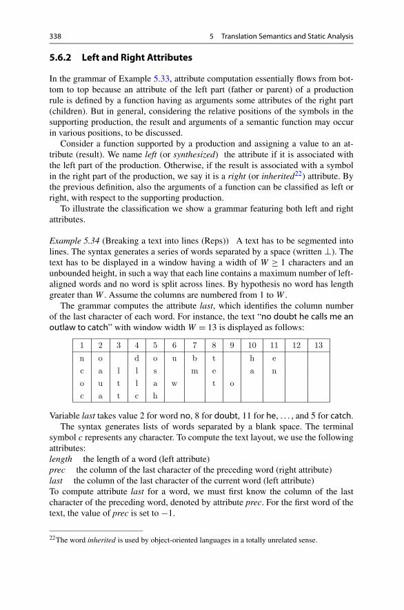
338 5 Translation Semantics and Static Analysis
5.6.2 Left and Right Attributes
In the grammar of Example 5.33, attribute computation essentially flows from bot-tom to top because an attribute of the left part (father or parent) of a productionrule is defined by a function having as arguments some attributes of the right part(children). But in general, considering the relative positions of the symbols in thesupporting production, the result and arguments of a semantic function may occurin various positions, to be discussed.
Consider a function supported by a production and assigning a value to an at-tribute (result). We name left (or synthesized) the attribute if it is associated withthe left part of the production. Otherwise, if the result is associated with a symbolin the right part of the production, we say it is a right (or inherited22) attribute. Bythe previous definition, also the arguments of a function can be classified as left orright, with respect to the supporting production.
To illustrate the classification we show a grammar featuring both left and rightattributes.
Example 5.34 (Breaking a text into lines (Reps)) A text has to be segmented intolines. The syntax generates a series of words separated by a space (written ⊥). Thetext has to be displayed in a window having a width of W ≥ 1 characters and anunbounded height, in such a way that each line contains a maximum number of left-aligned words and no word is split across lines. By hypothesis no word has lengthgreater than W . Assume the columns are numbered from 1 to W .
The grammar computes the attribute last, which identifies the column numberof the last character of each word. For instance, the text “no doubt he calls me anoutlaw to catch” with window width W = 13 is displayed as follows:
Variable last takes value 2 for word no, 8 for doubt, 11 for he, . . . , and 5 for catch.The syntax generates lists of words separated by a blank space. The terminal
symbol c represents any character. To compute the text layout, we use the followingattributes:length the length of a word (left attribute)prec the column of the last character of the preceding word (right attribute)last the column of the last character of the current word (left attribute)To compute attribute last for a word, we must first know the column of the lastcharacter of the preceding word, denoted by attribute prec. For the first word of thetext, the value of prec is set to −1.
22The word inherited is used by object-oriented languages in a totally unrelated sense.

5.6 Semantic Translations 339
Table 5.4 Attribute grammar of Example 5.34
# Syntax Right attributes Left attributes
1 S0 → T1 prec1 := −1
2 T0 → T1⊥T2 prec1 := prec0
prec2 := last1 last0 := last2
3 T0 → V1 last0 := if (prec0 + 1+ length1)≤W
then (prec0+ 1+ length1)
else length1end if
4 V0 → cV1 length0 := length1 + 1
5 V0 → c length0 := 1
Attribute computation is expressed by the rules of the attribute grammar in Ta-ble 5.4. Two remarks on the syntax: first, the subscripts of nonterminal symbolsare added as reference for the semantic functions, but they do not differentiate thesyntactic classes; i.e., the productions with and without subscripts are equivalent.Second, the syntax has an ambiguity caused by production rule T → T⊥T , whichis bilaterally recursive. But the drawbacks an ambiguous syntax has for parsing donot concern us here, because the semantic evaluator receives exactly one parse treeto work on. The ambiguous syntax is more concise, and this reduces also the numberof semantic rules.
The length of a word V is assigned to the left attribute length in the rules associ-ated with the last two productions. Attribute prec is a right one, because the value isassigned to a symbol in the right part of the first two productions. Attribute last is aleft one; its value decorates the nodes with label T of a syntax tree and provides thefinal result in the root of the tree.
In order to choose a feasible attribute evaluation schedule, let us examine the de-pendencies between the assignment statements for a specific syntax tree. In Fig. 5.14the left and right attributes are, respectively, placed to the left and the right of anode; the nodes are numbered for reference. To simplify drawing, the subtrees ofnonterminal V are omitted, but attribute length, which is the relevant information,is present with its value.
The attributes of a decorated tree can be viewed as the nodes of another directedgraph, the (data) dependence graph. For instance, observe arc last(2)→ prec(4):it represents a dependence of the latter attribute from the former, induced by func-tion prec2 := last1, which is supported by production rule 2. A function result hasas many dependence arcs as it has arguments. Notice the arcs interconnect onlyattributes pertaining to the same production.
To compute the attributes, the assignments must be executed in any order satis-fying the precedences expressed by the dependence graph. At the end, the tree iscompletely decorated with all the attribute values.

340 5 Translation Semantics and Static Analysis
Fig. 5.14 Decorated tree with dependence graph for Example 5.34
An important quality of the attribute evaluation process is that the result is in-dependent of the application order of functions. This property holds for grammarscomplying with certain conditions, to be considered soon.
Usefulness of Right Attributes This grammar uses both left and right attributes,so the questions arise: can we define the same semantics without using right at-tributes (as we did in the first example of attribute grammar)? And then, is it conve-nient to do so?
The first answer is yes, since we show that the position of the last letter of a wordcan be computed by a different approach. Initially compute the left attribute length,then construct a new left attribute list, having as domain a list of integers represent-ing word lengths. In Fig. 5.14, node T7, which covers the text he calls, would havethe attribute list= 〈2,5〉. After processing all the nodes, the value list in the subrootT1 of the tree is available, list = 〈2,5,2,5〉. It is then straightforward, knowing thepage width W , to compute the position of the last character of each word.
But this solution is fundamentally bad, because the computation required at theroot of the tree has essentially the same organization and complexity as the orig-inal text segmentation problem: nothing has been gained by the syntax-directedapproach, since the original problem has not been decomposed into simpler sub-problems.

5.6 Semantic Translations 341
Another drawback is that information is now concentrated in the root, rather thandistributed on all the nodes by means of the right attribute last, as it was in theprevious grammar.
Finally, to counterbalance the suppression of right attributes, it is often neces-sary to introduce non-scalar attributes, such as lists or sets, or other complex datastructures.
In conclusion, when designing an attribute grammar the most elegant and effec-tive design is often obtained relying on both left and right attributes.
5.6.3 Definition of Attribute Grammar
It is time to formalize the concepts introduced by previous examples. This is donein the next definition (Definition 5.35).
Definition 5.35 (Attribute grammar) An attribute grammar is defined as follows.1. A context-free syntax G= (V ,Σ,P,S), where V and Σ are the terminal and
nonterminal sets, P the production rule set, and S the axiom. It is convenientto avoid the presence of the axiom in the right parts of productions.
2. A set of symbols, the (semantic) attributes, associated with nonterminal andterminal syntax symbols. The set of the attributes associated with symbol, e.g.,D, is denoted attr(D).
The attribute set of a grammar is partitioned into two disjoint subsets, theleft attributes and the right attributes.
3. Each attribute σ has a domain, the set of values it may take.4. A set of semantic functions (or rules). Each function is associated with a pro-
duction rule:
p : D0 →D1D2 . . .Dr r ≥ 0
where D0 is a nonterminal and the other symbols can be terminal or nonter-minal. The production p is the syntactic support of the function. In general,several functions may have the same support.
Notation: the attribute σ associated with a symbol Dk is denoted by σk , oralso by σD if the syntactic symbol occurs exactly once in production p.
A semantic function has the form
σk := f(attr
({D0,D1, . . . ,Dr}) \ {σk}
)
where 0≤ k ≤ r ; function f assigns to the attribute σ of symbol Dk , the valuecomputed by the function body; the arguments of f can be any attributes of thesame production p, excluding the result of the function.
Usually the semantic functions are total functions in their domains. Theyare written in a suitable notation, termed semantic metalanguage, such as aprogramming language or a higher level specification language, which can beformal, or informal as a pseudo-code.

342 5 Translation Semantics and Static Analysis
A function σ0 := f (. . .) defines an attribute, qualified as left, of the nonter-minal D0, which is the left part (or father or parent) of the production.
A function σk := f (. . .) with k ≥ 1, defines an attribute, qualified as right,of a symbol (sibling or child) Dk occurring in the right part.
It is forbidden (as stated in (2)) for the same attribute to be left in a functionand right in another one.
Notice that since terminal characters never occur in the left part, their at-tributes cannot be of the left type.23
5. Consider the set fun(p) of all the functions supported by production p. Theymust satisfy the following conditions:(a) for each left attribute σ0 of D0, there exists in fun(p) exactly one function
defining the attribute(b) for each right attribute δ0 of D0, no function exists in fun(p) defining the
attribute(c) for each left attribute σi , where i ≥ 1, no function exists in fun(p) defin-
ing the attribute(d) for each attribute δi , where i ≥ 1, there exists in fun(p) exactly one func-
tion defining the attributeThe left attributes σ0 and the right ones δi , with i ≥ 1, are termed internal forproduction p, because they are defined by functions supported by p.
The right attributes δ0 and left attributes σi , with i ≥ 1, are termed externalfor production p, because they are defined by functions supported by otherproductions.
6. Some attributes can be initialized with constant values or with values computedby external functions. This is often the case for the so-called lexical attributes,those associated with terminal symbols. For such attributes the grammar doesnot specify a computation rule.
Example 5.36 (Example 5.34, p. 338, continued) We refer again to the grammar ofExample 5.34 on p. 338, where the attributes are classified as follows:left attributes: length and lastright attributes: precinternal/external: for production 2 the internal attributes are prec1, prec2, and
last0; the external ones are prec0, last0, and last2 (attribute length is not pertinentto production 2)
Then we have
attr(T )= {prec, last} attr(V )= {length} attr(S)= ∅
23In practice, the attributes of terminal symbols are often not defined by the semantic functions ofthe grammar, but are initialized with values computed during lexical analysis, which is the scanningprocess that precedes parsing and semantic analysis.

5.6 Semantic Translations 343
A caution against misuse of not local attributes. Item 4 expresses a sort of principleof locality of semantic functions: it is an error to designate as argument or result ofa semantic function supported by p, an attribute which is not pertinent to produc-tion p. An instance of such error occurs in the modified rule (2):
# Syntax Semantic functions
1 S0 → T1 . . .
2 T0 → T1⊥T2 prec1 := prec0 + length0︸ ︷︷ ︸non-pertinent attr.
3 . . . . . .
Here the principle of locality is violated because length /∈ attr(T ): any attribute of anode, other than the father or a sibling, is out of scope.
The rationale of the condition that left and right attributes be disjoint sets is dis-cussed next. Each attribute of a node of the syntax tree must be defined by exactlyone assignment, otherwise it may take two or more different values depending onthe order of evaluation, and the meaning of the tree would not be unique. To preventthis, the same attribute may not be left and right, because in that case there wouldbe two assignments, as shown in the fragment:
# Support Semantic functions
1 A→ BC σC := f1 (attr(A,B))2 C→DE σC := f2 (attr(D,E))
Clearly variable σC , internal for both productions, is a right attribute in the former,a left one in the latter. Therefore the final value it takes, will depend on the order offunction applications. Then the semantics loses the most desirable property of beingindependent of the implementation of the evaluator.
5.6.4 Dependence Graph and Attribute Evaluation
An advantage of a grammar as a specification of a translation is that it does not getinvolved with the details of the tree traversing procedures. In fact, the attribute evalu-ation program can be automatically constructed, starting from the functional depen-dencies between attributes, knowing of course the bodies of the semantic functions.
To prepare for that, we introduce the dependence graph of a semantic function:the nodes of this directed graph are the arguments and result, and there is an arc fromeach argument to the result. Collecting the dependence graphs for all the functionssupported by the same production, we obtain the dependence graph of a production.The next example (Example 5.37) shows a case.

344 5 Translation Semantics and Static Analysis
Fig. 5.15 Grammar of Example 5.34 and dependence graphs of productions
Example 5.37 (Dependence graph of productions) We reproduce from p. 339 inFig. 5.15 the grammar of Example 5.34. For clarity we lay each graph over thesupporting production (dotted edges), to evidence the association between attributesand syntactic components.
Production 2 is the most complex, with three semantic functions, each one withjust one argument, hence one arc (visually differentiated by the style) of the graph.
Notice that a node with (respectively without) incoming arcs is an attribute oftype internal (respectively external).

5.6 Semantic Translations 345
The dependence graph of a (decorated) syntax tree, already introduced, is ob-tained by pasting together the graphs of the individual productions used in the treenodes. For example, look back at Fig. 5.14 on p. 340.
5.6.4.1 Attribute Values as Solution of EquationsWe expect each sentence of a technical language to have exactly one meaning, i.e.,a unique set of values assigned to the semantic attributes; otherwise we would befaced with an undesirable case of semantic ambiguity.
We know the values are computed by assignments and there is exactly one as-signment per attribute instance in the tree. We may view the set of assignmentsas a system of simultaneous equations, where the unknowns are the attribute val-ues. From this perspective, the solution of the system is the meaning of the sen-tence.
For a sentence, consider now the attribute dependence graph of the tree, andsuppose it contains a directed path
σ1 → σ2 → ·· ·→ σj−1 → σj with j > 1
where each σk stands for some attribute instance. The names of the attribute in-stances can be the same or different. The corresponding equations are as follows:
σj = fj (. . . , σj−1, . . .)
σj−1 = fj−1(. . . , σj−2, . . .)
. . .
σ2 = f2(. . . , σ1, . . .)
since the result of a function is an argument of the next one.For instance, in Fig. 5.14 on p. 340 one such path is the following:
prec(T1)→ prec(T2)→ last(T2)→ prec(T4)→ prec(T5)→ ·· ·Revisiting the previous examples of decorated trees, it would be easy to verify that,for any sentence and syntax tree, no path of the dependence graph ever makes acircuit, to be formalized next.
A grammar is acyclic if, for each sentence, the dependence graph of the tree24 isacyclic. The next property (Property 5.38) states when a grammar can be consideredcorrect.
Property 5.38 (Correct attribute grammar) Given an attribute grammar satisfyingthe conditions of Definition 5.35, consider a syntax tree. If the attribute dependencegraph of the tree is acyclic, the system of equations corresponding to the semanticfunctions has exactly one solution.
24We assume the parser returns exactly one syntax tree per sentence.

346 5 Translation Semantics and Static Analysis
To prove the property, we show that, under the acyclicity condition, the equa-tions can be ordered in such a way that any semantic function is applied after thefunctions that compute its arguments. This produces a value for the solution, sincethe functions are total. The solution is clearly unique, as in a classical system ofsimultaneous linear equations.
Let G= (V ,E) be an acyclic directed graph, and identify the nodes by numbersV = {1,2, . . . , |V |}. The next algorithm (Algorithm 5.39) computes a total orderof nodes, called topological. The result ord[1 . . . |V |] is the vector of sorted nodes:it gives the identifier of the node that has been assigned to the ith position (1≤ i ≤|V |) in the ordering.
Algorithm 5.39 (Topological sorting)begin
i := 0 - - initialize node counter i
while V �= ∅ do
n := any node of set V without incoming arcs
- - notice: such a node exists as graph G is acyclic
i ++ - - increment node counter i
ord[i] := n - - put node n into vect. ord at pos. i
V := V \ {n} - - remove node n from set V
- - remove the dangling arcs from set E
E :=E \ {arcs going out from node n}end while
end
In general many different topological orders are possible, because the dependencegraph typically does not enforce a total order relation.
Example 5.40 (Topological sorting) Applying the algorithm to the graph of Fig. 5.14on p. 340, we obtain a topological order:
length3, length6, length9, length11,prec1,prec2, last2,prec4,
prec5, last5,prec7,prec8, last8,prec10, last10, last7, last4, last1
Next we apply the semantic functions in topological order. Pick the first node, itsequation is necessarily constant, i.e., it initializes the result attribute. Then proceedby applying the next equations in the order, which guarantees availability of allarguments. Since all the functions are total, a result is always computed. The treeis thus progressively decorated with a unique set of values. Therefore for an acyclicgrammar the meaning of a sentence is a single-valued function.
Actually the above evaluation algorithm is not very efficient, because on onehand it requires computing the topological sort, and on the other hand it may requiremultiple visits of the same node of the syntax tree. We are going to consider more

5.6 Semantic Translations 347
efficient algorithms, although less general, which operate under the assumption of afixed order of visit (scheduling) of the tree nodes.
Now consider what happens if the dependence graph of a tree contains a paththat makes a circuit, implying that in the chain:
σ1 → σ2 → ·· ·→ σj−1 → σj j > 1
two elements i and k, with 1 ≤ i < k ≤ j , are identical, i.e., σi = σk . Then thesystem of equations may have more than one solution, i.e., the grammar may besemantically ambiguous.
A remaining problem is how to check whether a given grammar is acyclic: howcan we be sure that no decorated syntax tree will ever present a closed dependencepath? Since the source language is usually infinite, the acyclicity test cannot beperformed by the exhaustive enumeration of the trees. An algorithm to decide if anattribute grammar is acyclic exists but is complex,25 and not used in practice. It ismore convenient to test certain sufficient conditions, which not only guarantee theacyclicity of a given grammar, but also permit constructing the attribute evaluationschedule, to be used by the semantic analyzer. Some simple yet practical conditionsare described next.
5.6.5 One Sweep Semantic Evaluation
A fast evaluator should compute the attributes of each tree node with a single visit,or at worst with a small number of visits of the nodes. A well-known order of visitof a tree is the depth-first traversal, which in many cases permits the evaluation ofthe attributes with just one sweep over the tree.
Let N be a node of a tree and N1, . . . ,Nr its children; denote by ti the subtreerooted in node Ni .
A depth-first visit algorithm first visits the root of the tree. Then, in order to visitthe generic subtree tN rooted in a node N , it recursively proceeds as follows. Itperforms a depth-first visit of the subtrees t1, . . . , tr , in an order, yet not necessarilycoincident with the natural one 1,2, . . . , r , i.e., according to some permutation of1,2, . . . , r .
When a node is visited, the local attributes are computed. This semantic evalua-tion algorithm, termed one sweep, computes the attributes according to the followingprinciples:• before entering and evaluating a subtree tN , it computes the right attributes of
node N (the root of the subtree)• at the end of visit of subtree tN , it computes the left attributes of N
We hasten to say that not all the grammars are compatible with this algorithm, be-cause more intricate functional dependencies may require several visits of the samenode. The appeal of this method is that it is very fast, and that practical, sufficient
25See [8, 9]. The asymptotic time complexity is NP -complete with respect to the size of theattribute grammar.

348 5 Translation Semantics and Static Analysis
conditions for one-sweep evaluation are simple to state and to check on the depen-dence graph dipp of each production p.
Experience with grammar design indicates it is often possible to satisfy the one-sweep conditions, sometimes with minor changes to the original semantic functions.
5.6.5.1 One-Sweep GrammarsFor each production rule p:
p : D0 →D1D2 . . .Dr r ≥ 0
we need to define a binary relation between the syntactic symbols of the right part,to be represented in a directed graph, called the sibling graph, denoted siblp . Theidea is to summarize the dependencies between the attributes of the semantic func-tions supported by the production. The nodes of the sibling graph are the symbols{D1,D2, . . . ,Dr} of the production. The sibling graph has an arc
Di →Dj with i �= j and i, j ≥ 1
if in the dependence graph dipp there is an arc σi → δj from an attribute of symbolDi to an attribute of symbol Dj .
We stress that the nodes of the sibling graph are not the same as the nodes of thedependence graph of the production: the former are syntactical symbols, the latterare attributes. Clearly all attributes of dipp having the same subscript j are coalescedinto a node Dj of siblp: in mathematical terms, the sibling graph is related to thedependence graph by a node homomorphism.
The next definition (Definition 5.41) states the conditions for having a one-sweepgrammar.
Definition 5.41 (One-sweep grammar) A grammar satisfies the one-sweep condi-tion if, for each production p:
p : D0 →D1D2 . . .Dr r ≥ 0
having dependence graph dipp , if the following clauses hold:1. graph dipp contains no circuit2. graph dipp does not contain a path:
λi → ·· ·→ ρi i ≥ 1
that goes from a left attribute λi to a right attribute ρi of the same symbol Di ,where Di is a sibling
3. graph dipp contains no arc λ0 → ρi , with i ≥ 1, from a left attribute of thefather node D0 to a right attribute of a sibling Di
4. the sibling graph siblp contains no circuit

5.6 Semantic Translations 349
We orderly explain each item.1. This condition is necessary for the grammar to be acyclic (a requirement for
ensuring existence and uniqueness of meaning).2. If we had a path λi → ·· ·→ ρi , with i ≥ 1, it would be impossible to compute
the right attribute ρi before visiting subtree ti , because the value of the leftattribute λi is available only after the visit of the subtree. This contravenes thedepth-first visit order we have opted for.
3. As in the preceding item, the value of attribute ρi would not be available whenwe start visiting the subtree ti .
4. This condition permits to topologically sort the children, i.e., the subtreest1, . . . , tr , and to schedule their visit in an order consistent with the precedencesexpressed by graph dipp . If the sibling graph had a circuit, there would be con-flicting precedence requirements on the order of visiting the sibling subtrees.In that case it would be impossible to find a schedule valid for all the attributesof the right part of production p.
Algorithm 5.42 (Construction of one-sweep evaluator) We write a semantic proce-dure for each nonterminal symbol, having as arguments the subtree to be decoratedand the right attributes of its root. The procedure visits the subtrees, and computesand returns the left attributes of the root (of the subtree).
For each production p:
p : D0 →D1D2 . . .Dr r ≥ 0
1. Choose a topological order, denoted TOS, of the nonterminals D1,D2, . . . ,Dr
with respect to the sibling graph siblp .2. For each symbol Di , with 1≤ i ≤ r , choose a topological order, denoted TOR,
of the right attributes of symbol Di with respect to the dependence graph dipp .3. Choose a topological order, denoted TOL, of the left attributes of symbol D0,
with respect to the dependence graph dipp .The three orders TOS, TOR and TOL, together prescribe how to arrange the instruc-tions in the body of the semantic procedure, to be illustrated in the coming example(Example 5.43).
Example 5.43 (One-sweep semantic procedure) For brevity we consider a gram-mar fragment containing just one production and we leave the semantic func-tions unspecified. Production D → ABC has the dependence graph dip shown inFig. 5.16.
It is straightforward to check the graph satisfies conditions (1), (2), and (3) ofDefinition 5.41, because:1. there are neither circuits2. nor any path from a left attribute λA, λB , or λC to a right attribute, such as ρB ,
of the same node3. nor any arc from a left attribute λD or μD to a right attribute of A, B or C

350 5 Translation Semantics and Static Analysis
Fig. 5.16 Dependence graph of the production rule of Example 5.43
4. the sibling graph sibl, below, is acyclic:
We explain where its arcs come from:• A→ C from dependence λA→ ρC
• C→ B from dependence ρC → ρB
Next we compute the topological orders.• sibling graph: TOS=A,C,B
• right attributes of each sibling: since A and B have only one right attribute, thetopological sorting is trivial; for C we have TOR= ρ,σ
• left attributes of D: the topological order is TOL= λ,μ
To complete the design, it remains to list the instructions of the semantic procedureof this production, in an order compatible with the chosen topological orders. Moreprecisely, the order of left attribute assignments is TOL, the order of procedure in-vocations (to evaluate subtrees) is TOS, and the order of right attribute assignmentsis TOR.
procedure D (in t, ρD ; out λD,μD)
- - t root of subtree to be decorated
ρA := f1(ρD)
- - abstract functions are denoted f1, f2, etc.
A(tA,ρA;λA)
- - invocation of A to decorate subtree tA
ρC := f2(λA)
σC := f3(ρC)
C(tC,ρC,σC;λC)
- - invocation of C to decorate subtree tC
ρB := f4(ρD,ρC)
5.6 Semantic Translations 351
B(tB,ρB;λB)
- - invocation of B to decorate subtree tC
λD := f5(ρD,λB,λC)
μD := f6(λD)
end procedure
To conclude, this method is very useful for designing an efficient recursive se-mantic evaluator, provided the grammar satisfies the one-sweep condition.
5.6.6 Other Evaluation Methods
One-sweep evaluation is practical, but some grammars have complicated dependen-cies which prevent its use. More general classes of evaluators and correspondinggrammar conditions are available, which we do not discuss.26 To expand the scopeof the one-sweep evaluation methods, we develop a rather intuitive idea. The evalu-ation process is decomposed into a cascade of two or more phases, each one of theone-sweep type, operating on the same syntax tree.
We describe the method focusing on two phases, but generalization is straight-forward. The attribute set attr of the grammar is partitioned by the designer intotwo disjoint sets Attr1 ∪Attr2 = Attr, to be, respectively, evaluated in phase one andtwo. Each attribute set, together with the corresponding semantic functions, can beviewed as an attribute subgrammar.
Next we have to check that the first subgrammar satisfies the general condi-tions 5.35 (p. 341) as well as the one-sweep condition 5.41 (p. 348). In particular,the general condition imposes that every attribute is defined by some semantic func-tion; as a consequence no attribute of set Attr1 may depend on any attribute of setAttr2; otherwise it would be impossible to evaluate the former attribute in phase one.
Then we construct the one-sweep semantic procedures for phase one, exactly aswe would have done for a one-sweep grammar. After the execution of phase one, allthe attributes in Attr1 have a value, and it remains to evaluate the attributes of thesecond set.
For phase two we have again to check whether the second subgrammar meetsthe same conditions. Notice, however, that for the second evaluator, the attributes ofset Attr1 are considered as initialized constants. This means that the dependenciesbetween the elements of Attr1, and between an element of Attr1 and an elementof Attr2, are disregarded when checking the conditions. In other words, only thedependencies inside Attr2 need to be considered. The phase two evaluator operateson a tree decorated with the attributes of the first set, and computes the remainingattributes in one sweep.
The crucial point for multi-sweep evaluation to work is to find a good partitionof the attributes into two (or more) sets. Then the construction works exactly as in
26Among them we mention the evaluators based on multiple visits, on the ordered attribute gram-mar (OAG) condition, and on the absolute acyclicity condition. A survey of evaluation methodsand grammar conditions is in Engelfriet [7].

352 5 Translation Semantics and Static Analysis
one sweep. Notice that not all the attribute values computed in stage one have to bestored in the decorated tree produced by phase one, but only those used as argumentsby semantic functions applied in the second sweep.
As a matter of fact, designing a semantic evaluator for a rich technical language isa complex task, and it is often desirable to modularize the project in order to masterthe difficulty; some forms of modularization are discussed in [6]. Partitioning theglobal attribute set into subsets associated with evaluation phases, offers a precioushelp for modularization. In practice, in many compilers the semantic analyzer issubdivided into phases of smaller complexity. For instance, the first stage analyzesthe declarations of the various program entities (variables, types, classes, etc.) andthe second stage processes the executable instructions of the programming languageto be compiled.
5.6.7 Combined Syntax and Semantic Analysis
For faster processing, it is sometimes possible and convenient to combine syntax treeconstruction and attribute computation, trusting the parser with the duty to invokethe semantic functions.
In the following discussion we use pure BNF syntax for the support, because theuse of EBNF productions makes it difficult to specify the correspondence betweensyntax symbols and attributes.
There are three typical situations for consideration, depending on the nature ofthe source language:• the source language is regular: lexical analysis with lexical attributes• the source syntax is LL(k): recursive descent parser with attributes• the source syntax is LR(k): shift–reduce parser with attributesNext we discuss the enabling conditions for such combined syntax-semantic pro-cessors.
5.6.7.1 Lexical Analysis with Attribute EvaluationThe task of a lexical analyzer (or scanner) is to segment the source text into thelexical elements, called lexemes or tokens, such as identifiers, integer or real con-stants, comments, etc. Lexemes are the smallest substrings that can be invested withsome semantic property. For instance, in many languages the keyword begin hasthe property of opening a compound statement, whereas its substring egin has nomeaning.
Each technical language uses a finite collection of lexical classes, as the onesjust mentioned. A lexical class is a regular formal language: a typical example isthe class of identifiers (Example 2.27) defined by the regular expression on p. 27.A lexeme of identifier class is a sentence belonging to the corresponding regularlanguage.
In language reference manuals we find two levels of syntactic specifications:from lower to higher, the lexical and syntactic levels. The former defines the formof the lexemes. The latter assumes the lexemes are given in the text, and considers

5.6 Semantic Translations 353
them to be the characters of its terminal alphabet. Moreover, the lexemes may carrya meaning, i.e., a semantic attribute, which is computed by the scanner.
Lexical Classes Focusing on typical lexicons, we notice that some lexical classes,viewed as formal languages, have a finite cardinality. Thus, the reserved keywordsof a programming language make a finite or closed class, including for instance:
{begin,end, if, then,else,do, . . . ,while}Similarly, the number of arithmetic, boolean, and relational operation signs is fi-nite. On the contrary, identifiers, integer constants, and comments are cases of openlexical classes, having unbounded cardinality.
A scanner is essentially a finite transducer (IO-automaton) that divides the sourcetext into lexemes, assigning an encoding to each one. In the source text the lexemesare separated, depending on their classes, by blank spaces or delimiters such asnew-line. The transducer returns the encoding of each lexeme and removes thedelimiters.
More precisely, the scanner transcribes into the target string each lexeme as apair of elements: the name, i.e., the encoding of the lexical class, and a semanticattribute, termed lexical.
Lexical attributes change from a class to another and are altogether missing fromcertain classes. Some typical cases are:• decimal constant: the attribute is the value of the constant in base ten• identifier: the attribute is a key, to be used by the compiler for quickly locating
the identifier in a symbol table• comment: a comment has no attribute, if the compilation framework does not
manage program documentation, and throws away source program comments;if the compiler keeps and classifies comments, their lexical attribute is instru-mental to retrieve them
• keyword: has no semantic attribute, just a code for identification
Unique Segmentation In a well-designed technical language, lexical definitionsshould ensure that, for any source text, the segmentation into lexemes is unique.A word of caution is necessary, for the concatenation of two or more lexical classesmay introduce ambiguity. For instance, string beta237 can be divided in many waysinto valid lexemes: a lexeme beta of class identifier followed by 237 of class integer;or an identifier beta2 followed by the integer 37, and so on.
In practice, this sort of concatenation ambiguity (p. 49) is often cured by impos-ing to the scanner the longest prefix rule. The rule tells the scanner to segment astring x = uv into the lexemes, say, u ∈ identifier and v ∈ integer, in such a waythat u is the longest prefix of x belonging to class identifier. In the example, the ruleassigns the whole string beta237 to class identifier.
By this prescription the translation is made single valued and can be computedby a finite deterministic transducer, augmented with the actions needed to evaluatethe lexical semantic attributes.

354 5 Translation Semantics and Static Analysis
Lexical Attributes We have observed that some lexical classes carry a semanticattribute and different classes usually have different attribute domains. Therefore,at a first glance it would seem necessary to differentiate the semantic functions foreach lexical class. However, it is often preferable to unify the treatment of lexicalattributes as far as possible, in order to streamline the scanner organization: remem-ber that a scanner has to be efficient because it is the innermost loop of the compiler.To this end, each lexical class is assigned the same attribute of type string, namedss, which contains the substring recognized as lexeme by the scanner.
For instance, the attribute ss of identifier beta237 is just a string “beta237” (or apointer thereto). Then the finite transducer returns the translation:
〈class= identifier, ss= ‘beta237’〉upon recognizing lexeme beta237. This pair clearly contains sufficient information,to pass as argument to a later invocation of an identifier-specific semantic function.The latter looks up string ss in the symbol table of the program under compilation;if it is not present, it inserts the string into the table and returns its position as asemantic attribute. Notice such identifier-specific semantic function is better viewedas a part of the attribute grammar of the syntax-directed translator, rather than of thescanner.
5.6.7.2 Attributed Recursive Descent TranslatorAssume the syntax is suitable for deterministic top-down parsing. Attribute eval-uation can proceed in lockstep with parsing, if the functional dependencies of thegrammar obey certain additional conditions beyond the one-sweep ones.
We recall the one-sweep algorithm (p. 348) visits in depth-first order the syntaxtree, traversing the subtrees t1, . . . , tr , for the current production D0 → D1 . . .Dr
in an order that may be different from the natural one. The order is a topologicalsorting, consistent with the dependencies between the attributes of nodes 1, . . . , r .
On the other hand, we know a parser constructs the tree in the natural order, i.e.,subtree tj is constructed after subtrees t1, . . . , tj−1. It follows that, to combine thetwo processes, we must exclude any functional dependence that would enforce anattribute evaluation order other than the natural one, as stated next (Definition 5.44).
Definition 5.44 (L condition) A grammar satisfies condition L27 if, for each pro-duction p : D0 →D1 . . .Dr , we have:1. the one-sweep condition 5.41 (p. 348) is satisfied, and2. the sibling graph siblp contains no arc Dj →Di with j > i ≥ 1
Notice the second clause prevents a right attribute of node Di to depend on any(left or right) attribute of a node Dj placed to its right in the production. As aconsequence, the natural order 1, . . . , r is a topological sort of the sibling graph andcan be applied to visit the sibling subtrees. The next property (Property 5.45) relatesthe L condition and deterministic parsing.
27The letter L stands for left to right.

5.6 Semantic Translations 355
Table 5.5 Grammar for converting fractional numbers (Example 5.46)
Grammar
Syntax Left attributes Right attributes
N0 →•D1 v0 := v1 l1 := 1
D0 → B1D2 v0 := v1 + v2 l1 := l0 l2 := l0 + 1
D0 → B1 v0 := v1 l1 := l0
B0 → 0 v0 := 0
B0 → 1 v0 := 2−l0
Attributes
Attribute Meaning Domain Type Assoc. symbols
v Value Real Left N , D, B
l Length Integer Right D, B
Property 5.45 (Attribute grammar and deterministic parsing) Let a grammar besuch that:• the syntax satisfies the LL(k) condition, and• the semantic rules satisfy the L conditionThen it is possible to construct a top-down deterministic parser with attribute evalu-ation, to compute the attributes at parsing time.
The construction of the semantic evaluator, presented in the coming example(Example 5.46), is a straightforward combination of a recursive descent parser anda one-sweep recursive evaluator.
Example 5.46 (Recursive descent parser with attribute evaluation) Revising Exam-ple 5.33 (p. 336), we write a grammar to convert a fractional number smaller than 1,from base two to base ten. The source language is defined by the regular expression
L= •(0 | 1)∗
The meaning of a string such as •01 is decimal number 0.25. The grammar is listedin Table 5.5. Notice the value of a bit is weighted by a negative exponent, equal toits distance from the fractional point.
The syntax is deterministic LL(2), as can be checked.Next we verify condition L, production by production.
N →•D The dependence graph has one arc v1 → v0, hence:• there are no circuits in the graph• there is no path from left attribute v to right attribute l of the same sibling• in the graph there is no arc from attribute v of father to a right attribute l of
a sibling• the sibling graph sibl has no arcs

356 5 Translation Semantics and Static Analysis
D→ BD The dependence graph:
• has no circuit• has no path from left attribute v to right attribute l of the same sibling• has no arc from left attribute v of father to right attribute v of a sibling• the sibling graph has no arcs
D→ B Same as above.B→ 0 The dependence graph has no arcs.B→ 1 The dependence graph has one arc l0 → v0, which is compatible with one
sweep, and there are not any brothers.Similar to a parser, the program comprises three procedures N , D, and B , having astheir arguments the left attributes of the father. To implement parser look-ahead, aprocedure uses two variables to store the current character cc1 and the next one cc2.Function read updates both variables. Variable cc2 determines the choice betweenthe syntactic alternatives of D.
procedure N (in ∅; out v0)
if cc1= ‘ • ’ thenread
elseerror
end ifl1 := 1 - - initialize a local var. with right attribute of D
D(l1, v0) - - call D to construct a subtree and compute v0
end procedure
procedure D (in l0; out v0)
case cc2 of‘0’, ‘1’ : begin - - case of rule D→ BD
B(l0, v1)
l2 := l0 + 1
D(l2, v2)
v0 := v1 + v2
end‘�’ : begin - - case of rule D→ B
B(l0, v1)
v0 := v1
end

5.6 Semantic Translations 357
otherwise error
end caseend procedure
procedure B (in l0; out v0)
case cc1 of‘0’ : v0 := 0 - - case of rule B→ 0
‘1’ : v0 := 2−l0 - - case of rule B→ 1
otherwise error
end caseend procedure
To activate the analyzer, the compiler invokes the axiom procedure.
Clearly a skilled programmer could improve in several ways the previousschematic implementation.
5.6.7.3 Attributed Bottom-Up ParserSupposing the syntax meets the LR(1) condition, we want to combine the bottom-up syntax tree construction with attribute evaluation. Some problems have to beaddressed: how to ensure that the precedences on semantic function calls inducedby attribute dependencies are consistent with the order of tree construction; when tocompute the attributes; and where to store their values.
Considering first the problem of when semantic functions should be invoked, itturns out that right attributes cannot be evaluated during parsing, even assumingthe grammar complies with the L condition (which was sufficient for top-downevaluation in one sweep). The reason is that a shift–reduce parser defers the choiceof the production until it performs a reduction, when the parser is in a macro-statecontaining the marked production D0 → D1 . . .Dr•. This is the earliest time theparser can choose the semantic functions to be invoked.
The next problem comes from attribute dependencies. Just before reduction, theparser stack contains r elements from top, which correspond to the syntactic sym-bols of the right part. Assuming the values of all the attributes of D1 . . .Dr areavailable, the algorithm can invoke the functions and return the values of the leftattributes of D0.
But a difficulty comes from the evaluation of the right attributes of D1 . . .Dr .Imagine the algorithm is about to construct and decorate the subtree of D1. In ac-cordance with the one-sweep evaluation, every right attribute ρD1 should be avail-able before evaluating the subtree rooted at D1. But attribute ρD1 may depend onsome right attribute ρ0 of the father D0, which is unavailable, because the syn-tax tree does not yet contain the upper part, including the node associated withthe father. The simplest way to circumvent this obstacle is to assume the gram-mar does not use right attributes. This ensures that the left attributes of a node willonly depend on the left attributes of the children, which are available at reductiontime.

358 5 Translation Semantics and Static Analysis
Fig. 5.17 Machine net for the arithmetic expressions (Example 5.47)
Fig. 5.18 Pilot graph of the arithmetic expressions (Example 5.47, Fig. 5.17)
Coming to the question of memorization, the attributes can be stored in the stack,next to the items (m-states of the pilot machine) used by the parser. Thus each stackelement is a record, made of a syntactic fields and one or more semantic fieldscontaining attribute values (or pointers to values stored elsewhere); see the nextexample (Example 5.47).
Example 5.47 (Calculating machine without right attributes) The syntax for certainarithmetic expressions is shown as a network in Fig. 5.17 and its pilot graph is inFig. 5.18. In the machine ME the final states of the alternative rule paths E → T
and E→E + T are unified; and similarly in MT . This syntax is BNF and the pilotmeets the LR(1) condition.28
28See also Example 5.14, p. 314, where the source grammar is the same, though there the machinesare drawn as trees by splitting the final states per rule, and thus the pilot (Fig. 5.6, p. 315) has morem-states; but its behavior as a recognizer is the same as here.

5.6 Semantic Translations 359
The following attribute grammar computes the expression value v, or sets totrue a predicate o in the case of overflow. Constant maxint is the largest integer thecalculator can represent. A character a has an initialized attribute v with the valueof the integer constant a. Both attributes are left:
Syntax Semantic functions
E0 →E1 + T2 o0 := o1 or (v1 + v2 > maxint)
v0 := if o0 then nil else (v1 + v2)
E0 → T1 o0 := o1
v0 := v1
T0 → T1 × a o0 := o1 or (v1 × value(a) > maxint)
v0 := if o0 then nil else (v1 × value(a))
T0 → a o0 := false
v0 := value(a)
We trace in Fig. 5.19 a computation of the pushdown machine, extended with thesemantic fields. The source sentence is a3 + a5, where the subscript of a constantis its value. When the parser terminates, the stack contains attributes v and o of theroot of the tree.
Right Attributes Independent of Father Actually, the prohibition to use rightattributes may badly complicate the task of writing an attribute grammar. Attributedomains and semantic functions may turn less simple and natural, although in prin-ciple we know any translation can be specified without using right attributes.
Grammar expressivity improves if right attributes are readmitted, although withthe following limitation on their dependencies (Definition 5.48).
Definition 5.48 (Condition A29 for bottom-up evaluation) For each productionp : D0 →D1 . . .Dr , the following must hold:1. the L condition (p. 354) for top-down evaluation is satisfied, and2. no right attribute ρDk
of a sibling depends on a right attribute σD0 of the father,with 1≤ k ≤ r .
Positively stated, the same condition becomes: a right attribute ρDkmay only
depend on the right or left attributes of symbols D1 . . .Dk−1, with 1≤ k ≤ r .If a grammar meets the A condition, the left attributes of nonterminal sym-
bols D1, . . . ,Dr are available when a reduction is executed. Thus the remainingattributes can be computed in the following order:1. right attributes of the same nonterminal symbols, in the order 1,2, . . . , r
2. left attributes of father D0Notice this order differs from the scheduling of top-down evaluation, in that rightattributes are computed later, during reduction.
29The letter A stands for ascending order.

360 5 Translation Semantics and Static Analysis
Fig. 5.19 Shift–reduce parsing trace with attribute evaluation (Example 5.47)
Finally we observe that this delayed evaluation gives more freedom to computethe right attributes in an order other than the natural left-to-right order necessarilyapplied by top-down parsers. This would allow to deal with more involved depen-dencies between the nodes of the sibling graph (p. 348), similarly to the one-sweepevaluators.
5.6.8 Typical Applications of Attribute Grammars
Syntax-directed translation is widely applied in compiler design. Attribute gram-mars provide a convenient and modular notation for specifying the large number oflocal operations performed by the compiler, without actually getting into the im-plementation of the compiler itself. Since it would be too long to describe withsome degree of completeness the semantic analysis operations for a programminglanguage, we simply present a few typical interesting parts in a schematic manner.Actually it is the case that the semantic analysis of programming languages com-prises rather repetitive parts, but spelling them out in detail, would not add to aconceptual understanding of compilation.

5.6 Semantic Translations 361
We selected for presentation the following: semantic checks, code generation,and the use of semantic information for making parsing deterministic.
5.6.8.1 Semantic ChecksThe formal language LF defined by the syntax is just a gross approximation byexcess to the actual programming (or technical) language LT to be compiled, thatis, the set inclusion LF ⊃ LT holds. The left member is a context-free language,while the right one is informally defined by the language reference manual. For-mally speaking, language LT belongs to a more complex language family, thecontext-sensitive one. Without repeating the reasons presented at the end of Chap. 3,a context-sensitive syntax cannot be used in practice, and formalization must be con-tented with the context-free approximation.
To touch the nature of such approximations, imagine a programming lan-guage LT . The sentences of LF are syntactically correct, yet they may violatemany prescriptions of the language manual, such as type compatibility betweenthe operands of an expression, agreement between the actual and formal parame-ters of a procedure, and consistence between a variable declaration and its use in aninstruction.
A good way to check such prescriptions is by means of semantic rules that returnboolean attributes called semantic predicates. A given source text violates a seman-tic prescription, if the corresponding semantic predicate turns out to be false afterevaluating the attributes. Then the compiler reports a corresponding error, referredto as a static semantic error.
In general, the functionally of the semantic predicates depends on other attributesthat represent various program properties. For an example, consider the agreementbetween a variable declaration and its use in an assignment statement. In a program,declaration and use are arbitrarily distant substrings, therefore the compiler muststore the type of the declared variable in an attribute, called symbol table or environ-ment. This attribute will be propagated through the syntax tree, to reach any nodewhere the variable is used in an assignment or in another statement. However, sucha propagation is just a fiction, because if it were performed by copying the table,then it would be too inefficient. In practice the environment is implemented by aglobal data structure (or object), which is in the scope of all the concerned semanticfunctions.
The next attribute grammar (Example 5.49) schematizes the creation of a symboltable and its use for checking the variables that appear in the assignments.
Example 5.49 (Symbol table and type checking) The example covers the declara-tions of scalar and vector variables to be used in the assignments. For the sake of theexample, we assume that the following semantic prescriptions have to be enforced:1. a variable may not be multiply declared2. a variable may not be used before declaration3. the only valid assignments are between scalar variables and between vector
variables of identical dimension

362 5 Translation Semantics and Static Analysis
Table 5.6 Grammar for checking the declaration of variables versus their use in the assignmentstatements (Example 5.49)
Syntax Semantic functions Comment
S→ P t1 := ∅ Initialize tab. to empty
P →DP t1 := t0t2 := insert (t0, n1,descr1)
Propag. tab. to subtreeadd description to tab.
P →AP t1 := t0t2 := t0
Propag. tab. to subtrees
P → ε No functions used here
D→ id dd0 := present (t0, nid)
if ¬dd0 thendescr0 := ‘sca’
end ifn0 := nid
Declare scalar variable
D→ id[const] dd0 := present (t0, nid)
if ¬dd0 thendescr0 := (‘vect’, vconst)
end ifn0 := nid
Declare vector variable
A→ L :=R t1 := t0t2 := t0ai0 := ¬〈descr1 is compatible with descr2〉
Propag. tab. to subtrees
L→ id descr0 := 〈type of nid in t0〉
L→ id[id] if
(〈type of nid1 in t0〉 = ‘vect’ and
〈type of nid2 in t0〉 = ‘sca’
)
then
descr0 := ‘sca’else
errorend if
Use indexed variable
R→ id descr0 := 〈type of nid in t0〉 Use sca./vect. variable
R→ const descr0 := ‘sca’ Use constant
R→ id[id] if
(〈type of nid1 in t0〉 = ‘vect’ and
〈type of nid2 in t0〉 = ‘sca’
)
then
descr0 := ‘sca’else
errorend if
Use indexed variable
The attribute grammar is shown in Table 5.6. The syntax is in a rather abstract formand distinguishes the variable declarations from their uses.
Attributes n and v are the name of a variable and the value of a constant, respec-tively. The symbol table is searched using as key the name n of a variable. For eachdeclared variable, the symbol table contains a descriptor descr with the variabletype (scalar or vector) and the vector dimension, if applicable. During its construc-tion, the table is hosted by attribute t . Predicate dd denounces a double declaration.

5.6 Semantic Translations 363
Predicate ai denounces a type incompatibility between the left and right parts of anassignment. Attribute t , the symbol table, is propagated to the whole tree for thenecessary local controls to take place. A summary of the attributes follows:
Attribute Meaning Domain Type Assoc. symbols
n Variable name String Left idv Constant value Number Left constdd Double declaration Boolean Left D
ai Left/right partsincompatible
Boolean Left D
descr Variable descriptor Record Left D,L,R
t Symbol table Array ofrecords
Right A,P
The semantic analyzer processes a declaration D, and if the declared variable isalready present in the symbol table, then it sets predicate dd to true. Otherwise thevariable descriptor is constructed and passed to the father (or parent) node, alongwith the variable name.
The left and right parts L and R of an assignment A have an attribute descr (de-scriptor) that specifies the type of each part: variable (indexed or not) or constant. If aname does not exist in the symbol table, then the descriptor is assigned an error code.
The semantic rules control the type compatibility of the assignment and returnpredicate ai. The control that the left and right parts of an assignment are compatibleis specified in pseudo-code: the error conditions listed in items (2) and (3) make thepredicate true.
For instance, in the syntactically correct text
D1︷ ︸︸ ︷a[10]
D2︷︸︸︷i
D3︷︸︸︷b
A4︷ ︸︸ ︷i := 4
A5 : ai=true︷ ︸︸ ︷c := a[i]
D6︷ ︸︸ ︷c[30]
D7 : dd=true︷︸︸︷
i
A8 : ai=true︷ ︸︸ ︷a := c
a few semantic errors have been detected in assignments A5, A8 and in the declara-tion D7.
Many improvements and additions would be needed for a real compiler, and wemention a few of them. First, to make diagnostic more accurate, it is preferable toseparate various error classes, e.g., undefined variable, incompatible type, wrongdimension, etc.
Second, the compiler must tell the programmer the position (e.g., the line num-ber) of each error occurrence. By enriching the grammar with other attributes andfunctions, it is not difficult to improve on diagnostic and error identification. In par-ticular any semantic predicate, when it returns true in some tree position, can bepropagated towards the tree root together with a node coordinate. Then in the rootanother semantic function will be in charge of writing comprehensive and readableerror messages.
Third, there are other semantic errors that are not covered by this example: forinstance the check that each variable is initialized before its first use in an expres-

364 5 Translation Semantics and Static Analysis
sion; or that if it is assigned a value, then it is used in some other statement. For suchcontrols, compilers adopt a more convenient method instead of attribute grammars,called static program analysis, to be described at the end of this chapter.
Finally, a program that has passed all the semantic controls in compilation, maystill produce dynamic or runtime errors when executed. See for instance the follow-ing program fragment:
array a[10]; . . . read (i); a[i] := · · ·The read instruction may assign to variable i a value that falls out of the interval1 . . .10, a condition clearly undetectable at compilation time.
5.6.8.2 Code GenerationSince the final product of compilation is to translate a source program to a sequenceof target instructions, their selection is an essential part of the process. The problemoccurs in different settings and connotations, depending on the nature of the sourceand target languages, and on the distance between them. If the differences betweenthe two languages are small, the translation can be directly produced by the parser, aswe have seen in Sect. 5.4.1 (p. 300) for the conversion from infix to polish notationof arithmetic expressions.
On the other hand, it is much harder to translate a high-level language, say Java,to a machine language, and the large distance between the two makes it conve-nient to subdivide the translation process into a cascade of simpler phases. Eachphase translates an intermediate language or representation to another one. Thefirst stage takes Java as source language, and the last phase produces machine codeas target language. Compilers have used quite a variety of intermediate representa-tions: textual representations in polish form, trees or graphs, representations similarto assembly language, etc.
An equally important goal of decomposition is to achieve portability with respectto the target and source language. In the first case, portability (also called retarget-ing) means the ease of modifying an existing compiler, when it is required to gen-erate code for a different machine. In the second case, the modification comes froma change in the source language, say, from Java to FORTRAN. In both cases somephases of a multi-phase compiler are independent of the source or target languages,and can be reused at no cost.
The first phase is a syntax-directed translator, guided by the syntax of say Java.The following phases select machine instructions and transform the program, in or-der to maximize the execution speed of the target program, to minimize its memoryoccupation, or, in some cases, to reduce the electric energy consumption.30 Noticethe first phase or phases of a compiler are essentially independent of the character-istic of the target machine; they comprise the so-called front-end.
30Code selecting phases are often designed by using specialized algorithms based on the recogni-tion of patterns on an intermediate tree representation. For an introduction to such methods, see,e.g., [3] or [4].

5.6 Semantic Translations 365
The last phases are machine dependent and are called the back-end compiler. Theback-end actually contains several subsystems, including at least a machine code se-lection module and a machine register allocation one. The same front-end compileris usually interfaced to several back-end compilers, each one oriented towards aspecific target machine.
The next examples offer a taste of the techniques involved in translating fromhigh-level to machine level instructions, in the very simple case of control instruc-tions. In a programming language, control statements prescribe the order and choiceof the instructions to be executed. Constructs like if then else and while do are trans-lated by the compiler to conditional and unconditional jumps. We assume the tar-get language offers a conditional instruction jump-if-false with two arguments: aregister rc containing the test condition; and the label of the instruction to jumpto.
In the syntax, the nonterminal L stands for a list of instructions. Clearly eachjump instruction requires a fresh label that differs from the already used labels: thetranslator needs an unbounded supply of labels. To create such new labels whenneeded, the compiler invokes a function fresh that at each invocation assigns a newlabel to the attribute n.
The translation of a construct is accumulated in attribute tr, by concatenating(sign •) the translations of the constituents and by inserting jump instructions withnewly created labels. Such labels have the form e_397, f_397, i_23, . . . , where theinteger suffix is the number returned by function fresh. Register rc is designated bythe homonymous attribute of nonterminal cond.
In the next examples (Examples 5.50 and 5.51), we, respectively, illustrate theseissues with conditional and iterative instructions.
Example 5.50 (Conditional instruction) The grammar of the conditional statementif then else, generated by nonterminal I , is shown in Table 5.7. For brevity we omitthe translation of a boolean condition cond and of the other language constructs.A complete compiler should include the grammar rules for all of them.
We exhibit the translation of a program fragment, by assuming the label counteris set to n= 7:
if (a > b)
thena := a − 1
elsea := b
end if. . .
tr(a > b)
jump-if-false rc, e_7tr(a := a − 1) jump f_7e_7 :tr(a := b)
f_7 :. . . - - rest of the program
Remember that tr(. . .) is the machine language translation of a construct. Registerrc is not chosen here, but when the compiler translates expression a > b and selectsa register to put the expression result into.
Next (Example 5.51) we show the translation of a loop with initial condition.

366 5 Translation Semantics and Static Analysis
Table 5.7 Grammar fortranslating conditional if thenelse instructions toconditional jumps with labels(Example 5.50)
Syntax Semantic functions
F → I n1 := fresh
I → if (cond)
thenL1
elseL2
end if
tr0 := trcond•jump-if-false rccond, e_n0•trL1• jump f_n0•e_n0 : •trL2•f_n0 :
Table 5.8 Grammar fortranslating iterative while doinstructions to conditionaljumps with labels(Example 5.51)
Syntax Semantic functions
F →W n1 := fresh
W →while (cond)
doL
end while
tr0 := i_n0 : • trcond•jump-if-false rccond, f_n0•trL• jump i_n0•f_n0 :
Example 5.51 (Iterative instruction) The grammar for a while do statement, shownin Table 5.8, is quite similar to that of Example 5.50 and does not need furthercomments.
It suffices to display the translation of a program fragment (assuming functionfresh returns value 8):
while (a > b)
doa := a − 1
end while. . .
i_8 : tr(a > b)
jump-if-false rc, f_8tr(a := a − 1) jump i_8f_8 :. . . - - rest of the program
Other conditional and iterative statements, e.g., multi-way conditionals, loops withfinal conditions, etc., require similar sets of compiler rules.
However, the straightforward translations obtained are often inefficient and needimprovement, which is done by the optimizing phases of the compiler.31 A trivialexample is the condensation of a chain of unconditional jumps into a single jumpinstruction.
5.6.8.3 Semantics-Directed ParsingIn a standard compilation process, we know that parsing comes before semanticanalysis: the latter operates on the syntax tree constructed by the former. But in somecircumstances, syntax is ambiguous and parsing cannot be successfully executedon its own, because it would produce too many trees and thus would puzzle the
31The optimizer is by far the most complex and expensive part of a modern compiler; the reader isreferred to, e.g., [3, 4, 10].

5.6 Semantic Translations 367
semantic evaluator. Actually this danger concerns just a few technical languages,because the majority is designed so that their syntax is deterministic. But in naturallanguage processing the change of perspective is dramatic, because the syntax ofhuman languages by itself is very ambiguous.
We are here considering the case when the reference syntax of the source lan-guage is indeterministic or altogether ambiguous, so that a deterministic look-aheadparser cannot produce a unique parse of the given text. A synergic organization ofsyntax and semantic analysis overcomes this difficulty, as explained next.
Focusing on artificial rather than natural languages, a reasonable assumption isthat no sentence is semantically ambiguous, i.e., that every valid sentence has aunique meaning. Of course this does not exclude a sentence from being syntacti-cally ambiguous. But then the uncertainty between different syntax trees can besolved at parsing time, by collecting and using semantic information as soon as it isavailable.
For top-down parsing, we recall that the critical decision is the choice betweenalternative productions, when their ELL(1) guide sets (p. 227) overlap on the currentinput character. Now we propose to help the parser solve the dilemma by testinga semantic attribute termed a guide predicate, which supplements the insufficientsyntactic information. Such a predicate has to be computed by the parser, which isenhanced with the capability to evaluate the relevant attributes.
Notice this organization resembles the multi-sweep attribute evaluation methoddescribed on p. 351. The whole set of semantic attributes is divided in two partsassigned for evaluation to cascaded phases. The first set includes the guide predi-cates and the attributes they depend on; this set must be evaluated in the first phase,during parsing. The remaining attributes may be evaluated in the second phase,after the, by now unique, syntax tree has been passed to the phase two evalua-tor.
We recall the requirements for the first set of attributes to be computable at pars-ing time: the attributes must satisfy the L condition (p. 354). Consequently the guidepredicate will be available when it is needed for selecting one of the alternative pro-ductions, for expanding a nonterminal Di in the production D0 →D1 . . .Di . . .Dr ,with 1 ≤ i ≤ r . Since the parser works depth-first from left to right, the part of thesyntax tree from the root down to the subtrees D1 . . .Di−1 is then available.
Following condition L, the guide predicate may only depend on the right at-tributes of D0 and on other (left or right) attributes of any symbol, which in theright part of the production precedes the root of the subtree Di under construction.
The next example (Example 5.52) illustrates the use of guide predicates.
Example 5.52 (A language without punctuation marks) The syntax of the historicalPascal-like language PLZ-SYS32 did without commas and any punctuation marks,thus causing many syntactic ambiguities, in particular in the parameter list of aprocedure. In this language a parameter is declared with a type and more parametersmay be grouped together by type.
32Designed in the 70’s for an 8-bit microprocessor with minimal memory resources.

368 5 Translation Semantics and Static Analysis
Procedure P contains five identifiers in its parameter list, which can be inter-preted in three ways:
P proc (XYT 1ZT 2)
⎧⎪⎪⎨
⎪⎪⎩
1. X has type Y and T 1,Z have type T 2
2. X,Y have type T 1 and Z has type T 2
3. X,Y,T 1,Z have type T 2
Insightfully, the language designers prescribed that type declarations must comebefore procedure declarations. For instance, if the type declarations occurring beforethe declaration of procedure P are the following:
type T 1= record . . . end type T 2= record . . . end
then case (1) is excluded, because Y is not a type and T 1 is not a variable. Similarlycase (3) is excluded, and therefore the ambiguity is solved.
It remains to be seen how the knowledge of the preceding type declarations canbe incorporated into the parser, to direct the choice between the several possiblecases.
Within the declarative section D of language PLZ-SYS, we need to consider justtwo parts of the syntax: the type declarations T and the procedure heading I (wedo not need to concern us here with procedure bodies). Semantic rules for typedeclarations will insert type descriptors into a symbol table t , managed as a leftattribute. As in earlier examples, attribute n is the name or key of an identifier.
Upon terminating the analysis of type declarations, the symbol table is distributedtowards the subsequent parts of the program, and in particular to the procedureheading declarations. For downward and rightward propagation, the left attributet is (conceptually) copied into a right attribute td. Then the descriptor descr of eachidentifier allows the parser to choose the correct production rule.
To keep the example small, we make drastic simplifications: the scope (or visi-bility) of the declared entities is global to the entire program; every type is declaredas a record not further specified; we omit the control of double declarations; andwe do not insert in the symbol table the descriptors for the declared procedures andtheir arguments.
The grammar fragment is listed in Table 5.9. Since type and variable identifiersare syntactically undistinguishable, as both the type_id and the var_id nonterminalsexpand to a generic identifier id, both alternative rules of nonterminal V start withthe string id id, because:
V → var_id V - - starts with var_id followed by var_idV → var_id - - starts with var_id followed by type_id
Therefore these alternative rules violate the LL(2) condition. Next the parser is en-hanced with a semantic test and consequently it is allowed to choose the correctalternative.

5.7 Static Program Analysis 369
Table 5.9 Grammar for using type declaration for disambiguation (Example 5.52)
Syntax Semantic functions
- - declarative partD→ T I
- - symbol table is copied from T to I
tdI := tT
- - type declarationT → type id= record . . . end T
- - descriptor is inserted in tablet0 := insert (t2, nid, ‘type’)
T → ε t0 := ∅- - procedure headingI → id proc (L)I
- - table is passed to L and to I ≡ 3tdL := td0 td3 := td0
I → ε
- - parameter listL→ V type_id L
- - table is passed to V and to L≡ 3tdV := td0 td3 := td0
L→ ε
- - variable list (of same type)V → var_id V
- - table is passed to var_id and to V ≡ 2td1 := td0 td2 := td0
V → var_id td1 := td0
type_id→ id
var_id→ id
Let cc1 and cc2, respectively, be the current terminal character (or rather lexeme)and the next one. The guide predicates for each alternative rule are listed here:
# Production rule Guide predicate
11’
V → var_idV 〈the descr. of cc2 in table td0〉 �= ‘type’ and〈the descr. of cc1 in table td0〉 �= ‘type’
22’
V → var_id 〈the descr. of cc2 in table td0〉 = ‘type’ and〈the descr. of cc1 in table td0〉 �= ‘type’
The mutually exclusive clauses 1 and 2 act as guide predicates, to select one alter-native out of 1 and 2. Clauses 1’ and 2’ are a semantic predicate controlling that theidentifier associated with var_id is not a type identifier.
Furthermore, we can add a semantic predicate to production rule L →V type_id L, in order to check whether the sort of type_id ≡ cc2 in the table isequal to “type”.
In this manner the top-down parser gets help from the values of the availablesemantic attributes and deterministically constructs the tree.
5.7 Static Program Analysis
In this last part of the book we describe a technique for program analysis and op-timization, used by all compilers translating a programming language, and also bymany software engineering tools.

370 5 Translation Semantics and Static Analysis
Imagine the front-end compiler has translated a program to an intermediate repre-sentation closer to the machine or the assembly language. The intermediate programis then analyzed by other compiler phases, the purpose and functionality of whichdiffer depending on these circumstances:verification to further examine the correctness of the programoptimization to transform the program into a more efficient version, for instance
by optimally assigning machine registers to program variablesscheduling and parallelizing to change the instruction order, for a better exploita-
tion of processor pipelines and multiple functional units, and for avoiding thatsuch resources be at times idle and at times overcommitted
Although very different, such cases use a common representation of the program,called a control-flow graph, similar to a program flowchart. It is convenient to viewthis graph as describing the state-transition function of a finite automaton. Hereour standpoint is entirely different from syntax-directed translation, because the au-tomaton is not used to formally specify a programming language, but just a particu-lar program on which attention is focused. A string recognized by the control-flowautomaton denotes an execution trace of that program, i.e., a sequence of machineoperations.
Static analysis consists of the study of certain properties of control-flow graphs,by using various methods that come from logic, automata theory and statistic. In ourconcise presentation we mainly consider the logical approach.
5.7.1 A Program as an Automaton
In a program control-flow graph, each node is an instruction. At this level the in-structions are usually simpler than in a high-level programming language, sincethey are a convenient intermediate representation produced by the front-end com-piler. Further simplifying matters, we assume the instruction operands are simplevariables and constants, that is, there are not any aggregate data types. Typical in-structions are assignments to variables, and elementary arithmetic, relational, andboolean expressions, usually with at most one operator.
In this book we only consider intraprocedural analysis, meaning that the control-flow graph describes one subprogram at a time. More advanced studies are interpro-cedural: they analyze the properties of a full program involving multiple proceduresand their invocations.
If the execution of an instruction p can be immediately followed by the executionof an instruction q , the graph has an arc directed from p to q . Thus an arc representsthe immediate precedence relation between instructions: p is the predecessor and q
is the successor.The first instruction that a program executes is the entry point, represented by the
initial node of the graph. For convenience we assume the initial instruction does nothave any predecessors. On the other hand, an instruction having no successors is aprogram exit point, or final node of the graph.

5.7 Static Program Analysis 371
Unconditional instructions have at most one successor. Conditional instructionshave two successors (and more than two for instructions such as the switch statementof the C language). An instruction with two or more predecessors is a confluence ofas many arcs of the graph.
A control-flow graph is not a faithful program representation, but just an ab-straction: it suffices for extracting the properties of interest, but some information ismissing, as explained next.• The true/false value determining the successor of a conditional instruction such
as if then else is typically not represented.• An unconditional go to instruction is not represented as a node, but simply as
the arc to the successor instruction.• An operation (arithmetic, read, write, etc.) performed by an instruction is re-
placed by the following abstraction:– a value assignment to a variable, by means of a statement such as an assign-
ment or a read instruction, is said to define that variable– if a variable occurs in an expression, namely, in the right part of an as-
signment statement or in a boolean expression of a conditional or in theargument list of a write instruction, we say the statement uses (or makesreference to) that variable
– thus a node representing a statement p, in the graph is associated with twosets: the set def (p) of defined variables and the set use(p) of used variables
Notice in this model the actual operations performed by a statement, say, mul-tiplication versus addition, are typically overlooked.
Consider for instance a statement p : a := a ⊕ b, where ⊕ is an unspecified binaryoperator. The instruction is represented in the control-flow graph by a node carryingthe following information:
def (p)= {a} use(p)= {a, b}In this abstract model the statements read(a) and a := 7 are undistinguishable, asthey carry the same associate information: def = {a} and use= ∅.
In order to clarify the concepts and to describe some applications of the method,we present a more complete example (Example 5.53).
Example 5.53 (Flowchart and control-flow graph) In Fig. 5.20 we see a subprogramwith its flowchart and its control-flow graph. In the abstract control-flow graph weneed not list the actual instructions, but just the sets of defined and used variables.
Instruction 1 has no predecessors and is the subprogram entry or initial node.Instruction 6 has no successors and is the program exit or final node. Node 5 hastwo successors, whereas node 2 is at the confluence of two predecessors. The setsuse(1) and def (5) are empty.
Language of Control-Flow Graph We consider the finite automaton A, repre-sented by a control-flow graph. Its terminal alphabet is the set I of program instruc-tions, each one schematized by a triple 〈label,definedvariables,usedvariables〉 such

372 5 Translation Semantics and Static Analysis
Fig. 5.20 Program, flowchart and abstract control-flow graph of Example 5.53
as⟨2,def (2)= {b},use(2)= {a}⟩
For the sake of brevity, we often denote such instruction by the first component,i.e., the instruction label or number. Notice that two nodes containing the sameinstruction, say x := y + 5, are made distinct by their labels.
We observe that the terminal characters are not written on the arcs but insidethe nodes, as we did with the local automata studied on p. 122. Clearly all the arcsentering the same node “read” the same character. The states of the automaton (asin the syntax charts on p. 169) are not given an explicit name, since they are anyhowidentified by the instruction label. The initial state is marked by an entering arrow(dart). The final states are those without successor.
The formal language L(A) recognized by the automaton, contains the stringsover alphabet I that label a path from the entry node to an exit node. Such pathdenotes a sequence of instructions, which may be executed when the program isrun.

5.7 Static Program Analysis 373
Clearly each node number is distinct since it corresponds to a different instructionlabel. This confirms that the formal language L(A) belongs to the family of locallanguages, which are a rather restricted subset of the regular language family REG.
In the previous example the alphabet is I = {1,2,3,4,5,6}. A recognized pathis the following:
1→ 2→ 3→ 4→ 5→ 2→ 3→ 4→ 5→ 6≡ 1234523456
The set of such recognized paths is the language L(A)= 1(2345)+6.
Conservative Approximations Actually the automaton specifies only an approx-imation of the valid execution paths of a program. Not all the recognized paths arereally executable by the program, because our model disregards the boolean condi-tion that selects a successor node of a conditional statement. A trivial example is thefollowing program fragment:
1 : if a ∗ ∗2≥ 0 then 2 : istr2 else 3 : istr3
where the formal language accepted by the automaton contains two paths {12,13},but path 13 is not executable because a square is never negative.
As a consequence of such an approximation, static analysis may sometimes reachpessimistic conclusions: in particular, it may discover errors in a never executedpath.
Of course, it is in general undecidable whether a path of a control-flow graph willever be executed, because this would be equivalent to deciding whether there existsa value assignment to the input variables that causes the execution of that path. Thelatter problem can be reduced to the halting problem of a Turing machine, which isundecidable.
As it is generally impossible to know which program paths are executable or not,it would be much worse if the static analysis erred by disregarding some path thatturns out to be executable, because then it may fail to detect some real errors.
In conclusion, the decision to examine all the recognized paths (from the initialnode to a final one) is a conservative approximation to program analysis, which maycause the diagnosis of nonexisting errors or the prudential assignment of unneces-sary resources, but it never misses real error conditions or real resource require-ments.
An usual hypothesis in static analysis is that the automaton is clean (p. 99), i.e.,each instruction is on a path from the initial node to a final one. Otherwise one ormore of the following anomalies may occur in the program: some executions neverterminate; or some instructions are never executed (the program contains so-calledunreachable code).
5.7.2 Liveness Intervals of Variables
A professional compiler performs several analysis passes over the intermediate rep-resentations of a program in order to improve it. A very interesting analysis, which
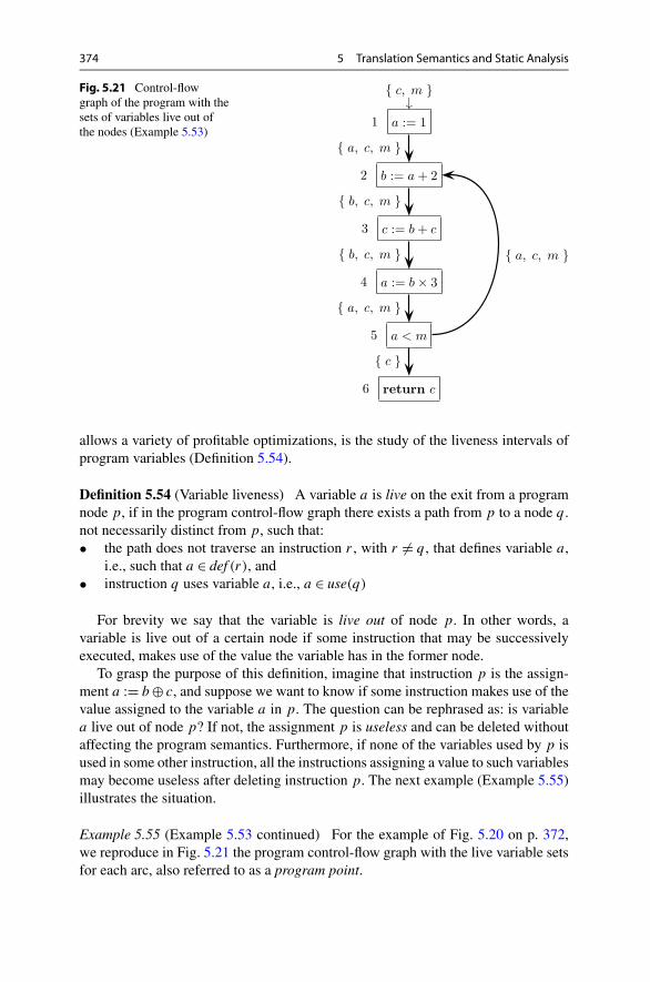
374 5 Translation Semantics and Static Analysis
Fig. 5.21 Control-flowgraph of the program with thesets of variables live out ofthe nodes (Example 5.53)
allows a variety of profitable optimizations, is the study of the liveness intervals ofprogram variables (Definition 5.54).
Definition 5.54 (Variable liveness) A variable a is live on the exit from a programnode p, if in the program control-flow graph there exists a path from p to a node q .not necessarily distinct from p, such that:• the path does not traverse an instruction r , with r �= q , that defines variable a,
i.e., such that a ∈ def (r), and• instruction q uses variable a, i.e., a ∈ use(q)
For brevity we say that the variable is live out of node p. In other words, avariable is live out of a certain node if some instruction that may be successivelyexecuted, makes use of the value the variable has in the former node.
To grasp the purpose of this definition, imagine that instruction p is the assign-ment a := b⊕ c, and suppose we want to know if some instruction makes use of thevalue assigned to the variable a in p. The question can be rephrased as: is variablea live out of node p? If not, the assignment p is useless and can be deleted withoutaffecting the program semantics. Furthermore, if none of the variables used by p isused in some other instruction, all the instructions assigning a value to such variablesmay become useless after deleting instruction p. The next example (Example 5.55)illustrates the situation.
Example 5.55 (Example 5.53 continued) For the example of Fig. 5.20 on p. 372,we reproduce in Fig. 5.21 the program control-flow graph with the live variable setsfor each arc, also referred to as a program point.

5.7 Static Program Analysis 375
Observe in the picture the variables that are live in each program point. Thusvariable c is live on the entrance to node 1, because there exists path 123 such thatc ∈ use(3), and neither node 1 nor node 2 defines c.
It is customary to say that variable a is live in the intervals (i.e., paths) 12 and452; it is not live in the intervals 234 and 56, and so on.
More precisely, we say that a variable is live-out for a node, if it is live on anyarc outgoing from the node. Similarly, a variable is live-in for a node, if it is live onsome arc entering the node. For instance, variables {a, c,m} ∪ {c} are live-out fornode 5.
5.7.2.1 Computing Liveness IntervalsLet I be the instruction set. Let D(a)⊆ I and U(a)⊆ I respectively be the sets ofthe instructions that define and use some variable a. For instance, in the running ex-ample (Fig. 5.20, p. 372) it is D(b)= {2} and U(b)= {3,4}. The liveness conditionwill be first expressed in terms of formal language operations, then by means of amore expressive set theoretical notation.
It is not difficult to see that variable a is live-out for node p if, and only if, for thelanguage L(A) accepted by the automaton, the following condition holds: languageL(A) contains a sentence x = upvqw, where u and w are (possibly empty) arbi-trary instruction sequences, p is any instruction, v is a possibly empty instructionsequence not containing a definition of a, and instruction q uses variable a. Theabove conditions are formalized as follows: s
u,w ∈ I ∗ ∧ p ∈ I ∧ v ∈ (I \D(a)
)∗ ∧ q ∈U(a) (5.1)
Observe again that the set difference contains all the instructions that do not definevariable a, whereas instruction q uses a.
The set of all the strings x that meet condition (5.1), denoted as Lp , is a sublan-guage of L(A), i.e., Lp ⊆ L(A). Moreover, language Lp is regular, because it canbe defined by the following intersection:
Lp = L(A)∩Rp (5.2)
where language Rp is regular and is defined by the extended (i.e., with a set differ-ence) regular expression Rp ,
Rp = I ∗p(I \D(a)
)∗U(a)I ∗ (5.3)
Formulas (5.2) and (5.3) prescribe that letter p must be followed by a letter q takenfrom set U(a), and that all the letters (if any) intervening between p and q must notbelong to set D(a).
It follows that in order to decide whether variable a is live out of node p, one hasto check that language Lp is not empty. We know one way of doing it: we constructthe recognizer of language Lp , that is, the product machine for the intersection (5.2),as explained in Chap. 3 on p. 134. If this machine does not contain any path fromthe initial state to a final one, then language Lp is empty.

376 5 Translation Semantics and Static Analysis
Anyway such a procedure is not practical, when taking into account the largedimension of the real programs to be analyzed. Therefore we introduce another spe-cialized method, which not only performs more efficiently, but computes at once allthe live variables in all the program points. The new method systematically exam-ines all the paths from the current program point to some instruction that uses somevariable.
The liveness computation will be expressed as a system of data-flow equations.Consider a node p of a control-flow graph or program A. A first equation expressesthe relation between the variables live-out liveout(p) and those live-in livein(p).A second equation expresses the relation between the variables live-out of a nodeand those live-in for its successors.
We denote by succ(p) the set of the (immediate) successors of node p, and byvar(A) the set of all the variables of program A.
Data-Flow Equations For each final (exit) node p:
liveout(p)= ∅ (5.4)
For any other node p:
livein(p) = use(p)∪ (liveout(p) \ def (p)
)(5.5)
liveout(p) =⋃
∀q∈succ(p)
livein(q) (5.6)
Comments:• In Eq. (5.4) no variable is live out of the (sub)program graph. Here we have dis-
regarded the output parameters (if any) of the subprogram, which are typicallyused after exiting the subprogram and thus can be considered to be live out ofthe final node, though in another subprogram.
• For Eq. (5.5) a variable is live-in for p if it is used in p; or if it is live-out for p
but not defined by p. Consider instruction 4 : a := b× 3 (Fig. 5.20 on p. 372).Out of 4, variables a, m, and c are live, because for each one there exists apath that reaches a use of that variable without traversing a node that defines thesame variable. On entering node 4, the following variables are live: b becauseit is used in 4; c and m because they are live-out for 4 and not defined in 4. Onthe contrary, variable a is not live-in for 4 because it is defined in 4, though it islive-out for 4.
• For Eq. (5.6), node 5 has successors 2 and 6; then the variables live-out for 5are those (namely, a, c and m) live-in for 2 and the one (namely, c) live-in for 6.
5.7.2.2 Solution of Data-Flow EquationsGiven a control-flow graph, it is straightforward to write the two Eqs. (5.5) and (5.6)for each instruction. For a graph with |I | = n ≥ 1 nodes, the resulting system has2× n equations with 2× n unknowns, i.e., livein(p) and liveout(p) for each instruc-tion p ∈ I . Each unknown is a set of variables and the solution to be computed is apair of vectors, each one containing n sets.

5.7 Static Program Analysis 377
To solve the equation system we use iteration, by taking the empty set as theinitial approximation (with i = 0) for every unknown:
∀p ∈ I : livein(p)= ∅ liveout(p)= ∅
Let i ≥ 0 be the current iteration. In each equation of the system (5.5), (5.6), wereplace the unknowns occurring in the right hand sides with the values of the cur-rent iteration, and thus we obtain the values of the next iteration i + 1. If at leastone unknown differs from the previous iteration, then we execute one more itera-tion; otherwise we terminate and the last vector pair computed is a solution of theequation system.
This solution is termed the least fixed point of the transformation that computesa new vector from the one of the preceding iteration.
To see why a finite number of iterations always suffices to converge to the leastfixed point solution, observe the following:• the cardinality of every set livein(p) and liveout(p) is bounded by the number of
program variables• every iteration may only add some variables to some sets or leave them un-
changed, but it never removes any variable from a set; in other words, the trans-formation is monotonic nondecreasing with respect to set inclusion
• if an iteration does not change any set, the algorithm terminatesWe illustrate the algorithm (Example 5.56) on the running example.
Example 5.56 (Running example (Example 5.53) continued: iterative computationof live variables) First we compute by inspection the sets of instructions that define(D) and use (U ) program variables:
Var. D U
a 1, 4 2, 5b 2 3, 4c 3 3, 6m ∅ 5
Next the equations for the program (Fig. 5.20 on p. 372) are written in Table 5.10.The names of the unknowns are shortened to in(p) and out(p) instead of livein(p)
and liveout(p), respectively.Then we compute and tabulate the successive approximations, starting from the
empty sets; at each iteration we first compute the in values and then the out values.The least fixed point is reached after five iterations: it would be easy to verify thatone more iteration would not change the last result.
It is important to note that the convergence speed to the fixed point is very sen-sitive to the order, although the solution does not depend on the processing order ofnodes.

378 5 Translation Semantics and Static Analysis
Table 5.10 Liveness equations of the program in Fig. 5.20 (Example 5.56)
Equations
1 in(1)= out(1) \ {a} out(1)= in(2)
2 in(2)= {a} ∪ (out(2) \ {b}) out(2)= in(3)
3 in(3)= {b, c} ∪ (out(3) \ {c}) out(3)= in(4)
4 in(4)= {b} ∪ (out(4) \ {a}) out(4)= in(5)
5 in(5)= {a,m} ∪ out(5) out(5)= in(2)∪ in(6)
6 in(6)= {c} out(6)= ∅
Unknowns computed at each iteration
in= out in out in out in out in out in out
1 ∅ ∅ a ∅ a, c c a, c c a, c,m c,m a, c,m
2 ∅ a b, c a, c b, c a, c b, c,m a, c,m b, c,m a, c,m b, c,m
3 ∅ b, c b b, c b,m b, c,m b, c,m b, c,m b, c,m b, c,m b, c,m
4 ∅ b a,m b,m a, c,m b, c,m a, c,m b, c,m a, c,m b, c,m a, c,m
5 ∅ a,m a, c a, c,m a, c a, c,m a, c a, c,m a, c,m a, c,m a, c,m
6 ∅ c ∅ c ∅ c ∅ c ∅ c ∅
We mention the time complexity of the iterative algorithm.33 The worst casecomplexity is O(n4), where n is the number of nodes, i.e., of instructions of thesubprogram. In practice, for many realistic programs the computational complexityis close to linear in time.
5.7.2.3 Application of Liveness AnalysisWe show two classical widespread applications of the previous analysis: memoryallocation for variables and detection of useless instructions.
Memory Allocation Liveness analysis is best applied to decide if two variablescan reside in the same memory cell (or in the same machine register). It is evidentthat if two variables are live in the same program point, both values must be presentin the memory when execution reaches that point, because they may have futureuses. Therefore their values cannot reside in the same cell: we then say the twovariables interfere.
Conversely, if two variables do not interfere, that is, they are never live in thesame program point, then the same memory cell or register can be used to keeptheir values.
Example 5.57 (Interference and register assignment) In the control-flow graph ofFig. 5.21 on p. 374, we see that variables a, c and m occur in the same set livein(2),therefore the three variables pairwise interfere. Similarly, the variable pairs (b, c),
33For a proof refer for instance to any of [3, 4, 10].

5.7 Static Program Analysis 379
Fig. 5.22 Control-flowgraph with live sets applied todetect the useless definitionsin the program(Example 5.58)
(b,m) and (c,m) interfere in the set livein(3). On the other hand, no set containsvariables a and b, which therefore do not interfere.
As stated before, two interfering variables must reside in different memory cells.It follows that each one of variables c and m needs a separate cell, while both vari-ables a and b may reside in the same cell, which has to be different from the previoustwo cells because variable a interferes with c and m. In conclusion we have foundthat three cells suffice to store the values of four program variables.
Current compilers optimally assign registers to program variables by means ofheuristic methods, by relying on the interference relation.
Useless Definitions An instruction defining a variable is useless if the value as-signed to the variable is never used by any instruction. This is tantamount to sayingthat the value is not live-out for the defining instruction. Therefore, to verify that adefinition of variable a by an instruction p is not useless, we have to check whethervariable a is present in the set liveout(p).
The program of Fig. 5.20 on p. 372 does not have any useless definitions, incontrast with the next example (Example 5.58).
Example 5.58 (Useless variable definition) Consider the program in Fig. 5.22. Thepicture lists the live variables in and out of each instruction. Variable c is not live-out for node 3, hence instruction 3 is useless. Useless instructions can be erased bythe compiler. The elimination of instruction 3 brings two benefits: the program isshorter and faster to execute, and variable c disappears from the sets in(1), in(2),in(3) and out(5). This reduces the interferences between variables and may bring areduction in the number of registers needed, which is often a bottleneck for programperformance.

380 5 Translation Semantics and Static Analysis
This is an example of the frequently occurring phenomenon of chain reactionoptimizations triggered by a simple program transformation.
5.7.3 Reaching Definitions
Another basic and widely applied type of static analysis is the search for the variabledefinitions that reach some program point.
To introduce the idea by an application, consider an instruction that assigns aconstant value to variable a. The compiler examines the program to see if the sameconstant can be replaced for the variable in the instructions using a. The benefitof the replacement is manyfold. First, a machine instruction having a constant asoperand (a so-called “immediate” operand) is often faster. Second, substituting witha constant a variable occurring in an expression, may produce an expression whereall the operands are constant. Then the expression value can be computed at compiletime, with no need to generate any machine code for it. Lastly, since the replacementeliminates one or more uses of a, it shortens the liveness intervals and reduces theinterferences between variables; thus the pressure on the processor registers is con-sequently reduced, too.
The above transformation is termed constant propagation. In order to developit, we need a few conceptual definitions, which are also useful for other programoptimizations and verifications.
Consider an instruction p : a := b⊕ c that defines variable a. For brevity, we de-note such a variable definition as ap , while D(a) denotes the set of all the definitionsof the same variable a in the subprogram under analysis. The following definition(Definition 5.59) formalizes the concept.
Definition 5.59 (Reaching definition) We say that the definition of a variable a inan instruction q , i.e., aq , reaches the entrance of an instruction p, if there exists apath from q to p such that it does not traverse a node (distinct from q) that definesvariable a.
When this happens, instruction p may use the value of variable a computed inthe instruction q .
Referring to automaton A, i.e., to the control-flow graph of the subprogram, thecondition above (Definition 5.59) can be restated more precisely as follows. Defi-nition aq reaches instruction p, if language L(A) contains a sentence of the formx = uqvpw, where u and w are (possibly empty) arbitrary instruction sequences,p is any instruction, v is a possibly empty instruction sequence not containing anydefinition of a, and instruction q defines variable a. The above conditions are for-malized in this way:
u,w ∈ I ∗ ∧ q ∈D(a)∧ v ∈ (I \D(a)
)∗ ∧ p ∈ I (5.7)
Notice that the instructions p and q may coincide.

5.7 Static Program Analysis 381
Fig. 5.23 Control-flowgraph with reachingdefinitions (Example 5.60)
Looking again at the program reproduced in Fig. 5.23 (identical to the one onp. 372), we find that definition a1 reaches the entrance of instructions 2, 3 and 4, butnot the entrance of instruction 5. Definition a4 reaches the entrance of instructions5, 6, 2, 3 and 4.
Data-Flow Equations for Reaching Definitions To compute the reaching defi-nitions in all the program points, we set up a system of equations similar to thosefor liveness analysis.
If node p defines variable a, we say that any other definition aq of the samevariable in another node q , with q �= p, is suppressed by p. Formally, the set ofdefinitions suppressed by instruction p is the following:
⎧⎪⎨
⎪⎩
sup(p)= {aq | q ∈ I ∧ q �= p∧
a ∈ def (q)∧ a ∈ def (p)}
if def (p) �= ∅sup(p)= ∅ if def (p)= ∅
Notice the set def (p) may contain more than one name, in the case of the instruc-tions that define multiple variables, such as the statement read(a, b, c).
The sets of definitions reaching the entrance to and exit from a node p are de-noted as in(p) and out(p), respectively. The set of the (immediate) predecessornodes of p is denoted as pred(p).
Data-Flow Equations For the initial node 1:
in(1)= ∅ (5.8)

382 5 Translation Semantics and Static Analysis
Table 5.11 Data-flowequations for the reachingdefinitions in the program(Example 5.60 in Fig. 5.23)
in(1)= {c?,m?}out(1)= {a1} ∪
(in(1) \ {a4}
)
in(2)= out(1)∪ out(5)
out(2)= {b2} ∪(in(2) \ ∅)= {b2} ∪ in(2)
in(3)= out(2)
out(3)= {c3} ∪(in(3) \ {c?}
)
in(4)= out(3)
out(4)= {a4} ∪(in(4) \ {a1}
)
in(5)= out(4)
out(5)= ∅∪ (in(5) \ ∅)= in(5)
in(6)= out(5)
out(6)= ∅∪ (in(6) \ ∅)= in(6)
For any other node p ∈ I :
out(p) = def (p)∪ (in(p) \ sup(p)
)(5.9)
in(p) =⋃
∀q∈pred(p)
out(q) (5.10)
Comments:• Equation (5.8) assumes for simplicity that no variables are passed as input pa-
rameters to the subprogram. Otherwise, more accurately, set in(1) should con-tain all the definitions, external to the subprogram, of the input parameters.
• Equation (5.9) inserts into the exit from p all the local definitions of p and thedefinitions reaching the entrance to p, provided the latter are not suppressedby p.
• Equation (5.10) states that any definition reaching the exit of some predecessornode, reaches also the entrance to p.
Similar to the liveness equations, the reaching definition system can be solved byiteration until the computed solution converges to the first fixed point. In the startingiteration all the unknown sets are empty.
We illustrate the situation in the next example (Example 5.60) with a programcontaining a loop.
Example 5.60 (Reaching definitions) Observe in Fig. 5.23 the same programcontrol-flow graph of p. 372, with the reaching definition sets computed by solv-ing the equation system listed in Table 5.11.
Variables c and m are the input parameters of the subprogram, and we may as-sume they are externally defined in the calling subprogram at some unknown pointsdenoted c? and m?.
For instance, notice that the external definition c? of variable c does not reach theentrance of instruction 4, since it is suppressed by instruction 3.

5.7 Static Program Analysis 383
We list the constant terms occurring in the equations:
Node Instruction def sup
1 a := 1 a1 a4
2 b := a + 2 b2 ∅3 c := b+ c c3 c?
4 a := b× 3 a4 a1
5 a < m ∅ ∅6 return c ∅ ∅
At iteration 0 all the sets are empty. After a few iterations, the unknown valuesconverge to the sets shown in Table 5.11.
5.7.3.1 Constant PropagationCarrying further the previous example (Example 5.60 and Fig. 5.23), we look foropportunities to replace a variable by a constant value. An instance of the problemis the question: can we replace the variable a in the instruction 2 with the constant 1assigned by instruction 1 (i.e., definition a1)? The answer is negative because theset in(2) of reaching definitions contains another definition of a, namely a4, whichimplies that some computation may use for a the value defined in the instruction 4.Therefore the program containing instruction b := 1+2 instead of b := a+2, wouldnot be equivalent to the original one, which is quite evident since a run can executethe loop body.
Generalizing this reasoning, it is easy to state a condition: in the instruction p, itis legal to replace with a constant k a variable a used in p, if the following conditionshold:1. there exists an instruction q : a := k that assigns constant k to variable a, such
that definition aq reaches the entrance of p, and2. no other definition ar of variable a reaches the entrance of p, with r �= q
In the next example (Example 5.61), we show some program improvements pro-duced by a constant propagation and by the induced simplifications.
Example 5.61 (Optimization following constant propagation) Figure 5.24 showsa simple program control-flow graph, and lists the reaching definition sets and thelive variable sets in the relevant points of the program. Observe that the only defini-tion of variable v reaching the entrance of node 2 is v1. By the previous condition,it is legal to replace variable v with constant 4 in the conditional instruction 2,which afterwards becomes the constant boolean expression 4 × 8 ≥ 0. Now vari-able v ceases to be live-out for assignment 1, which becomes useless and can bedeleted.
But program simplification does not end here. The compiler can compute thevalue of the constant expression34 8× 4 = 32 ≥ 0 = true, thus determining whichone of the successor legs of statement 2 will be taken, say the one to the left. Then
34Anticipating a computation to compile time is termed constant folding.
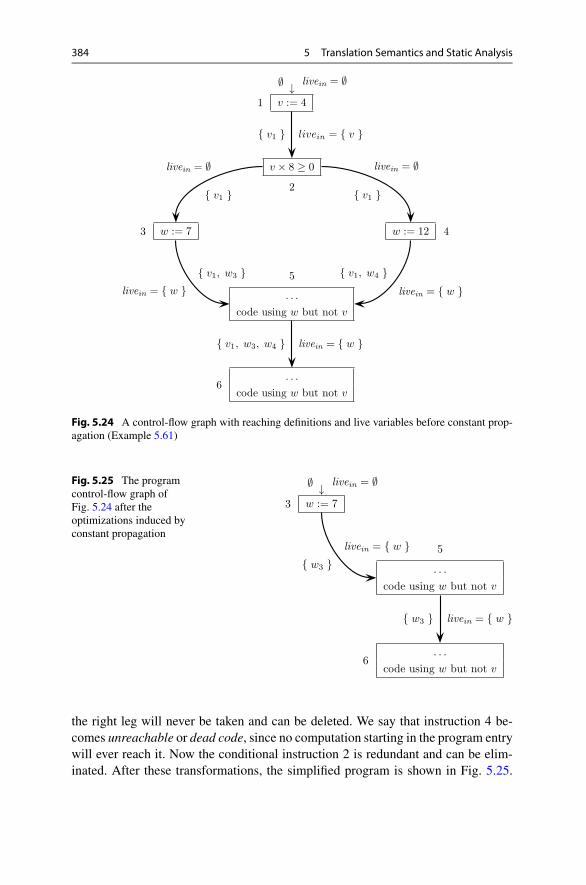
384 5 Translation Semantics and Static Analysis
Fig. 5.24 A control-flow graph with reaching definitions and live variables before constant prop-agation (Example 5.61)
Fig. 5.25 The programcontrol-flow graph ofFig. 5.24 after theoptimizations induced byconstant propagation
the right leg will never be taken and can be deleted. We say that instruction 4 be-comes unreachable or dead code, since no computation starting in the program entrywill ever reach it. Now the conditional instruction 2 is redundant and can be elim-inated. After these transformations, the simplified program is shown in Fig. 5.25.

5.7 Static Program Analysis 385
Now the analysis could proceed to determine if constant w = 7 can be legallypropagated to the rest of the program.
5.7.3.2 Availability of Variables and InitializationsA basic correctness check a compiler should perform is to control that the variablesare initialized before their first use. More generally, a variable used in some instruc-tion must, on entrance to the instruction, have a value computed by means of a validassignment (or by another statement type that can define variables). Otherwise wesay that the variable is not available, and a compile-time error occurs.
Coming back to the program control-flow graph of Fig. 5.23 on p. 381, observethat node 3 uses variable c, but on the path 123 no instruction executed before node3 assigns a value to c. This is not necessarily an error: if variable c is an inputparameter of the subprogram, its value is supplied by the subprogram invocationstatement. In such a case, variable c has a value on the entrance to node 3 and noerror occurs. The same discussion applies to variable m.
Variable b is available on the entrance to node 3 because its value was defined innode 2 by an assignment, which uses variable a; the latter is in turn available on theentrance to 2, following the initialization in the node 1.
This sort of reasoning becomes intricate, and we need to clarify the concept ofavailability in the next definition (Definition 5.62). For simplicity we assume thatthe subprogram does not have any input parameters.
Definition 5.62 (Variable availability) A variable a is available on the entrance tonode p, i.e., just before the execution of instruction p, if in the program control-flowgraph every path from the initial node 1 to the entrance of p, contains a statementthat defines variable a.
By comparing this notion with the concept of reaching definition introduced onp. 380, we notice a difference in the quantification over paths. If the definition aq ofvariable a reaches the entrance of node p, there necessarily exists a path from node 1to node p that traverses the defining instruction q . But this does not guarantee thatvariable a is available on the entrance to p, because we cannot exclude that thereexists another path from 1 to p, which avoids node q as well as any other node thatdefines variable a.
It follows that the condition of a variable definition being available on a nodeentrance is more constraining than that of the variable definition reaching the samenode.
To compute the variables available on the entrance to node p, let us examinemore closely the set of definitions reaching the exits of the predecessors of p. Iffor every node q that is a predecessor of p, the set of reaching definitions out(q)
on the exit from q contains (at least) one definition of variable a, then variable a
is available on the entrance to p. In that case we also say that some definition of a
always reaches node p.It is simple to convert the latter condition into an effective test that the variables
are correctly initialized. For an instruction q , the new notation out′(q) denotes, asout(q) did, the set of the variable definitions reaching the exit from q , but with

386 5 Translation Semantics and Static Analysis
Fig. 5.26 Control-flowgraph with the availablevariables for Example 5.63
their subscripts deleted. For instance, for out(q)= {a1, a4, b3, c6}we have out′(q)={a, b, c}.Badly Initialized Variables An instruction p is not well initialized if the follow-ing predicate holds:
∃q ∈ pred(p) such that use(p) � out′(q) (5.11)
The condition says that there exists a node q predecessor of p, such that the set ofdefinitions reaching its exit does not include all the variables used in p. Therefore,when the program execution runs on a path through q , one or more variables usedin p do not have a value. The next example (Example 5.63) illustrates the situation.
Example 5.63 (Detecting uninitialized variables) Observe the program control-flow graph in Fig. 5.26, completed with the sets of reaching definitions.
Condition (5.11) is false in the node 2, since for every predecessor (nodes 1and 4) the set out′ contains a definition of a, which is the only variable used in 2. Onthe other hand, the condition is true in the node 3 because no definition of variable c
reaches the exit from 2. Our analysis has thus detected a program error: instruction 3uses an uninitialized variable, namely c.
To find all the remaining initialization errors, we can proceed as follows. Wereplace any erroneous instructions discovered so far, such as node 3, by a dummyno-operation instruction. Then we update the computation of the reaching definitionsets and we evaluate condition (5.11) again. By so doing, we would discover thatinstruction 4 is not well initialized because definition b3 is not really available, al-though it is present in the set out(3), because instruction 3 has already been markedas ineffective. Then also instruction 4 becomes ineffective. Continuing in the samemanner, no other errors would be discovered.
The previous analysis allows to catch at compile time many errors that had goneunnoticed during the preceding phases of parsing and semantic analysis, with thebenefit that they will not cause hard-to-understand runtime errors or raise exceptionsduring program execution.

References 387
To conclude, static analysis35 encompasses many more conditions and propertiesthan the cases of liveness and reaching definitions we have been able to present. Itis a powerful general method for analyzing programs before execution, in order tooptimize them or to verify their correctness.
References
1. A. Aho, J. Ullman, The Theory of Parsing, Translation, and Compiling, vol. 1: Parsing(Prentice-Hall, Englewood Cliffs, 1972)
2. A. Aho, J. Ullman, The Theory of Parsing, Translation and Compiling, vol. 2: Compiling(Prentice-Hall, Englewood Cliffs, 1973)
3. A. Aho, M. Lam, R. Sethi, J. Ullman, Compilers: Principles, Techniques and Tools(Prentice-Hall, Englewood Cliffs, 2006)
4. A. Appel, Modern Compiler Implementation in Java (Cambridge University Press, Cam-bridge, 2002)
5. J. Berstel, Transductions and Context-Free Languages (Teubner, Stuttgart, 1979)6. S. Crespi Reghizzi, G. Psaila, Grammar partitioning and modular deterministic parsing.
Comput. Lang. 24(4), 197–227 (1998)7. J. Engelfriet, Attribute grammars: attribute evaluation methods, in Methods and Tools for
Compiler Construction, ed. by B. Lorho (Cambridge University Press, Cambridge, 1984),pp. 103–138
8. D.E. Knuth, Semantics of context-free languages. Math. Syst. Theory 2(2), 127–145 (1968)9. D.E. Knuth, Semantics of context-free languages (errata corrige). Math. Syst. Theory 5(2),
95–99 (1971)10. S. Muchnick, Advanced Compiler Design and Implementation (Morgan Kaufmann, San Ma-
teo, 1997)11. F. Nielson, H. Nielson, C. Hankin, Principles of Program Analysis (Springer, New York,
2005)12. J. Sakarovich, Elements of Automata Theory (Cambridge University Press, Cambridge,
2009)13. R.D. Tennent, Semantics of Programming Languages (Prentice-Hall, Englewood Cliffs,
1991)14. G. Winskel, The Formal Semantics of Programming Languages (MIT Press, Cambridge,
1993)15. W. Yang, Mealy machines are a better model of lexical analyzers. Comput. Lang. 22, 27–38
(1996)
35A book on the theory of static program analysis is [11]. For a survey of applications in compila-tion, see, e.g., [3, 4, 10].

Index
Symbols2I-automaton, 323, 324ε move, 105
AA-condition for attribute evaluation, 359Abstract syntax tree, 303, 335Acceptance
by empty stack, 144with final state, 148
Accepting mode of pushdown machine, 149Accessible
state, 99, 177subsets, 115
Acyclic attribute grammar, 345, 347Acyclicity test, 347Algol 60, 52Algorithm
Berry and Sethi, 129bottom-up parser construction, see ELR(1)
parser constructioncomposition of local automata, 124conversion of translation grammar to
postfix form, 316deterministic automaton from a regular
expression construction, 127determinization of finite automaton, 131Earley parser, 253ELR(1) parser construction, 190
pointerless, 222with vector stack, 202
finite automaton complementation, 132finite automaton determinization, see
Powerset constructionfrom grammar to nondeterministic
pushdown automaton, 143from regular expression to deterministic
finite automaton, see Berry andSethi algorithm
from regular expression to grammar, 67local recognizer construction, 122
merge of kernel-equivalent m-states, 219one-sweep evaluator construction, 349operator precedence parallel parser
construction, 281operator precedence sequential parser
construction, 275pilot graph construction, 183powerset construction, 117predictive parser construction
as DPDA, 237by recursive procedures, 238
predictive pushdown transducerconstruction, 308
spontaneous move elimination, 115syntax tree construction, 262top-down parser construction, see
Predictive parser constructiontopological sorting, 346
Alphabet, 7unary, 75
Alphabetic homomorphism, 79, 298Alternative, 18, 31Ambiguity, 45
conditional instruction, 52, 301, 305degree, 46EBNF, 85inherent, 53, 119, 160of automaton, 111, 160of bilateral recursion, 47of circular derivation, 304of concatenation, 49of regular expression, 21, 68of translation, 304of union, 48source grammar, 305versus nondeterminism, 160
ANTLR, 242, 248Aperiodic language, 136Arden identity, 72Arithmetic expression, 38, 39, 45, 48, 54, 55,
59, 85, 311
S. Crespi Reghizzi et al., Formal Languages and Compilation,Texts in Computer Science, DOI 10.1007/978-1-4471-5514-0,© Springer-Verlag London 2013
389

390 Index
Arithmetic expression (cont.)calculating machine, 358machine net, 167parenthesis-free, 70polish, 302syntax chart, 169
Artificial language, 5Attribute, 334, 336
inherited, see Right attributeleft, see Left attributelexical, see Lexical attributeright, see Right attributesynthesized, see Left attribute
Attribute grammar, 335, 360A-condition, 359acyclic, 345applications, 360definition, 341L condition, 354multi-sweep, 351, 367one-sweep, 348
Attribute subgrammar, 351Automaton
ambiguous, 111, 160clean, 99configuration, 94equivalent, 95finite, 96finite deterministic, 97for local language, 122from regular expression, 119, 121generalized, 113local, 122
normalized, 123minimization, 101nondeterministic, 107product, 134to regular expression, 112two-way, 331unidirectional, 94with spontaneous moves, 109
Available variables, 385Axiom, 30, 31
BBack-end compiler, 365Base of macro-state, 183Berry, 129Berry and Sethi, 129
algorithm, 130Berstel, 121, 295Binary operator, 301Block structure, 29BMC, 112
BNF grammar, 31, 206Bottom-up
attribute evaluation, 359deterministic translation, 313parser with attribute evaluator, 357syntax analysis, 163
Brzozowski and McCluskey, 112BS, see Berry and SethiBT, 261BuildTree, 261
CCancellation rule of Dyck, 42Candidate, 174
identifier, 190Cardinality of language, 8Cartesian product of automata, 134CF family, 68, 74, 78, 81, 83, 151
closure properties, 44Choice of a regular expression, 19Chomsky
hierarchy, 33, 86normal form, 33, 61
Circular derivation, 36, 304Clean automaton, 99, 373Cleaning
of automaton, 99of grammar, 35
Cleaveland, 89Closing mark, 25Closure
function, 174in Earley parser, 250of macro-state, 183
Closure propertiesof CF, 44, 78of CF and REG, 78of DET, 155of REG, 23under substitution, 81under translation, 332under transliteration, 81
Code generation, 364Codes and ambiguity, 50Coke–Younger–Kasami algorithm, 247Compaction of pilot, 218Compiler
decomposition, 351language, 334
Complementautomaton, 132of language, 13of regular language, 132
Completion in Earley parser, 251

Index 391
Computation, 94, 107, 147label, 98, 107length, 107of nondeterministic automaton, 107
Concatenation, 9of context-free languages, 44, 78of Dyck languages, 50of languages, 12
Condensed skeleton tree, 40Conditional instruction, 52, 301, 305
ambiguity, 52, 301, 305Configuration of an automaton, 94, 143, 147Conflict
convergence, 182reduce–reduce, 182shift–reduce, 182
Conservative approximation, 373Constant
folding, 383propagation, 380, 383
Context-dependent language, 86Context-free
deterministic, 155grammar
definition, 31from pushdown automaton, 151introduction, 29
translation, 299Context-sensitive language, 86Control instruction translation, 365Control-flow graph, 370, 371
automaton, 371language, 371
Convergence conflict, 182, 184, 186Convergent transitions, 184Copy rule, 57Copy-free normal form, 57Cross operation, 16
DDart, 232Data-flow equations, 376, 381
liveness, 376reaching definitions, 381solution, 376
Dead code, 384Decidable language, 95Decimal constant, 96, 99, 109, 111Decision algorithm, 92Decompiler, 297Decorated tree, 337, 339Degree of operator, 301Dependence graph, 339, 343, 348
of decorated tree, 339, 345
of semantic function, 343Derivation, 33
circular, 36EBNF, 84left, 41of regular expression, 20right, 41self-nested, 74
DET family, 155, 244Deterministic
finite automaton, 97language, 155
unambiguity, 159language families comparison, 242pushdown automaton, 155
subclasses, 160simple grammar, 161
Determinization of automaton, 114, 130Dictionary, 8Difference of languages, 13Digrams, 121Distance of strings, 286Distinctly parenthesized grammar, 43, 162Distinguishability of states, 101Document type definition, 162Double service lemma, 158DTD, 162Dyck
cancellation rule, 42language, 42, 69, 79
concatenation, 50Dynamic error, 364
EEarley
algorithm, 248, 252closure, 250introductory example, 249nonterminal shift, 251parser, 252
completeness, 257completion algorithm, 252computational complexity, 259correctness, 257function BuildTree, 262grammar ambiguity, 268grammar unambiguity, 260nullable nonterminals, 265optimization, 260syntax analysis algorithm, 253syntax tree construction, 261syntax tree construction complexity,
266terminal shift algorithm, 253

392 Index
Earley (cont.)vector, 252
terminal shift, 250vector, 252
Early scanning, 207EBNF grammar, 82, 165
ambiguity, 85derivation, 84translation, 313
Editing distance, 286ELL(1)
condition, 214direct, 233violation, 236
parserdirect construction, 231step by step construction, 217
parsing, 211PCFG, 226violation remedy, 246
ELL(k)
condition, 240parser, 242
ELR(1)condition, 185grammar, 245language, 245parser
pointerless, 222vector-stack, 201
parser construction, 183ELR(k)
grammar, 245language, 245relation with ELR(1), 245
Empty string, 9Encryption, 298End mark, 305Engelfriet, 351Environment, 361Epsilon move, 105Equations of unilinear grammar, 71, 72Equivalence
of finite automata, 98, 103of grammars
generalized structural, 56strong, 55weak, 55
Equivalent regular expressions, 21Error
dynamic, 284objective, 284recovery, 286, 287
panic mode, 287panic mode with token insertion, 288
semantic, 285state, 98static, 284subjective, 284syntactic, 285treatment, 284type, 284
Expansion of nonterminal, 56Extended regular expression, 132, 135External attribute, 342
FFIN family, 19Finals, 121Finite
automaton, 96deterministic, 97left-linear grammar, 112
transducer, 328, 329opposite passes, 331with look-ahead, 332
Finite-state family, 109Flex, 332Floyd, 158
Operator Precedence languages, 274Follow set, see Set of followersFollowers, see Set of followersFormal language, 5Free monoid, 14Front-end compiler, 364
GGeneral
automaton, 93parser, 248
Generalized automaton, 113Goal-oriented, see PredictiveGrammar
ambiguity, 46ambiguity from ambiguous r.e., 68attribute, 335BNF, 31, 206Chomsky classification, 86clean, 35cleaning, 35context-free, 29context-sensitive, 86EBNF, 82, 165equivalent, 35errors, 35extended context-free, 82, 165homogeneous, 33, 64

Index 393
Grammar (cont.)invertible, 59left-linear, 69linear, 68marked BNF grammar rule, 169normal form, 33, 56not left-recursive, 63of regular language, 67of Van Wijngarten, 89operator, 62parenthesized, 43, 161representations, 32right linearized, 171right-linear, 69, 103simple deterministic, 161, 242strictly unilinear, 70target, 299translation, 298, 307type 0, 86type 1, 86type 2, 86type 3, 69, 86unilinear, 69
Graphcontext-sensitive, 87dependence, 339local automaton, 122parser control-flow, 226pilot, 183program control-flow, 370reachability, 36sibling, 348state-transition, 96syntax chart, 169syntax tree, 38
Greibach normal form, 33, 65, 152Guide
predicate, 367set, 227, 232
HHandle, 176, 190Hierarchical list, 27Hierarchy of Chomsky, 86Homomorphism
alphabetic, 79nonalphabetical, 80
IIncremental
compilation, 289parser, 289
Infix operator, 301Inherent ambiguity, 53, 119, 160
Inherited attribute, see Right attributeInitial of a string, 10Initial state uniqueness, 109Initials, see Set of initialsInstruction scheduling, 370Interference between variables, 378Intermediate
language, 364representation, 364, 370
Internal attribute, 342Interprocedural static analysis, 370Intersection
of context-free and regular language, 153of context-free languages, 79of regular languages, 133, 134
Intraprocedural static analysis, 370Inverse translation, 296Invertible grammar, 59IO-automaton, 328
sequential, 329Item, see Candidate
JJavaScript Object Notation, 272JFLAP, 152JSON, 272Jumps, 365
KKernel
equivalent macro-states, 184of macro-state, 183
Knuth, 176, 197, 211, 244
LL condition for attribute evaluation, 354Language, 8
abstraction, 24artificial, 5complement, 13context free, 29, 86, 151context sensitive, 87context-free, 35context-sensitive, 86decidable, 95Dyck, 42empty, 8equation, 71finite, 8formal, 5formalized, 5generated, 34infinite, 8
recursive derivations, 37local, 122

394 Index
Language (cont.)locally testable, 122nullable, 10recursive, 95recursively enumerable, 95regular, 19replica, 77
with center, 88source, 296substitution of, 26target, 81, 296unary alphabet, 75universal, 13with three equal powers, 76, 87with two equal powers, 73
Least fixed point, 377Left
attribute, 338, 341derivation, 41quotient, 17, 210recursive grammar
top-down parsing, 214recursive rule, 63
elimination, 63Left-linear grammar, 69, 112Left-recursion, 33
elimination, 65immediate, 64LR(1), 211nonimmediate, 64
Left/right terminal set, 270Leftmost derivation, see Left derivationLength of string, 8Levenshtein distance, 286Lex, 332Lexeme, 352Lexical
analysis, 352attribute, 342, 353, 354class, 352, 353
closed and open, 353finite and non-, 353
level, 352segmentation, 353
Lineargrammar, 68language equation, 71regular expression, 124
Linguistic abstraction, 24List
abstract, 25concrete, 25hierarchical, 27with precedence, 27
with separators, 25Live variable, 374, 383Live-in, 375Live-out, 375Liveness, 374, 376, 378
equations, 376interval, 373, 375
LL(1)grammar, 242relation with LR(1), 243
LL(2) example, 240LL(k)
grammar, 244relation with LR(k), 244
Localautomaton, 123
normalized, 123language, 122, 136, 372
automaton, 122composition of, 123
set, 125regular expression, 125
testability, 122Locally testable language, 136Longest prefix rule, 353Look-ahead
extending, 205increasing, 240set, 174
LR(1)family, 244grammar, 244grammar transformation, 205, 208parser
relation with ELR(1), 197superflous features, 201
relation with DET, 244LR(2) to LR(1), 207, 208LR(k)
early scanning, 207grammar, 206left quotient, 210transformation, 211
Lukasiewicz, 302
MM-state, see Macro-stateMachine net, 165Macro-state, 182
base, 183closure, 183kernel, 183
Marked BNF grammar rule, 169, 207, 208McNaughton, 137

Index 395
Meaning, 334Memory allocation, 378Metagrammar, 31Metalanguage of regular expression, 30Minimal automaton, 100Minimization of automaton, 101Mirror reflection, 10Mixfix operator, 301Multi-sweep semantic evaluator, 351Multiple transition property, 184
NNerode relation, 101Nested structure, 29Network of finite machines, 165Nivat theorem, 326Non-deterministic
union, 158Non-LR(k), 211Noncounting language, 136Nondeterminism motivation, 105Nondeterministic
automaton conversion to deterministic,114, 130
finite automaton, 104, 107, 109pushdown automaton, 143, 144
Nonnullable normal form, 57Nonterminal, 30
alphabet, 31expansion, 56shift, 179
in Earley parser, 251Normal form
Chomsky, 61copy-free, 57Greibach, 65nonnullable, 57real-time, 65without repeated right parts, 59
Normalized local automaton, 123Not left-recursive grammar, 63Nullable
language, 10nonterminal, 57regular expression, 126
Numbered regular expression, 126
OOAG, 351On line machine, 150One-sweep
attribute evaluation, 347attribute grammar, 348semantic evaluator construction, 349
Opening mark, 25Operator
binary, 301degree, 301infix, 301mixfix, 301postfix, 301prefix, 301unary, 301variadic, 301
Operator grammar, 62normal form, 33, 62
Operator precedencegrammar, 269languages, 274relation, 269, 271sequential parser, 275
Opposite passes, 331Optimization of program, 295, 370, 379, 383
PPalindrome, 30, 43, 162, 300
nondeterminism, 159pushdown machine, 148
Panic mode error recovery, 287Papert, 137Parallel parser, 268, 281Parenthesis
language, 41, 161redundant, 304
Parenthesizedexpression, 40grammar, 43, 161tree, 40, 261
Parser, 162choice criteria, 246Coke–Younger–Kasami, 247Earley, 252general, 248local, 268, 269parallel, 268, 277, 281predictive, 236, 237recursive descent, 238, 239semantics-directed, 248, 366top-down and bottom-up, 163top-down deterministic, 237with attribute evaluation, 352with attribute evaluator, 355with translation, 311
Parser control-flow graph, 226direct construction, 232
PCFG, 218, 226direct construction, 232

396 Index
Pilotcompaction, 218construction, 183graph, 183machine of translator, 314
Pin, 121PLZ-SYS, 367Pointerless ELR(1) parser, 222Polish notation, 48, 300, 302Portability of compiler, 364Postaccessible state, 99Postfix
normal form, 315operator, 301
Powerof language, 12of string, 10
Powerset construction, 117Precedence
of operators, 11relation, 269
Prediction in Earley parser, 250Predictive
parser, 236direct construction, 231
parser automaton, 237pushdown automaton, 143pushdown transducer, 308
Prefix, 10operator, 301
Prefix-free language, 11Product
machine, 134of automata, 134
Production, 31Program
analysis, 369optimization, 295, 370, 379, 383
Projection, 80Prospect set, 226, 232Pumping property, 73Pure syntactic translation, 298Pushdown automaton, 95, 142, 143, 146, 151
accepting modes, 149conversion to grammar, 151definition, 146determinism, 155deterministic subclasses, 160forms of non-determinism, 155time complexity, 146
Pushdown IO-automaton, 305Pushdown transducer, 305, 307, 310
from translation grammar, 307nondeterministic, 310
QQuotient
of grammars, 210of languages, 16
RRabin and Scott, 323
machine, 323Rational translation, see Regular translationReachable
nonterminal, 35state, 99
Reaching definition, 380, 383always, 385
Real-time normal form, 65Recognition algorithm, 92Recognize, see AcceptRecursion bilateral, 47Recursive
derivation, 37descent, 354
parser, 213, 238, 239parser with attributes, 354translator, 311
machine net, 165semantic evaluator, 350
Reduce move, 176Reduce–reduce conflict, 182, 185, 206Reduce–shift conflict, see Shift–reduce
conflictReflection, 10
of context-free language, 45, 78of language, 11recognizer of, 106
REG family, 19, 68, 74, 78, 82closure properties, 23included in CF, 68
Register assignment, 378Regular expression, 17
ambiguity, 21, 68, 69extended, 22, 135from automaton, 112language defined, 21linear, 124metalanguage, 30nullability, 126numbered, 22, 126Thompson method, 119with complement, 132with intersection, 132
Regular expression to automaton, 119Berry and Sethi, 129structural method, 119Thompson, 119

Index 397
Regular language, 19intersection, 133pumping property, 73
Regular translation, 321expression, 323
Repeated right parts, 59Replica, 77, 88Reps, 338Retargeting, 364Reversal as translation, 299Right
attribute, 338, 340, 341, 357derivation, 41
Right-linear grammar, 69, 103Right-linearized grammar, 200, 237Right-recursion, 33
LR(1), 211Rightmost derivation, see Right derivationRoger, 152Rule
Chomsky normal, 33copy, 33, 57empty, 33Greibach normal, 33homogeneous, 33homogeneous binary, 61left-linear, 33left-recursive, 33linear, 33recursive, 33right-linear, 33right-recursive, 33subcategorization, 33terminal, 33with operators, 33
Run-time error, 364
SSakarovich, 113, 134, 295Scan in Earley parser, 250Scanner, 352Scheduling of instructions, 370Searching a text for a word, 107Self-nested derivation, 74Self-nesting, 42Semantic
analysis, 335attribute, 334, 338
lexical, 353check, 361error, 361evaluator, 335, 347
multi-sweep, 351one-sweep, 347
recursive, 350function, 336, 341interpretation, 55metalanguage, 334, 341predicate, 361procedure, 350rule, 336translation, 333
Semantics, 5, 293, 333, 334Semantics-directed parser, 248, 366Sentence, 8
ambiguous, 21Sentential form, 34Sequential
function, 330transducer, 329
Setof followers, 129, 173of initials, 121, 174
Set operations, 13Sethi, 129Shift
move, 176terminal or nonterminal, 182
Shift–reduceconflict, 182, 185, 208parser with attribute evaluator, 357translator, 313
Sibling graph, 348Simple deterministic grammar, 161, 242Single-transition property, 214, 218Single-valued translation, 305Sink state, see Trap stateSkeleton tree, 40
condensed, 40Sms, 190Source
grammar, 299ambiguity, 305
language, 296Spontaneous loop in pushdown machine, 150Spontaneous move, 105, 109, 147
elimination, 114, 115Stack
candidate, 190m-state, 190macro-state, 190
Starof context-free language, 44, 78operation, 14properties, 15
Star-free language, 136State
accessible, 99

398 Index
State (cont.)distinguishable, 100postaccessible, 99reachable, 99trap, 98useful, 99useless, 99
State-transition diagram, 96pushdown machine, 148
Static error, 361Static program analysis, 364, 369, 387
interprocedural, 370intraprocedural, 370
STP, see Single-transition propertyStrictly unilinear grammar, 70String, 8
empty, 9String form, 34Strong equivalence of grammars, 55Structural adequacy, 55, 70Subcategorization rule, 57Subjacent automaton, 325, 328, 330, 332
pushdown, 306Substitution, 26, 81
closure property, 81Substring, 10Suffix, 10Symbol table, 285, 361Syntactic
analysis, 162error, 285level, 352procedure, 212, 238semantic analyzer, 355support, 336, 341translation, 298translation scheme, 299
Syntactic-semantic analysis, 352Syntax, 5
abstract, 24analysis, 162
bottom-up and top-down, 163chart, 169, 372tree, 38
abstract, 303, 335as translation, 319
Syntax-directedcompiler, 334translation, 121, 299, 334
Synthesized attribute, see Left attribute
TTarget
grammar, 299
language, 81, 296Terminal
alphabet, 31shift in Earley parser, 250symbol, 7
Thompson, 119Token, 352TOL, 349Tomita, 248Top-down
deterministic translation, 311parsing, 211syntax analysis, 163
Topological sort, 346TOR, 349TOS, 349Transition networks, 169Translation
closure properties, 332function, 296, 297, 330
sequential, 330grammar, 298, 307, 327
EBNF, 313postfix normal form, 315rule normalization, 307to pushdown transducer, 307
rational, see Regular translationregular, see Regular translationrelation, 296scheme, 299single-valued, 305syntactic, 298
Translatorbottom-up, 313comparison, 320top-down, 311two-way, 331with recursive procedures, 311
Transliteration, 79, 298to words, 80
Trap state, 98Tree
construction, 261decorated, 337syntax, 38
Tree pattern matching, 364Turing machine, 86, 95Two-input automaton, 323, 324Two-pass compiler, 335Type 0 grammar, 86Type 1 grammar, 86Type 2 grammar, 86Type 3 grammar, 69, 86Type checking, 361

Index 399
UUnary
alphabet, 75operator, 301
Undecidabilitydeterministic context-free language, 245deterministic pushdown automaton, 245LR(k), 245
Undistinguishability of states, 101Unilinear grammar, 69, 110
equations, 71Uninitialized variable, 386Union of context-free languages, 43, 78Universal language, 13, 14Unreachable code, 373, 384Useful state, 99Useless
assignment, 374state, 99
elimination, 99variable definition, 379
Uzgalis, 89
VVan Wijngarten, 89Variable
availability, 385definition, 371
suppressed, 381initialization, 385, 386use, 371
Variadic operator, 301Vector-stack parser, 201Vocabulary, 8VW grammar, 89
WWeak equivalence of grammars, 55Well-defined nonterminal, 35Word, 8
XXML, 42, 162
YYang, 332