STDP Allows Fast Rate-Modulated Coding with Poisson-Like Spike TrainsMatthieu Gilson1,2.*, Timothee Masquelier3.*, Etienne Hugues3

1 Department of Electrical and Electronic Engineering, The University of Melbourne, Melbourne, Australia, 2 Lab for Neural Circuit Theory, Riken Brain Science Insitute,

Wako-shi, Saitama, Japan, 3 Unit for Brain and Cognition, Universitat Pompeu Fabra, Barcelona, Spain

Abstract

Spike timing-dependent plasticity (STDP) has been shown to enable single neurons to detect repeatedly presentedspatiotemporal spike patterns. This holds even when such patterns are embedded in equally dense random spiking activity,that is, in the absence of external reference times such as a stimulus onset. Here we demonstrate, both analytically andnumerically, that STDP can also learn repeating rate-modulated patterns, which have received more experimental evidence,for example, through post-stimulus time histograms (PSTHs). Each input spike train is generated from a rate function using astochastic sampling mechanism, chosen to be an inhomogeneous Poisson process here. Learning is feasible providedsignificant covarying rate modulations occur within the typical timescale of STDP (,10–20 ms) for sufficiently many inputs(,100 among 1000 in our simulations), a condition that is met by many experimental PSTHs. Repeated patternpresentations induce spike-time correlations that are captured by STDP. Despite imprecise input spike times and evenvariable spike counts, a single trained neuron robustly detects the pattern just a few milliseconds after its presentation.Therefore, temporal imprecision and Poisson-like firing variability are not an obstacle to fast temporal coding. STDPprovides an appealing mechanism to learn such rate patterns, which, beyond sensory processing, may also be involved inmany cognitive tasks.

Citation: Gilson M, Masquelier T, Hugues E (2011) STDP Allows Fast Rate-Modulated Coding with Poisson-Like Spike Trains. PLoS Comput Biol 7(10): e1002231.doi:10.1371/journal.pcbi.1002231

Editor: Mark C. W. van Rossum, University of Edinburgh, United Kingdom

Received March 31, 2011; Accepted September 1, 2011; Published October 27, 2011

Copyright: � 2011 Gilson et al. This is an open-access article distributed under the terms of the Creative Commons Attribution License, which permitsunrestricted use, distribution, and reproduction in any medium, provided the original author and source are credited.

Funding: This research was supported by the Fyssen Foundation (TM), the FP7 European Project Coronet (TM), NICTA Victoria Research Lab (MG), The Bionic EarInstitute (MG). TM and EH thank Gustavo Deco for the time granted to complete this project. The funders had no role in study design, data collection and analysis,decision to publish, or preparation of the manuscript.

Competing Interests: The authors have declared that no competing interests exist.

* E-mail: gilsonm@unimelb.edu.au (MG); timothee.masquelier@alum.mit.edu (TM)

. These authors contributed equally to this work.

Introduction

STDP is now a well-established physiological mechanism of

activity-driven synaptic regulation [1], which can capture spiking

information at a short timescale, down to milliseconds [2,3].

Although the relationship between the stimulating input structure

and the resulting weight specialization has been investigated in a

number of theoretical studies [4,5,6,7], most of them have limited

their scope to general and abstract input structures.

A practical and fundamental question is to understand how, in

natural or experimental situations, STDP can participate in the

learning process. Importantly, although repeated stimulus presen-

tations, or task trials, induce memorization (e.g. [8]), the

underlying neural mechanisms remain largely unknown. In this

respect, a recent numerical study showed that a repeating

arbitrary, but reliable, spatiotemporal spike pattern embedded in

equally dense random activity can be learned and robustly

detected by a single neuron equipped with STDP [9]. However,

such reliable spike patterns have received scarce experimental

evidence (but see [10,11,12,13,14,15,16]) and may constitute a

very special case of activity. More generally, and across trials, spike

trains often exhibit large variability, and can be described using an

underlying probabilistic firing intensity, for example through

inhomogeneous Poisson sampling. This hypothesis is tenable with

most – if not all – experimental datasets, where the temporal

spiking probability – or rate – is measured by a post stimulus time

histogram (PSTH) [17]. PSTHs usually exhibit temporal peaks,

whose spread width is of the order of ,10–20 ms in many

experimental findings [18,19,20,21,22,23,24,25,26]. Whether

STDP is able to learn such rate patterns is currently unclear.

Somewhat surprisingly, our study shows that such spread widths

and Poisson-like firing variability are not an obstacle to STDP-

based pattern learning, and fast and efficient detection afterwards.

We consider a single postsynaptic neuron excited by presynaptic

neurons (Fig. 1Schema), of which an arbitrary and hidden number

are involved in the repeating presentation of a given pattern,

embedded in otherwise random spike trains. A main and novel

contribution of this study concerns patterns generated using

covariations of the input instantaneous rates, from which spikes

are generated through an inhomogeneous Poisson process. To

predict the evolution of the synaptic weights and the resulting

neuronal selectivity, we analyze theoretically a dynamical system

that describes the effect of STDP. We confirm these results using

numerical simulations. We demonstrate that repeated presenta-

tions of such rate patterns induce spike-time correlations that are

captured by STDP, even when rate peaks have a width up to 10–

20 ms. In general, STDP favors synapses corresponding to early

spikes in the pattern, resulting in fast response whenever the

pattern is presented [9]. However, when the pattern exhibits sharp

and/or large-amplitude peaks for several inputs, STDP tends to

PLoS Computational Biology | www.ploscompbiol.org 1 October 2011 | Volume 7 | Issue 10 | e1002231

favor some of the corresponding synapses. Besides rate-modulated

patterns, our theory also applies to spike patterns that we therefore

include here for the sake of completeness.

Materials and Methods

We first describe the models of patterned activity used to train

the neuron. Then, we present the models of STDP and Poisson

neuron, which are the basis of the mathematical framework that

describes the weight evolution. We build on our previous

theoretical work where the synaptic dynamics is governed by the

firing rates and spike-time correlations of input spike trains [27].

That framework is adapted to the present situation where spike

trains convey repeating patterns, which allows us to predict the

neuronal specialization in terms of the pattern, STDP and

neuronal parameters.

From spike patterns to rate-modulated patternsRecent work has focused on generating spike trains with a given

correlation structure, using a mixture of spike coordination and

rate covariation [28]. Here these two mechanisms are used to

generate each a class of patterns: spike patterns (model S) and rate-

modulated patterns (model R), the last mimicking PSTH-like

probabilistic spiking activity. Throughout the present paper, we

consider a single pattern that is presented to an unknown subset of

N0 among N excitatory afferent (or input) plastic synapses that

stimulate a single neuron (Fig. 1Schema). The afferents involved

and those not involved in the pattern will be denoted by pattern

and non-pattern afferents, respectively. Pattern presentations

occur randomly with frequency f and duration L, without

overlapping. All pattern models rely on latencies 0ƒtmi ƒL for

each pattern afferent i~1,:::,N0 and m§0. Unless said otherwise

(cf. bimodal patterns below), the latencies tmi are uniformly

distributed in 0,L½ �, i.e., corresponding to a (single) realization of a

homogeneous Poisson process with intensity rate r0 for the

duration L for each input. Once determined these latencies

(possibly none) for all pattern inputs, we generate the input spikes

for each pattern presentation as follows:

N Model S: Spike pattern with fixed latencies. Every latency tmi

induces a spike with probability p at each pattern presentation;

the precise spike time corresponds to the laps tmi after the start

of the presentation. In order to preserve the mean firing rate,

spikes generated using a homogeneous Poisson spike train with

rate (1{p)r0 are added. Fig. 1S1 shows an example with p~1and Fig. 1SD1 an example with p~1=

ffiffiffi2p

(‘D’, standing for

Deletion, is used whenever pv1).

N Model SJ: Spike pattern with Jittered latencies (Fig. 1SJ1). This

model is derived from model S, such that the spike times are

chosen around each latency tmi using a Gaussian-distributed

jitter with spread width smi §0. Simulations will often use a

common value smi ~s. We will only use p~1 in this case.

Fig. 1SJ1 shows an example with s~10 ms.

N Model R: Poisson Rate-modulated pattern (Fig. 1R1). Inho-

mogeneous Poisson sampling is used to generate the spike

times at each presentation. For pattern afferent i, the

corresponding instantaneous rate intensity is generated using

the latencies tmi , each being the center of a Gaussian kernel

function with spread width smi w0 and total area am

i (the

Gaussian peak alone has a maximal height ami

�sm

i

ffiffiffiffiffiffi2pp

). We

will often use a normalized amplitude (ami ~1), such that the

resulting mean firing rate is comparable to patterns of models

S with the same latencies, as well as a common spread width

smi ~s for all spike trains.

For each of the (N{N0) non-pattern inputs, as well as the N0

pattern inputs outside pattern presentations, latencies similar to tmi

are generated using a homogeneous Poisson process with rate r0;

then the same spike generation applies according to each model.

Note that the choice of Gaussian functions in model R is

motivated by analytical tractability, but any peaked function could

be used. We did not consider a probability of occurrence for the

Gaussian peaks in model R (similar to pv1 in model SD) as

variability was already present in the spike generation.

In the remainder of the present paper, we sometimes refer to

models S in general as spike patterns, which include model SJ, in

contrast to model R.

In the baseline simulations, and unless stated otherwise, we use

N~1000, N0~500, r0~20 Hz, f ~1:5 Hz and L~50 ms.

Phenomenological model of STDPWe use an abstract model of STDP where the weight change

depends on the relative spike timing and the current value for the

weight. In our model, each single spike and each pair of

presynaptic and postsynaptic spikes contribute once to plasticity.

A sole pair with respective times ti and tout induces a weight

change dJi determined by the following contributions

dJ~

win at time ti

wout at time tout

W ti{tout,Jið Þ at time max ti,toutð Þ

8><>: , ð1Þ

The rate-based contributions win and wout account for the (one-

shot) effect of each pre-and postsynaptic spikes, respectively

[4,27]. They model homeostatic synaptic scaling mechanisms

[29] (see also Discussion) and allow us to examine theoretically

the weight specialization depending on individual spikes, while

evacuating rate effects [27]. Those terms are not seen in typical

STDP experiments, but they could be easily missed if its

magnitude is lower than the STDP changes. Theoretically,

woutƒ0 can be chosen equal to zero provided depression

Author Summary

In vivo neural responses to stimuli are known to have a lotof variability across trials. If the same number of spikes isemitted from trial to trial, the neuron is said to be reliable.If the timing of such spikes is roughly preserved acrosstrials, the neuron is said to be precise. Here wedemonstrate both analytically and numerically that thewell-established Hebbian learning rule of spike-timing-dependent plasticity (STDP) can learn response patternsdespite relatively low reliability (Poisson-like variability)and low temporal precision (10–20 ms). These features arein line with many experimental observations, in which apoststimulus time histogram (PSTH) is evaluated overmultiple trials. In our model, however, information isextracted from the relative spike times between afferentswithout the need of an absolute reference time, such as astimulus onset. Relevantly, recent experiments show thatrelative timing is often more informative than the absolutetiming. Furthermore, the scope of application for our studyis not restricted to sensory systems. Taken together, ourresults suggest a fine temporal resolution for the neuralcode, and that STDP is an appropriate candidate forencoding and decoding such activity.

STDP Allows Fast Inhomogeneous Poisson Rate Coding

PLoS Computational Biology | www.ploscompbiol.org 2 October 2011 | Volume 7 | Issue 10 | e1002231

dominates the STDP effects. Even though there exists a

parameter range for which rate effects are small (or even balance

each other) and STDP dominates the plasticity effects, we have

used values for these rate-based coefficients that gave very robust

results without any fine-tuning in our baseline numerical

simulations.

Figure 1. Pattern models and associated cross-correlograms. Schema: representation of N0~3 pattern (bottom) and N{N0~3 non-pattern(top) inputs that excite, through synapses with weights J1,:::,JN , a postsynaptic neuron equipped with STDP. Grey areas indicate the patternpresentations. For afferent i, tm

i denotes the latency of the mth spike (Model S) or rate peak (Model R). Below, the left panels (label 1) show the rasterplots (each dot indicates a spike) for N~4 afferents, involving N0~3 pattern inputs. The right panels (label 2) compare predictions (dotted anddashed lines) that correspond to Equation (1) and numerical simulations (circles) for the correlograms. The dashed lines involve an additionalapproximation compared to the dotted line that is more accurate (compare Equations (S11) in Text S1 and (13), respectively). All patterns have thesame latencies tm

i . (S) Model S with p~1, no jitter and f ~1:5 Hz. Spike times (dots) are the same across presentations for the three pattern inputs(bottom), but not for the fourth non-pattern input (top). The cross-correlogram between second and first afferent exhibits a peak of heightfp2~1:5 Hz at t1

1{t12~{10 ms, cf. Equation (13). (SD) Model S with p~1=

ffiffiffi2p

(notice the missing spikes, and the ones added to compensate, inwhite) and f ~3 Hz, other parameters being the same as in (S). The correlogram is similar to that in (S), in particular its height equal to fp2~1:5 Hz.(SJ) Model SJ with Gaussian jittering at each presentation with spread width s~10 ms. The correlogram has a peak centered at t1

1{t12~{10 ms and

spread width sffiffiffi2p

, cf. Equation (14). (R) Model R. The rate functions were obtained by convolving the spike trains of (S1) by a Gaussian withamplitude a~1 and width s~10 ms (both inside and outside pattern presentations). The rate profiles are thus the same across all patternpresentations for the three pattern inputs (bottom), except for border effects, but not for the non-pattern input (top). From the rate functions, thespikes (dots) are generated using inhomogeneous Poisson processes and thus differ between presentations, both in timing and count. The cross-correlogram between second and first afferents for model R is similar to that in (SJ), cf. Equation (17). The simulated correlograms are averaged over1000 s for spike patterns (S, SD, SJ) and 50000 s for rate-modulated patterns (R).doi:10.1371/journal.pcbi.1002231.g001

STDP Allows Fast Inhomogeneous Poisson Rate Coding

PLoS Computational Biology | www.ploscompbiol.org 3 October 2011 | Volume 7 | Issue 10 | e1002231

The STDP learning window function W describes the effect of

long-term potentiation (LTP) and long-term depression (LTD) on

the weight Ji as a function of the spike-time difference ti{tout and

weight Ji. The learning rate g determines the speed of learning.

We consider a classic learning window function determined by a

decaying exponential W+ for each side (see dashed line Fig. 2A):

W (ti{tout,Ji)~

fz Jið ÞWz ti{toutð Þ if tiƒtout (LTP, applied at t~tout)

f{ Jið ÞW{ ti{toutð Þ if tiwtout (LTD, applied at t~ti)

(,ð2Þ

where W+(u)~+a+: exp +u=t+ð Þ fits the mean effect observed

in experimental data [30]; a complete list of parameters can be

found in Text S1 (Section S3.2). The scaling functions f+determine the dependence of the change in the weight on its

current value [31]. In the analysis and most numerical simulations,

we use additive STDP, for which these functions are constant,

namely f+(Ji)~1, like in [9], which leads to bimodal weight

distributions [32], and therefore strong resulting selectivity.

However a slightly multiplicative STDP can be of interest,

because it can ensure both competition and homeostasis [33],

without the need for the additional rate-based homeostatic terms

(win~wout~0). This will be used in the Results section (‘Influence

of the STDP and neuronal parameters’) with the model proposed

in [6] for which a parameter c scales between additive (c~0) and

multiplicative (c~1) STDP:

fz Jið Þ~ 1{Ji=Jmaxð Þc

f{ Jið Þ~ Ji=Jmaxð Þc: ð3Þ

The constant Jmax is the upper ‘‘soft’’ bound, while the lower

bound is set to zero.

However, a too strong weight dependence weakens (and

eventually impairs) the resulting specialization [6,33].

Poisson neuron modelThe Poisson neuron [4] is an abstract neuronal model where the

spiking mechanism that generates the spike train Sout tð Þ is

approximated by an inhomogeneous Poisson process. The latter

is driven by a (positive) rate function that mimics the mean

potential of a soma receiving pre-synaptic activity:

rout tð Þ~ n0zXi,m

Ji ttmi

� �e t{ttm

i

� �" #z

, ð4Þ

where x½ �z is the positive part: x½ �z~ max x,0ð Þ. The time course

of each EPSP following the m-th spike arriving at synapse i at time

ttmi is described by the kernel function e rescaled by the weight Ji.

The constant n0 relates to other non-plastic input connections that

are not considered in detail; they can be excitatory or inhibitory.

Our analysis assumes e tð Þ~0 for tv0 in order to preserve

causality and e to be normalized:Ðz?

0e sð Þds~1. Note that the

calculations are exact only when the soma potential is positive at

all times. Numerical simulations use e tð Þ~H(t) exp ({t=td )ð{ exp ({t=tr)Þ=(td{tr), where td~10 ms and tr~2:5 ms are

the decaying and rising time constants, respectively; H denotes the

Heaviside step function.

To minimize false alarms in a detection scheme using a single

neuron, we have used inhibition (background activity n0v0),

which leads to a subthreshold regime where the postsynaptic

neuron has a low output firing rate. This complies with in vivo

experiments where neurons receive excitatory and inhibitory

inputs that almost balance each other [34] or even favor inhibition

[35]. Using strong inhibition, a single Poisson neuron can be

trained to be almost as reliable as a deterministic LIF neuron for

pattern detection (see Results section).

Evolution of the synaptic weightsOur choice for the models of additive STDP and Poisson

neuron allows us to derive a dynamical system to analytically

examine the weight dynamics. We draw on a previously developed

framework [4,27], where details can be found. Under the

assumption of slow learning compared to other (firing and

synaptic) mechanisms, an intermediate averaging period T can

be chosen between the two corresponding time scales. The

expectation of the weight update corresponding to Equation (1)

over the period t{T ,t½ � can be evaluated using the firing rates and

spike-time covariance of the input and output spike trains:

dJidt

tð Þ&Ð t

t{TSdJi t0ð ÞTdt0

~Ð t

t{TSwinSi t0ð ÞzwoutSout t0ð Þz

Ðz?{? W uð ÞSi t0ð ÞSout t0zuð ÞduTdt0

~winni tð Þzwoutnout tð Þz ~WWnout tð Þni tð ÞzÐz?{? W uð ÞFi(t,u)ds

:ð5Þ

Here spikes are considered to be quasi-instantaneous events, so

the spike trains Si tð Þ and Sout tð Þ for of input i and the neuron are

modeled as a sum of delta functions (Dirac combs). The angular

brackets denote the ensemble average over the randomness of the

spike trains, since we generate external inputs using stochastic

processes. In Equation (5), the terms win and wout are associated

with the mean (time-averaged) firing rates of the i-th afferent and

neuron, ni tð Þ and nout tð Þ, respectively, which are defined similar

to:

ni tð Þ~ 1

T

ðtt{T

SSi t0ð ÞTdt0: ð6Þ

The contributions of spike pairs that involve the STDP learning

window function W in Equation (1) is decomposed into two terms

(on the last line). The first one gives the product of the pre- and

postsynaptic firing rates with ~WW~Ðz?{? W uð Þdu, the integral

value of W . The second one gives the convolution of W with the

neuron-to-input (time-averaged) cross-covariance between the

neuron and input i:

Figure 2. Effective STDP learning window. (A) Plot of the functionsk(u,0)~ W � e½ � uð Þ in Equation (30) (solid line) and the STDP learningwindow function W (dashed line). (B) Plots of the function k(u,s) fors~0; 10; and 30 ms.doi:10.1371/journal.pcbi.1002231.g002

STDP Allows Fast Inhomogeneous Poisson Rate Coding

PLoS Computational Biology | www.ploscompbiol.org 4 October 2011 | Volume 7 | Issue 10 | e1002231

Fi t,uð Þ~ 1

T

ðtt{T

SSout t0ð ÞSj t0zuð ÞTdt0{

1

T

ðtt{T

SSout t0ð ÞTdt01

T

ðtt{T

SSj t0zuð ÞTdt0:

ð7Þ

The Poisson neuron described by Equation (4) leads to the

following consistency equations for the neuronal output firing rate

and neuron-to-input covariance, respectively:

nout tð Þ~n0zPk

Jk tð Þnk tð Þ

Fi t,uð Þ~Pk

Jk tð ÞÐz?{? e sð ÞCki t,uzsð Þds

8><>: , ð8Þ

where the input-to-input (time-averaged) cross-covariance is

defined by

Cij t,uð Þ& 1

T

ðtt{T

SSi t0ð ÞSj t0zuð ÞTdt0{

1

T

ðtt{T

SSi t0ð ÞTdt01

T

ðtt{T

SSj t0zuð ÞTdt0:

ð9Þ

Equations (8) are exact only when the soma potential in

Equation (4) is positive at all times; this is of importance when

considering negative values for the constant n0. As will be justified

in the following section, the input firing rates in Equation (6) and

spike-time covariance in Equation (9) are independent of time t, so

we omit the latter variable thereafter (except for the plastic weights

when it is useful to precise). We combine Equations (5) and (8) to

obtain Equation (29) in Results. Using matrix notation, it can be

rewritten as a linear differential for the drift (first stochastic

moment) of the synaptic weights in terms of the input properties:

dJ

dttð Þ&J tð Þ n woutez ~WWn

� �TzA

h iz winnTzn0 woutez ~WWn

� �Th i

: ð10Þ

The N-column vector n contains the input firing rates ni; xT

denotes the transpose of x; J is the N-row vector of the weights; we

have also defined e as the N-column vector that has all its elements

equal to one. The matrix A absorbs the input correlations,

neuronal and STDP parameters

A~

ðz?

{?W � e½ � uð ÞC uð Þdu, ð11Þ

where � denotes the usual convolution of functions.

Repeating patterns and input spike-train structureThe previous section showed how the weight evolution defined

in Equation (1) is determined by the input firing rates in Equation

(6) and spike-time covariances embodied in the coefficients of

matrix A in Equation (11). In order to predict the weight

evolution, we need to evaluate the respective variables n and C for

input spike trains that convey pattern activity. The present study

compares the two classes of patterns described at the beginning of

Materials and Methods: model S with coordination of spike times;

and model R with covariation of firing rates for inhomogeneous

Poisson processes. We provide details of the calculations that lead

to the following results in Text S1 (Section 1).

In all the pattern models considered throughout this paper,

input spike trains have a quasi-constant mean firing rate as defined

in Equation (6). This follows because we consider relatively short

patterns (L*50 ms) compared to the averaging period T and that

the pattern spikes (per input) correspond to a firing rate

comparable to the background rate. We focus on the ‘‘difficult’’

situation where the frequency of the pattern presentations is not

too high, such that the condition fLvv1 is satisfied. In this case,

the discrepancies between the numbers of pattern spikes for

different inputs and different presentations do not affect the mean

firing rates, which are almost identical for all inputs (and roughly

equal to the background rate):

ni&r0: ð12Þ

For rate-modulated patterns of model R, Equation (12) requires

that all rate peaks are normalized (ami ~1). Detailed calculations

are provided in Text S1 (Section 1.1).

Similar to the mean firing rates ni, the mean covariances Cij are

also practically independent of time t. In spike patterns of model S

(with no jitter), pattern inputs repeatedly and consistently fire

spikes with given latencies. Consequently, each pair of pattern

input spike trains involves synchrony with time lags that are

determined by the relative spike latencies. In other words, the

corresponding spike-time correlogram Cij uð Þ defined in Equation

(9) exhibits a peak for those preferred time lags, as detailed in Text

S1 (Section 1.2). Namely, for two pattern inputs i and j with

respective latencies tmi and tn

j , we have

Cij uð Þ&fp2Xm,n

d u{tnj ztm

i

� �, ð13Þ

where f is the frequency of the pattern presentation and p is the

probability for a spike at each latency to be fired during a pattern

presentation. The approximation in Equation (13) neglects a term

related to the ‘‘silence’’ for pattern inputs during the pattern

presentation beside the spikes at latencies tmi . The same term

applies to all pairs among the N0 pattern inputs and can thus be

ignored when studying the emerging weight structure; this also

partly explains discrepancies between theoretical predictions and

numerical simulations (see ‘‘Weight specialization by competi-

tion’’). Jittering the spike times around the mean latencies tmi

amounts to replace the delta function in Equation (13) by the

convolution of the jitter distributions. Consequently, Gaussian

jitters with spread widths smi in model SJ lead to:

Cij uð Þ&fp2Xm,n

G u{tnj ztm

i ,ffiffiffiffiffiffiffiffiffiffiffiffiffiffiffiffiffiffiffiffism

i 2zsnj 2

q� �, ð14Þ

where G is the normalized Gaussian function of width s:

G s,sð Þ~ exp ({s2=2s2)=ffiffiffiffiffiffiffiffiffiffi2ps2p

: ð15Þ

Details are provided in Text S1 (Section 1.3).

STDP Allows Fast Inhomogeneous Poisson Rate Coding

PLoS Computational Biology | www.ploscompbiol.org 5 October 2011 | Volume 7 | Issue 10 | e1002231

Model SB is a particular case of model S, where inputs are

partitioned into two groups. Each input i in group x~1,2 has a

single latency t1i generated by a Gaussian distribution that is

common to all inputs from the same group, namely with mean

latency �ttx and variance �ssx. Recall that we constrain this special

case of model S to p~1 and no jitter (smi ~0). After population

average (denoted by the overline), the mean cross-correlogram

between input groups x and y in Equation (13) becomes:

�CCxy uð Þ&fG u{�ttyz�ttx,

ffiffiffiffiffiffiffiffiffiffiffiffiffiffiffiffiffiffiffi�ssx

2z�ssy2

q� : ð16Þ

Details are provided in later in Text S1 (Section 1.5). In a sense,

the randomness over each population plays the same role as

individual jitters in Equation (14).

For patterns of model R, the covariances are given in a similar

manner by the convolution of the Gaussian kernels that determine

the rate covariations for each spike train (Fig. 1R1):

Cij uð Þ&fXm,n

ami an

j G u{tnj ztm

i ,ffiffiffiffiffiffiffiffiffiffiffiffiffiffiffiffiffiffiffiffism

i 2zsnj 2

q� �, ð17Þ

where tmi , sm

i and ami are the center, the width and the amplitude,

respectively, of the corresponding rate peaks. Note that we take

into account the whole Gaussian functions even outside the

pattern of duration L. See Text S1 (Section 1.4) for details.

The expressions in Equations (13), (14) and (17) are actually

particular cases of the same general formulation given in Equation

(28) in Results. Once known the input firing rates and spike-time

correlations for a given pattern, the weight dynamics can be

analyzed using Equation (10).

Homeostatic equilibriumWe require STDP to produce a stable equilibrium for the mean

input weight Jav~P

i Ji

�N, which also stabilizes the neuronal

output firing rate. This favors an effective weight specialization

when maintaining the mean weight between the lower and upper

bounds, which allows to potentiate (select) some weights while

depressing (discarding) others. As detailed in Text S1 (Section 2.1),

we average Equation (10) and ignore matrix A to evaluate the

dynamics of the mean weight. Note that this is equivalent to

averaging over all inputs Equation (29) in Results and neglecting

the correlation terms involving Fi. The conditions

winw0

woutƒ0

~WWv0

8><>: ð18Þ

ensure stable fixed points both for Jav at the equilibrium value

J�av&n�out{n0

Nr0ð19Þ

and output neuronal firing rate at

n�out&{winr0

woutz ~WWr0

: ð20Þ

For the equilibrium to be realizable, the equilibrium value J�av

must be within the weight bounds (e.g., Fig. S1 in Text S1), which

implies in particular that n�outwn0; a sufficiently large value for win

can ensure this condition to be satisfied [4,27] or a negative value

n0v0 can be used, as chosen here. Here the equilibrium is

homeostatic [29] in the sense that the constraint in Equation (19)

scales up the weights if their number decreases in order to

maintain the level of the neuronal firing rate. This also guaranties

that the neuron will not become silent when it is stimulated.

Weight specialization by competitionFor sufficiently strong input correlations (i.e., peaked correlo-

grams in the right panels of Fig. 1), the spike-based correlation

terms A become the leading order in Equation (10), because the

other terms roughly cancel each other so long as the homeostatic

equilibrium remains satisfied. This causes competition between

individual weights, but does not impair the stability of homeostasis.

When the homeostatic equilibrium is realizable, the mean

weight Jav~P

i Ji=N quickly converges close to the predicted

equilibrium value J�av and remains in the vicinity during the whole

simulation time. Here the discrepancy of about 15–20% can be

explained by the fact that the prediction does not involve the mean

input spike-time correlation; cf. Section 2.1 in Text S1 for details.

Meanwhile, a portion of individual synapses become potentiated,

whereas most of the remainder become depressed almost to zero.

The result is a bimodal weight distribution, where selected inputs

have potentiated synapses, while the remainder hardly affects the

output neuronal firing. A typical example can be found in Fig. S1

in Text S1.

Now we show how to predict such a competition between

synaptic weights using Equation (10). We adapt previous results

[4,27] to the present context. The key to predict the weight

evolution is thus the spectral analysis of matrix B~nwoutez ~WWn� �T

zA. More precisely, the weight specialization is

determined by a divergent behavior of individual weights related

to the eigenvalues of B that have a positive real part. Meanwhile,

the preservation of the homeostatic equilibrium is ensured by a

largely negative (real) eigenvalue of B that dominates the

spectrum. In the simulations of section ‘‘General case of an

arbitrary pattern’’, this eigenvalue is roughly N woutz ~WWr0

� �r0&{2700, about 100 times larger in magnitude than the other

eigenvalues. Due to the fast time scale related to this large negative

eigenvalue, we consider that homeostasis is attained well before

specialization begins. To ensure a strong neuronal selectivity after

learning, we have chosen the parameters such that the equilibrium

mean input weight J�av in Equation (19) is low compared to Jmax.

Because this equilibrium value is low compared to the initial

distribution (uniform between zero and a maximal value, smaller

than the upper bound), almost all weights are depressed at the

beginning of the learning epoch. Consequently, we assume the

weights to be roughly homogeneous before being specialized. This

explains why the initial weight distribution has no impact in the

present study. Note that homeostatic mechanisms (in particular

winw0 here) save silent synapses from becoming static.

The emerging weight structure is determined by the eigenvalues

with largest positive real parts of matrix B, which are actually

closely related to those of A in Equation (11). Therefore, the

weight specialization can be predicted with a satisfactory

approximation by studying the spectra of A alone. For this

purpose, we use the expression in Equation (11) obtained when

using the Poisson neuron. For both models S and R, the common

expression for their input spike-time correlograms leads to similar

dynamics; cf. Equations (28) and (30) in Results. Following

Equation (11), the elements of A involve the convolution of W � ewith the Gaussian kernel function G in Equation (15) that

describes the temporal variability in our pattern models. This leads

STDP Allows Fast Inhomogeneous Poisson Rate Coding

PLoS Computational Biology | www.ploscompbiol.org 6 October 2011 | Volume 7 | Issue 10 | e1002231

to the expression for k u,sð Þ : ~ W � eð Þ � G(.,s)½ �(u) in Equation

(31) in Results. It follows that the temporal resolution of the

pattern, measured by smi , affects the spectrum of A, hence the

weight dynamics. This effect is verified using numerical simulation

in Results. The following section provides a simplified analysis for

the weight dynamics for some particular distributions of latencies.

However, in the general case, a more complete study of the

spectrum of A is necessary.

Following this initial splitting, some weights start to win the

competition to drive the neuronal output firing. More precisely,

inputs with potentiated weights also have stronger cross-covari-

ance with the output spike train in the ‘‘causal’’ range, namely for

Fi t,uð Þ for uv0. From Equation (8), it is clear that the synaptic

weights linearly scale the input cross-covariance structure Cij t,uð Þin the expression of the neuron-to-input covariance structure

Fi t,uð Þ. Because of the PSP response (here embodied in the kernel

function e), peaks in Cij .,uð Þ become peaks in Fi .,uð Þ, but shifted

toward more negative values of u, i.e., toward the causal side.

Actually, Fi t,uð Þ is related to the driving of the neuronal output

firing by input i via peaks (or positive values) for uv0. In other

words, these correspond to spikes that perdict the neuronal output

firing in the next instant [3] It follows that an STDP rule that

induces potentiation for causal firing (W (u)w0 for uv0) results in

more potentiation for the weights that are already strong (and thus

take a good part in driving the neuron).

In the case of additive STDP, groups of weights diverge apart

from each other until saturation at the upper bound or fading to

zero. Then, the choice of the weight bounds affects the learned

selectivity of the neuron. Since almost all weights asymptotically

become either quiescent at zero or saturated at Jmax, the number

of potentiated weights is roughly NJ�av

�Jmax (provided the

homeostatic equilibrium is realizable). The portion of selected

pattern inputs can thus be adjusted via the equilibrium value in

Equation (19). The previous study by Masquelier and colleagues

used win~wout~0 [9], for which the equilibrium is not realizable.

It follows that all input weights tend to be depressed so long as the

neuron is not silent. Stronger input correlations (e.g., more

frequent pattern presentations) and tuning the STDP parameters

are then necessary to obtain effective learning; further details are

discussed in Text S1 (Section S2.4). For weight-dependent STDP,

the above-mentioned trends are still qualitatively valid, even

though the fixed point for the mean weight J�av is also determined

by the scaling functions f+ in Equation (1) and individual weights

saturate at stable intermediate values between the bounds. A too

strong weight dependence of the learning window may prevent the

splitting of the weight distribution [6] and thus compromise the

resulting neuronal specialization.

Potentiation of inputs corresponding to early patternspikes

Until now, the analysis did not assume any specific distribution

of latencies for the pattern models (either S or R), except that the

number of pattern spikes for each pattern input roughly

corresponds the time-average input firing rate. Now we consider

the default case of uniformly distributed latencies during the

pattern presentation. We show that a general trend arise because

of the temporal (approximate) antisymmetry of the STDP learning

window considered here, namely inputs with early spikes are more

likely to be selected compared to others.

When A has certain properties, the weight evolution can be

described in a more intuitive way than studying its full spectrum.

For this alternative analysis, we assume identical input firing rates

and homogeneous initial weights. Following a previous study [4],

the relative evolution of two input weights Ji and Jj can be

evaluated using the reformulation of the learning equation (29) in

Results. Namely, the difference between their derivatives yields

d

dtJi{Jj

� �~X

k

Jk Aki{Akj

� �: ð21Þ

If, for example, each matrix element of the column for input i is

stronger than the corresponding element for input j, namely

AkiwAkj , ð22Þ

then Ji{Jj will increase. Because the homeostatic equilibrium

remains satisfied during the weight specialization (due to the large

negative eigenvalue of B that dominates the remainder of the

spectrum), the sum of all input weights is constrained toPi

Ji&NJav. Combining these two trends, when inputs can be

divided into two groups of inputs (say, with respective indices i and

j) such that Equation (22) holds for all indices in each group, the

weights Ji are potentiated whereas Jj are depressed.

Now we consider patterns of either model S or R for which the

latency for each input is chosen randomly with uniform density

over the pattern duration. In other words, all latencies can be

found across the population of inputs. In this case, the effect of

STDP arises from the temporal antisymmetry of k in Equation

(31) and Fig. 2, itself related to our choice for W . For a relatively

short pattern duration L, each pattern input i has only a few spikes

or peaks with latencies tmi . In the simple case of a single pattern

spike per input, the contributions to the elements of A are more

likely to be positive for early latencies tmi vtn

j , since we have then

for most tmi vtr

kvtnj :

k tmi {tr

k,.� �

wk tnj {tr

k,.� �

: ð23Þ

As a general trend that extends the explanation above, when

input i has earlier spikes than input j, Equation (23) is satisfied for

most indices r and input i should win the competition over input j.Further developments of this argument are presented in Text S1

(Section S2.2) for the specific patterns of models SB and RB that

are examined in the section ‘‘Influence of the spike distribution

within the pattern’’.

A subsequent effect has been demonstrated in a previous

numerical study [9]: when some weights saturate (or are

significantly large), inputs with spikes that come earlier tend to

be potentiated. A Poisson neuron is more likely to fire a

postsynaptic spike after each input spike cluster that corresponds

to potentiated weights, which explains this reduction of the firing

latency. For the deterministic LIF neuron, this effect is more

pronounced. However, this prediction may not be valid for a

general pattern, in particular with an inhomogeneous spike

distribution (see Sections ‘Influence of the spike distribution within

the pattern’ and ‘General case of an arbitrary pattern’ in Results);

therefore, we did not develop the theory in that direction.

A previous study used similar techniques to investigate the

weight dynamics for a general class of time-varying inputs [36].

Apart from the specific input spike trains considered here, a crucial

difference here lies in our use of the temporal (approximate)

antisymmetry of function k to extract the spiking information

(correlations) from the pattern. In the present study, the weight

dynamics is very robust, since A then contains both positive and

negative matrix elements and Equation (10) has a stronger drift. If

STDP Allows Fast Inhomogeneous Poisson Rate Coding

PLoS Computational Biology | www.ploscompbiol.org 7 October 2011 | Volume 7 | Issue 10 | e1002231

function W � e is rather symmetrical as considered by [36], early

spikes are not predicted to be potentiated, but patterns may still be

learnable.

Fano factor of the spike count for spike trains of modelSD

For a given pattern input i of model SD, we denote by ni the

number of spikes involved in the pattern presentation. Each spike

has probability p to occur, leading to a number of spikes n1i that

follows a binomial distribution, with mean E n1i

�~pni and

variance var(n1i )~p(1{p)ni. To compensate the missing spikes,

a homogeneous Poisson spike train with rate (1{p)r0 is added to

the aforementioned spike train. Because the pattern presentation

has duration L, the number n2i of additional spikes has the same

mean and variance E n2i

�~var(n2

i )~(1{p)r0L. The random

variables n1i and n2

i being independent, the total spike count

si~n1i zn2

i during pattern presentation gives the following Fano

factor for the spike train of input i:

FF (ni,p)~var(si)

E si½ �~

var(n1i )zvar(n2

i )

E n1i

�zE n2

i

� ~(nipzr0L)(1{p)

nipz 1{pð Þr0L: ð24Þ

Note that, for the mean value ni~E ni½ �~r0L, the Fano factor

simplifies to FF E ni½ �,pð Þ~1{p2. When p decreases from 1 to 0,

FF increases continuously from 0 to 1, therefore interpolating

from a reliable to a Poisson (highly variable) spike train. Jitters for

Model SDJ do not affect the spike count and thus neither the Fano

factor.

For model R, the Fano factor for the spike count of any input is

FF~1, since each spike train is generated using a single

inhomogeneous Poisson process.

Note that these Fano factors correspond to continuous time.

The finite time step used in discrete-time simulations has an effect,

which we minimize by taking sufficiently small time steps.

Convergence indexIn Fig. 3Conv, we use the convergence index:

c~1=NX

i

Ji=Jmax{tJi=Jmaxz0:5sj j, ð25Þ

where t � � �s denotes the floor function and � � �j j the absolute value.

This index is positive and vanishes when all synapses are either

maximally reinforced or completely depressed (i.e. bimodal

distribution). It was calculated every 50 s and a running average

of the last four data points was used in order to remove noise in the

plot.

Mutual informationWe use information theory to quantify how good the

postsynaptic neuron is at detecting the beginning pattern after

convergence (section ‘‘General case of an arbitrary pattern’’).

Detection is considered to be successful when the neuron fires at

least two times at the beginning of the stimulus presentation.

Specifically, we discretize time into 25 ms bins. Each of those bins

could either correspond to the first 25 ms of the pattern (or

stimulus), case referred to as s, or not (�ss), and could contain at least

2 postsynaptic spikes (r) or not (�rr). Note that for the LIF neuron the

time window considered for counting spikes was actually shifted

10 ms backward since, because of s, the potential rise actually

starts before the theoretical start of the pattern presentation, which

may shift backward the postsynaptic spikes signaling the pattern.

The Poisson neuron does not require this because the rate

increases mostly during the pattern presentation, and eventual

preceding spikes have no influence. For both neurons the mutual

information between the postsynaptic response and the presence of

the stimulus is:

MI~P(r,s)log2

P(r,s)

P(r):P(s)

� zP(�rr,s)log2

P(�rr,s)

P(�rr):P(s)

�

zP(r,�ss)log2

P(r,�ss)

P(r):P(�ss)

� zP(�rr,�ss)log2

P(�rr,�ss)

P(�rr):P(�ss)

� :

ð26Þ

Note that in signal detection terms, the first term corresponds to

‘‘hits’’, the second to ‘‘misses’’, the third to ‘‘false alarms’’, and the

last one to ‘‘correct rejections’’. A perfect detector would lead to

P(r,�ss)~P(�rr,s)~0, P(r,s)~P(s)~P(r) and P(�rr,�ss)~P(�ss)~P(�rr).An upper bound on the mutual information is given by:

MImax~{P(s)log2P(s){P(�ss)log2P(�ss)&0:23 bits: ð27Þ

Details can be found in Equation (S31) in Text S1.

Results

Throughout this paper, we consider a single pattern that is

repeatedly presented to an unknown subset of N0 among N

excitatory afferent (or input) plastic synapses that stimulate a single

neuron (Fig. 1Schema). We use different models for the generation

of input spike trains, as detailed in Materials and Methods: spike

patterns where the spike times are fixed (model S) or exhibit jitter

compared to a reference (model SJ); and patterns that consist of

fast covarying rate functions (model R).

We first show that the repeating pattern presentations

determine a specific spike-time cross-correlation structure between

afferents. Despite qualitative differences between spike and rate

patterns, we found a common expression for their corresponding

correlograms. Then, we examine how STDP can capture such

signatures and select some inputs involved in the pattern activity,

at the expense of all other (pattern and non-pattern) afferents. We

finally evaluate the neuronal selectivity to the learned pattern,

depending on the pattern, STDP and neuronal parameters.

Spike-time correlograms as the signature of a repeatingpattern

We focus on the situation where the pattern is difficult to learn

and detect. Namely, relatively short duration L and low

presentation frequency f imply that the mean firing rate (averaged

over hundreds of milliseconds) is roughly the same across all

afferents irrespective of the pattern presentations (&r0, which

further requires ami ~1 for model R). For the example of model S,

our choice of parameters implies that the discrepancies in the

mean rate across inputs typically correspond to fL*7:5%,

synonymous with very low signal-to-noise ratio as far as learning

is concerned. In this case, neuronal specialization cannot be

achieved relying on a simple rate difference.

The key to learn such patterns consists in extracting information

contained at a fine timescale: the repetitive pattern presentations

induce spike-time correlations between pattern inputs (see

Materials and Methods). Using our theoretical framework, we

can derive a common equation for the cross-covariance Cij uð Þbetween inputs i and j that is valid for all models S (including SJ)

and R:

STDP Allows Fast Inhomogeneous Poisson Rate Coding

PLoS Computational Biology | www.ploscompbiol.org 8 October 2011 | Volume 7 | Issue 10 | e1002231

Cij uð Þ&fp2Xm,n

ami an

j G tnj {tm

i ,ffiffiffiffiffiffiffiffiffiffiffiffiffiffiffiffiffiffiffiffism

i 2zsnj 2

q� �, ð28Þ

which is a sum of Gaussian kernel functions G defined in Equation

(15) centered around the latencies tmi that determine the pattern.

The (time-averaged) cross-correlogram in Fig. 1 (right panels)

corresponding to Cij uð Þ contains information about the spike

timing (model S) or spike distribution (model R) within the pattern,

as illustrated by Fig. 1. Both the relative latency positions tnj {tm

i

and temporal resolution smi of the pattern determine peaks in the

correlogram. For model SD where pattern spikes occur with a

given probability p at each presentation, it is clear from Equation

(1) that a pattern with a frequency kf (with k§1) and occurrence

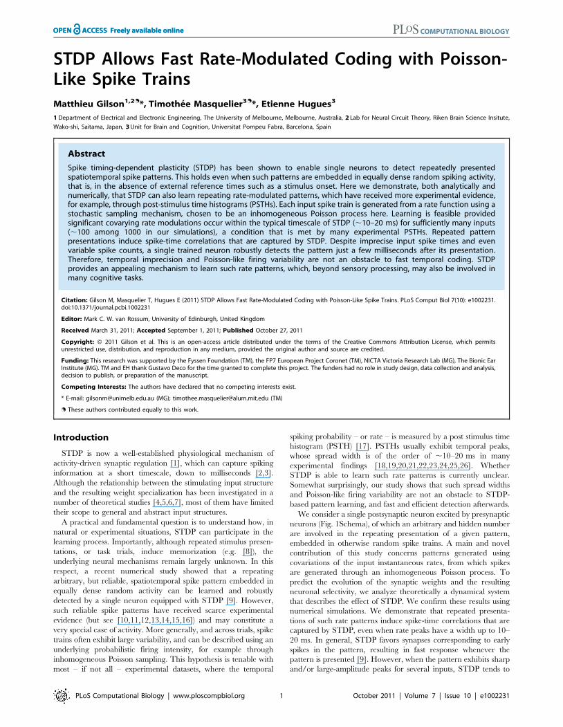
Figure 3. Emerged input selectivity after learning (t&2000 s). Comparison between a trained Poisson neuron for the different pattern types inFig. 1: (S) model S with f ~1:5 Hz, p~1, and s~0 ms, (SD) model S with f ~3 Hz, p~1=

ffiffiffi2p

, and s~0 ms, (SJ) model S with f ~1:5 Hz, p~1, ands~10 ms and (R) model R with f ~1:5 Hz and width s~10 ms; and (RL) a trained LIF neuron with the model R. All patterns have the same latenciestmi . See Text S1 Section S3.2 for details about the parameters. Top panels (label 1): Input raster plots for N~1000 afferents. Darker grey dots indicate

stronger weights for synapses whose EPSPs significantly contribute to variations of the soma potential. Again each pattern presentation is indicatedby a grey rectangle. In all plots, the cluster of black dots at the beginning of the pattern presentation indicates that STDP has potentiated synapsescorresponding to early spikes in the pattern. All non-pattern synapses have been almost completely depressed. The insets display the weighthistogram at the end of the learning epoch: the distribution is bimodal with about 70 out of 1,000 potentiated synapses. Bottom panels (label 2):Evolution of the lumped EPSPs (solid curve), namely the contribution to rout in the rhs of Equation (4) without the positive part for Poisson neuronsand V (t) in Equation (S34) for the LIF neuron. The horizontal dashed line indicates the ‘‘threshold’’: zero for Poisson neurons (under which no spike isemitted), and Vt for the LIF neuron; the vertical dashed lines the output spikes. The dotted curves represent the lumped EPSPs before training. (Conv)Plot of the convergence index defined in Equation (24) as a function of time for all models. A lower value indicates a bimodal distribution of theweights at the bounds, to evaluate the learning progression.doi:10.1371/journal.pcbi.1002231.g003

STDP Allows Fast Inhomogeneous Poisson Rate Coding

PLoS Computational Biology | www.ploscompbiol.org 9 October 2011 | Volume 7 | Issue 10 | e1002231

probability p~1� ffiffiffi

kp

has the same correlogram as the same

pattern with reliable spikes (p~1) and frequency f (Fig. 1S2 and

SD2 with k~2). This means that non reliability of firing can be

compensated by more frequent repetition, as far as spike-time

correlations are concerned.

For model SD, the Fano factor of the spike count scales between

FF~0 (reliable) for p~1 to FF~1 (Poisson) for p~0 (see

Equation (24) in Materials and Methods) and the influence of such

a variability on learning will be examined. On the other hand,

model R always gives FF~1 as any Poisson process does. For

both models SJ and R, the temporal precision can be varied

through smi . In particular, with a same value for s, they may only

differ by the Fano factor. Fig. 1SJ2 and 1R2 show that Gaussian

jitters for model S and Gaussian-peaked rate modulations for

model R lead to similar correlograms when they have the same

temporal accuracy s. By comparing results for these models, we

will assess the effect of the Fano factor on both learning and

detection afterwards.

Weight specialization induced by temporally HebbianSTDP

Now we examine how this spiking information induced by

pattern presentation can be captured by STDP. Our theoretical

analysis is based on the additive STDP rule and Poisson neuron

model, which allow the prediction of the weight specialization

induced by STDP [4,27]. In our phenomenological model of

synaptic plasticity, STDP is described by a temporal learning

window (Fig. 2A). The Poisson neuron linearly sums excitatory

postsynaptic potentials (EPSPs) resulting from each incoming spike

to determine the soma potential, which is used as an instantaneous

rate function to generate an output spike train. The theoretical

predictions will be verified numerically using both Poisson and

leaky integrate-and-fire (LIF) neurons, and the effect of weight

dependence in the STDP rule will be also examined. Details are

provided in Materials and Methods.

The first stochastic moment for the plastic weight Ji follows a

differential equation that is of the form:

dJi

dt~W ni,nout tð Þ½ �z

Xk

Jk(t)Aki, ð29Þ

cf. Materials and Methods before Equation (10). Here W is a

function of the mean (time-averaged) firing rates ni and nout tð Þ of

the i-th afferent and neuron, respectively; see Equation (6) for the

detailed expression. The coefficients Aij of matrix A defined in

Equation (11) involve the spike-time cross-correlations between

input spike trains i and j. Note that for the pattern models S and

R, the input firing rates and spike-time cross-correlograms are

time invariant; the output neuronal firing rate only evolves as the

consequence of the learning process.

This dichotomy between mean firing rates on the one hand and

spike-time correlation coefficients on the other hand highlights the

separation of timescales in representing the information contained

in spike trains [4,27]. In our framework, the firing rates ni and nout

are low-pass filtered variables, but spiking information at a short

timescale is still contained in the time-averaged spike-time

correlations Cij uð Þ through the time variable u (see Equation (9)

in Materials and Methods). Consequently, the weight evolution

can be analyzed as a double dynamics that is a mixture of:

N a homeostatic equilibrium that stabilizes the mean incoming

weight (over all inputs) and relates to the first term in Equation

(29);

N a specialization by competition between individual weights

related to the spike-time correlations via the second term in

Equation (29).

A typical example is illustrated in Fig. S1 in Text S1.

Specialization leads to the potentiation of some weights at the

expense of others, then the neuron behaves as a coincidence

detector for the selected inputs. The weight selection can be

predicted via the matrix A, which is tractable when using the

Poisson neuron model. Because of the similarity between the

correlation structures that they induce, cf. Equation (28), a

common expression for the coefficients Aij that appear in

Equation (29) can be derived both for models S and R. It relies

on the difference between the latencies tmi and tn

j of inputs i and j,namely

Aij&fp2Xm,n

ami an

j k tnj {tm

i ,ffiffiffiffiffiffiffiffiffiffiffiffiffiffiffiffiffiffiffiffism

i 2zsnj 2

q� �: ð30Þ

Model S corresponds to ami ~an

j ~0 (in addition to smi ~sn

j ~0for models S and SD, but not SJ) and model R to p~1. The kernel

function k u,sð Þ is defined by

k u,sð Þ~ W � eð Þ � G(.,s)½ �(u): ð31Þ

Note that k u,0ð Þ~ W � e½ � uð Þ, which is represented in Fig. 2A.

As shown in Fig. 2B, the more spread the Gaussians are (viz. larger

value for s), the smoother and smaller the function k u,sð Þ is as a

function of the time difference u.

From the Equation (31), it can be seen that the STDP effects are

impaired if the STDP time constants are much smaller than those

of the PSP response. This is not the case in the brain (and in our

simulations), where all these constants are in the 10–30 ms range.

The spectral analysis mentioned above describes how an

initially homogeneous weight distribution will begin to split as a

result of STDP. The strength of cross-covariances between pattern

inputs reflects their tendency to drive the firing of output spikes.

When some weights become stronger compared to the remainder,

this driving effect becomes stronger. It follows that the cross-

covariances between the potentiated inputs and the postsynaptic

neuron increase in a causal manner, in turn inducing further (and

stronger for additive STDP) potentiation. This self-reinforcing

mechanism (described in more detail in Materials and Methods)

leads to a clear potentiation of some pattern inputs, until they

either saturate at the upper bound (additive STDP) or reach an

equilibrium value (weight-dependent STDP).

Synapses with earliest spikes are selected in generalCompetition between weights Ji leads to the reinforcement of

those with stronger correlation term, so the rule of thumb is that

inputs i with larger coefficients Aijw0 (for all indices j) will be

selected by STDP. Because W is roughly antisymmetric and we do

not consider slow synapses, k in Equation (30) is such that negative

arguments contribute positively to the sum in coefficients Aij . It

follows that pattern synapses with early spikes tend to be selected

when the spike density is somehow constant for all pattern inputs

(see Materials and Methods). When some strong inputs start

driving the neuronal firing (as mentioned above), other pattern

inputs corresponding to earlier spikes also tend to be reinforced for

temporally Hebbian STDP, which further favors inputs with early

spikes until the weight strengthening finally stabilizes. This is

STDP Allows Fast Inhomogeneous Poisson Rate Coding

PLoS Computational Biology | www.ploscompbiol.org 10 October 2011 | Volume 7 | Issue 10 | e1002231

illustrated for models S and R by simulations using Poisson

neurons in Fig. 3S1, SD1, SJ1 and R1 (black clusters). Non-pattern

synapses have also been completely depressed by STDP.

While keeping the output neuronal firing rate low on average

(due to the homeostatic equilibrium), the potentiated synapses (due

to weight competition) ensure a significant increase of the

membrane potential (solid curve) at the beginning of each pattern

presentation. This usually causes early postsynaptic spikes (vertical

dashed lines) that can be used for fast pattern detection

(quantification with mutual information will be discussed later).

The trained neuron is thus selective to the quasi-simultaneous

arrival of the earliest pattern spikes, and can serve as ‘‘earliest

predictor’’ of the subsequent spike events, at the risk of triggering a

false alarm if these subsequent events do not occur, but with the

benefit of being very reactive (to learn the full pattern, several

neurons in competition can be used [37]). Comparatively, the

membrane potential before training (dotted curve) is similar during

and outside pattern presentation.

Model S with p~1, f ~1:5 Hz (and s~0 ms), or with

p~1=ffiffiffi2p

, f ~3 Hz (and still s~0 ms) have the same correlation

structure (Fig. 1S2 and SD2). Therefore, despite different Fano

factors, they lead to the same final weights (Fig. 3S1 and SD1

insets), at approximately the same speed (Fig. 3Conv). However,

after learning the increase of the summed EPSPs (solid curve) is

stronger in the first case (Fig. 3S2) than in the second (Fig. 3SD2)

because of the missing spikes.

Likewise, model SJ with s~10 ms (and p~1, f ~1:5 Hz) and

model R with s~10 ms (and still f ~1:5 Hz) have similar correlation

structures (Fig. 1 SJ2 and R2) and thus lead to the same final weights

(Fig. 3SJ1 and R1 insets). Here too, they have approximately the same

learning speed (Fig. 3Conv) despite the difference in their Fano factors.

The use of s~10 ms induces a more spread rise of EPSPs,

comparable in both cases (Fig. 3SJ2 and R2). Indeed, with model R

the deviations from the mean spike counts at each pattern presentation

tend to compensate across the n<70 selected afferents (with Poisson

processes like here, the total spike count’s coefficient of variation

decreases in 1=ffiffiffinp

). Since the EPSP rise is more spread for model SJ

and R than with model S, the detection performance is poorer, but it

remains acceptable, even with a decision rule based only on the

neuron’s spiking output (this will be discussed later).

In our simulations spike count variability (as measured by the

Fano factor FF ) does not slow down the learning, whereas spiking

temporal imprecision (related to s) does. In terms of convergence

speed, we have S,SD.SJ,R (see Fig. 3Conv).

A LIF neuron trained with model R (Fig. 3RL) also selects pattern

synapses with early spikes, which results here in two postsynaptic

spikes each time the pattern is presented. With our choice of

parameters learning was found to be slower for the LIF neuron

(Fig. 3Conv). Note that, for model S with other parameters, selectivity

can emerge in a few tens of pattern presentation [9]. The fact that the

LIF neuron behaves similarly to the Poisson neuron justifies a

posteriori the use of the latter for convenience in the theoretical

analysis. In a regime where the LIF neuron is sensitive to volleys of

almost coincident spikes, only the inputs with the very first spikes may

remain potentiated at the end of the learning epoch, whereas the

synapses corresponding to later spikes are depressed [9]. However, a

thorough discussion of these effects is beyond the scope of the present

paper. Here we focus on the Poisson neuron, for which new analytical

results are presented below. Extensive numerical studies with the LIF

neuron can be found in previous work [9,37,38].

Influence of the spike distribution within the patternThe above-mentioned rule of thumb that inputs with early

spikes are favored does not hold for all patterns. To illustrate how

the spike distribution among pattern inputs affects the weight

evolution, we use a specific configuration of models S and R,

where pattern afferents are partitioned into two groups (or

populations) with respective numbers of inputs N1 and N2. More

precisely, this bimodal distribution of input latencies is such that

the afferents of group 1 tend to fire before those in group 2:

N Model SB: bimodal spike pattern (Fig. 4SB). Each afferent ibelonging to group x (x~1,2) has only one pattern spike

corresponding to latency t1i , which is randomly drawn from a

Gaussian distribution with mean �ttx and spread width �ssx.

Inputs in group 1 tend to arrive before those in group 2:�tt1v�tt2. We also set p~1 and s1

i ~0 (no jitter).

N Model RB: bimodal rate-modulated pattern (Fig. 4RB). Within

each group, all afferents have the same Gaussian rate function

centered on �ttx (�tt1v�tt2) with spread width s1i ~�ssx for input i in

group x; amplitudes are unitary (a1i ~1).

The overline indicates group variables. In this way, we control

the crucial parameters that determine the clustering of spikes

within the early and late groups, namely their sizes and temporal

resolutions, whose effect will be assessed against the difference

between their latencies.

In terms of population averages, both models have the same

expression for the input spike-time correlations given in Equations

(16) and (17) with respective mean latency �ttx and temporal spread

�ssx, as illustrated in Fig. 4SB2 and 4RB2. This illustrates another

connection between these two pattern models despite their

different spike generation mechanisms. Note that, for model R,

the amplitudes ami and the number of inputs with clustered pattern

spikes (e.g. group size for model RB) plays a similar role.

We consider the situation where the inputs from the first group

fire sufficiently early compared to the second group (say

t2{t1w10 ms). Our framework allows us to study the effect of

the pattern parameters on the resulting competition between the

two groups; detailed calculations are provided in Text S1 (Section

S2.2).When both groups have similar size (N2&N1) and spread

width (�ss2&�ss1), STDP tends to select the first group in agreement

to the previous section, see Fig. 4SB3,6 and 4RB3,6. However,

when the second group is more populated (N2wN1), STDP

preferably selects the late group as shown in Fig. 4SB4,7 and

4RB4,7. Now, when the second group has a narrower spread

(�ss2v�ss1), while both groups have comparable size (N2&N1),

STDP tends to select the second group as shown in Fig. 4SB5,8

and 4RB5,8. This extends previous results on the effect of

correlation spread for two input groups that have no correlation

between them [39]. Simulations with models SB and RB exhibit

similar trends, in agreement with the resemblance between their

(population averaged) spike-time correlograms.

In summary, potentiation of synapses corresponding to early

pattern spikes competes with another trend that favors densely

populated and narrow spike clusters, irrespective of the spike

generation type within the pattern. Note that this does not affect

the success of pattern detection, but only its timing.

General case of an arbitrary patternNow we go back to the case of a general pattern that has

arbitrary latencies tmi . We examine how the trends revealed by the

analytical study of models SB and RB adapt here. A complete

description of the weight evolution involves the spectrum of matrix

B~n woutez ~WWn �T

zA, as Equation (28) can be rewritten as a

linear differential matrix equation of the form dJ=dt~JBzX (see

Equation (10) in Materials and Methods). The spectrum of this

matrix (circles) is represented in Fig. 5ABC for a pattern of model

STDP Allows Fast Inhomogeneous Poisson Rate Coding

PLoS Computational Biology | www.ploscompbiol.org 11 October 2011 | Volume 7 | Issue 10 | e1002231

Figure 4. Influence of the spike distribution within the pattern. Comparison between a spike pattern of model SB (SB panels) and a rate-modulated pattern of Model RB (RB panels), both having a bimodal distribution of latencies. (SB1) Model SB. The plot displays N1~30 afferents thatfire with a mean latency �tt1~15 ms with a spread �ss1~5 ms around this latency, and N2~45 afferents that fire with a mean latency �tt2~35 ms and

STDP Allows Fast Inhomogeneous Poisson Rate Coding

PLoS Computational Biology | www.ploscompbiol.org 12 October 2011 | Volume 7 | Issue 10 | e1002231

R: most eigenvalues are close to those of A (pluses), which can thus

be used to predict the weight evolution; the large negative eigen-

value of matrix B roughly equal to N woutz ~WWr0

� �r0 and ass-

ociated with the homeostatic equilibrium is not displayed there for

clarity. Note that eigenvalues may be complex numbers. Likewise,

the dominant left eigenvector(s) that determine the weight

specialization are similar for both matrices (Fig. 5DEF). As shown

in Fig. 5GH, the weight evolution can be satisfactorily predicted

using either the whole matrix A (label ‘whole A’) or its principal

eigenvectors (label ‘princ eig vect A’) both for models S and R.

Note that our predictions slightly overestimate the number of

potentiated weights here (as in Fig. S1, in Text S1). Neglecting rate

effects, more than 80% of the potentiated weight can be predicted

(label ‘A only’), meaning that spike-time correlations dominate.

In a similar manner to the simpler model RB when a pattern

of model R has more spread rate peaks, the elements of A go to

zero (Fig. 5ABC) as the function k(u,s) becomes flatter when sincreases (Fig. 2B). Consequently, the weight specialization

weakens, which significantly decreases the quality of detection,

as estimated by the mutual information defined in Equation

(25) and plotted in Fig. 6. With the same spread width,

Gaussian jitters (Fig. 6SJ) and Gaussian rate peaks (Fig. 6R)

give similar performance: because sufficiently many inputs are

used spiking variability of model R (FF~1 within the pattern

Figure 5. Theoretical prediction of the weight specialization. Comparison between the matrices A and B~n woutez ~WWn �T

zA in Equation(10) for a given pattern of model SJ (or its equivalent of model R) using various values for s: (AD) 0 ms, (BE) 10 ms and (CF) 30 ms. (ABC) Spectra ofmatrices A (pluses) and B (dots). (DEF) Comparison between the principal eigenvectors (one of the complex conjugated pair) of matrices A (x-axis)and B (y-axis). The positive and imaginary parts of the coordinates for are represented by crosses and circles, respectively. The diagonal indicatesperfect alignment. For (G) Model SJ and (H) model R, comparison between simulated (Fig. 3) and predicted weight evolution. After 2000 s, weightsare labeled as potentiated if above J�av and depressed otherwise; both simulations with models S and R exhibit around 70 potentiated and 930depressed weights. The black and grey histograms count the number of potentiated weights that are correctly and wrongly predicted, respectively;the white histogram the depressed weights incorrectly predicted. The prediction ‘whole A’ are obtained by simulating the differential equation (10)with the whole matrix A in B~n woutez ~WWn

�TzA, whereas ‘princ eig vect A’ only involve the two principal complex-conjugated eigenvectors of A,

cf. (B). The prediction ‘correl only’ uses a projection the principal eigenvectors of A to analytically predict the potentiated weights, which ignores rateeffects.doi:10.1371/journal.pcbi.1002231.g005

same spread �ss2~5 ms. (SB2) The average cross-correlogram over the respective groups (circles) corresponds to Equation (16). (RB1) Model RB. Theplot displays two afferents of each group. In each group all the afferents have the same pattern rate function: Gaussians centered respectively on�tt1~15 ms and �tt2~35 ms with width �ss1~�ss2~10 ms and amplitudes am

i ~1. (RB2) The cross-correlogram between two afferents in distinct groupsexhibits a peak at �tt1{�tt2~20 ms. Plots SB3–8 and RB3–8 are similar to those in Fig. 3. (SB3,SB6 and RB3,RB6) N1~N2 and �ss1~�ss2 : the earliest clusteris selected. (SB4,SB7 and RB4,RB7) N2~2N1wN1 and �ss1~�ss2 : the latest cluster is selected. (SB5,SB8 and RB5,RB8) N1~N2 and �ss2~�ss1=2: the latestcluster is selected.doi:10.1371/journal.pcbi.1002231.g004

STDP Allows Fast Inhomogeneous Poisson Rate Coding

PLoS Computational Biology | www.ploscompbiol.org 13 October 2011 | Volume 7 | Issue 10 | e1002231

presentation) hardly impairs the detection w.r.t. Model SJ with

(FF~0 for p~1). Together with results comparing models SB

and RB in Fig. 4, this supports our conclusion that the weight

evolution induced by STDP is mainly determined by the

input spike-time cross-correlograms, and that unreliability in

the spike count (as measured by the Fano Factor) has little

effect.

Now, as an illustration of an arbitrary pattern that mimics real

PSTHs, we consider a longer rate-modulated pattern

(L~500 ms). We assume that the inputs are modulated by some

global strength (e.g. image or movie contrast, sound volume), while

individual rates encode local features. For this purpose, the rate

functions are multiplied both for pattern and non-pattern inputs

by a common envelope. The latter corresponds to superimposed

20-ms spread peaks distributed in time with a homogeneous

Poisson process at 20 Hz, as illustrated in Fig. 7AB. For all inputs,

the envelope is repeated identically during all pattern presenta-

tions. In our simulation, STDP selects a single cluster of rate peaks

in the pattern (e.g. third peak in Fig. 7CD) and mainly reinforces

inputs corresponding to that ‘‘population’’ peak. In agreement to

the results for the simpler model RB, STDP favors clustered, high-

amplitude and narrow modulations. Interestingly, even though the

population firing rate in Fig. 7B may be much larger outside than

during pattern presentations, the neuron fires almost only during

the presentations (Fig. 7D).

To further evaluate the relative strengths of the mean input

firing rates and spike-time correlations induced by the pattern, we

also simulated a pattern with a lower firing rate than the noisy

activity surrounding it: 15 Hz vs. 25 Hz, respectively. The output

neuron could still be trained successfully, although not as well as

for the control case of 20 Hz vs. 20 Hz (not shown here).

These results show that STDP can learn non-flat rate-

modulated patterns relying on the same competition between

afferent weights as described above for the more difficult case of

quasi constant input firing rate. Realistic PSTHs can thus be

learned provided sufficiently many inputs exhibit significant rate

modulations on a ‘‘fast’’ time scale, namely ranging up to 10–

20 ms with our parameters. In this case, correlation effects

dominate the weight dynamics.

Influence of the STDP and neuronal parametersFinally, we examine the influence of the STDP and neuronal

parameters on both learning and detection afterwards for a typical

pattern of model R (similar results were obtained with model S).

To estimate the quality of detection, we evaluate the neuronal

response after training averaged over 10 pattern presentations (in

Figure 6. Effect of the jitter s for model SJ, and the spread width s for model R on learning and detection. Model R is also tested on aLIF neuron (panel RL). The plots are similar to Fig. 3, except for the LIF neuron: the unconstrained postsynaptic soma potential that is plotted ignoresthe threshold (horizontal dashed line). When the pattern is presented (grey area), the soma potential rise is stronger for small s, synonymous withmore robust selectivity, even though detection does not completely collapse for larger values. To quantify the detection quality we used mutualinformation between pattern presentations and postsynaptic spikes (see Equation (26) in Materials and Methods): the latter decreases with s. The LIFneuron is on average slightly more reliable than the Poisson neuron (here perfect detection corresponds to mutual information equal to 0.23 bits).doi:10.1371/journal.pcbi.1002231.g006

STDP Allows Fast Inhomogeneous Poisson Rate Coding

PLoS Computational Biology | www.ploscompbiol.org 14 October 2011 | Volume 7 | Issue 10 | e1002231

Figure 7. Long pattern of model R with duration L~500 ms and global time-varying spike density. (A) Individual rate functions for apattern (bottom) and a non-pattern (top) input. During all pattern presentations (grey areas), the pattern input exhibits the same rate modulations(similar plot to Fig. 1R1). The width of rate peaks is randomly chosen around s~10 ms and the amplitudes (e.g. am

i ) are multiplied by a commontemporal envelope (see text). (B) Population-averaged spike histogram (bars) and theoretical firing rate (solid line, average of individual rate functionsof (A)). (C and D) Input raster plot and lumped EPSP response after learning (similar to Fig. 3). The black cluster in (C) indicates that the third

STDP Allows Fast Inhomogeneous Poisson Rate Coding

PLoS Computational Biology | www.ploscompbiol.org 15 October 2011 | Volume 7 | Issue 10 | e1002231

order to remove noise and display clear trends). We keep in mind

that the goal is detection of each pattern presentation by the

neuron, though.

In our model, the mean output firing rate of the neuron is

constrained by STDP close to an equilibrium value n�out that

depends on the rate-based contributions win and wout, the ratio

LTP/LTD (related to ~WW ), and the background excitation/

inhibition n0 (cf. Equation (4)). For a good detection performance,

in other words minimizing false alarms, n�out in Equation (20) must

be kept low, which can be achieved using a small value for win, as

illustrated in Fig. 8A. However, such a small value also decreases

the magnitude of the response to the pattern. The use of win and

wout prevents the pitfalls where all synapses become depressed,

leading to a quiescent neuron, or on the contrary maximally

reinforced, leading to a very active non selective neuron. They also

allow the use of asymmetric STDP where overall depression is

stronger than the overall potentiation ( ~WWv0), relieving the

requirement to tune depression only slightly higher than

potentiation [9], as illustrated in Fig. 8B where the ratio between

depression and potentiation for STDP hardly affects the detection

performance. We also looked at the effects of weight dependence

using the model proposed in [6], for which a parameter c scales

between additive (c~0) and multiplicative (c~1) STDP (Fig. 8C).

These simulations were done without the homeostatic terms win

and wout, aiming to show that learning is still possible without

them. However, we had to fine tune some parameters:

Jmax~0:1020 (vs 0.1215 in the baseline simulation, cf. Text S1

Section S3.2), a{=az~0:56 (vs 0.82 in the baseline). Conver-

gence took about 4000 s (vs 2000 s in the baseline). With these

values learning fails with pure additive STDP (c~0), leads to good

detection performance with slightly multiplicative STDP

(c~0:01). This performance decreases with more multiplicative

STDP (c~0:02), and collapses with c~0:05, which leads to a

unimodal final weight distribution. In comparison, additive STDP,

also with win~wout~0, could hardly learn and detect patterns of

type SJ with jitters larger than 2 ms [9]. Small values for c in

Fig. 8C ensure both homeostasis and strong competition for

weight-dependent STDP [33], which results in good detection for

a jitter of 10 ms.

Inhibitory background activity (n0v0) is used to obtain an

equilibrium with both a low mean firing rate n�out and a positive

mean input weight J�av (see Equations (20) and (19)). As mentioned

above, the first ensures that the trained Poisson neuron has a low

number of false alarms. The second leads to successful detection

with sufficiently many potentiated pattern inputs that imply a

significant increase of the soma potential during each pattern

presentation. In contrast, the case n0§0 corresponds to a noisy

neuron and the pattern response is then not so strong compared to

n�av, weakening detection as illustrated in Fig. 8D (n0~0). In this

case, inhibition helps to increase the sensitivity of the neuron to

correlated inputs, both for learning and detection. This effect,

together with that of win, is predicted by the analytical evaluation

of the mutual information in Text S1 (Section S2.3).

We also verified the robustness of our scheme with respect to the

number of pattern afferents N0. So far, we have used

N0=N~50%, which ensured that STDP could choose among

many afferent candidates. Decreasing N0=N weakens the neuronal

response, but down to as few as &12%, the detection remains

acceptable; only for &6% the performance collapses (Fig. 8E).

Successful detection can be achieved provided there are

sufficiently many pattern inputs such that the potentiation of

‘‘half’’ of them (while depressing the others) leads to a significant

response of the soma potential.

Last, Fig. 8F examines pattern of various durations L (between

3 and 100 ms). When L?0, the pattern inputs behave as a

narrowly correlated group which is selected by STDP [4], but, not

sufficiently many inputs have a rate peak in the pattern, so

performance decreases. Increasing L beyond the time scale of

STDP does not significantly change detection, since only a portion

of the pattern is learned (e.g. the beginning in Fig. 8F). Patterns of

duration Lw10 ms fully use the temporal (approximate) anti-

symmetry of the STDP learning window W .

Taken together, these results show that the proposed STDP-

based pattern learning/recognition mechanism works for a broad

range of parameters. It also works similarly for Poisson and LIF

neurons, which supports the theory that the proposed learning

scheme relies on the STDP qualitative properties, namely the

temporal antisymmetry of the learning window W , rather than on

a precise quantitative configuration or neuronal model.

Discussion

The contribution of this paper is twofold. First, we have

demonstrated how an additive-like STDP leading to strong

competition between afferents can train a neuron in an

unsupervised fashion to detect not only spike patterns but, more

surprisingly, rate-modulated patterns resembling typical PSTHs.

Second, we have shown that despite distinct variability (as

measured by the Fano factor) but provided they have the same

temporal precision, both spike and rate-modulated patterns are

equivalent from the point of view of STDP. Both induce similar

spike-time correlation structures, hence similar neuronal special-

izations. Altogether, our results indicate that temporal inaccuracy

(up to 10–20 ms), and Poisson-like firing variability (both for the

inputs and the postsynaptic neuron) are not an obstacle to robust

learning and efficient single-trial detection afterwards by a single

neuron.

Summary of resultsA previous simulation study showed that a repeating arbitrary

spatiotemporal spike pattern (model S) hidden in continuous

equally dense distractor spike trains can be robustly detected and

learned by a single neuron equipped with STDP [9] Here we have

demonstrated that these results extend to the case of patterns of

temporally modulated instantaneous firing rates (model R), from

which the spikes are generated at each presentation, e.g., through

an inhomogeneous Poisson process. To gain analytical insight, we

developed a theoretical framework, which extends previous studies

that showed how STDP favors correlated inputs [4,3,7,6]. We

confirmed that Hebbian STDP (cf. Fig. 2A) tends to favor synapses

corresponding to early spikes in the pattern, generalizing previous

results on spike patterns [9]. An interesting corollary is that the

neuronal response thus becomes faster presentation after presen-

tation. However, this rule is not general when considering specific

spike distributions within the pattern, both for spike and rate-

modulated patterns. As summarized in Fig. 4, inhomogeneities of

the spike density also play an important role in the selection

process, with a preference for densest and narrowest peaks, similar

population peak in the pattern in (B) has been selected. The inset displays the bimodal final weight distribution and shows that only a few weightswere potentiated. While remaining sensitive to the mean input spike rate in (B), the postsynaptic neuron is above all selective to the third patternpeak for the two presentations displayed in (D).doi:10.1371/journal.pcbi.1002231.g007

STDP Allows Fast Inhomogeneous Poisson Rate Coding

PLoS Computational Biology | www.ploscompbiol.org 16 October 2011 | Volume 7 | Issue 10 | e1002231

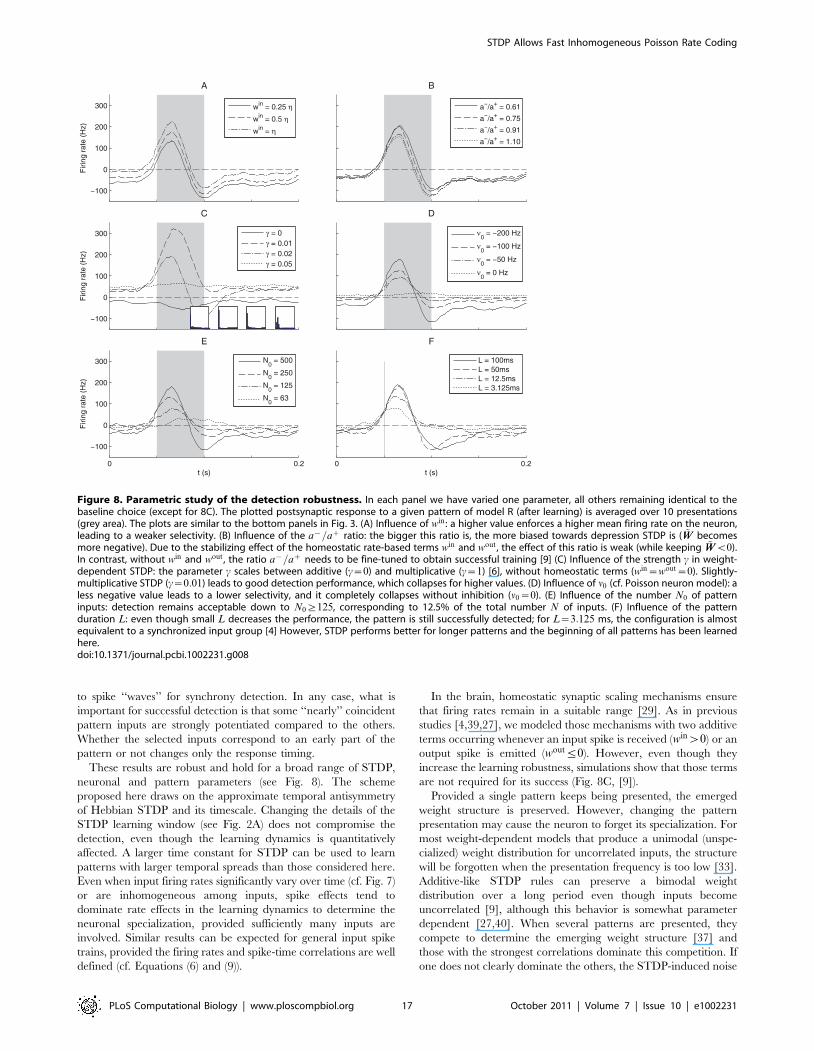
to spike ‘‘waves’’ for synchrony detection. In any case, what is

important for successful detection is that some ‘‘nearly’’ coincident

pattern inputs are strongly potentiated compared to the others.

Whether the selected inputs correspond to an early part of the

pattern or not changes only the response timing.

These results are robust and hold for a broad range of STDP,

neuronal and pattern parameters (see Fig. 8). The scheme

proposed here draws on the approximate temporal antisymmetry

of Hebbian STDP and its timescale. Changing the details of the

STDP learning window (see Fig. 2A) does not compromise the

detection, even though the learning dynamics is quantitatively

affected. A larger time constant for STDP can be used to learn

patterns with larger temporal spreads than those considered here.

Even when input firing rates significantly vary over time (cf. Fig. 7)

or are inhomogeneous among inputs, spike effects tend to

dominate rate effects in the learning dynamics to determine the

neuronal specialization, provided sufficiently many inputs are

involved. Similar results can be expected for general input spike

trains, provided the firing rates and spike-time correlations are well

defined (cf. Equations (6) and (9)).

In the brain, homeostatic synaptic scaling mechanisms ensure

that firing rates remain in a suitable range [29]. As in previous

studies [4,39,27], we modeled those mechanisms with two additive

terms occurring whenever an input spike is received (winw0) or an

output spike is emitted (woutƒ0). However, even though they

increase the learning robustness, simulations show that those terms

are not required for its success (Fig. 8C, [9]).

Provided a single pattern keeps being presented, the emerged

weight structure is preserved. However, changing the pattern

presentation may cause the neuron to forget its specialization. For

most weight-dependent models that produce a unimodal (unspe-

cialized) weight distribution for uncorrelated inputs, the structure

will be forgotten when the presentation frequency is too low [33].

Additive-like STDP rules can preserve a bimodal weight

distribution over a long period even though inputs become

uncorrelated [9], although this behavior is somewhat parameter

dependent [27,40]. When several patterns are presented, they

compete to determine the emerging weight structure [37] and

those with the strongest correlations dominate this competition. If

one does not clearly dominate the others, the STDP-induced noise

Figure 8. Parametric study of the detection robustness. In each panel we have varied one parameter, all others remaining identical to thebaseline choice (except for 8C). The plotted postsynaptic response to a given pattern of model R (after learning) is averaged over 10 presentations(grey area). The plots are similar to the bottom panels in Fig. 3. (A) Influence of win: a higher value enforces a higher mean firing rate on the neuron,leading to a weaker selectivity. (B) Influence of the a{=az ratio: the bigger this ratio is, the more biased towards depression STDP is ( ~WW becomesmore negative). Due to the stabilizing effect of the homeostatic rate-based terms win and wout, the effect of this ratio is weak (while keeping ~WWv0).In contrast, without win and wout, the ratio a{=az needs to be fine-tuned to obtain successful training [9] (C) Influence of the strength c in weight-dependent STDP: the parameter c scales between additive (c~0) and multiplicative (c~1) [6], without homeostatic terms (win~wout~0). Slightly-multiplicative STDP (c~0:01) leads to good detection performance, which collapses for higher values. (D) Influence of n0 (cf. Poisson neuron model): aless negative value leads to a lower selectivity, and it completely collapses without inhibition (n0~0). (E) Influence of the number N0 of patterninputs: detection remains acceptable down to N0§125, corresponding to 12.5% of the total number N of inputs. (F) Influence of the patternduration L: even though small L decreases the performance, the pattern is still successfully detected; for L~3:125 ms, the configuration is almostequivalent to a synchronized input group [4] However, STDP performs better for longer patterns and the beginning of all patterns has been learnedhere.doi:10.1371/journal.pcbi.1002231.g008

STDP Allows Fast Inhomogeneous Poisson Rate Coding

PLoS Computational Biology | www.ploscompbiol.org 17 October 2011 | Volume 7 | Issue 10 | e1002231

(due to weights jumps) may cause the neuron to switch its

specialization between patterns of comparable correlation

strength. This happens, for example, when the learning rate is

sufficiently large [41].

Implications for neuroscienceOne can distinguish two kinds of response variability, or lack

thereof: reliability and precision [42]. When a neuron fires

approximately the same number of spikes on each trial, it is said to

be reliable, whereas when the spikes occur almost at the same time

across trials it is said to be precise. Our study demonstrates that

STDP-based pattern learning needs a precision of 10–20 ms,

whereas it is almost insensitive to a lack of reliability (see Section

S1.6 and Fig. S2 and S3 in Text S1 for the case FFw1), provided

the patterns involve at least ,100 afferents, which is very probable

as a typical cortical neuron has about 10,000 afferents. In

particular, it can cope with the Poisson-like variability often

observed experimentally [43,44]. Evidence for neural activity with

the required precision abounds, at least in sensory systems exposed

to dynamical stimuli [18,19,20,21,23,22] and, even more impor-

tantly, to naturalistic stimuli [24,25,26]. Moreover, for slowly

varying or even static stimuli, learning with STDP may be still

possible when neural activity oscillations are able to attribute to

spikes stimulus-specific preferred phases [38].

Importantly, the mechanism we propose does not need an

external time reference such as a stimulus onset. Patterns are

learned and recognized is a clock-free system, as they are

embedded in random but similar spiking activity. This is possible

because STDP only relies on relative timing. A low absolute time

precision with respect to the stimulus onset (e.g., estimated by a

PSTH) does not preclude far more precise relative latencies, in

agreement with experimental observations [45,46,47,25,48] For

example, this is the case with trial-dependent input fluctuations

(e.g., correlated noise) that affects spike times similarly.

At a broader level, the rate-modulated patterns considered here

can account for a large class of the naturalistic temporal stimuli

[17] that a subject experiences in vision, audition, touch or

multimodal integration, and we demonstrated that STDP

genuinely enables learning and recognition for such patterns.

This suggests an important role of this plasticity rule in the

development and learning of receptive fields, in perceptual

learning, which typically involves many repeated trials [49] and,

beyond sensory processing, in other cognitive processes or tasks

with fast time scales (tens of ms). Importantly, the relatively low

precision and high firing variability considered here correspond to

a much weaker assumption than models of spike trains generally

used with STDP, and the present results reconcile STDP with

experimentally observed spike trains.

Future workA recent study has proposed a general scheme for the derivation

of a linear-nonlinear Poisson (LNP) cascade model to reproduce

the dynamics of a spiking neuron [38] In short, a stochastically

firing LNP neuron model describes how the input current is

filtered by the synapses and dendrites (linear part), and then

transformed to calculate the instantaneous rate (nonlinear part).

The Poisson neuron used here is a particular and simple case in

the class of LNP models. In particular, we have not considered

here with the Poisson neuron a linear filter (described by the PSP

kernel e) that diverges at the time origin, which is necessary to

match the LIF dynamics. Further analysis using the LNP model

could help to understand in more depth the general agreement

and specific discrepancies between the LIF and the Poisson

neurons in our scheme.

For biological realism, a desirable extension of the present

framework consists in the learning of a pattern ensemble with a

recurrent neural network. This can be achieved with a simple

connectivity scheme where afferent connections are trained

similarly to the single neuron case: a differentiated specialization

can be achieved using lateral inhibition, which prevents neurons

from learning the same pattern features [37] In the case of a

general recurrent network with plastic synapses, the learning and

the neuronal dynamics are intricately coupled and new behavior

will certainly appear [50] For a particular network configuration

with plastic recurrent synapses, a numerical proof that STDP can

successfully learn and retrieve spike patterns (model S) has been

given [51] A layered network with both feed-forward and lateral

STDP-plastic connections was shown to reliably transmit volleys of

almost synchronous spikes by means of delay selection [52] with

jitters up to 20 ms. Our results are consistent with that previous

numerical study in the sense that STDP tends to select among all

incoming connections those corresponding to denser clusters of

spikes. This is indeed synonymous with a higher synchronization

among the selected inputs, and because neurons within each layer

have lateral connections, they tend to synchronize their output

spike volley. A recurrent network where STDP operates can also

generate spontaneous and repeating patterned activity [53,54,55]

Our findings also suggest that similar results may be obtained with

rate-modulated patterns (model R). Beyond these particular

results, the existence and the properties of a mapping between

input patterns and output patterns of interconnected neurons

whose connections are modified by STDP remains unknown. For

example, the ongoing activity in a network as observed in the brain

(e.g., due to background inputs) can clearly affects the ‘‘signal-to-

noise ratio’’ of pattern activity and should be taken into account.

However, the present analysis is a necessary prerequisite to identify

some important dynamical ingredients that may allow a network

to learn, retrieve and generate a pattern ensemble.

Supporting Information

Text S1 Detailed calculations about the statistics concerning the

pattern inputs (Equations (12), (13), (14), (16) and (17)); the

derivation of Equation (24) involving the Fano factor for model

SD; details about the homeostatic equilibrium (Equations (18), (19)

and (20)); the predicted weight evolution for models SB and RB in

Fig. 4; an analytical evaluation the mutual information defined in

Equation (26); comments about the previous work in [9]; details

about the parameters used in numerical simulations; four

supplementary figures that further describe our results.

(DOC)

Acknowledgments

The authors are greatly indebted to Gustavo Deco for his support and to

Sonja Grun for a critical reading of an earlier version of the manuscript.

We thank Dan Goodman and Romain Brette for having developed the

Brian simulator [56], both efficient and user-friendly, and for the quality of

their support. We also thank Tom Morse and ModelDB (http://senselab.

med.yale.edu/modeldb/) for distributing our code.

Author Contributions

Conceived and designed the experiments: MG TM EH. Performed the

experiments: MG TM. Analyzed the data: MG TM EH. Wrote the paper:

MG TM EH.

STDP Allows Fast Inhomogeneous Poisson Rate Coding

PLoS Computational Biology | www.ploscompbiol.org 18 October 2011 | Volume 7 | Issue 10 | e1002231

References

1. Caporale N, Dan Y (2008) Spike timing-dependent plasticity: a hebbian learning

rule. Annu Rev Neurosci 31: 25–46.

2. Gerstner W, Kempter R, van Hemmen JL, Wagner H (1996) A neuronal

learning rule for sub-millisecond temporal coding. Nature 383: 76–81.

3. Song S, Miller K, Abbott L (2000) Competitive hebbian learning through spike-

timing-dependent synaptic plasticity. Nat Neurosci 3: 919–926.

4. Kempter R, Gerstner W, van Hemmen JL (1999) Hebbian learning and spiking

neurons. Phys Rev E 59: 4498–4514.

5. van Rossum MCW, Turrigiano GG (2001) Correlation based learning from

spike timing dependent plasticity. Neurocomputing 38: 409–415.

6. Gutig R, Aharonov R, Rotter S, Sompolinsky H (2003) Learning inputcorrelations through nonlinear temporally asymmetric hebbian plasticity.

J Neurosci 23: 3697–3714.

7. Song S, Abbott LF (2001) Cortical development and remapping through spike

timing-dependent plasticity. Neuron 32: 339–350.

8. Agus TR, Thorpe SJ, Pressnitzer D (2010) Rapid formation of robust auditory

memories: insights from noise. Neuron 66: 610–618.

9. Masquelier T, Guyonneau R, Thorpe SJ (2008) Spike timing dependent

plasticity finds the start of repeating patterns in continuous spike trains. PLoS

ONE 3: e1377.

10. Frostig RD, Frostig Z, Harper RM (1990) Recurring discharge patterns in

multiple spike trains. Biol Cybern 62: 487–493.

11. Prut Y, Vaadia E, Bergman H, Haalman I, Slovin H, et al. (1998)

Spatiotemporal structure of cortical activity: properties and behavioralrelevance. J Neurophysiol 79: 2857–74.

12. Fellous JM, Tiesinga PH, Thomas PJ, Sejnowski TJ (2004) Discovering spikepatterns in neuronal responses. J Neurosci 24: 2989–3001.

13. Abeles M (2004) Neuroscience. Time is precious. Science 304: 523–4.

14. Luczak A, Bartho P, Marguet SL, Buzsaki G, Harris KD (2007) Sequential

structure of neocortical spontaneous activity in vivo. Proc Natl Acad Sci U S A

104: 347–352.

15. Rolston JD, Wagenaar DA, Potter SM (2007) Precisely timed spatiotemporal

patterns of neural activity in dissociated cortical cultures. Neuroscience 148:294–303.

16. Ikegaya Y, Matsumoto W, Chiou HY, Yuste R, Aaron G (2008) Statisticalsignificance of precisely repeated intracellular synaptic patterns. PLoS One 3:

e3983.

17. Richmond BJ (2009) Stochasticity, spikes and decoding: sufficiency and utility oforder statistics. Biol Cybern 100: 447–457.

18. Bair W, Koch C (1996) Temporal precision of spike trains in extrastriate cortexof the behaving macaque monkey. Neural Comput 8: 1185–1202.

19. Berry MJ, Meister M (1998) Refractoriness and neural precision. J Neurosci 18:2200–2211.

20. Buracas GT, Zador AM, DeWeese MR, Albright TD (1998) Efficientdiscrimination of temporal patterns by motion-sensitive neurons in primate

visual cortex. Neuron 20: 959–969.

21. Reinagel P, Reid RC (2000) Temporal coding of visual information in thethalamus. J Neurosci 20: 5392–5400.

22. Lu T, Liang L, Wang X (2001) Temporal and rate representations of time-varying signals in the auditory cortex of awake primates. Nat Neurosci 4:

1131–1138.

23. Reinagel P, Reid RC (2002) Precise firing events are conserved across neurons.

J Neurosci 22: 6837–6841.

24. Butts DA, Weng C, Jin J, Yeh CI, Lesica NA, et al. (2007) Temporal precision in

the neural code and the timescales of natural vision. Nature 449: 92–95.

25. Desbordes G, Jin J, Weng C, Lesica NA, Stanley GB, et al. (2008) Timingprecision in population coding of natural scenes in the early visual system. PLoS

Biol 6: e324.

26. Haider B, Krause MR, Duque A, Yu YG, Touryan J, et al. (2010) Synaptic and

network mechanisms of sparse and reliable visual cortical activity duringnonclassical receptive field stimulation. Neuron 65: 107–121.

27. Gilson M, Burkitt AN, Grayden DB, Thomas DA, van Hemmen JL (2009)Emergence of network structure due to spike-timing-dependent plasticity in

recurrent neuronal networks. I. input selectivity–strengthening correlated input

pathways. Biol Cybern 101: 81–102.

28. Brette R (2009) Generation of correlated spike trains. Neural Comput 21:

188–215.

29. Turrigiano GG (2008) The self-tuning neuron: Synaptic scaling of excitatory

synapses. Cell 135: 422–435.

30. Bi G, Poo MM (2001) Synaptic modification by correlated activity : Hebb’spostulate revisited. Ann Rev Neurosci 24: 139–166.

31. Bi G, Poo M (1998) Synaptic modifications in cultured hippocampal neurons:dependence on spike timing, synaptic strength, and postsynaptic cell type.

J Neurosci 18: 10464–10472.32. van Rossum MC, Bi GQ, Turrigiano GG (2000) Stable hebbian learning from

spike timing-dependent plasticity. J Neurosci 20: 8812–8821.

33. Gilson M, Burkitt AN, Grayden DB, Thomas DA, van Hemmen JL (2010)Emergence of network structure due to spike-timing-dependent plasticity in

recurrent neuronal networks v: self-organization schemes and weight depen-dence. Biol Cybern 103: 365–386.

34. Haider B, Duque A, Hasenstaub AR, McCormick DA (2006) Neocortical

network activity in vivo is generated through a dynamic balance of excitationand inhibition. J Neurosci 26: 4535–4545.

35. Rudolph M, Pospischil M, Timofeev I, Destexhe A (2007) Inhibition determinesmembrane potential dynamics and controls action potential generation in awake

and sleeping cat cortex. J Neurosci 27: 5280–5290.

36. Sprekeler H, Michaelis C, Wiskott L (2007) Slowness: an objective for spike-timing-dependent plasticity? PLoS Comput Biol 3: e112.

37. Masquelier T, Guyonneau R, Thorpe SJ (2009) Competitive STDP-based spikepattern learning. Neural Comput 21: 1259–1276.

38. Masquelier T, Hugues E, Deco G, Thorpe SJ (2009) Oscillations, phase-of-firingcoding, and spike timing-dependent plasticity: an efficient learning scheme.

J Neurosci 29: 13484–13493.

39. Kistler WM, van Hemmen JL (2000) Modeling synaptic plasticity in conjunctionwith the timing of pre- and postsynaptic action potentials. Neural Comput 12:

385–405.40. Billings G, van Rosum MCW (2009) Memory retention and spike-timing-

dependent plasticity. J Neurophysiol 101: 2775–2788.

41. Meffin H, Besson J, Burkitt AN, Grayden DB (2006) Learning the structure ofcorrelated synaptic subgroups using stable and competitive spike-timing-

dependent plasticity. Physical Review E 73: 041911.42. Tiesinga P, Fellous JM, Sejnowski TJ (2008) Regulation of spike timing in visual

cortical circuits. Nat Rev Neurosci 9: 97–107.43. Softky WR, Koch C (1993) The highly irregular firing of cortical cells is

inconsistent with temporal integration of random EPSPs. J Neurosci 13:

334–350.44. Shadlen MN, Newsome WT (1998) The variable discharge of cortical neurons:

implications for connectivity, computation, and information coding. J Neurosci18: 3870–3896.

45. Johansson RS, Birznieks I (2004) First spikes in ensembles of human tactile

afferents code complex spatial fingertip events. Nat Neurosci 7: 170–177.46. Chase SM, Young ED (2007) First-spike latency information in single neurons

increases when referenced to population onset. Proc Natl Acad Sci U S A 104:5175–5180.

47. Gollisch T, Meister M (2008) Rapid neural coding in the retina with relativespike latencies. Science 319: 1108–1111.

48. Panzeri S, Diamond ME (2010) Information carried by population spike times in

the whisker sensory cortex can be decoded without knowledge of stimulus time.Front Synaptic Neurosci 2: 1–14.

49. Sasaki Y, Nanez JE, Watanabe T (2010) Advances in visual perceptual learningand plasticity. Nat Rev Neurosci 11: 53–60.

50. Gilson M, Burkitt AN, Grayden DB, Thomas DA, van Hemmen JL (2009)

Emergence of network structure due to spike-timing-dependent plasticity inrecurrent neuronal networks IV : Structuring synaptic pathways among

recurrent connections. Biol Cybern 101: 427–444.51. Nowotny T, Rabinovich MI, Abarbanel HDI (2003) Spatial representation of

temporal information through spike-timing-dependent plasticity. Phys Rev E 68:011908.

52. Suri RE, Sejnowski TJ (2002) Spike propagation synchronized by temporally

asymmetric hebbian learning. Biol Cybern 87: 440–445.53. Izhikevich EM (2006) Polychronization: computation with spikes. Neural

Comput 18: 245–282.54. Morrison A, Aertsen A, Diesmann M (2007) Spike-timing-dependent plasticity

in balanced random networks. Neural Comput 19: 1437–1467.

55. Fiete IR, Senn W, Wang CZH, Hahnloser RHR (2010) Spike-time-dependentplasticity and heterosynaptic competition organize networks to produce long

scale-free sequences of neural activity. Neuron 65: 563–576.56. Goodman D, Brette R (2008) Brian: a simulator for spiking neural networks in

python. Front Neuroinformatics 2: 5.

STDP Allows Fast Inhomogeneous Poisson Rate Coding

PLoS Computational Biology | www.ploscompbiol.org 19 October 2011 | Volume 7 | Issue 10 | e1002231