Noname manuscript No.

(will be inserted by the editor)

A metric space approach to the information channel

capacity of spike trains.

James B. Gillespie · Conor J. Houghton

Received: date / Accepted: date

Abstract A novel method is presented for calculating the information channel capac-

ity of spike trains. This method works by fitting a χ-distribution to the distribution

of distances between responses to the same stimulus: the χ-distribution is the length

distribution for a vector of Gaussian variables. The dimension of this vector defines an

effective dimension for the noise and by rephrasing the problem in terms of distance

based quantities, this allows the channel capacity to be calculated. As an example, the

capacity is calculated for a data set recorded from auditory neurons in zebra finch.

Keywords Spike train, information channel capacity, Gaussian channel, chi-

distribution, metric space, van Rossum metric.

James B. Gillespie · Conor J. HoughtonSchool of Mathematics, Trinity College Dublin, Dublin 2, IrelandE-mail: gillesjb@tcd.ieE-mail: houghton@maths.tcd.ie

2

1 Introduction

Although spike trains are a significant component of neuronal signalling, it is difficult

to determine which properties of spike trains are important for communication. One

common approach attempts to match some of the language of information theory to

spike train data. However, although spike times in a spike train are described by contin-

uous variables, this problem is usually approached using discrete information theory.

This is because the number of spikes varies from spike train to spike train, making

an information theory desciption, where the spike times are identified with continuous

variables, difficult to apply. It is possible to avoid this difficulty by using a metric space

approach to spike trains. Here, a novel method is proposed for calculating the channel

capacity of spike trains. This is a measure of the maximum mutual information which

can be achieved between the stimulus and the spike trains.

In the usual discrete approach to estimating the information-theory quantities for

spike trains, time is discretized and the spike trains converted into a sequences of ones

and zeros, indicating the presence or absence of a spike in the corresponding time bin

[Bialek et al. , 1991, De Ruyter Van Steveninck et al. , 1997, Rieke et al. , 1999]. The

binary sequence is then split into a set of short intervals, called words. The distribution

of words is estimated and used to calculate the Shannon entropy.

This method is usually applied in a specific experimental set-up; one which will

also be considered here. The spike trains are recorded in vivo from a sensory neuron

during stimulation by the corresponding modality. Spikes are recorded during multiple

repetitions of the same stimulus so that the average entropy of the response is known

for two regimes, one where the stimulus varies, the entropy of the signal response, and

one where the stimulus is repeated, the entropy of the noise response. The entropy

of the noise response is the conditional entropy, conditioned on the signal. In the

discrete approach, the distribution of words is calculated in each case. The difference

between the entropy of the signal response and noise response is the mutual information

between the stimulus and the response. In [De Ruyter Van Steveninck et al. , 1997]

this is characterized as a measure of the information the spike train carries about the

stimulus.

This approach introduced information theory into the study of spike trains and

information theory has subsequently been used extensively in neuroscience, see for ex-

ample [Borst and Theunissen , 1999]. It can be difficult to interpret information theory

quantities in neuroscience; for example, information theory is best defined relative to

a reference measure, the counting measure in the case of the discrete theory, and it

can be hard to know what the correct measure should be. Furthermore, the utility of

an information theory approach to neuroscience has not been definitively established;

while it is hoped that quantifying information in spike trains will help describe how

information is coded, this has not yet been achieved. However it is not intended to

comment on these larger issues here.

Leaving aside these questions, the original approach to information theory suffers

from a data sampling problem. For typical bin size and word length the number of

possible words is extremely large and a typical electro-physiology experiment may not

yield enough words to accurately estimate the entropy. In the original application of

the method data from fly was used, where the short timescales involved in the escape

response in fly ensured that a small word length was possible. This however is not true

in other systems.

3

Another related problem is that the discretization approach ignores the structural

similarities of the spike trains. Two similar sequences from a spike train, which would

produce a similar synaptic response, will map to different words and there is no no-

tion of some words being similar and others dissimilar. It is possible to address these

problems; for example, sampling can be made more efficient in a metric-based bin-less

approach to estimating the word distribution [Victor , 2002]. Here, however, an alter-

native framework is proposed based on continuous rather than discrete information

theory.

The approach taken in this paper is to consider information channel capacity theory

on the metric space of spike trains. In information channel capacity theory, time is

discretized but there is a continuous random variable for each time unit. Here, the

Gaussian random variable used in information channel capacity theory is replaced by

a metric distance random variable and the fragment length of spike train representing

the time unit is defined under the assumption that the noise should be additive and

Gaussian. This leads to a model of noise on the metric space. This means that only the

model parameters need to be estimated to calculate the channel capacity, not the whole

distribution. As such, a smaller sample set is needed than in the discrete approach.

The approach is tested on an example data set: spike trains recorded from the

auditory fore brain of zebra finch. Of particular note is the validity of the noise model

and the Anderson-Darling test is use to check this.

1.1 The van Rossum metric

A metric space is arguably the most general mathematical structure that is useful for

considering spike trains [Victor and Purpura , 1996, Victor , 2005, Houghton and Victor

, 2009]. Indeed, while there are a number of natural ways that a metric structure can

be defined on the space of spike trains, it seems difficult or even impossible to find

useful natural coordinates for the space.

The L2 van Rossum metric is used here [van Rossum , 2001]. A spike train consists

of a set of spike times u = {u1, u2, .., un}. In order to calculate the van Rossum metric,

the spike train is filtered. It is mapped to a function of time, f(t;u):

u 7→ f(t;u) =

[

n∑

i=1

h(t− ui)

]

(1)

where h(t) is a causal exponential kernel:

h(t) =

{

0 t < 0

e−t/τ t ≥ 0(2)

and τ is a timescale parametrizing the metric. The L2 metric on the space of real

functions then induces a metric on the space of spike trains, specifically, if u1 and u2

are two spike trains, then the distance between them is

d(u1,u2) =

√

∫

[f(t;u1)− f(t;u2)]2dt. (3)

As in kernel density estimation, [Silverman , 1986], the precise shape of the kernel is

not thought to be significant. However, the timescale is important. A standard method

4

has been developed for calculating the optimal timescale. If a metric geometry is rel-

evant to the content encoded in the spike trains, the metric should measure a shorter

distance between responses to the same stimulus and a longer one for responses to dif-

ferent stimuli. This means that the timescale should be chosen so that a distance-based

clustering accurately clusters spike trains by stimuli. This accuracy is evaluated by cal-

culating the transmitted information, an information-theory measure of how well the

distance-based clustering matches the the clustering by stimulus [Victor and Purpura

, 1996]. Of course, this is not the only spike train metric, other metrics have been con-

sidered for spike trains and for point processes, considered generally, [Rubin , 1974a,b].

This is mentioned again in the Discussion.

2 Methods

The intention here is to proceed by analogy with a coordinate space. Although no

coordinate system is being proposed here, the fiction of an underlying set of spike

train coordinates is maintained and the calculations will proceed as if the distances

measured on the metric space matched the Euclidean distances calculated using some

coordinates. In this way, the channel capacity, which is usually expressed in terms of

coordinate-based quantities, will be re-expressed in terms of distance quantities.

2.1 Gaussian channel capacity theory

Gaussian channel capacity theory quantifies the maximum information that can be

communicated by a continuous time-discrete channel with Gaussian noise. The channel

at a time interval i is modeled by a signal Xi, additive noise Zi and output Yi, so

Yi = Xi + Zi (4)

where the noise is independent identically distributed (iid), Gaussian, and independent

of the signal, fZi(z) = fN (z, σ), and Xi is a continuous random variable [Shannon ,

1948, Cover and Thomas , 1991]. The idea is that a code consists of a set of codewords

sufficiently well separated to make them distinguishable despite the noise. Of course,

the capacity of the channel is infinite unless there is some limit on Xi; in the traditional

application of this theory, which can be typified by radio communications, the most

convenient constraint is a power constraint. For any codeword (x1, x2, . . . , xn) it is

required that

1

n

n∑

i=1

x2i ≤ ν2. (5)

The main result of information channel capacity theory is that the capacity of a

Gaussian channel is

C =1

2log2

(

1 +ν2

σ2

)

bits per time unit. (6)

This is a bound, the mutual information of the channel cannot exceed C. This bound,

C, is calculated using the distribution which maximizes the mutual information: a

Gaussian distribution with zero mean and with variance ν2. Calculating the actual

mutual information would require knowing the distribution of Xi.

The purpose of this paper is to apply Gaussian channel capacity theory to the

metric space of spike trains.

5

2.2 Noise on the metric space of spike trains.

For good or ill, noise is often modelled as Gaussian. A rough application of the central

limit theorem implies that an aggregation of numerous extraneous factors has a distri-

bution that is approximately Gaussian. Now, given a vector of k iid Gaussian random

variables,

Z = (Z1, Z2, . . . , Zk) (7)

with

fZi(zi) = fN (zi;σ) =

1

σ√2π

e−z2

i/2σ2

(8)

the length of vectors drawn from this distribution has a χ-distribution

f|Z|(|z| = ζ) = fχ(ζ; k, σ) =1

σk2k/2−1Γ (k2)ζk−1e−ζ2/2σ2

. (9)

It is easy to show that if Z and Z′ are iid Gaussian variables with variance σ2 their

difference is Gaussian with variance σ2d = 2σ2 and, hence,

fZ−Z′(z − z′ = δ) = fN (δ;σd). (10)

Similarly for two Gaussian vectors Z and Z′

f|Z−Z′|(|z− z′| = ζ) = fχ(ζ; k, σd). (11)

In short, Gaussian-distributed variables lead to χ-distributed distances and the param-

eter k in the χ distribution corresponds to the number of dimensions in the underlying

space.

Consider now the hypothetical situation where coordinates are identified describing

a length L = kλ fragment of spike train, with one coordinate for each length-λ section

of the fragment. Consider also the experimental set-up mentioned above, where the

response to a repeated stimulus is recorded and the variation of the responses is taken

to be noise. The coordinate should, in this case, behave as a Gaussian variable and

the coordinate vector describing the whole fragment would be a Gaussian vector, like

Z above. It is, of course, an assumption, but assuming the variables in Z were iid,

the distances, ζ, between spike trains corresponding to the same stimulus should be

χ-distributed with probability density fχ(ζ; k, σd).

It is proposed here to turn this on its head and work back from an assumption

that the distances have the χ-distribution fχ(ζ; k, σd). Coordinates for the space of

spike trains have not been found and there may not be useful coordinates for spike

trains. Nonetheless, it is possible to calculate distances; in the analogy, it is possible to

compute ζ, but Z is not defined. Thus, if a length λ of spike train corresponds to single

dimension; a length L should have dimension L/λ and, therefore, the noise should be

described by a χ-distribution with

k =L

λ. (12)

The number, k, is the noise dimension. Of course, k in general is not an integer, and

it is not really a dimension, it is more like an average dimension, the average number

of coordinates that would be required to describe length L fragments of spike train for

that cell, as estimated by examining the noise.

It will be seen in the Results section that χ-distributed noise is a good approximate

model for the example data considered in this paper.

6

2.3 Gaussian channel capacity theory and spike trains

So, information channel capacity theory hinges on the calculation of quantities which

can be viewed as distances. It is possible to rewrite the formula for C in terms of

distance quantities. It is noted above that σ2d = 2σ2, the other quantity which appears

in the formula for C is the power constraint ν2, in the classical Gaussian channel

capacity theory a limit is imposed on the variance of a code word. Here, the only

available quantity is the variance in the distance between different length-λ fragments

of spike train: this is related to the variance in Yi, rather than Xi. This quantity,

ξ2d, is found by calculating the distance between fragments corresponding to different

stimuli and working out the variance. Of course, since Zi and Xi are independent, the

corresponding Xi-related quantity is

ν2d = ξ2d − σ2d. (13)

It remains to relate ν2 and ν2d . This is not difficult but there are two differences

between them which need to be addressed. Firstly, the distance variance is related in

the usual way to the variance of the random variable by

ξ2d = 2ξ2. (14)

The second difference is that ν2d relates to the variance of Xi whereas ν2 is a con-

straint on the variance over an individual codeword. However, it can be seen from the

derivation of the channel capacity in, for example Cover and Thomas [1991], that this

distinction does not matter.

To summarize, the noise dimension distinguishes a length λ for which the distance

distribution behaves as if it has additive Gaussian noise. This is used as the discrete time

interval in Gaussian channel capacity theory. The noise variance σ2 and the output

variance σ2 + ν2 can be calculated from the corresponding inter-fragment distance

variances, σ2d and ξ2d = σ2

d + ν2d . The channel capacity is then

C =1

2log2

(

1 +ν2dσ2d

)

=1

2log2

(

ξ2dσ2d

)

bits per λ. (15)

3 Results

3.1 Data

In this paper, zebra finch spike trains are used to give an example application. The

dataset has 24 sets of spike trains. Each set of spike trains is recorded from a site

in field L of the auditory fore-brain of anesthetized zebra finch during playback of

20 con-specific songs. Each song is repeated ten times, to give a total of 200 spike

trains. These spike trains, and the experimental conditions used to produce them, are

described in Narayan et al. [2006], Wang et al. [2007]. Data were collected from sites

which showed enhanced activity during song playback. Of the 24 sites considered here,

six are classified as single-unit sites and the rest as consisting of between two and five

units [Narayan et al. , 2006]. The average spike rate during song playback is 15.1 Hz

with a range across sites of 10.5-33 Hz. For these data, a timescale of τ = 12.8 ms is

used in the metric, following Houghton [2009a].

7

G

M

P

Fig. 1 Example raster plots. These are example raster plots for the G, M and P sites. Eachshows the ten responses to the same song, one of the twenty used to make the whole data set.The spike trains are one second long and start at song onset.

The primary assumption is that the distances between noise responses will have a

χ-distribution. For the data here, 900 distances are calculated for each cell; that is ten

choose two, or 45, fragment pairs for each of the twenty songs. It will be seen below

that the quantities required for calculating the capacity are estimated by consider-

ing the distribution of inter-fragment distances for different fragment lengths. Here,

though, for the purpose of discussing how well the noise responses are modelled by a

χ-distribution, the fragments are chosen to be one second long. For each cell the dis-

tribution is approximated using kernel density estimation with a Epanechnikov kernel

whose bandwidth is determined by least-squares cross-validation [Silverman , 1986].

The L2-error between this curve and the χ-distribution is then calculated; the appro-

priate χ-distribution is chosen by using the moments to estimate k and σd, as described

below. The error of the 24 sites lies in the range [0.022, 0.102], with average 0.054 and

standard deviation 0.0196.

Of the 24 sites examined, three have been selected, based on their L2-errors, to

demonstrate the detailed application of the theory. These are labelled G, M and P;

abbreviating good, middling and poor: raster plots for these three sites are shown in

Fig. 1 and a comparison between the noise response distribution and the χ-distribution

is given in Fig. 2. Additional processing was required for one of the 24 sites. This site

appeared to give an unusual result, further inspection revealed that three spike trains

were anomalous, showing a non-biological firing pattern. These specific spike trains

were removed and the site became unremarkable; this site in not one of three featured

sites.

3.2 Estimating the variances and noise length

The formula for the channel capacity C requires three quantities, the two variances

ξ2d and σ2d, and λ, the length of spike train for which C is the capacity. This means

that estimators are required for these quantities. Here, they are calculated from the

8

G M P

0

0.6

0 4 8 0

0.8

0 4 8 0

1.2

0 4 8

Fig. 2 A comparison between the distance distributions for the noise responses and the corre-sponding χ-distributions. Kernel density estimation is used to generate the probability densitydistribution of the distances, for the sites G, M and P. In each case, this is compared to theχ-distribution, where the parameters of the distribution are estimated from the moments.

moments of the distribution of distances between fragments of spike train. Rather

than choosing a particular fragment length, the moments are calculated for a range of

fragments lengths and curve fitting is used to extract a robust estimate.

To calculate ξ2d and σ2d two types of variation need to be considered, the variance

of the noise for σ2d and of the signal for ξ2d . For a given fragment length L, a set of

inter-fragment distances is calculated. This set is composed of two parts: the distances

between the noise responses, the fragments responding to the same stimulus and the

distances between the signal responses, that is the responses to different stimuli. Now,

by linearity, the variation of the signal distances should be

ξ2d(L) =L

λξ2d (16)

and the variation of the noise distances

σ2d(L) =

L

λσ2d. (17)

Here, ξd(L)2 and σd(L)

2 are distance variances measured for length L fragments of

spike train and the quantities with no explicit argument, ξ2d = ξ2d(λ) and σ2d = σ2

d(λ),

are the variances with L = λ.

Calculating k is more difficult since this requires that the distribution of noise

distances is fitted to a χ-distribution. To do this the second and fourth non-central

moments are used. For the distribution fχ(ζ; k, σ)

〈ζ2〉 = σ2k

〈ζ4〉 = σ4k(k + 2). (18)

This means that

k =2〈ζ2〉2

〈ζ4〉 − 〈ζ2〉2 . (19)

Let k(L) be k calculated, in this way, for fragments of length L. Under the assumptions

used here,

k(L) =L

λ. (20)

The calculation of average values of ξd(L) and σd(L) is illustrated for three example

sites in Fig. 3 and the average value of k(L) for the same three sites in Fig. 4.

9

G M P

0

27

37

0 0.5 1 0

24

32

0 0.5 1 0

18

29

0 0.5 1

Fig. 3 The variance for signal and noise plotted against fragment length. In each case theupper graph represents ξd(L), the variance of the signal distances against the fragment lengthL, for sites G,M and P respectively. The lower graph represents σd(L), the variance of thenoise distances against the fragment length L, for the same sites. In each case the behavior iswell approximated by a fitted line with zero intercept.

G M P

0

17

0 0.25 0.5 0.75 1 0

20

0 0.25 0.5 0.75 1 0

19

0 0.25 0.5 0.75 1

Fig. 4 Plots of k(L)/2. For G, M and P the moments of the distance distributions havebeen used to calculate k(L)/2 against fragment lengths, L, up to one second. The straight linerepresents the predicted least squares fit of the data.

3.3 Testing the noise model

One of the crucial steps in the method presented here is the translation of an additive

Gaussian noise model to a χ-distribution model of the noise on the metric space of

spike trains. It is important to test this model since it relies on both the translation and

on the original assumption of additive Gaussian noise. Actually, it can be seen from

the comparison of the kernel density estimated distribution and the χ-distribution,

Fig. 4, that it seems to work very well. It is, however, always difficult to make a more

direct, quantitative, evaluation of the appropriateness of a statistical model. Usually

the best that can be done is to attempt to significantly rule out the distribution using

a statistical test and to show that this attempt fails. This is what is done here.

The Anderson-Darling goodness-of-fit test was chosen to hypothesis test the model

[Anderson and Darling , 1952]. The Anderson-Darling test relies on comparing a test

statistic to a table of critical p-values and such tables are only available for a few

specific distributions. The χ-distribution used in this paper is not one of these and

p-values are estimated here using a simple simulation.

The Anderson-Darling test defines a statistic calculated on a set of outcomes

{X1, X2, . . . , Xn} ordered with X1 ≤ X2 ≤ . . . ≤ Xn. To test whether this data

significantly differs from a distribution with cumulative F (x) the statistic

A2 = −n− S (21)

10

is calculated where

S =

n∑

k=1

2k − 1

n(log(F (Xk)) + log(1− F (Xn+1−k)) . (22)

In the case being considered here, the distribution is a χ-distribution with k and σ

fitted to the data set. To test that this is a good model, the statistic A2 is calculated

for the experimental data, the distribution of distances. This is then compared to the

distribution of the statistic itself for data drawn according to F . If the experimental

value of the test statistic is greater than 0.95 of the values of the test statistic for data

drawn according to F then the experimental data is said to differ significantly from

F . In fact the result is usually phrased in terms of the fraction of simulated values

larger than the experimental value, this is called the p-value and so a distribution is

significantly ruled out if the corresponding p-value is less than 0.05.

Of course, a positive result in this context would be the failure to significantly rule

out the distribution. This does not show that some other distribution would be still

more suitable, however statements of that sort would be difficult to make since they rely

on some overall distribution of possible statistical models. Nonetheless, the Anderson-

Darling test is considered a useful and sensitive test of hypothesised statistical models

[Stephens , 1974].

There is no theoretical calculation of the distribution of the test statistics available

and so the experimental value of the statistic is compared to a collection of values

calculated for simulated data. For each site, a fragment length is chosen to make the

k-value close to being an integer, the granularity of the data makes this an imperfect

process but, using an integer makes it easy to calculate simulated data. If [k] is the

integer which is nearly equal k, then |[k] − k| has a range of [0.0003, 0.1661] with

average 0.045428. The Box-Muller transform is used to generate a [k]-vector of normal

random variables with standard deviation σd, where σd is the standard deviation of

the distances. The length of this vector has a χ-distribution. Applying this 900 times

generates a sample of points {X1, ..., X900} from the χ-distributed random variable.

The Anderson-Darling method is then used to compute a theoretical test statistic A2

from this set. This process is carried out 1000 times giving a distribution of values

of the test statistic. The p-value for the experimental result is the fraction of these

simulated values of the test statistic which are greater than the experimental value.

Using the Anderson-Darling method, the real test statistic for each cell was found

and the corresponding p-values computed. The null hypothesis is that the distances

follow a χ-distribution fχ(x;k, σd), where k and σd are calculated from the moments

of the distribution. At the significance level of 0.05 there was insufficient evidence to

reject the null hypothesis for 23 out of the 24 sites. This means that the noise model

presented here passes the Anderson-Darling test for all but one site. Out of the 23 cells

that pass the p-values are in the range of [0.055, 0.988], with average p-value of 0.523

and standard deviation 0.28. One site does fail, its p-value is actually indistinguishable

from zero, but this is not surprising for experimental electrophysiological data.

To test the sensitivity of the test, it was applied using the wrong distribution. For

a site with value k the hypotheses that the data is modelled by a χ-distribution with

[k] ± 1 and [k] ± 2 has been tested. It was possible to rule out the distributions with

[k] + 1 for all sites and with [k]− 1 for all but one site and in that case the p-value was

low, 0.069. For [k]± 2 the p-value was zero in every case, in other words, in each case,

the value of the statistic for the experimental data was larger than all 1000 values of

the simulated data.

11

Cell L2 error

⟨

ξ2d(L)

L

⟩ ⟨

σ2

d(L)

L

⟩

λ C Cs−1 p-value

G 0.037 34 23.83 0.0313 0.2564 8.189 0.324

M 0.041 29.4 21.94 0.0271 0.2111 7.791 0.841

P 0.09 26.7 16.35 0.0287 0.3538 12.333 0.174

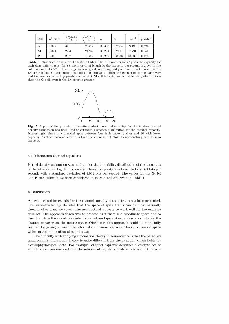
Table 1 Numerical values for the featured sites. The column marked C gives the capacity foreach time unit, that is, for a time interval of length λ; the capacity per second is given in thecolumn marked Cs−1. The designation of good, middling and poor were made based on theL2 error in the χ distribution; this does not appear to affect the capacities in the same wayand the Anderson-Darling p-values show that M cell is better modelled by the χ-distributionthan the G cell, even if the L2 error is greater.

0

0.05

0.1

0 5 10 15 20

Fig. 5 A plot of the probability density against measured capacity for the 24 sites. Kerneldensity estimation has been used to estimate a smooth distribution for the channel capacity.Interestingly, there is a bimodal split between four high capacity sites and 20 with lowercapacity. Another notable feature is that the curve is not close to approaching zero at zerocapacity.

3.4 Information channel capacities

Kernel density estimation was used to plot the probability distribution of the capacities

of the 24 sites, see Fig. 5. The average channel capacity was found to be 7.358 bits per

second, with a standard deviation of 4.962 bits per second. The values for the G, M

and P sites which have been considered in more detail are given in Table 1

4 Discussion

A novel method for calculating the channel capacity of spike trains has been presented.

This is motivated by the idea that the space of spike trains can be most naturally

thought of as a metric space. The new method appears to work well for the example

data set. The approach taken was to proceed as if there is a coordinate space and to

then translate the calculation into distance-based quantities, giving a formula for the

channel capacity on the metric space. Obviously, this approach could be more fully

realized by giving a version of information channel capacity theory on metric space

which makes no mention of coordinates.

One difficulty with applying information theory to neuroscience is that the paradigm

underpinning information theory is quite different from the situation which holds for

electrophysiological data. For example, channel capacity describes a discrete set of

stimuli which are encoded in a discrete set of signals, signals which are in turn em-

12

bedded with noise in a continuous space of outputs. This is hardly the situation that

holds in the sensory pathways. Moreover, the theorems which are proved for informa-

tion theory often become principles or techniques when applied in this less well-defined

context. These issues are nicely summarized in, for example, Johnson [2003], where

rate-distortion theory is suggested as the correct information theory framework for the

sort of data discussed here. However, applying rate distortion theory to sensory electro-

physiological data is quite a challenge, it requires a well-defined stimulus space and a

relevant rate distortion function. It seems likely, though, that the technique suggested

in this paper, the redefining of coordinate-based information quantities as metric space

objects and a model of noise based on an analogy with a coordinate-based noise model,

will be useful in developing this rate distortion theory.

The van Rossum metric is used. This is because it has an L2 Pythagorean structure

in the interval length. There is also an L2 Victor-Purpura metric [Dubbs, Seiler and

Magnasco , 2009] but the L2 structure in that case refers to the individual spikes. Of

course, this raises the question of what is the most suitable metric structure for spike

trains. This has been studied for the data used here by evaluating the accuracy of

distance based clustering [Houghton , 2009a,b, Houghton and Victor , 2009]. However,

these comparisons show that the metrics all have a similar performance. Furthermore,

the clustering-technique is really only a good probe for the local metric structure.

The question of the most appropriate metric structure for spike trains has not been

answered; the L2 van Rossum metric is certainly the metric which fits easiest into the

metric space approach to information that is proposed here.

Neural spike trains can be considered as point processes and developing a distance

measure on spike trains from the perspective of point processes is a challenge to future

approaches. Rate-distortion theory of point processes has suggested distance measures

on spike trains [Rubin , 1974a,b]. Although they may not seem natural in a neurosci-

entific context, a more comprehensive theory of information theory and the geometry

of spike trains should make it possible to relate these metrics to spike train analysis.

Conversely, it would be good to have a fuller account of what properties of spike trains

distinguish them within the general family of point processes.

This method has been applied to a single example dataset; it will be interesting

to establish how well it performs on other sets of spike trains. In particular, it will

be interesting to see if the basic assumption that the inter-fragment distances for

signal responses satisfy a χ-distribution, is accurate. Conversely, it would be useful to

generalize the discussion presented here to allow for other noise processes.

Acknowledgements

JBG wishes to thank the Irish Research Council of Science, Engineering and Technol-

ogy for an Embark Postgraduate Research Scholarship. CJH wishes to thank Science

Foundation Ireland for Research Frontiers Programme grant 08/RFP/MTH1280. They

are grateful to Garrett Greene, Louis Aslett and Daniel McNamee for useful discussion

and to Kamal Sen for the use of the data analysed here.

13

References

Anderson, T. W. & Darling, D. A. (1952) Asymptotic theory of certain ‘goodness-of-fit’

criteria based on stochastic processes Annals of Mathematical Statistics, 23:193–212.

Bialek, W., Rieke, F., de Ruyter van Steveninck, R. R. & Warland, D. (1991) Reading

a neural code. Science, 252:1854–1857.

Borst, A. & Theunissen, F. (1999) Information theory and neural coding Nature

Neuroscience, 2:947–957.

Cover, T. M. & Thomas J. A. (1991) Elements of information theory. Wiley.

De Ruyter Van Steveninck, R. R., Lewen, G. D., Strong, S. P., Koberle, R. & Bialek,

W. (1997) Reproducibility and variability in neural spike trains. Science, 275:1805–

1808.

Dubbs, A. J., Seiler, B. A. & Magnasco, M. O. (2009) A fast Lp spike alignment metric.

(http://arxiv.org/abs/0907.3137).

Houghton, C. (2009) Studying spike trains using a van Rossum metric with a synapses-

like filter. Journal of Computational Neuroscience, 26:149–155.

Houghton, C. (2009) A comment on ‘a fast l p spike alignment met-

ric’ by A. J. Dubbs, B. A. Seiler and M. O. Magnasco [arxiv:0907.3137].

(http://arxiv.org/abs/0908.1260).

C. Houghton, C. & Victor, J. (2009) Measuring representational distances - the spike-

train metrics approach. (book chapter, in press).

Johnson, D. H. (2003) Dialogue concerning neural coding and information theory.

(http://www.ece.rice.edu/ dhj/dialog.pdf).

Narayan, R., Grana, G. & Sen, K. (2006) Distinct time scales in cortical discrimination

of natural sounds in songbirds. Journal of Neurophysiology, 96:252–258.

Rieke, F., Warland, D., De Ruyter Van Steveninck, R. R. & Bialek, W. (1999) Spikes:

exploring the neural code. MIT Computational Neuroscience Series.

Rubin, I. (1974) Information rates and data-compression schemes for Poisson processes.

IEEE Transactions on Information Theory 20:200–210.

Rubin, I. (1974) Rate Distortion Functions for Non-Homogeneous Poisson Processes.

IEEE Transactions on Information Theory 20:669–672.

Shannon, C. E. (1948) A mathematical thoery of communication. Bell Systems Tech-

nical Journal, 27:379–423,623–656.

Silverman, B. W. (1986) Density Estimation. London: Chapman and Hall.

Stephens, M. A. (1974) EDF Statistics for Goodness of Fit and Some Comparisons

Journal of the American Statistical Association 69:730–737.

van Rossum, M. (2001) A novel spike distance. Neural Computation, 13:751–763.

Victor, J. D. & Purpura, K. P. (1996) Nature and precision of temporal coding in

visual cortex: a metric-space analysis. Journal of Neurophysiology, 76:1310–1326.

Victor, J. D. (2002) Binless strategies for estimation of information from neural data.

Physical Review E, 66:051903.

Victor, J. D. (2005) Spike train metrics. Current Opinion in Neurobiology, 15:585–592.

Wang, L., Narayan, R., Grana, G., Shamir, M. & Sen, K (2007) Cortical discrimi-

nation of complex natural stimuli: can single neurons match behavior? Journal of

Neuroscience, 27:582–9.