Statistical Regimes Across Constrainedness Regions
21
Statistical Regimes Across Constrainedness Regions* CARLA P. GOMES [email protected] Department of Computer Science, Cornell University, Ithaca, USA ` [email protected] Dpt. d’Informa `tica, Universitat de Lleida, Jaume II, 69, E-25001, Lheida, Spain BART SELMAN [email protected] Department of Computer Science, Cornell University, Ithaca, USA CHRISTIAN BESSIE ` RE [email protected] LIRMM-CNRS, 161 rue Ada, 34392, Montpellier Cedex 5, France Abstract. Much progress has been made in terms of boosting the effectiveness of backtrack style search methods. In addition, during the last decade, a much better understanding of problem hardness, typical case complexity, and backtrack search behavior has been obtained. One example of a recent insight into backtrack search concerns so-called heavy-tailed behavior in randomized versions of backtrack search. Such heavy-tails explain the large variance in runtime often observed in practice. However, heavy-tailed behavior does certainly not occur on all instances. This has led to a need for a more precise characterization of when heavy-tailedness does and when it does not occur in backtrack search. In this paper, we provide such a characterization. We identify different statistical regimes of the tail of the runtime distributions of randomized backtrack search methods and show how they are correlated with the Bsophistication^ of the search procedure combined with the inherent hardness of the instances. We also show that the runtime distribution regime is highly correlated with the distribution of the depth of inconsistent subtrees discovered during the search. In particular, we show that an exponential distribution of the depth of inconsistent subtrees combined with a search space that grows exponentially with the depth of the inconsistent subtrees implies heavy-tailed behavior. Keywords: backtrack search, runtime distributions, heavy-tailed distributions, phase transitions, typical case analysis 1. Introduction Significant advances have been made in recent years in the design of search engines for constraint satisfaction problems (CSP), including Boolean satisfiability problems (SAT). For complete solvers, the basic underlying solution strategy is backtrack search enhanced by a series of increasingly sophisticated techniques, such as non-chronological backtracking [10, 25], fast pruning and propagation methods [4, 14, 22, 24, 28], nogood (or clause) learning (e.g., [2, 7, 21, 26]), and more recently randomization and restarts *Research supported by the Intelligent Information Systems Institute, Cornell University (AFOSR grant F49620-01-1-0076), MURI (AFOSR grant F49620-01-1-0361) and Ministerio de Educacio ´n y Ciencia (TIN- 2004 grant 07933-C03-03). We thank the anonymous reviewers for their insightful comments. Constraints, 10, 317–337, 2005 # 2005 Springer Science + Business Media, Inc. Manufactured in The Netherlands. CESAR FERNANDEZ ´
Transcript of Statistical Regimes Across Constrainedness Regions
Statistical Regimes Across ConstrainednessRegions*
CARLA P. GOMES [email protected]
Department of Computer Science, Cornell University, Ithaca, USA
Dpt. d’Informatica, Universitat de Lleida, Jaume II, 69, E-25001, Lheida, Spain
BART SELMAN [email protected]
Department of Computer Science, Cornell University, Ithaca, USA
CHRISTIAN BESSIERE [email protected]
LIRMM-CNRS, 161 rue Ada, 34392, Montpellier Cedex 5, France
Abstract. Much progress has been made in terms of boosting the effectiveness of backtrack style search
methods. In addition, during the last decade, a much better understanding of problem hardness, typical case
complexity, and backtrack search behavior has been obtained. One example of a recent insight into backtrack
search concerns so-called heavy-tailed behavior in randomized versions of backtrack search. Such heavy-tails
explain the large variance in runtime often observed in practice. However, heavy-tailed behavior does certainly
not occur on all instances. This has led to a need for a more precise characterization of when heavy-tailedness
does and when it does not occur in backtrack search. In this paper, we provide such a characterization. We
identify different statistical regimes of the tail of the runtime distributions of randomized backtrack search
methods and show how they are correlated with the Bsophistication^ of the search procedure combined with the
inherent hardness of the instances. We also show that the runtime distribution regime is highly correlated with
the distribution of the depth of inconsistent subtrees discovered during the search. In particular, we show that an
exponential distribution of the depth of inconsistent subtrees combined with a search space that grows
exponentially with the depth of the inconsistent subtrees implies heavy-tailed behavior.
Keywords: backtrack search, runtime distributions, heavy-tailed distributions, phase transitions, typical case
analysis
1. Introduction
Significant advances have been made in recent years in the design of search engines for
constraint satisfaction problems (CSP), including Boolean satisfiability problems (SAT).
For complete solvers, the basic underlying solution strategy is backtrack search enhanced
by a series of increasingly sophisticated techniques, such as non-chronological
backtracking [10, 25], fast pruning and propagation methods [4, 14, 22, 24, 28], nogood
(or clause) learning (e.g., [2, 7, 21, 26]), and more recently randomization and restarts
*Research supported by the Intelligent Information Systems Institute, Cornell University (AFOSR grant
F49620-01-1-0076), MURI (AFOSR grant F49620-01-1-0361) and Ministerio de Educacion y Ciencia (TIN-
2004 grant 07933-C03-03). We thank the anonymous reviewers for their insightful comments.
Constraints, 10, 317–337, 2005# 2005 Springer Science + Business Media, Inc. Manufactured in The Netherlands.
CESAR FERNANDEZ´
[12, 13]. For example, in areas such as planning and finite model-checking, we are now
able to solve large CSP’s with up to a million variables and several million constraints
(see e.g., [3, 23]).
The study of problem structure of combinatorial search problems has also provided
tremendous insights in our understanding of the interplay between structure, search
algorithms, and more generally, typical case complexity. For example, the work on phase
transition phenomena in combinatorial search has led to a better characterization of
search cost, beyond the worst-case notion of NP-completeness. While the notion of NP-
completeness captures the computational cost of the very hardest possible instances of a
given problem, in practice, one may not encounter many instances that are quite that
hard. In general, CSP problems exhibit an Beasy-hard-easy^ pattern of search cost,
depending on the constrainedness of the problem [15]. The computational hardest
instances appear to lie at the phase transition region, the area in which instances change
from being almost all solvable to being almost all unsolvable. The discovery of
Bexceptionally hard instances^ revealed an interesting phenomenon : such instances
seem to defy the Beasy-hard-easy^ pattern, they occur in the under-constrained area, but
they seem to be considerably harder than other similar instances and even harder than
instances from the critically constrained area.This phenomenon was first identified by
Hogg and Williams in graph coloring and by Gent and Walsh in satisfiability problems
[11, 16]. However, it was shown later that such instances are not inherently difficult; for
example, by renaming the variables such instances can often be easily solved [29, 30].
Therefore, the Bhardness^ of exceptionally hard instances does not reside purely in the
instances, but rather in the combination of the instance with the details of the search
method. Smith and Grant provide a detailed analysis of the occurrence of exceptionally
hard instances for backtrack search, by considering a deterministic backtrack search
procedure on sets of instances with the same parameter setting (see e.g., [31]). Recently,
researchers have noted that for a proper understanding of search behavior one has to
study full runtime distributions1 [8, 9, 12, 16, 17], as opposed to only considering
statistics such as the mean of the distribution. In our work we have focused on the study
of randomized backtrack search algorithms [12]. By studying the runtime distribution
produced by a randomized algorithm on a single instance, we can analyze the variance
caused solely by the algorithm, and therefore separate the algorithmic variance from the
variance between different instances drawn from an underlying distribution. We have
shown previously that the runtime distributions of randomized backtrack search
procedures can exhibit extremely large variance, even when solving the same instance
over and over again [12, 13]. This work on the study of the runtime distributions of
randomized backtrack search algorithms further clarified that the source of extreme
variance observed in exceptional hard instances was not due to the inherent hardness of
the instances: A randomized version of a search procedure on such instances in general
solves the instance easily, even though it has a non-negligible probability of taking very
long runs to solve the instance, considerably longer than all the other runs combined.
Such extreme fluctuations in the runtime of backtrack search algorithms are nicely
captured by so-called heavy-tailed distributions, distributions that are characterized by
extremely long tails with some of its moments infinite [12, 16]. The decay of the tails of
318 C. P. GOMES ET AL.
heavy-tailed distributions follows a power lawVmuch slower than the decay of standard
distributions, such as the normal or the exponential distribution, that have tails that decay
exponentially. Further insights into the empirical evidence of heavy-tailed phenomena of
randomized backtrack search methods were provided by abstract models of backtrack
search that show that, under certain conditions, such procedures provably exhibit heavy-
tailed behavior [6, 13, 33, 34].
1.1. Main Results
So far, evidence for heavy-tailed behavior of randomized backtrack search procedures on
concrete instance models has been largely empirical. Moreover, it is clear that not all
problem instances exhibit heavy-tailed behavior. The goal of this work is to provide a
better characterization of when heavy-tailed behavior occurs, and when it does not, when
using randomized backtrack search methods. We study the empirical runtime
distributions of randomized backtrack search procedures across different constrainedness
regions of random binary constraint satisfaction models.2 In order to obtain the most
accurate empirical runtime distributions, all our runs are performed without censorship
(i.e., we run our algorithms without a cutoff ). Our study reveals dramatically different
statistical regimes for randomized backtrack search algorithms across the different
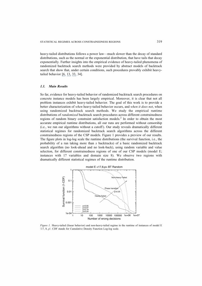
constrainedness regions of the CSP models. Figure 1 provides a preview of our results.
The figure plots in log-log scale the runtime distributions (the survival function, i.e., the
probability of a run taking more than x backtracks) of a basic randomized backtrack
search algorithm (no look-ahead and no look-back), using random variable and value
selection, for different constrainedness regions of one of our CSP models (model E;
instances with 17 variables and domain size 8). We observe two regions with
dramatically different statistical regimes of the runtime distribution.
Figure 1. Heavy-tailed (linear behavior) and non-heavy-tailed regime in the runtime of instances of model E
b17, 8, pÀ. CDF stands for Cumulative Density Function Log-log scale.
STATISTICAL REGIMES ACROSS CONSTRAINEDNESS REGIONS 319

In the first regime (the bottom two curves in Figure 1, p e 0.07), we see heavy-tailed
behavior. This means that the runtime distributions decay slowly. In the log-log plot, we
see linear behavior over several orders of magnitude. When we increase the
constrainedness of our model (higher p), we encounter a different statistical regime in
the run-time distributions, where the heavy-tails disappear. In this region, the instances
become inherently hard for the backtrack search algorithm, all the runs become homo-
geneously long, and therefore the variance of the backtrack search algorithm decreases
and the tails of its survival function decay rapidly (see top two curves in Figure 1, with
p = 0.19 and p = 0.24; tails decay exponentially).
A common intuitive understanding of the extreme variability of backtrack search is
that on certain runs the search procedure may hit a very large inconsistent subtree that
needs to be fully explored, causing Bthrashing^ behavior.
To confirm this intuition and in order to get further insights into the statistical behavior
of our backtrack search method, we study the inconsistent sub-trees discovered by the
algorithm during the search (see Figure 2).
The distribution of the depth of inconsistent trees is quite revealing: when the
distribution of the depth of the inconsistent trees decreases exponentially (see Figure 3,
bottom panel, p = 0.07) the runtime distribution of the backtrack search method has a
power law decay (see Figure 3, top panel, p = 0.07). In other words, when the backtrack
search heuristic has a good probability of finding relatively shallow inconsistent subtrees,
and this probability decreases exponentially as the depth of the inconsistent subtrees
increases, heavy-tailed behavior occurs. Contrast this behavior with the case in which
the survival function of the runtime distribution of the backtrack search method is not
heavy-tailed (see Figure 3, top panel, p = 0.24). In this case, the distribution of the
depth of inconsistent trees no longer decreases exponentially (see Figure 3, bottom panel,
p = 0.24).
Figure 2. Inconsistent subtrees in backtrack search.
320 C. P. GOMES ET AL.

In essence, these results show that the distribution of inconsistent subproblems
encountered during backtrack search is highly correlated with the tail behavior of the
runtime distribution. We provide a formal analysis that links the exponential search tree
depth distribution with heavy-tailed runtime profiles. As we will see below, the
predictions of our model closely match our empirical data.
The structure of the paper is as follows. In the next section we provide definitions of
concepts used throughout the paper, namely concepts related to constraint networks and
search trees, a description of the random models used for the generation of our problem
instances, and a description of the search algorithms that we use in our experimentation.
In Section 3 we provide empirical results. In Section 4 we present a theoretical model of
heavy-tailed runtime distributions that considers the distribution of the depth of
Figure 3. Example of a heavy-tailed instance ( p = 0.07) and a non-heavy-tailed instance ( p = 0.24): (top)
Survival function of runtime distribution, (bottom) probability density function of depth of inconsistent subtrees
encountered during search. The subtree depth for p = 0.07 instance is exponentially distributed Log-log scale.
STATISTICAL REGIMES ACROSS CONSTRAINEDNESS REGIONS 321
inconsistent subtrees and the growth of the search space inside such inconsistent
subtrees; in Section 4 we also compare the results of our theoretical model with our
empirical results. In Section 5 we present conclusions and discuss future research
directions.
2. Definitions, Problem Instances, and Search Methods
2.1. Constraint Networks
A finite binary constraint network P ¼ X ;D; Cð Þ is defined as a set of n variables
X ¼ x1; . . . ; xnð Þ, a set of domains D ¼ D x1ð Þ; . . . ;D xnð Þf g, where D(xi) is the finite set
of possible values for variable xi, and a set C of binary constraints between pairs of
variables. A constraint Cij on the ordered set of variables (xi, xj ) is a subset of the
Cartesian product D(xi) � D(xj) that specifies the allowed combinations of values for the
variables xi and xj. A solution of a constraint network is an instantiation of the variables
such that all the constraints are satisfied. The constraint satisfaction problem (CSP)
involves finding a solution for the constraint network or proving that none exists. We
used a direct CSP encoding and also a Boolean satisfiability encoding (SAT) [32].
2.2. Random Problems
The CSP research community has always made a great use of randomly generated
constraint satisfaction problems for comparing different search techniques and studying
their behavior. Several models for generating these random problems have been
proposed over the years. The oldest one, which was the most commonly used until the
middle 90¶s, is model A. A network generated by this model is characterized by four
parameters bN, D, p1, p2À, where N is the number of variables, D the size of the domains,
p1 the probability of having a constraint between two variables, and p2 , the probability
that a pair of values is forbidden in a constraint. Notice that the variance in the type of
problems generated with the same four parameters can be large, since the actual number
of constraints for two problems with the same parameters can vary from one problem to
another, and the actual number of forbidden tuples for two constraints inside the same
problem can also be different. Model B does not have this variance. In model B, the four
parameters are again N, D, p1, and p2, where N is the number of variables, and D the
size of the domains. But now, p1 is the proportion of binary constraints that are in the
network (i.e., there are exactly c = )p1 I N I (N j 1) /22 constraints), and p2 is the
proportion of forbidden tuples in a constraint (i.e., there are exactly t = )p2 I D22forbidden tuples in each constraint). Problem classes in this model are denoted by bN, D,
c, tÀ. In [1] it was shown that model B (and model A as well) can be Bflawed^ when we
increase N. Indeed, when N goes to infinity, we will almost surely have a flawed variable
(that is, one variable which has all its values inconsistent with one of the constraints
involving it). Model E was proposed to overcome this weakness. It is a three parameter
322 C. P. GOMES ET AL.
model, bN, D, pÀ, where N and D are the same as in the other models, and )p I D2 I N I(N j 1) /22 forbidden pairs of values are selected with repetition out of the D2 I N I(N j 1) /2 possible pairs. There is also a way of tackling the problem of awed variables
in model B. In [35] it is shown that by enforcing certain constraints on the relative values
of N, D, p1, and p2, one can guarantee that model B is sound and scalable, for a range
of values of the parameters. In our work, we only considered instances of model B that
fall within such a range of values.
2.3. Search Trees
A search tree is composed of nodes and arcs. A node u represents an ordered partial
instantiation I uð Þ ¼ xi1 ¼ Vi1 ; :::; xik ¼ Vikð Þ. A search tree is rooted at the particular node
u0 with I(u0) = ;. There is an arc from a node u to a node uc if I(uc) = (I(u), x = v), x and v
being a variable and one of its values. The node uc is called a child of u and u a parent of
uc. Every node u in a tree T defines a subtree Tu that consists of all the nodes and arcs
below u in T. The depth of a subtree Tu is the length of the longest path from u to any
other node in Tu. An inconsistent subtree (IST) is a maximal subtree that does not contain
any node u such that I(u) is a solution (see Figure 2). The maximum depth of an
inconsistent subtree is referred to the Binconsistent subtree depth^ (ISTD). We denote by
T(A, P) the search tree of a backtrack search algorithm A solving a particular instance
P, which contains a node for each instantiation visited by A until a solution is reached
or inconsistency of P is proved. Once assigned a partial instantiation I uð Þ ¼ xi1 ¼ðVi1 ; : : :; xik ¼ Vik Þ for node u, the algorithm will search for a partial instantiation of some
of its children. In the case that there exists no instantiation which does not violate the
constraints, algorithm A will take another value for variable xik , and start again checking
the children of this new node. In this situation, it is said that a backtrack happens. We use
the number of wrong decisions or backtracks to measure the search cost of a given
algorithm [5].3
2.4. Algorithms
We studied different search procedures that differ in the amount of propagation they
perform, and in the order in which they generate instantiations. We used three levels of
propagation: no propagation (backtracking, BT), removal of values directly inconsistent
with the last instantiation performed (forward-checking, FC), and arc consistency
propagation (maintaining arc consistency, MAC). We used three different heuristics for
variable selection: random selection of the next variable to instantiate (random),
variables pre-ordered by decreasing degree in the constraint graph (deg), and selection of
the variable with smallest domain first, ties broken by decreasing degree (dom+deg) and
always random value selection. For the SAT encodings we used the Davis-Putnam-
Logemann-Loveland procedure. More specifically we used a simplified version of Satz
[20], without its standard heuristic, and with static variable ordering, injecting some
randomness in the value selection heuristics.
STATISTICAL REGIMES ACROSS CONSTRAINEDNESS REGIONS 323
2.5. Heavy-tailed or Pareto-like Distributions
As we discussed earlier, the runtime distributions of backtrack search methods are often
characterized by very long tails or heavy-tails (HT). These are distributions that have so-
called Pareto like decay of the tails. For a general Pareto distribution F(x), the probability
that a random variable is larger than a given value x, i.e., its survival function, is:
1� F xð Þ ¼ P X > x½ � � Cx��; x > 0;
where � 9 0 and C 9 0 are constants. I.e., we have power-law decay in the tail of the
distribution. These distributions have infinite variance when 1 G � G 2 and infinite mean
and variance when 0 G � e 1. The log-log plot of the tail of the survival function (1 j
F(x)) of a Pareto-like distribution shows linear behavior with slope determined by �.
3. Empirical Results
In the previous section we defined our models and algorithms, as well as the concepts
that are central in our study: the runtime distributions of our backtrack search methods
and the associated distributions of the depth of the inconsistent subtrees found by the
backtrack method. As we discussed in the introduction, our key findings are: (1) we
observe different regimes in the behavior of these distributions as we move along
different instance constrainedness regions; (2) when the depth of the inconsistent
subtrees encountered during the search by the backtrack search method follows an
exponential distribution, the corresponding backtrack search method search exhibits
heavy-tailed behavior. In this section, we provide the empirical data upon which these
findings are based.4
We present results for the survival functions of the search cost (number of wrong
decisions or number of backtracks) of our backtrack search algorithms. All the plots
were computed with at least 10,000 independent executions of a randomized backtrack
search procedure on a given (uniquely generated) problem satisfiable instance. For
each parameter setting we considered over 20 instances. In order to obtain more ac-
curate empirical runtime distributions, all our runs were performed without cen-
sorship, i.e., we run our algorithms without any cutoff.5 We also instrumented the code
to obtain the information for the corresponding inconsistency sub-tree depth (ISTD)
distributions.
Figure 4 (top) provides a detailed view of the heavy-tailed and non-heavy-tailed
regions, as well as the progression from one region to the other. The figure displays the
survival function (logYlog scale) for running (pure) backtrack search with random
variable and value selection on instances of Model E with 17 variables and a domain size
of 8 for values of p (the constrainedness of the instances) ranging from 0.05 e p e 0.24.
We clearly identify a heavy-tailed region in which the log-log plot of the survival
functions exhibits linear behavior, while in the non-heavy-tailed region the drop of the
324 C. P. GOMES ET AL.
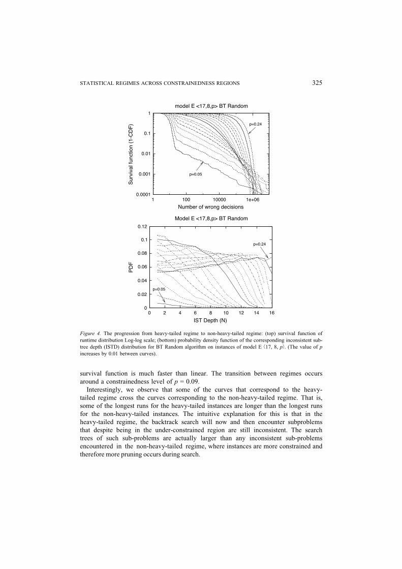
survival function is much faster than linear. The transition between regimes occurs
around a constrainedness level of p = 0.09.
Interestingly, we observe that some of the curves that correspond to the heavy-
tailed regime cross the curves corresponding to the non-heavy-tailed regime. That is,
some of the longest runs for the heavy-tailed instances are longer than the longest runs
for the non-heavy-tailed instances. The intuitive explanation for this is that in the
heavy-tailed regime, the backtrack search will now and then encounter subproblems
that despite being in the under-constrained region are still inconsistent. The search
trees of such sub-problems are actually larger than any inconsistent sub-problems
encountered in the non-heavy-tailed regime, where instances are more constrained and
therefore more pruning occurs during search.
Figure 4. The progression from heavy-tailed regime to non-heavy-tailed regime: (top) survival function of
runtime distribution Log-log scale; (bottom) probability density function of the corresponding inconsistent sub-
tree depth (ISTD) distribution for BT Random algorithm on instances of model E b17, 8, pÀ. (The value of p
increases by 0.01 between curves).
STATISTICAL REGIMES ACROSS CONSTRAINEDNESS REGIONS 325
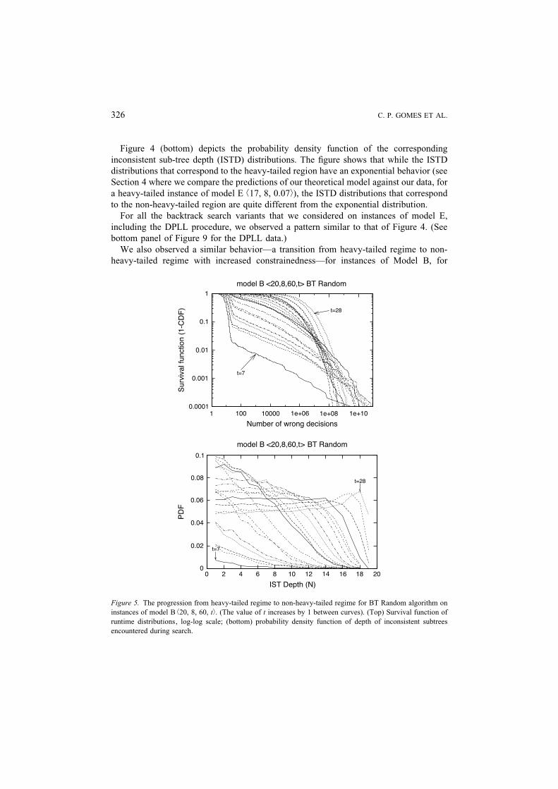
Figure 4 (bottom) depicts the probability density function of the corresponding
inconsistent sub-tree depth (ISTD) distributions. The figure shows that while the ISTD
distributions that correspond to the heavy-tailed region have an exponential behavior (see
Section 4 where we compare the predictions of our theoretical model against our data, for
a heavy-tailed instance of model E b17, 8, 0.07À), the ISTD distributions that correspond
to the non-heavy-tailed region are quite different from the exponential distribution.
For all the backtrack search variants that we considered on instances of model E,
including the DPLL procedure, we observed a pattern similar to that of Figure 4. (See
bottom panel of Figure 9 for the DPLL data.)
We also observed a similar behaviorVa transition from heavy-tailed regime to non-
heavy-tailed regime with increased constrainednessVfor instances of Model B, for
Figure 5. The progression from heavy-tailed regime to non-heavy-tailed regime for BT Random algorithm on
instances of model B b20, 8, 60, tÀ. (The value of t increases by 1 between curves). (Top) Survival function of
runtime distributions, log-log scale; (bottom) probability density function of depth of inconsistent subtrees
encountered during search.
326 C. P. GOMES ET AL.
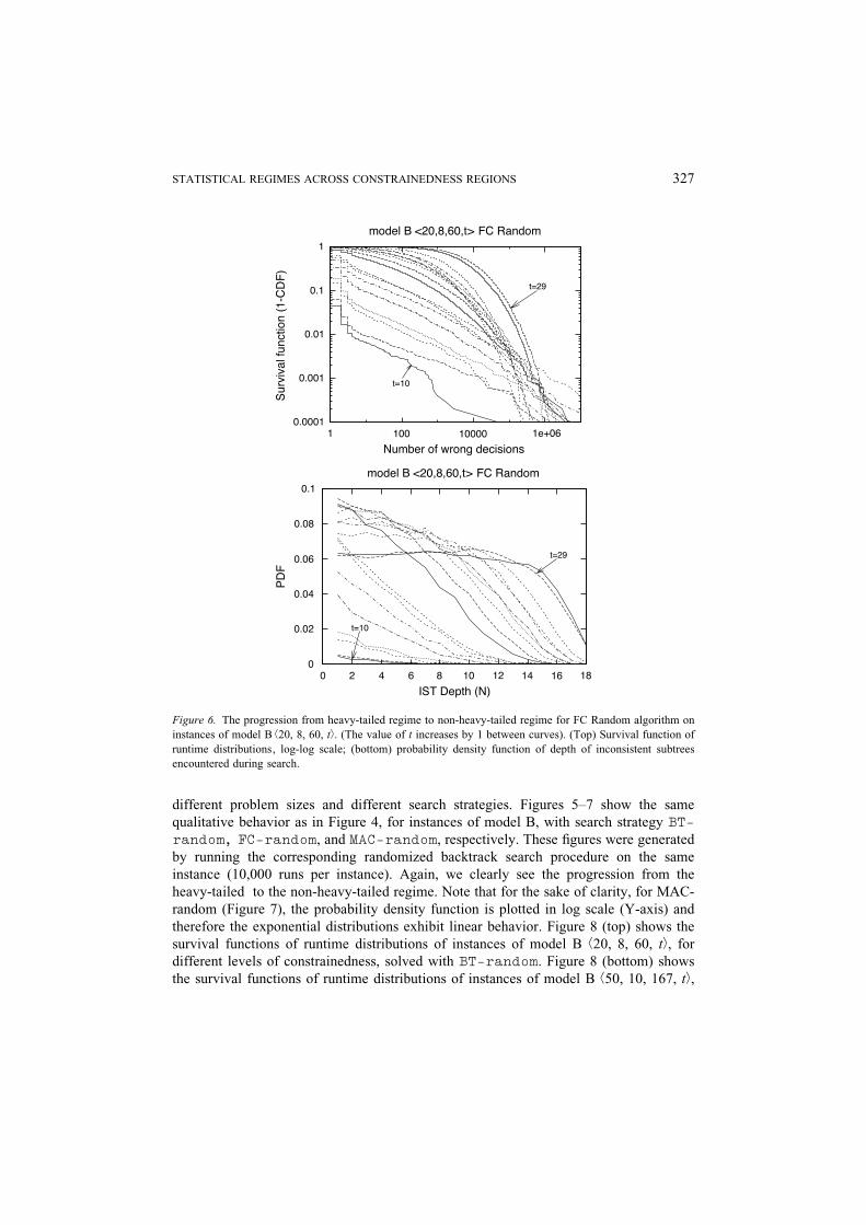
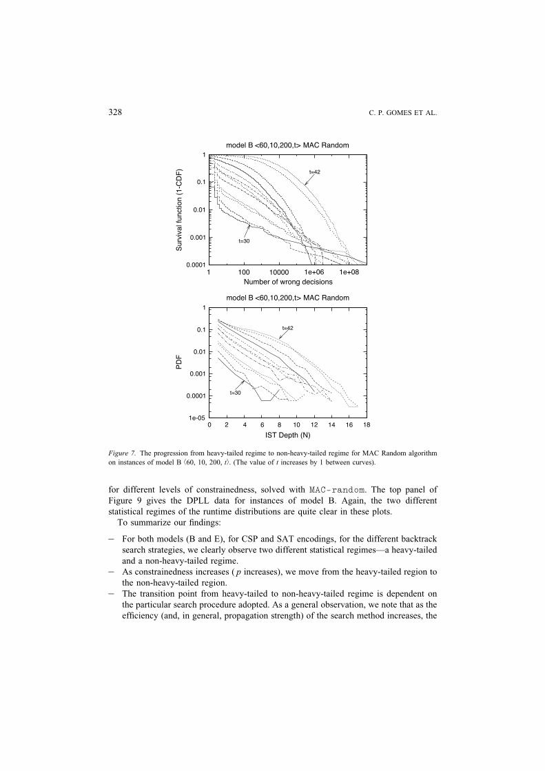
different problem sizes and different search strategies. Figures 5Y7 show the same
qualitative behavior as in Figure 4, for instances of model B, with search strategy BT-
random, FC-random, and MAC-random, respectively. These figures were generated
by running the corresponding randomized backtrack search procedure on the same
instance (10,000 runs per instance). Again, we clearly see the progression from the
heavy-tailed to the non-heavy-tailed regime. Note that for the sake of clarity, for MAC-
random (Figure 7), the probability density function is plotted in log scale (Y-axis) and
therefore the exponential distributions exhibit linear behavior. Figure 8 (top) shows the
survival functions of runtime distributions of instances of model B b20, 8, 60, tÀ, for
different levels of constrainedness, solved with BT-random. Figure 8 (bottom) shows
the survival functions of runtime distributions of instances of model B b50, 10, 167, tÀ,
Figure 6. The progression from heavy-tailed regime to non-heavy-tailed regime for FC Random algorithm on
instances of model B b20, 8, 60, tÀ. (The value of t increases by 1 between curves). (Top) Survival function of
runtime distributions, log-log scale; (bottom) probability density function of depth of inconsistent subtrees
encountered during search.
STATISTICAL REGIMES ACROSS CONSTRAINEDNESS REGIONS 327
for different levels of constrainedness, solved with MAC-random. The top panel of
Figure 9 gives the DPLL data for instances of model B. Again, the two different
statistical regimes of the runtime distributions are quite clear in these plots.
To summarize our findings:
Y For both models (B and E), for CSP and SAT encodings, for the different backtrack
search strategies, we clearly observe two different statistical regimesVa heavy-tailed
and a non-heavy-tailed regime.
Y As constrainedness increases ( p increases), we move from the heavy-tailed region to
the non-heavy-tailed region.
Y The transition point from heavy-tailed to non-heavy-tailed regime is dependent on
the particular search procedure adopted. As a general observation, we note that as the
efficiency (and, in general, propagation strength) of the search method increases, the
Figure 7. The progression from heavy-tailed regime to non-heavy-tailed regime for MAC Random algorithm
on instances of model B b60, 10, 200, tÀ. (The value of t increases by 1 between curves).
328 C. P. GOMES ET AL.

extension of the heavy-tailed region increases and therefore the heavy-tailed
threshold gets closer to the phase transition.
Y Exponentially distributed inconsistent sub-tree depth (ISTD) combined with
exponential growth of the search space as the tree depth increases implies heavy-
tailed runtime distributions. We observe that as the ISTD distributions move away
from the exponential distribution, the runtime distributions become non-heavy-tailed.
These results suggest that heavy-tailed behavior in the cost distributions depends on
the efficiency of the search procedure as well as on the level of constrainedness of the
problem. Increasing the algorithm efficiency tends to shift the heavy-tail threshold closer
to the phase transition. We conjecture that even when considering more sophisticated
search methods involving, e.g., intelligent backtracking and no-good learning (see e.g.,
[2, 7, 21, 26]), one will encounter qualitatively the same pattern, albeit for larger problem
instances. Although we have not yet studied this pattern for more sophisticated search
Figure 8. Heavy-tailed and non-heavy-tailed regimes for instances of model B: (top) b20, 8, 60, tÀ, using BT-
random, (bottom) b50, 10, 167, tÀ, using MAC-random.
STATISTICAL REGIMES ACROSS CONSTRAINEDNESS REGIONS 329
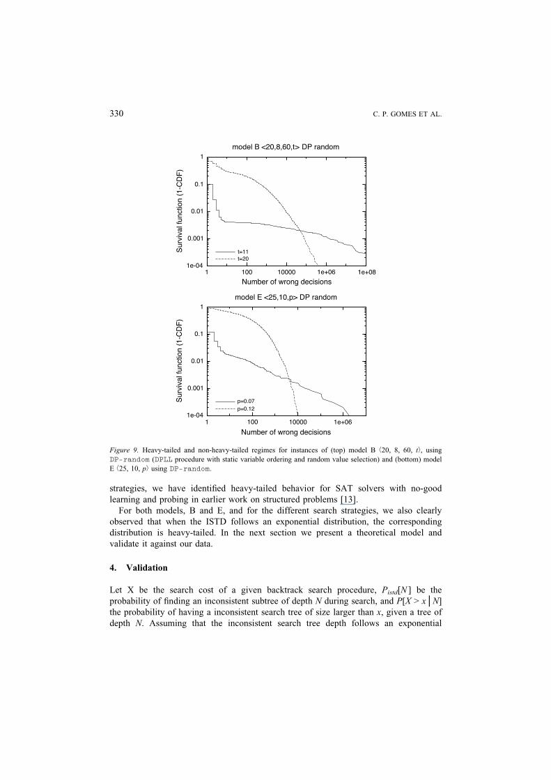
strategies, we have identified heavy-tailed behavior for SAT solvers with no-good
learning and probing in earlier work on structured problems [13].
For both models, B and E, and for the different search strategies, we also clearly
observed that when the ISTD follows an exponential distribution, the corresponding
distribution is heavy-tailed. In the next section we present a theoretical model and
validate it against our data.
4. Validation
Let X be the search cost of a given backtrack search procedure, Pistd[N ] be the
probability of finding an inconsistent subtree of depth N during search, and P[X 9 xªN]
the probability of having a inconsistent search tree of size larger than x, given a tree of
depth N. Assuming that the inconsistent search tree depth follows an exponential
Figure 9. Heavy-tailed and non-heavy-tailed regimes for instances of (top) model B b20, 8, 60, tÀ, using
DP-random (DPLL procedure with static variable ordering and random value selection) and (bottom) model
E b25, 10, pÀ using DP-random.
330 C. P. GOMES ET AL.
distribution in the tail and the search cost inside an inconsistent tree grows exponentially,
then the cost distribution of a search method is lower bounded by a Pareto distribution.
More formally:
4.1. Theoretical Model
Assumptions:
Y Pistd[N ] is exponentially distributed in the tail, i.e.,
Pistd N½ � ¼ B1e�B2N ;N > n0 ð1Þ
where B1, B2, and n0 are constants.
Y P[X 9 xªN ] is modeled as a complementary Heavyside function, 1 j H(x j k N ),
where k is a constant and
H x� að Þ ¼ 0; x G a
1; x � a
�
Then, P[X 9 x] is Pareto-like distributed
P X > x½ � � �x��
for x > kn0 , where � and � are constants.
Derivation of result: Note that P[X 9 x] is lower bounded as follows
P X > x½ � �Z 1
N¼0
Pistd N½ �P X > x Nj½ �dN ð2Þ
This is a lower bound since we consider only one inconsistent tree contributing to the
search cost, when in general there are more inconsistent trees. Given the assumptions
above, Equation (2) results
P X > x½ � �Z 1
N¼0
Pistd N½ � 1� H x� kN� �� �
dN ¼Z 1
N¼ ln xln k
Pistd N½ �dN ð3Þ
Since x > kn0 , we can use Equation (1) for Pistd[N], so Equation (3) results in:
P X > x½ � �Z 1
N¼ ln xln k
B1e�B2N dN ¼ B1
B2
e�B2
ln x
ln k¼ �x��
STATISTICAL REGIMES ACROSS CONSTRAINEDNESS REGIONS 331
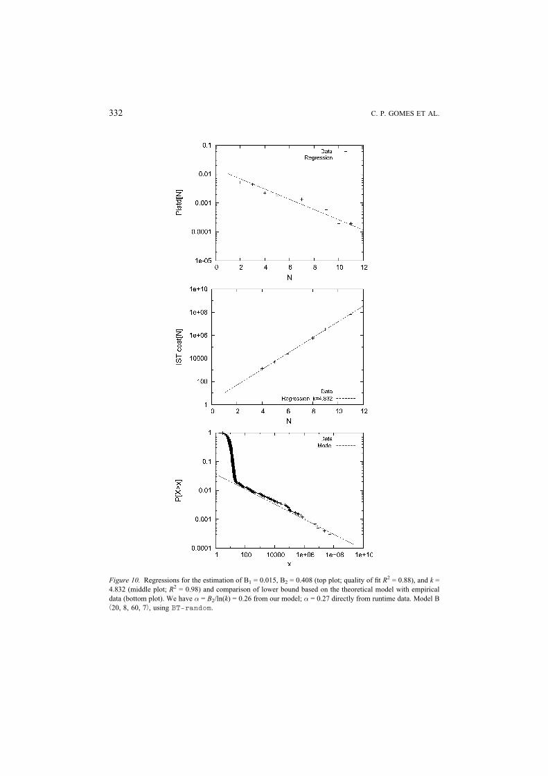
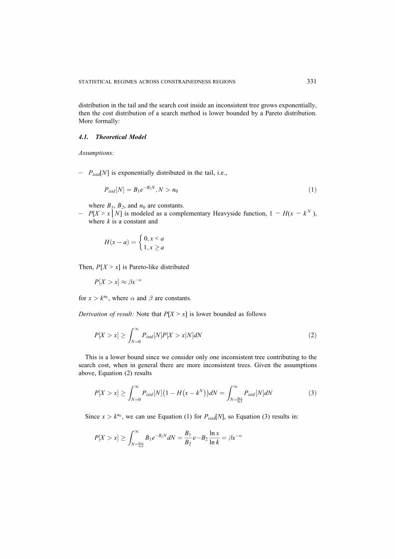
Figure 10. Regressions for the estimation of B1 = 0.015, B2 = 0.408 (top plot; quality of fit R2 = 0.88), and k =
4.832 (middle plot; R2 = 0.98) and comparison of lower bound based on the theoretical model with empirical
data (bottom plot). We have � = B2/ln(k) = 0.26 from our model; � = 0.27 directly from runtime data. Model B
b20, 8, 60, 7À, using BT-random.
332 C. P. GOMES ET AL.
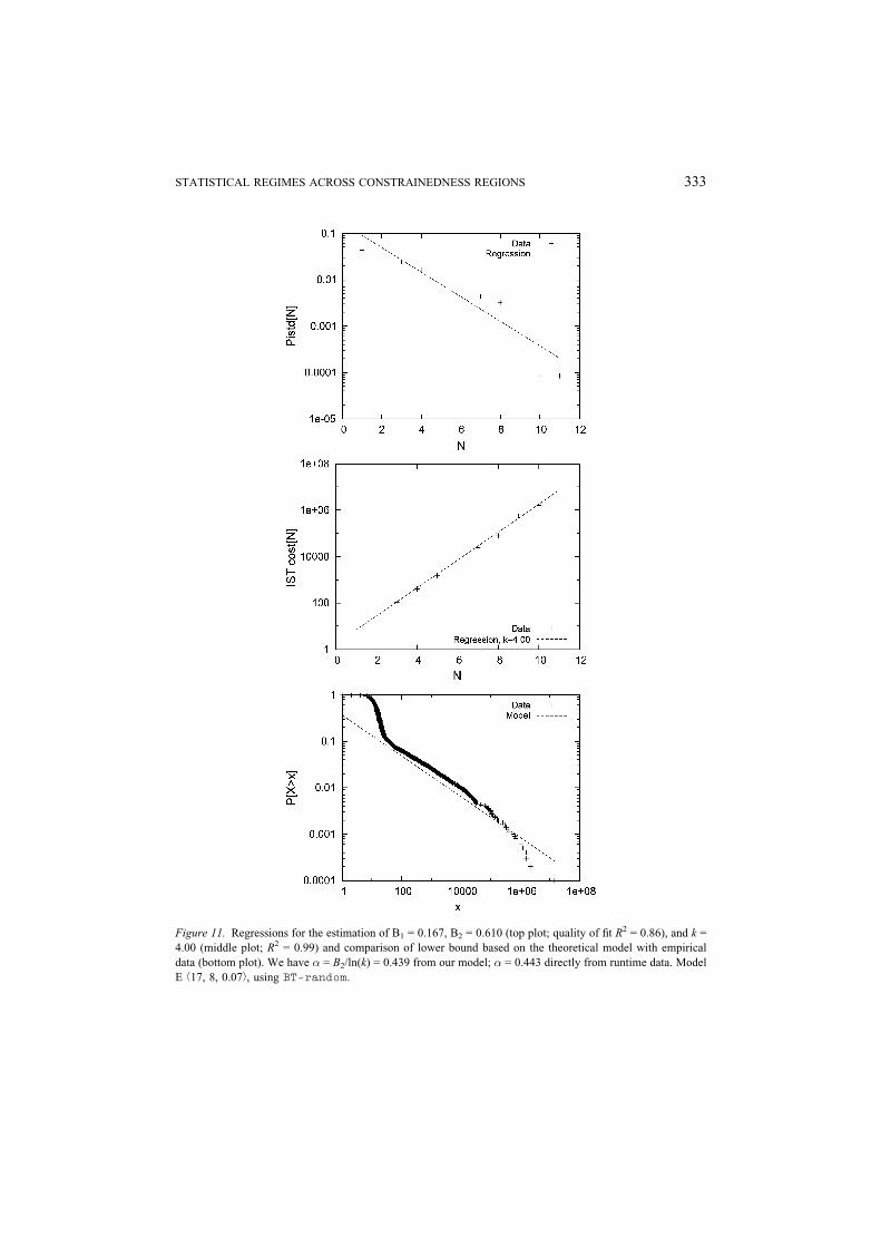
Figure 11. Regressions for the estimation of B1 = 0.167, B2 = 0.610 (top plot; quality of fit R2 = 0.86), and k =
4.00 (middle plot; R2 = 0.99) and comparison of lower bound based on the theoretical model with empirical
data (bottom plot). We have � = B2/ln(k) = 0.439 from our model; � = 0.443 directly from runtime data. Model
E b17, 8, 0.07À, using BT-random.
STATISTICAL REGIMES ACROSS CONSTRAINEDNESS REGIONS 333
with
� ¼ B2
ln k; � ¼ B1
B2
Note that when 1 G � G 2, X has infinite variance; when � e 1, X has infinite mean and
infinite variance.
In order to empirically validate our theoretical model we compared its predictions
against our data, for instances of model B and E. Figures 10 and 11 illustrate the com-
parison for two instances. Figure 10 concerns an instance from model B b20, 8, 60, 7À,
running BT-random, the same instance plotted in Figure 8 (top), for which heavy-
tailed behavior was observed (t = 7). The plots in Figure 10 provide the regression data
and fitted curves for the parameters B1, B2 , and k, using n0 = 1. The good quality of the
linear regression fit suggests that our assumptions are very reasonable. Based on the es-
timated values for k, B1, and B2 , we then compare the lower bound predicted using the
formal analysis presented above with the empirical data. As we can see from Figure 10,
the theoretical model provides a good (tight) lower bound for the empirical data. In
Figure 11 we illustrate the comparison between our theoretical model and our data for
an instance from model E b17, 8, 0.07À, also running BT-random, the same instance
plotted in Figure 3 (top), for which heavy-tailed behavior was observed ( p = 0.07).
As in the previous case, the theoretical model lower bounds the empirical data quite
well.
5. Conclusions and Future Work
We have studied the runtime distributions of complete backtrack search methods on
instances of well-known random CSP binary models. Our results reveal different regimes
in the runtime distributions of the backtrack search procedures and corresponding
distributions of the depth of the inconsistent sub-trees. We see a changeover from heavy-
tailed behavior to non-heavy-tailed behavior when we increase the constrainedness of the
problem instances. The exact point of changeover depends on the sophistication of the
search procedure, with more sophisticated solvers exhibiting a wider range of heavy-
tailed behavior. In the non-heavy-tailed region, the instances become harder and harder
for the backtrack search algorithm, and the runs become nearly homogeneously long. We
have also shown that there is a clear correlation between the the distributions of the depth
of the inconsistent sub-trees encountered by the backtrack search method and the heavy-
tailedness of the runtime distributions, with exponentially distributed sub-tree depths
leading to heavy-tailed search. To further validate our findings, we compared our
theoretical model, which models exponentially distributed subtrees in the search space,
with our empirical data: the theoretical model provides a good (tight) lower bound for
the empirical data. Our findings on the distribution of inconsistent subtrees in backtrack
334 C. P. GOMES ET AL.
search give, in effect, information about the inconsistent subproblems that are created
during the search.
We believe that these results can be exploited in the design of more efficient restart
strategies and backtrack solvers. Note that a restart strategy provably eliminates heavy-
tailed behavior [13]. Furthermore, heavy-tailed distributions are characterized by a wide
range of run-times. By using fast restarts not only does a solver avoid the long-tailed
runs, it also has a good chance of encountering very short successful runs. Many current
state-of-art SAT solvers exploit such restart strategies [23]. However, current restart
schemes are somewhat adhoc, and are often tuned by hand. In practice, it has been
observed that relatively fast restarts are most effective. One interesting direction for
future research is whether one can detect during a single run whether the solver has
reached a large inconsistent subtree. For preliminary results on this issue, see [18, 19].
More generally, an important research direction is the design of more sophisticated restart
strategies.
Another interesting direction for future research involves the study of more structured
problem domains. In recent work, we have introduced the notion of a Bbackdoor set^,
which is a special set of variables such that, when assigned values, the polytime
propagation mechanism of the solver can resolve the remaining instance [33, 34]. (For a
closely related notion, see the work on treewidth and cutset [8, 27].) We have found that
practical, structured instances, have surprisingly small sets of backdoor variables (often
only a few dozen from among thousands of variables). Moreover, variable selection
heuristics are quite good at finding those backdoor variables, which explains the presence
of very short, successful runs in structured domains. Further work is needed to better
understand the semantics of backdoor sets, namely by relating the presence of small
backdoor sets with the structure of different problem domains. In other recent work we
have also provided some initial results on the connections between backdoors, restarts,
and heavy-tails in combinatorial search [34]. We hope the findings reported in this paper
will provide additional insights on the nature of heavy-tailed behavior in combinatorial
search and lead to further improvements in the design of restart strategies and search
methods.
Notes
1. Namely the probability (density) function (PDF); the cumulative distribution
function (CDF) and the survival function (SF) or tail probability.
2. Hogg and Williams (94) provided the first report of heavy-tailed behavior in the
context of backtrack search. They considered a deterministic backtrack search
procedure on different instances drawn from a given distribution. Our work is of
different nature as we study heavy-tailed behavior of the runtime distribution of a
given randomized backtrack search method on a particular problem instance, thereby
isolating the variance in runtime due solely to different runs of the randomized
algorithm.
3. In the rest of the paper sometimes we refer to the search cost as runtime. Even
though there are some discrepancies between runtime and the search cost measured
STATISTICAL REGIMES ACROSS CONSTRAINEDNESS REGIONS 335
in number of wrong decisions or backtracks, such differences are not significant in
terms of the tail regime of the distributions.
4. Instance generator and data available from the authors.
5. For our data analysis, we needed purely uncensored data. We could therefore only
consider relatively small problem instances. The results appear to generalize to
larger instances.
References
1. Achlioptas, D., Kirousis, L., Kranakis, E., Krizanc, D., Molloy, M., & Stamatiou Y. (1997). Random
constraint satisfaction: A more accurate picture. In Proceedings CP’97, Linz, Austria, pages 107Y120.
2. Bayardo, R., & Miranker, D. (1996). A complexity analysis of space-bounded learning algorithms for the
constraint satisfaction problem. In Proceedings of the Thirteenth National Conference on Artificial
Intelligence (AAAI-96), pages 558Y562. Portland, OR.
3. Berre, D. L., & Simon, L. (2004). Fifty-five solvers in Vancouver: The sat 2004 competition. In
Proceedings of SAT’04.
4. Bessiere, C., & Regin, J. (1996). MAC and combined heuristics: Two reasons to forsake FC (and CBJ?) on
hard problems. In Proceedings CP’96, Cambridge, MA, pages 61Y75.
5. Bessiere, C., Zanuttini, B., & Fernandez, C. (2004). Measuring search trees. In B. Hnich (ed.) Proceedings
ECAI’04 Workshop on Modelling and Solving Problems with Constraints, Valencia, Spain.
6. Chen, H., Gomes, C., & Selman, B. (2001). Formal models of heavy-tailed behavior in combinatorial
search. In Proceedings CP’01, Paphos, Cyprus, pages 408Y421.
7. Dechter, R. (1990). Enhancement schemes for constraint processing: Back-jumping, learning and cutset
decomposition. Artif. Intell. 41(3): 273Y312.
8. Dechter, R. (2003). Constraint processing. Morgan Kaufmann.
9. Frost, D., Rish, I., & Vila, L. (1997). Summarizing CSP hardness with continuous probability distributions.
In AAAI-97, Providence, Rhode Island, pages 327Y333.
10. Gaschnig, J. (1977). A general backtrack algorithm that eliminates most redundant tests. In Proceedings
IJCAI’77, Cambridge, MA, page 447.
11. Gent, I., & Walsh, T. (1994). Easy problems are sometimes hard. Artif. Intell. 70: 335Y345.
12. Gomes, C., Selman, B., & Crato, N. (1997). Heavy-tailed distributions in combinatorial search. In
Proceedings CP’97, Linz, Austria, pages 121Y135.
13. Gomes, C. P., Selman, B., Crato, N., & Kautz, H. (2000). Heavy-tailed phenomena in satisfiability and
constraint satisfaction problems. J. Autom. Reason. 24(1Y2): 67Y100.
14. Haralick, R., & Elliot, G. (1980). Increasing tree search efficiency for constraint satisfaction problems.
Artif. Intell. 14: 263Y313.
15. Hogg, T., Huberman, B., & Williams, C. (1996). Phase transitions and search problems. Artif. Intell.
81(1Y2): 1Y15.
16. Hogg, T., & Williams, C. (1994). The hardest constraint problems: A double phase transition. Artif. Intell.
69: 359Y377.
17. Hoos, H. H., & Stutzle, T. (2004). Stochastic Local Search: Foundations and Applications. Morgan
Kaufmann.
18. Horvitz, E., Ruan, Y., Gomes, C., Kautz, H., Selman, B., & Chickering, M. (2001). A Bayesian approach to
tackling hard computational problems. In Proceedings of the Seventeenth Conference On Uncertainty in
Artificial Intelligence (UAI-01).
19. Kautz, H., Horvitz, E., Ruan, Y., Gomes, C., & Selman, B. (2002). Dynamic restart policies. In Proceedings
of the Eighteenth National Conference on Artificial Intelligence (AAAI-02), Edmonton, Canada.
20. Li, C., & Ambulagan. (1997). Heuristics based on unit propagation for satisfiability problems. In
Proceedings IJCAI’97, Nagoya, Japan, pages 366Y371.
336 C. P. GOMES ET AL.
21. Marques-Silva, J. P., & Sakallah, K. A. (1999). GRASPVA search algorithm for propositional satisfiability.
IEEE Trans. Comput. 48(5): 506Y521.
22. Mohr, R., & Henderson, T. (1986). Arc and path consistency revisited. Artif. Intell. 28: 225Y233.
23. Moskewicz, M., Madigan, C., Zhao, Y., Zhang, L., & Malik, S. (2001). Chaff: Engineering an efficient SAT
solver. In Proceedings of the 39th Design Automation Conference, Las Vegas.
24. Nadel, B. (1989) Constraint satisfaction algorithms. Comput. Intell. 5: 188Y224.
25. Prosser, P. (1993a). Domain filtering can degrade intelligent backtrack search. In Proceedings IJCAI’93,
Chambry, France, pages 262Y267.
26. Prosser, P. (1993b), Hybrid algorithms for the constraint satisfaction problem. Comput. Intell. 9(3):
268Y299.
27. Rish, I., & Dechter, R. (2000). Resolution versus Search: Two strategies for SAT’. J. Autom. Reason. 24
(1/2): 225Y275.
28. Sabin, D., & Freuder, E. (1994). Contradicting conventional wisdom in constraint satisfaction. In
Proceedings PPCP’94, Seattle, WA.
29. Selman, B., & Kirkpatrick, S. (1996). Finite-size scaling of the computational cost of systematic search.
Artif. Intell. 81(1Y2): 273Y295.
30. Smith, B., & Grant, S. (1995). Sparse constraint graphs and exceptionally hard problems. In Proceedings
IJCAI’95, Montral, Canada, pages 646Y651.
31. Smith, B., & Grant, S. (1997). Modelling exceptionally hard constraint satisfaction problems. In
Proceedings CP’97, Linz, Austria, pages 182Y195.
32. Walsh, T. (2000) SAT vs CSP. In Proceedings CP’00, Singapore, pages 441Y456.
33. Williams, R., Gomes, C., & Selman, B. (2003). Backdoors to Typical Case Complexity.
34. Williams, R., Gomes, C., & Selman, B. (2003). On the connections between backdoors, restarts, and heavy-
tailedness in combinatorial search. In Proceedings of Sixth International Conference on Theory and
Applications of Satisfiability Testing (SAT-03).
35. Xu, K., & Li, W. (2000). Exact phase transition in random constraint satisfaction problems. J. Artif. Intell.
Res. 12: 93Y103.
STATISTICAL REGIMES ACROSS CONSTRAINEDNESS REGIONS 337