Statistical Analysis of Neuromuscular Blockade

Response: Contributions to an Automatic

Controller Calibration

M. Eduarda Silva a,c, Teresa Mendonça a,c, Isabel Silva a,b,

Hugo Magalhães a,c

aDepartamento de Matemática Aplicada, Faculdade de Ciências - Universidade do

Porto, Rua do Campo Alegre 687, 4169-007 Porto, PORTUGAL

bDepartamento de Engenharia Civil, Faculdade de Engenharia - Universidade do

Porto, Rua Dr. Roberto Frias , 4200-465 Porto, PORTUGAL

cUI&D Matemática e Aplicações, Universidade de Aveiro, Aveiro, PORTUGAL

Abstract

Muscle relaxant drugs are currently given during surgical operations. The designof controllers for the automatic control of neuromuscular blockade benefits froman individual tuning of the controller to the characteristics of the patient. A novelapproach to the characterization of the neuromuscular blockade response induced byan initial bolus at the beginning of anaesthesia is proposed. This approach is basedon the statistical analysis of the data using principal components and Walsh-Fourierspectral analysis. These methods provide information about the patients dynamics,allowing the on-line autocalibration of the controller, using multiple linear regressiontechniques. Observed and simulated data are used to compare different approachesto the characterization of the bolus response.

Key words:

Control Application, On-line Autocalibration, Principal Components Analysis,Regression models, Walsh-Fourier Analysis, Wiener models.

Email addresses: mesilva@fc.up.pt (M. Eduarda Silva), tmendo@fc.up.pt(Teresa Mendonça), imsilva@fc.up.pt (Isabel Silva), hfmagalh@fc.up.pt (HugoMagalhães).

Preprint submitted to Elsevier Science 24 May 2004

1 Introduction

The development of automatic control systems for the continuous adminis-tration of drugs has been a subject of interest in the last decades and, inparticular, for the control of the neuromuscular blockade during a surgicalprocedure. The non-depolarising types of muscle relaxant act by blocking theneuromuscular transmission, thereby producing muscle paralysis. The extentof muscle paralysis (or muscle relaxation) is then measured from an evokedEMG obtained at the hand by electrical external stimulation. A variety ofdifferent approaches to the design of an automatic control system for the neu-romuscular blockade has been proposed (Linkens, 1994; Schilden and Olkkola,1991; Wait et al., 1987). The design of these controllers is usually supportedon a prototype for the nonlinear dynamical relationship between the musclerelaxant dose and the induced muscle paralysis. Such a prototype, which canbe deduced from the available pharmacokinetic and pharmacodynamic datafor the drug, merely describes the average characteristics of the response tothe drug. However, in practice, a large variability of the individual responsesto the infusion of the muscle relaxant is observed (Lago et al., 1998; Mendonçaand Lago, 1998). This variability suggests the need for an individual tuningof the controller according to the characteristics of the patient (Lago et al.,1998; Mendonça and Lago, 1998).

For clinical reasons, the patient must undergo an initial bolus dose to inducetotal muscle relaxation in a very short period of time (usually shorter than 5minutes). It is reasonable to assume that the response of the patient to thebolus carries valuable information that should be accounted for in the designof an automatic control system for the neuromuscular blockade, thus resultingin an improved tuning of the controller to the patients individual dynamicsand dosage requirements.

Methods for the on-line autocalibration of a digital PID controller parametersfor the administration of a muscle relaxant have been already proposed (Lagoet al., 1998, 2000; Mendonça and Lago, 1998). The parameters of the PIDcontroller (namely the proportional gain, the derivative gain and the integraltime constant) have been obtained from the L and R parameters deducedfrom the Ziegler-Nichols step response method (Franklin, 1994), applied tothe pharmacokinetic/pharmacodynamic model for the muscle relaxant. Thesubsequent tuning of the controller to the dynamics of a patient undergoingsurgery is performed by adjusting multiple linear regression models of L andR−1 on explanatory or predictor variables extracted from the observed bolus

response. Here, three different approaches to the characterization of the ob-served bolus response are considered. The bolus response is analysed using twostatistical techniques: principal components analysis, PCA, and Walsh-Fourierspectral analysis, WFA, thus obtaining predictor variables for the controller

2

parameters. The descriptions of the bolus response proposed here, PCA andWFA, are compared with an alternative method based on the bolus responseshape parameters, SPA (Lago et al., 1998, 2000; Mendonça and Lago, 1998).

2 Bolus Response Data Analysis

In this section the neuromuscular blockade model is presented and three dif-ferent approaches are used to characterize the observed bolus response.

2.1 Empirical Model

The dynamic response of the neuromuscular blockade may be modelled by aWiener structure (Lago et al., 1998; Weatherley et al., 1983). It is composedby a linear compartmental pharmacokinetic model relating the drug infusionrate u(t) (µg kg−1min−1), to the plasma concentration cp(t) (µgml−1), and anonlinear dynamic model relating cp(t) to the induced pharmacodynamic re-sponse, r(t) (%). The variable r(t), normalized between 0 and 100, measuresthe level of the neuromuscular blockade, 0 corresponding to full paralysis and100 to full muscular activity. In this study the muscle relaxation drug usedis the atracurium (Ward et al., 1983; Weatherley et al., 1983). The pharma-cokinetic model may be described by the state equations,

x1(t) = −λ1x1(t) + a1u(t),

x2(t) = −λ2x2(t) + a2u(t),

cp(t) =2

∑

i=1

xi(t),

(1)

where ai (kgml−1) and λi (min−1) (i = 1, 2) are the pharmacokinetic patient-dependent parameters, u(t) is the quantity of drug administered by time unit,xi(t) (i = 1, 2) are the state variables and cp(t) is the plasma concentration.The pharmacodynamic effect for atracurium may be modelled by the Hillequation,

r(t) =100Cβ

50

Cβ50 + cβe (t)

, (2)

where the effect concentration ce(t) (µgml−1) is related to cp(t) by

3

ce(t) = ke0cp(t) − ke0ce(t), (3)

where ke0 (min−1), C50 (µgml−1) and β are also patient-dependent param-eters. Figure 1a) illustrates the responses induced on 85 patients by the ad-ministration of a bolus of 500 µg kg−1 of atracurium in the beginning of thesurgery. In order to accommodate the clinical data, the model for atracurium

has been modified including on the linear part of the system a first order block,

g(s) =1/τ

s + 1/τ, (4)

in a series connection. The time constant τ (min) is assumed to be a randomvariable independent of the remaining pharmacokinetic / pharmacodynamicparameters (Lago et al., 1998).

Therefore, the linear part of the resulting empirical model may be representedby the following transfer function from u to ce,

hL(s) =(

a1

s+ λ1

+a2

s+ λ2

)

ke0

s+ ke0

1/τ

s+ 1/τ. (5)

The neuromuscular relaxation level is simulated assuming an uniform distribu-tion for τ and a multidimensional log-normal distribution for the seven phar-macokinetic/pharmacodynamic parameters and used throughout this study.Also, for a better replication of the clinical environment, simulated measure-ment log-normal noise is added to each of the generated models. Figure 1b)illustrates 100 responses simulated the empirical model (equations (2) and (5))using an uniform distribution for τ on the interval [0,3.5] minutes. As illus-trated, the empirical model replicates well the characteristics of the patientsresponses in figure 1(a).

2.2 Bolus Response Shape Parameters

A method to characterize the bolus response based on shape parameters ob-tained on-line, has been proposed (Lago et al., 1998; Mendonça and Lago,1998; Lago et al., 2000). The diagram on figure 2 represents the shape param-eters used to characterize the response induced by a bolus of muscle relaxantadministered at t = 0 minutes. T80, T50 and T10 are elapsed times betweenthe bolus administration and the time the response r(t) becomes less than80%, 50% and 10%, respectively. S is a slope parameter and P is a persistence

4

(a)

0 2 4 6 8 100

20

40

60

80

100

120

time (minutes)

r(t)

%(b)

0 2 4 6 8 100

20

40

60

80

100

120

time (minutes)

r(t)

%

Fig. 1. The responses induced by a bolus of 500 µg kg−1 of atracurium on 85 patientsundergoing surgery-(a) and simulated responses (100 models) induced by a bolus of500 µg kg−1 of atracurium with added measurement noise-(b)

parameter, since it describes the duration of the bolus effect on the patient.However, in a clinical situation the bolus response may not reach a sufficientlylow level to allow the estimation of parameter P. Thus, although the param-eter P is used in this study with simulated data, it cannot be used in a realsituation.

P

r(t)

S

80%

50%

10%

T80 T50 T10 time (min)

Fig. 2. Parameters used to characterize the neuromuscular blockade response inducedby a bolus of a muscle relaxant administered at t = 0 minutes.

2.3 Bolus Response Principal Components Analysis

Principal component analysis is a statistical procedure which is performedin order to simplify the description of a set of correlated variables. In thepresent situation those variables are the m time consecutive measurements,r(1), ..., r(m), of the muscle relaxation response induced by the bolus of musclerelaxant given in the beginning of anaesthesia. The measurements are takenevery δt seconds on the interval [0, (m − 1).δt] (δt = 20 seconds is a typicalvalue). Let r be the random vector r = [r(1), ..., r(m)]T with mean r0 andcorrelation matrix Σ.

5

(a)

0 2 4 6 8 100

20

40

60

80

100

120

time (minutes)

r(t)

%(b)

0 2 4 6 8 100

20

40

60

80

100

120

time(minutes)

Pro

ject

ions

r(t)

%

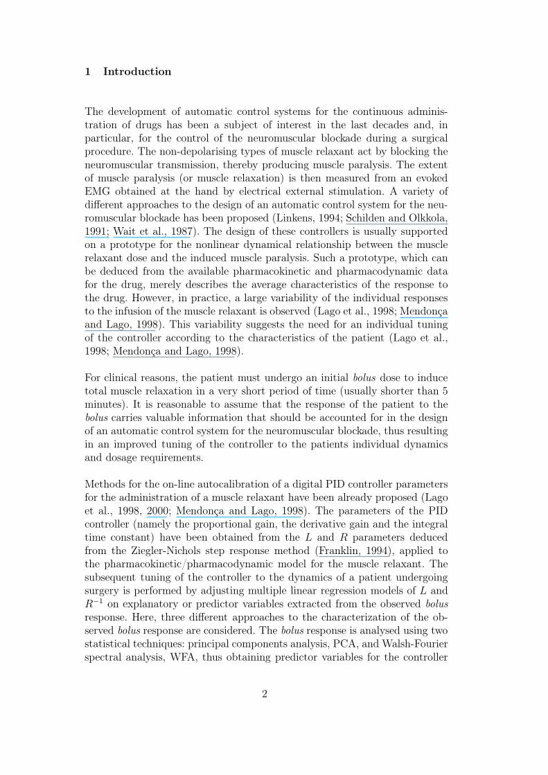
Fig. 3. Simulated responses (100 models) induced by a bolus of 500 µg kg−1 ofatracurium without added noise -(a) and projections of these simulated responsesusing 3 principal components -(b).

Each principal component is a linear combination of these variables. The co-efficients of these linear combinations are chosen such that they define or-thogonal directions of maximum variability and are obtained as the eigenvec-tors, ν1, . . . ,νm, of Σ. Considering only the k most significant eigenvalues,θ1, . . . , θk, the vector r is projected on a lower dimensional space without loos-ing much information, as follows

r ≈ r0 + νa, (6)

where

a = νT (r− r0), (7)

and ν = [ν1, . . . ,νk].

The proportion of the total variation in the original data explained by the firstk components is given by

pk =

∑kj=1

θj∑m

j=1θj

.

Consider the 100 simulated responses induced by a bolus of 500 µgkg−1 ofatracurium without added noise, represented in Figure 3(a). Performing PCAon this data, it is found that the proportions of the total variation explainedby the first 3, 5 and 10 principal components are p3 = 98.5%, p5 = 99.8%and p10 = 100%, respectively. Thus, for practical purposes it is consideredthat the muscle relaxation response can be accurately represented by the firstthree principal components. The projections of each simulated response on thislower dimensional space is obtained from equation (6) for k = 3. Figure 3(b)illustrates the projections for the set of 100 simulated responses representedin figure 3(a).

6

2.4 Bolus Response Walsh-Fourier Spectral Analysis

Walsh-Fourier spectral analysis is a procedure used to analyse and characterizetime series, specially when sharp discontinuities and changes of level occur inthe data. The procedure is similar to the well known Fourier analysis, usedto characterize periodic variation in a continuous signal. The Walsh-Fourieranalysis is based in the Walsh functions which form a complete, ordered andorthonormed set of rectangular waves taking the values -1 and 1 (Beauchamp,1975; Harmuth, 1977; Kohn, 1980). The Walsh functions may be ordered inthe so called Walsh or sequency order, which is comparable to the frequencyorder of sines and cosines. The sequency-ordered Walsh functions are denotedby W (n, t), where t ∈ [0, 1[ and n = 1, 2, . . . , the sequency, represents thenumber of times that the function switches signs in the unit interval.

Let {X(t)} be a stationary stochastic process, with zero mean and absolutelysummable autocovariance function, R(k). The Walsh-Fourier spectral density

function of X(t) is defined as (Morettin, 1981; Robinson, 1972; Stoffer, 1987,1991)

f(λ) =∞∑

τ=0

Γ(τ)W (τ, λ), 0 ≤ λ < 1, (8)

where Γ(j) is the logical covariance defined by

Γ(j) =1

N

N−1∑

k=0

R(j ⊕ k − k), 1 ≤ j < N, (9)

with ⊕ being the dyadic sum (Robinson, 1972). Let x(0), . . . , x(N − 1) be Nobservations of the process. An estimator of the spectral density is the Walsh

periodogram of the data

IW (λj) =

[

1√N

N−1∑

n=0

x(n)W (n, λj)

]2

, (10)

where λj is a sequency of the form λj = j/N, 1 ≤ j ≤ N − 1. One can plotIW (λj) versus λj to inspect for peaks. In the sequency domain, a peak indicates”a switch each λj time points”.

Considering that during the surgical intervention a patient attains differentlevels of neuromuscular blockade, we investigate how the Walsh-Fourier anal-

ysis, WFA, can contribute to improve the controller. Accordingly, the Walshperiodogram of the induced neuromuscular blockade, r(t), is evaluated on

7

0 20 40 600

4000

8000

12000

H−seq

Pow

er

Fig. 4. Walsh periodogram of one of the patients.

data collected during surgery: 34 clinical trials with neuromuscular blockadeinduced by a bolus of atracurium, measured during, approximately, 42 min-utes, in a total of 128 samples. The periodograms thus obtained present peaksin the neighbourhood of the sequencies 3/128, 7/128 and 15/128 which cor-respond to average periods (Harmuth, 1977) of 14.2 minutes, 6.1 minutes and2.8 minutes, respectively. In Figure 4 the Walsh periodogram of one of the realcases is exhibited.

To investigate the relationship between the relaxation level at the average

periods given by the Walsh-Fourier spectral analysis and the shape parame-ters (T10, T50, T80, S and P), the correlation coefficients are computed, forsimulated models with and without added noise and for the set of real dataavailable, and found significant. Table 1 presents the correlation coefficientsbetween T50 and the relaxation level at some of the average periods, whichare highly significant (p-value < 0.001), thus establishing a clear relationshipbetween these parameters and validating the use of T50 to characterize theindividual dynamic model (Lago et al., 1998, 2000; Mendonça and Lago, 1998).

Without With Real

noise noise data

r (1.7) r (3.0) r (1.7) r (3.0) r (3.0) r (7.0)

T50 0.86 0.94 0.85 0.93 0.90 0.77

Table 1Correlation coefficients.

3 Regression models for the controller parameters

In this section, multiple linear regression models for each of the controllerparameters, L and R−1, on the explanatory (or predictor) variables extracted

8

from the observed bolus response are constructed as follows. Consider a set ofN independent observations (φi, ψi1, . . . , ψip), i = 1, . . . , N where φi representsthe observed value of the controller parameter, either L or R−1, and the ψij

represent the observed values of the explanatory or predictor variables. Herethe explanatory or predictor variables considered are: the shape parameters(SPA), the principal components (PCA) and the values of the bolus responseat the Walsh-Fourier periods (WFA). Preliminary data analysis indicates thata multiple linear regression model is adequate.

Let Φ(N × 1) represent the vector of the controller parameter variables, as-sumed uncorrelated. Let Ψ be a N × (p + 1) matrix of observed constantsextracted from the bolus response,

Ψ =

1 ψ11 . . . ψ1p

1 ψ21 . . . ψ2p

. . . . . . . . . . . .

1 ψN1 . . . ψNp

, (11)

and let α denote a ((p + 1) × 1) vector of unknown parameters. Then, thecontroller parameters and the bolus response are related by the equation,

Φ = Ψ α + ε, (12)

where ε is a vector of uncorrelated random variables, normally distributedwith mean 0 and variance σ2. The observations on Φ and Ψ are obtainedfrom a set of N = 500 simulated models for the neuromuscular blockaderesponse, without and with added noise, as introduced in section 2.1. Themultiple regression models are then fitted by least-squares. The variables tobe included in the model, are chosen by a stepwise selection method (Draperand Smith, 1981) and the usual residual checks are performed for all theregression models. In the following sections, the regression models presentedare obtained from the simulated data without added noise. In the last section,to compare the different approaches, the worst case is considered: simulateddata (neuromuscular blockade level) with added noise.

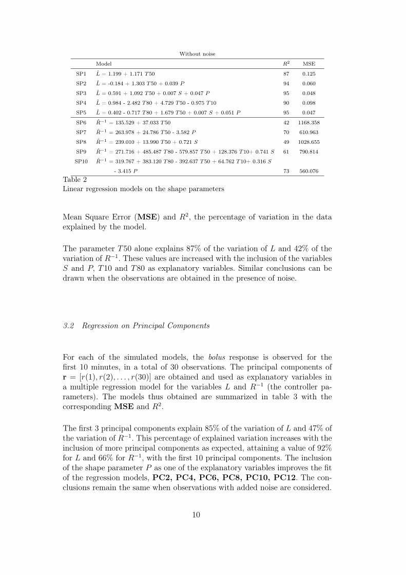
3.1 Regression on the Shape Parameters

In this section the shape parameters are used as explanatory variables for thecontroller parameters. Linear regression models of L and R−1, on T50, T10,T80, S and P are computed and summarized in table 2 with the corresponding

9

Without noise

Model R2 MSE

SP1 L = 1.199 + 1.171 T50 87 0.125

SP2 L = -0.184 + 1.303 T50 + 0.039 P 94 0.060

SP3 L = 0.591 + 1.092 T50 + 0.007 S + 0.047 P 95 0.048

SP4 L = 0.984 - 2.482 T80 + 4.729 T50 - 0.975 T10 90 0.098

SP5 L = 0.402 - 0.717 T80 + 1.679 T50 + 0.007 S + 0.051 P 95 0.047

SP6 R−1 = 135.529 + 37.033 T50 42 1168.358

SP7 R−1 = 263.978 + 24.786 T50 - 3.582 P 70 610.963

SP8 R−1 = 239.010 + 13.990 T50 + 0.721 S 49 1028.655

SP9 R−1 = 271.716 + 485.487 T80 - 579.857 T50 + 128.376 T10+ 0.741 S 61 790.814

SP10 R−1 = 319.767 + 383.120 T80 - 392.637 T50 + 64.762 T10+ 0.316 S

- 3.415 P 73 560.076

Table 2Linear regression models on the shape parameters

Mean Square Error (MSE) and R2, the percentage of variation in the dataexplained by the model.

The parameter T50 alone explains 87% of the variation of L and 42% of thevariation of R−1. These values are increased with the inclusion of the variablesS and P, T10 and T80 as explanatory variables. Similar conclusions can bedrawn when the observations are obtained in the presence of noise.

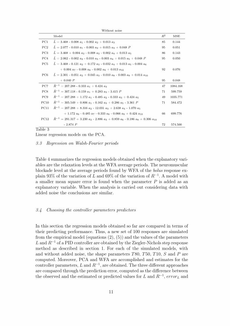
3.2 Regression on Principal Components

For each of the simulated models, the bolus response is observed for thefirst 10 minutes, in a total of 30 observations. The principal components ofr = [r(1), r(2), . . . , r(30)] are obtained and used as explanatory variables ina multiple regression model for the variables L and R−1 (the controller pa-rameters). The models thus obtained are summarized in table 3 with thecorresponding MSE and R2.

The first 3 principal components explain 85% of the variation of L and 47% ofthe variation of R−1. This percentage of explained variation increases with theinclusion of more principal components as expected, attaining a value of 92%for L and 66% for R−1, with the first 10 principal components. The inclusionof the shape parameter P as one of the explanatory variables improves the fitof the regression models, PC2, PC4, PC6, PC8, PC10, PC12. The con-clusions remain the same when observations with added noise are considered.

10

Without noise

Model R2 MSE

PC1 L = 3.468 - 0.008 a1 - 0.002 a2 + 0.013 a3 85 0.144

PC2 L = 2.077 - 0.010 a1 - 0.003 a2 + 0.015 a3 + 0.048 P 95 0.051

PC3 L = 3.468 + 0.004 a2 - 0.008 a3 - 0.002 a4 + 0.013 a5 86 0.143

PC4 L = 2.062 - 0.002 a2 - 0.010 a3 - 0.003 a4 + 0.015 a5 + 0.048 P 95 0.050

PC5 L = 3.468 - 0.121 a2 + 0.172 a3 - 0.032 a4 + 0.013 a5 - 0.004 a6

+ 0.004 a7 - 0.008 a8 - 0.002 a9 + 0.013 a10 92 0.076

PC6 L = 2.301 - 0.051 a2 + 0.045 a3 - 0.010 a8 - 0.003 a9 + 0.014 a10

+ 0.040 P 95 0.048

PC7 R−1 = 207.288 - 0.333 a1 + 0.424 a3 47 1084.168

PC8 R−1 = 307.118 - 0.159 a1 + 0.283 a3 - 3.415 P 71 599.759

PC9 R−1 = 207.288 + 1.172 a1 - 0.485 a2 - 0.333 a3 + 0.424 a5 49 1035.771

PC10 R−1 = 305.549 + 0.806 a1 - 0.162 a3 + 0.286 a5 - 3.361 P 71 584.472

PC11 R−1 = 207.288 + 8.316 a2 - 12.031 a3 + 2.638 a4 - 1.070 a5

+ 1.172 a6 - 0.485 a7 - 0.333 a8 - 0.066 a9 + 0.424 a10 66 699.776

PC12 R−1 = 291.317 + 3.230 a2 - 2.886 a3 + 0.859 a6 - 0.186 a8 + 0.306 a10

- 2.874 P 72 574.500

Table 3Linear regression models on the PCA.

3.3 Regression on Walsh-Fourier periods

Table 4 summarizes the regression models obtained when the explanatory vari-ables are the relaxation levels at the WFA average periods. The neuromuscularblockade level at the average periods found by WFA of the bolus response ex-plain 93% of the variation of L and 69% of the variation of R−1. A model witha smaller mean square error is found when the parameter P is added as anexplanatory variable. When the analysis is carried out considering data withadded noise the conclusions are similar.

3.4 Choosing the controller parameters predictors

In this section the regression models obtained so far are compared in terms oftheir predicting performance. Thus, a new set of 100 responses are simulatedfrom the empirical model (equations (2), (5)) and the values of the parametersL and R−1 of a PID controller are obtained by the Ziegler-Nichols step responsemethod as described in section 1. For each of the simulated models, withand without added noise, the shape parameters T80, T50, T10, S and P arecomputed. Moreover, PCA and WFA are accomplished and estimates for thecontroller parameters, L and R−1, are obtained. The three different approachesare compared through the prediction error, computed as the difference betweenthe observed and the estimated or predicted values for L and R−1, errorL and

11

Without noise

Model R2 MSE

WF1 L = 1.448 + 0.008 r(0.7) + 0.010 r(1.3) + 0.005 r(1.7) + 0.025 r(3.0)

+ 0.108 r(7.0) - 0.445 r(14.0) 93 0.065

WF2 L = 0.179 + 0.008 r(0.7) + 0.010 r(1.3) + 0.006 r(1.7) + 0.025 r(3.0)

+ 0.082 r(7.0) - 0.161 r(14.0) + 0.036 P 95 0.048

WF3 L = 2.094 + 0.016 r(1.3) + 0.027 r(3.0) + 0.104 r(7.0) - 0.445 r(14.0) 93 0.067

WF4 L = 0.816 + 0.014 r(1.3) + 0.003 r(1.7) + 0.026 r(3.0)

+ 0.081 r(7.0) - 0.161 r(14.0) + 0.036 P 95 0.049

WF5 R−1 = 100.659 + 0.573 r(0.7) + 0.429 r(1.7) + 0.288 r(3.0)

- 1.417 r(7.0) + 30.568 r(14.0) 69 638.302

WF6 R−1 = 180.072 + 0.593 r(0.7) + 0.350 r(1.7) + 0.307 r(3.0)

+ 13.138 r(14.0) - 2.243 P 72 569.560

WF7 R−1 = 153.535 + 0.504 r(1.7) + 0.232 r(3.0) - 1.277 r(7.0) + 30.365 r(14.0) 68 647.796

WF8 R−1 = 233.641 + 0.425 r(1.7) + 0.261 r(3.0) + 13.354 r(14.0) - 2.212 P 72 579.985

Table 4Linear regression models on the WFA average periods.

SP1 SP2 SP3 SP4 SP5 PC1 PC2 PC3 PC4 PC5 PC6 WF1 WF2 WF3 WF4

−1

−0.5

0

0.5

1

erro

r L

SP6 SP7 SP8 SP9 SP10 PC7 PC8 PC9 PC10 PC11 PC12 WF5 WF6 WF7

−50

0

50

100

erro

r R−1

Fig. 5. Boxplots of the errors, errorL and errorR−1 obtained from 100 simulatedneuromuscular blockade level models with added noise noise.

errorR−1 , respectively.

The results presented in this section refer to the worst case, which is when thedata is observed with noise.

Figure 5 represents the boxplots of errorL and errorR−1. Concerning param-eter L, the errors that present a higher dispersion are those obtained fromthe models with the PCA and WFA regressors. Also L is, generally, under-estimated by SP and PCA and overestimated by WFA. Now, consider the

12

With noise

Model R2 MSE

SP4 L = 1.130 + 1.920 T50 - 0.458 T10 89 0.105

SP5 L = 0.223 + 0.565 T80 + 0.454 T50 + 0.176 T10 + 0.004 S + 0.044 P 94 0.059

M1 L = 1.210 + 1.273 T50 - 0.253 r(14.0) 91 0.087

PC1 L = 3.468 + 0.008 a1 - 0.002 a2 + 0.013 a3 85 0.145

PC2 L = 2.129 + 0.010 a1 - 0.003 a2 + 0.015 a3 + 0.045 P 94 0.057

M2 L = 3.719 + 0.010 a1 - 0.004 a2 + 0.014 a3 - 0.310 r(14.0) 91 0.092

WF3 L =2.127 + 0.015 r(1.3) + 0.029 r(3.0) + 0.067 r(7.0) - 0.335 r(14.0) 90 0.096

WF4 L = 0.689 + 0.013 r(1.3) + 0.004 r(1.7) + 0.026 r(3.0)

+ 0.079 r(7.0) - 0.117 r(14.0) + 0.040 P 94 0.056

SP9 R−1 = 208.877 + 76.627 T80 - 123.180 T50 + 52.049 T10+ 0.418 S 57 880.635

SP10 R−1 = 276.985 + 27.283 T80 + 0.103 S - 3.439 P 69 627.804

M3 R−1 = 205.484 + 85.045 T80 - 80.426 T50 + 16.118 T10 + 0.436 S

+ 21.472 r(14.0) 64 738.834

PC7 R−1 = 207.288 + 0.316 a1 + 0.424 a3 46 1090.990

PC8 R−1 = 304.874 + 0.128 a1 + 0.287 a3 - 3.282 P 70 618.584

M4 R−1 = 187.053 + 0.099 a2 + 0.307 a3 + 24.981 r(14.0) 63 749.225

WF5 R−1 = 153.924 + 0.503 r(1.7) + 0.299 r(3.0) + 25.173 r(14.0) 62 767.205

WF7 R−1 = 248.650 + 0.383 r(1.7) + 0.359 r(3.0) + 10.223 r(14.0) - 2.585 P 71 601.216

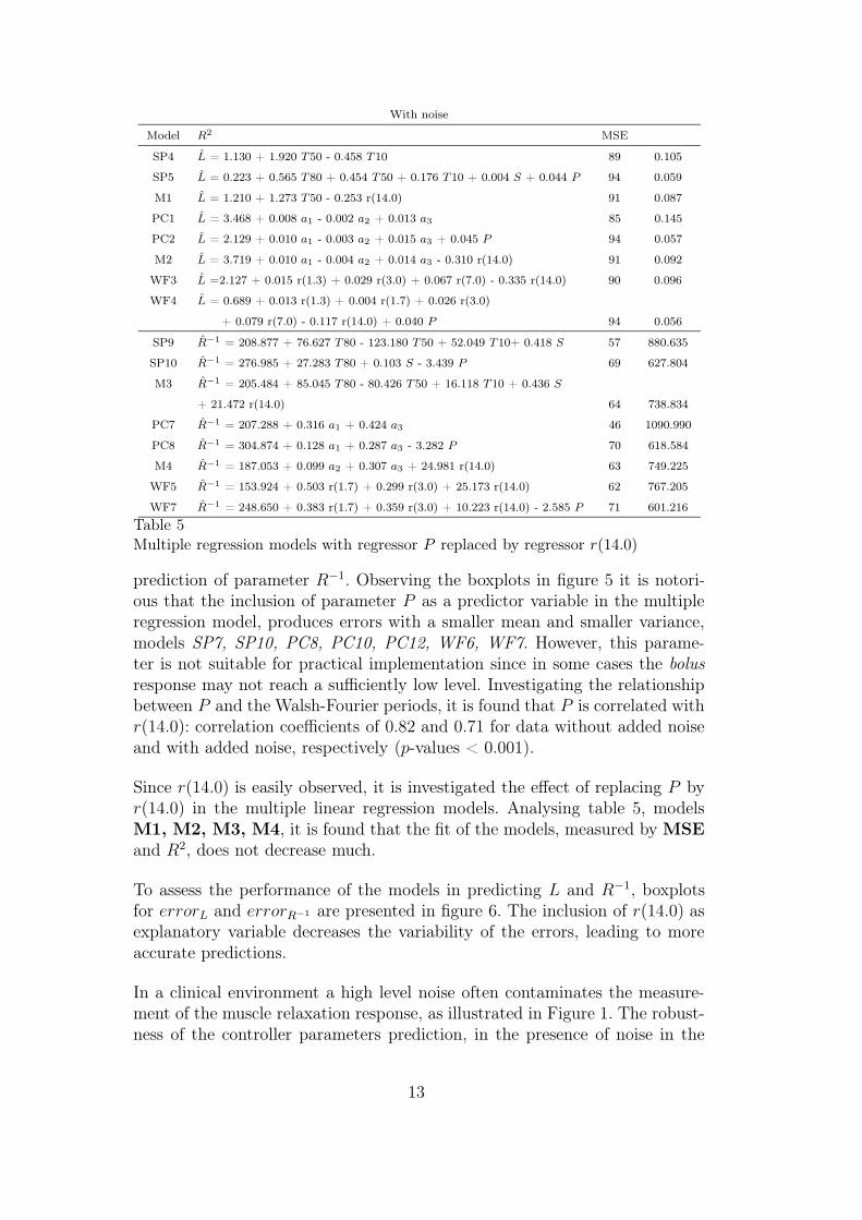
Table 5Multiple regression models with regressor P replaced by regressor r(14.0)

prediction of parameter R−1. Observing the boxplots in figure 5 it is notori-ous that the inclusion of parameter P as a predictor variable in the multipleregression model, produces errors with a smaller mean and smaller variance,models SP7, SP10, PC8, PC10, PC12, WF6, WF7. However, this parame-ter is not suitable for practical implementation since in some cases the bolus

response may not reach a sufficiently low level. Investigating the relationshipbetween P and the Walsh-Fourier periods, it is found that P is correlated withr(14.0): correlation coefficients of 0.82 and 0.71 for data without added noiseand with added noise, respectively (p-values < 0.001).

Since r(14.0) is easily observed, it is investigated the effect of replacing P byr(14.0) in the multiple linear regression models. Analysing table 5, modelsM1, M2, M3, M4, it is found that the fit of the models, measured by MSE

and R2, does not decrease much.

To assess the performance of the models in predicting L and R−1, boxplotsfor errorL and errorR−1 are presented in figure 6. The inclusion of r(14.0) asexplanatory variable decreases the variability of the errors, leading to moreaccurate predictions.

In a clinical environment a high level noise often contaminates the measure-ment of the muscle relaxation response, as illustrated in Figure 1. The robust-ness of the controller parameters prediction, in the presence of noise in the

13

SP4 SP5 M1 PC1 PC2 M2 WF3 WF4

−1

−0.5

0

0.5

1

erro

r L

SP9 SP10 M3 PC7 PC8 M4 WF5 WF7

−50

0

50

100

erro

r R−1

Fig. 6. Boxplots of the errors (100 models with noise).

bolus response measurement, has been investigated in detail. All the predictorshave been found to be very insensitive to the presence of noise, the periods ofthe WFA achieving the best results. Therefore, it can be concluded that theon-line prediction of the controller parameters from the patient bolus responseis a robust technique suitable for use in a clinical environment.

4 Final remarks

Here, the problem of inferring patients individualized information from theresponse induced by an initial bolus dose given in the beginning of anaesthesiais considered. This individualized information is very important for the designof improved on-line autocalibrated automatic controllers of muscle relaxation.Two different statistical techniques are used to analyse and characterize thebolus response data: principal components analysis and Walsh-Fourier spectralanalysis. Parameters deduced from the analysis are then used as predictors forthe controller parameters, allowing the on-line autotuning of a PID controller.Results are illustrated using realistic dynamic models that mimic not only thelarge variability of patients responses to the administration of atracurium, butalso the large level of measurement noise which occurs in a clinical environ-ment. The robustness of the PCA and WFA for characterizing the patientsindividual responses to the bolus has been firmly established.

14

Acknowledgements

The authors would like to thank the referees for their comments which helpedto improve the paper. The third author would like to thank the PRODEP IIIand the fourth author, the Foundation for Science and Technology under theThird Community Support Framework for the financial support during thecourse of this project.

References

Beauchamp, K.G., 1975. Walsh Functions and their applications, AcademicPress.

Draper, N.R., Smith, H., 1981. Applied Regression Analysis, John Wiley.Franklin, G.F., 1994. Feedback control of dynamic systems, Addison-Wesley.Harmuth, H.F., 1977. Transmission of Information by Orthogonal Function,

Springer-Verlag.Kohn, R., 1980. On the Spectral Decomposition of Stationarity Time Series

using Walsh Functions, Adv. Appl. Probab., 12, 183–199.Lago, P., Mendonça, T., Gonçalves, L., 1998. On-line Autocalibration of a

PID Controller of Neuromuscular Blockade, Proceedings of the 1998 IEEEInternational Conference on Control Applications, 363–367, Trieste, Italy.

Lago, P., Mendonça, T., Azevedo, H., 2000. Comparison of On-line Auto-calibration Techniques of a Controller of Neuromuscular Blockade, Pro-ceedings of IFAC Modeling and Control in Biomedical Systems, Karlsburg-Greisfswald, Germany, 263–268.

Linkens, D.A., 1994. Intelligent Control in Biomedicine, Taylor and Francis.Mendonça, T., Lago, P., 1998. Control Strategies for the Automatic Control

of Neuromuscular Blockade, Control Eng. Pract., 6, 1225–1231.Morettin, P.A., 1981. Walsh Spectral Analysis, SIAM Rev., 23, 279–291.Robinson, G.S., 1972. Logical Convolution and Discrete Walsh and Fourier

Power Spectra, IEEE Trans. Audio Electroacoust., AU-20, 271–280.Schilden, H., Olkkola, K.T., 1991. Use of a pharmacokinetic-dynamic model

for the automatic feedback control of atracurium, Eur. Clin. Pharmacol.,40, 293–296.

Stoffer, D.S., 1987. Walsh-Fourier Analysis of discrete-valued Time Series, J.Time Ser. Anal., 8, 449–467.

Stoffer, D.S., 1991. Walsh- Fourier Analysis and its Statistical Applications,J. Am. Stat. Assoc., 86, 461–479.

Wait, C., Goat, V., Blogg, C., 1987. Feedback control of neuromuscular block-ade: a simple system for the infusion of anaesthesia, Anesthesia, 42, 1212–1217.

Ward, S., Neill, A., Weatherley, B., Corall, M., 1983. Pharmacokinetics of

15

atracurium besylate in healthy patients (after a single i.v. bolus dose), Br.J. Anaesth., 55, 113–118.

Weatherley, B., Williams, S., Neill, S., 1983. Pharmacokinetics, Pharmacody-namics and Dose-Response Relationships of atracurium Administered i.v.,Br. J. Anaesth., 55, 39s–45s.

16