AboutThiseBook

ePUBisanopen,industry-standardformatforeBooks.However,supportofePUBanditsmanyfeaturesvariesacrossreadingdevicesandapplications.Useyourdeviceorappsettingstocustomizethepresentationtoyourliking.Settingsthatyoucancustomizeoftenincludefont,fontsize,singleordoublecolumn,landscapeorportraitmode,andfiguresthatyoucanclickortaptoenlarge.Foradditionalinformationaboutthesettingsandfeaturesonyourreadingdeviceorapp,visitthedevicemanufacturer’sWebsite.Manytitlesincludeprogrammingcodeorconfigurationexamples.Tooptimize

thepresentationoftheseelements,viewtheeBookinsingle-column,landscapemodeandadjustthefontsizetothesmallestsetting.Inadditiontopresentingcodeandconfigurationsinthereflowabletextformat,wehaveincludedimagesofthecodethatmimicthepresentationfoundintheprintbook;therefore,wherethereflowableformatmaycompromisethepresentationofthecodelisting,youwillseea“Clickheretoviewcodeimage”link.Clickthelinktoviewtheprint-fidelitycodeimage.Toreturntothepreviouspageviewed,clicktheBackbuttononyourdeviceorapp.

StatisticalAnalysisMicrosoft®Excel®2013

ConradCarlberg

800E.96thStreetIndianapolis,Indiana46240

StatisticalAnalysis:Microsoft®Excel®2013Copyright©2014byPearsonEducationAllrightsreserved.Nopartofthisbookshallbereproduced,storedinaretrievalsystem,ortransmittedbyanymeans,electronic,mechanical,photocopying,recording,orotherwise,withoutwrittenpermissionfromthepublisher.Nopatentliabilityisassumedwithrespecttotheuseoftheinformationcontainedherein.Althougheveryprecautionhasbeentakeninthepreparationofthisbook,thepublisherandauthorassumenoresponsibilityforerrorsoromissions.Norisanyliabilityassumedfordamagesresultingfromtheuseoftheinformationcontainedherein.

ISBN-13:978-0-7897-5311-3ISBN-10:0-7897-5311-1

LibraryofCongressControlNumber:2013956944

PrintedintheUnitedStatesofAmerica

FirstPrinting:April2014withcorrectionsMay2014

Editor-in-ChiefGregWiegand

AcquisitionsEditorLorettaYates

DevelopmentEditorBrandonCackowski-Schnell

ManagingEditorKristyHart

ProjectEditorElaineWiley

CopyEditorKeithCline

IndexerTimWright

ProofreaderSaraSchumacher

TechnicalEditorMichaelTurner

EditorialAssistantCindyTeeters

CoverDesignerMattColeman

CompositorNonieRatcliff

TrademarksAlltermsmentionedinthisbookthatareknowntobetrademarksorservicemarkshavebeenappropriatelycapitalized.QuePublishingcannotattesttotheaccuracyofthisinformation.Useofaterminthisbookshouldnotberegardedasaffectingthevalidityofanytrademarkorservicemark.

WarningandDisclaimerEveryefforthasbeenmadetomakethisbookascompleteandasaccurateaspossible,butnowarrantyorfitnessisimplied.Theinformationprovidedisonan“asis”basis.Theauthorandthepublishershallhaveneitherliabilitynorresponsibilitytoanypersonorentitywithrespecttoanylossordamagesarisingfromtheinformationcontainedinthisbook.

SpecialSalesForinformationaboutbuyingthistitleinbulkquantities,orforspecialsalesopportunities(whichmayincludeelectronicversions;customcoverdesigns;andcontentparticulartoyourbusiness,traininggoals,marketingfocus,orbrandinginterests),pleasecontactourcorporatesalesdepartmentatcorpsales@pearsoned.comor(800)382-3419.

Forgovernmentsalesinquiries,pleasecontactgovernmentsales@pearsoned.com.

ForquestionsaboutsalesoutsidetheU.S.,pleasecontactinternational@pearsoned.com.

ContentsataGlance

Introduction

1AboutVariablesandValues

2HowValuesClusterTogether

3Variability:HowValuesDisperse

4HowVariablesMoveJointly:Correlation

5HowVariablesClassifyJointly:ContingencyTables

6TellingtheTruthwithStatistics

7UsingExcelwiththeNormalDistribution

8TestingDifferencesBetweenMeans:TheBasics

9TestingDifferencesBetweenMeans:FurtherIssues

10TestingDifferencesBetweenMeans:TheAnalysisofVariance

11AnalysisofVariance:FurtherIssues

12ExperimentalDesignandANOVA

13StatisticalPower

14MultipleRegressionAnalysisandEffectCoding:TheBasics

15MultipleRegressionAnalysis:FurtherIssues

16AnalysisofCovariance:TheBasics

17AnalysisofCovariance:FurtherIssues

Index

TableofContents

Introduction

UsingExcelforStatisticalAnalysisAboutYouandAboutExcelClearingUptheTermsMakingThingsEasierTheWrongBox?WaggingtheDog

What’sinThisBook

1AboutVariablesandValuesVariablesandValues

RecordingDatainListsScalesofMeasurement

CategoryScalesNumericScalesTellinganIntervalValuefromaTextValue

ChartingNumericVariablesinExcelChartingTwoVariables

UnderstandingFrequencyDistributionsUsingFrequencyDistributionsBuildingaFrequencyDistributionfromaSampleBuildingSimulatedFrequencyDistributions

2HowValuesClusterTogetherCalculatingtheMean

UnderstandingFunctions,Arguments,andResultsUnderstandingFormulas,Results,andFormatsMinimizingtheSpread

CalculatingtheMedianChoosingtoUsetheMedian

CalculatingtheModeGettingtheModeofCategorieswithaFormula

FromCentralTendencytoVariability

3Variability:HowValuesDisperseMeasuringVariabilitywiththeRangeTheConceptofaStandardDeviation

ArrangingforaStandardThinkinginTermsofStandardDeviations

CalculatingtheStandardDeviationandVarianceSquaringtheDeviationsPopulationParametersandSampleStatisticsDividingbyN–1

BiasintheEstimateDegreesofFreedom

Excel’sVariabilityFunctionsStandardDeviationFunctionsVarianceFunctions

4HowVariablesMoveJointly:CorrelationUnderstandingCorrelation

TheCorrelation,CalculatedUsingtheCORREL()FunctionUsingtheAnalysisToolsUsingtheCorrelationToolCorrelationIsn’tCausation

UsingCorrelationRemovingtheEffectsoftheScaleUsingtheExcelFunctionGettingthePredictedValuesGettingtheRegressionFormula

UsingTREND()forMultipleRegression

CombiningthePredictorsUnderstanding“BestCombination”UnderstandingSharedVarianceATechnicalNote:MatrixAlgebraandMultipleRegressioninExcel

MovingontoStatisticalInference

5HowVariablesClassifyJointly:ContingencyTablesUnderstandingOne-WayPivotTables

RunningtheStatisticalTestMakingAssumptions

RandomSelectionIndependentSelectionsTheBinomialDistributionFormulaUsingtheBINOM.INV()Function

UnderstandingTwo-WayPivotTablesProbabilitiesandIndependentEventsTestingtheIndependenceofClassifications

TheYuleSimpsoneffectSummarizingtheChi-SquareFunctions

UsingCHISQ.DIST()UsingCHISQ.DIST.RT()andCHIDIST()UsingCHISQ.INV()UsingCHISQ.INV.RT()andCHIINV()UsingCHISQ.TEST()andCHITEST()UsingMixedandAbsoluteReferencestoCalculateExpectedFrequenciesUsingthePivotTable’sIndexDisplay

6TellingtheTruthwithStatisticsAContextforInferentialStatistics

EstablishingInternalValidityThreatstoInternalValidity

ProblemswithExcel’sDocumentation

TheF-TestTwo-SampleforVariancesWhyRuntheTest?AFinalPoint

7UsingExcelwiththeNormalDistributionAbouttheNormalDistribution

CharacteristicsoftheNormalDistributionTheUnitNormalDistribution

ExcelFunctionsfortheNormalDistributionTheNORM.DIST()FunctionTheNORM.INV()Function

ConfidenceIntervalsandtheNormalDistributionTheMeaningofaConfidenceIntervalConstructingaConfidenceIntervalExcelWorksheetFunctionsThatCalculateConfidenceIntervalsUsingCONFIDENCE.NORM()andCONFIDENCE()UsingCONFIDENCE.T()UsingtheDataAnalysisAdd-InforConfidenceIntervalsConfidenceIntervalsandHypothesisTesting

TheCentralLimitTheoremMakingThingsEasierMakingThingsBetter

8TestingDifferencesBetweenMeans:TheBasicsTestingMeans:TheRationale

Usingaz-TestUsingtheStandardErroroftheMeanCreatingtheCharts

Usingthet-TestInsteadofthez-TestDefiningtheDecisionRuleUnderstandingStatisticalPower

9TestingDifferencesBetweenMeans:FurtherIssues

UsingExcel’sT.DIST()andT.INV()FunctionstoTestHypothesesMakingDirectionalandNondirectionalHypothesesUsingHypothesestoGuideExcel’st-DistributionFunctionsCompletingthePicturewithT.DIST()

UsingtheT.TEST()FunctionDegreesofFreedominExcelFunctionsEqualandUnequalGroupSizesTheT.TEST()Syntax

UsingtheDataAnalysisAdd-int-TestsGroupVariancesint-TestsVisualizingStatisticalPowerWhentoAvoidt-Tests

10TestingDifferencesBetweenMeans:TheAnalysisofVarianceWhyNott-Tests?TheLogicofANOVA

PartitioningtheScoresComparingVariancesTheFTest

UsingExcel’sWorksheetFunctionsfortheFDistributionUsingF.DIST()andF.DIST.RT()UsingF.INV()andFINV()TheFDistribution

UnequalGroupSizesMultipleComparisonProcedures

TheSchefféProcedurePlannedOrthogonalContrasts

11AnalysisofVariance:FurtherIssuesFactorialANOVA

OtherRationalesforMultipleFactorsUsingtheTwo-FactorANOVATool

TheMeaningofInteractionTheStatisticalSignificanceofanInteractionCalculatingtheInteractionEffect

TheProblemofUnequalGroupSizesRepeatedMeasures:TheTwoFactorWithoutReplicationTool

Excel’sFunctionsandTools:LimitationsandSolutionsMixedModelsPoweroftheFTest

12ExperimentalDesignandANOVACrossedFactorsandNestedFactors

DepictingtheDesignAccuratelyNuisanceFactors

FixedFactorsandRandomFactorsTheDataAnalysisAdd-In’sANOVAToolsDataLayout

CalculatingtheFRatiosAdaptingtheDataAnalysisToolforaRandomFactorDesigningtheFTestTheMixedModel:ChoosingtheDenominatorAdaptingtheDataAnalysisToolforaNestedFactorDataLayoutforaNestedDesignGettingtheSumsofSquaresCalculatingtheFRatiofortheNestingFactor

13StatisticalPowerControllingtheRisk

DirectionalandNondirectionalHypothesesChangingtheSampleSizeVisualizingStatisticalPowerQuantifyingPower

TheStatisticalPoweroft-TestsNondirectionalHypotheses

MakingaDirectionalHypothesisIncreasingtheSizeoftheSamplesTheDependentGroupst-Test

TheNoncentralityParameterintheFDistributionVarianceEstimatesTheNoncentralityParameterandtheProbabilityDensityFunction

CalculatingthePoweroftheFTestCalculatingtheCumulativeDensityFunctionUsingPowertoDetermineSampleSize

14MultipleRegressionAnalysisandEffectCoding:TheBasicsMultipleRegressionandANOVA

UsingEffectCodingEffectCoding:GeneralPrinciplesOtherTypesofCoding

MultipleRegressionandProportionsofVarianceUnderstandingtheSeguefromANOVAtoRegressionTheMeaningofEffectCoding

AssigningEffectCodesinExcelUsingExcel’sRegressionToolwithUnequalGroupSizesEffectCoding,Regression,andFactorialDesignsinExcel

ExertingStatisticalControlwithSemipartialCorrelationsUsingaSquaredSemipartialtoGettheCorrectSumofSquares

UsingTrend()toReplaceSquaredSemipartialCorrelationsWorkingWiththeResidualsUsingExcel’sAbsoluteandRelativeAddressingtoExtendtheSemipartials

15MultipleRegressionAnalysisandEffectCoding:FurtherIssuesSolvingUnbalancedFactorialDesignsUsingMultipleRegression

VariablesAreUncorrelatedinaBalancedDesignVariablesAreCorrelatedinanUnbalancedDesignOrderofEntryIsIrrelevantintheBalancedDesign

OrderEntryIsImportantintheUnbalancedDesignAboutFluctuatingProportionsofVariance

ExperimentalDesigns,ObservationalStudies,andCorrelationUsingAlltheLINEST()Statistics

UsingtheRegressionCoefficientsUsingtheStandardErrorsDealingwiththeInterceptUnderstandingLINEST()’sThird,Fourth,andFifthRowsGettingtheRegressionCoefficientsGettingtheSumofSquaresRegressionandResidualCalculatingtheRegressionDiagnosticsHowLINEST()HandlesMulticollinearityForcingaZeroConstantTheExcel2007VersionANegativeR2?

ManagingUnequalGroupSizesinaTrueExperimentManagingUnequalGroupSizesinObservationalResearch

16AnalysisofCovariance:TheBasicsThePurposesofANCOVA

GreaterPowerBiasReduction

UsingANCOVAtoIncreaseStatisticalPowerANOVAFindsNoSignificantMeanDifferenceAddingaCovariatetotheAnalysis

TestingforaCommonRegressionLineRemovingBias:ADifferentOutcome

17AnalysisofCovariance:FurtherIssuesAdjustingMeanswithLINEST()andEffectCodingEffectCodingandAdjustedGroupMeansMultipleComparisonsFollowingANCOVA

UsingtheSchefféMethodUsingPlannedContrasts

TheAnalysisofMultipleCovarianceTheDecisiontoUseMultipleCovariatesTwoCovariates:AnExample

Index

AbouttheAuthor

ConradCarlbergstartedwritingaboutExcel,anditsuseinquantitativeanalysis,beforeworkbookshadworksheets.Asagraduatestudent,hehadthegreatgoodfortunetolearnsomethingaboutstatisticsfromthewonderfullygiftedGeneGlass.Heremembersmuchofthatandhaslearnedmoresince.Thisisabookhehaswantedtowriteforyears,andheisgratefulfortheopportunity.

Dedication

ForToni,whohasbeenputtingupwiththissortofthingfor17yearsnow,withallmylove.

Acknowledgments

I’dliketothankLorettaYates,whoguidedthisbook’soverallprogress,andwhotreatsmyself-imposedcriseswithanunexpectedsortofpragmaticoptimism.MichaelTurner’stechnicaleditwasjustright,anditwasadelighttoseehow,atthestatslabanyway,themorethingschange...well,youknow.KeithClinekepttheproseontrack,despitemyoccasionalhowlsofprotest,withhiscopyedit.Andintheend,ElaineWileysomehowmanagedtogetthewholethingputtogether.Mythankstoeachofyou.

WeWanttoHearfromYou!

Asthereaderofthisbook,youareourmostimportantcriticandcommentator.Wevalueyouropinionandwanttoknowwhatwe’redoingright,whatwecoulddobetter,whatareasyou’dliketoseeuspublishin,andanyotherwordsofwisdomyou’rewillingtopassourway.Wewelcomeyourcomments.Youcanemailorwritetoletusknowwhatyoudidordidn’tlikeaboutthisbook—aswellaswhatwecandotomakeourbooksbetter.Pleasenotethatwecannothelpyouwithtechnicalproblemsrelatedtothetopicofthisbook.Whenyouwrite,pleasebesuretoincludethisbook’stitleandauthoraswellasyournameandemailaddress.Wewillcarefullyreviewyourcommentsandsharethemwiththeauthorandeditorswhoworkedonthebook.Email:feedback@quepublishing.comMail:QuePublishingATTN:ReaderFeedback800East96thStreetIndianapolis,IN46240USA

ReaderServices

Visitourwebsiteandregisterthisbookatquepublishing.com/registerforconvenientaccesstoanyupdates,downloads,orerratathatmightbeavailableforthisbook.

Introduction

UsingExcelforStatisticalAnalysisWhat’sinThisBook

TherewasnoreasonIshouldn’thavealreadywrittenabookaboutstatisticalanalysisusingExcel.ButIdidn’t,althoughIknewIwantedto.Finally,ItalkedPearsonintolettingmewriteitforthem.Becarefulwhatyouaskfor.It’sbeenastruggle,butatlastI’vegotitoutofmysystem,andIwanttostartbytalkinghereaboutthereasonsforsomeofthechoicesImadeinwritingthisbook.

UsingExcelforStatisticalAnalysisTheproblemisthatit’sahugeamountofmaterialtocoverinabookthat’ssupposedtobeonly400to500pages.ThetextusedinthefirststatisticscourseItookwasabout600pages,anditwaspurelystatistics,noExcel.In2001,Ico-authoredabookaboutExcel(nostatistics)thatranto750pages.ToshoehornstatisticsandExcelinto400pagesorsotakessomepickingandchoosing.Furthermore,IdidnotwantthisbooktobeanexpandedHelpdocument,likeoneortwoothersI’veseen.Instead,Itakeanapproachthatseemedtoworkwellinanearlierbookofmine,BusinessAnalysiswithExcel.Theideainboththatbookandthisoneistoidentifyatopicinstatistical(orbusiness)analysis;discussthetopic’srationale,itsprocedures,andassociatedissues;andonlythengetintohowit’scarriedoutinExcel.Youshouldn’texpecttofinddiscussionsof,say,theWeibullfunctionorthelognormaldistributionhere.Theyhavetheiruses,andExcelprovidesthemasstatisticalfunctions,butmypickingandchoosingforcedmetoignorethem—atmyperil,probably—andtousethespacesavedformaterialonmorebread-and-buttertopicssuchasstatisticalregression.

AboutYouandAboutExcelHowmuchbackgroundinstatisticsdoyouneedtogetvaluefromthisbook?Myintentionisthatyouneednone.Thebookstartsoutwithadiscussionofdifferentwaystomeasurethings—bycategories,suchasmodelsofcars,byranks,suchasfirstplacethroughtenth,bynumbers,suchasdegreesFahrenheit—andhowExcel

handlesthosemethodsofmeasurementinitsworksheetsanditscharts.Thisbookmovesontobasicstatistics,suchasaveragesandranges,andonlythentointermediatestatisticalmethodssuchast-tests,multipleregression,andtheanalysisofcovariance.Thematerialassumesknowledgeofnothingmorecomplexthanhowtocalculateanaverage.Youdonotneedtohavetakencoursesinstatisticstousethisbook.AstoExcelitself,itmatterslittlewhetheryou’reusingExcel97,Excel2013,oranyversioninbetween.VerylittlestatisticalfunctionalitychangedbetweenExcel97andExcel2003.Thefewchangesthatdidoccurhadtodoprimarilywithhowfunctionsbehavedwhentheuserstress-testedthemusingextremevaluesorinveryunlikelysituations.TheRibbonshowedupinExcel2007andisstillwithusinExcel2013.ButnearlyallstatisticalanalysisinExceltakesplaceinworksheetfunctions—verylittleismenudriven—andtherewasalmostnochangetothefunctionlist,functionnames,ortheirargumentsbetweenExcel97andExcel2007.TheRibbondoesintroduceafewdifferences,suchashowtogetatrendlineintoachart.ThisbookdiscussesthedifferencesinthestepsyoutakeusingthetraditionalmenustructureandthestepsyoutakeusingtheRibbon.InExcel2010,severalapparentlynewstatisticalfunctionsappeared,butthedifferencesweremoreapparentthanreal.Forexample,throughExcel2007,thetwofunctionsthatcalculatestandarddeviationsareSTDEV()andSTDEVP().Ifyouareworkingwithasampleofvalues,youshoulduseSTDEV(),butifyouhappentobeworkingwithafullpopulation,youshoulduseSTDEVP().Ofcourse,thePstandsforpopulation.BothSTDEV()andSTDEVP()remaininExcel2010and2013,buttheyaretermedcompatibilityfunctions.Itappearsthattheymaybephasedoutinsomefuturerelease.Excel2010addedwhatitcallsconsistencyfunctions,twoofwhichareSTDEV.S()andSTDEV.P().Notethataperiodhasbeenaddedineachfunction’sname.Theperiodisfollowedbyaletterthat,forconsistency,indicateswhetherthefunctionshouldbeusedwithasampleofvaluesorapopulationofvalues.OtherconsistencyfunctionswereaddedtoExcel2010,andthefunctionstheyareintendedtoreplacearestillsupportedinExcel2013.Thereareafewsubstantivedifferencesbetweenthecompatibilityversionandtheconsistencyversionofsomefunctions,andthisbookdiscussesthosedifferencesandhowbesttouseeachversion.

ClearingUptheTerms

Terminologyposesanotherproblem,bothinExcelandinthefieldofstatistics(and,itturnsout,intheareaswherethetwooverlap).Forexample,it’snormaltousethewordalphainastatisticalcontexttomeantheprobabilitythatyouwilldecidethatthere’satruedifferencebetweenthemeansoftwogroupswhentherereallyisn’t.ButExcelextendsalphatousagesthatarerelatedbutmuchlessstandard,suchastheprobabilityofgettingsomenumberofheadsfromflippingafaircoin.It’snotwrongtodoso.It’sjustunusual,andthereforeit’sanunnecessaryhurdletounderstandingtheconcepts.Thevocabularyofstatisticsitselfisfullofnamesthatmeanverydifferentthingsinslightlydifferentcontexts.Thewordbeta,forexample,canmeantheprobabilityofdecidingthatatruedifferencedoesnotexist,whenitdoes.Itcanalsomeanacoefficientinaregressionequation(forwhichExcel’sdocumentationunfortunatelyusestheletterm),andit’salsothenameofadistributionthatisacloserelativeofthebinomialdistribution.NoneofthatisduetoExcel.It’sduetohavingmoreconceptsthantherearelettersintheGreekalphabet.Youcanseethepotentialforconfusion.ItgetsworsewhenyouhookExcel’sterminologyupwiththatofstatistics.Forexample,inExcelthewordcellmeansarectangleonaworksheet,theintersectionofarowandacolumn.Instatistics,particularlytheanalysisofvariance,cellusuallymeansagroupinafactorialdesign:Ifanexperimentteststhejointeffectsofsexandanewmedication,onecellmightconsistofmenwhoreceiveaplacebo,andanothermightconsistofwomenwhoreceivethemedicationbeingassessed.Unfortunately,youcan’tdependonseeing“cell”whereyoumightexpectit:withincellerroriscalledresidualerrorinthecontextofregressionanalysis.Sothisbookpresentsyouwithsometermsyoumightotherwisefindredundant:Iusedesigncellforanalysiscontextsandworksheetcellwhenreferringtothesoftwarecontextwherethere’sanypossibilityofconfusionaboutwhichImean.Forconsistency,though,ItryalwaystousealpharatherthanTypeIerrororstatisticalsignificance.Ingeneral,Iusejustonetermforagivenconceptthroughout.Iintendtocomplainaboutitwhenthepossibilityofconfusionexists:whenmeansquaredoesn’tmeanmeansquare,yououghttoknowaboutit.

MakingThingsEasierIfyou’rejuststartingtostudystatisticalanalysis,yourtiming’smuchbetterthanminewas.Youhaveavoidedsomeoftheobstaclestounderstandingstatisticsthatonce—asrecentlyasthe1980s—stoodintheway.I’llmentionthoseobstaclesonceortwicemoreinthisbook,partlytoventmyspleenbutalsotostresshowmuchbetterExcelhasmadethings.

Supposethat25yearsagoyouwerecalculatingsomethingasbasicasthestandarddeviationoftwentynumbers.Youhadnoaccesstoacomputer.Or,iftherewasonearound,itwasamainframeoramini,andwhoeverownedithadmoreimportantusesforitthantosupportaPsychology101assignment.SoyoutrudgeddowntothePsychbuilding’sbasement,wheretherewasaroomfilledwithgraymetaldeskswithaddingmachinesonthem.Someoftheaddingmachinesmightevenhavebeenpluggedintoasourceofelectricity.YouenteredyourtwentynumbersverycarefullybecausetheaddingmachinesdidnotcomewithUndobuttonsorCtrl+Z.Theelectricity-enabledmachineswereindemandbecausetheyhadamemoryfunctionthatallowedyoutoenteranumber,squareit,andaddtheresulttowhatwasalreadyinthememory.Itcouldtakehalfanhourtocalculatethestandarddeviationoftwentynumbers.Itwasallincrediblytediousanditdistractedyoufromthemainpoint,whichwastheconceptofastandarddeviationandthereasonyouwantedtoquantifyit.Ofcourse,25yearsagoourteachersweretellingushowluckyweweretohaveaddingmachinesinsteadofhavingtousepaper,pencil,andaboxoferasers.Thingsaredifferentin2013,andtruthbetold,theyhavebeenchangingsincethemid1980swhenapplicationssuchasLotus1-2-3andMicrosoftExcelstartedtofindtheirwayontopersonalcomputers’floppydisks.Now,allyouhavetodoisenterthenumbersintoaworksheet—ormaybenoteventhat,ifyoudownloadedthemfromaserversomewhere.Then,type=STDEV.S(anddragacrossthecellswiththenumbersbeforeyoupressEnter.Ittakeshalfaminuteatmost,nothalfanhouratleast.Severalstatisticshaverelativelysimpledefinitionalformulas.Thedefinitionalformulatendstobestraightforwardandthereforegivesyouactualinsightintowhatthestatisticmeans.Butthosesamedefinitionalformulasoftenturnouttobedifficulttomanageinpracticeifyou’reusingpaperandpencil,orevenanaddingmachineorhandcalculator.Roundingerrorsoccurandcompoundoneanother.Sostatisticiansdevelopedcomputationalformulas.Thesearemathematicallyequivalenttothedefinitionalformulas,butaremuchbettersuitedtomanualcalculations.Althoughit’snicetohavecomputationalformulasthateasethearithmetic,thoseformulasmakeyoutakeyoureyeofftheball.You’resoinvolvedwithaccumulatingthesumofthesquaredvaluesthatyouforgetthatyourpurposeistounderstandhowvaluesvaryaroundtheiraverage.That’soneprimaryreasonthatanapplicationsuchasExcel,oranapplicationspecificallyandsolelydesignedforstatisticalanalysis,issohelpful.Ittakesthedrudgeryofthearithmeticoffyourhandsandfreesyoutothinkaboutwhatthe

numbersactuallymean.Statisticsisconceptual.It’snotjustarithmetic.Anditshouldn’tbetaughtasthoughitis.

TheWrongBox?ButshouldyouevenbeusingExceltodostatisticalcalculations?Afterall,peoplehavebeenmoaningaboutinadequaciesinExcel’sstatisticalfunctionsfortwentyyears.TheExcelforumonCompuServehadplentyofcomplaintsaboutthisissue,asdidtheUsenetnewsgroups.AsIwritethisintroduction,IcanswitchfromWordtoFirefoxandseethatsomepeoplearestillcomplainingonWikipediatalkpages,andotherscontributeangryscreedstopublicationssuchasComputationalStatistics&DataAnalysis,whichIbelievearethereasaremindertousalloftheimportanceoftakingourprescriptionmedication.IhavesometimesfoundmyselfasupsetaboutproblemswithExcel’sstatisticalfunctionsasanyone.Andit’struethatExcelhashad,andinsomecasescontinuestohave,problemswiththealgorithmsitusestomanagecertainfunctionssuchastheinverseoftheFdistribution.Butmostofthecomplaintsthatarevoicedfallintooneoftwocategories:thosethatarebasedonmisunderstandingsabouteitherExcelorstatisticalanalysis,andthosethatarebasedoncomplaintsthatExcelisn’taccurateenough.Ifyoureadthisbook,you’llbeabletoavoidthosekindsofmisunderstandings.AstoinaccuraciesinExcelresults,let’slookalittlemorecloselyatthat.Thecomplaintsaretypicallyalongtheselines:

IenterintoanExcelworksheettwodifferentformulasthatshouldreturnthesameresult.Simplealgebraicrearrangementoftheequationsprovesthat.ButthenIfindthatExcelcalculatestwodifferentresults.

Well,forthedatatheusersupplied,theresultsdifferatthefifteenthdecimalplace,soExcel’sresultsdisagreewithoneanotherbyapproximatelyfivein111trillion.Orthis:

ItriedtogettheinverseoftheFdistributionusingtheformulaFINV(0.025,4198986,1025419),butIgotanunexpectedresult.IsthereabuginFINV?

No.Onceuponatime,FINVreturnedthe#NUM!errorvalueforthosearguments,butnolonger.However,that’snotthepoint.Withsomanydegreesoffreedom(overfourmillionandonemillion,respectively),thepersonwhoaskedthe

questionwaseffectivelydealingwithpopulations,notsamples.Tousethatsortofinferentialtechniquewithsomanydegreesoffreedomisastrikinginstanceof“unclearontheconcept.”WoulditbebetterifExcel’smathweremoreaccurate—oratleastmoreinternallyconsistent?Sure.Buteventhefinger-waggersadmitthatExcel’sstatisticalfunctionsareacceptableatleast,asthefollowingcommentshows.

Theycanrarelybereliedonformorethanfourfigures,andthenonlyfor0.001<p<0.999,plentygoodforroutinehypothesistesting.

Nowlook.Chapter6,“TellingtheTruthwithStatistics,”goesintothisissuefurther,butthepointdeservesabettersoapbox,closertothestartofthebook.Regardlessoftheaccuracyofastatementsuchas“Theycanrarelybereliedonformorethanfourfigures,”it’spointlesstomakeit.It’sirrelevantwhetherafindingis“statisticallysignificant”atthe0.001levelinsteadofthe0.005level,andtoworryaboutwhetherExcelcansuccessfullydistinguishbetweenthetwofindingsistomissthecontext.Therearemanypossibleexplanationsforaresearchoutcomeotherthantheoneyou’reseeking:arealandreplicabletreatmenteffect.Randomchanceisonlyoneofthese.It’sonethatgetsalotofattentionbecauseweattachthewordsignificancetoourteststoruleoutchance,butit’snotmoreimportantthanotherpossibleexplanationsyoushouldbeconcernedaboutwhenyoudesignyourstudy.It’sthedesignofyourstudy,andhowwellyouimplementit,thatallowsyoutoruleoutalternativeexplanationssuchasselectionbiasanddisproportionatedropoutrates.Thoseexplanations—biasanddropoutrates—arejusttwoexamplesofpossibleexplanationsforanapparenttreatmenteffect:explanationsthatmightmakeatreatmentlooklikeithadaneffectwhenitactuallydidn’t.Eventhestrongestdesigndoesn’tenableyoutoruleoutachanceoutcome.Butifthedesignofyourstudyissound,andyouobtainedwhatlookslikeameaningfulresult,you’llwanttocontrolchance’sroleasanalternativeexplanationoftheresult.So,youcertainlywanttorunyourdatathroughtheappropriatestatisticaltest,whichdoeshelpyoucontroltheeffectofchance.Ifyougetaresultthatdoesn’tclearlyruleoutchance—orruleitin—you’remuchbetterofftoruntheexperimentagainthantotakeapositionbasedonaborderlineoutcome.Attheveryleast,it’sabetteruseofyourtimeandresourcesthantoworryinprintaboutwhetherExcel’sFtestsareaccuratetothefifthdecimalplace.

WaggingtheDog

Andaskyourselfthis:Onceyoureachthepointofplanningthestatisticaltest,areyougoingtorejectyourfindingsiftheymightcomeaboutbychancefivetimesin1,000?Isthattoolooseacriterion?Whataboutjustonetimein1,000?Howmanyangelsareonthatpinheadanyway?Ifyou’reconcernedthatExcelwon’treturnthecorrectdistinctionbetweenoneandfivechancesin1,000thattheresultofyourstudyisduetochance,youallowwhat’sreallyanirrelevancytodictatehow,andusingwhatcalibrations,you’regoingtoconductyourstatisticalanalysis.It’spointlesstoworryaboutwhetheratestisaccuratetoonepointinathousandortwoinathousand.Yourdecisionrulesforriskingachancefindingshouldbebasedonmoresubstantivegrounds.Chapter9,“TestingDifferencesBetweenMeans:FurtherIssues,”goesintothematteringreaterdetail,butaquicksummaryoftheissueisthatyoushouldlettheriskofmakingthewrongdecisionbeguidedbythecostsofabaddecisionandthebenefitsofagoodone—notbywhichcriterionappearstobethemoreselective.

What’sinThisBookYou’llfindthattherearetwobroadtypesofstatistics.I’mnottalkingaboutthatscurrilouslineaboutlies,damnedliesandstatistics—bothitssourceanditsapplicabilityaredisputed.I’mtalkingaboutdescriptivestatisticsandinferentialstatistics.Nomatterifyou’veneverstudiedstatisticsbeforethis,you’realreadyfamiliarwithconceptssuchasaveragesandranges.Thesearedescriptivestatistics.Theydescribeidentifiedgroups:Theaverageageofthemembersis42years;therangeoftheweightsis105pounds;themedianpriceofthehousesis$270,000.Avarietyofothersortsofdescriptivestatisticsexists,suchasstandarddeviations,correlations,andskewness.Thefirstfivechaptersofthisbooktakeafairlycloselookatdescriptivestatistics,andyoumightfindthattheyhavesomeaspectsthatyouhaven’tconsideredbefore.Descriptivestatisticsprovidesyouwithinsightintothecharacteristicsofarestrictedsetofbeingsorobjects.Theycanbeinterestinganduseful,andtheyhavesomepropertiesthataren’tatallwellknown.Butyoudon’tgetabetterunderstandingoftheworldfromdescriptivestatistics.Forthat,ithelpstohaveahandleoninferentialstatistics.Thatsortofanalysisisbasedondescriptivestatistics,butyouareaskingandperhapsansweringbroaderquestions.Questionssuchasthis:

Theaveragesystolicbloodpressureinthisgroupofpatientsis135.HowlargeamarginoferrormustIreportsothatifItookanother99samples,

95ofthe100wouldcapturethetruepopulationmeanwithinmarginscalculatedsimilarly?

Inferentialstatisticsenablesyoutomakeinferencesaboutapopulationbasedonsamplesfromthatpopulation.Assuch,inferentialstatisticsbroadensthehorizonsconsiderably.Therefore,Ihavepreparedtwonewchaptersoninferentialstatisticsforthis2013editionofStatisticalAnalysis:MicrosoftExcel.Chapter12,“ExperimentalDesignandANOVA,”explorestheeffectsoffixedversusrandomfactorsonthenatureofyourFtests.Italsoexaminescrossedandnestedfactorsinfactorialdesigns,andhowafactor’sstatusinafactorialdesignaffectsthemeansquareyoushoulduseintheFratio’sdenominator.Ihavealsoexpandedcoverageofthetopicofstatisticalpower,andthiseditiondevotesanentirechaptertoit.Chapter13,“StatisticalPower,”discusseshowtouseExcel’sworksheetfunctionstogenerateFdistributionswithdifferentnoncentralityparameters.(Excel’snativeF()functionsallassumeanoncentralityparameterofzero.)YoucanusethiscapabilitytocalculatethepowerofanFtestwithoutresortingto80-year-oldcharts.Butyouhavetotakeonsomeassumptionsaboutyoursamples,andaboutthepopulationsthatyoursamplesrepresent,tomakethesortofgeneralizationthatinferentialstatisticsmakesavailabletoyou.FromChapter6throughtheendofthisbook,you’llfinddiscussionsoftheissuesinvolved,alongwithexamplesofhowthoseissuesworkoutinpractice.And,bytheway,howyouworkthemoutusingMicrosoftExcel.

1.AboutVariablesandValues

InThisChapterVariablesandValuesScalesofMeasurementChartingNumericVariablesinExcelUnderstandingFrequencyDistributions

VariablesandValuesItmustseemoddtostartabookaboutstatisticalanalysisusingExcelwithadiscussionofordinary,everydaynotionssuchasvariablesandvalues.Butvariablesandvalues,alongwithscalesofmeasurement(coveredinthenextsection),areattheheartofhowyourepresentdatainExcel.AndhowyouchoosetorepresentdatainExcelhasimplicationsforhowyourunthenumbers.Withyourdatalaidoutproperly,youcaneasilyandefficientlycombinerecordsintogroups,pullgroupsofrecordsaparttoexaminethemmoreclosely,andcreatechartsthatgiveyouinsightintowhattherawnumbersarereallydoing.Whenyouputthestatisticsintotablesandcharts,youbegintounderstandwhatthenumbershavetosay.Whenyoulayoutyourdatawithoutconsideringhowyouwillusethedatalater,itbecomesmuchmoredifficulttodoanysortofanalysis.Excelisgenerallyveryflexibleabouthowandwhereyouputthedatayou’reinterestedin,butwhenitcomestopreparingaformalanalysis,youwanttofollowsomeguidelines.Infact,someofExcel’sfeaturesdon’tworkatallifyourdatadoesn’tconformtowhatExcelexpects.Toillustrateoneusefularrangement,youwon’tgowrongifyouputdifferentvariablesindifferentcolumnsanddifferentrecordsindifferentrows.Avariableisanattributeorpropertythatdescribesapersonorathing.Ageisavariablethatdescribesyou.Itdescribesallhumans,alllivingorganisms,allobjects—anythingthatexistsforsomeperiodoftime.Surnameisavariable,andsoareWeightinPoundsandBrandofCar.Databasejargonoftenreferstovariablesasfields,andsomeExceltoolsusethatterminology,butinstatisticsyougenerallyusethetermvariable.Variableshavevalues.Thenumber20isavalueofthevariableAge,thenameSmithisavalueofthevariableSurname,130isavalueofthevariableWeightin

Pounds,andFordisavalueofthevariableBrandofCar.Valuesvaryfrompersontopersonandfromobjecttoobject—hencethetermvariable.

RecordingDatainListsWhenyourunastatisticalanalysis,yourpurposeisgenerallytosummarizeagroupofnumericvaluesthatbelongtothesamevariable.Forexample,youmighthaveobtainedandrecordedtheweightinpoundsfor20people,asshowninFigure1.1.

Figure1.1ThislayoutisidealforanalyzingdatainExcel.

ThewaythedataisarrangedinFigure1.1iswhatExcelcallsalist—avariablethatoccupiesacolumn,recordsthateachoccupyadifferentrow,andvaluesinthecellswheretherecords’rowsintersectthevariable’scolumn.(Therecordistheindividualbeing,object,location—whatever—thatthelistbringstogetherwith

other,similarrecords.IfthelistinFigure1.1ismadeupofstudentsinaclassroom,eachstudentconstitutesarecord.)Alistalwayshasaheader,usuallythenameofthevariable,atthetopofthecolumn.InFigure1.1,theheaderisthelabelWeightinPoundsincellA1.

NoteAlistisaninformalarrangementofheadersandvaluesonaworksheet.It’snotaformalstructurethathasanameandproperties,suchasachartorapivottable.Excel2007through2013offeraformalstructurecalledatablethatactsmuchlikealist,buthassomebellsandwhistlesthatalistdoesn’thave.Thisbookhasmoretosayabouttablesinsubsequentchapters.

Therearesomeinterestingquestionsthatyoucananswerwithasingle-columnlistsuchastheoneinFigure1.1.YoucouldselectallthevaluesandlookatthestatusbaratthebottomoftheExcelwindowtoseesummaryinformationsuchastheaverage,thesum,andthecountoftheselectedvalues.Thosearejustthequickestandsimpleststatisticalanalysesyoumightdowiththisbasicsingle-columnlist.

TipYoucanturnthedisplayofindicatorssuchassimplestatisticsonandoff.Right-clickthestatusbarandselectordeselecttheitemsyouwanttoshoworhide.However,youwon’tseeastatisticunlessthecurrentselectioncontainsatleasttwovalues.ThestatusbarofFigure1.1showstheaverage,count,andsumoftheselectedvalues.(Theworksheettabshavebeensuppressedtounclutterthefigure.)

Again,thisbookhasmuchmoretosayaboutthericheranalysesofasinglevariablethatareavailableinExcel.Butfirst,supposethatyouaddasecondvariable,Sex,tothelistinFigure1.1.Youmightgetsomethinglikethetwo-columnlistinFigure1.2.Allthevaluesforaparticularrecord—here,aparticularperson—arefoundinthesamerow.So,inFigure1.2,thepersonwhoseweightis129poundsisfemale(row2),thepersonwhoweighs187poundsismale(row3),andsoon.

Figure1.2Theliststructurehelpsyoukeeprelatedvaluestogether.

Usingtheliststructure,youcaneasilydothesimpleanalysesthatappearinFigure1.3,whereyouseeapivottableandapivotchart.Thesearepowerfultoolsandwellsuitedtostatisticalanalysis,butthey’realsoveryeasytouse.

Figure1.3ThepivottableandpivotchartsummarizetheindividualrecordsshowninFigure1.2.

Allthat’sneededforthepivotchartandpivottableinFigure1.3isthesimple,informal,unglamorouslistinFigure1.2.Butthatlist,andthefactthatitkeepsrelatedvaluesofweightandsextogetherinrecords,makesitpossibletodotheanalysesshowninFigure1.3.WiththelistinFigure1.2,you’rejustafewclicksawayfromanalyzingandchartingaverageweightbysex.

NoteInExcel2013,it’selevenclicksifyoudoitallyourself;yousaveaclickifyoustartwiththeRecommendedPivotTablesbuttonontheRibbon’sInserttab.Andifyouselectthefulllistorevenjustasubsetoftherecordsinthelist(say,cellsA4:B4)theQuickAnalysistoolgetsyouaweight-by-sexpivottableinonlythreeclicks.

NotethatyoucannotcreateastandardExcelcolumnchartdirectlyfromthedataasdisplayedinFigure1.2.Youfirstneedtogettheaverageweightofmenandwomen,thenassociatethoseaverageswiththeappropriatelabels,andfinallycreatethechart.Apivotchartismuchquicker,moreconvenient,andmorepowerful.

ScalesofMeasurementThere’sadifferenceinhowweightandsexaremeasuredandreportedinFigure1.2thatisfundamentaltoallstatisticalanalysis—andtohowyoubringExcel’stoolstobearonthenumbers.Thedifferenceconcernsscalesofmeasurement.

CategoryScalesInFigures1.2and1.3,thevariableSexismeasuredusingacategoryscale,oftencalledanominalscale.Differentvaluesinacategoryvariablemerelyrepresentdifferentgroups,andthere’snothingintrinsictothecategoriesthatdoesanythingbutidentifythem.Ifyouthrowoutthepsychologicalandculturalconnotationsthatwepileontolabels,there’snothingaboutMaleandFemalethatwouldleadyoutoputoneontheleftandtheotherontherightinFigure1.3’spivotchart,thewayyou’dputJunetotheleftofJuly.Anotherexample:SupposethatyouwanttocharttheannualsalesofFord,GeneralMotors,andToyotacars.Thereisnoorderthat’snecessarilyimpliedbythenamesthemselves:They’rejustcategories.Thisisreflectedinthewaythat

Excelmightchartthatdata(seeFigure1.4).

Figure1.4Excel’sColumnchartsalwaysshowcategoriesonthehorizontalaxisandnumericvaluesontheverticalaxis.

NoticethesetwoaspectsofthecarmanufacturercategoriesinFigure1.4:Adjacentcategoriesareequidistantfromoneanother.NoadditionalinformationissuppliedbythedistanceofGMfromToyota,orToyotafromFord.Thechartconveysnoinformationthroughtheorderinwhichthemanufacturersappearonthehorizontalaxis.There’snoimplicationthatGMhasless“car-ness”thanToyota,orToyotalessthanFord.Youcouldarrangetheminalphabeticalorderifyouwanted,orinorderofnumberofvehiclesproduced,butthere’snothingintrinsictothescaleofmanufacturers’namesthatsuggestsanyrankorder.

NoteThisisoneofmanyquirksofterminologyinExcel.ThenameFordisofcourseavalue,butExcelpreferstocallitacategoryandtoreservethetermvaluefornumericvaluesonly.

Incontrast,theverticalaxisinthechartshowninFigure1.4iswhatExceltermsavalueaxis.Itrepresentsnumericvalues.NoticeinFigure1.4thatapositiononthevertical,valueaxisconveysrealquantitativeinformation:themorevehiclesproduced,thetallerthecolumn.TheverticalandthehorizontalaxesinExcel’sColumnchartsdifferinseveralways,butthemostcrucialisthattheverticalaxisrepresentsnumericquantities,whilethehorizontalaxissimplyindicatestheexistenceofcategories.

Ingeneral,Excelchartsputthenamesofgroups,categories,products,oranyotherdesignationonacategoryaxisandthenumericvalueofeachcategoryonthevalueaxis.Butthecategoryaxisisn’talwaysthehorizontalaxis(seeFigure1.5).

Figure1.5IncontrasttoColumncharts,Excel’sBarchartsalwaysshowcategoriesontheverticalaxisandnumericvaluesonthehorizontalaxis.

TheBarchartprovidespreciselythesameinformationasdoestheColumnchart.Itjustrotatesthisinformationby90degrees,puttingthecategoriesontheverticalaxisandthenumericvaluesonthehorizontalaxis.I’mnotbelaboringtheissueofmeasurementscalesjusttomakeapointaboutExcelcharts.Whenyoudostatisticalanalysis,youchooseatechniquebasedinlargepartonthesortofquestionyou’reasking.Inturn,thewayyouaskyourquestiondependsinpartonthescaleofmeasurementyouuseforthevariableyou’reinterestedin.Forexample,ifyou’retryingtoinvestigatelifeexpectancyinmenandwomen,it’sprettybasictoaskquestionssuchas,“Whatistheaveragelifespanofmales?offemales?”You’reexaminingtwovariables:sexandage.Oneofthemisacategoryvariable,andtheotherisanumericvariable.(Asyou’llseeinlaterchapters,ifyouaregeneralizingfromasampleofmenandwomentoapopulation,thefactthatyou’reworkingwithacategoryvariableandanumericvariablemightsteeryoutowardwhat’scalledat-test.)InFigures1.3through1.5,youseethatnumericsummaries—averageandsum—arecomparedacrossdifferentgroups.Thatsortofcomparisonformsoneofthemajortypesofstatisticalanalysis.Ifyoudesignyoursamplesproperly,youcanthenaskandanswerquestionssuchasthese:

Aremenandwomenpaiddifferentlyforcomparablework?Comparethe

averagesalariesofmenandwomenwhoholdsimilarjobs.Isanewmedicationmoreeffectivethanaplaceboattreatingaparticulardisease?Compare,say,averagebloodpressureforthosetakinganalphablockerwiththatofthosetakingasugarpill.DoRepublicansandDemocratshavedifferentattitudestowardagivenpoliticalissue?Askarandomsampleofpeopletheirpartyaffiliation,andthenaskthemtorateagivenissueorcandidateonanumericscale.

Noticethateachofthesequestionscanbeansweredbycomparinganumericvariableacrossdifferentcategoriesofinterest.

NumericScalesAlthoughthereisonlyonetypeofcategoryscale,therearethreetypesofnumericscales:ordinal,interval,andratio.YoucanusethevalueaxisofanyExcelcharttorepresentanytypeofnumericscale,andyouoftenfindyourselfanalyzingonenumericvariable,regardlessoftype,intermsofanothervariable.Briefly,thenumericscaletypesareasfollows:

Ordinalscalesareoftenrankings,andtellyouwhofinishedfirst,second,third,andsoon.Theserankingstellyouwhocameoutahead,butnothowfarahead,andoftenyoudon’tcareaboutthat.SupposethatinaqualifyingraceJaneran100metersin10.54seconds,Maryin10.83seconds,andEllenin10.84seconds.Becauseit’sapreliminaryheat,youmightcareonlyabouttheirorderoffinish,andnotabouthowfasteachwomanran.Therefore,youmightconvertthetimemeasurementstoorderoffinish(1,2and3),andthendiscardthetimingsthemselves.Ordinalscalesaresometimesusedinabranchofstatisticscallednonparametricsbutareusedinfrequentlyintheparametricanalysesdiscussedinthisbook.Intervalscalesindicatedifferencesinmeasuressuchastemperatureandelapsedtime.IfthehightemperatureFahrenheitonJuly1is100degrees,101degreesonJuly2,and102degreesonJuly3,youknowthateachdayisonedegreehotterthanthepreviousday.So,anintervalscaleconveysmoreinformationthananordinalscale.Youknow,fromtheorderoffinishonanordinalscale,thatinthequalifyingraceJaneranfasterthanMaryandMaryranfasterthanEllen,buttherankingsbythemselvesdon’ttellyouhowmuchfaster.Ittakeselapsedtime,anintervalscale,totellyouthat.Ratioscalesaresimilartointervalscales,buttheyhaveatruezeropoint,oneatwhichthereisacompleteabsenceofsomequantity.TheCelsiustemperaturescalehasazeropoint,butitdoesn’tindicateacomplete

absenceofheat,justthatwaterfreezesthere.Therefore,10degreesCelsiusisnottwiceaswarmas5degreesCelsius,soCelsiusisnotaratioscale.Degreeskelvindoeshaveatruezeropoint,oneatwhichthereisnomolecularmotionandthereforenoheat.Kelvinisaratioscale,and100degreeskelvinistwiceaswarmas50degreeskelvin.Otherfamiliarratioscalesareheightandweight.

It’sworthnotingthatconvertingbetweeninterval(orratio)andordinalmeasurementisaone-wayprocess.Ifyouknowhowmanysecondsittakesthreepeopletorun100meters,youhavemeasuresonaratioscalethatyoucanconverttoanordinalscale—gold,silver,andbronzemedals.Youcan’tgotheotherway,though:Ifyouknowwhowoneachmedal,you’restillinthedarkastowhetherthebronzemedalwaswonwithatimeof10secondsor10minutes.

TellinganIntervalValuefromaTextValueExcelhasanastonishinglybroadscope,andnotonlyinstatisticalanalysis.Asmuchskillashasbeenbuiltintoit,though,itcan’tquitereadyourmind.Itdoesn’tknow,forexample,whetherthe1,2,and3youjustenteredintoaworksheet’scellsrepresentthenumberofteaspoonsofoliveoilyouuseinthreedifferentrecipesor1st,2nd,and3rdplaceinapoliticalprimary.Inthefirstcase,youmeanttoindicateliquidmeasuresonanintervalscale.Inthesecondcase,youmeanttoenterthefirstthreeplacesinanordinalscale.ButtheybothlookaliketoExcel.

NoteThisisacaseinwhichyoumustrelyonyourownknowledgeofnumericscalesbecauseExcelcan’ttellwhetheryouintendanumberasavalueonanordinaloranintervalscale.Ordinalandintervalscaleshavedifferentcharacteristics—foronething,ordinalscalesdonotfollowanormaldistribution,a“bellcurve.”Anordinalvariablehasoneinstanceofthevalue1,oneinstanceof2,oneinstanceof3,andsoon,soitsdistributionisflatinsteadofcurved.Excelcan’ttellthedifferencebetweenanordinalandanintervalvariable,though,soyouhavetotakecontrolifyou’retoavoidusingastatisticaltechniquethat’swrongforagivenscaleofmeasurement.

Textisadifferentmatter.YoumightusethelettersA,BandCtonamethreedifferentgroups,andinthatcaseyou’reusingtextvaluesonanominal,categoryscale.Youcanalsousenumbers:1,2and3torepresentthesamethreegroups.

Butifyouuseanumberasanominalvalue,it’sagoodideatostoreitintheworksheetasatextvalue.Forexample,onewaytostorethenumber2asatextvalueinaworksheetcellistoprecedeitwithanapostrophe:'2.(You’llseetheapostropheintheformulaboxbutnotinthecell.)Onachart,Excelhassomecomplicateddecisionrulesthatitusestodeterminewhetheranumberisonlyanumber.(Excel2013hassomeadditionaltoolstohelpyouparticipateinthedecision-makingprocess,asyou’llseelaterinthischapter).Someofthoserulesconcernthetypeofchartyourequest.Forexample,ifyourequestaLinechart,Exceltreatsnumbersonthehorizontalaxisasthoughtheywerenominal,textvalues.ButifinsteadyourequestanXYchartusingthesamedata,Exceltreatsthenumbersonthehorizontalaxisasvaluesonanintervalscale.You’llseemoreaboutthisinthenextsection.So,asdisquietingasitmaysound,anumberinExcelmaybetreatedasanumberinonecontextandnotinanother.Excel’srulesareprettyreasonable,though,andifyougivethemalittlethoughtwhenyouseetheirresults,you’llfindthattheymakegoodsense.IfExcel’srulesdon’tdothejobforyouinaparticularinstance,youcanprovideanassist.Figure1.6showsanexample.

Figure1.6Youdon’thavedataforallthemonthsintheyear.

Supposethatyourunabusinessthatoperatesonlywhenpublicschoolsareinsession,andyoucollectrevenuesduringallmonthsexceptJune,JulyandAugust.Figure1.6showsthatExcelinterpretsdatesascategories—butonlyiftheyareenteredastext,astheyareinthefigure.NoticethesetwoaspectsoftheworksheetandchartinFigure1.6:

ThedatesareenteredintheworksheetcellsA2:A10astextvalues.One

waytotellistolookintheformulabox,justtotherightofthefxsymbol,whereyouseethetextvalueJanuary.Becausetheyaretextvalues,Excelhasnowayofknowingthatyoumeanthemtorepresentdates,andsoittreatsthemassimplecategories—justlikeitdoesforGM,Ford,andToyota.Excelchartsthedates-as-textaccordingly,withequaldistancesbetweenthem:MayisasfarfromAprilasitisfromSeptember.

CompareFigure1.6withFigure1.7,wherethedatesarerealnumericvalues,notsimplytext:

Youcanseeintheformulaboxthatit’sanactualdate,notjustthenameofamonth,incellA2,andthesameistrueforthevaluesincellsA3:A10.TheExcelchartautomaticallyrespondstothetypeofvaluesyouhavesuppliedintheworksheet.Theprogramrecognizesthatthenumbersenteredrepresentmonthlyintervalsand,althoughthereisnodataforJunethroughAugust,thechartleavesplacesforwherethedatawouldappearifitwereavailable.Becausethehorizontalaxisnowrepresentsanumericscale,notsimplecategories,itfaithfullyreflectsthefactthatinthecalendar,MayisfourtimesasfarfromSeptemberasitisfromApril.

Figure1.7Thehorizontalaxisaccountsforthemissingmonths.

NoteAdatevalueinExcelisjustanumericvalue:thenumberofdaysthathaveelapsedbetweenthedateinquestionandJanuary1,1900.Excelassumesthatwhenyouenteravaluesuchas1/1/14,threenumbersseparatedbytwoslashes,youintenditasadate.Exceltreatsitasa

numberbutappliesadateformatsuchasmm/yyormm/dd/yyyytothatnumber.Youcandemonstratethisforyourselfbyenteringalegitimatedate(notsomethingsuchas34/56/78)inaworksheetcellandthensettingthecell’snumberformattoNumberwithzerodecimalplaces.

ChartingNumericVariablesinExcelSeveralcharttypesinExcellendthemselvesbeautifullytothevisualrepresentationofnumericvariables.Thisbookreliesheavilyonchartsofthattypebecausemostofusfindstatisticalconceptsthataredifficulttograspintheabstractaremuchclearerwhenthey’reillustratedincharts.

ChartingTwoVariablesEarlierthischapterbrieflydiscussedtwocharttypesthatuseacategoryvariableononeaxisandanumericvariableontheother:ColumnchartsandBarcharts.Thereareother,similartypesofcharts,suchasLinecharts,thatareusefulforanalyzinganumericvariableintermsofdifferentcategories—especiallytimecategoriessuchasmonths,quarters,andyears.However,oneparticulartypeofExcelchart,calledanXY(Scatter)chart,showstherelationshipbetweenexactlytwonumericvariables.Figure1.8providesanexample.

Figure1.8InanXY(Scatter)chart,boththehorizontalandverticalaxesarevalueaxes.

NoteSincethe1990satleast,ExcelhascalledthissortofchartanXY(Scatter)chart.Inits2007version,ExcelstartedreferringtoitasanXYchartinsomeplaces,asaScatterchartinothers,andasanXY(Scatter)chartinstillothers.Forthemostpart,thisbookoptsforthebrevityofXYchart,andwhenyouseethattermyoucanbeconfidentit’sthesameasanXY(Scatter)chart.

ThemarkersinanXYchartshowwhereaparticularpersonorobjectfallsoneachoftwonumericvariables.Theoverallpatternofthemarkerscantellyouquiteabitabouttherelationshipbetweenthevariables,asexpressedineachrecord’smeasurement.Chapter4,“HowVariablesMoveJointly:Correlation,”goesintoconsiderabledetailaboutthissortofrelationship.InFigure1.8,forexample,youcanseetherelationshipbetweenaperson’sheightandweight:Generally,thegreatertheheight,thegreatertheweight.Therelationshipbetweenthetwovariablesdiffersfundamentallyfromthosediscussedearlierinthischapter,wheretheemphasisisplacedonthesumoraverageofanumericvariable,suchasnumberofvehicles,accordingtothecategoryofanominalvariable,suchasmakeofcar.However,whenyouareinterestedinthewaythattwonumericvariablesarerelated,youareaskingadifferentsortofquestion,andyouuseadifferentsortofstatisticalanalysis.Howareheightandweightrelated,andhowstrongistherelationship?Doestheamountoftimespentonacellphonecorrespondinsomewaytothelikelihoodofcontractingcancer?Dopeoplewhospendmoreyearsinschooleventuallymakemoremoney?(Andifso,doesthatrelationshipholdallthewayfromelementaryschooltopost-graduatedegrees?)Thisisanothermajorclassofempiricalresearchandstatisticalanalysis:theinvestigationofhowdifferentvariableschangetogether—or,instatisticaljargon,howtheycovary.Excel’sXYchartscantellyouaconsiderableamountabouthowtwonumericvariablesarerelated.Figure1.9addsatrendlinetotheXYchartinFigure1.8.

Figure1.9Atrendlinegraphsanumericrelationship,whichisalmostneveranaccuratewaytodepictreality.

ThediagonallineyouseeinFigure1.9isatrendline.Itisanidealizedrepresentationoftherelationshipbetweenmen’sheightandweight,atleastasdeterminedfromthesampleof17menwhosemeasuresarechartedinthefigure.Thetrendlineisbasedonthisformula:

Weight=5.2*Height–152Excelcalculatestheformulabasedonwhat’scalledtheleastsquarescriterion.You’llseemuchmoreaboutthisinChapter4.Supposethatyoupickedseveral—say,20—differentvaluesforheightininches,pluggedthemintothatformula,andthenusedtheformulatocalculatetheresultingweight.IfyounowcreatedanExcelXYchartthatshowsthosevaluesofheightandweight,youwouldgetachartthatshowsastraightlinesimilartothetrendlineyouseeinFigure1.9.That’sbecausearithmeticisniceandcleananddoesn’tinvolveerrors.Theformulaappliesarithmeticwhichresultsinasetofpredictedweightsthat,plottedagainstheightonachart,describeastraightline.Reality,though,isseldomfreefromerrors.Somepeopleweighmorethanaformulathinkstheyshould,giventheirheight.Otherpeopleweighless.(Statisticalanalysistermsthesediscrepancieserrorsordeviations.)Theresultisthatifyouchartthemeasuresyougetfromactualpeopleinsteadoffromamechanicalformula,you’regoingtogetasetofdatathatlookslikethesomewhatscatteredmarkersinFigures1.8and

1.9.Realityismessy,andthestatistician’sapproachtocleaningitupistoseektoidentifyregularpatternslurkingbehindthereal-worldmeasures.Ifthosereal-worldmeasuresdon’tpreciselyfitthepatternthathasbeenidentified,thereareseveralexplanations,includingthese(andthey’renotmutuallyexclusive):

Peopleandthingsjustdon’talwaysconformtoidealmathematicalpatterns.Dealwithit.Theremaybesomeproblemwiththewaythemeasuresweretaken.Getbetteryardsticks.Someother,unexaminedvariablemaycausethedeviationsfromtheunderlyingpattern.Comeupwithsomemoretheory,andthencarryoutmoreresearch.

UnderstandingFrequencyDistributionsInadditiontochartsthatshowtwovariables—suchasnumbersbrokendownbycategoriesinaColumnchart,ortherelationshipbetweentwonumericvariablesinanXYchart—thereisanothersortofExcelchartthatdealswithonevariableonly.It’sthevisualrepresentationofafrequencydistribution,aconceptthat’sabsolutelyfundamentaltointermediateandadvancedstatisticalmethods.Afrequencydistributionisintendedtoshowhowmanyinstancesthereareofeachvalueofavariable.Forexample:

Thenumberofpeoplewhoweigh100pounds,101pounds,102pounds,andsoonThenumberofcarsthatget18milespergallon(mpg),19mpg,20mpg,andsoonThenumberofhousesthatcostbetween$200,001and$205,000,between$205,001and$210,000,andsoon

Becauseweusuallyroundmeasurementstosomeconvenientlevelofprecision,afrequencydistributiontendstogroupindividualmeasurementsintoclasses.Usingtheexamplesjustgiven,twopeoplewhoweigh100.2and100.4poundsmighteachbeclassedas100pounds;twocarsthatget18.8and19.2mpgmightbegroupedtogetherat19mpg;andanynumberofhousesthatcostbetween$220,001and$225,000wouldbetreatedasinthesamepricelevel.Asit’susuallyshown,thechartofafrequencydistributionputsthevariable’svaluesonitshorizontalaxisandthecountofinstancesontheverticalaxis.Figure1.10showsatypicalfrequencydistribution.

Figure1.10Typically,mostrecordsclustertowardthecenterofafrequencydistribution.

Youcantellquiteabitaboutavariablebylookingatachartofitsfrequencydistribution.Forexample,Figure1.10showstheweightsofasampleof100people.Mostofthemarebetween140and180pounds.Inthissample,thereareaboutasmanypeoplewhoweighalot(say,over175pounds)astherearewhoseweightisrelativelylow(say,upto130).Therangeofweights—thatis,thedifferencebetweenthelightestandtheheaviestweights—isabout85pounds,from116to200.TherearelotsofwaysthatadifferentsampleofpeoplemightprovidedifferentweightsthanthoseshowninFigure1.10.Forexample,Figure1.11showsasampleof100vegans.(NoticethatthedistributionoftheirweightsisshifteddownthescalesomewhatfromthesampleofthegeneralpopulationshowninFigure1.10.)

Figure1.11ComparedtoFigure1.10,thelocationofthefrequencydistributionhasshiftedtotheleft.

ThefrequencydistributionsinFigures1.10and1.11arerelativelysymmetric.Theirgeneralshapesarenotfarfromtheidealizednormal“bell”curve,whichdepictsthedistributionofmanyvariablesthatdescribelivingbeings.Thisbookhasmuchmoretosayinlaterchaptersaboutthenormalcurve,partlybecauseitdescribessomanyvariablesofinterest,butalsobecauseExcelhassomanywaysofdealingwiththenormalcurve.Still,manyvariablesfollowadifferentsortoffrequencydistribution.Someareskewedright(seeFigure1.12)andothersleft(seeFigure1.13).

Figure1.12Afrequencydistributionthatstretchesouttotherightiscalledpositivelyskewed.

Figure1.13Negativelyskeweddistributionsarenotascommonaspositivelyskeweddistributions.

Figure1.12showscountsofthenumberofmistakesonindividualfederaltaxforms.It’snormaltomakeafewmistakes(say,oneortwo),andit’sabnormaltomakeseveral(say,fiveormore).Thisdistributionispositivelyskewed.Anothervariable,homeprices,tendstobepositivelyskewed,becausealthoughthere’sareallowerlimit(ahousecannotcostlessthan$0)thereisnotheoreticalupperlimittothepriceofahouse.Housepricesthereforetendtobunchupbetween$100,000and$300,000,withfewerbetween$300,000and$400,000,andfewerstillasyougoupthescale.Aqualitycontrolengineermightsample100ceramictilesfromaproductionrunof10,000andcountthenumberofdefectsoneachtile.Mostwouldhavezero,one,ortwodefects,severalwouldhavethreeorfour,andaveryfewwouldhavefiveorsix.Thisisanotherpositivelyskeweddistribution—quiteacommonsituationinmanufacturingprocesscontrol.Becausetruelowerlimitsaremorecommonthantrueupperlimits,youtendtoencountermorepositivelyskewedfrequencydistributionsthannegativelyskewed.Butnegativeskewscertainlyoccur.Figure1.13mightrepresentpersonallongevity:Relativelyfewpeopledieintheirtwenties,thirtiesandforties,comparedtothenumberswhodieintheirfiftiesthroughtheireighties.

UsingFrequencyDistributionsIt’shelpfultousefrequencydistributionsinstatisticalanalysisfortwobroadreasons.Oneconcernsvisualizinghowavariableisdistributedacrosspeopleor

objects.Theotherconcernshowtomakeinferencesaboutapopulationofpeopleorobjectsonthebasisofasample.Thosetworeasonshelpdefinethetwogeneralbranchesofstatistics:descriptivestatisticsandinferentialstatistics.Alongwithdescriptivestatisticssuchasaverages,rangesofvalues,andpercentagesorcounts,thechartofafrequencydistributionputsyouinastrongerpositiontounderstandasetofpeopleorthingsbecauseithelpsyouvisualizehowavariablebehavesacrossitsrangeofpossiblevalues.Intheareaofinferentialstatistics,frequencydistributionsbasedonsampleshelpyoudeterminethetypeofanalysisyoushouldusetomakeinferencesaboutthepopulation.Asyou’llseeinlaterchapters,frequencydistributionsalsohelpyouvisualizetheresultsofcertainchoicesthatyoumustmake—choicessuchastheprobabilityofcomingtothewrongconclusion.

VisualizingtheDistribution:DescriptiveStatisticsIt’susuallymucheasiertounderstandavariable—howitbehavesindifferentgroups,howitmaychangeovertime,andevenjustwhatitlookslike—whenyouseeitinachart.Forexample,here’stheformulathatdefinesthenormaldistribution:

u=(1/((2π).5)σ)e ̂(–(X–μ)2/2σ2)AndFigure1.14showsthenormaldistributioninchartform.

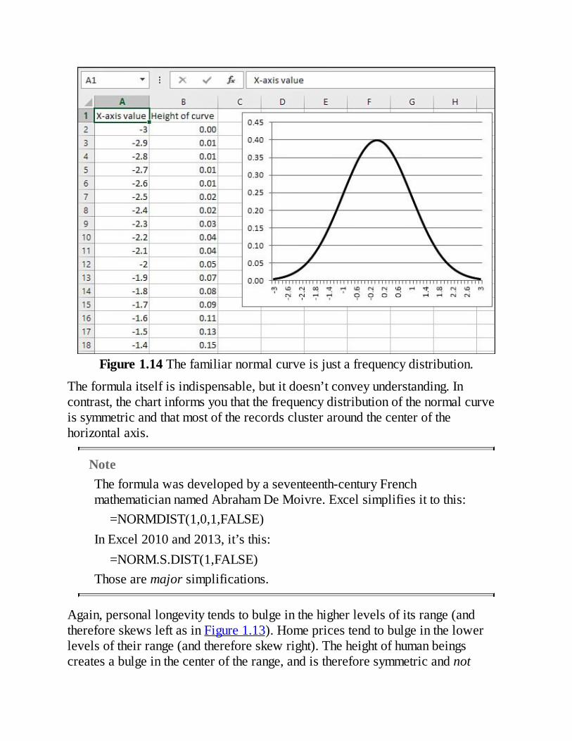
Figure1.14Thefamiliarnormalcurveisjustafrequencydistribution.

Theformulaitselfisindispensable,butitdoesn’tconveyunderstanding.Incontrast,thechartinformsyouthatthefrequencydistributionofthenormalcurveissymmetricandthatmostoftherecordsclusteraroundthecenterofthehorizontalaxis.

NoteTheformulawasdevelopedbyaseventeenth-centuryFrenchmathematiciannamedAbrahamDeMoivre.Excelsimplifiesittothis:

=NORMDIST(1,0,1,FALSE)InExcel2010and2013,it’sthis:

=NORM.S.DIST(1,FALSE)Thosearemajorsimplifications.

Again,personallongevitytendstobulgeinthehigherlevelsofitsrange(andthereforeskewsleftasinFigure1.13).Homepricestendtobulgeinthelowerlevelsoftheirrange(andthereforeskewright).Theheightofhumanbeingscreatesabulgeinthecenteroftherange,andisthereforesymmetricandnot

skewed.Somestatisticalanalysesassumethatthedatacomesfromanormaldistribution,andinsomestatisticalanalysesthatassumptionisanimportantone.Thisbookdoesnotexplorethetopicingreatdetailbecauseitcomesupinfrequently.Beaware,though,thatifyouwanttoanalyzeaskeweddistributiontherearewaystonormalizeitandthereforecomplywiththerequirementsoftheanalysis.Verygenerally,youcanuseExcel’sSQRT()andLOG()functionstohelpnormalizeanegativelyskeweddistribution,andanexponentiationoperator(forexample,=A2^2tosquarethevalueinA2)tohelpnormalizeapositivelyskeweddistribution.

NoteFindingjusttherighttransformationforaparticulardatasetcanbeamatteroftrialanderror,however,andtheExcelSolveradd-incanhelpinconjunctionwithExcel’sSKEW()function.SeeChapter2,“HowValuesClusterTogether,”forinformationonSolver,andChapter7,“UsingExcelwiththeNormalDistribution,”forinformationonSKEW().ThebasicideaistouseSKEW()tocalculatetheskewnessofyourtransformeddataandtohaveSolverfindtheexponentthatbringstheresultofSKEW()closesttozero.

VisualizingthePopulation:InferentialStatisticsTheothergeneralrationaleforexaminingfrequencydistributionshastodowithmakinganinferenceaboutapopulation,usingtheinformationyougetfromasampleasabasis.Thisisthefieldofinferentialstatistics.Inlaterchaptersofthisbook,youwillseehowtouseExcel’stools—inparticular,itsfunctionsanditscharts—toinferapopulation’scharacteristicsfromasample’sfrequencydistribution.Afamiliarexampleisthepoliticalsurvey.Whenapollsterannouncesthat53%ofthosewhowereaskedpreferredSmith,heisreportingadescriptivestatistic.Fifty-threepercentofthesamplepreferredSmith,andnoinferenceisneeded.Butwhenanotherpollsterreportsthatthemarginoferroraroundthat53%statisticisplusorminus3%,sheisreportinganinferentialstatistic.Sheisextrapolatingfromthesampletothelargerpopulationandinferring,withsomespecifieddegreeofconfidence,thatbetween50%and56%ofallvoterspreferSmith.Thesizeofthereportedmarginoferror,sixpercentagepoints,dependsheavilyonhowconfidentthepollsterwantstobe.Ingeneral,thegreaterdegreeof

confidenceyouwantinyourextrapolation,thegreaterthemarginoferrorthatyouallow.Ifyou’reonanarcheryrangeandyouwanttobevirtuallycertainofhittingyourtarget,youmakethetargetaslargeasnecessary.Similarly,ifthepollsterwantstobe99.9%confidentofherprojectionintothepopulation,themarginmightbesogreatastobeuseless—say,plusorminus20%.Andalthoughit’snotheadlinematerialtoreportthatsomewherebetween33%and73%ofthevoterspreferSmith,thepollstercanbeconfidentthattheprojectionisaccurate.Butthesizeofthemarginoferroralsodependsoncertainaspectsofthefrequencydistributioninthesampleofthevariable.Inthisparticular(andrelativelystraightforward)case,theaccuracyoftheprojectionfromthesampletothepopulationdependsinpartonthelevelofconfidencedesired(asjustbrieflydiscussed),inpartonthesizeofthesample,andinpartonthepercentfavoringSmithinthesample.Thelattertwoissues,samplesizeandpercentinfavor,arebothaspectsofthefrequencydistributionyoudeterminebyexaminingthesample’sresponses.Ofcourse,it’snotjustpoliticalpollingthatdependsonsamplefrequencydistributionstomakeinferencesaboutpopulations.Herearesomeothertypicalquestionsposedbyempiricalresearchers:

Whatpercentofthenation’sexistinghouseswereresoldlastquarter?WhatistheincidenceofcardiovasculardiseasetodayamongdiabeticswhotookthedrugAvandiabeforequestionsaboutitssideeffectsarosein2007?Isthatincidencereliablydifferentfromtheincidenceofcardiovasculardiseaseamongthosewhonevertookthedrug?Asampleof100carsfromaparticularmanufacturer,madeduring2013,hadaveragehighwaygasmileageof26.5mpg.Howlikelyisitthattheaveragehighwaympg,forallthatmanufacturer’scarsmadeduringthatyear,isgreaterthan26.0mpg?Yourcompanymanufacturescustomglassware.Yourcontractwithacustomercallsfornomorethan2%defectiveitemsinaproductionlot.Yousample100unitsfromyourlatestproductionrunandfind5thataredefective.Whatisthelikelihoodthattheentireproductionrunof1,000unitshasamaximumof20thataredefective?

Ineachofthesefourcases,thespecificstatisticalprocedurestouse—andthereforethespecificExceltools—wouldbedifferent.Butthebasicapproachwouldbethesame:Usingthecharacteristicsofafrequencydistributionfromasample,comparethesampletoapopulationwhosefrequencydistributioniseither

knownorfoundedingoodtheoreticalwork.UsethenumericfunctionsinExceltoestimatehowlikelyitisthatyoursampleaccuratelyrepresentsthepopulationyou’reinterestedin.

BuildingaFrequencyDistributionfromaSampleConceptually,it’seasytobuildafrequencydistribution.Takeasampleofpeopleorthingsandmeasureeachmemberofthesampleonthevariablethatinterestsyou.Yournextstepdependsonhowmuchsophisticationyouwanttobringtotheproject.

TallyingaSampleOnestraightforwardapproachcontinuesbydividingtherelevantrangeofthevariableintomanageablegroups.Forexample,supposethatyouobtainedtheweightinpoundsofeachof100people.Youmightdecidethatit’sreasonableandfeasibletoassigneachpersontoaweightclassthatistenpoundswide:75to84,85to94,95to104,andsoon.Then,onasheetofgraphpaper,makeatallyintheappropriatecolumnforeachperson,assuggestedinFigure1.15.

Figure1.15Thisapproachhelpsclarifytheprocess,buttherearequickerandeasierways.

TheapproachshowninFigure1.15usesagroupedfrequencydistribution,andtallyingbyhandintogroupswastheonlypracticaloptionasrecentlyasthe1980s,beforepersonalcomputerscameintotrulywidespreaduse.ButusinganExcelfunctionnamedFREQUENCY(),youcangetthebenefitsofgroupingindividualobservationswithoutthetediumofmanuallyassigningindividualrecordstogroups.

GroupingwithFREQUENCY()Ifyouassembleafrequencydistributionasjustdescribed,youhavetocountupalltherecordsthatbelongtoeachofthegroupsthatyoudefine.Excelhasafunction,FREQUENCY(),thatwilldotheheavyliftingforyou.AllyouhavetodoisdecideontheboundariesforthegroupsandthenpointtheFREQUENCY()

functionatthoseboundariesandattherawdata.Figure1.16showsonewaytolayoutthedata.

Figure1.16ThegroupsaredefinedbythenumbersincellsC2:C8.

InFigure1.16,theweightofeachpersoninyoursampleisrecordedincolumnA.ThenumbersincellsC2:C8definetheupperboundariesofwhatthissectionhascalledgroups,andwhatExcelcallsbins.Upto85poundsdefinesonebin;from86to95definesanother;from96to105definesanother,andsoon.

NoteThere’snospecialneedtousethecolumnheadersshowninFigure1.16,cellsA1,C1,andD1.Infact,ifyou’recreatingastandardExcelchartasdescribedhere,there’snogreatneedtosupplycolumnheadersatall.Ifyoudon’tincludetheheaders,ExcelnamesthedataSeries1andSeries2.Ifyouusethepivotchartinsteadofastandardchart,though,youwillneedtosupplyacolumnheaderforthedatashownincolumnAinFigure1.16.

ThecountofrecordswithineachbinappearsinD2:D8.Youdon’tcountthemyourself—youcallonExceltodothatforyou,andyoudothatbymeansofaspecialkindofExcelformula,calledanarrayformula.You’llreadmoreabout

arrayformulasinChapter2,aswellasinlaterchapters,butfornowherearethestepsneededtogetthebincountsshowninFigure1.16:

1.Selecttherangeofcellsthattheresultswilloccupy.Inthiscase,that’stherangeofcellsD2:D8.

2.Type,butdon’tyetenter,thefollowingformula:=FREQUENCY(A2:A101,C2:C8)

whichtellsExceltocountthenumberofrecordsinA2:A101thatareineachbindefinedbythenumericboundariesinC2:C8.

3.Afteryouhavetypedtheformula,holddowntheCtrlandShiftkeyssimultaneouslyandpressEnter.Thenreleaseallthreekeys.ThiskeyboardsequencenotifiesExcelthatyouwantittointerprettheformulaasanarrayformula.

NoteWhenExcelinterpretsaformulaasanarrayformula,itplacescurlybracketsaroundtheformulaintheformulabox.

TipYoucanusethesamerangefortheDataargumentandtheBinsargumentintheFREQUENCY()function:forexample,=FREQUENCY(A1:A101,A1:A101).Don’tforgettoenteritasanarrayformula.ThisisaconvenientwaytogetExceltotreateveryrecordedvalueasitsownbin,andyougetthecountforeveryuniquevalueintherangeA1:A101.

TheresultsappearverymuchlikethoseincellsD2:D8ofFigure1.16,ofcoursedependingontheactualvaluesinA2:A101andthebinsdefinedinC2:C8.Younowhavethefrequencydistributionbutyoustillshouldcreatethechart.Comparedtoearlierversions,Excel2013makesitquickerandeasiertocreatecertainbasicchartssuchastheoneshowninFigure1.16.Assumingthedatalayoutusedinthatfigure,herearethestepsyoumightuseinExcel2013tocreatethechart:

1.Selectthedatayouwanttochart—thatis,therangeC1:D8.(Iftherelevantdatarangeissurroundedbyemptycellsorworksheetboundaries,allyouneedtoselectisasinglecellintherangeyouwanttochart.)

2.ClicktheInserttab,andthenclicktheRecommendedChartsbuttonintheChartsgroup.

3.ClicktheClusteredColumnchartexampleintheInsertChartwindow,andthenclickOK.

YoucangetothervariationsoncharttypesinExcel2013byclicking,forexample,theInsertColumnChartbutton(intheChartsgroupontheInserttab).ClickMoreChartTypesatthebottomofthedrop-downtoseevariouswaysofstructuringBarcharts,Linecharts,andsoongiventhelayoutofyourunderlyingdata.Thingsweren’tassimpleinearlierversionsofExcel.Forexample,herearethestepsinExcel2010,againassumingthedataislocatedasinFigure1.16:

1.Selectthedatayouwanttochart—thatis,therangeC1:D8.2.ClicktheInserttab,andthenclicktheInsertColumnChartbuttonintheChartsgroup.

3.ChoosetheClusteredColumncharttypefromthe2-Dcharts.Anewchartappears,asshowninFigure1.17.BecausecolumnsCandDontheworksheetbothcontainnumericvalues,Excelinitiallythinksthattherearetwodataseriestochart:onenamedBinsandonenamedFrequency.

Figure1.17Valuesfrombothcolumnsarechartedasdataseriesatfirstbecausethey’reallnumeric.

4.FixthechartbyclickingSelectDataintheDesigntabthatappearswhenachartisactive.ThedialogboxshowninFigure1.18appears.

Figure1.18YoucanalsousetheSelectDatadialogboxtoaddanotherdataseriestothechart.

5.ClicktheEditbuttonunderHorizontal(Category)AxisLabels.AnewAxisLabelsdialogboxappears;dragthroughcellsC2:C8toestablishthatrangeasthebasisforthehorizontalaxis.ClickOK.

6.ClicktheBinslabelintheleftlistboxshowninFigure1.18.ClicktheRemovebuttontodeleteitasachartedseries.ClickOKtoreturntothechart.

7.Removethecharttitleandserieslegend,ifyouwant,byclickingeachandpressingDelete.

Atthispoint,youwillhaveanormalExcelchartthatlooksmuchliketheoneshowninFigure1.16.

UsingNumericValuesasCategoriesThedifferencesbetweenhowExcel2010andExcel2013handlechartspresentagoodillustrationoftheproblemscreatedbytheuseofnumericvaluesascategories.The“ChartingTwoVariables”sectionearlierinthischapteralludestotheambiguityinvolvedwhenyouwantExcelto

treatnumericvaluesascategories.IntheexampleshowninFigure1.16,youpresenttwonumericvariables—BinsandFrequency—toExcel’schartingfacility.Becausebothvariablesarenumeric(andtheirvaluesarestoredasnumbersratherthantext),therearevariouswaysthatExcelcantreatthemincharts:Treateachcolumn—theBinsvariableandtheFrequencyvariable—asdataseriestobecharted.ThisistheapproachyoumighttakeifyouwantedtochartbothIncomeandExpensesovertime:youwouldhaveExceltreateachvariableasadataseries,andthedifferentrowsintheunderlyingdatarangewouldrepresentdifferenttimeperiods.YougetthischartifyouchooseClusteredChartintheInsertColumnChartdrop-down.Treateachrowintheunderlyingdatarangeasadataseries.Then,thecolumnsaretreatedasdifferentcategoriesonthecolumnchart’shorizontalaxis.YougetthisresultifyouclickMoreColumnChartsatthebottomoftheInsertColumnChartdrop-down—it’sthethirdexamplechartintheInsertChartwindow.Treatoneofthevariables—BinsorFrequency—asacategoryvariableforuseonthehorizontalaxis.ThisisthecolumnchartyouseeinFigure1.16andisthefirstoftherecommendedcharts.

Excel2013,atleastintheareaofcharting,recognizesthepossibilitythatyouwillwanttousenumericvaluesasnominalcategories.ItletsyouexpressanopinionwithoutforcingyoutotakealltheextrastepsrequiredbyExcel2010.Still,ifyou’retoparticipateeffectively,youneedtorecognizethedifferencesbetween,say,intervalandnominalvariables.Youalsoneedtorecognizetheambiguitiesthatcropupwhenyouwanttouseanumberasacategory.

GroupingwithPivotTablesAnotherapproachtoconstructingthefrequencydistributionistouseapivottable.Arelatedtool,thepivotchart,isbasedontheanalysisthatthepivottableprovides.IpreferthismethodtousinganarrayformulathatemploysFREQUENCY().Withapivottable,oncetheinitialgroundworkisdone,Icanusethesamepivottabletodoanalysesthatgobeyondthebasicfrequencydistribution.ButifallIwantisaquickgroupcount,FREQUENCY()isusuallythefasterway.

Again,there’smoreonpivottablesandpivotchartsinChapter2andlaterchapters,butthissectionshowsyouhowtousethemtoestablishthefrequencydistribution.Buildingthepivottable(andthepivotchart)requiresyoutospecifybins,justastheuseofFREQUENCY()does,butthathappensalittlefurtheron.

NoteAreminder:WhenyouusetheFREQUENCY()methoddescribedinthepriorsection,aheaderatthetopofthecolumnofrawdatacanbehelpfulbutisnotrequired.Whenyouusethepivottablemethoddiscussedinthissection,theheaderisrequired.

BeginwithyoursampledatainA1:A101ofFigure1.16,justasbefore.Selectanyoneofthecellsinthatrangeandthenfollowthesesteps:

1.ClicktheInserttab.ClickthePivotChartbuttonintheChartsgroup.(PriortoExcel2013,clickthePivotTabledrop-downintheTablesgroupandchoosePivotChartfromthedrop-downlist.)Whenyouchooseapivotchart,youautomaticallygetapivottablealongwithit.ThedialogboxinFigure1.19appears.

Figure1.19Ifyoubeginbyselectingasinglecellintherangecontainingyourinputdata,Excelautomaticallyproposestherangeofadjacentcellsthatcontain

data.

2.ClicktheExistingWorksheetoptionbutton.ClickintheLocationrangeeditbox.Then,toavoidoverwritingvaluabledata,clicksomeblankcellintheworksheetthathasotheremptycellstoitsrightandbelowit.

3.ClickOK.TheworksheetnowappearsasshowninFigure1.20.

Figure1.20Withonefieldonly,younormallyuseitforbothAxisFields(Categories)andSummaryValues.

4.ClicktheWeightInPoundsfieldinthePivotTableFieldslistanddragitintotheAxis(Categories)area.

5.ClicktheWeightInPoundsfieldagainanddragitintotheΣValuesarea.DespitetheuppercaseGreeksigma,whichisasummationsymbol,theΣValuesinapivottablecanshowaverages,counts,standarddeviations,andavarietyofstatisticsotherthanthesum.However,Sumisthedefaultstatisticforafieldthatcontainsnumericvaluesonly.

6.ThepivottableandpivotchartarebothpopulatedasshowninFigure1.21.Right-clickanycellthatcontainsarowlabel,suchasC2.ChooseGroupfromtheshortcutmenu.

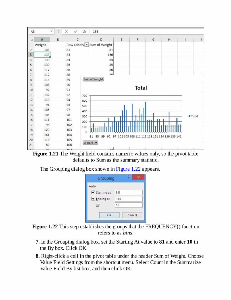
Figure1.21TheWeightfieldcontainsnumericvaluesonly,sothepivottabledefaultstoSumasthesummarystatistic.

TheGroupingdialogboxshowninFigure1.22appears.

Figure1.22ThisstepestablishesthegroupsthattheFREQUENCY()functionreferstoasbins.

7.IntheGroupingdialogbox,settheStartingAtvalueto81andenter10intheBybox.ClickOK.

8.Right-clickacellinthepivottableundertheheaderSumofWeight.ChooseValueFieldSettingsfromtheshortcutmenu.SelectCountintheSummarizeValueFieldBylistbox,andthenclickOK.

9.ThepivottableandchartreconfigurethemselvestoappearasinFigure1.23.Toremovethefieldbuttonsintheupper-andlower-leftcornersofthepivotchart,selectthechart,clicktheAnalyzetab,clickFieldButtons,andselectHideAll.

Figure1.23Thissample’sfrequencydistributionhasaslightrightskewbutisreasonablyclosetoanormalcurve.

BuildingSimulatedFrequencyDistributionsItcanbehelpfultoseehowafrequencydistributionassumesaparticularshapeasthenumberofunderlyingrecordsincreases.StatisticalAnalysis:Excel2013hasavarietyofworksheetsandworkbooksforyoutodownloadfromthisbook’swebsite(www.quepublishing.com/title/9780789753113).TheworkbookforChapter1hasaworksheetnamedFigure1.24thatsamplesrecordsatrandomfromapopulationofvaluesthatfollowsanormaldistribution.Thefollowingfigure,aswellastheworksheetonwhichit’sbased,showshowafrequency

distributioncomescloserandclosertothepopulationdistributionasthenumberofsampledrecordsincreases.

Figure1.24Thisfrequencydistributionisbasedonapopulationofrecordsthatfollowanormaldistribution.

BeginbyclickingthebuttonlabeledClearRecordsincolumnA.AllthenumberswillbedeletedfromcolumnA,leavingonlytheheadervalueincellA1.(Thepivottableandpivotchartwillremainastheywere:It’sacharacteristicofpivottablesandpivotchartsthattheydonotrespondimmediatelytochangesintheirunderlyingdatasources.)Decidehowmanyrecordsyou’dliketoadd,andthenenterthatnumberincellD1.Youcanalwayschangeittoanothernumber.ClickthebuttonlabeledAddRecordstoChart.Whenyoudoso,severaleventstakeplace,alldrivenbyVisualBasicproceduresthatarestoredintheworkbook:

Asampleistakenfromtheunderlyingnormaldistribution.ThesamplehasasmanyrecordsasspecifiedincellD1.(Theunderlying,normallydistributedpopulationisstoredinaseparate,hiddenworksheetnamed

RandomNormalValues;youcandisplaytheworksheetbyright-clickingaworksheettabandselectingUnhidefromtheshortcutmenu.)ThesampleofrecordsisaddedtocolumnA.IftherewerenorecordsincolumnA,thenewsampleiswrittenstartingincellA2.Iftherewerealready,say,100recordsincolumnA,thenewsamplewouldbeginincellA102.Thepivottableandpivotchartareupdated(or,inExcelterms,refreshed).AsyouclicktheAddRecordstoChartbuttonrepeatedly,moreandmorerecordsareusedinthechart.Thegreaterthenumberofrecords,themorenearlythechartcomestoresembletheunderlyingnormaldistribution.

Ineffect,thisiswhathappensinanexperimentwhenyouincreasethesamplesize.Largersamplesresemblemorecloselythepopulationfromwhichyoudrawthemthandosmallersamples.Thatgreaterresemblanceisn’tlimitedtotheshapeofthedistribution:Itincludestheaveragevalueandmeasuresofhowthevaluesvaryaroundtheaverage.Otherthingsbeingequal,youwouldpreferalargersampletoasmalleronebecauseit’slikelytorepresentthepopulationmoreclosely.Butthiseffectcreatesacost-benefitproblem.Itisusuallythecasethatthelargerthesample,themoreaccuratetheexperimentalfindings—andthemoreexpensivetheexperiment.Manyissuesareinvolvedhere(andthisbookdiscussesthem),butatsomepointtheincrementalaccuracyofadding,say,tenmoreexperimentalsubjectsnolongerjustifiestheincrementalexpenseofaddingthem.Oneofthebitsofadvicethatstatisticalanalysisprovidesistotellyouwhenyou’rereachingthepointwhenthereturnsbegintodiminish.Withthematerialinthischapter—scalesofmeasurement,thenatureofaxesonExcelcharts,andfrequencydistributions—inhand,Chapter2movesontothebeginningsofpracticalstatisticalanalysis,themeasurementofcentraltendency.

2.HowValuesClusterTogether

InThisChapterCalculatingtheMeanCalculatingtheMedianCalculatingtheModeFromCentralTendencytoVariability

Whenyouthinkaboutagroupthat’smeasuredonsomenumericvariable,youoftenstartthinkingaboutthegroup’saveragevalue.Onascaleof1to10,howwelldoregisteredIndependentsthinkthepresidentisdoing?WhatistheaveragemarketvalueofahouseinMinneapolis?What’sthemostpopularfirstnameforboysbornlastyear?Theanswertoeachofthosequestions,andquestionslikethem,isusuallyexpressedasanaverage,althoughthewordaverageineverydayusageisn’twelldefined,andyouwouldgoaboutfiguringeachaveragedifferently.Forexample,toinvestigatepresidentialapproval,youmightgoto100Independentvoters,askthemeachforaratingfrom1to10,addupalltheratings,anddivideby100.That’sonekindofaverage,andit’smorepreciselytermedthemean.Ifyou’reaftertheaveragecostofahouseinMinneapolis,youprobablyasksomegroupsuchasaboardofrealtors.They’lllikelytellyouwhatthemedianpriceis.Thereasonyou’relesslikelytogetthemeanpriceisthatinrealestatesales,therearealwaysafewhousesthatsellforreallyoutrageousamountsofmoney.Thosefewhousespullthemeanupsofarthatitisn’treallyrepresentativeofthepriceofatypicalhouseintheregionyou’reinterestedin.Themedian,ontheotherhand,isrightonthe50thpercentileforhouseprices;halfthehousessoldforlessthanthemedianpriceandhalfsoldformore.(It’salittlemorecomplicatedthanthis,andI’llcoverthecomplexitiesshortly.)Itisn’taffectedbyhowfarsomehomepricesarefromanaverage,justbyhowmanyareaboveanaverage.Inthatsortofsituation,wherethedistributionofvaluesisn’tsymmetric,themedianoftengivesyouamuchbettersenseoftheaverage,typicalvaluethandoesthemean.Andifyou’rethinkingofaverageasameasureofwhat’smostpopular,you’reusuallythinkingintermsofamode—themostfrequentlyoccurringvalue.Forexample,in2013,Jacobwasthemodalboy’snameamongnewborns.

Eachofthesemeasures—themean,themedianandthemode—islegitimatelyifimpreciselythoughtofasanaverage.Moreprecisely,eachofthemisameasureofcentraltendency:thatis,howagroupofpeopleorthingstendtoclusterinsomewayaroundacentralvalue.

UsingTwoSpecialExcelSkillsYouwillfindtwoparticularskillsinExcelindispensableforstatisticalanalysis—andthey’realsohandyforothersortsofworkyoudoinExcel.Oneisthedesignandconstructionofpivottablesandpivotcharts.Theotherisarray-enteringformulas.Thischapterspendsmoretimethanyoumightexpectonthemechanicsofcreatingapivotchartthatshowsafrequencydistribution—andthereforehowtodisplaythemodegraphically.ThematerialreviewsandextendstheinformationonpivottablesthatisincludedinChapter1,“AboutVariablesandValues.”You’llalsofindthatthischapterdetailstherationaleforarrayformulasandthetechniquesinvolvedindesigningthem.There’safairamountofinformationonhowyoucanuseExceltoolstopeerinsidetheseexoticformulastoseehowtheywork.YousawsomeskimpyinformationaboutarrayformulasinChapter1.Youneedtobefamiliarwithpivottablesandcharts,andwitharrayformulas,ifyouaretouseExcelforstatisticalanalysistoanymeaningfuldegree.Thischapter,whichconcernscentraltendency,discussesthetechniquesmorethanyoumightexpect.Butbeginningtopickthemupherewillpaydividendslaterwhenyouusethemtorunmoresophisticatedstatisticalanalysis.TheyareeasiertoexplorewhenyouusethemtocalculatemeansandmodesthanwhenyouusethemtoexplorethenatureoftheCentralLimitTheorem.

CalculatingtheMeanWhenyou’rereading,talking,orthinkingaboutstatisticsandthewordmeancomesup,itreferstothetotaldividedbythecount.Thetotaloftheheightsofeveryoneinyourfamilydividedbythenumberofpeopleinyourfamily.Thetotalpricepergallonofgasolineatallthegasstationsinyourcity,dividedbythenumberofgasstations.Thetotalnumberofabaseballplayer’shitsdividedbythenumberofatbats.

Inthecontextofstatistics,it’sveryconvenient,andmoreprecise,tousethewordmeanthisway.Itavoidsthevaguenessofthewordaverage,which—asjustdiscussed—canrefertothemean,tothemedian,ortothemode.Soit’ssortofashamethatExcelusesthefunctionnameAVERAGE()insteadofMEAN().Nevertheless,Figure2.1givesanexampleofhowyougetameanusingExcel.

Figure2.1TheAVERAGE()functioncalculatesthemeanofitsarguments.

UnderstandingtheelementsthatExcel’sworksheetfunctionshaveincommonwithoneanotherisimportanttousingthemproperly,andofcourseyoucan’tdogoodstatisticalanalysisinExcelwithoutusingthestatisticalfunctionsproperly.TherearemorestatisticalworksheetfunctionsinExcel,welloveronehundred,thananyotherfunctioncategory.SoIproposetospendsomeinkhereontheelementsofworksheetfunctionsingeneralandstatisticalfunctionsinparticular.Agoodplacetostartiswiththecalculationofthemean,showninFigure2.1.

UnderstandingFunctions,Arguments,andResultsThefunctionthat’sdepictedinFigure2.1,AVERAGE(),isatypicalexampleofstatisticalworksheetfunctions.

DefiningaWorksheetFunctionAnExcelworksheetfunction—morebriefly,afunction—isjustaformulathatsomeoneatMicrosoftwrotetosaveyoutime,effort,andmistakes.

NoteFormally,aformulainExcelisanexpressioninaworksheetcellthatbeginswithanequalsign(=);forexample,=3+4isaformula.FormulasoftenemployfunctionssuchasAVERAGE()andanexampleis=AVERAGE(A1:A20)+5,wheretheAVERAGE()functionhasbeenusedintheformula.Nevertheless,aworksheetfunctionisitselfaformula;youjustuseitsnameanditsargumentswithouthavingtodealwiththewayitgoesaboutcalculatingitsresults.(Thenextsectiondiscussesfunctions’arguments.)

SupposethatExcelhadnoAVERAGE()function.Inthatcase,togettheresultshownincellB13ofFigure2.1,youwouldhavetoentersomethinglikethisinB13:

=(B2+B3+B4+B5+B6+B7+B8+B9+B10+B11)/10Or,ifExcelhadaSUM()andaCOUNT()functionbutnoAVERAGE(),youcouldusethis:

=SUM(B2:B11)/COUNT(B2:B11)Butyoudon’tneedtobotherwiththosebecauseExcelhasanAVERAGE()function,andinthiscaseyouuseitasfollows:

=AVERAGE(B2:B11)So—atleastinthecasesofExcel’sstatistical,mathematical,andfinancialfunctions—allthetermworksheetfunctionmeansisaprewrittenformula.Thefunctionresultsinasummaryvaluethat’susuallybasedonother,individualvalues.

DefiningArgumentsMoreterminology:Those“other,individualvalues”arecalledarguments.That’sahighfalutinnameforthevaluesthatyouhandofftothefunction—or,putanotherway,thatyouplugintotheprewrittenformula.Intheinstanceofthefunction

=AVERAGE(B2:B11)therangeofcellsrepresentedbyB2:B11isthefunction’sargument.Theargumentsalwaysappearinparenthesesfollowingthefunction.Asinglerangeofcellsisregardedasoneargument,eventhoughthesinglerangeB2:B11containstenvalues.AVERAGE(B2:B11,C2:C11)containstwoarguments:onerangeoftenvaluesincolumnBandonerangeoftenvaluesincolumnC.(Excelhasafewfunctions,suchasPI(),thattakenoargumentsbutyouhaveto

supplytheparenthesesanyway.)

NoteExcel2013enablesyoutospecifyasmanyas255argumentstoafunction.(Earlierversions,suchasExcel2003,allowedyoutospecifyonly30arguments.)Butthisdoesn’tmeanthatyoucanpassamaximumof255valuestoafunction.EvenAVERAGE(A1:A1048576),whichcalculatesthemeanofthevaluesinoveramillioncells,hasonlyoneargument.

ManystatisticalandmathematicalfunctionsinExceltakethecontentsofworksheetcellsastheirarguments—forexample,SUM(A2:A10).Somefunctionshaveadditionalargumentsthatyouusetofine-tunetheanalysis.You’llseemuchmoreaboutthesefunctionsinlaterchapters,butastraightforwardexampleinvolvestheFREQUENCY()function,whichwasintroducedinChapter1:

=FREQUENCY(B2:B11,E2:E6)Inthisexample,supposethatyouwantedtocategorizethepricepergallondatainFigure2.1intofivegroups:lessthan$1,between$1and$2,between$2and$3,andsoon.Youcoulddefinethelimitsofthosegroupsbyenteringthevalueattheupperlimitoftherange—thatis,$1,$2,$3,$4,andsoon—incellsE2:E6.TheFREQUENCY()functionexpectsthatyouwilluseitsfirstargumenttotellitwheretheindividualobservationsare(here,they’reinB2:B11,calledthedataarraybyExcel)andthatyou’lluseitssecondargumenttotellitwheretofindtheboundariesofthegroups(here,E2:E6,calledthebinsarray).SointhecaseoftheFREQUENCY()function,theargumentshavedifferentpurposes:Thedataarrayargumentcontainstherangeaddressofthevaluesthatyouwanttogroup,andthebinsarrayargumentcontainstherangeaddressoftheboundariesyouwanttouseforthebins.Contrastthatwithsomethingsuchas=SUM(A1,A2,A3),wheretheSUM()functionexpectseachofitsargumentstocontributetothetotal.Touseworksheetfunctionsproperly,youmustbeawareofthepurposeofeachoneofafunction’sarguments.Excelgivesyouanassistwiththat.WhenyoustarttoenterafunctionintoacellinanExcelworksheet,asmallpopupwindowappearswiththefxsymbolattheleftofthenames(anddescriptions)offunctionsthatmatchwhatyou’vetypedsofar.Ifyoudouble-clickthefxsymbol,thepopupisreplacedbyonethatdisplaysthefunctionnameanditsarguments.SeeFigure2.2,wheretheuserhasjustbegun

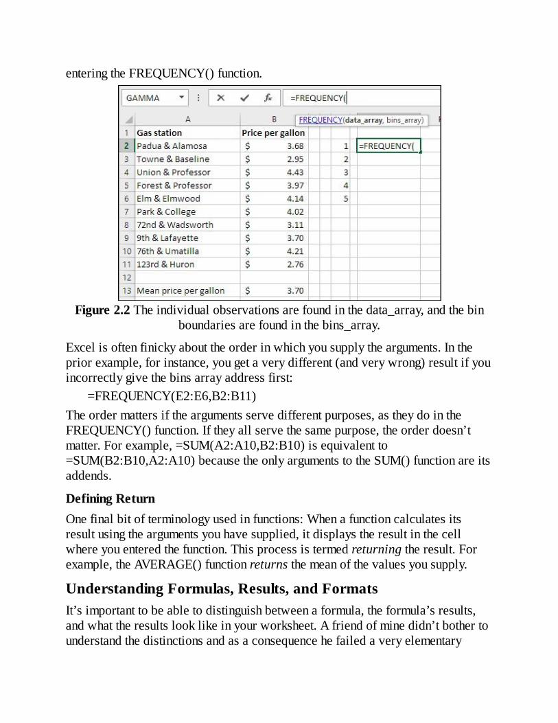
enteringtheFREQUENCY()function.

Figure2.2Theindividualobservationsarefoundinthedata_array,andthebinboundariesarefoundinthebins_array.

Excelisoftenfinickyabouttheorderinwhichyousupplythearguments.Inthepriorexample,forinstance,yougetaverydifferent(andverywrong)resultifyouincorrectlygivethebinsarrayaddressfirst:

=FREQUENCY(E2:E6,B2:B11)Theordermattersiftheargumentsservedifferentpurposes,astheydointheFREQUENCY()function.Iftheyallservethesamepurpose,theorderdoesn’tmatter.Forexample,=SUM(A2:A10,B2:B10)isequivalentto=SUM(B2:B10,A2:A10)becausetheonlyargumentstotheSUM()functionareitsaddends.

DefiningReturnOnefinalbitofterminologyusedinfunctions:Whenafunctioncalculatesitsresultusingtheargumentsyouhavesupplied,itdisplaystheresultinthecellwhereyouenteredthefunction.Thisprocessistermedreturningtheresult.Forexample,theAVERAGE()functionreturnsthemeanofthevaluesyousupply.

UnderstandingFormulas,Results,andFormatsIt’simportanttobeabletodistinguishbetweenaformula,theformula’sresults,andwhattheresultslooklikeinyourworksheet.Afriendofminedidn’tbothertounderstandthedistinctionsandasaconsequencehefailedaveryelementary

computerliteracycourse.Myfriendknewthatamongotherlearningobjectiveshewassupposedtoshowhowtouseaformulatoaddtogetherthenumbersintwoworksheetcellsandshowtheresultoftheadditioninathirdcell.Thenumbers11and14wereinA1andA2,respectively.Becausehedidn’tunderstandthedifferencebetweenaformulaandtheresultofaformula,heenteredtheactualsum,25,inA3,insteadoftheformula=A1+A2.Whenhelearnedthathe’dfailedthetest,hewassurprisedtofindoutthat“There’ssomewaytheycantellthatyoudidn’tentertheformula.”WhatcouldIsay?Hewaspre-law.Earlierthischapterdiscussedthefollowingexampleoftheuseofasimplestatisticalfunction:

=AVERAGE(B2:B11)Infact,that’saformula.AnExcelformulabeginswithanequalsign(=).Thisparticularformulaconsistsofafunctionname(here,AVERAGE)anditsarguments(here,B2:B11).Inthenormalcourseofevents,afteryouhavefinishedenteringaformulaintoaworksheetcell,Excelrespondsasfollows:

Theformulaitself,includinganyfunctionandargumentsinvolved,appearsintheformulabox.Theresultoftheformula—inthiscase,whatthefunctionreturns—appearsinthecellwhereyouenteredtheformula.Thepreciseresultoftheformulamightormightnotappearinthatcell,dependingonthecellformatthatyouhavespecified.Forexample,ifyouhavelimitedhowmanydecimalplacesshowupinthecell,theresultmayappearlessprecise.

Iusedthephrase“normalcourseofevents”justnowbecausetherearestepsyousometimestaketooverridethem(seeFigure2.3).

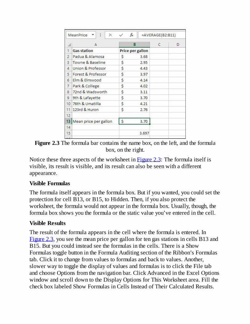
Figure2.3Theformulabarcontainsthenamebox,ontheleft,andtheformulabox,ontheright.

NoticethesethreeaspectsoftheworksheetinFigure2.3:Theformulaitselfisvisible,itsresultisvisible,anditsresultcanalsobeseenwithadifferentappearance.

VisibleFormulasTheformulaitselfappearsintheformulabox.Butifyouwanted,youcouldsettheprotectionforcellB13,orB15,toHidden.Then,ifyoualsoprotecttheworksheet,theformulawouldnotappearintheformulabox.Usually,though,theformulaboxshowsyoutheformulaorthestaticvalueyou’veenteredinthecell.

VisibleResultsTheresultoftheformulaappearsinthecellwheretheformulaisentered.InFigure2.3,youseethemeanpricepergallonfortengasstationsincellsB13andB15.Butyoucouldinsteadseetheformulasinthecells.ThereisaShowFormulastogglebuttonintheFormulaAuditingsectionoftheRibbon’sFormulastab.Clickittochangefromvaluestoformulasandbacktovalues.Another,slowerwaytotogglethedisplayofvaluesandformulasistoclicktheFiletabandchooseOptionsfromthenavigationbar.ClickAdvancedintheExcelOptionswindowandscrolldowntotheDisplayOptionsforThisWorksheetarea.FillthecheckboxlabeledShowFormulasinCellsInsteadofTheirCalculatedResults.

SameResult,DifferentAppearanceInFigure2.3,thesameformulaisincellB15asincellB13,buttheformulaappearstoreturnadifferentresult.Actually,bothformulasreturnthevalue3.697.ButcellB13isformattedtoshowcurrency,andUnitedStatescurrencyformatsdisplaytwodecimalvaluesonly,byconvention.So,ifyoucallforthecurrencyformatandyouroperatingsystemisusingU.S.currencyconventions,thedisplayisadjustedtoshowjusttwodecimals.Youcanchangethenumberofdecimalsdisplayedifyouwish,byselectingthecellandthenclickingeithertheIncreaseDecimalortheDecreaseDecimalbuttonintheNumbergroupontheHometab.

MinimizingtheSpreadThemeanhasaspecialcharacteristicthatmakesitmoreusefulforcertainintermediateandadvancedstatisticalanalysesthanthemedianandthemode.Thatcharacteristichastodowiththedistanceofeachindividualobservationfromthemeanofthoseobservations.Supposethatyouhavealistoftennumbers—say,theagesofallyourcloserelatives.Pluckanothernumberoutoftheair.Subtractthatnumberfromeachofthetenagesandsquaretheresultofeachsubtraction.Now,findthetotalofalltensquareddifferences.Ifthenumberthatyouchose,theonethatyousubtractedfromeachofthetenages,happenstobethemeanofthetenages,thenthetotalofthesquareddifferencesisminimized(thusthetermleastsquares).Thattotalissmallerthanitwouldbeifyouchoseanynumberotherthanthemean.Thisoutcomeprobablyseemsastrangethingtocareabout,butitturnsouttobeanimportantcharacteristicofmanystatisticalanalyses,asyou’llseeinlaterchaptersofthisbook.Here’saconcreteexample.Figure2.4showstheheightofeachoftenpeopleincellsA2:A11.

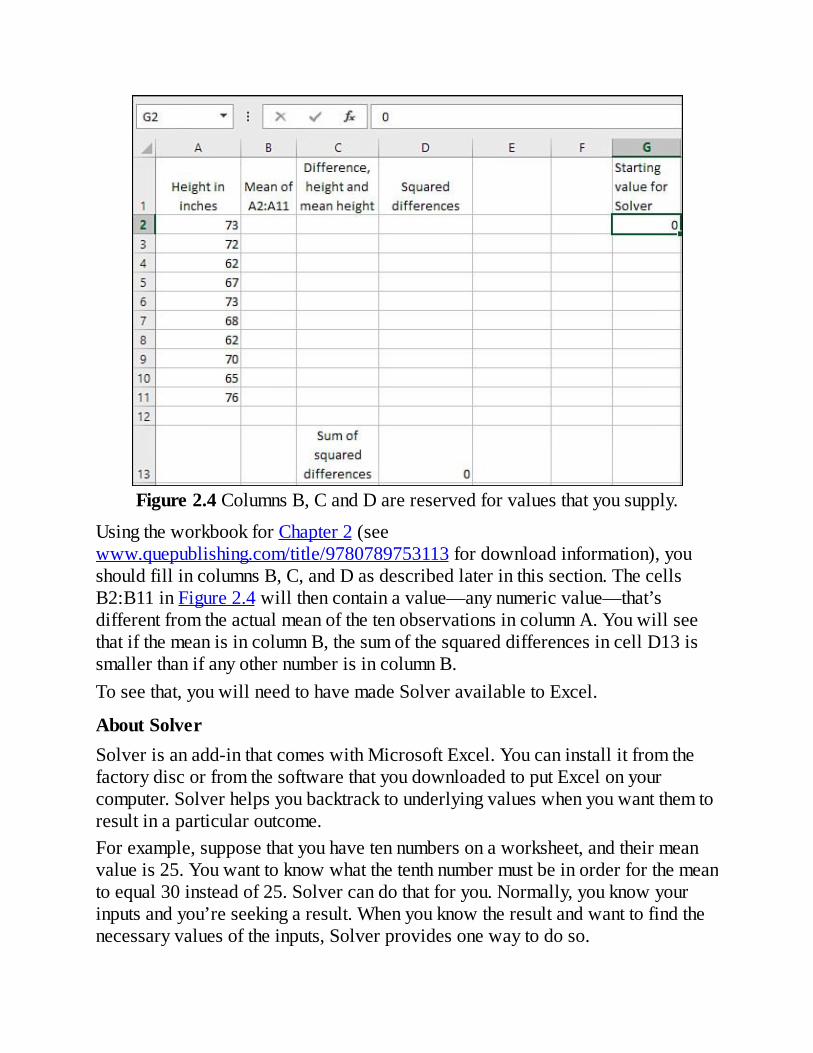
Figure2.4ColumnsB,CandDarereservedforvaluesthatyousupply.

UsingtheworkbookforChapter2(seewww.quepublishing.com/title/9780789753113fordownloadinformation),youshouldfillincolumnsB,C,andDasdescribedlaterinthissection.ThecellsB2:B11inFigure2.4willthencontainavalue—anynumericvalue—that’sdifferentfromtheactualmeanofthetenobservationsincolumnA.YouwillseethatifthemeanisincolumnB,thesumofthesquareddifferencesincellD13issmallerthanifanyothernumberisincolumnB.Toseethat,youwillneedtohavemadeSolveravailabletoExcel.

AboutSolverSolverisanadd-inthatcomeswithMicrosoftExcel.YoucaninstallitfromthefactorydiscorfromthesoftwarethatyoudownloadedtoputExcelonyourcomputer.Solverhelpsyoubacktracktounderlyingvalueswhenyouwantthemtoresultinaparticularoutcome.Forexample,supposethatyouhavetennumbersonaworksheet,andtheirmeanvalueis25.Youwanttoknowwhatthetenthnumbermustbeinorderforthemeantoequal30insteadof25.Solvercandothatforyou.Normally,youknowyourinputsandyou’reseekingaresult.Whenyouknowtheresultandwanttofindthenecessaryvaluesoftheinputs,Solverprovidesonewaytodoso.

Theexampleinthepriorparagraphistriviallysimple,butitillustratesthemainpurposeofSolver:YouspecifytheoutcomeandSolverdeterminestheinputvaluesneededtoreachtheoutcome.YoucoulduseanotherExceltool,GoalSeek,tosolvethelatterproblem.ButSolveroffersyoumanymoreoptionsthandoesGoalSeek.Forexample,usingSolver,youcanspecifythatyouwantanoutcomemaximizedorminimized,insteadofsolvingforaparticularoutcome(asrequiredbyGoalSeek).That’srelevantherebecausewewanttofindavaluethatminimizesthesumofthesquareddifferences.

FindingandInstallingSolverIt’spossiblethatSolverisalreadyinstalledandavailabletoExcelonyourcomputer.TouseSolverinExcel2007through2013,clicktheRibbon’sDatatabandfindtheAnalysisgroup.IfyouseeSolverthereyou’reallset.(InExcel2003orearlier,checkforSolverintheToolsmenu.)Ifyoudon’tfindSolverontheRibbonortheToolsmenu,takethesestepsinExcel2007through2013:

1.ClicktheRibbon’sFiletabandchooseOptions.2.ChooseAdd-InsfromtheOptionsnavigationbar.3.AtthebottomoftheViewandManageMicrosoftOfficeAdd-Inswindow,makesurethattheManagedrop-downissettoExcelAdd-Ins,andthenclickGo.

4.TheAdd-Insdialogboxappears.IfyouseeSolverAdd-inlisted,fillitscheckboxandclickOK.

YoushouldnowfindSolverintheAnalysisgroupontheRibbon’sDatatab.Ifyou’reusingExcel2003orearlier,startbychoosingAdd-InsfromtheToolsmenu.Thencompletestep4intheprecedinglist.Ifyoudidn’tfindSolverintheAnalysisgroupontheDatatab(orontheToolsmenuinearlierExcelversions),andifyoudidnotseeitintheAdd-Insdialogboxinstep4,thenSolverwasnotinstalledwithExcel.Youwillhavetoreruntheinstallationroutine,andyoucanusuallydosoviatheProgramsitemintheWindowsControlPanel.Thesequencevariesaccordingtotheoperatingsystemyou’rerunning,butyoushouldchoosetochangefeaturesforMicrosoftOffice.ExpandtheExceloptionbyclickingtheplussignbyitsiconandthendothesameforAdd-ins.Clickthedrop-downbySolverandchooseRunfromMyComputer.Completetheinstallation

sequence.Whenit’sthrough,youshouldbeabletomaketheSolveradd-inavailabletoExcelusingthesequenceoffourstepsprovidedearlierinthissection.

SettingUptheWorksheetforSolverWiththeactualobservationsinA2:A11,asshowninFigure2.4,continuebytakingthesesteps:

1.EnteranynumberincellG2.Itis0inFigure2.4,butyoucoulduse10or1066or3.1416ifyouprefer.Whenyou’rethroughwiththesesteps,you’llfindthemeanofthevaluesinA2:A11hasreplacedthevalueyounowbeginwithincellG2.

2.IncellB2,enterthisformula:=$G$2

3.CopyandpastetheformulainB2intoB3:B11.Becausethedollarsignsinthecelladdressmakeitafixedreference,youwillfindthateachcellinB2:B11containsthesameformula.AndbecausetheformulaspointtocellG2,whatevernumberistherealsoappearsinB2:B11.

4.IncellC2,enterthisformula:=A2–B2

5.CopyandpastetheformulainC2intoC3:C11.TherangeC2:C11nowcontainsthedifferencesbetweeneachindividualobservationandwhatevervalueyouchosetoputincellG2.

6.IncellD2,enterthefollowingformula,whichusesthecaretasanexponentiationoperatortoreturnthesquareofthevalueincellC2:=C2^2

7.CopyandpastetheformulainD2intoD3:D11.TherangeD2:D11nowcontainsthesquareddifferencesbetweeneachindividualobservationandwhatevernumberyouenteredincellG2.

8.Togetthesumofthesquareddifferences,enterthisformulaincellD13:=SUM(D2:D11)

9.NowstartSolver.WithcellD13selected,clicktheDatatabandlocatetheAnalysisgroup.ClickSolvertobringupthedialogboxshowninFigure2.5.

Figure2.5TheSetObjectivefieldshouldcontainthecellyouwantSolvertomaximize,minimize,orsettoaspecificvalue.

10.Youwanttominimizethesumofthesquareddifferences,sochoosetheMinradiobutton.

11.BecauseD13wastheactivecellwhenyoustartedSolver,itistheaddressthatappearsintheSetObjectivefield.ClickintheByChangingVariableCellsboxandthenclickincellG2.ThisestablishesthecellwhosevalueSolverwillmodify.

12.ClickSolve.SolvernowiteratesthroughasequenceofvaluesforcellG2.Itstopswhenitsinternaldecision-makingrulesdeterminethatithasfoundaminimumvalueforcellD13andthattestingmorevaluesincellG2won’thelp.AtthatpointSolver

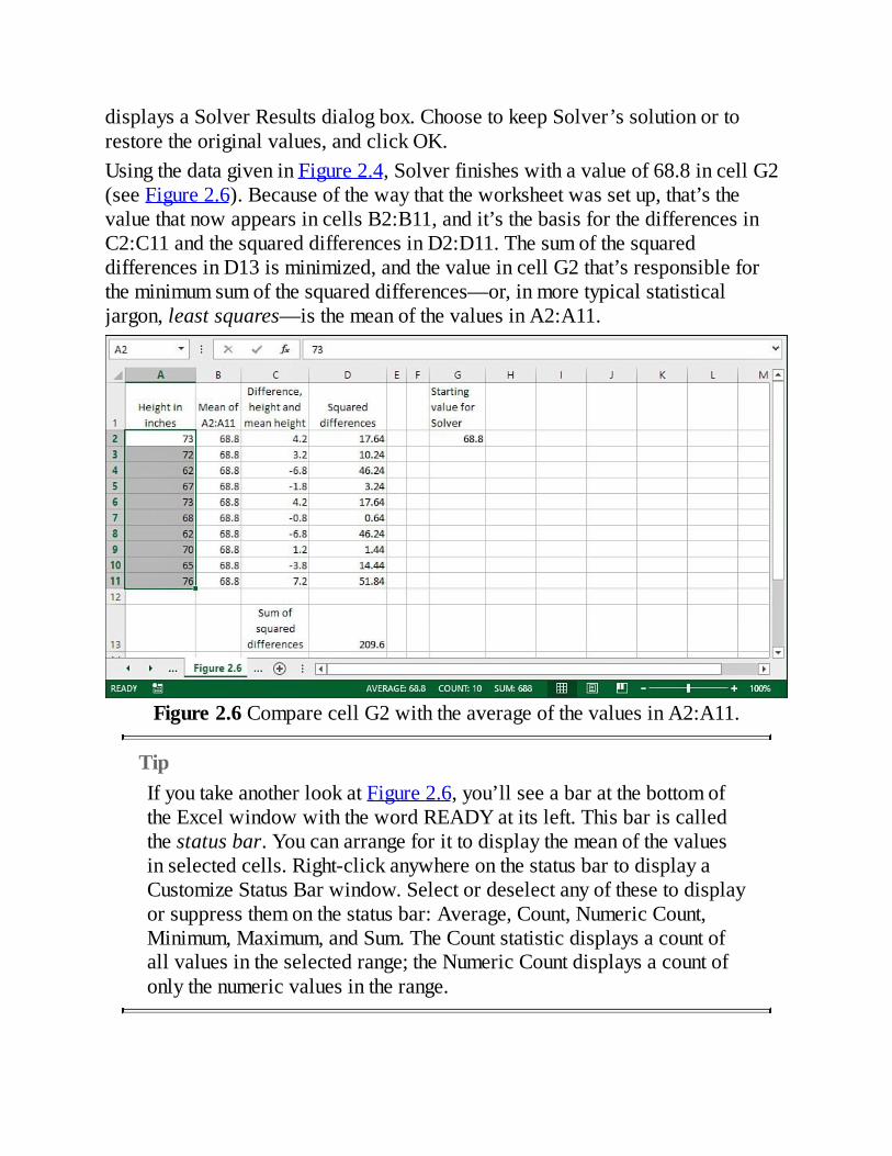
displaysaSolverResultsdialogbox.ChoosetokeepSolver’ssolutionortorestoretheoriginalvalues,andclickOK.UsingthedatagiveninFigure2.4,Solverfinisheswithavalueof68.8incellG2(seeFigure2.6).Becauseofthewaythattheworksheetwassetup,that’sthevaluethatnowappearsincellsB2:B11,andit’sthebasisforthedifferencesinC2:C11andthesquareddifferencesinD2:D11.ThesumofthesquareddifferencesinD13isminimized,andthevalueincellG2that’sresponsiblefortheminimumsumofthesquareddifferences—or,inmoretypicalstatisticaljargon,leastsquares—isthemeanofthevaluesinA2:A11.

Figure2.6ComparecellG2withtheaverageofthevaluesinA2:A11.

TipIfyoutakeanotherlookatFigure2.6,you’llseeabaratthebottomoftheExcelwindowwiththewordREADYatitsleft.Thisbariscalledthestatusbar.Youcanarrangeforittodisplaythemeanofthevaluesinselectedcells.Right-clickanywhereonthestatusbartodisplayaCustomizeStatusBarwindow.Selectordeselectanyofthesetodisplayorsuppressthemonthestatusbar:Average,Count,NumericCount,Minimum,Maximum,andSum.TheCountstatisticdisplaysacountofallvaluesintheselectedrange;theNumericCountdisplaysacountofonlythenumericvaluesintherange.

Afewcommentsonthisdemonstration:Itworkswithanysetofrealnumbers,andanysizeset.Supplysomenumbers,totaltheirsquareddifferencesfromsomeothernumber,andthentellSolvertominimizethatsum.Theresultwillalwaysbethemeanoftheoriginalset.Thisisademonstration,notaproof.Theproofthatthesquareddifferencesfromthemeansumtoasmallertotalthanfromanyothernumberisnotcomplexanditcanbefoundinavarietyofsources.Thisdiscussionusesthetermsdifferencesandsquareddifferences.You’llfindthatit’smorecommoninstatisticalanalysistospeakandwriteintermsofdeviationsandsquareddeviations.

Thishastobethemostroundaboutwayofcalculatingameaneverdevised.TheAVERAGE()function,forexample,islotssimpler.ButtheexerciseusingSolverinthissectionisimportantfortworeasons:

Understandingotherconcepts,includingcorrelation,regression,andthegenerallinearmodel,willcomemucheasierifyouhaveagoodfeelfortherelationshipbetweenthemeanofasetofscoresandtheconceptofminimizingsquareddeviations.IfyouhavenotyetusedExcel’sSolver,youhavenowhadaglimpseofit,althoughinthecontextofaproblemsolvedmuchmorequicklyusingothertools.

Ihaveusedaverysimplestatisticalfunction,AVERAGE(),asacontexttodiscusssomebasicsoffunctionsandformulasinExcel.ThesebasicsapplytoallExcel’smathematicalandstatisticalfunctions,andtomanyfunctionsinothercategoriesaswell.You’llneedtoknowaboutsomeotheraspectsoffunctions,butI’llpickthemupaswegettothem:They’remuchmorespecificthantheissuesdiscussedinthischapter.It’stimetogetontothenextmeasureofcentraltendency:themedian.

CalculatingtheMedianThemedianofagroupofobservationsisusually,andsomewhatcasually,thoughtofasthemiddleobservationwhentheyareinsortedorder.Andthat’susuallyagoodwaytothinkofit,evenifit’salittleimprecise.It’softensaid,forexample,thathalftheobservationsliebelowthemedianwhilehalflieaboveit.TheExceldocumentationsaysso.Sodoesmyoldcollegestatstext.Butno.Supposethatyourobservationsconsistofthenumbers1,2,3,4,and

5.Themiddlemostnumberinthatsetis3.Butitisnottruethathalfthenumberslieaboveitorbelowit.Itisaccuratetostatethatthesamenumberofobservationsliebelowthemedianaslieaboveit.Inthepriorexample,twoobservationsliebelow3andtwolieabove3.Ifthereisanevennumberofobservationsinthedataset,thenit’saccuratetosaythathalfliebelowthemedianandhalfaboveit.Butwithanevennumberofobservationsthereisnospecific,middlerecord,andthereforethereisnoidentifiablemedianrecord.Addoneobservationtothepriorset,sothatitconsistsof1,2,3,4,5,and6.Thereisnorecordinthemiddleofthatset.Ormakeit1,2,3,3,3,and4.Althoughoneofthe3’sisthemedian,thereisnospecific,identifiablerecordinthemiddleoftheset.Oneway,usedbyExcel,tocalculatethemedianwithanevennumberofrecordsistotakethemeanofthetwomiddlenumbers.Inthisexample,themeanof3and4is3.5,whichExcelcalculatesasthemedianof1,2,3,4,5,and6.Andthen,withanevennumberofobservations,exactlyhalftheobservationsliebelowandhalfabovethemedian.

NoteOtherwaystocalculatethemedianareavailablewhentherearetiedvaluesoranevennumberofvalues:Onemethodisinterpolationintoagroupoftiedvalues.ButthemethodusedbyExcelhasthevirtueofsimplicity:It’seasytocalculate,understand,andexplain.Andyouwon’tgofarwrongwhenExcelcalculatesamedianvalueof65.5wheninterpolationwouldhavegivenyou65.7.

ThesyntaxfortheMEDIAN()functionechoesthesyntaxoftheAVERAGE()function.ForthedatashowninFigure2.7,youjustenterthisformula:

=MEDIAN(A2:A61)

Figure2.7Themeanandthemedianaredifferentinasymmetricdistributions.

ChoosingtoUsetheMedianThemedianissometimesamoredescriptivemeasureofcentraltendencythanthemean.Forexample,Figure2.7showswhat’scalledaskeweddistribution—thatis,thedistributionisn’tsymmetric.Mostofthevaluesbunchupontheleftside,andafewarelocatedofftotheright(ofcourse,adistributioncanskeweitherdirection—thisonehappenstoskewright).Thissortofdistributionistypicalofhomepricesandit’sthereasonthattherealestateindustryreportsmediansinsteadofmeans.InFigure2.7,noticethatthemedianhomepricereportedis$193,000andthemeanhomepriceis$232,000.Themedianrespondsonlytothenumberofrankedobservations,butthemeanalsorespondstothesizeoftheobservations’values.Supposethatinthecourseofaweekthepriceofthemostexpensivehouseincreasesby$100,000andtherearenootherchangesinhousingprices.Themedianremainswhereitwas,becauseit’sstillatthe50thpercentileinthedistributionofhomeprices.It’sthat50%rankthatmatters,notthedollarsassociatedwiththemostexpensivehouse—or,forthatmatter,thecheapest.Incontrast,themeanwouldreactifthemostexpensivehouseincreasedinprice.InthesituationshowninFigure2.7,anincreaseof$120,000inthemostexpensivehouse’spricewouldincreasethemeanby$2,000—butthemedianwouldremainwhereitis.

Themedian’srelativelystaticqualityisonereasonthatit’sthepreferredmeasureofcentraltendencyforhousingpricesandsimilardata.Anotherreasonisthatwhendistributionsareskewed,themediancanprovideabettermeasureofhowthingstendcentrally.HaveanotherlookatFigure2.7.Whichstatisticseemstoyoutobetterrepresentthetypicalhomepriceinthatfigure:themeanof$232,000orthemedianof$193,000?It’sasubjectivejudgment,ofcourse,butmanypeoplewouldjudgethat$193,000isabettersummaryofthepricesofthesehousesthanis$232,000.

CalculatingtheModeThemeangivesyouameasureofcentraltendencybytakingalltheactualvaluesinagroupintoaccount.Themedianmeasurescentraltendencydifferently,bygivingyouthemidpointofarankedgroupofvalues.Themodetakesyetanothertack:Ittellsyouwhichoneofseveralvaluesoccursmostfrequently.YoucangetthisinformationfromtheFREQUENCY()function,asdiscussedinChapter1.ButtheMODE()functionreturnsthemostfrequentlyoccurringobservationonly,andit’salittlequickertouse.Furthermore,asyou’llseeinthissection,alittleworkcangetMODE()toworkwithdataonanominalscale—that’salsopossiblewithFREQUENCY()butit’salotmorework.Supposeyouhaveasetofnumbersinarangeofcells,asshowninFigure2.8.Thefollowingformulareturnsthenumericvaluethatoccursmostfrequentlyinthatrange(inFigure2.8,theformulaisenteredincellC1):

=MODE(A2:A21)

Figure2.8Excel’sMODE()functionworksonlywithnumericvalues.

ThepivotchartinFigure2.8providesthesameinformationgraphically.NoticethatthemodereturnedbythefunctionincellC1isthesamevalueasthemostfrequentlyoccurringvalueshowninthepivotchart.Theproblemisthatyoudon’tusuallycareaboutthemodeofnumericvalues.It’spossiblethatyouhaveathandalistoftheagesofthepeoplewholiveonyourblock,ortheweightofeachplayeronyourfavoritefootballteam,ortheheightofeachstudentinyourdaughter’sfourthgradeclass.It’sevenconceivablethatyouhaveagoodreasontoknowthemostfrequentlyoccurringage,weight,orheightinagroupofpeople.(Intheareaofinferentialstatistics,coveredinthesecondhalfofthisbook,themodeofwhat’scalledareferencedistributionisoftenofinterest.Atthispoint,though,we’redealingwithmorecommonplaceproblems.)Butyoudon’tnormallyneedthemodeofpeople’sheights,ofirises’sepallengths,ortheagesofrocks.Amongotherpurposes,numericmeasuresaregoodforrecordingsmalldistinctions:Joeis33yearsoldandJaneis34;Daveweighs230poundsandDonweighs232;Jakeis47inchestallandJudystands48inches.Inagroupof18or20people,it’squitepossiblethateveryoneisofadifferentage,oradifferentweightoradifferentheight.Thesameistrueofmostobjectsandnumericmeasurementsthatyoucanthinkof.

Inthatcase,itisnotplausiblethatyouwouldwanttoknowthemodalage,orweight,orheight.Themean,yes,orthemedian,butwhywouldyouwanttoknowthatthemostfrequentlyoccurringageinyourpokerclubis47years,whenthenextmostfrequentlyoccurringageis46andthenextis48?Themodeisseldomausefulstatisticwhenthevariablebeingstudiedisnumericandungrouped.It’swhenyouareinterestedinnominaldata—asdiscussedinChapter1,categoriessuchasbrandsofcarsorchildren’sgivennamesorpoliticalpreferences—thatthemodeisofinterest.It’sworthnotingthatthemodeistheonlysensiblemeasureofcentraltendencywhenyou’redealingwithnominaldata.Themodalboy’snamefornewbornsin2013wasJacob;thatstatisticisinterestingtosomepeopleinsomeway.Butwhat’sthemeanofJacob,Michael,andEthan?ThemedianofEmma,Isabella,andEmily?Themodeistheonlysensiblemeasureofcentraltendencyfornominaldata.ButExcel’sMODE()functiondoesn’tworkwithnominaldata.Ifyoupresenttoit,asitsargument,arangethatcontainsexclusivelytextdatasuchasnames,MODE()returnsthe#N/Aerrorvalue.Ifoneormoretextvaluesareincludedinalistofnumericvalues,MODE()simplyignoresthetextvalues.I’lltakethisopportunitytocomplainthatitdoesn’tmakealotofsenseforExceltoprovideanalyticsupportforasituationthatseldomoccurs(forexample,caringaboutthemodalheightofagroupoffourthgraders)whileitfailstosupportsituationsthatoccurallthetime(“Whichmodelofcardidwesellmostoflastweek?”).Figure2.9showsacoupleofsolutionstotheproblemwithMODE().

Figure2.9MODE()ismuchmoreusefulwithcategoriesthanwithintervalorordinalscalesofmeasurement.

ComparedtothepivotchartshowninFigure2.8,wherejustonevaluepokesupabovetheothersbecauseitoccurstwiceinsteadofonce,thefrequencydistributioninFigure2.9ismoreinformative.YoucanseethatFord,themodalvalue,leadsToyotabyaslimmarginandGMbysomewhatmore.(ThisreportisgenuineandwasexportedtoExcelbyausedcardealerfromapopularsmallbusinessaccountingpackage.)

NoteSomeofthestepsthatfollowaresimilar,evenidentical,tothestepstakentocreateapivotchartinChapter1.Theyarerepeatedhere,partlyforconvenienceandpartlysothatyoucanbecomeaccustomedtoseeinghowpivottablesandpivotchartsarebuilt.Perhapsmoreimportant,thevaluesonthehorizontalaxisinthepresentexamplearemeasuredonanominalscale.Becauseyou’resimplylookingforthemode,noorderingisimplied,andtheshapeofthedistributionisarbitrary.ContrastthatwithFigures1.21and1.23,wherethepurposeistodeterminewhetherthedistributionisnormalorskewed.There,you’reaftertheshapeofthedistributionofanintervalvariable,sotheleft-to-rightorderonthehorizontalaxisisimportant.

TocreateapivotchartthatlooksliketheoneinFigure2.9,followthesesteps:1.ArrangeyourrawdatainanExcellistformat:thefieldnameinthefirstcolumn(suchasA1)andthevaluesinthecellsbelowthefieldname(suchasA2:A21).It’sbestifallthecellsadjacenttothelistareempty.

2.Selectacellinyourlist.3.ClicktheRibbon’sInserttab,andclickthePivotChartbuttonintheChartsgroup.ThedialogboxshowninFigure2.10appears.

Figure2.10Inthisdialogboxyoucanacceptoreditthelocationoftheunderlyingdata,andindicatewhereyouwantthepivottabletostart.

4.Ifyoutookstep2andselectedacellinyourlistbeforeclickingthePivotChartbutton,Excelhasautomaticallysuppliedthelist’saddressintheTable/Rangeeditbox.Otherwise,identifytherangethatcontainsyourrawdatabydraggingthroughitwithyourmousepointer,bytypingitsrangeaddress,orbytypingitsnameifit’sanamedtableorrange.ThelocationofthedatashouldnowappearintheTable/Rangeeditbox.

5.Ifyouwantthepivottableandpivotcharttoappearintheactiveworksheet,clicktheExistingWorksheetbuttonandclickintheLocationeditbox.Thenclickinaworksheetcellthathasseveralemptycolumnstoitsrightandseveralemptyrowsbelowit.ThisistokeepExcelfromaskingifyouwantthepivottabletooverwriteexistingdata.ClickOKtogetthelayoutshowninFigure2.11.

Figure2.11ThePivotTableFieldListpaneappearsautomatically.

6.InthePivotTableFieldspane,dragthefieldorfieldsyou’reinterestedindownfromthelistandintotheappropriateareaatthebottom.Inthisexample,youwoulddragMakedownintotheAXIS(CATEGORIES)areaandalsodragitintotheΣValuesarea.

Thepivotchartandthepivottablethatthepivotchartisbasedonbothupdateassoonasyou’vedroppedafieldintoanareainthePivotTableFieldspane.IfyoustartedwiththedatashowninFigure2.9,youshouldgetapivotchartthat’sidentical,ornearlyso,tothepivotchartinthatfigure.

NoteExcelmakesoneoftwoassumptions,dependingonwhetherthecellthat’sactivewhenyoubegintocreatethepivottablecontainsdata.One,ifyoustartedbyselectinganemptycell,Excelassumesthat’swhereyouwanttoputthepivottable’supper-leftcorner.Excelputstheactivecell’saddressintheLocationeditbox.Two,ifyoustartedbyselectingacellthatcontainsavalueorformula,Excelassumesthatcellispartofthesourcedataforthepivottableorpivotchart.Excelfindstheboundariesofthecontiguous,filledcellsandputstheresultingaddressintheTable/Rangeeditbox.(Thisisthereasonthatstep1suggeststhatallcellsadjacenttoyourlistbeempty.)

ThisistheoutcomeshowninFigure2.10.

Afewcommentsonthisanalysis:Themodeisquiteausefulstatisticwhenit’sappliedtocategories:politicalparties,consumerbrands,daysoftheweek,statesinaregion,andsoon.Excelreallyshouldhaveabuilt-inworksheetfunctionthatreturnsthemodefortextvalues.Butitdoesn’t,andthenextsectionshowsyouhowtowriteyourownworksheetformulaforthemode,onethatwillworkforbothnumericandtextvalues.Whenyouhavejustafewdistinctcategories,considerbuildingapivotcharttoshowhowmanyinstancesthereareofeach.Apivotchartthatshowsthenumberofinstancesofeachcategoryisanappealingwaytopresentyourdatatoanaudience.(Thereisnotypeofchartthatcommunicateswellwhentherearemanycategoriestoconsider.Thevisualclutterobscuresthemessage.Inthatsortofsituation,considercombiningcategoriesoromittingsome.)StandardExcelchartsdonotshowthenumberofinstancespercategorywithoutsomepreliminarywork.Youwouldhavetogetacountofeachcategorybeforecreatingthechart,andthat’sthepurposeofthepivottablethatunderliesthepivotchart.Thepivotchart,basedonthepivottable,issimplyafasterwaytocompletetheanalysisthancreatingyourowntabletocountcategorymembershipandthenbasingastandardExcelchartonthattable.Themodeistheonlysensiblemeasureofcentraltendencywhenyou’reworkingwithnominaldatasuchascategorynames.Themedianrequiresthatyourankorderthingsinsomeway:shortesttotallest,leastexpensivetopriciest,orslowesttofastest.IntermsofthescaletypesintroducedinChapter1,youneedatleastanordinalscaletogetamedian,andmanycategoriesarenominal,notordinal.CategoriesthatarerepresentedbyvaluessuchasFord,GM,andToyotahaveneitherameannoramedian.

GettingtheModeofCategorieswithaFormulaIhavepointedoutthatExcel’sMODE()functiondoesnotworkwhenyousupplyitwithtextvaluesasitsarguments.Hereisamethodforgettingthemodeusingaworksheetformula.Ittellsyouwhichtextvalueoccursmostofteninyourdataset.You’llalsoseehowtoenteraformulathattellsyouhowmanyinstancesofthemodeexistinyourdata.

Ifyoudon’twanttoresorttoapivotcharttogetthemodeofagroupoftextvalues,youcangettheirmodewiththeformula

=INDEX(A2:A21,MODE(MATCH(A2:A21,A2:A21,0)))assumingthatthetextvaluesareinA2:A21.(Therangecouldoccupyasinglecolumn,asinA2:A21,orasinglerow,asinA2:Z2.Itwillnotworkproperlywithamultirow,multicolumnrangesuchasA2:Z21.)Ifyou’resomewhatnewtoExcel,thatformulaisn’tgoingtomakeanysensetoyouatall.Istructuredit,I’vebeenusingExcelfrequentlysince1994,andIstillhavetostareattheformulaandthinkitthroughbeforeIseewhyitreturnsthemode.Soiftheformulaseemsbaffling,don’tworryaboutit.Itwillbecomeclearinthefullnessoftime,andinthemeantimeyoucanuseittogetthemodalvalueforanysetoftextvaluesinaworksheet.SimplyreplacetherangeaddressA2:A21withtheaddressoftherangethatcontainsyourtextvalues.Briefly,thecomponentsoftheformulaworkasfollows:

TheMATCH()functionreturnsthepositioninthearrayofvalueswhereeachindividualvaluefirstappears.ThethirdargumenttotheMATCH()function,0,tellsExcelthatineachcaseanexactmatchisrequiredandthearrayisnotnecessarilysorted.So,foreachinstanceofFordinthearrayofvaluesinA2:A21,MATCH()returns1;foreachinstanceofToyota,itreturns2;foreachinstanceofGM,itreturns4.TheresultsoftheMATCH()functionareusedastheargumenttoMODE().Inthisexample,therearetwentyvaluesforMODE()toevaluate:someequal1,someequal2andsomeequal4.MODE()returnsthemostfrequentlyoccurringofthosenumbers.TheresultofMODE()isusedasthesecondargumenttoINDEX().Itsfirstargumentisthearraytoexamine.Thesecondargumenttellsithowfarintothearraytolook.Here,itlooksatthefirstvalueinthearray,whichisFord.If,say,GMhadbeenthemostfrequentlyoccurringtextvalue,MODE()wouldhavereturned4andINDEX()wouldhaveusedthatvaluetofindGMinthearray.

UsinganArrayFormulatoCounttheValuesWiththemodalvalue(Ford,inthisexample)inhand,westillwanttoknowhowmanyinstancesthereareofthatmode.Thissectiondescribeshowtocreatethearrayformulathatcountstheinstances.Figure2.9alsoshows,incellC2,thecountofthenumberofrecordsthatbelongtothemodalvalue.Thisformulaprovidesthatcount:

=SUM(IF(A2:A21=C1,1,0))Theformulaisanarrayformula,andmustbeenteredusingthespecialkeyboardsequenceCtrl+Shift+Enter.Youcantellthataformulahasbeenenteredasanarrayformulaifyouseecurlybracketsarounditintheformulabox.Ifyouarrayenterthepriorformula,itwilllooklikethisintheformulabox:

{=SUM(IF(A2:A21=C1,1,0))}Butdon’tsupplythecurlybracketsyourself.Ifyoudo,Excelinterpretsthisastext,notasaformula.Here’showtheformulaworks:AsshowninFigure2.9,cellC1containsthevalueFord.SothefollowingfragmentofthearrayformulatestswhethervaluesintherangeA2:A21equalthevalueFord:

A2:A21=C1Becausethereare20cellsintherangeA2:A21,thefragmentreturnsanarrayofTRUEandFALSEvalues:TRUEwhenacellcontainsFordandFALSEotherwise.Thearraylookslikethis:

{TRUE;FALSE;TRUE;FALSE;FALSE;FALSE;TRUE;FALSE;TRUE;TRUE;FALSE;FALSE;FALSE;TRUE;TRUE;FALSE;FALSE;TRUE;FALSE;FALSE}

Specifically,cellA2containsFord,andsoitpassesthetest:ThefirstvalueinthearrayisthereforeTRUE.CellA3doesnotcontainFord,andsoitfailsthetest:ThesecondvalueinthearrayisthereforeFALSE—andsoonforall20cells.

NoteThearrayofTRUEandFALSEvaluesisanintermediateresultofthisarrayformula(andofmanyothers,ofcourse).Assuch,itisnotroutinelyvisibletotheuser,whonormallyneedstoseeonlytheendresultoftheformula.Ifyouwanttoseeintermediateresultssuchasthisone,usetheFormulaAuditingtool.See“LookingInsideaFormula,”laterinthischapter,formoreinformation.

Nowstepoutsidethatfragment,which,aswe’vejustseen,resolvestoanarrayofTRUEandFALSEvalues.ThearrayisusedasthefirstargumenttotheIF()function.Excel’sIF()functiontakesthreearguments:

ThefirstargumentisavaluethatcanbeTRUEorFALSE.Inthisexample,that’seachvalueinthearrayjustshown,returnedbythefragmentA2:A21=C1.ThesecondargumentisthevaluethatyouwanttheIF()functiontoreturn

whenthefirstargumentisTRUE.Intheexample,thisis1.ThethirdargumentisthevaluethatyouwanttheIF()functiontoreturnwhenthefirstargumentisFALSE.Intheexample,thisis0.

TheIF()functionexamineseachofthevaluesinthearraytoseeifit’saTRUEvalueoraFALSEvalue.WhenavalueinthearrayisTRUE,theIF()functionreturns,inthisexample,a1,anda0otherwise.Therefore,thefragment

IF(A2:A21=C1,1,0)returnsanarrayof1sand0sthatcorrespondstothefirstarrayofTRUEandFALSEvalues.Thatarraylookslikethis:

{1;0;1;0;0;0;1;0;1;1;0;0;0;1;1;0;0;1;0;0}A1correspondstoacellinA2:A21thatcontainsthevalueFord,anda0correspondstoacellinthesamerangethatdoesnotcontainFord.Finally,thearrayof1sand0sispresentedtotheSUM()function,whichtotalsthevaluesinthearray.Here,thattotalis8.

RecappingtheArrayFormulaToreviewhowthearrayformulacountsthevaluesforthemodalcategoryofFord,considerthefollowing:

Theformula’spurposeistocountthenumberofinstancesofthemodalcategory,Ford,whosenameisincellC1.Theinnermostfragmentintheformula,A2:A21=C1,returnsanarrayof20TRUEorFALSEvalues,dependingonwhethereachofthe20cellsinA2:A21containsthesamevalueasisfoundincellC1.TheIF()functionexaminestheTRUE/FALSEarrayandreturnsanotherarraythatcontains1swheretheTRUE/FALSEarraycontainsTRUE,and0swheretheTRUE/FALSEarraycontainsFALSE.TheSUM()functiontotalsthevaluesinthearrayof1sand0s.TheresultisthenumberofcellsinA2:A21thatcontainthevalueincellC1,whichisthemodalvalueforA2:A21.

UsinganArrayFormulaVariousreasonsexistforusingarrayformulasinExcel.Twoofthemosttypicalreasonsaretosupportafunctionthatrequiresitbearray-entered,andtoenableafunctiontoworkonmorethanjustonevalue.

AccommodatingaFunctionOnereasonyoumightneedtouseanarrayformulaisthatyou’reemployinga

functionthatmustbearray-enteredifitistoreturnresultsproperly.Forexample,theFREQUENCY()function,whichcountsthenumberofvaluesbetweenalowerboundandanupperbound(see“DefiningArguments,”earlierinthischapter)requiresthatyouenteritinanarrayformula.Anotherfunctionthatrequiresarray-entryistheLINEST()function,whichwillbediscussedingreatdetailinseveralsubsequentchapters.BothFREQUENCY()andLINEST(),alongwithanumberofotherfunctions,returnanarrayofvaluestotheworksheet.Youneedtoaccommodatethatarray.Todoso,beginbyselectingarangeofcellsthathasthenumberofrowsandcolumnsneededtoshowthefunction’sresults.(Knowinghowmanyrowsandcolumnstoselectdependsonyourknowledgeofthefunctionandyourexperiencewithit.)ThenyouentertheformulathatcallsthefunctionbymeansofCtrl+Shift+EnterinsteadofsimplyEnter;again,thissequenceiscalledarrayenteringtheformula.

AccommodatingaFunction’sArgumentsSometimesyouuseanarrayformulabecauseitemploysafunctionthatusuallytakesasinglevalueasanargument,butyouwanttosupplyitwithanarrayofvalues.TheexampleincellC2ofFigure2.9showstheIF()function,whichusuallyexpectsasingleconditionasitsfirstargument,insteadacceptinganarrayofTRUEandFALSEvaluesasitsfirstargument:

=SUM(IF(A2:A21=C1,1,0))Typically,theIF()functiondealswithonlyonevalueasitsfirstargument.Forexample,supposeyouwantcellC2toshowthevalueCurrentifcellA1containsthevalue2014;otherwise,B1shouldshowthevaluePast.YoucouldputthisformulainB1,enterednormallywiththeEnterkey:

=IF(A1=2014,“Current”,“Past”)Youcanenterthatformulanormally,viatheEnterkey,becauseyou’rehandingoffjustonevalue,2014,toIF()asitsfirstargument.However,theexampleconcerningthenumberofinstancesofthemodevalueisthis:

=SUM(IF(A2:A21=C1,1,0))ThefirstargumenttoIF()inthiscaseisanarrayofTRUEandFALSEvalues.TosignalExcelthatyouaresupplyinganarrayratherthanasinglevalueasthefirstargumenttoIF(),youentertheformulausingCtrl+Shift+Enter,insteadoftheEnterkeyaloneasyouusuallywouldforanormalExcelformulaorvalue.

LookingInsideaFormulaExcelhasacoupleoftoolsthatcomeinhandyfromtimetotimewhenaformulaisn’tworkingexactlyasyouexpect—orwhenyou’rejustinterestedinpeekinginsidetoseewhat’sgoingon.Ineachcaseyoucanpulloutafragmentofaformulatoseewhatitdoes,inisolationfromtheremainderoftheformula.

UsingFormulaEvaluationIfyou’reusingExcel2002oramorerecentversion,youhaveaccesstoaformulaevaluationtool.Beginbyselectingacellthatcontainsaformula.Thenstartformulaevaluation.InExcel2007through2013,you’llfinditontheRibbon’sFormulastab,intheFormulaAuditinggroup;inExcel2002and2003,chooseTools,FormulaAuditing,EvaluateFormula.Ifyouweretobeginbyselectingacellwiththearrayformulathatthissectionhasdiscussed,youwouldseethewindowshowninFigure2.12.

Figure2.12Formulaevaluationstartswiththeformulaasit’senteredintheactivecell.

Now,ifyouclickEvaluate,ExcelbeginsevaluatingtheformulafromtheinsideoutandthedisplaychangestowhatyouseeinFigure2.13.

Figure2.13TheformulaexpandstoshowthecontentsofA2:A21andC1.

ClickEvaluateagainandyou’llseetheresultsofthetestofA2:A21withC1,asshowninFigure2.14.

Figure2.14ThearrayofcellcontentsbecomesanarrayofTRUEandFALSE,dependingonthecontentsofthecells.

ClickEvaluateagainandthewindowshowstheresultsoftheIF()function,whichinthiscasereplacesTRUEwith1andFALSEwith0(seeFigure2.15).

Figure2.15Each1representsacellthatequalsthevalueincellC1.

AfinalclickofEvaluateshowsyouthefinalresult,whentheSUM()functiontotalsthe1sand0storeturnacountofthenumberofinstancesofFordinA2:A21,asshowninFigure2.16.

Figure2.16ThereareeightinstancesofFordinA2:A21.

YoucouldusetheSUMIF()orCOUNTIF()functionifyouprefer.IliketheSUM(IF())structurebecauseIfindthatitgivesmemoreflexibilityincomplicatedsituationssuchassummingtheresultsofmultiplyingtwoormoreconditionalarrays.

UsingtheRecalculateKeyAnothermethodforlookinginsideaformulaisavailableinallWindowsversionsofExcel,andmakesuseoftheF9key.TheF9keyforcesacalculationandcanbe

usedtorecalculateaworksheet’sformulaswhenautomaticrecalculationhasbeenturnedoff.IfthatwereallyoucoulddowiththeF9key,itsscopewouldbeprettylimited.Butyoucanalsouseittocalculateaportionofaformula.SupposethatyouhavethisarrayformulainaworksheetcellanditsargumentsasgiveninFigure2.9:

=SUM(IF(A2:A21=C1,1,0))Ifthecellthatcontainstheformulaisactive,you’llseetheformulaintheformulabox.DragacrosstheA2:A21=C1portionwithyourmousepointertohighlightit.Then,whileit’sstillhighlighted,pressF9togettheresultshowninFigure2.17.

Figure2.17NoticethatthearrayofTRUEandFALSEvaluesisidenticaltotheoneshowninFigure2.14.

Excelformulasseparaterowsbysemicolonsandcolumnsbycommas.ThearrayinFigure2.17isbasedonvaluesthatarefoundindifferentrows,sotheTRUEandFALSEitemsareseparatedbysemicolons.Iftheoriginalvalueswereindifferentcolumns,theTRUEandFALSEitemswouldbeseparatedbycommas.Ifyou’reusingExcel2002orlater,useformulaevaluationtostepthroughaformulafromtheinsideout.Alternatively,usinganyWindowsversionofExcel,usetheF9keytogetaquicklookathowExcelevaluatesasinglefragmentfromtheformula.

FromCentralTendencytoVariabilityThischapterhasexaminedthethreeprincipalmeasuresofcentraltendencyinasetofvalues.Centraltendencyisacriticallyimportantattributeinanysampleorpopulation,butsoisvariability.Ifthemeaninformsyouwherethevaluestendtocluster,thestandarddeviationandrelatedstatisticstellyouhowthevaluestendtodisperse.Youneedtoknowboth,andChapter3,“Variability:HowValuesDisperse,”getsyoustartedonvariability.

3.Variability:HowValuesDisperse

InThisChapterMeasuringVariabilitywiththeRangeTheConceptofaStandardDeviationCalculatingtheStandardDeviationandVarianceBiasintheEstimateExcel’sVariabilityFunctions

Chapter2,“HowValuesClusterTogether,”wentintosomedetailaboutmeasuresofcentraltendency:themethodsyoucanusetodeterminewhereonascaleofvaluesyoucanfindthevaluethat’sthemosttypicalandrepresentativeofagroup.Intuitively,anaveragevalueisoftenthemostinterestingstatistic,certainlymoreinterestingthananumberthattellsyouhowvaluesfailtocometogether.Butunderstandingtheirvariationgivescontexttothecentraltendencyofthevalues.Forexample,peopletendtobemoreinterestedinthemedianvalueofhousesinaneighborhoodthantheyareintherangeofthosevalues.However,astatisticsuchastherange,whichisonewaytomeasurevariability,putsanaverageintocontext.Supposethatyouknowthatthemedianpriceofahouseinagivenneighborhoodis$250,000.Youalsoknowthattherangeofhomeprices—thedifferencebetweenthehighestandthelowestprices—inthesameneighborhoodis$300,000.Youdon’tknowforsure,becauseyoudon’tknowhowskewedthedistributionis,butareasonableguessisthatthepricesrangefrom$100,000to$400,000.That’squiteaspreadinasingleneighborhood.Ifyouweretoldthattherangeofpriceswas$100,000,thenthevaluesmightrunfrom$200,000to$300,000.Intheformercase,theneighborhoodcouldincludeeverythingfromlittlebungalowstoMcMansions.Inthelattercase,thehousesareprobablyfairlysimilarinsizeandquality.It’snotenoughtoknowanaveragevalue.Togivethataverageameaning—thatis,acontext—youalsoneedtoknowhowthevariousmembersofasampledifferfromitsaverage.

MeasuringVariabilitywiththeRange

Justastherearethreeprimarywaystomeasurethecentraltendencyinafrequencydistribution,there’smorethanonewaytomeasurevariability.Twoofthesemethods,thestandarddeviationandthevariance,arecloselyrelatedandtakeupmostofthediscussioninthischapter.Athirdwayofmeasuringvariabilityistherange:themaximumvalueinasetminustheminimumvalue.It’susuallyhelpfultoknowtherangeofthevaluesinafrequencydistribution,ifonlytoguardagainsterrorsindataentry.Forexample,supposeyouhavealistinanExcelworksheetthatcontainsthebodytemperatures,measuredinFahrenheit,of100men.Ifthecalculatedrange,themaximumtemperatureminustheminimumtemperature,is888degrees,youknowprettyquicklythatsomeonedroppedadecimalpointsomewhere.Perhapsyouentered986insteadof98.6.Therangeasastatistichassomeattributesthatmakeitunsuitableforuseinmuchstatisticalanalysis.Nevertheless,inpartbecauseit’smucheasiertocalculatebyhandthanothermeasuresofvariability,therangecanbeuseful.

NoteHistorically,particularlyintheareaofstatisticalprocesscontrol(atechniqueusedinthemanagementofqualityinmanufacturing),somewell-knownpractitionershavepreferredtherangeasanestimateofvariability.Theyclaim,withsomejustification,thatastatisticsuchasthestandarddeviationisinfluencedbothbytheunderlyingnatureofamanufacturingsystemandbyspecialeventssuchashumanerrorsthatcauseasystemtogooutofcontrol.It’struethatthestandarddeviationtakeseveryvalueintoaccountincalculatingtheoverallvariabilityinasetofnumbers,andsomeofthosevaluesarenormaloutliers—redherringsthatdon’treallycallforfurtherinvestigation.Itdoesn’tfollowfromthat,though,thattherangeissensitiveonlytotheoccasionalproblemsthatrequiredetectionandcorrection.

Theuseoftherangeasthesolemeasureofvariabilityinadatasethassomedrawbacks,butit’sagoodideatocalculateitanywaytobetterunderstandthenatureofyourdata.Forexample,Figure3.1showsafrequencydistributionthatcanbesensiblydescribedinpartbyusingtherange.

Figure3.1Thedistributionisapproximatelysymmetric,andtherangeisausefuldescriptor.

Becauseanappreciablenumberoftheobservationsappearateachendofthedistribution,it’susefultoknowthattherangethatthevaluesoccupyis34.Figure3.2presentsadifferentpicture.Ittakesonlyoneextremevaluefortherangetopresentamisleadingpictureofthedegreeofvariabilityinadataset.

Figure3.2Thesolitaryvalueatthetopofthedistributioncreatesarangeestimatethatmisdescribesthedistribution.

Thesizeoftherangedependsonthelargestandthesmallestvaluesinthedistribution.Therangedoesnotchangeuntilandunlessthere’sachangeinoneorbothofthosevalues,themaximumandtheminimum.Alltheothervaluesinthefrequencydistributioncouldchangeandtherangewouldremainthesame.Theothervaluescouldbedistributedmorehomogeneously,ortheycouldbunchupnearoneortwomodes,andtherangewouldstillnotchange.Furthermore,thesizeoftherangedependsheavilyonthenumberofvaluesinthefrequencydistribution.SeeFigure3.3forexamplesthatcomparetherangewiththestandarddeviationforsamplesofvarioussizes,drawnfromapopulationwherethestandarddeviationis15.

Figure3.3Samplesofsizesfrom2to20areshownincolumnsBthroughF,andstatisticsappearinrows22through24.

Noticethatthemeanandthestandarddeviationarerelativelystableacrossfivesamplesizes,buttherangemorethandoublesfrom27to58asthesamplesizegrowsfrom2to20.That’sgenerallyundesirable,particularlywhenyouwanttomakeinferencesaboutapopulationonthebasisofasample.Youwouldnotwantyourestimateofthevariabilityofvaluesinapopulationtodependonthesizeofthesamplethatyoutake.TheeffectthatyouseeinFigure3.3isduetothefactthatthelikelihoodofobtainingarelativelylargeorsmallvalueincreasesasthesamplesizeincreases.(Thisistruemainlyofdistributionssuchasthenormalcurvethatcontainmanyoftheirobservationsnearthemiddleoftherange.)Althoughthesamplesizehasaneffectonthecalculatedrange,itseffectonthestandarddeviationismuchlesspronouncedbecausethestandarddeviationtakesintoaccountallthevaluesinthesample,notjusttheextremes.

ExcelhasnoRANGE()function.Togettherange,youmustusesomethingsuchasthefollowing,substitutingtheappropriaterangeaddressfortheoneshown:

=MAX(A2:A21)–MIN(A2:A21)

TheConceptofaStandardDeviationSupposesomeonetoldyouthatyoustand19unitstall.Whatdoyouconcludefromthatinformation?Doesthatmeanyou’retall?short?ofaverageheight?Whatpercentofthepopulationistallerthanyouare?Youdon’tknow,andyoucan’tknow,becauseyoudon’tknowhowlonga“unit”is.Ifaunitisfourincheslong,thenyoustand76inches,or6'4"(rathertall).Ifaunitisthreeincheslong,thenyoustand57inches,or4'9"(rathershort).Theproblemisthatthere’snothingstandardaboutthewordunit.(Infact,that’soneofthereasonsit’ssuchausefulword.)Nowsupposefurtherthatthemeanheightofallhumansis20units.Ifyou’re19unitstall,youknowthatyou’reshorterthanaverage.Buthowmuchshorterisoneunitshorter?If,say,3%ofthepopulationstandsbetween19and20units,thenyou’reonlyalittleshorterthanaverage.Only3%ofthepopulationstandsbetweenyouandtheaverageheight.If,instead,34%ofthepopulationwerebetween19and20unitstall,thenyou’dbefairlyshort:Everyonewho’stallerthanthemeanof20,plusanother34%between19and20units,wouldbetallerthanyou.Supposenowthatyouknowthemeanheightinthepopulationis20units,andthat3%ofthepopulationisbetween19and20unitstall.Withthatknowledge,withthecontextprovidedbyknowingthemeanheightandthevariabilityofheight,“unit”becomesastandard.Nowwhensomeonetellsyouthatyou’re19unitstall,youcanapplyyourknowledgeofthewaythatstandardbehaves,andimmediatelyconcludethatyou’reaskoshshorterthanaverage.

ArrangingforaStandardAstandarddeviationactsmuchlikethefictitiousunitdescribedinthepriorsection.Inanyfrequencydistribution(suchasthosediscussedinChapter1,“AboutVariablesandValues”)thatfollowsanormalcurve,thesestatementsaretrue:

Youfindabout34%oftherecordsbetweenthemeanandonestandarddeviationfromthemean.Youfindabout14%oftherecordsbetweenoneandtwostandarddeviationsfromthemean.

Youfindabout2%oftherecordsbetweentwoandthreestandarddeviationsfromthemean.

ThesestandardsaredisplayedinFigure3.4.

Figure3.4Theseproportionsarefoundinallnormaldistributions.

ThenumbersshownonthehorizontalaxisinFigure3.4arecalledz-scores.Az-score,orsometimesz-value,tellsyouhowmanystandarddeviationsaboveorbelowthemeanarecordis.Ifsomeonetellsyouthatyourheightinz-scoreunitsis+1.0,it’sthesameassayingthatyourheightisonestandarddeviationabovethemeanheight.Similarly,ifyourweightinz-scoresis–2.0,yourweightistwostandarddeviationsbelowthemeanweight.Becauseofthewaythatz-scoressliceupthefrequencydistribution,youknowthataz-scoreof+1.0meansthat84%oftherecordsliebelowit:Yourheightof1.0zmeansthatyouareastallasortallerthan84%oftheotherobservations.That84%comprisesthe50%belowthemean,plusthe34%betweenthemeanandonestandarddeviationabovethemean.Yourweight,–2.0z,meansthatyououtweighonly2%oftheotherobservations.Hencethetermstandarddeviation.It’sstandardbecauseitdoesn’tmatterwhetheryou’retalkingaboutheight,weight,IQ,orthediameterofmachined

pistonrings.Ifit’savariablethat’snormallydistributed,thenonestandarddeviationabovethemeanisequaltoorgreaterthan84%oftheotherobservations.Twostandarddeviationsbelowthemeanisequaltoorlessthan98%oftheotherobservations.It’sadeviationbecauseitexpressesadistancefromthemean:adeparturefromthemeanvalue.Andit’satthispointinthediscussionthatwegetbacktothematerialinChapter2regardingthemean,thatitisthenumberthatminimizesthesumofthesquareddeviationsoftheoriginalvalues.Moreonthatshortly,in“DividingbyN–1,”butfirstit’shelpfultobringinalittlemorebackground.

ThinkinginTermsofStandardDeviationsWithsomeimportantexceptions,youarelikelytofindyourselfthinkingmoreaboutstandarddeviationsthanaboutothermeasuresofvariability.(Thoseexceptionsbegintopileupwhenyoustartworkingwiththeanalysisofvarianceandmultipleregression,butthosetopicsareafewchaptersoff.)Thestandarddeviationisinthesameunitofmeasurementasthevariableyou’reinterestedin.Ifyou’restudyingthedistributionofmilespergallonofgasolineinasampleofcars,youmightfindthatthestandarddeviationis4milespergallon.ThemeanmileageofcarbrandAmightbe4mpg,oronestandarddeviation,greaterthanbrandB’smeanmileage.That’sveryconvenientandit’sonereasonthatstandarddeviationsaresouseful.It’shelpfultobeabletothinktoyourself,“Themeanheightis69inches.Thestandarddeviationis3inches.”Thetwostatisticsareinthesamemetric.Thevarianceisadifferentmatter.It’sthesquareofthestandarddeviation,andit’sfundamentaltostatisticalanalysis,andyou’llseemuchmoreaboutthevarianceinthisandsubsequentchapters.Butitdoesn’tlenditselfwelltostatementsinEnglishaboutthevariabilityofameasuresuchasbloodserumcholesterolormilespergallon.Forexample,it’seasytogetcomfortablewithstatementssuchas“Inourstudy,themeanwas20milespergallonandthestandarddeviationwas5milespergallon.”Youcanquicklyidentifyacarthatgets15milespergallonassomethingofagasguzzler.It’slessfuelefficientthan84%oftheothercarsinvolvedinthatstudy.It’salothardertofeelcomfortablewith“Inourstudy,themeanwas20milespergallonandthevariancewas25squaredmilespergallon.”Whatdoesa“squaredmilepergallon”evenmean?Butthat’swhatthevarianceis:thesquareofthestandarddeviation.Fortunately,standarddeviationsaremoreintuitivelyinformative.Supposeyou

havethempgoftenToyotacarsinB2:B11,andthempgoftenGMcarsinB12:B21.Onewaytoexpressthedifferencebetweenthetwobrands’meangasmileageisthis:

=(AVERAGE(B2:B11)–AVERAGE(B12:B21))/STDEV(B2:B21)ThatExcelformulagetsthedifferenceinthemeanvaluesforthetwobrands,anddividesbythestandarddeviationofthempgforall20cars.It’sshowninFigure3.5.

Figure3.5Thedifferencebetweentwobrands,expressedinstandarddeviationunits.

InFigure3.5,thedifferencebetweenthetwobrandsinstandarddeviationunitsis1.0.Asyoubecomemorefamiliarandcomfortablewithstandarddeviations,youwillfindyourselfautomaticallythinkingthingssuchas,“Onestandarddeviation—that’squiteabit.”Expressedinthisway,youdon’tneedtoknowwhether26mpgversus23mpgisalargedifferenceorasmallone.Nordoyouneedtoknowwhether5.6mmol/L(millimolesperliter)ofLDLcholesterolishigh,low,ortypical(seeFigure3.6).Allyouneedtoknowisthat5.6ismorethanonestandarddeviationabovethemeanof4.8toconcludethatitindicatesmoderate

riskofdiseasesassociatedwiththethickeningofarterialwalls.

Figure3.6Thedifferencebetweenoneobservationandasamplemean,expressedinstandarddeviationunits.

Thepointisthatwhenyou’rethinkingintermsofstandarddeviationunitsinanapproximatelynormaldistribution,youautomaticallyknowwhereaz-scoreisintheoveralldistribution.Youknowhowfaritisfromanotherz-score.Youknowwhetherthedifferencebetweentwomeans,expressedasz-scores,islargeorsmall.First,though,youhavetocalculatethestandarddeviation.Excelmakesthatveryeasy.Therewasatimewhencollegestudentssatsidebysideatdesksinlaboratorybasements,calculatingsumsofsquaresonBurroughsaddingmachineswithhandcranks.Nowallthat’sneededistoentersomethinglike=STDEV(A2:A21).

CalculatingtheStandardDeviationandVarianceExcelprovidesyouwithnofewerthansixfunctionstocalculatethestandard

deviationofasetofvalues,andit’sprettyeasytogetthestandarddeviationonaworksheet.Ifthevaluesyou’reconcernedwithareincellsA2:A21,youmightenterthisformulatogetthestandarddeviation:

=STDEV(A2:A21)(Otherversionsofthefunctionarediscussedlaterinthischapter,inthesectiontitled“Excel’sVariabilityFunctions.”)Thesquareofastandarddeviationiscalledthevariance.It’sanotherimportantmeasureofthevariabilityinasetofvalues.Also,severalfunctionsinExcelreturnthevarianceofasetofvalues.OneisVAR().Again,otherversionsarediscussedlaterin“Excel’sVariabilityFunctions.”YouenteraformulathatusestheVAR()functionjustasyouenteronethatusesastandarddeviationfunction:

=VAR(A2:A21)That’ssosimpleandeasy,itmightnotseemsensibletotakethewrapsoffasomewhatintimidatingformula.Butlookingathowthestatisticisdefinedoftenhelpsunderstanding.So,althoughmostofthischapterhastodowithstandarddeviations,it’simportanttolookmorecloselyatthevariance.Understandingoneparticularaspectofthevariancemakesitmucheasiertounderstandthestandarddeviation.Here’swhat’softencalledthedefinitionalformulaofthevariance:

NoteDifferentformulashavedifferentnames,evenwhentheyareintendedtocalculatethesamequantity.Formanyyears,statisticiansavoidedusingthedefinitionalformulajustshownbecauseitledtoclumsycomputations,especiallywhentherawscoreswerenotintegers.Computationalformulaswereusedinstead,andalthoughtheytendedtoobscuretheconceptualaspectsofaformula,theymadeitmucheasiertodotheactualcalculations.Nowthatweusecomputerstodothecalculations,yetadifferentsetofalgorithmsisused.Thosealgorithmsareintendedtoimprovetheaccuracyofthecalculationsfarintothetailsofthedistributions,wherethenumbersgetsosmallthattraditionalcalculationmethodsyieldmoreapproximationthanexactitude.

Here’sthedefinitionalformulainwords:

Youhaveasampleofvalues,wherethenumberofvaluesisrepresentedbyN.TheletteriisjustanidentifierthattellsyouwhichoneoftheNvaluesyou’reusingasyouworkyourwaythroughthesample.Withthosevaluesinhand,Excel’sstandarddeviationfunctiontakesthefollowingsteps.RefertoFigure3.7toseethestepsasyoumighttaketheminaworksheetifyouwantedtotreatExcelasthetwenty-firstcenturyequivalentofaBurroughsaddingmachine:

1.CalculatethemeanoftheNvalues( ).InFigure3.7,themeanisshownincellC2.

2.SubtractthemeanfromeachoftheNvalues .Thesedifferences(ordeviations)appearincellsE2:E21inFigure3.7.

3.Squareeachdeviation.SeecellsG2:G21.4.Findthetotal(Σ)ofthesquareddeviations,shownincellI2.5.DividebyNtofindthemeansquareddeviation.SeecellK2.

Figure3.7Thelongwayaroundtothevarianceandthestandarddeviation.

Step5resultsinthevariance.Ifyouthinkyourwaythroughthosesteps,you’llseethatthevarianceistheaveragesquareddeviationfromthemean.Aswe’vealreadyseen,thisquantityisnotintuitivelymeaningful.Youdon’tsay,for

example,thatJohn’sLDLmeasureisonevariancehigherthanthemean.Butthevarianceisanimportantandpowerfulstatistic,andyou’llfindthatyougrowmorecomfortablethinkingaboutitasyouworkyourwaythroughsubsequentchaptersinthisbook.Ifyouwantedtotakeasixthstepinadditiontothefivelistedhere,youcouldtakethesquarerootofthevariance.Step6resultsinthestandarddeviation,shownas21.91incellM2ofFigure3.7.TheExcelformulais=SQRT(K2).Asacheck,youfindthesamevalueof21.91incellN5ofFigure3.7.It’smucheasiertoentertheformula=STDEVP(A2:A21)thantogothroughallthemanipulationsinthesixstepsjustgiven.Nevertheless,it’sausefulexercisetogrinditoutontheworksheetevenjustonce,tohelpyourselflearnandretaintheconceptsofsquaring,summing,andaveragingthedeviationsfromthemean.Figure3.8showsthefrequencydistributionfromFigure3.7graphically.

Figure3.8Thefrequencydistributionapproximatesbutdoesn’tduplicateanormaldistribution.

NoticeinFigure3.8thatthecolumnsrepresentthecountofrecordsindifferentsetsofvalues.Anormaldistributionisshownasacurveinthefigure.Thecountsmakeitclearthatthisfrequencydistributionisclosetoanormaldistribution;however,largelybecausethenumberofobservationsissosmall,thefrequenciesdepartsomewhatfromthefrequenciesthatthenormaldistributionwouldcauseyoutoexpect.Nevertheless,thestandarddeviationinthisfrequencydistributioncapturesthevaluesincategoriesthatareroughlyequivalenttothenormaldistribution.Forexample,themeanofthedistributionis56.55andthestandarddeviationis

21.91.Therefore,az-scoreof–1.0(thatis,onestandarddeviationbelowthemean)representsarawscoreof34.64.Figure3.4saystoexpectthat34%oftheobservationswillcomebetweenthemeanandonestandarddeviationoneachsideofthemean.IfyouexaminetherawscoresincellsA2:A21inFigure3.7,you’llseethatsixofthemfallbetween34.64and56.65.Sixis30%ofthe20observations,andisagoodapproximationoftheexpected34%.

SquaringtheDeviationsWhysquareeachdeviationandthentakethesquarerootoftheirtotal?Oneprimaryreasonisthatifyousimplytaketheaveragedeviation,theresultisalwayszero.Supposeyouhavethreevalues:8,5,and2.Theiraveragevalueis5.Thedeviationsare3,0,and–3.Thedeviationstotaltozero,andthereforethemeanofthedeviationsmustequalzero.Thesameistrueofanysetofrealnumbersyoumightchoose.Becausetheaveragedeviationisalwayszero,regardlessofthevaluesinvolved,it’suselessasanindicatoroftheamountofvariabilityinasetofvalues.Therefore,eachdeviationissquaredbeforetotalingthem.Becausethesquareofanynumberispositive,youavoidtheproblemofalwaysgettingzeroforthetotalofthedeviations.Itispossible,ofcourse,tousetheabsolutevalueofthedeviations:thatis,treateachdeviationasapositivenumber.Thenthesumofthedeviationsmustbeapositivenumber,justasisthesumofthesquareddeviations.Andinfacttherearesomewhoarguethatthisfigure,calledthemeandeviation,isabetterwaytocalculatethevariabilityinasetofvaluesthanthestandarddeviation.Butthatargument,suchasitis,goeswellbeyondthescopeofthisbook.Thestandarddeviationhaslongbeenthepreferredmethodofmeasuringtheamountofvariabilityinasetofvalues.

PopulationParametersandSampleStatisticsYounormallyusethewordparameterforanumberthatdescribesapopulationandstatisticforanumberthatdescribesasample.Sothemeanofapopulationisaparameter,andthemeanofasampleisastatistic.Thisbooktriestoavoidusingsymbolswherepossible,butyou’regoingtocomeacrossthemsoonerorlater—oneoftheplacesyou’llfindthemisExcel’sdocumentation.It’straditionaltouseGreeklettersforparametersthatdescribeapopulationandtouseRomanlettersforstatisticsthatdescribeasample.So,you

usetheletterstorefertothestandarddeviationofasampleandσtorefertothestandarddeviationofapopulation.Withthoseconventionsinmind—thatis,GreekletterstorepresentpopulationparametersandRomanletterstorepresentsamplestatistics—theequationthatdefinesthevarianceforasamplethatwasgivenearliershouldreaddifferentlyforthevarianceofapopulation.Thevarianceasaparameterisdefinedinthisway:

Theequationshownhereisfunctionallyidenticaltotheequationforthesamplevariancegivenearlier.ThisequationusestheGreekσ,pronouncedsigma.Thelowercaseσisthesymbolusedinstatisticstorepresentthestandarddeviationofapopulation,andσ2torepresentthepopulationvariance.Theequationalsousesthesymbolμ.TheGreekletter,pronouncedmew,representsthepopulationmean,whereasthesymbol ,pronouncedXbar,representsthesamplemean.(It’susually,butnotalways,relatedGreekandRomanlettersthatrepresentthepopulationparameterandtheassociatedsamplestatistic.)Thesymbolforthenumberofvalues,N,isnotreplaced.Itisconsideredneitherastatisticnoraparameter.

DividingbyN–1Anotherissueisinvolvedwiththeformulathatcalculatesthevariance(andthereforethestandarddeviation).Itstaysinvolvedwhenyouwanttoestimatethevarianceofapopulationbymeansofthevarianceofasamplefromthatpopulation.IfyouwonderedwhyChapter2wenttosuchlengthstodiscussthemeanintermsofminimizingthesumofsquareddeviations,you’llfindthereasoninthissection.RecallfromChapter2thispropertyofthemean:Ifyoucalculatethedeviationofeachvalueinasamplefromthemeanofthesample,squarethedeviationsandtotalthem,thentheresultissmallerthanitisifyouuseanynumberotherthanthemean.YoucanfindthisconceptdiscussedatlengthinthesectionofChapter2titled“MinimizingtheSpread.”Supposenowthatyouhaveasampleof100pistonringstakenfromapopulationof,say,10,000ringsthatyourcompanyhasmanufactured.Youhaveameasureofthediameterofeachringinyoursample,andyoucalculatethevarianceoftherings’diametersusingthedefinitionalformula:

You’llgetanaccuratevalueforthevarianceinthesample,butthatvalueislikelytounderestimatethevarianceinthepopulationof10,000rings.Inturn,ifyoutakethesquarerootofthevariancetoobtainthestandarddeviationasanestimateofthepopulation’sstandarddeviation,theunderestimatecomesalongfortheride.Samplesinvolveerror:Inpractice,theirstatisticsarealmostneverpreciselyequaltotheparametersthey’remeanttoestimate.Ifyoucalculatethemeanageoftenpeopleinastatisticsclassthathasthirtystudents,itisalmostcertainthatthemeanageofthetenstudentsamplewilldifferfromthemeanageofthethirtystudentclass.Similarly,itisverylikelythatthemeanpistonringdiameterinyoursampleisdifferent,evenifonlyslightly,fromthemeandiameterofyourpopulationof10,000pistonrings.Yoursamplemeaniscalculatedonthebasisofthe100ringsinyoursample.Therefore,theresultofthecalculation

whichusesthesamplemean isdifferentfrom,andsmallerthan,theresultofthiscalculation:

whichusesthepopulationmeanμ.TheoutcomeisasdemonstratedinChapter2.Bearinmindthatwhenyoucalculatedeviationsusingthemeanofthesample’sobservations,youminimizethesumofthesquareddeviationsfromthesamplemean.Ifyouuseanyothernumber,suchasthepopulationmean,theresultwilldifferfrom,andwillbelargerthan,theresultwhenyouusethesamplemean.Therefore,anytimeyouestimatethevariance(orthestandarddeviation)ofapopulationusingthevariance(orstandarddeviation)ofasample,yoursamplestatisticisalmostcertaintounderestimatethesizeofthepopulationparameter.Therewouldbenoproblemifyoursamplemeanhappenedtobethesameasthepopulationmean,butinanymeaningfulsituationthat’swildlyunlikelytohappen.Istheresomecorrectionfactorthatcanbeusedtocompensatefortheunderestimate?Yes,thereis.Youwouldusethisformulatoaccuratelycalculatethevarianceinasample:

Butifyouwanttoestimatethevalueofthevarianceofthepopulationfromwhichyoutookyoursample,youdividebyN–1:

Thequantity(N–1)inthisformulaiscalledthedegreesoffreedom.Similarly,thisformulaisthedefinitionalformulatoestimateapopulation’sstandarddeviationonthebasisoftheobservationsinasample(it’sjustthesquarerootofthesampleestimateofthepopulationvariance):

IfyoulookintothedocumentationforExcel’svariancefunctions,you’llseethatVAR()or,inExcel2010and2013,VAR.S()isrecommendedifyouwanttoestimateapopulationvariancefromasample.Thosefunctionsusethedegreesoffreedomintheirdenominators.ThefunctionsVARP()and,inExcel2010and2013,VAR.P()arerecommendedifyouarecalculatingthevarianceofapopulationbysupplyingtheentirepopulation’svaluesastheargumenttothefunction.Equivalently,ifyoudohaveasamplefromapopulationbutdonotintendtoinferthepopulationvariance—thatis,youjustwanttoknowthesample’svariance—youwoulduseVARP()orVAR.P().ThesefunctionsuseN,nottheN–1degreesoffreedom,intheirdenominators.ThesameistrueofSTDEVP()andSTDEV.P().Usethemtogetthestandarddeviationofapopulationorofasamplewhenyoudon’tintendtoinferthepopulation’sstandarddeviation.UseSTDEV()orSTDEV.S()toinferapopulationstandarddeviationfromasampleofobservations.

BiasintheEstimateButwhenyouuseN,insteadoftheN–1degreesoffreedom,inthecalculationofthevariance,youarebiasingthestatisticasanestimator.Itisthenbiasednegatively:it’sanunderestimateofthevarianceinthepopulation.Asdiscussedinthepriorsection,that’sthereasontousethedegreesoffreedominsteadoftheactualsamplesizewhenyouinferthepopulationvariancefromthesamplevariance.Sodoingremovesthebiasfromtheestimator.

It’seasytoconclude,then,thatusingN–1inthedenominatorofthestandarddeviationalsoremovesitsbiasasanestimatorofthepopulationstandarddeviation.Butitdoesn’t.Thesquarerootofanunbiasedestimatorisnotitselfnecessarilyunbiased.MuchofthebiasinthestandarddeviationisinfactremovedbytheuseofthedegreesoffreedominsteadofNinthedenominator.Butalittleisleft,andit’susuallyregardedasnegligible.Thelargerthesamplesize,ofcourse,thesmallerthecorrectioninvolvedinusingthedegreesoffreedom.Withasampleof100values,thedifferencebetweendividingby100anddividingby99isquitesmall.Withasampleoftenvalues,thedifferencebetweendividingby10anddividingby9canbemeaningful.Similarly,thedegreeofbiasthatremainsinthestandarddeviationisverysmallwhenthedegreesoffreedominsteadofthesamplesizeisusedinthedenominator.Thestandarddeviationremainsabiasedestimator,butthebiasisonlyabout1%whenthesamplesizeisassmallas20,andtheremainingbiasbecomessmalleryetasthesamplesizeincreases.

NoteYoucanestimatethebiasinthestandarddeviationasanestimatorofthepopulationstandarddeviationthatremainsafterthedegreesoffreedomhasreplacedthesamplesizeinthedenominator.Inanormaldistribution,thisexpressionisanunbiasedestimatorofthepopulationstandarddeviation:(1+1/[4*{n-1}])*s

DegreesofFreedomTheconceptofdegreesoffreedomisimportanttocalculatingvariancesandstandarddeviations.Butasyoumovefromdescriptivestatisticstoinferentialstatistics,youencountertheconceptmoreandmoreoften.Anyinferentialanalysis,fromasimplet-testtoacomplicatedmultivariatelinearregression,usesdegreesoffreedom(df)bothaspartofthemath,andtohelpevaluatehowreliablearesultmightbe.Theconceptofdegreesoffreedomisalsoimportantforunderstandingstandarddeviations,asthepriorsectiondiscussed.Unfortunately,degreesoffreedomisnotastraightforwardconcept.It’susualforpeopletotakelongerthantheyexpecttobecomecomfortablewithit.Fundamentally,degreesoffreedomreferstothenumberofvaluesthatarefreeto

vary.Itisoftentruethatoneormorevaluesinasetareconstrained.Theremainingvalues—thenumberofvaluesinthatsetthatareunconstrained—constitutethedegreesoffreedom.Considerthemeanofthreevalues.Onceyouhavecalculatedthemeanandsticktoit,itactsasaconstraint.Youcanthensettwoofthethreevaluestoanytwonumbersyouwant,butthethirdvalueisconstrainedbythecalculatedmean.Take6,8,and10.Theirmeanis8.Twoofthemarefreetovary,andyoucouldchange6to2and8to24.Butbecausethemeanactsasaconstraint,theoriginal10isthenconstrainedtobecome–2ifthemeanof8istobemaintained.Whenyoucalculatethedeviationofeachobservationfromthemean,youareimposingaconstraint—thecalculatedmean—onthevaluesinthesample.Alloftheobservationsbutone(thatis,N–1ofthevalues)arefreetovary,andwiththemthesumofthesquareddeviations.Oneoftheobservationsisforcedtotakeonaparticularvalue,inordertoretainthevalueofthemean.Inlaterchapters,particularlyconcerningtheanalysisofvarianceandlinearregression,youwillseethattherearesituationsinwhichmoreconstraintsonasetofdataexist,andthereforethenumberofdegreesoffreedomisfewerthantheN–1valueforthevariancesandstandarddeviationsthischapterdiscusses.

Excel’sVariabilityFunctionsThe2010versionofExcelreorganizedandrenamedseveralstatisticalfunctions,andExcel2013retainsthosechanges.Theaimistonamethefunctionsaccordingtoamoreconsistentpatternthanwasusedinearlierversions,andtomakeafunction’spurposemoreapparentfromitsname.

StandardDeviationFunctionsForexample,Excelhassince1995offeredtwofunctionsthatreturnthestandarddeviation:

STDEV()—Thisfunctionassumesthatitsargumentlistisasamplefromapopulation,andthereforeusesN–1inthedenominator.STDEVP()—Thisfunctionassumesthatitsargumentlististhepopulation,andthereforeusesNinthedenominator.

Inits2003version,Exceladdedtwomorefunctionsthatreturnthestandarddeviation:

STDEVA()—ThisfunctionworkslikeSTDEV()exceptthatitacceptsalphabetic,textvaluesinitsargumentlistandalsoBoolean(TRUEorFALSE)values.TextvaluesandFALSEvaluesaretreatedaszeroes,and

TRUEvaluesaretreatedasones.STDEVPA()—ThisfunctionacceptstextandBooleanvalues,justasdoesSTDEVA(),butagainitassumesthattheargumentlistconstitutesapopulation.

MicrosoftdecidedthatusingP,forpopulation,attheendofthefunctionnameSTDEVP()wasinconsistentbecausetherewasnoSTDEVS().Thatwouldneverdo,andtoremedythesituation,Excel2010and2013includetwonewstandarddeviationfunctionsthatappendalettertothefunctionname.Thatlettertellsyouwhetherthefunctionisintendedforusewithasampleoronapopulation:

STDEV.S()—ThisfunctionworksjustlikeSTDEV;itignoresBooleanvaluesandtext.STDEV.P()—ThisfunctionworksjustlikeSTDEVP;italsoignoresBooleanvaluesandtext.

STDEV.S()andSTDEV.P()aretermedconsistencyfunctionsbecausetheyintroduceanew,moreconsistentnamingconventionthantheearlierversions.MicrosoftalsostatesthattheircomputationalgorithmsbringaboutmoreaccurateresultsthanisthecasewithSTDEV()andSTDEVP().Excel2013continuestosupporttheoldSTDEV()andSTDEVP()functions,althoughitisnotatpresentclearhowlongtheywillcontinuetobesupported.Inrecognitionoftheirdeprecatedstatus,STDEV()andSTDEVP()occupythebottomofthelistoffunctionsthatappearsinapop-upwindowwhenyoubegintotype=STDinaworksheetcell.Excel2013referstothemascompatibilityfunctions.

VarianceFunctionsSimilarconsiderationsapplytotheworksheetfunctionsthatreturnthevariance.Thefunction’snameisusedtoindicatewhetheritisintendedforapopulationortoinferapopulationvaluefromasample,andwhetheritcandealwithnonnumericvaluesinitsarguments.

VAR()hasbeenavailableinExcelsinceitsearliestversions.Itreturnsanunbiasedestimateofapopulationvariancebasedonvaluesfromasampleandusesdegreesoffreedominthedenominator.ItisthesquareofSTDEV().VARP()hasbeenavailableinExcelforaslongasVAR().Itreturnsthevarianceofapopulationandusesthenumberofrecords,notthedegreesoffreedom,inthedenominator.ItisthesquareofSTDEVP().VARA()madeitsfirstappearanceinExcel2003.Seethediscussionof

STDEVA(),earlierinthischapter,forthedifferencebetweenVAR()andVARA().

FunctionalConsistencyThedocumentationforExcel2013stressesthenotionofconsistencyinthenamingoffunctions:Ifafunctionshowsthatit’sintendedforusewithapopulationbymeansofanappendedletterP,thenthenameofafunctionintendedforusewithasampleshouldbehavethesameway.ItshouldhavetheletterSappendedtoit.That’sfairenough,soExcel2013offersitsusersSTDEV.P()forusewithapopulationandSTDEV.S()forusewithasample.However,whatifwewanttoincludetextand/orBooleanvaluesintheargumenttothefunction?Inthatcase,wemustresorttothe2003functionsSTDEVA()andSTDEVPA().Notice,though,thesepoints:One,thereisnoSTDEVSA(),asconsistencywithSTDEVPA()wouldimply.Two,thereisnoperiodseparatingSTDEV()fromtherestofthefunctionnameinSTDEVPA(),asthereiswithSTDEV.P()andSTDEV.S().Three,neitherSTDEVA()norSTDEVPA()isflaggedasdeprecatedinthefunctionpop-upwindow,sothereisapparentlynointenttosupplantthemwithsomethingsuchasSTDEV.S.A()orSTDEVA.P().AstotheenhancementofSTDEV()withSTDEVA(),andSTDEVP()withSTDEVPA(),Microsoftdocumentationsuggeststhattheyweresuppliedforconsistencywith2003’sVARA()andCOUNTA(),whichalsoallowfortextandBooleanvalues.Ifso,itiswhatEmersonreferredtoas“afoolishconsistency.”WhenauserfindsthatheorsheneedstocalculatethestandarddeviationofasetofvaluesthatmightincludethewordweaselorthelogicalvalueFALSE,thenthatuserhasdoneapoorjobofplanningeitherthelayoutoftheworksheetorthecourseoftheanalysis.Idonotputthesecomplaintshereinordertoassertmyrighttorant.Iputthemheresothat,iftheyhavealsooccurredtoyou,you’llknowthatyou’renotaloneinyourthoughts.

VARPA()alsofirstappearedinExcel2003andtakesthesameapproachto

itsnonnumericargumentsasdoesSTDEVPA().VAR.S()firstappearedinExcel2010.MicrosoftstatesthatitscomputationsaremoreaccuratethanarethoseusedbyVAR().ItsuseandintentisthesameasVAR().VAR.P()alsofirstappearedinExcel2010.ItssimilaritiestoVARP()areanalogoustothosebetweenVAR()andVAR.S().

4.HowVariablesMoveJointly:Correlation

InThisChapterUnderstandingCorrelationUsingCorrelationUsingTREND()forMultipleRegressionMovingontoStatisticalInference

Chapter2,“HowValuesClusterTogether,”discussedhowthevaluesononevariablecantendtoclustertogetheratanaverageofsomesort—amean,amedian,oramode.Chapter3,“Variability:HowValuesDisperse,”discussedhowthevaluesofonevariablefailtoclustertogether:howtheydispersearoundamean,asmeasuredbythestandarddeviationanditscloserelative,thevariance.Thischapterbeginsalookathowtwoormorevariablescovary:thatis,howhighervaluesononevariableareassociatedwithhighervaluesonanother,andhowlowervaluesonthetwovariablesarealsoassociated.Thereversesituationalsooccursfrequently,whenhighervaluesononevariableareassociatedwithlowervaluesonanothervariable.

UnderstandingCorrelationThedegreetowhichtwovariablesbehaveinthisway—thatis,thewaytheycovary—iscalledcorrelation.Afamiliarexampleisheightandweight.Theyhavewhat’scalledapositivecorrelation:Highvaluesononevariableareassociatedwithhighvaluesontheothervariable(seeFigure4.1).

Figure4.1Apositivecorrelationappearsinachartasagenerallower-lefttoupper-righttrend.

ThechartinFigure4.1hasamarkerforeachofthe12peoplewhoseheightandweightappearincellsA2:B13.Generally,thelowertheperson’sheight(accordingtothehorizontalaxis),thelowertheperson’sweight(accordingtotheverticalaxis),andthegreatertheweight,thegreatertheheight.ThereversesituationappearsinFigure4.2,whichchartsthenumberofpointsscoredinagameagainsttheorderofeachplayer’sfinish.Thehigherthenumberofpoints,thelower(thatis,thebetter)thefinish.That’sanexampleofanegativecorrelation:Highervaluesononevariableareassociatedwithlowervaluesontheothervariable.

Figure4.2Anegativecorrelationappearsasageneralupper-lefttolower-righttrend.

NoticethefigureincellE2ofbothFigure4.1and4.2.Itisthecorrelationcoefficient.Itexpressesthestrengthanddirectionoftherelationshipbetweenthetwovariables.InFigure4.1,thecorrelationcoefficientis.82,apositivenumber.Thereforethetwovariablesvaryinthesamedirection:Apositivecorrelationcoefficientindicatesthathighervaluesononevariableareassociatedwithhighervaluesontheothervariable.InFigure4.2,thecorrelationcoefficientis–.98,anegativenumber.Therefore,therelationshipbetweenthetwovariablesisanegativeone,indicatedbythedirectionofthetrendinFigure4.2’schart.Highervaluesononevariableareassociatedwithlowervaluesontheothervariable.Thecorrelationcoefficient,orr,cantakeonvaluesthatrangefrom–1.0to+1.0.Thecloserthatristoplusorminus1.0,thestrongertherelationship.Whentwovariablesareunrelated,thecorrelationthatyoumightcalculatebetweenthetwoofthemshouldbecloseto0.0.Forexample,Figure4.3showstherelationshipbetweenthenumberoflettersinaperson’slastnameandthenumberofgallonsofwaterthatperson’shouseholdusesinamonth.

Figure4.3Twouncorrelatedvariablestendtodisplayarelationshipsuchasthisone:arandomsprayofmarkersonthechart.

TheCorrelation,CalculatedNoticetheformulaintheformulabarshowninFigure4.3:

=CORREL(A2:A13,B2:B13)Thefactthatyou’recalculatingacorrelationcoefficientatallimpliesthattherearetwoormorevariablestodealwith—rememberthatthecorrelationcoefficientrexpressesthestrengthofarelationshipbetweentwovariables.InFigures4.1through4.3,twovariablesarefound:oneincolumnA,oneincolumnB.TheargumentstotheCORREL()functionindicatewherethevaluesofthosetwovariablesaretobefoundintheworksheet.Onevariable,onesetofvalues,isinthefirstrange(here,A2:A13),andtheothervariable,anditssetofvalues,isinthesecondrange(here,B2:B13).IntheargumentstotheCORREL()functionitmakesnodifferencewhichvariableyouidentifyfirst.TheformulathatcalculatesthecorrelationinFigure4.3couldjustaswellhavebeenthis:

=CORREL(B2:B13,A2:A13)IneachrowoftherangesthatyouhandofftoCORREL()thereshouldbetwovaluesassociatedwiththesamepersonorobject.InFigure4.1,whichdisplaysacorrelationbetweenheightandweight,row2couldhaveJohn’sheightincolumnAandhisweightincolumnB;itcouldhavePat’sheightincolumnAandweight

incolumnB,andsoon.Theimportantpointtorecognizeisthatrexpressesthestrengthofarelationshipbetweentwovariables.Theonlywaytomeasurethatrelationshipistotakethevaluesofthevariablesonasetofpeopleorthingsandthenmaintainthepairingforthestatisticalanalysis(sothatyoudon’tassociate,say,John’sheightwithPat’sweight).InExcel,youmaintainthecorrectpairingbyputtingthetwomeasuresinthesamerow.Youcouldcalculateavalueforrif,forexample,John’sheightwereinA2andhisweightinB4—thatis,thevaluescouldbescatteredrandomlythroughtherows—buttheresultofyourcalculationwouldbeincorrect.Excelassumesthattwovaluesinthesamerowofalistgotogetherandthattheyconstituteapair.InthecaseoftheCORREL()function,fromapurelymechanicalstandpointallthat’sreallynecessaryisthattherelatedobservationsoccupythesamerelativepositionsinthetwoarrays.If,forsomereason,youwantedtouseA2:A13andB3:B14insteadofA2:A13andB2:B13,allwouldbewellaslongasJohn’sdataisinA2andB3,Pat’sinA3andB4,andsoon.However,thatstructure,A2:A13andB3:B14,doesn’tconformtotherulesgoverningExcel’slistsandtables.AsI’vedescribeditthatstructurewouldwork,butitcouldeasilycomebacktobiteyou.Unlessyouhavesomecompellingreasontodootherwise,keepmeasuresthatbelongtothesamepersonorobjectinthesamerow.

NoteIfyouhavesomeexperienceusingExceltocalculatestatistics,youmaybewonderingwhenthischapterisgoingtogetaroundtothePEARSON()function.Theansweristhatitwon’t.Excelhastwoworksheetfunctionsthatcalculater:CORREL()andPEARSON().Theytakethesameargumentsandreturnpreciselythesameresults.Thereisnogoodreasonforthisduplicatedfunctionality:WhenIinformedaproductmanageratMicrosoftaboutitin1995,heresponded,“Huh.”KarlPearsondevelopedthecorrelationcoefficientthatisreturnedbytheExcelfunctionsCORREL()andPEARSON()inthelatenineteenthcentury.Theabbreviationsr(forthestatistic)andρ(rho,theGreekr,fortheparameter)standforregression,ameasurethat’scloselyrelatedtocorrelation,andaboutwhichthisbookwillhavemuchmoretosayinthisandsubsequentchapters.AnythingthatthisbookhastosayaboutCORREL()appliesto

PEARSON().IpreferCORREL()simplybecauseithasfewerletterstotype.

So,asisthecasewiththestandarddeviationandthevariance,Excelhasafunctionthatcalculatesthecorrelationonyourbehalf,andyouneednotdoalltheaddingandsubtracting,multiplyinganddividingyourself.Still,alookatoneofthecalculationformulasforrcanhelpprovidesomeinsightintowhatit’sabout.Thecorrelationisbasedonthecovariance,whichissymbolizedassxy:

Thatformulamaylookfamiliarifyou’vereadChapter3.There,yousawthatthevarianceiscalculatedbysubtractingthemeanfromeachvalueandsquaringthedeviation—thatis,multiplyingthedeviationbyitself: or

.Inthecaseofthecovariance,youtakeadeviationscorefromonevariableandmultiplyitbythedeviationscorefromtheothervariable: .

NoteNoticethatthedenominatorintheformulaforthecovarianceisN–1.Thereasonisthesameasitiswiththevariance,discussedinChapter3:Inasample,fromwhichyouwanttomakeinferencesaboutapopulation,degreesoffreedominsteadofNisusedtomaketheestimateindependentofsamplesize.Excel2010and2013haveaCOVARIANCE.S()functionforusewithasampleofvaluesandaCOVARIANCE.P()functionforusewithasetofvaluesthatyouregardasapopulation.Alongthesamelines,noticefromitsformulathatthecovarianceofavariablewithitselfissimplythevariable’svariance.

Toseetheeffectofcalculatingthecovarianceinthisway,supposethatyouhavetwovariables,heightandweight,andapairofmeasurementsofthosevariablesforeachoftwomen(seeFigure4.4).

Figure4.4Largedeviationsononevariablepairedwithlargedeviationsontheotherresultinalargercovariance.

InFigure4.4,oneperson(Sam)weighsmorethanthemeanweightof175,andhealsoistallerthanthemeanheightof67inches.Therefore,bothofSam’sdeviationscores,hismeasureminusthemeanofthatmeasure,willbepositive(seecellsD5andE5ofFigure4.4).Andthereforetheproductofhisdeviationscoresmustalsobepositive(seecellF5).Incontrast,Lamontweighslessthanthemeanweightandisshorterthanthemeanheight.Therefore,bothhisdeviationscoreswillbenegative(cellsD6andE6).However,theruleformultiplyingtwonegativenumberscomesintoplay,andLamontwindsupwithapositiveproductforthedeviationscoresincellF6.Thesetwodeviationproducts,whichareboth125,aretotaledinthisfragmentfromtheequationforthecovariance.(Thefullequationisgivenearlierinthissection.)

Thecombinedeffectofsummingthetwodeviationproductsistomovethecovarianceawayfromavalueofzero:Sam’sproductof125movesitfromzero,andLamont’sproduct,also125,movesitevenfurtherfromzero.NoticethediagonallineinthechartinFigure4.4.That’scalledaregressionline(or,inExcelterms,atrendline).Inthiscase(asistrueofanycasethathasjusttworecords),bothmarkersonthechartfalldirectlyontheregressionline.Whenthathappens,thecorrelationisperfect:either+1.0or–1.0.Perfectcorrelationsaretheresultofeithertheanalysisoftrivialoutcomes(forexample,thecorrelationbetweendegreesFahrenheitanddegreesCelsius)orexamplesinstatisticstextbooks.Therealworldofexperimentalmeasurementsismuchmoremessy.Wecanderiveageneralrulefromthisexample:Wheneachpairofvaluesconsistsoftwopositivedeviations,ortwonegativedeviations,theresultisforeachrecordtopushthecovariancefurtherfromzero.Theeventualresultwillbetopushthecorrelationcoefficientawayfromzeroandtoward+1.0.Thisisasitshouldbe:Thestrongertherelationshipbetweentwovariables,thefurtherthecorrelationisfrom0.0.Themorethathighvaluesononevariablegowithhighvaluesontheother(andlowvaluesononegowithlowvaluesontheother),thestrongertherelationshipbetweenthetwovariables.Whataboutasituationinwhicheachpersonisrelativelyhighononevariableandrelativelylowontheother?SeeFigure4.5forthatanalysis.

Figure4.5ThecovarianceisasstrongasinFigure4.4,butit’snegative.

InFigure4.5,therelationshipbetweenthetwovariableshasbeenreversed.Now,Samisstilltallerthanthemeanheight(positivedeviationinD5)butweighslessthanthemeanweight(negativedeviationinE5).Lamontisshorterthanthemeanheight(negativedeviationinD6)butweighsmorethanthemeanweight(positivedeviationinE6).TheresultisthatbothSamandLamonthavenegativedeviationproductsinF5andF6.Whentheyaretotaled,theircombinedeffectistopushthecovarianceawayfromzero.TherelationshipisasstrongasitisinFigure4.4,butitsdirectionisdifferent.Thestrengthoftherelationshipbetweenvariablesismeasuredbythesizeofthecorrelationandhasnothingtodowithwhetherthecorrelationispositiveornegative.Forexample,thecorrelationbetweenbodyweightandhoursperweekspentjoggingmightbeastrongone.Butitwouldlikelybenegative,perhaps–0.6,becauseyouwouldexpectthatthemoretimespentjoggingthelowerthebody

weight.

WeakeningtheRelationshipLastly,Figure4.6showswhathappenswhenyoumixpositivewithnegativedeviationproducts.

Figure4.6Peter’sdeviationproductisnegative,whereasSam’sandLamont’sarestillpositive.

Figure4.6showsthatSamandLamont’sdeviationproductsarestillpositive(cellsF5andF6).However,addingPetertothemixweakenstheobservedrelationshipbetweenheightandweight.Peter’sheightisabovethemeanofheight,buthisweightisbelowthemeanofweight.Theresultisthathisheightdeviationispositive,hisweightdeviationisnegative,andtheproductofthetwoisthereforenegative.Thishastheeffectofpullingthecovariancebacktowardzero,giventhatbothSamandLamonthavepositivedeviationproducts.Itisevidenceofaweaker

relationshipbetweenheightandweight:Peter’smeasurementstellusthatwecan’tdependontallheightpairingwithheavyweightandshortheightpairingwithlowweight,asisthecasewithSamandLamont.Whentheobservedrelationshipweakens,sodoesthecovariance(it’sclosertozeroinFigure4.6thaninFigures4.4and4.5).Inevitably(becausethecorrelationcoefficientisbasedonthecovariance),thecorrelationcoefficientalsogetsclosertozero:It’sshownasrinthechartsinFigures4.4and4.5,whereit’saperfect1.0and–1.0.InFigure4.6,rismuchweaker:.27isaweakcorrelationforcontinuousvariablessuchasheightandweight.NoticeinFigure4.6thatSamandPeter’sdatamarkersdonottouchtheregressionline.That’sanotheraspectofanimperfectcorrelation:Theplotteddatapointsdeviatefromtheregressionline.Imperfectcorrelationsareexpectedwithreal-worlddata,anddeviationsfromtheregressionlinearetherule,nottheexception.

MovingfromtheCovariancetotheCorrelationEvenwithoutExcel’sCORREL()function,it’seasytogetfromthecovariancetothecorrelation.Thedefinitionalformulaforthecorrelationcoefficientbetweenvariablexandvariableyisasfollows:

Inwords,thecorrelationisequaltothecovariance(sxy)dividedbytheproductofthestandarddeviationofx(sx)andthestandarddeviationofy(sy).Thedivisionremovestheeffectofthestandarddeviationsofthetwovariablesfromthemeasurementoftheirrelationship.Takingthespreadofthetwovariablesoutofthecorrelationfixesthelimitsofthecorrelationcoefficienttoaminimumof–1.0(perfectnegativecorrelation)andamaximumof+1.0(perfectpositivecorrelation)andamidpointof0.0(noobservedrelationship).I’mstressingthecalculationsofthecovarianceandthecorrelationcoefficientbecausetheycanhelpyouunderstandthenatureofthesetwostatistics.Whenrelativelylargevaluesonbothvariablesgotogether,thecovarianceislargerthanotherwise.Alargercovarianceresultsinalargercorrelationcoefficient.Inpractice,youalmostneverdotheactualcalculations,butleavethemtotheExcelworksheetfunctionsCORREL()forthecorrelationcoefficientandCOVARIANCE.S()orCOVARIANCE.P()forthecovariance.Whydoesn’tExcelhaveCORREL.S()andCORREL.P()functions?Supposefirstthatyou’redealingwithapopulationofvalues.ThentheformulaforrwoulduseNtocalculatethecovarianceofXwithY.ItwouldalsousethesquarerootofN

tocalculatethestandarddeviationsofbothXandY.Thedenominatorintheformulaforrmultipliesthetwostandarddeviationsbyoneanother,soyouwindupdividingNbyN.Thesituationisequivalentifyou’reworkingwithasampleofvalues,butinthatcaseyouwindupdividing(N–1)by(N–1).Moresuccinctly,theresultofthisexpressionCOVARIANCE.P(X,Y)/(STDEV.P(X)*STDEV.P(Y))willalwaysequaltheresultofthisexpression:COVARIANCE.S(X,Y)/(STDEV.S(X)*STDEV.S(Y))

UsingtheCORREL()FunctionFigure4.7showshowyoumightusetheCORREL()functiontolookintotherelationshipbetweentwovariablesthatinterestyou.Supposethatyou’realoanofficeratacompanythatprovideshomeloansandyouwanttoexaminetherelationshipbetweenpurchasepricesandbuyers’annualincomeforloansthatyourofficehasmadeduringthepastmonth.

Figure4.7It’salwaysagoodideatovalidatethecorrelationwithachart.

YougatherthenecessarydataandenteritintoanExcelworksheetasshownincolumnsAthroughCofFigure4.7.NoticeinFigure4.7thatthere’savalue—here,thebuyer’snameincolumnA—thatuniquelyidentifieseachpairofvalues.Althoughanidentifierlikethatisn’tatallnecessaryforcalculatingacorrelationcoefficient,itcanbeabighelpinverifyingthataparticularrecord’svaluesonthetwovariablesactuallybelongtogether.Forexample,withoutthebuyer’snameincolumnA,itwouldbemoredifficulttocheckthattheNeils’housecost$195,000andtheirannualincomeis$110,877.Ifyoudon’thavethevaluesononevariablepairedwiththepropervaluesontheothervariable,thecorrelationcoefficientwillbecalculatedcorrectlyonlybyaccident.Therefore,it’sgoodtohaveawayofmakingsurethat,forexample,theNeils’incomeof$110,877matchesupwiththecostof$195,000.

NoteFormally,theonlyrestrictionisthattwomeasuresofthesamerecordoccupythesamerelativepositioninthetwoarrays,asnotedearlierin“TheCorrelation,Calculated.”Irecommendthateachvalueforagivenrecordoccupythesamerowbecausethatmakesthedataeasiertovalidate,andbecauseyoufrequentlywanttouseCORREL()withcolumnsinalistortableasitsarguments.Listsandtablesoperatecorrectlyonlyifeachvalueforagivenrecordisonthesamerow.

Youwouldgetthecorrelationbetweenhousingpriceandincomeinthepresentsampleeasilyenough.Justenterthefollowingformulainsomeworksheetcell,asshownincellJ2inFigure4.7:

=CORREL(B2:B21,C2:C21)Simplygettingthecorrelationisn’ttheendofthejob,though.Correlationcoefficientscanbetricky.Herearetwowaystheycansteeryouwrong:

There’sastrongrelationshipbetweenthetwovariables,butthenormalcorrelationcoefficient,r,obscuresthatrelationship.There’snostrongrelationshipbetweenthetwovariables,butoneortwohighlyunusualobservationsmakeitseemasthoughthereisone.

Figure4.8showsanexampleofastrongrelationshipthatrdoesn’ttellyouabout.

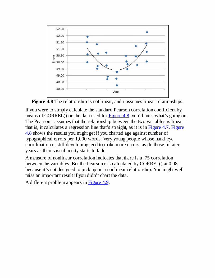
Figure4.8Therelationshipisnotlinear,andrassumeslinearrelationships.

IfyouweretosimplycalculatethestandardPearsoncorrelationcoefficientbymeansofCORREL()onthedatausedforFigure4.8,you’dmisswhat’sgoingon.ThePearsonrassumesthattherelationshipbetweenthetwovariablesislinear—thatis,itcalculatesaregressionlinethat’sstraight,asitisinFigure4.7.Figure4.8showstheresultsyoumightgetifyouchartedageagainstnumberoftypographicalerrorsper1,000words.Veryyoungpeoplewhosehand-eyecoordinationisstilldevelopingtendtomakemoreerrors,asdothoseinlateryearsastheirvisualacuitystartstofade.Ameasureofnonlinearcorrelationindicatesthatthereisa.75correlationbetweenthevariables.ButthePearsonriscalculatedbyCORREL()at0.08becauseit’snotdesignedtopickuponanonlinearrelationship.Youmightwellmissanimportantresultifyoudidn’tchartthedata.AdifferentproblemappearsinFigure4.9.

Figure4.9Justoneoutliercanoverstatetherelationshipbetweenthevariables.

InFigure4.9,twovariablesthatareonlyweaklyrelatedareshownincellsA1:B20(yes,B20,notB21).ThecorrelationbetweenthemisshownincellG3:Itisonly.24.Somehow,becauseofatypoorincorrectreadingsonmetersoradatabasequerythatwasstructuredineptly,twoadditionalvaluesappearincellsA21:B21.WhenthosetwovaluesareincludedintheargumentstotheCORREL()function,thecorrelationchangesfromaweak0.24toquiteastrong0.91.Thishappensbecauseofthewaythecovariance,andthereforethecorrelation,isdefined.Let’sreviewacovarianceformulagivenearlier,usedwithasetofobservationsthatconstituteasample:

Theexpressioninthenumeratormultipliesanobservation’sdeviationfromthemeanofXtimestheobservation’sdeviationfromthemeanofY.Theadditionofthatonerecord,whereboththeXandtheYvaluesdeviatebythousandsofunitsfromthemeansofthetwovariables,inflatesthecovariance,andthereforethecorrelation,farabovetheirvaluesbasedonthefirst20records.

YoumightnothaverealizedwhatwasgoingonwithouttheaccompanyingXYchart.Thereyoucanseetheoneobservationthatturnswhatisbasicallynorelationshipintoastrongone.Ofcourse,it’spossiblethattheoneoutlierisentirelylegitimate.Butinthatcase,itmightbethatthestandardcorrelationcoefficientisnotanappropriateexpressionoftherelationshipbetweenthetwovariables(anymorethanthemeanisanappropriateexpressionofcentraltendencyinadistributionthat’shighlyskewed).MakeitahabittocreateXYchartsofvariablesthatyouinvestigateviacorrelationanalysis.Thestandardr,thePearsoncorrelationcoefficient,isthebasisformanysophisticatedstatisticalanalyses,butitwasnotdesignedtoassessthestrengthofrelationshipsthatareeithernonlinearorcontainextremeoutliers.Fortunately,Excelmakesitveryeasytocreatethecharts.Forexample,tocreatetheXYchartshowninFigure4.9,takethesesteps:

1.WithrawdataasshownincellsA1:B21,selectanycellinthatrange.2.ClicktheRibbon’sInserttab.3.ClicktheInsertScatter(X,Y)orBubbleChartbuttonintheChartsgroup.4.ClicktheScattertypeinthedrop-down.

UsingtheAnalysisToolsSincethe1990s,Excelhasincludedanadd-inthatprovidesavarietyoftoolsthatperformstatisticalanalysis.InseveralExcelversions,Microsoft’sdocumentationhasreferredtoitastheAnalysisToolPak.ThisbooktermsittheDataAnalysisadd-inbecausethat’sthelabelyouseeintheRibbonaftertheadd-inhasbeeninstalledinExcel2010and2013.ManyofthetoolsintheDataAnalysisadd-inarequiteuseful.OneofthemistheCorrelationtool.Thereisn’tactuallyalotofsenseindeployingitifyouhaveonlytwoorthreevariablestoanalyze.Then,it’sfastertoentertheformulaswiththeCORREL()functionontheworksheetyourselfthanitistojumpthroughthefewhoopsthatDataAnalysisputsintheway.Withmorethantwoorthreevariables,considerusingtheCorrelationtool.Youcanusethisformulatoquicklycalculatethenumberofuniquecorrelationcoefficientsinasetofkvariables:

k*(k–1)/2Ifyouhavethreevariables,then,youwouldhavetocalculatethreecorrelations(3*2/2).That’seasyenough,butwithfourvariablestherearesixpossiblecorrelations(4*3/2),andwithfivevariablesthereareten(5*4/2).Then,

usingtheCORREL()functionforeachcorrelationgetstobetimeconsuminganderrorprone,andthat’swheretheDataAnalysisadd-in’sCorrelationtoolbecomesmorevaluable.YougetattheDataAnalysisadd-inmuchasyougetatSolver;seeChapter2foranintroductiontoaccessingandusingtheSolveradd-in.WithExcel2007orlater,clicktheRibbon’sDatatabandlookforDataAnalysisintheAnalysisgroup.(InExcel2003orearlier,lookforDataAnalysisintheToolsmenu.)IfyoufindDataAnalysisyou’rereadytogo,andyoucanskipforwardtothenextsection,“UsingtheCorrelationTool.”Ifyoudon’tseeDataAnalysis,you’llneedtomakeitavailabletoExcel,andyoumightevenhavetoinstallitfromtheinstallationdiscorthedownloadedinstallationutility.

NoteTheDataAnalysisadd-inhasmuchmorethanjustaCorrelationtool.Itincludesatoolthatreturnsdescriptivestatisticsforasinglevariable,toolsforseveralinferentialteststhatarediscussedindetailinthisbook,movingaverages,andseveralothertools.IfyouintendtouseExceltocarryoutbeginning-to-intermediatestatisticalanalysis,IsuggestthatyouinstallandbecomefamiliarwiththeDataAnalysisadd-in.Youwon’tfindthescopeofanalysesavailableinSPSSorSAS,butyouwillfindsometoolsthatwillprovehelpfulfromtimetotime.

TheDataAnalysisadd-inmighthavebeeninstalledonyourworkingdiskbutnotyetmadeavailabletoExcel.Ifyoudon’tseeDataAnalysisintheAnalysisgroupoftheDatatab,takethesesteps:

1.InOffice2010or2013,clicktheFiletabandclickOptionsinitsnavigationbar.InOffice2007,clicktheOfficebuttonandclicktheExcelOptionsbuttonatthebottomofthemenu.

2.TheExcelOptionswindowopens.ClickAdd-Insinitsnavigationbar.3.Ifnecessary,selectExcelAdd-InsintheManagedrop-down,andthenclickGo.

4.TheAdd-Insdialogboxappears.IfyouseeAnalysisToolPaklisted,besureitscheckboxisfilled.(AnalysisToolPakisanoldtermforthisadd-in.)ClickOK.

YoushouldnowfindDataAnalysisintheAnalysisgroupontheDatatab.Skip

aheadtothesectiontitled“UsingtheCorrelationTool.”ThingsarealittlequickerinversionsofExcelpriorto2007.ChooseAdd-InsfromtheToolsmenu.LookforAnalysisToolPakintheAdd-Insdialogbox,andfillitscheckboxifyouseeit.ClickOK.YoushouldnowfindDataAnalysisintheToolsmenu.IfyoudonotfindAnalysisToolPakintheAdd-Insdialogbox,regardlessoftheversionofExcelyou’reusing,you’llneedtomodifytheinstallation.Youcandothisifyouhaveaccesstotheinstallationdiscordownloadedinstallationfile.It’susuallybesttostartfromtheControlPanel.ChooseAddorRemoveSoftware,orProgramsandFeatures,orPrograms,dependingontheversionofWindowsthatyou’rerunning.ChoosetochangetheinstallationofOffice.WhenyougettotheExcelportionoftheinstallation,clickExcel’sexpandbox(theonewithaplussigninsideabox).You’llseeanotherexpandboxbesideAdd-Ins.ClickittodisplayAnalysisToolPak.Useitsdrop-downtoselectRunFromMyComputer,andthenContinueandOKyourwaybacktoExcel.Nowcontinuewithstep1intheprecedinglist.

UsingtheCorrelationToolTousetheCorrelationtoolinDataAnalysis,beginwithdatalaidoutasshowninFigure4.10.

Figure4.10TheCorrelationtoolcandealwithlabels,sobesuretousetheminthefirstrowofyourlist.

ThenclickDataAnalysisintheDatatab’sAnalysisgroup,andchooseCorrelation

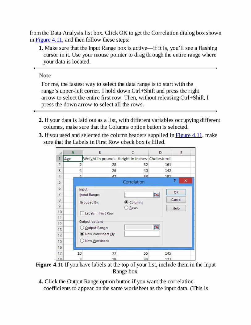
fromtheDataAnalysislistbox.ClickOKtogettheCorrelationdialogboxshowninFigure4.11,andthenfollowthesesteps:

1.MakesurethattheInputRangeboxisactive—ifitis,you’llseeaflashingcursorinit.Useyourmousepointertodragthroughtheentirerangewhereyourdataislocated.

NoteForme,thefastestwaytoselectthedatarangeistostartwiththerange’supper-leftcorner.IholddownCtrl+Shiftandpresstherightarrowtoselecttheentirefirstrow.Then,withoutreleasingCtrl+Shift,Ipressthedownarrowtoselectalltherows.

2.Ifyourdataislaidoutasalist,withdifferentvariablesoccupyingdifferentcolumns,makesurethattheColumnsoptionbuttonisselected.

3.IfyouusedandselectedthecolumnheaderssuppliedinFigure4.11,makesurethattheLabelsinFirstRowcheckboxisfilled.

Figure4.11Ifyouhavelabelsatthetopofyourlist,includethemintheInputRangebox.

4.ClicktheOutputRangeoptionbuttonifyouwantthecorrelationcoefficientstoappearonthesameworksheetastheinputdata.(Thisis

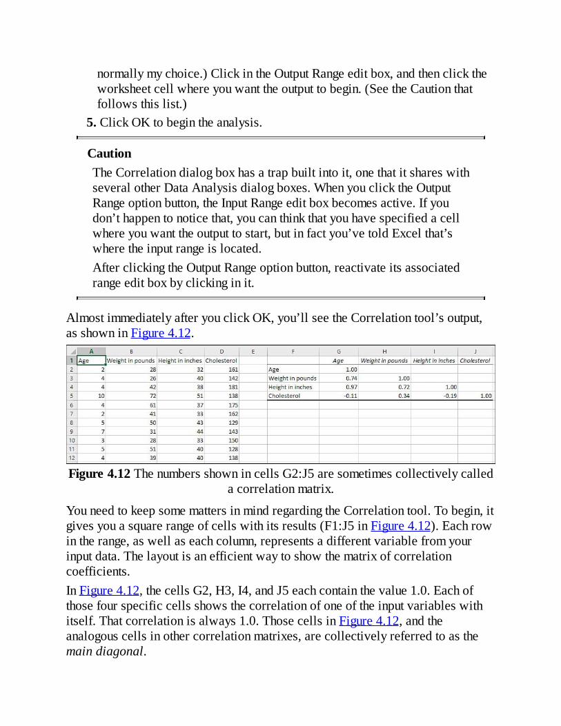
normallymychoice.)ClickintheOutputRangeeditbox,andthenclicktheworksheetcellwhereyouwanttheoutputtobegin.(SeetheCautionthatfollowsthislist.)

5.ClickOKtobegintheanalysis.

CautionTheCorrelationdialogboxhasatrapbuiltintoit,onethatitshareswithseveralotherDataAnalysisdialogboxes.WhenyouclicktheOutputRangeoptionbutton,theInputRangeeditboxbecomesactive.Ifyoudon’thappentonoticethat,youcanthinkthatyouhavespecifiedacellwhereyouwanttheoutputtostart,butinfactyou’vetoldExcelthat’swheretheinputrangeislocated.AfterclickingtheOutputRangeoptionbutton,reactivateitsassociatedrangeeditboxbyclickinginit.

AlmostimmediatelyafteryouclickOK,you’llseetheCorrelationtool’soutput,asshowninFigure4.12.

Figure4.12ThenumbersshownincellsG2:J5aresometimescollectivelycalledacorrelationmatrix.

YouneedtokeepsomemattersinmindregardingtheCorrelationtool.Tobegin,itgivesyouasquarerangeofcellswithitsresults(F1:J5inFigure4.12).Eachrowintherange,aswellaseachcolumn,representsadifferentvariablefromyourinputdata.Thelayoutisanefficientwaytoshowthematrixofcorrelationcoefficients.InFigure4.12,thecellsG2,H3,I4,andJ5eachcontainthevalue1.0.Eachofthosefourspecificcellsshowsthecorrelationofoneoftheinputvariableswithitself.Thatcorrelationisalways1.0.ThosecellsinFigure4.12,andtheanalogouscellsinothercorrelationmatrixes,arecollectivelyreferredtoasthemaindiagonal.

Youdon’tnormallyseecorrelationcoefficientsabovethemaindiagonalbecausetheywouldberedundantwiththosebelowit.YoucanseeincellH4thatforthissample,thecorrelationbetweenheightandweightis0.72.ExcelcouldshowthesamecorrelationincellI3,butdoingsowouldn’taddanynewinformation:Thecorrelationbetweenheightandweightisthesameasthecorrelationbetweenweightandheight.Thesuppressionofthecorrelationcoefficientsabovethemaindiagonalisprincipallytoavoidvisualclutter.Moreadvancedstatisticalanalysessuchasprincipalcomponentsanalysisoftenrequirethefullypopulatedsquarematrix.TheCorrelationtool,likesomeotherDataAnalysistools,reportsstaticvalues.Forexample,inFigure4.12,thenumbersinthecorrelationmatrixarenotformulassuchas

=CORREL(A2:A31,B2:B31)butratherthestaticresultsoftheformulas.Inconsequence,ifanynumbersintheinputrangechange,orifyouaddorremoverecordsfromtheinputrange,thecorrelationmatrixdoesnotautomaticallyupdatetoreflectthechange.YoumustruntheCorrelationtoolagainifyouwantachangeintheinputdatatoresultinachangeintheoutput.TheDataAnalysisadd-inhasproblems—problemsthatdateallthewaybacktoitsintroductioninExcel95.One,theOutputRangeissue,isdescribedinaCautionearlierinthissection.ThetoolnamedANOVA:TwoFactorWithoutReplicationemploysanapproachtorepeatedmeasuresthatinvolvessomerestrictiveassumptions.TheANOVA:TwoFactorWithReplicationforcesyoutosupplyequalcellsizes.Althoughthisdoesnotexhaustthelistofdrawbacks,theDataAnalysisadd-inisneverthelessausefuladjunct.

CorrelationIsn’tCausationItcanbesurprisinglyeasytoseethatchangesinonevariableareassociatedwithchangesinanothervariable,andconcludethatonevariable’sbehaviorcauseschangesintheother’s.Forexample,itmightverywellbetruethattheregularitywithwhichchildreneatbreakfasthasadirecteffectontheirperformanceinschool.Certainly,TVcommercialsassertthateatingbreakfastcerealsenhancesconcentration.Butthere’sanimportantdifferencebetweenbelievingthatonevariableisrelatedtoanotherandbelievingthatchangestoonevariablecausechangestoanother.Someobservationalresearch,relyingoncorrelationsbetweennutritionandachievement,concludesthateatingbreakfastregularlyimprovesacademic

achievement.Other,morecarefulstudiesshowthatthequestionismorecomplicated—thatvariablessuchasabsenteeismcomeintoplay,andthatcoaxinginformationoutofamassofcorrelationcoefficientsisn’tasinformativeorcredibleasamanufacturerofsugar-coatedcerealflakesmightwish.Besidestheissueofthecomplexityoftherelationships,therearetwogeneralreasons,discussednext,thatyoushouldbeverycarefulofassumingthatacorrelationalrelationshipisalsocausal.

AThirdVariableItsometimeshappensthatyoufindastrongcorrelationbetweentwovariablesthatsuggestsacausalrelationship.TheclassicexampleisthenumberofbooksinschooldistrictlibrariesandscoresonthestandardizedSATexams.Supposeyoufoundastrongcorrelation—say,0.7—betweenthenumberofbooksperstudentindistricts’librariesandtheaverageperformancebythosedistricts’studentsontheSATs.Afirst-glanceinterpretationmightbethattheavailabilityofalargernumberofbooksresultsinmoreknowledge,thusbetteroutcomesonstandardizedtests.Amorecarefulexaminationmightrevealthatcommunitieswheretheannualhouseholdincomeishigherhavemoreinthewayofpropertytaxestospendonschoolsandtheirlibraries.Suchcommunitiesalsotendtospendmoreonotherimportantaspectsofchildren’sdevelopment,suchasnutritionandstablehomeenvironments.Inotherwords,childrenraisedinwealthierdistrictsaremorelikelytoscorewellonstandardizedtests.Incontrast,itisdifficulttoarguethatsimplyaddingmorebookstoaschoollibrarywillresultinhigherSATscores.Thethirdvariablehere,inadditiontonumberoflibrarybooksandSATscores,isthewealthofthecommunity.Anotherexampleconcernstheapparentrelationshipbetweenchildhoodvaccinationsandtheincidenceofautism.Ithasbeenarguedthatoverthepastseveraldecades,vaccinationhasbecomemoreandmoreprevalent,ashasautism.Somehaveconcludedthatchildhoodvaccines,orthepreservativesusedintheirmanufacture,causeautism.Butcloseexaminationofstudiesthatapparentlysupportedthatcontentiondisclosedproblemswiththestudies’methods,inparticularthemethodsusedtoestablishanincreasedprevalenceofautism.Furtherstudyhassuggestedthatathirdvariable,morefrequentandsophisticatedtestsforautism,hasbeenatwork,bringingaboutanincreaseinthediagnosesofautismratherthananincreaseintheprevalenceoftheconditionitself.Untanglingcorrelationandcausationisaproblem.Inthe1950sand1960s,thelinkbetweencigarettesmokingandlungcancerwasdebatedonthefrontpagesofnewspapers.Somesaidthatthelinkwasmerelycorrelation,andnotcausation.

Theonlywaytoconvincinglydemonstratecausationwouldbebymeansofatrueexperiment:Randomlyassignpeopletosmokingandnonsmokinggroupsandforcethoseintheformergrouptosmokecigarettes.Then,afteryearsofenforcedsmokingorabstinence,comparetheincidenceoflungcancerinthetwogroups.Thatsolutionisobviouslybothapracticalandethicalimpossibility.Butitisgenerallyconcededtodaythatsmokingcigarettescauseslungcancer,evenintheabsenceofatrueexperiment.Correlationdoesnotbyitselfmeancausation,butwhenit’sbuttressedbythefindingsofrepeatedobservationalstudies,andwhentheeffectofathirdvariablecanberuledout(bothliquorconsumptionandsleeplosswerepositedandthendiscardedaspossiblethirdvariablescausinglungcanceramongsmokers),it’sreasonabletoconcludethatcausationispresent.

TheDirectionoftheEffectAnotherpossibilitytokeepinmindwhenyouconsiderwhetheracorrelationrepresentscausationisthatyoumightbelookingatthewrongvariableasthecause.Ifyoufindthattheincidenceofgunownershipcorrelatesstronglywiththeincidenceofviolentcrime,youmightcometotheconclusionthatthere’sacausalrelationship.Andtheremightbecauseinvolved.However,withoutmorerigorousresearch,whetheryouconcludethat“Moregunsresultinmoreviolentcrime”or“Peoplerespondtomoreviolentcrimebybuyingmoreguns”islikelytodependmoreonyourownpoliticalandculturalsensibilitiesthanonempiricalevidence.

UsingCorrelationTothispoint,wehavetalkedmostlyabouttheconceptofacorrelationcoefficient—howitisdefinedandhowitcanilluminatethenatureoftherelationshipbetweentwovariables.That’susefulinformationbyitself,butthingsgomuchfurtherthanthat.Forexample,it’sprobablyoccurredtoyouthatifyouknowthevalueofonevariable,youcanpredictthevalueofanothervariablethat’scorrelatedwiththefirst.Thatsortofpredictionisthefocusoftheremainderofthischapter.Thebasicsdiscussedhereturnouttobethefoundationofseveralanalysesdiscussedinlaterchapters.Usedinthisway,thetechniquegoesbythenameregression,whichisthebasisforthedesignationofthecorrelationcoefficient,r.

NoteWhythewordregression?Inthenineteenthcentury,ascientistandmathematiciannamedFrancisGaltonstudiedheredityandnoticedthatnumericrelationshipsexistbetweenparentsandchildrenasmeasured

bycertainstandardvariables.Forexample,Galtoncomparedtheheightsoffatherstotheheightsoftheirsons,andhecametoaninterestingfinding:Sons’heightstendedtobeclosertotheirownmeanthandidtheheightsoftheirfathers.Putanotherway,fatherswhostood,say,twostandarddeviationsabovethemeanheightoftheirgenerationtendedtohavesonswhosemeanheightwasjustonestandarddeviationabovetheirowngeneration’smeanheight.Similarly,fatherswhowereshorterthanaveragetendedtohavesonswhowerealsoshorterthanaverage,butwhowereclosertotheaveragethantheirfatherswere.Thesons’heightregressedtowardthemean.

SubsequentworkbyKarlPearson,mentionedearlierinthischapter,developedtheconceptsandmethodsassociatedwiththecorrelationcoefficient.Figure4.13showssomeheights,ininches,offathersandsons,andanXYchartshowingvisuallyhowthetwovariablesareassociated.

Figure4.13Theregressionlineshowswherethedatapointswouldfallifthecorrelationwereaperfect1.0.

Giventhattwovariables—here,fathers’heightandsons’height—arecorrelated,itshouldbepossibletopredictavalueononevariablefromavalueontheothervariable.Anditispossible,butthehitchisthatthepredictionwillbeperfectlyaccurateonlywhentherelationshipisofverylimitedinterest,suchastherelationshipbetweenweightinouncesandweightingrams.Thepredictioncanbeperfectonlywhenthecorrelationisperfect,andthathappensonlyinhighlyartificialortrivialsituations.

ThenextsectiondiscusseshowtomakethatsortofpredictionwithoutrelyingonExcel.ThenI’llshowhowExceldoesitquicklyandeasily.

RemovingtheEffectsoftheScaleChapter3discussedthestandarddeviationandz-scores,andshowedhowyoucanexpressavalueintermsofstandarddeviationunits.Forexample,ifyouhaveasampleoftenpeoplewhosemeanheightis68incheswithastandarddeviationof4inches,thenyoucanexpressaheightof72inchesasonestandarddeviationabovethemean—or,equivalently,asaz-scoreof+1.0.Sodoingremovestheattributesoftheoriginalscaleofmeasurementandmakescomparisonsbetweendifferentvariablesmuchclearer.Thez-scoreiscalculated,andthusstandardized,bysubtractingthemeanfromagivenvalueanddividingtheresultbythestandarddeviation.Thecorrelationcoefficientusesananalogouscalculation.Toreview,thedefinitionalformulaofthecorrelationcoefficientis

or,inwords,thecorrelationisthecovariancedividedbytheproductofthestandarddeviationsofthetwovariables.Itisthereforestandardizedtorangefrom0toplusorminus1.0,uninfluencedbytheunitofmeasureusedintheunderlyingvariables.Thecovariance,likethevariance,canbedifficulttovisualize.Supposethatyouhavetheweightsinpoundsofthesametenpeople,alongwiththeirheights.Youmightcalculatethemeanoftheirweightsat150poundsandthestandarddeviationoftheirweightsat25pounds.It’seasytoseeadistanceof25poundsonthehorizontalaxisofachart.It’smoredifficulttovisualizethevarianceofyoursample,whichis625squaredpounds—oreventocomprehenditsmeaning.Similarly,itcanbedifficulttocomprehendthemeaningofthecovariance(unlessyou’reusedtoworkingwiththemeasuresinvolved,whichisoftenthecaseforphysicistsandengineers—they’reusuallyfamiliarwiththecovarianceofmeasurestheyworkwith,andsometimestermthecorrelationcoefficientthedimensionlesscovariance).Inyoursampleoftenpeople,forexample,youmighthaveheightmeasuresaswellasweightmeasures.Ifyoucalculatethecovarianceofheightandweightinyoursample,youmightwindupwithsomevaluesuchas58.5foot-pounds.Butthisisnotoneoftheclassicalmeaningsoffoot-pound,ameasureofforceorenergy.Itisameasureofhowpoundsandfeetcombineinyoursample.Andit’snotalwaysclearhowyouvisualizeorotherwiseinterpretthatmeasurement.

Thecorrelationcoefficientresolvesthatdifficultyinawaythat’ssimilartothez-score.Youdividethecovariancebythestandarddeviationofeachvariable,thusremovingtheeffectofthetwoscales—here,heightandweight—andyou’releftwithanexpressionofthestrengthoftherelationshipthatisn’taffectedbyyourchoiceofmeasure,whetherfeetorinchesorcentimeters,orpoundsorouncesorkilograms.Aperfect,one-to-onerelationshipisplusorminus1.0.Theabsenceofarelationshipis0.0.Thecorrelationsofmostvariablesfallsomewherebetweentheextremes.Inthez-scoreyouhaveawaytomeasurehowfarfromthemeanapersonorobjectisfound,withoutreferencetotheunitofmeasurement.PerhapsJohn’sheightis70.8inches,oraz-scoreonheightof0.70.Perhapsthecorrelationbetweenheightandweightinyoursample—again,uncontaminatedbythescalesofmeasurement—is0.65.YoucannowpredictJohn’sweightwiththisequation:

Putintowords,John’spredicteddistancefromthemeanonweightistheproductofthecorrelationcoefficientandhisdistancefromthemeanonheight.John’spredictedz-scoreonweightequalsthecorrelationrtimeshisz-scoreonheight,or.65*.70,or.455.SeeFigure4.14forthespecifics.

Figure4.14Theregressionlineisthebasisforpredictingoneofthevariablesfromtheother.

NoteJohn’spredictedz-scoreonweight(.455)issmallerthanhisz-scoreonheight(.70).Hisweightispredictedtoregresstowardthemeanonweight,justasason’spredictedheightisclosertothemeanthanhisfather’sheight.Thisregressionalwaystakesplacewhenthecorrelationisnotperfect:thatis,whenitislessthan±1.0.That’sinherentintheequationgivenaboveforweightandheight,repeatedhereinamoregeneralform:zy=rxyzx.Considerthatequationandkeepinmindthatrisalwaysbetween–1.0and+1.0.

Themeanweightinyoursampleis150pounds,andthestandarddeviationis25.YouhaveJohn’spredictedz-scoreforweight,0.455,fromthepriorformula.Youcanchangethatintopoundsbyrearrangingtheformulaforaz-score:

z=(X––X)/sX=sz+–X

InJohn’scase,youhavethefollowing:161.375=25*0.455+150

Toverifythisresult,seecellB22inFigure4.14.So,thecorrelationof.65leadsyoutopredictthatJohnweighs161.375pounds.ButthenJohntellsyouthatheactuallyweighs155pounds.Whenyouuseareasonablystrongcorrelationtomakepredictions,youdon’texpectyourpredictionstobeexactlycorrectwithanyrealfrequency,anymorethanyouexpectthepredictionforatenthofaninchofraintomorrowtobeexactlycorrect.Inbothsituations,though,youexpectthepredictiontobereasonablyclosemostofthetime.

UsingtheExcelFunctionThepriorsectiondescribedhowtouseacorrelationbetweentwovariables,plusaz-scoreoneachvariable,topredictaperson’sweightinpoundsfromhisheightininches.Thisinvolvedmultiplyingonez-scorebyacorrelationtogetanotherz-score,andthenconvertingthelatterz-scoretoaweightinpoundsbyrearrangingtheformulaforaz-score.Behindthescenes,itwasalsonecessarytocalculatethemeanandstandarddeviationofbothvariablesaswellasthecorrelationbetweenthetwo.Iinflictedallthisonyoubecauseithelpsilluminatetherelationshipbetweenrawscoresandcovariances,betweenz-scoresandcorrelations.Asyouwouldexpect,

Excelrelievesyouofthetediumofdoingallthatformulaichandwaving.Figure4.15showstherawdataandsomepreliminarycalculationsthattheprecedingdiscussionwasbasedon.

Figure4.15TheTREND()functiontakescareofallthecalculationsforyou.

TopredictJohn’sweightusingthedataasshowninFigures4.14and4.15,enterthisformulainsomeemptycell(it’sC18inFigure4.15):

=TREND(C2:C11,B2:B11,B18)Withthisdataset,theformulareturnsthevalue161.375.TogetthesamevalueusingthescenicrouteusedinFigure4.14,youcouldalsoentertheformula

=((B18-B13)/B14)*C16*C14+C13whichcarriesoutthemaththatwassketchedinthepriorsection:CalculateJohn’sz-scoreforheight,multiplyitbythecorrelation,multiplythatbythestandarddeviationforweight,andaddthemeanweight.Fortunately,theTREND()functionrelievesyouofallthoseopportunitiestomakeamistake.TheTREND()function’ssyntaxisasfollows:

=TREND(known_y’s,known_x’s,new_x’s,const)

NoteThefourthargument,const,isoptional.Asectionnamed“ForcingaZeroConstant”inChapter15,“MultipleRegressionAnalysisandEffectCoding:FurtherIssues,”discussesthereasonyoushouldomittheconstargument,whichisthesameassettingittoFALSE.It’sbesttodelay

thatdiscussionuntilmoregroundworkhasbeenlaid.

ThefirstthreeargumentstoTREND()arediscussednext.

known_y’sThesearevaluesthatyoualreadyhaveinhandforthevariableyouwanttopredict.Intheexamplefromthepriorsection,thatvariableisweight:theideawastopredictJohn’sweightonthebasisofthecorrelationbetweenheightandweight,combinedwithknowledgeofJohn’sheight.It’sconventionalinstatisticalwritingtodesignatethepredictedvariableasY,anditsindividualvaluesasy’s.

known_x’sThesearevaluesofthevariableyouwanttopredictfrom.Eachmustbepairedupwithoneoftheknown_y’s.You’llfindthattheeasiestwaytodothisistoaligntwoadjacentrangesasinFigure4.15,wheretheknown_x’sareinB2:B11andtheknown_y’sareinC2:C11.

new_x’sThisvalue(orvalues)belongstothepredictorvariable,butyoudonothave,orarenotsupplying,associatedvaluesforthepredictedvariable.Therearevariousreasonsthatyoumightusenew_x’sasanargumenttoTREND(),butthetypicalreasonisthatyouwanttopredicty’sforthenew_x’sbasedontherelationshipbetweentheknown_y’sandtheknown_x’s.Forexample,theknown_x’smightbeyears:1980,1981,1982,andsoon.Theknown_y’smightbecompanyrevenueforeachofthoseyears.Andyournew_xmightbenextyear’snumber,suchas2015,forwhichyou’dliketopredictrevenue.(NotthatIrecommendpredictingrevenuefromayear’sdesignation.)

GettingthePredictedValuesIfyouhaveonlyonenew_xvaluetopredictfrom,youcanentertheformulawiththeTREND()functionnormally,justbytypingitandpressingEnter.ThisisthesituationinFigure4.15,whereyouwouldenterthefollowingformula

=TREND(C2:C11,B2:B11,B18)inablankcellsuchasC18togetthepredictedweightgiventheheightinB18.Butsupposeyouwanttoknowwhatthepredictedweightofallthesubjectsinyoursamplewouldbe,giventhecorrelationbetweenthetwovariables.TREND()doesthisforyou,too:Yousimplyneedtoarray-entertheformula.Youstartbyselectingarangeofcellswiththesamedimensionsasisoccupiedby

yourknown_x’s.InFigure4.15,that’sB2:B11,soyoumightselectD2:D11.Thentypethefollowingformula

=TREND(C2:C11,B2:B11)andarray-enteritwithCtrl+Shift+EnterinsteadofsimplyEnter.

NoteArrayformulasarediscussedinmoredetailinChapter2,inthesectiontitled“UsinganArrayFormulatoCounttheValues.”

TheresultappearsinFigure4.16.

Figure4.16Thecurlybracketsaroundtheformulaintheformulaboxindicatethatit’sanarrayformula.

YoucangetsomemoreinsightintothemeaningofthetrendlineinthechartifyouusethepredictedvaluesinD2:D11ofFigure4.16.IfyoucreateanXYchartusingthevaluesinB2:B11andD2:D11,you’llfindthatyouhaveachartthatduplicatesthetrendlineinFigure4.16’schart.Soalineartrendlineinachartrepresentstheunrealisticsituationinwhichalltheobservationsobedientlyfollowaformulathatrelatestwovariables.ButEdeatstoomuchandDougisn’teatingenough.They,alongwiththerestofthesubjects,straytosomedegreefromtheperfecttrendline.Ifit’sunrealistic,what’sthepointofincludingatrendlineinachart?It’slargelyamatterofhelpingyouvisualizehowfarindividualobservationsfallfromthe

mathematicalformula.Thelargerthedeviations,thelowerthecorrelation.Themorethattheindividualpointshugthetrendline,thegreaterthecorrelation.Yes,youcangetthatinformationfromthemagnitudeoftheresultreturnedbyCORREL().Butthere’snothinglikeseeingitcharted.

NoteBecausesomanyoptionsareavailableforcharttrendlines,IhavewaitedtoevenmentionhowyougetoneinExcel2013.ForatrendlinesuchastheoneshowninFigures4.14through4.16,clickthecharttoselectitandthenclicktheChartElementsbutton(thestylizedplussignthatappearsnexttothechart).FilltheTrendlinecheckboxtogetalineartrendline.YoucanobtainothertypesoftrendlinebyclickingthearrowthatappearswhenyoumoveyourmousepointeroverTrendline.

GettingtheRegressionFormulaAnearliersectioninthischapter,“RemovingtheEffectsoftheScale,”discussedhowyoucanusez-scores,meansandstandarddeviations,andthecorrelationcoefficienttopredictonevariablefromanother.Thesubsequentsection,“UsingtheExcelFunction,”describedhowtousetheTREND()functiontogodirectlyfromtheobservedvaluestothepredictedvalues.Neitherdiscussiondealtwiththeformulathatyoucanuseontherawdata.Intheexamplesthatthischapterhasused—predictingonevariableonthebasisofitsrelationshipwithanothervariable—itispossibletousetwoExcelfunctions,SLOPE()andINTERCEPT(),togeneratetheformulathatreturnsthepredictedvaluesthatyougetwithTREND().Thereisarelatedfunction,LINEST(),thatismorepowerfulthaneitherSLOPE()orINTERCEPT().Itcanhandlemanymorevariablesandreturnmuchmoreinformation,andsubsequentchaptersofthisbook,particularlyChapter14,“MultipleRegressionAnalysisandEffectCoding:TheBasics,”andChapter16,“AnalysisofCovariance:TheBasics,”discussitindepth.However,thischapterdiscussesSLOPE()andINTERCEPT()brieflysothatyou’llknowwhattheirpurposeisandbecausetheyserveasanintroductionofsortstoLINEST().Aformulathatbestdescribestherelationshipbetweentwovariables,suchasheightandweightinFigures4.14through4.16,requirestwonumbers:aslopeandanintercept.Theslopereferstotheregressionline’ssteepness(orlackthereof).Backingeometryclassyourteachermighthavereferredtothisasthe“riseover

therun.”Theslopeindicatesthenumberofunitsthatthelinemovesupforeveryunitthatthelinemovesright.Theslopecanbepositiveornegative:Ifit’spositive,theregressionlineslopesfromlowerlefttoupperright,asinFigure4.16;ifit’snegative,theslopeisfromupperlefttolowerright.YoucalculatethevalueoftheslopedirectlyinExcelwiththeSLOPE()function.Forexample,usingthedatainFigures4.14through4.16,thevaluereturnedbytheformula

=SLOPE(C2:C11,B2:B11)is4.06.Thatis,foreveryunitincrease(eachinch)inheightinthissample,youexpectslightlyover4poundsincreaseinweight.Buttheslopeisn’tallyouneed:Youalsoneedwhat’scalledtheintercept.That’sthevalueofthepredictedvariable—here,weight—atthepointthattheregressionlinecrossesitsaxis.InFigure4.17,theregressionlinehasbeenextendedtotheleft,tothezeropointonthehorizontalaxiswhereitcrossestheverticalaxis.Thepointwheretheregressionlinecrossestheverticalaxisisthevalueoftheintercept.

Figure4.17Therangesofvaluesontheaxeshavebeenincreasedsoastoshowtheintercept.

Thevaluesoftheregressionline’sslopeandinterceptareshowninB18andB19ofFigure4.17.NoticethattheinterceptvalueshownincellB19matchesthepointinthechartwheretheregressionlinecrossestheverticalaxis.ThepredictedvaluesforweightareshownincellsD2:D11ofFigure4.17.They

arecalculatedusingthevaluesfortheslopeandinterceptinB18andB19,andareidenticaltothepredictedvaluesinFigure4.16thatwerecalculatedusingTREND().Noticethesethreepointsabouttheformula,shownintheformulabox:

Youmultiplyaknown_xvaluebythevalueoftheslope,andaddthevalueoftheintercept.Nocurlybracketsappeararoundtheformula.Therefore,incontrasttotheinstanceoftheTREND()functioninFigure4.16,youcanentertheformulanormally.Youentertheformulainonecell—inthefigure,youmightaswellstartincellD2—andeithercopyandpasteordraganddropintotheremainingcellsintherange(here,that’sD3:D11).Sodoingadjuststhereferencetotheknown_xvalue.Butbecauseyoudon’twanttoadjustthereferencestothecellwiththeslopeandthecellwiththeintercept,dollarsignsareusedtomakethosereferencesabsolutepriortothecopy-and-pasteoperation.

NoteYetanotherwayistobeginbyselectingtheentireD2:D11range,typingtheformula(includingthedollarsignsthatmaketwoofthecellreferencesabsolute),andfinishingwithCtrl+Enter.Thissequenceenterstheformulainarangeofselectedcells,withthereferencesadjustingaccordingly.Itisnotanarrayformula:youhavenotfinishedwithCtrl+Shift+Enter.

It’salsoworthnotingthatanearliersectioninthischapter,“RemovingtheEffectsoftheScale,”showshowtoworkwithz-scoresandthecorrelationcoefficienttopredictthez-scoreononevariablefromthez-scoreontheother.Inthatcontext,bothvariableshavebeenconvertedtoz-scoresandconsequentlyhaveastandarddeviationof1.0andameanof0.0.Therefore,theformula

PredictedValue=Slope*PredictorValue+Interceptreducestothisformula:

Predictedz-score=CorrelationCoefficient*Predictorz-scoreWhenbothvariablesareexpressedasz-scores,thecorrelationcoefficientistheslope.Also,z-scoreshaveameanofzero,sotheinterceptdropsoutoftheequation:Itsvalueisalwayszerowhenyou’reworkingwithz-scores.

UsingTREND()forMultipleRegression

Itoftenhappensthatyouhaveonevariablewhosevaluesyouwouldliketopredict,andtwo(ormore)variablesthatyouwouldliketouseaspredictors.Althoughit’snotapparentfromthediscussionsofarinthischapter,it’spossibletousebothvariablesaspredictorssimultaneously.Usingtwoormoresimultaneouspredictorscansometimesimprovetheaccuracyoftheprediction,comparedtoeitherpredictorbyitself.

CombiningthePredictorsInthesortofsituationjustdescribed,SLOPE()andINTERCEPT()won’thelpyou,becausetheyweren’tdesignedtohandlemultiplepredictors.ExcelinsteadprovidesyouwiththefunctionsTREND()andLINEST(),whichcanhandleboththesinglepredictorandthemultiplepredictorsituations.That’sthereasonyouwon’tseeSLOPE()andINTERCEPT()discussedfurtherinthisbook.Theyserveasausefulintroductiontotheconceptsinvolvedinregression,buttheyareunderpoweredandtheircapabilitiesareavailableinTREND()andLINEST()whenyouhaveonlyonepredictorvariable.

NoteIt’seasytoconcludethatTREND()andLINEST()areanalogoustoSLOPE()andINTERCEPT(),buttheyarenot.TheresultsofSLOPE()andINTERCEPT()combinetoformanequationbasedonasinglepredictor.LINEST()byitselftakestheplaceofSLOPE()andINTERCEPT()forbothsingleandmultiplepredictors.TREND()returnsonlytheresultsofapplyingthepredictionequation.Justasinthecaseofthesinglepredictorvariable,youcanuseTREND()withmorethanonepredictorvariabletoreturnthepredictionsdirectlytotheworksheet.LINEST()doesnotreturnthepredictedvaluesdirectly,butitdoesprovideyouwiththeequationthatTREND()usestocalculatethepredictedvalues(anditalsoprovidesavarietyofstatisticsthatarediscussedinChapters14and16).ThefunctionnameLINESTisacontractionoflinearestimation.

Figure4.18showsresultsfromamultipleregressionanalysisalongwithresultsfromtwostandardregressionanalyses.

Figure4.18ThepredictedvaluesincolumnsE,F,andGareallbasedonTREND().

InFigure4.18,columnsEandFeachcontainvalues,predictedfromasinglevariable,ofthesortthatthischapterhasalreadydiscussed.ColumnEshowstheresultsofregressingIncomeonEducation,andColumnFshowstheresultsofregressingIncomeonAge.Onewayofassessingtheaccuracyofpredictedvaluesistocalculatetheircorrelationwiththeactualvalues,andyou’llfindthosecorrelationsinFigure4.18,cellsJ2andJ3.Inthissample,thecorrelationofEducationwithIncomeis.63andAgewithIncomeis.72.Thesearegood,strongcorrelationsandindicatethatbothEducationandAgeareusefulpredictorsofIncome,butitmaybepossibletodobetteryet.InFigure4.18,columnGcontainsthisarrayformula:

=TREND(C2:C31,A2:B31)Noticethedifferencebetweenthatformulaand,say,theoneinColumnE:

=TREND(C2:C31,A2:A31)BothformulasusetheIncomevaluesinC2:C31astheknown_y’s.ButtheformulainColumnE,whichpredictsIncomefromEducation,usesonlytheEducationvaluesinColumnAastheknown_x’s.TheformulainColumnG,whichpredictsIncomefrombothEducationandAge,usestheEducationvaluesinColumnAandtheAgevaluesinColumnBastheknown_x’s.ThecorrelationoftheactualincomevaluesinColumnCwiththosepredictedbyEducationandAgeincolumnGisshownincellJ4ofFigure4.18.Thatcorrelation,.80,isabitstrongerthanthecorrelationofeitherIncomewithIncomepredictedbyEducation(0.63),orofIncomewithIncomepredictedbyAge(0.72).Thismeansthat—tothedegreethatthissampleisrepresentativeofthepopulation—youcandoamoreaccuratejobofpredictingIncomewhenyoudosousingbothEducationandAgethanyoucanusingeithervariablealone.

Understanding“BestCombination”

ThepriorsectionshowsthatyoucanuseTREND()withtwoormorepredictorvariablestoimprovetheaccuracyofthepredictedvalues.Understandinghowthatcomesaboutinvolvestwogeneraltopics:themechanicsoftheprocessandtheconceptofsharedvariance.

CreatingaLinearCombinationYousometimeshearmultipleregressiondiscussedintermsofa“bestcombination”or“optimalcombination”ofvariables.Multipleregression’sprincipaltaskistocombinethepredictorvariablesinsuchawayastomaximizethecorrelationofthecombinedvariableswiththepredictedvariable.Considertheproblemdiscussedinthepriorsection,inwhicheducationandagewereusedfirstseparately,thenjointlytopredictincome.Inthejointanalysis,youhandededucationandagetoTREND()andaskedfor—andgot—thebestavailablepredictionsofincomegiventhosepredictorsinthatsample.Inthecourseofcompletingthatassignment,TREND()figuredoutthecoefficientneededforeducationandthecoefficientneededforagethatwouldresultinthemostaccuratepredictions.Morespecifically,TREND()derivedandused(butdidnotshowyou)thisequation:

PredictedIncome=3.39*Education+1.89*Age+(–73.99)WiththedataasgiveninFigure4.18and4.19,thatequation(termedtheregressionequation)resultsinasetofpredictedincomevaluesthatcorrelateinthissamplewiththeactualincomevaluesbetterthananyothercombinationofeducationandage.

Figure4.19ThepredictionsusetheregressionequationinsteadofTREND().

Howdoyougetthatequation,andwhywouldyouwantto?OnewaytogettheequationistousetheLINEST()function,shownnext.Astowhyyouwouldwanttoknowtheregressionequation,afulleranswertothathastowaituntilChapter14.Fornow,it’senoughtoknowthatyoudon’twanttouseapredictorvariable

thatdoesn’tcontributemuchtotheaccuracyoftheprediction.Theregressionequation,incombinationwithsomeassociatedstatistics,enablesyoutodecidewhichpredictorvariablestouseandwhichtoignore.

UsingLINEST()fortheRegressionEquationFigure4.19containsquiteabitofinformationstartingwithcellsA1:C3,whichshowmostoftheresultsofrunningLINEST()ontherawdataintherangeA6:C35.

NoteLINEST()canreturntwomorerows,notshownhere.Theyhavebeenomittedbecausethemeaningoftheircontentswon’tbecomeclearuntilChapter14.

ThefirstrowofresultsreturnedbyLINEST()includestheregressioncoefficientsandtheintercept.ComparethecontentsofA1:C1inFigure4.19withtheequationgiventowardtheendofthepriorsection.Thefinalcolumninthefirstrowoftheresultsalwayscontainstheintercept.Here,that’s–73.99,foundincellC1.StillinthefirstrowofanyresultreturnedbyLINEST(),thecolumnsthatprecedethefinalonealwayscontaintheregressioncoefficients.Thesearethevaluesthataremultipliedbythepredictorvariablesintheregressionequation.Inthisexample,thereareonlytwopredictorvariables—educationandage—sothereareonlytworegressioncoefficients,foundincellsA1andB1.Figure4.19usesthelabelsb2,b1andaincellsE1,F1andG1.Thelettersaandbarestandardsymbolsusedinmuchoftheliteratureconcerningregressionanalysis.I’minflictingthemonyouonlysothatwhenyouencounterthemelsewhereyou’llknowwhattheyreferto.(“Elsewhere”doesnotincludeMicrosoft’sHelpdocumentationonLINEST(),whichishighlyidiosyncratic.)Ifthisexampleusedathirdpredictorvariable,standardsourceswouldrefertoitasb3.Theinterceptisnormallyreferredtoasa.

LINEST()RunsBackwardOnthetopicofidiosyncrasies,here’sonethathasbeenmakingmenutssinceExcel3.LINEST()returnstheregressioncoefficientsinthereverseoftheorderinwhichtheyappearontheworksheet.Figure4.19showsthisprettyclearly.There,youfindEducationinthefirstcolumnoftheinputdata,andAgeinthesecondcolumn.But

LINEST()returnstheregressioncoefficientforAgefirst(cellA1)andthenEducation(cellA2).Asjustnoted,LINEST()alwaysreturnstheinterceptlast,inthefinalcolumn,firstrowofitsoutput.Thisreversalcanbehugelyinconvenient.It’seasyenoughtohandlewhenyouhaveonlyacoupleofpredictorvariables.However,whenyouhaveasmanyasfiveorsix,makinguseoftheequationontheworksheetbecomesverytricky.SupposeyourrawdataforthepredictorvariableswereintherangeA6:E100,andyouentertheLINEST()functioninA1:F3.Togetapredictedvalueforthefirstrecord,you’dneedthis:=A1*E6+B1*D6+C1*C6+D1*B6+E1*A6+F1Noticehowtheorderofthecoefficientsinrow1runsonewayandtheorderofthepredictorvariablesrunsintheoppositedirection.IfMicrosofthadgottenitrightinthe1990s,yourequationcouldhavebeenalongtheselines(whichismucheasiertocomposeandunderstand):=A1*A6+B1*B6+C1*C6+D1*D6+E1*E6+F1Thereisabsolutelynogoodreason,statisticalorprogrammatic,forthissituation.Itisthesortofthingthathappensfromtimetotimewhentheprogrammersandthesubjectmatterexpertsaren’ttalkingthesamelanguage(assumingthatthey’retalkingatall).IfMicrosofthadgottenitrighttobeginwith,wewouldn’tbesaddledwiththisnonsense20yearslater.Butoncethefunctionhitthemarketplace,Microsoftcouldn’ttakeitback.Bythetimethenextreleaseappeared,thereweretoomanyworkbooksouttherethatdependedonfindingLINEST()’sregressioncoefficientsinaparticularorder.TREND()getsitrightandcalculatesthepredictedvaluesproperly,butTREND()returnsonlythepredictedvalues,nottheregressioncoefficients.TheDataAnalysisadd-inhasaRegressiontoolthatreturnstheregressionequationwiththecoefficientsintheproperorder.ButtheRegressiontoolwritesstaticvaluestotheworksheet,soifyourdatachangeatallandyouwanttoseetheresults,youhavetoruntheRegressiontoolagain.

ThereversaloftheorderoftheregressioncoefficientsimposedbyLINEST()is

thereasonyouseeb2asalabelincellE1ofFigure4.19,andb1incellF1.Ifyouwanttoderivethepredictedvaluesyourselfdirectlyfromtherawdataandtheregressioncoefficients—andtherearetimesyouwanttodothatratherthanrelyingonTREND()todoitforyou—youneedtobesurethatyou’remultiplyingthecorrectvariablebythecorrectcoefficient.Figure4.19doesthisincolumnsEthroughG.ItthenaddsthevaluesinthosecolumnstogetthepredictedincomeincolumnH.Forexample,theformulaincellE6is

=A6*$F$2InF6:

=B6*$E$2AndinG6,allyouneedistheintercept:

=$G$2InH6,youcanaddthemuptogetthepredictedincomeforthefirstrecord:

=E6+F6+G6

NoteIhaveusedthecoefficientsincellsE2,F2,andG2inthesepredictionequations,ratherthantheidenticalcoefficientsinA1,B1,andC1.Thereasonisthatifyou’reusingtheworkbookthatyoucandownloadfromthisbook’swebsite(www.quepublishing.com.com/title/9780789753113),Iwantyoutobeabletochangethevaluesofthecoefficientsusedintheformulas.Ifyouchangeanyofthecoefficients,you’llseethatthecorrelationincellJ6becomessmaller.That’sthecorrelationbetweentheactualandpredictedincomevalues,andisameasureoftheaccuracyoftheprediction.Earlier,Isaidthatmultipleregressionreturnsthebestcombinationofthepredictorvariables,soifyouchangethevalueofanycoefficientyouwillreducethevalueofthecorrelation.YouneedtomodifythevaluesinE2,F2,andG2ifyouwanttotrythisexperiment.ButthecoefficientsinA1,B1,andC1arewhatLINEST()returnsandsoyoucan’tconvenientlychangethemtoseewhathappensincellJ6.(Youcannotchangeindividualvaluesreturnedbyanarrayformula.)

UnderstandingSharedVariance

Towardthebeginningofthischapterthereisadiscussionofastatisticcalledthecovariance.Recallthatitisanalogoustothevarianceofasinglevariable.Thatis,thevarianceistheaverageofthesquareddeviationsofeachvaluefromthemean,whereasthecovarianceistheaverageofthecrossproductsofthedeviationsofeachoftwovariablesfromitsmean:

Ifyoudividethecovariancebytheproductofthetwostandarddeviations,yougetthecorrelationcoefficient:

Anotherwaytoconceptualizethecovarianceisintermsofsettheory.ImaginethatIncomeandEducationeachrepresentasetofvaluesassociatedwiththepeopleinyoursample.Thosetwosetsintersect:thatis,thereisatendencyforincometoincreaseaseducationincreases.Andthecovarianceisactuallythevarianceoftheintersectionof,inthisexample,incomeandeducation.Viewedinthatlight,it’sbothpossibleandusefultosaythateducationsharessomevariancewithincome,thateducationandincomehavesomeamountofvarianceincommon.Buthowmuch?Youcaneasilydeterminewhatproportionofvarianceissharedbythetwovariablesbysquaringthevaluesinthepriorformula:

Nowwe’restandardizingthemeasureofthecovariancebydividingitssquarebythetwovariances.Theresultistheproportionofonevariable’svariancethatithasincommonwiththeothervariable.Thisisusuallytermedr2and,perhapsobviously,pronouncedr-squared.It’susualtocapitalizetherwhentherearemultiplepredictorvariables:thenyouhaveamultipleR2.Figure4.19hasthecorrelationbetweentheactualincomevariableincolumnCandthepredictedincomevariableincolumnH.Thatcorrelationisreturnedby=CORREL(C6:C35,H6:H35).Itsvalueis.7983anditappearsincellJ6.ItisthemultipleRforthisregressionanalysis.ThesquareofthemultipleR,orthemultipleR2,isshownincellK6.Itsvalueis.6373.LetmeemphasizethatthemultipleR2,here.6373,istheproportionofvarianceintheIncomevariablethatissharedwiththeincomeaspredictedbyeducationandage.Itisameasureoftheusefulnessoftheregressionequationinpredicting,inthiscase,income.Closetotwo-thirdsofthevariabilityinincome,almost64%ofincome’svariance,canbepredictedby(a)knowingaperson’s

educationandage,and(b)knowinghowtocombinethosetwovariablesoptimallywiththeregressionequation.(Ofcourse,thatfindingisbasedonthisparticularsampleofvalues,whichiswildlyunrepresentativeoftheactualpopulation.)

NoteThemultipleR2isalsoreturnedbyLINEST()incellA3ofFigure4.19.

YoumightseeR2referredtoasthecoefficientofdetermination.That’snotalwaysameaningfuldesignation.Itisoftentruethatchangesinonevariablecausechangesinanother,andinthatcaseit’sappropriatetosaythatonevariable’svaluedeterminesanother’s.Butwhenyou’rerunningaregressionanalysisoutsidethecontextofatrueexperimentaldesign,youusuallycan’tinfercausation.(Seethischapter’searliersectiononcorrelationandcausation.)Inthatverycommonsituation,thetermcoefficientofdeterminationprobablyisn’tapt,and“R2”doesjustfine.Isthereadifferencebetweenr2andR2?Notmuch.Thesymbolr2isnormallyreservedforasituationwherethere’sasinglepredictorvariable,andR2foramultiplepredictorsituation.Withasimpleregression,you’recalculatingthecorrelationrbetweenthesinglepredictorandtheknown_y’s;withmultipleregression,you’recalculatingthemultiplecorrelationRbetweentheknown_y’sandacomposite—thebestcombinationoftheindividualpredictors.Afterthatbestcombinationhasbeencreatedinmultipleregression,theprocessofcalculatingthecorrelationanditssquareisthesamewhetherthepredictorisasinglevariableoracompositeofmorethanonevariable.SotheuseofR2insteadofr2issimplyawaytoinformthereaderthattheanalysisinvolvedmultipleregressioninsteadofsimpleregression.(TheRegressiontoolintheDataAnalysisadd-indoesnotdistinguishandalwaysusesRandR2initslabeling.)

SharedVarianceIsn’tAdditive

It’seasytoassume,intuitively,thatyoucouldsimplytakether2betweeneducationandincome,andther2betweenageandincome,andthentotalthosetwor2valuestocomeupwiththecorrectR2forthemultipleregression.Unfortunately,it’snotquitethatsimple.IntheexamplegiveninFigure4.19,thesimplecorrelationbetweeneducationandincomeis.63;betweenageandincomeit’s.72.Theassociatedr2valuesare.40

and.53,whichsumto.93.ButtheactualR2is.6373.Theproblemisthatthevaluesusedforageandeducationarethemselvescorrelated—thereissharedvarianceinthepredictors.Therefore,tosimplyaddtheirr2valueswithincomeistoaddthesamevariancemorethanonce.Onlyifthepredictorsareuncorrelatedwilltheirsimpler2valueswiththepredictedvariablesumtothemultipleR2.TheprocessofarrangingforpredictorvariablestobeuncorrelatedwithoneanotherisamajortopicinChapter14.Itisoftenrequiredwhenyou’redesigningatrueexperimentandwhenyouhaveunequalgroupsizes.

ATechnicalNote:MatrixAlgebraandMultipleRegressioninExcelTheremainingmaterialinthischapterisintendedforreaderswhoarewellversedinstatisticsbutmaybesomewhatnewtoExcel.Ifyou’renotfamiliarwithmatrixalgebraandseenoparticularneedtouseit—whichisthecasefortheoverwhelmingmajorityofthosewhodohigh-qualitystatisticalanalysisusingExcel—thenbyallmeansheaddirectlyforChapter5,“HowVariablesClassifyJointly:ContingencyTables.”Figure4.20repeatstherawdatashowninFigure4.19butusesmatrixmultiplicationandmatrixdeterminantstoobtaintheregressioncoefficientsandtheintercept.Ithastheadvantageofreturningtheregressioncoefficientsandtheinterceptintheproperorder.

Figure4.20Excel’smatrixfunctionsareusedtocreatetheregressioncoefficients.

Beginbyinsertingacolumnof1simmediatelyfollowingthecolumnswiththepredictorvariables.Thisisacomputationaldevicetomakeiteasiertocalculatetheintercept.Figure4.20showsthevectorofunitiesincolumnC.

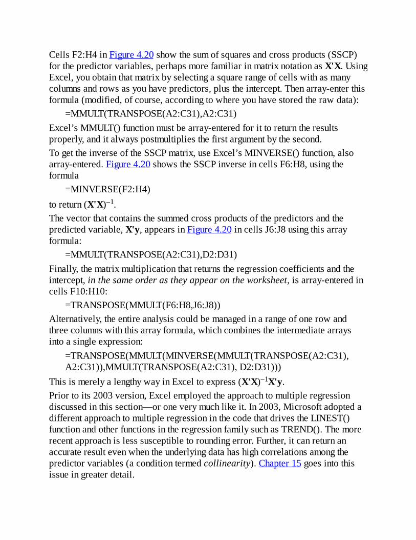
CellsF2:H4inFigure4.20showthesumofsquaresandcrossproducts(SSCP)forthepredictorvariables,perhapsmorefamiliarinmatrixnotationasX'X.UsingExcel,youobtainthatmatrixbyselectingasquarerangeofcellswithasmanycolumnsandrowsasyouhavepredictors,plustheintercept.Thenarray-enterthisformula(modified,ofcourse,accordingtowhereyouhavestoredtherawdata):

=MMULT(TRANSPOSE(A2:C31),A2:C31)Excel’sMMULT()functionmustbearray-enteredforittoreturntheresultsproperly,anditalwayspostmultipliesthefirstargumentbythesecond.TogettheinverseoftheSSCPmatrix,useExcel’sMINVERSE()function,alsoarray-entered.Figure4.20showstheSSCPinverseincellsF6:H8,usingtheformula

=MINVERSE(F2:H4)toreturn(X'X)–1.Thevectorthatcontainsthesummedcrossproductsofthepredictorsandthepredictedvariable,X'y,appearsinFigure4.20incellsJ6:J8usingthisarrayformula:

=MMULT(TRANSPOSE(A2:C31),D2:D31)Finally,thematrixmultiplicationthatreturnstheregressioncoefficientsandtheintercept,inthesameorderastheyappearontheworksheet,isarray-enteredincellsF10:H10:

=TRANSPOSE(MMULT(F6:H8,J6:J8))Alternatively,theentireanalysiscouldbemanagedinarangeofonerowandthreecolumnswiththisarrayformula,whichcombinestheintermediatearraysintoasingleexpression:

=TRANSPOSE(MMULT(MINVERSE(MMULT(TRANSPOSE(A2:C31),A2:C31)),MMULT(TRANSPOSE(A2:C31),D2:D31)))

ThisismerelyalengthywayinExceltoexpress(X'X)–1X'y.Priortoits2003version,Excelemployedtheapproachtomultipleregressiondiscussedinthissection—oroneverymuchlikeit.In2003,MicrosoftadoptedadifferentapproachtomultipleregressioninthecodethatdrivestheLINEST()functionandotherfunctionsintheregressionfamilysuchasTREND().Themorerecentapproachislesssusceptibletoroundingerror.Further,itcanreturnanaccurateresultevenwhentheunderlyingdatahashighcorrelationsamongthepredictorvariables(aconditiontermedcollinearity).Chapter15goesintothisissueingreaterdetail.

MovingontoStatisticalInferenceChapter5takesastepbackfromthecontinuousvariablesthatareemphasizedinthischapter,tosimpler,nominalvariableswithonlyafewpossiblevalueseach.Theyareoftenbeststudiedusingtwo-waytablesthatcontainsimplecountsintheircells.However,whenyoustarttomakeinferencesaboutpopulationsusingcontingencytablesbuiltonsamples,youstartgettingintosomeveryinterestingareas.Thisisthebeginningofstatisticalinference,anditwillleadquicklytomatterssuchasgenderbiasinuniversityclasses.

5.HowVariablesClassifyJointly:ContingencyTables

InThisChapterUnderstandingOne-WayPivotTablesMakingAssumptionsUnderstandingTwo-WayPivotTablesTheYuleSimpsoneffectSummarizingtheChi-SquareFunctions

InChapter4,“HowVariablesMoveJointly:Correlation,”yousawthewaysinwhichtwocontinuousvariablescancovary:togetherinadirect,positivecorrelation,andapartinanindirect,negativecorrelation—ornotatallwhennorelationshipbetweenthetwoexists.Thischapterexploreshowtwonominalvariablescanvarytogether,orfailtodoso.RecallfromChapter1,“AboutVariablesandValues,”thatvariablesmeasuredonanominalscalehavenames(suchasFordorToyota,RepublicanorDemocrat,SmithorJones)astheirvalues.Variablesmeasuredonanordinal,interval,orratioscalehavenumbersastheirvaluesandtheirrelationshipscanbemeasuredbymeansofcovarianceandcorrelation.Fornominalvariables,wehavetomakedowithtables.

UnderstandingOne-WayPivotTablesAsthequalitycontrolmanagerofafactorythatproducessophisticated,cutting-edgesmartphones,oneofyourresponsibilitiesistoseetoitthatthephonesleavingthefactoryconformtosomestandardsforusability.Yourfactoryisproducingthephonesataphenomenalrate,andyoujustdon’thavethestafftocheckeveryphone.Therefore,youarrangetohaveasampleof50phonestesteddaily,checkingforconnectionproblems.Youknowthatzero-defectmanufacturingisbothterriblyexpensiveandagenerallyimpossiblegoal:Yourcompanywillbesatisfiedifonly1%ofitsphonesfailtoestablishaconnectionwithacelltowerthat’swithinreach.Todayyourfactoryproduced1,000phones.Didyoumeetyourgoalofatmosttendefectiveunitsin1,000?Youcan’tpossiblyanswerthatquestionyet.First,youneedmoreinformation

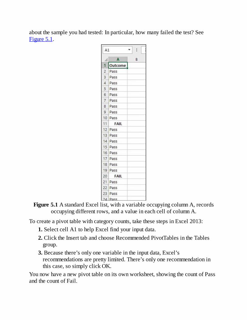
aboutthesampleyouhadtested:Inparticular,howmanyfailedthetest?SeeFigure5.1.

Figure5.1AstandardExcellist,withavariableoccupyingcolumnA,recordsoccupyingdifferentrows,andavalueineachcellofcolumnA.

Tocreateapivottablewithcategorycounts,takethesestepsinExcel2013:1.SelectcellA1tohelpExcelfindyourinputdata.2.ClicktheInserttabandchooseRecommendedPivotTablesintheTablesgroup.

3.Becausethere’sonlyonevariableintheinputdata,Excel’srecommendationsareprettylimited.There’sonlyonerecommendationinthiscase,sosimplyclickOK.

Younowhaveanewpivottableonitsownworksheet,showingthecountofPassandthecountofFail.

TheRecommendedPivotTablesfeaturecanbeahandyone,particularlyifyouknowyou’renotgoingtoaskalotoftheanalysis.Buildingapivottablethiswaycanbeaswift,three-clickprocess.ButyouhavetoberunningExcel2013,andyouhavetoacceptvariousdefaults.Forexample,Ioftenuseandreusepivottablesthatarebasedonconstantlyexpandingdatasets.Itsavesmetimeandaggravationtohavethedatasetonthesameworksheetasthepivottable.RecommendedPivotTables,though,automaticallylocatetheresultingpivottableonanewworksheet.MovingthepivottabletotheworksheetthatrefreshesorotherwisecontainstheunderlyingdatasetwastesthetimeIsavedbycallingforaRecommendedPivotTable.Nevertheless,ifyou’reafteraquicksummaryofadataset,aRecommendedPivotTableisoftenagoodchoice.Bycontrast,herearethestepsyouneedifyouwanttobuildityourself—orifyouneedtodosobecauseyou’renotrunningExcel2013:

1.SelectcellA1.2.ClicktheInserttabandchoosePivotTableintheTablesgroup.3.IntheCreatePivotTabledialogbox,clicktheExistingWorksheetoptionbutton,clickintheLocationeditbox,andthenclickincellC1ontheworksheet.ClickOK.

4.InthePivotTableFieldslist,clickOutcomeanddragitintotheRowLabelsarea.

5.ClickOutcomeagainanddragitintotheSummaryValuesarea,designatedbyΣValues.Becauseatleastonevalueintheinputrangeistext,thesummarystatisticisCount.

It’softenusefultoshowthecountsinthepivottableaspercentages.Ifyou’reusingExcel2010or2013,right-clickanycellinthepivottable’sCountcolumnandchooseShowValuesAsfromtheshortcutmenu.(Seethefollowingnoteifyou’reusinganearlierversionofExcel.)Thenclick%ofColumnTotalinthecascadingmenu.

NoteMicrosoftmadesignificantchangestotheuserinterfaceforpivottablesbetweenExcel2003and2007,andagainbetweenExcel2007and2010,andyetagainfor2013.Inthisbook,Itrytoprovideinstructionsthatworkregardlessoftheversionyou’reusing.That’snotalwaysfeasible.

Inthiscase,youcoulddothefollowinginExcel2007through2013.Right-clickoneoftheCountorTotalcellsinthepivottable,suchasD2orD3inFigure5.2.ChooseValueFieldSettingsfromtheshortcutmenuandclicktheShowValuesAstab.Click%ofColumnTotalintheShowValuesAsdrop-down.ThenclickOK.InExcel2003orearlier,right-clickoneofthepivottable’svaluecellsandchooseFieldSettingsfromtheshortcutmenu.Usethedrop-downlabeledShowDataAsintheFieldSettingsdialogbox.

Figure5.2Aquickandeasysummaryofyoursampleresults.

Younowhaveastatisticalsummaryofthepass/failstatusofthe50phonesinyoursample,asshowninFigure5.2.TheresultsshowninFigure5.2aren’tgreatnews.Outoftheentirepopulationof1,000phonesthatweremadetoday,nomorethan1%(10total)shouldbedefectiveifyou’retomeetyourtarget.Butinasampleof50phonesyoufound2

defectives.Inotherwords,a5%sample(50of1,000)gotyou20%(2of10)ofthewaytowardyourself-imposedlimit.Youfound2defectivesin50phones.Atthatratethe1,000phonepopulationwouldhave40defectiveunits,butyourtargetmaximumis10.Youcouldtakeanothernineteen50-unitsamplesfromthepopulation.Attherateof2defectivesin50units,you’dwindupwith40defectivesoverall,andthat’sfourtimesthenumberyoucantoleratefromthefullpopulation.However,itisarandomsample.Assuch,therearelimitstohowrepresentativethesampleisofthepopulationitcomesfrom.It’spossiblethatyoujusthappenedtogetyourhandsonasampleof50phonesthatincluded2defectiveunitswhenthefullpopulationhasasmallerdefectiverate.Howlikelyisthat?Here’showExcelcanhelpyouanswerthatquestion.

RunningtheStatisticalTestAlargenumberofquestionsintheareasofbusiness,manufacturing,medicine,socialscience,gambling,andsoonarebasedonsituationsinwhichtherearejusttwotypicaloutcomes:succeeds/fails,breaks/doesn’tbreak,cures/sickens,Republican/Democrat,wins/loses.Instatisticalanalysis,thesesituationsaretermedbinomial:“bi”referringto“two,”and“nomial”referringto“names.”Severalhundredyearsago,duelargelytoakeeninterestintheoutcomesofbets,mathematiciansstartedlookingcloselyatthenatureofthoseoutcomes.Wenowknowalotmorethanweoncedidabouthowthenumbersbehaveinthelongrun.Andyoucanusethatknowledgeasaguidetoananswertothequestionposedearlier:Howlikelyisitthatthereareatmost10defectivesintheproductionlotof1,000phones,whenyoufoundtwoinasampleofjust50?

FramingtheHypothesisStartbysupposingthatyouhadapopulationof100,000phonesthathas1,000defectives—thusthesame1%defectrateasyouhopeforinyouractualproductionlotof1,000phones.

NoteThissortofsuppositionisoftencalledanullhypothesis.Itassumesthatnodifferenceexistsbetweentwovalues,suchasavalueobtainedfromasampleandavalueassumedforapopulation;anothertypeofnullhypothesisassumesthatnodifferenceexistsbetweentwopopulationvalues.Theassumptionofnodifferenceisbehindthetermnullhypothesis.Youoftenseethattheresearcherhasframedanother

hypothesisthatcontradictsthenullhypothesis,calledthealternativehypothesis.

Ifyouhadalltheresourcesyouneeded,youcouldtakehundredsofsamples,eachsampleconsistingof50units,fromthatpopulationof100,000.Youcouldexamineeachsampleanddeterminehowmanydefectiveunitswereinit.Ifyoudidthat,youcouldcreateaspecialkindoffrequencydistribution,calledasamplingdistribution,basedonthenumberofdefectivesineachsample.(FrequencydistributionsarediscussedinsomedetailinChapter1.)Underyoursuppositionofjust1%defectiveinthepopulation,oneofthosehypotheticalsampleswouldhavezerodefects;anothersamplewouldhavetwo(justliketheoneyoutookinreality);anothersamplewouldhaveonedefect;andsoonuntilyouhadexhaustedallthoseresourcesintheprocessoftakinghundredsofsamples.Youcouldchartthenumberofdefectsineachsample,creatingasamplingdistributionthatshowsthefrequencyofeachspecificnumberofdefectsfoundinyoursamples.

UsingtheBINOM.DIST()FunctionBecauseofalltheresearchandtheoreticalworkthatwasdonebythosemathematiciansstartinginthe1600s,youknowwhatthatfrequencydistributionlookslikewithouthavingtotakeallthosesamples.You’llfinditinFigure5.3.

Figure5.3Asamplingdistributionofthenumberofdefectsineachofmany,manysampleswouldlooklikethis.

ThedistributionthatyouseechartedinFigure5.3isoneofmanybinomial

distributions.Theshapeofeachbinomialdistributionisdifferent,dependingonthesizeofthesamplesandtheprobabilityofeachalternativeinthepopulation.ThebinomialdistributionyouseeinFigure5.3isbasedonasamplesizeof50andaprobability(inthisexample,ofdefectiveunits)of1%.Thetableandtheaccompanyingcharttellyouthat,givenapopulationwitha1%defectrate,60.50%of50-itemsampleswouldcontainzerodefectiveitems,another30.56%wouldcontainonedefectiveitem,andsoon.Forcontrast,Figure5.4showsanexampleofthebinomialdistributionbasedonasamplesizeof100andadefective-unitprobabilityof3%.

Figure5.4ComparewithFigure5.3:Thedistributionhasshiftedtotheright.

ThedistributionsshowninFigures5.3and5.4arebasedonthetheoryofbinomialdistributionsandaregenerateddirectlyusingExcel’sBINOM.DIST()function.

NoteIfyouareusingaversionofExcelpriorto2010,youmustusethecompatibilityfunctionBINOMDIST().Noticethatthereisnoperiodinthefunctionname,asthereiswiththeconsistencyfunctionBINOM.DIST().Theargumentstothetwofunctionsareidenticalastobothargumentnameandargumentmeaning.

Forexample,inFigure5.4,theformulaincellE3isasfollows:=BINOM.DIST(D3,$B$1,$B$2,FALSE)

or,usingargumentnamesinsteadofcelladdresses:

=BINOM.DIST(Number_s,Trials,Probability_s,Cumulative)HerearetheargumentstotheBINOM.DIST()function:

Numberofsuccesses—ExcelcallsthisNumber_s.InBINOM.DIST(),asusedincellE3ofFigure5.4,that’sthevaluefoundincellD3:zero.Inthisexample,it’sthenumberofdefectiveitemsthataresuccessfullyfoundinasample.Trials—IncellE3,that’sthevaluefoundincell$B$1:100.Inthecontextofthisexample,Trialsmeansnumberofcellphonesinasample.Anothertermforthisaspectofthebinomialdistributionissamplesize.Probabilityofsuccess—ExcelcallsthisProbability_s.Thisistheprobabilityofasuccess—offindingwhatyou’relookingfor,inthiscaseadefectiveunit—inthepopulation.Inthisexample,we’reassumingthattheprobabilityis3%,whichisthevaluefoundincell$B$2.Cumulative—ThisargumenttakeseitheraTRUEorFALSEvalue.IfyousetittoTRUE,Excelreturnstheprobabilityforthisnumberofsuccessesplustheprobabilityofallsmallernumbersofsuccesses.Thatis,ifthenumberofsuccessescitedinthisformulais2,andifCumulativeisTRUE,thenBINOM.DIST()returnstheprobabilityfor2successesplustheprobabilityof1successplustheprobabilityofzerosuccesses(inFigure5.4,thatis41.98%incellF5).WhenCumulativeissettoFALSE,Excelreturnstheprobabilityofoneparticularnumberofsuccesses.AsusedincellE4,forexample,thatistheprobabilityofthenumberofsuccessesfoundinD4(1successinD4leadsto14.71%ofsamplesincellE4).

So,Figure5.4showstheresultsofenteringtheBINOM.DIST()function11times,eachtimewithadifferentnumberofsuccessesbutthesamenumberoftrials(thatis,samplesize),thesameprobabilityofdefectiveitemsinthepopulation,andthesamecumulativeoption.Ifyoutriedtoreplicatethisresultbytakingafewactualsamplesofsize50withasuccessprobabilityof3%,youwouldnotgetwhatisshowninFigure5.4.Aftertaking20or30samplesandchartingthenumberofdefectsineachsample,youwouldbegintogetaresultthatlookslikeFigure5.4.After,say,500samples,yoursamplingdistributionwouldlookverymuchlikeFigure5.4.(ThatoutcomewouldbeanalogoustothedemonstrationforthenormaldistributionshownattheendofChapter1,in“BuildingSimulatedFrequencyDistributions.”)Butbecauseweknowthecharacteristicsofthebinomialdistribution,underdifferentsamplesizesandwithdifferentprobabilitiesofsuccessinthepopulation,itisn’tnecessarytogetanewdistributionbyrepeatedsamplingeach

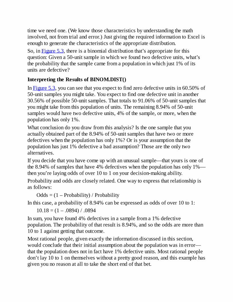
timeweneedone.(Weknowthosecharacteristicsbyunderstandingthemathinvolved,notfromtrialanderror.)JustgivingtherequiredinformationtoExcelisenoughtogeneratethecharacteristicsoftheappropriatedistribution.So,inFigure5.3,thereisabinomialdistributionthat’sappropriateforthisquestion:Givena50-unitsampleinwhichwefoundtwodefectiveunits,what’stheprobabilitythatthesamplecamefromapopulationinwhichjust1%ofitsunitsaredefective?

InterpretingtheResultsofBINOM.DIST()InFigure5.3,youcanseethatyouexpecttofindzerodefectiveunitsin60.50%of50-unitsamplesyoumighttake.Youexpecttofindonedefectiveunitinanother30.56%ofpossible50-unitsamples.Thattotalsto91.06%of50-unitsamplesthatyoumighttakefromthispopulationofunits.Theremaining8.94%of50-unitsampleswouldhavetwodefectiveunits,4%ofthesample,ormore,whenthepopulationhasonly1%.Whatconclusiondoyoudrawfromthisanalysis?Istheonesamplethatyouactuallyobtainedpartofthe8.94%of50-unitsamplesthathavetwoormoredefectiveswhenthepopulationhasonly1%?Orisyourassumptionthatthepopulationhasjust1%defectiveabadassumption?Thosearetheonlytwoalternatives.Ifyoudecidethatyouhavecomeupwithanunusualsample—thatyoursisoneofthe8.94%ofsamplesthathave4%defectiveswhenthepopulationhasonly1%—thenyou’relayingoddsofover10to1onyourdecision-makingability.Probabilityandoddsarecloselyrelated.Onewaytoexpressthatrelationshipisasfollows:

Odds=(1–Probability)/ProbabilityInthiscase,aprobabilityof8.94%canbeexpressedasoddsofover10to1:

10.18=(1–.0894)/.0894Insum,youhavefound4%defectivesinasamplefroma1%defectivepopulation.Theprobabilityofthatresultis8.94%,andsotheoddsaremorethan10to1againstgettingthatoutcome.Mostrationalpeople,givenexactlytheinformationdiscussedinthissection,wouldconcludethattheirinitialassumptionaboutthepopulationwasinerror—thatthepopulationdoesnotinfacthave1%defectiveunits.Mostrationalpeopledon’tlay10to1onthemselveswithoutaprettygoodreason,andthisexamplehasgivenyounoreasonatalltotaketheshortendofthatbet.

Ifyoudecidethatyouroriginalassumption,thatthepopulationhasonly1%defectives,waswrong—ifyougowiththeoddsanddecidethatthepopulationhasmorethan1%defectiveunits—thatdoesn’tnecessarilymeanyouhavepersuasiveevidencethatthepercentageofdefectsinthepopulationis4%,asitisinyoursample(althoughthat’syourbestestimaterightnow).Allyourconclusionsaysisthatyouhavedecidedthatthepopulationof1,000unitsyoumadetodayincludesmorethantendefectiveunits.

SettingYourDecisionRulesNow,itcanbealittledisturbingtofindthatalmost9%(8.94%)ofthesamplesof50phonesfroma1%defectivepopulationwouldhaveatleast4%defectivephones.It’sdisturbingbecausemostpeoplewouldnotregard9%ofthesamplesasabsolutelyconclusive.Theywouldnormallydecidethatthedefectrateinthepopulationishigherthan1%,buttherewouldbeanaggingdoubt.Afterall,we’veseenthatalmostonesampleintenfroma1%defectivepopulationwouldhave4%defectsormore,soit’ssurelynotimpossibletogetabadsamplefromagoodpopulation.Let’seavesdrop:“Ihave50phonesthatIsampledatrandomfromthe1,000wemadetoday—andwe’rehopingthattherearenomorethan1%defectiveunitsinthatentireproductionrun.Twoofthesample,or4%,aredefective.Excel’sBINOM.DIST()function,withthosearguments,tellsmethatifItook10samplesof50each,Icanexpectthatoneofthem(8.94%ofthesamples,ornearly1in10)wouldhavetwoorevenmoredefectives.Maybethat’sthesampleIhavehere.Maybethefullproductionrunreallydoeshaveonly1%defective.”Tempting,isn’tit?Thisiswhyyoushouldspecifyyourdecisionrulebeforeyou’veseenthedata,andwhyyoushouldn’tfudgeitafterthedatahascomein.Ifyouseethedataandthendecidewhatyourcriterionwillbe,youareallowingthedatatoinfluenceyourdecisionruleafterthefact.That’scalledcapitalizingonchance.Traditionalexperimentalmethodsadviseyoutospecifythelikelihoodofmakingthewrongdecisionaboutthepopulationbeforeyouseethedata.Theideaisthatyoushouldbringacost-benefitapproachtosettingyourcriterion.Supposethatyousellyour1,000phonestoawholesalerata5%markup.Thetermsofyourcontractwiththewholesalercallforyoutorefundthepriceofanentireshipmentifthewholesalerfindsmorethan1%defectiveunitsintheshipment.Thecostofthatrefundhastobebornebytheprofitsyou’vemade.Supposethatyoumakeabaddecision.Thatis,youdecidethepopulationof1,000phonesfromwhichyoudrewyoursamplehas1%orfewerdefectiveunits,when

infactithas,say,3%.Inthatcase,the21stsalecouldcostyoualltheprofitsyou’vemadeonthefirst20sales.Therefore,youwanttomakeyourcriterionfordecidingtoashipthe1,000-unitlotstrongenoughthatatmostoneshipmentin20willfailtomeetthewholesaler’sacceptancecriterion.

NoteTheapproachdiscussedinthisbookcanbethoughtofasamoretraditionalone,followingthemethodsdevelopedintheearlypartofthetwentiethcenturybytheoristssuchasR.A.Fisher.Itissometimestermedafrequentistapproach.OtherstatisticaltheoristsandpractitionersfollowaBayesianmodel,underwhichthehypothesesthemselvescanbethoughtofashavingprobabilities.ThematterisasubjectofsomecontroversyandiswellbeyondthescopeofabookonExcel.Beaware,though,thatwherethereisachoicethatmattersinthewayfunctionsaredesignedandtheDataAnalysisadd-inworks,Microsofthastakenaconservativestanceandadoptedthefrequentistapproach.

MakingAssumptionsYoumustbesuretomeettwobasicassumptionsifyouwantyouranalysisofthedefectivephoneproblem—andother,similarproblems—tobevalid.You’llfindthatallproblemsinstatisticalinferenceinvolveassumptions;sometimestherearemorethanjusttwo,andsometimesitturnsoutthatyoucangetawaywithviolatingtheassumptions.Inthiscase,therearejusttwo,butyoucan’tgetawaywithanyviolations.

RandomSelectionTheanalysisassumesthatyoutakesamplesfromyourpopulationatrandom.Inthephoneexample,youcan’tlookatthepopulationofphonesandpickthe50thatlookleastlikelytobedefective.Well,moreprecisely,youcandothatifyouwantto.Butifyoudo,youarecreatingasamplethatissystematicallydifferentfromthepopulation.Youneedasamplethatyoucanusetomakeaninferenceaboutallthephonesyoumade,andyourjudgmentaboutwhichphoneslookbestwasnotpartofthemanufacturingprocess.Ifyouletyourjudgmentinterferewithrandomselectionofphonesforyoursample,you’llwindupwithasamplethatisn’ttrulyrepresentativeofthepopulation.

Andtherearen’tmanythingsmoreuselessthananonrepresentativesample.(JustaskGeorgeGallupabouthispredictionthatTrumanwouldlosetoDeweyin1948.)Ifyoudon’tpickarandomsampleofphones,youmakeadecisionaboutthepopulationofphonesthatyouhavemanufacturedonthebasisofanonrepresentativesample.Ifyoursamplehasnotasingledefectivephone,howconfidentcanyoubethattheoutcomeisduetothequalityofthepopulation,andnotthequalityofyourjudgmentinselectingthesample?

UsingExceltoHelpSampleRandomlyThequestionofusingExceltosupportarandomselectioncomesupoccasionally.Here’stheapproachthatIuseandprefer.Startwithaworksheetlistofvaluesthatuniquelyidentifymembersofapopulation.Intheexamplethischapterhasused,thosevaluesmightbeserialnumbers.SupposethatlistoccupiesA1:A1001,withalabelsuchasSerialNumberincellA1.Youcancontinuebytakingthesesteps:

1.IncellB1,enteralabelsuchasRandomNumber.2.SelecttherangeB2:B1001.(ButseetheTipattheendofthesesteps.)3.Typetheformula=RAND()andenteritintoB2:B1001usingCtrl+Enter.Thisgeneratesalistofrandomvaluesinrandomorder.ThevaluesreturnedbyRAND()areunrelatedtotheidentifyingserialnumbersincolumnA.LeavetherangeB2:B1001selected.

4.Sothatyoucansortthem,converttheformulastovaluesbyclickingtheCopybuttonontheRibbon’sHometab,thenclickingPaste,choosingPasteSpecial,selectingtheValuesoption,andthenclickingOK.YounowhaverandomnumbersinB2:B1001.

5.SelectanycellintherangeA1:B1001.ClicktheRibbon’sDatatabandclicktheSortbutton.Forthisexample,makesurethattheMyDataHasHeaderscheckboxisfilled.

6.IntheSortBydrop-down,chooseRandomNumber.AcceptthedefaultsfortheSortOnandtheOrderdrop-downsandclickOK.

TipHere’satimesaverIpickedupfromBillJelenin2012,andIwishI’dlearnedaboutitlongbeforethat.SupposethatyouhavealistofvaluesorformulasinA1:A1000,andthatyouwanttofillB1:B1000withformulassuchas=A1/$D$1,=A2/$D$1,andsoon.OnewayistoentertheformulainB1,copyit,selectB2:B1000,andclickPaste.Youcould

alsoclicktheFillHandleinB1anddragdownthroughB2:B1000.(TheFillHandleistheblacksquareonthelower-rightcorneroftheactivecell.)Eitherway,youexposeyourselftotheerror-pronetediumofselectingB2:B1000.AbetterwayistoselectcellB1afterenteringyourformulathere,anddouble-clickingtheFillHandle.Excelautomaticallyfillsdownforyouasfarasthebottommostrowofanadjacentlist.(Inthisexample,that’srow1000.)

Theresultistosorttheuniqueidentifiersintorandomorder,asshowninFigure5.5.Youcannowprintoffthefirst50(orthesizeofthesampleyouwant)andselectthemfromyourpopulation.

Figure5.5Insteadofserialnumber,theuniqueidentifierincolumnAcouldbename,SocialSecuritynumber,phonenumber—whateverismostaptforyour

populationofinterest.

NoteRandomnumbersthatyougenerateinthiswayarereallypseudo-randomnumbers.Computershavearelativelylimitedinstructionset,andexecutetheirinstructionsrepeatedly.Thismakesthemveryfastandveryaccuratebutnotveryrandom.Nevertheless,thepseudo-randomnumbersproducedbyExcel’sRAND()functionpasssomerigoroustestsfornonrandomnessandarewellsuitedtoanysortofrandomselectionyou’reatalllikelytoneed.

IndependentSelections

It’simportantthattheindividualselectionsbeindependentofoneanother:thatis,thefactthatPhone0001isselectedforthesamplemustnotchangethelikelihoodthatanotherspecificunitwillbeselected.Supposethatthephonesleavethefactoryfloorpackagedin50-unitcartons.Itwouldobviouslybeconvenienttograboneofthosecartons,evenatrandom,anddeclarethatit’stobeyour50-unitsample.Butifyoudidthat,youcouldeasilybeintroducingsomesortofstructuraldependencyintothesystem.Forexample,ifthe50phonesinagivencartonweremanufacturedsequentially—iftheywere,say,the51stthrough100thphonestobemanufacturedthatday—thenasubsetofthemmightbesubjecttothesamecalibrationerrorinapieceofequipment.Inthatcase,thelackofindependenceinmakingtheselectionsagainintroducesanonrandomelementintowhatisassumedtobearandomprocess.Acorollarytotheissueofindependenceisthattheprobabilityofbeingselectedmustremainthesamethroughtheprocess.Inpractice,it’sdifficulttoadhereslavishlytothisrequirement,butthedifferencebetween1/1,000and1/999,orbetween1/999and1/998issosmallthattheyaregenerallytakentobeequivalentprobabilities.Yourunintothissituationifyou’resamplingwithoutreplacement—whichoftenhappenswhenyou’redoingdestructivetesting.Thehypergeometricdistributioncanprovehelpfulwhentheselectionprobabilitiesaregreater(say,1/20or1/30).ExcelsupportsthehypergeometricdistributionwithitsHYPGEOM.DIST()worksheetfunction.

TheBinomialDistributionFormulaIftheseassumptions—randomandindependentselectionwithjusttwopossiblevalues—aremet,thentheformulaforthebinomialdistributionisvalid:

Inthisformula:nisthenumberoftrials.risthenumberofsuccessfultrials.

isthenumberofcombinations.

pistheprobabilityofasuccessinthepopulation.qis(1–p),ortheprobabilityofafailureinthepopulation.

(ThenumberofcombinationsisoftencalledthenCrformula,or“nthingstakenratatime.”)You’llfindtheformulaworkedoutinFigure5.6foraspecificnumberoftrials,successes,andprobabilityofsuccessinthepopulation.CompareFigure5.6withFigure5.4.Inbothfigures:

Thenumberoftrials,orn,representingthesamplesize,is100.Thenumberofsuccessfultrials,orr,representingthenumberofdefectsinthesample,is4(cellD7inFigure5.4).Theprobabilityofasuccessinthepopulation,orp,is.03.

InFigure5.6:

Figure5.6BuildingtheresultsofBINOM.DIST()fromscratch.

Thevalueofqiscalculatedsimplybysubtractingpfrom1incellC4.

Thevalueof iscalculatedincellC5withtheformula

=COMBIN(C1,C2).TheformulaforthebinomialdistributionisusedincellC6tocalculatetheprobabilityoffoursuccessesinasampleof100,givenaprobabilityofsuccessinthepopulationof3%.

NotethattheprobabilitycalculatedincellC6ofFigure5.6isidenticaltothevaluereturnedbyBINOM.DIST()incellE7ofFigure5.4.Ofcourse,it’snotnecessarytousethenCrformulatocalculatethebinomialprobability;that’swhatBINOM.DIST()isfor.Still,IliketocalculateitfromscratchfromtimetotimeasacheckthatIhaveusedBINOM.DIST()anditsargumentsproperly.

UsingtheBINOM.INV()FunctionYouhavealreadyseenExcel’sBINOM.DIST()function,inFigures5.3and5.4.

There,theargumentsusedwereasfollows:Numberofsuccesses—Moregenerally,that’sthenumberoftimessomethingoccurred;here,that’sthenumberofinstancesthatphonesaredefective.ExceltermsthisargumentsuccessesorNumber_s.Numberoftrials—Thenumberofopportunitiesforsuccessestooccur.Inthecurrentexample,that’sthesamplesize.Probabilityofsuccess—Thepercentoftimessomethingoccursinthepopulation.Inpractice,thisisusuallytheprobabilitythatyouaretestingforbymeansofasample:“Howlikelyisitthattheprobabilityofsuccessinthepopulationis1%,whentheprobabilityofsuccessinmysampleis4%?”Cumulative—TRUEtoreturntheprobabilityassociatedwiththisnumberofsuccesses,plusallsmallernumbersofsuccessesdowntoandincludingzero.FALSEtoreturntheprobabilityassociatedwiththisnumberofsuccessesonly.

BINOM.DIST()returnstheprobabilitythatasamplewiththegivennumberofsuccessescanbedrawnfromapopulationwiththegivenprobabilityofsuccess.TheoldercompatibilityfunctionBINOMDIST()takesthesameargumentsandreturnsthesameresults.Asyou’llseeinthisandlaterchapters,avarietyofExcelfunctionsthatreturnprobabilitiesfordifferentdistributionshaveaformwhosenameendswith.DIST().Forexample,NORM.DIST()returnstheprobabilityofobservingavalueinanormaldistribution,giventhedistribution’smeanandstandarddeviation,andthevalueitself.Anotherformofthesefunctionsendswith.INV()insteadof.DIST().TheINVstandsforinverse.InthecaseofBINOM.INV(),theargumentsareasfollows:

Trials—JustasinBINOM.DIST(),thisisthenumberofopportunitiesforsuccesses(here,thesamplesize).Probability—JustasinBINOM.DIST(),thisistheprobabilityofsuccessesinthepopulation.(Theprobabilityisunknownbuthypothesized.)Alpha—ThisisthevaluethatBINOM.DIST()returns:thecumulativeprobabilityofobtainingsomenumberofsuccessesinthesample,giventhesamplesizeandthepopulationprobability.(Thetermalphaforthisvalueisnonstandard.)

Withthesearguments,BINOM.INV()returnsthenumberofsuccesses(here,defectivephones)associatedwiththealphaargumentyousupply.Iknowthat’sconfusing,andthismayhelpclearitup:LookbacktoFigure5.4.Supposeyou

enterthisformulaonthatworksheet:=BINOM.INV(B1,B2,F8)

Thatwouldreturnthenumber6.Here’swhatthatmeansandwhatyoucaninferfromit,giventhesetupinFigure5.4:

You’vetoldmethatyouhaveasampleof100phones(cellB1).Thesamplecomesfromapopulationofphones—aproductionlot—whereyouhopetheprobabilityofaphonebeingdefectiveisatmost3%(cellB2).Youplantocountthenumberofdefectivephonesinthe100-itemsample.Sometimesyou’llgetabadsampleandrejecttheproductionlotofphoneserroneously—thelotmeetsyour3%defectivecriterion,butthesamplehas,say,10%defective.Youwanttoholdtheprobabilityofmakingthatmistaketo8%.Lookedatfromthestandpointofacorrectdecision,youwanttokeeptheprobabilitythatyou’llacceptthelotcorrectlytoatleast92%.Youhavecomeupwiththesefigures,92%probabilityofatruepositiveand8%ofafalsepositive,fromaseparateanalysisofthecostsofmistakenlyrejectingagoodlot:thefalsepositive.Givenallthat,youshouldconcludethatthesampledidnotcomefromapopulationwithonly3%defectiveifyouget6ormoredefectiveunitsinyoursample—ifyougetthatmany,you’reintothe8%ofthesamplesthatyourcost-benefitanalysishaswarnedyouoff.Althoughyoursamplecouldcertainlybeamongthe8%ofsampleswith6defectivesfroma3%defectiveproductionlot,that’stoounlikelyapossibilitytosuitmostpeople.Mostpeoplewoulddecideinsteadthattheproductionlothasmorethan3%defectives.Again,the92%and8%probabilitiesarguethatit’s11to1(92%dividedby8%)thattheproductionlotisn’tjust3%defective.Ifitwere,you’dbe11timesaslikelytogetasamplewithfewerthan6defectivesthantogetasamplewith6ormore.

Torecap:Youbeginbydecidingthatyouwanttoholdyourfalsepositiveratetoaround8%.Ifyourproductionlotreallyhasjust3%defective,youarrangeyourdecisionrulesothatyourprobabilityofrejectingthelotashavingtoomanydefectsisabout8%.Bysettingtheprobabilityofmakingthaterrorto8%,usingasamplesizeof100,andassumingthelotpercentdefectiveis3%,youcandeployExcel’sBINOM.INV()functiontolearnhowmanydefectivesinasampleof100itemswouldcauseyoutodecideyouroverallproductionlothasmisseditscriterionof3%defectiveitems.So,the.INV()formofthefunctionturnsthe.DIST()formonitshead,asfollows:

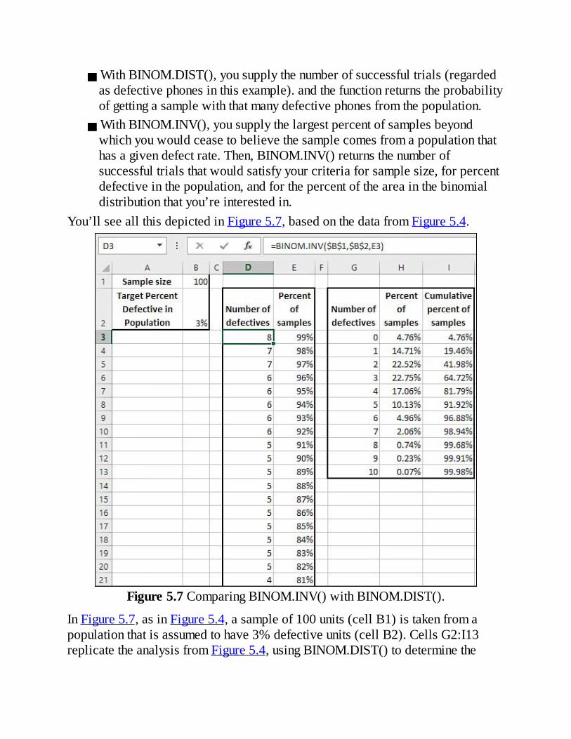
WithBINOM.DIST(),yousupplythenumberofsuccessfultrials(regardedasdefectivephonesinthisexample).andthefunctionreturnstheprobabilityofgettingasamplewiththatmanydefectivephonesfromthepopulation.WithBINOM.INV(),yousupplythelargestpercentofsamplesbeyondwhichyouwouldceasetobelievethesamplecomesfromapopulationthathasagivendefectrate.Then,BINOM.INV()returnsthenumberofsuccessfultrialsthatwouldsatisfyyourcriteriaforsamplesize,forpercentdefectiveinthepopulation,andforthepercentoftheareainthebinomialdistributionthatyou’reinterestedin.

You’llseeallthisdepictedinFigure5.7,basedonthedatafromFigure5.4.

Figure5.7ComparingBINOM.INV()withBINOM.DIST().

InFigure5.7,asinFigure5.4,asampleof100units(cellB1)istakenfromapopulationthatisassumedtohave3%defectiveunits(cellB2).CellsG2:I13replicatetheanalysisfromFigure5.4,usingBINOM.DIST()todeterminethe

percent(H2:H13)andcumulativepercent(I2:I13)ofsamplesthatyouwouldexpecttohavedifferentnumbersofdefectiveunits(cellsG2:G13).ColumnsDandEuseBINOM.INV()todeterminethenumberofdefects(columnD)youwouldexpectinagivenpercentofsamples.Thatis,inanywherefrom82%to91%ofsamplesfromtheproductionlot,youwouldexpecttofindasmanyasfivedefectiveunits.ThisfindingisconsistentwiththeBINOM.DIST()analysis,whichshowsthatacumulative91.92%ofsampleshaveasmanyasfivedefects(seecellI8).Thefollowingsectionsofferafewcommentsonallthisinformation.

SomewhatComplexReasoningDon’tletthecomplexitythrowyou.Itusuallytakesseveraltripsthroughthereasoningbeforethelogicofitbeginstosettlein.Thegenerallineofthoughtpursuedhereissomewhatmorecomplicatedthanthereasoningyoufollowwhenyou’redoingotherkindsofstatisticalanalysis,suchaswhethertwosamplesindicatethatthemeansarelikelytobedifferentintheirpopulations.Thereasoningaboutmeandifferencestendstobelesscomplicatedthanisthecasewiththebinomialdistribution.Threeissuescomplicatethelogicofabinomialanalysis.Oneisthecumulativenatureoftheoutcomemeasure:thenumberofdefectiveunitsinthesample.Totestwhetherthesamplecamefromapopulationwithanacceptablenumberofdefectives,youneedtoaccountforzerodefectiveunits,onedefectiveunit,twodefectiveunits,andsoon.Anothercomplicatingissueisthatmorepercentagesthanusualareinvolved.Inmostotherkindsofstatisticalanalysis,theonlypercentageyou’reconcernedwithisthepercentofthetimethatyouwouldobserveasampleliketheoneyouobtained,giventhatthepopulationisasyouassumeittobe.It’sonlywhenyou’reworkingwithanominalscaleforyouroutcomemeasaurethatyoumustworkwithoutcomepercentages:X%ofpatientssurvivedoneyear;Y%ofcarshadbrakefailure;Z%ofregisteredvoterswereRepublicans.Theothercomplicatingfactoristhattheoutcomemeasureisaninteger.Youdon’tget3.5defectiveunits;aphoneiseitherdefectiveoritisn’t.(Thingsaredifferentwhenyou’retestingthenumberofdefectsperunit,butthat’sadifferentsortofsituation.)Therefore,theassociatedprobabilitiesdon’tincreasesmoothly.Instead,theyincreasebysteps,asthenumberofdefectiveunitsincreases.ReferbacktoFigure5.4andnoticehowtheprobabilitiesfirstincreaseandthendecreaseinstepsasthenumberofdefectiveunits—aninteger—increases.

TheGeneralFlowofHypothesisTestingStill,thebasicreasoningfollowedhereisanalogoustothereasoningusedinothersituations.Thenormalprocessisasfollows:

TheHypothesisSetupanassumption(oftencalledanhypothesis,sometimesanullhypothesis,tobecontrastedwithanalternativehypothesis).Intheexamplediscussedhere,thenullhypothesisisthatthepopulationfromwhichthesampleofphonescamehasa1%defectrate;thetermnullsuggeststhatnothingunusualisgoingon,that1%isthenormalexpectation.Thealternativehypothesisisthatthepopulationdefectrateishigherthan1%.

TheSamplingDistributionDeterminethecharacteristicsofthesamplingdistributionthatwouldresultifthehypothesisweretrue.Therearevarioustypesofsamplingdistributions,andyourchoiceisusuallydictatedbythequestionyou’retryingtoanswerandbythelevelofmeasurementavailabletoyou.Here,thelevelofmeasurementwasnotonlynominal(acceptableversusdefective)butbinomial(justtwopossiblevalues).YouusethefunctionsinExcelthatpertaintothebinomialdistributiontodeterminetheprobabilitiesassociatedwithdifferentnumbersofdefectsinthesample.

TheErrorRateDecidehowmuchriskofincorrectlyrejectingthehypothesisisacceptable.Thischapterhastalkedaboutthatdecisionwithoutactuallymakingitinthephonequalityexample;itadvisesyoutotakeintoaccountissuessuchasthecostsofmakinganincorrectdecisionversusthebenefitsofmakingacorrectone.(ThisbookdiscussesotherrelatedissuesinChapter13,“StatisticalPower.”)Inmanybranchesofstatisticalanalysis,itisconventionaltoadoptlevelssuchas.05and.01aserrorrates.Unfortunately,thechoiceoftheselevelsisoftendictatedbytradition,notthelogicandmathematicsofthesituation.Thelimitationsoftheprintedpagealsocomeintoplay.Ifyourcost-benefitanalysistellsyouthatanidealerrorrateis12%,youcaneasilyplugthatintoBINOM.INV().Butthetablesintheappendicesoftraditionalstatisticstextstendtoshowonlythe.05and.01errorrates.Whatevertherationaleforadoptingaparticularerrorrate,notethatit’susualtomakethatdecisionpriortoanalyzingthedata.Youshoulddecideonanerrorratebeforeyouseeanyresults;thenyouhavemoreconfidenceinyoursampleresults

becauseyouhavespecifiedbeforehandwhatpercentofthetime(5%,1%,orsomeotherfigure)yourconclusionwillbeinerror.

HypothesisAcceptanceorRejectionInthisfourthphaseofhypothesistesting,obtainthesampleandcalculatethepertinentstatistic(here,numberofdefectivephonesinthesample).Comparetheresultwiththenumberthatthesamplingdistribution,derivedinstep2,leadsyoutoexpect.Forexample:

Youchooseanerrorrateof5%.Inapopulationwitha3%defectrate,youwouldget10defectiveunitsin4%ofthe200-unitsamplesyoumighttake.Tendefectiveunitsmakesyoursampletooraretocontinuetobelievethatthepopulationhasa3%defectrate.

Youget10defectiveunitsonly4%ofthetime,butyoustartedoutbychoosinganerrorratecriterionof5%.Ontheotherhand,asamplewith,say,8defectiveunitsmightoccur8%ofthetimeinapopulationwith3%defects,andaccordingtoyour5%criterionthat’snotunusualenoughtoconcludethatthepopulationhasgreaterthana3%defectrate.Figure5.3representsthehypothesisthatthepopulationhas1%defectiveunits.Asampleof50withzero,one,ortwodefectiveunitswouldoccurin98.62%ofthepossiblesamples.Therefore,ifyouadopted.05asyourerrorrate,twosampledefectswouldcauseyoutorejectthehypothesisof1%defectsinthepopulation.Thepresenceoftwodefectiveunitsinthe50-unitsampletakesyoupastthe.95criterion,thecomplementofthe.05errorrate.

ChoosingBetweenBINOM.DIST()andBINOM.INV()ThefunctionsBINOM.DIST()andBINOM.INV()aretwosidesofthesamecoin.Theydealwiththesamenumbers.ThedifferenceisthatyousupplyBINOM.DIST()withanumberofsuccessfultrialsandittellsyoutheprobability,butyousupplyBINOM.INV()withaprobabilityandittellsyouthenumberofsuccessfultrials.Youcangetthesamesetofresultseitherway,butIprefertocreateanalysessuchasFigures5.3and5.4usingBINOM.DIST().InFigure5.4,youcouldsupplytheintegersinD3:D13anduseBINOM.DIST()toobtaintheprobabilitiesinE3:E13.OryoucouldsupplythecumulativeprobabilitiesinF3:F13anduseBINOM.INV()toobtainthenumberofsuccessesinD3:D13.Butjustintermsofworksheetmechanics,it’seasiertopresentaseriesofintegers

toBINOM.DIST()thanitistopresentaseriesofprobabilitiestoBINOM.INV().

Alpha:AnUnfortunateArgumentNameStandardstatisticalusageemploysthenamealphafortheprobabilityofincorrectlyrejectinganullhypothesis,ofdecidingthatsomethingunexpectedisgoingonwhenit’sreallybusinessasusual.ButintheBINOM.INV()function,Excelusestheargumentnamealphafortheprobabilityofobtainingaparticularnumberofsuccessesinasample,givenasamplesizeandtheprobabilityofsuccessesinthepopulation—notaconflictingdefinitionbyanymeans,butonesoinclusivethatithaslittlerealmeaning.Ifyou’reaccustomedtothestandardusage,orevenifyou’renotyetaccustomedtoit,don’tbemisledbytheidiosyncraticExcelterminology.

NoteInversionsofExcelpriorto2010,BINOM.INV()wasnamedCRITBINOM().Likeallthe“compatibilityfunctions,”CRITBINOM()isstillavailableinExcel2010and2013.

UnderstandingTwo-WayPivotTablesTwo-waypivottablesare,onthesurface,asimpleextensionoftheone-waypivottablediscussedatthebeginningofthischapter.There,youobtaineddataonsomenominalmeasure—theexamplethatwasusedwasacceptableversusdefective—andputitintoanExcellist.ThenyouusedExcel’spivottablefeaturetocountthenumberofinstancesofacceptableunitsanddefectiveunits.Onlyonefield,acceptableversusdefective,wasinvolved,andthepivottablehadonlyrowlabelsandacount,orapercent,foreachlabel(referbacktoFigure5.2).Atwo-waypivottableaddsasecondfield,alsonormallymeasuredonanominalscale.Supposethatyouhaveathanddatafromatelephonesurveyofpotentialvoters,manyofwhomwerewillingtodiscloseboththeirpoliticalaffiliationandtheirattitude(approveordisapprove)ofapropositionthatwillappearonthenextstatewideelectionballot.YourdatamightappearasshowninFigure5.8.

Figure5.8Therelationshipbetweenthesetwosetsofdatacanbequicklyanalyzedwithapivottable.

Tocreateatwo-waypivottablewiththedatashowninFigure5.8,takethesesteps:

1.SelectcellA1tohelpExcelfindyourinputdata.2.ClicktheInserttabandchoosePivotTableintheTablesgroup.3.IntheCreatePivotTabledialogbox,clicktheExistingWorksheetoptionbutton,clickintheLocationeditbox,andthenclickincellD1ontheworksheet.ClickOK.

4.InthePivotTableFieldslist,clickPartyanddragitintotheRowLabelsarea.

5.StillinthePivotTableFieldslist,clickPropositionanddragitintotheColumnLabelsarea.

6.ClickPropositionagainanddragitintotheΣValuesareainthePivotTableFieldslist.Becauseatleastonevalueintheinputrangeistext,thesummarystatisticisCount.(YoucouldequallywelldragPartyintotheΣValuesarea.)

TheresultisshowninFigure5.9.

Figure5.9BydisplayingthePartyandthePropositionfieldssimultaneously,youcantellwhetherthere’sajointeffect.

Thereisanotherwaytoshowtwofieldsinapivottablethatsomeusersprefer—andthatsomereportformatsmakenecessary.InsteadofdraggingPropositionintotheColumnLabelsareainstep5,dragitintotheRowLabelsareaalongwithParty(seeFigure5.10).

Figure5.10Reorientingthetableinthiswayiscalled“pivotingthetable.”

Thetermcontingencytableissometimesusedforthissortofanalysisbecauseitcanhappenthattheresultsforonevariablearecontingentontheinfluenceoftheothervariable.Forexample,youwouldoftenfindthatattitudestowardaballotpropositionarecontingentontherespondents’politicalaffiliations.FromthedatashowninFigure5.10,youcaninferthatmoreRepublicansopposethepropositionthanDemocrats.Howmanymore?MorethancanbeattributedtothefactthattherearesimplymoreRepublicansinthissample?Onewaytoanswerthatistochangehowthepivottabledisplaysthedata.Followthesesteps,whicharebasedonthelayoutinFigure5.9:

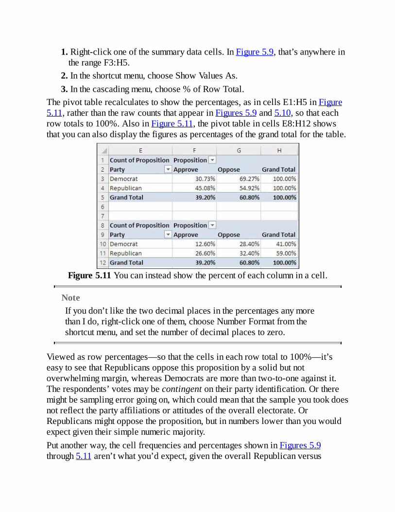
1.Right-clickoneofthesummarydatacells.InFigure5.9,that’sanywhereintherangeF3:H5.

2.Intheshortcutmenu,chooseShowValuesAs.3.Inthecascadingmenu,choose%ofRowTotal.

Thepivottablerecalculatestoshowthepercentages,asincellsE1:H5inFigure5.11,ratherthantherawcountsthatappearinFigures5.9and5.10,sothateachrowtotalsto100%.AlsoinFigure5.11,thepivottableincellsE8:H12showsthatyoucanalsodisplaythefiguresaspercentagesofthegrandtotalforthetable.

Figure5.11Youcaninsteadshowthepercentofeachcolumninacell.

NoteIfyoudon’tlikethetwodecimalplacesinthepercentagesanymorethanIdo,right-clickoneofthem,chooseNumberFormatfromtheshortcutmenu,andsetthenumberofdecimalplacestozero.

Viewedasrowpercentages—sothatthecellsineachrowtotalto100%—it’seasytoseethatRepublicansopposethispropositionbyasolidbutnotoverwhelmingmargin,whereasDemocratsaremorethantwo-to-oneagainstit.Therespondents’votesmaybecontingentontheirpartyidentification.Ortheremightbesamplingerrorgoingon,whichcouldmeanthatthesampleyoutookdoesnotreflectthepartyaffiliationsorattitudesoftheoverallelectorate.OrRepublicansmightopposetheproposition,butinnumberslowerthanyouwouldexpectgiventheirsimplenumericmajority.Putanotherway,thecellfrequenciesandpercentagesshowninFigures5.9through5.11aren’twhatyou’dexpect,giventheoverallRepublicanversus

Democraticratioof295to205.NordotheobservedcellfrequenciesfollowtheoverallpatternofApproveversusOppose,whichat304opposeto196approveapproximatestheratioofRepublicanstoDemocrats.Howcanyoutellwhatthefrequenciesineachcellwouldbeiftheyfollowedtheoverall“marginal”frequencies?Togetananswertothatquestion,westartwithabrieftourofyourlocalcardroom.

ProbabilitiesandIndependentEventsSupposethatyoudrawacardatrandomfromastandarddeckofcards.Becausethereare13cardsineachofthefoursuits,theprobabilitythatyoudrawadiamondis.25.Youputthecardbackinthedeck.Nowyoudrawanothercard,againatrandom.Theprobabilitythatyoudrawadiamondisstill.25.Asdescribed,thesearetwoindependentevents.Thefactthatyoufirstdrewadiamondhasnoeffectatallonthedenominationyoudrawnext.Underthatcircumstance,thelawsofprobabilitystatethatthechanceofdrawingtwoconsecutivediamondsis.0625,or.25times.25.Theprobabilitythatyoudrawtwocardsofanytwonamedsuits,underthesecircumstances,isalso.0625,becauseallfoursuitshavethesamenumberofcardsinthedeck.It’sthesameconceptwithafaircoin,onethathasanequalchanceofcomingupheadsortailswhenit’stossed.Headsisa50%shot,andsoistails.Whenyoutossthecoinonce,it’s.5tocomeupheads.Whenyoutossthecoinagain,it’sstill.5tocomeupheads.Becausethefirsttosshasnothingtodowiththesecond,theeventsareindependentofoneanotherandthechanceoftwoheads(oraheadsfirstandthenatail,ortwotails)is.5*.5,or.25.

NoteThegambler’sfallacyisrelevanthere.Somepeoplebelievethatifacoin,evenacoinknowntobefair,comesupheadsfivetimesinarow,thecoinis“due”tocomeuptails.Giventhatit’safaircoin,theprobabilityofheadsisstill50%onthesixthtoss.Peoplewhoindulgeinthegambler’sfallacyignorethefactthattheunusualeventhasalreadyoccurred.Thatevent,thestreakoffiveheads,isinthepast,andhasnosayaboutthenextoutcome.

Thisruleofprobabilities—thatthelikelihoodofoccurrenceoftwoindependent

eventsistheproductoftheirrespectiveprobabilities—isinplaywhenyouevaluatecontingencytables.NoticeinFigure5.11thattheprobabilityinthesampleofbeingaDemocratis41%(cellH10)andaRepublicanis59%(cellH11).Similarly,irrespectiveofpoliticalaffiliation,theprobabilitythatarespondentapprovesofthepropositionis39.2%(cellF12)andopposesit60.8%(cellG12).Ifapprovalisindependentofparty,theruleofindependenteventsstatesthattheprobabilityof,say,beingaRepublicanandapprovingthepropositionis.59*.392,or.231.SeecellE16inFigure5.12.

Figure5.12Movingfromobservedcountstoexpectedcounts.

Youcancompletetheremainderofthetable,theotherthreecellsF16,E15,andF15,asshowninFigure5.12.Then,bymultiplyingthepercentagesbythetotalcount,500,youwindupwiththenumberofrespondentsyouwouldexpectineachcellifpartyaffiliationwereindependentofattitudetowardtheproposal.TheseexpectedcountsareshownincellsE21:F22.InFigure5.12,youseethesetables:

D1:G5—ThesearetheoriginalcountsasshowninthepivottableinFigure5.9.D7:G11—Thesearetheoriginalcountsdisplayedaspercentagesofthetotalcount.Forexample,41.0%incellG9is205dividedby500,and12.6%incellE9is63dividedby500.D13:G17—Thesearethecellpercentagesasobtainedfromthemarginalpercentages.Forexample,35.9%incellF16istheresultofmultiplying60.8%incellF17(thecolumnpercentage)by59.0%incellG16(therowpercentage).Toreview,ifpartyaffiliationisindependentofattitudetowardtheproposition,thentheirjointprobabilityistheproductofthetwoindividualprobabilities.ThepercentagesshowninE15:F16aretheprobabilitiesthatareexpectedifpartyandattitudeareindependentofoneanother.D19:G23—TheexpectedcountsareinE21:F22.TheyareobtainedbymultiplyingtheexpectedpercentagesinE15:G16by500,thetotalnumberofrespondents.

Nowyouareinapositiontodeterminethelikelihoodthattheobservedcountswouldhavebeenobtainedunderanassumption:thatinthepopulation,thereisnorelationshipbetweenpartyaffiliationandattitudetowardtheproposition.Thenextsectionshowsyouhowthat’sdone.

TestingtheIndependenceofClassificationsPriorsectionsofthischapterdiscussedhowyouusethebinomialdistributiontotesthowlikelyitisthatanobservedproportioncomesfromanassumed,hypotheticaldistribution.Thetheoreticalbinomialdistributionisbasedontheuseofonefieldthathasonlytwopossiblevalues.Butwhenyou’redealingwithacontingencytable,you’redealingwithatleasttwofields(andeachfieldcancontaintwoormorecategories).Theexamplethat’sbeendiscussedsofarconcernstwofields:partyaffiliationandattitudetowardaproposition.AsI’llexplainshortly,theappropriatedistributionthatyourefertointhisandsimilarcasesiscalledthechi-square(pronouncedkaisquare)distribution.

UsingtheCHISQ.TEST()FunctionExcelhasaspecialchi-squaretestthatiscarriedoutbyafunctionnamedCHISQ.TEST().ItwasnewinExcel2010,butonlythenamewasnew.Ifyou’reusinganearlier

versionofExcel,youcanuseCHITEST()instead.Thetwofunctionstakethesameargumentsandreturnthesameresults.CHITEST()isretainedasaso-called“compatibilityfunction”inExcel2010and2013.InExcel2010and2013,youuseCHISQ.TEST()bypassingtheobservedandtheexpectedfrequenciestoitasarguments.WiththedatalayoutshowninFigure5.12,youwoulduseCHISQ.TEST()asfollows:

=CHISQ.TEST(E3:F4,E21:F22)TheobservedfrequenciesareincellsE3:F4,andtheexpectedfrequencies,derivedasdiscussedinthepriorsection,areincellsE21:F22.TheresultoftheCHISQ.TEST()functionistheprobabilitythatyouwouldgetobservedfrequenciesthatdifferbyasmuchasthisfromtheexpectedfrequencies,ifpoliticalaffiliationandattitudetowardthepropositionareindependentofoneanother.Inthiscase,CHISQ.TEST()returns0.001.Thatis,assumingthatthepopulation’spatternoffrequenciesisasshownincellsE21:F22inFigure5.12,youwouldgetthepatternincellsE3:F4inonly1of1,000samplesobtainedinasimilarway.Whatconclusioncanyoudrawfromthat?Theexpectedfrequenciesarebasedontheassumptionthatthefrequenciesintheindividualcells(suchasE3:F4)followthemarginalfrequencies.IftherearetwiceasmanyRepublicansasDemocrats,thenyouwouldexpecttwiceasmanyRepublicansinfavorthanDemocratsinfavor.Similarly,youwouldexpecttwiceasmanyRepublicansopposedasDemocratsopposed.Inotherwords,yournullhypothesisisthattheexpectedfrequenciesareinfluencedbynothingotherthanthefrequenciesonthemargins:thatpartyaffiliationisindependentofattitudetowardtheproposal,andthedifferencesbetweenobservedandexpectedfrequenciesisduesolelytosamplingerror.If,however,somethingelseisgoingon,thatmightpushtheobservedfrequenciesawayfromwhatyou’dexpectifattitudeisindependentofparty.TheresultoftheCHISQ.TEST()functionsuggeststhatsomethingelseisgoingon.It’simportanttorecognizethatthechi-squaretestitselfdoesnotpinpointtheobservedfrequencieswhosedeparturefromtheexpectedcausesthisexampletorepresentanimprobableoutcome.AllthatCHISQ.TEST()tellsusisthatthepatternofobservedfrequenciesdiffersfromwhatyouwouldexpectonthebasisofthemarginalfrequenciesforaffiliationandattitude.It’suptoyoutoexaminethefrequenciesanddecidewhythesurveyoutcomeindicatesthatthereisanassociationbetweenthetwovariables,thattheyarenotinfactindependentofoneanother.

Forexample,doessomethingaboutthepropositionmakeitevenmoreunattractivetoDemocratsthantoRepublicans?Certainlythat’sareasonableconclusiontodrawfromthesenumbers.Butyouwouldsurelywanttolookatthepropositionandthenatureofthepublicityithasreceivedbeforeyouplacedanyconfidenceinthatconclusion.Thissituationhighlightsoneoftheproblemswithnonexperimentalresearch.Surveysentailself-selection.TheresearchercannotrandomlyassignrespondentstoeithertheRepublicanortheDemocraticpartyandthenaskfortheirattitudetowardapoliticalproposition.Ifonevariableweredietandtheothervariablewereweight,itwouldbepossible—intheoryatleast—toconductacontrolledexperimentanddrawasoundconclusionaboutwhetherdifferencesinfoodintakecausedifferencesinweight.Butsurveyresearchisalmostneversoclearcut.There’sanotherdifficultythatthischapterwilldealwithinthesectiontitled“TheYuleSimpsonEffect.”

UnderstandingtheChi-SquareDistributionFigures5.3and5.4showhowtheshapeofthebinomialdistributionchangesasthesamplesizechangesandthenumberofsuccesses(intheexample,thenumberofdefects)inthepopulationchanges.Thedistributionofthechi-squarestatisticalsochangesaccordingtothenumberofobservationsinvolved(seeFigure5.13).

Figure5.13Thedifferencesintheshapesofthedistributionsareduesolelytotheirdegreesoffreedom.

ThethreecurvesinFigure5.13showthedistributionofchi-squarewithdifferentnumbersofdegreesoffreedom.Supposethatyousampleavalueatrandomfromanormallydistributedpopulationofvalueswithaknownmeanandstandarddeviation.Youcreateaz-score,asdescribedinChapter3,“Variability:HowValuesDisperse,”subtractingthemeanfromthevalueyousampled,anddividingbythestandarddeviation.Here’stheformulaoncemore,forconvenience:

Nowyousquarethez-score.Whenyoudoso,youhaveavalueofchi-square.Inthiscase,ithasonedegreeoffreedom.Ifyousquaretwoindependentz-scoresandsumthesquares,thesumisachi-squarewithtwodegreesoffreedom.Generally,thesumofnsquaredindependentz-scoresisachi-squarewithndegreesoffreedom.InFigure5.13,thecurvethat’slabeleddf=4isthedistributionofrandomlysampledgroupsoffoursquared,summedz-scores.Thecurvethat’slabeleddf=8

isthedistributionofrandomlysampledgroupsofeightsquared,summedz-scores,andsimilarlyforthecurvethat’slabeleddf=10.AsFigure5.13suggests,themorethedegreesoffreedominasetofchi-squares,themorecloselythetheoreticaldistributionresemblesanormalcurve.Noticethatwhenyousquarethez-score,thedifferencebetweenthesampledvalueandthemeanissquaredandisthereforealwayspositive:

Sothefartherawaythesampledvaluesarefromthemean,thelargerthecalculatedvaluesofchi-square.Themeanofachi-squaredistributionisn,itsdegreesoffreedom.Thestandarddeviationofthedistributionis .Asisthecasewithotherdistributions,suchasthenormalcurve,thebinomialdistribution,andothersthatthisbookcoversinsubsequentchapters,youcancompareachi-squarevaluethatiscomputedfromsampledatatothetheoreticalchi-squaredistribution.Ifyouknowthechi-squarevaluethatyouobtainfromasample,youcancompareittothetheoreticalchi-squaredistributionthat’sbasedonthesamenumberofdegreesoffreedom.Youcantellhowmanystandarddeviationsitisfromthemean,andinturnthattellsyouhowlikelyitisthatyouwillobtainachi-squarevalueaslargeastheoneyouhaveobserved.Ifthechi-squarevaluethatyouobtainfromyoursampleisquitelargerelativetotheoreticalmean,youmightabandontheassumptionthatyoursamplecomesfromapopulationdescribedbythetheoreticalchi-square.Intraditionalstatisticaljargon,youmightrejectthenullhypothesis.Itisbothpossibleandusefultothinkofaproportionasakindofmean.Supposethatyouhaveaskedasampleof100possiblevoterswhethertheyvotedinthepriorelection.Youfindthat55ofthemtellyouthattheydidvote.Ifyouassignedavalueof1ifapersonvotedand0ifnot,thenthesumofthevariableVotedwouldbe55,anditsaveragewouldbe0.55.Ofcourse,youcouldalsosaythat55%ofthesamplevotedlasttimeout,andinthatcasethetwowaysoflookingatitareequivalent.Therefore,youcouldrestatethez-scoreformulaintermsofproportionsinsteadofmeans:z=(p–π)/sπInthisequation,theletterp(forproportion)replacesXandtheletterπreplaces.Thestandarddeviationinthedenominator,sπ,dependsonthesizeofπ.When

yourclassificationschemeisbinomial(suchasvotedversusdidnotvote),the

standarddeviationoftheproportionis

wherenisthesamplesize.So,thez-scorebasedonproportionsbecomesthis:

Here’sthechi-squarevaluethatresults:x2=(p–π)2/(π*(1–π)/n)

Inmanysituations,thevalueofpistheproportionthatyouobserveinyoursample,whereasthevalueofπisahypotheticalvaluethatyou’reinvestigating.Thevalueofπcanalsobethevalueofaproportionthatyouwouldexpectiftwomethodsofclassification,suchaspoliticalpartyandattitudetowardaballotproposal,areindependentofoneanother.That’sthemeaningofπdiscussedinthissection.Thediscussioninthissectionhasbeenfairlyabstract.Thenextsectionshowshowtoputtheconceptsintopracticeonaworksheet.

UsingtheCHISQ.DIST()andCHISQ.INV()FunctionsTheCHISQ.TEST()functionreturnsaprobabilityvalueonly.Thatcanbeveryhandyifallyou’reafteristheprobabilityofobservingtheactualfrequenciesassumingthereisnodependencebetweenthetwovariables.Butit’susuallybesttodothespadeworkandcalculatethevalueofthechi-squarestatistic.Ifyoudoso,you’llgetmoreinformationbackandyoucanbecleareraboutwhat’sgoingon.Furthermore,it’seasiertopinpointthelocationofanyproblemsthatmightexistinyoursourcedata.Theprocessofusingchi-squaretotestanullhypothesisisdescribedverysparinglyinthepriorsection.Thissectiongoesmorefullyintothematter.Figure5.14repeatssomeoftheinformationinFigure5.12.

Figure5.14Theexpectedcountsarebasedonthehypothesisthatpoliticalpartyandattitudetowardthepropositionareindependentofoneanother.

Inthisexample,ExcelteststheassumptionthatyouwouldhaveobservedthecountsshownincellsE3:F4ofFigure5.14ifpoliticalpartyandattitudetowardthepropositionwereunrelatedtooneanother.Iftheywere,ifthenullhypothesisweretrue,thenthecountsyouwouldexpecttoobtainaretheonesshownincellsE9:F10.Thereareseveralalgebraicallyequivalentwaystogoaboutcalculatingachi-squarestatisticwhenyou’reworkingwithacontingencytable(atablesuchastheonesshowninFigure5.14).Somemethodsworkdirectlywithcellfrequencies,someworkwithproportionsinsteadoffrequencies,andonesimplifiedformulaisintendedforuseonlywithatwo-by-twotable.Ichosetousetheoneusedherebecauseitemphasizesthecomparisonbetweentheobservedandtheexpectedcellfrequencies.TheformoftheequationusedinFigure5.14is

where

kindexeseachcellinthetable.fo,kistheobservedcount,orthefrequency,ineachcell.

fe,kistheexpectedfrequencyineachcell.So,foreachcell:

1.Subtracttheexpectedfrequencyfromtheobservedfrequency.2.Squarethedifference.3.Dividetheresultbythecell’sexpectedfrequency.

Totaltheresultstogetthevalueofchi-square.ThisprocedureisshowninFigure5.14,wherecellsE13:F14showtheresultsofthethreestepsjustgivenforeachcell.CellE16containsthesumofE13:F14andisthechi-squarevalueitself.

TipYoucancombinethethreestepsjustgivenforeachcell,plustotalingtheresults,intoonestepbyusinganarrayformula.AsthedataislaidoutinFigure5.14,thisarrayformulaprovidesthechi-squarevalueinonestep:=SUM((E3:F4-E9:F10)^2/E9:F10)Recallthattoarray-enteraformula,youuseCtrl+Shift+EnterinsteadofsimplyEnter.

CellE17containstheCHISQ.DIST.RT()function,withthechi-squarevalueinE16asoneargumentandthedegreesoffreedomforchi-square,whichis1inthiscase,asthesecondargument.Chi-square,whenusedinthisfashion,hasdegreesoffreedomthatistheproductofthenumberofcategoriesinonefield,minus1,andthenumberofcategoriesintheotherfield,minus1.Inotherwords,supposethatthereareJlevelsofpoliticalpartyandKlevelsofattitudetowardtheballotproposition.Thenthischi-squaretesthas(J–1)*(K–1)degreesoffreedom.Becauseeachfieldhastwocategories,thetesthas(2–1)*(2–1)or1degreeoffreedom.Theprobabilityofobservingthesefrequenciesifthetwocategoriesareindependentisabout1in1,000.Notethatthenumberofcasesinthecellshasnobearingonthedegreesoffreedomforthistest.Allthatmattersisthenumberoffieldsandthenumberofcategoriesineachfield.

TheYuleSimpsoneffectIntheearly1970s,acausecélèbreputalittle-knownstatisticalphenomenononthefrontpages—atleastonthefrontpagesoftheBerkeleystudentnewspapers.AlawsuitwasbroughtagainsttheUniversityofCalifornia,allegingthatdiscriminationagainstwomenwasoccurringintheadmissionsprocessattheBerkeleycampus.Figure5.15presentsthedamningevidence.

Figure5.15MenwereadmittedtograduatestudyatBerkeleywithdisproportionatefrequency.

In1973,44%ofmenwereadmittedtograduatestudyatBerkeley,comparedtoonly35%ofwomen.Thisisprettyclearprimafacieevidenceofsexdiscrimination.TheexpectedfrequenciesareshownincellsH3:I4andaretestedagainsttheobservedfrequencies,returningachi-squareof111.25incellC8.TheCHISQ.DIST.RT()functionreturnsaprobabilityoflessthan.001forsuchalargechi-squarewith1degreeoffreedom.Thismakesitveryunlikelythatadmissionandsexwereindependentofoneanother.TheOJSimpsonjurytooklongerthanaBerkeleyjurywouldhave.SomeBerkeleyfacultyandstaff(Bickel,Hammel,andO’Connell,1975)gotinvolvedand,usingworkdonebyKarlPearson(ofthePearsoncorrelationcoefficient)andaScotnamedUdnyYule,dugmoredeeplyintothenumbers.Theyfoundthatwheninformationaboutadmissionstospecificdepartmentswasincluded,theapparentdiscriminationdisappeared.Furthermore,moreoftenthannotwomenenjoyedhigheradmissionratesthandidmen.Figure5.16showssomeofthatadditionaldata.

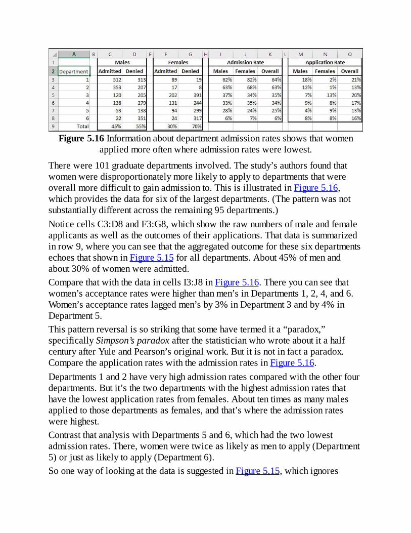
Figure5.16Informationaboutdepartmentadmissionratesshowsthatwomenappliedmoreoftenwhereadmissionrateswerelowest.

Therewere101graduatedepartmentsinvolved.Thestudy’sauthorsfoundthatwomenweredisproportionatelymorelikelytoapplytodepartmentsthatwereoverallmoredifficulttogainadmissionto.ThisisillustratedinFigure5.16,whichprovidesthedataforsixofthelargestdepartments.(Thepatternwasnotsubstantiallydifferentacrosstheremaining95departments.)NoticecellsC3:D8andF3:G8,whichshowtherawnumbersofmaleandfemaleapplicantsaswellastheoutcomesoftheirapplications.Thatdataissummarizedinrow9,whereyoucanseethattheaggregatedoutcomeforthesesixdepartmentsechoesthatshowninFigure5.15foralldepartments.About45%ofmenandabout30%ofwomenwereadmitted.ComparethatwiththedataincellsI3:J8inFigure5.16.Thereyoucanseethatwomen’sacceptancerateswerehigherthanmen’sinDepartments1,2,4,and6.Women’sacceptancerateslaggedmen’sby3%inDepartment3andby4%inDepartment5.Thispatternreversalissostrikingthatsomehavetermedita“paradox,”specificallySimpson’sparadoxafterthestatisticianwhowroteaboutitahalfcenturyafterYuleandPearson’soriginalwork.Butitisnotinfactaparadox.ComparetheapplicationrateswiththeadmissionratesinFigure5.16.Departments1and2haveveryhighadmissionratescomparedwiththeotherfourdepartments.Butit’sthetwodepartmentswiththehighestadmissionratesthathavethelowestapplicationratesfromfemales.Abouttentimesasmanymalesappliedtothosedepartmentsasfemales,andthat’swheretheadmissionrateswerehighest.ContrastthatanalysiswithDepartments5and6,whichhadthetwolowestadmissionrates.There,womenweretwiceaslikelyasmentoapply(Department5)orjustaslikelytoapply(Department6).SoonewayoflookingatthedataissuggestedinFigure5.15,whichignores

departmentaldifferencesinadmissionrates:Women’sapplicationsaredisproportionatelyrejected.AnotherwayoflookingatthedataissuggestedinFigure5.16:Somedepartmentshaverelativelyhighadmissionrates,andadisproportionatelylargenumberofmenapplytothosedepartments.Otherdepartmentshaverelativelylowadmissionrates,regardlessoftheapplicant’ssex,andadisproportionatelylargenumberofwomenapplytothosedepartments.Neitherthisanalysisnortheoriginal1975paperproveswhyadmissionratesdiffer,eitherinmen’sfavorintheaggregateorinwomen’sfavorwhendepartmentinformationisincluded.Alltheyproveisthatyouhavetobeverycarefulaboutassumingthatonevariablecausesanotherwhenyou’reworkingwithsurveydataorwith“grabsamples”—thatis,samplesthataresimplycloseathandandthereforeconvenient.TheBerkeleygraduateadmissionsdataisfarfromtheonlypublishedexampleoftheYuleSimpsoneffect.Studiesintheareasofmedicine,education,andsportshaveexhibitedsimilaroutcomes.Idon’tmeantoimplythattheuseofatrueexperimentaldesign,withrandomselectionandrandomassignmenttogroups,wouldhavepreventedtheinitialerroneousconclusionintheBerkeleycase.Anexperimenterwouldhavetodirectstudentstoapplytorandomlyselecteddepartments,whichisclearlyimpractical.(Alternatively,bogusapplicationswouldhavetobemadeandevaluated,afterwhichtheexperimenterwouldhavedifficultyfindinganothertestbedforfutureresearch.)Althoughatrueexperimentaldesignusuallymakesitpossibletointerpretresultssensibly,it’snotalwaysfeasible.

SummarizingtheChi-SquareFunctionsInversionsofExcelpriortoExcel2010,justthreefunctionsaredirectlyconcernedwithchi-square:CHIDIST(),CHIINV(),andCHITEST().Theirpurposes,results,andargumentsarecompletelyreplicatedbyfunctionsintroducedinExcel2010.Thosenew“consistency”functionsarediscussednext,andtheirrelationshipstotheolder,“compatibility”functionsarealsonoted.

UsingCHISQ.DIST()TheCHISQ.DIST()functionreturnsinformationabouttheleftsideofthechi-squaredistribution.Youcancallforeithertherelativefrequencyofachi-squarevalueorthecumulativefrequency—thatis,thecumulativeareaorprobability—atthechi-squarevalueyousupply.

Note

Excelfunctionsreturncumulativeareasthataredirectlyinterpretableastheproportionofthetotalareaunderthecurve.Therefore,theycanbetreatedascumulativeprobabilities,fromtheleftmostpointonthecurve’shorizontalaxisthroughthevaluethatyouhaveprovidedtothefunction,suchasthechi-squarevaluetoCHISQ.DIST().

ThesyntaxoftheCHISQ.DIST()functionis=CHISQ.DIST(X,Df,Cumulative)

where:Xisthechi-squarevalue.Dfisthedegreesoffreedomforchi-square.Cumulativeindicateswhetheryouwantthecumulativeareaortherelativefrequency.

IfyousetCumulativetoTRUE,thefunctionreturnsthecumulativeareatotheleftofthechi-squareyousupply,andistheprobabilitythatthischi-squareorasmalleronewilloccuramongthechi-squarevalueswithagivennumberofdegreesoffreedom.Becauseofthewaymosthypothesesareframed,it’susualthatyouwanttoknowthearea—theprobability—totherightofagivenchi-squarevalue.Therefore,you’remorelikelytowanttouseCHISQ.DIST.RT()thanCHISQ.DIST()—see“UsingCHISQ.DIST.RT()andCHIDIST()”foradiscussionofCHISQ.DIST.RT().IfyousetCumulativetoFALSE,thefunctionreturnstherelativefrequencyofthespecificchi-squarevalueinthefamilyofchi-squareswiththedegreesoffreedomyouspecified.Youseldomneedthisinformationforhypothesistesting,butit’sveryusefulforchartingchi-square,asshowninFigure5.17.

Figure5.17CHISQ.DIST()returnstheheightofthecurvewhenCumulativeisFALSE,andreturnstheareaunderthecurvewhenCumulativeisTRUE.

NoteTheonlychi-squarefunctionwithaCumulativeargumentisCHISQ.DIST().ThereisnoCumulativeargumentforCHISQ.INV()andCHISQ.INV.RT()becausetheyreturnaxispoints,notvaluesthatrepresenteitherrelativefrequencies(theheightofthecurve)orprobabilities(theareaunderthecurve,whichyoucallforbysettingtheCumulativeargumenttoTRUE).ThereisnoCumulativeargumentforCHISQ.DIST.RTbecausethecumulativeareaisthedefaultresult;youcangetthecurveheightatagivenchi-squarevalueusingCHISQ.DIST().

UsingCHISQ.DIST.RT()andCHIDIST()

TheconsistencyfunctionCHISQ.DIST.RT()andthecompatibilityfunctionCHIDIST()areequivalentastoarguments,usage,andresults.Thesyntaxis

=CHISQ.DIST.RT(X,Df)where:

Xisthechi-squarevalue.Dfisthedegreesoffreedomforchi-square.

ThereisnoCumulativeargument.CHISQ.DIST.RT()andCHIDIST()bothreturncumulativeareasonly,anddonotreturnrelativefrequencies.TogetrelativefrequenciesyouwoulduseCHISQ.DIST()andsetCumulativetoFALSE.CHISQ.DIST()iscloselyrelatedtoCHISQ.DIST.RT(),asyoumightexpect.CHISQ.DIST()equals1–CHISQ.DIST.RT().Whenyouwanttotestanullhypothesisusingchi-square,ashasbeendoneearlierinthischapter,it’slikelythatyouwillwanttouseCHISQ.DIST.RT()or,equivalently,CHIDIST().Thelargerthedepartureofasampleobservationfromapopulationparametersuchasaproportion,thelargertheassociatedvalueofchi-square.(Recallthattocalculatechi-square,yousquarethedifferencebetweenthesampleobservationandtheparameter,therebyeliminatingnegativevalues.)Therefore,underanullhypothesissuchasthatoftheindependenceoftwofieldsinacontingencytable,youwouldwanttoknowthelikelihoodofarelativelylargechi-squarevalue.AsyoucanseeinFigure5.18,achi-squareof10(cellA22)isfoundintherightmost4%(cellB22)ofachi-squaredistributionthathas4degreesoffreedom(cellE1).

Figure5.18Thefarthertotherightyougetinachi-squaredistribution,thelargerthevalueofchi-squareandthelesslikelyyouaretoobservethatvaluepurelyby

chance.

Thattellsyouthatonly4%ofsamplesfromapopulationwheretwovariables,ofthreelevelseach,areindependentofoneanotherwouldresultinachi-squarevalueaslargeas10.Soit’s96%to4%,or24to1,againstachi-squareof10underwhatevernullhypothesisyouhaveadopted:forexample,noassociationbetweenclassificationsinathree-by-threecontingencytable.

UsingCHISQ.INV()CHISQ.INV()returnsthechi-squarevaluethatdefinestherightborderoftheareainthechi-squaredistributionthatyouspecify,forthedegreesoffreedomthatyouspecify.Thesyntaxis

=CHISQ.INV(Probability,Df)where:

Probabilityistheareainthechi-squaredistributiontotheleftofthechi-squarevaluethatthefunctionreturns.Dfisthenumberofdegreesoffreedomforthechi-squarevalue.

So,theexpressionCHISQ.INV(.3,4)returnsthechi-squarevaluethatdividestheleftmost30%oftheareafromtherightmost70%oftheareaunderthechi-squarecurvethathas4degreesoffreedom.Recallthatthechi-squaredistributionisbuiltonsquaredz-scores,whichthemselvesinvolvethedifferencebetweenanobservationandameanvalue.Yourinterestintheprobabilityofobservingagivenchi-squarevalue,andyourinterestinthatchi-squarevalueitself,usuallycentersonareasthatareintherighttailofthedistribution.Thisisbecausethelargerthedifferencebetweenanobservationandameanvalue—whetherthatdifferenceispositiveornegative—thelargerthevalueofchi-square,becausethedifferenceissquared.Therefore,younormallyask,“Whatistheprobabilityofobtainingachi-squarethislargeifmynullhypothesisistrue?”Youdonottendtoask,“Whatistheprobabilityofobtainingachi-squarevaluethissmallifmynullhypothesisistrue?”Inconsequence,andasapracticalmatter,youwillnothavemuchneedfortheCHISQ.INV()function.Itreturnschi-squarevaluesthatboundtheleftendofthedistribution,butyourinterestisnormallyfocusedontherightend.

UsingCHISQ.INV.RT()andCHIINV()AsisthecasewithBINOM.DIST(),CHISQ.DIST.RT()returnstheprobability;yousupplythechi-squarevalueanddegreesoffreedom.AndaswithBINOM.INV(),CHISQ.INV.RT()returnsthechi-squarevalue;yousupplytheprobabilityandthedegreesoffreedom.(SodoestheCHIINV()compatibilityfunction.)Thiscanbehelpfulwhenyouknowtheprobabilitythatyouwillrequiretorejectanullhypothesis,andsimplywanttoknowwhatvalueofchi-squareisneededtodoso,giventhedegreesoffreedom.Thesetwoprocedurescometothesamething:

Determineacriticalvalueforchi-squarebeforeanalyzingtheexperimentaldata—Decideinadvanceonaprobabilityleveltorejectanullhypothesis.Determinethedegreesoffreedomforyourtestbasedonthe

designofyourexperiment.UseCHISQ.INV.RT()tofixacriticalvalueofchi-squareinadvance,giventheprobabilitylevelyourequireandthedegreesoffreedomimpliedbythedesignofyourexperiment.Comparethechi-squarefromyourexperimentaldatawiththecriticalvalueofchi-squarefromCHISQ.INV.RT()andretainorrejectthenullhypothesisaccordingly.Thisisaformal,traditionalapproach,andenablesyoutostatewithalittlemoreassurancethatyousettledonyourdecisionrulesbeforeyousawtheexperimentaloutcome.Decidebeforehandontheprobabilitylevelonly—Selecttheprobabilityleveltorejectanullhypothesisinadvance.Calculatethechi-squarefromtheexperimentaldataanduseCHISQ.DIST.RT()andthedegreesoffreedomtodeterminewhetherthechi-squarevaluefallswithintheareainthechi-squaredistributionimpliedbytheprobabilitylevelyouselected.Retainorrejectthenullhypothesisaccordingly.Thisapproachisn’tquitesoformal,butitresultsinthesameoutcomeasdecidingbeforehandonacriticalchi-squarevalue.Bothapproacheswork,andit’smoreimportantthatyouseewhytheyareequivalentthanforyoutodecidewhichoneyouprefer.

UsingCHISQ.TEST()andCHITEST()TheCHISQ.TEST()consistencyfunctionandtheCHITEST()compatibilityfunctionbothreturntheprobabilityofobservingapatternofcellcountsinacontingencytablewhentheclassificationmethodsthatdefinethetableareindependentofoneanother.Forexample,intermsoftheBerkeleystudycitedearlierinthischapter,thoseclassificationsaresexandadmissionstatus.ThesyntaxofCHISQ.TEST()is

=CHISQ.TEST(observedfrequencies,expectedfrequencies)whereeachargumentisaworksheetrangeofvaluessuchthattherangeshavethesamedimensions.TheargumentsforCHITEST()areidenticaltothoseforCHISQ.TEST().Theexpectedfrequenciesarefoundbytakingtheproductoftheassociatedmarginalvaluesanddividingbythetotalfrequency.Figure5.19showsonewaythatyoucangeneratetheexpectedfrequencies.

Figure5.19Ifyousetuptheinitialformulaproperlywithmixedandabsolutereferences,youcaneasilycopyandpasteittocreatetheremainingformulas.

InFigure5.19,cellsH3:J5displaytheresultsofformulasthatmakeuseoftheobservedfrequenciesincellsB3:E5.TheformulasinH3:J5aredisplayedincellsH10:J12.TheformulaincellH3is=$D3*B$5/$D$5.Ignoreforamomentthedollarsignsthatresultinmixedandabsolutecellreferences.ThisformulainstructsExceltomultiplythevalueincellD3(thetotalmen)bythevalueincellB5(thetotaladmitted)anddividebythevalueincellD5(thetotalofthecellfrequencies).Theresultoftheformula,3461,iswhatyouwouldestimatetobethenumberofmaleadmissionsifallyouknewwasthenumberofmen,thenumberofadmissions,thenumberapplying,andthatsexandadmissionstatuswereindependentofoneanother.Theotherthreeestimatedcellsarefilledinviathesameapproach:Multiplythemarginalfrequenciesforeachcellanddividebythetotalfrequency.

UsingMixedandAbsoluteReferencestoCalculateExpectedFrequenciesNownoticethemixedandabsolutereferencinginthepriorformulaforcellH3.Thecolumnmarginal,cellD3,ismadeamixedreferencebyanchoringitscolumnonly.Therefore,youcancopyandpaste,ordraganddrop,theformulatotherightwithoutchangingthereferencetotheTotalAdmittedcolumn,columnD.Similarly,therowmarginal,cellB5,ismadeamixedreferencebyanchoringits

rowonly.Youcancopyandpasteitdownwithoutchangingitsrow.Lastly,thetotalfrequenciescell,D5,ismadeabsolutebyanchoringbothitsrowandcolumn.YoucancopytheformulaanywhereandthepastedformulawillstilldividebythevalueinD5.Noticehoweasythismakesthings.IfyoutakethepriorformulainH3:

=$D3*B$5/$D$5anddragitonecolumntotheright,yougetthisformula:

=$D3*C$5/$D$5TheresultistomultiplybyC5insteadofB5,bytotaldeniedinsteadoftotaladmitted.YoucontinuetouseD3,totalmen.Andtheresultistheestimateofthenumberofmendeniedadmission.AndifyoudragitonerowdownintoH4,yougetthisformula:

=$D4*B$5/$D$5NowyouareusingcellD4,totalwomeninsteadoftotalmen.YoucontinuetouseB5,totaladmitted.Andtheresultistheestimateofthenumberofwomenadmitted.Inshort,ifyousetupyouroriginalformulaproperlywithmixedandabsolutereferences,it’stheonlyoneyouneedtowrite.Afteryou’vedonethat,dragitrighttofillintheremainingcellsinitsrow.Thendragthosecellsdowntofillintheremainingcellsintheircolumns.Withtherangethatcontainstheobservedfrequenciesandtherangethatcontainsthecomputed,expectedfrequencies,youcanuseCHISQ.TEST()todeterminetheprobabilityofobservingthosefrequenciesgiventheexpectedfrequencies,whichassumenodependencebetweensexandadmissionstatus:

=CHISQ.TEST(B3:C4,H3:I4)Asnotedearlierinthechapter,youbypassthecalculationofthechi-squarevalueitselfandgettheprobabilitydirectlyinthecellwhereyouentertheCHISQ.TEST()function.There’snoneedtosupplythedegreesoffreedombecauseCHISQ.TEST()cancalculatethemitself,notingthenumberofrowsandcolumnsineithertheobservedorintheexpectedfrequenciesrange.

UsingthePivotTable’sIndexDisplayAseasyasitistogeneratetheexpectedfrequenciesinatwo-by-twocontingencytable,itcangetcomplicatedwhenyou’redealingwithmorerowsandcolumns,orwithadifferentnumberofrowsandcolumns,orwithathirdclassification.

Ifyouroriginaldataisintheformofalistthatyou’veusedtocreateapivottable,youcandisplaythecountsasanIndex.Thissimplifiesthetaskofgettingtheexpectedfrequencies.Figure5.20showsanexample.

Figure5.20TheIndexdisplayhelpsyoumovefromobservedtoexpectedfrequencies.

ThefirstpivottableinFigure5.20showsthenormalresultofshowingthecountincellsdefinedbytwonominalvariables.ItrepeatstheanalysisshowninFigure5.9.Thesecondpivottable,foundinE8:H12,usesthesamesourcedataasthefirstpivottableandisstructuredidentically.However,itshowswhatExceltermstheIndex.Togetthatdisplay,takethesesteps:

1.Replicatethefirstpivottable.Youcaneitherbuildasecondpivottablefromscratchorsimplycopyandpastethefirstpivottable.

2.Right-clickinanyoneofthesummarycellsofthesecondpivottable.TheshortcutmenucontainsaShowValuesAsitem.

3.MoveyourmousepointerovertheShowValuesAsitemtodisplayacascadingmenuthatcontainstheIndexitem.ClickIndex.

NoteIfyou’reusingExcel2007,followtheinstructionsinthenoteinthis

chapter’s“UnderstandingOne-WayPivotTables”section.ChooseIndexfromtheShowValuesAsdrop-down.

Thefinaltaskistodividetheobservedfrequenciesbytheindexvalues.ThatisdoneincellsF14:G15ofFigure5.20bymeansofthisarrayformula:

=F3:G4/F10:G11Theresultistheexpectedcellfrequencies,basedonthemarginalfrequencies,assumingnodependencybetweensexandadmissionstatus.Thereisnoneedtostructureaninitialformulaproperly,eitherastopointingitatthecorrectmarginalfrequenciesorastochangingthecorrectcellreferencesfromrelativetomixed.

6.TellingtheTruthwithStatistics

InThisChapterAContextforInferentialStatisticsProblemswithExcel’sDocumentationTheF-TestTwo-SampleforVariances

SeveraldecadesagoamannamedDarrellHuffwroteabooktitledHowtoLiewithStatistics.Thebookdescribesavarietyofamusingwaysthatsomepeople,oftenunintentionally,usestatisticsinwaysthatmisleadotherpeople.IglancedthroughHuff’sbookagainasIwaspreparingthisbook(althoughIwasn’tyetinkindergartenwhenitwaspublished),anditremindedmethatmanyofthewaystherearetogowrongwithstatisticshavetodowithcontext.Withthenextchapter,thisbookmovesfromthecontextofdescriptivestatisticsintothatofinferentialstatistics—makinginferencesaboutpopulationsfromobservationsofsamples.BeforeIstarttogetintothenutsandboltsofinferentialstatisticsinExcel,Ithinkit’simportanttotakealookathowtheinappropriateuseofbothdescriptiveandinferentialstatisticalanalysiscanmislead.Ibelievethattwobroadsourcesofproblemswithempiricalresearchgetinourway:

ObtainingthedatabymeansofaweakexperimentaldesignMisunderstandinghowtheanalysissoftwareworks,orthemeaningofitsresults

Therefore,I’mgoingtospendhalfthischaptertalkingaboutthecontextofstatisticalanalysis:howyougoaboutcreatingasituationinwhichstatisticscanhaveactualmeaning.Whennumbersaregatheredoutsidethecontextofastrongexperimentaldesign,theirmeaningissuspect.Worse,asHuffnoted,theycaneasilymislead.Yourstrongestapproachtoarrangingtherightcontextistoattendtopossiblethreatstothevalidityofyourresearch,andastrongdesignisyourbestmeansofdealingwiththosethreats.I’mgoingtospendtheotherhalfofthischapterdiscussingproblemswithhowExcelimplementsanddocumentssometoolsthatareintendedtoautomatevariousstatisticalanalyses.You’reprobablynotreadingthisbook—oratleastthisfarinthebook—togeta

senseforhowandwhystatisticalanalysisismeaningless.AllIcandoisencourageyoutoreadthischapterandtakeatleastsomeofittoheart.Withouttherightframeworkforanexperiment,thenumericanalysisoftheresultsistrulymeaningless:awasteoftimeforboththeresearcherandtheconsumeroftheresearch.Andthere’snoquickerwaytolosecredibilityinanyresearchcommunitythantoassumethatthesoftwareknowswhatit’sdoing.

AContextforInferentialStatisticsStatisticsprovidesawaytostudyhowpeopleandthingsrespondtotheworldand,assuch,it’safascinating,annoying,andsometimescontraryfieldtoworkin.Descriptivestatisticsinparticularseemstoexerciseapeculiarholdoversomepeople.Somesportsfansareabletorattleofftheyearlybattingaverages,quarterbackratings,and/orassistspergameachievedbytheirfavoriteplayers.Inthecloselyrelatedareaofinferentialstatistics,therearespecialtiessuchastestconstructionthatdependheavilyonthemeasurementofmeans,standarddeviations,andcorrelationstocreateteststhatnotonlymeasurewhattheyaresupposedtobutdosowithgoodaccuracy.Butit’stheareaofhypothesistestingthatmostpeoplereadingthisbookthinkofwhentheyencounterthetermstatistics.That’snaturalbecausetheyfirstencounteredstatisticalinferencewhentheyreadaboutexperimentsintheirintroductorypsychologyclasses,andlateroninpsychlabswheretheyconductedtheirownresearch,collectedtheirowndata,andusedinferentialstatisticstosummarizethenumbersandgeneralizefromthem.Andthat’sashame—butit’sunderstandablebecausestatisticsisusuallybadlytaughtasanundergraduatecourse.Perhapsyourexperiencewasdifferent—Ihopeso—butmanypeoplewantnomorecoursesinstatisticsaftercompletingtheircollegeordepartment’srequirement.Certainlythatwasmyownexperienceatasmall,fairlywellregardedliberalartscollegequiteafewyearsago.Itwasn’tuntilIreachedgraduateschoolandstartedtakingstatisticsfrompeoplewhoactuallyknewwhattheyweretalkingaboutthatIdevelopedarealinterestinthetopic.Still,statisticsseemstoexertastrangleholdonempiricalresearchatcollegesanduniversities,andthat’sacaseofthetailwaggingthedog.Whenitcomestoactuallydoingresearch,it’sarguablethatstatisticsistheleastimportanttoolinyourkit.Ifeelentirelycomfortablemakingthatargument.I’vespentyearsreadingreportsofresearchthatexpendedlargeamountsofeffortonstatisticalanalysis.Butthe

sameresearchspentverylittleeffortbuildingandcarryingoutanexperimentaldesignthatwouldenablethestatisticstoactuallymeansomething.About50yearsago,inthemid-1960s,DonaldCampbellandJulianStanleypublishedamonographtitled“ExperimentalandQuasi-ExperimentalDesignsforResearch.”Knownmorebroadlybyitsauthors’surnames,thispaperexploredanddistinguishedbetweentwotypesofvalidity:generalizabilityorexternalvalidity,andinternalvalidity.CampbellandStanleyheldthatbothtypesofvalidityarenecessaryforexperimentalresearchtobeuseful.Itmustbeinternallyvalid—thatis,itmustbedesignedsothatwecanhaveconfidenceinthecomparisonstheexperimentmakes.Atthesametimetheexperimentmustbeexternallyvalidorgeneralizable;thesubjectsmustbechosensothatwecangeneralizetheexperimentalresultstothepopulationswe’reinterestedin.Apharmaceuticalmanufacturermightconductanexperimentthatshowswithimpeccableinternalvaliditythatitsnewdrughasnosignificantsideeffects.Butifitsexperimentalsubjectswerefireants,I’mnotgoingtotakethedrug.

EstablishingInternalValidityAvalidexperimentbeginswiththerandomselectionofsubjectsfromthepopulationthatyouwanttogeneralizeto.(Therefore,theyoughtnotallbecollegestudentsifyou’retestingadrugforthegeneralpopulation.)Thenyouadoptanalphaorerrorrate:theriskyou’rewillingtorunofdeciding,mistakenly,thatyourtreatmenthasaneffect.

NoteSeveralexcellentreferencesonbuildinggoodsamplingplansexist;theyincludeWilliamCochran’sSamplingTechniques(1977)andLeslieKish’sSurveySampling(1995).

Yournextstepistorandomlyassignyoursubjectstooneoftwoormoregroups.Inthesimplestdesigns,thereisonetreatmentgroupandone“control”or“comparison”group.Youcarryoutyourtreatmentonthetreatmentgroupandadministersomeothertreatmenttothecomparisongroup—orjustleaveitalone.Finally,youtakesomesortofmeasurerelatedtothetreatment:Ifyouadministeredastatin,youmightmeasurethesubjects’cholesterollevels.Ifyoushowedonegroupaninflammatorypoliticalblog,youmightaskthemabouttheirattitude

towardapolitician.Ifyouapplieddifferentkindsoffertilizertodifferentsetsofplantedcitrustrees,youmightwaitandseehowtheirfruitsdifferedamonthlater.Finally,youwouldrunyouroutcomemeasuresthroughonestatisticalroutineoranothertoseewhetherthedatacontradictsanhypothesisofnotreatmenteffect,attheerrorrate(thealpha)youadoptedattheoutset.Thewholepointofallthisrigmaroleistowindupwithtwogroupsthatareequivalentinallrespectsbutone:theeffectofthetreatmentthatoneofthemreceivedandthattheotherdidn’t.Therandomassignmenttogroupsattheoutsethelpstopreventanysystematicdifferencebetweenthegroups.Then,bymanagingbothgroupsthesamewiththeexceptionofthetreatmentitself,youhelptoensurethatyoucanisolatethetreatmentastheonlysourceofadifferencebetweenthegroups.Itisthatdifferencethatyouroutcomemeasureisintendedtoquantify.Ifthewayyouhavemanagedthegroupsmakesitplausiblethattheonlymeaningfuldifferencebetweenthemisduetothetreatment,yourexperimentissaidtohaveinternalvalidity.Theinternalcomparisonbetweenthegroupsisavalidone.Ifyoursubjectswererepresentativeofthepopulationyouwanttogeneralizeto,yourexperimentissaidtohaveexternalvalidity.It’sthenvalidtogeneralizeyourfindingsfromyoursampletothepopulation.

ThreatstoInternalValidityCampbellandStanleyidentifiedandwroteaboutseventhreats,inadditiontosamplingerror—alsoknownasstatisticalchance—totheinternalvalidityofanexperiment.Theestablishmentviarandomselection(andthemanagementviaexperimentaldesign)ofequivalenttreatmentandcontrolgroupsismeanttoeliminatethesethreats.

SelectionThewaythatsubjectsareselectedforthetreatmentandcomparisongroupscanthreatentheinternalvalidityoftheexperiment,particularlyiftheyselectthemselves.Supposethataresearcherwantedtocomparethesuccessratesoftwomedicalprocedures,eachofwhichisconductedatadifferenthospitalinamajorcity.Iftheresultsofthetwoproceduresarecompared,it’simpossibletodeterminewhetheranydifferencein,say,survivalratesisduetotheprocedureortodifferencesinthepopulationsfromwhichthehospitalsdrawtheirpatients.Itmaynotbefeasibletodoso,buttheusualrecommendationistoassignparticipantsrandomlytotreatmentgroups,whichinthiscasewouldbeexpectedtoequalize

theeffectofbelongingtoonepopulationortheother.Alarge-scalestudymightcontrolselectionbiasbypoolingtheresultsobtainedfrommanyhospitals,randomlyassigningeachinstitutiontoonetreatmentoranother.(Thisapproachcanraiseotherproblems.)

HistoryAneventofmajorproportionsmaytakeplaceandhaveaneffectonhowsubjectsrespondtoatreatment.Perhapsyouarefield-testingtheeffectofapoliticalcampaignontheattitudesoftheelectoratetowardanincumbent.Atthesametime,afinancialdisasteroccursthatdamageseveryone’sincomeprospects,regardlessofpoliticalleanings.Itnowbecomesverydifficulttoteasetheeffectsofthecampaignoutfromtheeffectsofthedisaster.However,undertheassumptionthatthedisasterexertsaroughlyequivalentimpactonboththegroupthatseesthecampaignandthegroupthatdoesnot,youhopetobeabletoattributeanydifferencetotheeffectofthecampaign.Withoutequivalenttreatmentandcomparisongroups,theresearcherhasnohopeofquantifyingthecampaign’seffects,asdistinctfromtheeffectsoftheevent.Ifthepeoplewhointeractwiththesubjectsareawareofwhoisinwhichgroup,it’spossiblethattheirawarenesscancontaminatetheeffectsofthetreatmentifthey(usuallyunintentionally)behaveinwaysthatsignaltheirexpectationstosubjectsorsubtlydirectthesubjects’behaviortodesiredoutcomes.Topreventthat—tokeepanawarenessofwhoisbeingtreatedfrombecomingpartofadifferentialhistoryforthegroups—youoftenseedouble-blindprocedures,particularlyinmedicalresearch.Theseproceduresareintendedtopreventboththepersonadministeringthetreatmentandthesubjectreceivingitfromknowingwhichtreatment,includingaplacebo,isbeinggiventoaparticularsubject.

InstrumentationAsusedhere,theterminstrumentationgoesbeyondmeasuringinstrumentssuchascalipersandincludesanysortofdevicethatcanreturnquantitativeinformation,includingasimplequestionnaire.Achangeinthewaythatanoutcomeismeasuredcanmakeinterpretationverydifficult.Forinstance,quiteapartfromthequestionoftreatmentversuscontrolgroupcomparisons,manyofthosewhohaveresearchedtheprevalenceofautismbelievetheapparentincreaseinautismratesoverthepastseveraldecadesisdueprimarilytochangesinhowitisdiagnosed,whichhaveledtohigherper-capitaestimatesofitsincidence.

TestingRepeatedlysubmittingthesubjectsinthegroupstotestingcancausechangesinthe

waytheyrespond.Thattesting,tothedegreeitoccurs,canintensify(ormask)whateveractualeffectsofthetreatmentmightbetakingplace.It’snotjusthumanorotherlivingsubjectswhoaresusceptibletothiseffect.Forexample,metalsthataresubjecttorepeatedstress-testingcanendupwithdifferentphysicalcharacteristicsthantheyotherwisewouldhave.Andyetsometestingatleastisaninevitablepartofanyquantitativeresearch.

MaturationMaturationratesdifferacrossdifferentagespans,andthiscanmakesomecomparisonssuspect.Evenwhenatreatmentandacomparisongrouphavebeenequatedonagebymeansofrandomassignmentandcovariance(seeChapter16,“AnalysisofCovariance:TheBasics,”andChapter17,“AnalysisofCovariance:FurtherIssues”),it’spossiblethatdifferentmaturationratesthatoccurduringthecourseofthetreatmentmakeitdifficulttobesurehowmuchdifferenceisduetotreatmentandhowmuchtomaturation.

RegressionRegressiontowardthemean(seeChapter4,“HowVariablesMoveJointly:Correlation”)canhaveapronouncedeffectonexperimentalresults,particularlywhenthesubjectsarechosenbecauseoftheirextremescoresonsomepretreatmentmeasurerelatedtotheoutcomemeasure.Betweenpretestandpost-test,thesubjectswilldrifttowardthemeanregardlessofanytreatmenteffect.Theuseofmatchedpairs,withonememberofeachpairrandomlyassignedtoadifferentgroup,isintendedtodoamoreefficientjobthanrandomizationinequatingtwogroupspriortoatreatment.However,itoftenhappensthattheregressioneffectundoesthisgoodintent,duetotheimperfectcorrelationonoutcomemeasuresacrosspairs.

MortalityExperimentalmortalitycomesaboutwhensubjectsineitheratreatmentoracomparisongroupfailtocompletetheirparticipationintheexperiment.(Inthiscontext,mortalitydoesnotnecessarilymeanthelossofparticipantsduetodeath;instead,itreferstoanyeffectoreffectsthatcausesubjectstostopparticipating.)Althoughrandomassignmentattheoutsethelpstoequategroupsastothelikelihoodoflosingsubjectsinthisfashion,itcanbeverydifficulttodistinguishdroppingoutduetothetreatmentfromdroppingoutforanyotherreason.Theproblemisparticularlyacuteinmedicalresearch,wheremanyexperimentstakeassubjectspeoplewhoselifeexpectancyisrelativelyshort.

ChanceTowardtheendoftheexperiment,whentheprotocolshaveallbeenmet,treatmentsapplied,andmeasurementstaken,statisticalanalysisentersthepicture.Youusuallyemployastatisticalanalysistotesthowlikelyitisthatyouobtainedtheresultsyoudidinyoursamplesjustbychance,whentheresultsforthefullpopulationswouldbedifferentifyouhadaccesstothem.Ifyouhaveemployedtheso-calledgoldstandardofrandomselectionandassignment,youhavedoneasmuchasyoucantoconstituteandmaintainequivalentgroups—groupsthathavetheseproperties:

Theyarenottheresultsofself-selection,orofanysortofsystematicassignmentthatwouldintroduceapreexistingbias.Theyaresubjecttothesamehistoricaloccurrencesthatcometopassduringthecourseoftheexperiment,frompoliticalunresttotheaccidentalintroductionofdustintoadelicatemanufacturingenvironment.Theyaremeasuredbythesamesetofinstrumentsthroughthecourseoftheexperiment.Theyarenotdifferentiallysensitizedbytheadministrationoftests.Theymatureatequivalentratesduringthecourseoftheexperiment.Theyhavenotbeendifferentiallyassignedtogroupsonthebasisofextremescores.Theydonotdropoutoftheexperimentatdifferentialrates.

Randomselectionandassignmentare,together,thebestwaystoensurethatyourexperimentalgroupshavetheseproperties.Butthesetechniquesareimperfect.Itcanbeentirelyplausiblethatsomeoutsideoccurrencehasagreaterimpactononegroupthanonanother,orthatrandomizationdidnoteliminatetheeffectofapreexistingbias,orthatmorethanchanceisinvolvedindifferentialdropoutrates...andsoon.Sothosethreatstotheinternalvalidityofyourexperimentexist,andyoudoyourbesttomitigatethembymeansofrandomization,buttheycanneverbecompletelyruledoutascompetingexplanationsfortheresultsyouobserve.Andtothedegreethatthesethreatsarepresent,statisticalanalysislosesmuchofitspoint.Astraditionallyusedinthetestingofhypotheses,statisticalanalysisservestoquantifytheroleofchanceintheoutcomeoftheexperiment.Buttheaccurateassessmentofthedegreetowhichchanceplaysapartdependsonthepresenceoftwoormoregroupsthatareequivalentexceptforthepresenceorabsenceofanexperimentaltreatment.

Considerthissituation:Foronemonthyouhaveadministeredanewdrugtoatreatmentgroupandwithheldit,insteadusingaplacebo,fromanothergroup.Thedrugisintendedtoreducetheleveloflowdensitylipoproteins(LDL)intheblood.Attheendofthemonth,bloodsamplesaretakenandyouconductastatisticalanalysisoftheresults.Youranalysisshowsthatthelikelihoodisabout1chancein1,000thatthemeanLDLofthetreatmentgroupandthatofthecontrolgroupcamefromthesamepopulation.Ifyouconcludethatthegroupmeanshadcomefromthesamepopulation,thentheadministrationofthetreatmentdidnotbringaboutpopulationswhosemeanLDLlevelspartedwaysasaresultoftakingthedrug.However,yourstatisticalanalysisstronglyindicatesthatthegroupsarenowrepresentativeoftwodifferentpopulations.Thisseemslikegreatnews...unlessyouhavenotcarefullyequatedthetwogroupsattheoutsetandmaintainedthatdegreeofequivalence.Inthatcase,youcannotstatethatthedifferencewasduetoyourdrug.Itcouldhavecomeaboutbecausethemembersofthecontrolgroupbecamefriendlyandwentoutforcheeseburgerseverydayaftertakingtheirplacebos.Therearereasonstocarryoutstatisticalanalysesthatdon’tinvolvetrueorevenquasi-experimentation.Forexample,thedevelopmentandanalysisofpsychologicaltestsandpoliticalsurveysinvolveextensionstoregressionanalysis(whichisthebasisformanyoftheanalysesdescribedinthesecondhalfofthisbook).Thosetestsarebynomeansrestrictedtotestsofcognitiveabilitiesorpoliticalattitudes,butcaninvolveotherareas—frommedicalanddrugtestingtoqualitycontrolinmanufacturingenvironments.Theirdevelopmentandinterpretationdependinlargemeasureonthekindsofstatisticalanalysisthatthisbookdiscusses,usingExcelastheplatform.Buttheseanalysesinvolvenohypotheses.Nevertheless,theuseofstatisticalanalysistoruleoutchanceasanexplanationofanexperimentaloutcomeisnormal,typical,andstandard.Whenwehearabouttheresultsofanexperimentregardingacondition,situation,orevenadiseasethatwe’reinterestedin,wewanttoknowsomethingaboutthenatureofthestatisticalanalysisthatwasused.Andinexperimentation,astatisticalanalysisispointlessifitisnotdoneinthecontextofasolidexperimentaldesign,onethatiscarefullymanaged.

ProblemswithExcel’sDocumentationThebasicpremiseofthisbookisthatMicrosoftExcelisanaccurateandreliabletoolforstatisticalanalysis.RoughlytwentyyearsofexperiencewithExcel’sworksheetfunctions—includingtearingthemaparttoseehowtheyworkinside—

convincesmethatthepremiseistrue.Butthat’snottosaythatyoucantakeallofExcel’sstatisticaltoolsatfacevalue.Eventheworksheetfunctions—thecoreofExcel’sanalysiscapabilities—meritclosestudyandcarefulapplicationifyouwanttobeconfidentoftheirresults.You’llseeinChapter15,“MultipleRegressionAnalysisandEffectCoding:FurtherIssues,”howoneofthemostimportantofthestatisticalfunctionsinExcelwentforseveralyearswithabugthatcouldactuallyreturnanegativesumofsquares.Theprecedingsectionprovidesanoverviewofhowaweakframeworkforcollectingdatacanrendersubsequentstatisticalanalysismeaningless.Manyoftheotherwaystogowrongwithstatisticshavetodowithmisunderstandingthenutsandboltsofstatisticalanalysis.It’sunfortunatethatExcelgivesthatsortofmisunderstandinganassisthereandthere.Butthoseassistsareprincipallyfoundinanadd-inthathasaccompaniedExcelsincethemid-1990s.ItusedtobeknownastheAnalysisToolPak(sic),orATP,andmorerecentlyastheDataAnalysisadd-in.Thatadd-inisacollectionofstatisticaltools.Itsintentistoprovidetheuserwithawaytocreate(mostly)inferentialstatisticalanalysessuchasanalysisofvarianceandregressionanalysis.Theseareanalysesthatyoucandodirectlyonaworksheet,usingExcel’snativeworksheetfunctions.Buttheadd-in’stoolsorganizeandlayouttheanalysisforyou,usingsensibleformatsanddialogboxchoicesinsteadofsomewhatclumsyfunctionarguments.Assuch,theadd-in’stoolscanmakeyourlifeeasier.Becausetheadd-inshipswithExcel,manynewusersquitereasonablyassumethatitencompassesallExcel’sstatisticalcapabilities.Afterall,itprovidesthreetypesofanalysisofvariance,ztests,t-tests,correlationandcovariancematrices,descriptivestatistics,andsoon.However,thetoolscanalsomislead,orsimplyfailtoinformyouoftheconsequencesofmakingcertaindecisions.Anystatisticalsoftwarecandothat,ofcourse,buttheDataAnalysisadd-inisespeciallypronetothatsortofproblembecauseitsdocumentationisterriblysparse.Agoodexampleistheadd-in’sExponentialSmoothingtool.Exponentialsmoothingisakindofmovingaverageusedtoforecastthenextvalueinatimeseries.Itreliesheavilyonanumericfactorcalledthesmoothingconstant,whichhelpstheforecastscorrectthemselvesbytakingpriorerrorsintheforecastsintoaccount.Butselectingasmoothingconstantcanbeafairlycomplicatedprocedure,involvingchoicesbetweenfasttrackingversussmoothing,andwhetherthetimeserieshasanupordowntrend,ornotrendatall.Makingthingsmoredifficultis

thatthestandardapproachistosupplythesmoothingconstant,buttheExponentialSmoothingtoolunaccountablyaskstheusertosupplythedampingfactorinstead.Thetermsmoothingconstantappearsinperhapstentimesasmanytextsasthetermdampingfactor,andthere’snoreasontoexpectthenewusertoknowwhatadampingfactoris.Thedampingfactorisjust1minusthesmoothingconstant,soit’satrivialproblem,butit’salsoanunnecessarycomplication.Considerate,informeddocumentationwouldusethemorecommonterm(smoothingconstant),oratleasttelltheuserhowtocalculatethedampingfactor,buttheadd-in’sdocumentationdidneitherformanyyears.MicrosofthascorrectedthatsituationinExcel2013but—maddeningly—althoughthedocumentationnowrefersexclusivelytothesmoothingconstant,theadd-in’sdialogboxstillrefersexclusivelytothedampingfactor.Gofigure.ThevarioustoolsintheDataAnalysisadd-intendtoexhibitthissortofhurdle,andmakingthingsmoredifficultyetisthefactthatmostofthetoolsprovideresultsasvalues,notasformulas.Thiscanmakeithardtotraceexactlywhatagiventoolistryingtoaccomplish.Forexample,supposeoneoftheDataAnalysisadd-in’stoolstellsyouthatthemeanvalueofaparticularvariableis4.5;theadd-inputsthevalue4.5intothecell.Ifthatvaluedoesn’tlookrighttoyou,you’llhavetodosomespadeworktofindthesourceofthediscrepancy.Butiftheadd-inshowedyoutheformulabehindtheresultof4.5,you’reonyourwaytosolvingtheproblemalotquicker.Acoupleofthetoolsarejustfine:TheCorrelationandCovariancetoolsprovideoutputthatisotherwisetedioustogenerateusingthebuilt-inworksheetfunctions,theydonotmisleadorobfuscate,andtheiroutputisusefulinapracticalsense.Theyaretheexception.(Buttheyprovideresultsasstaticvaluesratherthanasformulas,andthat’sinconvenient.)Togiveyouanin-depthexampleofthesortofproblemI’mdescribing,Itaketheremainderofthischaptertodiscussoneofthetools,theF-TestTwo-SampleforVariances,insomedepth.Idosofortworeasons:

Atonetime,statisticiansranthisanalysistoavoidviolatinganassumptionmadeintestingfordifferencesbetweenmeans.Ithassincebeenshownthatviolatingtheassumptionhasanegligibleeffect,atmost,inmanysituations.Therearestillgoodreasonstousethistool,particularlyinmanufacturingapplicationsthatdependonstatisticalanalysis.Butthere’salmostnodocumentationonthetechnique,especiallyasit’smanagedinExcel’sDataAnalysisadd-in.Workingthroughtheproblemswiththeadd-ingivesagoodsenseofthesort

ofthingyoushouldlookoutforwheneveryou’restartingtouseunfamiliarstatisticalsoftware—andthatincludesExcel’sbuilt-inworksheetfunctionsanditsadd-ins.Ifsomethingabouttheresultspuzzlesyou,don’ttakeitonfaith.Questionit.

Ihopetoconveyasenseofhowtheotherendofthestatisticalanalysiscontinuum—theanalysisendratherthantheexperimentaldesignend—alsodeservesyourcloseattention.Andthatappliesnotonlytoadd-insbuttothebuilt-inworksheetfunctions.

TheF-TestTwo-SampleforVariancesThefirstportionofthischapterspentseveralpagesdiscussingwhyunderstandingstatisticsisunimportant—atleastascomparedtotheexperimentaldesigninwhichthedatawascollected—andnowIwanttoturnthetelescopearoundandlookatwhyunderstandingstatisticsisimportant:IfIdon’tunderstandtheconcepts,Ican’tpossiblyinterprettheanalyses.And,giventhatthedatawasobtainedsensibly,theanalysisofthenumbersisimportant.Sometimesthesoftwareavailabledoesagoodjobofrunningthenumbersbutabadjobofexplainingwhatithasdone.Weexpectthesoftware’sdocumentationtoprovideclarification,butwe’reoftendisappointed.OneofthetoolsintheDataAnalysisadd-in,F-TestTwo-SampleforVariances,providesaprimeexampleofwhyit’sabadideatosimplytakedocumentationatitsword.Hereisthemeatofitsdocumentation,fromtheExcel2013Helpdocuments:ThetoolcalculatesthevaluefofanF-statistic(orF-ratio).Avalueoffcloseto1providesevidencethattheunderlyingpopulationvariancesareequal.Intheoutputtable,iff<1“P(F<=f)one-tail”givestheprobabilityofobservingavalueoftheF-statisticlessthanfwhenpopulationvariancesareequal,and“FCriticalone-tail”givesthecriticalvaluelessthan1forthechosensignificancelevel,Alpha.Iff>1,“P(F<=f)one-tail”givestheprobabilityofobservingavalueoftheF-statisticgreaterthanfwhenpopulationvariancesareequal,and“FCriticalone-tail”givesthecriticalvaluegreaterthan1forAlpha.Gotthat?NeitherdidI.Amongotheruses,theFtest—thestatisticalconcept,nottheExceltool—helpsdeterminewhetherthevariancesoftwodifferentsamplesareequalinthepopulationsfromwhichthesamplesweretaken.TheF-Testtoolattemptstoperformthistestforyou.However,asyou’llsee,ittakesmorebackgroundthanthattogetthetooltoyieldusefulinformation.

WhyRuntheTest?

Asyou’llseeinChapter9,“TestingDifferencesBetweenMeans:FurtherIssues,”andChapter10,“TestingDifferencesBetweenMeans:TheAnalysisofVariance,”oneofthebasicassumptionsmadebysomestatisticaltestsisthatdifferentgroupshavethesamevariance—or,equivalently,thesamestandarddeviation—ontheoutcomemeasure.Inthefirsthalfofthelastcentury,textbooksadvisedyoutorunanFtestforequalvariancesbeforetestingwhetherdifferentgroupshaddifferentmeans.IftheFtestindicatedthatthegroupshaddifferentvariances,theadvicewasthatyoushouldnotbothermovingaheadtotestthedifferencebetweenmeans,becauseyouwouldbeviolatingabasicassumptionofthattest.Thenalongcamethe“robustnessstudies”ofthe1950sand1960s.Thatworktestedtheeffectsofviolatingthebasicassumptionsthatunderliemanystatisticaltests.Thestatisticianswhostudiedthoseissueswereinterestedindeterminingwhethertheassumptionsthatwereusedtodevelopthetheoreticalmodelswerestillimportantwhenitcametimetoactuallyapplythemodels.Thatis,itcanbeimportanttomakeanassumptionwhenyou’reworkingoutatheory,perhapsinordertosimplifythetheory’sconditions.Later,whenitcomestimetoapplythetheory,theassumptionmightturnouttobeunimportant.Someoftheassumptions,asyou’dexpect,areimportantthroughout.Forexample,it’susuallyimportantthatobservationsbeindependentofoneanother:thatJohn’sscoreonatesthavenobearingonJane’sscore,astheymightifJohnandJaneweresiblingsandthemeasurewassomebiochemicaltrait.Buttheassumptionofequalvariancesisoftenunimportant.Whenallgroupshavethesamenumberofobservations,theirvariancescandifferwidelywithoutseriouslyharmingtheaccuracyofat-testorananalysisofvariance.Butthecombinationofdifferentgroupsizeswithdifferentgroupvariancescancauseproblemsforthosetests.Supposethatonegrouphas20observationsandavarianceof5;anothergrouphas10observationsandavarianceof2.5.So,onegroupistwiceaslargeastheother,anditsvarianceistwiceaslargeastheother’s.Inthatsituation,statisticaltablesandfunctionsmighttellyouthattheprobabilityofanincorrectdecisionis5%,whenit’sactually3%.That’squiteasmallimpactforsamplesizesandvariancesthataresodiscrepant.Therefore,statisticiansusuallyregardthesetestsasrobustwithrespecttotheviolationoftheassumptionofequalvariances,particularlywhenthesamplesizesareequal.Thisdoesn’tmeanthatyoushouldn’tuseanFtesttohelpdecidewhethertwosamplevariancesareequalinthepopulation.Butifyourpurposeistotestdifferencesingroupmeans,asinat-testorananalysisofvariance,youwouldn’tusuallybothertotestthevariancesifyourgroupsizeswereroughlyequal.Or,ifboththegroupsizesandthevariancesareverydiscrepant,yourtimeisusually

betterspentdeterminingwhyrandomselectionandrandomassignmentresultedinthosediscrepancies.It’salwaysmoreimportanttomakesureyouhavedesignedvalidcomparisonsthanitistocrossthelaststatisticalt.Intheabsenceofthatrationale—asapreliminarytoatestofgroupmeans—therationaleforrunninganFtestwhenitsendpurposeistocomparevariancesisfairlyrestricted.Certainlysomedisciplines,suchasoperationsresearchandprocesscontrol,testthevariabilityofqualitymeasuresfrequently.Butotherareassuchasmedicine,business,andbehavioralsciencesfocusmuchmoreoftenondifferencesinmeansthanondifferencesinvariability.

NoteIt’seasytoconfusetheFtestdiscussedherewiththeFtestusedintheanalysisofvarianceandcovariance,discussedinChapters10through17.AnFtestisalwaysbasedontheratiooftwovariances.Asusedhere,thefocusisonthequestionofwhethertwosampledgroupshavedifferentvariancesinthepopulations.Asusedintheanalysisofvarianceandcovariance,thefocusisonthevariabilityofgroupmeansdividedbythevariabilityofvalueswithingroups.Inbothcases,theinferentialstatisticisF,aratioofvariances.Inbothcases,youcomparethatFratiotoacurvethat’salmostaswellknownasthenormalcurve.Onlythepurposeofthetestdiffers:testingdifferencesinvariancesasanendinitselfversustestingdifferencesinvariancestomakeinferencesaboutdifferencesinmeans.

Isuspectthatunlessyou’reinamanufacturingenvironment,you’llhaveonlyoccasionalusefortheF-TestTwo-SampleforVariancestool.Ifyoudo,you’llwanttoknowhowtoprotectyourselfinthesituationswhereitcanmisleadyou.Ifyoudon’t,youmaywanttounderstandalittlemoreabouthowExcel’sowndocumentationcansteeryouwrong.

UsingtheTool:ANumericExampleFigure6.1showsanexampleofhowyoumightusetheF-Testtool.

Figure6.1YourchoiceofthesetofobservationstodesignateasVariable1makesadifferenceintheresults.

SupposethatyouspecifytherangeA1:A21(Men)forVariable1inthedialogbox,andB1:B21(Women)asVariable2.YoufilltheLabelscheckbox,acceptthedefault.05valueforalpha,andselectcellD2asthelocationtostarttheoutput.

NoteNoticeinFigure6.1thatyoucanacceptthedefaultvalueof.05foralpha,orchangeittosomeothervalue.Excel’sdocumentation,includingtheDataAnalysisdocumentation,usesthetermalphainconsistentlyindifferentcontexts.InExcel’sdocumentationfortheF-Testtool,thetermalphaisusedcorrectly.AsusedbytheF-TestTwo-SampleforVariancestool,theconceptofalphaisasdiscussedinChapter5,“HowVariablesClassifyJointly:

ContingencyTables,”andasIwillpickitupagaininChapter8,“TestingDifferencesBetweenMeans:TheBasics.”Itisthelikelihoodthatyouwillconcludeadifferenceexistswheninfactthereisnodifference.Inthepresentcontext,itisthelikelihoodthatyoursampledatawillconvinceyouthatthepopulationsfromwhichyoudrewthetwosampleshavedifferentvariances,wheninfacttheyhavethesamevariance.Thatusageagreeswiththenormalstatisticalinterpretationoftheterm.It’salsoworthnotingthattwoassumptionsthatunderlietheFtest,theassumptionsthatthesamplescomefromnormallydistributedpopulationsandthattheobservationsareindependentofoneanother,arecriticallyimportant.Ifeitherassumptionisviolated,there’sgoodreasontosuspectthattheFtestisnotvalid.(Whenthegroupsizesareroughlyequal,however,youneedn’tworryabouttheassumptionofnormaldistributionsfort-tests.)

AfteryouclickOK,theF-TesttoolrunsanddisplaystheresultsshowninD2:F11ofFigure6.2.

Figure6.2NoticethatthevarianceofMenisgreaterthanthevarianceofWomeninthesamples,andthattheFratioislargerthan1.0.

Noonetellsyou—notthedocumentation,notthedialogbox,nototherbooksthatdealwiththeDataAnalysisadd-in—thatthedatayoudesignateasVariable1intheF-Testtool’sdialogboxisalwaystreatedasthenumeratorintheFratio.

TheF-TestToolAlwaysDividesVariable1byVariable2Whyisitimportanttoknowthat?Supposethatyourresearchhypothesiswasthatmenhavegreatervariabilitythanwomenonwhateveritisthatyou’vemeasuredinFigures6.1and6.2.IfyouarrangedthingsasshowninFigure6.2,withthemen’smeasuresinthenumeratoroftheFratio,thenalliswell.YourresearchhypothesisisthatmenhavegreatervariabilityonthismeasureandthewayyousetuptheFtestconformstothathypothesis.Thetestasyouhavesetitupaskswhethermen’s

variabilityissomuchgreaterthanwomen’sthatyoucanruleoutchance—thatis,samplingerror—asanexplanationforthedifferenceintheirvariances.Butnowsupposethatyoudidn’tknowthattheF-TesttoolalwaysplacesVariable1inthenumeratorandVariable2inthedenominator.Inthatcase,youmightinallinnocenceinstructtheF-Testtooltotreatthewomen’smeasuresasVariable1andthemen’sasVariable2.WiththedatainFigures6.1and6.2,youwouldgetanFratiooflessthan1.Youwouldbehypothesizingthatmenexhibitgreatervariabilityonthemeasure,andthenproceedingtotesttheopposite.Aslongasyouknewwhatwasgoingon,nogreatharmwouldcomefromthat.It’seasyenoughtointerprettheresultsproperly.Butitcouldbeconfusing,particularlyifyoutriedtointerpretthemeaningofthecriticalvaluereportedbytheF-Testtool.Moreonthatinthefollowingsection.

TheF-TestToolChangestheDecisionRuleTheF-TesttoolchangesthewaytheFratioiscalculated,dependingonwhichdatasetisidentifiedasVariable1andwhichasVariable2.Thetoolalsochangesthewaythatitcalculatestheinferentialstatistics,accordingtowhetherthecalculatedFstatisticisgreaterorlessthan1.0.NoticethechartinFigure6.2.ThechartisnotpartoftheoutputproducedbytheF-Testtool.IhavecreateditusingExcel’sF.DIST()worksheetfunction.

NoteIfyoudownloadtheExcelworkbooksforthisbookfromthepublisher’swebsite(quepublishing.com/title/9780789753113),youcanseeexactlyhowthechartwascreatedbyopeningtheworkbookforChapter6andactivatingtheworksheetforFigure6.2.

ThecurveinthechartrepresentsallthepossibleFratiosyoucouldcalculateusingsamplesof20observationseach,assumingthatbothsamplescomefrompopulationsthathavethesamevariance.(TheshapeofanFdistributiondependsonthenumberofobservationsintheratio’snumeratoranditsdenominator.)Atsomepoint,theratioofthesamplevariancesgetssolargethatitbecomesirrationaltobelievethattheunderlyingpopulationshavethesamevariance.Ifthosepopulationshavethesamevariance,youwouldhavetobelievethatsamplingerrorisresponsiblewhenyougetanFratiothatdoesn’tequal1.Itdoesn’ttakemuchsamplingerrortogetanFratioof,say,1.05or1.10.Butwhenyougetasamplewhosevarianceistwicethatoftheothersample—well,eitheran

improbablylargedegreeofsamplingerrorisatworkortheunderlyingpopulationshavedifferentvariances.“Improbablylarge”isasubjectivenotion.Whatiswildlyunlikelytomemightbesomewhatoutoftheordinarytoyou.Soeachresearcherdecideswhatconstitutesthedividinglinebetweentheimprobableandtheunbelievable(oftenguidedbythecostofmakinganincorrectdecision).It’sconventionaltoexpressthatdividinglineintermsofprobability.IntheF-TestdialogboxshowninFigure6.1,ifyouacceptthedefaultvalueof.05foralpha,youaresayingthatyouwillregarditasunbelievableifsomethingcouldoccuronly5%ofthetime.InthecaseoftheF-Test,youwouldbesayingthatyouregarditasunbelievabletogetaratiosolargethatitcouldoccuronly5%ofthetimewhenbothpopulationshavethesamevariance.That’swhattheverticallinelabeledCriticalFinFigure6.2isabout.Itshowswherethelargest5%oftheFratioswouldbegin.AnyFratioyouobtainedthatwaslargerthanthecriticalFvaluewouldbelongtothat5%and,therefore,becauseyouselected.05asyouralphacriterion,wouldserveasevidencethattheunderlyingpopulationshaddifferentvariances.Theotherverticalline,labeledObservedF,isthevalueoftheactualFratiocalculatedfromthedatainA2:B21.It’stheratioofthevariances,whichareshownastheresultoftheVAR.S()functioninA24:B24andasreturnedbytheF-Testtoolasstatic,calculatedvaluesinE6:F6.TheF-TesttoolalsoreturnstheFratioinE9,andit’sthatvalue,2.6,thatappearsinthechartastheverticallinelabeledObservedF.TheobservedFratioof2.60inFigure6.2isevenfartherfromaratioof1.0thanisthecriticalvalueof2.17.Soifyouhadusedanalphaof.05,yourdecisionrulewouldleadyoutorejectthehypothesisthatthetwopopulationsthatunderliethesampleshaveequalvariances.Butwhathappensiftheinvestigator,notknowingwhatExcelwilldoaboutformingtheFratio,happenstoidentify,intheF-Testtool’sdialogbox,themeasuresofwomenasVariable1?ThentheF-Testtoolputsthevarianceforwomen,460.8,inthenumeratorandthevarianceformen,1198.8,inthedenominator.TheFratioisnowlessthan1.0andyougettheoutputshowninFigure6.3.

Figure6.3WiththesmallervariancenowinthenumeratoroftheFratio,theresultsarestill“significant”butreversed.

Ifyouknowwhat’sgoingon—andyoudonow—it’snottoohardtoconcludethattheobservedFratioof0.38isjustasunlikelyas2.60.Ifthepopulationvariancesareequal,themostlikelyresultsofdividingonesamplevariancebytheotherarecloseto1.0.LookingatthetwocriticalvaluesinFigures6.2and6.3,2.17atthehighendand0.46atthelowendcutoff5%oftheareaunderthecurve:5%ateachend.WhetheryouputthelargervarianceinthenumeratorbydesignatingitasVariable1orinthedenominatorbydesignatingitVariable2,theratioisunlikelytooccurwhenthepopulationshaveequalvariances,soifyouaccept5%asarationalcriterion,yourejectthathypothesis.

UnderstandingtheFDistributionFunctions

ThecellsG10:G11inbothFigures6.2and6.3containworksheetfunctionsthatpertaintotheFdistribution.TheF-Testtooldoesnotsupplythem—Ihavedoneso—butnoticethatthevaluesshowninG10:G11areidenticaltothoseinE10:E11,whichtheF-Testtooldoessupply.However,theF-Testtooldoesnotsupplytheformulasorfunctionsitusestocalculateresults:Itsuppliesonlythestaticresults.Therefore,tomorefullyunderstandwhat’sbeingdonebyatoolsuchastheF-TestintheDataAnalysisadd-in,youneedtoknowandunderstandtheworksheetfunctionsthetooluses.CellG10inFigure6.2usesthisformula:

=F.DIST.RT(E9,E8,F8)TheF.DIST.RTfunctionreturnsaprobability,whichyoucaninterpretasanareaunderthecurve.TheRTsuffixonthefunctioninformsExcelthatanareaintherighttailofthecurveisneeded;ifyouuseF.DIST()instead,Excelreturnsanareainthelefttailofthecurve.Thefunction’sfirstargument,whichhereisE9,isanFvalue.UsedasanargumenttotheF.DIST.RT()function,thevalueincellE9callsfortheareaunderthecurvethatliestotherightofthatvalue.InFigure6.2,thevalueinE9is2.60,soExcelreturns0.02:2%oftheareaunderthiscurveliestotherightofanFvalueof2.60.Asnotedintheprecedingsection,theshapeofanFdistributiondependsonthenumberofobservationsthatformthevarianceinthenumeratorandinthedenominatoroftheFratio.Moreformally,youusethedegreesoffreedominsteadoftheactualnumberofobservations:ThedegreesoffreedominthisusageoftheFtestisthenumberofobservationsminus1.ThesecondandthirdargumentstotheF.DIST.RT()functionarethedegreesoffreedomforthenumeratorandforthedenominator,respectively.Youcanconcludefromtheresultreturnedbythisfunctionthat,assumingmenandwomenhavethesamevarianceinthepopulations,youwouldseeanFratioatleastaslargeas2.60inonly2%ofthesamplesyoumighttakefromthepopulations.YoumightregarditasmorerationaltoconcludethattheassumptionofequalpopulationvariancesisincorrectthantoconcludethatyouobtainedafairlyunlikelyFratio.TheformulaincellG11ofFigure6.2isasfollows:

=F.INV(0.95,E8,F8)Insteadofreturninganareaunderthecurve,asF.DIST()andF.DIST.RT()do,theF.INV()functionacceptsanareaasanargumentandreturnsacorrespondingFvalue.Here,thesecondandthirdargumentsinE8andF8arethesameasintheF.DIST.RT()function:thedegreesoffreedomforthenumeratorandthe

denominator.The0.95argumenttellsExcelthattheFvaluethatcorrespondsto95%oftheareaunderthecurveisneeded.Thefunctionreturns2.17incellG11,so95%ofthecurveliestotheleftofthevalue2.17inanFdistributionwith19and19degreesoffreedom.TheF-Testtoolreturnsthesamevalue,asavalue,incellE11.(Thefunction’sINVsuffixisshortforinverse.Thevalueofthestatisticisconventionallyregardedastheinverseofthearea.)ComparethefunctionsinFigure6.2thatwerejustdiscussedwiththeversionsinFigure6.3.There,thisformulaisincellG10:

=F.DIST(E9,E8,F8,TRUE)Thistime,theF.DIST()functionisusedinsteadoftheF.DIST.RT()function.TheF.DIST()functionreturnstheareatotheleftoftheFvaluethatyousupply(here,thatvalueis0.38,whichisthevalueincellE9,theratioofthewomen’svariancetothemen’svariance).

NoteTheF.DIST()functiontakesafourthargumentthattheF.DIST.RT()functiondoesnottake.InF.DIST()youcansupplythevalueTRUE,asbefore,torequesttheareatotheleftoftheFvalue.IfyouinsteadsupplyFALSE,ExcelreturnstheheightofthecurveatthepointoftheFvalue.Amongotheruses,thisheightvalueisindispensableforchartinganFdistribution.Similarconsiderationsapplytothechartingofnormaldistributions,t-distributions,chi-squaredistributions,andsoon.

YoucanseebycomparingthechartsinFigures6.2and6.3thatyou’reasunlikelytogetaratioof0.38(women’stomen’svariance)asyouaretogetaratioof2.60(men’stowomen’svariance).Butitcanconfusetheissuethatthecriticalvalueisdifferentinthetwosetsofoutput.Itis2.17inFigure6.2becausetheF-TesttoolisworkingwithanFratiothat’slargerthan1.0,sothequestionishowmuchlargerthan1.0musttheobservedFratiobeinordertocutofftheupper5%ofthedistribution(orwhateveralphayouchooseinsteadof0.05).Thecriticalvalueis0.46inFigure6.3becausetheF-TesttoolisworkingwithanFratiothat’ssmallerthan1.0,sothequestionishowmuchsmallerthan1.0musttheobservedFratiobeinorderthatyouconsideritimprobablysmall—smallerthanthesmallest5%oftheratiosyouobserveifthepopulationshavethesamevariance.Thatcriticalvalueof0.46incellG11ofFigure6.3isreturnedbythisformula:

=F.INV(0.05,E8,F8)Whereas,asnotedearlier,theformulaincellG11ofFigure6.2isthis:

=F.INV(0.95,E8,F8)InthelatterversionthefunctionreturnstheFvaluethatcutsoffthelower95%oftheareaunderthecurve:Thus,largervalueshavea5%orsmallerchanceofoccurring.Intheformerversion,thefunctionreturnstheFvaluethatcutsoffthelower5%oftheareaunderthecurve.Thisisthecriticalvalueyouwantifyou’vesetuptheobservedFratiosothatthesmallervarianceisinthenumerator.ThereisanF.INV.RT()functionthatyoumightuseinsteadof=F.INV(0.95,E8,F8).It’ssimplyamatterofpersonalpreference.TheF.INV.RT()functionreturnstheFvaluethatcutsofftherighttail,notthelefttailastheF.INV()functiondoes.Therefore,thesetwofunctionsareequivalent:

=F.INV(0.95,E8,F8)and

=F.INV.RT(0.05,E8,F8)

NoteAgain,theF-Testtooldoesnotsupplyachart.It’sagoodideatoviewthetestresultsinachartsothatyou’remoresureaboutwhat’sgoingon,butyouhavetoconstructthatyourself.Downloadtheworkbookfromthepublisher’swebsitetoseehowtodefinethechart.

MakingaNondirectionalHypothesisSofarwe’vebeeninterpretingtheF-Testtool’sresultsintermsoftwomutuallyexclusivehypotheses:

Thereisnodifferencebetweenthetwopopulations,asmeasuredbytheirvariances.Thepopulationofmenhasalargervariancethandoesthepopulationofwomen.

Thesecondhypothesisiscalledadirectionalhypothesisbecauseitspecifieswhichofthetwovariancesyouexpecttobethelarger.(Thisisalsocalled,somewhatcarelessly,aone-tailedhypothesis,becauseyoupayattentiontoonlyonetailofthedistribution.It’saslightlycarelessandpotentiallymisleadingusagebecause,asyou’llseeinlaterchapters,manynondirectionalhypothesesmake

referencetoonetailonlyintheFdistribution.)Whatifyoudidn’twanttotakeapositionaboutwhichvarianceisgreater?Thenyourtwo,mutuallyexclusivehypothesesmightbethefollowing:

Thereisnodifferencebetweenthetwopopulations,asmeasuredbytheirvariances.Thereisadifferencebetweenthetwopopulations,asmeasuredbytheirvariances.

Noticethatthesecondhypothesisdoesn’tspecifywhichpopulationvarianceisgreater—simplythatthetwopopulationvariancesarenotequal.It’sanondirectionalhypothesis.ThathasmajorimplicationsforthewayyougoaboutstructuringandinterpretingyourFtest(andyourt-tests,asyou’llseeinChapters8and9).

LookingatItGraphicallyFigure6.4showshowthenondirectionalsituationdiffersfromthedirectionalsituationshowninFigures6.2and6.3.

Figure6.4Inanondirectionalsituation,thealphaareaissplitbetweenthetwotails.

InacaseliketheoneshowninFigure6.4,youdonottakeapositionregardingwhichpopulationhasthelargervariance,justthatoneofthemdoes.So,ifyoudecidethatyou’rewillingtoregardanoutcomewitha5%likelihoodasimprobableenoughtorejectthenullhypothesis,that5%probabilitymustbesharedbybothtailsofthedistribution.Thelowertailgets2.5%,andtheuppertailgets2.5%.(Ofcourse,youcoulddecidethat1%,not5%,isnecessaryto

rejectanhypothesisoranyothervaluethatyourpersonalandprofessionaljudgmentregardsas“improbable.”Theimportantpointtonoteisthatinanondirectionalsituationyoudividethatimprobablealphapercentagebetweenthetwotailsofthedistribution.Thedivisionisnormally,butnotnecessarily,50-50.)Oneoftheconsequencesofadoptinganondirectionalalternativehypothesisisthatthecriticalvaluesmovefartherintothetailsthantheirlocationswithadirectionalhypothesis.InFigure6.4,thenondirectionalhypothesismovestheuppercriticalvaluetoabout2.5,whereasinFigure6.2thedirectionalhypothesisplacedthecriticalvalueat2.17.(Itissolelycoincidencethattheuppercriticalvalueisabout2.5andcutsoff2.5%ofthearea.)ThereasonthecriticalvaluemovesisthatinFigure6.4,thecriticalvaluescutoffthelowerandupper2.5%ofthedistributions,ratherthanthelower5%ortheupper5%,asinFigures6.2and6.3.Therefore,thecriticalvaluesarefartherfromthecenterofthedistributioninFigure6.4.

RunningtheF-TestToolforaNondirectionalHypothesisIfyouwanttouseanondirectionalhypothesis,halvethealphalevelaccordingly.AdjustthealphalevelintheF-Testtool’sdialogbox.Ifyouwanttheoverallalphaleveltobe5%,enter0.025whenyourunthetool.SpecifyinganalphalevelaffectsonlythecriticalFvaluereturnedbytheF-Testtool.Youcanalwayslookatthep-valuefortheobservedFvaluereturnedbythetool(forexample,cellE10inFigure6.3);then,decidewhetherthep-valueissmallenoughtoregardasimprobablethehypothesisthattheresultisduetosamplingerror.Inpractice,it’samatterofwhetheryouwanttothinkintermsoftheprobabilities(payattentiontoalphaandthep-value)orintermsoftheFvalues(comparetheobservedandcriticalFratios).

ATraptoAvoidOnethingyoumustnotdoifyouhavemadeanondirectionalhypothesisistolookatthedatabeforedecidingwhichgroup’sdatatoputintheFratio’snumeratorbyusingthatgroupasVariable1intheF-Testtool’sdialogbox.It’slegitimatetodecidebeforeseeingthedatathatyouwilltreatwhichevergrouphasthelargervarianceasVariable1.Notthis:“Iseethatmenhavethegreatervariance,soI’lltreattheirdataasVariable1.”Butinsteadthis:“IwillputwhichevergrouphasthegreatervarianceinthenumeratoroftheFratiobydesignatingthatgroupasVariable1.”It’salsolegitimatetoassignoneofthetwosetsofdatatoVariable1withacoinfliporsomeotherrandomevent.

IfyoudecidethatyouwillalwaysputthelargervarianceintheFratio’snumerator,youwillnevergetanFratiothat’slessthan1.0.You’reaskingtheuppertailofthedistributiontostandinforthelowertailtoo.Therefore,ifthetestisnondirectional,youmustbesuretoputhalfthealphathatyoureallywantinthedialogbox.NoticethatthisisconsistentwiththeadviceIgaveyouintheprecedingsectiontospecifyhalfthealphayoureallywantwhenyou’redealingwiththeF-Testtool’sdialogboxandyou’remakinganondirectionalalternativehypothesis.

TheAvailableChoicesInsummary,thewayyousetthingsupintheDataAnalysisadd-in’sF-Testtooldependsonwhetheryoumakeadirectionalornondirectionalhypothesis.Thenexttwosectionsbrieflydiscusseachalternativegiventhatyousetalpha,theprobabilitythatyourobservedresultisduetochance,to0.05.

DirectionalHypothesesMakethedirectionalhypothesisthatyourtheoryleadsyoutosupport.Iftheorytellsyouthatmenshouldhavealargervarianceonsomemeasurethanwomen,letyouralternativehypothesisbeadirectionalone:thatmenhavethelargervariance.UsetheF-Testtool’sdialogboxtoputthemen’svarianceinthenumeratoroftheFratio(setthemen’sdataasVariable1)andsetalphato0.05.ConcludethatyouralternativehypothesisiscorrectonlyiftheobservedFratioexceedsthecriticalFratio.Donotrejectthenullhypothesisofnodifferenceevenifthemen’ssamplevarianceissignificantlysmallerthanthewomen’s.Onceyou’vemadeadirectionalhypothesisthatpointsinaparticulardirection,youmustlivewithit.It’scapitalizingonchancetomakeadirectionalhypothesisafteryou’veseenwhattheoutcomeis.

NondirectionalHypothesesMakeanondirectionalhypothesisthatthesampledpopulationshavedifferentvariances,butdon’tspecifywhichisgreater.Forconvenience,treatthegroupwiththelargervarianceasVariable1,cutthealphainhalfwhenyoucompletethedialogboxentries,andruntheF-Testtoolonce.Ifthereportedp-valueislessthanhalfthenominalalpha,adoptyouralternativehypothesisthatthepopulationshavedifferentvariances.IgnoretheF-Test’soutputlabel“P(F<=f)one-tail.”Thelabelitselfismisleading,thesymbolsareundefined,andthelabelremainsthesamewhethertheobtainedFratioislargerorsmallerthanthecriticalvalue.Furthermore,theprobabilitythat

onevalueislessthanorequaltoanotheriseither1.0or0.0:Eitheritisoritisn’t.ThevaluesFandfaretwospecificnumbers,andastatementsuchas“Theprobabilitythat2.60isgreaterthan2.17is.02”hasnomeaning.Tothecontrary:IntheF-Testtool’soutput,thequantitylabeled“P(F<=f)one-tail”istheprobabilityofobtainingtheobservedFratioundertheassumptionthatthepopulationsfromwhichthesamplesweretakenhavethesamevariance.

AFinalPointInthischapterIhavetriedtosketchthecontinuumofthewaysthatstatisticalanalysiscansteeryouoffcourse,andthemethodsavailableforprotectingyourself.Atoneendofthatcontinuum,thescientificmethodforcesustoconsiderandcontrolpossiblecausesofexperimentalresults,otherthantheonethatactuallycapturesourinterest.Intheoverallcontextofthedesignofexperiments,statisticalanalysisandcontrolisrelativelyunimportant.Controllingtheeffectsofchanceontheconclusionsyoudrawisimportant,yes,butchanceisonlyoneofseveralcategoriesofthreatstothevalidityofanycomparativeexperiment.Attheotherendyoufindtheminutiaeofmanagingthetoolsthatenableyoutoundertakestatisticalanalysisatall.Thesecondhalfofthischaptertriestodrawyourattentiontothetypeofpitfallthatyouneedtobearinmind,nomatterwhatstatisticalprocedureyouhaveinmindorevenwhichstatisticalapplicationyouintendtorun.Thedocumentationofthesoftwaretendstobequitesparse,particularlyifyoulimityourreadingtothedocumentationprovidedbythesoftware’spublisher.Thereareplentyoftrapsthatgounmentioned.Yourbestdefenseagainstthosetrapsconsistsofagoodgroundinginstatisticaltheory,plusplentyofexperimentingwiththesoftwaresothatyoucanbecomefamiliarwithitsidiosyncrasies.Thatsaid,thenextchaptertakesuptheidiosyncrasiesyou’llfindinhowExcelhandlesthenormaldistribution.

7.UsingExcelwiththeNormalDistribution

InThisChapterAbouttheNormalDistributionExcelFunctionsfortheNormalDistributionConfidenceIntervalsandtheNormalDistributionTheCentralLimitTheorem

AbouttheNormalDistributionYoucannotgothroughlifewithoutencounteringthenormaldistribution,or“bellcurve,”onanalmostdailybasis.It’sthefoundationforgrading“onthecurve”whenyouwereinelementaryandhighschool.Theheightandweightofpeopleinyourfamily,inyourneighborhood,inyourcountryeachfollowanormalcurve.Thenumberoftimesafaircoincomesupheadsintenflipsfollowsanormalcurve.Thetitleofacontentiousandcontroversialbookpublishedinthe1990s.Eventhatridiculouslyabbreviatedlistisremarkableforaphenomenonthatwasonlystartingtobeperceived300yearsago.Thenormaldistributionoccupiesaspecialnicheinthetheoryofstatisticsandprobability,andExceloffersmoreworksheetfunctionsthatpertaintothenormaldistributionthantoanyother,suchasthet,thebinomial,thePoisson,andsoon.AnotherreasonExcelpayssomuchattentiontothenormaldistributionisthatsomanyvariablesthatinterestresearchers—inadditiontothefewjustmentioned—followanormaldistribution.

CharacteristicsoftheNormalDistributionThereisn’tjustonenormaldistribution,butaninfinitenumber.Despitethefactthattherearesomanyofthem,youneverencounteroneinnature.Thosearenotcontradictorystatements.Thereisanormalcurve—or,ifyouprefer,normaldistributionorbellcurveorGaussiancurve—foreverynumber,becausethenormalcurvecanhaveanymeanandanystandarddeviation.Anormalcurvecanhaveameanof100andastandarddeviationof16,orameanof54.3andastandarddeviationof10.Italldependsonthevariableyou’remeasuring.Thereasonyouneverseeanormaldistributioninnatureisthatnatureismessy.Youseeahugenumberofvariableswhosedistributionsfollowanormal

distributionveryclosely.Butthenormaldistributionistheresultofanequation,andcanthereforebedrawnprecisely.Ifyouattempttoemulateanormalcurvebychartingthenumberofpeoplewhoseheightis56”,allthosewhoseheightis57”,andsoon,youwillstartseeingadistributionthatresemblesanormalcurvewhenyougettosomewherearound30people.Asyoursamplegetsintothehundreds,you’llfindthatthefrequencydistributionlooksprettynormal—notquite,butnearly.Asyougetintothethousandsyou’llfindyourfrequencydistributionisnotvisuallydistinguishablefromanormalcurve.Butifyouapplythefunctionsforskewnessandkurtosisdiscussedinthischapter,you’llfindthatyourcurvejustmissesbeingperfectlynormal.Youhavetinyamountsofsamplingerrortocontendwith,forone;foranother,yourmeasureswon’tbeperfectlyaccurate.

SkewnessAnormaldistributionisnotskewedtotheleftortherightbutissymmetric.Askeweddistributionhasvalueswhosefrequenciesbunchupinonetailandstretchoutintheothertail.

SkewnessandStandardDeviationsTheasymmetryinaskeweddistributioncausestheinterpretationofastandarddeviationtodifferfromitsmeaninginasymmetricdistribution,suchasthenormalcurveorthet-distribution(seeChapter8,“TestingDifferencesBetweenMeans:TheBasics,”andChapter9,“TestingDifferencesBetweenMeans:FurtherIssues,”forinformationonthet-distribution).Inasymmetricdistributionsuchasthenormal,closeto34%oftheareaunderthecurvefallsbetweenthemeanandonestandarddeviationbelowthemean.Becausethedistributionissymmetric,anadditional34%oftheareaalsofallsbetweenthemeanandonestandarddeviationabovethemean.Buttheasymmetryinaskeweddistributioncausestheequalpercentagesinasymmetricdistributiontobecomeunequal.Forexample,inadistributionthatskewsrightyoumightfind44%oftheareaunderthecurvebetweenthemeanandonestandarddeviationbelowthemean;another24%mightbebetweenthemeanandonestandarddeviationaboveit.Inthatcase,youstillhaveabout68%oftheareaunderthecurvebetweenonestandarddeviationbelowandonestandarddeviationabovethemean.Butthat68%issplitsothatitsbulkisprimarilybelowthemean.

VisualizingSkewedDistributions

Figure7.1showsseveraldistributionswithdifferentdegreesofskewness.

Figure7.1Acurveissaidtobeskewedinthedirectionthatittailsoff:ThelogXcurveis“skewedleft”or“skewednegative.”

ThenormalcurveshowninFigure7.1(basedonarandomsampleof5,000numbers,generatedbyExcel’sDataAnalysisadd-in)isnottheidealizednormalcurvebutacloseapproximation.Itsskewness,calculatedbyExcel’sSKEW()function,is–0.02.That’sveryclosetozero;apurelynormalcurvehasaskewnessofexactlyzero.TheX2andlogXcurvesinFigure7.1arebasedonthesameXvaluesasformthefigure’snormaldistribution.TheX2curvetailstotherightandskewspositivelyat0.57.ThelogXcurvetailstotheleftandskewsnegativelyat–0.74.It’sgenerallytruethatanegativeskewnessmeasureindicatesadistributionthattailsoffleft,andapositiveskewnessmeasuretailsoffright.TheFcurveinFigure7.1isbasedonatrueF-distributionwith4and100degreesoffreedom.(ThisbookhasmuchmoretosayaboutF-distributionsbeginninginChapter10,“TestingDifferencesBetweenMeans:TheAnalysisofVariance.”AnF-distributionisbasedontheratiooftwovariances,eachofwhichhasaparticularnumberofdegreesoffreedom.)F-distributionsalwaysskewright.Itisincludedheresothatyoucancompareitwithanotherimportantdistribution,t,whichappearsinthenextsectiononacurve’skurtosis.

QuantifyingSkewnessSeveralmethodsareusedtocalculatetheskewnessofasetofnumbers.Although

thevaluestheyreturnareclosetooneanother,notwomethodsyieldexactlythesameresult.Unfortunately,norealconsensushasformedononemethod.Imentionthemheresothatyou’llbeawareofthelackofconsensus.Moreresearchersreportsomemeasureofskewnessthanwasoncethecase,tohelptheconsumersofthatresearchbetterunderstandthenatureofthedataunderstudy.It’smuchmoreeffectivetoreportameasureofskewnessthantoprintachartinajournalandexpectthereadertodecidehowfarthedistributiondepartsfromthenormal.Thatdeparturecanaffecteverythingfromthemeaningofcorrelationcoefficientstowhetherinferentialtestshaveanymeaningwiththedatainquestion.Forexample,onemeasureofskewnessproposedbyKarlPearson(ofthePearsoncorrelationcoefficient)isshownhere:

Skewness=(Mean–Mode)/StandardDeviationButit’smoretypicaltousethesumofthecubedz-scoresinthedistributiontocalculateitsskewness.Onesuchmethodcalculatesskewnessasfollows:

Thisissimplytheaveragecubedz-score.ExcelusesavariationofthatformulainitsSKEW()function:

AlittlethoughtwillshowthattheExcelfunctionalwaysreturnsalargervaluethanthesimpleaverageofthecubedz-scores.Ifthenumberofvaluesinthedistributionislarge,thetwoapproachesarenearlyequivalent.Butforasampleofonlyfivevalues,Excel’sSKEW()functioncaneasilyreturnavaluehalfagainaslargeastheaveragecubedz-score.SeeFigure7.2,wheretheoriginalvaluesincolumnAaresimplyreplicated(twice)incolumnE.NoticethatthevaluereturnedbySKEW()dependsonthenumberofvaluesitevaluates.

Figure7.2Themeancubedz-scoreisnotaffectedbythenumberofvaluesinthedistribution.

KurtosisAdistributionmightbesymmetricbutstilldepartfromthenormalpatternbybeingtallerorflatterthanthetruenormalcurve.Thisqualityiscalledacurve’skurtosis.

TypesofKurtosisSeveraladjectivesthatfurtherdescribethenatureofacurve’skurtosisappearalmostexclusivelyinstatisticstextbooks:

Aplatykurticcurveisflatterandbroaderthananormalcurve.(Aplatypusissonamedbecauseofitsbroadfoot.)Amesokurticcurveoccupiesamiddlegroundastoitskurtosis.Anormalcurveismesokurtic.Aleptokurticcurveismorepeakedthananormalcurve:Itscentralareaismoreslender.Thisforcesmoreofthecurve’sareaintothetails.Oryoucanthinkofitasthickertailspullingmoreofthecurve’sareaoutofthemiddle.

Thet-distribution(seeChapter8)isleptokurtic,butthemoreobservationsina

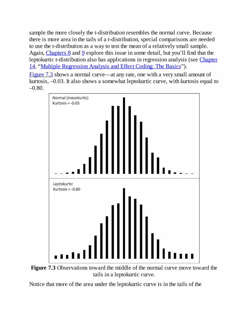
samplethemorecloselythet-distributionresemblesthenormalcurve.Becausethereismoreareainthetailsofat-distribution,specialcomparisonsareneededtousethet-distributionasawaytotestthemeanofarelativelysmallsample.Again,Chapters8and9explorethisissueinsomedetail,butyou’llfindthattheleptokurtict-distributionalsohasapplicationsinregressionanalysis(seeChapter14,“MultipleRegressionAnalysisandEffectCoding:TheBasics”).Figure7.3showsanormalcurve—atanyrate,onewithaverysmallamountofkurtosis,–0.03.Italsoshowsasomewhatleptokurticcurve,withkurtosisequalto–0.80.

Figure7.3Observationstowardthemiddleofthenormalcurvemovetowardthetailsinaleptokurticcurve.

Noticethatmoreoftheareaundertheleptokurticcurveisinthetailsofthe

distribution,withlessoccupyingthemiddle.Thet-distributionfollowsthispattern,andtestsofsuchstatisticsasmeanstakeaccountofthiswhen,forexample,thepopulationstandarddeviationisunknownandthesamplesizeissmall.Withmoreoftheareainthetailsofthedistribution,thecriticalvaluesneededtorejectanullhypothesisarelargerthanwhenthedistributionisnormal.Theeffectalsofindsitswayintotheconstructionofconfidenceintervals(discussedlaterinthischapter).

QuantifyingKurtosisTherationaletoquantifykurtosisisthesameastherationaletoquantifyskewness:Anumbercansometimesdescribemoreefficientlythanachartcan.Furthermore,knowinghowfaradistributiondepartsfromthenormalhelpstheconsumeroftheresearchputotherreportedfindingsincontext.ExcelofferstheKURT()worksheetfunctiontocalculatethekurtosisinasetofnumbers.Unfortunatelythereisnomoreconsensusregardingaformulaforkurtosisthanthereisforskewness.Buttherecommendedformulasdotendtoagreeonusingsomevariationonthez-scoresraisedtothefourthpower.Here’sonetextbookdefinitionofkurtosis:

Inthisdefinition,Nisthenumberofvaluesinthedistribution,andzrepresentstheassociatedz-scores:thatis,eachvaluelessthemean,dividedbythestandarddeviation.Thenumber3issubtractedtosettheresultequaltozeroforthenormalcurve.Then,positivevaluesforthekurtosisindicatealeptokurticdistributionwhereasnegativevaluesindicateaplatykurticdistribution.Becausethez-scoresareraisedtoanevenpower,theirsum(andthereforetheirmean)cannotbenegative.Subtracting3isaconvenientwaytogiveplatykurticcurvesanegativekurtosis.Someversionsoftheformuladonotsubtract3.Thoseversionswouldreturnthevalue3foranormalcurve.Excel’sKURT()functioniscalculatedinthisfashion,followinganapproachthat’sintendedtocorrectbiasinthesample’sestimationofthepopulationparameter:

TheUnitNormalDistributionOneparticularversionofthenormaldistributionhasspecialimportance.It’s

calledtheunitnormalorstandardnormaldistribution.Itsshapeisthesameasanynormaldistributionbutitsmeanis0anditsstandarddeviationis1.Thatlocation(themeanof0)andspread(thestandarddeviationof1)makesitastandard,andthat’shandy.Becauseofthosetwocharacteristics,youimmediatelyknowthecumulativeareabelowanyvalue.Intheunitnormaldistribution,thevalue1isonestandarddeviationabovethemeanof0,andso84%oftheareafallstoitsleft.Thevalue–2istwostandarddeviationsbelowthemeanof0,andso2.275%oftheareafallstoitsleft.Suppose,however,thatyouwereworkingwithadistributionthathasameanof7.63centimetersandastandarddeviationof.124centimeters—perhapsthatrepresentsthediameterofamachinepartwhosesizemustbeprecise.Ifsomeonetoldyouthatoneofthemachinepartshasadiameterof7.816,you’dprobablyhavetothinkforamomentbeforeyourealizedthat’soneandone-halfstandarddeviationsabovethemean.Butifyou’reusingtheunitnormaldistributionasayardstick,hearingofaz-scoreof1.5tellsyouexactlywherethatmachinepartisinthedistribution.Soit’squickerandeasiertointerpretthemeaningofavalueifyouusetheunitnormaldistributionasyourframework.Excelhasworksheetfunctionstailoredforthenormaldistribution,andtheyareeasytouse.Excelalsohasworksheetfunctionstailoredspecificallyfortheunitnormaldistribution,andtheyareeveneasiertouse:Youdon’tneedtosupplythedistribution’smeanandstandarddeviation,becausethey’reknown.Thenextsectiondiscussesthosefunctions,forbothExcel2013andearlierversions.

ExcelFunctionsfortheNormalDistributionExcelnamesthefunctionsthatpertaintothenormaldistributionsothatyoucantellwhetheryou’redealingwithanynormaldistribution,ortheunitnormaldistributionwithameanof0andastandarddeviationof1.Excelreferstotheunitnormaldistributionasthe“standard”normal,andthereforeusestheletterSinthefunction’sname.SotheNORM.DIST()functionreferstoanynormaldistribution,whereastheNORMSDIST()compatibilityfunctionandtheNORM.S.DIST()consistencyfunctionreferspecificallytotheunitnormaldistribution.

TheNORM.DIST()FunctionSupposeyou’reinterestedinthedistributioninthepopulationofhigh-densitylipoprotein(HDL)levelsinadultsover20yearsofage.Thatvariableisnormally

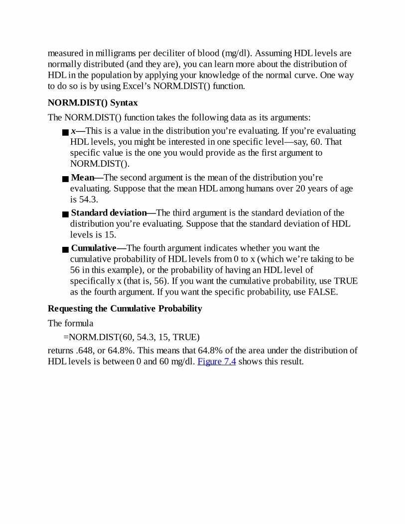
measuredinmilligramsperdeciliterofblood(mg/dl).AssumingHDLlevelsarenormallydistributed(andtheyare),youcanlearnmoreaboutthedistributionofHDLinthepopulationbyapplyingyourknowledgeofthenormalcurve.OnewaytodosoisbyusingExcel’sNORM.DIST()function.

NORM.DIST()SyntaxTheNORM.DIST()functiontakesthefollowingdataasitsarguments:

x—Thisisavalueinthedistributionyou’reevaluating.Ifyou’reevaluatingHDLlevels,youmightbeinterestedinonespecificlevel—say,60.ThatspecificvalueistheoneyouwouldprovideasthefirstargumenttoNORM.DIST().Mean—Thesecondargumentisthemeanofthedistributionyou’reevaluating.SupposethatthemeanHDLamonghumansover20yearsofageis54.3.Standarddeviation—Thethirdargumentisthestandarddeviationofthedistributionyou’reevaluating.SupposethatthestandarddeviationofHDLlevelsis15.Cumulative—ThefourthargumentindicateswhetheryouwantthecumulativeprobabilityofHDLlevelsfrom0tox(whichwe’retakingtobe56inthisexample),ortheprobabilityofhavinganHDLlevelofspecificallyx(thatis,56).Ifyouwantthecumulativeprobability,useTRUEasthefourthargument.Ifyouwantthespecificprobability,useFALSE.

RequestingtheCumulativeProbabilityTheformula

=NORM.DIST(60,54.3,15,TRUE)returns.648,or64.8%.Thismeansthat64.8%oftheareaunderthedistributionofHDLlevelsisbetween0and60mg/dl.Figure7.4showsthisresult.

Figure7.4Youcanadjustthenumberofgridlinesbyformattingtheverticalaxistoshowmoreorfewermajorunits.

Ifyoumouseoverthelinethatshowsthecumulativeprobability,you’llseeasmallpop-upwindowthattellsyouwhichdatapointyouarepointingat,aswellasitslocationonboththehorizontalandverticalaxes.Oncecreated,thechartcantellyoutheprobabilityassociatedwithanyofthecharteddatapoints,notjustthe60mg/dlthissectionhasdiscussed.AsshowninFigure7.4,youcanuseeitherthechart’sgridlinesoryourmousepointertodeterminethatameasurementof,forexample,60.3mg/dlorbelowaccountsforabout66%ofthepopulation.

RequestingthePointEstimateThingsaredifferentifyouchooseFALSEasthefourth,CumulativeargumenttoNORM.DIST().Inthatcase,thefunctionreturnstheprobabilityassociatedwiththespecificpointyouspecifyinthefirstargument.UsethevalueFALSEfortheCumulativeargumentifyouwanttoknowtheheightofthenormalcurveataspecificvalueofthedistributionyou’reevaluating.Figure7.5showsonewayto

useNORM.DIST()withtheCumulativeargumentsettoFALSE.

Figure7.5Theheightofthecurveatanypointistheprobabilitythatthepointappearsinarandomsamplefromthefulldistribution.

Itdoesn’toftenhappenthatyouneedapointestimateoftheprobabilityofaspecificvalueinanormalcurve,butifyoudo—forexample,todrawacurvethathelpsyouorsomeoneelsevisualizeanoutcome—thensettingtheCumulativeargumenttoFALSEisagoodwaytogetit.NORM.DIST()thenreturnsthevaluethatdefinestheheightofthenormalcurveatthepointyouspecifyandassuchrepresentstheprobabilityofobservingthatpointrelativetootherpointsonthehorizontalaxis.(Youmightalsoseethisvalue—theprobabilityofaspecificpoint,theheightofthecurveatthatpoint—referredtoastheprobabilitydensityfunctionorprobabilitymassfunction.Theterminologyhasnotbeenstandardized.)Ifyou’reusingaversionofExcelpriorto2010,youcanusetheNORMDIST()compatibilityfunction.ItisthesameasNORM.DIST()astobothargumentsand

returnedvalues.

TheNORM.INV()FunctionAsapracticalmatter,you’llfindthatyouusuallyhaveneedfortheNORM.DIST()functionafterthefact.Thatis,youhavecollecteddataandknowthemeanandstandarddeviationofasampleorpopulation.Butwheredoesagivenvaluefallinanormaldistribution?Thatvaluemightbeasamplemeanthatyouwanttocomparetothemeanofapopulation,oritmightbeanindividualobservationthatyouwanttoassessinthecontextofalargergroup.Inthatcase,youwouldpasstheinformationalongtoNORM.DIST(),whichwouldtellyoutherelativeprobabilityofobservinguptoaparticularvalue(Cumulative=TRUE)orthatspecificvalue(Cumulative=FALSE).Youcouldthencomparethatprobabilitytotheprobabilityofafalsepositive(thealpharate)ortothatofafalsenegative(thebetarate)thatyoualreadyadoptedforyourexperiment.TheNORM.INV()functioniscloselyrelatedtotheNORM.DIST()functionandgivesyouaslightlydifferentangleonthings.NORM.DIST()returnsavaluethatrepresentsanarea—thatis,aprobability.NORM.INV()returnsavaluethatrepresentsapointonthenormalcurve’shorizontalaxis,onethat’sassociatedwithaprobabilitywhichyousupply.ThepointthatNORM.INV()returnsisthesameasthepointthatyouprovideasthefirstargumenttoNORM.DIST().Forexample,thepriorsectionshowedthattheformula

=NORM.DIST(60,54.3,15,TRUE)returns.648.Thevalue60isequaltoorlargerthan64.8%oftheobservationsinanormaldistributionthathasameanof54.3andastandarddeviationof15.Theothersideofthecoin:Theformula

=NORM.INV(0.648,54.3,15)returns60.Ifyourdistributionhasameanof54.3andastandarddeviationof15,then64.8%ofthedistributionliesatorbelowavalueof60.Thatillustrationisjust,well,illustrative.Youwouldnotnormallyneedtoknowthepointthatmeetsorexceeds64.8%ofadistribution.Butsupposethatinpreparationforaresearchprojectyoudecidethatyouwillconcludethatatreatmenthasareliableeffectonlyifthemeanoftheexperimentalgroupisinthetop5%ofthepopulationofhypotheticalgroupmeansthatmightbeacquiredsimilarly.(Thisisconsistentwiththetraditionalnullhypothesisapproachtoexperimentation,whichChapters8and9discussinconsiderablymoredetail.)Inthatcase,youwouldwanttoknowwhatscorewoulddefinethat

top5%.Ifyouknowthemeanandstandarddeviation,NORM.INV()doesthejobforyou.Stilltakingthepopulationmeanat54.3andthestandarddeviationat15,theformula

=NORM.INV(0.95,54.3,15)returns78.97.Fivepercentofanormaldistributionthathasameanof54.3andastandarddeviationof15liesaboveavalueof78.97.Asyousee,theformulauses0.95asthefirstargumenttoNORM.INV().That’sbecauseNORM.INVassumesacumulativeprobability:noticethatunlikeNORM.DIST(),theNORM.INV()functionhasnofourth,Cumulativeargument.Soaskingwhatvaluecutsoffthetop5%ofthedistributionisequivalenttoaskingwhatvaluecutsoffthebottom95%ofthedistribution.Inthiscontext,choosingtouseNORM.DIST()orNORM.INV()islargelyamatterofthesortofinformationyou’reafter.IfyouwanttoknowhowlikelyitisthatyouwillobserveanumberatleastaslargeasX,handXofftoNORM.DIST()togetaprobability.Ifyouwanttoknowthenumberthatservesastheboundaryofanarea—anareathatcorrespondstoagivenprobability—handtheareaofftoNORM.INV()togetthatnumber.Ineithercase,youneedtosupplythemeanandthestandarddeviation.InthecaseofNORM.DIST,youalsoneedtotellthefunctionwhetheryou’reinterestedinthecumulativeprobabilityorthepointestimate.TheconsistencyfunctionNORM.INV()isnotavailableinversionsofExcelpriorto2010,butyoucanusethecompatibilityfunctionNORMINV()instead.TheargumentsandtheresultsareaswithNORM.INV().

UsingNORM.S.DIST()There’smuchtobesaidforexpressingdistances,weights,durations,andsoonintheiroriginalunitofmeasure.That’swhatNORM.DIST()isfor.Butwhenyouwanttouseastandardunitofmeasureforavariablethat’sdistributednormally,youshouldthinkofNORM.S.DIST().TheSinthemiddleofthefunctionnameofcoursestandsforstandard.It’squickertouseNORM.S.DIST()becauseyoudon’thavetosupplythemeanorstandarddeviation.Becauseyou’remakingreferencetotheunitnormaldistribution,themean(0)andthestandarddeviation(1)areknownbydefinition.AllthatNORM.S.DIST()needsisthez-scoreandwhetheryouwantacumulativearea(TRUE)orapointestimate(FALSE).Thefunctionusesthissimplesyntax:

=NORM.S.DIST(z,Cumulative)

Thus,theresultofthisformula=NORM.S.DIST(1.5,TRUE)

informsyouthat93.3%oftheareaunderanormalcurveisfoundtotheleftofaz-scoreof1.5.(SeeChapter3,“Variability:HowValuesDisperse,”foranintroductiontotheconceptofz-scores.)

CautionNORMSDIST()isavailableinversionsofExcelpriorto2010,anditremainsavailableasacompatibilityfunctioninExcel2010and2013.Itistheonlyoneofthenormaldistributionfunctionswhoseargumentlistdiffersfromthatofitsassociatedconsistencyfunction.NORMSDIST()hasnocumulativeargument:Itreturnsbydefaultthecumulativeareatotheleftofthezargument.ExcelwillwarnthatyouhavemadeanerrorifyousupplyaCumulativeargumenttoNORMSDIST().Ifyouwantthepointestimateratherthanthecumulativeprobability,youshouldusetheNORMDIST()functionwith0asthesecondargumentand1asthethird.Thosetwotogetherspecifytheunitnormaldistribution,andyoucannowsupplyFALSEasthefourthargumenttoNORMDIST()togetthepointestimateratherthanthecumulativeprobability.Here’sanexample:=NORMDIST(1,0,1,FALSE)

UsingNORM.S.INV()It’sevensimplertousetheinverseofNORM.S.DIST(),whichisNORM.S.INV().Allthelatterfunctionneedsisaprobability:

=NORM.S.INV(.95)Thisformulareturns1.64,whichmeansthat95%oftheareaunderthenormalcurveliestotheleftofaz-scoreof1.64.Ifyou’vetakenacourseinelementaryinferentialstatistics,thatnumberprobablylooksfamiliar—asfamiliarasthe1.96thatcutsoff97.5%ofthedistribution.Thesearefrequentlyoccurringnumbersbecausetheyareassociatedwiththeall-too-frequentlyoccurring“p<.05”and“p<.025”entriesatthebottomoftablesinjournalreports—arutthatyoudon’twanttogetcaughtin.Chapters8and9havemuchmoretosayaboutthosesortsofentries,inthecontextofthet-distribution(whichiscloselyrelatedtothenormaldistribution).ThecompatibilityfunctionNORMSINV()takesthesameargumentandreturnsthe

sameresultasdoesNORM.S.INV().ThereisanotherExcelworksheetfunctionthatpertainsdirectlytothenormaldistribution:CONFIDENCE.NORM().Todiscussthepurposeanduseofthatfunctionsensibly,it’snecessaryfirsttoexplorealittlebackground.

ConfidenceIntervalsandtheNormalDistributionAconfidenceintervalisarangeofvaluesthatgivestheuserasenseofhowpreciselyastatisticestimatesaparameter.Themostfamiliaruseofaconfidenceintervalislikelythe“marginoferror”reportedinnewsstoriesaboutpolls:“Themarginoferrorisplusorminus3percentagepoints.”Thisstatementismeanttoindicatethatmostsamples—perhaps19outof20—takensimilarlywouldreturnresultswithin3percentagepointsoftheactualpopulationparameter.Butconfidenceintervalsareusefulincontextsthatgowellbeyondthatsimplesituation.Confidenceintervalscanbeusedwithdistributionsthataren’tnormal—thatarehighlyskewedorinsomeotherwaynon-normal.Butit’seasiesttounderstandwhatthey’reaboutinsymmetricdistributions,sothetopicisintroducedhere.Don’tletthatgetyouthinkingthatyoucanuseconfidenceintervalswithnormaldistributionsonly.

TheMeaningofaConfidenceIntervalSupposethatyoumeasuredtheHDLlevelinthebloodof100adultsonaspecialdietandcalculatedameanof50mg/dlwithastandarddeviationof20.You’reawarethatthemeanisastatistic,notapopulationparameter,andthatanothersampleof100adults,onthesamediet,wouldverylikelyreturnadifferentmeanvalue.Overmanyrepeatedsamples,thegrandmean—thatis,themeanofthesamplemeans—wouldturnouttobevery,veryclosetothepopulationparameter.Butyourresourcesdon’textendthatfarandyou’regoingtohavetomakedowithjusttheonestatistic,the50mg/dlthatyoucalculatedforyoursample.Althoughthevalueof20thatyoucalculateforthesamplestandarddeviationisastatistic,itisthesameastheknownpopulationstandarddeviationof20.YoucanmakeuseofthesamplestandarddeviationandthenumberofHDLvaluesthatyoutabulatedinordertogetasenseofhowmuchplaythereisinthatsampleestimate.Youdosobyconstructingaconfidenceintervalaroundthatmeanof50mg/dl.Perhapstheintervalextendsfrom45to55.(Andhereyoucanseetherelationshipto“plusorminus3percentagepoints.”)Doesthattellyouthatthetruepopulationmeanissomewherebetween45and55?

No,itdoesn’t,althoughitmightwellbe.Justastherearemanypossiblesamplesthatyoumighthavetaken,butdidn’t,therearemanypossibleconfidenceintervalsyoumighthaveconstructedaroundthesamplemeans,butcouldn’t.Asyou’llsee,youconstructyourconfidenceintervalinsuchawaythatifyoutookmanymoremeansandputconfidenceintervalsaroundthem,95%oftheconfidenceintervalswouldcapturethetruepopulationmean.Astothespecificconfidenceintervalthatyoudidconstruct,theprobabilitythatthetruepopulationmeanfallswithintheintervaliseither1or0:Eithertheintervalcapturesthepopulationmeanoritdoesn’t.However,itismorerationaltoassumethattheoneconfidenceintervalthatyoutookisoneofthe95%thatcapturethepopulationmeanthantoassumeitisn’t.Soyouwouldtendtobelieve,with95%confidence,thattheintervalisoneofthosethatcapturesthepopulationmean.AlthoughI’vespokenof95%confidenceintervalsinthissection,youcanalsoconstruct90%or99%confidenceintervals,oranyotherdegreeofconfidencethatmakessensetoyouinaparticularsituation.You’llseenexthowyourchoiceswhenyouconstructtheintervalaffectthenatureoftheintervalitself.Itturnsoutthatitsmoothesthediscussionifyou’rewillingtosuspendyourdisbeliefabit,andbriefly:I’mgoingtoaskyoutoimagineasituationinwhichyouknowwhatthestandarddeviationofameasureisinthepopulation,butthatyoudon’tknowitsmeaninthepopulation.Thosecircumstancesarealittleoddbutfarfromimpossible.

ConstructingaConfidenceIntervalAconfidenceintervalonamean,asdescribedinthepriorsection,requiresthesebuildingblocks:

ThemeanitselfThestandarddeviationoftheobservationsThenumberofobservationsinthesampleThelevelofconfidenceyouwanttoapplytotheconfidenceinterval

Startingwiththelevelofconfidence,supposethatyouwanttocreatea95%confidenceinterval:Youwanttoconstructitinsuchawaythatifyoucreated100confidenceintervalsaround100samplemeans,95ofthemwouldcapturethetruepopulationmean.Inthatcase,becauseyou’redealingwithanormaldistribution,youcouldentertheseformulasinaworksheet:

=NORM.S.INV(0.025)

=NORM.S.INV(0.975)TheNORM.S.INV()function,describedinthepriorsection,returnsthez-scorethathastoitslefttheproportionofthecurve’sareagivenastheargument.Therefore,NORM.S.INV(0.025)returns–1.96.That’sthez-scorethathas0.025,or2.5%,ofthecurve’sareatoitsleft.Similarly,NORM.S.INV(0.975)returns1.96,whichhas97.5%ofthecurve’sareatoitsleft.Anotherwayofsayingitisthat2.5%ofthecurve’sarealiestoitsright.ThesefiguresareshowninFigure7.6.

Figure7.6Adjustingthez-scorelimitadjuststhelevelofconfidence.CompareFigures7.6and7.7.

Figure7.7Wideningtheintervalgivesyoumoreconfidencethatyouarecapturingthepopulationparameter,butinevitablyresultsinavaguerestimate.

TheareaunderthecurveinFigure7.6,andbetweenthevalues46.1and53.9onthehorizontalaxis,accountsfor95%oftheareaunderthecurve.Thecurve,intheory,extendstoinfinitytotheleftandtotheright,soallpossiblevaluesforthepopulationmeanareincludedinthecurve.Ninety-fivepercentofthepossiblevaluesliewithinthe95%confidenceintervalbetween46.1and53.9.TheFigures46.1and53.9werechosensoastocapturethat95%.Ifyouwanteda99%confidenceinterval(orsomeotherintervalmoreorlesslikelytobeoneoftheintervalsthatcapturesthepopulationmean),youwouldchoosedifferentfigures.Figure7.7showsa99%confidenceintervalaroundasamplemeanof50.InFigure7.7,the99%confidenceintervalextendsfrom44.8to55.2,atotalof2.6pointswiderthanthe95%confidenceintervaldepictedinFigure7.6.Ifahundred99%confidenceintervalswereconstructedaroundthemeansof100samples,99ofthem(not95asbefore)wouldcapturethepopulationmean.Theadditionalconfidenceisprovidedbymakingtheintervalwider.Andthat’salwaysthetradeoffinconfidenceintervals.Thenarrowertheinterval,themorepreciselyyou

drawtheboundaries,butthefewersuchintervalswillcapturethestatisticinquestion—here,that’sthemean.Thebroadertheinterval,thelesspreciselyyousettheboundariesbutthelargerthenumberofintervalsthatcapturethestatistic.Otherthansettingtheconfidencelevel,theonlyfactorthat’sunderyourcontrolisthesamplesize.Yougenerallycan’tdictatethatthestandarddeviationistobesmaller,butyoucantakelargersamples.Asyou’llseeinChapters8and9,thestandarddeviationusedinaconfidenceintervalaroundasamplemeanisnotthestandarddeviationoftheindividualrawscores.Itisthatstandarddeviationdividedbythesquarerootofthesamplesize,andthisisknownasthestandarderrorofthemean.ThedatasetusedtocreatethechartsinFigures7.6and7.7hasastandarddeviationof20,knowntobethesameasthepopulationstandarddeviation.Thesamplesizeis100.Therefore,thestandarderrorofthemeanis

StandardError=

or2.Tocompletetheconstructionoftheconfidenceinterval,youmultiplythestandarderrorofthemeanbythez-scoresthatcutofftheconfidencelevelyou’reinterestedin.Figure7.6,forexample,showsa95%confidenceinterval.Theintervalmustbeconstructedsothat95%liesunderthecurveandwithintheinterval.Therefore,5%mustlieoutsidetheinterval,with2.5%dividedequallybetweenthetails.Here’swheretheNORM.S.INV()functioncomesintoplay.Earlierinthissection,thesetwoformulaswereused:

=NORM.S.INV(0.025)=NORM.S.INV(0.975)

Theyreturnthez-scores–1.96and1.96,whichformtheboundariesfor2.5%and97.5%oftheunitnormaldistribution,respectively.Ifyoumultiplyeachbythestandarderrorof2,andaddthesamplemeanof50,youget46.1and53.9,thelimitsofa95%confidenceintervalonameanof50andastandarderrorof2.Ifyouwanta99%confidenceinterval,usetheformulas

=NORM.S.INV(0.005)=NORM.S.INV(0.995)

toreturn–2.58and2.58.Thesez-scorescutoffonehalfofonepercentoftheunitnormaldistributionateachend.Theremainderoftheareaunderthecurveis99%.Multiplyingeachz-scorebythestandarderrorof2andadding50forthemeanresultsin44.8and55.2,thelimitsofa99%confidenceintervalonameanof50

andastandarderrorof2.Atthispointitcanhelptobackawayfromthearithmeticandfocusinsteadontheconcepts.Anyz-scoreissomenumberofstandarddeviations—soaz-scoreof1.96isapointthat’sfoundat1.96standarddeviationsabovethemean,andaz-scoreof–1.96isfound1.96standarddeviationsbelowthemean.Becausethenatureofthenormalcurvehasbeenstudiedsoextensively,weknowthat95%oftheareaunderanormalcurveisfoundbetween1.96standarddeviationsbelowthemeanand1.96standarddeviationsabovethemean.Whenyouputaconfidenceintervalaroundasamplemean,youstartbydecidingwhatpercentageofotherconfidenceintervals,ifcollectedandcalculated,youwouldwanttocapturethepopulationmean.So,ifyoudecidedthatyouwanted95%ofpossibleconfidenceintervalstocapturethepopulationmean,youwouldputitslimitsat1.96standarddeviationsaboveandbelowyoursamplemean.Youassume,ofcourse,thattheconfidenceintervalyouconstructaroundthesamplemeanisamongthe95%thatcapturesthepopulationmean,ratherthanamongthe5%thatdoesn’t.Buthowlargeistherelevantstandarddeviation?Inthissituation,therelevantunitsarethemselvesmeanvalues.Youneedtoknowthestandarddeviationnotoftheoriginalandindividualobservations,butofthemeansthatarecalculatedfromthoseobservations.Thatstandarddeviationhasaspecialname,thestandarderrorofthemean.Becauseofmathematicalderivationsandlongexperiencewiththewaythenumbersbehave,weknowthatagood,closeestimateofthestandarddeviationofthemeanvaluesisthestandarddeviationofindividualscores,dividedbythesquarerootofthesamplesize.That’sthestandarddeviationyouwanttousetodetermineyourconfidenceinterval.Intheexamplethissectionhasexplored,thestandarddeviationoftheoriginalsetofsampledvaluesis20andthesamplesizeis100,sothestandarderrorofthemeanis2.Whenyoucalculate1.96standarderrorsbelowthemeanof50andabovethemeanof50,youwindupwithvaluesof46.1and53.9.That’syour95%confidenceinterval.Ifyoutookanother99samplesfromthepopulation,95of100similarconfidenceintervalswouldcapturethepopulationmean.It’ssensibletoconcludethattheconfidenceintervalyoucalculatedisoneofthe95thatcapturethepopulationmean.It’snotsensibletoconcludethatit’soneoftheremaining5thatdon’t.

ExcelWorksheetFunctionsThatCalculateConfidenceIntervals

Theprecedingsection’sdiscussionoftheuseofthenormaldistributionmadetheassumptionthatyouknowthestandarddeviationinthepopulation.That’snotanimplausibleassumption,butitistruethatyouoftendon’tknowthepopulationstandarddeviationandmustestimateitonthebasisofthesampleyoutake.Therearetwodifferentdistributionsthatyouneedaccessto,dependingonwhetheryouknowthepopulationstandarddeviationorareestimatingit.Ifyouknowit,youmakereferencetothenormaldistribution.Ifyouareestimatingitfromasample,youusethet-distribution.Excel2010and2013havetwoworksheetfunctions,CONFIDENCE.NORM()andCONFIDENCE.T(),thathelpcalculatethewidthofconfidenceintervals.YouuseCONFIDENCE.NORM()whenyouknowthepopulationstandarddeviationofthemeasure(suchasthischapter’sexampleusingHDLlevels).YouuseCONFIDENCE.T()whenyoudon’tknowthemeasure’sstandarddeviationinthepopulationandareestimatingitfromthesampledata.Chapters8and9havemoreinformationonthisdistinction,whichinvolvesthechoicebetweenusingthenormaldistributionandthet-distribution.VersionsofExcelpriorto2010havetheCONFIDENCE()functiononly.ItsargumentsandresultsareidenticaltothoseoftheCONFIDENCE.NORM()consistencyfunction.Priorto2010therewasnosingleworksheetfunctiontoreturnaconfidenceintervalbasedonthet-distribution.However,asyou’llseeinthissection,it’sveryeasytoreplicateCONFIDENCE.T()usingeitherT.INV()orTINV().YoucanreplicateCONFIDENCE.NORM()usingNORM.S.INV()orNORMSINV().

UsingCONFIDENCE.NORM()andCONFIDENCE()Figure7.8showsasmalldatasetincellsA2:A17.ItsmeanisincellB2andthepopulationstandarddeviationincellC2.

Figure7.8YoucanconstructaconfidenceintervalusingeitheraCONFIDENCE()functionoranormaldistributionfunction.

InFigure7.8,avaluecalledalphaisincellF2.Theuseofthattermisconsistentwithitsuseinothercontextssuchashypothesistesting.Itistheareaunderthecurvethatisoutsidethelimitsoftheconfidenceinterval.InFigure7.6,alphaisthesumoftheshadedareasinthecurve’stails.Eachshadedareais2.5%ofthetotalarea,soalphais5%or0.05.Theresultisa95%confidenceinterval.CellG2inFigure7.8showshowtousetheCONFIDENCE.NORM()function.NotethatyoucouldusetheCONFIDENCE()compatibilityfunctioninthesameway.Thesyntaxis

=CONFIDENCE.NORM(alpha,standarddeviation,size)wheresizereferstosamplesize.AsthefunctionisusedincellG2,itspecifies0.05foralpha,22forthepopulationstandarddeviation,and16forthecountofvaluesinthesample:

=CONFIDENCE.NORM(F2,C2,COUNT(A2:A17))Thisreturns10.78astheresultofthefunction,giventhosearguments.CellsG4andI4show,respectively,theupperandlowerlimitsofthe95%confidence

interval.Thereareseveralpointstonote:

CONFIDENCE.NORM()isused,notCONFIDENCE.T().Thisisbecauseyouhaveknowledgeofthepopulationstandarddeviationandneednotestimateitfromthesamplestandarddeviation.Ifyouhadtoestimatethepopulationvaluefromthesample,youwoulduseCONFIDENCE.T(),asdescribedinthenextsection.Becausethesumoftheconfidencelevel(forexample,95%)andalphaalwaysequals100%,Microsoftcouldhavechosentoaskyoufortheconfidencelevelinsteadofalpha.Itisstandardtorefertoconfidenceintervalsintermsofconfidencelevelssuchas95%,90%,99%,andsoon.Microsoftwouldhavedemonstratedagreaterdegreeofconsiderationforitscustomershaditchosentousetheconfidencelevelinsteadofalphaasthefunction’sfirstargument.TheHelpdocumentationstatesthatCONFIDENCE.NORM(),aswellastheothertwoconfidenceintervalfunctions,returnstheconfidenceinterval.Itdoesnot.Thevaluereturnedisone-halfoftheconfidenceinterval.Toestablishthefullconfidenceinterval,youmustsubtracttheresultofthefunctionfromthemeanandaddtheresulttothemean.

StillinFigure7.8,therangeE7:I11constructsaconfidenceintervalidenticaltotheoneinE1:I4.It’susefulbecauseitshowswhat’sgoingonbehindthescenesintheCONFIDENCE.NORM()function.Thefollowingcalculationsareneeded:

CellF8containstheformula=F2/2.Theportionunderthecurvethat’srepresentedbyalpha—here.0.05,or5%—mustbesplitinhalfbetweenthetwotailsofthedistribution.Theleftmost2.5%oftheareawillbeplacedinthelefttail,totheleftofthelowerlimitoftheconfidenceinterval.CellF9containstheremainingareaunderthecurveafterhalfofalphahasbeenremoved.Thatistheleftmost97.5%ofthearea,whichisfoundtotheleftoftheupperlimitoftheconfidenceinterval.CellG8containstheformula=NORM.S.INV(F8).Itreturnsthez-scorethatcutsoff(here)theleftmost2.5%oftheareaundertheunitnormalcurve.CellG9containstheformula=NORM.S.INV(F9).Itreturnsthez-scorethatcutsoff(here)theleftmost97.5%oftheareaundertheunitnormalcurve.

NowwehaveincellG8andG9thez-scores—thestandarddeviationsintheunitnormaldistribution—thatbordertheleftmost2.5%andrightmost2.5%ofthedistribution.Togetthosez-scoresintotheunitofmeasurementwe’reusing—a

measureoftheamountofHDLintheblood—it’snecessarytomultiplythez-scoresbythestandarderrorofthemean,andaddandsubtractthatfromthesamplemean.

NoteBearinmindthatbecausewe’rethinkingintermsofsamplemeans,it’sthestandarddeviationofthosemeans—thestandarderrorofthemean—thatisthestandarddeviationwe’reinterestedin.

Thisformulacalculatestheconfidenceinterval’slowerlimitincellG11:=B2+(G8*C2/SQRT(COUNT(A2:A17)))

Workingfromtheinsideout,theformuladoesthefollowing:1.DividesthestandarddeviationincellC2bythesquarerootofthenumberofobservationsinthesample.Asnotedearlier,thisdivisionreturnsthestandarderrorofthemean.

2.Multipliesthestandarderrorofthemeanbythenumberofstandarderrorsbelowthemean(–1.96)thatboundsthelower2.5%oftheareaunderthecurve.ThatvalueisincellG8.

3.Addsthemeanofthesample,foundincellB2.Steps1through3returnthevalue46.41.NotethatitisidenticaltothelowerlimitreturnedusingCONFIDENCE.NORM()incellG4.SimilarstepsareusedtogetthevalueincellI11.Thedifferenceisthatinsteadofaddinganegativenumber(renderednegativebythenegativez-score–1.96),theformulaaddsapositivenumber(thez-score1.96multipliedbythestandarderrorreturnsapositiveresult).NotethatthevalueinI11isidenticaltothevalueinI4,whichdependsonCONFIDENCE.NORM()insteadofonNORM.S.INV().NoticethatCONFIDENCE.NORM()asksyoutosupplythreearguments:

Alpha,or1minustheconfidencelevel—Excelcan’tpredictwithwhatlevelofconfidenceyouwanttousetheinterval,soyouhavetosupplyit.Standarddeviation—BecauseCONFIDENCE.NORM()usesthenormaldistributionasareferencetoobtainthez-scoresassociatedwithdifferentareas,itisassumedthatthepopulationstandarddeviationisinuse.(SeeChapters8and9formoreonthismatter.)Exceldoesn’thaveaccesstothefullpopulationandthuscan’tcalculateitsstandarddeviation.Therefore,itreliesontheusertosupplythatfigure.Size,or,moremeaningfully,samplesize—Youaren’tdirectingExcel’s

attentiontothesampleitself(cellsA2:A17inFigure7.8),soExcelcan’tcountthenumberofobservations.YouhavetosupplythatnumbersothatExcelcancalculatethestandarderrorofthemean.

YoushoulduseCONFIDENCE.NORM()orCONFIDENCE()ifyoufeelcomfortablewiththemandhavenoparticulardesiretogrinditoutusingNORM.S.INV()andthestandarderrorofthemean.BearinmindthatCONFIDENCE.NORM()andCONFIDENCE()donotreturnthewidthoftheentireinterval,justthewidthoftheupperhalf,whichisidenticalinasymmetricdistributiontothewidthofthelowerhalf.

UsingCONFIDENCE.T()Figure7.9makestwobasicchangestotheinformationinFigure7.8:ItusesthesamplestandarddeviationincellC2anditusestheCONFIDENCE.T()functionincellG2.Thesetwobasicchangesalterthesizeoftheresultingconfidenceinterval.

Figure7.9Otherthingsbeingequal,aconfidenceintervalconstructedusingthet-distributioniswiderthanoneconstructedusingthenormaldistribution.

Noticefirstthatthe95%confidenceintervalinFigure7.9runsfrom46.01to

68.36,whereasinFigure7.8itrunsfrom46.41to67.97.TheconfidenceintervalinFigure7.8isnarrower.YoucanfindthereasoninFigure7.3.There,youcanseethatthere’smoreareaunderthetailsoftheleptokurticdistributionthanunderthetailsofthenormaldistribution.Youhavetogooutfartherfromthemeanofaleptokurticdistributiontocapture,say,95%ofitsareabetweenitstails.Therefore,thelimitsoftheintervalarefartherfromthemeanandtheconfidenceintervaliswider.Becauseyouusethet-distributionwhenyoudon’tknowthepopulationstandarddeviation,usingCONFIDENCE.T()insteadofCONFIDENCE.NORM()bringsaboutawiderconfidenceinterval.Theshiftfromthenormaldistributiontothet-distributionalsoappearsintheformulasincellsG8andG9ofFigure7.9,whichare:

=T.INV(F8,COUNT(A2:A17)-1)and

=T.INV(F9,COUNT(A2:A17)-1)NotethatthesecellsuseT.INV()insteadofNORM.S.INV(),asisdoneinFigure7.8.InadditiontotheprobabilitiesincellsF8andF9,T.INV()needstoknowthedegreesoffreedomassociatedwiththesamplestandarddeviation.RecallfromChapter3thatasample’sstandarddeviationusesinitsdenominatorthenumberofobservationsminus1.Whenyousupplythepropernumberofdegreesoffreedom,youenableExceltousethepropert-distribution:There’sadifferentt-distributionforeverydifferentnumberofdegreesoffreedom.

UsingtheDataAnalysisAdd-InforConfidenceIntervalsExcel’sDataAnalysisadd-inhasaDescriptiveStatisticstoolthatcanbehelpfulwhenyouhaveoneormorevariablestoanalyze.TheDescriptiveStatisticstoolreturnsvaluableinformationaboutarangeofdata,includingmeasuresofcentraltendencyandvariability,skewnessandkurtosis.Thetoolalsoreturnshalfthesizeofaconfidenceinterval,justasCONFIDENCE.T()does.

NoteTheDescriptiveStatisticstool’sconfidenceintervalisverysensiblybasedonthet-distribution.YoumustsupplyarangeofactualdataforExceltocalculatetheotherdescriptivestatistics,andsoExcelcaneasilydeterminethesamplesizeandstandarddeviationtouseinfindingthestandarderrorofthemean.BecauseExcelcalculatesthestandarddeviationbasedontherangeofvaluesyousupply,theassumptionisthat

thedataconstitutesasample,andthereforeaconfidenceintervalbasedontinsteadofzisappropriate.

TousetheDescriptiveStatisticstool,youmustfirsthaveinstalledtheDataAnalysisadd-in.Chapter4,“HowVariablesMoveJointly:Correlation,”providesstep-by-stepinstructionsforitsinstallation.Oncethisadd-inisinstalledfromtheOfficediscandmadeavailabletoExcel,you’llfinditintheAnalysisgroupontheRibbon’sDatatab.Oncetheadd-inisinstalledandavailable,clickDataAnalysisintheDatatab’sAnalysisgroup,andchooseDescriptiveStatisticsfromtheDataAnalysislistbox.ClickOKtogettheDescriptiveStatisticsdialogboxshowninFigure7.10.

Figure7.10TheDescriptiveStatisticstoolisahandywaytogetinformationquicklyonthemeasuresofcentraltendencyandvariabilityofoneormore

variables.

NoteTohandleseveralvariablesatonce,arrangetheminalistortablestructure,entertheentirerangeaddressintheInputRangebox,andclickGroupedbyColumns.

Togetdescriptivestatisticssuchasthemean,skewness,count,andsoon,besuretofilltheSummaryStatisticscheckbox.Togettheconfidenceinterval,fillthe

ConfidenceLevelforMeancheckboxandenteraconfidencelevelsuchas90,95,or99intheassociatededitbox.IfyourdatahasaheadercellandyouhaveincludeditintheInputRangeeditbox,filltheLabelscheckbox;thisinformsExceltousethatvalueasalabelintheoutputandnottotrytouseitasaninputvalue.WhenyouclickOK,yougetoutputthatresemblesthereportshowninFigure7.11.

Figure7.11Theoutputconsistssolelyofstaticvalues.Therearenoformulas,sonothingrecalculatesautomaticallyifyouchangetheinputdata.

NoticethatthevalueincellD16isthesameasthevalueincellG2ofFigure7.9.Thevalue11.17iswhatyouaddandsubtractfromthesamplemeantogetthefullconfidenceinterval.Theoutputlabelfortheconfidenceintervalismildlymisleading.Usingstandardterminology,theconfidencelevelisnotthevalueyouusetocalculatethefullconfidenceinterval(here,11.17);rather,itistheprobability(or,equivalently,theareaunderthecurve)thatyouchooseasameasureoftheprecisionofyourestimateandthelikelihoodthattheconfidenceintervalisonethatcapturesthepopulationmean.InFigure7.11,theconfidencelevelis95%.

ConfidenceIntervalsandHypothesisTestingBothconceptuallyandmathematically,confidenceintervalsarecloselyrelatedtohypothesistesting.Asyou’llseeinthenexttwochapters,youoftentesta

hypothesisaboutasamplemeanandsometheoreticalnumber,oraboutthedifferencebetweenthemeansoftwodifferentsamples.Incaseslikethoseyoumightusethenormaldistributionorthecloselyrelatedt-distributiontomakeastatementsuchas,“Thenullhypothesisisrejected;theprobabilitythatthetwomeansaresampledfromthesamepopulationislessthan0.05.”Thatstatementisineffectthesameassaying,“Themeanofthesecondsampleisoutsidea95%confidenceintervalconstructedaroundthemeanofthefirstsample.”

TheCentralLimitTheoremThereisajointfeatureofthemeanandthenormaldistributionthatthisbookhassofartouchedononlylightly.Thatfeatureisthecentrallimittheorem,afearsome-soundingphenomenonwhoseeffectsareactuallystraightforward.Informally,itgoesasinthefollowingfairytale.Supposeyouareinterestedininvestigatingthegeographicdistributionofvehicletrafficinalargemetropolitanarea.Youhaveunlimitedresources(that’swhatmakesthisafairytale)andsoyousendoutanentirearmyofdatacollectors.Eachofyour2,500datacollectorsistoobserveadifferentintersectioninthecityforasequenceoftwo-minuteperiodsthroughouttheday,andcountandrecordthenumberofvehiclesthatpassthroughtheintersectionduringthatperiod.Yourdatacollectorsreturnwithatotalof517,000two-minutevehiclecounts.Thecountsareaccuratelytabulated(that’smorefairytale,butthat’salsotheendofit)andenteredintoanExcelworksheet.YoucreateanExcelpivotchartasshowninFigure7.12togetapreliminarysenseofthescopeoftheobservations.

Figure7.12Tokeepthingsmanageable,thenumberofvehiclesisgroupedbytens.

InFigure7.12,differentrangesofvehiclesareshownas“rowlabels”inA2:A11.So,forexample,therewere48,601instancesofbetween0and9vehiclescrossingintersectionswithintwo-minuteperiods.Yourdatacollectorsrecordedanother52,053instancesofbetween10and19vehiclescrossingintersectionswithinatwo-minuteperiod.Noticethatthedatafollowsauniform,rectangulardistribution.Everygrouping(forexample,0to9,10to19,andsoon)containsroughlythesamenumberofobservations.Next,youcalculateandchartthemeanobservationofeachofthe2,500intersections.TheresultappearsinFigure7.13.

Figure7.13Chartingmeansconvertsarectangulardistributiontoanormaldistribution.

PerhapsyouexpectedtheoutcomeshowninFigure7.13,perhapsnot.Mostpeopledon’t.Theunderlyingdistributionisrectangular.Figure7.12showsthatthereareasmanyinstancesofintersectionsinyourcitytraversedbyzerototenvehiclespertwo-minuteperiodasthereareinstancesofintersectionsthatattract90to100vehiclespertwo-minuteperiod.Butifyoutakesamplesfromthatsetof517,000observations,calculatethemean

ofeachsample,andplottheresults,yougetsomethingclosetoanormaldistribution.Andthisistermedthecentrallimittheorem.Takesamplesfromapopulationthatisdistributedinanyway:rectangular,skewed,binomial,bimodal,whatever(it’srectangularinFigure7.12).Getthemeanofeachsampleandchartafrequencydistributionofthemeans(refertoFigure7.13).Thechartofthemeanswillresembleanormaldistribution.Thelargerthesamplesize,theclosertheapproximationtothenormaldistribution.ThemeansinFigure7.13arebasedonsamplesof100each.Ifthesampleshadcontained,say,200observationseach,thechartwouldhavecomeevenclosertoanormaldistribution.

MakingThingsEasierDuringthefirsthalfofthetwentiethcentury,greatreliancewasplacedonthecentrallimittheoremasawaytocalculateprobabilities.Supposeyouwanttoinvestigatetheprevalenceofleft-handednessamonggolfers.Youbelievethat10%ofthegeneralpopulationisleft-handed.Youhavetakenasampleof1,500golfersandwanttoreassureyourselfthatthereisn’tsomesortofsystematicbiasinyoursample.Youcounttheleftiesandfind135.Assumingthat10%ofthepopulationisleft-handedandthatyouhavearepresentativesample,whatistheprobabilityofselecting135orfewerleft-handedgolfersinasampleof1,500?Theformulathatcalculatesthatexactprobabilityis

or,asyoumightwritetheformulausingExcelfunctions:=SUM(COMBIN(1500,ROW(A1:A135))*(0.1^ROW(A1:A135))*(0.9 (̂1500-ROW(A1:A135))))

(Theformulamustbearray-enteredinExcel,usingCtrl+Shift+EnterinsteadofsimplyEnter.)That’sformidable,whetheryouusesummationnotationorExcelfunctionnotation.Itwouldtakealongtimetocalculateitsresultbyhand,inpartbecauseyou’dhavetocalculate1,500factorial.Whenmainframeandminicomputersbecamebroadlyaccessibleinthe1970sand1980s,itbecamefeasibletocalculatetheexactprobability,butunlessyouhadajobasaprogrammer,youstilldidn’thavethecapabilityonyourdesktop.WhenExcelcamealong,youcouldmakeuseofBINOMDIST(),andinExcel

2010and2013youhaveBINOM.DIST().Here’sanexample:=BINOM.DIST(135,1500,0.1,TRUE)

Anyofthoseformulasreturnstheexactbinomialprobability,10.48%.(Thatfiguremayormaynotmakeyoudecidethatyoursampleisnonrepresentative;it’sasubjectivedecision.)Butevenin1950therewasn’tmuchcomputingpoweravailable.Youhadtorely,soI’mtold,onsliderulesandcompilationsofmathematicalandscientifictablestogetthejobdoneandcomeupwithsomethingclosetothe10.48%figure.Alternatively,youcouldcallonthecentrallimittheorem.Thefirstthingtonoticeisthatadichotomousvariablesuchashandedness—right-handedversusleft-handed—hasastandarddeviationjustasanynumericvariablehasastandarddeviation.Ifyouletpstandforoneproportionsuchas0.1and(1–p)standfortheotherproportion,0.9,thenthestandarddeviationofthatvariableisasfollows:

Thatis,thesquarerootoftheproductofthetwoproportions,suchthattheysumto1.0.Withasampleofsomenumbernofpeoplewhopossessorlackthatcharacteristic,thestandarddeviationofthatnumberofpeopleis

andthestandarddeviationofadistributionofthehandednessof1,500golfers,assuming10%leftiesand90%righties,wouldbe

or11.6.Youknowwhatthenumberofgolfersinyoursamplewhoareleft-handedshouldbe:10%of1,500,or150.Youknowthestandarddeviation,11.6.Andthecentrallimittheoremtellsyouthatthemeansofmanysamplesfollowanormaldistribution,giventhatthesamplesarelargeenough.Surely1,500isalargesample.Therefore,youshouldbeabletocompareyourfindingof135left-handedgolferswiththenormaldistribution.Theobservedcountof135,lessthehypothesizedmeanof150,dividedbythestandarddeviationof11.6,resultsinaz-scoreof–1.29.Anytablethatshowsareasunderthenormalcurve—andthat’sanyelementarystatisticstextbook—willtellyouthataz-scoreof–1.29correspondstoanarea,aprobability,of9.84%.Intheabsenceofastatisticstextbook,youcoulduseeither

=NORM.S.DIST(–1.29,TRUE)or,equivalently

=NORM.DIST(135,150,11.6,TRUE)Theresultofusingthenormaldistributionis9.84%.Thatanalysistellsyouthatyoucanexpecttofind135orfewerleft-handedgolfersinasampleof1,500,in9.84%ofsamplessimilarlyobtained.Incontrast,theresultofusingtheexactbinomialdistributionis10.48%,orslightlyoverhalfapercentdifference.Thetwoapproachesreturndifferentfigures,butthemeaningsofthefiguresarethesame.Theanalysisusingthebinomialdistributiontellsyouthatyoucanexpecttofind135orfewerleft-handedgolfersinasampleof1,500,in10.48%ofsamplessimilarlyobtained,giventhatthepopulationmeanforleft-handednessis10%.Ineithercase,it’suptoyoutodecidehowtointerpretthefigure.Youmightdecidethatifyou’dget135orfewerleft-handedgolfersinonlyabout10%ofsamples,youprobablygotholdofanonrepresentativesample.Or,youmightdecideasamplethathasa10%probabilityofoccurringisn’tterriblyunusualandthatyouprobablyhavearepresentativesample.

MakingThingsBetterThe9.84%figure,calculatedbyreferringtothenormaldistribution,iscalledthenormalapproximationtothebinomial.Itwasandtosomedegreeremainsapopularalternativetomakingreferencetothebinomialdistributionitself.TheapproximationusedtobepopularbecausecalculatingthenCrcombinationsformulawassolaboriousanderrorprone.Theapproximationisstillinsomeusebecausenoteveryonewhohasneededtocalculateabinomialprobabilitysincethemid-1980shashadaccesstotheappropriatesoftware.Andthenthere’scognitiveinertiatocontendwith.Thatslightdiscrepancybetween9.84%and10.48%isthesortthatstatisticianshaveinpastyearsreferredtoas“negligible,”andperhapsitis.However,otherconstraintshavebeenplacedonthenormalapproximationmethod,suchastheadvicenottouseitifeithernporn(1–p)islessthan5.Or,dependingonthesourceyouread,lessthan10.Andtherehasbeencontentiousdiscussionintheliteratureabouttheuseofa“correctionforcontinuity,”whichismeanttodealwiththefactthatthingssuchascountsofgolfersgoupby1(youcan’thavethree-fourthsofagolfer),whereasthingssuchaskilogramsandyardsareinfinitelydivisible.Sothenormalapproximationtothebinomial,priortotheaccessibilityofthehugeamountsofcomputingpowerwenowenjoy,wasamixedblessing.

Thenormalapproximationtothebinomialhangsitshatonthecentrallimittheorem.Largelybecauseithasbecomerelativelyeasytocalculatetheexactbinomialprobability,youseenormalapproximationstothebinomiallessandless.Thesameistrueofotherapproximations.Thecentrallimittheoremremainsacornerstoneofstatisticaltheory,but(asfarbackas1970)anationallyrenownedstatisticianwrotethatit“doesnotplaythecrucialroleitoncedid.”

8.TestingDifferencesBetweenMeans:TheBasics

InThisChapterTestingMeans:TheRationaleUsingthet-TestInsteadofthez-Test

Onetypicaluseofinferentialstatisticsistotestthelikelihoodthatthedifferencebetweenthemeansoftwogroupsisduetochance.Severalsituationscallforthissortofanalysis,buttheyeachusetheapproachthat’susuallytermedthet-test.You’llfindasmanyreasonstorunt-testsasyouhaveoutcomestocontrast.Forexample,indifferentdisciplinesyoumightwanttomakethesecomparisons:

Business—ThemeanprofitmarginsoftwoproductlinesMedicine—TheeffectsofdifferentcardiovascularexerciseroutinesonthemeanbloodpressureoftwogroupsofpatientsEconomics—ThemeansalariesearnedbymenandbywomenEducation—MeantestscoresachievedbystudentsonatestaftertwodifferentcurriculaAgriculture—Themeancropyieldsassociatedwiththeuseoftwodifferentfertilizers

You’llnoticethateachoftheseexampleshastodowithcomparingtwomeanvalues,andthat’scharacteristicoft-tests.Whenyouwanttotestthedifferenceinthemeansofexactlytwogroups,youcanuseat-test.Youalsomightuseat-testifyouwanttotestthedifferencebetweenthemeanofonegroupandahypotheticalvalue:Forexample,isthemeangrossprofitmarginearnedonthemanufactureofhybridvehiclesgreaterthan13%?Itmightoccurtoyouthatifyouhad,say,threegroupstocompare,itwouldbepossibletocarryoutthreet-tests:GroupAversusB,AversusC,andBversusC.Butdoingsowouldexposeyoutoagreaterriskofanincorrectconclusionthanyouthinkyou’rerunning.Sowhenthemeansofthreeormoregroupsareinvolved,youdon’tuset-tests.Youuseanothertechniqueinstead,usuallytheanalysisofvariance(ANOVA)or,equivalently,multipleregressionanalysis(seeChapter10,“TestingDifferencesBetweenMeans:TheAnalysisofVariance,”Chapter12,“ExperimentalDesignandANOVA,”Chapter14,“MultipleRegressionAnalysisandEffectCoding:TheBasics,”andChapter15,“MultipleRegressionAnalysis

andEffectCoding:FurtherIssues”).Thereverseisnottrue,though.AlthoughyouneedtouseANOVAormultipleregressioninsteadoft-testswiththreeormoremeans,youcanalsouseANOVAormultipleregressionwhenyouaredealingwithtwomeansonly.Then,yourchoiceoftechniqueismoreamatterofpersonalpreferencethanofanytechnicalissue.

TestingMeans:TheRationaleChapter3,“Variability:HowValuesDisperse,”discussedtheconceptofvariability—howvaluesdispersearoundamean,andhowonewayofmeasuringwhetherthereisgreatvariabilityoronlyalittleisbytheuseofthestandarddeviation.Thatchapternotedthatafteryou’veworkedwithstandarddeviationsforawhile,youdevelopanalmostvisceralfeelforhowbigadifferenceastandarddeviationrepresents.Chapter3alsohintedthatyoucanmakemorerigorousinterpretationsofthedifferencebetweentwomeansthansimplynoting,“They’re1.5standarddeviationsapart.That’squiteadifference.”Thischapterdevelopsthathintintoamoreobjectiveframework.Indiscussingdifferencesthataremeasuredinstandarddeviationunits,Chapter3discussedz-scores:

Inwords,az-scoreisthedifferencebetweenaspecificvalueandamean,dividedbythestandarddeviation.NotetheuseoftheGreeksymbolσ(lowercasesigma),whichindicatesthatthez-scoreisformedusingthepopulationstandarddeviationratherthanusingasamplestandarddeviation,symbolizedusingtheRomancharacters.Now,thatspecificvaluesymbolizedasXisn’tnecessarilyaparticularvaluefromasample.Itcouldbesomeother,hypotheticalvalue.Supposeyou’reinterestedinthemeanageofthepopulationofseaturtlesintheGulfofMexico.Yoususpectthatthe2010oilwelldisasterintheGulfkilledoffmoreoftheolderseaturtlesthanitdidyoungadultturtles.Inthiscase,youwouldbeginbystatingtwohypotheses:

Onehypothesis,oftencalledthenullhypothesis,isnormallytheoneyouexpectyourresearchfindingstoreject.Here,itwouldbethatthemeanageofturtlesintheGulfisthesameasthemeanageofturtlesworldwide.Anotherhypothesis,oftencalledthealternativeorresearchhypothesis,istheonethatyouexpecttoshowistenable.Youmightframeitindifferent

ways.Onewayis,“Gulfturtlesnowhavealowermeanagethanturtlesworldwide.”Or,“Gulfturtleshaveadifferentmeanagethanturtlesworldwide.”

Thenullandalternativehypothesesarestructuredsothattheycannotbothbetrue:Itcan’tbethecase,forexample,thatthemeanageofGulfturtlesisthesameasthemeanageofseaturtlesworldwide,andthatthemeanageofGulfturtlesisdifferentfromthemeanageofseaturtlesworldwide.Becausethehypothesesareframedsoastobemutuallyexclusive,itispossibletorejectonehypothesisandthereforeregardtheotherhypothesisastenable.

NoteWeusethetermpopulationfrequentlyindiscussingstatisticalanalysis.Don’ttakethewordtooliterally:it’susedprincipallyasaconceptualdevicetokeepthediscussionmorecrisp.Here,we’retalkingabouttwopossiblepopulationsofseaturtles—thosethatliveintheGulfofMexicoandthosethatliveinotherbodiesofwater.Inanothersense,theyconstituteonepopulation:seaturtles.Butwe’reinterestedintheeffectsofaneventthatmighthaveresultedinoneolderpopulationofturtlesthatliveoutsidetheGulf,andoneyoungerpopulationthatlivesintheGulf.Didthateventresultintwopopulationswithdifferentmeanages,ordotheturtlesstillbelongtowhatis,intermsofmeanage,asinglepopulation?

SupposethatyournullhypothesisisthatGulfturtleshavethesamemeanageasallseaturtles,andyouralternativehypothesisisthatthemeanageofGulfturtlesislowerthanthemeanageofallseaturtles.Youcountthecarapaceringsonasampleof16turtlesfromtheGulf,obtainedrandomlyandindependently,andusethenumberofringsoneachturtletoestimatethemeanageofyoursampleat45years.CanyourejectthehypothesisthatthemeanageofturtlesintheGulfofMexicoisactually55years,thoughtbysomeresearcherstobethemeanageofalltheworld’sseaturtles?

Usingaz-TestBeforeyoucananswerthatquestion,youwouldneedtoknowwhattesttoapply.Doyouknowthestandarddeviationoftheageoftheworld’sseaturtles?Itcouldbethatenoughresearchhasbeendoneontheageofseaturtlesworldwidethatyouhaveathandacredible,empiricallyderivedandgenerallyacceptedvalueofthestandarddeviationoftheageofseaturtles.

Perhapsthatvalueis20.Inthatcaseyoucouldusethefollowingequationforaz-score:

z=(55–45)/20z=0.5

YouhaveadoptedanullhypothesisthatthemeanageofseaturtlesintheGulfofMexicois55,thesameageasallseaturtles.YouhavetakenasampleofthoseGulfturtles,andcalculatedameanageof45.Whatisthelikelihoodthatyouwouldobtainasamplemeanof45ifthepopulationmeanis55?Ifyoutookmany,manysamplesofturtlesfromtheGulfandcalculatedthemeanageofeachsample,youwouldwindupwithasamplingdistributionofmeans.Thatdistributionwouldbenormalanditsmeanwouldbethemeanofthepopulationyou’reinterestedin;furthermore,ifyournullhypothesisiscorrect,thatmeanwouldbe55.So,whenyouapplytheformula

foraz-score,youcanthinkoftheXnotasanindividualobservationbutasasamplemean.Youcanthinkofthe notasasamplemeanbutapopulationmean.Andtheσrepresentsnotthestandarddeviationofindividualobservationsbutthestandarddeviationofthepopulationofsamplemeans.Inotherwords,youaretreatingasamplemeanasanindividualobservation.Yourpopulationdoesnotcompriseindividualobservations,butinsteadcomprisessamplemeans.Thestandarddeviationofthosesamplemeansiscalledthestandarderrorofthemean,anditcanbeestimatedwithtwonumbers:

Thestandarddeviationoftheindividualobservationsinyoursample(or,asjustdiscussed,theknownstandarddeviationofthepopulation).Youcanuseeither,butyourchoicehasimplicationsforthetypeoftestyourun;see“Usingthet-Testinsteadofthez-Test”laterinthischapter.Inthisexample,that’sthestandarddeviationoftheagesoftheturtlesyousampledfromtheGulfofMexico.Thesamplesize.Here,that’s16:Yoursampleconsistedof16turtles.

UnderstandingtheStandardErroroftheMeanSupposethatyoutaketwoobservationsfromapopulationandthattogethertheyconstituteonesample.Thetwoobservationsaretakenrandomlyandareindependentofoneanother.Youcanrepeatthatprocessmanytimes,takingtwoobservationsfromthepopulationandtreatingeachpairofobservationsasasample.Eachsamplehasamean:

Thepopulationvarianceisrepresentedas (RecallfromChapter3thatthevarianceisthesquareofthestandarddeviation.)So,thevarianceofmanysamplemeans,eachbasedontwoobservations,canbewrittenasfollows:

Inthisexample,wearetakingthemeanoftwoobservations:dividingtheirsumby2,orequivalentlymultiplyingtheirsumby0.5.Wewon’tdoithere,butit’snotdifficulttoshowthatwhenyoumultiplyavariablebyaconstant,theresultingvarianceistheoriginalvariancetimesthesquareoftheconstant.Moreexactly:

Andtherefore:

Whentwovariables,suchasX1andX2here,areindependentofoneanother,thevarianceoftheirsumisequaltothesumoftheirvariances:

Pluggingthatbackintothepriorformulawegetthis:

Thevarianceofthefirstmemberineachofmanysamples, ,equalsthevarianceofthepopulationfromwhichthesamplesaredrawn, .Thevarianceofthesecondmemberofallthosesamplesalsoequals .Therefore:

Moregenerally,substitutingntorepresentthesamplesize,wegetthefollowing:

Inwords,thevarianceofthemeansofsamplesfromapopulationisequaltothevarianceofthepopulationdividedbythesamplesize.Youdon’tseethetermusedveryoften,buttheexpression isreferredtoasthevarianceerrorofthemean.Itssquarerootisshownas andreferredtoasthestandarderrorofthemean—that’satermthatyouseefairlyoften.It’seasytogetusingthisformula:

NoteThetermstandarderrorhashistoricallybeenusedtodenotethestandarddeviationofsomethingotherthanindividualobservations:Forexample,thestandarderrorofthemean,asusedhere,referstothestandarddeviationofsamplemeans.Otherexamplesarethestandarderrorofestimateinregressionanalysisandthestandarderrorofmeasurementinpsychometrics.Whenyourunacrossstandarderror,justbearinmindthatitisastandarddeviation,butthattheindividualdatapointsthatmakeupthestatisticarenotnormallytheoriginalobservations,butareobservationsthathavealreadybeenmanipulatedinsomefashion.

Irepeatthisbecauseit’sparticularlyimportant:Thesymbolisthestandarderrorofthemean.Itiscalculatedbydividingthesamplevariance(orthepopulationvariance,ifknown)bythesamplesizeandtakingthesquarerootoftheresult.Itisdefinedasthestandarddeviationofthemeanscalculatedfromrepeatedsamplesfromapopulation.Becauseyoucancalculateitfromindividualobservations,youneedtakeonlyonesample.Usethatsample’svarianceasanestimatorofthepopulationvariance.Armedwiththatinformationandthesamplesize,youcanestimatethevalueofthestandarddeviationofthemeansofrepeatedsampleswithoutactuallytakingthem.

UsingtheStandardErroroftheMeanFigure8.1showshowtwopopulationsmightlookifyouwereabletogetateachmemberoftheturtlepopulationandputitsageonachart.ThecurveontheleftshowstheagesofthepopulationofturtlesintheGulfofMexico,wherethemeanageis45years.Thatmeanageisindicatedinthefigurebytheheavydashedverticalline.

Figure8.1Thestandarddeviationofthevaluesthatunderliethechartsis20.

VisualizingtheUnderlyingDistributionsFigure8.1showsfiveother,thinnerverticallines.Theybelongtothecurveontheright.Theyrepresentthelocationof,fromlefttoright,2σbelowthemean,1σbelowthemean,themeanitself,1σabovethemean,and2σabovethemean.

NoteDesigningthechartsinFigure8.1takesalittlepractice.Idiscusswhat’sinvolvedlaterinthischapter.

NoticethatthemeanoftheleftcurveisatAge45onthehorizontalaxis.Thismatchesthefindingthatyougotfromyoursample.Buttheimportantpointisthatintermsoftherightcurve,whichrepresentstheagesofthepopulationofalltheworld’sseaturtles,Age45fallsbetween1σbelowitsmean,atAge35,andthemeanitself,atAge55.Instandarddeviationterms,themeanageofGulfturtles,45,isnotatallfarfromthemeanageofallseaturtles,55.Thetwomeansareonlyhalfastandarddeviationapart.So,itdoesn’ttakemuchtogowiththenotion—thenullhypothesis—thattheGulf

turtles’agescamefromthesamepopulationastherestoftheturtles’ages.Youcaneasilychalkuptheten-yeardifferenceinthemeanstosamplingerror.Butthere’saflawinthatargument:Itusesthewrongstandarddeviation.Thestandarddeviationof20usedinthechartsinFigure8.1isthestandarddeviationofindividualages.Andyou’renotcomparingtheagesofindividualstoamean,you’recomparingonemeantoanothermean.Therefore,theproperstandarddeviationtouseisthestandarderrorofthemean:thestandarddeviationofsamplemeans.Figure8.2showstheeffectofusingthestandarderrorofthemeaninsteadoftherawscorestandarddeviation.

Figure8.2Withasamplesizeof16,thestandarderrorisone-fourththesizeofthestandarddeviation.

ThecurvesshowninFigure8.2aremuchnarrowerthanthoseinFigure8.1.Thisisasitshouldbe:ThestandarddeviationusedinFigure8.2isthestandarderrorofthemean,whichisalwayssmallerthanthestandarddeviationofindividualobservationsforsamplesizesgreaterthan1(andsamplesofsize1havenostandarddeviationsinthefirstplace).That’sclearifyoukeepinmindtheformulaforthestandarderrorofthemean,showninthelastsectionandrepeatedhere:

ThecurveontherightinFigure8.2stillusesthinverticallinestoshowthelocationsofoneandtwostandarderrorsaboveandbelowthemean.Becausethestandarderrorsaresmallerthanthestandarddeviations,theyclingmorecloselytothecurve’smeanthandothestandarddeviationsinFigure8.1.Butthegrandmeansthemselvesareinthesamelocations,45yearsand55years,inbothfigures:Changingfromthestandarddeviationofindividualagestothestandarderrorofmeanageshasnoeffectonthegrandmeans.TheneteffectisthatthemeanageoftheGulfturtlesisfartherfromthemeanofallseaturtleswhenthedistanceismeasuredinstandarderrorsofthemean.InFigure8.2,themeanageofGulfturtles,45,istwostandarderrorsbelowthemeanofallseaturtles,whereasthemeansareonlyhalfastandarddeviationapartinFigure8.1.WiththecontextprovidedinFigure8.2,it’smuchmoredifficulttodismissthedifferenceasduetosamplingerror—thatis,tocontinuetobuyintothenullhypothesisofnodifferencebetweentheoverallpopulationmeanandthemeanofthepopulationofGulfturtles.

ErrorRatesandStatisticalTestsEvenifyou’refairlynewtoinferentialstatistics,you’veprobablyseenfootnotessuchas“p<.05”or“p<.01”atthebottomoftablesthatreporttheresultsofempiricalresearch.Thepstandsfor“probability,”andthemeaningofthefootnoteissomethingsuchas,“Theprobabilityofobservingadifferenceatleastthislargeinthesample,whenthereisnodifferenceinthepopulation,is.05.”ThisbookingeneralandChapter9,“TestingDifferencesBetweenMeans:FurtherIssues,”inparticularhavemuchmoretosayaboutthissortoferror,andhowtomanipulateandcontrolitusingExcelfunctionsandtools.Unhelpfully,itgoesbyvariousdifferentnames,suchasalpha,TypeIerror,andsignificancelevel.(IusealphainthisbookbecauseTypeIerrordoesnotimplyaprobabilitylevelandbecausesignificancelevelisambiguousastothesortofsignificanceinquestion.)YoucanbegintodevelopanideaofhowthissortoferrorworksbylookingagainatFigure8.2andbybecomingfamiliarwithacoupleofExcelfunctions.Theprobabilityofmistakenlyrejectinganullhypothesis,ofdecidingthatGulfturtlesreallydonothavethesamemeanageastherestoftheworld’sturtleswhentheyactuallydo,isentirelyunderyourcontrol.Youcansetitbyfiat:Youcandeclarethatyouarewillingtomakethiskindoferrorfivetimesin100(.05)oronetimein100(.01)oranyotherfractionthat’slargerthanzeroandlessthan1.Thisdecisioniscalledsettingthealphalevel.

Settingalphaisjustoneofthedecisionsyoushouldmakebeforeyouevenseeyourexperimentaldata.Youshouldalsomakeotherdecisionssuchaswhetheryouralternativehypothesisisdirectionalornondirectional.Again,Chapter9goesintomoredepthabouttheseissues.Fornow,supposethatyouhadbegunbyspecifyinganalphalevelof.05foryourstatisticaltest.Inthatcase,giventhedatathatyoucollected,andthatappearsinFigure8.2,yourdecisionrulewouldtellyoutorejectthenullhypothesisofnodifferencebetweentheGulfturtlepopulation’sageandthatofallseaturtles.Thelikelihoodofobservingasamplemeanof45whenthepopulationmeanis55,givenastandarderrorof5,isonly.02275or2.275%.

NoteI’llhavemoretosayaboutthismatterinsubsequentchapters,butitbearsmentioninghere.Iprefernottoreportprobabilitylevelswithsuchadegreeofapparentprecisionas.02275.Doingsoimpliesadegreeofaccuracyinmeasuringprobabilitythatsimplydoesnotexistunlessalltheassumptionsforagiventestaremet.Thatneverhappens:again,realityismessy.I’mreportingthevalueof.02275hereonlybecauseitmakesthecomparisonwitha.05alphalevelmuchmorecrisp.

That’slessthanhalftheprobabilityofincorrectlyrejectingthenullhypothesisthatyousaidyouwerewillingtoacceptwhenyouadopteda.05valueforalphaattheoutset.Byadopting.05asyouralphalevel,yousaidthatyouwerewillingtorejectanullhypothesis5%ofthetimeatmost,wheninfactitistrue.Inthiscase,thatmeansyouwouldbewillingtoconcludethere’sadifferencebetweenthemeanageofallGulfturtlesandallseaturtles,wheninfactthereisnodifference,in5%ofthesamplesyoumighttake.Theresultyouobtainedwouldoccurnot5%ofthetime,butonly2.275%ofthetime,whennodifferenceinmeanageexists.Youwerewillingtorejectthenullhypothesisifyougotafindingthatwouldoccuronly5%ofthetime,andhereyouhaveonethatoccursonly2.275%ofthetime,giventhatthenullhypothesisistrue.Insteadofassumingthatyouhappenedtotakeaveryunlikelysample,itmakesmoresensetoconcludethatthenullhypothesisiswrong.(ComparethislineofreasoningwiththatdiscussedinChapter7,“UsingExcelwiththeNormalDistribution,”inthesectiontitled“ConstructingaConfidenceInterval.”)Youcandeterminetheprobabilityofgettingthesampleresult(here,2.275%)easilyenoughinExcelbyusingtheNORM.DIST()functiontoreturntheresultsof

az-test.NORM.DIST()returnstheprobabilityofobservingagivenvalueinanormaldistributionwithaparticularmeanandstandarddeviation.Itssyntaxisshownhere:

NORM.DIST(value,mean,standarddeviation,cumulative)Inthisexample,youwouldusethearguments

NORM.DIST(45,55,5,TRUE)where:

45isthesamplevaluethatyouaretesting.55isthemeanassumedbythenullhypothesis.5isthestandarderrorofthemean,thepopulationstandarddeviationof20dividedbythesquarerootofthesamplesizeof16:σ/ or20/4.

TRUEspecifiesthatyouwantthecumulativeprobability—thatis,thetotalareaunderthenormalcurvetotheleftofthevalueof45.

NoteIfyou’reusingaversionofExcelpriorto2010,youshoulduseNORMDIST()insteadofNORM.DIST().Theargumentsandresultsarethesameforbothversionsofthefunction.

ThevaluereturnedbyNORM.DIST(45,55,5,TRUE)is.02275.Visually,itisthe2.275%oftheareainthecurveontheright,thecurveforallturtles,inFigure8.2,totheleftofthesamplemean,orAge45,onitshorizontalaxis.Thatarea,.02275,istheprobabilitythatyoucouldobserveasamplemeanof45orlessifthenullhypothesisisactuallytrue.ItisentirelypossiblethatsamplingerrorcouldcauseyoursampleofGulfturtlestohaveameanageof45,whenthepopulationofGulfturtleshasameanageof55.Buteventhoughit’spossible,it’simprobable.Moretothepoint,itislessprobablethanthealphaerrorrateof.05yousignedupforatthebeginningoftheexperiment.Youwerewillingtomaketheerrorofrejectingatruenullhypothesisasmuchas5%ofthetime,andyouobtainedaresultthat,ifthenullhypothesisistrue,wouldoccuronly2.275%ofthetime.Therefore,yourejectthenullhypothesisand,inthesomewhatbaroqueterminologyofstatisticaltesting,“entertainthealternativehypothesis.”

CreatingtheChartsYoucanteachyourselfquiteabitaboutboththenatureofastatisticaltestand

aboutthedatathatplaysintothattest,bychartingthedata.Ifyou’regoingtodothat,considerchartingboththeactualobservations(ortheirsummaries,suchasthemeanandstandarddeviation)andtheunseen,theoreticaldatathatthetestisbasedon(suchasthepopulationfromwhichthesamplecame,orthedistributionofthemeansofsamplesyoudidn’ttake).Thischaptercontainsseveralfiguresthatshowthedistributionsofhypotheticalpopulations,ofhypotheticalsamples,andofactualsamples.TheeasiestandquickestwaytounderstandhowthosechartsarecreatedistoopentheExcelworkbookforChapter8,“TestingDifferencesBetweenMeans:TheBasics,”thatyoucandownloadfromthisbook’swebsite(www.quepublishing.com/title/9780789753113).Selectaworksheet(they’rekeyedtothefigures)andopenthechartonthatworksheetbyclickingit.Youcanthenselectthedataseriesinthechart,onebyone,andnotetheworksheetrangethatthedataseriesrepresents.(Abordercalledarangefindersurroundstheassociatedworksheetrangeswhenyouselectadataseriesinthechart.)Youcanalsochoosetoformatthedataseriestoseewhatlineandfilloptionsareinusethatgivethechartitsparticularappearance.

NoteDon’tneglecttoseewhatcharttypeisinuse.Inthischapterandthenext,Iusebothlineandareacharts.Thereareseveralconsiderations,butmychoiceoftendependsonwhetherIneedtoshowonedistributionbehindanother,sothatthenatureoftheiroverlapisalittleclearer.

However,theworkbooksthemselvesdon’tnecessarilyclarifytherationaleforthestructureofagivenchart.ThissectiondiscussesthestructureofthechartinFigure8.1,whichismoderatelycomplex.

TheUnderlyingRangesThechartinFigure8.1isbasedonsixworksheetranges,althoughonlyfiveappearonthechart.ThedataincolumnAprovidesthebasisforcalculationsincolumnsBthroughF.ColumnsBthroughFappearinthechart.Thecolumnsarestructuredasfollows.

ColumnA:Thez-ScoresThefirstrangeisincolumnA.Itcontainsthetypicalrangeofpossiblez-scores.Normally,thatrangewouldbeginat–3.0(orthreestandarddeviationsbelowthemeanof0.0)andendat+3.0(threestandarddeviationsabovethemean).I

eliminatedz-scoresbelow–2.7becausetheywouldbeassociatedwithnegativeages.Therefore,therangeofz-scoresontheworksheetrunsfrom–2.7through+3.0,occupyingcellsA2:A59.OneeasywaytogetthatseriesofdataintoA2:A59istoenterthefirstz-scoreyouwanttouseinA2;here,that’s–2.7.EnterthisformulaincellA3:

=A2+0.1Thatreturns–2.6.CopyandpastethatformulaintotherangeA4:A59toendtheserieswithavalueof+3.0.Youcanuselargerorsmallerincrementsthan0.1ifyouwant.Ifindthatincrementsof0.1strikeagoodbalancebetweensmoothlinesonthechartandadataserieswithamanageablelength.

ColumnB:TheHorizontalAxisThosez-scoresincolumnAdonotappearonthechart,buttheyformthebasisfortherangesthatdo.It’susuallybettertoshowthescaleofmeasurementonthechart’shorizontalaxis,notz-scores,socolumnBcontainstheagevaluesthatcorrespondtothez-scores.ThevaluesincolumnBareusedforthehorizontalaxisonthechart.Excelconvertsz-scorestoagevaluesusingthisformulaincellB2:=A2*20+55.Theformulatakesthez-scoreincellA2,multipliesitby20,andadds55.Wewantthespreadonthehorizontalaxistoreflectthestandarddeviationofthevaluestobegraphed.Thatstandarddeviationis20,andweuseitasthemultipleforthez-scores.Thentheformulaaddsthemeanofthevaluestobechartedbecausethemeanofthez-scoresiszero.TheformulaiscopiedandpastedintoB3:B59.Ichosetoadd55,thehigherofthetwomeans,tomakesurethatthechartdisplayedpositiveagesonly.Ameanof45wouldleadtonegativeagesontheleftendoftheaxiswhenthestandarddeviationis20.(Sodoes55,butthentherearefewernegativeagestosuppress.)

ColumnC:ThePopulationValuesColumnCbeginsthecalculationofthevaluesthatareshownonthechart’sverticalaxis.ColumnC’slabel,RelativeFrequency,Overall,indicatesthattheheightofachartedcurveatanyparticularpointisdefinedbyavalueinthiscolumn.Inthiscase,thecurveonthechartthat’slabeledAgesofAllTurtlesdependsonthevaluesincolumnC.TheformulaincellC2is

=NORM.S.DIST(A2,FALSE)/10anditrequiressomecomment.InExcel2010and2013,theformulausesthe

NORM.S.DIST()function.(IfyouareusinganearlierversionofExcel,besuretoseethefollowingsidebar.)That’stheappropriatefunctionbecauseweareconductingaz-test.Asyou’llseeinthischapter’ssectionont-tests,youuseztotestthedifferenceinmeanswhenyouknowthepopulationstandarddeviation,andyouusetwhenyoudon’t.Theresultofthefunction,whetheryouuseNORM.S.DIST()orNORMDIST(),isdividedby10.ThisisduetothefactthatIsuppliedabout60(actually,58)z-scoresasthebasisfortheanalysis.Thetotalofthecorrespondingpointestimatesisverycloseto10.Bydividingby10,youcanformatcolumnCaspercentages,whichmakestheverticalaxisoftheaccompanyingcharteasiertointerpret.

USINGNORMDIST()INSTEADOFNORM.S.DIST()IfyourversionofExcelprecedesthe2010version,youcouldinsteadusetheNORMDIST()function.Theissueofbackcompatibilityisalittlepainfulinthisinstance.Forthepresentpurposeofdrawinganormalcurve,wedonotwantthefunctiontoreturnthecumulativeareaunderthecurve.Wewanttoknowhowhighthecurveisatanygivenpoint(andwithoutgettingintotheintegralcalculusofthematter,theheightofthecurveatanygivenpointonthehorizontalaxisisproportionaltotheprobabilityofthatparticularscoreoccurring).Ifthefunctionreturnsthecumulativearea,itreturnsthetotalareaunderthecurvetotheleftofthepointonthehorizontalaxis.Thatisveryusefulinformation,butitdoesn’thelpdrawthecurve.Insteadofthecumulativearea,wewanttheprobabilityforonespecificpointonthehorizontalaxis—alsotermedthepointestimate.NORM.S.DIST()isaccommodatinginthatregard.Ithastwoarguments:Thefirstisthez-score,thepointonthehorizontalaxisofanormalcurvethatyou’reinterestedin.Thesecondargumentspecifieswhetheryouwantthecumulativeprobability(TRUE)orthepointestimate(FALSE),whichisthecurve’sheightandwhichrepresentstheprobabilityofobservingthatspecificz-score.That’swellandgoodifyou’reusingExcel2010or2013.Ifyou’reusingExcel2007orearlier,youdon’thaveaccesstoNORM.S.DIST().Conceptually,theclosestfunctioninearlierversionsisNORMSDIST().Butthatfunctiondoesn’tallowyoutochoosebetweenapointestimateandthecumulativeprobability.NORMSDIST()takesoneargumentonly,thez-score.Itreturnsthecumulativeprobabilitywilly-nilly.

So,ifyou’reusingaversionpriortoExcel2010,you’llneedtoreplaceNORM.S.DIST()withNORMDIST(),whichdoesallowyoutospecifypointestimateversuscumulative.However,becauseNORMDIST()isintendedforusewithabroaderrangeofnormaldistributionsthantheunitnormal(whichalwayshasameanof0andastandarddeviationof1),youneedtosupplymoreinformation—specifically,thedistribution’smeanandstandarddeviation.TouseNORMDIST()insteadofNORM.S.DIST()inthisparticularinstance,then,youwouldusethisformulaincellC2:=NORMDIST(A2,0,1,FALSE)/10.

ColumnD:TheStandardDeviationsIt’simportantforthecharttoshowthelocationsofoneandtwo(butseldomthree)standarddeviationsfromthemeanofthepopulation.Withthosevisible,it’seasiertoevaluatewherethesamplemeanisfound,relativetothelocationofthehypothesizedpopulationmean.Thoselocationsappearasfivethinverticallinesinthechart:–2σ,–1σ,μ,+1σ,and+2σ.ThebestwaytoshowthoselinesinanExcelchartisbymeansofadataserieswithonlyfivevalues.YoucanseetwoofthosevaluesincellsD9andD19inFigure8.1.Ienteredtheminthoserowssothattheywouldlineupwithage15andage35,whichcorrespondtothez-scores–2.0and–1.0.NoticethatthevaluesinD9andD19areidenticaltothevaluesinC9andC19.Ineffect,I’msettinguptwodataseries,wherethesecondserieshasfiveofthesamevaluesinthefirstseries.Inthenormalcourseofevents,theyoverlaponthechartandyoucanseeonlythefullseriesincolumnC.Butyoucancallforerrorbarsfortheseconddataseries.It’sthoseerrorbarsthatformthethinverticallinesonthechart.WhynotcallforerrorbarsfortheseriesincolumnC?Becausetheneverydatapointinthecolumnwouldhaveanerrorbar,notjustthepointsthatlocateastandarddeviation.I’llexplainhowtocreateerrorbarsforadataseriesshortly.

ColumnE:TheDistributionofSampleMeansColumnEcontainsthevaluesthatappearonthechartwiththelabelAgesofGulfTurtles.TheyareidenticaltothevaluesincolumnB,andtheyarecalculatedinthesameway,usingNORM.S.DIST().However,thecurveneedstobeshiftedtotheleftby10years,toreflectthefactthatthealternativehypothesishasitthatthemeanageofGulfturtlesis45,10yearslessthanturtlesoverall.Therefore,theformulaincellE2is

=NORM.S.DIST(A7,FALSE)/10whichpointstoA7foritsz-score,whereastheformulaincellC2pointstoA2foritsz-score,andis

=NORM.S.DIST(A2,FALSE)/10Theeffectistoleft-shiftthecurveforGulfturtlesby10yearsonthechart;eachrowontheworksheetrepresents2yearsofturtles’ages,sowepointthefunctioninE2downfiverowsfromA2toA7,or10years.

ColumnF:TheMeanoftheSampleFinally,weneedadataseriesonthechartthatwillshowwherethesamplemeanislocated.It’sshownbyaheavydashedverticallineonthechart.ThatlineisestablishedontheworksheetbyasinglevalueincellF24.Itappearsonthechartbymeansofanothererrorbar,whichisattachedtothedataseriesforcolumnF.

CreatingtheChartsWiththedataestablishedintheworksheetincolumnsAthroughF,asdescribedpreviously,hereisonesequenceofstepsyoucanusetocreatethechartasshowninFigure8.1:

1.Beginbyputtingeverythingexceptthehorizontalaxislabelsontothechart.SelecttherangeC1:F59.

2.ClicktheRibbon’sInserttabandthenclicktheAreabuttonintheChartsgroup.

3.Clickthebuttonforthe2-DAreachart.Anewchartappears,embeddedintheactiveworksheet.

4.ClickthelegendonthechartandpressDelete.5.ClickthemajorhorizontalgridlinesandpressDelete.(Youcanskipsteps4and5ifyouwant,butthepresenceofthelegendandthegridlinescandistractattentionfromthemainmessageofthechart.)

6.Nowestablishthelabelsforthechart’shorizontalaxis.Whenachartisselected,agrouplabeledChartToolsappearsontheRibbon.ClickitsDesigntabandchooseSelectData.TheSelectDataSourcedialogboxinFigure8.3appears.

Figure8.3ThisdialogboxwillseemunfamiliarifyouareusedtoExcel2003oranearlierversion.

7.ThedataseriesnamedRelativeFrequency,Overallshouldbeselectedintheleftlistbox.Ifitisnot,selectitnow.ClicktheEditbuttonintherightlistbox.(Ifyoudon’tseethatseriesname,makesurethatyouselectedC1:F59instep1.)

8.TheAxisLabelsdialogboxappears.YoushouldseetheflashingI-barintheAxisLabelRangebox.DragthroughtherangeB2:B59,typeitsaddress,orotherwiseselectitontheworksheet.ClickOKtoreturntotheSelectDataSourcedialogbox,andthenclickOKagaintoreturntotheworksheet.DoingsoestablishesthevaluesintherangeB2:B59asthelabelsforthechart’shorizontalaxis.ThechartshouldnowappearverymuchasisshowninFigure8.4.

Figure8.4Removingthelegendandthegridlinesmakesiteasiertoseetheoverlapofthecurvesandthelocationofthestandarddeviations.

Steps9through14suppressthedataseriesthatrepresentsthemeanageofGulfturtlesandinsteadestablishanerrorbarthatdisplaysthelocationofthemeanage.

9.ClicktheFormattab(inExcel2010,theLayouttab)intheChartToolsarea.FindtheCurrentSelectionareaontheleftendoftheRibbonanduseitsdrop-downboxtoselectthedataseriesnamedMean,Gulf.

10.ChooseFormatSelectionintheCurrentSelectionarea.AFormatDataSeriesdialogboxappears.ClicktheFill&Linebutton(thepaintbucket)initsnavigationbar,andthenclicktheNoFilloptionbutton.

11.ClicktheBorderbuttoninthedialogbox.ClicktheNoLineoptionbuttonintheBorderarea,andthenclosethedialogbox.Bysuppressingboththefillandtheborderinsteps10and11,youpreventthedataseriesitselffromappearingonthechart.Steps12through14replacethedataserieswithanerrorbar.

12.SwitchtotheDesigntabunderChartToolsandclicktheAddChartElementbutton.SelectErrorBarsfromthedrop-downmenu.(InExcel2010,withtheLayouttabstillselected,clicktheErrorBarsdrop-downarrow.)ChooseMoreErrorBarsOptionsfromthedrop-downmenu.TheFormatErrorBarsdialogboxappears.ClicktheMinusandtheNoCapbuttonsintheVerticalErrorBarswindow.

13.IntheErrorAmountpaneontheVerticalErrorBarswindow,clickthePercentageoptionbuttonandsetthepercentageto100%.Thisensuresthat

theerrorbardescendsallthewaytothehorizontalaxis.14.ClickFill&LineintheFormatErrorBarsnavigationbar.SelecttheDash

TypeyouwantandadjusttheWidthtosomethingrelativelyheavy,suchas2.25.ClosetheFormatErrorBarsdialogbox.Steps15through19aresimilartosteps9through14.Theysuppresstheappearanceofthedataseriesthatrepresentsthestandarddeviationsandreplacesitwitherrorbars.

15.ClicktheFormattab(inExcel2010,theLayouttab).UsetheCurrentSelectiondrop-downboxtoselectthedataseriesnamedStandardDeviationLocations,Overall.

16.ChooseFormatSelection.ClickFill&LineintheFormatDataSeriesbox,andthenclicktheNoFilloptionbutton.

17.ClicktheNoLineoptionbuttonintheBorderarea,andthenclosetheFormatDataSerieswindow.

18.SwitchtotheDesigntabunderChartToolsandclicktheAddChartElementbutton.SelectErrorBarsfromthedrop-downmenu.(InExcel2010,withtheLayouttabstillselected,clicktheErrorBarsdrop-downarrow.)ChooseMoreErrorBarsOptionsfromthedrop-downmenu.ClicktheMinusandtheNoCapbuttonsintheVerticalErrorBarswindow.

19.IntheErrorAmountpaneontheVerticalErrorBarswindow,clickthePercentageoptionbuttonandsetthepercentageto100%.ClosetheFormatErrorBarswindowtoreturntotheworksheet.ThechartshouldnowappearasshowninFigure8.5.

Figure8.5Youstillhavetoadjustthesettingsforthecurvesbeforethestandard

deviationlinesmakesense.

20.Finally,setthefilltransparencyandborderpropertiessothatyoucanseeonecurvebehindtheother.Right-clicktheleftcurve,whichthenbecomesoutlinedwithdatamarkers.(YoucouldusetheCurrentSelectiondrop-downinstead,butthecurvesaremucheasiertolocateonthechartthanthemeanorstandarddeviationseries.)ChooseFormatDataSeriesfromtheshortcutmenu.

21.ClicktheFill&LinebuttonontheFormatDataSeriesdialogbox.22.ClicktheSolidFilloptionbuttonintheFillarea.SettheTransparencyto

somevaluebetween50%to75%.23.ClicktheSolidLineoptionbuttonintheBorderarea.24.Ifyouwant,youcanclickBorderStylesinthenavigationbarandseta

widerborderline.25.ClosetheFormatDataSeriestoreturntotheworksheet.26.Repeatsteps20through25fortherightcurve.Besurethatyouhave

selectedthecurveontheright:Youcantellifyouhavedonesocorrectlybecausedatamarkersappearontheborderoftheselectedcurve.

ThechartshouldnowappearverymuchliketheoneshowninFigure8.1.(Youmightneedtoadjustthetransparencyofeitherorbothcurves.)ToreplicateFigure8.2,theprocessisidenticaltothe26-stepprocedurejustoutlined.However,youbeginwithdifferentdefinitionsofthetwocurvesincolumnsCandE.Theformula

=NORM.DIST(B2,55,5,FALSE)shouldbeenteredincellC2andcopiedandpastedintoC3:C59.Weneedtospecifythemean(55)andthestandarderror(5)becausewe’renotusingthestandardunitnormaldistributionreturnedbyNORM.S.DIST().Thatdistributionhasameanof0andastandarddeviationof1.Therefore,weuseNORM.DIST()insteadbecauseitallowsustospecifythemeanandstandarddeviation.Similarly,theformula

=NORM.DIST(B2,45,5,FALSE)shouldbeenteredincellE2toadjustthemeanfrom55to45forthecurvethatrepresentstheGulfsample.ItshouldthenbecopiedandpastedintoE3:E59.Togetthemeansandstandarddeviations,enterthisformulaincellD27:

=C27Thencopyandpasteitintothesecells:D29,D32,D35,andD37.Again,thiswillallbeeasierandquickerifyouhavetheactualworkbookfromthe

publisheropen,sothatyoucancomparetheresultsoftheinstructionsgivenearlierwithwhatyouseeintheChapter8workbook.

Usingthet-TestInsteadofthez-TestChapter3wentintosomedetailaboutthebiasinvolvedinthesamplestandarddeviationasanestimatorofthepopulationstandarddeviation.Thereitwasshownthatbecausethesamplemeanisusedinsteadofthe(unknown)populationmean,thesamplestandarddeviationissmallerthanthepopulationstandarddeviation,andthatmostofthatbiasisremovedbytheuseofthedegreesoffreedominsteadofthesamplesizeinthedenominatorofthevariance.AlthoughusingN–1insteadofNactsasabiascorrection,itdoesn’teliminatesamplingerror.Oneoftheprincipalfunctionsofinferentialstatisticsistohelpyoumakestatementsabouttheprobabilityofobtaininganobservedstatistic,underthehypothesisthatadifferentstateofnatureexists.Forexample,thepriortwosectionsdiscussedhowtodeterminetheprobabilityofobservingasamplemeanof45fromapopulationwhosemeanisknowntobe55—whichisjustaformalwayofasking,“HowlikelyisitthatthemeanageofseaturtlesintheGulfofMexicois45whenweknowthatthemeanageofallseaturtlesis55?Dowehavetwopopulationswithdifferentmeanages,ordidwejustgetanonrepresentativesampleofGulfturtles?”Thosetwopriorsectionspositedafairlyunlikelysetofcircumstances.Itisparticularlyunlikelythatyouwouldknowtheactualmeanageoftheworld’spopulationofseaturtles.IassumedthatknowledgelargelybecauseIwantedyoutoknowthevalueofσ,thepopulationstandarddeviation.Ifyouknowσinthesecircumstances,youcertainlyknowμ,thepopulationmean,soIfiguredthatImightaswellgiveittoyou.Butwhatifyoudidn’tknowthevalueofthepopulationstandarddeviation?Inthatcase,youmightwellestimateitusingthevaluethatyoucalculateforyoursample:sinsteadofσ.

NoteIt’squiteplausiblethatyoumightencounterareal-worldresearchsituationinwhichyouknowapopulationstandarddeviationbutmightsuspectthatμhaschangedwhereasσdidnot.Thissituationoftencomesaboutinmanufacturingqualitycontrol.Youwouldusethesameanalysis,employingNORM.DIST()andthestandarderrorofthemean.Youwouldsubstituteahypothesizedvalueforthemean,thesecond

argumentinNORM.DIST(),foranothervaluethatyoupreviouslyknewtobethemean.

Inevitably,though,samplingerrorwillprovideyouwithamis-estimateofthepopulationstandarddeviation.Andinthatcase,makingreferenceviaNORM.DIST()tothenormaldistribution,treatingyoursamplestatisticasaz-score,canmisleadyou.Recallthataz-scoreisdefinedasfollows:

Or,inthecaseofmeans,likethis:

Ineithercase,youdividebyσ.Butifyoudon’tknowσandusesinstead,youformaratioofthissort:

Noticethatthesamplestandarddeviation,notthatofthepopulation,isinthedenominator.Whenyouformthatratio,itisnolongeraz-scorebutat-statistic.Furthermore,thenormaldistributionistheappropriatecontexttointerpretaz-score,butitisnottheappropriatepointofreferenceforat-statistic.Afamilyoft-distributionsprovidetheappropriatecontextandprobabilityareas.Theylookverymuch,butnotquite,likethenormaldistribution,andwithsmallsamplesizesthiscanmakemeaningfuldifferencestoyourprobabilitystatements.Figure8.6showsat-distribution(brokenline)alongwithanormalcurve(solidline).

Figure8.6Noticethatthet-distributionisalittleshorteratthetopandthickerinthetailsthanthenormaldistribution.

Thet-distributionshowninFigure8.6isthedistributionoftwith4degreesoffreedom.Thet-distributionhasaslightlydifferentshapeforeverychangeinthenumberofdegreesoffreedom,andasthedegreesoffreedomgetslargertheshapemorenearlyapproachesthenormaldistribution.

NoteIfyouhavedownloadedtheExcelworkbooksfromthepublisher’swebsite,youcanopentheworkbookforChapter8.ActivatetheworksheetforFigure8.6.There,changethenumberofdegreesoffreedomincellB1toseehowthechartedt-distributionchanges.You’llsee,forexample,thatthet-distributionisalmostindistinguishablefromthenormaldistributionwhenthedegreesoffreedomreaches20or30.

DefiningtheDecisionRuleLet’smakeachangeortwototheexampleoftheageofseaturtles:Assumethatyoudonotknowthepopulationstandarddeviationoftheirage,andsimplywanttocomparethemeanageinyoursamplewithahypotheticalfigureof55years.

Youdon’tknowthepopulationstandarddeviation,andmustestimateitfromyoursampledata.Youplanonarelativelysmallsamplesizeof16,soyoushouldprobablyusethet-distributionasareferenceratherthanthenormaldistribution.(Comparethet-distributionwith15degreesoffreedomtothenormal,assuggestedintheearliernote.)SupposethatyouhavereasontosuspectthatthemeanageofturtlesintheGulfofMexicois45,10yearsyoungerthanwhatyoubelievetobethemeanageofallseaturtles.YoumightthereforeformanalternativehypothesisthatGulfturtles’meanageis45,andtherecanbegoodreasonstostatethealternativehypothesiswiththatdegreeofprecision.Moretypically,aresearcherwouldadoptaless-restrictivestatement.Theresearchermightuse“Gulfturtleshaveameanagelessthan55”asthealternativehypothesis.Aftercollectingandanalyzingthedata,theresearchermightgoontousethesamplemeanasthebestestimateavailableoftheGulfturtles’meanage.WithyoursampleofGulfturtles’ages,you’reinapositiontotestyourhypothesis,butbeforeyoudosoyoushouldspecifyalpha,theerrorratethatyouarewillingtotolerate.Perhapsyou’rewillingtobewrong1timein20—asstatisticiansoftenphraseit,“alphais.05.”Whatspecificallydoesthatmean?Figure8.7providesavisualguide.

Figure8.7Theareainthelefttailoftheright-handdistributionrepresentsalpha.

Idon’tmeantosuggestthatotherfiguresandsectionsinthisbookaren’timportant,butIdothinkthatwhatyouseeinFigure8.7isatleastascriticalforunderstandinginferentialstatisticsasanythingelseinthisoranyotherbook.TherearetwocurvesinFigure8.7.Theoneontherightrepresentsthedistributionofthemeansyouwouldcalculateonmany,manysamples,ifyournullhypothesisistrue:thattheGulfpopulationmeanis55.Thegrandmean,themeanofallsamplesfromthepopulationandshownbyaverticallineinthatcurve,showsthelocationofthepopulationmean,againassumingthatyournullhypothesisistrue.Thecurveontheleftrepresentsthedistributionofthemeansyouwouldcalculate(again,onmany,manysamples)ifyouralternativehypothesisistrue:thattheactualmeanageisnot55butasmallernumbersuchas45.It’snotpossibleforbothcurvestorepresentreality.Ifthepopulationmeanisreally55,thenthecurveontheleftispossibleonlyintheory.Ifthepopulationmeanisreally45,thenthecurveontherightisimaginary.(Ofcourse,it’sentirelypossiblethatthepopulationmeanisneither45nor55,butusingspecificvaluesherehelpstomakeacrisperexample.)InFigure8.7,lookcloselyatthelefttailoftherightcurve,whichrepresentsthe

nullhypothesis.Noticethatthere’sasectioninthetailthatisshadeddifferentlyfromtheremainderofthecurve.Thatsectionisboundedontherightatthevalue46.2.Thatvalueseparatesthesectioninthelefttailoftherightcurvefromtherestofthecurve.Overthecourseofmanysamplesfromapopulationwhosemeanis55,somesampleswillhavemeanvalueslessthan55,somewillbelessthan50,somemorethan60,andsoon.Becauseweknowthatthemeanofthecurve—thegrandmeanofthosemanysamples—is55andthatthestandarderrorofthemeanis5,themathematicsofthet-distributiontellsusthat5%ofthesamplemeanswillbelessthanorequalto46.2.(Forconvenience,theremainderofthisdiscussionwillround46.2offto46.)That5%isthealpha—theerrorrate—youhaveadopted.ItisrepresentedvisuallyinFigure8.7bytheshadedareainthelefttailoftherightcurve.Ifyoursample,theonethatyouactuallytake,hasameanof46orless,youhavedecidedtoconcludethatthesampledidnotcomefromadistributionthatrepresentsthenullhypothesis.Instead,youwillconcludethatthesamplecamefromthedistributionthatrepresentsyouralternativehypothesis.Thevalue46inthisexampleiscalledthecriticalvalue.Itisthecriterionassociatedwiththeerrorrate.Sointhiscase,ifyougetasamplemeanof46orless,yourejectthenullhypothesis.Youknowthatwithasamplemeanof46orlessthere’sstilla5%chancethatthenullhypothesisistrue,butyouhavedecidedthat’sariskyou’rewillingtorun.

FindingtheCriticalValueforaz-TestTheearliersectiononz-testsdidnotdiscusshowtofindthecriticalvaluethatcutoff5%oftheareaunderthecurve.Instead,itsimplynotedthatavalueequaltoorlessthanthesamplemeanof45wouldoccuronly2.275%ofthetimeifthenullhypothesisweretrue.Ifyouknewthepopulationstandarddeviationandwantedtouseaz-test,youshoulddeterminethecriticalvalueforalpha—justasthoughyoudidnotknowthestandarddeviationandwerethereforeusingat-test.Butinthecaseofaz-test,youwouldusethenormaldistribution,notthetdistribution.InExcel,youcouldfindthecriticalvaluewiththeNORM.INV()function:

=NORM.INV(0.05,55,5)ThegeneralruleforstatisticaldistributionfunctionsinExcelisthatifthenameendsinDIST,thefunctionreturnsanarea(interpretedasaprobability).IfthenameendsinINV,thefunctionreturnsavaluealongthehorizontalaxisofthedistribution.Here,we’reinterestedindeterminingthecriticalvalue—thevalueonthehorizontalaxisthatcutsoff5%oftheareaunderthenormalcurve.

So,wesupplyastheargumentstoNORM.INV()thesevalues:.05—Theareawe’reinterestedinunderthecurvethatrepresentsthedistribution55—Themeanofthedistribution5—Thestandarderrorofthemean:thestandarddeviationoftheindividualvalues,20,dividedbythesquarerootofthesamplesize,16

TheNORM.INV()function,giventhosearguments,returns46.776.Ifthemeanofyoursampleislessthanthatfigure,youareinthe5%areaofthedistributionthatrepresentsthenullhypothesisand,givenyourdecisionruleofadoptinga.05errorrateasalpha,youcanrejectthenullhypothesis.

FindingtheCriticalValueforat-TestIfyoudon’tknowthepopulationstandarddeviationandthereforeareusingat-testinsteadofaz-test,thelogicisthesamebutthemechanicsdifferalittle.ThefunctionyouuseisT.INV()ratherthanNORM.INV()becausethet-distributionisdifferentfromthenormaldistribution.Here’showyouwoulduseT.INV()inthissituation:

=T.INV(0.05,15)Thatformulareturnsatvaluesuchthat5%oftheareaunderthet-distributionliestoitsleft,justasNORM.INV()canreturnazvaluesuchthat5%oftheareaunderanormaldistributionliestoitsleft.However,NORM.INV()returnsthecriticalvalueinthescaleyoudefinewhenyousupplythemeanandthestandarddeviationastwoofitsarguments.T.INV()isnotsoaccommodating,andyouhavetoseetothescaleconversionyourself.YoutellT.INV()whatarea,orprobability,you’reinterestedin.That’sthe0.05argumentintheprecedingexample.Youalsotellitthenumberofdegreesoffreedom.That’sthe15intheexample.Yoursamplesizeis16,fromwhichyousubtract1togetthedegreesoffreedom.(Recallthattheshapeoft-distributionsvarieswiththedegreesoffreedom,sotheareatotheleftofagivencriticalvaluedoessoaswell.)It’seasytoconvertthescaleoftvaluestothescaleyou’reinterestedin.Inthisexample,weknowthatthestandarderrorofthemeanis,or20/4,or5—justaswassuppliedtoNORM.INV().Wealsoknowthatthemeanofthedistributionthatrepresentsthenullhypothesisis55.So,it’smerelyamatterofmultiplyingthetvaluebythestandarderrorandaddingthemean:

=T.INV(0.05,15)*5+55

Thatformulareturnsthevalue46.234.ButtheformulausingNORM.INV()returned46.776.Soifyou’rerunningat-test,youneedasamplemean—acriticalvalue—ofatmost46.234torejectthenullhypothesis.Ifyou’rerunningaz-test,youcanrejectthenullifyoursamplemeanisashighas46.776,asshowninthepriorsection.Thedifferenceisduetothedifferentshapesofthenormaldistributionandthet-distributionwith15degreesoffreedom.

ComparingtheCriticalValuesStepbackamomentandreviewthepurposeofthisanalysis.Youknow,orassume,thattheworld’sseaturtlepopulationhasameanageof55.YoususpectthatthemeanageofseaturtlesintheGulfofMexicois45.Youhaveadoptedanalphalevelof0.05asprotectionagainstincorrectlyrejectingthenullhypothesisthatthemeanageofGulfturtlesis55,thesameastherestoftheworld’sseaturtles.Theprecedingtwosectionshaveshownthatifyoursamplemeanis46.776andyou’rerunningaz-test,youcanrejectthenullhypothesisknowingthatyourchanceofgoingwrongis5%.Ifyou’rerunningat-test,yoursamplemeanmustbeslightlyfartherawayfromthenullhypothesisvalueof55.Thesamplemeanmustbeatmost46.234,abouthalfayearyoungerthan46.776,ifyouaretorejectthenullwithyourspecifiedalphaof0.05.IfyouglancebackatFigure8.6,you’llseethatthetailsofthet-distributionareslightlythickerthanthetailsofthenormaldistribution.Thataffordsmoreheadroominthetailsforareaunderthecurve,andanareasuchas5%isboundedbyacriticalvaluethat’sfartherfromthemeanthanisthecasewiththenormaldistribution.Youhavetogofartherfromthemeantogetintothat5%area,andthereforerejectthenullhypothesis,whenyouuseat-test.Thatmeansthatthet-testhasslightlylessstatisticalpowerthanthez-test.Thesection“UnderstandingStatisticalPower,”whichappearsshortly,hasmoreonthatconcept.

RejectingtheNullHypothesisJustlookingatFigure8.7,youcanseethatasamplewithameanvaluethat’slessthan46ismuchmorelikelytocomefromtheleftcurve,whichrepresentsyouralternativehypothesis,thanfromtherightcurve,whichrepresentsyournullhypothesis.Asamplewithameanlessthan46ismuchmorelikelytocomefromthecurvewhosemeanis46thanfromthecurvewhosemeanis55.Therefore,it’srationaltoconcludethatthesamplecamefromtheleftdistributioninFigure8.7.Ifso,thenullhypothesis—inthiscase,thattherightdistributionreflectsthetruestateofnature—shouldberejected.

Butthereissomeprobabilitythatasamplemeanof46orlesscancomefromtherightcurve.Thatprobabilityinthisexampleis5%.Youralphais5%;youoftenseethisexpressedas“YourTypeIerrorrateis5%.”(You’llseethisstatedinresearchreportsas“p<.05”andasthe“levelofsignificance.”It’sthatusagethatledtothehorriblyambiguoustermstatisticalsignificance.)

UnderstandingStatisticalPowerFigure8.8showstheothersideofthealphacoin.Noticetheareaundertheleftcurvethatisshaded.Thatshadedareaistotheleftofthecriticalvalueof46.Incontrast,inFigure8.7,theshaded,alphaareaistotheleftofthecriticalvalueintherightcurve.

Figure8.8Thesamplemeanfallswithintheareathatrepresentsthestatisticalpowerofthist-test.

Supposethatthealternativehypothesisistrue,andthatGulfturtleshaveameanageof45years.SomeofthepossiblesamplesyoumighttakefromtheGulfhaveameanagegreaterthan46.Youhavealreadyidentifiedthatnumber,46,asthecriticalvalueassociatedwithanalphaof.05,ofaprobabilityofrejectingthenullhypothesiswhenitistrue.

So,asamplemeanthat’slessthan46causesyoutorejectthenullhypothesis.Ifthenullhypothesisisfalse,thealternativemustbetrue:ThemeanageofGulfturtlesislessthanthemeanageofthepopulationofallseaturtles.Gettingasamplemeanthat’slessthan46inthisexamplewouldthenrepresentacorrectdecision.Theprobabilityofthatoutcome—theprobabilityofrejectingafalsenullhypothesis—istermedstatisticalpower.Youcanquantifystatisticalpowerbylookingtothecurvethatrepresentsthealternativehypothesis;inallthefiguresshownsofarinthischapter,that’stheleftcurve.Youwanttoknowtheareaunderthecurvethat’stotheleftofthecriticalvalueof46.Inthiscase,thepoweris58%.Giventhehypothesesyouhavesetup,thevalueofthesamplemean,andthesizeofthestandarderrorofthemean,youhavea58%chanceofcorrectlyrejectingthenullhypothesis.Noticethatthestatisticalpowerdependsonthepositionoftheleftcurve(moregenerally,thecurvethatrepresentsthealternativehypothesis)withrespecttothecriticalvalue.Inthisexample,thefarthertotheleftthatthiscurveisplaced,themoreofitfallstotheleftofthecriticalvalue(here,46).Theprobabilityofobtainingasamplemeanlowerthan46increases,andthereforethestatisticalpower—whichisexactlythatprobability—increases.

NoteThisbookgoesintogreaterdetailonthetopicofstatisticalpowerinChapter9,“TestingDifferencesBetweenMeans:FurtherIssues,”andChapter13,“StatisticalPower,”butthequickestwaytocalculate,inExcel,thepowerofthist-testisbyusingtheformula=T.DIST(t-statistic,df,TRUE)wherethet-statisticisthecriticalvaluelessthesamplemeandividedbythestandarderrorofthemean,dfisthedegreesoffreedomforthetest,andTRUEcallsforExceltoreturnthecumulativeareaunderthecurve.Inthisexample,theformula=T.DIST((46-45)/5,15,TRUE)returns.5779,or58%,thestatisticalpowerofthet-testwiththisparticularsetofdata,alphalevel,andtheformofthealternativehypothesis.

Noticethatthestatisticalpower(inthiscase58%)andthealpharate(inthiscase5%)donottotalto100%.Intuitively,it’seasytoexpectthatthey’dsumto100%

becausepoweristheprobabilityofcorrectlyrejectingthenullhypothesis,andalphaistheprobabilityofincorrectlydoingso.Butthetwoprobabilitiesbelongtodifferentcurves,todifferentstatesofnature.Powerispertinentandquantifiableonlyundertheassumptionthatthealternativehypothesisistrue.Alphaispertinentandquantifiableonlyundertheassumptionthatthenullhypothesisistrue.Therefore,thereisnospecialreasontoexpectthattheywouldsumto100%;theyarepropertiesofanddescribedifferentrealities.Asthenextsectionshows,though,thereisaquantitythattogetherwithstatisticalpowercomprises100%ofthepossibilitieswhenthealternativehypothesisistrue.

StatisticalPowerandBetaYouwillsometimesseeareferencetoanothersortoferrorrate,termedbeta.Alpha,asjustdiscussed,istheprobabilitythatyouwillrejectatruenullhypothesis,andissometimestermedTypeIerror.Betaisalsoanerrorrate,butitistheprobabilitythatyouwillrejectatruealternativehypothesis.Theprevioussectionexplainedthatstatisticalpoweristheprobabilitythatyouwillrejectafalsenullhypothesis,andthereforeacceptatruealternativehypothesis.So,betais1–power.Ifthepowerofyourstatisticaltestis58%,sothatyouwillacceptatruealternativehypothesis58%ofthetime,betais42%,andyouwillmistakenlyrejectatruealternativehypothesis42%ofthetime.Thislattertypeoferror,rejectingatruealternativehypothesis,issometimescalledaTypeIIerror.Figure8.9illustratestherelationshipbetweenstatisticalpowerandbeta.

Figure8.9Together,powerandbetaaccountfortheentireareaunderthecurvethatrepresentsthealternativehypothesis.

ManipulatingtheErrorRateThespecificationofthealphaerrorrateiscompletelyunderyourcontrol.Youcanchoosetosetalphaat,forexample,.01.Inthatcase,only1%oftheareaundertherightcurvewouldbeintheshadedsection,andthecriticalvalue—thevaluethatdividesalphafromtheremainderoftherightcurve—movesaccordingly.Figure8.10showstheresultofchangingalphafrom.05,asinFigure8.7,to.01.

Figure8.10Reducingalphalowerstheprobabilityofrejectingatruenullhypothesis.

Ifyouwanttoprovidemoreprotectionagainstrejectingthenullhypothesiswhenit’strue,youcansimplyadoptasmallervalueofalpha.InFigure8.10,forexample,alphahasbeenreducedto.01fromthe.05that’sshowninFigure8.7.Butnoticethatreducingalphafrom.05to.01alsohasaneffectonthepowerofthet-test.Reducingalphamovesthecriticalvalue,inthiscase,totheleft,from46inFigure8.7to42inFigure8.10.Pushingthecriticalvaluetotheleft,to42,makesitnecessaryforthesamplemeantocomeinbelow42torejectthenullhypothesis.Thatreducesthestatisticalpower.Butwithalphaat.05,youcanrejectthenullhypothesisifthesamplemeanisashighas46.SeethepowerasdisplayedinFigure8.11,andcompareittoFigure8.8.

Figure8.11ComparetoFigure8.8,whichshowsthepowerofthet-testwhenalphaissetto.05.

InFigure8.11,withthecriticalvaluereducedfromAge46toAge42,andalphareducedfrom.05to.01,thepowerhasalsobeenreduced.Asamplemeanof45causesyoutorejectthenullhypothesiswhenalphaissetto.05,butyoudon’trejectthenullhypothesiswhenalphaissetto.01.Thisillustratestheimportanceofassessingthecostsofrejectingatruenullhypothesis(withaprobabilityofalpha)vis-à-visthecostsofrejectingatruealternativehypothesis(withaprobabilityofbeta).Supposethatyouwerecomparingthebenefitsofanexpensivedrugtreatmenttothoseofaplacebo.Thepossibilityexiststhatthedrughasnobeneficialeffect;thatwouldbethenullhypothesis.Ifyousetalphato,say,.01,yourunonlya1%chanceofdecidingthatthedrughasaneffectwhenitdoesn’t.Thatmaysavepeoplemoney:Theywon’tspenddollarstobuyadrugthathasnoeffect(exceptinthe1%ofthetimethatyoumistakenlyrejectthenullhypothesis).However,reducingalphafrom.05to.01alsoreducesstatisticalpowerandmakesitlesslikelythatyouwillrejectthenullhypothesiswhenitisfalse.Then,whenthedrughasabeneficialeffect,youstandapoorerchanceofreachingthecorrect

conclusion.Youmaywellpreventpeoplewhocouldhavebeenhelpedbythedrugfromtakingit,becauseyouwillnothaverejectedafalsenullhypothesis.Overthepast100years,ithasbecomemoreamatteroftraditionandconveniencetousealphalevelsof.01and.05.Ittakessomeextraworktoassesstherelativecostsofcommittingeithertypeoferror,butit’sworthitifyourdecisionisbasedoncost-benefitanalysisratherthanontradition.AndbecauseExcelmakesitsoeasytodeterminetheseprobabilities,convenienceisnoexcuse:Younolongerneedrelyontablesthatshowcriticalvaluesforonlythe.01and.05significancelevelsoft-distributionswithdifferentdegreesoffreedom.Chapter9goesmorefullyintousingExcel’sworksheetfunctions,particularlyT.DIST(),T.DIST.RT(),andT.DIST.2T(),todeterminethoseprobabilitiesbasedonissuessuchasthedirectionalityofyourhypotheses,yourchoiceofalphalevel,andsamplesizes.Chapter13discussessimilarissuesinthecontextoftheanalysisofvarianceandtheF-test,whichyouusewhenyouhavemorethantwogroupstocompare.Chapter13alsoshowsyouhowyoucanuseExcel’sworksheetfunctionstocalculatethepoweroftheF-testexactly,insteadofrelyingonapproximatetablesthathavebeenaroundfor80years.

9.TestingDifferencesBetweenMeans:FurtherIssues

InThisChapterUsingExcel’sT.DIST()andT.INV()FunctionstoTestHypothesesUsingtheT.TEST()FunctionUsingtheDataAnalysisAdd-int-Tests

Thereareseveralwaystotestthelikelihoodthatthedifferencebetweentwogroupmeansisduetochance,andnotalloftheminvolveat-test.Evenlimitingthescopetoat-test,threegeneralapproachesareavailabletoyouinExcel:

TheT.DIST()andT.INV()functionsTheT.TEST()functionTheDataAnalysisadd-in

Thischapterillustrateseachoftheseapproaches.You’llwanttoknowabouttheT.TEST()functionbecauseit’ssoquick(ifnotbroadlyinformative).YoumightdecidenevertousetheT.DIST()andT.INV()functionsdirectly,butyoushouldknowhowtousethembecausetheycanshowyoustepbystepwhat’sgoingoninthet-test.Andyou’llwanttoknowhowtousetheDataAnalysist-testtoolbecauseit’smoreinformativethanT.TEST()andquickertosetupthanT.DIST()andT.INV().

UsingExcel’sT.DIST()andT.INV()FunctionstoTestHypothesesTheExcel2010and2013worksheetfunctionsthatapplytothet-distributiondifferdramaticallyfromthoseinExcel2007andearlier.Thedifferenceshavetodoprimarilywithwhetheryouassignalphatothelefttailofthet-distribution,therighttail,orboth.RecallfromChapter8,“TestingDifferencesBetweenMeans:TheBasics,”thatalpha,theprobabilityofrejectingatruenullhypothesis,isentirelyunderyourcontrol.(Beta,theprobabilityofrejectingatruealternativehypothesis,isnotfullyunderyourcontrolbecauseitdependsinpartonthepopulationmeanifthealternativehypothesisistrue;again,seeChapter8formoreonthatmatter.)AsIstructuredtheexamplesinChapter8,yoususpectedattheoutsetthatthemeanageofyoursampleofturtlesfromtheGulfofMexicowouldbelessthana

hypothesizedvalueof55years.Youputtheentirealphaintothelefttailofthecurveontheright(see,forexample,Figure8.7).Whenyouadoptthisapproach,yourejectthepossibilitythatthealternativecouldexistattheotherendofthenulldistribution.Inthatexample,byplacingallofalphaintothelefttailofthenulldistribution,youassumedthatGulfturtlesarenotonaverageolderthanthetotalpopulationofturtles:Theirmeaniseithersmallerthan(thealternativehypothesis)ornotreliablydifferentfrom(thenullhypothesis)themeanofthetotalpopulation.Thisiscalledaone-tailedoradirectionalhypothesis.However,whenyoumakeatwo-tailedornondirectionalhypothesis,youralternativehypothesisdoesnotspecifywhetheronegroup’smeanwillbelargerorsmallerthanthatoftheothergroup.Thenullhypothesisisthesame,nodifferenceinthepopulationmeans,butthealternativehypothesisissomethingsuchas“Thepopulationmeanfortheexperimentalgroupisdifferentfromthepopulationmeanforthecontrolgroup”—differentfromratherthanlessthanorgreaterthan.Thedifferencebetweendirectionalandnondirectionalhypothesesmightseempicayune,butitmakesamajordifferencetothestatisticalpowerofyourt-tests.

MakingDirectionalandNondirectionalHypothesesThemainbenefittomakingadirectionalhypothesis,astheexampleinChapter8did,isthatdoingsoincreasesthepowerofthestatisticaltest.Butthereisalsoaresponsibilityyouassumewhenyoumakeadirectionalhypothesis.Supposethat,justasinChapter8,youmadeadirectionalhypothesisaboutthemeanageofGulfturtles:thattheirmeanagewouldbelowerthanthatofallseaturtles.Presumablyyouhadgoodreasonforthishypothesis,thattheoilspilltherein2010wouldhaveaharmfuleffectonturtles,killingolderturtlesdisproportionately.Yournullhypothesis,ofcourse,isthatthereisnodifferenceinthemeanagesofGulfturtlesandturtlesworldwide.Youputall5%ofthealphaintothelefttailofthedistributionthatrepresentsthenullhypothesis,asshowninFigure8.7,anddoingsoresultsinacriticalvalueof46.Asamplemeanabove46meansthatyoucontinuetoregardthenullhypothesisastenable(whilerecognizingthatyoumightbemissingagenuinedifference).Asamplemeanbelow46meansthatyourejectthenullhypothesis(whilerecognizingthatyoumightbedoingsoerroneously).Butwhatifyougetasamplemeanof64?That’sasfarabovethenullhypothesismeanof55asthecriticalvalueof46isbelowit.Givenyournullhypothesisthat

theGulfmeanandthepopulationmeanareboth55,isn’titasunlikelythatyou’dgetasamplemeanof64asthatyou’dgetoneof46?Yes,itis,butthat’sirrelevant.Whenyouadoptedyouralternativehypothesis,youmadeitadirectionalone.YouralternativestatedthatthemeanageofGulfturtlesislessthan,notequalto,andnotmorethan,themeanageoftherestoftheworld’spopulationofturtles.Andyouadopteda0.05alphalevel.Nowyouobtainasamplemeanof64.Ifyouthereforerejectyournullhypothesis,youarechangingyouralphalevelafterthefact.Youarechangingitfrom0.05to0.10,becauseyouareputtinghalfyouralphaintothelefttailofthedistributionthatrepresentsthenullhypothesis,andhalfintotherighttail.Because5%ofthedistributionisinthelefttail,5%mustalsobeintherighttail,andyourtotalalphaisnot0.05but0.10.Okay,thenwhynotchangethingssothatthelefttailcontains2.5%oftheareaunderthecurveandtherighttaildoestoo?Thenyou’rebacktoatotalalphalevelof5%.Butthenyou’vechangedthecriticalvalue.You’vemoveditfartherawayfromthemean,sothatitcutsoffnot5%oftheareaunderthecurve,but2.5%.Andthesamecommentappliestotherighttail.Thecriticalvaluesarenownot46and64,but44and66,andyoucan’trejectthenullhypothesiswhetheryougetasamplemeanof45or65.Youcanseethekindoflogicalandmathematicaldifficultiesyoucangetintoifyoudon’tfollowtherules.Decidewhetheryouwanttomakeadirectionalornondirectionalhypothesis.Decideonanalphalevel.Makethosedecisionsbeforeyoustartseeingresults,andstickwiththem.You’llsleepbetter.Andyouwon’tleaveyourselfopentoachargethatyoustackedthedeck.

UsingHypothesestoGuideExcel’st-DistributionFunctionsThissectionshowsyouhowtochooseanExcelfunctiontobestfityournullandalternativehypotheses.Thepreviouschapter’sexampleentailedasinglegroupt-test,whichcomparedasamplemeantoahypotheticalvalue.Thissectiondiscussesaslightlymorecomplicatedexample,whichinvolvesnotonebuttwogroups.Figure9.1showsscoresonapaper-and-pencildrivingtest,incellsB2:C11.Participants,whowereallticketedforminortrafficinfractions,wereselectedrandomlyandrandomlyassignedtoeitheranexperimentalgroupthatattendedaclassontrafficlawsoracontrolgroupthatdidnothingspecial.

Figure9.1NotefromtheNameboxthattherangeB2:B11hasbeennamedExpGroup.

MakingaDirectionalHypothesisSupposefirstthattheresearcherbelievesthattheclasscouldhaveincreasedthetestscoresbutcouldnothavedecreasedthem.Theresearchermakesthedirectionalhypothesisthattheexperimentalgroupwillhaveahighermeanthanthecontrolgroup.Thenullhypothesisisthatthereisnodifferencebetweenthegroupsasassessedbythetest.Theresearcheralsodecidestoadopta0.05alpharatefortheexperiment.Itcosts$100perstudenttodeliverthetraining,butthenormalproceduressuchasflaggingadriver’slicensecostonly$5perparticipant.Therefore,theresearcherwantstoholdtheprobabilityofdecidingtheprogramhasaneffect,whenitreallydoesn’t,toonechancein20,whichisequivalenttoanalpharateof0.05.Aftertheclasswasfinished,bothgroupstookamultiplechoicetest,withtheresultsshowninFigure9.1.Thisresearcherbelievesinrunningat-testbytakingthelongwayaround,andthere’salottobesaidforthat.Bytakingthingsonestepatatime,it’spossibletolookattheresultsofeachstepandseeifanythinglooksirrational.Inturn,ifthere’saproblem,it’seasiertodiagnose,find,andfixifyou’redoingtheanalysisstepbystep.Here’sanoverviewofwhattheresearcherdoesatthispoint.Rememberthatthe

alphalevelhasalreadybeenchosen,thedirectionalityofthehypothesishasbeenset(theexperimentalgroupisexpectedtoscorebetter,notjustdifferently,onthetestthanthecontrolgroup),andthedatahasbeencollectedandenteredasinFigure9.1.Thesearetheremainingsteps:

1.Forconvenience,givenamestotherangesofscoresinB2:B11andC2:C11inFigure9.1.

2.RecallingfromChapter3,“Variability:HowValuesDisperse,”thatthevarianceistheaveragesquareddeviationfromthemean,calculateandtotalupthesquareddeviationsfromeachgroup’smean.

3.Getthepooledvariancefromthesquareddeviationscalculatedinstep2.4.Calculatethestandarderrorofthemeandifferencesfromthepooledvariance.

5.Calculatethet-statisticusingtheobservedmeandifferenceandtheresultofstep4.

6.UseT.INV()toobtainthecriticalt-statistic.7.Comparethet-statistictothecriticalt-statistic.Ifthecomputedt-statisticissmallerthanthecriticalt-statisticforanalphaof0.05,regardthenullhypothesisastenable.Otherwise,rejectthenullhypothesis.

Thenextfewsectionsexploreeachofthesesevenstepsinmoredetail.

Step1:NametheScoreRangesTomakeiteasiertorefertothedataranges,beginbynamingthem.Therearevariouswaystonamearange,andsomewaysofferdifferentoptionsthanothers.Thesimplestmethodistheoneusedhere.SelecttherangeB2:B11,clickintheNamebox(attheleftendoftheformulabar),andtypethenameExpGroup.PressEnter.SelectC2:C11,clickintheNamebox,andtypethenameControlGroup.PressEnter.

Step2:CalculatetheTotaloftheSquaredDeviationsYouareafterwhat’scalledapooledvarianceinordertocarryoutthet-test.Youhavetwogroups,theexperimentalandthecontrol,andeachhasadifferentmean.Accordingtothenullhypothesis,bothgroupscanbethoughtofascomingfromthesamepopulation,anddifferencesinthegroupmeansandthegroupstandarddeviationsareduetonothingmorethansamplingerror.However,muchofthesamplingerrorthatexistscanbemitigatedtosomedegreebypoolingthevariabilityineachgroup.Thatprocessbeginsbycalculatingthesumofthesquareddeviationsoftheexperimentalgroupscoresaroundtheirmean,

andthesumofthesquareddeviationsofthecontrolgroupscoresaroundtheirmean.Excelprovidesaworksheetfunctiontodothis:DEVSQ().Theformula

=DEVSQ(B2:B11)calculatesthemeanofthevaluesinB2:B11,subtractseachofthetenvaluesfromtheirmean,squarestheresults,andtotalsthem.Ifyoudon’ttrustme,andifyoudon’ttrustDEVSQ(),youcouldinsteadusethisarrayformula(don’tforgettoenteritwithCtrl+Shift+Enter):

=SUM((B2:B11–AVERAGE(B2:B11))^2)Usingthenamesalreadyassignedtothescoreranges,theformula

=DEVSQ(ExpGroup)+DEVSQ(ControlGroup)returnsthetotalofthesquareddeviationsfromtheexperimentalgroup’smean,plusthetotalofthesquareddeviationsfromthecontrolgroup’smean.TheresultofthisstepappearsincellF1ofFigure9.1.Theformulaitself,enteredastext,isshownincellG1.

Step3:CalculatethePooledVarianceAgain,thevariancecanbethoughtofastheaverageofthesquareddeviationsfromthemean.Wecancalculateapooledvarianceusingthetotalsquareddeviationswiththisformula:

=F1/(COUNT(ExpGroup)–1+COUNT(ControlGroup)–1)Thatformulausesthesumofthesquareddeviations,incellF1,asitsnumerator.TheformuladividesthatsumbythenumberofscoresintheExperimentalgroup,plusthenumberofscoresintheControlgroup,lessoneforeachgroup.That’swhyIjustsaidthatthevariance“canbethoughtof”astheaveragesquareddeviation.Itcanbehelpfulconceptuallytothinkofitinthatway.ButusingExcel’sCOUNT()function,youdividebythegroupsizeminus1,insteadofbytheactualcount,sothecomputedvarianceisnotquiteequaltotheconceptualvariance.Thedifferencebecomessmallerandsmallerasthegroupsizeincreases,ofcourse.IfyouthinkbacktoChapter3,whichdiscussedthereasontodividebythedegreesoffreedominsteadofbytheactualcount,you’llrecallthattheformulalosesonedegreeoffreedombecausecalculatingthemean(andstickingtothatmeanasthedeviationsarecalculated)exertsaconstraintonthevalues.Inthiscase,we’redealingwithtwogroups,hencetwomeans,andwelosetwo(notjustone)degreesoffreedominthedenominatorofthevariance.

NoteWhynotusetheoverallvarianceofthetwogroupscombined?Ifthatwereappropriate,youcouldusethesingleformula=VAR.S(B2:C11)togetthevarianceofall20values.Infact,wewanttodivide,orpartition,thattotalvarianceintwo:onecomponentthatisduetothedifferencebetweenthemeansofthegroups,andonecomponentthatisduetothevariabilityofindividualscoresaroundeachgroup’smean.It’sthatlatter,within-groupsvariancethatwe’reafterhere.Usingthedeviationsofalltheobservationsfromthegrandmeanwouldnotresultinapurelywithin-groupvarianceestimate.Itwouldincludeacomponentthat’sduetothedifferencebetweenthetwogroupmeans,acomponentthathasnobusinessinanestimateofwithingroupvariability.

Step4:GettingtheStandardErroroftheDifferenceinMeansLet’srecallChapter3onceagain:Thestandarderrorofthemeanisaspecialkindofstandarddeviation.Itisthestandarddeviationthatyouwouldcalculateifyoutooksamplesfromapopulation,calculatedthemeanofeachsample,andthencalculatedthestandarddeviationofthosemeans.Althoughthat’sthedefinition,youcanestimatethestandarderrorofthemeanfromjustonesample:Itisthestandarddeviationofyoursinglesampledividedbythesquarerootofitssamplesize.Similarly,youcanestimatethevarianceerrorofthemeanbydividingthevarianceofyoursamplebythesamplesize.Thestandarderrorofthemeanistheproperdivisortousewhenyouhaveonlyonemeantotestagainstaknownorhypothesizedvalue,suchastheexampleinChapter8wherethemeanofasamplewastestedagainstaknownpopulationparameter.Inthepresentcase,though,youhavetwogroups,notjustone,andtheproperdivisorisnotthestandarderrorofthemean,butthestandarderrorofthedifferencebetweentwomeans.Thatisthevaluethatthefirststepsinthisprocesshavebeenworkingtoward.Asaresultofstep3,youhavethepooledwithin-groupsvariance.Toconvertthepooledvariancetothevarianceerror,youmustdividethepooledwithin-groupsvariancebythesamplesizesofbothgroups.Because,asyou’llsee,thegroupsmayconsistofdifferentnumbersofsubjects,themoregeneralformula

isasfollows,whereNasusualindicatesthesamplesize:

(Theformula,ofcourse,simplifiesifbothgroupshavethesamenumberofsubjects.Andasyou’llsee,anequalnumberofsubjectsalsomakestheinterpretationofthestatisticaltestmorestraightforward.)Thatpriorequationreturnsthevarianceerrorofthedifferencebetweentwomeans.Togetthestandarderrorofthedifference,asshownincellF3ofFigure9.1,simplytakeitssquareroot:

Thestandarderrorofthedifferencebetweentwomeansisdefinedinthisfashion:Supposethatyougetthemeansoftwogroupsandcalculatethedifferencebetweenthemeans.Yourepeatthatprocessmanytimes.Eventuallyyoucalculatethestandarddeviationofallthosemeandifferences.Thatresultisthestandarderrorofthedifferencebetweentwomeans.ButjustaswasdoneinChapter8withthestandarderrorofthemean,wecanestimatethestandarderrorofthedifferencebetweentwomeansusingtwosamplesonlyandapplyingthelatterformula.

Step5:Calculatethet-StatisticThissteptakeslesstimethananyother,assumingthatyou’vedonethepropergroundwork.Justsubtractonegroupmeanfromtheotheranddividetheresultbythestandarderrorofthemeandifference.You’llfindtheformulaandtheresultforthisexample,2.24,incellF4ofFigure9.1.It’saneasysteptotakebutit’sonethatmaskssomeminorcomplexity,andthatcanbealittleconfusingatfirst.Exceptintheveryunlikelyeventthatbothgroupshavethesamemeanvalue,thet-statisticwillbepositiveornegativedependingonwhetheryousubtractthelargermeanfromthesmallerorviceversa.Itcanhappenthatyou’llgetalarge,negativet-statisticwhenyourhypothesesledyoutoexpecteitherapositiveoneornoreliabledifference.Forexample,youmighttestanautotirethatyouexpecttoraisemileage,andyouphraseyouralternativehypothesisaccordingly.Butwhentheresultscomeinandyousubtractthecontrolgroupmeanmilespergallon(mpg)fromtheexperimentalgroupmeanmpg,youwindupwithanegativenumber,henceanegativet-statistic.Itgetsworseifthet-statisticissomethinglike–5.1:avaluethatishighlyimprobableifthenullhypothesisistrue.Thatkindofresultismorelikelyduetoconfusedlogicorincorrectmaththanitistoaninherentlyimprobableresearchoutcome.So,ifitoccurs,thefirstthingyoushoulddoisverifythatyouphrasedyourhypothesestoconformtoyour

understandingofthetreatmenteffect.Thenyoushouldcheckyourmath—includingthewaythatyoupresentedthedatatoExcel’sfunctionsandtools.Ifyou’vehandledthosematterscorrectly,allyoucandoisswallowyoursurprise,continuetoentertainthenullhypothesis,andplanyournextexperimentusingtheknowledgeyou’vegainedinthepresentone.

CautionBecarefulaboutthissortofthingifandwhenyouusetheDataAnalysist-testtools.TheysubtractwhatevervaluesyoudesignateasVariable2fromthevaluesyoudesignateasVariable1.Itdoesn’tmattertothattoolwhetheryouralternativehypothesisisthatVariable2’smeanwillbelarger,orVariable1’s.Variable2isalwayssubtractedfromVariable1.It’shelpfultobeawareofthiswhenyouapplytheVariable1andVariable2designations.

Step6:DeterminetheCriticalValueUsingT.INV()Youneedtoknowthecriticalvalueoft:thevaluethatyou’llcomparetothet-statisticyoucalculatedinstep5.Togetthatvalue,youneedtoknowthedegreesoffreedomandthealphalevelyouhaveadopted.Thedegreesoffreedomiseasy.It’sthedenominatorofthestandarderrorofthemeandifference:thatis,it’sthetotalsamplesizeofbothgroups,minus2.Thisexamplehastenobservationsineachgroup,sothedegreesoffreedomis10+10–2,or18.Youhavealreadyspecifiedanalphaof0.05andadirectionalalternativehypothesisthatstatestheexperimentalgroupwillhaveahighermeanthanthecontrolgroup.ThesituationappearsgraphicallyinFigure9.2.

Figure9.2Thisdirectionalhypothesisplacesallofalphaintherighttailoftheleftdistribution.

Tofindthevaluethatdividesthealphaareafromtherestoftheleftdistribution,enterthisformula:

=T.INV(0.95,18)Thatformulareturns1.73,thecriticalvalueforthissituation,thesmallestvaluethatyourcalculatedt-statisticcanbeifyouaretorejectthenullhypothesisatyourchosenlevelofalpha.Noticethatyouralphais.05buttheformulauses.95asthefirstargumenttotheT.INV()function.TheT.INV()function(aswellastheTINV()compatibilityfunction)returnsthet-valueforwhichthepercentunderthecurveliestotheleft.Inthiscase,95%oftheareaofthet-distributionwith18degreesoffreedomliestotheleftofthet-value1.73.Therefore,5%oftheareaunderthecurveliestotherightof1.73,andthat5%isyouralpharate.Toconvertthet-valuetothescaleofmeasurementusedonthechart’shorizontalaxis,justmultiplythet-valuebythestandarderrorofthemeandifferencesandaddthecontrolgroupmean.ThosevaluesareshowninFigure9.1,incellsF3

(standarderror)andC13(controlmean).Theresultisavalueof61,inthisexample’soriginalscaleofmeasurement.Supposethatyourtreatmentwasnotintendedtoimprovedrivers’scoresonatestontrafficlawsbuttheirgolfscores.Yournullhypothesis,asbefore,wouldprobablybethatthepost-treatmentmeanscoresarethesame,ifthetreatmentwereadministeredtothefullpopulation.Butyouralternativehypothesismightwellbethatthetreatmentgroup’smeanscoreislowerthanthatofthecontrolgroup.Withthesamealpharateasbefore,0.05,thechangeinthedirectionofyouralternativehypothesisisshowninFigure9.3.

Figure9.3Theexperimentalgroup’smeanstillexceedsthecriticalvalue.

Now,thecriticalvalueoftthatdividesthealphaareafromtherestoftheareaunderthecontrolgroup’sdistributionofsamplemeanshas5%oftheareatoitsleft,not95%asinthepriorexample.Youcanfindoutwhatthet-valueisbyusingthisformula:

=T.INV(.05,18)Thealpharateisthesameinbothexamples,andbothexamplesuseadirectionalhypothesis.Thedegreesoffreedomisthesameinbothcases.Thesoledifference

isthedirectionofthealternativehypothesis;inFigure9.3youexpecttheexperimentalgroup’smeantobelower,nothigher,thanthatofthecontrolgroup.OnewaytodealwiththissituationisasshowninFigure9.3.Theareathatrepresentsalphaisplacedinthelefttailofthecontrolgroup’sdistribution,borderedbythecriticalvaluethatseparatesthe5%alphaareafromtheremaining95%oftheareaunderthecurve.Whenyouwant5%oftheareatoappeartotheleftofthecriticalvalue,youuse0.05asthefirstargumenttoT.INV().Whenyouwant95%oftheareatoappeartotheleftofthecriticalvalue,use95%asthefirstargument.T.INV()respondswiththecriticalvaluethatyouspecifywiththeprobabilityyou’reinterestedin,alongwiththedegreesoffreedomthatdefinestheshapeofthecurve.Thet-distributionhasameanofzeroanditissymmetric(although,asChapter8discussed,itsshapeisnotthesameasthatofthenormaldistribution).Earlierinthissectionyousawthattheformula=T.INV(0.95,18)returns1.73.Becausethet-distributionhasazeromeanandissymmetric,theformula

=T.INV(0.05,18)returns–1.73.Either1.73or–1.73isacriticalvalueforadirectionalt-testwithanalphaof5%and18degreesoffreedom.IincludedFigure9.3(andtherelateddiscussionoftheplacementoftheareathatrepresentsalpha)primarilytoprovideabetterpictureofwhereandhowyourhypothesesaffecttheplacementofalpha.Thischaptergetsmoredeeplyintothatmatterwhenittakesupnondirectionalhypotheses.

Step7:Comparethet-StatistictotheCriticalt-StatisticYoucalculatedtheobservedt-statisticas2.24instep5.Youobtainedthecriticalvalueof1.73instep6.Yourobservedt-statisticislargerthanthecriticalvalueandsoyourejectthenullhypothesiswith95%confidence.(That95%is,ofcourse,1–alpha.)

CompletingthePicturewithT.DIST()SofarthissectionhasdiscussedtheuseoftheT.INV()functiontogetacriticalvalue,givenanalphaanddegreesoffreedom.TheothersideofthatcoinisrepresentedbytheT.DIST(),theT.DIST.RT(),andtheT.DIST.2T()functions.WhenyouuseoneofthosethreeT.DISTfunctions,youspecifyacriticalvalueratherthananalphavalue.Youstillmustsupplythedegreesoffreedom.Here’sthesyntaxforT.DIST():

=T.DIST(x,df,cumulative)

wherexisat-value,dfisthedegreesoffreedom,andcumulativespecifieswhetheryouwantalltheareaunderthecurvetotheleftofthet-statisticortheprobabilityassociatedwiththatt-statisticitself(that’stherelativeheightofthecurveatthepointdefinedbythet-statistic).So,usingthefiguresfromthepriorsection,theformula

=T.DIST(1.73,18,TRUE)returns0.95.Ninety-fivepercentoftheareaunderat-distributionwith18degreesoffreedomliestotheleftofat-valueof1.73.Becausethet-distributionissymmetric,boththeformulas

=1–T.DIST(1.73,18,TRUE)and=T.DIST(–1.73,18,TRUE)

return0.05,andyoumightwanttousethemifyourhypotheseswereassuggestedinFigure9.3—thatis,alphaisinthelefttailofthecontrolgroup’sdistribution.IfyoursituationweresimilartothatshowninFigure9.2,withalphaintherighttailofthecontrolgroupdistribution,youmightfinditmoreconvenienttousethisformofT.DIST():

=T.DIST.RT(1.73,18)Italsoreturns0.05.Usingthe.RTaspartofthefunction’snameindicatestoExcelthatyou’reinterestedintheareaintherighttailofthet-distribution.NoticethatthereisnocumulativeargumentasthereisinT.DIST().Thefunctionassumes,sensibly,thatyouwanttoobtainthecumulativeareatotherightofthecriticalvalue.Again,becauseofthesymmetryofthet-distribution,youcangetthecurve’sheightat1.73byusingthis(whichyouwouldalsouseforitsheightat–1.73):

=T.DIST(1.73,18,FALSE)ThefinalformoftheT.DIST()functionisT.DIST.2T(),whichreturnsthecombinedareasintheleftandrighttailsofthet-distribution.It’susefulwhenyouaremakinganondirectionalhypothesis(seeFigure9.5inthenextsection).Thesyntaxis

=T.DIST.2T(x,df)where,again,xreferstothet-valueanddftothedegreesoffreedom,andthereisnocumulativeargument.Thisusageofthefunction

=T.DIST.2T(1.73,18)returns0.10.That’sbecause5%oftheareaunderthet-distributionwith18degreesoffreedomliestotherightof1.73,and5%liestotheleftof–1.73.IdonotbelieveyouwillfindthatyouhavemuchuseforT.DIST.2T,inlargemeasure

becausewithnondirectionalhypothesesyouareasinterestedinanegativet-valueasapositiveone,andT.DIST.2T,likethepre-2010functionTDIST(),cannotcopewithanegativevalueasitsfirstargument.ItismorestraightforwardtouseT.DIST()andT.DIST.RT().

UsingtheT.TEST()FunctionTheT.TEST()functionisaquickwaytoarriveattheprobabilityofat-statisticthatitcalculatesforyou.Inthatsense,itdiffersfromT.DIST(),whichrequiresyoutosupplyyourownt-statisticanddegreesoffreedom;then,T.DIST()returnstheassociatedprobability.AndT.INV()returnsthet-valuethat’sassociatedwithagivenprobabilityanddegreesoffreedom.Regardlessofthefunctionyouwanttouse,youmustalwayssupplythedegreesoffreedom,eitherdirectlyinT.DIST()andT.INV()orindirectly,asyou’llsee,inT.TEST().Thenextsectiondiscusseshowdegreesoffreedomintwo-grouptestsdiffersfromdegreesoffreedominChapter8’sone-grouptests.

DegreesofFreedominExcelFunctionsRegardlessoftheExcelfunctionyouusetogetinformationaboutat-distribution,youmustalwaysspecifythenumberofdegreesoffreedom.AsdiscussedinChapter8,thisisbecauset-distributionswithdifferentdegreesoffreedomhavedifferentshapes.Andwhentwodistributionshavedifferentshapes,theareasthataccountfor,say,5%oftheareaunderthecurvehavedifferentboundaries,alsotermedcriticalvalues.Forexample,inat-distributionwithfivedegreesoffreedom,5%ofitsarealiestotherightofat-statisticof2.01.Inat-distributionwithsixdegreesoffreedom,5%ofitsarealiestotherightofat-statisticof1.94.(Asthenumberofdegreesoffreedomincreases,thet-distributionbecomesmoreandmoresimilartothenormaldistribution.)

NoteYoucancheckmeonthesefiguresbyusingT.INV(.95,5)andT.INV(.95,6).

SoyoumusttellExcelhowmanydegreesoffreedomareinvolvedinyourparticulart-test.Whenyouestimateapopulationstandarddeviationfromasample,thesamplesizeisNandthenumberofdegreesoffreedomisN–1.Thedegreesoffreedominat-testiscalculatedsimilarly.

Inthecaseofat-test,Nrepresentsthenumberofcasesinagroup.Soifyouaretestingthemeanofonesampleagainstahypothesizedvalue(aswasdoneinChapter8),thedegreesoffreedomtouseinthet-testisthenumberofrecordsinthesample,minusone.Ifyouaretestingthemeanofonesampleagainstthemeanofanothersample(aswasdoneinthepriorsection),thedegreesoffreedomforthetestisN1+N2–2:Youloseonedegreeoffreedomforeachgroup’smean.

EqualandUnequalGroupSizesThereisnoreasonyoucannotrunat-testongroupsthatcontaindifferentnumbersofobservations.ThatstatementappliesnomatterwhetheryouuseT.DIST()andT.INV()orT.TEST().Ifyouworkyourwayonceagainthroughtheexamplesprovidedinthischapter’sfirstsection,you’llseethatthereisnocalculationthatrequiresbothgroupstohavethesamenumberofcases.However,twoissuespertaintotheuseofequalgroupsizesint-tests.Thesearediscussedindetaillaterinthischapter,buthere’sabriefoverview.

DependentGroupst-TestsSometimesyouwanttouseat-testontwogroupswhosememberscanbepairedinsomeway.Forexample,youmightwanttocomparethemeanscoreofonegroupofpeoplebeforeandafteratreatment.Inthatcase,youcanpairJoe’spretestscorewithhispost-testscore,Mary’spretestscorewithherpost-testscore,andsoon.IfyoutaketoheartthediscussionofexperimentaldesigninChapter6,“TellingtheTruthwithStatistics,”youwon’tregardasimplecomparisonofapretestwithapost-testasnecessarilyavalidexperiment.Butifyouhavearrangedforapropercomparisongroup,youcanrunat-testonthepretestscoresversusthepost-testscores.Thet-testtakesthepairingofobservationsintoaccount.Andbecauseeachpretestscorecanbepairedwithapost-testscore,yourtwogroupsbydefinitionhavethesamenumberofobservations;you’llseenextwhythatcanbeimportant.Otherwaysthatyoumightwanttopairtheobservationsintwogroupsincludefamilyrelationshipssuchasfather-sonandbrother-sister,andmembersofpairsmatchedonsomeothervariablewhoarethenrandomlyassignedtooneofthetwogroupsinthet-test.TheDataAnalysisadd-inhasatoolthatperformsadependentgroupst-test.Theadd-inreferstoitasT-Test:PairedTwoSampleforMeans.

UnequalGroupVariances

Oneoftheassumptionsofthet-testisthatthepopulationsfromwhichthetwogroupsaredrawnhavethesamevariance.Althoughthatassumptionismade,bothempiricalresearchandtheoreticalworkhaveshownthatviolatingtheassumptionmakeslittleornodifferencewhenthetwogroupsarethesamesize.However,supposethatthetwopopulationshavedifferentvariances—say,30and10.Ifthetwogroupshavedifferentsamplesizesandthelargergroupissampledfromthepopulationwiththelargervariance,theprobabilityofmistakenlyrejectingatruenullhypothesisissmallerthanT.DIST()wouldleadyoutoexpect.Ifthelargergroupissampledfromthepopulationwiththesmallervariance,theprobabilityofmistakenlyrejectingatruenullhypothesisislargerthanyouwouldotherwiseexpect.Figure9.4showswhatcanhappen.

Figure9.4Differentgroupsizesanddifferentvariancescombinetoincreaseordecreasethestandarderrorofmeandifferences.

IndividualscoresincolumnsAandBaresummarizedincolumnsDthroughF.Group1has30observationsandavarianceof10.1;Group2has10observationsandavarianceof30.2.Thelargergrouphasthesmallervariance.IndividualscoresincolumnsHandIaresummarizedincolumnsLandM.Groups3and4havethesamenumbersofobservationsasGroups1and2,buttheirvariabilityhasbeenreversed:thelargergroupnowhasthelargervariance.Eventhoughthegroupsizesarethesameinbothinstances,andthevariancesarethesamesize,thestandarderrorofthedifferenceinmeansisnoticeablysmallerincellE7thanitisincellL7.Thatresultsinanunderestimateofthestandarderrorinthepopulation.Group1hasthreetimestheobservationsasGroup2,andthereforeitslowervariabilityhasagreatereffectonthestandarderrorinrow7thandoesGroup2’slargervariability.Theneteffectis,inthelongrun,anunderestimateofthestandarderrorinthepopulation.Whenthestandarderrorissmaller,youdonotneedaslargeadifferencebetweenmeanstoconcludethattheobserveddifferenceisreliable,andthatyouareintheregionofthecurvewhereyouwillrejectthenullhypothesis.(SeeFigure9.12forademonstrationofthateffect.)Becauseyoutendtobeworkingwithanunderestimateofthepopulationvariabilityinthissituation—largergroup,smallervariance—youwillconcludethatthedifferenceisreliablemoreoftenthanyouthinkyouwillwhenthenullhypothesisistrue.NowconsiderthesituationshownincolumnsHthroughMinFigure9.4.Thelargergroupnowhasthelargervariance.Becauseithasmoreobservations,itonceagaincontributesmoreofitsvariabilitytotheeventualstandarderrorcalculationincellL7.Theeffectistomakethestandarderrorlargerthanotherwise;infact,itis25%largerthanincellE7.Nowthestandarderrorwillbelargerthaninthepopulationinthelongrun.Youwillrejectatruenullhypothesislessfrequentlythanyouexpect.Ihavemadethedifferencesingroupsizesandvariancesfairlydramaticinthisexample.Onegroupisthreetimesaslargeastheother,andonevarianceisthreetimesaslargeastheother.Thesearedifferencesthatyou’reunlikelytoencounterinactualempiricalresearch.Evenifyoudo,theeffectisnotalargeone.However,itcouldmakeadifference,andExcel’sT.TEST()functionhasanacceptedmethodofhandlingthesituation.Seethesection,“UsingtheTypeArgument”formoreinformation.TheDataAnalysisadd-inhasatoolthatincorporatesthelattermethod.ThetoolisnamedT-Test:Two-SampleAssumingUnequalVariances.Noticethatbecauseadependentgroupst-testbydefinitionusestwogroupsthat

haveequalsamplesizes,theissueofunequalvariancesanderrorratedoesn’tarise.Havingequalgroupsizesmeansthatyoudon’tneedtoworryabouttheequalvarianceassumption.

TheT.TEST()SyntaxThesyntaxfortheT.TEST()functionis

=T.TEST(Array1,Array2,Tails,Type)ThissyntaxdiffersmarkedlyfromthatforT.DIST()andT.INV().Thereisnoxargument,whichisthet-valuethatyousupplytoT.DIST(),andthereisnoprobabilityargument,whichistheareathatyousupplytoT.INV().Noristhereadegreesoffreedomargument,asthereisforbothT.DIST()andT.INV().ThereasonthatthoseargumentsaremissinginT.TEST()isthatyoutellExcelwheretofindtherawdata.IfyouwereusingT.TEST()withtheproblemshowninFigure9.1,forexample,youmightsupplyB2:B11astheArray1argument,andC2:C11astheArray2argument.ThefactthatyouaresupplyingtherawdatatotheT.TEST()functionhastheseresults:

TheT.TEST()functioniscapableofdoingthebasiccalculationsitself.ItcancountthedegreesoffreedombecauseitknowshowmanyvaluesthereareinArray1andArray2.Itcancalculatethepooledwithin-groupsvarianceandthestandarderrorofthemeandifferences.Itcancalculatethemeanofeacharray.Therefore,itcancalculateat-statistic.Becauseitcancalculatethet-statisticanddegreesoffreedomitselfbylookingatthetwoarrays,T.TEST()cananddoesreturntheprobabilityofobservingthatcalculatedt-statisticinat-distributionwiththatmanydegreesoffreedom.

IdentifyingT.TEST()ArraysTheT.TEST()functionreturnsonlyaprobabilitylevel:theprobabilitythatyouwouldobserveadifferenceinthemeansoftwogroupsaslargeasyouhaveobserved,assumingthatthereisnodifferencebetweenthegroupsinthepopulationsfromwhichthesamplescame(intheexampleshowninFigure9.1,betweenpeoplewhogetthetrainingandpeoplewhodon’t).WiththedataasshowninFigure9.1,youcouldenterthisformulainsomeblankcell(cellF6inthatfigure):

=T.TEST(ExpGroup,ControlGroup,1,2)

NoteIfyou’reusingExcel2007orearlier,usethecompatibilityfunctionTTEST()instead.(Notetheabsenceoftheperiodinthefunctionname.)

Array1andArray2aretwoarraysofvalueswhosemeansarebeingcompared.Intheexample,Array1isarangeofcellsthathasbeengiventhenameExpGroup;thatrangeisB2:B11.Array2isarangeofcellsthathasbeengiventhenameControlGroup,andit’sC2:C11.Themeansandstandarddeviationsofthetwogroups,calculatedseparatelyusingtheAVERAGE()andSTDEV.S()functions,areintherangeB13:C14.Theyaretherestrictlyforyourinformation;theyhavenothingtodowiththeT.TEST()functionoritsuse.

UsingtheTailsArgumentTheTailsargumentconcernsthedirectionalityofyourhypotheses.Thepresentexampleassumesthatthetreatmentwillnotdecreasethescoreonatraffictest,comparedtoacontrolgroup.Therefore,theresearcherexpectsthattheexperimentalgroupwillscorewellenoughonthetestthattheonlyconcerniswhethertheexperimentalmeanishighenoughthatchancecanberuledoutasanexplanationfortheoutcome.Thehypothesisisdirectional.Thissituationissimilartothehypothesesthatwereusedinthepriorsection,inwhichtheexperimenterbelievedthatthetreatmentwouldleavetheexperimentalgrouphigher(orlower)ontheoutcomemeasurethanthecontrolgroup.Thehypothesesweredirectional.Iftheexperimenter’salternativehypothesiswerethattheexperimentalgroup’smeanwouldbedifferentfromthatofthecontrolgroup(nothigherthanorlowerthan,justdifferent),thenthealternativehypothesisisnondirectional.

SettingtheTailsArgumentto1InFigure9.2,theexperimenterhasadopted.05asalpha.Therighttailoftheleftcurvecontainsallofalpha,whichis.05or5%oftheareaundertheleftcurve.Figure9.2isavisualrepresentationoftheexperimenter’sdecisionrule,whichinwordsisthis:

Iexpectthatthetreatmentwillraisetheexperimentalgroup’smeanscoreonthetestabovethecontrolgroup’smeanscore.Butifthetwopopulationmeansarereallythesame,Iwanttoprotectmyselfagainstdecidingthatthetreatmentwaseffectivejustbecausechance—thatis,samplingerror—

workedinfavoroftheexperimentalgroup.SoI’llsetthebaratapointwhereonly5%ofthepossiblesampleexperimentalmeansareaboveit,giventhattheexperimentalandcontrolmeansinthepopulationsarereallythesame.TheT.TEST()functionwilltellmehowmuchoftheareaundertheleftcontrolgroupcurveexceedsthemeanoftheexperimentalgroup.

GiventhedatashowninFigure9.1,theexperimenterrejectsthenullhypothesisthatthetwomeansarethesame.Thealternativehypothesisisthereforetenable:thattheexperimentalmeaninthefullpopulationisgreaterthanthecontrolmeaninthefullpopulation.Noticethevalue0.019incellF7ofFigure9.1.ItshowstheresultoftheT.TEST()function.CellG7showsthatthefunction’sthirdargument,Tails,isequalto1.ThattellsExceltoreporttheerrorprobabilityinonetailonly.SowhenExcelreportstheresultofT.TEST()at0.019,itissayingthat,inthisexample,1.9%oftheareaisfoundabove,andonlyabove,theexperimentalgroupmean.

InterpretingtheT.TEST()ResultIt’simportanttorecognizethatthevaluereturnedbyT.TEST()isnotthesameasalpha,althoughthetwoquantitiesareconceptuallyrelated.Astheexperimenter,yousetalphatoavaluesuchas.01,.025,.05,andsoon.Incontrast,theT.TEST()functionreturnsthepercentageoftheleftcurvethatfallstotherightoftherightcurve’smean.Thatpercentagemightbelessthanorequaltoalpha,inwhichcaseyourejectthenullhypothesis;oritmightbegreaterthanalpha,inwhichcaseyoucontinuetoregardthenullhypothesisastenable.InFigure9.2,thevalue0.019isrepresentedastheareaundertheleft,controlgroupcurvethatexceedstheexperimentalgroupmean.Only1.9%ofthetimewouldyougetanexperimentalgroupmeanaslargeasthisonewhentheexperimentalandcontrolpopulationmeanswerereallythesame.Theexperimentersetalphaat.05.Theexperimentalgroup’smeanwasevenfartherfromthecontrolgroup’smeanthanisimpliedbyanalphaof.05(thecriticalvaluethatdividesthechartedalpharegionfromtherestofthecontrolgroup’sdistribution).Sotheexperimentercanrejectthenullhypothesisatthe.05levelofconfidence—notatthe.019levelofconfidence.Onceyouhavespecifiedanalphaandanalternativehypothesis,youstickwithit.Forexample,supposethattheexperimentalgroup’smeanscorehadbeennot65.2but30.4.That’sasfarbelowthecontrolgroupmeanastheactualresultisabove

thecontrolgroupmean.Isthata“statisticallysignificant”finding?Inasense,yesitis.Itwouldoccurataboutthesame1.9%ofthetimethattheactualfindingdid,giventhatthemeansareequalinthepopulations.Buttheexperimenteradoptedthealternativehypothesisthattheexperimentalgroup’smeanwouldbehigherthanthetreatmentgroup’smean.Thatalternativeimpliedthattheerrorrate,theentire.05or5%,shouldbeputintherighttailofthecontrolgroup’scurve.Anexperimentalgroupmeanof30.4doesnotexceedtheminimumvalueforthatalpharegion,andsothealternativehypothesismustberejected.Thenullhypothesis,thatthegroupmeansareequal,mustberetainedeventhoughastartlinglylowexperimentalgroupmeancameabout.

NoteThereisanotherimportantpointregardingfiguressuchas.019,takenasaprobability.Theveryuseofafiguresuchas.019or1.9%impliesadegreeofprecisionintheresearchthatalmostsurelyisn’tthere.Toachievethatprecision,alltheassumptionsmustbemetperfectly—theunderlyingdistributionsmustbeperfectlycongruentwiththetheoreticaldistributions,allobservationsmustbeperfectlyindependentofoneanother,groupsmusthavestartedoutexactlyequivalentontheoutcomemeasure,andsoon.Otherwise,measuringprobabilitiesinthousandthsisfalseprecision.Therefore,assumingthatyouhavechosenyouralpharaterationallytobeginwith,it’sbetterpracticetoreportyourfindingsintermsofthatalpharateratherthanasanumberthatimpliesadegreeofprecisionthat’snotavailabletoyou.

SettingtheTailsArgumentto2Nowsupposethattheexperimenterhadasomewhatmoremodestviewofthetreatmenteffect,andadmittedit’spossiblethatinsteadofraisingtheexperimentalgroup’sscores,thetreatmentmightlowerthem.Inthatcase,thenullhypothesiswouldremainthesame—thatthepopulationmeansarethesame—butthealternativehypothesiswouldbedifferent.Insteadofstatingthattheexperimentalgroupmeanishigherthanthecontrolgroupmean,thealternativehypothesiswouldstatethatitisdifferentfromthecontrolgroupmean:thatis,eitherhigherorlowerthanthecontrolgroupmean,andtheexperimenterwon’tpredictwhich.Figure9.5illustratesthisconcept.

Figure9.5Theareathatrepresentsalphaisdividedbetweenthetwotailsofthedistributionthatrepresentsthecontrolgroupsamplemean.

NoteSomepeoplerefertoadirectionaltestasonetailedandanondirectionaltestastwotailed.There’snothingwrongwiththatterminologyifyou’resureyou’retalkingaboutat-test.Buttheusagecancreateconfusionwhenyoustartthinkingabouttheanalysisofvariance,orANOVA,whichisusedtotestmorethantwomeans.InANOVAyoumighttestnondirectional(two-tailed)hypothesesbymeansofaone-tailedF-test.

Figure9.5representsanondirectionaldecisionrule.Hereitisinwords:Iexpectthatthetreatmentgroup’smeanwilldifferfromtheexperimentalgroup’smean.Idon’tknowifthetreatmentwilladdtotheirknowledgeandincreasetheirtestscores,orifitwillconfusethemandlowertheirtest

scores.Butifthetwogroupmeansarereallythesameintheirrespectivepopulations,Iwanttoprotectmyselfagainstdecidingthatthetreatmentmatteredjustbecausechance—thatis,samplingerror—pushedtheexperimentalgroup’sscoresuporpulledthemdown.Therefore,I’llsetnotjustonebuttwobars.Undermynullhypothesis,theexperimentalandcontrolmeansinthepopulationsarereallythesame.I’llplacetheupperbarsothatonly2.5%ofthecurve’sareaisaboveit,andthelowerbarsothatonly2.5%ofthecurve’sareaisbelowit.Thatway,Istillrunonlyonechancein20ofrejectingatruenullhypothesis,andIdon’thavetocommitmyselfaboutwhetherthetreatmenthelpsorhurts.

Thisiscalledanondirectionaltestbecausetheexperimenterisnotsettinganalternativehypothesisthatstatesthattheexperimentalmeanwillbehigherthanthemeanofthecontrolgroup,nordoesthealternativestatethattheexperimentalmeanwillbelower.Allthealternativehypothesisstatesisthatthetwomeanswillbedifferentbeyondanamountthatcanbereasonablyattributedtochance.Thetestisalsosometimestermedatwo-tailedtestbecausetheerrorrate,alpha,issplitbetweenthetwotailsofthecurvethatrepresentsthepossiblecontrolgroupsamplemeans.Inthisexample,alphaisstill.05,but.025isinthelefttailand.025isintherighttail.Inthissituation,theexperimentercanrejectthenullhypothesisiftheexperimentalgroup’smeanfallsbelowthelowercriticalvalueorabovetheuppercriticalvalue.Thisdiffersfromthedecisionruleusedwithdirectionalhypotheses,whichcanforcetheexperimentertoregardthenullhypothesisastenableeventhoughtheexperimentalmeanmightfallimprobablyfarfromthecontrolgroupmean,inanunexpecteddirection.There’sacosttonondirectionaltests,though.Nondirectionaltestsallowformorepossibilitiesthandirectionaltests,buttheirstatisticalpowerislower.ComparetheuppercriticalvalueinFigure9.2withthatinFigure9.5.InFigure9.2,thedirectionaltestputsallofalphaintotherighttail,andsodoingplacesthecriticalvalueatabout61.InFigure9.5,thenondirectionaltestputsonlyhalfofalpha,.025,intotherighttail,andsodoingraisesthecriticalvaluefromabout61toalittleover67.Whenacriticalvaluemovesawayfromthemeanofthesamplingdistributionthatrepresentsthecomparisongroup,thepowerofthestatisticaltestisreduced.CompareFigures9.6and9.7.

Figure9.6Theexperimentalgroupmeanexceedsthecriticalvaluebecausetheentirealphaisallocatedtotherighttailoftheleftcurve.

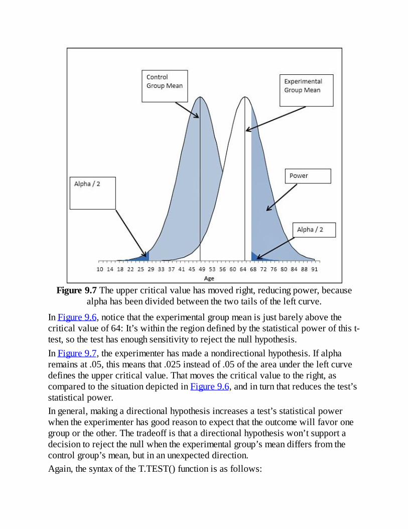
Figure9.7Theuppercriticalvaluehasmovedright,reducingpower,becausealphahasbeendividedbetweenthetwotailsoftheleftcurve.

InFigure9.6,noticethattheexperimentalgroupmeanisjustbarelyabovethecriticalvalueof64:It’swithintheregiondefinedbythestatisticalpowerofthist-test,sothetesthasenoughsensitivitytorejectthenullhypothesis.InFigure9.7,theexperimenterhasmadeanondirectionalhypothesis.Ifalpharemainsat.05,thismeansthat.025insteadof.05oftheareaundertheleftcurvedefinestheuppercriticalvalue.Thatmovesthecriticalvaluetotheright,ascomparedtothesituationdepictedinFigure9.6,andinturnthatreducesthetest’sstatisticalpower.Ingeneral,makingadirectionalhypothesisincreasesatest’sstatisticalpowerwhentheexperimenterhasgoodreasontoexpectthattheoutcomewillfavoronegrouportheother.Thetradeoffisthatadirectionalhypothesiswon’tsupportadecisiontorejectthenullwhentheexperimentalgroup’smeandiffersfromthecontrolgroup’smean,butinanunexpecteddirection.Again,thesyntaxoftheT.TEST()functionisasfollows:

=T.TEST(Array1,Array2,Tails,Type)IntheT.TEST()function,youstatewhetheryouwantExceltoexamineonetailonlyorbothtails.IfyousetTailsto1,Excelreturnstheareaofthecurvebeyondthecalculatedt-statisticinonetail.IfyousetTailsto2,Excelreturnsthetotaloftheareastotherightofthet-statisticandtotheleftofthenegativeofthet-statistic.Soifthecalculatedtis3.7,T.TEST()withtwotailsreturnstheareaunderthecurvetotheleftof–3.7plustheareatotherightof+3.7.

UsingtheTypeArgumentTheTypeargumenttotheT.TEST()functiontellsExcelwhatkindoft-testtorun,andyourchoiceinvolvessomeassumptionsthatthischapterhasasyetjusttouchedon.Mostteststhatsupportstatisticalinferencemakeassumptionsaboutthenatureofthedatayousupply.Theseassumptionsareusuallyduetothemathematicsthatunderliesthetest.Inpractice:

Youcansafelyignoresomeassumptions.Someassumptionsgetviolated,butthereareproceduresfordealingwiththeviolation.Someassumptionsmustbemetorthetestwillnotworkasintended.

TheTypeargumentintheT.TEST()functionpertainstothesecondsortofassumption:WhenyouspecifyaType,youtellExcelwhichassumptionyou’reworriedaboutandthuswhichprocedureitshouldusetodealwiththeviolation.Thetheoryoft-testsmakesthreedistinctassumptionsaboutthedatayouhavegathered.

NormalDistributionsThet-testassumesthatbothsamplesaretakenfrompopulationsthataredistributednormallyonthemeasureyouareusing.IfyouroutcomemeasurewereanominalvariablesuchasIllversusHealthy,youwouldbeviolatingtheassumptionofnormalitybecausethereareonlytwopossiblevaluesandthemeasurecannotbedistributednormally.Thisassumptionbelongstothesetthatyoucansafelyignoreinpractice.Considerableresearchhasinvestigatedtheeffectofviolatingthenormalityassumptionanditshowsthatthepresenceofunderlying,non-normaldistributionshasonlyatrivialeffectontheresultsofthet-test.(Statisticianssometimessaythatthet-testisrobustwithrespecttotheviolationoftheassumptionofnormality,andthestudiesjustmentionedarereferredtoastherobustnessstudies.)

IndependentObservationsThet-testassumesthattheindividualrecordsareindependentofoneanother.Thatis,theassumptionisthatthefactthatyouhaveobservedavalueinonegrouphasnoeffectonthelikelihoodofobservinganothervalueineithergroup.Supposeyouweretestingthestatusofagene.IfFredandJudyarebrotherandsister,thestatusofFred’sgenemightwellmirrorthestatusofJudy’sgene(andviceversa).Theobservationswouldnotbeindependentofoneanother,whethertheywereinthesamegrouporintwodifferentgroups.Thisisanimportantassumptionbothintheoryandinpractice:Thet-testisnotrobustwithrespecttotheviolationoftheassumptionofindependenceofobservations.However,youoftenfindthatquantifiablerelationshipsexistbetweenthetwogroups—andinthatcaseyoucanmanagetheassumption,eveniftheobservationsaren’tindependentofoneanother.Forexample,youmightwanttotesttheeffectofanewtypeofcartireongasmileage.Supposefirstthatyouacquire,say,20newcarsofrandommakesandmodelsandassignthem,alsoatrandom,touseeitheranexistingtireorthenewtype.Butwiththatsmallasample,randomassignmentisnotnecessarilyaneffectivewaytoequatethetwogroupsofcars.

NoteEvenoneoutlierineithergroupcanexertadisproportionateinfluenceonthatgroup’smeanvaluewhenthereareonlytenrandomlyselectedcarsinthegroup.Randomselectionandassignmentareusuallyhelpfulinequatinggroups,butfromtimetotimeyouhappentogetabunchofsubcompactsandoneHumVee.

Nowsupposethatyouacquiretwocarsfromeachoftendifferentmodellines.Thenyourandomlyassignonecarfromeachmodel-pairtogetfourtiresofanexistingtype,andtheothercarinthepairtogetfourtiresofyournewtype.ThelayoutofthisexperimentisshowninFigure9.8.

Figure9.8AsyousawinChapter4,“HowVariablesMoveJointly:Correlation,”youcanpairupobservationsinalistbyputtingtheminthesamerow.

Inthisdesign,theobservationsclearlyviolatetheassumptionofindependence.Thefactthatonecarfromeachmodelhasbeenplacedinonegroupmeansthattheprobabilityis100%thatanothercar,identicalbutforthetires,isplacedintheothergroup.Becausetheonlydifferencebetweenthemembersofamatchedpairisthetires,thetwogroupshavebeenequatedonothervariables,suchasweightandnumberofcylinders.Andbecausetheexperimentercanpairuptheobservations,theamountofdependencebetweenthetwogroupscanbecalculatedandusedtoadjustthet-test.AsisshowninFigure9.8,thecorrelationingasmileagebetweenthetwogroupsisafairlyhigh0.68;therefore,theR-squared,theamountofsharedvarianceingasmileage,isalmost47%.Becauseofthepairingofobservationsindifferentgroups,thedependentgroupst-testhasonedegreeoffreedomforeachpair,minus1.SointheexampleshowninFigure9.8,thedependentgroupst-testhas10pairsminus1,or9degreesoffreedom.Figure9.8alsoshowstheresultoftheT.TEST()functiononthetwoarraysincolumnsBandC.Withninedegreesoffreedom,takingintoaccountthecorrelationbetweenthetwogroups,thelikelihoodofgettingasamplemeandifferenceof4.43milespergallonisonly.04,ifthereisnodifferenceintheunderlyingpopulations.Ifyouhadstartedoutbysettingyouralpharateto.05,youcouldrejectthenullhypothesisofnodifference.

CalculatingtheStandardErrorforDependentGroupsOneofthereasonstouseadependentgroupst-testwhenyoucandosoisthatthetestbecomesmorepowerful,justasusingalargervalueofalphaormakingadirectionalhypothesismakesthet-testmorepowerful.Toseehowthiscomesabout,considerthewaythatthestandarderrorofthedifferencebetweentwo

meansiscalculated.HereistheformulaforthevarianceofavariablenamedA:

Then,ifAisactuallyequaltoX–Y,wehavethefollowing:

Rearrangingtheelementsinthatexpressionresultsinthis:

Expandingthatexpressionbycarryingoutthesquaringoperation,wegetthis:

ThefirsttermhereisthevarianceofX.ThethirdtermisthevarianceofY.ThesecondtermincludesthecovarianceofXandY(seeChapter4forinformationonthecovarianceanditsrelationshiptothecorrelationcoefficient.)Sotheequationcanberewrittenas

or

Therefore,thevarianceofthedifferencebetweentwovariablescanbeexpressedasthevarianceofthefirstvariableplusthevarianceofthesecondvariable,lesstwicethecovariance.Chapter4alsodiscussesthecovarianceasthecorrelationbetweenthetwovariablestimestheirstandarddeviations.Theonlypartofthatyoushouldbothertorememberisthatyousubtractaquantitythatdependsonthestrengthofthecorrelationbetweenthetwovariables.Inthecontextofthedependentgroupst-test,thosevariablesmightbethescoresofthesubjectsinGroup1andthescoresoftheirsiblingsinGroup2—orthempgattainedbythecarmodelsinGroup1andthempgfortheidenticalmodelsinGroup2,andsoon.It’sworthnotingthatwhenyouarerunninganindependentgroupst-test,aswasdoneinthefirstpartofthischapter,thereisnocorrelationbetweenthescoresofthetwogroups,becausenobasisexistsonwhichtopairupthescores.Thenthestandarderrorofthemeandifferencesisjustthesumofthegroups’variances.Withequalsamplesizes,thesumofthegroups’variancesisthesameasthepooledvariancediscussedearlierinthechapter.Butwhenmembersofthetwogroupscanbepairedup,youcancalculatea

correlationandreducethesizeofthestandarderroraccordingly(refertothefinalequationjustgiven).Inturn,thisgivesyourtestgreaterpower.Toreview,here’sthebasicequationforthet-statistic:

Clearly,whenthedenominatorissmaller,theratioislarger.Alargert-statisticismorelikelytoexceedthecriticalvalue.Therefore,whenyoucanpairupmembersoftwogroups,youcancalculatethecorrelationontheoutcomevariablebetweenthetwogroups.Thatresultsinasmallerdenominator,becauseyousubtractit(multipliedby2andbytheproductofthestandarddeviations)fromthesumofthevariances.

NoteThere’snoneedtorememberthespecificsofthisdiscussion.Forexample,Exceltakescareofallthecalculationsforyouifyou’vereadthisbookandknowhowtoapplythebuilt-inworksheetfunctionssuchasT.TEST().Theimportantpointtotakefromtheprecedingdiscussionisthatadependentgroupst-testcanbeamuchmoresensitive,powerfultestthananindependentgroupstest.We’llreturntothispointinChapter15,“MultipleRegressionAnalysisandEffectCoding:FurtherIssues.”

Inacasesuchasthecartireexample,youexpectthattheobservationsarenotindependent,butbecauseyoucanpairupthedependentrecords(eachmodelofcarisrepresentedonceineachgroup),youcanquantifythedegreeofdependency;thatis,youcancalculatethecorrelationbetweenthetwosetsofscoresbecauseyouknowwhichscoreinonegroupgoeswithwhichscoreintheothergroup.Onceyouhavequantifiedthedependency,youcanuseittomakethestatisticaltestmoresensitive.ThatisthepurposeofoneofthevaluesyoucanselectfortheT.TEST()function’sTypeargument.Ifyousupplythevalue1asitsTypeargument,youinformExcelthattherecordsinthetwoarraysarerelatedinsomewayandthatthecorrelationshouldfactorintothefunction’sresult.Soifeacharraycontainsoneoftwotwins,Record1inonearrayshouldberelatedtoRecord1inthesecondarray,Record2inonearrayshouldberelatedtoRecord2intheotherarray,andsoon.

RunningtheCarExampleTwoWaysFigure9.8showshowyoucanrunadependentgroupst-testtwodifferentways.Onewaygrindstheanalysisoutformulabyformula:It’smoretediousbutitshows

youwhat’sgoingonandhelpsyoulaythegroundworkforunderstandingmoreadvancedanalysissuchasANCOVA.Theotherwayisquick—itrequiresonlyoneT.TEST()formula—butallyougetfromitisaprobabilitylevel.It’susefulifyou’repressedfortime(orifyouwanttocheckyourwork),butit’snothelpfulifwhatyou’reafterisunderstanding.Toreview,columnsA,B,andCinFigure9.8containdataonthempgoftenpairsofcars.Eachpairofcarsoccupiesadifferentrowontheworksheet,andapairconsistsoftwocarsfromthesamemanufacturer/model.Theexperimenteristryingtoestablishwhetherornotthedifferencebetweenthegroups,typeofcartire,makesadifferencetomeangasmileage.TherangeshavebeennamedTireAandTireB.TherangenamedTireAoccupiescellsB2:B11,andtherangenamedTireBoccupiescellsC2:C11.Therangenamesmakeitalittleeasiertoconstructformulasthatrefertothoseranges,andtomaketheformulasabitmoreself-documenting.Thefollowingformulasareneededtogrindouttheanalysis.ThecellreferencesarealltoFigure9.8.

GroupMeansThemeanmpgforeachgroupappearsincellsF2andI2.TheformulasusedinthosetwocellsappearincellsG2andJ2.Inthesesamples,thecarsusingTireBgetbettergasmileagethanthoseusingTireA.Itremainstodecidewhethertoattributethedifferenceingasmileagetothetiresortochance.

GroupVariabilityThevariancesappearinF3andI3,andtheformulasthatreturnthevariancesareincellsG3andJ3.ThestandarddeviationsareinF4andI4.TheformulasthemselvesareshowninG4andJ4.TheformsofthefunctionsthattreatthedataincolumnsBandCassamplesareusedintheformulas.

StandardErroroftheMeanWhenyou’retestingagroupmeanagainstahypothesizedvalueaswasdoneinChapter8,youusethestandarderrorofthemeanasthet-test’sdenominator;thestandarderrorofthemeanisthestandarddeviationofmanymeans,notofmanyindividualobservations.When,ashere,you’retestingtwogroupmeansagainstoneanother,youusethestandarderrorofthedifferencebetweenmeans;thatis,thestandarddeviationofmanymeandifferences.Thisexampleisabouttocalculatethestandarderrorofthedifference,buttodosoitneedstousethevarianceerrorofthemean,whichis

thesquareofthestandarderrorofthemean.Thatvalue,oneforeachgroup,appearsincellsF5andI5;theformulasareinG5andJ5.

CorrelationAsdiscussedearlierinthischapter,youneedtoquantifythedegreeofdependencebetweenthetwogroupsinadependentgroupst-test.Youdosoinordertoadjustthesizeofthedenominatorinthet-statistic.Inthisexample,Figure9.8showsthecorrelationincellF7andtheformulaincellG7.IdentifyingthecarmodelsincellsA2:A11isnotstrictlypartofthet-test.Butitunderscoresthenecessityofkeepingbothmembersofapairinthesamerowoftherawdata.Forexample,CarModel1appearsincellB2andcellC2,Model2appearsincellB3andcellC3,andsoon.OnlywhenthedataislaidoutinthisfashioncantheCORREL()functionaccuratelycalculatethecorrelationbetweenthetwogroups.

NoteThepreviousstatementisnotstrictlytrue.Therequirementisthateachmemberofapairoccupythesamerelativepositionineacharray.Soifyouusedsomethingsuchas=CORREL(A1:A10,B11:B20),youneedtobesurethatonepairisinA1andB11,anotherpairinA2andB12,andsoon.Theeasiestwaytomakesureofthissetupistostartbotharraysinthesamerow—andthatalsohappenstoconformtothelayoutofExcellistsandtables.

StandardErroroftheDifferenceBetweenMeansCellF8calculatesthestandarderrorofthedifferencebetweenmeans,asitisderivedearlierinthischapterinthesectiontitled“CalculatingtheStandardErrorforDependentGroups.”Itisthesquarerootofthesumofthevarianceerrorofthemeanforeachgroup,lesstwicetheproductofthecorrelationandthestandarderrorofthemeanofeachgroup.TheformulausedincellF8appearsincellG8.

Calculatingthet-StatisticThet-statisticfortwodependentgroupsistheratioofthedifferencebetweenthegroupmeanstothestandarderrorofthemeandifferences.ThevalueforthisexampleisincellF9andtheformulaincellG9.

CalculatingtheProbabilityTheT.DIST()functionhasalreadybeendiscussed;yousupplyitwiththe

argumentsthatidentifythet-statistic(here,thevalueinF9),thedegreesoffreedom(9,thenumberofpairsminus1),andwhetheryouwantthecumulativeareaunderthet-distributionthroughthevaluespecifiedbythet-statistic(here,TRUE).Inthiscase,96%oftheareaunderthet-distributionwith9degreesoffreedomliestotheleftofat-statisticof1.93.Butit’stheareatotherightofthatt-statisticthatwe’reinterestedin;see,forexample,Figure9.2,wherethatareaappearsinthecurveforthecontrolgroup,totherightofthemeanoftheexperimentalgroup.Theresultoftheformulainthisexampleis.04,or4%.Anexperimenterwhohadadopted.05asalpha,theriskofrejectingatruenullhypothesis,andwhohadmadeadirectionalalternativehypothesis,wouldrejectthenullhypothesisofnodifferenceinthepopulationmeanmpgvalues.

UsingtheT.TEST()FunctionAlltheprecedinganalysis,includingthefunctionsusedinrows2through10ofFigure9.8,canbecompressedintooneformula,whichalsoreturns.04incellF11ofFigure9.8.ThefullformulaappearsincellG11.ItsargumentsincludethenamedrangethatcontainstheindividualmpgfiguresforTireAandthoseforTireB.Thethirdargument,Tails,isgivenas1,soT.TEST()returnsadirectionaltest.Itcalculatestheareatotherightofthecalculatedt-statistic.IftheTailsargumenthadbeensetto2,T.TEST()wouldreturn.08.Inthatcase,itwouldreturntheareaunderthecurvetotheleftofat-statisticof–1.93,plustheareaunderthecurvetotherightofat-statisticof1.93.Thefourthargument,Type,isalsosetto1inthisexample.Thatvaluecallsforadependentgroupst-test.IfyouopentheworkbookforChapter9,availablefordownloadfromthebook’swebsiteathttp://www.quepublishing.com/title/9780789753113,youcancheckthevaluesinFigure9.8forcellsF10andF11.Thevaluesinthetwocellsareidenticalto16decimalplaces.

UsingtheDataAnalysisAdd-int-TestsTheDataAnalysisadd-inhas19tools,rangingalphabeticallyfromANOVAtoz-tests.Threeofthetoolsperformt-tests,andthethreetoolsreflectthepossiblevaluesfortheTypeargumentoftheT.TEST()function:

DependentGroupsEqualVariances

UnequalVariancesThepriormajorsectionofthischapterdiscusseddependentgroupst-testsinsomedetail.Itcoveredtherationalefordependentgroupstests.ItcomparedtheuseofseveralExcelfunctionssuchasT.DIST()toarriveatananswerwiththeuseofasinglesummaryT.TEST()functiontoarriveatthesameanswer.ThissectionshowsyouhowtousetheDataAnalysisadd-intooltoperformthesamedependentgroupst-testwithoutrecoursetoworksheetfunctions.Thetooloccupiesamiddlegroundbetweenthelabor-intensiveuseofseveralworksheetfunctionsandtheminimallyinformativeT.TEST()function.Thetoolrunsthefunctionforyou,soit’squick,anditshowsaverages,standarddeviations,groupcounts,t-statistics,criticalvalues,andprobabilities,soit’smuchmoreinformativethanthesingleT.TEST()function.Theprincipaldrawbacktotheadd-in’stoolisthatallitsresultsarereportedasstaticvalues,soifyouwantorneedtochangeoraddavaluetotherawdata,youhavetorunthetoolagain.Theresultsdon’tautomaticallyrefreshthewaythatworksheetfunctionsdowhentheirunderlyingdatachanges.

GroupVariancesint-TestsEarlier,thischapternotedthatthebasictheoryoft-testsassumesthatthepopulationsfromwhichthegroupsaresampledhavethesamevariance.Theprocedurethatfollowsfromtheassumptionofequalvariancesisthattwovariances,onefromeachsample,arepooledtoarriveatanestimateofthepopulationvariance.ThatpoolingisdoneasshownincellsF1:F2ofFigure9.1andasrepeatedhereindefinitionalform:

Thatdiscussionwentontopointoutthatboththeoreticalandempiricalresearchhaveshownthatwhenthetwosampleshavethesamenumberofobservations,violatingtheequalvariancesassumptionmakesanegligibledifferencetotheoutcomeofthet-test.Inturn,thatfindingimpliesthatyoudon’tworryaboutunequalvarianceswhenyou’rerunningadependentgroupst-test.Bydefinition,thetwogroupshavethesamesamplesize,becauseeachmemberofonegroupmustbepairedwithexactlyonememberoftheothergroup.Thatleavesthecasesinwhichgroupsizesaredifferentandsoaretheirvariances.Whenthelargergrouphasthelargersamplevariance,itcontributesagreatershareofgreatervariabilitytothepooledestimateofpopulationvariancethandoesthesmallergroup.

Asaresult,thestandarderrorofthemeandifferenceisinflated.Thatstandarderroristhedenominatorinthet-test,andthereforethet-ratioisreduced.Youareworkingwithanactualalpharatethatislessthanthenominalalpharate,andstatisticiansrefertoyourt-testasconservative.Theprobabilitythatyouwillrejectatruenullhypothesisislowerthanyouthink.Butifthelargergrouphasthesmallersamplevariance,itcontributesagreatershareoflowervariabilitythandoesthesmallergroup.Thisreducesthesizeofthestandarderror,inflatesthevalueofthet-ratio,andinconsequenceyouareworkingwithanactualalphathatislargerthanthenominalalpha.Statisticianswouldsaythatyourt-testisliberal.Theprobabilitythatyouwillrejectatruenullhypothesisisgreaterthanyouthink.

TheDataAnalysisAdd-InEqualVariancest-TestThistoolistheclassict-test,largelyasitwasoriginallydevisedintheearlypartofthetwentiethcentury.Itmaintainstheassumptionthatthepopulationvariancesareequal,it’scapableofdealingwithgroupsofdifferentsamplesizes,anditassumesthattheobservationsareindependentofoneanother.(Thus,itdoesnotcalculateanduseacorrelation.)Toruntheequalvariancestool(ortheunequalvariancestoolorthepairedsample,dependentgroupstool),youmusthavetheDataAnalysisadd-ininstalled,asdescribedinChapter4.Oncetheadd-inisinstalled,youcanfinditintheAnalysisgroupontheRibbon’sDatatab.ToruntheEqualVariancest-test,activateaworksheetwiththedatafromyourtwogroups,asincolumnsBandCinFigure9.8,andthenclicktheDataAnalysisbuttonintheAnalysisgroup.Youwillseealistboxwiththenamesoftheavailabledataanalysistools.Scrolldownuntilyouseet-Test:Two-SampleAssumingEqualVariances.Clickit,andthenclickOK.ThedialogboxshowninFigure9.9appears.

Figure9.9Thet-testtoolsalwayssubtractVariable2fromVariable1whencalculatingthet-statistic.

HereareafewcommentsregardingthedialogboxinFigure9.9(whichalsoapplytothedialogboxesthatappearifyouchoosetheunequalvariancest-testorthepairedsamplet-test):

Asnoted,Variable2isalwayssubtractedfromVariable1.Ifyoudon’twanttogetcaughtupintheveryminorlogicalcomplicationsofnegativet-statistics,makeitaruletodesignatethegroupwiththelargermeanasVariable1.Sodoingisnotthesameaschanginganondirectionalhypothesistoadirectionaloneafteryou’veseenthedata.Youarenotalteringyourdecisionruleafterthefact;youaresimplydecidingthatyouprefertoworkwithpositiveratherthannegativet-statistics.Ifyouincludecolumnheadersinyourdataranges,filltheLabelscheckboxtousethoseheadersinsteadofVariable1andVariable2intheoutput.ThecautionregardingtheOutputRange,madeinChapter4,holdsforthet-testdialogboxes.Whenyouchoosethatoptionbutton,ExcelimmediatelyactivatestheaddressboxforVariable1.BesuretomakeOutputRange’sassociatededitboxactivebeforeyouclickinthecellwhereyouwanttheoutputtostart.LeavingtheHypothesizedMeanDifferenceboxblankisthesameassettingittozero.Ifyouenteranumbersuchas5,youarechangingthenullhypothesisfrom“Mean1–Mean2=0”to“Mean1–Mean2=5.”Inthatcase,besurethatyou’vethoughtthroughtheissuesregardingdirectionalhypothesesdiscussedpreviouslyinthischapter.

Aftermakingyourchoicesinthedialogbox,clickOK.Youwillseetheanalysis

shownincellsE1:G14inFigure9.10.

Figure9.10NotethatthePairedtestincolumnsI:KprovidesamoresensitivetestthantheEqualVariancestestincolumnsE:G.

NotethefollowingpointsraisedbytheEqualVariancesanalysisinE1:G14inFigure9.10,particularlyincomparisontothePairedSample(dependentgroups)analysisinI1:K14.Comparethecalculatedt-statisticinF10withthatinJ10.TheanalysisinE1:G14assumesthatthetwogroupsareindependentofoneanother.Therefore,theanalysisdoesnotcomputeacorrelationcoefficient,asisdoneinthe“pairedsample”analysis.Inturn,thedenominatorofthet-statisticisnotreducedbyafigurethatdependsinpartonthecorrelationbetweentheobservationsinthetwogroups.Asaresult,thet-statisticinF10issmallerthantheoneinJ10:smallenoughthatitdoesnotexceedthecriticalvalueneededtorejectthenullhypothesisatthe.05levelofalphaeitherforadirectionaltest(cellF12)oranondirectionaltest(cellF14).Alsocomparethedegreesoffreedomforthetwotests.TheEqualVariancestestuses18degreesoffreedom:tenfromeachgroup,lesstwoforthemeansofthetwogroups.ThePairedSampletestusesninedegreesoffreedom:tenpairsofobservations,lessoneforthemeanofthedifferencesbetweenthepairs.

Asaresult,thePairedSamplet-testhasalargercriticalvalue.Iftheexperimenterisusingadirectionalhypothesis,thecriticalvalueis1.734fortheEqualVariancestestand1.833forthePairedSampletest.Thepatternissimilarforanondirectionaltest:2.101versus2.262.Thisdifferenceincriticalvaluesisduetothedifferenceindegreesoffreedom:Otherthingsbeingequal,at-distributionwithasmallernumberofdegreesoffreedomrequiresalargercriticalvalue.ButeventhoughthePairedSampletestrequiresalargercriticalvalue,becausefewerdegreesoffreedomareavailable,itisstillmorepowerfulthantheEqualVariancestestbecausethecorrelationbetweenthetwogroupsresultsinasmallerdenominatorforthet-statistic.Theweakerthecorrelation,however,thesmallertheincreaseinpower.Youcanconvinceyourselfofthisbyreviewingtheformulaforthestandarderrorofthedifferencebetweentwomeansforthedependentgroupst-test.Seethesectionearlierinthischaptertitled“CalculatingtheStandardErrorforDependentGroups.”

TheDataAnalysisAdd-InUnequalVariancest-TestFigure9.11showsacomparisonbetweentheresultsoftheDataAnalysisadd-in’sEqualVariancestestandtheUnequalVariancestest.

Figure9.11Thedatahasbeensetuptoreturnaliberalt-test.

Itisusualtoassumeequalvariancesinthet-test’stwogroupsiftheirsamplesizesareequal.Butwhatiftheyareunequal?Thepossibleoutcomesareasfollows:

Ifthegroupwiththelargersamplesizehasthelargervariance,youralphalevelissmallerthanyouthink.Ifthenominalalpharatethatyouhavechosenis0.05,forexample,theactualerrorratemightbe0.03.Youwillrejectthenullhypothesislessoftenthanyoushould.Thus,thet-testisconservative.(Thecorollaryisthatstatisticalpowerislowerthanisapparent.)Ifthegroupwiththelargersamplesizehasthesmallervariance,youralphalevelisgreaterthanyouthink.Ifthenominalalpharatethatyouhavechosenis0.05,forexample,theactualerrorratemightbe0.08.Youwillmoreoftenerroneouslyconcludeadifferenceexistsinthepopulationwhereitdoesn’t.Thet-testisliberal,andthecorollaryisthatstatisticalpowerisgreaterthanyouwouldexpect.

Accordingly,therawdataincolumnsBandCinFigure9.11includesthefollowing:

TheTireBgroup,whichhas20records,hasavarianceof79.TheTireAgroup,whichhas10records,hasavarianceof166.

Sothelargergrouphasthesmallervariance,whichmeansthatthet-testoperatesliberally—theactualalphaislargerthanthenominalalphaandthetest’sstatisticalpowerisincreased.However,evenwiththataddedpower,theEqualVariancest-testdoesnotreportat-statisticthatisgreaterthanthecriticalvalue,foreitheradirectionaloranondirectionalhypothesis.ThemainpointtonoticeinFigure9.11isthedifferenceindegreesoffreedombetweentheEqualVariancestestshownincellsE1:G14andtheUnequalVariancestestincellsI1:K14.ThedegreesoffreedomincellF9is28,asyouwouldexpect.Twentyrecordsinonegroupplustenrecordsintheothergroup,lesstwoforthegroupmeans,resultsin28degreesoffreedom.However,thedegreesoffreedomfortheUnequalVariancestestincellJ9is13,whichappearstobearnorelationshiptothenumberofrecordsinthetwogroups.Alsonotethatthet-statisticitselfisdifferent:1.090inF10versus0.964incellJ10.TheUnequalVariancestestuseswhat’scalledWelch’scorrection,soastoadjustfortheliberal(orconservative)effectofalargergroupwithasmaller(orlarger)variance.Thecorrectionprocedureinvolvestwosteps:

1.Forthet-statistic’sdenominator,usethesquarerootofthesumofthetwovariances,ratherthanthestandarderrorofthemeandifference.

2.Adjustthedegreesoffreedominadirectionthatmakesaliberaltestmoreconservative,oraconservativetestmoreliberal.

Thespecificsoftheadjustmenttothedegreesoffreedomarenotconceptuallyilluminating,sotheyareskippedhere;it’senoughtostatethattheadjustmentdependsontheratiosofthegroups’variancestotheirassociatednumberofrecords.Forexample,thedatainFigure9.11involvesalargergroupwithasmallervariance,soyouexpectthenormalt-testtobeliberal,withahigheractualalphathanthenominalalphaselectedbytheexperimenter.WhenWelch’scorrectionisapplied,thet-TestforUnequalVariancesuses13degreesoffreedomratherthan28.Asthepriorsectionnoted,at-distributionwithfewerdegreesoffreedomhasalargercriticalvalueforcuttingoffanalphaareathandoesonewithmoredegreesoffreedom.

Accordingly,theUnequalVariancestestwith13degreesoffreedomneedsacriticalvalueof1.771tocutoff5%oftheuppertailofthedistribution(cellJ12).TheEqualVariancestest,whichuses28degreesoffreedom,cutsoff5%ofthedistributionatthelowercriticalvalueof1.701(cellF12).Thisisbecausethet-distributionisslightlyleptokurtic,withthickertailsinthedistributionswithfewerdegreesoffreedom.

VisualizingStatisticalPowerBothChapter8andthischapterhavehadmuchtosayaboutstatisticalpower.Severalfactorscaninfluencehowsensitiveat-testistoexperimentaldata:thesizeofthetreatmenteffect,thesamplesizes,thestandarddeviationoftheoutcomemeasure,thesizeofalpha,andthedirectionalityofthehypotheses.Thosefactorsallacttogethertoinfluencepower.Figure9.12showsaworksheetthatcanhelpyouvisualizetheeffectsofthosefactors.

Figure9.12Thespinnersenableyoutoincreaseordecreasetheirassociatedvalues.

YoucanfindtheworksheetshowninFigure9.12intheworkbookforChapter9

thatisavailableonthebook’swebsiteathttp://www.quepublishing.com/title/9780789753113.Useittoincreaseordecreasethetreatmenteffect,changesamplesizes(andthereforestandarderrors),standarddeviations(andthereforestandarderrors,again),andsoon.Whenyoudoso,thechartredrawstoshowtheresultofthechangeyoumade.Watchinparticularwhathappensintherightcurvethatrepresentstheexperimentalgroup.Thepowerofthet-test,asthesecurvesarelaidout,istheareaundertherightcurvethatliestotherightofthecriticalvaluethatboundsthealphaarea(shownintherighttailoftheleftdistribution).Forexample,ifyoureducethetreatmenteffectbyreducingMean2,therightcurveispulledtotheleftandlessofitliestotherightofthecriticalvalue.Powerisreduced.Alternatively,ifyoudecreasethesizeofthestandarddeviation,thesizeofthestandarderrorsdecreases.Thatpullsthealphaareatotheleft,leavingmoreoftheareaoftherightcurvetotherightofthecriticalvalue.

WhentoAvoidt-TestsThetheoreticalunderpinningsoft-testsdonotaccountformorethantwogroups.TheexamplesinChapters8and9haveallinvolvedanexperimentalgroupandacontrolgroup.Althoughthisisatypicaldesignforgoodexperiments,itissomewhatrestrictive.Therearemanyinterestingquestionswhoseanswersrequiretheuseofthreeormoregroups(forexample,adrugtrialinvolvingagroupthattakesanewdrug,agroupthattakesanexistingdrugoraplacebo,andagroupthattakesnomedicationatall).Forthissortofsituation,t-testsarenotappropriate.Chapter10,“TestingDifferencesBetweenMeans:TheAnalysisofVariance,”explainswhythatisso,andintroducesthestatisticaltestthatisdesignedtohandlethreeormoregroups:theanalysisofvariance.

10.TestingDifferencesBetweenMeans:TheAnalysisofVariance

InThisChapterWhyNott-Tests?TheLogicofANOVAUsingExcel’sFWorksheetFunctionsUnequalGroupSizesMultipleComparisonProcedures

Chapter8,“TestingDifferencesBetweenMeans:TheBasics,”andChapter9,“TestingDifferencesBetweenMeans:FurtherIssues,”wentintosomedetailabouthowtousez-testsandt-teststodeterminetheprobabilitythattwogroupmeanscomefromthesamepopulation.Chapter10triestoconvinceyoutouseadifferentmethodwhenyou’reinterestedinthreemeansormore.Theneedtotestwhetherthreeormoremeanscomefromdifferentpopulationscomesupfrequently.Therearemorethantwomajorpoliticalorganizationstopayattentionto.Medicalresearchisnotlimitedtoacomparisonbetweenatreatmentandano-treatmentcontrolgroup,butoftencomparestwoormoretreatmentarmstoacontrolarm.Therearemorethantwobrandsofcarthatmightearndifferentratingsforsafety,mileage,andownersatisfaction.Anyoneofseveraldifferentstrainsofwheatmightproducethebestcropundergivenconditions.

WhyNott-Tests?Ifyouwantedtousestatisticalinferencetotestwhetherornotmorethantwosamplemeansarelikelytohavedifferentpopulationvalues,it’snaturaltothinkofrepeatedt-tests.Youcoulduseonet-testtocompareGMwithFord,anothertocompareGMwithToyota,andyetanothertocompareFordwithToyota.Theproblemisthatifyoudoso,you’retakingunfairadvantageoftheprobabilities.Thet-testwasdesignedtocomparetwogroupmeans,notthree,notfour,notmore.Ifyourunmultiplet-testsonthreeormoremeans,youinflatetheapparentalpharate.Thatis,youmightset.05(beforehand)astheacceptableriskofrejectingatruenullhypothesis.Thatmistakemightwellcometopassbecausetwosamplemeansareimprobablyfarapart,butinfactcomefromthesame

population,whichcanhaveonemeanonly.Youmightthinkyourriskofbeingmisledbysamplingerrorisonly.05,butit’shigherthanthatifyouuseseveralt-teststocomparemorethantwomeans.Asithappens,multiplet-testscaninflateyournominalalphalevelfrom,say,.05to.40.Afullerexplanationwillhavetowaituntilafewrelevantconceptshavebeendiscussed,butFigure10.1givesyouthebasicidea.

Figure10.1Witheveryadditionalt-test,thecumulativeprobabilityofrejectingatruenullhypothesisincreases.

Supposethatyouhavefivemeanstocompare.Therearetenwaystomakepairwisecomparisonsinasetoffivemeans.(IfJisthenumberofmeans,thegeneralformulaisJ(J–1)/2.)Ifyousetalphaat.05,thatnominalalpharateistheactualalpharateforonet-test.Butifyourunanothert-test,youhave95%oftheoriginalprobabilityspaceremaining(with5%takenupbythealphayouusedforthefirstt-test).Settingthenominalalphato.05forthesecondt-testmeansthattheprobabilityrejectingatruenullhypothesisineitherofthet-testsis.05+(.05×.95),or.098(cellC3inFigure10.1).Hereisperhapsamoreintuitivewayoflookingatit.Supposethatyouhaverunanexperimentthatcollectsthemeansoffivegroupsonsomeoutcomemeasurefollowingtreatments.Youseethatthelargestandsmallestmeansareimprobablyfarapart—atanyrate,farapartgiventhenullhypothesisthatthetreatmentshadnodifferentialeffects.Youchoosetorunat-testonthelargestandsmallestmeansandfindthatsolargeadifferencewouldoccurlessthan1%ofthetimeifthe

meanscamefromthesamepopulation.Theproblemisthatyouhavecherry-pickedthetwogroupswiththelargestdifferenceintheirmeans,withoutalsopickinggroupsthatmaycontributesubstantiallytothevariabilityoftheoutcomemeasure.IfyouthinkbacktoChapter9,you’llrecallthatyourunat-testbydividingameandifferencebyafactorthatdependsontheamountofvariabilityinthegroupstested.Ifyourunanexperimentthatreturnsfivemeans,andyoucomparethelargestandthesmallestwhileignoringtheothers,youhavestackedthedeckinfavorofdifferencesinmeanswithoutalsoallowingforpossiblygreatervariabilitywithingroups.Whatyouaredoingissometimescalledcapitalizingonchance.Therecommendedapproachwhenyourresearchinvolvesmorethantwogroupsistousetheanalysisofvariance,orANOVA.Thisapproachtestsallyourmeanssimultaneously,takingintoaccountalltheWithinGroupsvariability,andletsyouknowwhetherthereisareliabledifferenceanywhereinthesetofmeans—includingcomplexcomparisonssuchasthemeanoftwogroupscomparedtothemeanoftwoothergroups.Ifthedatapassesthatinitialtest,youcanusefollow-upprocedurescalledmultiplecomparisonstopinpointthesource,orsources,ofthesignificantdifferencethatANOVAalertedyouto.

TheLogicofANOVAThethinkingbehindANOVAbeginswithawayofexpressingeachobservationineachgroupbymeansofthreeparts:

ThegrandmeanofalltheobservationsThemeanofeachgroup,andhowfareachgroupmeandiffersfromthegrandmeanEachobservationineachgroup,andhowfareachobservationdiffersfromthegroupmean

ANOVAusesthesecomponentstodeveloptwoestimatesofthepopulationvariance.Oneisbasedentirelyonthevariabilityofobservationswithineachgroup.Oneisbasedentirelyonthevariabilityofgroupmeansaroundthegrandmean.Ifthosetwoestimatesareverydifferentfromoneanother,that’sevidencethatthegroupscamefromdifferentpopulations—populationsthathavedifferentmeans.

PartitioningtheScoresSupposeyouhavethreegroupsofpeople,andeachgroupwilltakeadifferent

pill:anewcholesterolmedication,anexistingmedication,oraplacebo.Figure10.2showshowthegrandmean,themeanofeachgroup,andeachperson’sdeviationfromthegroupmeancombinetoexpresseachperson’smeasuredHDLlevel.

Figure10.2ThismodelisthebasisformanystatisticalmethodsfromANOVAtologisticregression.

Inpractice,youseldomhavereasontoexpresseachsubject’sscoreinthisway—asacombinationofthegrandmean,thedeviationofeachgroupmeanfromthegrandmean,andthesubject’sdeviationfromthegroupmean.Butviewingthescoresinthiswayhelpslaythegroundworkfortheanalysis.Theobjectiveistoanalyzethetotalvariabilityofallthescoresintotwosets:variabilityduetoindividualsubjectscoresandvariabilityduetothedifferencesingroupmeans.Byanalyzingthevariabilityinthisway,youcancometoaconclusionaboutthelikelihoodthatchancecausedthedifferencesingroupmeans.(Thisisthesameobjectivethatt-testshave,butANOVAnormallyassessesthreeormoremeans.Infact,iftherearejusttwogroups,theFstatisticyougetfrom

ANOVAisidenticaltothesquareoftheratioyougetfromat-test.)Figure10.2showshowthevariationduetoindividualobservationsisseparatedfromvariationduetodifferencesbetweengroupmeans.Asyou’llseeshortly,thisseparationputsyouinapositiontoevaluatethedistancebetweenmeansinlightofthedistancebetweentheindividualsthatmakeupthemeans.Figure10.3showsthetwoverydifferentpathstoestimatingthevariabilityinthedataset.Row2containsthegroupmeans,andthedifferencesbetweenthesemeansleadtothesumofsquaresbetween,incellM2.Row4containsnotgroupmeansbutthesumsofthesquareddeviationswithineachgroup,whichleadtothesumofsquareswithin,incellM4.

Figure10.3Thisfigurejustshowsthemechanicsoftheanalysis.Youdon’tusuallymanagethemyourself,butturnthemoverto,forexample,theData

Analysisadd-in.

Figure10.3showshowtheoverallsumofsquaresisallocatedtoeitherindividualvariationortovariationbetweenthegroupmeans.

SumofSquaresBetweenGroups

InFigure10.3,theformulasthemselvesappearintherangeH9:M13.TheresultsofthoseformulasappearintherangeH2:M6.TherangeH2:M2inFigure10.3showshowthesumofsquaresbetweengroupmeansiscalculated.EachgroupmeanappearsinH2:J2.(ComparewiththecellsC2,C5,andC8inFigure10.2.)CellK2containsthesumofthesquareddeviationsofeachgroupmeanfromthegrandmean.ThisfigureisreturnedusingtheworksheetfunctionDEVSQ(),asshownincellK9.TheresultinK2mustbemultipliedbythenumberofindividualobservationsineachgroup.Becauseeachgrouphasthesamenumberofobservations,thiscanbedonebymultiplyingthetotalinK2by3,eachgroup’ssamplesize(typicallyrepresentedbythelettern).Theresult,usuallylabeledsumofsquaresbetweenorSSB,appearsincellM2.Herearethespecifics:

SSB=3*((53–50)^2+(46–50)^2+(51–50)^2)SSB=3*(9+16+1)

SSB=78NotethatSSBistheconventionalnotationforsumofsquaresbetween.

SumofSquaresWithinGroupsTherangeH4:M4inFigure10.3showshowthesumofsquareswithingroups(SSW)iscalculated.ThefunctionDEVSQ()isusedinH4:J4togetthesumofthesquareddeviationswithineachgroupfromthatgroup’smean.Therangereferences—forexample,=DEVSQ(D2:D4)incellH4—aretocellsshowninFigure10.2.TheDEVSQ(D2:D4)functionincellH4subtractsthemeanofthevaluesinD2:D4fromeachofthevaluesthemselves,squaresthedifferences,andsumsthesquareddifferences.Herearethespecifics:

SSw1=(55–53)2+(50–53)2+(54–53)2

SSw1=4+9+1SSw1=14

SSwistheconventionalnotationforsumofsquareswithingroups,andthenumeral1inthesubscriptindicatesthattheformulaisdealingwiththefirstgroup.Afterthesumofsquareddeviationsisobtainedforeachofthethreegroups,incellsH4:J4,thesumsaretotaledincellK4andthattotaliscarriedoverintocellM4.NoweightingisneededasitisinM2,wherethetotalofthesquared

deviationsismultipliedbythesamplesizeofthreepergroup.Theproofofthisappearsinaworksheettitled“MSBproof”intheworkbookforChapter10,whichyoucandownloadfromthebook’swebsiteathttp://www.quepublishing.com/title/9780789753113.

NoteEachgroupinthisbasicexamplehasthesamenumberofsubjects.Theanalysisofvariancehandlesdifferentnumbersofsubjectsorobservationspergroupquiteeasily—automatically,infact,ifyouusetoolssuchastheDataAnalysisadd-in’ssinglefactorANOVAtool.(Inthisexample,thetypeofmedicationtakenisafactor.Iftheexamplealsotestedfordifferencesinoutcomesaccordingtothesubject’ssex,thattoowouldbetermedafactor.)Youoftenencountertwo-factor,three-factor,ormorecomplexdesigns,andtheissueofequalgroupsizesthenbecomesmoredifficulttomanage.Chapter11,“AnalysisofVariance:FurtherIssues,”exploresthisproblemingreaterdetail.

Withthisdataset,thesumofsquaresbetweengroupsis78,incellM2ofFigure10.3,andthesumofsquareswithingroupsis34,incellM4.Thosetwosumsofsquarestotalto112,whichisalsothevalueyougetusingtheDEVSQ()functiononthefulldataset,asincellM6.

ComparingVariancesWhatwehavedonehere—andwhateverystandardanalysisofvariancedoes—isbreakdown,orpartition,thetotalvariationthatiscalculatedbysummingthesquareddeviationsofeveryscorefromthegrandmean.Thetotalofthesquareddeviationsis112,andit’spartitionedintoasumofsquaresbetweengroupmeans(here,78)andasumofsquaresamongobservationswithingroups(here,34).Oncethat’sdone,wecancreatetwodifferent,independentestimatesofthetotalvariance.

VarianceBasedonSumsofSquaresWithinGroupsRecallfromChapter3,“Variability:HowValuesDisperse,”thatavarianceissimplythesumofthesquareddeviationsofscoresfromtheirmean,dividedbythedegreesoffreedom.Youhavethesumofsquares,basedonvariabilitywithingroups,incellE2ofFigure10.4.Youarriveat34bytotalingthesumofsquareswithineachgroup,justasdescribedintheprecedingsection.

Figure10.4Howthesumsofsquareswithingroupsareaccumulated.

Eachgrouphas2degreesoffreedom:Therearethreeobservationspergroup,andyouloseonedegreeoffreedompergroupbecauseeachgroupmeanisfixed.(Chapter3providestherationaleforthisadjustment.)Youcandivideeachgroup’ssumofsquaresby2togetthevarianceforeachgroup.ThisisdoneincellsB5:D5ofFigure10.4.Eachofthosethreevariancesisanestimateofthevariabilityinthepopulationfromwhichthesamplesweredrawntocreatethethreegroups.TakingtheaverageofthethreevariancesincellE5providesanevenmoreefficientestimateofthepopulationvariance.Amathematicallyequivalentwaytoarriveatthetotalwithingroupvarianceistodividethetotalofthewithingroupsumsofsquaresbythetotalnumberofsubjectslessthenumberofgroups.ThetotalwithingroupsumofsquaresisshownincellG5ofFigure10.4.Whenthenumberofsubjectsisthesameineachgroup,yougetthetotaldegreesoffreedomforwithingroupvariationbymeansofN–J,whereJisthenumberofgroupsandNisthetotalnumberofsubjects.(Theformulaiseasilyadjustedwhenthegroupshavedifferentnumbersofsubjects.)Thenumberofsubjectslessthenumberofgroups,incellH5,isdividedintothetotalwithingroupsumofsquarestoproducethetotalwithingroupvarianceincellI5.ANOVAtermsthisquantitymeansquarewithin,oftenabbreviatedasMSW.NoticethatitisidenticaltotheaveragewithingroupvarianceincellE5.Underthenullhypothesis,allthreegroupsweredrawnfromthesamepopulation.Inthatcase,thereisonlyonepopulationmean,andanydifferencesbetweenthethreegroups’meansisduetosamplingerror.Therefore—stillassumingthatthenullhypothesisistrue—anydifferencesinthewithingroupvariancesarealsoduetosamplingerror:Inotherwords,eachgroup

variance(andtheaverageofthegroups’variances)isanestimateofthevarianceinthepopulation.Whenthereisonlyonepopulationmeanforthescorestovaryaround,thethreewithingroupvariancesareeachanestimateofthesamepopulationvariance,theparameterσ2.Noticealso—andthisisimportant—thattheestimateofthewithingroupvariationisunaffectedbythedistancebetweenthegroupmeans.Thewithingroupsumofsquares(andthereforethewithingroupvariance)accumulatesthesquareddeviationsofeachscorefromitsowngroupmean.Thethreegroupmeanscouldbe1,2,and3;ortheycouldbe0,98.6,and100,000.Itdoesn’tmatter:Thewithingroupvariationisaffectedonlybythedistancesoftheindividualscoresfromthemeanoftheirgroup,andthereforeisunaffectedbythedistancesbetweenthegroupmeans.Whyisthatimportant?Becauseweareabouttocreateanotherestimateofthepopulationvariancethatisbasedonthedifferencesbetweenthegroupmeans.Thenwe’llbeabletocompareanestimatebasedonthedifferencesbetweenmeanswithanestimatethat’snotbasedonthedifferencesbetweenmeans.Ifthetwoestimatesareverydifferent,there’sreasontobelievethatthethreegroupsarenotsamplesfromthesamepopulation,butfromdifferentpopulationswithdifferentmeans.Andthat,inoneparagraph,iswhatthelogicoftheanalysisofvarianceisallabout.

VarianceBasedonSumsofSquaresBetweenGroupsFigure10.5showshowyoumightcalculatewhatANOVAcallsmeansquarebetween,orMSB.CellsB2:D2containthemeansofthethreegroups,andthegrandmeanisincellE2.Thesumofthesquareddeviationsofthegroupmeans(53,46,and51)fromthegrandmean(50)isincellF2.Thatfigure,26,isreachedwith=DEVSQ(B2:D2).

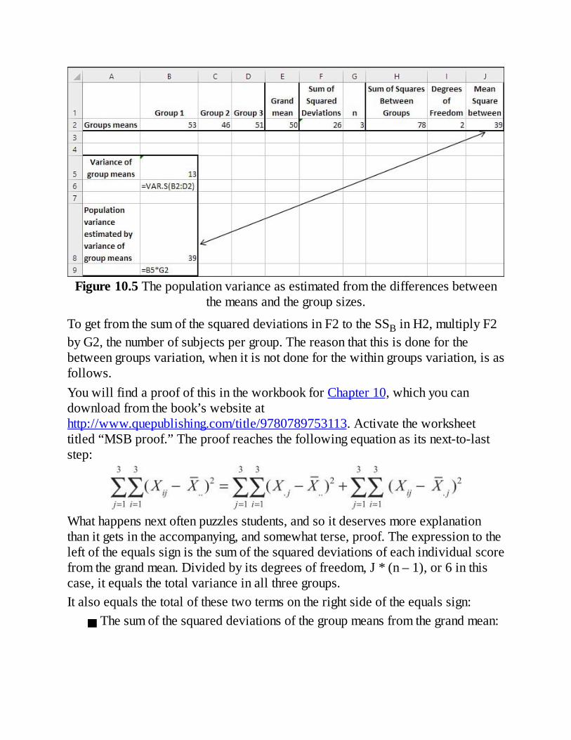
Figure10.5Thepopulationvarianceasestimatedfromthedifferencesbetweenthemeansandthegroupsizes.

TogetfromthesumofthesquareddeviationsinF2totheSSBinH2,multiplyF2byG2,thenumberofsubjectspergroup.Thereasonthatthisisdoneforthebetweengroupsvariation,whenitisnotdoneforthewithingroupsvariation,isasfollows.YouwillfindaproofofthisintheworkbookforChapter10,whichyoucandownloadfromthebook’swebsiteathttp://www.quepublishing.com/title/9780789753113.Activatetheworksheettitled“MSBproof.”Theproofreachesthefollowingequationasitsnext-to-laststep:

Whathappensnextoftenpuzzlesstudents,andsoitdeservesmoreexplanationthanitgetsintheaccompanying,andsomewhatterse,proof.Theexpressiontotheleftoftheequalssignisthesumofthesquareddeviationsofeachindividualscorefromthegrandmean.Dividedbyitsdegreesoffreedom,J*(n–1),or6inthiscase,itequalsthetotalvarianceinallthreegroups.Italsoequalsthetotalofthesetwotermsontherightsideoftheequalssign:

Thesumofthesquareddeviationsofthegroupmeansfromthegrandmean:

Thesumofthesquareddeviationsofeachscorefromthemeanofitsowngroup:

Noticeinthelattersummationthatitoccursonceforeachindividualrecord,astheiindexrunsfrom1to3ineachofthej=1to3groups.However,thereisnoiindexwithintheparenthesesintheformersummation,whichoperatesonlywiththemeanofeachgroupanditsdeviationfromthegrandmean.Nevertheless,thesummationsignthatrunsifrom1to3musttakeeffect,sothegrandmeanissubtractedfromagroupmean,theresultsquared,andthesquareddeviationisadded,notjustoncebutonceforeachobservationinthegroup.Andthatismanagedbychanging

tothis

ormoregenerallyfromthis

tothis

Inwords,thetotalsumofsquaresismadeupoftwoparts:thesquareddifferencesofindividualscoresaroundtheirowngroupmeans,andthesquareddifferencesofthegroupmeansaroundthegrandmean.Thevariabilitywithinagrouptakesaccountofeachindividualdeviationbecauseeachindividualscore’sdeviationissquaredandadded.Thevariabilitybetweengroupsmustalsotakeaccountofeachindividualscore’s

deviationfromthegrandmean,butthatis,atleastinpart,afunctionofthegroup’sdeviationfromthegrandmean.Therefore,thegroup’sdeviationiscalculated,squared,andthenmultipliedbythenumberofscoresrepresentedbyitsmean.Anotherwayofputtingthisnotionistogobacktothestandarderrorofthemean,introducedinChapter7,“UsingExcelwiththeNormalDistribution,”inthesectiontitled“ConstructingaConfidenceInterval.”There,Ipointedoutthatthestandarderrorofthemean(thatis,thestandarddeviationcalculatedusingmeansasindividualobservations)canbeestimatedbydividingthevarianceoftheindividualscoresinonesamplebythesamplesizeandthentakingthesquareroot:

Thevarianceerrorofthemeanisjustthesquareofthestandarderrorofthemean:

ButinanANOVAcontext,youhavefoundthevarianceerrorofthemeandirectly,becauseyouhavetwoor(usually)moregroupmeansandcanthereforecalculatetheirvariance.ThishasbeendoneinFigure10.5,incellB5,giving13asthevarianceof53,46and51.CellB6showstheformulaincellB5:=VAR.S(B2:D2).Rearrangingthepriorequationtosolvefors2,wehave

Then,usingthefiguresinthepresentexamples2=3×13s2=39

whichisthesamefigureasisreturnedasMSBincellJ2ofFigure10.5,and,asyou’llsee,incellD18ofFigure10.7.

TheFTestTorecap,inMSWandMSBwehavetwoseparateandindependentestimatesofthepopulationvariance.One,MSW,isunrelatedtothedifferencesbetweenthegroupmeansanddependsentirelyonthedifferencesbetweenindividualobservationsandthemeansofthegroupstheybelongto.Theotherestimate,MSB,isunrelatedtothedifferencesbetweenindividual

observationsandgroupmeans.Itdependsentirelyonthedifferencesbetweengroupmeansandthegrandmeanandthenumberofindividualobservationsineachgroup.Supposethatthenullhypothesisistrue:thatthethreegroupsarenotsampledfromdifferentpopulations—populationsthatmightdifferbecausetheyreceiveddifferentmedicationsthathavedifferenteffects—butinsteadaresampledfromonepopulation,becausethedifferentmedicationsdonothavedifferentialeffectsonthosewhotakethem.Inthatcase,theobserveddifferencesinthesamplemeanswouldbeduetosamplingerror,nottoanyintrinsicdifferenceinthemedicationsthatexpressesitselfreliablyinanoutcomemeasure.Ifthat’sthecase,wewouldexpectaratioofthetwovarianceestimatestobe1.0.Wewouldhavetwoestimatesofthesamequantity—thepopulationvariance—andinthelongrunwewouldexpecttheratioofthepopulationvariancetoitselftoequal1.0.This,despitethefactthatwegoaboutestimatingthatvarianceintwodifferentways—oneintheratio’snumeratorandoneinitsdenominator.Butwhatifthevariancebasedondifferencesbetweengroupmeansislargerelativetothevariancebasedondeviationswithingroups?Thentheremaywellbesomethingotherthansamplingerrorthat’spushingthegroupmeansapart.Inthatcase,ourestimateofthepopulationvariance,arrivedatbycalculatingthedifferencesbetweengroupmeans,hasbeenincreasedbeyondwhatwewouldexpectifthethreegroupswerereallyjustmanifestationsofthesamepopulation.Wewouldthenhavetorejectthenullhypothesisofnodifferencebetweenthegroupsandconcludethattheycamefromatleasttwodifferentpopulations—populationsthathavedifferentmeans.Howlargemusttheratioofthetwovariancesbebeforewecanbelievethatit’sduetosomethingsystematicratherthansimplesamplingerror?TheanswertothatliesintheFdistribution.Whenyouformaratiooftwovariances—inthesimplestANOVAdesigns,itistheratioofMSBtoMSW—youformwhat’scalledanFratio,justasyoucalculateat-statisticbydividingameandifferencebythestandarderrorofthemean.Andjustasyoucompareat-statistictoat-distribution,youcomparethecalculatedFratiowithanFdistribution.SuppliedwiththevalueofthecalculatedFratioanditsdegreesoffreedom,theFdistributionwilltellyouhowlikelyyourFratioisifthereisnodifferenceinthepopulationmeans.Figure10.7pullsallthisdiscussiontogetherintoonereport,createdbyExcel’sDataAnalysisadd-in.First,though,youhavetoruntheANOVA:SingleFactortool.ChooseDataAnalysisintheAnalysisgroupontheRibbon’sDatatab.Select

ANOVA:SingleFactorfromthelistoftoolstogetthedialogboxshowninFigure10.6.(TherearethreeANOVAtoolsintheDataAnalysisadd-in.Allthetoolsareavailabletoyouafteryouhaveinstalledtheadd-inasdescribedinthesection“UsingtheAnalysisTools”inChapter4,“HowVariablesMoveJointly:Correlation.”)

Figure10.6Ifyourdataisinalistortableformat,withheadersaslabelsinthefirstrow,thesummarytablewillusetheheadersaslabels.

SomecommentsaboutFigure10.7areinorderbeforewegettotheFratio.

Figure10.7NoticethattherawdataislaidoutinA1:C4sothateachgroupoccupiesadifferentcolumn.

TheusersuppliedthedataincellsA1:C4.TheDataAnalysisadd-in’sANOVA:SingleFactortoolwasusedtocreatetheanalysisincellsA7:G21.TheSourceofVariationlabelincellA17indicatesthatthesubsequentlabels—inA18andA19here—tellyouwhetheraparticularrowdescribesvariabilitybetweenorwithingroups.Moreadvancedanalysescalloutothersourcesofvariation.Insomeresearchreportsyou’llseesourceofvariationabbreviatedasSV.HerearetheotherabbreviationsExceluses:

SS,incellB17,standsforsumofsquares.df,incellC17,standsfordegreesoffreedom.MS,incellD17,standsformeansquare.

Thevaluesforsumsofsquares,degreesoffreedom,andmeansquaresareasdiscussedinearliersectionsofthischapter.Forexample,eachmeansquareistheresultofdividingasumofsquaresbyitsassociateddegreesoffreedom.TheFratioincellE18isnotassociatedspecificallywiththeBetweenGroupssourceofvariation,eventhoughitistraditionallyfoundinthatrow.Itistheratio

ofMSBtoMSWandisthereforeassociatedwithbothsourcesofvariation,BetweenandWithin.However,theFratioistraditionallyshownontherowthatbelongstothesourceofvariationthat’sbeingtested.Here,thesourceisthebetweengroupseffect.Inamorecomplicateddesign,youmighthavenotjustonefactor(here,medication)buttwoormore—perhapsbothmedicationandsex.Thenyouwouldhavetwoeffectstotest,andyouwouldfindanFratioontherowformedicationandanotherFratioontherowforsex.InFigure10.7,theFratioreportedinE18islargeenoughthatitissaidtobesignificantatlessthanthe.05level.TherearetwowaystodeterminethisfromtheANOVAtable:comparingthecalculatedFtothecriticalF,andcalculatingalphafromthecriticalF.

ComparingtheCalculatedFtotheCriticalFThecalculatedFratio,6.88,islargerthanthevalue5.14that’slabeledFcritandfoundincellG18.TheFcritvalueisthecriticalvalueintheFdistributionwiththegivendegreesoffreedomthatcutsoffthearearepresentingalpha,theprobabilityofrejectingatruenullhypothesis.If,ashere,thecalculatedFisgreaterthanthecriticalF,youknowthatthecalculatedFisimprobableifthenullhypothesisistrue.Thisisjustlikeyouknowthatacalculatedt-ratio,onethat’sgreaterthanacriticalt-ratio,isimprobableifthenullhypothesisistrue.

CalculatingAlphaTheproblemwithcomparingthecalculatedandthecriticalFratiosisthattheANOVAreportpresentedbytheDataAnalysisadd-indoesn’tremindyouwhatalphalevelyouchose.Conceptually,thisissueisthesameasisdiscussedinChapters8and9,wheretherelationshipsbetweendecisionrules,alpha,andcalculatedversuscriticalt-ratioswerecovered.Thetwodifferencesherearethatwe’relookingatmorethanjusttwomeansandthatwe’reusinganFdistributionratherthananormaldistributionorat-distribution.Figure10.8,comingupinthenextsection,showsashadedareaintherighttailofthecurve.Thisistheareathatrepresentsalpha.ThecurveshowstherelativefrequencywithwhichyouwillobtaindifferentvaluesoftheFratioassumingthatthenullhypothesisistrue.Mostofthetimewhenthenullistrue,youwouldgetFratioslessthan5.143basedonrepeatedsamplesfromthesamepopulation(thecriticalFratioshowninFigure10.7).Someofthetime,duetosamplingerror,you’llgetalargerFratioeventhoughthenullhypothesisistrue.That’salpha,the

percentofpossiblesamplesthatcauseyoutorejectatruenullhypothesis.

Figure10.8Likethet-distribution,theFdistributionhasonemode.Unlikethet-distribution,itisasymmetric.

JustlookingattheANOVAreportinFigure10.7,youcanseethattheFratios,calculatedandcritical,tellyoutorejectthenullhypothesis.YouhavecalculatedanFratiothatislargerthanthecriticalF.YouareintheregionwhereacalculatedFislargeenoughtobeimprobableifthenullhypothesisistrue.Buthowimprobableisit?Youknowtheanswertothatonlyifyouknowthevalueofalpha.Ifyouadoptedanalphaof.05,yougetaparticularcriticalFvaluethatcutsofftherightmost5%oftheareaunderthecurve.Ifyouinsteadadoptsomethingsuchas.01astheerrorrate,you’llgetalargercriticalFvalue,onethatcutsoffjusttherightmost1%oftheareaunderthecurve.It’sridiculousthattheDataAnalysisadd-indoesn’ttellyouwhatlevelofalphawasadoptedtoarriveatthecriticalFvalue.You’reingoodshapeifyourememberwhatalphayouchosewhenyouweresettinguptheanalysisintheANOVAdialogbox,butwhatifyoudon’tremember?ThenyouneedtobringoutthefunctionsthatExcelprovidesforFratios.

UsingExcel’sWorksheetFunctionsfortheFDistributionExcelprovidestwotypesofworksheetfunctionsthatpertaintotheFdistributionitself:theF.DIST()functionsandtheF.INV()functions.AswithT.DIST()and

T.INV(),theF.DIST()functionsreturnthesizeoftheareaunderthecurve,givenanFratioasanargument.TheF.INV()functionsreturnanFratio,giventhesizeoftheareaunderthecurve.

UsingF.DIST()andF.DIST.RT()YoucanusetheF.DIST()function(or,inversionsearlierthanExcel2010,theFDIST()function)totellyouatwhatalphaleveltheFcritvalueiscritical.TheF.DIST()functionisanalogoustotheT.DIST()functiondiscussedinChapters8and9:YousupplyanFratioanddegreesoffreedom,andthefunctionreturnstheamountofthecurvethat’scutoffbythatratio.UsingthedataaslaidoutinFigure10.7,youcouldenterthefollowingfunctioninsomeemptycellonthatworksheet:

=1–F.DIST(G18,C18,C19,TRUE)Theformularequiressomecomments.Tobegin,herearethefirstthreeargumentsthatF.DIST()requires:

TheFratioitself—Inthisexample,that’stheFcritvaluefoundincellG18.ThedegreesoffreedomforthenumeratoroftheFratio—That’sfoundincellC18.ThenumeratorisMSB.

Thedegreesoffreedomforthedenominator—That’sfoundincellC19.ThedenominatorisMSW.

Thefourthargument,whosevalueisgivenasTRUEinthecurrentexample,specifieswhetheryouwantthecumulativeareatotheleftoftheFratioyousupply(TRUE)ortheprobabilityassociatedwiththatspecificpoint(FALSE).TheTRUEvalueisusedherebecausewewanttobeginbygettingtheentireareaunderthecurvethat’stotheleftoftheFratio.TheF.DIST()function,asgiveninthecurrentexample,returnsthevalue.95.That’sbecause95%oftheFdistribution,withtwoandsixdegreesoffreedom,liestotheleftofanFratioof5.143.However,we’reinterestedintheamountthatliestotheright,nottheleft.Therefore,wesubtractitfrom1.Anotherapproachyoucoulduseisthis:

=F.DIST.RT(G18,C18,C19)TheF.DIST.RT()functionreturnstherightendofthedistributioninsteadoftheleft,sothere’snoneedtosubtractitsresultfrom1.Itendnottousethisapproach,though,becauseithasnofourthargument.Thatforcesmetorememberwhichfunctionuseswhicharguments,andI’dratherspendmyenergythinkingaboutwhatafunction’sresultmeansthanrememberingitssyntax.

FDIST()VERSUSF.DIST()IfanearlierversionisforcingyoutouseFDIST()insteadofF.DIST(),bearinmindthatFDIST()isequivalenttoF.DIST.RT(),nottoF.DIST().Annoyingbutinescapable,giventheinsistenceonasortofconsistency.Theconsistencyinthiscaseistheinsistenceonreturningtheleftportionofadistributionwhenthefunction’snameendsin.DIST(thatis,NORM.DIST,NORM.S.DIST,T.DIST,andsoon).However,youhavetoworkveryhardtoinventasituationinwhichyouwouldexpecttheFratio’snumeratortobesmallerthanitsdenominator;infact,ifyoudoencountersuchasituation,it’sprobablyduetomis-specifyingthemodelforyourdata.TheFtestisaright-tailedtest,unlikethez-testorthet-test,wherethedirectionalityofthedifferenceisimportant.Asitis,though,keepitinmindthatthesetwoformulasareequivalent:

=F.DIST.RT(G18,C18,C19)=FDIST(G18,C18,C19)

UsingF.INV()andFINV()TheF.INV()function(or,inversionsearlierthanExcel2010,theFINV()function)returnsavaluefortheFratiowhenyousupplyanareaunderthecurve,plusthenumberofdegreesoffreedomforthenumeratoranddenominatorthatdefinethedistribution.ThetraditionalapproachhasbeentoobtainacriticalFvalueearlyoninanexperiment.Theresearcherknowshowmanygroupswouldbeinvolved,andwouldhaveatleastagoodideaofhowmanyindividualobservationswouldbeavailableattheconclusionoftheexperiment.And,ofcourse,alphaischosenbeforeanyoutcomedataisavailable.Supposethataresearcherwastestingfourgroupsconsistingoftenpeopleeach,andthatthe.05alphalevelwasselected.ThenanFvaluecouldbelookedupintheappendixtoastatisticstextbook;or,sinceExcel2010becameavailable,thefollowingformulacouldbeusedtodeterminethecriticalFvalue:

=F.INV(.95,3,36)Alternatively,priortoExcel2010,youwouldusethisone:

=FINV(.05,3,36)Thesetwoformulasreturnthesamevalue,2.867.Theolder,FINV()functionreturnstheFvaluethatcutsofftherightmost5%ofthedistribution;thenewer

F.INV()functionreturnstheFvaluethatcutsofftheleftmost95%ofthedistribution.Clearly,Excelhasinadvertentlysetatrapforyou.Ifyou’reusedtoFINV()andareconvertingtoF.INV(),youmustbecarefultousethestructure

=F.INV(.95,3,36)andnotthestructure

=F.INV(.05,3,36)whichfollowstheolderconventions,becauseifyoudo,you’llgettheFvaluethatcutsofftheleftmost5%ofthedistributioninsteadoftheleftmost95%ofthedistribution.F.INV()hasreturnedacriticalFvalue,andtheANOVAtestcannowbecompletedusingtheactualdata—justasisshowninFigure10.7.ThecalculatedF(incellE18ofFigure10.7)iscomparedtothecriticalF,andifthecalculatedFisgreaterthanthecriticalF,thenullhypothesisisrejected.Thissequenceofeventsisprobablyhelpfulbecause,iffollowed,theresearchercanpointtoitasevidencethatthedecisionruleswereadoptedpriortoseeinganyoutcomemeasures.NoticeinFigure10.7thata“P-value”isreportedbytheDataAnalysisadd-inincellF18.Itistheprobability,calculatedfromFDIST()orF.DIST(),ofobtainingthecalculatedFifthenullhypothesisistrue.Thereisastrongtemptation,then,fortheresearchertosay,“Wecanrejectthenullnotonlyatthe.05level,butatthe.03level.”Butthereareatleasttworeasonsnottosuccumbtothattemptation.First,andmostimportant,isthattodosoimpliesthatyouhavealteredthedecisionruleafterthedatahascomein—andthatleadstocapitalizingonchance.Second,toclaima3%levelofsignificanceinsteadoftheapriori5%levelistoattributemoreimportancetoa2%differencethanexists.Thereare,aspointedoutinChapter6,“TellingtheTruthwithStatistics,”manythreatstothevalidityofanexperiment,andstatisticalchance—includingsamplingerror—isonlyoneofthem.Giventhatcontext,tomakeanissueofanapparent2%differenceinalphalevelisstrainingatgnats.

TheFDistributionJustasthereisadifferentt-distributionforeverynumberofdegreesoffreedominthesampleorsamples,thereisadifferentFdistributionforeverycombinationofdegreesoffreedomforMSBandMSW.Figure10.8showsanexampleusingdfB=3anddfW=16.ThechartinFigure10.8showsanFdistributionfor3and16degreesoffreedom.

ThecurveisdrawnusingExcel’sF.DIST()function.Forexample,theheightofthecurveatthepointwheretheFratiois1.0isgivenby

=F.DIST(1,3,16,FALSE)wherethefirstargument,1,istheFratioforthatpointonthecurve;3isthedegreesoffreedomforthenumerator;16isthedegreesoffreedomforthedenominator;andFALSEindicatesthatExcelshouldreturntheprobabilitydensityfunction(theheightofthecurveatthatpoint)ratherthanthecumulativedensity(thetotalprobabilityforallFratiosfrom0throughthevalueofthefunction’sfirstargument—here,that’s1).NoticethatthepatternoftheargumentsissimilartothepatternoftheargumentsfortheT.DIST()function,discussedindetailinChapter9.Theshadedareaintherighttailofthecurverepresentsalpha,theprobabilityofrejectingatruenullhypothesis.Ithasbeensethereto.05.ThecurveyouseeassumesthatthevariancesbasedonMSBandMSWarethesameinthepopulation,asisthecasewhenthenullhypothesisistrue.Still,samplingerroralonecancauseyoutogetanFratioaslargeastheoneinthischapter’sexample;Figure10.7showsthattheobtainedFratiois6.88(cellE18)andfully5%oftheFratiosinFigure10.8aregreaterthan3.2.(However,thedistributioninFigure10.8isbasedondifferentdegreesoffreedomthantheexampleinFigure10.7.ThechangewasmadetoprovideamoreinformativevisualexampleoftheFdistributioninFigure10.8.)TheFdistributiondescribestherelativefrequencyofoccurrenceofratiosofvariances,andisusedtodeterminethelikelihoodofobservingagivenratioundertheassumptionthattheratioofonevariancetoanotheris1inthepopulation.(GeorgeSnedecornamedtheFdistributioninhonorofSirRonaldFisher,aBritishstatisticianwhowasresponsibleforthedevelopmentoftheanalysisofvariance,explainingtheinteractionoffactors—seeChapter12,“ExperimentalDesignandANOVA”)andavarietyofotherstatisticalconceptsandtechniquesthatwerethecuttingedgeoftheoryintheearlytwentiethcentury.)Todescribeat-distribution,youmustspecifyjustonenumberofdegreesoffreedom,buttodescribeanFdistribution,youmustspecifythenumberofdegreesoffreedomforthevarianceinthenumeratorandthenumberofdegreesoffreedomforthevarianceinthedenominator.

UnequalGroupSizesFromtimetotime,youmayfindthatyouhaveadifferentnumberofsubjectsinsomegroupsthaninothers.Thissituationdoesnotnecessarilyposeaproblemin

thesinglefactorANOVA,althoughitmightdoso,andyouneedtounderstandtheimplicationsifithappenstoyou.Considerfirstthepossibilitythatadifferentialdropoutratehashadaneffectonyourresults.Thisisparticularlylikelytoposeaproblemifyouarrangedforequalgroupsizes,orevenroughlyequalgroupsizes,andattheendofyourexperimentyoufindthatyouhaveveryunequalgroupsizes.Thismightoccurforatleasttworeasons:

Youusedconvenienceor“grab”samples.Thatis,yourgroupsconsistofpreexistingsetsofpeopleorplantsorotherresponsivebeings.Theremightwellbesomethingaboutthereasonsforthosegroupingsthatcausedsomesubjectstobemissingattheendoftheexperiment.Becausethegroupingsprecededthetreatmentyou’reinvestigating,youmightinadvertentlywindupassigninganoutcometoatreatmentwhenithadtodonotwiththetreatmentbutwiththenonrandomgrouping.Yourandomlyassignedsubjectstogroups,butsomethingaboutthenatureofthetreatmentscausesthemtodropoutofonetreatmentatagreaterratethanfromothertreatments.Youmayneedtoexaminethenatureofthetreatmentsmorecloselyifyoudidnotanticipatedifferentialdropoutrates.

Ineithercase,becarefulofthelogicofanyconclusionsyoureach,quiteapartfromthestatisticsinvolved.Still,itcanhappenthatevenwithrandomassignment,andtreatmentsthatdonotcausesubjectstodropout,youwindupwithdifferentgroupsizes.Forexample,ifyouareconductinganexperimentthattakesdaysorweekstocomplete,youfindpeoplemoving,forgettingtoshowup,gettingill,orbeingabsentforanyofavarietyofreasonsunrelatedtotheexperiment.Eventhen,thiscancauseyouaproblemwiththestatisticalanalysis.Asyouwillseeinthenextchapter,theproblemisdifferentandmoredifficulttomanagewhenyousimultaneouslyanalyzetwofactors.Inasingle-factorANOVA,theissuepertainstotherelationshipbetweengroupsizesandwithingroupvariances.SeveralassumptionsaremadebythemathematicsthatunderlieANOVA,butjustasistruewitht-tests,notalltheassumptionsmustbemetfortheanalysistobeaccurate.Oneoftheassumptionsisthatobservationsbeindependentofoneanother.IfthefactthatanobservationisinGroup1hasanyeffectonthelikelihoodthatanotherobservationisinGroup1,orthatit’sinGroup2,theobservationsaren’tindependent.Ifthevalueofoneobservationdependsinsomewayonthevalueofanotherobservation,theyarenotindependent.InthatcasethereareconsequencesfortheprobabilitystatementsmadebyANOVA,andthoseconsequencescan’tbe

quantified.Independenceofobservationsisanassumptionthatmustbemet.

NoteAnimportantexceptionisthet-testfordependentgroupsandtheanalysisofcovariance(discussedinChapter16,“AnalysisofCovariance:TheBasics”).Inthosecases,thedependencyisdeliberateandcanbemeasuredandaccountedfor.

Anotherimportantassumptionisthatthewithingroupvariancesareequal.Butunlikelackofindependence,violatingtheequalvarianceassumptionisnotfataltothevalidityoftheanalysis.Longexperienceandmuchresearchleadstothesethreegeneralstatements:

Whendifferentwithingroupvariancesexist,equalsamplesizesmeanthattheeffectontheprobabilitystatementsisnegligible.Therearelimitstothisprotection,though:Ifonewithingroupvarianceistentimesthesizeofanother,seriousdistortionsofalphacanoccur.Ifsamplesizesaredifferentandthelargersampleshavethesmallervariances,theactualalphaisgreaterthanthenominalalpha.Youmightstartoutbysettingalphaat.05butyourchanceofmakingaTypeIerrorisactually,say,.09.TheeffectistoshifttheFdistributiontotheright,sothatthecriticalFvaluecutsoffnot5%oftheareaunderthecurvebut,say,9%.StatisticianssaythatinthiscasetheFtestisliberal.Ifsamplesizesaredifferentandthelargersampleshavethelargervariances,theoppositeeffecttakesplace.Yournominalalphamightbe.05butinactualityitissomethingsuchas.03.TheFdistributionhasbeenshiftedtotheleftandthecriticalFratiocutsoffonly3%ofthedistribution.StatisticianstermthisaconservativeFtest.

Thereisnopracticalwaytocorrectthisproblemotherthantoarrangeforequalgroupsizes.Noristhereapracticalwaytocalculatetheactualalphalevel.Thebestsolutionistobeawareoftheeffect(whichissometimestermedtheBehrens-Fisherproblem)andadjustyourconclusionsaccordingly.Bearinmindthatthesmallerthedifferencesbetweenthegroupvariances,thesmallertheeffectonthenominalalphalevel.

MultipleComparisonProceduresTheFtestissometimestermedanomnibustest:Thatis,ittestssimultaneouslywhetherthereisatleastonereliabledifferencebetweenanyofthegroupmeans

(orlinearcombinationsofgroupmeans)thatarebeingtested.Byitself,itdoesn’tpinpointwhichmeandifferencesareresponsibleforanimprobablylargeFratio.Supposethatyoutestfourgroupmeans,whichare100,90,70,and60,andgetanFratiothat’slargerthanthecriticalFratioforthealphalevelyouadopted.Probably(notnecessarily,butprobably)themeanof100issignificantlydifferentfromthemeanof60;theyarethehighestandlowestmeansinanexperimentthatresultedinasignificantFratio.Butwhatabout100and70?Isthatasignificantdifferenceinthisexperiment?Howabout90and60?Youneedtoconductmultiplecomparisonstomakethosedecisions.Unfortunately,thingsstarttogetcomplicatedatthispoint.Thereareroughly(dependingonyourpointofview)ninemultiplecomparisonproceduresthatyoucanchoosefrom.Theydifferoncharacteristicssuchasthefollowing:

PlannedversusunplannedcomparisonsDistributionused(normallyt,F,orq)Errorrate(alpha)percomparisonorpersetofcomparisonsSimplecomparisonsonly(thatis,onegroupmeanversusanothergroupmean)orcomplexcomparisons(forexample,themeanoftwogroupsversusthemeanoftwoothergroups)

Thereareotherissuestoconsider,too,includingthestatisticalsensitivityorpoweroftheprocedure.Forgoodorill,Excelsimplifiesyourdecisionbecauseitdoesnotalwayssupporttherequiredstatisticaldistribution.Forexample,twowell-regardedmultiplecomparisonproceduresaretheTukeyandtheNewman-Keuls.Boththeseproceduresrelyonadistributioncalledthestudentizedrangestatistic,usuallyreferredtoasq.Exceldoesnotsupportthatstatistic:Itdoesnothave,forexample,aQ.INV()oraQ.DIST()function.Othermethodsemploymodificationsof,forexample,thet-distribution.Dunnett’sproceduremodifiesthet-distributiontoproduceadifferentcriticalvaluewhenyoucompareone,two,three,ormoremeanswithacontrolgroupmean.Exceldoesnotsupportthatsortofcomparisonexceptinthelimitingcasewherethereareonlytwogroups.Dunn’sprocedureemploysthet-distribution,butonlyforplannedcomparisonsinvolvingtwomeans.Whenthecomparisonsinvolvemorethantwomeans,theDunnprocedureusesamodificationofthet-distribution.TheDunnprocedurehasonlyslightlymorestatisticalpowerthantheScheffé(seethenextparagraph),whichdoesnotrequireplannedcontrasts.Fortunately(ifitwasbydesign,I’lleatmykeyboard),Exceldoessupporttwomultiplecomparisonprocedures:plannedorthogonalcontrastsandtheScheffé

method.Theformeristhemostpowerfulofthevariousmultiplecomparisonprocedures(andalsothemostrestrictive).Thelatteristheleastpowerfulprocedure(andgivesyouthemostleewayinyouranalysis).However,youhavetopiecetheanalysestogetherusingtheavailableworksheetfunctions.Theremainderofthischaptershowsyouhowtodothat.Speakinggenerally,theNewman-Keulsisprobablythebestchoiceforamultiplecomparisontestofsimplecontrasts(Mean1versusMean3,Mean1versusMean4,Mean2versusMean3,andsoon)whenyouwanttokeepyourerrorratetoaper-comparisonbasis(ratherthantoaper-familybasis—that’smuchmoreconservativeandyou’llprobablymisssomegenuinedifferences).TheNewman-Keulstest,asmentionedpreviously,usestheqorstudentizedrangedistribution.Youcanfindtablesofthosevaluesinmanyintermediatestatisticaltexts,andsomewebsitesofferyoufreelookups.IsuggestthatyouconsiderrunningyourANOVAinExcelusingtheDataAnalysisadd-in,particularlyifyourexperimentaldesignincludesjustonefactorortwofactorswithequalgroupsizes.Taketheoutputtoageneralstatisticstextanduseitinconjunctionwiththetablesyoufindtheretocompleteyourmultiplecomparisons.

NoteYoucouldalsousethefreewarestatisticalprogramRifyoumust,butafterafewyearsofusingR,IfindIspendmoretimedealingwithitsuserinterfaceandidiosyncraticlayoutsthanIgainfromhavingtheoccasionalneedforanalysesthatIcan’tdocompletelyinExcel.

IfyouwanttostaywithinwhatExcelhastooffer,youcangetjustasmuchstatisticalpowerfromplannedorthogonalcontrasts,whicharediscussednext,asfromNewman-Keuls.AndyoucandoplentyofdatasnoopingwithoutplanningathingbeforehandifyouuseExceltorunyourScheffécomparisons.

TheSchefféProcedureTheSchefféisthemostflexibleoftheavailablemultiplecomparisonprocedures.Youcanmakeasmanycomparisonsasyouwant,andtheyneednotbesimplyonemeancomparedtoanother.Ifyouhadfivegroups,forexample,youcouldusetheSchefféproceduretocomparethemeanoftwogroupswiththemeanoftheremainingthreegroups.Itmightmakenosensetodosointhecontextofyourexperiment,buttheSchefféprocedureallowsit.YoucanalsousetheSchefféwithunequalgroupsizes,althoughthattopicisdeferreduntilChapter14,“Multiple

RegressionAnalysisandEffectCoding:TheBasics.”Furthermore,intheSchefféprocedure,alphaissharedamongallthecomparisonsyoumake.Ifyoumakejustonecomparisonandhavesetalphato.05,youhavea5%chanceofconcludingthatthedifferenceyoucalculateisareliableone,wheninfactitisnot.Or,ifyoumake20comparisonsandhavesetalphato.05,thenyouhavea5%chanceofrejectingatruenullhypothesissomewhereinthe20comparisons.Thisisverydifferent,andmuchmoreconservative,thanrunninga5%chanceofrejectingatruenullineachofthecomparisons.Figure10.9showshowtheScheffémultiplecomparisonproceduremightworkinanexperimentwithtwotreatmentgroupsandacontrolgroup.

Figure10.9TheDataAnalysisadd-inprovidesthepreliminaryANOVAinA9:G20.

WiththerawdatalaidoutasshownincellsB2:D7inFigure10.9,youcanruntheANOVA:SingleFactortoolintheDataAnalysisadd-intocreatethereportshowninA9:G20.Thesestepswilltakecareofit:

1.WiththeDataAnalysisadd-ininstalledasdescribedinChapter4,clickDataAnalysisintheRibbon’sAnalysisgroup.SelectANOVA:SingleFactorfromthelistboxandclickOK.ThedialogboxshownearlierinFigure10.6appears.

2.WiththeflashingI-barintheInputRangeeditbox,dragthroughtherangeB2:D7sothatitsaddressappearsintheeditbox.

3.BesuretheColumnsoptionischosen.(BecauseofthewayExcel’slistandtablestructuresoperate,itisveryseldomthatyou’llwanttogroupthedatasothateachgroupoccupiesadifferentrow.Butifyoudo,that’swhattheRowsoptionisfor.)

4.Ifyouincludedcolumnlabelsintheinputrange,assuggestedinstep2,filltheLabelscheckbox.

5.EnteranalphavalueintheAlphaeditbox,oracceptthedefaultvalue.Exceluses.05ifyouleavetheAlphaeditboxblank.

6.ClicktheOutputRangeoptionbutton.Whenyoudoso—infact,wheneveryouchooseadifferentOutputoptionbutton—theadd-ingivestheInputRangeboxthefocus,andwhateveryoutypeorselectnextoverwriteswhatyouhavealreadyputintheInputRangeeditbox.BesuretoclickintheOutputRangeeditboxafterchoosingtheOutputRangeoptionbutton.

7.Clickacellontheworksheetwhereyouwanttheoutputtostart.InFigure10.9,that’scellA9.

8.ClickOK.ThereportshownincellsA9:G20inFigure10.9appears.(TogetallthedatatofitinFigure10.9,Ihavedeletedacoupleofemptyrows.)Asignificantresultatthe.05levelfromtheANOVA,whichyouverifyfromcellF17ofFigure10.9,tellsyouthatthereisareliabledifferencesomewhereinthedata.Tofindit,youcanproceedtooneormoremultiplecomparisonsamongthemeansusingtheScheffémethod.ThismethodisnotsupporteddirectlybyExcel,evenwiththeDataAnalysisadd-in.Infact,nomultiplecomparisonmethodisdirectlysupportedinExcel.ButyoucanperformaSchefféanalysisbyenteringtheformulasandfunctionsdescribedinthissection.TheScheffémethod,alongwithseveralotherapproachestomultiple

comparisons,beginsinExcelbysettinguparangeofcellsthatdefinehowthegroupmeansaretobecombined(thatis,thecontrastsyoulookforamongthemeans).InFigure10.9,thatrangeofcellsisB24:D27.ThefirstcontrastisdefinedbythedifferencebetweenthemeanforMedicationAandthemeanforMedicationB.ThemeanforMedicationAwillbemultipliedby1;themeanforMedicationBwillbemultipliedby–1;themeanforthePlacebowillbemultipliedby0.Theresultsaresummed.The1sandthe0sand,ifused,thefractionsthataremultipliedbythemeansarecalledcontrastcoefficients.Thecoefficientstellyouwhetheragroupmeanisinvolvedinthecontrast(1),omittedfromthecontrast(0),orinvolvedinacombinationwithothermeans(acoefficientsuchas.33or.5).Ofcourse,theuseofthesecoefficientsisalongwindedwayofsaying,forexample,thatthemeanofMedicationBissubtractedfromthemeanofMedicationA,buttherearegoodreasonstobeverboseaboutit.Thefirstreasonisthatyouneedtocalculatethestandarderrorofthecontrast.Youwilldividethestandarderrorintotheresultofcombiningthemeansusingthecontrastcoefficients.Thegeneralformulaforthestandarderrorofacontrastis

whereMSeisthemeansquareerrorfromtheANOVAtable(cellD18inFigure10.9)andeachnisthesamplesizeofeachgroup.SothestandarderrorforthefirstcontrastinFigure10.9,incellE24,iscalculatedwiththisformula:

=SQRT($D$18*(B24^2/$B$12+C24^2/$B$13+D24^2/$B$14))

NoteThemeansquareerrorjustmentionedis,inthesimplerANOVAdesigns,thesameasthewithingroupvarianceyou’veseensofarinthischapter.TherearetimeswhenyoudonotdivideanMSBvaluebyanMSWvaluetoarriveatanF.Instead,youdividebyavaluethatismoregenerallyknownasMSebecausetheproperdivisorisnotawithingroupsvariance.Theproperdivisorissometimesaninteractionterm(seeChapter12).TheMSedesignationisjustamoregeneralwaytoidentifythedivisorthanisMSW.Inthesingle-factorandfullycrossedmultiple-factordesignscoveredinthisbook,youcanbesurethatMSW

andMSemeanthesamething:withingroupvariance.

Inwords,thismeansyousquareeachcontrastcoefficientanddividetheresultbythegroup’ssamplesize.Totaltheresults.MultiplybytheMSe,andtakethesquareroot.TheconventionalwaytosymbolizethestandarderrorofthecontrastisSΨ,whereΨrepresentsthecontrast.(TheGreeksymbolΨisrepresentedinEnglishaspsi,andpronounced“sigh.”)ThepriorformulamakesthereferencetoD18absolutebymeansofthedollarsigns:$D$18.DoingsomeansthatyoucancopyandpastetheformulaintocellsE25:E27andkeepintactthereferencetoD18,withitsMSevalue.ThesameistrueofthereferencestocellsB12,B13,andB14:EachstandarderrorinE24:E27usesthesamevaluesforthegroupsizes,so$B$12,$B$13,and$B$14areusedtomakethereferencesabsolute.ThereferencestoB24,C24,andD24areleftrelativebecauseyouwantthemtoadjusttothedifferentcontrastcoefficientsasyoucopyandpastetheformulaintoE25:E27.Thecontrastdividedbyitsstandarderrorisrepresentedasfollows:

ThefirstratioiscalculatedusingthisformulaincellF24:=($D$12*B24+$D$13*C24+$D$14*D24)/E24

Theformulamultipliesthemeanofeachgroup(inD12,D13,andD14)bythecontrastcoefficientforthatgroupinthecurrentcontrast(inB24,C24,andD24),andthendividesbythestandarderrorofthecontrast(inE24).TheformulaiscopiedandpastedintoF25:F27.Therefore,thecelladdressesofthemeansinD12,D13,andD14aremadeabsolute:Eachmeanisusedineachcontrast.Thecontrastcoefficientschangefromcontrasttocontrast,andtheircellsusetherelativeaddressesB24,C24,andD24.Thisallowsthecoefficientaddressestoadjustastheformulaispastedintodifferentrows.TherelativeaddressingalsoallowsthereferencetoE24tochangetoE25,E26,andE27astheformulaiscopiedandpastedintoF25:F27.ThesumofthemeanstimestheircoefficientsisdividedbythestandarderrorsofthecontrastsinF24:F27.TheresultofthatdivisioniscomparedtothecriticalvalueshowninG24:G27.(It’sthesamecriticalvalueforeachcontrastinthecaseoftheSchefféprocedure.)

NoteThepriorformulaincludesatermthatsumstheproductsofthegroups’

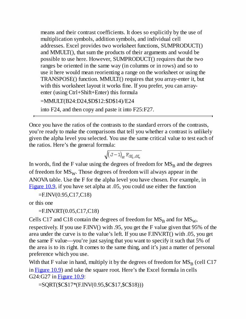
meansandtheircontrastcoefficients.Itdoessoexplicitlybytheuseofmultiplicationsymbols,additionsymbols,andindividualcelladdresses.Excelprovidestwoworksheetfunctions,SUMPRODUCT()andMMULT(),thatsumtheproductsoftheirargumentsandwouldbepossibletousehere.However,SUMPRODUCT()requiresthatthetworangesbeorientedinthesameway(incolumnsorinrows)andsotouseitherewouldmeanreorientingarangeontheworksheetorusingtheTRANSPOSE()function.MMULT()requiresthatyouarray-enterit,butwiththisworksheetlayoutitworksfine.Ifyouprefer,youcanarray-enter(usingCtrl+Shift+Enter)thisformula=MMULT(B24:D24,$D$12:$D$14)/E24intoF24,andthencopyandpasteitintoF25:F27.

Onceyouhavetheratiosofthecontraststothestandarderrorsofthecontrasts,you’rereadytomakethecomparisonsthattellyouwhetheracontrastisunlikelygiventhealphalevelyouselected.Youusethesamecriticalvaluetotesteachoftheratios.Here’sthegeneralformula:

Inwords,findtheFvalueusingthedegreesoffreedomforMSBandthedegreesoffreedomforMSW.ThosedegreesoffreedomwillalwaysappearintheANOVAtable.UsetheFforthealphalevelyouhavechosen.Forexample,inFigure10.9,ifyouhavesetalphaat.05,youcoulduseeitherthefunction

=F.INV(0.95,C17,C18)orthisone

=F.INV.RT(0.05,C17,C18)CellsC17andC18containthedegreesoffreedomforMSBandforMSW,respectively.IfyouuseF.INV()with.95,yougettheFvaluegiventhat95%oftheareaunderthecurveistothevalue’sleft.IfyouuseF.INV.RT()with.05,yougetthesameFvalue—you’rejustsayingthatyouwanttospecifyitsuchthat5%oftheareaistoitsright.Itcomestothesamething,andit’sjustamatterofpersonalpreferencewhichyouuse.WiththatFvalueinhand,multiplyitbythedegreesoffreedomforMSB(cellC17inFigure10.9)andtakethesquareroot.Here’stheExcelformulaincellsG24:G27inFigure10.9:

=SQRT($C$17*(F.INV(0.95,$C$17,$C$18)))

Thiscriticalvaluecanbeusedforanycontrastyoumightbeinterestedin,nomatterhowmanymeansareinvolvedinthecontrast,solongasthecontrastcoefficientssumtozero—astheydoineachcontrastinFigure10.9.(Youwouldhavedifficultycomingupwithasetofcoefficientsthatdonotsumtozeroandthatresultinameaningfulcontrast.)Inthiscase,noneofthetestedcontrastsresultsinaratiothat’slargerthanthecriticalvalue.TheSchefféprocedureisthemostconservativeofthemultiplecomparisonprocedures,inlargepartbecauseitallowsyoutomakeanycontrastyouwant,afteryou’veseentheresultsofthedescriptiveanalysis(soyouknowwhichgroupshavethelargestdifferencesinmeanvalues)andtheinferentialanalysis(theANOVA’sFtesttellsyouwhetherthere’sasignificantdifferencesomewhere).Thetradeoffisofstatisticalpowerforflexibility.TheSchefféprocedureisnotapowerfulmethod:It’sconservative,anditfailstoregardthesecontrastsassignificantatthe.05level.However,itgivesyougreatleewayindecidinghowtofollowuponasignificantFtest.

NoteThesecondandthirdcomparisonsaresoclosetosignificanceatthe.05levelthatIwoulddefinitelyreplicatetheexperiment,particularlygiventhattheomnibusFtestreturnedaprobabilityof.05.

PlannedOrthogonalContrastsTheotherapproachtomultiplecomparisonsthatthischapterdiscussesisplannedorthogonalcontrasts,whichsoundsalotmoreintimidatingthanitis.

PlannedContrastsTheplannedpartjustmeansthatyoupromisetodecide,inadvanceofseeinganyresults,whichgroupmeans,orsetsofgroupmeans,youwanttocompare.Sometimesyoudon’tknowhowtosharpenyourfocusuntilyou’veseensomepreliminaryresults,andinthatsituationyoucanuseoneoftheafter-the-factmethods,suchastheSchefféprocedure.Butparticularlyinanerawhenveryexpensivemedicalanddrugresearchtakesplace,it’snotatallunusualtoplanthecontrastsofinterestlongbeforethetreatmenthasbeenadministered.

OrthogonalContrastsTheorthogonalpartmeansthatthecontrastsyoumakedonotemployredundantinformation.Youwouldbeemployingredundantinformationif,forexample,onecontrastsubtractedthemeanofaGroup3fromthemeanofGroup1,andanother

contrastsubtractedthemeanofGroup3fromthemeanofGroup2.BecausethetwocontrastsbothsubtractGroup3’smeanfromthatofanothergroup,theinformationisredundant.Ifthegroupshaveequalsamplesizes,there’sasimplewaytodeterminewhethercomparisonsareorthogonal.SeeFigure10.10.

Figure10.10Theproductsofagroup’scontrastcoefficientsmustsumtozerofortwocontraststobeorthogonal.

Figure10.10showsthesamecontrastcoefficientsaswereusedinFigure10.9fortheSchefféillustration.Thecoefficientssumtozerowithinacomparison.Butimposingtheconditionthatdifferentcontrastsbeorthogonalmeansthatthesumoftheproductsofthecoefficientsfortwocontrastsalsosumtozero.That’seasiertoseethanitistoread.LookatcellE9inFigure10.10.Itcontains1,thesumofthenumbersinB9:D9.Thosethreenumbersaretheproductsofcontrastcoefficients.Row9combinesthecontrastcoefficientsforcontrasts1and2,socellB9containstheproductofcellsB3andB4.Similarly,cellC9containstheproductofcellsC3andC4,andD9containstheproductofD3andD4.SummingcellsB9:D9intoE9resultsin1.Thatmeansthatcontrasts1and2arenotorthogonaltooneanother.Also,themeanofGroup1ispartofboththosecontrasts—that’sredundantinformation,socontrasts1and2aren’torthogonal.It’sasimilarsituationinRow10,whichtestswhetherthecontrastsinrows3and5areorthogonal.ThemeanofGroup2appearsinbothcontrasts(thefactthatitis

subtractedinonecontrastbutaddedintheothermakesnodifference),andasaresultthetotaloftheproductsisnonzero.Contrast1andContrast3arenotorthogonal.Row11teststhecontrastsinrows3and6,andherewehaveapairoforthogonalcontrasts.Theproductsofthecontrastcoefficientsinrow3androw6areshowninB11:D11andaretotaledinE11,whereyouseea0.Thattellsyouthatthecontrastsdefinedinrows3and6areorthogonal,andyoucanproceedwithcontrasts1and4:themeanofGroup1versusthemeanofGroup2,andthemeanofGroups1and2takentogetherversusthemeanofGroup3.Noticethatnoneofthethreemeansappearsinitsentiretyinbothcontrast1andcontrast4.ThegeneralruleisthatifyouhaveKmeans,onlyK–1contraststhatcanbemadefromthosemeansareorthogonal.Here,therearethreemeans,soonlytwocontrastsareorthogonal.

EvaluatingPlannedOrthogonalContrastsThecontraststhatyoucalculate,theonesthatarebothplannedandorthogonal,arecalculatedexactlyasyoucalculatedthecontrastsfortheSchefféprocedure.Thenumeratoranddenominatoroftheratio,theΨandthesΨ,arecalculatedinthesamewayandhavethesamevalues—andthereforesodotheratios.ComparetheratiosincellsF24andF25inFigure10.11withthoseincellsF24andF27inFigure10.9.

Figure10.11Onlytwocontrastsareorthogonaltooneanother,soonlythosetwoappearinrows24and25.

TheratioofacontrasttoitsstandarderrorisreferredtoasΨ/sΨbytheSchefféprocedure,butit’sreferredtoasat-ratioinplannedorthogonalcontrasts.Thedifferencesbetweenthetwoproceduresdiscussedsofarhavetodosolelywithwhenyouplanthecontrastsandwhethertheyareorthogonal.Wenowarriveatthepointthatcausesthetwoprocedurestodiffernumerically.Youcomparethet-ratios(shownincellsF24andF25inFigure10.11)tothet-distributionwiththesamenumberofdegreesoffreedomasisassociatedwiththeMSeintheANOVAtable;Figure10.11showsthattobe12(seecellC18)forthisdataset.Togetthecriticalt-valuewithanalphaof.05foranondirectional

comparison,youwouldusethisformulaasit’susedincellG24ofFigure10.11:=T.INV.2T(.05,$C$18)

NoteIfyouuseanyoftheT.DISTfunctionsinExcel2010,it’sagoodideatoinserttheABSfunctionintotheformula:forexample,T.DIST(ABS(F24),$C$18).Thisissothatthet-ratiowillbeconvertedtoitsabsolutevalue(apositivenumber)ifthedirectionofthesubtractionthatthecontrastcoefficientscallforresultsinanegativenumber.TheT.DIST(),T.DIST.2T(),andT.DIST.RT()functionsdonotallowthefirstargumenttobenegative.ThissituationhasbeencorrectedinExcel2013forT.DIST()andT.DIST.RT().

NoticethattheaverageofMedAandMedBproducesasignificantresultagainsttheplacebousingplannedorthogonalcontrasts,whereasitwasnotsignificantatthe.05levelusingtheSchefféprocedure.ThisisanexampleofhowtheSchefféprocedureismoreconservativeandtheplannedorthogonalcontrastsprocedureismorepowerfulstatistically.However,youcan’tuseplannedorthogonalcontraststodowhatmanytextscall“datasnooping.”Thatsortofafter-the-factexplorationofadatasetiscontrarytotheentireideabehindplannedcontrasts.Chapter11,comingupnext,continuesthediscussionofhowtouseExceltoperformtheanalysisofvariance,anditgetsintoanareathatmakesANOVAanevenmorepowerfultechnique:two-andthree-factoranalyses.

11.AnalysisofVariance:FurtherIssues

InThisChapterFactorialANOVATheMeaningofInteractionTheProblemofUnequalGroupSizesExcel’sFunctionsandTools:LimitationsandSolutions

Thesortofstatisticalanalysisthatthischapterexaminesiscalledfactorialanalysis.Thetermfactorialinthiscontexthasnothingtodowithmultiplyingsuccessivelysmallerintegers(asExceldoeswithitsFACT()function).Intheterminologyusedbyexperimentaldesign,afactorisavariable—oftenmeasuredonanominalscale—withtwoormorelevelstowhichtheexperimentalsubjectsbelong.Whenanexperimentaldesignemploystwoormorefactorssimultaneously,it’susuallytermedafactorialdesign.Youmightwanttoexaminetheeffectsoftwodifferentmedicationsonbothmenandwomen.Thatimpliesafactorialdesign,oneinwhichbothsexesareadministeredeachoftwomedications.

FactorialANOVAIt’snotonlypossiblebutoftenwisetodesignanexperimentthatusesmorethanjustonefactor.Therearedifferentwaystocombinethefactors.Figure11.1showstwoofthemorebasicapproaches:crossedandnested.

Figure11.1Twofactorscanbeeithercrossedornested.

TherangeB5:D11inFigure11.1showsthelayoutofadesigninwhichtwo

factors,HospitalandTreatment,arecrossed.EverylevelofHospitalappearswitheverylevelofTreatment—andthat’sthedefinitionofcrossed.Theintentofthedesignistoenabletheresearchertolookintoeveryavailablecombinationofthetwofactors.Thistypeofcrossingisattheheartofmultifactorresearch.Notonlyareyouinvestigating,inthisexample,therelativeeffectsofdifferenttreatmentsonpatientoutcomes,youaresimultaneouslyinvestigatingtherelativeeffectofdifferenthospitals.Furthermore,youareinvestigatinghow,ifatall,thetwofactorsinteracttoproduceoutcomesthatyoucouldnotidentifyinanyotherway.Howelseareyougoingtodeterminewhetherlaparoscopies,ascomparedtomoreinvasivesurgicaltechniques,havedifferentresultsatUniversityHealthCenterthantheydoatGoodSamaritanHospital?ContrastthatcrosseddesignwiththeonedepictedinG5:K11ofFigure11.1.TreatmentisfullycrossedwithHospitalasbefore,butanadditionalfactor,Doctor,hasbeenincluded.ThelevelsofDoctorarenestedwithinlevelsofHospital:Inthisdesign,doctorsdonotpracticeatbothhospitals.YoucanmakethesameinferencesaboutHospitalandTreatmentasinthefullycrosseddesign,becausethosetwofactorsremaincrossed.Butyoucannotmakethesamekindofinferenceaboutdifferentdoctorsatdifferenthospitalsbecauseyouhavenotdesignedawaytoobservethemindifferentinstitutions(andtheremaybenowaytodoso).However,thereareoftenotheradvantagestoexplicitlyrecognizingthenesting.

NoteActually,nestingisgoingoninthedesignshowninB5:D11.Patientsarenestedwithintreatmentsandhospitals.Thisisthecaseforallfactorialdesigns,wheretheindividualsubjectisnestedwithinsomecombinationoffactorlevels.It’ssimplynottraditionalinstatisticalterminologytorecognizethatindividualsubjectsarenested,exceptincertaindesignsthatexplicitlyrecognizesubjectasafactor.

OtherRationalesforMultipleFactorsThestudyofinteraction,orhowtwofactorscombinetoproduceeffectsthatneitherfactorcanproduceonitsown,isoneprimaryrationaleforusingmorethanonefactoratonce.Anotherisefficiency:Thissortofdesignenablestheresearchertostudytheeffectsofeachvariablewithouthavingtorepeattheexperiment,probablywithadifferentsetofsubjects.

Yetanotherreasonisstatisticalpower:thesensitivityofthestatisticaltest.Byincludingatestoftwofactors—ormore—insteadofjustonefactor,youoftenincreasetheaccuracyofthestatisticaltests.Figure11.2showsanexampleofanANOVAthattestswhetherthereisadifferenceincholesterollevelsbetweengroupsthataregivendifferenttreatments,orbetweenthosetreatmentgroupsandagroupthattakesaplacebo.

Figure11.2Thereisnostatisticallysignificantdifferencebetweengroupsatthe.05confidencelevel,butcomparetoFigure11.3.

Figure11.3Addingafactorthatexplainssomeoftheerrorvariancemakesthestatisticaltestmorepowerful.

TheanalysisofvarianceshowninFigure11.2wasproducedbyExcel’sDataAnalysisadd-in:specifically,itsANOVA:SingleFactortool(discussedinChapter10,“TestingDifferencesBetweenMeans:TheAnalysisofVariance”).ButFigure11.3showshowaddinganotherfactormakestheFtestsensitiveenoughtodecidethatthereisareliable,nonrandomdifferencebetweenthemeansfordifferenttreatments.InFigure11.3,theANOVAsummarytableisshownincellsA9:G16.Someaspectsofitsstructurelookalittleodd,andthischaptercoverstheminthesectiontitled“UsingtheTwo-FactorANOVATool.”TheANOVAinFigure11.3wasproducedbytheDataAnalysisadd-innamedANOVA:TwoFactorWithReplication.Thattoolwasusedinsteadofthesingle-factorANOVAtoolbecausetheexamplenowhastwofactors:TreatmentandEthnicity.ThenumbersfortheinputdatainFigure11.3arepreciselythesameasinFigure11.2.Theonlydifferenceisthatthepatientethnicityfactorhasbeenadded.Butasadirectresult,theTreatmenteffectinFigure11.3isnowsignificantbelowthe.05

level(seecellF12)andtheEthnicityfactorisalsosignificantbelow.05(seecellF11).Howdoesthatcomeabout?IfyoulookattherowintheANOVAtableforBetweenGroupsinFigure11.2,you’llseethattheMS(themeansquare)BetweenincellD20is48.79.It’sthesameincellD12inFigure11.3.That’sasitshouldbe:Withabalanceddesign,onewithequalcellsizes,addingafactorsuchasEthnicityhasnoeffectonthemeanvaluesforTreatment.It’sthevariabilityofthetreatmentmeansthatismeasuredbythevalueof48.79asthatfactor’smeansquare:Ifthemeanvaluesdon’tchange,theirmeansquarecan’t.However,thevalueoftheFratioinFigure11.2(3.026incellE20)issmallerthantheFratioinFigure11.3(11.22incellE12)—thevalueinFigure11.3ismorethanthreetimesaslarge,eventhoughthenumeratorof48.79isidentical.ThecauseofthemuchlargerFratioinFigure11.3isitsmuchsmallerdenominator.InFigure11.2,48.79isdividedbythemeansquarewithin(MSW)of16.12toresultinanFratioof3.026,toosmalltorejectthenullhypothesiswithsofewdegreesoffreedom.InFigure11.3,48.79isdividedbytheMSWof4.35,muchsmallerthanthevalueof16.12inFigure11.2.TheresultisamuchlargerFratio,11.22,whichdoessupportrejectingthenullhypothesisatthe.05confidencelevel.Here’swhathappens:TheamountoftotalvariabilitystaysthesamewhentheEthnicityfactorisrecognized.However,thatEthnicityfactoraccountsfor195.35ofthesumsofsquaresthatinFigure11.2areallocatedfirsttothesumofsquareswithin,andthen,afterdividingbythedegreesoffreedom,totheMSW.ButinFigure11.3,after195.35ofthesumofsquareshasbeenassociatedwithEthnicity,theremainingsumofsquaresforthewithin-cellvariationdropsdramatically,from241.87(cellB21inFigure11.2)to39.13(cellB14inFigure11.3).TheMSWalsodrops,alongwiththesumofsquares;theFratio’sdenominatorshrinks,andtheFratioitselfincreasestothepointthattheobserveddifferencesamongthetreatmentmeansarequiteunlikelyifthenullhypothesisistrue—andsowerejectit.AndthishappenstotheTreatmentfactorbecausewehaveaddedthesimultaneousanalysisoftheEthnicityfactor.

UsingtheTwo-FactorANOVAToolTousetheDataAnalysisadd-in’sANOVA:TwoFactorWithReplicationtool,youmustlayoutyourdatainaparticularway.ThatwayappearsinFigure11.3,andthereareseveralimportantissuestokeepinmind.

Youmustincludeacolumnontheleftandarowatthetopoftheinputdatarange,toholdcolumnandrowlabelsifyouwanttousethem.Youcanleavethatcolumnandrowblankifyouwant,butExcelexpectstherowandcolumntobethere,borderingtheactualnumericdataandcitedaspartoftheANOVAtool’sInputRange.WhenIrantheANOVAtoolonthedatainFigure11.3,forexample,theaddressofthedatarangeIsuppliedwasA1:D7,wherecolumnAwasreservedforrowheadersandrow1wasreservedforcolumnheaders.Youmusthavethesamenumberofobservationsineachcell.AcellinANOVAterminologyistheintersectionofarowlevelandacolumnlevel.Therefore,inFigure11.3,therangeB2:B3constitutesacell,andsodoesB4:B5,andC6:C7andsoon;thereareninecellsinthedesign.

NoteTheremainderofthischapter,andofthisbook,attemptstodistinguishbetweenacellinadesign(designcell)andacellonaworksheet(worksheetcell)wherethepotentialforconfusionexists.So,adesigncellmightrefertoarangeofworksheetcells,suchasB2:B3,andaworksheetcellmightrefertoB2.

Eachdesigncellinyourinputdataforthetwo-factorANOVAtoolmusthavethesamenumberofobservations.Tounderstandhowtheadd-inensuresthatyou’renottryingtocheatandsneakanextraobservationinonedesigncelloranother,it’sbesttotakealookathowthedialogboxforcesyourhand(seeFigure11.4).

Figure11.4Noticethatthedialogboxdoesnotaskyouifyou’reusinglabels:Itassumesthatyouaredoingso.

Theinputrange,asnotedearlier,isA1:D7.Ifyoufailtoreservearowanda

columnforcolumnandrowlabels,Exceldisplaysthecrypticcomplaintthat“Eachsamplemustcontainthesamenumberofrows.”

NoteThetooldiscussedinthissectionisnamedANOVA:TwoFactorWithReplication.Thetermreplicationreferstothenumberofobservationsinadesigncell.ThedesigncellsinFigure11.3eachhavetwoobservations,orreplicates.ThethirdANOVAtoolintheDataAnalysisadd-inallowsforaspecialsortofdesignthathasonlyonereplicateperdesigncell—hencethetool’sname,ANOVA:TwoFactorWithoutReplication.Thefinalsectioninthischapterprovidessomeinformationonthatspecialtypeofdesign.

Thatinitialcolumnforrowheadersexcepted,theadd-inassumesthateachremainingcolumninyourinputrangerepresentsadifferentlevelofafactor.InFigure11.3,forexample,moredatacouldhavebeenaddedinE1:E7toaccommodateanotherleveloftheTreatmentfactor.SothatExcelcancheckthatallyourdesign’scellshavethesamenumberofobservations,you’rerequiredtoenterthenumberof“rowspersample.”Thisismoreidiosyncraticterminology:morestandardwouldhavebeen“observationsperdesigncell.”However,forthedatainFigure11.3,therearetwoobservations(inthiscase,twopatients)perdesigncell(ortworowspersample,ifyouprefer),soyouwouldenter2intheRowsPerSampletextbox.Youcouldenter1intheRowsPerSampleboxifyouwanted,andtheadd-inwouldnotcomplain,eventhoughwithoneobservationpercelltherecanbenowithin-cellvarianceandyou’llgetridiculousresults.ButExceldoescomplainifyoudon’tprovidearowandacolumnforheaders.It’safunnyworld.Missingdataisn’tallowed.IntheFigure11.3example,noworksheetcellmaybeblankintherangeB2:D7.Ifyouleaveacellblank,Excelcomplainsthatnon-numericdatawasfoundintheinputrange.TheeditboxforAlphaservesthesamefunctionasitdoesintheANOVA:SingleFactortooldiscussedinChapter10:IttellsExcelhowtodeterminetheFcritvalueintheoutput.Forexample,cellG12inFigure11.3gives4.26asthevalueofFcrit,whichisthevaluethatthecalculatedFratiomustexceedifthedifferencesinthegroupmeansfortheTreatmentfactoraretoberegardedasstatisticallysignificant.ExcelusesthedegreesoffreedomandthevalueofalphathatyouspecifytofindthevalueofFcrit.Supposethatyouspecify.05.The

ANOVAtooluseseithertheF.INV()ortheF.INV.RT()functiontoreturnthepropervalueofFcrit.Ifyouprefertothinkintermsofthe95%ofthedistributiontotheleftofthecriticalvalue,useF.INV():

=F.INV(0.95,2,9)Here’sthealternativeifyouprefertothinkintermsofthe5%ofthedistributiontotherightofthecriticalvalue:

=F.INV.RT(0.05,2,9)Ineithercase,ExcelknowsthattheFdistributioninquestionhas2and9degreesoffreedom.Itknowsaboutthe2becauseitcancountthethreelevelsoftheTreatmentfactorinyourrangeofinputdata,andthreelevelslessoneforthegrandmeanresultsin2degreesoffreedom.Itknowsaboutthe9becauseitcancountthetotalnumberofobservationsinyourinputdatarange(18),subtractthedegreesoffreedomforeachofyourtwofactors(4intotal),andsubtractanother4fortheinteraction.(You’llseeshortlyhowtocalculatethedegreesoffreedomforaninteraction.)Thatleaves10,andsubtractinganother1forthegrandmeanleaves9.Insum,yousupplythealphaandtheinputrangeviathedialogboxshowninFigure11.4,andExcelcanusethatinformationtocalculatetheFcritvaluestowhichyouwillcomparethecalculatedFvalues.Bytheway,don’treadtoomuchsignificanceintothelabelsthattheANOVA:TwoFactorsWithReplicationtoolputsinitsANOVAsummarytable.InFigure11.3,noticethatthetoolusesthelabelSampleincellA11,andthelabelColumnsincellA12.Inthisparticularexample,SamplereferstotheEthnicityfactor,andColumnsreferstotheTreatmentfactor.ThelabelsSampleandColumnsaredefaults,andthereisnowaytooverridethem,shortofoverwritingthemafterthetoolhasproduceditsoutput.Inparticular,SamplesrepresentingEthnicitydoesnotimplythatthelevelsofTreatmentarenotsamples,andColumnsforlevelsofTreatmentdoesnotimplythatlevelsofEthnicityarenotinrows.Further,thetwo-factorANOVAtoolusesthelabelWithintoindicatethesourceofwithingroupsvariation(cellA14inFigure11.3).Theone-factorANOVAtoolusesthelabelWithinGroups.Thedifferenceinthelabelsdoesnotimplyanydifferenceinthemeaningoftheassociatedstatistics.WithinGroupsSumofSquares,regardlessofwhetherit’slabeledWithinorWithinGroups,isstillthesumofthesquareddeviationsoftheindividualobservationsineachdesigncellfromthatcell’smean.Laterinthisbook,wheremultipleregressionisdiscussedasanalternativeapproachtoANOVA,you’llseethetermresidualusedtoreferto

thismeasureofvariability.

TheMeaningofInteractionTheterminteraction,inthecontextoftheanalysisofvariance,meansthewaythefactorsoperatejointly:Theyhavedifferenteffectswithsomecombinationsoflevelsthanwithothercombinations.Figure11.5showsanillustration.

Figure11.5TreatmentBhasadifferenteffectonwhiteparticipantsthanontheothertwogroups.

IchangedtheinputdatashowninFigure11.3forthepurposeofFigure11.5:ThescoresforthetwowhitesubjectsinTreatmentBwereraisedroughly6pointseach.AlltheothervaluesarethesameinFigure11.5astheywereinFigure11.3.Theresult—asyoucanseebycomparingthechartsinFigure11.3withthechartinFigure11.5—isthatthemeanvalueforwhitesubjectsincreasestothepointthatitishigherthanforLatinosubjectsinTreatmentB.InFigure11.3,interactionisabsent.RegardlessofTreatment,Latinoshavethehighestscores,followedbywhitesandthenbyAsians.TreatmentByieldsthehighestscores,followedbyTreatmentAandthenPlacebo.Thereisno

differentialeffectofTreatmentaccordingtoEthnicityatthespecifiedalphalevel.InFigure11.5,interactionispresent.Oftheninepossiblecombinationsofthreetreatmentsandthreeethnicities,eightarethesameastheywereinFigure11.3,buttheninth—TreatmentBwithwhites—climbsmarkedly,sothatwhites’scoresunderTreatmentBarehigherthanbothLatinos’andAsians’.Thereisadifferentialeffect,aninteraction,betweenethnicityandtreatment;asshowninFigure11.7,theFratiofortheinteractionexceedsthecriticalFvalue.Theresearcherwouldnothavebeenabletodeterminethisiftwosingle-factorexperimentshadbeencarriedout.ThedatafromoneexperimentwouldhaveshownthatLatinoshavethehighestaveragescore,followedbywhitesandthenbyAsians.ThedatafromtheotherexperimentwouldhaveshownthatTreatmentByieldsthehighestscores,followedbyTreatmentAandthenPlacebo.Therewouldhavebeennohint,noreasontobelieve,thatTreatmentBwouldhavesuchamarkedeffectonwhites.

TheStatisticalSignificanceofanInteractionANOVAterminologycallsfactorssuchasTreatmentandEthnicityinthepriorexamplemaineffects.Thishelpstodistinguishthemfromtheeffectsofinteractions.Inadesignwiththesamenumberofobservationsineachdesigncell(suchastheexamplethatthischapterhasdiscussed,whichhastwoobservationsperdesigncell),thesumsofsquares,degreesoffreedom,andthereforethemeansquaresforthemaineffectsareidenticaltotheresultsofthesingle-factorANOVA.Figure11.6demonstratesthis.

Figure11.6Themaineffectmeansquaresinthesingle-factorANOVAsarethesameasinthetwo-factorANOVA.

ThesamedatasetusedinFigure11.3isanalyzedthreetimesinFigure11.6.(Inpractice,youwouldneverdothis.It’sbeingdonehereonlytoshowhowmaineffectsareindependentofeachotherandofinteractionsinanANOVAwithequalgroupsizes.)Theanalysesareasfollows:

TherangeA1:G11runsasingle-factorANOVAwithEthnicityasthefactor.TherangeA13:G23runsasingle-factorANOVAwithTreatmentasthefactor.TherangeI1:O16runsatwo-factorANOVA,includingtheinteractiontermforEthnicityandTreatment.

ComparetheBetweenGroupsSS,df,andMSinworksheetcellsB8:D8withthesamestatisticsinJ11:L11.YouwillbecomparingthevarianceduetoEthnicitygroupmeansinthesingle-factorANOVAwiththesamestatisticsinthetwo-factorANOVA.Noticethattheyareidentical,andyou’llseethesamesortofthinginanyANOVAthathasanequalnumberofobservations,orequaln’s,ineachofitsdesigncells(giventhattheobservations’valuesthemselvesareidenticalinthetwoANOVAs).Theanalysisofthemaineffectinasingle-factorANOVAwillbeidenticaltothesamemaineffectinafactorialANOVA,uptotheFratio.Thesumsofsquares,degreesoffreedom,andmeansquareswillbethesameinthesingle-factorANOVAandthefactorialANOVA.Asafurtherexample,comparetheBetweenGroupsSS,df,andMSincells

B20:D20withthesamestatisticsinJ12:L12.YouwillbecomparingthevarianceduetoTreatmentgroupmeansinthesingle-factorANOVAwiththesamestatisticsinthetwofactorANOVA.Noticethattheyare,again,identical.Ineachcase,though,theassociatedFratioisdifferentinthesingle-factorcasefromitsvalueinthetwo-factorcase.Thereasonhasnothingtodowiththemaineffectitself.Itisduesolelytotheotherfactor,andtotheinteraction,inthetwo-factoranalysis.TheSumsofSquaresfortheotherfactorandtheinteractioninthetwo-factoranalysiswerepartoftheWithinGroupvariationinthesingle-factoranalysis.Movingthesequantitiesintoanothermaineffect,andintotheinteractioninthefactorialANOVA,reducestheMSW,whichisthedenominatoroftheFtesthere.Thus,theFratioisdifferent.Asthischapterhasalreadypointedout,thatchangetothemagnitudeoftheFratiocanconvertalesssensitivetestthatretainsthenullhypothesistoamorepowerfulstatisticaltestthatrejectsthenullhypothesis.

CalculatingtheInteractionEffectYoucaninferfromthisdiscussionthatthereisnodifferencebetweenthesingle-factorandthemultiple-factorANOVAwithequalgroupsizesinhowthesumsofsquaresandmeansquaresarecalculatedforthemaineffects.Sumthesquareddeviationsofthegroupmeansforeachmaineffectfromthegrandmean.Multiplybythenumberofobservationsperdesigncellandbythenumberoflevelsoftheothermaineffect.Dividebythedegreesoffreedomforthateffecttogetitsmeansquare.Nothingaboutthetwo-factorANOVAwithequaln’schangesthat.Hereitisagaininequationform:

Inthisequation,nisthenumberofobservationsperdesigncell,Kisthenumberoflevelsoftheothermaineffect,andJisthenumberoflevelsofEthnicity.Similarly,thesumofsquaresforTreatmentwouldbeasfollows:

NoteIfyoueverhavetodothissortofthingbyhandinanExcelworksheet,rememberthattheDEVSQ()functionisahandywaytogetthesumofthesquareddeviationsofasetofindividualobservationsorasetof

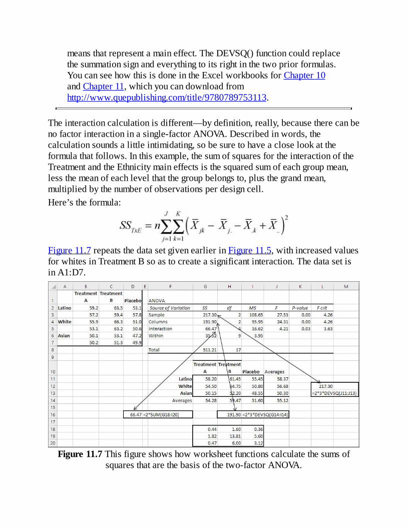
meansthatrepresentamaineffect.TheDEVSQ()functioncouldreplacethesummationsignandeverythingtoitsrightinthetwopriorformulas.YoucanseehowthisisdoneintheExcelworkbooksforChapter10andChapter11,whichyoucandownloadfromhttp://www.quepublishing.com/title/9780789753113.

Theinteractioncalculationisdifferent—bydefinition,really,becausetherecanbenofactorinteractioninasingle-factorANOVA.Describedinwords,thecalculationsoundsalittleintimidating,sobesuretohaveacloselookattheformulathatfollows.Inthisexample,thesumofsquaresfortheinteractionoftheTreatmentandtheEthnicitymaineffectsisthesquaredsumofeachgroupmean,lessthemeanofeachlevelthatthegroupbelongsto,plusthegrandmean,multipliedbythenumberofobservationsperdesigncell.Here’stheformula:

Figure11.7repeatsthedatasetgivenearlierinFigure11.5,withincreasedvaluesforwhitesinTreatmentBsoastocreateasignificantinteraction.ThedatasetisinA1:D7.

Figure11.7Thisfigureshowshowworksheetfunctionscalculatethesumsofsquaresthatarethebasisofthetwo-factorANOVA.

TherangeF1:L8containstheANOVAtableforthedatainA1:D7,andyoucanseethattheinteractionisnowstatisticallysignificantatthe.05level.(ItisnotsignificantinFigure11.3,butIhaveraisedthevaluesforwhitesunderTreatmentBforFigure11.7;sodoingmakestheinteractionstatisticallysignificantandalsochangesthesumsofsquaresforbothmaineffects.)InFigure11.7,therangeF10:J14containsthegroupaverages,themaineffectsaverages,andtheirlabels.Forexample,cellG11contains58.20,theaveragevalueforLatinosunderTreatmentA.CellJ11contains58.37,theoverallaverageforLatinos,andcellG14contains54.28,theoverallaverageforTreatmentA.CellJ14contains55.12,thegrandmeanofallobservations.WiththatpreliminaryworkinF10:J14,it’spossibletogetthesumsofsquaresforbothmaineffectsandtheinteraction.Afterthatit’seasytocompletetheANOVAtable,dividingthesumsofsquaresbythedegreesoffreedomtogetmeansquares,andfinallyformingratiosofmeansquarestogettheFratios.First,cellL12contains217.30,thesumofsquaresfortheEthnicityeffect.Theformulainthecellis

=2*3*DEVSQ(J11:J13)FollowingtheformulafortheEthnicitymaineffectgivenearlierinthissection,itisthenumberofobservationspergroup(2)timesthenumberoflevelsoftheothermaineffect(3),timesthesumofthesquareddeviationsoftheEthnicitygroupmeansfromthegrandmean.TheresultisidenticaltothesumofsquaresforEthnicityinworksheetcellG3ofFigure11.7,whichwasproducedbytheANOVA:TwoFactorWithReplicationtool.Similarly,cellH16contains191.90.Thecell’sformulais

=2*3*DEVSQ(G14:I14)ItisthesumofsquaresfortheTreatmentmaineffect,anditsresultisidenticaltotheresultproducedbytheANOVAtoolinworksheetcellG4.TheformulasthatreturnthesumsofsquaresinL12andH16bothfollowthegeneralpatterngivenearlierby

StillusingFigure11.7,youfindthesumofsquaresfortheinteractionbetweenTreatmentandEthnicityinworksheetcellG5,producedbytheANOVAtool.Itsvalue,66.47,alsoappearsincellD16.Thewaytoarriveatthesumofsquaresfortheinteractionrequiresalittleexplanation.

Irepeatherethegeneralformulafortheinteractionsumofsquares:

Thefirstpartofthatequation

iswhat’srepresentedintheformulaincellD16:=2*SUM(G18:I20)

Thisformulasumsacrossthevaluesintheintersectionsofrows18to20andcolumnsGtoI,andthendoublesthatsumbecausetherearetwoobservationsperdesigncell.Thesecondpartoftheequation

representswhat’sineachofthecellsinG18:I20.CellG18,forexample,containsthisformula:

=(G11–G$14–$J11+$J$14)^2IttakesthevalueofworksheetcellG11(LatinosunderTreatmentA),subtractsthemeaninG14foreveryoneunderTreatmentA,subtractsthemeanforallLatinosintheexperimentinJ11,andaddsthegrandmeanofallscoresinJ14.Theresultistheuniqueeffectofbeinginthatdesigncell:aLatinosubjecttakingTreatmentA.Intermsofthegeneralformula,worksheetcellG18usesthesevalues:

istheworksheetcell,G11,withthemeanscoresofLatinosunderTreatmentA,worksheetcellsB2:B3. istheworksheetcell,G14,thatcontainsthemeanofallscoresinTreatmentA,worksheetcellsG11:G13. istheworksheetcell,J11,thatcontainsthemeanofallLatinos’scoresinG11:I11. istheworksheetcellthatcontainsthegrandmeanofallscores,J14.

NoticethattheformulaincellG18usesrelative,mixed,andabsoluteaddressing.OnceyouhaveentereditinG18,youcandragittwocolumnstotherighttopickuptheproperformulasforLatinosunderTreatmentBandalsounderPlacebo,in

cellsH18:I18.Oncethefirstrowofthreeformulashasbeenestablished(inG18:I18),selectthosethreecellsanddragthemdownintoG19:I20usingthefillhandle.(That’sthesmallblacksquareinthebottomrightcorneroftheselection.)TheformulaadjuststopickupwhitesandAsiansunderTreatmentBandPlacebo.Finally,addupthevaluesinG18:I20.Multiplyby2,thenumberofobservationsperdesigncell,togetthefullsumofsquareddeviationsfortheinteractioninworksheetcellD16.Thedegreesoffreedomfortheinteractionis,bycomparison,mucheasiertofind.Justmultiplytogetherthedegreesoffreedomforeachmaineffectinvolvedintheinteraction.Inthepresentexample,eachmaineffecthastwodegreesoffreedom.Therefore,theTreatmentbyEthnicityinteractionhasfourdegreesoffreedom.IftherehadbeenanotherlevelofTreatment,thentheTreatmentmaineffectwouldhavehadthreedegreesoffreedomandtheinteractionwouldhavehadsixdegreesoffreedom.

TheWheel,ReinventedIamawarethatIhavebelaboredtheseformulasbeyondwhat’sneededtocompleteabasic3-by-3analysisofvariance,maineffects,andinteraction.I’mdoingitanywayfortworeasonsthatseemprettygoodtome.OneisthatinkeepingwithmostoftheoutputprovidedbytheDataAnalysisadd-in’stools,theANOVAtoolsprovidenoformulas—juststaticvalues.Aworksheetcellthatcontainsameansquaredoesnotcontaintheformulathatcallsfortheworksheetcellwiththesumofsquarestobedividedbytheworksheetcellwiththedegreesoffreedom.NordoesaworksheetcellthatcontainsanFratiocontainaformulathatdividesamaineffectmeansquarebyawithingroupsmeansquare.Allyougetintheoutputistheresultofthecalculation.Thatmakesithardtolookmorecloselyatwhat’sgoingonortootherwisecheckonit.WhenI’mlearningastatisticalprocedure,Iliketobeabletochangeanobservationhereandanobservationthere,toseewhateffectmychangeshaveontheoutcome.Forexample,it’sausefullearningtechniquetoseewhathappenswhenyouchangeanobservationthatis,atpresent,closetoagroup’smeantoavaluethat’sfarfromthegroup’smean.Sodoingcanhaveamajorimpactonbothamaineffect’svarianceandaninteraction’svariance,withconsequencesforwhethereithereffecttakesyououtsidethelevel

you’vesetforalpha—ormakeswhathadbeenasignificanteffectaninsignificantone.ButwiththeANOVAtoolsintheDataAnalysisadd-in,youcan’tdothat.Alltheresultsarestaticvalues.Ifyouknowwhattheformulasareandhowtheywork,youcansubstitutethemanddoyourownexperimentingwiththeinputdata.Moreimportant—andthesecondreasonforemphasizingtheformulas—isthatI’veprovideddefinitionalformulasinthischapter.It’sfairlyclearwhytheydowhattheydo:Forexample,theyaccumulatesquareddeviationsfromamean,andthat’sjustwhatavariancedoes.Usingthedefinitionalformulas,it’seasiertoseetheparallelsbetweentheinferentialstatisticsandthedescriptivestatisticsthatformtheirunderpinnings.Unfortunately,thoseconceptuallyrichdefinitionalformulascauseproblemsifyou’reahumanbeingtryingtoapplythemtoreal-worldnumbers.Peoplerearrangedtheformulasahundredyearsagoandinsodoingmadethemlessarduousforpaper-and-pencilcalculations,andlesspronetoseriousroundingerror.Even40yearsago,whenhandcalculatorsstartedtofeaturetemporarymemoriesandsquarerootfunctions,therewerecalculationformulasthatwereeasiertousethanthedefinitionalformulas.ButalthoughthecalculationformulaswereeasiertouseintheabsenceofPCs,theydidnotconveytheconceptsbehindthem.Here’sonecalculationformulawidelyusedbackintheday:

Doesthatlooktoyoulikeaformulaforthesumofsquareddeviationsfromagrandmean?Itdidn’ttomeinthe1980sanditdoesn’tnow.Butitis.Here’swhattheformulaforsquareddeviationsfromameanlooksliketome:

Takethemeanofafactorlevel,subtractthegrandmean,squarethedifference,sumthesquareddifferences,andmultiplytoaccountforthe

numberofobservationsandthenumberoflevelsintheotherfactor.Stillslightlycomplicated,butnothingliketheprecedingformula.ThepointisthatwithExcelyoucanworkwithformulasthatareeasytounderstandwithoutgoingthroughthekindsoflaboredcomputationsthatusedtoresultinroundingerrorsandevenmoreegregiouspaper-and-pencilarithmeticerrors.Therefore,IemphasizethosedefinitionalformulasandshowyouhowtheyworkoutinthecontextofanExcelworksheet.Aslongasyou’rewillingtoslogthroughsomeparagraphsthatmightseemlikeoverexplaining,you’llemergewithabetterunderstandingofwhytheseanalysesworkastheydo.Andwhenwegetaroundtoshowinghowanalysisofvarianceisjustadifferentwayofusingmultipleregression,you’llbebetterpreparedtounderstandtherelationshipsinvolved.

TheProblemofUnequalGroupSizesInANOVAdesignswithtwoormorefactors,groupsizematters.Asitturnsout,whenyouhavethesamenumberofobservationsineachdesigncell,thereisnoambiguityinhowthesumsofsquaresarepartitioned—thatis,howthesumsofsquaresareallocatedtotherowfactor,tothecolumnfactor,totheinteraction,andtotheremainingwithin-cellsumsofsquares.That’showtheexamplesusedsofarinthischapterhavebeenpresented.Figure11.8showsanotherexampleofwhat’scalledabalanceddesign.

Figure11.8Inabalanceddesign,thetotalsumofsquaresisthesamewhetherit’scalculateddirectlyorbysummingthemaineffects,interaction,andwithin-cell.

Figure11.8showstwowaysofcalculatingthetotalsumofsquaresinthedesign.Recallthatthetotalsumofsquaresisthetotalofeachobservation’ssquareddeviationfromthegrandmean.Itisthenumeratorofthevariance,andthedegreesoffreedomisthedenominator.ReturningbrieflytothelogicofANOVA,it’sthattotalsumofsquaresthatwewanttopartition,allocatingsometodifferencesingroupmeansand,infactorialdesigns,totheinteraction.InFigure11.8,noticecellsB16andB17.Theydisplaythesamevalue,2510.94,forthetotalsumofsquares,butthetwocellsarriveatthatvaluedifferently.CellB16usesExcel’sDEVSQ()functionontheoriginaldatasetinC3:E8.Asyou’vealreadyseen,DEVSQ()returnsthesumofthesquareddeviationsofitsargumentsfromtheirmean—theverydefinitionofasumofsquares.CellB17calculatesthetotalsumofsquaresdifferently.ItdoessobyaddingupthesumofsquaresasallocatedtothePatientfactor,totheTreatmentfactor,totheinteractionbetweenthetwofactors,andtotheremainingvariabilitywithindesigncellsthatisnotassociatedwithdifferencesinthemeansofthefactorlevels.Becausethetwowaysofcalculatingthetotalsumofsquareshaveidenticalresults,thesepointsareclear:

Allthevariabilityisaccountedforbythemaineffects,interaction,andwithin-groupsumsofsquares.Otherwise,thesumofsquaresfromtotalingthemaineffects,interaction,andwithin-groupsourceswouldbelessthanthesumofsquaresbasedonDEVSQ().Noneofthevariabilityhasbeencountedtwice.Forexample,itisnotthecasethatsomeofthevariabilityhasbeenallocatedtothePatientandalsotothePatientbyTreatmentinteraction.Otherwise,thesumofsquaresfromtotalingthemaineffects,interaction,andwithin-groupsourceswouldbegreaterthanthesumofsquaresbasedonDEVSQ().

Inotherwords,thereisnoambiguityinhowthesumsofsquaresaredividedupamongthevariouspossiblesourcesofvariability.NowcomparethetotalsumsofsquarescalculatedinFigure11.8withthetotalsinFigure11.9.

Figure11.9Inanunbalanceddesign,thetotalsumofsquaresascalculateddirectlydiffersfromthetotalofthemaineffects,interaction,andwithin-cell.

TheDEVSQ()resultisinarguable.UsedasfollowsinworksheetcellB19inFigure11.9

=DEVSQ(C3:E12)DEVSQ()calculatesthetotalsumofsquaresavailableforallocationamongthe

sourcesofvariation.ButthesumofthedifferenteffectsinworksheetcellB20isnolongeridenticaltothevalueinB19:aquantityof35.28hasbeencountedtwice—noticethatthevalueinB20isgreaterthanthevalueinB19by35.28.SomeofthesurplushasbeenputinthesumofsquaresforPatient,someforTreatment,somefortheinteraction,andsometotheremainingwithin-cellvariability.TheunderlyingreasonforthissituationwillnotbecomeclearuntilChapter14,“MultipleRegressionAnalysisandEffectCoding:TheBasics,”butitisduetotheunequaln’s.Withoneimportantexception,anytimeyouhaveunequaln’sinthecellsofamultifactordesign—anytimethatdifferentcombinationsofoneormorefactorlevelshavedifferentnumbersofobservations—thesumsofsquaresintheANOVAbecomeambiguous.Whenthesumsofsquaresareambiguous,soarethemeansquaresandthereforetheFratios,andyoucannolongertellwhat’sgoingonwiththeassociatedprobabilitystatements.

NoteAnoccasionallyimportantexceptiontotheproblemI’vejustdescribedisproportionalcellfrequencies.Thissituationcomesaboutwheneachlevelofonefactorhas,say,twiceasmanyobservationsasthesamelevelontheotherfactor.Themultipliercouldbeanumberotherthan2,ofcourse,suchas1.5or2.5.Theconditionthatmustbeinplaceisasfollows:Thenumberofobservationsineachdesigncellmustequaltheproductofthenumberofobservationsinitsrow,timesthenumberofobservationsinitscolumn,dividedbythetotalnumberofobservations.Ifthatconditionismet,thepartitioningofthesumsofsquaresisunambiguous.Youcan’tuseExcel’sDataAnalysistwo-factorANOVAtoolonsuchadataset,becauseitdemandsequalnumbersofobservationsineachdesigncell.ButthemethodsdiscussedinChapter14,includingtheDataAnalysisRegressiontool,workjustfine.

Severalapproachesareavailabletoyouifyouhaveadesignwithtwoormorefactors,unequaln’s,anddisproportionalfrequencies.NoneoftheseapproachesisconsistentwiththeANOVAtoolsintheDataAnalysisadd-in.ThesemethodsarediscussedinChapters14and15,though,andyou’llfindthattheyaresopowerfulandflexiblethatyouwon’tmisstheANOVAtoolswhenyouhavetwoormorefactorsandunequaln’s.

RepeatedMeasures:TheTwoFactorWithoutReplicationToolThere’sathirdANOVAtoolintheDataAnalysisadd-in.Chapter10andthis

chapterhavediscussedthesingle-factorANOVAtoolandtheANOVAtoolfortwofactorswithreplication.Thissectionprovidesabriefdiscussionofthetwo-factorwithoutreplicationtool.First,areminder:InANOVAterminology,replicationsimplymeansthateachdesigncellhasmorethanoneobservation,orreplicate.So,thenameofthistoolimpliesoneobservationperdesigncell.ThereisatypeofANOVAthatusesoneobservationperdesigncell,traditionallytermedrepeatedmeasuresanalysis.It’saspecialcaseofadesigncalledarandomizedblock,inwhichsubjectsareassignedtoblocksthatreceiveaseriesoftreatments.Therandomizedcomesfromtheusualconditionthattreatmentsberandomlyassignedtosubjectswithinblocks,butthisconditiondoesnotapplytoarepeatedmeasuresdesign.Thesubjectsarechosenforeachblockbasedontheirsimilarity,inordertominimizethevariationamongsubjectswithinblocks;thiswillmakethetestsofdifferencesbetweentreatmentsmorepowerful.Youoftenfindsiblingsassignedtoablock,orpairsofsubjectswhoarematchedonsomevariablethatcorrelateswiththeoutcomemeasure.Alternatively,thedesignmightinvolveonlyonesubjectperblock,actingashisowncontrol,andinthatcasetherandomizedblockdesignistermedarepeatedmeasuresdesign.ThisisthedesignthatANOVA:TwoFactorWithoutReplicationisintendedtohandle.Buthere’swhatExcel’sdocumentationandotherbooksonusingExcelforstatisticalanalysisdon’ttellyou:Arandomizedblockdesigningeneralandarepeatedmeasuresdesigninparticularmakeanadditionalassumption,beyondtheusualANOVAassumptionsaboutissuessuchasequaldesigncellvariances.Thisdesignassumesthatthecovariancesbetweendifferenttreatmentlevelsarehomogeneous:notnecessarilyequal,butnotsignificantlydifferent.(Theassumptionsofhomogeneousvariancesandcovariancesaretogethercalledcompoundsymmetry.)Inotherwords,thedatayouobtainmustnotactuallycontradictthehypothesisthatthecovariancesinthepopulationareequal.Ifyourdatadoesn’tconformtotheassumption,yourprobabilitystatementsaresuspect.Youcanuseacoupleofteststodeterminewhetheryourdatasetmeetsthisassumption,andExceliscapableofcarryingthemout.(Box’stestisone,andtheGeisser-GreenhouseconservativeFtestisanother.)However,thesetestsarelaborioustoconstruct,eveninthecontextofanExcelworksheet.Myrecommendationistouseasoftwarepackagespecificallydesignedtoincludethissortofanalysis.Inparticular,themultivariateFstatisticinamultivariateANOVAtestdoesnotmaketheassumptionofhomogeneityof

covariance,andthereforeifyouarrangeforthattest,inadditiontotheunivariateF,youdon’thavetoworryaboutMessrs.Box,Geisser,andGreenhouse.

Excel’sFunctionsandTools:LimitationsandSolutionsThischapterhasfocusedontwo-factordesigns:inparticular,thestudyofmaineffectsandinteractioneffectsinbalanceddesigns—thosethathaveanequalnumberofobservationsineachdesigncell.Indoingso,thechapterhasmadeuseofExcel’sDataAnalysisadd-inandhasshownhowtouseitsANOVA:TwoFactorWithReplicationtoolsoastocarryoutafactorialanalysisofvariance.Onelimitationinparticularisclear:Youmusthaveequaldesigncellsizestousethattool.Inaddition,thetoolimposesacoupleotherlimitationsonyou:

Itdoesnotallowforthreeormorefactors.That’sastandardsortofdesign,andyouneedawaytoaccountformorethanjusttwofactors.Itdoesnotallowfornestedfactors.Figure11.1showsthedifferencebetweencrossedandnestedfactors,butdoesnotmakecleartheimplicationsforExcel’stwo-factorANOVAtool(seeFigure11.10).

Figure11.10Ifyoushowthenestedfactorascrossed,thenatureofthedesignbecomesclearer.

AsthedesignislaidoutinFigure11.10,inA3:D15,it’sclearthatMDisnestedwithinHospital:Thatis,it’snotthecasethateachlevelofMDappearsateachlevelofHospital.However,althoughit’scustomarytodepictthedesigninthatway,itdoesn’tconformtotheexpectationsoftheANOVAtwo-factoradd-in.Thattoolwantsonefactor’slevelstooccupydifferentrowsandtheotherfactor’slevelstooccupydifferentcolumns.IfyoulaythedesignoutastheANOVAtoolwants—asshowninF2:H15inFigure

11.10—thenyou’reactingasthoughyouhaveafullycrosseddesign.ThatdesignhasonlytwolevelsoftheMDfactor,whereasinfacttherearefour.Certainly,MDsdonotlimittheirpracticestopatientsinonehospitalonly,buttheintentoftheexperimentistoaccountforMDswithinhospitals,notMDsacrosshospitals.ThedesignaslaidoutinJ2:N15showsthenestingclearlyandconformstotheANOVAtool’srequirementthatonefactoroccupycolumnsandthattheotheroccupyrows.However,thatrequirement,appliedtoanesteddesign,inevitablyleadstoemptycells,andtheANOVAtoolswon’tacceptemptycells,whetheroftheworksheetcellvarietyorthedesigncellvariety.TheANOVAtoolsregardsuchcellsasnon-numericdataandwon’tprocessthem.Here’sanotherlimitationoftheDataAnalysisadd-in:TheANOVAtoolsdonotprovideforaveryusefuladjunct,oneormorecovariates.Acovariateisanothervariablethat’snormallymeasuredattheintervalorratiolevelofmeasurement.Theuseofacovariateinananalysisofvariancechangesittoananalysisofcovariance(ANCOVA)andisintendedtoreducebiasintheoutcomevariableandtoincreasethestatisticalpoweroftheanalysis(seeChapter16,“AnalysisofCovariance:TheBasics”).Thesedifficulties—unequalgroupsizesinfactorialdesigns,threeormorefactors,andtheuseofcovariates—aredealtwithinChapter14.Asyou’llsee,theanalysisofvariancecanbeseenasaspecialcaseofsomethingcalledtheGeneralLinearModel,whichthisbookhintedatinthediscussionsurroundingFigure10.2.RegressionanalysisisamoreexplicitwayofexpressingtheGeneralLinearModel,andExcel’ssupportforthetoolsofregressionanalysisissuperb.You’llseehowthosetoolscanbebroughttobearonthespecialproblemsraisedbyunequalgroupsizes,threeormorefactorsandtheuseofcovariates.Chapter12,“ExperimentalDesignandANOVA,”andChapter13,“StatisticalPower,”discusstwoissuesthatIhavesofartouchedononlylightlyinthisbook,butthataredirectlyrelatedtothetestingofmeandifferencesthatANOVAisintendedtoperform:theuseofmixedmodelsandthestatisticalpoweroftheFtest.Thefinaltwosectionsofthischapterprovideabriefoverviewofthesetwotopics.

MixedModelsItispossibletoregardonefactorinafactorialexperimentasafixedfactorandanotherfactorasarandomfactor.Whenyouregardafactorasfixed,youadoptthepositionthatyoudonotintendtogeneralizeyourexperimentalfindingstootherpossiblelevelsofthatfactor.Forexample,inanexperimentthatcomparestwodifferentmedicaltreatments,youwouldprobablyregardtreatmentasafixed

factor,andprobablynottrytogeneralizeyourfindingstoothertreatmentsnotrepresentedintheexperiment.Butinthatsameexperiment,youmightwellalsohavearandomfactorsuchasHospital.YouwanttoaccountforvariabilityinoutcomesthatisduetotheHospitalfactor,soyouincludeit.However,youdon’twanttorestrictyourconclusionsabouttreatmentstotheiruseatonlythehospitalsinyourexperiment,soyouregardthehospitalsasarandomselectionfromamongthosethatexist,andtreatHospitalasarandomfactor.Ifyouhavearandomfactorandafixedfactorinthesameexperiment,youareworkingwithamixedmodel.Intermsoftheactualcalculations,Excel’stwo-factorANOVAtoolwithreplicationwillworkfineonamixedmodel,althoughyoudohavetochangethedenominatoroftheFtestforthefixedfactorfromthewithin-groupmeansquaretotheinteractionmeansquare.Thereareotherissueswhenyou’reusingamixedmodelthatyoushouldtakeintoaccountinplanningyouranalysis.Chapter12discussesthesematters.

PoweroftheFTestChapter9,“TestingDifferencesBetweenMeans:FurtherIssues,”goesintosomedetailregardingthepoweroft-tests:boththeconceptandhowyoucanquantifyit.Ftestsintheanalysisofvariancecanalsobedescribedintermsofstatisticalpower:howitisaffectedbythehypotheticaldifferencesinpopulationmeans,samplesizes,theselectedalphalevel,andtheunderlyingvariabilityofnumericobservations.However,inExcelit’sfairlyeasytodepictanalternativedistribution,onethatmightexistifthenullhypothesisiswrong,inthecaseofthet-test.Thatalternativedistributionhasthesameshape,oftennormalorclosetonormal,asthedistributionwhenthenullhypothesisistrue.That’snotthecasewiththeFdistribution.Whenthenullhypothesisofequalgroupmeansisfalse,theFdistributiondoesnotjustshiftrightorleftasthet-distributiondoes.TheFdistributionstretchesouttoassumeadifferentshape,andbecomeswhat’scalledanoncentralF.ToquantifythepowerofagivenFtest,youneedtobeabletocharacterizethenoncentralFdistributionandcompareittothecentralFdistribution,whichapplieswhenthenullhypothesisistrue.OnlybycomparingthetwodistributionscanyoutellhowmuchofeachliesaboveandbelowthecriticalFvalue,andthat’sthekeytodeterminingthestatisticalpoweroftheFtest.

YoucandeterminetheshapeofthenoncentralFdistributionusinganestofotherdistributionssuchasthegammadistributionandthebetadistribution,constantssuchasthebaseofthenaturallogarithms,andsoon.ThefundamentalfiguresareallavailableinExcel:samplesizes,factorleveleffects,andwithingroupvariance.Bycombiningthosefiguresyoucancomeupwithwhat’scalledanoncentralityparameterforuseinapowertablethat’softenincludedasanappendixtostatisticstextbooks.ButbyusingExceltocalculatethenoncentralityparameterandtheshapeoftherelevantFdistribution,you’reinapositiontocalculateandrecalculate—directly—anFtest’spowerinresponsetovaryinginputssuchassamplesizeandmeansquares.You’llreadaboutthatinChapter13.

12.ExperimentalDesignandANOVA

InThisChapterCrossedFactorsandNestedFactorsFixedFactorsandRandomFactorsCalculatingtheFRatios

Manyexperimentstakeplaceinsettingsthataretosomedegreeintactandthereforenotsubjecttoexperimentalmanipulation.Forexample,somemedicalresearchtakesplaceinhospitals.It’softentruethattheexperimentercannotmanipulatecertainaspectsofhowthehospitalmanageshealthcare.

CrossedFactorsandNestedFactorsSupposethatanexperimenterwantstoinvestigatetheeffectofcardiologists’useofdigitalhandhelddevicesonthesuccessthatpatientshaveinmanagingtheirbloodpressure.Ifdoctorsusedigitaldevicestoimmediatelyaccessfullin-patientrecords,modifyprescriptions,andarrangechangesindiets,hypertensivepatientsmightbeabletokeeptheirbloodpressureundercontrolmoreeffectivelythaninhospitalswheremoretraditionalproceduresarefollowed.Thedifficultythatmightconfronttheexperimenteristhathospitalseitherofferdoctorsthatsortofdigitaltoolortheydon’t.Onlyhospitalsintransitionwouldhavesomecardiologistsusingdigitaltechnologyandothersrelyingonpapercharts,manualprescriptions,anddietaryorders.SotheexperimentaldesignmightcallforafactorcalledDigitalDeviceUsage,whichrecordswhetheraparticipatinghospitalusesthesortofdigitaltechnologythat’sunderevaluation.Theexperimentermightworkwithtwohospitalsthatusethetechnologyandtwothatdon’t.Ateachhospital,theremightbearandomsampleof4in-patientswhohavebeenintreatmentforbetween7and10days.(Yes,thisexperimentaldesignhasproblems:Thehospitalshaveself-selectedthemselvesintoeitherdigitalortraditionalrecordmanagement.Butit’stypicalofexploratoryresearch.)Whatdoesthisdesignlooklike?Figure12.1showsonewaytodepictit.

Figure12.1ThislayoutignoresHospitalasafactorintheexperiment.

Inasense,Figure12.1representstheexperimentaldesign.Thereare16patients,8ineach“treatment”category:Thedoctoruseseitherdigitaltechnologyortraditionalpencil-and-papermethods.ButthelayoutinFigure12.1failstoaccountforanyHospitaleffect.Asdescribedearlier,fourhospitalsareinvolved,andFigure12.1tacitlyassumesthatreceivingtreatmentatagivenhospitalhasnoreliableeffectontheoutcomemeasure.Youcan’tmeasureaneffectifyoudon’taccountforit,andnoHospitaleffectisaccountedforinFigure12.1.Figure12.2showsalayoutthatdoesprovidehospitalinformation.

Figure12.2ThislayoutincludesHospitalasafactorintheexperiment,butitdoessoinaccurately.

ThedesignshowninFigure12.2iscalledacrossedfactorialdesign.Thetermfactorialsimplymeansthattherearetwo(ormore)factorsinvolved:here,that’sTreatmentandHospital.Thetermcrossedmeansthateachlevelofeachfactorappearsateachleveloftheotherfactor.So,forexample,Hospital1haspatientswhosedoctorsusedigitalequipmentanditalsohaspatientswhosedoctorsusetraditionalstorage-and-retrievalmethods.TreatmentcrossesHospital.Butthisisnothowtheactualdesignwasdescribed.Therearefourhospitals,nottwo,andeachhospitalemploysonlyonelevelofthetreatment:eitherdigitalor

traditional,butnotboth.TherearetwohospitalsateachlevelofTreatment,butthey’redifferenthospitalsandthedesignasdepictedinFigure12.2ismisleading.

DepictingtheDesignAccuratelyFigure12.3showsoneaccuratelayoutofthisdesign.

Figure12.3ThislayoutmakesclearhowtheHospitalfactorisnestedwithintheTreatmentfactor.

Thedesignasdescribed,andaslaidoutinFigure12.3,istermedanestedfactorialdesign.Eachlevelofonefactorappearsatonlyoneleveloftheotherfactor.Here,Hospitals1and2appearonlywiththeDigitaltreatment,andHospitals3and4appearonlywiththeTraditionaltreatment.SoisFigure12.1reallyinaccurate?WhyshouldwecareaboutaHospitalfactoratall?WhynotsimplyignoreHospital?Thereasonisthattheremaywellbesomethingaboutthemedicalcareatagivenhospital(orhospitals)thataffectsheartpatients’response,entirelyindependentofandapartfromthetechnology,digitalversustraditional,usedbythemedicalstaff.(Thisisonereasonthattheself-selectionofthehospitalsintoonetechnologyortheotherconstitutesaflawintheexperimentaldesign.)IfweignoretheHospitalfactorentirely,assuggestedinFigure12.1,wemissanyeffectitmighthave,eitherattributingittotheTreatmentfactororlosingitinthe

errorvariance.WemightactasifthelayoutinFigure12.2representsreality,combiningHospitals1and2,andHospitals3and4,intotwogenerichospitals.ButthatgetsusrightbacktothelayoutshowninFigure12.1.Therefore,weapplythenesteddesignshowninFigure12.3,includingsomemodificationstothestatisticalanalysis,asdiscussedlaterinthischapter.

NuisanceFactorsIntheexamplethatthischapterhasbeenconsidering,youcanthinkofHospitalasa“nuisance”factor.Theexperimenterisnotinterestedindifferencesinpatientoutcomesacrosshospitals.Theinterestcentersondifferencesinpatientoutcomesthatcanbeattributedtotheuseofnewerinformationtechnologies.ButthenatureofthetreatmentdeliverysystemforcestheexperimentertopayattentiontoHospitalasafactor.Atthetimethattheexperimenttakesplace,onlyasmallsubsetofhospitalsusebothtraditionalandnewertechnologies,andtheydosoonlybecausetheyareintransition.Therefore,whentheexperimenterselectsahospitalandthehospitalagreestoparticipate,thehospitalisautomaticallypartofeitherthedigitaltechnologysampleorthetraditionaltechnologysample.Furthermore,theexperimentcan’tignoreapossibleHospitalfactor.Thatfactormightexertaninfluenceontheoutcomesachievedbycardiacpatientsforreasonsentirelyapartfromthehospital’schoiceoftechnology—this,despitethefactthataHospitaleffectisn’tofinteresttotheexperimenter.That’swhysuchfactorsaresometimestermednuisancefactors:You’reatmostperipherallyinterestedintheireffects,butyouhavetotakeaccountofthem.Notallnestedfactorsarenuisancefactors,byanymeans.Butitistruethatnuisancefactorstendtobenested,duetotherealitiesofmanyexperimentaltestbeds.

FixedFactorsandRandomFactorsIt’salsotruethattheexperimenterinthisexamplewantstoinvestigateaspecificissue:thedifferentialeffectsofusinghandhelddigitaldevicesontheeffectivenessofcardiaccareversustraditionalmethodsofstoringandretrievingpatientinformation.Theexperimenterisn’tinterestedinanyotherinformationmanagementmethods.Theexperimentisn’tintendedtogeneralizeitsfindingstoothermethodsofpatientinformationmanagement:Itspurposeisrestrictedtocomparingoutcomesthatareassociatedwithtwospecificmethods.TheTreatmentfactorinthisexampleisthereforereferredtoasafixedfactor.The

experimenter’sinterestisfixedonthetreatmentsthatareemployedintheexperiment.Incontrast,theexperimenterdoesnotwanttorestrictthefindingstothefourparticularhospitalsinwhichtheresearchtakesplace.Thefourhospitalsarerandomlyselectedfromthepopulationofhospitalsinwhichdoctorsusedigitalhandhelddevicesandfromthepopulationofhospitalsinwhichthedoctorsdon’t.TheHospitalfactoristhereforetermedarandomfactor.Designsinwhichthereisjustonefactor,andthatfactorisfixed,areamongthemostfrequentlyusedintheliterature,whetherthatliteratureconsistsofmarketresearch,operationsresearch,medicalresearchorbehavioralresearch.Factorialdesignsthatemploytwoormorefixedfactors,usuallyfullycrossedwithoneanother,arealsopopularapproachesbecausetheyoftenbringaboutgreaterstatisticalpowerthandosinglefactorexperiments.Theyalsotendtousescarceresourcesmoreefficientlythandosinglefactordesigns.Anotherusefuldesigniscalledamixedmodel.Amixedmodelusesoneormorefixedfactorsandoneormorerandomfactors.Theexamplediscussedearlierinthischapterisamixedmodel:ItusesafixedTreatmentfactorandarandomHospitalfactor.Bothmixedmodelsandnestedmodelscallfordifferentanalysisofvariance(ANOVA)computationsthandoesadesignwithtwofixedandcrossedfactors.Thedifferencesdonotcomeintoplayuntilit’stimetocalculatetheFratios,butimportantdifferencesexistintheirformulas.IfyouuseFratiosthatareintendedforacrosseddesignwithfixedfactorswhenyoushouldbeusingthecalculationsforamixeddesign,youcaneasilymistakeaneffectthatishighlysignificantforonethatfewwouldconsidersignificant.Ifyouhaveanequalnumberofobservationsineachdesigncell,however,theANOVA:Two-FactorWithReplicationtool(partofExcel’sDataAnalysisadd-in)caneasilyhandlemixedmodels.Asmallamountoftweakingisallthat’sneeded.Idescribethatadditionalworkinlatersectionsofthischapter.Torecapitulate:

Nestedfactorshavelevelsthatdonotappearateverylevelofanotherfactor.Anexampleishospitalsthatprovide,ordonotprovide,aparticulartreatment.HospitalisnestedwithinTreatment.Factorswhoselevelsdoappearateverylevelofanotherfactoraretermedcrossedfactors.Randomfactorscompriselevelsthatareconsideredrandomselectionsfromalargerpopulation.IfHospitalisafactorinanexperiment,itisverylikelythattheexperimenterwantstogeneralizethefindingstoother

hospitalsnotincludedintheexperiment.Inthatcase,Hospitalisarandomfactor.Factorswhoselevelsexhaustthelevelsofinterest,suchasMalepatientsversusFemalepatients,aretermedfixedfactors.Nestedfactorsarefrequentlyregardedasrandomfactors.Theycanbealegitimatesourceofvariationinyourexperimentalresults,butitcanalsohappenthatyouregardtheireffectsasonlymarginallyinteresting.Inthesecases,yousometimeshearthemreferredtoinformallyasnuisancefactors.

Theselabels—nestedversuscrossed,randomversusfixed—arenotjustfussydistinctionswithoutadifference.Theyhaverealconsequencesfortheprobabilitystatementsthatyouwanttoquantifyusingtheanalysisofvariance.

TheDataAnalysisAdd-In’sANOVAToolsExcel’sDataAnalysisadd-inincludesthreetoolsthatperformANOVAs:

ANOVA:SingleFactorANOVA:Two-FactorWithReplicationANOVA:Two-FactorWithoutReplication

TheANOVA:SingleFactorToolThesinglefactortoolcanbeaquickandhandywayofrunningaone-wayANOVA,especiallyifyou’reprimarilyinterestedinFratiosandprobabilitylevels.Ifyouwantthericheranalysisavailablefromtheleast-squaresapproachtoANOVA,you’rebetteroffwithLINEST()ortheDataAnalysisadd-in’sRegressiontool,inconjunctionwithacodingmethodsuchaseffectcoding(refertoChapter14,“MultipleRegressionAnalysisandEffectCoding:TheBasics”).

TheANOVA:Two-FactorWithoutReplicationToolWhenyouhavetwofactorsandoneobservationpercell,youmightthinkthattheadd-in’sTwo-FactorWithoutReplicationtoolisthemethodofchoice.Thistoolis,infact,justameansofanalyzingarepeatedmeasuresdesign.Therefore,itrequiresthatyourdatasetmeetsthecompoundsymmetryassumption,whichimplieshomogeneousvariancesandcovariances.Thisassumptionisrarelymet,andit’spossiblethatyoucanbebetteroffrunningamultivariateANOVAifyouhaveatruerepeatedmeasuresdesignoranysortofrandomizedblockdesign.

TheANOVA:Two-FactorWithReplicationToolTheANOVA:Two-FactorWithReplicationtoolcanbeusefulifyouhaveexactlytwofactorsandifeachdesigncellcontainsthesamenumberofobservations.

NoteThetoolcannothandledesignswithdifferentnumbersofobservationsperdesigncell.Forexample,inadesignthatappliesTreatment1andTreatment2toMalesandFemales,thenumberofobservationsforTreatment1MalesmustequalthenumberofobservationsforTreatment2Females.ThisisalimitationoftheDataAnalysistool,notofthefactorialANOVAitself.

Inaddition,theTwo-FactorWithReplicationtoolassumesthatbothfactorsarefixedandthatnonestingisinvolved.However,it’safairlysimplemattertomodifythetool’sresultssothatittreatsoneofthefactorsasnested,orasrandomandcrossedwithafixedfactor.Subsequentsectionsinthischaptershowyouhowtodoso,butfirsthavealookattheresultsofananalysisinwhichbothfactorsarefixedandcrossed(seeFigure12.4).

Figure12.4TheimportantpointstonoteherearehowtolayouttheinputdataandthedenominatoroftheFratios.

DataLayout

ThefirstaspectisthelayoutoftheinputdataincolumnsAthroughC.TherearetwolevelsoftheTreatmentfactorwhoselabelsappearincellsB1andC1.(IftherewerethreeormorelevelsoftheTreatmentfactor,theycouldoccupycolumnsD,E,andsoon.)Inthiscase,therearealsotwolevelsoftheSexfactor.IfsomefactorsuchasEthnicity,ratherthanSex,wereunderinvestigation,additionallevelscouldbeidentifiedinsubsequentrows.Youdon’thavetosupplythelabelsincolumnAorinrow1.Youcouldleavethatcolumnandrowblank.Butyouhavetoincludethecolumnandtherowintheinputrangethatyouidentifyinthetool’sdialogbox(seeFigure12.5).

Figure12.5NoticethatthereisnoLabelscheckboxinthedialogbox.Thetoolusesanylabelsintheresults’descriptivesectiononly.

WhenyouchoosetheANOVA:Two-FactorWithReplicationtoolfromtheDataAnalysisdialogbox,youseethedialogboxshowninFigure12.5.AsthedataislaidoutinFigure12.4,youshouldenterA1:C21intheInputRangeeditbox.Thatis,youdon’tneedtosupplythelabelsincolumnAorrow1,butyoudohavetoincludearowandacolumninwhichthelabelswouldbeifyouhadsuppliedthem.AlsonotetheeditboxforNumberofRowsperSampleinFigure12.5.There’snoprovisionforspecifying,say,9rowsforSample1and11rowsforSample2.Each“sample”isrequiredtohavethesamenumberofobservations.Inthisway,thetoolavoidsdealingwiththe(fairlycommon)situationofanunequalnumberofobservationsperdesigncell.

NoteTohandleanunbalanceddesign,onewithanunequalnumberof

observationspercell,youneedtoadoptaleast-squaresapproach.Excel’sworksheetfunctions,andeventheDataAnalysisadd-in’sRegressiontool,arefullycapableofhandlinganunbalanceddesign.SeeChapter14andChapter15fortherelevantinformation.

CalculatingtheFRatiosFigure12.4alsoshowsthatinatwo-factorANOVAwithfixedfactors,theFratiosforthemaineffectsandtheinteractionallusethemeansquarewithin(MSW)asthedenominator.TheFratiosintherangeI4:I6areeachtheresultofdividingtheassociatedmeansquareinH4:H6bytheMSWinH7.Thisisthecorrectapproachwithtwocrossedandfixedfactors.

AdaptingtheDataAnalysisToolforaRandomFactorAlthoughtheANOVA:Two-FactorWithReplicationtoolassumesthatbothfactorsarefixed,youcaneasilyadaptittoaccountforonerandomandonefixedfactor.Itcanbeimportanttodosobecausetreatingarandomfactorasfixedcanmisleadyouregardingthesignificanceofthefactorthatisactuallyfixed.Figure12.6showsanexampleofwhatcanhappen.

Figure12.6TheHospitalfactorisrandom,andtheMethodfactorisfixed.

Figure12.6(likeFigure12.4)showsthattheTwo-FactorWithReplicationtoolalwaysusesthelabelsSamplesandColumnstorepresent,respectively,thefactorsthatoccupytherowsandthecolumnsofyourinputdata.Thisusageisn’tparticularlyhelpful;there’snoreason,forinstance,whythecolumnsshouldnotbethoughtofasrepresentingsamples.(Infact,theveryuseofthetermSamplesintheoutputsuggeststhatthetoolistreatingthefactorasarandomfactorratherthanasafixedfactor.Don’tbemisled:Lefttoitsowndevices,thetooltreatsbothfactorsasfixed.)Nevertheless,supposethatyouwanttothinkoftheHospitalfactorasrandom;thatis,youwanttogeneralizeyourfindingstoallhospitals,notjusttothehospitalsfromwhichyoutookyourdata.Andyouwanttoregardthethreemethodsasrepresentingafixedfactor,suchasthreemethodscommonlyusedinhospitalstotreataparticulardisease.YourobjectiveinrunninganANOVAistodeterminewhetherthetreatmentmethodsresultinreliablydifferentoutcomes.Putanotherway,youwanttoquantifythestatisticalsignificanceofthedifferencesinthemeanvaluesofthethreemethods.

DesigningtheFTestChapter10,“TestingDifferencesBetweenMeans:TheAnalysisofVariance,”discussesthelogicoftheFratiointhesinglefactoranalysisofvariance.Withjustonefixedfactor,youdividethemeansquarebetween(MSB)bytheMSW.Assumingthateachgrouphasthesamemeaninthepopulation(thenullhypothesis),bothMSBandMSWestimatethesamequantity:variabilityamongindividualobservationswithingroups,oftenabbreviatedsimplyasσ2.Underthatassumption,theFratiowilltendtobearound1.0.Ontheotherhand,assumingthatatleastonegrouphasadifferentmeaninthepopulation(thealternativehypothesis),MSBincludessomethingmorethanjustindividualvariationwithingroups.Inthatcase,MSBincludesvariationduetodifferencesbetweengroupmeans.Underthatassumption,theFratiotendstobegreaterthan1.0.Putdifferently,MSBincludesanysourceofvariabilityinMSW,plusthepossibilityofextravariation.InthecaseofthesinglefactorANOVA,thatextravariation—tothedegreethatitexists—isduetodifferencesinthefactor’sgroupmeans.Ifthenullhypothesisistrue,weexpectnoextravariation:ifthepopulationgroupmeansareequal,anyextravariabilityprovidedbydifferencesinthesamplegroupmeansisjust,well,samplingerror.Inthelongrun,overmanydifferentreplicationsofthesameexperimentwewindupwiththeseexpectedvalues:MSB=MSW=

or1.0.Ifthenullhypothesisisfalse,sothatthepopulationmeansdifferfromoneanother,weexpectextravariationinMSB.Againinthelongrun,wewindupwiththeseexpectedvalues:

MSW=

whereajisthedifferencebetweenthejthmeaninthepopulationandthepopulation’sgrandmean.InthiscasetheFratiotendstoexceed1.0.

NoteAnexpectedvalueofameansquareissimplyahypotheticallong-termaverage,calculatedusingmanyimaginaryreplicationsofthesameexperiment.

SotheexpectationfortheFratioincreasestothedegreethatthepopulationmeansdifferfromoneanother.TheideainassemblinganFratio,nomatterwhatsortofdesignyou’reusing,istoputallthesourcesofvariationinthedenominatorthatareinthenumerator,excepttheeffectthattheFratioismeanttotest.Andthat’spreciselywhat’sdoneinthesinglefactorANOVA,whetherornotyouuseExcel’ssinglefactorANOVAtool.Inatwo-factorANOVAwherebothfactorsarefixedandthereisnonesting,youdividetheMSBforagivenfactorbytheMSW.Fortheinteractionbetweenthetwofactors,youdividethemeansquarefortheinteractionbytheMSW.However,whenyouhaveamixedmodel—say,onefixedfactorandonerandomfactor—thingsarealittledifferent.They’reeasilyhandled,buttheyarealittledifferent.Andifyouhaveanestedmodel,thingsarealsoalittledifferent.Inthecaseofthemixedmodel,youneedtochangethedenominatorintheFtestforthefixedfactor.Andwithanestedmodel,youneedtoadjustwhatyoursoftwaremightregardastheinteractionterm(theTwo-FactorWithReplicationtooldoesjustthat).YoualsoneedtoadjustthedenominatoroftheFratioforthenestingfactor.Thenextfewsectionsshowhowtodothis,andhoweasyitistoaccomplish.

TheMixedModel:ChoosingtheDenominatorFigure12.6showstwoANOVAtables,bothbasedontheinputdataintherangeA1:K7.ThefirstANOVAtable,intherangeA10:G16,showstheresultsthattheANOVA:TwoFactorWithReplicationtoolcalculates.NoteinparticularthattheFratiofortheSamplefactor,incellE12,is9.007.With2and30degreesof

freedom,thatratioissignificantatthe.001level(seecellF12).ThatFratioof9.007iscalculatedbydividingtheSamplemeansquareof71.292bytheMSWof7.916(seecellsD12andD15).ButtheMSWisthewrongdenominatorforthisFratio.WhenyouhavetwofactorsinanANOVA,oneofwhichisfixedandoneofwhichisrandom,theFratioforthefixedfactoristheratioofthemeansquareforthatfactortothemeansquarefortheinteractioneffect.Thetheoryoftheexpectedvaluesofmeansquaresandtheircoefficientsisbeyondthescopeofthisdiscussion,butthefollowingtwostatementsarepertinenthere:

Theexpectedvalueofthemeansquareforthefixedfactorinthissituationincludesthevariancefortheinteractioneffect,thevarianceforthefixedeffect,andσ2.Theexpectedvaluefortheinteractionmeansquareincludesthevariancefortheinteractioneffect,andσ2.

Therefore,inatwofactormixedmodel,theproperdenominatorforthefixedeffect’sFratioisthemeansquarefortheinteraction,nottheMSW.Theexpectedvalueofthemeansquareforthefixedfactorincludesthevariabilityduetothefixedfactoritself,thevariabilityduetotheinteraction,andσ2.Wedividethemeansquareforthefixedfactorbythecombinationofthevariabilityduetotheinteraction,andσ2.Inthisexample,that’samatterofdividingthemeansquareforMethodbythemeansquarefortheinteractionofMethodandHospital.Themainpointtotakeawayfromthisisthatinamixedmodelweexpectthevariabilityduetofixedfactormeanstoincludevariabilityduetothefixedfactoritselfplustheinteractionofthefixedandrandomfactors.Therefore,theappropriatedenominatorfortheFratioforthefixedeffectisthemeansquarefortheinteraction.Inamodelwithonlyfixedfactors,theinteractionisnotexpectedtobepartoftheexpectedvalueforagivenfixedfactor,andtheappropriatedenominatoroftheFratioistheMSW.

StillinFigure12.6,noticethesecondANOVAtable,intherangeA18:G24.IhavechangedtheFratiofortheSamplefactorinthesecondtablesothatitdividesthemeansquarefortheSamplefactorbythemeansquarefortheinteraction.TheresultisamuchsmallerFratio,shownincellE20as1.699.With2and18degreesoffreedom(becausethedffortheinteractionis18andthedfforMSWis30),thatFratioisnotsignificantateventhe0.2level.FewwouldregardthatasevidenceofareliableeffectfortheMethodfactor.

NoteInadditiontotheusualassumptionsinANOVAsuchasindependenceofobservationsandhomogeneityofvarianceacrosscells,mixedmodelsmaketheadditionalassumptionofcompoundsymmetry.Chapter11,“AnalysisofVariance:FurtherIssues,”includesabriefdiscussionofthisassumptioninrandomizedblockdesigns.(Manyrandomizedblockdesignsareexamplesofmixedmodels.)Violationoftheassumptiontendstoreducealphabelowitsnominallevel,butthereductionisnotthoughttobeserious.

TheANOVAtooldidnotgetthecalculationswrong.Itsimplytreatsbothfactorsasfixedwhenoneofthemisactuallyrandom(andunfortunatelyExcel’sdocumentationdoesn’twarnyouofthatfact).IhavealsomodifiedtheentryincellF20tothisformula:

=F.DIST.RT(E20,C20,C22)ThetoolsfoundintheDataAnalysisadd-ingenerallyreturnstaticvaluesratherthanworksheetformulas,andthat’strueofthetwo-factorANOVAtool.So,simplychangingthedenominatoroftheFratioincellE20doesnotresultinanewandaccurateassessmentoftheprobabilityoftherevisedFratio.AfterenteringtheproperformulafortheFratioinE20

=D20/D22IenteredtheF.DIST.RT()functioninF20toobtaintheareaintherighttailofthecentralFdistributionwith2and18degreesoffreedom:Inthiscase,morethan20%ofthatarealiestotherightoftheobtainedFratio.TheexampleshowninFigure12.6showshowyoucanbemisledintothinkingthatafixedfactorinvolvesasignificantdifferencewheninfactitdoesnot.Allittakesisfailingtotakeaccountofthepresenceofarandomfactorinthedesign,treatingitinsteadasfixed.That’sthecasewiththeHospitalfactorinthisexample.TheANOVAtooltreatstheHospitalfactorasfixed,andthereisaconsequenceforMethod,thefactorthatactuallyisfixed.Buttheeffectcanworktheotherway.It’sentirelypossibletogetanonsignificantfindingforthefixedfactorifyoutreatwhat’sactuallyarandomfactorasfixed.Thenyoumightdecidethat(usingthisexample)theMethodmakesnodifference,wheninfactitdoes.ItdependsontherelativesizesofthemeansquarefortheinteractionandtheMSW.(ThedegreesoffreedomfortheselecteddenominatoralsoexertaneffectontheprobabilityoftheFratio.)

AdaptingtheDataAnalysisToolforaNestedFactorAsimilarchangetotheANOVAtool’sresultsenablesyoutodealwithanestedfactorinatwo-factordesign.Figure12.7showsthelayoutissuesinvolved.

Figure12.7ThislayoutC2:K10showsthetrueconceptuallayout.TherangeC12:G20showsthesamedatalaidoutforanalysis.

DataLayoutforaNestedDesignFigure12.7showstwowaysoflayingoutthedataforatwo-factorANOVAwithonefactornestedinanother.TherangeC2:K10showshowthedataisactuallycollected.LevelsB1throughB4ofFactorBarefoundonlyinlevelA1ofFactorA.LevelsB5throughB8ofFactorBarefoundonlyinlevelA2ofFactorA.Thisisatruenesteddesign(sometimestermedahierarchicaldesign).ButalthoughthelayoutinC2:K10ofFigure12.7isconceptuallyaccurate,itcan’tbeanalyzedbytheExcel’stwo-factorANOVAtool.IfyouidentifyC2:K10astheInputRangeinthetool’sdialogbox(seeFigure12.2),thenExceldisplaysanerrormessageregardingnon-numericdatawhenyouclickOK.ThesolutionistorearrangethedataasshowninC12:G20inFigure12.4.We’ll

temporarilypretendthatwehaveafullycrosseddesign,withonlyfourlevelsofFactorBthatcrossbothlevelsofFactorA.IfyouruntheANOVA:Two-FactorWithReplicationtoolonthedatainC12:G20,yougettheresultsshowninFigure12.8.

Figure12.8TherangeA13:G19containstheANOVAtool’sactualoutput

AnesteddesignsuchastheoneshowninC2:K10ofFigure12.7doesn’thaveaninteractionterminthetraditionalsense.Afullycrosseddesignwithtwofactors,impliedbythelayoutinC12:G20ofFigure12.7,hasaninteractiontermthataddressesthequestionofwhetheronefactoroperatesdifferentlyatdifferentlevelsoftheotherfactor.Butinanesteddesign,thatquestioncan’tbeaddressed.Youdon’thaveallthe

levelsofeachfactorrepresentedatalllevelsoftheotherfactor,soyoucan’tassesswhetheronelevelofthenestedfactoractsdifferentlyacrosslevelsoftheotherfactor:Therequisitedatajustisn’tthere.Instead,thebestyoucandoistoisolatevariabilityintheresultsaccordingtoitsapparentsource.Thecorrectanalysisofatwo-factornesteddesignappearsintherangeA21:G27inFigure12.8.Therearetwopointstonote:obtainingsumsofsquaresandmeansquaresforthenestedfactorandgettingtheproperFratiofortheotherfactor.

GettingtheSumsofSquaresInthekindofsituationdiscussedhere,twofactorsincludingonenestedfactor,thesumofsquaresforthenestedfactoriseasilycomputedbyaddingthesumofsquaresforthenestedfactortothesumofsquaresforwhattheANOVAtoolthinksistheinteractionterm.So,inFigure12.8,thesumofsquaresforthe“BwithinA”termincellB24isthetotalofcellsB15andB16.Thesameistrueofthedegreesoffreedomforthe“BwithinA”factor.Totalthedegreesoffreedomforthenestedfactorandtheinteraction.Thedegreesoffreedomfor“BwithinA”inFigure12.8isthetotalofcellsC15andC16.Thenthemeansquarefor“BwithinA”isobtainedbydividingB24byC24.TheFratioforthenestedfactoristhemeansquareforthatfactordividedbytheMSW.

CalculatingtheFRatiofortheNestingFactorThemixedmodeldiscussedearlierinthischapterusesthemeansquarefortheinteractionasthedenominatoroftheFratioforthefixedfactor.Similarly,inanesteddesign,theproperdenominatorforthenestingfactor’sFratioisthemeansquareforthenestedfactor.IntheexampleshowninFigure12.8,FactorBisnestedwithinFactorA.Therefore,theFratioforFactorAusesthemeansquareforFactorBasitsdenominator.InFigure12.8,notethattheFratioforFactorAincellE23istheresultofdividingcellD23byD24.TheANOVAtool,whichassumesthatthefactorsarefullycrossed,correctlyusestheMSWasthedenominatorfortheFratioofeacheffect(bothfactorsandtheirinteraction).Butthat’sthewrongdenominatorforthenestingfactorbecausetheANOVAtool’sassumptionthatit’safullycrosseddesigniswrong.Instead,youshouldusethemeansquareforthenestedFactorBasthedenominatorfortheFratioofthenestingFactorA.Andinthisexample,doingsoreturnsanFratiothatisnotsignificant.Incontrast,treatingthenestedfactorascrossedresultsinanFratioof5.27,whichwith1and24degreesoffreedomissignificantatthe.03level.

NoteAnydesignwithanestedfactorinvolvessomeadditionalassumptionsbeyondthosenormallyusedinacrossed-factoranalysiswithfixedfactors.Inparticular,withincellvariabilityispooledwiththevariabilityduetothenestedfactor.Intermediate-levelstatisticaltextsdescribeprocedurestotestthehomogeneityofthepooledvariancesinthisandsimilarsituations.

TheDataAnalysisadd-inforExceloffersanANOVA:Two-FactorWithReplicationtoolthatisdesignedforusewithtwo-factordesignsinwhichthefactorsarebothfixedandfullycrossed.Anadditionalrequirementisthatalldesigncellshavethesamenumberofobservations.Despitetheserestrictions,thetoolcanbeahandywaytoassesstwo-factordesignswithonerandomandonefixedfactor(amixedmodel)anddesignsinwhichonefactorisnestedinsidetheother.Ineachcase,it’snecessarytoadjusttheFratioofthefixedfactoror,whenthere’sanestedfactor,theFratioofthenestingfactor.ThisisaneasyadjustmentgiventheresultsthattheANOVAtoolwritestotheworksheet.Inthecaseofthenestedfactor,it’salsonecessarytocombinethesumsofsquaresandthedegreesoffreedomforthenestedfactorwiththeinteractionterm.ThesesimplemodificationsextendtheapplicabilityoftheANOVAtool.Theycanalsohelpprotecttheuseragainsterroneouslyconcludingthatasignificanteffectisnonsignificant,andalsoagainstthereverseerrorofconcludingthatanonsignificanteffectissignificant.

13.StatisticalPower

InThisChapterControllingtheRiskTheStatisticalPoweroft-TestsTheNoncentralityParameterintheFDistributionCalculatingthePoweroftheFTest

Whenyouundertakeatrueexperiment,youoftenmakearandomselectionofpotentialsubjectsfromapopulationthatinterestsyouandassignthematrandomtooneoftwoormoregroups.Often,thosegroupsmightbeatreatmentgroupandacontrolgroup,ortheymightbetwoormoretreatmentgroupsandacontrolgroup.Whensomesortoferror(samplingerrorormeasurementerror,forexample)causesyoutoconcludethatyourtreatmentshaveareliable,replicableeffectonthepopulationwheninfacttheydon’t,it’scalledTypeIerror.YoucanquantifytheprobabilityofmakingaTypeIerror,andthatprobabilityisoftencalled“statisticalsignificance”oralpha,symbolizedasá.There’sanothersortoferror,conceptuallysimilartoTypeIerror.Itistheerrorthatyoumakewhenyourexperimentalresultsleadyoutoconcludethatyourtreatmentswillhavenoeffectifappliedtothepopulation,wheninfacttheywould.YoucanalsoquantifythisTypeIIerroranddeterminetheprobabilitythatitwilloccur.Thatprobabilityisoftencalledbetaandsymbolizedasβ.

ControllingtheRiskSeveralfactorshelpdeterminetheprobabilityofbothaTypeIandaTypeIIerror.Amongthosefactorsarethesizeofthesamplesyoutake,thesizeofthedifferencesbetweenthegroupmeans,andthesizeofthestandarddeviationoftheoutcomemeasurerelativetothedifferencesbetweenthegroupmeans.Withthatinformationinhand,youcanuseExceltocalculatetheprobabilityofnotmakingaTypeIIerror.Thatprobabilityiscalledstatisticalpowerandisequalto1–β.Nothingprofoundaboutthat:ifβistheprobabilityofamakingaTypeIIerror,then1–βistheprobabilityofavoidingaTypeIIerror:statisticalpower(or,moresimply,power).

Powerreferstothesensitivityofyourstatisticaltesttodetectatrue,replicabledifferencebetweenatreatmentgroupandacomparisongroup.Ifyourstatisticaltestwon’tdothatreliably,youwillmakeaTypeIIerrorwithprobabilityβ.Thesmallerthatyoucanmakeβ,thegreateryoucanmake1–β,andthegreateryourtest’sstatisticalpower.Statisticalpowerisamatterofgreatconcernwhenyou’redesigningexperiments,foravarietyofreasons.Idescribetwoofthemostimportantreasonsnext.

DirectionalandNondirectionalHypothesesThetypeofalternativehypothesisyouchooseaffectspower.Youmightchooseanondirectionalhypothesis(forexample,“Wehypothesizethatourtreatmentgroupwillhaveadifferentmeanthanourcontrolgroup.”),inwhichthedirectionofthedifferenceisirrelevant.Oryoumightchooseadirectionalhypothesis(forexample,“Wehypothesizethatourtreatmentgroupwillhaveahighermeanthanourcontrolgroup.”),inwhichthedirectionofthedifferenceiscrucial.Yourchoiceofanondirectionalinsteadofadirectionalhypothesiscaneasilychangeyourexperiment’sstatisticalpowerfrom,say,80%to40%.Youwouldgofromrecognizingrealtreatmenteffectsin80%ofimaginaryrepeatedexperimentstorecognizingthem40%ofthetime.

NoteThedirectionalityofyouralternativehypothesisiscloselytiedbothtopowerandtotheissueofTypeIerror,oralpha,mentionedearlierinthispaper.Latersectionsofthischapterexplorethatrelationshipbetweenalphaandthedirectionalityofhypothesesinsomedetail.

ChangingtheSampleSizeThesizeofthesampleyoutakealsoaffectspower.Therewillusuallybeanoptimumsamplesizeforadesiredlevelofpower,andyoucanoftenuseapilotstudytodeterminewhattheoptimumsamplesizeis.Thatsortofanalysiscantellyouwhenyouareplanningontoosmallasample(so,yourstatisticalpowermightbeonly20%andyouwouldmisstoomanyrealtreatmenteffects).Equallyimportant,itcantellyouwhenyouhavetoolargeasampleinmind.Itmaybethatyouareplanningon50subjectspergroup,andthatwouldgetyouto90%power.Apoweranalysiscouldshowthatyouwouldstillhave85%powerifyoucutthesamplesizeinhalfandusedonly25subjectspergroup.Youmightwelldecidenottoexpendscarceresourcesonlargergroupsizeswhenthegainin

statisticalpowerisonly5%.

VisualizingStatisticalPowerBothalphaandbetaaretheprobabilityofmakinganerror,buttheyassumetwodifferentrealities:

Alphaistheprobabilitythatyouwilldecidethatadifferenceingroupmeansexistsinthepopulation,whentherealityisthatthereisnosuchdifference.Betaistheprobabilitythatyouwilldecidethatnodifferenceingroupmeansexistsinthepopulation,whentherealityisthatthereisatleastonesuchdifference.

ABasicAnalysisTovisualizestatisticalpowerithelpstoshowthedistributionofyourteststatisticineachsortofreality:nodifferencebetweengroupsversusatleastonedifferencebetweengroupsinthepopulationyou’reinterestedin.Westartherewithasimplesituation.Supposethatyouhavedevelopedanewmedicationthatyoubelievelowers“bad”cholesterollevels.Yourandomlyselectandrandomlyassign20peopletoeachoftwogroups,atreatmentgroupthattakesyourmedicationandacomparisongroupthattakesaplacebo.Afteronemonthoftreatment,yougetcholesterollevelsfromeachofthe40participants,calculatethemeancholesterollevelofeachgroup,andsubtractthetreatmentgroup’smeanfromthecomparisongroup’smean.Now,yourhypothesesdescribetwopossiblerealities:

Yournullhypothesisisthatinthepopulationsfromwhichyoutookyoursamples,themeancholesterollevelforthepopulationthat(hypothetically)takesyourmedicationisthesameasthemeancholesterollevelofthepopulationthat(hypothetically)takesaplacebo.Youralternativehypothesisisthatthehypotheticaltreatmentpopulationhasalowermeancholesterollevelthanthehypotheticalplacebopopulation.

ThesetwostatesofnatureshowupinFigure13.1.

Figure13.1Thecurveontheleftrepresentstheno-differencereality.Thecurveontherightrepresentsthedifferent-meansreality.

Thetwopopulationsmightreallyhavethesamemeancholesterollevelaftertakingyourmedication(ortheplacebo).Inthatcase,doingthesameexperimentmany,manytimeswouldtendtoresultinameandifferenceofzero,orclosetoit.Somereplicationsoftheexperimentwouldresultinapositivedifference,andsomeanegativedifference,simplyduetosamplingerror.

NoDifferenceBetweenPopulationMeansIfyourepeatedtheexperimentmanytimeswhenthepopulationmeansdidnotdiffer,andplottedtheresults,youwouldgetacurveliketheoneontheleftinFigure13.1.Themeanofthatcurvewouldbezerobecausethetwopopulationshavethesamemeancholesterollevel,butsamplingerrorwouldcausesomeresultssmallerthanzeroandsomelargerthanzero.Ifyouhadadoptedanalphalevelof5%,youwouldrejectthenullhypothesiswhenitistrue,5%ofthetime.Thiscomesaboutbecausesamplingerrorcausessomeofthemeandifferencestobesolarge(greaterthan13,thecriticalvalue

associatedwithalphainthiscase)thatitisnotsensibletoconcludethatthenullhypothesisistrue.Becauseyoucangetresultslikethatevenwhenthereisnodifferencebetweenthepopulationmeans,it’sanerrortoconcludethatapopulationdifferenceexists—bytradition,it’scalledaTypeIerror.Theprobabilitythatitwilloccuriscalledalpha,symbolizedasα.

ActualDifferenceBetweenPopulationMeansWhatifthetwopopulationsreallyhaddifferentcholesterollevelsafterbeingtreatedwitheitheryourmedicationoraplacebo?Thenitmightbethattheplacebopopulationhasacholesterollevelthat’sabout8pointshigherthanthetreatmentpopulation.Overrepeated,hypotheticalreplicationsoftheexperiment,themeandifferencebetweenthesamplemeanswouldtendtobe8orclosetoit.Butsomereplicationsoftheexperiment,whenthereisadifferenceof8pointsinthepopulations,wouldreturnadifferenceofmorethan8pointsandsomeconsiderablyless—perhapsonly1or2points.Inthelongrun,ifyouchartedtheresults,youwouldlikelygetacurvemuchliketheoneontherightinFigure13.1.Itsmeanwouldbe8becausethat’sthedifferencebetweenthepopulationmeans.Someresultswouldhaveameandifferencesmallerthanzero,andotherswouldhaveameandifferencelargerthan13.Statisticalpowerisameaningfulissueonlywhenthenullhypothesisisfalse,andthereforewhenthealternativehypothesisistrue.InthesituationthatFigure13.1depicts,youwouldrejectthenullhypothesisiftheresultofyourexperimentwerethatthetreatmentgrouphadacholesterollevelatleast13pointslowerthanthecomparisongroup.AsshowninFigure13.1,thatcouldhappenlessthanhalfthetimeevenifthepopulationmeanforthetreatmentgroupisasmuchas12pointslowerthantheplacebogroup(becausetheobserveddifferenceof12wouldnotexceedthecriticalvalueof13).Asdesigned,thisexperimenthasrelativelylowstatisticalpower.Ifyouknewthatbeforehand,youmightnotgotothetroubleandexpenseofrunningtheexperimentasit’sdesigned.Youhavelessthana50-50chanceofconcludingthatthemedicationmakesadifferencewhenitdoes.Thisissoevenwhenyouwouldconcludeotherwiseifyouactuallyknewthetruepopulationvalues.Itwouldbeanerror—bytradition,it’sknownasaTypeIIerror.Theprobabilitythatitwilloccuriscalledbeta,symbolizedasβ.

QuantifyingPowerButexactlywhatisthepowerofthisexperiment?AsIpointedoutearlier,βisa

probability,andpoweris1–β,soitmustbepossibletoquantifystatisticalpower.Wecandothisfairlyeasilyintheexperimentdescribedinthischapter.Becausethereareonlytwogroupsinvolved,theexperimentermightwelluseat-testtoassesstheresults.Excelhasgoodfunctionalsupportforanalyzingthet-distribution,andinthiscaseyoucandeterminethepowerofthet-testwiththefollowinginformation.

TheNecessaryFiguresAsmallpilotstudyinformsyouthatyourmedicationmightreducecholesterollevelbyanaverageof8.5points,andthestandarddeviationofthesubjectsinyourpilotstudyisabout7.8points.Yourfullexperimentwillinvolve20peopleineachoftwogroups,soyourt-testwillhave40–2=38degreesoffreedom.Youdecidetosetalphato5%or0.05.Thatmeansyouintendtorejectthenullhypothesisofnopopulationdifferenceifyougetasampledifferencethatwouldhappenonly5%ofthetimeintherealitywherethenullhypothesisistrue.Therefore,youwillrejectthenullhypothesisifthedifferenceinthesamplemeansis13.1.Thatfigureisyourcriticalvalue:95%ofthet-distributionwith38degreesoffreedomhasadifferencebetweensamplemeansof13.1orless.Youcalculatethat13.1criticalvalueasfollows.Excel’sT.INV()functiontellsyouthat95%ofthet-distributionwith38degreesoffreedomfallsbelow1.69.Usedasfollows=T.INV(0.95,38)theT.INV()functionreturnsthet-valueof1.69.Toconvertthet-valuetoyourscaleof“bad”cholesterolmeasures,multiplythet-valueof1.69bythestandarddeviationof7.8.Theresultis13.1.

FromtheCriticalValuetoPowerInadistributionwherethemeanis8.5andthestandarddeviationis7.8,thefollowingExcelformulatellsyouhowmuchoftheareaunderthecurveliestotherightofthecriticalvalueof13.1.Thefirstargumentmerelycalculatesthet-valuewithintheT.DIST()functionitself.Itsubtractsthemeanof8.5fromthecriticalvalueof13.1,anddividestheresultbythestandarddeviationof7.8:=1–T.DIST((13.1–8.5)/7.8,38,TRUE)

NoteThedistributionwe’rediscussinghereisthedistributionofmean

differences—thatis,thedistribution,acrossmanyexperiments,ofthedifferencesbetweenthemeansofthetreatmentgroupandthecomparisongroup.Thesedifferencesthemselveshaveastandarddeviation.Hereit’stakentobe7.8.BothChapter9,“TestingDifferencesBetweenMeans:FurtherIssues,”andsubsequentsectionsofthepresentchapterdiscussthemeaningandcalculationofthestandarderrorofthedifferenceofsamplemeans.

Excel2010and2013bothhaveastatisticalfunction,T.DIST.RT(),whichrelievesyouoftheburdenofsubtractingfrom1.0togettherightinsteadoftheleftpartofthecurve.Inthiscase,youcoulduse=T.DIST.RT((13.1–8.5)/7.8,38)Either1–T.DIST()orT.DIST.RT()returnsthevalue0.28,whichisthepowerofthet-testinthissituation.Twenty-eightpercentoftheareaofthet-distributionliestotherightofacriticalvalueof13.1,whichasjustnotedisthet-valueof1.69timesthestandarderrorof7.8.Thatcriticalvaluecutsoffthetop5%ofthedistributionthatrepresentsthenullhypothesis,oralpha.Butthatcriticalvalueof13.1alsocutsoffthetop28%ofthedistributionthatrepresentsthealternativehypothesis.Ifthealternativehypothesisrepresentsreality—ifyourmedicationreallyhasaneffectonthepopulation’scholesterollevel—youwouldstillhavetogetadifferenceof13.1pointsfromyoursamplestorejectthenullhypothesis.Thatwouldcomeaboutonly28%ofthetimewheninrealitythealternativehypothesisistrue.Inotherwords,thisexperimentasdescribedhasrelativelylowpower—ithasonlyslightlymorethanonechanceinfourofrejectingafalsenullhypothesis.I’lldiscusssomeofthewaystoincreasethestatisticalpowerinsubsequentsections.Beforegoingontothenextsection,it’shelpfultoreviewwhatthepresentonehasdiscussed:

Asimpleexperimentassumestworealities,oneinwhichthereisnopost-treatmentdifferenceinthepopulationsrepresentedbyyoursamples(thenullhypothesis),andoneinwhichadifferenceexists(thealternativehypothesis).Bysettingalphatoaparticularlevel,youestablishacriticalvaluebasedonyourdesirenottorejectatruenullhypothesis.Ifyourpost-treatmentoutcomemeasureiswithinthecriticalvalue,youwillconcludethatthenullhypothesisistrueandrejectthealternativehypothesis.

Ifyourpost-treatmentoutcomemeasureisbeyondthecriticalvalue,youwillrejectthenullhypothesisandconcludethatthealternativehypothesisistrue.Inthedistributionthatrepresentsthealternativehypothesis,theportionthat’sfoundbeyondthecriticalvalueistheprobabilitythatyouwillrejectthenullhypothesis.Thatdistributionrepresentsrealityifthealternativehypothesisistrue.Itisthepowerofthestatisticaltest:theprobabilitythatyouwillrejectafalsenullhypothesis.

Evenmoreconcisely:Establishacriticalvaluethatwillbeyourcriterionforrejectingthenullhypothesis.Determinethepercentageofthedistributionrepresentingthealternativehypothesisthatisbeyondthecriticalvalue.Thatpercentageisthetest’sstatisticalpower.

TheStatisticalPoweroft-TestsThemainintentofthischapteristodiscussthemeaningandcalculationofthestatisticalpoweroftheFtestwhenusedasacriterionfortheanalysisofvariance(ANOVA).However,thepresentsectionfocusesexclusivelyonthestatisticalpowerofthet-test.Thereasonisthatitismuchmorestraightforwardtocalculate,andtovisualize,thestatisticalpowerofthet-testwithdifferentdesignsthantodosowiththeFtest.Therefore,thissectionservesasanintroductiontothecalculationofthepoweroftheFtest.Astheprecedingsectionnoted,thepowerofastatisticaltestistheprobabilitythatyouwillrejectthenullhypothesiswheninfactthenullhypothesisisfalse.At-testisoftenusedtocomparethedifferencebetweentwomeansthatarebasedonsamples.Thesamplescomefrompopulations.Inthatcontext,thetest’sstatisticalpoweristheprobabilitythatyouwillconcludethatthetwopopulationmeansaredifferentwhentheyaredifferent.(Itcanalsorepresenttheprobabilityofcorrectlydecidingthatonepopulationmeanisnotjustdifferentfrombutlargerthantheother.)Withinthatcontext,severaldifferentsituationscanaffectthepowerofthet-test:

Thealternativehypothesisisnondirectional.Thealternativehypothesisisdirectional.Thenumberofobservationschanges.Thedesigncallsforadependentgroups(or“paired”)t-test.

Thenextfoursectionsshowtheeffectofthesefoursituationsonthepowerofthet-test.TheeffectsonthepoweroftheFtestareanalogous.

NondirectionalHypothesesWhenyoumakeanondirectionalalternativehypothesistoguideyourt-test,youstatethatthepopulationmeansofthetwogroupsaredifferent.Youdonotspecifywhichmeanyouexpecttobegreaterthantheother.Theeffectofusinganondirectionalhypothesisistodividethealpha—theprobabilityofrejectingatruenullhypothesis—betweenthetwotailsofthet-distribution.

NoteThedivisionofalphabetweenthetwotailsofthedistributionhasledtotheuseofthetermtwo-tailedtesttodescribeanondirectionalalternativehypothesis.ItrytoavoidthatusagebecauseitleadstoambiguityinFtestsandsubsequentmultiplecomparisontests.Incontrasttoat-test,anFtestisalwaysone-tailed,eventhoughyoumightwellbeusingadirectionalalternativehypothesis.

Figure13.2depictsasituationinwhichtheexperimentermakesanondirectionalhypothesis.

Figure13.2Thealphalevelissplitbetweenthetwotailsofthecurveontheleft.

Figure13.2depictstheresultofusingExcel’sDataAnalysisadd-intotestthedifferencebetweenthetwogroupmeans,withtheunderlyingdataincellsA2:B21.NoticethatIchosetheadd-in’s“equalvariances”t-testtool.ThecurveontheleftinFigure13.2representsthenullhypothesisofnodifferenceinthepopulationmeans.Ifthosetwomeansareequal,thenrepeatedsampleswhichsubtractthecontrolmeanfromthetreatmentmeanwillhavealong-termaverageofzero.Somesampledifferenceswillbelessthanzero,andsomewillbegreaterthanzero,andifyouchartedthosedifferencesyouwouldeventuallywindupwithacurvethatlooksliketheoneontheleftinFigure13.2.

PayingOfftoAlphaIfwesetalphato5%,wecanidentifytwowedgesunderthecurve,eachofwhichconstitutes2.5%oftheareaunderthecurve.ThosewedgesareidentifiedasAlpha/2inFigure13.2.Infact,weintendtocarryoutoneexperimentonly.Supposethatthenullhypothesisistrue.Thenwemightbeunluckyandhappentogetforoursamplestwogroupswhosemeandifferenceisunusuallylarge:morethan18,say,orlessthan–17.Ifwe’reunlucky,we’llpayoff.Basedontheunusuallylargedifferencebetweenthesamplemeans,we’llconcludethatthere’sadifferenceinthe

populationmeanswheninfactthereisn’t.

GettingItRightWhenThere’saDifferenceFigure13.2alsoshowsacurve,ontheright,whichrepresentsanalternativerealityinwhichthepopulationtreatmentmeanisdifferentfromthepopulationcontrolmean.Inthisreality,thetreatmentmeanis10.55pointsgreaterthanthecontrolmean,andsothedistributionofthedifferencesbetweensamplemeanshasanaverageof10.55.Some(hypothetical)sampleswouldhaveadifferenceinmeansgreaterthan10.55,andsomewouldhaveadifferencesmallerthan10.55.Ourselectionofanalphalevelcausesustoacceptthenullhypothesis—andtorejectthealternativehypothesis—ifwegetasamplemeandifferencethat’sbetween–17and17.Thosecriticalvaluesaretheonesthatcutoffthetwowedgesinthecurveontheleft.Butifwegetameandifferencegreaterthan17orlessthan–17,we’llrejectthenullhypothesis.Iftherealityofthesituationisthatthepopulationmeandifferenceisnotzero,thenwewillhavegottenitright;we’llrejectthenullwhenit’sfalse.Ifthepopulationdifferenceisactually10.55,wecanquantifythepowerofthet-testinthissituation.Itistheareaundertheright-handcurvethat’stotherightofthecriticalvalue.Itistheprobabilitythat—assumingthealternativehypothesisistrue,andfurthermorethatthepopulationdifferenceis10.55—wewillgetasampleresultthatislargerthanourcriticalvalue.Itisthepowerofthet-test.

QuantifyingthePowerInExcel,wecanquantifythatpower,asfollows:Takethedifferencebetweenthecriticalvalue(16.89,showninFigure13.2,cellF24)andthemeanoftheright-handcurve(10.55,thedifferencebetweenthetreatmentmeanandthecontrolmeanincellsE4:F4).Thatdifferenceis6.34,shownincellH27.Divide6.34bythestandarderrorofthedifferencebetweenthemeans.Thestandarderrorinthiscaseis8.34,shownincellF23ofFigure13.2.Theresultofthedivisionis0.76.It’sshownincellI27,anditisat-value:thedifferencebetweenameanandacriterion,dividedbyitsstandarderror.UseExcel’sT.DIST.RT()functiontoreturntheproportionoftheareaunderat-distributiontotherightofat-valueof0.76with38degreesoffreedom:T.DIST.RT(.76,38)=0.23Inwords,thepowerofthist-testis0.23or23%.That’snotaverypowerfultest.Thenextthreesectionsofthispaperdiscusshowtoincreasethetest’spower.

MakingaDirectionalHypothesisYoucanincreasethepowerbymakingadirectionalhypothesisinsteadofanondirectionalhypothesis(seeFigure13.3).

Figure13.3Thealphalevelisnolongersplit,butoccupiessolelythewedgeintherighttailoftheleft-handcurve.

Figure13.2assumesanondirectionalalternativehypothesis:thatthetreatmentgroupmeanisdifferentfromthecontrolgroupmean.Therefore,wemustallowfortwopossibilities:thatthetreatmentmeanislargerthanthecontrolgroupmeanorthatitissmallerthanthecontrolgroupmean.Inthatcase,someofthealpharatemustbeineachtailofthedistributionthatrepresentsthenullhypothesis.Butifweexcludethepossibilitythatthetreatmentmeancouldbesmallerthanthecontrolmean,wecanputallthealphaintotherighttailoftheleftcurve.ThatiswhatisshowninFigure13.3.NoticethatalphaisnolongerlabeledasAlpha/2butsimplyasAlpha.Theentire5%ofthedistributionhasbeenplacedintherighttailofthedistribution.Theeffectofdoingthatistolowerthecriticalvalue.Noticethatalphaiscutofffromtherestoftheleftcurveat14onthehorizontalaxis.ComparethattoFigure13.2,wherethecriticalvalueisalmost17.So,withadirectionalhypothesisyoudon’thavetogetameandifferenceaslarge

asyoudowithanondirectionalhypothesisinordertorejectthenullhypothesis.That’sanotherwayofsayingthatthepowerofthet-testisgreaterwhenyouuseadirectionalhypothesis.Inthiscase,cellJ27inFigure13.3showsthattheT.DIST.RT()functionreturns0.34or34%:morethan10%greaterthanwithanondirectionalhypothesis(23%).Thereasonforthisincreaseinpoweristheshiftofthecriticalvaluetotheleftonthehorizontalaxis,increasingtheareaundertheright-handcurvethatliestotherightofthecriticalvalue.That’sausefulincrease,but34%powerstillisn’tverygood.Anothermethodofincreasingpoweristoincreasethesamplesize,discussednext.

NoteAnotherwaytoincreasepower,closelyrelatedtomakingadirectionalhypothesis,istorelaxalpha,from(say)0.05to0.10.Youcansetalphabyfiat,simplybystatingthatyouwanttorestrictthepossibilityofaTypeIerrorto5%,orto10%,orsomeothervalue.Ofcourse,doingsochangesnotonlyalphabutpower,andsettingthetwovaluesshouldbebasedontherelativecostsofthetwotypesoferror,asagainstthebenefitsofmakingthecorrectdecision.Thatsortofcost-benefitanalysiscanbeverysimpleifyou’reassessingtheperformanceofanewtypeofgolfclub.Anditcanbeexcruciatinglydifficultifyou’reassessingtheeffectofanewmedicationtotreatheartdisease.

IncreasingtheSizeoftheSamplesInFigure13.4,Ihavedoubledthesizeofeachsample,from20to40.

Figure13.4Thedegreesoffreedomforthet-testhasincreasedfrom38to78.

ThesituationinFigure13.4resultsinpowerforthet-testthat’sgreaterthan50%.Noticethatthestandarderrorofthedifferencebetweenmeans,incellI25,is5.82.InFigures13.2and13.3,thestandarderroris8.34.Thecriticalvalueisfoundbymultiplyingthet-valueforaparticularprobability(here,1.64)bythestandarderrorofthedifferencebetweenmeans.Becausethestandarderrorhasbeenreduced(from8.34to5.82)bydoublingthesamplesizes,thecriticalvalueislowered.JustasinFigure13.3,loweringthecriticalvalueincreasesthepowerofthet-test.ThepowerofthetestshowninFigure13.4isactually55.8%.Youcanseethisinthechart.There,thesectionoftheright-handcurvethatrepresentspoweroccupiestheentirerighthalfofthecurveplusabitofitslefthalf.Noticethatthepowersectionextendstotheleftofthemeanoftheright-handcurve.Statisticalpowerof56%isamajorincreaseoverthe23%thatwestartedwith,butbyusingadependentgroupst-testit’spossibletodobetteryet.

TheDependentGroupst-Test

Supposethattheindividualobservationsinthetwosamples,TreatmentandControl,actuallyrepresentedlinkedpairs:forexample,abrotherandasister,ortwovehiclesofthesamebrandandmodel.Inthatcase,youcancalculateacorrelationbetweenthetwosetsofscores.Ifthecorrelationislargeenough,youcanattributemuchofthevariabilityinthescorestothecorrelation.Ineffect,youremovethatvariabilityfromthestandarderrorofthedifferencebetweenmeansandallocateittothecorrelation.Theresultisthatthestandarderrorofthedifferencebetweenmeansbecomessmaller.Alongwithit,thecriticalvaluegetslower.Andthatincreasesthepowerofthet-test(seeFigure13.5).

Figure13.5Accountingforthecorrelationincreasesthestatisticalpower,muchasANCOVAcanincreasethepowerofanANOVA.

JustasoccurredinFigure13.4,Figure13.5showsthatthestandarderrorofthedifferencebetweenmeanshasbeenreduced—thistimeto4.24(seecellF23).Onceagain,reducingthesizeofthestandarderrorhastheeffectofloweringthecriticalvalue,thistimeto7.34(seecellF24).Youcanseethesourceofthiseffectbyexaminingtheformulaforthestandarderrorofthedifferencebetweenthemeans.Hereistheformulaforthestandarderrorwhenthemeansareofindependentgroups,withthesamenumberof

observationspergroup,orn:

Incontrast,hereistheformulaforthestandarderrorwhenthemeansareofgroupsthatcomprisepairedobservations,ordependentgroups:

Noticethatthesecondformulaaboveisthesameasthefirst,exceptthatthesecondformulasubtractsatermwhosesizeisafunctionofthesizeofthecorrelationrbetweenthetwogroups.Therefore,thelargerthecorrelation,thesmallerthestandarderror.Andthesmallerthestandarderror,thesmallerthecriticalvalue.(Recallthatthecriticalvalueistheproductofthestandarderrorandthet-valueassociatedwiththesizeofalpha.)Eachofthemethodsdiscussedinthissection,andthemethod’squantitativeresults,canalsotakeplaceintheFtestusedintheanalysisofvarianceorcovariance:

YoumightoptfordirectionalhypotheseswhenyouplanamultiplecomparisonsprocedurefollowingasignificantFtest.YoumightcalculatethepowerofanFtestunderacertainsetofconditions(asdiscussedintheremainderofthischapter)anddecidethatyourpowerisnothighenoughtoproceed.Inthatcase,youmightevaluatethepoweravailableifyouincreasedyoursamplesizes.Youmightdecidetoconductananalysisofcovariance,whichmightallocateasubstantialamountoferrorvariancetotherelationshipbetweenthecovariateandtheoutcomemeasure.Theresult,asmallerdegreeoferrorvariance,isthesameasyougetwithadependentgroupst-testwhenthecorrelationisreasonablystrong.

Ineachcase,youcanevaluatethepoweroftheFtestunderadifferentsetofconditions.ThenextsectiontakesuptheproblemofquantifyingthepoweroftheFtest.

TheNoncentralityParameterintheFDistributionAnFratioistheratiooftwovariances.Whenusedinthecontextoftheanalysisofvariance,onevariance(thenumerator)isbasedonthevariabilityofthemeans

ofsampledgroups.Theothervariance,inthedenominator,isbasedonthevariabilityofindividualvalueswithingroups.Whenthegroupmeansdiffer,thenumeratorinvolvesanoncentralityparameterthatstretchesthedistributionoftheFratio,outtotheright.Thissectiondiscussesthemeaning,calculation,andsymbolicrepresentationofthenoncentralityparameterintheliteratureontheanalysisofvariance.ThefinalsectioninthischapterdiscussestherelationshipofthenoncentralityparametertothecalculationofthestatisticalpoweroftheFtestinananalysisofvariance.

VarianceEstimatesTherationalefortheFtestintheanalysisofvarianceprovidesthattherearetwowaystoestimatethevarianceinthemeasuresoftreatmentoutcome:

Betweengroups—Anestimatethatdependsexclusivelyonthedifferencesbetweengroupmeansandthenumberofobservationspergroup.Theestimateisbasedarearrangementoftheformulaforthestandarderrorofthemean.Withingroups—Anestimatethatdependsexclusivelyonthevariancewithineachgroup.Thisestimatedoesnotinvolvethedifferencesbetweenthegroupmeans,butistheaverageofthewithin-groupvariances.

Bothfiguresestimatethesamevalue:thevarianceoftheindividualoutcomemeasures.Wecanformaratio,termedtheFratio,ofthetwovarianceestimates,dividingthebetween-groupsestimatebythewithin-groupsestimate.Itturnsoutthat

Thewithin-groupsfigurecomprisesthevarianceinthepopulationfromwhichthesubjectsweresampled.Thebetween-groupsfigurecomprisesthevarianceinthesamepopulation,plusanyvarianceattributabletothedifferencesbetweenthegroupmeans.

CentralFDistributionsSo,wewindupwiththisFratio:F=(σε2+σB2)/σε2

whereσε2=Estimateofpopulationvariance

andσB2=Estimateofvariabilityduetoanydifferencesbetweenthegroupmeans

Iftherearenodifferencesbetweenthegroupmeansinthepopulation,σB2iszero,andtheFratioisasfollows:F=(σε2+0)/σε2=1.0

WhenσB2iszero,theratiofollowsacentralFdistribution.Wesamplethesubjectsthatmakeupourtreatmentgroupsandcontrolgroupsfrompopulations:thepopulationofsubjectsfromwhichweobtainasampleforGroup1,thepopulationofsubjectsfromwhichweobtainasampleforGroup2,andsoon.Thosepopulationswouldhavemeanvaluesontheoutcomemeasureifwewereabletoadministerthetreatmenttoafullpopulation.Ifthereisnodifferenceamongthosepopulationmeans,weexpecttheFratiotoequal1.0.Ofcourse,usingoursampledata,weoftencalculateanFratiothatdoesnotequal1.0evenwhentheFratiocomesfromacentralFdistribution.That’sbecauseoursamplesarenotperfectlyrepresentativeofthepopulationsonwhichtheyarebased.Figure13.6showstherelativefrequencyofdifferentFratiosbasedonsampleswhentherearenodifferencesinthemeansofthepopulations.

Figure13.6ThedistributionofFratioswhentherearenopopulationdifferencesingroupmeansistermedthecentralFdistribution.

TheshapeofthedistributionofcentralFratiosisdeterminedsolelybythenumberofdegreesoffreedomforthenumeratorandthenumberofdegreesoffreedomforthedenominator.YougenerallydecidethatanFratiois“statisticallysignificant”ifyouwouldobserveitbytheaccidentofsamplingerror,whenitspopulationvalueis1.0,lessthan5%ofthetime(thatis,p<.05),orlessthan1%ofthetime(p<.01),orlessthan0.1%ofthetime(p<.001),andsoon.Figure13.6showstherelativelikelihoodoftwoofthoseaccidentsofsamplingerror.Theselikelihoodsaretermedalphalevels.Youmightdecidethatyouwanttolimitthemistakeofdecidingthattherearedifferencesbetweenmeans,whentherearenot,to5%ofthepossibleexperimentslikethisonethatyoumightcarryout.Thenyouwouldsetalphato.05.Inthatcase,ifyoureventualFratioturnedouttobelargerthantheFratiothatcutsoffthetop5%ofthedistribution,youwoulddecidethatatruedifferenceinmeansexists.Ifnodifferenceinthepopulationmeansexists,yourresultwouldcomeaboutonly5%ofthetime.Itismorerationaltodecidethatthereisadifferencebetweenthepopulationmeansthanitistodecidethata19-to-1shotcamehome.

NoncentralFDistributionsButwhatifthereisadifferenceinthepopulationmeans?Inthatcase,thedistributionofFratiosdoesnotfollowthecentralFdistributionshowninFigure13.6.Itisinsteadwhat’scalledanoncentralF.Figure13.7showsseveralnoncentralFdistributions.

Figure13.7Thelargerthenoncentralityparameter,themorestretched-outtheFdistribution.

ThenoncentralityparameteriscloselyrelatedtotheσB2termintheexpectedvalueoftheFratio,shownearlierasF=(σε2+σB2)/σε2

Whentherearedifferencesbetweenthegroupmeansinthepopulation,thetermσB2isexpectedtobegreaterthanzero;itisthevarianceofthegroupmeans.So,whenthatvarianceoftheσB2terminthenumeratorisgreaterthanzero,thenumeratorgetslarger,asdoesthevalueoftheFratio,andthedistributionstretchesouttotherightinitschart.Thenoncentralityparameterhasbeendefinedvariouslyandinconsistentlyformanyyears,buttheliteratureonstatisticsappearstobesettlinginonbothagenerallyacceptedsymbolfortheparameter(theGreekletterlambda,λ)andontheformula.Forexample,onegenerallywell-regardedtextinits1968editionusedtheGreekcharacterδtorepresentthenoncentralityparameterandgavethisformula:

wherejindexesthegroups,nisthenumberofobservationspergroup,andβisthedifferencebetweenagroupmeanandthegrandmean.Butthesamebook’s2013editiongivesthecharacterasλandtheequationas

whichisalgebraicallyequivalentexceptthatitisthesquareoftheversioninthe1968edition.Withanequalnumberofobservationspergroup,λistheratiooftheANOVAtable’ssumofsquaresbetweentoitsmeansquarewithin.Other,andotherwisewell-regarded,booksthatarenowthirtyyearsoldconfusethenoncentralityparameterwitharelatedfigure,ϕ,whichhasfordecadesbeenusedtolookupthevalueofstatisticalpowerincharts.Formoreonhowϕisused(andtogetasenseofthedifficultyofusingthoseoldcharts)see,forexample,theSeptember1957issueoftheJournaloftheAmericanStatisticalAssociation.

NoteItellyouthisnottocriticizeotherauthors,butsothatyouwon’tbesurprisedifyouconsultanoldertextandfindinconsistenciesintheformulasandsymbols.

TheNoncentralityParameterandtheProbabilityDensityFunctionYoucangetabettersenseofhowthesizeofthenoncentralityparameteraffectstheshapeoftheFdistributionbyusingittocalculatetheprobabilitydensityfunction.Theprobabilitydensityfunction,orPDF,returnstherelativefrequencyofthevalueofastatistic.ThereisaPDFforvariousdistributions;themostfamiliararethenormaldistribution,thechi-squaredistribution,thet-distribution,andtheFdistribution.YoucanusethePDFtoreturntheY-ordinateassociatedwiththeX-valueofeachofthefollowingdistributions.

DeterminingthePDFTouseExceltoobtainthePDFforadistribution,settheCumulativeargumentin

thestatistic’s.DISTfunctiontoFALSE.Forexample:

StandardNormalDistributionTheheightofthenormalcurveforaz-valueof–0.5:=NORM.S.DIST(-.5,FALSE)returns0.352,therelativeheightofthestandardnormaldistributionforaz-valueof–0.5.Settingthesecond,cumulativeargumenttoTRUEreturns0.309,thecumulativeareaunderthenormalcurvetotheleftofaz-valueof–0.5.

Thet-DistributionTheheightofthet-distributionatat-valueof1.45with15degreesoffreedom:=T.DIST(1.45,15,FALSE)returns0.137,theheightofthet-distributionwith15degreesoffreedomatat-valueof1.45.SettingtheCumulativeargumenttoTRUEinsteadreturns0.916,theprobabilityofallvaluesthrough1.45inthet-distributionwith15degreesoffreedom.Thenoncentralt-distributionhasthesameshapeasthecentralt-distributionbutisshiftedtotheleftortherightofthecentralt-distribution,whichhasameanofzero.

Chi-SquareDistributionTheheightofthechi-squaredistributionatachi-squarevalueof3,with4degreesoffreedom:=CHISQ.DIST(3,4,FALSE)returns0.167.Settingthethird,CumulativeargumenttoTRUEreturns0.442,thetotalprobabilityofallchi-squarevaluesupto3,inachi-squaredistributionwith4degreesoffreedom.Thenoncentralchi-squaredistributionhasadifferentshapethanthecentralchi-squaredistribution.

TheFDistributionTheheightofthecentralFdistributionatanFvalueof2.00with3(numerator)and45(denominator)degreesoffreedom:=F.DIST(2,3,45,FALSE)returns0.148.Settingthefourth,CumulativeargumenttoTRUEreturns0.872,thecumulativeprobabilityofallFvaluesthrough2,inanFdistributionwith3and45degreesoffreedom.Likethechi-squaredistribution,thenoncentralFdistributionhasadifferentshapethanthecentralFdistribution.

DeterminingthePDFfortheNoncentralFDistribution

AlthoughExcel’sworksheetfunctionsprovidegoodsupportforthecentralchi-squareandthecentralFdistributions,theydonotprovidedirectsupportfornoncentralchi-squareandFdistributions.TheremainderofthissectiondiscusseshowtouseExceltodeterminethePDFfornoncentralFdistributions.Thefinalsectioninthischaptershowshowtodeterminethecumulativedensityfunction(CDF)fornoncentralFdistributions,sothatyoucandeterminethestatisticalpowerofanFtest.TheworkbookthataccompaniesthischaptercontainsaworksheetdepictedinFigure13.8.

Figure13.8ChangeanyofthefiguresincellsB2:B4toseetheireffectonthenoncentralFdistribution.

ThecentralFdistribution’sshapeissolelyafunctionofthedegreesoffreedomforthenumeratorandforthedenominatoroftheFratio.TheshapeofthenoncentralFdistributionis,inaddition,afunctionofthenoncentralityparameter.ToseethechangestotheshapeofthenoncentralFdistributiononanExcelchart,changeanyofthethreefiguresincellsB2:B4ontheworksheet.Asyouchangeanyofthethreefigures,theformulasforthePDFrecalculateandthechartisredrawn.TheformulasincolumnEarearrayformulasandmustbeenteredusingCtrl+Shift+EnterinsteadofsimplypressingtheEnterkey.HereistheformulausedincellE2,whichiscopiedandpasteddowntocellE61:

=SUM((E (̂-Lambda/2)*

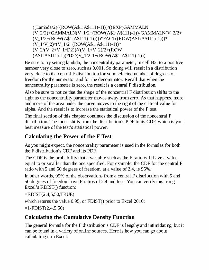
((Lambda/2) (̂ROW(A$1:A$111)-1)))/((EXP(GAMMALN(V_2/2)+GAMMALN(V_1/2+(ROW(A$1:A$111)-1))-GAMMALN(V_2/2+(V_1/2+(ROW(A$1:A$111)-1)))))*FACT((ROW(A$1:A$111)-1)))*(V_1/V_2) (̂V_1/2+(ROW(A$1:A$111)-1))*(V_2/(V_2+V_1*D2)) (̂(V_1+V_2)/2+(ROW(A$1:A$111)-1))*D2 (̂V_1/2-1+(ROW(A$1:A$111)-1)))

Besuretotrysettinglambda,thenoncentralityparameter,incellB2,toapositivenumberveryclosetozero,suchas0.001.SodoingwillresultinadistributionveryclosetothecentralFdistributionforyourselectednumberofdegreesoffreedomforthenumeratorandforthedenominator.Recallthatwhenthenoncentralityparameteriszero,theresultisacentralFdistribution.AlsobesuretonoticethattheshapeofthenoncentralFdistributionshiftstotherightasthenoncentralityparametermovesawayfromzero.Asthathappens,moreandmoreoftheareaunderthecurvemovestotherightofthecriticalvalueforalpha.AndtheresultistoincreasethestatisticalpoweroftheFtest.ThefinalsectionofthischaptercontinuesthediscussionofthenoncentralFdistribution.Thefocusshiftsfromthedistribution’sPDFtoitsCDF,whichisyourbestmeasureofthetest’sstatisticalpower.

CalculatingthePoweroftheFTestAsyoumightexpect,thenoncentralityparameterisusedintheformulasforboththeFdistribution’sCDFanditsPDF.TheCDFistheprobabilitythatavariablesuchastheFratiowillhaveavalueequaltoorsmallerthantheonespecified.Forexample,theCDFforthecentralFratiowith5and50degreesoffreedom,atavalueof2.4,is95%.Inotherwords,95%oftheobservationsfromacentralFdistributionwith5and50degreesoffreedomhaveFratiosof2.4andless.YoucanverifythisusingExcel’sF.DIST()function:=F.DIST(2.4,5,50,TRUE)whichreturnsthevalue0.95,orFDIST()priortoExcel2010:=1-FDIST(2.4,5,50)

CalculatingtheCumulativeDensityFunctionThegeneralformulafortheFdistribution’sCDFislengthyandintimidating,butitcanbefoundinavarietyofonlinesources.HereishowyoucangoaboutcalculatingitinExcel:

You’llneedtodefinefiveExcelnames,whichcanbeeitherdefinedconstantsor(preferably)referencestoworksheetcells,asfollows:

Lambda—Asdefinedearlier,theratioofthesumofsquaresbetweentothemeansquarewithin.V_1—Thedegreesoffreedomforthemeansquarebetween.V_2—Thedegreesoffreedomforthemeansquarewithin.e—Thebaseofthenaturallogarithms,2.7183.YoucangetthiseasilybyusingExcel’sEXP()function:=EXP(1).F—ThecriticalvaluethatcutsoffthearearepresentedbyalphainthecentralFdistribution.InFigure13.9,thatvalueisobtainedby=F.INV(1-0.01,V_1,V_2).Notethatalphaisgivenas.01inFigure13.9,soit’ssubtractedfrom1.0toconformtothesyntaxoftheF.INV()function.

Figure13.9CellsC7:C11arenamedaccordingtothetextvaluesincellsB7:B11.

NoteOfcourse,youcanusecellreferencesinsteadofdefinednamesintheformulathatfollows.Andyoucouldgivetheworksheetcellsanynamesyouwish,makingtheappropriatechangestotheargumentsinthearrayformula.Butit’seasiertocomparetheformulatoversionsinothersourcesifyouusethedefinednames.

Then,array-enterthefollowingformulabyfirsttypingitandthenholdingdown

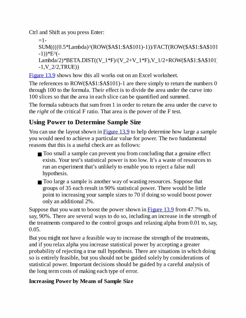
CtrlandShiftasyoupressEnter:=1-SUM((((0.5*Lambda) (̂ROW($A$1:$A$101)-1))/FACT(ROW($A$1:$A$101)-1))*E (̂-Lambda/2)*BETA.DIST((V_1*F)/(V_2+V_1*F),V_1/2+ROW($A$1:$A$101)-1,V_2/2,TRUE))

Figure13.9showshowthisallworksoutonanExcelworksheet.ThereferencestoROW($A$1:$A$101)-1aretheresimplytoreturnthenumbers0through100totheformula.Theireffectistodividetheareaunderthecurveinto100slicessothattheareaineachslicecanbequantifiedandsummed.Theformulasubtractsthatsumfrom1inordertoreturntheareaunderthecurvetotherightofthecriticalFratio.ThatareaisthepoweroftheFtest.

UsingPowertoDetermineSampleSizeYoucanusethelayoutshowninFigure13.9tohelpdeterminehowlargeasampleyouwouldneedtoachieveaparticularvalueforpower.Thetwofundamentalreasonsthatthisisausefulcheckareasfollows:

Toosmallasamplecanpreventyoufromconcludingthatagenuineeffectexists.Yourtest’sstatisticalpoweristoolow.It’sawasteofresourcestorunanexperimentthat’sunlikelytoenableyoutorejectafalsenullhypothesis.Toolargeasampleisanotherwayofwastingresources.Supposethatgroupsof35eachresultin90%statisticalpower.Therewouldbelittlepointtoincreasingyoursamplesizesto70ifdoingsowouldboostpoweronlyanadditional2%.

SupposethatyouwanttoboostthepowershowninFigure13.9from47.7%to,say,90%.Thereareseveralwaystodoso,includinganincreaseinthestrengthofthetreatmentscomparedtothecontrolgroupsandrelaxingalphafrom0.01to,say,0.05.Butyoumightnothaveafeasiblewaytoincreasethestrengthofthetreatments,andifyourelaxalphayouincreasestatisticalpowerbyacceptingagreaterprobabilityofrejectingatruenullhypothesis.Therearesituationsinwhichdoingsoisentirelyfeasible,butyoushouldnotbeguidedsolelybyconsiderationsofstatisticalpower.Importantdecisionsshouldbeguidedbyacarefulanalysisofthelongtermcostsofmakingeachtypeoferror.

IncreasingPowerbyMeansofSampleSize

So,youmightaswellconsiderincreasingyoursamplesize,eventhoughanincreaseinobservationsusuallyentailsgreatercosts.UsingthelayoutshowninFigure13.9youcanuseExcel’sSolvertotellyouwhatsamplesizeresultsinstatisticalpowerof,say,90%.Todoso,youwillneedtohaveSolverinstalledwithExcel.(Solverisanadd-inthatusuallycomeswithExcelontheinstallationdiscordownloadedinstallationfile.)It’sstraightforwardtoinstallSolverandtheinstructionstodosoarefoundinmanyplaces,bothonlineandinprint(forexample,inthisbookinChapter2,“HowValuesClusterTogether”).WithSolverinstalled,takethesesteps:

1.Ifnecessary,selecttheworksheetthatcontainsthevaluesandformulasshowninFigure13.9.

2.ClicktheDatatabonExcel’sRibbon.3.ClickSolverintheDatatab’sAnalysisgroup.4.OntheSolverdialogbox,selectC12astheSetObjectivecell.5.ClicktheValueOfoptionbuttonandenter0.9intheassociatededitbox.6.EnterC2intheByChangingVariableCellseditbox.7.ClickSolve.

Solvertriesoutdifferentvaluesforthesamplesizepergroupuntilitfindsasamplesizethatsatisfiesyourcriterionof90%power.Inthiscase,youneed16observationspergrouptoobtainpowerof90.52%(seeFigure13.10).

Figure13.10Otherthingsheldequal,inthiscasedoublingthesamplesizefrom8

to16roughlydoublesthepowerfrom47%to90%.

NoteIfyoutryoutthisexample,Solvermightnotreturnpreciselythevaluescitedhere—forexample,itmightreturn15.8insteadof16.0incellC2.ThatcaneasilyhappenwhenSolver’soptionsaresettoslightlydifferentvalues.InFigure13.10,IwantedtomakesuretogetanintegerinC2,soIcalledforcellC2asaconstraintandsetitsoperatortoint.Ialsorelaxedtheconstraintprecisionto0.01.Thefiguresdiscussednextassumesolvedvaluesof16incellC2and90.52%incellC12.

Afewpointsaboutthisanalysis:

SumofSquaresBetweenandWithinTheSSB,changesfrom160to320.ThisisbecauseIhaveusedthisformula=20*C2tocalculateSSB.Inadesignthathasanequalnumberofobservationspergroup,thegeneralformulaforSSBis

Withthisdata,thesquareddeviationsofthegroupmeansfromthegrandmeanequals20:(2.42-4.66)2+(3.29-4.66)2+(8.28-4.66)2=20Withasamplesizeof8pergroup,thatresultsinanSSBof8*20=160,andof16*20=320with16pergroup.Themeansquarewithin,orMSW,doesnotchangebecauseitistheaverageofthewithingroupvariancesandassuchisnotaffectedbyachangeinthenumberofobservationspergroup.

V2,orDegreesofFreedomWithinThevaluefordegreesoffreedomwithin,orDFW,changesalongwiththechangeinthenumberofobservationspergroup.ThisistheformulausedtodetermineDFW:=((C8+1)*C2)-C8-1

Thatis1.Getthenumberofgroups.Add1toDegreesofFreedomBetween(DFB)incellC8.

2.MultiplytheresultbythenumberofobservationspergroupinC2.Theresultisthetotalnumberofobservations.

3.SubtractDFB,andsubtract1fromtheresult.TheformulathereforereturnsN–k–1,orthetotalnumberofobservationslessDFBless1,orDFW.AlongwithalphaandDFB,thisvalueisneededtocalculatethevalueofthecriticalF.

CriticalFValueThecriticalFvalueisreturnedbythisformula:=F.INV(1-C4,V_1,V_2)ThevalueinC4isalpha,theprobabilityofrejectingatruenullhypothesis.V_1isDFB,whichdoesnotchangeinresponsetoachangeinsamplesize.V_2isDFW,whichdoeschangeassamplesizechanges.Therefore,younormallyexpectthecriticalFvaluetochangeasyoumodifythenumberofobservationspersample.

14.MultipleRegressionAnalysisandEffectCoding:TheBasics

InThisChapterMultipleRegressionandANOVAMultipleRegressionandProportionsofVarianceAssigningEffectCodesinExcelUsingExcel’sRegressionToolwithUnequalGroupSizesEffectCoding,Regression,andFactorialDesignsinExcelUsingTREND()toReplaceSquaredSemipartialCorrelations

Chapter10,“TestingDifferencesBetweenMeans:TheAnalysisofVariance,”andChapter11,“AnalysisofVariance:FurtherIssues,”focusontheanalysisofvariance,orANOVA,partlybecauseit’safamiliarapproachtoanalyzingthereliabilityofthedifferencesbetweenthreeormoremeans,butalsobecauseExceloffersavarietyofworksheetfunctionsandDataAnalysisadd-intoolsthatsupportANOVAdirectly.Furthermore,ifyouexaminethedefinitionalformulasforcomponentssuchassumofsquaresbetweengroups,itcanbecomefairlyclearhowANOVAaccomplisheswhatitdoes.Andthat’sagoodfoundation.Asabasisforunderstandingmoreadvancedmethods,it’sgoodtoknowthatANOVAallocatesvariabilityaccordingtoitscauses:differencesbetweengroupmeansanddifferencesbetweenobservationswithingroups.Ifonlyasapointofdeparture,it’shelpfultobeawarethattheallocationofthesumsofsquaresisneatandtidyonlywhenyou’reworkingwithequalgroupsizes(orproportionalgroupsizes;seeChapter12,“ExperimentalDesignandANOVA,”foradiscussionofthatexception).Butasit’straditionallymanaged,ANOVAisveryrestrictive.Observationsaregroupedintodesigncellsthathelpclarifythenatureoftheexperimentaldesignthat’sinuse(reviewFigures11.1and11.10forexamples)butthataren’tespeciallyusefulforcarryingouttheanalysis.There’sabetterway.Itgetsyoutothesameplacebyusingstrongerandmoreflexiblemethods.It’smultipleregression,andittestsdifferencesbetweengroupmeansusingthesamestatisticaltechniquesthatareusedinANOVA:sumsofsquareddeviationsoffactor-levelmeanscomparedtosumsofsquareddeviations

ofindividualobservations.Youstillusemeansquaresanddegreesoffreedom.YoustilluseFtests.Butyourmethodofgettingtothatpointisverydifferent.Multipleregressionreliesoncorrelationsandtheirnearneighbors,percentagesofsharedvariance.Itenablesyoutolayyourdataoutinlistformat,whichisastructurethatExcel(alongwithmostdatabasemanagementsystems)handlesquitesmoothly.ThatlayoutenablesyoutodealwithmostofthedrawbackstousingtheANOVAapproach,suchasunbalanceddesigns(thatis,unequalsamplesizes)andtheuseofcovariates.BoththeANOVAandthemultipleregressionapproachesarebasedontheGeneralLinearModel,andthischapterwillhaveabitmoretosayaboutthat.First,let’scompareanANOVAwithananalysisofthesamedatasetusingmultipleregressiontechniques.

MultipleRegressionandANOVAChapter4,“HowVariablesMoveJointly:Correlation,”providessomeexamplesoftheuseofmultipleregressiontopredictvaluesonadependentvariablegivenvaluesonpredictorvariables.Thoseexamplesinvolvedonlyvariablesmeasuredonintervalscales(forexample,predictingweightfromheightandage).TousemultipleregressionwithnominalvariablessuchasTreatment,Diagnosis,andEthnicity,youneedacodingsystemthatdistinguishesthelevelsofafactorfromoneanother,usingnumberssuchas1and0.Figure14.1showshowthesamedatawouldbelaidoutforanalysisusingANOVAandusingmultipleregression.

Figure14.1ANOVAexpectstabularinput,andmultipleregressionexpectsitsinputinalistformat.

ThedatasetusedinFigure14.1isthesameastheoneusedinFigure10.7.Figure14.1showstwoseparateanalyses.OneisastandardANOVAfromtheDataAnalysisadd-in’sANOVA:SingleFactortool,intheA6:G20range;itisalsorepeatedfromFigure10.7.TheANOVAtoolwasrunonthedatainA1:C4.TheotheranalysisisoutputfromtheDataAnalysisadd-in’sRegressiontool,intheI4:M20range.(IshouldmentionthattokeepdowntheclutterinFigure14.1,Ihavedeletedsomeresultsthataren’tpertinenttothiscomparison.)TheRegressiontoolwasrunonthedatainL1:N10.You’reabouttoseehowandwhythetwoanalysesarereallyoneandthesame,astheyalwaysareintheequaln’scase.First,though,Iwanttodrawyourattentiontosomenumbers:

Thesumsofsquares,degreesoffreedom,meansquares,andFratiointheANOVAtable,incellsB17:E18,areidenticaltothesamestatisticsintheregressionoutput,incellsJ14:M15.(There’snosignificancetothefactthatthesumsofsquares[SS]anddegreesoffreedom[df]columnsappearindifferentordersinthetwotables.That’smerelyhowtheprogrammerschosetodisplaytheresults.)ThegroupmeansinD10:D12arecloselyrelatedtotheregressioncoefficientsinJ18:J20.Theregressioninterceptof50inJ18isequaltothemeanofthegroupmeans,whichwithequaln’sisthesameasthegrandmeanofallobservations.TheinterceptplusthecoefficientforGroup1,in

J19,equalsGroup1’smean(seecellD10).TheinterceptplusthecoefficientforGroup2,inJ20,equalsGroup2’smean,incellD11.Andthisexpression,J18–(J19+J20),or50–(–1),equals51,themeanofGroup3incellD12.ComparingcellsE17andM14,youcanseethattheANOVAdividesthemeansquarebetweengroups(MSB)bythemeansquarewithingroups(MSW)togetanFratio.TheregressionanalysisdividesthemeansquareregressionbythemeansquareresidualtogetthesameFratio.Theonlydifferenceisintheterminology.

NoteInbothatechnicalandaliteralsense,bothmultipleregressionandANOVAanalyzevariance,sobothapproachescouldbetermed“analysisofvariance.”It’scustomary,though,toreservethetermsanalysisofvarianceandANOVAfortheapproachdiscussedinChapters10through12,whichcalculatesthevarianceofthegroupmeansdirectly.Thetermmultipleregressionisusedfortheapproachdiscussedinthischapter,whichasyou’llseeusesaproportionsofvarianceapproach.

Wehave,then,anANOVAthatconcernsitselfwithdividingthetotalvariabilityintothevariabilitythat’sduetodifferencesingroupmeansandthevariabilitythat’sduetodifferencesinindividualobservations.Wehavearegressionanalysisthatconcernsitselfwithcorrelationsandregressioncoefficientsbetweentheoutcomevariable,herenamedScore,andtwopredictorvariablesinM2:N10namedGroup1andGroup2.Howisitthatthesetwoapparentlydifferentkindsofanalysisreportthesameinferentialstatistics?Theanswertothatliesinhowthepredictorvariablesaresetupfortheregressionanalysis.

UsingEffectCodingAsImentionedattheoutsetofthischapter,thereareseveralcompellingreasonstousethemultipleregressionapproachinpreferencetothetraditionalANOVAapproach.Thebenefitscomeataslightcost,onethatyoumightnotregardasacostatall.YouneedtoarrangeyourdatasothatitlookssomethingliketherangeL1:N10inFigure14.1.Youdon’tneedtosupplycolumnsheadersasisdoneinL1:N1,butitcanprovehelpfultodoso.

NoteIhavegiventhenamesGroup1andGroup2tothetwosetsofnumbersincolumnsMandNofFigure14.1.Asyou’llsee,thenumbersinthosecolumnsindicatetowhichgroupasubjectbelongs.

TherangeL2:L10containsthescoresthatareanalyzed:thesameonesasarefoundinA2:C4.ThevaluesinM2:N10aretheresultofacodingschemecalledeffectcoding.Theyencodeinformationaboutgroupmembershipusingnumbers—numbersthatcanbeusedasdatainaregressionanalysis.TherangesL2:L10,M2:M10,andN2:N10arecalledvectors.Asit’sbeenlaidoutinFigure14.1,membersofGroup1getthecode1intheGroup1vectorinM2:M10.MembersofGroup2getthecode0intheGroup1vector,andmembersofGroup3geta–1inthatvector.SomecodesforgroupmembershipswitchintheGroup2vector,N2:N10.MembersofGroup1geta0andmembersofGroup2geta1.MembersofGroup3againgeta–1.Oncethosevectorsaresetup(andshortlyyou’llseehowtouseExcelworksheetfunctionstomakethejobquickandeasy),allyoudoisruntheDataAnalysisadd-in’sRegressiontool,asshowninChapter4.YouusetheScorevectorastheInputYRangeandtheGroup1andGroup2vectorsastheInputXRange.TheresultsyougetareasinFigure14.1,inI4:J11andI12:M20.

EffectCoding:GeneralPrinciplesTheeffectcodesusedinFigure14.1werenotjustmadeuptobringaboutresultsidenticaltotheANOVAoutput.Severalgeneralprinciplesregardingeffectcodingapplytothepresentexampleaswellastoanyothersituation.Effectcodingcanhandletwogroups,threegroupsormore,morethanonefactor(sothatthereareinteractionvectorsaswellasgroupvectors),unequaln’s,theuseofoneormorecovariates(seeChapter16,“AnalysisofCovariance:TheBasics”),andsoon.Effectcodinginconjunctionwithmultipleregressionhandlesthemall.Incontrast,underthetraditionalANOVAapproach,twoExceltoolsautomatetheanalysisforyou.YouuseANOVA:SingleFactorifyouhaveonefactor,andyouuseANOVA:TwoFactorswithReplicationifyouhavetwofactors.TheANOVAtools,asnotedbefore,cannothandlemorethantwofactorsandcannothandleunequaln’sinthetwo-factorcase.Thefollowingsectionsdetailthegeneralrulestofollowforeffectcoding.

HowManyVectorsThereareasmanyvectorsforafactorastherearedegreesoffreedomforthatfactor(thatis,thenumberofavailablelevelsforafactorminus1).InFigure14.1,thereisonlyonefactor,andithasthreelevels.Knowingtheeffectcodesfromtwovectorscompletelyaccountsforgroupmembershipusingnothingbut1s,0sand–1s.Eachcodeinformsyouwhereanysubjectisrelativetothethreetreatmentgroups.(Wecoverthepresenceofadditionalgroupslaterinthischapter.)

GroupCodesThemembersofonegroup(or,ifyouprefer,themembersofonelevelofafactor)getacodeof1inagivenvector.Allotherobservationsexceptthemembersofoneothergroupgeta0onthatvector.Themembersofthatothergroupgetacodeof–1.Therefore,inFigure14.1,thecodeassignmentsareasfollows:

TheGroup1vector—MembersofGroup1geta1inthevectornamedGroup1.MembersofGroup2geta0becausethey’remembersofneitherGroup1norGroup3.MembersofGroup3geta–1:Usingeffectcoding,onegroupmustgeta–1inallvectors.TheGroup2vector—MembersofGroup2geta1inthevectornamedGroup2.MembersofGroup1geta0becausethey’remembersofneitherGroup2norGroup3.Again,membersofGroup3geta–1throughout.

InFigure14.2,youcanseethatanadditionallevel,Group4,ofthefactorhasbeenaddedbyputtingitsobservationsincellsD2:D4.Toaccommodatethatextralevel,anothercodingvectorhasbeenaddedincolumnI.Noticethattherearestillasmanycodingvectorsastherearedegreesoffreedomforthisfactor’seffect.(Thisisalwaystrueifthecodinghasbeendonecorrectly.)InthevectornamedGroup3,membersofGroup1andGroup2getthecode0,membersofGroup3getthecode1,andmembersofGroup4geta–1justastheydoinvectorsGroup1andGroup2.

Figure14.2Anadditionalfactorlevelrequiresanadditionalvector.

InFigure14.2,youcanseethatthegeneralprinciplesforeffectcodinghavebeenfollowed.Inadditiontosettingupasmanycodingvectorsastherearedegreesoffreedom:

Ineachvector,adifferentgrouphasbeenassignedthecode1.Withtheexceptionofonegroup,allothergroupshavebeenassignedthecode0inagivenvector.Onegrouphasbeenassignedthecode–1throughoutthecodingvectors.

OtherTypesofCodingInthiscontext—thatis,theuseofcodingwithmultipleregression—therearetwoothergeneraltechniques:orthogonalcodinganddummycoding.Dummycodingisthesameaseffectcoding,exceptthattherearenocodesof–1.Onegroupgetscodesof1inagivenvector;allothergroupsget0.Dummycodingworksandproducesthesameinferentialresults(sumsofsquares,meansquares,andsoon)asdoeseffectcoding,butoffersnospecialbenefitbeyondwhat’savailablewitheffectcoding.Theregressionequationhasdifferentcoefficientswithdummycodingthanwitheffectcoding.Theregressioncoefficientswithdummycodinggivethedifferencebetweengroupmeansandthemeanofthegroupthatreceives0sthroughout.Therefore,dummycodingcansometimesproveusefulwhenyouplantocompareseveralgroupmeanswiththemeanofonecomparisongroup;amultiplecomparisonstechniqueduetoDunnettisdesignedforthatsituation.(Dummycodingisalsousefulinlogisticregression,whereitcanmaketheregressioncoefficientsconsistentwiththeoddsratios.)

Orthogonalcodingisnearlyidenticaltoplannedorthogonalcontrasts,discussedattheendofChapter10.Onebenefitoforthogonalcodingcomesifyou’redoingyourmultipleregressionwithpaperandpencil.Orthogonalcodesleadtomatricesthatareeasilyinverted;whenthecodesaren’torthogonal,thematrixinversionissomethingyouwouldn’twanttowatch,muchlessdo.ButwithpersonalcomputersandExcel,theneedtosimplifymatrixinversionsusingorthogonalcodinghaslargelydisappeared.(Excelhasaworksheetfunction,MINVERSE(),thatdoesitforyou.)Nowthatyou’vebeenalertedtothefactthatdummycodingexists,thisbookwillhavenomoretosayaboutit.WereturntothetopicoforthogonalcodinginChapter15,“MultipleRegressionAnalysisandEffectCoding:FurtherIssues.”

MultipleRegressionandProportionsofVarianceChapter4goesintosomedetailaboutthenatureofcorrelation.Oneparticularlyimportantpointisthatthesquareofacorrelationcoefficientrepresentstheproportionofsharedvariancebetweentwovariables.Forexample,ifthecorrelationcoefficientbetweencaloricintakeandweightis0.5,thenthesquareof0.5,or0.25,tellsyoutheproportionofvariancethatthetwovariableshaveincommon.Therearevariouswaystocharacterizethisrelationship.Ifit’sreasonabletobelievethatoneofthevariablescausestheother,perhapsbecauseyouknowthatoneprecedestheotherintime,youmightsaythat25%ofthevariabilityinthesubsequentvariable,weightgainorloss,isduetodifferencesintheprecedentvariable,diet.Ifit’snotclearthatonevariablecausestheother,orifthedirectionofthecausationisn’tclear,forexample,withvariablessuchascrimeandpoverty,thenyoumightsaythatcrimeandpovertyhave25%oftheirvarianceincommon.Sharedvariance,explainedvariance,predictedvariance—allarephrasesthatsuggestthatwhenonevariablechangesinvalue,sodoestheother,withorwithoutthepresenceofdirectcausation.Whenyousetupcodedvectors,asshowninFigures14.1and14.2,youcreateanumericvariablethathasacorrelation,andthereforecommonvariance,withanoutcomevariable.Atthispointyou’reinapositiontodeterminehowmuchofthevariability—thesumofsquares—intheoutcomevariableyoucanattributetothecodedvector.Andthat’sjustwhatyou’redoingwhenyoucalculatethebetween-groupsvarianceinatraditionalANOVA.BackinChapter1,“AboutVariablesandValues,”I

arguedthatnominalvariables,variableswhosevaluesarejustnames,don’tworkwellwithnumericanalysessuchasaverages,standarddeviations,orcorrelations.Butbyworkingwiththemeanvaluesassociatedwithanominalvariable,youcanget,say,themeancholesterollevelforMedicationA,forMedicationB,andforaplacebo.Then,calculatingthevarianceofthosemeanstellsyouhowmuchofthetotalsumofsquaresisduetodifferencesbetweenmeans.Youcanalsouseeffectcodingtogettothesameresultviaadifferentroute.EffectcodingtranslatesanominalvariablesuchasMedicationtonumericvalues(1,0,and–1)thatyoucancorrelatewithanoutcomevariable.Figure14.3appliesthistechniquetothedatapresentedearlierinFigure14.1.

Figure14.3Twowaystocalculatethesumofsquaresbetweengroups.

InFigure14.3,IhaveremovedsomeancillaryinformationfromtheDataAnalysisadd-in’sANOVAandRegressiontoolssoastofocusonthesumsofsquares.NoticethattheANOVAreportinA6:E11gives78asthesumofsquaresbetweengroups(SSB).ItusestheapproachdiscussedinChapters10and11toarriveatthatfigure.TheportionoftheRegressionoutputshowninK1:L5showsthatthemultipleR2is0.696(seealsocellL12).AsdiscussedinChapter4,themultipleR2istheproportionofvariancesharedbetween(a)theoutcomevariableand(b)thecombinationofthepredictorvariablesthatresultsinthestrongestcorrelation.NoticethatifyoumultiplythemultipleR2of0.696timesthetotalsumofsquares,112incellB11,youget78:theSSBshownincellB8.ThatbestcombinationofpredictorvariablesisshownincolumnGofFigure14.4.

Figure14.4GettingthemultipleR2explicitly.

Togetthebestcombinationexplicitlytakesjustthreesteps(andasyou’llsee,it’squickertogetitimplicitlyusingtheTREND()function).Youneedtheregressioncoefficients,whichareshowninFigure14.3(cellsL8:L10):

1.MultiplythecoefficientforGroup1byeachvalueforGroup1.PuttheresultincolumnD.

2.MultiplythecoefficientforGroup2byeachvalueforGroup2.PuttheresultincolumnE.

3.AddtheinterceptincolumnFtothevaluesincolumnsDandEandputtheresultincolumnG.

NoteYoucangettheresultthat’sshownincolumnGbyarray-enteringthisTREND()functioninanine-row,one-columnrange:TREND(A2:A10,B2:C10).Thatapproachisusedlaterinthechapter.Inthemeantimeit’shelpfultoseetheresultofapplyingtheregressionequationexplicitly.

Asacheck,thefollowingformulaisenteredincellG12:=CORREL(A2:A10,G2:G10)

ThisoneisenteredincellG13:=G12^2

Theyreturn,respectively,(a)thecorrelationbetweenthebestcombinationofthe

predictorsandtheoutcomevariableand(b)thesquareofthatcorrelation,orR2.ComparethevaluesyouseeincellsG12andG13withthoseyouseeincellsL4andL5onFigure14.3,whichwereproducedbytheRegressiontoolintheDataAnalysisadd-in.Ofcourse,ifyoumultiplytheR2valueincellG13onFigure14.4bythetotalsumofsquaresincellB11onFigure14.3,youstillgetthesameSSB,78.Inasingle-factoranalysis,theANOVA’sSumofSquaresBetweenGroupsisidenticaltoregression’sSumofSquaresRegression.

UnderstandingtheSeguefromANOVAtoRegressionItoftenhelpsatthispointtostepbackfromthemathinvolvedinbothANOVAandregressionandtoreviewtheconceptsinvolved.Themaingoalofbothtypesofanalysisistodisaggregatethevariability—asmeasuredbysquareddeviationsofindividualobservationsfromthegrandmean—inadatasetintotwocomponents:

ThevariabilitycausedbydifferencesinthemeansofgroupsthatpeoplebelongtoTheremainingvariabilitywithingroups,asmeasuredbythesquareddeviationsofindividualobservationsfromtheirgroup’smean

VarianceEstimatesviaANOVAANOVAreachesitsgoalinpartbycalculatingthesumofthesquareddeviationsofthegroupmeansfromthegrandmeanandinpartbycalculatingthesumofthesquareddeviationsoftheindividualobservationsfromtheirrespectivegroupmeans.Thosetwosumsofsquaresarethenconvertedtovariancesbydividingbytheirrespectivedegreesoffreedom.

SumofSquaresWithinGroupsThesumofthesquareddeviationswithineachgroupiscalculatedandthensummedacrossthegroupstogetthesumofsquareswithingroups(SSW).Groupmeansareinvolvedinthesecalculations,butonlytofindthedeviationscoreforeachobservation.Thedifferencesbetweengroupmeansarenotinvolved.

SumofSquaresBetweenGroupsThebetweengroupsvarianceisbasedonthevarianceerrorofthemean—thatis,thevarianceofthegroupmeansmultipliedbythenumberofgroups.Thisisconvertedtoanestimateofthepopulationvariancebyrearrangingtheequationforthevarianceerrorofthemean,whichis

tothisform:

Theseequationsimplyestimates:thevaluesthatweexpectiftherearenodifferencesamongthepopulationmeans.Inwords,thevarianceofallobservationsisestimatedasthevarianceofthegroupmeansmultipliedbythenumberofobservationsineachgroup.Putanotherway,underthenullhypothesisofnodifferencesamongthepopulationmeans,theexpectedvalueofMSBisthepopulationvariance.(TheconceptofthevarianceerrorofthemeanisintroducedinChapter8,“TestingDifferencesBetweenMeans:TheBasics,”inthesectiontitled“TestingMeans:TheRationale.”)Incontrasttotheestimatesjustdiscussed,youcalculatethesumofsquaresbetweengroupsbymultiplyingthesumofthesquareddeviationsofthegroupmeansbythenumberofobservationsineachgroup:

ComparingtheVarianceEstimatesTherelativesizeofthevarianceestimates—theFratio,theestimatefrombetweengroupsvariabilitydividedbytheestimatefromwithingroupsvariability—tellsyouthelikelihoodthatthegroupmeansarereallydifferentinthepopulation,orthattheirdifferencecanbeattributedtosamplingerror.Thisisasgoodaspotasanytonotethatalthoughameansquareisavariance,meansquarebetweengroupsdoesnotsignifythevarianceofthegroupmeans.Itisanestimateofthetotalvarianceofalltheobservations,basedonthevariabilityamongthegroupmeans.Inthesameway,meansquarewithingroupsdoesnotsignifythevarianceoftheindividualobservationswithineachgroup;afterall,youtotalthesumofsquaresineachgroup.Itisanestimateofthetotalvarianceofalltheobservationsbasedonthevariabilitywithineachgroup.Therefore,youhavetwoindependentestimatesofthetotalvariance:betweengroups,basedondifferencesbetweengroupmeans,andwithingroups,basedondifferencesbetweenindividualobservationsandthemeanoftheirgroup.Iftheestimatebasedongroupmeansexceedstheestimatebasedonwithincellvariationbyanimprobableamount,itmustbeduetooneormoredifferencesingroupmeansthatare,underthenullhypothesis,alsoimprobablylarge.

VarianceEstimatesviaRegression

Regressionanalysistakesadifferenttack.Itsetsupnewvariablesthatrepresentthesubjects’membershipinthedifferentgroups;thesearethevectorsofeffectcodesinFigures14.1through14.4.Thenamultipleregressionanalysisdeterminestheproportionofthevarianceinthe“outcome”or“predicted”variablethatisassociatedwithgroupmembership,asrepresentedbytheeffectcodevariables;thisisthebetweengroupsvariance.Theremaining,unattributedvarianceisthewithingroupsvariance(or,asregressionanalysistermsit,residualvariance).Onceagain,youdividethebetweengroupsvariancebythewithingroupsvariancetorunyourFtest.Or,ifyouworkyourwaythroughit,youfindthattocalculatetheFtest,theactualvaluesofthesumsofsquaresandvariancesareunnecessarywhenyouuseregressionanalysis(seeFigure14.5).

Figure14.5YoucanrunanFtestusingproportionsofvarianceonly.

InFigure14.5,cellsA7:E10presentanANOVAsummaryofthedatainA1:C4inthetraditionalmanner,reportingsumsofsquares,degreesoffreedom,andthemeansquaresthatresultfromdividingsumsofsquaresbydegreesoffreedom.ThefinalfigureisanFratioof6.88incellE8.ButthesumsofsquaresareunnecessarytocalculatetheFratio.Whatmattersistheproportionofthetotalvarianceintheoutcomevariablethat’sattributabletothecodedvectorsthathererepresentgroupmembership.CellL8containstheproportionofvariance,.6964,that’sduetoregressiononthevectors,andcellL9containstheremainingorresidualproportionofvariance,.3036.Divideeachproportionbyitsaccompanyingdegreesoffreedomandyougetthemeansquares—orwhatwouldbethemeansquaresifyoumultipliedthembythetotalsumofsquares,112(cellB10).Finally,dividecellN8bycellN9togetthesameFvalueincellO8thatyouseeincellE8.Evidently,thesumofsquaresissimplyaconstantthatforthepurposeofcalculatinganFratiocanbeignored.YouwillseemoreaboutworkingsolelywithproportionsofvarianceinChapter

17,“AnalysisofCovariance:FurtherIssues,”whenthetopicofmultiplecomparisonsbetweenmeansisrevisited.

TheMeaningofEffectCodingEarlierchaptershavereferredoccasionallytosomethingcalledtheGeneralLinearModel,andwe’reatapointinthediscussionofregressionanalysisthatitmakessensetomakethediscussionmoreformal.EffectcodingiscloselyrelatedtotheGeneralLinearModel.It’susefultothinkofanindividualobservationasthesumofseveralcomponents:

AgrandmeanAneffectthatreflectstheamountbywhichagroupmeandiffersfromthegrandmeanAn“error”effectthatmeasureshowmuchanindividualobservationdiffersfromitsgroup’smean

Algebraicallythisconceptisrepresentedasfollowsforpopulationparameters:Xij=μ+βj+εij

Or,usingRomaninsteadofGreeksymbolsforsamplestatistics:

EachobservationisrepresentedbyX,specificallytheithobservationinthejthgroup.Eachobservationisacombinationofthefollowing:

Thegrandmean,Theeffectofbeinginthejthgroup,bj.UndertheGeneralLinearModel,simplybeinginaparticulargrouptendstopullitsobservationsupifthegroupmeanishigherthanthegrandmean,orpushthemdownifthegroupmeanislowerthanthegrandmean.Theresultofbeingtheithobservationinthejthgroup,eij.Thisisthedistanceoftheobservationfromthegroupmean.It’srepresentedbytheletterebecause—forreasonsoftraditionthataren’tverygood—itisregardedaserror.Anditisfromthatusagethatyougettermssuchasmeansquareerroranderrorvariance.Quantitiessuchasthosearesimplytheresidualvariationamongobservationsonceyouhaveaccountedforothersourcesofvariation,suchasgroupmeans(bj)andinteractioneffects.

VariousassumptionsandrestrictionscomeintoplaywhenyouapplytheGeneralLinearModel,andsomeofthemmustbeobservedifyourstatisticalanalysisisto

haveanyrealmeaning.Forexample,it’sassumedthattheeijerrorvaluesareindependentofoneanother;thatis,ifoneobservationisabovethegroupmean,thatfacthasnoinfluenceonwhethersomeotherobservationisabove,below,ordirectlyonthegroupmean.Otherexamplesincludetherestrictionsthatthebjeffectssumtozero,asdotheeijerrorvalues.Thisisasyouwouldexpect,becauseeachbjeffectisadeviationfromthegrandmean,andeacheijerrorvalueisadeviationfromagroupmean.Thesumofsuchdeviationsisalwayszero.NoticethatI’vereferredtothebjvaluesaseffects.That’sstandardterminologyanditisbehindthetermeffectcoding.Whenyouuseeffectcodingtorepresentgroupmembership,asisdoneinthepriorsection,thecoefficientsinaregressionequationthatrelatestheoutcomevariabletothecodedvectorsarethebjvalues:thedeviationsofagroup’smeanfromthegrandmean.TakealookbackatFigure14.1.ThegrandmeanofthevaluesincellsL2:L10(identicaltothoseinA2:C4)is50.TheaveragevalueinGroup1is53,sotheeffect—thatis,b1—ofbeinginGroup1is3.InthevectorthatrepresentsmembershipinGroup1,whichisinM2:M10,membersofGroup1areassigneda1.AndtheregressioncoefficientfortheGroup1vectorincellJ19is3:theeffectofbeinginGroup1.Hence,effectcoding.ItworksthesamewayforGroup2.Thegrandmeanis50andthemeanofGroup2is46,sotheeffectofbeingamemberofGroup2is–4.AndtheregressioncoefficientfortheGroup2vector,whichrepresentsmembershipinGroup2viaa1,is–4(seecellJ20).Noticefurtherthattheinterceptisequaltothegrandmean.SoifyouapplytheGeneralLinearModeltoanobservationinthisdataset,you’reapplyingtheregressionequation.ForthefirstobservationinGroup2,forexample,theGeneralLinearModelsaysthatitshouldequal

orthis,usingactualvalues:48=50+(–4)+2

AndtheregressionequationsaysthatavalueinanygroupisfoundbyIntercept+(Group1b-weight*ValueonGroup1)+(Group2b-weight*ValueonGroup2)

orthefollowing,usingactualvaluesforanobservationin,say,Group2:50+(3*0)+(–4*1)

Thisequals46,whichisthemeanofGroup2.Theregressionequationdoesnotgofurtherthanestimatingthegrandmeanplustheeffectofbeinginaparticulargroup.Theremainingvariability(forexample,havingascoreof48insteadoftheGroup2mean46)isregardedasresidualorerrorvariation.Themeanofthegroupthat’sassignedacodeof–1throughoutisfoundbytakingthenegativeofthesumoftheb-weights.Inthiscase,that’s–(3+–4),or1.AndthemeanofGroup3isinfact51,1morethanthegrandmean.

NoteFormally,usingeffectcoding,theinterceptisequaltothemeanofthegroupmeans:Here,that’s(53+46+51)/3,or50.Whenthereisanequalnumberofobservationspergroup,themeanofallobservationsisequaltothemeanofthegroupmeans.Thatisnotnecessarilytruewhenthegroupshavedifferentnumbersofobservations:then,theinterceptisnotnecessarilyequaltothemeanofallobservations.Buttheinterceptequalsthemeanofthegroupmeanseveninanunequaln’sdesign.

AssigningEffectCodesinExcelExcelmakesitveryeasytosetupyoureffectcodevectors.ThequickestwayistouseExcel’sVLOOKUP()function.You’llseehowtodososhortly.First,takealookatFigure14.6.TherangeA1:B10containsthedatafromFigure14.1laidoutasalist.ThisarrangementismuchmoreusefulgenerallythanisthearrangementinA1:C4ofFigure14.1,whereitislaidoutespeciallytocatertotheANOVAtool’srequirements.

Figure14.6TheeffectcodevectorsincolumnsCandDarepopulatedusing

VLOOKUP().

TherangeF1:H4inFigure14.6containsanotherlist,onethat’susedtoassociateeffectcodeswithgroupmembership.NoticethatF2:F4containsthenamesofthegroupsasusedinA1:A10.G2:G4containstheeffectcodesthatwillbeusedinthevectornamedGroup1;that’sthevectorinwhichobservationsfromGroup1geta1.Lastly,H2:H4containstheeffectcodesthatwillbeusedinthevectornamedGroup2.TheeffectvectorsthemselvesarefoundadjacenttotheoriginalA1:B10list,incolumnsCandD.TheyarelabeledincellsC1andD1withvectornamesthatIfindconvenientandlogical,butyoucouldnamethemanythingyouwish.(BearinmindthatyoucanusethelabelsintheoutputoftheRegressiontool.)ToactuallycreatethevectorsincolumnsCandD,takethesesteps(youcantrythemoutusingtheExcelfileforChapter14,availableatquepublishing.com/title/9780789753113):

1.EnterthisformulaincellC2:=VLOOKUP(A2,$F$2:$H$4,2,0)

2.EnterthisformulaincellD2:=VLOOKUP(A2,$F$2:$H$4,3,0)

3.MakeamultipleselectionofC2:D2bydraggingthroughthem.4.Moveyourmousepointerovertheselectionhandleinthebottom-rightcornerofcellD2.

5.HolddownthemousebuttonanddragdownthroughRow10.YourworksheetshouldnowresembletheoneshowninFigure14.6,andinparticulartherangeB1:D10.Ifyou’renotalreadyfamiliarwiththeVLOOKUP()function,herearesomeitemstokeepinmind.Tobegin,VLOOKUP()takesavalueinsomeworksheetcell,suchasA2,andlooksupacorrespondingvalueinthefirstcolumnofaworksheetrange,suchasF2:H4inFigure14.6.VLOOKUP()returnsanassociatedvalue,suchas(inthisexample)1,0,or–1.So,asusedintheformula

=VLOOKUP(A2,$F$2:$H$4,2,0)theVLOOKUP()functionlooksupthevalueitfindsincellA2(firstargument).Itlooksforthatvalue(Group1inthisexample)inthefirstcolumnoftherangeF2:H4(secondargument).VLOOKUP()returnsthevaluefoundincolumn2(thirdargument)ofthesecondargument.Thelookuprangeneednotbesortedbyitsfirstcolumn:that’sthepurposeofthefourthargument,0,whichalsorequiresExcelto

findanexactmatchtothelookupvalue,notjustanapproximatematch,andwhichacceptsanunsortedlookuprange.Soinwords,theformula

=VLOOKUP(A2,$F$2:$H$4,2,0)looksforthevaluethat’sinA2.ItlooksforitinthefirstcolumnofF2:H4,thelookuprange.Asithappens,thatvalue,Group1,isfoundinthefirstrowoftherange.ThethirdargumenttellsVLOOKUP()whichcolumntolookin.Itlooksincolumn2ofF2:H4,andfindsthevalue1.So,VLOOKUP()returns1.Similarly,theformula

=VLOOKUP(A2,$F$2:$H$4,3,0)looksforGroup1inthefirstcolumnofF2:H4—thatis,intherangeF2:F4.ThatvalueisonceagainfoundincellF2,soVLOOKUP()returnsavaluefromthatrowofthelookuprange.Thethirdargument,3,saystoreturnthevaluefoundinthethirdcolumnofthelookuprange,andthat’scolumnH.Therefore,VLOOKUP()returnsthevaluefoundinthethirdcolumnofthefirstrowofthelookuprange,whichiscellH2,or0.Figure14.7showshowyoucouldextendthisapproachifyouhadnotthreebutfourgroups.

Figure14.7Addingagroupaddsavector,andanadditionalcolumninthelookuprange.

NoticethattheformulaasitappearsincellE7uses$A7asthefirstargumenttoVLOOKUP.Thisreference,whichanchorstheargumenttocolumnA,isusedsothattheformulacanbecopiedandpastedorautofilledacrosscolumnsC,D,andEwithoutlosingthereferencetocolumnA.(Thethirdargument,4,wouldhavetobeadjusted.)Noticealsothatthelookuprange(F2:H4inFigure14.6andG2:J5inFigure14.7)conformstothegeneralrulesforeffectcoding:

There’sonefewervectorthantherearelevelsinafactor.Ineachvector,onegrouphasa1,allothergroupsbutthelastonehavea0.Thelastgrouphasa–1inallvectors.

Allyouhavetodoismakesureyourlookuprangeconformstothoserules.Then,theVLOOKUP()functionwillmakesurethatthecorrectcodeisassignedtothememberofthecorrectgroupineachvector.

UsingExcel’sRegressionToolwithUnequalGroupSizesChapter10discussedtheproblemofunequalgroupsizesinasingle-factorANOVA.Thediscussionwasconfinedtotheissueofassumptionsthatunderlietheanalysisofvariance.Chapter10pointedoutthattheassumptionofequalvariancesindifferentgroupsisnotamatterofconcernwhenthesamplesizesareequal.However,whenthen’sareunequalandthelargergroupshavethesmallervariances,theFtestismoreliberalthanyouexpect:Youwillrejectthenullhypothesissomewhatmoreoftenthanyoushould.Thesizeof“somewhat”dependsonthemagnitudeofdiscrepanciesingroupsamplesizesandvariances.Similarly,ifthelargergroupshavethelargervariances,theFtestismoreconservativethanitsnominallevel:Ifyouthinkyou’reworkingwithanalphaof.05,youmightactuallybeworkingwithanalphaof.03.Asapracticalmatter,there’slittleyoucandoaboutthisproblemapartfromrandomlydiscardingafewobservationstoachieveequalgroupsizes,andperhapsmaintaininganawarenessofwhat’shappeningtothealphalevelyouadopted.Fromthepointofviewofactuallyrunningatraditionalanalysisofvariance,thepresenceofunequalgroupsizesmakesnodifferencetotheresultsofasingle-factorANOVA.Thesumofsquaresbetweenisstillthegroupsizetimesthesquareofeacheffect,summedacrossgroups.Thesumofsquareswithinisstillthesumofthesquaresofeachobservationfromitsgroup’smean.Ifyou’reusingExcel’sSingleFactorANOVAtool,thesumsofsquares,meansquares,andFratiosarecalculatedcorrectlyintheunequaln’ssituation.Figure14.8showsanexample.

Figure14.8There’snoambiguityabouthowthesumsofsquaresareallocatedinasingle-factorANOVAwithunequaln’s.

ComparetheANOVAsummaryinFigure14.8withthatinFigure14.9,whichanalyzesthesamedatasetusingeffectcodingandmultipleregression.

Figure14.9ThetotalpercentageofvarianceexplainedisequivalenttothesumofsquaresbetweeninFigure14.8.

ThereareacoupleofpointsofinterestinFigures14.8and14.9.First,noticethatthesumofsquaresbetweenandthesumofsquareswithinareidenticalinboththe

ANOVAandtheregressionanalysis:ComparecellsB10:B11inFigure14.8withcellsH11:H12inFigure14.9.EffectcodingwithregressionanalysisisequivalenttostandardANOVA,evenwithunequaln’s.AlsonoticethevalueoftheregressionequationinterceptincellG16ofFigure14.9.Itis56.41.Thatisnotthegrandmean,themeanofallobservations,asitiswithequaln’s,anequalnumberofobservationsineachgroup.Withunequaln’s,theinterceptoftheregressionequationisthemeanofthegroupmeans—thatis,themeanof57.43,59.85,and51.94.Actually,thisistrueoftheequaln’scasetoo.It’sjustthatthepresenceofequalgroupsizesmaskswhat’sgoingon:Eachmeanisweightedbyaconstantsamplesize.So,thepresenceofunequaln’spergroupposesnospecialdifficultiesforthecalculationsineithertraditionalanalysisofvarianceorthecombinationofmultipleregressionwitheffectcoding.AsInotedattheoutsetofthissection,youneedtobearinmindtherelationshipbetweengroupsizesandgroupvariances,anditspotentialimpactonthenominalalpharate.It’swhentwoormorefactorsareinvolvedandthegroupsizesareunequalthatthenatureofthecalculationsbecomesarealissue.Thenextsectionintroducesthetopicoftheregressionanalysisofdesignswithtwoormorefactors.

EffectCoding,Regression,andFactorialDesignsinExcelEffectcodingisnotlimitedtosingle-factordesigns.Infact,effectcodingisatitsmostvaluableinfactorialdesignswithunequalcellsizes.Therestofthischapterdealswiththeregressionanalysisoffactorialdesigns.Chapter15takesupthespecialproblemsthatariseoutofunequaln’sinfactorialdesignsandhowtheregressionapproachhelpsyousolvethem.Effectcoding,combinedwiththemultipleregressionapproach,alsoenablesyoutocopewithfactorialdesignswithmorethantwofactors,whichtheDataAnalysisadd-in’sANOVAtoolscannothandleatall.(Asyou’llseeinChapter16,effectcodingisalsoofconsiderableassistanceintheanalysisofcovariance.)Toseewhytheregressionapproachissohelpfulinthecontextoffactorialdesigns,it’sbesttostartwithanotherlookatcorrelationsandtheirsquares,theproportionsofvariance.Figure14.10showsatraditionalANOVAwithabalanceddesign(equalgroupsizes).

Figure14.10Thedesignisbalanced:Thereisnoambiguityabouthowtoallocatethesumofsquares.

Figure14.11showsthesamedatasetasinFigure14.10,laidoutforregressionanalysis.Inparticular,thedataisinExcellistform,andeffectcodevectorshavebeenadded.ColumnsD,E,andFcontaintheeffectcodesforthemainTreatmentandPatienteffects.ColumnsGandHcontaintheinteractioneffects,andarecreatedbycross-multiplyingthemaineffectscolumns.

Figure14.11ComparetheANOVAfortheregressionincellsJ3:O3withthetotaleffectsanalysisincellsA17:D17inFigure14.10.

Figure14.11showsacorrelationmatrixintherangeJ8:P13,labeled“rmatrix.”It’sbasedonthedatainC1:H19.(AcorrelationmatrixsuchasthisoneisveryeasytocreateusingtheCorrelationtoolintheDataAnalysisadd-in.)Immediatelybelowthecorrelationmatrixisanothermatrix,labeled“R2matrix,”thatcontainsthesquaresofthevaluesinthecorrelationmatrix.TheR2matrixshowstheamountofvariancesharedbetweenanytwovariables.Aspointedoutinthesection“VarianceEstimatesviaRegression,”earlierinthischapter,youcanuseR2,theproportionofvariancesharedbytwovariables,toobtainthesumofsquaresinanoutcomevariablethat’sattributabletoacodedvector.Forexample,inFigure14.11,youcanseeincellsK18:K19thatthetwoPatientvectors,Pt1andPt2,share12.90%and1.51%oftheirvariancewiththeScorevariable.Takentogether,that’s14.41%ofthePatientfactorvariancethat’ssharedwiththeScorevariable.Thetotalsumofsquaresis3730,asshownincellL5ofFigure14.11(andincellB21ofFigure14.10),and14.41%ofthe3730is537.67,theamountofthetotalsumofsquaresthat’sattributabletothePatientfactor.Exceptit’snot.IfyoulookatFigure14.10,you’llfindincellB14that497.33isthesumofsquaresforthePatientfactor(labeledbytheANOVAtool,somewhatunhelpfully,asColumns).It’sabalanceddesign,withanequalnumber(3)ofobservationsperdesigncell,sotheambiguitycausedbyunequaln’sinfactorialdesignsdoesn’tarise.WhydoestheANOVAtableinFigure14.10saythatthesum

ofsquaresforthePatientfactoris497.33,whilethesumoftheproportionsofvarianceshowninFigure14.11leadstoasumofsquaresof537.67?ThereasonisthatthetwovectorsthatrepresentthePatientfactorarecorrelated.NoticeinFigure14.11thatworksheetcellM11showsthatthere’sacorrelationof.5betweenvectorPt1andvectorPt2,thetwovectorsthatidentifygroupmembershipforthethree-levelPatientfactor.AndinworksheetcellM19youcanseethatthetwovectorsshare25%oftheirvariance.Becausethat’sthecase,wecan’tsimplyaddthe12.90%(theR2ofPt1withScore)and1.51%(theR2ofPt2withScore)andmultiplytheirsumtimesthetotalsumofsquares.ThetwoPatientvectorsshare25%oftheirvariance,andsosomeofthe12.90%thatPt1shareswithScoreisalsosharedbyPt2.We’redouble-countingthatvariance,andsowegetahigherPatientsumofsquares(537.67)thanweshould(497.33).

ExertingStatisticalControlwithSemipartialCorrelationsFromtimetotimeyouhearorreadnewsreportsthatmention“holdingincomeconstant”or“removingeducationfromthecomparison”orsomesimilarstatisticalhand-waving.That’swhat’sinvolvedwhentwocodedvectorsarecorrelatedwithoneanother,suchasPt1andPt2inFigure14.11.Here’swhatthey’reusuallytalkingaboutwhenonevariableis“heldconstant,”andhowit’susuallydone.Supposeyouwantedtoinvestigatetherelationshipbetweeneducationandattitudetowardaballotproposalinanupcomingelection.Youknowthatthere’sarelationshipbetweeneducationandincome,andthatthere’sprobablyarelationshipbetweenincomeandattitudetowardtheballotproposal.Youwouldliketoexaminetherelationshipbetweeneducationandattitude,uncontaminatedbytheincomevariable.Thatmightenableyoutotargetyouradvertisingabouttheproposalbysponsoringcertaintelevisionprogrammingwhoseviewerstendtobefoundatcertaineducationlevels.Youcollectdatafromarandomsampleofregisteredvotersandpulltogetherthiscorrelationmatrix:

YouwouldliketoremovetheeffectofIncomeontheEducationvariable,butleaveitseffectontheAttitudevariable.Here’stheExcelformulatodothat:

=(.55–(.45*.35))/SQRT(1–.35^2)Themoregeneralversionis

wherethesymbolr1(2,3)iscalledasemipartialcorrelation.Itisthecorrelationofvariable1withvariable2,withtheeffectofvariable3removedfromvariable2.Withthedataasgiveninthepriorcorrelationmatrix,thesemipartialcorrelationofAttitudewithEducation,withtheeffectofIncomeremovedfromEducationonly,is.42.That’s.13lessthantheraw,unalteredcorrelationofAttitudewithEducation.It’sentirelypossibletoremovetheeffectofthethirdvariablefromboththefirstandthesecond,usingthisgeneralformula:

Andwiththegivendataset,theresultwouldbe.47.Thiscorrelation,inwhichtheeffectofthethirdvariableisremovedfromboththeothertwo,iscalledapartialcorrelation;asbefore,it’sasemipartialcorrelationwhenyouremovetheeffectofthethirdfromonlyoneoftheothertwo.

NoteInyetanotherembarrassinginstanceofstatisticians’inabilitytoreachconsensusonasensiblenameforanything,somerefertowhatIhavecalledasemipartialcorrelationasapartcorrelation.Everyonemeansthesamething,though,whentheyspeakofpartialcorrelations.

Theproblemdiscussedintheprecedingsectionconcernscorrelatedvectorsandtheeffectthattheircorrelationhasonhowvarianceintheoutcomevariableisallocated.Toremovetheeffectofonevectoronanother(suchasthetwodiscussedearlier,Pt1andPt2),youcouldusetheformulagivenhereforsemipartialcorrelation.I’llstartbyshowingyouhowyoumightdothatwiththedatausedinFigure14.11.ThenI’llshowyouhowmucheasier—nottomentionhowmuchmoreelegant—itistosolvetheproblemusingExcel’sTREND()function.

UsingaSquaredSemipartialtoGettheCorrectSumofSquares

AsshowninFigure14.11,therelevantrawcorrelationsareasfollows:

Applyingtheformulaforthesemipartialcorrelation,wegetthefollowingformulaforthesemipartialcorrelationbetweenScoreandPt2,aftertheeffectofPt1hasbeenremovedfromPt2:

=(–0.1229–(–0.3592*0.5))/SQRT(1–0.5^2)Thisresolvesto.0655.Squaringthatcorrelationresultsin.0043,whichistheproportionofvariancethatScorehasincommonwithPt2aftertheeffectofPt1hasbeenpartialedoutofPt2.ThesquaredcorrelationbetweenScoreandPt1is.129(seeFigure14.11,cellK18).Ifweadd.129to.0043,weget.1333asthecombinedproportionofvariancesharedbetweenthetwoPatientvectorsandtheScorevariable—orifyouprefer,13.3%isthepercentageofvariancesharedbyScoreandthetwoPatientvectors—withtheredundantvariancesharedbyPt1andPt2partialedoutofPt2.Now,multiply.1333by3730(Figure14.11,cellL5)togettheportionofthetotalsumofsquaresthat’sattributabletothetwoPatientvectorsor,what’sthesamething,tothePatientfactor.Theresultis497.33,preciselythesumofsquarescalculatedbythetraditionalANOVAinFigure14.10’scellB14.Iwentthroughthosegyrations—draggingyoualongwithme,Ihope—todemonstratetheseconcepts:

Whentwopredictorvariablesarecorrelated,someofthesharedvariancewiththeoutcomevariableisredundant.Youcan’tsimplyaddtogethertheirR2valuesbecausesomeofthevariancewillbeallocatedtwice.Youcanremovetheeffectofonepredictoronanotherpredictor’scorrelationwiththeoutcomevariable,andthusyouremovethevariancesharedbyonepredictorfromthatsharedbytheotherpredictor.Withthatadjustmentmade,theproportionsofsharedvarianceareindependentofoneanotherandarethereforeadditive.

Inprehistory,aslongas25yearsago,manyextantcomputerprogramstookpreciselytheapproachdescribedinthissectiontocarryoutmultipleregression.SupposethatyouattemptedthesamethingusingExcelwith,say,eightornine

predictorvariables(andyougettoeightornineveryquicklywhenyouconsiderthefactorinteractions).You’dshortlydriveyourselfcrazytryingtoestablishthecorrectformulasforthesemipartialcorrelationsandtheirsquares,keepingthepairingofthecorrelationsstraightineachformula.ExcelprovidesawonderfulalternativeintheformofTREND(),andI’llshowyouhowtouseitinthiscontextnext.

UsingTrend()toReplaceSquaredSemipartialCorrelationsToreview,youcanusesquaredsemipartialcorrelationstoarrangethatthevariancesharedbetweenapredictorvariableandtheoutcomevariableisuniquetothosetwovariablesalone:thatthesharedvarianceisnotredundantwiththevariancesharedbytheoutcomevariableandadifferentpredictorvariable.UsingthevariablesshowninFigure14.11asexamples,thesequenceofeventsisasfollows:

1.EnterthepredictorvariableTxintotheanalysisbycalculatingitsproportionofsharedvariance,R2,withScore.

2.NoticethatTxhasnocorrelationwithPt1,thenextpredictorvariable.Therefore,TxandPt1havenosharedvarianceandthereisnoneedtopartialTxoutofPt1.CalculatetheproportionofvariancethatPt1shareswithScore.

3.NoticethatPt1andPt2arecorrelated.CalculatethesquaredsemipartialcorrelationofPt2withScore,partialingPt1outofPt2inorderthatthesquaredsemipartialcorrelationconsistofuniquesharedvarianceonly.

Exceloffersyouanotherwaytoremovetheeffectsofonevariablefromanother:theTREND()function.ThisworksheetfunctionisdiscussedinChapter4,inthesectiontitled“GettingthePredictedValues.”Here’saquickreview.Oneofthemainusesofregressionanalysisistoprovideawaytopredictonevariable’svalueusingtheknownvaluesofanothervariableorvariables.UsuallyyouprovideknownvaluesofthepredictorvariablesandoftheoutcomevariabletotheLINEST()functionortotheRegressiontool.Yougetback,amongotherresults,anequationthatyoucanusetopredictanewoutcomevalue,basedonnewpredictorvalues.Forexample,youmighttrypredictingtomorrow’sclosingvalueontheDowJonesIndustrialAverageusing,aspredictors,today’svolumeontheNewYorkStockExchangeandtoday’sadvance-decline(A-D)ratio.Youcouldcollecthistoricaldataonvolume,theA-Dratio,andtheDow.YouwouldpassthathistoricaldatatoLINEST()andusetheresultingregressionequationontoday’svolumeandA-D

datatopredicttomorrow’sDowclosing.

NoteDon’tbother.Thisisjustanexample.It’salreadybeentriedandthere’salotmoretoit—andevensoitdoesn’tworkverywell.

TheproblemisthatneitherLINEST()northeRegressiontoolprovideyoutheactualpredictedvalues.Youhavetoapplytheregressionequationyourself,andthat’stediousifyouhavemanypredictors,ormanyvaluestopredict,orboth.That’swhereTREND()comesin.YougiveTREND()thesameargumentsthatyougiveLINEST()andTREND()returnsnottheregressionequationitself,buttheresultsofapplyingit.Figure14.12hasanexample.(RememberthattogetanarrayofresultsfromTREND(),ashere,youmustarray-enteritwithCtrl+Shift+Enter.)

Figure14.12TREND()enablesyoutobypasstheregressionequationandgetits

resultsdirectly.

InFigure14.12,youseethevaluesofthetwoPatientvectorsfromFigure14.11;theyareincolumnsAandB.IncolumnDaretheresultsofusingtheTREND()functiononthePt1andPt2values.TREND()firstcalculatestheregressionequationandthenappliesittothevariablesyougiveittoworkwith.Inthiscase,columnDcontainsthevaluesofPt2thatitwouldpredictbyapplyingtheregressionequationtothePt1valuesincolumnA.BecausethecorrelationbetweenPt1andPt2isnotaperfect1.0or–1.0,thepredictedvaluesofPt2donotmatchtheactualvalues.ColumnsFthroughIinFigure14.12takeaslightlydifferentpathtothesameresult.ColumnsFandGcontaintheresultsofthearrayformula

=LINEST(B2:B19,A2:A19,,TRUE)wheretherelationshipbetweenthepredictedvariableinB2:B19withthepredictorvariableinA2:A19isanalyzed.Thefirstrowoftheresultscontains.5and0,whicharetheregressioncoefficientandintercept,respectively.Theregressionequationconsistsoftheinterceptplustheresultofmultiplyingthecoefficienttimesthepredictorvariableit’sassociatedwith.Thereisonlyonepredictorvariableinthisinstance,sotheregressionequation—enteredincellI2—isasfollows:

=$G$2+$F$2*A2ItiscopiedandpastedintoI3:I19sothatthepredictorvaluemultipliedbythecoefficientadjuststoA3,A4,andsoon.NotethatthevaluesincolumnsDandIareidentical.Ifallyou’reafterisnottheequationitselfbuttheresultsofapplyingit,youwantTREND(),asshownincolumnD.Forsimplicityandclarity,IhaveusedonlyonepredictorvariablefortheexampleinFigure14.12.ButlikeLINEST(),TREND()iscapableofhandlingmultiplepredictorvariables;thesyntaxmightbesomethingsuchas

=TREND(A1:A101,B1:N101)whereyourpredictedvariableisincolumnAandyourpredictorvariablesareincolumnsBthroughN.Onefinalitemtokeepinmind:IfyouwanttoseetheresultsoftheTREND()functionontheworksheet(whichisn’talwaysthecase),youneedtobeginbyselectingtheworksheetcellsthatwilldisplaytheresultsandthenarray-enterthe

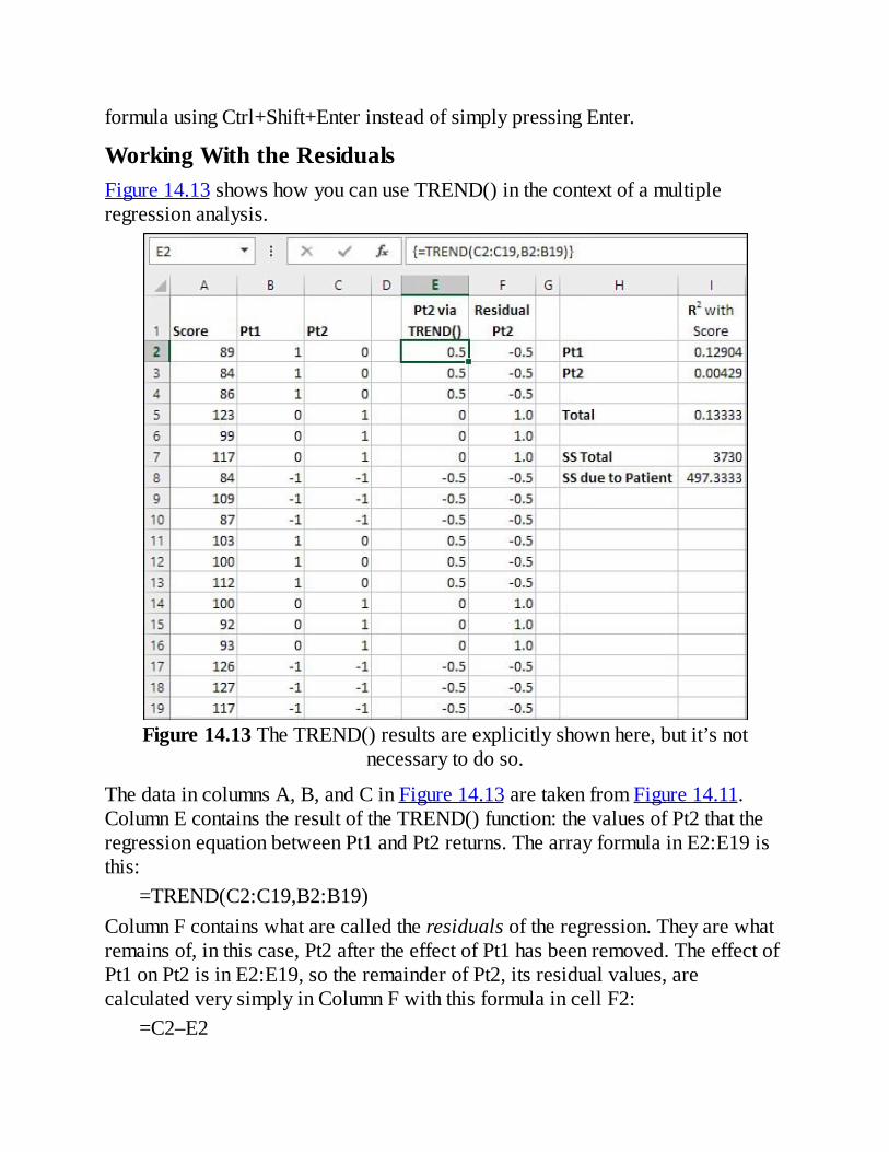
formulausingCtrl+Shift+EnterinsteadofsimplypressingEnter.

WorkingWiththeResidualsFigure14.13showshowyoucanuseTREND()inthecontextofamultipleregressionanalysis.

Figure14.13TheTREND()resultsareexplicitlyshownhere,butit’snotnecessarytodoso.

ThedataincolumnsA,B,andCinFigure14.13aretakenfromFigure14.11.ColumnEcontainstheresultoftheTREND()function:thevaluesofPt2thattheregressionequationbetweenPt1andPt2returns.ThearrayformulainE2:E19isthis:

=TREND(C2:C19,B2:B19)ColumnFcontainswhatarecalledtheresidualsoftheregression.Theyarewhatremainsof,inthiscase,Pt2aftertheeffectofPt1hasbeenremoved.TheeffectofPt1onPt2isinE2:E19,sotheremainderofPt2,itsresidualvalues,arecalculatedverysimplyinColumnFwiththisformulaincellF2:

=C2–E2

ThatformulaiscopiedandpastedintoF3:F19.NowthefinalcalculationsaremadeincolumnI.(Don’tbeconcerned.I’mdoingallthisjusttoshowhowandwhyitworks,bothfromthestandpointoftheoryandfromthestandpointofExcelworksheetfunctions.I’mabouttoshowyouhowtogetitalldonewithjustacoupleofformulas.)StartincellI2,wheretheR2betweenPt1andScoreappears.Itisobtainedwiththisformula:

=RSQ(B2:B19,A2:A19)TheRSQ()worksheetfunction(itsnameis,ofcourse,shortfor“r-squared”)isoccasionallyuseful,butit’slimitedbecauseitcandealwithonlytwovariables.We’reworkingwiththerawR2incellI2.That’sbecause,althoughTxenterstheequationfirstinFigure14.11,TxandPt1sharenovariance(seecellL18inFigure14.11).Therefore,therecanbenooverlapbetweenTxandPt1,asthereisbetweenPt1andPt2.CellI3containstheformula

=RSQ(A2:A19,F2:F19)whichreturnstheproportionofvariance,R2,inScorethat’ssharedwiththeresidualsofPt2.WehavepredictedPt2fromPt1incolumnEusingTREND().WehavecalculatedtheresidualsofPt2afterremovingwhatitshareswithPt1.NowtheR2oftheresidualswithScoretellsusthesharedvariancebetweenScoreandPt2,withtheeffectofPt1removed.Inotherwords,incellI3we’relookingatthesquaredsemipartialcorrelationbetweenScoreandPt2,withPt1partialedout.Andwehavearrivedatthatfigurewithoutresortingtoformulasofthissort,discussedinanearliersection:

(Whatwe’vedoneinFigure14.13mightnotlooklikemuchofanimprovement,butreadjustalittlefurtheron.)Tocompletethedemonstration,cellI5inFigure14.13containsthetotalofthetwoR2valuesinI2andI3.ThatisthetotalproportionofthevarianceinScoreattributabletoPt1andPt2takentogether.CellI7containsthetotalsumofsquares;compareitwithcellL5inFigure14.11.CellI8containstheproductofcellsI5andI7:theproportionofthetotalsumofsquaresattributabletothetwoPatientvectors,timesthetotalsumofsquares.Theresult,497.33,isthesumofsquaresduetothePatientfactor.Compareittocell

B14inFigure14.10:thetwovaluesareidentical.Whatwehavesucceededindoingsofaristodisaggregatethetotalsumofsquaresduetoregression(cellL3inFigure14.11)andallocatethecorrectamountofthattotaltothePatientfactor.ThesamecanbedonewiththeTreatmentfactor,andwiththeinteractionofTreatmentwithPatient.It’simportantthatyoubeabletodoso,becauseyouwanttoknowwhethertherearesignificantdifferencesintheresultsaccordingtoasubject’sTreatmentstatus,Patientstatus,orboth.Youcan’ttellthatsolelyfromtheoverallsumofsquaresduetotheregression:Youhavetobreakitoutmorefinely.Yes,theANOVAgivesyouthatbreakdownautomatically,whereasregressiondoesn’t.Butthetechniqueofregressionissomuchmoreflexibleandcanhandlesomanymoresituationsthatthebestapproachistouseregressionandbolsteritasnecessarywiththemoredetailedanalysisdescribedhere.Nextup:howtogetthatmoredetailedanalysiswithjustacoupleofformulas.

UsingExcel’sAbsoluteandRelativeAddressingtoExtendtheSemipartialsHere’showtogetthosesquaredsemipartialcorrelations—andthusthesumsofsquaresattributabletoeachmainandinteractioneffect—nearlyautomatically.Figure14.14showstheprocess.

Figure14.14Effectcodingandmultipleregressionanalysisforabalancedfactorialdesign.

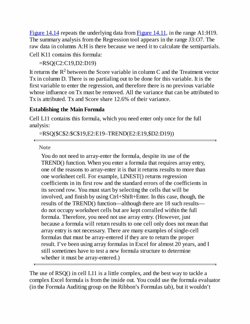
Figure14.14repeatstheunderlyingdatafromFigure14.11,intherangeA1:H19.ThesummaryanalysisfromtheRegressiontoolappearsintherangeJ3:O7.TherawdataincolumnsA:Histherebecauseweneedittocalculatethesemipartials.CellK11containsthisformula:

=RSQ(C2:C19,D2:D19)ItreturnstheR2betweentheScorevariableincolumnCandtheTreatmentvectorTxincolumnD.Thereisnopartialingouttobedoneforthisvariable.Itisthefirstvariabletoentertheregression,andthereforethereisnopreviousvariablewhoseinfluenceonTxmustberemoved.AllthevariancethatcanbeattributedtoTxisattributed.TxandScoreshare12.6%oftheirvariance.

EstablishingtheMainFormulaCellL11containsthisformula,whichyouneedenteronlyonceforthefullanalysis:

=RSQ($C$2:$C$19,E2:E19–TREND(E2:E19,$D2:D19))

NoteYoudonotneedtoarray-entertheformula,despiteitsuseoftheTREND()function.Whenyouenteraformulathatrequiresarrayentry,oneofthereasonstoarray-enteritisthatitreturnsresultstomorethanoneworksheetcell.Forexample,LINEST()returnsregressioncoefficientsinitsfirstrowandthestandarderrorsofthecoefficientsinitssecondrow.Youmuststartbyselectingthecellsthatwillbeinvolved,andfinishbyusingCtrl+Shift+Enter.Inthiscase,though,theresultsoftheTREND()function—althoughthereare18suchresults—donotoccupyworksheetcellsbutarekeptcorralledwithinthefullformula.Therefore,youneednotusearrayentry.(However,justbecauseaformulawillreturnresultstoonecellonlydoesnotmeanthatarrayentryisnotnecessary.Therearemanyexamplesofsingle-cellformulasthatmustbearray-enterediftheyaretoreturntheproperresult.I’vebeenusingarrayformulasinExcelforalmost20years,andIstillsometimeshavetotestanewformulastructuretodeterminewhetheritmustbearray-entered.)

TheuseofRSQ()incellL11isalittlecomplex,andthebestwaytotackleacomplexExcelformulaisfromtheinsideout.Youcouldusetheformulaevaluator(intheFormulaAuditinggroupontheRibbon’sFormulastab),butitwouldn’t

helpmuchinthisinstance.Takingitfromtheright,considerthisfragment:TREND(E2:E19,$D2:D19)

ThatfragmentsimplyreturnsthevaluesofPt1thatarecalculatedfromitsrelationshipwithTx.BecausethecorrelationbetweenTxandPt1is0,theresultisanarrayof0s:themeanofPt1.Youdon’tactuallyseethecalculatedvalueshere:Theystayintheformulaandoutoftheway.Backingupalittle,thefragment

E2:E19–TREND(E2:E19,$D2:D19)returnstheresiduals:thevaluesinE2:E19thatremainafteraccountingfortheirrelationshipwiththevaluesinD2:D19.Atthispoint,theresidualvaluesareequaltotheactualvaluesinE2:E19:BecausethecorrelationbetweenTxandPt1is0,theresultsoftheTREND()functionareall0s.Therefore,noadjustmentismadetoPt1valuesonthebasisoftheirrelationshiptoTxvalues.Finally,here’sthefullformulaincellL11:

=RSQ($C$2:$C$19,E2:E19–TREND(E2:E19,$D2:D19))ThisformulacalculatestheR2betweentheScorevariableincellsC2:C19andtheresidualsofthevaluesinE2:E19.It’sthesquaredsemipartialcorrelationbetweenScoreandPt1,partialingTxoutofPt1.Asyousee,thevaluereturnedbytheformulaincellL11,0.129,isidenticaltotherawsquaredcorrelationbetweenScoreandPt1(comparewithcellK18inFigure14.11).Thisisbecauseinabalanceddesignusingeffectcoding,ashere,thevectorsfordifferentmaineffectsandtheinteractionsaremutuallyindependent.TheTxvectorisindependentof,thusuncorrelatedwith,thePt1vector,thePt2vectorandalltheinteractionvectors.(However,asyou’veseen,vectorsbelongingtothesamefactorsuchasPt1andPt2arecorrelated.)Whentwovectorsareuncorrelated,there’snothingineitheronetoremoveofitscorrelationwiththeother.Sointheory,theformulaincellL11couldhavebeen

=RSQ(C2:C19,E2:E19)becauseitreturnsthesamevalueasthesemipartialcorrelationdoes.Butforpracticalreasonsit’sbettertoentertheformulaasgiven,forreasonsyou’llseenext.

ExtendingtheFormulaAutomaticallyIfyouselectcellL11asit’sshowninFigure14.14,clickandholdtheselectionhandle,anddragtotherightintocellO11,themixedandrelativeaddressesadjust

andthefixedreferenceremainsfixed.

NoteTheselectionhandleistheblacksquareinthelower-rightcorneroftheactivecell.

Whenyoudoso,theformulainL11becomesthisformulainM11:=RSQ($C$2:$C$19,F2:F19–TREND(F2:F19,$D2:E19))

TheR2valuereturnedbythisformulaisnowbetweenScoreinC2:C19andPt2inF2:F19—butwiththeeffectsofTxandPt1partialedoutofPt2.IncopyingandpastingtheformulafromL11toM11,thereferencesadjusted(orfailedtodoso)inafewways,asdetailednext.

TheAbsoluteReferenceThereferenceto$C$2:$C$19,whereScoreisfound,didnotadjust.Itisanabsolutereference,andpastingthereferencetoanothercell,M11,hasnoeffectonit.Theabsolutereferencetotheoutcomemeasure,Score,isneededbyalltheformulas,soastocalculateitssquaredsemipartialcorrelationwitheachcodedvector.

TheRelativeReferencesThereferencestoE2:E19inL11becomeF2:F19inM11.Thereferencesarerelativeandadjustaccordingtothelocationyoupastethemto.BecauseM11isonecolumntotherightofL11,thereferenceschangefromcolumnEtocolumnF.Insodoing,theformulaturnsitsattentionfromPt1incolumnEtoPt2incolumnF.

TheMixedReferenceThereferenceto$D2:D19inL11becomes$D2:E19inM11.Itisamixedreference:thefirstcolumn,theDin$D2,isfixedbymeansofthedollarsign.Thesecondcolumn,theDinD19,isrelativebecauseit’snotimmediatelyprecededbyadollarsign.SowhentheformulaispastedfromcolumnLtocolumnM,$D2:D19becomes$D2:E19.ThathastheeffectofpredictingPt2(columnF)frombothTx(columnD)andPt1(columnE).Thisisexactlywhatwe’reafter.Eachtimewepastetheformulaonecolumntotheright,weshifttoanewpredictorvariable.Furthermore,weextendtherangeofthepredictorvariablesthatwewanttopartialoutofthenewpredictor.InthedownloadedcopyoftheworkbookforChapter14,you’llfindthatbyextendingtheformulaouttocolumnO,theformulaincellO11is

=RSQ($C$2:$C$19,H2:H19–TREND(H2:H19,$D2:G19))andisextendedallthewayouttocapturethefinalinteractionvectorincolumnH.ThissectionofChapter14developedarelativelystraightforwardwaytocalculatesharedvariancewiththeeffectofothervariablesremoved,bymeansoftheTREND()functionandresidualvalues.Wecannowapplythatmethodtodesignsthathaveunequaln’s.Asyou’llsee,unequaln’ssometimesbringaboutunwantedcorrelationsbetweenfactors,andsometimesaretheresultofexistingcorrelations.Ineithercase,regressionanalysisofthesortintroducedinthischaptercanhelpyoumanagethecorrelationsand,inturn,makethepartitionofthevariabilityintheoutcomemeasureunambiguous.Thenextchaptertakesupthattopic.

15.MultipleRegressionAnalysisandEffectCoding:FurtherIssues

InThisChapterSolvingUnbalancedFactorialDesignsUsingMultipleRegressionExperimentalDesigns,ObservationalStudies,andCorrelationUsingAlltheLINEST()StatisticsManagingUnequalGroupSizesinaTrueExperimentManagingUnequalGroupSizesinObservationalResearch

Chapter14,“MultipleRegressionAnalysisandEffectCoding:TheBasics,”discussestheconceptofusingmultipleregressionanalysistoaddressthequestionofwhethergroupmeansdiffermorethancanreasonablybeexplainedbychance.Thebasicideaistocodenominalvariablessuchastypeofmedicationadministered,orsex,orethnicity,soastorepresentthemasnumericvariables.Codedinthatway,nominalvariablescanbeusedasinputtomultipleregressionanalysis.Youcancalculatecorrelationsbetweenpredictorvariablesandthepredictedvariable—and,what’sequallyimportant,betweenthepredictorvariablesthemselves.Fromthereit’sashortsteptotestingwhetherchanceisareasonableexplanationforthedifferencesyouobserveinthepredictedvariable.Thischapterexploressomeoftheissuesthatarisewhenyougobeyondthebasicsofusingmultipleregressiontoanalyzevariance.Inparticular,it’salmostinevitableforyoutoencounterunbalancedfactorialdesigns—thosewithunequalnumbersofobservationsperdesigncell.Finally,thischapterdiscusseshowbesttousetheworksheetfunctions,suchasLINEST()andTREND(),thatunderlietheDataAnalysisadd-in’smorestaticRegressiontool.

SolvingUnbalancedFactorialDesignsUsingMultipleRegressionAnunbalanceddesigncancomeaboutforavarietyofreasons,andit’susefultoclassifythereasonsaccordingtowhethertheimbalanceiscausedbythefactorsthatyou’restudyingorthepopulationfromwhichyou’vesampled.Thatdistinctionisusefulbecauseithelpspointyoutowardthebestwaytosolvetheproblemsthattheimbalanceinthedesignpresents.Thischapterhasmoretosayaboutthatinalatersection.First,let’slookattheresultsoftheimbalance.

Figure15.1repeatsadatasetthatalsoappearsinFigures14.10and14.11.

Figure15.1Thisdesignisbalanced:Ithasanequalnumberofobservationsineachgroup.

InFigure15.1,thedataispresentedasabalancedfactorialdesign;thatis,twoormorefactorswithanequalnumberofobservationspercell.Forthepurposesofthisexample,inFigure15.2oneobservationhasbeenmovedfromonegrouptoanother.TheobservationthathasaScoreof93andisshowninFigure15.1inthegroupdefinedbyaSurgicaltreatmentonanOutpatientbasishasinFigure15.2beenmovedtotheShortStaypatientbasis.

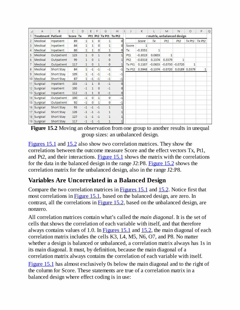
Figure15.2Movinganobservationfromonegrouptoanotherresultsinunequalgroupsizes:anunbalanceddesign.

Figures15.1and15.2alsoshowtwocorrelationmatrices.TheyshowthecorrelationsbetweentheoutcomemeasureScoreandtheeffectvectorsTx,Pt1,andPt2,andtheirinteractions.Figure15.1showsthematrixwiththecorrelationsforthedatainthebalanceddesignintherangeJ2:P8.Figure15.2showsthecorrelationmatrixfortheunbalanceddesign,alsointherangeJ2:P8.

VariablesAreUncorrelatedinaBalancedDesignComparethetwocorrelationmatricesinFigures15.1and15.2.NoticefirstthatmostcorrelationsinFigure15.1,basedonthebalanceddesign,arezero.Incontrast,allthecorrelationsinFigure15.2,basedontheunbalanceddesign,arenonzero.Allcorrelationmatricescontainwhat’scalledthemaindiagonal.Itisthesetofcellsthatshowsthecorrelationofeachvariablewithitself,andthatthereforealwayscontainsvaluesof1.0.InFigures15.1and15.2,themaindiagonalofeachcorrelationmatrixincludesthecellsK3,L4,M5,N6,O7,andP8.Nomatterwhetheradesignisbalancedorunbalanced,acorrelationmatrixalwayshas1sinitsmaindiagonal.Itmust,bydefinition,becausethemaindiagonalofacorrelationmatrixalwayscontainsthecorrelationofeachvariablewithitself.Figure15.1hasalmostexclusively0sbelowthemaindiagonalandtotherightofthecolumnforScore.Thesestatementsaretrueofacorrelationmatrixinabalanceddesignwhereeffectcodingisinuse:

Thecorrelationsbetweenthemaineffectsarezero.SeecellsL5andL6inFigure15.1.Thecorrelationsbetweenthemaineffectsandtheinteractionsarezero.SeecellsL7:N8inFigure15.1.Amaineffectthatrequirestwoormorevectorshasnonzerocorrelationsbetweenitsvectors.Thisisalsotrueofunbalanceddesigns.SeecellM6inFigures15.1and15.2.(RecallfromChapter14thatamaineffecthasasmanyvectorsasithasdegreesoffreedom.Usingeffectcoding,afactorthathastwolevelsneedsjustonevectortodefineeachobservation’slevel,andafactorthathasthreelevelsneedstwovectorstodefineeachobservation’slevel.)Interactionvectorsthatinvolvethesamefactorshavenonzerocorrelations.Thisisalsotrueofunbalanceddesigns.SeecellO8inFigures15.1and15.2.

ThosecorrelationsofzeroinFigure15.1areveryuseful.Whentwovariablesareuncorrelated,itmeansthattheysharenovariance.InFigure15.1,TreatmentandPatientStatusareuncorrelated;youcantellthatfromthefactthattheTxvector(representingTreatment,whichhastwolevels)hasazerocorrelationwithboththePt1andthePt2vectors(representingPatientStatus,whichhasthreelevels).Therefore,whatevervariancethatTreatmentshareswithScoreisuniquetoTreatmentandScore,andisnotsharedwiththePatientStatusvariable.ThereisnoambiguityabouthowthevarianceinScoreistobeallocatedacrossthepredictorvariables,TreatmentandPatientStatus.Thisisthereasonthat,withabalanceddesign,youcanaddupthesumofsquaresforallthefactorsandtheirinteractions,addthewithingroupvariance,andarriveatthetotalsumofsquares.There’snoambiguityabouthowthevarianceoftheoutcomevariablegetsdividedup,andthetotalofthesumsofsquaresequalstheoverallsumofsquareddeviationsofeachobservationfromthegrandmean.

VariablesAreCorrelatedinanUnbalancedDesignButifthedesignisunbalanced,ifnotalldesigncellscontainthesamenumberofobservations,thentherewillbecorrelationsbetweenthevectorsthatwouldotherwisebeuncorrelated.InFigure15.2,youcanseethatTxiscorrelatedat0.0655and0.1374withPt1andPt2,respectively(cellsL5:L6).ComparewithFigure15.1,wherethesamevectorshavecorrelationsof0.0becausethedesigncellshavethesamenumbersofobservations.ButinFigure15.2,becauseTreatmenthasanonzerocorrelationwithPatientStatus,Treatmentsharesvariance

withPatientStatus.(Moreprecisely,becausetheTx,Pt1,andPt2vectorsarenowcorrelatedwithoneanother,theyhavevarianceincommon.)Inturn,thevariancethatTreatmentshareswithScorecan’tbesolelyattributedtoTreatment.Thethreemaineffectpredictorvectorsarecorrelated,andthereforesharesomeoftheirvariance,andthereforehavesomevariancejointlyincommonwithScore.Thesameistruefortheotherpredictorvariables.MerelyshiftingoneobservationfromthePatientStatusofOutpatienttoShortStaycausesallthecorrelationsthathadpreviouslybeenzerotobenonzero.Therefore,theynowhavevarianceincommon.Anyofthatcommonvariancemightalsobesharedwiththeoutcomevariable,andwe’redealingonceagainwithambiguity:HowdowetellhowtodividethevarianceintheoutcomevariablebetweenTreatmentandPatientStatus?BetweenTreatmentandtheTreatmentbyPatientStatusinteraction?Thetaskofallocatingsomeproportionofvariancetoonepredictorvariable,andsometootherpredictorvariables,dependslargelyonthedesignoftheresearchthatgatheredthedata.Therearewaystocompletethattask,andwe’recomingtothemshortly.First,let’sreturntothenice,clean,unambiguousbalanceddesigntopointoutarelatedreasonthatequalgroupsizesarehelpful.

OrderofEntryIsIrrelevantintheBalancedDesignFigures15.3and15.4continuetheanalysisofthebalanceddatasetinFigure15.1.Figures15.3and15.4looksomewhatcomplex,buttherearereallyonlyacoupleofcrucialpointstotakeawayfromthem.

Figure15.3Inthisanalysis,TreatmententerstheregressionequationbeforePatientStatus.

Figure15.4PatientStatusenterstheregressionequationfirstinthisanalysis.

Inbothfigures,therangeJ1:O21containsaregressionanalysisandatraditionalanalysisofvarianceforthedataintherangeC2:H19.Therearethreeobservationsineachcell,sothedesignisbalanced.Alsoinbothfigures,cellsJ3:O7containthepartialresultsofusingtheDataAnalysisadd-in’sRegressiontool.Asdiscussedearlierinthischapter,thecorrelationsbetweenmaineffectsvectorsinabalanceddesignarezero.Buttherearenonzerocorrelationsbetweenvectorsthatrepresentthesamefactor:Inthiscase,thereisanonzerocorrelationbetweenvectorPt1andvectorPt2forthePatientStatusfactor.SquaredsemipartialcorrelationsinL11:O11ofFigures15.3and15.4removefromeachvectorasitenterstheanalysisanyvariancethatitshareswithvectorsthathavealreadyentered.Therefore,thesumsofsquaresattributedtoeachfactorandtheinteraction(cellsK12,M12,andO12inFigure15.3andcellsL12,M12andO12inFigure15.4)areuniqueandunambiguous.TheyareidenticaltothesumsofsquaresreportedinthetraditionalanalysisofvarianceshowninJ14:O21inFigures15.3and15.4.Now,comparetheproportionsofvarianceshownincellsK11:O11ofFigure15.3withthesamecellsinFigure15.4.

NoticethatinFigures15.3and15.4thepredictorvariablesappearindifferentordersintheanalysisshownincellsJ9:O12.InFigure15.3,TreatmententerstheregressionequationfirstviaitsTxvector.TheTreatmentvariableshares0.126ofitsvariancewiththeScoreoutcome.BecauseTreatmententerstheequationfirst,allofthevarianceitshareswithScoreisattributedtoTreatment.Noonemadeadecisiontogivethevariablethat’senteredfirstallitsavailablevariance:whenVariableXisthefirsttoentertheequation,there’snovariablethatenteredearlierwithwhichVariableXcansharevariance.Youdon’thavetolivewiththat,though.YoumightwanttoadjustTreatmentforPatientStatusevenifTreatmententerstheequationfirst.Alatersectioninthischapter,“ManagingUnequalGroupSizesinaTrueExperiment,”dealswiththatpossibility.Next,andstillinFigure15.3,thetwoPatientStatusvectors,Pt1andPt2,entertheregressionequation,inthatorder.Theyaccount,respectively,for0.129and0.004ofthevarianceinScore.ThevariablesPt1andPt2arecorrelated,andthevarianceattributedtoPt2isreducedaccordingtotheamountofvariancealreadyattributedtoPt1.(Seethesectiontitled“UsingTREND()toReplaceSquaredSemipartialCorrelations”inChapter14foradiscussionofthatreductionusingthesquaredsemipartialcorrelation.)ComparethoseproportionsforPatientStatus,0.129and0.004,inFigure15.3withtheonesshowninFigure15.4,cellsK11:L11.InFigure15.4,itisPatientStatus,notTreatment,thatenterstheequationfirst.AllthevariancethatPt1shareswithScoreisattributedtoPt1.ItisidenticaltotheproportionofvarianceshowninFigure15.3,becausePt1andTreatmentareuncorrelated:Thesamplesizeisthesameineachgroup.Therefore,thereisnoambiguityinhowthevarianceinScoreisallocated,anditmakesnodifferencewhetherTreatmentorPatientStatusenterstheequationfirst.Whentwopredictorvariablesareuncorrelated,thevariancethateachshareswiththeoutcomevariableisuniquetoeachpredictorvariable.It’salsoagoodideatonoticethattheregressionanalysisincellsJ3:O7andthetraditionalANOVAsummaryincellsJ14:O21returnthesameaggregateresults.Inparticular,thesumofsquares,degreesoffreedom,andthemeansquarefortheregressionincellsK5:M5arethesameastheparallelvaluesincellsK19:M19.ThesameistruefortheresidualvariationinK6:M6andK20:M20(labeledWithininthetraditionalANOVAsummary).TheonlymeaningfuldifferencebetweentheANOVAtablethataccompaniesastandardregressionanalysisandastandardANOVAsummarytableisthattheregressionanalysisusuallylumpsalltheresultsforthepredictorsintoonelinelabeledRegression.AlittleadditionalworkofthesortdescribedinChapter14andinthischapterisoftenneededinordertoallocatethevariancetothe

individualfactorsproperly.Butthefindingsarethesameintheaggregate.TotalupthesumsofsquaresforTreatment,Patient,andtheirinteractioninK16:K18,andyougetthesametotalasisshownfortheRegressionsumofsquaresinL5.Thenextsectiondiscusseshowtheseresultsdifferwhenyou’reworkingwithanunbalanceddesign.

OrderEntryIsImportantintheUnbalancedDesignForcontrast,considerFigures15.5and15.6.TheiranalysesarethesameasinFigures15.3and15.4,exceptthatFigures15.5and15.6arebasedontheunbalanceddesignshowninFigure15.2.(Figures15.3and15.4arebasedonthebalanceddesignshowninFigure15.1.)

Figure15.5TheTreatmentvariableenterstheequationfirstandsharesthesamevariancewithScoreasinFigures15.3and15.4.

Figure15.6TheproportionsofvarianceforalleffectsaredifferentherethaninFigures15.3through15.5.

ThedatasetusedinFigures15.5and15.6isnolongerbalanced.ItisthesameastheoneshowninFigure15.2,whereoneobservationhasbeenmovedfromthePatientStatusofOutpatienttoShortStay.Asdiscussedearlierinthischapter,thatonemovecausesthecorrelationsofScorewithPatientStatusandwiththeinteractionvariablestochangefromtheirvaluesinthecaseofthebalanceddesign(Figure15.1).Italsochangesthecorrelationsbetweenalltheeffectvectors,whichcausesthemtosharevariance:thecorrelationsarenolongerzero.TheonecorrelationthatdoesnotchangebetweenthebalancedandtheunbalanceddesignsisthatofTreatmentandScore.TheproportionofvarianceinScorethat’sattributedtoTreatmentis0.126inFigure15.3(cellK11),whereTxisenteredfirst,andinFigure15.4(cellM11),whereTxisenteredthird.TworeasonscombinetoensurethatthecorrelationbetweenTreatmentandScoreremainsat–0.3551,andthesharedvarianceat0.126,evenwhenthebalanceddesignismadeunbalanced:

MovingonesubjectfromOutpatienttoShortStaychangesneitherthatsubject’sScorevaluenortheTreatmentvalue.Becauseneithervariablechangesitsvalue,thecorrelationremainsthesame.InFigure15.5,whereTreatmentisstillenteredintotheregressionequationfirst,theproportionofsharedvarianceisstill0.126.Althoughthereisnow

acorrelationbetweenTreatmentandPatientStatus(cellsL5andL6inFigure15.2),TreatmentlosesnoneofthevarianceitshareswithPatientStatus.Becauseit’senteredfirst,itkeepsallthesharedvariancethat’savailabletoit.

Figure15.6showswhathappenswhenPatientStatusenterstheequationbeforeTreatmentintheunbalanceddesign.Inthebalanceddesign,thevectorPt1correlatesat–0.3592withScore(seeFigure15.1,cellK5).Intheunbalanceddesign,onevalueinPt1changeswiththemoveofonesubjectfromOutpatienttoShortStay,sothecorrelationbetweenPt1andScorechanges(asdoesthecorrelationbetweenPt2andScore).InFigures15.1and15.2,youcanseethatthecorrelationbetweenPt1andScorechangesfrom–0.3592to–0.3019asthedesignbecomesunbalanced.Thesquareofthecorrelationistheproportionofvariancesharedbythetwovariables,andthesquareof–0.3019is0.0911.However,intheunbalanceddesignanalysisinFigure15.5,theproportionofvarianceshownassharedbyScoreandPt1is0.078(seecellL11).ThedifferenceoccursbecauseTxandPt1themselvessharesomevariance,and,becauseTreatmentisalreadyintheequation,ithaslaidclaimtoallthevarianceitshareswithScore.Therefore,whenPt1enterstheequation,theproportionofvarianceitshareswithScorefallsfrom.0911to.078.ButinFigure15.6,wherePt1enterstheequationfirst,thePt1vectoraccountsfor0.091ofthevarianceoftheScoreoutcomevariable(seecellK11).Therearetwopointstonoticeaboutthatvalue:

Itisthesquareofthecorrelationbetweenthetwovariables,–0.3019.ItisnotequaltotheproportionofvarianceallocatedtoPt1whenPt1enterstheequationafterTx,asitdoesinFigure15.5.

WithPt1asthevectorthatenterstheregressionequationfirst,itclaimsallthevariancethatitshareswiththeoutcomevariable,Score,andthat’sthesquareofthecorrelationbetweenPt1andScore.BecausePt1inthiscase—enteringtheequationfirst—cedesnoneofitssharedvariancetoTreatment,Pt1getsadifferentproportionofthevarianceofScorethanitdoeswhenitenterstheequationafterTreatment.

AboutFluctuatingProportionsofVarianceIntuitively,youmightthinkthatinanunbalanceddesign,wherecorrelationsbetweenthepredictorvariablesarenonzero,movingavariableupintheorderofentrywouldincreasetheamountofvarianceintheoutcomevariablethat’s

allocatedtothepredictor.Forexample,inFigures15.5and15.6,thePt1vectorisallocated0.078ofthevarianceinScorewhenit’senteredaftertheTxvector,but0.091oftheScorevariancewhenit’senteredfirst.Andthingsoftenturnoutthatway,butnotnecessarily.LookingagainatFigures15.5and15.6,noticethattheTxvectorisallocated0.126ofthevarianceinScorewhenit’senteredfirst,but0.129ofthevariancewhenit’senteredthird.So,althoughsomeofthevariancethatitshareswithScoreisallocatedtoPt1andPt2inFigure15.6,Txstillsharesalargerproportionofvariancewhenitisenteredthirdthanwhenitisenteredfirst.There’snogeneralruleaboutit.Astheorderofentryischanged,theamountanddirectionthatsharedvariancefluctuatesdependsonthemagnitudeandthedirectionofthecorrelationsbetweenthevariablesinvolved.Fromanempiricalviewpoint,that’swellandgood.Youwantthenumberstodeterminetheconclusionsthatyoudraw,evenifthewaytheybehaveseemscounterintuitive.Thingsareevenbetterwhenyouhaveequalgroupsizes.Then,asI’vepointedoutseveraltimes,thecorrelationsbetweenthevectorsthatrepresentdifferentfactorsarezero,thereisnosharedvariancebetweenthefactorstoworryabout,andyougetthenice,cleanresultsinFigures15.3and15.4,wheretheorderofentrymakesnodifferenceintheallocationofvariancetothefactors.(ComparecellsK11:M11inFigure15.3withthesamerangeinFigure15.4.)Butit’sworrisomewhengroupsizesareunequalandthedesignisunbalanced.Then,vectorsthatareuncorrelatedinthecaseofequalgroupsizesbecomecorrelated.It’sworrisomebecauseyoudon’twanttoinsertyourselfintothemix.SupposeyoudecidetoforcePatientStatusintotheregressionequationbeforeTreatment,andthatdoingsoincreasestheproportionofvarianceattributedtoPatientStatus.Itmightthencomeaboutthatdifferencesbetween,say,InpatientandOutpatientmeetyourcriterionforalpha.Youdon’twantwhatispossiblyanarbitrarydecisiononyourpart(tomovePatientStatusup)toaffectyourdecisiontotreatthedifferencebetweenInpatientandOutpatientasrealratherthantheresultofsamplingerror.Youcanadoptsomerulesthathelpmakeyourdecisionlessarbitrary.Todiscussthoserulessensibly,it’snecessaryfirsttodiscusstherelationshipbetweenpredictorcorrelationsandgroupsizesfromadifferentviewpoint.

ExperimentalDesigns,ObservationalStudies,andCorrelationChapter4,“HowVariablesMoveJointly:Correlation,”discussestheproblemsthatarisewhenyoutrytoinferthatcausationispresentwhenallthat’sreally

goingoniscorrelation.Oneofthoseproblemsistheissueofdirectionality:Doesaperson’sattitudetowardagivensocialissuecausehimorhertoidentifywithaparticularpoliticalparty?Ordoesanexistingpartyaffiliationcausetheattitudetobeadopted?Theproblemofgroupsizesandcorrelationsbetweenvectorsisacaseinwhichcausalitymaywellbepresent,butifsoitsdirectionisn’tnecessarilyclear.Supposeyou’reconductinganexperiment—atrueexperiment,oneinwhichyouhaveselectedparticipantsrandomlyfromthepopulationyou’reinterestedinandhaveassignedthematrandomtoequallysizedgroups.Youthensubjectthegroupstooneormoretreatments,perhapswithdouble-blindingsothatneitherthesubjectsnorthoseadministeringthetreatmentsknowwhichtreatmentisinuse.Thisistrueexperimentalwork,theso-calledgoldstandardofresearch.Butduringthemonth-longcourseoftheexperiment,unplannedeventsoccur.Slippingpastyourrandomselectionandassignment,abrotherandsisternotonlytakepartbutarealsoassignedtothesametreatment,invalidatingtheassumptionofindependenceofobservations.Anassistantinadvertentlyadministersthewrongmedicationtoonesubject,convertinghimfromonetreatmenttoanother.Threepeoplehavesuchbadreactionstotheirtreatmentthattheyquit.Equipmentfails.Andsoon.Theresultofthisattritionisthatwhatstartedoutasabalancedfactorialdesignisnowanunbalanceddesign.Ifyou’retestingonlyonefactor,thenfromtheviewpointofstatisticalanalysisit’snotacauseforgreatconcern.AsnotedinChapter10,“TestingDifferencesBetweenMeans:TheAnalysisofVariance,”youmayhavetotakenoteoftheBehrens-Fisherproblem,butifthegroupvariancesareequivalent,there’snoseriouscauseforworryaboutthestatisticalanalysis.Ifyouhavemorethanonefactor,though,youhavetodealwiththeproblemofpredictorvectorsandtheallocationofvariancethatthischapterhasdiscussed,becauseambiguityinhowtoapportionthevarianceentersthepicture.Onepossiblemethodistorandomlydropsomesubjectsfromtheexperimentuntilyourgroupsizesareonceagainequal.That’snotalwaysafeasiblesolution,though.Ifthesubjectattritionhasbeengreatenoughandisconcentratedinoneortwogroups,youmightfindyourselfhavingtothrowawayathirdofyourobservationstoachieveequalgroupsizes.Furthermore,thesituationI’vejustdescribedresultsinunequalgroupsizesforreasonsthatareduetothefactoftheexperimentandhowitiscarriedout.Therearewaystodealwiththeunequalgroupsizesmathematically.OneisdiscussedinChapter14,whichdemonstratestheuseofsquaredsemipartialcorrelationsto

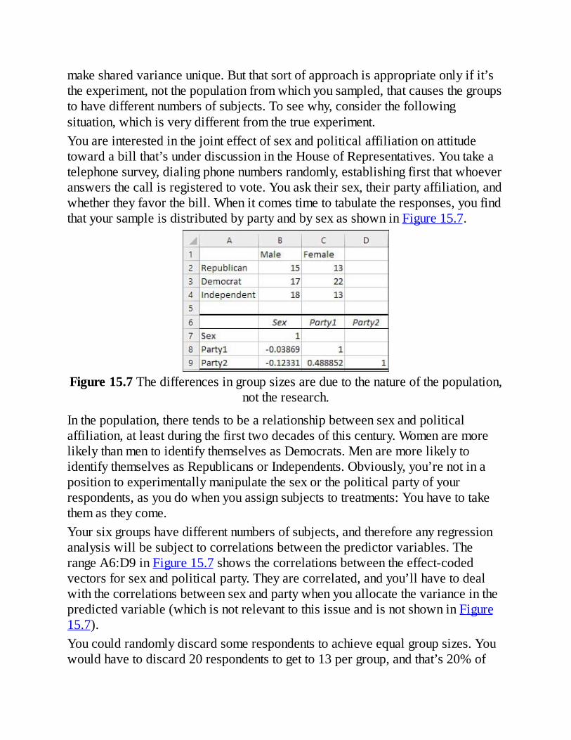
makesharedvarianceunique.Butthatsortofapproachisappropriateonlyifit’stheexperiment,notthepopulationfromwhichyousampled,thatcausesthegroupstohavedifferentnumbersofsubjects.Toseewhy,considerthefollowingsituation,whichisverydifferentfromthetrueexperiment.Youareinterestedinthejointeffectofsexandpoliticalaffiliationonattitudetowardabillthat’sunderdiscussionintheHouseofRepresentatives.Youtakeatelephonesurvey,dialingphonenumbersrandomly,establishingfirstthatwhoeveranswersthecallisregisteredtovote.Youasktheirsex,theirpartyaffiliation,andwhethertheyfavorthebill.Whenitcomestimetotabulatetheresponses,youfindthatyoursampleisdistributedbypartyandbysexasshowninFigure15.7.

Figure15.7Thedifferencesingroupsizesareduetothenatureofthepopulation,nottheresearch.

Inthepopulation,theretendstobearelationshipbetweensexandpoliticalaffiliation,atleastduringthefirsttwodecadesofthiscentury.WomenaremorelikelythanmentoidentifythemselvesasDemocrats.MenaremorelikelytoidentifythemselvesasRepublicansorIndependents.Obviously,you’renotinapositiontoexperimentallymanipulatethesexorthepoliticalpartyofyourrespondents,asyoudowhenyouassignsubjectstotreatments:Youhavetotakethemastheycome.Yoursixgroupshavedifferentnumbersofsubjects,andthereforeanyregressionanalysiswillbesubjecttocorrelationsbetweenthepredictorvariables.TherangeA6:D9inFigure15.7showsthecorrelationsbetweentheeffect-codedvectorsforsexandpoliticalparty.Theyarecorrelated,andyou’llhavetodealwiththecorrelationsbetweensexandpartywhenyouallocatethevarianceinthepredictedvariable(whichisnotrelevanttothisissueandisnotshowninFigure15.7).Youcouldrandomlydiscardsomerespondentstoachieveequalgroupsizes.Youwouldhavetodiscard20respondentstogetto13pergroup,andthat’s20%of

yoursample—quiteabit.Butmoreseriousisthefactthatindoingsoyouwouldbeactingasthoughtherewerenorelationshipbetweensexandpoliticalaffiliationinthepopulation.That’smanipulatingsubstantiverealitytoachieveastatisticalsolution,andthat’sthewrongthingtodo.Let’sreviewthetwosituations:

Atrueexperimentinwhichthelossofsomesubjectsand,inconsequence,unequalgroupsizesareattributabletoaspectsofthetreatments.Correlationsamongpredictorscomeaboutbecausethenatureoftheexperimentinducesunequalgroupsizes.Anobservationalstudyinwhichthewaysthepopulationclassifiesitselfresultsinunequalgroupsizes.Thoseunequalgroupsizescomeaboutbecausethevariablesarecorrelated.

Socausationispresenthere,butitsdirectiondependsonthesituation.Inthefirstcase,youwouldnotbealteringrealitytoomitafewsubjectstoachieveequalgroupsizes.ButyoucoulddoequallywellwithoutdiscardingdatabyusingthetechniqueofsquaredsemipartialcorrelationsdiscussedinthischapterandinChapter14.Byforcingeachvariabletocontributeuniquevariance,youcandealwithunequalgroupsizesinawaythat’sunavailabletoyouifyouusetraditionalanalysisofvariancetechniques.Inthissortofsituation,it’susualtoobservetheuniquevariancewhileswitchingtheorderofentryintotheregressionequation.Anexamplefollowsshortly.Inthesecondcase,theobservationalstudyinwhichcorrelationsinthepopulationcauseunequalgroupsizes,it’sunwisetodiscardobservationsinpursuitofequalgroupsizes.However,youstillwanttoeliminatetheambiguitythat’scausedbytheresultingcorrelationsamongthepredictors.Variousapproacheshavebeenproposedandused,withvaryingdegreesofsuccessandofsense.

NoteApproachessuchasforwardinclusion,backwardelimination,andstepwiseregressionareavailable,andmaybeappropriatetoasituationthatyouareconfrontedwith.Eachoftheseapproachesconcernsitselfwithrepeatedlychangingtheorderinwhichvariablesareenteredinto,andremovedfrom,theregressionequation.Statisticaldecisionrules,usuallyinvolvingthemaximizationofR2,areusedtoarriveatasolution.IntheExcelcontext,theuseofthesemethodsinevitablyrequiresVBAtomanagetherepetitiveprocess.BecausethisbookavoidstheuseofVBAasmuchaspossible—it’snotabookabout

programming—Isuggestthatyouconsultaspecializedstatisticsapplicationifyouthinkoneofthoseapproachesmightbeappropriate.

OneapproachthatdeservesseriousconsiderationinanobservationalstudywithunequalgroupsizesiswhatKerlingerandPedhazurtermtheaprioriorderingapproach(refertoMultipleRegressioninBehavioralResearch,1973).Youconsiderthenatureofthepredictorvariablesthatyouhaveunderstudyanddetermineifoneofthemislikelytohavecausedtheother,oratleastprecededtheother.Inthatcase,theremaybeastrongargumentforfollowingthatorderinconstructingtheregressionequation.Inthesex-and-politicsexample,itispossiblethataperson’ssexmightexertsomeinfluence,howeverslight,onhisorherchoiceofpoliticalaffiliation.Butourpoliticalaffiliationdoesnotdetermineoursex.Sothere’sagoodargumentinthiscaseforforcingthesexvectortoentertheregressionequationbeforetheaffiliationvectors.Youcandothatsimplybytheleft-to-rightorderinwhichyouputthevariablesontheExcelworksheet.BoththeRegressiontoolintheDataAnalysisadd-inandtheworksheetfunctionsconcernedwithregression,suchasLINEST()andTREND(),entertheleftmostpredictorvectorfirst,thentheoneimmediatelytoitsright,andsoon.Beforediscussinghowtodothatit’simportanttotakeacloserlookattheinformationthattheLINEST()worksheetfunctionmakesavailabletoyou.

UsingAlltheLINEST()StatisticsIhavereferredtotheworksheetfunctionLINEST()inthisandpreviouschapters,butthosedescriptionshavebeensketchy.We’reatthepointthatyouneedamuchfullerdiscussionofwhatLINEST()candoforyou.Figure15.8showstheLINEST()worksheetfunctionactingonthedatasetmostrecentlyshowninFigure15.6,intherangeC1:H19.ThedatasetisrepeatedontheworksheetinFigure15.8.

Figure15.8LINEST()alwaysreturns#N/Aerrorvaluesbelowitssecondrowandtotherightofitssecondcolumn.

Youcanobtaintheregressioncoefficientsonly,ifthat’sallyou’reafter,byselectingarangeconsistingofonerowandasmanycolumnsastherearecolumnsinyourinputdata.Thentypeaformulasuchasthisone:

=LINEST(A2:A20,B2:E20)Finally,array-entertheformulabythekeyboardcombinationCtrl+Shift+EnterinsteadofsimplyEnter.Ifyouwantalltheavailableresults,youmustselectarangewithfiverows,notjustone,andyoualsoneedtosetaLINEST()argumenttoTRUE.ThathasbeendoneinFigure15.8,wheretheformulaisasfollows:

=LINEST(C2:C19,D2:H19,,TRUE)Themeaningsofthethirdargument(whichisnotusedhere)andthefourthargumentarediscussedlaterinthissection.

UsingtheRegressionCoefficientsLet’stakeacloserlookatwhat’sinJ3:O7inFigure15.8,theanalysisofthemaineffectsTreatmentandPatientStatus,andtheirinteraction.Chapter4discussesthedatainthefirsttworowsoftheLINEST()results,buttoreview,thefirstrowcontainsthecoefficientsfortheregressionequation,andthesecondrowcontainsthestandarderrorsofthecoefficients.

LINEST()’smostglaringdrawbackisthatitreturnsthecoefficientsinthereverseorderthatthepredictorvariablesexistontheworksheet.IntheworksheetshowninFigure15.8,columnDcontainsthefirstPatientStatusvector,Pt1;columnEcontainsthesecondPatientStatusvector,Pt2;andcolumnFcontainstheonlyTreatmentvector,Tx.ColumnsGandHcontainthevectorsthatrepresenttheinteractionbetweenPatientStatusandTreatmentbyobtainingthecross-productsofthethreemaineffectsvectors.So,readinglefttoright,theunderlyingdatashowsthetwoPatientStatusvectors,theTreatmentvector,andthetwointeractionvectors.However,theLINEST()resultsreversethisorder.TheregressioncoefficientforPT1isincellN3,forPt2inM3,andTxinL3.K3containsthecoefficientforthefirstinteractionvector,andJ3forthesecondinteractionvector.TheinterceptisalwaysintherightmostcolumnoftheLINEST()results(assumingthatyoubeganbyselectingthepropernumberofcolumnstocontaintheresults).YoumakeuseoftheregressioncoefficientsincombinationwiththevaluesonthepredictorstoobtainapredictedvalueforScore.Forexample,usingtheregressionequationbasedonthecoefficientsinJ3:O3,youcouldpredictthevalueofScoreforthesubjectinrow2withthisequation(O3istheinterceptandisfollowedbytheproductofeachpredictorvaluewithitscoefficient):

=O3+N3*D2+M3*E2+L3*F2+K3*G2+J3*H2Giventhelengthoftheformula,plusthefactthatthepredictorvaluesrunlefttorightwhiletheircoefficientsrunrighttoleft,youcanseewhyTREND()isagoodalternativeifyou’reaftertheresultsofapplyingtheregressionequation.TREND()handlesthemultiplicationsandadditionsonyourbehalf,soyoudon’thavetoworryaboutmatchingtheproperpredictorvariablewiththepropercoefficient.Igomoredeeplyintothematterlaterinthischapter,inthesectiontitled,“HowLINEST()CalculatesItsResults.”

UsingtheStandardErrorsThesecondrowoftheLINEST()resultscontainsthestandarderrorsoftheregressioncoefficients.Theyareusefulbecausetheytellyouhowlikelyitisthatthecoefficient,inthepopulation,isactuallyzero.Inthiscase,forexample,thecoefficientforthesecondPatientStatusvector,Pt2,is2.931whileitsstandarderroris4.066(cellsM3:M4inFigure15.8).A95%confidenceintervalonthecoefficientspanszero(seethesectiontitled“ConstructingaConfidenceInterval”inChapter7,“UsingExcelwiththeNormalDistribution”).Infact,thecoefficient

iswithinonestandarderrorofzeroandthere’snothingtoconvinceyouthatthecoefficientinthepopulationisn’tzero.Sowhat?Well,ifthecoefficientisreallyzero,there’snopointinkeepingitintheregressionequation.Hereitisagain:

=O3+N3*D2+M3*E2+L3*F2+K3*G2+J3*H2ThecoefficientforPt2isincellM3.Ifitwerezero,thentheexpressionM3*E2wouldalsobezeroandwouldaddliterallynothingtotheresultoftheequation.Youmightaswellomititfromtheanalysis.Ifyoudoso,thepredictor’ssumofsquaresanddegreeoffreedomarepooledintotheresidualvariance.Thispoolingcanreducetheresidualmeansquare,ifonlyslightly,makingthestatisticaltestsslightlymorepowerful.(Thiscancomeaboutwhentheadditionaldegreeoffreedomincreasesthemeansquare’sdenominatormorethantheadditionalsumofsquaresincreasesitsnumerator.)However,somestatisticiansadheretothe“neverpoolrule,”andprefertoavoidthispractice.Ifyoudodecidetopoolbydroppingapredictorthatmightwellhaveazerocoefficientinthepopulation,youshouldreportyourresultsbothwithandwithoutthepredictorintheequationsothatyouraudiencecanmakeupitsownmind.

DealingwiththeInterceptTheinterceptisthepointontheverticalaxiswhereachartedregressionlinecrosses—intercepts—thataxis.Inthenormalcourseofevents,theinterceptisequaltothemeanofthepredictedvariable;here,that’sScore.Witheffectcoding,theinterceptisactuallyequaltothemeanofthegroupmeans.Chapter14pointsoutthatifyouhavethreegroupmeanswhosevaluesare53,46,and51,theregressionequation’sinterceptwitheffectcodingis50.(Withequalcellsizes,thegrandmeanoftheindividualobservationsisalso50;seethesectiontitled“MultipleRegressionandANOVA”inChapter14.)ThethirdargumenttoLINEST(),whichExceltermsconst,takesthevalueTRUEorFALSE;ifyouomittheargument,asisdoneinFigure15.8,thedefaultvalueTRUEisused.TheTRUEvaluecausesExceltocalculatetheintercept,sometimescalledtheconstant,normally.IfyousupplyFALSEinstead,Excelforcestheinterceptintheequationtobezero.RecallfromChapter2,“HowValuesClusterTogether,”thatthesumofthesquareddeviationsissmallerwhenthedeviationsarefromthemeanthanfromanyothernumber.IfyoutellExceltoforcetheintercepttozero,theresultisthatthesquareddeviationsarenotfromthemean,butfromzero,andtheirsumwill

thereforebelargerthanitwouldbeotherwise.Itcaneasilyhappenthat,asaresult,thesumofsquaresfortheregressionbecomesmuchlargerthanitiswhentheinterceptiscalculatednormally.(Furthermore,theresidualsumofsquaresgainsadegreeoffreedom,makingthemeansquareresidualsmaller.)AllthiscanadduptoanapparentlyandspuriouslylargerR2andFratiofortheregressionthanifyouallowExceltocalculatetheinterceptnormally.Ifyouforcetheintercepttozero,otherandworseresultscancomeabout,suchasnegativesumsofsquares.Anegativesumofsquaresistheoreticallyimpossible,becauseasquaredquantitymustbepositive,andthereforethesumofsquaredquantitiesmustalsobepositive.

NoteAnegativesumofsquarescomesaboutonlywhentheapplication’scodinghastakenplaceunencumberedbyanunderstandingofthemathinvolved.Laterinthischapter,IshowyouhowExcelretainedthecodingerrorthroughits2002version.

Insomeapplicationsofregressionanalysis,particularlyinthephysicalsciencesandwherethepredictorsarecontinuousratherthancodedcategoricalvariables,thegrandmeanisexpectedtobezero.Then,itmaymakesensetoforcetheintercepttozero.Butit’smorelikelytobesenseless.Ifyouexpecttheoutcomevariabletohaveameanofzeroanyway,arationalsamplewilltendtoreturnazero(orclosetozero)interceptevenifyoudon’tmakeExcelinterfere.So,there’slittletogainandmuchtolosebyforcingtheintercepttozerobysettingLINEST()’sthirdargumenttoFALSE.Infairness,Ishouldnotethatthisisamatterofsomedisagreementamongstatisticians.Idonotgointothegorydetailsinthisbookbutalatersectionofthischapter,“ForcingaZeroConstant,”providessomeadditionalinformation.

UnderstandingLINEST()’sThird,Fourth,andFifthRowsIfyouwantLINEST()toreturnstatisticsotherthanthecoefficientsfortheregressionequation,youmustsetLINEST()’sfourthandfinalargumenttoTRUE.FALSEisthedefault,andifyoudon’tsetthefourthargumenttoTRUE,LINEST()returnsonlythecoefficients.IfyousetthefourthargumenttoTRUE,LINEST()returnsthecoefficientsandstandarderrorsdiscussedearlier,plussixadditionalstatistics.Theseadditional

figuresarealwaysfoundinthethirdthroughfifthrowsandinthefirsttwocolumnsoftheLINEST()results.Thismeansthatyoumustbeginbyselectingarangethat’sfiverowshigh.(AsyoucanseeinFigure15.8,thethirdthroughfifthrowscontain#N/AtotherightofthesecondcolumnofLINEST()results.ThisisalwaysthecasewhenLINEST()’sfourthargumentissettoTRUEandyoubeginbyselectingfiverowsandatleastthreecolumns.)

TipYoushouldalsobeginbyselectingasmanycolumnsfortheLINEST()resultsastherearecolumnsintheinputrange:Onecolumnforeachpredictorandoneforthepredictedvariable.LINEST()doesnotreturnacoefficientforthepredictedvariable,butitdoesreturnavaluefortheintercept.So,ifyourinputdataisincolumnsAthroughF,andifyouwanttheadditionalstatistics,youshouldbeginbyselectingasix-column,five-rowrangesuchasG1:L5beforearray-enteringtheformulawiththeLINEST()function.

ThestatisticsfoundinthethirdthroughfifthrowsandinthefirstandsecondcolumnsoftheLINEST()resultsaredetailednext.

Column1,Row3:TheMultipleR2

R2isanenormouslyusefulstatisticandisdefinedandinterpretedinseveralways.It’sthesquareofthecorrelationbetweentheoutcomevariableandthebestcombinationofthepredictors.Itexpressestheproportionofvariancesharedbythatbestcombinationandtheoutcomevariable.Thecloseritcomesto1.0,thebettertheregressionequationpredictstheoutcomevariable,soithelpsyougaugetheaccuracyofapredictionmadeusingtheregressionequation.ItisintegraltotheFtestthatassessesthereliabilityoftheregression.DifferencesinR2valuesareusefulforjudgingwhetheritmakessensetoretainavariableintheregressionequation.It’shardtoseethepointofperformingacompleteregressionanalysiswithoutlookingfirstattheR2value.DoingsowouldbelikedrivingfromSanFranciscotoSeattlewithoutfirstcheckingthatyourroutepointsnorth.

Column2,Row3:TheStandardErrorofEstimate

ThestandarderrorofestimategivesyouadifferenttakethanR2ontheaccuracyoftheregressionequation.Ittellsyouhowmuchdispersionthereisinthe

residuals,whicharethedifferencesbetweentheactualvaluesandthepredictedvalues.Thestandarderrorofestimateisthestandarddeviationoftheresiduals,andifitisrelativelysmallthenthepredictionisrelativelyaccurate:Thepredictedvaluestendtobeclosetotheactualvalues.It’sactuallyalittlemorecomplicatedthanthat.Althoughyou’llseeinvarioussourcesthestandarderrorofestimatedefinedasthestandarddeviationoftheresiduals,it’snotthefamiliarstandarddeviationthatdividesbyN–1.Theresidualshavefewerdegreesoffreedombecausetheyareconstrainedbynotjustonestatistic,themean,butbythenumberofpredictorvariables.Here’soneformulaforthestandarderrorofestimate:

Thatisthesquarerootofthesumofsquaresoftheresiduals,dividedbythenumberofobservations(N),lessthenumberofpredictors(k),less1.Asyou’llseelater,allthesefiguresarereportedbyLINEST().ThestatisticsreturnedbyLINEST()initsthirdthroughfifthrowsareallcloselyrelated.Forexample,theformulajustgivenforthestandarderrorofestimateusesthevalueinthefifthrow,secondcolumn(theresidualsumofsquares),andinthefourthrow,secondcolumn(thedegreesoffreedomfortheresidual).Here’sanotherformulaforthestandarderrorofestimate:

Noticethatthelatterformulausesthesumofsquaresoftherawscores,nottheresiduals,asdoestheformerformula.Theresiduals,thedifferencesbetweenthepredictedandtheactualscores,areameasureoftheinaccuracyoftheprediction.Thatinaccuracyisaccountedforinthelatterformulaintheformof(1–R2),theproportionofvarianceintheoutcomevariablethatisnotpredictedbytheregressionequation.Somesourcesgivethisformulaforthestandarderrorofestimate:

Thelatterformulaisagoodwaytoconceptualize,butnottocalculate,thestandarderrorofestimate.Conceptually,youcanconsiderthatyou’remultiplyingameasureoftheamountofunpredictability, ,bythestandarddeviationofthepredictedvariable(Y)togetameasureofthevariabilityofthepredictedvalues—theamountofuncertaintyinthepredictions.ButtheproperdivisorforthesumofsquaresofYisnot(N–1),asisusedwiththesamplestandarddeviation,

but(N–k–1),takingaccountofthefactthatthekpredictorsexertkadditionalconstraints.IfNisverylargerelativetok,itmakeslittledifference,andmanypeoplefinditconvenienttothinkofthestandarderrorofestimateintheseterms.

Column1,Row4:TheFRatioTheFratiofortheregressionisgiveninthefirstcolumn,fourthrowoftheLINEST()results.YoucanuseittotestthelikelihoodofobtainingbychanceanR2aslargeasLINEST()reports,whenthereisnorelationshipinthepopulationbetweenthepredictedandthepredictorvariables.Tomakethattest,usetheFratioreportedbyLINEST()inconjunctionwiththenumberofpredictorvariables(whichisthedegreesoffreedomforthenumerator)andN–k–1(whichisthedegreesoffreedomforthedenominator).YoucanusethemasargumentstotheF.DIST()ortheF.DIST.RT()function,discussedatsomelengthinChapter10,toobtaintheexactprobability.LINEST()alsoreturns(N–k–1),thedegreesoffreedomforthedenominator(discussedlater).MorerelationshipsamongtheLINEST()statisticsinvolvetheFratio.TherearetwowaystocalculatetheFratiofromtheotherfiguresreturnedbyLINEST().Youcanusetheequation

whereSSregisthesumofsquaresfortheregressionandSSresisthesumofsquaresfortheresidual.(Togethertheymakeupthetotalsumofsquares.)ThesumsofsquaresarefoundinLINEST()’sfifthrow:TheSSregisinthefirstcolumnandtheSSresisinthesecondcolumn.Thedf1figureissimplythenumberofpredictors.Thedf2figure,(N–k–1),isinthefourthrow,secondcolumnoftheLINEST()results,immediatelytotherightoftheFratioforthefullregression.So,usingtherangeJ3:O7inFigure15.8,youcouldgettheFratiowiththisformula:

=(J7/5)/(K7/K6)WhyshouldyoucalculatetheFratiowhenLINEST()alreadyprovidesitforyou?Noreasonthatyoushould.Butseeingthefiguresandnoticinghowtheyworktogethernotonlyhelpspeopleunderstandtheconceptsinvolved,italsohelpstomakeabstractformulasmoreconcrete.AnotherilluminatingexerciseinvolvescalculatingtheFratiowithoutevertouchingasumofsquares.Again,usingtheLINEST()resultsfoundinJ3:O7ofFigure15.8,here’saformulathatcalculatesFrelyingonR2anddegreesof

freedomonly:=(J5/5)/((1–J5)/K6)

Thisformuladoesthefollowing:1.ItdividesR2by5(thedegreesoffreedomforthenumerator,whichisthenumberofpredictors).

2.Itdivides(1–R2)by(N–k–1),thedegreesoffreedomforthedominator.3.Itdividestheresultof(1)bytheresultof(2).

Moregenerally,thisformulaapplies:

IfyouexaminetherelationshipbetweenFandR2,andhowR2iscalculatedusingtheratiooftheSSregtothesumofSSregandSSres,youwillseehowtheFratiofortheregressionislargelyafunctionofhowwelltheregressionequationpredicts,asmeasuredbyR2.Toconvinceyourselfthisisso,downloadtheworkbookforChapter15fromquepublishing.com/title/9780789753113.ThenexaminethecontentsofcellM12ontheworksheetforFigure15.8.

DegreesofFreedomfortheFTestinRegressionLINEST()returnsinitsfourthrow,secondcolumnthedegreesoffreedomforthedenominatoroftheFtestoftheregressionequation.Asintraditionalanalysisofvariance,thedegreesoffreedomforthedenominatoris(N–k–1),althoughthefigureisarrivedatalittledifferentlybecausetraditionalanalysisofvariancedoesnotconvertfactorstocodedvectors.Thedegreesoffreedomforthenumeratoristhenumberofpredictorvectors.

LookingInsideLINEST()MicrosoftExcel’sLINEST()worksheetfunctionhasalongandcheckeredhistory.Itiscapableofreturningamultipleregressionanalysiswithupto64predictorvariablesandoneoutcomeor“predicted”variable.(Earlierversionspermittedupto16predictorvariables.)LINEST()performsquitewellinmostsituations.Itreturnsaccurateregressioncoefficientsandintercepts,thestandarderrorsofthecoefficientsandoftheintercept,andsixsummarystatisticsregardingtheregression:R2,thestandarderrorofestimate,theFratioforthefullregression,thedegreesoffreedomfortheresidual,andthesumsofsquaresfortheregressionandfortheresidual.

ButLINEST()hassomedrawbacks,rangingfromtheinconvenienttothepotentiallydisastrous.

NoteThepresentsection,“LookingInsideLINEST(),”isalmostexclusivelyconcernedwiththewaythatLINEST()isimplementedinExcel.Ifyourowninterestliesprimarilywithstatisticaltheoryandanalysis,considerskippingaheadtothesectiontitled“ManagingUnequalGroupSizesinaTrueExperiment.”Ifyouwanttoknowmoreaboutbothtraditionalandmorerecentmethodsforsolvingthemultipleregressionequations,andaboutissuessuchasmulticollinearityanddealingwiththeintercept,you’llfindsomeusefulinformationinthepresentsection.

HowLINEST()CalculatesItsResultsOnedifficultyisthattheregressioncoefficientsandtheirstandarderrorsareshowninreverseoftheorderinwhichtheirassociatedunderlyingvariablesappearontheworksheet(seeFigure15.9).

Figure15.9LINEST()returnscoefficientsinreverseoftheworksheetorder.

InFigure15.9,thepredictorvariablesareyearsofeducationandyearsofage.EducationdataisincolumnA,andAgedataisincolumnB.Thepredictedvariable,Income,isincolumnC.TheformulathatusestheLINEST()functionisarray-entered(withCtrl+Shift+Enter)intherangeE5:G9.Theformulainthisexampleisasfollows:

=LINEST(C2:C21,A2:B21,TRUE,TRUE)TheproblemisthattheregressioncoefficientforAgeisincellE5andthecoefficientforEducationisincellF5:inleft-to-rightorder,thecoefficientforAgecomesbeforethecoefficientforEducation.Butintheunderlyingdataset,theEducationdata(columnA)precedestheAgedata(columnB).(Theintercept,incellG5inFigure15.9,alwaysappearsrightmostintheLINEST()results.)SoifyouwanttousetheregressionequationtoestimatetheincomeofthefirstpersoninRow2,youneedtousethisformula(parenthesesincludedforclarityonly):

=(E5*B2)+(F5*A2)+G5insteadofthemorenaturalandmoreeasilyinterpreted:

=(E5*A2)+(F5*B2)+G5Withjusttwovariables,thisisareallyminorissue.Butwithfive,ten,perhapstwentyvariables,itbecomesexasperating.Tocompletetheregressionequationyouneedtoproceedleft-to-rightforthevariablesandright-to-leftforthecoefficients.Withtwentyofeach,it’stediousanderrorprone.Andthereisabsolutelynogoodreasonforit—statistical,theoretical,orprogrammatic.IrecognizethatonecouldusetheTREND()functioninsteadofassemblingtheregressionformula,coefficientbycoefficientandvariablebyvariable,butthereareoftentimeswhenyouneedtoseetheresultofmodifyingonevariableorcoefficientandtheonlywaytodothatistocallthemoutseparatelyinthefullequation.Nevertheless,thisisprincipallyamatterofconvenience.TheissuesthatI’mgoingtodiscussinsubsequentsectionsaremoreserious,particularlyifyou’restillusingaversionofExcelearlierthan2003.ThissectioncontinueswithadiscussionofhowtheresultsprovidedbyLINEST()weretraditionallycalculated,andhowyoucanreplicatethoseresultsusingExcel’snativeworksheetfunctions.AlittlematrixalgebraisneededanditwillbedesirableforyoutobefamiliarwiththeconceptsbehindtheworksheetfunctionsMMULT(),MINVERSE(),andTRANSPOSE().Onceyou’veseenhowtoreplicatetheLINEST()resultsusingstraightforwardmatrixalgebra,you’llbeinapositiontoseehowMicrosoftgotitbadlywrongwhenitofferedLINEST()’sthirdoption,const.Thatoptioncalculatesregressionstatistics“withouttheconstant,”alsoknownas“forcingtheinterceptthroughzero.”Althoughtheassociatedproblemshavebeenfixed,anyonewhoisstillusingaversionofExcelearlierthan2003isintroubleifthatoptionisselected,whetherinLINEST(),TREND()ortheRegressiontoolintheDataAnalysisadd-in.

NoteInfairness,IshouldnotethatMicrosoftwasnotalone.In1986,wellbeforeLINEST()camealong,LelandWilkinsonwroteinthemanualforSystat,initsdiscussionofitsMGLHprogram,“Thetotalsumofsquaresmustberedefinedforaregressionmodelwithzerointercept.Itisnolongercenteredaboutthemeanofthedependentvariable.Otherdefinitionsofsumsofsquarescanleadtostrangeresultslikenegative

squaredmultiplecorrelations.”Alas,Microsoft’scodedeveloperswerenotconversantwithstatisticaltheoryanymorethanweretheotherdevelopersWilkinsonwasreferringto.

YouwillseeshortlyhowMicrosofthaschangeditsalgorithmtoavoidreturninganegativeR2andhowitcameaboutinthefirstplace.Thisisnecessaryinformationforanyoneneedingtomigratearegressionanalysisfrom,say,Excel2002toExcel2013,ortounderstandhowandwhyExcel2002’sresultscanbesodifferentfromthosereturnedbyExcel2013.MicrosofthasalsoincludedinthecodeforLINEST()amethodfordealingwithseveremulticollinearityintheXmatrix.(Multicollinearityisjustahighfalutinwordfortwoormorepredictorvariablesthatareperfectlycorrelated,ornearlyso.)Microsoftdeserveskudosforrecognizingandacknowledgingthattheproblemexisted.ButthewaythatthesolutionismanifestedintheresultsofLINEST()sinceExcel2003ispotentiallydisastrous.Withtheinformationinthissection,you’llbeinapositiontoavoidthatparticulartrap.SubsequentsectionsshowyouhowtoassemblethedifferentresultsyougetfromLINEST()usingotherworksheetfunctions.Someofthesemethodswillbeclear,evenobvious.Otherswillseemunclearandtheyaren’tatallintuitivelyrich.Butbytakingthingsapart,Ithinkyou’llfinditmucheasiertounderstandthewaytheyworktogether.

GettingtheRegressionCoefficientsThefirststepistolayoutthedataasshowninFigure15.10.

Figure15.10Addacolumnthatcontainsnothingbut1stotherangeofpredictorvariables.

Figure15.10showsthatacolumncontaining1sisincludedwiththeotherpredictor,orX,values.Thiscolumn(it’scolumnBinFigure15.10)enablesthematrixoperationsdescribedbelowtocalculateaninterceptanditsstandarderror.Althoughyoudon’tseethatcolumnof1swhenyourunLINEST()directlyonyourinputdata,Exceladdsit(invisibly)onyourbehalf.

GettingtheSumofSquaresandCrossProducts(SSCP)You’llneedaccesstowhat’scalledthetransposeofthedatainB3:E22.Atransposedmatrixsimplyputstherowsoftheoriginalmatrixintocolumns,andtheoriginalcolumnsintorows.YoucandothatexplicitlyontheworksheetusingExcel’sTRANSPOSE()function.InFigure15.10,therangeH2:AA5containsthisarrayformula:

=TRANSPOSE(B3:E22)(RecallthatyouenteranarrayformulausingCtrl+Shift+EnterinsteadofsimplyEnter.)Withthosetwomatricessetup,youcangetwhat’scalledthesumofsquaresandcross-productsmatrix,oftencalledtheSSCPmatrix.Youcanusethisarrayformula:

=MMULT(H2:AA5,B3:E22)

NoteInthenotationusedbymatrixalgebra,it’sconventionaltoshowinboldfaceasymbolsuchas“X”thatrepresentsamatrix.Matrixtranspositionisdenotedwithanapostrophe,soX’meansthetransposition(orsimplythetranspose)ofX.Andtheinverseofamatrixisindicatedbythe“–1”superscript.TheinverseofthematrixYisindicatedbyY-1.

Ifyoudon’twanttobotherputtingthetransposeoftheXmatrixdirectlyontheworksheet,youcouldusethisarrayformulainsteadtogettheSSCPmatrix:

=MMULT(TRANSPOSE(B3:E22),B3:E22)Excel’sMMULT()functionperformsmatrixmultiplication.Here,thetransposeoftheXmatrix(B3:E22)ispostmultipliedbytheoriginalXmatrix.MatrixalgebraconventionswoulddenoteitasX'X.

NoteUnlikeregularalgebra,matrixmultiplicationisnotcommutative.IfXandYarebothmatrices,XYdoesnotgivethesameresultasYXexceptundercertainspecialconditions.

GettingtheInverseoftheSSCPMatrixThenextstepistogettheinverseoftheSSCPmatrix.Amatrix’sinverseisanalogoustoaninverseinsimplearithmetic.Theinverseofthenumber4is1/4:Whenyoumultiplyanumberbyitsinverse,youget1.Similarly,whenyoumultiplyamatrixbyitsinverse,yougetanewmatrixwith1sinitsmaindiagonaland0severywhereelse.Figure15.11showstheSSCPmatrixinG3:J6,itsinverseinG10:J13,andtheresultofthemultiplicationofthetwomatricesinL10:O13.

Figure15.11ThematrixinL10:O13iscalledanidentitymatrix.

CalculatingtheRegressionCoefficientsandInterceptImentionedearlierthatfewoftheintermediateresultsthatLINEST()returnsareintuitivelyrich.TheinverseoftheSSCPmatrixisanexampleofthat.There’smuchinformationburiedinthematrixinverse,butnoflashofinspirationislikelytotellyouthatit’shiddenthere.Forexample,seeFigure15.12.

Figure15.12TheSSCPmatrixanditsinverse,combinedwiththeXandYmatrices,returntheregressioncoefficientsandtheintercept.

InFigure15.12,noticetherangeG18:J18.Itcontainsthisarrayformula:=TRANSPOSE(MMULT(G10:J13,MMULT(TRANSPOSE(B3:E22),A3:A22)))

Inwords,theformulausesmatrixmultiplicationviatheMMULT()functiontocombinethetransposedXmatrix(B3:E22)withtheYmatrix(A3:A22)withtheinverseoftheSSCPmatrix(G10:J13).TheresultinG18:J18istheintercept(G18)andtheregressioncoefficients(H18:J18).Thecoefficientsareinthesameorderthattheunderlyingvaluesappearontheworksheet—thatis,columnsC,DandEcontainthevaluesforvariablesX1,X2andX3respectively,andcellsH18,I18andJ18containtheassociatedregressioncoefficients.CellsG21:J21containthefirstrowoftheLINEST()resultsforthesameunderlyingdataset(exceptthatthe1sincolumnBareomittedfromtheLINEST()argumentsbecauseLINEST()suppliesthemforyou).Noticethatthevaluesfortheinterceptandthecoefficientsareidenticaltothoseinrow18.TheonlydifferenceisthatLINEST()hasreturnedthemoutoforder.Insum,togettheinterceptandregressioncoefficientsusingmatrixalgebrainsteadofusingLINEST(),followthesegeneralsteps:

1.GettheSSCPmatrixusingX'X.UseMMULT()andTRANSPOSE()topostmultiplythetransposeoftheXmatrixbytheXmatrix.

2.UseMINVERSE()tocalculatetheinverseoftheSSCPmatrix.3.Usethearrayformulagivenaboveandrepeatedheretocalculatetheinterceptandcoefficients:

=TRANSPOSE(MMULT(G10:J13,MMULT(TRANSPOSE(B3:E22),A3:A22)))

GettingtheSumofSquaresRegressionandResidualItprobablyseemsalittleperversetogofromthecalculationofregressioncoefficientstosumsofsquares,skippingoverstandarderrors,R2,Ftests,andsoon.Butyouneedthesumsofsquarestocalculatethoseotherstatistics.Beforegettingtothematterofcalculatingthesumsofsquares,it’shelpfultoreviewthemeaningofthesumofsquaresregressionandthesumofsquaresresidual.Asumofsquares,inmoststatisticalcontexts,isthesumofthesquaresofthedifferences(ordeviations)betweenindividualvaluesandthemeanofthevalues.Soifourvaluesare2and4,themeanis3.2–3is–1,andthesquareddeviationis+1.4–3is1,andthesquareddeviationis+1.Therefore,thesumofsquaresis1+1,or2.

NoteThetermsumofsquaresdatestotheearlypartofthetwentiethcenturyandissomethingofamisnomer.Thetermsuggeststhatthetaskistofindthesumofthesquaredvalues,notthesumofthesquareddeviationsfromthemean.Inthiscase,Excel’sfunctionnamesaremoredescriptivethanthestatisticaljargon.ExcelusesthefunctionDEVSQ()tosumthesquareddeviations,andthefunctionSUMSQ()tosumthesquaresoftherawvalues.

Ourpurposeincalculatingthosetwosumsofsquaresistodivide(somesay“partition”)thetotalsumofsquaresintotwoparts:

ThesumofsquaresregressionisthesumofthesquareddeviationsoftheYvaluesthatarepredictedbytheregressioncoefficientsandintercept,fromthemeanofthepredictedvalues.ThesumofsquaresresidualisthesumofthesquareddeviationsofthedifferencesbetweentheactualYvaluesandthepredictedYvalues,fromthe

meanofthosedeviations.

CalculatingthePredictedValuesThosetwodefinitionsofsumsofsquaresarefairlydensewhenwritteninEnglish.It’susuallyeasiertounderstandwhat’sgoingonifyouseetheminthecontextofanExcelworksheet(seeFigure15.13).

Figure15.13Calculatingthesumsofsquares.

InFigure15.13,Ihaverepeatedtheregressioncoefficientsandtheintercept,ascalculatedusingthematrixalgebradiscussedearlier,intherangeG3:J3.Becausetheyappearinthecorrectorder,youcaneasilyusethemtocalculatethepredictedYvaluesasshownintherangeL3:L22.Thisistheformulathat’susedincellL3:

=$G$3+SUMPRODUCT(C3:E3,$H$3:$J$3)TheinterceptandcoefficientsinG3:J3areidentifiedusingdollarsignsandthereforeabsoluteaddressing.TheXvaluesinC3:E3areidentifiedusingrelativeaddressing.ThereforeyoucandraganddroporcopyandpastefromcellL3intotherangeL4:L22.

Justasacheck,Figure15.13alsoshowsthepredictedYvaluesinM3:M22,usingthisarrayformulainthatrange:

=TREND(A3:A22,C3:E22)You’llnotethatthepredictedvaluesusingacombinationofmatrixalgebraandordinaryarithmeticareidenticaltothepredictedvaluesusingTREND().Thereareactuallyslightdifferences,buttheydonotbegintoshowupuntilthefourteenthdecimalplace.(Forexample,thedifferencebetweencellL8andcellM8is0.000000000000057.)

CalculatingthePredictionErrorsThevaluesshowninFigure15.13,intherangeO3:O22,aretheerrorsinthepredictedvalues.TheyaresimplythedifferencesbetweentheactualYvaluesinA3:A22andthepredictedvaluesinL3:L22.So,forexample,theformulaincellO3is=A3–L3.

CalculatingtheSumsofSquaresWiththepredictedvaluesandtheerrorsofprediction,we’reinapositiontocalculatethesumsofsquares.ThesumofsquaresregressionisfoundwiththisformulaincellG24:

=DEVSQ(L3:L22)AndthesumofsquaresresidualisfoundwithasimilarformulaincellH24:

=DEVSQ(O3:O22)Noticethatthetwosumsofsquarestotalto21612.905.ThisisthesamevalueasappearsincellG26.TheformulainG26is:

=DEVSQ(A3:A22)whichisthesumofthesquareddeviationsoftheoriginalYvalues.So,theprocessdescribedinthissectionhasaccomplishedthefollowing:

PredictedYvaluesonthebasisofthecombinationoftheXvaluesandtheregressioncoefficientsandinterceptObtainedthesumofsquareddeviationsofthepredictedYvalues(thesumofsquaresregression)CalculatedtheerrorsofpredictionbysubtractingthepredictedYvaluesfromtheactualYvaluesObtainedthesumofsquareddeviationsoftheerrorsofprediction(thesumofsquaresresidual)DemonstratedthatthetotalsumofsquaresoftheactualYvalueshasbeen

dividedintotwoportions:thesumofsquaresregressionandthesumofsquaresresidual

CalculatingtheRegressionDiagnosticsNowthatwehavethesumofsquaresregressionandthesumofsquaresresidual,it’seasytogettheresultsthathelpyoudiagnosetheaccuracyoftheregressionequation.

CalculatingR2

TheR2issimplytheproportionofvariabilityintheYvaluesthatcanbeattributedtovariabilityinthebestcombinationoftheXvariables.ThatbestcombinationistheresultofapplyingtheregressioncoefficientstotheXvariables—thatis,thebestcombinationasrepresentedbythepredictedYvalues.Therefore,theR2iscalculatedbythisratio:

(SumofSquaresRegression)/(SumofSquaresTotal)Becausethesumofsquarestotalisthesumoftheregressionandtheresidualsumsofsquares,youcaneasilycalculateR2ontheworksheetasshowninFigure15.14.

Figure15.14Calculatingthegoodness-of-fitstatistics.

InFigure15.14,cellG14containsthisformula:=G12/(G12+H12)Itreturnstheratiooftheregressionsumofsquarestothetotalsumofsquares.

CalculatingtheStandardErrorofEstimateIntheexampleshowninFigure15.14,thenumberofobservationsis20,foundinrows3through22.Thenumberofpredictorsis3,foundincolumnsCthroughE.Thereforethenumberofdegreesoffreedomforthesumofsquaresresidualis16:20–3–1.YoucanconfirmthisfromtheLINEST()resultsinFigure15.14,cellsG6:J10,wherethedegreesoffreedomfortheresidualshowsupincellH9.So,togetthestandarderrorofestimate,dividethesumofsquaresresidualbythedegreesoffreedomfortheresidual,andtakethesquarerootoftheresult.TheformulausedincellG15ofFigure15.14isasfollows:

=SQRT(H12/16)TheresultisidenticaltothatprovidedbytheLINEST()resultsincellH8.

CalculatingtheFRatiofortheRegressionThereareacoupleofwaystogoaboutcalculatingtheFratioforthefullregression.Bothinvolveusingthedegreesoffreedomfortheresidualandthedegreesoffreedomfortheregression.Theprecedingsectiondiscussedhowtogetthedegreesoffreedomfortheresidual.ThedegreesoffreedomfortheregressionisthenumberofXvectors.So,inFigure15.14,therearethreeXvectorsandthedegreesoffreedomfortheregressionis3.OnewaytocalculatetheFratioistousetheR2value.Figure15.14doesthatincellG17,wheretheformulaisasfollows:

=(G14/3)/((1–G14)/16)Inwords,thenumeratoristheR2valuedividedbytheregressiondegreesoffreedom.Thedenominatoris(1–R2)dividedbytheresidualdegreesoffreedom.AnotherwayusesthesumsofsquaresinsteadoftheR2value.It’smathematicallyequivalentbecauseweusethesumsofsquarestocalculatetheR2value.TheformulausedincellG18ofFigure15.14isasfollows:

=(G12/3)/(H12/16)Thenumeratoristhesumofsquaresregressiondividedbyitsdegreesoffreedom.Thedenominatoristhesumofsquaresresidualdividedbyitsdegreesoffreedom.

Youmayknowthatasumofsquareddeviationsdividedbyitsdegreesoffreedomisavariance,oftentermedameansquare.That’swhatwehaveincellG18:onevariancedividedbyanother.AndtheratiooftwovariancesisanFratio.Here,wehavethevarianceoftheYscoresaspredictedbytheregressionequation,dividedbythevarianceoftheerrorsinthosepredictions.Iftheresultingratioismeaningfullylargerthan1.0,weregardtheregressionasareliableone:anoutcomethatweexpecttobesimilarifwerepeatthisresearchwithadifferentbutsimilarlyobtainedsampleofobservations.AndyoucantestthereliabilityoftheobservedFratiobyusingExcel’sF.DIST()function.

GettingtheStandardErrorsThefinaltaskindeconstructingtheLINEST()functionistocalculatethevaluesofthestandarderrorsoftheinterceptandtheregressioncoefficients.ThesevaluesarereturnedinthesecondrowoftheLINEST()results.Figure15.15showstherequiredcalculations.

Figure15.15Calculatingthestandarderrors.

Figure15.15showstheSSCPmatrixanditsinverse,shownearlierinFigure15.12.Togetthestandarderrorsoftheregressioncoefficientsandtheintercept,weneedtomultiplytheinverseoftheSSCPmatrixbythemeansquareforthe

residual.Figure15.15showstheinverseoftheSSCPmatrixincellsG12:J15.Theprecedingsectionshowedhowtocalculatethemeansquareresidual:Justdividethesumofsquaresresidualbytheresidualdegreesoffreedom.Figure15.15doesthatforthisexampleincellM14usingthisformula:

=L14/16NotethatL14containsthesumofsquaresresidualand16isthedegreesoffreedomfortheresidual.

NoteCellL14inFigure15.15calculatesthesumofsquaresresidualinamoreconcisefashionthanisdoneinFigures15.13and15.14,wheretheerrorsofprediction(theresiduals)areshownexplicitlyandtheDEVSQ()functionisusedtogetthesumofsquares.CellL14inFigure15.15usesthisarrayformulainstead:=SUM(((A3:A22)-(MMULT(B3:E22,TRANSPOSE(G3:J3))))^2)whichaccomplishesthesameresultwithintheformulainsteadofshowingtheintermediatecalculationsontheworksheet.

ThematrixshowninFigure15.15,cellsG18:J21,istheresultofmultiplyingtheinverseoftheSSCPmatrixbythemeansquareresidual.Thearrayformulaisasfollows:

=G12:J15*M14ThesquarerootsoftheelementsinthemaindiagonalofthematrixinG18:J21arethestandarderrorsfortheregressionequation.TheyareshowninFigure15.15,incellsG24:J24.Theformulasareasfollows:

G24:=SQRT(G18)H24:=SQRT(H19)I24:=SQRT(I20)J24:=SQRT(J21)

TherelevantportionoftheLINEST()resultsisalsoshowninFigure15.15,incellsL24:O24.NotethatthevaluesinthatrangeareidenticaltothoseinG24:J24,butofcourseLINEST()returnstheminreverseoftheorderinwhichtheoriginalvariablesareenteredontheworksheet.

HowLINEST()HandlesMulticollinearityIt’snotunusual—infact,it’sthenormalstateofaffairs—forthepredictorvariablesinamultipleregressionequationtobecorrelatedwithoneanother.Supposethatyouwereinvestigatingtherelationshipbetweenincomeasanoutcomevariable,andageandyearsofeducationaspredictorvariables.Youexpectagetobepositivelycorrelatedwithyearsofeducation.Youdon’texpectaperfectcorrelationof1.0betweenthetwovariables,butyou’renotatallsurprisedtofindamoderatelystrongcorrelation,somethingalongthelinesof0.7.Multipleregressionanalysisingeneral(andExcel’sLINEST()functioninparticular)isperfectlycapableofdealingwithcorrelatedpredictorvariables(whatExceltermsthex-values,asdistinctfromthepredictedvariable’sy-values).Infact,that’soneofthepurposesofmultipleregressionanalysis:todeterminetheamountofvariabilityinthepredictedvariablethat’suniquelyattributabletoeachpredictorvariable.Andtodeterminethatuniqueportionofthevariance,youhavetobeabletountangletherelationshipsbetweenthepredictorvariables.Butthere’saproblemwhenoneofthepredictorvariablesiscompletelydependentononeormoreoftheotherpredictors.Inthatcase,traditionalapproachestogeneratingthemultipleregressionequation(andthegoodness-of-fitstatisticssuchasR2)areuninterpretableorsimplywrong.Figure15.16showsanexample.

Figure15.16InExcel2002,LINEST()calculatesreportsazeroforeachofthe

regressioncoefficientstandarderrors.

TheparticularresultshowninFigure15.16isduetoExcel2002(oranearlierversion),andtotheparticularsetofinputs.NoticethatX(2)isalinearfunctionofX(1),thetwovariablesarethereforeperfectlycorrelated,andcollinearityispresent.Whenyouincludethevectorof1stotheleftoftheX(1)andX(2)vectors,theinputvaluesresultinasumofsquaresandcrossproducts(SSCP)matrix,denotedasX.ThematrixproductX'Xcanbeinverted,buttheinversehasnegativevaluesonthemaindiagonalandthereforereturnsnegativestandarderrors.Excel2002evidentlyconvertsnegativestandarderrorsofthecoefficientsinLINEST()’sresultstozeros.Figure15.17depictsanother,relatedproblemwiththeExcel2002versionofLINEST().

Figure15.17InExcel2002,LINEST()returnsnothingbut#NUM!errorvaluesforthissetofinputs.

InFigure15.17,theproblemisthatthecollinearitycausestheX'Xmatrixproduct(again,includingavectorof1stotheleftoftheX(1)vector)tohavenoinverse—ithasadeterminantofzero—andthereforenoneoftheregressionstatisticscanbecalculatedusingtraditionalapproaches.

QRDecompositionThe“traditionalapproaches”Imentioninthepriorparagraphhavetodowithfairlystraightforwardtechniquesofmatrixalgebra:matrixtransposition,multiplication,andinversion(althoughnomatrixinversionprocessshouldbe

termed“straightforward”ifmorethanthreevariablesareinvolved).InExcel2003through2013,Microsoftemploysadifferentapproachtosolvingthemultipleregressionproblem:QRdecomposition.Thisprocesshastwoadvantages:

QRdecompositionisnotstumpedbyseriouscollinearity,asistheprocessofmatrixinversion.Themultipleregressioncalculationscanbecompletedandanalternativeresultprovided,onethatomitsthelineardependencyinthepredictorvariables.Itdoesnotrelyonmatrixmultiplicationandinversionoftherawvalues,whicharethoughttocausenumericoverflowsinmanycomputersystemsandconsequentinaccuraciesintheresults.QRdecompositiondoesinvolvematrixmanipulation,buttheinputvaluesareadjustedbeforehandtonearlyeliminatetheoverflowsthatcancauseinaccurateresults.

NoteHowever,manystatisticiansregardtheinaccuraciesasutterlyinsignificantandtypicalofwhatFreud,inadifferentcontext,termedthe“narcissismofsmalldifferences.”

Becausethisisintendedtobearelativelybriefdiscussion,IwillnotgetintotheparticularsofQRdecompositionhere,excepttonotethatitusuallyinvolvesthereplacementoftheobservedXvalueswitheitherzerosorwithsumsofsquares.Matrixoperationsarestillinvolvedbutthereismuchlessopportunityforthemtocausenumericoverflows.Thebenefitsthereforeincludemorepreciseresultsandintermediatecalculationsthatarenotderailedbynegativesumsofsquaresandbydeterminantsthatequalzero.Figures15.18and15.19repeatthedatasetsusedinFigures15.16and15.17,withtheLINEST()resultsthatarereturnedinExcel2003throughExcel2013.

Figure15.18TheLINEST()regressionequationreturnsnonzerostandarderrors—withoneexception.

Figure15.19LINEST()returnsnumericresultsratherthanamatrixoferrorvalues.

NoticeinbothFigure15.18andFigure15.19thatoneofthevariableshasazerovaluebothfortheregressioncoefficient(cellB9inbothfigures)andforitsstandarderror(cellB10inbothfigures).ThisisExcel’swayofcommunicatingtotheuserthatitregardstheX(1)variableinbothcasesascontributingnouniqueinformationintheestimationofY.Therefore,LINEST()assignsX(1)aregressioncoefficientof0.0,whichistantamounttoremovingX(1)fromtheregressionequation:

Ŷ=-7.586+0.0*X(1)+1.480*X(2)

WhenyoumultiplyX(1)byzeroforallrecords,X(1)hasdroppedoutoftheequation.IfX(1)iscompletelydependentonX(2)—orviceversa—thentheinformationinoneofthevariablesiscompletelyredundantandoneofthemshouldbeomittedfromtheequation.ThevariablesX(1)andX(2)areperfectlydependentononeanother.X(2)isjustX(1)minus1—or,ifyouprefer,X(1)isjustX(2)plus1.Therefore,X(1)cannotprovideanyinformationaboutYoncetheinformationinYattributabletoX(2)hasbeenaccountedfor.

NoteThecompletedependencyinX(1)andX(2)meansthatthechoiceofwhichvariabletodropfromtheregressionequationiscomputationallyarbitrary.Here,Excel’salgorithmchoosestodropX(1).Fromtheperspectiveofinterpretingtheresults,youmightnotregardthechoiceasarbitrary.

Notice,bytheway,thattheomissionofoneoftheXvariablesisreflectedinthedegreesoffreedom(df)fortheresidual,incellB12inbothFigure15.18andFigure15.19.Thedfresidualisthenumberofcaseslessthenumberofpredictorvariables,minus1.Therearefivecases,oneeachinrows2through6.AfteromittingoneofthecollinearXvariables,thereisoneXvariableleftontheworksheet.So,5caseslesstheXvariableremainingontheworksheet,lessoneleaves3degreesoffreedom,asreportedbyLINEST().

ADifficultDiagnosisThedependencyintheXvariablesneednotberestrictedtotwoofthevariables,suchasthecaseinwhichvariableX2istheresultofmultiplyingvariableX1byaconstant.Inthatsortofsituation,asimplecorrelationanalysisrevealsthedependency.ButseeFigure15.20.

Figure15.20ThedependencyisclearfromthecorrelationmatrixinB9:D11,particularlyB10,butnotfromB23:D25.

InFigure15.20,thecorrelationbetweenB2:B6andC2:C6isbothperfectandobviousfromthecorrelationmatrixinB9:D11.X2issimplytwiceX1.Butthereisnozero-ordercorrelationof1.0inthedatashowninB16:D20;thereisnocorrelationof1.0inthematrixshowninB24,B25andC25.Here,X3isthesumofX1andX2.Thereisnoperfectcorrelationbetweenanyoftheindividualvariables,butthereisperfectlineardependencybetweenX3and(X1andX2),asisshownincellsG23andG25.TodeterminethatthedependencyexistswithoutrunningLINEST()youmustcheckforavaliddeterminantoftheSSCPmatrix.

NoWarningThisisallsensible,andit’stheapproachtakenbythemajorstatistical

applicationssuchasSAS,SPSS,andR.However,thosepackagesgoastepfurtherandalerttheuserwithamessagetotheeffectthatthereiscompletelineardependencyintheunderlyingdataandthatoneormorevariableshavebeenremovedfromtheequation.That’sconsiderate.WithoutknowledgeofwhatExcelmightdoifitencountersthissortoflineardependency,theusermightnotunderstandthereasonthatoneofthevariables’regressioncoefficientsis0.0,thatitsstandarderrorisgivenas0.0,andthatthedffortheresidualhasinconsequencebeenincreasedby1.Ofcourse,LINEST()isaworksheetfunctionandassuchisexpectedtoreturnresults,notwarnings.However,itwouldbeconsistentwiththebehaviorofotherExcelworksheetfunctionsifLINEST()weretoreturnavaluesuchas#NUM!or#N/A!intheappropriatecolumnofitsfirstandsecondrowswhenQRdecompositionrevealslineardependencyamongtheXvariables.Furthermore,TREND()usesthesameapproachtocalculatingtheregressionequationasdoesLINEST().ButnowhereintheTREND()resultsisitapparentthatavariablehasbeenomittedfromtheregressionequation.Granted,ausershouldalwaysarrangeforandexaminetheresultsreturnedbyLINEST()beforeuncriticallyacceptingtheresultsofTREND().Nevertheless,TREND()isaccompaniedbynowarningatallthatsomethingunexpectedmighthaveoccurred.

ForcingaZeroConstantOneoftheoptionsthathasalwaysbeenavailableinExcel’sLINEST()worksheetfunctionistheconstargument,shortforconstant.Toreview,thefunction’ssyntaxis=LINEST(Yvalues,Xvalues,const,stats)where:

Yvaluesrepresentstherangethatcontainstheoutcomevariable(orthevariablethatistobepredictedbytheregressionequation).Xvaluesrepresentstherangethatcontainsthevariableorvariablesthatareusedaspredictors.constiseitherTRUEorFALSE,andindicateswhetherLINEST()shouldincludeaconstant(alsocalledanintercept)intheequation,orshouldomittheconstant.IfconstisTRUEoromitted,theconstantiscalculatedandincluded.IfconstisFALSE,theconstantisomittedfromtheequation.stats,ifTRUE,tellsLINEST()toincludestatisticsthatarehelpfulinevaluatingthequalityoftheregressionequation.Inparticular,these

statisticshelpyougaugethestrengthoftherelationshipbetweentheYvaluesandtheXvalues.

SettingtheconstargumenttoFALSEcaneasilyhavemajorimplicationsforthenatureoftheresultsthatLINEST()returns.Andthereistherealquestionofwhethertheconstargumentisausefuloptionatall.Infact,thequestionisnotatalllimitedtoLINEST()andExcel.Itextendstothewholeareaofregression,regardlessoftheplatformusedtoperformtheanalysis.Therearecrediblepractitionerswhobelievethatit’simportanttoforcetheconstanttozeroincertainsituations,usuallyinthecontextofregressiondiscontinuitydesigns.Others,includingmyself,believethatifforcingtheconstanttozeroappearstobeausefulandinformativeoption,thenlinearregressionitselfand,morebroadly,thegenerallinearmodelmightwellbethewrongwaytoanalyzethedata.

NoteIshouldmentionthatit’seasytoreachtheconclusionthatforcingtheconstanttozeronecessarilyresultsinamoreaccurateoutcome.Thatisnotthecase.ThebeliefisbasedonahighervalueforR2,andthusanFratiothatarguesmorestronglyforrejectinganullhypothesisofnorelationshipbetweentheYvariableandtheXcomposite.Itcanbeeasytomisunderstandwhathappensmathematicallywhentheconstantisforcedtozero.Thissectiondiscussestheeffectatsomelength.

TheExcel2007VersionFigure15.21showsanexampleofthedifferencebetweenLINEST()resultswhentheconstantiscalculatednormally,andwhenitisforcedtoequalzero.

Figure15.21LINEST()returnsthesameresultswhetheryouuseExcel2007,2010,or2013.

InFigure15.21,thetwosetsofresultsarebasedonthesameunderlyingdataset,withtheYvaluesinA2:A21andtheXvaluesinB2:D21.ThefirstsetofresultsinF3:I7isbasedonaconstantcalculatednormally.(TheconstargumenthasbeensettoTRUE.)ThesecondsetofresultsinF10:I14isbasedonaconstantthatisforcedtoequalzero.(TheconstargumenthasbeensettoFALSE.)Noticethatnotasinglevalueintheresultsisthesamewhentheconstantisforcedtozeroaswhentheconstantiscalculatednormally.Figure15.22beginstodemonstratehowthiscomesabout.

Figure15.22Thedeviationsarecenteredonthemeans.

InFigure15.22,cellsG15:H15containthesumsofsquaresfortheregressionandtheresidual,respectively.TheyarebasedonthepredictedYvalues,inL21:L40,andthedeviationsofthepredictedvaluesfromtheactuals,inM21:M40.ThesumsofsquaresarecalculatedbymeansoftheDEVSQ()function,whichsubtractseveryvalueintheargument’srangefromthemeanofthosevalues,squarestheresultandsumsthesquares.ThevalueincellG13,0.595,istheR2fortheregression.Oneusefulwaytocalculatethatfigure(andausefulwaytothinkofit)isasfollows:=G15/(G15+H15)Thatis,R2istheratioofthesumofsquaresregressiontothetotalsumofsquaresoftheYvalues.Theresult,0.595,statesthat59.5%ofthevariabilityintheYvaluesisattributabletovariabilityinthecompositeoftheXvalues.NoticeinFigure15.22thatthestatisticsreportedinG11:J15areidenticaltothosereportedinG3:J7(exceptthatLINEST()reportstheregressioncoefficientsandtheirstandarderrorsinthereverseofworksheetorder).TheresultsinG11:J15arecalculatedusingExcel’smatrixfunctions;theresultsinG3:J7arecalculatedusingtheLINEST()function.AlsonoticeinFigure15.22thatthecorrelationbetweentheactualandthepredictedYvaluesisgivenincellH22.Itis0.772.Thesquareofthatcorrelation,

incellH23,is0.595.ThatisofcourseR2,thesamevaluethatyougetbycalculatingtheratioofthesumofsquaresregressiontothetotalsumofsquares.There’snothingmagicalaboutanyofthis.It’sallasisexpectedaccordingtothemathematicsunderlyingregressionanalysis.NowexaminethesamesortofanalysisshowninFigure15.23.

Figure15.23Thedeviationsarecenteredonzero.

NoticethevaluesforthesumofsquaresregressionandthesumofsquaresresidualinFigure15.23.TheyarebothmuchlargerthanthesumsofsquaresreportedinFigure15.22.ThereasonisthatthedeviationsthataresquaredandsummedinFigure15.23arethedifferencesbetweenthevaluesandzero,notbetweenthevaluesandtheirmean.Thischangeinthenatureofthedeviationsalwaysincreasesthetotalsumofsquares.(Forthereasonthatthisisso,seeChapter2.)Thechangefromcenteringthepredictedvaluesontheirmean,andtheerrorsinpredictionontheirmean,alsochangestherelativesizeofthesumsofsquares.Itcanhappenthatthesumofsquaresregressiongetslargerrelativetothesumofsquaresresidual,andtheresultistoincreasetheapparentvalueofR2.(Theoppositecanalsohappen,resultinginadecreaseintheapparentvalueofR2.)UsingthesumsofsquaresshowninFigure15.22andFigure15.23,forexample,hasthefollowingtworesults.

Figure15.22:12870.037/(12870.037+8742.913)=.595(comparewithcellsG5andG13)

Figure15.23:55879.198/(55879.198+12875.802)=.813(comparewithcellsG5andG13)

So,thesuppressionoftheconstantinFigure15.23hasresultedinanincreaseintheR2from.595to.813,andthat’sasubstantialincrease.Butdoesitreallymeanthattheregressionequationthat’sreturnedinFigure15.23ismoreaccuratethantheonereturnedinFigure15.22?Afterall,thesquarerootofR2isthemultiplecorrelationbetweentheactualYvaluesandthepredictedYvalues.Thehigherthatcorrelation,themoreaccuratetheprediction.Wecantestthatbycalculatingthecorrelations,squaringthemandcomparingtheresultstothevaluesforR2thatarereturnedunderthetwoconditionsfortheconstant:presentandabsent.LookfirstagainatFigure15.22.There,themultipleRiscalculatedat.772andthemultipleR2iscalculatedat.595(cellsH22andH23).Thevalueof.595agreeswiththevaluereturnedbyLINEST()incellG5,andwiththeratioofthesumsofsquaresincellG13.NowreturntoFigure15.23.There,themultipleRiscalculatedat.684andthemultipleR2iscalculatedat.468(cellsH22andH23).Butthevalueof.468doesnotagreewiththevaluereturnedbyLINEST()incellG5,andbytheratioofthesumsofsquaresincellG13.Insum,runningLINEST()onthedatashowninFigure15.22andFigure15.23hastheseeffectsontheapparentaccuracyofthepredictions:

TheR2reportedbyLINEST()withouttheconstantishigherthanthatreportedbyLINEST()withtheconstant.TheaccuracyoftheregressionequationwhenevaluatedbymeansofthecorrelationbetweentheactualYvaluesandthepredictedYvaluesislowerwhentheregressionequationomitstheconstant.

Thisisaninconsistency,evenanapparentcontradiction.Regardedasaratioofsumsofsquares,R2ishigherwithouttheconstant.RegardedasthesquareofthecorrelationbetweentheactualandpredictedYvalues,R2islowerwithouttheconstant.Ofcourse,theproblemisduetothefactthatinomittingtheconstant,weare

redefiningwhat’smeantbythetermsumofsquares.Asaresult,we’redismemberingthemeaningoftheR2.Ifthepredictedvalues,particularlytheoutliers,happentobegenerallyfartherfromzerothanfromtheirownmean,thenthesumofsquaresregressionwillbeinflatedascomparedtoregressionwiththeconstant.Inthatcase,theR2willtendtobegreaterwithouttheconstantintheregressionequationthanitiswiththeconstant—regardlessoftheaccuracyofthepredictionsfromthetwoequations.

ANegativeR2?Finally,supposethatyou’restillusingaversionofExcelthroughExcel2002,andyouhaveusedLINEST(),withouttheconstant,onadatasetsuchastheoneshowninFigure15.24.

Figure15.24AnegativeR2ispossibleonlyifsomeonehasmadeamistake.

EventheideaofanegativeR2isridiculous.Outsidetherealmofimaginarynumbers,thesquareofanumbercannotbenegative,andordinaryleastsquaresanalysisdoesnotinvolveimaginarynumbers.HowdoestheR2valueof-0.09122incellF4ofFigure15.24getthere?Forthatmatter,howdoesExcel2002comeupwithanegativesumofsquaresregressionandanegativeFratio(cellsF6andF5respectivelyinFigure15.24)?Ifthesquareofanumbermustbepositive,thenthesumofsquarednumbersmustalsobepositive.Further,anFratioistheratiooftwovariances.Avarianceisan

averageofsquareddeviations,andthereforemustalsobepositive—andtheratiooftwopositivenumbersmustalsobepositive.ThesourceofthenegativeR2ispoorlyinformedcoding.Recallthat,whentheconstantiscalculatednormally,thetotalsumofsquaresoftheactualYvaluesequalsthetotalofthesumofsquaresregressionandthesumofsquaresresidual.Forexample,inFigure15.22,thetotalsumofsquaresisshownincellA23at21612.950.ItisreturnedbyExcel’sDEVSQ()function,whichsumsthesquareddeviationsofeachvaluefromthemeanofthevalues.AlsoinFigure15.22,thesumofsquaresregressionandthesumofsquaresresidualareshownincellsG15:H15.Thetotalofthosetwofiguresis21612.950:thevalueofthetotalsumofsquaresincellA23.Therefore,onewaytocalculatethesumofsquaresregressionistosubtractthesumofsquaresresidualfromthetotalsumofsquares.Anothermethod,ofcourse,istocalculatethesumofsquaresregressiondirectlyonthepredictedvalues.Butifyou’rewritingtheunderlyingcodein,say,theCprogramminglanguage,it’smuchquickertogetthesumofsquaresregressionbysubtractionthanbydoingthemathfromscratchonthepredictedvalues.Thesumofsquaresresidualthat’sreturnedinallversionsofExcelequalstheresultofpointingSUMSQ(),notDEVSQ(),attheresidualvalueswhentheconstantisforcedtozero.Thisisentirelycorrect,giventhatyouwanttoforcetheconstanttozero.Thesumofsquaresresidualusingthenormalcalculationoftheconstantisasfollows:Residual=Actual–Predicted

Thatis,findeachofNresidualvalues,whichistheactualYvaluelessthepredictedYvalue(Ŷ).Subtractthemeanoftheresiduals( )fromeachresidual,squarethedifferenceandsumthesquareddifferences.Excel’sDEVSQ()functiondoespreciselythis.Thesumofsquaresresidualforcingtheconstanttozeroisasfollows:

or,moresimply:

Excel’sSUMSQ()functiondoespreciselythis.

Now,whatLINEST()didinExcelversion2002(andearlier)wastousetheequivalentofSUMSQ()togetthesumofsquaresresidual,buttheequivalentofDEVSQ()togetthetotalsumofsquares.IfyouaddSUMSQ(Predictedvalues)toSUMSQ(Residualvalues),yougetSUMSQ(Actualvalues).ButonlyinthesituationwherethemeanoftheactualvaluesiszerocanSUMSQ(Predictedvalues)plusSUMSQ(Residualvalues)equalDEVSQ(Actualvalues).

NoteThissituationiscertainlypossible,anditcanhappenwhenthevalueshavealreadybeenconvertedbysubtractingthevariable’smeanfromeachvalue.

TheproblemhasbeencorrectedinExcel2003andsubsequentversions.ButaslateasExcel2010theproblemlivedoninExcelcharts.Ifyouaddalineartrendlinetoachart,callforittoforcetheconstanttozero,anddisplaytheR2valueonthechart,itcanstillshowupasanegativenumber(seeFigure15.25).

Figure15.25AnegativeR2canappearwithachart’strendline.

Note

Excel2013hasfixedtheproblemwithmiscalculatingtheR2inachart’slineartrendline.

NoticeinFigure15.25thatalthoughExcel2010wasusedtoproducethechart,thelineartrendline’spropertiesincludeanegativeR2value.(Theequationitselfwouldbecorrect,though,ifyouchosetoshowitalongwithR2.)

ManagingUnequalGroupSizesinaTrueExperimentFigure15.26showsseveralanalysesofadatasetusedearlierinthischapter.Thedesignisunbalanced,asitisinFigures15.5and15.6,andIwillshowonewaytodealwiththeproportionsofvariancetoensurethateachvariableisallocateduniquevarianceonly.

Figure15.26Uniquevarianceproportionscanbedeterminedbysubtraction.

EachoftheinstancesofLINEST()inFigure15.26usesScoreasthepredictedoroutcomevariable.Thefourinstancesdifferastowhichvectorsareusedaspredictors:

TherangeJ2:O6usesallfivevectorsaspredictors.Thearrayformulausedtoreturnthoseresultsis=LINEST(C2:C19,D2:H19,,TRUE).TherangeJ9:M13usesonlythemaineffects,leavingtheinteractionsout.Thearrayformulausedis=LINEST(C2:C19,D2:F19,,TRUE).TherangeJ16:K20usesonlytheTreatmentvector.Thearrayformulais=LINEST(C2:C19,F2:F19,,TRUE).TherangeM16:O20usesonlythetwoPatientStatusvectors.Thearrayformulais=LINEST(C2:C19,D2:E19,,TRUE).

Supposethere’sgoodreasontoregardthedataandtheunderlyingdesignshowninFigure15.26asatrueexperiment.Inthatcase,there’sastrongargumentforassigninguniqueproportionsofvariancetoeachmaineffectandtotheinteraction.Theproblemoftheorderofentryofthevariablesintotheregressionequationremains,though,asdiscussedearlierinthesectiontitled“OrderEntryIsImportantintheUnbalancedDesign.”Thatproblemcanbesolvedbyadjustingthevarianceattributedtoeachvariableforthevariancethatcouldbeattributedtotheothervariables.Here’showthatworksoutwiththeanalysesinFigure15.26.We’llbearrangingtoassigntoeachfactoronlythevariancethatcanbeuniquelyattributedtoit;therefore,itdoesn’tmatterwhichfactorwestartwith,andthisexamplestartswithTreatment.(ThesameoutcomeresultsifyoustartwithPatientStatus,andverifyingthatwouldbeagoodtestofyourunderstandingoftheseprocedures.)TherangeJ9:M13inFigure15.26containstheLINEST()resultsfromregressingScoreonthetwomaineffects,TreatmentandPatientStatus.AllthevarianceinScorethatcanbeattributedtothemaineffects,leavingasidetheinteractionforthemoment,ismeasuredincellJ11:R2is0.247.TherangeM16:O20showstheresultsofregressingScoreonPatientStatusalone.TheR2forthatregressionis0.118(cellM18).BysubtractingthevarianceattributabletoPatientStatusfromthevarianceattributabletothemaineffectsofTreatmentandPatientStatus,youcanisolatethevarianceduetoTreatmentalone.ThatisdoneincellK23ofFigure15.26.TheformulainK23is=J11–M18andtheresultis0.129.Similarly,youcansubtractthevarianceattributabletoTreatmentfromthevarianceattributabletothemaineffects,todeterminetheamountofvarianceattributabletoPatientStatus.That’sdoneincellK24withtheformula=J11–J18,whichreturnsthevalue0.121.

Finally,theproportionofvarianceattributabletotheTreatmentbyPatientStatusinteractionappearsincellK25,withtheformula=J4–J11.That’sthetotalR2forScoreregressedontothemaineffectsandtheinteraction,lesstheR2forthemaineffectsalone.Theapproachoutlinedinthissectionhastheeffectofremovingvariancethat’ssharedbytheoutcomevariableandonepredictorfromtheanalysisofanotherpredictor.Butthisapproachhasdrawbacks.Forexample,thetotalofthesumsofsquaresinL23:L26ofFigure15.26is3739.73,whereasthetotalsumofsquaresforthedatasetis3730(addtheSSregtotheSSresinthefifthrowofanyoftheLINEST()analysesinFigure15.26).Thereasonthatthetwocalculationsarenotequalistheadjustmentoftheproportionsofvariancebysubtraction.Thisisn’taperfectsituation,andthereareotherapproachestoallocatingthetotalsumofsquaresinanunbalanceddesign.Theonedescribedhereisaconservativeone.It’sathornyproblem,though.Thereisnotnowandneverhasbeencompleteconsensusonhowtoallocatethesumofsquaresamongcorrelatedpredictorsinunbalanceddesigns.

ManagingUnequalGroupSizesinObservationalResearchOneofthoseotherapproachestotheproblemismoreappropriateforanobservationalstudyinwhichyoucanreasonablyassumethatonepredictorcausesanother,oratleastprecedesitintime.Inthatcase,youmightwellbejustifiedinassigningallthevariancesharedbetweenthepredictorstotheonethathasgreaterprecedence.Figure15.27showshowyouwouldmanagethiswiththesamedatausedinpriorfiguresinthischapter,butassumingthatthedatarepresentsdifferentvariables.

Figure15.27Underthisapproachtheproportionsofvariancesumto1.0.

TheonlydifferenceinhowthesumofsquaresisallocatedinFigures15.26and15.27isthatinFigure15.27thefirstvariable,Sex,isnotadjustedforthesecondvariable,PoliticalAffiliation.However,PoliticalAffiliationisadjustedsothatthevarianceitshareswithScoreisindependentofSex.Also,thevarianceassociatedwiththeinteractionofSexwithPoliticalAffiliationisadjustedforthemaineffects.(ThiswasalsodoneinFigure15.26.)Thatadjustmentismanagedbysubtractingthevarianceexplainedbyallthemaineffects,cellJ11inFigure15.26,fromthevarianceexplainedbyallthepredictors,cellJ4.Thereareexceptions,butit’snormaltoremovevariancesharedbymaineffectsandinteractionsfromtheinteractionsandallowittoremainwiththemaineffects.TheresultofusingthedirectlyapplicablevarianceintheSexvariableistomake

thetotalofthesumsofsquaresforthemainandinteractioneffects,plustheresidual,equalthetotalsumofsquares.CellsL23:L26inFigure15.27sumtothetotalsumofsquares,3730,unlikeinFigure15.26.Therefore,theproportionofexplainedvariance,cellsK23:K26inFigure15.27,sumto1.000,whereasinFigure15.26theproportionsofvariancesumto1.003.ComparetheproportionsofvarianceandthesumsofsquaresinFigure15.27withthosereportedinFigure15.5.Thelabelsforthevariablesaredifferent,buttheunderlyingdataisthesame(andsoarethevarianceproportionsandthesumsofsquares).IntherangeK11:O12ofFigure15.5,thefirstvariableisunadjustedforthesecondvariable,justasinFigure15.27,andthesumsofsquaresarethesame.ThesecondvariableisPatientStatusinFigure15.5andPoliticalAffiliationinFigure15.27.Thatvariableisadjustedsothatitisnotallocatedanyvariancethatitshareswiththefirstvariable,andagainthesumsofsquaresarethesame.Thesameistruefortheinteractionofthetwovariables.Thedifferencebetweenthetwofiguresisthemethodusedtoarriveattheadjustmentsforthesecondandsubsequentvariables.InFigure15.27,theproportionsofvarianceforPoliticalAffiliationandfortheinteractionwereobtainedbysubtractingthevarianceofvariablesalreadyintheequation.Thesumsofsquareswerethenobtainedbymultiplyingtheproportionofvariancebythetotalsumofsquares.Figure15.28repeatsforconveniencetheANOVAtablefromFigure15.5alongwiththeassociatedproportionsofvariance.

Figure15.28Theproportionsofvariancealsosumto1.0usingsquaredsemipartialcorrelations.

IncontrasttoFigure15.27,theproportionsofvarianceshowninFigure15.28wereobtainedbysquaredsemipartialcorrelations:correlatingtheoutcome

variablewitheachsuccessivepredictorvariableafterremovingfromthepredictorthevarianceitshareswithvariablesalreadyintheequation.Thetwomethodsareequivalentmathematically.Ifyougivesomethoughttoeachapproach,youwillseethattheyareequivalentlogically—eachinvolvesremovingsharedvariancefrompredictorsastheyentertheregressionequation—andthat’sonereasontoshowbothmethodsinthischapter.ThemethodsusedinFigures15.5and15.27arealsoequivalentintheeasewithwhichyoucansetthemup.That’snottrueofFigure15.26,though,whereyouadjustTreatmentforPatientStatus.Itisasubtlepoint,butyoucalculatethesquaredsemipartialcorrelationsbyusingExcel’sRSQ()function,whichcannothandlemultiplepredictors.Therefore,youmustcombinethemultiplepredictorsfirstbyusingTREND()asanargumenttoRSQ()—seeChapter14forthedetails.However,TREND()cannothandlepredictorsthataren’tcontiguousontheworksheet,aswouldbethecaseifyouwantedtoadjustthevectornamedPt2forTxandforPt1.Inthatsortofcase,whereExcelimposesadditionalconstraintsonyouduetotherequirementsofitsfunctionarguments,it’ssimplertorunLINEST()severaltimes,asshowninFigure15.26,thanitistotrytoworkaroundtheconstraints.Nevertheless,manypeopleprefertheconcisenessoftheapproachthatusessquaredsemipartialcorrelationsanduseitwherepossible,resortingtothemultipleLINEST()approachonlywhenthedesignoftheanalysisforcesthemtoadoptit.IfyouhaveworkedyourwaythroughtheconceptsdiscussedinChapters14and15—andifyou’vetakenthetimetoworkthroughhowtheconceptsaremanagedusingExcelworksheetfunctions—thenyou’rewellplacedtounderstandthetopicofChapter16,“AnalysisofCovariance:TheBasics,”and17,“AnalysisofCovariance:FurtherIssues.”Asyou’llsee,theanalysisofcovarianceislittlemorethananextensionofmultipleregressionusingnominalscalefactorstomultipleregressionusingintervalscalecovariatesinadditiontonominalfactors.

16.AnalysisofCovariance:TheBasics

InThisChapterThePurposesofANCOVAUsingANCOVAtoIncreaseStatisticalPowerTestingforaCommonRegressionLineRemovingBias:ADifferentOutcome

Theverytermanalysisofcovariancesoundsmysteriousandforbidding.Andthereareenoughinsandoutstothetechnique(usuallycalledANCOVA)thatthisbookspendstwochaptersonit—asitdoeswitht-tests,ANOVA,andmultipleregression.ThischapterdiscussesthebasicsofANCOVA,andChapter17,“AnalysisofCovariance:FurtherIssues,”goesintosomeofthespecialapproachesthatthetechniquerequiresandissuesthatcanarise.Despitetakingtwochapterstodiscusshere,ANCOVAissimplyacombinationoftechniquesyou’vealreadyreadaboutandprobablyexperimentedwithonExcelworksheets.TocarryoutANCOVA,yousupplywhat’sneededforanANOVAor,equivalently,amultipleregressionanalysiswitheffectcoding:thatis,anoutcomevariableandoneormorefactorswithlevelsyou’reinterestedin.Youalsosupplywhat’stermedacovariate:anadditionalnumericvariable,usuallymeasuredonanintervalscale,thatcovaries(andthereforecorrelates)withtheoutcomevariable.Thisisjustasinsimpleregression,inwhichyoudeveloparegressionequationbasedonthecorrelationbetweentwovariables.Inotherwords,allthatANCOVAdoesiscombinethetechniqueoflinearregression,discussedinChapter4,“HowVariablesMoveJointly:Correlation,”alongwithTREND()andLINEST(),withtheeffectcodingvectorsdiscussedinChapter14,“MultipleRegressionAnalysisandEffectCoding:TheBasics,”andChapter15,“MultipleRegressionAnalysisandEffectCoding:FurtherIssues.”Atitssimplest,ANCOVAislittlemorethanaddinganumericvariabletothevectorsthat,viaeffectcoding,representcategories,asdiscussedinChapters14and15.

ThePurposesofANCOVAUsingANCOVAinsteadofat-testorANOVAcanhelpintwogeneralways:byprovidinggreaterpowerandbyreducingbias.

GreaterPowerUsingANCOVAratherthanANOVAcanreducethesizeoftheerrorterminanFtest.RecallfromChapter11,“AnalysisofVariance:FurtherIssues,”inthesectiontitled“FactorialANOVA,”thataddingasecondfactortoasingle-factorANOVAcancausesomevariabilitytoberemovedfromtheerrortermandtobeattributedinsteadtothesecondfactor.BecausetheerrortermisusedasthedenominatoroftheFratio,asmallererrortermnormallyresultsinalargerFratio.AlargerFratiomeansthatit’slesslikelythattheresultswereduetochance—theunpredictablevagariesofsamplingerror.ThesameeffectcanoccurinANCOVA.Somevariabilitythatwouldotherwisebeassignedtotheerrorterm(oftencalledtheresidualerrorwhenyou’reusingmultipleregressioninsteadoftraditionalANOVAtechniques)isassignedtotheoutcomemeasure’srelationshipwithacovariate.Theerrorsumofsquaresisreducedandthereforetheresidualmeansquareisalsoreduced.TheresultisalargerFratio:amoresensitive,statisticallypowerfultestofthedifferencesingroupmeans.

NoteDon’tbemisledbythetermanalysisofcovarianceintothinkingthatthetechniqueplacescovarianceintothesamerolethatvarianceoccupiesintheanalysisofvariance.TheroutetohypothesistestingisthesameinbothANOVAandANCOVA:TheFtestisusedinboth,andanFtestistheratiooftwovariances.Butinanalysisofcovariance,therelationshipoftheoutcomevariabletothecovariateisquantified,andusedtoincreasepoweranddecreasebias—hencethetermANCOVA,primarilytodistinguishitfromANOVA.

BiasReductionANCOVAcanalsoservewhat’scalledabiasreductionfunction.Ifyouhavetwoormoregroupsofsubjects,eachofwhichwillreceiveadifferenttreatment(ormedication,orcourseofinstruction,orwhateveritisthatyou’reinvestigating),youwantthegroupstobeequivalentattheoutset.Then,anydifferenceattheendoftreatmentcanbechalkeduptothetreatment(or,aswe’veseen,tochance).Thebestwaytoarrangeforthatequivalenceisrandomassignmenttogroups.Butrandomassignment,especiallywithsmallersamplesizes,doesn’tensurethatallgroupsstartonthesamefooting.Assumingthatassignmentofsubjectstogroupsisrandom,thenANCOVAcangiverandomassignmentanassist,andhelp

equatethegroups.ThisresultofapplyingANCOVAcanincreaseyourconfidencethatmeandifferencesyouseesubsequenttotreatmentareinfactduetotreatmentandnottosomepreexistingcondition.UsingANCOVAforbiasreduction—tostatisticallyequategroupmeans—canbemisleading,though:notbecauseit’sespeciallytrickymathematically,butbecausetheresearchhastobedesignedandimplementedproperly.Chapter17hasmoretosayaboutthatissue.First,let’slookatacoupleofexamples.

UsingANCOVAtoIncreaseStatisticalPowerFigure16.1containsdatafromashockinglysmallmedicalexperiment.Thefigureanalyzesthedataintwodifferentwaysthatreturnthesameresults.Iprovidebothanalyses—multipleregressionandtraditionalanalysisofvariance—todemonstrateonceagainthatwithbalanceddesignsthetwoapproachesareequivalent.

Figure16.1Theseanalysesindicatethatthedifferenceingroupmeansmightbeduetosamplingerroralone.

Figure16.1showsalayoutsimilartooneyou’veseenseveraltimesinChapters14and15:

GrouplabelsincolumnAthatindicatethetypeoftreatmentadministeredtosubjectsValuesofanoutcomevariableincolumnBAcodedvectorincolumnCthatenablesyoutousemultipleregressiontotestthedifferencesinthemeansofthegroups,asmeasuredbytheoutcomevariable

ANOVAFindsNoSignificantMeanDifferenceInthiscase,theindependentvariablehasonlytwovalues—medicationandcontrol—soonlyonecodedvectorisneeded.TherangeH14:I18showstheresultsofthisarrayformula:

=LINEST(B2:B21,C2:C21,,TRUE)AsdiscussedinChapters14and15,theLINEST()function,incombinationwiththeeffectcodingincolumnCandthegenerallinearmodel,providesthedatasummariesneededforananalysisofvariance.ThatanalysishasbeenpiecedtogetherintherangeE20:J22ofFigure16.1.ThesumsofsquaresincellsF21:F22comefromcellsH18:I18intheLINEST()results.ThedegreesoffreedomincellG21comesfromthefactthatthereisonlyonecodedvector,andincellG22fromcellI17.Asusual,themeansquaresinH21:H22arecalculatedbydividingthesumsofsquaresbythedegreesoffreedom.TheFratioinI21isformedbydividingthemeansquarefortreatmentbytheresidualmeansquare.(NoticethatthefiguresarethesameinI8:K9,despitetheuseofthetraditionalterminologyBetweenandWithin.)TheprobabilityofobtaininganFratiothislargebecauseofsamplingerror,whenthegroupmeansareidenticalinthepopulation,isinJ21.NoticethatthecalculatedFratioinI21isthesameasthatreturnedbyLINEST()incellH17,andbytheDataAnalysisadd-ininL8.TheprobabilityincellJ21isobtainedbymeansoftheformula

=F.DIST.RT(I21,G21,G22)whichmakesuseoftheratioitselfandthedegreesoffreedomforitsnumeratoranddenominator.Seethesectiontitled“UsingF.DIST()andF.DIST.RT()”inChapter10,“TestingDifferencesBetweenMeans:TheAnalysisofVariance,”formoreinformation.ThepvalueincellJ21statesthatyoucanexpecttoobtainanFratioaslargeas

2.36,with1and18degreesoffreedom,asoftenas14%ofthetimewhenthepopulationvaluesofthetreatmentgroup’smeanandthecontrolgroup’smeanarethesame.StillinFigure16.1,therangeH7:M11showsatraditionalanalysisofvarianceproducedbyExcel’sDataAnalysisadd-in,specificallybyitsANOVA:SingleFactortool,whichrequiresthattheinputdatabelaidoutwitheachgroupoccupyingadifferentcolumn(orifyouprefer,adifferentrow).ThishasbeendoneintherangeE1:F11.Noticethatthesumsofsquares,degreesoffreedom,meansquares,Fratio,andprobabilityoftheFratioareidenticaltothosereportedbyorcalculatedfromtheLINEST()analysis.TheANOVA:SingleFactortoolprovidessomeinformationthatLINEST()doesn’t,atleastnotdirectly.Thedescriptivestatisticsreportedbytheadd-inareinI3:L4,andthegroupmeansareofparticularinterest,becauseunlikeANOVA,ANCOVAroutinelyandautomaticallyadjuststhem.(OnlywhenthegroupshavethesamemeansonthecovariatedoesANCOVAfailtoadjustthemeansontheoutcomevariable.)

NoteTheLINEST()worksheetfunctionalsoreturnsthegroupmeans,indirectly,ifyou’reusingeffectcoding.Acodedvector’sregressioncoefficientplustheinterceptequalsthemeanofthegroupthat’sassigned1sinthatvector.SoinFigure16.1,thecoefficientplustheinterceptinH14:I14equals73.71,themeanoftheMedicationgroup.Thisaspectofeffectcodingisdiscussedinthesectiontitled“MultipleRegressionandANOVA”inChapter14.

ThemainpointtocomeawaywithfromFigure16.1isthatstandardANOVAtechniquestellyouit’squitepossiblethatthedifferencebetweenthegroupmeans,73.7and63.1,isduetosamplingerror.

AddingaCovariatetotheAnalysisFigure16.2addsanothersourceofinformation,acovariate.

Figure16.2ANCOVAtraditionallyreferstotheoutcomevariableasYandthecovariateasX.

InFigure16.2,acovariatehasbeenaddedtotheunderlyingdata,incolumnC.IhavelabeledthecovariateasX,becausemostwritingthatyoumaycomeacrossconcerningANCOVAusestheletterXtorefertothecovariate.Laterinthischapter,you’llseethatit’simportanttotestwhat’scalledthetreatmentbycovariateinteraction,whichmightbeabbreviatedassomethingsuchasGroup1byXorGroup2byX.There,itcanbeusefultohavealettersuchasXstandinfortheactualnameofthecovariateintheinteraction’slabel.WewanttouseANCOVAtotestgroupmeandifferencesintheoutcomevariable(conventionallydesignatedasY)afteranyeffectofthecovariateontheoutcomevariablehasbeenaccountedfor.ThechartinFigure16.2showstherelationshipbetweentheoutcomevariable(supposeit’sHDLcholesterollevelsinadolescents)andthecovariate(supposeit’stheweightinpoundsofthosesamechildren).Eachgroupischartedseparately,andyoucanseethattherelationshipisaboutthesameineachgroup:Thetrendlinesareverynearlyparallel.You’llsoonseewhythat’simportantandhowtotestforitstatistically.Forthemoment,simplybeawarethatthequestionofparalleltrendlinesisthesameasthatoftreatmentbycovariateinteractionmentionedearlierinthissection:Whenthetrendlinesareinfactparallel,there’s

nointeractionbetweentreatmentandcovariate.Youcancheckexplicitlywhetherthegroupshavedifferentmeansonthecovariate,andyoushoulddoso,butbysimplyglancingatthechart’shorizontalaxisyoucanseethatthere’sjustamoderatedifferencebetweenthetwogroupsasmeasuredonthecovariateX(weight).Asithappens,theaverageweightoftheMedicationgroupis103.9andthatoftheControlgroupis108.6.Thisisjustthesortofdifferencethattendstocomeaboutwhenarelativelysmallnumberofsubjectsisassignedtoeachgroupatrandom.It’snotthedramaticdifferencethatyoucangetfrompreexistinggroupings,suchaspeoplenewlyenrolledinweightlossprogramsversusthosewhoarenot.Itisnotthevanishinglysmalldifferencethatcomesfromrandomlyassigningthousandsofsubjectstooneofseveralgroups.It’sthemoderatelysmalldifferencethat’sduetotheimperfectefficiencyoftherandomassignmentofarelativelysmallnumberofsubjects.AndthatmakesasituationsuchastheonedepictedinFigures16.1and16.2anidealcandidateforANCOVA.Youcanuseittomakeminoradjustmentstothemeansoftheoutcomemeasure(HDLlevel)byequatingthegroupsonthecovariate(weight).Sodoinggivesrandomassignmenttogroupsanassist.(Ideally,randomassignmentequatesthegroups,butwhat’sidealisn’tnecessarilyreal.)YoucanalsouseANCOVAtoimprovethesensitivity,orpower,oftheFtest.RecallfromFigure16.1thatusingANOVA—andthususingnocovariate—noreliabledifferencebetweenthetwogroupswasfound.Figure16.3showswhathappenswhenyouusethecovariatetobeefuptheanalysis.

Figure16.3ThisanalysisnotestheincrementinR2duetoaddingapredictor,asdiscussedinChapter15.

Figure16.3displaystwoinstancesofLINEST().TheinstanceintherangeH2:I6usesthisarrayformula:

=LINEST(B2:B21,C2:C21,,TRUE)ThisinstanceanalyzestherelationshipbetweenY(HDLlevel)andX(weight).Forconvenience,theR2valueiscalledoutinthefigure.CellH4showsthat0.52or52%ofthevarianceinYissharedwithX;anotherwayofstatingthisisthatvariabilityinweightexplains52%ofthevariabilityinHDL.TheotherinstanceofLINEST()isinL2:N6,anditanalyzestherelationshipbetweenYandthebestcombinationofthecovariateandthecodedvector.(ThephrasebestcombinationasusedheremeansthattheunderlyingmathcalculatesthecombinationofthecovariateandthecodedvectorthathasthehighestpossiblecorrelationwithY.Chapter4goesintothismattermorefully.)TheR2valueincellL4is0.88.Byincludingthecodedvectorintheregression

equationasapredictor,alongwiththecovariateX,wecanaccountfor0.88or88%ofthevarianceinY.That’sanadditional36%ofthevarianceinY,overandabovethe52%alreadyaccountedforbythecovariatealone.Thisbookhasalreadymadeextensiveuseofthetechniqueofcomparingvarianceexplainedbeforeandvarianceexplainedafteroneormorepredictorsareaddedtotheequation.Chapter15inparticularusesthetechniquebecauseit’ssousefulinthecontextofunbalanceddesigns.Statisticianshaveakeenearforthebonmotandanappreciationofthedesirabilityofconsensusonconcise,descriptiveterminology.Therefore,theyhavecoinedtermssuchasmodelscomparisonapproach,incrementalvarianceexplained,andregressionapproachwhentheymeanthemethodusedhere.Regardlessofthetechnique’sname,itputsyouinapositiontoreassessthereliabilityof,inthisexample,thedifferenceinthemeanHDLlevelsofthetwogroups.UsingANOVAalone,anearliersectioninthischaptershowedthatthedifferencecouldbeattributedtosamplingerrorasmuchas14%ofthetime.ButtheANCOVAinFigure16.3,intherangeH13:M16,changesthatfindingsubstantially.ThecellsinquestionareH15:M15.ThetotalsumofsquaresoftheoutcomevariableappearsincellK11,usingthisformula:

=DEVSQ(B2:B21)WeknowfromcomparingtheR2valuesfromthetwoinstancesofLINEST()thatthetreatmentvectoraccountsfor36%ofthevariabilityinYafterXhasenteredtheequation;thatvalueappearsincellK8.Therefore,theformula

=K8*K11enteredincellI15givesusthesumofsquaresduetoTreatment.ConvertedtoameansquareandthentothenumeratoroftheFratioincellL15,thisresultishighlyunlikelytooccurasaresultofsamplingerror,andanexperimenterwouldconcludethatthetreatmenthasareliableeffectonHDLlevelsafterremovingtheeffectofdifferencesinthecovariateWeightfromtheoutcomemeasure.BesuretonoticethattheFratio’sdenominatorinFigure16.3is32.97(cellK16),butinFigure16.1it’s239.11(cellH22).Mostofthevariabilitythat’sassignedtoresidualvariationinFigure16.1isassignedtothecovariateinFigure16.3,thusdecreasingthedenominator,increasingtheFratioandmakingthetestmuchmoresensitive.

TheGroupMeansAreAdjustedFigure16.4providesfurtherinsightintohowitcanhappenthatanANOVAfailstoreturnareliabledifferenceingroupmeanswhileanANCOVAdoesso.

Figure16.4TheadjustmentofthemeanscombinedwiththesmallerresidualerrormakestheFtestmuchmorepowerful.

InFigure16.4,noticetheverticallinelabeledMeanofCovariateinthechart.Itislocatedat106.23onthehorizontalXaxis;thatvalue,106.23,isthegrandmeanofallsubjectsonthecovariate,Weight.Theverticallinerepresentingthemeanofthecovariateiscrossedbytwodiagonalregressionlines.Eachregressionline(inExcelterminology,trendline)representstherelationshipineachgroup,MedicationorControl,betweenthecovariateWeightandtheoutcomevariableHDL.Thepointontheverticalaxisatwhicheachregressionlinecrossesthemeanofthecovariateiswherethatgroup’sHDLmeanwouldbeifthetwogroupshadstartedoutwiththesamemeanWeight.ThisishowANCOVAgoesaboutadjustinggroupmeansonanoutcomevariableasiftheystartedoutwithequalmeansonthecovariate.Ingeneral,youuseANCOVAtotaketherelationshipbetweenthecovariateandtheoutcomemeasureasastartingpoint.Youcandrawalinethatrepresentstherelationship,justastheregressionlinesaredrawnforeachgroupinFigure16.4.Thereisapointwhereeachregressionlinecrossestheverticallinethatrepresentsthecovariate’smean.Thatpointiswherethegroup’smeanonthe

outcomevariable(here,HDL)wouldbeifthegroup’smeanonthecovariatewereequaltothegrandmeanonthecovariate(here,Weight).So,inFigure16.4,youcanseethattheactualYmeanoftheControlgroupis63.1.Itisshowninthechartasthelowerofthetwohorizontallines.ButtheregressionlineindicatesthatiftheControlgroup’scovariatemeanwereslightlylower(106.23insteadofitsactual108.59),thentheControlgroup’smeanonY,theHDLoutcomemeasure,wouldbe58.5insteadofitsobserved63.1.Similarly,theregressionlinefortheMedicationgroupcrossesthegrandmeanofthecovariateat78.31.IftheMedicationgroup’smeanonthecovariatewere106.23insteadofitsactual103.87,wewouldexpectitsHDLmeantobe78.31(insteadoftheactuallyobserved73.71).Inthiscase,therefore,thecombinedeffectofeachgroup’sregressionlineanditsactualmeanvalueontheweightcovariateistopushthegroupHDLmeansfartherapart.ThedistancebetweentheHDLmeanswouldincreasefromtheactual73.71–63.10=10.61,totheadjusted78.31–58.50=19.81.Withthegroupmeansfartherapart,thesumofsquaresattributabletothedifferencebetweenthemeansbecomeslarger,andthereforethenumeratoroftheFtestalsobecomeslarger—theresultisamorestatisticallypowerfultest.Ineffect,theprocessofadjustingthegroupmeanssays,“Someofthetreatmenteffecthasbeenmaskedbythefactthatthetwogroupsdidnotstartoutonanequalfooting.There’sarelationshipbetweenweightandHDL,andtheMedicationgroupstartedoutwithahandicapbecauseitslowermeanweightmaskedthetreatmenteffect.TheregressionofHDLonweightenablesustoviewthedifferencebetweenthetwogroupsasthoughtheyhadstartedoutonanequalfootingpriortothetreatment.Wecanactasthoughbothgroupsbeganatameanweightof106.23,insteadof103.87fortheMedicationgroupand108.59fortheControlgroup.”

CalculatingtheAdjustedMeansIt’susuallyhelpfultochartyourdatainExcel,regardlessofthetypeofanalysisyou’redoing,butit’sparticularlyimportanttodosowhenyou’reworkingwiththeregressionofonevariableonanother(andwiththecloselyrelatedissueofcorrelations,asdiscussedinChapter4).InthecaseofANCOVA,whereyou’reworkingwiththerelationshipbetweenanoutcomevariableandacovariateinmorethanonegroup,chartingthedataasshowninFigure16.4helpsyouvisualizewhat’sgoingonwiththeanalysis—forexample,theadjustmentofthegroupmeansasdiscussedintheprecedingsection.

Butit’salsogoodtobeabletocalculatetheadjustedmeansdirectly.Fortunately,theformulaisfairlysimple.Foragivengroup,allyouneedarethefollowingvalues.(TheyarenotalldisplayedinFigure16.4—it’salreadyclutteredenough—butyoucanverifythembydownloadingChapter16’sworkbookfromwww.quepublishing.com/title/9780789753113.)

Thegroup’sobservedmeanvalueontheoutcomevariable.ForthedatainFigure16.4,that’s63.1intheControlgroup.Theregressioncoefficientforthecovariate.InFigure16.4,that’s1.947.(It’seasytogettheregressioncoefficient,butit’snotimmediatelyapparenthowtodoso.Moreonthatshortly.)Thegroup’smeanvalueonthecovariate.Inthisexample,that’s108.59intheControlgroup.Thegrandmeanvalueonthecovariate.InFigure16.4,that’s106.23.

Withthosefournumbersinhand,here’stheformulafortheControlgroup’sadjustedmean.(Youcangettheadjustedmeanforanygroupbysubstitutingitsactualmeanvaluesontheoutcomevariableandonthecovariate.)

Thesymbolsintheformulaareasfollows: istheadjustedmeanoftheoutcomevariableforthejthgroup,thevalueyou’resolvingfor. istheactual,observedmeanoftheoutcomevariableforthejthgroup.

bisthecommonregressioncoefficientforthecovariate. isthemeanofthecovariateforthejthgroup.

isthegrandmeanofthecovariate.UsingtheactualvaluesfortheControlgroupinFigure16.4,wehavethefollowing:

58.5=63.1–1.947*(108.59–106.23)Wheredidthefigure1.947forthecommonregressioncoefficientcomefrom?It’stheaverageofthetwoseparateregressioncoefficientscalculatedforeachgroup.Thisissometimescalledthepooledorthecommonregressioncoefficient.InFigure16.4,it’stheaverageofthevaluesincellsO2andO9.Ifyou’reinterestedingettingtheindividualadjustedscoresinadditiontotheadjustedgroupmeans,youcanusethefollowingsimplemodificationofthe

formulagivenearlier:

Inthiscase,thesymbolsareasfollows: istheadjustedvalueoftheoutcomevariablefortheithsubjectinthejth

group,thevalueyou’resolvingfor.Yijistheactual,observedvalueoftheoutcomevariablefortheithsubjectinthejthgroup.bisthecommonregressioncoefficientforthecovariate.Xijisthevalueofthecovariatefortheithsubjectinthejthgroup.

isthegrandmeanofthecovariate.

ACommonRegressionSlopeInthecourseofpreparingtowritethisbook,Ilookedthrough11statisticstextsonmyshelves,eachofwhichIhaveusedasastudent,asateacher,orboth.Severalofthosetextsdiscussthefactthatastatisticianusesacommonregressioncoefficienttoadjustgroupmeans,butnowherecouldIfindadiscussionofwhythat’sdone—nothingtosupplyasareference,soI’llcoverithere.RefertoFigure16.4andnoticethetwosetsofLINEST()results.CellO2containstheregressioncoefficientforthecovariatebasedonthedatafortheMedicationgroup,1.998.CellO9containstheregressioncoefficientforthecovariatecalculatedfromthedatafortheControlgroup,1.896.Althoughclose,thetwoarenotidentical.AfundamentalassumptioninANCOVAisthattheregressionslopes—thecoefficients—ineachgrouparethesameinthepopulation,andthatanydifferenceintheobservedslopesisduetosamplingerror.Infact,intheexamplewe’veusedsofarinthischapter,thetwocoefficientsof1.998and1.896areonly0.102apart.Laterinthischapter,I’llshowyouhowtotestwhetherthedifferencebetweenthecoefficientsisrealandreliableorjustsamplingerror.Youmightintuitivelythinkthatthewaytogetthecommonregressionlinewouldbetoignoretheinformationaboutgroupmembershipandsimplyregresstheoutcomevariableonthecovariateforallsubjects.Figure16.5showswhythat’snotaworkablesolution.

Figure16.5Whenthegroupmeansdifferoneithertheoutcomeorthecovariate,theregressionbecomeslessaccurate.

ThesamedatafortheoutcomevariableandthecovariateappearsinFigure16.5asinFigure16.4.Butevenavisualinspectiontellsyouthattherelationshipbetweenthetwovariablesisnotasstrongwhenallthedataiscombined:ThemarkersthatrepresenttheindividualobservationsarefartherfromtheregressionlineinFigure16.5thanisthecaseinFigure16.4.Thereasonisthatthetwogroups,MedicationandControl,havelittleoverlapontheoutcomevariable(plottedontheverticalaxis).InFigure16.5,thesameregressionequationthatisbasedontenMedicationgroupobservationswithahighermeanontheoutcomevariablemustalsobebasedonthetenobservationswithalowermeanontheoutcomevariable.Inthesortofsituationpresentedbythisdata,itisnotthatacommonregressionlinehasamarkedlydifferentcoefficientthantheregressionlinescalculatedforeachgroup.Thecoefficientsarequiteclose.Figure16.4showsthatthecoefficientfortheMedicationgroupaloneis1.998(cellO2);fortheControlgroup,it’s1.896(cellO9).AsyouwillseeincellH10ofFigure16.6,thecoefficientis1.948whenthegroupmembershipisincludedintheequation.WhatmattersisthatifyouuseasingleregressionlineascalculatedandshowninFigure16.5,thedeviationsoftheindividualobservationsaregreaterthanifyouusetworegressionlines,bothwiththesameslopebutdifferentintercepts,asshownin

Figure16.4.

Figure16.6Iftheadditionalvariancecanbeattributedtosamplingerror,it’sreasonabletoassumeacommonregressioncoefficient.

Therefore,youcanloseaccuracyifyouuseasingleregressionbasedonallthedata.Thesolutionistouseacommonregressionslope.Taketheaverageoftheregressioncoefficientscalculatedforthecovariateineachgroup:cellsO2andO9inFigure16.4.Atfirstglancethismayseemlikeaquick-and-dirtyguesstimate,butit’sactuallythebestestimateavailableforthecommonregressionline.Supposethatyouconvertedeachobservationtoaz-score:thatis,subtracteachgroup’smeanfromeachindividualscoreanddividetheresultbythegroup’sstandarddeviation.Thishastheeffectofrescalingthescoresonboththecovariateandtheoutcomevariabletohaveameanof0andastandarddeviationof1.

Havingrescaledthedata,ifyoucalculatethetotalregressionasinFigure16.5,thecoefficientforthecovariatewillbeidenticaltotheaverageofthecoefficientsinthesinglegroupanalyses.(Thisholdsonlyifthegroupshavethesamenumberofobservations,sothatthedesignisbalanced.)

TestingforaCommonRegressionLineWhyisitsoimportanttohaveacommonregressionline?It’slargelyaquestionofinterpretingtheresults.It’sconvenienttobeabletousethesamecoefficientforeachgroup;thatway,youneedchangeonlythegroupmeansontheoutcomemeasureandthecovariatetocalculateeachgroup’sadjustedmean.Therearewaystodealwiththesituationinwhichthedatasuggeststhattheregressioncoefficientbetweenthecovariateandtheoutcomevariableisdifferentindifferentgroups.Thisbookdoesnotdiscussthosetechniques,butifyouareconfrontedwiththatsituation,youcanfindguidanceinTheJohnson-NeymanTechnique,ItsTheoryandApplication,byPalmerJohnsonandLeoFay(Biometrika,December1950),andinTheAnalysisofCovarianceandAlternatives,byB.E.Huitema(Wiley,1980;Wiley,2011).Obviously,theJohnson-Fayarticleandthe1980editionoftheHuitemabookpredatetheexistenceofExcel,butthediscussionofusingLINEST()andotherworksheetfunctionsinthischapterandthenextpositionsyoutomakeuseofthetechniquesifnecessary.Thequestionofdeterminingwhetheryoucanassumeacommonregressioncoefficientremains.(YoumayseethistopicdiscussedashomogeneityofregressioncoefficientsinothermaterialonANCOVA.)Figure16.6illustratestheapproach,whichyou’llrecognizefromearliersituationsinwhichwehaveevaluatedthesignificanceofincrementalvariancethat’sattributabletovariablesaddedtotheregressionequation.Figure16.6containsanewvectorincolumnE.ItrepresentstheinteractionoftheTreatmentvector—medicationorcontrol—withthecovariate.It’seasilycreated:YousimplymultiplyavalueintheTreatmentvectorbytheassociatedvalueinthecovariate’svector.IfthereisadditionalinformationthatcolumnE’sinteractionvectorcanprovide,itwillshowupasanincrementtotheproportionofvariancealreadyexplainedbytheinformationabouttreatmentgroupmembershipandthecovariate,Weight.IfthereisasignificantamountofadditionalvarianceintheoutcomemeasureHDLthatisexplainedbytheinteractionvector,considerusingtheJohnson-NeymantechniquesandthosediscussedinHuitema’sbook,bothmentionedearlier.

However,theanalysisinFigure16.6showsthatinthiscasethere’slittlereasontobelievethatincludingthefactor-covariateinteractionexplainsameaningfulamountofadditionalvarianceintheoutcomemeasure.Inthatcase,it’srationaltoconcludethattheslopeoftheregressionbetweenthecovariateandtheoutcomevariableisthesameinbothgroups.ThecomparisonofmodelsintherangeG16:M18teststhatincrementofvariance,asfollows:LINEST()isusedinG3:J7toanalyzetheregressionoftheHDLoutcomemeasureonalltheavailablepredictors:theweightcovariate,thetreatment,andtheweightbytreatmentinteraction.LINEST()returnstheR2valueinitsthirdrow,firstcolumn,sothetotalproportionofvarianceintheoutcomemeasurethat’sexplainedbythosethreepredictorsis0.8854.LINEST()isusedonceagaininG10:I14totesttheregressionofHDLonthecovariateandthetreatmentfactoronly,omittingtheweightbytreatmentinteraction.Inthisanalysis,R2incellG12turnsouttobe0.8849.ThedifferencebetweenthetwovaluesforR2is0.0005,shownincellH17ofFigure16.6.That’shalfofathousandthofthevariance,soyouwouldn’tregarditasmeaningful.However,theformaltestappearsinG16:M18.CellH17isobtainedbysubtraction,theR2inG12fromthatinG5.Theproportionofthevariancethatremainsintheresidualtermisalsoobtainedbysubtraction:1.0lessthetotalproportionofvarianceexplainedinthefullmodel,theR2incellG5.It’snotnecessarytoinvolveasumofsquarescolumnintheanalysis,buttokeeptheanalysisonfamiliarground,thesumsofsquaresareshowninI17:I18.BothvaluesaretheproductoftheproportionofvarianceexplainedincolumnHandthetotalsumofsquares.Noticethesealternatives:

Youcanobtainthetotalsumofsquareswiththeformula=DEVSQ(B2:B21),substitutingforB2:B21whateverworksheetrangecontainsyouroutcomemeasure.Youcanalsogetthetotalsumofsquaresfromthesumofsquares(regression)plusthesumofsquares(residual);thesevaluesarefoundbothinG7:H7andinG14:H14.Youcanobtaintheincrementalsumofsquaresbytakingthedifferenceinthesumofsquares(regression)forthetwomodels.InFigure16.6,forexample,youcouldsubtractcellG14fromcellG7togettheincrementalsumofsquares.

ThedegreesoffreedomfortheR2incrementisthedifferenceinthenumberofpredictorvectorsineachanalysis.Inthiscase,thefullmodelhasthreevectors:

thecovariate,thetreatment,andthecovariatebytreatmentinteraction.Therestrictedmodelhastwovectors:thecovariateandthetreatment.So,3–2=1,andtheR2incrementhas1df.Thedegreesoffreedomforthedenominatoristhenumberofobservations,lessthenumberofvectorsforthefullmodel,less1forthegrandmean.Inthiscase,that’s20–3–1=16.Asusual,themeansquaresareformedbytheratioofthesumofsquarestothedegreesoffreedom.Finally,theFratioisthemeansquarefortheR2incrementdividedbythemeansquarefortheresidual.Inthiscase,thepvalueof.79indicatesthat79%oftheareainanFdistributionwith1and16dffallstotherightoftheobtainedFratio:clearevidencethatthecovariatebyfactorinteractionissimplysamplingerror.NotethatyoucoulddispensewiththesumsofsquaresentirelybydividingeachproportionofvariancebytheassociateddegreesoffreedomandthenformingtheFratiousingtheresults:

0.07=(0.0005/1)/(0.1146/16)Thisisgenerallytrue,notjustforthetestofafactorbycovariateinteraction.TheroutetoanFtestviasumsofsquaresisduelargelytotherelianceonaddingmachinesintheearlypartofthetwentiethcentury.Astedious,cumbersome,anderrorproneasthosemethodswere,theyweremoretractablethanrepeatedlycalculatingentireregressionanalysestodeterminethedifferencesinproportionsofexplainedvariancethatresult.Aslateasthe1970s,booksonregressionanalysisshowedhowdifferentregressionequationscouldbeobtainedfromtheoverallanalysisbypiecingtogetherinterceptsandcoefficients.Thisapproachsavedtimeandhadsomepedagogicalvalue,but40yearslaterit’smuchmorestraightforwardtousetheLINEST()functionrepeatedly,withdifferentsetsofpredictors,andtotesttheresultingdifferenceinR2values.

RemovingBias:ADifferentOutcomeTheadjustmentofthegroupmeansinthepriorexampleresultedinanincreaseinthesensitivityoftheFtest,duetotheallocationofvariancetothecovariateinsteadoftoresidualvariation.Theoutcomewasthatthedifferencebetweenthegroupmeans,initiallyjudgednonsignificant,becameonethatwaslikelyreliableandnotmerelyduetosamplingerror.Thingscanworkoutdifferently.ItcanhappenthatdifferencesbetweengroupmeansthatanANOVAjudgessignificantturnouttobeunreliablewhenyourunanANCOVAinstead—evenwiththeincreasedsensitivityduetotheuseofa

covariate.Figure16.7hasanexample.

Figure16.7Anadditionalfactorlevelrequiresanadditionalcodedvector.

CompareFigure16.7withFigure16.1.Twodifferencesarefairlyclear:Figure16.1depictsananalysiswithonefactorthathastwolevels.Figure16.7’sanalysisusesafactorthathasthreelevels:acontrolgroupasbefore,buttwoexperimentalmedicationsinsteadofjustone.Thatadditionalfactorlevelsimplymeansthatthere’sanadditionalvector,andthereforeanadditionalregressionlinetotest.TheothermeaningfuldifferencebetweenFigure16.1and16.7isthattheinitialANOVAinFigure16.1indicatesnoreliabledifferencebetweentheMedicationandControlgroupmeansontheoutcomevariablenamedY,whichmeasureseachsubject’sHDL.ThesubsequentANCOVAthatbeginswithFigure16.2showsthatthemeansareadjustedtobefartherapart,andtheresidualmeansquareisreducedenoughthattheresultisareliabledifferencebetweenthetwomeans.ButinFigure16.7,theANOVAindicatesareliabledifferencesomewhereinthegroupmeansiftheexperimentersetalphato.05.(RecallthatneitherANOVAnorANCOVAbyitselfpinpointsthesourceofareliabledifference.AllthatasignificantFratiotellsyouisthatthereisareliabledifferencesomewhereinthegroupmeans.Butwhenthereareonlytwogroups,asinFigure16.1,thepossibilitiesarelimited.)InFigure16.7,boththetraditionalANOVAsummaryin

J8:O12,andtheregressionapproachinH15:J19andF21:K23,indicatethatatleastonesignificantdifferenceingroupmeansexists.TheFratio’sp-valueof.048issmallerthanthealphaof.05.Sowhat’sthepointofusingANCOVAinthissituation?TheanswerbeginswiththeanalysisinFigure16.8,whichaddsacovariateincolumnCtothelayoutinFigure16.7.

Figure16.8Thefactorbycovariateinteractionagainfailstocontributemeaningfulsharedvariance.

Figure16.8containsananalysisthatisanecessarypreliminarytosubsequentfigures.ItusesthemodelscomparisonapproachtotestwhetherthereisareliabledifferenceintheregressionslopesofHDLonWeightwithineachgroup.TherangeA21:B25containsthefirsttwocolumnsofaLINEST()analysisofHDLregressedontoallthepredictionvectorsinC2:G19.ThetotalproportionofHDLthat’spredictedbythosevectorsappearsincellA23:63.46%ofthevariancein

HDLisassociatedwiththecovariate,thetwotreatmentvectors,andthefactorbycovariateinteractionincolumnsFandG.AnotherinstanceofLINESTisinD21:E25,whereHDLisregressedontothecovariateandthetwotreatmentvectors,leavingthefactorbycovariateinteractionoutoftheanalysis.Inthiscase,cellD23showsthat61.18%ofthevarianceinHDLisassociatedwiththecovariateandthetreatmentfactor.Theincrementinexplainedvariance(orR2)fromputtingthecovariatebyfactorinteractionintheequationistherefore63.46%–61.18%,or2.3%,asshownincellH22.Theremainingvaluesinthemodelscomparisonareasfollows:

Theunexplainedproportionofvariance—theresidual—incellH23is1.0minustheproportionofexplainedvarianceinthefullmodel,shownincellA23.ThedegreesoffreedomfortheR2incrementisthenumberofpredictionvectorsinthefullmodel(5)minusthenumberofpredictionvectorsintherestrictedmodel(3),resultingin2dfforthecomparison’snumerator.Thedegreesoffreedomforthedenominatoristhenumberofobservations(18)lessthenumberofvectorsforthefullmodel(5)lessoneforthegrandmean(1),resultingin12dfforthecomparison’sdenominator.Thecolumnheaded“Prop/df”(H21:H23)isnotameansquare,becausewe’renotbotheringtomultiplyanddividebytheconstanttotalsumofsquaresinthisanalysis.WesimplydividetheincrementinR2byitsdfandtheresidualproportionbyitsdf.Ifyouweretomultiplyeachofthosebythetotalsumofsquares,youwouldarriveattwomeansquares,buttheirFratiowouldbeidenticaltotheoneshownincellK22.TheFratioincellK22islessthanoneandthereforeinsignificant,buttocompletetheanalysis,IshowincellL22theprobabilityofthatFratioifthefactorbycovariateinteractionwereduetotruepopulationdifferencesinsteadofsimplesamplingerror.

Ibelaborthisanalysisofparallelregressionslopes(or,ifyouprefer,commonregressioncoefficients)hereforseveralreasons.Oneisthatit’sanimportantcheck,andExcelmakesitveryeasytocarryout.AllyouhavetodoisrunLINEST()acoupleoftimes,subtractoneR2fromanother,calculatetheappropriatedegreesoffreedom,andrunanFtestonthedifferenceintheR2s.Thesecondreasonisthatinthischapter’sfirstexample,IpostponedrunningthetestforhomogeneityofregressioncoefficientsuntilafterIhaddiscussedthelogicofandrationaleforANCOVAandillustrateditsmechanicsusingExcel.In

practice,youshouldrunthehomogeneitytestbeforeothertaskssuchascalculatingadjustedmeans.Ifyouhavewithingroupregressioncoefficientsthatdiffersignificantly,there’slittlepointinadjustingthemeansusingacommoncoefficient.Therefore,Iwantedtoputthetestforacommonslopehere,todemonstratewhereitshouldoccurintheorderofanalysis.Becauseinthisexamplewe’redealingwithregressioncoefficientsthatdonotdiffersignificantlyacrossgroups,wecanmoveontoexaminingtheregressionlines(seeFigure16.9).

Figure16.9TheregressionslopesadjusttheobservedmeanstoshowtheexpectedHDLifeachgroupstartedwiththesameaverageweight.

NoticethetableintherangeA21:D23ofFigure16.9.Itprovidesthemeanweight—thecovariateX—foreachofthethreegroupsattheoutsetofthestudy.Clearly,randomassignmentofsubjectstodifferentgroupshasfailedtoequatethegroupsastotheirmeanweightattheoutset.Whengroupmeansdifferonthecovariate,andwhenthecovariateiscorrelatedwiththeoutcomemeasure,thenthegroupmeansontheoutcomemeasurewillbeadjustedasthoughthegroupswereequivalentonthecovariate.YoucanseethiseffectinFigure16.9,justasyoucaninFigure16.4.InFigure16.4,theMedicationgroupweighedlessthantheControlgroup,butitsHDLwashigherthanthatoftheControlgroup.Theadjustment’seffectwastopushthemeansfartherapart.ButinFigure16.9,theMed1grouphasthelowestmeanof120.2onthecovariate

andalsohasthelowestunadjustedmeanontheHDLoutcomemeasure,about46.(Seethelowesthorizontallineinthechart.)Furthermore,theControlgrouphasthehighestmeanof154.6onthecovariateandalsohasthehighestunadjustedmeanontheHDLmeasure,about66.(Seethehighesthorizontallineinthechart.)Whendifferentgroupshavedifferentmeansonthecovariate,andwiththecovariateandtheoutcomemeasurecorrelatedpositivelywithineachgroup,theeffectcanbetocloseupthedifferencesbetweenthegroupmeans.Noticethattheregressionlinesareclosertogetherwheretheycrosstheverticallinethatrepresentsthegrandmeanofthecovariate:wherethegroupswouldbeonHDLiftheystartedoutequivalentontheweightmeasure.So,theadjustedgroupmeansareclosertogetherthanaretherawmeans.Figure16.7showsthatthegrouprawmeansaresignificantlydifferentatthe.05alphalevel.Aretheadjustedmeansalsosignificantlydifferent?SeeFigure16.10.

Figure16.10Withthegroupmeansadjustedclosertogether,thereisnolongerasignificantdifference.

CompareFigure16.10withFigure16.3.Structurally,thetwoanalysesaresimilar,differingonlyinthatFigure16.3hasjustonetreatmentvector,whereasFigure16.10hastwo.Buttheyhavedifferentinputdataanddifferentresults.BothregresstheoutcomemeasureYontothecovariateX,andinaseparateanalysis

theyregressYontothecovariateplusthetreatment.TheresultinFigure16.3istofindthatthegroupmeansontheoutcomemeasurearesignificantlydifferentsomewhere,inpartbecausetherawmeansarepushedapartbytheregressionadjustments.Incontrast,theresultinFigure16.10showsthatdifferencesintherawmeansthatwerejudgedsignificantlydifferentbyANOVAare,adjustedfortheregression,possiblyduetosamplingerror.TheANCOVAsummaryinH11:M16assignssomesharedvariancetothecovariate(47%,or1560.74intermsofsumsofsquares),butnotenoughtoreducetheresidualtoresultinanFratioforthetreatmentfactorthatissignificantatalevelthatmostwouldacceptasmeaningful.InFigure16.10,IcouldhaveleftthesumofsquaresandthemeansquarecolumnsoutoftheanalysisinH11:M16andfollowedthestrictproportionofvarianceapproachusedinFigure16.8,cellsG21:L23.IincludetheminFigure16.10justtodemonstratethateithercanbeused—dependingmainlyonwhetheryouwanttofollowatraditionallayoutandincludethem,oramoresparselayoutandomitthem.Chapter17looksatsomespecialconsiderationsconcerningtheanalysisofcovariance,includingsituationsthatappearappropriateforitsusebutarenot,multiplecomparisonsfollowingasignificantfindinginANCOVA,multiplecovariates,andfactorialdesigns.

17.AnalysisofCovariance:FurtherIssues

InThisChapterAdjustingMeanswithLINEST()andEffectCodingEffectCodingandAdjustedGroupMeansMultipleComparisonsFollowingANCOVATheAnalysisofMultipleCovariance

ThefinalchapterinthisbookbuildsonChapter16,“AnalysisofCovariance:TheBasics.”Thischapterlooksatsomespecialconsiderationsconcerningtheanalysisofcovariance,includingacloserlookatadjustingmeansusingacovariate,multiplecomparisonsfollowingasignificantfindinginANCOVA,multiplecovariates,andfactorialdesigns.

AdjustingMeanswithLINEST()andEffectCodingThere’saspecialbenefittousingLINEST()inconjunctionwitheffectcodingtorunyourANCOVA.Doingsomakesitmucheasiertoobtaintheadjustedmeansthanusinganytraditionalcomputationmethods.Ofcourse,youwanttheadjustedmeansfortheirintrinsicinterest—“Whatwouldmyresultshavelookedlikeifallthegroupshadbegunwiththesamemeanvalueonthecovariate?”ButyoualsowantthembecausetheFratiofromtheANCOVAmightindicateoneormorereliabledifferencesamongtheadjustedgroupmeans.Ifso,you’llwanttocarryoutamultiplecomparisonsproceduretodeterminewhichadjustedmeansarereliablydifferent.(SeeChapter10,“TestingDifferencesBetweenMeans:TheAnalysisofVariance,”foradiscussionofmultiplecomparisonsfollowinganANOVA.)Figure17.1showsthedataandpreliminaryanalysisforastudyofautotires.Itisknownthatatire’sage,evenifithasjustbeensittinginawarehouse,contributestoitsdeterioration.Onewaytomeasurethatdeteriorationisbycheckingforevidenceofcrackingonthetire’sexterior.

Figure17.1AvisualscanofthedataindicatesthatanANCOVAwouldbeareasonablenextstep.

Youdecidetotestwhetherthedifferencesinthetypesofstoresthatselltiresareassociatedwiththedegreeofdeteriorationofthetires,apartfromthatexpectedonthebasisofthetires’ages.Youexaminetwelvedifferenttiresforthedegreeofdeteriorationasevidencedbytheamountofsurfacecrackingyoucanmeasure.Youexaminefourrandomlyselectedtiresfromeachofthreetypesofstore:retailersthatspecializeintires,autodealerswhoserepairfacilitiesselltires,andrepairgarages.YoucomeawaywiththefindingsshowninFigure17.1.Bylookingattherelationshipbetweenthemeandegreeofcrackingandthemeantireageateachtypeofstore,youcantellthatastheageincreases,sodoesthedegreeofcracking.Youdecidetotestthemeandifferencesincrackingamongstoretypes,usingtireageasacovariate.Thefirststep,asdiscussedinChapter16,istocheckwhethertheregressioncoefficientsbetweencrackingandagearehomogeneousinthethreedifferentgroups.ThattestappearsinFigure17.2.

Figure17.2AdatalayoutsimilartothisisneededforanalysisbyLINEST().

ThereareseveralaspectstonoteregardingthedatainFigure17.2.TheindividualobservationshavebeenrearrangedinFigure17.2sothattheyoccupytwocolumns,BandC:onefortiresurfacecrackingandoneforage.Figure17.1showsthedataintwocolumnsthatspanthreedifferentranges,onerangeforeachtypeofstore(columnsB,C,E,F,H,andI).

NoteIorganizedthedatashowninFigure17.1toappearasitmightinareport,wheretheemphasisisvisualinterpretationratherthanstatisticalanalysis.IrearrangeditinFigure17.2toalistlayout,whichisappropriateforeverymethodofanalysisandchartingavailableinExcel.YoucouldusealistlayouttogetsomethingsimilartotheanalysisinFigure17.1withapivottable,andalsotheLINEST()analysesinFigure17.2.

FourvectorshavebeenaddedinFigure17.2fromcolumnDthroughcolumnG.ColumnsDandEcontainthefamiliareffectcodestoindicatethetypeofstore

associatedwitheachtire.ThevectorsincolumnsFandGarecreatedbymultiplyingthecovariate’svaluebythevalueofeachofthefactor’svectors.So,forexample,cellF2containstheproductofcellsC2andD2,andcellG2containstheproductofcellsC2andE2.ThevectorsincolumnsFandGrepresenttheinteractionbetweenthefactor,StoreType,andthecovariate,TireAge.Anyvariabilityintheoutcomemeasurethattheinteractionvectorsexplainisdueeithertoarealdifferenceintheregressionslopesbetweencrackingandageinthedifferenttypesofstore,ortosamplingerror.TheANCOVAusuallystartswithatestofwhethertheregressionlinesdifferatdifferentlevelsofthefactor.Tomakethattest,weuseLINEST()twice.Eachinstancereturnstheamountofvariabilityintheoutcomemeasure,orR2,that’sexplainedbythefollowing:

Thefullmodel(covariate,factor,andfactor-covariateinteraction)Arestrictedmodel(covariateandfactoronly)

Thedifferenceinthetwomeasuresofexplainedvarianceisattributabletothefactor-covariateinteraction.InFigure17.2,theinstanceofLINEST()forthefullmodelisintherangeJ2:K6.ThecellwiththeR2islabeledaccordingly,andshowsthat0.92,or92%,ofthevarianceintheoutcomemeasureisexplainedbyallfivepredictorvectors.Bycomparison,theinstanceofLINEST()intherangeJ9:K13representstherestrictedmodelandomitstheinteractionvectorsincolumnsFandGfromtheanalysis.TheR2incellJ11is0.90,sothecovariateandthefactorvectorsaloneaccountfor90%ofthevarianceintheoutcomemeasure.Thedifferencebetween92%inthefullmodeland90%intherestrictedmodelshowsthattheinteractionofthecovariatewiththefactoraccountsforascant2%ofthevarianceintheoutcome.Despitethefactthatsolittlevarianceisattributabletotheinteraction,it’sbesttocompletetheanalysis.That’sdoneintherangeA16:G17ofFigure17.2.ThereyoucanfindatraditionalANOVAsummarythatteststhe2%ofvarianceexplainedbythefactor-covariateinteractionagainsttheresidualvariance.(YoucangettheresidualproportionofvariancebysubtractingtheR2incellJ4from1.0.Equivalently,youcangettheresidualsumofsquaresfromcellK6.)Noticefromthep-valueincellG16thatthisFratiowith2and6degreesoffreedomcanbeexpectedbychanceabouthalfthetime.Therefore,weretaintheassumptionthattheregressionslopeoftheoutcomevariableonthecovariateisthesameineachstoretype,inthepopulation,andthatanydifferencesamongthe

threeregressioncoefficientsismerelysamplingerror.

NoteYoumightwonderwhytheresultsofthetwoinstancesofLINEST()inFigure17.2eachoccupyonlytwocolumns:LINEST()calculatesresultsforasmanycolumnsastherearepredictorvectors,plusonefortheintercept.So,forexample,theresultsinJ2:K6couldoccupyJ2:O6.That’ssixcolumns:fiveforthefivevectorsincolumnsC:Gandonefortheintercept.Iwantedtosavespaceinthefigure,andsoIbeganbyselectingJ2:K6andthenarray-enteredtheformulawiththeLINEST()function.ThefocushereisprimarilyonR2andsecondarilyonthesumsofsquares,andthosevaluesoccupyonlythefirsttwocolumnsofLINEST()results.Theremainingcolumnswouldhavedisplayedonlytheindividualregressioncoefficientsandtheirstandarderrors,andatthemomenttheyarenotofinterest(buttheybecomesoinFigure17.5).

TipYoumightwanttokeepthisinyourhippocket:YouneednotshowallthepossibleresultsofLINEST(),andyoucansuppressoneormorerowsorcolumnssimplybyfailingtoselectthembeforearray-enteringtheformula.However,onceyouhavedisplayedaroworcolumnofLINEST()results,youcannotsubsequentlydeleteitexceptbydeletingtheentirerangeofLINEST()results.Ifyouattempttodoso,you’llgettheExcelerrormessage“Youcannotchangepartofanarray.”

ThenextstepistoperformtheANCOVAontheTireAgecovariateandtheStoreTypefactor.Figure17.3showsthatanalysis.

Figure17.3Therelationshipsbetweenthecovariateandtheoutcome,andbetweenthefactorandtheoutcome,arebothreliable.

TwoinstancesofLINEST()areneededinFigure17.3totesttherelationshipbetweenthecovariateandtheoutcomemeasure,andbetweenthefactorplusthecovariate,andtheoutcomemeasure.TherangeH2:I6showsthefirsttwocolumnsofaLINEST()analysisoftheregressionoftheoutcomemeasureonthecovariateandonthetwofactorvectors.CellH4showsthat0.90ofthevarianceintheoutcomevariableisexplainedbythecovariateandthefactor.(Thisanalysisis,ofcourse,identicaltotheoneshowninJ9:K13ofFigure17.2.)ThesecondinstanceofLINEST()inFigure17.3,inH9:I13,showstheregressionoftheoutcomevariableonthecovariateonly.Thecovariateexplains0.60ofthevariabilityintheoutcomemeasure,asshownincellH11.Notethatthisfigure,0.60,or60%,isrepeatedincellB16aspartofthefullANCOVAanalysis.ThedifferencebetweentheR2forthecovariateandthefactor,andtheR2forthecovariatealone,is0.29,or29%,ofthevarianceintheoutcomemeasure.ThisdifferenceisattributabletothefactorStoreType.(SeecellB17inFigure17.3.)

ThesumsofsquaresintherangeC16:C18contributelittletotheanalysis;includingthemworksouttolittlemorethanmultiplyinganddividingbythesameconstantwhentheFratioiscomputed.Butit’straditionaltoincludethem.ThedegreesoffreedomarecountedasdiscussedseveraltimesinChapter16.Thecovariateaccountsfor1dfandthefactoraccountsforasmanydfastherearelevelsminus1.(Itisnotaccidentalthatthenumberofvectorsforeachsourceofvariationisequaltothenumberofdfforthatsource.)Theresidualdegreesoffreedomisthetotalnumberofobservationslessthenumberofcovariatesandfactorvectorsless1.Here,that’s12–3–1,or8.Asusual,dividingthesumofsquaresbythedegreesoffreedomresultsinthemeansquares.TheratioofthemeansquareforthecovariatetothemeansquareresidualgivestheFratioforthecovariate;theFratioforthefactoris,similarly,theresultofdividingthemeansquareforthefactorbythemeansquarefortheresidual.(Youcoulddispensewiththesumsofsquares,dividetheproportionofvarianceexplainedbytheassociateddf,andformthesameFratiosusingtheresultsofthosedivisions.Thismethodisdiscussedinthesection“TestingforaCommonRegressionLine,”inChapter16.)AnFratiofortheStorefactorof11.2(seecellF17inFigure17.3)with2and8dfoccursbychance,duetosamplingerror,1%ofthetime(cellG17)thatstoretypehasnoeffectoncrackinginthepopulation.Therefore,thereisareliabledifferencesomewhereintheadjustedmeans.Withonlytwomeans,itwouldbeobviouswheretolookforasignificantdifference.Withthreeormoremeans,it’smorecomplicated.Forexample,onemeanmightdiffersignificantlyfromtheothertwo,whicharenotsignificantlydifferent.Orallthreemeansmightdiffersignificantly.Withfourormoregroups,thepossibilitiesbecomemorecomplexyetandincludequestionssuchaswhethertheaverageoftwogroupmeansdifferssignificantlyfromtheaverageoftwoothergroupmeans.Thesekindsofconsiderations,andtheirsolutions,arediscussedinChapter10,inthesectiontitled“MultipleComparisonProcedures.”Butwhatyou’reinterestedin,followinganANCOVAthatreturnsasignificantlylargeFratioforafactor,iscomparingtheadjustedmeans.Becausemultiplecomparisonsinvolvetheuseofresidual(alsoknownaswithin-cell)variance,somemodificationisneededtoaccountforthevariationassociatedwiththecovariate.InChapter16,onewaytoobtainadjustedgroupmeansinExcelwasdiscussed.Thatwasdonetoprovideconceptualbackgroundfortheprocedure.Butthereis

aneasierway,providedyou’reusingLINEST()andeffectcodingtorepresentgroupmembership(asthisbookhasdonefortheprecedingthreechapters).We’llcoverthatmethodnext.

EffectCodingandAdjustedGroupMeansFigure17.4showsagainhowtoarriveatadjustedgroupmeansusingtraditionalmethodsfollowingasignificantFratioinanANCOVA.

Figure17.4ThesefiguresrepresenttherecommendedcalculationstoadjustgroupmeansusingthecovariateinatraditionalANCOVA.

Youhavealotofworktodoifyou’reusingtraditionalapproachestorunningananalysisofcovariance.Figure17.4illustratesthefollowingtasks:

Theunadjustedgroupmeansfortheoutcomemeasure(tirecracking)andthecovariate(tireage),alongwiththegrandmeanforbothvariables,arecalculatedandshowninrow8.Foreachgroup,thesumofthesquaresofthecovariateisfound(row10).

ThesesumsareaccumulatedincellK10.Foreachgroup,thesumofthecovariateisfound,squared,anddividedbythenumberofobservationsinthatgroup.Thosevalues,incellsC11,F11,andI11,areaccumulatedincellK11.ThedifferencebetweenthevaluesinK10andK11iscalculatedandstoredinK12.Thisquantityisoftenreferredtoasthecovariatetotalsumofsquares.Thecross-productsofthecovariateandtheoutcomemeasureandcalculatedandsummedforeachgroupinB14,E14,andH14.TheyareaccumulatedintoK14.Withineachgroupthetotalofthecovariateismultipliedbythetotaloftheoutcomemeasure,andtheresultisdividedbythenumberofsubjectspergroup.TheresultsareaccumulatedinK15.ThedifferencebetweenthevaluesinK14andK15iscalculatedandstoredinK16.Thequantityisoftenreferredtoasthetotalcross-product.Thetotalcross-productinK16isdividedbythecovariatetotalsumofsquaresinK12.Theresult,showninK18,isthecommonregressioncoefficientoftheoutcomemeasureonthecovariate,andsymbolizedasbw.Lastly,theformulagiventowardtheendofChapter16isappliedtogettheadjustedgroupmeans.InFigure17.4,thefiguresaresummarizedinB18:F20.ThecommonregressioncoefficientincellsC18:C20ismultipliedbythedifferencebetweenthegroupmeansonthecovariateinD18:D20lessthegrandmeanofthecovariateinE18:E20.TheresultissubtractedfromtheunadjustedgroupmeansinB18:B20togettheadjustedgroupmeansinF18:F20.

That’safairamountofwork.SeeFigure17.5foraquickerway.

Figure17.5Usingeffectcodingwithequalsamplesizesresultsintheregressioncoefficientsthatequaltheadjustments.

ComparethevaluesoftheadjustedmeansinFigure17.5,cellsC16:C18,withthoseinFigure17.4,cellsF18:F20.Theyareidentical.InFigure17.5,though,theyarecalculatedbyaddingtheregressioncoefficientfromtheLINEST()analysistothegrandmeanoftheoutcomevariable.So,inFigure17.5,thesecalculationsareused:ThegrandmeanoftheoutcomemeasureisputinB16:B18usingtheformula=AVERAGE($B$2:$B$13).WithANOVA(notANCOVA),theinterceptreturnedbyLINEST()witheffectcodingisthegrandmeanoftheoutcomemeasure.ThatisnotgenerallythecasewithANCOVA,however,becausethepresenceofthecovariatechangesthenatureoftheregressionequation.Therefore,wecalculatethegrandmeanexplicitlyandputitinB16:B18.TheregressioncoefficientreturnedbyLINEST()witheffectcodingrepresentstheeffectofbeinginaparticulargroup—thatis,thedeviationfromthegrandmeanthatisassociatedwithbeinginthegroupassigned1sinagivenvector.That’s

actuallyafairlystraightforwardconcept,butit’sverydifficulttodescribecrisplyinEnglish.Thesituationismademorecomplex,andunnecessarilyso,bytheorderinwhichLINEST()returnsitsresults.Tohelpclarifythings,let’sconsidertwoexamples—butfirstalittlebackground.InChapter4,“HowVariablesMoveJointly:Correlation,”inasidebarranttitled“LINEST()RunsBackward,”IpointedoutthatLINEST()returnsresultsinanorderthat’sthereverseoftheorderofitsinputs.InFigure17.5,then,theleft-to-rightorderinwhichthevectorsappearintheworksheetiscovariatefirstincolumnC,thenfactorvector1incolumnD,thenfactorvector2incolumnE.However,intheLINEST()resultsshownintherangeG2:J6,theleft-to-rightorderisasfollows:firstfactorvector2(coefficientinG2),thenfactorvector1(coefficientinH2),thenthecovariate(coefficientinI2).Theequation’sinterceptisalwaystherightmostentryinthefirstrowoftheLINEST()resultsandisincellJ2.InFigure17.5,anobservationthatbelongstotheRetailOutletstoretypegetsthevalue1inthevectorlabeledStoreVector1.Thatvector’sregressioncoefficientisfoundincellH2,sotheadjustedmeanforRetailOutletsisfoundwiththisformulaincellC16:

=B16+H2Similarly,theregressioncoefficientforStoreVector2—therightmostvectorinFigure17.5—isfoundincellG2—theleftmostcoefficientintheLINEST()results.So,theadjustedmeanfortheAutoDealerstoretype(thetypethat’sassigned1sintheStoreVector2column)isfoundincellC17withthefollowingformula:

=B17+G2.WhatofthethirdgroupinFigure17.5,Garage?Observationsinthatgrouparenotassignedavalueof1ineitherofthestoretypevectors.Inaccordancewiththeconventionsofeffectcoding,whenyouhavethreeormoregroups,oneofthemisassigned1innoneofthefactorvectorsbuta–1ineachofthem.That’sthecaseherewiththeGarageleveloftheStorefactor.Thetreatmentofthatgroupisalittledifferent.Tofindtheadjustedmeanofthatgroup,yousubtractthesumoftheotherregressioncoefficientsfromthegrandmean.Therefore,theformulausedinFigure17.5,cellC18,isasfollows:

=B18-(G2+H2)GiventhedifficultypresentedbyLINEST()inassociatingaparticularregressioncoefficientwiththeproperpredictionvector,thisprocessisalittlecomplicated.

Butconsiderallthemachinationsneededbytraditionaltechniques,showninFigure17.4,togettheadjustedmeans.Incomparison,theapproachshowninFigure17.5merelyrequiresyoutogetthegrandmeanoftheoutcomevariable,runLINEST(),andaddthegrandmeantotheappropriateregressioncoefficient.Again,incomparison,that’sprettyeasy.

NoteDon’tforgetthatyoucanalwaysgettheregressioncoefficientsinthecorrectorderbyusingtheDataAnalysisadd-in’sRegressiontool.AndafairlystraightforwardarrayformulathatreturnstheregressioncoefficientsinthecorrectorderisdiscussedattheendofChapter4.

MultipleComparisonsFollowingANCOVAIfyouobtainanFratioforthefactorinanANCOVAthatindicatesareliabledifferenceamongtheadjustedgroupmeans,youwilloftenwanttoperformsubsequentteststodeterminewhichmeans,orcombinationsofmeans,differreliably.Thesetestsarecalledmultiplecomparisonsandhavebeendiscussedinthesectiontitled“MultipleComparisonProcedures”inChapter10.Youmightfinditusefultoreviewthatmaterialbeforeundertakingthepresentsection.Themultiplecomparisonproceduresarediscussedfurtherhere,fortworeasons:

Theideaistotestthedifferencesbetweenthegroupmeansasadjustedforregressiononthecovariate.Yousawinthepriorsectionofthischapterhowtomakethoseadjustments,anditsimplyremainstoplugtheadjustmentsintothemultiplecomparisonprocedureproperly.Themultiplecomparisonprocedurereliesinpartonthemeansquareerror,typicallytermedtheresidualerrorwhenyou’reusingmultipleregressiontoperformtheANOVAorANCOVA.BecausesomeofwhatwastheresidualerrorinANOVAisallocatedtothecovariateinANCOVA,it’snecessarytoadjustthemultiplecomparisonformulassothattheyusethepropervaluefortheresidualerror.

UsingtheSchefféMethodChapter10,thisbook’sintroductorychapterontheanalysisofvariance,showshowtousemultiplecomparisonprocedurestodeterminewhichofthepossiblecontrastsamongthegroupmeansbringaboutasignificantoverallFratio.Forexample,withthreegroups,it’squitepossibletoobtainanimprobablylargeFratioduesolelytothedifferencebetweenthemeansofGroup1andGroup2;the

meanofGroup3mightbehalfwaybetweentheothertwomeansandsignificantlydifferentfromneither.TheFratiothatyoucalculatewiththeanalysisofvariancedoesn’ttellyouwherethereliabledifferencelies,onlythatthereisatleastonereliabledifference.Multiplecomparisonprocedureshelpyoupinpointwherethereliabledifferencesaretobefound.Ofcourse,whenyouhaveonlytwogroups,it’ssuperfluoustoconductamultiplecomparisonprocedure.Withjusttwogroups,there’sonlyonedifference.Figure10.9demonstratestheuseoftheScheffémethodofmultiplecomparisons.TheSchefféisoneofseveralmethodsthataretermedposthocmultiplecomparisons.Thatis,youcancarryouttheSchefféafterfindingthattheFratioindicatesthepresenceofatleastonereliabledifferenceinthegroupmeans,withouthavingspecifiedbeforehandwhichcomparisonsyou’reinterestedin.Thereisanotherclassofapriorimultiplecomparisons,whicharemorepowerfulstatisticallythanaposthoccomparison,butyoumusthaveplannedwhichcomparisonstomakebeforeseeingyouroutcomedata.(OnetypeofaprioricomparisonisdemonstratedinFigure10.11.)Figure17.6showshowtheScheffémethodcanbeusedfollowinganANCOVA.Asnotedinthepriorsection,youmustmakesomeadjustmentsbecauseyou’rerunningthemultiplecomparisonprocedureontheadjustedmeans,nottherawmeans,andalsobecauseyou’reusingadifferenterrorterm,onethathasalmostcertainlyshrunkbecauseofthepresenceofthecovariate.

Figure17.6LINEST()analysesreplacetheANOVAtablesusedinFigure10.9.

Figure10.9showstherelevantdescriptivestatisticsandthetraditionalanalysisofvariancetablethatprecedestheuseofamultiplecomparisonprocedure.Youcan,ifyouwish,useExcel’sDataAnalysisadd-in—specifically,theANOVASingleFactorandtheANOVATwoFactorwithReplicationtools—toobtainthepreliminaryanalyses.Ofcourse,iftheFratioisnotlargeenoughtoindicateareliablemeandifferencesomewhere,youwouldstoprightthere:There’snopointintestingforareliablemeandifferencewhentheANOVAortheANCOVAtellsyouthereisn’tonetobefound.Figure17.6doesnotshowtheresultsofusingtheDataAnalysisadd-inbecauseitisn’tcapableofdealingwithcovariates.Asyou’veseen,theLINEST()worksheetfunctionisfullycapableofhandlingacovariatealongwithfactors,andit’susedtwiceinFigure17.6:

ToanalyzetheoutcomevariableDegreeofCrackingbythecovariateTire

AgeandthefactorStoreType(therangeD1:E6)ToanalyzethecovariatebythefactorStoreType(therangeA1:B6)

You’llseeshortlyhowtheinstanceofLINEST()inA1:B6,whichanalyzesthecovariatebythefactor,comesintoplayinthemultiplecomparison.Asyou’veseeninFigure17.5,withequalgroupsizesandeffectcoding,theadjustedgroupmeansequalthegrandmeanoftheoutcomevariableplustheregressioncoefficientforthevector.Figure17.6repeatsthisanalysisintherangeB9:C11becausetheadjustedmeansareneededforthemultiplecomparison.ThegroupsizesarealsoneededandareshowninD9:D11.

AdjustingtheMeanSquareResidualInFigure17.6,therangeB13:B15showsanadjustmenttotheresidualmeansquare.IfyoureferbacktoFigure10.9(andalsoFigure10.10),you’llnotethattheresidualmeansquareisusedinthedenominatorforthemultiplecomparison.ForthepurposeofANCOVA’somnibusFtest,nospecialadjustmentisneeded.YousimplyallocatesomeofthevariabilityintheoutcomemeasuretothecovariateandworkwiththereducedmeansquareresidualasthesourceoftheFratio’sdenominator.Butwhenyou’reconductingamultiplecomparisonprocedure,youneedtoadjustthemeansquareresidualfromtheANCOVA.Whenyouareusingthemeansquareresidualtotestnotallthemeans,asintheANCOVA,butinafollow-upmultiplecomparison,it’snecessarytoadjustthemeansquareresidualtoreflectthedifferencesbetweenthegroupsonthecovariate.Todoso,beginbygettingtheresidualmeansquarefromtheregressionoftheoutcomevariableonthecovariateandthefactor.ThisisdoneusingtheinstanceofLINEST()intherangeD2:E6.IncellB13,theratiooftheresidualsumofsquarestotheresidualdegreesoffreedomiscalculated,usingthisformula:

=E6/E5ThenthequantityincellB14iscalculatedusingthisformula:

=1+(A6/(E15*B6))Inwords:Dividetheregressionsumofsquaresforthecovariateonthefactor(cellA6)bytheproductofthedegreesoffreedomfortheregression(cellE15)andtheresidualsumofsquaresforthecovariateonthefactor(cellB6).ThefollowingNotediscussestherationaleforadding1totheresult.Then,multiplytheresidualmeansquarefromtheanalysisoftheoutcomevariablebytheadjustmentfactor.IncellB15,that’shandledbythisformula:

=B13*B14

NoteNotice,bytheway,thatiftherearenodifferencesamongthegroupmeansonthecovariate,theadjustmentistheequivalentofmultiplyingthemeansquareresidualby1.0.Whenthegroupshavethesamemeanonthecovariate,theregressionsumofsquaresforthecovariateonthefactoris0.0,andthevaluecalculatedincellB14mustthereforeequal1.0.Inthatcase,theadjustedmeansquareresidualisidenticaltothemeansquareresidualfromtheANCOVA.Thereisthennothingtoaddbackintothemeansquareresidualthat’sduetodifferencesamongthegroupsonthecovariate.

OtherNecessaryValuesThenumberofdegreesoffreedomfortheregressionisputincellE15inFigure17.6.Itisequaltothenumberofgroups,minus1.Asmentionedpreviously,itisusedtohelpcomputetheadjustmentforthemeansquareresidual,anditisalsousedtohelpdeterminethecriticalvalueforthemultiplecomparison,incellsG19:G21.ThecoefficientsthatdeterminethenatureofthecontrastsappearincellsB19:D21.Theseareusually1s,–1s,and0s,andtheydeterminewhichmeansareinvolvedinagivencontrast,andtowhatdegree.So,the1,the–1,andthe0inB19:D19indicatethatthemeanofGroup2istobesubtractedfromthemeanofGroup1andthatGroup3isnotinvolved.IfthecoefficientsforGroups1and2wereboth1/2andthecoefficientforGroup3were–1,thepurposeofthecontrastwouldbetocomparetheaverageofGroups1and2withthemeanofGroup3.ThestandarddeviationsofthecontrastsappearincellsE19:E21.TheyarecalculatedexactlyasisdonefollowinganANOVAandasshowninFigure10.9,withthesingleexceptionthattheyusetheadjustedresidualmeansquareinsteadofanunadjustedresidualmeansquare—becauseinanANOVA,there’snocovariatetoadjustfor.Thestandarddeviationsofthecontrastssimplyreducetheadjustedresidualmeansquareaccordingtothenumberofobservationsineachgroupandthecontrastcoefficient.Themeansquareisavariance,sothesquarerootoftheresultrepresentsthestandarderrorofthecontrast.Forexample,theformulaforthestandarderrorincellE19is

=SQRT(B15*(B19^2/D9+C19^2/D10+D19^2/D11))

which,moregenerally,isasfollows:

Takethesumofthesquaredcontrastcoefficientsdividedbyeachgroupsize.Multiplythattimesthe(adjusted)residualmeansquareandtakethesquareroot.Thisgivesyouthestandarderrorofthecontrast.Inthiscase,thesamplesizesareallequalandthesumofthesquaredcoefficientsequals2ineachcontrast,sothestandarderrorsshowninE19:E21areallequal.(ButinFigure10.9,thecontrastcoefficientsforthefourthcontrastwerenotall1s,–1s,and0s,soitsstandarderrordiffersfromtheotherthree.)StillinFigure17.6,therangeF19:F21containstheratiosofthecontraststotheirstandarderrors.(Infact,thesearethereforet-ratios.)Thecontrastissimplythesumofthecoefficientstimestheassociatedandadjustedmeans,sotheformulausedincellF19isasfollows:

=($C$9*B19+$C$10*C19+$C$11*D19)/E19

TipTheabsoluteaddressingisusedsothattheformulacanbedraggedintoF20:F21withoutmodifyingtheaddressesthatidentifytheadjustedgroupmeansinC9:C11.

CompletingtheComparisonThecriticalvaluestocomparewiththeratiosinF19:F21areinG19:G21.AsinFigure10.9,eachcriticalvalueisthesquarerootofthecriticalFvaluetimesthedegreesoffreedomfortheregression.ThecriticalvalueintheScheffémethoddoesnotvarywiththecontrast,andtheformulausedincellG19isasfollows:

=SQRT(E15*(F.INV.RT(0.05,E15,E5)))ThevalueinE15isthedegreesoffreedomregression,andthevalueincellE5isthedegreesoffreedomfortheresidual.TheF.INV.RTfunctionreturnsthevalueoftheFdistributionwith(inthisexample)2and8degreesoffreedom,suchthat0.05oftheareaunderthecurveistoitsright.Therefore,cellF19containsthecriticalvaluethatthecalculatedt-ratiomustsurpassifyouwanttoregarditassignificantatthe95%levelofconfidence.

Note

InFigure10.9,IusedF.INV()with0.95asanargument.Here,IuseF.INV.RT()with0.05asanargument.Idosomerelytodemonstratethatthetwofunctionsareequivalent.Theformerreturnsavaluethathas95%oftheareaunderthecurvetoitsleft;thelatterreturnsavaluethathas5%oftheareatoitsright.Thetwoformsareequivalent,andthechoiceisentirelyamatterofwhetheryouprefertothinkofthe95%ofthetimethatthepopulationvaluesofthenumeratorandthedenominatorareequal,orthe5%ofthetimethatthey’renot.

ThetworatiosinF20andinF21bothexceedthecriticalvalue;theratioinF19doesnot.SotheScheffémultiplecomparisonprocedureindicatesthattwocontrasts(RetailOutletversusGarageandAutoDealerversusGarage)resultintheoverallANCOVAFratiothatsuggestsatleastonereliablegroupmeandifferenceintirecracking,ascorrectedforthecovariateoftireage.ThereisnoreliabledifferenceforRetailOutletversusAutoDealer.ThecommentsmadeinChapter10regardingtheSchefféprocedureholdforcomparisonsmadefollowingANCOVAjustastheydofollowingANOVA.TheSchefféisthemostflexibleofthemultiplecomparisonprocedures;youcanspecifyasmanycontrastsasmakesensetoyou,andyoucandosoafteryou’veseentheoutcomeoftheexperimentorotherresearcheffort.Thepriceyoupayforthatflexibilityisreducedstatisticalpower:SomecomparisonsthatothermethodswouldregardasreliabledifferenceswillbemissedbytheScheffétechnique.Itispossible,though,thatthegaininstatisticalpowerthatyougetfromusingANCOVAinsteadofANOVAmorethanmakesupforthelossduetousingtheSchefféprocedureinpreferencetoamoreintrinsicallypowerfulproceduresuchasplannedcontrasts.

UsingPlannedContrastsAsnotedinthesectiononmultiplecomparisonsinChapter10,youcangetmorestatisticalpowerifyouplanthecomparisonsbeforeyouseethedata.SodoingallowsyoutouseamoresensitivetestthantheScheffé(butagain,thetradeoffisoneofpowerforflexibility).InFigure17.6,youcanseethattheScheffémethoddoesnotregardthedifferenceinadjustedmeansontheoutcomemeasureforRetailOutletversusAutoDealerasareliableone.Thecalculatedcontrastdividedbyitsstandarderror,incellF19,issmallerthanthecriticalvalueshownincellG19.SoyouconcludethatsomeothermeandifferenceisresponsibleforthesignificantFvalueforthefullANCOVA,andthecomparisonsinF20:G21bearthisout.

TheanalysisinFigure17.7presentsadifferentpictureofRetailOutletversusAutoDealer.

Figure17.7Aplannedcontrastgenerallyhasgreaterstatisticalpowerthanaposthoccontrast.

TheplannedcontrastshowninFigure17.7requiresjustslightlylessinformationthanisshownfortheScheffétestinFigure17.6.Oneaddedbitofdatarequiredistheactualgroupmeansonthecovariate(X,orinthiscaseTireAge).Figure17.7extractstherequiredinformationfromtheLINEST()analysesinA2:B6andD2:E6,andfromthedescriptivestatisticsinB9:E11.TheresidualmeansquareincellB13istheratiooftheresidualsumofsquares(cellE6)fortheoutcomemeasureonthecovariateandthefactor,totheresidualdegreesoffreedom(cellE5).ThisisthesameasisshowninFigure17.6,cellB13.CellB14containstheresidualsumofsquaresofthecovariateonthefactorandistakendirectlyfromcellB6.ThecomparisonofRetailOutletversusAutoDealerisactuallycarriedoutinRow18.CellB18containsthedifferencebetweentheadjustedmeansontheoutcomemeasureoftheretailoutletsandtheautodealers.Itservesasthe

numeratorofthet-ratio.Moreformally,itisthesumofthecontrastcoefficients(1and–1)timestheassociatedgroupmeans(90.69and72.76).So,(1×90.69)+(–1×72.76)equals17.93.Thedenominatorofthet-ratioincellC18iscalculatedasfollows:

=SQRT(B13*((1/E9+1/E10)+(D9-D10)^2/B14))Moregenerally,thatformulais

Thet-ratioitselfisincellD18andistheresultofdividingthedifferencebetweentheadjustedmeansincellB18bythedenominatorcalculatedincellC18.Noticethatitsvalue,3.19,isgreaterthanthecriticalvalueof1.86incellE18.Thecriticalvalueiseasilyobtainedwiththisformula,giventhatalphais.05andthatthereare8degreesoffreedom:=T.INV(0.95,E5)CellE5contains8,theresidualdegreesoffreedomthatresultsfromregressingtheoutcomemeasureonthecovariateandthefactor.So,theinstanceofT.INV()incellE5requeststhevalueofthet-distributionwith8degreesoffreedomsuchthat95%oftheareaunderitscurveliestotheleftofthevaluereturnedbythefunction.Becausethecalculatedt-ratioincellD18islargerthanthecriticalt-valueincellE18,youconcludethatthemeanvalueoftirecracking,adjustedforthecovariateoftireage,isgreaterinthepopulationofretailoutletsthaninthepopulationofautodealers.BecauseoftheargumentusedfortheT.INV()function,youreachthisconclusionatthe95%levelofconfidence.Sobyplanninginadvancetomakethiscomparison,youcanuseanapproachthatismorepowerfulandmaydeclareacomparisonreliablewhenaposthocapproachsuchastheSchefféwouldfailtodoso.Someconstraintsareinvolvedinusingthemorepowerfulprocedure,ofcourse.Themostnotableoftheconstraintsisthatyouwon’tcherry-pickcertaincomparisonsafteryouseethedataandthenproceedtouseanapproachthatassumesthecomparisonwasplannedinadvance.

TheAnalysisofMultipleCovarianceThetitleofthissectionsoundskindofhighfalutin,butthetopicbuildsprettyeasilyonthefoundationdiscussedinChapter16.Thenotionofmultiple

covarianceissimplytheuseoftwoormorecovariatesinanANCOVAinsteadofthesinglecovariatethathasbeendemonstratedinChapter16andthusfarinthepresentchapter.

TheDecisiontoUseMultipleCovariatesYou’llwanttokeepinmindacoupleofmechanicalconsiderations,andtheyarecoveredlaterinthissection.First,it’simportanttoconsideragainthepurposesofaddingoneormorecovariatestoanANOVAsoastorunanANCOVA.Theprincipalreasontouseacovariateistoreallocatevariabilityintheoutcomevariable.Thisvariability,inanANOVA,wouldbetreatedaserrorvarianceandwouldcontributetothesizeofthedenominatoroftheFratio.Whenthedenominatorincreaseswithoutanaccompanyingincreaseinthenumerator,thesizeoftheratiodecreases;inturn,thisreducesthelikelihoodthatyou’llhaveanFratiothatindicatesareliabledifferenceingroupmeans.Addingacovariatetotheanalysisallocatessomeofthaterrorvariancetothecovariateinstead.ThisnormallyhastheeffectofreducingthedenominatoroftheFratioandthereforeincreasingtheFratioitself.Addingthecovariatedoesn’thelpthingsmuchifitscorrelationwiththeoutcomevariableisweak—thatis,ifitsharesasmallproportionofitsvariancewiththeoutcomevariablesothattheR2betweenthecovariateandtheoutcomevariableissmall.IftheR2issmall,there’slittlevarianceintheoutcomevariablethatcanbereallocatedfromtheerrorvariancetothecovariate.Inacaselikethat,there’slittletobegained.Supposethatyouhaveanoutcomevariablethatcorrelateswellwithacovariate,butyouareconsideringaddinganothercovariatetotheanalysis.SodoingmightreducetheerrorvarianceevenfurtherandmightthereforegivetheFtestevenmorestatisticalpower.Whatcharacteristicsshouldyoulookforinthesecondcovariate?Aswiththefirstcovariate,thereshouldbesomedecentrationaleforincludingasecondcovariate.Itshouldmakegoodsense,intermsofthetheoryofthesituation,toincludeanycovariateatall.Inastudyofcholesterollevels,itmakesgoodsensetousebodyweightasacovariate.Toaddthestreetnumberofthepatient’shomeaddressasasecondcovariatewouldbederanged,eventhoughitmightaccidentallycorrelatewellwithcholesterollevels.Ifthesecondcovariatedoesn’tsharemuchvariancewiththeoutcomevariable,itwon’tfunctionwellasameansofdrawingvarianceoutoftheFratio’serrorterm.Furthermore,it’sbestifthesecondcovariatedoesnotcorrelatewellwiththefirst

covariate.Thereasonisthatifthetwocovariatesthemselvesarestronglyrelated,thefirstcovariatewillclaimthevariancesharedwiththeoutcomemeasure,andtherewillbelittleleftthatcanbeallocatedtothesecondcovariate.That’saprimaryreasonthatyoudon’tfindmultiplecovariatesusedinpublishedexperimentalresearchasoftenasyoufindanalysesthatuseasinglecovariateonly.Itmaybestraightforwardtofindagoodfirstcovariate.Itismoredifficulttofindasecondcovariatethatnotonlycorrelateswellwiththeoutcomemeasure,butpoorlywiththefirstcovariate.Furthermore,thereareotherminorproblemswithaddingamarginalcovariate.You’llloseanadditionaldegreeoffreedomfortheresidual.Addingacovariatetoarelativelysmallsamplemakestheregressionequationlessstable.Otherthingsbeingequal,thelargertheresidualdegreesoffreedomtothenumberofvariablesintheequation,thebetter.Addingacovariatedoespreciselytheopposite:Itaddsavariableandsubtractsadegreeoffreedomfromtheresidualvariation.So,youshouldhaveagood,soundreasonforaddingacovariate.

TwoCovariates:AnExampleFigure17.8extendsthedatashowninFigure16.10.Itdoessobyaddingacovariatetotheonethatwasalreadyinuse.

Figure17.8Anewcovariate,X2,hasbeenaddedincolumnD.

IfyoucompareFigure17.8withFigure16.10,you’llnoticethatthecovariateX2

wasinsertedimmediatelytotherightoftheexistingcovariate,X1(inFigure16.10,it’sjustlabeledX).YoucouldaddX2totherightofthesecondtreatmentvector,butthenyou’drunintoadifficulty.OneofyourtasksistorunLINEST()toregresstheoutcomevariableYontothetwocovariates.Ifthecovariatesaren’tadjacenttooneanother—forexample,ifX1isincolumnCandX2isincolumnF—thenyouwon’tbeabletorefertothemastheknown-xsargumentintheLINEST()function.LINEST()requiresthatknown-xsoccupyadjacentcolumns,soifyouwantedtouseonlyX1andX2aspredictorstheywouldhavetooccupysomethingsuchascolumnsCandD,andnotsomethingsuchascolumnsCandF.LaidoutasshowninFigure17.8,withthecovariatesadjacenttooneanotherincolumnsCandD,youcanusethefollowingarrayformulatogettheLINEST()resultsthatappearintherangeI2:J6:

=LINEST(B2:B19,C2:D19,,TRUE)ThisinstanceofLINEST()servesthesamepurposeastheoneinH2:I6ofFigure16.10:Itquantifiestheproportionofvariance,R2,intheoutcomemeasurethatcanbeaccountedforbythecovariateorcovariates.InFigure16.10,withonecovariate,thatproportionis0.47.InFigure17.8,withtwocovariates,theproportionis0.65.Addingthesecondcovariateaccountsforanadditional0.65–0.47=0.18,or18%ofthevarianceintheoutcomemeasure—ausefulincrementgoingfromonecovariatetotwo.Theuseoftwovectors,C2:D19,intheknown-xsargumenttoLINEST()givenpreviouslyisthesecondmechanicaladjustmentyoumustmaketoaccommodateasecondcovariate.Thefirst,ofcourse,istheinsertionofthesecondcovariate’svaluesadjacentontheworksheettothoseofthefirstcovariate.TherangeM2:Q6inFigure17.8containsthefullLINEST()resultsfortheoutcomemeasureYregressedontothecovariatesandtheeffect-codedtreatmentvectors.BycomparingthetwovaluesforR2wecantellwhethertheuseofthetreatmentfactorvectorsaddareliableincrementtothevarianceexplainedbythecovariates.AddingthetreatmentvectorsincreasestheR2from0.65to0.79,or14%,asshownincellL8.Finally—justasinFigure16.10,butnowwithtwocovariates—wecantestthesignificanceofthedifferencesinthetreatmentgroupmeansaftertheeffectsofthecovariateshavebeenremovedfromtheregression.ThatanalysisisfoundinFigure17.8inI14:N16.TomakeiteasiertocompareFigure17.8withFigure16.10,IhaveincludedthesumsofsquaresintheanalysisinFigure17.8.Thetotalsumofsquaresisshown

incellL11andiscalculatedusingtheDEVSQ()functionontheoutcomemeasure:=DEVSQ(B2:B19)

ThesumofsquaresforthecovariatesisfoundbymultiplyingtheR2forthecovariates,0.65,timesthetotalsumofsquares.(However,LINEST()doesprovideitdirectlyincellI6.)Similarly,thesumofsquaresforthetreatmentsafteraccountingforthecovariatesisfoundbymultiplyingtheincrementalR2incellL8bythetotalsumofsquares.TheresidualsumofsquaresisfoundmosteasilybytakingitdirectlyfromtheoverallLINEST()analysis,incellN6.AlltheprecedingisjustasitwasinFigure16.10,butthedegreesoffreedomdifferslightly.There’sanothercovariate,sothedegreesoffreedomforthecovariateschangesfrom1inFigure16.10to2inFigure17.8.Similarly,weloseadegreeoffreedomfromtheresidual.Thatlossofadegreeoffreedomfromtheresidualincreasestheresidualmeansquareveryslightly,butthatismorethanmadeupforbythereductionintheresidualsumofsquares.TheneteffectistomaketheFtestmorepowerful.ComparetheFratioforTreatmentinFigure16.10(2.52incellL15)withtheoneinFigure17.8(4.37incellM15).Itisnowlargeenoughthat,withtheassociateddegreesoffreedom,youcanconcludethatthegroupmeans,adjustedforthetwocovariates,arelikelytodifferinthepopulationsatoverthe95%confidencelevel(100%–3.5%=96.5%).

Index

Aaprioriorderingapproach,396absolutereferences

calculatingexpectedfrequencies,145-146semipartialcorrelations,381-384

adaptingANOVADataAnalysistoolfornestedfactors,326-327forrandomfactors,322-323

adjustedgroupmeans,458-461adjustingmeanswithLINEST()andeffectcoding,453-458alpha,126-127alternativehypotheses,113

directionalityof,332TheAnalysisofCovarianceandAlternatives(Wiley,2011),445AnalysisToolPak.SeeDataAnalysisadd-inANCOVA(analysisofcovariance),433

adjustedgroupmeans,458-461commonregressionline,testingfor,445-447increasingstatisticalpower,435-444multiplecomparisonproceduresplannedcontrasts,466-468Schefféprocedure,462-466

multiplecovariates,469-471purposesofbiasreduction,434-435greaterpower,434

removingbias,447-452ANOVA(analysisofvariance)

comparingvariancessumsofsquareswithingroups,269-270

comparingwithmultipleregression,355-356

DataAnalysisadd-intools,306-307experimentaldesignaccuratedesigndepiction,317datalayout,320-322mixedmodels,318nesteddesigns,327-328nuisancefactors,317-318

Fdistribution,279-280Ftest,273-276alpha,calculating,276designing,323-325statisticalpower,350-354

factorialANOVA,293-299crossedfactors,315-316fixedfactors,312interaction,294,299-305nestedfactors,294,315-316randomfactors,318-319

factorialdesigns,293F.DIST()function,277F.DIST.RT()function,277FINV()function,278-279F.INV()function,278-279means,adjustingwithLINEST()andeffectcoding,453-458multiplecomparisonprocedures,282-291orthogonalcontrasts,289-290plannedcontrasts,289Schefféprocedure,284-289

noncentralFdistribution,313,344-350PDF,348-350varianceestimates,344-347

partitioningthescores,265-268proportionalcellfrequencies,309replication,310single-factorANOVA,unequalgroupsizes,280-282

sumofsquaresbetweengroups,266-267,270-273withingroups,267-268

versust-tests,263-265Two-FactorANOVAtool(DataAnalysisadd-in),297-299unequalgroupsizes,305-310varianceestimates,363-364

ANOVA:SingleFactortool(DataAnalysisadd-in),319ANOVA:Two-FactorWithReplicationtool(DataAnalysisadd-in),320-321

adaptingfornestedfactors,326-327adaptingforrandomfactors,322-323

ANOVA:Two-FactorWithoutReplicationtool(DataAnalysisadd-in),309-310,320

limitationsof,310-313arguments,32-34

forBINOM.DIST()function,115forBINOM.INV()function,122Tailsargument,243-244forTREND()function,94-95forT.TEST()functionTypeargument,248

arrayformulas,50-51dataarrays,33values,counting,48-49

arrays,identifyingforT.TEST()function,242-243assigning

effectcodesinExcel,368-370nominalvaluetonumbers,8-9

assumptionsindependentselections,119-120randomselection,118-119

average,29-30AVERAGE()function,30-31

B

balancedfactorialdesigns,386-387comparingwithunbalanceddesigns,386-393

Barcharts,6bellcurves,14bestcombination,100-104beta

andstatisticalpower,224biasreductionfunction,434-435BINOM.DIST()function,113-115

arguments,115interpretingresultsof,116settingdecisionrules,116-117

binomialdistributions,112-117BINOM.DIST()function,113-115BINOM.INV()function,121-127complexityof,123-125formula,120-121hypothesistesting,125-126normalapproximationtothebinomial,198

BINOM.INV()function,121-127alpha,126-127arguments,122

buildingfrequencydistributions,18-26groupingwithFREQUENCY(),19-23groupingwithpivottables,22-26tallyingthesample,18

pivotcharts,45-46simulatedfrequencydistributions,26-28

Ccalculating

binomialprobability,120-121CDF,350-352correlation,75-81

CORREL()function,75-76,81-84covariance,77-79

exactprobability,196-198expectedfrequencies,145-146Fratios,322-323,329interactioneffect,302-305mean,30-40minimizingthespread,36

median,41-42mode,42-54withworksheetformula,47-48

probabilityint-tests,254regression,96-99standarddeviation,62-63standarderrorofthemean,202-204t-statistic,254variance,62-63bias,68-70degreesoffreedom,68dividingN-1,66-68

Campbell,Donald,151capitalizingonchance,117categoryscales,5-7

numericvaluesascategories,23causalrelationships,88-90CDF(cumulativedensityfunction)

calculating,350-352CentralLimitTheorem,30,194-198

exactprobability,calculating,196-198normalapproximationtothebinomial,198

centraltendency,30.Seealsovariabilitymean,minimizingthespread,36median,calculating,41-42mode,calculating,42-54

chance,asthreattointernalvalidity,154-155

characteristicsofnormaldistribution,171-176kurtosis,174-176skewness,172-174

chartsBarcharts,6frequencydistributions,12-28pivotcharts,3-4building,45-46

XYcharts,10-12correlationanalysis,84

CHIDIST()function,141-142CHIINV()function,143-144CHISQ.DIST()function,135-137,140-141CHISQ.DIST.RT()function,141-142CHISQ.INV()function,135-137,143CHISQ.INV.RT()function,143-144CHISQ.TEST()function,132-135,144-145chi-squaredistribution

CHIDIST()function,141-142CHIINV()function,143-144CHISQ.DIST()function,135-137,140-141CHISQ.DIST.RT()function,141-142CHISQ.INV()function,135-137,143CHISQ.INV.RT()function,143-144CHISQ.TEST(),144-145CHISQ.TEST()function,132-135CHITEST()function,144-145

CHITEST()function,144-145coding

dummycoding,360effectcoding,358-359,365-367assigningeffectcodesinExcel,368-370factorialdesigns,372-377means,adjusting,453-458

orthogonalcoding,360

coefficientofdetermination,105commonregressionline,testingfor,445-447comparing

ANOVAandmultipleregression,355-356balancedandunbalancedfactorialdesigns,386-393BINOM.DIST()andBINOM.INV(),126correlationandcausalrelationships,88-90criticalvalues,221FDIST()andF.DIST()functions,277meansbetweentwogroups,199-200z-scores,201-204

variancesbasedonsumofsquaresbetweengroups,270-273basedonsumofsquareswithingroups,269-270

compatibilityfunctions,xiicomplexityofbinomialanalysis,123-125computationalformulas,xivCONFIDENCE()function,188-191confidenceintervals,183-194

CONFIDENCE()function,188-191CONFIDENCE.NORM()function,188-191CONFIDENCE.T()function,191-192constructing,184-187hypothesistesting,194

CONFIDENCE.NORM()function,188-191CONFIDENCE.T()function,191-192consistencyinnamingfunctions,72-71constructingconfidenceintervals,184-187contingencytables,129

chi-squaredistribution,CHISQ.TEST()function,132-135Indexdisplay(pivottables),146-147probabilities,130-131Simpson’sparadox,139YuleSimpsoneffect,137-139

controllingriskofTypeIIerrors,331-337

convertingbetweenintervalandordinalmeasurement,7CORREL()function,75-76,81-84correlation,73-91

analyzingwithXYcharts,84calculating,75-81CORREL()function,75-76

versuscausalrelationships,88-90correlationcoefficient,74-75covariance,77-80definitionalformula,80-81imperfectcorrelations,80negativecorrelation,73-74nonlinear,83andobservationalstudies,394-397positivecorrelation,73-74regressioncalculating,96-99intercept,97-98multipleregression,99-100sharedvariance,104-105slope,97

semipartialcorrelations,374-375absolutereferences,381-384sumofsquares,obtaining,376-377

TREND()function,93-96correlationcoefficient,74-75

calculating,82-83regression,91-93

Correlationtool(DataAnalysisadd-in),84-88OutputRangeissue,88

countingvalueswitharrayformulas,48-49covariance,79-80

calculating,77-79multiplecovarianceanalysis,469-471

creating

one-waypivottables,109-112two-waypivottables,128

CRITBINOM()function,127criticalvalues

comparing,221findingfort-tests,220-221forz-tests,220

crossedfactors,294,315-316

DDataAnalysisadd-in

ANOVA:TwoFactorWithoutReplicationtool,309-310ANOVA:SingleFactortool,319Correlationtool,84-88DescriptiveStatisticstool,192-193EqualVariancest-Testtool,256-258F-TestTwo-SampleforVariancestool,157-170directionalhypotheses,169nondirectionalhypotheses,166-168

problemswithExcel’sdocumentation,156-157t-Teststool,255-262groupvariances,255-256

Two-FactorANOVAtool,297-299UnequalVariancest-Testtool,258-260

dataarrays,33datevaluesinExcel,9DeMoivre,Abraham,16decisionrules

definingfort-test,218-219nondirectional,246settingforBINOM.DIST()function,116-117

definingworksheetfunctions,31-32definitionalformulas,xiv

correlation,80-81

standarddeviation,64variance,63-64

degreesoffreedom,68-70Fdistribution,279-280specifyinginExcelfunctions,238-239

dependentgroupt-tests,239-240,252-253statisticalpower,342-344

descriptivestatistics,xvi-xviifrequencydistributions,15-17

DescriptiveStatisticstool(DataAnalysisadd-in),192-193designinganFtest,323-325DEVSQ()function,268directionalhypotheses,228-229

F-TestTwo-SampleforVariancestool,169T.DIST()function,237-238T.INV()function,229-237t-tests,340-341

distributionofsamplemeans,chartingforstatisticaltests,212distributions,PDF,348-350documentation(Excel),problemswith,156-157dummycoding,360

Eeffectcoding,365-367,385

adjustedgroupmeans,458-461factorialdesigns,372-377means,adjusting,453-458

EqualVariancest-Testtool(DataAnalysisadd-in),256-258errorrates

manipulating,224-226standarderrorofthemean,206-208TypeIerror,331

establishinginternalvalidity,151-152evaluatingformulas,36evaluatingplannedorthogonalcontrasts,290-291

exactprobability,calculating,196-198Excel,xii

Barcharts,6compatibilityfunctions,xiiDataAnalysisadd-inANOVA:TwoFactorWithoutReplicationtool,309-310Correlationtool,84-88DescriptiveStatisticstool,192-193F-TestTwo-SampleforVariancestool,157-170t-Teststool,255-262UnequalVariancest-Testtool,258-260

datevalues,9documentation,problemswith,156-157effectcoding,368-370formulas,31,34-35evaluating,51-53

inaccuraciesin,xv-xvilists,2-3matrixalgebra,106-107Ribbon,xiiSolver,37installing,37-38settingupworksheetsfor,38-40

terminology,xii-xiiitreatmenteffect,xv-xvivalueaxis,5XYcharts,10-12

expectedcounts,130-131expectedfrequencies,calculating,145-146experimentaldesign,394-397

accuratedesigndepiction,317crossedfactors,315-316datalayout,320-322Fratios,calculating,322-323Ftest,designing,323-325

mixedmodels,318nesteddesigns,327-328nestedfactors,315-316nuisancefactors,317-318unequalgroupsizes,managing,428-429

experimentalmortality,154exponentialsmoothing,156

FFdistribution,279-280Fratios,344

calculating,322-323,329mixedmodel,selectingdenominator,325-326

Ftests,273-276,312-313alpha,calculating,276CDF,calculating,350-352designing,323-325Fratios,344multiplecomparisonprocedures,282-291noncentralFdistribution,313,344-350PDF,348-350varianceestimates,344-347

power,calculating,350-354reasonsforrunning,158-159

factorialANOVA,293-299crossedfactors,294,315-316fixedfactors,312interaction,294,299-305interactioneffect,calculating,302-305statisticalsignificanceof,300-302

nestedfactors,294,315-316noncentralFdistribution,313randomfactors,318-319rationalesformultiplefactors,294-296Two-FactorANOVAtool(DataAnalysisadd-in),297-299

factorialdesigns,293comparingbalancedandunbalanceddesigns,386-393effectcoding,372-377unbalanceddesigns,solvingwithmultipleregression,385-394

factors,293crossedfactors,294nestedfactors,294randomfactorsadaptingANOVADataAnalysistoolfor,322-323

Fay,Leo,445F.DIST()function,165,277F.DIST.RT()function,165-166,277F.INV()function,165-166,278-279FINV()function,278-279Fisher,R.A.,117fixedfactors,312fluctuatingproportionsofvariance,393-394forcingzeroconstant,421-422formatting

formulas,35formulas,31,34-35

arguments,32-34arrayformulas,30,50-51countingvalueswith,48-49

binomialdistributions,120-121computationalformulas,xivdefinitionalformulas,xivevaluating,36formatting,35recalculating,53-54returningtheresultvisibleresults,35

visibleformulas,35frequencydistributions,12-28

binomialdistributions,112-117

BINOM.DIST()function,113-115complexity,123-125hypothesistesting,125-126

buildingfromasample,18-26groupingwithFREQUENCY(),19-23groupingwithpivottables,22-26tallyingthesample,18

chi-squaredistributionCHISQ.DIST()function,135-137CHISQ.INV()function,135-137CHISQ.TEST()function,132-135

indescriptivestatistics,15-17ininferentialstatistics,17-18normaldistributionCentralLimitTheorem,194-198characteristicsof,171-176unitnormaldistribution,176-177

range,56-58reasonsforusing,15simulatedfrequencydistributionsbuilding,26-28

standarddeviation,64-65FREQUENCY()function,19-23,43F-TestTwo-SampleforVariancestool,157-170

directionalhypotheses,169nondirectionalhypotheses,166-168numericexample,159-161

functionsarguments,32-34AVERAGE(),30-31BINOM.DIST(),113-115arguments,115interpretingresultsof,116settingdecisionrules,116-117

BINOM.INV(),121-127

alpha,126-127arguments,122

CHIDIST(),141-142CHIINV(),143-144CHISQ.DIST(),135-137,140-141CHISQ.DIST.RT(),141-142CHISQ.INV(),135-137,143CHISQ.INV.RT(),143-144CHISQ.TEST(),132-135,144-145CHITEST(),144-145CONFIDENCE(),188-191CONFIDENCE.NORM(),188-191CONFIDENCE.T(),191-192consistencyinnaming,72-71CORREL(),75-76,81-84CRITBINOM(),127degreesoffreedom,specifying,238-239DEVSQ(),268F.DIST(),165,277F.DIST.RT(),165-166,277F.INV(),165-166FINV(),278-279F.INV(),278-279FREQUENCY(),19-23INTERCEPT(),97KURT(),176LINEST(),100-103,397-428calculationofresults,404-406Excel2007version,422-425intercept,399-400means,adjusting,453-458multicollinearity,handling,416-421negativeR2,425-428QRdecomposition,417-419regressioncoefficients,398

regressiondiagnostics,calculating,412-416standarderrors,398-399statistics,401-404sumofsquaresregression,410-412

MATCH(),48MEDIAN(),41-42MINVERSE(),107MMULT(),107MODE(),43-45NORM.DIST(),177-180NORMDIST(),210NORM.INV(),180-181NORM.S.DIST(),181-182NORM.S.INV(),182PEARSON(),76regressioncoefficients,obtaining,406-410returningtheresult,34SKEW(),17SLOPE(),97STDEV(),62-63,70STDEVA(),70STDEVP(),70STDEV.P(),71STDEVPA(),70T.DIST(),237-238T.INV(),hypothesistesting,229-237TREND(),93-96,99-100arguments,94-95replacingsquaredsemipartialcorrelations,377-384

T.TEST(),254-255arrays,identifying,242-243results,interpreting,244-245syntax,242Typeargument,248

T.TEST()function

Tailsargument,243-244VAR(),63,71VARA(),71VARP(),68,71VAR.S(),68VLOOKUP(),368-370worksheetfunctionsdefining,31-32

GGalton,Francis,90gambler’sfallacy,130GeneralLinearModel,365grandmean,366groupvariances,int-tests,255-256

Hhistory,asthreattointernalvalidity,152-153horizontalaxis,chartingforstatisticaltests,210HowtoLiewithStatistics,149Huff,Darrell,149Huitema,B.E.,445hypothesistesting,227-238

inbinomialanalysis,125-126confidenceintervals,194directionalhypotheses,228-229T.DIST()function,237-238T.INV()function,229-237

inferentialstatistics,150-151nondirectionalhypotheses,228-229t-tests,338-340

IidentifyingarraysforT.TEST()function,242-243imperfectcorrelations,80

inaccuraciesinExcel,xv-xviincreasing

samplesizeoft-tests,341-342statisticalpowerwithANCOVA,435-444

independentobservationsint-tests,249-250independentselections,119-120Indexdisplay(pivottables),146-147individualobservations,effectcoding,365-367inferentialstatistics,xvii,150-155

frequencydistributions,17-18hypothesistesting,150-151internalvalidity,establishing,151-152validity,internalvalidity,151-155

installingSolver,37-38instrumentation,asthreattointernalvalidity,153interaction,294,299-305

statisticalsignificanceof,300-302intercept,97-98

inLINEST()function,399-400INTERCEPT()function,97internalvalidity

establishing,151-152threatstochance,154-155history,152-153instrumentation,153maturation,153mortality,154regression,153-154selection,152testing,153

interpretingBINOM.DIST()results,116T.TEST()functionresults,244-245

intervalscales,7

J-KJohnson,Palmer,445TheJohnson-NeymanTechnique,ItsTheoryandApplication(Biometrika,December1950),445KURT()function,176kurtosis

innormaldistribution,174-176quantifying,176

Lleptokurticcurves,175limitations

ofANOVA:TwoFactorWithoutReplicationtool,310-313LINEST()function,99-103,397-428

calculationofresults,404-406Excel2007version,422-425intercept,399-400means,adjusting,453-458multicollinearity,handling,416-421negativeR2,425-428QRdecomposition,417-419regressioncoefficients,398regressioncoefficients,obtaining,406-410regressiondiagnostics,calculating,412-416standarderrors,398-399statistics,401-404sumofsquaresregression,410-412zeroconstant,forcing,421-422

lists,2-3locatingSolver,37-38

Mmanagingunequalgroupsizes

inobservationalresearch,430-432intrueexperiments,428-429

manipulatingerrorrates,224-226MATCH()function,48matrixalgebra,106-107maturation,asthreattointernalvalidity,153means

adjustedgroupmeans,458-461calculating,30-40comparingbetweentwogroups,199-200z-scores,201-204

deviation,65grandmean,366spread,minimizing,36standarderror,202-208errorrates,206-208

statisticalpower,222-224beta,224

testing,200-201measuring

standarddeviationvariance,60-61z-scores,60

variability,56-58median,29

calculating,41-42MEDIAN()function,41-42mesokurticcurves,175MicrosoftExcel.SeeExcelminimizingthespread,36MINVERSE()function,107mixedmodels,318

selectingdenominator,325-326mixedreferences,calculatingexpectedfrequencies,145-146MMULT()function,107mode,30

calculating,42-54

withworksheetformula,47-48values,countingwitharrayformulas,48-49

MODE()function,43-45mortalityasthreattointernalvalidity,154multicollinearityinLINEST()function,416-421multiplecomparisonprocedures,282-291

orthogonalcontrasts,289-290plannedcontrasts,289,466-468Schefféprocedure,284-289,462-466

multiplecovarianceanalysis,469-471multiplefactors,rationalefor,294-296multipleregression,355-356

bestcombination,100-104coefficientofdetermination,105combiningpredictors,99-100comparingwithANOVA,355-356effectcoding,358-359factorialdesigns,372-377predictorvariables,105-106proportionsofvariance,360-363sharedvariance,104-105solvingunbalancedfactorialdesigns,385-394TREND()function,99-100,379-381varianceestimates,364-365

Nnegativecorrelation,73-74negativeR2,425-428negativelyskeweddistributions,14-15nesteddesigns,327-328nestedfactors,294,315-316

adaptingANOVADataAnalysistoolfor,326-327nominalscales,5-7noncentralFdistribution,313,344-350

PDF,348-350

varianceestimates,344-347nondirectionaldecisionrules,246nondirectionalhypotheses,228-229

F-TestTwo-SampleforVariancestool,166-168t-tests,338-340

nondirectionaltests,246-248nonlinearcorrelation,83normalapproximationtothebinomial,198normaldistribution

CentralLimitTheorem,194-198exactprobability,calculating,196-198normalapproximationtothebinomial,198

characteristicsof,171-176kurtosis,174-176skewness,172-174

confidenceintervals,183-194constructing,184-187hypothesistesting,194

NORM.DIST()function,177-180NORM.INV()function,180-181NORM.S.DIST()function,181-182NORM.S.INV()function,182int-tests,249unitnormaldistribution,176-177

NORM.DIST()function,177-180NORMDIST()function,210NORM.INV()function,180-181NORM.S.DIST()function,181-182NORM.S.INV()function,182nuisancefactors,inexperimentaldesign,317-318nullhypotheses,113

rejecting,222statisticalpower,222-224beta,224errorrate,manipulating,224-226

numbers,asnominalvalue,8-9numericexampleofF-Testtool,165-161numericscales,7

intervalscales,7ratioscales,7

numericvariables,XYcharts,10-12

Oobservationalstudies,394-397

aprioriorderingapproach,396unequalgroupsizes,managing,430-432

observations,effectcoding,365-367observedcounts,130-131obtaining

regressioncoeffecientswithLINEST(),406-410sumofsquareswithsemipartialcorrelation,376-377

one-tailedtests,246one-waypivottables,creating,109-112ordinalscales,7orthogonalcoding,360orthogonalcontrasts,289-290OutputRangeissue(Correlationtool),88

Pparameters,66

confidenceintervals,183-194constructing,184-187

partitioningscores(ANOVA),265-268PDF(probabilitydensityfunction),348-350Pearson,Karl,76,91PEARSON()function,76percentages,displayingpivottablecountsas,111pivotcharts,3-4

building,45-46pivottables,3-4,22-26

Indexdisplay,146-147one-waypivottables,creating,109-112two-waypivottables,127-137creating,128expectedcounts,130-131observedcounts,130-131

plannedcontrasts,289ANCOVA,466-468

plannedorthogonalcontrasts,evaluating,290-291platykurticcurves,175populationfrequency,201populationparameters,66populationvalues,chartingforstatisticaltests,210positivecorrelation,73-74positivelyskeweddistributions,14-15power,332

determiningsamplesize,352-354directionalityofalternativehypotheses,332ofFtests,350-354increasingwithANCOVA,435-444quantifying,335-337samplesize,332oft-tests,337-344nondirectionalhypotheses,338-340

visualizing,333-335prediction,regression,90-91

TREND()function,93-96probability,130-131

calculating,120-121exactprobability,calculating,196-198gambler’sfallacy,130observedversusexpectedcounts,130-131Simpson’sparadox,139ofTypeIIerrors,controllingrisk,331-337

problemswithExcel’sdocumentation,156-157

proportionalcellfrequencies,309proportionsofvariance,360-363,393-394purposeofANCOVA

biasreduction,434-435greaterpower,434

QQRdecomposition,417-419quantifying

kurtosis,176power,335-337statisticalpower,223

Rrandomfactors,318-319

adaptingANOVADataAnalysistoolfor,322-323randomselection,118-119range,measuringvariability,56-58ratioscales,7rationalesformultiplefactors,294-296reasonsforusingfrequencydistributions,15Recalculatekey,53-54regression,90-93

calculating,96-99commonregressionline,testingfor,445-447intercept,97-98multipleregression,355-356bestcombination,100-104coefficientofdetermination,105combiningpredictors,99-100comparingwithANOVA,355-356effectcoding,358-359factorialdesigns,372-377predictorvariables,105-106proportionsofvariance,360-363

solvingunbalancedfactorialdesigns,385-394TREND()function,99-100

slope,97asthreattointernalvalidity,153-154TREND()function,93-96unequalgroupsizes,370-372varianceestimates,364-365

regressioncoefficients,obtainingfromLINEST()function,406-410regressionlines,78rejectingnullhypotheses,222relativeaddressing,381-384removingbiasusingANCOVA,447-452replacingsquaredsemipartialcorrelationswithTREND()function,377-384replication,310residuals,379-381results

ofBINOM.DIST(),interpreting,116ofLINEST(),calculation,404-406ofT.TEST()function,interpreting,244-245visibleresults,35

returningtheresult,34Ribbon(Excel),xiiriskofTypeIIerrors,controlling,331-337

Ssamplesize,calculatingwithpower,352-354scalesofmeasurement,4-9

Barcharts,6categoryscales,5-7numericscales,7intervalscales,7ordinalscales,7ratioscales,7

ordinalscales,7scattercharts,10-12

Schefféprocedure,284-289ANCOVA,462-466

selection,asthreattointernalvalidity,152semipartialcorrelations,374-375

absolutereferences,381-384squaredsemipartialcorrelations,replacingwithTREND()function,377-384sumofsquares,obtaining,376-377

settingupworksheetsforSolver,38-40sharedvariance,104-105sigma,66Simpson’sparadox,139simulatedfrequencydistributions,building,26-28single-columnlists,2-3single-factorANOVA,unequalgroupsizes,280-282SKEW()function,17skeweddistribution,41skewness,innormaldistribution,172-174SLOPE()function,97Solver,37

installing,37-38settingupworksheetsfor,38-40

specifyingdegreesoffreedominExcelfunctions,238-239spread,minimizing,36squaredsemipartialcorrelations,replacingwithTREND()function,377-384standarddeviation,58-62

calculating,62-63bias,68-70

chartingforstatisticaltests,211-212definitionalformula,64degreesoffreedom,69-70meandeviation,65measuring,56-58populationparameters,66squaringthedeviations,65variance,60-61

z-scores,60standarderrorofthemean,202-208

errorrates,206-208int-tests,253

Stanley,Julian,151statisticalinference

assumptionsindependentselections,119-120randomselection,118-119

binomialprobability,calculating,120-121statisticalpower,222-224

beta,224directionalityofalternativehypotheses,332errorrate,manipulating,224-226ofFtests,350-354increasingwithANCOVA,435-444quantifying,223,335-337risk,controlling,331-337samplesize,332oft-tests,337-344dependentgroupt-tests,342-344directionalhypotheses,340-341nondirectionalhypotheses,338-340

visualizing,260-261,333-335statisticalprocesscontrol,56statisticalsignificanceofinteraction,302-305statisticaltests

chartingthedatacreatingthecharts,212-216distributionofsamplemeans,212horizontalaxis,210meanofthesample,212-213populationvalues,210standarddeviation,211-212z-scores,209-210

t-test,216-226t-testscriticalvalue,finding,220-221decisionrule,defining,218-219

z-tests,findingcriticalvalue,220statistics,xvi-xvii

descriptivestatistics,frequencydistributions,15-17inferentialstatistics,xvii,150-155frequencydistributions,17-18hypothesistesting,150-151validity,151

STDEV()function,62-63,70STDEVA()function,70STDEVP()function,70STDEV.P()function,71STDEVPA()function,70STDEV.S()function,71studentizedrangestatistic,283sumofsquares

betweengroups,266-267withingroups,267-270obtainingwithsemipartialcorrelation,376-377

syntaxTREND()function,94-95T.TEST()function,242

TTailsargument,243-244T.DIST()function,237-238t-distributions,175terminology,xii-xiiitesting

forcommonregressionline,445-447Ftest,273-276hypotheses,227-238

directionalhypotheses,228-229nondirectionalhypotheses,228-229T.DIST()function,237-238T.INV()function,229-237

means,200-201nondirectionaltests,246-248asthreattointernalvalidity,153t-testsversusANOVA,263-265correlation,253-254dependentgroupt-tests,239-240,252-253EqualVariancest-Testtool(DataAnalysisadd-in),256-258groupvariability,253increasingsamplesize,341-342independentobservations,249-250normaldistributions,249probability,calculating,254standarderror,calculatingfordependentgroups,250-252standarderrorofthemean,253statisticalpower,337-344t-statistic,calculating,254unequalgroupvariances,240-241UnequalVariancest-Testtool(DataAnalysisadd-in),258-260whentoavoid,261-262

threatstointernalvaliditychance,154-155history,152-153instrumentation,153maturation,153mortality,154regression,153-154selection,152testing,153

T.INV()function,hypothesistesting,229-237treatmenteffect,xv-xvi

TREND()function,93-96,99-100arguments,94-95replacingsquaredsemipartialcorrelations,377-384

t-statistic,calculating,254t-test,216-226T.TEST()function,254-255

arrays,identifying,242-243results,interpreting,244-245syntax,242Tailsargument,243-244Typeargument,248

t-tests,199versusANOVA,263-265correlation,253-254criticalvalue,finding,220-221decisionrule,defining,218-219dependentgroupt-tests,239-240,252-253EqualVariancest-Testtool,256-258groupvariability,253groupvariances,255-256increasingsamplesize,341-342independentobservations,249-250normaldistributions,249probability,calculating,254standarderror,calculatingfordependentgroups,250-252standarderrorofthemean,253statisticalpower,337-344dependentgroupt-tests,342-344directionalhypotheses,340-341nondirectionalhypotheses,338-340

t-statistic,calculating,254T.TEST()function,Tailsargument,243-244unequalgroupvariances,240-241UnequalVariancest-Testtool(DataAnalysisadd-in),258-260whentoavoid,261-262

t-Teststool(DataAnalysisadd-in),255-262two-columnlists,3-4Two-FactorANOVAtool(DataAnalysisadd-in),297-299two-tailedtests,246two-waypivottables,127-137

creating,128expectedcounts,130-131observedcounts,130-131

Typeargument,248TypeIerrors,331TypeIIerrors,controllingriskof,331-337

Uunbalancedfactorialdesigns

comparingwithbalanceddesigns,386-393solvingwithmultipleregression,385-394

unequalgroupsizesmanaginginobservationalresearch,430-432intrueexperiments,428-429

regressionanalysis,370-372unequalgroupvariances,240-241

insingle-factorANOVA,280-282UnequalVariancest-Testtool(DataAnalysisadd-in),258-260unitnormaldistribution,176-177

Vvalidity,151

internalvalidity,threatsto,152-155valueaxis,5values,1-4

arguments,32-34numericvaluesascategories,23

VAR()function,63,71VARA()function,71

variability,55groupvariabilityint-tests,253measuringwithrange,56-58

variables,1-4inbalancedfactorialdesigns,386-387frequencydistributions,12-28numericvariables,XYcharts,10-12

variance,60-61ANOVAcomparingvariances,268-273Fdistribution,279-280factorialANOVA,293-299factorialdesigns,293F.DIST()function,277F.DIST.RT()function,277FINV()function,278-279F.INV()function,278-279partitioningthescores,265-268proportionalcellfrequencies,309replication,310sumofsquaresbetweengroups,266-267,270-273sumofsquareswithingroups,267-270versust-tests,263-265unequalgroupsizes,280-282,305-310

calculating,62-63bias,68-70dividingN-1,66-68

definitionalformula,63-64degreesoffreedom,68-70estimatesinnoncentralFdistribution,344-347fluctuatingproportionsofvariance,393-394F-TestTwo-SampleforVariancestool,157-170asparameter,66proportionsofvariance,360-363sharedvariance,104-105

unequalgroupvariances,240-241VARP()function,68,71VAR.S()function,68visibleformulas,35visibleresults,35visualizingstatisticalpower,260-261,333-335VLOOKUP()function,368-370

Wwhentoavoidt-tests,261-262worksheetformulas

mode,calculating,47-48recalculating,53-54

worksheetfunctionsdefining,31-32LINEST(),397-428

X-Y-ZXYcharts,correlationanalysis,84YuleSimpsoneffect,137-139zeroconstant,forcing(LINEST()function),421-422z-scores,60,99,200

chartingforstatisticaltests,209-210comparingmeansbetweentwogroups,201-204predicting,92-93

z-tests,findingcriticalvalue,220