Microsoft Excel 2016 - Level 2.pdf
405
Microsoft Office Excel® 2016 Level 2 Contents About This Course .................................................................................................................. 7 Course Prerequisites .............................................................................................................................................7 Course Overview...................................................................................................................................................7 Course Objectives .................................................................................................................................................8 How To Use This Book ..........................................................................................................................................8 Lesson 1: Creating Advanced Formulas .................................................................................. 9 TOPIC A: Apply Range Names ....................................................................................................... 10 Range Names .....................................................................................................................................................10 Adding Range Names Using the Name Box .......................................................................................................13 Adding Range Names Using the New Name Dialog Box ....................................................................................14 Editing a Range Name and Deleting a Range Name .......................................................................................... 15 Using Range Names in Formulas........................................................................................................................ 17 Activity 1-1 ......................................................................................................................................................... 21 TOPIC B: Use Specialized Functions ............................................................................................... 28 Function Categories............................................................................................................................................28 The Excel Function Reference ............................................................................................................................. 30 Function Syntax ..................................................................................................................................................34 Function Entry Dialog Boxes ............................................................................................................................... 37 Using Nested Functions ......................................................................................................................................41 Automatic Workbook Calculations .....................................................................................................................42 Showing and Hiding Formulas............................................................................................................................ 43 Enabling Iterative Calculations ........................................................................................................................... 43 Activity 1-2 ......................................................................................................................................................... 45 Summary ..................................................................................................................................... 51 Review Questions ........................................................................................................................ 51 Lesson 2: Analyzing Data with Logical and Lookup Functions ............................................... 53 TOPIC A: Use Text Functions ......................................................................................................... 54 Text Functions ....................................................................................................................................................54 The LEFT and RIGHT Functions ........................................................................................................................... 55 The MID Function ...............................................................................................................................................56 The LEN Function ................................................................................................................................................57 The TRIM Function .............................................................................................................................................58 The UPPER, LOWER, and PROPER Functions ......................................................................................................59 The CONCATENATE Function .............................................................................................................................. 60 The TRANSPOSE Function ...................................................................................................................................64 Activity 2-1 ......................................................................................................................................................... 67 TOPIC B: Use Logical Functions ..................................................................................................... 71 Logical Functions ................................................................................................................................................71 Logical Operators ...............................................................................................................................................71 The AND Function...............................................................................................................................................72 The OR Function .................................................................................................................................................74
-
Upload
khangminh22 -
Category
Documents
-
view
2 -
download
0
Transcript of Microsoft Excel 2016 - Level 2.pdf
Microsoft Office Excel® 2016 Level 2
Contents
About This Course .................................................................................................................. 7
Course Prerequisites ............................................................................................................................................. 7 Course Overview ................................................................................................................................................... 7 Course Objectives ................................................................................................................................................. 8 How To Use This Book .......................................................................................................................................... 8
Lesson 1: Creating Advanced Formulas .................................................................................. 9
TOPIC A: Apply Range Names ....................................................................................................... 10 Range Names ..................................................................................................................................................... 10 Adding Range Names Using the Name Box ....................................................................................................... 13 Adding Range Names Using the New Name Dialog Box .................................................................................... 14 Editing a Range Name and Deleting a Range Name .......................................................................................... 15 Using Range Names in Formulas ........................................................................................................................ 17 Activity 1-1 ......................................................................................................................................................... 21
TOPIC B: Use Specialized Functions ............................................................................................... 28 Function Categories............................................................................................................................................ 28 The Excel Function Reference ............................................................................................................................. 30 Function Syntax .................................................................................................................................................. 34 Function Entry Dialog Boxes ............................................................................................................................... 37 Using Nested Functions ...................................................................................................................................... 41 Automatic Workbook Calculations ..................................................................................................................... 42 Showing and Hiding Formulas ............................................................................................................................ 43 Enabling Iterative Calculations ........................................................................................................................... 43 Activity 1-2 ......................................................................................................................................................... 45
Summary ..................................................................................................................................... 51 Review Questions ........................................................................................................................ 51
Lesson 2: Analyzing Data with Logical and Lookup Functions ............................................... 53
TOPIC A: Use Text Functions ......................................................................................................... 54 Text Functions .................................................................................................................................................... 54 The LEFT and RIGHT Functions ........................................................................................................................... 55 The MID Function ............................................................................................................................................... 56 The LEN Function ................................................................................................................................................ 57 The TRIM Function ............................................................................................................................................. 58 The UPPER, LOWER, and PROPER Functions ...................................................................................................... 59 The CONCATENATE Function .............................................................................................................................. 60 The TRANSPOSE Function ................................................................................................................................... 64 Activity 2-1 ......................................................................................................................................................... 67
TOPIC B: Use Logical Functions ..................................................................................................... 71 Logical Functions ................................................................................................................................................ 71 Logical Operators ............................................................................................................................................... 71 The AND Function ............................................................................................................................................... 72 The OR Function ................................................................................................................................................. 74
The IF Function ................................................................................................................................................... 75 Activity 2-2 ......................................................................................................................................................... 76
TOPIC C: Use Lookup Functions .................................................................................................... 83 Lookup Functions ............................................................................................................................................... 83 The LOOKUP Function ........................................................................................................................................ 84 The VLOOKUP Function ...................................................................................................................................... 85 The HLOOKUP Function ...................................................................................................................................... 87 Activity 2-3 ......................................................................................................................................................... 89
TOPIC D: Use Date Functions ........................................................................................................ 94 The TODAY Function ........................................................................................................................................... 94 The NOW Function ............................................................................................................................................. 95 Serializing Dates and Times with Functions ....................................................................................................... 96 Activity 2-4 ......................................................................................................................................................... 97
TOPIC E: Use Financial Functions ................................................................................................ 100 The IPMT Function............................................................................................................................................ 100 The PPMT Function .......................................................................................................................................... 102 The NPV Function ............................................................................................................................................. 103 The FV Function ................................................................................................................................................ 105 Activity 2-5 ....................................................................................................................................................... 107
Summary ................................................................................................................................... 114 Review Questions ...................................................................................................................... 114
Lesson 3: Organizing Worksheet Data with Tables ............................................................. 116
TOPIC A: Create and Modify Tables ............................................................................................ 117 Tables ............................................................................................................................................................... 117 Table Components............................................................................................................................................ 118 The Create Table Dialog Box ............................................................................................................................ 119 The Table Tools – Design Contextual Tab ......................................................................................................... 120 Styles and Quick Style Sets ............................................................................................................................... 121 Customizing Row Display ................................................................................................................................. 123 Table Modification Options .............................................................................................................................. 124 Activity 3-1 ....................................................................................................................................................... 126
TOPIC B: Sort and Filter Data ...................................................................................................... 130 The Difference Between Sorting and Filtering .................................................................................................. 130 Sorting Data ..................................................................................................................................................... 131 Advanced Filtering............................................................................................................................................ 134 Filter Operators ................................................................................................................................................ 136 Removing Duplicate Values .............................................................................................................................. 137 Activity 3-2 ....................................................................................................................................................... 140
TOPIC C: Use Subtotal and Database Functions to Calculate Data ................................................ 145 SUBTOTAL Functions ........................................................................................................................................ 146 The Subtotal Dialog Box ................................................................................................................................... 147 Summary Functions in Tables ........................................................................................................................... 152 Database Functions .......................................................................................................................................... 153 Activity 3-3 ....................................................................................................................................................... 156
Summary ................................................................................................................................... 165 Review Questions ...................................................................................................................... 165
Lesson 4: Visualizing Data with Charts ............................................................................... 167
TOPIC A: Create Charts ............................................................................................................... 168
Charts ............................................................................................................................................................... 168 Chart Types ...................................................................................................................................................... 169 Chart Insertion Methods .................................................................................................................................. 173 Resizing and Moving the Chart ........................................................................................................................ 174 Adding Additional Data .................................................................................................................................... 177 Switching Between Rows and Columns ............................................................................................................ 178 Activity 4-1 ....................................................................................................................................................... 180
TOPIC B: Modify and Format Charts ............................................................................................ 183 The Difference Between Modifying and Formatting ........................................................................................ 183 Chart Elements ................................................................................................................................................. 184 Minimize Extraneous Chart Elements .............................................................................................................. 184 The Chart Tools Contextual Tabs ...................................................................................................................... 184 Formatting the Chart with a Style .................................................................................................................... 185 Adding a Legend to the Chart .......................................................................................................................... 188 Activity 4-2 ....................................................................................................................................................... 189
TOPIC C: Create a Trendline ........................................................................................................ 194 Trendlines ......................................................................................................................................................... 194 Types of Trendlines ........................................................................................................................................... 196 Adding a Trendline ........................................................................................................................................... 199 The Format Trendline Task Pane ...................................................................................................................... 200 Activity 4-3 ....................................................................................................................................................... 201
TOPIC D: Create Advanced Charts ............................................................................................... 206 Dual Axis Charts ............................................................................................................................................... 206 Creating Custom Chart Templates ................................................................................................................... 211 Viewing Chart Animations ................................................................................................................................ 214 Activity 4-4 ....................................................................................................................................................... 216
Summary ................................................................................................................................... 223 Review Questions ...................................................................................................................... 223
Lesson 5: Analyzing Data with PivotTables, Slicers, and PivotCharts ................................... 225
TOPIC A: Create a PivotTable ...................................................................................................... 226 PivotTables ....................................................................................................................................................... 226 Start with Questions, End with Structure ......................................................................................................... 229 The Create PivotTable Dialog Box .................................................................................................................... 230 The PivotTable Fields Pane ............................................................................................................................... 232 Summarize Data in a PivotTable ...................................................................................................................... 236 The “Show Values As” Functionality of a PivotTable ........................................................................................ 237 External Data ................................................................................................................................................... 238 PowerPivot ....................................................................................................................................................... 239 PowerPivot Functions ....................................................................................................................................... 240 Activity 5-1 ....................................................................................................................................................... 241
TOPIC B: Filter Data by Using Slicers ........................................................................................... 247 Slicers ............................................................................................................................................................... 247 The Insert Slicers Dialog Box ............................................................................................................................ 248 Activity 5-2 ....................................................................................................................................................... 250
TOPIC C: Analyze Data with PivotCharts ...................................................................................... 254 PivotCharts ....................................................................................................................................................... 254 Creating PivotCharts ........................................................................................................................................ 254 Applying a Style to a PivotChart ....................................................................................................................... 256
Activity 5-3 ....................................................................................................................................................... 258 Summary ................................................................................................................................... 264 Review Questions ...................................................................................................................... 264
Lesson 6: Inserting Graphics ............................................................................................... 265
TOPIC A: Insert and Modify Graphic Objects ............................................................................... 266 Graphical Objects ............................................................................................................................................. 266 Inserting Shapes ............................................................................................................................................... 268 Inserting WordArt ............................................................................................................................................ 269 Inserting Text Boxes ......................................................................................................................................... 270 Inserting Images ............................................................................................................................................... 273 The Picture Tools – Format Contextual Tab ..................................................................................................... 276 The Drawing Tools – Format Contextual Tab ................................................................................................... 276 The SmartArt Tools Contextual Tabs ................................................................................................................ 277 Activity 6-1 ....................................................................................................................................................... 279
TOPIC B: Layer and Group Graphic Objects ................................................................................. 286 Layering Objects ............................................................................................................................................... 286 Grouping Objects .............................................................................................................................................. 288 Positioning Objects ........................................................................................................................................... 289 Activity 6-2 ....................................................................................................................................................... 290
TOPIC C: Incorporate SmartArt ................................................................................................... 293 About SmartArt ................................................................................................................................................ 294 The Choose a SmartArt Graphic Dialog Box ..................................................................................................... 294 About the Text Pane ......................................................................................................................................... 296 Activity 6-3 ....................................................................................................................................................... 297
Summary ................................................................................................................................... 301 Review Questions ...................................................................................................................... 301
Lesson 7: Enhancing Workbooks ........................................................................................ 302
TOPIC A: Customize Workbooks ................................................................................................. 303 Comments ........................................................................................................................................................ 303 Hyperlinks ......................................................................................................................................................... 304 Watermarks ..................................................................................................................................................... 306 Background Pictures......................................................................................................................................... 308 Activity 7-1 ....................................................................................................................................................... 311
TOPIC B: Manage Themes........................................................................................................... 316 About Themes .................................................................................................................................................. 316 Customizing Themes ........................................................................................................................................ 317 Activity 7-2 ....................................................................................................................................................... 318
TOPIC C: Create and Use Templates ............................................................................................ 321 Templates ......................................................................................................................................................... 321 Template Types ................................................................................................................................................ 322 Creating a Template ......................................................................................................................................... 323 Modifying a Template ...................................................................................................................................... 326 Activity 7-3 ....................................................................................................................................................... 329
TOPIC D: Protect Files ................................................................................................................. 333 Recovering Lost Data ....................................................................................................................................... 333 The Changes Group .......................................................................................................................................... 337 Worksheet and Workbook Protection .............................................................................................................. 338 The Protect Worksheet Option ......................................................................................................................... 344
The Protect Workbook Option .......................................................................................................................... 348 Activity 7-4 ....................................................................................................................................................... 349
TOPIC E: Preparing a Workbook for Multiple Audiences .............................................................. 352 Displaying Data in Multiple International Formats .......................................................................................... 353 Utilize International Symbols ........................................................................................................................... 357 Modifying Worksheets Using the Accessibility Checker ................................................................................... 358 Managing Fonts ............................................................................................................................................... 360 Activity 7-5 ....................................................................................................................................................... 363
Summary ................................................................................................................................... 370 Review Questions ...................................................................................................................... 370
LESSON LABS ......................................................................................................................... 371
Lesson 1 ..................................................................................................................................... 371 Lesson Lab 1-1 .................................................................................................................................................. 371
Lesson 2 ..................................................................................................................................... 372 Lesson Lab 2-1 .................................................................................................................................................. 372 Lesson Lab 2-2 .................................................................................................................................................. 373
Lesson 3 ..................................................................................................................................... 374 Lesson Lab 3-1 .................................................................................................................................................. 374
Lesson 4 ..................................................................................................................................... 375 Lesson Lab 4-1 .................................................................................................................................................. 375 Lesson Lab 4-2 .................................................................................................................................................. 376
Lesson 5 ..................................................................................................................................... 377 Lesson Lab 5-1 .................................................................................................................................................. 377 Lesson Lab 5-2 .................................................................................................................................................. 378
Lesson 6 ..................................................................................................................................... 379 Lesson Lab 6-1 .................................................................................................................................................. 379
Lesson 7 ..................................................................................................................................... 380 Lesson Lab 7-1 .................................................................................................................................................. 380 Lesson Lab 7-2 .................................................................................................................................................. 381
COURSE WRAP-UP ................................................................................................................. 382
Post-Course Assessment ............................................................................................................ 382 Course Summary ........................................................................................................................ 384 Next Steps ................................................................................................................................. 384 Answer Keys .............................................................................................................................. 385
Lesson 1 Review Questions ............................................................................................................................... 385 Lesson 2 Review Questions ............................................................................................................................... 386 Lesson 3 Review Questions ............................................................................................................................... 387 Lesson 4 Review Questions ............................................................................................................................... 388 Lesson 5 Review Questions ............................................................................................................................... 389 Lesson 6 Review Questions ............................................................................................................................... 390 Lesson 7 Review Questions ............................................................................................................................... 391 Post-Course Assessment ................................................................................................................................... 392
Appendices ........................................................................................................................ 396
Keyboard Shortcut Quick Reference Sheet .................................................................................. 396 Glossary..................................................................................................................................... 398

Index ......................................................................................................................................... 400

[7] Microsoft Office Excel 2016 Level 2
ABOUT THIS COURSE
COURSE PREREQUISITES
This manual assumes the user has completed or has an understanding of the materials covered in the first part of the Microsoft Office Excel 2016 courseware, including:
Using absolute, relative, and mixed references Using formulas and functions in a worksheet Managing and organizing worksheets Editing and formatting Excel data Printing and saving Excel files Customizing the Excel interface
COURSE OVERVIEW
Welcome to the second part of our Microsoft Office Excel 2016 courseware. This version of Excel incorporates some new features and connectivity options in efforts to make collaboration and production as easy as possible. This course is intended to help all users get up to speed on the different features of Excel and to become familiar with its more advanced selection of features. We will cover how to create and use advanced formulas, analyze data, organize worksheet data with tables, visualize data with charts, insert graphics, and enhance workbooks.
[8] Microsoft Office Excel 2016 – Part 2
COURSE OBJECTIVES
By the end of this course users should be comfortable in creating advanced formulas, analyzing data with functions, analyzing data using functions and PivotTables, working with tables, visualizing data with charts, inserting graphics, and enhancing workbooks.
HOW TO USE THIS BOOK
This course is broken up into seven lessons. Each lesson focuses on several key topics, each of which are broken down into easy-to-follow concepts. At the end of each topic, you will be given an activity to complete. At the end of each lesson, we will summarize what has been covered and provide a few review questions for you to answer. Supplemental learning for selected topics is provided in the form of Lesson Labs at the end of this book. Before you begin, download the course’s Exercise Files to a convenient location. They will be referenced throughout this course and are a key part of your learning experience.
[9] Microsoft Office Excel 2016 Level 2
LESSON 1: CREATING ADVANCED
FORMULAS
Lesson Objectives
In this lesson you will learn how to:
Apply range names
Use specialized functions

[10] Microsoft Office Excel 2016 – Part 2
TOPIC A: Apply Range Names To help ensure that everyone who works on the same workbook can understand what formulas and calculations are doing, it is important to use cell and range names. While cell references can be used to identify where formulas are getting information to calculate data, it is not always obvious. Excel allows you to give individual cells and cell ranges names, and then use those names in formulas and functions. Then, you can tell at just a glance what the data is and it is being used. Topic Objectives In this topic, you will learn:
About cell and range names How to add range names using the Name box and the New Name
dialog box How to edit and delete range names How cell and range names are used in formulas
RANGE NAMES
Range names are meaningful labels that you can assign to individual cells or cell ranges. You can use a range name anywhere you would use a cell reference or cell range reference. This means you can use a name like “Employees” to describe a range of cells rather than their reference (such as C2:C55).
[11] Microsoft Office Excel 2016 Level 2
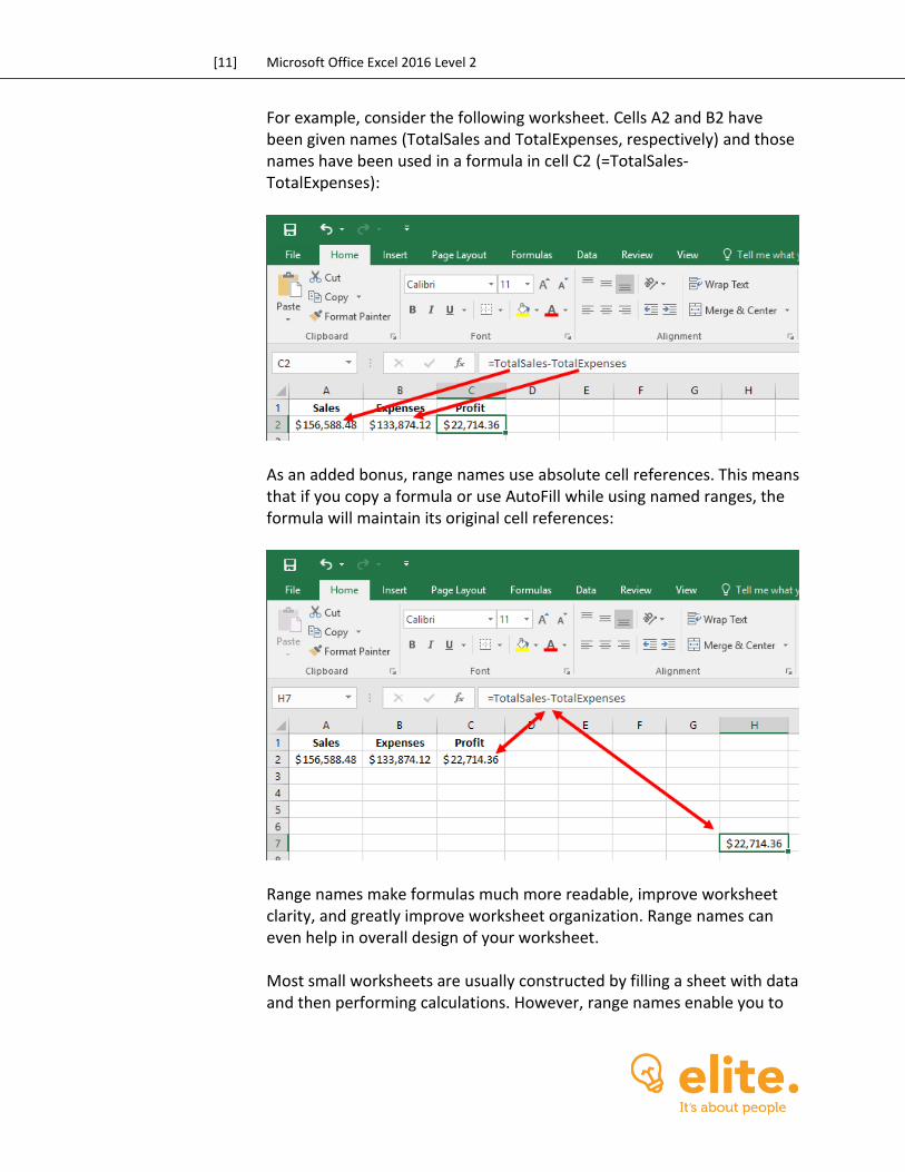
For example, consider the following worksheet. Cells A2 and B2 have been given names (TotalSales and TotalExpenses, respectively) and those names have been used in a formula in cell C2 (=TotalSales-TotalExpenses):
As an added bonus, range names use absolute cell references. This means that if you copy a formula or use AutoFill while using named ranges, the formula will maintain its original cell references:
Range names make formulas much more readable, improve worksheet clarity, and greatly improve worksheet organization. Range names can even help in overall design of your worksheet. Most small worksheets are usually constructed by filling a sheet with data and then performing calculations. However, range names enable you to
[12] Microsoft Office Excel 2016 – Part 2
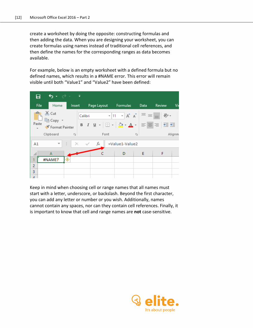
create a worksheet by doing the opposite: constructing formulas and then adding the data. When you are designing your worksheet, you can create formulas using names instead of traditional cell references, and then define the names for the corresponding ranges as data becomes available. For example, below is an empty worksheet with a defined formula but no defined names, which results in a #NAME error. This error will remain visible until both “Value1” and “Value2” have been defined:
Keep in mind when choosing cell or range names that all names must start with a letter, underscore, or backslash. Beyond the first character, you can add any letter or number or you wish. Additionally, names cannot contain any spaces, nor can they contain cell references. Finally, it is important to know that cell and range names are not case-sensitive.
[13] Microsoft Office Excel 2016 Level 2
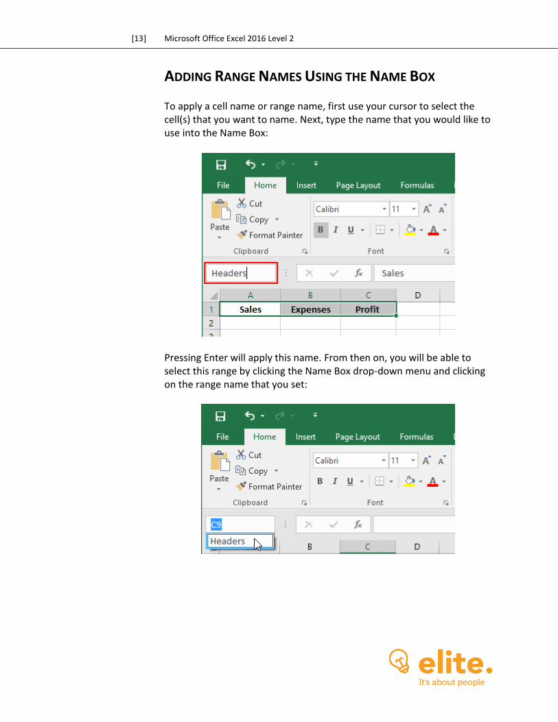
ADDING RANGE NAMES USING THE NAME BOX
To apply a cell name or range name, first use your cursor to select the cell(s) that you want to name. Next, type the name that you would like to use into the Name Box:
Pressing Enter will apply this name. From then on, you will be able to select this range by clicking the Name Box drop-down menu and clicking on the range name that you set:
[14] Microsoft Office Excel 2016 – Part 2
ADDING RANGE NAMES USING THE NEW NAME DIALOG
BOX
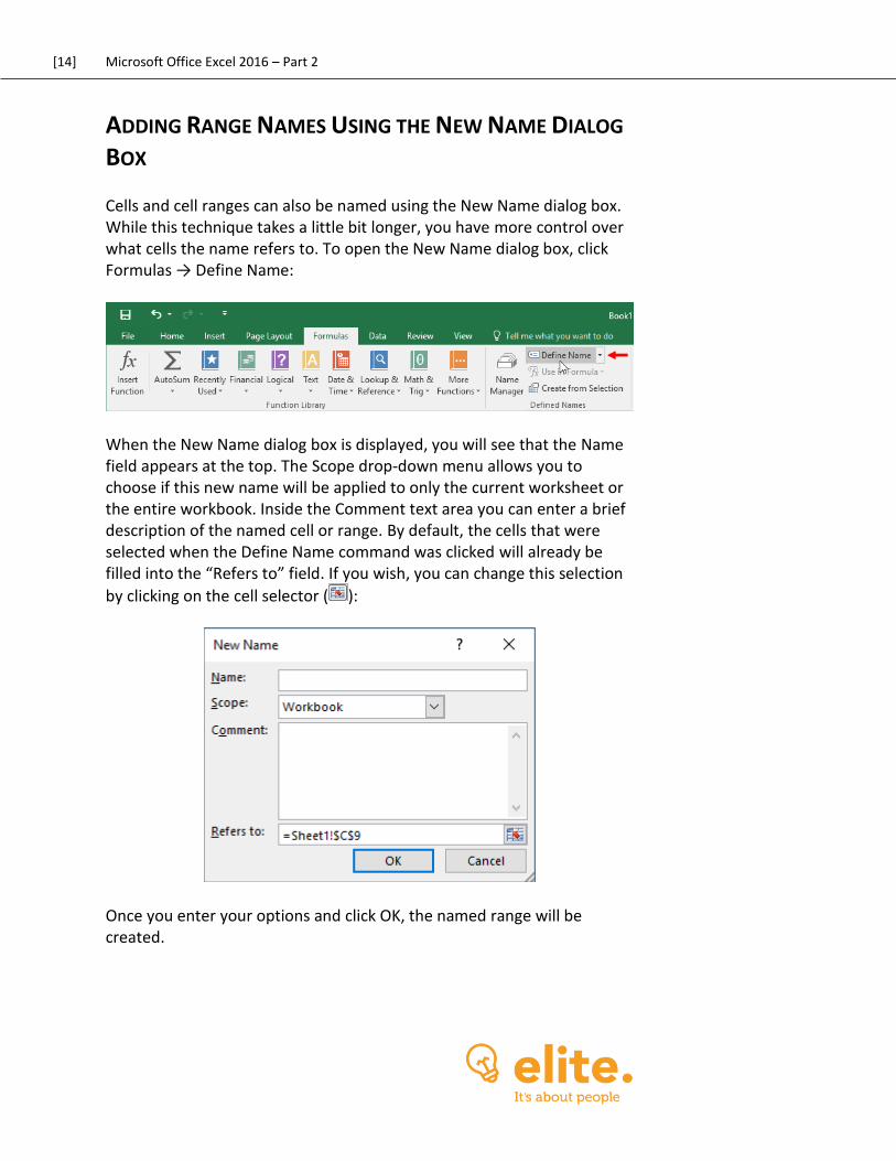
Cells and cell ranges can also be named using the New Name dialog box. While this technique takes a little bit longer, you have more control over what cells the name refers to. To open the New Name dialog box, click Formulas → Define Name:
When the New Name dialog box is displayed, you will see that the Name field appears at the top. The Scope drop-down menu allows you to choose if this new name will be applied to only the current worksheet or the entire workbook. Inside the Comment text area you can enter a brief description of the named cell or range. By default, the cells that were selected when the Define Name command was clicked will already be filled into the “Refers to” field. If you wish, you can change this selection
by clicking on the cell selector ( ):
Once you enter your options and click OK, the named range will be created.
[15] Microsoft Office Excel 2016 Level 2
EDITING A RANGE NAME AND DELETING A RANGE NAME
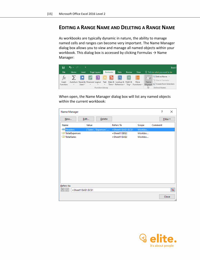
As workbooks are typically dynamic in nature, the ability to manage named cells and ranges can become very important. The Name Manager dialog box allows you to view and manage all named objects within your workbook. This dialog box is accessed by clicking Formulas → Name Manager:
When open, the Name Manager dialog box will list any named objects within the current workbook:
[16] Microsoft Office Excel 2016 – Part 2
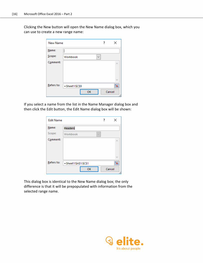
Clicking the New button will open the New Name dialog box, which you can use to create a new range name:
If you select a name from the list in the Name Manager dialog box and then click the Edit button, the Edit Name dialog box will be shown:
This dialog box is identical to the New Name dialog box; the only difference is that it will be prepopulated with information from the selected range name.
[17] Microsoft Office Excel 2016 Level 2
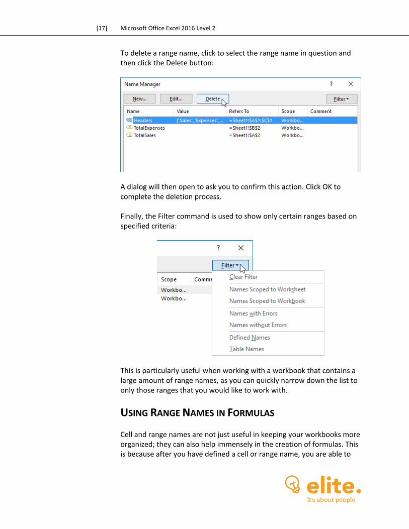
To delete a range name, click to select the range name in question and then click the Delete button:
A dialog will then open to ask you to confirm this action. Click OK to complete the deletion process. Finally, the Filter command is used to show only certain ranges based on specified criteria:
This is particularly useful when working with a workbook that contains a large amount of range names, as you can quickly narrow down the list to only those ranges that you would like to work with.
USING RANGE NAMES IN FORMULAS
Cell and range names are not just useful in keeping your workbooks more organized; they can also help immensely in the creation of formulas. This is because after you have defined a cell or range name, you are able to

[18] Microsoft Office Excel 2016 – Part 2
use that name in place of the usual cell reference. This makes formulas much more readable.
[19] Microsoft Office Excel 2016 Level 2
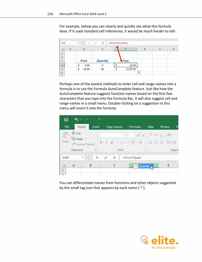
For example, below you can clearly and quickly see what this formula does. If it used standard cell references, it would be much harder to tell:
Perhaps one of the easiest methods to enter cell and range names into a formula is to use the Formula AutoComplete feature. Just like how the AutoComplete feature suggests function names based on the first few characters that you type into the Formula Bar, it will also suggest cell and range names in a small menu. Double-clicking on a suggestion in this menu will insert it into the formula:
You can differentiate names from functions and other objects suggested
by the small tag icon that appears by each name ( ).
[20] Microsoft Office Excel 2016 – Part 2
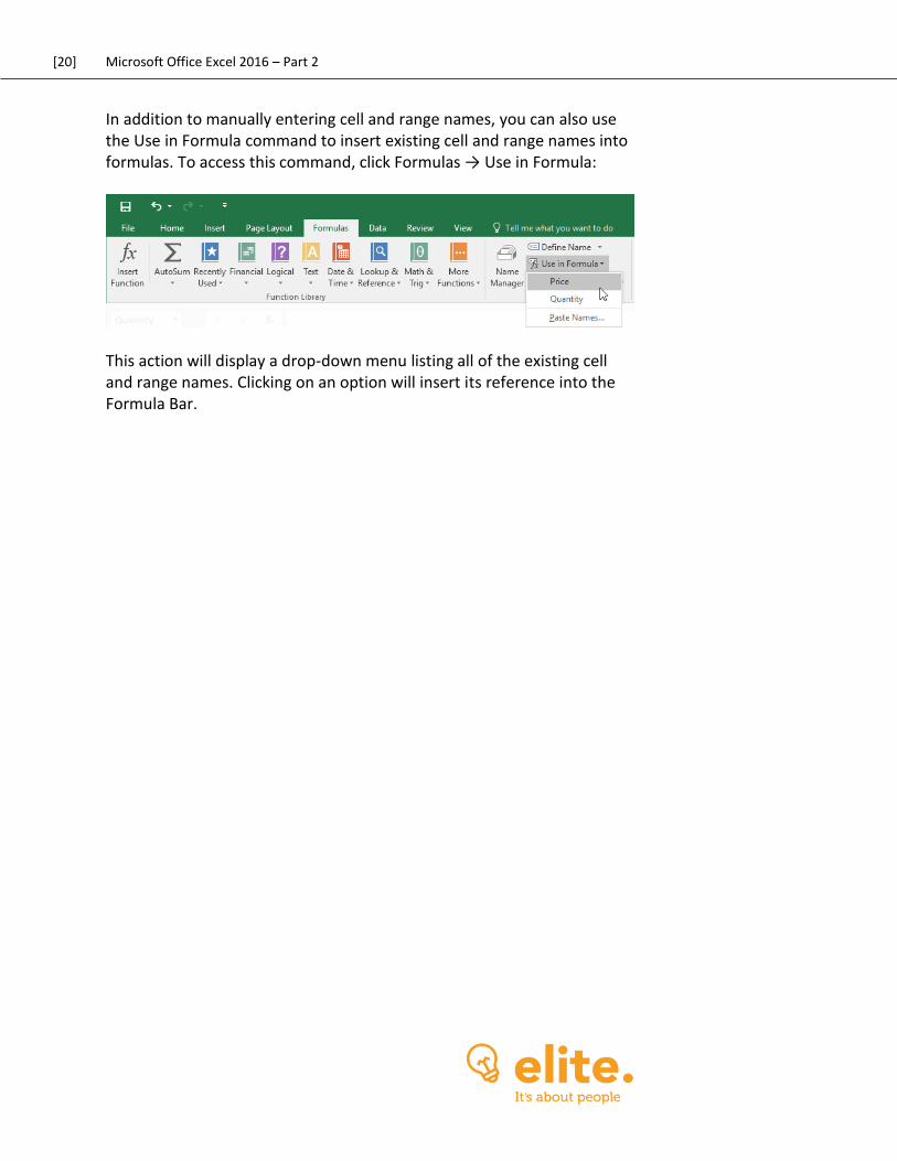
In addition to manually entering cell and range names, you can also use the Use in Formula command to insert existing cell and range names into formulas. To access this command, click Formulas → Use in Formula:
This action will display a drop-down menu listing all of the existing cell and range names. Clicking on an option will insert its reference into the Formula Bar.
[21] Microsoft Office Excel 2016 Level 2
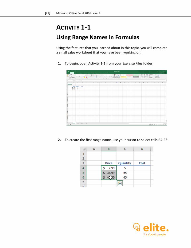
ACTIVITY 1-1
Using Range Names in Formulas Using the features that you learned about in this topic, you will complete a small sales worksheet that you have been working on.
1. To begin, open Activity 1-1 from your Exercise Files folder:
2. To create the first range name, use your cursor to select cells B4:B6:
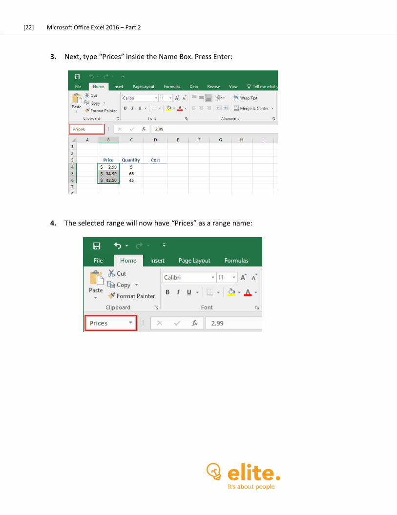
[22] Microsoft Office Excel 2016 – Part 2
3. Next, type “Prices” inside the Name Box. Press Enter:
4. The selected range will now have “Prices” as a range name:
[23] Microsoft Office Excel 2016 Level 2
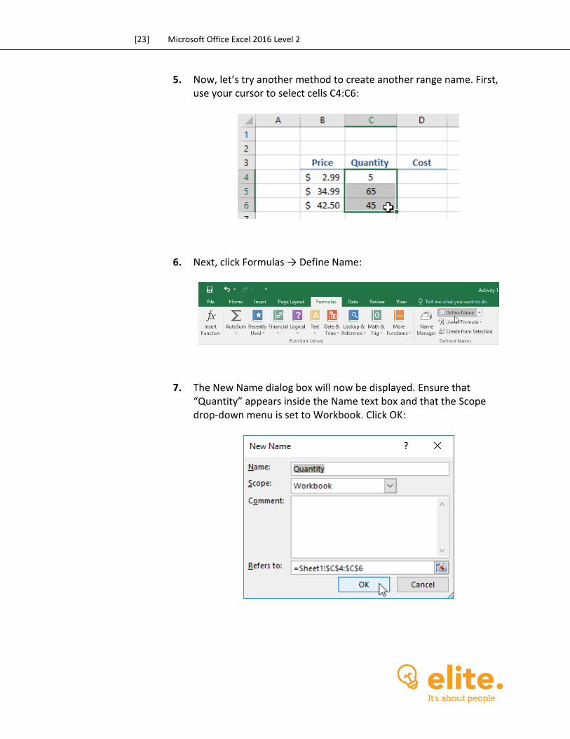
5. Now, let’s try another method to create another range name. First, use your cursor to select cells C4:C6:
6. Next, click Formulas → Define Name:
7. The New Name dialog box will now be displayed. Ensure that “Quantity” appears inside the Name text box and that the Scope drop-down menu is set to Workbook. Click OK:
[24] Microsoft Office Excel 2016 – Part 2
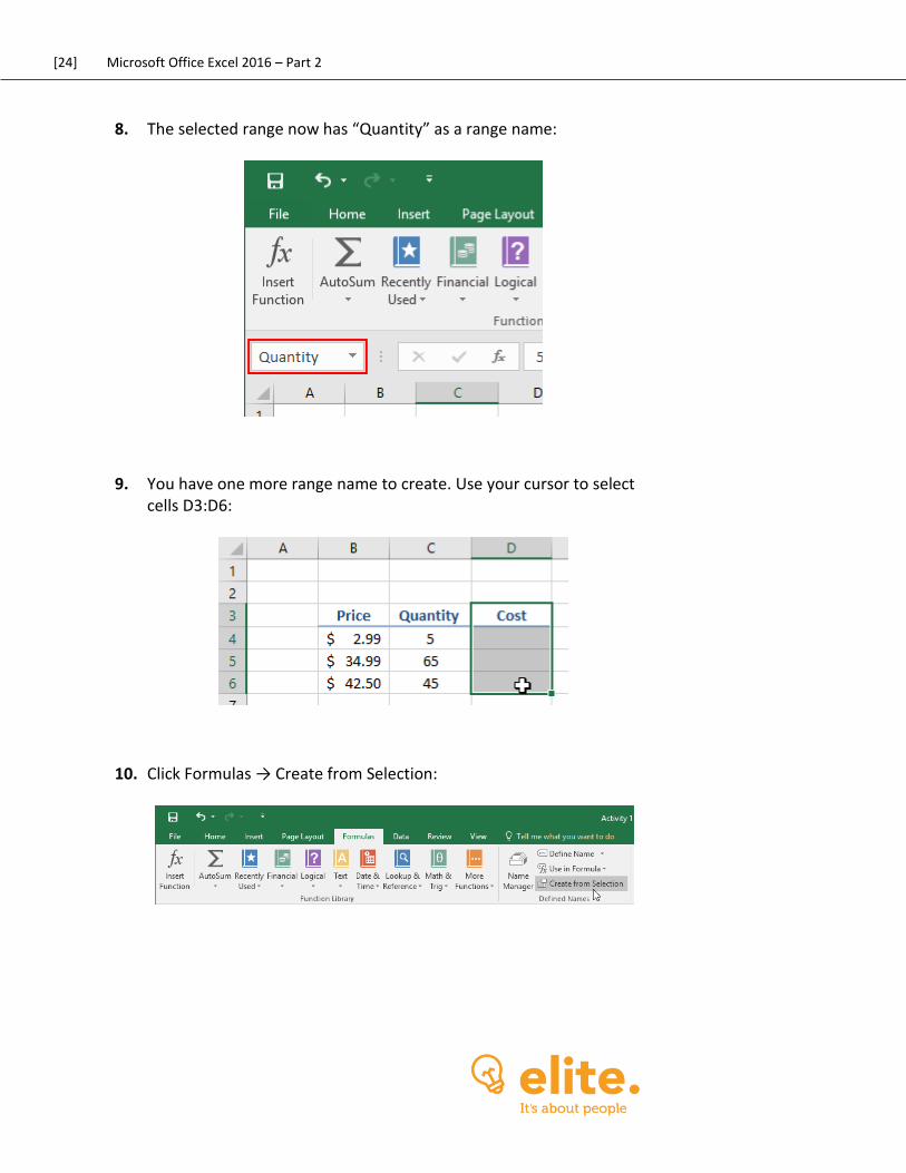
8. The selected range now has “Quantity” as a range name:
9. You have one more range name to create. Use your cursor to select cells D3:D6:
10. Click Formulas → Create from Selection:
[25] Microsoft Office Excel 2016 Level 2
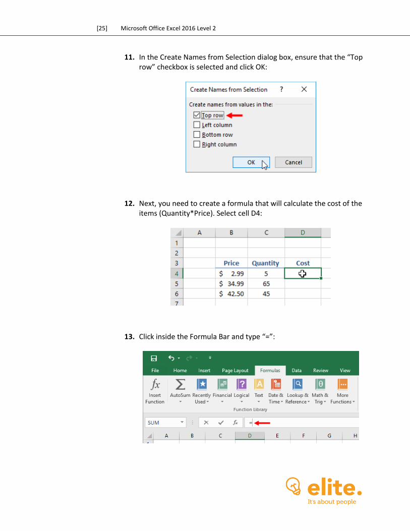
11. In the Create Names from Selection dialog box, ensure that the “Top row” checkbox is selected and click OK:
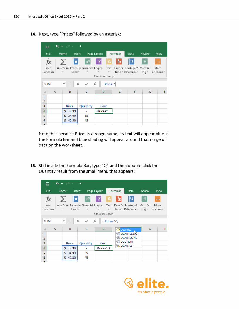
12. Next, you need to create a formula that will calculate the cost of the items (Quantity*Price). Select cell D4:
13. Click inside the Formula Bar and type “=”:
[26] Microsoft Office Excel 2016 – Part 2
14. Next, type “Prices” followed by an asterisk:
Note that because Prices is a range name, its text will appear blue in the Formula Bar and blue shading will appear around that range of data on the worksheet.
15. Still inside the Formula Bar, type “Q” and then double-click the Quantity result from the small menu that appears:
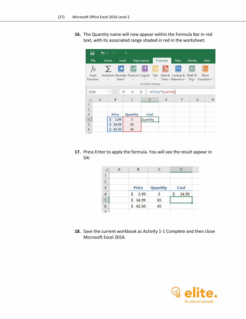
[27] Microsoft Office Excel 2016 Level 2
16. The Quantity name will now appear within the Formula Bar in red text, with its associated range shaded in red in the worksheet:
17. Press Enter to apply the formula. You will see the result appear in D4:
18. Save the current workbook as Activity 1-1 Complete and then close Microsoft Excel 2016.

[28] Microsoft Office Excel 2016 – Part 2
TOPIC B: Use Specialized Functions While the basic functions in Excel cover the majority of use cases, there are some situations where a specialized function is more appropriate. In order to find and use specialized functions, you must be familiar with their syntax and understand how they work on a fundamental level. Topic Objectives In this topic, you will learn:
About function categories About the Excel function reference About function syntax About function entry dialog boxes Using nested functions About automatic workbook calculations How to show and hide formulas How to enable iterative calculations
FUNCTION CATEGORIES
Every built-in function that is available in Excel has been categorized into one of 12 standard categories. These categories are available on the Formulas tab, with some categories available under the More Functions drop-down menu:
(Note that you can expand the number of standard categories using add-ons.)
[29] Microsoft Office Excel 2016 Level 2
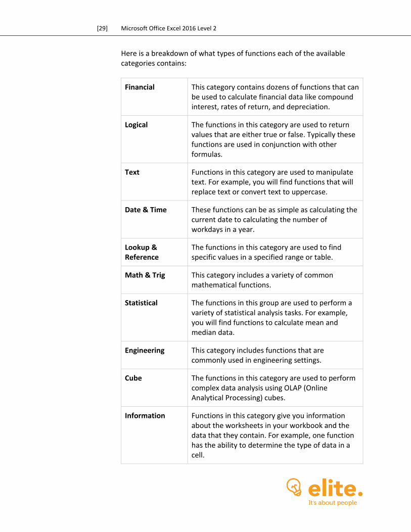
Here is a breakdown of what types of functions each of the available categories contains:
Financial This category contains dozens of functions that can be used to calculate financial data like compound interest, rates of return, and depreciation.
Logical The functions in this category are used to return values that are either true or false. Typically these functions are used in conjunction with other formulas.
Text Functions in this category are used to manipulate text. For example, you will find functions that will replace text or convert text to uppercase.
Date & Time These functions can be as simple as calculating the current date to calculating the number of workdays in a year.
Lookup & Reference
The functions in this category are used to find specific values in a specified range or table.
Math & Trig This category includes a variety of common mathematical functions.
Statistical The functions in this group are used to perform a variety of statistical analysis tasks. For example, you will find functions to calculate mean and median data.
Engineering This category includes functions that are commonly used in engineering settings.
Cube The functions in this category are used to perform complex data analysis using OLAP (Online Analytical Processing) cubes.
Information Functions in this category give you information about the worksheets in your workbook and the data that they contain. For example, one function has the ability to determine the type of data in a cell.
[30] Microsoft Office Excel 2016 – Part 2
Compatibility The functions in this category are unique in that they are actually older versions of functions that are still available. Such functions are useful if you are working with workbooks that were created in older versions of Excel.
Web The functions found in this category are used to return data from web services, return data from XML content, and return URL-encoded string data.
THE EXCEL FUNCTION REFERENCE
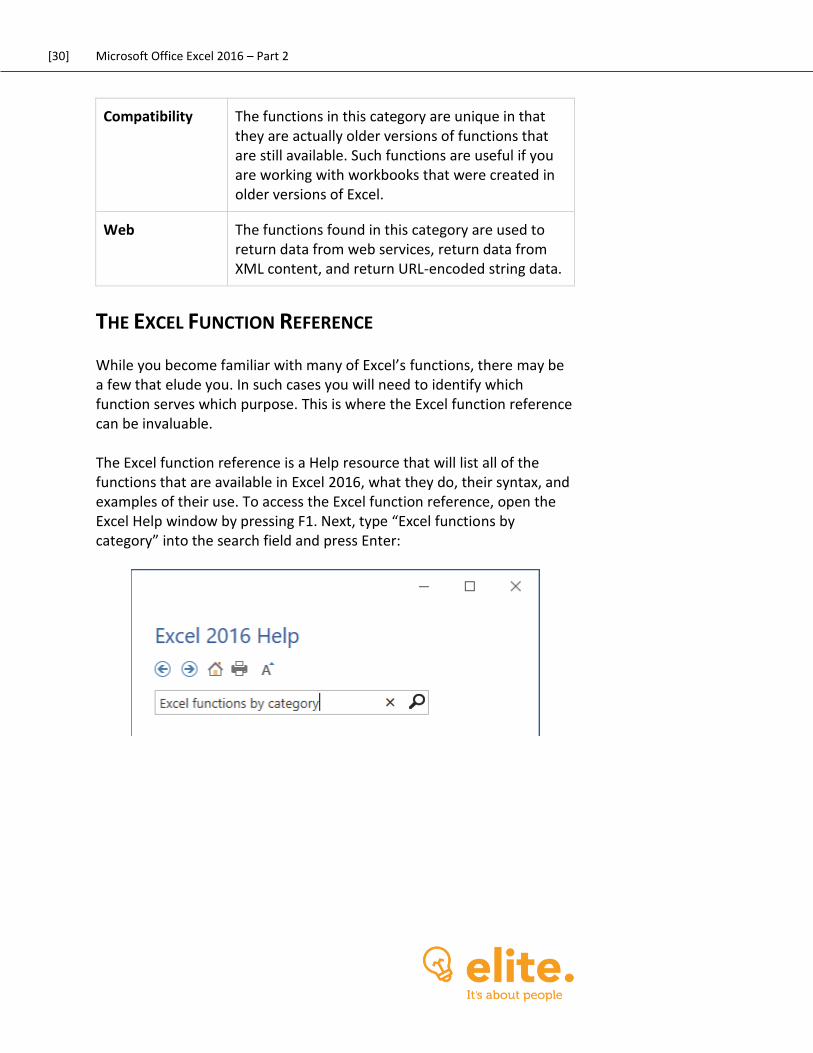
While you become familiar with many of Excel’s functions, there may be a few that elude you. In such cases you will need to identify which function serves which purpose. This is where the Excel function reference can be invaluable. The Excel function reference is a Help resource that will list all of the functions that are available in Excel 2016, what they do, their syntax, and examples of their use. To access the Excel function reference, open the Excel Help window by pressing F1. Next, type “Excel functions by category” into the search field and press Enter:
[31] Microsoft Office Excel 2016 Level 2
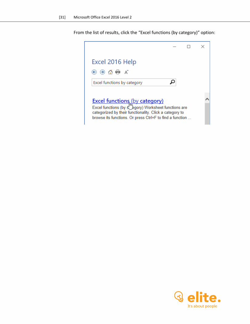
From the list of results, click the “Excel functions (by category)” option:
[32] Microsoft Office Excel 2016 – Part 2
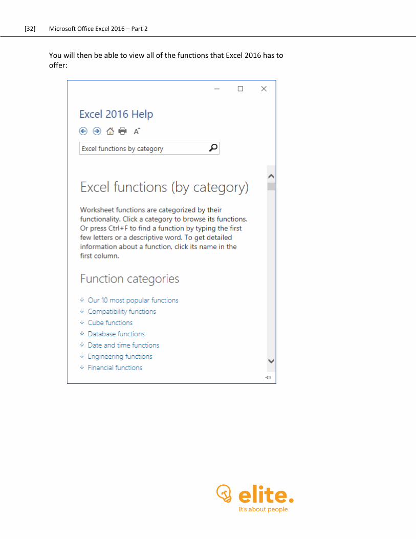
You will then be able to view all of the functions that Excel 2016 has to offer:
[33] Microsoft Office Excel 2016 Level 2
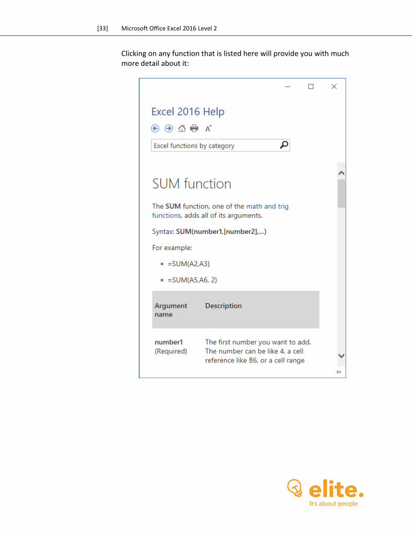
Clicking on any function that is listed here will provide you with much more detail about it:
[34] Microsoft Office Excel 2016 – Part 2
FUNCTION SYNTAX
Functions are a major part of what makes Excel so popular, so now you will explore some different types of functions and learn some tricks that you can use to perform complex calculations. Just keep in mind that even the most complex of formulas can be broken down into simple parts. Remember to pay attention to the order of precedence (using the BEDMAS acronym) and the number of parentheses you use. The SUMIF Function
=SUMIF(range, criteria, [sum_range])
The SUMIF function is used to calculate the sum of values in a specified range if they meet a specified criteria. For example, you could calculate total sales figures and only include numbers that are less than a specified value. The sum_range argument is optional; you can use it if you want to add cells to the sum other than those specified in the argument. If you choose to leave out this argument, the function will only calculate the sum of the values from the previous range argument. Below are some example of the SUMIF function in action:
Function Description
=SUMIF(A1:C10, “<5”) Only numbers in the range A1:C10 that are under 5 will be added together.
=SUMIF(A1:C10, “December”, D1:D10)
Only numbers in the range D1:D10 will be added together where they correspond with the text entry of “December” in the range A1:C10.
=SUMIF(A1:A10, 5) All numbers with the value of 5 that fall within the A1:A10 range will be added together.
The AVERAGEIF Function
=AVERAGEIF(range, criteria, [average_range])
[35] Microsoft Office Excel 2016 Level 2
The AVERAGEIF function will return the average of every cell within a range if the specified criteria is met. For example, if you wanted to calculate the average sale amount in a set range of sales data only for sales below a certain amount you could use this function. The average_range argument is optional; it can be used if you want to add cells to the sum other than those specified by the range argument. If you choose to leave out this argument, the function will only calculate the average of the values from the range argument. Below are some AVERAGEIF functions in action:
Function Description
=AVERAGEIF(A1:C10, “<5”) The average of all numbers in the range A1:C10 that are under 5 will be calculated.
=AVERAGEIF(A1:C10, “December”, D1:D10)
The average for the numbers in the range D1:D10 will be calculated where they correspond with the text entry of “December” in the range A1:C10.
The COUNTIF Function
=COUNTIF(range, criteria)
The COUNTIF function will count the number of cells in a specified range if the criteria is met. For example, this function could be used to count the number of sales associates who have sold X number of products.
Function Description
=COUNTIF(A1:C10, “<5”) This function will count all cells within the A1:C10 range where the value is 5 or lower.
=COUNTIF(A1:A10, 5) This function will count all cells within the A1:A10 range only where the value is 5.
[36] Microsoft Office Excel 2016 – Part 2
IFS Functions The functions that have been covered so far (AVERAGEIF, COUNTIF, and SUMIF) all have an equivalent IFS function that allow you to perform those respective calculations on data that requires more than just one specified criteria. With a few exceptions, such functions have very similar syntax:
=SUMIFS(sum_range, criteria_range1, criteria1, [criteria_range2], [criteria2], …)
=AVERAGEIFS(average_range, criteria_range1, criteria1, [criteria_range2], [criteria2], …)
=COUNTIFS(criteria_range, criteria1, [criteria_range2], [criteria2], …)
The COUNTA Function
=COUNTA(value1, [value2],…)
The COUNTA function is used to count the number of cells specified by the argument (value1, value2, etc.) that are not empty.
Function Description
=COUNTA(A1:A10) All cells that contain data within the A1:A10 cell range will be counted.
=COUNTA(A1:A10, B1, C1) All cells that contain data within the A1:A10 range, as well as cells B1 and C1, will be counted.
[37] Microsoft Office Excel 2016 Level 2
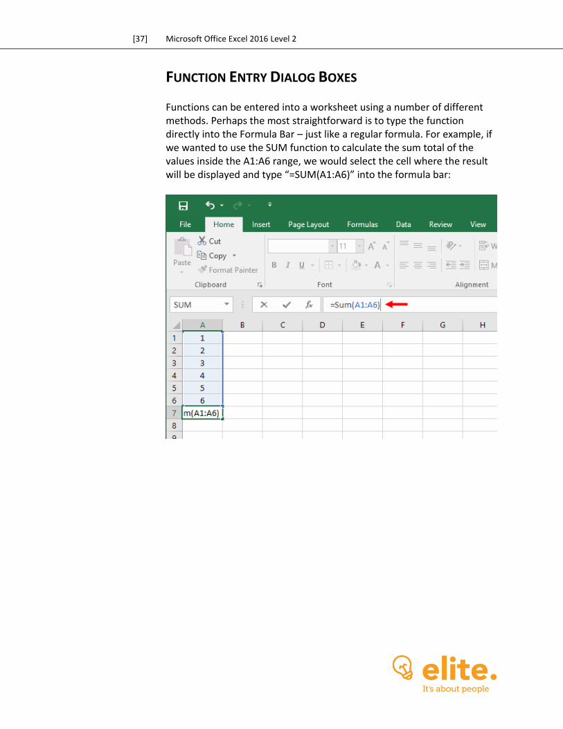
FUNCTION ENTRY DIALOG BOXES
Functions can be entered into a worksheet using a number of different methods. Perhaps the most straightforward is to type the function directly into the Formula Bar – just like a regular formula. For example, if we wanted to use the SUM function to calculate the sum total of the values inside the A1:A6 range, we would select the cell where the result will be displayed and type “=SUM(A1:A6)” into the formula bar:
[38] Microsoft Office Excel 2016 – Part 2
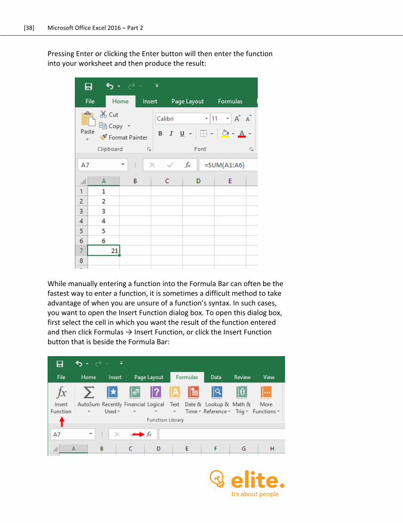
Pressing Enter or clicking the Enter button will then enter the function into your worksheet and then produce the result:
While manually entering a function into the Formula Bar can often be the fastest way to enter a function, it is sometimes a difficult method to take advantage of when you are unsure of a function’s syntax. In such cases, you want to open the Insert Function dialog box. To open this dialog box, first select the cell in which you want the result of the function entered and then click Formulas → Insert Function, or click the Insert Function button that is beside the Formula Bar:

[39] Microsoft Office Excel 2016 Level 2
[40] Microsoft Office Excel 2016 – Part 2
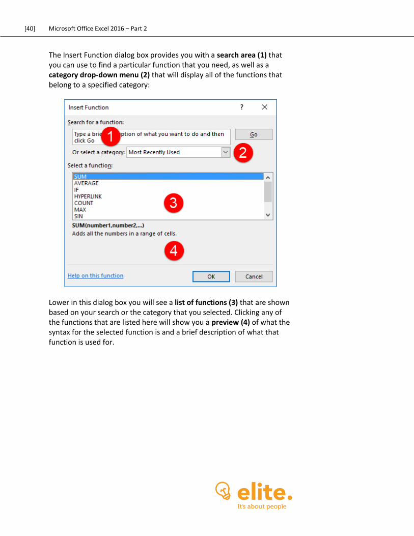
The Insert Function dialog box provides you with a search area (1) that you can use to find a particular function that you need, as well as a category drop-down menu (2) that will display all of the functions that belong to a specified category:
Lower in this dialog box you will see a list of functions (3) that are shown based on your search or the category that you selected. Clicking any of the functions that are listed here will show you a preview (4) of what the syntax for the selected function is and a brief description of what that function is used for.
[41] Microsoft Office Excel 2016 Level 2
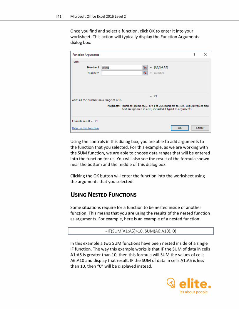
Once you find and select a function, click OK to enter it into your worksheet. This action will typically display the Function Arguments dialog box:
Using the controls in this dialog box, you are able to add arguments to the function that you selected. For this example, as we are working with the SUM function, we are able to choose data ranges that will be entered into the function for us. You will also see the result of the formula shown near the bottom and the middle of this dialog box. Clicking the OK button will enter the function into the worksheet using the arguments that you selected.
USING NESTED FUNCTIONS
Some situations require for a function to be nested inside of another function. This means that you are using the results of the nested function as arguments. For example, here is an example of a nested function:
=IF(SUM(A1:A5)>10, SUM(A6:A10), 0)
In this example a two SUM functions have been nested inside of a single IF function. The way this example works is that IF the SUM of data in cells A1:A5 is greater than 10, then this formula will SUM the values of cells A6:A10 and display that result. IF the SUM of data in cells A1:A5 is less than 10, then “0” will be displayed instead.
[42] Microsoft Office Excel 2016 – Part 2
AUTOMATIC WORKBOOK CALCULATIONS
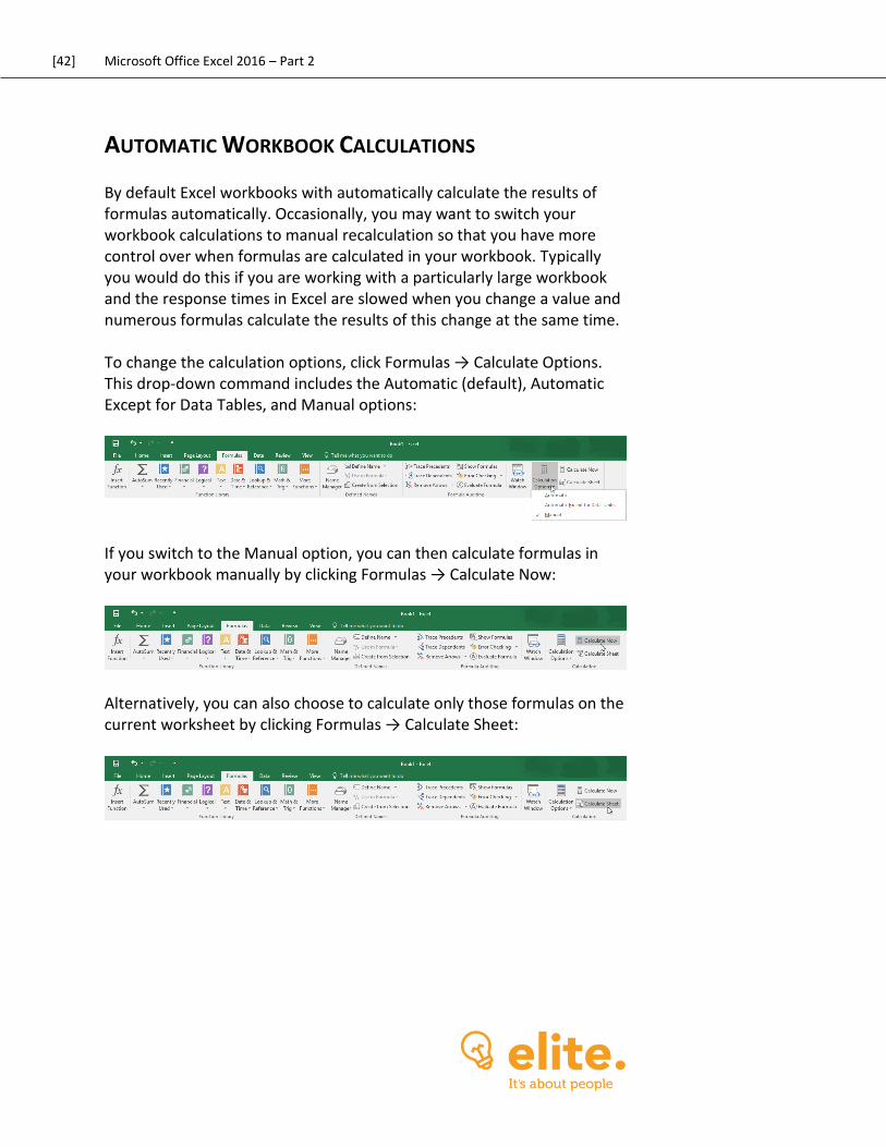
By default Excel workbooks with automatically calculate the results of formulas automatically. Occasionally, you may want to switch your workbook calculations to manual recalculation so that you have more control over when formulas are calculated in your workbook. Typically you would do this if you are working with a particularly large workbook and the response times in Excel are slowed when you change a value and numerous formulas calculate the results of this change at the same time. To change the calculation options, click Formulas → Calculate Options. This drop-down command includes the Automatic (default), Automatic Except for Data Tables, and Manual options:
If you switch to the Manual option, you can then calculate formulas in your workbook manually by clicking Formulas → Calculate Now:
Alternatively, you can also choose to calculate only those formulas on the current worksheet by clicking Formulas → Calculate Sheet:
[43] Microsoft Office Excel 2016 Level 2
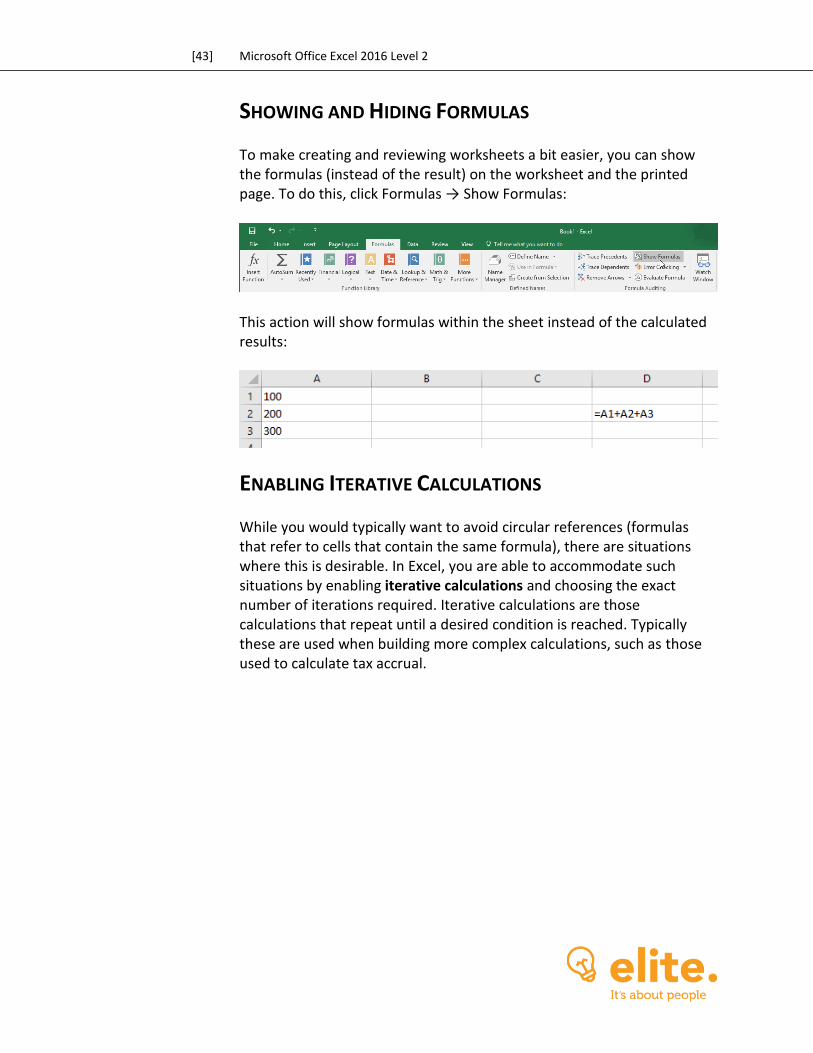
SHOWING AND HIDING FORMULAS
To make creating and reviewing worksheets a bit easier, you can show the formulas (instead of the result) on the worksheet and the printed page. To do this, click Formulas → Show Formulas:
This action will show formulas within the sheet instead of the calculated results:
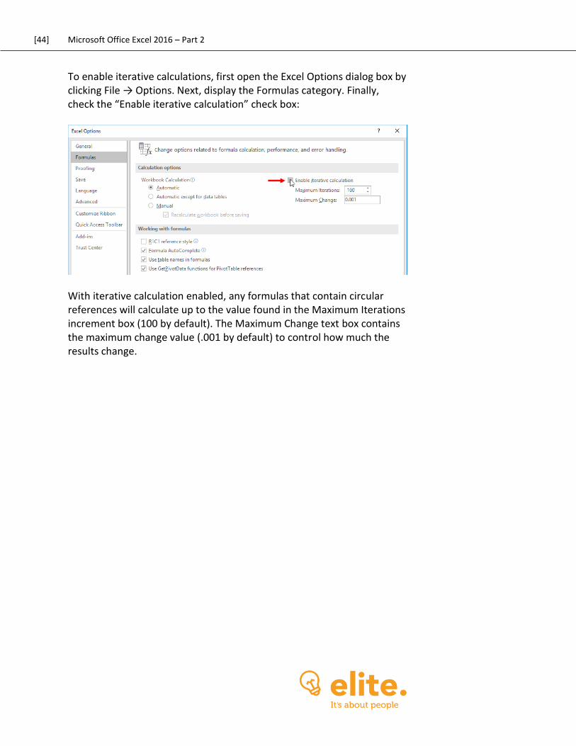
ENABLING ITERATIVE CALCULATIONS
While you would typically want to avoid circular references (formulas that refer to cells that contain the same formula), there are situations where this is desirable. In Excel, you are able to accommodate such situations by enabling iterative calculations and choosing the exact number of iterations required. Iterative calculations are those calculations that repeat until a desired condition is reached. Typically these are used when building more complex calculations, such as those used to calculate tax accrual.
[44] Microsoft Office Excel 2016 – Part 2
To enable iterative calculations, first open the Excel Options dialog box by clicking File → Options. Next, display the Formulas category. Finally, check the “Enable iterative calculation” check box:
With iterative calculation enabled, any formulas that contain circular references will calculate up to the value found in the Maximum Iterations increment box (100 by default). The Maximum Change text box contains the maximum change value (.001 by default) to control how much the results change.
[45] Microsoft Office Excel 2016 Level 2
ACTIVITY 1-2
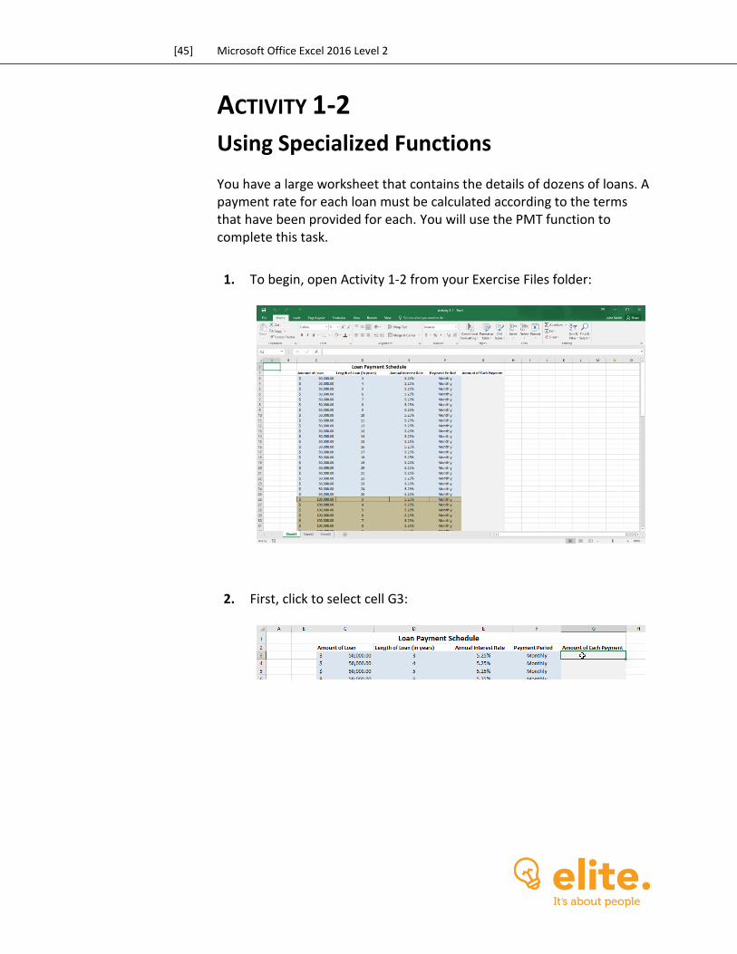
Using Specialized Functions You have a large worksheet that contains the details of dozens of loans. A payment rate for each loan must be calculated according to the terms that have been provided for each. You will use the PMT function to complete this task.
1. To begin, open Activity 1-2 from your Exercise Files folder:
2. First, click to select cell G3:
[46] Microsoft Office Excel 2016 – Part 2
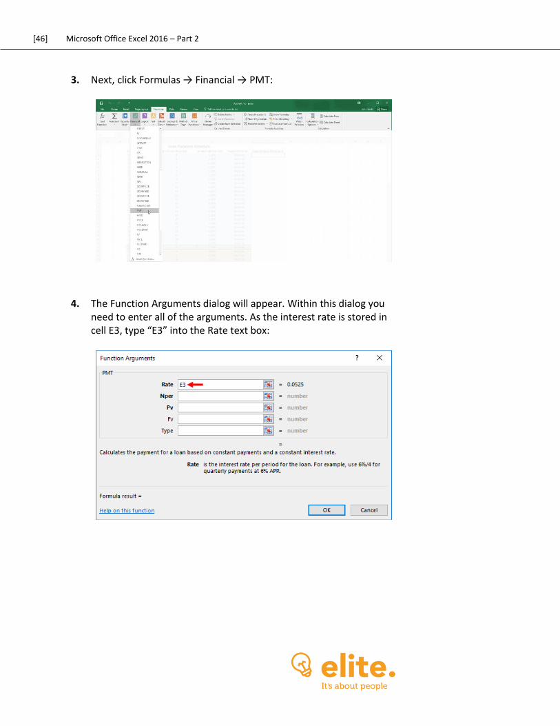
3. Next, click Formulas → Financial → PMT:
4. The Function Arguments dialog will appear. Within this dialog you need to enter all of the arguments. As the interest rate is stored in cell E3, type “E3” into the Rate text box:
[47] Microsoft Office Excel 2016 Level 2
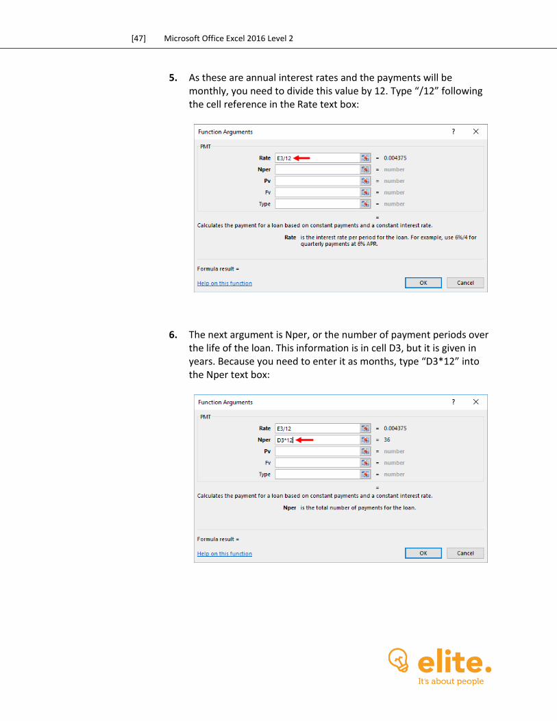
5. As these are annual interest rates and the payments will be monthly, you need to divide this value by 12. Type “/12” following the cell reference in the Rate text box:
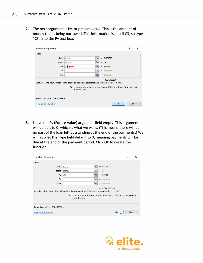
6. The next argument is Nper, or the number of payment periods over the life of the loan. This information is in cell D3, but it is given in years. Because you need to enter it as months, type “D3*12” into the Nper text box:
[48] Microsoft Office Excel 2016 – Part 2
7. The next argument is Pv, or present value. This is the amount of money that is being borrowed. This information is in cell C3, so type “C3” into the Pv text box:
8. Leave the Fv (Future Value) argument field empty. This argument will default to 0, which is what we want. (This means there will be no part of the loan left outstanding at the end of the payments.) We will also let the Type field default to 0, meaning payments will be due at the end of the payment period. Click OK to create the function:
[49] Microsoft Office Excel 2016 Level 2
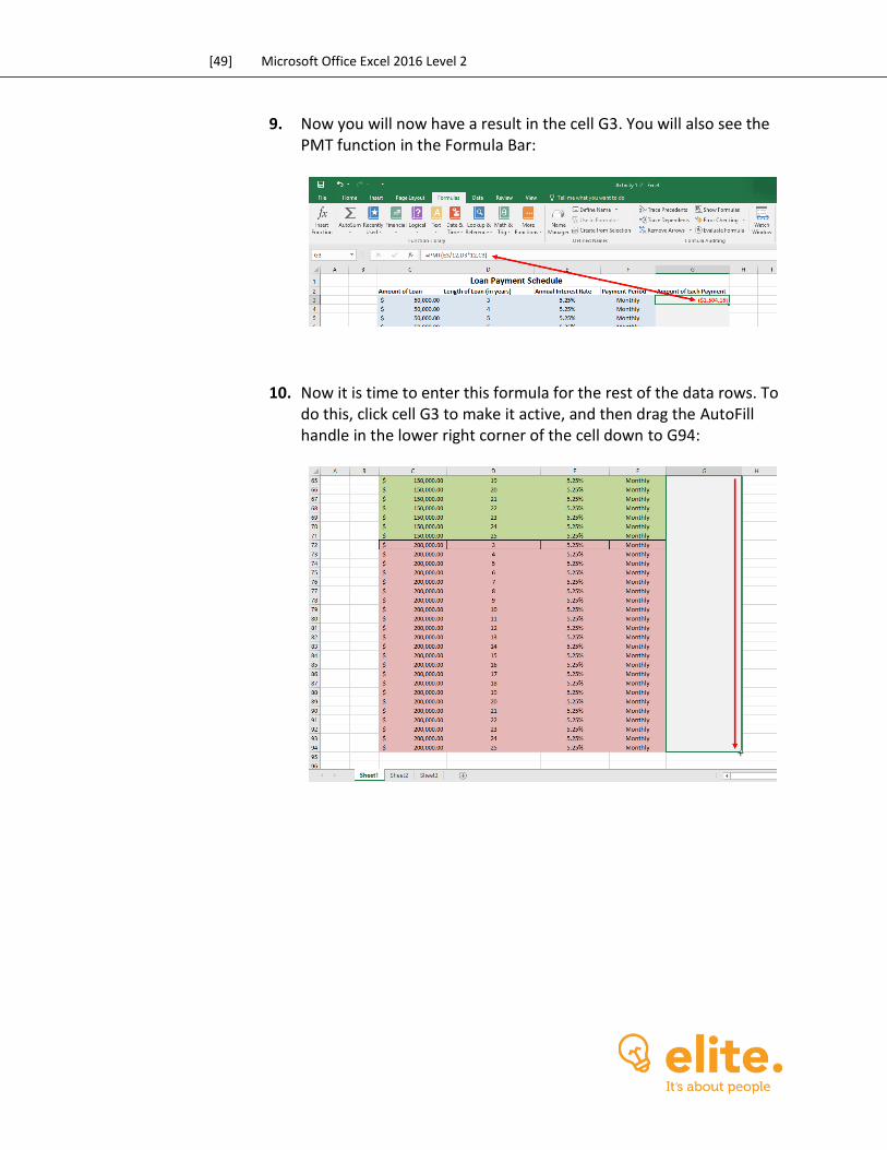
9. Now you will now have a result in the cell G3. You will also see the PMT function in the Formula Bar:
10. Now it is time to enter this formula for the rest of the data rows. To do this, click cell G3 to make it active, and then drag the AutoFill handle in the lower right corner of the cell down to G94:
[50] Microsoft Office Excel 2016 – Part 2
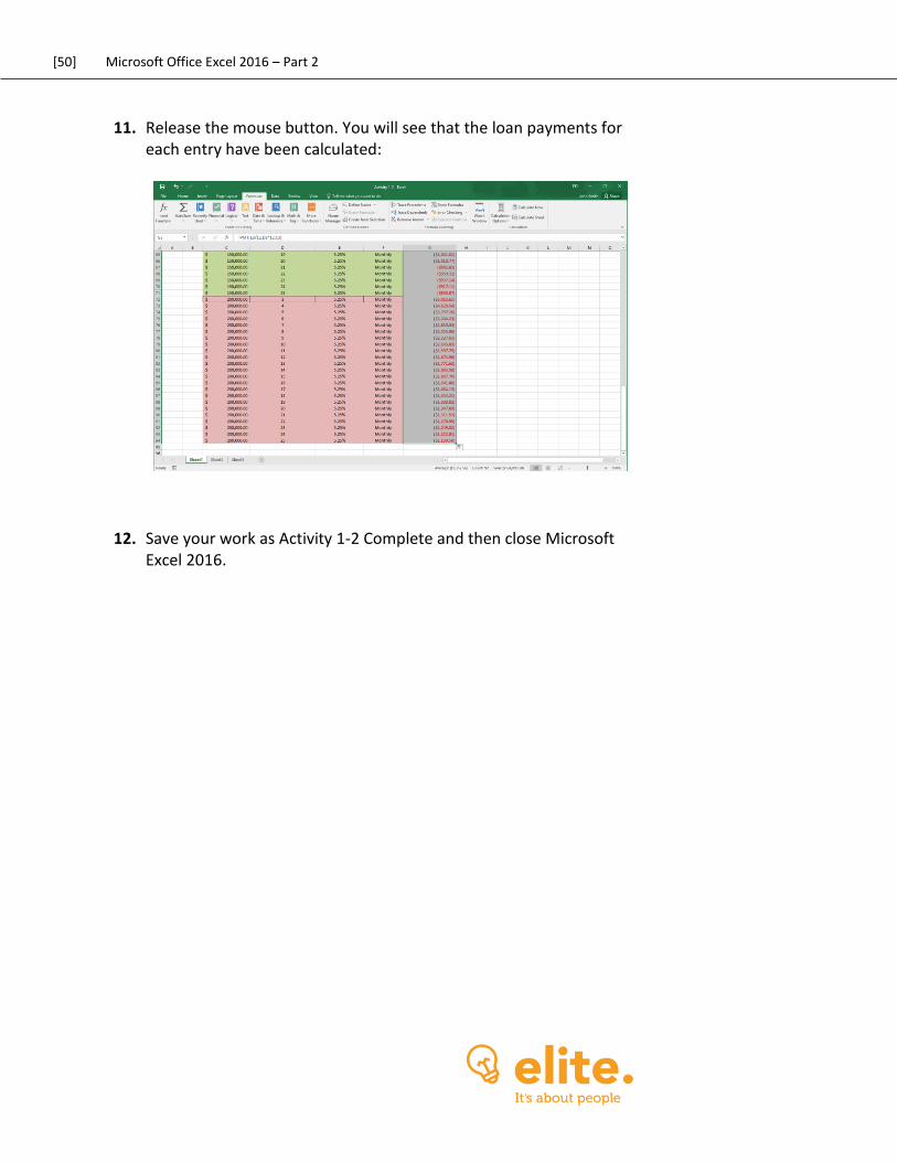
11. Release the mouse button. You will see that the loan payments for each entry have been calculated:
12. Save your work as Activity 1-2 Complete and then close Microsoft Excel 2016.
[51] Microsoft Office Excel 2016 Level 2
Summary Over the course of this lesson you learned about range names and how to apply them. Additionally, you learned about the different function categories and specialized functions that are available. You should also now be familiar with function syntax, nested functions, automatic workbook calculations, and iterative calculations.
REVIEW QUESTIONS
1. Where do you type in a new range name for a selected range?
2. How many default function categories are there in Microsoft Excel 2016?
3. What is the command sequence to show formulas rather than calculated values in cells?
4. What is a nested function?
5. What is the command sequence to change workbook calculations to manual?

[53] Microsoft Office Excel 2016 Level 2
LESSON 2: ANALYZING DATA WITH
LOGICAL AND LOOKUP
FUNCTIONS
Lesson Objectives
In this lesson you will learn how to:
Use text functions
Use logical functions
Use lookup functions
Use date functions
Use financial functions
[54] Microsoft Office Excel 2016 – Part 2
TOPIC A: Use Text Functions While you are now familiar with Excel’s more commonly used functions, you still need to learn about some of its more specialized ones. In this topic you will learn about functions that are specific to text analysis. Topic Objectives In this topic, you will learn:
About text functions About LEFT and RIGHT functions About the MID function About the LEN function About the TRIM function About the UPPER, LOWER, and PROPER functions About the CONCATENATE function About the TRANSPOSE function
TEXT FUNCTIONS
Text functions are used in Excel to analyze text-based worksheet data. While such functions can be used for data analysis, they are typically used instead to prepare data for analysis. This is because they allow you to format textual data for use in other areas. For example, you can use text functions to import textual data from another workbook and format it so that it meets the formatting requirements for the destination workbook.
[55] Microsoft Office Excel 2016 Level 2
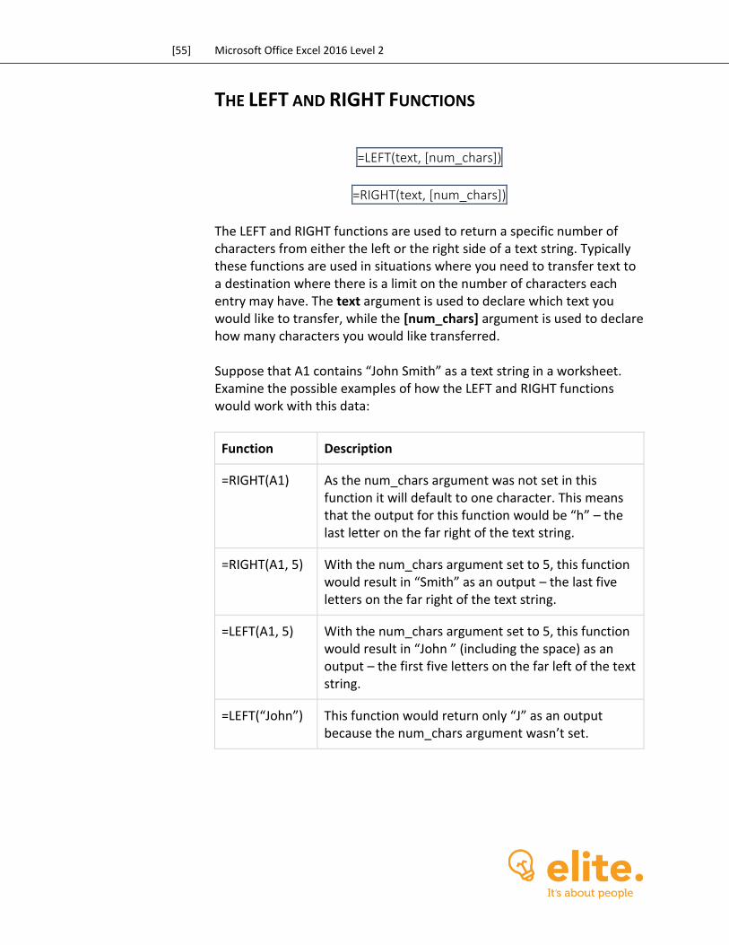
THE LEFT AND RIGHT FUNCTIONS
=LEFT(text, [num_chars])
=RIGHT(text, [num_chars])
The LEFT and RIGHT functions are used to return a specific number of characters from either the left or the right side of a text string. Typically these functions are used in situations where you need to transfer text to a destination where there is a limit on the number of characters each entry may have. The text argument is used to declare which text you would like to transfer, while the [num_chars] argument is used to declare how many characters you would like transferred. Suppose that A1 contains “John Smith” as a text string in a worksheet. Examine the possible examples of how the LEFT and RIGHT functions would work with this data:
Function Description
=RIGHT(A1) As the num_chars argument was not set in this function it will default to one character. This means that the output for this function would be “h” – the last letter on the far right of the text string.
=RIGHT(A1, 5) With the num_chars argument set to 5, this function would result in “Smith” as an output – the last five letters on the far right of the text string.
=LEFT(A1, 5) With the num_chars argument set to 5, this function would result in “John ” (including the space) as an output – the first five letters on the far left of the text string.
=LEFT(“John”) This function would return only “J” as an output because the num_chars argument wasn’t set.
[56] Microsoft Office Excel 2016 – Part 2
THE MID FUNCTION
=MID(text, start_num, num_chars)
Similar in use and design to the LEFT and RIGHT functions, the MID function will return characters from the middle of a text string. As with the LEFT and RIGHT functions, the text argument is used to reference the cell(s) with the text string in question or to enter a text string directly into the function surrounded by double quotation marks. The start_num argument is unique to the MID function as it tells the function which character in the text string to start with. The num_chars argument then allows you to set the number of characters that you would like to return from the starting point that you set in the previous argument. Keep in mind that while the num_chars arguments behaves the same as it does in the LEFT and RIGHT functions, it is required in order for the MID function to operate correctly. Suppose that A1 contains “John Smith” as a text string in a worksheet. Examine the possible examples of how the MID function would work with this text string:
Function Description
=MID(A1, 5, 5) In this case, the text is contained within cell A1. The start_num argument is set to 5, so the function will start five characters (including spaces) into the text string. The num_chars argument is set to five so the five characters after the starting position will be returned. This means that “Smith” would be the output for this formula.
=MID(A1, 1, 4) In this case, the text is contained within cell A1. The start_num function is set to 1, so the function will start at the beginning of the text string. The num_chars argument is set to 4 so the four characters after the starting position will be returned. This means that “John” would be the output for this formula.
[57] Microsoft Office Excel 2016 Level 2
THE LEN FUNCTION
=LEN(text)
The LEN (short for length) function’s sole purpose is to return the number of characters that appear within a text string. While there can be many uses for this function, it is typically used to ensure that text strings are of the correct length. For example, you could use this function to make sure that all of the text data within a row is under a specified length. The only argument in this function, text, is used to specify where the text data that you would like to count is stored. Suppose that A1 contains “John Smith” as a text string and B1 contains “Jane Doe” as a text string. Examine the possible examples of how the LEN function would work with this information in mind:
Function Description
=LEN(A1) In this case the LEN function has the text argument set to A1. This means that a count of the text string within this cell will be returned. The output of this function would then be 10.
=LEN(B1) In this case the LEN function has the text argument set to B1. This means that a count of the text string within this cell will be returned. The output of this function would then be 8.
[58] Microsoft Office Excel 2016 – Part 2
THE TRIM FUNCTION
=TRIM(text)
The TRIM function is used to remove any empty spaces from text strings, excluding spaces between words. This function can be very useful in solving data compatibility issues. For example, a frequent problem in data entry is random spaces at the beginning or end of a text string. Such problems can greatly affect your ability to work with text-based data. Note that the only argument in this function, text, is used to specify where the text data that you would like to work with is stored. Suppose that A1 contains “ John Smith” as a text string and B1 contains “Jane ” as a text string. Examine the possible examples of how the TRIM function would work with this information in mind:
Function Description
=TRIM(A1) In this case the TRIM function has the text argument set to A1. “John Smith” will be returned with all of the spaces at the beginning of this text string removed.
=TRIM(B1) In this case the TRIM function has the text argument set to B1. “Jane” will be returned with all of the spaces at the end of this text string removed.

[59] Microsoft Office Excel 2016 Level 2
THE UPPER, LOWER, AND PROPER FUNCTIONS
=UPPER(text)
=LOWER(text)
=PROPER(text)
The UPPER, LOWER, and PROPER functions are used to change the casing of text-based data. The UPPER function will convert all lowercase characters into uppercase, while the LOWER function will do the opposite. The PROPER function will only capitalize the first character of each word in a text string. For all of these functions, the only argument is text. This used to indicate the text-based data that you would like this function to work with. Suppose that A1 contains “John Smith” as a text string and B1 contains “jANe smiTh” as a text string. Examine the possible examples of how the UPPER, LOWER, and PROPER functions would work with this information in mind:
Function Description
=UPPER(A1) In this example, the UPPER function will convert all of the text within cell A1 to uppercase. This means that the output would be “JOHN SMITH”.
=LOWER(A1) In this example, the LOWER function will convert all of the text within cell A1 to lowercase. This means that the output would be “john smith”.
=PROPER(B1) In this example, the PROPER function ensures that only the first character in each word in cell B1 is capitalized. This means that “Jane Smith” would be the resulting output.
[60] Microsoft Office Excel 2016 – Part 2
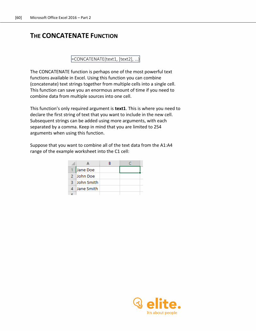
THE CONCATENATE FUNCTION
=CONCATENATE(text1, [text2], …)
The CONCATENATE function is perhaps one of the most powerful text functions available in Excel. Using this function you can combine (concatenate) text strings together from multiple cells into a single cell. This function can save you an enormous amount of time if you need to combine data from multiple sources into one cell. This function’s only required argument is text1. This is where you need to declare the first string of text that you want to include in the new cell. Subsequent strings can be added using more arguments, with each separated by a comma. Keep in mind that you are limited to 254 arguments when using this function. Suppose that you want to combine all of the text data from the A1:A4 range of the example worksheet into the C1 cell:
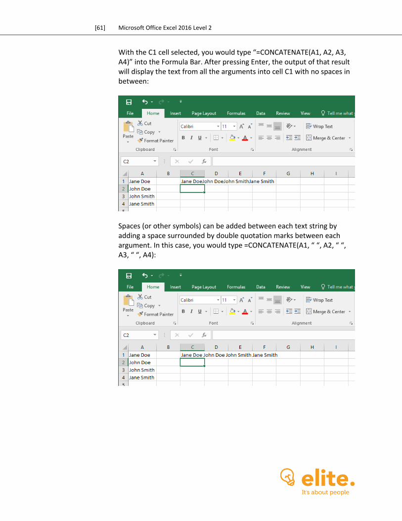
[61] Microsoft Office Excel 2016 Level 2
With the C1 cell selected, you would type “=CONCATENATE(A1, A2, A3, A4)” into the Formula Bar. After pressing Enter, the output of that result will display the text from all the arguments into cell C1 with no spaces in between:
Spaces (or other symbols) can be added between each text string by adding a space surrounded by double quotation marks between each argument. In this case, you would type =CONCATENATE(A1, “ “, A2, “ “, A3, “ “, A4):
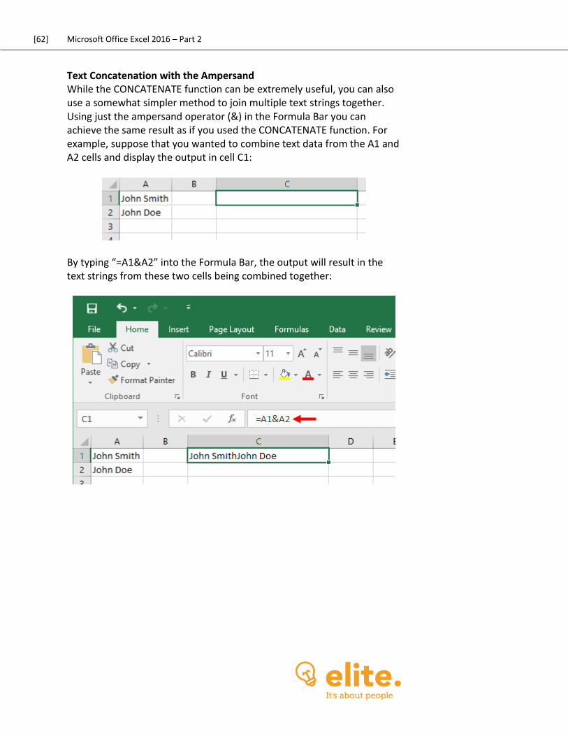
[62] Microsoft Office Excel 2016 – Part 2
Text Concatenation with the Ampersand While the CONCATENATE function can be extremely useful, you can also use a somewhat simpler method to join multiple text strings together. Using just the ampersand operator (&) in the Formula Bar you can achieve the same result as if you used the CONCATENATE function. For example, suppose that you wanted to combine text data from the A1 and A2 cells and display the output in cell C1:
By typing “=A1&A2” into the Formula Bar, the output will result in the text strings from these two cells being combined together:
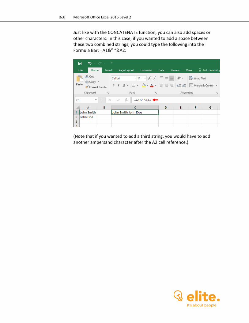
[63] Microsoft Office Excel 2016 Level 2
Just like with the CONCATENATE function, you can also add spaces or other characters. In this case, if you wanted to add a space between these two combined strings, you could type the following into the Formula Bar: =A1&” “&A2:
(Note that if you wanted to add a third string, you would have to add another ampersand character after the A2 cell reference.)

[64] Microsoft Office Excel 2016 – Part 2
THE TRANSPOSE FUNCTION
The Transpose function will shift a vertical range of cells to a horizontal range and the reverse. To operate correctly, this function needs to be entered as an array formula in a range that has the same number of rows and columns. For example, suppose that you wanted to transpose the values in column A so that they appear horizontally on row 1:
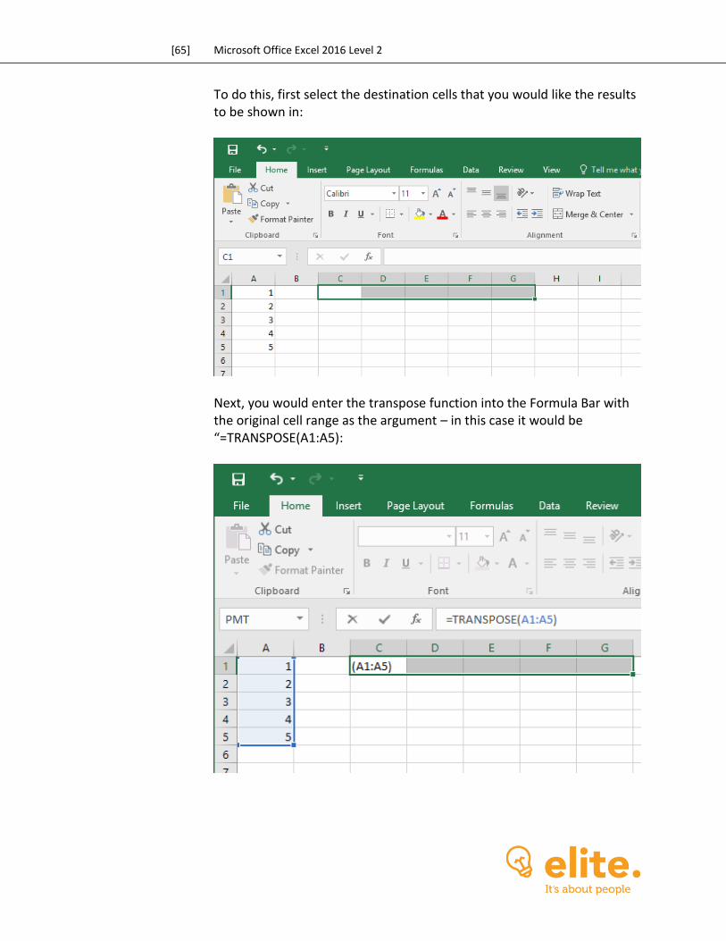
[65] Microsoft Office Excel 2016 Level 2
To do this, first select the destination cells that you would like the results to be shown in:
Next, you would enter the transpose function into the Formula Bar with the original cell range as the argument – in this case it would be “=TRANSPOSE(A1:A5):
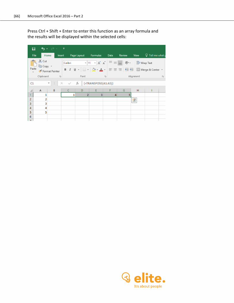
[66] Microsoft Office Excel 2016 – Part 2
Press Ctrl + Shift + Enter to enter this function as an array formula and the results will be displayed within the selected cells:
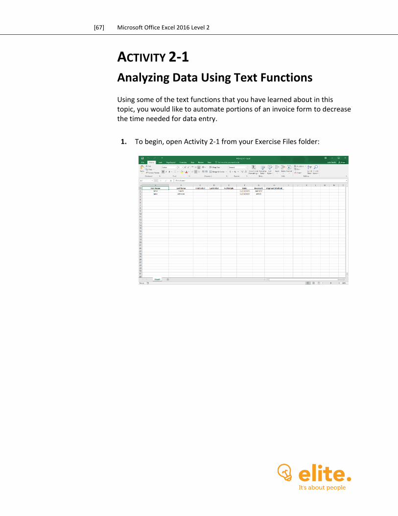
[67] Microsoft Office Excel 2016 Level 2
ACTIVITY 2-1
Analyzing Data Using Text Functions Using some of the text functions that you have learned about in this topic, you would like to automate portions of an invoice form to decrease the time needed for data entry.
1. To begin, open Activity 2-1 from your Exercise Files folder:
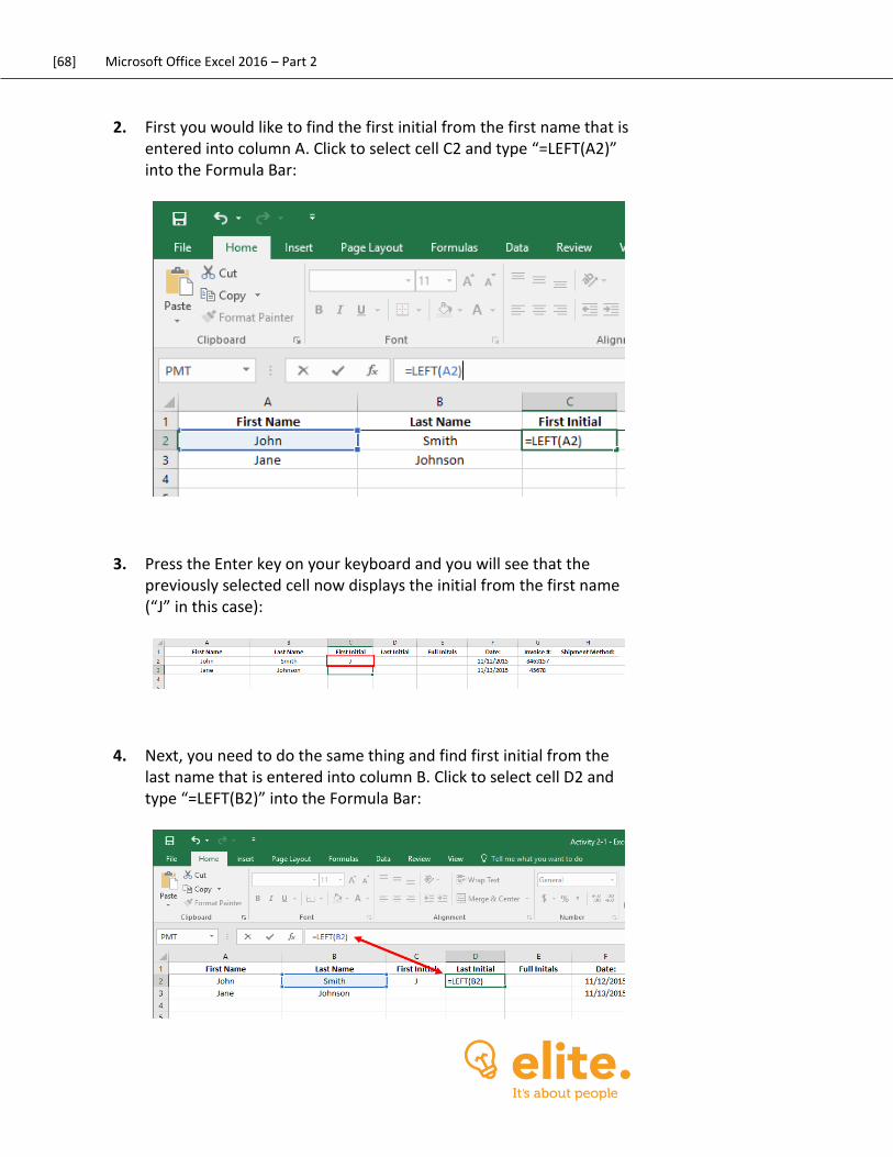
[68] Microsoft Office Excel 2016 – Part 2
2. First you would like to find the first initial from the first name that is entered into column A. Click to select cell C2 and type “=LEFT(A2)” into the Formula Bar:
3. Press the Enter key on your keyboard and you will see that the previously selected cell now displays the initial from the first name (“J” in this case):
4. Next, you need to do the same thing and find first initial from the last name that is entered into column B. Click to select cell D2 and type “=LEFT(B2)” into the Formula Bar:
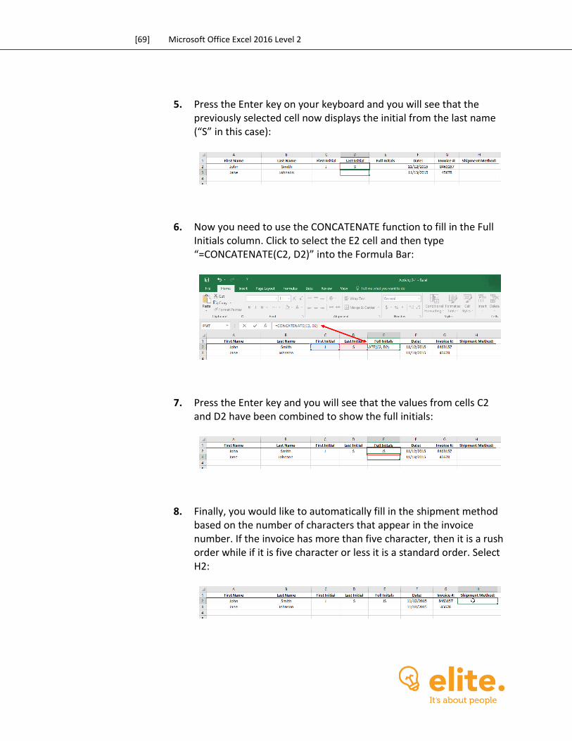
[69] Microsoft Office Excel 2016 Level 2
5. Press the Enter key on your keyboard and you will see that the previously selected cell now displays the initial from the last name (“S” in this case):
6. Now you need to use the CONCATENATE function to fill in the Full Initials column. Click to select the E2 cell and then type “=CONCATENATE(C2, D2)” into the Formula Bar:
7. Press the Enter key and you will see that the values from cells C2 and D2 have been combined to show the full initials:
8. Finally, you would like to automatically fill in the shipment method based on the number of characters that appear in the invoice number. If the invoice has more than five character, then it is a rush order while if it is five character or less it is a standard order. Select H2:
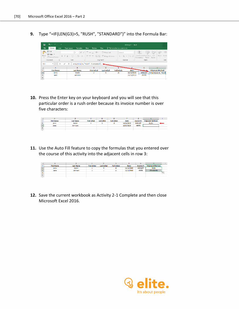
[70] Microsoft Office Excel 2016 – Part 2
9. Type “=IF(LEN(G3)>5, "RUSH", "STANDARD")” into the Formula Bar:
10. Press the Enter key on your keyboard and you will see that this particular order is a rush order because its invoice number is over five characters:
11. Use the Auto Fill feature to copy the formulas that you entered over the course of this activity into the adjacent cells in row 3:
12. Save the current workbook as Activity 2-1 Complete and then close Microsoft Excel 2016.
[71] Microsoft Office Excel 2016 Level 2
TOPIC B: Use Logical Functions Logical functions are used to ask yes or no questions of your data. Over the course of this topic you will learn all about the logical functions that are available in Excel 2016, including the AND, OR, and IF functions. Topic Objectives In this topic, you will learn:
About logical functions About logical operators About the AND function About the OR function About the IF function
LOGICAL FUNCTIONS
Excel contains a collection of logical functions that allow you to essentially ask yes or no questions of your data. Such questions return a positive (TRUE) or negative (FALSE) response. Logical functions also allow you to perform calculations when certain conditions are met. For example, logical functions could be used to ask your data if the sales department met its goals for this quarter. Or, it could be used to find out if the sales department met its goal, and if so, what the bonus would be for the people in that department.
LOGICAL OPERATORS
Logical operators are used to compare two values against one another to see if they meet a specified logical condition. Should the values meet the logical condition (2 > 1) then the output would be the logical value of TRUE. If the values do not meet the logical condition (2 < 1), then the output would instead be FALSE. Due to this behavior, logical operators are instrumental in constructing conditions for functions and calculations to run correctly.
[72] Microsoft Office Excel 2016 – Part 2
Below you will find a table with all of the logical operators that are available in Excel 2016 and what they do:
Operator Symbol Examples with TRUE Result
Equal to = 1 = 1
Greater than > 2 > 1
Less than < 1 < 2
Greater than or equal to >= 2 >= 2 3 >=2
Less than or equal to <= 2 <= 2 1 <=2
Not equal to <> 1 <> 2
THE AND FUNCTION
=AND(logical1, [logical2], …)
This function will return a TRUE value when all of the arguments are true. On the flipside, it will return a FALSE value when all arguments in this function are false. While there can be a varied amount of use cases for this function, you would typically use it for conditional purposes. For example, you could use this function to check if all of the departments in an organization have met all of their goals for the current quarter. The first argument that is required in this function is logical1. You can have up to 30 of these arguments in one AND function with each argument separated by a comma. These arguments are where you enter the logical values and operators that you would like to test for (e.g. A1>B2). Additionally, you also have the option of entering a formula as a single argument. Suppose that A1 contains the value of 15, while cell B1 holds the value 20, and C1 contains 25. Additionally, assume that D1 holds the logical value of FALSE:
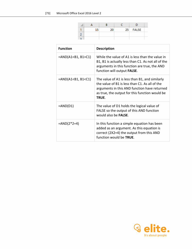
[73] Microsoft Office Excel 2016 Level 2
Function Description
=AND(A1<B1, B1>C1) While the value of A1 is less than the value in B1, B1 is actually less than C1. As not all of the arguments in this function are true, the AND function will output FALSE.
=AND(A1<B1, B1<C1) The value of A1 is less than B1, and similarly the value of B1 is less than C1. As all of the arguments in this AND function have returned as true, the output for this function would be TRUE.
=AND(D1) The value of D1 holds the logical value of FALSE so the output of this AND function would also be FALSE.
=AND(2*2=4) In this function a simple equation has been added as an argument. As this equation is correct (2X2=4) the output from this AND function would be TRUE.
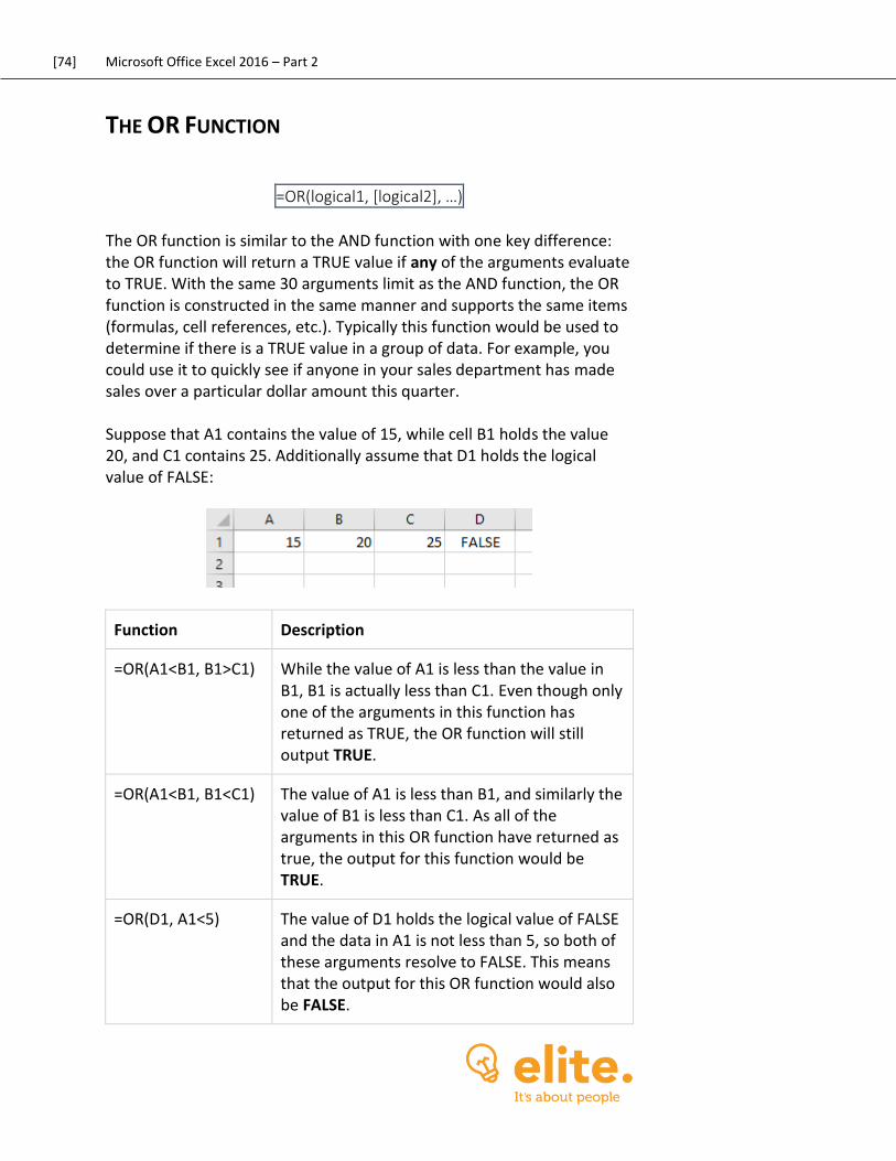
[74] Microsoft Office Excel 2016 – Part 2
THE OR FUNCTION
=OR(logical1, [logical2], …)
The OR function is similar to the AND function with one key difference: the OR function will return a TRUE value if any of the arguments evaluate to TRUE. With the same 30 arguments limit as the AND function, the OR function is constructed in the same manner and supports the same items (formulas, cell references, etc.). Typically this function would be used to determine if there is a TRUE value in a group of data. For example, you could use it to quickly see if anyone in your sales department has made sales over a particular dollar amount this quarter. Suppose that A1 contains the value of 15, while cell B1 holds the value 20, and C1 contains 25. Additionally assume that D1 holds the logical value of FALSE:
Function Description
=OR(A1<B1, B1>C1) While the value of A1 is less than the value in B1, B1 is actually less than C1. Even though only one of the arguments in this function has returned as TRUE, the OR function will still output TRUE.
=OR(A1<B1, B1<C1) The value of A1 is less than B1, and similarly the value of B1 is less than C1. As all of the arguments in this OR function have returned as true, the output for this function would be TRUE.
=OR(D1, A1<5) The value of D1 holds the logical value of FALSE and the data in A1 is not less than 5, so both of these arguments resolve to FALSE. This means that the output for this OR function would also be FALSE.
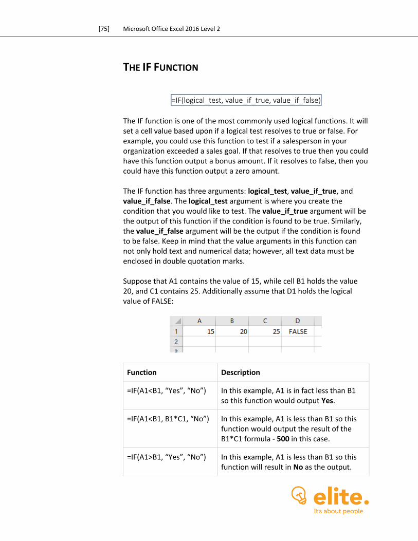
[75] Microsoft Office Excel 2016 Level 2
THE IF FUNCTION
=IF(logical_test, value_if_true, value_if_false)
The IF function is one of the most commonly used logical functions. It will set a cell value based upon if a logical test resolves to true or false. For example, you could use this function to test if a salesperson in your organization exceeded a sales goal. If that resolves to true then you could have this function output a bonus amount. If it resolves to false, then you could have this function output a zero amount. The IF function has three arguments: logical_test, value_if_true, and value_if_false. The logical_test argument is where you create the condition that you would like to test. The value_if_true argument will be the output of this function if the condition is found to be true. Similarly, the value_if_false argument will be the output if the condition is found to be false. Keep in mind that the value arguments in this function can not only hold text and numerical data; however, all text data must be enclosed in double quotation marks. Suppose that A1 contains the value of 15, while cell B1 holds the value 20, and C1 contains 25. Additionally assume that D1 holds the logical value of FALSE:
Function Description
=IF(A1<B1, “Yes”, “No”) In this example, A1 is in fact less than B1 so this function would output Yes.
=IF(A1<B1, B1*C1, “No”) In this example, A1 is less than B1 so this function would output the result of the B1*C1 formula - 500 in this case.
=IF(A1>B1, “Yes”, “No”) In this example, A1 is less than B1 so this function will result in No as the output.
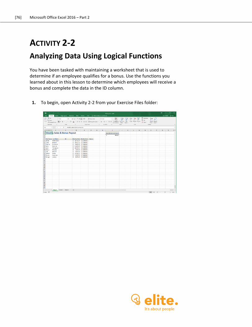
[76] Microsoft Office Excel 2016 – Part 2
ACTIVITY 2-2
Analyzing Data Using Logical Functions You have been tasked with maintaining a worksheet that is used to determine if an employee qualifies for a bonus. Use the functions you learned about in this lesson to determine which employees will receive a bonus and complete the data in the ID column.
1. To begin, open Activity 2-2 from your Exercise Files folder:
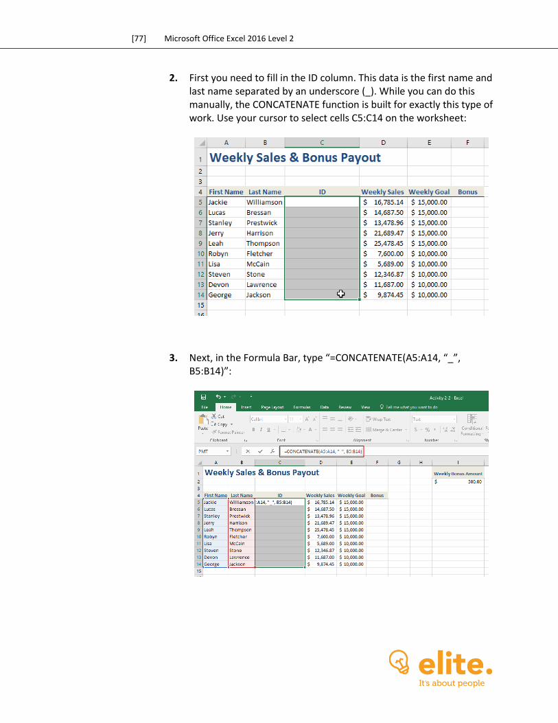
[77] Microsoft Office Excel 2016 Level 2
2. First you need to fill in the ID column. This data is the first name and last name separated by an underscore (_). While you can do this manually, the CONCATENATE function is built for exactly this type of work. Use your cursor to select cells C5:C14 on the worksheet:
3. Next, in the Formula Bar, type “=CONCATENATE(A5:A14, “_”, B5:B14)”:
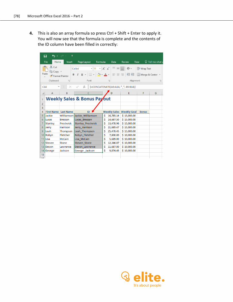
[78] Microsoft Office Excel 2016 – Part 2
4. This is also an array formula so press Ctrl + Shift + Enter to apply it. You will now see that the formula is complete and the contents of the ID column have been filled in correctly:
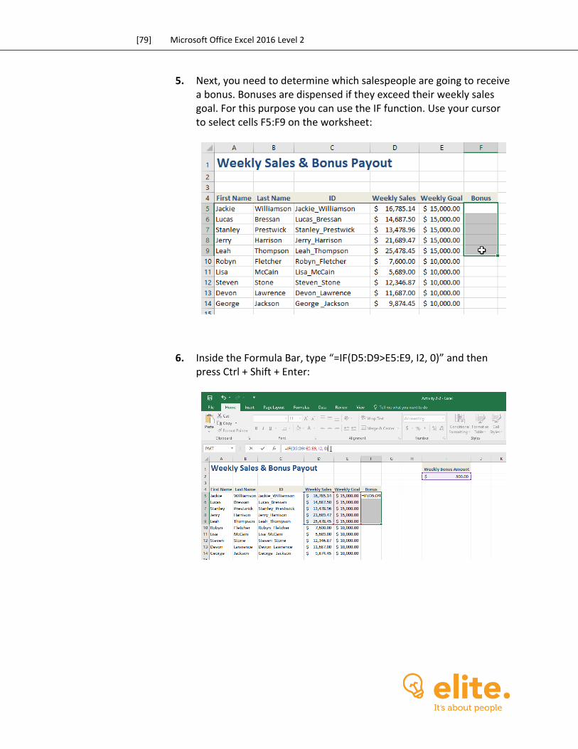
[79] Microsoft Office Excel 2016 Level 2
5. Next, you need to determine which salespeople are going to receive a bonus. Bonuses are dispensed if they exceed their weekly sales goal. For this purpose you can use the IF function. Use your cursor to select cells F5:F9 on the worksheet:
6. Inside the Formula Bar, type “=IF(D5:D9>E5:E9, I2, 0)” and then press Ctrl + Shift + Enter:
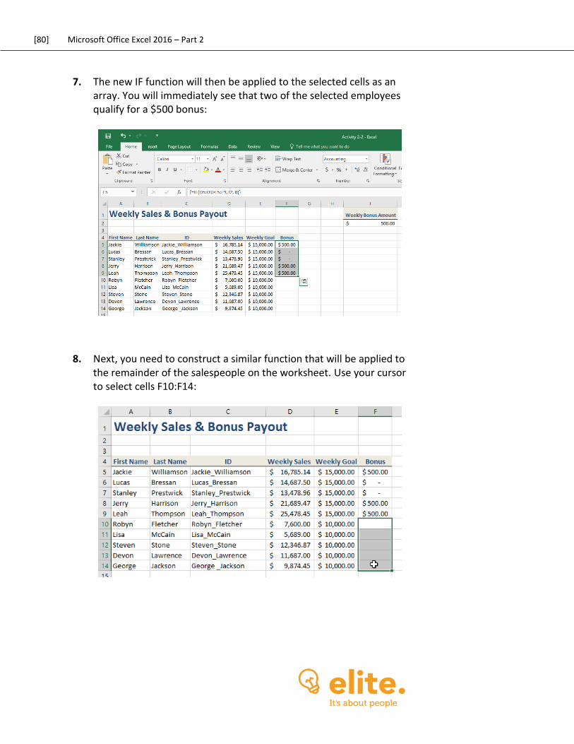
[80] Microsoft Office Excel 2016 – Part 2
7. The new IF function will then be applied to the selected cells as an array. You will immediately see that two of the selected employees qualify for a $500 bonus:
8. Next, you need to construct a similar function that will be applied to the remainder of the salespeople on the worksheet. Use your cursor to select cells F10:F14:
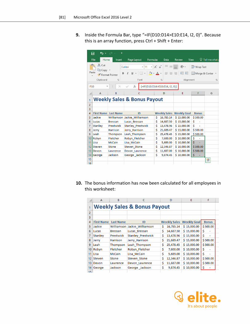
[81] Microsoft Office Excel 2016 Level 2
9. Inside the Formula Bar, type “=IF(D10:D14>E10:E14, I2, 0)”. Because this is an array function, press Ctrl + Shift + Enter:
10. The bonus information has now been calculated for all employees in this worksheet:

[82] Microsoft Office Excel 2016 – Part 2
11. Save your work as Activity 2-2 Complete and then close Microsoft Excel 2016.
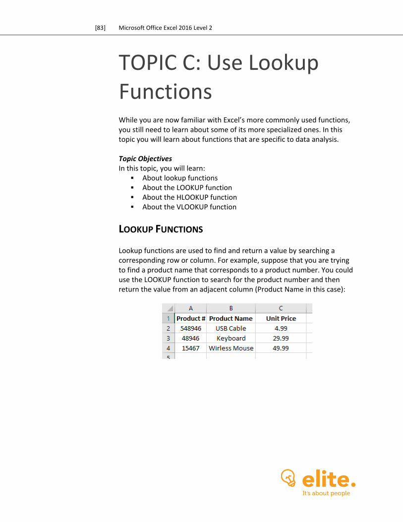
[83] Microsoft Office Excel 2016 Level 2
TOPIC C: Use Lookup Functions While you are now familiar with Excel’s more commonly used functions, you still need to learn about some of its more specialized ones. In this topic you will learn about functions that are specific to data analysis. Topic Objectives In this topic, you will learn:
About lookup functions About the LOOKUP function About the HLOOKUP function About the VLOOKUP function
LOOKUP FUNCTIONS
Lookup functions are used to find and return a value by searching a corresponding row or column. For example, suppose that you are trying to find a product name that corresponds to a product number. You could use the LOOKUP function to search for the product number and then return the value from an adjacent column (Product Name in this case):
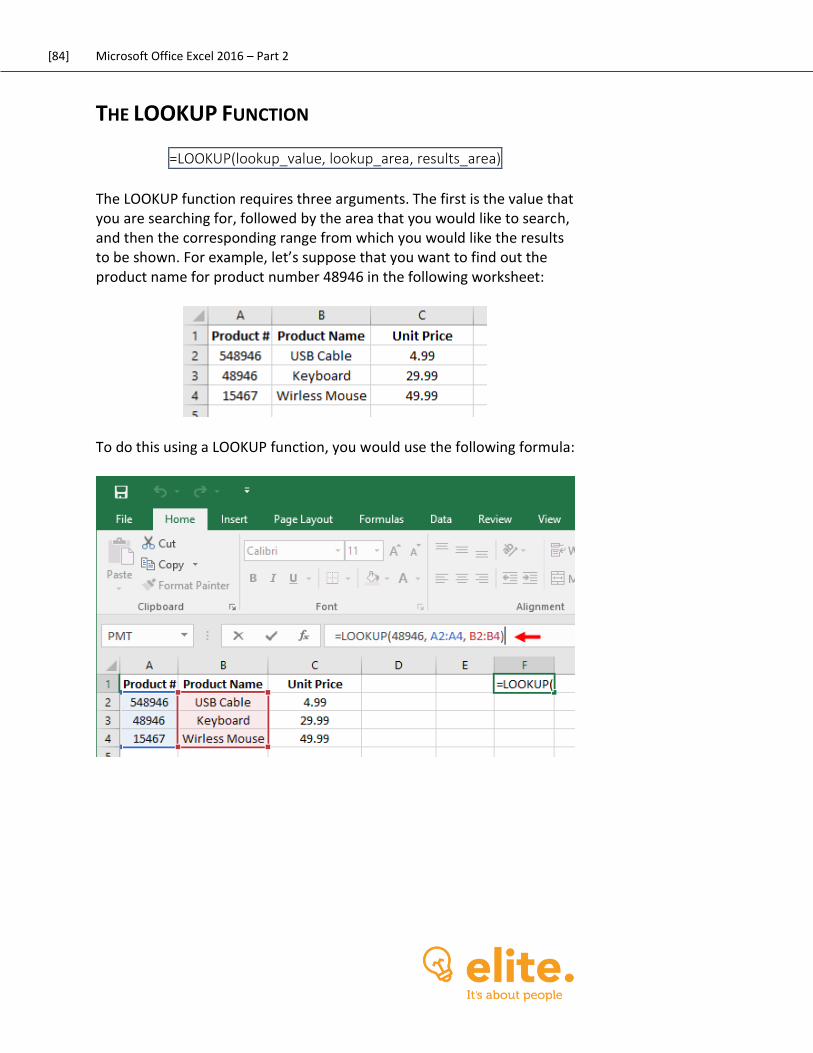
[84] Microsoft Office Excel 2016 – Part 2
THE LOOKUP FUNCTION
=LOOKUP(lookup_value, lookup_area, results_area)
The LOOKUP function requires three arguments. The first is the value that you are searching for, followed by the area that you would like to search, and then the corresponding range from which you would like the results to be shown. For example, let’s suppose that you want to find out the product name for product number 48946 in the following worksheet:
To do this using a LOOKUP function, you would use the following formula:
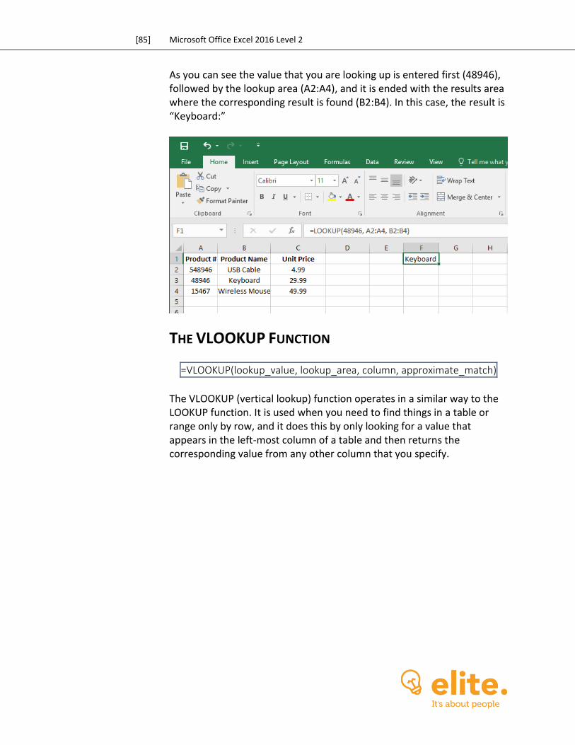
[85] Microsoft Office Excel 2016 Level 2
As you can see the value that you are looking up is entered first (48946), followed by the lookup area (A2:A4), and it is ended with the results area where the corresponding result is found (B2:B4). In this case, the result is “Keyboard:”
THE VLOOKUP FUNCTION
=VLOOKUP(lookup_value, lookup_area, column, approximate_match)
The VLOOKUP (vertical lookup) function operates in a similar way to the LOOKUP function. It is used when you need to find things in a table or range only by row, and it does this by only looking for a value that appears in the left-most column of a table and then returns the corresponding value from any other column that you specify.
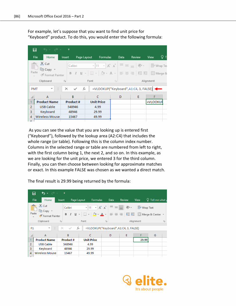
[86] Microsoft Office Excel 2016 – Part 2
For example, let’s suppose that you want to find unit price for “Keyboard” product. To do this, you would enter the following formula:
As you can see the value that you are looking up is entered first (“Keyboard”), followed by the lookup area (A2:C4) that includes the whole range (or table). Following this is the column index number. Columns in the selected range or table are numbered from left to right, with the first column being 1, the next 2, and so on. In this example, as we are looking for the unit price, we entered 3 for the third column. Finally, you can then choose between looking for approximate matches or exact. In this example FALSE was chosen as we wanted a direct match. The final result is 29.99 being returned by the formula:
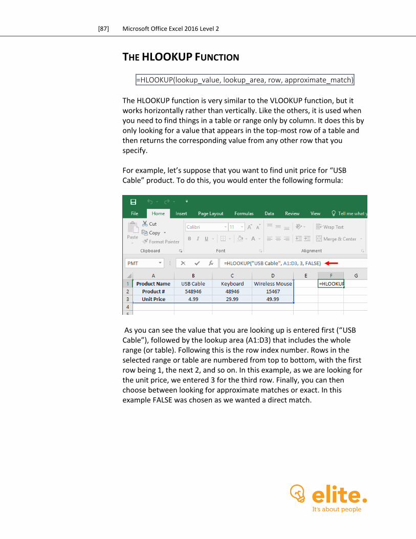
[87] Microsoft Office Excel 2016 Level 2
THE HLOOKUP FUNCTION
=HLOOKUP(lookup_value, lookup_area, row, approximate_match)
The HLOOKUP function is very similar to the VLOOKUP function, but it works horizontally rather than vertically. Like the others, it is used when you need to find things in a table or range only by column. It does this by only looking for a value that appears in the top-most row of a table and then returns the corresponding value from any other row that you specify. For example, let’s suppose that you want to find unit price for “USB Cable” product. To do this, you would enter the following formula:
As you can see the value that you are looking up is entered first (“USB Cable”), followed by the lookup area (A1:D3) that includes the whole range (or table). Following this is the row index number. Rows in the selected range or table are numbered from top to bottom, with the first row being 1, the next 2, and so on. In this example, as we are looking for the unit price, we entered 3 for the third row. Finally, you can then choose between looking for approximate matches or exact. In this example FALSE was chosen as we wanted a direct match.

[88] Microsoft Office Excel 2016 – Part 2
The final result is 4.99 being returned by the formula:
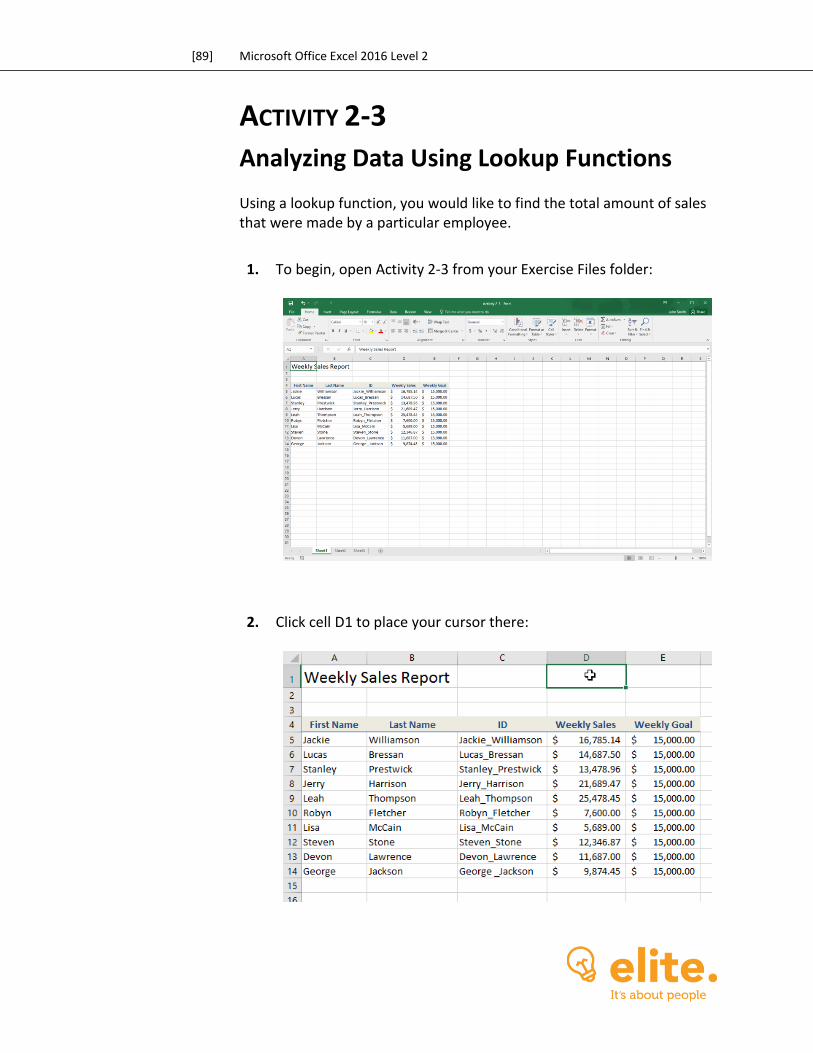
[89] Microsoft Office Excel 2016 Level 2
ACTIVITY 2-3
Analyzing Data Using Lookup Functions Using a lookup function, you would like to find the total amount of sales that were made by a particular employee.
1. To begin, open Activity 2-3 from your Exercise Files folder:
2. Click cell D1 to place your cursor there:

[90] Microsoft Office Excel 2016 – Part 2
3. You would like to find out the weekly sales that Lucas made, so start by typing “=VLOOKUP(“Lucas”,” into the Formula Bar (without the outer most quotation marks):
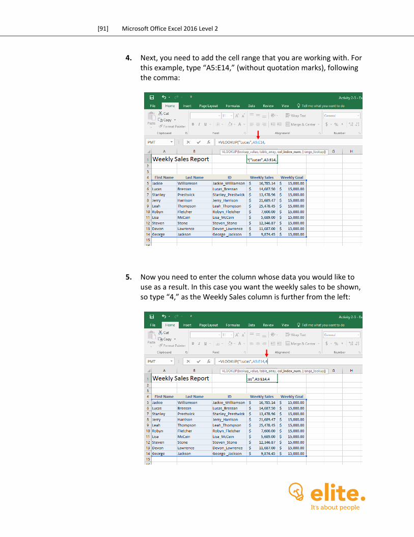
[91] Microsoft Office Excel 2016 Level 2
4. Next, you need to add the cell range that you are working with. For this example, type “A5:E14,” (without quotation marks), following the comma:
5. Now you need to enter the column whose data you would like to use as a result. In this case you want the weekly sales to be shown, so type “4,” as the Weekly Sales column is further from the left:
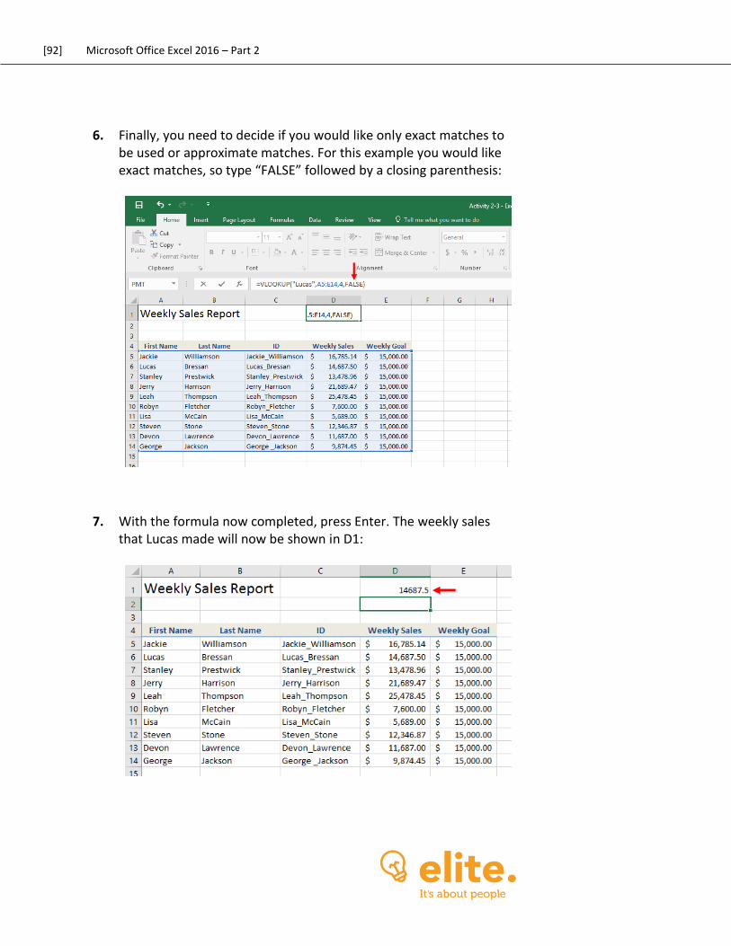
[92] Microsoft Office Excel 2016 – Part 2
6. Finally, you need to decide if you would like only exact matches to be used or approximate matches. For this example you would like exact matches, so type “FALSE” followed by a closing parenthesis:
7. With the formula now completed, press Enter. The weekly sales that Lucas made will now be shown in D1:

[93] Microsoft Office Excel 2016 Level 2
8. Save the changes that you have made to the workbook as Activity 2-3 Complete and then close Microsoft Excel 2016 to complete this exercise.

[94] Microsoft Office Excel 2016 – Part 2
TOPIC D: Use Date Functions Entering the current date and time into a worksheet is one of the more common tasks that you will complete using Excel. Over the course of this topic, you will learn how to add date information using the TODAY and NOW date functions. Topic Objectives In this topic, you will learn:
About the TODAY function About the NOW function How to serialize dates and times with functions
THE TODAY FUNCTION
About as simple as a function can get, the TODAY function has no arguments:
=TODAY()
When executed, it will simply print today’s date into a cell:
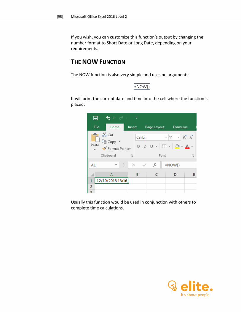
[95] Microsoft Office Excel 2016 Level 2
If you wish, you can customize this function’s output by changing the number format to Short Date or Long Date, depending on your requirements.
THE NOW FUNCTION
The NOW function is also very simple and uses no arguments:
=NOW()
It will print the current date and time into the cell where the function is placed:
Usually this function would be used in conjunction with others to complete time calculations.
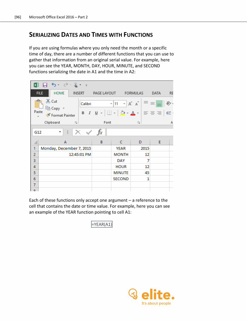
[96] Microsoft Office Excel 2016 – Part 2
SERIALIZING DATES AND TIMES WITH FUNCTIONS
If you are using formulas where you only need the month or a specific time of day, there are a number of different functions that you can use to gather that information from an original serial value. For example, here you can see the YEAR, MONTH, DAY, HOUR, MINUTE, and SECOND functions serializing the date in A1 and the time in A2:
Each of these functions only accept one argument – a reference to the cell that contains the date or time value. For example, here you can see an example of the YEAR function pointing to cell A1:
=YEAR(A1)
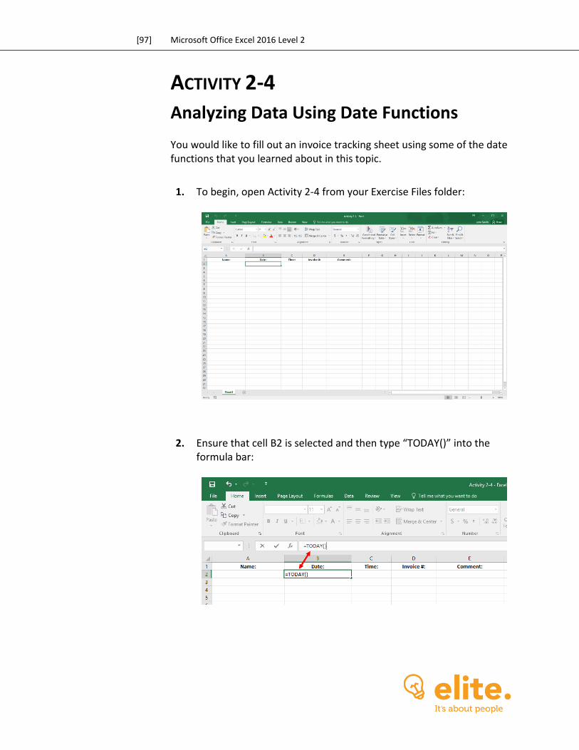
[97] Microsoft Office Excel 2016 Level 2
ACTIVITY 2-4
Analyzing Data Using Date Functions You would like to fill out an invoice tracking sheet using some of the date functions that you learned about in this topic.
1. To begin, open Activity 2-4 from your Exercise Files folder:
2. Ensure that cell B2 is selected and then type “TODAY()” into the formula bar:
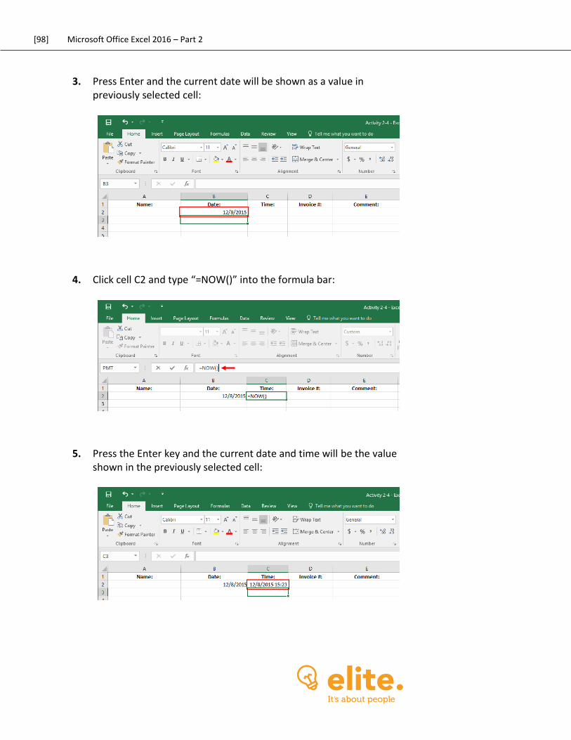
[98] Microsoft Office Excel 2016 – Part 2
3. Press Enter and the current date will be shown as a value in previously selected cell:
4. Click cell C2 and type “=NOW()” into the formula bar:
5. Press the Enter key and the current date and time will be the value shown in the previously selected cell:
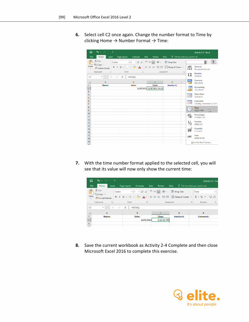
[99] Microsoft Office Excel 2016 Level 2
6. Select cell C2 once again. Change the number format to Time by clicking Home → Number Format → Time:
7. With the time number format applied to the selected cell, you will see that its value will now only show the current time:
8. Save the current workbook as Activity 2-4 Complete and then close Microsoft Excel 2016 to complete this exercise.
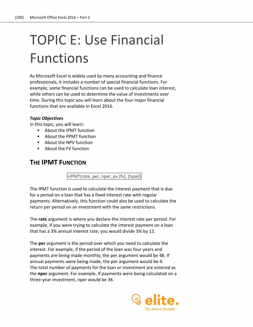
[100] Microsoft Office Excel 2016 – Part 2
TOPIC E: Use Financial Functions As Microsoft Excel is widely used by many accounting and finance professionals, it includes a number of special financial functions. For example, some financial functions can be used to calculate loan interest, while others can be used to determine the value of investments over time. During this topic you will learn about the four major financial functions that are available in Excel 2016. Topic Objectives In this topic, you will learn:
About the IPMT function About the PPMT function About the NPV function About the FV function
THE IPMT FUNCTION
=IPMT(rate, per, nper, pv [fv], [type])
The IPMT function is used to calculate the interest payment that is due for a period on a loan that has a fixed interest rate with regular payments. Alternatively, this function could also be used to calculate the return per period on an investment with the same restrictions. The rate argument is where you declare the interest rate per period. For example, if you were trying to calculate the interest payment on a loan that has a 3% annual interest rate, you would divide 3% by 12. The per argument is the period over which you need to calculate the interest. For example, if the period of the loan was four years and payments are being made monthly, the per argument would be 48. If annual payments were being made, the per argument would be 4. The total number of payments for the loan or investment are entered as the nper argument. For example, if payments were being calculated on a three-year investment, nper would be 36.
[101] Microsoft Office Excel 2016 Level 2
Finally, the pv argument is where you enter the principal of the loan or total amount of money being invested. In addition to the required argument, the IPMT function includes two optional arguments: fv and type. The fv argument is used to enter the future value of the investment after all payments have been made to it, or if working with a loan the balance of the loan. If you choose not set this argument, it will default to 0 (the typical balance of a loan after all the payments are made). Finally, the type argument is used to indicate if payments are due at the end of each payment period (indicated by “0” or by omitting the argument), or at the beginning (indicated by “1”). If left blank, this argument will default to 0. Suppose that in a worksheet, A1 contains the value of $15,000, while cell B1 holds the value 6%, and C1 contains the value 4:
With that information in mind, below you can see how an IPMT function could be constructed to determine how much interest the borrower would owe one and a half years into the four year loan:
Function Description Result
=IPMT(B1/12, 18, C1*12, A1) This function will calculate the how much interest a borrower will owe for the loan (A1), one and a half years into the term (18) with an annual interest rate of 6% (B1/12) and a total term of four years (C1*12).
($50.46)
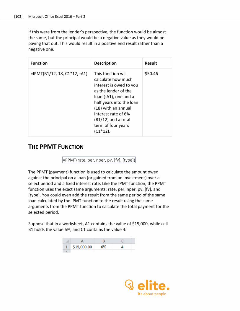
[102] Microsoft Office Excel 2016 – Part 2
If this were from the lender’s perspective, the function would be almost the same, but the principal would be a negative value as they would be paying that out. This would result in a positive end result rather than a negative one.
Function Description Result
=IPMT(B1/12, 18, C1*12, -A1) This function will calculate how much interest is owed to you as the lender of the loan (-A1), one and a half years into the loan (18) with an annual interest rate of 6% (B1/12) and a total term of four years (C1*12).
$50.46
THE PPMT FUNCTION
=PPMT(rate, per, nper, pv, [fv], [type])
The PPMT (payment) function is used to calculate the amount owed against the principal on a loan (or gained from an investment) over a select period and a fixed interest rate. Like the IPMT function, the PPMT function uses the exact same arguments: rate, per, nper, pv, [fv], and [type]. You could even add the result from the same period of the same loan calculated by the IPMT function to the result using the same arguments from the PPMT function to calculate the total payment for the selected period. Suppose that in a worksheet, A1 contains the value of $15,000, while cell B1 holds the value 6%, and C1 contains the value 4:
[103] Microsoft Office Excel 2016 Level 2
With that information in mind, below you can see how a PPMT function could be constructed to determine the required payment on the principal of a loan, one and a half years into the four year loan:
Function Description Result
=PPMT(B1/12, 18, C1*12, A1) This function will calculate the amount owed to the principal of a loan (A1), one and a half years into the loan (18) with an annual interest rate of 6% (B1/12) and a total term of four years (C1*12).
$(301.81)
THE NPV FUNCTION
=NPV(rate, value1, [value2], …)
If you are unfamiliar with NPV (net present value) calculations, they are used to compare the value of money today to the value of money in the future, taking inflation and returns into account. In particular, the NPV function is used to calculate the net present value of an asset or investment using the estimated (or known) future cash flow, as well as the discount rate per period. The rate argument in this function is used to declare the discount rate per period. The value arguments are used to represent any future cash flow. For example, suppose that an initial cost of $75,000 was incurred (A1) with a discount rate of 9% (A2). The cash flows for the next consecutive four years are $16,000, $14,000, $12,000, and $10,000 (A3:A6) respectively:
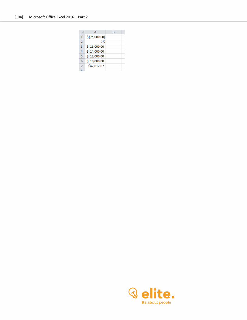
[104] Microsoft Office Excel 2016 – Part 2
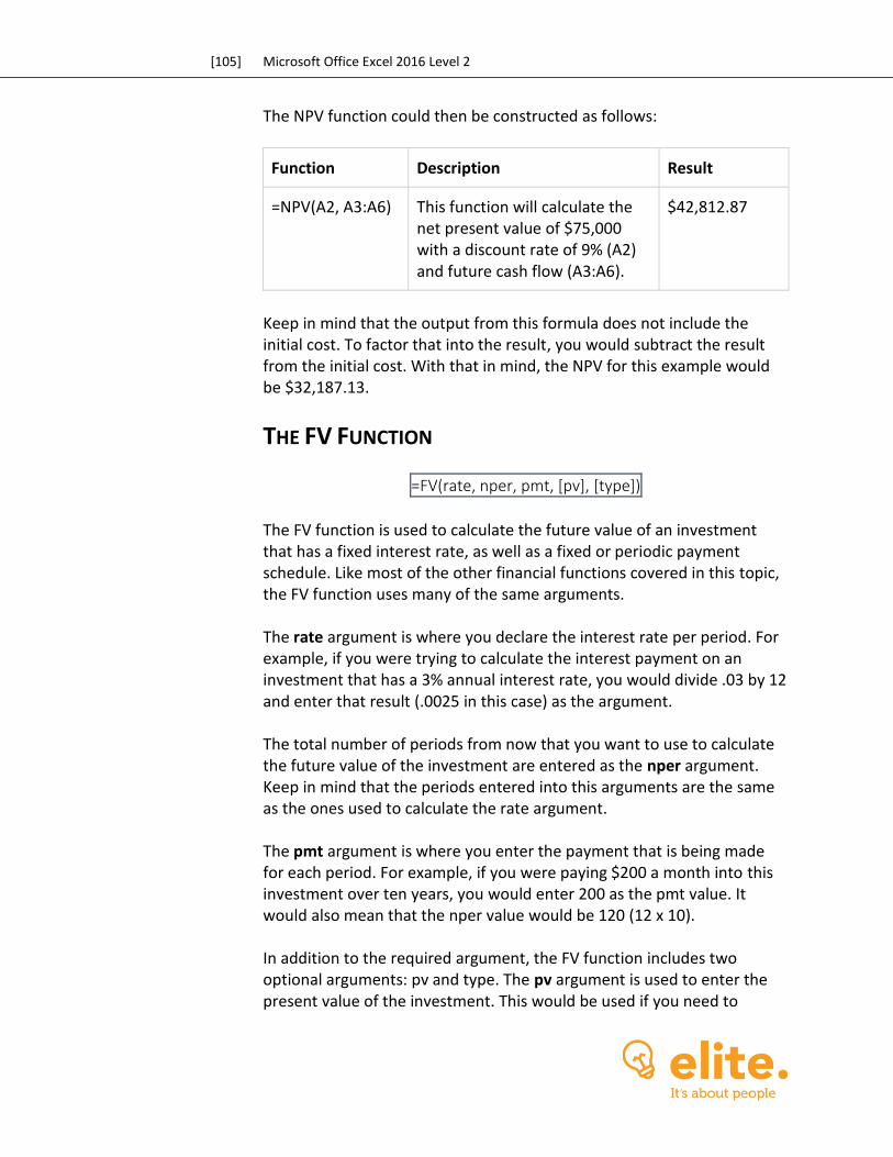
[105] Microsoft Office Excel 2016 Level 2
The NPV function could then be constructed as follows:
Function Description Result
=NPV(A2, A3:A6) This function will calculate the net present value of $75,000 with a discount rate of 9% (A2) and future cash flow (A3:A6).
$42,812.87
Keep in mind that the output from this formula does not include the initial cost. To factor that into the result, you would subtract the result from the initial cost. With that in mind, the NPV for this example would be $32,187.13.
THE FV FUNCTION
=FV(rate, nper, pmt, [pv], [type])
The FV function is used to calculate the future value of an investment that has a fixed interest rate, as well as a fixed or periodic payment schedule. Like most of the other financial functions covered in this topic, the FV function uses many of the same arguments. The rate argument is where you declare the interest rate per period. For example, if you were trying to calculate the interest payment on an investment that has a 3% annual interest rate, you would divide .03 by 12 and enter that result (.0025 in this case) as the argument. The total number of periods from now that you want to use to calculate the future value of the investment are entered as the nper argument. Keep in mind that the periods entered into this arguments are the same as the ones used to calculate the rate argument. The pmt argument is where you enter the payment that is being made for each period. For example, if you were paying $200 a month into this investment over ten years, you would enter 200 as the pmt value. It would also mean that the nper value would be 120 (12 x 10). In addition to the required argument, the FV function includes two optional arguments: pv and type. The pv argument is used to enter the present value of the investment. This would be used if you need to
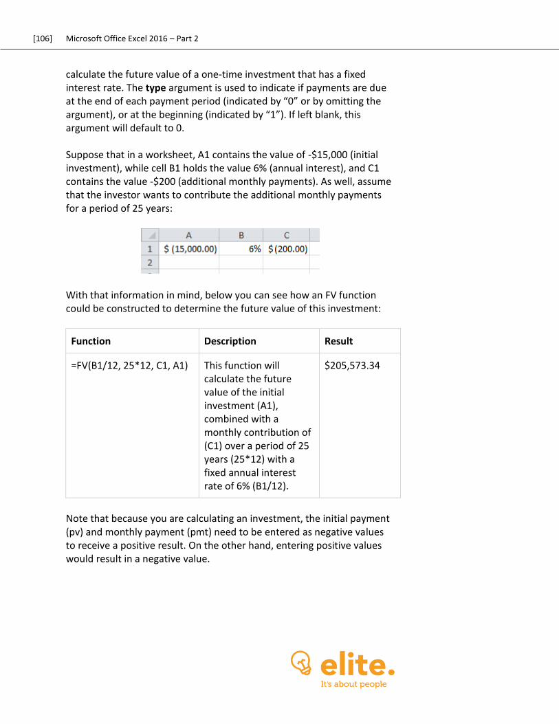
[106] Microsoft Office Excel 2016 – Part 2
calculate the future value of a one-time investment that has a fixed interest rate. The type argument is used to indicate if payments are due at the end of each payment period (indicated by “0” or by omitting the argument), or at the beginning (indicated by “1”). If left blank, this argument will default to 0. Suppose that in a worksheet, A1 contains the value of -$15,000 (initial investment), while cell B1 holds the value 6% (annual interest), and C1 contains the value -$200 (additional monthly payments). As well, assume that the investor wants to contribute the additional monthly payments for a period of 25 years:
With that information in mind, below you can see how an FV function could be constructed to determine the future value of this investment:
Function Description Result
=FV(B1/12, 25*12, C1, A1) This function will calculate the future value of the initial investment (A1), combined with a monthly contribution of (C1) over a period of 25 years (25*12) with a fixed annual interest rate of 6% (B1/12).
$205,573.34
Note that because you are calculating an investment, the initial payment (pv) and monthly payment (pmt) need to be entered as negative values to receive a positive result. On the other hand, entering positive values would result in a negative value.
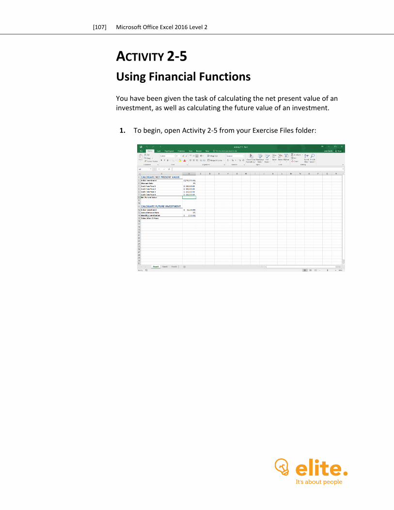
[107] Microsoft Office Excel 2016 Level 2
ACTIVITY 2-5
Using Financial Functions You have been given the task of calculating the net present value of an investment, as well as calculating the future value of an investment.
1. To begin, open Activity 2-5 from your Exercise Files folder:
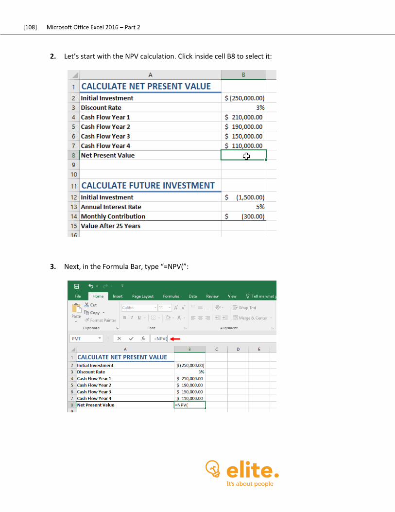
[108] Microsoft Office Excel 2016 – Part 2
2. Let’s start with the NPV calculation. Click inside cell B8 to select it:
3. Next, in the Formula Bar, type “=NPV(”:
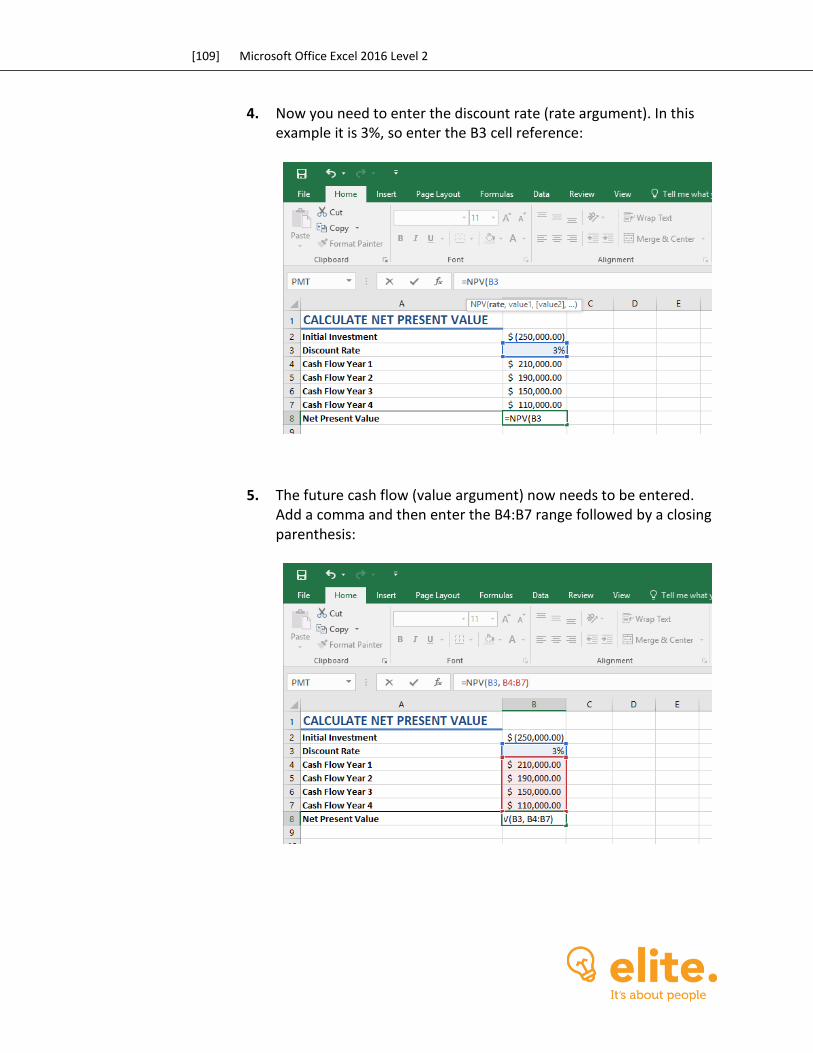
[109] Microsoft Office Excel 2016 Level 2
4. Now you need to enter the discount rate (rate argument). In this example it is 3%, so enter the B3 cell reference:
5. The future cash flow (value argument) now needs to be entered. Add a comma and then enter the B4:B7 range followed by a closing parenthesis:
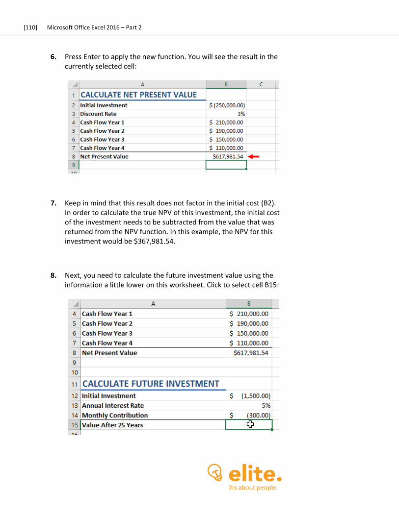
[110] Microsoft Office Excel 2016 – Part 2
6. Press Enter to apply the new function. You will see the result in the currently selected cell:
7. Keep in mind that this result does not factor in the initial cost (B2). In order to calculate the true NPV of this investment, the initial cost of the investment needs to be subtracted from the value that was returned from the NPV function. In this example, the NPV for this investment would be $367,981.54.
8. Next, you need to calculate the future investment value using the information a little lower on this worksheet. Click to select cell B15:
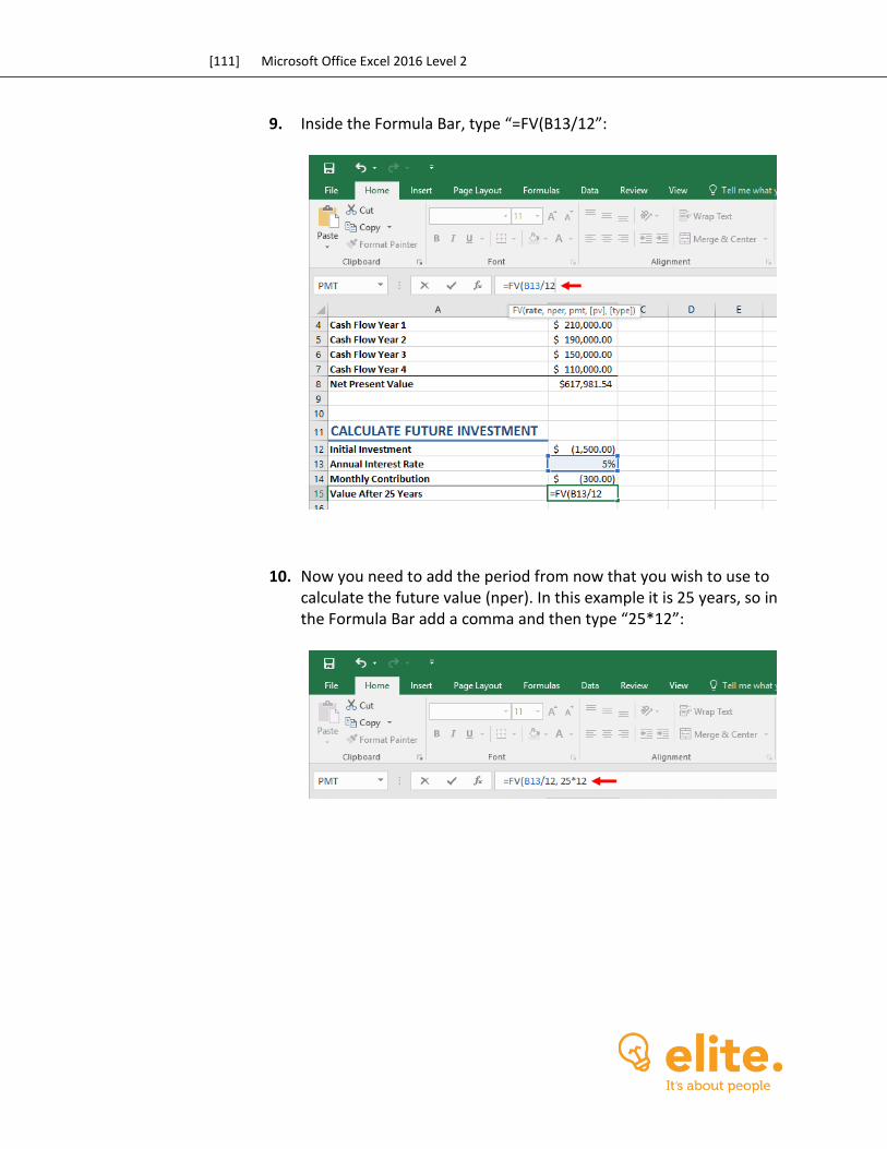
[111] Microsoft Office Excel 2016 Level 2
9. Inside the Formula Bar, type “=FV(B13/12”:
10. Now you need to add the period from now that you wish to use to calculate the future value (nper). In this example it is 25 years, so in the Formula Bar add a comma and then type “25*12”:
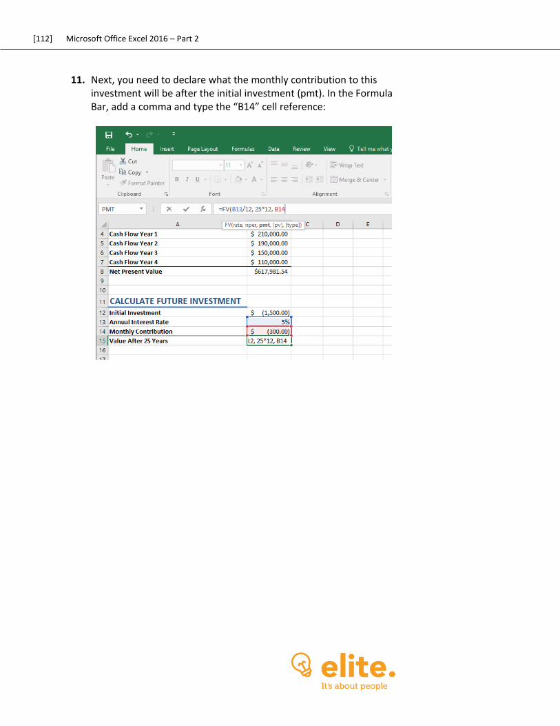
[112] Microsoft Office Excel 2016 – Part 2
11. Next, you need to declare what the monthly contribution to this investment will be after the initial investment (pmt). In the Formula Bar, add a comma and type the “B14” cell reference:
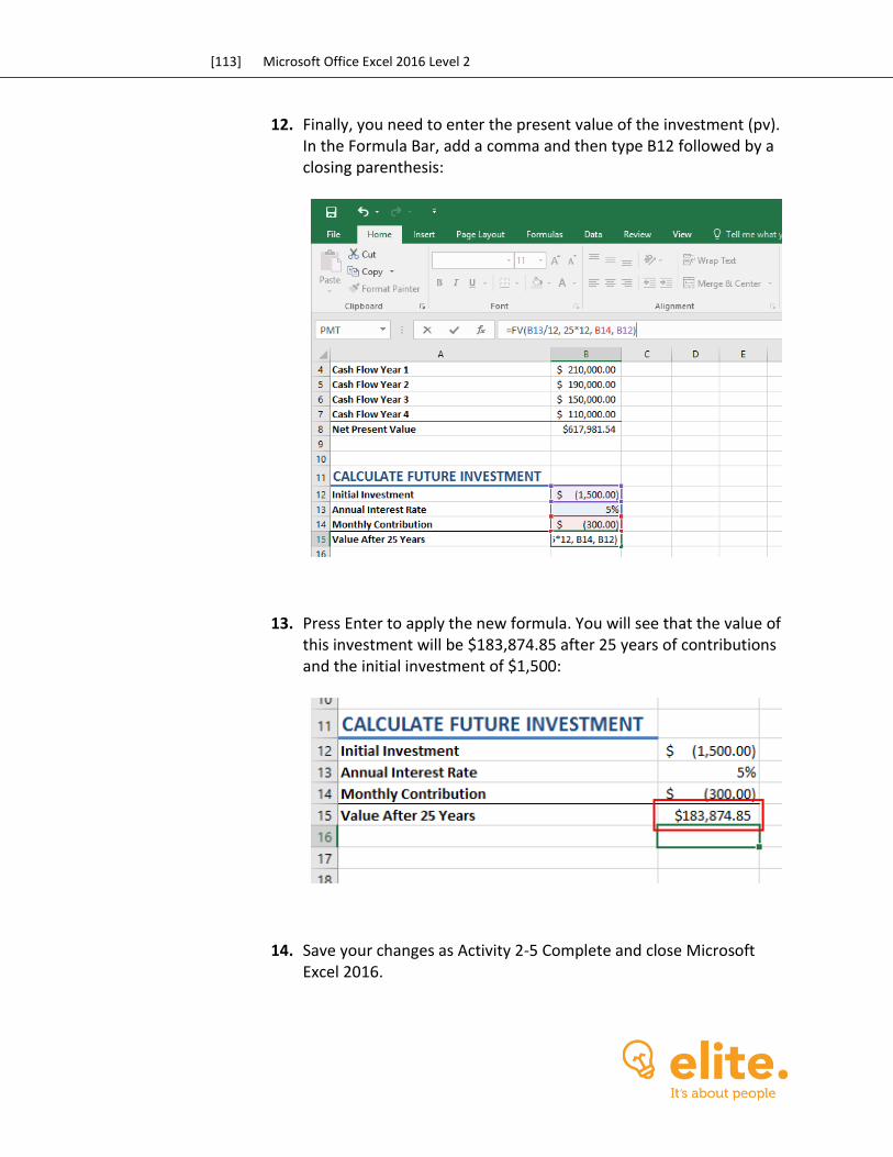
[113] Microsoft Office Excel 2016 Level 2
12. Finally, you need to enter the present value of the investment (pv). In the Formula Bar, add a comma and then type B12 followed by a closing parenthesis:
13. Press Enter to apply the new formula. You will see that the value of this investment will be $183,874.85 after 25 years of contributions and the initial investment of $1,500:
14. Save your changes as Activity 2-5 Complete and close Microsoft Excel 2016.
[114] Microsoft Office Excel 2016 – Part 2
Summary Over the course of this lesson you learned how to analyze data in your worksheets using a variety of different functions. You learned how to use text functions to manage and manipulate text, as well as date functions to return date information. Additionally, you learned about the many different financial functions that you have available to you and how they operate.
REVIEW QUESTIONS
1. What is the TRIM function used for?
2. What is the CONCATENATE function used for?
3. What are the only two possible outputs from a logical function?
4. What is the difference between the TODAY function and the NOW function?
5. What is the FV function used for?

[115] Microsoft Office Excel 2016 Level 2
[116] Microsoft Office Excel 2016 – Part 2
LESSON 3: ORGANIZING
WORKSHEET DATA
WITH TABLES
Lesson Objectives
In this lesson you will learn how to:
Create and modify tables
Sort data and filter data
Use subtotal features and database functions
[117] Microsoft Office Excel 2016 Level 2
TOPIC A: Create and Modify Tables While formulas and functions are great at analyzing data within your workbook, they are more apt at analyzing entire workbooks rather than specific sets of data. If you need to analyze smaller sets of data within a large workbook or break down large sets of data into smaller parts, then converting your data into tables is often the best solution. Tables allow you to use Excel’s powerful organizational capabilities without modifying the data itself. Using tables you can narrow down specific data, focus on only the important information, and more. Topic Objectives In this topic, you will learn:
About tables About the components of a table How to use the Create Table dialog box About the Table Tools – Design contextual tab How to use and apply table styles, as well as Quick Styles How to customize row display About table modification options
TABLES
A table is a specially designated range of information that has added functionality. You can have multiple tables per worksheet, and tables can be as large or small as the amount of data you want to work with. Tables can be created from existing data ranges or from empty ranges and then populated afterwards. Once a table has been created, it will automatically be given a generic name such as “Table1” or “Table2” depending upon the number of tables present in the current worksheet; however, these names can be changed at any time. Additionally, tables are flexible in that you can convert a table back to a normal range at any point without affecting the contents. A table is made from adjacent columns of data, with a unique label or heading for each column. Columns and rows may be added to a table just as you would when working with a normal range.
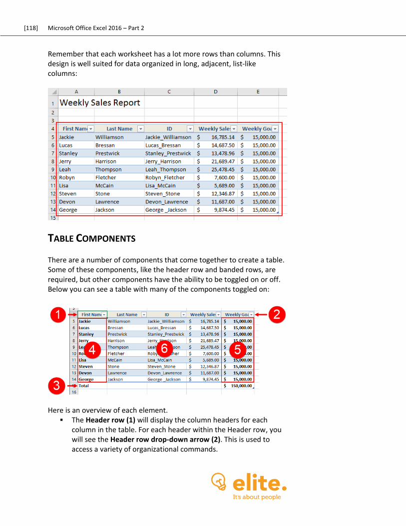
[118] Microsoft Office Excel 2016 – Part 2
Remember that each worksheet has a lot more rows than columns. This design is well suited for data organized in long, adjacent, list-like columns:
TABLE COMPONENTS
There are a number of components that come together to create a table. Some of these components, like the header row and banded rows, are required, but other components have the ability to be toggled on or off. Below you can see a table with many of the components toggled on:
Here is an overview of each element.
The Header row (1) will display the column headers for each column in the table. For each header within the Header row, you will see the Header row drop-down arrow (2). This is used to access a variety of organizational commands.
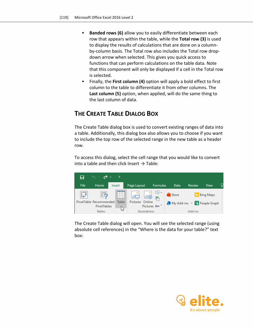
[119] Microsoft Office Excel 2016 Level 2
Banded rows (6) allow you to easily differentiate between each row that appears within the table, while the Total row (3) is used to display the results of calculations that are done on a column-by-column basis. The Total row also includes the Total row drop-down arrow when selected. This gives you quick access to functions that can perform calculations on the table data. Note that this component will only be displayed if a cell in the Total row is selected.
Finally, the First column (4) option will apply a bold effect to first column to the table to differentiate it from other columns. The Last column (5) option, when applied, will do the same thing to the last column of data.
THE CREATE TABLE DIALOG BOX
The Create Table dialog box is used to convert existing ranges of data into a table. Additionally, this dialog box also allows you to choose if you want to include the top row of the selected range in the new table as a header row. To access this dialog, select the cell range that you would like to convert into a table and then click Insert → Table:
The Create Table dialog will open. You will see the selected range (using absolute cell references) in the “Where is the data for your table?” text box:

[120] Microsoft Office Excel 2016 – Part 2
Clicking the OK button will convert the selected cell range into a table.
THE TABLE TOOLS – DESIGN CONTEXTUAL TAB
Whenever you are working with a table, the Table Tools – Design contextual tab will appear on the ribbon. Using the controls on this tab, you can modify just about any aspect of your table:
Here is a brief description of the various groups that on this tab and the commands and options that they contain.
Properties This group allows you to view and edit the current table’s name. You can also redefine the table size using the Resize Table command.
Tools Within this group, the Remove Duplicates command allows you to remove duplicate values from the current table. The “Summarize with PivotTable” command will create a PivotTable out of the current table, and the “Convert to Range” command will convert it back to a regular range. You can also insert a slicer into the table using the Insert Slicer command.
External Table Data The commands in this group are used to export table data to other applications, as well as manage data links to external resources.
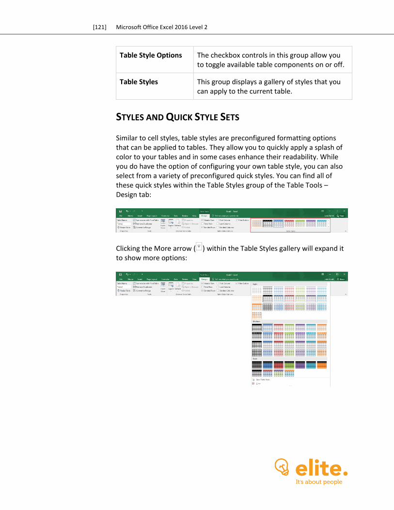
[121] Microsoft Office Excel 2016 Level 2
Table Style Options The checkbox controls in this group allow you to toggle available table components on or off.
Table Styles This group displays a gallery of styles that you can apply to the current table.
STYLES AND QUICK STYLE SETS
Similar to cell styles, table styles are preconfigured formatting options that can be applied to tables. They allow you to quickly apply a splash of color to your tables and in some cases enhance their readability. While you do have the option of configuring your own table style, you can also select from a variety of preconfigured quick styles. You can find all of these quick styles within the Table Styles group of the Table Tools – Design tab:
Clicking the More arrow ( ) within the Table Styles gallery will expand it to show more options:
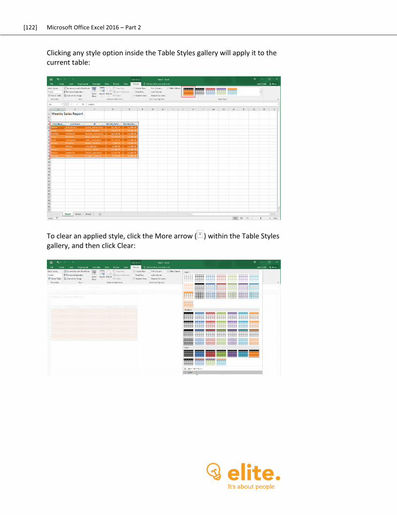
[122] Microsoft Office Excel 2016 – Part 2
Clicking any style option inside the Table Styles gallery will apply it to the current table:
To clear an applied style, click the More arrow ( ) within the Table Styles gallery, and then click Clear:
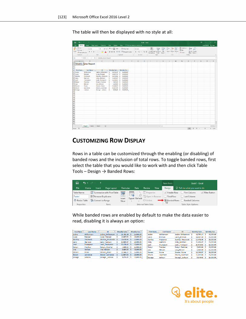
[123] Microsoft Office Excel 2016 Level 2
The table will then be displayed with no style at all:
CUSTOMIZING ROW DISPLAY
Rows in a table can be customized through the enabling (or disabling) of banded rows and the inclusion of total rows. To toggle banded rows, first select the table that you would like to work with and then click Table Tools – Design → Banded Rows:
While banded rows are enabled by default to make the data easier to read, disabling it is always an option:
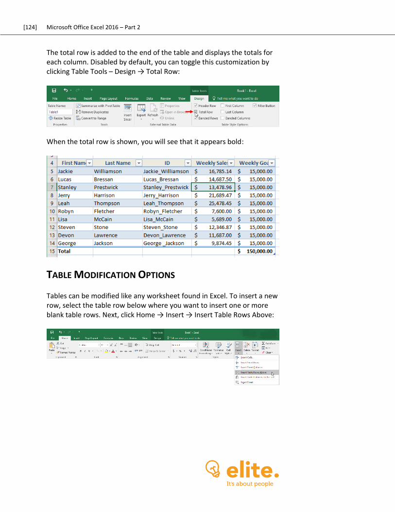
[124] Microsoft Office Excel 2016 – Part 2
The total row is added to the end of the table and displays the totals for each column. Disabled by default, you can toggle this customization by clicking Table Tools – Design → Total Row:
When the total row is shown, you will see that it appears bold:
TABLE MODIFICATION OPTIONS
Tables can be modified like any worksheet found in Excel. To insert a new row, select the table row below where you want to insert one or more blank table rows. Next, click Home → Insert → Insert Table Rows Above:
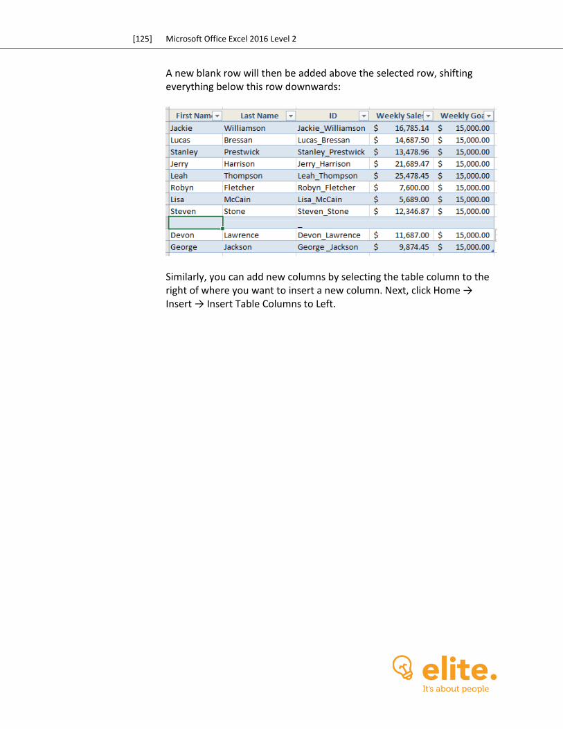
[125] Microsoft Office Excel 2016 Level 2
A new blank row will then be added above the selected row, shifting everything below this row downwards:
Similarly, you can add new columns by selecting the table column to the right of where you want to insert a new column. Next, click Home → Insert → Insert Table Columns to Left.
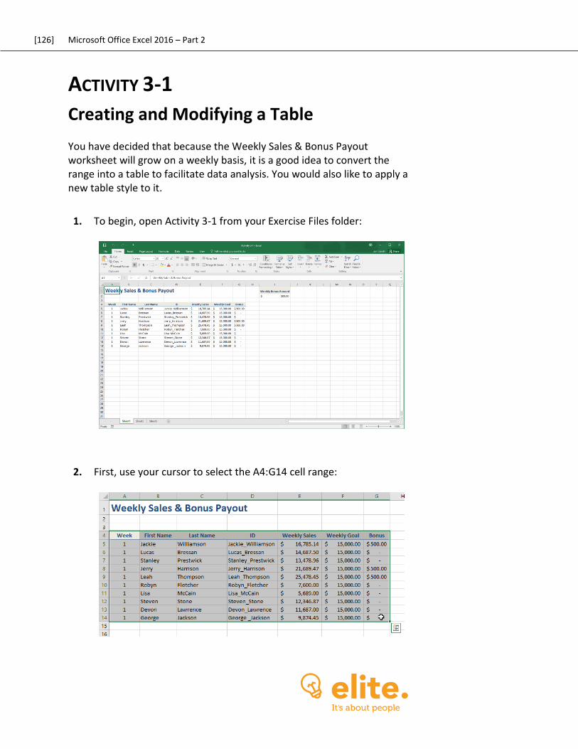
[126] Microsoft Office Excel 2016 – Part 2
ACTIVITY 3-1
Creating and Modifying a Table You have decided that because the Weekly Sales & Bonus Payout worksheet will grow on a weekly basis, it is a good idea to convert the range into a table to facilitate data analysis. You would also like to apply a new table style to it.
1. To begin, open Activity 3-1 from your Exercise Files folder:
2. First, use your cursor to select the A4:G14 cell range:
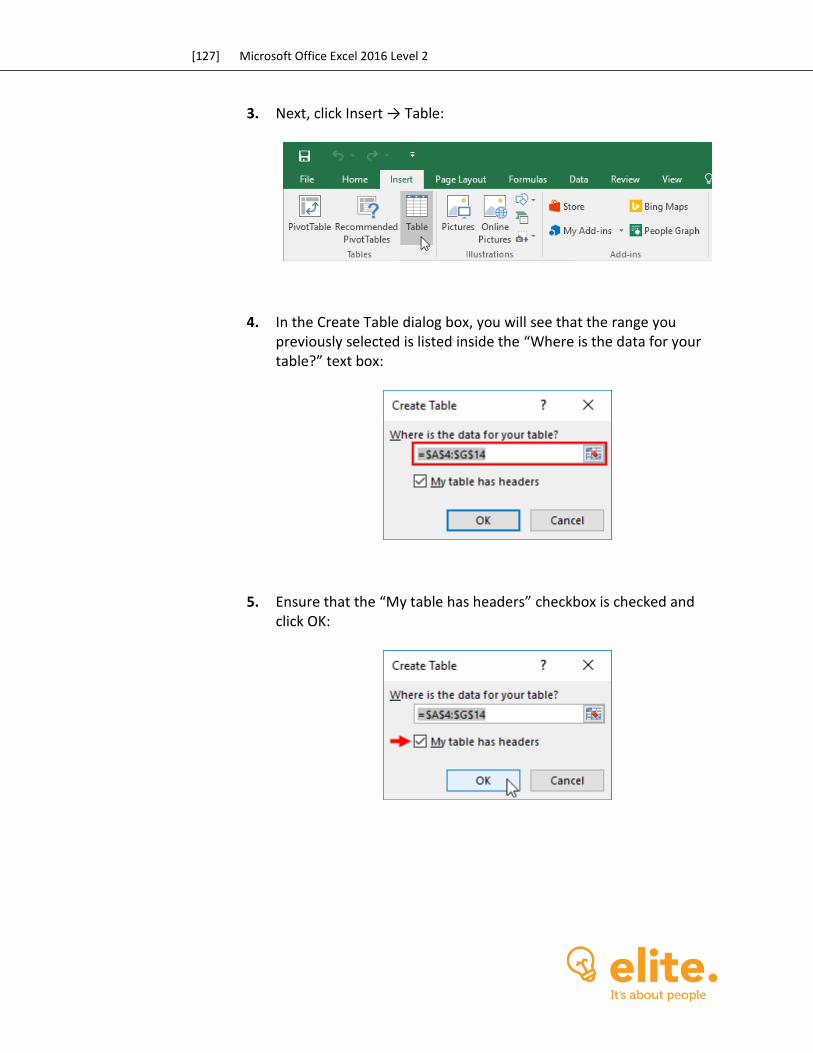
[127] Microsoft Office Excel 2016 Level 2
3. Next, click Insert → Table:
4. In the Create Table dialog box, you will see that the range you previously selected is listed inside the “Where is the data for your table?” text box:
5. Ensure that the “My table has headers” checkbox is checked and click OK:
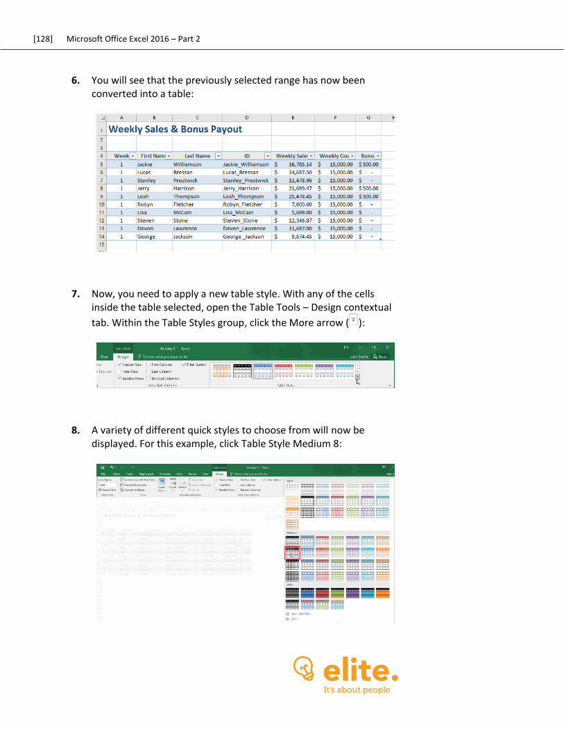
[128] Microsoft Office Excel 2016 – Part 2
6. You will see that the previously selected range has now been converted into a table:
7. Now, you need to apply a new table style. With any of the cells inside the table selected, open the Table Tools – Design contextual
tab. Within the Table Styles group, click the More arrow ( ):
8. A variety of different quick styles to choose from will now be displayed. For this example, click Table Style Medium 8:
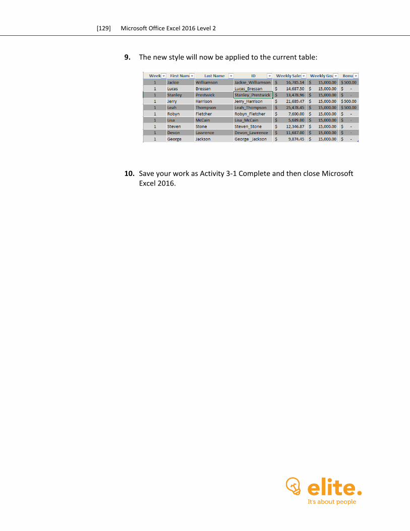
[129] Microsoft Office Excel 2016 Level 2
9. The new style will now be applied to the current table:
10. Save your work as Activity 3-1 Complete and then close Microsoft Excel 2016.
[130] Microsoft Office Excel 2016 – Part 2
TOPIC B: Sort and Filter Data The data that populates your worksheets is typically randomly sorted. This can cause a problem if you need to conduct data analysis or simply get a better grasp of the data at hand. Using tables you are able to quickly sort and filter data in a number of different ways to best suit your goals. Over the course of this topic, you will learn how to sort and filter data in tables and ranges. Topic Objectives In this topic, you will learn:
About the difference between sorting and filtering About sorting data About advanced filtering About filter operators How to remove duplicate values
THE DIFFERENCE BETWEEN SORTING AND FILTERING
Typically you are able to sort worksheet data alphabetically or numerically in ascending or descending order, but there are also options to sort data based on date and time, and even cell color. While you are able to sort by either row or column, the vast majority of sorting is done by column due to how most worksheets are constructed. Additionally, multiple sorts can be applied to the same set of data. Keep in mind when sorting table data that in order to make the most of Excel’s table functionality, you should make sure that your table contains headers. This will make the data more meaningful and easier to read, particularly if you are passing the data onto someone else in the future. It is also important to keep in mind that when you sort data you are not changing the data in the worksheet; you are only changing how it is displayed. Additionally, while there is no option available to clear a sort and return it back to its original state, the Undo command can have the same effect. Finally, if you apply a sort and then save your workbook, the
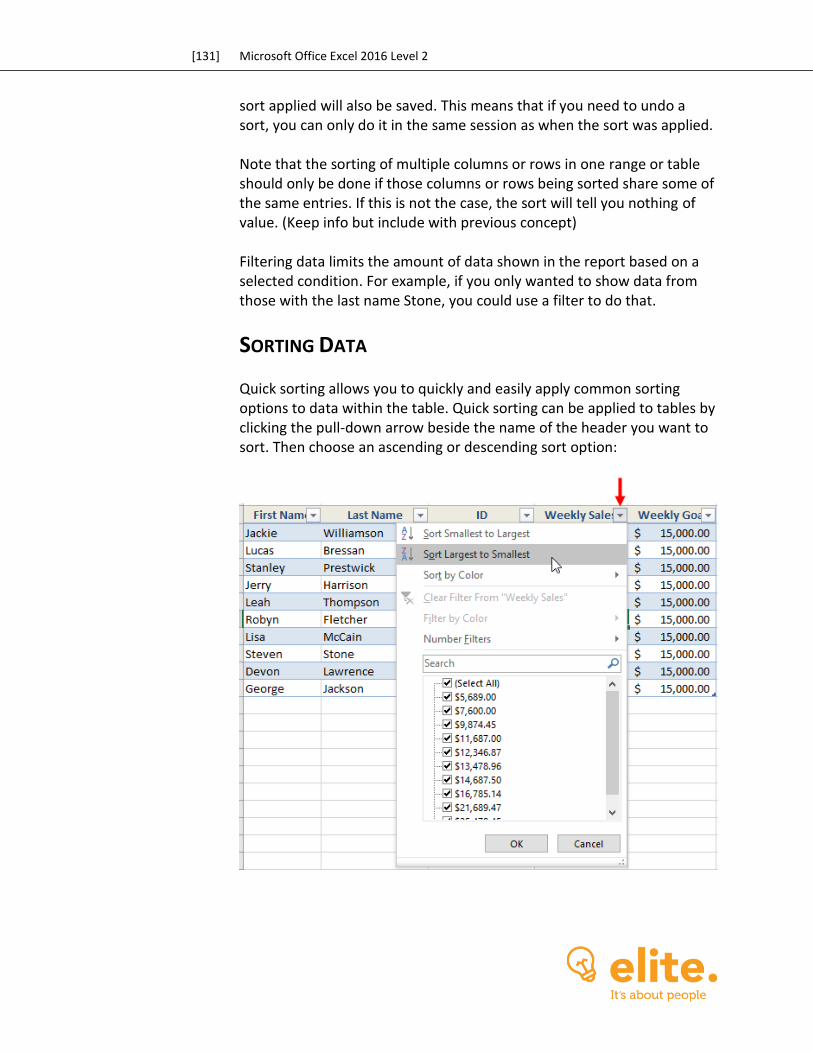
[131] Microsoft Office Excel 2016 Level 2
sort applied will also be saved. This means that if you need to undo a sort, you can only do it in the same session as when the sort was applied. Note that the sorting of multiple columns or rows in one range or table should only be done if those columns or rows being sorted share some of the same entries. If this is not the case, the sort will tell you nothing of value. (Keep info but include with previous concept) Filtering data limits the amount of data shown in the report based on a selected condition. For example, if you only wanted to show data from those with the last name Stone, you could use a filter to do that.
SORTING DATA
Quick sorting allows you to quickly and easily apply common sorting options to data within the table. Quick sorting can be applied to tables by clicking the pull-down arrow beside the name of the header you want to sort. Then choose an ascending or descending sort option:

[132] Microsoft Office Excel 2016 – Part 2
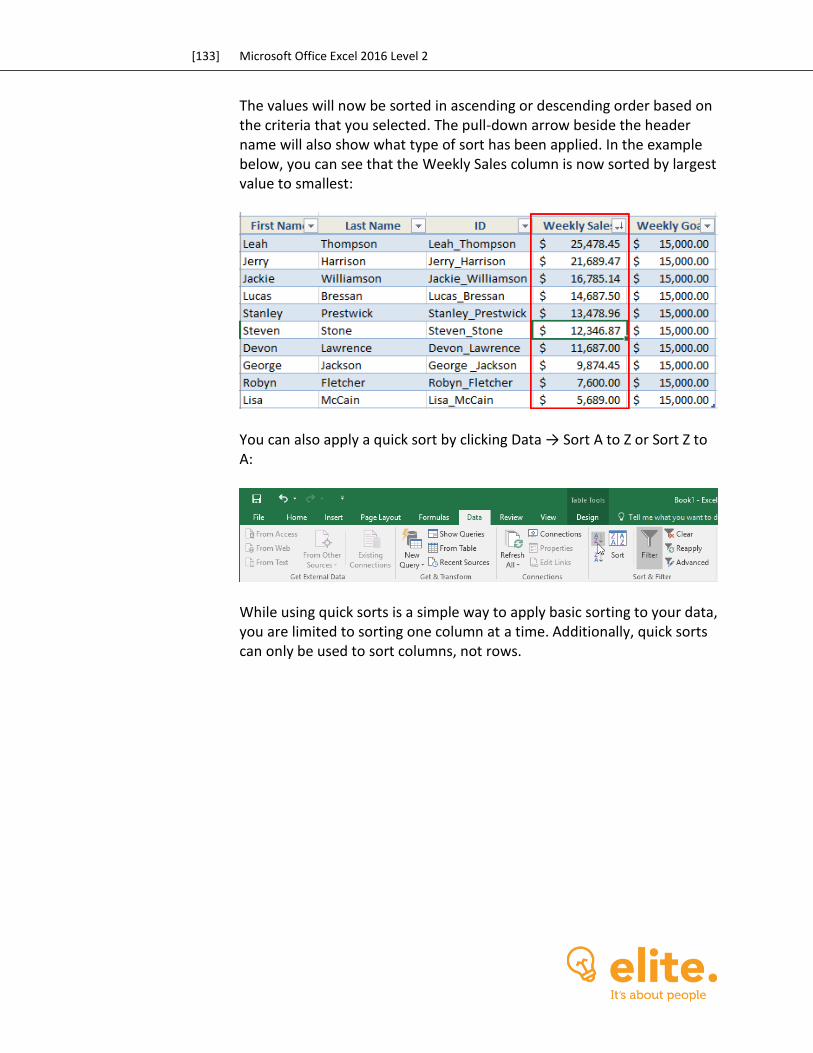
[133] Microsoft Office Excel 2016 Level 2
The values will now be sorted in ascending or descending order based on the criteria that you selected. The pull-down arrow beside the header name will also show what type of sort has been applied. In the example below, you can see that the Weekly Sales column is now sorted by largest value to smallest:
You can also apply a quick sort by clicking Data → Sort A to Z or Sort Z to A:
While using quick sorts is a simple way to apply basic sorting to your data, you are limited to sorting one column at a time. Additionally, quick sorts can only be used to sort columns, not rows.
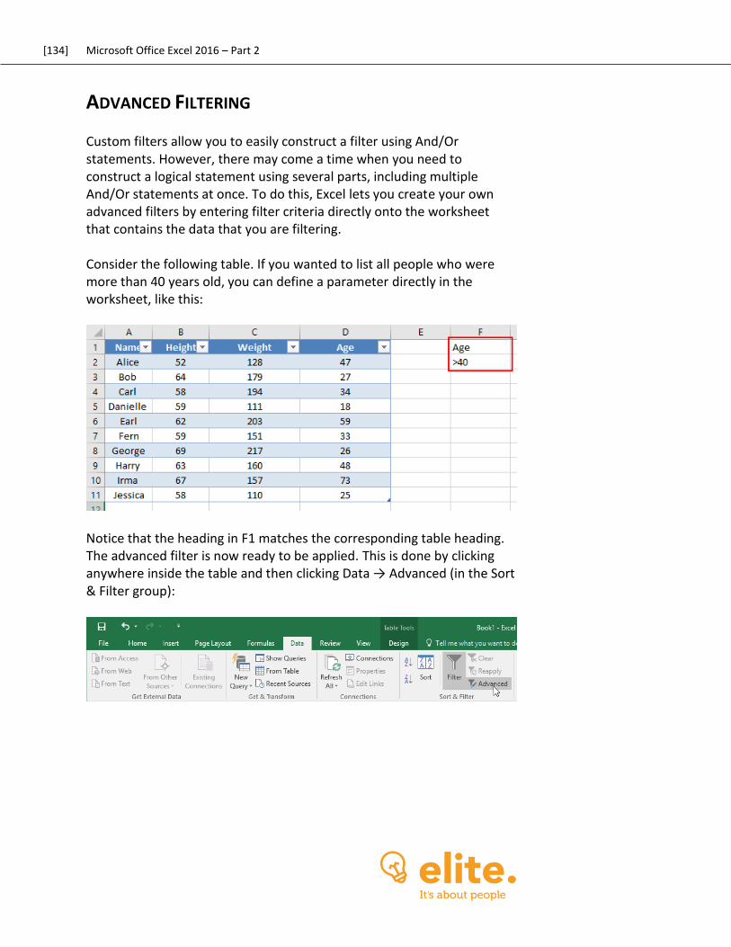
[134] Microsoft Office Excel 2016 – Part 2
ADVANCED FILTERING
Custom filters allow you to easily construct a filter using And/Or statements. However, there may come a time when you need to construct a logical statement using several parts, including multiple And/Or statements at once. To do this, Excel lets you create your own advanced filters by entering filter criteria directly onto the worksheet that contains the data that you are filtering. Consider the following table. If you wanted to list all people who were more than 40 years old, you can define a parameter directly in the worksheet, like this:
Notice that the heading in F1 matches the corresponding table heading. The advanced filter is now ready to be applied. This is done by clicking anywhere inside the table and then clicking Data → Advanced (in the Sort & Filter group):
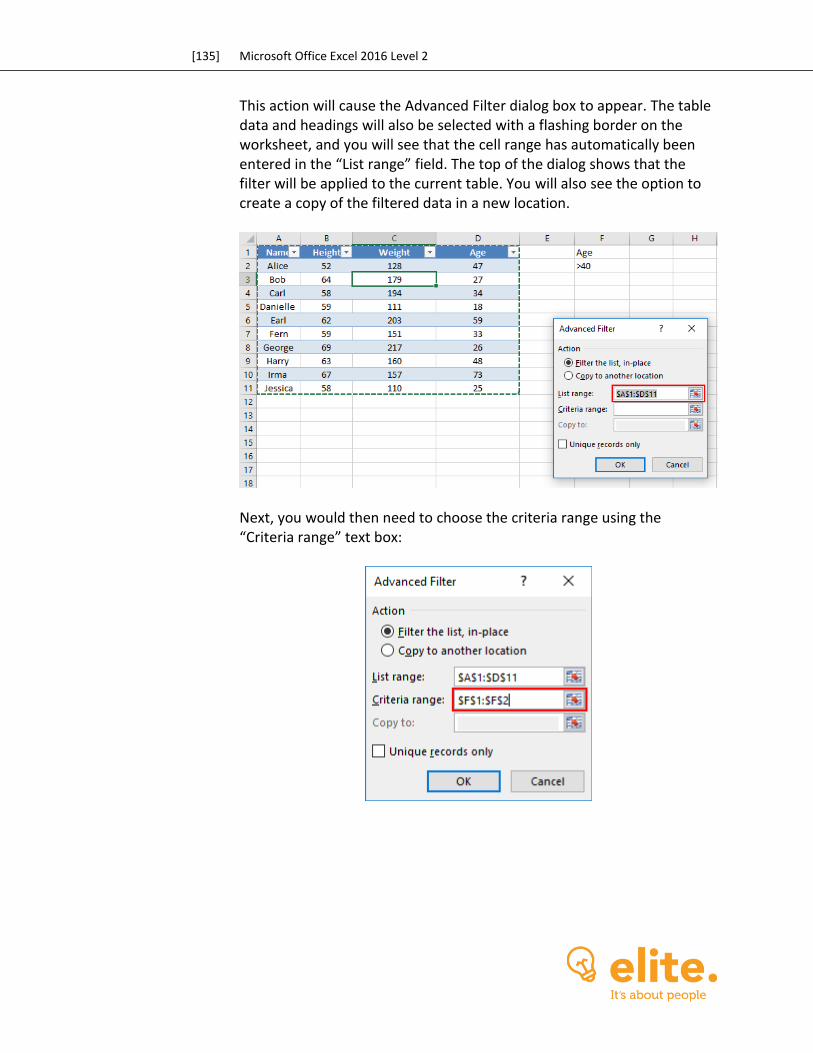
[135] Microsoft Office Excel 2016 Level 2
This action will cause the Advanced Filter dialog box to appear. The table data and headings will also be selected with a flashing border on the worksheet, and you will see that the cell range has automatically been entered in the “List range” field. The top of the dialog shows that the filter will be applied to the current table. You will also see the option to create a copy of the filtered data in a new location.
Next, you would then need to choose the criteria range using the “Criteria range” text box:
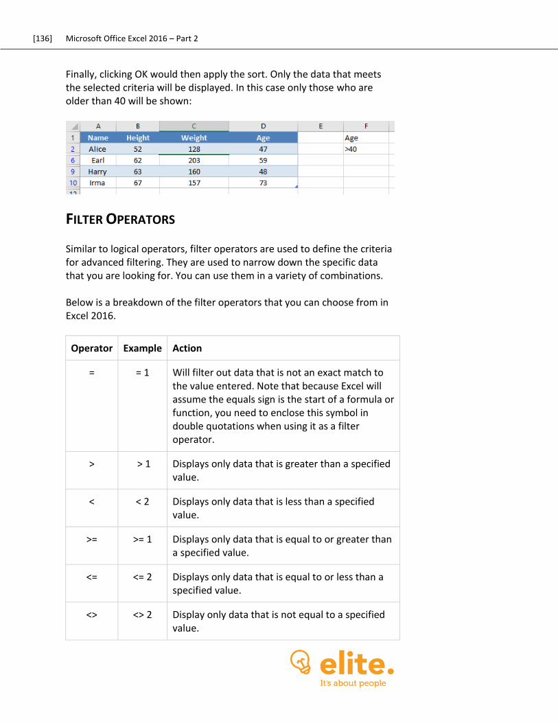
[136] Microsoft Office Excel 2016 – Part 2
Finally, clicking OK would then apply the sort. Only the data that meets the selected criteria will be displayed. In this case only those who are older than 40 will be shown:
FILTER OPERATORS
Similar to logical operators, filter operators are used to define the criteria for advanced filtering. They are used to narrow down the specific data that you are looking for. You can use them in a variety of combinations. Below is a breakdown of the filter operators that you can choose from in Excel 2016.
Operator Example Action
= = 1 Will filter out data that is not an exact match to the value entered. Note that because Excel will assume the equals sign is the start of a formula or function, you need to enclose this symbol in double quotations when using it as a filter operator.
> > 1 Displays only data that is greater than a specified value.
< < 2 Displays only data that is less than a specified value.
>= >= 1 Displays only data that is equal to or greater than a specified value.
<= <= 2
Displays only data that is equal to or less than a specified value.
<> <> 2 Display only data that is not equal to a specified value.
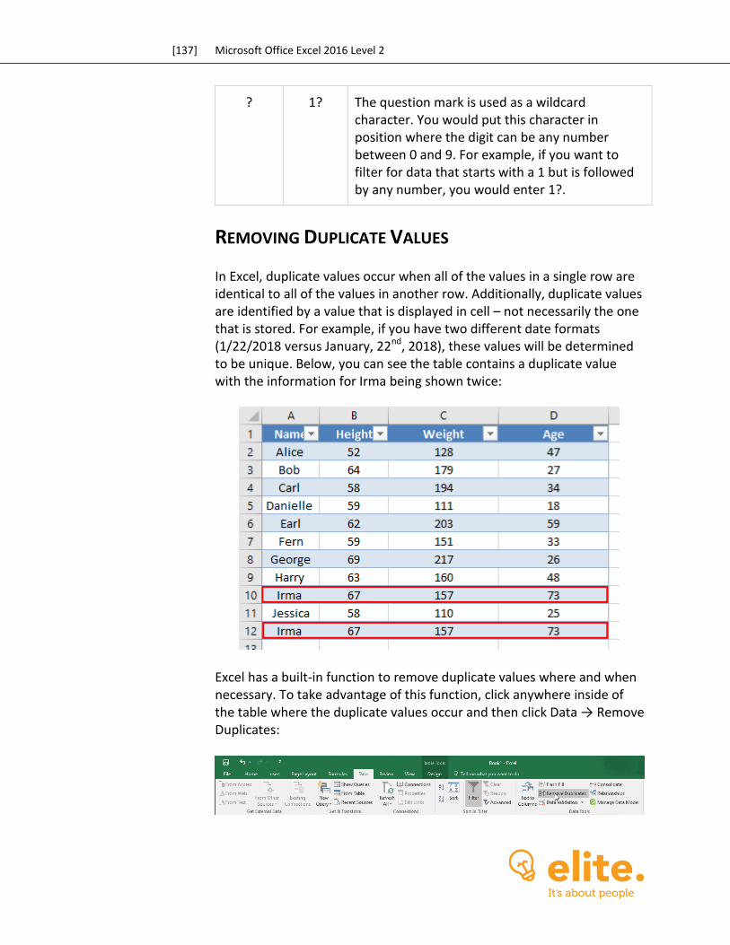
[137] Microsoft Office Excel 2016 Level 2
? 1? The question mark is used as a wildcard character. You would put this character in position where the digit can be any number between 0 and 9. For example, if you want to filter for data that starts with a 1 but is followed by any number, you would enter 1?.
REMOVING DUPLICATE VALUES
In Excel, duplicate values occur when all of the values in a single row are identical to all of the values in another row. Additionally, duplicate values are identified by a value that is displayed in cell – not necessarily the one that is stored. For example, if you have two different date formats (1/22/2018 versus January, 22nd, 2018), these values will be determined to be unique. Below, you can see the table contains a duplicate value with the information for Irma being shown twice:
Excel has a built-in function to remove duplicate values where and when necessary. To take advantage of this function, click anywhere inside of the table where the duplicate values occur and then click Data → Remove Duplicates:

[138] Microsoft Office Excel 2016 – Part 2
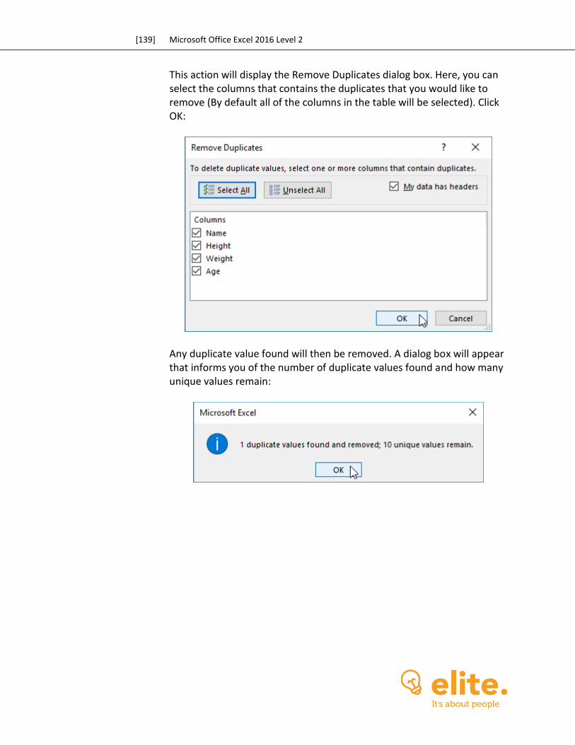
[139] Microsoft Office Excel 2016 Level 2
This action will display the Remove Duplicates dialog box. Here, you can select the columns that contains the duplicates that you would like to remove (By default all of the columns in the table will be selected). Click OK:
Any duplicate value found will then be removed. A dialog box will appear that informs you of the number of duplicate values found and how many unique values remain:
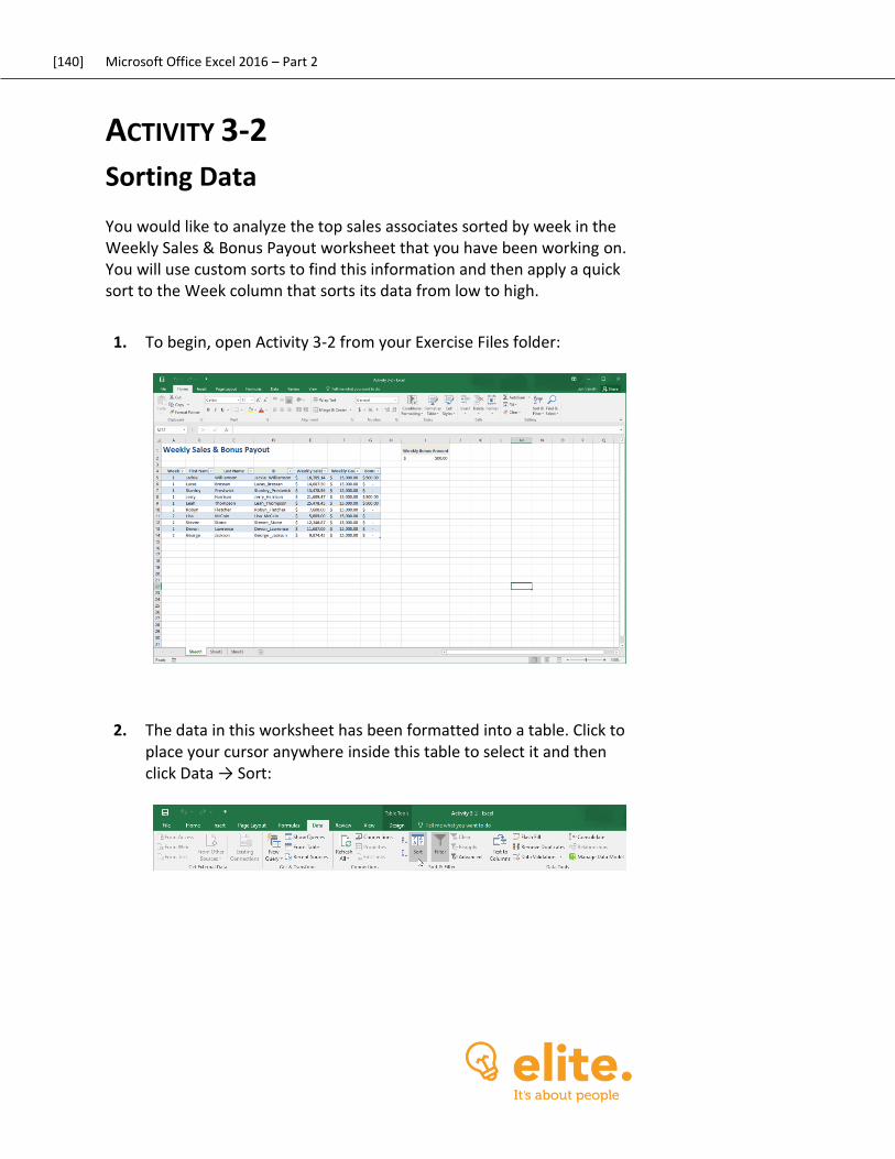
[140] Microsoft Office Excel 2016 – Part 2
ACTIVITY 3-2
Sorting Data You would like to analyze the top sales associates sorted by week in the Weekly Sales & Bonus Payout worksheet that you have been working on. You will use custom sorts to find this information and then apply a quick sort to the Week column that sorts its data from low to high.
1. To begin, open Activity 3-2 from your Exercise Files folder:
2. The data in this worksheet has been formatted into a table. Click to place your cursor anywhere inside this table to select it and then click Data → Sort:
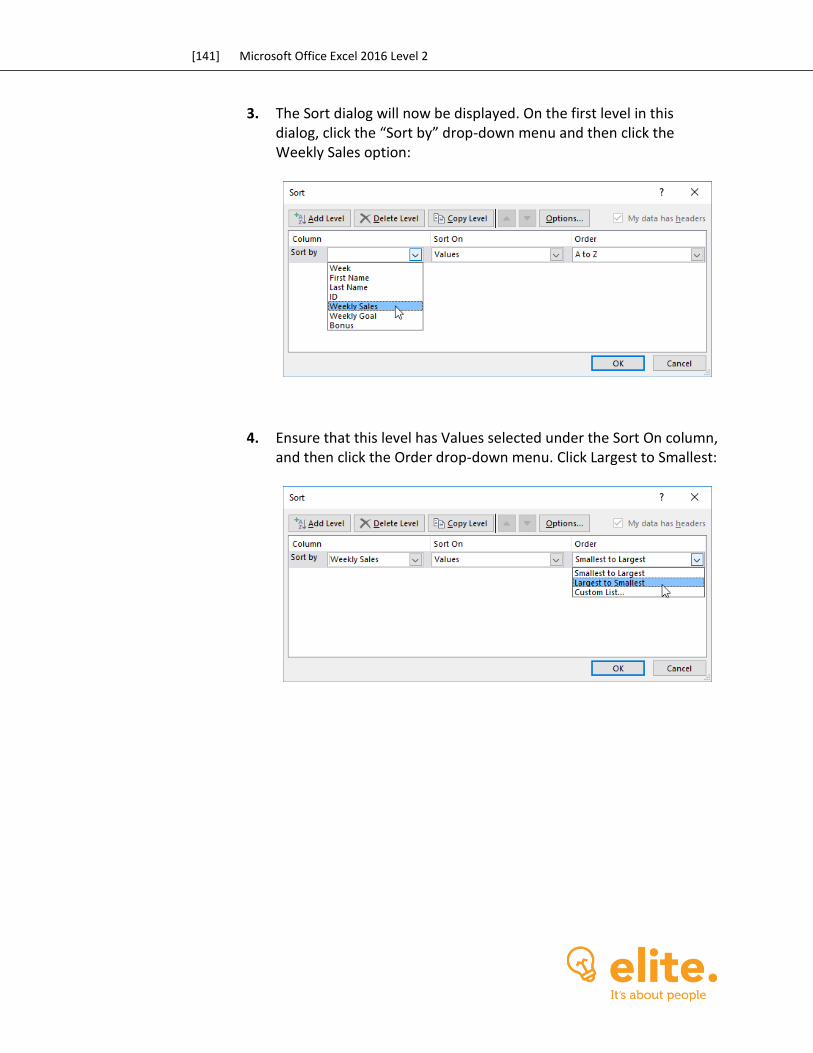
[141] Microsoft Office Excel 2016 Level 2
3. The Sort dialog will now be displayed. On the first level in this dialog, click the “Sort by” drop-down menu and then click the Weekly Sales option:
4. Ensure that this level has Values selected under the Sort On column, and then click the Order drop-down menu. Click Largest to Smallest:
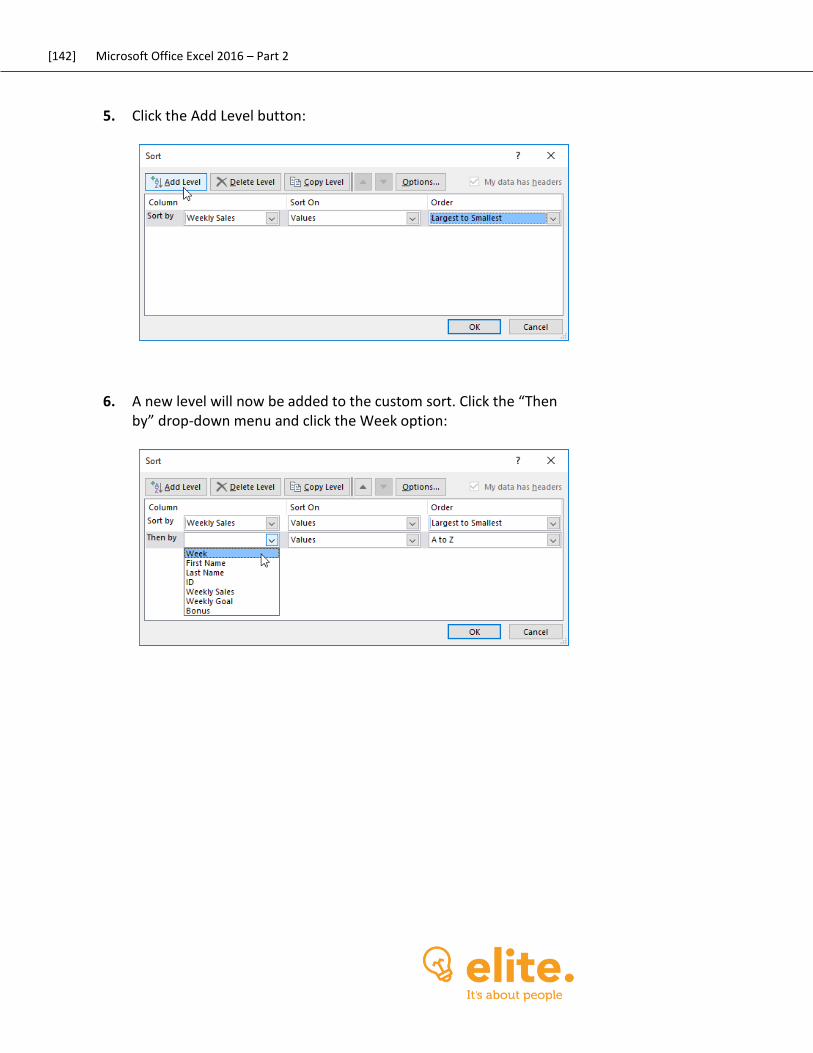
[142] Microsoft Office Excel 2016 – Part 2
5. Click the Add Level button:
6. A new level will now be added to the custom sort. Click the “Then by” drop-down menu and click the Week option:
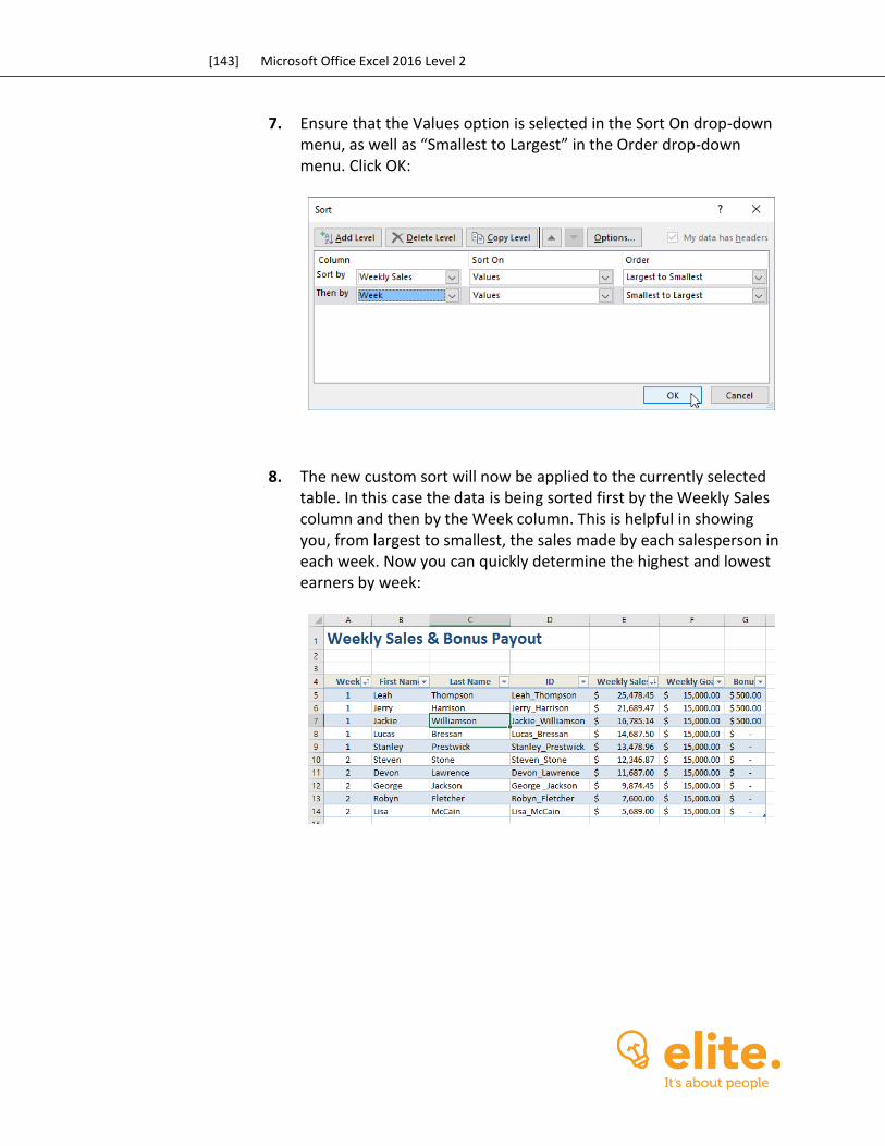
[143] Microsoft Office Excel 2016 Level 2
7. Ensure that the Values option is selected in the Sort On drop-down menu, as well as “Smallest to Largest” in the Order drop-down menu. Click OK:
8. The new custom sort will now be applied to the currently selected table. In this case the data is being sorted first by the Weekly Sales column and then by the Week column. This is helpful in showing you, from largest to smallest, the sales made by each salesperson in each week. Now you can quickly determine the highest and lowest earners by week:
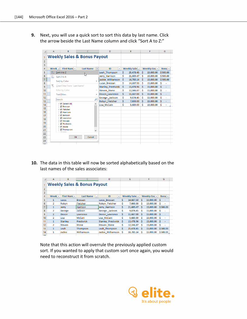
[144] Microsoft Office Excel 2016 – Part 2
9. Next, you will use a quick sort to sort this data by last name. Click the arrow beside the Last Name column and click “Sort A to Z:”
10. The data in this table will now be sorted alphabetically based on the last names of the sales associates:
Note that this action will overrule the previously applied custom sort. If you wanted to apply that custom sort once again, you would need to reconstruct it from scratch.
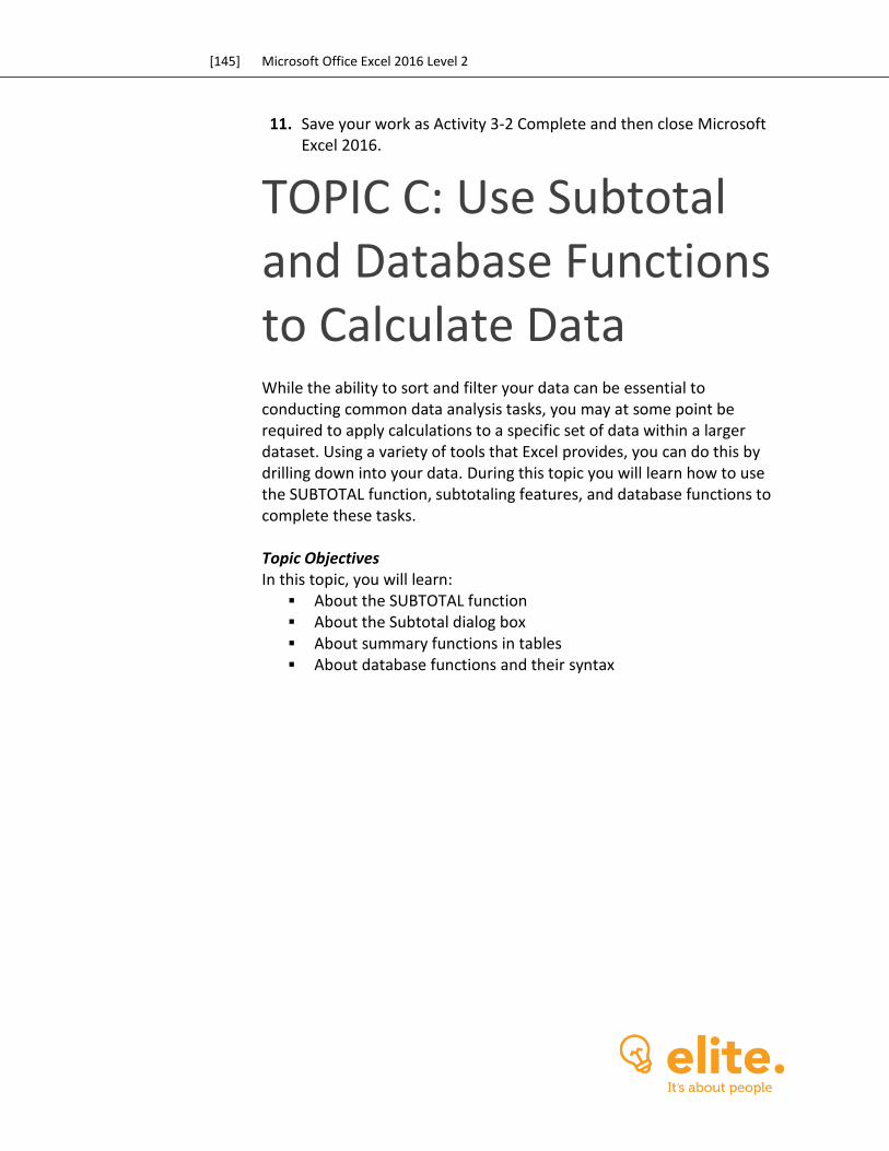
[145] Microsoft Office Excel 2016 Level 2
11. Save your work as Activity 3-2 Complete and then close Microsoft Excel 2016.
TOPIC C: Use Subtotal and Database Functions to Calculate Data While the ability to sort and filter your data can be essential to conducting common data analysis tasks, you may at some point be required to apply calculations to a specific set of data within a larger dataset. Using a variety of tools that Excel provides, you can do this by drilling down into your data. During this topic you will learn how to use the SUBTOTAL function, subtotaling features, and database functions to complete these tasks. Topic Objectives In this topic, you will learn:
About the SUBTOTAL function About the Subtotal dialog box About summary functions in tables About database functions and their syntax
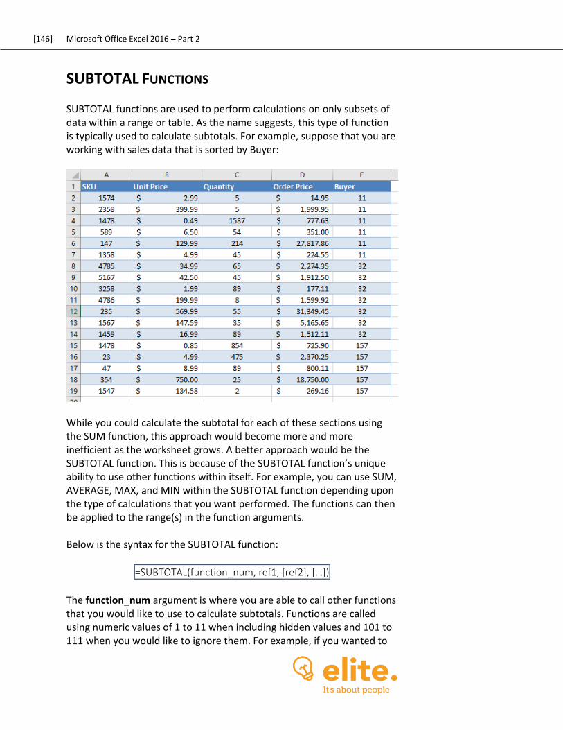
[146] Microsoft Office Excel 2016 – Part 2
SUBTOTAL FUNCTIONS
SUBTOTAL functions are used to perform calculations on only subsets of data within a range or table. As the name suggests, this type of function is typically used to calculate subtotals. For example, suppose that you are working with sales data that is sorted by Buyer:
While you could calculate the subtotal for each of these sections using the SUM function, this approach would become more and more inefficient as the worksheet grows. A better approach would be the SUBTOTAL function. This is because of the SUBTOTAL function’s unique ability to use other functions within itself. For example, you can use SUM, AVERAGE, MAX, and MIN within the SUBTOTAL function depending upon the type of calculations that you want performed. The functions can then be applied to the range(s) in the function arguments. Below is the syntax for the SUBTOTAL function:
=SUBTOTAL(function_num, ref1, [ref2], […])
The function_num argument is where you are able to call other functions that you would like to use to calculate subtotals. Functions are called using numeric values of 1 to 11 when including hidden values and 101 to 111 when you would like to ignore them. For example, if you wanted to
[147] Microsoft Office Excel 2016 Level 2
call the SUM function and include hidden values in the calculation, you would type “9” as the argument. Below is a table that tells you what value calls what function:
Function Argument Including Hidden Values
Function Argument Ignoring Hidden Values
Function
1 101 AVERAGE
2 102 COUNT
3 103 COUNTA
4 104 MAX
5 105 MIN
6 106 PRODUCT
7 107 STDEV
8 108 STDEVP
9 109 SUM
10 110 VAR
11 111 VARP
This function also uses reference arguments (ref1, ref2, etc.) to identify the ranges that you want this function to work with. For example, if you wanted the SUM of the A1:C10 range (including hidden values), you would type =SUBTOTAL (9, A1:C10). You can have up to 254 ranges within a single SUBTOTAL function.
THE SUBTOTAL DIALOG BOX
To use Excel’s subtotal feature, use your mouse to select the range of data you want to apply subtotals to and then click Data → Subtotal:

[148] Microsoft Office Excel 2016 – Part 2
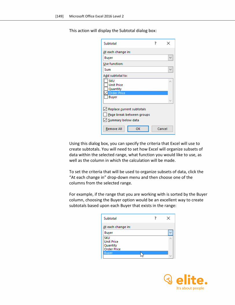
[149] Microsoft Office Excel 2016 Level 2
This action will display the Subtotal dialog box:
Using this dialog box, you can specify the criteria that Excel will use to create subtotals. You will need to set how Excel will organize subsets of data within the selected range, what function you would like to use, as well as the column in which the calculation will be made. To set the criteria that will be used to organize subsets of data, click the “At each change in” drop-down menu and then choose one of the columns from the selected range. For example, if the range that you are working with is sorted by the Buyer column, choosing the Buyer option would be an excellent way to create subtotals based upon each Buyer that exists in the range:

[150] Microsoft Office Excel 2016 – Part 2
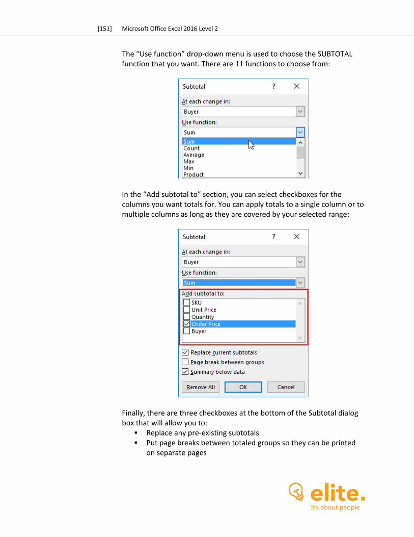
[151] Microsoft Office Excel 2016 Level 2
The “Use function” drop-down menu is used to choose the SUBTOTAL function that you want. There are 11 functions to choose from:
In the “Add subtotal to” section, you can select checkboxes for the columns you want totals for. You can apply totals to a single column or to multiple columns as long as they are covered by your selected range:
Finally, there are three checkboxes at the bottom of the Subtotal dialog box that will allow you to:
Replace any pre-existing subtotals Put page breaks between totaled groups so they can be printed
on separate pages
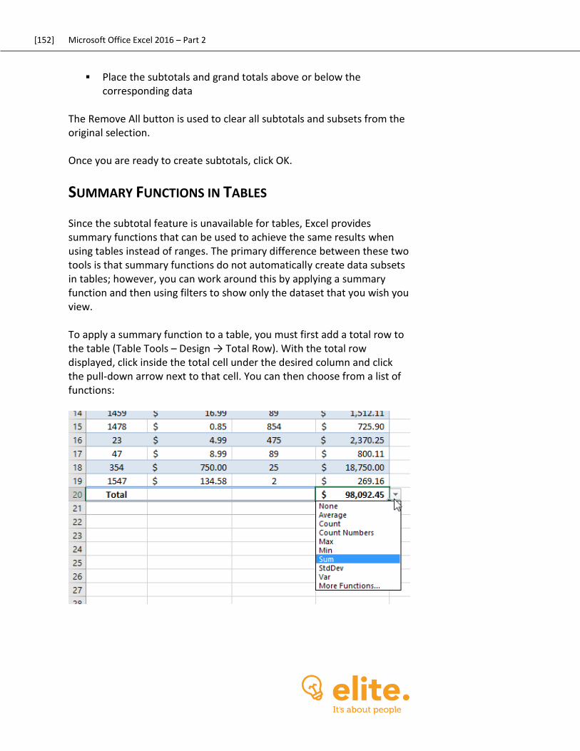
[152] Microsoft Office Excel 2016 – Part 2
Place the subtotals and grand totals above or below the corresponding data
The Remove All button is used to clear all subtotals and subsets from the original selection. Once you are ready to create subtotals, click OK.
SUMMARY FUNCTIONS IN TABLES
Since the subtotal feature is unavailable for tables, Excel provides summary functions that can be used to achieve the same results when using tables instead of ranges. The primary difference between these two tools is that summary functions do not automatically create data subsets in tables; however, you can work around this by applying a summary function and then using filters to show only the dataset that you wish you view. To apply a summary function to a table, you must first add a total row to the table (Table Tools – Design → Total Row). With the total row displayed, click inside the total cell under the desired column and click the pull-down arrow next to that cell. You can then choose from a list of functions:
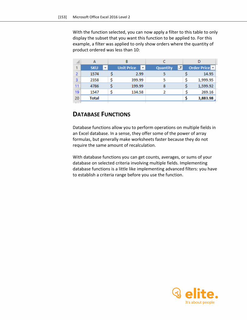
[153] Microsoft Office Excel 2016 Level 2
With the function selected, you can now apply a filter to this table to only display the subset that you want this function to be applied to. For this example, a filter was applied to only show orders where the quantity of product ordered was less than 10:
DATABASE FUNCTIONS
Database functions allow you to perform operations on multiple fields in an Excel database. In a sense, they offer some of the power of array formulas, but generally make worksheets faster because they do not require the same amount of recalculation. With database functions you can get counts, averages, or sums of your database on selected criteria involving multiple fields. Implementing database functions is a little like implementing advanced filters: you have to establish a criteria range before you use the function.
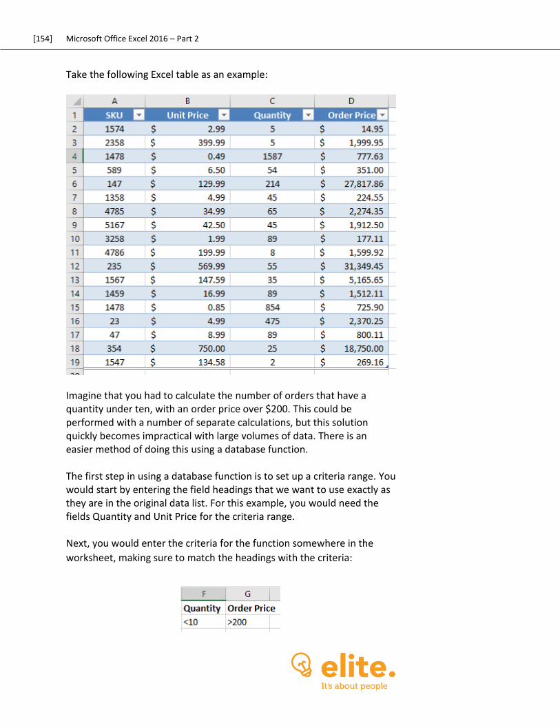
[154] Microsoft Office Excel 2016 – Part 2
Take the following Excel table as an example:
Imagine that you had to calculate the number of orders that have a quantity under ten, with an order price over $200. This could be performed with a number of separate calculations, but this solution quickly becomes impractical with large volumes of data. There is an easier method of doing this using a database function. The first step in using a database function is to set up a criteria range. You would start by entering the field headings that we want to use exactly as they are in the original data list. For this example, you would need the fields Quantity and Unit Price for the criteria range. Next, you would enter the criteria for the function somewhere in the
worksheet, making sure to match the headings with the criteria:
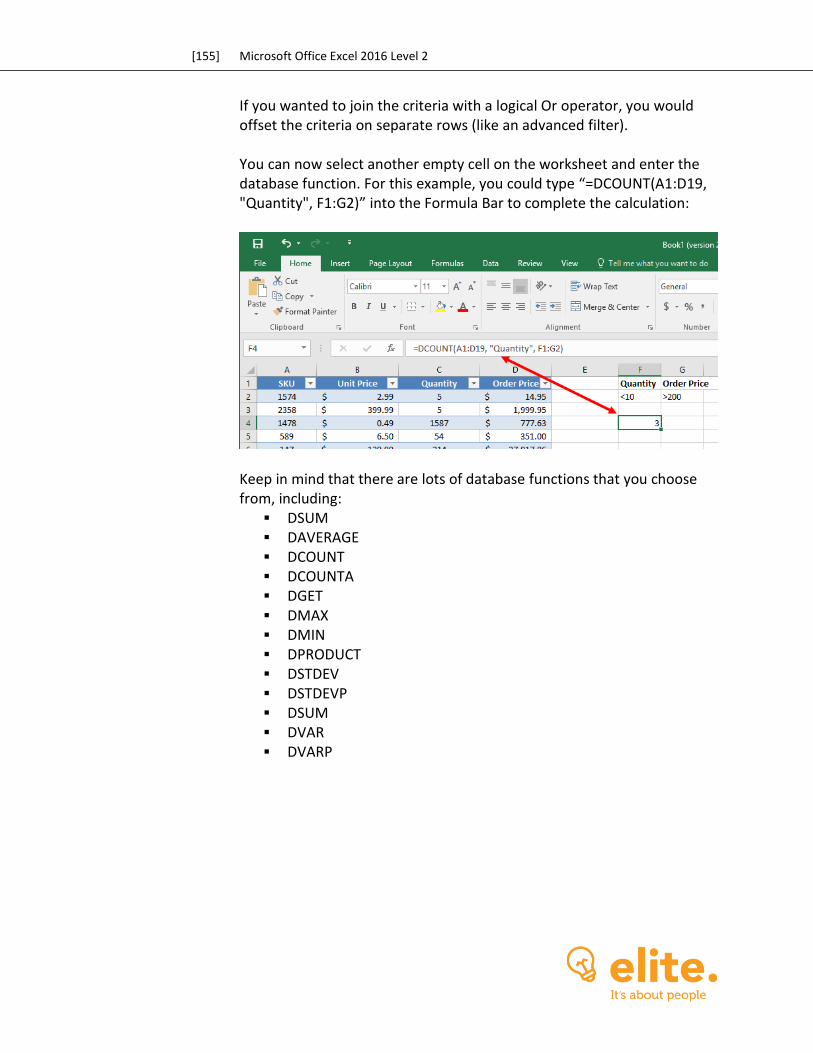
[155] Microsoft Office Excel 2016 Level 2
If you wanted to join the criteria with a logical Or operator, you would offset the criteria on separate rows (like an advanced filter). You can now select another empty cell on the worksheet and enter the database function. For this example, you could type “=DCOUNT(A1:D19, "Quantity", F1:G2)” into the Formula Bar to complete the calculation:
Keep in mind that there are lots of database functions that you choose from, including:
DSUM DAVERAGE DCOUNT DCOUNTA DGET DMAX DMIN DPRODUCT DSTDEV DSTDEVP DSUM DVAR DVARP
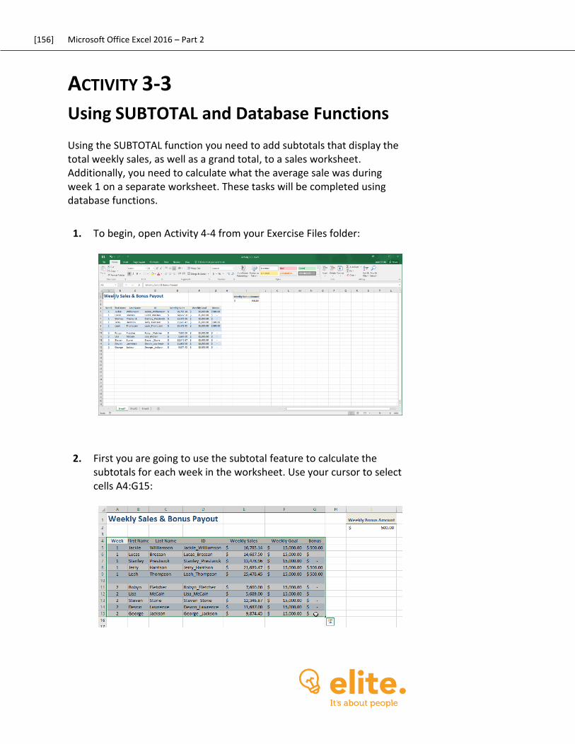
[156] Microsoft Office Excel 2016 – Part 2
ACTIVITY 3-3
Using SUBTOTAL and Database Functions Using the SUBTOTAL function you need to add subtotals that display the total weekly sales, as well as a grand total, to a sales worksheet. Additionally, you need to calculate what the average sale was during week 1 on a separate worksheet. These tasks will be completed using database functions.
1. To begin, open Activity 4-4 from your Exercise Files folder:
2. First you are going to use the subtotal feature to calculate the subtotals for each week in the worksheet. Use your cursor to select cells A4:G15:
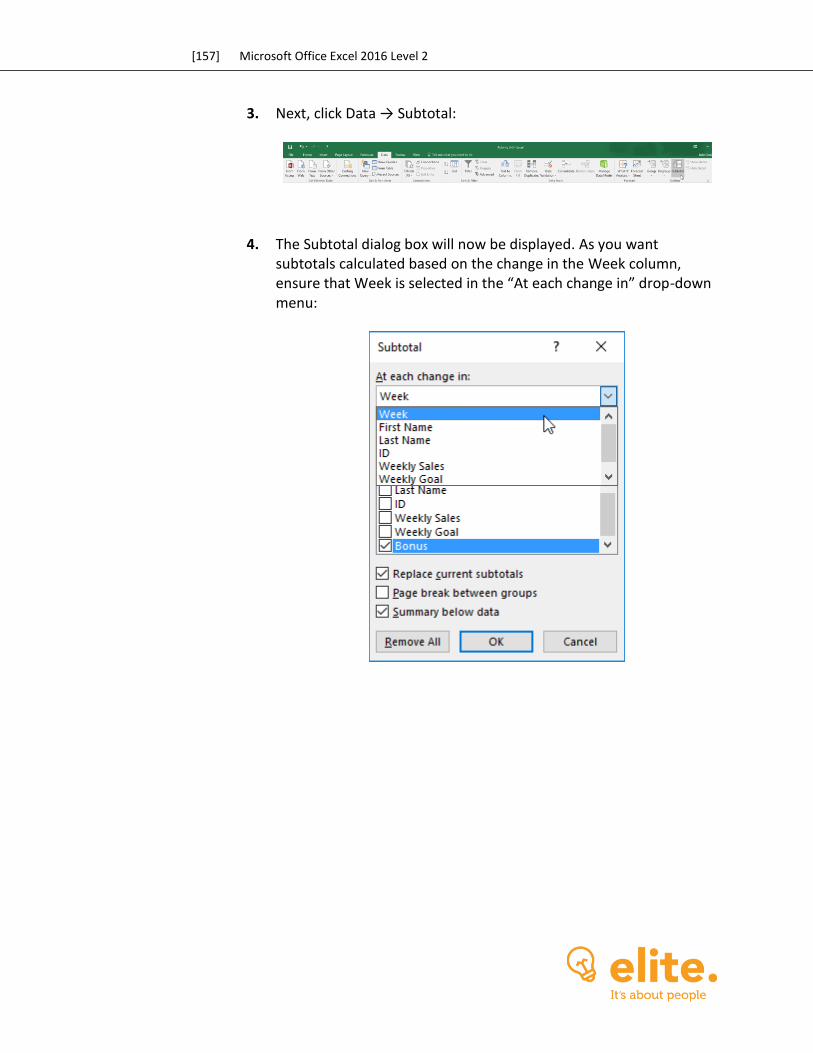
[157] Microsoft Office Excel 2016 Level 2
3. Next, click Data → Subtotal:
4. The Subtotal dialog box will now be displayed. As you want subtotals calculated based on the change in the Week column, ensure that Week is selected in the “At each change in” drop-down menu:
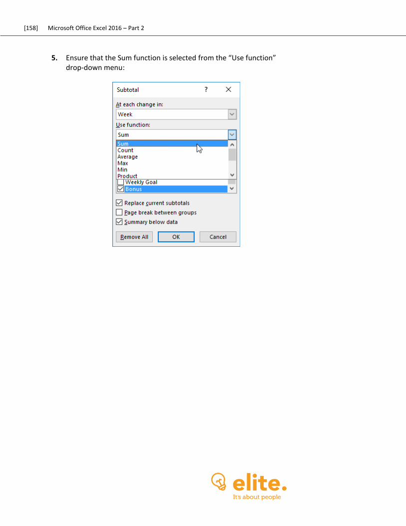
[158] Microsoft Office Excel 2016 – Part 2
5. Ensure that the Sum function is selected from the “Use function” drop-down menu:
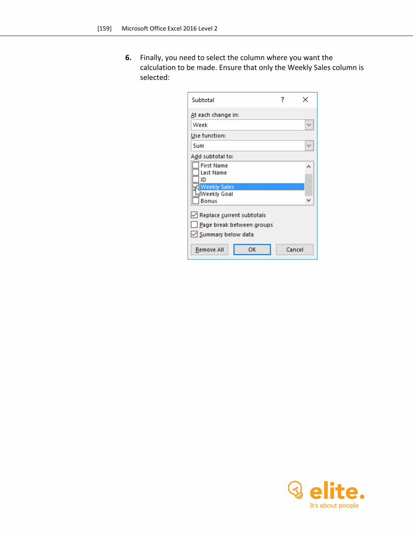
[159] Microsoft Office Excel 2016 Level 2
6. Finally, you need to select the column where you want the calculation to be made. Ensure that only the Weekly Sales column is selected:
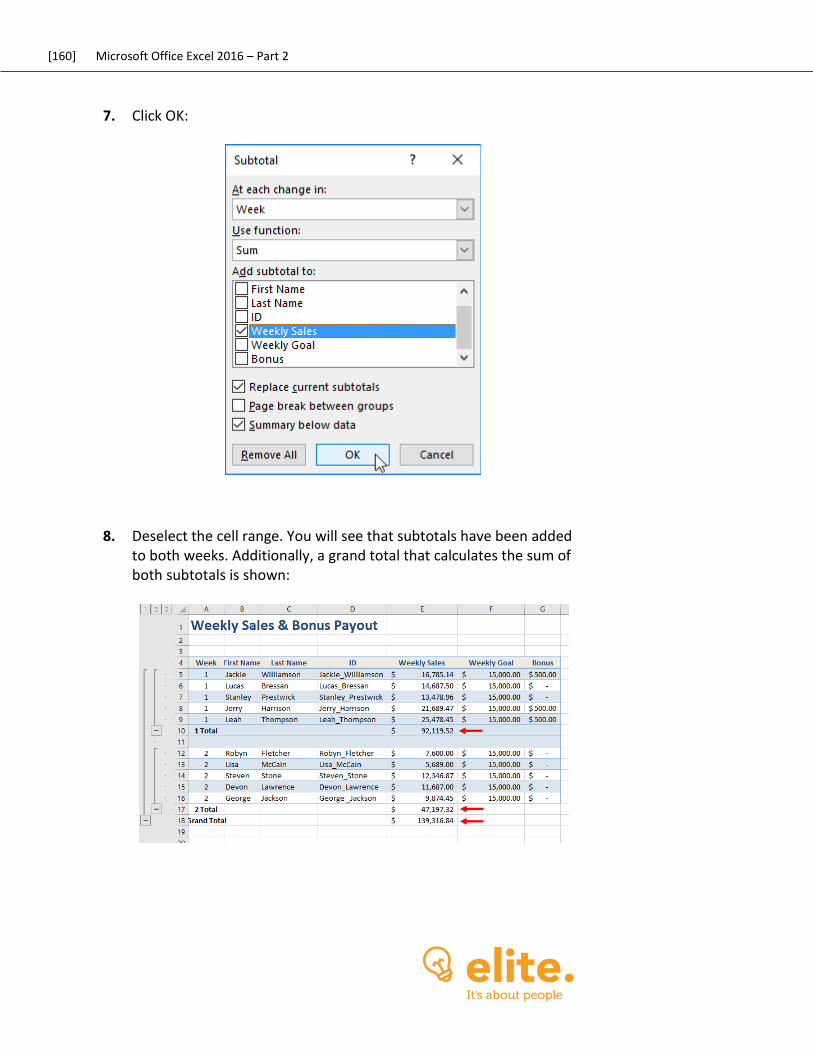
[160] Microsoft Office Excel 2016 – Part 2
7. Click OK:
8. Deselect the cell range. You will see that subtotals have been added to both weeks. Additionally, a grand total that calculates the sum of both subtotals is shown:
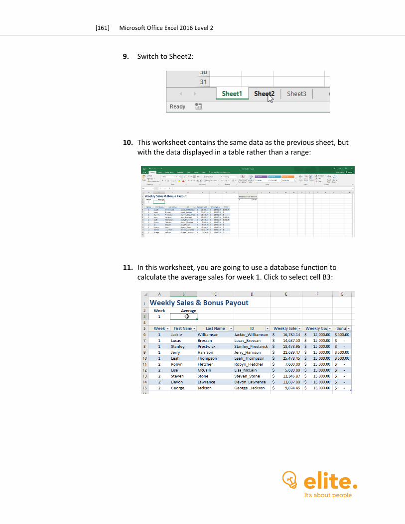
[161] Microsoft Office Excel 2016 Level 2
9. Switch to Sheet2:
10. This worksheet contains the same data as the previous sheet, but with the data displayed in a table rather than a range:
11. In this worksheet, you are going to use a database function to calculate the average sales for week 1. Click to select cell B3:
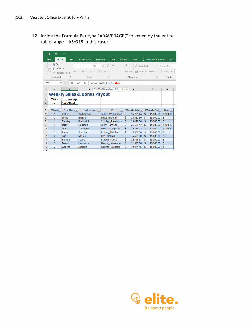
[162] Microsoft Office Excel 2016 – Part 2
12. Inside the Formula Bar type “=DAVERAGE(“ followed by the entire table range – A5:G15 in this case:
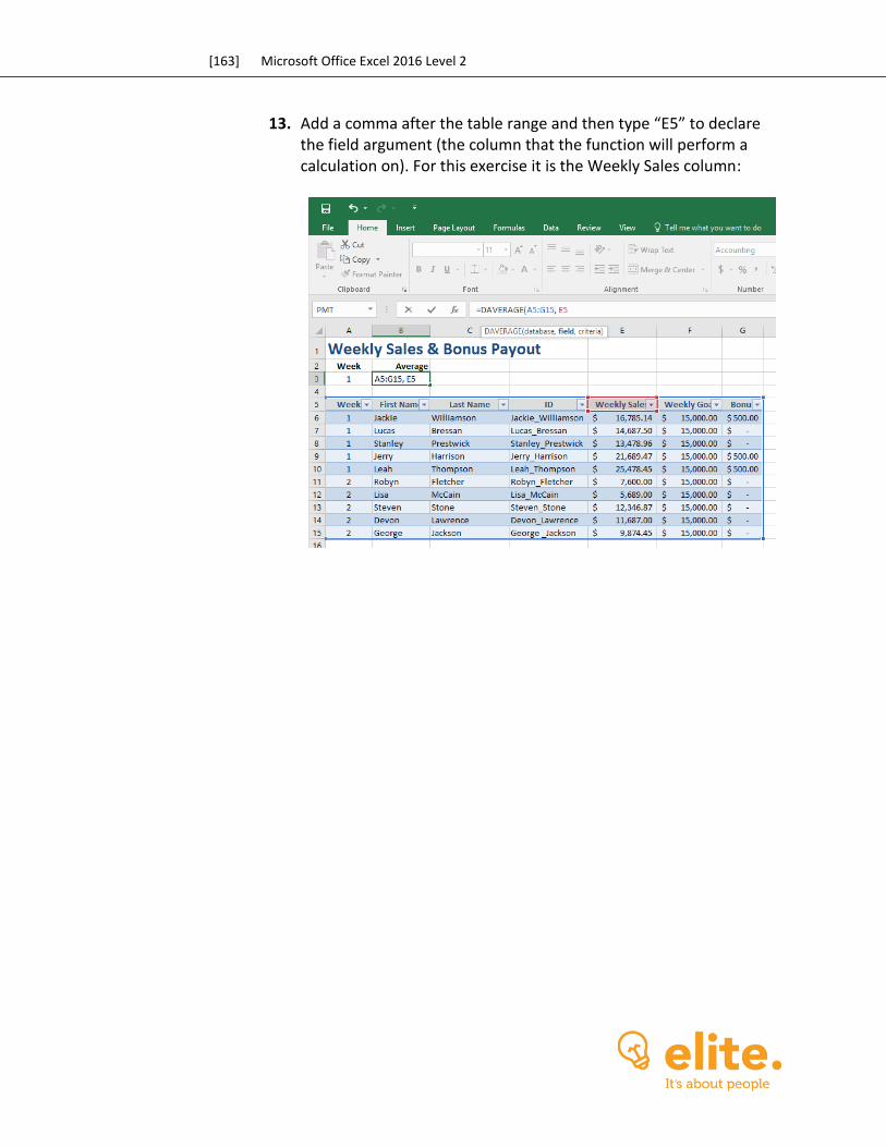
[163] Microsoft Office Excel 2016 Level 2
13. Add a comma after the table range and then type “E5” to declare the field argument (the column that the function will perform a calculation on). For this exercise it is the Weekly Sales column:
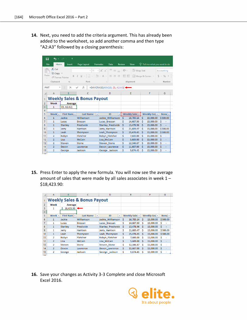
[164] Microsoft Office Excel 2016 – Part 2
14. Next, you need to add the criteria argument. This has already been added to the worksheet, so add another comma and then type “A2:A3” followed by a closing parenthesis:
15. Press Enter to apply the new formula. You will now see the average amount of sales that were made by all sales associates in week 1 – $18,423.90:
16. Save your changes as Activity 3-3 Complete and close Microsoft Excel 2016.
[165] Microsoft Office Excel 2016 Level 2
Summary In this lesson you learned how to organize workbook data. You can create tables, sort data, apply filters, and use the SUBTOTAL and database functions. By taking advantage of all these tools you will be able to take your data analysis tasks a few steps further and learn more about your data than ever before.
REVIEW QUESTIONS
1. What is the command sequence to add a table?
2. What are Quick Sorts?
3. What do levels refer to when creating a custom sort?
4. What is quick sorting?
5. What is an easy way to differentiate database functions from logical functions?

[167] Microsoft Office Excel 2016 Level 2
LESSON 4: VISUALIZING DATA
WITH CHARTS
Lesson Objectives
In this lesson you will learn how to:
Create charts
Modify and format existing charts
Create a trendline
Create advanced charts
[168] Microsoft Office Excel 2016 – Part 2
TOPIC A: Create Charts While pure data can be analyzed by those familiar with this data and the tools that Excel provides, sometimes you need graphical assistance to help interpret it. Additionally, charts are an enormous help when people do not have time to study the data and only need a brief overview of the relevant information. Over the course of this topic, you will learn how to create charts of different types, using different methods in Excel 2016. Topic Objectives In this topic, you will learn:
About charts About chart types How to insert a chart How to resize and move a chart How to add additional data How to switch between rows and columns
CHARTS
Charts are graphical representations of data and relationships in a dataset. They are commonly used in situations where viewers need to be able to quickly interpret data, without having to wade through the worksheet itself.
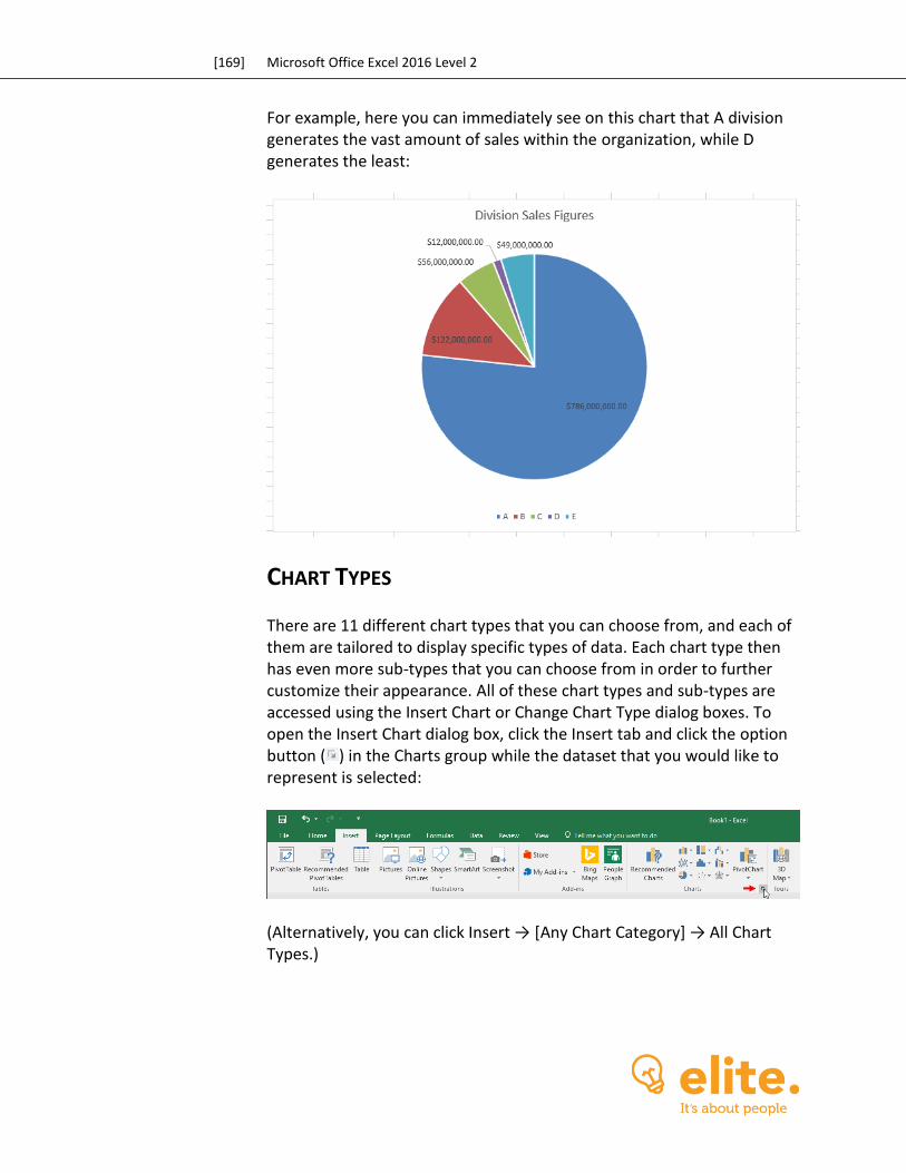
[169] Microsoft Office Excel 2016 Level 2
For example, here you can immediately see on this chart that A division generates the vast amount of sales within the organization, while D generates the least:
CHART TYPES
There are 11 different chart types that you can choose from, and each of them are tailored to display specific types of data. Each chart type then has even more sub-types that you can choose from in order to further customize their appearance. All of these chart types and sub-types are accessed using the Insert Chart or Change Chart Type dialog boxes. To open the Insert Chart dialog box, click the Insert tab and click the option button ( ) in the Charts group while the dataset that you would like to represent is selected:
(Alternatively, you can click Insert → [Any Chart Category] → All Chart Types.)
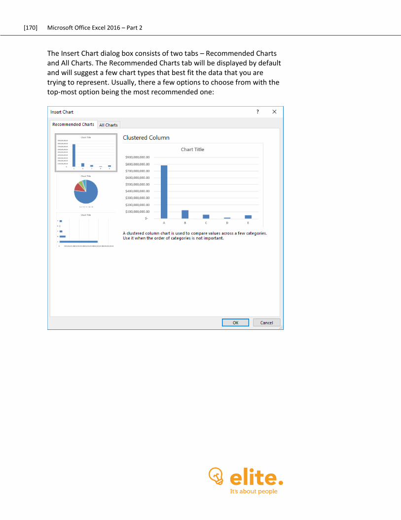
[170] Microsoft Office Excel 2016 – Part 2
The Insert Chart dialog box consists of two tabs – Recommended Charts and All Charts. The Recommended Charts tab will be displayed by default and will suggest a few chart types that best fit the data that you are trying to represent. Usually, there a few options to choose from with the top-most option being the most recommended one:
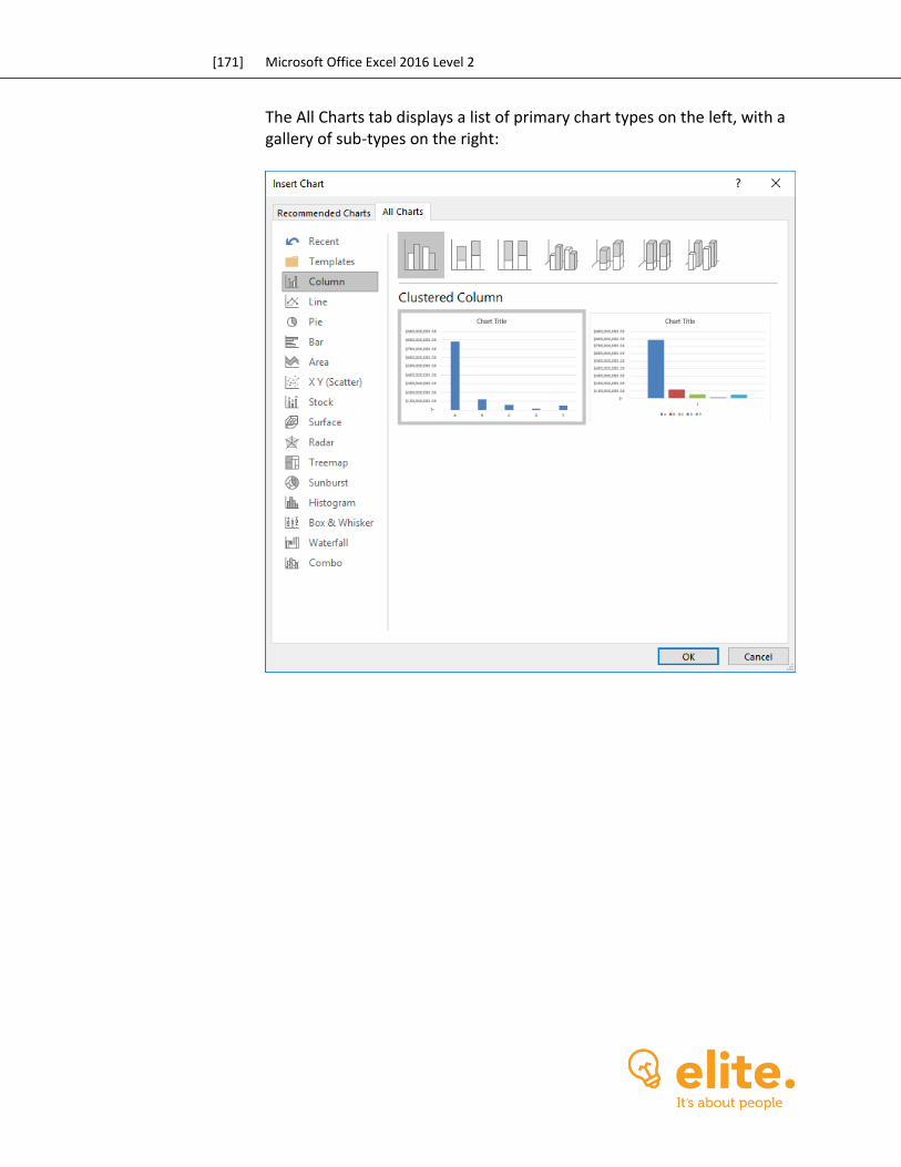
[171] Microsoft Office Excel 2016 Level 2
The All Charts tab displays a list of primary chart types on the left, with a gallery of sub-types on the right:

[172] Microsoft Office Excel 2016 – Part 2
Below is a breakdown of each chart type that is available and what data each type is best suited to display:
Column: Best suited to display data changes over time or to compare separate data points.
Line: Typically used to display data changes over a period of time. Pie: Used to compare different data points in relation to a total.
For example, you could use this chart type to show the total expenses of a company broken down by department.
Bar: Typically this chart type is used to compare different data points. It is similar to the Column chart type, but instead has the X-axis as the vertical axis and the Y-axis as the horizontal axis.
Area: This chart type is typically used to illustrate rates of change over a period of time, as well as include the total value in a trend.
X Y (Scatter): Used to illustrate values from a variety of different trends and their relationship to one another.
Stock: As the name implies, this chart type is designed to show data fluctuations in a stock market.
Surface: While more complex than other options, this chart type is used to find favorable patterns between two separate data sets.
Radar: This chart type is used to compare values from multiple data sets all on the same chart with each separate data (category) on a separate axis. Typically, this chart type is best suited to identify outliers and commonalities between data points.
Treemap: This chart type is designed to display hierarchical data through nested rectangles. Each branch of the tree is shown as a rectangle which is then tiled with smaller rectangles that show sub-branches.
Sunburst: Displays data hierarchy as a series of rings where each ring represents the children of the ring it encloses.
Histogram: A column chart that is designed to show frequency data.
Box & Whisker: Also known as a box plot, this chart type is designed to depict groups of numerical data as boxes on the chart. These boxes will also have a line that extends from each end (whiskers) that are used to describe upper and lower quartiles.
Waterfall: Sometimes referred to as a flying bricks chart or a Mario chart, this chart type represents data through a series of columns that are suspended in mid-air. These are typically used to understand how an initial value (e.g. sales revenue) is affected by positive or negative values (e.g. staff costs).
[173] Microsoft Office Excel 2016 Level 2
Combo: This type of chart combines the features of the bar chart and the line chart. Typically, this type of chart is useful if you need to compare values in different categories.
CHART INSERTION METHODS
When inserting a new chart into a worksheet, you should always have the dataset that you would like represented selected. If you select only one cell within the dataset in question, Excel will automatically try and guess the data range that you are trying to represent. While this is a good idea in theory, this feature does not always work as intended in practice. Additionally, when you are inserting charts remember to include the row or column header when selecting the dataset. This will ensure that categories that you want plotted along the X axis of the chart are your column labels from the dataset and the data series are row labels. Once the data set, including labels, is selected, you can then insert a chart using one of several options. Perhaps the most direct way is to use the commands inside the Charts group of the Insert tab; however, you can also use the Insert Chart dialog box, or insert the most recommended chart type for the selected data using keyboard shortcuts. If you would like the most recommended chart type to be inserted onto the same worksheet, you would press Alt + F1. If you want the default chart type to be inserted into a new worksheet, press F11.
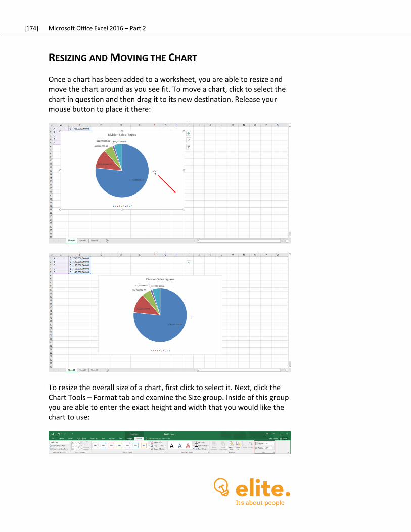
[174] Microsoft Office Excel 2016 – Part 2
RESIZING AND MOVING THE CHART
Once a chart has been added to a worksheet, you are able to resize and move the chart around as you see fit. To move a chart, click to select the chart in question and then drag it to its new destination. Release your mouse button to place it there:
To resize the overall size of a chart, first click to select it. Next, click the Chart Tools – Format tab and examine the Size group. Inside of this group you are able to enter the exact height and width that you would like the chart to use:
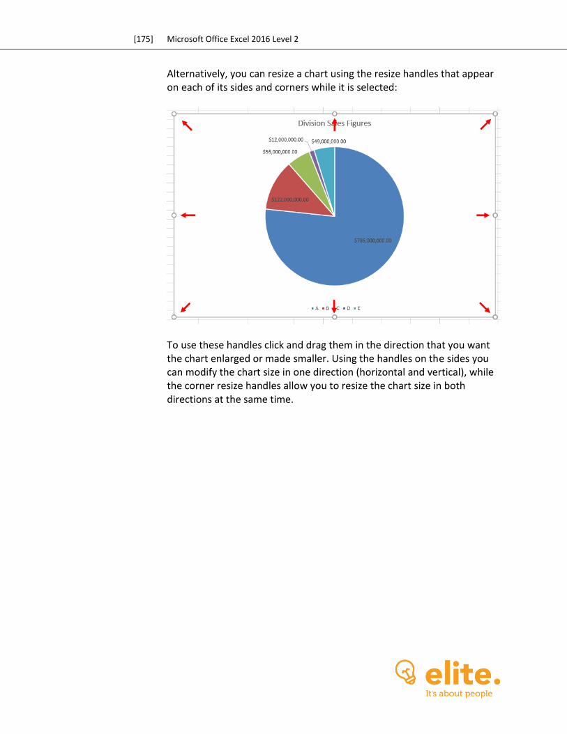
[175] Microsoft Office Excel 2016 Level 2
Alternatively, you can resize a chart using the resize handles that appear on each of its sides and corners while it is selected:
To use these handles click and drag them in the direction that you want the chart enlarged or made smaller. Using the handles on the sides you can modify the chart size in one direction (horizontal and vertical), while the corner resize handles allow you to resize the chart size in both directions at the same time.
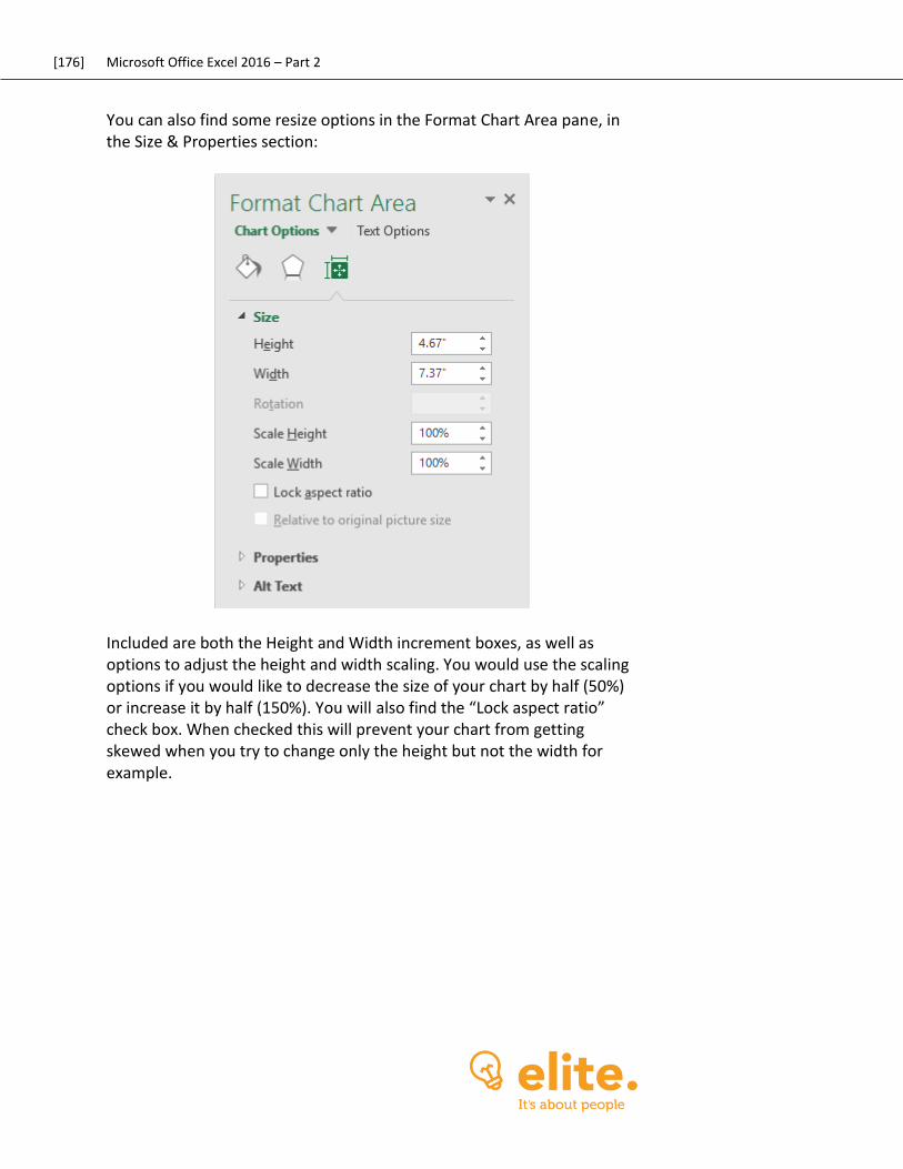
[176] Microsoft Office Excel 2016 – Part 2
You can also find some resize options in the Format Chart Area pane, in the Size & Properties section:
Included are both the Height and Width increment boxes, as well as options to adjust the height and width scaling. You would use the scaling options if you would like to decrease the size of your chart by half (50%) or increase it by half (150%). You will also find the “Lock aspect ratio” check box. When checked this will prevent your chart from getting skewed when you try to change only the height but not the width for example.
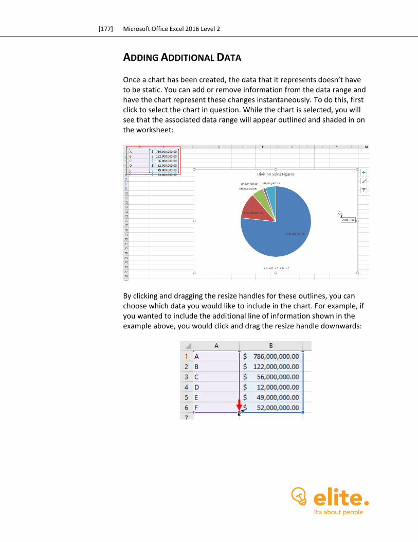
[177] Microsoft Office Excel 2016 Level 2
ADDING ADDITIONAL DATA
Once a chart has been created, the data that it represents doesn’t have to be static. You can add or remove information from the data range and have the chart represent these changes instantaneously. To do this, first click to select the chart in question. While the chart is selected, you will see that the associated data range will appear outlined and shaded in on the worksheet:
By clicking and dragging the resize handles for these outlines, you can choose which data you would like to include in the chart. For example, if you wanted to include the additional line of information shown in the example above, you would click and drag the resize handle downwards:
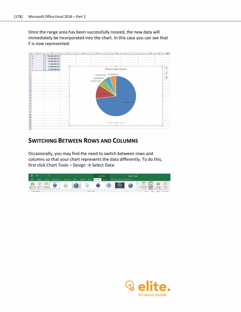
[178] Microsoft Office Excel 2016 – Part 2
Once the range area has been successfully resized, the new data will immediately be incorporated into the chart. In this case you can see that F is now represented:
SWITCHING BETWEEN ROWS AND COLUMNS
Occasionally, you may find the need to switch between rows and columns so that your chart represents the data differently. To do this, first click Chart Tools – Design → Select Data:
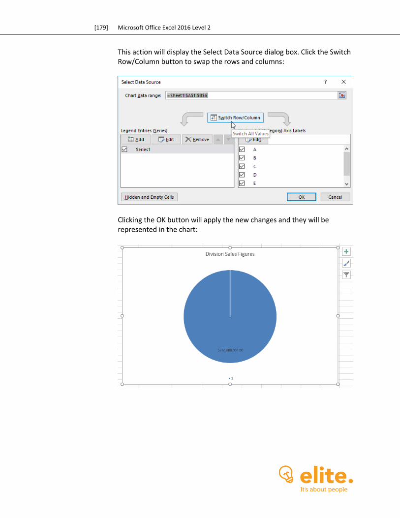
[179] Microsoft Office Excel 2016 Level 2
This action will display the Select Data Source dialog box. Click the Switch Row/Column button to swap the rows and columns:
Clicking the OK button will apply the new changes and they will be represented in the chart:
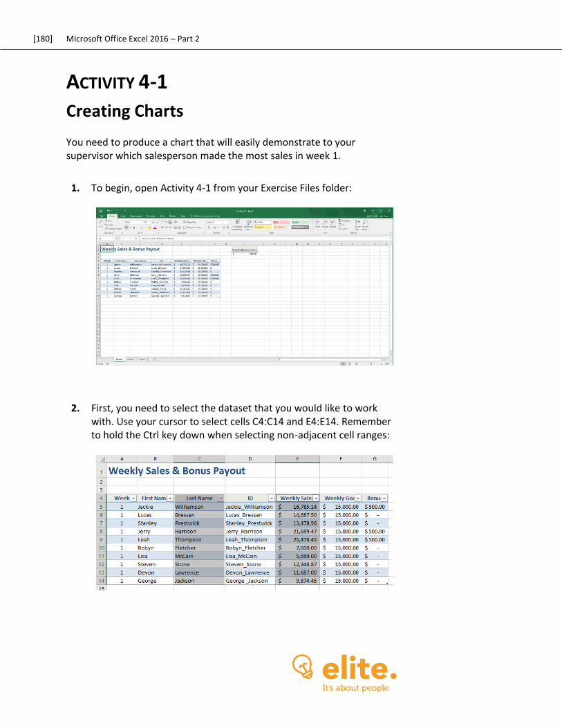
[180] Microsoft Office Excel 2016 – Part 2
ACTIVITY 4-1
Creating Charts You need to produce a chart that will easily demonstrate to your supervisor which salesperson made the most sales in week 1.
1. To begin, open Activity 4-1 from your Exercise Files folder:
2. First, you need to select the dataset that you would like to work with. Use your cursor to select cells C4:C14 and E4:E14. Remember to hold the Ctrl key down when selecting non-adjacent cell ranges:
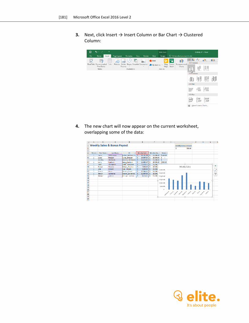
[181] Microsoft Office Excel 2016 Level 2
3. Next, click Insert → Insert Column or Bar Chart → Clustered Column:
4. The new chart will now appear on the current worksheet, overlapping some of the data:
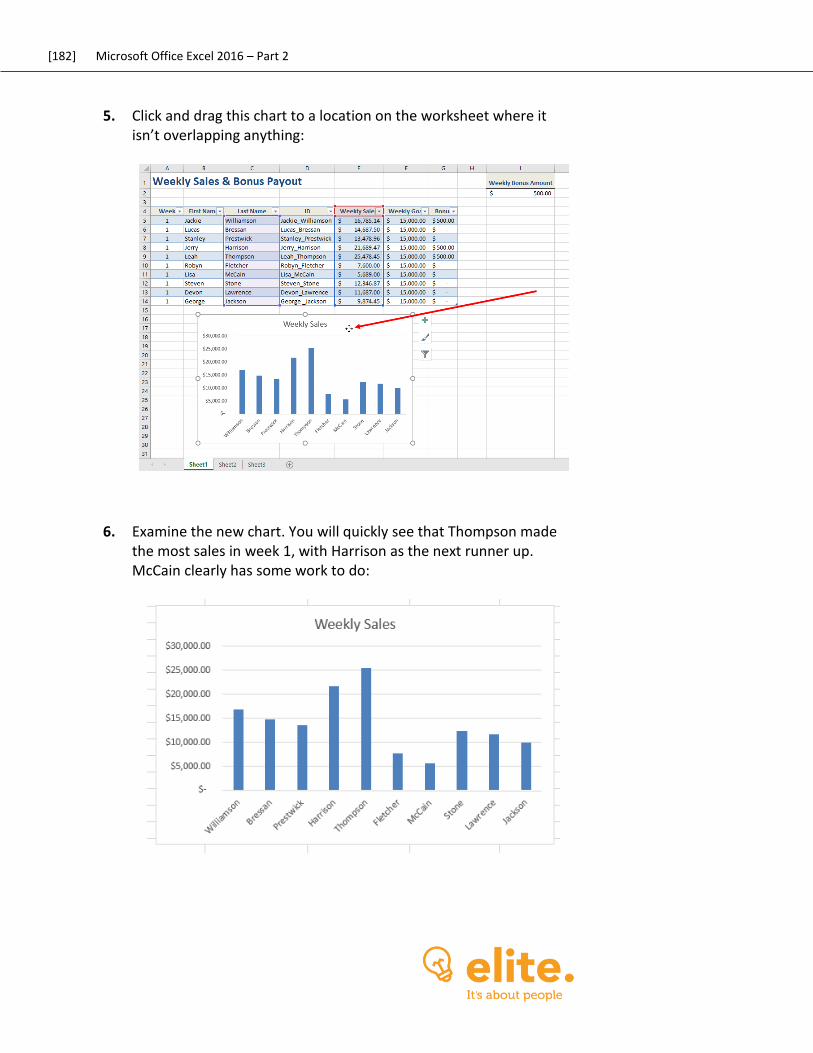
[182] Microsoft Office Excel 2016 – Part 2
5. Click and drag this chart to a location on the worksheet where it isn’t overlapping anything:
6. Examine the new chart. You will quickly see that Thompson made the most sales in week 1, with Harrison as the next runner up. McCain clearly has some work to do:
[183] Microsoft Office Excel 2016 Level 2
7. Save your worksheet as Activity 4-1 Complete and close Microsoft Excel 2016.
TOPIC B: Modify and Format Charts Charts can be added quickly and easily using the default chart configurations, but sometimes those configurations are not suitable. In such cases, you will need to know how to modify and format your chart to include more or less data, adjust the size of the chart, and apply company branding. Topic Objectives In this topic, you will learn:
About modification vs. formatting About chart elements Guidelines for including chart elements About the Chart Tools contextual tabs About formatting the chart with a style How to add a legend to the chart
THE DIFFERENCE BETWEEN MODIFYING AND
FORMATTING
While modifying and formatting charts sound like the same thing, they are actually different in this context. When you choose to modify a chart, you are changing the various elements that are used to illustrate the data. For example, adding or removing chart elements or changing the chart type would be considering modifying a chart. Formatting is the process of altering the overall appearance of the chart. This includes changing the chart’s colors, fonts, and/or size. For example, if you need to change a chart to incorporate your organization’s branding rules, you would in fact be formatting it.
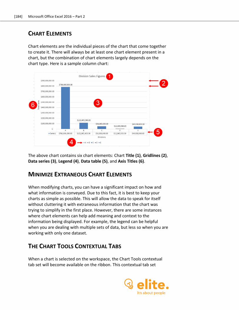
[184] Microsoft Office Excel 2016 – Part 2
CHART ELEMENTS
Chart elements are the individual pieces of the chart that come together to create it. There will always be at least one chart element present in a chart, but the combination of chart elements largely depends on the chart type. Here is a sample column chart:
The above chart contains six chart elements: Chart Title (1), Gridlines (2), Data series (3), Legend (4), Data table (5), and Axis Titles (6).
MINIMIZE EXTRANEOUS CHART ELEMENTS
When modifying charts, you can have a significant impact on how and what information is conveyed. Due to this fact, it is best to keep your charts as simple as possible. This will allow the data to speak for itself without cluttering it with extraneous information that the chart was trying to simplify in the first place. However, there are some instances where chart elements can help add meaning and context to the information being displayed. For example, the legend can be helpful when you are dealing with multiple sets of data, but less so when you are working with only one dataset.
THE CHART TOOLS CONTEXTUAL TABS
When a chart is selected on the workspace, the Chart Tools contextual tab set will become available on the ribbon. This contextual tab set
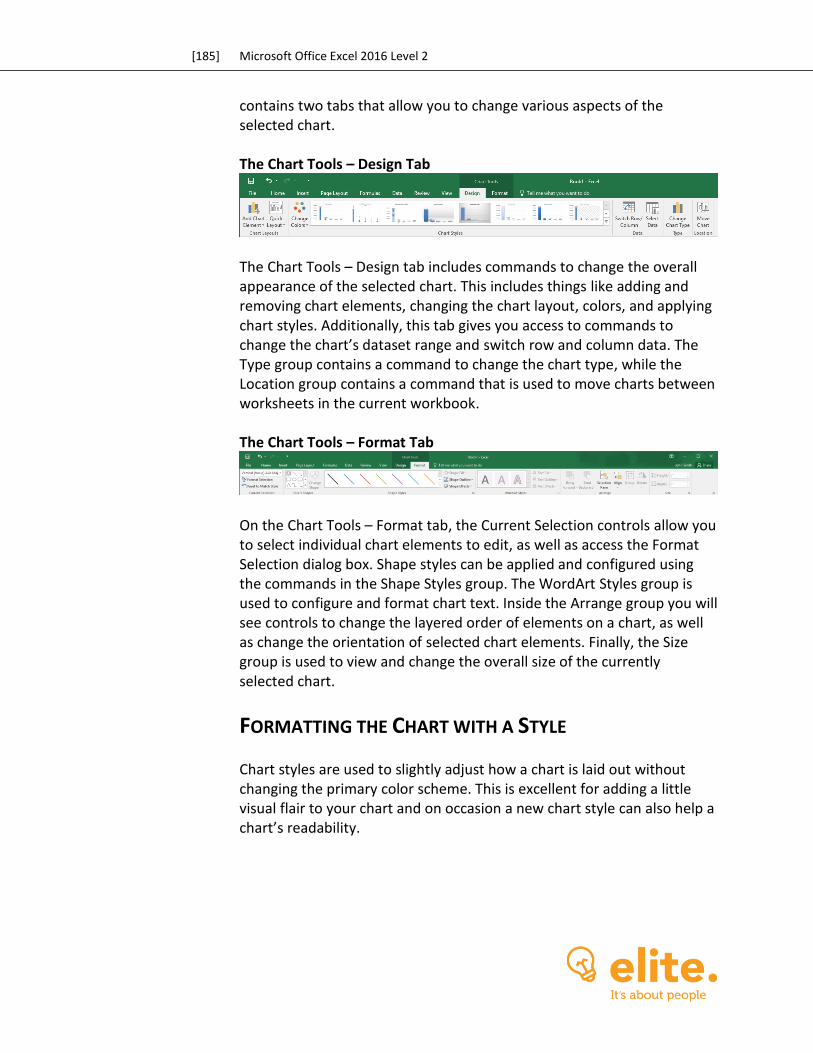
[185] Microsoft Office Excel 2016 Level 2
contains two tabs that allow you to change various aspects of the selected chart. The Chart Tools – Design Tab
The Chart Tools – Design tab includes commands to change the overall appearance of the selected chart. This includes things like adding and removing chart elements, changing the chart layout, colors, and applying chart styles. Additionally, this tab gives you access to commands to change the chart’s dataset range and switch row and column data. The Type group contains a command to change the chart type, while the Location group contains a command that is used to move charts between worksheets in the current workbook. The Chart Tools – Format Tab
On the Chart Tools – Format tab, the Current Selection controls allow you to select individual chart elements to edit, as well as access the Format Selection dialog box. Shape styles can be applied and configured using the commands in the Shape Styles group. The WordArt Styles group is used to configure and format chart text. Inside the Arrange group you will see controls to change the layered order of elements on a chart, as well as change the orientation of selected chart elements. Finally, the Size group is used to view and change the overall size of the currently selected chart.
FORMATTING THE CHART WITH A STYLE
Chart styles are used to slightly adjust how a chart is laid out without changing the primary color scheme. This is excellent for adding a little visual flair to your chart and on occasion a new chart style can also help a chart’s readability.
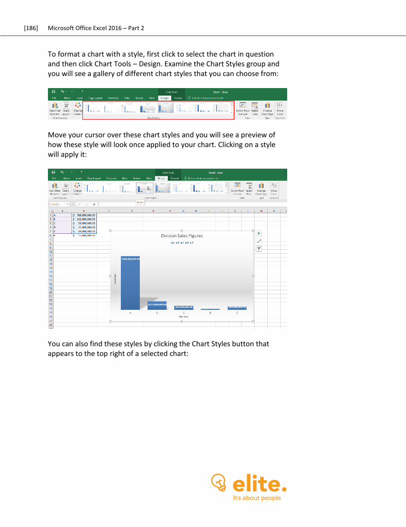
[186] Microsoft Office Excel 2016 – Part 2
To format a chart with a style, first click to select the chart in question and then click Chart Tools – Design. Examine the Chart Styles group and you will see a gallery of different chart styles that you can choose from:
Move your cursor over these chart styles and you will see a preview of how these style will look once applied to your chart. Clicking on a style will apply it:
You can also find these styles by clicking the Chart Styles button that appears to the top right of a selected chart:

[187] Microsoft Office Excel 2016 Level 2
This button will display a scrolling menu of the same chart styles that you can select from:
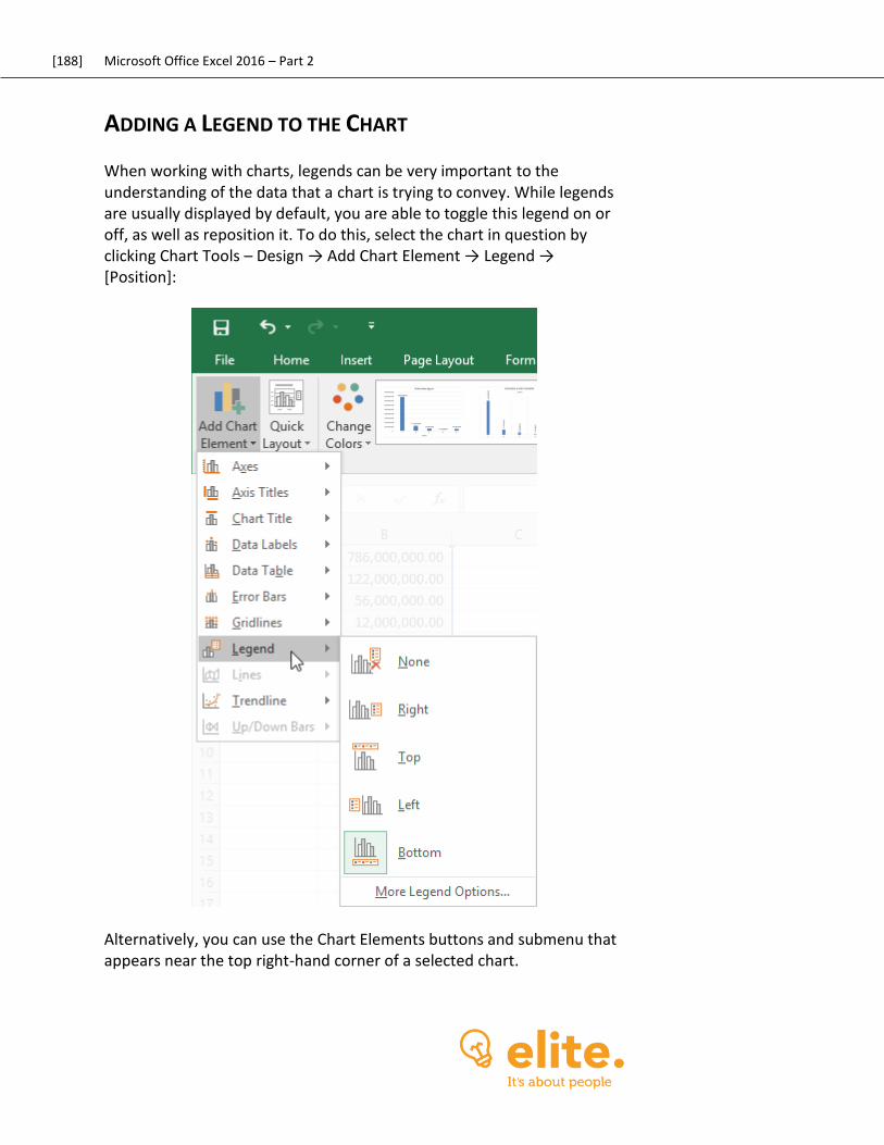
[188] Microsoft Office Excel 2016 – Part 2
ADDING A LEGEND TO THE CHART
When working with charts, legends can be very important to the understanding of the data that a chart is trying to convey. While legends are usually displayed by default, you are able to toggle this legend on or off, as well as reposition it. To do this, select the chart in question by clicking Chart Tools – Design → Add Chart Element → Legend → [Position]:
Alternatively, you can use the Chart Elements buttons and submenu that appears near the top right-hand corner of a selected chart.
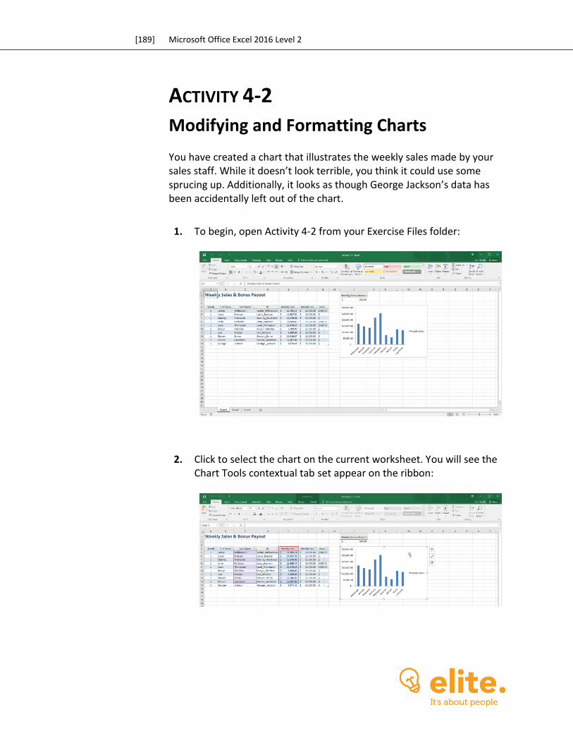
[189] Microsoft Office Excel 2016 Level 2
ACTIVITY 4-2
Modifying and Formatting Charts You have created a chart that illustrates the weekly sales made by your sales staff. While it doesn’t look terrible, you think it could use some sprucing up. Additionally, it looks as though George Jackson’s data has been accidentally left out of the chart.
1. To begin, open Activity 4-2 from your Exercise Files folder:
2. Click to select the chart on the current worksheet. You will see the Chart Tools contextual tab set appear on the ribbon:
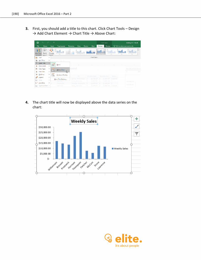
[190] Microsoft Office Excel 2016 – Part 2
3. First, you should add a title to this chart. Click Chart Tools – Design → Add Chart Element → Chart Title → Above Chart:
4. The chart title will now be displayed above the data series on the chart:
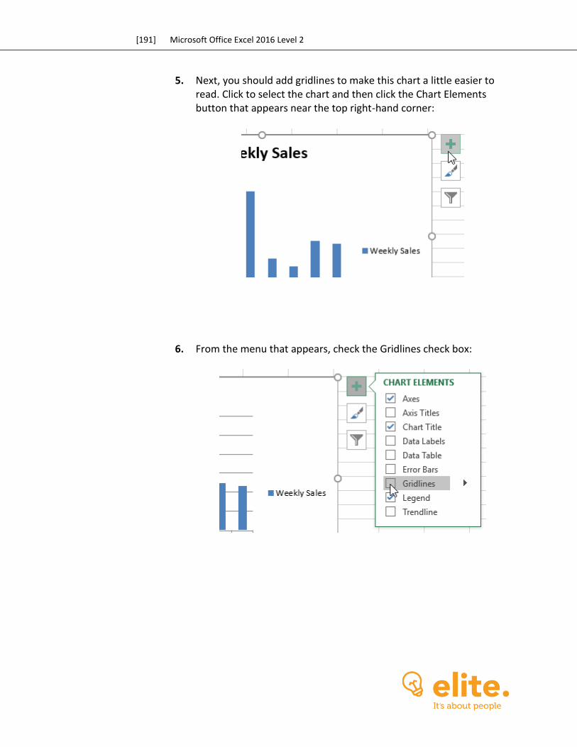
[191] Microsoft Office Excel 2016 Level 2
5. Next, you should add gridlines to make this chart a little easier to read. Click to select the chart and then click the Chart Elements button that appears near the top right-hand corner:
6. From the menu that appears, check the Gridlines check box:
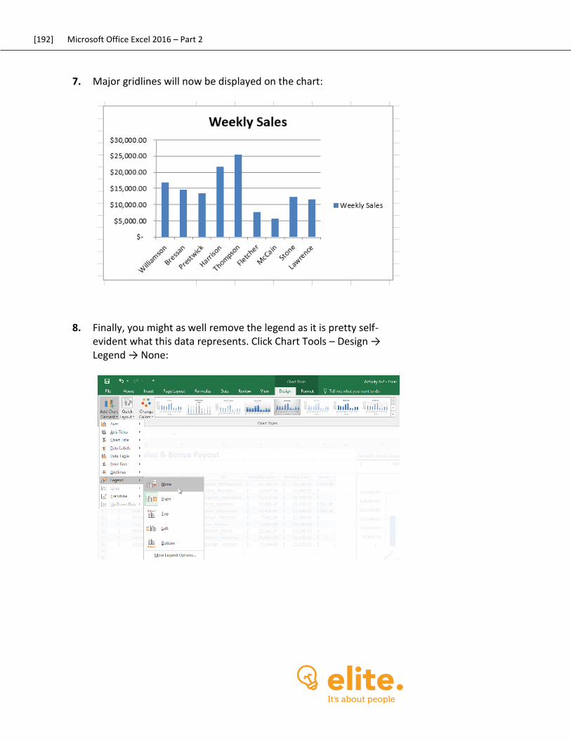
[192] Microsoft Office Excel 2016 – Part 2
7. Major gridlines will now be displayed on the chart:
8. Finally, you might as well remove the legend as it is pretty self-evident what this data represents. Click Chart Tools – Design → Legend → None:
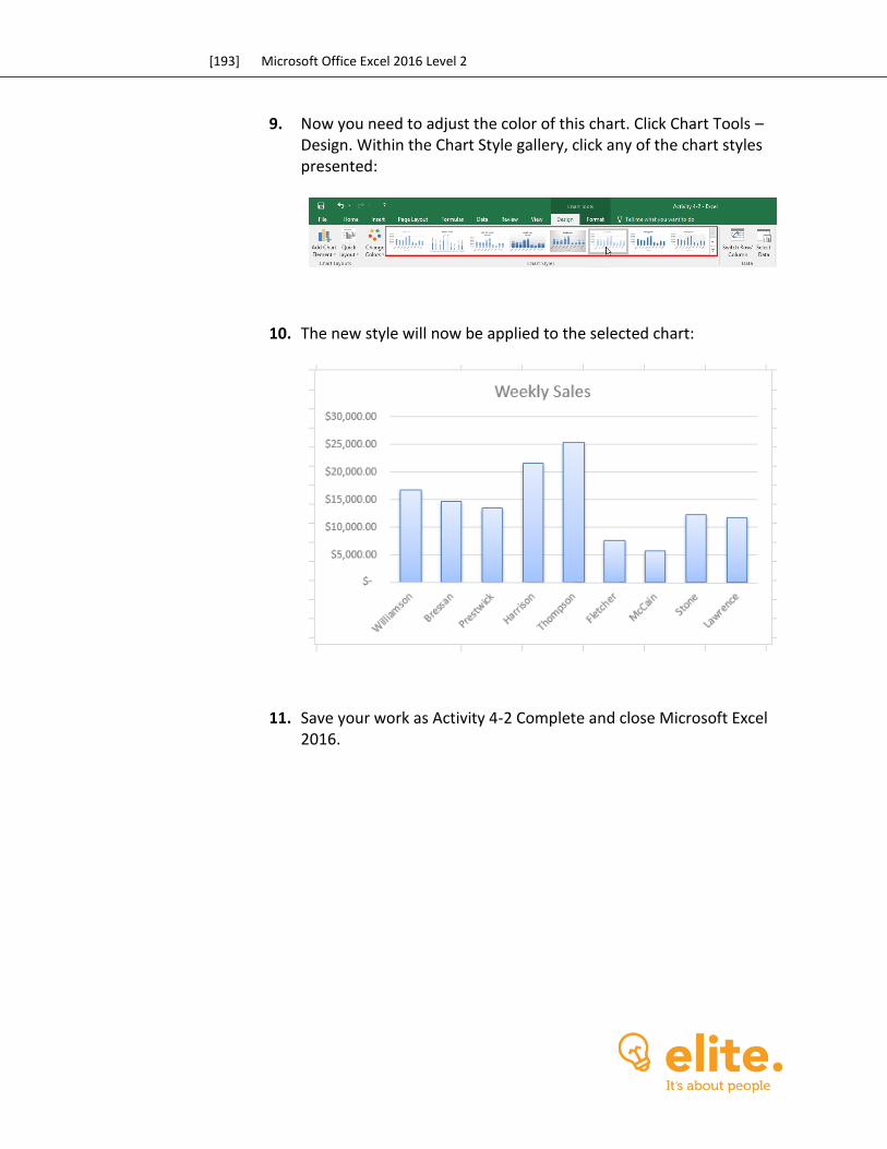
[193] Microsoft Office Excel 2016 Level 2
9. Now you need to adjust the color of this chart. Click Chart Tools – Design. Within the Chart Style gallery, click any of the chart styles presented:
10. The new style will now be applied to the selected chart:
11. Save your work as Activity 4-2 Complete and close Microsoft Excel 2016.
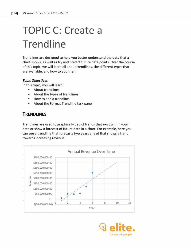
[194] Microsoft Office Excel 2016 – Part 2
TOPIC C: Create a Trendline Trendlines are designed to help you better understand the data that a chart shows, as well as try and predict future data points. Over the course of this topic, we will learn all about trendlines, the different types that are available, and how to add them. Topic Objectives In this topic, you will learn:
About trendlines About the types of trendlines How to add a trendline About the Format Trendline task pane
TRENDLINES
Trendlines are used to graphically depict trends that exist within your data or show a forecast of future data in a chart. For example, here you can see a trendline that forecasts two years ahead that shows a trend towards increasing revenue:

[195] Microsoft Office Excel 2016 Level 2

[196] Microsoft Office Excel 2016 – Part 2
TYPES OF TRENDLINES
Excel includes six different trend types that you can add to a chart. The type of trendline that you add depends on the type of data that the chart represents. Let’s breakdown each type of trendline and the type of data that they are best suited to represent:
Exponential – These types of trendlines are curved to illustrate data rising or falling at constant rates:
Linear – This trendline is typically used to represent simple linear data sets. It is a way to illustrate that something is increasing or decreasing over time:
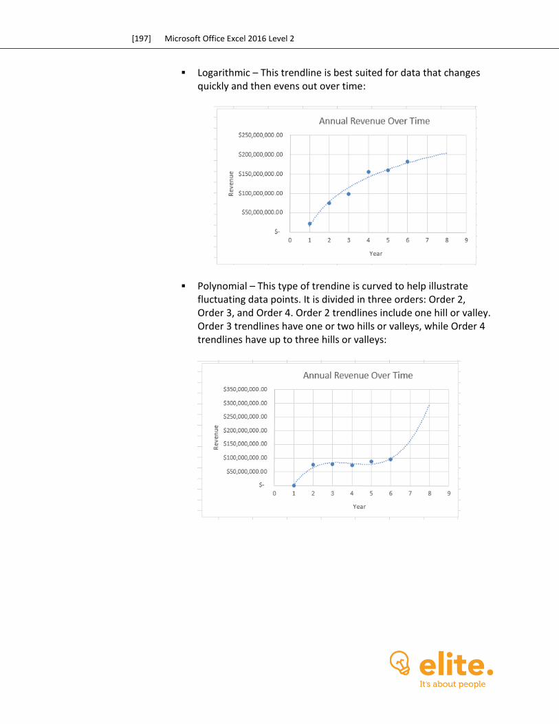
[197] Microsoft Office Excel 2016 Level 2
Logarithmic – This trendline is best suited for data that changes quickly and then evens out over time:
Polynomial – This type of trendine is curved to help illustrate fluctuating data points. It is divided in three orders: Order 2, Order 3, and Order 4. Order 2 trendlines include one hill or valley. Order 3 trendlines have one or two hills or valleys, while Order 4 trendlines have up to three hills or valleys:

[198] Microsoft Office Excel 2016 – Part 2
Power – This type of trendline is also curved, but is used with data sets that compare measurements at a specific rate. For example, you could use this trendline to measure acceleration over time:
Moving average – This type of trendline is intended to smooth out data that includes a lot of fluctuation. It does this by averaging a chosen number of data points. The number of data points is decided by setting the Period option. If this option is set to “2” then the first two points will be used to create the trendline:
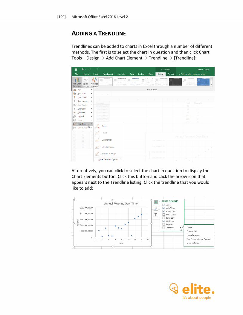
[199] Microsoft Office Excel 2016 Level 2
ADDING A TRENDLINE
Trendlines can be added to charts in Excel through a number of different methods. The first is to select the chart in question and then click Chart Tools – Design → Add Chart Element → Trendline → [Trendline]:
Alternatively, you can click to select the chart in question to display the Chart Elements button. Click this button and click the arrow icon that appears next to the Trendline listing. Click the trendline that you would like to add:
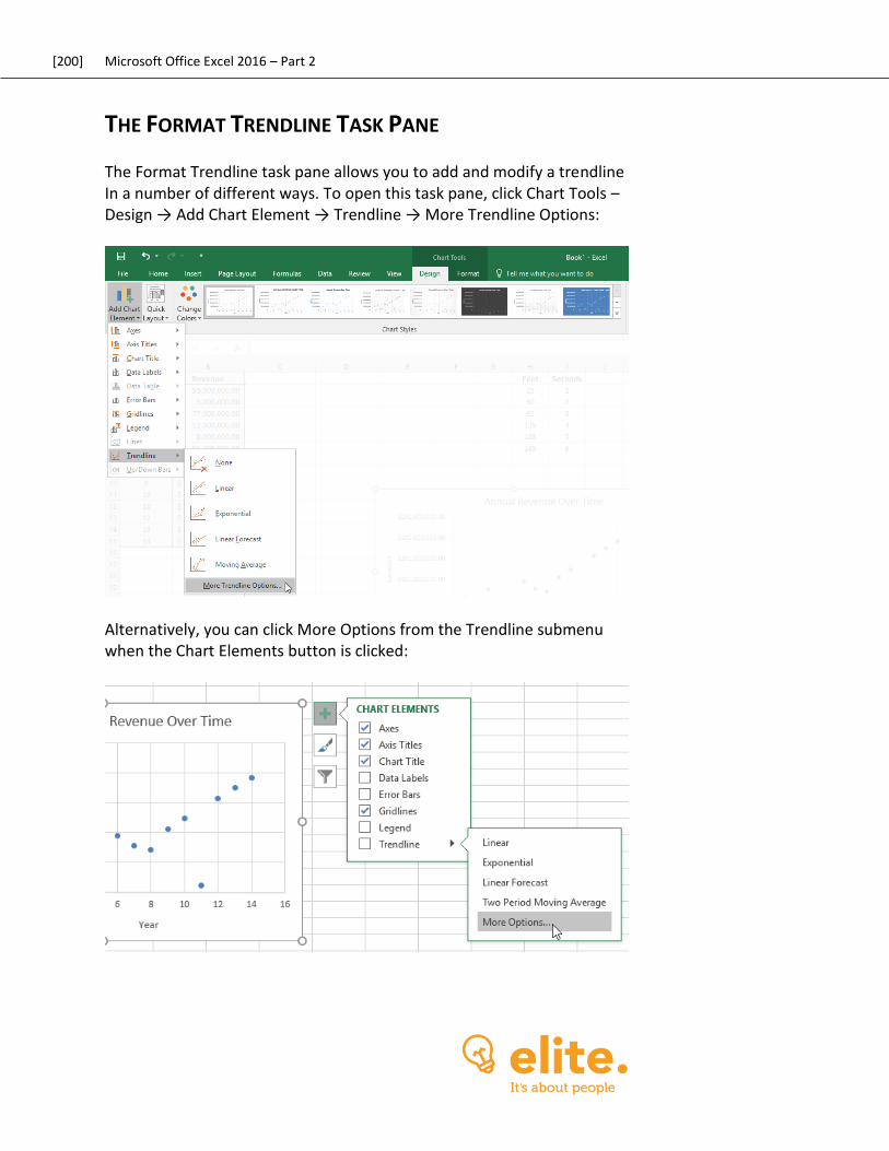
[200] Microsoft Office Excel 2016 – Part 2
THE FORMAT TRENDLINE TASK PANE
The Format Trendline task pane allows you to add and modify a trendline In a number of different ways. To open this task pane, click Chart Tools – Design → Add Chart Element → Trendline → More Trendline Options:
Alternatively, you can click More Options from the Trendline submenu when the Chart Elements button is clicked:
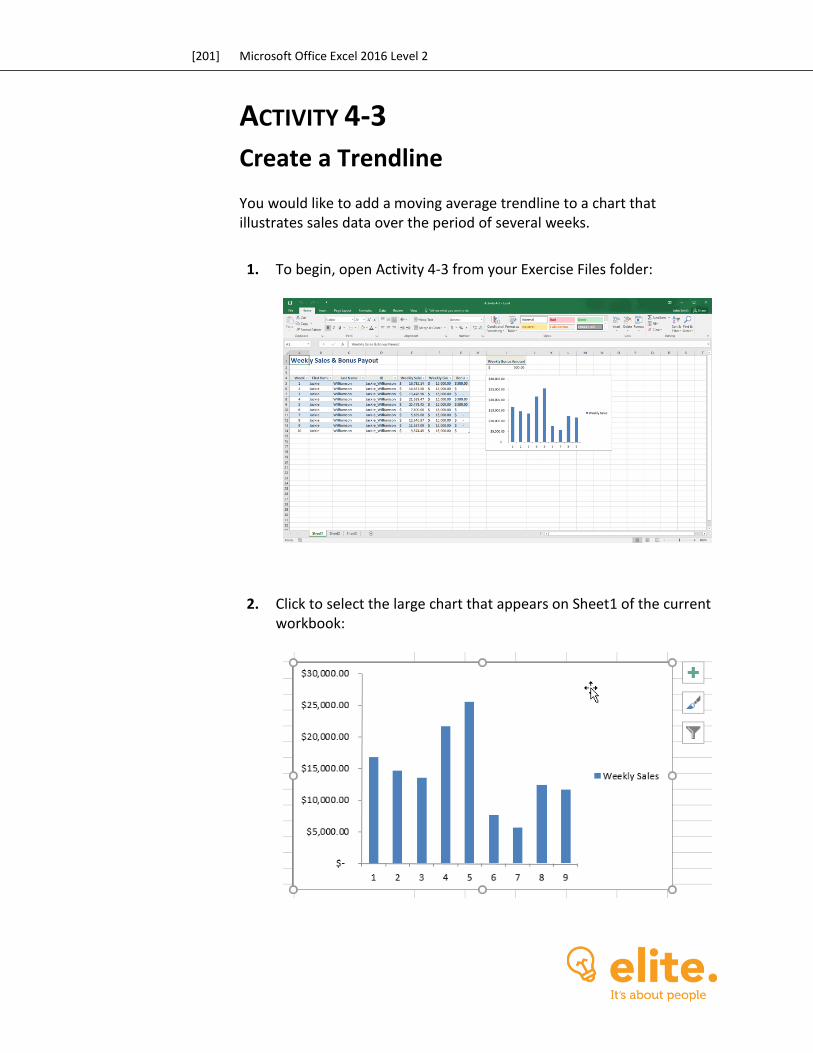
[201] Microsoft Office Excel 2016 Level 2
ACTIVITY 4-3
Create a Trendline You would like to add a moving average trendline to a chart that illustrates sales data over the period of several weeks.
1. To begin, open Activity 4-3 from your Exercise Files folder:
2. Click to select the large chart that appears on Sheet1 of the current workbook:
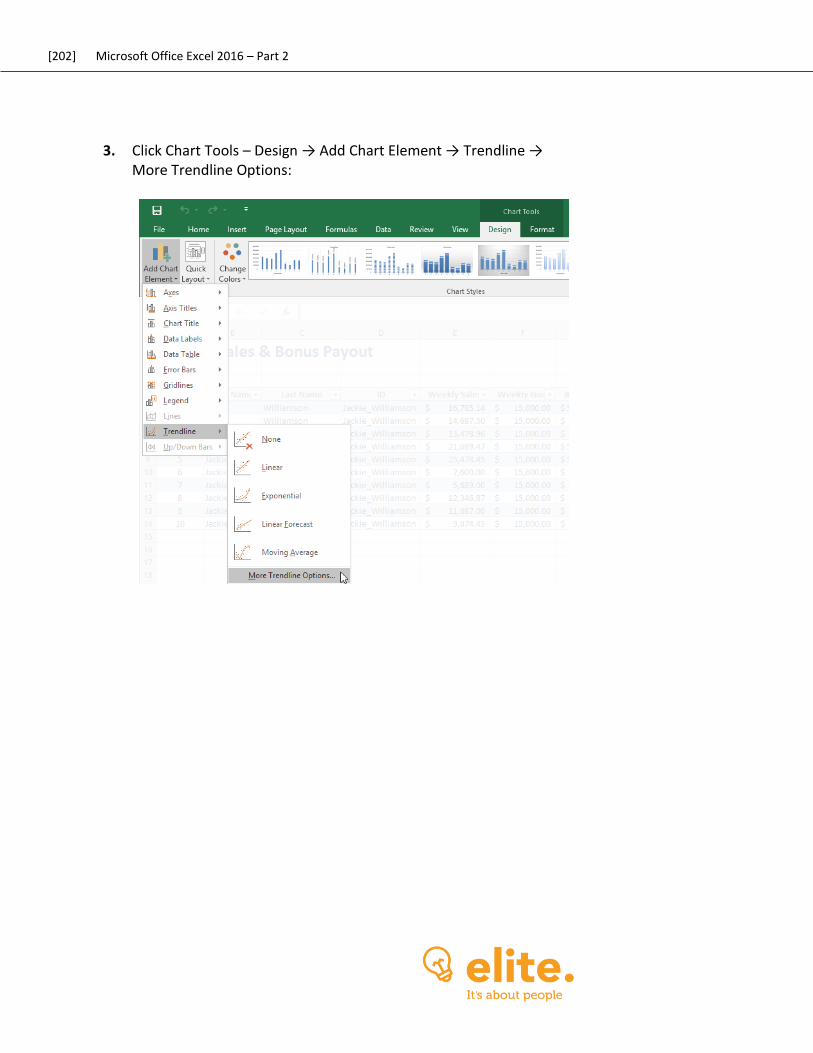
[202] Microsoft Office Excel 2016 – Part 2
3. Click Chart Tools – Design → Add Chart Element → Trendline → More Trendline Options:
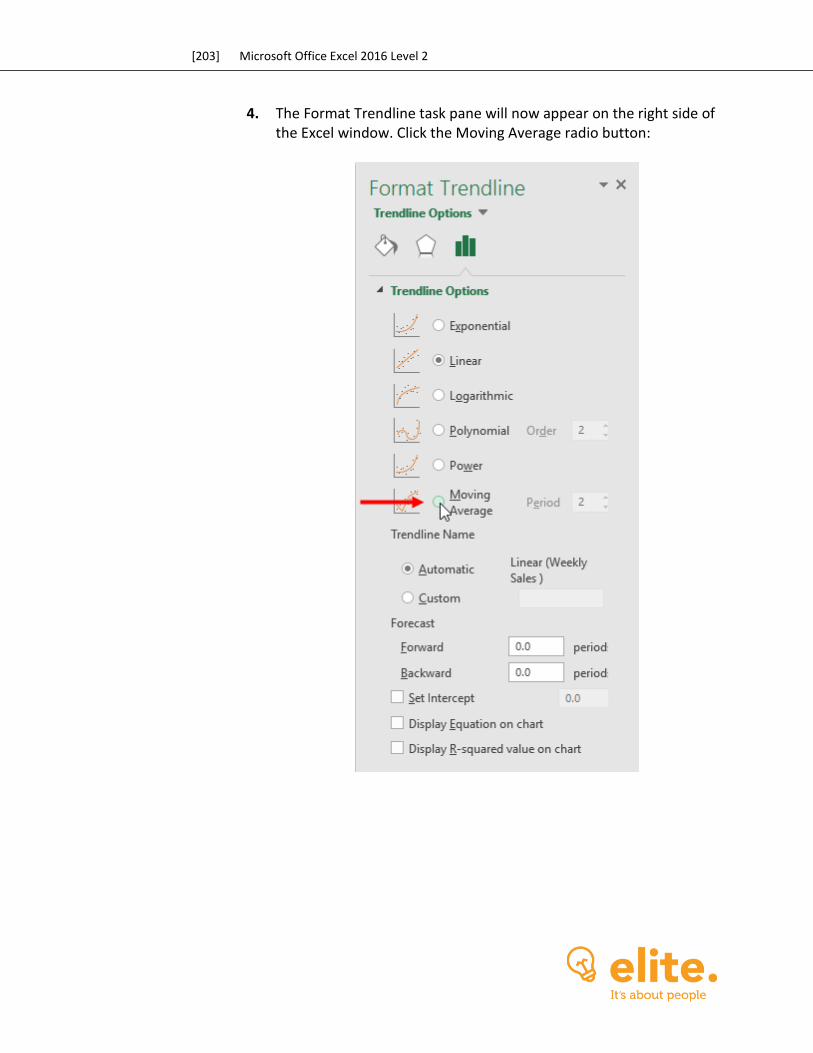
[203] Microsoft Office Excel 2016 Level 2
4. The Format Trendline task pane will now appear on the right side of the Excel window. Click the Moving Average radio button:
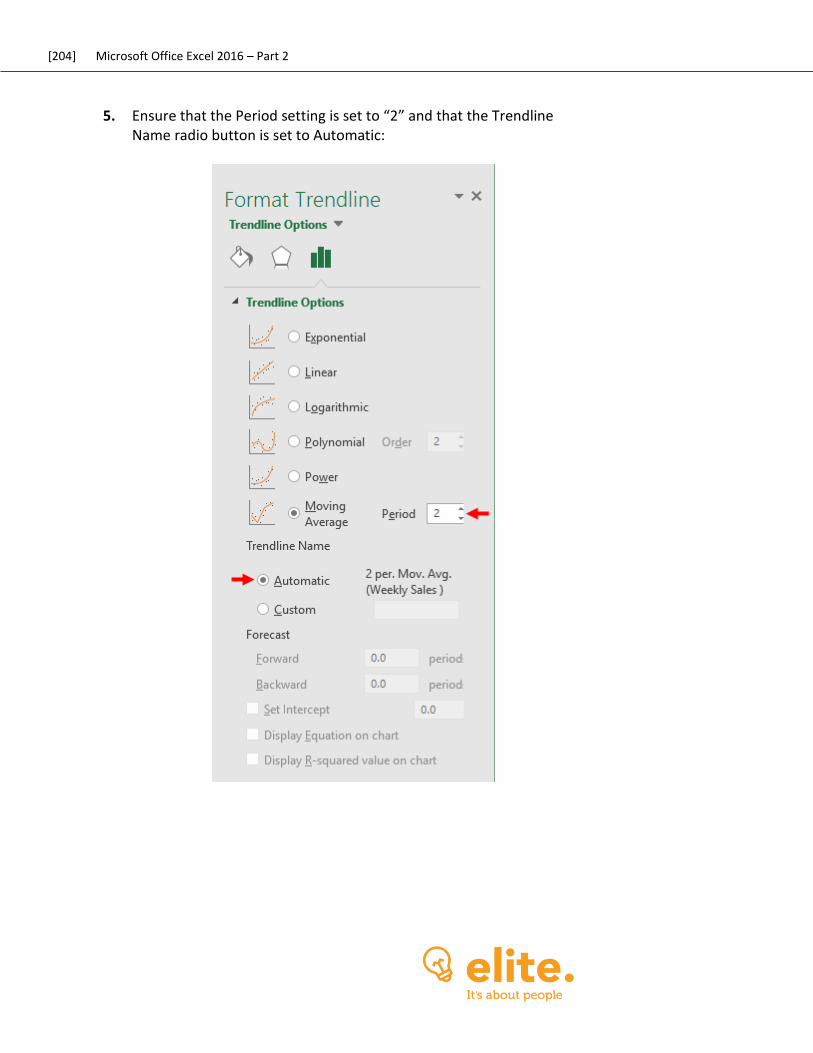
[204] Microsoft Office Excel 2016 – Part 2
5. Ensure that the Period setting is set to “2” and that the Trendline Name radio button is set to Automatic:
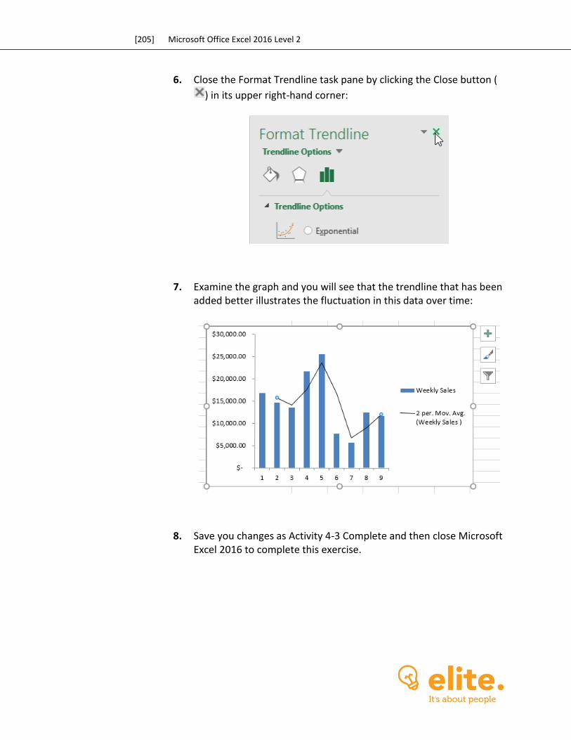
[205] Microsoft Office Excel 2016 Level 2
6. Close the Format Trendline task pane by clicking the Close button (
) in its upper right-hand corner:
7. Examine the graph and you will see that the trendline that has been added better illustrates the fluctuation in this data over time:
8. Save you changes as Activity 4-3 Complete and then close Microsoft Excel 2016 to complete this exercise.
[206] Microsoft Office Excel 2016 – Part 2
TOPIC D: Create Advanced Charts Beyond the basic chart types that are available and the simple modifications that you can make to them, Excel 2016 offers more advanced charts that can be used to represent your data. Over the course of this topic you will learn how to create advanced charts. Topic Objectives In this topic, you will learn:
About dual axis charts How to create custom chart templates How to view chart animations
DUAL AXIS CHARTS
A chart in Excel 2016 is capable of displaying two different (but related) pieces of data through dual axis. For example, if you wanted to see the total sales of a company, as well as the percentage of those sales that were from international customers, a dual axis chart can do this for you by including a second scale.
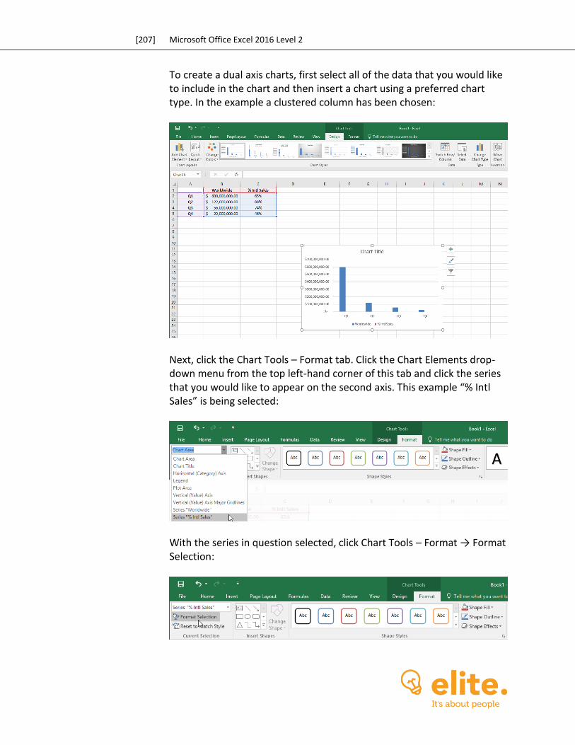
[207] Microsoft Office Excel 2016 Level 2
To create a dual axis charts, first select all of the data that you would like to include in the chart and then insert a chart using a preferred chart type. In the example a clustered column has been chosen:
Next, click the Chart Tools – Format tab. Click the Chart Elements drop-down menu from the top left-hand corner of this tab and click the series that you would like to appear on the second axis. This example “% Intl Sales” is being selected:
With the series in question selected, click Chart Tools – Format → Format Selection:
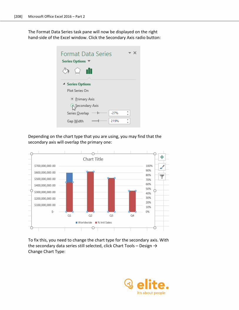
[208] Microsoft Office Excel 2016 – Part 2
The Format Data Series task pane will now be displayed on the right hand-side of the Excel window. Click the Secondary Axis radio button:
Depending on the chart type that you are using, you may find that the secondary axis will overlap the primary one:
To fix this, you need to change the chart type for the secondary axis. With the secondary data series still selected, click Chart Tools – Design → Change Chart Type:
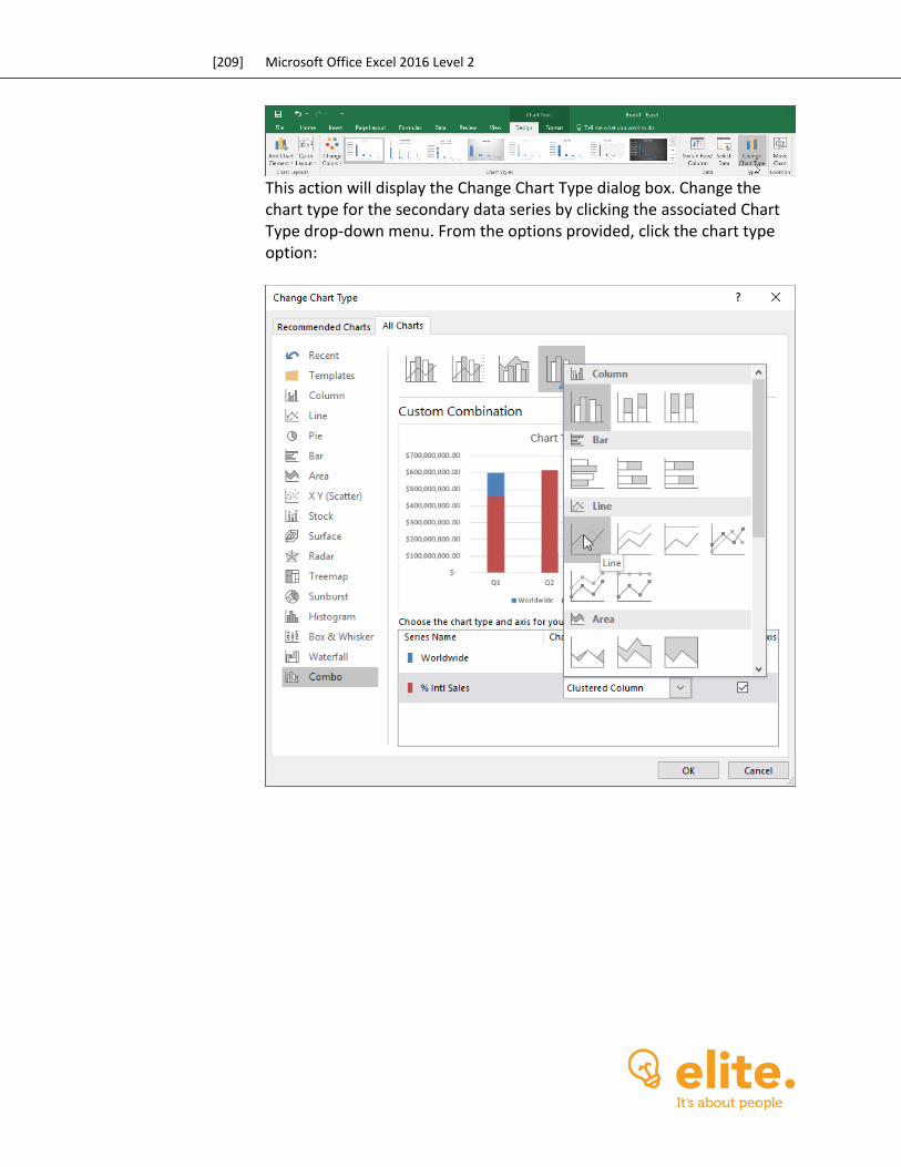
[209] Microsoft Office Excel 2016 Level 2
This action will display the Change Chart Type dialog box. Change the chart type for the secondary data series by clicking the associated Chart Type drop-down menu. From the options provided, click the chart type option:
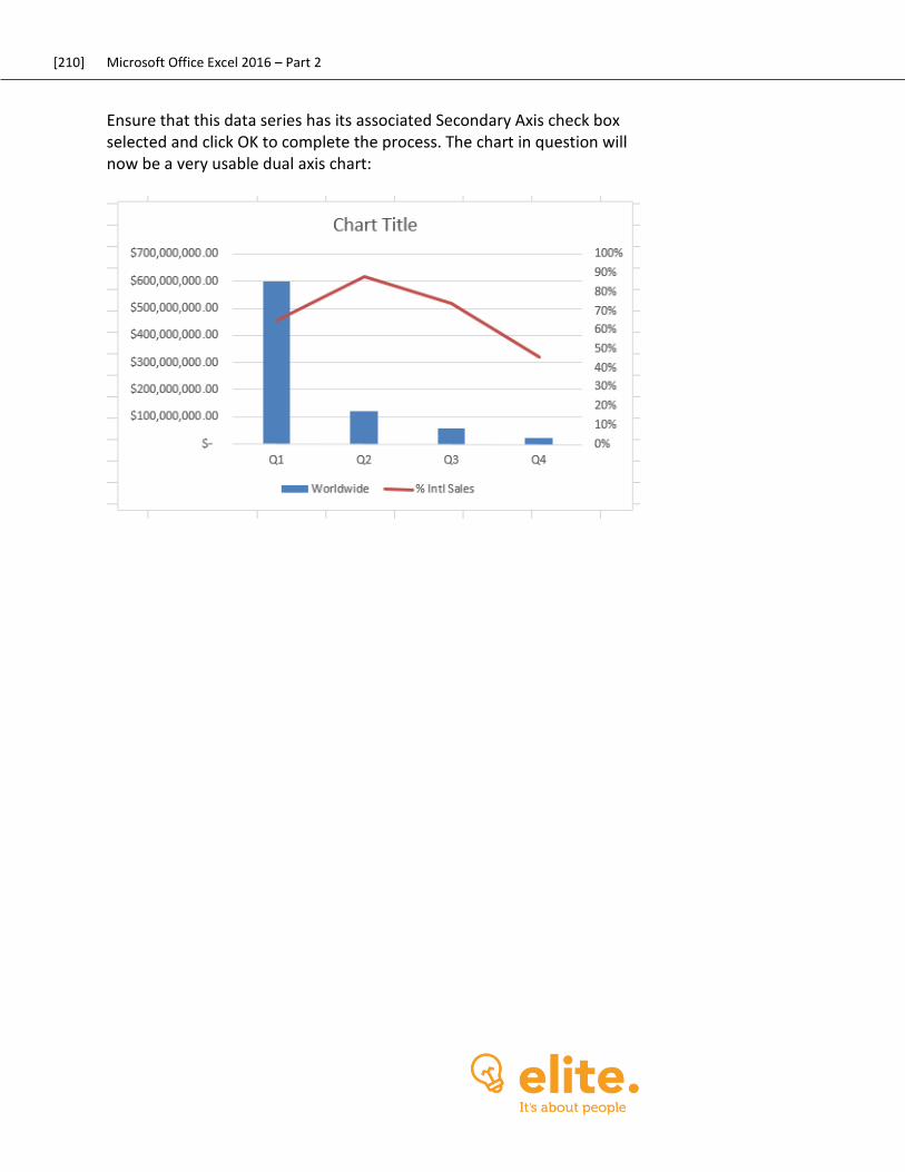
[210] Microsoft Office Excel 2016 – Part 2
Ensure that this data series has its associated Secondary Axis check box selected and click OK to complete the process. The chart in question will now be a very usable dual axis chart:
[211] Microsoft Office Excel 2016 Level 2
CREATING CUSTOM CHART TEMPLATES
It can take a long time to create a fully customized chart to suit your exact needs, so Excel includes the ability to save an existing chart as a chart template (.crtx). This will allow you to quickly recreate this type of chart using a different data set. To create a custom chart template, first click to select the chart that you want to work with. Next, right-click this chart and then click Save as Template:
[212] Microsoft Office Excel 2016 – Part 2
This action will display the Save Chart Template dialog box, with the Charts folder already open. In the “File name” text box, enter a name for this new template and then click Save:
[213] Microsoft Office Excel 2016 Level 2
With the new custom chart template saved, you can then create new charts using this template using the Templates category of the All Charts tab in the Change Chart Type dialog box:
[214] Microsoft Office Excel 2016 – Part 2
VIEWING CHART ANIMATIONS
Charts in Excel 2016 include the ability to animate data as you update its associated data points. For example, if you were to change the data for Q2 in the example below from 88% to 22%, the chart will animate this change and adjust the axis as required:
While this type of animation isn’t intended for presentation purposes, they do help you understand the impact certain changes can have on your data.
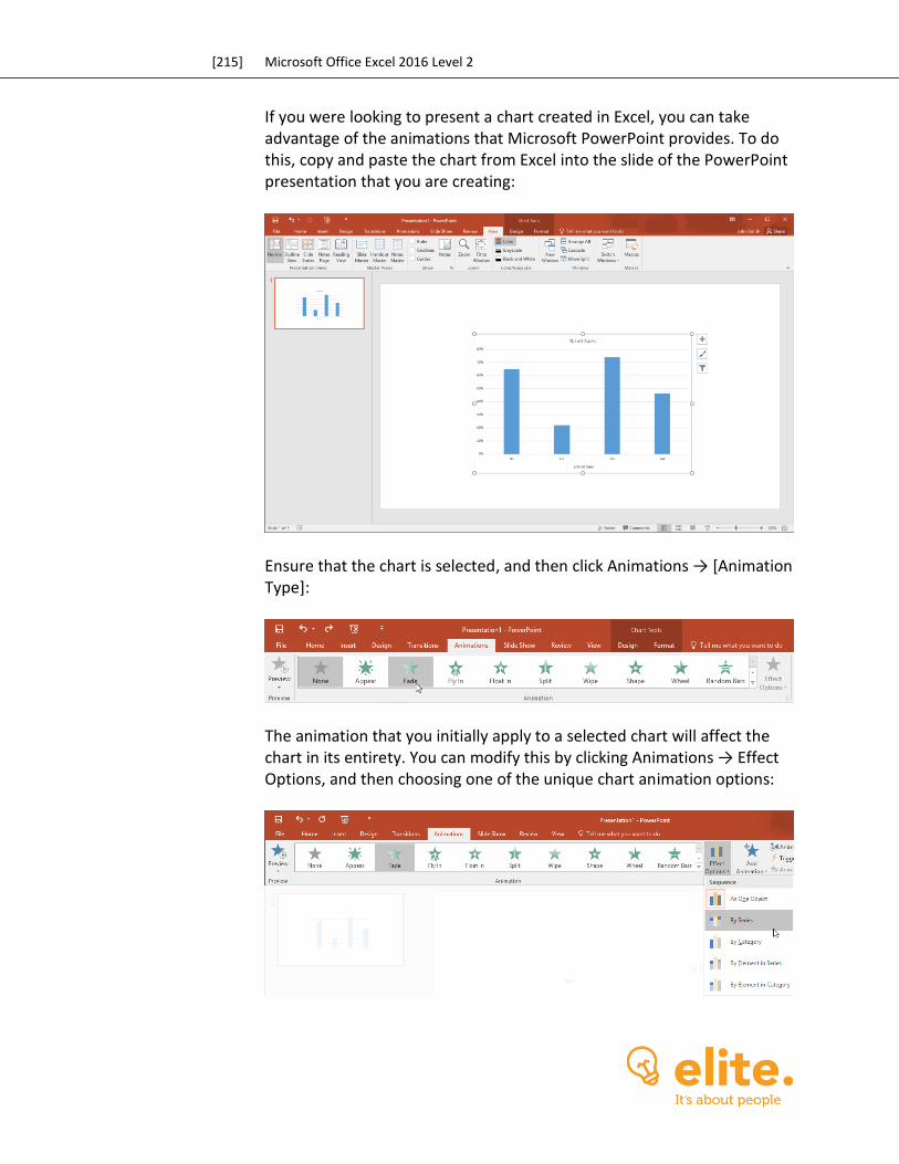
[215] Microsoft Office Excel 2016 Level 2
If you were looking to present a chart created in Excel, you can take advantage of the animations that Microsoft PowerPoint provides. To do this, copy and paste the chart from Excel into the slide of the PowerPoint presentation that you are creating:
Ensure that the chart is selected, and then click Animations → [Animation Type]:
The animation that you initially apply to a selected chart will affect the chart in its entirety. You can modify this by clicking Animations → Effect Options, and then choosing one of the unique chart animation options:
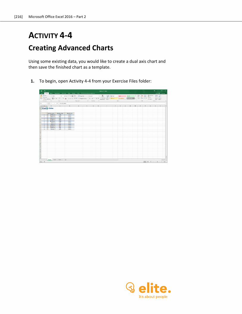
[216] Microsoft Office Excel 2016 – Part 2
ACTIVITY 4-4
Creating Advanced Charts Using some existing data, you would like to create a dual axis chart and then save the finished chart as a template.
1. To begin, open Activity 4-4 from your Exercise Files folder:
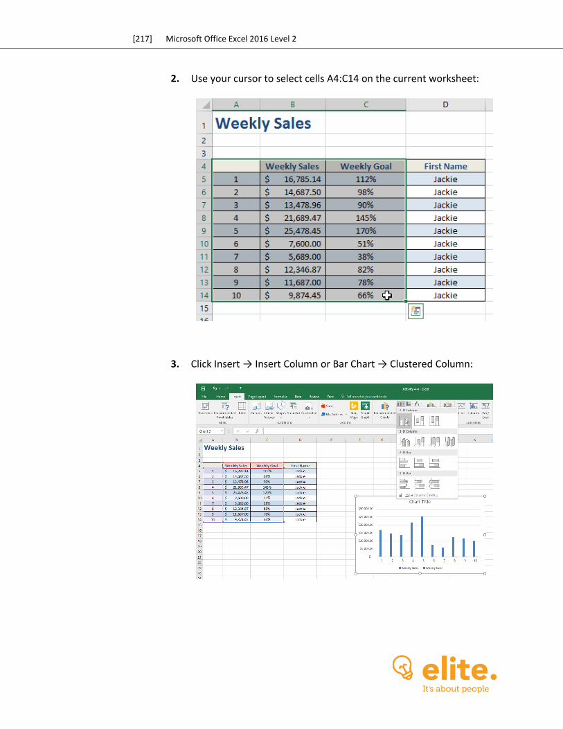
[217] Microsoft Office Excel 2016 Level 2
2. Use your cursor to select cells A4:C14 on the current worksheet:
3. Click Insert → Insert Column or Bar Chart → Clustered Column:

[218] Microsoft Office Excel 2016 – Part 2
4. With the chart now added, you need to select the second data series. Click Chart Tools – Format → Chart Elements → Series “Weekly Goal:”
5. Next, you need to open the Format Data Series task pane by clicking Chart Tools – Format → Format Selection:
6. Inside the Format Data Series task pane, click the Secondary Axis radio button:
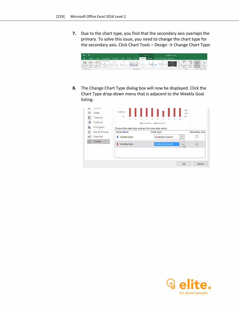
[219] Microsoft Office Excel 2016 Level 2
7. Due to the chart type, you find that the secondary axis overlaps the primary. To solve this issue, you need to change the chart type for the secondary axis. Click Chart Tools – Design → Change Chart Type:
8. The Change Chart Type dialog box will now be displayed. Click the Chart Type drop-down menu that is adjacent to the Weekly Goal listing:
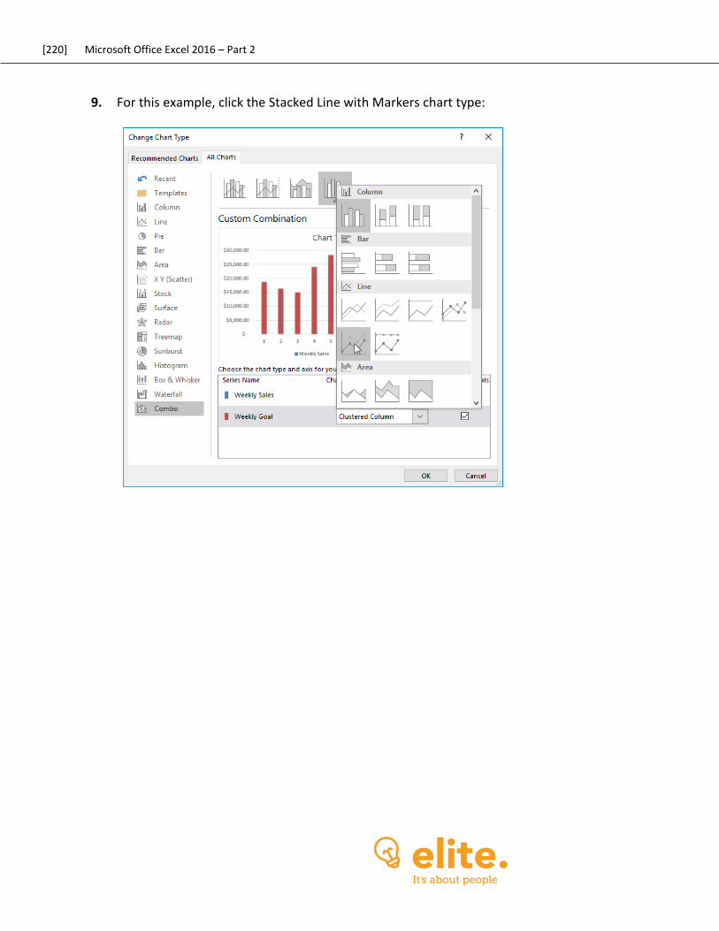
[220] Microsoft Office Excel 2016 – Part 2
9. For this example, click the Stacked Line with Markers chart type:
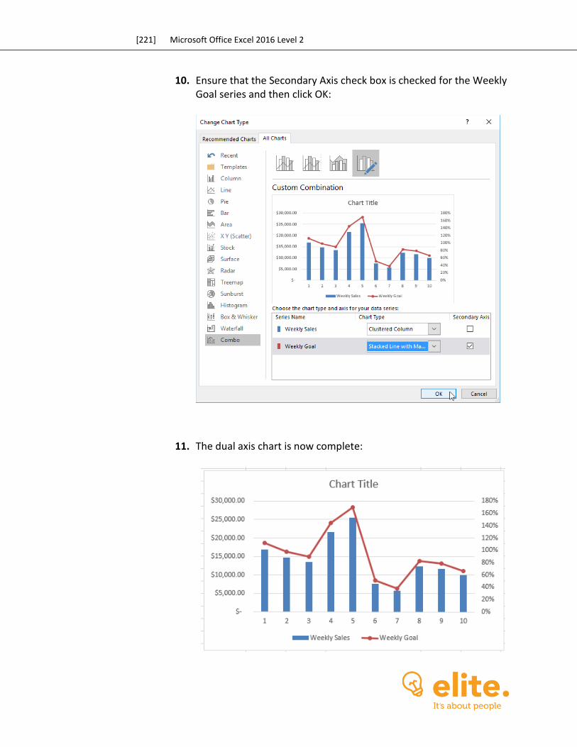
[221] Microsoft Office Excel 2016 Level 2
10. Ensure that the Secondary Axis check box is checked for the Weekly Goal series and then click OK:
11. The dual axis chart is now complete:

[222] Microsoft Office Excel 2016 – Part 2
12. Now you need to save this chart as a template. Right-click the chart and then click Save as Template:
13. The Save Chart Template dialog box will now be displayed. Type “Activity 4-4 Complete” into the “File name” text box and then click the Save button:
14. Save the current workbook as Activity 4-4 Complete.
[223] Microsoft Office Excel 2016 Level 2
Summary This lesson taught you how to insert charts into worksheets as well as the best way to format charts to meet the specific needs of you and your audience. Additionally, you learned about the wide variety of charts that are available to you depending upon the data that you are working with. You should now feel comfortable modifying as well as formatting existing charts. You should also understand how to work with dual axis charts, create custom chart templates, and view chart animations.
REVIEW QUESTIONS
1. What are charts?
2. How many different chart types can you choose from?
3. What is the difference between modification and formatting?
4. When are the Chart Tools contextual tabs displayed?
5. What is the command sequence to add a trendline using the ribbon?


[225] Microsoft Office Excel 2016 – Part 2
LESSON 5: ANALYZING DATA WITH
PIVOTTABLES, SLICERS, AND PIVOTCHARTS
Lesson Objectives
In this lesson you will learn how to:
Create a PivotTable
Filter data using slicers
Analyze data using PivotCharts
[226] Microsoft Office Excel 2016 – Part 2
TOPIC A: Create a PivotTable One of the most powerful tools that you have your disposal when analyzing data in Excel is the PivotTable. While extremely useful, these interactive objects are somewhat cumbersome to execute properly and are often misused. For this reason it is important to understand how they work and gain some fundamental understanding of their purpose before creating PivotTables of your own data. Topic Objectives In this topic, you will learn:
About PivotTables How to start with questions and end with structure About the Create PivotTable dialog box About the PivotTable fields pane How to summarize data in a PivotTable About the “Show value as” functionality About using external data with PivotTables About PowerPivot About PowerPivot functions
PIVOTTABLES
Why are PivotTables called PivotTables? Because they let you move data around easily (by dragging and dropping fields) to perform a sort of rotation on the structure of your table and at the same time, change your view of the data. With PivotTables, columns can become rows and rows can become columns, all without altering the original data. When a PivotTable is created, you are given the option to put it on the worksheet that you currently have open or on a new one. In either case, once the PivotTable is created you can pivot, re-pivot, sort, and summarize your data without affecting it directly. You are able to choose the level of detail that you want to view depending on your needs. Additionally, you have access to all of the summary functions in Excel to complete your data analysis.

[227] Microsoft Office Excel 2016 – Part 2
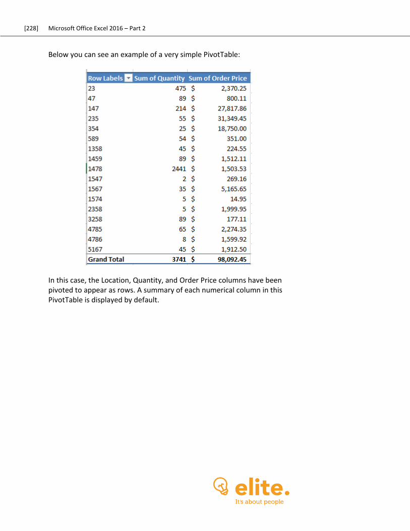
[228] Microsoft Office Excel 2016 – Part 2
Below you can see an example of a very simple PivotTable:
In this case, the Location, Quantity, and Order Price columns have been pivoted to appear as rows. A summary of each numerical column in this PivotTable is displayed by default.
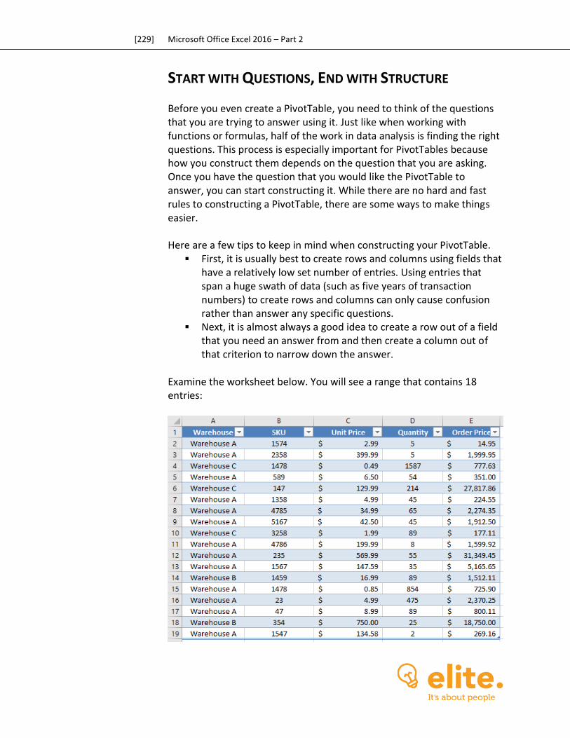
[229] Microsoft Office Excel 2016 – Part 2
START WITH QUESTIONS, END WITH STRUCTURE
Before you even create a PivotTable, you need to think of the questions that you are trying to answer using it. Just like when working with functions or formulas, half of the work in data analysis is finding the right questions. This process is especially important for PivotTables because how you construct them depends on the question that you are asking. Once you have the question that you would like the PivotTable to answer, you can start constructing it. While there are no hard and fast rules to constructing a PivotTable, there are some ways to make things easier. Here are a few tips to keep in mind when constructing your PivotTable.
First, it is usually best to create rows and columns using fields that have a relatively low set number of entries. Using entries that span a huge swath of data (such as five years of transaction numbers) to create rows and columns can only cause confusion rather than answer any specific questions.
Next, it is almost always a good idea to create a row out of a field that you need an answer from and then create a column out of that criterion to narrow down the answer.
Examine the worksheet below. You will see a range that contains 18 entries:
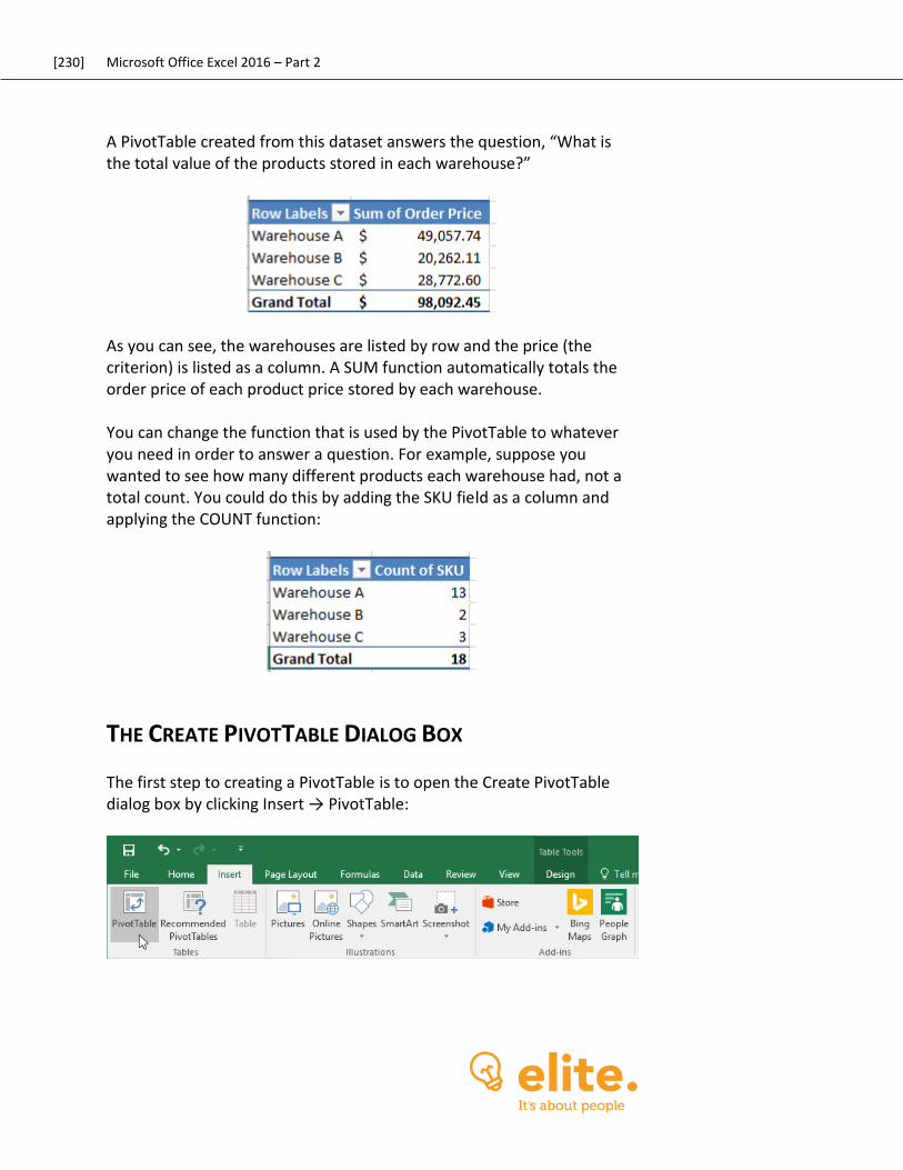
[230] Microsoft Office Excel 2016 – Part 2
A PivotTable created from this dataset answers the question, “What is the total value of the products stored in each warehouse?”
As you can see, the warehouses are listed by row and the price (the criterion) is listed as a column. A SUM function automatically totals the order price of each product price stored by each warehouse. You can change the function that is used by the PivotTable to whatever you need in order to answer a question. For example, suppose you wanted to see how many different products each warehouse had, not a total count. You could do this by adding the SKU field as a column and applying the COUNT function:
THE CREATE PIVOTTABLE DIALOG BOX
The first step to creating a PivotTable is to open the Create PivotTable dialog box by clicking Insert → PivotTable:
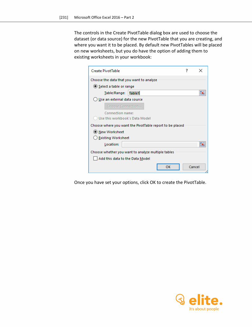
[231] Microsoft Office Excel 2016 – Part 2
The controls in the Create PivotTable dialog box are used to choose the dataset (or data source) for the new PivotTable that you are creating, and where you want it to be placed. By default new PivotTables will be placed on new worksheets, but you do have the option of adding them to existing worksheets in your workbook:
Once you have set your options, click OK to create the PivotTable.
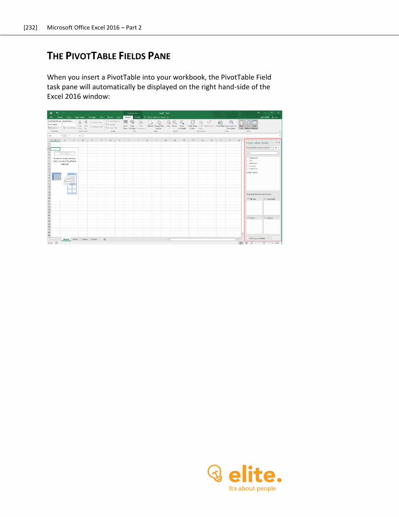
[232] Microsoft Office Excel 2016 – Part 2
THE PIVOTTABLE FIELDS PANE
When you insert a PivotTable into your workbook, the PivotTable Field task pane will automatically be displayed on the right hand-side of the Excel 2016 window:

[233] Microsoft Office Excel 2016 – Part 2
The PivotTable Field List pane is the primary tool that you will use to configure PivotTables. (Note that it is hidden when the PivotTable is not selected.) The top portion of this pane (1) lists all of the fields from the dataset that you can add to the PivotTable. To add or remove a field from the PivotTable, toggle the corresponding checkbox. Alternatively, to give you more control over field placement on the PivotTable, you can click and drag these fields to the PivotTable itself. Note that field names are derived from the column header in the dataset:
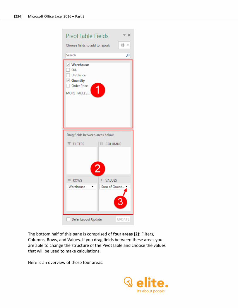
[234] Microsoft Office Excel 2016 – Part 2
The bottom half of this pane is comprised of four areas (2): Filters, Columns, Rows, and Values. If you drag fields between these areas you are able to change the structure of the PivotTable and choose the values that will be used to make calculations. Here is an overview of these four areas.
[235] Microsoft Office Excel 2016 – Part 2
Adding fields to the Filters area will include those field values as filter criteria.
The Columns area will create columns out of unique field entries. Similarly, the Rows area will create rows out of unique field
entries. Finally, fields that are dragged to the Values area will have
calculations performed on them or their values summarized. Note that any fields that appear in these four areas will include a
pull-down arrow (3) that give you access to a number of different settings and the Field Settings dialog that you can use to further customize your PivotTable.
Remember that any changes that you make in the PivotTable Field List pane will be applied dynamically. Additionally, due to the flexible nature of PivotTables, you can add or remove fields to or from the pane at any time.
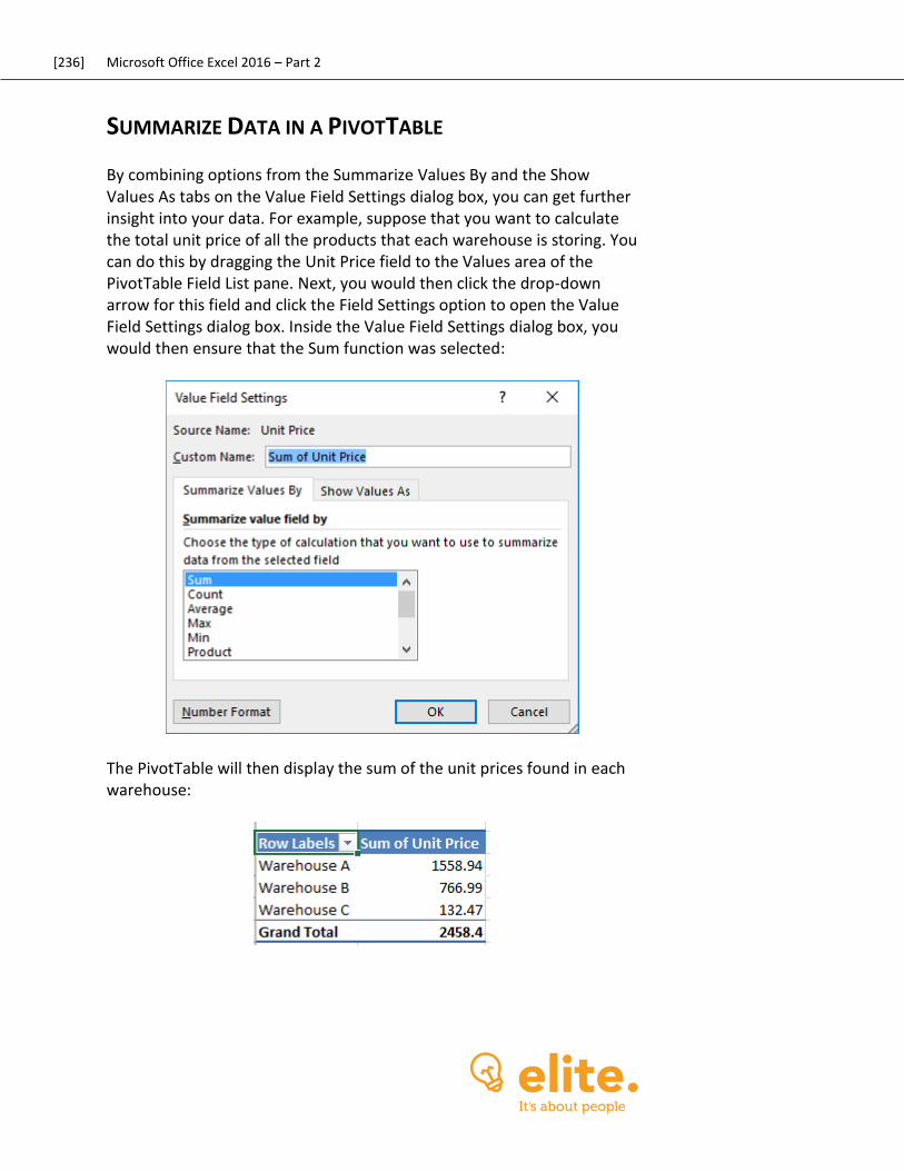
[236] Microsoft Office Excel 2016 – Part 2
SUMMARIZE DATA IN A PIVOTTABLE
By combining options from the Summarize Values By and the Show Values As tabs on the Value Field Settings dialog box, you can get further insight into your data. For example, suppose that you want to calculate the total unit price of all the products that each warehouse is storing. You can do this by dragging the Unit Price field to the Values area of the PivotTable Field List pane. Next, you would then click the drop-down arrow for this field and click the Field Settings option to open the Value Field Settings dialog box. Inside the Value Field Settings dialog box, you would then ensure that the Sum function was selected:
The PivotTable will then display the sum of the unit prices found in each warehouse:
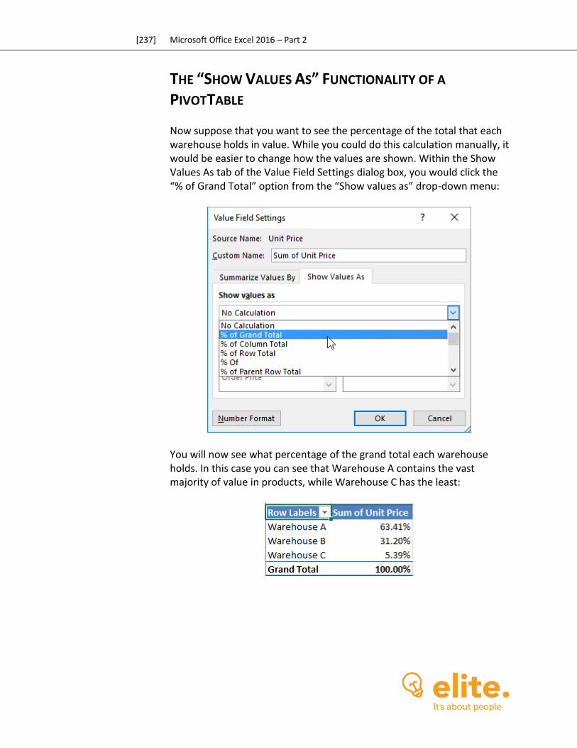
[237] Microsoft Office Excel 2016 – Part 2
THE “SHOW VALUES AS” FUNCTIONALITY OF A
PIVOTTABLE
Now suppose that you want to see the percentage of the total that each warehouse holds in value. While you could do this calculation manually, it would be easier to change how the values are shown. Within the Show Values As tab of the Value Field Settings dialog box, you would click the “% of Grand Total” option from the “Show values as” drop-down menu:
You will now see what percentage of the grand total each warehouse holds. In this case you can see that Warehouse A contains the vast majority of value in products, while Warehouse C has the least:
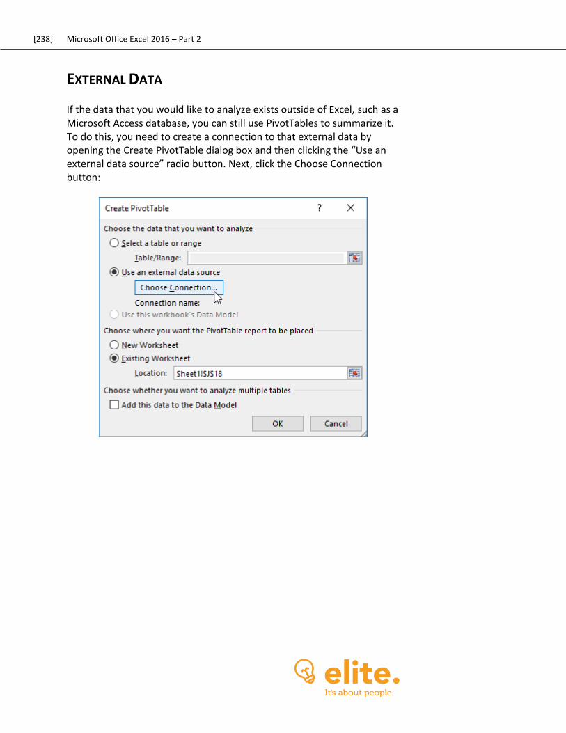
[238] Microsoft Office Excel 2016 – Part 2
EXTERNAL DATA
If the data that you would like to analyze exists outside of Excel, such as a Microsoft Access database, you can still use PivotTables to summarize it. To do this, you need to create a connection to that external data by opening the Create PivotTable dialog box and then clicking the “Use an external data source” radio button. Next, click the Choose Connection button:
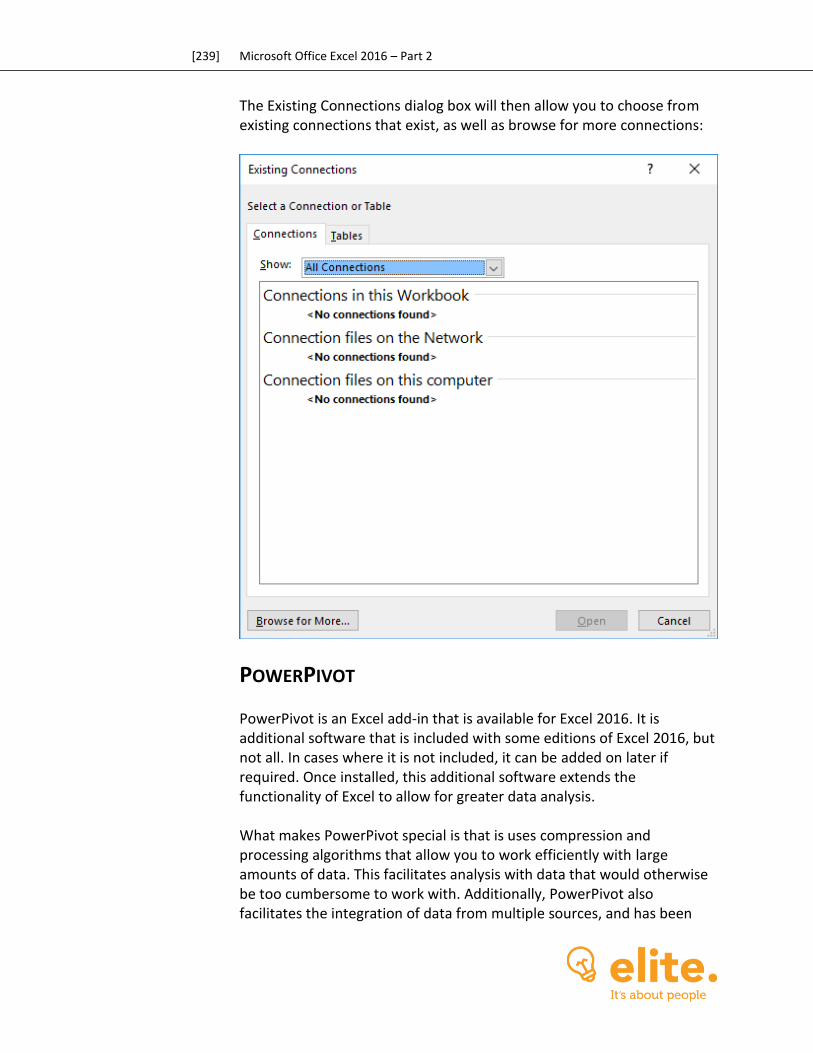
[239] Microsoft Office Excel 2016 – Part 2
The Existing Connections dialog box will then allow you to choose from existing connections that exist, as well as browse for more connections:
POWERPIVOT
PowerPivot is an Excel add-in that is available for Excel 2016. It is additional software that is included with some editions of Excel 2016, but not all. In cases where it is not included, it can be added on later if required. Once installed, this additional software extends the functionality of Excel to allow for greater data analysis. What makes PowerPivot special is that is uses compression and processing algorithms that allow you to work efficiently with large amounts of data. This facilitates analysis with data that would otherwise be too cumbersome to work with. Additionally, PowerPivot also facilitates the integration of data from multiple sources, and has been

[240] Microsoft Office Excel 2016 – Part 2
designed with extra features and flexibility for environments that rely on Microsoft SharePoint and/or Microsoft SQL servers.
POWERPIVOT FUNCTIONS
DAX (Data Analysis Expression) is a type of formula language that is used to create custom calculations inside calculated columns in a PowerPivot table. It is also used to create measures inside a PivotTable. This means that PowerPivot provides you with additional functions using DAX that can be used to work with relational data in a much more powerful manner. Arguments in a DAX function commonly use tables and columns. For example, below you can see a DAX function that uses the Totals and Date columns from the Employee Sales table as arguments:
=TOTALQTD(SUM(‘Employee Sales’[Totals]), ‘Employee Sales’[Date])
While there are lots of DAX functions that you can choose from, each is classified under one of the following categories:
Data and Time functions: Functions of this type are used to manipulate date and time values. As such, they are similar to the data and time functions that can be used in Excel.
Filter functions: These functions are used to manipulate data and filter it dynamically.
Information functions: This type of function is used to scan the values inside a cell range and match them against an expected data type.
Logical functions: Typically these functions are used to validate expressions and values, and then work with other data that is based upon the evaluation.
Math and Trigonometric functions: Functions of this type are used to perform mathematical calculations.
Statistical functions: These functions are used to generate statistical data like minimum and maximum values, as well as averages.
Time Intelligence functions: This type of function is used to manipulate data using time periods. They can be used to compare data of one time period against another.
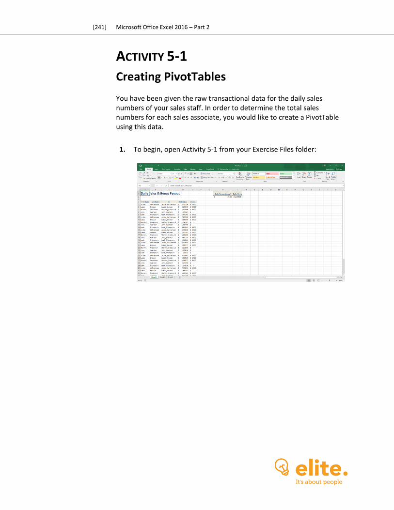
[241] Microsoft Office Excel 2016 – Part 2
ACTIVITY 5-1
Creating PivotTables You have been given the raw transactional data for the daily sales numbers of your sales staff. In order to determine the total sales numbers for each sales associate, you would like to create a PivotTable using this data.
1. To begin, open Activity 5-1 from your Exercise Files folder:
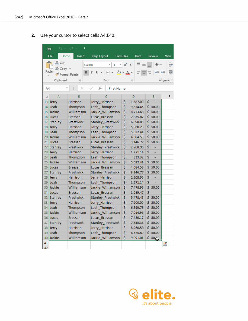
[242] Microsoft Office Excel 2016 – Part 2
2. Use your cursor to select cells A4:E40:
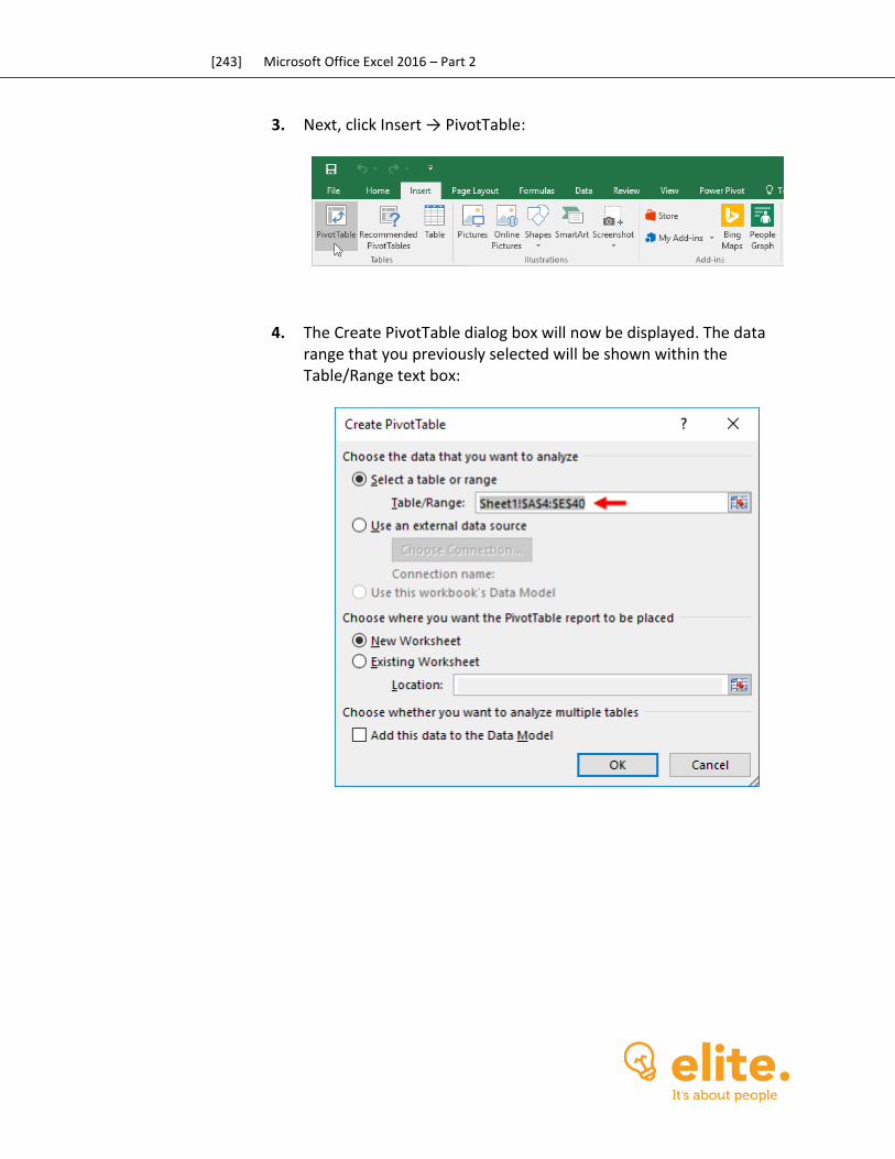
[243] Microsoft Office Excel 2016 – Part 2
3. Next, click Insert → PivotTable:
4. The Create PivotTable dialog box will now be displayed. The data range that you previously selected will be shown within the Table/Range text box:
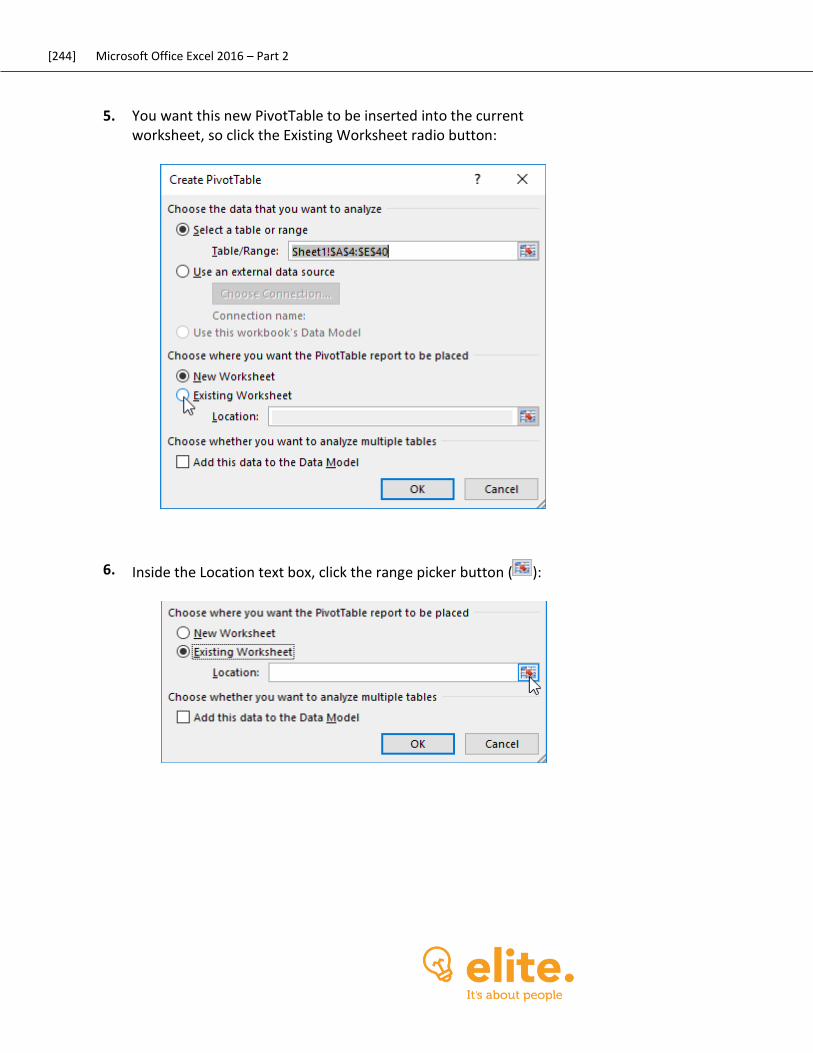
[244] Microsoft Office Excel 2016 – Part 2
5. You want this new PivotTable to be inserted into the current worksheet, so click the Existing Worksheet radio button:
6. Inside the Location text box, click the range picker button ( ):
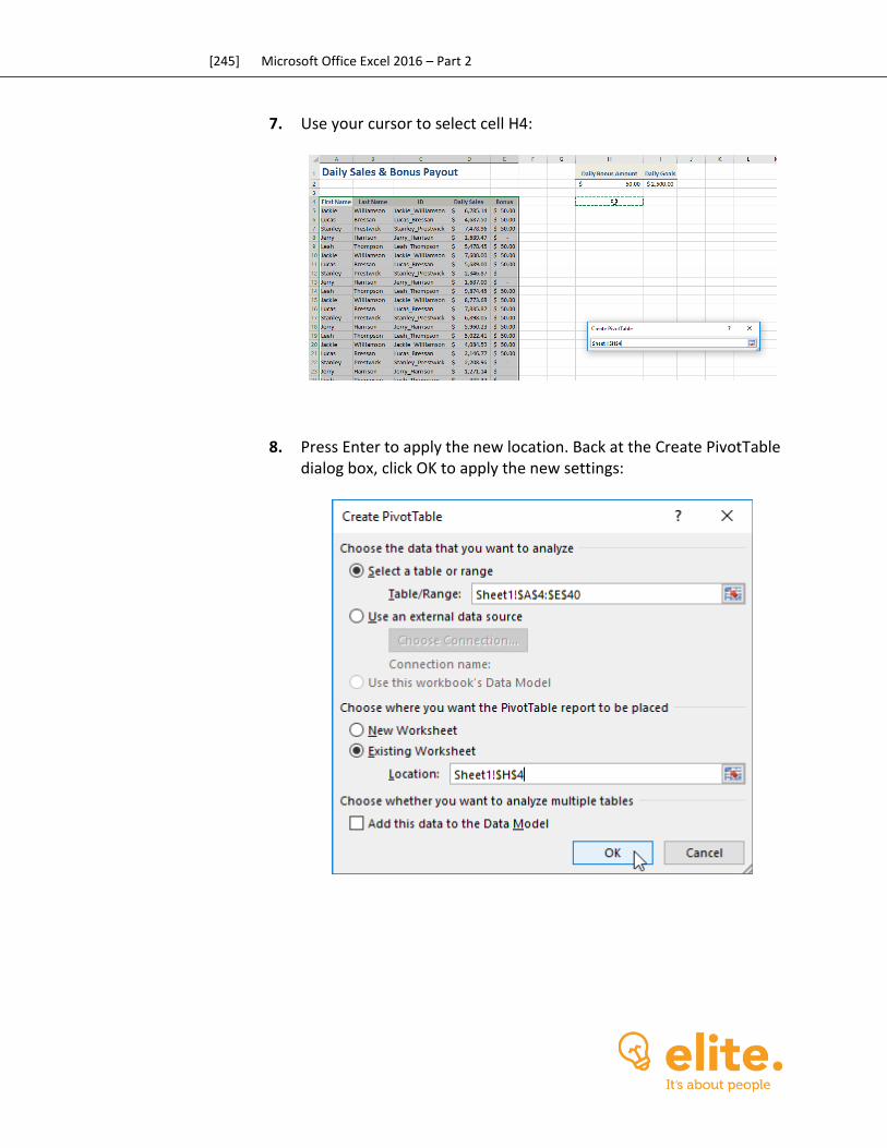
[245] Microsoft Office Excel 2016 – Part 2
7. Use your cursor to select cell H4:
8. Press Enter to apply the new location. Back at the Create PivotTable dialog box, click OK to apply the new settings:
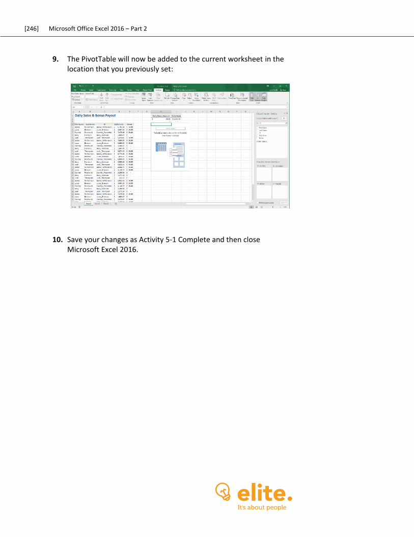
[246] Microsoft Office Excel 2016 – Part 2
9. The PivotTable will now be added to the current worksheet in the location that you previously set:
10. Save your changes as Activity 5-1 Complete and then close Microsoft Excel 2016.
[247] Microsoft Office Excel 2016 – Part 2
TOPIC B: Filter Data by Using Slicers While regular filters can be effective in drilling down through your data, they can quickly become a chore to manage. Between having to clear existing filters before applying new ones and trying to determine which data is actively being filtered out, filters definitely have some downsides. To give you more control over filtering capabilities, Excel provides slicers. These are easy-to-use filters that can be applied multiple times without negative effects on the data’s readability. Throughout this topic you will learn about slicers and how to use them to filter data in a PivotTable. Topic Objectives In this topic, you will learn:
About slicers About the Insert Slicer dialog box
SLICERS
Slicers can be a great help when working with PivotTable data. While the main purpose of PivotTables is to help you analyze information and find patterns or trends that might be difficult to spot in a large volume of raw data, the Slicer tool takes this idea to the next level. Slicers can be created out of any field that exists within the dataset for the PivotTable. These slicers can then be used to filter each field by its unique entries. For example, if you wanted to filter out data from one of the three warehouses in a worksheet that tracks inventory, a slicer would be able to do that for you easily. Slicers can also be linked to more than one PivotTable. Typically this occurs when using raw transactional data as a dataset and multiple PivotTables exist for that data.
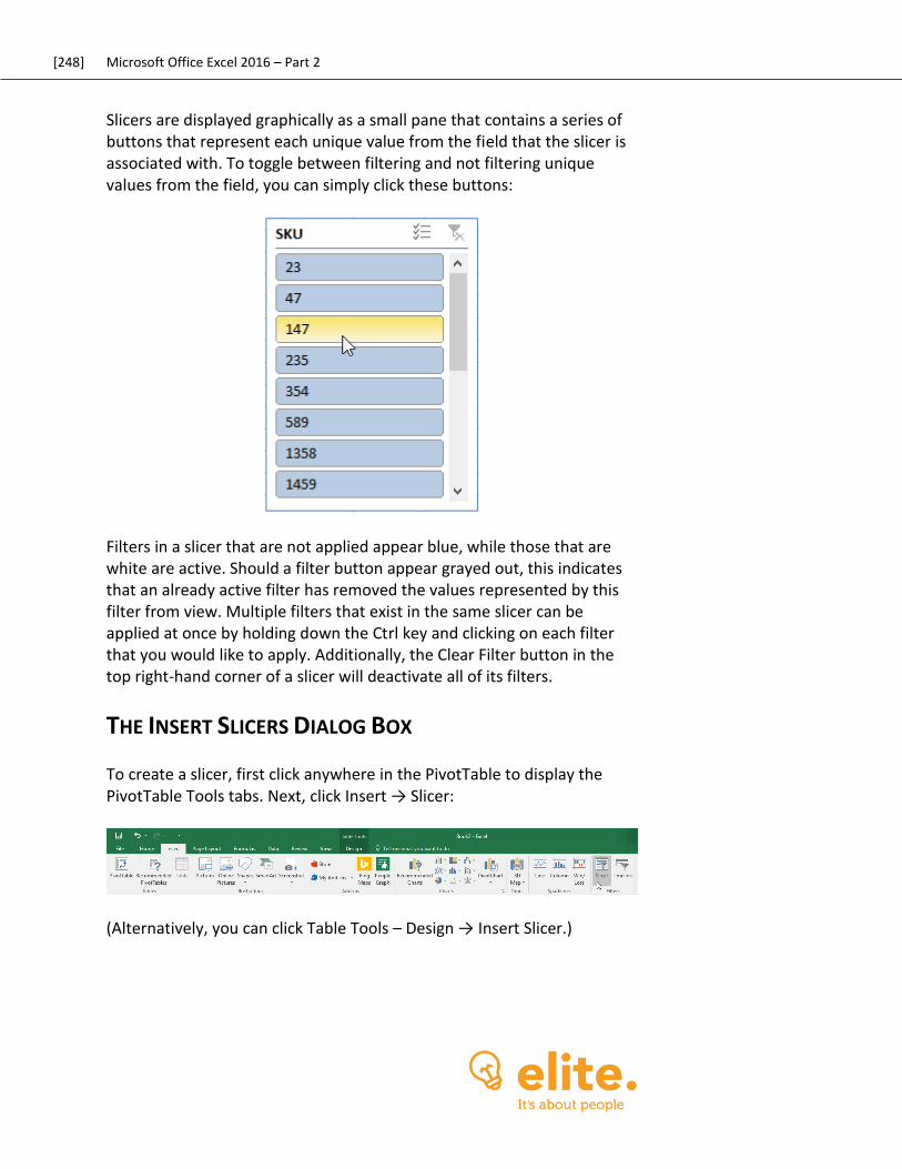
[248] Microsoft Office Excel 2016 – Part 2
Slicers are displayed graphically as a small pane that contains a series of buttons that represent each unique value from the field that the slicer is associated with. To toggle between filtering and not filtering unique values from the field, you can simply click these buttons:
Filters in a slicer that are not applied appear blue, while those that are white are active. Should a filter button appear grayed out, this indicates that an already active filter has removed the values represented by this filter from view. Multiple filters that exist in the same slicer can be applied at once by holding down the Ctrl key and clicking on each filter that you would like to apply. Additionally, the Clear Filter button in the top right-hand corner of a slicer will deactivate all of its filters.
THE INSERT SLICERS DIALOG BOX
To create a slicer, first click anywhere in the PivotTable to display the PivotTable Tools tabs. Next, click Insert → Slicer:
(Alternatively, you can click Table Tools – Design → Insert Slicer.)
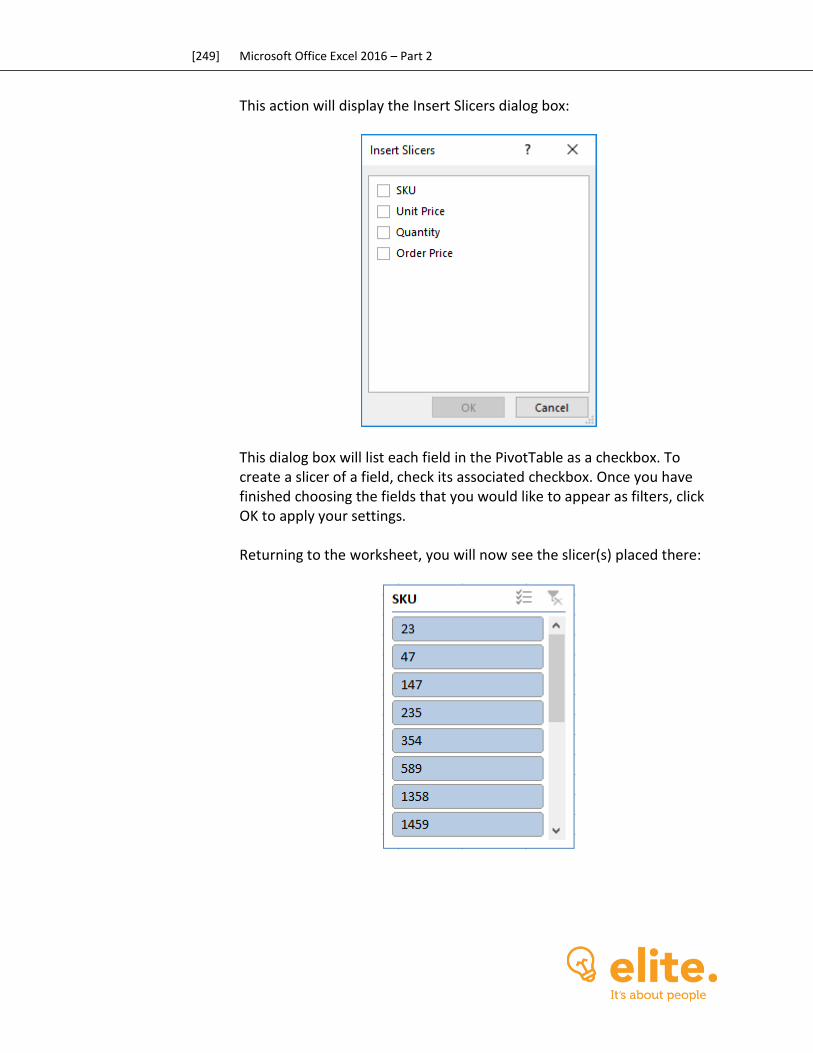
[249] Microsoft Office Excel 2016 – Part 2
This action will display the Insert Slicers dialog box:
This dialog box will list each field in the PivotTable as a checkbox. To create a slicer of a field, check its associated checkbox. Once you have finished choosing the fields that you would like to appear as filters, click OK to apply your settings. Returning to the worksheet, you will now see the slicer(s) placed there:
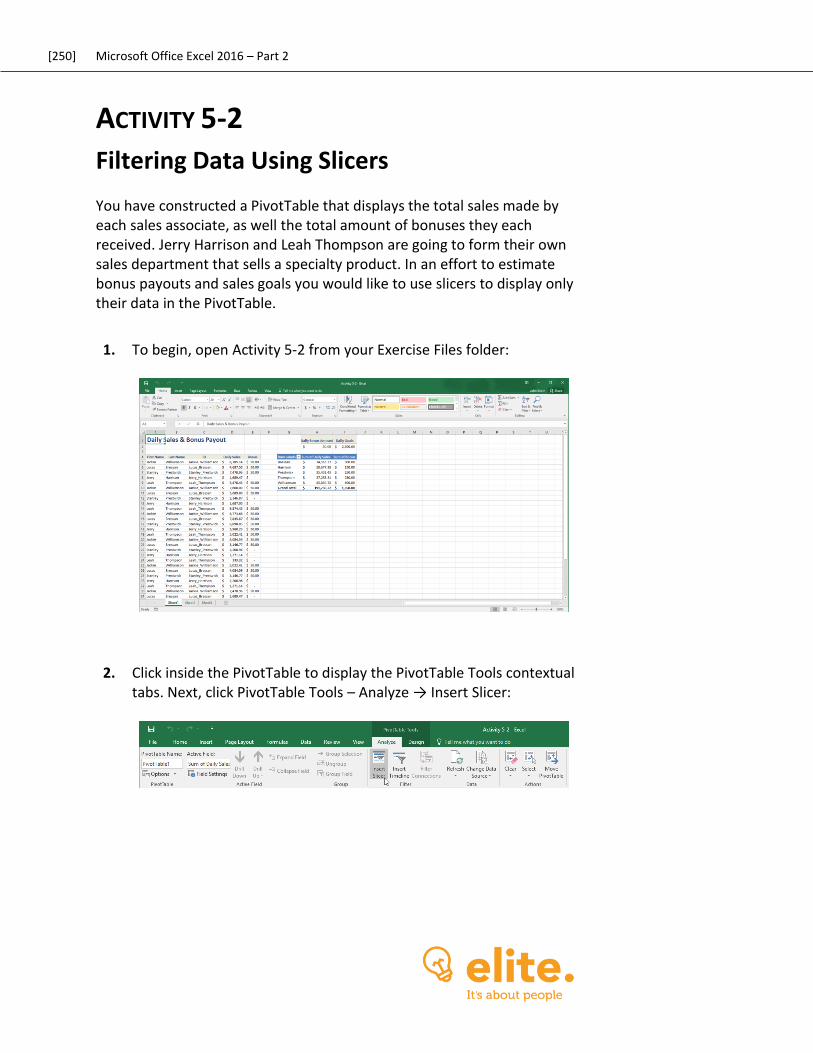
[250] Microsoft Office Excel 2016 – Part 2
ACTIVITY 5-2
Filtering Data Using Slicers You have constructed a PivotTable that displays the total sales made by each sales associate, as well the total amount of bonuses they each received. Jerry Harrison and Leah Thompson are going to form their own sales department that sells a specialty product. In an effort to estimate bonus payouts and sales goals you would like to use slicers to display only their data in the PivotTable.
1. To begin, open Activity 5-2 from your Exercise Files folder:
2. Click inside the PivotTable to display the PivotTable Tools contextual tabs. Next, click PivotTable Tools – Analyze → Insert Slicer:
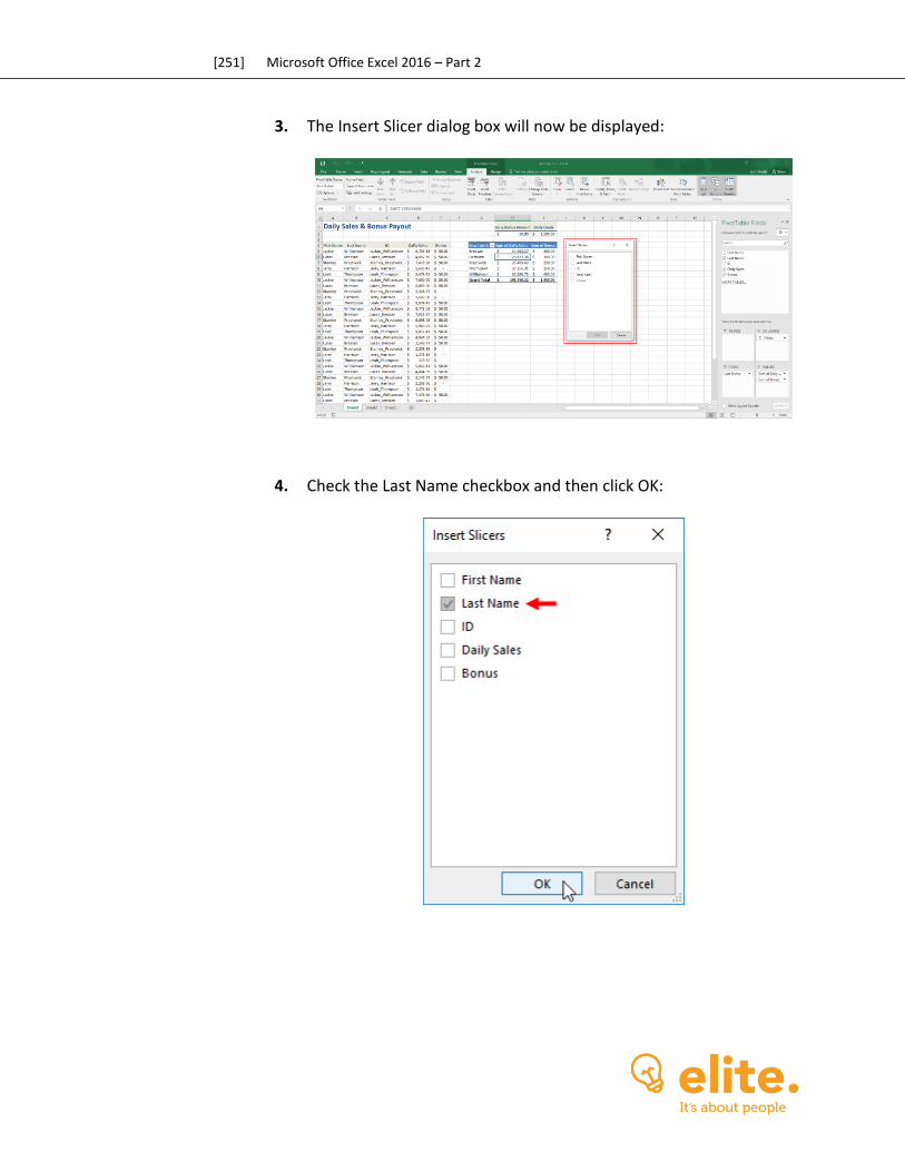
[251] Microsoft Office Excel 2016 – Part 2
3. The Insert Slicer dialog box will now be displayed:
4. Check the Last Name checkbox and then click OK:

[252] Microsoft Office Excel 2016 – Part 2
5. A slicer for the Last Name field will now be on your worksheet:
6. For this exercise you want to filter out everyone except for Jerry Harrison and Leah Thompson. While holding down the Ctrl key, click the Bressan, Prestwick, and Williamson buttons:
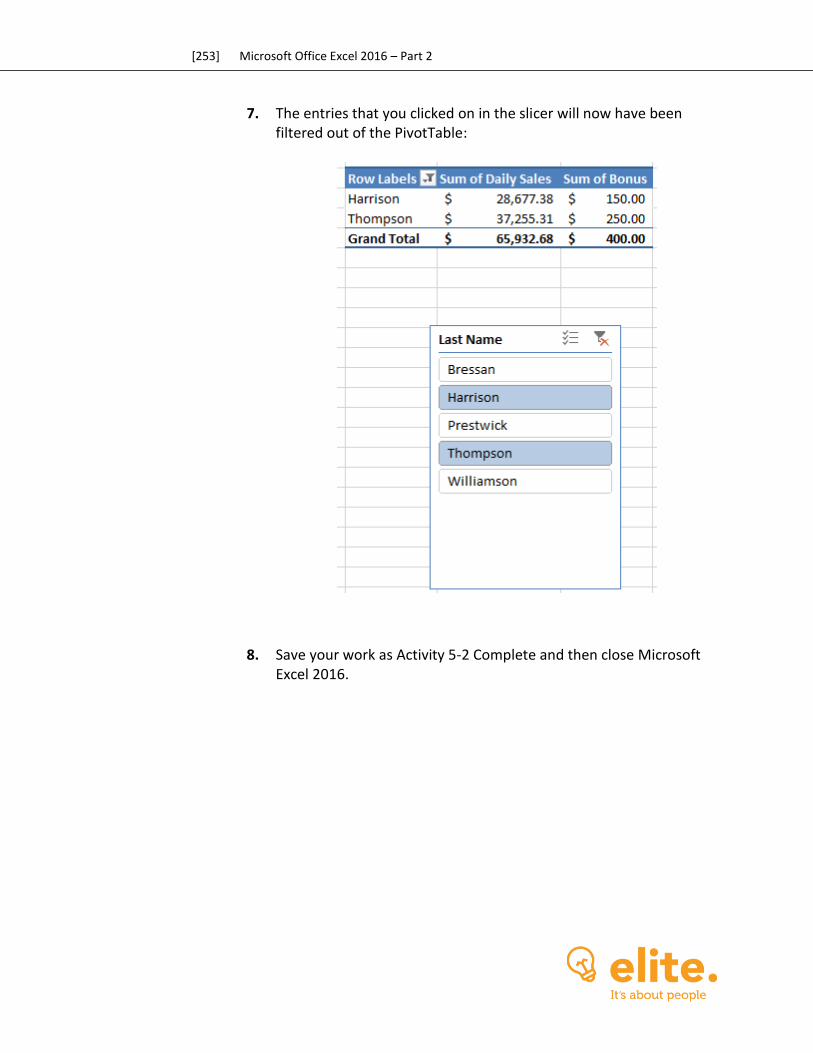
[253] Microsoft Office Excel 2016 – Part 2
7. The entries that you clicked on in the slicer will now have been filtered out of the PivotTable:
8. Save your work as Activity 5-2 Complete and then close Microsoft Excel 2016.
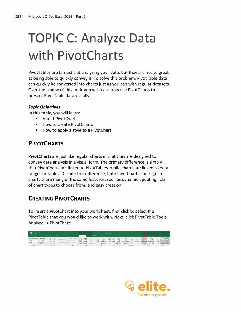
[254] Microsoft Office Excel 2016 – Part 2
TOPIC C: Analyze Data with PivotCharts PivotTables are fantastic at analyzing your data, but they are not so great at being able to quickly convey it. To solve this problem, PivotTable data can quickly be converted into charts just as you can with regular datasets. Over the course of this topic you will learn how use PivotCharts to present PivotTable data visually. Topic Objectives In this topic, you will learn:
About PivotCharts How to create PivotCharts How to apply a style to a PivotChart
PIVOTCHARTS
PivotCharts are just like regular charts in that they are designed to convey data analysis in a visual form. The primary difference is simply that PivotCharts are linked to PivotTables, while charts are linked to data ranges or tables. Despite this difference, both PivotCharts and regular charts share many of the same features, such as dynamic updating, lots of chart types to choose from, and easy creation.
CREATING PIVOTCHARTS
To insert a PivotChart into your worksheet, first click to select the PivotTable that you would like to work with. Next, click PivotTable Tools – Analyze → PivotChart:
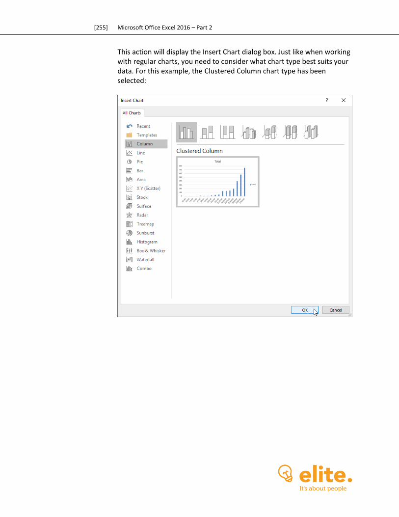
[255] Microsoft Office Excel 2016 – Part 2
This action will display the Insert Chart dialog box. Just like when working with regular charts, you need to consider what chart type best suits your data. For this example, the Clustered Column chart type has been selected:
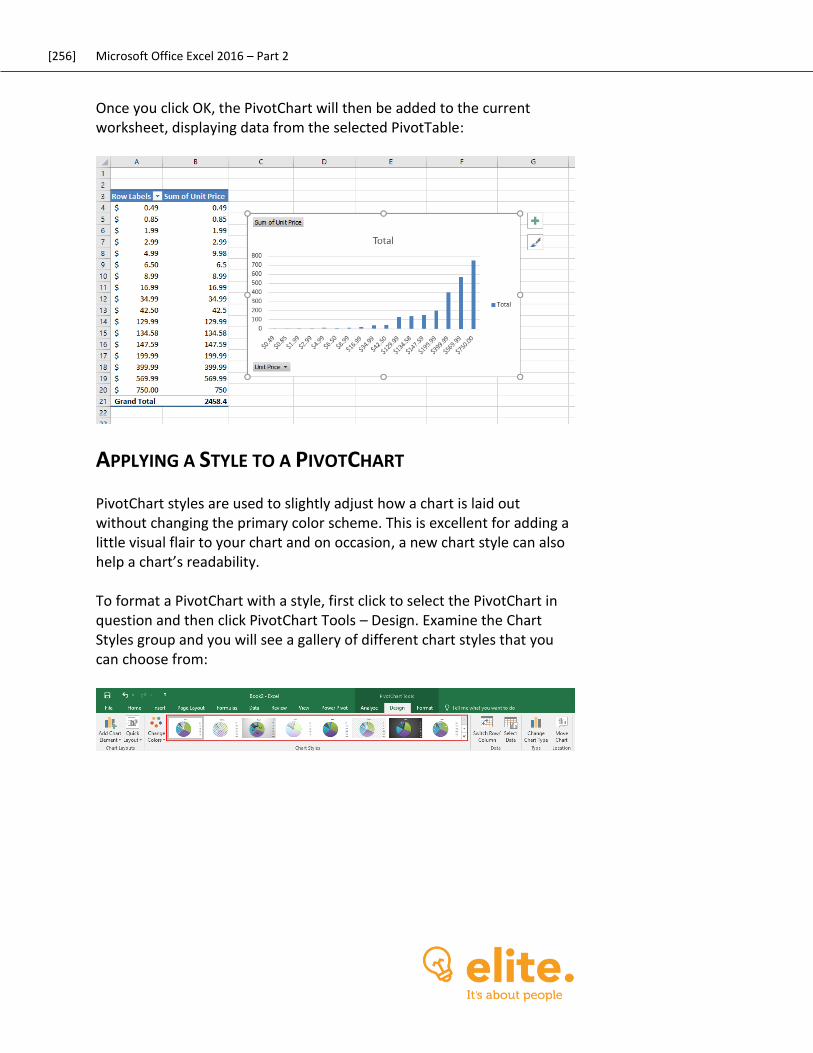
[256] Microsoft Office Excel 2016 – Part 2
Once you click OK, the PivotChart will then be added to the current worksheet, displaying data from the selected PivotTable:
APPLYING A STYLE TO A PIVOTCHART
PivotChart styles are used to slightly adjust how a chart is laid out without changing the primary color scheme. This is excellent for adding a little visual flair to your chart and on occasion, a new chart style can also help a chart’s readability. To format a PivotChart with a style, first click to select the PivotChart in question and then click PivotChart Tools – Design. Examine the Chart Styles group and you will see a gallery of different chart styles that you can choose from:

[257] Microsoft Office Excel 2016 – Part 2
Move your cursor over these chart styles and you will see a preview of how these style will look once applied to your chart. Clicking on a style will apply it:
You can also find these styles by clicking the Chart Styles button that appears to the top right of a selected chart:
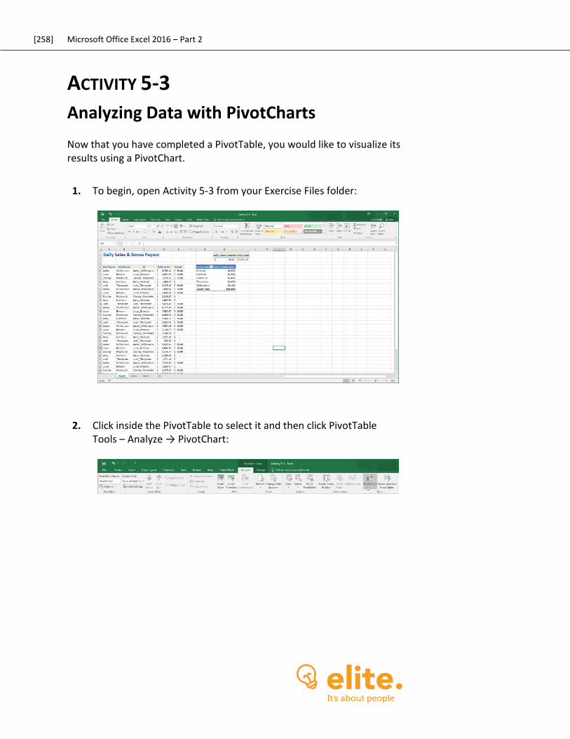
[258] Microsoft Office Excel 2016 – Part 2
ACTIVITY 5-3
Analyzing Data with PivotCharts Now that you have completed a PivotTable, you would like to visualize its results using a PivotChart.
1. To begin, open Activity 5-3 from your Exercise Files folder:
2. Click inside the PivotTable to select it and then click PivotTable Tools – Analyze → PivotChart:
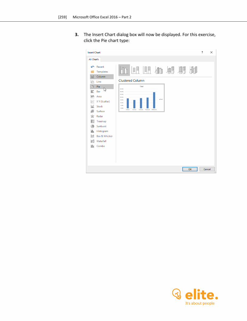
[259] Microsoft Office Excel 2016 – Part 2
3. The Insert Chart dialog box will now be displayed. For this exercise, click the Pie chart type:
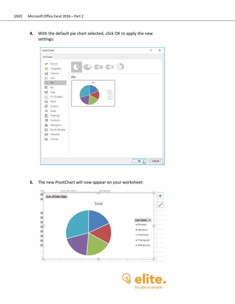
[260] Microsoft Office Excel 2016 – Part 2
4. With the default pie chart selected, click OK to apply the new settings:
5. The new PivotChart will now appear on your worksheet:
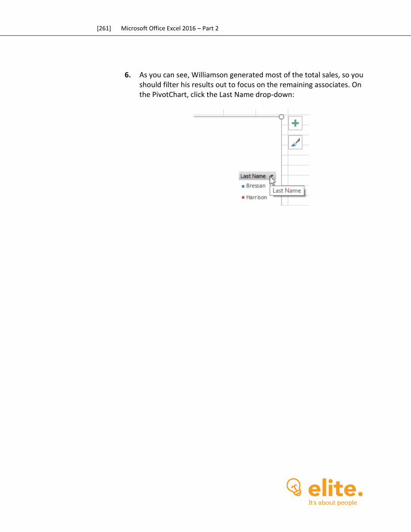
[261] Microsoft Office Excel 2016 – Part 2
6. As you can see, Williamson generated most of the total sales, so you should filter his results out to focus on the remaining associates. On the PivotChart, click the Last Name drop-down:
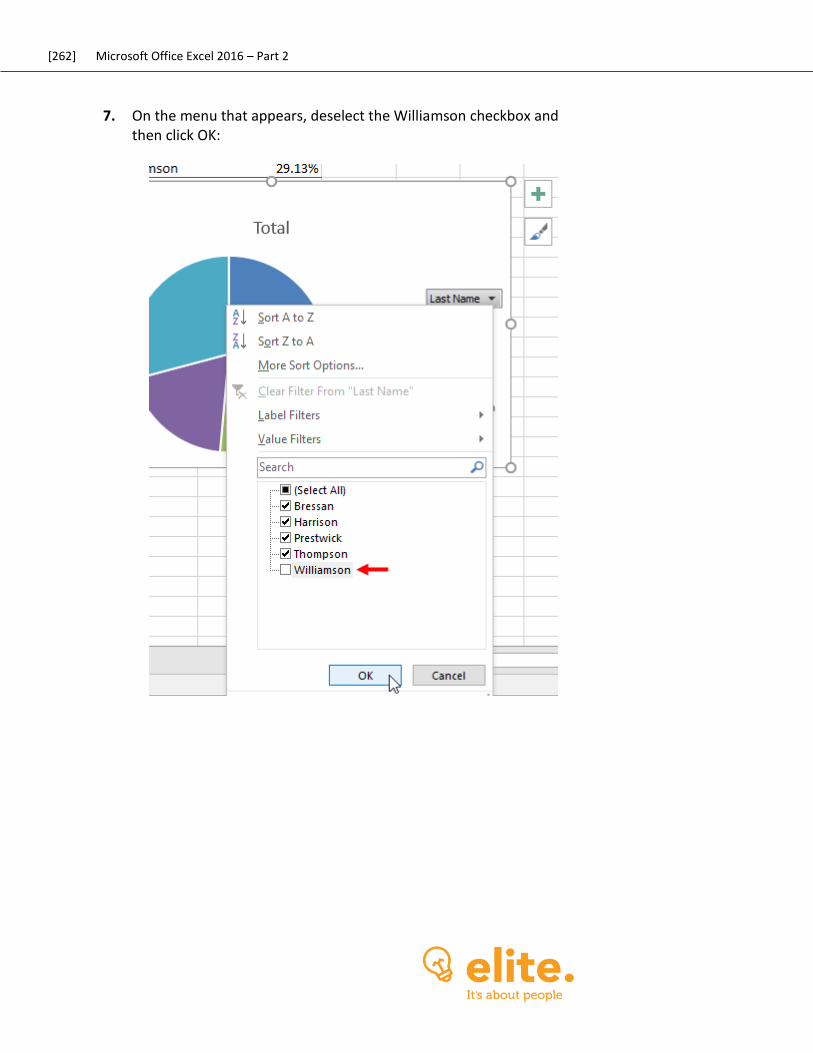
[262] Microsoft Office Excel 2016 – Part 2
7. On the menu that appears, deselect the Williamson checkbox and then click OK:
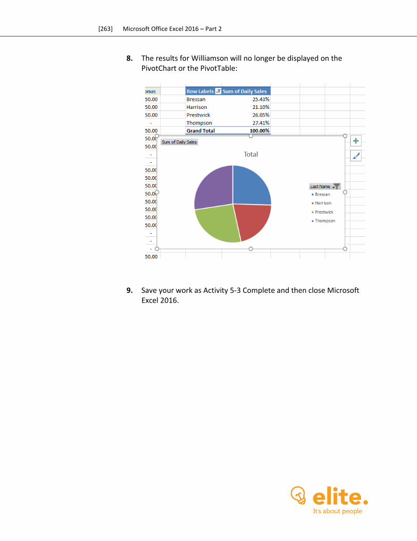
[263] Microsoft Office Excel 2016 – Part 2
8. The results for Williamson will no longer be displayed on the PivotChart or the PivotTable:
9. Save your work as Activity 5-3 Complete and then close Microsoft Excel 2016.

[264] Microsoft Office Excel 2016 – Part 2
Summary In this lesson you learned what PivotTables are and how they can be best used to answer many different types of questions you may have of your data. You now know how to insert a PivotTable, as well as add and remove fields from it. Additionally you are able to generate PivotCharts from a PivotTable, as well as use slicers to selectively filter out unique field entries.
REVIEW QUESTIONS
1. What is pivoting in Excel?
2. What is transactional data?
3. What happens to fields that are dragged to the Values area on the PivotTable Field List pane?
4. What is the command sequence to insert a PivotChart?
5. What do the buttons on a slicer represent?

[265] Microsoft Office Excel 2016 – Part 2
LESSON 6: INSERTING GRAPHICS
Lesson Objectives
In this lesson you will learn how to:
Insert and modify graphical objects
Layer and group graphic objects
Incorporate SmartArt into your workbooks
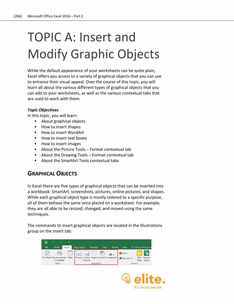
[266] Microsoft Office Excel 2016 – Part 2
TOPIC A: Insert and Modify Graphic Objects While the default appearance of your worksheets can be quite plain, Excel offers you access to a variety of graphical objects that you can use to enhance their visual appeal. Over the course of this topic, you will learn all about the various different types of graphical objects that you can add to your worksheets, as well as the various contextual tabs that are used to work with them. Topic Objectives In this topic, you will learn:
About graphical objects How to insert shapes How to insert WordArt How to insert text boxes How to insert images About the Picture Tools – Format contextual tab About the Drawing Tools – Format contextual tab About the SmartArt Tools contextual tabs
GRAPHICAL OBJECTS
In Excel there are five types of graphical objects that can be inserted into a workbook: SmartArt, screenshots, pictures, online pictures, and shapes. While each graphical object type is mostly tailored to a specific purpose, all of them behave the same once placed on a worksheet. For example, they are all able to be resized, changed, and moved using the same techniques. The commands to insert graphical objects are located in the Illustrations group on the Insert tab:
[267] Microsoft Office Excel 2016 – Part 2
Here is an overview of these commands:
The Picture command will insert image files from outside of Excel into your worksheet. These can be pictures that were downloaded from the Internet, uploaded from a digital camera, or created using imaging software. Most common image formats are supported.
The Online Pictures command gives you access to the Bing search engine, which you can then use to find the exact picture that you need directly from the Internet.
The Shapes drop-down command is used to insert basic shapes, including circles, squares, rectangles, text callouts, and arrows. You can customize all of these objects in a variety of ways.
Clicking the SmartArt command will allow you to choose and insert a SmartArt graphic. These types of graphics are pre-configured and are typically used to graphically represent text-based content, such as flowcharts and lists.
Finally, the Screenshot command will allow you to take a screenshot of any open window or your desktop. This screenshot will then be inserted into the current worksheet.

[268] Microsoft Office Excel 2016 – Part 2
INSERTING SHAPES
To insert a shape into the current worksheet, first click Insert → Shapes:
This dropdown command will reveal that there are nine major categories in the Shapes menu:
Recently Used Shapes: Contains the most recently used shapes (up to the last 24).
Lines: Create a variety of lines and plain arrows. Rectangles: Create a variety of rectangular shapes. Basic Shapes: Create basic shapes, such as circles and triangles.
Fun shapes like smiley faces are also included here. Block Arrows: Create block-style arrows and lines. Equation Shapes: Create mathematical shapes. Flowchart: Create shapes used in flowcharts, such as decision
points and terminators. Stars and Banners: Offers 20 different types of these shapes. Callouts: Annotate other drawings and images.
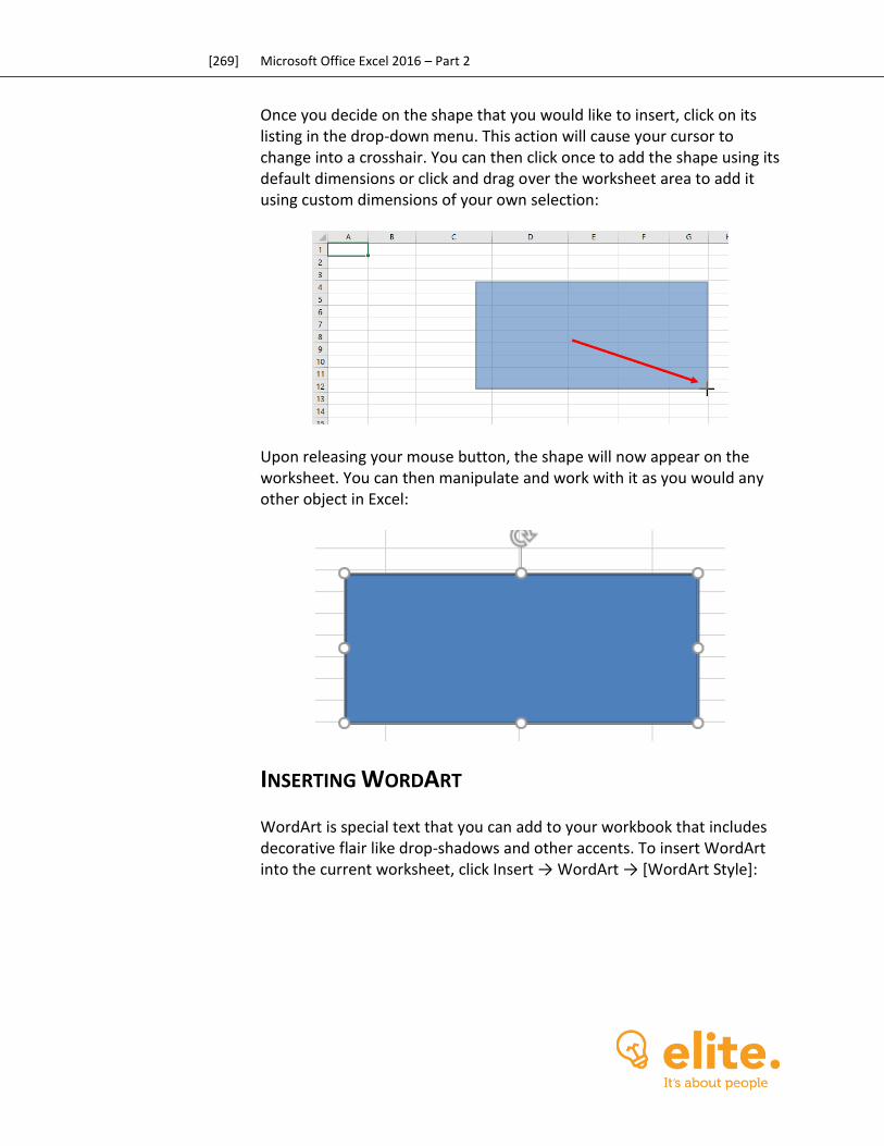
[269] Microsoft Office Excel 2016 – Part 2
Once you decide on the shape that you would like to insert, click on its listing in the drop-down menu. This action will cause your cursor to change into a crosshair. You can then click once to add the shape using its default dimensions or click and drag over the worksheet area to add it using custom dimensions of your own selection:
Upon releasing your mouse button, the shape will now appear on the worksheet. You can then manipulate and work with it as you would any other object in Excel:
INSERTING WORDART
WordArt is special text that you can add to your workbook that includes decorative flair like drop-shadows and other accents. To insert WordArt into the current worksheet, click Insert → WordArt → [WordArt Style]:
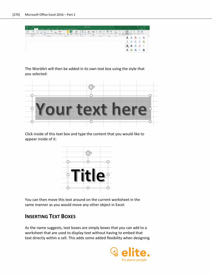
[270] Microsoft Office Excel 2016 – Part 2
The WordArt will then be added in its own text box using the style that you selected:
Click inside of this text box and type the content that you would like to appear inside of it:
You can then move this text around on the current worksheet in the same manner as you would move any other object in Excel.
INSERTING TEXT BOXES
As the name suggests, text boxes are simply boxes that you can add to a worksheet that are used to display text without having to embed that text directly within a cell. This adds some added flexibility when designing
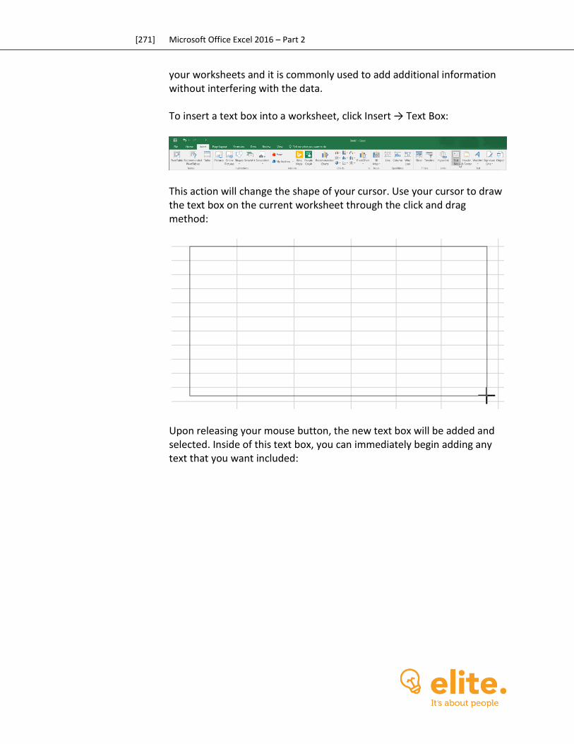
[271] Microsoft Office Excel 2016 – Part 2
your worksheets and it is commonly used to add additional information without interfering with the data. To insert a text box into a worksheet, click Insert → Text Box:
This action will change the shape of your cursor. Use your cursor to draw the text box on the current worksheet through the click and drag method:
Upon releasing your mouse button, the new text box will be added and selected. Inside of this text box, you can immediately begin adding any text that you want included:
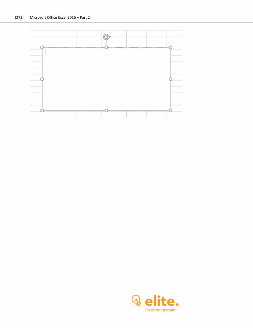
[272] Microsoft Office Excel 2016 – Part 2
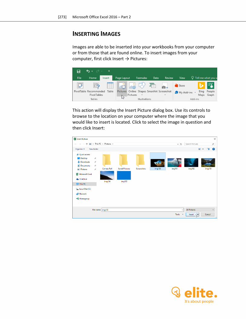
[273] Microsoft Office Excel 2016 – Part 2
INSERTING IMAGES
Images are able to be inserted into your workbooks from your computer or from those that are found online. To insert images from your computer, first click Insert → Pictures:
This action will display the Insert Picture dialog box. Use its controls to browse to the location on your computer where the image that you would like to insert is located. Click to select the image in question and then click Insert:
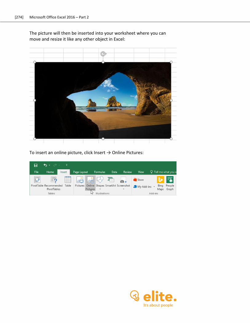
[274] Microsoft Office Excel 2016 – Part 2
The picture will then be inserted into your worksheet where you can move and resize it like any other object in Excel:
To insert an online picture, click Insert → Online Pictures:
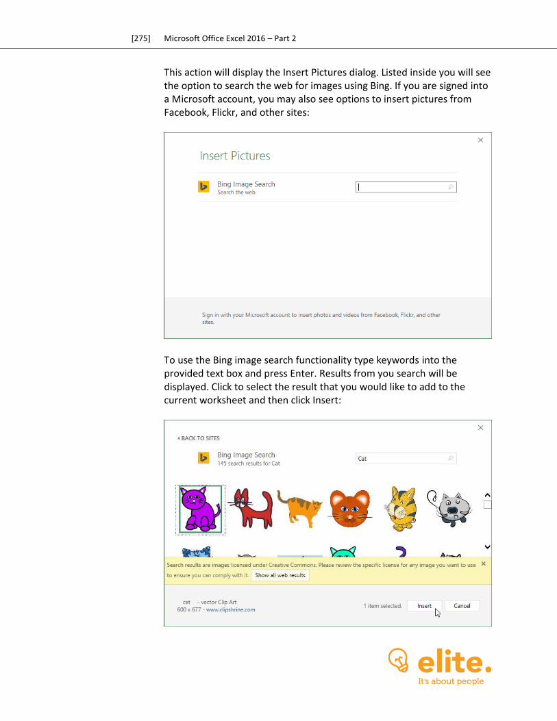
[275] Microsoft Office Excel 2016 – Part 2
This action will display the Insert Pictures dialog. Listed inside you will see the option to search the web for images using Bing. If you are signed into a Microsoft account, you may also see options to insert pictures from Facebook, Flickr, and other sites:
To use the Bing image search functionality type keywords into the provided text box and press Enter. Results from you search will be displayed. Click to select the result that you would like to add to the current worksheet and then click Insert:
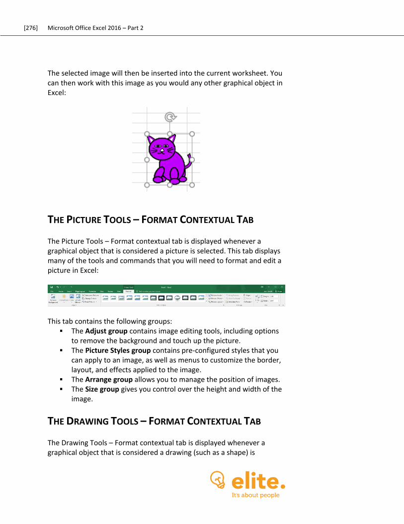
[276] Microsoft Office Excel 2016 – Part 2
The selected image will then be inserted into the current worksheet. You can then work with this image as you would any other graphical object in Excel:
THE PICTURE TOOLS – FORMAT CONTEXTUAL TAB
The Picture Tools – Format contextual tab is displayed whenever a graphical object that is considered a picture is selected. This tab displays many of the tools and commands that you will need to format and edit a picture in Excel:
This tab contains the following groups:
The Adjust group contains image editing tools, including options to remove the background and touch up the picture.
The Picture Styles group contains pre-configured styles that you can apply to an image, as well as menus to customize the border, layout, and effects applied to the image.
The Arrange group allows you to manage the position of images. The Size group gives you control over the height and width of the
image.
THE DRAWING TOOLS – FORMAT CONTEXTUAL TAB
The Drawing Tools – Format contextual tab is displayed whenever a graphical object that is considered a drawing (such as a shape) is
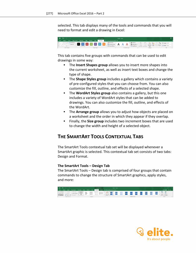
[277] Microsoft Office Excel 2016 – Part 2
selected. This tab displays many of the tools and commands that you will need to format and edit a drawing in Excel:
This tab contains five groups with commands that can be used to edit drawings in some way:
The Insert Shapes group allows you to insert more shapes into the current worksheet, as well as insert text boxes and change the type of shape.
The Shape Styles group includes a gallery which contains a variety of pre-configured styles that you can choose from. You can also customize the fill, outline, and effects of a selected shape.
The WordArt Styles group also contains a gallery, but this one includes a variety of WordArt styles that can be added to drawings. You can also customize the fill, outline, and effects of the WordArt.
The Arrange group allows you to adjust how objects are placed on a worksheet and the order in which they appear if they overlap.
Finally, the Size group includes two increment boxes that are used to change the width and height of a selected object.
THE SMARTART TOOLS CONTEXTUAL TABS
The SmartArt Tools contextual tab set will be displayed whenever a SmartArt graphic is selected. This contextual tab set consists of two tabs: Design and Format. The SmartArt Tools – Design Tab The SmartArt Tools – Design tab is comprised of four groups that contain commands to change the structure of SmartArt graphics, apply styles, and more:
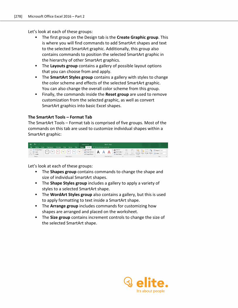
[278] Microsoft Office Excel 2016 – Part 2
Let’s look at each of these groups: The first group on the Design tab is the Create Graphic group. This
is where you will find commands to add SmartArt shapes and text to the selected SmartArt graphic. Additionally, this group also contains commands to position the selected SmartArt graphic in the hierarchy of other SmartArt graphics.
The Layouts group contains a gallery of possible layout options that you can choose from and apply.
The SmartArt Styles group contains a gallery with styles to change the color scheme and effects of the selected SmartArt graphic. You can also change the overall color scheme from this group.
Finally, the commands inside the Reset group are used to remove customization from the selected graphic, as well as convert SmartArt graphics into basic Excel shapes.
The SmartArt Tools – Format Tab The SmartArt Tools – Format tab is comprised of five groups. Most of the commands on this tab are used to customize individual shapes within a SmartArt graphic:
Let’s look at each of these groups:
The Shapes group contains commands to change the shape and size of individual SmartArt shapes.
The Shape Styles group includes a gallery to apply a variety of styles to a selected SmartArt shape.
The WordArt Styles group also contains a gallery, but this is used to apply formatting to text inside a SmartArt shape.
The Arrange group includes commands for customizing how shapes are arranged and placed on the worksheet.
The Size group contains increment controls to change the size of the selected SmartArt shape.
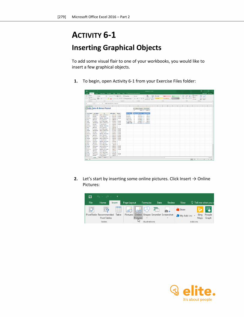
[279] Microsoft Office Excel 2016 – Part 2
ACTIVITY 6-1
Inserting Graphical Objects To add some visual flair to one of your workbooks, you would like to insert a few graphical objects.
1. To begin, open Activity 6-1 from your Exercise Files folder:
2. Let’s start by inserting some online pictures. Click Insert → Online Pictures:
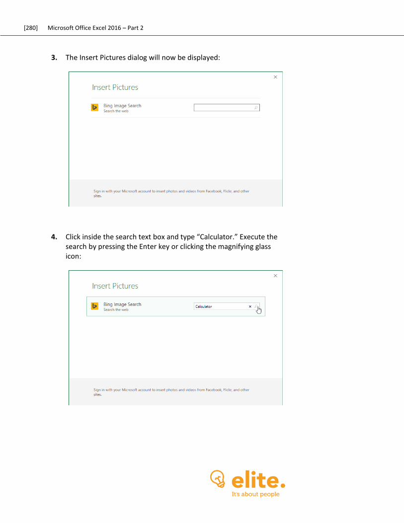
[280] Microsoft Office Excel 2016 – Part 2
3. The Insert Pictures dialog will now be displayed:
4. Click inside the search text box and type “Calculator.” Execute the search by pressing the Enter key or clicking the magnifying glass icon:
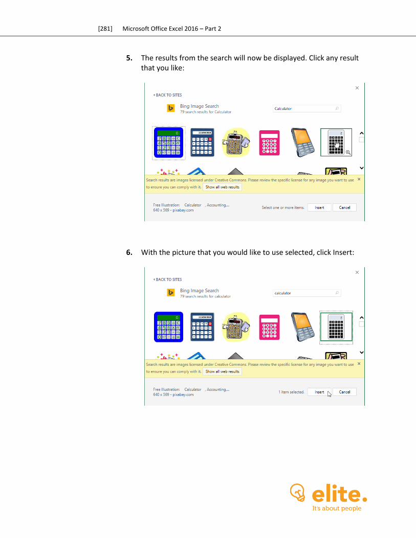
[281] Microsoft Office Excel 2016 – Part 2
5. The results from the search will now be displayed. Click any result that you like:
6. With the picture that you would like to use selected, click Insert:
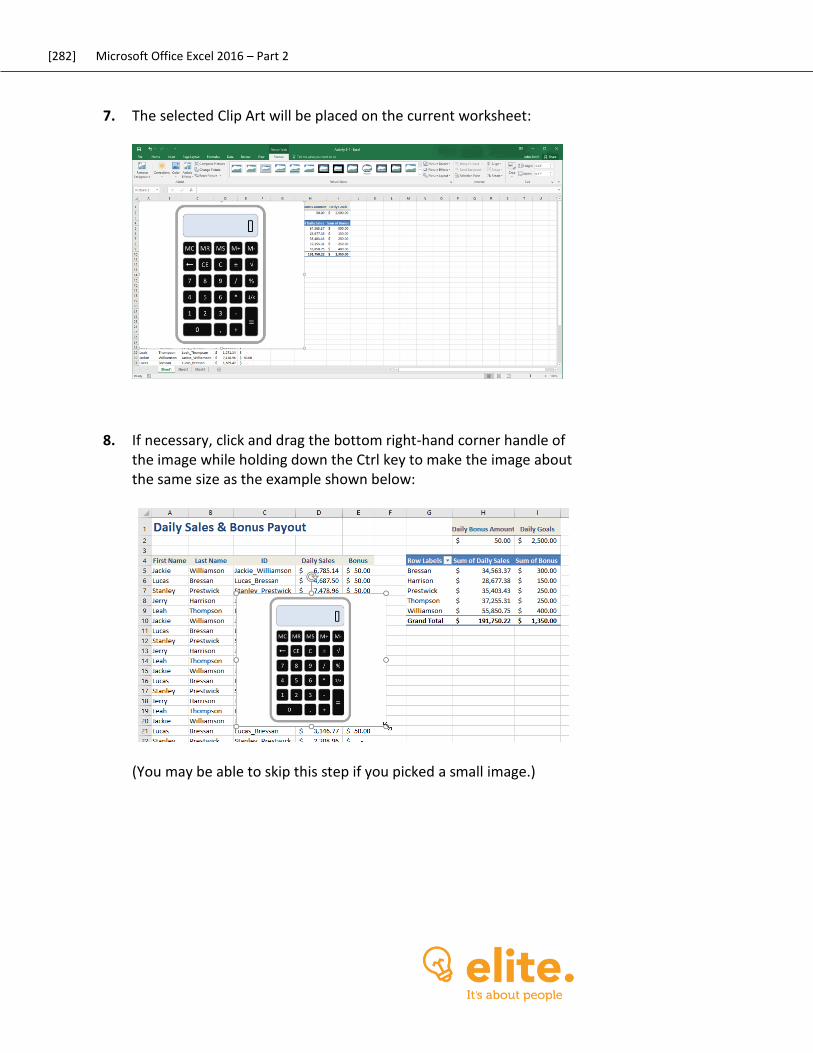
[282] Microsoft Office Excel 2016 – Part 2
7. The selected Clip Art will be placed on the current worksheet:
8. If necessary, click and drag the bottom right-hand corner handle of the image while holding down the Ctrl key to make the image about the same size as the example shown below:
(You may be able to skip this step if you picked a small image.)
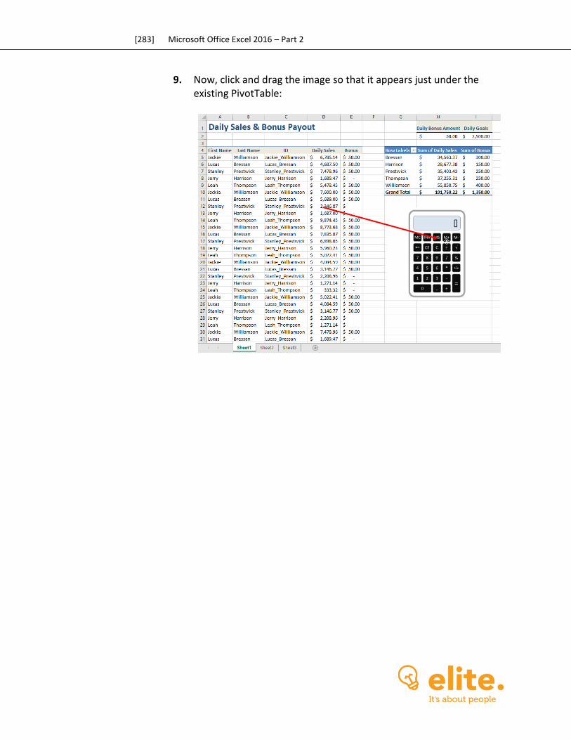
[283] Microsoft Office Excel 2016 – Part 2
9. Now, click and drag the image so that it appears just under the existing PivotTable:
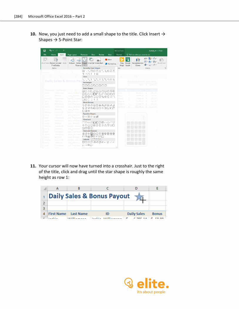
[284] Microsoft Office Excel 2016 – Part 2
10. Now, you just need to add a small shape to the title. Click Insert → Shapes → 5-Point Star:
11. Your cursor will now have turned into a crosshair. Just to the right of the title, click and drag until the star shape is roughly the same height as row 1:
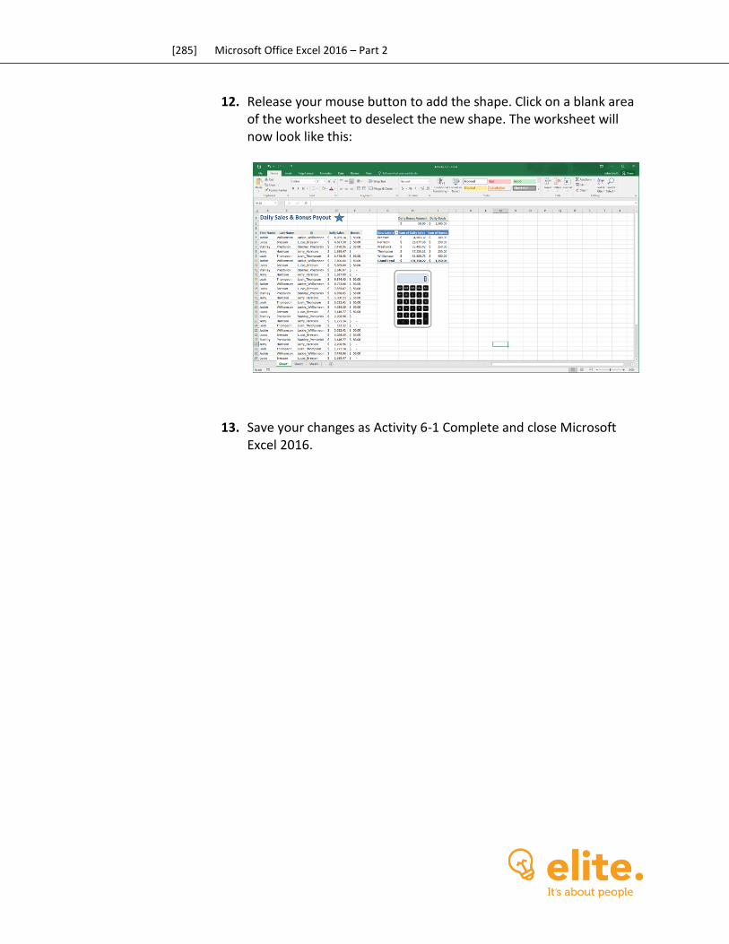
[285] Microsoft Office Excel 2016 – Part 2
12. Release your mouse button to add the shape. Click on a blank area of the worksheet to deselect the new shape. The worksheet will now look like this:
13. Save your changes as Activity 6-1 Complete and close Microsoft Excel 2016.
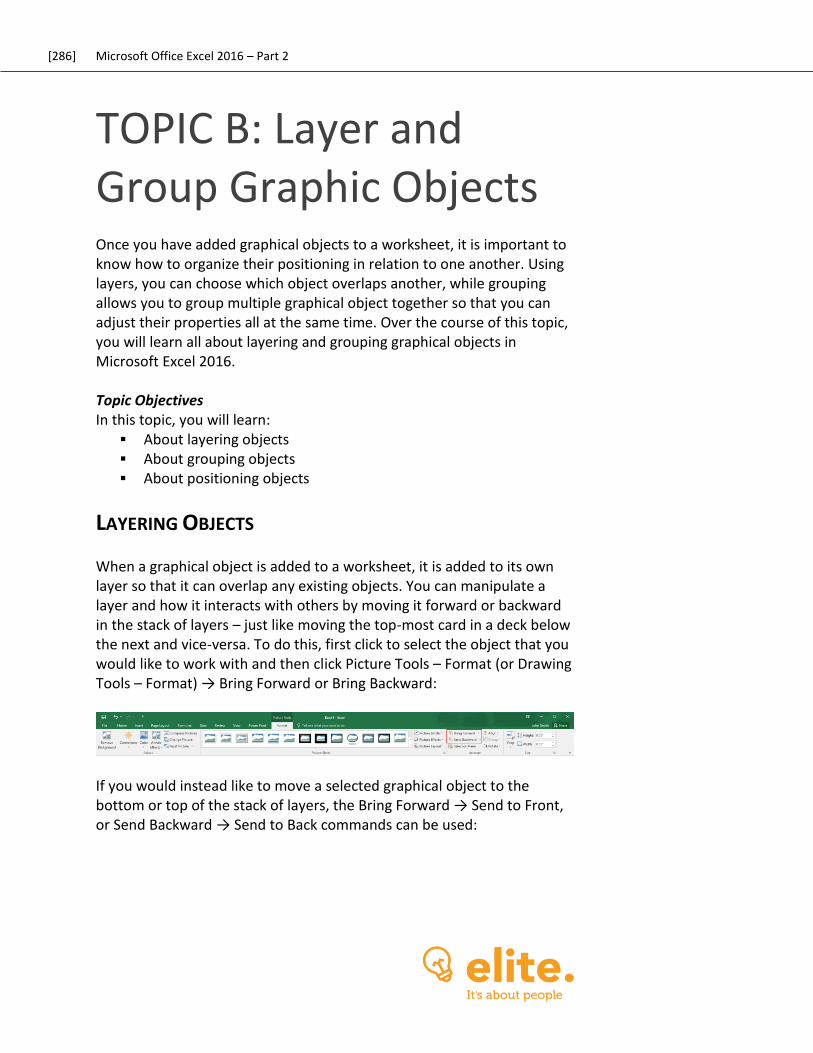
[286] Microsoft Office Excel 2016 – Part 2
TOPIC B: Layer and Group Graphic Objects Once you have added graphical objects to a worksheet, it is important to know how to organize their positioning in relation to one another. Using layers, you can choose which object overlaps another, while grouping allows you to group multiple graphical object together so that you can adjust their properties all at the same time. Over the course of this topic, you will learn all about layering and grouping graphical objects in Microsoft Excel 2016. Topic Objectives In this topic, you will learn:
About layering objects About grouping objects About positioning objects
LAYERING OBJECTS
When a graphical object is added to a worksheet, it is added to its own layer so that it can overlap any existing objects. You can manipulate a layer and how it interacts with others by moving it forward or backward in the stack of layers – just like moving the top-most card in a deck below the next and vice-versa. To do this, first click to select the object that you would like to work with and then click Picture Tools – Format (or Drawing Tools – Format) → Bring Forward or Bring Backward:
If you would instead like to move a selected graphical object to the bottom or top of the stack of layers, the Bring Forward → Send to Front, or Send Backward → Send to Back commands can be used:
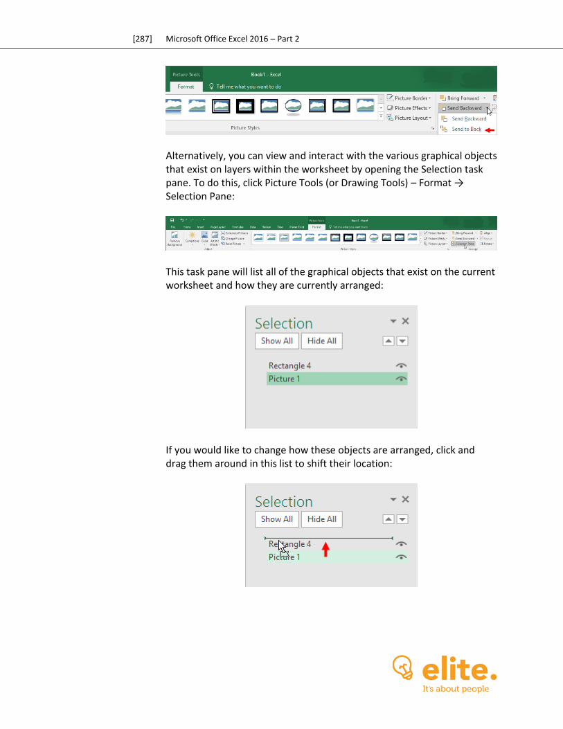
[287] Microsoft Office Excel 2016 – Part 2
Alternatively, you can view and interact with the various graphical objects that exist on layers within the worksheet by opening the Selection task pane. To do this, click Picture Tools (or Drawing Tools) – Format → Selection Pane:
This task pane will list all of the graphical objects that exist on the current worksheet and how they are currently arranged:
If you would like to change how these objects are arranged, click and drag them around in this list to shift their location:
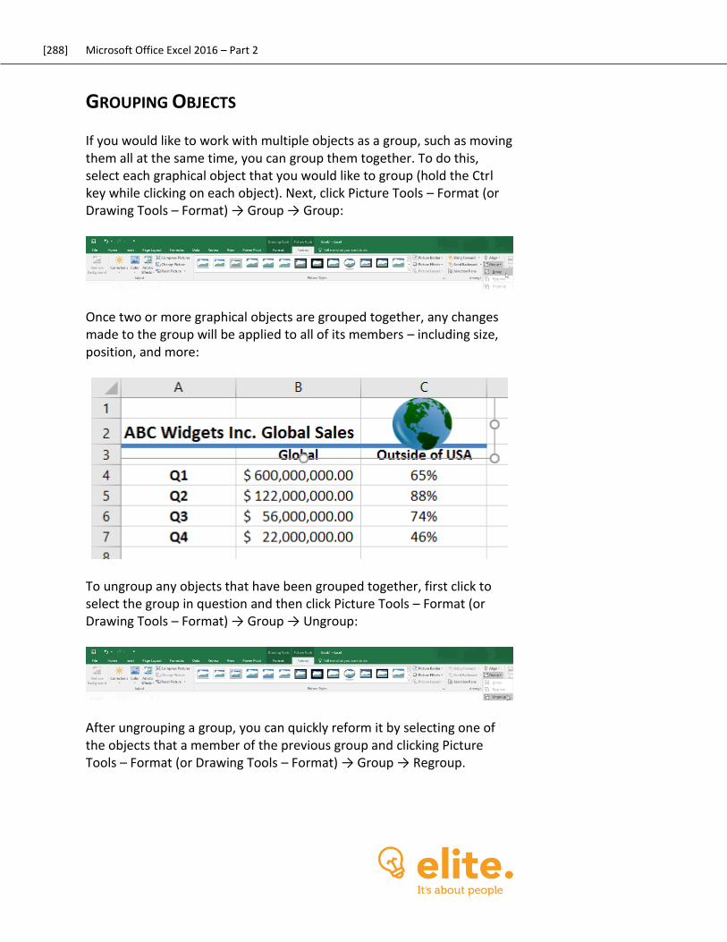
[288] Microsoft Office Excel 2016 – Part 2
GROUPING OBJECTS
If you would like to work with multiple objects as a group, such as moving them all at the same time, you can group them together. To do this, select each graphical object that you would like to group (hold the Ctrl key while clicking on each object). Next, click Picture Tools – Format (or Drawing Tools – Format) → Group → Group:
Once two or more graphical objects are grouped together, any changes made to the group will be applied to all of its members – including size, position, and more:
To ungroup any objects that have been grouped together, first click to select the group in question and then click Picture Tools – Format (or Drawing Tools – Format) → Group → Ungroup:
After ungrouping a group, you can quickly reform it by selecting one of the objects that a member of the previous group and clicking Picture Tools – Format (or Drawing Tools – Format) → Group → Regroup.
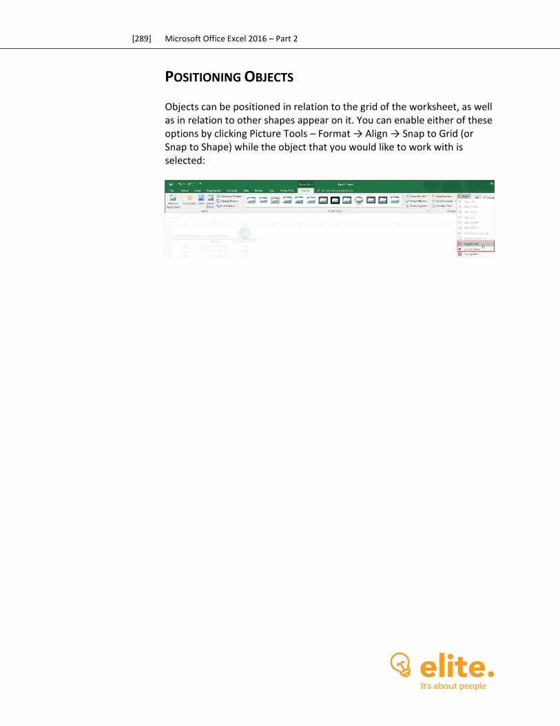
[289] Microsoft Office Excel 2016 – Part 2
POSITIONING OBJECTS
Objects can be positioned in relation to the grid of the worksheet, as well as in relation to other shapes appear on it. You can enable either of these options by clicking Picture Tools – Format → Align → Snap to Grid (or Snap to Shape) while the object that you would like to work with is selected:
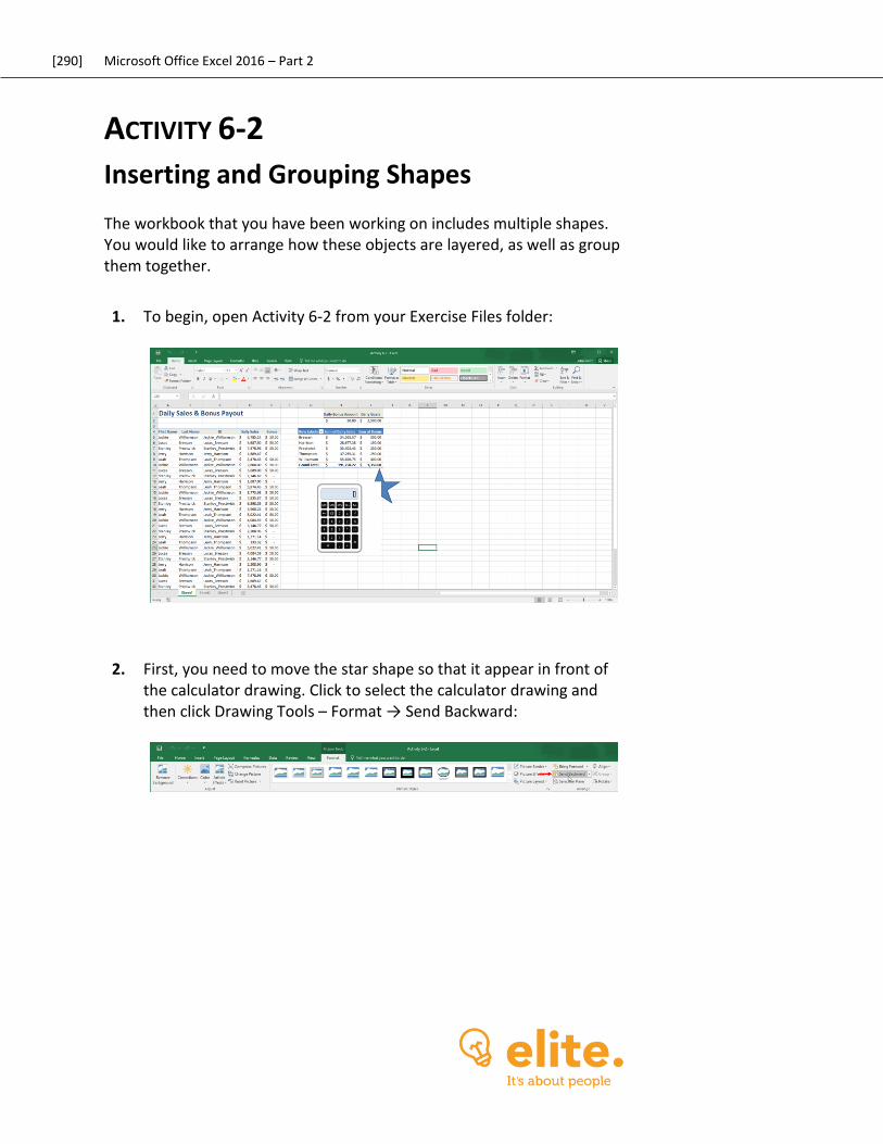
[290] Microsoft Office Excel 2016 – Part 2
ACTIVITY 6-2
Inserting and Grouping Shapes The workbook that you have been working on includes multiple shapes. You would like to arrange how these objects are layered, as well as group them together.
1. To begin, open Activity 6-2 from your Exercise Files folder:
2. First, you need to move the star shape so that it appear in front of the calculator drawing. Click to select the calculator drawing and then click Drawing Tools – Format → Send Backward:
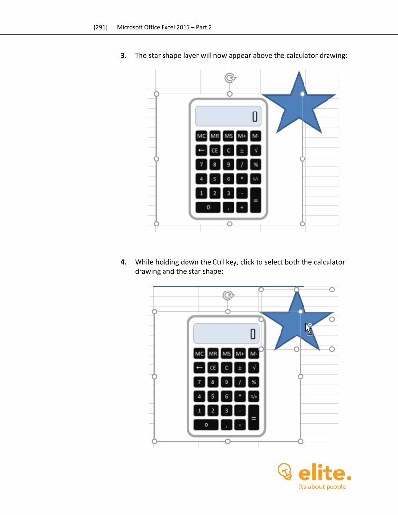
[291] Microsoft Office Excel 2016 – Part 2
3. The star shape layer will now appear above the calculator drawing:
4. While holding down the Ctrl key, click to select both the calculator drawing and the star shape:
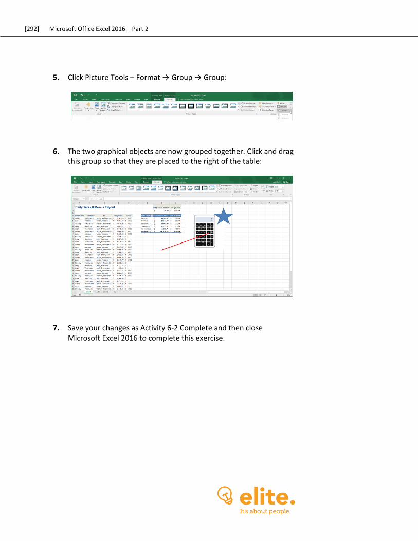
[292] Microsoft Office Excel 2016 – Part 2
5. Click Picture Tools – Format → Group → Group:
6. The two graphical objects are now grouped together. Click and drag this group so that they are placed to the right of the table:
7. Save your changes as Activity 6-2 Complete and then close Microsoft Excel 2016 to complete this exercise.
[293] Microsoft Office Excel 2016 – Part 2
TOPIC C: Incorporate SmartArt SmartArt combines text-based information with graphics to create a more appearance-driven look. Using Excel’s tools, you will be able to create great SmartArt that can be used for a variety of different purposes. Over the course of this topic, you will learn how to insert SmartArt into your workbooks, as well as customize it after it has been inserted. Topic Objectives In this topic, you will learn:
About SmartArt graphics About the Choose a SmartArt Graphic dialog box About the Text pane
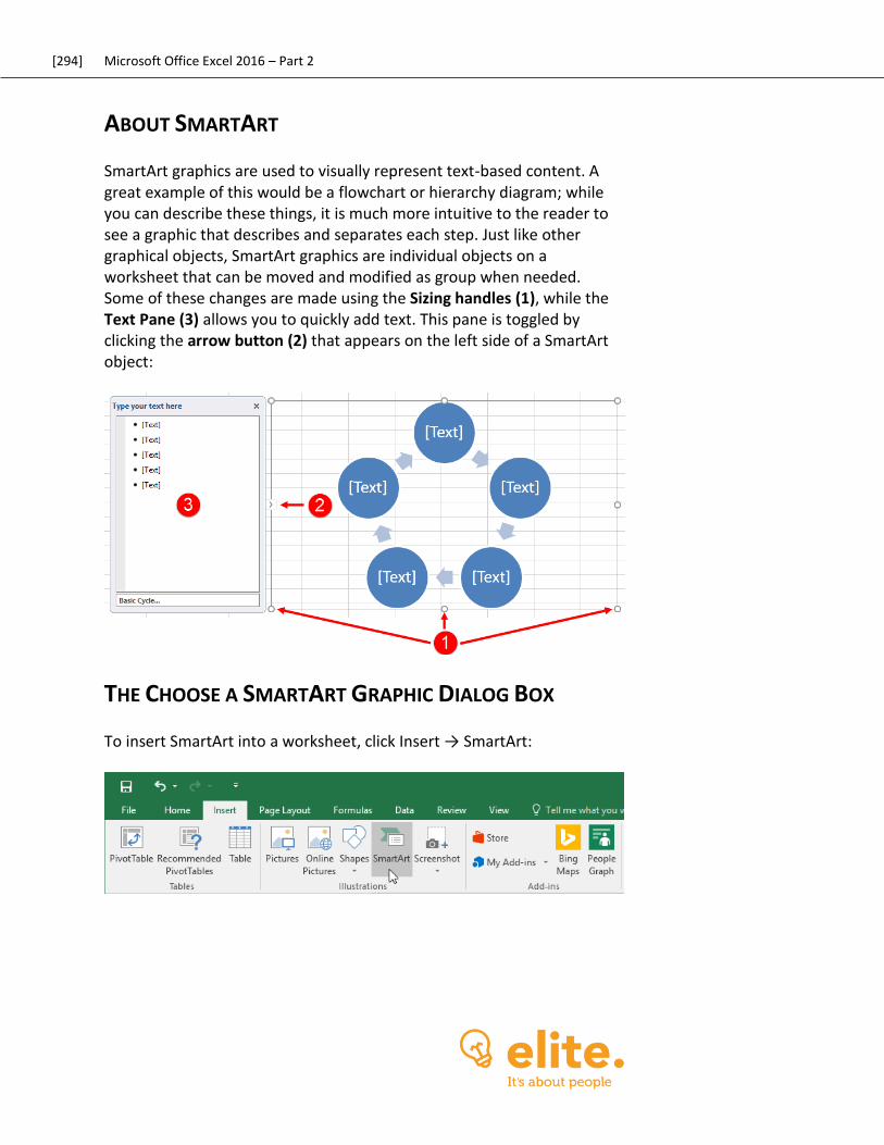
[294] Microsoft Office Excel 2016 – Part 2
ABOUT SMARTART
SmartArt graphics are used to visually represent text-based content. A great example of this would be a flowchart or hierarchy diagram; while you can describe these things, it is much more intuitive to the reader to see a graphic that describes and separates each step. Just like other graphical objects, SmartArt graphics are individual objects on a worksheet that can be moved and modified as group when needed. Some of these changes are made using the Sizing handles (1), while the Text Pane (3) allows you to quickly add text. This pane is toggled by clicking the arrow button (2) that appears on the left side of a SmartArt object:
THE CHOOSE A SMARTART GRAPHIC DIALOG BOX
To insert SmartArt into a worksheet, click Insert → SmartArt:
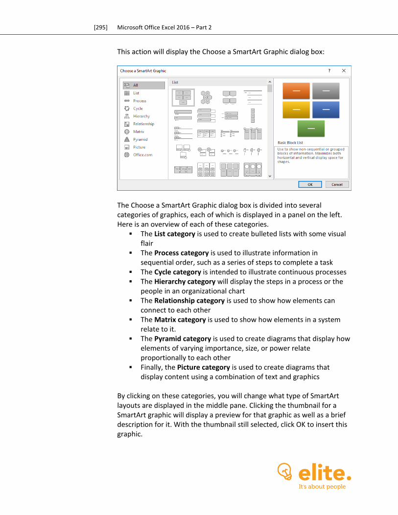
[295] Microsoft Office Excel 2016 – Part 2
This action will display the Choose a SmartArt Graphic dialog box:
The Choose a SmartArt Graphic dialog box is divided into several categories of graphics, each of which is displayed in a panel on the left. Here is an overview of each of these categories.
The List category is used to create bulleted lists with some visual flair
The Process category is used to illustrate information in sequential order, such as a series of steps to complete a task
The Cycle category is intended to illustrate continuous processes The Hierarchy category will display the steps in a process or the
people in an organizational chart The Relationship category is used to show how elements can
connect to each other The Matrix category is used to show how elements in a system
relate to it. The Pyramid category is used to create diagrams that display how
elements of varying importance, size, or power relate proportionally to each other
Finally, the Picture category is used to create diagrams that display content using a combination of text and graphics
By clicking on these categories, you will change what type of SmartArt layouts are displayed in the middle pane. Clicking the thumbnail for a SmartArt graphic will display a preview for that graphic as well as a brief description for it. With the thumbnail still selected, click OK to insert this graphic.
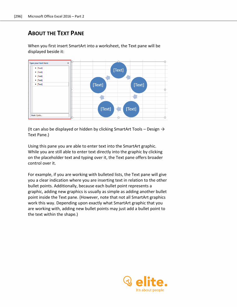
[296] Microsoft Office Excel 2016 – Part 2
ABOUT THE TEXT PANE
When you first insert SmartArt into a worksheet, the Text pane will be displayed beside it:
(It can also be displayed or hidden by clicking SmartArt Tools – Design → Text Pane.) Using this pane you are able to enter text into the SmartArt graphic. While you are still able to enter text directly into the graphic by clicking on the placeholder text and typing over it, the Text pane offers broader control over it. For example, if you are working with bulleted lists, the Text pane will give you a clear indication where you are inserting text in relation to the other bullet points. Additionally, because each bullet point represents a graphic, adding new graphics is usually as simple as adding another bullet point inside the Text pane. (However, note that not all SmartArt graphics work this way. Depending upon exactly what SmartArt graphic that you are working with, adding new bullet points may just add a bullet point to the text within the shape.)
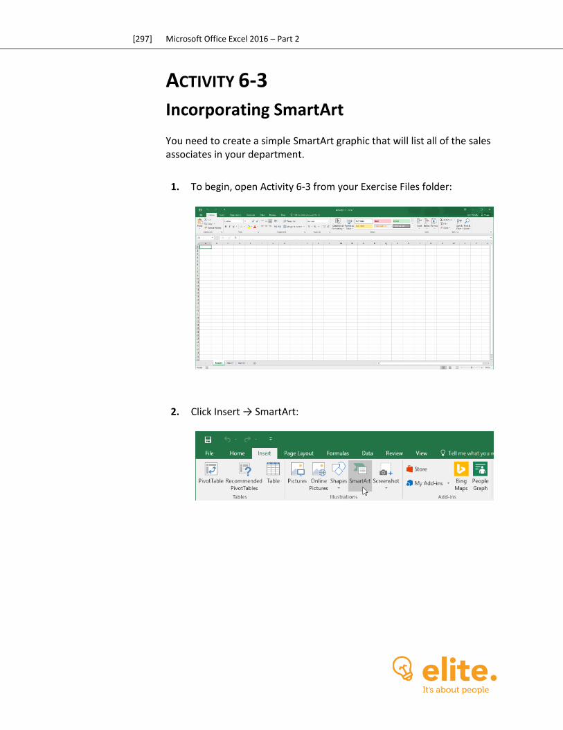
[297] Microsoft Office Excel 2016 – Part 2
ACTIVITY 6-3
Incorporating SmartArt You need to create a simple SmartArt graphic that will list all of the sales associates in your department.
1. To begin, open Activity 6-3 from your Exercise Files folder:
2. Click Insert → SmartArt:

[298] Microsoft Office Excel 2016 – Part 2
3. The Choose a SmartArt Graphic dialog box will now be displayed. Ensure that either the All or List category has been chosen and then ensure that the Basic Block List graphic has been selected. Click OK:
4. The SmartArt graphic will now be placed on the current worksheet:
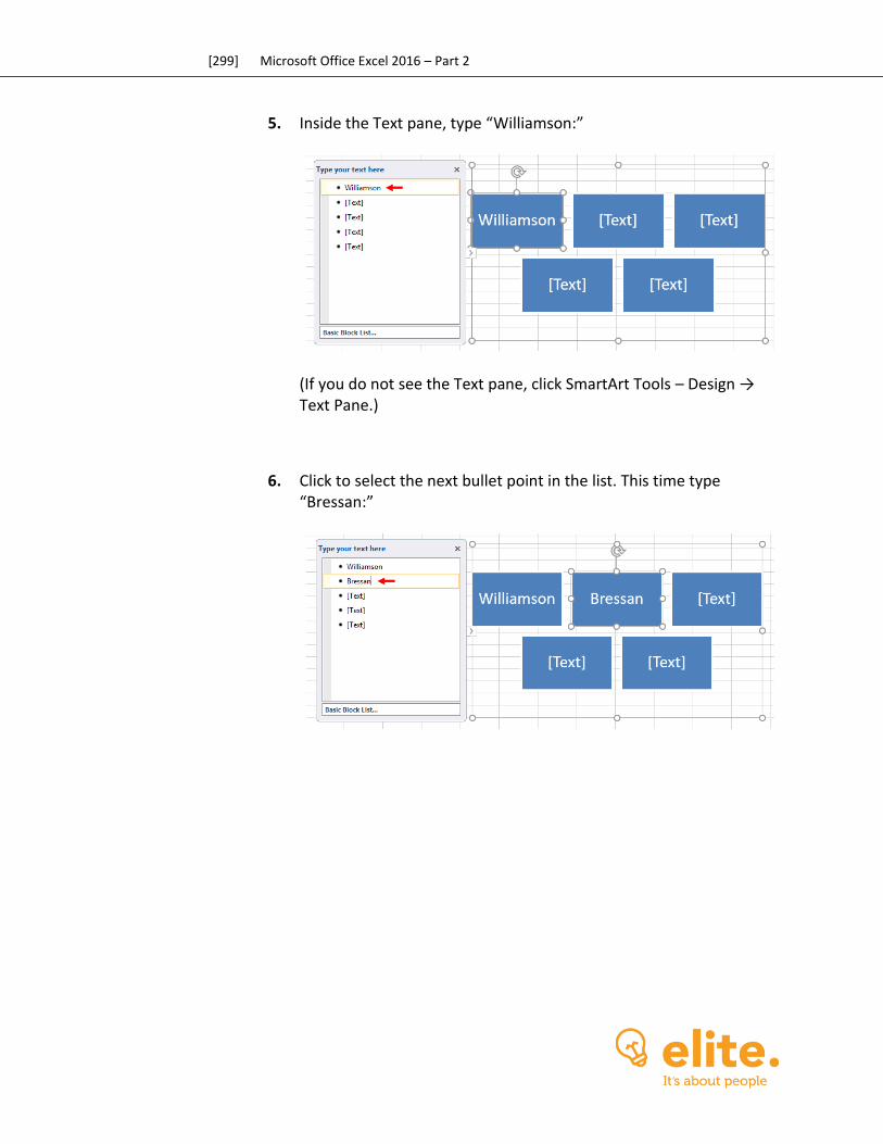
[299] Microsoft Office Excel 2016 – Part 2
5. Inside the Text pane, type “Williamson:”
(If you do not see the Text pane, click SmartArt Tools – Design → Text Pane.)
6. Click to select the next bullet point in the list. This time type “Bressan:”
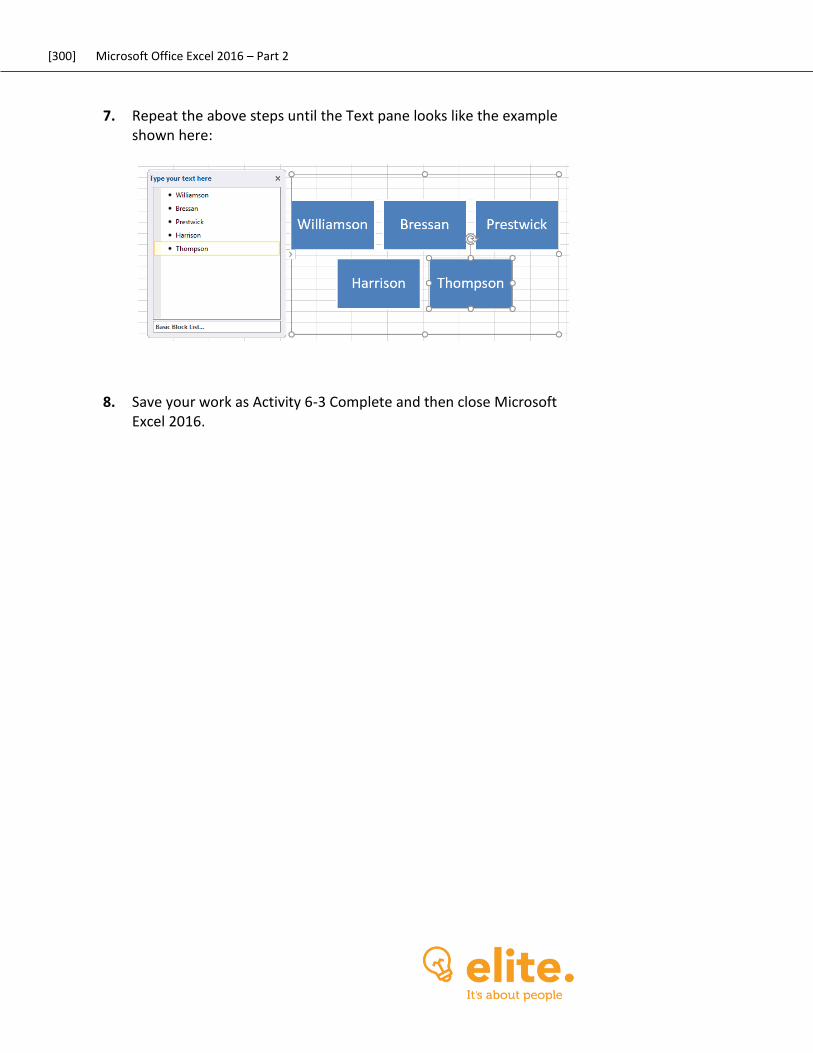
[300] Microsoft Office Excel 2016 – Part 2
7. Repeat the above steps until the Text pane looks like the example shown here:
8. Save your work as Activity 6-3 Complete and then close Microsoft Excel 2016.
[301] Microsoft Office Excel 2016 – Part 2
Summary This lesson taught you how graphical objects can be used to enhance the appearance of your workbooks. You learned how to insert graphical objects of different types into worksheets as well as how to modify them to suit your needs. Additionally, you learned about SmartArt, how it works, and how to add it to a worksheet.
REVIEW QUESTIONS
1. What are the five types of graphical objects that can be inserted into Excel workbooks?
2. Are shapes considered pictures or drawings?
3. How do you open the Selection pane?
4. What are SmartArt graphics used for?
5. How do you open the Choose a SmartArt Graphic dialog box?
[302] Microsoft Office Excel 2016 – Part 2
LESSON 7: ENHANCING
WORKBOOKS
Lesson Objectives
In this lesson you will learn how to:
Customize workbooks
Manage themes
Create and use templates
Protect files
Prepare a workbook for audiences
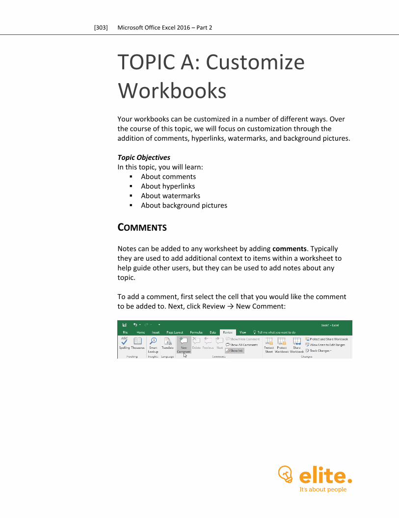
[303] Microsoft Office Excel 2016 – Part 2
TOPIC A: Customize Workbooks Your workbooks can be customized in a number of different ways. Over the course of this topic, we will focus on customization through the addition of comments, hyperlinks, watermarks, and background pictures. Topic Objectives In this topic, you will learn:
About comments About hyperlinks About watermarks About background pictures
COMMENTS
Notes can be added to any worksheet by adding comments. Typically they are used to add additional context to items within a worksheet to help guide other users, but they can be used to add notes about any topic. To add a comment, first select the cell that you would like the comment to be added to. Next, click Review → New Comment:

[304] Microsoft Office Excel 2016 – Part 2
This action will create a new comment and a red comment indicator will appear in the upper right-hand corner of the currently selected cell. The comment will be labeled with the current user’s name, but this can be changed by replacing that text as needed. To add text to the comment, type inside the provided text area:
Once you are done, click anywhere outside of the comment text area to hide it; however, the red comment indicator will remain visible:
To view the comment again, click to select the cell in question or simply hover your cursor over it. To delete a comment, click to select the cell in which the comment has been placed and click Review → Delete.
HYPERLINKS
Hyperlinks are a mainstay in the computing world. They enable you to navigate around your computer, browse the Internet, and jump to different cells within the same workbook. Excel lets you use this handy
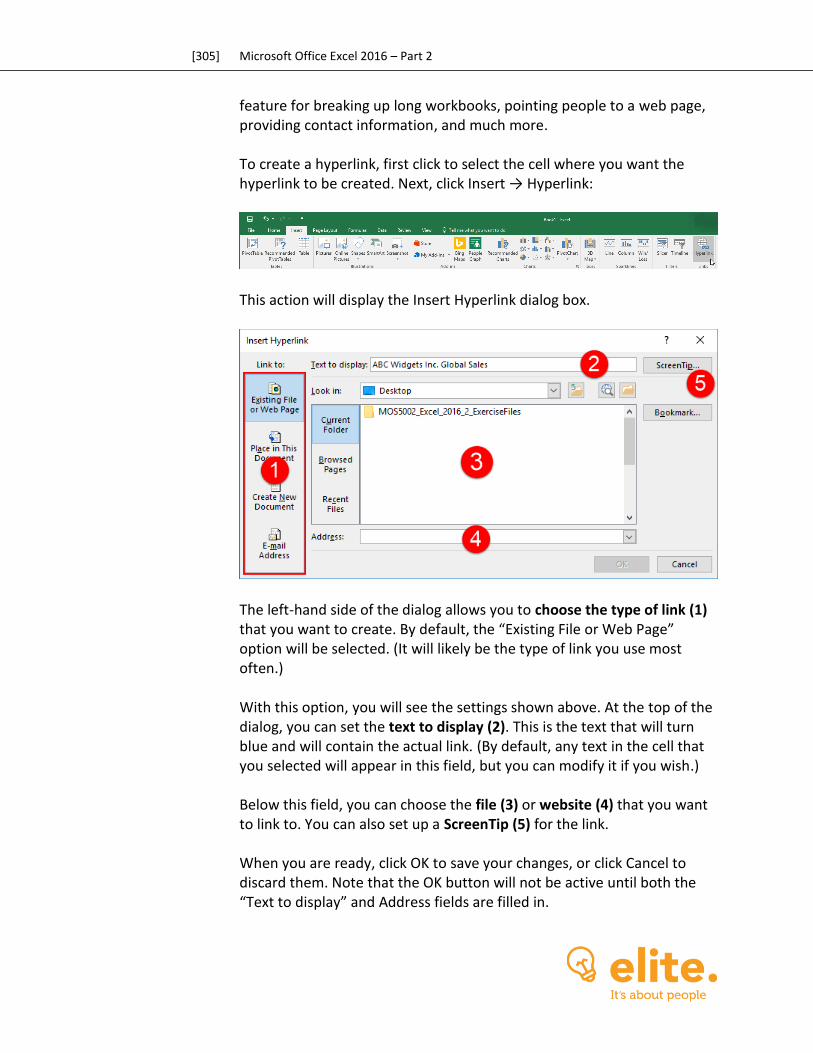
[305] Microsoft Office Excel 2016 – Part 2
feature for breaking up long workbooks, pointing people to a web page, providing contact information, and much more. To create a hyperlink, first click to select the cell where you want the hyperlink to be created. Next, click Insert → Hyperlink:
This action will display the Insert Hyperlink dialog box.
The left-hand side of the dialog allows you to choose the type of link (1) that you want to create. By default, the “Existing File or Web Page” option will be selected. (It will likely be the type of link you use most often.) With this option, you will see the settings shown above. At the top of the dialog, you can set the text to display (2). This is the text that will turn blue and will contain the actual link. (By default, any text in the cell that you selected will appear in this field, but you can modify it if you wish.) Below this field, you can choose the file (3) or website (4) that you want to link to. You can also set up a ScreenTip (5) for the link. When you are ready, click OK to save your changes, or click Cancel to discard them. Note that the OK button will not be active until both the “Text to display” and Address fields are filled in.
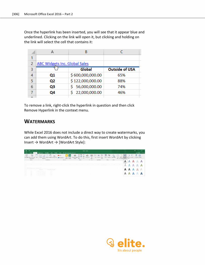
[306] Microsoft Office Excel 2016 – Part 2
Once the hyperlink has been inserted, you will see that it appear blue and underlined. Clicking on the link will open it, but clicking and holding on the link will select the cell that contains it:
To remove a link, right-click the hyperlink in question and then click Remove Hyperlink in the context menu.
WATERMARKS
While Excel 2016 does not include a direct way to create watermarks, you can add them using WordArt. To do this, first insert WordArt by clicking Insert → WordArt → [WordArt Style]:
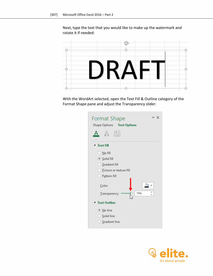
[307] Microsoft Office Excel 2016 – Part 2
Next, type the text that you would like to make up the watermark and rotate it if needed:
With the WordArt selected, open the Text Fill & Outline category of the Format Shape pane and adjust the Transparency slider:
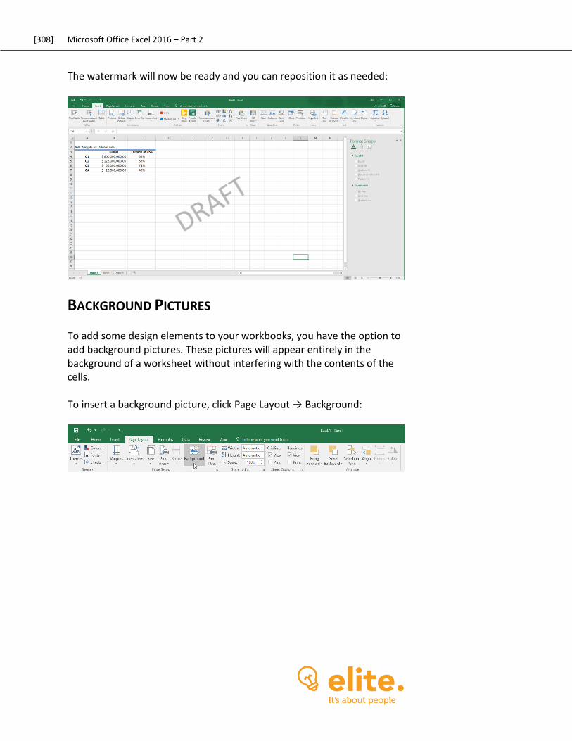
[308] Microsoft Office Excel 2016 – Part 2
The watermark will now be ready and you can reposition it as needed:
BACKGROUND PICTURES
To add some design elements to your workbooks, you have the option to add background pictures. These pictures will appear entirely in the background of a worksheet without interfering with the contents of the cells. To insert a background picture, click Page Layout → Background:
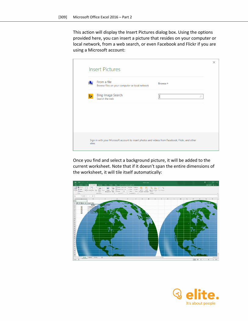
[309] Microsoft Office Excel 2016 – Part 2
This action will display the Insert Pictures dialog box. Using the options provided here, you can insert a picture that resides on your computer or local network, from a web search, or even Facebook and Flickr if you are using a Microsoft account:
Once you find and select a background picture, it will be added to the current worksheet. Note that if it doesn’t span the entire dimensions of the worksheet, it will tile itself automatically:

[310] Microsoft Office Excel 2016 – Part 2
To remove a background image, click Page Layout → Delete Background:
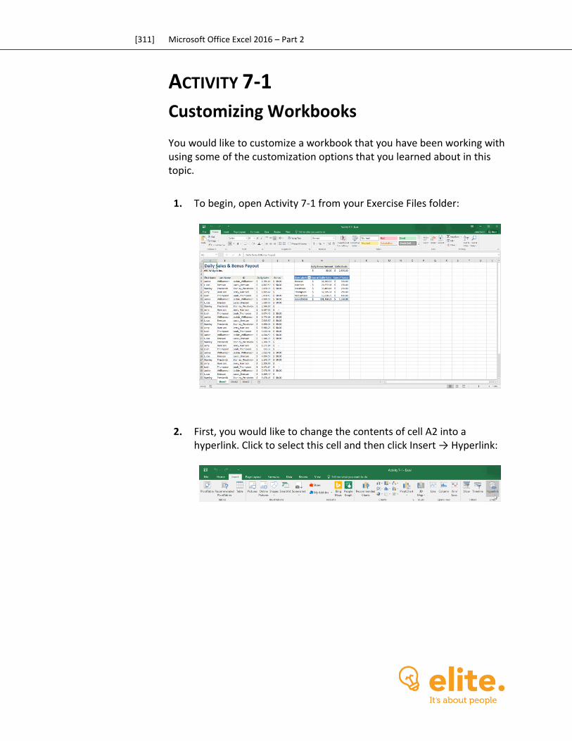
[311] Microsoft Office Excel 2016 – Part 2
ACTIVITY 7-1
Customizing Workbooks You would like to customize a workbook that you have been working with using some of the customization options that you learned about in this topic.
1. To begin, open Activity 7-1 from your Exercise Files folder:
2. First, you would like to change the contents of cell A2 into a hyperlink. Click to select this cell and then click Insert → Hyperlink:
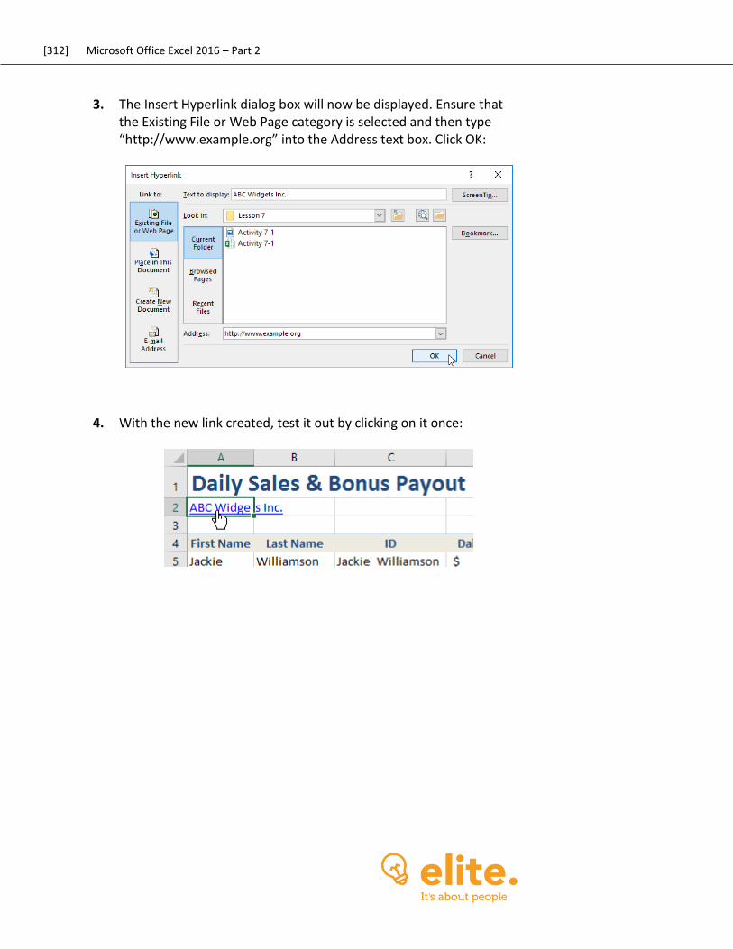
[312] Microsoft Office Excel 2016 – Part 2
3. The Insert Hyperlink dialog box will now be displayed. Ensure that the Existing File or Web Page category is selected and then type “http://www.example.org” into the Address text box. Click OK:
4. With the new link created, test it out by clicking on it once:
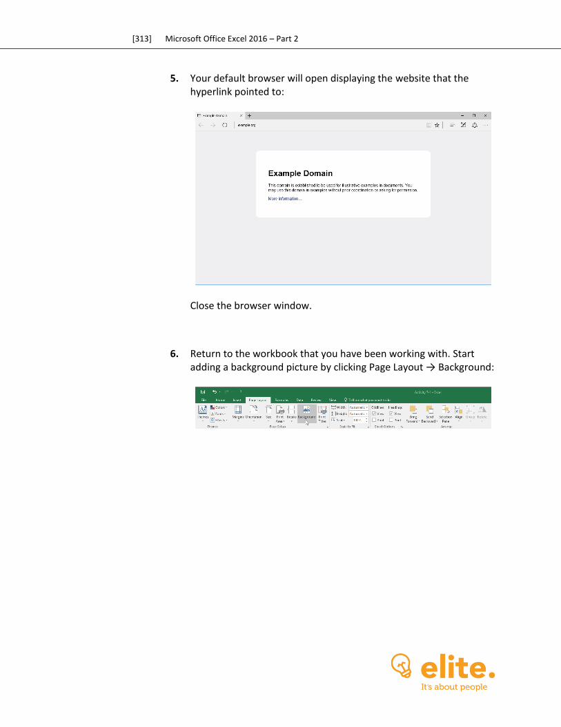
[313] Microsoft Office Excel 2016 – Part 2
5. Your default browser will open displaying the website that the hyperlink pointed to:
Close the browser window.
6. Return to the workbook that you have been working with. Start adding a background picture by clicking Page Layout → Background:
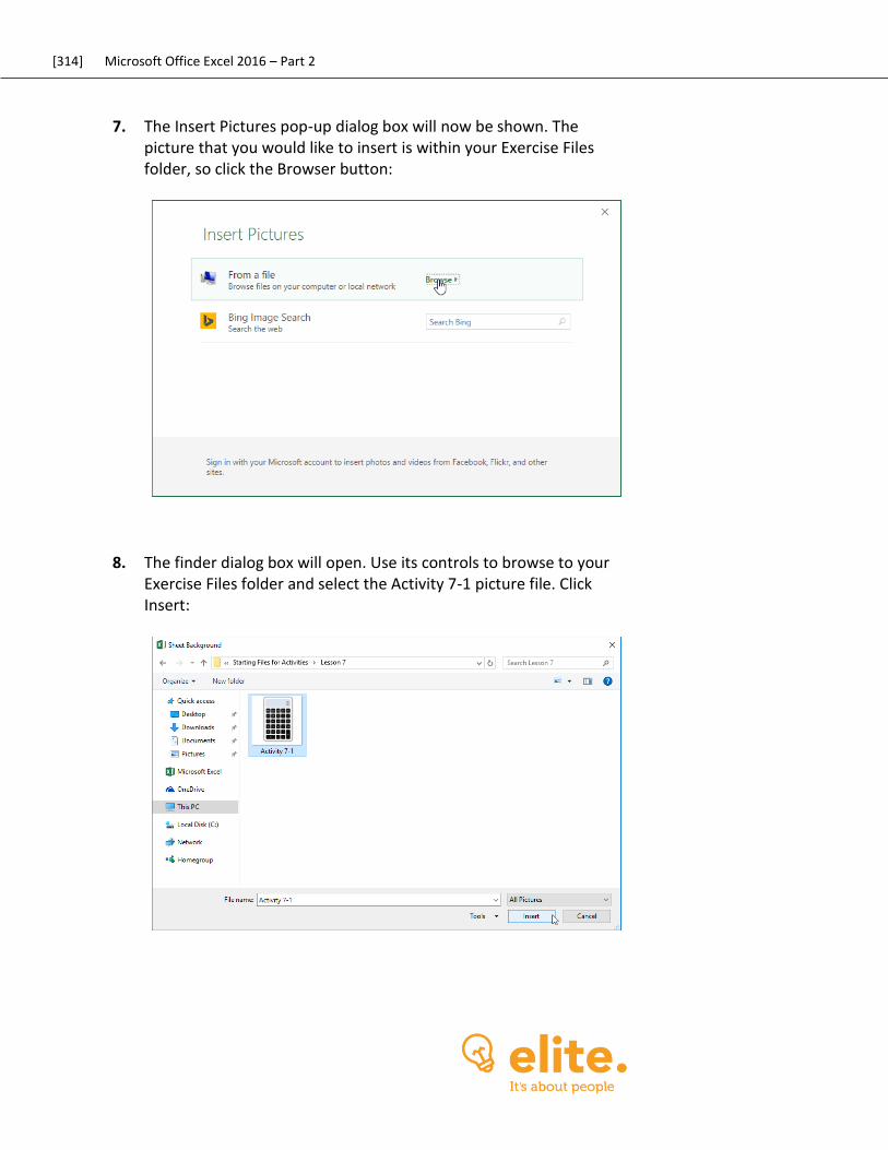
[314] Microsoft Office Excel 2016 – Part 2
7. The Insert Pictures pop-up dialog box will now be shown. The picture that you would like to insert is within your Exercise Files folder, so click the Browser button:
8. The finder dialog box will open. Use its controls to browse to your Exercise Files folder and select the Activity 7-1 picture file. Click Insert:
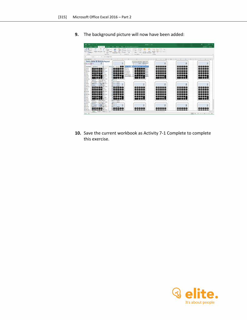
[315] Microsoft Office Excel 2016 – Part 2
9. The background picture will now have been added:
10. Save the current workbook as Activity 7-1 Complete to complete this exercise.
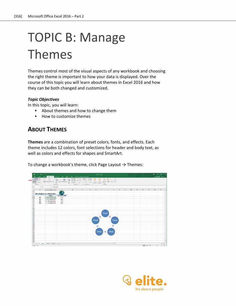
[316] Microsoft Office Excel 2016 – Part 2
TOPIC B: Manage Themes Themes control most of the visual aspects of any workbook and choosing the right theme is important to how your data is displayed. Over the course of this topic you will learn about themes in Excel 2016 and how they can be both changed and customized. Topic Objectives In this topic, you will learn:
About themes and how to change them How to customize themes
ABOUT THEMES
Themes are a combination of preset colors, fonts, and effects. Each theme includes 12 colors, font selections for header and body text, as well as colors and effects for shapes and SmartArt. To change a workbook’s theme, click Page Layout → Themes:
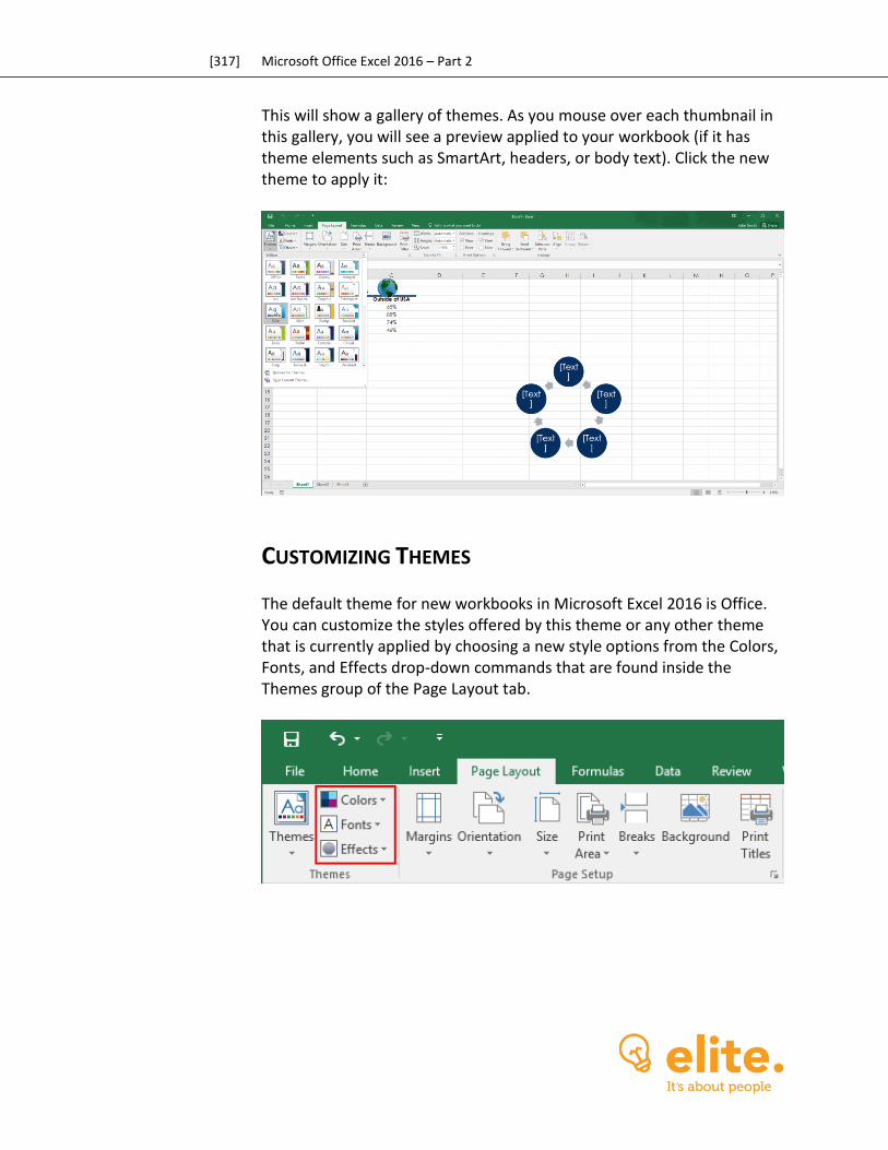
[317] Microsoft Office Excel 2016 – Part 2
This will show a gallery of themes. As you mouse over each thumbnail in this gallery, you will see a preview applied to your workbook (if it has theme elements such as SmartArt, headers, or body text). Click the new theme to apply it:
CUSTOMIZING THEMES
The default theme for new workbooks in Microsoft Excel 2016 is Office. You can customize the styles offered by this theme or any other theme that is currently applied by choosing a new style options from the Colors, Fonts, and Effects drop-down commands that are found inside the Themes group of the Page Layout tab.
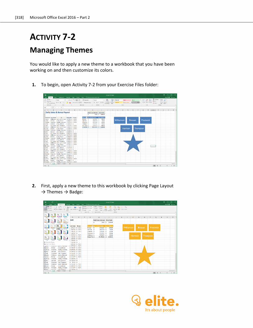
[318] Microsoft Office Excel 2016 – Part 2
ACTIVITY 7-2
Managing Themes You would like to apply a new theme to a workbook that you have been working on and then customize its colors.
1. To begin, open Activity 7-2 from your Exercise Files folder:
2. First, apply a new theme to this workbook by clicking Page Layout → Themes → Badge:
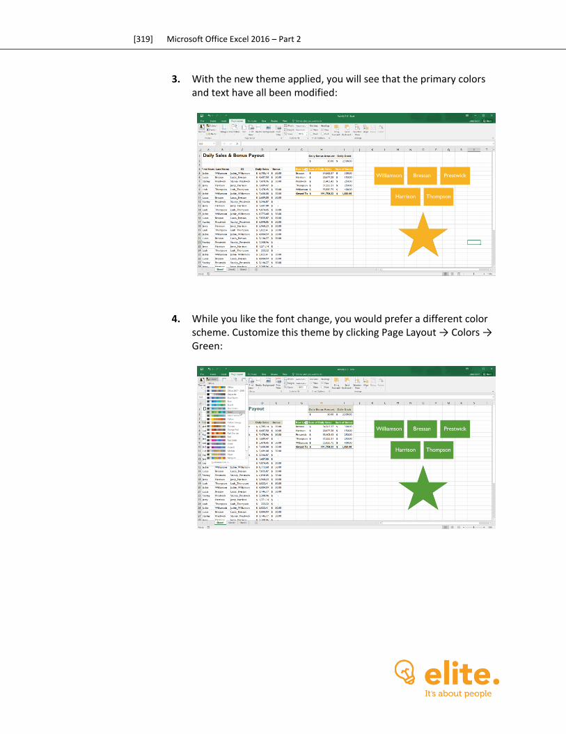
[319] Microsoft Office Excel 2016 – Part 2
3. With the new theme applied, you will see that the primary colors and text have all been modified:
4. While you like the font change, you would prefer a different color scheme. Customize this theme by clicking Page Layout → Colors → Green:
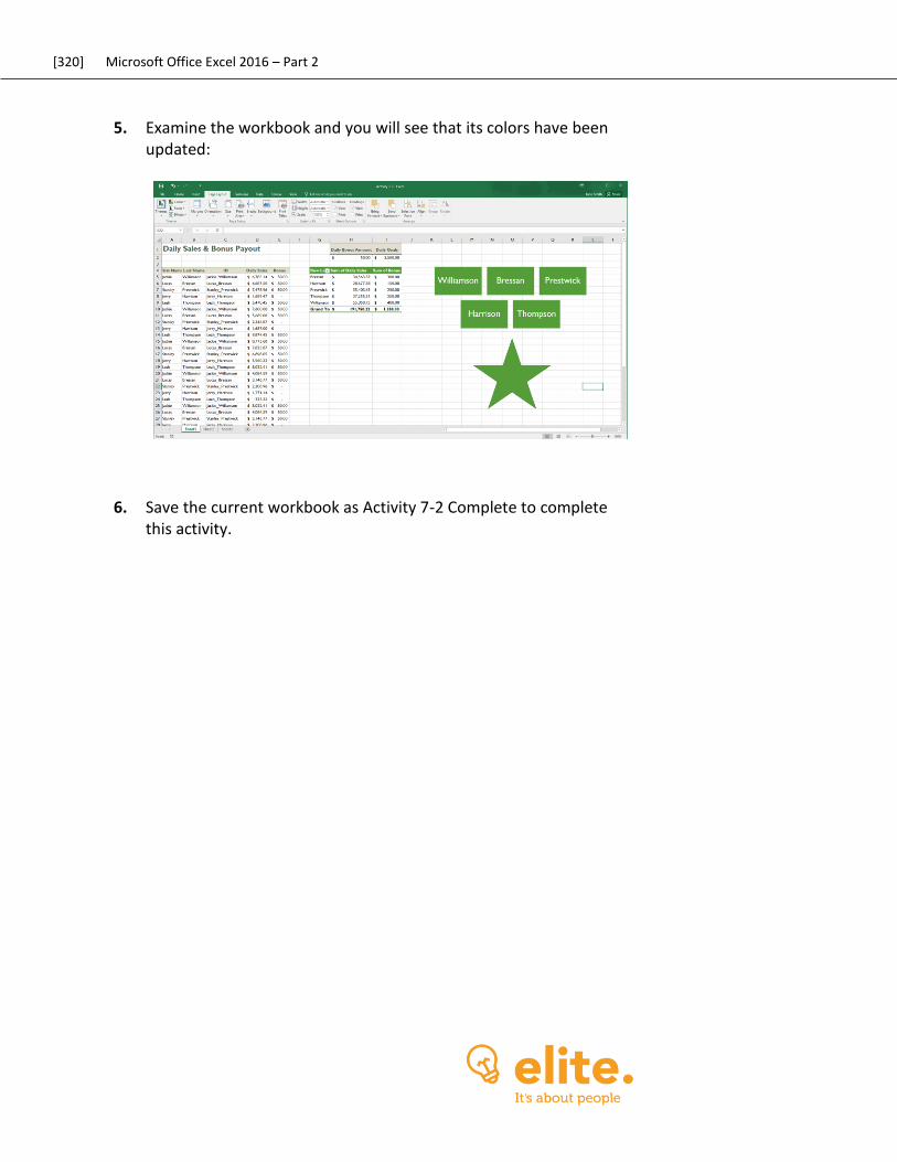
[320] Microsoft Office Excel 2016 – Part 2
5. Examine the workbook and you will see that its colors have been updated:
6. Save the current workbook as Activity 7-2 Complete to complete this activity.
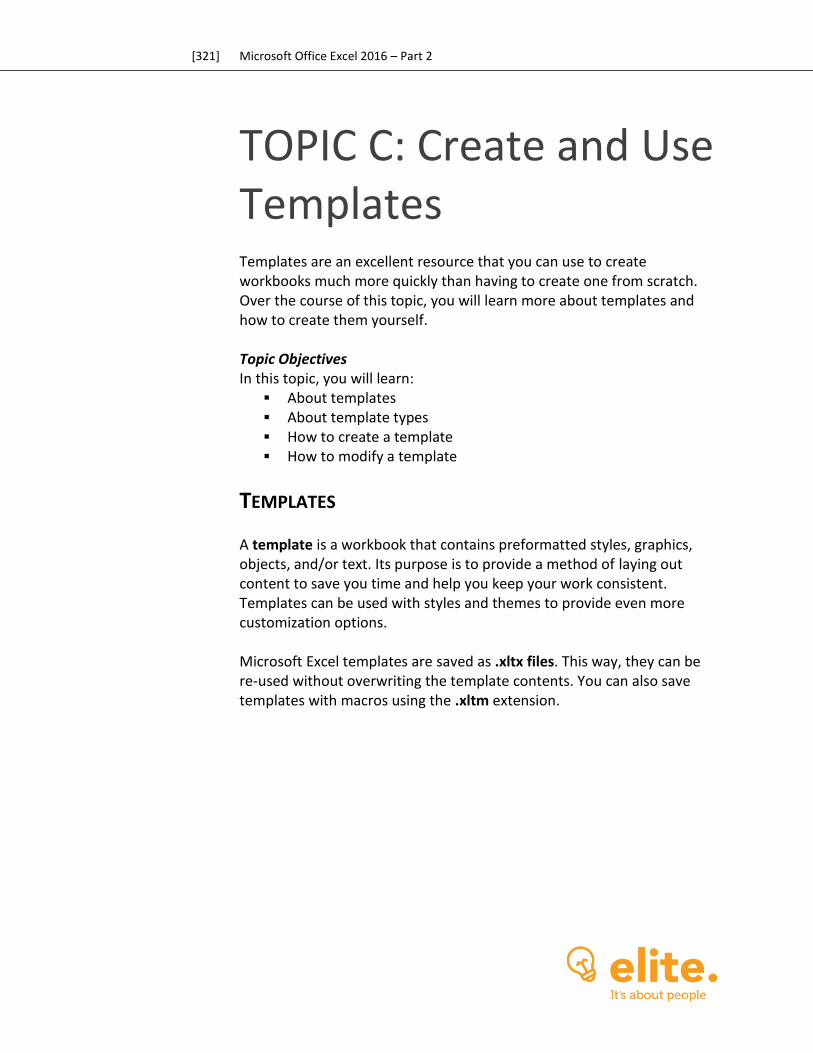
[321] Microsoft Office Excel 2016 – Part 2
TOPIC C: Create and Use Templates Templates are an excellent resource that you can use to create workbooks much more quickly than having to create one from scratch. Over the course of this topic, you will learn more about templates and how to create them yourself. Topic Objectives In this topic, you will learn:
About templates About template types How to create a template How to modify a template
TEMPLATES
A template is a workbook that contains preformatted styles, graphics, objects, and/or text. Its purpose is to provide a method of laying out content to save you time and help you keep your work consistent. Templates can be used with styles and themes to provide even more customization options. Microsoft Excel templates are saved as .xltx files. This way, they can be re-used without overwriting the template contents. You can also save templates with macros using the .xltm extension.

[322] Microsoft Office Excel 2016 – Part 2
TEMPLATE TYPES
Microsoft Excel 2016 includes many different predefined templates that you can choose from that cover a wide variety of different needs. If you can’t initially find the exact template for your purposes, you can probably find it using the search function.
Custom templates are those that are created by yourself, your organization, or someone that you are working with. You can see these templates listed under the Personal heading of the new workbook window:
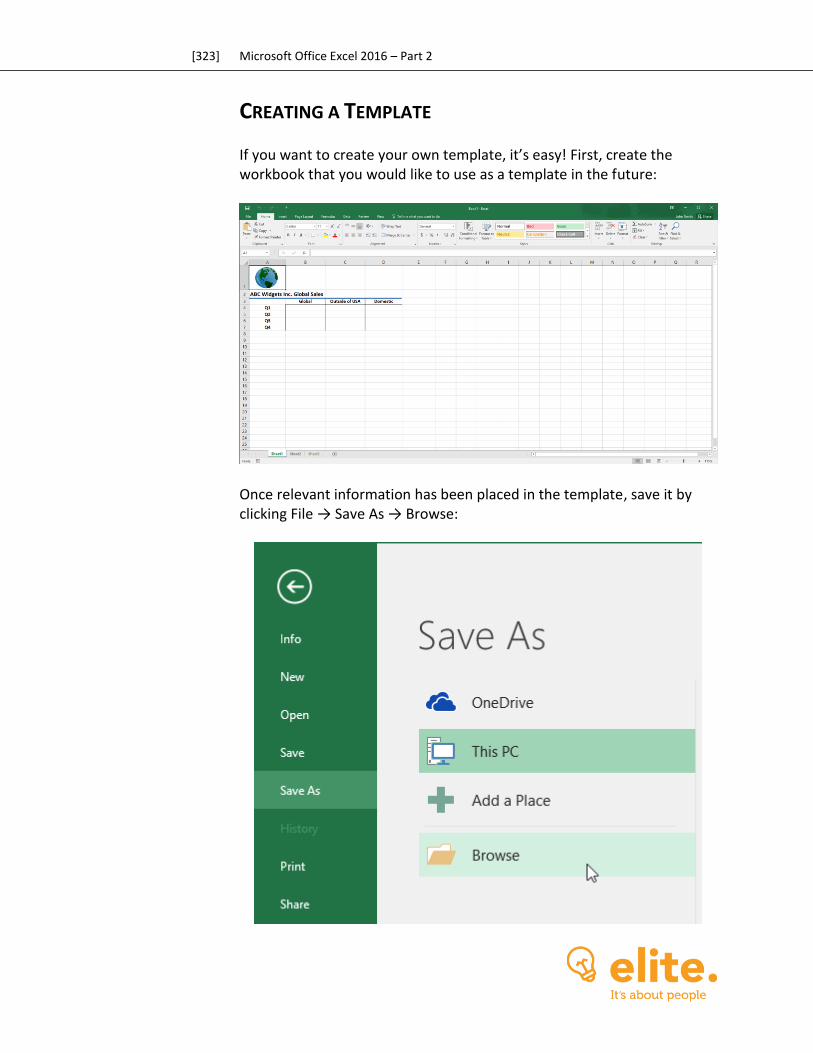
[323] Microsoft Office Excel 2016 – Part 2
CREATING A TEMPLATE
If you want to create your own template, it’s easy! First, create the workbook that you would like to use as a template in the future:
Once relevant information has been placed in the template, save it by clicking File → Save As → Browse:
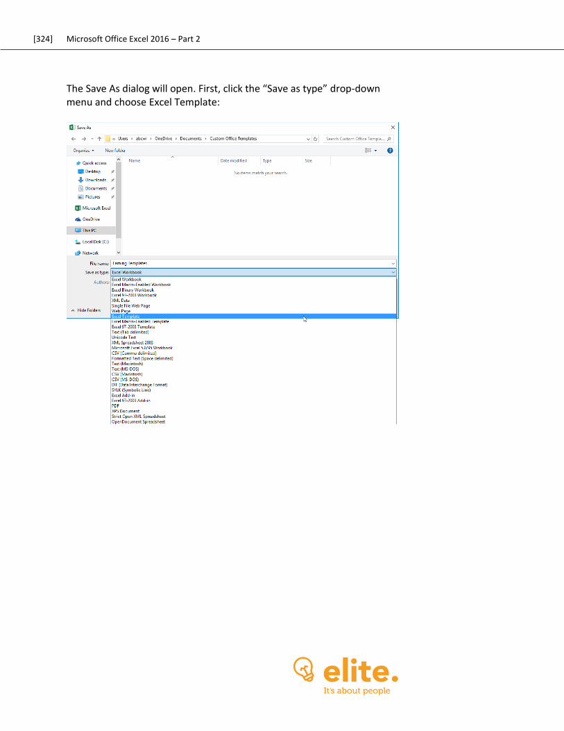
[324] Microsoft Office Excel 2016 – Part 2
The Save As dialog will open. First, click the “Save as type” drop-down menu and choose Excel Template:
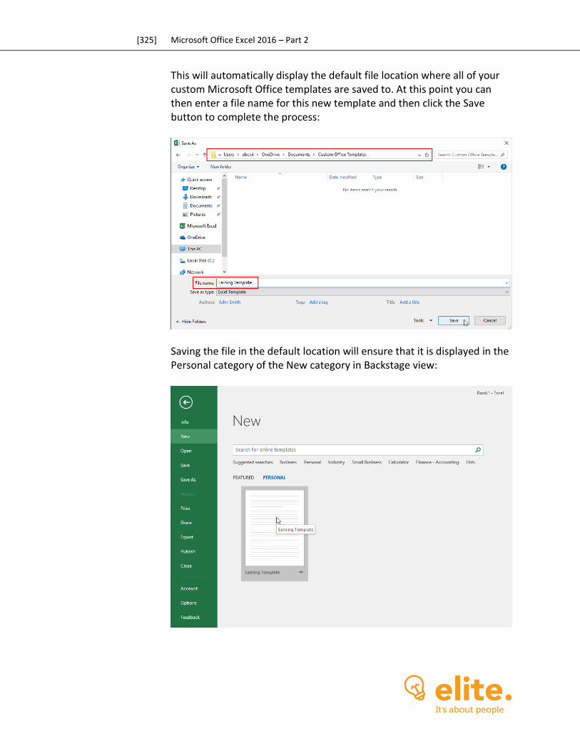
[325] Microsoft Office Excel 2016 – Part 2
This will automatically display the default file location where all of your custom Microsoft Office templates are saved to. At this point you can then enter a file name for this new template and then click the Save button to complete the process:
Saving the file in the default location will ensure that it is displayed in the Personal category of the New category in Backstage view:
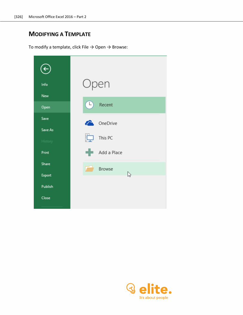
[326] Microsoft Office Excel 2016 – Part 2
MODIFYING A TEMPLATE
To modify a template, click File → Open → Browse:
[327] Microsoft Office Excel 2016 – Part 2
In the Open dialog box, navigate to the location of the template file, select it, and click Open:
(If you cannot see your template file, ensure that the filter above the Open button is set to All Excel Files.) If you are using File Explorer to open a template for modification, double-clicking a template will open a new Excel workbook based on the template and not the actual template itself. In order to open the template for modification, right-click the template file and click Open:
[328] Microsoft Office Excel 2016 – Part 2
Once a template file is open for modification, Excel’s title bar will display the template name (not Book1, Book2, etc.):
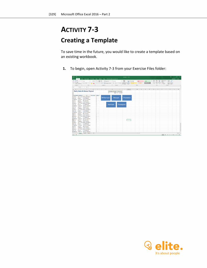
[329] Microsoft Office Excel 2016 – Part 2
ACTIVITY 7-3
Creating a Template To save time in the future, you would like to create a template based on an existing workbook.
1. To begin, open Activity 7-3 from your Exercise Files folder:
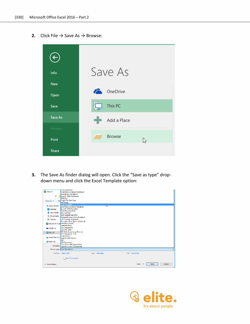
[330] Microsoft Office Excel 2016 – Part 2
2. Click File → Save As → Browse:
3. The Save As finder dialog will open. Click the “Save as type” drop-down menu and click the Excel Template option:
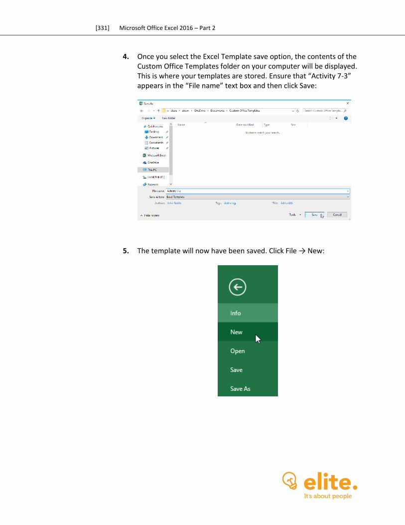
[331] Microsoft Office Excel 2016 – Part 2
4. Once you select the Excel Template save option, the contents of the Custom Office Templates folder on your computer will be displayed. This is where your templates are stored. Ensure that “Activity 7-3” appears in the “File name” text box and then click Save:
5. The template will now have been saved. Click File → New:
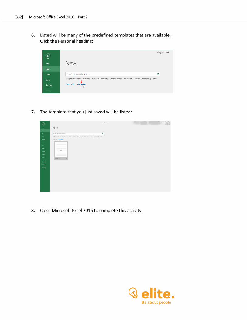
[332] Microsoft Office Excel 2016 – Part 2
6. Listed will be many of the predefined templates that are available. Click the Personal heading:
7. The template that you just saved will be listed:
8. Close Microsoft Excel 2016 to complete this activity.
[333] Microsoft Office Excel 2016 – Part 2
TOPIC D: Protect Files One of the most important aspects that you need to understand while working with your data in Excel is how to protect Excel files from data loss, as well as unauthorized access. Over the course of this topic you will learn about the various ways that Excel 2016 can protect your work. Topic Objectives In this topic, you will learn:
How to recover lost data About the Changes group on the Review tab About worksheet and workbook protection How to protect a worksheet How to protect a workbook
RECOVERING LOST DATA
The AutoRecover feature works in the background to automatically save the workbook that you are working on. This saved copy of the file is called a version and it can be recovered if Excel or your computer experiences an error. If you saved the file previously, you can find each version by clicking File → Info, and then examining the Manage Workbook section:
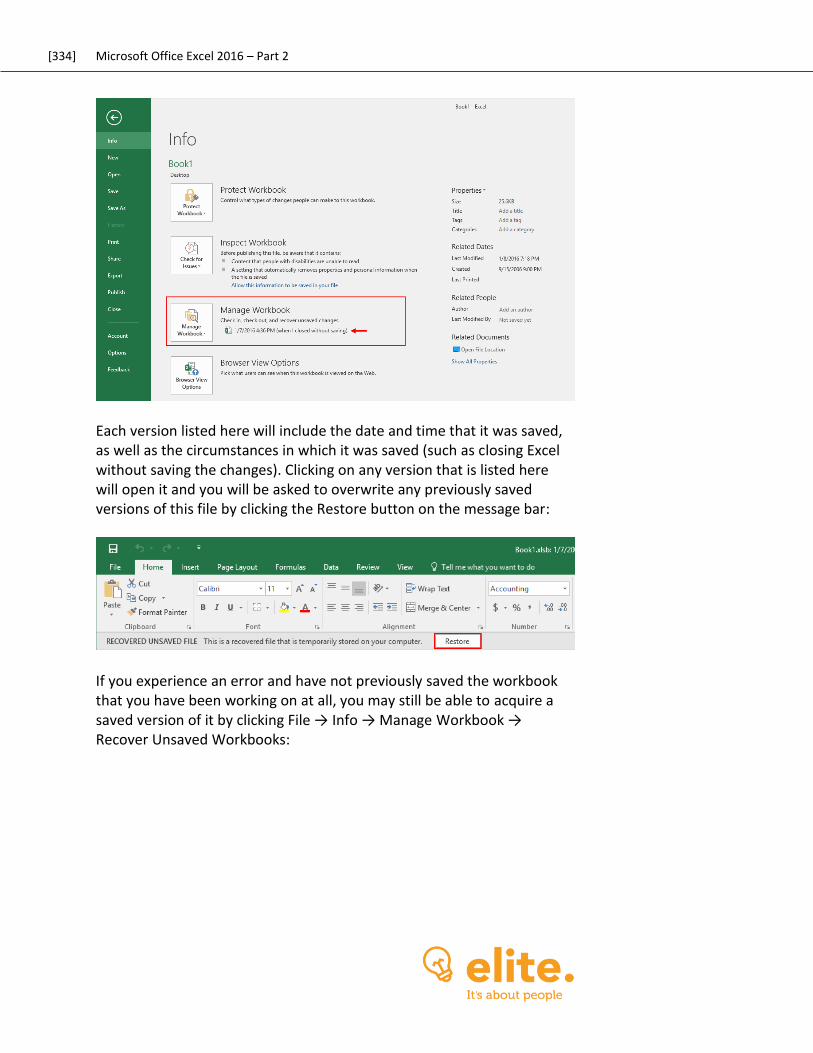
[334] Microsoft Office Excel 2016 – Part 2
Each version listed here will include the date and time that it was saved, as well as the circumstances in which it was saved (such as closing Excel without saving the changes). Clicking on any version that is listed here will open it and you will be asked to overwrite any previously saved versions of this file by clicking the Restore button on the message bar:
If you experience an error and have not previously saved the workbook that you have been working on at all, you may still be able to acquire a saved version of it by clicking File → Info → Manage Workbook → Recover Unsaved Workbooks:
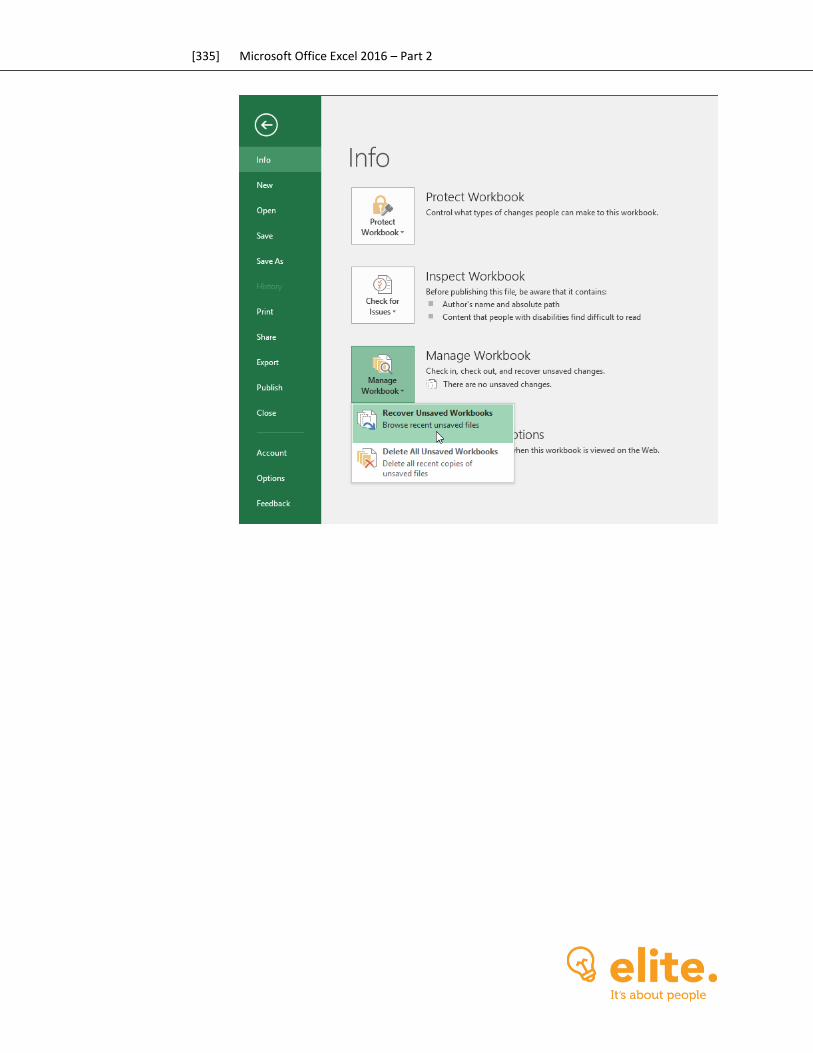
[335] Microsoft Office Excel 2016 – Part 2
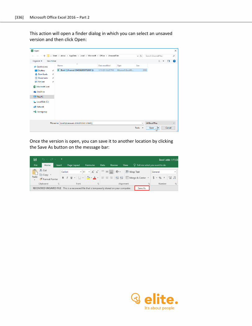
[336] Microsoft Office Excel 2016 – Part 2
This action will open a finder dialog in which you can select an unsaved version and then click Open:
Once the version is open, you can save it to another location by clicking the Save As button on the message bar:
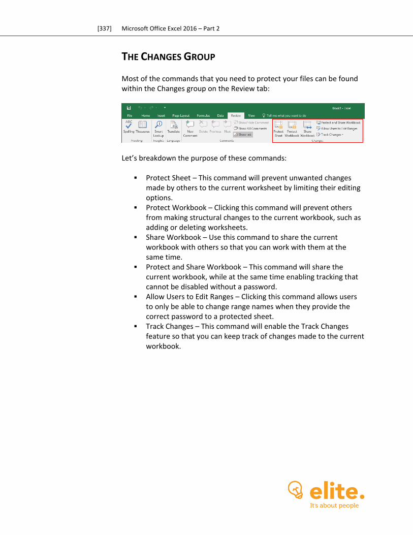
[337] Microsoft Office Excel 2016 – Part 2
THE CHANGES GROUP
Most of the commands that you need to protect your files can be found within the Changes group on the Review tab:
Let’s breakdown the purpose of these commands:
Protect Sheet – This command will prevent unwanted changes made by others to the current worksheet by limiting their editing options.
Protect Workbook – Clicking this command will prevent others from making structural changes to the current workbook, such as adding or deleting worksheets.
Share Workbook – Use this command to share the current workbook with others so that you can work with them at the same time.
Protect and Share Workbook – This command will share the current workbook, while at the same time enabling tracking that cannot be disabled without a password.
Allow Users to Edit Ranges – Clicking this command allows users to only be able to change range names when they provide the correct password to a protected sheet.
Track Changes – This command will enable the Track Changes feature so that you can keep track of changes made to the current workbook.
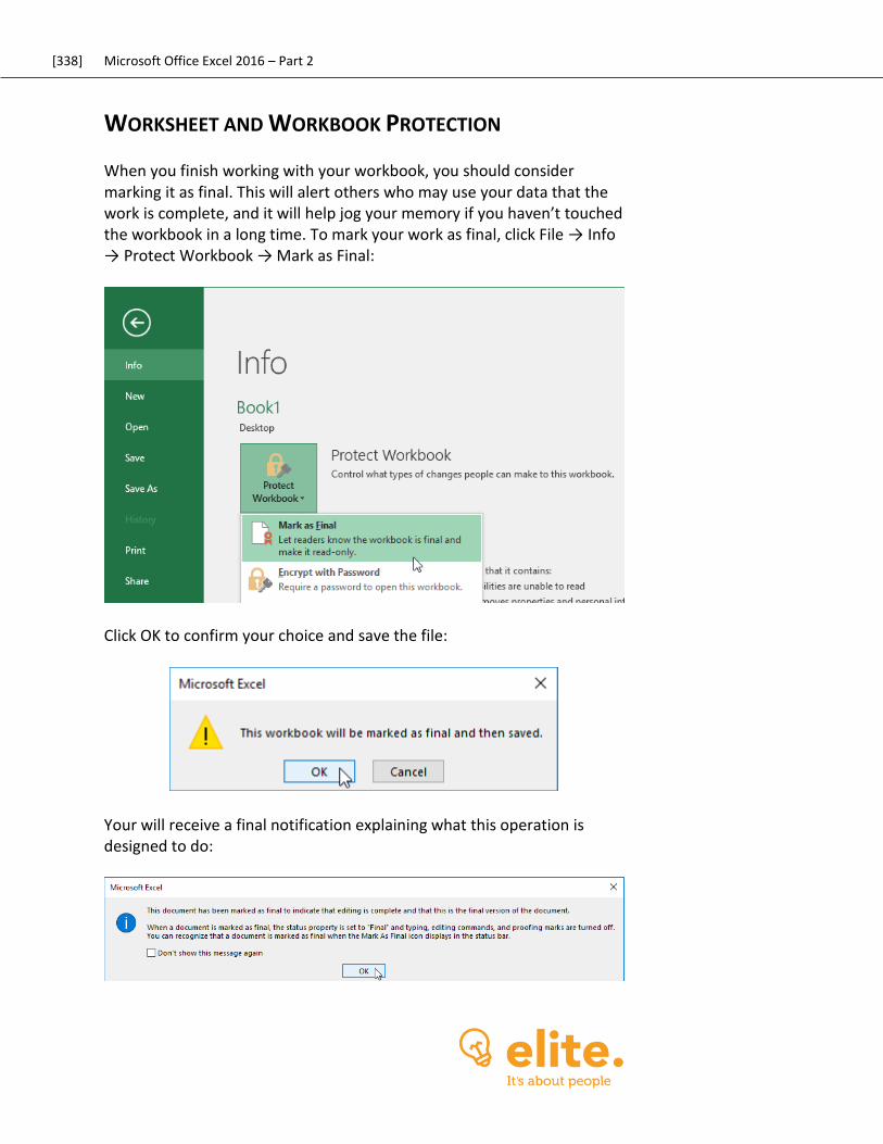
[338] Microsoft Office Excel 2016 – Part 2
WORKSHEET AND WORKBOOK PROTECTION
When you finish working with your workbook, you should consider marking it as final. This will alert others who may use your data that the work is complete, and it will help jog your memory if you haven’t touched the workbook in a long time. To mark your work as final, click File → Info → Protect Workbook → Mark as Final:
Click OK to confirm your choice and save the file:
Your will receive a final notification explaining what this operation is designed to do:
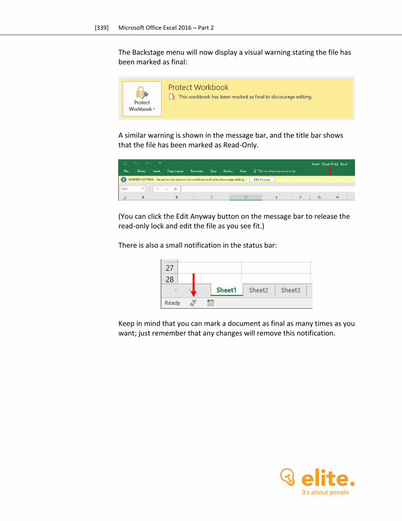
[339] Microsoft Office Excel 2016 – Part 2
The Backstage menu will now display a visual warning stating the file has been marked as final:
A similar warning is shown in the message bar, and the title bar shows that the file has been marked as Read-Only.
(You can click the Edit Anyway button on the message bar to release the read-only lock and edit the file as you see fit.)
There is also a small notification in the status bar:
Keep in mind that you can mark a document as final as many times as you want; just remember that any changes will remove this notification.
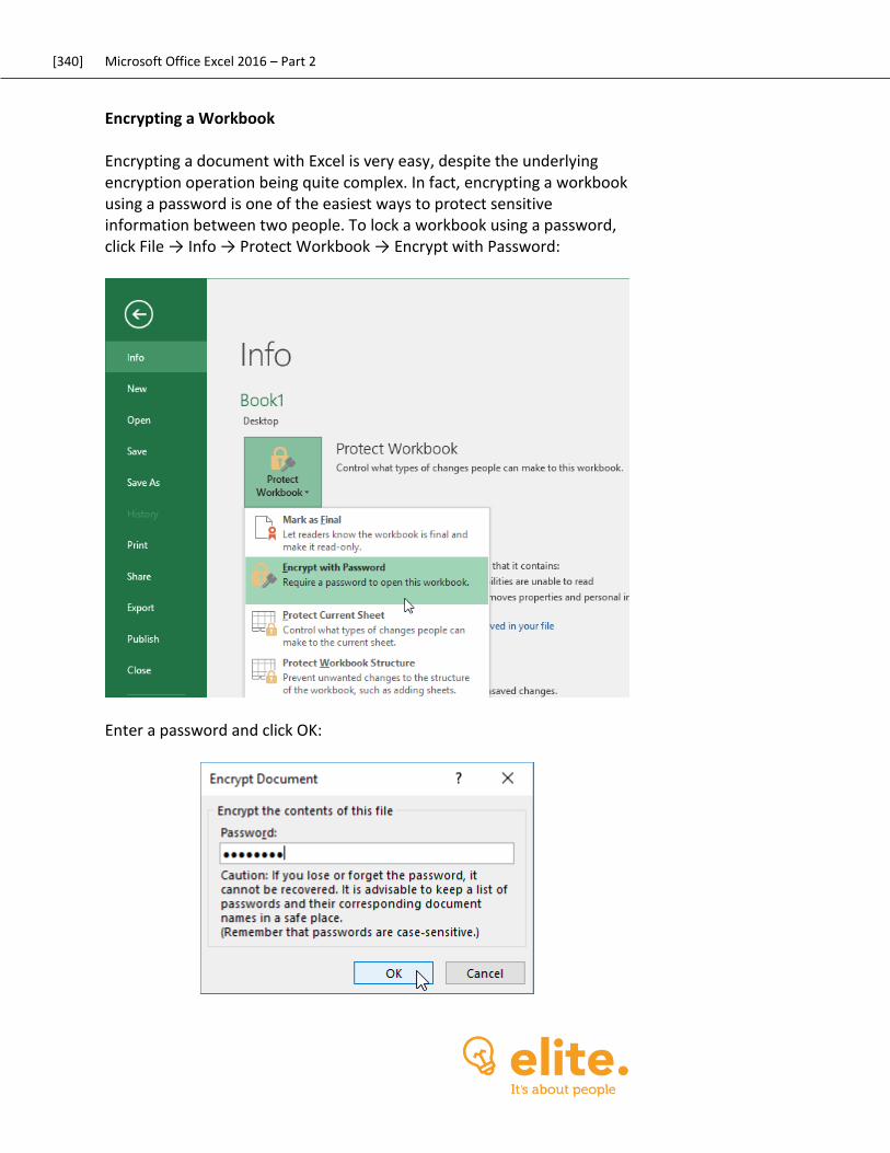
[340] Microsoft Office Excel 2016 – Part 2
Encrypting a Workbook Encrypting a document with Excel is very easy, despite the underlying encryption operation being quite complex. In fact, encrypting a workbook using a password is one of the easiest ways to protect sensitive information between two people. To lock a workbook using a password, click File → Info → Protect Workbook → Encrypt with Password:
Enter a password and click OK:
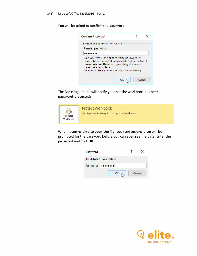
[341] Microsoft Office Excel 2016 – Part 2
You will be asked to confirm the password:
The Backstage menu will notify you that the workbook has been password-protected:
When it comes time to open the file, you (and anyone else) will be prompted for the password before you can even see the data. Enter the password and click OK:
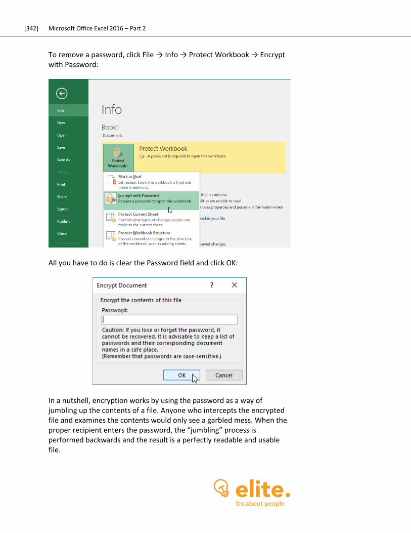
[342] Microsoft Office Excel 2016 – Part 2
To remove a password, click File → Info → Protect Workbook → Encrypt with Password:
All you have to do is clear the Password field and click OK:
In a nutshell, encryption works by using the password as a way of jumbling up the contents of a file. Anyone who intercepts the encrypted file and examines the contents would only see a garbled mess. When the proper recipient enters the password, the “jumbling” process is performed backwards and the result is a perfectly readable and usable file.
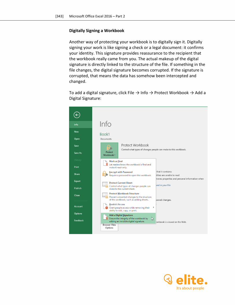
[343] Microsoft Office Excel 2016 – Part 2
Digitally Signing a Workbook Another way of protecting your workbook is to digitally sign it. Digitally signing your work is like signing a check or a legal document: it confirms your identity. This signature provides reassurance to the recipient that the workbook really came from you. The actual makeup of the digital signature is directly linked to the structure of the file. If something in the file changes, the digital signature becomes corrupted. If the signature is corrupted, that means the data has somehow been intercepted and changed. To add a digital signature, click File → Info → Protect Workbook → Add a Digital Signature:

[344] Microsoft Office Excel 2016 – Part 2
Excel will ask if you would like to obtain a digital ID from a Microsoft partner. Clicking No will cancel the entire action, while clicking Yes will open your default browser to a list of digital ID services:
Speak with your IT department or contact a digital security company to determine what type of digital signature will be best for your needs.
THE PROTECT WORKSHEET OPTION
We know that workbooks (individual Excel files) are composed of one or more worksheets. Complex workbooks might make use of several worksheets, each of which might contain important data that is used by the rest of the workbook. In order to help protect your data, you can choose to protect a single worksheet in a workbook using the File menu. To begin, make sure you are viewing the worksheet you want to protect and then click File → Info → Protect Workbook → Protect Current Sheet:
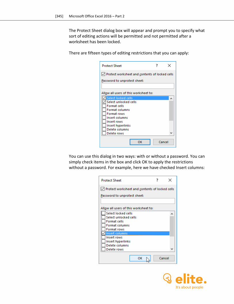
[345] Microsoft Office Excel 2016 – Part 2
The Protect Sheet dialog box will appear and prompt you to specify what sort of editing actions will be permitted and not permitted after a worksheet has been locked. There are fifteen types of editing restrictions that you can apply:
You can use this dialog in two ways: with or without a password. You can simply check items in the box and click OK to apply the restrictions without a password. For example, here we have checked Insert columns:
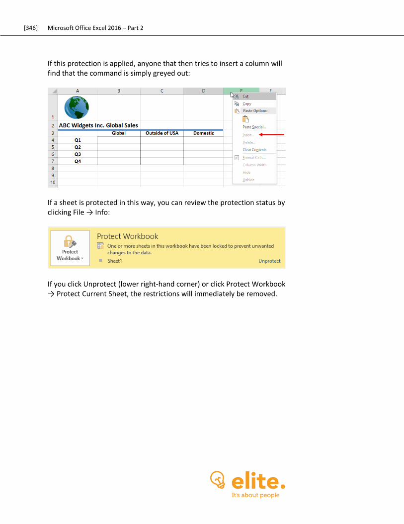
[346] Microsoft Office Excel 2016 – Part 2
If this protection is applied, anyone that then tries to insert a column will find that the command is simply greyed out:
If a sheet is protected in this way, you can review the protection status by clicking File → Info:
If you click Unprotect (lower right-hand corner) or click Protect Workbook → Protect Current Sheet, the restrictions will immediately be removed.
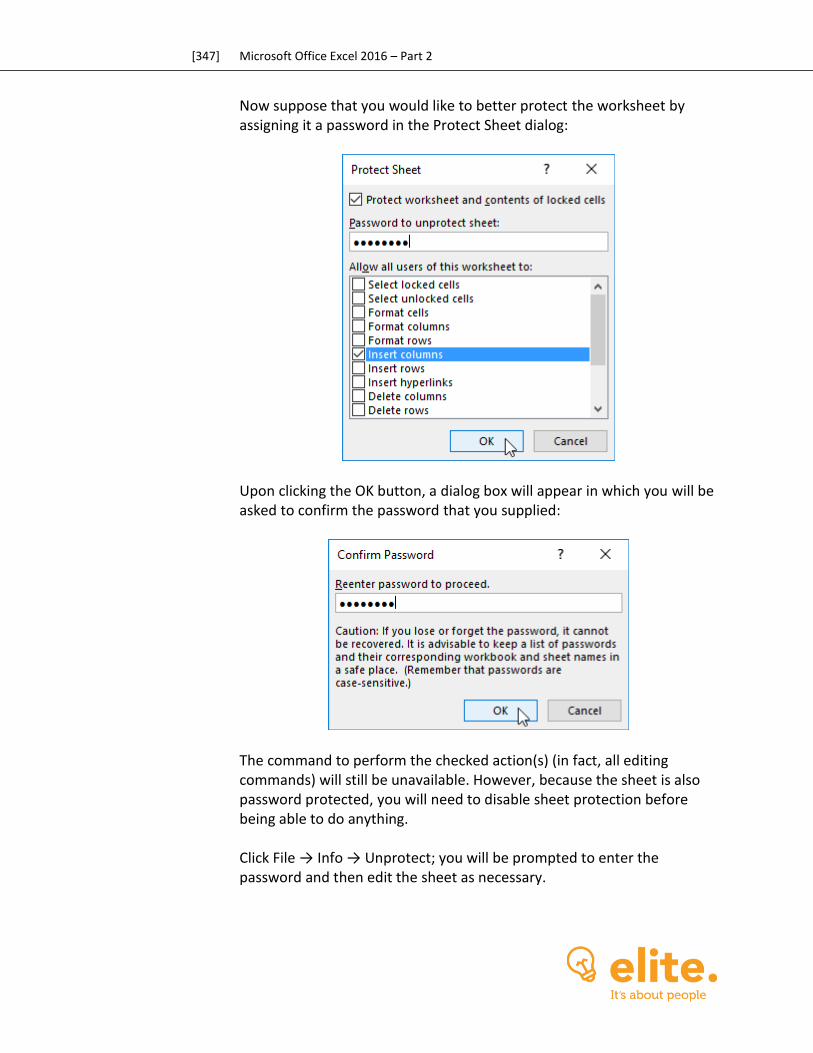
[347] Microsoft Office Excel 2016 – Part 2
Now suppose that you would like to better protect the worksheet by assigning it a password in the Protect Sheet dialog:
Upon clicking the OK button, a dialog box will appear in which you will be asked to confirm the password that you supplied:
The command to perform the checked action(s) (in fact, all editing commands) will still be unavailable. However, because the sheet is also password protected, you will need to disable sheet protection before being able to do anything. Click File → Info → Unprotect; you will be prompted to enter the password and then edit the sheet as necessary.
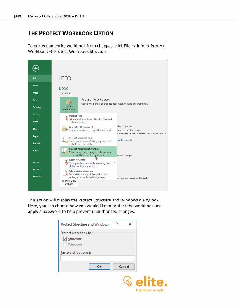
[348] Microsoft Office Excel 2016 – Part 2
THE PROTECT WORKBOOK OPTION
To protect an entire workbook from changes, click File → Info → Protect Workbook → Protect Workbook Structure:
This action will display the Protect Structure and Windows dialog box. Here, you can choose how you would like to protect the workbook and apply a password to help prevent unauthorized changes:
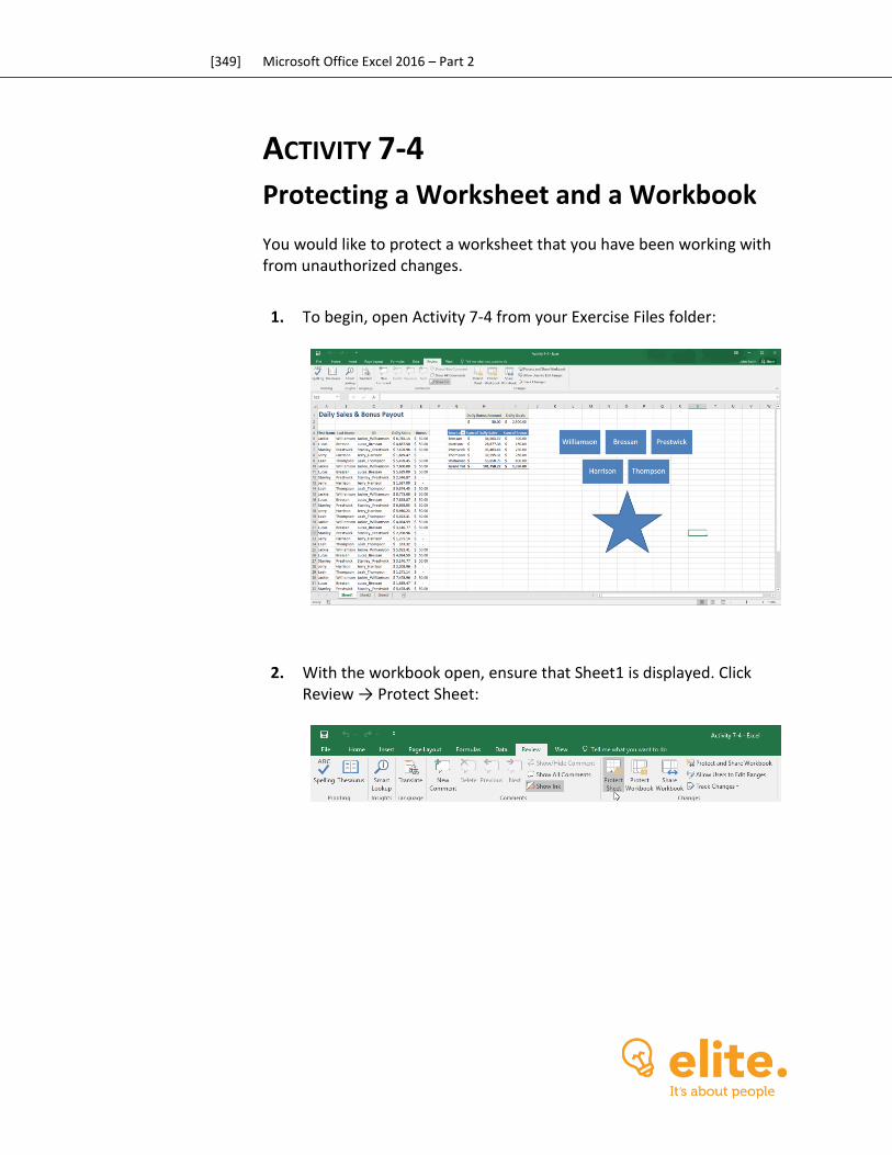
[349] Microsoft Office Excel 2016 – Part 2
ACTIVITY 7-4
Protecting a Worksheet and a Workbook You would like to protect a worksheet that you have been working with from unauthorized changes.
1. To begin, open Activity 7-4 from your Exercise Files folder:
2. With the workbook open, ensure that Sheet1 is displayed. Click Review → Protect Sheet:

[350] Microsoft Office Excel 2016 – Part 2
3. This action will display the Protect Sheet dialog box. Type a memorable password into the “Password to unprotect sheet” text box:
4. Check both the “Delete columns” and “Delete rows” check boxes and then click OK:
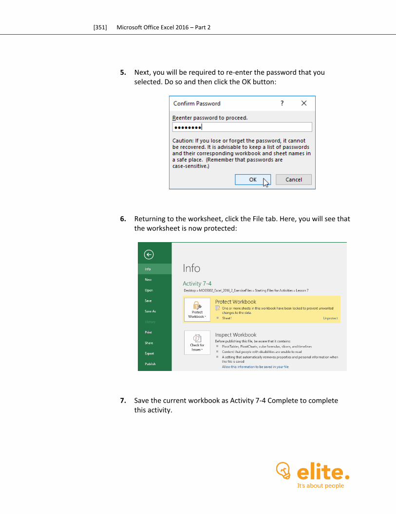
[351] Microsoft Office Excel 2016 – Part 2
5. Next, you will be required to re-enter the password that you selected. Do so and then click the OK button:
6. Returning to the worksheet, click the File tab. Here, you will see that the worksheet is now protected:
7. Save the current workbook as Activity 7-4 Complete to complete this activity.
[352] Microsoft Office Excel 2016 – Part 2
TOPIC E: Preparing a Workbook for Multiple Audiences One thing to keep in mind when working and managing workbooks created by Excel 2016, is that multiple audiences from other regions of the world may be required to use and understand them. For this reason it is important to ensure that your workbooks are suitable for multiple audiences when are where required. Topic Objectives In this topic, you will learn:
How to display data in multiple international formats How to modify worksheets using the accessibility checker How to utilize international symbols How to manage fonts
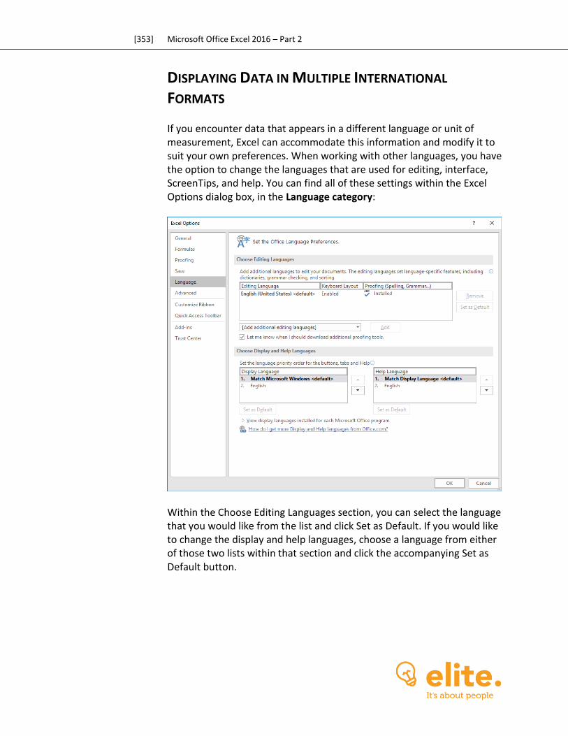
[353] Microsoft Office Excel 2016 – Part 2
DISPLAYING DATA IN MULTIPLE INTERNATIONAL
FORMATS
If you encounter data that appears in a different language or unit of measurement, Excel can accommodate this information and modify it to suit your own preferences. When working with other languages, you have the option to change the languages that are used for editing, interface, ScreenTips, and help. You can find all of these settings within the Excel Options dialog box, in the Language category:
Within the Choose Editing Languages section, you can select the language that you would like from the list and click Set as Default. If you would like to change the display and help languages, choose a language from either of those two lists within that section and click the accompanying Set as Default button.
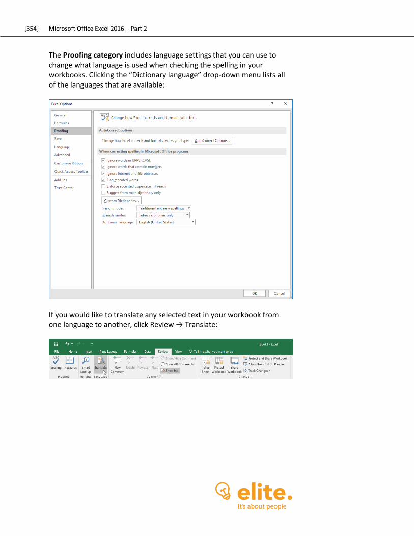
[354] Microsoft Office Excel 2016 – Part 2
The Proofing category includes language settings that you can use to change what language is used when checking the spelling in your workbooks. Clicking the “Dictionary language” drop-down menu lists all of the languages that are available:
If you would like to translate any selected text in your workbook from one language to another, click Review → Translate:
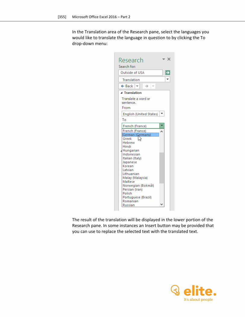
[355] Microsoft Office Excel 2016 – Part 2
In the Translation area of the Research pane, select the languages you would like to translate the language in question to by clicking the To drop-down menu:
The result of the translation will be displayed in the lower portion of the Research pane. In some instances an Insert button may be provided that you can use to replace the selected text with the translated text.
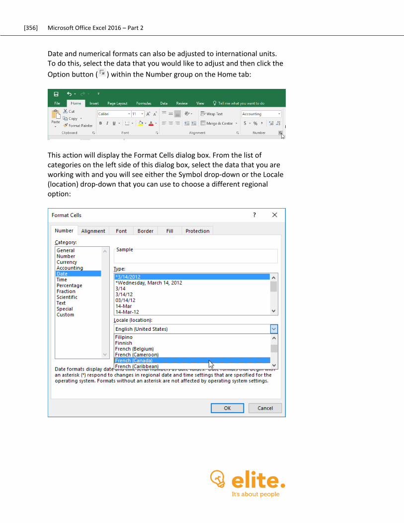
[356] Microsoft Office Excel 2016 – Part 2
Date and numerical formats can also be adjusted to international units. To do this, select the data that you would like to adjust and then click the
Option button ( ) within the Number group on the Home tab:
This action will display the Format Cells dialog box. From the list of categories on the left side of this dialog box, select the data that you are working with and you will see either the Symbol drop-down or the Locale (location) drop-down that you can use to choose a different regional option:
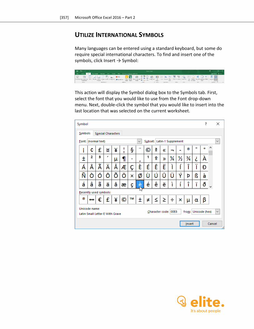
[357] Microsoft Office Excel 2016 – Part 2
UTILIZE INTERNATIONAL SYMBOLS
Many languages can be entered using a standard keyboard, but some do require special international characters. To find and insert one of the symbols, click Insert → Symbol:
This action will display the Symbol dialog box to the Symbols tab. First, select the font that you would like to use from the Font drop-down menu. Next, double-click the symbol that you would like to insert into the last location that was selected on the current worksheet.
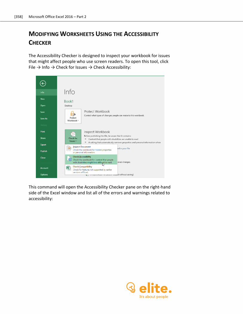
[358] Microsoft Office Excel 2016 – Part 2
MODIFYING WORKSHEETS USING THE ACCESSIBILITY
CHECKER
The Accessibility Checker is designed to inspect your workbook for issues that might affect people who use screen readers. To open this tool, click File → Info → Check for Issues → Check Accessibility:
This command will open the Accessibility Checker pane on the right-hand side of the Excel window and list all of the errors and warnings related to accessibility:
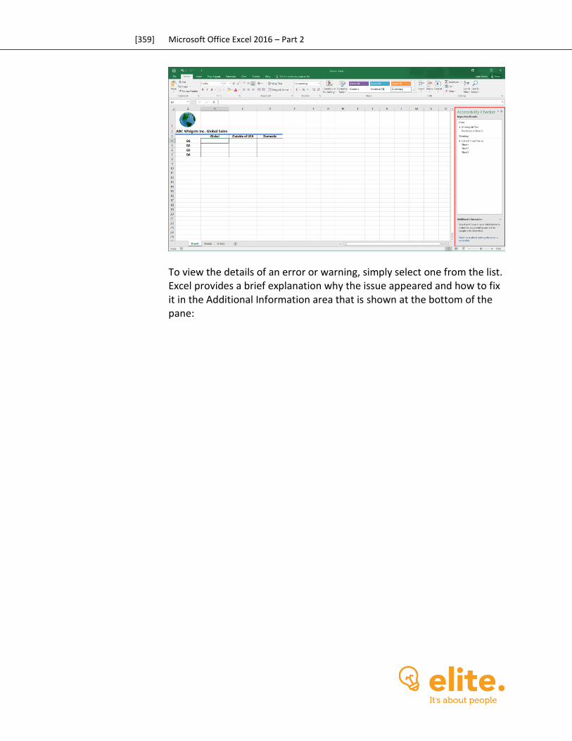
[359] Microsoft Office Excel 2016 – Part 2
To view the details of an error or warning, simply select one from the list. Excel provides a brief explanation why the issue appeared and how to fix it in the Additional Information area that is shown at the bottom of the pane:
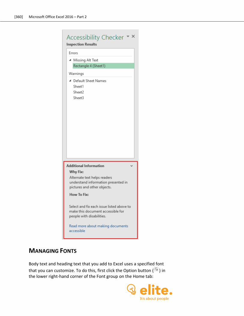
[360] Microsoft Office Excel 2016 – Part 2
MANAGING FONTS
Body text and heading text that you add to Excel uses a specified font
that you can customize. To do this, first click the Option button ( ) in the lower right-hand corner of the Font group on the Home tab:
[361] Microsoft Office Excel 2016 – Part 2
This action will open the Format Cells dialog box to the Font tab. By scrolling to the top of the Font list box you will see both the headings and body font listings:
[362] Microsoft Office Excel 2016 – Part 2
You can change how these basic fonts appear by selecting either of them and then choosing a font style, size, color, and font effect using the controls found on this tab:

[363] Microsoft Office Excel 2016 – Part 2
ACTIVITY 7-5
Preparing a Workbook for Multiple Audiences The workbook that you have been working on needs to be checked by the Accessibility Checker for any errors, and you need to change every instance of the dollar symbol to the English pound symbol.
1. To begin, open Activity 7-5 from your Exercise Files folder:
2. Use your cursor to select cells D:5 to D40:
[364] Microsoft Office Excel 2016 – Part 2
3. Next, click the Option button ( ) in the lower right-hand corner of the Number group on the Home tab:
4. The Format Cells dialog box will now be displayed. Ensure that the Accounting category is selected from the Category list on the left:
[365] Microsoft Office Excel 2016 – Part 2
5. Next, click the Symbol drop-down menu and click the English (United Kingdom) option:
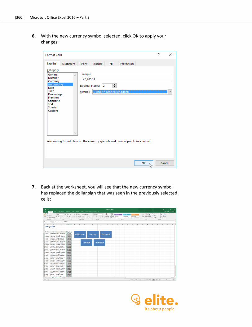
[366] Microsoft Office Excel 2016 – Part 2
6. With the new currency symbol selected, click OK to apply your changes:
7. Back at the worksheet, you will see that the new currency symbol has replaced the dollar sign that was seen in the previously selected cells:
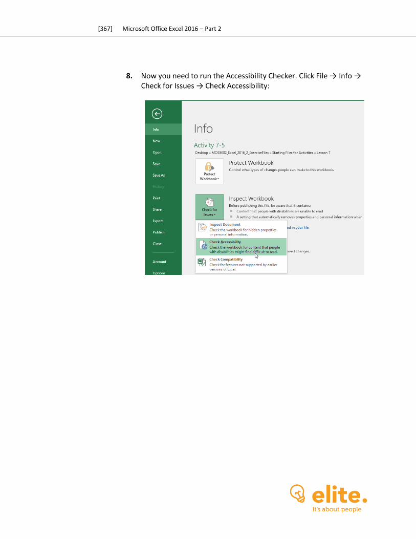
[367] Microsoft Office Excel 2016 – Part 2
8. Now you need to run the Accessibility Checker. Click File → Info → Check for Issues → Check Accessibility:
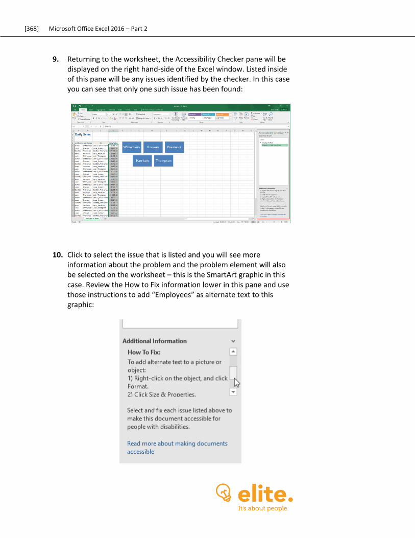
[368] Microsoft Office Excel 2016 – Part 2
9. Returning to the worksheet, the Accessibility Checker pane will be displayed on the right hand-side of the Excel window. Listed inside of this pane will be any issues identified by the checker. In this case you can see that only one such issue has been found:
10. Click to select the issue that is listed and you will see more information about the problem and the problem element will also be selected on the worksheet – this is the SmartArt graphic in this case. Review the How to Fix information lower in this pane and use those instructions to add “Employees” as alternate text to this graphic:
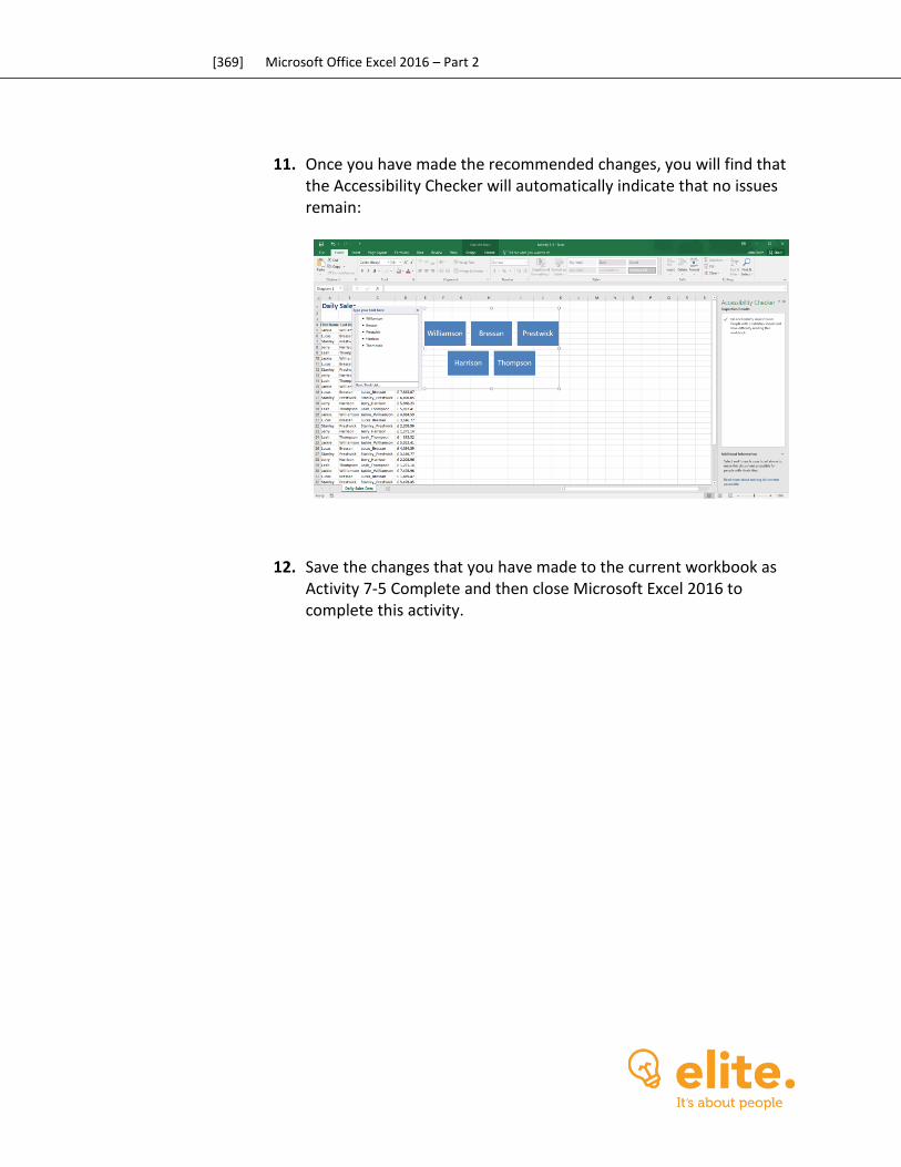
[369] Microsoft Office Excel 2016 – Part 2
11. Once you have made the recommended changes, you will find that the Accessibility Checker will automatically indicate that no issues remain:
12. Save the changes that you have made to the current workbook as Activity 7-5 Complete and then close Microsoft Excel 2016 to complete this activity.
[370] Microsoft Office Excel 2016 – Part 2
Summary Over the course of this lesson you learned about the various different ways that you can enhance your workbooks in Excel 2016. You should now be familiar with the customization options that are available, as well as how to manage themes to control the appearance of your workbooks. At this point, you should also be comfortable creating and using templates, as well as protecting your workbooks against data loss and unauthorized access. Finally, you now know how to prepare your workbooks when working with multiple audiences.
REVIEW QUESTIONS
1. What is the command sequence to insert a comment?
2. What are themes?
3. What are the two primary template types?
4. In what group on the Review tab can you find the Protect Sheet command?
5. What is the command sequence to use the Accessibility Checker?
[371] Microsoft Office Excel 2016 – Part 2
LESSON LABS
Lesson 1
LESSON LAB 1-1
Objective To understand how to apply and use range names, as well as apply and use specialized functions.
Briefing You have been given a workbook that lists the total sales numbers for every branch of your company sorted by region. You need to calculate the average amount made in sales by each region, but only for stores that made under $1,000,000.
Task Apply the following range names to the indicated cells:
A4:A27: Store B4:B9: Region_1 B10:B14: Region_2 B15:B17: Region_3 B18:B22: Region_4 B23:B27: Region_5
In the designated cells, use the AVERAGEIF function to calculate the average of the stores by region only where the stores earned under $1,000,000 in sales.
Hints Remember that logical operators need to be enclosed in double quotations when constructing this function.
Sample Data
[372] Microsoft Office Excel 2016 – Part 2
Lesson 2
LESSON LAB 2-1
Objective To understand how to analyze data using functions.
Briefing You have been tasked with finishing a sales worksheet that lists the actual sales and sales goals for each store in your company.
Task Use an IF function to determine if each store in every region has met their sales goal outlined in the worksheet.
Hints Remember that the IF function syntax is as follows: IF(logical_test, value_if_true, value_if_false).
Sample Data
Follow-Up Questions Use the UPPER function to convert the text found in cell A1 entirely to uppercase.
[373] Microsoft Office Excel 2016 – Part 2
LESSON LAB 2-2
Objective To understand how to use lookup functions.
Briefing You need to use a LOOKUP function to find specific information from the provided worksheet.
Task Add a LOOKUP function to cell G2 to find out if store 358 met its sales goal.
Hints Remember that the syntax for a LOOKUP function is as follows: =LOOKUP(lookup_value, lookup_area, results_area).
Sample Data
Follow-Up Questions Add the current date to cell E1 using the TODAY function.
[374] Microsoft Office Excel 2016 – Part 2
Lesson 3
LESSON LAB 3-1
Objective To understand how to create and customize tables, as well as sort table data.
Briefing A worksheet that you have been working on requires a table. Additionally, you need to sort this data to better see what stores have not met their sales goal.
Task Create a new table from the data in the A3:D27 range in the sample workbook. Apply any one of the table styles that are available. Sort the data in the table by the Sales Goal Met column from A to Z.
Hints You can find the table styles in the Table Styles gallery on the Table Tools – Design tab.
Sample Data
[375] Microsoft Office Excel 2016 – Part 2
Lesson 4
LESSON LAB 4-1
Objective To understand how to create and modify charts based on existing data.
Briefing For an upcoming presentation, you would like to create a chart based upon sales data that you have been working with.
Task Using the B3:C27 range in the provided Sample Data file, create a new chart that will best illustrate actual sales numbers against sales goals for each of the stores listed. Once you have chosen and inserted a new chart, hide the primary horizontal axis.
Hints Remember that each chart type is best suited to a specific type of data, so if one chart does not look right, try another type. There might be a number of different solutions.
Sample Data
Follow-Up Questions Apply a new style to the chart that you just created.
[376] Microsoft Office Excel 2016 – Part 2
LESSON LAB 4-2
Objective To understand how to utilize trendlines while working with charts.
Briefing To get a better picture of the sales data that has been collected over a period of time, you would like to add a trendline to a chart.
Task Add the moving average trendline to the chart that appears on the supplied worksheet. Ensure that this trendline represents only the actual sales data.
Hints Ensure that the moving average trendline is set to two periods.
Sample Data
Follow-Up Questions Using the Format Trendline task pane, change the color of the trendline to red.
[377] Microsoft Office Excel 2016 – Part 2
Lesson 5
LESSON LAB 5-1
Objective To understand how to create and use PivotTables to analyze data.
Briefing Using a PivotTable, you would like to see the total amount of sales made by stores that made their sales goal and stores that did not.
Task Using the provided data (A3:D27) in the Sample Data file, create a new PivotTable on the current worksheet (Sheet1) that starts in cell F3. Add data to the PivotTable by adding the Sales Goals Met field as a column. Next, add the Sales field to the Values area. Ensure that the Sales field uses the SUM function. Apply the appropriate data formats to the resulting table and adjust the column widths as necessary.
Hints Remember that you can click and drag fields from the field list in the top half of the PivotTable Field List pane to the four areas on the bottom half.
Sample Data
[378] Microsoft Office Excel 2016 – Part 2
LESSON LAB 5-2
Objective To understand how to present data using PivotCharts, as well as filter data using slicers.
Briefing Using a PivotTable that you previously created, you would like to create a PivotChart that best illustrates the data that it presents.
Task Create a PivotChart on the worksheet of the Sample Data file that uses the Column chart type. Insert a slicer that filters out data from store 122 as this location recently closed.
Hints You can insert a slicer by clicking PivotChartTools – Analyze → Insert Slicer. Additionally, by holding down the Ctrl key and clicking on button in a slicer you can choose to filter out that option.
Sample Data
Follow-Up Questions On the PivotChart, add data labels to the outside end position.
[379] Microsoft Office Excel 2016 – Part 2
Lesson 6
LESSON LAB 6-1
Objective To understand how to work with graphical objects.
Briefing You are going to be presenting the data that is stored in the Sample Data worksheet. To improve the visual elements of this worksheet, you would like to add some graphical objects.
Task Insert any online image that you find relevant to the provided workbook. Position it so that it doesn’t overlap any other data. Insert the Horizontal Bullet List Smart Art graphic into the worksheet. Position this SmartArt so that it doesn’t overlap any other data.
Hints To add a new shape to a SmartArt graphic, use the Text pane.
Sample Data
Follow-Up Questions As the header for each SmartArt shape, enter one of the column names (Store #, Sales, Sales Goal, and Sales Goal Met).
[380] Microsoft Office Excel 2016 – Part 2
Lesson 7
LESSON LAB 7-1
Objective To understand how to customize a workbook and manage its themes.
Briefing You would like to improve the appearance of the Sample Data worksheet using themes and other elements available to you.
Task Change the company name (D1) to a hyperlink that points to http://www.example.org. Next, add the supplied picture as the background. Change the theme of the Sample Data worksheet to the Ion theme
Hints When choosing a background, ensure that you choose the Browse button that appears in the “From a file” section.
Sample Data
Follow-Up Questions Add a comment to cell D1 that states the following: “This hyperlink leads to a placeholder page. Please update.”
[381] Microsoft Office Excel 2016 – Part 2
LESSON LAB 7-2
Objective To understand how to create templates, protect files, and use the Accessibility Checker.
Briefing The data on the Sample Data worksheet needs to be accessible by a wide variety of different people.
Task Execute the Accessibility Checker and make any changes that are recommended. Protect the current worksheet to prevent the deletion of rows and columns. Save the Sample Data worksheet as a template.
Hints Follow the instructions listed inside the Accessibility Checker pane to learn how to make any required changes.
Sample Data
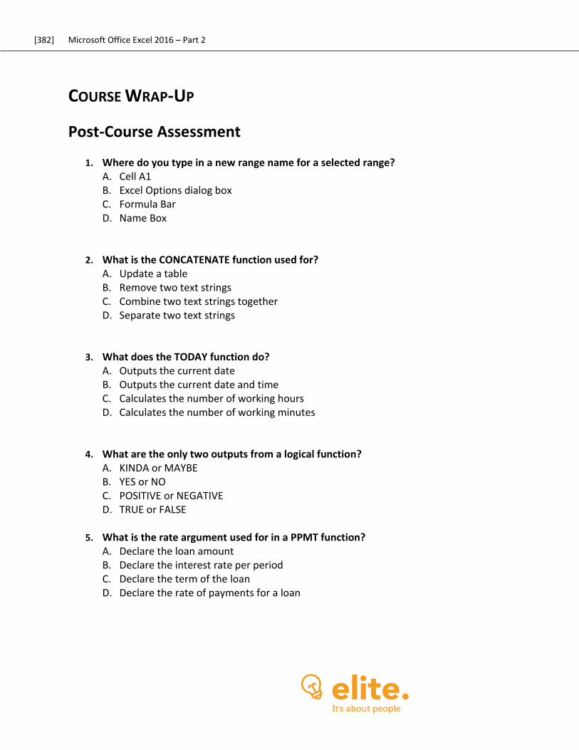
[382] Microsoft Office Excel 2016 – Part 2
COURSE WRAP-UP
Post-Course Assessment
1. Where do you type in a new range name for a selected range? A. Cell A1 B. Excel Options dialog box C. Formula Bar D. Name Box
2. What is the CONCATENATE function used for? A. Update a table B. Remove two text strings C. Combine two text strings together D. Separate two text strings
3. What does the TODAY function do? A. Outputs the current date B. Outputs the current date and time C. Calculates the number of working hours D. Calculates the number of working minutes
4. What are the only two outputs from a logical function? A. KINDA or MAYBE B. YES or NO C. POSITIVE or NEGATIVE D. TRUE or FALSE
5. What is the rate argument used for in a PPMT function?
A. Declare the loan amount B. Declare the interest rate per period C. Declare the term of the loan D. Declare the rate of payments for a loan
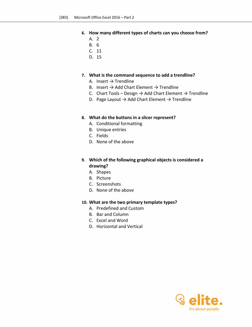
[383] Microsoft Office Excel 2016 – Part 2
6. How many different types of charts can you choose from? A. 2 B. 6 C. 11 D. 15
7. What is the command sequence to add a trendline? A. Insert → Trendline B. Insert → Add Chart Element → Trendline C. Chart Tools – Design → Add Chart Element → Trendline D. Page Layout → Add Chart Element → Trendline
8. What do the buttons in a slicer represent? A. Conditional formatting B. Unique entries C. Fields D. None of the above
9. Which of the following graphical objects is considered a drawing? A. Shapes B. Picture C. Screenshots D. None of the above
10. What are the two primary template types?
A. Predefined and Custom B. Bar and Column C. Excel and Word D. Horizontal and Vertical
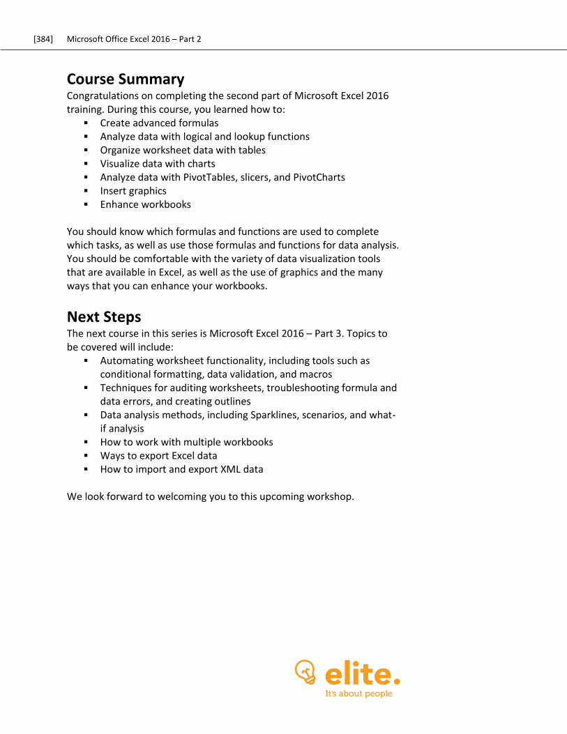
[384] Microsoft Office Excel 2016 – Part 2
Course Summary Congratulations on completing the second part of Microsoft Excel 2016 training. During this course, you learned how to:
Create advanced formulas Analyze data with logical and lookup functions Organize worksheet data with tables Visualize data with charts Analyze data with PivotTables, slicers, and PivotCharts Insert graphics Enhance workbooks
You should know which formulas and functions are used to complete which tasks, as well as use those formulas and functions for data analysis. You should be comfortable with the variety of data visualization tools that are available in Excel, as well as the use of graphics and the many ways that you can enhance your workbooks.
Next Steps The next course in this series is Microsoft Excel 2016 – Part 3. Topics to be covered will include:
Automating worksheet functionality, including tools such as conditional formatting, data validation, and macros
Techniques for auditing worksheets, troubleshooting formula and data errors, and creating outlines
Data analysis methods, including Sparklines, scenarios, and what-if analysis
How to work with multiple workbooks Ways to export Excel data How to import and export XML data
We look forward to welcoming you to this upcoming workshop.
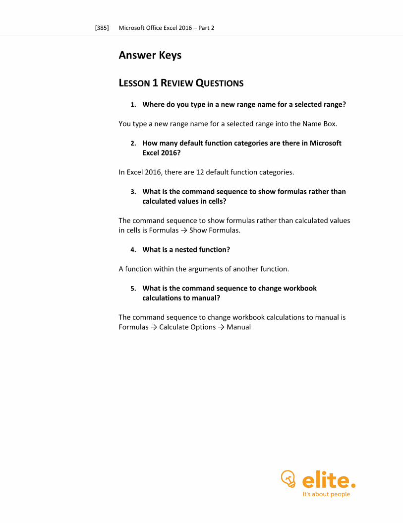
[385] Microsoft Office Excel 2016 – Part 2
Answer Keys
LESSON 1 REVIEW QUESTIONS
1. Where do you type in a new range name for a selected range? You type a new range name for a selected range into the Name Box.
2. How many default function categories are there in Microsoft Excel 2016?
In Excel 2016, there are 12 default function categories.
3. What is the command sequence to show formulas rather than calculated values in cells?
The command sequence to show formulas rather than calculated values in cells is Formulas → Show Formulas.
4. What is a nested function? A function within the arguments of another function.
5. What is the command sequence to change workbook calculations to manual?
The command sequence to change workbook calculations to manual is Formulas → Calculate Options → Manual
[386] Microsoft Office Excel 2016 – Part 2
LESSON 2 REVIEW QUESTIONS
1. What is the TRIM function used for? The TRIM function is used to remove empty spaces from a string, excluding those that appear between two words.
2. What is the CONCATENATE function used for? The CONCATENATE function is used to combine (concatenate) two text strings together from multiple cells into one single cell.
3. What are the only two possible outputs from a logical function? The output from a logical function is either TRUE or FALSE.
4. What is the difference between the TODAY function and the NOW function?
The difference between the TODAY function and the NOW function is that the TODAY function will only print the current date, while the NOW function prints both the date and time.
5. What is the FV function used for? The FV function is used to calculate the future value of an investment that has a fixed interest rate, as well as a fixed or periodic payment schedule.
[387] Microsoft Office Excel 2016 – Part 2
LESSON 3 REVIEW QUESTIONS
1. What is the command sequence to add a table? To add a table, click Insert → Table.
2. What are Quick Sorts? Quick sorting allows you to quickly and easily apply common sorting options to data within a range or table. For example, you can sort the contents of a range or table alphabetically.
3. What do levels refer to when creating a custom sort? Levels are specific criterion on which the sort will be based. For example, a level could sort a specified column in alphabetical order.
4. What is quick sorting? Quick sorting allows you to quickly and easily apply common sorting options to data within the table in ascending or descending order.
5. What is an easy way to differentiate database functions from logical functions?
An easy way to differentiate database functions from logical functions is by looking for a “D” at the beginning of the function name. If you find one, this means that it is a database function.
[388] Microsoft Office Excel 2016 – Part 2
LESSON 4 REVIEW QUESTIONS
1. What are charts? Charts are graphical representations of data and its relationships.
2. How many different chart types can you choose from? You can choose from up to 11 different chart types.
3. What is the difference between modification and formatting? When you choose to modify a chart, you are changing the various elements that are used to illustrate the data. Formatting, on the other hand, is the process of altering the overall appearance of the chart.
4. When are the Chart Tools contextual tabs displayed? The Chart Tools contextual tab set is displayed whenever a chart is selected.
5. What is the command sequence to add a trendline using the ribbon?
The command sequence to add a trendline using the ribbon is Chart Tools – Design → Add Chart Element → Trendline → [Trendline].
[389] Microsoft Office Excel 2016 – Part 2
LESSON 5 REVIEW QUESTIONS
1. What is pivoting in Excel? Pivoting is the act of moving data around to change the table’s structure.
2. What is transactional data? Transactional data refers to data that has not been summarized in any way; this means that only column titles (fields) are present. Additionally, each entry (or transaction) in transactional data appears on its own row.
3. What happens to fields that are dragged to the Values area on the PivotTable Field List pane?
Fields that are dragged to the Values area of the PivotTable Field List pane will have calculations performed on them or their values summarized.
4. What is the command sequence to insert a PivotChart? The command sequence to insert a PivotChart is PivotTable Tools – Options → PivotChart.
5. What do the buttons on a slicer represent? The buttons on a slicer represent unique entries that exist within the field that is associated with the slicer.
[390] Microsoft Office Excel 2016 – Part 2
LESSON 6 REVIEW QUESTIONS
1. What are the five types of graphical objects that can be inserted into Excel workbooks?
The five types of graphical objects that can be inserted into Excel workbooks are SmartArt, screenshots, pictures, online pictures, and shapes.
2. Are shapes considered pictures or drawings? Shapes are considered drawings.
3. How do you open the Selection pane? To open the Selection pane, click Picture Tools (or Drawing Tools) – Format → Selection Pane
4. What are SmartArt graphics used for? SmartArt graphics are used to visually represent text-based content in a chart or diagram.
5. How do you open the Choose a SmartArt Graphic dialog box? To open the Choose a SmartArt Graphic dialog box, click Insert → SmartArt.
[391] Microsoft Office Excel 2016 – Part 2
LESSON 7 REVIEW QUESTIONS
1. What is the command sequence to insert a comment? To insert a comment, click Review → New Comment.
2. What are themes? Themes are combinations of preset colors, fonts, and effects
3. What are the two primary template types? The two primary template types are predefined and custom.
4. In what group on the Review tab can you find the Protect Sheet command?
You can find this command in the Changes group on the Review tab.
5. What is the command sequence to use the Accessibility Checker?
To use the Accessibility Checker, click File → Info → Check for Issues → Check Accessibility.
[392] Microsoft Office Excel 2016 – Part 2
POST-COURSE ASSESSMENT
1. Where do you type in a new range name for a selected range? A. Cell A1 B. Excel Options dialog box C. Formula Bar D. Name Box
You can type a new range name for a selected range into the Name Box.
2. What is the CONCATENATE function used for? A. Update a table B. Remove two text strings C. Combine two text strings together D. Separate two text strings
Using this function you can combine (concatenate) text strings together from multiple cells into a single cell.
3. What does the TODAY function do? A. Outputs the current date B. Outputs the current date and time C. Calculates the number of working hours D. Calculates the number of working minutes
The TODAY function will output the current date.
4. What are the only two outputs from a logical function? A. KINDA or MAYBE B. YES or NO C. POSITIVE or NEGATIVE D. TRUE or FALSE
The output from a logical function is either TRUE or FALSE.
[393] Microsoft Office Excel 2016 – Part 2
5. What is the rate argument used for in a PPMT function? A. Declare the loan amount B. Declare the interest rate per period C. Declare the term of the loan D. Declare the rate of payments for a loan
The rate argument is used to declare the interest rate per period.
6. How many different types of charts can you choose from? A. 2 B. 6 C. 11 D. 15
You can choose from up to 11 different chart types in Excel 2016.
7. What is the command sequence to add a trendline? A. Insert → Trendline B. Insert → Add Chart Element → Trendline C. Chart Tools – Design → Add Chart Element → Trendline D. Page Layout → Add Chart Element → Trendline
The command sequence to add a trendline is Chart Tools – Design → Add Chart Element → Trendline.
8. What do the buttons in a slicer represent? A. Conditional formatting B. Unique entries C. Fields D. None of the above
The buttons on a slicer represent unique entries that exist within the field that is associated with the slicer.
9. Which of the following graphical objects is considered a drawing? A. Shapes B. Picture C. Screenshots D. None of the above
Of the graphical objects listed, only shapes are considered a drawing.

[394] Microsoft Office Excel 2016 – Part 2

[395] Microsoft Office Excel 2016 – Part 2
10. What are the two primary template types? A. Predefined and Custom B. Bar and Column C. Excel and Word D. Horizontal and Vertical
The two primary template types are predefined and custom.
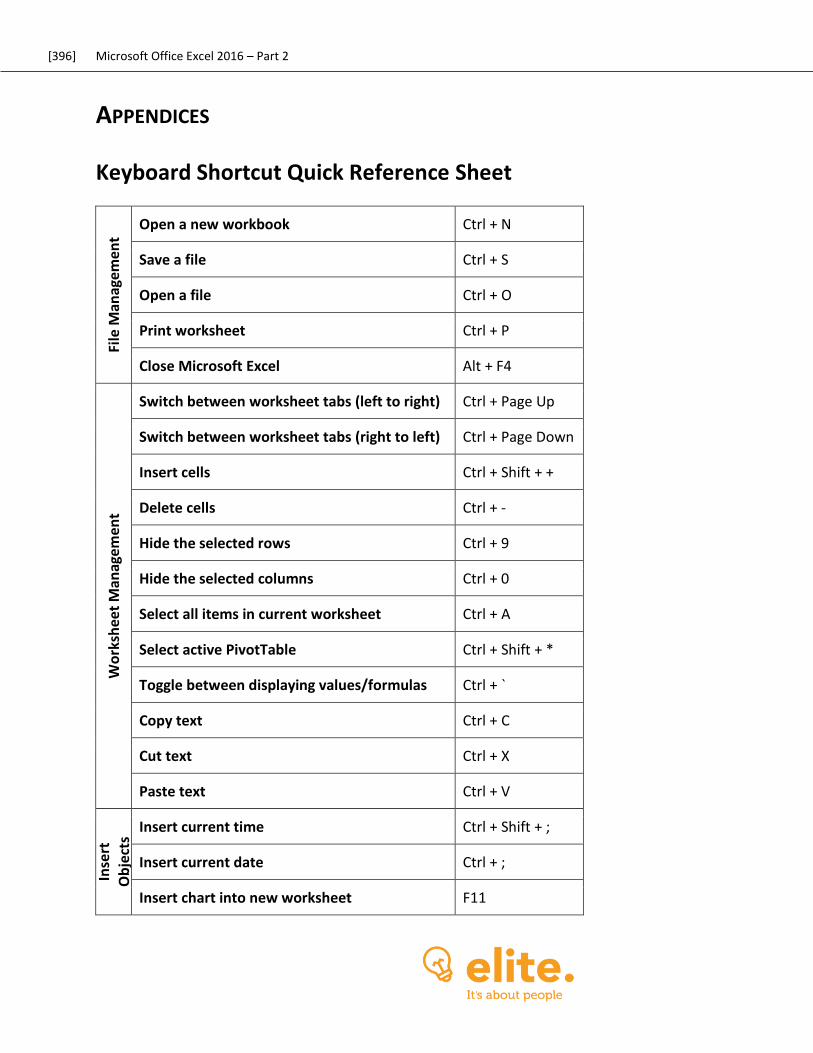
[396] Microsoft Office Excel 2016 – Part 2
APPENDICES
Keyboard Shortcut Quick Reference Sheet
File
Man
agem
ent
Open a new workbook Ctrl + N
Save a file Ctrl + S
Open a file Ctrl + O
Print worksheet Ctrl + P
Close Microsoft Excel Alt + F4
Wo
rksh
eet
Man
agem
ent
Switch between worksheet tabs (left to right) Ctrl + Page Up
Switch between worksheet tabs (right to left) Ctrl + Page Down
Insert cells Ctrl + Shift + +
Delete cells Ctrl + -
Hide the selected rows Ctrl + 9
Hide the selected columns Ctrl + 0
Select all items in current worksheet Ctrl + A
Select active PivotTable Ctrl + Shift + *
Toggle between displaying values/formulas Ctrl + `
Copy text Ctrl + C
Cut text Ctrl + X
Paste text Ctrl + V
Inse
rt
Ob
ject
s
Insert current time Ctrl + Shift + ;
Insert current date Ctrl + ;
Insert chart into new worksheet F11
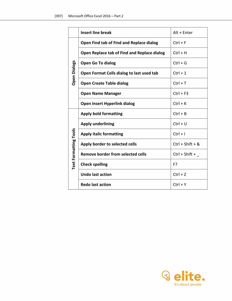
[397] Microsoft Office Excel 2016 – Part 2
Insert line break Alt + Enter
Op
en D
ialo
gs
Open Find tab of Find and Replace dialog Ctrl + F
Open Replace tab of Find and Replace dialog Ctrl + H
Open Go To dialog Ctrl + G
Open Format Cells dialog to last used tab Ctrl + 1
Open Create Table dialog Ctrl + T
Open Name Manager Ctrl + F3
Open Insert Hyperlink dialog Ctrl + K
Text
Fo
rmat
tin
g To
ols
Apply bold formatting Ctrl + B
Apply underlining Ctrl + U
Apply italic formatting Ctrl + I
Apply border to selected cells Ctrl + Shift + &
Remove border from selected cells Ctrl + Shift + _
Check spelling F7
Undo last action Ctrl + Z
Redo last action Ctrl + Y
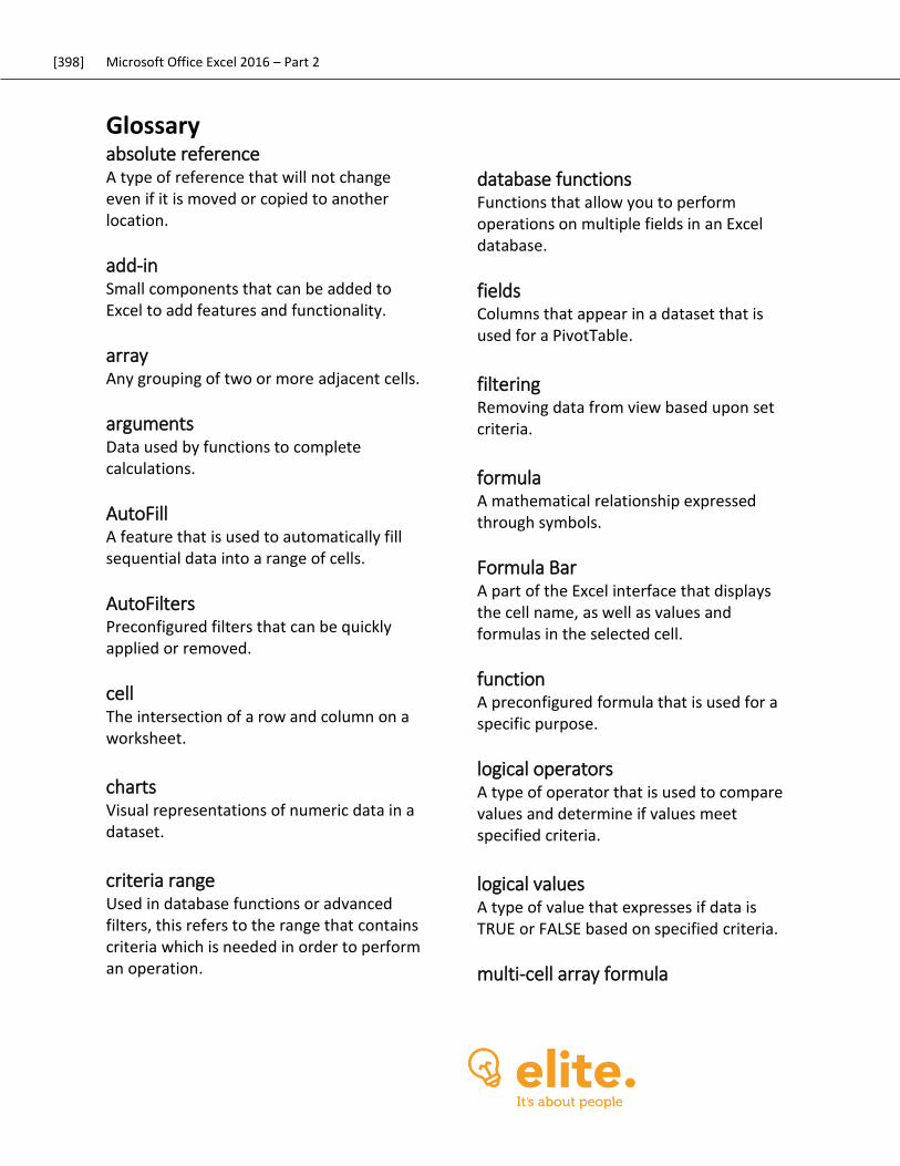
[398] Microsoft Office Excel 2016 – Part 2
Glossary absolute reference A type of reference that will not change even if it is moved or copied to another location.
add-in Small components that can be added to Excel to add features and functionality.
array Any grouping of two or more adjacent cells.
arguments Data used by functions to complete calculations.
AutoFill A feature that is used to automatically fill sequential data into a range of cells.
AutoFilters Preconfigured filters that can be quickly applied or removed.
cell The intersection of a row and column on a worksheet.
charts Visual representations of numeric data in a dataset.
criteria range Used in database functions or advanced filters, this refers to the range that contains criteria which is needed in order to perform an operation.
database functions Functions that allow you to perform operations on multiple fields in an Excel database.
fields Columns that appear in a dataset that is used for a PivotTable.
filtering Removing data from view based upon set criteria.
formula A mathematical relationship expressed through symbols.
Formula Bar A part of the Excel interface that displays the cell name, as well as values and formulas in the selected cell.
function A preconfigured formula that is used for a specific purpose.
logical operators A type of operator that is used to compare values and determine if values meet specified criteria.
logical values A type of value that expresses if data is TRUE or FALSE based on specified criteria.
multi-cell array formula
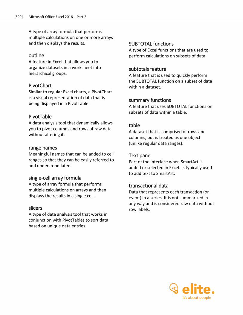
[399] Microsoft Office Excel 2016 – Part 2
A type of array formula that performs multiple calculations on one or more arrays and then displays the results.
outline A feature in Excel that allows you to organize datasets in a worksheet into hierarchical groups.
PivotChart Similar to regular Excel charts, a PivotChart is a visual representation of data that is being displayed in a PivotTable.
PivotTable A data analysis tool that dynamically allows you to pivot columns and rows of raw data without altering it.
range names Meaningful names that can be added to cell ranges so that they can be easily referred to and understood later.
single-cell array formula A type of array formula that performs multiple calculations on arrays and then displays the results in a single cell.
slicers A type of data analysis tool that works in conjunction with PivotTables to sort data based on unique data entries.
SUBTOTAL functions A type of Excel functions that are used to perform calculations on subsets of data.
subtotals feature A feature that is used to quickly perform the SUBTOTAL function on a subset of data within a dataset.
summary functions A feature that uses SUBTOTAL functions on subsets of data within a table.
table A dataset that is comprised of rows and columns, but is treated as one object (unlike regular data ranges).
Text pane Part of the interface when SmartArt is added or selected in Excel. Is typically used to add text to SmartArt.
transactional data Data that represents each transaction (or event) in a series. It is not summarized in any way and is considered raw data without row labels.

[400] Microsoft Office Excel 2016 – Part 2
Index
A
Accessibility Checker ...................................................................................................................... 346 Array Formulas ................................................................................................................................ 80 AutoComplete
And formulas .............................................................................................................................. 22 AutoFill ............................................................................................................................... 15, 51, 384
B
BEDMAS ........................................................................................................................................... 37
C
Chart Adding gridlines to .................................................................................................................... 185 Adding title to ........................................................................................................................... 184 Applying style to ....................................................................................................................... 187 Chart Tools – Design tab ........................................................................................... 178, 179, 187 Chart Tools – Format tab .......................................................................................................... 179 Chart Tools – Layout tab ........................................................................................................... 184 Creating ............................................................................................................................ 167, 175 Editing legend ........................................................................................................................... 186 Elements of ............................................................................................................................... 177 Moving ...................................................................................................................................... 176 Types of .................................................................................................................................... 163 What is? .................................................................................................................................... 162
Clip Art Inserting .................................................................................................................................... 268 Moving ...................................................................................................................................... 272
D
DAX Functions DAX language............................................................................................................................ 230 Types of .................................................................................................................................... 230 What are? ................................................................................................................................. 230
E
Editing Tools Redo ......................................................................................................................................... 383 Undo ......................................................................................................................................... 383
Excel Options Dialog .............................................................................................................. 369, 379
[401] Microsoft Office Excel 2016 – Part 2
F
File management Digital signature ....................................................................................................................... 331 Encrypt with password ............................................................................................................. 328 Entering password.................................................................................................................... 329 Mark as Final ............................................................................................................................ 326 Read-Only ................................................................................................................................. 327 Removing password ................................................................................................................. 330
Filtering AutoFilters ................................................................................................................ 159, 374, 384 Operators ................................................................................................................................. 134 With criteria range ................................................................................................................... 132
Find and Replace Dialog ................................................................................................................ 383 Functions
AVERAGEIF ................................................................................................................................. 38 AVERAGEIFS ............................................................................................................................... 39 Categories of .............................................................................................................................. 31 CONCATENATE ..................................................................................................................... 62, 79 COUNTA ..................................................................................................................................... 39 COUNTIF ..................................................................................................................................... 38 COUNTIFS ................................................................................................................................... 39 Database .......................................................................................................................... 148, 156 DAVERAGE ................................................................................................................................ 156 FV (Future Value) ............................................................................................................. 104, 110 Help with .................................................................................................................................... 33 IPMT ......................................................................................................................................... 100 LEFT ............................................................................................................................................ 57 LEN ............................................................................................................................................. 59 LOWER ....................................................................................................................................... 61 MID............................................................................................................................................. 58 NOW ........................................................................................................................................... 95 NPV .................................................................................................................................. 103, 107 PMT ............................................................................................................................................ 48 PPMT ........................................................................................................................................ 102 PROPER ...................................................................................................................................... 61 RIGHT ......................................................................................................................................... 57 SUBTOTAL ................................................................................................................................ 143 SUMIF ......................................................................................................................................... 37 SUMIFS ....................................................................................................................................... 39 Summarizing table data with ................................................................................................... 147 Syntax of..................................................................................................................................... 37 Text ............................................................................................................................................ 56 TODAY ........................................................................................................................................ 94 TRIM ........................................................................................................................................... 60 UPPER ......................................................................................................................................... 61
H
Headers and Footers And themes .............................................................................................................................. 306
Help ................................................................................................................................................. 33 Hyperlinks
Dialog box overview ................................................................................................................. 294
[402] Microsoft Office Excel 2016 – Part 2
What are? ................................................................................................................................. 295
I
Images Moving ...................................................................................................................................... 272 Picture Tools – Format tab ....................................................................................................... 265
L
Logical Functions AND function .............................................................................................................................. 74 IF function ................................................................................................................. 72, 77, 81, 82 Operators ................................................................................................................................... 73 OR function ................................................................................................................................. 76
M
Microsoft PowerPivot for Excel ..................................................................................................... 229 What is? .................................................................................................................................... 229
P
PivotChart Creating ............................................................................................................................ 244, 248 Filtering ..................................................................................................................................... 251 What is? .................................................................................................................................... 244
PivotTable ....................................................................... 119, 225, 254, 364, 365, 376, 382, 384, 385 And PivotCharts ................................................................................................................ 244, 253 And slicers ........................................................................................................................ 237, 243 Creating ............................................................................................................................ 221, 233 Designing .................................................................................................................................. 220 Field List pane ................................................................................................... 224, 254, 364, 376 Modifying fields displayed ........................................................................................................ 224 Value Field Settings dialog box ................................................................................................. 226 What is? .................................................................................................................................... 218
R
Range Name Creating from selection .............................................................................................................. 27 Creating with Name Box ....................................................................................................... 17, 25 Creating with New Name dialog box .............................................................................. 18, 20, 26 Deleting ...................................................................................................................................... 21 Editing ......................................................................................................................................... 20 Filtering ....................................................................................................................................... 21 Parameters for ............................................................................................................................ 16 Selecting ..................................................................................................................................... 17 Using in formulas .................................................................................................................. 22, 29 What is? ...................................................................................................................................... 14
[403] Microsoft Office Excel 2016 – Part 2
S
ScreenTip Hyperlinks ................................................................................................................................ 294
Selection and Visibility Pane .................................................................................................. 290, 377 Shapes
Drawing Tools – Format tab ..................................................................................................... 265 Inserting ................................................................................................................................... 273 Types of .................................................................................................................................... 258
Slicers Creating ............................................................................................................................ 238, 240 Using ................................................................................................................................ 238, 242 What are? ................................................................................................................................. 237
SmartArt Inserting ........................................................................................................................... 283, 286 SmartArt Tools – Design tab ..................................................................................... 266, 285, 288 SmartArt Tools – Format tab .................................................................................................... 267 Using Text pane ................................................................................................................ 285, 288 What is? ........................................................................................................................... 283, 377
Sorting ........................................................................................................................................... 129 And tables ................................................................................................................................ 130 On multiple rows/columns ....................................................................................................... 130 Quick sort ......................................................................................................................... 130, 141 With custom criteria ................................................................................................................ 137
Subtotals Command on Data tab ..................................................................................................... 144, 152 Dialog box .........................................................................................................142, 145, 146, 152 Function ................................................................................................................................... 143
T
Table Applying style to ............................................................................................................... 120, 127 Components of ......................................................................................................................... 117 Creating ............................................................................................................................ 118, 126 Subtotals .................................................................................................................................. 143 Summary functions .................................................................................................................. 147 Table Tools – Design tab .......................................................................................................... 119 What is? ................................................................................................................................... 116
Template Modifying ......................................................................................................................... 315, 316 Saving ....................................................................................................................................... 312 Viewing personal ...................................................................................................................... 314 What is? ................................................................................................................................... 310
Themes Changing .................................................................................................................................. 306 What are? ................................................................................................................................ 305
W
WordArt......................................................................................................................... 179, 266, 267 Workbook protection
Current worksheet ................................................................................................................... 332
[404] Microsoft Office Excel 2016 – Part 2
Editing restrictions .................................................................................................................... 333 Notification ............................................................................................................................... 334 Password .................................................................................................................................. 333